Compass: Spatio Temporal Sentiment Analysis of US ElectionWhat Twi�er Says!

Debjyoti Paul, Feifei Li, Murali Krishna Teja, Xin Yu, Richie FrostUniversity of Utah

{deb,lifeifei,teja614,xiny,rfrost}@cs.utah.edu

ABSTRACTWith the widespread growth of various social network tools andplatforms, analyzing and understanding societal response and crowdreaction to important and emerging social issues and events throughsocial media data is increasingly an important problem. However,there are numerous challenges towards realizing this goal e�ec-tively and e�ciently, due to the unstructured and noisy nature ofsocial media data. �e large volume of the underlying data alsopresents a fundamental challenge. Furthermore, in many applica-tion scenarios, it is o�en interesting, and in some cases critical, todiscover pa�erns and trends based on geographical and/or temporalpartitions, and keep track of how they will change overtime.

�is brings up the interesting problem of spatio-temporal sen-timent analysis from large-scale social media data. �is paper in-vestigates this problem through a data science project called “USElection 2016, What Twi�er Says”. �e objective is to discover sen-timent on Twi�er towards either the democratic or the republicanparty at US county and state levels over any arbitrary temporalintervals, using a large collection of geotagged tweets from a periodof 6 months leading up to the US Presidential Election in 2016. Ourresults demonstrate that by integrating and developing a combi-nation of machine learning and data management techniques, itis possible to do this at scale with e�ective outcomes. �e resultsof our project have the potential to be adapted towards solvingand in�uencing other interesting social issues such as buildingneighborhood happiness and health indicators.

CCS CONCEPTS•Information systems→Online analytical processing engines;Spatial-temporal systems; Sentiment analysis; Social tagging;

KEYWORDSSpatio-Temporal; Sentiment Analysis; Scalable Framework; Burstyevents; Election; Crowd Sentiment

1 INTRODUCTIONSince the inception of Twi�er, people have been using the platformto express their opinion about current a�airs, politics, business,sports, �nance and entertainment. �ere are studies with statistics

Permission to make digital or hard copies of all or part of this work for personal orclassroom use is granted without fee provided that copies are not made or distributedfor pro�t or commercial advantage and that copies bear this notice and the full citationon the �rst page. Copyrights for components of this work owned by others than ACMmust be honored. Abstracting with credit is permi�ed. To copy otherwise, or republish,to post on servers or to redistribute to lists, requires prior speci�c permission and/or afee. Request permissions from permissions@acm.org.KDD ’17, August 13-17, 2017, Halifax, NS, Canada© 2017 ACM. 978-1-4503-4887-4/17/08. . .$15.00DOI: h�p://dx.doi.org/10.1145/3097983.3098053

Figure 1: Popularity of Republican (Red) and Democratic(Blue) parties at US county level returned by Compass for aquery time interval; http://www.estorm.org.[36] showing that twi�er is being used predominantly by people ofage under 30 and the voice of young generation ma�ers in pavingroad to the future of any country. Growing social media usagecoupled with enhanced computing technologies have enabled us toanalyze peoples opinion from their tweets at a large scale. An eventlike election that a�racts the interest of crowd and has signi�cantimpact on society is worth analyzing.

In this work we provide a framework to analyze the sentimentof the masses in spatio-temporal domain for any topic of interest.In particular, we used the US Presidential Election 2016 as a con-crete example and analyzed the sentiment of crowd regarding thiselection. Masses express their feelings in tweets thus making it avaluable source of peoples true opinion. �e vast amount of rawdata that is generated in Twi�er during an important and longevent such as a Presidential Election poses a unique challenge togather, analyze and extract information. Furthermore, people areinquisitive about the popularity of political parties with respect togeographical location; also about how breakout events, news andmedia a�airs change the masses sentiment over time.

Using the Twi�er stream as our primary data source and restrict-ing ourselves to geo-tagged tweets, we developed a Sentiment Anal-ysis framework to analyze and visualize large spatio-temporal data.We dub the framework Compass, which stands for ComprehensiveAnalytics on Sentiment for Spatiotemporal Data. Compass facil-itates the end user to select an arbitrary time range to visualizepopularity of the two political parties for each county (or state)of US for the speci�ed time range. Alongside we present a burstyevent detection technique to capture major event or subevents thathappened before the US election. �e objective is to capture thereaction of people on such events early in the process.

�e Compass framework is generic where specialized machinelearning models can be integrated to do speci�c task. For electionanalysis we deployed machine learning and deep learning models

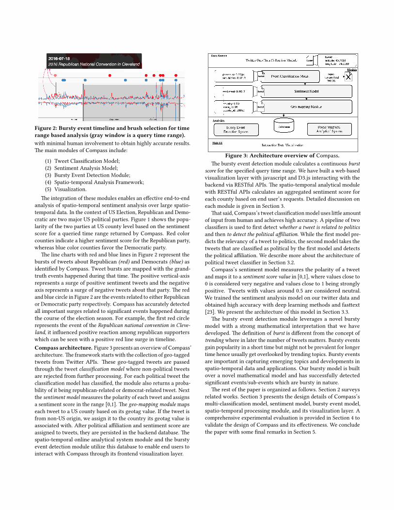
Figure 2: Bursty event timeline and brush selection for timerange based analysis (gray window is a query time range).with minimal human involvement to obtain highly accurate results.�e main modules of Compass include:

(1) Tweet Classi�cation Model;(2) Sentiment Analysis Model;(3) Bursty Event Detection Module;(4) Spatio-temporal Analysis Framework;(5) Visualization.

�e integration of these modules enables an e�ective end-to-endanalysis of spatio-temporal sentiment analysis over large spatio-temporal data. In the context of US Election, Republican and Demo-cratic are two major US political parties. Figure 1 shows the popu-larity of the two parties at US county level based on the sentimentscore for a queried time range returned by Compass. Red colorcounties indicate a higher sentiment score for the Republican party,whereas blue color counties favor the Democratic party.

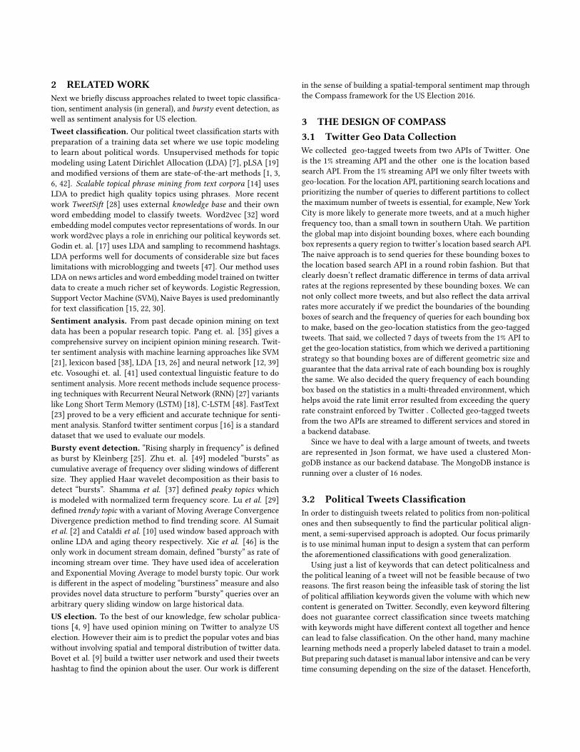
�e line charts with red and blue lines in Figure 2 represent thebursts of tweets about Republican (red) and Democrats (blue) asidenti�ed by Compass. Tweet bursts are mapped with the grand-truth events happened during that time. �e positive vertical-axisrepresents a surge of positive sentiment tweets and the negativeaxis represents a surge of negative tweets about that party. �e redand blue circle in Figure 2 are the events related to either Republicanor Democratic party respectively. Compass has accurately detectedall important surges related to signi�cant events happened duringthe course of the election season. For example, the �rst red circlerepresents the event of the Republican national convention in Cleve-land, it in�uenced positive reaction among republican supporterswhich can be seen with a positive red line surge in timeline.Compass architecture. Figure 3 presents an overview ofCompass’architecture. �e framework starts with the collection of geo-taggedtweets from Twi�er APIs. �ese geo-tagged tweets are passedthrough the tweet classi�cation model where non-political tweetsare rejected from further processing. For each political tweet theclassi�cation model has classi�ed, the module also returns a proba-bility of it being republican-related or democrat-related tweet. Nextthe sentiment model measures the polarity of each tweet and assignsa sentiment score in the range [0,1]. �e geo-mapping module mapseach tweet to a US county based on its geotag value. If the tweet isfrom non-US origin, we assign it to the country its geotag value isassociated with. A�er political a�liation and sentiment score areassigned to tweets, they are persisted in the backend database. �espatio-temporal online analytical system module and the burstyevent detection module utilize this database to enable end users tointeract with Compass through its frontend visualization layer.

Figure 3: Architecture overview of Compass.�e bursty event detection module calculates a continuous burst

score for the speci�ed query time range. We have built a web-basedvisualization layer with javascript and D3.js interacting with thebackend via RESTful APIs. �e spatio-temporal analytical modulewith RESTful APIs calculates an aggregated sentiment score foreach county based on end user’s requests. Detailed discussion oneach module is given in Section 3.

�at said,Compass’s tweet classi�cation model uses li�le amountof input from human and achieves high accuracy. A pipeline of twoclassi�ers is used to �rst detect whether a tweet is related to politicsand then to detect the political a�liation. While the �rst model pre-dicts the relevancy of a tweet to politics, the second model takes thetweets that are classi�ed as political by the �rst model and detectsthe political a�liation. We describe more about the architecture ofpolitical tweet classi�er in Section 3.2.

Compass’s sentiment model measures the polarity of a tweetand maps it to a sentiment score value in [0,1], where values close to0 is considered very negative and values close to 1 being stronglypositive. Tweets with values around 0.5 are considered neutral.We trained the sentiment analysis model on our twi�er data andobtained high accuracy with deep learning methods and fas�ext[23]. We present the architecture of this model in Section 3.3.

�e bursty event detection module leverages a novel burstymodel with a strong mathematical interpretation that we havedeveloped. �e de�nition of burst is di�erent from the concept oftrending where in later the number of tweets ma�ers. Bursty eventsgain popularity in a short time but might not be prevalent for longertime hence usually get overlooked by trending topics. Bursty eventsare important in capturing emerging topics and developments inspatio-temporal data and applications. Our bursty model is builtover a novel mathematical model and has successfully detectedsigni�cant events/sub-events which are bursty in nature.

�e rest of the paper is organized as follows. Section 2 surveysrelated works. Section 3 presents the design details of Compass’smulti-classi�cation model, sentiment model, bursty event model,spatio-temporal processing module, and its visualization layer. Acomprehensive experimental evaluation is provided in Section 4 tovalidate the design of Compass and its e�ectiveness. We concludethe paper with some �nal remarks in Section 5.

2 RELATEDWORKNext we brie�y discuss approaches related to tweet topic classi�ca-tion, sentiment analysis (in general), and bursty event detection, aswell as sentiment analysis for US election.Tweet classi�cation. Our political tweet classi�cation starts withpreparation of a training data set where we use topic modelingto learn about political words. Unsupervised methods for topicmodeling using Latent Dirichlet Allocation (LDA) [7], pLSA [19]and modi�ed versions of them are state-of-the-art methods [1, 3,6, 42]. Scalable topical phrase mining from text corpora [14] usesLDA to predict high quality topics using phrases. More recentwork TweetSi� [28] uses external knowledge base and their ownword embedding model to classify tweets. Word2vec [32] wordembedding model computes vector representations of words. In ourwork word2vec plays a role in enriching our political keywords set.Godin et. al. [17] uses LDA and sampling to recommend hashtags.LDA performs well for documents of considerable size but faceslimitations with microblogging and tweets [47]. Our method usesLDA on news articles and word embedding model trained on twi�erdata to create a much richer set of keywords. Logistic Regression,Support Vector Machine (SVM), Naive Bayes is used predominantlyfor text classi�cation [15, 22, 30].Sentiment analysis. From past decade opinion mining on textdata has been a popular research topic. Pang et. al. [35] gives acomprehensive survey on incipient opinion mining research. Twit-ter sentiment analysis with machine learning approaches like SVM[21], lexicon based [38], LDA [13, 26] and neural network [12, 39]etc. Vosoughi et. al. [41] used contextual linguistic feature to dosentiment analysis. More recent methods include sequence process-ing techniques with Recurrent Neural Network (RNN) [27] variantslike Long Short Term Memory (LSTM) [18], C-LSTM [48]. FastText[23] proved to be a very e�cient and accurate technique for senti-ment analysis. Stanford twi�er sentiment corpus [16] is a standarddataset that we used to evaluate our models.Bursty event detection. “Rising sharply in frequency” is de�nedas burst by Kleinberg [25]. Zhu et. al. [49] modeled “bursts” ascumulative average of frequency over sliding windows of di�erentsize. �ey applied Haar wavelet decomposition as their basis todetect “bursts”. Shamma et al. [37] de�ned peaky topics whichis modeled with normalized term frequency score. Lu et al. [29]de�ned trendy topic with a variant of Moving Average ConvergenceDivergence prediction method to �nd trending score. Al Sumaitet al. [2] and Cataldi et al. [10] used window based approach withonline LDA and aging theory respectively. Xie et al. [46] is theonly work in document stream domain, de�ned “bursty” as rate ofincoming stream over time. �ey have used idea of accelerationand Exponential Moving Average to model bursty topic. Our workis di�erent in the aspect of modeling “burstiness” measure and alsoprovides novel data structure to perform “bursty” queries over anarbitrary query sliding window on large historical data.US election. To the best of our knowledge, few scholar publica-tions [4, 9] have used opinion mining on Twi�er to analyze USelection. However their aim is to predict the popular votes and biaswithout involving spatial and temporal distribution of twi�er data.Bovet et al. [9] build a twi�er user network and used their tweetshashtag to �nd the opinion about the user. Our work is di�erent

in the sense of building a spatial-temporal sentiment map throughthe Compass framework for the US Election 2016.

3 THE DESIGN OF COMPASS3.1 Twitter Geo Data CollectionWe collected geo-tagged tweets from two APIs of Twi�er. Oneis the 1% streaming API and the other one is the location basedsearch API. From the 1% streaming API we only �lter tweets withgeo-location. For the location API, partitioning search locations andprioritizing the number of queries to di�erent partitions to collectthe maximum number of tweets is essential, for example, New YorkCity is more likely to generate more tweets, and at a much higherfrequency too, than a small town in southern Utah. We partitionthe global map into disjoint bounding boxes, where each boundingbox represents a query region to twi�er’s location based search API.�e naive approach is to send queries for these bounding boxes tothe location based search API in a round robin fashion. But thatclearly doesn’t re�ect dramatic di�erence in terms of data arrivalrates at the regions represented by these bounding boxes. We cannot only collect more tweets, and but also re�ect the data arrivalrates more accurately if we predict the boundaries of the boundingboxes of search and the frequency of queries for each bounding boxto make, based on the geo-location statistics from the geo-taggedtweets. �at said, we collected 7 days of tweets from the 1% API toget the geo-location statistics, from which we derived a partitioningstrategy so that bounding boxes are of di�erent geometric size andguarantee that the data arrival rate of each bounding box is roughlythe same. We also decided the query frequency of each boundingbox based on the statistics in a multi-threaded environment, whichhelps avoid the rate limit error resulted from exceeding the queryrate constraint enforced by Twi�er . Collected geo-tagged tweetsfrom the two APIs are streamed to di�erent services and stored ina backend database.

Since we have to deal with a large amount of tweets, and tweetsare represented in Json format, we have used a clustered Mon-goDB instance as our backend database. �e MongoDB instance isrunning over a cluster of 16 nodes.

3.2 Political Tweets Classi�cationIn order to distinguish tweets related to politics from non-politicalones and then subsequently to �nd the particular political align-ment, a semi-supervised approach is adopted. Our focus primarilyis to use minimal human input to design a system that can performthe aforementioned classi�cations with good generalization.

Using just a list of keywords that can detect politicalness andthe political leaning of a tweet will not be feasible because of tworeasons. �e �rst reason being the infeasible task of storing the listof political a�liation keywords given the volume with which newcontent is generated on Twi�er. Secondly, even keyword �lteringdoes not guarantee correct classi�cation since tweets matchingwith keywords might have di�erent context all together and hencecan lead to false classi�cation. On the other hand, many machinelearning methods need a properly labeled dataset to train a model.But preparing such dataset is manual labor intensive and can be verytime consuming depending on the size of the dataset. Henceforth,

Compass uses semi-supervised techniques to prepare its trainingdata for building its political tweets classi�cation module.

�e two important parts of the module are training data prepara-tion and creation of classi�cation model. �is approach is genericand can work with any topic e.g. politics, sports, �nance etc.

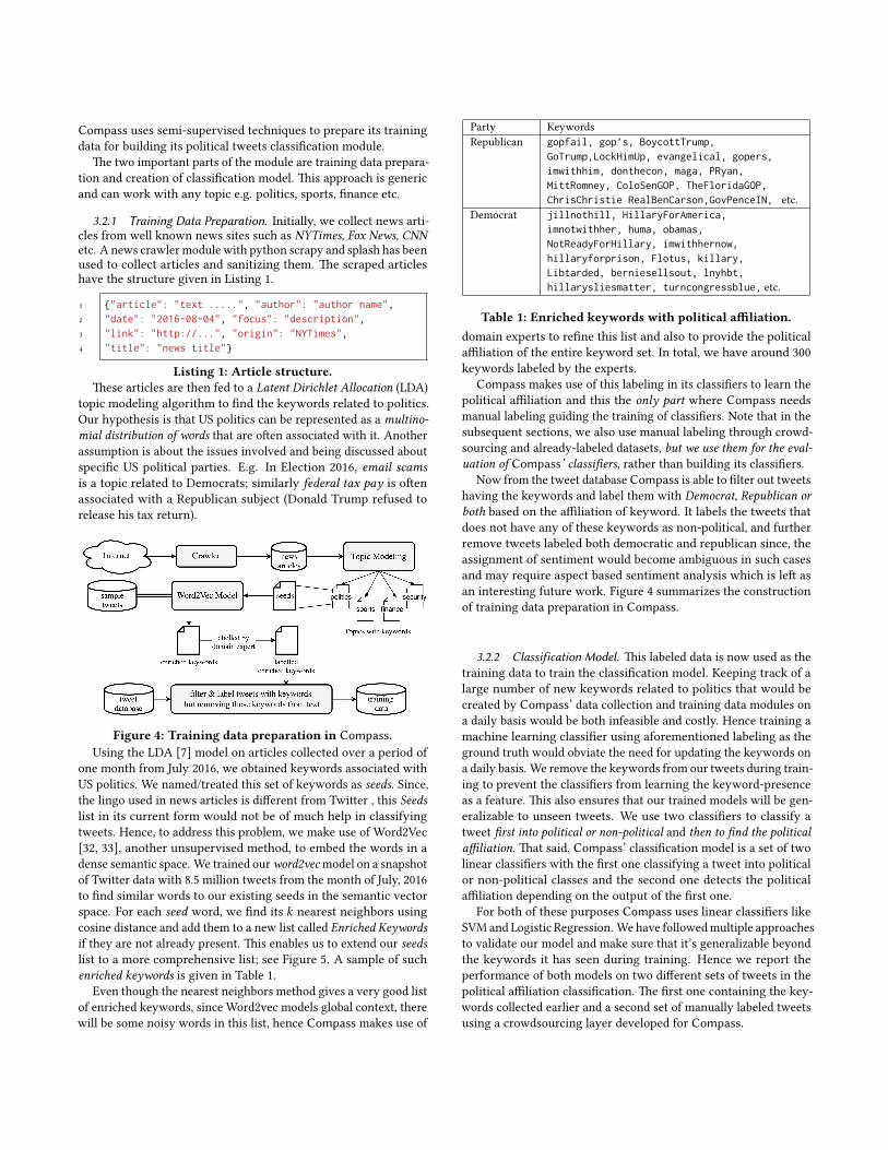
3.2.1 Training Data Preparation. Initially, we collect news arti-cles from well known news sites such as NYTimes, Fox News, CNNetc. A news crawler module with python scrapy and splash has beenused to collect articles and sanitizing them. �e scraped articleshave the structure given in Listing 1.

1 {"article": "text .....", "author": "author name",2 "date": "2016-08-04", "focus": "description",3 "link": "http://...", "origin": "NYTimes",4 "title": "news title"}

Listing 1: Article structure.�ese articles are then fed to a Latent Dirichlet Allocation (LDA)

topic modeling algorithm to �nd the keywords related to politics.Our hypothesis is that US politics can be represented as a multino-mial distribution of words that are o�en associated with it. Anotherassumption is about the issues involved and being discussed aboutspeci�c US political parties. E.g. In Election 2016, email scamsis a topic related to Democrats; similarly federal tax pay is o�enassociated with a Republican subject (Donald Trump refused torelease his tax return).

Figure 4: Training data preparation in Compass.Using the LDA [7] model on articles collected over a period of

one month from July 2016, we obtained keywords associated withUS politics. We named/treated this set of keywords as seeds. Since,the lingo used in news articles is di�erent from Twi�er , this Seedslist in its current form would not be of much help in classifyingtweets. Hence, to address this problem, we make use of Word2Vec[32, 33], another unsupervised method, to embed the words in adense semantic space. We trained ourword2vec model on a snapshotof Twi�er data with 8.5 million tweets from the month of July, 2016to �nd similar words to our existing seeds in the semantic vectorspace. For each seed word, we �nd its k nearest neighbors usingcosine distance and add them to a new list called Enriched Keywordsif they are not already present. �is enables us to extend our seedslist to a more comprehensive list; see Figure 5. A sample of suchenriched keywords is given in Table 1.

Even though the nearest neighbors method gives a very good listof enriched keywords, since Word2vec models global context, therewill be some noisy words in this list, hence Compass makes use of

Party KeywordsRepublican gopfail, gop’s, BoycottTrump,

GoTrump,LockHimUp, evangelical, gopers,imwithhim, donthecon, maga, PRyan,MittRomney, ColoSenGOP, TheFloridaGOP,ChrisChristie RealBenCarson,GovPenceIN, etc.

Democrat jillnothill, HillaryForAmerica,imnotwithher, huma, obamas,NotReadyForHillary, imwithhernow,hillaryforprison, Flotus, killary,Libtarded, berniesellsout, lnyhbt,hillarysliesmatter, turncongressblue, etc.

Table 1: Enriched keywords with political a�liation.domain experts to re�ne this list and also to provide the politicala�liation of the entire keyword set. In total, we have around 300keywords labeled by the experts.

Compass makes use of this labeling in its classi�ers to learn thepolitical a�liation and this the only part where Compass needsmanual labeling guiding the training of classi�ers. Note that in thesubsequent sections, we also use manual labeling through crowd-sourcing and already-labeled datasets, but we use them for the eval-uation of Compass’ classi�ers, rather than building its classi�ers.

Now from the tweet database Compass is able to �lter out tweetshaving the keywords and label them with Democrat, Republican orboth based on the a�liation of keyword. It labels the tweets thatdoes not have any of these keywords as non-political, and furtherremove tweets labeled both democratic and republican since, theassignment of sentiment would become ambiguous in such casesand may require aspect based sentiment analysis which is le� asan interesting future work. Figure 4 summarizes the constructionof training data preparation in Compass.

3.2.2 Classification Model. �is labeled data is now used as thetraining data to train the classi�cation model. Keeping track of alarge number of new keywords related to politics that would becreated by Compass’ data collection and training data modules ona daily basis would be both infeasible and costly. Hence training amachine learning classi�er using aforementioned labeling as theground truth would obviate the need for updating the keywords ona daily basis. We remove the keywords from our tweets during train-ing to prevent the classi�ers from learning the keyword-presenceas a feature. �is also ensures that our trained models will be gen-eralizable to unseen tweets. We use two classi�ers to classify atweet �rst into political or non-political and then to �nd the politicala�liation. �at said, Compass’ classi�cation model is a set of twolinear classi�ers with the �rst one classifying a tweet into politicalor non-political classes and the second one detects the politicala�liation depending on the output of the �rst one.

For both of these purposes Compass uses linear classi�ers likeSVM and Logistic Regression. We have followed multiple approachesto validate our model and make sure that it’s generalizable beyondthe keywords it has seen during training. Hence we report theperformance of both models on two di�erent sets of tweets in thepolitical a�liation classi�cation. �e �rst one containing the key-words collected earlier and a second set of manually labeled tweetsusing a crowdsourcing layer developed for Compass.

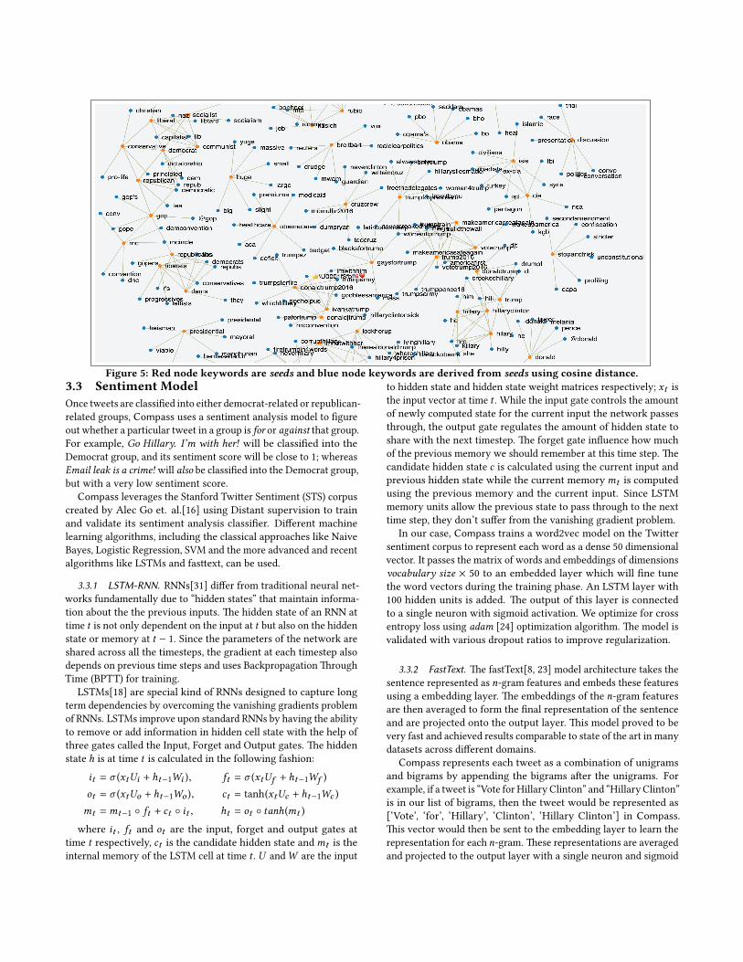
Figure 5: Red node keywords are seeds and blue node keywords are derived from seeds using cosine distance.3.3 Sentiment ModelOnce tweets are classi�ed into either democrat-related or republican-related groups, Compass uses a sentiment analysis model to �gureout whether a particular tweet in a group is for or against that group.For example, Go Hillary. I’m with her! will be classi�ed into theDemocrat group, and its sentiment score will be close to 1; whereasEmail leak is a crime! will also be classi�ed into the Democrat group,but with a very low sentiment score.

Compass leverages the Stanford Twi�er Sentiment (STS) corpuscreated by Alec Go et. al.[16] using Distant supervision to trainand validate its sentiment analysis classi�er. Di�erent machinelearning algorithms, including the classical approaches like NaiveBayes, Logistic Regression, SVM and the more advanced and recentalgorithms like LSTMs and fas�ext, can be used.

3.3.1 LSTM-RNN. RNNs[31] di�er from traditional neural net-works fundamentally due to “hidden states” that maintain informa-tion about the the previous inputs. �e hidden state of an RNN attime t is not only dependent on the input at t but also on the hiddenstate or memory at t − 1. Since the parameters of the network areshared across all the timesteps, the gradient at each timestep alsodepends on previous time steps and uses Backpropagation �roughTime (BPTT) for training.

LSTMs[18] are special kind of RNNs designed to capture longterm dependencies by overcoming the vanishing gradients problemof RNNs. LSTMs improve upon standard RNNs by having the abilityto remove or add information in hidden cell state with the help ofthree gates called the Input, Forget and Output gates. �e hiddenstate h is at time t is calculated in the following fashion:

it = σ (xtUi + ht−1Wi ), ft = σ (xtUf + ht−1Wf )

ot = σ (xtUo + ht−1Wo ), ct = tanh(xtUc + ht−1Wc )

mt =mt−1 ◦ ft + ct ◦ it , ht = ot ◦ tanh(mt )

where it , ft and ot are the input, forget and output gates attime t respectively, ct is the candidate hidden state andmt is theinternal memory of the LSTM cell at time t . U andW are the input

to hidden state and hidden state weight matrices respectively; xt isthe input vector at time t . While the input gate controls the amountof newly computed state for the current input the network passesthrough, the output gate regulates the amount of hidden state toshare with the next timestep. �e forget gate in�uence how muchof the previous memory we should remember at this time step. �ecandidate hidden state c is calculated using the current input andprevious hidden state while the current memorymt is computedusing the previous memory and the current input. Since LSTMmemory units allow the previous state to pass through to the nexttime step, they don’t su�er from the vanishing gradient problem.

In our case, Compass trains a word2vec model on the Twi�ersentiment corpus to represent each word as a dense 50 dimensionalvector. It passes the matrix of words and embeddings of dimensionsvocabulary size × 50 to an embedded layer which will �ne tunethe word vectors during the training phase. An LSTM layer with100 hidden units is added. �e output of this layer is connectedto a single neuron with sigmoid activation. We optimize for crossentropy loss using adam [24] optimization algorithm. �e model isvalidated with various dropout ratios to improve regularization.

3.3.2 FastText. �e fastText[8, 23] model architecture takes thesentence represented as n-gram features and embeds these featuresusing a embedding layer. �e embeddings of the n-gram featuresare then averaged to form the �nal representation of the sentenceand are projected onto the output layer. �is model proved to bevery fast and achieved results comparable to state of the art in manydatasets across di�erent domains.

Compass represents each tweet as a combination of unigramsand bigrams by appending the bigrams a�er the unigrams. Forexample, if a tweet is “Vote for Hillary Clinton” and “Hillary Clinton”is in our list of bigrams, then the tweet would be represented as[‘Vote’, ‘for’, ‘Hillary’, ‘Clinton’, ‘Hillary Clinton’] in Compass.�is vector would then be sent to the embedding layer to learn therepresentation for each n-gram. �ese representations are averagedand projected to the output layer with a single neuron and sigmoid

activation function. We optimized for binary-crossentropy usingthe same adam optimizer as mentioned in the LSTM model above.

3.4 Geomapping ModulePeoples opinion and a�itude towards public events always varieswith region. When one local event happens, it usually resultsinto wider range of discussion and news. To analyze geographicproperties of opinions from twi�er, we use geotagged tweets asmentioned earlier. Mapping of geotagged tweets to counties isimportant for faster processing. �ere are online services for thispurpose, e.g., Google provides a Geocoding web service for it, butthis is not feasible for large scale processing. Instead, Compass useshigh precision GeoJSON i.e. geospatial data interchange format(RFC 7946)[20] to delineate geo-features. We use e�cient ray-tracing technique to �nd a point within a featured polygon. Ageo-tree based approach with country→ state→ county as nodesat each level provides signi�cant pruning power and saves costlycomparison signi�cantly. �is also increases the throughput ofCompass. To further improve scalability and throughput, we extendthe above idea to a distributed and parallel se�ing. In particular,we have integrated the above Geomapping Module into Simba [45],a spatio-temporal analytical engine built over Spark SQL.

3.5 Bursty Event Detection in Compass�e impact of any political event can be noticed by its popularityboth in positive and negative sense. Popularity is a vague termassociated with event. In social media trending is a term used wherenumber of people talking about a event is considered as parameter.�ese events usually gains a�ention over a considerable amountof time. Another type of popularity is measured when an eventgets tremendous response from people but only for a small periodof time. But sometimes they get overshadowed by trending onessince the number of people involved over an extended period mightbe considerably less. �e la�er type needs proper mathematicalmodel to measure its popularity. If properly modeled, it can alsodetect the events that can be trending in future. We call this typeof events as bursty events in�uenced from the phenomenon Burst.

It is also noticeable that there is o�en a “spatial locality” e�ect,where an event usually �rst becomes popular in local area, then inthe state and the whole country. If we can capture the bursts at alocal area then we are a step ahead in detecting it. Hence capturingbursty local events is critical in large spatial data.

�at said, to the best of our knowledge, we found there is lackof proper consensus on the de�nition of burst in various literatures.We present the mathematical model of burst by leveraging intuitionsfrom classic physics. In the experiment and result section we showhow our bursty model is e�ective for elections, where every nowand then election campaigns generate interesting stories. Such anevent creates sentiment waves among the crowd on Twi�er. It

is quite interesting to analyze peoples reaction especially in theevent of election where peoples opinion ma�ers and change overtime with the development of new events.

De�nition 1 (Burst). Burst is a phenomenon identi�ed when atleast n number of event occurrences (of the same event) happens inτ time where τ is determined from probability distribution of gapsbetween occurrences.

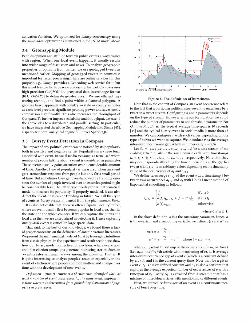
Figure 6: �e de�nition of burstiness.Note that in the context of Compass, an event occurrence refers

to the fact that a particular political story/event is mentioned by atweet in a tweet stream. Con�guring n and τ parameters dependson the type of stream. However with our formulation we couldreduce the number of parameters to one threshold parameter. ForGamma Ray Bursts the typical average time-span is 10 seconds[44] and the typical bursty event in social media is more than 15minutes. We can con�gure τ with such values depending on thetype of bursts we want to capture. We introduce ν as the averageinter-event occurrence gap, which is numerically ν = τ/n.

Let Se = {a0,a1,a2, . . . ,am−1, am , . . .} be a data stream of mi-croblog article ai about the same event e each with timestampst0 < t1 ≤ t2 ≤ . . . tm−1 ≤ tm ≤ . . . respectively. Note that theymay occur sporadically along the time dimension, i.e., the gap be-tween ti and ti+1 is an arbitrary values depending on the timestampvalue of the occurrences of ai and ai+1.

We de�ne term surge st,τe of the event e at a timestamp t be-tween two occurrences ai−1 and ai with Holt’s Linear method ofExponential smoothing as follows.

st,τe =

1τe if t is 0α (t )sti−1,τe + (1 − α∗) 1

τe , if t is tiα (t )sti ,τe otherwise

where 0 ≤ α ≤ 1.In the above de�nition, α is a the smoothing parameter, hence, α

is time-variant and a smoothing variable, we de�ne α (t ) and α∗ as:

α (t ) = e−t−ti−1νe ;

α∗ = e−t−ti−1νe = e−1 where t − ti−1 = νe

where ti−1 is last timestamp of the occurrence of e before time t(i.e., ai−1, the (i-1)-th article with mentioning of e), νe is averageinter-event occurrence gap of event e (which is a constant de�nedby τe/ne ), and t is the current query time. Note that for a givenevent e , τe is a user-de�ned constant and ne is also a constant thatcaptures the average expected number of occurrences of e with atimespan of τe . Lastly, Se is extracted from a stream S that has amixture of microblog articles with mentioning of di�erent events.

Next, we introduce burstiness of an event as a continuous mea-sure of burst over time.

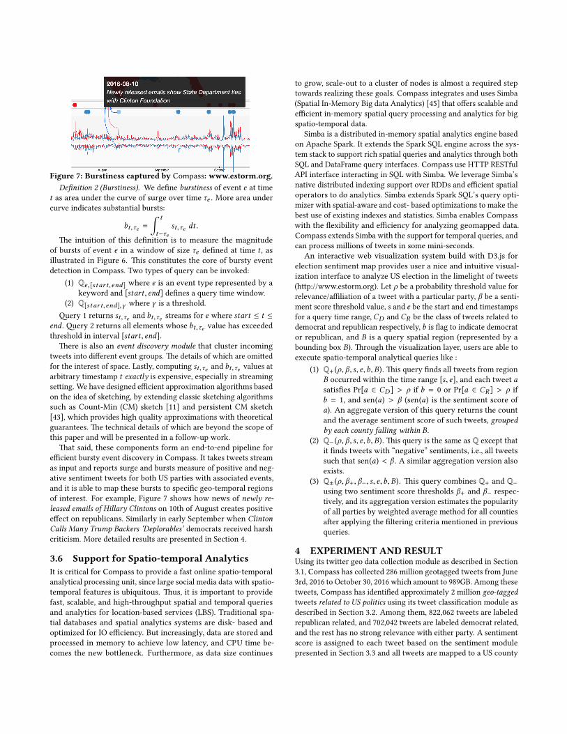
Figure 7: Burstiness captured by Compass: www.estorm.org.De�nition 2 (Burstiness). We de�ne burstiness of event e at time

t as area under the curve of surge over time τe . More area undercurve indicates substantial bursts:

bt,τe =

∫ t

t−τest,τe dt .

�e intuition of this de�nition is to measure the magnitudeof bursts of event e in a window of size τe de�ned at time t , asillustrated in Figure 6. �is constitutes the core of bursty eventdetection in Compass. Two types of query can be invoked:

(1) Qe,[star t,end] where e is an event type represented by akeyword and [start , end] de�nes a query time window.

(2) Q[star t,end],γ where γ is a threshold.�ery 1 returns st,τe and bt,τe streams for e where start ≤ t ≤

end . �ery 2 returns all elements whose bt,τe value has exceededthreshold in interval [start , end].

�ere is also an event discovery module that cluster incomingtweets into di�erent event groups. �e details of which are omi�edfor the interest of space. Lastly, computing st,τe and bt,τe values atarbitrary timestamp t exactly is expensive, especially in streamingse�ing. We have designed e�cient approximation algorithms basedon the idea of sketching, by extending classic sketching algorithmssuch as Count-Min (CM) sketch [11] and persistent CM sketch[43], which provides high quality approximations with theoreticalguarantees. �e technical details of which are beyond the scope ofthis paper and will be presented in a follow-up work.

�at said, these components form an end-to-end pipeline fore�cient bursty event discovery in Compass. It takes tweets streamas input and reports surge and bursts measure of positive and neg-ative sentiment tweets for both US parties with associated events,and it is able to map these bursts to speci�c geo-temporal regionsof interest. For example, Figure 7 shows how news of newly re-leased emails of Hillary Clintons on 10th of August creates positivee�ect on republicans. Similarly in early September when ClintonCalls Many Trump Backers ‘Deplorables’ democrats received harshcriticism. More detailed results are presented in Section 4.

3.6 Support for Spatio-temporal AnalyticsIt is critical for Compass to provide a fast online spatio-temporalanalytical processing unit, since large social media data with spatio-temporal features is ubiquitous. �us, it is important to providefast, scalable, and high-throughput spatial and temporal queriesand analytics for location-based services (LBS). Traditional spa-tial databases and spatial analytics systems are disk- based andoptimized for IO e�ciency. But increasingly, data are stored andprocessed in memory to achieve low latency, and CPU time be-comes the new bo�leneck. Furthermore, as data size continues

to grow, scale-out to a cluster of nodes is almost a required steptowards realizing these goals. Compass integrates and uses Simba(Spatial In-Memory Big data Analytics) [45] that o�ers scalable ande�cient in-memory spatial query processing and analytics for bigspatio-temporal data.

Simba is a distributed in-memory spatial analytics engine basedon Apache Spark. It extends the Spark SQL engine across the sys-tem stack to support rich spatial queries and analytics through bothSQL and DataFrame query interfaces. Compass use HTTP RESTfulAPI interface interacting in SQL with Simba. We leverage Simba’snative distributed indexing support over RDDs and e�cient spatialoperators to do analytics. Simba extends Spark SQL’s query opti-mizer with spatial-aware and cost- based optimizations to make thebest use of existing indexes and statistics. Simba enables Compasswith the �exibility and e�ciency for analyzing geomapped data.Compass extends Simba with the support for temporal queries, andcan process millions of tweets in some mini-seconds.

An interactive web visualization system build with D3.js forelection sentiment map provides user a nice and intuitive visual-ization interface to analyze US election in the limelight of tweets(h�p://www.estorm.org). Let ρ be a probability threshold value forrelevance/a�liation of a tweet with a particular party, β be a senti-ment score threshold value, s and e be the start and end timestampsfor a query time range, CD and CR be the class of tweets related todemocrat and republican respectively, b is �ag to indicate democrator republican, and B is a query spatial region (represented by abounding box B). �rough the visualization layer, users are able toexecute spatio-temporal analytical queries like :

(1) Q+ (ρ, β, s, e,b,B). �is query �nds all tweets from regionB occurred within the time range [s, e], and each tweet asatis�es Pr[a ∈ CD ] > ρ if b = 0 or Pr[a ∈ CR ] > ρ ifb = 1, and sen(a) > β (sen(a) is the sentiment score ofa). An aggregate version of this query returns the countand the average sentiment score of such tweets, groupedby each county falling within B.

(2) Q− (ρ, β, s, e,b,B). �is query is the same as Q except thatit �nds tweets with “negative” sentiments, i.e., all tweetssuch that sen(a) < β . A similar aggregation version alsoexists.

(3) Q± (ρ, β+, β−, s, e,b,B). �is query combines Q+ and Q−using two sentiment score thresholds β+ and β− respec-tively, and its aggregation version estimates the popularityof all parties by weighted average method for all countiesa�er applying the �ltering criteria mentioned in previousqueries.

4 EXPERIMENT AND RESULTUsing its twi�er geo data collection module as described in Section3.1, Compass has collected 286 million geotagged tweets from June3rd, 2016 to October 30, 2016 which amount to 989GB. Among thesetweets, Compass has identi�ed approximately 2 million geo-taggedtweets related to US politics using its tweet classi�cation module asdescribed in Section 3.2. Among them, 822,062 tweets are labeledrepublican related, and 702,042 tweets are labeled democrat related,and the rest has no strong relevance with either party. A sentimentscore is assigned to each tweet based on the sentiment modulepresented in Section 3.3 and all tweets are mapped to a US county

(or a country if it is outside the US) based on the geo-mappingmodule in Compass (Section 3.4). Spatio-temporal bursty detectionover these tweets is supported by the bursty model and computationdetailed in Section 3.5. Lastly, a visualization that supports spatio-temporal analytics as introduced in Section 3.6 is presented througha web interface, available at h�p://www.estorm.org.

To validate the design of Compass and investigate the e�ec-tiveness of its core components, we have conducted an extensiveexperimental evaluation using the above data set.

4.1 Tweet Classi�cation4.1.1 Political vs Non-Political tweet classification. As the boot-

strap method in Section 3.2 shows, we obtained enriched Keywordswith LDA and Word2Vec. Given these keywords, we build a basic�lter to distinguish Political tweets and Non-Political tweets. Atweet which contains any keyword is regarded as a political tweet.However this basic �lter would fail when a new political tweetarrives without any previously identi�ed political keyword in it.To solve this problem, we build a binary classi�er to obtain be�erperformance in general.

With the basic �lter, we obtain around 1.5 million of geo-taggedpolitical tweets. To make the dataset balanced, we pick around 1.5+million of non-political tweets randomly and add them to the data.We created training and testing data used an 80-20 split.

We instantiate and develop the classi�er in Section 3.2 basedon text classi�ers like SVM and Logistic Regression (LR) to detectwhether a tweet is political or non-political; they are denoted asPOLM1 and POLM2 (POLM stands for POLitical Model) respectively.For each model, two sets of features are tried: one is unigram andthe other is the combination of unigram and bigram. As shown inthe Table 2 both of Compass’ linear classi�ers performed very well.Especially, the combination features can improve the model.

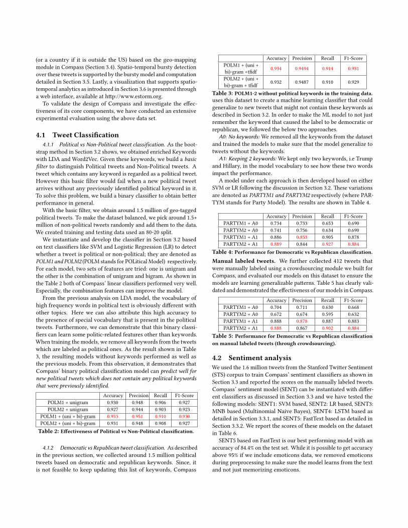
From the previous analysis on LDA model, the vocabulary ofhigh frequency words in political text is obviously di�erent withother topics. Here we can also a�ribute this high accuracy tothe presence of special vocabulary that is present in the politicaltweets. Furthermore, we can demonstrate that this binary classi-�ers can learn some politic-related features other than keywords.When training the models, we remove all keywords from the tweetswhich are labeled as political ones. As the result shown in Table3, the resulting models without keywords performed as well asthe previous models. From this observation, it demonstrates thatCompass’ binary political classi�cation model can predict well fornew political tweets which does not contain any political keywordsthat were previously identi�ed.

Accuracy Precision Recall F1-ScorePOLM1 + unigram 0.930 0.948 0.906 0.927POLM2 + unigram 0.927 0.944 0.903 0.923

POLM1 + (uni + bi)-gram 0.933 0.951 0.910 0.930POLM2 + (uni + bi)-gram 0.931 0.948 0.908 0.927Table 2: E�ectiveness of Political vs Non-Political classi�cation.

4.1.2 Democratic vs Republican tweet classification. As describedin the previous section, we collected around 1.5 million politicaltweets based on democratic and republican keywords. Since, itis not feasible to keep updating this list of keywords, Compass

Accuracy Precision Recall F1-ScorePOLM1 + (uni +bi)-gram +t�df 0.934 0.9494 0.914 0.931

POLM2 + (uni +bi)-gram + t�df 0.932 0.9487 0.910 0.929

Table 3: POLM1-2 without political keywords in the training data.uses this dataset to create a machine learning classi�er that couldgeneralize to new tweets that might not contain these keywords asdescribed in Section 3.2. In order to make the ML model to not justremember the keyword that caused the label to be democratic orrepublican, we followed the below two approaches.

A0: No keywords: We removed all the keywords from the datasetand trained the models to make sure that the model generalize totweets without the keywords.

A1: Keeping 2 keywords: We kept only two keywords, i.e Trumpand Hillary, in the model vocabulary to see how these two wordsimpact the performance.

A model under each approach is then developed based on eitherSVM or LR following the discussion in Section 3.2. �ese variationsare denoted as PARTYM1 and PARTYM2 respectively (where PAR-TYM stands for Party Model). �e results are shown in Table 4.

Accuracy Precision Recall F1-ScorePARTYM1 + A0 0.734 0.733 0.653 0.690PARTYM2 + A0 0.741 0.756 0.634 0.690PARTYM1 + A1 0.886 0.853 0.905 0.878PARTYM2 + A1 0.889 0.844 0.927 0.884

Table 4: Performance for Democratic vs Republican classi�cation.

Manual labeled tweets. We further collected 412 tweets thatwere manually labeled using a crowdsourcing module we built forCompass, and evaluated our models on this dataset to ensure themodels are learning generalizable pa�erns. Table 5 has clearly vali-dated and demonstrated the e�ectiveness of our models inCompass.

Accuracy Precision Recall F1-ScorePARTYM1 + A0 0.704 0.711 0.630 0.668PARTYM2 + A0 0.672 0.674 0.595 0.632PARTYM1 + A1 0.888 0.878 0.887 0.883PARTYM2 + A1 0.888 0.867 0.902 0.884

Table 5: Performance for Democratic vs Republican classi�cationon manual labeled tweets (through crowdsourcing).

4.2 Sentiment analysisWe used the 1.6 million tweets from the Stanford Twi�er Sentiment(STS) corpus to train Compass’ sentiment classi�ers as shown inSection 3.3 and reported the scores on the manually labeled tweets.Compass’ sentiment model (SENT) can be instantiated with di�er-ent classi�ers as discussed in Section 3.3 and we have tested thefollowing models: SENT1: SVM based, SENT2: LR based, SENT3:MNB based (Multinomial Naive Bayes), SENT4: LSTM based asdetailed in Section 3.3.1, and SENT5: FastText based as detailed inSection 3.3.2. We report the scores of these models on the datasetin Table 6.

SENT5 based on FastText is our best performing model with anaccuracy of 84.4% on the test set. While it is possible to get accuracyabove 95% if we include emoticons data, we removed emoticonsduring preprocessing to make sure the model learns from the textand not just memorizing emoticons.

Method AccuracySENT1 + unigram 0.819SENT2 + unigram 0.813SENT3 + unigram 0.813

SENT1 + (uni + bi)-gram 0.808SENT2 + (uni + bi)-gram 0.827SENT3 + (uni + bi)-gram 0.825

SENT4 0.828SENT5 0.844

Table 6: Comparison of models for sentiment analysis.4.3 Bursty Event DetectionOur bursty model has made successful early detection of signi�cantevents throughout the election season. We compared our resultswith the original events happened [5]. An event is bursty when itsbursty score is more than 1. Table 7 lists event dates, bursty scoreand keywords related to events. �e measured parameters br+, br−,bd+, bd− are bursty scores for republican positive tweets, republicannegative tweets, democrats positive tweets and democrats negativetweets respectively. Due to space constraint, we present only asample of events as result. �e bursty score from Table 7 suggeststhat our system successfully detected these events and keywords.It also shows that cumulatively there is more surge of Republicantweets than the Democrats.

Date Keywords br+ br− bd+ bd−Event Description

19thOct

debatenight, debateTrump, answer thequestion, power transfer

11.8 8.3 5.6 7.4Flash Poll Trump Wins Final PresidentialDebate

12thOct

sexual assault, sexualpredator, grabbing,dressing rooms

2.2 2 1.8 1.5Women Accuse Trump of inappropriatelytouching them

9thOct

debate tonight, jumpingship, tape

15.8 10.0 5.9 7.7Trump and Clinton face o� second presi-dential debate

7thOct

Women, sexual assault,Respect, abuse, hated

3.4 4.8 1.6 2.02Tape leaks showing Trump talking aboutgroping women

4thOct

Pence, Kaine, crazy sys-tem, Poor Black, tax re-turns

4.0 2.6 2.2 2.7Kaine and Pence face o� in vice presidentialdebate

28thSep

Clinton, answer ques-tions, FBI, won the de-bate

2.3 1.9 1.9 1.72Clinton slams Trump in blistering presi-dential debate

10thSep

BasketOfDeplorables,Trump supporters,voters

1.72 1.3 1.3 1.7Clinton called out for Trump supporter de-plorable

29thAug

Huma Abedin, Separate,Joe, Breitbart

1.85 1.4 0.7 0.8Clinton aide Abedin separates from Weiner

25thJul

DNC convention, Demo-cratic, Hillary, Michelle,emails

1.3 1.1 2.3 2.0Democratic National Convention Philadel-phia

21thJul

Make America Great,trumps speech, support-ers, jobs

2.2 1.1 2.0 2.3Trump accepts Republican presidentialnomination

18thJul

GOP convention,Trump, RNC, RNC inCLE

2.5 1.4 1.1 0.97Republican National Convention in Cleve-land

Table 7: Sample of bursty events detected with burst scores.

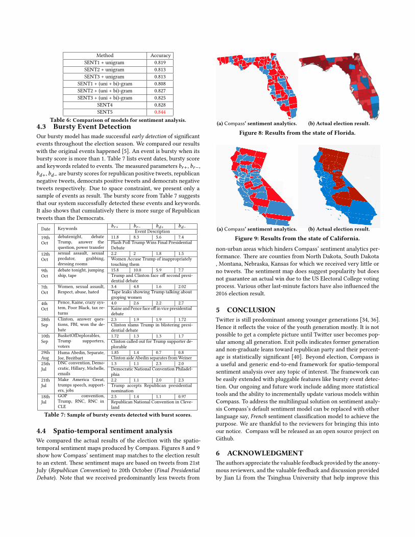
4.4 Spatio-temporal sentiment analysisWe compared the actual results of the election with the spatio-temporal sentiment maps produced by Compass. Figures 8 and 9show how Compass’ sentiment map matches to the election resultto an extent. �ese sentiment maps are based on tweets from 21stJuly (Republican Convention) to 20th October (Final PresidentialDebate). Note that we received predominantly less tweets from

(a) Compass’ sentiment analytics. (b) Actual election result.

Figure 8: Results from the state of Florida.

(a) Compass’ sentiment analytics. (b) Actual election result.

Figure 9: Results from the state of California.

non-urban areas which hinders Compass’ sentiment analytics per-formance. �ere are counties from North Dakota, South Dakota, Montana, Nebraska, Kansas for which we received very li�le orno tweets. �e sentiment map does suggest popularity but doesnot guarantee an actual win due to the US Electoral College votingprocess. Various other last-minute factors have also in�uenced the2016 election result.

5 CONCLUSIONTwi�er is still predominant among younger generations [34, 36].Hence it re�ects the voice of the youth generation mostly. It is notpossible to get a complete picture until Twi�er user becomes pop-ular among all generation. Exit polls indicates former generationand non-graduate leans toward republican party and their percent-age is statistically signi�cant [40]. Beyond election, Compass isa useful and generic end-to-end framework for spatio-temporalsentiment analysis over any topic of interest. �e framework canbe easily extended with pluggable features like bursty event detec-tion. Our ongoing and future work include adding more statisticaltools and the ability to incrementally update various models withinCompass. To address the multilingual solution on sentiment analy-sis Compass’s default sentiment model can be replaced with otherlanguage say, French sentiment classi�cation model to achieve thepurpose. We are thankful to the reviewers for bringing this intoour notice. Compass will be released as an open source project onGithub.

6 ACKNOWLEDGMENT�e authors appreciate the valuable feedback provided by the anony-mous reviewers, and the valuable feedback and discussion providedby Jian Li from the Tsinghua University that help improve this

work. Debjyoti Paul, Feifei Li, Murali Krishna Teja, Xin Yu, andRichie Frost were supported in part by NSF grants 1200792, 1251019,1443046, 1619287 and the associated REU grants. Feifei Li was alsosupported in part by NSFC grant 61428204, a Google Faculty award,and a Huawei gi� award.

REFERENCES[1] Deepak Agarwal and Bee-Chung Chen. 2010. fLDA: matrix factorization through

latent dirichlet allocation. In WSDM.[2] Loulwah AlSumait, Daniel Barbara, and Carlo�a Domeniconi. 2008. On-line

lda: Adaptive topic models for mining text streams with applications to topicdetection and tracking. In ICDM. IEEE.

[3] Anima Anandkumar, Dean P Foster, Daniel J Hsu, Sham M Kakade, and Yi-KaiLiu. 2012. A spectral algorithm for latent dirichlet allocation. In NIPS.

[4] David Anuta, Josh Churchin, and Jiebo Luo. 2016. Election Bias: ComparingPolls and Twi�er in the 2016 US Election. arXiv:1701.06232 (2016).

[5] AOL. 2016. 2016 Presidential Election Timeline. (2016). h�ps://www.aol.com/2016-election/timeline/ [accessed 08-02-2017].

[6] David M Blei. 2012. Probabilistic topic models. CACM 55, 4 (2012), 77–84.[7] David M Blei, Andrew Y Ng, and Michael I Jordan. 2003. Latent dirichlet alloca-

tion. JMLR 3, Jan (2003), 993–1022.[8] Piotr Bojanowski, Edouard Grave, Armand Joulin, and Tomas Mikolov. 2016. En-

riching Word Vectors with Subword Information. arXiv preprint arXiv:1607.04606(2016).

[9] Alexandre Bovet, Flaviano Morone, and Hernan A Makse. 2016. Predicting elec-tion trends with Twi�er: Hillary Clinton versus Donald Trump. arXiv:1610.01587(2016).

[10] Mario Cataldi, Luigi Di Caro, and Claudio Schifanella. 2010. Emerging topic de-tection on twi�er based on temporal and social terms evaluation. In MDM/KDD.

[11] Graham Cormode and S. Muthukrishnan. 2004. An Improved Data StreamSummary: �e Count-Min Sketch and Its Applications. In LATIN.

[12] Cıcero Nogueira Dos Santos and Maira Ga�i. 2014. Deep Convolutional NeuralNetworks for Sentiment Analysis of Short Texts.. In COLING.

[13] Adnan Duric and Fei Song. 2011. Feature selection for sentiment analysis basedon content and syntax models. Decision Support Systems 53, 4 (2011), 704–711.

[14] Ahmed El-Kishky, Yanglei Song, Chi Wang, Clare R Voss, and Jiawei Han. 2014.Scalable topical phrase mining from text corpora. PVLDB 8, 3 (2014).

[15] Alexander Genkin, David D Lewis, and David Madigan. 2007. Large-scaleBayesian logistic regression for text categorization. Technometrics 49, 3 (2007).

[16] Alec Go, Richa Bhayani, and Lei Huang. 2009. Twi�er sentiment classi�cationusing distant supervision. CS224N Project, Stanford 1, 12 (2009).

[17] Frederic Godin, Viktor Slavkovikj, Wesley De Neve, Benjamin Schrauwen, andRik Van de Walle. 2013. Using topic models for twi�er hashtag recommendation.In WWW.

[18] Sepp Hochreiter and Jurgen Schmidhuber. 1997. Long short-term memory. Neuralcomputation 9, 8 (1997), 1735–1780.

[19] �omas Hofmann. 1999. Probabilistic latent semantic analysis. In Uncertainty inarti�cial intelligence. 289–296.

[20] IETF. 2017. RFC 7946 - �e GeoJSON Format. (2017). h�ps://tools.ietf.org/html/rfc7946 [accessed 08-Feb-2017].

[21] Long Jiang, Mo Yu, Ming Zhou, Xiaohua Liu, and Tiejun Zhao. Target-dependenttwi�er sentiment classi�cation. In ACL HLT. 151–160.

[22] �orsten Joachims. 1998. Text categorization with support vector machines:Learning with many relevant features. In ECML.

[23] Armand Joulin, Edouard Grave, Piotr Bojanowski, and Tomas Mikolov. 2016. Bagof Tricks for E�cient Text Classi�cation. arXiv preprint arXiv:1607.01759 (2016).

[24] Diederik Kingma and Jimmy Ba. 2014. Adam: A method for stochastic optimiza-tion. arXiv:1412.6980 (2014).

[25] Jon Kleinberg. 2003. Bursty and hierarchical structure in streams. Data Miningand Knowledge Discovery 7, 4 (2003), 373–397.

[26] E�hymios Kouloumpis, �eresa Wilson, and Johanna D Moore. 2011. Twi�ersentiment analysis: �e good the bad and the omg! Icwsm 11, 538-541 (2011).

[27] Siwei Lai, Liheng Xu, Kang Liu, and Jun Zhao. 2015. Recurrent ConvolutionalNeural Networks for Text Classi�cation.. In AAAI, Vol. 333. 2267–2273.

[28] �anzhi Li, Sameena Shah, Xiaomo Liu, Armineh Nourbakhsh, and Rui Fang.2016. TweetSi�: Tweet Topic Classi�cation Based on Entity Knowledge Baseand Topic Enhanced Word Embedding. In CIKM.

[29] Rong Lu and Qing Yang. 2012. Trend analysis of news topics on twi�er. IJMLC2, 3 (2012).

[30] Andrew McCallum, Kamal Nigam, and others. 1998. A comparison of eventmodels for naive bayes text classi�cation. In AAAI, Vol. 752. 41–48.

[31] Larry Medsker and Lakhmi C Jain. 1999. Recurrent neural networks: design andapplications. CRC press.

[32] Tomas Mikolov, Kai Chen, Greg Corrado, and Je�rey Dean. 2013. E�cientestimation of word representations in vector space. arXiv:1301.3781 (2013).

[33] Tomas Mikolov, Ilya Sutskever, Kai Chen, Greg S Corrado, and Je� Dean. 2013.Distributed representations of words and phrases and their compositionality. InNIPS. 3111–3119.

[34] Dong-Phuong Nguyen, Rilana Gravel, RB Trieschnigg, and �eo Meder. 2013. ”How old do you think I am?” A study of language and age in Twi�er. (2013).

[35] Bo Pang, Lillian Lee, and others. 2008. Opinion mining and sentiment analysis.FTIR 2, 1–2 (2008), 1–135.

[36] PRC. 2016. Demographics of Social Media Users in 2016. (2016). h�p://www.pewinternet.org/2016/11/11/social-media-update-2016/ [accessed 08-Feb-2017].

[37] David A. Shamma, Lyndon Kennedy, and Elizabeth F. Churchill. 2011. Peaks andPersistence: Modeling the Shape of Microblog Conversations. In CSCW.

[38] Maite Taboada, Julian Brooke, Milan To�loski, Kimberly Voll, and Manfred Stede.2011. Lexicon-based methods for sentiment analysis. Computational Linguistics37, 2 (2011), 267–307.

[39] Duyu Tang, Bing Qin, and Ting Liu. 2015. Document Modeling with GatedRecurrent Neural Network for Sentiment Classi�cation.. In EMNLP. 1422–1432.

[40] New York Times. 2016. Election 2016: Exit Polls. (2016). h�ps://www.nytimes.com/interactive/2016/11/08/us/politics/election-exit-polls.html

[41] Soroush Vosoughi, Helen Zhou, and Deb Roy. 2016. Enhanced twi�er sentimentclassi�cation using contextual information. arXiv:1605.05195 (2016).

[42] Chong Wang and David M Blei. 2011. Collaborative topic modeling for recom-mending scienti�c articles. In SIGKDD.

[43] Zhewei Wei, Ge Luo, Ke Yi, Xiaoyong Du, and Ji-Rong Wen. 2015. PersistentData Sketching. In SIGMOD.

[44] Wikipedia. 2016. Swi� Gamma-Ray Burst Mission — Wikipedia, �e Free Encyclo-pedia. (2016). h�ps://en.wikipedia.org/wiki/Swi� Gamma-Ray Burst Mission#Notable detections [accessed 08-Feb-2017].

[45] Dong Xie, Feifei Li, Bin Yao, Gefei Li, Liang Zhou, and Minyi Guo. 2016. Simba:E�cient in-memory spatial analytics. In SIGMOD.

[46] Wei Xie, Feida Zhu, Jing Jiang, Ee-Peng Lim, and Ke Wang. 2013. Topicsketch:Real-time bursty topic detection from twi�er. In ICDM. 837–846.

[47] Wayne Xin Zhao, Jing Jiang, Jianshu Weng, Jing He, Ee-Peng Lim, Hongfei Yan,and Xiaoming Li. 2011. Comparing twi�er and traditional media using topicmodels. In ECIR.

[48] Chunting Zhou, Chonglin Sun, Zhiyuan Liu, and Francis Lau. 2015. A C-LSTMneural network for text classi�cation. arXiv:1511.08630 (2015).

[49] Yunyue Zhu and Dennis Shasha. 2003. E�cient Elastic Burst Detection in DataStreams. In SIGKDD.