
SS 2009Maschinelles Lernen und Neural Computation 150 Kapitel 8: Kernel-Methoden.
Technische Universität München
Institut für Energietechnik
Lehrstuhl für Thermodynamik
Computation of the Thermoacoustic Driving
Capability of Rocket Engine Flames
with Detailed Chemistry
Attila Lehel Török
Vollständiger Abdruck der von der Fakultät für Maschinenwesen der Techni-
schen Universität München zur Erlangung des akademischen Grades eines
DOKTOR-INGENIEURS
genehmigten Dissertation.
Vorsitzender:
Univ.-Prof. P.-S. Koutsourelakis, Ph.D.
Prüfer der Dissertation:
1. Univ.-Prof. Dr.-Ing. T. Sattelmayer
2. Prof. Dr ir J. Steelant, Universität Leuven
Die Dissertation wurde am 16.09.2014 bei der Technischen Universität München eingereicht
und durch die Fakultät für Maschinenwesen am 17.11.2015 angenommen.

Danksagung
Die vorliegende Arbeit entstand am Lehrstuhl für Thermodynamik der Techni-
schen Universität München und wurde durch die Network Partnering Initiative
von ESA-ESTEC gefördert.
Besonders danke ich Herrn Prof. Dr.-Ing. Thomas Sattelmayer für das mir ent-
gegengebrachte Vertrauen, für die gewährten wissenschaftlichen Freiräume und
die mir - sowohl während meiner Zeit als wissenschaftlicher Mitarbeiter als
auch danach - bereitgestellten Rahmenbedingungen. Weiterhin danke ich Herrn
Prof. Dr ir Johan Steelant für die Betreuung meiner Arbeit während meines
zwölfmonatigen Forschungsaufenthaltes bei ESTEC, die fachlichen Impulse und
die freundliche Übernahme des Koreferats. Herrn Prof. Phaedon-Stelios
Koutsourelakis Ph.D. danke ich für die Übernahme des Prüfungsvorsitzes.
Sowohl während meiner Zeit am Lehrstuhl als auch bei ESTEC habe ich viele
Menschen kennengelernt, denen ich in vielerlei Hinsicht dankbar bin. Bei admi-
nistrativen Angelegenheiten konnte ich mich stets auf die Unterstützung in den
Sekretariaten verlassen. Auf der Suche nach Hilfe bei technischen Problemen
wurde ich oft im Büro der Admins, aber auch immer wieder in den Werkstätten
fündig. Und bei fachlichen Fragen haben mich die Anregungen meiner Kolle-
ginnen und Kollegen vorangebracht. Von der kameradschaftlichen Unterstüt-
zung und dem freundschaftlichen Umgang untereinander hat aber nicht nur mein
Wissen sondern auch meine Gemütslage immer wieder profitiert. Die Zeit am
Lehrstuhl wird mir daher, trotz schwieriger Phasen, stets in schöner Erinnerung
bleiben.
Mein größter Dank gilt aber meiner wunderbaren Familie. Insbesondere meinen
Eltern für die Unterstützung während der langen Jahre meiner Ausbildung und
den Zuspruch den ich schon mein ganzes Leben erfahren darf; und meiner Ehe-
frau und meinen Kindern für all das Glück das wir teilen dürfen und all die
Freude die sie in mein Leben bringen. Ihnen möchte ich dieses Buch von gan-
zem Herzen widmen.
München, im Juli 2016 Attila Török

Kurzfassung
Berechnungstools für die Vorhersage von Verbrennungsinstabilitäten in Rake-
tentriebwerken benötigen ein Modell für die Wärmefreisetzung der Flamme. In
dieser Arbeit werden die Parameter eines solchen Modells für eine H2-O2 Flam-
me mittels CFD und detaillierter Chemie berechnet. Diverse Anregungsmetho-
den und ihr Einfluss auf die Wärmefreisetzung werden untersucht. Simulationen
mit der so errechneten Flammentransferfunktion bestätigen das Auftreten der in
Experimenten beobachteten Instabilitäten.
Abstract
Computational tools for the prediction of combustion instabilities in rocket en-
gines require a heat release model to represent the flame. In this thesis parame-
ters of such a model are calculated for a H2-O2 flame using CFD with detailed
chemistry. Several excitation methods are considered and their effects on heat
release fluctuations are analyzed. Simulations with the thus determined flame
transfer function confirm the appearance of thermoacoustic oscillations that
were observed in experiments.

i
Contents
Contents ................................................................................................................. i
List of Tables ........................................................................................................ v
List of Figures .................................................................................................... vii
Nomenclature .................................................................................................... xiii
1 Introduction .................................................................................................. 1
1.1 Space Flight Today .................................................................................. 1
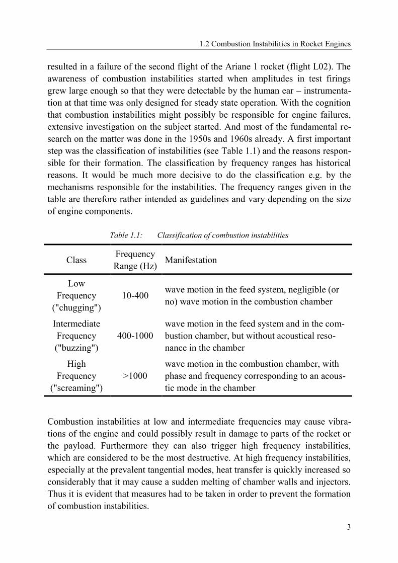
1.2 Combustion Instabilities in Rocket Engines ........................................... 2
1.3 This Thesis ............................................................................................... 5
2 Computational Fluid Dynamics .................................................................. 7
2.1 Basic Equations of Fluid Dynamics ........................................................ 7
2.2 Closing the System of Equations ............................................................. 8
2.2.1 Ideal Gases.......................................................................................... 8
2.2.2 Real Gases .......................................................................................... 9
2.3 Transport Properties .............................................................................. 11
2.4 Multicomponent Flow ........................................................................... 14
2.5 Mass Diffusion ...................................................................................... 17
2.6 Turbulence ............................................................................................. 20
2.7 Solver Theory in ANSYS CFX ............................................................. 21
2.8 Non-Reflecting Boundary Conditions in CFX ...................................... 23
3 Combustion ................................................................................................. 25
3.1 Chemical Kinetics .................................................................................. 25
3.1.1 System of Equations ......................................................................... 25
3.1.2 Thermodynamic Data ....................................................................... 26
3.1.3 Chemical Rate Expressions .............................................................. 26
Contents
ii
3.1.4 Third Body Reactions ....................................................................... 27
3.1.5 Pressure-Dependent Rate Constant .................................................. 28
3.1.6 Intermediate Complex-Forming Bimolecular Reactions ................. 29
3.1.7 Stiff System of ODEs ....................................................................... 30
3.1.8 Choice of Reaction Mechanism ....................................................... 32
3.2 Turbulence-Chemistry Interaction......................................................... 33
3.2.1 Assumed PDF of Temperature ......................................................... 33
3.2.2 Assumed PDF of Composition ......................................................... 35
3.2.3 Mean Chemical Production Rates .................................................... 36
3.2.4 Additional Equations in the Flow Solver ......................................... 37
3.3 Tabulation .............................................................................................. 38
3.3.1 Tabulation of Chemical Kinetics ...................................................... 38
3.3.2 Tabulation of Turbulence-Chemistry Interaction............................. 40
3.4 Approach for the Simulation of Combustion in this Thesis .................. 41
4 Simulation of Combustion in Reacting Flows ......................................... 45
4.1 Constant Volume Reactor ...................................................................... 45
4.1.1 Validation of the implementation in CFX ........................................ 45
4.1.2 Influence of the Reaction Mechanism .............................................. 47
4.2 Laminar Non-Premixed Flame .............................................................. 49
4.2.1 Experimental Data ............................................................................ 50
4.2.2 Numerical Simulation ....................................................................... 50
4.2.3 Results .............................................................................................. 51
4.3 Turbulent Flame at Atmospheric Pressure ............................................ 53
4.3.1 Experimental Data ............................................................................ 53
4.3.2 Numerical Simulation ....................................................................... 54
4.3.3 Simulation with Detailed Chemistry ................................................ 55
4.3.4 Influence of Tabulation .................................................................... 59
4.3.5 Influence of Reaction Mechanism.................................................... 61
4.3.6 Influence of Turbulence Chemistry Interaction ............................... 62
4.4 Turbulent Flame at High Pressure ......................................................... 68
Contents
iii
4.4.1 Experimental Data ............................................................................ 68
4.4.2 Numerical Simulation ....................................................................... 69
4.4.3 Simulation with Detailed Chemistry ................................................ 70
4.4.4 Influence of Reaction Mechanism.................................................... 72
4.4.5 Influence of Turbulence-Chemistry Interaction ............................... 73
5 Preliminary Studies for the Simulation of Instabilities .......................... 77
5.1 The Hydrodynamic System ................................................................... 77
5.1.1 Experimental Data and Theoretical Background ............................. 77
5.1.2 Set-Up for Numerical Simulations ................................................... 79
5.1.3 Results in ANSYS CFX ................................................................... 80
5.2 Heat Release and Pressure ..................................................................... 82
5.2.1 Set-Up for Numerical Simulation .................................................... 82
5.2.2 Results in ANSYS CFX ................................................................... 84
5.3 Methods for Simulation of Instabilities ................................................. 87
5.3.1 Velocity Excitation ........................................................................... 87
5.3.2 Velocity and Pressure Excitation ..................................................... 87
5.3.3 Pressure Excitation ........................................................................... 90
6 Simulation of Instabilities on a Rocket Engine Flame ............................ 93
6.1 Experimental Data ................................................................................. 93
6.2 Basic Numerical Setup .......................................................................... 94
6.3 Simulation without Excitation ............................................................... 95
6.4 Velocity Excitation .............................................................................. 100
6.5 Pressure Excitation .............................................................................. 103
6.5.1 Mass Source and Sink Terms on Boundaries ................................. 103
6.5.2 Moving Wall ................................................................................... 107
6.5.3 Fluctuating Pressure as Input to Chemical Kinetics ...................... 109
6.5.4 Conclusion for Pressure Excitation ................................................ 111
6.6 Extension to Fluctuating Inlet Mass Flow Rates ................................. 112
7 Evaluation of Combustion Instabilities .................................................. 117
7.1 Mean Flow Properties .......................................................................... 118
Contents
iv
7.2 Acoustics Analysis without Combustion ............................................ 119
7.3 Thermoacoustic Analysis with Heat Release ...................................... 121
7.3.1 Flame Transfer Function ................................................................ 121
7.3.2 Shape Function ............................................................................... 122
7.3.3 Simulation and Results ................................................................... 122
8 Summary and Conclusions ...................................................................... 127
References ........................................................................................................ 131
A Appendix ................................................................................................... 141
A.1 Material Properties .............................................................................. 141
A.2 Reaction Mechanisms .......................................................................... 142
v
List of Tables
Table 1.1: Classification of combustion instabilities ....................................... 3
Table 2.1: Overview of transport phenomena ................................................ 12
Table 2.2: Coefficients from Neufeld et al. [67] for calculating Ω(l,s)*
.......... 13
Table 4.1: Flame and flow conditions [14] .................................................... 54
Table 4.2: Dimensions (axial radial) of grids used for grid convergence .... 56
Table 4.3: Operating conditions of RCM-3 test case [37] ............................. 68
Table 4.4: Dimensions of the Mascotte single injector illustrated in
Figure 4.26 ..................................................................................... 69
Table 6.1: Operating conditions for combustion chamber BKD with
injector head L42 [35] ................................................................... 93
Table 7.1: Operating conditions for the simulation of the combustion
chamber in CFX .......................................................................... 118
Table 7.2: Parameters for FTF from the simulation of a single flame in
BKD L42 ..................................................................................... 121
Table A.1: Molar masses of the species involved in combustion ................. 141
Table A.2: Coefficients for the polynomials in equations (3.3), (3.4) and
(3.5) in the lower temperature range (up to 1000 K) .................. 141
Table A.3: Coefficients for the polynomials in equations (3.3), (3.4) and
(3.5) in the upper temperature range (above 1000 K) ................. 141
Table A.4: Reaction mechanism from Jachimowski [47], modified by
Wilson and MacCormack [105]. ................................................. 142
Table A.5: Efficiency factors ≠1 for the mechanism in Table A.4. .............. 142
Table A.6: Reaction mechanism from Ó Conaire et al. [69]. ....................... 143
Table A.7: Troe parameters for the mechanism in Table A.6. ...................... 143
Table A.8: Efficiency factors ≠1 for the mechanism in Table A.6. .............. 144

vii
List of Figures
Figure 2.1: Comparison of equations of state for oxygen at 154.18 K............ 10
Figure 2.2: Illustration of terms and definitions in CFX (with
modifications from [4]) ................................................................. 19
Figure 2.3: Simplified solution flow chart for inner iterations within
ANSYS CFX [4] ........................................................................... 21
Figure 2.4: Illustration of finite volume methods: The cell-centered or
volume-filled method (left) and the cell-vertex or element-
filled method (right) ...................................................................... 23
Figure 4.1: Temperature curves for a constant volume reactor from CFX
and SENKIN with the mechanism from Jachimowski [47] at
1 bar ............................................................................................... 46
Figure 4.2: Total energy equation and thermal energy equation compared .... 47
Figure 4.3: Reaction mechanisms compared based on the progress of a
constant volume reactor in CFX at 1 bar ...................................... 47
Figure 4.4: Reaction mechanisms compared based on the progress of a
constant volume reactor in CFX at 60 bar .................................... 48
Figure 4.5: Ignition time plotted against pressure for a constant volume
reactor starting at 1100 K and 60 bar ............................................ 48
Figure 4.6: Ignition time plotted against the equivalence ratio for a
constant volume reactor starting at 1100 K and 60 bar ................. 49
Figure 4.7: Schematic illustration of the laminar burner ................................. 50
Figure 4.8: OH mass fraction plot from simulation with detailed
chemistry and diffusion ................................................................. 52
Figure 4.9: Abel-transformed OH* image from experiment ........................... 52
Figure 4.10: N2 mass fraction plot from simulation with detailed chemistry
and diffusion .................................................................................. 53
List of Figures
viii
Figure 4.11: Schematic illustration of the vitiated coflow burner [14] ............. 54
Figure 4.12: OH mass fraction plots from simulations of the flame from
Cabra et al. [14] (grids from top: XS, S, M, L, XL) ..................... 55
Figure 4.13: Temperature plots from simulations of the flame from Cabra
et al. [14] (grids from top: XS, S, M, L, XL) ................................ 56
Figure 4.14: OH mass fraction profiles for z/d = 1, 8, 11, 14 and 26 (from
top left) from simulations of the flame from Cabra et al. [14] ..... 57
Figure 4.15: Temperature profiles for z/d = 1, 8, 11, 14 and 26 (from top
left) from simulations of the flame from Cabra et al. [14] ............ 58
Figure 4.16: OH mass fraction plots from simulations of the flame from
Cabra et al. [14]; top: 20 mf-steps, middle: 30 mf-steps,
bottom: no tabulation .................................................................... 60
Figure 4.17: Temperature plots from simulations of the flame from Cabra
et al. [14]; top: 20 mf-steps, middle: 30 mf-steps, bottom: no
tabulation ....................................................................................... 60
Figure 4.18: OH mass fraction plots from simulations of the flame from
Cabra et al. [14]; above: Jachimowski, below: Ó Conaire............ 61
Figure 4.19: Temperature plots from simulations of the flame from Cabra
et al. [14]; above: Jachimowski [47], below: Ó Conaire et al.
[69] ................................................................................................ 62
Figure 4.20: OH mass fraction plots from simulations of the flame from
Cabra et al. [14]; from the top: 1. no PDF, 2. T-PDF, 3.
Y-PDF, 4. T- and Y-PDF .............................................................. 63
Figure 4.21: Temperature plots from simulations of the flame from Cabra
et al. [14]; from the top: 1. no PDF, 2. T-PDF, 3. Y-PDF, 4.
T- and Y-PDF ................................................................................ 64
Figure 4.22: TI plot from the simulation of the flame from Cabra et al. [14]
with T- and Y-PDF ........................................................................ 65
Figure 4.23: 2
Y plot from the simulation of the flame from Cabra et al.
[14] with T- and Y-PDF ................................................................ 65
Figure 4.24: Influence of assumed PDF approaches on OH mass fraction
profiles at z/d = 1, 8, 11, 14 and 26 (from top left) from
simulations of the flame from Cabra et al. [14] ............................ 66
List of Figures
ix
Figure 4.25: Influence of assumed PDF approaches on temperature
profiles at z/d = 1, 8, 11, 14 and 26 (from top left) from
simulations of the flame from Cabra et al. [14] ............................ 67
Figure 4.26: Mascotte single injector geometry [68] ......................................... 69
Figure 4.27: OH* contours from the Mascotte single injector test case [37]
(top: average emission image, bottom: Abel-transformed
emission image) ............................................................................. 71
Figure 4.28: OH mass fractions plot from the simulation of the Mascotte
single injector test case [37] .......................................................... 71
Figure 4.29: Temperatures in the Mascotte single injector [37] in
experiment and simulations ........................................................... 72
Figure 4.30: OH mass fraction plots from simulations of the Mascotte
single injector test case [37]; above: Jachimowski [47],
below: Ó Conaire et al. [69] .......................................................... 73
Figure 4.31: OH mass fraction plots from simulations of the Mascotte
single injector test case [37]; above: no PDF, below: T-PDF ....... 73
Figure 4.32: TI plot from the simulation of the Mascotte single injector
test case [37] with consideration of the assumed PDF of
temperature only ............................................................................ 74
Figure 4.33: 2
Y plot from the simulation of the Mascotte single injector
test case [37] with consideration of the assumed PDF of
temperature only ............................................................................ 75
Figure 5.1: The near wall velocity overshoot (Richardson's annular
effect) ............................................................................................. 79
Figure 5.2: Phase shift for ω* = 1950 and pmax = 10 Pa at one Opening,
with Δt = 0.01s .............................................................................. 80
Figure 5.3: Numerical simulation and analytical solution for ω* = 1950
and pmax = 10Pa at one Opening .................................................... 81
Figure 5.4: Illustration of domain and grid in the Rijke tube at the
position of the heater ..................................................................... 83
Figure 5.5: Oscillating pressure in the Rijke tube at the position of the
heater ............................................................................................. 84
List of Figures
x
Figure 5.6: Oscillating pressure and velocity in the Rijke tube at the
position of the heater ..................................................................... 84
Figure 5.7: Oscillating pressure and heat flux in the Rijke tube at the
position of the heater ..................................................................... 85
Figure 5.8: Oscillating pressure and heat flux in the Rijke tube at the
position of the heater at limit cycle ............................................... 86
Figure 5.9: FFT gain of the calculated heat release at the limit cycle in
Figure 5.9 ....................................................................................... 86
Figure 5.10: Fluctuation of pressure and transverse velocity at x = 0.20 m
and y = -0.75 m.............................................................................. 88
Figure 5.11: Distribution of pressure (above) and velocity (below) in the
computational domain ................................................................... 89
Figure 5.12: Cross section of a 3D computational domain with illustration
of the translational periodic boundaries (left) and of the
pressure excitation methods (right) ............................................... 90
Figure 6.1: OH mass fraction plots from simulations of OP7 of a single
L42 flame on a 2D grid ................................................................. 96
Figure 6.2: Temperature plots from simulations of OP7 of an L42 flame
on a 2D grid ................................................................................... 97
Figure 6.3: OH mass fraction plots from simulations of OP3 and OP7 .......... 97
Figure 6.4: Temperature plots from simulations of OP3 and OP7 with .......... 98
Figure 6.5: Plot of volumetric heat release from simulation of OP7 of the
L42 flame ...................................................................................... 98
Figure 6.6: Distribution of heat release along the axis from simulation of
OP7 of the L42 flame .................................................................... 98
Figure 6.7: O2 mass fraction plot from simulation of OP7 of an L42
flame on a quasi-2D grid ............................................................... 99
Figure 6.8: Streamlines from simulation of OP7 of an L42 flame on a
quasi-2D grid ................................................................................. 99
Figure 6.9: Pressure field for the first transverse mode in a cylindrical
chamber ....................................................................................... 101

List of Figures
xi
Figure 6.10: Distribution of temperature and OH mass fraction along the
axis of an L42 flame with and without velocity excitation ......... 102
Figure 6.11: Fluctuation of global heat release over time as response to
velocity excitation ....................................................................... 103
Figure 6.12: Outlet pressure and heat release from excitation with mass
source terms on boundaries ......................................................... 105
Figure 6.13: Pressure amplitudes and phase offsets resulting from
fluctuating mass source terms on boundaries.............................. 106
Figure 6.14: Outlet pressure and heat release from excitation with a
moving wall at OP7 ..................................................................... 107
Figure 6.15: Rayleigh-Integral along the axis from simulation of OP7
resulting from excitation with moving wall (at 1 bar and
10000 Hz) .................................................................................... 108
Figure 6.16: Pressure amplitudes and phase offsets resulting from
excitation with a moving wall ..................................................... 109
Figure 6.17: Fluctuating pressure and heat release from excitation in
external routine ............................................................................ 109
Figure 6.18: Rayleigh-Integral along the axis from simulation of OP7 with
excitation (1 bar, 10000 Hz) ........................................................ 110
Figure 6.19: Phase shift between pressure and heat release fluctuations for
OP3 and OP7 ............................................................................... 111
Figure 6.20: Symbolic illustration of the domains used for a propellant
feed system .................................................................................. 112
Figure 6.21: Outlet pressure and corresponding mass flow rates at the
outlet ............................................................................................ 113
Figure 6.22: Rayleigh-Integral along the axis from simulation of OP7 with
fluctuating mass flow rates and pressure excitation (1 bar,
10000 Hz) .................................................................................... 114
Figure 7.1: Schematic illustration of the domain for the calculation of
mean flow properties in CFX ...................................................... 118
Figure 7.2: Mach number plot from simulation of OP3 in CFX ................... 119
List of Figures
xii
Figure 7.3: Temporal evolution of pressure at a virtual microphone in
PIANO for OP3 without combustion being considered.............. 120
Figure 7.4: FFT gain of the pressure signal from Figure 7.3 ......................... 120
Figure 7.5: Shape function resembling the form of heat release
distribution along the axis from the simulation of an L42
flame OP3 .................................................................................... 122
Figure 7.6: Temporal evolution of pressure at a virtual microphone in
PIANO for OP3 with combustion being considered after
1.0 ms .......................................................................................... 123
Figure 7.7: FFT gain of the pressure signal from Figure 7.6 ......................... 123
Figure 7.8: Pressure distribution at inflow and combustion chamber wall
for OP3 ........................................................................................ 124
Figure 7.9: Pressure distribution at the faceplate for OP3 ............................. 124
xiii
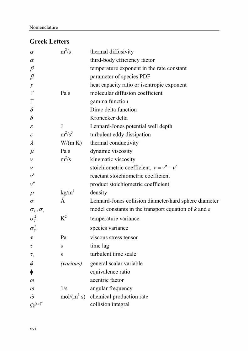
Nomenclature
Symbols
a m5/(kg s
2) parameter of the Redlich-Kwong equation
a Troe parameter
a0 m5/(kg s
2) gas constant for Redlich-Kwong equation
a1, a2,…, a7 (various) coefficients of fits to thermodynamic data
A (various) pre-exponential factor
A m² area
A area of clipped part of temperature PDF
A, B,…, H coefficients of the collision integral
A, B,…, D parameters of the shape function
b m3/kg gas constant of Redlich-Kwong equation
B representing an expression (see species PDF)
B representing an expression (see Richardson's effect)
c m3/kg correction coefficient for Redlich-Kwong equation
c mol/m³ molar concentration
c shift parameter of the broadening factor
c m/s speed of sound
cp J/(kg K) specific heat capacity at constant pressure
Cp J/(mol K) molar heat capacity at constant pressure
CT modeling constant of the T transport equation
CY modeling constant of the Y transport equation
Cε1, Cε2 k-ε-model constants in the ε transport equation
Cμ k-ε-model constant of turbulent viscosity
d asymmetry parameter of the broadening factor
d, D m diameter
D m2/s kinematic diffusivity (diffusion coefficient)
DAB
m2/s binary diffusion coefficient
Nomenclature
xiv
e Euler's number
E J/mol activation energy in the rate constant
f general function
f Hz frequency
F general collision broadening factor
Fcent broadening factor at the center of the fall-off curve
h J/kg specific enthalpy
H J/mol K molar enthalpy
i imaginary unit: i 2
1
IT fluctuation intensity
J Bessel function
k m2/s
2 turbulent kinetic energy
k J/K Boltzmann constant: k = 1.38010-23
J/K
k 1/m wave number
k0 (various) forward rate coefficient at the low-pressure limit
k∞ (various) forward rate coefficient at the high-pressure limit
kb (various) backward rate constant
kf (various) forward rate constant
K m/s2 constant for Richardson's annular effect
K table coordinate
Kc (various) equilibrium constant based on molar concentration
Kp (various) equilibrium constant based on partial pressures
L m length
Le Lewis number
m sum of stoichiometric coefficient
m kg/s mass flow rate
M kg/mol molar mass
Ma Mach number
n modified exponent of Redlich-Kwong equation
n interaction parameter
N width parameter of the broadening factor
N number of elements in a set
O m2 control surface
p Pa pressure
Nomenclature
xv
P probability density function
P kg/(m2 s) turbulence production
Pr Prandtl number
q mol/(m s) rate-of-progress variable
Q W heat flux or heat release
r, R m radius
R J/(kg K) specific gas constant
Ru J/(mol K) universal gas constant: Ru = 8.314 J/(mol K)
sf shape function
S J/(mol K) molar entropy
S mol/kg summand
SE kg/(m s3) energy source term
SM kg/(m2 s
2) momentum source term (vector)
Ss kg/(m3 s) species source term
t s time
T K temperature
T*, T
**, T
*** K Troe parameters
T1,T2,T3,T4 (various) terms for calculation of mean chemical production rate
u m/s (axial) velocity; component of velocity vector
U m/s velocity vector
V m3 control volume
v m3/kg specific volume
vm m3/mol molar volume
x, X Cartesian coordinate
X mole fraction
y (various) representing a vector of dependent variables
y, Y Cartesian coordinate
Y mass fraction
z Cartesian coordinate
Nomenclature
xvi
Greek Letters
m2/s thermal diffusivity
third-body efficiency factor
temperature exponent in the rate constant
parameter of species PDF
heat capacity ratio or isentropic exponent
Pa s molecular diffusion coefficient
gamma function
Dirac delta function
Kronecker delta
J Lennard-Jones potential well depth
m2/s
3 turbulent eddy dissipation
W/(m K) thermal conductivity
Pa s dynamic viscosity
m2/s kinematic viscosity
stoichiometric coefficient,
reactant stoichiometric coefficient
product stoichiometric coefficient
kg/m3 density
Å Lennard-Jones collision diameter/hard sphere diameter
,k model constants in the transport equation of k and ε
2
T K2 temperature variance
2
Y species variance
τ Pa viscous stress tensor
s time lag
t s turbulent time scale
(various) general scalar variable
equivalence ratio
acentric factor
1/s angular frequency
mol/(m3 s) chemical production rate
, *l s collision integral
Nomenclature
xvii
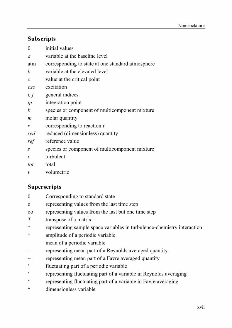
Subscripts
0 initial values
a variable at the baseline level
atm corresponding to state at one standard atmosphere
b variable at the elevated level
c value at the critical point
exc excitation
i, j general indices
ip integration point
k species or component of multicomponent mixture
m molar quantity
r corresponding to reaction r
red reduced (dimensionless) quantity
ref reference value
s species or component of multicomponent mixture
t turbulent
tot total
v volumetric
Superscripts
0 Corresponding to standard state
o representing values from the last time step
oo representing values from the last but one time step
T transpose of a matrix
^ representing sample space variables in turbulence-chemistry interaction
^ amplitude of a periodic variable
– mean of a periodic variable
– representing mean part of a Reynolds averaged quantity
~ representing mean part of a Favre averaged quantity
' fluctuating part of a periodic variable
' representing fluctuating part of a variable in Reynolds averaging
'' representing fluctuating part of a variable in Favre averaging
* dimensionless variable
Nomenclature
xviii
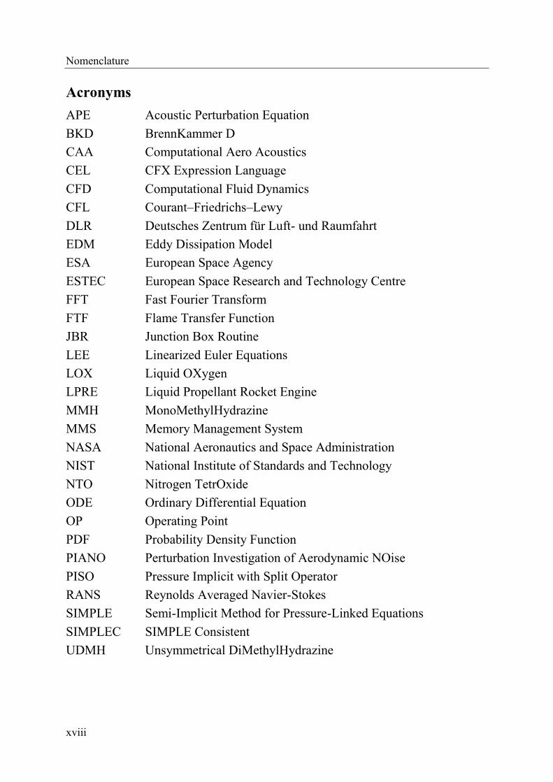
Acronyms
APE Acoustic Perturbation Equation
BKD BrennKammer D
CAA Computational Aero Acoustics
CEL CFX Expression Language
CFD Computational Fluid Dynamics
CFL Courant–Friedrichs–Lewy
DLR Deutsches Zentrum für Luft- und Raumfahrt
EDM Eddy Dissipation Model
ESA European Space Agency
ESTEC European Space Research and Technology Centre
FFT Fast Fourier Transform
FTF Flame Transfer Function
JBR Junction Box Routine
LEE Linearized Euler Equations
LOX Liquid OXygen
LPRE Liquid Propellant Rocket Engine
MMH MonoMethylHydrazine
MMS Memory Management System
NASA National Aeronautics and Space Administration
NIST National Institute of Standards and Technology
NTO Nitrogen TetrOxide
ODE Ordinary Differential Equation
OP Operating Point
PDF Probability Density Function
PIANO Perturbation Investigation of Aerodynamic NOise
PISO Pressure Implicit with Split Operator
RANS Reynolds Averaged Navier-Stokes
SIMPLE Semi-Implicit Method for Pressure-Linked Equations
SIMPLEC SIMPLE Consistent
UDMH Unsymmetrical DiMethylHydrazine
1
1 Introduction
1.1 Space Flight Today
Over the past 100 years the presence of mankind in space has developed from
mere dreams and ideas to a matter of course in our everyday lives and is almost
indispensable in many scientific disciplines. Navigation and communication sat-
ellites help to improve terrestrial infrastructure and are available from even the
remotest regions of our planet. Earth monitoring satellites are used e.g. for me-
teorology, oceanography or geodesy. The view from space back to our Earth
offers the possibility to explore the environment we live in and to gain aware-
ness for the steps necessary for its conservation. Space observatories offer the
possibility to study distant regions of the universe without the obstructive effects
of Earth's atmosphere. Space probe missions target astronomical objects in our
solar system and help to further explore the extraterrestrial universe. The near-
weightlessness on board of space laboratories or space stations allow for funda-
mental research e.g. in material sciences, physics, biology or medicine. For all
these purposes there is a constant need for means of transport to bring freight
and humans to space. Given the expensive payloads, not to mention invaluable
human lives, it is apparent that a reliable means of transport is necessary.
Today and in the foreseeable future the most relevant option to enter space is to
use chemical rockets. In launch vehicles usually liquid propellants are used for
the main engine, while solid propellants are mostly employed in boosters to in-
crease the payload capacity of the spacecraft. Among the liquid propellants the
group called earth-storable is easiest to be handled, since these propellants are in
liquid state at standard conditions. Typically employed combinations usually use
N2O4 (nitrogen tetroxide, short: NTO) as an oxidizer and N2H2 (hydrazine) or
one of its organic compounds (MMH, UDMH, Aerozin 50) as a fuel. The ad-
vantage of these propellants is that they are hypergolic, i.e. they react on contact,
which makes them favorable for applications where multiple restarts are re-
quired. Cryogenic propellant combinations in contrast need an additional device
1 Introduction
2
for ignition. A further disadvantage is the low temperature which is required to
keep the propellants liquefied. The high specific impulse (highest among all
propellants in practical use) on the other hand makes the cryogenic combination
of hydrogen and liquid oxygen (LOX) very attractive. It has been successfully
used for the propulsion of various rocket engines, among which Vulcain (main
engine for Ariane 5) and the Space Shuttle Main Engine are probably most fa-
mous. It will also be employed in future engines, currently e.g. in Vinci, the new
upper stage engine of Ariane 5. The work described in this thesis focuses on this
cryogenic combination. For the sake of completeness a third group of liquid
propellants referred to as cryogenic-storable is also worth mentioning, since it
has been frequently applied in rocket engines. It is the combination of a cryo-
genic (usually LOX) and an earth-storable propellant (usually RP-1, a form of
kerosene).
In a liquid propellant rocket engine (LPRE) usually a turbo-pump is used to
bring propellants from their tanks to the combustion chamber. Pressure-fed sys-
tems are only employed for low thrust application and are mostly irrelevant in
launch vehicles. In engines using the H2/O2 combination propellants are general-
ly injected through coaxial injectors into the combustion chamber, with oxygen
in the core and hydrogen in the annulus. In large engines usually several hun-
dreds of these coaxial injectors are mounted on the faceplate, so that this injector
head – due to its resemblance – is usually also referred to as shower head.
Through the exothermic reaction of the propellants within the combustion
chamber heat is released. Burnt gases exit the combustion chamber through the
de Laval nozzle, which converts thermal energy to directed kinetic energy. For a
detailed description of LPRE elements and rocket propulsion in general the book
of Sutton and Biblarz [97] can be recommended, which served as a valuable
source for the composition of this introductory chapter.
1.2 Combustion Instabilities in Rocket Engines
A major factor in the reliability of a LPRE is its design with respect to stability
of combustion. Combustion instabilities have probably been an issue ever since
the first rocket engines were developed. Over the decades they have caused sev-
eral setbacks in engine development programs and even flight failures. In the
beginning of the 1960s the development of the F-1 engine of the Saturn V rocket
(e.g. flown in the Apollo program) was strongly delayed due to combustion in-
stabilities. And it was combustion instabilities in one of the Viking engines that
1.2 Combustion Instabilities in Rocket Engines
3
resulted in a failure of the second flight of the Ariane 1 rocket (flight L02). The
awareness of combustion instabilities started when amplitudes in test firings
grew large enough so that they were detectable by the human ear – instrumenta-
tion at that time was only designed for steady state operation. With the cognition
that combustion instabilities might possibly be responsible for engine failures,
extensive investigation on the subject started. And most of the fundamental re-
search on the matter was done in the 1950s and 1960s already. A first important
step was the classification of instabilities (see Table 1.1) and the reasons respon-
sible for their formation. The classification by frequency ranges has historical
reasons. It would be much more decisive to do the classification e.g. by the
mechanisms responsible for the instabilities. The frequency ranges given in the
table are therefore rather intended as guidelines and vary depending on the size
of engine components.
Table 1.1: Classification of combustion instabilities
Class Frequency
Range (Hz) Manifestation
Low
Frequency
("chugging")
10-400 wave motion in the feed system, negligible (or
no) wave motion in the combustion chamber
Intermediate
Frequency
("buzzing")
400-1000
wave motion in the feed system and in the com-
bustion chamber, but without acoustical reso-
nance in the chamber
High
Frequency
("screaming")
>1000
wave motion in the combustion chamber, with
phase and frequency corresponding to an acous-
tic mode in the chamber
Combustion instabilities at low and intermediate frequencies may cause vibra-
tions of the engine and could possibly result in damage to parts of the rocket or
the payload. Furthermore they can also trigger high frequency instabilities,
which are considered to be the most destructive. At high frequency instabilities,
especially at the prevalent tangential modes, heat transfer is quickly increased so
considerably that it may cause a sudden melting of chamber walls and injectors.
Thus it is evident that measures had to be taken in order to prevent the formation
of combustion instabilities.
1 Introduction
4
Therefore, to decrease the probability of their occurrence additional tests were
introduced in the design process of LPREs. In the beginning these tests consist-
ed of a large number of experiments. Operating conditions for the configurations
to be considered were varied over a wide range. The configuration which
showed combustion instabilities in the fewest cases was then considered to be
the most stable. This design for statistical stability relied on the presence of
some kind of natural trigger. However, it was not safe to assume that during
flight there are no further triggers as those already present during testing. There-
fore, instead of waiting for combustion instabilities to occur spontaneously, de-
velopers started to use various devices to trigger combustion instabilities
artificially, e.g. gas injection, pulse guns or bombs. Transients imposed by either
of these devices had to diminish when the source of the disturbance was
removed. An engine was only considered to be dynamically stable if it was
always able to return to stable operation after any kind of transients.
Once combustion instabilities were detected design changes had to be made in
order to eliminate them. One approach was aiming at reducing the energy that is
fed to the wave by making changes to e.g. the injector or the chamber geometry.
Another approach was aiming at introducing damping devices, such as acoustic
liners or baffles, to increase energy loss. With the experience gained over the
years many suggestions and design criteria were formulated that have proven to
be successful in the past.
In 1972 all findings on the subject of combustion instabilities in LPREs were
collected by NASA in an extensive reference book [40], which is usually
referred to as "SP-194". It is considered the standard work on the subject and up
until today is cited in virtually all corresponding publications. From
contributions to a course at the ESTEC site of ESA in 1993 on combustion
instabilities in LPREs a text book was compiled [92]. It was intended to be a
successor of NASAs SP-194 and aiming to summarize the state of the art on the
subject at that time.
In the past more than 20 years since then research has continued, as combustion
instability in LPREs has remained a complex phenomenon that is not fully
mastered. Up until today only full-scale engine tests are able to detect acoustic
instabilities securely. A reliable computational tool would help to reduce the
amount of these costly experiments. At Lehrstuhl für Thermodynamik the CAA
code called PIANO [18] has been chosen to be used for this purpose. Various
activities have been focusing on extending PIANO's capabilities (see [65] and
1.3 This Thesis
5
[72]) and on applying the code for the evaluation of combustion chamber
acoustics (see e.g. [48], [49] or [94]). PIANO requires a separate model for the
heat release of the flame, which provides the thermoacoustic feedback when
coupled to the acoustic field. The quality of this model is essential for the
prediction capabilities of the code. Transient CFD simulations are used in order
to calculate the parameters of such a model (see e.g. [91]). While in other
activities ([91], [94]) EDM is used to account for combustion, in this thesis the
computation of the dynamic heat release is carried out by using unsteady RANS
simulations in combination with detailed chemistry.
1.3 This Thesis
Calculating chemical processes with a detailed reaction mechanism is very time
consuming. In this thesis this is done in an external routine, while the flow itself
is calculated in ANSYS CFX. In the external routine the assumed PDF approach
is implemented and considered for turbulence-chemistry interaction. Tabulation
methods which are able to reduce the required time for calculating the combus-
tion process are also made available and their influence on the results is dis-
cussed. Comparison of a constant volume reactor in CFX with data generated by
CHEMKIN [52] is used to show the proper implementation of reaction kinetics.
Numerical results are compared with experimental data from Cabra et al. [14]
and from the Mascotte test rig [36].
In a rocket combustion chamber hydrogen and oxygen are injected at tempera-
tures below 100 K and pressures up to 200 bar. For oxygen these values are
above its critical pressure and below its critical temperature. At high pressures
and low temperatures the appearance of attractive forces between molecules
(van der Waals forces) is the most significant effect. Two-parameter equations
of state show good agreement with real gas behavior without increasing the
computational effort significantly. Several of these equations are available in
ANSYS CFX. In this thesis the equation of state introduced by Redlich and
Kwong [85] has been selected to account for these forces when supercritical ox-
ygen is present in simulations.
The identification of the source of combustion instabilities is always linked to
the question of how heat release fluctuations couple with acoustic quantities like
pressure or velocity. In order to produce self-excited thermoacoustic fluctuations
in a rocket combustion chamber it would be necessary to model the entire
1 Introduction
6
chamber geometry so that feedback mechanisms can emerge. However, the nu-
merical simulation of combustion processes is very time consuming. Therefore
it is not feasible to include an entire combustion chamber in the simulation. Al-
ternatively the computational domain can be limited to a region around the
flame from one injector only. In this case a forcing technique has to be devel-
oped that is able to excite the computational domain. One further advantage of
this approach is that the influence of pressure and velocity fluctuations can be
observed separately. In this work pressure and velocity excitation methods are
considered and their applicability investigated. Results from numerical simula-
tions were compared to data available from experiments of a model combustion
chamber at DLR, which show self-excited thermoacoustic fluctuations [35].
Simulations with PIANO were conducted based on data available from experi-
ments [35] and from numerical simulations.
The theoretical background required for the CFD simulations presented in this
thesis is presented in chapter 2. An introduction to the theory of detailed chemis-
try that is required for the implementation in ANSYS CFX is given in chapter 3.
Results from simulation of reactive flows without excitation are presented in
chapter 4. In chapter 5 computations for the assessment of solver capabilities are
presented and possible methods for excitation of a rocket engine flame are dis-
cussed. In chapter 6 one velocity excitation method and three pressure excitation
methods are applied to the flame of the DLR model combustion chamber. In
chapter 7 the stability of the same model combustion chamber is investigated
with PIANO.
7
2 Computational Fluid Dynamics
In this chapter a brief introduction to the governing equations of computational
fluid dynamics (CFD) is given. They follow the notation and terminology of the
ANSYS CFX – Solver Theory Guide [4]. The scope is reduced to the equations
relevant for this thesis. Further information on CFD and more detailed descrip-
tions are available from various books on the topic (see e.g. Hirsch [44],
Patankar [70], Pope [77] or White [104]).
2.1 Basic Equations of Fluid Dynamics
Three laws of conservation form the basis for fluid dynamics. These are the laws
for the conservation of mass, momentum and energy. Here the corresponding
equations are given in differential form. In the strict sense only the momentum
conservation equations given in (2.2) are called "Navier-Stokes equations".
However, it is common practice to use this term for the whole system of conser-
vation equations as introduced in this section. For brevity they are given without
the additional terms required for turbulent flows. The mass conservation equa-
tion, also referred to as the continuity equation, is:
0t
U (2.1)
The momentum equations are:
Mpt
UU U τ S (2.2)
In this equation SM are the momentum source terms and τ is the stress tensor:
23
T τ U U U (2.3)
The total energy equation is:
tot
tot E
h ph T S
t t
U U τ (2.4)
2 Computational Fluid Dynamics
8
Total enthalpy htot is related to static enthalpy h by:
21
2toth h U (2.5)
The thermal energy equation is an alternative formulation in which high-speed
energy effects are neglected:
: E
h ph T p S
t t
U U τ U (2.6)
SE is the energy source term and :τ U is called the viscous dissipation term.
The thermal energy equation can help to avoid stability issues and is e.g. often
preferred in transient liquid simulations [4]. This equation is particularly im-
portant to attain a solution in transient simulations of combustion at high pres-
sure, in which oxygen is present as a real gas (see section 4.4 and chapter 6).
Transport properties such as dynamic viscosity or thermal conductivity can
be related to thermodynamic properties (see section 2.3). Thus remain seven un-
knowns: density , three components of the velocity vector U , pressure p, tem-
perature T and specific enthalpy h. The continuity equation, the three momen-
tum equations and the energy equation provide a total of five conservation equa-
tions. Therefore two further equations are required to relate these quantities to
each other (see section 2.2).
2.2 Closing the System of Equations
Two equations are needed to close the system of equations, one for density and
one for enthalpy.
2.2.1 Ideal Gases
For ideal gases the ideal gas law applies:
RT
p RTv
(2.7)
The equation used for enthalpy is:
ref
T
ref p
T
h h c T dT (2.8)
For ideal gases in CFX by default a 4th
order polynomial is used for the specific
heat capacity pc as shown in equation (2.15). For ideal gases in CFX a table is
2.2 Closing the System of Equations
9
generated for enthalpy h T according to equation (2.8). In case the thermal
energy equation is selected the value of static enthalpy is known from solving
the flow. With the reference values of enthalpy and temperature used for table
generation static temperature T is extracted by table inversion. The same applies
for the total energy equation with the only difference that instead of static values
of enthalpy and temperature total values are used.
2.2.2 Real Gases
For ideal gases intermolecular forces can be neglected. For real gases in contrast
they are important and have to be accounted for [1]. At high pressures and low
temperatures the appearance of attractive forces between molecules (Van der
Waals forces) is the most significant effect. Further real gas effects like dissocia-
tion, recombination, ionization and vibration of molecules are only relevant in
the region of very high temperatures [90]. Within the flow solver they remain
unconsidered in this thesis. Some of the effects are included through the use of
detailed chemistry as introduced in chapter 3.
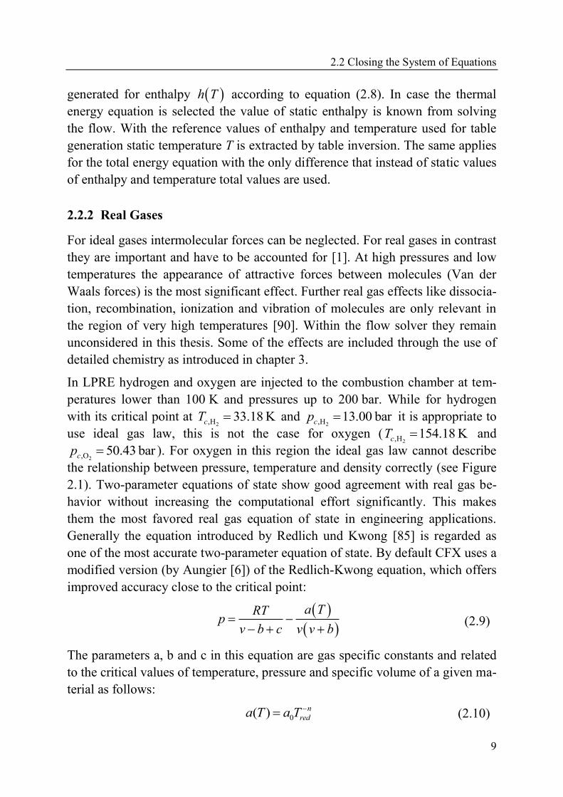
In LPRE hydrogen and oxygen are injected to the combustion chamber at tem-
peratures lower than 100 K and pressures up to 200 bar. While for hydrogen
with its critical point at 2,H 33.18 KcT and
2,H 13.00 barcp it is appropriate to
use ideal gas law, this is not the case for oxygen (2,H 154.18 KcT and
2,O 50.43 barcp ). For oxygen in this region the ideal gas law cannot describe
the relationship between pressure, temperature and density correctly (see Figure
2.1). Two-parameter equations of state show good agreement with real gas be-
havior without increasing the computational effort significantly. This makes
them the most favored real gas equation of state in engineering applications.
Generally the equation introduced by Redlich und Kwong [85] is regarded as
one of the most accurate two-parameter equation of state. By default CFX uses a
modified version (by Aungier [6]) of the Redlich-Kwong equation, which offers
improved accuracy close to the critical point:
a TRTp
v b c v v b
(2.9)
The parameters a, b and c in this equation are gas specific constants and related
to the critical values of temperature, pressure and specific volume of a given ma-
terial as follows:
0( ) n
reda T a T (2.10)
2 Computational Fluid Dynamics
10
where red cT T T is the reduced temperature (normalized by its value at the crit-
ical point) and:
2 2
0
0.42747 c
c
R Ta
p (2.11)
0.08664 c
c
R Tb
p (2.12)
0
cc
c
c c
R Tc b v
ap
v v b
(2.13)
The exponent n in equation (2.10) can be obtained by using the acentric factor ω
as follows:
20.4986 1.2735 0.4754n (2.14)
Substituting 0.5n and 0c in equation (2.9) yields the original form of the
Redlich-Kwong equation. For many materials critical temperature, pressure,
volume and acentric factor are stored in the materials database of CFX (from
Poling et al. [75]). Data for other substances are for example available from the
NIST database [55].
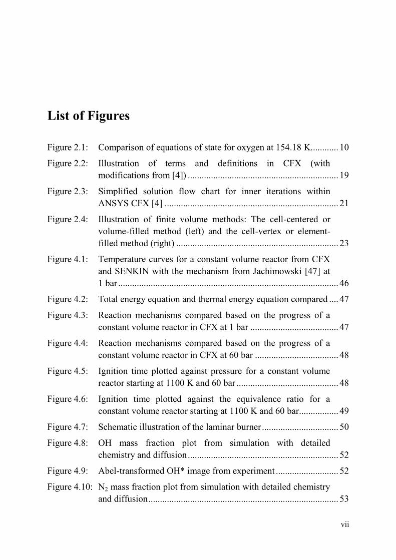
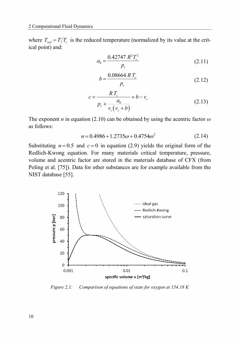
Figure 2.1: Comparison of equations of state for oxygen at 154.18 K
2.3 Transport Properties
11
Figure 2.1 shows for oxygen at its critical temperature (154.18 K) a comparison
between ideal gas law and the modified Redlich-Kwong equation of state. The
saturation curve was generated with data from NIST [55].
For the evaluation of density CFX uses a property table ,T p , which is gen-
erated in a pre-processing step before the simulation is started. For this purpose
ranges of temperature and pressure have to be specified in CFX Pre. Also a
number has to be entered to state in how many equally spaced intervals the
ranges are divided. With CFX-Post it is possible to visualize this table in order
to detect regions where the discretization is not adequate.
When a material with the Redlich-Kwong equation of state is involved in the
simulation, specific heat capacity is a function of temperature and pressure – see
section 2.3. CFX thus generates a table for enthalpy ,h T p during pre-
processing. When the thermal energy model is selected, static pressure p and
static enthalpy h are known from solving the flow. During simulation static tem-
perature T is then extracted from this table. In case the total energy equation is
selected, the table is generated for total enthalpy instead. Finding temperature
from enthalpy is more complicated then. Details of the procedure are described
in the CFX documentation [4].
In simulations of combustion, where for oxygen the Redlich-Kwong equation of
state is used (see section 4.4 and chapter 6), large ranges or temperature and
pressure have to be covered. Despite the large number of table entries (up to 4
million per table) usually problems with these tables caused the crash of the
simulations. A solution could only be obtained with the thermal energy model.
2.3 Transport Properties
A quite detailed description of all transport phenomena can be found in Bird et
al. [10]. For the evaluation of transport properties in numerical simulation some-
times the work of Kee et al. [54] is referenced (e.g. by Smooke et al. [96]). This
report is not available anymore, but the follow-up document (Kee et al. [50])
gives a very good description for the calculation of transport properties. An
overview of the most important transport phenomena is given in Table 2.1. It is
also known that mass can be transported through temperature gradients (Soret
effect) and that energy can be transported through concentrations gradients.
However, these effects are relatively small. Therefore they are usually not in-
cluded in the simulation of combustion [103].
2 Computational Fluid Dynamics
12
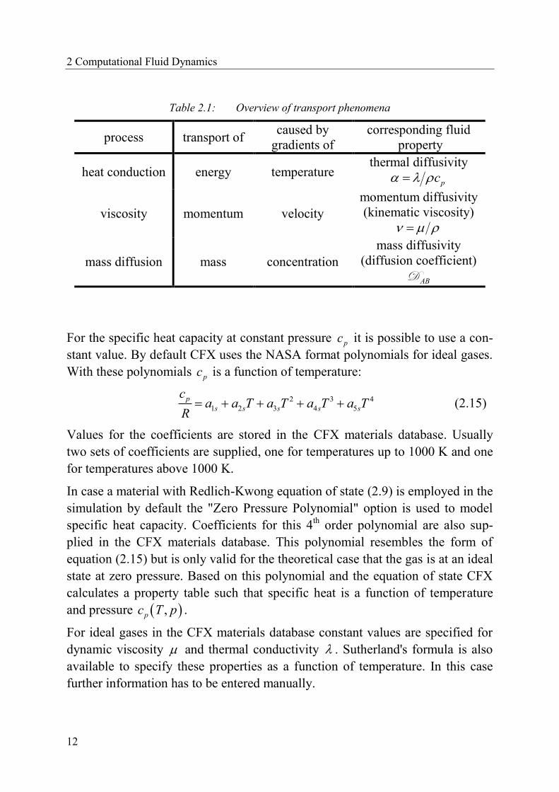
Table 2.1: Overview of transport phenomena
process transport of caused by
gradients of
corresponding fluid
property
heat conduction energy temperature thermal diffusivity
pc
viscosity momentum velocity
momentum diffusivity
(kinematic viscosity)
mass diffusion mass concentration
mass diffusivity
(diffusion coefficient)
ABD
For the specific heat capacity at constant pressure pc it is possible to use a con-
stant value. By default CFX uses the NASA format polynomials for ideal gases.
With these polynomials pc is a function of temperature:
2 3 4
1 2 3 4 5
p
s s s s s
ca a T a T a T a T
R (2.15)
Values for the coefficients are stored in the CFX materials database. Usually
two sets of coefficients are supplied, one for temperatures up to 1000 K and one
for temperatures above 1000 K.
In case a material with Redlich-Kwong equation of state (2.9) is employed in the
simulation by default the "Zero Pressure Polynomial" option is used to model
specific heat capacity. Coefficients for this 4th order polynomial are also sup-
plied in the CFX materials database. This polynomial resembles the form of
equation (2.15) but is only valid for the theoretical case that the gas is at an ideal
state at zero pressure. Based on this polynomial and the equation of state CFX
calculates a property table such that specific heat is a function of temperature
and pressure ,pc T p .
For ideal gases in the CFX materials database constant values are specified for
dynamic viscosity and thermal conductivity . Sutherland's formula is also
available to specify these properties as a function of temperature. In this case
further information has to be entered manually.

2.3 Transport Properties
13
For real gases other options are selected by default [3]. Dynamic viscosity is
evaluated from the simple formula:
6
(2,2)* 226.69 10
MT
(2.16)
This is based on kinetic gas theory (see [45]) and the hard sphere diameter in
CFX is determined from the critical molar volume:
3,0.809 m cv (2.17)
When the Rigid Non Interacting Sphere model is used, the collision integral (2,2)* is simply unity. For the Interacting Sphere model the value of the colli-
sion integral (2,2)* is evaluated from:
(l,s)*
exp exp expB
red red redred
A C E G
DT FT HTT (2.18)
Coefficients for this accurate empirical equation are given by Neufeld et al. [67]
as listed in Table 2.2.
Table 2.2: Coefficients from Neufeld et al. [67] for calculating Ω(l,s)*
(l,s) A B C D E F G H
(1,1) 1.06036 0.15610 0.19300 0.47635 1.03587 1.52996 1.76474 3.89411
(2,2) 1.6145 0.14874 0.52487 0.77320 2.16178 2.43787 - -
The reduced temperature required for equation (2.18) is in this case calculated
from the critical temperature cT :
1.2593red
c
TT
T (2.19)
For thermal conductivity of real gases the modified Eucken-Model can be used
in the form:
1.77
1.32v v
R
c c
(2.20)
This has also been derived from kinetic gas theory [75].
Information on the binary diffusion coefficient ABD (for diffusion between two
species/components A and B) is given in section 2.5, along with further infor-
mation on mass diffusion in general.

2 Computational Fluid Dynamics
14
The fluid properties in the last column of Table 2.1 can be related to each other
by dimensionless numbers (Prandtl, Schmidt and Lewis number):
Pr
(2.21)
ScAB
D (2.22)
LeAB
D (2.23)
In numerical simulations it can be adequate to use a constant (mostly close to
unity) for one of these dimensionless numbers, instead of having to evaluate all
three fluid properties separately.
2.4 Multicomponent Flow
For a multicomponent fluid in CFX the conservation equation presented in sec-
tion 2.1 are solved for the bulk motion of the fluid. All components share the
same mean pressure, temperature and velocity [3]. The fluid properties depend
on the composition of the multicomponent mixture. They are calculated based
on the local mass fraction weighted average of the components’ properties. For
instance bulk viscosity is calculated as:
sN
s s
s
Y (2.24)
Other fluid properties like specific heat at constant pressure, specific heat at
constant volume and thermal conductivity are calculated accordingly.
For the transport of the components within the fluid additional equations are
necessary. When a multi-component flow with Ns involved species is simulated
in CFX, one component has to be chosen for which a constraint equation is
solved. This makes sure that the sum of all mass fractions is equal to one. For
each of the remaining 1sN species one transport equation is solved. The
transport equation of each species s has the form [4]:
eff
j ss ss s
j j j
u YY YS
t x x x
(2.25)
where effs is the effective molecular diffusion coefficient and Ss a source term.
2.4 Multicomponent Flow
15
In a turbulent flow density and mass fractions are averaged values (see section
2.6). The effective diffusion coefficient in equation (2.25) is calculated from the
sum of molecular and turbulent diffusion:
Sceff
ts s
t
(2.26)
In turbulent (reactive) flow molecular transport is usually less important than
turbulent transport [71]. Turbulent diffusion is dependent on the choice of the
turbulent Schmidt number Sct and the model constants of the turbulence model
(see section 2.6) which define turbulent viscosity t . In this thesis the default
values are used. The molecular diffusion coefficient in CFX is assumed to be:
s sD (2.27)
The kinematic diffusivity Ds of a component s can be set (e.g. according to
equation (2.47) in section 2.5) in “Component Models” on the “Fluid Models”
tab of the domain in CFX Pre for all component for which a transport equation
is solved. If no value is specified, CFX uses bulk viscosity for all components of
the fluid. This way all species have the same diffusivity:
s (2.28)
This means that the Schmidt number is unity for all components:
Sc 1s s (2.29)
This simplification has usually no large effect on the results, when the flow is
turbulent. In a laminar flow, especially where the material properties of the
components differ considerably, this simplification is not adequate. The availa-
ble possibilities in CFX for that case are discussed in section 2.5.
For multicomponent fluids on the right hand side of the energy equation (see
section 2.1) an additional term is employed:
sN
ss s
sj j
Yh
x x
(2.30)
The evaluation of this term is considerably simplified, when the species diffusiv-
ities are assumed to be:
s pc (2.31)
This corresponds to the Lewis number being one for each component:
Le 1s p ic (2.32)
2 Computational Fluid Dynamics
16
This simplification results in term (2.30) being simplified to:
j p j
h
x c x
(2.33)
For turbulent flow the assumption Le 1s is usually as good as the common
practice of using Sc 1s for all components [4]. For fluids consisting of many
components this simplification can significantly reduce numerical cost, as only
one diffusion term has to be assembled [4]. Especially for laminar flow compo-
nent dependant diffusivities have to be set. Section 2.5 provides more infor-
mation on the topic.
Rules for mixing at high pressures and low temperatures are different from ideal
mixing. For the calculation with gas mixtures Redlich and Kwong [85] suggest-
ed to determine the parameters a and b for their equation from:
sN
s s
s
b X b (2.34)
1 1 2 2 12 1 2... 2 ...a a X a X a X X with 1
2
12 1 2( )a a a (2.35)
where X denotes mole fraction. Aungier [6] suggested using the following corre-
lations for the modified equation:
2
2
, ,
1
,
,
s
s
Nn
s c s c s
n s
c Ns c s
s c s
X T p
TX T
p
(2.36)
,
,
s
cc N
s c s
s c s
Tp
X T
p
(2.37)
sN
s s
s
X (2.38)
In CFX 11.0 it was not possible to implement these mixing rules. In version 12.0
a beta feature has been added that allows users to define arbitrary mixing rules.
However, this feature and its effect on the simulation have not been examined in
this thesis. The effect of real mixing rules on the simulation of supercritical
combustion with EDM is examined by Poschner and Pfitzner (see e.g. [78] or
[79]).

2.5 Mass Diffusion
17
2.5 Mass Diffusion
In this section a brief introduction to the theory of mass diffusion is given and
the options that are available in ANSYS CFX to consider diffusion are present-
ed. In a mixture consisting of two materials, say species s and component k, the
mass flux (mass flow per unit area) of species s can be described as [10]:
,s
s i sk
i
Yj
x
D (2.39)
In honor of Fick [26] this is called Fick's law with skD as the binary diffusion
coefficient and sY as the mass fraction of species (or component) s. Similarly for
component k in this mixture one can state:
,k
k i ks
i
Yj
x
D (2.40)
It is important to note, that:
sk ksD D (2.41)
The diffusion coefficient for a binary mixture of species s and k is usually given
by an expression that is credited to Chapman and Enskog. Combining this ex-
pression with ideal gas law, the equation (as given in Poling et al. [75]):
32
12 2 (1,1)*
0.00266sk
sk sk
T
p M
D (2.42)
gives the diffusion coefficient skD in cm²/s, where temperature T is in K, pres-
sure p in bar and the characteristic length sk in Å. For equation (2.42) the re-
duced molar mass skM has to be given in g/mol and is calculated from the molar
masses of the two species as:
2 s k
sk
s k
M MM
M M
(2.43)
The characteristic length sk is calculated from the Lennard-Jones collision di-
ameters:
2
s ksk
(2.44)
Collision diameter as well as well depth of the Lennard-Jones potential for
various species are available from several sources e.g. from Svehla [98].
2 Computational Fluid Dynamics
18
The diffusion collision integral (1,1)* is either tabulated or calculated from equa-
tion (2.18) with coefficients given in Table 2.2. The reduced temperature re-
quired for equation (2.18) is in this case considered as:
red skT kT (2.45)
with k as the Boltzmann constant. The interaction value sk of the Lennard-
Jones potential well depth is calculated from the individual values:
1
2
sk s k (2.46)
For a mixture of more than two species, a mixture diffusion coefficient can be
calculated from the binary diffusion coefficients. For the diffusion of a species s
into a mixture the coefficient can be calculated as [51]:
1s
ss N
k sk
k s
YD
X
D
(2.47)
with X denoting mole fraction. Through the use of expressions in CEL (CFX
Expression Language) this equation has been implemented in CFX in course of
this thesis. However, this simplified approach is only an approximation and has
an important disadvantage: Since the sum of all diffusion components is not ze-
ro, the difference is balanced by the constraint species. Therefore the results are
affected by the choice of the constraint species.
Preuß and Spille-Kohoff [81] show results from several numerical simulations
of diffusion processes in CFX. In two cases the results are independent of the
choice of constraint species. In their work they implemented the additional term
required for the method introduced by Ramshaw [83] and the diffusion fluxes
from Stefan-Maxwell diffusion through the use of the source term in the species
transport equation. Unfortunately they do not go into details for their implemen-
tation. To understand the difficulty in this task, it is important to point out how
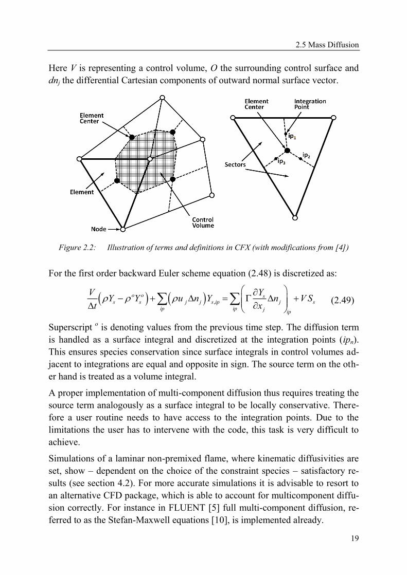
CFX handles this equation. Figure 2.2 illustrates required terms and definitions.
The differential form of the species transport equation (2.25) is rewritten in inte-
gral conservation form, with volume integrals involving gradient or divergence
operators converted to surface integrals:
s
s j s j j s
jV O O V
d YY dV u Y dn dn S dV
dt x
(2.48)
2.5 Mass Diffusion
19
Here V is representing a control volume, O the surrounding control surface and
dnj the differential Cartesian components of outward normal surface vector.
Figure 2.2: Illustration of terms and definitions in CFX (with modifications from [4])
For the first order backward Euler scheme equation (2.48) is discretized as:
,
o o ss s j j s ip j s
ip ip j ip
V YY Y u n Y n V S
t x
(2.49)
Superscript o is denoting values from the previous time step. The diffusion term
is handled as a surface integral and discretized at the integration points (ipn).
This ensures species conservation since surface integrals in control volumes ad-
jacent to integrations are equal and opposite in sign. The source term on the oth-
er hand is treated as a volume integral.
A proper implementation of multi-component diffusion thus requires treating the
source term analogously as a surface integral to be locally conservative. There-
fore a user routine needs to have access to the integration points. Due to the
limitations the user has to intervene with the code, this task is very difficult to
achieve.
Simulations of a laminar non-premixed flame, where kinematic diffusivities are
set, show – dependent on the choice of the constraint species – satisfactory re-
sults (see section 4.2). For more accurate simulations it is advisable to resort to
an alternative CFD package, which is able to account for multicomponent diffu-
sion correctly. For instance in FLUENT [5] full multi-component diffusion, re-
ferred to as the Stefan-Maxwell equations [10], is implemented already.
2 Computational Fluid Dynamics
20
2.6 Turbulence
In a turbulent flow variables (density, mass fractions, velocity, etc.) seem to
show irregular or random fluctuations. The chaotic seeming procedures are very
complex and it is difficult to simulate them numerically. Several ways exist how
to deal with turbulence in CFD. One possible way is to decompose a fluctuating
quantity into an averaged and a varying component according to:
(2.50)
For compressible flows the averaging is density-weighted (Favre averaging):
with
(2.51)
For transient simulations the equations in CFX are actually ensemble-averaged.
When the decomposition of the fluctuating flow variables is carried out in the
Navier-Stokes equations (as introduced in section 2.1) the Reynolds averaged
Navier Stokes (RANS) equations are obtained which are also referred to as
Reynolds equations. Unfortunately these equations cannot be solved because
turbulent stresses and heat-flux quantities appear which have to be regarded as
new unknowns. Equations are required that relate these unknowns to the mean
flow variables. This closure problem is handled through turbulence modeling.
Turbulent-viscosity models assume that Reynolds stresses can be determined by
mean velocity gradients. For negligible density fluctuations this relationship can
be written as:
2
3
ji ki j t ij t
j i k
uu uu u k
x x x
(2.52)
The turbulent viscosity (or eddy viscosity) t has to be modeled. In this thesis
for turbulent flow the k-ε turbulence model is employed, which is one of the
most widely used turbulence models. In this case t is expressed as:
2
t
kC
(2.53)
One additional transport equation is solved for turbulent kinetic energy k:
tj
j j k j
k ku k
t x x x
P (2.54)
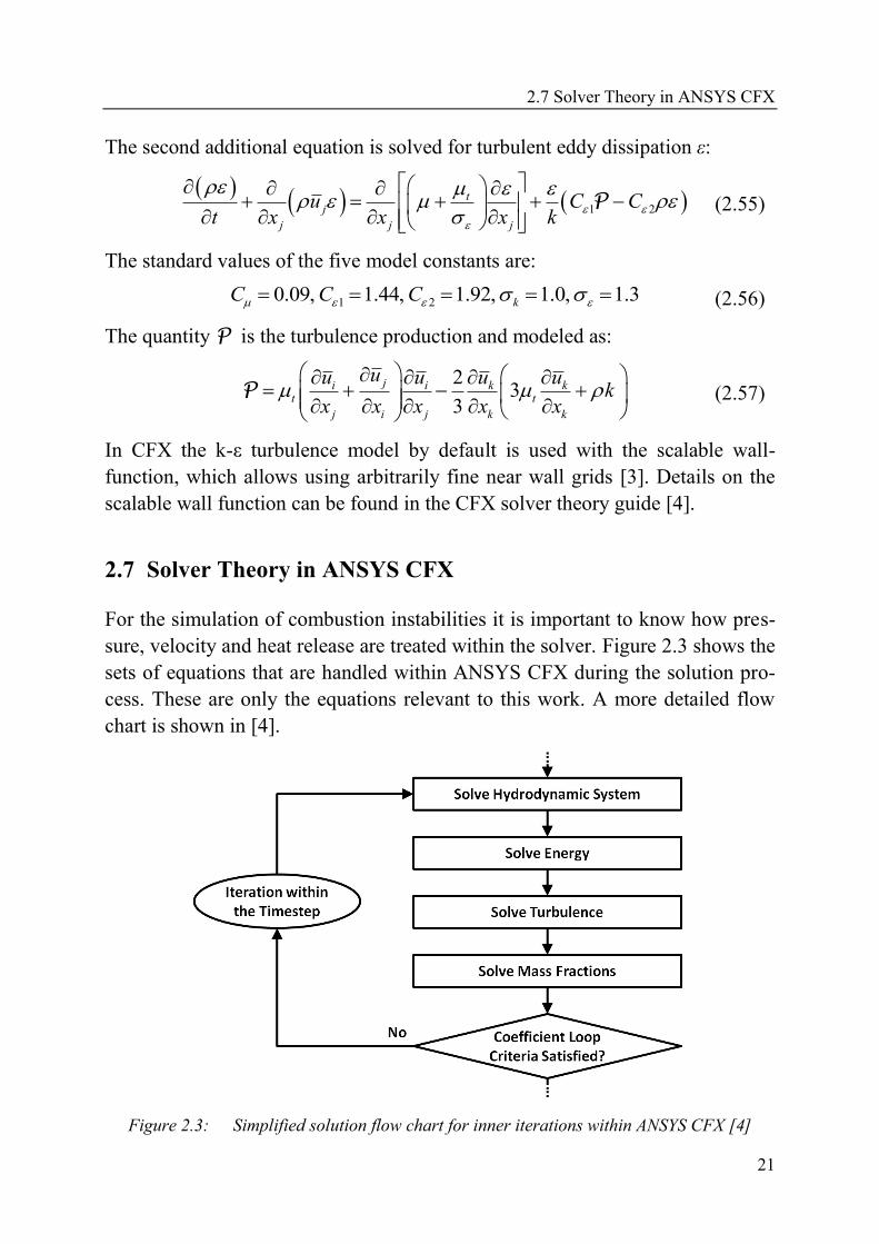
2.7 Solver Theory in ANSYS CFX
21
The second additional equation is solved for turbulent eddy dissipation ε:
1 2t
j
j j j
u C Ct x x x k
P (2.55)
The standard values of the five model constants are:
1 20.09, 1.44, 1.92, 1.0, 1.3kC C C (2.56)
The quantity P is the turbulence production and modeled as:
2
33
ji i k kt t
j i j k k
uu u u uk
x x x x x
P (2.57)
In CFX the k-ε turbulence model by default is used with the scalable wall-
function, which allows using arbitrarily fine near wall grids [3]. Details on the
scalable wall function can be found in the CFX solver theory guide [4].
2.7 Solver Theory in ANSYS CFX
For the simulation of combustion instabilities it is important to know how pres-
sure, velocity and heat release are treated within the solver. Figure 2.3 shows the
sets of equations that are handled within ANSYS CFX during the solution pro-
cess. These are only the equations relevant to this work. A more detailed flow
chart is shown in [4].
Figure 2.3: Simplified solution flow chart for inner iterations within ANSYS CFX [4]

2 Computational Fluid Dynamics
22
It is important to note that there is just one box for the hydrodynamic system.
This is because CFX is a coupled solver, i.e. the equations for pressure and ve-
locity (mass and momentum) are solved together. Therefore there is no need for
pressure correction algorithms such as SIMPLEC [102] or PISO [46] that are
employed in segregated solvers. A problem arising from discretization is the
odd-even decoupling of the pressure field (for details see e.g. Hirsch [44] or
Patankar [70]). This problem can be best resolved by using staggered grids [39],
i.e. different grids for pressure and velocity fields. In CFX a collocated grid is
employed and the approach to avoid decoupling is a different. The strategy is
similar to the approach introduced by Rhie and Chow [87] and its modification
by Majumdar [62]. A detailed description of the adopted method is given in the
CFX solver theory guide [4].
Important for the implementation of combustion are also the next steps in the
iteration. The energy equation is solved right after the mass and momentum
equations (see Figure 2.3). Therefore the influence of heat release on the hydro-
dynamic system becomes effective in the next inner iteration loop. The "Solve
Mass Fractions" step is the last task within the inner loop of a time step. Manip-
ulations on the species transport equations will affect the hydrodynamic system
and the energy equation only in the next inner iteration loop.
CFX uses an element-based finite volume method for discretization. For the ad-
vection term it is possible to either use the first-order accurate "Upwind" scheme
or to specify a factor for blending first and second order differencing or to use
the "High Resolution" scheme, which is based on the boundedness principles
used by Barth and Jesperson [7]. Usually by default the "High Resolution"
scheme is chosen, except for turbulence equations, which use the first order up-
wind scheme. Available options for the transient scheme are the first and the
second order backward Euler scheme. In addition it is also possible to choose
the "High Resolution" option which is second order scheme but reverts to the
first order scheme to maintain a bounded solution [3].
Whether a simulation in CFX is compressible or incompressible is determined
by the choice of the equation of state. If a constant density is specified the simu-
lation is incompressible. When materials with the ideal gas equation of state or
the Redlich-Kwong equation of state are selected the simulation is compressible.
Simulations using materials with variable density, as well as multi-component
fluids composed of these materials, are able to calculate the speed of sound cor-
rectly.
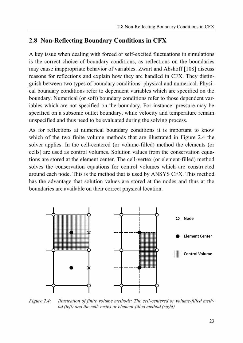
2.8 Non-Reflecting Boundary Conditions in CFX
23
2.8 Non-Reflecting Boundary Conditions in CFX
A key issue when dealing with forced or self-excited fluctuations in simulations
is the correct choice of boundary conditions, as reflections on the boundaries
may cause inappropriate behavior of variables. Zwart and Abshoff [108] discuss
reasons for reflections and explain how they are handled in CFX. They distin-
guish between two types of boundary conditions: physical and numerical. Physi-
cal boundary conditions refer to dependent variables which are specified on the
boundary. Numerical (or soft) boundary conditions refer to those dependent var-
iables which are not specified on the boundary. For instance: pressure may be
specified on a subsonic outlet boundary, while velocity and temperature remain
unspecified and thus need to be evaluated during the solving process.
As for reflections at numerical boundary conditions it is important to know
which of the two finite volume methods that are illustrated in Figure 2.4 the
solver applies. In the cell-centered (or volume-filled) method the elements (or
cells) are used as control volumes. Solution values from the conservation equa-
tions are stored at the element center. The cell-vertex (or element-filled) method
solves the conservation equations for control volumes which are constructed
around each node. This is the method that is used by ANSYS CFX. This method
has the advantage that solution values are stored at the nodes and thus at the
boundaries are available on their correct physical location.
Figure 2.4: Illustration of finite volume methods: The cell-centered or volume-filled meth-
od (left) and the cell-vertex or element-filled method (right)
2 Computational Fluid Dynamics
24
With the cell-centered method additional procedures are required to evaluate
numerical boundary conditions. A simple extrapolation can results in an incom-
patibility with physical boundary conditions, so that boundary conditions be-
come over-specified [73]. This over-specification of the boundary conditions
introduces spurious waves in the domain. To avoid these numerically reflective
boundary conditions a more sophisticated procedure has to be implemented,
such as the methodology introduced by Poinsot and Lele [73]. However, as men-
tioned above: ANSYS CFX does not require any additional procedures since all
conservation equations are solved also on the boundary nodes. Therefore, nu-
merical boundary conditions in ANSYS CFX are inherently non-reflective
[108].
Reflections at physical boundary conditions usually can arise from specifica-
tions which are inconsistent with the physical nature of the flow. An outlet with
uniform static pressure for example has to be placed in a sufficient distance
downstream from the last obstacle. If in a given case this is not possible ANSYS
CFX offers some alternative options for the boundary specifications which are
less reflective. Advice for setting boundary conditions correctly is available
from the ANSYS CFX – Solver Modeling Guide [3] and the validation report of
Zwart and Abshoff [108].
In transient simulations reflections at physical boundary conditions in some cas-
es are physically reasonable. In some simulations it might still be desirable to
allow an acoustic wave to exit the domain. With a beta feature that is imple-
mented in ANSYS CFX it is possible to have such physically non-reflective
boundary conditions. The methodology is based on characteristic analysis that
has been introduced by Poinsot and Lele [73]. Zwart and Abshoff [108] show
results from simulations of different representative test-cases to illustrate the
proper implementation of this feature in ANSYS CFX. Furthermore this feature
also offers a good possibility to excite the domain (see section 5.3.2).
25
3 Combustion
3.1 Chemical Kinetics
In this section all equations are listed that are necessary for the implementation
of chemical kinetics as far as done in this work. They can also be found in simi-
lar form in either Kee et al. [53] or Turns [101], which served as the two main
sources for this section.
3.1.1 System of Equations
The combustion process is defined by the change in temperature T(t) and molar
concentrations cs(t) over time. In a general form, the system of equations that
has to be solved is therefore:
1
d, , ...,
d sN
Tf T c c
t
1
d, , ...,
d s
sN
cf T c c
t
(3.1)
This is one equation for temperature and Ns equations for composition, one for
each of the involved species s. Each cell of the domain that is used by the CFD
solver to calculate the flow can be treated as one constant volume reactor. For
ideal gases in an adiabatic system the equations can be written as [101]:
d
d
s s
s
s
N N
u s s s
s s
N
s p u
s
R T HT
tc C R
d
d
ss
c
t
(3.2)
Thermodynamic properties and chemical rate expressions that are required for
equations (3.2) are specified below.
3 Combustion
26
3.1.2 Thermodynamic Data
Thermodynamic properties of each reacting species are obtained from polyno-
mials. The form of these polynomials is taken from Gordon and McBride [34]:
0
2 3 4
1 2 3 4 5sp
s s s s s
u
Ca a T a T a T a T
R (3.3)
02 3 42 3 4 5 6
12 3 4 5
s s s s s ss
u
H a a a a aa T T T T
R T T (3.4)
02 3 43 4 5
1 2 7ln2 3 4
s s s ss s s
u
S a a aa T a T T T T a
R (3.5)
The superscript 0 is corresponding to standard pressure p
0. For perfect gases the-
se properties are independent of pressure, therefore their values are as well the
actual values. In order to improve accuracy two different polynomials are used –
one for low (up to 1000 K) and one for high temperatures (above 1000 K). In
this case seven coefficients are needed for each of the two temperature ranges.
In this thesis the values of the coefficients for equations (3.3), (3.4) and (3.5) are
taken from the CFX materials database. They are listed in Table A.2 for the low
and Table A.3 for the high temperature range.
3.1.3 Chemical Rate Expressions
The chemical production rate s of the sth species is given by:
1
rN
s sr r
r
q
(s = 1, …, Ns) (3.6)
where νsr is the difference of product and reactant stoichiometric coefficient:
sr sr sr (3.7)
and qr is the rate-of-progress variable for the rth reaction. Its value can be calcu-
lated from:
1 1
s s
sr sr
N N
r fr s br s
s s
q k c k c
(3.8)
where frk and brk are the forward and backward rate constants of the rth reac-
tion. The molar concentration sc of each species s is obtained from:
s
s
s
Yc
M
(3.9)
3.1 Chemical Kinetics
27
with sY denoting its mass fraction,
sM its molar mass and density. The for-
ward rate constants of the rN reactions strongly depend on temperature. This
temperature dependence is specified by (modified) Arrhenius law:
expr rfr r
u
Ek A T
R T
(3.10)
The pre-exponential factor rA , the temperature exponent
r and the activation
energy rE are specified (see Table A.4 and Table A.6) for each reaction. The
backward rate constants brk can then be obtained from the forward rate con-
stants by using equilibrium constants:
fr
br
cr
kk
K (3.11)
The equilibrium constants based on molar concentrations crK can be determined
from the equilibrium constants based on partial pressure prK . The two constants
are related by:
1
Nssrs
atmcr pr
u
pK K
R T
(3.12)
The equilibriums constants prK are obtained with the relationship:
0 0
exp r rpr
u u
S HK
R R T
(3.13)
The Δ in this case expresses the change that occurs when a reaction is complete,
i.e. all reactants have turned into products. Following equations apply:
0 0
1
sN
r ssr
su u
S S
R R
(3.14)
0 0
1
sN
r ssr
su u
H H
R T R T
(3.15)
3.1.4 Third Body Reactions
In some reactions a “third body” appears that does not participate in the reaction
but is required as a collision partner. In a dissociation reaction this third body
adds the energy that is needed in order to break the bond of a molecule. In a re-
combination reaction its kinetic energy increases when the liberated energy from

3 Combustion
28
the newly formed molecule is transferred. The expression for the rate-of-
progress variable for these reactions is:
1 1 1
s ss
sr sr
N NN
r sr s fr s br s
s s s
q c k c k c
(3.16)
When compared to equation (3.8) an additional factor appears here:
1
1
s
s
N
N sr s
s
c c
(3.17)
In this factor the concentration of all involved species are included along with
their respective efficiencies as third bodies sr . This factor can be regarded as
the concentration of the third body, so that equation (3.16) can be written as:
1 1
1 1
s s
sr sr
N N
r fr s br s
s s
q k c k c
(3.18)
If 1sr for all species, the first factor in equation (3.16) is the total concentra-
tion of the mixture. Third body efficiencies that differ from 1 are specified along
with the reaction mechanism (see Table A.5 and Table A.8).
3.1.5 Pressure-Dependent Rate Constant
The chemical rate constant of certain dissociation and recombination reactions
does not only depend on temperature but apparently also on pressure. This pres-
sure-dependency can be explained by the fact that the reaction at hand is not el-
ementary, but rather a sequence of reactions [103]. To handle this pressure-
dependency, the forward rate coefficients of a reaction are given for the low-
( 0k ) and the high-pressure limit ( k ). In order to facilitate reading, subscripts r
and f are omitted:
0 00 0 exp
u
Ek A T
R T
(3.19)
expu
Ek A T
R T
(3.20)
A reduced pressure can be calculated by:
0
1
sN
red s s
s
kp c
k
(3.21)
3.1 Chemical Kinetics
29
with which the rate constant can be defined to be:
1
red
red
pk k F
p
(3.22)
In the simplest case F = 1, which is the approach suggested by Lindemann [58].
In reactions (9) and (15) of the Ó Conaire mechanism [69] (see Table A.6) the
concept of Troe (see [32] and [100]) is followed. F has to be calculated in a
more complicated way from:
12
loglog 1 log
log
redcent
red
p cF F
N d p c
(3.23)
with the constants1 given by:
0.4 0.67log centc F (3.24)
0.75 1.27log centN F (3.25)
0.14d (3.26)
**
*** *1 exp exp expcent
T T TF a a
T T T
(3.27)
The parameters a, T***
, T* and T
** are specified along with the reaction mecha-
nism (see Table A.7). In cases where T**
is not given, the last summand of equa-
tion (3.27) has to be omitted. Having determined the forward rate coefficient
from equation (3.22), the backward rate constant and the rate-of-progress varia-
ble can be calculated by using the equations given in 3.1.3.
3.1.6 Intermediate Complex-Forming Bimolecular Reactions
There are certain reactions that show anomalous temperature dependence – with
rate constant minima [43] or a sharp up-turn [42] of the rate constant at moder-
ate and high temperatures. The explanation for this occurrence is that an inter-
mediate complex formation is involved in the reaction [42]. In order to handle
this behavior, the rate constant is calculated as the sum of two (or more) rate ex-
pressions (see reactions 14 and 19 in Table A.5).
1 Definitions for constants are taken from [32]. They are incorrectly quoted in [52] and [103].
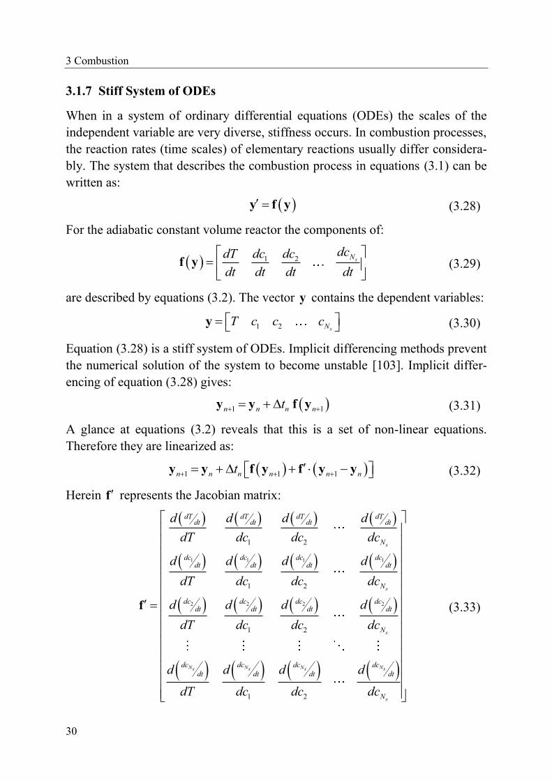
3 Combustion
30
3.1.7 Stiff System of ODEs
When in a system of ordinary differential equations (ODEs) the scales of the
independent variable are very diverse, stiffness occurs. In combustion processes,
the reaction rates (time scales) of elementary reactions usually differ considera-
bly. The system that describes the combustion process in equations (3.1) can be
written as:
y f y (3.28)
For the adiabatic constant volume reactor the components of:
1 2 sNdcdT dc dc
dt dt dt dt
f y (3.29)
are described by equations (3.2). The vector y contains the dependent variables:
1 2 sNT c c c y (3.30)
Equation (3.28) is a stiff system of ODEs. Implicit differencing methods prevent
the numerical solution of the system to become unstable [103]. Implicit differ-
encing of equation (3.28) gives:
1 1n n n nt y y f y (3.31)
A glance at equations (3.2) reveals that this is a set of non-linear equations.
Therefore they are linearized as:
1 1 1n n n n n nt y y f y f y y (3.32)
Herein f represents the Jacobian matrix:
1 1 1 1
2 2 2 2
1 2
1 2
1 2
1 2
s
s
s
N N N Ns s s s
s
dT dT dT dTdt dt dt dt
N
dc dc dc dcdt dt dt dt
N
dc dc dc dcdt dt dt dt
N
dc dc dc dc
dt dt dt dt
N
d d d d
dT dc dc dc
d d d d
dT dc dc dc
d d d d
dT dc dc dc
d d d d
dT dc dc dc
f (3.33)
3.1 Chemical Kinetics
31
This is evaluated at the old values ny . Rearranging of equation (3.32) gives:
1
1n n n n nt t
y y 1 f f y (3.34)
and shows that the main task for finding 1ny is matrix inversion. Through line-
arization the implicit differencing scheme has become semi-implicit. It is not
guaranteed to be stable but gives a better stability than explicit methods [80].
The time step size nt has to be small enough so that the linear approximation is
justified. Therefore it is indispensable to apply an algorithm with step size ad-
justment.
There are different groups of higher-order methods to implicitly solve a stiff sys-
tem of ODEs. One of these groups is the Rosenbrock methods which are also
known as Kaps-Rentrop methods and which represent the most useful generali-
zation of the Runge-Kutta method [80]. For a system of up to about ten inde-
pendent variables these methods are similarly effective as more complicated al-
gorithms [80] and are therefore appropriate for the 8 species in H2-O2-
combustion or the 9 species in H2-Air-combustion.
A general purpose implementation of a Kaps-Rentrop scheme in C is available
from Press et al. [80]. This implementation has an embedded step size adjust-
ment algorithm. The initial step size 0t has to be delivered by the calling rou-
tine; the size for the next step is then calculated (either increased or decreased
within certain limits) upon the error that was determined. When the tabulation
method described in section 3.3.1 is not applied, the relevant step size can be
saved as an initial step size for the next time the same cell in the domain needs
to be calculated.
Together with the parameters that control the integration additional routines
need to be provided that supply the required data. The CFD time step size t
and the starting values of dependant variables 0
y are available from CFX. One
subroutine gives f y , the derivative of temperature and concentrations with
respect to time by calculating equations (3.2). The Jacobian matrix is computed
in another subroutine. Differentiation is carried out by numerical differencing
[12], where a five-point midpoint formula is used for differentiation with respect
to temperature T and a three-point endpoint formula for differentiation with re-
spect to molar concentrations sc . For turbulent flow, of course the averaged val-
ues of variables are used as given in section 3.2.
3 Combustion
32
3.1.8 Choice of Reaction Mechanism
A large number of authors have proposed mechanisms describing the detailed
chemical kinetics of hydrogen oxidation. All of these mechanisms are validated
and suitable for a certain range of temperature and pressure. An overview of
available mechanisms and underlying shock tube data is given e.g. by Schultz
and Shepherd [93].
The external routine that is used in this work for calculating combustion was
originally intended to be used for modeling of supersonic combustion. Therefore
a hydrogen-air reaction mechanism was implemented that was designed to be
applied for scramjet combustion. Jachimowski [47] compared the kinetic behav-
ior predicted by the reaction mechanism he assembled with shock-tube data in
the range from 0.5 to 2.0 atm. His mechanism was slightly altered by Wilson
and MacCormack [105]. Most of the reactions remained unchanged, but the re-
action rates were refined to improve agreement with experiments in the range
over 17 atm and 2300 K. When NO-formation is neglected this reaction scheme
(Table A.4) consists of 19 elementary reactions and 8 species: H2, O2, H2O, H,
O, OH, HO2 and H2O2; if N2 is also present in a simulation it is only considered
as a third body. This mechanism is perfectly tailored for combustion in scram-
jets, but is not validated for pressures (60 bar and more) that might appear in
rocket engines.
Two more recent detailed kinetic mechanisms for H2/O2 mixtures were suggest-
ed by Li et al. [56] and by Ó Conaire et al. [69]. They are both based on the
mechanism by Mueller et al. [66] and aiming to be used for a wide range of ap-
plications. Experiments used for comparison cover a wide range of conditions
(Li et al.: 298-3000 K, 0.3-87 atm, = 0.25-5.0; Ó Conaire et al.: 298-2700 K,
0.05-87 atm, = 0.2-6.0). Both mechanisms seeming to be equally suitable, the
one of Ó Conaire et al. (Table A.6) was chosen in this work to be used for com-
parison with the altered Jachimowski mechanism described above. It also con-
tains 19 reactions and the same 8 species (further species that might be present
in a simulation are only considered as third bodies). Two reactions (9 and 15) in
this mechanism have pressure-dependent rate constants. For two other reactions
(14 and 19) the rate constants have to be calculated as the sum of two rate ex-
pressions.
3.2 Turbulence-Chemistry Interaction
33
3.2 Turbulence-Chemistry Interaction
In section 3.1 each cell of the domain has been treated as one constant volume
reactor. This treatment is only valid when the properties of the reacting mixture
are homogeneous in the whole cell. In a turbulent flow, however, these proper-
ties fluctuate in time and space (see section 2.6). The system of equations that
needs to be solved for combustion remains the same as given in equations (3.1)
and (3.2) except that now averaged values are used for calculation.
A way to account for the influence of turbulence on chemistry is to use Probabil-
ity Density Functions (PDF). The following brief description goes along with
the explanation of Gerlinger et al. [31]. With P as the joint PDF of temperature
and composition, the mean rate-of-progress variable can be determined from:
1 1 1ˆ ˆ ˆˆ ˆ ˆ ˆ ˆ ˆ, ,..., , ,..., ...
s s sr r N N Nq q T c c P T c c dT dc dc (3.35)
where T and ˆsc represent sample space variables and qr is the rate-of-progress
variable from equation (3.18). When statistical independence of temperature and
composition is assumed, the PDF can be written as:
1 1ˆ ˆ ˆ ˆ ˆˆ ˆ, ,..., ,...,
s sN T Y NP T c c P T P Y Y (3.36)
This simplifies the integration of equation (3.35) which now can be done in con-
secutive steps:
1 1
1 1
s s
sr sr
N N
r fr s br s
s s
q k c k c
(3.37)
3.2.1 Assumed PDF of Temperature
The PDF of temperature used in this work is assumed to be a Gaussian (normal)
distribution:
2
22
ˆ1ˆ exp
22T
TT
T TP T
(3.38)
where:
2 2
T T (3.39)
3 Combustion
34
is the variance2 of temperature for which an additional transport equation is
solved (see section 3.2.4). For each forward and each backward reaction the
time averaged reaction constants are calculated from:
ˆ
ˆ ˆ ˆr r T
T
k k T P T dT (3.40)
The normal distribution is defined from to , which is outside of any
physical temperatures and cannot be integrated numerically. Therefore limits are
introduced which correspond to the relevant temperature range. The resulting
clipped normal distribution is:
2
0
min max2200
1 min 2 max
ˆ1ˆ ˆ ˆexp
22
ˆ ˆA A
T
T TP T H T T H T T
T T T T
(3.41)
Clipping is carried out by the introduction of a Heaviside function. The clipped
parts of the distribution are added through Dirac delta functions at the place
where clipping takes place [59], with 1A and 2A representing the areas of the
clipped parts. The parameters of the clipped distribution 0T and 0 are different
from given moments T and T . With equations:
1 ˆ
ˆ ˆ ˆ; , 0T TT
f T P T T dT T (3.42)
2
2
2 ˆˆ ˆ ˆ; , 0T T T
Tf T T P T T dT (3.43)
these two parameters can be found using a Newton algorithm, where the ith itera-
tion provides the (i+1)th
approximate solution [19]:
1 1
20
0
2 2
20 0
1
1
0 0 1
2 2
0 0 2
i i
i i
f fi i iT
f f
T
T T f
f
(3.44)
Clipping can only be successfully performed when the mean temperature is well
within the specified range, otherwise the Newton method will fail. As soon as
the parameters 0T and 0 are known, numerical integration is used to calculate
2 In this thesis σ denotes standard deviation. This is also the case in Girimaji [33] and Lock-
wood and Naguib [59], but is in contrast to Gerlinger (e.g. in [30]), Di Domenico [19] and
Förster [28], who use the letter σ to denote variance.
3.2 Turbulence-Chemistry Interaction
35
the averaged reaction constants according to equation (3.40). Simpson’s method
on the one hand and Romberg’s method on the other (both taken from Press et
al. [80]) have been implemented for this purpose. While both algorithms show
similar performance, it is Simpson’s rule that has been used for all simulations.
The required computational effort for using equation (3.40) is considerably
higher than that necessary for calculating the rate constants with Arrhenius law
only.
3.2.2 Assumed PDF of Composition
The PDF of composition used in this work is the multivariate β-distribution that
has been suggested by Girimaji [33]:
1 1
1
111
ˆ ˆ ˆ ˆ,..., 1
s
s s
s
s s
NN N
ss
Y N s sNssss
P Y Y Y Y
(3.45)
where the Dirac delta function is required for normalization. The parameters s
are specified as:
1
2
11
sN
k kk
s s
Y
Y YY
B
(3.46)
The sum of species mass fraction variances is:
2 2
1
sN
Y s
s
Y
(3.47)
Only one additional transport equation has to be solved for 2
Y (see section
3.2.4). The advantage of equation (3.45) is that integration can be performed
analytically. The respective term in equation (3.37) can then be expressed as:
11
11 11
only for third body reactions 1
1s srsr
s s s
sr r
r
NN N N
s srs jm srs sr sm
si s s srj
jc
M MB m j
(3.48)
with:
1
1
sN
fr sr
s
m
and 1
1
sN
fr sr
s
m
(3.49)

3 Combustion
36
Since the transport equation (equation (3.59) in section 3.2.4) is to loosely cou-
pled with the species mass fractions, it is important to make sure that:
20 1sN
Y s s
s
Y Y (3.50)
when equation (3.48) is calculated. Even though equation (3.48) looks quite
complicated, the numerical effort for its calculation is only slightly larger than
that for the corresponding term in equation (3.18).
3.2.3 Mean Chemical Production Rates
Without turbulence-chemistry interaction the chemical production rates are cal-
culated according to equation (3.6). With the equations in sections 3.2.1 and
3.2.2 the mean chemical production rates can now be calculated as [31]:
1 2 3 4 1 2 3 4
1 1
r rN N
s sr r sr f f f f b b b b rr r
q
T T T T T T T T (3.51)
where the set of terms T1 to T4 for each forward and backward reaction is avail-
able as:
1r rkT (3.52)
2
1
1sr
s
r
Nm
r
s sM
T (3.53)
1
3
1
s sr
r
N
s srs nr m
rn
n
B m n
T (3.54)
4 4
1 1
s sN N
sr sr sr sr s r
s ss s
YB
M M
T S (3.55)
The first summand of equation (3.55):
4
1
sN
sr srr
s sM
S (3.56)
together with the terms in equation (3.49) only need to be calculated at the be-
ginning of the calculation as they only depend on the applied reaction mecha-
nism.
3.2 Turbulence-Chemistry Interaction
37
3.2.4 Additional Equations in the Flow Solver
Several possibilities exist on how to obtain T and Y . In this thesis two
additional transport equations have been included in the solver: one for variance
of temperature and one for variance of composition. They are both chosen to be
specific (solved on a per-unit-mass basis) scalars without any units. In order to
model the two additional variables, for each of them the corresponding check
box in the domain settings is ticked and the transport equation option selected.
By selecting the kinematic diffusivity check box and setting the kinematic
diffusivity to zero, the turbulent diffusion term is included only.
The equation for the transport of temperature variance is derived from the
equation for thermal enthalpy [30] and has the form:
2
2 22 2 2
Pr Pr Pr
t T t TT j T T
j j t j t j t
Tu C
t x x x x
(3.57)
The first source term on the right represents production caused by temperature
gradients. The second term accounts for dissipation caused by molecular diffu-
sion where for the modeling constant usually 2.0TC is applied. The turbulent
timescale t can be obtained from the turbulence model:
t
k
(3.58)
A source term for the influence of compressibility is not included, as there is no
adequate model available. It would be possible to include a source term that ac-
counts for interaction of temperature fluctuations with chemical reactions. How-
ever, experience showed [29] that this term produces significant errors, when
statistical independence of temperature and species fluctuations is assumed.
Therefore this term is not considered either.
The other additional equation is for the transport of species variance:
2
2 22 2
1
2Pr Pr Pr
sN
t Y t s YY j Y Y
sj j t j t j t
Yu C
t x x x x
(3.59)
This equation is quite similar to equation (3.57). The first source term on the
right hand side describes production through mass fraction gradients, while the
second source term describes dissipation. The value of the constant is usually
taken to be 2.0YC . The turbulent timescale t is the same as above. There is
no source term representing production or dissipation caused by the interaction
3 Combustion
38
of species fluctuations and chemical reactions, as it produces erroneous results
[29]. Equations (3.57) and (3.59) act on the assumption that Pr Sc and
Pr Sct t . In the present work the default values Pr 1.0 and Pr 0.9t were cho-
sen. Detailed explanations of these transport equations as well as their variations
and the assumptions for the underlying models are given by Gerlinger [30] along
with available alternatives.
To include the sources on the right hand side of equations (3.57) and (3.59) in
CFX a subdomain has to be defined. For the simulations presented in this thesis
the subdomain extends over the entire domain. Similarly to the species transport
equations, the sources for equations (3.57) and (3.59) are calculated in external
routines. They remain constant for one solver time step and are recalculated at
the end of each time step.
3.3 Tabulation
3.3.1 Tabulation of Chemical Kinetics
Solving the stiff system of equations (3.2) for combustion is very time consum-
ing. There are several ways to reduce these costs. For example Liang et al. [57]
developed an efficient semi-implicit solver that compared to CHEMKIN [52] is
able to save up to 70 % CPU time. Another way is to use sensitivity analysis
[103]. Very often tabulation methods are used. In this work an in-situ tabulation
method is applied (see [27] and [28]) where the temperature and the molar con-
centrations are tabulated in the required region of interest. The required table
needs one dimension for temperature and one for each involved species. The
ranges of temperature and concentrations are divided in equidistant segments:
T , 1c , …, sNc . If the entire table was to be filled, the number of necessary
points in the table would be enormously high. Since only a small fraction of all
combinations of temperatures and molar concentrations will appear during the
combustion process, only the required combinations are tabulated.
When a certain combination of temperature and concentrations 1, , ...,sNT c c
needs to be calculated, a check is performed whether the required entry in the
table is already available. For this purpose the values are rounded down to the
closest values in the table 1, ,, , ...,sa a N aT c c . If this point in the table is required
for the first time, it is generated as follows.
3.3 Tabulation
39
First, with the methods described in section 3.1.7, the state is determined that the
adiabatic constant volume reactor (defined by equations (3.2)) reaches in terms
of temperature and concentrations after t , which is the solver time step from
CFX. The result is an array with 1sN components and can be written as:
1, , 1, 2, ,, , ...,s sa a N a new new new N newT c c T c c c f (3.60)
Then the parameters (temperature or concentration) are changed to an elevated
level (b), one at a time, while the other parameters are held constant at their
baseline level (a). At each combination of temperature and concentrations the
system is evaluated, giving 1, ,, , ...,sb a N aT c cf , 1, ,, , ...,
sa b N aT c cf , …
Finally all relevant data is stored in a table and is available to be used according
to the formula:
1 1, ,
1, , 1, ,
1 1,
1, , 1, ,
1, 1,
,
1, , 1, ,
, ,
, , ..., , , ...,
, , ..., , , ...,
, , ..., , , ..., ...
, , ..., , , ...,
s s
s s
s s
s s
s s
s s
N a a N a
ab a N a a a N a
b a
a
a b N a a a N a
b a
N N a
a a N b a a N a
N b N a
T c c T c c
T TT c c T c c
T T
c cT c c T c c
c c
c cT c c T c c
c c
f f
f f
f f
f f
(3.61)
The structure of the tables used in this thesis corresponds to the hybrid approach
described by Förster [28], which is a compromise between using either an array
or a list for data storage. While an array has the advantage that its entries can be
accessed very quickly, it has the drawback that it requires too much memory
already when it is initialized. A list in contrast only requires the memory neces-
sary for its entries. Depending on the number of entries in the list, the search can
be very time consuming. With the hybrid approach [28] the first three
coordinates – say K T , 1K c and 2K c – determine the position of a list in
a three-dimensional array. For each combination of the remaining coordinates –
3K c , …, sNK c – that has been requested before there is one entry in the list.
Each of these entries contains all relevant data to evaluate equation (3.61).
Instead of storing data in one point in the table, an alternative would be to save
the results from all parameter combinations separately. Even though the number
of entries in the lists would increase, the required memory size would decrease
(per entry as well as overall). Also the time for table generation would be de-
3 Combustion
40
creased. However, with the increased number of entries in the lists, the time re-
quired for searching the lists would be increased as well. Also for evaluating
equation (3.61) not only one but 1sN searches would be necessary. While this
alternative was not implemented nor examined in this thesis, it appears sensible
to assess its saving potentials with respect to memory requirements and compu-
tational time.
With the tabulation method described above one has to keep in mind, that the
factors that influence the reaction process are only evaluated one at a time. The
fact that two or more factors in combination might have a much larger influence
on the reactor is not taken care of. In that respect it is to be expected that using
equation (3.61) to obtain data from the table instead of solving the stiff system
of ODEs would predict a slower progress of the reactions. To account for this
fact intervals in the table ( 1, , ...,sNT c c ) are much smaller than those used by
Lyubar [61], who used all possible combinations of baseline and elevated level
for evaluation.
One further drawback of this tabulation method is the fact that the ranges of
temperature and concentrations have to be known before the simulation is start-
ed. The required region depends on many aspects of the flow, such as e.g.
transport processes or boundary conditions. As a matter of fact it has turned out
to be advisable to run a simulation without tabulations first, in order to have an
appropriate number of segments for each dimension of the table. In this respect
the in situ adaptive tabulation method introduced by Pope [76] is more conven-
ient.
3.3.2 Tabulation of Turbulence-Chemistry Interaction
When turbulence chemistry interactions are evaluated, two additional parame-
ters need to be tabulated as well: one for temperature variance and one for spe-
cies variance. This means, that the dimension of the table is increasing by two,
so that more points in the table are necessary. But also calculating the points in
the table becomes more time consuming, since as mentioned before (see section
3.2.1), the numerical effort increases considerably, when equation (3.40) is used
to calculate the rate constants. Consequently a tabulation method to obtain the
rate constants is necessary. Table generation in this case is performed as a pre-
processing step before the simulation, since the dimension of the table is rela-
tively low.
3.4 Approach for the Simulation of Combustion in this Thesis
41
Only two dependent variables need to be considered to tabulate the rate constant
[8], since ,r Tk f T . Instead of temperature variance, however, fluctuation
intensity is used:
TTI
T
(3.62)
The rate constant for each reaction is thus tabulated as ,r Tk f T I .
Using tabulated data for the calculation of the rate constant accelerates the com-
putation significantly. The drawback is, in addition to a loss in precision, that
pressure dependence (see section 3.1.5) cannot be considered.
3.4 Approach for the Simulation of Combustion in this Thesis
ANSYS CFX has been chosen to simulate the rocket engine flame. Several pos-
sibilities are already implemented in CFX that allow the simulation of combus-
tion processes. In addition CFX also offers multiple possibilities to define fur-
ther functionalities in external routines. In this work a multi-component, variable
composition mixture is used in CFX. While in this mixture all species of a de-
tailed reaction mechanism are present, CFX only solves the equations for non-
reacting flow. An external routine is used to calculate combustion.
For a multi-component flow in ANSYS CFX it is assumed [3] that the compo-
nents are mixed at the molecular level. That means that they have the same pres-
sure and temperature. A single velocity field is calculated for the multi-
component fluid. A drift velocity arising from diffusion is superimposed for
each component. Components can be selected from the materials library that is
provided by CFX-Pre [2], where the material properties for many species are
defined.
When a multi-component flow with Ns involved species is simulated in CFX, the
equations of the hydrodynamic system are solved first, then the equations for
energy and turbulence and finally one transport equation for Ns - 1 species,
which recalling equation (2.25) has the form:
eff
j ss ss s
j j j
u YY YS
t x x x
(3.63)
For the remaining component a constraint equation is solved, making sure the
sum of all mass fractions is equal to one. At the end of each solver time step an
3 Combustion
42
external routine (called Junction Box Routine – JBR – in CFX) is called, which
accounts for reactions. JBRs have to be written in FORTRAN, since only then it
is possible to access all values of the Memory Management System (MMS) of
CFX. From this FORTRAN code however, subroutines can be called to process
the data. For the implementation of combustion almost only subroutines in C
were used. Material properties in external routines (see appendix A.1) are taken
from the materials library in CFX.
Two different options have been investigated on how to link the external routine
to the solver. In the first, mass fractions and temperatures were read from the
MMS. Then, in the JBR, the values were recalculated and overwritten. Access-
ing all required variables from a JBR is only possible by using a subroutine
(GETVAR) that is usually not available to users of CFX. In the second option
the JBR was used to calculate the source terms Ss of the species transport equa-
tions (3.63) from the difference between old and new concentrations. The re-
quired effort for the implementation of this second method is somewhat larger,
as within the solver additional CEL (CFX Expression Language) functions are
necessary to read the source term values from the MMS. The computational ef-
fort is in both cases practically the same.
However, especially for a commercial solver, where the user does not have any
insight in the code, it is difficult to assess the effect of overwriting variables. As
this method directly interferes with the intended use of data fields within the
solver, other variables could be affected in an unintended way. Therefore over-
writing variables only appears to be unproblematic when it is used for initializa-
tion. In contrast the source terms in the species transport equations are meant to
be used to include the effects of chemical reactions. This is also how the built-in
combustion models in CFX account for change of composition. Therefore, as a
user one should be able to rely on the fact that this feature is correctly imple-
mented and validated. In conclusion the link through the source terms seems to
be better suited for the implementation of chemistry through external routines.
Thus in the following this is the approach that is pursued.
For each species s the source term for the transport equation (3.63) is calculated
in the external routine from the values of mass fractions before (old) and after
(new) combustion:
, ,s s new s oldS Y Yt
(3.64)

3.4 Approach for the Simulation of Combustion in this Thesis
43
With the first order backward Euler scheme, the discrete approximation of the
transient term of the species conservation equation (3.63) in CFX is:
o o
s s s
V
VY dV Y Y
t t
(3.65)
Whereas for the second order backward Euler scheme, the resulting discretiza-
tion is:
3 12 2
2o oo
s s s s
V
VY dV Y Y Y
t t
(3.66)
with o representing the last and
oo the last but one time step. From the compari-
son of equation (3.64) with (3.65) and (3.66), respectively, it is plausible that the
first order backward Euler scheme has to be used. For the use with the second
order backward Euler method, the calculation of the source term would need to
be altered. This would make the external routine more complicated. Furthermore
it is known [3] that the second order backward Euler scheme is inappropriate for
quantities that must remain bounded. It is therefore advisable that for the de-
scribed approach the first order backward Euler scheme is selected for the spe-
cies transport equations in CFX.
When solving for the species conservation equation (3.63), CFX uses the so
called "conservative mass fraction". Although the range of a mass fraction is
physically limited to the range 0 to 1, the species conservation equation is not
bounded. The combustion source term, which is calculated in the external rou-
tine, may cause the "conservative mass fraction" of a species to exceed either of
these limits. This is not the case for the hybrid variable "mass fraction" (which
CFX uses as output to CFD-Post). The value of "mass fraction" is calculated
from the value of the "conservative mass fraction" taking into consideration the
additional premise that all mass fraction values have to be in the range 0 to 1.
Therefore it is preferable to use the "mass fraction" value of each species for the
calculation of source terms in the external routine.
With the described approach one has to keep in mind that flow (within CFX)
and combustion (in the external routine) are calculated separately. This method
is referred to as operator splitting (see e.g. [16], [28] or [106]). The source terms
in the species transport equation in CFX are calculated and updated only once
per time step. The larger the time step is the larger is the error that is incorpo-
rated through operator splitting.

45
4 Simulation of Combustion in Reacting Flows
The purpose of the simulations presented in this chapter is to illustrate the capa-
bilities of the approach that is chosen in this thesis to account for reacting flows.
CHEMKIN [52], which can be regarded as a benchmark for chemical kinetics
solvers, is used to show that combustion is correctly implemented in the external
routine. Results from numerical simulations are compared to experimental data
available from various steady state flames. On the basis of these flames it is also
shown how the choice of different options within the flow solver and within the
external routine affect the results.
4.1 Constant Volume Reactor
4.1.1 Validation of the implementation in CFX
For the simulation of combustion with external routines in CFX, each cell in the
domain is regarded as one constant volume reactor. To show that reaction kinet-
ics is correctly implemented, computations are carried out with a homogeneous
constant volume reactor. In CFX a small mesh with only few nodes (an
isochore, sealed off cube, without any flow) is used. At t = 0 ms with tempera-
ture T = 1100 K the composition is as follows:
20.02871HY ,
20.22775OY and
2 2 21N H OY Y Y
The first order backward Euler transient scheme is used for the simulation in
CFX and the total energy equation is applied. Data obtained from this simulation
is compared to data from calculations with the SENKIN [60] module of the
CHEMKIN [52] package. This package uses the ODE solver VODE [11], while
the external routine in CFX uses an ODE solver that has been adapted from
Press et al. [80]. The thermodynamic database in CHEMKIN uses the same
polynomials as in equations (3.3) to (3.5), but with different coefficients than in
CFX. Therefore the coefficients in CHEMKIN were changed, so that their val-
ues agree with those used within CFX and the external routine.
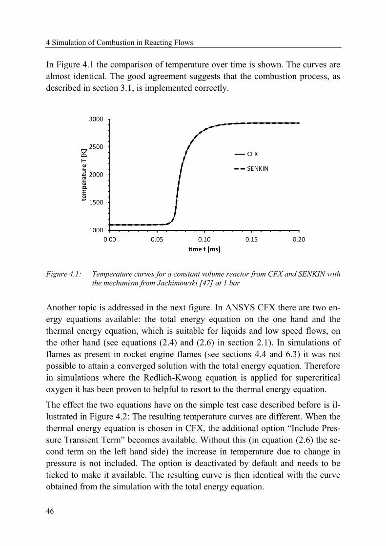
4 Simulation of Combustion in Reacting Flows
46
In Figure 4.1 the comparison of temperature over time is shown. The curves are
almost identical. The good agreement suggests that the combustion process, as
described in section 3.1, is implemented correctly.
Figure 4.1: Temperature curves for a constant volume reactor from CFX and SENKIN with
the mechanism from Jachimowski [47] at 1 bar
Another topic is addressed in the next figure. In ANSYS CFX there are two en-
ergy equations available: the total energy equation on the one hand and the
thermal energy equation, which is suitable for liquids and low speed flows, on
the other hand (see equations (2.4) and (2.6) in section 2.1). In simulations of
flames as present in rocket engine flames (see sections 4.4 and 6.3) it was not
possible to attain a converged solution with the total energy equation. Therefore
in simulations where the Redlich-Kwong equation is applied for supercritical
oxygen it has been proven to helpful to resort to the thermal energy equation.
The effect the two equations have on the simple test case described before is il-
lustrated in Figure 4.2: The resulting temperature curves are different. When the
thermal energy equation is chosen in CFX, the additional option “Include Pres-
sure Transient Term” becomes available. Without this (in equation (2.6) the se-
cond term on the left hand side) the increase in temperature due to change in
pressure is not included. The option is deactivated by default and needs to be
ticked to make it available. The resulting curve is then identical with the curve
obtained from the simulation with the total energy equation.
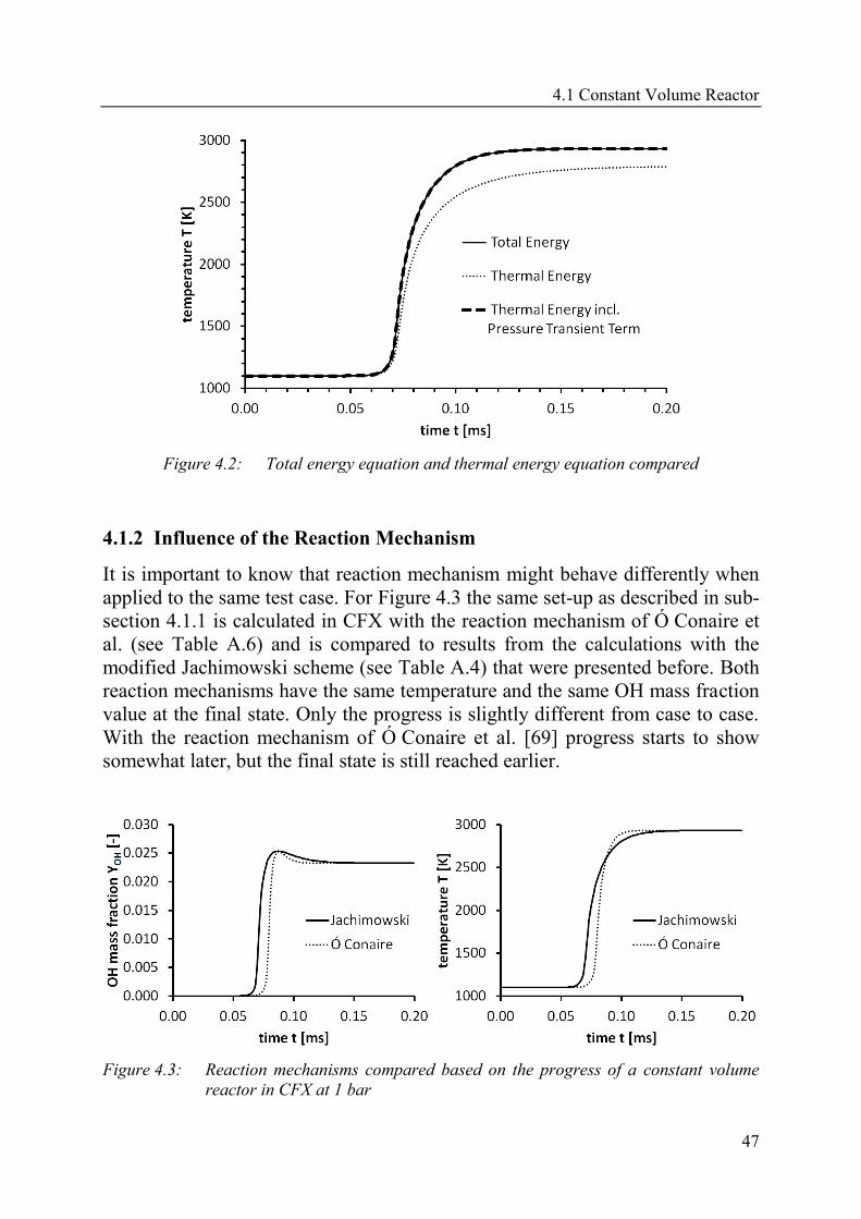
4.1 Constant Volume Reactor
47
Figure 4.2: Total energy equation and thermal energy equation compared
4.1.2 Influence of the Reaction Mechanism
It is important to know that reaction mechanism might behave differently when
applied to the same test case. For Figure 4.3 the same set-up as described in sub-
section 4.1.1 is calculated in CFX with the reaction mechanism of Ó Conaire et
al. (see Table A.6) and is compared to results from the calculations with the
modified Jachimowski scheme (see Table A.4) that were presented before. Both
reaction mechanisms have the same temperature and the same OH mass fraction
value at the final state. Only the progress is slightly different from case to case.
With the reaction mechanism of Ó Conaire et al. [69] progress starts to show
somewhat later, but the final state is still reached earlier.
Figure 4.3: Reaction mechanisms compared based on the progress of a constant volume
reactor in CFX at 1 bar

4 Simulation of Combustion in Reacting Flows
48
The set-up that is shown in Figure 4.4 is chosen to represent the conditions in
the high pressure region. At t = 0 ms the simulation is initialized at T = 1100 K
and p = 60 bar. In this case progress first starts to show with the mechanism of
Ó Conaire et al. [69]. Once a certain state is reached progress is so fast that the
curve becomes almost vertical and at final state seems to turn at right angles into
a horizontal line.
Figure 4.4: Reaction mechanisms compared based on the progress of a constant volume
reactor in CFX at 60 bar
The ignition time (which in SENKIN is defined as the time when the tempera-
ture rises 400 K above the initial temperature) with the mechanism of Ó Conaire
et al. is not only shorter for p = 60 bar. As shown in Figure 4.5 this is true for all
pressures above 5 bar.
Figure 4.5: Ignition time plotted against pressure for a constant volume reactor starting at
1100 K and 60 bar
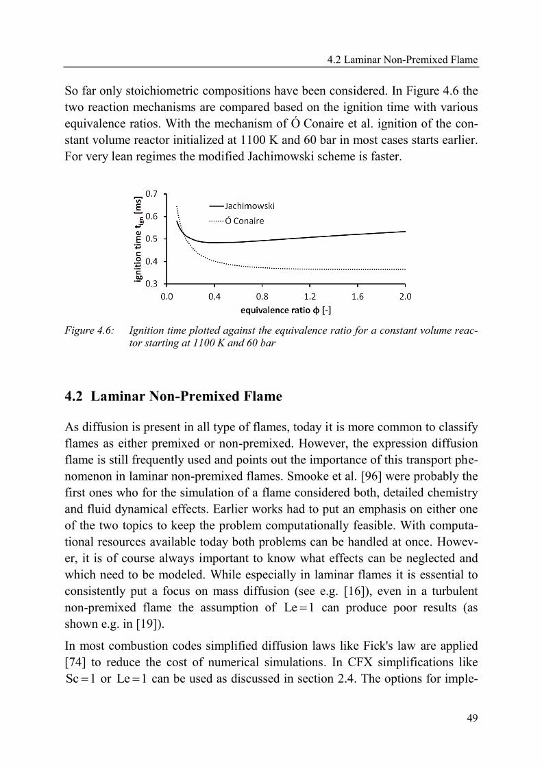
4.2 Laminar Non-Premixed Flame
49
So far only stoichiometric compositions have been considered. In Figure 4.6 the
two reaction mechanisms are compared based on the ignition time with various
equivalence ratios. With the mechanism of Ó Conaire et al. ignition of the con-
stant volume reactor initialized at 1100 K and 60 bar in most cases starts earlier.
For very lean regimes the modified Jachimowski scheme is faster.
Figure 4.6: Ignition time plotted against the equivalence ratio for a constant volume reac-
tor starting at 1100 K and 60 bar
4.2 Laminar Non-Premixed Flame
As diffusion is present in all type of flames, today it is more common to classify
flames as either premixed or non-premixed. However, the expression diffusion
flame is still frequently used and points out the importance of this transport phe-
nomenon in laminar non-premixed flames. Smooke et al. [96] were probably the
first ones who for the simulation of a flame considered both, detailed chemistry
and fluid dynamical effects. Earlier works had to put an emphasis on either one
of the two topics to keep the problem computationally feasible. With computa-
tional resources available today both problems can be handled at once. Howev-
er, it is of course always important to know what effects can be neglected and
which need to be modeled. While especially in laminar flames it is essential to
consistently put a focus on mass diffusion (see e.g. [16]), even in a turbulent
non-premixed flame the assumption of Le 1 can produce poor results (as
shown e.g. in [19]).
In most combustion codes simplified diffusion laws like Fick's law are applied
[74] to reduce the cost of numerical simulations. In CFX simplifications like
Sc 1 or Le 1 can be used as discussed in section 2.4. The options for imple-
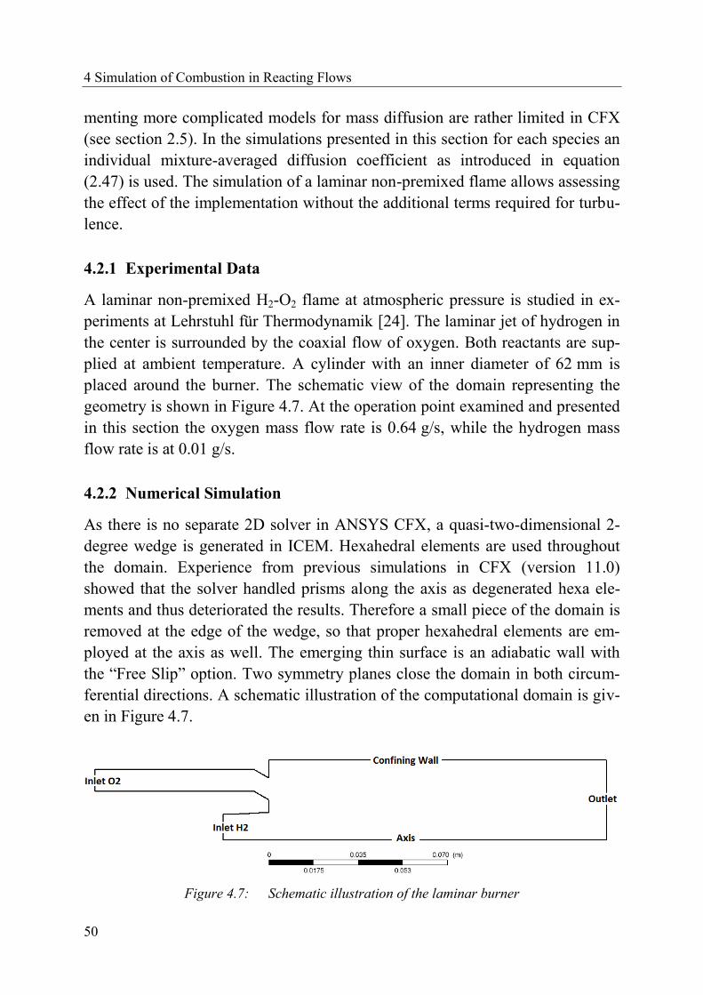
4 Simulation of Combustion in Reacting Flows
50
menting more complicated models for mass diffusion are rather limited in CFX
(see section 2.5). In the simulations presented in this section for each species an
individual mixture-averaged diffusion coefficient as introduced in equation
(2.47) is used. The simulation of a laminar non-premixed flame allows assessing
the effect of the implementation without the additional terms required for turbu-
lence.
4.2.1 Experimental Data
A laminar non-premixed H2-O2 flame at atmospheric pressure is studied in ex-
periments at Lehrstuhl für Thermodynamik [24]. The laminar jet of hydrogen in
the center is surrounded by the coaxial flow of oxygen. Both reactants are sup-
plied at ambient temperature. A cylinder with an inner diameter of 62 mm is
placed around the burner. The schematic view of the domain representing the
geometry is shown in Figure 4.7. At the operation point examined and presented
in this section the oxygen mass flow rate is 0.64 g/s, while the hydrogen mass
flow rate is at 0.01 g/s.
4.2.2 Numerical Simulation
As there is no separate 2D solver in ANSYS CFX, a quasi-two-dimensional 2-
degree wedge is generated in ICEM. Hexahedral elements are used throughout
the domain. Experience from previous simulations in CFX (version 11.0)
showed that the solver handled prisms along the axis as degenerated hexa ele-
ments and thus deteriorated the results. Therefore a small piece of the domain is
removed at the edge of the wedge, so that proper hexahedral elements are em-
ployed at the axis as well. The emerging thin surface is an adiabatic wall with
the “Free Slip” option. Two symmetry planes close the domain in both circum-
ferential directions. A schematic illustration of the computational domain is giv-
en in Figure 4.7.
Figure 4.7: Schematic illustration of the laminar burner
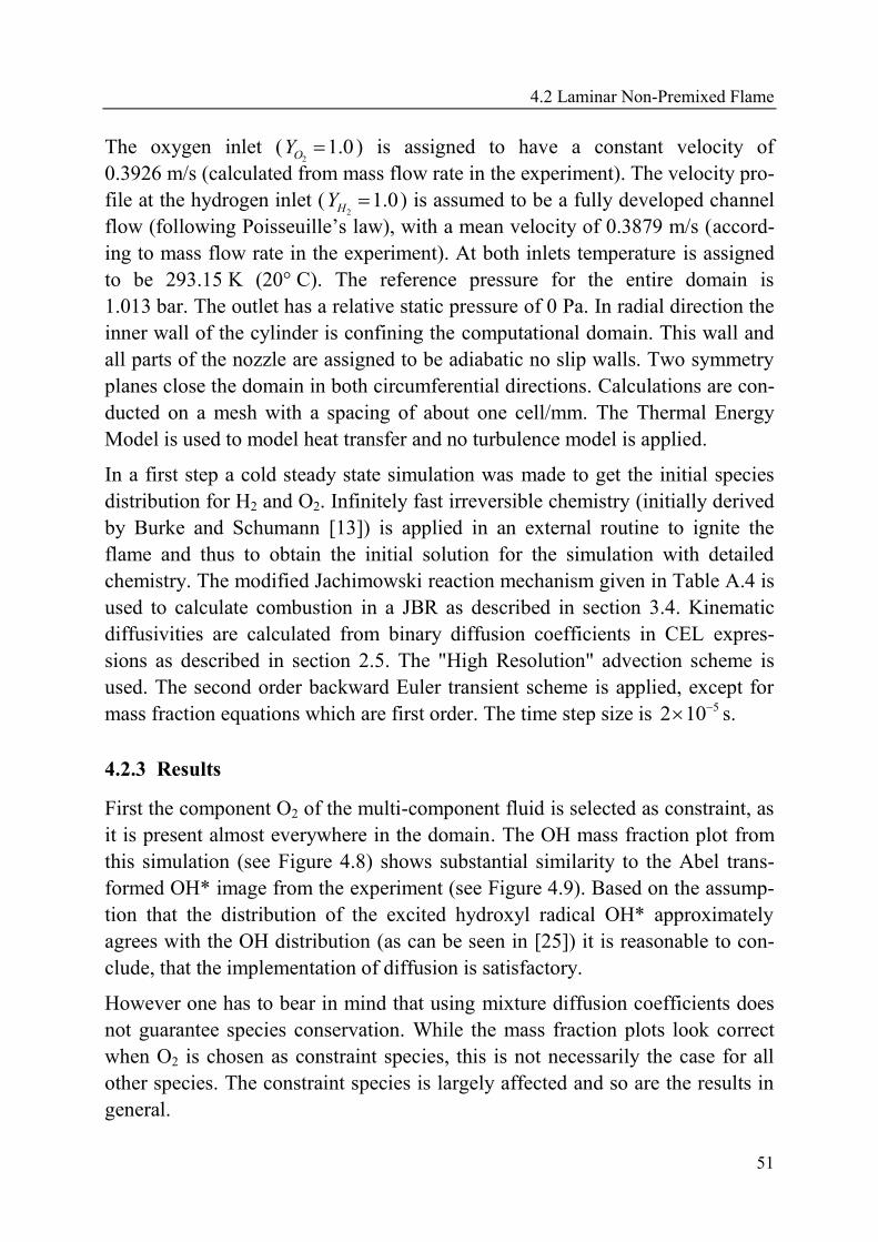
4.2 Laminar Non-Premixed Flame
51
The oxygen inlet (2
1.0OY ) is assigned to have a constant velocity of
0.3926 m/s (calculated from mass flow rate in the experiment). The velocity pro-
file at the hydrogen inlet (2
1.0HY ) is assumed to be a fully developed channel
flow (following Poisseuille’s law), with a mean velocity of 0.3879 m/s (accord-
ing to mass flow rate in the experiment). At both inlets temperature is assigned
to be 293.15 K (20° C). The reference pressure for the entire domain is
1.013 bar. The outlet has a relative static pressure of 0 Pa. In radial direction the
inner wall of the cylinder is confining the computational domain. This wall and
all parts of the nozzle are assigned to be adiabatic no slip walls. Two symmetry
planes close the domain in both circumferential directions. Calculations are con-
ducted on a mesh with a spacing of about one cell/mm. The Thermal Energy
Model is used to model heat transfer and no turbulence model is applied.
In a first step a cold steady state simulation was made to get the initial species
distribution for H2 and O2. Infinitely fast irreversible chemistry (initially derived
by Burke and Schumann [13]) is applied in an external routine to ignite the
flame and thus to obtain the initial solution for the simulation with detailed
chemistry. The modified Jachimowski reaction mechanism given in Table A.4 is
used to calculate combustion in a JBR as described in section 3.4. Kinematic
diffusivities are calculated from binary diffusion coefficients in CEL expres-
sions as described in section 2.5. The "High Resolution" advection scheme is
used. The second order backward Euler transient scheme is applied, except for
mass fraction equations which are first order. The time step size is 52 10 s.
4.2.3 Results
First the component O2 of the multi-component fluid is selected as constraint, as
it is present almost everywhere in the domain. The OH mass fraction plot from
this simulation (see Figure 4.8) shows substantial similarity to the Abel trans-
formed OH* image from the experiment (see Figure 4.9). Based on the assump-
tion that the distribution of the excited hydroxyl radical OH* approximately
agrees with the OH distribution (as can be seen in [25]) it is reasonable to con-
clude, that the implementation of diffusion is satisfactory.
However one has to bear in mind that using mixture diffusion coefficients does
not guarantee species conservation. While the mass fraction plots look correct
when O2 is chosen as constraint species, this is not necessarily the case for all
other species. The constraint species is largely affected and so are the results in
general.
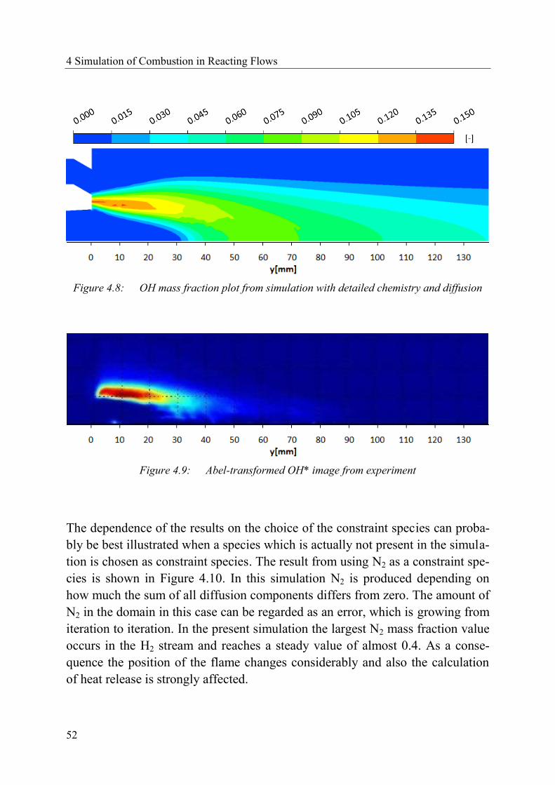
4 Simulation of Combustion in Reacting Flows
52
Figure 4.8: OH mass fraction plot from simulation with detailed chemistry and diffusion
Figure 4.9: Abel-transformed OH* image from experiment
The dependence of the results on the choice of the constraint species can proba-
bly be best illustrated when a species which is actually not present in the simula-
tion is chosen as constraint species. The result from using N2 as a constraint spe-
cies is shown in Figure 4.10. In this simulation N2 is produced depending on
how much the sum of all diffusion components differs from zero. The amount of
N2 in the domain in this case can be regarded as an error, which is growing from
iteration to iteration. In the present simulation the largest N2 mass fraction value
occurs in the H2 stream and reaches a steady value of almost 0.4. As a conse-
quence the position of the flame changes considerably and also the calculation
of heat release is strongly affected.
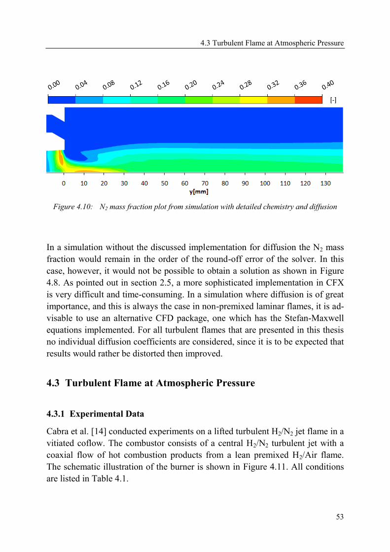
4.3 Turbulent Flame at Atmospheric Pressure
53
Figure 4.10: N2 mass fraction plot from simulation with detailed chemistry and diffusion
In a simulation without the discussed implementation for diffusion the N2 mass
fraction would remain in the order of the round-off error of the solver. In this
case, however, it would not be possible to obtain a solution as shown in Figure
4.8. As pointed out in section 2.5, a more sophisticated implementation in CFX
is very difficult and time-consuming. In a simulation where diffusion is of great
importance, and this is always the case in non-premixed laminar flames, it is ad-
visable to use an alternative CFD package, one which has the Stefan-Maxwell
equations implemented. For all turbulent flames that are presented in this thesis
no individual diffusion coefficients are considered, since it is to be expected that
results would rather be distorted then improved.
4.3 Turbulent Flame at Atmospheric Pressure
4.3.1 Experimental Data
Cabra et al. [14] conducted experiments on a lifted turbulent H2/N2 jet flame in a
vitiated coflow. The combustor consists of a central H2/N2 turbulent jet with a
coaxial flow of hot combustion products from a lean premixed H2/Air flame.
The schematic illustration of the burner is shown in Figure 4.11. All conditions
are listed in Table 4.1.
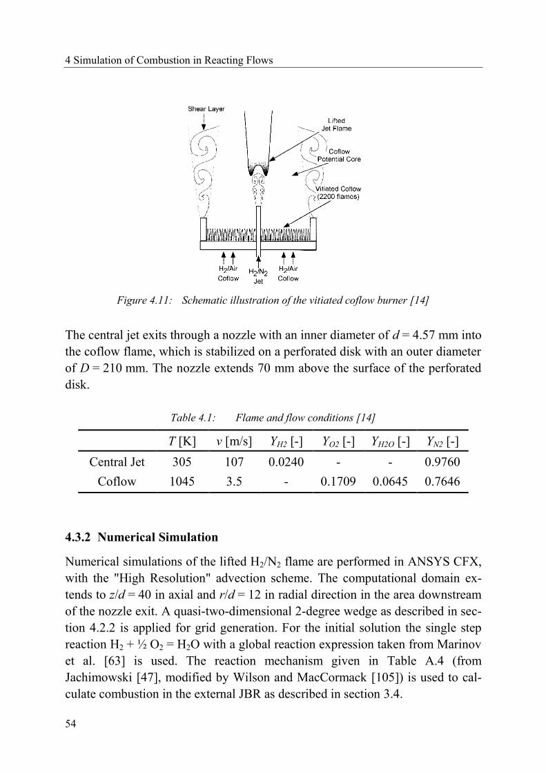
4 Simulation of Combustion in Reacting Flows
54
Figure 4.11: Schematic illustration of the vitiated coflow burner [14]
The central jet exits through a nozzle with an inner diameter of d = 4.57 mm into
the coflow flame, which is stabilized on a perforated disk with an outer diameter
of D = 210 mm. The nozzle extends 70 mm above the surface of the perforated
disk.
Table 4.1: Flame and flow conditions [14]
T [K] v [m/s] YH2 [-] YO2 [-] YH2O [-] YN2 [-]
Central Jet 305 107 0.0240 - - 0.9760
Coflow 1045 3.5 - 0.1709 0.0645 0.7646
4.3.2 Numerical Simulation
Numerical simulations of the lifted H2/N2 flame are performed in ANSYS CFX,
with the "High Resolution" advection scheme. The computational domain ex-
tends to z/d = 40 in axial and r/d = 12 in radial direction in the area downstream
of the nozzle exit. A quasi-two-dimensional 2-degree wedge as described in sec-
tion 4.2.2 is applied for grid generation. For the initial solution the single step
reaction H2 + ½ O2 = H2O with a global reaction expression taken from Marinov
et al. [63] is used. The reaction mechanism given in Table A.4 (from
Jachimowski [47], modified by Wilson and MacCormack [105]) is used to cal-
culate combustion in the external JBR as described in section 3.4.
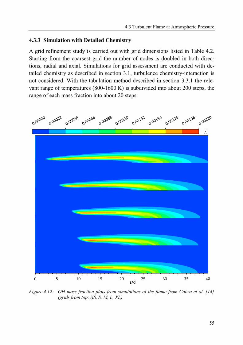
4.3 Turbulent Flame at Atmospheric Pressure
55
4.3.3 Simulation with Detailed Chemistry
A grid refinement study is carried out with grid dimensions listed in Table 4.2.
Starting from the coarsest grid the number of nodes is doubled in both direc-
tions, radial and axial. Simulations for grid assessment are conducted with de-
tailed chemistry as described in section 3.1, turbulence chemistry-interaction is
not considered. With the tabulation method described in section 3.3.1 the rele-
vant range of temperatures (800-1600 K) is subdivided into about 200 steps, the
range of each mass fraction into about 20 steps.
Figure 4.12: OH mass fraction plots from simulations of the flame from Cabra et al. [14]
(grids from top: XS, S, M, L, XL)
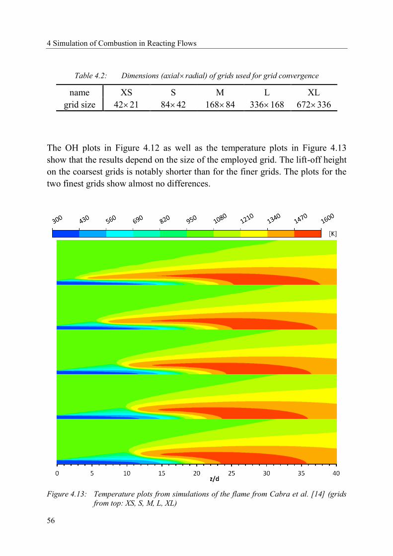
4 Simulation of Combustion in Reacting Flows
56
Table 4.2: Dimensions (axialradial) of grids used for grid convergence
name XS S M L XL
grid size 4221 8442 16884 336168 672336
The OH plots in Figure 4.12 as well as the temperature plots in Figure 4.13
show that the results depend on the size of the employed grid. The lift-off height
on the coarsest grids is notably shorter than for the finer grids. The plots for the
two finest grids show almost no differences.
Figure 4.13: Temperature plots from simulations of the flame from Cabra et al. [14] (grids
from top: XS, S, M, L, XL)
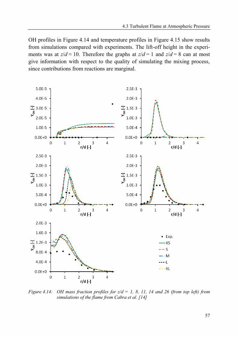
4.3 Turbulent Flame at Atmospheric Pressure
57
OH profiles in Figure 4.14 and temperature profiles in Figure 4.15 show results
from simulations compared with experiments. The lift-off height in the experi-
ments was at z/d ≈ 10. Therefore the graphs at z/d = 1 and z/d = 8 can at most
give information with respect to the quality of simulating the mixing process,
since contributions from reactions are marginal.
Figure 4.14: OH mass fraction profiles for z/d = 1, 8, 11, 14 and 26 (from top left) from
simulations of the flame from Cabra et al. [14]
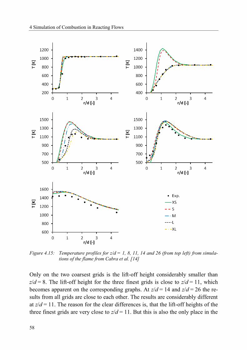
4 Simulation of Combustion in Reacting Flows
58
Figure 4.15: Temperature profiles for z/d = 1, 8, 11, 14 and 26 (from top left) from simula-
tions of the flame from Cabra et al. [14]
Only on the two coarsest grids is the lift-off height considerably smaller than
z/d = 8. The lift-off height for the three finest grids is close to z/d = 11, which
becomes apparent on the corresponding graphs. At z/d = 14 and z/d = 26 the re-
sults from all grids are close to each other. The results are considerably different
at z/d = 11. The reason for the clear differences is, that the lift-off heights of the
three finest grids are very close to z/d = 11. But this is also the only place in the
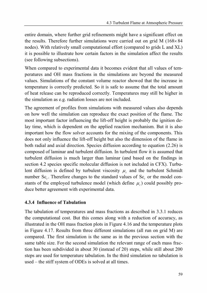
4.3 Turbulent Flame at Atmospheric Pressure
59
entire domain, where further grid refinements might have a significant effect on
the results. Therefore further simulations were carried out on grid M (16884
nodes). With relatively small computational effort (compared to grids L and XL)
it is possible to illustrate how certain factors in the simulation affect the results
(see following subsections).
When compared to experimental data it becomes evident that all values of tem-
peratures and OH mass fractions in the simulations are beyond the measured
values. Simulations of the constant volume reactor showed that the increase in
temperature is correctly predicted. So it is safe to assume that the total amount
of heat release can be reproduced correctly. Temperatures may still be higher in
the simulation as e.g. radiation losses are not included.
The agreement of profiles from simulations with measured values also depends
on how well the simulation can reproduce the exact position of the flame. The
most important factor influencing the lift-off height is probably the ignition de-
lay time, which is dependent on the applied reaction mechanism. But it is also
important how the flow solver accounts for the mixing of the components. This
does not only influence the lift-off height but also the dimension of the flame in
both radial and axial direction. Species diffusion according to equation (2.26) is
composed of laminar and turbulent diffusion. In turbulent flow it is assumed that
turbulent diffusion is much larger than laminar (and based on the findings in
section 4.2 species specific molecular diffusion is not included in CFX). Turbu-
lent diffusion is defined by turbulent viscosity t and the turbulent Schmidt
number Sct . Therefore changes to the standard values of Sct or the model con-
stants of the employed turbulence model (which define t ) could possibly pro-
duce better agreement with experimental data.
4.3.4 Influence of Tabulation
The tabulation of temperatures and mass fractions as described in 3.3.1 reduces
the computational cost. But this comes along with a reduction of accuracy, as
illustrated in the OH mass fraction plots in Figure 4.16 and the temperature plots
in Figure 4.17. Results from three different simulations (all run on grid M) are
compared. The first simulation is the same as in the previous section with the
same table size. For the second simulation the relevant range of each mass frac-
tion has been subdivided in about 30 (instead of 20) steps, while still about 200
steps are used for temperature tabulation. In the third simulation no tabulation is
used – the stiff system of ODEs is solved at all times.
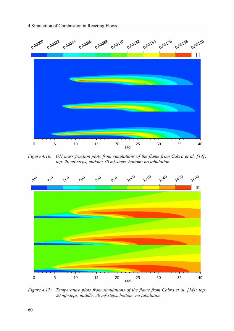
4 Simulation of Combustion in Reacting Flows
60
Figure 4.16: OH mass fraction plots from simulations of the flame from Cabra et al. [14];
top: 20 mf-steps, middle: 30 mf-steps, bottom: no tabulation
Figure 4.17: Temperature plots from simulations of the flame from Cabra et al. [14]; top:
20 mf-steps, middle: 30 mf-steps, bottom: no tabulation
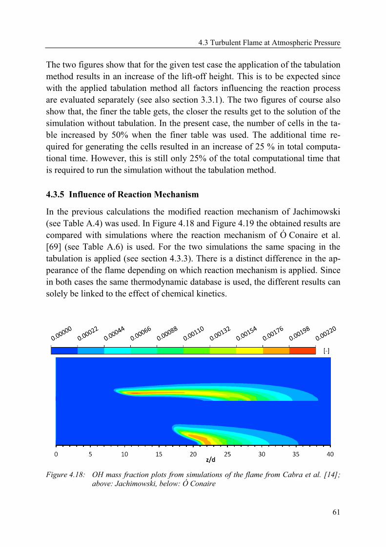
4.3 Turbulent Flame at Atmospheric Pressure
61
The two figures show that for the given test case the application of the tabulation
method results in an increase of the lift-off height. This is to be expected since
with the applied tabulation method all factors influencing the reaction process
are evaluated separately (see also section 3.3.1). The two figures of course also
show that, the finer the table gets, the closer the results get to the solution of the
simulation without tabulation. In the present case, the number of cells in the ta-
ble increased by 50% when the finer table was used. The additional time re-
quired for generating the cells resulted in an increase of 25 % in total computa-
tional time. However, this is still only 25% of the total computational time that
is required to run the simulation without the tabulation method.
4.3.5 Influence of Reaction Mechanism
In the previous calculations the modified reaction mechanism of Jachimowski
(see Table A.4) was used. In Figure 4.18 and Figure 4.19 the obtained results are
compared with simulations where the reaction mechanism of Ó Conaire et al.
[69] (see Table A.6) is used. For the two simulations the same spacing in the
tabulation is applied (see section 4.3.3). There is a distinct difference in the ap-
pearance of the flame depending on which reaction mechanism is applied. Since
in both cases the same thermodynamic database is used, the different results can
solely be linked to the effect of chemical kinetics.
Figure 4.18: OH mass fraction plots from simulations of the flame from Cabra et al. [14];
above: Jachimowski, below: Ó Conaire
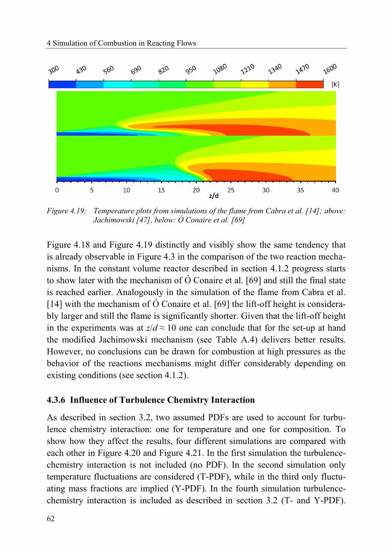
4 Simulation of Combustion in Reacting Flows
62
Figure 4.19: Temperature plots from simulations of the flame from Cabra et al. [14]; above:
Jachimowski [47], below: Ó Conaire et al. [69]
Figure 4.18 and Figure 4.19 distinctly and visibly show the same tendency that
is already observable in Figure 4.3 in the comparison of the two reaction mecha-
nisms. In the constant volume reactor described in section 4.1.2 progress starts
to show later with the mechanism of Ó Conaire et al. [69] and still the final state
is reached earlier. Analogously in the simulation of the flame from Cabra et al.
[14] with the mechanism of Ó Conaire et al. [69] the lift-off height is considera-
bly larger and still the flame is significantly shorter. Given that the lift-off height
in the experiments was at z/d ≈ 10 one can conclude that for the set-up at hand
the modified Jachimowski mechanism (see Table A.4) delivers better results.
However, no conclusions can be drawn for combustion at high pressures as the
behavior of the reactions mechanisms might differ considerably depending on
existing conditions (see section 4.1.2).
4.3.6 Influence of Turbulence Chemistry Interaction
As described in section 3.2, two assumed PDFs are used to account for turbu-
lence chemistry interaction: one for temperature and one for composition. To
show how they affect the results, four different simulations are compared with
each other in Figure 4.20 and Figure 4.21. In the first simulation the turbulence-
chemistry interaction is not included (no PDF). In the second simulation only
temperature fluctuations are considered (T-PDF), while in the third only fluctu-
ating mass fractions are implied (Y-PDF). In the fourth simulation turbulence-
chemistry interaction is included as described in section 3.2 (T- and Y-PDF).
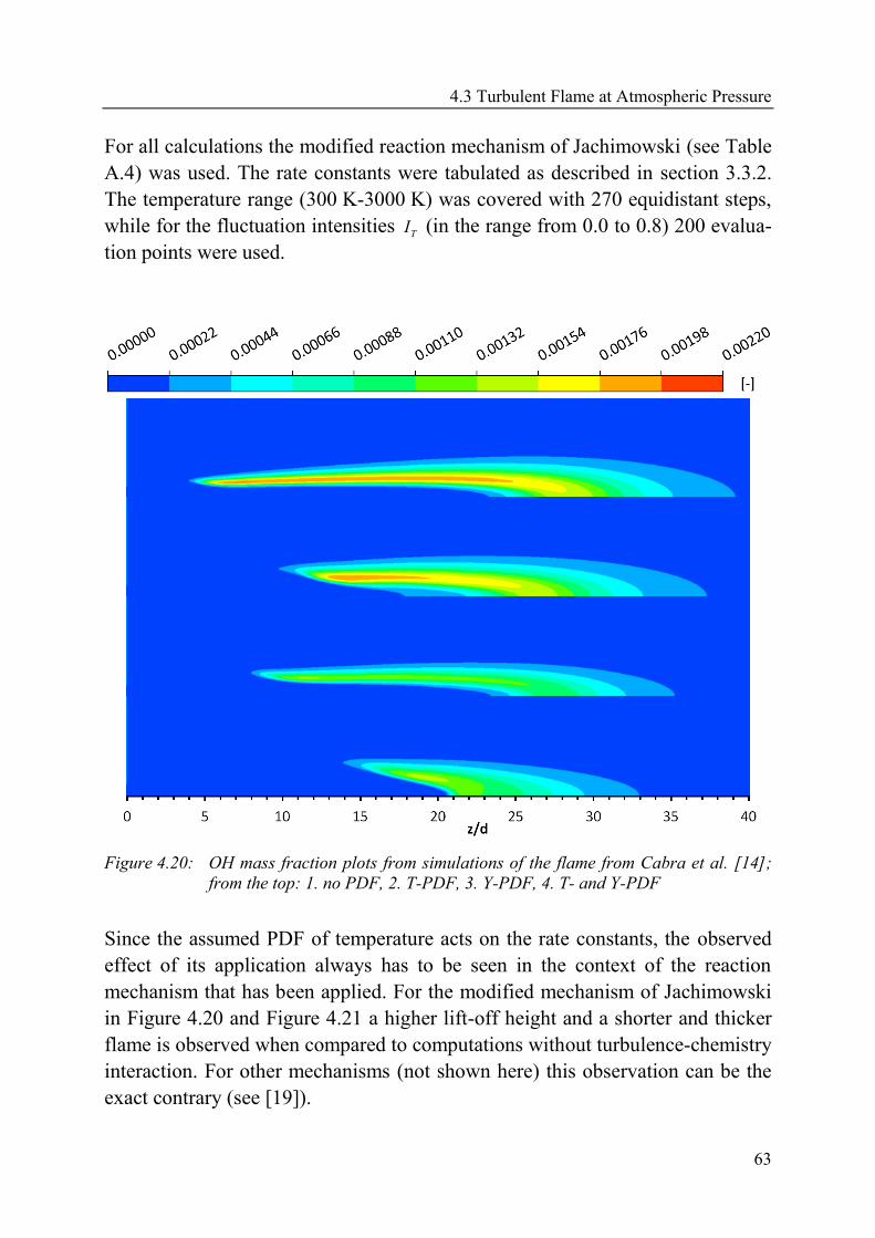
4.3 Turbulent Flame at Atmospheric Pressure
63
For all calculations the modified reaction mechanism of Jachimowski (see Table
A.4) was used. The rate constants were tabulated as described in section 3.3.2.
The temperature range (300 K-3000 K) was covered with 270 equidistant steps,
while for the fluctuation intensities TI (in the range from 0.0 to 0.8) 200 evalua-
tion points were used.
Figure 4.20: OH mass fraction plots from simulations of the flame from Cabra et al. [14];
from the top: 1. no PDF, 2. T-PDF, 3. Y-PDF, 4. T- and Y-PDF
Since the assumed PDF of temperature acts on the rate constants, the observed
effect of its application always has to be seen in the context of the reaction
mechanism that has been applied. For the modified mechanism of Jachimowski
in Figure 4.20 and Figure 4.21 a higher lift-off height and a shorter and thicker
flame is observed when compared to computations without turbulence-chemistry
interaction. For other mechanisms (not shown here) this observation can be the
exact contrary (see [19]).
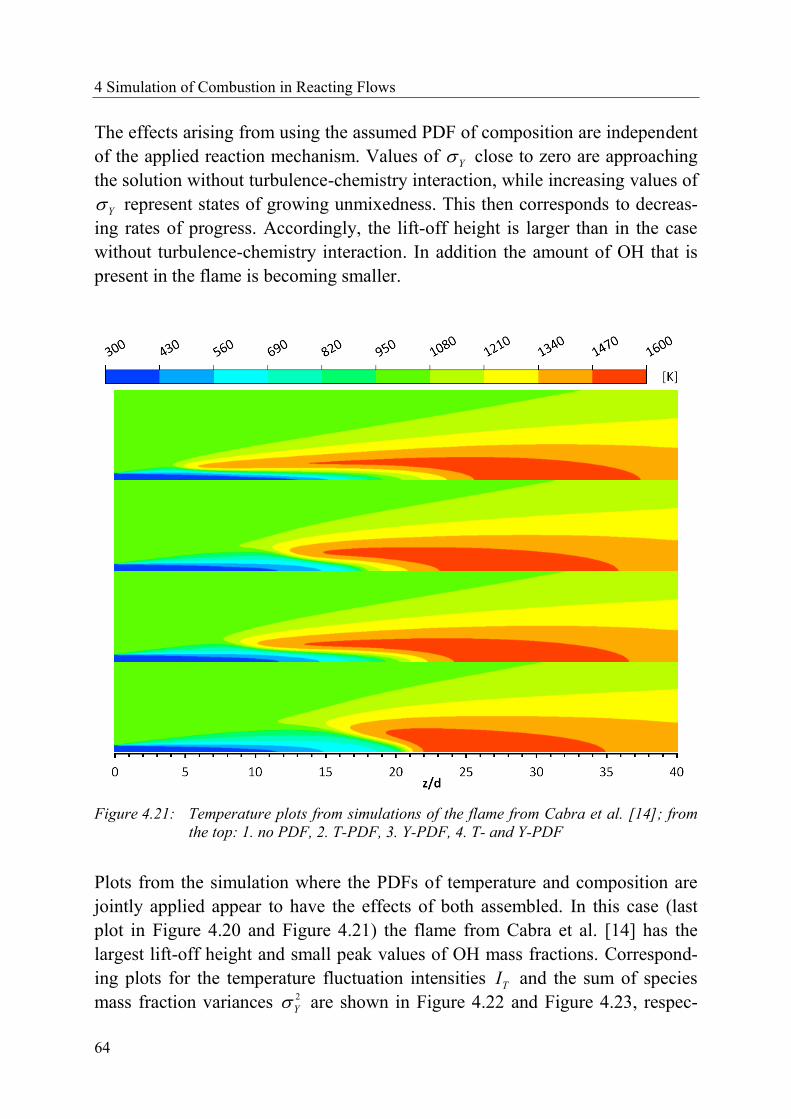
4 Simulation of Combustion in Reacting Flows
64
The effects arising from using the assumed PDF of composition are independent
of the applied reaction mechanism. Values of Y close to zero are approaching
the solution without turbulence-chemistry interaction, while increasing values of
Y represent states of growing unmixedness. This then corresponds to decreas-
ing rates of progress. Accordingly, the lift-off height is larger than in the case
without turbulence-chemistry interaction. In addition the amount of OH that is
present in the flame is becoming smaller.
Figure 4.21: Temperature plots from simulations of the flame from Cabra et al. [14]; from
the top: 1. no PDF, 2. T-PDF, 3. Y-PDF, 4. T- and Y-PDF
Plots from the simulation where the PDFs of temperature and composition are
jointly applied appear to have the effects of both assembled. In this case (last
plot in Figure 4.20 and Figure 4.21) the flame from Cabra et al. [14] has the
largest lift-off height and small peak values of OH mass fractions. Correspond-
ing plots for the temperature fluctuation intensities TI and the sum of species
mass fraction variances 2
Y are shown in Figure 4.22 and Figure 4.23, respec-
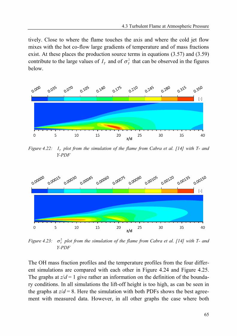
4.3 Turbulent Flame at Atmospheric Pressure
65
tively. Close to where the flame touches the axis and where the cold jet flow
mixes with the hot co-flow large gradients of temperature and of mass fractions
exist. At these places the production source terms in equations (3.57) and (3.59)
contribute to the large values of TI and of 2
Y that can be observed in the figures
below.
Figure 4.22: TI plot from the simulation of the flame from Cabra et al. [14] with T- and
Y-PDF
Figure 4.23: 2
Y plot from the simulation of the flame from Cabra et al. [14] with T- and
Y-PDF
The OH mass fraction profiles and the temperature profiles from the four differ-
ent simulations are compared with each other in Figure 4.24 and Figure 4.25.
The graphs at z/d = 1 give rather an information on the definition of the bounda-
ry conditions. In all simulations the lift-off height is too high, as can be seen in
the graphs at z/d = 8. Here the simulation with both PDFs shows the best agree-
ment with measured data. However, in all other graphs the case where both
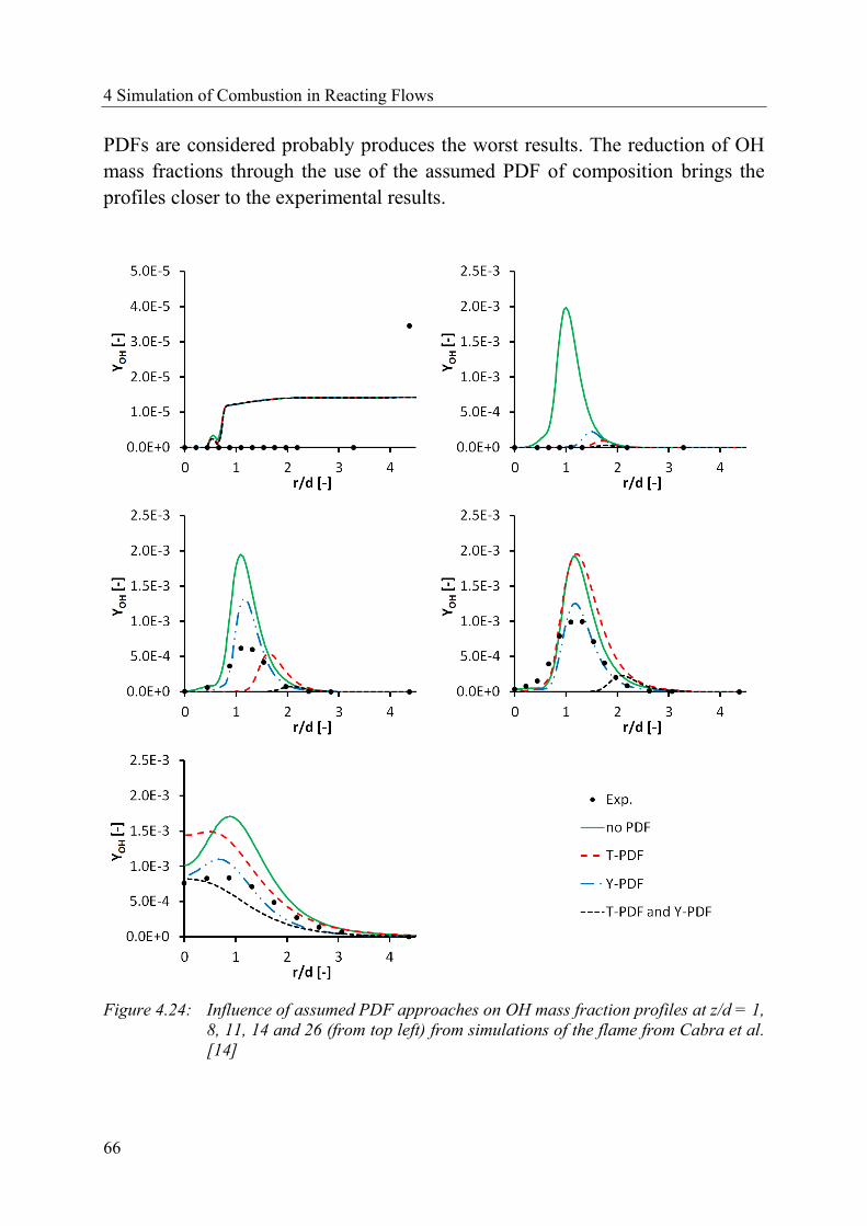
4 Simulation of Combustion in Reacting Flows
66
PDFs are considered probably produces the worst results. The reduction of OH
mass fractions through the use of the assumed PDF of composition brings the
profiles closer to the experimental results.
Figure 4.24: Influence of assumed PDF approaches on OH mass fraction profiles at z/d = 1,
8, 11, 14 and 26 (from top left) from simulations of the flame from Cabra et al.
[14]
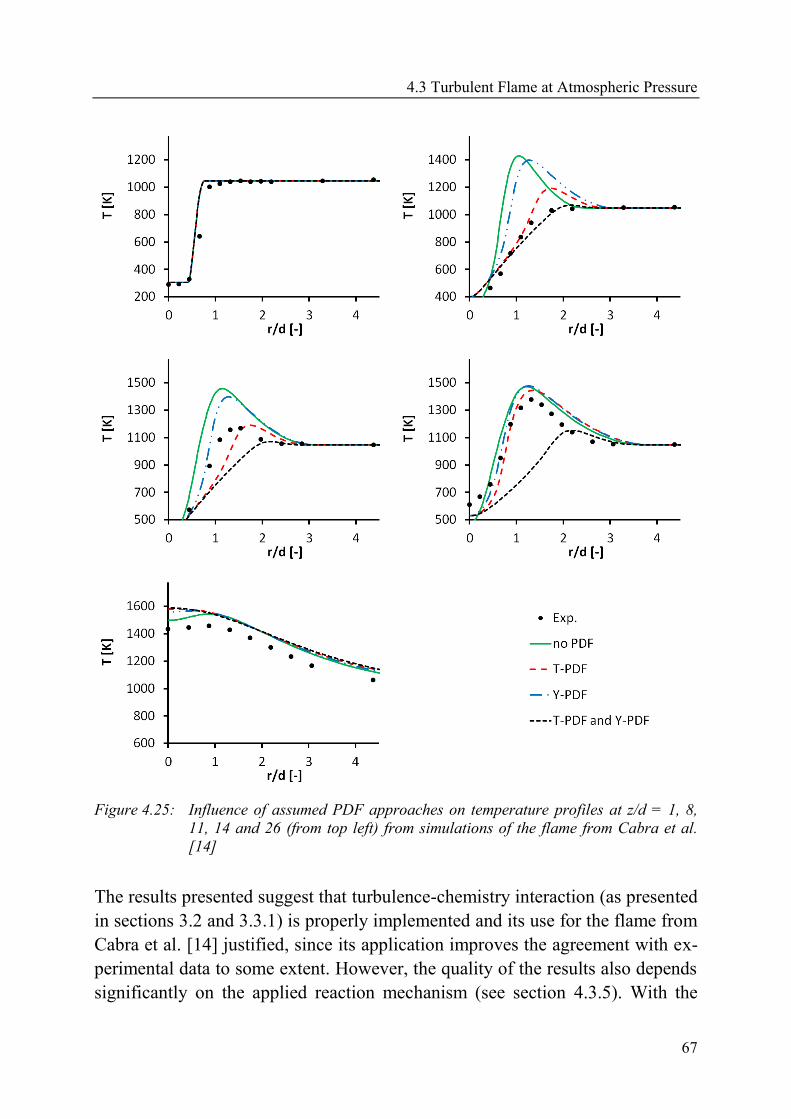
4.3 Turbulent Flame at Atmospheric Pressure
67
Figure 4.25: Influence of assumed PDF approaches on temperature profiles at z/d = 1, 8,
11, 14 and 26 (from top left) from simulations of the flame from Cabra et al.
[14]
The results presented suggest that turbulence-chemistry interaction (as presented
in sections 3.2 and 3.3.1) is properly implemented and its use for the flame from
Cabra et al. [14] justified, since its application improves the agreement with ex-
perimental data to some extent. However, the quality of the results also depends
significantly on the applied reaction mechanism (see section 4.3.5). With the
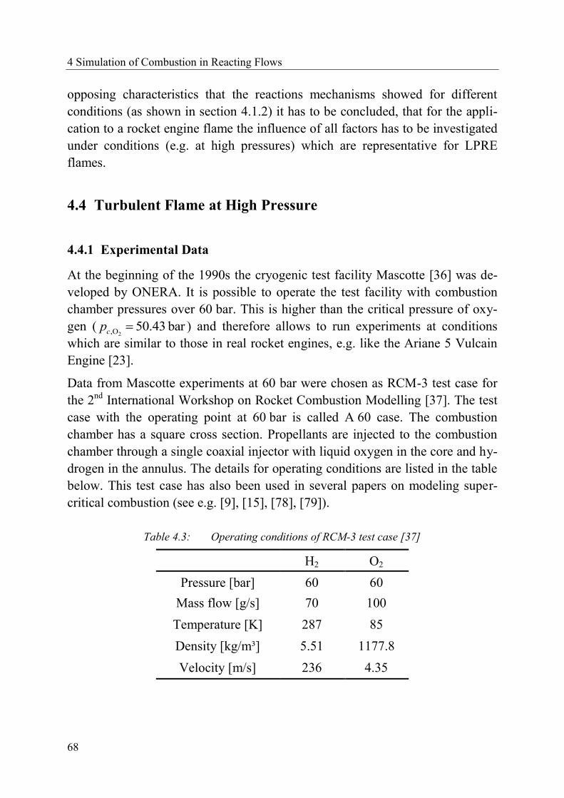
4 Simulation of Combustion in Reacting Flows
68
opposing characteristics that the reactions mechanisms showed for different
conditions (as shown in section 4.1.2) it has to be concluded, that for the appli-
cation to a rocket engine flame the influence of all factors has to be investigated
under conditions (e.g. at high pressures) which are representative for LPRE
flames.
4.4 Turbulent Flame at High Pressure
4.4.1 Experimental Data
At the beginning of the 1990s the cryogenic test facility Mascotte [36] was de-
veloped by ONERA. It is possible to operate the test facility with combustion
chamber pressures over 60 bar. This is higher than the critical pressure of oxy-
gen (2,O 50.43 barcp ) and therefore allows to run experiments at conditions
which are similar to those in real rocket engines, e.g. like the Ariane 5 Vulcain
Engine [23].
Data from Mascotte experiments at 60 bar were chosen as RCM-3 test case for
the 2nd
International Workshop on Rocket Combustion Modelling [37]. The test
case with the operating point at 60 bar is called A 60 case. The combustion
chamber has a square cross section. Propellants are injected to the combustion
chamber through a single coaxial injector with liquid oxygen in the core and hy-
drogen in the annulus. The details for operating conditions are listed in the table
below. This test case has also been used in several papers on modeling super-
critical combustion (see e.g. [9], [15], [78], [79]).
Table 4.3: Operating conditions of RCM-3 test case [37]
H2 O2
Pressure [bar] 60 60
Mass flow [g/s] 70 100
Temperature [K] 287 85
Density [kg/m³] 5.51 1177.8
Velocity [m/s] 236 4.35
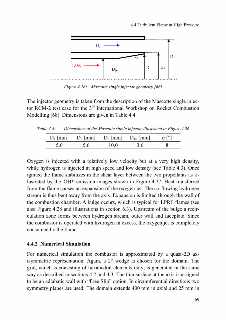
4.4 Turbulent Flame at High Pressure
69
Figure 4.26: Mascotte single injector geometry [68]
The injector geometry is taken from the description of the Mascotte single injec-
tor RCM-2 test case for the 3rd
International Workshop on Rocket Combustion
Modelling [68]. Dimensions are given in Table 4.4.
Table 4.4: Dimensions of the Mascotte single injector illustrated in Figure 4.26
D1 [mm] D2 [mm] D3 [mm] D10 [mm] α [°]
5.0 5.6 10.0 3.6 8
Oxygen is injected with a relatively low velocity but at a very high density,
while hydrogen is injected at high speed and low density (see Table 4.3). Once
ignited the flame stabilizes in the shear layer between the two propellants as il-
lustrated by the OH* emission images shown in Figure 4.27. Heat transferred
from the flame causes an expansion of the oxygen jet. The co-flowing hydrogen
stream is thus bent away from the axis. Expansion is limited through the wall of
the combustion chamber. A bulge occurs, which is typical for LPRE flames (see
also Figure 4.28 and illustrations in section 6.3). Upstream of the bulge a recir-
culation zone forms between hydrogen stream, outer wall and faceplate. Since
the combustor is operated with hydrogen in excess, the oxygen jet is completely
consumed by the flame.
4.4.2 Numerical Simulation
For numerical simulation the combustor is approximated by a quasi-2D ax-
isymmetric representation. Again, a 2° wedge is chosen for the domain. The
grid, which is consisting of hexahedral elements only, is generated in the same
way as described in sections 4.2 and 4.3. The thin surface at the axis is assigned
to be an adiabatic wall with “Free Slip” option. In circumferential directions two
symmetry planes are used. The domain extends 400 mm in axial and 25 mm in
4 Simulation of Combustion in Reacting Flows
70
radial direction. For initial simulations a grid with 200492 nodes (axial ra-
dialcircumferential) was used, which later was refined to 399972 nodes.
The grid is clustered close to the injector in radial and axial direction. The noz-
zle at the exit was not included. Instead a constant pressure boundary condition
at the outlet was chosen (0 Pa relative to the reference pressure of 60 bar). Mass
flow rates and temperatures at the inlets are prescribed according to Table 4.3.
All other boundaries are adiabatic no slip walls. Turbulence is modeled with the
k-ε-model, with a turbulence intensity of 5 % at the injector. The length of the
inlet duct is chosen to be 40 mm.
The material in the multi-component flow is a variable composition mixture
containing 8 species: H2, O2, H2O, H, O, OH, HO2 and H2O2. Transport equa-
tions for 7 of these species are solved. H2O is chosen to be calculated from a
constraint equation, making sure that the mass fractions of all components sum
up to unity. Only O2 is treated as a real gas according to equation (2.9). All other
species are treated as ideal gases and ideal mixing applies. Following the finding
of section 4.2 no species specific diffusion coefficients are considered and it is
assumed that turbulent diffusion is much more dominant. The eddy dissipation
model (EDM) that is implemented in ANSYS CFX has been used with the sin-
gle step reaction H2 + ½ O2 = H2O to obtain an initial solution.
The Upwind option was chosen as advection scheme and the first order back-
ward Euler option as transient scheme with time steps of 51 10 s. The "Thermal
Energy" option is chosen to model heat transfer, since it was not possible to ob-
tain a solution with the total energy equation when oxygen with the Redlich-
Kwong equation is involved in the simulation of the flame.
4.4.3 Simulation with Detailed Chemistry
OH* emission images from the experiments are shown in Figure 4.27. The OH
mass fractions from numerical simulations are plotted in Figure 4.28. The under-
lying simulation was carried out with the modified reaction mechanism of
Jachimowski (see Table A.4). The plot shows a good agreement with experi-
mental data as far as the flame zone and the expansion angle are considered. The
flame in the simulation shows a small lift-off, which in the Abel-transformed
emission image seems not to be present. One reason for this could be the igni-
tion delay time of the applied reaction scheme. In simulations with EDM, where
combustion is only linked to turbulence and not to reaction kinetics, it stabilizes
at the injector.
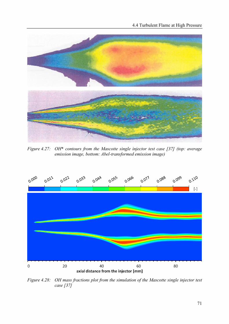
4.4 Turbulent Flame at High Pressure
71
Figure 4.27: OH* contours from the Mascotte single injector test case [37] (top: average
emission image, bottom: Abel-transformed emission image)
Figure 4.28: OH mass fractions plot from the simulation of the Mascotte single injector test
case [37]
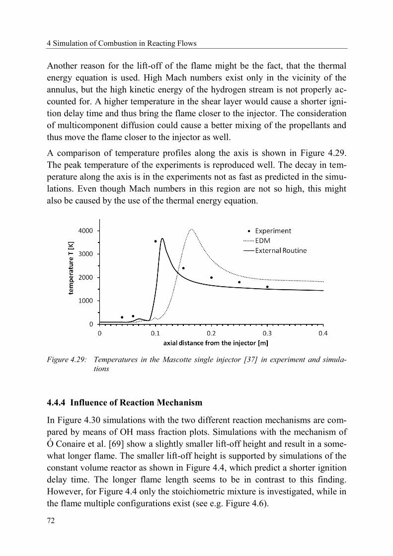
4 Simulation of Combustion in Reacting Flows
72
Another reason for the lift-off of the flame might be the fact, that the thermal
energy equation is used. High Mach numbers exist only in the vicinity of the
annulus, but the high kinetic energy of the hydrogen stream is not properly ac-
counted for. A higher temperature in the shear layer would cause a shorter igni-
tion delay time and thus bring the flame closer to the injector. The consideration
of multicomponent diffusion could cause a better mixing of the propellants and
thus move the flame closer to the injector as well.
A comparison of temperature profiles along the axis is shown in Figure 4.29.
The peak temperature of the experiments is reproduced well. The decay in tem-
perature along the axis is in the experiments not as fast as predicted in the simu-
lations. Even though Mach numbers in this region are not so high, this might
also be caused by the use of the thermal energy equation.
Figure 4.29: Temperatures in the Mascotte single injector [37] in experiment and simula-
tions
4.4.4 Influence of Reaction Mechanism
In Figure 4.30 simulations with the two different reaction mechanisms are com-
pared by means of OH mass fraction plots. Simulations with the mechanism of
Ó Conaire et al. [69] show a slightly smaller lift-off height and result in a some-
what longer flame. The smaller lift-off height is supported by simulations of the
constant volume reactor as shown in Figure 4.4, which predict a shorter ignition
delay time. The longer flame length seems to be in contrast to this finding.
However, for Figure 4.4 only the stoichiometric mixture is investigated, while in
the flame multiple configurations exist (see e.g. Figure 4.6).

4.4 Turbulent Flame at High Pressure
73
Figure 4.30: OH mass fraction plots from simulations of the Mascotte single injector test
case [37]; above: Jachimowski [47], below: Ó Conaire et al. [69]
4.4.5 Influence of Turbulence-Chemistry Interaction
Simulations were carried out using the modified mechanism of Jachimowski
(Table A.4). The method described in section 3.3.2 is used to tabulate rate con-
stants.
Figure 4.31: OH mass fraction plots from simulations of the Mascotte single injector test
case [37]; above: no PDF, below: T-PDF
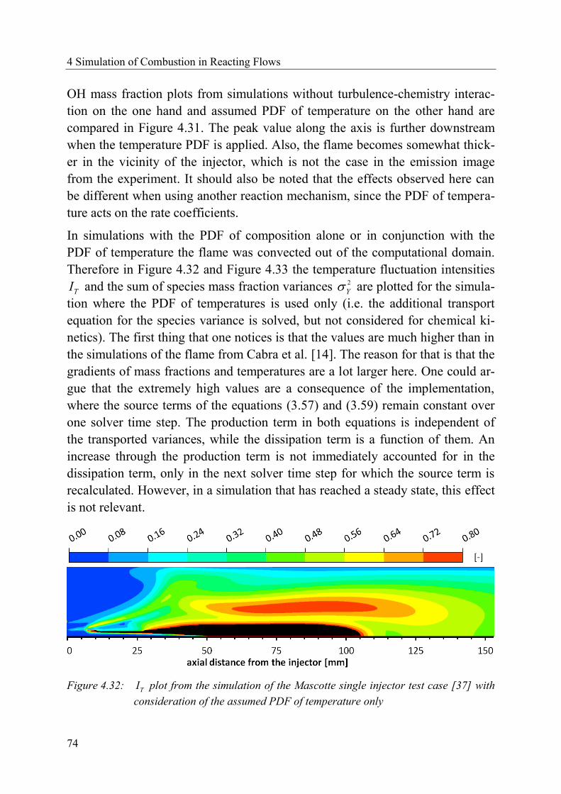
4 Simulation of Combustion in Reacting Flows
74
OH mass fraction plots from simulations without turbulence-chemistry interac-
tion on the one hand and assumed PDF of temperature on the other hand are
compared in Figure 4.31. The peak value along the axis is further downstream
when the temperature PDF is applied. Also, the flame becomes somewhat thick-
er in the vicinity of the injector, which is not the case in the emission image
from the experiment. It should also be noted that the effects observed here can
be different when using another reaction mechanism, since the PDF of tempera-
ture acts on the rate coefficients.
In simulations with the PDF of composition alone or in conjunction with the
PDF of temperature the flame was convected out of the computational domain.
Therefore in Figure 4.32 and Figure 4.33 the temperature fluctuation intensities
TI and the sum of species mass fraction variances 2
Y are plotted for the simula-
tion where the PDF of temperatures is used only (i.e. the additional transport
equation for the species variance is solved, but not considered for chemical ki-
netics). The first thing that one notices is that the values are much higher than in
the simulations of the flame from Cabra et al. [14]. The reason for that is that the
gradients of mass fractions and temperatures are a lot larger here. One could ar-
gue that the extremely high values are a consequence of the implementation,
where the source terms of the equations (3.57) and (3.59) remain constant over
one solver time step. The production term in both equations is independent of
the transported variances, while the dissipation term is a function of them. An
increase through the production term is not immediately accounted for in the
dissipation term, only in the next solver time step for which the source term is
recalculated. However, in a simulation that has reached a steady state, this effect
is not relevant.
Figure 4.32: TI plot from the simulation of the Mascotte single injector test case [37] with
consideration of the assumed PDF of temperature only
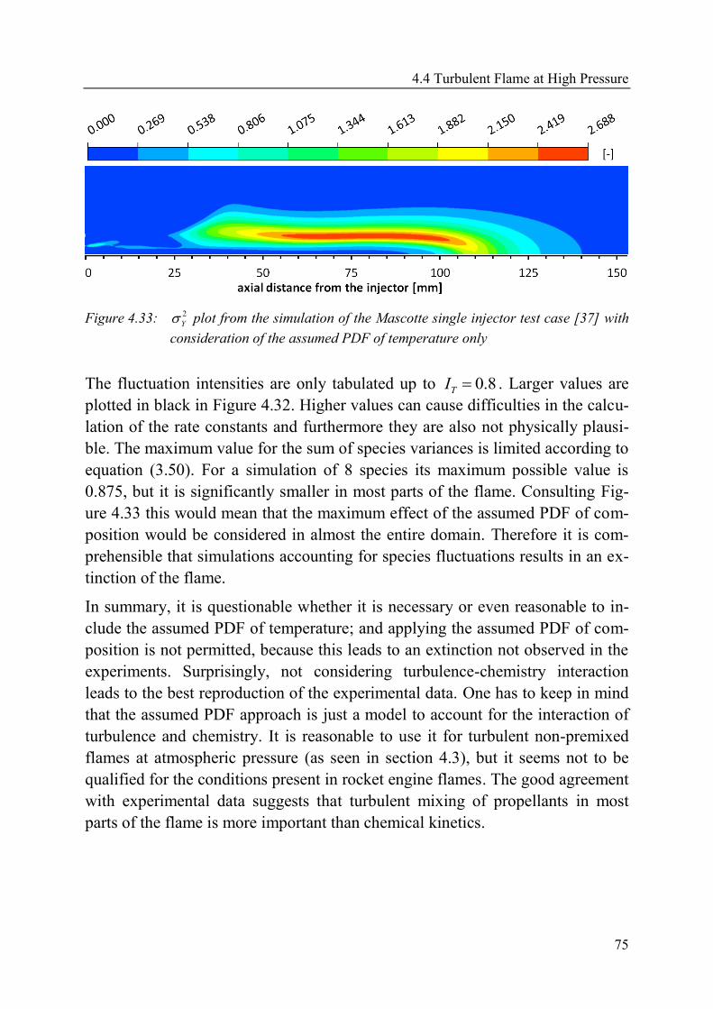
4.4 Turbulent Flame at High Pressure
75
Figure 4.33: 2
Y plot from the simulation of the Mascotte single injector test case [37] with
consideration of the assumed PDF of temperature only
The fluctuation intensities are only tabulated up to 0.8TI . Larger values are
plotted in black in Figure 4.32. Higher values can cause difficulties in the calcu-
lation of the rate constants and furthermore they are also not physically plausi-
ble. The maximum value for the sum of species variances is limited according to
equation (3.50). For a simulation of 8 species its maximum possible value is
0.875, but it is significantly smaller in most parts of the flame. Consulting Fig-
ure 4.33 this would mean that the maximum effect of the assumed PDF of com-
position would be considered in almost the entire domain. Therefore it is com-
prehensible that simulations accounting for species fluctuations results in an ex-
tinction of the flame.
In summary, it is questionable whether it is necessary or even reasonable to in-
clude the assumed PDF of temperature; and applying the assumed PDF of com-
position is not permitted, because this leads to an extinction not observed in the
experiments. Surprisingly, not considering turbulence-chemistry interaction
leads to the best reproduction of the experimental data. One has to keep in mind
that the assumed PDF approach is just a model to account for the interaction of
turbulence and chemistry. It is reasonable to use it for turbulent non-premixed
flames at atmospheric pressure (as seen in section 4.3), but it seems not to be
qualified for the conditions present in rocket engine flames. The good agreement
with experimental data suggests that turbulent mixing of propellants in most
parts of the flame is more important than chemical kinetics.

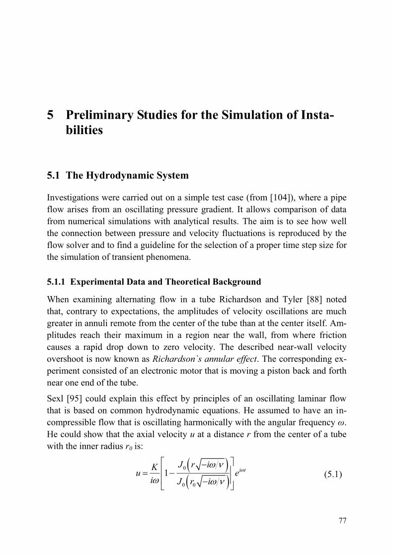
77
5 Preliminary Studies for the Simulation of Insta-
bilities
5.1 The Hydrodynamic System
Investigations were carried out on a simple test case (from [104]), where a pipe
flow arises from an oscillating pressure gradient. It allows comparison of data
from numerical simulations with analytical results. The aim is to see how well
the connection between pressure and velocity fluctuations is reproduced by the
flow solver and to find a guideline for the selection of a proper time step size for
the simulation of transient phenomena.
5.1.1 Experimental Data and Theoretical Background
When examining alternating flow in a tube Richardson and Tyler [88] noted
that, contrary to expectations, the amplitudes of velocity oscillations are much
greater in annuli remote from the center of the tube than at the center itself. Am-
plitudes reach their maximum in a region near the wall, from where friction
causes a rapid drop down to zero velocity. The described near-wall velocity
overshoot is now known as Richardson`s annular effect. The corresponding ex-
periment consisted of an electronic motor that is moving a piston back and forth
near one end of the tube.
Sexl [95] could explain this effect by principles of an oscillating laminar flow
that is based on common hydrodynamic equations. He assumed to have an in-
compressible flow that is oscillating harmonically with the angular frequency ω.
He could show that the axial velocity u at a distance r from the center of a tube
with the inner radius r0 is:
0
0 0
1 i tJ r iK
u ei J r i
(5.1)
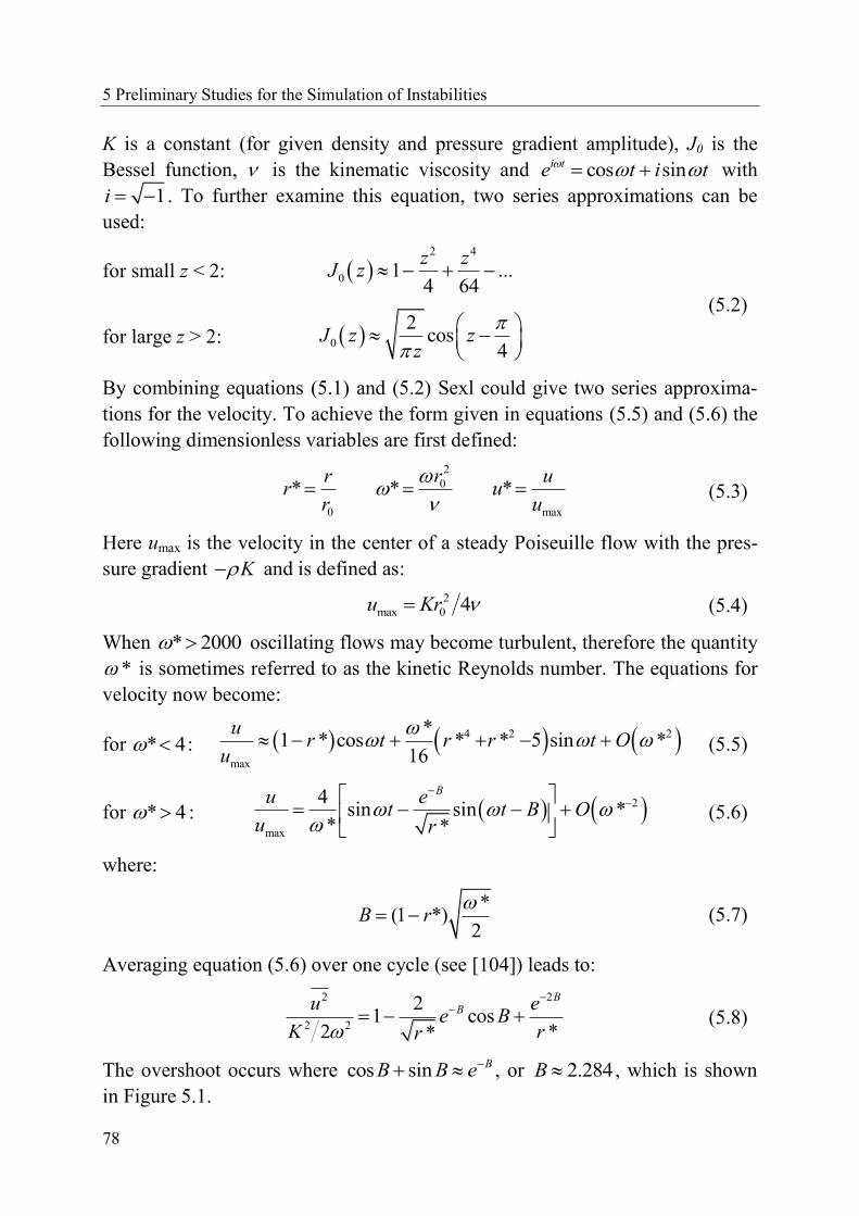
5 Preliminary Studies for the Simulation of Instabilities
78
K is a constant (for given density and pressure gradient amplitude), J0 is the
Bessel function, is the kinematic viscosity and cos sini te t i t with
1i . To further examine this equation, two series approximations can be
used:
for small z < 2: 2 4
0 1 ...4 64
z zJ z
(5.2)
for large z > 2: 0
2cos
4J z z
z
By combining equations (5.1) and (5.2) Sexl could give two series approxima-
tions for the velocity. To achieve the form given in equations (5.5) and (5.6) the
following dimensionless variables are first defined:
2
0
0 max
* * *r r u
r ur u
(5.3)
Here umax is the velocity in the center of a steady Poiseuille flow with the pres-
sure gradient K and is defined as:
2
max 0 4u Kr (5.4)
When * 2000 oscillating flows may become turbulent, therefore the quantity
* is sometimes referred to as the kinetic Reynolds number. The equations for
velocity now become:
for * 4 : 4 2 2
max
*1 * cos * * 5 sin *
16
ur t r r t O
u
(5.5)
for * 4 : 2
max
4sin sin *
* *
Bu et t B O
u r
(5.6)
where:
*
(1 *)2
B r
(5.7)
Averaging equation (5.6) over one cycle (see [104]) leads to:
2 2
2 2
21 cos
2 **
BBu e
e BK rr
(5.8)
The overshoot occurs where cos sin BB B e , or 2.284B , which is shown
in Figure 5.1.

5.1 The Hydrodynamic System
79
Figure 5.1: The near wall velocity overshoot (Richardson's annular effect)
5.1.2 Set-Up for Numerical Simulations
In his explanation of Richardson's annular effect, Sexl [95] assumed incom-
pressibility. Thus the fluid used in the simulations is air with constant density
(“Air at 25 C”) from the material library of ANSYS CFX. The computational
domain is designed according to the corresponding experiment of Richardson
and Tyler [88]. As there is no separate 2D-solver in CFX, the L = 33 cm long
tube with an inner radius of r0 = 3.1 cm is represented by a quasi-2D grid, ac-
cording to the recommendation of ANSYS for the axisymmetric case: a 2°
wedge with two nodes in circumferential direction and an adiabatic free slip wall
at the axis. In order to resolve the near wall velocity overshoot, the grid is de-
signed to have >10 points in the range 0 < B < 2.284, which resulted in 155 cells
in radial direction. The domain is randomly chosen to have 65 cells in axial di-
rection. It is not necessary to pay special attention to the number of cells in axial
direction, as the simulation is incompressible.
The Reference Pressure is set to p0 = 101325 Pa. The "Total Energy" option is
chosen for heat transfer. No turbulence model is selected (laminar flow). The
"High Resolution" option is chosen as advection scheme. The "Second Order
Backward Euler" option is set as transient scheme.
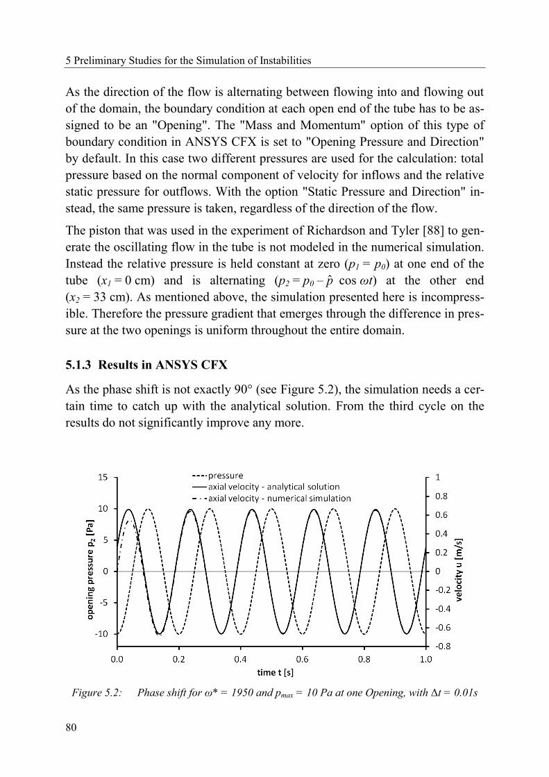
5 Preliminary Studies for the Simulation of Instabilities
80
As the direction of the flow is alternating between flowing into and flowing out
of the domain, the boundary condition at each open end of the tube has to be as-
signed to be an "Opening". The "Mass and Momentum" option of this type of
boundary condition in ANSYS CFX is set to "Opening Pressure and Direction"
by default. In this case two different pressures are used for the calculation: total
pressure based on the normal component of velocity for inflows and the relative
static pressure for outflows. With the option "Static Pressure and Direction" in-
stead, the same pressure is taken, regardless of the direction of the flow.
The piston that was used in the experiment of Richardson and Tyler [88] to gen-
erate the oscillating flow in the tube is not modeled in the numerical simulation.
Instead the relative pressure is held constant at zero (p1 = p0) at one end of the
tube (x1 = 0 cm) and is alternating (p2 = p0 – p cos ωt) at the other end
(x2 = 33 cm). As mentioned above, the simulation presented here is incompress-
ible. Therefore the pressure gradient that emerges through the difference in pres-
sure at the two openings is uniform throughout the entire domain.
5.1.3 Results in ANSYS CFX
As the phase shift is not exactly 90° (see Figure 5.2), the simulation needs a cer-
tain time to catch up with the analytical solution. From the third cycle on the
results do not significantly improve any more.
Figure 5.2: Phase shift for ω* = 1950 and pmax = 10 Pa at one Opening, with Δt = 0.01s
5.1 The Hydrodynamic System
81
The good agreement of results from numerical simulation and analytical solution
shows that the connection between pressure and velocity fluctuations is well re-
produced. This is to be expected since, as already mentioned in section 2.7,
ANSYS CFX is a coupled solver. However, the choice of time step size has to
be carefully considered to achieve accurate results (see Figure 5.3).
To obtain the data shown in Figure 5.3 velocities are averaged over one cycle
starting at t = 0.5 s. Even if the velocities are averaged several cycles later, the
results do not improve any more. An improvement can only be achieved by de-
creasing the time step size in the simulation.
Figure 5.3: Numerical simulation and analytical solution for ω* = 1950 and pmax = 10Pa
at one Opening
A series of calculations are carried out, where the period T, the amplitude of the
opening pressure p and the time step Δt are changed to see their effect on the
results. Furthermore the simulations are also carried out on a shorter domain,
where the length of the tube is chosen to be 3.3 cm (while the diameter remains
at 6.2 cm, and the number of grid nodes does not change). For all simulations
the results are evaluated by comparison with the analytical solution shown in
Figure 5.3.
A conclusion that can definitively be drawn is the fact, that results become better
for decreasing time steps (as already illustrated in Figure 5.3). But the quality of
the results cannot be linked to one decisive factor. In certain simulations even
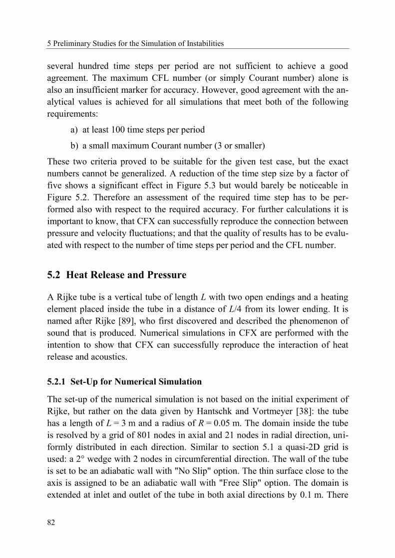
5 Preliminary Studies for the Simulation of Instabilities
82
several hundred time steps per period are not sufficient to achieve a good
agreement. The maximum CFL number (or simply Courant number) alone is
also an insufficient marker for accuracy. However, good agreement with the an-
alytical values is achieved for all simulations that meet both of the following
requirements:
a) at least 100 time steps per period
b) a small maximum Courant number (3 or smaller)
These two criteria proved to be suitable for the given test case, but the exact
numbers cannot be generalized. A reduction of the time step size by a factor of
five shows a significant effect in Figure 5.3 but would barely be noticeable in
Figure 5.2. Therefore an assessment of the required time step has to be per-
formed also with respect to the required accuracy. For further calculations it is
important to know, that CFX can successfully reproduce the connection between
pressure and velocity fluctuations; and that the quality of results has to be evalu-
ated with respect to the number of time steps per period and the CFL number.
5.2 Heat Release and Pressure
A Rijke tube is a vertical tube of length L with two open endings and a heating
element placed inside the tube in a distance of L/4 from its lower ending. It is
named after Rijke [89], who first discovered and described the phenomenon of
sound that is produced. Numerical simulations in CFX are performed with the
intention to show that CFX can successfully reproduce the interaction of heat
release and acoustics.
5.2.1 Set-Up for Numerical Simulation
The set-up of the numerical simulation is not based on the initial experiment of
Rijke, but rather on the data given by Hantschk and Vortmeyer [38]: the tube
has a length of L = 3 m and a radius of R = 0.05 m. The domain inside the tube
is resolved by a grid of 801 nodes in axial and 21 nodes in radial direction, uni-
formly distributed in each direction. Similar to section 5.1 a quasi-2D grid is
used: a 2° wedge with 2 nodes in circumferential direction. The wall of the tube
is set to be an adiabatic wall with "No Slip" option. The thin surface close to the
axis is assigned to be an adiabatic wall with "Free Slip" option. The domain is
extended at inlet and outlet of the tube in both axial directions by 0.1 m. There
5.2 Heat Release and Pressure
83
the pressure is assumed to be constant [20]. Since buoyancy is not modeled, the
initial axial flow in the tube is not driven by upward moving heated air, but
through a pressure difference between the two open ends: the relative static
pressure is set to 0.0 Pa at the outlet and 0.5 Pa at the inlet. Inlet and outlet are
both "Openings" with the "Static Pressure and Direction" option since in the ex-
cited state backflow appears. In both circumferential directions symmetry
boundaries are used. One of the two symmetry boundaries contains a gap at
X = 0.75 m (corresponding to L/4 of the tube) in which a wall is inserted. This
wall is assigned a constant temperature of 1500 K and serves as heating element.
A sketch of this heater is shown in Figure 5.4. It extends over the entire radius
but has only one face in axial direction.
Figure 5.4: Illustration of domain and grid in the Rijke tube at the position of the heater
The reference pressure is set to 0 1atmp . The fluid that is applied in the simu-
lations is air as ideal gas. The molar mass ( 28.96 g molM ), the viscosity
( 51.831 10 kg m s ), the specific heat ( 1004.4 J kgKpc ) and the thermal
conductivity ( 0.0261W m K ) of the fluid were those of air at 25 °C. The
"Total Energy" option has been chosen to model heat transfer. No turbulence
model has been selected (laminar flow). The "High Resolution" option has been
chosen as advection scheme and the "Second Order Backward Euler" option as
transient scheme.

5 Preliminary Studies for the Simulation of Instabilities
84
5.2.2 Results in ANSYS CFX
A transient simulation is started from a steady state solution with an additional
pressure peak at the position of the heater. This results in an oscillating motion
of the fluid. The plot of pressure over time in Figure 5.5 shows that after the ini-
tial disturbance pressure oscillations adopt a sinusoidal shape. One period is re-
solved by roughly 60 time steps (time step size 0.25 ms).
Figure 5.5: Oscillating pressure in the Rijke tube at the position of the heater
Values of pressure and axial velocity are acquired from monitor points at
Y = 0.025 m at the position of the heater (X = 0.75 m). As shown in Figure 5.6
the pressure oscillations lag the velocity oscillations by approximately 90°.
While the predominant direction of the flow remains, there is also considerable
backflow during each period.
Figure 5.6: Oscillating pressure and velocity in the Rijke tube at the position of the heater

5.2 Heat Release and Pressure
85
The total heat flux is obtained from summation over all surface elements:
i
i
Q Q (5.9)
where for each surface element i the heat flux transferred to the flow in the adja-
cent volume element is calculated from:
surface elementcenter
i surface
T TQ k A
s
(5.10)
Δs is the distance between the center of the surface element and the center of the
volume element. The phase shift between oscillating pressure and heat flux is
about 40° and is thus in the required range to fulfill the Rayleigh criterion (see
[82] and [84]). This explains the growing amplitudes of pressure, velocity and
heat flux oscillations.
Figure 5.7: Oscillating pressure and heat flux in the Rijke tube at the position of the heater
Backflow at the heater causes nonlinearities on the heat flux, which first show
through the appearance of higher harmonics in the heat flux oscillations (see
Figure 5.7). Also the formation of a limit cycle can be reproduced (Figure 5.8).
At the limit cycle higher harmonics in the pressure oscillations appear as well,
which are a consequence of the higher harmonics in the heat flux oscillations. A
fast Fourier transform of the heat release in Figure 5.8 delivers the frequency
spectrum as shown in Figure 5.9. The amplitudes are scaled relative to the first
harmonic of the Rijke tube.
All finding described so far are in agreement with experimental [41] and numer-
ical data [38]. The higher harmonics are however much more distinct in the sim-
ulation presented here. This is a consequence of the heater design, which causes

5 Preliminary Studies for the Simulation of Instabilities
86
further nonlinearities in the heat flux: As can be seen in Figure 5.4 the distance
Δs between the center of the surface element and the center of the volume ele-
ment is very much dependant on how far away the element is from the axis.
Consequently, according to equation (5.10), much more heat is transferred to the
flow in the vicinity of the axis than at the confining wall.
Figure 5.8: Oscillating pressure and heat flux in the Rijke tube at the position of the heater
at limit cycle
Figure 5.9: FFT gain of the calculated heat release at the limit cycle in Figure 5.9
It can be concluded that the expected characteristics of the Rijke tube are well
reproduced in the presented simulation in CFX. Since the velocities in the tube
are relatively low in comparison with the speed of sound ( Ma 0.1 ) a simula-
tion with the "Thermal Energy" equation with the “Include Pressure Transient
Term” option produces essentially the same results.
5.3 Methods for Simulation of Instabilities
87
5.3 Methods for Simulation of Instabilities
5.3.1 Velocity Excitation
In section 5.1 the alternating pressure at one open end of the domain served as a
good method to get an oscillating flow in the pipe. For simulations with incom-
pressible fluid a uniform pressure gradient was achieved in the entire domain.
Pressure gradients act on the momentum equations, which in CFX [4] are:
Mpt
UU U τ S (5.11)
with MS as source terms. Instead of generating a gradient in the pressure field, it
is also possible to use the source term to get the fluid in motion:
M p S (5.12)
The results presented in section 5.1 can also be achieved by an alternative set-
up. The x-component of the momentum source term is set to:
,M x
dpS
dx (5.13)
with (see section 5.1 for reference):
2 1
2 1
ˆcos
dp p p pt
dx x x L
(5.14)
With the source term in the momentum equation the motion of the fluid can be
manipulated at any place in the domain, also for compressible flow and without
directly affecting the pressure field. That is, the influence of velocity fluctua-
tions on the combustion process can be observed separately from the effect of
pressure fluctuations.
5.3.2 Velocity and Pressure Excitation
Rey et al. [86] used a simple generic geometry to illustrate modulation tech-
niques. The same set-up is studied here. A flow of air as ideal gas is simulated at
a temperature of 300 K and a pressure of 1 bar in a 40 cm long and 25 cm wide
domain on a uniform structured mesh (81512 nodes). The axial velocity im-
posed at the inlet is 10 m/s. The first transverse mode of the domain has a fre-
quency of about f = 700 Hz. The time step that has been used for all simulations
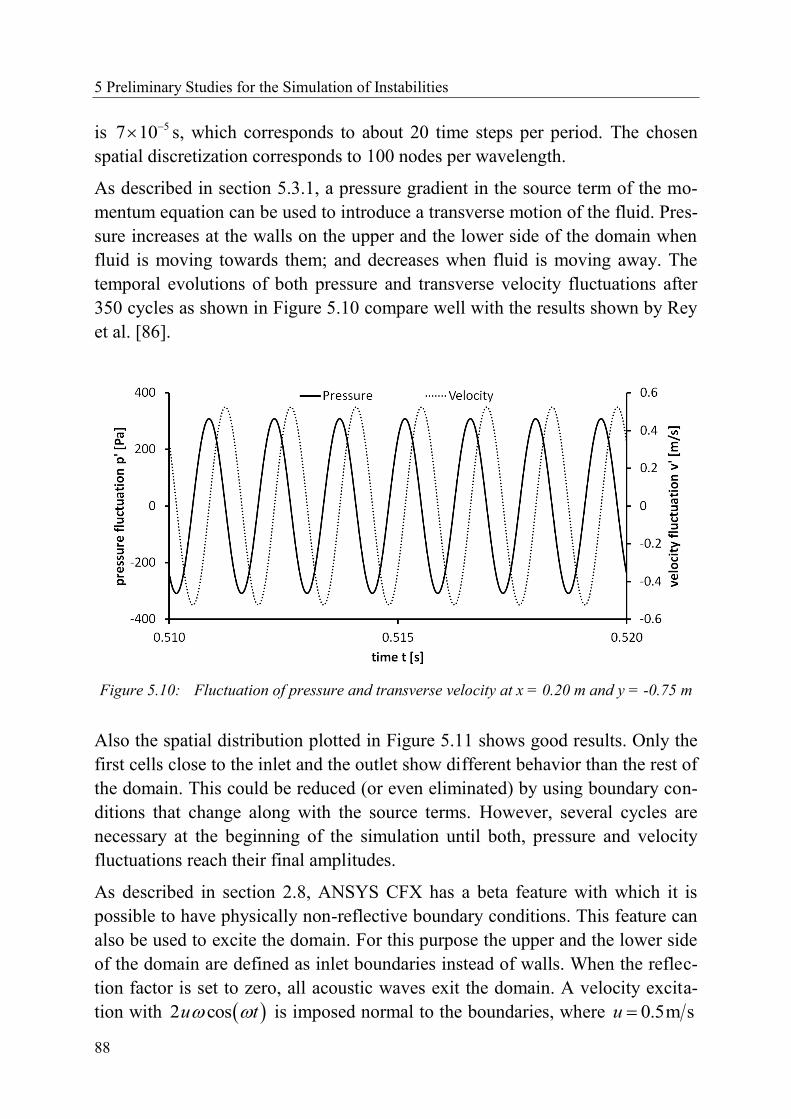
5 Preliminary Studies for the Simulation of Instabilities
88
is 57 10 s, which corresponds to about 20 time steps per period. The chosen
spatial discretization corresponds to 100 nodes per wavelength.
As described in section 5.3.1, a pressure gradient in the source term of the mo-
mentum equation can be used to introduce a transverse motion of the fluid. Pres-
sure increases at the walls on the upper and the lower side of the domain when
fluid is moving towards them; and decreases when fluid is moving away. The
temporal evolutions of both pressure and transverse velocity fluctuations after
350 cycles as shown in Figure 5.10 compare well with the results shown by Rey
et al. [86].
Figure 5.10: Fluctuation of pressure and transverse velocity at x = 0.20 m and y = -0.75 m
Also the spatial distribution plotted in Figure 5.11 shows good results. Only the
first cells close to the inlet and the outlet show different behavior than the rest of
the domain. This could be reduced (or even eliminated) by using boundary con-
ditions that change along with the source terms. However, several cycles are
necessary at the beginning of the simulation until both, pressure and velocity
fluctuations reach their final amplitudes.
As described in section 2.8, ANSYS CFX has a beta feature with which it is
possible to have physically non-reflective boundary conditions. This feature can
also be used to excite the domain. For this purpose the upper and the lower side
of the domain are defined as inlet boundaries instead of walls. When the reflec-
tion factor is set to zero, all acoustic waves exit the domain. A velocity excita-
tion with 2 cosu t is imposed normal to the boundaries, where 0.5m su
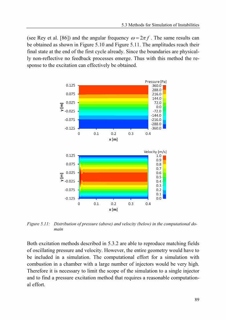
5.3 Methods for Simulation of Instabilities
89
(see Rey et al. [86]) and the angular frequency 2 f . The same results can
be obtained as shown in Figure 5.10 and Figure 5.11. The amplitudes reach their
final state at the end of the first cycle already. Since the boundaries are physical-
ly non-reflective no feedback processes emerge. Thus with this method the re-
sponse to the excitation can effectively be obtained.
Figure 5.11: Distribution of pressure (above) and velocity (below) in the computational do-
main
Both excitation methods described in 5.3.2 are able to reproduce matching fields
of oscillating pressure and velocity. However, the entire geometry would have to
be included in a simulation. The computational effort for a simulation with
combustion in a chamber with a large number of injectors would be very high.
Therefore it is necessary to limit the scope of the simulation to a single injector
and to find a pressure excitation method that requires a reasonable computation-
al effort.
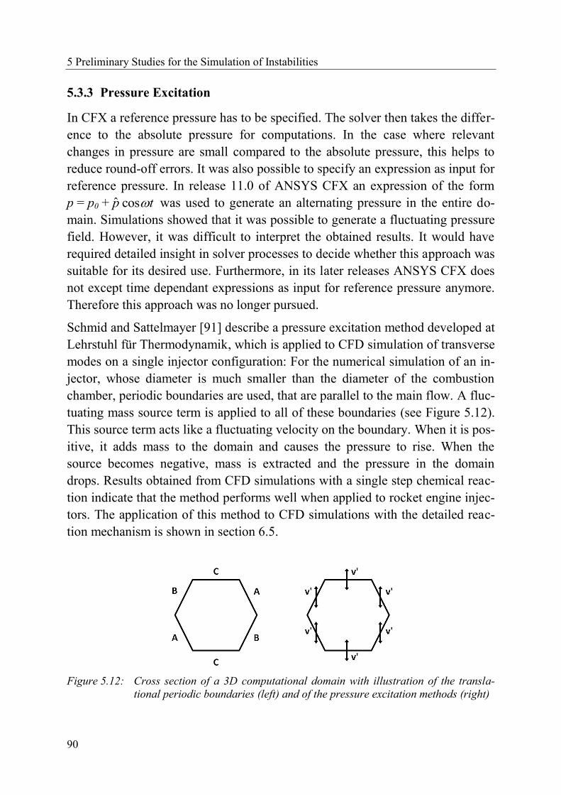
5 Preliminary Studies for the Simulation of Instabilities
90
5.3.3 Pressure Excitation
In CFX a reference pressure has to be specified. The solver then takes the differ-
ence to the absolute pressure for computations. In the case where relevant
changes in pressure are small compared to the absolute pressure, this helps to
reduce round-off errors. It was also possible to specify an expression as input for
reference pressure. In release 11.0 of ANSYS CFX an expression of the form
p = p0 + ˆ cosp t was used to generate an alternating pressure in the entire do-
main. Simulations showed that it was possible to generate a fluctuating pressure
field. However, it was difficult to interpret the obtained results. It would have
required detailed insight in solver processes to decide whether this approach was
suitable for its desired use. Furthermore, in its later releases ANSYS CFX does
not except time dependant expressions as input for reference pressure anymore.
Therefore this approach was no longer pursued.
Schmid and Sattelmayer [91] describe a pressure excitation method developed at
Lehrstuhl für Thermodynamik, which is applied to CFD simulation of transverse
modes on a single injector configuration: For the numerical simulation of an in-
jector, whose diameter is much smaller than the diameter of the combustion
chamber, periodic boundaries are used, that are parallel to the main flow. A fluc-
tuating mass source term is applied to all of these boundaries (see Figure 5.12).
This source term acts like a fluctuating velocity on the boundary. When it is pos-
itive, it adds mass to the domain and causes the pressure to rise. When the
source becomes negative, mass is extracted and the pressure in the domain
drops. Results obtained from CFD simulations with a single step chemical reac-
tion indicate that the method performs well when applied to rocket engine injec-
tors. The application of this method to CFD simulations with the detailed reac-
tion mechanism is shown in section 6.5.
Figure 5.12: Cross section of a 3D computational domain with illustration of the transla-
tional periodic boundaries (left) and of the pressure excitation methods (right)
5.3 Methods for Simulation of Instabilities
91
Starting from the same perception (i.e. that the velocity fluctuations cause the
pressure fluctuations), another pressure excitation method can be deduced. In
this case the boundaries that are parallel to the main flow are defined as adia-
batic free slip walls and are subject to displacement. The relative position of the-
se moving walls to their idle position is obtained by integration of the same ve-
locity equation that has been given by Schmid and Sattelmayer [91]. The mesh
in the entire domain deforms accordingly. This feature is implemented in CFX
[4] and can easily be applied. Simulations on a simple mesh with air as ideal gas
show that this excitation method produces the same fluctuating pressures as the
method discussed before. The application of moving walls to CFD simulations
of the single injector configuration of a rocket engine flame is presented in sec-
tion 6.5.
The objective for finding a pressure excitation method is to gain knowledge on
how pressure fluctuations affect the combustion process. In the present work
combustion is calculated in an external routine, which requires temperature and
molar concentrations as input parameters. Temperature is read directly from
CFX. Molar concentrations are calculated from mass fractions and density. Pres-
sure does not have a direct impact on the combustion process. However, a
changing pressure within the flow solver would of course affect temperature and
density. Instead of generating a fluctuating pressure within the flow solver, it
can also be simulated in the external routine. In this case the routine reads CFXT ,
CFX and CFXp from the flow solver. Additionally an excitation pressure excp is
given, which varies with time. Since thermoacoustic fluctuations are considered
to be isentropic the following equations apply:
1
CFX excexc CFX
CFX
p pT T
p
(5.15)
1
CFX excexc CFX
CFX
p p
p
(5.16)
Equations (5.15) and (5.16) can be used to calculate excT and exc as new input
parameters for the chemical kinetics solver. The isentropic exponent can be
calculated from specific heat capacities.

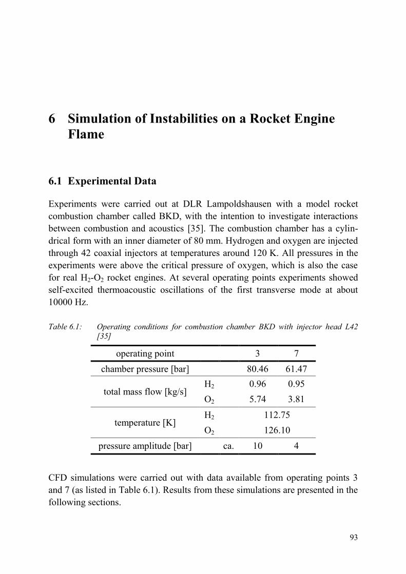
93
6 Simulation of Instabilities on a Rocket Engine
Flame
6.1 Experimental Data
Experiments were carried out at DLR Lampoldshausen with a model rocket
combustion chamber called BKD, with the intention to investigate interactions
between combustion and acoustics [35]. The combustion chamber has a cylin-
drical form with an inner diameter of 80 mm. Hydrogen and oxygen are injected
through 42 coaxial injectors at temperatures around 120 K. All pressures in the
experiments were above the critical pressure of oxygen, which is also the case
for real H2-O2 rocket engines. At several operating points experiments showed
self-excited thermoacoustic oscillations of the first transverse mode at about
10000 Hz.
Table 6.1: Operating conditions for combustion chamber BKD with injector head L42
[35]
operating point 3 7
chamber pressure [bar] 80.46 61.47
total mass flow [kg/s] H2 0.96 0.95
O2 5.74 3.81
temperature [K] H2 112.75
O2 126.10
pressure amplitude [bar] ca. 10 4
CFD simulations were carried out with data available from operating points 3
and 7 (as listed in Table 6.1). Results from these simulations are presented in the
following sections.
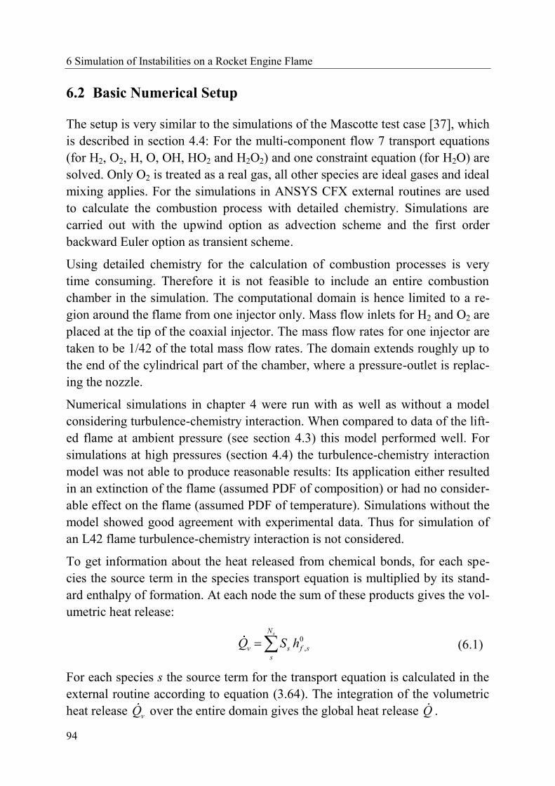
6 Simulation of Instabilities on a Rocket Engine Flame
94
6.2 Basic Numerical Setup
The setup is very similar to the simulations of the Mascotte test case [37], which
is described in section 4.4: For the multi-component flow 7 transport equations
(for H2, O2, H, O, OH, HO2 and H2O2) and one constraint equation (for H2O) are
solved. Only O2 is treated as a real gas, all other species are ideal gases and ideal
mixing applies. For the simulations in ANSYS CFX external routines are used
to calculate the combustion process with detailed chemistry. Simulations are
carried out with the upwind option as advection scheme and the first order
backward Euler option as transient scheme.
Using detailed chemistry for the calculation of combustion processes is very
time consuming. Therefore it is not feasible to include an entire combustion
chamber in the simulation. The computational domain is hence limited to a re-
gion around the flame from one injector only. Mass flow inlets for H2 and O2 are
placed at the tip of the coaxial injector. The mass flow rates for one injector are
taken to be 1/42 of the total mass flow rates. The domain extends roughly up to
the end of the cylindrical part of the chamber, where a pressure-outlet is replac-
ing the nozzle.
Numerical simulations in chapter 4 were run with as well as without a model
considering turbulence-chemistry interaction. When compared to data of the lift-
ed flame at ambient pressure (see section 4.3) this model performed well. For
simulations at high pressures (section 4.4) the turbulence-chemistry interaction
model was not able to produce reasonable results: Its application either resulted
in an extinction of the flame (assumed PDF of composition) or had no consider-
able effect on the flame (assumed PDF of temperature). Simulations without the
model showed good agreement with experimental data. Thus for simulation of
an L42 flame turbulence-chemistry interaction is not considered.
To get information about the heat released from chemical bonds, for each spe-
cies the source term in the species transport equation is multiplied by its stand-
ard enthalpy of formation. At each node the sum of these products gives the vol-
umetric heat release:
0
,
sN
v s f s
s
Q S h (6.1)
For each species s the source term for the transport equation is calculated in the
external routine according to equation (3.64). The integration of the volumetric
heat release vQ over the entire domain gives the global heat release Q .
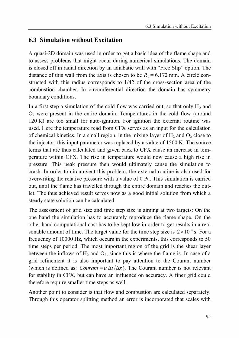
6.3 Simulation without Excitation
95
6.3 Simulation without Excitation
A quasi-2D domain was used in order to get a basic idea of the flame shape and
to assess problems that might occur during numerical simulations. The domain
is closed off in radial direction by an adiabatic wall with “Free Slip” option. The
distance of this wall from the axis is chosen to be R1 = 6.172 mm. A circle con-
structed with this radius corresponds to 1/42 of the cross-section area of the
combustion chamber. In circumferential direction the domain has symmetry
boundary conditions.
In a first step a simulation of the cold flow was carried out, so that only H2 and
O2 were present in the entire domain. Temperatures in the cold flow (around
120 K) are too small for auto-ignition. For ignition the external routine was
used. Here the temperature read from CFX serves as an input for the calculation
of chemical kinetics. In a small region, in the mixing layer of H2 and O2 close to
the injector, this input parameter was replaced by a value of 1500 K. The source
terms that are thus calculated and given back to CFX cause an increase in tem-
perature within CFX. The rise in temperature would now cause a high rise in
pressure. This peak pressure then would ultimately cause the simulation to
crash. In order to circumvent this problem, the external routine is also used for
overwriting the relative pressure with a value of 0 Pa. This simulation is carried
out, until the flame has travelled through the entire domain and reaches the out-
let. The thus achieved result serves now as a good initial solution from which a
steady state solution can be calculated.
The assessment of grid size and time step size is aiming at two targets: On the
one hand the simulation has to accurately reproduce the flame shape. On the
other hand computational cost has to be kept low in order to get results in a rea-
sonable amount of time. The target value for the time step size is 62 10 s. For a
frequency of 10000 Hz, which occurs in the experiments, this corresponds to 50
time steps per period. The most important region of the grid is the shear layer
between the inflows of H2 and O2, since this is where the flame is. In case of a
grid refinement it is also important to pay attention to the Courant number
(which is defined as: Courant u t x ). The Courant number is not relevant
for stability in CFX, but can have an influence on accuracy. A finer grid could
therefore require smaller time steps as well.
Another point to consider is that flow and combustion are calculated separately.
Through this operator splitting method an error is incorporated that scales with
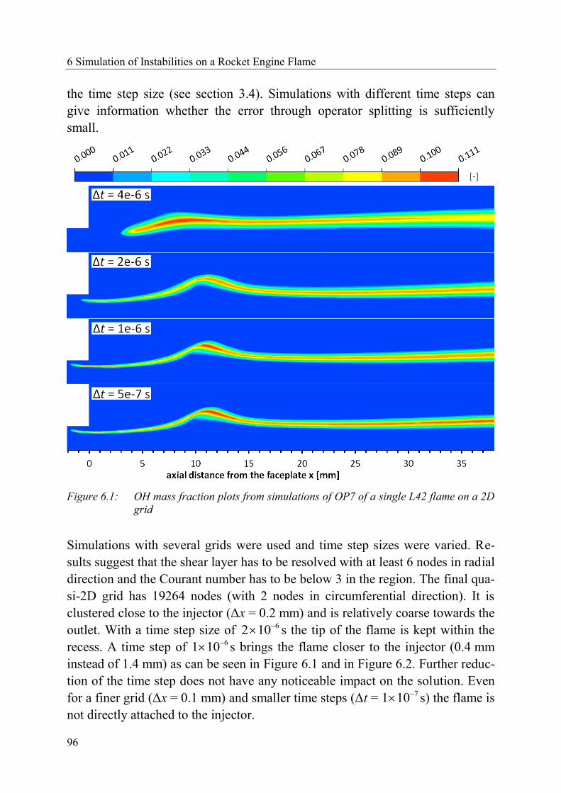
6 Simulation of Instabilities on a Rocket Engine Flame
96
the time step size (see section 3.4). Simulations with different time steps can
give information whether the error through operator splitting is sufficiently
small.
Figure 6.1: OH mass fraction plots from simulations of OP7 of a single L42 flame on a 2D
grid
Simulations with several grids were used and time step sizes were varied. Re-
sults suggest that the shear layer has to be resolved with at least 6 nodes in radial
direction and the Courant number has to be below 3 in the region. The final qua-
si-2D grid has 19264 nodes (with 2 nodes in circumferential direction). It is
clustered close to the injector (Δx = 0.2 mm) and is relatively coarse towards the
outlet. With a time step size of 62 10 s the tip of the flame is kept within the
recess. A time step of 61 10 s brings the flame closer to the injector (0.4 mm
instead of 1.4 mm) as can be seen in Figure 6.1 and in Figure 6.2. Further reduc-
tion of the time step does not have any noticeable impact on the solution. Even
for a finer grid (Δx = 0.1 mm) and smaller time steps (Δt = 71 10 s) the flame is
not directly attached to the injector.
6.3 Simulation without Excitation
97
Figure 6.2: Temperature plots from simulations of OP7 of an L42 flame on a 2D grid
For the assessment of grid and time step size the conditions from operating point
7 are used. However, results for operating point 3 are extracted from simulations
on the same grid and with the same time step size. For both operating points
simulations are conducted with 75 10t . OH mass fraction plots and tem-
perature plots from these simulations are shown in Figure 6.3 and Figure 6.4,
respectively.
Figure 6.3: OH mass fraction plots from simulations of OP3 and OP7
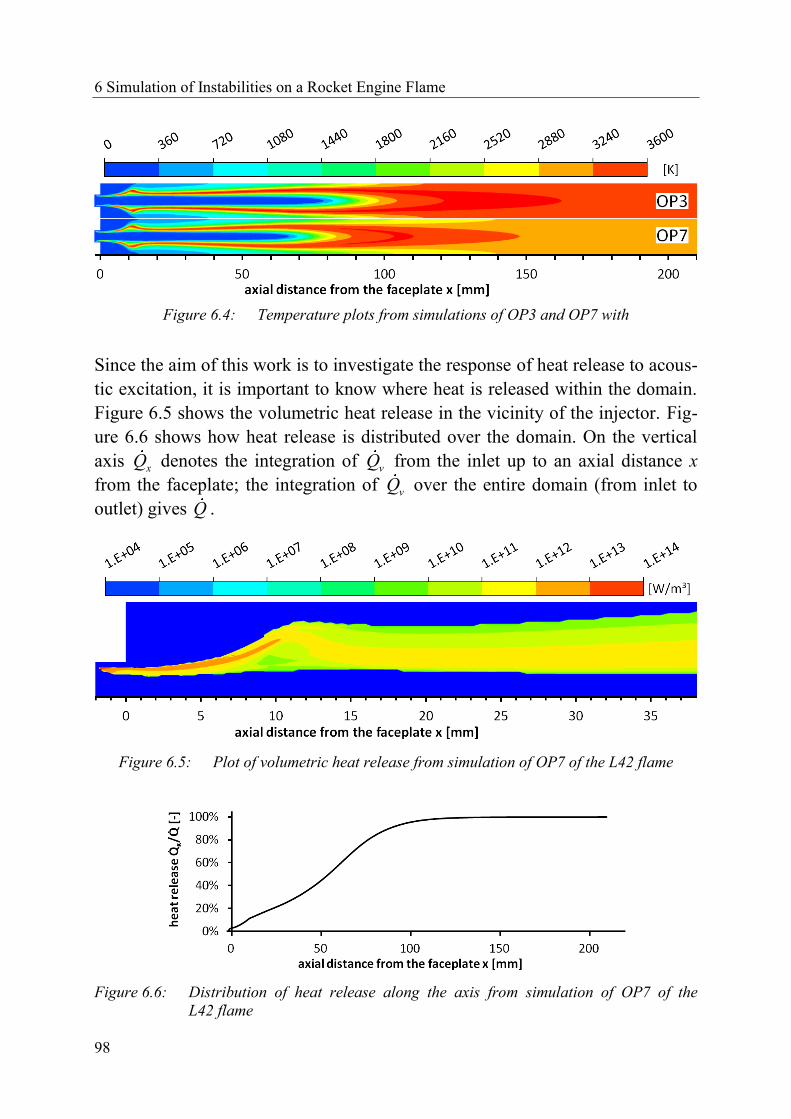
6 Simulation of Instabilities on a Rocket Engine Flame
98
Figure 6.4: Temperature plots from simulations of OP3 and OP7 with
Since the aim of this work is to investigate the response of heat release to acous-
tic excitation, it is important to know where heat is released within the domain.
Figure 6.5 shows the volumetric heat release in the vicinity of the injector. Fig-
ure 6.6 shows how heat release is distributed over the domain. On the vertical
axis xQ denotes the integration of
vQ from the inlet up to an axial distance x
from the faceplate; the integration of vQ over the entire domain (from inlet to
outlet) gives Q .
Figure 6.5: Plot of volumetric heat release from simulation of OP7 of the L42 flame
Figure 6.6: Distribution of heat release along the axis from simulation of OP7 of the
L42 flame
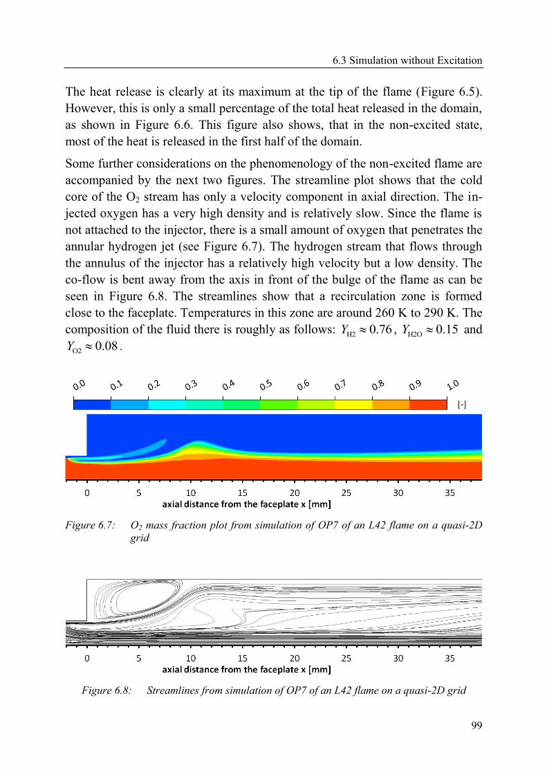
6.3 Simulation without Excitation
99
The heat release is clearly at its maximum at the tip of the flame (Figure 6.5).
However, this is only a small percentage of the total heat released in the domain,
as shown in Figure 6.6. This figure also shows, that in the non-excited state,
most of the heat is released in the first half of the domain.
Some further considerations on the phenomenology of the non-excited flame are
accompanied by the next two figures. The streamline plot shows that the cold
core of the O2 stream has only a velocity component in axial direction. The in-
jected oxygen has a very high density and is relatively slow. Since the flame is
not attached to the injector, there is a small amount of oxygen that penetrates the
annular hydrogen jet (see Figure 6.7). The hydrogen stream that flows through
the annulus of the injector has a relatively high velocity but a low density. The
co-flow is bent away from the axis in front of the bulge of the flame as can be
seen in Figure 6.8. The streamlines show that a recirculation zone is formed
close to the faceplate. Temperatures in this zone are around 260 K to 290 K. The
composition of the fluid there is roughly as follows: H2 0.76Y , H2O 0.15Y and
O2 0.08Y .
Figure 6.7: O2 mass fraction plot from simulation of OP7 of an L42 flame on a quasi-2D
grid
Figure 6.8: Streamlines from simulation of OP7 of an L42 flame on a quasi-2D grid
6 Simulation of Instabilities on a Rocket Engine Flame
100
3D simulations are conducted based upon the findings from the 2D simulations.
The three dimensional domain has a hexagonal cross-section. Its cross-section
area is equivalent to the cross-section area of the entire combustion chamber di-
vided by 42 (the number of injectors). The generation of the 3D grid was strong-
ly influenced by the form of the final 2D grid. The two grids have exactly the
same spacing in axial direction. In the 3D case the grid is designed as an O-grid
in the vicinity of the axis. It has about the same number of nodes in radial direc-
tion as the 2D grid in this region. In the region away from the axis the grid spac-
ing in radial direction has the same number of nodes and almost exactly the
same grid spacing. In circumferential direction the 3D grid is resolved with 72
nodes in the outer region, which corresponds to one grid node every 5°. The fi-
nal three-dimensional grid has 637531 nodes.
For simulations without excitation, the six boundaries on the lateral sides of the
domain are free-slip walls. The ignition procedure is the same as introduced be-
fore. A transient simulation is run until a steady state is reached, as indicated by
various monitor points in the domain. Results on the 3D grid resemble the re-
sults on the 2D grid presented above and serve as an initial solution for simula-
tions with excitation. In order to reach a state that can be considered to be
steady, it is necessary to have about 3500 iterations with a time step size of 62 10 s. The required computational time sums up to about 30 days on 16
cores (on one machine with 64GB memory and two Intel Xeon E5-2660 proces-
sors, each with 8 cores at 2.20GHz and no hyperthreading). A time step size of 61 10 s would require almost twice these resources.
6.4 Velocity Excitation
The domain for simulations with velocity excitation is represented by the previ-
ously described 3D grid with hexagonal cross section. The six boundaries paral-
lel to the main flow are now defined as translational periodic interfaces. Flow
leaving the domain through one of these boundaries is entering at the same time
through the opposing boundary. In simulations without excitation there should
be no flow through the interfaces, so that in this case these boundaries are
equivalent to the previously used free-slip walls. Velocity fluctuations are then
achieved through the use of a source term in the momentum equation as de-
scribed above (see section 5.3.1). For the specification of this source term it is
helpful to visualize the transverse mode that is to be simulated. Figure 6.9 illus-
trates the T1 mode in a cylinder based on the pressure field.

6.4 Velocity Excitation
101
Figure 6.9: Pressure field for the first transverse mode in a cylindrical chamber
In the considered instant the pressure is at its maximum on the top and its mini-
mum at the bottom. The momentum equation in CFX as stated before in equa-
tion (2.2) is:
Mpt
UU U τ S (6.2)
A look at this equation reveals that, through the first term on the right hand side,
the pressure gradient would cause a vertical motion of the fluid within the cylin-
der. In the simulation of a flame from a single injector there is no pressure gra-
dient present. Instead one component which is at right angles to the mean flow
(in this case the z-component) of the source term in equation (6.2) is used to
simulate the transverse motion of the fluid within the domain. The source term is
set as:
,M z
dpS
dz (6.3)
The pressure profile is assumed to be approximately linear in z-direction. In a
combustion chamber of diameter D, an injector in the middle of the cylinder
would experience a pressure gradient in the order of:
ˆ2
cosdp p
tdz D
(6.4)
which is how the source term is specified in the simulation. The value of p is
taken to be 4 bar. This is the value that has been measured in the experiment at

6 Simulation of Instabilities on a Rocket Engine Flame
102
operating point 7 (see Table 6.1). The source does not act on the flow within the
recess, so it is only active for regions with x > 0.
A look on the left hand side of equation (6.2) reveals that the magnitude of ve-
locity fluctuations that is caused by the source term depends on density. The mo-
tion of the fluids is therefore not uniform. The oxygen core with a density of
about 950 kg/m³ experiences only little deviations from its idle position. In con-
trast the burnt mixture, with densities slightly above 2 kg/m³, shows a strong
vertical movement. In the vicinity of the injector this behavior causes a better
mixing of the reactants, so that the flame length is shortened as shown in Figure
6.10. Data for the excited state is evaluated at an instant where the flame is at its
idle position.
Figure 6.10: Distribution of temperature and OH mass fraction along the axis of an L42
flame with and without velocity excitation
Results from the simulation with velocity excitation are shown in Figure 6.11.
The displayed velocity is recorded at the outlet on the axis. On the secondary
vertical axis the instantaneous heat release Q is associated with the average val-
ue Q . The graph clearly shows that the global heat release responds with exactly
the double frequency of the velocity excitation. The same effect has already
been observed by Schmid and Sattelmayer [91], who explained this with the
symmetric form of the flame. The heat release is roughly at its maximum when
the transverse velocity is at its extreme value; and it is at its minimum when the
transverse velocity is zero.
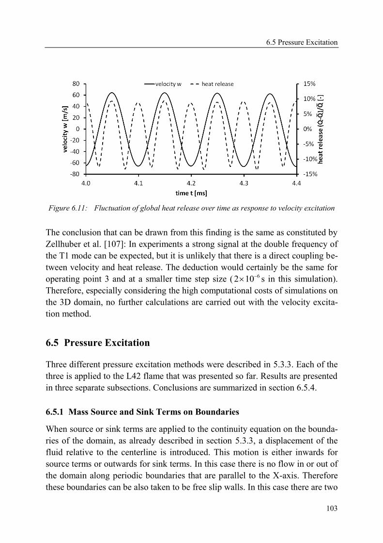
6.5 Pressure Excitation
103
Figure 6.11: Fluctuation of global heat release over time as response to velocity excitation
The conclusion that can be drawn from this finding is the same as constituted by
Zellhuber et al. [107]: In experiments a strong signal at the double frequency of
the T1 mode can be expected, but it is unlikely that there is a direct coupling be-
tween velocity and heat release. The deduction would certainly be the same for
operating point 3 and at a smaller time step size ( 62 10 s in this simulation).
Therefore, especially considering the high computational costs of simulations on
the 3D domain, no further calculations are carried out with the velocity excita-
tion method.
6.5 Pressure Excitation
Three different pressure excitation methods were described in 5.3.3. Each of the
three is applied to the L42 flame that was presented so far. Results are presented
in three separate subsections. Conclusions are summarized in section 6.5.4.
6.5.1 Mass Source and Sink Terms on Boundaries
When source or sink terms are applied to the continuity equation on the bounda-
ries of the domain, as already described in section 5.3.3, a displacement of the
fluid relative to the centerline is introduced. This motion is either inwards for
source terms or outwards for sink terms. In this case there is no flow in or out of
the domain along periodic boundaries that are parallel to the X-axis. Therefore
these boundaries can be also taken to be free slip walls. In this case there are two

6 Simulation of Instabilities on a Rocket Engine Flame
104
symmetry planes that can be used to reduce the size of the domain, so that only
¼ of the previously used domain is needed. In fact, to reduce the computational
cost further, even the quasi 2D grid is sufficient to produce the required results.
Which is what is presented in the following. The mass source term is imple-
mented on the boundary as suggested by Schmid and Sattelmayer [91]:
ˆ
cos sin y
m pv t ky n
A c
(6.5)
In this equation c is the speed of sound and k c is the wave number. The
pressure fluctuation that this continuity source term is aiming to achieve in the
entire domain is also specified at the outlet boundary:
ˆ sinoutp p t (6.6)
Within the domain the local speed of sound varies in a wide range. Therefore an
averaged value is taken from the simulation without excitation. Volume
weighted averaging over the entire domain gives 1634 ms
c .
When a source term is applied in the continuity equation then secondary sources
appear in all other equations as well [3]. For the calculation of these secondary
source terms on the boundary CFX has to know composition, temperature, tur-
bulence data and velocity components of the fluid mass flux. When the mass
source term is negative (sink term) the solver uses local values of the flow for
the mass leaving the domain. For a positive source term additional information
is required that has to be specified in CFX Pre along with the mass source term.
For the specification of these variables it is also possible to use the local values
of the flow in the required instant. For simulations presented in this subsection
this has been the case for all variables except the species mass fractions.
Several options were considered for the specification of the composition on the
boundary. The first was to use the local values, as for all other quantities. In
simulations with single step chemistry also using 2
1.0H OY on the boundary
worked very well, since H2O is the product of the reaction. Another option was
to use 2
1.0HY since in the considered experiments the combustion chamber
BKD is operated with hydrogen in excess, great part of which flows along the
boundary to the outlet. One further consideration was to use an inert species,
which in contrast to H2O and H2 is not accounted for in the reaction scheme.
Amplitude and phase shift of the heat release response to pressure excitation dif-
fer considerably from case to case.

6.5 Pressure Excitation
105
In simulations with single chemical reaction there may be only products present
at the boundary that is used for excitation. In simulations with detailed chemis-
try in contrast the fluid at the same boundary is composed of up to eight species
that are all involved in a system of forward and backward reactions according to
the equations introduced in chapter 3. In a non-excited state, as described in sec-
tion 6.3, for each species production or consumption due to chemical kinetics
are in equilibrium with transport processes in the flow solver according to equa-
tion (2.25). A change in pressure due to excitation entails a change in density
and temperature, which are both input parameters to the chemical kinetics solv-
er. Through the change in the source term there is a shift in the described equi-
librium which implies changes in composition and heat release. But mass that is
removed through the sink terms on the boundary is no longer accounted for in
the calculation of heat release. Mass that is introduced in the domain through the
source terms on the boundary impairs the calculation of heat release in a similar
way.
The consequence of using 2
1.0H OY is illustrated in Figure 6.12. Fluctuating
heat release is related to the value from the steady state solution, which should
be the mean during excitation. Even though the flame appears to remain within
the domain, the mean value of heat release is smaller than expected. Results
from further simulation show that the higher the excitation amplitude is, the
more the mean deviates from its supposed value. This is apparently an effect of
dissociation reactions, since this effect does not occur in simulations with single
step reactions.
Figure 6.12: Outlet pressure and heat release from excitation with mass source terms on
boundaries
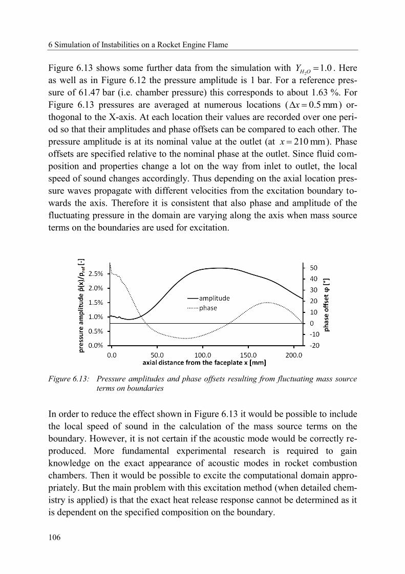
6 Simulation of Instabilities on a Rocket Engine Flame
106
Figure 6.13 shows some further data from the simulation with 2
1.0H OY . Here
as well as in Figure 6.12 the pressure amplitude is 1 bar. For a reference pres-
sure of 61.47 bar (i.e. chamber pressure) this corresponds to about 1.63 %. For
Figure 6.13 pressures are averaged at numerous locations ( 0.5 mmx ) or-
thogonal to the X-axis. At each location their values are recorded over one peri-
od so that their amplitudes and phase offsets can be compared to each other. The
pressure amplitude is at its nominal value at the outlet (at 210 mmx ). Phase
offsets are specified relative to the nominal phase at the outlet. Since fluid com-
position and properties change a lot on the way from inlet to outlet, the local
speed of sound changes accordingly. Thus depending on the axial location pres-
sure waves propagate with different velocities from the excitation boundary to-
wards the axis. Therefore it is consistent that also phase and amplitude of the
fluctuating pressure in the domain are varying along the axis when mass source
terms on the boundaries are used for excitation.
Figure 6.13: Pressure amplitudes and phase offsets resulting from fluctuating mass source
terms on boundaries
In order to reduce the effect shown in Figure 6.13 it would be possible to include
the local speed of sound in the calculation of the mass source terms on the
boundary. However, it is not certain if the acoustic mode would be correctly re-
produced. More fundamental experimental research is required to gain
knowledge on the exact appearance of acoustic modes in rocket combustion
chambers. Then it would be possible to excite the computational domain appro-
priately. But the main problem with this excitation method (when detailed chem-
istry is applied) is that the exact heat release response cannot be determined as it
is dependent on the specified composition on the boundary.
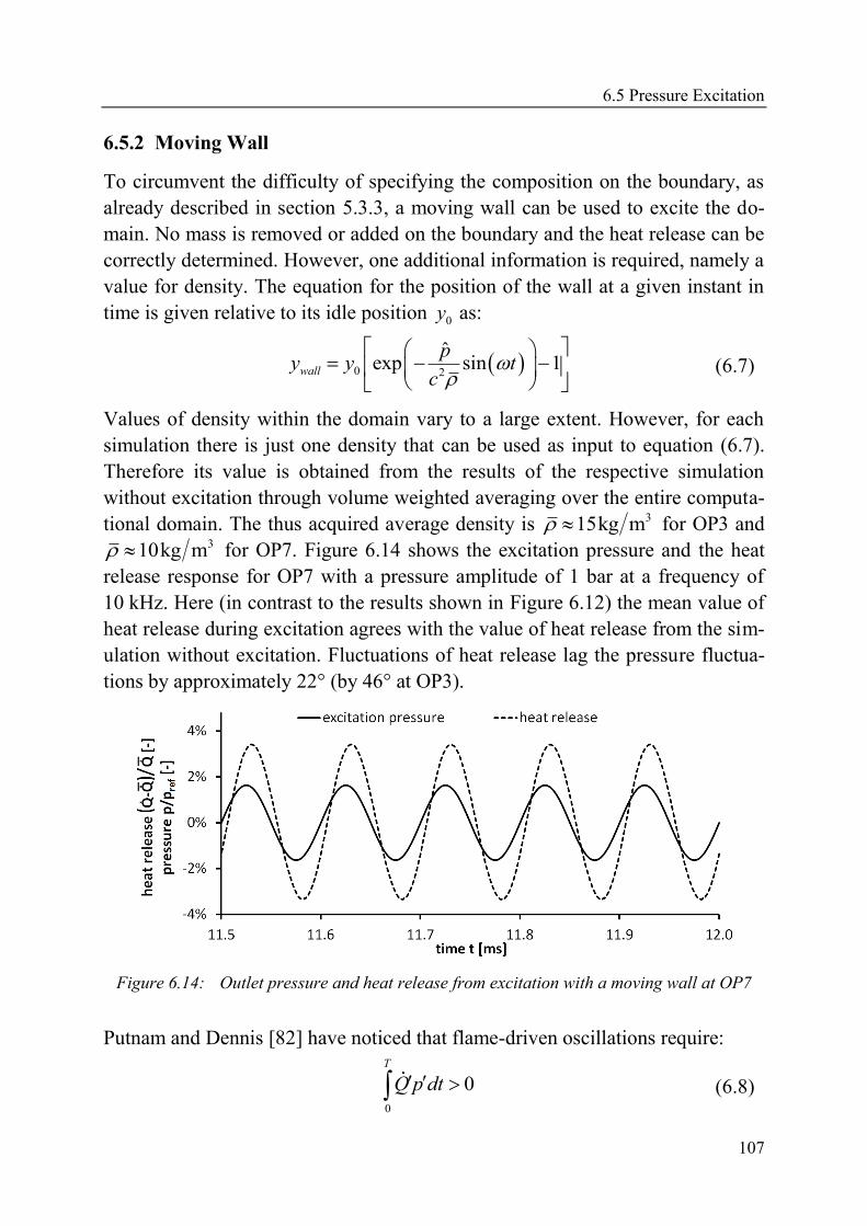
6.5 Pressure Excitation
107
6.5.2 Moving Wall
To circumvent the difficulty of specifying the composition on the boundary, as
already described in section 5.3.3, a moving wall can be used to excite the do-
main. No mass is removed or added on the boundary and the heat release can be
correctly determined. However, one additional information is required, namely a
value for density. The equation for the position of the wall at a given instant in
time is given relative to its idle position 0y as:
0 2
ˆexp sin 1wall
py y t
c
(6.7)
Values of density within the domain vary to a large extent. However, for each
simulation there is just one density that can be used as input to equation (6.7).
Therefore its value is obtained from the results of the respective simulation
without excitation through volume weighted averaging over the entire computa-
tional domain. The thus acquired average density is 315kg m for OP3 and 310kg m for OP7. Figure 6.14 shows the excitation pressure and the heat
release response for OP7 with a pressure amplitude of 1 bar at a frequency of
10 kHz. Here (in contrast to the results shown in Figure 6.12) the mean value of
heat release during excitation agrees with the value of heat release from the sim-
ulation without excitation. Fluctuations of heat release lag the pressure fluctua-
tions by approximately 22° (by 46° at OP3).
Figure 6.14: Outlet pressure and heat release from excitation with a moving wall at OP7
Putnam and Dennis [82] have noticed that flame-driven oscillations require:
0
0
T
Q p dt (6.8)
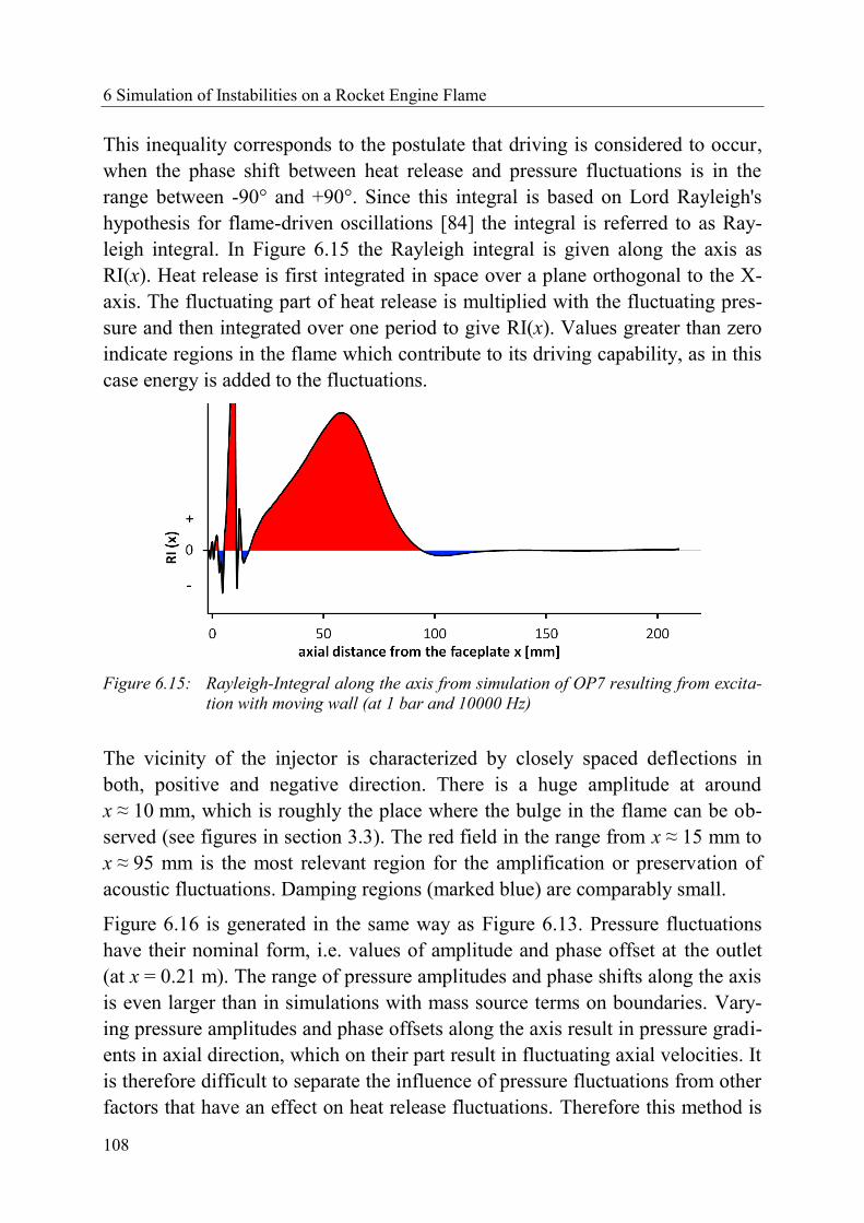
6 Simulation of Instabilities on a Rocket Engine Flame
108
This inequality corresponds to the postulate that driving is considered to occur,
when the phase shift between heat release and pressure fluctuations is in the
range between -90° and +90°. Since this integral is based on Lord Rayleigh's
hypothesis for flame-driven oscillations [84] the integral is referred to as Ray-
leigh integral. In Figure 6.15 the Rayleigh integral is given along the axis as
RI(x). Heat release is first integrated in space over a plane orthogonal to the X-
axis. The fluctuating part of heat release is multiplied with the fluctuating pres-
sure and then integrated over one period to give RI(x). Values greater than zero
indicate regions in the flame which contribute to its driving capability, as in this
case energy is added to the fluctuations.
Figure 6.15: Rayleigh-Integral along the axis from simulation of OP7 resulting from excita-
tion with moving wall (at 1 bar and 10000 Hz)
The vicinity of the injector is characterized by closely spaced deflections in
both, positive and negative direction. There is a huge amplitude at around
x ≈ 10 mm, which is roughly the place where the bulge in the flame can be ob-
served (see figures in section 3.3). The red field in the range from x ≈ 15 mm to
x ≈ 95 mm is the most relevant region for the amplification or preservation of
acoustic fluctuations. Damping regions (marked blue) are comparably small.
Figure 6.16 is generated in the same way as Figure 6.13. Pressure fluctuations
have their nominal form, i.e. values of amplitude and phase offset at the outlet
(at x = 0.21 m). The range of pressure amplitudes and phase shifts along the axis
is even larger than in simulations with mass source terms on boundaries. Vary-
ing pressure amplitudes and phase offsets along the axis result in pressure gradi-
ents in axial direction, which on their part result in fluctuating axial velocities. It
is therefore difficult to separate the influence of pressure fluctuations from other
factors that have an effect on heat release fluctuations. Therefore this method is
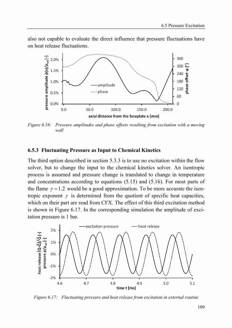
6.5 Pressure Excitation
109
also not capable to evaluate the direct influence that pressure fluctuations have
on heat release fluctuations.
Figure 6.16: Pressure amplitudes and phase offsets resulting from excitation with a moving
wall
6.5.3 Fluctuating Pressure as Input to Chemical Kinetics
The third option described in section 5.3.3 is to use no excitation within the flow
solver, but to change the input to the chemical kinetics solver. An isentropic
process is assumed and pressure change is translated to change in temperature
and concentrations according to equations (5.15) and (5.16). For most parts of
the flame 1.2 would be a good approximation. To be more accurate the isen-
tropic exponent is determined from the quotient of specific heat capacities,
which on their part are read from CFX. The effect of this third excitation method
is shown in Figure 6.17. In the corresponding simulation the amplitude of exci-
tation pressure is 1 bar.
Figure 6.17: Fluctuating pressure and heat release from excitation in external routine

6 Simulation of Instabilities on a Rocket Engine Flame
110
With this excitation method the flow in CFX is only influenced through the
source terms in the species transport equations. Changing these source terms in
the external routine introduces a change in composition and thereby of course
also causes pressure fluctuations within the flow solver. However, these pressure
fluctuations are small compared to the excitation pressure (around 5 %) so that
the zero pressure outlet boundary that is used is still acceptable. Also radial and
axial velocity fluctuations remain small in size. The response in heat release can
therefore be ascribed almost exclusively to uniform pressure fluctuations.
In Figure 6.17 the phase shift between excitation pressure and global heat re-
lease is very close to 90°. This is not always the case when heat release is inves-
tigated at specific locations along the X-axis. In Figure 6.18 the Rayleigh-
Integral RI(x) is shown, which is generated in the same way as for Figure 6.15.
The scale on the vertical axis is here also the same as in Figure 6.15 to illustrate
that the predicted driving capability is smaller than in the previous subsection.
The phase offset between excitation pressure and local heat release fluctuations
is close to 90°. Red and blue areas are almost similar in size.
Figure 6.18: Rayleigh-Integral along the axis from simulation of OP7 with excitation (1 bar,
10000 Hz)
Figure 6.18 shows, that even though the pressure excitation is in phase every-
where in the domain, the response in heat release is not. The reason for this is
that composition and densities of all constant volume reactors differ considera-
bly in the entire domain. Thus the delay in the response to excitation differs ac-
cordingly. Furthermore during excitation the behavior of a constant volume re-
actor also depends on the behavior of other upstream constant volume reactors.
Depending on their performance the convected composition has an additional
fluctuation.
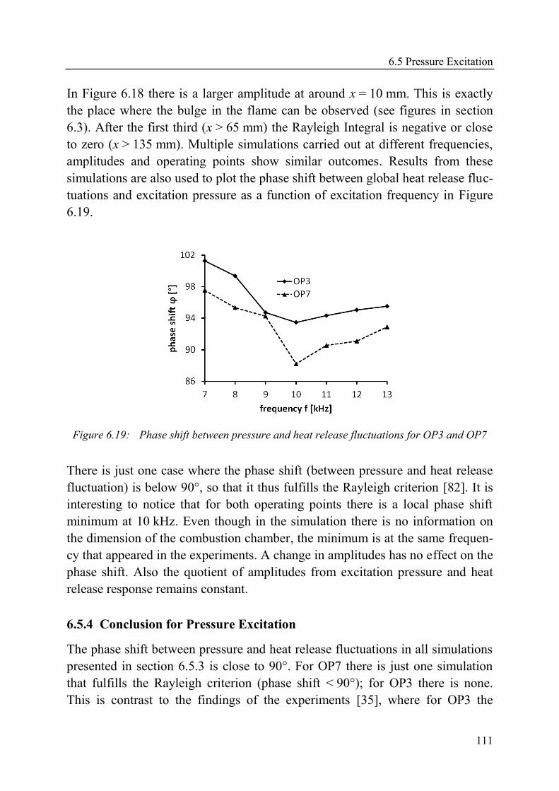
6.5 Pressure Excitation
111
In Figure 6.18 there is a larger amplitude at around x = 10 mm. This is exactly
the place where the bulge in the flame can be observed (see figures in section
6.3). After the first third (x > 65 mm) the Rayleigh Integral is negative or close
to zero (x > 135 mm). Multiple simulations carried out at different frequencies,
amplitudes and operating points show similar outcomes. Results from these
simulations are also used to plot the phase shift between global heat release fluc-
tuations and excitation pressure as a function of excitation frequency in Figure
6.19.
Figure 6.19: Phase shift between pressure and heat release fluctuations for OP3 and OP7
There is just one case where the phase shift (between pressure and heat release
fluctuation) is below 90°, so that it thus fulfills the Rayleigh criterion [82]. It is
interesting to notice that for both operating points there is a local phase shift
minimum at 10 kHz. Even though in the simulation there is no information on
the dimension of the combustion chamber, the minimum is at the same frequen-
cy that appeared in the experiments. A change in amplitudes has no effect on the
phase shift. Also the quotient of amplitudes from excitation pressure and heat
release response remains constant.
6.5.4 Conclusion for Pressure Excitation
The phase shift between pressure and heat release fluctuations in all simulations
presented in section 6.5.3 is close to 90°. For OP7 there is just one simulation
that fulfills the Rayleigh criterion (phase shift < 90°); for OP3 there is none.
This is contrast to the findings of the experiments [35], where for OP3 the
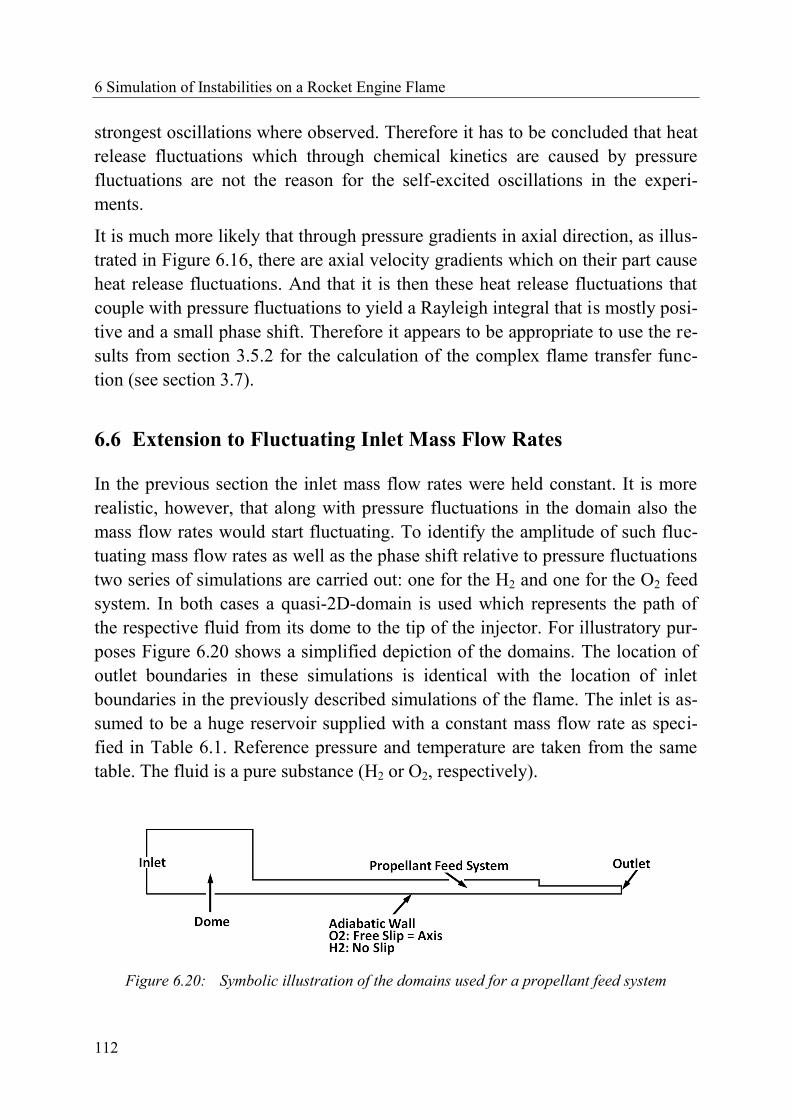
6 Simulation of Instabilities on a Rocket Engine Flame
112
strongest oscillations where observed. Therefore it has to be concluded that heat
release fluctuations which through chemical kinetics are caused by pressure
fluctuations are not the reason for the self-excited oscillations in the experi-
ments.
It is much more likely that through pressure gradients in axial direction, as illus-
trated in Figure 6.16, there are axial velocity gradients which on their part cause
heat release fluctuations. And that it is then these heat release fluctuations that
couple with pressure fluctuations to yield a Rayleigh integral that is mostly posi-
tive and a small phase shift. Therefore it appears to be appropriate to use the re-
sults from section 3.5.2 for the calculation of the complex flame transfer func-
tion (see section 3.7).
6.6 Extension to Fluctuating Inlet Mass Flow Rates
In the previous section the inlet mass flow rates were held constant. It is more
realistic, however, that along with pressure fluctuations in the domain also the
mass flow rates would start fluctuating. To identify the amplitude of such fluc-
tuating mass flow rates as well as the phase shift relative to pressure fluctuations
two series of simulations are carried out: one for the H2 and one for the O2 feed
system. In both cases a quasi-2D-domain is used which represents the path of
the respective fluid from its dome to the tip of the injector. For illustratory pur-
poses Figure 6.20 shows a simplified depiction of the domains. The location of
outlet boundaries in these simulations is identical with the location of inlet
boundaries in the previously described simulations of the flame. The inlet is as-
sumed to be a huge reservoir supplied with a constant mass flow rate as speci-
fied in Table 6.1. Reference pressure and temperature are taken from the same
table. The fluid is a pure substance (H2 or O2, respectively).
Figure 6.20: Symbolic illustration of the domains used for a propellant feed system
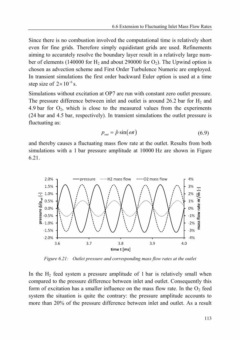
6.6 Extension to Fluctuating Inlet Mass Flow Rates
113
Since there is no combustion involved the computational time is relatively short
even for fine grids. Therefore simply equidistant grids are used. Refinements
aiming to accurately resolve the boundary layer result in a relatively large num-
ber of elements (140000 for H2 and about 290000 for O2). The Upwind option is
chosen as advection scheme and First Order Turbulence Numeric are employed.
In transient simulations the first order backward Euler option is used at a time
step size of 62 10 s.
Simulations without excitation at OP7 are run with constant zero outlet pressure.
The pressure difference between inlet and outlet is around 26.2 bar for H2 and
4.9 bar for O2, which is close to the measured values from the experiments
(24 bar and 4.5 bar, respectively). In transient simulations the outlet pressure is
fluctuating as:
ˆ sinoutp p t (6.9)
and thereby causes a fluctuating mass flow rate at the outlet. Results from both
simulations with a 1 bar pressure amplitude at 10000 Hz are shown in Figure
6.21.
Figure 6.21: Outlet pressure and corresponding mass flow rates at the outlet
In the H2 feed system a pressure amplitude of 1 bar is relatively small when
compared to the pressure difference between inlet and outlet. Consequently this
form of excitation has a smaller influence on the mass flow rate. In the O2 feed
system the situation is quite the contrary: the pressure amplitude accounts to
more than 20% of the pressure difference between inlet and outlet. As a result

6 Simulation of Instabilities on a Rocket Engine Flame
114
the amplitude of the mass flow rate at the outlet is much larger than in the H2
feed system. It can also be noticed that fluctuating mass flow rates are not exact-
ly in phase. The phase shift between fluctuating pressure and fluctuating mass
flow rate is around -164° for H2 and -170° for O2. The different phase shifts are
mainly due to different fluid properties and the different geometries of the feed
systems. For the sake of completeness one further factor has to be mentioned
that also has an influence on the mass flow rates at the outlets: While mass flow
rates at the inlets are constant, pressures here are fluctuating and reach almost
10 % of the excitation amplitude at the outlet.
The findings from these preliminary simulations are used to specify fluctuating
mass flow rates for the simulation of the flame according to:
ˆ sinm m m t t (6.10)
Simulations of the flame with fluctuating mass flow rates (without applying any
further excitation method) show only very small fluctuations of heat release.
Accordingly, there is no significant difference in the heat release response
whether in a simulation with pressure excitation as described in section 6.5.3
there are additional fluctuating inlet mass flow rates or not. While the amplitude
ratios remain the same, the phase shifts between pressure and heat release is de-
creased to 86.3° (as compared to 88.2° with pressure excitation only). The most
significant difference is observable in the Rayleigh-Integral in Figure 6.22,
where the peaks in the vicinity of the injector are more distinct (see Figure 6.18
for comparison).
Figure 6.22: Rayleigh-Integral along the axis from simulation of OP7 with fluctuating mass
flow rates and pressure excitation (1 bar, 10000 Hz)

6.6 Extension to Fluctuating Inlet Mass Flow Rates
115
Since the phase angle is still close to 90° the fluctuating mass flow rates do not
explain the occurrence of combustion instabilities as observed in the experi-
ments. However, the peaks in the Rayleigh-Integral close to the injector provide
an indication that processes in the shear layer might be responsible for triggering
thermoacoustic oscillations. Therefore an investigation of these phenomena in
the vicinity of the injector, with a much finer grid and probably through the use
of Large Eddy Simulation appears to be advisable for future projects.

117
7 Evaluation of Combustion Instabilities
The experiments on the model combustion chamber BKD presented by Gröning
et al. [35] show self-excited thermoacoustic fluctuations. An artificial trigger
(such as e.g. a bomb) is not required given that in these experiments combustion
instabilities are naturally triggered. At all operating points the chamber pressure
is above the critical pressure of oxygen so that it is operated at conditions similar
to real rocket engines (e.g. see [22] and [23]). Its thrust of 25 kN is comparable
to that of an upper stage engine [21]. Data available from these experiments (ge-
ometry, mass flow rates, pressure amplitudes, etc.) as well as from CFD simula-
tions (see chapter 6) can be used to evaluate the stability of the chamber.
For the evaluation of combustion instabilities the research code PIANO is used,
which was developed at DLR [18]. PIANO uses block-structured curvilinear
grids. For spatial discretization it applies a dispersion-relation-preserving finite
difference scheme [99], which is a forth order scheme optimized for computa-
tional acoustics. For time integration a forth order Runge-Kutta scheme is used.
It is possible to use either linearized Euler equations (LEEs) or a modification,
the acoustic perturbation equations (APEs). In former activities at Lehrstuhl für
Thermodynamik APEs were preferred (see e.g. Pieringer [72]). Morgenweck
[65] compares results from simulations with APEs and LEEs and discusses the
differences. Recently the focus is on using the more general LEEs (e.g. [49],
[94]), which deliver better results.
For the simulations in PIANO presented here the faceplate of the combustion
chamber is modeled as an inflow with zero mass flow fluctuation. Walls are set
to be adiabatic slip walls. Since the divergent part of the nozzle is included, the
outflow is placed in the supersonic part of the domain. Therefore the choice of
boundary condition at the outflow has no effect on the results within the subson-
ic part.
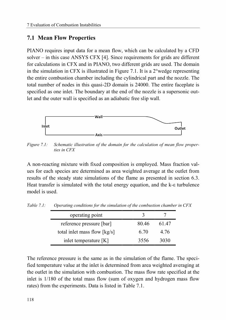
7 Evaluation of Combustion Instabilities
118
7.1 Mean Flow Properties
PIANO requires input data for a mean flow, which can be calculated by a CFD
solver – in this case ANSYS CFX [4]. Since requirements for grids are different
for calculations in CFX and in PIANO, two different grids are used. The domain
in the simulation in CFX is illustrated in Figure 7.1. It is a 2°wedge representing
the entire combustion chamber including the cylindrical part and the nozzle. The
total number of nodes in this quasi-2D domain is 24000. The entire faceplate is
specified as one inlet. The boundary at the end of the nozzle is a supersonic out-
let and the outer wall is specified as an adiabatic free slip wall.
Figure 7.1: Schematic illustration of the domain for the calculation of mean flow proper-
ties in CFX
A non-reacting mixture with fixed composition is employed. Mass fraction val-
ues for each species are determined as area weighted average at the outlet from
results of the steady state simulations of the flame as presented in section 6.3.
Heat transfer is simulated with the total energy equation, and the k-ε turbulence
model is used.
Table 7.1: Operating conditions for the simulation of the combustion chamber in CFX
operating point 3 7
reference pressure [bar] 80.46 61.47
total inlet mass flow [kg/s] 6.70 4.76
inlet temperature [K] 3556 3030
The reference pressure is the same as in the simulation of the flame. The speci-
fied temperature value at the inlet is determined from area weighted averaging at
the outlet in the simulation with combustion. The mass flow rate specified at the
inlet is 1/180 of the total mass flow (sum of oxygen and hydrogen mass flow
rates) from the experiments. Data is listed in Table 7.1.
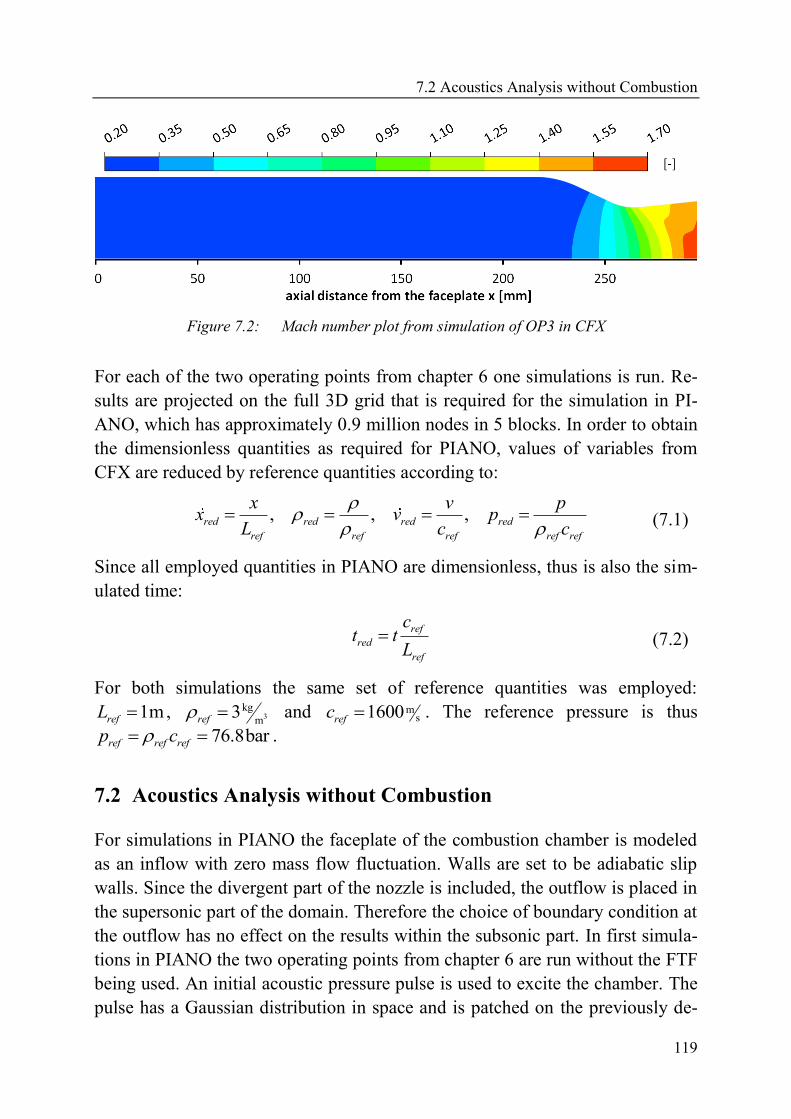
7.2 Acoustics Analysis without Combustion
119
Figure 7.2: Mach number plot from simulation of OP3 in CFX
For each of the two operating points from chapter 6 one simulations is run. Re-
sults are projected on the full 3D grid that is required for the simulation in PI-
ANO, which has approximately 0.9 million nodes in 5 blocks. In order to obtain
the dimensionless quantities as required for PIANO, values of variables from
CFX are reduced by reference quantities according to:
, , ,red red red red
ref ref ref ref ref
x v px v p
L c c
(7.1)
Since all employed quantities in PIANO are dimensionless, thus is also the sim-
ulated time:
ref
red
ref
ct t
L (7.2)
For both simulations the same set of reference quantities was employed:
1mrefL , 3kg
m3ref and m
s1600refc . The reference pressure is thus
76.8barref ref refp c .
7.2 Acoustics Analysis without Combustion
For simulations in PIANO the faceplate of the combustion chamber is modeled
as an inflow with zero mass flow fluctuation. Walls are set to be adiabatic slip
walls. Since the divergent part of the nozzle is included, the outflow is placed in
the supersonic part of the domain. Therefore the choice of boundary condition at
the outflow has no effect on the results within the subsonic part. In first simula-
tions in PIANO the two operating points from chapter 6 are run without the FTF
being used. An initial acoustic pressure pulse is used to excite the chamber. The
pulse has a Gaussian distribution in space and is patched on the previously de-

7 Evaluation of Combustion Instabilities
120
scribed mean flow. During simulation data is recorded by virtual microphones
that are placed on user-defined circles within the domain. In Figure 7.3 the re-
cording of pressure at a virtual microphone is plotted over time.
Figure 7.3: Temporal evolution of pressure at a virtual microphone in PIANO for OP3
without combustion being considered
An FFT of the pressure signal in Figure 7.3 can deliver the relevant frequencies
within the domain. For operating point 3 this is shown in Figure 7.4. Since val-
ues on the vertical axis depend on the considered time range of the pressure sig-
nal all values shown in Figure 7.4 are relative to the highest peak.
Figure 7.4: FFT gain of the pressure signal from Figure 7.3
The highest peak in Figure 7.4 marks the first tangential mode, which for operat-
ing point 3 is at about 11660 Hz. Also the 12560 Hz for operating point 7 is
larger than the value of about 10000 Hz that was measured during experiments.
7.3 Thermoacoustic Analysis with Heat Release
121
This result is very much dependent on the isentropic exponent that has to be de-
fined in an input file at the beginning of the simulation. The heat capacity ratio
for both simulations is taken from CFD results of the single flame configura-
tion presented in chapter 6. The area averaged value of the heat capacity ratio is
1.1995 for operating point 3 and 1.2199 for operating point 7. Simulations with
lower values of as present in the regions of higher temperatures and maxi-
mum heat release would produce a value closer to the expected 10000 Hz from
experiments.
7.3 Thermoacoustic Analysis with Heat Release
7.3.1 Flame Transfer Function
The idea behind the simulations in chapter 6 was to calculate the parameters of a
complex FTF, which then can be used in PIANO. Available thermoacoustic
models typically use a simple two parameter formulation [64]. Among these the
one introduced by Crocco and Cheng [17] has become most popular over the
past decades (see e.g. Pieringer [72]). This FTF has been implemented in PI-
ANO and is currently in use at Lehrstuhl für Thermodynamik (see e.g. [72] or
[94]). It relates fluctuations of heat release to pressure fluctuations and has the
form:
1 i pQ Qn e
p
(7.3)
where Q and p denote the complex perturbations. Simulations in chap-
ter 6 were conducted with various pressure excitation methods. Results from the
simulation with a moving wall at 1 bar amplitude are used to calculate the two
parameters n and τ for the FTF.
Table 7.2: Parameters for FTF from the simulation of a single flame in BKD L42
OP p' [bar] f [Hz] φ [rad] gain [-] n [-] τ [-]
3 1 11660 0.803 1.731 1.246 2.09610-5
7 1 12560 0.384 2.074 1.118 3.00810-5
The gain is the ratio of the amplitudes of fluctuating heat release rate and pres-
sure normalized with their respective mean values. From phase shift and gain
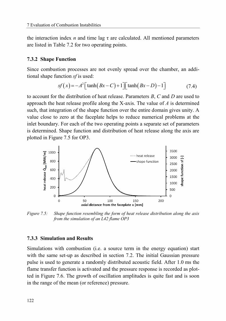
7 Evaluation of Combustion Instabilities
122
the interaction index n and time lag τ are calculated. All mentioned parameters
are listed in Table 7.2 for two operating points.
7.3.2 Shape Function
Since combustion processes are not evenly spread over the chamber, an addi-
tional shape function sf is used:
2 tanh 1 tanh 1sf x A Bx C Bx D (7.4)
to account for the distribution of heat release. Parameters B, C and D are used to
approach the heat release profile along the X-axis. The value of A is determined
such, that integration of the shape function over the entire domain gives unity. A
value close to zero at the faceplate helps to reduce numerical problems at the
inlet boundary. For each of the two operating points a separate set of parameters
is determined. Shape function and distribution of heat release along the axis are
plotted in Figure 7.5 for OP3.
Figure 7.5: Shape function resembling the form of heat release distribution along the axis
from the simulation of an L42 flame OP3
7.3.3 Simulation and Results
Simulations with combustion (i.e. a source term in the energy equation) start
with the same set-up as described in section 7.2. The initial Gaussian pressure
pulse is used to generate a randomly distributed acoustic field. After 1.0 ms the
flame transfer function is activated and the pressure response is recorded as plot-
ted in Figure 7.6. The growth of oscillation amplitudes is quite fast and is soon
in the range of the mean (or reference) pressure.
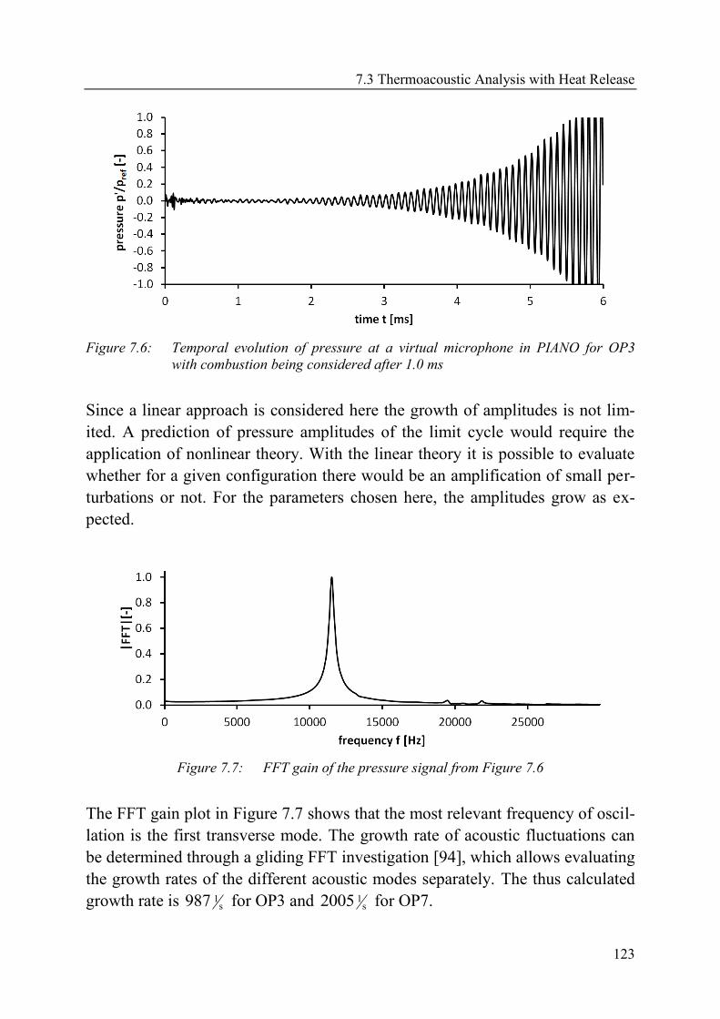
7.3 Thermoacoustic Analysis with Heat Release
123
Figure 7.6: Temporal evolution of pressure at a virtual microphone in PIANO for OP3
with combustion being considered after 1.0 ms
Since a linear approach is considered here the growth of amplitudes is not lim-
ited. A prediction of pressure amplitudes of the limit cycle would require the
application of nonlinear theory. With the linear theory it is possible to evaluate
whether for a given configuration there would be an amplification of small per-
turbations or not. For the parameters chosen here, the amplitudes grow as ex-
pected.
Figure 7.7: FFT gain of the pressure signal from Figure 7.6
The FFT gain plot in Figure 7.7 shows that the most relevant frequency of oscil-
lation is the first transverse mode. The growth rate of acoustic fluctuations can
be determined through a gliding FFT investigation [94], which allows evaluating
the growth rates of the different acoustic modes separately. The thus calculated
growth rate is 1s987 for OP3 and 1
s2005 for OP7.
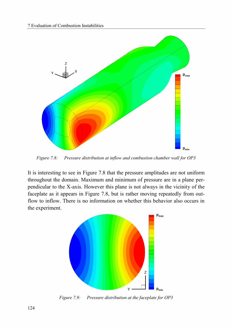
7 Evaluation of Combustion Instabilities
124
Figure 7.8: Pressure distribution at inflow and combustion chamber wall for OP3
It is interesting to see in Figure 7.8 that the pressure amplitudes are not uniform
throughout the domain. Maximum and minimum of pressure are in a plane per-
pendicular to the X-axis. However this plane is not always in the vicinity of the
faceplate as it appears in Figure 7.8, but is rather moving repeatedly from out-
flow to inflow. There is no information on whether this behavior also occurs in
the experiment.
Figure 7.9: Pressure distribution at the faceplate for OP3

7.3 Thermoacoustic Analysis with Heat Release
125
Figure 7.9 shows the pressure distribution as it appears after 5 ms in the vicinity
of the faceplate, which is where the pressure sensors are located in the experi-
ment [35]. The pressure amplitudes are much larger at this point in the simula-
tion, as with the linear approach the limit cycle cannot be reproduced. However,
the distribution itself agrees with experimental data (see [35]).

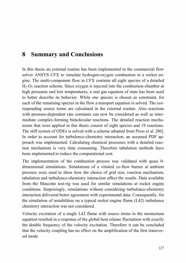
127
8 Summary and Conclusions
In this thesis an external routine has been implemented in the commercial flow
solver ANSYS CFX to simulate hydrogen-oxygen combustion in a rocket en-
gine. The multi-component flow in CFX contains all eight species of a detailed
H2-O2 reaction scheme. Since oxygen is injected into the combustion chamber at
high pressures and low temperatures, a real gas equation of state has been used
to better describe its behavior. While one species is chosen as constraint, for
each of the remaining species in the flow a transport equation is solved. The cor-
responding source terms are calculated in the external routine. Also reactions
with pressure-dependent rate constants can now be considered as well as inter-
mediate complex-forming bimolecular reactions. The detailed reaction mecha-
nisms that were applied in this thesis consist of eight species and 19 reactions.
The stiff system of ODEs is solved with a scheme adopted from Press et al. [80].
In order to account for turbulence-chemistry interaction, an assumed PDF ap-
proach was implemented. Calculating chemical processes with a detailed reac-
tion mechanism is very time consuming. Therefore tabulation methods have
been implemented to reduce the computational cost.
The implementation of the combustion process was validated with quasi 0-
dimensional simulations. Simulations of a vitiated co-flow burner at ambient
pressure were used to show how the choice of grid size, reaction mechanism,
tabulation and turbulence-chemistry interaction affect the results. Data available
from the Mascotte test-rig was used for similar simulations at rocket engine
conditions. Surprisingly, simulations without considering turbulence-chemistry
interaction delivered better agreement with experimental data. Consequently, for
the simulation of instabilities on a typical rocket engine flame (L42) turbulence
chemistry interaction was not considered.
Velocity excitation of a single L42 flame with source terms in the momentum
equation resulted in a response of the global heat release fluctuation with exactly
the double frequency of the velocity excitation. Therefore it can be concluded
that the velocity coupling has no effect on the amplification of the first transver-
sal mode.
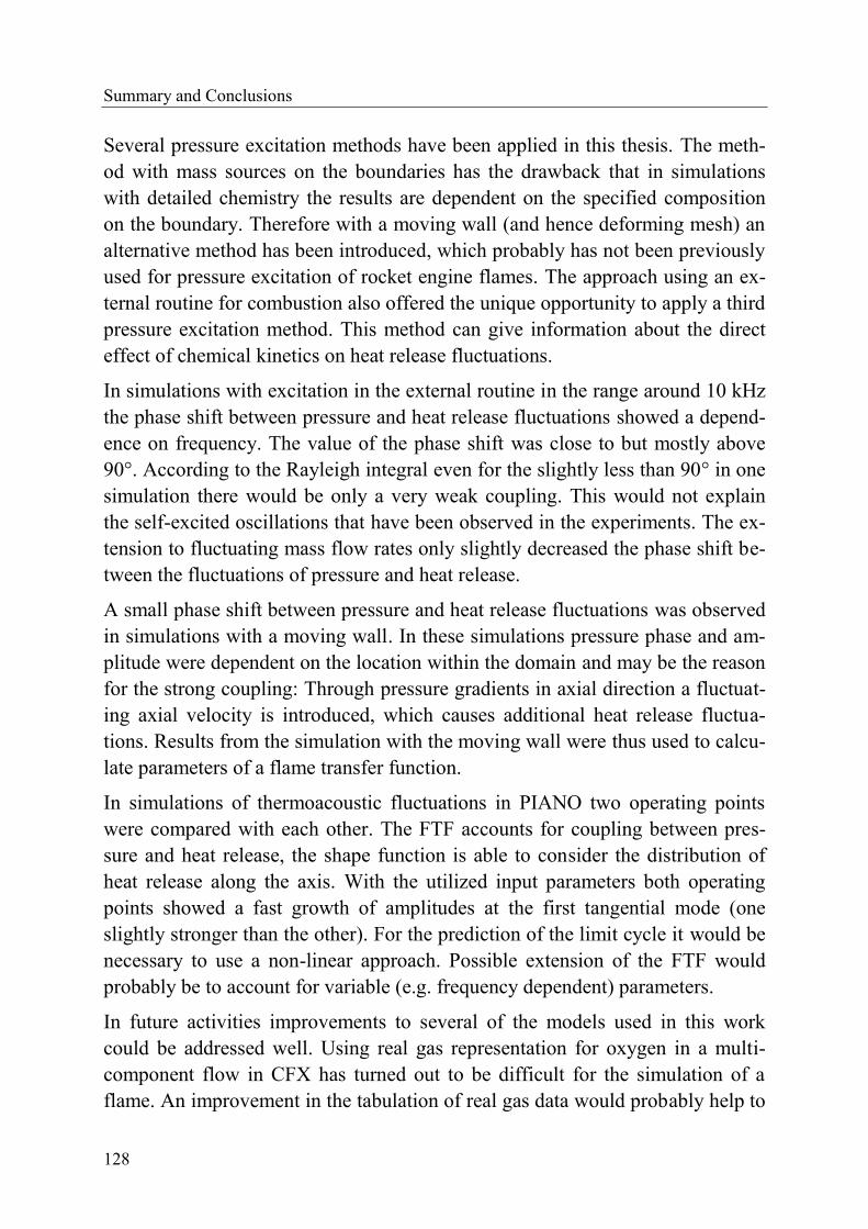
Summary and Conclusions
128
Several pressure excitation methods have been applied in this thesis. The meth-
od with mass sources on the boundaries has the drawback that in simulations
with detailed chemistry the results are dependent on the specified composition
on the boundary. Therefore with a moving wall (and hence deforming mesh) an
alternative method has been introduced, which probably has not been previously
used for pressure excitation of rocket engine flames. The approach using an ex-
ternal routine for combustion also offered the unique opportunity to apply a third
pressure excitation method. This method can give information about the direct
effect of chemical kinetics on heat release fluctuations.
In simulations with excitation in the external routine in the range around 10 kHz
the phase shift between pressure and heat release fluctuations showed a depend-
ence on frequency. The value of the phase shift was close to but mostly above
90°. According to the Rayleigh integral even for the slightly less than 90° in one
simulation there would be only a very weak coupling. This would not explain
the self-excited oscillations that have been observed in the experiments. The ex-
tension to fluctuating mass flow rates only slightly decreased the phase shift be-
tween the fluctuations of pressure and heat release.
A small phase shift between pressure and heat release fluctuations was observed
in simulations with a moving wall. In these simulations pressure phase and am-
plitude were dependent on the location within the domain and may be the reason
for the strong coupling: Through pressure gradients in axial direction a fluctuat-
ing axial velocity is introduced, which causes additional heat release fluctua-
tions. Results from the simulation with the moving wall were thus used to calcu-
late parameters of a flame transfer function.
In simulations of thermoacoustic fluctuations in PIANO two operating points
were compared with each other. The FTF accounts for coupling between pres-
sure and heat release, the shape function is able to consider the distribution of
heat release along the axis. With the utilized input parameters both operating
points showed a fast growth of amplitudes at the first tangential mode (one
slightly stronger than the other). For the prediction of the limit cycle it would be
necessary to use a non-linear approach. Possible extension of the FTF would
probably be to account for variable (e.g. frequency dependent) parameters.
In future activities improvements to several of the models used in this work
could be addressed well. Using real gas representation for oxygen in a multi-
component flow in CFX has turned out to be difficult for the simulation of a
flame. An improvement in the tabulation of real gas data would probably help to
Summary and Conclusions
129
avoid problems that occur due to the use of tables. In simulations with a deform-
ing mesh all points on the walls moved simultaneously. An expedient improve-
ment of this method would be to have points on the wall which move with vari-
ous velocities. Results from simulation with fluctuating mass flow rates indicat-
ed that processes in the shear layer might be responsible for triggering
thermoacoustic oscillations. An investigation of phenomena in the vicinity of the
injector appears to be advisable for future projects.

131
References
[1] Anderson, J. D.: Hypersonic and High Temperature Gas Dynamics.
AIAA; 2006
[2] ANSYS, Inc.: ANSYS CFX – Pre User’s Guide. ANSYS, Inc., Release
13.0; 2010
[3] ANSYS, Inc.: ANSYS CFX – Solver Modeling Guide. ANSYS, Inc., Re-
lease 13.0; 2010
[4] ANSYS, Inc.: ANSYS CFX – Solver Theory Guide. ANSYS, Inc., Re-
lease 13.0; 2010
[5] ANSYS, Inc.: ANSYS FLUENT User’s Guide. ANSYS, Inc., Release
13.0; 2010
[6] Aungier, R. H.: A Fast, Accurate Real Gas Equation of State for Fluid
Dynamic Analysis Applications. Journal of Fluids Engineering, Vol. 117,
pp. 277-281; 1995
[7] Barth, T. J.; Jesperson, D. C.: The Design and Application of Upwind
Schemes on Unstructured Meshes. AIAA Paper 89-0366; 1989
[8] Baurle, R. A.: Modeling of Turbulent Reacting Flows with Probability
Density Functions for Scramjet Applications. Ph.D. thesis, North Carolina
State University; 1995
[9] Benarous, A.; Liazid A.: H2-O2 Supercritical Combustion Modeling
Using a CFD Code. Thermal Science, vol. 13, no. 3, pp. 139-152; 2009
[10] Bird, R. B.; Stewart, W. E.; Lightfoot, E. N.: Transport Phenomena.
2nd
ed., John Wiley & Sons; 2007
[11] Brown, P. N.; Byrne, G. D.; Hindmarsh, A. C.: VODE, a Variable-
Coefficient ODE Solver. SIAM Journal on Scientific and Statistical Com-
puting, vol. 10, no. 5, pp. 1038-1051; 1989
[12] Burden, R. L.; Faires, J. D.: Numerical Analysis. 7th ed., Brooks/Cole;
2001
[13] Burke, S. P.; Schumann, T. E. W.: Diffusion Flames. Industrial and En-
gineering Chemistry, vol. 20, pp. 998-1005; 1928
References
132
[14] Cabra, R.; Myhrvold, T.; Chen, J. Y., Dibble, R. W.; Karpentis, A.
N., Barlow, R.S.: Simultaneous Laser Raman-Rayleigh-LIF Measure-
ments and Numerical Modeling Results of a Lifted Turbulent Jet Flame in
Vitiated Coflow. Proceedings of the Combustion Institute, Vol. 29,
pp. 1881-1888; 2002
[15] Cheng, G.C.; Farmer, R.: Real Fluid Modeling of Multiphase Flows in
Liquid Rocket Engine Combustors. Journal of Propulsion and Power,
vol. 22, no. 6, pp. 1373-1381; 2006
[16] Contreras Espada, J: Numerical Simulation of Reacting Flows under
Laminar Conditions with Detailed Chemistry. Ph.D. thesis, TU Darm-
stadt/EKT; 2010
[17] Crocco, L.; Cheng, S.-I: Theory of Combustion Instability in Liquid
Propellant Rocket Motors. Butterworths Scientific Publications; 1956
[18] Delfs, J.; Bauer, M.; Ewert, R.; Grogger, H.; Lummer, M.; Lauke,
T.: Numerical Simulation of Aerodynamic Noise with DLR's Aeroacoustic
Code PIANO. PIANO manual for version 5.2; DLR 2008
[19] Di Domenico, M.: Numerical Simulations of Soot Formation in Turbu-
lent Flows. Ph.D. thesis, DLR Institut für Verbrennungstechnik Stuttgart,
2007
[20] Dowling, A. P.; Ffowcs Williams, J. E.: Sound and Sources of Sound.
Ellis Horwood; 1983
[21] EADS Astrium: Aestus Rocket Engine. URL:
http://cs.astrium.eads.net/sp/ launcher-propulsion/rocket-engines/aestus-
rocket-engine.html [2013-09-17]
[22] EADS Astrium: Vinci Rocket Engine - Thrust Chamber. URL: http://
cs.astrium.eads.net/sp/launcher-propulsion/rocket-engines/vinci-rocket-
engine.html [2013-09-17]
[23] EADS Astrium: Vulcain Rocket Engine - Thrust Chamber. URL: http://
cs.astrium.eads.net/sp/launcher-propulsion/rocket-engines/vulcain-rocket-
engine.html [2013-09-17]
[24] Fiala, T.; Sattelmayer, T.: Heat Release and OH* Radiation in Laminar
Non-Premixed Hydrogen-Oxygen Flames. 51st AIAA Aerospace Scienc-
es Meeting including the New Horizons Forum and Aerospace Exposi-
tion; 2013
[25] Fiala. T.; Sattelmayer, T.: A Posteriori Computation of OH* Radiation
from Numerical Simulations in Rocket Combustion Chambers. 5th Euro-
pean Conference for Aeronautics and Space Sciences; 2013
References
133
[26] Fick, A: Ueber Diffusion. Annalen der Physik, vol. 170, pp. 59 86; 1855
[27] Förster, H.; Sattelmayer, T.: Computationally efficient Tabulation of
H2-Air Combustion with Turbulence-Chemistry Interaction. 14th
AIAA/AHI Int. Space Planes and Hypersonic Sys. and Techn. Confer-
ence, Canberra, AIAA-2006-8038; 2006
[28] Förster, H: Einfluss der Turbulenz-Chemie Interaktion auf das Zündver-
halten schwach stabilisierter Überschallflammen. Ph.D. thesis, Techni-
sche Universität München; 2010
[29] Gerlinger, P.: Investigation of an Assumed PDF Approach for Finite-
Rate Chemistry. Combustion Science and Technology, vol. 175: 841-872;
2003
[30] Gerlinger, P.: Numerische Verbrennungssimulation. Springer; 2005
[31] Gerlinger, P.; Möbus, H.; Brüggemann, D.: An Implicit Multigrid
Method for Turbulent Combustion. Journal of Computational Physics,
vol. 167, pp. 247-276; 2001
[32] Gilbert, R. G., Luther, K.; Troe, J.: Theory of Thermal Unimolecular
Reactions in the Fall-off Range. II. Weak Collision Rate Constants. Be-
richte der Bunsengesellschaft für physikalische Chemie, 87: 169–177;
1983
[33] Girimaji, S. S.: Assumed β-pdf Model for Turbulent Mixing: Validation
and Extension to Multiple Scalar Mixing. Combustion Science and Tech-
nology, vol. 78, pp. 177-196; 1991
[34] Gordon, S.; McBride, B. J.: Computer Program for Calculation of
Complex Chemical Equilibrium Compositions, Rocket Performance, Inci-
dent and Reflected Shocks and Chapman-Jouguet Detonations. NASA
Report SP-273; 1971
[35] Gröning, S; Oschwald, M.; Sattelmayer, T.: Selbst erregte tangentiale
Moden in einer Raketenbrennkammer unter repräsentativen Bedingun-
gen. 61. Deutscher Luft- und Raumfahrtkongress; 2012
[36] Habiballah, M.; Orain, M.; Grisch, F.; Vingert, L.; Gicquel, P.: Ex-
perimental Studies of High-Pressure Cryogenic Flames on the Mascotte
Facility. Combustion Science and Technology, Vol. 178, pp. 101-128 ;
2006
[37] Habiballah, M.; Zurbach, S.: Test Case RCM-3, Mascotte single injec-
tor, 60 bar. 2nd
International Workshop on Rocket Combustion Modeling;
2001
References
134
[38] Hantschk, C.-C.; Vortmeyer, D.: Numerical Simulation of Self-Excited
Thermoacoustic Instabilities in a Rijke Tube. Journal of Sound and Vibra-
tion, vol. 220, pp. 511-522; 1999
[39] Harlow, F. H.; Welch, J. E.: Numerical calculation of time-dependent
viscous incompressible flow of fluid with free surface. The Physics of Flu-
ids, vol. 8, pp. 2182-2189; 1965
[40] Harrje, D. T.; Reardon, F. H.: Liquid Propellant Rocket Combustion
Instability. NASA SP-194; 1972
[41] Heckl, M. A.: Non-linear acoustic effects in the Rijke Tube. Acustica,
vol. 72, pp. 63-71; 1990
[42] Hippler, H.; Troe, J.: Rate constants of the reaction
HO+H2O2→HO2+H2O at T ≥ 1000 K. Chemical Physics Letters,
vol. 192, pp. 333-337; 1992
[43] Hippler, H.; Troe, J.; Willner, J.: Shock wave study of the reaction
HO2+HO2→H2O2+O2: Confirmation of a rate constant minimum near
700K. Journal of Chemical Physics, vol. 93, pp. 1755-1760; 1990
[44] Hirsch, C.: Numerical Computation of Internal and External Flows.
2nd
ed., Elsevier; 2007
[45] Hirschfelder, J. O., Curtiss, C. F., Bird, R. B.: Molecular Theory of
Gases and Liquids. Wiley; 1954
[46] Issa, R. I.: Solution of the Implicit Discretized Fluid Flow Equations by
Operator Splitting. Journal of Computational Physics, vol. 62, pp. 40-65;
1985
[47] Jachimowski, C. J.: An Analytical Study of the Hydrogen-Air Reaction
Mechanism with Application to Scramjet Combustion. NASA Technical
Paper 2791; 1988
[48] Kaess, R.; Koeglmeier, S; Behr, R.; Kniesner, B.; Sattelmayer, T.: Impact of Axial Gradients on Combustion Chamber Acoustics. 5th Euro-
pean Conference for Aerospace Sciences; 2013
[49] Kaess, R.; Koeglmeier, S; Schmid, M; Sattelmayer, T.: Linearized Eu-
ler Calculation of Acoustic of a Rocket Combustion Chamber. Proceeding
of the 2nd REST Modelling Workshop; 2010
[50] Kee, R. J.; Dixon-Lewis, G.; Warnatz, J.; Coltrin, M. E.; Miller, J.
A.: A FORTRAN Computer Code Package for the Evaluation of Gas-
Phase, Multicomponent Transport Properties. Sandia National Laborato-
ries Report, SAND86-8246; 1986
References
135
[51] Kee, R. J.; Grcar, J. F.; Smooke, M. D.; Miller, J. A.: A FORTRAN
Program for Modeling Steady Laminar One-Dimensional Premixed
Flames. Sandia National Laboratories Report, SAND85-8240; 1985
[52] Kee, R. J.; Rupley, F. M; Meeks, E.: CHEMKIN-III: A FORTRAN
Chemical Kinetics Package for the Analysis of Gas-Phase Chemical and
Plasma Kinetics. Sandia National Laboratories Report SAND96-8216;
1996
[53] Kee, R. J.; Rupley, F. M; Miller, J. A.: CHEMKIN-II: A FORTRAN
Chemical Kinetics Package for the Analysis of Gas-Phase Chemical Ki-
netics. Sandia National Laboratories Report SAND89-8009; 1989
[54] Kee, R. J.; Warnatz, J.; Miller, J. A.: A FORTRAN Computer Code
Package for the Evaluation of Gas-Phase Viscosities, Conductivities, and
Diffusion Coefficients. Sandia National Laboratories Report, SAND83-
8209; 1983
[55] Lemmon, E. W.; McLinden, M. O.; Friend, D. G.: Thermophysical
Properties of Fluid Systems. NIST Chemistry WebBook, NIST Standard
Reference Database Number 69. - URL: http://webbook.nist.gov; 2005
[56] Li, J.; Zhao, Z.; Kazakov, A.; Dryer, F. L.: An Updated Comprehen-
sive Kinetic Model of Hydrogen Combustion. International Journal of
Chemical Kinetics, vol. 36, pp. 566-575; 2004
[57] Liang, L.; Kong, S.-G.; Jung C.; Reitz, R. D.: Development of a Semi-
implicit Solver for Detailed Chemistry in Internal Combustion Engine
Simulations. Journal of Engineering for Gas Turbines and Power,
vol.-129, pp. 271-278; 2007
[58] Lindemann, F. A.: Discussion on “The radiation theory of chemical ac-
tion”. Transactions of the Faraday Society, vol. 17, pp. 598-599; 1922
[59] Lockwood, F. C.; Naguib, A. S.: The Prediction of the Fluctuations in
the Properties of Free, Round-Jet, Turbulent, Diffusion Flames. Combus-
tion and Flame, vol. 24., pp. 109-124; 1975
[60] Lutz, A. E.; Kee, R. J.; Miller J. A.: SENKIN: A FORTRAN Program
for Predicting Homogeneous Gas Phase Chemical Kinetics with Sensi-
tivity Analysis. Sandia National Laboratories Report SAND87-8248 Re-
vised; 1997
[61] Lyubar, A.: Numerisch effiziente Modellierung von Überschallbrenn-
kammern mit detaillierter Kinetik. Ph.D. thesis, Technische Universität
München; 2005
References
136
[62] Majumdar, S.: Role of Underrelaxation in Momentum Interpolation for
Calculation of Flow with Nonstaggered Grids. Numerical Heat Transfer,
vol. 13, pp. 125-125; 1988
[63] Marinov, N. M.; Westbrook, C. K.; Pitz, W. J.: Detailed and Global
Chemical Kinetics Model for Hydrogen. Transport Phenomena in Com-
bustion, pp. 118-129; 1996
[64] Mitchell, C. E.: Analytical Models for Combustion Instability. Progress
in Astronautics and Aeronautics, vol. 169, Liquid Rocket Combustion
Instability, chapter 15; 1995
[65] Morgenweck, D.: Modellierung des Transferverhaltens im Zeitbereich
zur Beschreibung komplexer Randbedingungen in Raketenschubkam-
mern. Ph.D. thesis, Technische Universität München; 2013
[66] Mueller, M. A.; Kim, T. J.; Yetter, R. A.; Dryer, F. L.: Flow reactor
studies and kinetic modeling of the H2O2 reaction. International Journal
of Chemical Kinetics, vol. 31, pp. 113-125; 1999
[67] Neufeld, P. D.; Janzen, A. R.; Aziz, R. A.: Empirical Equations to Cal-
culate 16 of the Transport Collision Integrals Ω(l.s)*
for the Lennard-Jones
(12-6) potential. The Journal of Chemical Physics, vol. 57, pp. 1100
1102; 1972
[68] Nicole, A.; Vingert, L.; Habiballah, M.: Test Case RCM-2, Mascotte
single injector, 60 bar. 3rd
International Workshop on Rocket Combustion
Modeling; 2006
[69] Ó Conaire, M.; Curran, H. J.; Simmie, J. M.; Pitz, W. J.; Westbrook,
C. K.: A Comprehensive Modeling Study of Hydrogen Oxidation. Interna-
tional Journal of Chemical Kinetics, vol. 36, pp. 603-622; 2004
[70] Patankar, S. V.: Numerical Heat Transfer and Fluid Flow. Hemisphere
Publishing Corp.; 1980
[71] Peters, N.: Turbulent Combustion. Cambridge University Press; 2000
[72] Pieringer, J. E.: Simulation selbsterregter Verbrennungsschwingungen
in Raketenschubkammern im Zeitbereich. Ph.D. thesis, Technische Uni-
versität München; 2008
[73] Poinsot, T. J.; Lele, S. K.: Boundary Conditions for Direct Simulations
of Compressible Viscous Flows. Journal of Computational Physics,
vol. 101, pp. 104-129; 2005
[74] Poinsot, T.; Veynante, D.: Theoretical and Numerical Combustion.
2nd
ed., Edwards; 2005
References
137
[75] Poling, E.; Prausnitz, J. M.; O’Connel, J. P.: The Properties of Gases
and Liquids. McGraw-Hill, New York; 2001
[76] Pope, S. B.: Computationally efficient implementation of combustion
chemistry using in situ adaptive tabulation. Combustion Theory Model-
ling. vol. 1, pp. 41-63; 1997
[77] Pope, S. B.: Turbulent Flows. Cambridge University Press; 2000
[78] Poschner, M.; Pfitzner M.: Real gas CFD simulation of supercritical
H2-LOX combustion in the Mascotte single-injector combustor using a
commercial CFD code. 46th AIAA Aerospace Sciences Meeting and Ex-
hibit, Reno, 7.-10.01.2008, AIAA 2008-952; 2008
[79] Poschner, M.; Pfitzner, M.: CFD simulation of supercritical LOX/GH2
combustion considering consistent real gas thermodynamics. 4th Europe-
an Combustion Meeting; 2009
[80] Press, W. H.; Teukolksy, S. A.; Vetterling, W. T.; Flannery, B. P.: Numerical Recipes in C. 2
nd ed., Cambridge University Press; 1992
[81] Preuß, E.; Spille-Kohoff, A.: Numerical Simulation of Multicomponent
Diffusion with ANSYS CFX. ANSYS Conference & 28th CADFEM Us-
ers' Meeting, Aachen; 2010
[82] Putnam, A. A.; Dennis, W. R.: Burner Oscillations of the Gauze-Tone
Type. The Journal of the Acoustical Society of America, vol. 26,
pp. 716-725; 1954
[83] Ramshaw, J. D.: Self-Consistent Effective Binary Diffusion in Multicom-
ponent Gas Mixtures. Journal of Non-Equilibrium Thermodynamics,
vol. 15, pp. 295-300; 1990
[84] Rayleigh, J. W. S: The Theory of Sound. Macmillan; 1877
[85] Redlich, O.; Kwong, J. N. S.: On the Thermodynamics of Solution. V -
An Equation of State. Fugacities of Gaseous Solutions. Chemical Re-
views, Vol. 44, pp. 233-244; 1949
[86] Rey, C.; Ducruix, S.; Candel, S.: A method for the transverse modula-
tion of reactive flows with application to combustion instability. Combus-
tion Theory and Modelling, vol. 9, pp. 5-22; 2005
[87] Rhie, C. M.; Chow, W. L.: A Numerical Study of the Turbulent Flow
Past an Isolated Airfoil with Trailing Edge Separation. AIAA Paper
82-0998, 1982
References
138
[88] Richardson, E. G.; Tyler, E.: The Transverse Velocity Gradient near the
Mouths of Pipes in Which an Alternating of Continuous Flow of Air is
Established. The Proceedings of the Physical Society, vol. 42, Part I,
pp. 1-15; 1929
[89] Rijke, P. L.: Notiz über eine neue Art, die Luft in einer an beiden Enden
offenen Röhre in Schwingung zu versetzen. Annalen der Physik, vol. 107,
pp. 339-343; 1859
[90] Rist, D.: Dynamik realer Gase. Springer; 1996
[91] Schmid, M.; Sattelmayer, T.: Influence of pressure and velocity pertur-
bations on the heat release fluctuations for coaxial GH2/GO2 injection.
4th European Conference for Aerospace Sciences; 2011
[92] Schöyer H. F. R.: Combustion Instability in Liquid Rocket Engines.
esa WPP-062; 1993
[93] Schultz, E.; Shepherd, J.: Validation of Detailed Reaction Mechanisms
for Detonation Simulation. Explosion Dynamics Laboratory Report
FM99-5; 2000
[94] Schulze, M.; Urbano, A; Zahn, M.; Schmid, M.; Sattelmayer, T.;
Oschwald, M.: Thermoacoustic Feedback Analysis of a Cylindrical
Combustion Chamber under Supercritical Conditions. 50th
AIAA/ASME/SAE/ASEE Joint Propulsion Conference, AIAA 2014-
3776, Cleveland, Ohio, USA, 2014
[95] Sexl, T.: Über den von E. G. Richardson entdeckten “Annulareffekt”.
Zeitschrift für Physik, vol. 61, pp. 349-362; 1930
[96] Smooke, M. D.; Mitchell, R. E.; Keyes, D. E.: Numerical Solution of
Two-Dimensional Axisymmetric Laminar Diffusion Flames. Combustion
Science and Technology, Vol. 67, pp 85-122; 1989
[97] Sutton, G. P.; Biblarz, O.: Rocket Propulsion Elements. 7th ed., John
Wiley & Sons; 2001
[98] Svehla, R. A.: Estimated Viscosities and Thermal Conductivities of Gas-
es at High Temperatures. NASA Technical Report R-132; 1962
[99] Tam, C. K. W.; Webb, J. C.: Dispersion-Relation-Preserving Finite
Difference Schemes for Computational Acoustic. Journal of Computation-
al Physics, vol. 107, pp. 262-291; 1993
[100] Troe, J.: Theory of Thermal Unimolecular Reactions in the Fall-off
Range. I. Strong Collision Rate Constants. Berichte der
Bunsengesellschaft für physikalische Chemie, 87: 161–169; 1983
References
139
[101] Turns, S. R.: An Introduction to Combustion. 2nd
ed., McGraw-Hill;
2000
[102] Van Doormaal, J. P.; Raithby, G. D.: Enhancements of the SIMPLE
Method for Predicting Incompressible Fluid Flows. Numerical Heat
Transfer, vol. 7, pp. 147-163; 1984
[103] Warnatz, J.; Maas, U.; Dibble R. W.: Combustion. 4th ed., Springer;
2006
[104] White, F. M.: Viscous Fluid Flow. McGraw-Hill, 3rd
ed.; 2006
[105] Wilson, G. J.; MacCormack R. W.: Modeling Supersonic Combustion
Using a Fully Implicit Numerical Method. AIAA Journal, vol. 30,
pp. 1008-1015; 1992
[106] Yang, B.; Pope, S. B.: An Investigation of the Accuracy of Manifold
Methods and Splitting Schemes in the Computational Implementation of
Combustion Chemistry. Combustion and Flame, vol. 112., pp. 16-32;
1998
[107] Zellhuber, M.; Tay Wo Chong, L.; Polifke, W.: Non-Linear Flame Re-
sponse at Small Perturbation Amplitudes - Consequences for Analysis of
Thermoacoustic Instabilities. Proceedings of the European Combustion
Meeting; 2011
[108] Zwart, P.; Abshoff, J.: Non-reflective Boundary Conditions in CFX-5.
CFX Validation Report, CFX-VAL01/07042/10/2005, Ansys Canada
Ltd.; 2005

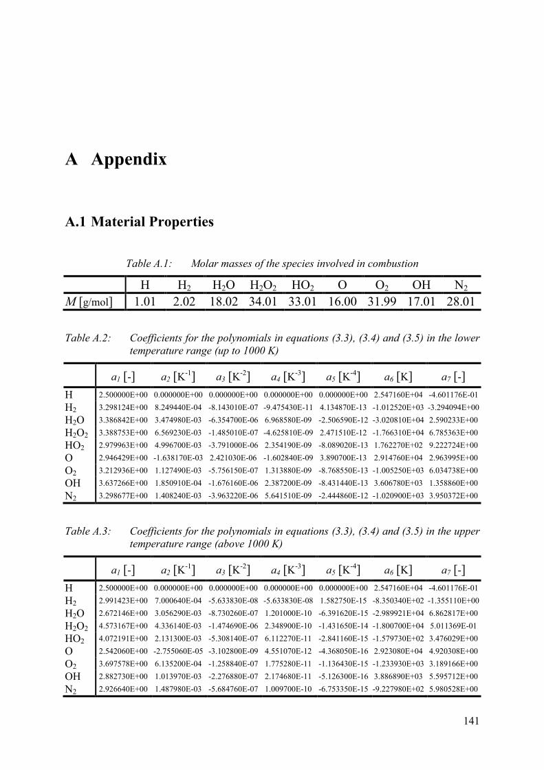
141
A Appendix
A.1 Material Properties
Table A.1: Molar masses of the species involved in combustion
H H2 H2O H2O2 HO2 O O2 OH N2
M [g/mol] 1.01 2.02 18.02 34.01 33.01 16.00 31.99 17.01 28.01
Table A.2: Coefficients for the polynomials in equations (3.3), (3.4) and (3.5) in the lower
temperature range (up to 1000 K)
a1 [-] a2 [K-1] a3 [K
-2] a4 [K-3] a5 [K
-4] a6 [K] a7 [-]
H 2.500000E+00 0.000000E+00 0.000000E+00 0.000000E+00 0.000000E+00 2.547160E+04 -4.601176E-01
H2 3.298124E+00 8.249440E-04 -8.143010E-07 -9.475430E-11 4.134870E-13 -1.012520E+03 -3.294094E+00
H2O 3.386842E+00 3.474980E-03 -6.354700E-06 6.968580E-09 -2.506590E-12 -3.020810E+04 2.590233E+00
H2O2 3.388753E+00 6.569230E-03 -1.485010E-07 -4.625810E-09 2.471510E-12 -1.766310E+04 6.785363E+00
HO2 2.979963E+00 4.996700E-03 -3.791000E-06 2.354190E-09 -8.089020E-13 1.762270E+02 9.222724E+00
O 2.946429E+00 -1.638170E-03 2.421030E-06 -1.602840E-09 3.890700E-13 2.914760E+04 2.963995E+00
O2 3.212936E+00 1.127490E-03 -5.756150E-07 1.313880E-09 -8.768550E-13 -1.005250E+03 6.034738E+00
OH 3.637266E+00 1.850910E-04 -1.676160E-06 2.387200E-09 -8.431440E-13 3.606780E+03 1.358860E+00
N2 3.298677E+00 1.408240E-03 -3.963220E-06 5.641510E-09 -2.444860E-12 -1.020900E+03 3.950372E+00
Table A.3: Coefficients for the polynomials in equations (3.3), (3.4) and (3.5) in the upper
temperature range (above 1000 K)
a1 [-] a2 [K-1] a3 [K
-2] a4 [K-3] a5 [K
-4] a6 [K] a7 [-]
H 2.500000E+00 0.000000E+00 0.000000E+00 0.000000E+00 0.000000E+00 2.547160E+04 -4.601176E-01
H2 2.991423E+00 7.000640E-04 -5.633830E-08 -5.633830E-08 1.582750E-15 -8.350340E+02 -1.355110E+00
H2O 2.672146E+00 3.056290E-03 -8.730260E-07 1.201000E-10 -6.391620E-15 -2.989921E+04 6.862817E+00
H2O2 4.573167E+00 4.336140E-03 -1.474690E-06 2.348900E-10 -1.431650E-14 -1.800700E+04 5.011369E-01
HO2 4.072191E+00 2.131300E-03 -5.308140E-07 6.112270E-11 -2.841160E-15 -1.579730E+02 3.476029E+00
O 2.542060E+00 -2.755060E-05 -3.102800E-09 4.551070E-12 -4.368050E-16 2.923080E+04 4.920308E+00
O2 3.697578E+00 6.135200E-04 -1.258840E-07 1.775280E-11 -1.136430E-15 -1.233930E+03 3.189166E+00
OH 2.882730E+00 1.013970E-03 -2.276880E-07 2.174680E-11 -5.126300E-16 3.886890E+03 5.595712E+00
N2 2.926640E+00 1.487980E-03 -5.684760E-07 1.009700E-10 -6.753350E-15 -9.227980E+02 5.980528E+00
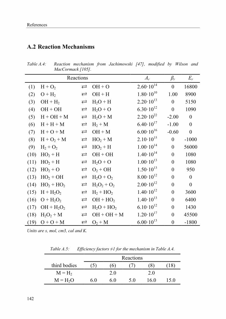
References
142
A.2 Reaction Mechanisms
Table A.4: Reaction mechanism from Jachimowski [47], modified by Wilson and
MacCormack [105].
Reactions Ar βr Er
(1) H + O2 OH + O 2.60·1014
0 16800
(2) O + H2 OH + H 1.80·1010
1.00 8900
(3) OH + H2 H2O + H 2.20·1013
0 5150
(4) OH + OH H2O + O 6.30·1012
0 1090
(5) H + OH + M H2O + M 2.20·1022
-2.00 0
(6) H + H + M H2 + M 6.40·1017
-1.00 0
(7) H + O + M OH + M 6.00·1016
-0.60 0
(8) H + O2 + M HO2 + M 2.10·1015
0 -1000
(9) H2 + O2 HO2 + H 1.00·1014
0 56000
(10) HO2 + H OH + OH 1.40·1014
0 1080
(11) HO2 + H H2O + O 1.00·1013
0 1080
(12) HO2 + O O2 + OH 1.50·1013
0 950
(13) HO2 + OH H2O + O2 8.00·1012
0 0
(14) HO2 + HO2 H2O2 + O2 2.00·1012
0 0
(15) H + H2O2 H2 + HO2 1.40·1012
0 3600
(16) O + H2O2 OH + HO2 1.40·1013
0 6400
(17) OH + H2O2 H2O + HO2 6.10·1012
0 1430
(18) H2O2 + M OH + OH + M 1.20·1017
0 45500
(19) O + O + M O2 + M 6.00·1013
0 -1800
Units are s, mol, cm3, cal and K.
Table A.5: Efficiency factors ≠1 for the mechanism in Table A.4.
Reactions
third bodies (5) (6) (7) (8) (18)
M = H2 2.0 2.0
M = H2O 6.0 6.0 5.0 16.0 15.0
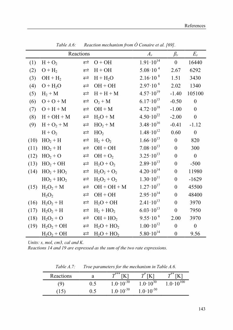
References
143
Table A.6: Reaction mechanism from Ó Conaire et al. [69].
Reactions Ar βr Er
(1) H + O2 O + OH 1.91·1014
0 16440
(2) O + H2 H + OH 5.08·10 4 2.67 6292
(3) OH + H2 H + H2O 2.16·10 8 1.51 3430
(4) O + H2O OH + OH 2.97·10 6 2.02 1340
(5) H2 + M H + H + M 4.57·1019
-1.40 105100
(6) O + O + M O2 + M 6.17·1015
-0.50 0
(7) O + H + M OH + M 4.72·1018
-1.00 0
(8) H + OH + M H2O + M 4.50·1022
-2.00 0
(9) H + O2 + M HO2 + M 3.48·1016
-0.41 -1.12
H + O2 HO2 1.48·1012
0.60 0
(10) HO2 + H H2 + O2 1.66·1013
0 820
(11) HO2 + H OH + OH 7.08·1013
0 300
(12) HO2 + O OH + O2 3.25·1013
0 0
(13) HO2 + OH H2O + O2 2.89·1013
0 -500
(14) HO2 + HO2 H2O2 + O2 4.20·1014
0 11980
HO2 + HO2 H2O2 + O2 1.30·1011
0 -1629
(15) H2O2 + M OH + OH + M 1.27·1017
0 45500
H2O2 OH + OH 2.95·1014
0 48400
(16) H2O2 + H H2O + OH 2.41·1013
0 3970
(17) H2O2 + H H2 + HO2 6.03·1013
0 7950
(18) H2O2 + O OH + HO2 9.55·10 6 2.00 3970
(19) H2O2 + OH H2O + HO2 1.00·1012
0 0
H2O2 + OH H2O + HO2 5.80·1014
0 9.56
Units: s, mol, cm3, cal and K.
Reactions 14 and 19 are expressed as the sum of the two rate expressions.
Table A.7: Troe parameters for the mechanism in Table A.6.
Reactions a T***
[K] T* [K] T
** [K]
(9) 0.5 1.0·10-30
1.0·1030
1.0·10100
(15) 0.5 1.0·10-30
1.0·10-30
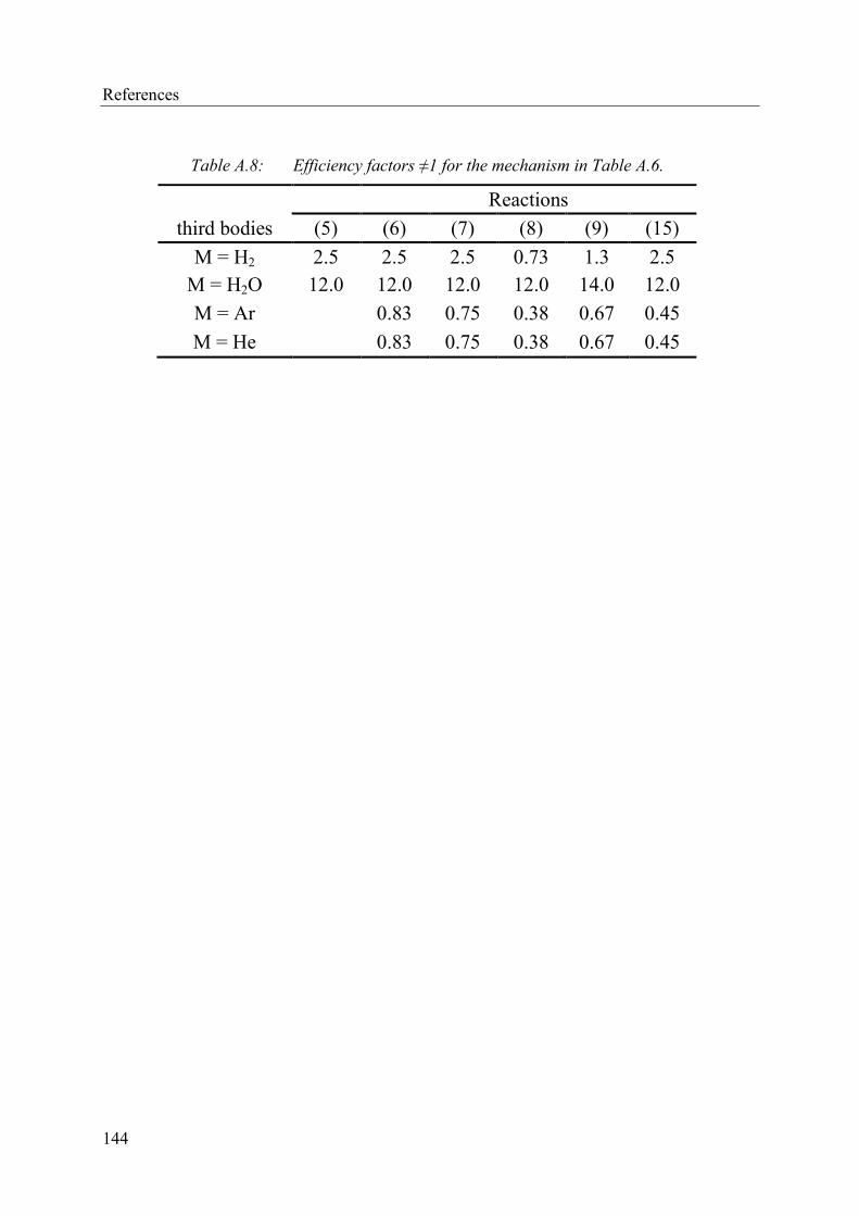
References
144
Table A.8: Efficiency factors ≠1 for the mechanism in Table A.6.
Reactions
third bodies (5) (6) (7) (8) (9) (15)
M = H2 2.5 2.5 2.5 0.73 1.3 2.5
M = H2O 12.0 12.0 12.0 12.0 14.0 12.0
M = Ar 0.83 0.75 0.38 0.67 0.45
M = He 0.83 0.75 0.38 0.67 0.45