
Constrained Model Predictive Control for Real-Time Tele ... · TECHNISCHE UNIVERSITAT¨ MUNCHEN¨...
139
T ECHNISCHE U NIVERSIT ¨ AT M ¨ UNCHEN Lehrstuhl f ¨ ur Luft- und Raumfahrt Constrained Model Predictive Control for Real-Time Tele-Operation Motion Planning Mingming Wang Vollst¨ andiger Abdruck der von der Fakult¨ at f ¨ ur Maschinenwesen der Technischen Univer- sit¨ at M ¨ unchen zur Erlangung des akademischen Grades eines Doktor-Ingenieurs (Dr.-Ing.) genehmigten Dissertation. Vorsitzender: Univ.-Prof. dr. ir. Daniel J. Rixen Pr ¨ ufer der Dissertation: 1. Univ.-Prof. Dr. rer. nat. Ulrich Walter 2. Univ.-Prof. Dr.-Ing. Alin Albu-Sch¨ affer Die Dissertation wurde am 14.01.2015 bei der Technische Universit¨ at M ¨ unchen eingereicht und durch die Fakult¨ at f ¨ ur Maschinenwesen am 17.06.2015 angenommen.
Transcript of Constrained Model Predictive Control for Real-Time Tele ... · TECHNISCHE UNIVERSITAT¨ MUNCHEN¨...
TECHNISCHE UNIVERSITAT MUNCHEN
Lehrstuhl fur Luft- und Raumfahrt
Constrained Model Predictive Controlfor Real-Time Tele-Operation Motion Planning
Mingming Wang
Vollstandiger Abdruck der von der Fakultat fur Maschinenwesen der Technischen Univer-sitat Munchen zur Erlangung des akademischen Grades eines
Doktor-Ingenieurs (Dr.-Ing.)
genehmigten Dissertation.
Vorsitzender: Univ.-Prof. dr. ir. Daniel J. Rixen
Prufer der Dissertation:
1. Univ.-Prof. Dr. rer. nat. Ulrich Walter
2. Univ.-Prof. Dr.-Ing. Alin Albu-Schaffer
Die Dissertation wurde am 14.01.2015 bei der Technische Universitat Munchen eingereichtund durch die Fakultat fur Maschinenwesen am 17.06.2015 angenommen.


Acknowledgements
The 4 years’ Ph.D life is a special and important experience in my life. It is full of passion,hope, desperation, struggle and happiness. As a foreigner in Germany, countless peoplefrom different countries have given me their hands to support and encourage me to success-fully get through my Ph.D life.
The first gratitude is devoted to Prof. Walter and Prof. Luo. Prof. Walter acceptedme as one of the members in his institute and gave me great freedom to do what I amreally interested in. As my primal supervisor, Prof. Luo guides me in my research andencourages me to go further. I thank Roberto Lampariello who gave me lots of suggestionsat the beginning of my first touch with Robotics. Many thanks to Prof. Igenbergs for hisencouragement and support. I also give my appreciation to Dr. Hohn and Dr. Rott fortheir helpful counsel and enduring my Chinglish. I thank Lars for his support on computer.Thanks to Claas for his picking me up from airport. He and Jan can always lift my spiritin the institute. I also thank Hein and Andi for sharing their experience with me. Furtherthanks to all the colleagues from Institute of Astronautics, it is the common experience withyou makes my Ph.D journey more colourful.
My German friends are a constant source of support. Evelyn, Herta, Ring, Family Yinand Family Babara gave me lots of help. They introduced Germany to me in detail andhelped me to pass through the dark period. The time spent with them will be a beautifulmemory in my life.
The last gratitude is devoted to my family. My parents encourage me to become the onewho I want to be and always support me to go further. My wife Ling, who perfectly manageour family and takes care of our little daughter Emily, owns my constant gratitude. It is yourlove, tolerance, endurance and optimism that supports me to finish this work.
Mingming WangGarching, 01.07.2014
V

Zusammenfassung
Zunehmende Anforderungen an den Satelliten-Service in der Erdumlaufbahn (On Orbit Ser-vicing, OOS) erfordern neue Technologien, um diese auszufuhren. Wegen ihrer Flexibilitat,Multifunktionalitat und Erweiterbarkeit sind Weltraum-Roboter eine der vielversprechend-sten Losungen dafur. In der vorliegenden Arbeit wird fur die Teleoperations-Aufgabeneines Weltraumroboters eine Architektur mit verteilter Echtzeit-Simulation basierend aufeinem Data Distribution Service (DDS) vorgestellt. Außerdem wird fur den frei schweben-den Roboter ein Model Predictive Control (MPC) Framework entworfen, das Kollisionenund Singularitaten bei Roboterbewegungen vermeidet. Ziel der vorliegenden Arbeit ist,fur so eine Simulation eine allgemeine Architektur zu entwerfen, die dem Boden-Operateureine intuitive Erkennung ermoglicht, und ein neues MPC Framework, das die vielfachenEinschrankungen beim Betrieb des Weltraumroboters in Betracht zieht und so die Leistungund Effektivitat verbessert.
Zu diesem Zweck wurde eine neue verteilte Echtzeitsimulation, RACOON, entwickelt,die auf einem DDS in Matlab/Simulink/Stateflow basiert. Sie liefert dem Boden-Operateureine intuitive Ansicht des Roboters und erweitert die Simulations-Architektur fur kollab-orative Teleoperation, Mehrkorperdynamik, Autonomous Mission Management (AMM),Weg- und Bahn-Planung, Bewegungskontrolle, virtuelle Realitat, usw., fur heutige kom-plexe Robotikmissionen.
Zunachst wird die Dynamik des Raumroboters mit einer Baumstruktur unter Nutzungvon Konzepten aus der Graphentheorie und raumlichen Beschreibungen dargestellt, umdamit ein Nonlinear Model Predictive Control (NMPC) Model zu verwirklichen. Aus derTopologie des Roboters wird eine Inertia Mapping Matrix (IMM) hergeleitet werden, um dieSparlichkeit eines JSIM und die Komplexitat von CRBA Algorithmen zu untersuchen unddie Dekomposition des JSIM zu unterstutzen.
Danach werden fur redundante Manipulatoren unter Berucksichtigung der Prioritat vonRedundanz und Aufgaben die Singularitats- und Kollisions-Probleme untersucht. Fur dieVermeidung von Singularitaten wird basierend auf dem Konzept von Handhabbarkeits-Ellipsoiden eine sogenannte STR-Methode entwickelt. Zur Kollisionsvermeidung, wird eineneue Zwei-Kontrollpunkte-Strategie vorgeschlagen, die Schwingung der Gelenkgeschwin-digkeit dampft und so eine glattere Bewegungsbahn des Roboterarms erzeugt.
In einer Anwendungsstudie wird gezeigt, wie bei der Ergreifung eines nicht koopera-tiven Zielsatelliten ein so gestalteter NMPC einen Manipulatorarm kollisions- und singu-laritatsfrei bewegt. Die Wirksamkeit und die Leistungsfahigkeit der hier neuen vorgeschla-genen Methoden werden mit traditionellen Methoden verglichen. Diese Arbeit zeigt dieMachbarkeit und die berlegenheit eines eingeschrankten MPC fur den Einsatz eines Wel-traumroboters.
VII


Abstract
The increasing demands of On-Orbit Servicing (OOS) require new technologies to completethe OOS mission. Space robot, since it is flexible, multi-functional and extendable, is oneof the most promising solutions for OOS. In this thesis, a distributed real-time simulationarchitecture based on DDS has been presented for space robotic tele-operation tasks. Be-sides, a constrained MPC framework considering system input/output, anti-collision andanti-singularity constraints has been developed for the free-floating space robot. The objec-tive of this thesis is to provide a general simulation architecture with intuitive perception forthe operators on ground, and a new control framework considering multiple constraints forthe application of the space robot while the performance and effectiveness are improved.
For that purpose, a new distributed real-time simulation architecture, RACOON, hasbeen implemented based on DDS in the environment Matlab/Simulink/Stateflow. The newsimulation architecture provides the operator on ground an intuitive view of space robotand makes the simulation architecture open for collaborative tele-operation. As a completesimulation system, the multi-body dynamics, AMM, path & trajectory planning, motioncontrol, virtual reality etc. subsystems, integrate together seamlessly to complete the wholespace robotic missions.
In order to realize the new control framework based on NMPC, firstly, the dynamics ofthe space robot with tree structure using the concepts of graph theory and spatial notationis introduced. A new IMM is derived from the topology of the space robot, which can beemployed to analyse the sparsity of the JSIM and the complexity of the CRBA algorithm,and assist the decomposition of the JSIM. Secondly, the singularity and collision avoidanceissues of redundant manipulators are investigated considering the redundancy and task pri-ority. A so-called STR method is developed based on the concept of manipulability ellipsoidfor singularity avoidance. For collision avoidance, a new strategy combining two controlpoints is proposed to restrain the vibration of joint velocity and generate smoother jointtrajectory reference. Thirdly, application of NMPC to space manipulator in capturing an un-cooperative target satellite is investigated. The system input/output, collision/singularityconstraints in practice imposed on decision variables are translated into linear inequalitiesas part of NMPC. An on-line QP algorithm with prioritized constraints is adopted to findthe optimal control efforts.
The effectiveness and performance of the new proposed methods in this thesis are demon-strated by comparison to traditional methods. Well-designed end-effector path, togetherwith the NMPC guarantees the success of the space manipulator to complete the captureof the un-cooperative target satellite. This work shows the feasibility and validity of con-strained MPC applied in the field of space robot. Furthermore, it can be used to supportfurther OOS mission and space exploration.
IX

Contents
Acknowledgements V
Zusammenfassung VII
Abstract IX
List of Figures XV
List of Tables XVII
Nomenclature XIXAcronyms . . . . . . . . . . . . . . . . . . . . . . . . . . . . . . . . . . . . . . . . . . . . . . . XIXSymbols . . . . . . . . . . . . . . . . . . . . . . . . . . . . . . . . . . . . . . . . . . . . . . . . XXIIIndices . . . . . . . . . . . . . . . . . . . . . . . . . . . . . . . . . . . . . . . . . . . . . . . . . XXIV
1. Introduction 11.1. Motivation . . . . . . . . . . . . . . . . . . . . . . . . . . . . . . . . . . . . . . . . . . . 2
1.1.1. On-Orbit Servicing . . . . . . . . . . . . . . . . . . . . . . . . . . . . . . . . . 21.1.2. Why Space Robotics . . . . . . . . . . . . . . . . . . . . . . . . . . . . . . . . 3
1.2. State of the art . . . . . . . . . . . . . . . . . . . . . . . . . . . . . . . . . . . . . . . . . 41.2.1. OOS Technology Demonstrators . . . . . . . . . . . . . . . . . . . . . . . . 41.2.2. Space Robotics Demonstrators . . . . . . . . . . . . . . . . . . . . . . . . . . 71.2.3. Technical Challenges of Space Robotics . . . . . . . . . . . . . . . . . . . . 10
1.3. Hypothesis and Problem Statements . . . . . . . . . . . . . . . . . . . . . . . . . . 121.4. Scope of Work . . . . . . . . . . . . . . . . . . . . . . . . . . . . . . . . . . . . . . . . . 13
1.4.1. Research Scope within Space Robotics . . . . . . . . . . . . . . . . . . . . . 131.4.2. Thesis Roadmap . . . . . . . . . . . . . . . . . . . . . . . . . . . . . . . . . . . 13
2. Simulation System Design 172.1. Mission Profile . . . . . . . . . . . . . . . . . . . . . . . . . . . . . . . . . . . . . . . . 172.2. Simulation Overall Design . . . . . . . . . . . . . . . . . . . . . . . . . . . . . . . . . 19
2.2.1. Racoon Design . . . . . . . . . . . . . . . . . . . . . . . . . . . . . . . . . . . . 192.2.2. Simulation Environment . . . . . . . . . . . . . . . . . . . . . . . . . . . . . 202.2.3. Data Distribution Service . . . . . . . . . . . . . . . . . . . . . . . . . . . . . 22
2.3. RacoonSim Design . . . . . . . . . . . . . . . . . . . . . . . . . . . . . . . . . . . . . . 242.3.1. Multi-body Dynamics . . . . . . . . . . . . . . . . . . . . . . . . . . . . . . . 252.3.2. Autonomous Mission Management . . . . . . . . . . . . . . . . . . . . . . 262.3.3. Path & Trajectory Planning . . . . . . . . . . . . . . . . . . . . . . . . . . . . 282.3.4. Motion Control . . . . . . . . . . . . . . . . . . . . . . . . . . . . . . . . . . . 292.3.5. Virtual Reality & Head-Up Display . . . . . . . . . . . . . . . . . . . . . . . 29
2.4. Summary . . . . . . . . . . . . . . . . . . . . . . . . . . . . . . . . . . . . . . . . . . . . 31
XI

Contents
3. Multibody Dynamics 333.1. Graphy Theory . . . . . . . . . . . . . . . . . . . . . . . . . . . . . . . . . . . . . . . . 343.2. Spatial Notation . . . . . . . . . . . . . . . . . . . . . . . . . . . . . . . . . . . . . . . 353.3. Dynamics Algorithm . . . . . . . . . . . . . . . . . . . . . . . . . . . . . . . . . . . . 36
3.3.1. Lagrange Formulation . . . . . . . . . . . . . . . . . . . . . . . . . . . . . . . 363.3.2. Composite Rigid Body Algorithm . . . . . . . . . . . . . . . . . . . . . . . 373.3.3. Inertia Mapping Matrix . . . . . . . . . . . . . . . . . . . . . . . . . . . . . . 383.3.4. Modified CRBA . . . . . . . . . . . . . . . . . . . . . . . . . . . . . . . . . . . 39
3.4. IMM Application . . . . . . . . . . . . . . . . . . . . . . . . . . . . . . . . . . . . . . . 393.4.1. Branch-induced Sparsity . . . . . . . . . . . . . . . . . . . . . . . . . . . . . 403.4.2. CRBA Computational Cost Analysis . . . . . . . . . . . . . . . . . . . . . . 403.4.3. JSIM Factorization Analysis . . . . . . . . . . . . . . . . . . . . . . . . . . . 42
3.5. Case Study . . . . . . . . . . . . . . . . . . . . . . . . . . . . . . . . . . . . . . . . . . . 443.6. Summary . . . . . . . . . . . . . . . . . . . . . . . . . . . . . . . . . . . . . . . . . . . . 47
4. Kinematic Control of Manipulator 494.1. Inverse Kinematics . . . . . . . . . . . . . . . . . . . . . . . . . . . . . . . . . . . . . . 49
4.1.1. Redundancy and Task Priority . . . . . . . . . . . . . . . . . . . . . . . . . . 494.1.2. General Solution for Inverse Kinematics . . . . . . . . . . . . . . . . . . . 50
4.2. Singularity Avoidance . . . . . . . . . . . . . . . . . . . . . . . . . . . . . . . . . . . . 514.2.1. Manipulability Ellipsoid . . . . . . . . . . . . . . . . . . . . . . . . . . . . . 524.2.2. Singular Task Reconstruction . . . . . . . . . . . . . . . . . . . . . . . . . . 534.2.3. STR with Multiple Subtasks . . . . . . . . . . . . . . . . . . . . . . . . . . . 554.2.4. Simulation Results . . . . . . . . . . . . . . . . . . . . . . . . . . . . . . . . . 57
4.3. Obstacle Detection and Avoidance . . . . . . . . . . . . . . . . . . . . . . . . . . . . 644.3.1. Collision Detection . . . . . . . . . . . . . . . . . . . . . . . . . . . . . . . . . 644.3.2. Collision Avoidance Strategy . . . . . . . . . . . . . . . . . . . . . . . . . . . 674.3.3. Simulation Results . . . . . . . . . . . . . . . . . . . . . . . . . . . . . . . . . 70
4.4. Summary . . . . . . . . . . . . . . . . . . . . . . . . . . . . . . . . . . . . . . . . . . . . 74
5. Model Predictive Control 775.1. Model Predictive Control . . . . . . . . . . . . . . . . . . . . . . . . . . . . . . . . . . 77
5.1.1. Principle and Formulation . . . . . . . . . . . . . . . . . . . . . . . . . . . . 785.1.2. MPC Properties . . . . . . . . . . . . . . . . . . . . . . . . . . . . . . . . . . . 80
5.2. NMPC Applied to Space Robot . . . . . . . . . . . . . . . . . . . . . . . . . . . . . . 815.2.1. Free-Floating Space Robot . . . . . . . . . . . . . . . . . . . . . . . . . . . . 825.2.2. Feedback Linearization . . . . . . . . . . . . . . . . . . . . . . . . . . . . . . 825.2.3. Observer Design . . . . . . . . . . . . . . . . . . . . . . . . . . . . . . . . . . 845.2.4. Optimization Index . . . . . . . . . . . . . . . . . . . . . . . . . . . . . . . . . 86
5.3. Inequality Constraints . . . . . . . . . . . . . . . . . . . . . . . . . . . . . . . . . . . . 875.3.1. Input/Output Constraints . . . . . . . . . . . . . . . . . . . . . . . . . . . . 875.3.2. Obstacle/Singularity Constraints . . . . . . . . . . . . . . . . . . . . . . . . 89
5.4. Quadratic Programming . . . . . . . . . . . . . . . . . . . . . . . . . . . . . . . . . . 925.4.1. KKT Conditions . . . . . . . . . . . . . . . . . . . . . . . . . . . . . . . . . . . 925.4.2. QP with Prioritized Constraints . . . . . . . . . . . . . . . . . . . . . . . . . 93
5.5. Simulation Study . . . . . . . . . . . . . . . . . . . . . . . . . . . . . . . . . . . . . . . 955.5.1. Simulation Set-up . . . . . . . . . . . . . . . . . . . . . . . . . . . . . . . . . . 955.5.2. Approach to the Target . . . . . . . . . . . . . . . . . . . . . . . . . . . . . . 955.5.3. Tracking a Predefined Path . . . . . . . . . . . . . . . . . . . . . . . . . . . . 97
XII

Contents
5.5.4. Tracking a Point on the Target . . . . . . . . . . . . . . . . . . . . . . . . . . 995.6. Summary . . . . . . . . . . . . . . . . . . . . . . . . . . . . . . . . . . . . . . . . . . . . 102
6. Conclusions and Future Research 1056.1. Conclusions . . . . . . . . . . . . . . . . . . . . . . . . . . . . . . . . . . . . . . . . . . 1056.2. Future Research . . . . . . . . . . . . . . . . . . . . . . . . . . . . . . . . . . . . . . . . 106
A. Bibliography 109
XIII

List of Figures
1.1. Engineering design MODPV loop . . . . . . . . . . . . . . . . . . . . . . . . . . . . 11.2. OOS manned projects . . . . . . . . . . . . . . . . . . . . . . . . . . . . . . . . . . . . 51.3. OOS unmanned projects . . . . . . . . . . . . . . . . . . . . . . . . . . . . . . . . . . 71.4. Space roboitcs projects . . . . . . . . . . . . . . . . . . . . . . . . . . . . . . . . . . . 91.5. OOS demonstrators classification . . . . . . . . . . . . . . . . . . . . . . . . . . . . 101.6. Structure of the work . . . . . . . . . . . . . . . . . . . . . . . . . . . . . . . . . . . . 15
2.1. Mission profile of space robot . . . . . . . . . . . . . . . . . . . . . . . . . . . . . . . 192.2. Subsystems of Racoon Lab . . . . . . . . . . . . . . . . . . . . . . . . . . . . . . . . . 202.3. Simulation environment of Racoon . . . . . . . . . . . . . . . . . . . . . . . . . . . 212.4. DDS Structure . . . . . . . . . . . . . . . . . . . . . . . . . . . . . . . . . . . . . . . . . 222.5. Racoon system set-up . . . . . . . . . . . . . . . . . . . . . . . . . . . . . . . . . . . . 242.6. Racoon simulation system set-up . . . . . . . . . . . . . . . . . . . . . . . . . . . . . 252.7. Workflow of high-level OOS missions . . . . . . . . . . . . . . . . . . . . . . . . . . 272.8. Workflow of capture phase . . . . . . . . . . . . . . . . . . . . . . . . . . . . . . . . . 272.9. VRML mechanism and its interfaces . . . . . . . . . . . . . . . . . . . . . . . . . . . 302.10. GUI, VR and HUD in MCC . . . . . . . . . . . . . . . . . . . . . . . . . . . . . . . . 31
3.1. Example of tree structure manipulators . . . . . . . . . . . . . . . . . . . . . . . . . 343.2. Generalized center of mass of link i . . . . . . . . . . . . . . . . . . . . . . . . . . . 353.3. Relationship among path matrix, IMM and JSIM . . . . . . . . . . . . . . . . . . . 383.4. Tree configuration and corresponding JSIM of one base with 4 links . . . . . . . 403.5. Humanoid and corresponding un-branched chain . . . . . . . . . . . . . . . . . . 443.6. Operations numbers of CRBA and ABA . . . . . . . . . . . . . . . . . . . . . . . . 463.7. Cost ratio of CRBA and ABA . . . . . . . . . . . . . . . . . . . . . . . . . . . . . . . 46
4.1. Schematic diagram of inverse kinematics based on task priority . . . . . . . . . 514.2. 3 revolute planar manipulator and its manipulability ellipsoid . . . . . . . . . . 534.3. Schematic diagram of singular task reconstruction . . . . . . . . . . . . . . . . . . 544.4. The functional behaviour of the turning parameters for singularity avoidance 554.5. Block scheme of STR for multiple subtasks . . . . . . . . . . . . . . . . . . . . . . . 564.6. 3 revolute planar manipulator and subtasks . . . . . . . . . . . . . . . . . . . . . . 574.7. Singularity avoidance with single task by STR method . . . . . . . . . . . . . . . 584.8. Singularity avoidance with single task by DLS method . . . . . . . . . . . . . . . 594.9. Singularity avoidance with two subtasks by STR method . . . . . . . . . . . . . 604.10. Singularity avoidance with two subtasks by DLS method . . . . . . . . . . . . . 614.11. Singularity avoidance with two subtasks and higher gain by STR method . . . 624.12. Singularity avoidance with two subtasks and higher gain by DLS method . . . 634.13. The relationship of two line segments . . . . . . . . . . . . . . . . . . . . . . . . . . 654.14. The relationship between line segment and triangle . . . . . . . . . . . . . . . . . 664.15. Collision avoidance with two control points . . . . . . . . . . . . . . . . . . . . . . 67
XV

List of Figures
4.16. The functional behaviour of the turning parameters for collision avoidance . . 694.17. 10 revolute planar manipulator and obstacles . . . . . . . . . . . . . . . . . . . . . 714.18. Path tracking without collision avoidance . . . . . . . . . . . . . . . . . . . . . . . 724.19. Path tracking with one control point for collision avoidance . . . . . . . . . . . . 734.20. Path tracking with two control points for collision avoidance . . . . . . . . . . . 74
5.1. Schematic diagram of MPC fundamental principle . . . . . . . . . . . . . . . . . 785.2. Basic NMPC control loop . . . . . . . . . . . . . . . . . . . . . . . . . . . . . . . . . . 795.3. The mismatch between open-loop prediction and closed-loop behaviour . . . 815.4. Schematic diagram of space robot . . . . . . . . . . . . . . . . . . . . . . . . . . . . 825.5. Linear feedback with NMPC for space robot . . . . . . . . . . . . . . . . . . . . . 845.6. Schematic diagram of anti-collision . . . . . . . . . . . . . . . . . . . . . . . . . . . 895.7. Schematic diagram of anti-singularity . . . . . . . . . . . . . . . . . . . . . . . . . . 905.8. Unfolding the space manipulator using RMAC method . . . . . . . . . . . . . . 965.9. Unfolding the space manipulator using NMPC method . . . . . . . . . . . . . . 975.10. Tracking infinite ring with anti-collision constraints . . . . . . . . . . . . . . . . . 985.11. Tracking line with anti-singularity constraints . . . . . . . . . . . . . . . . . . . . 995.12. Relative relationship of end-effector frame and capture point frame . . . . . . . 1005.13. Tracking capture point on target satellite . . . . . . . . . . . . . . . . . . . . . . . . 1015.14. Screenshot of tracking the capture point on target . . . . . . . . . . . . . . . . . . 102
XVI
List of Tables
1.1. OOS overview and its typical applications (Waltz (1993)) . . . . . . . . . . . . . 31.2. OOS manned projects . . . . . . . . . . . . . . . . . . . . . . . . . . . . . . . . . . . . 51.3. OOS unmanned projects . . . . . . . . . . . . . . . . . . . . . . . . . . . . . . . . . . 6
3.1. Modified composite rigid body algorithm . . . . . . . . . . . . . . . . . . . . . . . 393.2. Required operation cost of different transforms . . . . . . . . . . . . . . . . . . . . 423.3. LTL and LTDL factorization algorithms . . . . . . . . . . . . . . . . . . . . . . . . . 43
4.1. Collision detection algorithms . . . . . . . . . . . . . . . . . . . . . . . . . . . . . . 66
XVII

Nomenclature
Acronyms
ABA . . . . . . . Articulated Body Algorithm
AFRL . . . . . . . Air Force Research Laboratory
AI . . . . . . . . . Artificial Intelligence
AMM . . . . . . . Autonomous Mission Management
API . . . . . . . . Application Programming Interface
ASTRO . . . . . . Autonomous Space Transport Robotic Operations
ATV . . . . . . . . Autonomous Transfer Vehicle
BVH . . . . . . . Bounding Volume Hierarchy
CAD . . . . . . . Computer Aided Design
CESSORS . . . . Chinese Experimental Space System for On-Orbit Robotistic Services
CNES . . . . . . . Centre National d’Etudes Spatiales
CRBA . . . . . . Composite Rigid Body Algorithm
CSA . . . . . . . . Canadian Space Agency
DARPA . . . . . Defence Advanced Research Projects Agency
DART . . . . . . Demonstration of Autonomous Rendezvous Technology
DCPS . . . . . . . Data-Centric Publish/Subscribe
DDS . . . . . . . Data Distribution Service
DEOS . . . . . . . DEutsche Orbitale Servicing Mission
DH . . . . . . . . Denavit-Hartenberg
DLR . . . . . . . . Deutsche Luft und Raumfahrttechnik
DLRL . . . . . . . Data Local Reconstruction Layer
DLS . . . . . . . . Damped Least-Squares
DMC . . . . . . . Dynamic Matrix Control
DOF . . . . . . . degree-of-freedom
XIX
Acronyms
DOR . . . . . . . degree-of-redundancy
ESA . . . . . . . . European Space Agency
ETS-VII . . . . . Engineering Test Satellite-VII
EVA . . . . . . . . Extra-Vehicular Activities
FREND . . . . . Front-end Robotics Enabling Near-Term Demonstration
FSM . . . . . . . . Finite State Machine
GEO . . . . . . . Geostationary Orbit
GJM . . . . . . . . Generalized Jacobian Matrix
GPC . . . . . . . Generalized Predictive Control
GPS . . . . . . . . Global Positioning System
GUI . . . . . . . . Graphical User Interface
HIL . . . . . . . . Hardware-in-loop
HST . . . . . . . . Hubble Space Telescope
HTV . . . . . . . H-II Transfer Vehicle
HUD . . . . . . . Head-Up Display
IDL . . . . . . . . Interface Definition Language
IMM . . . . . . . Inertia Mapping Matrix
IMU . . . . . . . . Inertia Measurement Unit
ISS . . . . . . . . International Space Station
JAXA . . . . . . . Japan Aerospace Exploration Agency
JSIM . . . . . . . Joint-Space Inertia Matrix
KF . . . . . . . . . Kalman Filter
KKT . . . . . . . Karush-Kuhn-Tucker
LEO . . . . . . . . Low Earth Orbit
LP . . . . . . . . . Linear Programming
MCC . . . . . . . Mission Control Center
MPC . . . . . . . Model Predictive Control
MPD . . . . . . . Maximum Projection Distance
XX
Acronyms
MSS . . . . . . . . Mobile Servicing System
NASA . . . . . . National Aeronautics and Space Administration
NASDA . . . . . NAtional Space Development Agency of Japan
NMPC . . . . . . Nonlinear Model Predictive Control
NRL . . . . . . . Naval Research Laboratory
OBB . . . . . . . . Oriented Bounding Box
OBDH . . . . . . On-Board Data Handling
OE . . . . . . . . Orbital Express
OLEV . . . . . . . Orbital Life Extension Vehicle
OMG . . . . . . . Object Management Group
OOS . . . . . . . On-Orbit Servicing
ORU . . . . . . . Orbital Replacement Unit
PRISMA . . . . . Prototype Research Instruments and Space Mission technology Advance-ment
PUMA . . . . . . Programmable Universal Machine for Assembly
QoS . . . . . . . . Quality of Service
QP . . . . . . . . Quadratic Programming
RACOON . . . . Robotic Actuation, Control and On Orbit Navigation Laboratory
RacoonSim . . . Racoon Simulation
RHC . . . . . . . Receding Horizon Control
RMAC . . . . . . Resolved Motion Acceleration Control
RNEA . . . . . . Recursive Newton-Euler Algorithm
ROKVISS . . . . RObotic Components Verification on the ISS
ROTEX . . . . . . Robot Technology Experiment
SMMR . . . . . . Solar Maximum Mission Repair
SPDM . . . . . . Special Purpose Dexterous Manipulator
SRMS . . . . . . . Shuttle Remote Manipulator System
SSC . . . . . . . . Swedish Space Corporation
SSL . . . . . . . . Space Systems Laboratory
SSN . . . . . . . . Space Surveillance Network
XXI
Symbols
SSTC . . . . . . . Shenzhen Space Technology Center
STR . . . . . . . . Singular Task Reconstruction
STS . . . . . . . . Space Transportation System
SVD . . . . . . . . Singular Value Decomposition
TFX . . . . . . . . Telerobotic Flight Experiment
TM/TC . . . . . Telemetry/Telecommand
VR . . . . . . . . Virtual Reality
VRML . . . . . . Virtual Reality Modelling Language
XML . . . . . . . Extensible Markup Language
XSS . . . . . . . . Experimental Satellite System
Symbols
a . . . . . . . . . . position vector of mass centerα0 . . . . . . . . . escaping gain for singularity avoidanceαc . . . . . . . . . turning parameter of repulsive motion for collision avoidanceαd . . . . . . . . . weight parameter for singularity avoidanceαe . . . . . . . . . turning parameter of cancelling primary taskαh . . . . . . . . . turning parameter of repulsive motion for singularity avoidanceαv . . . . . . . . . weight parameter for singularity avoidancec . . . . . . . . . . bias vectorca . . . . . . . . . composite rigid body addct . . . . . . . . . composite rigid body transformcta . . . . . . . . . composite rigid body transform for DH nodectb . . . . . . . . . composite rigid body transform for non-DH nodectc . . . . . . . . . composite rigid body transform for node connecting direct to the baseD0 . . . . . . . . . numbers of moving links without connecting to the baseD0a . . . . . . . . numbers of moving links without connecting to the base for DH nodeD0b . . . . . . . . numbers of moving links without connecting to the base for non-DH
nodeD0c . . . . . . . . number of saving operations in composite rigid body transformD1 . . . . . . . . . numbers of non-zero elements above the diagonal of IMMD1a . . . . . . . . numbers of non-zero elements above the diagonal of IMM for DH nodeD1b . . . . . . . . numbers of non-zero elements above the diagonal of IMM for non-DH
nodeD1c . . . . . . . . number of saving operations in vector transformD2 . . . . . . . . . sum of elements above the diagonal of IMMdif . . . . . . . . . influence zone of collisionD . . . . . . . . . diagonal matrixdsr . . . . . . . . . security zone of collision
XXII
Symbols
duf . . . . . . . . . unsafe zone of collisionE . . . . . . . . . identity matrixE . . . . . . . . . . edge setǫDLS . . . . . . . . threshold to active the DLS methodηac . . . . . . . . . damper coefficient of anti-collision constraintηas . . . . . . . . . damper coefficient of anti-singularity constraintf . . . . . . . . . . spatial forcefx . . . . . . . . . external force/torque vectorf . . . . . . . . . . force vectorΓ . . . . . . . . . . cost functionh . . . . . . . . . . arbitrary vectorH . . . . . . . . . joint-space inertia matrixH . . . . . . . . . spatial inertia matrixI . . . . . . . . . . inertia matrixJ . . . . . . . . . . Jacobian matrixJ . . . . . . . . . . matrix projection onto the null-spaceJ+ . . . . . . . . . pseudo-inverse of Jacobian matrixK . . . . . . . . . computational cost of algorithmK . . . . . . . . . gain matrixL . . . . . . . . . . LagrangianL . . . . . . . . . . lower triangular matrixλac . . . . . . . . . switching function for anti-collision constraintλas . . . . . . . . . switching function for anti-singularity constraintλ(⋅) . . . . . . . . parent arrayM . . . . . . . . . inertia mapping matrixm . . . . . . . . . massm . . . . . . . . . moment vectorM∗ . . . . . . . . augmented inertia mapping matrixNc . . . . . . . . . control horizonnnDH . . . . . . . number of non-DH nodesNp . . . . . . . . . prediction horizonO . . . . . . . . . algorithm complexity representationO . . . . . . . . . obstacles setP . . . . . . . . . link setq . . . . . . . . . . generalized coordinateq . . . . . . . . . . generalized velocityq . . . . . . . . . . generalized accelerationjRi . . . . . . . . coordinate transformation matrixjri . . . . . . . . . position vector from the origin of frame i to that of frame j
R . . . . . . . . . real setSact . . . . . . . . active sets . . . . . . . . . . motion axis of generalized linkS . . . . . . . . . . cross product operatorσ . . . . . . . . . . singular valueσif . . . . . . . . . influence zone of singularityσm . . . . . . . . . minimum singular valueσsr . . . . . . . . . security zone of singularityσuf . . . . . . . . unsafe zone of singularity
XXIII

Indices
τ . . . . . . . . . . internal joint torque vectorT . . . . . . . . . kinetic energyT . . . . . . . . . path matrixθ . . . . . . . . . . joint position vector
θ . . . . . . . . . . joint velocity vectorT∗ . . . . . . . . . augmented path matrixu . . . . . . . . . . control input vectorum . . . . . . . . . left singular vector correspond to minimum singular valueU . . . . . . . . . potential energyV . . . . . . . . . . vertex setVR . . . . . . . . Voronoi regionv . . . . . . . . . . spatial velocityv . . . . . . . . . . translational velocityvt . . . . . . . . . vector transformvta . . . . . . . . . vector transform for DH nodevtb . . . . . . . . . vector transform for non-DH nodevtc . . . . . . . . . vector transform for node connecting direct to the baseω . . . . . . . . . angular velocityx . . . . . . . . . . system states vectorxd . . . . . . . . . desired end-effector pathxc . . . . . . . . . end-effector velocity with feedbackxd . . . . . . . . . desired end-effector velocityxe . . . . . . . . . end-effector velocityxo . . . . . . . . . obstacle avoidance velocityxp . . . . . . . . . end-effector modified velocityxe . . . . . . . . . end-effector pathξ . . . . . . . . . . generalized forcejXi . . . . . . . . spatial transformation matrixy . . . . . . . . . . control output vector
Indices
x . . . . . . . . . . scalarx . . . . . . . . . . maximum within intervalx . . . . . . . . . . minimum within intervalx . . . . . . . . . . value from estimationx∗ . . . . . . . . . values in optimumx . . . . . . . . . . vectorX . . . . . . . . . matrix[⋅]T . . . . . . . . transpose of ⋅
XXIV

1. Introduction
[On President Bush’s plan to get to Mars in 10 years] Stupid. Robots would do abetter job and be much cheaper because you don’t have to bring them back.
—Stephen W. Hawking
It’s the human demands and desires that stimulate the scientists and engineers to doscientific research to explore the unknown world and build new machines working for us.Normally, the general research procedure can be illustrated as in Figure 1.1.
People want to invent/build something new based on their demands or the motivation.The next step would be orientation, where generally series of solutions are emerged. Theorientation phase will make our thoughts divergence, to search all possible feasible solu-tions. As a matter of fact, since there are financing, technical, human capital etc. issues, it isimpossible to implement all of the possible solutions. Some of the resolution will be chosento move forward based on the specific criteria among these. A decision phase is critical toevaluate all the possible solutions and find out the potentially best ones. Subsequently, amodel, which is also named as prototype, will be established both in digital and physicalenvironment. This prototyping design is used to check the feasibility of the solution, anddemonstrate the technologies and performance of the proposed design. All aspects of theprototype, such as its hardware, software, functionality, etc. will be tested in the verificationphase. These tests will indicate the cons and pros of the design and show up whether itmeets the proposed demands and requirements. All these five steps finally form an engi-neering design loop, which will also show in this thesis. If the prototype cannot pass the testand fulfil the proposed demands, the design loop will proceed iteratively until the designmakes the human satisfied, where then can stop the loop.
Orientation
Prototype
Verificaiton
Motivation
Decision
MODPV
Figure 1.1.: Engineering design MODPV loop
1

1. Introduction
1.1. Motivation
The motivation of this research origins from two aspects. Objectively speaking, there arethousands of malfunctioning satellites are currently floating in outer space which are harm-ful for future satellite launch and space operations. In the past two decades, some of the mostextraordinary successes in space exploration have emphasized the growing importance ofOn-Orbit Servicing (OOS). The challenges have moved beyond simply launching complexspacecraft and system. What we need to face are the fully exploitation of the flight systems,construction of large structures in situ to enable new scientific ventures, and provide sys-tems that reliably and cost-effectively support the next step in space exploration. The visionfor OOS is straightforward to refuel, repair, or upgrade satellites after launched.
The other aspect of research motivation comes from the space race of our competitorswhich are hostile to us. Just as was illustrated in Destruction and Creation by John R. Boyd inBoyd (1987):
In a real world of limited resources and skills, individuals and groups form, dissolveand reform their cooperative or competitive postures in a continuous struggle to removeor overcome physical and social environmental obstacles. In a cooperative sense, whereskills and talents are pooled, the removal or overcoming of obstacles represents an im-proved capacity for independent action for all concerned. In a competitive sense, whereindividuals and groups compete for scarce resources and skills, an improved capacity forindependent action achieved by some individuals or groups constrains that capacity forother individuals or groups. Naturally, such a combination of real world scarcity andgoal striving to overcome this scarcity intensifies the struggle of individuals and groupsto cope with both their physical and social environments.
From above illustration, one can derive that it is the cooperation and competition be-tween individuals or organizations that motivate us to gain an improved capacity whichintensifies the struggle of individuals and groups to enhance self-development and researchactivities. From this viewpoint, OOS has already become such an ability which extensivelyinvestigated and strengthened by world wild research and academic agencies. A list ofspace projects about OOS proceeded in the past and planned in the future will be describedin section 1.2.
1.1.1. On-Orbit Servicing
Since a wide spectrum of using cases exists in space, OOS would be of great benefit for spaceexploration, which can reduce risk of mission failure and mission cost, increase mission per-formance and flexibility, and enable new missions. OOS includes a variety of applications,which can be grouped into five main operations.
2

1. Introduction
Table 1.1.: OOS overview and its typical applications (Waltz (1993))
Operations Typical Applications
Assembly Spacecraft constructionsSpacecraft updateDeployment of appendages
Orbit transfer Orbit correctionsRetrieval from orbitEarth return
Re-supply ConsumablesComponents
Maintenance and repair InspectionModificationCleaning and resurfacingTests and checkout
Special Emergencey operationsScavengingAttitute control
Accordingly, On-Orbit Servicing (OOS) can be defined as follows refer to Wikipedia(2014)
OOS includes installation, maintenance, and repair work on an orbiting man-made object (satellite, space station, space vehicle, etc.) with the aim of extendingthe useful life of the target object and/or enhancing the capability of the target(upgrade).
1.1.2. Why Space Robotics
Robotics is the branch of technology that deals with the design, construction, operation,structural disposition, manufacture and application of robots. it is concerned with the studyof those machines which can replace human beings in the execution of a task, as regardsboth physical activity and decision making.
With the advancement of science and technology, the researchers are coming up withinnovative ideas to construct robots that could simply the sophisticated tasks. Currently avast spectrum of robots working around our daily life, such as on shop-floor, in the operationroom, in rehabilitation centres and even at home. There are also many other applications ofrobotics in area where use of human is impractical and undesirable, and these are underseaand planetary exploration, satellite retrieval and repair, defusing of explosive devices, andwork in radioactive environments, which induced different kinds of robots, such as manipu-lators, motion generators, loco-motors, swimming robots and flying robots that can be usedto meet above specific requirements.
Refer to Table 1.3, where an OOS spacecraft is uncrewed, and with broad variety of mis-sions to be executed on-orbit, in combination with the unpredictable nature of the servingmissions, which call for a flexible and multi-functional flight segment. Robotic system is the
3

1. Introduction
only means available today to fulfil these requirements. The application of space robotics inouter space has the following major advantages:
• The human operator has no needs to be on-orbit which greatly reduces the risk ofhuman and launch cost;
• robot with dexterous end-effector can perform different types of tasks, sch as grasp-ing, observation, ORU exchange, assembly, etc., while other OOS technology can notpossess all these capacities simultaneously;
• With predefined interface, robot can be integrated into the spacecraft as an indepen-dent module;
• The workspace of robot is predictable and controllable, and the operation in its workspaceis much more accurate;
• With pre-designed system or tele-operation, the space robot has the complete auton-omy and flexibility to solve collision avoidance and emergency situation.
1.2. State of the art
After the first satellite launched into space 60 years ago, thousands of various types of space-craft, such as communication, telemetry, observation etc. have been sent into space by dif-ferent countries and organizations. According to the United States SSN, until the end of2013, there are more than 21,000 objects larger than 10 cm orbiting the earth, while only 1071satellites are operational Cain (2013). However, there are still no routine OOS proceduresprovided to remove or repair these defunct objects. As a matter of fact, most malfunctioningspacecraft require only a minor maintenance operation on-orbit to return to its operation sta-tus. Therefore, the accomplishment of OOS missions would be of great benefit for spacecraftoperations, since a wide spectrum of applications exist as illustrated in Table 1.1.
Before going deep into discussing the topics, some of the seminal missions in the past,present and future which helped us to define OOS are reviewed. There are two kinds of OOStechnology, one is human involved spacecraft, the other is unmanned space demonstrators,both of which will be illustrated in the follows. Through this review, it becomes apparentthat, OOS has become a technical developing tendency as specific critical needs.
1.2.1. OOS Technology Demonstrators
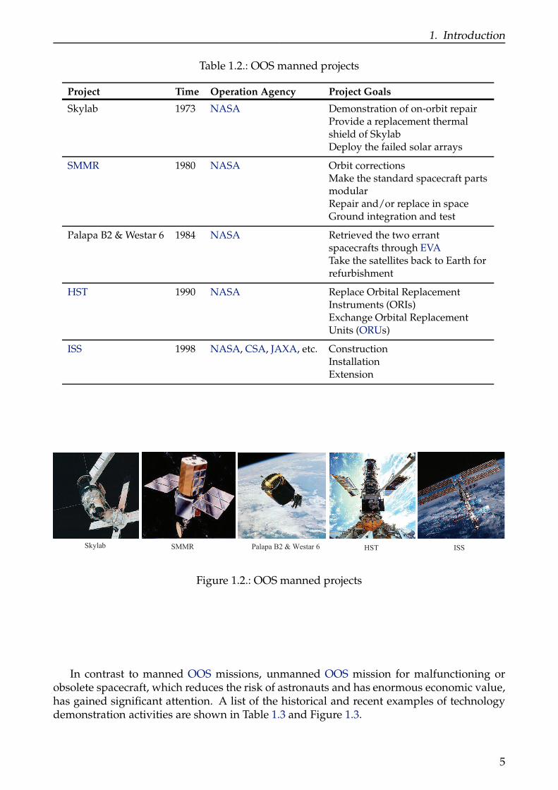
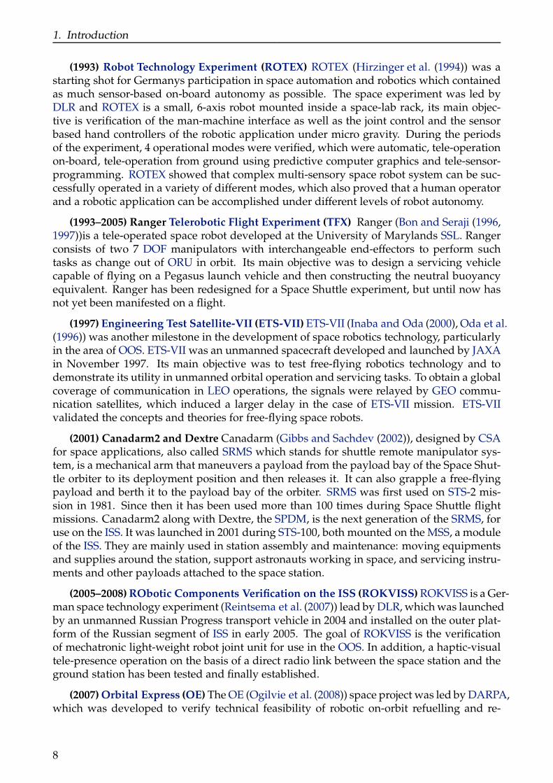
The first planned OOS mission was performed in 1973 on Skylab, through EVA. After that,refer to NASA (2010), numbers of OOS projects have been conducted with human-in-the-loop which are listed in Table 1.2 and Figure 1.2.
4
1. Introduction
Table 1.2.: OOS manned projects
Project Time Operation Agency Project Goals
Skylab 1973 NASA Demonstration of on-orbit repairProvide a replacement thermalshield of SkylabDeploy the failed solar arrays
SMMR 1980 NASA Orbit correctionsMake the standard spacecraft partsmodularRepair and/or replace in spaceGround integration and test
Palapa B2 & Westar 6 1984 NASA Retrieved the two errantspacecrafts through EVATake the satellites back to Earth forrefurbishment
HST 1990 NASA Replace Orbital ReplacementInstruments (ORIs)Exchange Orbital ReplacementUnits (ORUs)
ISS 1998 NASA, CSA, JAXA, etc. ConstructionInstallationExtension
Skylab SMMR Palapa B2 & Westar 6 HST ISS
Figure 1.2.: OOS manned projects
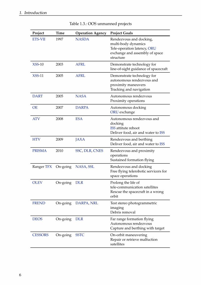
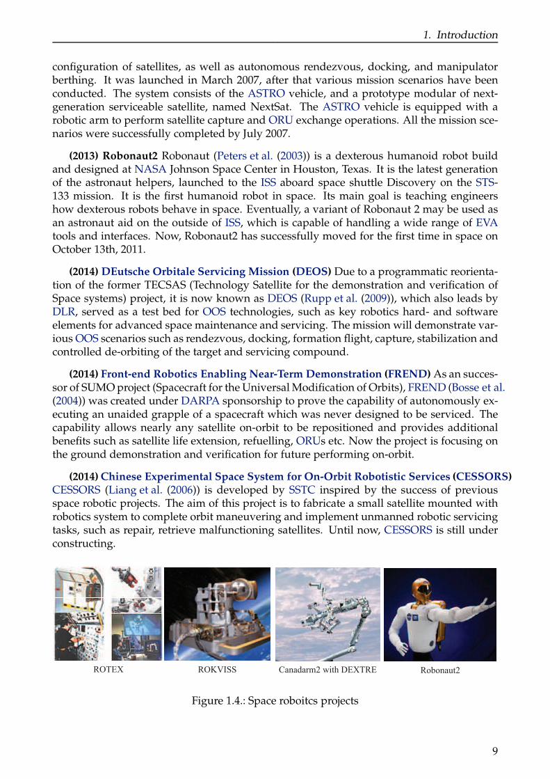
In contrast to manned OOS missions, unmanned OOS mission for malfunctioning orobsolete spacecraft, which reduces the risk of astronauts and has enormous economic value,has gained significant attention. A list of the historical and recent examples of technologydemonstration activities are shown in Table 1.3 and Figure 1.3.
5
1. Introduction
Table 1.3.: OOS unmanned projects
Project Time Operation Agency Project Goals
ETS-VII 1997 NASDA Rendezvous and docking,multi-body dynamicsTele-operation latency, ORUexchange and assembly of spacestructure
XSS-10 2003 AFRL Demonstrate technology forline-of-sight guidance of spacecraft
XSS-11 2005 AFRL Demonstrate technology forautonomous rendezvous andproximity maneuversTracking and navigation
DART 2005 NASA Autonomous rendezvousProximity operations
OE 2007 DARPA Autonomous dockingORU exchange
ATV 2008 ESA Autonomous rendezvous anddockingISS attitute rebootDeliver food, air and water to ISS
HTV 2009 JAXA Rendezvous and berthingDeliver food, air and water to ISS
PRISMA 2010 SSC, DLR, CNES Rendezvous and proximityoperationsSustained formation flying
Ranger TFX On-going NASA, SSL Rendezvous and dockingFree flying telerobotic servicers forspace operations
OLEV On-going DLR Prolong the life oftele-communication satellitesRescue the spacecraft in a wrongorbit
FREND On-going DARPA, NRL Test stereo photogrammetricimagingDebris removal
DEOS On-going DLR Far range formation flyingAutonomous rendezvousCapture and berthing with target
CESSORS On-going SSTC On-orbit maneuveringRepair or retrieve malfuctionsatellites
6

1. Introduction
XSS-10 DART
PRISMA OLEV
ATV
XSS-11
DEOSFREND
ETS-VII
OE HTV
Ranger TFX
CESSORS
Figure 1.3.: OOS unmanned projects
1.2.2. Space Robotics Demonstrators
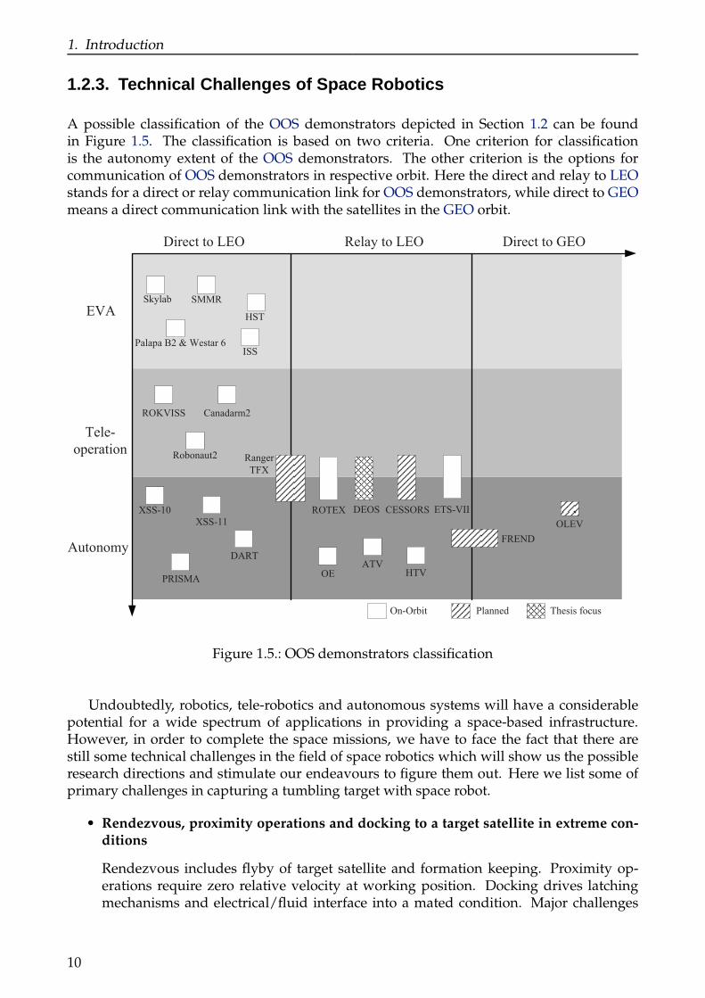
It has already been decades since the first robotic manipulator arm – space shuttle remotemanipulator system applied in the STS-2 mission in 1981. Here we will give a brief overviewof the past and undergoing space robotic demonstrators.
7
1. Introduction
(1993) Robot Technology Experiment (ROTEX) ROTEX (Hirzinger et al. (1994)) was astarting shot for Germanys participation in space automation and robotics which containedas much sensor-based on-board autonomy as possible. The space experiment was led byDLR and ROTEX is a small, 6-axis robot mounted inside a space-lab rack, its main objec-tive is verification of the man-machine interface as well as the joint control and the sensorbased hand controllers of the robotic application under micro gravity. During the periodsof the experiment, 4 operational modes were verified, which were automatic, tele-operationon-board, tele-operation from ground using predictive computer graphics and tele-sensor-programming. ROTEX showed that complex multi-sensory space robot system can be suc-cessfully operated in a variety of different modes, which also proved that a human operatorand a robotic application can be accomplished under different levels of robot autonomy.
(1993–2005) Ranger Telerobotic Flight Experiment (TFX) Ranger (Bon and Seraji (1996,1997))is a tele-operated space robot developed at the University of Marylands SSL. Rangerconsists of two 7 DOF manipulators with interchangeable end-effectors to perform suchtasks as change out of ORU in orbit. Its main objective was to design a servicing vehiclecapable of flying on a Pegasus launch vehicle and then constructing the neutral buoyancyequivalent. Ranger has been redesigned for a Space Shuttle experiment, but until now hasnot yet been manifested on a flight.
(1997) Engineering Test Satellite-VII (ETS-VII) ETS-VII (Inaba and Oda (2000), Oda et al.(1996)) was another milestone in the development of space robotics technology, particularlyin the area of OOS. ETS-VII was an unmanned spacecraft developed and launched by JAXAin November 1997. Its main objective was to test free-flying robotics technology and todemonstrate its utility in unmanned orbital operation and servicing tasks. To obtain a globalcoverage of communication in LEO operations, the signals were relayed by GEO commu-nication satellites, which induced a larger delay in the case of ETS-VII mission. ETS-VIIvalidated the concepts and theories for free-flying space robots.
(2001) Canadarm2 and Dextre Canadarm (Gibbs and Sachdev (2002)), designed by CSAfor space applications, also called SRMS which stands for shuttle remote manipulator sys-tem, is a mechanical arm that maneuvers a payload from the payload bay of the Space Shut-tle orbiter to its deployment position and then releases it. It can also grapple a free-flyingpayload and berth it to the payload bay of the orbiter. SRMS was first used on STS-2 mis-sion in 1981. Since then it has been used more than 100 times during Space Shuttle flightmissions. Canadarm2 along with Dextre, the SPDM, is the next generation of the SRMS, foruse on the ISS. It was launched in 2001 during STS-100, both mounted on the MSS, a moduleof the ISS. They are mainly used in station assembly and maintenance: moving equipmentsand supplies around the station, support astronauts working in space, and servicing instru-ments and other payloads attached to the space station.
(2005–2008) RObotic Components Verification on the ISS (ROKVISS) ROKVISS is a Ger-man space technology experiment (Reintsema et al. (2007)) lead by DLR, which was launchedby an unmanned Russian Progress transport vehicle in 2004 and installed on the outer plat-form of the Russian segment of ISS in early 2005. The goal of ROKVISS is the verificationof mechatronic light-weight robot joint unit for use in the OOS. In addition, a haptic-visualtele-presence operation on the basis of a direct radio link between the space station and theground station has been tested and finally established.
(2007) Orbital Express (OE) The OE (Ogilvie et al. (2008)) space project was led by DARPA,which was developed to verify technical feasibility of robotic on-orbit refuelling and re-
8
1. Introduction
configuration of satellites, as well as autonomous rendezvous, docking, and manipulatorberthing. It was launched in March 2007, after that various mission scenarios have beenconducted. The system consists of the ASTRO vehicle, and a prototype modular of next-generation serviceable satellite, named NextSat. The ASTRO vehicle is equipped with arobotic arm to perform satellite capture and ORU exchange operations. All the mission sce-narios were successfully completed by July 2007.
(2013) Robonaut2 Robonaut (Peters et al. (2003)) is a dexterous humanoid robot buildand designed at NASA Johnson Space Center in Houston, Texas. It is the latest generationof the astronaut helpers, launched to the ISS aboard space shuttle Discovery on the STS-133 mission. It is the first humanoid robot in space. Its main goal is teaching engineershow dexterous robots behave in space. Eventually, a variant of Robonaut 2 may be used asan astronaut aid on the outside of ISS, which is capable of handling a wide range of EVAtools and interfaces. Now, Robonaut2 has successfully moved for the first time in space onOctober 13th, 2011.
(2014) DEutsche Orbitale Servicing Mission (DEOS) Due to a programmatic reorienta-tion of the former TECSAS (Technology Satellite for the demonstration and verification ofSpace systems) project, it is now known as DEOS (Rupp et al. (2009)), which also leads byDLR, served as a test bed for OOS technologies, such as key robotics hard- and softwareelements for advanced space maintenance and servicing. The mission will demonstrate var-ious OOS scenarios such as rendezvous, docking, formation flight, capture, stabilization andcontrolled de-orbiting of the target and servicing compound.
(2014) Front-end Robotics Enabling Near-Term Demonstration (FREND) As an succes-sor of SUMO project (Spacecraft for the Universal Modification of Orbits), FREND (Bosse et al.(2004)) was created under DARPA sponsorship to prove the capability of autonomously ex-ecuting an unaided grapple of a spacecraft which was never designed to be serviced. Thecapability allows nearly any satellite on-orbit to be repositioned and provides additionalbenefits such as satellite life extension, refuelling, ORUs etc. Now the project is focusing onthe ground demonstration and verification for future performing on-orbit.
(2014) Chinese Experimental Space System for On-Orbit Robotistic Services (CESSORS)CESSORS (Liang et al. (2006)) is developed by SSTC inspired by the success of previousspace robotic projects. The aim of this project is to fabricate a small satellite mounted withrobotics system to complete orbit maneuvering and implement unmanned robotic servicingtasks, such as repair, retrieve malfunctioning satellites. Until now, CESSORS is still underconstructing.
ROTEX ROKVISS Canadarm2 with DEXTRE Robonaut2
Figure 1.4.: Space roboitcs projects
9
1. Introduction
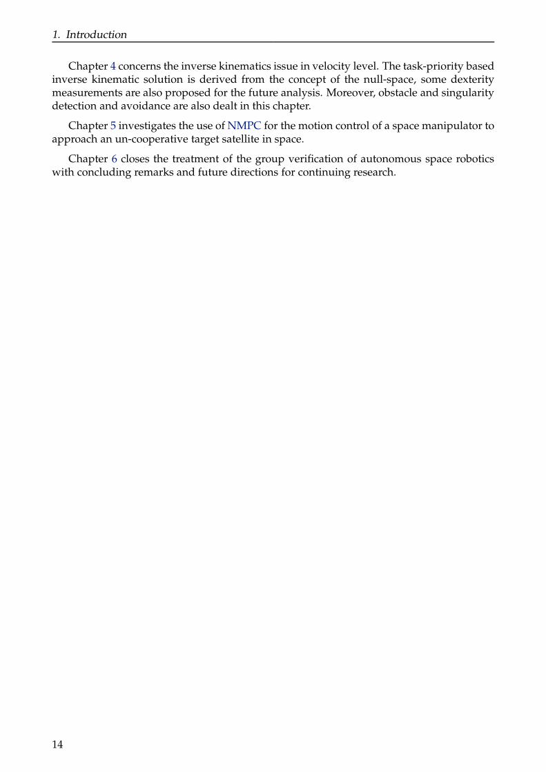
1.2.3. Technical Challenges of Space Robotics
A possible classification of the OOS demonstrators depicted in Section 1.2 can be foundin Figure 1.5. The classification is based on two criteria. One criterion for classificationis the autonomy extent of the OOS demonstrators. The other criterion is the options forcommunication of OOS demonstrators in respective orbit. Here the direct and relay to LEOstands for a direct or relay communication link for OOS demonstrators, while direct to GEOmeans a direct communication link with the satellites in the GEO orbit.
EVA
Tele-
operation
Autonomy
Direct to LEO Relay to LEO Direct to GEO
On-Orbit Planned Thesis focus
Skylab SMMR
Palapa B2 & Westar 6
HST
ISS
XSS-10
XSS-11
DART
OE
OLEV
ROTEX ETS-VIIDEOS
FREND
ATVHTV
CESSORS
PRISMA
Ranger
TFX
ROKVISS Canadarm2
Robonaut2
Figure 1.5.: OOS demonstrators classification
Undoubtedly, robotics, tele-robotics and autonomous systems will have a considerablepotential for a wide spectrum of applications in providing a space-based infrastructure.However, in order to complete the space missions, we have to face the fact that there arestill some technical challenges in the field of space robotics which will show us the possibleresearch directions and stimulate our endeavours to figure them out. Here we list some ofprimary challenges in capturing a tumbling target with space robot.
• Rendezvous, proximity operations and docking to a target satellite in extreme con-ditions
Rendezvous includes flyby of target satellite and formation keeping. Proximity op-erations require zero relative velocity at working position. Docking drives latchingmechanisms and electrical/fluid interface into a mated condition. Major challenges
10

1. Introduction
include completing above missions optimally in all range of lighting conditions, with-out collision and violating the actuators’ work limits.
• Object recognition and state estimation under space environment
To search and find an un-cooperative target without communication link in space is anintractable task. After the target is detected, since there is no prior knowledge abouttarget, its geometry must be reconstructed with sensory data to estimate the states ofthe target and determine the grasping point and capturing strategies.
• Full immersion tele-presence with haptic and multi modal sensor feedback
Tele-presence will provide the operator a physical sense of working at the place ofspace robot. It must be as real as the robot working site which need multiple modalsensor feedback, such as fully immersion displays, sound, touch, etc.
• Supervised autonomy with time-delay
Complete autonomy of robotics still relies on the advancement of AI. So a supervisedautonomy or the tele-operation would be a realistic choice. But the communicationtime-delay in the control loop will degrade the ability to tele-operation. Challenges in-clude the run-time states prediction, visualization prediction and ability to work aheadof real-time.
• Understanding the distinctive characteristics of space robotic dynamics
Space robotics with a floating base possesses some particular properties compared tofixed base robot. The interaction between space manipulator and it base (spacecraft)will induce some difficulties in controller design and path planning.
• Optimized motion planning and control with various constraints during capturingphase
All real systems have some constraints, such as input and output boundaries, possiblecollision, etc. During capturing, it would be of great benefit if the system can han-dle all these constraints optimally while achieving some optimization index. Majorchallenges include developing a general framework to realize on-line path planning,constraints handling, and optimization simultaneously.
• Verification and validation of autonomous system on-board
The software of space robots running on-orbit autonomously is a big software engi-neering project. It includes different subsystems from various programmers. Exhaus-tive and deep exploration of the codes has to be done before launch. Verification andvalidation techniques are required to more fully assure the feasibility and reliability inall conditions.
11

1. Introduction
1.3. Hypothesis and Problem Statements
As illustrated in section 1.2.3, in order to complete capturing an un-cooperative target satel-lite using space robot, the major objective of this work is how to control the space robot toexecute the required missions in complex space environment. Traditional control schemescan be classified by different objectives:
Resolved Motion Rate Controller was first proposed for a free-floating space manipulator inUmetani and Yoshida (1989) using the GJM. Later, similar controllers designed for kinemat-ically non-redundant and redundant manipulators can be found in Masutani et al. (1989),Nenchev (1993), Papadopoulos and Moosavian (1994), Rekleitis et al. (2007), Xu and Kanade(1993).
Adaptive Controller is another widely developed strategy since it can be used to overcomethe uncertainties and parameters variation issues. However, since the high non-linearity ofthe dynamics of space robot, the design of the adaptive control law is not easy. The appli-cation of adaptive control can be found in Abiko and Hirzinger (2007), Gu and Xu (1993),Wang and Xie (2009), Xu et al. (1992), Xu (1991).
Robust Controller provides another feasible controller solution for space robot to handlethe parameters variation and unknown dynamics effects. The application of robust controlfor single or dual-arm can be found in Huang et al. (2007), Pathak et al. (2008), Tang et al.(2011), Xu et al. (1995).
Among aforementioned controllers, the possible collision and singularity issues duringmotion of space robot are out of consideration, moreover, input/output constraints of thesystem are also difficult to incorporate into the control schemes. Accordingly, the hypothesisof this work is:
The conventional control framework based on traditional control strategies are not adequateto solve the motion control issue of space manipulator in capturing another tumbling targetwhen obstacle and singularity issues are taken into account.
Originated from chemical processing industries, Model Predictive Control (MPC), alsoreferred to Receding Horizon Control (RHC), has gradually expanded its application to thefield of aerospace such as spacecraft formation keeping Manikonda et al. (1999), spacecrafttrajectory planning Richards et al. (2002), rendezvous and docking with a tumbling targetPark et al. (2011), etc. As an effective control strategy, MPC has the capacity to handle theconstraints and perform on-line optimization. Nevertheless, the application of MPC requiresan explicit system model for states prediction. Similarly, if collision and singularity issuesare considered in the design of MPC, they must be handled in advance and integrated intothe framework of controller. Therefore, the problems for this work can be listed as follows:
• The dynamics equations of the space robotic system must be derived to represent therelationship between the states acceleration response and the given forces and torques;
• Computational efficient collision detection algorithm which can deal with multipleconvex and non-convex obstacles has to be completed when space robot works in acomplex environment;
• Singularity issue during the motion of space robot must be taken into account to im-pede the joint from generating enormous velocity;
12

1. Introduction
• With the derived dynamics equations of space robotics system, MPC strategy can beimplemented for the space robot to perform the capturing mission.
1.4. Scope of Work
1.4.1. Research Scope within Space Robotics
With the advancement of science and technology, especially great progress in the field ofcomputer science, the extent of autonomy in OOS is increasing, while human operator, asan indispensable role, will play as a monitor or supervisor role without involving direct op-eration too much. In light of space robots currently planned by world wide space agencies,an increase in the number and the capacity of robots applied in space missions will be aforegone conclusion in the coming years. In summary, the concept of tele-operated and fullautonomy of space robotics, as main concern in this thesis, seems advantageous for OOSoperation, since it alleviates the operators’ workload and avoids the human involving in thedirect operations. Accordingly, refer to section 1.3, we can break our main goal down to itsparticulars into the following aspects:
• Development and design of a simulation and test environment, representative forspace robotics;
• Evaluation the influence of geometry to the dynamics of space robotics;
• Provision of specific algorithms for obstacle and singularity avoidance in inverse kine-matics control;
• Construction of a general control framework based on MPC with various constraintsfor autonomous space robotics;
• Assessment of the feasibility of the proposed general control framework.
1.4.2. Thesis Roadmap
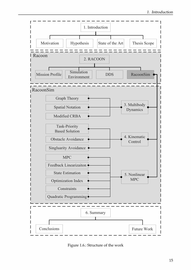
The overview of the thesis structure is presented in Figure 1.6. An introductory part aboutthe research motivation, state of the art, and research scope within space robotics are in-cluded in Chapter 1.
Chapter 2 presents a new distributed real-time simulation architecture based on DDSfor space robotic autonomous and tele-operation tasks. The space mission profile and back-ground of space robotic tele-operation are firstly recalled. Within this context, a closer lookinto RACOON system overall design and simulation environment are described. The de-tailed characters of DDS are subsequently exhibited. Next, RacoonSim system and its relatedsubsystems are introduced. Additionally, a user-friendly VR user interface for coexistenceof working operator and space robot is developed.
Chapter 3 focuses on a modelling scheme that uses the concepts of graph theory andspatial notation for calculating the joint-space dynamics of general tree structure space ma-nipulator systems. This chapter is relevant to the development of appropriate trajectoryplanning and control algorithms in the following chapters.
13
1. Introduction
Chapter 4 concerns the inverse kinematics issue in velocity level. The task-priority basedinverse kinematic solution is derived from the concept of the null-space, some dexteritymeasurements are also proposed for the future analysis. Moreover, obstacle and singularitydetection and avoidance are also dealt in this chapter.
Chapter 5 investigates the use of NMPC for the motion control of a space manipulator toapproach an un-cooperative target satellite in space.
Chapter 6 closes the treatment of the group verification of autonomous space roboticswith concluding remarks and future directions for continuing research.
14
1. Introduction
1. Introduction
Motivation State of the Art Thesis Scope
Racoon2. RACOON
Mission ProfileSimulation
EnvironmentRacoonSimDDS
6. Summary
Conclusions Future Work
3. Multibody
Dynamics
Graph Theory
Spatial Notation
Modified CRBA
Task-Priority
Based Solution
Obstacle Avoidance
Singluarity Avoidance
MPC
Feedback Linearizaiton
State Estimation
Optimization Index
Constraints
Quadratic Programming
RacoonSim
4. Kinematic
Control
5. Nonlinear
MPC
Hypothesis
Figure 1.6.: Structure of the work
15

2. Simulation System Design
I do not fear computers. I fear the lack of them.
—Isaac Asimov
The increasing demands of satellite maintenance, on-orbit assembly and space debris re-moval etc. call for applications of space robot to perform tasks in the particular harsh spaceenvironment. However, it is still impossible to develop a fully autonomous space robot withthe present robotic technology until now. For this reason, an operator tele-operating spacerobot from ground station becomes an option. To lengthen in duration and enlarge the scopeof tele-operation, a Geostationary Orbit (GEO) relay satellite is employed to address thecommunication issue between ground station and servicer satellite. This chapter presents anew distributed real-time simulation architecture based on Data Distribution Service (DDS)for space robotic tele-operation tasks. The objective is to make the simulation architectureopen for collaborative tele-operation research and provide the operator an intuitive view ofspace robotic tele-operation in a wide set of scenarios. The mission profile and backgroundof space robotic tele-operation are firstly recalled. Within this context, a closer look intoRobotic Actuation, Control and On Orbit Navigation Laboratory (RACOON) system over-all design and simulation environment are described. Secondly, the detailed charactersof DDS, including DDS specification and its core idea of data distribution, are exhibited.Thirdly, Racoon Simulation (RacoonSim) system, which comprises multi-body dynamics,Autonomous Mission Management (AMM), path & trajectory planning and control subsys-tems of space manipulator, is introduced. Additionally, a user-friendly Virtual Reality (VR)user interface for coexistence of working operator and space robot is developed, which iscomposed of 3 dimensional space mouse, joystick and Head-Up Display (HUD) as part ofthe Mission Control Center (MCC). Well-designed simulation system architecture makes theHardware-in-loop (HIL) verification possible and can be extended easily in the future.
2.1. Mission Profile
A typical OOS mission is composed of a series of space missions. Before a specific OOSoperation is executed, some operations about spacecraft must be conducted to decrease therelative distance between spacecraft and target satellite. During this period, lots of demon-stration missions can also be performed such as flyby, formation flying to test the feasibilityof new sensors and technologies. After the servicer satellite moves into the work scope of thespace manipulator, space robot will take charge of the OOS mission to perform the subse-quent mission flow. A typical OOS mission before capturing can be described as follows:
17
2. Simulation System Design
1. Attitude control The servicer satellite together with space manipulator is separatedfrom the upper stage of the rocket and released into space. At the beginning of itsorbital life, an attitude reconstruction procedure has to be performed to stabilize theservicer satellite. Attitude determination equipment such as infrared horizon sensor,sun sensor or gyroscope can be employed to assist the attitude reconstruction of theservicer satellite.
2. Drift orbit After the success of attitude control, the servicer satellite moves into thedrift orbit phase. In this phase, orbit phasing will be conducted to regulate the orbitof servicer into the same orbit as the target satellite or a slightly lower orbit. Theattitude of servicer satellite will be maintained, absolute navigation equipment likestar trackers, IMU and GPS receivers will be used during this phase.
3. Rendezvous At the end of the drift orbit phase, the servicer satellite is at a positionwithin a distance of 5 km to 300 m of the target. The phase will utilize the absoluteand relative navigation equipment like GPS, IMU, radar or lidar to guide the servicersatellite into a range of 300 m for the future space missions.
4. Proximity When the servicer satellite moves within 300 m of the target satellite, a prox-imity procedure starts to drive the servicer to the target from 300 m to several meters.Besides the relative distance, the relative attitude and the relative translational and an-gular velocities between the two satellites have to be decreased for the coming dockingmission. In this phase, the visual sensors can be added in for target tracking and mon-itoring. The MCC will observe the whole rendezvous and proximity phases. Whenthe relative sensors lose the target or the service moves into an unsafe region, an emer-gence action has to be taken autonomously or commanded by the operators.
5. Station keeping Before the action of the space manipulator, a phase named stationkeeping has to be performed to guarantee the safety of the coming robotic operations.During this phase, the target satellite will be in the workspace of space manipulator. Acontrol loop must be closed on board to keep the relative position and orientation outof collision.
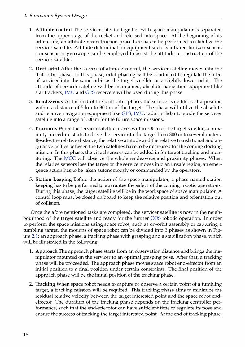
Once the aforementioned tasks are completed, the servicer satellite is now in the neigh-bourhood of the target satellite and ready for the further OOS robotic operation. In orderto perform the space missions using space robot, such as on-orbit assembly or capturing atumbling target, the motions of space robot can be divided into 3 phases as shown in Fig-ure 2.1: an approach phase, a tracking phase with grasping and a stabilization phase, whichwill be illustrated in the following.
1. Approach The approach phase starts from an observation distance and brings the ma-nipulator mounted on the servicer to an optimal grasping pose. After that, a trackingphase will be proceeded. The approach phase moves space robot end-effector from aninitial position to a final position under certain constraints. The final position of theapproach phase will be the initial position of the tracking phase.
2. Tracking When space robot needs to capture or observe a certain point of a tumblingtarget, a tracking mission will be required. This tracking phase aims to minimize theresidual relative velocity between the target interested point and the space robot end-effector. The duration of the tracking phase depends on the tracking controller per-formance, such that the end-effecotor can have sufficient time to regulate its pose andensure the success of tracking the target interested point. At the end of tracking phase,
18
2. Simulation System Design
neither the end-effector nor the robot joints are at rest. Their states will be the initialvalue of the next phase.
3. Stabilization Once the relative pose between space robot end-effector and target in-terested point reduces to zero and the gripper on the end-effector is closed, in orderto retain the stable attitude of the target, a stabilization phase must be carried out todecrease the angular velocity of the target to zero and be ready for further space oper-ations. In the stabilization phase, by exerting external forces and torques or adjustingthe internal torques of robot joints simultaneously, the relative motion between theservicer and the target will be brought to zero.
Far Range Satellite Maneuver Close Range Operation by Space Manipulator
Rendezvous Approach Tracking Stabilization
TargetTarget
Target
Servicer
Servicer
Servicer
Figure 2.1.: Mission profile of space robot
After the space manipulator completing the capture, further space operations can be car-ried out such as inspection, de-orbit or ORU exchange, etc. In fact, besides above generaluses of space robot, there are still some other potential applications of space robot. For ex-ample, as a result of dynamic coupling between spacecraft and space manipulator, it can beutilized to regulate spacecraft attitude for decreasing on-board fuel consumption. Accord-ing to the external force and torque exerted on the spacecraft, the servicer satellite will beoperated in three flying modes. If there are no forces and torques exert on the servicer, itis termed free-floating mode. When only torque is applied to the servicer, it is called free-flying mode. Another mode is auto-flying mode. Before-mentioned three kinds of spacephases can be performed under these three flying modes. The flying modes switch can becontrolled by the operator in terms of the particular requirements.
2.2. Simulation Overall Design
2.2.1. Racoon Design
The RACOON system is designed to assist the operator with intuitive view and validate thefeasibility and the performance of the on-going space robot project. Hence, the followingsubsystems will be included in the RACOON system. A schematic diagram of RACOONsystem is shown in Figure 2.2.
19

2. Simulation System Design
Figure 2.2.: Subsystems of Racoon Lab
Operator Console: It is an alias of MCC. The operator will send a series of commandsfrom MCC uplink to the servicer satellite via the GEO relay satellite. The communicationrelay will be simulated by adding an individual node in the simulation system to relay theinformation. MCC will also receive the telemetry information collected from the states ofspace robot & target satellite and display them on a big screen to help the operator enhancethe awareness and understand of the real-time situation in space. The operator can alsocontrol the space robot in real-time by joystick or 3 dimensional space mouse. A VR isalso running when the operation is proceeding. These will be introduced in detail in theSection 2.3.5.
TM/TC: This subsystem is responsible for the signal relay between MCC and GEO re-lay satellite. It transmits the tele-commands from MCC to the GEO relay satellite and thetelemetry information from servicer to the MCC. The information dissemination betweenvarious nodes is based on DDS.
RacoonSim: This system contains two subsystems, one is dynamics of servicer and tar-get, and the other is OBDH subsystem. For detailed description of RacoonSim system designwill be presented in Section 2.3.
Hardware-in-loop (HIL): This system can include different types of hardware, such assensors, actuators, etc. Since the expandability and scalability of the simulation system, theproposed simulation architecture is easy to replace the software by particular hardware.
2.2.2. Simulation Environment
One of the first and major implementation solutions adopted was to build RACOON ontop of Matlab/Simulink environment (see Figure 2.3). This environment integrates suffi-cient properties to cope with the aforementioned requirements, assuring high flexibility andavailability of existed functionality.
20

2. Simulation System Design
XML/IDL
C/C++
VRML
CAD (CATIA/SolidWorks)
Java/JavaScript
Simulink CoderSimulink
Stateflow
MATLAB
Hardware
Virtual Reality
Figure 2.3.: Simulation environment of Racoon
Normally, modern engineering design starts from the application of CAD system, such asCATIA®or SolidWorks®. CAD can assist the designer in the creation, modification, analysis,or optimization of a design. On the one hand, it provides the designer an efficient andintuitive tool to improve the quality of the design and increase the productivity. On theother hand, the objects designed by CAD will be as a basic input of VR. In this paper, VRMLis chosen to represent 3 dimensional interactive vector graphics. In order to increase theinteractivity and immersion of the operator, Java/JavaScript is integrated into VRML to dealwith the interactive event response issue. The transformation between CAD and VRML canbe implemented by using different software.
XML is a mark-up language that defines a set of rules for encoding documents in a formatthat is both human-readable and machine-readable. Its main design goals are simplicity,generality and usability over the Internet. In our design, XML is utilized to describe theconfigurations and initial states of the RACOON system. Another application for XML isDDS QoS configuration.
As a major programming language, C/C++ programming language can establish con-nections among various applications. That’s why it is also employed here to deal with thedifferent interfaces of relevant applications involved in RACOON. Before simulation starts,it proceeds the XML file to extract the configuration and initial states of RACOON simu-lation system. Furthermore, it is employed to process the IDL file which is subsequentlyinvolved in DDS.
At the core of RACOON simulation system is Matlab/Simulink/Stateflow/SimulinkCoder, where Simulink is a data flow graphical programming environment for modelingand simulating multi-domain dynamic systems. A number of hardware and software prod-ucts are available for use with Simulink. Stateflow, integrated in Simulink, provides a con-trol logic tool to model reactive systems via state machines and flow charts. Coupled withSimulink Coder, Simulink model can automatically generate C/C++ source code for dis-tributed real-time simulation.
21
2. Simulation System Design
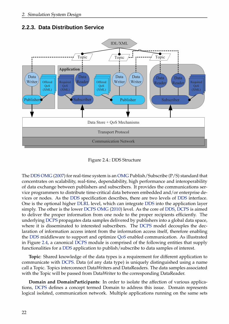
2.2.3. Data Distribution Service
Application
Data
Writer
IDL/XML
Topic TopicTopic
Subscriber Publisher Subscriber
Data
Reader
Data
ReaderData
Reader
Communication Network
Transport Protocol
Data Store + QoS Mechanisms
Publisher
Data
Writer
Data
WriterOffered
QoS
(XML)
Required
QoS
(XML)
Offered
QoS
(XML)
Required
QoS
(XML)
Figure 2.4.: DDS Structure
The DDS OMG (2007) for real-time system is an OMG Publish/Subscribe (P/S) standard thatconcentrates on scalability, real-time, dependability, high performance and interoperabilityof data exchange between publishers and subscribers. It provides the communications ser-vice programmers to distribute time-critical data between embedded and/or enterprise de-vices or nodes. As the DDS specification describes, there are two levels of DDS interface.One is the optional higher DLRL level, which can integrate DDS into the application layersimply. The other is the lower DCPS OMG (2010) level. As the core of DDS, DCPS is aimedto deliver the proper information from one node to the proper recipients efficiently. Theunderlying DCPS propagates data samples delivered by publishers into a global data space,where it is disseminated to interested subscribers. The DCPS model decouples the dec-laration of information access intent from the information access itself, therefore enablingthe DDS middleware to support and optimize QoS enabled communication. As illustratedin Figure 2.4, a canonical DCPS module is comprised of the following entities that supplyfunctionalities for a DDS application to publish/subscribe to data samples of interest.
Topic: Shared knowledge of the data types is a requirement for different application tocommunicate with DCPS. Data (of any data type) is uniquely distinguished using a namecall a Topic. Topics interconnect DataWriters and DataReaders. The data samples associatedwith the Topic will be passed from DataWriter to the corresponding DataReader.
Domain and DomainParticipants: In order to isolate the affection of various applica-tions, DCPS defines a concept termed Domain to address this issue. Domain representslogical isolated, communication network. Multiple applications running on the same sets
22

2. Simulation System Design
of hosts on different Domains are totally isolated from each other. Applications that wantto exchange data must belong to the same Domain. To belong to a Domain, DCPS APIs areused to configure and create a DomainParticipant with a specific Domain Index. Domainsare differentiated by the Domain Index. Applications that have created DomainParticapantswith the same Domain Index belong to the same Domain. DomainParticipant includes Top-ics, Publishers and Subscribers. Therefore all the DCPS entities belong to a Domain.
Publisher and DataWriter: The data sending side used entities call publishers and DataWrit-ers. A DataWriter is the actual object used to send data samples. It is associated with a singletopic. A publisher is the DCPS object responsible for the actual sending data. Publisher ownand manage a group of DataWriters with similar behaviour or QoS policies. When data isassigned to send to an application, it first calls the method on a DataWriter, the data sam-ple is then passed to the publisher object which does actually dissemination of data on thenetwork.
Subscriber and DataReader: The data receiving side uses objects call subscribers andDataReaders. A DataReader is the actual object used to receive the published data samples.It is associated with a single topic. A subscriber is the DCPS object responsible for the actualreceiving data. Subscribers own and manage a group of DataReaders with similar behaviouror QoS policies. When data is sent to an application, it is first processed by a subscriber, thedata sample is then stored in the appropriate DataReader.
QoS Policies: For real-time applications, the following features, such as efficiency, de-terminism, flexible delivery bandwidth, thread awareness and fault-tolerant operations areoften required. DCPS, and thus DDS, are designed and implemented specifically to addressthese requirements through the configuration parameters know as QoS policies defined byDCPS standard. QoS policies control many aspects of how and when data are distributedbetween applications. It is a significant feature of DDS for the users to configure the QoSpolicies for each DDS entity or communication node. Until now, over 50 QoS policies cate-gories are supported by DDS. Therefore, users can employ various QoS policies to controlnumbers of behaviour of communication entities (DomainParticipant, Topic, Publisher/-Subscriber, DataWriter/DataReader) utilized in your applications.
23

2. Simulation System Design
Racoon Simulation
Ethernet
TM/TC Relay Mission Control Center
Dynamics System OBDH System Hardware
DDS DDS
DDS DDS DDS
Servicer Target
Relay Algorithm
Planning Controller Sensor Actuator
VR Joystick & 3D MouseGUI
Figure 2.5.: Racoon system set-up
The entities and properties of DDS presented above bring important benefit to simu-lation applications, such as low latency, better communication determinism and runtimebehaviour, enhanced QoS polices and wire interoperability, which makes the DDS middle-ware a necessary choice for building a distributed real-time simulation system. The publish-subscribe approach to distributed communications is a generic mechanism that can be em-ployed by many different types of applications. Based on the DDS middleware used throughEthernet and the overall design in Section 2.2.1, we developed the space tele-operationsimulator with 5 relevant subsystems running on the separate host computers. The twosubsystems in dashed rectangle in Figure 2.5 are the core simulation part which is termedRacoonSim and will be illustrated in Section 2.3 in detail. MCC system acquires operatorinputs and gives the force and scenery feedback to the operator. TM/TC relay system cal-culates the relative states among MCC, servicer and GEO relay satellite, and simulates thephenomenon of signal relay among them. Hardware system incorporates the instruments(sensors, actuators, etc.) and feedback to OBDH and Dynamic system, respectively.
2.3. RacoonSim Design
RacoonSim, the core of the RACOON laboratory, as shown in Figure 2.6, includes threeprimary parts: dynamics, OBDH, and human-machine interface. Dynamics algorithm ismainly responsible for simulation of 6 DOF target satellite and multiple DOF space ma-nipulator. Human-machine interface provides a means for operator to interact with theRacoonSim system and intensifies the ability of perception and immension. OBDH system,which is the guarantee for completing the OOS mission, is composed of AMM, path & trajec-tory planning, and motion controller subsystems, which will be described in the followingsections.
24
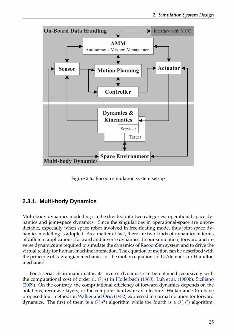
2. Simulation System Design
Multi-body Dynamics
Target
Dynamics &
Kinematics
Servicer
Space Environment
On-Board Data Handling
AMMAutonomous Mission Management
ActuatorSensor Motion Planning
Interface with MCC
Controller
Figure 2.6.: Racoon simulation system set-up
2.3.1. Multi-body Dynamics
Multi-body dynamics modelling can be divided into two categories: operational-space dy-namics and joint-space dynamics. Since the singularities in operational-space are unpre-dictable, especially when space robot involved in free-floating mode, thus joint-space dy-namics modelling is adopted. As a matter of fact, there are two kinds of dynamics in termsof different applications: forward and inverse dynamics. In our simulation, forward and in-verse dynamics are required to simulate the dynamics of RacoonSim system and to drive thevirtual reality for human-machine interaction. The equation of motion can be described withthe principle of Lagrangian mechanics, or the motion equations of D’Alembert, or Hamiltonmechanics.
For a serial chain manipulator, its inverse dynamics can be obtained recursively withthe computational cost of order n, O(n) in Hollerbach (1980), Luh et al. (1980b), Siciliano(2009). On the contrary, the computational efficiency of forward dynamics depends on thenotations, recursive layers, or the computer hardware architecture. Walker and Orin haveproposed four methods in Walker and Orin (1982) expressed in normal notation for forwarddynamics. The first of them is a O(n3) algorithm while the fourth is a O(n2) algorithm.
25
2. Simulation System Design
Balafoutis in Balafoutis and Patel (1989), Balafoutis et al. (1988) derived a more efficient al-gorithm by using orthogonal Cartesian tensors. With the concept of spatial notation, Lillyin Lilly and Orin (1991), Lilly and Bonaventura (1995), Featherstone in Featherstone and Orin(2000), Featherstone (2008) have developed a modified version of CRBA, which need lesscomputing effort. With the aid of the decoupled natural orthogonal complement, Sahain Saha (1999) have obtained another set of motion equations based on Euler-Lagrange me-chanics. In addition, Park, Bobrow and Sohl in Park et al. (1995), Sohl and Bobrow (2001)provided a recursive multi-body dynamics for branched kinematic chains using the tech-nique and notation from the theory of Lie groups and Lie algebras. McMillan and Orinin McMillan and Orin (1995), McMillan et al. (1995) developed an ABA which produces aO(n) forward dynamic algorithm without an explicit inverse of JSIM. On the other hand, Ro-driguez and Jain in Rodriguez et al. (1991) applied Kalman Filtering and smoothing methodto formulate the inverse and forward dynamics using spatial notation as Featherstone.
In the field of space robotics, Vafa and Dubowsky in Vafa and Dubowsky (1990) pro-posed a virtual manipulator technique to simplify the dynamics of space robotic system.Dubowsky and Papadopoulos in Dubowsky and Papadopoulos (1993), Papadopoulos andMoosavian in Papadopoulos and Moosavian (1994) developed a decoupled dynamics algo-rithm using a minimum set of body-fixed barycentric vectors. In Xu and Kanade (1993),Xu and Shum (1991) Xu derived the dynamics of planar manipulator with a free-floatingbase. Umetani and Yoshida in Umetani and Yoshida (1989) obtained a GJM for a free-floatingspace robot and provided a SpaceDyn Yoshida (1999) software for validation use. In thisthesis, we will develop a unified equation of motion for a space manipulator with generaltree-structure, based on the graph theory and spatial notation. The detailed informationabout multi-body dynamics will be illustrated in chapter 3.
2.3.2. Autonomous Mission Management
In the RacoonSim, the space tasks can be conducted in manual or autonomous operationalmodes. In the manual mode, an operator sends commands or utilizes joystick or other con-trol instruments to perform the space mission. In the autonomous mode, the space missionis conducted fully autonomously with a minimum number of interventions from the oper-ator. Therefore, an AMM subsystem is necessary to provide the ability of autonomy for theservicer satellite.
Refer to Brooks (1986), Rekleitis et al. (2007), one can see that AMM is fully at the core ofthe OBDH system of the servicer satellite. The fully implementation of AMM relies on thepreloaded space missions, which are designed and encoded with a hierarchical FSM enginesuch as Matlab/Stateflow. The concept of the hierarchical FSM allows a high-level FSM toactivate or invoke a lower-level. This supplies the capability to implement a hierarchical de-composition of a high-level task into a sequence of lower-level tasks. Various space missionsare then considered as different states which can be switched from one to another when tele-commands sent by the operator are triggered or specific conditions are met. These specificconditions include the lighting condition, communication condition, thermal condition, orthe tele-commands sent by operators, etc.
26

2. Simulation System Design
Attitude control Drift orbit
Rendezvous
ProximityStation keeping
Release
Flyby
Capture
Safe mode
De-orbit
Launch
Terminate
Figure 2.7.: Workflow of high-level OOS missions
Figure 2.7 depicts the operations sequence of the OOS missions as illustrated in sec-tion 2.1 employing FSM. Each phase is represented by a state with related transition condi-tions. When the conditions are met, transitions between phases will be performed to proceedthe operations sequence. Figure 2.8 illustrates the implementation of capture phase of spacemanipulator with FSM. As proposed in Rekleitis et al. (2007), a soft-stop is used to pause theprocess and then restart it, while a hard-stop fully terminates the process.
Waiting Enable
Approach
Tracking
Init
StabilizationOperation
Start
TerminateHard-stop
Soft-stop
Figure 2.8.: Workflow of capture phase
The role of the operator is to initialize the space operations by submitting high-levelcommand, conduct space mission manually in real-time by using specific instruments, and
27
2. Simulation System Design
monitor the process of the servicer performing tasks. In case of emergency, the operatorcould send a halt or abort command with highest priority to the autonomy engine.
2.3.3. Path & Trajectory Planning
Based on the knowledge or the preloaded task schedule, AMM determines the high-levelaction of the space robot, while the motion planning subsystem generates appropriate pathsto accomplish the required tasks considering the un-structured environment and singularityissue. Generally, the motion planning problem can be categorized into two classes of globaland local planning methods.
Global path and trajectory planning methods try to search an optimal motion which gen-erates a safe path between initial configuration and goal configuration in the free configura-tion space. Agrawal and Xu (1994) presented a global optimum path planning scheme basedon variational approach for redundant space manipulators. Papadopoulos and Poulakakis(2002) introduced a planning methodology for non-holonomic mobile platform using poly-nomials considering obstacles. Using genetic algorithms, Xu et al. (2008) developed a non-holonomic path planing technique with the advantages of smooth path and constrainedmotion of the manipulator and the disturbance to the base. In Lampariello (2010) a methodof motion planning for capturing a tumbling target is presented based on non-linear op-timization and collision avoidance. Order 4 B-spline is adopted to parametrize the jointtrajectories. The merits of global planning methods are performance optimization and outof singularity issue, however, on-line optimization requires fairly computational effort andthe actual end-effector path can not be predicted. When an off-line optimization is used, itcan’t deal with the un-structured environment.
Local planning methods require the inverse kinematics to reconstruct the time sequenceof joint variables. Dubowsky and Torres (1991) employed an enhanced disturbance map toplan the manipulator’s motion for reducing the disturbances to the base. Nenchev (1992),Nenchev and Uchiyama (1995) provided a reaction null-space to generate a motion withoutinfluencing the attitude of the base. Yoshida (2003) proposed a similar concept, named zeroreaction manoeuvre to reduce the disturbance on the base. These local planning methodsconfront inevitable singularity problems. To overcome the dynamic singularity problem,one way is to adopt the global planning methods as illustrated before. The other way is todevelop singularity avoidance strategies. Many works have been done in this field such asin Chiaverini (1997), Maciejewski and Klein (1988), Marani et al. (2002), Mayorga and Wong(1988), Nakamura and Hanafusa (1986), Qiu et al. (2006), Schreiber et al. (1999). The existedsingularity avoidance strategies have the various disadvantages as introduced in Kim et al.(2006). In this thesis, a Singular Task Reconstruction (STR) method for singularity avoid-ance will be developed in chapter 4. Another problem that will meet in local planningmethods is the mobile obstacles in workspace of the manipulator. Until now, like sin-gularity issue, series of publications Faverjon and Tournassoud (1987), Glass et al. (1995),Kanehiro et al., Khatib and Burdick (1986), Kim and Khosla (1992), Maciejewski and Klein(1985), Seraji and Bon (1999), Yunong Zhang et al. (2003), Zlajpah and Nemec (2002) haveemerged in the last 3 decades. A main problem to the existed collision avoidance strategyis, normally only the nearest point on the manipulator to the obstacles is adopted to exe-cute the collision avoidance, which leads to vibration of the joint velocity when the control
28

2. Simulation System Design
point switches during its motion. Two control points are employed for collision avoidanceto suppress the possible fluctuation and will be illustrate in chapter 4.
2.3.4. Motion Control
Controllers are designed and implemented for realization of planning problem by using ac-tuators and sensors under control law. Depending on the control objectives, various controlschemes have been developed for space manipulators.
A so-called Resolved Motion Acceleration Control (RMAC) for a free-floating space ma-nipulator was developed in Umetani and Yoshida (1989) by using the GJM. This method isfounded on two feedback loops, an inner loop based on space robot non-linear inverse dy-namics and an outer loop operating on the tracking error. A similar control method wasalso developed in Masutani et al. (1989), Papadopoulos and Moosavian (1994). Nenchev(1993) introduced a resolved acceleration type controller based on a specific fixed-attituderestricted Jacobian matrix to suppress the disturbance of the manipulator to the base. Adap-tive controller is another feasible solution to fit the uncertain space environment. Gu and Xu(1993), Xu et al. (1992), Xu (1991) proposed an adaptive control scheme for a space manipu-lator in Cartesian space with an extended manipulator model. The demerit of this methodis that it requires the acceleration of the base. Ma and Huo (1995) introduced two adaptivecontrol schemes, corresponding to availability and unavailability of joint acceleration mea-surement. It is shown that when the joint acceleration measurement is available, the zeroend-effector velocity tracking error can be guaranteed. Wang and Xie (2009) presented apassivity based Jacobian tracking controller for free-floating space robot without involvingthe measurement of the joint acceleration.
However, the conventional controller design is incapable to address the input and out-put constraints issue and optimize the performance index on-line. More recently, controllerscheme based on MPC has received significant attention. Hedjar and Boucher (2005) pro-posed a feedback non-linear predictive controller without on-line optimization for a two-link rigid robot. Vivas and Mosquera (2005) described an efficient predictive functionalcontrol of a PUMA robot. Combined with fuzzy logic, a new NMPC has been presentedin Jasour and Farrokhi (2009). Chi-Ying Lin and Yen-Chung Liu (2012) applied MPC on pre-cision tracking control and constraint handling of mechatronic servo system. In the field ofspace robotics, McCourt and Silva (2006) investigated the application of MPC for the cap-ture of a target satellite using a deployable planar manipulator. The application of NMPC inthe field of space robotics considering singularity and collision constraints will be illustratedin chapter 5.
2.3.5. Virtual Reality & Head-Up Display
In the RacoonSim design, how to intensify the interactivity between operator and machinereally matters a great deal. In order to provide an immersion and intuitive feeling for theoperator, development of a virtual reality system is significantly necessary. As a power-ful tool, Virtual Reality (VR) is not only widely employed in the game industry, but alsohas the potential to enhance existing trainings and operations. The programmers can buildvirtual tools, vehicles, robots, even humans in a corresponding virtual environment, which
29

2. Simulation System Design
makes VR economical, reusable, and time-scalable. In fact, ISS, ETS-VII, ROKVISS etc. spaceprojects adopt VR method as a training tool or for the tele-operation of space robot.
As explained in section 2.2.2, the virtual model and environment rely on the previousdesigned CAD model, which can be done by some commercial software, such as CATIA®,SolidWorks®, Autodesk®, etc. The virtual model will be transformed to a particular formatwhich can be driven by the simulation data. A VRML language, with seamless interface toMatlab/Simulink is chosen in this thesis. A schematic diagram about the principle of VRMLis depicted in Figure 2.9. Route manges the driving events, specific Java/Javascript appletsare added into the model to proceed the complex events and to intensify the interactivity.
CATIA/Solidworks
VRML
Interface Matlab/Simulink
Shapes (Positioning,
Rotationing, Scaling,
etc.)
Sensors
World/Background
Route
Script
Java Applet
eventTrigger
eventIn
eventDirect
eventOut
Figure 2.9.: VRML mechanism and its interfaces
For the control input of operator, joystick and 3 dimensional mouse are employed. Whena space robot task is processing, it is important for the VR system to supply the full sceneof space robot and the relative scene between the end-effector and target. The relative scenewill offer a preview on top of end-effector to target satellite. Therefore, a HUD with fullrelative information and explicit vision of target satellite is built to assist the operator inthe tele-operation tasks. It is also possible to provide the operator with complementaryinformation to augment the VR model, such as alarm audio when collision nearly happen,or text information about the system states. A schematic diagram of GUI, VR and HUD aspart of MCC is shown in Figure 2.10. These auxiliary subsystems play an important role inunderstanding the space environment and enhancing the immersion and interactivity.
30
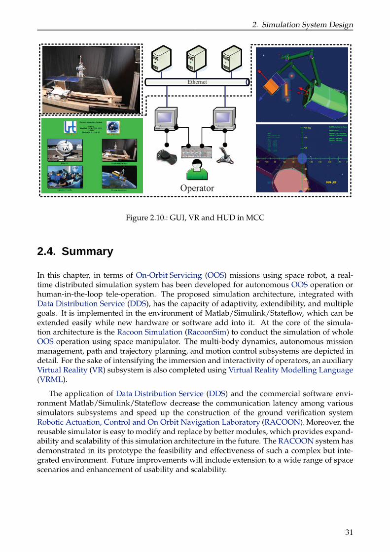
2. Simulation System Design
Ethernet
Operator
Figure 2.10.: GUI, VR and HUD in MCC
2.4. Summary
In this chapter, in terms of On-Orbit Servicing (OOS) missions using space robot, a real-time distributed simulation system has been developed for autonomous OOS operation orhuman-in-the-loop tele-operation. The proposed simulation architecture, integrated withData Distribution Service (DDS), has the capacity of adaptivity, extendibility, and multiplegoals. It is implemented in the environment of Matlab/Simulink/Stateflow, which can beextended easily while new hardware or software add into it. At the core of the simula-tion architecture is the Racoon Simulation (RacoonSim) to conduct the simulation of wholeOOS operation using space manipulator. The multi-body dynamics, autonomous missionmanagement, path and trajectory planning, and motion control subsystems are depicted indetail. For the sake of intensifying the immersion and interactivity of operators, an auxiliaryVirtual Reality (VR) subsystem is also completed using Virtual Reality Modelling Language(VRML).
The application of Data Distribution Service (DDS) and the commercial software envi-ronment Matlab/Simulink/Stateflow decrease the communication latency among varioussimulators subsystems and speed up the construction of the ground verification systemRobotic Actuation, Control and On Orbit Navigation Laboratory (RACOON). Moreover, thereusable simulator is easy to modify and replace by better modules, which provides expand-ability and scalability of this simulation architecture in the future. The RACOON system hasdemonstrated in its prototype the feasibility and effectiveness of such a complex but inte-grated environment. Future improvements will include extension to a wide range of spacescenarios and enhancement of usability and scalability.
31


3. Multibody Dynamics
Accordingly, we find Euler and D’Alembert devoting their talent and their patience tothe establishment of the laws of rotation of the solid bodies. Lagrange has incorporated hisown analysis of the problem with his general treatment of mechanics, and since his timeM. Poinsot has brought the subject under the power of a more searching analysis thanthat of the calculus, in which ideas take the place of symbols, and intelligent propositionssupersede equations.
—James Clerk Maxwell
Due to the increasing demands of On-Orbit Servicing (OOS) missions and the particularharsh environment of space, the application of space robot has received significant attention.In the last decades, numerous contributions have been made in the field of robot dynamics.From a systemic viewpoint, dynamics algorithm should be formulated with a compact setof equations for ease of development and implementation, while the greatest computationalefficiency is obtained synchronously. Generally, the dynamics algorithms are mainly con-cerned for two particular calculations: forward dynamics and inverse dynamics. Forwarddynamics, mainly required for simulation, is concerned about the calculation of the accel-eration response when a given force exerts on a given rigid body, on the contrary, inversedynamics is the calculation of the required force to drive a given rigid body to implementa given acceleration response. Inverse dynamics is of great importance in the controllerdesign, trajectory planning, mechanical design, etc.
This chapter relevant to the development of appropriate trajectory planning and con-trol algorithms, focuses on a modelling scheme that uses the concepts of graph theory andspatial notation for calculating the joint-space forward dynamics of tree structure space ma-nipulator systems. Firstly, the configuration description of space manipulators using graphtheory, the parent array, and path matrix are introduced. Secondly, based on the concept ofgeneralized link, the spatial notation and composite rigid body are presented. Thirdly, theComposite Rigid Body Algorithm (CRBA) is exhibited. The Inertia Mapping Matrix (IMM)is then derived from the path matrix, which can be used to analyse the sparsity of the inertiamatrix and the complexity of the CRBA algorithm. Within the context, a modified CRBAcombining ideas of IMM and spatial vector is proposed to calculate the dynamics of treestructure space manipulators. Its computational procedure and complexity by using IMMare analysed. Finally, a case study and comparison by using a humanoid configuration forbranched and un-branched chains particularly verify the effectiveness and potential of theproposed modified CRBA for the space manipulators.
33

3. Multibody Dynamics
3.1. Graphy Theory
Assumptions used in this chapter are firstly listed here. An N degree-of-freedom (DOF) ma-nipulator with n rotational joints mounted on a spacecraft (floating base) is considered. Eachrotational joint has ni DOF, therefore N = ∑n
i=1 ni. The whole mechanical chain is composedof n + 1 rigid bodies, and has N + 6 generalized coordinates. In this chapter, we assume thateach joint has one single rotational axis along z axis, therefore N = n.
Description of interconnection structures of multi-body systems can be illustrated bygraph theory. In order to reflect the affiliation between the joints and present a more com-pact inertia matrix, instead of using a regular numbering scheme, a depth-first numberingscheme is adopted in this chapter. A general manipulator with tree structure can be shownby a set of n links (vertices), numbered 1,⋯, n, a base link numbered 0 and a set of n joints(arcs), numbered 1,⋯, n. Each arc connects two vertices, the joints are numbered such thatjoint i connects body i to its parent. A general kinematic tree and a binary kinematic tree astwo examples are displayed in Figure 3.1.
1 5
12
141311
J1
J1
J1
J1
(b) binary kinematic tree
0
J1
J1
J1
J1
J1
J1
J1111111 J1
J1
J1
121212
141414
J1
J1
J1
J1
J1
J1
J1J1
J1
J1
111
222
333 444
555
666
777
888
999 101010
2
3 4
6
7
8
9 10
(a) general kinematic tree
root
0
root
111
1
2
222
333
3
444
4
5
555
666
6
777
7
888
8
999
9
101010
10
Figure 3.1.: Example of tree structure manipulators
The connectivity of a kinematic tree can be denoted by the parent array λ(⋅). It has oneentry for each mobile body, which indicates the body number of its parent. Hence, the parentarray for a general kinematic tree as shown in Figure 3.1 is λ(⋅) = 0,1,2,2,0,5,6,5,8,8, andλ(i) is the parent number of the body i and 0 ≤ λ(i) < i. For a specified tree structure graph,using only the parent array λ(i) can express the configuration of the system.
One important matrix in graph theory used to illustrate the connectivity of tree structureis the path matrix T, and its elements are defined as follows:
Tij =⎧⎪⎪⎨⎪⎪⎩−1 (i is on path between 0 and j)
0 (i isn’t on path between 0 and j)(3.1)
The tree structure can uniquely be determined by the parent array λ(⋅) or the path matrixT. There is no column in the path matrix corresponding to vertex 0. From the definition of T,
34

3. Multibody Dynamics
every row has at least one non-zero element. If Tij is the only non-zero element in row i, thevertex j is a terminal vertex. We define nλ(i) = ∑
nj=1∣Tji∣ denotes the number of parent links of
link i and nν(i) = ∑nj=1∣Tij ∣ denotes the number of offspring of link i for further application.
3.2. Spatial Notation
The so-called spatial notation was introduced and employed in Featherstone (2008). Both theangular and linear components of physical quantities like velocity, acceleration and force aredealt with a unified framework (e.g. 6×1 vector and 6×6 matrix). In the following, a variablewith bar represents a spatial tensor. A spatial velocity v and a spatial force f of link i can bedenoted as vi = [ωT
i ,vTi ]T and f i = [mT
i ,fTi ]T. The spatial transformation matrix is:
jXi = [ jRi 0jRiS(jri) jRi
] (3.2)
where jXi ∈ R6×6 represents the spatial transformation matrix, jRi ∈ R3×3 stands for thecoordinate transformation matrix, from coordinate frame i to j. jri ∈ R3×1 is a positionvector from the origin of frame i to that of frame j expressed in frame i. S ∈ R3×3 is the crossproduct operator, for an arbitrary 3 dimensional vector a = [ax, ay, az]T, it can be defined as
S(a) =⎡⎢⎢⎢⎢⎢⎣
0 −az ayaz 0 −ax−ay ax 0
⎤⎥⎥⎥⎥⎥⎦(3.3)
J¸(i)
z¸(¸(i))
z¸(i)
a¸(i)
zi
b¸(i)
ai
J1
eC¸(i)
eCi
edi + b¸(i)
biedied¸(i)
Figure 3.2.: Generalized center of mass of link i
Likewise, an inertia matrix is defined for each individual link in its own frame system.For link i, the spatial inertia matrix Hi, expressed in its own coordinate frame, can be repre-sented as follows
Hi = [Ii +miS(ai)TS(ai) miS(ai)miS(ai)T miE3
] (3.4)
35

3. Multibody Dynamics
where Ii is the inertia of link i with respect to its gravity center. ai is the position vectorfrom the origin of frame i to the mass center of link i, mi is the mass of link i and E3 is a3×3 identity matrix. For detailed description of spatial notation, refer to Featherstone (2008)and Lilly and Orin (1991). For a composite rigid body inertia expressed by spatial notation,it may be computed recursively based on the concept of generalized link (see Figure 3.2)using the following equation
Hλ(i) = iXTλ(i)Hi
iXλ(i) + Hλ(i) (3.5)
where Hi and Hλ(i) are the spatial composite rigid body inertia for body i and spatial inertiaof body λ(i), respectively.
3.3. Dynamics Algorithm
The dynamic model can be obtained from Newtonian or Lagrange mechanics. There are sev-eral different dynamic formulations applied in the field of multi-body dynamics: Newton-Euler, Lagrange-Euler, D’Alembert, Hamilton. Nevertheless, all these formulations with differ-ent representations are equivalent since they describe the same physical phenomenon. Gen-erally speaking, the choose of dynamics formulation will depend on different objectives suchas notation simplicity, computational cost, etc. Once the dynamic formulation is determined,corresponding motion equations about a specific multi-body system can be derived from theformulation. This section first reviews the basic steps of Composite Rigid Body Algorithmderived from the Lagrange formulation. Then the Inertia Mapping Matrix is obtained byusing path matrix T. A modified Composite Rigid Body Algorithm (CRBA) in terms ofInertia Mapping Matrix (IMM) is proposed based on the spatial notation.
3.3.1. Lagrange Formulation
Not like Newton’s second law which denotes the relationship between the forces and move-ments, Lagrange formulation is represented by energy and generalized coordinates, whichdescribes the relationship between forces and movements from energy aspect, has obtainedconsiderable applications in the field of dynamics of multi-body and complex systems. WithLagrange formulation, the equations of motion about one complex system can be derivedin a systematic way independent of the reference coordinate frame. The Lagrangian can befirstly represented by energy, like kinetic and potential energy, as a function of the general-ized coordinates qi(i = 1,2,⋯, n).
L = T (q, q) − U(q) (3.6)
where T and U denote the kinetic and potential energies of the whole system. The Lagrangeequations can be expressed by
d
dt(∂L∂q)T
− (∂L∂q)T
= ξ (3.7)
where ξ is the generalized force composed of the internal and external non-conservativeforces, such as the joint actuator torques, the joint friction torques, and the joint torquesinduced by the contact with the environment.
36

3. Multibody Dynamics
In our analysis, since the space robot is in a micro gravitational environment, it is rea-sonable to set U = 0. The kinetic energy T with a quadratic form of the generalized velocityq can be expressed by:
T =1
2qTH(q)q (3.8)
Substitute equation 3.8 into equation 3.7, a general formulation derived from Lagrangiancan be denoted as
H(q)q + c(q, q) = τ + fx (3.9)
where H(q) is the Joint-Space Inertia Matrix, q, q, q are the vectors of joint position, jointvelocity and joint acceleration, respectively. c(q, q) is a bias vector containing Coriolis, cen-trifugal and gravity terms. For the space application, the gravity term can be omitted sincethe micro-gravity environment in space. τ is an internal joint force/torque vector and fx isthe external force/torque acting on the space robot.
3.3.2. Composite Rigid Body Algorithm
As was illustrated in the beginning, dynamics algorithms can be divided into two categories:forward and inverse dynamics. To simplify the matter, the forward and inverse dynamicscan be encapsulated into two functions, FwdDyn and InvDyn:
q = FwdDyn(model,q, q,τ ,fx) (3.10)
τ = InvDyn(model,q, q, q,fx) (3.11)
the symbol model refers to a set of data that describes a particular rigid body system, such asits configuration, joint type, parameters of each link, etc. As explained in Walker and Orin(1982) and Featherstone (2008), the equations of motion for a tree structure rigid body sys-tem can be expressed in matrix form as expressed in equation 3.9. The inertia matrix H canbe derived analytically or computed numerically. The goal is to find an efficient algorithmwhich is more efficient than O(n3) to compute the inertia matrix. If there is an inverse dy-namics algorithm function InvDyn as in equation 3.11, then the non-linear terms of Coriolisand centrifugal force vector c(q, q) can be calculated by
c(q, q) = InvDyn(model,q, q,0,0) (3.12)
Comparing equation 3.11 with equation 3.12 and referring to equation 3.9, we can obtain
Hq = InvDyn(model,q, q, q,fx) + fx − c(q, q)= InvDyn(model,q,0, q,0) − InvDyn(model,q,0,0,0) (3.13)
Since the velocity term q and external force term fx in equation 3.13 can be cancelled out,these vectors can be set to 0. This equation induces a simple O(n2) algorithm for calculat-ing H, which is the first method proposed in Walker and Orin (1982). Featherstone namedmethod 3 in Walker and Orin (1982) as Composite Rigid Body Algorithm (CRBA) to com-pute the inertia parameters of composite sets of rigid bodies at the outer end of the manipu-lator chain. By setting the sets of joint velocities to 0, and the joint accelerations to 0 or a unitvector, the column of the inertia matrix can be calculated efficiently through successive ap-plication of inverse dynamics algorithm such as Recursive Newton-Euler Algorithm (RNEA).
37
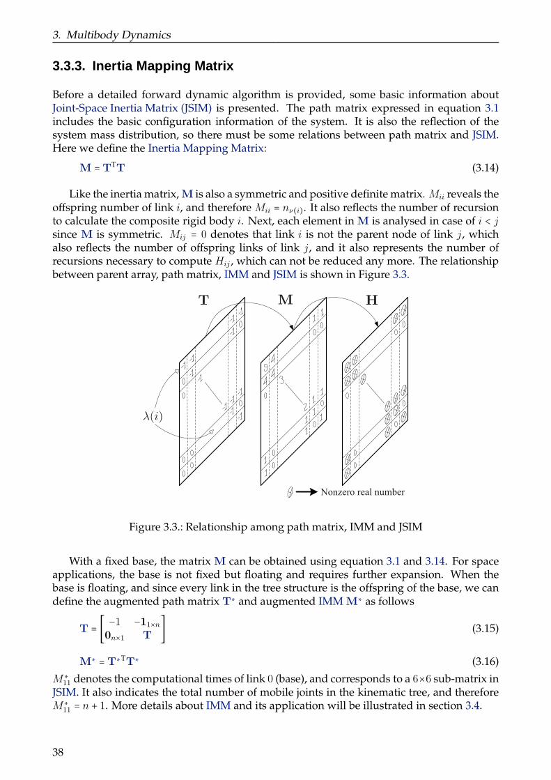
3. Multibody Dynamics
3.3.3. Inertia Mapping Matrix
Before a detailed forward dynamic algorithm is provided, some basic information aboutJoint-Space Inertia Matrix (JSIM) is presented. The path matrix expressed in equation 3.1includes the basic configuration information of the system. It is also the reflection of thesystem mass distribution, so there must be some relations between path matrix and JSIM.Here we define the Inertia Mapping Matrix:
M = TTT (3.14)
Like the inertia matrix, M is also a symmetric and positive definite matrix. Mii reveals theoffspring number of link i, and therefore Mii = nν(i). It also reflects the number of recursionto calculate the composite rigid body i. Next, each element in M is analysed in case of i < jsince M is symmetric. Mij = 0 denotes that link i is not the parent node of link j, whichalso reflects the number of offspring links of link j, and it also represents the number ofrecursions necessary to compute Hij , which can not be reduced any more. The relationshipbetween parent array, path matrix, IMM and JSIM is shown in Figure 3.3.
T
¸(i)
M H
Nonzero real number
Figure 3.3.: Relationship among path matrix, IMM and JSIM
With a fixed base, the matrix M can be obtained using equation 3.1 and 3.14. For spaceapplications, the base is not fixed but floating and requires further expansion. When thebase is floating, and since every link in the tree structure is the offspring of the base, we candefine the augmented path matrix T∗ and augmented IMM M∗ as follows
T = [ −1 −11×n
0n×1 T] (3.15)
M∗ = T∗TT∗ (3.16)
M∗11
denotes the computational times of link 0 (base), and corresponds to a 6×6 sub-matrix inJSIM. It also indicates the total number of mobile joints in the kinematic tree, and thereforeM∗
11= n + 1. More details about IMM and its application will be illustrated in section 3.4.
38

3. Multibody Dynamics
3.3.4. Modified CRBA
Refer to Lilly and Bonaventura (1995), Yoshida (1997) and equation 3.9, for a floating basedrobot, the general dynamics equation can be described by the following expression:
[ Hb Hbm
HTbm Hm
] q + [ cbcm] = [f b
τ] +∑
k
JkTe fk
e (3.17)
where Hb, Hbm and Hm are the base inertia matrix, dynamic coupling matrix and manipu-lator’s inertia matrix, respectively. cb and cm are the Coriolis and centrifugal force vectorsof the base and manipulator, respectively. f b ∈ R6×1 and f k
e ∈ R6×1 are the generalized forcesapplied on the base and end-effector k, respectively. Jk
e ∈ R6×n is the Jacobian matrix of kth
end-effector.
Considering the IMM defined in section 3.3.3, a modified CRBA is proposed here basedon spatial notation. From Figure 3.2, supposing only joint i is in motion and qi = 1, the totalforce f i and moment mi exerted on link j (j ≤ i) can be computed by inward recursionfrom the link i to the link 0. If we employ spatial notation, the spatial force f i exerted ongeneralized link i and the spatial force f i (j ≤ i) can be computed by inward recursion. Theformulae of calculating spatial force and corresponding elements in JSIM can be expressedby
⎧⎪⎪⎨⎪⎪⎩f i =Hisi
fλ(j) = λ(j)XTj f j
Ô⇒⎧⎪⎪⎨⎪⎪⎩(Hm)ij = sT
j f j
(Hbm)i = 0XTi f i
(3.18)
where si ∈ R6×1 represents the motion axis of joint i. si can be set to [0 0 0 0 0 1]T or[0 0 1 0 0 0]T for a prismatic joint or rotational joint, respectively. The basic steps of themodified CRBA are shown in Table 3.1.
Table 3.1.: Modified composite rigid body algorithm
Input: λ(i),model,mi, Ii,ai,bi,T,M,qini, qini,τ ,fx
step 1: c(q, q) = InvDyn(model,q, q,0,0)step 2: for i = n,⋯ ,0
do Hi, f i
for j = i − 1,⋯ ,0
if Tij ≠ 0 do f j
if Mij = 0H(i+6)(j+6) = 0else H(i+6)(j+6) = (Hm)ij
endend
step 3: Hb = H0; (Hbm)i = 0X
Ti f i
Integrate: q =H−1(q)(τ + fx − c(q, q))
3.4. IMM Application
IMM can be employed to explore the geometry of JSIM and cost analysis of CRBA. It alsooffers a general method to search the properties of JSIM and supplies an analytical tool toexplore how different topologies affect the cost.
39
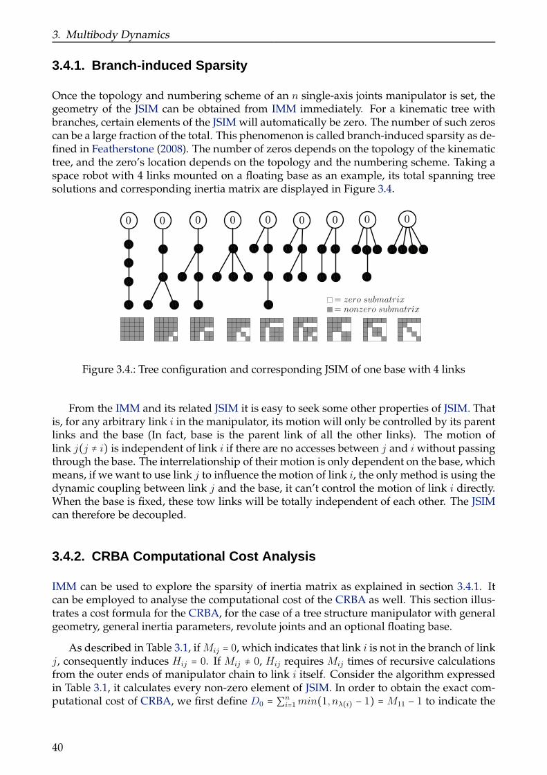
3. Multibody Dynamics
3.4.1. Branch-induced Sparsity
Once the topology and numbering scheme of an n single-axis joints manipulator is set, thegeometry of the JSIM can be obtained from IMM immediately. For a kinematic tree withbranches, certain elements of the JSIM will automatically be zero. The number of such zeroscan be a large fraction of the total. This phenomenon is called branch-induced sparsity as de-fined in Featherstone (2008). The number of zeros depends on the topology of the kinematictree, and the zero’s location depends on the topology and the numbering scheme. Taking aspace robot with 4 links mounted on a floating base as an example, its total spanning treesolutions and corresponding inertia matrix are displayed in Figure 3.4.
J1
J1
J1
J1
0
J1
J1
J1
J1
0
J1J1
J1
J1
0 0
J1 J1 J1 J1J1
J1 J1
J1
0
J1
J1 J1 J1
0
J1J1
J1J1
0 0 0
J1 J1J1
J1
J1
J1
J1
J1
= nonzero submatrix= zero submatrix
Figure 3.4.: Tree configuration and corresponding JSIM of one base with 4 links
From the IMM and its related JSIM it is easy to seek some other properties of JSIM. Thatis, for any arbitrary link i in the manipulator, its motion will only be controlled by its parentlinks and the base (In fact, base is the parent link of all the other links). The motion oflink j(j ≠ i) is independent of link i if there are no accesses between j and i without passingthrough the base. The interrelationship of their motion is only dependent on the base, whichmeans, if we want to use link j to influence the motion of link i, the only method is using thedynamic coupling between link j and the base, it can’t control the motion of link i directly.When the base is fixed, these tow links will be totally independent of each other. The JSIMcan therefore be decoupled.
3.4.2. CRBA Computational Cost Analysis
IMM can be used to explore the sparsity of inertia matrix as explained in section 3.4.1. Itcan be employed to analyse the computational cost of the CRBA as well. This section illus-trates a cost formula for the CRBA, for the case of a tree structure manipulator with generalgeometry, general inertia parameters, revolute joints and an optional floating base.
As described in Table 3.1, if Mij = 0, which indicates that link i is not in the branch of linkj, consequently induces Hij = 0. If Mij ≠ 0, Hij requires Mij times of recursive calculationsfrom the outer ends of manipulator chain to link i itself. Consider the algorithm expressedin Table 3.1, it calculates every non-zero element of JSIM. In order to obtain the exact com-putational cost of CRBA, we first define D0 = ∑n
i=1min(1, nλ(i) − 1) = M11 − 1 to indicate the
40
3. Multibody Dynamics
numbers of moving links without connectivity to the base and D1 = ∑ni=1(nλ(i) − 1) = ∑n
i=2Mii
to show the numbers of non-zero elements above the diagonal of IMM. The depth of the treewill influence the computational complexity. If nλ(i) has an upper limit dmax, then we canobtain 0 ≤ D0 ≤ n − 1 and 0 ≤ D1 ≤ n(dmax − 1). The cost of CRBA represented by KCRBA
depends on D0 and D1 rather than directly on n and can be denoted as
KCRBA = D0(ca + ct) +D1vt (3.19)
where the symbol ca, ct and vt stand for composite rigid body add, composite rigid bodytransform and vector transform, respectively. When D0 = 0 happens, this means every mo-bile body connects to the fixed base directly. Then the JSIM is a diagonal matrix, whichrequires the least computational cost, and so the theoretical minimum complexity of CRBAis O(1). When there are no branches in the kinematic tree, the JSIM is dense, D0 = n andD1 = n(n − 1)/2, which requires the maximum computational cost. This provides a compu-tational cost estimation of CRBA
O(1) ≤ KCRBA ≤ O(n3) (3.20)
In fact, most of the practical system have a value of D0 that is either equal to or less thanthe maximum possible value. For example, the asymptotic complexity of CRBA for a binarykinematic tree as shown in Figure 3.1 is O(nlog(n)) Featherstone (2005).
Many investigations have been made to find the minimum-cost implementations for op-erations ca, ct and vt. However, the minimum cost for ct and vt mainly depends on howthe link coordinate frame are defined. This is another aspect that makes the situation morecomplicated for a tree structure robot. The minimum cost for ct and vt relied on the co-ordinate frame located in accordance with a set of Denavit-Hartenberg (DH) parameters(Denavit and Hartenberg (1955)), in which case the coordinate transformation expressionby λ(i)Ri can be realized via the successive application of two axis screw transforms: onealigns with the x-axis and the other aligns with z-axis. However, if a link connects morethan one offspring link, then only one offspring link can possess the benefit of transforma-tion with DH parameters. We define DH nodes and non-DH nodes, for those nodes haveand do not have the benefit of DH parameters, respectively. The number of non-DH nodescan be determined by path matrix, if the offspring nodes of link i is nν(i), then the numberof non-DH can be denoted by
nnDH =n
∑i=1
max(0, nν(i) − 1) = n − 1 − n−1
∑i=1
∣Ti,i+1∣ (3.21)
where the number of non-DH nodes nnDH equals to the number of zeros in the super-diagonal of path matrix T. For the un-branched case, nν(i) ≤ 1 denotes that there are nonon-DH nodes in the tree. Using the subscripts a and b to represent the DH node and non-DH node, the cost of CRBA can be expressed by
KCRBA = D0a(ca + cta) +D1avta +D0b(ca + ctb) +D1bvtb (3.22)
Equation 3.19 and 3.22 are the cost formulae of computing JSIM with fixed base, however,when a floating base exists, some more reductions can be made since 3 of DH parametersbetween link i and its parent link λ(i) can be set to 0, if link λ(i) happened to be a floatingbase McMillan et al. (1995). Therefore the operations on each affected ct and vt transforms
41
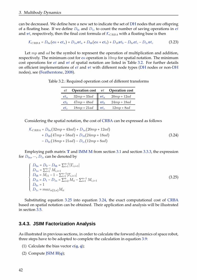
3. Multibody Dynamics
can be decreased. We define here a new set to indicate the set of DH nodes that are offspringof a floating base. If we define D0c and D1c to count the number of saving operations in ct
and vt, respectively, then the final cost formula of KCRBA with a floating base is then
KCRBA = D0a(ca + cta) +D1avta +D0b(ca + ctb) +D1bvtb −D0cctc −D1cvtc (3.23)
Let mp and ad be the symbol to represent the operation of multiplication and addition,respectively. The minimum cost for ca operation is 10mp for spatial notation. The minimumcost operations for ct and vt of spatial notation are listed in Table 3.2. For further detailson efficient implementations of ct and vt with different node types (DH nodes or non-DHnodes), see (Featherstone, 2008).
Table 3.2.: Required operation cost of different transforms
ct Operation cost vt Operation cost
cta 32mp + 33ad vta 20mp + 12adctb 47mp + 48ad vtb 24mp + 18adctc 18mp + 21ad vtc 12mp + 8ad
Considering the spatial notation, the cost of CRBA can be expressed as follows
KCRBA =D0a(32mp + 43ad) +D1a(20mp + 12ad)+D0b(47mp + 58ad) +D1b(24mp + 18ad)−D0c(18mp + 21ad) −D1c(12mp + 8ad)
(3.24)
Employing path matrix T and IMM M from section 3.1 and section 3.3.3, the expressionfor D0a, ⋯, D1c can be denoted by
⎧⎪⎪⎪⎪⎪⎪⎪⎪⎪⎪⎨⎪⎪⎪⎪⎪⎪⎪⎪⎪⎪⎩
D0a = D0 −D0b = ∑n−1i=1 ∣Ti,i+1∣
D1a = ∑n−1i=1 Mi,i+1
D0b =M11 − 1 −∑n−1i=1 ∣Ti,i+1∣
D1b =D1 −D1a = ∑ni=2Mii −∑n−1
i=1 Mi,i+1
D0c = 1D1c =maxi∈[2,n]Mii
(3.25)
Substituting equation 3.25 into equation 3.24, the exact computational cost of CRBAbased on spatial notation can be obtained. Their application and analysis will be illustratedin section 3.5.
3.4.3. JSIM Factorization Analysis
As illustrated in previous sections, in order to calculate the forward dynamics of space robot,three steps have to be adopted to complete the calculation in equation 3.9:
(1) Calculate the bias vector c(q, q);
(2) Compute JSIM H(q);
42
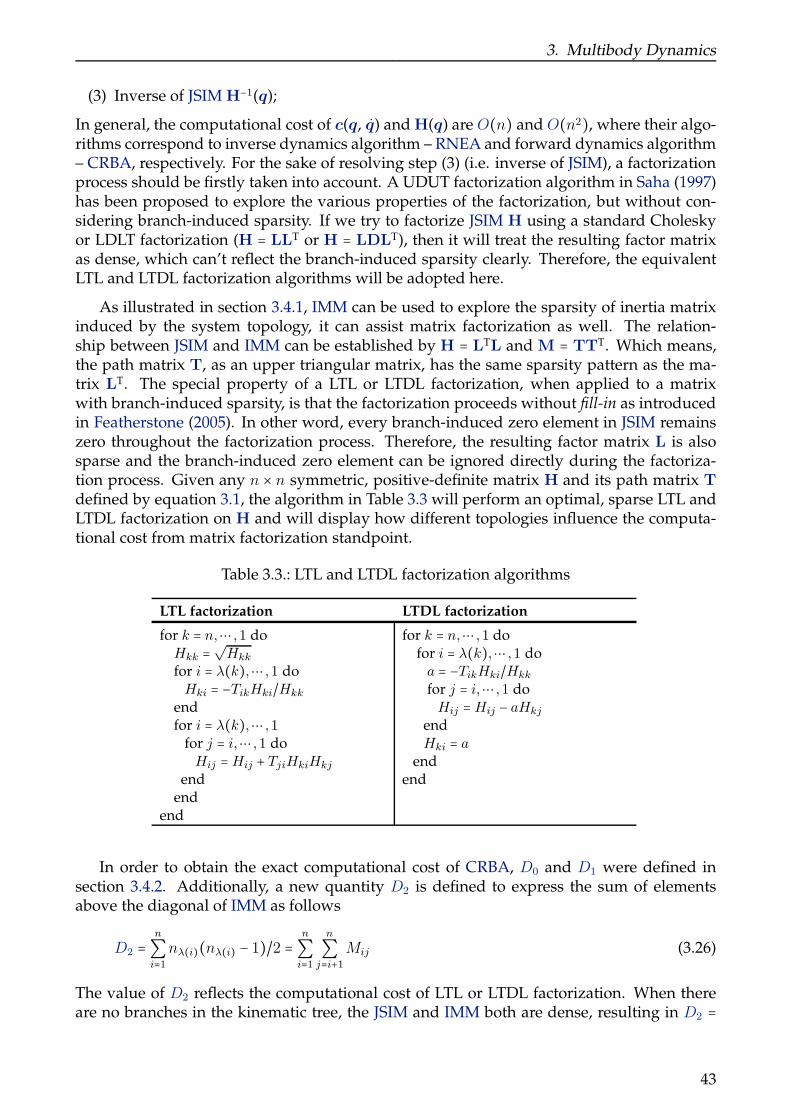
3. Multibody Dynamics
(3) Inverse of JSIM H−1(q);
In general, the computational cost of c(q, q) and H(q) are O(n) and O(n2), where their algo-rithms correspond to inverse dynamics algorithm – RNEA and forward dynamics algorithm– CRBA, respectively. For the sake of resolving step (3) (i.e. inverse of JSIM), a factorizationprocess should be firstly taken into account. A UDUT factorization algorithm in Saha (1997)has been proposed to explore the various properties of the factorization, but without con-sidering branch-induced sparsity. If we try to factorize JSIM H using a standard Choleskyor LDLT factorization (H = LLT or H = LDLT), then it will treat the resulting factor matrixas dense, which can’t reflect the branch-induced sparsity clearly. Therefore, the equivalentLTL and LTDL factorization algorithms will be adopted here.
As illustrated in section 3.4.1, IMM can be used to explore the sparsity of inertia matrixinduced by the system topology, it can assist matrix factorization as well. The relation-ship between JSIM and IMM can be established by H = LTL and M = TTT. Which means,the path matrix T, as an upper triangular matrix, has the same sparsity pattern as the ma-trix LT. The special property of a LTL or LTDL factorization, when applied to a matrixwith branch-induced sparsity, is that the factorization proceeds without fill-in as introducedin Featherstone (2005). In other word, every branch-induced zero element in JSIM remainszero throughout the factorization process. Therefore, the resulting factor matrix L is alsosparse and the branch-induced zero element can be ignored directly during the factoriza-tion process. Given any n × n symmetric, positive-definite matrix H and its path matrix T
defined by equation 3.1, the algorithm in Table 3.3 will perform an optimal, sparse LTL andLTDL factorization on H and will display how different topologies influence the computa-tional cost from matrix factorization standpoint.
Table 3.3.: LTL and LTDL factorization algorithms
LTL factorization LTDL factorization
for k = n,⋯ ,1 doHkk =
√Hkk
for i = λ(k),⋯ ,1 doHki = −TikHki/Hkk
endfor i = λ(k),⋯ ,1
for j = i,⋯ ,1 doHij =Hij + TjiHkiHkj
endend
end
for k = n,⋯ ,1 dofor i = λ(k),⋯ ,1 doa = −TikHki/Hkk
for j = i,⋯ ,1 doHij =Hij − aHkj
endHki = a
endend
In order to obtain the exact computational cost of CRBA, D0 and D1 were defined insection 3.4.2. Additionally, a new quantity D2 is defined to express the sum of elementsabove the diagonal of IMM as follows
D2 =n
∑i=1
nλ(i)(nλ(i) − 1)/2 = n
∑i=1
n
∑j=i+1
Mij (3.26)
The value of D2 reflects the computational cost of LTL or LTDL factorization. When thereare no branches in the kinematic tree, the JSIM and IMM both are dense, resulting in D2 =
43
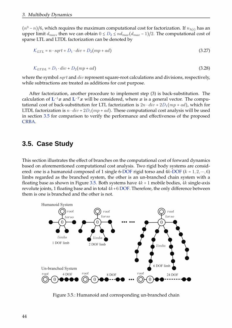
3. Multibody Dynamics
(n3 − n)/6, which requires the maximum computational cost for factorization. If nλ(i) has anupper limit dmax, then we can obtain 0 ≤ D2 ≤ ndmax(dmax − 1)/2. The computational cost ofsparse LTL and LTDL factorization can be denoted by
KLTL = n ⋅ sqrt +D1 ⋅ div +D2(mp + ad) (3.27)
KLTDL =D1 ⋅ div +D2(mp + ad) (3.28)
where the symbol sqrt and div represent square-root calculations and divisions, respectively,while subtractions are treated as additions for cost purpose.
After factorization, another procedure to implement step (3) is back-substitution. Thecalculation of L−1x and L−Tx will be considered, where x is a general vector. The compu-tational cost of back-substitution for LTL factorization is 2n ⋅ div + 2D1(mp + ad), which forLTDL factorization is n ⋅ div + 2D1(mp + ad). These computational cost analysis will be usedin section 3.5 for comparison to verify the performance and effectiveness of the proposedCRBA.
3.5. Case Study
This section illustrates the effect of branches on the computational cost of forward dynamicsbased on aforementioned computational cost analysis. Two rigid body systems are consid-ered: one is a humanoid composed of 1 single 6-DOF rigid torso and 4k-DOF (k = 1,2,⋯,6)limbs regarded as the branched system, the other is an un-branched chain system with afloating base as shown in Figure 3.5. Both systems have 4k + 1 mobile bodies, 4k single-axisrevolute joints, 1 floating base and in total 4k+6 DOF. Therefore, the only difference betweenthem is one is branched and the other is not.
J1
J1
J1
J1
J1
J1
J1J1
J1
J1J1
J1
J1
J1 J1
J1
J1 J1
J1 J1
J1 J1J1
J1
0
torso
J1 J1
J1 J1
0
root
J1 J1
J1 J1J1 J1
0
J1 J1
limbs
1 DOF limb 2 DOF limb
6 DOF limb
0 J1 J1 J1 J1 0 J1 J1 J1 0 J1 J1J1 J1 J1
Humanoid System
Un-branched System
4 DOF 8 DOF 24 DOF
root root
rootrootroot
torso torso
limbs
limbs
Figure 3.5.: Humanoid and corresponding un-branched chain
44

3. Multibody Dynamics
To calculate the exact operations of different algorithms, we first need to evaluate thevarious quantities for the branched and un-branched systems based on equation 3.25. Ac-cording to the definition of augmented path matrix T∗ and augment IMM M∗, the quantitiesD0, D0, . . . , D1c for branched and un-branched systems can be computed as follows
D(branched) =⎧⎪⎪⎪⎪⎪⎪⎪⎨⎪⎪⎪⎪⎪⎪⎪⎩
D0 = 4k D1 = 2k(k + 1)D0a = 4k − 3 D1a = 2k2 − k
D0b = 3 D1b = 3kD0c = 1 D1c = k
(3.29)
D(un − branched) =⎧⎪⎪⎪⎪⎪⎪⎪⎨⎪⎪⎪⎪⎪⎪⎪⎩
D0 = 4k D1 = 2k(4k + 1)D0a = 4k D1a = 2k(4k + 1)D0b = 0 D1b = 0D0c = 1 D1c = 4k
(3.30)
Substituting the various D quantities into equation 3.24, the computational cost of CRBAfor humanoid and un-branched systems can be list as follows: (40k2 + 168k + 27)mp and(24k2 + 206k + 24)ad for humanoid; (160k2 + 120k − 18)mp and (96k2 + 164k − 21)ad for un-branched chain.
The comparison of CRBA applied to branched and un-branched systems is performed.Figure 3.6 shows the operations number of these calculations without considering the addi-tion cost (#ad = 0). One can see that, with small number of DOF, i.e. n ≤ 10, the computa-tional cost for branched and un-branched system is nearly the same. However, as the DOFincreases, the computational cost for un-branched system increases more rapidly than thatfor branched system. Figure 3.7 shows the cost ratio of CRBA applied to branched and un-branched systems, which indicates that, the CRBA runs more quickly on branched systemthan on the equivalent un-branched chain. The cost ratio increases as the number of mo-bile joints increases. When n ≥ 22, CRBA runs more than twice as quickly on the branchedsystem than on the equivalent un-branched chain.
To verify the performance of proposed algorithm in this chapter, the ABA is utilized tocompare with modified CRBA. As introduced in section 3.4.3, in order to solve the forwarddynamics problem using CRBA, three steps have to be performed. The most efficient algo-rithm for calculating c(q, q) is RNEA proposed in Balafoutis and Patel (1989), which needs(93n − 69) multiplications and (81n − 66) additions. To calculate the cost of the inverse ofJSIM H−1(q), LTDL factorization and back-substitution algorithm expressed in section 3.4.3is adopted. For an n × n general symmetric, positive matrix, the cost of factorization andback-substitution is D1 ⋅ div + D2(mp + ad) and n ⋅ div + 2D1(mp + ad). When the branch-induced sparsity of JSIM is considered and div = mp is assumed, the cost of JSIM inversewith sparsity is (3D1 +D2 + n)multiplications and (2D1 +D2) additions.
The algorithm of Articulated Body Algorithm (ABA) expressed in McMillan et al. (1995)is used for comparison reason. The computational cost formula for an un-branched chainwith a floating base is (224n − 30)mp + (205n − 37)ad. To obtain an exact computational costfor the humanoid, a correction of (66mp + 57ad) is applied to account for the additionaltransformation cost at each non-DH node.
45

3. Multibody Dynamics
10 14 18 22 26 300
5000
10000
15000
Degree of freedom (#ad=0)
Ope
ratio
ns
un−branched CRBAun−branched ABAbranched CRBAbranched ABA
Figure 3.6.: Operations numbers of CRBA and ABA
10 14 18 22 26 301
1.4
1.8
2.2
2.6
3
Degree of freedom
Rat
io
un−branched #ad=0un−branched #ad=mpbranched #ad=0branched #ad=mp
Figure 3.7.: Cost ratio of CRBA and ABA
Figure 3.6 shows the operations number of ABA and CRBA applied to branched andun-branched system without considering the addition cost (#ad = 0). One can see that,when only small number of DOF is considered, i.e.n ≤ 10, both CRBA and ABA applied tobranched and un-branched system have almost the same computational efficiency. Whenonly un-branched chain is considered, ABA is much faster than CRBA on condition that
46
3. Multibody Dynamics
n > 10, especially when n ≥ 14. The cost ratio between CRBA and ABA for un-branched chainincreases as the number of mobile joints increases. But if there are branches in the kinematictree, ABA runs only slightly faster than CRBA even when n = 30. The ratio between CRBAand ABA for branched system increase slowly as the number of mobile joints increases. TheCRBA is only about 14% slower than the ABA assuming ad = mp, or 17% slower assumingad = 0 when n = 30. One can therefore conclude that, O(n3) algorithms are still competitivewith O(n) algorithms, providing there is sufficient branching in the kinematic tree.
3.6. Summary
This chapter presents a detailed JSIM algorithm and its computational analysis for a spacerobot with tree structure, and therefore makes the following contributions:
• It combines graph theory and spatial notation, and proposes an IMM and a modifiedCRBA;
• It employs IMM to explore branched-induced sparsity and explicitly offers the com-putational cost of JSIM;
• It provides a decomposition algorithm to assist the inverse of JSIM considering IMM.Its computational cost is also analysed.
The branched-induced sparsity of the inertia matrix depends on the system topologyand numbering scheme. The complexity of calculating the JSIM is estimated between O(1)and O(n3) by using IMM. The case study shows that for two systems with equal numbers ofDOF, the calculation cost for the branched system is much lower than for the un-branchedchain. According to the comparison, it shows that when there is efficient branching in thekinematic tree, O(n3) algorithms are still competitive with O(n) algorithms even at highvalue of n. Furthermore, this approach provides a more intuitive way of understanding theproperties of the JSIM and its computational complexity. The general dynamic formulationpresented here is an essential element of the constrained motion model developed for spacemanipulators and will be employed in the following chapters for kinematic analysis andcontroller design.
47


4. Kinematic Control of Manipulator
A single idea, if it is right, save us the labor of an infinity of experiences.
—Jacques Maritain
This chapter focuses on the kinematics analysis of the redundant manipulator at ve-locity level considering singularity and obstacle avoidance issues. A manipulator movingin its workspace without enough degree-of-freedom (DOF) will have limited applications,therefore, redundant manipulator receives wide spread attention in the research academiaand industry. The application of redundant manipulators often faces the following issues:completing multiple subtasks synchronously, possible emergence of singularity of the ma-nipulator during its motion and existence of obstacles in the workspace of the manipulator,etc. In this chapter, inverse kinematics analysis with multiple prioritized subtasks is firstlyreviewed. A so-called Singular Task Reconstruction (STR) method is developed based onthe concept of manipulability ellipsoid for singularity avoidance. When the manipulatormoves in an unstructured environment with obstacles, a collision avoidance strategy con-sidering two control points is proposed to restrain the vibration of joint velocity and gen-erate smoother joint trajectory reference. The proposed singularity and collision avoidancestrategies are demonstrated by simulation works.
4.1. Inverse Kinematics
Inverse kinematics refers to determining the joint parameters to realize a required configu-ration of the manipulator or enable the end-effector to track a predefined path in task-space.In this section, we analyse the inverse kinematics of multiple prioritized subtasks at velocitylevel for redundant manipulator. As illustrated in section 3.1, an N DOF manipulator withn rotational joints is considered. In this chapter, we assume that each joint has one singlerotational axis along z axis, therefore N = n.
4.1.1. Redundancy and Task Priority
The degree-of-redundancy (DOR) for fixed base robot has been defined as the difference be-tween the DOF of the manipulator and the number of end-effector task variables. In general,6 DOF manipulator can meet the end-effector task-space motion requirements. However, inpractice, there are some other tasks as well as end-effector task to fulfil synchronously, suchas joint range limits, singularity and collision avoidance, etc. When considering free-floatingspace manipulator, base motion control by using manipulator’s redundancy can be regarded
49

4. Kinematic Control of Manipulator
as additional manipulator’s task. These additional tasks call for system redundancy to meetthe aforementioned requirements.
Supposing a general case at velocity level is taken into account. If there are m tasksrequired for the manipulator, each task need mi task variables, then the total number oftask variables M = ∑m
i=1mi. According to the definition of degree-of-redundancy (DOR),three cases of redundancy can be distinguished in reference to the total number of taskvariables M and the number of manipulator DOF N . The first case can be characterizedby N < mini∈[1,m]mi, which indicates that, there are not sufficient DOF to satisfy even thesimplest task with the minimum number of task variables, without mentioning residual re-dundancy available for other tasks. This case is highly unusual, and primary of theoreticalinterest. The second case can be denoted as N ≥ M . In this case, besides the required taskvariables, there will be some additional redundancy left to satisfy certain criteria. For thethird case, mini∈[1,m]mi ≤ N < M , the available DOR will not suffice to accomplish all thetasks concurrently, although the manipulator may contain some redundancy with referenceto one single task.
As aforementioned the third case, if it is impossible to accomplish all the tasks com-pletely, since the shortage of DOF, then it would be reasonable to perform the most sig-nificant task preferentially and the less significant tasks as much as possible using the re-maining DOR. Different tasks required can be categorized into a list of subtasks with var-ious level of significance, and this was firstly defined as tasks with the order of priorityin Nakamura et al. (1987). Even for a 6 DOF manipulator, the subtasks decomposition be-tween position and orientation is highly favourable. It will enlarge the workspace of theprimary subtask by allowing incompleteness for the second subtask. Redundancy analy-sis and application based on the concept of task priority will be discussed in the followingsection.
4.1.2. General Solution for Inverse Kinematics
Let θ = (θ1,⋯ , θn)T ∈ Rn×1 and x = (x1,⋯ , xm)T ∈ RM×1 denote the joint-space and task-spacemanipulator, the relationship between these two spaces can be established by using Jacobianmatrix, and hence can be expressed by the following formula:
⎧⎪⎪⎪⎪⎪⎪⎪⎨⎪⎪⎪⎪⎪⎪⎪⎩
J1θ = x1
J2θ = x2
⋯
Jmθ = xm
(4.1)
where Ji ∈ Rmi×n is the Jacobian matrix of the ith manipulator task. If task 1 is chosen as theprimary task, the other tasks will be treated as the secondary tasks. Generally, the primarytask should be ensure to accomplish, and thereby holds the highest priority. Based on thesignificance of tasks, total m tasks can thus form a top-down hierarchy. For an arbitrary taskmi, suppose that there are sufficient DOF to perform this task, the solutions can be describedas follows:
θ = J+i xi + (En − J+i Ji)hi (4.2)
50

4. Kinematic Control of Manipulator
where J+i ∈ Rn×mi is the pseudo-inverse of Ji. (En −J+i Ji) is the null-space of Ji and hi ∈ Rn×1
is an arbitrary vector. If the priority of the tasks is taken into account, in order to fulfilall the m tasks expressed in equation 4.1, a recursive algorithm can be adopted to solve thepriority based inverse kinematics problem at velocity level. In accordance with equation 4.2,enabling i = 1 and substituting this equation into the second task x2 gives the solution of h1:
h = J+x2 + (En − J+2 J2)h2 (4.3)
where J2 = J2(En − J+1J1) represents the projection of J2 onto the null-space of J1, x2 = x2 −J2J
+1x1 indicates the modification of secondary task due to the existing of the first subtask.
Accordingly, the solution sufficing to coordinate exactly subtask 1 and 2 in joint-space canbe denoted by
θ = J+1 x1 + J+2˙x2 + (En − J
+1J1)(En − J
+2 J2)h2 (4.4)
Employing equation 4.4, the second subtask will be performed without influencing thefirst one. Accordingly, substituting the obtained solutions from upper tasks into the succes-sive task sequentially, the solution meeting total m subtasks can be represented as follows:
θ = J+1 x1 + J+2˙x2 + J
+3˙x3 +⋯ + (En − J
+1J1)(En − J
+mJm)hm (4.5)
The last term En − J+mJm in equation 4.5 is the projection matrix with respect to J1,⋯ ,Jm,which is symmetric and idempotent. A schematic diagram of this algorithm is shown inFigure 4.1. Equation 4.5 reveals the inverse kinematics solution considering the priority ofsubtasks. This solution will be utilized in singularity and collision avoidance as a foundationin the following sections.
_ = J+
1_x1 + (E
n¡ J
+
1 J1)h1
J1_ = _x1
h1
Start
Output
J2_ = _x2
Jm¡1
_ = _xm¡1
Jm
_ = _xm
h2
hm¡1
hm
_ = J+
1_x1 + ¢ ¢ ¢ + (En ¡ (²)+(²))h2
_ = J+
1_x1 + ¢ ¢ ¢ + (E
n¡ (²)+(²))h
m¡1
_ = J+
1_x1 + ¢ ¢ ¢ + (En ¡ (²)+(²))hm
Figure 4.1.: Schematic diagram of inverse kinematics based on task priority
4.2. Singularity Avoidance
None consideration about the singularity of Jacobian matrix has been taken in section 4.1.Singularity appears when the set of joint configuration θ∗ make the Jacobian matrix J(θ∗)
51

4. Kinematic Control of Manipulator
rank-deficient. It occurs not only at the boundary of the workspace, but also in the workspaceof the manipulator. The pseudo-inverse of J(θ∗) cannot be determined at such configura-tion. Singularity limits the application of inverse kinematics to solve joint velocity near suchconfiguration, moreover, in the neighbourhood of singularity, even a small velocity changein task-space requires an enormous joint velocity change in joint-space, which leads to largetracking error and is also harmful for the structure of manipulator.
As an inherent characteristic of articulated manipulator, singularity is an inevitable is-sue during the manipulator tracking a path defined in its task-space. In this section, a newSingular Task Reconstruction method was proposed based on the concept of manipulabil-ity ellipsoid to solve kinematic and algorithmic singularity problems. The basic idea islike the geometric method in Jinhyun Kim et al. (2004), Kim et al. (2006), Qiu et al. (2006):through projecting the desired task onto the direction of manipulability ellipsoid princi-pal axis when the manipulator approaches its singular configuration, the modified task candrive the manipulator out of its singularity region, and guarantee path tracking performancesimultaneously. Moreover, this algorithm can be simply extended in the framework of task-priority based method. Based on a real-time evaluation of singular value and eigenvector,this method does not require a preliminary knowledge of the singular configuration. Theperformance and effectiveness of the proposed singular task reconstruction algorithm arevalidated by simulation works. The method illustrated here is also the cornerstone of con-straint conversion expressed in chapter 5.
4.2.1. Manipulability Ellipsoid
During the mechanical design and task execution of the manipulator, large dexterity is re-quired for better manipulation. However, when the chosen dexterity approaches 0, the ma-nipulator has entered into the neighbourhood of the singularity. Various of dexterity mea-sures have been proposed, such as manipulability measure in Yoshikawa (1984), conditionnumber in Klein and Blaho (1987), etc. A good review is listed in Klein and Blaho (1987).Among these measures, the most effective dexterity measure for singularity is the minimumsingular value σm of Jacobian matrix J which can be gained through SVD:
J =UΣVT (4.6)
Σ =
⎡⎢⎢⎢⎢⎢⎣σ1
⋱ 0m×(n−m)
σm
⎤⎥⎥⎥⎥⎥⎦(4.7)
where U = [u1,⋯ ,um]T is an m×m real unitary orthogonal matrix, σ1,⋯ , σm are the singularvalues of J with the relationship σ1 ≥ σ2 ≥ ⋯ ≥ σm ≥ 0, and VT, the transpose of V =[v1,⋯ ,vn] is an n×n real unitary matrix. The m columns of U and n columns of V are calledleft-singular vectors and right-singular vectors of J, respectively.
Since J maps velocities from joint-space to task-space by linear transformation, for the
joint velocity within unit norm ∥θ∥2 = θTθ ≥ 1, refer to Walker (1994) a corresponding ma-nipulability ellipsoid can be defined in Rm:
xeT(JTJ)−1xe ≤ 1 (4.8)
52

4. Kinematic Control of Manipulator
This definition forms an ellipsoid with its semi-axes in the directions of the columns ofU, and the length of the semi-axes are the corresponding singular values in Σ. Figure 4.2exemplifies the manipulability ellipsoid of a planar manipulator with 3 revolute joints.
YI
§I XI
1
2
3_xe = J _
_ 1
_ 2
_ 3
u1
¾1
u2
¾2
v1
v2
v3
_ = J+ _xe
Figure 4.2.: 3 revolute planar manipulator and its manipulability ellipsoid
Along the direction of the major axes of the manipulability ellipsoid, larger end-effectorvelocity can be generated, on the contrary, smaller end-effector velocity can be obtainedwhen along the direction of the minor axes of the manipulability ellipsoid. Therefore, if allthe singular values are nearly equal, which means, the manipulability ellipsoid is almosta sphere, the end-effector can move isotropically along all the directions of the task-space.When the minimum value σm is 0, end-effector can not move along the direction of theminor axes, a singularity occurs at such configuration. Contrarily, when σm moves awayfrom zero, no attention should be paid for the singularity issue. In the following section, theminimum singular value σm and it corresponding left-singular vector um will be utilized forthe purpose of singularity avoidance.
4.2.2. Singular Task Reconstruction
From the definition of the manipulability ellipsoid in equation 4.8, it can be seen that asingularity emerges when σi = 0 along the ith principal axis direction. Generally speaking,the minimum singular value σm of J has a special significance since it is the only accuratemeasure of proximity to a singularity. Physically, σm depicts the ratio of task-space velocityand joint-space velocity in the direction for which it is hardest to move. The direction isgiven by the corresponding output left-singular vector um. Therefore, if we modify the pathalong the mth principal axis, one can obtain end-effector’s singularity-free path as follows:
xp = xe − (xe ⋅um)um = (Em −umumT)xe (4.9)
where xe ⋅um represents the projection of the given task xe along the unit vector um.
Equation 4.9 guarantees that the manipulator leaves the singularity region, but suffersa big performance loss. In order to improve the performance of singularity avoidance, aweight factor αv is introduced to equation 4.9:
xp = (Em −αvumumT)xe (4.10)
where αv is a turning parameter according to the quantity of the minimum singular valueσm. As shown in Figure 4.3, if σif is a predefined threshold stands for the influence zone and
53

4. Kinematic Control of Manipulator
σuf for the unsafe region, then αv can be defined as follows referring to Maciejewski and Klein(1985), Zlajpah and Nemec (2002):
αv =
⎧⎪⎪⎪⎪⎪⎨⎪⎪⎪⎪⎪⎩
0 σm > σif
1
2(1 + cos(πσm−σuf
σif−σuf)) σuf < σm ≤ σif
1 σm ≤ σuf
(4.11)
_xp
¾if
¾uf
um
um¡1
¾m
¾min = 0
Desired Path
Reconstructed Path
Singularity
Figure 4.3.: Schematic diagram of singular task reconstruction
When σm initially is smaller than the unsafe threshold, equation 4.10 will not guaranteean escape from the singular region and will induce large tracking error. In order to overcomethis drawback, we add a third term, a turning parameter αh into equation 4.10:
xp = (Em −αvumumT)xe + αhum (4.12)
which causes a repulsive action driving the manipulator out of the neighbourhood of thesingularity. The turning parameter αh can be defined as follows:
αh =⎧⎪⎪⎨⎪⎪⎩0 σm > σuf
α0(σuf − σm) σm ≤ σuf
(4.13)
where α0 is the escaping gain for singularity avoidance. In fact, one should only consider theSingular Task Reconstruction when the scalar product xe ⋅ um ≤ 0 and σm ≤ σif . Therefore,the Singular Task Reconstruction (STR) method can be expressed as follows:
xp = (Em −1 − sgn(xe ⋅um)
2αvumum
T) xe + αhum (4.14)
54

4. Kinematic Control of Manipulator
¾m¾uf ¾if
®0
®v
®h
0
1
Figure 4.4.: The functional behaviour of the turning parameters for singularity avoidance
Equation 4.14 reflects a geometrical concept: no matter where the manipulator is initiallyin the unsafe zone or approaches to the singularity region, the modified task-space pathwill push the system away from the singular region autonomously. Neglecting the null-space motion, i.e. h = 0, and considering single task case, the inverse kinematic solution inequation 4.2 becomes:
θ = J+xp (4.15)
4.2.3. STR with Multiple Subtasks
In section 4.1.2, we have derived inverse kinematics in velocity level for multiple subtaskswith various task-priorities. Here the application of STR will extend to the inverse kine-matics taking account of task-priority. First, two subtasks case are considered. Refer toequation 4.4, when J+
1can not be determined, i.e. kinematic singularity of the first subtask
occurs, or when J2 meets its own singularities, the algorithm singularity issue emerges, it isabsolutely critical to adopt necessary reactions to prevent such singularities from happen-ing. In this chapter, the STR method will be applied to both subtasks recursively. Then thekinematic and algorithmic singularities of J1 and J2 can be removed autonomously. For us-ing the STR method, a Singular Value Decomposition (SVD) algorithm is required to obtainthe minimum singular value σm and corresponding left-singular vector um.
As depicted in equation 4.4, neglecting the null-space motion, the joint-space velocitycan be divided into two parts:
θ = θ1 + θ2 = J+1 x1p + J+2˙x2p (4.16)
The first subtask x1 is reconstructed as ˙x1p by using STR method for singularity avoidance:
J1 =U1Σ1VT1 (4.17)
x1p = x1 −1 − sgn(x1 ⋅um1)
2αvum1u
Tm1x1 + αhum1 (4.18)
Likewise, the modified second subtask ˙x2 can be reconstructed as:
J2 = U2Σ2VT2 (4.19)
55

4. Kinematic Control of Manipulator
˙x2p = ˙x2 −1 − sgn( ˙x2 ⋅ um2)
2αvum2u
Tm2
˙x2 + αhum2 (4.20)
When we extend the STR method to multiple subtasks with task-priority, referring toequation 4.5, the generalized formulation can be denoted as:
⎧⎪⎪⎪⎪⎪⎪⎨⎪⎪⎪⎪⎪⎪⎩
θ = ∑mi=0 θi
θi = J+i ˙xip
Ji = JiJ∗i
J∗i = J∗i−1 − J
+i−1Ji−1
,
⎧⎪⎪⎪⎪⎪⎨⎪⎪⎪⎪⎪⎩
θ0 = 0x0 = 0J0 = 0J∗0= En
(4.21)
where ˙xi = xi−Jiθi−1 represents the ith subtask modification with respect to its higher prior-ity subtasks. When a singularity is detected in Ji, the STR approach will be executed on thesubtask ˙xi, which can be described as follows:
Ji = UiΣiVTi (4.22)
˙xip = ˙xi −1 − sgn( ˙xi ⋅ umi)
2αvumiu
Tmi
˙xi + αhumi (4.23)
¹J0 J¤
1
J¤
0
J0
¹J1 J¤
2J1
¹J2 J¤
3J2
STR TMIK _x1
_¹x1p _¹x1_ 1
_ 0
STR TMIK _x2
_¹x2p _¹x2_ 2
¹JmEndJm
STR TMIK _xm
_¹xmp_¹xm
_ m
J¤
m
_ m¡1
TM: Task Modification
IK: Inverse Kinematics
STR: Singular Task Reconstruction
_
Figure 4.5.: Block scheme of STR for multiple subtasks
Accordingly, in the multiple subtasks cases, all of the singularities, no matter kinematicor algorithmic, can be handled by applying the STR method recursively. The schematicblock diagram of the STR method for multiple subtasks referring to equation 4.5 is depictedin Figure 4.5.
56

4. Kinematic Control of Manipulator
4.2.4. Simulation Results
In this section, we demonstrate the effectiveness of our proposed STR method by presentingsome simulation results. A 3 revolute manipulator was adopted in this study for verificationpurpose (see Figure 4.6). Two simulation cases were executed considering kinematic andalgorithmic singularities. In order to show the performance of the STR method, widely-usedsingularity avoidance approach, i.e. Damped Least-Squares (DLS) method with numericalfiltering is employed for comparison reason.
J+DLS = J+(JJT + λ2umumT)−1 (4.24)
λ2 =⎧⎪⎪⎨⎪⎪⎩0 σm > ǫDLS
(1 − ( σmǫDLS)2)λ2
max σm ≤ ǫDLS
(4.25)
where λ is a weighting factor, also referred to as the damping factor, which can be appliedto set the relative importance of the minimum residual criterion versus the norm of thesolution. λmax denotes the maximum value of damping factor λ. ǫDLS is the threshold toactivate the DLS method for singularity avoidance.
o
y
x
2
l1
l2
l3
rPrimary Task
Secondary Task
workspace
1
3
(x0; y0)
Figure 4.6.: 3 revolute planar manipulator and subtasks
In the simulation, the link length in Figure 4.6 is set to l1 = l2 = 0.35 and l3 = 0.26. Theprimary task is tracking a circle in x − y plane with center (x0, y0) = (0.70,0.00) and radiusr = 0.30. The simulation sample time is 1 millisecond.
Due to the truncation error accumulation, the inverse kinematic solutions as given insection 4.1.2 are expected to suffer from typical numerical drift problem when implementedin discrete time. This drawback can be overcome by replacing the end-effector velocity xe
with a feedback correction term as in Siciliano (2009):
xc = xd +Kike = xd +Kik(xd −xe) (4.26)
where Kik ∈ Rn×n is a positive definite (usually diagonal) gain matrix, and e denotes thetask-space error between the desired and the actual end-effector position.
57
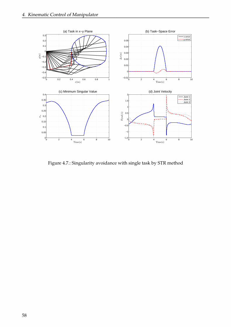
4. Kinematic Control of Manipulator
0 0.2 0.4 0.6 0.8 1−0.5
−0.4
−0.3
−0.2
−0.1
0
0.1
0.2
0.3
x(m)
y(m
)
(a) Task in x−y Plane
0 2 4 6 8 10−0.01
0
0.01
0.02
0.03
0.04
0.05
Time(s)
∆x(m
)
(b) Task−Space Error
x errory error
0 2 4 6 8 100
0.05
0.1
0.15
0.2
0.25
0.3
0.35
0.4
Time(s)
σm
(c) Minimum Singular Value
0 2 4 6 8 10−1.5
−1
−0.5
0
0.5
1
1.5
2
Time(s)
θ(rad/s)
(d) Joint Velocity
Joint 1Joint 2Joint 3
Figure 4.7.: Singularity avoidance with single task by STR method
58
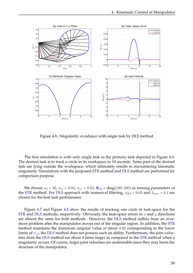
4. Kinematic Control of Manipulator
0 0.2 0.4 0.6 0.8 1−0.5
−0.4
−0.3
−0.2
−0.1
0
0.1
0.2
0.3
x(m)
y(m
)
(a) Task in x−y Plane
0 2 4 6 8 10−0.01
0
0.01
0.02
0.03
0.04
0.05
Time(s)
∆x(m
)
(b) Task−Space Error
x errory error
0 2 4 6 8 100
0.05
0.1
0.15
0.2
0.25
0.3
0.35
0.4
Time(s)
σm
(c) Minimum Singular Value
0 2 4 6 8 10−8
−6
−4
−2
0
2
4
6
8
10
Time(s)
θ(rad/s)
(d) Joint Velocity
Joint 1Joint 2Joint 3
Figure 4.8.: Singularity avoidance with single task by DLS method
The first simulation is with only single task as the primary task depicted in Figure 4.6.The desired task is to track a circle in its workspace in 10 seconds. Some part of the desiredtask are lying outside the workspace, which ultimately results in encountering kinematicsingularity. Simulations with the proposed STR method and DLS method are performed forcomparison purpose.
We choose α0 = 20, σif = 0.05, σuf = 0.02, Kik = diag(100,100) as turning parameters ofthe STR method. For DLS approach with numerical filtering, ǫDLS = 0.05 and λmax = 0.1 arechosen for the best task performance.
Figure 4.7 and Figure 4.8 show the results of tracking one circle in task-space for theSTR and DLS methods, respectively. Obviously, the task-space errors in x and y directionsare almost the same for both methods. However, the DLS method suffers from an over-shoot problem after the manipulator moves out of the singular region. In addition, the STRmethod maintains the minimum singular value of about 0.02 corresponding to the lowerlimits of σuf , the DLS method does not possess such an ability. Furthermore, the joint veloc-ities from the DLS method are about 4 times larger as compared to the STR method when asingularity occurs. Of course, larger joint velocities are undesirable since they may harm thestructure of the manipulator.
59

4. Kinematic Control of Manipulator
0 0.2 0.4 0.6 0.8 1−0.5
−0.4
−0.3
−0.2
−0.1
0
0.1
0.2
0.3
x(m)
y(m
)
(a) Task in x−y Plane
0 2 4 6 8 10−20
−15
−10
−5
0
5
10
Time(s)
θ(rad/s)
(b) Joint Velocity
Joint 1Joint 2Joint 3
4 4.5 5 5.5 6−2
−1.5
−1
−0.5
0
0.5
1
0 2 4 6 8 10−0.01
0
0.01
0.02
0.03
0.04
0.05
Time(s)
∆x1(m
)
(c) Primary Task−Space Error
x errory error
0 2 4 6 8 100
0.05
0.1
0.15
0.2
0.25
0.3
0.35
0.4
Time(s)
σm
(d) Primary Task Minimum Singular Value
0 2 4 6 8 10−0.2
0
0.2
0.4
0.6
0.8
1
1.2
1.4
1.6
1.8
Time(s)
∆x2(m
)
(e) Secondary Task−Space Error
0 2 4 6 8 100
0.1
0.2
0.3
0.4
0.5
0.6
Time(s)
σm
(f) Secondary Task Minimum Singular Value
Figure 4.9.: Singularity avoidance with two subtasks by STR method
60

4. Kinematic Control of Manipulator
0 0.2 0.4 0.6 0.8 1−0.5
−0.4
−0.3
−0.2
−0.1
0
0.1
0.2
0.3
x(m)
y(m
)
(a) Task in x−y Plane
0 2 4 6 8 10−20
−15
−10
−5
0
5
10
Time(s)
θ(rad/s)
(b) Joint Velocity
Joint 1Joint 2Joint 3
4 4.5 5 5.5 6−2
−1.5
−1
−0.5
0
0.5
1
0 2 4 6 8 10−0.01
0
0.01
0.02
0.03
0.04
0.05
Time(s)
∆x1(m
)
(c) Primary Task−Space Error
x errory error
0 2 4 6 8 100
0.05
0.1
0.15
0.2
0.25
0.3
0.35
0.4
Time(s)
σm
(d) Primary Task Minimum Singular Value
0 2 4 6 8 10−0.2
0
0.2
0.4
0.6
0.8
1
1.2
1.4
1.6
1.8
Time(s)
∆x2(m
)
(e) Secondary Task−Space Error
0 2 4 6 8 100
0.1
0.2
0.3
0.4
0.5
0.6
Time(s)
σm
(f) Secondary Task Minimum Singular Value
Figure 4.10.: Singularity avoidance with two subtasks by DLS method
To verify the performance of the STR method applying in multiple subtasks with task-priority, a secondary task is introduced as shown in Figure 4.6, while the primary task is stillto track a circle as depicted previously. The secondary task x2 is to keep the orientation ofthe end-effector equal to 90 . Figure 4.9 and Figure 4.10 show the results of completing twosubtasks in task-space using the STR and DLS methods with control gains K1 = diag(1.5,1.5)and K2 = 0.5, respectively. One can see that, STR method generates smoother joint velocitythan DLS approach. Moreover, primary task-space error is smaller for STR method, whilethe minimum singular value for J1 is maintained about 0.02 as defined beforehand. Sincethe conflict between the primary and secondary tasks, both kinematic and algorithmic sin-gularities emerge, while STR method successfully drives the matrix J2 out of the singular
61

4. Kinematic Control of Manipulator
region.
0 0.2 0.4 0.6 0.8 1−0.5
−0.4
−0.3
−0.2
−0.1
0
0.1
0.2
0.3
x(m)
y(m
)
(a) Task in x−y Plane
0 2 4 6 8 10−20
−15
−10
−5
0
5
10
Time(s)
θ(rad/s)
(b) Joint Velocity
Joint 1Joint 2Joint 3
4 4.5 5 5.5 6−2
−1.5
−1
−0.5
0
0.5
1
1.5
0 2 4 6 8 10−0.01
0
0.01
0.02
0.03
0.04
0.05
Time(s)
∆x1(m
)
(c) Primary Task−Space Error
x errory error
0 2 4 6 8 100
0.05
0.1
0.15
0.2
0.25
0.3
0.35
0.4
Time(s)
σm
(d) Primary Task Minimum Singular Value
0 2 4 6 8 10−0.2
0
0.2
0.4
0.6
0.8
1
1.2
1.4
1.6
1.8
Time(s)
∆x2(m
)
(e) Secondary Task−Space Error
0 2 4 6 8 100
0.1
0.2
0.3
0.4
0.5
0.6
Time(s)
σm
(f) Secondary Task Minimum Singular Value
Figure 4.11.: Singularity avoidance with two subtasks and higher gain by STR method
62
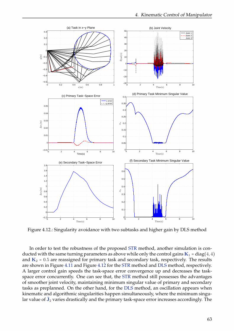
4. Kinematic Control of Manipulator
0 0.2 0.4 0.6 0.8 1−0.5
−0.4
−0.3
−0.2
−0.1
0
0.1
0.2
0.3
x(m)
y(m
)
(a) Task in x−y Plane
0 2 4 6 8 10−30
−20
−10
0
10
20
30
40
50
Time(s)
θ(rad/s)
(b) Joint Velocity
Joint 1Joint 2Joint 3
0 2 4 6 8 10−0.01
0
0.01
0.02
0.03
0.04
0.05
Time(s)
∆x1(m
)
(c) Primary Task−Space Error
x errory error
0 2 4 6 8 100
0.05
0.1
0.15
0.2
0.25
0.3
0.35
0.4
Time(s)
σm
(d) Primary Task Minimum Singular Value
0 2 4 6 8 10−0.2
0
0.2
0.4
0.6
0.8
1
1.2
1.4
1.6
1.8
Time(s)
∆x2(m
)
(e) Secondary Task−Space Error
0 2 4 6 8 100
0.1
0.2
0.3
0.4
0.5
0.6
Time(s)
σm
(f) Secondary Task Minimum Singular Value
Figure 4.12.: Singularity avoidance with two subtasks and higher gain by DLS method
In order to test the robustness of the proposed STR method, another simulation is con-ducted with the same turning parameters as above while only the control gains K1 = diag(4,4)and K2 = 0.5 are reassigned for primary task and secondary task, respectively. The resultsare shown in Figure 4.11 and Figure 4.12 for the STR method and DLS method, respectively.A larger control gain speeds the task-space error convergence up and decreases the task-space error concurrently. One can see that, the STR method still possesses the advantagesof smoother joint velocity, maintaining minimum singular value of primary and secondarytasks as preplanned. On the other hand, for the DLS method, an oscillation appears whenkinematic and algorithmic singularities happen simultaneously, where the minimum singu-lar value of J2 varies drastically and the primary task-space error increases accordingly. The
63
4. Kinematic Control of Manipulator
rapid fluctuation in joint velocity requires huge joint acceleration to accomplish such taskwhich is highly unwelcome in a real-world situation. This simulation reveals the robustnessof the STR method while the DLS method is more sensitive to the control gains.
From the simulation results on single task and two subtasks with task-priorities, theeffectiveness and robustness of the STR method are demonstrated through simulation stud-ies. When the manipulator is in the neighbourhood of a singularity, the selected minimumsingular value and its corresponding left singular vector guarantee the effectiveness androbustness of the proposed STR method.
4.3. Obstacle Detection and Avoidance
In order to perform various missions effectively, the motion control of robotic manipulatorsin the presence of workspace obstacles has been a prime concern over the past few decades.The existed solution to this problem, termed as collision avoidance, is normally consideredas a planning problem can be roughly categorized into the two classes of global and localplanning methods. As was described in section 2.3.3, global planning methods try to searchan optimal collision-free motion for the robots which generates a safe path between initialand goal configuration in the free configuration space. Its computational cost is expensiveand grows dramatically as the number of manipulator’s joints increase. Moreover, globalmethods are only suitable for structural and static environments which aren’t the case forgeneral space missions. The un-modelled and moving obstacles call for the on-line planningand control which entails local planning strategy as a main research topic. In this section, wepropose a new collision avoidance strategy with two control points to suppress the possiblefluctuation problems induced by the control point switch. Two control points are chosen toprevent collision between the manipulator and the obstacles and vibration issues.
4.3.1. Collision Detection
Before a collision avoidance strategy taking effect, what matters most is how to detect themoving obstacles nearby. Normally, object detection algorithms involve 3 dimensional spacemodelling problem and can be classified into two categories of Bounding Volume Hierarchy(BVH) and space decomposition algorithms as illustrated in Ericson (2005). Both two algo-rithms use the hierarchical structure to reduce the number of intersection tests of the geo-metrical elements and enhance the on-line computational efficiency. Comparing space de-composition algorithm with BVH algorithm, the former one needs more memory to restoreand less flexibility which often applied in the sparse environment with equally distributedobjects, while BVH method, which is applicable to use in the complex environment to calcu-late the possible collision, has gained a wide spectrum of attention both in academic researchor industrial application. Before we go into the detection algorithm in detail, let us first recallthe definition of the strictly convex objects and Voronoi region.
Strictly convex objects. LetO represent a closed subset of R3 and X(O) be the interior of(greater open subset of) O. O is strictly convex if and only if λA + (1 − λ)B ∈ X(O), ∀A ∈ O,∀B ∈ O and 0 < λ < 1.
64
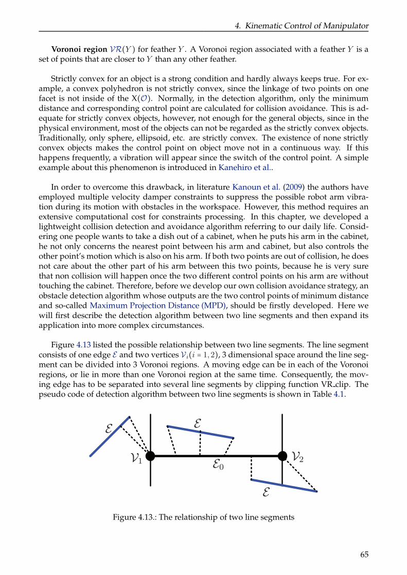
4. Kinematic Control of Manipulator
Voronoi region VR(Y ) for feather Y . A Voronoi region associated with a feather Y is aset of points that are closer to Y than any other feather.
Strictly convex for an object is a strong condition and hardly always keeps true. For ex-ample, a convex polyhedron is not strictly convex, since the linkage of two points on onefacet is not inside of the X(O). Normally, in the detection algorithm, only the minimumdistance and corresponding control point are calculated for collision avoidance. This is ad-equate for strictly convex objects, however, not enough for the general objects, since in thephysical environment, most of the objects can not be regarded as the strictly convex objects.Traditionally, only sphere, ellipsoid, etc. are strictly convex. The existence of none strictlyconvex objects makes the control point on object move not in a continuous way. If thishappens frequently, a vibration will appear since the switch of the control point. A simpleexample about this phenomenon is introduced in Kanehiro et al..
In order to overcome this drawback, in literature Kanoun et al. (2009) the authors haveemployed multiple velocity damper constraints to suppress the possible robot arm vibra-tion during its motion with obstacles in the workspace. However, this method requires anextensive computational cost for constraints processing. In this chapter, we developed alightweight collision detection and avoidance algorithm referring to our daily life. Consid-ering one people wants to take a dish out of a cabinet, when he puts his arm in the cabinet,he not only concerns the nearest point between his arm and cabinet, but also controls theother point’s motion which is also on his arm. If both two points are out of collision, he doesnot care about the other part of his arm between this two points, because he is very surethat non collision will happen once the two different control points on his arm are withouttouching the cabinet. Therefore, before we develop our own collision avoidance strategy, anobstacle detection algorithm whose outputs are the two control points of minimum distanceand so-called Maximum Projection Distance (MPD), should be firstly developed. Here wewill first describe the detection algorithm between two line segments and then expand itsapplication into more complex circumstances.
Figure 4.13 listed the possible relationship between two line segments. The line segmentconsists of one edge E and two vertices V i(i = 1,2), 3 dimensional space around the line seg-ment can be divided into 3 Voronoi regions. A moving edge can be in each of the Voronoiregions, or lie in more than one Voronoi region at the same time. Consequently, the mov-ing edge has to be separated into several line segments by clipping function VR clip. Thepseudo code of detection algorithm between two line segments is shown in Table 4.1.
V1V2
E0
EE
E
Figure 4.13.: The relationship of two line segments
65
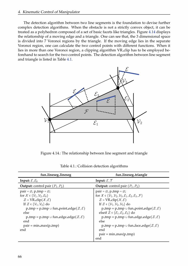
4. Kinematic Control of Manipulator
The detection algorithm between two line segments is the foundation to devise furthercomplex detection algorithms. When the obstacle is not a strictly convex object, it can betreated as a polyhedron composed of a set of basic facets like triangles. Figure 4.14 displaysthe relationship of a moving edge and a triangle. One can see that, the 3 dimensional spaceis divided into 7 Voronoi regions by the triangle. If the moving edge lies in the separateVoronoi region, one can calculate the two control points with different functions. When itlies in more than one Voronoi region, a clipping algorithm VR clip has to be employed be-forehand to search for the two control points. The detection algorithm between line segmentand triangle is listed in Table 4.1.
F
E1
V1
E2
V2
E3
V3
E
E
E
Figure 4.14.: The relationship between line segment and triangle
Table 4.1.: Collision detection algorithms
fun lineseg lineseg fun lineseg triangle
Input: E ,E0 Input: E ,TOutput: control pair (P1, P2) Output: control pair (P1, P2)pair = ∅, p tmp = ∅;for X ∈ V1,V2,E0Z = VR clip(X ,E)If Z ∈ V1,V2 do
p tmp = p tmp ∪ fun point edge(Z,E)else
p tmp = p tmp ∪ fun edge edge(Z,E)endpair = min max(p tmp)
end
pair = ∅, p tmp = ∅;for X ∈ V1,V2,V3,E1,E2,E3,FZ = VR clip(X ,E)If Z ∈ V1,V2,V3 do
p tmp = p tmp ∪ fun point edge(Z,E)elseif Z ∈ E1,E2,E3 do
p tmp = p tmp ∪ fun edge edge(Z,E)else
p tmp = p tmp ∪ fun face edge(Z,E)endpair = min max(p tmp)
end
66
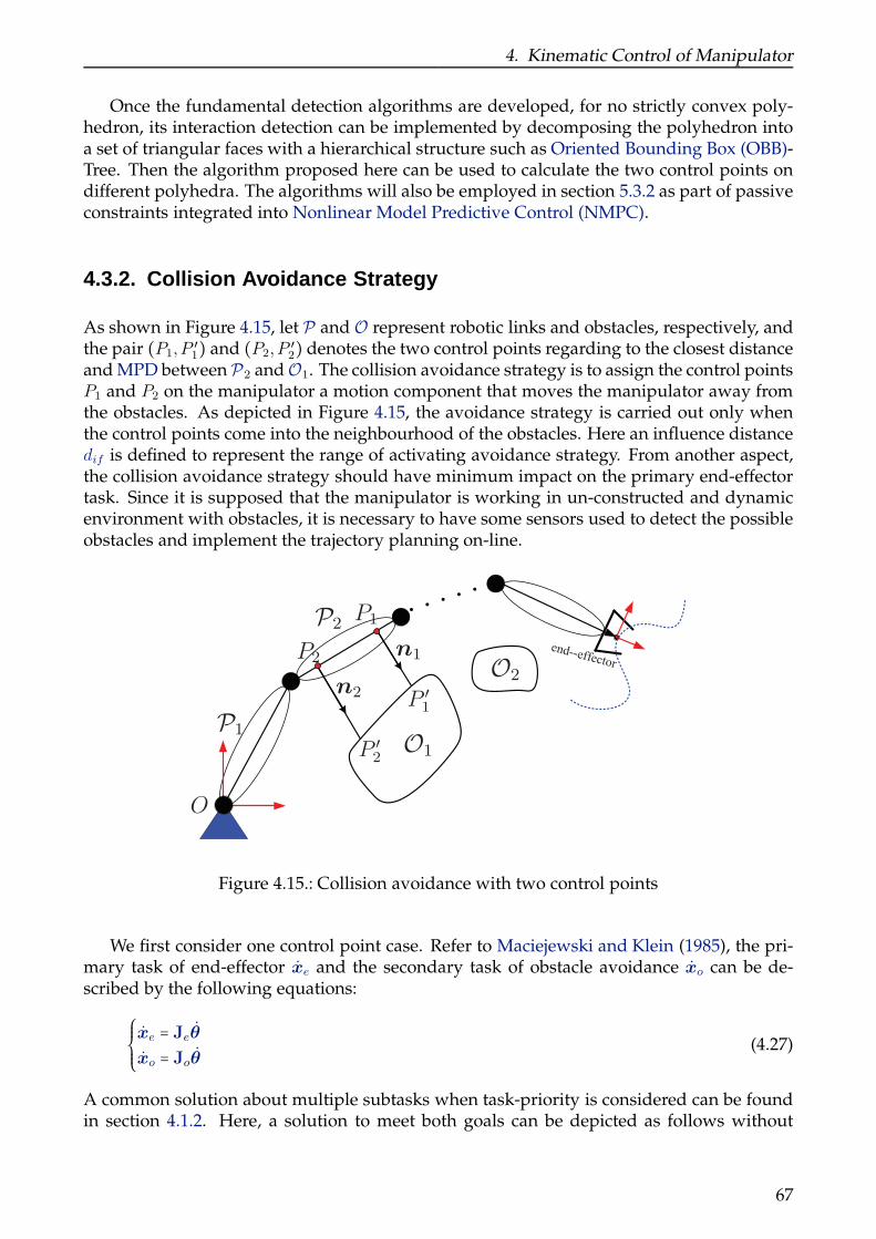
4. Kinematic Control of Manipulator
Once the fundamental detection algorithms are developed, for no strictly convex poly-hedron, its interaction detection can be implemented by decomposing the polyhedron intoa set of triangular faces with a hierarchical structure such as Oriented Bounding Box (OBB)-Tree. Then the algorithm proposed here can be used to calculate the two control points ondifferent polyhedra. The algorithms will also be employed in section 5.3.2 as part of passiveconstraints integrated into Nonlinear Model Predictive Control (NMPC).
4.3.2. Collision Avoidance Strategy
As shown in Figure 4.15, let P and O represent robotic links and obstacles, respectively, andthe pair (P1, P
′1) and (P2, P
′2) denotes the two control points regarding to the closest distance
and MPD between P2 andO1. The collision avoidance strategy is to assign the control pointsP1 and P2 on the manipulator a motion component that moves the manipulator away fromthe obstacles. As depicted in Figure 4.15, the avoidance strategy is carried out only whenthe control points come into the neighbourhood of the obstacles. Here an influence distancedif is defined to represent the range of activating avoidance strategy. From another aspect,the collision avoidance strategy should have minimum impact on the primary end-effectortask. Since it is supposed that the manipulator is working in un-constructed and dynamicenvironment with obstacles, it is necessary to have some sensors used to detect the possibleobstacles and implement the trajectory planning on-line.
end--effector
O1
n1
P1
P2
n2
O
O2
P1
P2
P 0
1
P 0
2
Figure 4.15.: Collision avoidance with two control points
We first consider one control point case. Refer to Maciejewski and Klein (1985), the pri-mary task of end-effector xe and the secondary task of obstacle avoidance xo can be de-scribed by the following equations:
⎧⎪⎪⎨⎪⎪⎩xe = Jeθ
xo = Joθ(4.27)
A common solution about multiple subtasks when task-priority is considered can be foundin section 4.1.2. Here, a solution to meet both goals can be depicted as follows without
67

4. Kinematic Control of Manipulator
considering the null-space motion h = 0:
θ = J+e xe + J+o(xo − JoJ
+e xd) (4.28)
where Jo = Jo(En − J+eJe) is the projection of matrix Jo on the null-space of Je. Each termin the proceeding equation has an simple interpretation. The first term J+e xe guarantees theimplementation of the primary task (normally, xc = xd +K(xd − xe) is employed instead ofxe for tracking stability reasons). The second term, which is projected on the null-space ofthe end-effector’s Jacobian matrix, depicts the motion of the control point without influenc-ing the motion of the end-effector. The term JoJ
+e xd describes the motion of control point
induced by the end-effector motion, and the matrix Jo which combines the null-space ofthe end-effector and the control point, is utilized to transform the assigned velocity of thecontrol point from operational-space to the joint-space.
Considering the Cartesian space, if we want to activate the collision avoidance strategyand assign a velocity to the control point, then xo should be a 3 dimensional vector, whichmeans Jo ∈ R3×n. This will require 3 additional DOR to complete the avoidance in a 3 dimen-sional Cartesian space. Nevertheless, not every manipulator has 3 DOR for the purpose ofcollision avoidance. This issue can be resolved by the geometric projection method as intro-duced in Zlajpah and Nemec (2002). In fact, the obstacle avoidance strategy only requires tocontrol the escape velocity in the direction of the line connecting the control point with thecorrespondent point on the obstacle, this is just one dimensional constraint and one DORwould be sufficient to avoid the possible collision. The derivative of the distance ∥P1P
′1∥ can
be denoted by the following equation if the obstacle is steady:
d1 = ⟨Joθ,n1⟩ = ⟨θ,nT1Jo⟩ (4.29)
n1 is the unit vectorP1P
′
1
∥P1P′
1∥ and notation ⟨u,v⟩ refers to the inner product of vector u and
v. Now we use Jd = nT1Jo as a new Jacobian matrix to replace Jo in equation 4.28, then
velocity xo and nT1JoJ
+e xd become scalar. Consequently, the calculating of Moore-Penrose
pseudo-inverse of nT1Jo is much faster since now it can be expressed as follows:
(nT1 Jo)+ = JT
on1(nT1 JoJ
Ton1)−1 (4.30)
There is no need to inverse any matrix in computing the pseudo-inverse of nT1Jo since
nT1JoJ
Ton1 is scalar. This of course saves a lot of computation effort in the trajectory plan-
ning. Recall the equation 4.28, the new inverse kinematic solution to complete primary taskand collision avoidance can be expressed by:
θ = J+e xe + (nT1 Jo)+(xo −n
T1JoJ
+e xd) (4.31)
A hidden issue of above solution is the possible singularity where the Jacobian matrix Je ornT
1Jo lose its rank. When a singularity happens, the joint velocity will go to infinity which
is not welcome. This problem can be tackled by employing the DLS method or the STRmethod developed in section 4.2.2.
In above analysis, only the nearest point between link and obstacle is taken into account,the switch between the control points results in bounce at some configurations when twoobjects are not strictly convex. However, we do not want to treat the control point P2 asthe third subtask. This is because normally for the simplicity and economical reasons, notso many DOR are available in a redundant manipulator. Hence, a better way would be,
68

4. Kinematic Control of Manipulator
choosing a new control point P0 on the manipulator which combines the information of thetwo control points P1 and P2 for the purpose of collision avoidance. Furthermore, the newcontrol point P0 should be moved on the manipulator continuously. It can be calculated asfollows:
P0 =dif − d1
2dif − d1 − d2P1 +
dif − d22dif − d1 − d2
P2 (4.32)
where d1 = ∥P1P′1∥ and d2 = ∥P2P
′2∥ are the distance between P1 and obstacle, P2 and obstacle,
respectively. The corresponding unit vector n0 for escaping from the obstacles is equal to n1
while the control point P1 is more critical. The desired critical point velocity xo = αcvo, vo isthe assigned nominal velocity and αc is the obstacle avoidance gain which depends on thecritical distance to the obstacles:
αc =⎧⎪⎪⎨⎪⎪⎩(dsr
d1)2 − 1 d1 < dsr
0 d1 ≥ dsr(4.33)
dsr defines another critical distance named security distance. If the manipulator is too closeto the obstacles d1 ≤ duf , the primary task xe should be cancelled which is controlled byturning parameter αe. The unsafe distance duf can be a predefined quantity or be yieldedaccording to the dynamic properties of the manipulator.
For smoother motion, the magnitude of xo should be 0 at dsr. Then the solution for theinverse kinematics in conjunction with obstacles avoidance can be expressed as:
θ = αeJ+e xe +αd (Jd(En − J
+eJe))+ (αcvo − JdJ
+e xd) (4.34)
The turning parameter αd can be defined as follows:
αd =
⎧⎪⎪⎪⎪⎪⎨⎪⎪⎪⎪⎪⎩
0 d1 ≥ dif1
2(1 + cos(π d1−dsr
dif−dsr)) dif ≤ d1 < dsr
1 d1 ≤ dsr
(4.35)
The functional behaviour of turning parameters αc, αd and αe is shown in Figure 4.16.
dduf dif
®c
dsr
®d®e
0
1
Figure 4.16.: The functional behaviour of the turning parameters for collision avoidance
From equation 4.34 and Figure 4.16, one can see that, after the control point P1 enters intothe influence zone, i.e. d1 < dif , the avoidance strategy begins to influence the configuration
69

4. Kinematic Control of Manipulator
of the manipulator. However, only part of the homogeneous solution is included. As thedistance between control point and the obstacles decreases, more homogeneous solution isexerted which diminishes the relative velocity between control point and the obstacles fromdif to dsr. Once the control point is in the range of the dsr, a bounce velocity xo is assignedand the complete homogeneous solution is included. This avoidance strategy will assurethe control point move out of the dangerous zone and guarantee the smooth transition evenwhen the control point P1 switches during the motion of the manipulator. Equation 4.34is designed for a single obstacle, when there are more than one obstacle in the workspace,since the shortage of DOR, one can not treat different obstacles as multiple subtasks. If theequation 4.34 is still in use without modification, the frequent switching of the control pointson the manipulator will also result in oscillation in joint velocities. This discontinuity of jointvelocity is highly unwelcome since it maybe harmful for the structure and actuators of themanipulator. To improve the performance, a weighted sum of the homogeneous solutionconsidering all the obstacles in the influence zone can be expressed by:
θ = αeJ+e xe +
no
∑i=1
wiαdi (Jdi(En − J+eJe))+ (αcivo − JdiJ
+e xd) (4.36)
no is the number of the obstacles in the influence zone, the weighting factor wi can be definedas:
wi =dif − d1i
∑no
i=1(dif − d1i) (4.37)
The definition of weighting factor wi shows the relative significance of the different obstaclesin the influence zone. When one obstacle is much closer than the others, i.e. d1i → 0, thenits corresponding weight factor increases and the velocity at that control point ramps up aswell.
4.3.3. Simulation Results
To verify the effectiveness and performance of the proposed method in this chapter, simu-lation results are presented by using a 10 revolute planar manipulator. The primary task isto move the end-effector across a corridor. A schematic diagram of the simulation is illus-trated in Figure 4.17. The widely used collision avoidance method in Zlajpah and Nemec(2002) is employed here with same turning parameters for comparison reason. For the sim-ulation of our proposed collision avoidance method, the link length in Figure 4.17 is set tol1 = l2 = ⋯ = l10 = 0.1m. The kinematic control gain K = diag(50,50). The desired end-effector trajectory is xd = [0.2266,0.2539 + 0.11t]T during 5 seconds and the motion of themanipulator has been constrained by two obstacles. The simulation sample time is set to 10milliseconds.
70

4. Kinematic Control of Manipulator
O
y
x
Obstacle 2Obstacle 1
Primary Task
l1
l2
l3
l10
l7
l6
l5l4
l8
l9
Figure 4.17.: 10 revolute planar manipulator and obstacles
The parameters of dif , dsr, duf are set to 0.1m, 0.05m and 0.02m. The assigned nominalvelocity is vo = 5m/s. The results of path tracking without control point, with one controlpoint and with two control points are shown in Figure 4.18, Figure 4.19 and Figure 4.20,respectively. One can see that, when no collision avoidance strategy is applied, some linkswill collide with the second obstacle when the manipulator tracking the desired path. If oneor two control points are considered, the manipulator can autonomously avoid the possiblecollision during its motion. The task-space tracking error with one control point, two controlpoints and without control point are equally the same, which means, the successful collisionavoidance strategy will not affect the primary task since it is completed in the null-space ofthe primary task’s Jacobian matrix. No matter one control point or two, the minimum dis-tance between different links and obstacles reveals the effectiveness of the avoidance strate-gies. The minimum distance between links and obstacles is constrained without movinginto the predefined security zone dsr. The main difference between the traditional collisionavoidance method and the proposed method lies in the generation of joint velocity. Onecan see that, at 3.73s, 4.56s and 4.80s, the joint velocity endures a sharp change because ofthe control point switch. This discontinuity will result in large jerk in the acceleration levelwhich is highly unexpected. While with the proposed method, in virtue of the autonomousregulation of control points, smoother joint velocities are generated without discontinuity.The proposed algorithm also provides us an intuitive way to understand and can be ex-panded to further application. The idea of regulating two control points will be adopted insection 5.3.2.
71
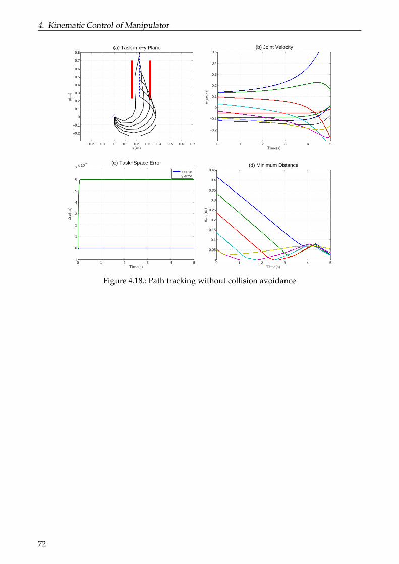
4. Kinematic Control of Manipulator
−0.2 −0.1 0 0.1 0.2 0.3 0.4 0.5 0.6 0.7
−0.2
−0.1
0
0.1
0.2
0.3
0.4
0.5
0.6
0.7
0.8
x(m)
y(m
)
(a) Task in x−y Plane
0 1 2 3 4 5
−0.2
−0.1
0
0.1
0.2
0.3
0.4
0.5
Time(s)
θ(rad/s)
(b) Joint Velocity
0 1 2 3 4 5−1
0
1
2
3
4
5
6
7x 10
−4
Time(s)
∆x(m
)
(c) Task−Space Error
x errory error
0 1 2 3 4 50
0.05
0.1
0.15
0.2
0.25
0.3
0.35
0.4
0.45
Time(s)
dmin(m
)
(d) Minimum Distance
Figure 4.18.: Path tracking without collision avoidance
72

4. Kinematic Control of Manipulator
−0.2 −0.1 0 0.1 0.2 0.3 0.4 0.5 0.6 0.7
−0.2
−0.1
0
0.1
0.2
0.3
0.4
0.5
0.6
0.7
0.8
x(m)
y(m
)
(a) Task in x−y Plane
0 1 2 3 4 5−0.6
−0.4
−0.2
0
0.2
0.4
0.6
0.8
Time(s)
θ(rad/s)
(b) Joint Velocity
0 1 2 3 4 5−1
0
1
2
3
4
5
6
7x 10
−4
Time(s)
∆x(m
)
(c) Task−Space Error
x errory error
0 1 2 3 4 50
0.05
0.1
0.15
0.2
0.25
0.3
0.35
0.4
0.45
Time(s)
dmin(m
)
(d) Minimum Distance
Figure 4.19.: Path tracking with one control point for collision avoidance
73
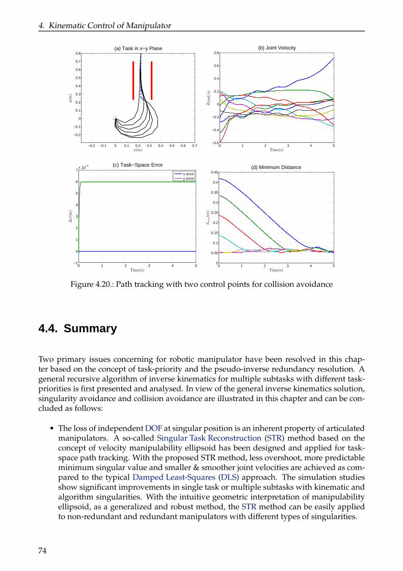
4. Kinematic Control of Manipulator
−0.2 −0.1 0 0.1 0.2 0.3 0.4 0.5 0.6 0.7
−0.2
−0.1
0
0.1
0.2
0.3
0.4
0.5
0.6
0.7
0.8
x(m)
y(m
)
(a) Task in x−y Plane
0 1 2 3 4 5−0.6
−0.4
−0.2
0
0.2
0.4
0.6
0.8
Time(s)
θ(rad/s)
(b) Joint Velocity
0 1 2 3 4 5−1
0
1
2
3
4
5
6
7x 10
−4
Time(s)
∆x(m
)
(c) Task−Space Error
x errory error
0 1 2 3 4 50
0.05
0.1
0.15
0.2
0.25
0.3
0.35
0.4
0.45
Time(s)
dmin(m
)
(d) Minimum Distance
Figure 4.20.: Path tracking with two control points for collision avoidance
4.4. Summary
Two primary issues concerning for robotic manipulator have been resolved in this chap-ter based on the concept of task-priority and the pseudo-inverse redundancy resolution. Ageneral recursive algorithm of inverse kinematics for multiple subtasks with different task-priorities is first presented and analysed. In view of the general inverse kinematics solution,singularity avoidance and collision avoidance are illustrated in this chapter and can be con-cluded as follows:
• The loss of independent DOF at singular position is an inherent property of articulatedmanipulators. A so-called Singular Task Reconstruction (STR) method based on theconcept of velocity manipulability ellipsoid has been designed and applied for task-space path tracking. With the proposed STR method, less overshoot, more predictableminimum singular value and smaller & smoother joint velocities are achieved as com-pared to the typical Damped Least-Squares (DLS) approach. The simulation studiesshow significant improvements in single task or multiple subtasks with kinematic andalgorithm singularities. With the intuitive geometric interpretation of manipulabilityellipsoid, as a generalized and robust method, the STR method can be easily appliedto non-redundant and redundant manipulators with different types of singularities.
74

4. Kinematic Control of Manipulator
• An inevitable issue during motion of space manipulator in its workspace is collisionavoidance. Conventional methods have the demerits of oscillation of the manipulatordue to the switch of the control point on the manipulator when the objects can notbe treated as the strictly convex objects. An extra control point corresponding to theMaximum Projection Distance (MPD) together with the nearest point of the minimumdistance is employed to suppress the possible fluctuation of the manipulator. The in-teraction test between line segment and line segment, rectangle, circle is implementedto provide the fully information of the two control points. An avoidance strategy isderived based on the general inverse kinematics solution using the two control pointsand the geometrical projection method. The new obstacle detection and avoidancestrategy does not require too many DOR to complete the collision avoidance, evenonly 1 DOR can handle the collision avoidance problem with multiple obstacles. Sim-ulation results demonstrate the performance of the proposed method when comparedto the traditional collision avoidance algorithm.
75

5. Model Predictive Control
Authority in science exists to be questioned, since heresy is the spring from which newideas flow.
—John C. Polanyi
This chapter investigates the application of Nonlinear Model Predictive Control (NMPC)to space manipulators in capturing an un-cooperative target satellite in space. How to con-trol the motion of space manipulator with high accuracy and various constraints is a sig-nificant guarantee for the completion of the demanded space tasks. The fundamental ideaand mathematical formulation of MPC is firstly introduced. In order to apply MPC to spacerobot, a feedback linearisation procedure is conducted to transform the non-linear systeminto a linear one. In addition, how to handle the different types of constraints in controllerdesign is another primary concern. The constraints appear in practice imposed on deci-sion variables are categorized into three classes: physical/security constraints, operationalconstraints and passive constraints. These constraints, together with varied priorities, con-stitute a new Quadratic Programming (QP) searching algorithm. A recursive state estima-tor regarding the minimum variance states estimation from Kalman Filter (KF) is derived.The controller has been implemented for a 7 DOF kinematically redundant manipulator in-stalled on a 6 DOF free-floating satellite via simulation studies considering singularity andobstacles in the workspace of the space manipulator. Real-time end-effector approaching totarget, path tracking and capturing target, particularly verify the effectiveness and prospectof the proposed NMPC strategy for space robot.
5.1. Model Predictive Control
MPC refers to a wide spread class of control strategies that apply an explicit model topredict the response of a plant. Originated from 1970s, MPC, also referred to RHC, hasbeen widely employed in the field of chemical processing industries as an effective con-trol strategy to deal with multi-variable constrained control problems. The interests inMPC and RHC started to surge only in the 1980s after exposition of the first papers on ID-COM Richalet et al. (1978) and DMC Cutler and Ramaker (1980), and the first comprehen-sive publication of GPC Clarke et al. (1987a,b). In the past two decades, various formula-tions about MPC have been developed for linear and non-linear systems Morari and H. Lee(1999), Qin and Badgwell (2003), that found successful applications especially in process in-dustries Camacho and Bordons (2004), Maciejowski (2002).
77
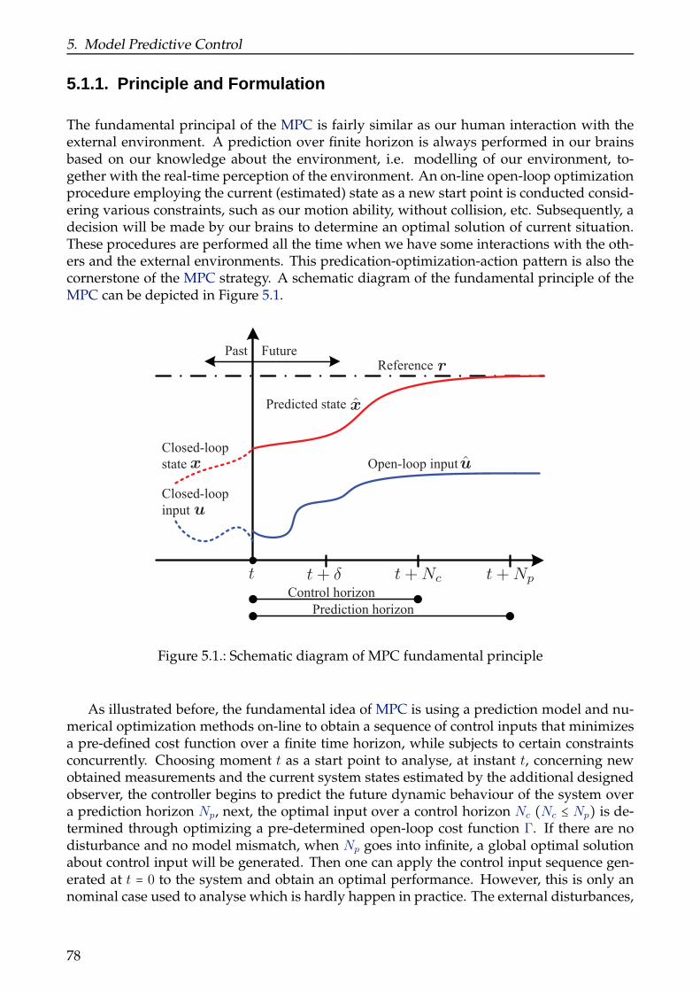
5. Model Predictive Control
5.1.1. Principle and Formulation
The fundamental principal of the MPC is fairly similar as our human interaction with theexternal environment. A prediction over finite horizon is always performed in our brainsbased on our knowledge about the environment, i.e. modelling of our environment, to-gether with the real-time perception of the environment. An on-line open-loop optimizationprocedure employing the current (estimated) state as a new start point is conducted consid-ering various constraints, such as our motion ability, without collision, etc. Subsequently, adecision will be made by our brains to determine an optimal solution of current situation.These procedures are performed all the time when we have some interactions with the oth-ers and the external environments. This predication-optimization-action pattern is also thecornerstone of the MPC strategy. A schematic diagram of the fundamental principle of theMPC can be depicted in Figure 5.1.
u
x
t t + ± t + Nc t + Np
Closed-loop
state
Closed-loop
input
Predicted state x
Open-loop input u
Past Future
Control horizon
Prediction horizon
Reference r
Figure 5.1.: Schematic diagram of MPC fundamental principle
As illustrated before, the fundamental idea of MPC is using a prediction model and nu-merical optimization methods on-line to obtain a sequence of control inputs that minimizesa pre-defined cost function over a finite time horizon, while subjects to certain constraintsconcurrently. Choosing moment t as a start point to analyse, at instant t, concerning newobtained measurements and the current system states estimated by the additional designedobserver, the controller begins to predict the future dynamic behaviour of the system overa prediction horizon Np, next, the optimal input over a control horizon Nc (Nc ≤ Np) is de-termined through optimizing a pre-determined open-loop cost function Γ. If there are nodisturbance and no model mismatch, when Np goes into infinite, a global optimal solutionabout control input will be generated. Then one can apply the control input sequence gen-erated at t = 0 to the system and obtain an optimal performance. However, this is only annominal case used to analyse which is hardly happen in practice. The external disturbances,
78
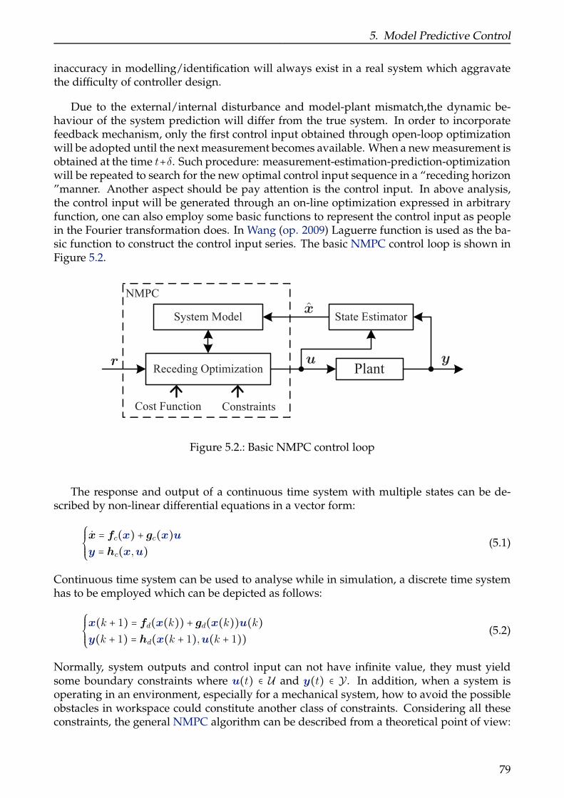
5. Model Predictive Control
inaccuracy in modelling/identification will always exist in a real system which aggravatethe difficulty of controller design.
Due to the external/internal disturbance and model-plant mismatch,the dynamic be-haviour of the system prediction will differ from the true system. In order to incorporatefeedback mechanism, only the first control input obtained through open-loop optimizationwill be adopted until the next measurement becomes available. When a new measurement isobtained at the time t+δ. Such procedure: measurement-estimation-prediction-optimizationwill be repeated to search for the new optimal control input sequence in a “receding horizon”manner. Another aspect should be pay attention is the control input. In above analysis,the control input will be generated through an on-line optimization expressed in arbitraryfunction, one can also employ some basic functions to represent the control input as peoplein the Fourier transformation does. In Wang (op. 2009) Laguerre function is used as the ba-sic function to construct the control input series. The basic NMPC control loop is shown inFigure 5.2.
NMPC
System Model
Receding Optimization
Cost Function Constraints
uPlant
State Estimatorx
yr
Figure 5.2.: Basic NMPC control loop
The response and output of a continuous time system with multiple states can be de-scribed by non-linear differential equations in a vector form:
⎧⎪⎪⎨⎪⎪⎩x = fc(x) + gc(x)uy = hc(x,u) (5.1)
Continuous time system can be used to analyse while in simulation, a discrete time systemhas to be employed which can be depicted as follows:
⎧⎪⎪⎨⎪⎪⎩x(k + 1) = fd(x(k)) + gd(x(k))u(k)y(k + 1) = hd(x(k + 1),u(k + 1)) (5.2)
Normally, system outputs and control input can not have infinite value, they must yieldsome boundary constraints where u(t) ∈ U and y(t) ∈ Y . In addition, when a system isoperating in an environment, especially for a mechanical system, how to avoid the possibleobstacles in workspace could constitute another class of constraints. Considering all theseconstraints, the general NMPC algorithm can be described from a theoretical point of view:
79
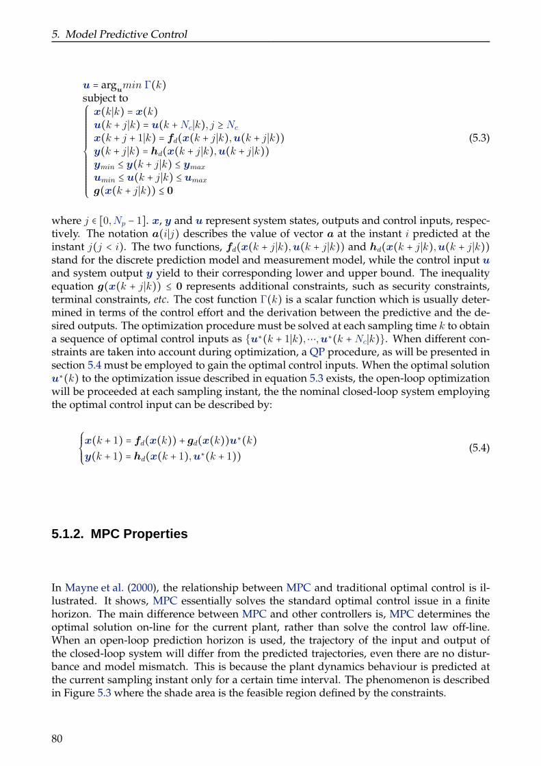
5. Model Predictive Control
u = argumin Γ(k)
subject to⎧⎪⎪⎪⎪⎪⎪⎪⎪⎪⎪⎪⎪⎪⎨⎪⎪⎪⎪⎪⎪⎪⎪⎪⎪⎪⎪⎪⎩
x(k∣k) = x(k)u(k + j∣k) = u(k +Nc∣k), j ≥ Nc
x(k + j + 1∣k) = fd(x(k + j∣k),u(k + j∣k))y(k + j∣k) = hd(x(k + j∣k),u(k + j∣k))ymin ≤ y(k + j∣k) ≤ ymax
umin ≤ u(k + j∣k) ≤ umax
g(x(k + j∣k)) ≤ 0
(5.3)
where j ∈ [0,Np − 1]. x, y and u represent system states, outputs and control inputs, respec-tively. The notation a(i∣j) describes the value of vector a at the instant i predicted at theinstant j(j < i). The two functions, fd(x(k + j∣k),u(k + j∣k)) and hd(x(k + j∣k),u(k + j∣k))stand for the discrete prediction model and measurement model, while the control input uand system output y yield to their corresponding lower and upper bound. The inequalityequation g(x(k + j∣k)) ≤ 0 represents additional constraints, such as security constraints,terminal constraints, etc. The cost function Γ(k) is a scalar function which is usually deter-mined in terms of the control effort and the derivation between the predictive and the de-sired outputs. The optimization procedure must be solved at each sampling time k to obtaina sequence of optimal control inputs as u∗(k + 1∣k),⋯,u∗(k +Nc∣k). When different con-straints are taken into account during optimization, a QP procedure, as will be presented insection 5.4 must be employed to gain the optimal control inputs. When the optimal solutionu∗(k) to the optimization issue described in equation 5.3 exists, the open-loop optimizationwill be proceeded at each sampling instant, the the nominal closed-loop system employingthe optimal control input can be described by:
⎧⎪⎪⎨⎪⎪⎩x(k + 1) = fd(x(k)) + gd(x(k))u∗(k)y(k + 1) = hd(x(k + 1),u∗(k + 1)) (5.4)
5.1.2. MPC Properties
In Mayne et al. (2000), the relationship between MPC and traditional optimal control is il-lustrated. It shows, MPC essentially solves the standard optimal control issue in a finitehorizon. The main difference between MPC and other controllers is, MPC determines theoptimal solution on-line for the current plant, rather than solve the control law off-line.When an open-loop prediction horizon is used, the trajectory of the input and output ofthe closed-loop system will differ from the predicted trajectories, even there are no distur-bance and model mismatch. This is because the plant dynamics behaviour is predicted atthe current sampling instant only for a certain time interval. The phenomenon is describedin Figure 5.3 where the shade area is the feasible region defined by the constraints.
80
5. Model Predictive Control
x1
x2
x(0) = x(0)x(0 + k) = x(k)
x(0 + Np)
x(k + Np)
Figure 5.3.: The mismatch between open-loop prediction and closed-loop behaviour
The key difference of MPC and standard controller design makes MPC possesses a seriesof properties:
• An explicit non-linear model is required in NMPC for prediction;
• Various constraints such as input, output, collision, etc can be integrated into NMPC;
• A specialized cost function can be predisposed and optimized on-line in NMPC;
• An on-line optimization of the open-loop control issue is necessary for the applicationof NMPC;
• An open-loop prediction in NMPC differs from the closed-loop behaviour.
The characteristics of NMPC show us its advantages in industrial applications, such asthe ability of constraints handling, multi-variable controller design and on-line optimiza-tion. However, on the other side, it also imports two consequences: the first one is the per-formance objective function to be minimized on-line over finite horizon does not guaranteethe optimal solution of closed-loop system behaviour; the second problem is the closed-loop system maybe un-stable because of the difference between finite horizon predictionand closed-loop behaviour.
5.2. NMPC Applied to Space Robot
As illustrated in section 2.3, the application of NMPC in the field of space robotics is re-ally rare. In Hirzinger et al. (1989), Inaba and Oda (2000), Oda et al. (1996), the predictioninformation was employed to assist the operators to complete the tele-operation withoutinvolving the control loop. In this chapter, NMPC will be applied to a free-floating spacerobot trying to capture a tumbling target satellite as shown in Figure 5.4.
81

5. Model Predictive Control
§I : inertia frame
§0 : base frame
§e : end-e®ector frame
CM : Center of Mass
XI
YI
ZI
X0 Y0
Z0
Xe Ye
Ze
System CM
rC0
re
rC2J1
J2
J3
Jn
Base CM
b0 ½0
b2
bn
a1
a2
an
½n
rCS
§I
§e
§0
b1Target
Servicer
Figure 5.4.: Schematic diagram of space robot
5.2.1. Free-Floating Space Robot
The dynamics of space robot with general structure is introduced in chapter 3 and expressedby equation 3.17. Before a contact between servicer and target occurs, there is no externalforces applied on the end-effector, i.e. f e = 0. If no actuators are activated to regulatethe servicer satellite position and attitude, f b = 0, the whole space robot system (base andmanipulator) is under the free-floating mode. The motion of the manipulator and the baseis intricately coupled and governed by the law of momentum conservation. Let l0 ∈ R6×1 bethe initial momentum of the system with respect to the inertial frame, it can be expressedby:
l0 =Hbxb +Hbmθ = 0 (5.5)
By substituting equation 5.5 into the kinematic mapping of the end-effector xe = Jbxb + Jeθ,the velocity of the end-effector can be given as follows:
xe = Jgθ = Jeθ − JbH−1b Hbmθ (5.6)
where Jg ∈ R6×n is termed the Generalized Jacobian Matrix (GJM) in Umetani and Yoshida(1989), Yoshida (1997). The dynamics formulation of free-floating space robot can be de-scribed by:
τ =H(θ)θ + c(θ, θ) (5.7)
where H(θ) = Hm −HTbmH
−1b Hbm ∈ Rn×n and c(θ, θ) = cm −HT
bmH−1b cb ∈ Rn×1 are the general-
ized inertia matrix and the non-linear force and torque vector for free-floating space robot,respectively.
5.2.2. Feedback Linearization
Continuous or discrete non-linear model expressed in equation 5.1 and 5.2 can be employedto predict the future behaviour of the plant, however, it is still hard to integrate this non-linear model for NMPC design. A feedback linearisation procedure is conducted through
82
5. Model Predictive Control
non-linear coordinate transform and non-linear state feedback to obtain a local linear model.Consider the continuous time state-space model expressed in equation 5.1, using Taylorexpansion at the point (x0,u0,y0), a so-called Jacobian linearisation method can be obtained:
⎧⎪⎪⎨⎪⎪⎩x = (∂fc(x0)
∂x+ ∂gc(x0)
∂xu0) (x −x0) + gc(x0)(u −u0)
y − y0 =∂hc(x0)
∂x(x −x0) (5.8)
One should note that Jacobian method is an exact approximation of the non-linear modelat (x0,u0), however, a control law based on the Jacobian model at such point may yielddegraded performance and robustness problems at other points.
Feedback linearisation provides us a powerful technical tool to convert the original non-linear model to an exact linear one over a large set of operation conditions. There are twomethods for feedback linearisation, one is input-output linearisation, the other is state-spacelinearisation. Both approaches rely on two operations: non-linear coordinate transformationand non-linear state feedback. In the input-output linearisation, the map between the actualoutput and the transformed input is linearised. When the dimension of transformed statesvariables is less than the system states, input-output linearisation method is restricted to useonly the so-called zero dynamics are stable. The goal of state-space linearisation is to linearthe map between the entire system states and the transformed inputs. This can be achievedwhen the dimension of the transformed states equals to the system states. A linearisedcontroller can be then synthesized for the new linear input-state model.
Considering an n-dimensional non-linear system as depicted in equation 5.1 without
using the subscript, if we assume β = Φ(x) and the artificial output y = h(x), then the newcoordinate βk through transformation can be obtained by the following expression:
βk =Φk(x) = Lk−1f h(x) 1 ≤ k ≤ n (5.9)
The system model represented by the new coordinates can be described by:
β1 = β2
β2 = β3
⋮ ⋮
βn = b(β) + a(β)uy = β1
(5.10)
where Lk−1f
g(x) is the Lie derivative of g(x). a(β) = LgLn−1f
h[Φ−1(β)] and b(β) = Lnfh[Φ−1(β)].
If the function a(β) ≠ 0 throughout the operation region, the new control input can be ex-pressed by:
u =βn − b(β)a(β) (5.11)
As a result, the new coordinate transformation β = Φ(x) linearises the map between thetransformed input and each of the system states.
In our NMPC law design, in order to obtain the linear system model, above state-spacefeedback linearisation is proceed due to the existence of the highly non-linear effect andcoupling terms in equation 5.7. The designer can then devise an outer loop control under the
83

5. Model Predictive Control
new framework to meet the conventional controller design requirements, such as trackingerror, model mismatch, and so forth. Obtaining such a linearised controller is guaranteedby the specific form of space robot dynamics since the inertia matrix H(θ) can be invertedat any robot configuration. Through non-linear state feedback of equation 5.7, the controlinput τ under linearised controller can be denoted by:
τ = H(θ)u + c(θ, θ) (5.12)
where u = θ stands for a new input vector. H(θ) and c(θ, θ) are the estimation of inertia
matrix H(θ) and non-linear force vector c(θ, θ), respectively. In the ideal case, i.e. without
any model mismatch, H = H and c = c. Therefore we obtain a linear and decoupled system
with simple second-order differential dynamics. if we choose x = [θ, θ]T as the system states,the linear form of dynamic equation 5.7 can be given by:
⎧⎪⎪⎨⎪⎪⎩x =Acx +Bcu
y = Ccx +Dcu(5.13)
where Ac = [0n,En;0n,0n], Bc = [0n,En]T, Cc = E2n, and Dc = [0n,0n]T. The new controlinput u = H−1(τ − c). With the aforementioned linear form dynamics of space robot, aNMPC strategy with linear feedback for space robot is shown in Figure 5.5.
NMPC
System Model
Receding Optimization
Cost Function Constraints
d
q_q
Space Robotu
Disturbance
¿
c( ;
_ )
H( )
Task Distribution
Trajectory Planning
State Estimatorx
Figure 5.5.: Linear feedback with NMPC for space robot
5.2.3. Observer Design
In this chapter, state-space feedback linearisation technique is used to generate a corre-sponding linear system model. The current state (or state estimation) is applied as an initialcondition to predict the system dynamic behaviour and integrate into the on-line optimiza-tion procedure to get an optimal control solution. Normally, since full states of the non-linearsystem can’t be directly measured in most cases, how to reconstruct the system states fromthe current observations will be of the primary concern in this section. The method of es-timating un-known system states based on the measurement, in a cybernetics context, istermed an observer. A system state observer is not inherently included in the implementa-tion of NMPC which gives us free choice in design of state observer.
Consider the discrete linear system expressed in equation 5.13 with additional distur-bance to the system states and measurements. The discrete linear system with disturbance
84

5. Model Predictive Control
can be expressed by
⎧⎪⎪⎨⎪⎪⎩x(k + 1) =Adx(k) +Bdu(k) +w(k)y(k) = Cdx(k) + v(k) (5.14)
where w(k) ∈ R2n×1 and v(k) ∈ Rn×1 are the disturbance vector to state and measurements,respectively. The state disturbance vector models un-determined disturbance to the systembehaviour that affects the system states, while the measurement disturbance vector repre-sents the measuring error caused by the sensor noise. The covariance matrix of w(k) andv(k) can be defined by:
⎧⎪⎪⎨⎪⎪⎩Ew(k)w(j)T = Λδ(k − j)Ev(k) v(j)T = Γδ(k − j) (5.15)
where δ(t) is the Dialac function. If the pair (Cd,Ad) is observable, a sequential or recursivesolution using the information only from the previous sample time can be constructed:
⎧⎪⎪⎨⎪⎪⎩x(k∣k) = x(k∣k − 1) +Kob(k)(y(k) −Cdx(k∣k − 1))x(k∣k − 1) =Adx(k − 1∣k − 1) +Bdu(k − 1) (5.16)
The system state estimations come from the predicted state estimation and the currentoutput measurement. The differences between the predicted output Cdx(k∣k − 1) and thecurrent output y(k)multiply the gain matrix Kob(k) forms a correction to the predicted stateestimation. How to design the gain matrix in terms of various criteria results in differentstate observers. Common pole placement or the Luenberger observer Maciejowski (2002),Wang (op. 2009) can be used to achieve required performance. However, if the poles are settoo small, the rapid decay of the reconstruction error is satisfied, otherwise, it also amplifythe measurement noise and modelling error. Therefore, the chosen of gain matrix Kob andthe poles of the observer must be very careful.
In this chapter, a Kalman Filter (KF) method Huang et al. (2009), Lee and Ricker (1994)of state estimation which takes measurement noise and modelling error into account is em-ployed. It is a minimum mean square error method which uses series of observed measure-ment to produce more accurate estimates of system states containing noise. Consider thestate disturbance and measurement noise expressed in equation 5.14, if we also assume thatthe initial state x(0) is an independent, normally distributed random variable with covari-ance P(0), the recursive estimator in equation 5.16 produces state estimation with minimumvariance. In the probabilistic formulation, the covariance matrix depicts the expected mag-nitudes of the disturbance to the system state and measurements. The ratio between thecovariance of the system state disturbance and measurement noise will undoubtedly affectthe determination of the gain matrix Kob. If the covariance of measurement noise is rela-tively large, the measurements are relatively uncertain and the feedback correction to themodel prediction should be small. On the contrary, the measurements are relatively certainand should have more weight of the feedback correction. Consequently, the Kalman Filtergain Kob(k) at sampling time k can be denoted as:
Kob(k) = P(k)CTd(CdP(k)CT
d +Γ)−1 (5.17)
The covariance matrix P(k) is propagated using the discrete filtering Riccati equation:
P(k + 1) =AdP(k)ATd +Λ −AdP(k)CT
d(CdP(k)CTd +Γ)−1CdP(k)AT
d (5.18)
85

5. Model Predictive Control
The initial covariance matrix P(0) can be determined by:
E[x(0) − x(0)][x(0) − x(0)]T = P(0) (5.19)
In the filtering Riccati equation, the first two terms AdP(k)ATd + Λ represent a priori
predicted estimate covariance of the system states at sampling time k. The remaining termdescribes the contribution of the output measurement in updating (a posteriori) estimatecovariance, which generally decreases the covariance. As was illustrated before, if the pair(Cd,Ad) is observable, Λ and Γ are positive definite, and P(0) is non-negative definite, as kgoes to infinite, the recursive in equation 5.18 tends to a constant matrix.
P(∞) =Ad(P(∞) −P(∞)CTd(CdP(∞)CT
d +Γ)−1CdP(∞))ATd +Λ (5.20)
This matrix is termed as steady-state discrete Raccati matrix. The KF gain Kob(∞) at steady-state can be then expressed by:
Kob(∞) = P(∞)CTd(CdP(∞)CT
d +Γ)−1 (5.21)
Like in the design of Luenberger observer, all the eigenvalues of (Ad −Kob(∞)Cd) are guar-anteed to be smaller than 1, which indicates, a nominal stable state observer is thereof welldesigned. The state estimator introduced in this section will be used in the following sec-tions to provide a more accurate estimation of system states.
5.2.4. Optimization Index
According to the NMPC algorithm expressed in equation 5.3, an appropriate cost functionΓ(k)must be chosen to obtain the local optimal control law. Generally, the cost function notonly should include direct relation with the tracking error between the predictive controlledoutput y(k + i∣k) and the reference trajectory r(k + i∣k), but also should contain the controlinputs effort ∆u(k + i∣k). Then a cost function with quadratic form can be described by:
Γ(k) = Np
∑i=1
∥y(k + i∣k) − r(k + i∣k)∥2Q(i) +Nc−1
∑i=0
∥∆u(k + i∣k)∥2T(i) (5.22)
where Q(i) and T(i) are the weight matrices of tracking error and control effort, respec-tively. If we define Y (k) = [y(k + 1∣k),⋯, y(k +Np∣k)]T, R(k) = [r(k + 1∣k),⋯,r(k +Np∣k)]T,and ∆U(k) = [∆u(k∣k),⋯,∆u(k +Nc − 1∣k)]T, then the cost function Γ(k) can be written asfollows:
Γ(k) = ∥Y (k) −R(k)∥2Q + ∥∆U(k)∥2T (5.23)
where Q = diag([Q(1),⋯,Q(Np)]) and T = diag([T(1),⋯,T(Nc − 1)]). Here if we define:
Y (k) =Φx(k) +Υu(k − 1) +Θ∆U(k) (5.24)
Consider the system discrete model expressed in equation , the matrices Φ, Υ and Θ can beexpressed by:
Φ =
⎡⎢⎢⎢⎢⎢⎢⎢⎢⎢⎢⎢⎢⎣
CdAd
⋮CdA
Nc
d
CdANc+1d
⋮
CdANp
d
⎤⎥⎥⎥⎥⎥⎥⎥⎥⎥⎥⎥⎥⎦
,Υ =
⎡⎢⎢⎢⎢⎢⎢⎢⎢⎢⎢⎢⎢⎣
CdBd
⋮
∑Nc−1i=0 CdA
idBd
∑Nc
i=0CdAidBd
⋮
∑Np−1i=0 CdA
idBd
⎤⎥⎥⎥⎥⎥⎥⎥⎥⎥⎥⎥⎥⎦
,Θ =
⎡⎢⎢⎢⎢⎢⎢⎢⎢⎢⎢⎢⎢⎣
CdBd ⋯ 0
⋮ ⋱ ⋮
∑Nc−1i=0 CdA
idBd ⋯ CdBd
∑Nc
i=0CdAidBd ⋯ ∑1
i=0CdAidBd
⋮ ⋱ ⋮
∑Np−1i=0 CdA
idBd ⋯ ∑
Np−Nc
i=0 CdAidBd
⎤⎥⎥⎥⎥⎥⎥⎥⎥⎥⎥⎥⎥⎦
(5.25)
86
5. Model Predictive Control
In consideration of equation 5.24, let us define a new variable ε(k) as follows:
ε(k) =R(k) −Φx(k) −Υu(k − 1) (5.26)
then the cost function Γ(k) can be denoted by the following equation:
Γ(k) = ∥Θ∆U(k) − ε(k)∥2Q + ∥∆U(k)∥2T = Γconst +∆U(k)Tϑ +∆U(k)TM∆U(k) (5.27)
where Γconst = ε(k)TQε(k), ϑ = −2ΘTQε(k) and M = ΘTQΘ + T. Without consideringthe constraints imposed on ∆U , the optimal control ∆U∗ = −1
2M−1ϑ can be used. When
various constraints about ∆U are taken into account and expressed by linear inequalitiesG∆U ≤ g, the optimization of NMPC strategy turns out a Quadratic Programming (QP)problem which will be introduced in section 5.4 in detail.
5.3. Inequality Constraints
None constraints are considered in the previous sections. In practice, all processes are sub-ject to certain constraints. Sensors have their own limited scopes, and actuators have limitedfield of action. Furthermore, security, environmental and operational conditions are oftendefined by the intersection of certain constraints for safety or economic reasons. Therefore,the control system will be implemented under a list of constraints. These facts make theintroduction of constraints in the cost function to be minimized necessary. In view of thecost function expressed in equation 5.27, the optimal control issue with different kinds ofconstraints over the receding horizon is denoted as a Quadratic Programming problem:
∆U∗(k) =min∆U
∆U(k)TM∆U(k) +ϑT∆U(k)subject to G∆U(k) ≤ g (5.28)
How to solve this QP problem will be depicted in section 5.4. Subsequently, we will concen-trate on translating various constraints into inequality equations and obtained the matrix G
and vector g.
5.3.1. Input/Output Constraints
Generally, bound in the amplitude of the control input τ (t) and limits in the output y(t)will be taken into account:
⎧⎪⎪⎨⎪⎪⎩τmin ≤ τ (t) ≤ τmax ∀t
ymin ≤ y(t) ≤ ymax ∀t(5.29)
Considering feedback linearization in section 5.2.2 and control limits in equation 5.29,there is no linear relationship between new input u(t) and real control input τ (t). Thanks tothe positive symmetric inertia matrix H, the new control input boundary umax =H−1(τ − c)and umin = H−1(τ − c), where τ and τ are the corresponding torque vectors fulfil control
87
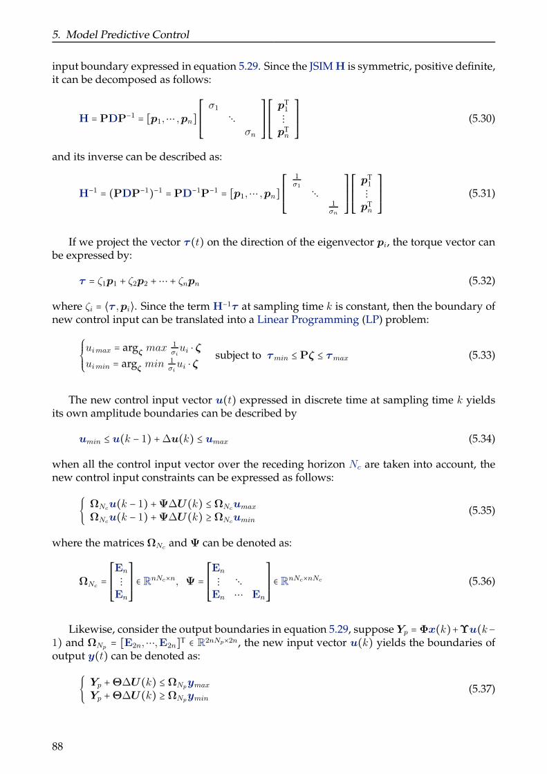
5. Model Predictive Control
input boundary expressed in equation 5.29. Since the JSIM H is symmetric, positive definite,it can be decomposed as follows:
H = PDP−1 = [p1,⋯ ,pn]⎡⎢⎢⎢⎢⎢⎣σ1
⋱σn
⎤⎥⎥⎥⎥⎥⎦⎡⎢⎢⎢⎢⎢⎣pT1
⋮pTn
⎤⎥⎥⎥⎥⎥⎦(5.30)
and its inverse can be described as:
H−1 = (PDP−1)−1 = PD−1P−1 = [p1,⋯ ,pn]⎡⎢⎢⎢⎢⎢⎣
1
σ1
⋱1
σn
⎤⎥⎥⎥⎥⎥⎦⎡⎢⎢⎢⎢⎢⎣pT1
⋮pTn
⎤⎥⎥⎥⎥⎥⎦(5.31)
If we project the vector τ (t) on the direction of the eigenvector pi, the torque vector canbe expressed by:
τ = ζ1p1 + ζ2p2 +⋯+ ζnpn (5.32)
where ζi = ⟨τ ,pi⟩. Since the term H−1τ at sampling time k is constant, then the boundary ofnew control input can be translated into a Linear Programming (LP) problem:
⎧⎪⎪⎨⎪⎪⎩uimax = arg
ζmax 1
σiui ⋅ ζ
uimin = argζmin 1
σiui ⋅ ζ
subject to τmin ≤ Pζ ≤ τmax (5.33)
The new control input vector u(t) expressed in discrete time at sampling time k yieldsits own amplitude boundaries can be described by
umin ≤ u(k − 1) +∆u(k) ≤ umax (5.34)
when all the control input vector over the receding horizon Nc are taken into account, thenew control input constraints can be expressed as follows:
ΩNcu(k − 1) +Ψ∆U(k) ≤ΩNc
umax
ΩNcu(k − 1) +Ψ∆U(k) ≥ΩNc
umin(5.35)
where the matrices ΩNcand Ψ can be denoted as:
ΩNc=
⎡⎢⎢⎢⎢⎢⎣En
⋮En
⎤⎥⎥⎥⎥⎥⎦∈ RnNc×n, Ψ =
⎡⎢⎢⎢⎢⎢⎣En
⋮ ⋱En ⋯ En
⎤⎥⎥⎥⎥⎥⎦∈ RnNc×nNc (5.36)
Likewise, consider the output boundaries in equation 5.29, suppose Yp = Φx(k)+Υu(k−1) and ΩNp
= [E2n,⋯,E2n]T ∈ R2nNp×2n, the new input vector u(k) yields the boundaries ofoutput y(t) can be denoted as:
Yp +Θ∆U(k) ≤ ΩNpymax
Yp +Θ∆U(k) ≥ ΩNpymin
(5.37)
88
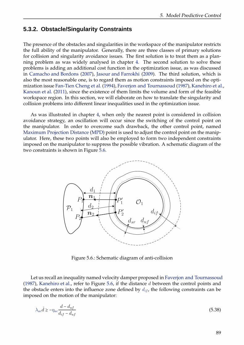
5. Model Predictive Control
5.3.2. Obstacle/Singularity Constraints
The presence of the obstacles and singularities in the workspace of the manipulator restrictsthe full ability of the manipulator. Generally, there are three classes of primary solutionsfor collision and singularity avoidance issues. The first solution is to treat them as a plan-ning problem as was widely analysed in chapter 4. The second solution to solve theseproblems is adding an additional cost function in the optimization issue, as was discussedin Camacho and Bordons (2007), Jasour and Farrokhi (2009). The third solution, which isalso the most reasonable one, is to regard them as motion constraints imposed on the opti-mization issue Fan-Tien Cheng et al. (1994), Faverjon and Tournassoud (1987), Kanehiro et al.,Kanoun et al. (2011), since the existence of them limits the volume and form of the feasibleworkspace region. In this section, we will elaborate on how to translate the singularity andcollision problems into different linear inequalities used in the optimization issue.
As was illustrated in chapter 4, when only the nearest point is considered in collisionavoidance strategy, an oscillation will occur since the switching of the control point onthe manipulator. In order to overcome such drawback, the other control point, namedMaximum Projection Distance (MPD) point is used to adjust the control point on the manip-ulator. Here, these two points will also be employed to form two independent constraintsimposed on the manipulator to suppress the possible vibration. A schematic diagram of thetwo constraints is shown in Figure 5.6.
duf
n1
difP1
P1 P0
1
d1
dsr
P0
2
O1
P2
n2
d2
Figure 5.6.: Schematic diagram of anti-collision
Let us recall an inequality named velocity damper proposed in Faverjon and Tournassoud(1987), Kanehiro et al., refer to Figure 5.6, if the distance d between the control points andthe obstacle enters into the influence zone defined by dif , the following constraints can beimposed on the motion of the manipulator:
λacd ≥ −ηacd − dufdif − duf
(5.38)
89

5. Model Predictive Control
where 0 < ηac < 1 is damper coefficient for adjusting convergence speed. λac is a switchingfunction to control whether current anti-collision constraint function uses or not, becausein some cases, like in capturing phaser, the interact face between the gripper and the targetsatellite is constrained by the collision avoidance. The switching function can be expressedas:
λac =⎧⎪⎪⎨⎪⎪⎩0 constraint is not considered
1 constraint is considered(5.39)
Given the initial condition d(0) ≥ duf , and in terms of λac = 1, the following inequality can bederived:
d(t) ≥ duf + (d(0) − duf)e− ηact
dif−duf ≥ duf ∀t > 0 (5.40)
Expression in equation 5.40 assures that the distance between the control point and theobstacles constrained by velocity damper will be never smaller than duf . Similarly, dsr is thesecurity distance as defined in chapter 4, once d < dsr, the inequality constraint expressed in
equation 5.38 will become hard constraint and will be illustrated in section 5.4. Note that d isconstrained by inequality 5.38, when the control point Pi enters into influence zone (d ≤ dif ),
a linear inequality constraint over the manipulator’s velocity θ can be obtained:
λac⟨JTPini, θ⟩ ≥ ⟨rP ′
i,ni⟩ − ηac di − duf
dif − duf(5.41)
_xe
¾sr
¾if
¾uf
ui
ui¡1
¾i
¾i = 0
Desired Path
Constrained Path
Singularity
Figure 5.7.: Schematic diagram of anti-singularity
Likewise, we also want to translate the singularity issue into a linear inequality con-straint as in equation 5.41. From the definition of the manipulability ellipsoid in equation 4.8,refer to Figure 5.7, it can be perceived that singularity emerges when the singular value ofthe Jacobian matrix σi = 0 along the ith principal axis direction. It also means, one can drive
90

5. Model Predictive Control
the manipulator far from singularity point through regulating the change rate of singularvalue appropriately as the obstacle avoidance. The change rate of singular value σi can beobtained through projecting the task-space velocity xe in the direction of the principal axisui:
σi = ⟨Jθ,ui⟩ (5.42)
If we define σif , σsr, σuf influence distance, security distance, and unsafe distance as beendone in collision avoidance, recall the velocity damper the following constraint will be de-fined:
λasσi ≥ −ηasσi − σuf
σif − σuf
(5.43)
λas and ηas are the switching function and turning parameter for velocity damper. As il-lustrated in equation 5.40, give the initial condition σi(0) > σuf and λas = 1, the followinginequality can be derived:
σi(t) ≥ σuf + (σi(0) − σuf)e− ηast
σif−σuf ≥ σuf ∀t > 0 (5.44)
Expression in equation 5.44 assures that the singular value σi will never smaller than σuf .
A linear inequality constraint for singularity issue over the manipulator’s velocity θ can beobtained:
λas⟨JTui, θ⟩ ≥ −ηas σi − σuf
σif − σuf
(5.45)
Next, we use the anti-collision and anti-singularity constraints to construct the matrix G
and vector g. Assuming that Nkac anti-collision constraints are activated at sampling time
k, the new control input u(k) yields the velocity damper constraint in equation 5.41 can beexpressed by:
Θvac [CvdAdx(k) +CvdBdu(k)] ≥Duf (5.46)
where Cvd = [0n,En], the matrix Θvac and vector Duf can be denoted as:
Θvac =
⎡⎢⎢⎢⎢⎢⎢⎣
λ1acn
T1JP1
⋮
λNk
acac nT
NkacJP
Nkac
⎤⎥⎥⎥⎥⎥⎥⎦, Duf =
⎡⎢⎢⎢⎢⎢⎢⎢⎣
⟨rP ′1,n1⟩ − ηac d1−duf
dif−duf
⋮
⟨rP ′Nkac
,nNkac⟩ − ηac dNk
ac−duf
dif−duf
⎤⎥⎥⎥⎥⎥⎥⎥⎦(5.47)
If we define yvp = CvdAdx(k) +CvdBdu(k − 1) and Θvb = [CvdBd,0n,⋯ ,0n] ∈ Rn×nNc , ac-cording to equation 5.46, let Dvp =Θv
acyvp and Θac =ΘvacΘvb, equation 5.46 can be expressed
by:
Dvp +Θac∆U(k) ≥Duf (5.48)
Similarly, the anti-singularity constraints can be treated as follows. If there are Nkas anti-
singularity constraints are activated at instant k, the control input u(k) yield the velocitydamper constraints in equation 5.45 can be expressed by:
Σvp +Θas∆U(k) ≥ Σuf (5.49)
91

5. Model Predictive Control
where Σvp = Θvasyvp and Θas = Θv
asΘvb. The matrix Θvas and vector Σuf can be expressed as
follows:
Θvas =
⎡⎢⎢⎢⎢⎢⎢⎣
λ1asn
T1J
⋮
λNk
asas nT
NkasJ
⎤⎥⎥⎥⎥⎥⎥⎦, Σuf =
⎡⎢⎢⎢⎢⎢⎢⎣
−ηasσ1−σuf
σif−σuf
⋮
−ηasσNkas−σuf
σif−σuf
⎤⎥⎥⎥⎥⎥⎥⎦(5.50)
After a variety of constraints are expressed by linear inequalities as in equations 5.35,5.37, 5.48 and 5.49, the quantities of G and g can be detived as follows:
G =
⎡⎢⎢⎢⎢⎢⎢⎢⎢⎢⎢⎢⎢⎣
Ψ
−ΨΘ
−Θ−Θac
−Θas
⎤⎥⎥⎥⎥⎥⎥⎥⎥⎥⎥⎥⎥⎦
, g =
⎡⎢⎢⎢⎢⎢⎢⎢⎢⎢⎢⎢⎢⎣
ΩNcumax −ΩNc
u(k − 1)−ΩNc
umin +ΩNcu(k − 1)
ΩNpymax −Yp
−ΩNpymin +Yp
Dvp −Duf
Σvp −Σuf
⎤⎥⎥⎥⎥⎥⎥⎥⎥⎥⎥⎥⎥⎦
(5.51)
To complete a given task with optimization, the inequality constraints denoted by equa-tions 5.35, 5.37, 5.48 and 5.49 should be integrated into the optimization problem. Of course,for collision avoidance, each link of the manipulator and every obstacle in workspace, alsobetween two different links yield inequality 5.41, which implies series of anti-collision con-straints will be imposed on the manipulator regarding to the relative relationship of twoarbitrary mobile objects in workspace. For singularity avoidance, every singular value canbe chosen to yield inequality 5.45, which indicates that anti-singularity constraints will beactivated according to the relative distance to the singular configuration. These linear in-equalities will be employed in QP problem as will be illustrated in section 5.4.
5.4. Quadratic Programming
As was indicated in section 5.1, the implementation of NMPC is not a trivial matter and is ir-refutably a more complicated task than the commissioning of conventional control schemes.Leadingly, the designed controller has to solve a non-linear QP problem with linear con-straints as shown in equation 5.28 to gain a sequence of optimal control effort ∆U∗(k)through searching in the current feasible region. A variety of methods are commonly usedincluding active set, interior point, augmented Lagrangian as introduced in Maciejowski(2002), Nocedal and Wright (2006), Wang (op. 2009). The choice of algorithm to solve QPneeds to consider the special structure of the NMPC problem.
5.4.1. KKT Conditions
The Karush-Kuhn-Tucker (KKT) conditions are first order necessary conditions for a solu-tion in non-linear optimization programming. The necessary conditions for QP problem in
92

5. Model Predictive Control
equation 5.28 given by KKT conditions can be expressed as follows:
⎧⎪⎪⎪⎪⎪⎪⎪⎨⎪⎪⎪⎪⎪⎪⎪⎩
M∆U +ϑ +GTλ = 0G∆U − g ≤ 0λT(G∆U − g) = 0λ ≥ 0
(5.52)
where the vector λ is the Lagrangian multipliers. The inequality constraints expressed inequation 5.28 may be composed of inactive constraints and active constraints. The constraintGi∆U ≤ gi is called active if Gi∆U = gi and inactive if Gi∆U < gi. The active set Sact madeup of the active constraints, plays a significant role in optimization theory since it determineswhich constraints will influence the finial result of optimization Nocedal and Wright (2006).If the active set Sact can be determined, the KKT conditions can be expressed in another way:
⎧⎪⎪⎪⎪⎪⎪⎪⎪⎪⎪⎨⎪⎪⎪⎪⎪⎪⎪⎪⎪⎪⎩
M∆U +ϑ +∑i∈Sact GTactλact = 0
Gi∆U − gi = 0 i ∈ SactGi∆U − gi < 0 i ∉ Sactλi ≥ 0 i ∈ Sactλi = 0 i ∉ Sact
(5.53)
Obviously, if the ith constraint is active, an equality constraint Gi∆U = gi can be imposedon the cost function which can be solved with Lagrange multiplier method. On the contrary,Gi∆U < gi denotes that the constraint is satisfied, thus it is inactive and can be discarded.An active set method, called Hildreth’s Quadratic Programming procedure Wang (op. 2009),will be employed in our NMPC design.
5.4.2. QP with Prioritized Constraints
During the optimization operation, the feasible region defined in the decision variables bythe active set of constraints may be empty due to the model-mismatch, external disturbance,and noise or artificially fault. Such a problem, will stop the standard QP procedure with-out output which is unacceptable for a controller in real-time provided to the space robot.In Qin and Badgwell (2003), it is depicted that, when a predicted input violates the bound-ary in the DMC-plus algorithm, it is set to its limits and the computation continues. Anothersolution to the infeasibility is first solve the QP problem without constraints and then clipto yield hard constraints. These methods prevent violation of hard constraints, but involvesa loss of performance and the solutions do not satisfy the KKT necessary conditions foroptimality.
The infeasibility problem, maybe lead to instability of the control-loop, motivates the aca-demic community to develop new techniques as introduced in Rawlings and Muske (1993),Scokaert and Rawlings (1999), Vada et al. (2001), Zheng and Morari (1995) aimed at recover-ing feasibility without violating hard constraints. In these techniques, how to handle con-straints is at the core of solving QP infeasibility problem. The linear constraints imposed ondecision variables can be categorized into three classes:
93

5. Model Predictive Control
• Physical/Security constraints: These limits should never be surpassed and are usuallyassociated to the device physical functioning or the security warranty. For instance, theinput bound of τ (t) expressed in equation 5.35 pertains to this kinds of constraints andwill be treated as hard constraints.
• Operational constraints: These limits are fixed by the operators as bounds withinwhich the decision variables are expected to maintain appropriate operating condi-tions. They can be violated in certain circumstance and be treated as soft constraintssuch as the limits of output y(t) denoted in equation 5.37.
• Passive constraints: Unlike physical/security or operational constraints which are im-posed on the decision variables at all the time, the passive limits will only be triggeredwhen the decision variables slide into its influence zone, such as the distance betweenthe link and obstacle enters into the collision influence zone, or the configuration ofthe manipulator comes into a influence zone of singularity. Under this circumstance,they can be considered as soft constraints and violated to some extent. Once the deci-sion variables enter into the security zone, the corresponding constraints turn to hardconstraints and can’t be violated any more. Actually, anti-singularity and anti-collisionconstraints in the robotic motion can be translated into suchlike passive constraints.
Like the prioritized tasks illustrated in chapter 4, the constraints belong to different cat-egories do not possess the same priority. If we use Ghc∆U(k) ≤ ghc and Gsc∆U(k) ≤ gsc torepresent hard and soft constraints respectively, and assign different priorities to various softconstraints according to their relative significance, the QP problem defined in equation 5.28can be rewritten as follows:
∆U∗(k) =min∆U
∆U(k)TM∆U(k) +ϑT∆U(k) + ρ∆gTsc∆gsc
subject to
hard constraints
⎧⎪⎪⎪⎪⎪⎨⎪⎪⎪⎪⎪⎩
x(k∣k) = x(k)x(k + j + 1∣k) = fd(x(k + j∣k),u(k + j∣k))u(k + j∣k) = u(k +Nc∣k), j ≥ Nc
Ghc∆U(k) ≤ ghc, j ≤ Np
soft constraints
⎧⎪⎪⎪⎨⎪⎪⎪⎩S1 ∶ G1
sc∆U(k) ≤ g1sc
⋮ ⋮ j ≤ Np
Sns∶ Gns
sc∆U(k) ≤ gnssc
(5.54)
where the constraint sets S1,⋯ ,Sns are constructed while constraint set Si has higher pri-
ority than Si+1. Refer to Nocedal and Wright (2006), Vada et al. (1999), Wang (op. 2009), analgorithm solving QP problem subject to the constraints with priorities is presented as fol-lows:
(1) Employing Hildreth’s QP procedure to solve the QP optimization problem defined inequation 5.54 only with hard constraints. If there is not a feasible solution, go to step(2); else, go to step (3).
(2) Checking existence of a solution to the first hard constraints at current sampling timewithout prediction, since the current hard constraints are more important than thepredicted constraints. If no solution exists, solve the QP problem without constraints,then clip the solution to yield hard constraints. This ensures the continuation of thecomputation with some performance loss. Else, employ the solution as an input to theplant.
94
5. Model Predictive Control
(3) Checking existence of a solution to the complete QP problem in equation 5.54. If thereis a feasible solution, the optimal control effort is determined. Else go to step (4).
(4) Set k = 1, from the highest priority constraints set S1, check existence of a solution tohard constraints and constraint set S1,⋯,Sk, if a feasible solution is found, k = k + 1and go to step (4). Else, if no feasible solution is found, S1,⋯,Sk can’t be satisfiedsimultaneously, go to step (5).
(5) Step (4) revealed S1,⋯,Sk−1 are satisfied while Sk,⋯,Sns can’t be satisfied. Com-
pute the optimal slack variables ∆gsc to minimize the violation of constraint sets Sk,⋯,Sns
and replace Sk,⋯,Snswith S ′k,⋯,S ′ns
, such that the renewed sets S1,⋯,Sk−1,S ′k,⋯,S ′ns
are satisfied. Go to step (6).
(6) At this step, there exists a solution which fulfils the constraint sets S1,⋯,Sk−1,S ′k,⋯,S ′ns.
Now, we can minimize the performance index in equation 5.54 subject to these con-straints and output the optimal solution ∆U∗(k).
The softening constraints offer additional region for the control input, to some extent, itexpands the feasible region of the decision variables. And, the constraints with prioritiesenable the most significant constraints execute as much as possible, which also enlarges thefeasible region of the control input.
5.5. Simulation Study
In this section, the robotic mission from approach to capture the target using space robot willbe implemented applying the proposed NMPC strategy. Four simulations, approach to thetarget, tracking a line with singularity, tracking a infinite ring with obstacles and tracking& capturing a point target, are executed to verify the performance and effectiveness of ourNMPC method.
5.5.1. Simulation Set-up
The NMPC algorithm implemented with a non-linear model and receding optimization,is employed for the space robot to complete the approach, tracking and capturing targetmissions. The tuning parameters relevant to NMPC are the sampling period, predictionhorizon Np, control horizon Nc and the input and output weights matrices Q(i) and T(i).The sampling time is set to 0.01s. According to the inaccuracy of long-term prediction andhigh burden of computation, the prediction horizon Np = 20 and the control horizon Nc = 5.The ratio between weights matrices Q(i) and T(i) indicates the importance of tracking errorand control effort. Here we choose Q(i) = En and T(i) = 0.05En.
5.5.2. Approach to the Target
As illustrated in chapter 2, once the servicer satellite comes into the neighbourhood of thetarget satellite and ready for the robotic mission, the first robotic mission would be un-folding the manipulator to an optimal grasping pose. The space manipulator is initially at
95
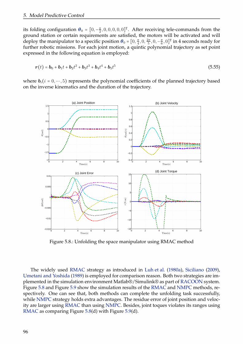
5. Model Predictive Control
its folding configuration θ0 = [0,−π2,0,0,0,0,0]T. After receiving tele-commands from the
ground station or certain requirements are satisfied, the motors will be activated and willdeploy the manipulator to a specific position θ0 = [0, π4 ,0, 2π5 ,0,−π
6,0]T in 4 seconds ready for
further robotic missions. For each joint motion, a quintic polynomial trajectory as set pointexpressed in the following equation is employed:
r(t) = b0 + b1t + b2t2 + b3t3 + b4t4 + b5t5 (5.55)
where bi(i = 0,⋯ ,5) represents the polynomial coefficients of the planned trajectory basedon the inverse kinematics and the duration of the trajectory.
0 2 4 6 8 10−2
−1.5
−1
−0.5
0
0.5
1
1.5
Time(s)
θ(rad)
(a) Joint Position
0 2 4 6 8 10−0.4
−0.2
0
0.2
0.4
0.6
0.8
1
1.2
Time(s)
θ(rad/s)
(b) Joint Velocity
0 2 4 6 8 10−0.015
−0.01
−0.005
0
0.005
0.01
Time(s)
∆θ(rad)
(c) Joint Error
0 2 4 6 8 10−15
−10
−5
0
5
10
15
Time(s)
τ(N
.m)
(d) Joint Torque
Figure 5.8.: Unfolding the space manipulator using RMAC method
The widely used RMAC strategy as introduced in Luh et al. (1980a), Siciliano (2009),Umetani and Yoshida (1989) is employed for comparison reason. Both two strategies are im-plemented in the simulation environment Matlab®/Simulink® as part of RACOON system.Figure 5.8 and Figure 5.9 show the simulation results of the RMAC and NMPC methods, re-spectively. One can see that, both methods can complete the unfolding task successfully,while NMPC strategy holds extra advantages. The residue error of joint position and veloc-ity are larger using RMAC than using NMPC. Besides, joint toques violates its ranges usingRMAC as comparing Figure 5.8(d) with Figure 5.9(d).
96

5. Model Predictive Control
0 2 4 6 8 10−2
−1.5
−1
−0.5
0
0.5
1
1.5
Time(s)
θ(rad)
(a) Joint Position
0 2 4 6 8 10−0.4
−0.2
0
0.2
0.4
0.6
0.8
1
1.2
Time(s)
θ(rad/s)
(b) Joint Velocity
0 2 4 6 8 10−0.025
−0.02
−0.015
−0.01
−0.005
0
0.005
0.01
0.015
Time(s)
∆θ(rad)
(c) Joint Error
0 2 4 6 8 10−15
−10
−5
0
5
10
15
Time(s)
τ(N
.m)
(d) Joint Torque
Figure 5.9.: Unfolding the space manipulator using NMPC method
5.5.3. Tracking a Predefined Path
Two simulations will be conducted independently in this section to show the collision andsingularity avoidance ability of the proposed NMPC strategy. For demonstration, two pre-defined tasks and three artificial obstacles are employed to test the effect of collision andsingularity avoidance.
In order to test the collision avoidance, three additional obstacles, two spheres and onecylinder are located in the workspace of the space manipulator. The primary task of theend-effector is to track a path with the form of infinite ring in 10 seconds. The simulationresults are shown in Figure 5.10. One can see that, the tracking task does not completelyconducted since the existence of the obstacles. When the manipulator approaches to theobstacles, the anti-collision constraints are activated to impede the occurrence of possiblecollision. The minimum distances between the manipulator and the obstacles are strictlyconstrained by the pre-defined unsafe distance duf . Three anti-collision constraints are ac-tivated during the tracking task. After collision avoidance, the NMPC strategy continuesto conduct the required task as much as possible as shown in Figure 5.10(c) and (d). Thejoint position and joint velocity also fulfil the output constraints as shown in Figure 5.10(e)and (f). The simulation results demonstrate that the proposed constrained MPC algorithmis satisfactory for obstacle avoidance especially when more than one obstacles in workspaceof the manipulator.
97

5. Model Predictive Control
−0.6 −0.4 −0.2 0 0.2 0.4 0.6 0.8 1 1.2−1.6
−1.4
−1.2
−1
−0.8
−0.6
−0.4
y(m)
z(m
)
(a) Task in y−z Plane
10 12 14 16 18 200
0.2
0.4
0.6
0.8
1
1.2
1.4
1.6
1.8
2
Time(s)
d(m
)
(b) Minimum Distance
10 12 14 16 18 20−0.4
−0.3
−0.2
−0.1
0
0.1
0.2
0.3
Time(s)
∆r(m
)
(c) Position Error
10 12 14 16 18 20−0.2
0
0.2
0.4
0.6
0.8
1
1.2
Time(s)
∆η,∆
ǫ
(d) Orientation Error
10 12 14 16 18 20−1
−0.5
0
0.5
1
1.5
2
Time(s)
θ(rad)
(e) Joint Position
10 12 14 16 18 20−1
−0.8
−0.6
−0.4
−0.2
0
0.2
0.4
0.6
0.8
1
Time(s)
θ(rad/s)
(f) Joint Velocity
Figure 5.10.: Tracking infinite ring with anti-collision constraints
The second simulation is to test the singularity avoidance ability of the proposed NMPCstrategy. The path is set to track a line in the workspace of space manipulator within 10seconds. Without adopting any measure for singularity issue, the singularity will occur at18th second. Like the anti-collision constraints, an anti-singularity constraint is activated atthat moment to prevent the manipulator from sliding into the singular configuration. Theminimum singular value σm is restricted at its unsafe quantity σuf . The tracking error forposition and orientation is promising, while the joint position and joint velocity also fulfilthe output constraints as shown in Figure 5.11(e) and (f). The oscillation in joint velocity isinduced by the damper coefficient λas. Some trade-off must be taken to choose the optimalvalue of λas.
98
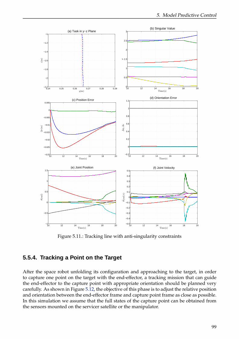
5. Model Predictive Control
0.24 0.25 0.26 0.27 0.28 0.29−2.2
−2
−1.8
−1.6
−1.4
−1.2
−1
y(m)
z(m
)
(a) Task in y−z Plane
10 12 14 16 18 200
0.5
1
1.5
2
2.5
3
Time(s)
σ
(b) Singular Value
10 12 14 16 18 20−0.03
−0.025
−0.02
−0.015
−0.01
−0.005
0
0.005
Time(s)
∆r(m
)
(c) Position Error
10 12 14 16 18 20−0.2
0
0.2
0.4
0.6
0.8
1
1.2
Time(s)
∆η,∆
ǫ
(d) Orientation Error
10 12 14 16 18 20−1
−0.5
0
0.5
1
1.5
Time(s)
θ(rad)
(e) Joint Position
10 12 14 16 18 20−0.5
−0.4
−0.3
−0.2
−0.1
0
0.1
0.2
0.3
0.4
0.5
Time(s)
θ(rad/s)
(f) Joint Velocity
Figure 5.11.: Tracking line with anti-singularity constraints
5.5.4. Tracking a Point on the Target
After the space robot unfolding its configuration and approaching to the target, in orderto capture one point on the target with the end-effector, a tracking mission that can guidethe end-effector to the capture point with appropriate orientation should be planned verycarefully. As shown in Figure 5.12, the objective of this phase is to adjust the relative positionand orientation between the end-effector frame and capture point frame as close as possible.In this simulation we assume that the full states of the capture point can be obtained fromthe sensors mounted on the servicer satellite or the manipulator.
99

5. Model Predictive Control
Jn
Xe
Ye
Ze
XI
YI
ZI
re
Xc
Yc
Zc
Xt
Yt
Zt
rc
Figure 5.12.: Relative relationship of end-effector frame and capture point frame
For the sake of simplification, tracking the capture point is decomposed into two sub-tasks. The first subtask is tracking the capture point without considering the translationaland rotational motion along x axis. This will drive the end-effector rightly locate in therear of the capture point and be ready for the next step mission, such as surveillance, tar-get state estimation, etc. If Rc = [nc sc ac] denotes the rotation matrix of the capture pointand Re = [ne se ae] the rotation matrix of the end-effector frame, the first subtask can berepresented as follows:
⎧⎪⎪⎨⎪⎪⎩re = rc +KP (rc − re) = [0, rcy +KPy(rcy − rey), rcz +KPz(rcz − rez)]Tωe = ωc +KO(ne ×nc) = [0,ωcy +KOy(nc1ne3 − nc3ne1),ωcz +KOz(nc2ne1 − nc1ne2)]T
(5.56)
where rc and re are the velocity vectors of the capture point and end-effector, respectively.KP and KO are the control gain matrix for position and orientation, respectively.
After x axis of the end-effector frame aligns with x axis of the capture point frame, asecond subtask can be activated to drive the end-effector close to the capture point. Thefinger of the end-effector will be activated to open for the coming capturing mission duringthis phase. Although the second subtask is mainly to reduce the relative translational androtational error along x axis, since the motion of the target satellite, a feedback of motionalong y and z axis are also required to compensate the drifting error. The designed path forthe second subtask can be given by:
⎧⎪⎪⎨⎪⎪⎩re = rc +KP (rc − re)ωe = ωc +KO(ηeǫc − ηcǫe − S(ǫc)ǫe) (5.57)
where ηc,ǫc and ηe,ǫe are the unit quaternions associated with the rotation matrix Rc
and Re, respectively. During this phase, NMPC strategy with anti-collision and anti-singularityconstraints developed in this chapter is employed to complete both subtasks. Figure 5.13
100
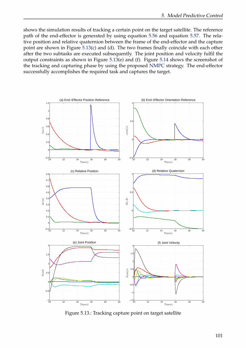
5. Model Predictive Control
shows the simulation results of tracking a certain point on the target satellite. The referencepath of the end-effector is generated by using equation 5.56 and equation 5.57. The rela-tive position and relative quaternion between the frame of the end-effector and the capturepoint are shown in Figure 5.13(c) and (d). The two frames finally coincide with each otherafter the two subtasks are executed subsequently. The joint position and velocity fulfil theoutput constraints as shown in Figure 5.13(e) and (f). Figure 5.14 shows the screenshot ofthe tracking and capturing phase by using the proposed NMPC strategy. The end-effectorsuccessfully accomplishes the required task and captures the target.
10 12 14 16 18 20−0.2
0
0.2
0.4
0.6
0.8
1
1.2
Time(s)
r(m
/s)
(a) End−Effector Position Reference
10 12 14 16 18 20−0.5
0
0.5
1
Time(s)
ω(rad/s)
(b) End−Effector Orientation Reference
10 12 14 16 18 20−0.1
0
0.1
0.2
0.3
0.4
0.5
0.6
0.7
0.8
Time(s)
∆r(m
)
(c) Relative Position
10 12 14 16 18 20−0.5
0
0.5
1
Time(s)
∆η,∆
ǫ
(d) Relative Quaternion
10 12 14 16 18 20−1
−0.5
0
0.5
1
1.5
2
Time(s)
θ(rad)
(e) Joint Position
10 12 14 16 18 20−1.5
−1
−0.5
0
0.5
1
1.5
2
Time(s)
θ(rad/s)
(f) Joint Velocity
Figure 5.13.: Tracking capture point on target satellite
101
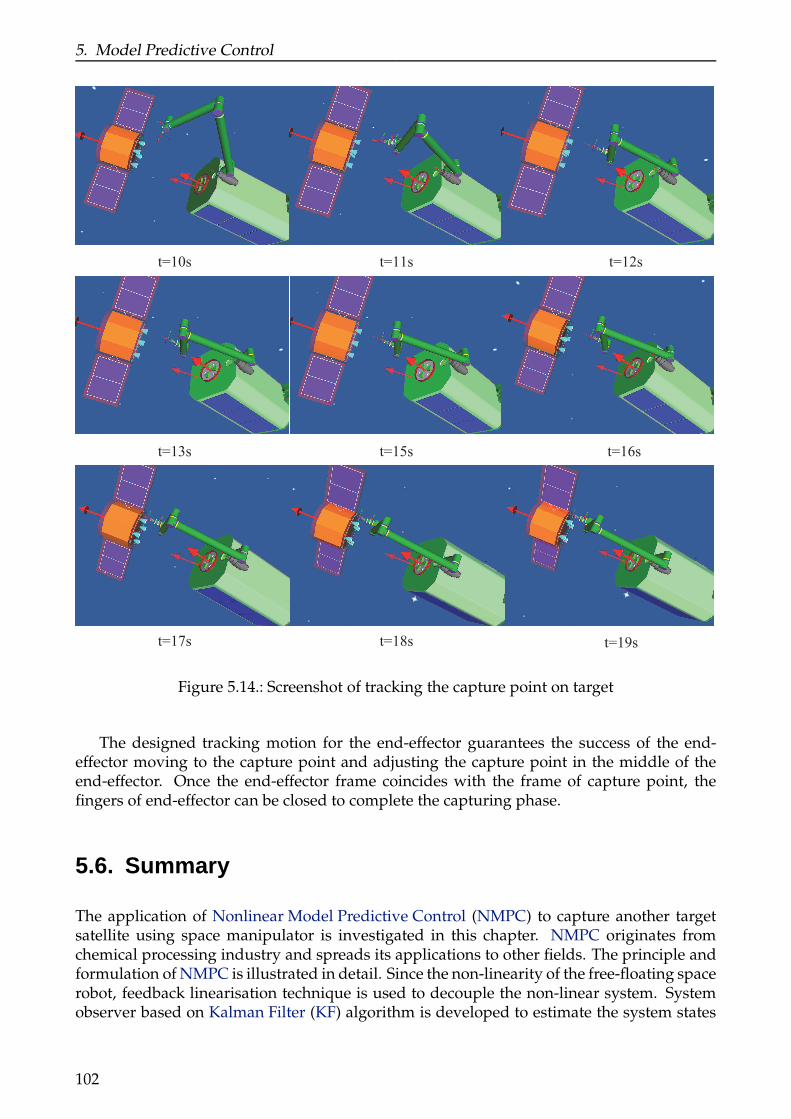
5. Model Predictive Control
t=10s t=11s t=12s
t=13s t=15s t=16s
t=17s t=18s t=19s
Figure 5.14.: Screenshot of tracking the capture point on target
The designed tracking motion for the end-effector guarantees the success of the end-effector moving to the capture point and adjusting the capture point in the middle of theend-effector. Once the end-effector frame coincides with the frame of capture point, thefingers of end-effector can be closed to complete the capturing phase.
5.6. Summary
The application of Nonlinear Model Predictive Control (NMPC) to capture another targetsatellite using space manipulator is investigated in this chapter. NMPC originates fromchemical processing industry and spreads its applications to other fields. The principle andformulation of NMPC is illustrated in detail. Since the non-linearity of the free-floating spacerobot, feedback linearisation technique is used to decouple the non-linear system. Systemobserver based on Kalman Filter (KF) algorithm is developed to estimate the system states
102
5. Model Predictive Control
when modelling error and measurement error are taken into account. The NMPC strategyutilizes a quadratic function as its optimization index, and combines various of constraints,which forms an on-line constrained Quadratic Programming (QP) problem. In this chapter,input/output constraints, obstacle/singularity constraints are successfully translated intolinear inequalities as part of the QP problem. Different constraints are categorized into di-verse constraints with unequal priorities for dealing with the possible infeasibility duringon-line optimization. Four simulations, approach to the target, tracking a infinite ring, track-ing a line and tracking a point on the target are performed to verify the proposed method. Asone can see that, not only the traditional input/output constraints are considered, but alsothe obstacle/singularity constraints are taken into account. This means, on the one hand,anti-collision and anti-singularity problems can be treated as planning problems as intro-duced in chapter 4, on the other hand, it can also be treated as control constraints to limitthe control input in a reasonable way. The simulation results convincingly demonstrated theproposed control framework in the application of space robot.
103


6. Conclusions and Future Research
There are now three types of scientists: experimental, theoretical and computational.
—Silvan S. Schweber
As a high potential solution for future On-Orbit Servicing (OOS) missions, the use ofspace robot introduces series of challenging issues to implement such a system working inouter space. This chapter concludes and discusses the results in the previous chapters. Theadvantages and disadvantages of the proposed methods are analysed. Furthermore, thepossible research directions in the future are listed to enhance and pursue this thesis.
6.1. Conclusions
Capturing an un-cooperative target satellite by using space manipulator is the main concernin this thesis. For that purpose, at the beginning of this work, a distributed real-time simula-tion system, RACOON has been established for space robotic technique demonstration. Theproposed RACOON system can simulate the scenario of space robot and offer the operatorson ground intuitive information, such as text, image and VR etc. which enhances the percep-tion ability of the operators. Moreover, the reusable simulator is easy to modify and replaceby better modules or related hardware, which provides expandability and scalability of thissimulation architecture in the future.
As a complex multi-body system, the dynamics of space robot possesses specific dy-namic equations. Considering the effect of the system topology to its dynamics, spatialnotation and graph theory are used to construct the dynamics equation of the space robotwith general tree structure. From path matrix and parent array, an IMM is derived whichhas the same pattern as the JSIM. The IMM reveals the influence of the system topologyto its dynamics. As a symmetric, positive definite matrix, IMM can be used to explore thebranched-induced sparsity and to analyse the computational cost of CRBA. The complexityof calculating the JSIM is estimated between O(1) and O(n3) by using IMM. The proposedalgorithm is competitive when there is sufficient branching in the kinematic tree.
The characteristics of the outer space introduce some special properties to the spacerobot. One of them is the dynamic coupling between the space manipulator and the space-craft when none external forces and torques applied on the spacecraft. Besides, the movingtarget satellite requires real-time collision avoidance when the space manipulator approachand track the target in its workspace. Furthermore, the un-predictable singularity may occurwhen the manipulator tries to track the path defined in Cartesian space. Traditional meth-ods consider the collision and singularity avoidance issues mainly as path planning problemwithout thinking the constraints of the system input and output. In this thesis, from path
105

6. Conclusions and Future Research
planning and control aspects, the singularity and collision avoidance issues are investigatedindependently.
At the path planning level, the proposed STR method for singularity avoidance utilizesthe minimum singular value σm as singular measurement and left-singular vector as pro-jection direction to reconstruct the path expressed in task-space. With the proposed STRmethod, less overshoot, more predictable minimum singular value, robustness and smaller& smoother joint velocities are achieved as compared to the typical DLS method. For colli-sion avoidance, a new control point, MPD point is introduced into the collision avoidancestrategy when non strictly convex objects are considered to suppress the possible fluctuationof the joint velocities. The new collision avoidance strategy ensures the continuous change ofthe control point, which also guarantees the smoother joint velocities. The new approachesfor collision and singularity avoidance can be expanded to fixed-base manipulator or spacemanipulator.
At the motion control level, NMPC strategy was chosen as the motion control methodfor free-floating space robot. As a finite horizon, on-line optimized control strategy, NMPCsuccessfully resolves the system input and output boundary conditions. Furthermore, usingvelocity damper, the collision and singularity issues are also translated into linear inequal-ities and integrated into the NMPC. An on-line QP with prioritized constraints is adoptedto search the optimal control effort over the prediction horizon. Simulation results showthat the proposed NMPC strategy can successfully fulfil multiple constraints and completethe required task as much as possible. To capture a point on the moving target satellite,a two-stage path of the end-effector is generated and implemented using constrained MPCstrategy. As a result, the issues in path planing become various constraints in motion control,which is fairly similar as our human interaction with external environment. One drawbackof NMPC is its computational burden which is caused by the on-line predication and QPalgorithm.
6.2. Future Research
How to realize capturing an un-cooperative target satellite is still a challenging issue untilnow. The simulation system RACOON and the control framework based on NMPC providethe first step into space robotic research field involving input/output boundary conditions,collision/singularity avoidance for the space robotic missions. The possible research ques-tions arising from this work can be listed as follows:
• Estimation and prediction of the states of the target satellites without prior knowl-edge. Full and perfect states are assumed to be known during this work, which isnot the case in practice. How to estimate the states of the target accurately is a bigissue in capturing. The accuracy of the estimation will influence the success of thecapture. One should widely use multiple sensors on-board and data integration tech-nique to compute the kinematic and dynamic parameters of the target. Moreover, theprediction of the target is also a considerable aspect that can be imported to the controlloop Lampariello and Hirzinger (2013).
• Determination of the capture point. It is another challenging issue for capture. Whenthe target satellite is moving and rotating, how to find a feasible capture point is the
106

6. Conclusions and Future Research
key to guarantee the success of capture. This involves collision, manipulability, in-put/output boundary conditions of the space robot.
• Robust stability of the NMPC strategy. The nominal stability of the MPC can beobtained by adding terminal constraint, terminal weighting matrix or contraction con-straint as illustrated in Mayne et al. (2000), Rawlings and Muske (1993), Zheng and Morari(1995). The NMPC strategy in this work assumes that the plant to be controlled andthe model for prediction are the same without considering model mismatch. The in-fluence of the plant uncertainty to the robust stability should be carefully analysed andpursued. Some techniques that synthesis robust NMPC can be found in Kothare et al.(1996), Mayne et al. (2000)
• Faster collision detection algorithm. The collision detection algorithm is very timeconsuming especially when multiple non-convex obstacles are in the workspace. An-other application of collision detection would be the contact between the space robotand the target satellite. These requires faster and more accurate collision detectionalgorithms.
• Contact theory. Once the frame of the capture point on the target coincides with theframe of the end-effector, the fingers of the end-effector will be activated to performclose action to complete the grasp. Nevertheless, due to the measurement noise, modelmismatch or external disturbance, there will be still some residual relative velocitiesbetween end-effector and the capture point. A contact will occur when the fingers ofthe end-effector close. The effect of the contact to the space robot and the target satellitehas to be investigated seriously to ensure safety and successful capture.
• Post-capture stabilization and further operations. After the capture is done, a post-capture stabilization should be performed to decrease the rotational velocity of thetarget satellite. During this phase, the attitude control of the servicer satellite has to beactivated to realize the stabilization of servicer and target as a whole. The space ma-nipulator will be used for further OOS operations, such as assembly, ORU exchange,repair etc. which require the developers to synthesis all the demanded mission elabo-rately.
In summary, the presented work in this dissertation provides a simulation tool for thecoming space robotic operations and opens the window to a field of studies in MPC appli-cation to space robot.
107

A. Bibliography
S. Abiko and G. Hirzinger. An adaptive control for a free-floating space robot by usinginverted chain approach. In 2007 IEEE/RSJ International Conference on Intelligent Robots andSystems, pages 2236–2241. IEEE, 2007. ISBN 978-1-4244-0912-9.
O.P Agrawal and Y. Xu. On the global optimum path planning for redundant space manip-ulators. IEEE Transactions on Systems, Man, and Cybernetics, 24(9):1306–1316, 1994.
C.A Balafoutis and R.V Patel. Efficient computation of manipulator inertia matrices andthe direct dynamics problem. IEEE Transactions on Systems, Man, and Cybernetics, 19(5):1313–1321, 1989.
C.A Balafoutis, R.V Patel, and P. Misra. Efficient modeling and computation of manipulatordynamics using orthogonal Cartesian tensors. IEEE Journal on Robotics and Automation, 4(6):665–676, 1988.
B. Bon and H. Seraji. On-line collision avoidance for the Ranger telerobotic flight experiment.In Proceedings of IEEE International Conference on Robotics and Automation, pages 2041–2048.IEEE, 1996. ISBN 0-7803-2988-0.
B. Bon and H. Seraji. Real-time model-based obstacle detection for the NASA Ranger Teler-obot. In Proceedings of International Conference on Robotics and Automation, pages 1580–1587.IEEE, 1997. ISBN 0-7803-3612-7.
Albert B. Bosse, W. J. Barnds, Michael A. Brown, N. G. Creamer, Andy Feerst, Carl G. Hen-shaw, Alan S. Hope, Bernard E. Kelm, Patricia A. Klein, Frank Pipitone, Bertrand E.Plourde, Brian P. Whalen, Jr.Peter Tchoryk, and Melissa Wright. SUMO: Spacecraft forthe universal modification of orbit. In Spacecraft Platforms and Infrastructure, pages 36–46.SPIE, 2004.
John R. Boyd. Destruction and creation. The Operational level of war. U.S. Army Comandand General Staff College, [Ft. Leavenworth and Kan.], 1987.
R. Brooks. A robust layered control system for a mobile robot. IEEE Journal on Robotics andAutomation, 2(1):14–23, 1986.
Fraser Cain. How Many Satellite are in Space?, 2013. URLwww.universetoday.com/42198/how-many-satellites-in-space/.
Eduardo F. Camacho and Carlos Bordons. Model predictive control. Advanced textbooks incontrol and signal processing. Springer, London [u.a.], 2004. ISBN 978-0-85729-398-5.
Eduardo F. Camacho and Carlos Bordons. Nonlinear Model Predictive Control: An Intro-ductory Review. In Rolf Findeisen, Frank Allgower, and Lorenz T. Biegler, editors, LectureNotes in Control and Information Sciences, pages 1–16. Springer Berlin Heidelberg, Berlinand Heidelberg, 2007. ISBN 978-3-540-72698-2.
109

A. Bibliography
Chi-Ying Lin and Yen-Chung Liu. Precision Tracking Control and Constraint Handling ofMechatronic Servo Systems Using Model Predictive Control. IEEE/ASME Transactions onMechatronics, 17(4):593–605, 2012.
S. Chiaverini. Singularity-robust task-priority redundancy resolution for real-time kinematiccontrol of robot manipulators. IEEE Transactions on Robotics and Automation, 13(3):398–410,1997.
D.W Clarke, C. Mohtadi, and P.S Tuffs. Generalized Predictive Control—Part II Extensionsand interpretations. Automatica, 23(2):149–160, 1987a.
D.W Clarke, C. Mohtadi, and P.S Tuffs. Generalized predictive control—Part I. The basicalgorithm. Automatica, 23(2):137–148, 1987b.
C. R. Cutler and B. L. Ramaker. Dynamic Matrix Control - A Computer Control Algorithm.In Joint Automatic Control Conference, 1980.
J. Denavit and R. S. Hartenberg. A Kinematic Notation for Lower-Pair Mechanisms Basedon Matrices. Trans. ASME, J. Appl. Mech., 22(2):215–221, 1955.
S. Dubowsky and E. Papadopoulos. The kinematics, dynamics, and control of free-flyingand free-floating space robotic systems. IEEE Transactions on Robotics and Automation, 9(5):531–543, 1993.
S. Dubowsky and M.A Torres. Path planning for space manipulators to minimize spacecraftattitude disturbances. In Proceedings. 1991 IEEE International Conference on Robotics andAutomation, pages 2522–2528. IEEE Comput. Soc. Press, 1991. ISBN 0-8186-2163-X.
Christer Ericson. Real-time collision detection. Morgan Kaufmann series in interactive 3Dtechnology. Elsevier, Amsterdam and Boston, 2005. ISBN 1558607323.
Fan-Tien Cheng, Wei-Ming Wang, and Fan-Chu Kung. Priority considerations for multiplegoals of redundant manipulators. In Proceedings of IEEE International Conference on Systems,Man and Cybernetics, pages 264–269. IEEE, 1994. ISBN 0-7803-2129-4.
B. Faverjon and P. Tournassoud. A local based approach for path planning of manipulatorswith a high number of degrees of freedom. In Proceedings. 1987 IEEE International Con-ference on Robotics and Automation, pages 1152–1159. Institute of Electrical and ElectronicsEngineers, 1987.
R. Featherstone. Efficient Factorization of the Joint-Space Inertia Matrix for Branched Kine-matic Trees. The International Journal of Robotics Research, 24(6):487–500, 2005.
R. Featherstone and D. Orin. Robot dynamics: equations and algorithms. In Proceedings2000 ICRA. Millennium Conference. IEEE International Conference on Robotics and Automation.Symposia Proceedings, pages 826–834. IEEE, 2000. ISBN 0-7803-5886-4.
Roy Featherstone. Rigid body dynamics algorithms. Springer, New York and N.Y, 2008. ISBN0387743146.
Graham Gibbs and Savi Sachdev. Canada and the International Space Station program:overview and status. Acta astronautica, 51(1-9):591–600, 2002.
110

A. Bibliography
K. Glass, R. Colbaugh, D. Lim, and H. Seraji. Real-time collision avoidance for redundantmanipulators. IEEE Transactions on Robotics and Automation, 11(3):448–457, 1995.
Y.-L Gu and Y. Xu. A normal form augmentation approach to adaptive control of space robotsystems. In [1993] Proceedings IEEE International Conference on Robotics and Automation,pages 731–737. IEEE Comput. Soc. Press, 1993. ISBN 0-8186-3450-2.
R. Hedjar and P. Boucher. Nonlinear Receding-Horizon Control of Rigid Link Robot Manip-ulators. International Journal of Advanced Robotic Systems, page 1, 2005.
G. Hirzinger, J. Heindl, and K. Landzettel. Predictive and knowledge-based telerobotic con-trol concepts. In Proceedings. 1989 International Conference on Robotics and Automation, pages1768–1777. IEEE Comput. Soc. Press, 1989. ISBN 0-8186-1938-4.
G. Hirzinger, B. Brunner, J. Dietrich, and J. Heindl. ROTEX-the first remotely controlledrobot in space. In Proceedings of the 1994 IEEE International Conference on Robotics and Au-tomation, pages 2604–2611. IEEE Comput. Soc. Press, 1994. ISBN 0-8186-5330-2.
John M. Hollerbach. A Recursive Lagrangian Formulation of Maniputator Dynamics and aComparative Study of Dynamics Formulation Complexity. IEEE Transactions on Systems,Man, and Cybernetics, 10(11):730–736, 1980.
P. Huang, J. Yan, J. Yuan, and Y. Xu. Robust control of space robot for capturing objects usingoptimal control method. In 2007 IEEE International Conference on Informaiton Acquisition,pages 397–402. IEEE Comput. Soc. Press, 2007. ISBN 1-4244-1220-X.
Rui Huang, Sachin C. Patwardhan, and Lorenz T. Biegler. Robust extended Kalman filterbased nonlinear model predictive control formulation. In Proceedings of the 48h IEEE Con-ference on Decision and Control (CDC) held jointly with 2009 28th Chinese Control Conference,pages 8046–8051. IEEE, 2009. ISBN 978-1-4244-3871-6.
N. Inaba and M. Oda. Autonomous satellite capture by a space robot: world first on-orbitexperiment on a Japanese robot satellite ETS-VII. In Proceedings 2000 ICRA. MillenniumConference. IEEE International Conference on Robotics and Automation. Symposia Proceedings,pages 1169–1174. IEEE, 2000. ISBN 0-7803-5886-4.
Ashkan M. Jasour and Mohammad Farrokhi. Path tracking and obstacle avoidance for re-dundant robotic arms using fuzzy NMPC. In 2009 American Control Conference, pages1353–1358. IEEE, 2009. ISBN 978-1-4244-4523-3.
Jinhyun Kim, G. Marani, Wan Kyun Chung, and Junku Yuh. A general singularity avoid-ance framework for robot manipulators: task reconstruction method. In IEEE InternationalConference on Robotics and Automation, 2004. Proceedings. ICRA ’04. 2004, pages 4809–4814Vol.5. IEEE, 2004. ISBN 0-7803-8232-3.
Fumio Kanehiro, Florent Lamiraux, Oussama Kanoun, Eiichi Yoshida, and Jean-Paul Lau-mond. A Local Collision Avoidance Method for Non-strictly Convex Polyhedra.
Oussama Kanoun, Florent Lamiraux, Pierre-Brice Wieber, Fumio Kanehiro, Eiichi Yoshida,and Jean-Paul Laumond. Prioritizing linear equality and inequality systems: Applicationto local motion planning for redundant robots. In 2009 IEEE International Conference onRobotics and Automation, pages 2939–2944. IEEE, 2009. ISBN 978-1-4244-2788-8.
111
A. Bibliography
Oussama Kanoun, Florent Lamiraux, and Pierre-Brice Wieber. Kinematic Control of Redun-dant Manipulators: Generalizing the Task-Priority Framework to Inequality Task. IEEETransactions on Robotics, 27(4):785–792, 2011.
O. Khatib and J. Burdick. Motion and force control of robot manipulators. In Proceedings.1986 IEEE International Conference on Robotics and Automation, pages 1381–1386. Institute ofElectrical and Electronics Engineers, 1986.
J.-O Kim and P.K Khosla. Real-time obstacle avoidance using harmonic potential functions.IEEE Transactions on Robotics and Automation, 8(3):338–349, 1992.
Jinhyun Kim, Giacomo Marani, Wan Kyun Chung, and Junku Yuh. Task reconstructionmethod for real-time singularity avoidance for robotic manipulators. Advanced Robotics,20(4):453–481, 2006.
C. A. Klein and B. E. Blaho. Dexterity Measures for the Design and Control of KinematicallyRedundant Manipulators. The International Journal of Robotics Research, 6(2):72–83, 1987.
Mayuresh V. Kothare, Venkataramanan Balakrishnan, and Manfred Morari. Robust con-strained model predictive control using linear matrix inequalities. Automatica, 32(10):1361–1379, 1996.
Roberto Lampariello. Motion Planning for the On-orbit Grasping of a Non-cooperative Tar-get Satellite with Collision Avoidance. In 10th International Symposium on Artificial Intelli-gence, Robotics and Automation in Space (i-SAIRAS 2010), 2010.
Roberto Lampariello and Gerd Hirzinger. Generating feasible trajectories for autonomouson-orbit grasping of spinning debris in a useful time. In 2013 IEEE/RSJ International Confer-ence on Intelligent Robots and Systems, pages 5652–5659. IEEE, 2013. ISBN 978-1-4673-6358-7.
Jay H. Lee and N. Lawrence Ricker. Extended Kalman Filter Based Nonlinear Model Predic-tive Control. Industrial & Engineering Chemistry Research, 33(6):1530–1541, 1994.
Bin Liang, Cheng Li, Lijun Xue, and Wenyi Qiang. A Chinese Small Intelligent Space RoboticSystem for On-Orbit Servicing. In 2006 IEEE/RSJ International Conference on IntelligentRobots and Systems, pages 4602–4607. IEEE, 2006. ISBN 1-4244-0258-1.
K. W. Lilly and D. E. Orin. Alternate Formulations for the Manipulator Inertia Matrix. TheInternational Journal of Robotics Research, 10(1):64–74, 1991.
K.W Lilly and C.S Bonaventura. A generalized formulation for simulation of space robotconstrained motion. In Proceedings of 1995 IEEE International Conference on Robotics andAutomation, pages 2835–2840. IEEE, 1995. ISBN 0-7803-1965-6.
J. Luh, M. Walker, and R. Paul. Resolved-acceleration control of mechanical manipulators.IEEE Transactions on Automatic Control, 25(3):468–474, 1980a.
J. Y. S. Luh, M. W. Walker, and R. P. C. Paul. On-Line Computational Scheme for MechanicalManipulators. Journal of Dynamic Systems, Measurement, and Control, 102(2):69, 1980b.
B. Ma and W. Huo. Adaptive control of space robot system with an attitude controlledbase. In Proceedings of 1995 IEEE International Conference on Robotics and Automation, pages1265–1270. IEEE, 1995. ISBN 0-7803-1965-6.
112
A. Bibliography
A. A. Maciejewski and C. A. Klein. Obstacle Avoidance for Kinematically Redundant Ma-nipulators in Dynamically Varying Environments. The International Journal of Robotics Re-search, 4(3):109–117, 1985.
Anthony A. Maciejewski and Charles A. Klein. Numerical filtering for the operation ofrobotic manipulators through kinematically singular configurations. Journal of Robotic Sys-tems, 5(6):527–552, 1988.
Jan M. Maciejowski. Predictive control: With constraints. Prentice Hall, Harlow and Englandand New York, 2002. ISBN 9780201398236.
V. Manikonda, P.O Arambel, M. Gopinathan, R.K Mehra, and F.Y Hadaegh. A model pre-dictive control-based approach for spacecraft formation keeping and attitude control. InProceedings of the 1999 American Control Conference (Cat. No. 99CH36251), pages 4258–4262.IEEE, 1999. ISBN 0-7803-4990-3.
G. Marani, Jinhyun Kim, Junku Yuh, and Wan Kyun Chung. A real-time approach for sin-gularity avoidance in resolved motion rate control of robotic manipulators. In Proceedings2002 IEEE International Conference on Robotics and Automation, pages 1973–1978. IEEE, 2002.ISBN 0-7803-7272-7.
Y. Masutani, F. Miyazaki, and S. Arimoto. Sensory feedback control for space manipulators.In Proceedings. 1989 International Conference on Robotics and Automation, pages 1346–1351.IEEE Comput. Soc. Press, 1989. ISBN 0-8186-1938-4.
D.Q Mayne, J.B Rawlings, C.V Rao, and P.O.M Scokaert. Constrained model predictivecontrol: Stability and optimality. Automatica, 36(6):789–814, 2000.
R.V Mayorga and A.K.C Wong. A singularities avoidance approach for the optimal localpath generation of redundant manipulators. In Proceedings. 1988 IEEE International Con-ference on Robotics and Automation, pages 49–54. IEEE Comput. Soc. Press, 1988. ISBN0-8186-0852-8.
Richard A. McCourt and Clarence W. de Silva. Autonomous Robotic Capture of a SatelliteUsing Constrained Predictive Control. IEEE/ASME Transactions on Mechatronics, 11(6):699–708, 2006.
S. McMillan and D.E Orin. Efficient computation of articulated-body inertias using succes-sive axial screws. IEEE Transactions on Robotics and Automation, 11(4):606–611, 1995.
S. McMillan, D.E Orin, and R.B McGhee. Efficient dynamic simulation of an underwatervehicle with a robotic manipulator. IEEE Transactions on Systems, Man, and Cybernetics, 25(8):1194–1206, 1995.
Manfred Morari and Jay H. Lee. Model predictive control: past, present and future. Com-puters & Chemical Engineering, 23(4-5):667–682, 1999.
Y. Nakamura, H. Hanafusa, and T. Yoshikawa. Task-Priority Based Redundancy Control ofRobot Manipulators. The International Journal of Robotics Research, 6(2):3–15, 1987.
Yoshihiko Nakamura and Hideo Hanafusa. Inverse Kinematic Solutions With SingularityRobustness for Robot Manipulator Control. Journal of Dynamic Systems, Measurement, andControl, 108(3):163, 1986.
113
A. Bibliography
NASA. On-orbit satellite servicing study: Project report. National Aeronautics and Space Ad-ministration. Goddard Space Flight Center, 2010.
D. Nenchev. A controller for a redundant free-flying space robot with spacecraft attitude/-manipulator motion coordination. In Proceedings of 1993 IEEE/RSJ International Conferenceon Intelligent Robots and Systems (IROS ’93), pages 2108–2114. IEEE, 1993. ISBN 0-7803-0823-9.
D. N. Nenchev. Restricted Jacobian Matrices of Redundant Manipulators in ConstrainedMotion Tasks. The International Journal of Robotics Research, 11(6):584–597, 1992.
D.N Nenchev and M. Uchiyama. Singularity-consistent path tracking: a null space basedapproach. In Proceedings of 1995 IEEE International Conference on Robotics and Automation,pages 2482–2489. IEEE, 1995. ISBN 0-7803-1965-6.
Jorge Nocedal and Stephen J. Wright. Numerical Optimization. Springer, Berlin and NewYork, 2 edition, 2006. ISBN 978-0-387-30303-1.
M. Oda, K. Kibe, and F. Yamagata. ETS-VII, space robot in-orbit experiment satellite. In Pro-ceedings of IEEE International Conference on Robotics and Automation, pages 739–744. IEEE,1996. ISBN 0-7803-2988-0.
Andrew Ogilvie, Justin Allport, Hannah Michael, and John Lymer. Autonomous SatelliteServicing Using the Orbital Express Demonstration Manipulator System. In Proc. of the 9thInternational Symposium on Artificial Intelligence, Robotics and Automation in Space (i-SAIRAS’08), pages 25–29, 2008.
OMG. Data Distribution Service for Real-time Systems: Version 1.2, 2007. URLhttp://www.omg.org/spec/DDS/1.2.
OMG. The Real-time Publish-Subscribe Wire Protocol DDS Interoperabil-ity Wire Protocol Specificiation (DDS-RTPS): Version 2.1, 2010. URLhttp://www.omg.org/spec/DDS-RTPS/2.1/.
E. Papadopoulos and I. Poulakakis. On path planning and obtacle avoidance for nonholo-nomic platforms with manipulator: a polynomial approach. The International Journal ofRobotics Research, 21(4):367–383, 2002.
Evangelos Papadopoulos and S. Ali A. Moosavian. Dynamics and control of space free-flyers with multiple manipulators. Advanced Robotics, 9(6):603–624, 1994.
F.C Park, J.E Bobrow, and S.R Ploen. A Lie Group Formulation of Robot Dynamics. TheInternational Journal of Robotics Research, 14(6):609–618, 1995.
H. Park, S. D. Cairano, and I. Kolmanovsky. Model predictive control for spacecraft ren-dezvous and docking with a rotating/tumbling platform and for debris avoidance. In2011 American Control Conference, pages 1922–1927. IEEE, 2011.
P. M. Pathak, R. P. Kumar, and A. Mukherjee. A scheme for robust trajectory control of spacerobots. Simulation Modelling Practice and Theory, 16(9):1337–1349, 2008.
R.A Peters, C.L Campbell, W.J Bluethmann, and E. Huber. Robonaut task learning throughteleoperation. In 2003 IEEE International Conference on Robotics and Automation, pages 2806–2811. IEEE, 2003. ISBN 0-7803-7736-2.
114
A. Bibliography
S.Joe Qin and Thomas A. Badgwell. A survey of industrial model predictive control tech-nology. Control Engineering Practice, 11(7):733–764, 2003.
Changwu Qiu, Qixin Cao, and Yijun Sun. Redundant Manipulator Control with Constraintsfor Subgoals. In 2006 IEEE International Conference on Automation Science and Engineering,pages 212–217. IEEE, 2006. ISBN 1-4244-0310-3.
J.B Rawlings and K.R Muske. The stability of constrained receding horizon control. IEEETransactions on Automatic Control, 38(10):1512–1516, 1993.
Detlef Reintsema, Klaus Landzettel, and Gerd Hirzinger. DLR’s Advanced Telerobotic Con-cepts and Experiments for On-Orbit Servicing. In Manuel Ferre, Martin Buss, RafaelAracil, Claudio Melchiorri, and Carlos Balaguer, editors, Springer Tracts in AdvancedRobotics, pages 323–345. Springer Berlin Heidelberg, Berlin and Heidelberg, 2007. ISBN978-3-540-71363-0.
Ioannis Rekleitis, Eric Martin, Guy Rouleau, Regent L’Archeveque, Kourosh Parsa, and EricDupuis. Autonomous capture of a tumbling satellite. Journal of Field Robotics, 24(4):275–296, 2007.
J. Richalet, A. Rault, J.L Testud, and J. Papon. Model predictive heuristic control. Automatica,14(5):413–428, 1978.
Arthur Richards, Tom Schouwenaars, Jonathan P. How, and Eric Feron. Spacecraft TrajectoryPlanning with Avoidance Constraints Using Mixed-Integer Linear Programming. Journalof Guidance, Control, and Dynamics, 25(4):755–764, 2002.
G. Rodriguez, A. Jain, and K. Kreutz-Delgado. A Spatial Operator Algebra for ManipulatorModeling and Control. The International Journal of Robotics Research, 10(4):371–381, 1991.
Thomas Rupp, Toralf Boge, Reinhard Kiehling, and Sellmaier Florian. Flight DynamicsChallenges of the German On-Orbit Servicing Mission DEOS. In 21st International Sympo-sium on Space Flight Dynamics, 2009.
S. K. Saha. Dynamics of Serial Multibody Systems Using the Decoupled Natural OrthogonalComplement Matrices. Journal of Applied Mechanics, 66(4):986, 1999.
S.K Saha. A decomposition of the manipulator inertia matrix. IEEE Transactions on Roboticsand Automation, 13(2):301–304, 1997.
G. Schreiber, M. Otter, and G. Hirzinger. Solving the singularity problem of non-redundantmanipulators by constraint optimization. In Proceedings 1999 IEEE/RSJ International Confer-ence on Intelligent Robots and Systems. Human and Environment Friendly Robots with High In-telligence and Emotional Quotients (Cat. No.99CH36289), pages 1482–1488. IEEE, 1999. ISBN0-7803-5184-3.
Pierre O. M. Scokaert and James B. Rawlings. Feasibility issues in linear model predictivecontrol. AIChE Journal, 45(8):1649–1659, 1999.
H. Seraji and B. Bon. Real-time collision avoidance for position-controlled manipulators.IEEE Transactions on Robotics and Automation, 15(4):670–677, 1999.
115

A. Bibliography
Bruno Siciliano. Robotics: Modelling, planning and control. Advanced textbooks in control andsignal processing. Springer, London, 2009. ISBN 9781846286414.
Garett A. Sohl and James E. Bobrow. A Recursive Multibody Dynamics and SensitivityAlgorithm for Branched Kinematic Chains. Journal of Dynamic Systems, Measurement, andControl, 123(3):391, 2001.
X. Tang, C. Tang, and H. Li. A backstepping robust control method for free-floatingspace robot system with dual-arms. In 2011 IEEE International Conference on Robotics andBiomimetics, pages 761–765. IEEE Comput. Soc. Press, 2011. ISBN 978-1-4577-2136-6.
Y. Umetani and K. Yoshida. Resolved motion rate control of space manipulators with gen-eralized Jacobian matrix. IEEE Transactions on Robotics and Automation, 5(3):303–314, 1989.
Jostein Vada, Olav Slupphaug, and Bjarne A. Foss. Infeasibility Handling in Linear MPCSubject to Prioritized Constraints. In Proceedings of the 14th World Congress, IFAC, IFACconference proceedings, pages 163–168. Published for the International Federation of Au-tomatic Control by Pergamon, 1999. ISBN 9780080427553.
Jostein Vada, Olav Slupphaug, and T. A. Johansen. Optimal Prioritized Infeasibility Han-dling in Model Predictive Control: Parametric Preemptive Multiobjective Linear Program-ming Approach. Journal of Optimization Theory and Applications, 109(2):385–413, 2001.
Z. Vafa and S. Dubowsky. The Kinematics and Dynamics of Space Manipulators: The VirtualManipulator Approach. The International Journal of Robotics Research, 9(4):3–21, 1990.
A. Vivas and V. Mosquera. Predictive Functional Control of a PUMA Robot. In ACSE-05Conference Proceedings, pages 35–40. ICGST, 2005.
I.D Walker. Impact configurations and measures for kinematically redundant and multiplearmed robot systems. IEEE Transactions on Robotics and Automation, 10(5):670–683, 1994.
M. W. Walker and D. E. Orin. Efficient Dynamic Computer Simulation of Robotic Mecha-nisms. Journal of Dynamic Systems, Measurement, and Control, 104(3):205, 1982.
Donald M. Waltz. On-orbit servicing of space systems. Orbit, a foundation series. Krieger Pub.Co., Malabar and Fla, original ed. edition, 1993. ISBN 9780894640025.
H. Wang and Y. Xie. Passivity based adaptive jacobian tracking for free-floating space ma-nipulators without using spacecraft acceleration. Automatica, 45(6):1510–1517, 2009.
Liuping Wang. Model predictive control system design and implementation using MATLAB R©.Advances in industrial control. Springer, London, op. 2009.
Wikipedia. On-Orbit Servicing, 2014. URL de.wikipedia.org/wiki/On-Orbit_Servicing.
W. Xu, Y. Liu, B. Liang, Y. Xu, C. Li, and W. Qiang. Non-holonomic path planning of a free-floating space robotic system using genetic algorihtm. Advanced Robotics, 22(4):451–476,2008.
Y. Xu, H.-Y Shum, J.-J Lee, and T. Kanade. Adaptive control of space robot system with anattitude controlled base. In Proceedings 1992 IEEE International Conference on Robotics andAutomation, pages 2005–2010. IEEE Comput. Soc. Press, 1992. ISBN 0-8186-2720-4.
116

A. Bibliography
Y. Xu, Y. Gu, Y. Wu, and R. Sclabassi. Robust control of free-floating space robot systems.International Journal of Control, 61(2):261–277, 1995.
Yangsheng Xu. Adaptive control of space robot system with an attitude controlled base, vol-ume CMU-RI-TR-91-14 of Technical report. Carnegie Mellon University. The Robotics Institute.Carnegie Mellon University, the Robotics Institute, Pittsburgh and Pa, 1991.
Yangsheng Xu and Takeo Kanade. Space robotics: Dynamics and control, volume 188 of TheKluwer international series in engineering and computer science. Kluwer Academic Publishers,Boston, 1993. ISBN 9780792392651.
Yangsheng Xu and Heung-Yeung Shum. Dynamic control of a space robot system with no thrustjets controlled base, volume CMU-RI-TR-91-33 of Technical report. Carnegie Mellon University.The Robotics Institute. Carnegie Mellon University, the Robotics Institute, Pittsburgh andPa, 1991.
K. Yoshida. A general formulation for under-actuated manipulators. In Proceedings of the1997 IEEE/RSJ International Conference on Intelligent Robot and Systems. Innovative Roboticsfor Real-World Applications. IROS ’97, pages 1651–1657. IEEE, 1997. ISBN 0-7803-4119-8.
K. Yoshida. The SpaceDyn: a MATLAB toolbox for space and mobile robots. In Proceedings1999 IEEE/RSJ International Conference on Intelligent Robots and Systems. Human and Envi-ronment Friendly Robots with High Intelligence and Emotional Quotients (Cat. No.99CH36289),pages 1633–1638. IEEE, 1999. ISBN 0-7803-5184-3.
K. Yoshida. Engineering Test Satellite VII Flight Experiments for Space Robot Dynamics andControl: Theories on Laboratory Test Beds Ten Years Ago, Now in Orbit. The InternationalJournal of Robotics Research, 22(5):321–335, 2003.
T. Yoshikawa. Analysis and Control of Robot Manipulators with Redundancy. In M. Bradyand R. Paul, editors, Robotics Research The First International Symposium, pages 735–747.MIT Press, 1984.
Yunong Zhang, Jun Wang, and Youshen Xia. A dual neural network for redundancy reso-lution of kinematically redundant manipulators subject to joint limits and joint velocitylimits. IEEE Transactions on Neural Networks, 14(3):658–667, 2003.
A. Zheng and M. Morari. Stability of model predictive control with mixed constraints. IEEETransactions on Automatic Control, 40(10):1818–1823, 1995.
L. Zlajpah and B. Nemec. Kinematic control algorithms for on-line obstacle avoidance forredundant manipulators. In IEEE/RSJ International Conference on Intelligent Robots and Sys-tem, pages 1898–1903. IEEE, 2002. ISBN 0-7803-7398-7.
117