econstor www.econstor.eu

Der Open-Access-Publikationsserver der ZBW – Leibniz-Informationszentrum WirtschaftThe Open Access Publication Server of the ZBW – Leibniz Information Centre for Economics

Standard-Nutzungsbedingungen:

Die Dokumente auf EconStor dürfen zu eigenen wissenschaftlichenZwecken und zum Privatgebrauch gespeichert und kopiert werden.

Sie dürfen die Dokumente nicht für öffentliche oder kommerzielleZwecke vervielfältigen, öffentlich ausstellen, öffentlich zugänglichmachen, vertreiben oder anderweitig nutzen.

Sofern die Verfasser die Dokumente unter Open-Content-Lizenzen(insbesondere CC-Lizenzen) zur Verfügung gestellt haben sollten,gelten abweichend von diesen Nutzungsbedingungen die in der dortgenannten Lizenz gewährten Nutzungsrechte.

Terms of use:

Documents in EconStor may be saved and copied for yourpersonal and scholarly purposes.

You are not to copy documents for public or commercialpurposes, to exhibit the documents publicly, to make thempublicly available on the internet, or to distribute or otherwiseuse the documents in public.

If the documents have been made available under an OpenContent Licence (especially Creative Commons Licences), youmay exercise further usage rights as specified in the indicatedlicence.

zbw Leibniz-Informationszentrum WirtschaftLeibniz Information Centre for Economics

Mukim, Megha; Nunnenkamp, Peter

Working Paper

The location choices of foreign investors: Adistrictlevel analysis in India

Kiel working paper, No. 1628

Provided in Cooperation with:Kiel Institute for the World Economy (IfW)

Suggested Citation: Mukim, Megha; Nunnenkamp, Peter (2010) : The location choices offoreign investors: A districtlevel analysis in India, Kiel working paper, No. 1628

This Version is available at:http://hdl.handle.net/10419/32811

The Location Choices of Foreign Investors: A District-level Analysis in India by Megha Mukim Peter Nunnenkamp

No. 1628 | June 2010

Kiel Institute for the World Economy, Hindenburgufer 66, 24105 Kiel, Germany

Kiel Working Paper No. 1628 | June 2010

The Location Choices of Foreign Investors: A District-level Analysis in India

Megha Mukim, Peter Nunnenkamp

Abstract: This paper analyzes the determinants of the location choices made by foreign investors at the district level in India to gauge the relative importance of economic geography factors, local business conditions, and the presence of previous foreign investors. We employ a discrete-choice model and Poisson regressions to control for the potential violation of the assumption of Independence of Irrelevant Alternatives. Our sample includes about 19,500 foreign investment projects approved in 447 districts from 1991-2005. We find that foreign investors strongly prefer locations where other foreign investors are. They are also attracted to industrially diverse locations and those with better infrastructure. We conclude that the concentration of FDI in a few locations could fuel regional divergence in post-reform India.

Keywords: FDI, economic geography, location choice, infrastructure

JEL classification: F23; R12

Megha Mukim London School of Economics Houghton Street London WC2A 2AE, United Kingdom Telephone: 0044 (020) 7955 7425 E-mail: m.mukim@lse.ac.uk

Peter Nunnenkamp

Kiel Institute for the World Economy Hindenburgufer 66 24100 Kiel, Germany Telephone: 0049 (0)431 8814 209 E-mail: peter.nunnenkamp@ifw-kiel.de

____________________________________ The responsibility for the contents of the working papers rests with the author, not the Institute. Since working papers are of a preliminary nature, it may be useful to contact the author of a particular working paper about results or caveats before referring to, or quoting, a paper. Any comments on working papers should be sent directly to the author. Coverphoto: uni_com on photocase.com

1

I. Introduction The stock of foreign direct investment (FDI) in India soared from less than US$ 2

billion in 1991, when the country opened up to world markets, to US$ 123 billion in

2008 (UNCTAD 2009). Policymakers in India as well as external observers attach

high expectations to FDI. According to the (former) Minister of Finance, P.

Chidambaram, “FDI worked wonders in China and can do so in India” (Indian

Express, November 11, 2005). Bajpai and Sachs (2000: 1) claim that FDI brings

“huge advantages with little or no downside.” However, the Chinese evidence also

suggests that FDI contributed to widening income gaps between prospering coastal

regions and provinces in the hinterland (e.g., Fujita and Hu 2001; Zhang and Zhang

2003).

Sachs, Bajpai and Ramiah (2002) argue that the reform-mindedness of Indian

states has rendered them more attractive to FDI. However, the concentration of FDI in

a few relatively advanced regions may prevent FDI effects from spreading across the

whole economy. To the extent that greater openness to FDI leads to further

agglomeration, FDI may fuel regional divergence, rather than promoting

convergence. According to the Schumpeterian growth model of Aghion et al. (2005),

more FDI promotes growth in relatively advanced regions, while leaving growth

almost unaffected in poorer regions. Indeed, FDI is clearly concentrated at the level of

Indian states (e.g., Purfield 2006). Maharashtra accounted for more than a quarter of

the amount of approved FDI in all-India in 2001-2005, followed by Delhi and

Karnataka, which together contributed another quarter. Preliminary evidence also

points to strong FDI clustering within large Indian states (Nunnenkamp and Stracke

2008).

For less advanced regions to share the benefits of FDI, it is thus important to

gain insights into the location choices of foreign investors. We estimate count and

discrete choice models using project-specific FDI data to assess the determinants of

location choices at the level of Indian districts. The focus is on the post-reform period

of 1991-2005. In addition to various factors reflecting the local business environment,

we account for economic geography factors, including distance-weighted market

potential, as well as previous location choices by foreign investors.

In the next section, we discuss how the present analysis relates to the previous

literature and we derive our hypotheses for the case of post-reform India. We describe

2

the data and introduce the estimation approach in Section III. Key findings are

presented in Section IV, while Section V carries out robustness checks. Section VI

concludes with a discussion of major contributions and limitations.

II. Hypotheses and related literature A fairly strong concentration of FDI in relatively few locations can be observed both

across and within host countries. The small group of developed countries persistently

absorbed more than two-thirds of worldwide FDI stocks.1 Among developing

countries, the 20 top performers account for more than 80 per cent of total FDI stocks.

At the level of particular host countries, FDI in the United States has been shown

repeatedly to be located primarily in a few large and relatively advanced states.2 At

the finer level of US economic areas, almost one third of the FDI transactions used by

Chung and Alcácer (2002) fall into just four major metropolitan areas (out of 170

economic areas). Coastal areas in China absorbed about 90 percent of overall FDI

inflows during the period 1986-1998 (Zhang and Zhang 2003). Likewise, the spatial

distribution of new greenfield FDI in Portugal in 1982-1992 was biased heavily

towards urban and coastal locations, especially around the largest cities of Lisbon and

Porto (Guimaraes, Figueiredo and Woodward 2000). FDI in India, too, is strongly

concentrated both across and within states (see Section III).

Models of location choice by foreign investors have addressed various factors

that may help explain the concentration of FDI across and within host countries. The

theoretical starting point typically is that foreign firms decide on a particular location

based on expected profitability. Consequently, location choices depend on how the

characteristics of one particular spatial unit and its geographic environment affect

firms’ profits relative to the characteristics of other spatial units. Major factors

shaping these choices include expected demand for a firm’s products, the supply of

required inputs, factor costs, and the quality of infrastructure. In addition, previous

location choices by peers and competitors figure prominently on the list of FDI

determinants and have received particular attention in the recent empirical literature.

1 See: http://stats.unctad.org/FDI 2 For instance, just two US states – California and New York – account for a quarter of the sample of manufacturing firms underlying the analysis of Coughlin, Terza and Arromdee (1991). See Coughlin and Segev (2000b) for an analysis at the level of US counties.

3

A priori considerations on more specific hypotheses involve considerable

ambiguity depending on the level of regional disaggregation and the type of FDI

(Alegría 2006; Blonigen et al. 2007). For instance, it may seem obvious that the size

and purchasing power of local markets induce more foreign investors to enter a

location. This hypothesis is most plausible in a cross-country context and as long as

FDI is purely horizontal.3 The motive of market access may also shape the

distribution of horizontal FDI across fairly large spatial units in major host countries

such as US or Indian states. Local demand should matter less, however, when location

choices relate to smaller spatial units such as Indian districts, or when FDI is

motivated by vertical specialization. Conversely, the surrounding market potential

might become more important with smaller spatial units being analyzed.

Similar ambiguity prevails with regard to the costs of production. The

relevance of wage costs, on which previous literature focuses, is “highly sensitive to

small alterations in the conditioning information set” in cross-country studies

according to the Extreme Bounds Analysis of Chakrabarti (2001). But even if higher

wages discourage (vertical) FDI flows at the host country level, location choices by

foreign investors within low-wage countries such as India are less likely to be

affected. Regional wage disparity is small compared to average wage gaps between

the host and source countries.4 As a result, the concentration of FDI within low-wage

countries is unlikely to be reversed by wage increases in its economic centres.

Availability of sufficiently skilled labour, which is the input of major interest

in various studies, is likely to be a local pull factor attributing to the concentration of

FDI within host countries such as India. According to the World Bank’s Investment

Climate Assessment, survey respondents complained about serious skill shortages in

various Indian states (World Bank 2004). Majumder (2008) stresses persistent

regional disparities with respect to education. Majumder also provides extensive

evidence on substantial variation in the regional quality of infrastructure, particularly

3 This type of FDI essentially duplicates the parent company’s production at home in the host countries of FDI. Market access motivations dominate over cost considerations. By contrast, vertical FDI provides a means to allocate specific steps of the production process to where the relevant cost advantages can be realized. 4 See Alegría (2006) for a similar line of reasoning. In the case of India, average labour costs (per worker and day worked in 2003-04) differed by a factor of less than two between relatively rich states such as Maharashtra (Rs. 438) and relatively poor states such as Bihar (Rs. 237) (Government of India 2006).

4

with regard to financial infrastructure. Regional disparities in the quality of

infrastructure appear to have widened in the post-reform era.

Local skills and efficient infrastructure can be expected to be important

regional pull factors of FDI even though FDI-related outsourcing may primarily

involve labour that is relatively low skilled from the country of origin’s point of view.

Feenstra and Hanson (1997) have clearly demonstrated that the corresponding labour

demand of foreign investors qualifies as relatively high skilled in lower-income host

countries such as or India. Even as early as the second half of the 1990s, UNCTAD

had argued that foreign investors were increasingly pursuing so-called complex

integration strategies. And that accordingly, host countries would have to offer “an

adequate combination of the principal locational determinants …. important for global

corporate competitiveness” (UNCTAD 1998: 112), including sufficiently skilled

labour, adequate infrastructure facilities and specialized support services. Specifically

related to India, UNCTAD (2004: 172-3) expects that services outsourced to India are

moving towards higher value-added levels, thereby giving rise to fiercer competition

for skilled local labour.

Regional disparities in India, in combination with increasingly complex

integration strategies of firms, may strengthen the incentives of foreign investors to

cluster in economic centres.5 It is thus of particular interest to assess the self-

reinforcing effects of FDI on current location choices. Existing clusters of FDI may

attract subsequent FDI by allowing for knowledge spillovers as well as offering a

wider range of intermediate inputs. According to Bobonis and Shatz (2007), an

additional one percent of FDI stock from a particular source country in a particular

US state boosts the value of subsequent FDI from that source country in that state by

0.11 to 0.15 percent. Head, Ries and Swenson (1995; 1999) use count data on location

choice of Japanese FDI in manufacturing industries of US states. The likelihood of a

state being chosen by a subsequent investor in a particular industry increases by 5-6

percent for states where the count of previous Japanese investments in this industry is

10 percent higher. By contrast, Guimaraes, Figueiredo and Woodward (2000) find the

self-reinforcing effects of previous location choices by foreign investors to be rather

weak in Portugal. Compared to the aforementioned studies on FDI at the level of US

5 Several studies suggest that regional inequality has increased in post-reform India, including Sachs, Bajpai and Ramiah (2002) and Kochhar et al. (2006). According to Lall and Chakravorty (2005), this also holds at the level of Indian districts.

5

states, Guimaraes et al. analyze location choices at a much finer regional level,

namely the 275 (fairly small) Portuguese conselhos, similar to our focus below on

Indian districts.

Among developing host countries, China has received most attention with

regard to the self-reinforcing effects of FDI. Head and Ries (1996) estimate a model

of self-reinforcing FDI using data on the distribution of 931 foreign ventures across

54 Chinese cities in 1984-1991. Cheng and Kwan (2000: 379) consider FDI in 29

Chinese provinces in 1985-1995, finding “a strong self-reinforcing effect of FDI on

itself.”6

Recent contributions to the literature have refined the tools of accounting for

economic geography and self-reinforcing FDI effects. Until recently, it was common

to apply a simple form of geographic relationship among spatial units, i.e., setting a

dummy variable equal to one for adjacent countries or regions.7 By contrast, distance-

related weighting schemes have been introduced by Blonigen et al (2007) as well as

Baltagi, Egger and Pfaffermayr (2007) to model more complex spatial effects, notably

the surrounding market potential and the self-reinforcing effects of existing FDI

clusters. Few studies have employed these tools so far at the regional level to assess

location choices of foreign investors within particular host countries, or a group of

host countries. For example, Alegría (2006) includes the external market potential,

weighted by inverse distances, as an economic geography factor driving 4,800

instances of intra-EU FDI in the period 1998-2005. Ledyaeva (2009) assesses FDI

determinants in Russian regions, accounting for external market potential and the

spatially lagged dependent FDI variable.8 Likewise, Crozet, Mayer and Mucchielli

(2004) include external market potential and spatially lagged dependent variables,

both weighted according to inverse distances in their study on FDI in France. The

latter study resembles the present analysis of FDI in FDI in two respects: (i) the

number of foreign investors deciding on where to locate is relatively large (almost

6 Coughlin and Segev (2000a) also use provincial FDI data for addressing the dependence among Chinese provinces by estimating a spatial error (autocorrelation) model. Increased FDI in a province has positive effects on FDI in neighbouring provinces. 7 Studies applying this concept of binary contiguity include: Head, Ries and Swenson (1995), Coughlin and Segev (2000a), and Bobonis and Shatz (2007). 8 As we do in the subsequent analysis, Ledyaeva (2009) performs several cross-section estimations for sub-periods of the whole period under consideration (1996-2005). Ledyaeva is mainly interested in whether FDI determinants and the type of FDI changed after the 1998 financial crisis in Russia.

6

4,000 observations over ten years), and (ii) location choices relate to narrowly defined

spatial units (92 French départements), rather than large regions such as US states.

III. Data and estimation a. FDI data

We draw on a detailed account of FDI approvals in India during the period 1991-

2005. The unpublished data were kindly made available by the Department of

Industrial Promotion and Policy (DIPP) of the Ministry of Commerce and Industry.

The dataset covers about 19,500 FDI projects, providing project-specific information

on approved amounts, the home country of the foreign investor, as well as the state

and district in India where the project is located. Non-resident Indians are included as

a distinct source of FDI. It is also possible to distinguish FDI projects by foreign

equity shares, making it possible to assess whether FDI determinants differ between

minority and majority owned subsidiaries in India. Moreover, information on planned

activities allows for a classification of FDI projects into broad sectors, notably a

distinction between FDI in manufacturing and services.9

Approved FDI amounts may deviate considerably from realized FDI.

However, it does not seriously constrain the subsequent analysis that the regional

distribution of realised FDI in India is not available.10 We focus on the counts of FDI

projects, rather than approved amounts. While it cannot be ruled out that some

approved FDI projects are not carried out at all, the count measure is unaffected by

the typical gap between approved and realised amounts for particular projects.

Changes in approval procedures after India’s reform program of 1991 should not pose

a major problem either. So-called automatic route approvals are included in the

database until October 2004, according to information received from the Ministry of

Commerce and Industry. Hence, our estimations are not distorted by the progressive

extension of the list of FDI projects subject to the automatic approval route. 9 The sector structure of FDI in India has changed considerably since the early 1990s. FDI in services accounted for about 60 percent of all approved FDI projects in recent years. In sharp contrast, FDI in manufacturing clearly dominated in the first half of the 1990s. FDI in the primary sector remained marginal throughout the period of observation. Chakraborty and Nunnenkamp (2008) observed similar shifts for realized FDI stocks. 10 It may also be noted that aggregate data on realized FDI in India is not perfect either. It is only since 2000 that the Reserve Bank of India reports a revised series of realized FDI inflows that includes reinvested earnings and debt transactions between related entities (to be counted as FDI according to international standards).

7

FDI in India is strongly concentrated at the state level. Maharashtra, Delhi and

Karnataka accounted for more than half of the amount of approved FDI in all-India in

2001-2005 (Nunnenkamp and Stracke 2008). Figure 1 shows that FDI is also spatially

concentrated within states, i.e. at the district level. The maps reveal the density of FDI

project applications; the size of the circles is proportional to the number of

applications within the district. The left-hand side map illustrates that whilst some

districts in the country potentially attract a lot of FDI activity, others are virtually

empty. Of the possible 604 districts, FDI seems to be attracted to only 320 districts

over the period of 1991-2005. Of these, 50 percent of all FDI is drawn to only six

districts. The right-hand side map replicates the same exercise, but after controlling

for district population. FDI applications increase in districts in the southern and

western parts of the country, and activity in districts around Delhi and Mumbai is

better highlighted.

b. Econometric model

The two most popular models of location choice are conditional logits (or nested

logits) and Poisson regressions.11 The use of a discrete choice framework to model

location behaviour stretches back to the 1970s, when Carlton (1979) adapted and

applied McFadden’s (1974) Random Utility Maximisation framework to firm location

decisions.

In line with the discrete choice framework, we start with positing a general

profit function to explain the location behaviour of foreign investors choosing a

location (here district) in India. Following McFadden (1974) it is assumed that an

investor i choosing to locate in district j will derive a profit of ijπ :

ijijij U επ += (1)

where ijU is the deterministic part and ijε represents the random variable. District j

will be preferred by the investor i if

ikij ππ > , jkk ≠∀ ,

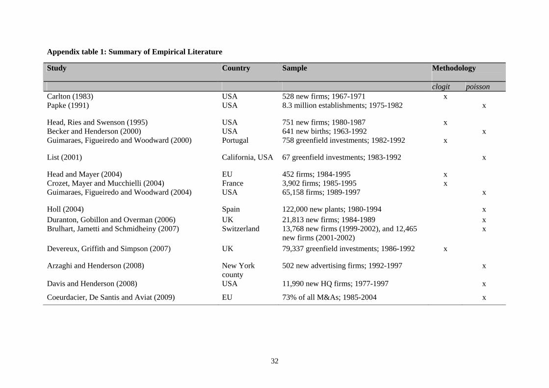
11 See Appendix table 1 for a summary of studies employing these models.

8

The stochastic nature of the profit function implies that the probability that location j

is selected by the investor i equals:

)(Pr ikijij obP ππ >= , jkk ≠∀ ,

It is assumed that the ith firm will choose district j if ikij ππ > for all k where k

indexes all the possible location choices to the ith firm. Under the assumption of

independent and identically distributed error terms ε , with type I extreme-value

distribution, the probability of choosing district j becomes:

∑=

= n

kik

ijij

U

UP

1

)exp(

)exp( (2)

The above equation expresses the conditional logit formulation. If we further assume

that the systematic part of profit is affected by a set of m regressors, we can estimate

the effects these have on location decisions. Typically, it is assumed that ijU is a

linear combination of the explanatory variables:

mijmijijij XXXU βββ +++= ........2

21

1 The simplicity of the conditional logit model (CLM) allows first insights into the

behaviour of foreign investors across different districts within the country. For

instance, it is possible that a foreign investor may consider large urban

agglomerations in different states as possible alternatives. In other words, an investor

may consider Kota in the state of West Bengal and Pune in Maharashtra as possible

alternatives since they serve as satellite towns to larger cities (Kolkata and Mumbai,

respectively).

In practice, however, the implementation of the conditional logit model in the

face of a large set of spatial alternatives is very cumbersome.12 The CLM is also

characterised by the assumption of Independence of Irrelevant Alternatives (IIA).

Consequently the ratio of the logit probabilities for any two alternatives j and k does 12 Guimaraes, Figueiredo and Woodward (2003) provide an overview of the problems and how different researchers have attempted to deal with them in the past.

9

not depend on any alternatives other than j and k . More formally this implies that

the ijε are independent across individuals and choices; all locations would be

symmetric substitutes after controlling for observables. This assumption could be

violated if districts within particular states are closer substitutes than others outside of

the state boundary. To effectively control for the IIA assumption, one would need to

introduce a dummy variable for each individual choice. This would amount to a

specification of the following type:

ijijjijijij zU εβδεπ ++=+= ' (3)

where jδ s are the alternative specific constants introduced to absorb factors that are

specific to each particular choice. In this case all explanatory variables (observable or

unobservable) that only change across choices are absorbed by the alternative specific

constants. However, in the presence of a large dataset this implementation would be

impractical because of the large number of parameters to be estimated.

As an econometric alternative, Guimaraes, Figueiredo and Woodward (2003)

show that the implementation of conditional logit models yields identical results to

Poisson regression models when the regressors are not individual specific. They

demonstrate how to control for the potential IIA violation by making use of an

equivalence relation between the CLM and Poisson regression likelihood functions. In

a separate paper, Guimaraes, Figueiredo and Woodward (2004) provide an empirical

demonstration. In this model the alternative constant is a fixed-effect in a Poisson

regression model, and coefficients of the model can be given an economic

interpretation compatible with the Random Utility Maximisation framework. Since

using both models yield identical parameter estimates, we will use Poisson

regressions to generate coefficients.

Let ijn be the number of investments in region j . Based on the profit function

in Equation (3), the probability of investor i selecting location j would then become:

∑=

+

+= J

jijj

ijjij

z

zP

1)'exp(

)'exp(

βδ

βδ

(4)

10

The parameters of equation (4) can then be estimated by maximising the following

log-likelihood:

∑=

=J

jijijcl PnL

1

logln (5)

Guimaraes, Figueiredo and Woodward (2003) show that Equation (5) is

equivalent to that of a Poisson model that takes ijn as the dependent variable and

includes a set of location-specific explanatory variables. The same results will be

obtained if we assume that ijη follows a Poisson distribution with expected value

equal to

E(nij ) = λij = exp(α 'd j + β'zij ) That is, the above problem can be modelled as a Poisson regression where we include

as explanatory variables jd (which vary across locations) and ijz (which vary across

groups of investors and locations); ijn is the number of investments in j .

More recently, Schmidheiny and Brulhart (2009) have shown that the

elasticities of the conditional logit and Poisson models establish the boundary values

at polar ends. In other words, they observe that the Poisson model implies more

elastic responses by, here, investment counts, to given changes in own-region

characteristics than the conditional logit model. Also, unlike in the conditional logit

model, in the Poisson model, one region’s change in locational attractiveness has no

impact on the number of investments located among any of the other regions. We will

exploit the features of both, conditional logits and Poisson, models to compute the

two extremes for the elasticities, i.e. the percentage change in the expected number of

firms in a region (or a neighbouring region) with respect to a unit change in the

locational characteristics of the region.13

13 The conditional logit model implies a zero-sum allocation process of a fixed number of investments over the J locations. In the Poisson model, by contrast, new investments are non-rivalrous, in the sense that we are in a positive-sum economy and one region’s gain is not another region’s loss.

11

c. Specification of variables

In the conditional logit model the dependent variable is a binary variable taking the

value of one if the investor chooses to invest in a district and zero otherwise. In the

Poisson model the dependent variable is the count of new foreign investment projects

approved in a district. As noted above, the overall sample includes about 19,500

foreign investment projects approved in 447 districts belonging to 35 states and union

territories. Whilst we have annual FDI observations for the period 1991-2005, data on

district-level location variables are available for only a few years. This restricts our

analysis to three cross-sections: 1991, 1996 and 2001. Our focus is on the fully

specified model for 2001, while the more limited estimations for the two earlier years

serve as robustness tests.

The independent variables include characteristics of the district that can affect

the profits of the investor. We classify these variables into those with an economic

geography dimension, those that reflect business conditions in the district (notably,

the availability of complementary factors of production and the quality of

infrastructure), and those that relate to the behaviour of previous investors within the

district as well as in other districts of the same state. A brief description of major

variables follows.14

The economic geography variables in our model are represented by the

Herfindahl index, market access, and population to indicate the size of the local

market. We use the Herfindahl index to measure the degree of economic diversity in

each region. jHI is the sum of squares of employment shares of all industries in

region j:

HI j =E jk

E j

⎛

⎝ ⎜ ⎜

⎞

⎠ ⎟ ⎟

2

k∑

Unlike measures of specialisation, which focus on one industry, the diversity index

considers the industry mix of the entire regional economy. The largest value for

jHI is one when the entire regional economy is dominated by a single industry. Thus

higher values signify lower levels of economic diversity.

14 See also Appendix table 2 for definitions and sources; Appendix table 3 presents summary statistics.

12

Access to larger markets should provide a stronger incentive for investors to

pick particular locations. For instance, investors in satellite towns, for instance

Gurgaon, would also have access to larger neighbouring markets, say Delhi. The

classic gravity model, which is commonly used in the analysis of trade between

regions and countries, states that the interaction between two places is proportional to

the size of the two places (as measured by population, employment or some other

index of social or economic activity), and inversely proportional to some measure of

separation such as distance. We use the formulation proposed initially by Hanson

(1959) that states that the accessibility at point 1 to a particular type of activity at area

2 (say, employment) is directly proportional to the size of the activity at area 2 (say,

number of jobs) and inversely proportional to some function of the distance

separating point 1 from area 2. Accessibility is thus defined as the potential for

opportunities for interaction. Thus, market accessibility is defined as:

MA j =Sm

d j −mb

j∑

where jMA is the accessibility indicator estimated for location j, mS is a size indicator

at destination m, jmd is a measure of distance between origin j and destination m,15

and b describes how increasing distance reduces the expected level of interaction.16

The accessibility measure is constructed using population as the size indicator and

distance as a measure of separation; it is estimated without exponent values. The

market access measure is constructed by allowing transport to occur along the straight

line connecting any two districts. Instead of calculating the distance between any pair

of districts across the country, we restrict the links to districts within a 500-kilometre

radius.

Turning to district characteristics reflecting business conditions, we use non-

agricultural hourly wage rates as an indicator of labour costs. We also account for

education (higher-secondary education or middle-higher schools) as a proxy of the

qualification of the workforce, which is traditionally considered to be an important

complementary factor of production. In addition, we employ various proxies for the

15 We are grateful to Eckhardt Bode for providing us with the syntax for computing the great circle (orthodormic) distance calculations. 16 In the original model proposed by Hanson (1959), b is an exponent describing the effect of the travel time between the zones.

13

availability and quality of district-level infrastructure, including power (electricity),

communications (telephone), transport (access to buses or roads), financial (bank

branches) and health (access to health centres) infrastructure.

Finally, following Crozet, Mayer and Mucchielli (2004), we include a variable

to account for previous investment choices by foreign investors. In particular, we

assess whether foreign investors are attracted to locations that attracted other foreign

investors before, and whether this effect is stronger for investors from the same

country of origin. We include a count variable to take account of all foreign firms

within a district and in all districts within the state, weighted by their distance.

Formally stated, we include:

FA j = Count j +Countm

d j −mj∈s∑ and FS j = Count j +

Countm

d j −mj∈s∑

where jFA and jFS refer, respectively, to all foreign and all same-country foreign

firms in location j . The value of FA is computed for all years leading up to the year

for which the cross-section is carried out.

Without convincing instruments, it is difficult to control for possible

endogeneity. In particular, location choices by previous investors may be jointly

determined with our dependent variable resulting in an omitted variable bias. The

limited availability of district-level data for a continuous set of years prevents us from

addressing endogeneity concerns by performing panel estimations. Rather, we

estimate three cross-sections to fully exploit the available data. Although, this does

not allow us to control for endogeneity concerns, it does reduce the possibility of bias.

There is also little reason to be concerned about reverse causality running from our

regressors to firm-specific location choices. Note also that we lag our regressors by

assessing their impact on location choices in the concurrent and the two subsequent

years, in order to mitigate possible endogeneity problems.

IV. Results and discussion We illustrate the key characteristics of the data and the subsequent modelling choices,

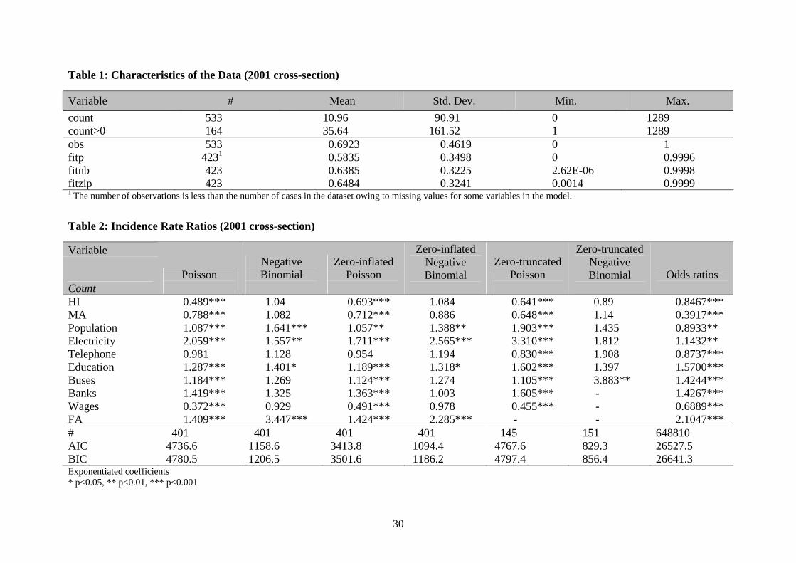
by using the 2001 cross-section as an example. One of the key characteristics of the

data is that it is over-dispersed. In Table 1, the mean number of investments per

14

district is around 11, while the standard deviation is over 90, i.e. over eight times the

mean. A Poisson model implies that the expected count, or mean value, is equal to the

variance. This is a strong assumption, and does not hold for our data.

A frequent occurrence with count data is an excess of zeroes compared to

what would be expected under a Poisson model. This is indeed a problem faced by

our data – the mean number of investments is about 35 when excluding zeros and the

standard deviation is 161, i.e. around 4.6 times the mean. Also note that 369 out of

533 districts did not receive any investments in 2001-2003.17 This implies that we

would need to take into account, both, over-dispersion and the excess of zeroes in the

data, when selecting a model to fit the data.

Another way to reiterate the unsuitability of the Poisson model in this case is

to show that such a model is unable to predict the excess zeroes found in our data. In

Table 1, “obs” refers to actual observations in the data, and fitp, fitnb and fitzip refer

to the predictions of the fitted Poisson, negative binomial and zero-inflated Poisson

models respectively. While 69.23% of the locations in the sample received no

investments, the Poisson model predicts that only 58.35% would get no investments.

Clearly the Poisson model underestimates the probability of zero counts. The negative

binomial model, which allows for greater variation in the count variable than that of a

true Poisson, predicts that 63.85% of all districts will receive no investments, much

closer to the observed value.

One way to account for the excess zeroes would be to assume that the data

comes from two separate populations, one where the number of investments is always

zero, and another where the count has a Poisson distribution. The distribution of the

outcome is then modelled in terms of two parameters – the probability of always zero

and the mean number of investments for those locations not in the always zero group.

The zero-inflated Poisson model (fitzip) predicts that 64.84% of all locations will

receive no investments, marginally better than the predictions of the negative

binomial model.

An alternative approach to deal with an excess of zeroes would be to use a

two-stage process, with a logit model to distinguish between the zero and positive

counts, and then a zero-truncated Poisson or negative binomial model for the positive

counts. In our case this would imply using a logit model to differentiate between

17 Although there are a total of 604 districts in India, we exclude all districts for which we do not have data for the regressors.

15

districts that receive no investments and those that do, and then a truncated model for

the number of districts that receive at least one investment. These models are referred

to as “hurdle models” – a binary probability model governs the binary outcome of

whether a count variable has a zero or positive realisation; if the realisation is

positive, the ‘hurdle’ is crossed and the conditional distribution of the positives is

governed by a truncated-at-zero count model data model (McDowell 2003).18

Against this backdrop, Table 2 reports the results of the 2001 cross-section

based on alternative models. The response variable is ‘count’, i.e. the number of

investments received by a district. The Poisson regression models the log of the

expected count as a function of the predictor variables. More formally,

)log()log( 1 xx μμβ −= + , where β is the regression coefficient, μ is the expected

count and the subscripts represent where the regressor, say x, is evaluated at x and

x+1 (here implying a unit percentage change in the regressor).19 Since the difference

of two logs is equal to the log of their quotient, i.e. )log()log()log( 11

x

xxx μ

μμμ ++ =− ,

we could also interpret the parameter estimate as the log of the ratio of expected

counts. In our case, the count refers to the ‘rate’ of investments per district. We report

exponentiated coefficients20, i.e. incidence rate ratios. The incidence rate ratios can be

interpreted as follows: if education (i.e. the proportion of the population with a high-

school degree) was to increase by a percentage unit, the rate ratio for count would be

expected to increase by a factor of 1.28, i.e. by 28 percentage points. As mentioned

earlier, the conditional logit and the Poisson models establish the range for the odds

ratios of the analysis. We also present the results of the conditional logit estimation in

the last column of Table 2, commonly referred to as ‘odds ratios’. The odds ratio can

be interpreted as follows: a unit percentage increase in education would be associated

with a 57 percent increase in the odds of receiving an investment in a district. An

incidence rate or odds ratio greater than one implies a positive effect; less than one

implies a negative effect, and equal to one means that changes in the predictor

variable leave the dependent variable unaffected.

18 We were unable to achieve convergence for the zero-inflated and the zero-truncated negative binomial models when using all regressors. We report the results of these models when convergence is achieved using limited regressors. 19 This is because the regressors are in logarithms of the original independent variables. 20 The unexponentiated coefficient results can be made available on request.

16

In order to select the preferred model, Table 2 also presents the Bayesian

information criterion (BIC) and Akaike’s information criterion (AIC). Since the

models are used to fit the same data, the model with the smallest values of the

information criteria is considered superior. By these criteria the negative binominal

models generally perform better than the Poisson models. Note that this holds not

only for the 2001 cross-section but also for the cross-sections for 1996 and 1991

reported in Appendix tables 4 and 5 as robustness tests.

The presentation and interpretation of results focuses on the 2001 cross-

section as the data situation is clearly superior compared to earlier years. Apart from

the health-related variable on infrastructure, the full set of explanatory variables is

available for 2001 (see also Appendix table 2). By contrast, two variables of major

interest – the Herfindahl index on economic diversity and labour costs – are lacking

for earlier years. Moreover, the data is available for most Indian districts in 2001,

whereas coverage of districts is limited in 1991 and 1996. Nevertheless, the results for

the two earlier cross-sections offer some valuable insights on the robustness of several

variables driving the location choices of foreign investors in post-reform India.

The dependent count variable used for 2001 cross-section actually includes

FDI projects approved during the three-year period 2001-2003. In this way we make

use of a larger part of the FDI database introduced in Section III above. At the same

time, the consideration of three years as regards approvals smoothes cyclical FDI

fluctuations.21 As a first result, it should be noted that we find a strong tendency of

foreign investors to go where other foreign investors are already present. The

preferred binominal models reveal a particularly strong clustering of FDI; but even

the Poisson models suggest that a percentage increase in the value of FA (which

includes investors within the same district and in neighbouring districts) would result

in a 40 percent increase in the expected rate of FDI counts. Whenever available22 the

coefficient is statistically significant at the 0.1 percent level. As shown in Appendix

table 4, the high statistical significance of FA and its strong quantitative impact also

holds in the earlier cross-section for 1996.23 This invites the conclusion that regional

clustering of FDI prevailed throughout most of the period under consideration. In 21 Similarly, we use FDI approvals in 1996-1998 for the 1996 cross-section and, respectively, approvals in 1991-1993 for the 1991 cross-section. 22 Since convergence could not be achieved with the full set of predictor variables within zero-truncated models, the coefficients for the dropped variables could not be computed. 23 FA does not enter the cross-section for 1991 in Appendix table 5 as 1991 is the first year covered in the FDI database.

17

other words, insofar as India’s reform program initiated in the early 1990s resulted in

more FDI, it is likely to have contributed to regional disparities in India by

exacerbating the concentration of FDI.

Turning to the economic geography variables, population consistently has a

positive effect and, typically, is highly significant at the one percent level. In the zero-

inflated negative binominal models, the quantitative effect is about 39 percent if

population increases by one percentage point. Similar results are achieved for the two

earlier cross-sections, even though the level of significance and the quantitative

impact vary somewhat over time and across models. Recalling the discussion on

horizontal FDI in Section II, population is surprisingly robust as a relevant driving

force of FDI at the district level. This finding qualifies the popular view held in

various source countries that the boom of FDI in post-reform India is mainly

associated with vertical, i.e. cost-cutting FDI; it rather appears that FDI is horizontal,

i.e. closely associated with the size of the local market.

In contrast to population in the district where FDI locates, distance-weighted

population in other districts - representing our proxy of market access (MA) - does

not appear to impact positively on FDI. In the preferred negative binominal models in

Table 2, MA does not differ significantly from zero; the Poisson models even suggest

a negative effect as the IRR are significantly below one.24 This is in conflict with the

hypothesis that districts in the neighbourhood of large metro areas are likely to

benefit, in terms of attracting more FDI, from having easier access to these markets

than remote Indian districts. Rather, it appears that large metro areas divert FDI

projects away from neighbouring districts, thereby perpetuating or even widening the

urban-rural divide.25 Conversely, the sharp urban-rural divide in India implies limited

market potential surrounding the metro areas, which further weakens any positive

effects MA may have on FDI.

HI seems to have a negative relationship (i.e. the IRR<1) with FDI projects.

Recall that this variable is a measure of the level of industrial diversity within the

24 MA also proves to be insignificant in the negative binominal models run for the earlier cross-sections. By contrast, the Poisson models often result in significantly positive results for MA in Appendix tables 4 and 5. The latter finding applies especially to the cross-section for 1996. Recall however that the reliability of the results for 1996 suffers from a drastically reduced number of observations. 25 It should be noted in this context that, for instance, almost 90 percent of approved FDI projects in Karnataka went to Bangalore; Kolkata accounted for 70 percent of projects approved in West Bengal (Nunnenkamp and Stracke 2008).

18

district. A higher HI implies higher employment concentration by one industry and

lower industrial diversity. Thus, the negative coefficient for HI is evidence of a

positive association between more industrial diversity and more FDI.

This could be since foreign investors are increasingly pursuing complex integration

strategies, as noted by UNCTAD (1998). Consequently, they rely on a diverse set of

intermediate inputs from various industries, giving locations a competitive edge

where these inputs are easily available. Our finding on HI is in line with Kathuria

(2002), according to whom the degree of vertical integration of FDI projects has

declined in post-reform India. Unfortunately, owing to lack of data we are unable to

test this relationship further for other cross-sections.

It is not only greater industrial diversity that attracts FDI to Indian districts.

The same applies to districts with a better-qualified workforce, as reflected in IRRs

typically being greater than one for our variable on education. With the exception of

the zero-truncated negative binominal model, education proves to be statistically

significant throughout in the cross-section for 2001, at the five per cent level or better.

The findings for education are somewhat weaker, both in terms of statistical

significance and quantitative impact, in the earlier cross-section for 1991 (Appendix

table 5). This may indicate that the availability of sufficiently qualified labour in

Indian districts has become more important over time as a complementary factor of

production. However, this conclusion can only be tentative, recalling that the

specification of our variable on education differs slightly between the cross-sections

due to data limitations.

While better-educated workers attract FDI, higher labour costs could be

expected to discourage FDI. However, the evidence for 2001 is ambiguous and we

are unable to make any comment for earlier years.26 The negative effect is highly

significant at the 0.1 percent level as well as quantitatively important in the three

Poisson models. By contrast, the negative binominal models – preferred because of

lower AIC and BIC statistics – reveal wage effects that do not differ significantly

from one, implying no change in the incidence rate ratios. As will be shown below,

the impact of wages on FDI differs considerably across sectors.

Finally, Table 2 reveals somewhat ambiguous findings concerning the

relationship between infrastructure and FDI at the district level. On the one hand,

26 As noted above, wage data at the district level are not available for the earlier cross-sections.

19

electricity enters with a highly significant and strongly positive coefficient

irrespective of the choice of model. On the other hand, telephone connections – our

proxy of communication infrastructure – typically remain insignificant. The evidence

varies across models with respect to financial infrastructure and transport

infrastructure (proxied by bus services in Table 2). This ambiguity resembles previous

findings at the level of Indian states. As a matter of fact, the role of infrastructure as a

determinant of FDI in India has remained disputed. While the World Bank (2004)

claims that deficient infrastructure represents an important bottleneck to investment

even in relatively advanced states such as Maharashtra and Gujarat, Chakravorty

(2003) finds that infrastructure had little influence in determining the location or

quantity of new industrial investment. Nunnenkamp and Stracke (2008) show that the

impact of infrastructure on state-level FDI depends on the specific indicator chosen.

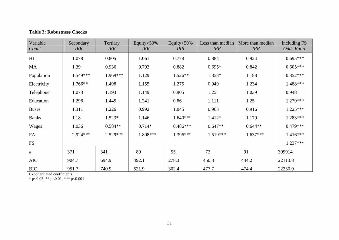
V. Robustness checks As a first robustness check, we differentiate between FDI in the secondary and the

tertiary sector and re-run the cross-section regressions for the year 2001 to observe if

the effect of the predictor variables varies across these two sectors. Although we

carried out the regressions using Poisson and zero-inflated and zero-truncated

methods as well, we only report the results of the simple negative binomial

specifications.27 This is to facilitate comparison, but more importantly because the

negative binomial model exhibited the best goodness-of-fit statistics. As before, the

coefficients are reported as Incidence Rate Ratios for ease of interpretation.

In several respects, the results for the manufacturing and services sub-samples

in Table 3 closely resemble the corresponding negative binominal model results for

the overall FDI sample in column 2 of Table 2 above. For both sub-samples, there

appears to be a strong tendency to locate where other foreign investors have chosen to

locate.28 We find, as before, that population has a positive effect on FDI projects.

While the tendency to follow previous investors appears to be slightly stronger in the

manufacturing sector, population has a somewhat stronger impact of FDI projects in

27 Results from the models are available on request. 28 We estimated FA for the total of projects within the same district and in neighbouring districts; i.e., this variable is not further disaggregated by the type of sector. This is because we would like to capture the effect of FDI drawn to locations for reasons of intra-industry advantages, but also for buyer-supplier linkages across sectors.

20

the services sector. This is in line with economic intuition, in which services

industries usually benefit more than manufacturing industries from being close to

where people are situated. As before for the overall sample, our measure of industrial

diversity (HI) is still not significantly different from one if the negative binominal

model is estimated for sector-specific FDI.29

Yet we find some interesting differences between FDI in manufacturing and

FDI in services. Most notably, the costs of local labour discourage FDI only in the

services sector. Here, the effect of wages is significant at the one percent level, and

quantitatively important with a one percentage point increase in wages resulting in a

decline by more than 40 percent in the expected count of FDI projects. The striking

contrast in wage effects between sectors invites the conclusion that vertical FDI,

which is mainly motivated by cost considerations, is largely restricted to India’s

services sector, whereas FDI in its manufacturing sector continues to be horizontal,

i.e., local market seeking.30 This could also be because certain services sectors rely on

access to cheap and abundant labour (for instance, call centres) and they would then

be theorised to be more sensitive to wage increases. However, since we are unable to

disaggregate the data down to the two-digit industry level, we cannot be certain which

specific industries within these sectors maybe driving the results. Moreover, the

sector-specific perspective adds to the ambiguity concerning infrastructure. The effect

of electricity proves to be strongly significant for FDI in manufacturing only, while

the presence of banking facilities at the district level encourages FDI in the services

sector at the five percent level of significance.

The next robustness test distinguishes between majority and minority foreign

owned joint ventures (JVs). We use foreign equity shares as presented in the DIPP

database to group all FDI projects into these two categories.31 This distinction may be

relevant as higher foreign equity shares tend to be associated with a relatively strong

bargaining position of foreign investors (e.g., Asiedu and Esfahani 2001) which, in

turn, may imply that location choices are more strongly determined by the preferences

of foreign investors than those of the host government. Nevertheless, Table 3 reveals

29 The IRR for our variable on education appears to be of similar size for FDI in manufacturing and services. In contrast to the corresponding estimation for the overall sample, however, this variable turns statistically insignificant at the five percent level for sector-specific FDI, although it remains significant at the 10 percent level. 30 Agarwal (2001) suspects FDI in India to be still domestic market seeking. 31 Information on the foreign equity share is missing for various FDI projects, which results in a considerably reduced number of observations.

21

few significant differences between majority and minority owned JVs with respect to

the determinants of location choices. Local market size, as reflected by population, as

well as financial infrastructure appears to matter more for minority owned JVs. This

is plausible given that majority owned JVs may turn primarily to international capital

markets for financing, and may also be more export oriented than minority owned

JVs.

Similar to minority owned JVs, smaller FDI projects appear to be more reliant

on local markets and local financing than larger FDI projects. This is revealed by our

third robustness test when considering the median of the value of foreign equity as the

dividing line between small and large FDI projects. In most other respects, however,

our results are hardly affected by distinguishing between small and large projects.

Finally, we re-run the CLM included in Table 2 above by separately

accounting for previous investment choices by foreign investors of the same country

of origin (FS).32 We find that foreign investors tend to locate where investors from the

same country of origin located before; the corresponding odds ratio is significantly

higher than one, at the 0.1 percent level. However, the tendency to follow investors

from the same country of origin does not appear to be stronger than the tendency to

follow other foreign investors. This is broadly in line with the findings of Crozet,

Mayer and Mucchielli (2004) for FDI in French départements. The results for almost

all other variables are robust to the inclusion of FS when comparing the last columns

in Tables 2 and 3.33

VI. Concluding remarks This paper contributes to the empirical literature relating to the geography of foreign

direct investment in a number of ways. Although there is some previous research on

the behaviour of foreign investors in emerging countries like China, to our knowledge

this is the first paper that analyses location decisions for over 19,500 FDI projects in

India. We differentiate between economic geography factors, such as the presence of

existing FDI, access to neighbouring markets and industrial diversity, and factors

32 This robustness test can only be performed for the CML as the choices of foreign investors need to be matched on a one-to-one basis with those belonging to the same country. This matching exercise is not possible to carry out when investments are grouped as a count variable. 33 The only exception refers to education that turns insignificant in Table 3.

22

relating to the local business conditions including the quality of infrastructure at the

level of districts. The difference between these two sets of factors is of obvious policy

relevance: Whilst public policy may be in a position to influence the level and quality

of infrastructure within a lagging region, its ability to affect economic clustering is

limited.

Indeed, we find that path dependence tends to constrain the influence of

regional policymakers. Foreign investors strongly prefer locations that already host

other foreign investors. This effect is significantly positive and robust across different

years, sectors and different types of FDI. Moreover, foreign investors tend to follow

previous investors from the same country of origin, but also investors from other

countries of origin. We also find that the degree of economic diversity within a

location attracts FDI, but we are unable to check this result for different years. More

surprisingly, districts in the neighbourhood of large metro areas do not benefit, in

terms of attracting more FDI, from having easier access to these markets than remote

Indian districts. On the contrary, our results suggest that large metro areas divert FDI

projects away from neighbouring districts, thereby perpetuating or even widening the

urban-rural divide.

However, geography is not destiny. It is in several respects that local business

conditions matter for the location choices of foreign investors at the level of districts.

For instance, the presence of an educated population is a significant factor drawing

FDI projects to a location. This clearly reveals that FDI in post-reform India is

attracted not only by lower labour costs but also by the availability of sufficiently

skilled labour as an important complementary factor of production. Providing

adequate schooling and training thus appears to be an important policy tool for

regional policymakers.

Investing in infrastructure represents another option to attract FDI. Access to

power, transport and financial infrastructure – factors that the World Bank often

classifies as ‘investment climate’ – clearly matters for location decisions of foreign

investors. However, the evidence is more ambiguous when it comes to the question of

which aspect of infrastructure is particularly relevant for FDI in particular sectors.

For instance, the presence of bank services within a location seems to be an important

factor driving location choices for FDI in services, but less so for FDI in

manufacturing. The opposite pattern turns out for power supply. This ambiguity may

23

render it difficult for policymakers to decide on investment priorities in the area of

infrastructure.

Future research may help overcome a few shortcomings once additional data

are made available by Indian authorities. Data limitations with respect to FDI

determinants at the district level do not permit us to estimate panel regressions, which

would allow us to better deal with endogeneity concerns. Additional insights might

also be gained if all FDI projects were differentiated between industrial sectors at a

disaggregated level. Industry-specific estimations could reveal whether the location

choices of foreign investors and the relative importance of economic geography and

local business conditions differ across industries. For instance, computer or financial

services would probably require different levels and types of labour skills than retail

or transport services. Finally, even though the FDI data offer various details on the

characteristics of joint ventures in India, it would be desirable to match this dataset

with data on the foreign parent company. Its size, age, productivity and technological

sophistication may shape location decisions, in addition to district characteristics,

considering that such firm characteristics influence the relative bargaining position of

foreign investors vis-à-vis regional authorities competing for FDI.

24

References

Agarwal, D.R. (2001). Foreign Direct Investment and Economic Development: A

Comparative Case Study of China, Mexico and India. In R.K. Sen (ed.), Socio-

Economic Development in the 21st Century. New Delhi: 257-288.

Aghion, P., R. Burgess, S.J. Redding, and F. Zilibotti (2005). Entry Liberalization and

Inequality in Industrial Performance. Journal of the European Economic

Association 3 (2-3): 291-302.

Alegría, R. (2006). Countries, Regions and Multinational Firms: Location

Determinants in the European Union. London School of Economics, mimeo.

Asiedu, E. and H.S. Esfahani (2001). Ownership Structure in Foreign Direct

Investment Projects. Review of Economics and Statistics 84 (4): 647-662.

Arzaghi, M and V. Henderson (2008). Networking off Madison Avenue. Brown

University.

Bajpai, N. and J.D. Sachs (2000). Foreign Direct Investment in India: Issues and

Problems. Development Discussion Paper, 759. Harvard Institute for

International Development, Harvard University. Cambridge, MA.

Baltagi, B.H., P. Egger and M. Pfaffermayr (2007). Estimating Models of Complex

FDI: Are There Third-Country Effects? Journal of Econometrics 140 (1): 260-

281.

Becker, R. and V. Henderson (2000). Effects of Air Quality Regulations on Polluting

Industries. Journal of Political Economy 108 (2): 379-421

Blonigen, B.A., R.B. Davis, G.R. Waddell and H.T. Naughton (2007). FDI in Space:

Spatial Autoregressive Relationships in Foreign Direct Investment. European

Economic Review 51 (5): 1303-1325.

Bobonis, G.J. and H.J. Shatz (2007). Agglomeration, Adjustment, and State Policies

in the Location of Foreign Direct Investment in the United States. Review of

Economics and Statistics 89 (1): 30–43.

Brulhart, M, M. Jametti and K. Schmidheiny (2007). Do Agglomeration Economies

Reduce the Sensitivity of Firm Location to Tax Differentials? Discussion

Paper 6606. Centre for Economic Policy Research (CEPR), London.

Carlton, D. (1979). Why New Firms Locate Where They Do: An Econometric Model.

In: W. Wheaton (ed.), Interregional Movements and Regional Growth.

Washington, DC.

25

Carlton, D. (1983). The Location and Employment Choices of New Firms: An

Econometric Model with Discrete and Continuous Endogenous Variables.

Review of Economics and Statistics 65 (3): 440-449.

Chakrabarti, A. (2001). The Determinants of Foreign Direct Investment: Sensitivity

Analyses. Kyklos 54(1): 89-113.

Chakraborty, C. and P. Nunnenkamp (2008). Economic Reforms, FDI and Economic

Growth in India: A Sector Level Analysis. World Development 36 (7): 1192-

1212.

Chakravorty, S. (2003). Industrial Location in Post-Reform India: Patterns of Inter-

regional Divergence and Intra-regional Convergence. Journal of Development

Studies 40(2): 120-152.

Cheng, L.K. and Y.K. Kwan (2000). What Are the Determinants of the Location of

Foreign Direct Investment? The Chinese Experience. Journal of International

Economics 51 (2): 379-400.

Chung, W. and J. Alcácer (2002). Knowledge Seeking and Location Choice of

Foreign Direct Investment in the United States. Management Science 48 (12):

1534-1554.

Coeurdacier, N, R.A. De Santis and A. Aviat (2009). Cross-border Mergers and

Acquisitions and European Integration. Economic Policy 57: 55-106

Coughlin, C.C. and E. Segev (2000a). Foreign Direct Investment in China: A Spatial

Econometric Study. World Economy 23 (1): 1-23.

Coughlin, C.C. and E. Segev (2000b). Location Determinants of New Foreign-owned

Manufacturing Plants. Journal of Regional Science 40 (2): 323-351.

Coughlin, C.C., J.V. Terza and V. Arromdee (1991). State Characteristics and the

Location of Foreign Direct Investment within the United States. Review of

Economics and Statistics 73 (4): 675–683.

Crozet, M., T. Mayer and J.-L. Mucchielli (2004). How Do Firms Agglomerate? A

Study of FDI in France. Regional Science and Urban Economics 34 (1): 27-

54.

Davis, J.C. and J.V. Henderson (2008). The Agglomeration of Headquarters. Regional

Science and Urban Economics 38 (5): 445-460.

Devereux, M.P., R. Griffith and H. Simpson (2007). Firm Location Decisions,

Regional Grants and Agglomeration Externalities. Journal of Public

Economics 91 (3/4): 413-435.

26

Duranton, G. L. Gobillon and H. Overman (2006). Assessing the Effects of Local

Taxation Using Microgeographic Data. London School of Economics.

Feenstra, R.C. and G.H. Hanson (1997). Foreign Direct Investment and Relative

Wages. Journal of International Economics 42 (3-4): 371-393.

Fujita, M. and D. Hu (2001). Regional Disparity in China 1985-1994: The Effects of

Globalization and Economic Liberalization. Annals of Regional Science 35

(1): 3-37.

Government of India (2006). Annual Survey of Industries 2003-04. Chandigarh

(Labour Bureau).

Guimaraes, P., O. Figueiredo and D. Woodward (2000). Agglomeration and the

Location of Foreign Direct Investment in Portugal. Journal of Urban

Economics 47 (1): 115-135.

Guimaraes, P., O. Figueiredo and D. Woodward (2003). A Tractable Approach to the

Firm Location Decision Problem. Review of Economics and Statistics 85 (1):

201-204.

Guimaraes, P., O. Figueiredo and D. Woodward (2004). Industrial Location

Modeling: Extending the Random Utility Framework. Journal of Regional

Science 44 (1): 1-20.

Hanson G.H. (1959). How Accessibility Shapes Land Use. Journal of American

Institute of Planners 25: 73-76.

Head, C.K. and T. Mayer (2004). Market Potential and the Location of Japanese

Investment in the European Union. Review of Economics and Statistics 86 (4):

959-972.

Head, C.K. and J.C. Ries (1996). Inter-City Competition for Foreign Investment:

Static and Dynamic Effects of China’s Incentive Areas. Journal of Urban

Economics 40 (1): 38-60.

Head, C.K., J.C. Ries and D.L. Swenson (1995). Agglomeration Benefits and

Location Choice: Evidence from Japanese Manufacturing Investments in the

United States. Journal of International Economics 38 (3/4): 223–247.

Head, C.K., J.C. Ries and D.L. Swenson (1999). Attracting Foreign Manufacturing:

Investment Promotion and Agglomeration. Regional Science and Urban

Economics 29 (2): 197-218.

27

Holl, A. (2004). Manufacturing Location and Impacts of Road Transport

Infrastructure: Empirical Evidence from Spain. Regional Science and Urban

Economics 34 (3): 341-363.

Kathuria, V. (2002). Liberalisation, FDI, and Productivity Spillovers: An Analysis of

Indian Manufacturing Firms. Oxford Economic Papers 54 (4): 688-718.

Kochhar, K., U. Kumar, R. Rajan, A. Subramanian, and I. Tokatlidis (2006). India’s

Pattern of Development: What Happened, What Follows? Journal of

Monetary Economics 53 (5): 981-1019.

Lall, S.V. and S. Chakravorty (2005). Industrial Location and Spatial Inequality:

Theory and Evidence from India. Review of Development Economics 9 (1):

47-68.

Ledyaeva, S. (2009). Spatial Econometric Analysis of Foreign Direct Investment

Determinants in Russian Regions. World Economy 32 (4): 643-666.

List, J.A. (2001). US County-level Determinants of Inbound FDI: Evidence from a

Two-step Modified Count Data Model. International Journal of Industrial

Organization 19 (6): 953-973.

Majumder, R. (2008). Infrastructure and Development in India: Interlinkages and

Policy Issues. Jaipur (Rawat Publications).

McDowell, A. (2003). From the Help Desk: Hurdle Models. Stata Journal 3 (2): 178-

184.

McFadden, D. (1974). Conditional Logit Analysis of Qualitative Behaviour. In: P.

Zarembka (ed.), Frontiers in Econometrics. Academic Press: New York

(Academic Press): 105-142.

Nunnenkamp, P. and R. Stracke (2008). Foreign Direct Investment in Post-Reform

India: Likely to Work Wonders for Regional Development? Journal of

Economic Development 33 (2): 55-84.

Papke, L.E. (1991). Interstate Business Tax Differentials and New Firm Location:

Evidence from Panel Data. Journal of Public Economics 45 (1): 47-68.

Purfield (2006). Mind the Gap - Is Economic Growth in India Leaving Some States

Behind? IMF Working Paper, WP/06/13, International Monetary Fund,

Washington, D.C.

Sachs, J.D., N. Bajpai, and A. Ramiah (2002). Understanding Regional Economic

Growth in India. Asian Economic Papers 1(3): 32-62.

28

Schmidheiny, K. and M. Brulhardt (2009). On the Equivalence of Location Choice

Models: Conditional Logit, Nested Logit and Poisson. CESifo Working Paper

2726. Munich.

UNCTAD (1998). World Investment Report 1998. New York and Geneva.

UNCTAD (2004). World Investment Report 2004. New York and Geneva.

UNCTAD (2009). World Investment Report 2009. New York and Geneva.

World Bank (2004). India: Investment Climate Assessment 2004: Improving

Manufacturing Competitiveness. Washington, D.C. (The World Bank).

Zhang, X. and K.H. Zhang (2003). How Does Globalisation Affect Regional

Inequality Within a Developing Country? Evidence from China. Journal of

Development Studies 39(4): 47-67.

29

Figure 1: Spatial Distribution of FDI Projects

Source: Department of Industrial Promotion and Policy, Ministry of Commerce and Industry

30

Table 1: Characteristics of the Data (2001 cross-section)

Variable # Mean Std. Dev. Min. Max. count 533 10.96 90.91 0 1289 count>0 164 35.64 161.52 1 1289 obs 533 0.6923 0.4619 0 1 fitp 4231 0.5835 0.3498 0 0.9996 fitnb 423 0.6385 0.3225 2.62E-06 0.9998 fitzip 423 0.6484 0.3241 0.0014 0.9999 1 The number of observations is less than the number of cases in the dataset owing to missing values for some variables in the model.

Table 2: Incidence Rate Ratios (2001 cross-section)

Variable

Count Poisson

Negative Binomial

Zero-inflated Poisson

Zero-inflated Negative Binomial

Zero-truncated Poisson

Zero-truncated Negative Binomial

Odds ratios

HI 0.489*** 1.04 0.693*** 1.084 0.641*** 0.89 0.8467*** MA 0.788*** 1.082 0.712*** 0.886 0.648*** 1.14 0.3917*** Population 1.087*** 1.641*** 1.057** 1.388** 1.903*** 1.435 0.8933** Electricity 2.059*** 1.557** 1.711*** 2.565*** 3.310*** 1.812 1.1432** Telephone 0.981 1.128 0.954 1.194 0.830*** 1.908 0.8737*** Education 1.287*** 1.401* 1.189*** 1.318* 1.602*** 1.397 1.5700*** Buses 1.184*** 1.269 1.124*** 1.274 1.105*** 3.883** 1.4244*** Banks 1.419*** 1.325 1.363*** 1.003 1.605*** - 1.4267*** Wages 0.372*** 0.929 0.491*** 0.978 0.455*** - 0.6889*** FA 1.409*** 3.447*** 1.424*** 2.285*** - - 2.1047*** # 401 401 401 401 145 151 648810 AIC 4736.6 1158.6 3413.8 1094.4 4767.6 829.3 26527.5 BIC 4780.5 1206.5 3501.6 1186.2 4797.4 856.4 26641.3 Exponentiated coefficients * p<0.05, ** p<0.01, *** p<0.001

31

Table 3: Robustness Checks

Variable Secondary Tertiary Equity>50% Equity<50% Less than median More than median Including FS Count IRR IRR IRR IRR IRR IRR Odds Ratio

HI 1.078 0.805 1.061 0.778 0.884 0.924 0.695***

MA 1.39 0.936 0.793 0.882 0.695* 0.842 0.605***

Population 1.549*** 1.969*** 1.129 1.526** 1.358* 1.188 0.852***

Electricity 1.766** 1.498 1.155 1.275 0.949 1.234 1.488***

Telephone 1.073 1.193 1.149 0.905 1.25 1.039 0.948

Education 1.296 1.445 1.241 0.86 1.111 1.25 1.279***

Buses 1.311 1.226 0.992 1.045 0.963 0.916 1.225***

Banks 1.18 1.523* 1.146 1.640*** 1.412* 1.179 1.283***

Wages 1.036 0.584** 0.714* 0.486*** 0.647** 0.644** 0.479***

FA 2.924*** 2.529*** 1.808*** 1.396*** 1.519*** 1.637*** 1.416***

FS 1.237***

# 371 341 89 55 72 91 309914

AIC 904.7 694.9 492.1 278.3 450.3 444.2 22113.8

BIC 951.7 740.9 521.9 302.4 477.7 474.4 22230.9 Exponentiated coefficients * p<0.05, ** p<0.01, *** p<0.001

32

Appendix table 1: Summary of Empirical Literature

Study Country Sample Methodology

clogit poisson Carlton (1983) USA 528 new firms; 1967-1971 x Papke (1991) USA 8.3 million establishments; 1975-1982 x

Head, Ries and Swenson (1995) USA 751 new firms; 1980-1987 x Becker and Henderson (2000) USA 641 new births; 1963-1992 x Guimaraes, Figueiredo and Woodward (2000) Portugal 758 greenfield investments; 1982-1992 x

List (2001) California, USA 67 greenfield investments; 1983-1992 x

Head and Mayer (2004) EU 452 firms; 1984-1995 x Crozet, Mayer and Mucchielli (2004) France 3,902 firms; 1985-1995 x Guimaraes, Figueiredo and Woodward (2004) USA 65,158 firms; 1989-1997 x

Holl (2004) Spain 122,000 new plants; 1980-1994 x Duranton, Gobillon and Overman (2006) UK 21,813 new firms; 1984-1989 x Brulhart, Jametti and Schmidheiny (2007) Switzerland 13,768 new firms (1999-2002), and 12,465

new firms (2001-2002) x

Devereux, Griffith and Simpson (2007) UK 79,337 greenfield investments; 1986-1992 x

Arzaghi and Henderson (2008) New York county

502 new advertising firms; 1992-1997 x

Davis and Henderson (2008) USA 11,990 new HQ firms; 1977-1997 x

Coeurdacier, De Santis and Aviat (2009) EU 73% of all M&As; 1985-2004 x

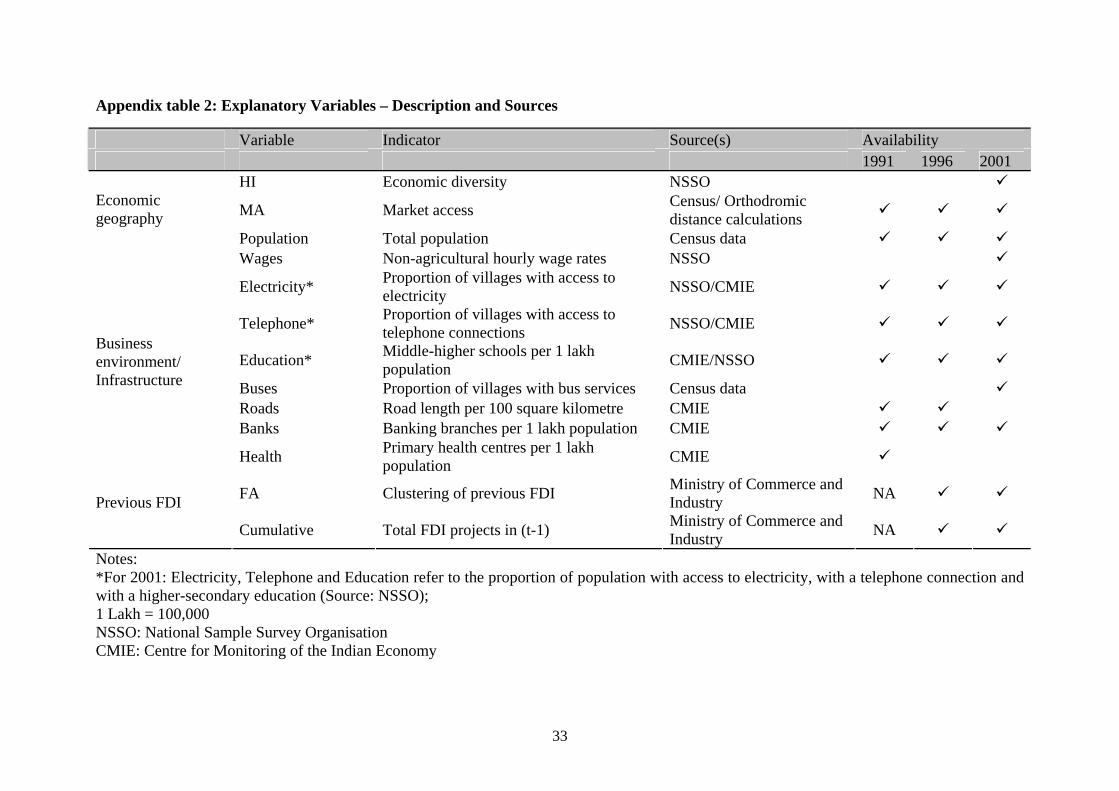
33

Appendix table 2: Explanatory Variables – Description and Sources

Variable Indicator Source(s) Availability 1991 1996 2001

HI Economic diversity NSSO

MA Market access Census/ Orthodromic distance calculations

Economic geography

Population Total population Census data Wages Non-agricultural hourly wage rates NSSO

Electricity* Proportion of villages with access to electricity NSSO/CMIE

Telephone* Proportion of villages with access to telephone connections NSSO/CMIE

Education* Middle-higher schools per 1 lakh population CMIE/NSSO

Buses Proportion of villages with bus services Census data Roads Road length per 100 square kilometre CMIE Banks Banking branches per 1 lakh population CMIE

Business environment/ Infrastructure

Health Primary health centres per 1 lakh population CMIE

FA Clustering of previous FDI Ministry of Commerce and Industry NA Previous FDI

Cumulative Total FDI projects in (t-1) Ministry of Commerce and Industry NA

Notes: *For 2001: Electricity, Telephone and Education refer to the proportion of population with access to electricity, with a telephone connection and with a higher-secondary education (Source: NSSO); 1 Lakh = 100,000 NSSO: National Sample Survey Organisation CMIE: Centre for Monitoring of the Indian Economy

34

Appendix table 3: Descriptive Statistics

Variable Expected sign # Mean

1991 1996 2001 1991 1996 2001

Investment decisions* (new/cumulative) 1,234 1,669 1,905 - 4,634 12,927

HI - 533 0.34

MA + 434 423 530 224,984 240,099 231,256

Population + 406 408 533 1,982,719 2,075,529 1,926,232

Wages - 454 89.54

Electricity + 334 350 533 0.84 0.88 0.56

Telephone + 126 117 533 0.46 1.12 0.09

Education + 231 305 533 0.17 0.22 0.06

Buses + 533 0.50

Roads + 207 184 61.25 69.30

Banks + 393 418 415 7.60 7.32 6.95

Health + 167 2.59

FA + 244 530 25.06 32.84 *Reference years: 1991, 1992, and 1993 (for 1991); 1996, 1997, and 1998 (for 1996); 2001, 2002, and 2003 (for 2001). Note: # refers to the number of districts for which there are observations.

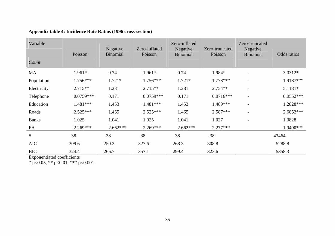
35

Appendix table 4: Incidence Rate Ratios (1996 cross-section)

Variable

Count

Poisson

Negative Binomial

Zero-inflated Poisson

Zero-inflated Negative Binomial

Zero-truncated Poisson

Zero-truncated Negative Binomial

Odds ratios

MA 1.961* 0.74 1.961* 0.74 1.984* - 3.0312*

Population 1.756*** 1.721* 1.756*** 1.721* 1.778*** - 1.9187***

Electricity 2.715** 1.281 2.715** 1.281 2.754** - 5.1181*

Telephone 0.0759*** 0.171 0.0759*** 0.171 0.0716*** - 0.0552***

Education 1.481*** 1.453 1.481*** 1.453 1.489*** - 1.2828***

Roads 2.525*** 1.465 2.525*** 1.465 2.587*** - 2.6852***

Banks 1.025 1.041 1.025 1.041 1.027 - 1.0828

FA 2.269*** 2.662*** 2.269*** 2.662*** 2.277*** - 1.9400***

# 38 38 38 38 38 43464

AIC 309.6 250.3 327.6 268.3 308.8 5288.8

BIC 324.4 266.7 357.1 299.4 323.6 5358.3 Exponentiated coefficients * p<0.05, ** p<0.01, *** p<0.001

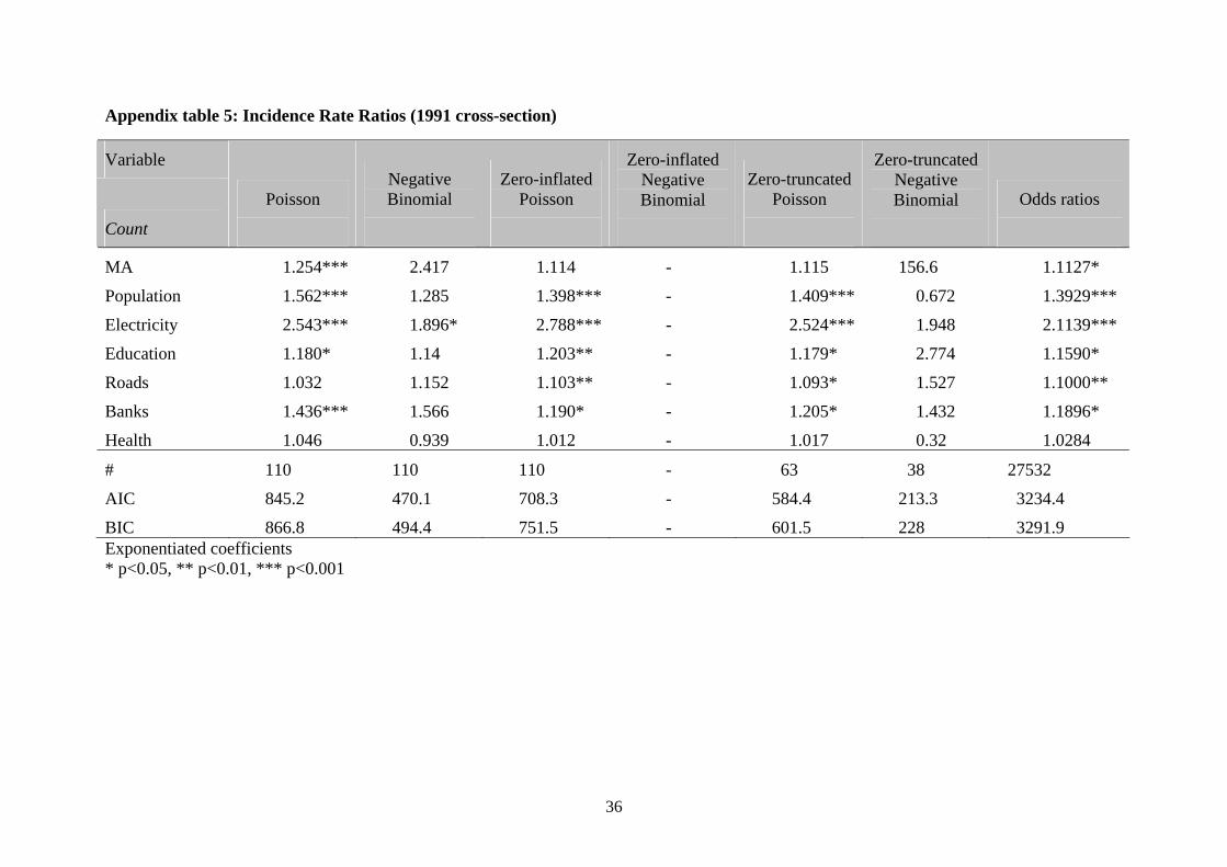
36

Appendix table 5: Incidence Rate Ratios (1991 cross-section)

Variable

Count

Poisson

Negative Binomial

Zero-inflated Poisson

Zero-inflated Negative Binomial

Zero-truncated Poisson

Zero-truncated Negative Binomial

Odds ratios

MA 1.254*** 2.417 1.114 - 1.115 156.6 1.1127*

Population 1.562*** 1.285 1.398*** - 1.409*** 0.672 1.3929***

Electricity 2.543*** 1.896* 2.788*** - 2.524*** 1.948 2.1139***

Education 1.180* 1.14 1.203** - 1.179* 2.774 1.1590*

Roads 1.032 1.152 1.103** - 1.093* 1.527 1.1000**

Banks 1.436*** 1.566 1.190* - 1.205* 1.432 1.1896*

Health 1.046 0.939 1.012 - 1.017 0.32 1.0284

# 110 110 110 - 63 38 27532

AIC 845.2 470.1 708.3 - 584.4 213.3 3234.4

BIC 866.8 494.4 751.5 - 601.5 228 3291.9 Exponentiated coefficients * p<0.05, ** p<0.01, *** p<0.001