Design, Implementation and Construction of a Controller ...
90
Design, Implementation and Construction of a Controller for a 6-DOF Serial Robot Diplomarbeit Werner Kollment Betreuer Ass.Prof. Dipl.-Ing. Dr.mont. Gerhard Rath O.Univ.-Prof. Dipl.-Ing. Dr.techn. Paul O’Leary Montanuniversit¨ at Leoben Institut f ¨ ur Automation June 2014
Transcript of Design, Implementation and Construction of a Controller ...
Design, Implementation andConstruction of a Controller for a
6-DOF Serial Robot
Diplomarbeit
Werner Kollment
Betreuer
Ass.Prof. Dipl.-Ing. Dr.mont. Gerhard Rath
O.Univ.-Prof. Dipl.-Ing. Dr.techn. Paul O’Leary
Montanuniversitat Leoben
Institut fur Automation
June 2014

1
Eidesstattliche Erklarung
Hiermit versichere ich, die vorliegende Arbeit selbststandig und unter ausschließlicher Verwen-
dung der angegebenen Literatur und Hilfsmittel erstellt zu haben.
Die Arbeit wurde bisher in gleicher oder ahnlicher Form keiner anderen Prufungsbehorde vorge-
legt und auch nicht veroffentlicht.
Leoben, 6. Juni 2014 Werner Kollment

2
Abstract
This thesis describes the design of a control unit for a six degree of freedom (6-DOF) industrial
robot. A fundamental theoretical introduction into robot kinematics is provided, whereby multi-
ple state-of-the-art approaches are explained and compared. The goal of this thesis is to establish
a kinematic framework, which is fully transparent for educational use. Furthermore, interfacing
additional algorithms and hardware components such as sensors is simplified; hence, expansion of
the system requires less effort compared to conventional controllers. The robot control is based on
an industrial personal computer (PC), which is divided into a real-time programmable logic con-
troller (PLC) and a conventional Windows desktop system. The robot is actuated by six frequency-
inverter driven servo motors, which are controlled by the PLC. The PLC is equipped with a generic
network interface, which enables execution of remote positioning commands. In this thesis, the
forward and inverse kinematic computations for the PLC are implemented in MATLAB. Simulink
is utilized to provided a real-time environment for the MATLAB functions on a remote PC in or-
der to communicate with the PLC. The network connection is established via the user datagram
protocol (UDP), whereby real-time capabilities are ensured. The overall system’s safety related
functions are controlled by a dedicated safety PLC. The correct functionality of this customized
implementation is validated with the existing industrial solution provided by Bernecker & Rainer.
As result of this thesis, a fully operational robot control is obtained, which is utilized for educa-
tional purposes such as student projects as well as research on robotic related topics.

3
Zusammenfassung
Diese Diplomarbeit beschreibt die Entwicklung einer Steuerung fur einen Industrieroboter mit
sechs Freiheitsgraden. Fur ein besseres Verstandnis der Kinematik werden die notwendigen Grund-
lagen im Text zusammengefasst und gelaufige Methoden erlautert. Die Zielsetzung dieser Diplom-
arbeit ist es, ein offenes Steuerungssystem fur die Ausbildung zu schaffen. Durch das neue Kon-
zept wird eine Einbindung von zusatzlichen Algorithmen und Hardware, wie zum Beispiel Sen-
soren, erleichtert. Die Steuerung basiert auf einem Industrie PC, die uber ein Echtzeitbetriebssy-
stem und ein parallel laufendes Windows System verfugt. Die sechs Servomotoren des Roboters
werden von sechs Frequenzumrichtern versorgt, welche vom Industrie PC gesteuert werden. Zur
Ansteuerung des Roboters wurde eine Netzwerkschnittstelle geschaffen, welche Positionierungs-
befehle entgegen nimmt und ausfuhrt. Die Vorwarts- und Ruckwartskinematik fur die Netzwerk-
schnittstelle wird in MATLAB berechnet. Die Kinematik wurde auf einen externen Computer im-
plementiert und uber das UDP-Protokoll uber eine Netzwerkschnittstelle kommuniziert. Um die
Echtzeitfahigkeit zu gewahrleisten wurde in Simulink eine Echtzeitumgebung fur die MATLAB-
Funktionen der Kinematik geschaffen. Alle sicherheitsrelevanten Funktionen der Steuerung wer-
den von einer Sicherheits- SPS uberwacht. Das Ergebnis dieser Diplomarbeit ist eine voll funkti-
onsfahige Robotersteuerung, die fur die Ausbildung und Forschung genutzt wird.
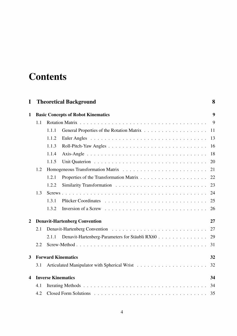
Contents
I Theoretical Background 8
1 Basic Concepts of Robot Kinematics 9
1.1 Rotation Matrix . . . . . . . . . . . . . . . . . . . . . . . . . . . . . . . . . . . . 9
1.1.1 General Properties of the Rotation Matrix . . . . . . . . . . . . . . . . . . 11
1.1.2 Euler Angles . . . . . . . . . . . . . . . . . . . . . . . . . . . . . . . . . 13
1.1.3 Roll-Pitch-Yaw Angles . . . . . . . . . . . . . . . . . . . . . . . . . . . . 16
1.1.4 Axis-Angle . . . . . . . . . . . . . . . . . . . . . . . . . . . . . . . . . . 18
1.1.5 Unit Quaterion . . . . . . . . . . . . . . . . . . . . . . . . . . . . . . . . 20
1.2 Homogeneous Transformation Matrix . . . . . . . . . . . . . . . . . . . . . . . . 21
1.2.1 Properties of the Transformation Matrix . . . . . . . . . . . . . . . . . . . 22
1.2.2 Similarity Transformation . . . . . . . . . . . . . . . . . . . . . . . . . . 23
1.3 Screws . . . . . . . . . . . . . . . . . . . . . . . . . . . . . . . . . . . . . . . . . 24
1.3.1 Plucker Coordinates . . . . . . . . . . . . . . . . . . . . . . . . . . . . . 25
1.3.2 Inversion of a Screw . . . . . . . . . . . . . . . . . . . . . . . . . . . . . 26
2 Denavit-Hartenberg Convention 27
2.1 Denavit-Hartenberg Convention . . . . . . . . . . . . . . . . . . . . . . . . . . . 27
2.1.1 Denavit-Hartenberg-Parameters for Staubli RX60 . . . . . . . . . . . . . . 29
2.2 Screw-Method . . . . . . . . . . . . . . . . . . . . . . . . . . . . . . . . . . . . . 31
3 Forward Kinematics 32
3.1 Articulated Manipulator with Spherical Wrist . . . . . . . . . . . . . . . . . . . . 32
4 Inverse Kinematics 34
4.1 Iterating Methods . . . . . . . . . . . . . . . . . . . . . . . . . . . . . . . . . . . 34
4.2 Closed Form Solutions . . . . . . . . . . . . . . . . . . . . . . . . . . . . . . . . 35
4
CONTENTS 5
4.2.1 Kinematic Decoupling . . . . . . . . . . . . . . . . . . . . . . . . . . . . 35
4.2.2 Geometric Approach . . . . . . . . . . . . . . . . . . . . . . . . . . . . . 35
4.2.3 Algebraic Approach . . . . . . . . . . . . . . . . . . . . . . . . . . . . . 38
4.2.4 Orientation . . . . . . . . . . . . . . . . . . . . . . . . . . . . . . . . . . 40
II Engineering Process 42
5 Development of the Software Concept 43
5.1 B&R Robotic Project . . . . . . . . . . . . . . . . . . . . . . . . . . . . . . . . . 43
5.1.1 Important Robot Specific NC Commands . . . . . . . . . . . . . . . . . . 43
5.2 B&R MATLAB via OPC . . . . . . . . . . . . . . . . . . . . . . . . . . . . . . . 47
5.3 B&R MATLAB via UDP . . . . . . . . . . . . . . . . . . . . . . . . . . . . . . . 47
5.4 B&R Motion Sample . . . . . . . . . . . . . . . . . . . . . . . . . . . . . . . . . 48
5.4.1 Cyclic Velocity Function Block . . . . . . . . . . . . . . . . . . . . . . . 48
5.4.2 Cyclic Position Function Block . . . . . . . . . . . . . . . . . . . . . . . 49
6 Design and Assembly of the Controller Hardware 50
6.1 Main Components . . . . . . . . . . . . . . . . . . . . . . . . . . . . . . . . . . . 50
6.2 Industrial PC APC810 . . . . . . . . . . . . . . . . . . . . . . . . . . . . . . . . 52
6.3 Safety PLC . . . . . . . . . . . . . . . . . . . . . . . . . . . . . . . . . . . . . . 53
6.4 Estimation of the Gear Ratio . . . . . . . . . . . . . . . . . . . . . . . . . . . . . 53
7 Programming of the Axis Controller 55
7.1 Single Axis Task . . . . . . . . . . . . . . . . . . . . . . . . . . . . . . . . . . . 55
7.2 Robot Control Task . . . . . . . . . . . . . . . . . . . . . . . . . . . . . . . . . . 55
7.3 Interpolation Concept . . . . . . . . . . . . . . . . . . . . . . . . . . . . . . . . . 58
7.4 Programming of the Safety PLC . . . . . . . . . . . . . . . . . . . . . . . . . . . 59
8 Implementation of Robot Kinematics 61
8.1 Implementation . . . . . . . . . . . . . . . . . . . . . . . . . . . . . . . . . . . . 61
8.1.1 Inverse Kinematics . . . . . . . . . . . . . . . . . . . . . . . . . . . . . . 61
8.1.2 Border Handling . . . . . . . . . . . . . . . . . . . . . . . . . . . . . . . 64
8.1.3 Implementation in MATLAB . . . . . . . . . . . . . . . . . . . . . . . . . 66
8.1.4 Implementation in Simulink . . . . . . . . . . . . . . . . . . . . . . . . . 67
CONTENTS 6
8.1.5 Test of the Kinematics . . . . . . . . . . . . . . . . . . . . . . . . . . . . 68
9 Conclusion and Future Work 69
A Source Code 70
A.1 Kinematics Test in MATLAB . . . . . . . . . . . . . . . . . . . . . . . . . . . . 70
A.2 Kinematics Test in Simulink . . . . . . . . . . . . . . . . . . . . . . . . . . . . . 73
A.3 Kinematics of the Staubli RX60 . . . . . . . . . . . . . . . . . . . . . . . . . . . 74
A.4 Statediagram of the RobotControl Task . . . . . . . . . . . . . . . . . . . . . . . . 84

CONTENTS 7
Introduction
The field of robotic conquers more and more parts of daily life. Although, robots are capable
of much more than pick and place tasks, they are primary used for such tasks. Most standard
robot controllers are therefore optimized for pick and place tasks. This leads to a limitation of
the applicability of robots in research. Most robot manufacturers also provide more advanced
controllers, but they cost twice as much as a standard robot. Due to this high cost and the fact, that
the mechanic system of the robots has hardly advanced in the last ten years, it was decided to build
a new controller for an already existing six degree of freedom serial robot. There are three main
issues, to be dealt with. The first one is the hardware components and their compatibility with the
motors and encoders of the existing robot arm. The second issue is the control software and the
different methods to control the six axes. The last issue is the mathematically complex kinematics
and the ways to use it. The main components of the hardware were supplied by Bernecker & Rainer
(B&R). They consist of six frequency converters to power the motors and a standard industrial PC,
which controls the whole system. Also necessary is a transformer to reduce the output voltage of
the inverter and make it compatible with the motors. In order to control the robot two different
types of control software are used. The first one is a standard robot control software from B&R.
The intention for this is to maintain the compatibility with industrial standards. The second control
software is a self developed control software. In this particular control software the kinematics is
excluded and implemented on a remote pc with more computation power instead. Both programs
use the UDP to communicate with each other. The kinematics itself was implemented in MATLAB
and Simulink, which allows a rapid prototyping of new kinematic concepts or the easy use of
machine vision.
Part I
Theoretical Background
8
Chapter 1
Basic Concepts of Robot Kinematics
The intention of this chapter is to give an overview of the elementary concepts of robot kinematic.
The first section explains how a rotation in three dimensional space can be formulated as a rota-
tion matrix and outlines its special properties. The next sections gives a summary of methods to
describe a rotation matrix such as Euler angles, Roll-Pitch-Yaw angles, Axis-Angle concept and
quaterions. The last two are a different description of the same kinematic concept. The last two
sections introduce homogeneous coordinates and the screw concept.
1.1 Rotation Matrix
Points are simply describable in three-dimensional space. In contrast, the description of a body’s
orientation in three-dimensional space is a complex task. For this purpose, a frame Σuvw of three
orthogonal unit vectors u,v,w is attached to the body. The frame and its origin indicates the
orientation and the position of the body. This frame acts as a local coordinate system. [15, p24-
p25] [16, p38-p47] [3, p21-p23]
This local frame Σuvw describes the rotation of a body or point from a previous frame Σxyz into a
new frame, when both frames share the same origin.
Position vector p of point P in Σxyz:
p =
⎡⎣pxpypz
⎤⎦ , (1.1)
Position vector p of point P in Σuvw:
p =
⎡⎣pupvpw
⎤⎦ . (1.2)
9
CHAPTER 1. BASIC CONCEPTS OF ROBOT KINEMATICS 10
x y
z
u
v
w�
�p
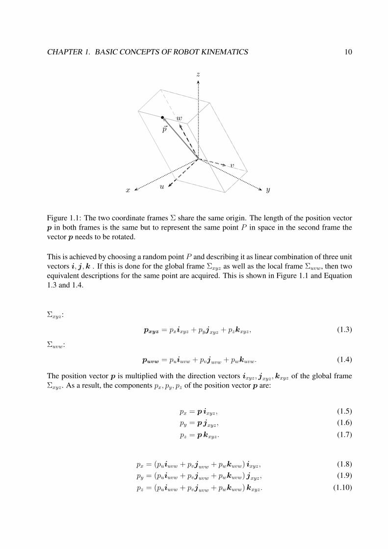
Figure 1.1: The two coordinate frames Σ share the same origin. The length of the position vector
p in both frames is the same but to represent the same point P in space in the second frame the
vector p needs to be rotated.
This is achieved by choosing a random point P and describing it as linear combination of three unit
vectors i, j,k . If this is done for the global frame Σxyz as well as the local frame Σuvw, then two
equivalent descriptions for the same point are acquired. This is shown in Figure 1.1 and Equation
1.3 and 1.4.
Σxyz:
pxyz = pxixyz + pyjxyz + pzkxyz, (1.3)
Σuvw:
puvw = puiuvw + pvjuvw + pwkuvw. (1.4)
The position vector p is multiplied with the direction vectors ixyz, jxyz,kxyz of the global frame
Σxyz. As a result, the components px, py, pz of the position vector p are:
px = p ixyz, (1.5)
py = p jxyz, (1.6)
pz = pkxyz. (1.7)
px = (puiuvw + pvjuvw + pwkuvw) ixyz, (1.8)
py = (puiuvw + pvjuvw + pwkuvw) jxyz, (1.9)
pz = (puiuvw + pvjuvw + pwkuvw)kxyz. (1.10)

CHAPTER 1. BASIC CONCEPTS OF ROBOT KINEMATICS 11
In concise matrix form,⎡⎣pxpypz
⎤⎦
︸ ︷︷ ︸pxyz
=
⎡⎣iuvwixyz juvxixyz kuvwixyziuvwjxyz juvxjxyz kuvwjxyziuvwkxyz juvxkxyz kuvwkxyz
⎤⎦
︸ ︷︷ ︸R
⎡⎣pupvpw
⎤⎦
︸ ︷︷ ︸puvw
. (1.11)
Rearranging the variables as shown in Equation 1.11 simplifies the operation to a simple matrix
transformation. The rotation matrix R describes the rotation of the local frame Σuvw in reference
to the global frame Σxyz. The relation ab = |a||b| cos(ϕ) is used to substitute the scalar product
with the cosine function. This is shown in Figure 1.2, for a rotation about the z-axis.
Rz(ϕ) =
⎡⎣ cos(ϕ) cos(90 + ϕ) 0cos(90− ϕ) cos(ϕ) 0
0 0 1
⎤⎦ . (1.12)
The previous rotation matrix is simplified by using the trigonometric identity sin(ϕ) = cos(90−ϕ)and − sin(ϕ) = cos(90 + ϕ).
Rz(ϕ) =
⎡⎣cos(ϕ) − sin(ϕ) 0sin(ϕ) cos(ϕ) 0
0 0 1
⎤⎦ , (1.13)
Rx(ϕ) =
⎡⎣1 0 00 cos(ϕ) − sin(ϕ)0 sin(ϕ) cos(ϕ)
⎤⎦ , (1.14)
Ry(ϕ) =
⎡⎣cos(ϕ) 0 − sin(ϕ)
0 1 0sin(ϕ) 0 cos(ϕ)
⎤⎦ . (1.15)
By switching the vectors p, ixyz, jxyz,kxyz, inversion of the rotation matrix is achieved.
⎡⎣pupvpw
⎤⎦
︸ ︷︷ ︸puvw
=
⎡⎣iuvwixyz iuvxjxyz iuvwkxyz
juvwixyz juvxjxyz juvwkxyz
kuvwixyz kuvxjxyz kuvwkxyz
⎤⎦
︸ ︷︷ ︸R-1
⎡⎣pxpypz
⎤⎦
︸ ︷︷ ︸pxyz
. (1.16)
1.1.1 General Properties of the Rotation Matrix
The rotation matrix is an orthogonal matrix RTR = I 1 and the properties are displayed in Equation
1.17 and Equation 1.18. Most of this properties are inherited from the cosine function,
1in this case also orthonormal
CHAPTER 1. BASIC CONCEPTS OF ROBOT KINEMATICS 12
x y
z
u
v
w
ϕ
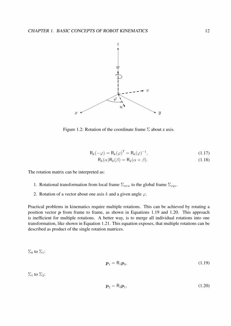
Figure 1.2: Rotation of the coordinate frame Σ about z axis.
Rk(−ϕ) = Rk(ϕ)T = Rk(ϕ)
−1, (1.17)
Rk(α)Rk(β) = Rk(α + β). (1.18)
The rotation matrix can be interpreted as:
1. Rotational transformation from local frame Σuvw to the global frame Σxyz.
2. Rotation of a vector about one axis k and a given angle ϕ.
Practical problems in kinematics require multiple rotations. This can be achieved by rotating a
position vector p from frame to frame, as shown in Equations 1.19 and 1.20. This approach
is inefficient for multiple rotations. A better way, is to merge all individual rotations into one
transformation, like shown in Equation 1.21. This equation exposes, that multiple rotations can be
described as product of the single rotation matrices.
Σ0 to Σ1:
p1 = R1p0, (1.19)
Σ1 to Σ2:
p2 = R2p1, (1.20)
CHAPTER 1. BASIC CONCEPTS OF ROBOT KINEMATICS 13
Σ0 to Σ2:
p2 = R2R1p0. (1.21)
Matrix multiplication is not commutative. For this reason, it has to be distinguished between
the matrix multiplication from left the pre-multiplication and the matrix multiplication from left
the post-multiplication. In many cases these two can only be distinguished by the indices of the
matrices or in case of the rotation matrix, by the order of the angles. For the rotation matrix these
two types of matrix multiplication have the following meaning: [15, p25-p30] [16, p49-p52]
pre-multiplication: local frame Σuvw rotates about the fixed global frame Σxyz,
post-multiplication: local frame Σuvw rotates about its principal axis.
1.1.2 Euler Angles
The Euler angles describe a rotation about the axes of three local frames. The sequence of the
rotations is important. Euler angles are commonly used to describe the orientation of a body in
space. Euler angles have the advantage, that there is no conversion to the actuating angle of the
drives necessary. This is possible because the actuating angle of the drive is measured between
stator and rotor, which is also the angle between the joints, where they are fixed. This is similar to
the Euler angle, which is measured between two frames.
Euler Angles ZYX Order
Figure 1.3 shows a rotation in ZYX order. The grey body shows the result of the previous rotation
and the black one the result of the actual one. Equation 1.22 displays the order of the single
rotations and Equation 1.23 shows the result of the multiplication. In Equation 1.23 the cosine and
sine function are substituted by cosα � cα and sinα � sα to improve the readability.
R = Rz(α)Rv1(β)Ru2(γ), (1.22)
R =
⎡⎣cαcβ cαsβcγ − sαcγ cαsβcγ + sαsγsαcβ sαsβsγ + cαcγ sαsβcγ − cαsγ−sβ cβsγ cβcγ
⎤⎦ . (1.23)
Inversion for ZXY Order
The rotation matrix is known for most orientation problems in kinematics . The rotations param-
eters are of interest. In case of the Euler-Angles are these the three angles α, β, γ for the known
rotation order, here ZYX. These angles are extracted from the rotation matrix, like in Equation
1.23, for the particular rotation order. This is done by searching for suitable entries and calculating

CHAPTER 1. BASIC CONCEPTS OF ROBOT KINEMATICS 14
x y
z
u1
v1
w1
(a) Rotation about Z-axis
x y
z
u1
v1
w1
(b) Rotation about Y-axis
x y
z
u1
v1
w1
(c) Rotation about X-axis
Figure 1.3: The figure shows the three single rotations of the Euler angle. It can be seen, that all
rotations are relative rotations.
CHAPTER 1. BASIC CONCEPTS OF ROBOT KINEMATICS 15
the inverse tangent for each angle with the entries. All entries are suitable where the term with
the second angle can be eliminated by division or the trigonometric identity 1 = sinα2 + cosα2.
Instead of the normal inverse tangent function the inverse tangent-two function is used to avoid
problems with the sign. The inverse tangent-two requires two parameters α = atan2(x, y). This
parameters are x � sinα and y � cosα.
R =
⎡⎣r11 r12 r13r21 r22 r23r31 r32 r33
⎤⎦ . (1.24)
There are two sets of inversion formulas for the Euler-angles. The reason for this are inverse
function of the trigonometric functions, which deliver two results for one input value 2.
π2, −π
2:
β = atan2(−r31,√r211 + r221), (1.25)
α = atan2(r21, r11), (1.26)
γ = atan2(r32, r33). (1.27)
π2, 3π
2:
β = atan2(−r31,−√r211 + r221), (1.28)
α = atan2(−r21,−r11), (1.29)
γ = atan2(−r32,−r33). (1.30)
Euler Angles ZYZ Order
Many robots, which have a spherical wrist, use a ZYZ order for the wrist axes. The purpose for
this are design and manufacturing advantages. For this reason the ZYZ order is more important
than the previous introduced ZYX order.
R(φ) = Rz(γ)Rv1(β)Rw2(α), (1.31)
R =
⎡⎣cγcβcα− sγsα −cγcβsα− sγcα cγsβsγcβcα− cγsα −sγcβsα + cγcα sγsβ
−sβcα sβsα cβ
⎤⎦ . (1.32)
2There would be more results but for the solution only the interval [0, 2π] is of interest.
CHAPTER 1. BASIC CONCEPTS OF ROBOT KINEMATICS 16
Inversion for ZYZ Order
The inversion problem for the ZYZ order is solved as shown for the XYZ order. Only the entries
from the rotation matrix change. [16, p53-p56] [3, p48-p50] [15, p53-p56]
0, π:
β = atan2(√
r213 + r223, r33), (1.33)
α = atan2(r32,−r31), (1.34)
γ = atan2(r23, r13). (1.35)
−π, 0:
β = atan2(−√
r213 + r223, r33), (1.36)
α = atan2(−r32,−r31), (1.37)
γ = atan2(−r23, r13). (1.38)
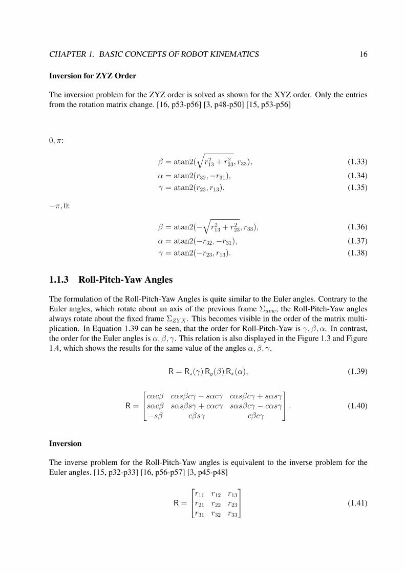
1.1.3 Roll-Pitch-Yaw Angles
The formulation of the Roll-Pitch-Yaw Angles is quite similar to the Euler angles. Contrary to the
Euler angles, which rotate about an axis of the previous frame Σuvw, the Roll-Pitch-Yaw angles
always rotate about the fixed frame ΣZY X . This becomes visible in the order of the matrix multi-
plication. In Equation 1.39 can be seen, that the order for Roll-Pitch-Yaw is γ, β, α. In contrast,
the order for the Euler angles is α, β, γ. This relation is also displayed in the Figure 1.3 and Figure
1.4, which shows the results for the same value of the angles α, β, γ.
R = Rz(γ)Ry(β)Rx(α), (1.39)
R =
⎡⎣cαcβ cαsβcγ − sαcγ cαsβcγ + sαsγsαcβ sαsβsγ + cαcγ sαsβcγ − cαsγ−sβ cβsγ cβcγ
⎤⎦ . (1.40)
Inversion
The inverse problem for the Roll-Pitch-Yaw angles is equivalent to the inverse problem for the
Euler angles. [15, p32-p33] [16, p56-p57] [3, p45-p48]
R =
⎡⎣r11 r12 r13r21 r22 r23r31 r32 r33
⎤⎦ (1.41)

CHAPTER 1. BASIC CONCEPTS OF ROBOT KINEMATICS 17
x y
z
u1
v1
w1
(a) Rotation about X-axis
x y
z
u2
v2
w2
(b) Rotation about Y-axis
x y
z
u3
v3
w3
(c) Rotation about Z-axis
Figure 1.4: This figure shows the three single rotations of Roll-Pitch-Yaw. It can be seen, that all
these rotation are absolute rotations (compare with Figure 1.3).
CHAPTER 1. BASIC CONCEPTS OF ROBOT KINEMATICS 18
x y
z
u1
v1
w1
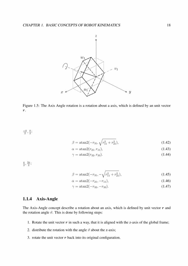
Figure 1.5: The Axis Angle rotation is a rotation about a axis, which is defined by an unit vector
r.
−π2, π2:
β = atan2(−r31,√r211 + r221), (1.42)
α = atan2(r21, r11), (1.43)
γ = atan2(r32, r33). (1.44)
π2, 3π
2:
β = atan2(−r31,−√r211 + r221), (1.45)
α = atan2(−r21,−r11), (1.46)
γ = atan2(−r32,−r33). (1.47)
1.1.4 Axis-Angle
The Axis-Angle concept describe a rotation about an axis, which is defined by unit vector r and
the rotation angle ϑ. This is done by following steps:
1. Rotate the unit vector r in such a way, that it is aligned with the z-axis of the global frame;
2. distribute the rotation with the angle ϑ about the z-axis;
3. rotate the unit vector r back into its original configuration.
CHAPTER 1. BASIC CONCEPTS OF ROBOT KINEMATICS 19
x y
z
�
α
β
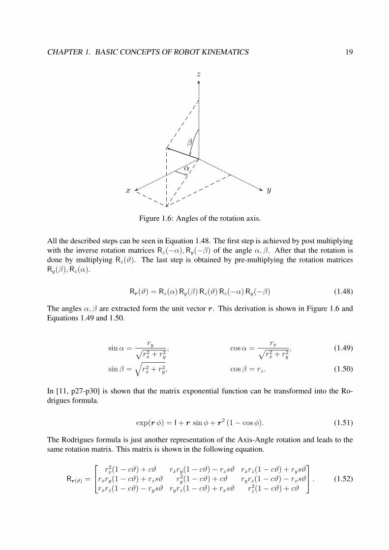
Figure 1.6: Angles of the rotation axis.
All the described steps can be seen in Equation 1.48. The first step is achieved by post multiplying
with the inverse rotation matrices Rz(−α),Ry(−β) of the angle α, β. After that the rotation is
done by multiplying Rz(ϑ). The last step is obtained by pre-multiplying the rotation matrices
Ry(β),Rz(α).
Rr(ϑ) = Rz(α)Ry(β)Rz(ϑ)Rz(−α)Ry(−β) (1.48)
The angles α, β are extracted form the unit vector r. This derivation is shown in Figure 1.6 and
Equations 1.49 and 1.50.
sinα =ry√
r2x + r2y, cosα =
rx√r2x + r2y
, (1.49)
sin β =√
r2x + r2y, cos β = rz. (1.50)
In [11, p27-p30] is shown that the matrix exponential function can be transformed into the Ro-
drigues formula.
exp(r φ) = I+ r sinφ+ r2 (1− cosφ). (1.51)
The Rodrigues formula is just another representation of the Axis-Angle rotation and leads to the
same rotation matrix. This matrix is shown in the following equation.
Rr(ϑ) =
⎡⎣ r2x(1− cϑ) + cϑ rxry(1− cϑ)− rzsϑ rxrz(1− cϑ) + rysϑrxry(1− cϑ) + rzsϑ r2y(1− cϑ) + cϑ ryrz(1− cϑ)− rxsϑrxrz(1− cϑ)− rysϑ ryrz(1− cϑ) + rxsϑ r2z(1− cϑ) + cϑ
⎤⎦ . (1.52)

CHAPTER 1. BASIC CONCEPTS OF ROBOT KINEMATICS 20
R−r(−ϑ) = Rr(ϑ). (1.53)
Inversion
The inversion for axis angles uses the known entries of the rotation matrix R to calculate the axis
r and the rotation angle ϑ. The equations for axis r and the rotation angle ϑ can be derived by
comparing the entries of the rotation matrix R with the entries of the generalized rotation matrix
Rr(ϑ) from Equation 1.52. [3, p51-p55] [15, p33-p35] [16, p52-p59]
R =
⎡⎣r11 r12 r13r21 r22 r23r31 r32 r33
⎤⎦ , (1.54)
ϑ = cos−1(r11 + r22 + r33 − 1
2), (1.55)
r =1
2 sinϑ
⎡⎣r32 − r23r13 − r31r21 − r12
⎤⎦ . (1.56)
1.1.5 Unit Quaterion
Quaterion can be explained as expansion of complex numbers for the three-dimensional space. A
quaterion consists of a scalar η and a vector ε. The square sum of a quaterion η2 + ε2x + ε2y + ε2z =1 equals one, which is the reason why it is called Unit Quaterion. In some applications, such
as interpolation or calculation of multiple rotations, the quaterion notation preferred because the
quaterions need less computation time than the equivalent matrix notation [17, p512]. Therefore,
they are also used to describe robot kinematics [13].
η = cosϑ
2, (1.57)
ε = sinϑ
2r. (1.58)
The vector r defines the rotation axis and ϑ the rotation angle. Quaterion rotations are equivalent
to the Axis-Angle rotations and rotations performed by matrix exponential function.
R =
⎡⎣2(η
2 + ε2x)− 1 2(εxεy − ηεz) 2(εxεz − ηεy)2(εxεy − ηεz) 2(η2 + ε2y)− 1 2(εyεz − ηεx)2(εxεz − ηεy) 2(εyεz − ηεx) 2(η2 + ε2z)− 1
⎤⎦ . (1.59)

CHAPTER 1. BASIC CONCEPTS OF ROBOT KINEMATICS 21
Inversion
The inversion of the quaterions is similar to the axis-angle inversion and can be derived the same
way. [11, 33-34] [3, p55-p56] [15, p35-p37] [4]
η =1
2
√r211 + r222 + r233 + 1, (1.60)
ε =1
2
⎡⎣sgn(r32 − r23)
√r211 − r222 − r233 + 1
sgn(r13 − r31)√r222 − r233 − r211 + 1
sgn(r21 − r12)√r233 − r211 − r222 + 1
⎤⎦ . (1.61)
1.2 Homogeneous Transformation Matrix
Every movement in three dimensional space can be described with a translation d and a rotation
R. Usually this is done by the vector equation 1.62. This form of a transformation is only suitable
for small systems or manual calculations. To simplify the calculation, one dimension is added by
using homogeneous coordinates, which enables a matrix form of the equation. The resulting 4× 4matrix is called homogeneous transformation matrix A.
p1 = d+ R10 p0, (1.62)
[1p1
]=
[1 0T
d R10
] [1p0
], (1.63)
A =
[1 0T
d R1
]. (1.64)
The transformation matrix can be separated in following parts:
A =
[scale factor perspective transformation
position vector rotation matrix
].
The position of the entries varies in literature. In this thesis the European convention is used as
shown in the previous equation. In most of the literature the American convention is used, which
looks as follows:
A =
[rotation matrix position vector
perspective transformation scale factor
].

CHAPTER 1. BASIC CONCEPTS OF ROBOT KINEMATICS 22
x y
z
�
u
v
w
�O
d
Figure 1.7: The homogeneous coordinates can be interpreted a coordinate frame, where the vector
d defines the origin and the unit vectors u,v,w the coordinate axes.
1.2.1 Properties of the Transformation Matrix
The transformation matrix is quite similar to the rotation matrix, which sometimes leads to a mix-
up. Contrary to the Rotation Matrix, the inverse of transformation matrix T can ’t be achieved by
transposing the matrix.
A−1 �= AT. (1.65)
A fast way to achieve the inverse of the transformation matrix is to use its structure, like Equation
1.66 shows. This equation can be interpreted as rotation R10
Tin the opposite direction and a linear
movement −R10
Td also in the opposite direction.
A−1 =
[1 0
−R10
Td R1
0T
](1.66)
The indices on the bottom of the transformation matrix A20 indicates the start frame Σ0 and the
indices on the top the end frame Σ2 of the transformation [15, p37-p39] [12, p45-p54] [3, p29-
p31] [16, p60-p63].
A20 = A1 A2 =
[1 0T
p1 R1
] [1 0T
p2 R2
], (1.67)
A20 = A1 A2 =
[1 0T
R1p1 + p1 R1R2
]. (1.68)
1. The homogeneous transformation matrix A moves and rotates a point from a local frame
Σuvw to the global frame ΣZY X ;

CHAPTER 1. BASIC CONCEPTS OF ROBOT KINEMATICS 23
Figure 1.8: The similarity transformation can be represented as vector addition of the position
vector of the origins and rotations of the frames.
2. The homogeneous transformation matrix A moves and rotates vectors;
3. The homogeneous transformation matrix A describes position and orientation of an object in
three-dimensional space;
4. The homogeneous transformation matrix A represents a frame, which was moved and ro-
tated.
pre-multiplication: Manipulates a local frame Σuvw about principal axis of the global frame Σxyz
post-multiplication: Manipulates a local frame Σuvw about principal axis of the previous local
frame
1.2.2 Similarity Transformation
The Similarity Transformation is used to shift between the coordinate systems. This is shown in
Figure 1.8 [3, p99-p103].
AToolGlobal = AGlobal
Basis
−1AEndefBasis A
ToolEndef (1.69)
It gets applied for following tasks:
1. Describe the tool frame in reference to other frames such as the global frame,

CHAPTER 1. BASIC CONCEPTS OF ROBOT KINEMATICS 24
x y
z
�
r
ϕ
p · (ϕ+ 2π)
Figure 1.9: Graphical representation of a screw motion of a point.
2. describe local coordinates in the global frame;
3. describe the origin of camera frames in reference to other frames.
1.3 Screws
Another way to describe kinematic transformations in three-dimensional space is the screw [8,
p303] [7]. An advantage of the screw is that it is possible to describe rotation and linear movements
at the same time. Equation 1.70 shows the equation for a screw in parameter form, where p stands
for the pitch and r for the radius.
x(t) =
⎡⎣r cosϕ(t)r sinϕ(t)
pϕ(t)
⎤⎦ , (1.70)
x(t) =
⎡⎣ 0
0pϕ(t)
⎤⎦+
⎡⎣cosϕ(t) sinϕ(t) 0sinϕ(t) cosϕ(t) 0
0 0 1
⎤⎦⎡⎣r00
⎤⎦ . (1.71)
The screw equation is transformed into a homogeneous transformation matrix, which allows the
usage of the homogeneous transformation properties and an easier calculation in matrix form.
Ascrew =
[1 0T
ϕ(t)2π
pd Rd(ϕ(t))
](1.72)

CHAPTER 1. BASIC CONCEPTS OF ROBOT KINEMATICS 25
x y
z
a
q
d
Figure 1.10: This figure shows a graphical interpretation of the Plucker-coordinates of a screw. It
can be seen, that the unit vector d represents the screw axis and the vector a the distance of the
footpoint.
1.3.1 Plucker Coordinates
Usually the screw axis isn’t placed in the origin of the coordinate system nor is it congruent with
the principal axis. To overcome this problem, a similarity transformation is performed on the
original screw.
A′screw = NAN−1, (1.73)
A′screw =
[1 0T
a I
] [1 0T
ϕ(t)2π
pd Rd(ϕ(t))
] [1 0T
−a I
], (1.74)
A′screw =
[1 0T
ϕ(t)2π
pd+ (I− Rd(ϕ(t)))a Rd(ϕ(t))
]. (1.75)
The vector q is the crossproduct of the position vector a and the direction vector d of the screw
axis. The vector q and the direction vector d are combined to the so called Plucker coordinates
[d, q]. This coordinates frequently appear in calculation of velocities and static torques.
q = a× d (1.76)
CHAPTER 1. BASIC CONCEPTS OF ROBOT KINEMATICS 26
1.3.2 Inversion of a Screw
In many cases in practical work is the inversion of the screw needed. The inversion starts with a
comparison of the entries t and R of A with the entries from the screw matrix A′screw.The first step
is to get the rotation angles ϕ and the rotation axis d from the rotation matrix Rd, the inversion of
Axis-Angle rotation is used.
A =
[1 0T
t R
]. (1.77)
t =ϕ
2πpd+ (I− Rd)a, (1.78)
d (I− Rd)a = d (t− ϕ
2πpd), (1.79)
Rd d = d this is caused by the fact that d is the rotation axis and rotation axes are never effected
by the rotation. To enable a further simplification; the position vector a has to be chosen that way
that it is orthogonal to the direction vector d, which leads to: da = 0. This means also that Rd aand d are orthogonal.
0 = d (t− ϕ
2πpd), (1.80)
t =ϕ
2πpd, (1.81)
p =2π
ϕ(d t). (1.82)

Chapter 2
Denavit-Hartenberg Convention
This chapter introduces two methods for a systematic description for an open kinematic chain. A
kinematic chain is a mechanical structure, where every joint is connected to the next by a variable
link. The first method is the Denavit-Hartenberg convention, which can be found in literature. The
second method is the screw method, which is based on screws.
2.1 Denavit-Hartenberg Convention
The Denavit-Hartenberg convention is one of the most simple methods to describe a kinematic
chain. This method only needs four scalar parameters to describe a joint. One of these parameters
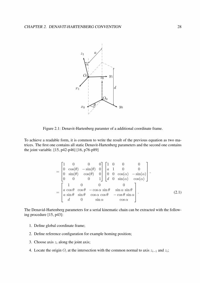
varies with the joint motion. This parameter is called joint variable and is usually the parameter dfor prismatic joints or for revolute joints the parameter θ. The four parameter have the following
meanings:
di . . . Coordinate of origin Oi along the z axis zi−1 of the previous frame,
ai . . . Distance between origin Oi and origin Oi−1,
αi . . . Angle between axis zi−1 and axis zi about the axis xi,
θi . . . Angle between axis xi−1 and axis xi about the axis zi−1.
These four parameter describe how a coordinate frame Σ has to be rotated and moved to achieve
the next frame. Figure 2.1 shows a graphical representation of the parameters. This is done by
matrix multiplication and is shown in the following Equation.
A =
[1 0T
0 Rx(α)
] [1 0T
d I
] [1 0T
a I
] [1 0T
0 Rz(θ)
],
=
⎡⎢⎢⎣1 0 0 00 1 0 00 0 cos(α) − sin(α)0 0 sin(α) cos(α)
⎤⎥⎥⎦⎡⎢⎢⎣1 0 0 00 1 0 00 0 1 0d 0 0 1
⎤⎥⎥⎦⎡⎢⎢⎣1 0 0 0a 1 0 00 0 1 00 0 0 1
⎤⎥⎥⎦⎡⎢⎢⎣1 0 0 00 cos(θ) − sin(θ) 00 sin(θ) cos(θ) 00 0 0 1
⎤⎥⎥⎦ ,
27
CHAPTER 2. DENAVIT-HARTENBERG CONVENTION 28
x0 y0
z0
�O0
x1
y1
z1
�O1
θ
α
d
a
Figure 2.1: Denavit-Hartenberg paramter of a additional coordinate frame.
To achieve a readable form, it is common to write the result of the previous equation as two ma-
trices. The first one contains all static Denavit-Hartenberg parameters and the second one contains
the joint variable. [15, p42-p46] [16, p76-p89]
=
⎡⎢⎢⎣1 0 0 00 cos(θ) − sin(θ) 00 sin(θ) cos(θ) 00 0 0 1
⎤⎥⎥⎦⎡⎢⎢⎣1 0 0 0a 1 0 00 0 cos(α) − sin(α)d 0 sin(α) cos(α)
⎤⎥⎥⎦ ,
=
⎡⎢⎢⎣
1 0 0 0a cos θ cos θ − cosα sin θ sinα sin θa sin θ sin θ cosα cos θ − cos θ sinα
d 0 sinα cosα
⎤⎥⎥⎦ . (2.1)
The Denavid-Hartenberg parameters for a serial kinematic chain can be extracted with the follow-
ing procedure [15, p43]:
1. Define global coordinate frame;
2. Define reference configuration for example homing position;
3. Choose axis zi along the joint axis;
4. Locate the origin Oi at the intersection with the common normal to axis zi−1 and zi;
CHAPTER 2. DENAVIT-HARTENBERG CONVENTION 29
5. Choose xi along the common normal to axis zi with direction to joint i+ 1;
6. Choose yi to complete the right-handed frame;
7. Determine homogeneous transformation for the joint.
There are some cases, where the rules of this convention aren’t clearly defined. This exceptions
are shown in the following list:
1. Two consecutive axes are parallel −→ origin Oi can be freely chosen;
2. Two consecutive axes are intersect −→ axis xi is arbitrary;
3. Joint i is prismatic −→ direction of axis zi−1 is arbitrary;
4. In frame 0 only z0 is specified −→ origin O0 and axis x0 can be freely choose;
5. Last frame n zn is not uniquely defined while xn is normal to zn−1.
In order to reduce the complexity of the calculation, it is intended to reduce the number of the
non-zero Denavit-Hartenberg parameters. A possible way is to select the free-settable parameter
in a way, that most of the following parameters get zero.
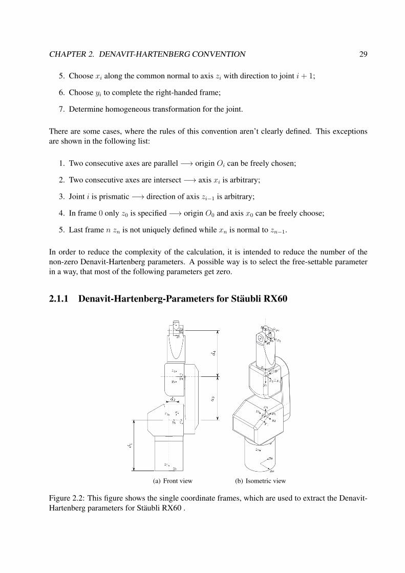
2.1.1 Denavit-Hartenberg-Parameters for Staubli RX60
(a) Front view (b) Isometric view
Figure 2.2: This figure shows the single coordinate frames, which are used to extract the Denavit-
Hartenberg parameters for Staubli RX60 .

CHAPTER 2. DENAVIT-HARTENBERG CONVENTION 30
The search of the Denavit-Hartenberg parameter is started with the definition of the initial frame
Σ0.
Σ0toΣ1: Frame Σ1 by shifting the origin of frame Σ0 along the z-axis to the intersection of the
first two axes. The distance d1, which the frame Σ0 was shifted, is the first parameter.
A1 =
⎡⎢⎢⎣1 0 0 00 cos θ1 − sin θ1 00 sin θ1 cos θ1 0d1 0 0 1
⎤⎥⎥⎦ . (2.2)
Σ1toΣ2: In order to enable a transformation according to the Denavit-Hartenberg convention, a
rotation of the frame Σ1 is necessary. The frame Σ1 is rotated α1 about the x-axis and θ1about the z-axis. Afterwards it is shifted about d2 along the z-axis to achieve the frame Σ2.
The distance d2 is free-settable because the axis 2 and axis 3 are parallel.
A2 =
⎡⎢⎢⎣1 0 0 00 sin θ2 cos θ2 0d2 0 0 10 cos θ2 − sin θ2 0
⎤⎥⎥⎦ . (2.3)
Σ2toΣ3: Frame Σ3 is achieved by shifting the frame Σ2 along the x-axis and rotate it θ3 about the
z-axis.
A3 =
⎡⎢⎢⎣1 0 0 0a3 − sin θ3 − cos θ3 00 cos θ3 − sin θ3 00 0 0 1
⎤⎥⎥⎦ . (2.4)
Σ3toΣ4: Frame Σ4 is achieved by rotating frame Σ3 α3 about the x-axis and
A4 =
⎡⎢⎢⎣1 0 0 00 cos θ4 sin θ4 00 0 0 −10 sin θ4 cos θ4 0
⎤⎥⎥⎦ . (2.5)
Σ4toΣ5: frame Σ5 is achieved by translating frame Σ4 d4 along the z-axis and rotate it α5 about
the x-axis.
A5 =
⎡⎢⎢⎣1 0 0 00 cos θ5 − sin θ5 00 0 0 1d4 − sin θ5 − cos θ5 0
⎤⎥⎥⎦ . (2.6)

CHAPTER 2. DENAVIT-HARTENBERG CONVENTION 31
Σ5toΣ6: The last frame Σ6 is calculated by rotating frame Σ5 α6 about the x-axis
A6 =
⎡⎢⎢⎣1 0 0 00 cos θ6 sin θ6 00 0 0 −10 sin θ6 cos θ6 0
⎤⎥⎥⎦ . (2.7)
All these parameters for the Staubli RX60 are given in Table 2.1.
joint di ai αi θi
1 d1 0 0 θ12 d2 0 -90 θ2 − 903 0 a3 0 θ3 + 904 0 0 90 θ45 d5 0 -90 θ56 0 0 90 θ6
Table 2.1: Denavit-Hartenberg-parameters for Staubli RX60 .
The designer of Staubli RX60 chose the geometric parameter in a way, that the kinematic equations
gets as simple as possible.
2.2 Screw-Method
The screw method is an alternative method to the Denavit-Hartenberg convention. The screw pa-
rameters are easier to evaluate than the Denavit-Hartenberg parameters, where a special orientation
of the previous coordinate frame is necessary to achieve the next frame.The screw method is also
more flexible in its usage [14]. This allows less experienced users to describe the kinematics.
The screw parameters are extracted with the following procedure:
1. Choose fixed coordinate system;
2. Define reference configuration for example homing position;
3. Identify screw axis d and distance a for each joint also identify the joint variable;
4. Determine homogeneous transformation matrix for each joint;
The transformation matrix is calculated by the following formula:
A =
[1 0T
ϕ2πtd+ (I− Rd(θ))a Rd(θ)
]. (2.8)
Chapter 3
Forward Kinematics
This chapter introduces the forward kinematics and how it can be achieved using the transformation
matrix of the Denavit-Hartenberg convention or the screw method. The second topic of this chapter
is the forward kinematics for a 6 degree of freedom manipulator with spherical wrist.
The forward kinematic 1 is a mathematical method to calculate the position and orientation of a
kinematic chain from the joint variables. For a better separation T is used instead of A for the
transformation matrix of a kinematic chain.
T60 = A1 A2 A3 A4 A5 A6, (3.1)
T60 = A1
⎡⎢⎢⎣1 0 0 0px nx sx axpy ny sy aypz nz sx az
⎤⎥⎥⎦ . (3.2)
position vector: p =
⎡⎣pxpypz
⎤⎦ , normal vector: n =
⎡⎣nx
ny
nz
⎤⎦ ,
sliding vector: s =
⎡⎣sxsysz
⎤⎦ , approach vector: a =
⎡⎣axayaz
⎤⎦ .
3.1 Articulated Manipulator with Spherical Wrist
This kind of manipulator has a spherical wrist, which is achieved by an intersection of the last three
joint axes. Any movement of the last three joints only changes the orientation of the end effector
but not the position. Now the forward kinematic can be separated in two problems, which is used
as an important simplification for the inverse problem.
1Sometimes the name direct kinematics is used for the forward kinematics.
32
CHAPTER 3. FORWARD KINEMATICS 33
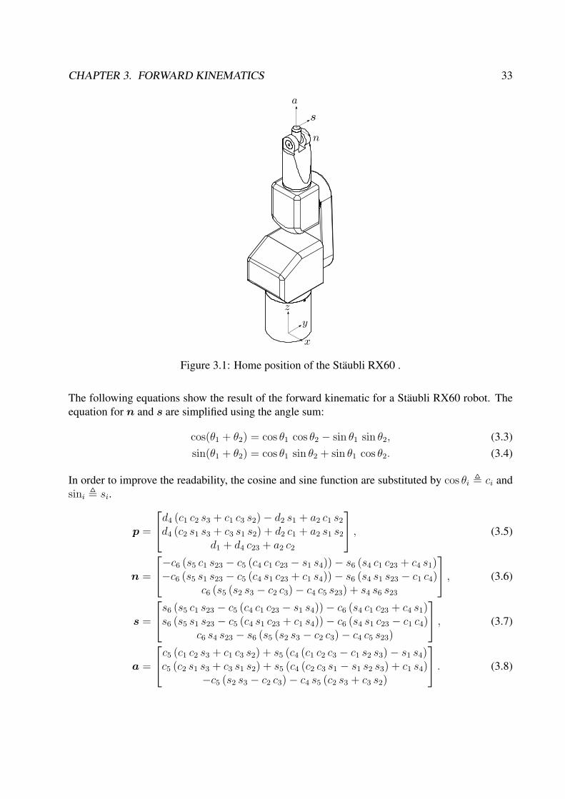
Figure 3.1: Home position of the Staubli RX60 .
The following equations show the result of the forward kinematic for a Staubli RX60 robot. The
equation for n and s are simplified using the angle sum:
cos(θ1 + θ2) = cos θ1 cos θ2 − sin θ1 sin θ2, (3.3)
sin(θ1 + θ2) = cos θ1 sin θ2 + sin θ1 cos θ2. (3.4)
In order to improve the readability, the cosine and sine function are substituted by cos θi � ci and
sini � si.
p =
⎡⎣d4 (c1 c2 s3 + c1 c3 s2)− d2 s1 + a2 c1 s2d4 (c2 s1 s3 + c3 s1 s2) + d2 c1 + a2 s1 s2
d1 + d4 c23 + a2 c2
⎤⎦ , (3.5)
n =
⎡⎣−c6 (s5 c1 s23 − c5 (c4 c1 c23 − s1 s4))− s6 (s4 c1 c23 + c4 s1)−c6 (s5 s1 s23 − c5 (c4 s1 c23 + c1 s4))− s6 (s4 s1 s23 − c1 c4)
c6 (s5 (s2 s3 − c2 c3)− c4 c5 s23) + s4 s6 s23
⎤⎦ , (3.6)
s =
⎡⎣s6 (s5 c1 s23 − c5 (c4 c1 c23 − s1 s4))− c6 (s4 c1 c23 + c4 s1)s6 (s5 s1 s23 − c5 (c4 s1 c23 + c1 s4))− c6 (s4 s1 c23 − c1 c4)
c6 s4 s23 − s6 (s5 (s2 s3 − c2 c3)− c4 c5 s23)
⎤⎦ , (3.7)
a =
⎡⎣c5 (c1 c2 s3 + c1 c3 s2) + s5 (c4 (c1 c2 c3 − c1 s2 s3)− s1 s4)c5 (c2 s1 s3 + c3 s1 s2) + s5 (c4 (c2 c3 s1 − s1 s2 s3) + c1 s4)
−c5 (s2 s3 − c2 c3)− c4 s5 (c2 s3 + c3 s2)
⎤⎦ . (3.8)

Chapter 4
Inverse Kinematics
This chapter presents methods for solution of the inverse kinematics.
Figure 4.1: Overview of solution methods for the inverse kinematics.
4.1 Iterating Methods
Figure 4.1 shows, that there are many different ways to solve the inverse kinematics. The iterating
methods are one of them. One dominant group of the iterating methods are the meta-heuristics.
The advantage of the meta-heuristics are, that the solvability of the inverse kinematics doesn’t de-
pend on the degree of freedom but they only deliver one solution of all possible. The most common
meta-heuristic algorithms for robots are the Artificial Neural Networks [5] [6] [10], the evolution-
ary algorithm [9]. Another group of the iterating algorithms are the Jacobian based methods. These
methods use the inverse of the Jacobian to solve the inverse kinematics. The use of the inverse of
34

CHAPTER 4. INVERSE KINEMATICS 35
the Jacobian is risky, because of the singularity of the Jacobian at special robot configurations, but
there are algorithms, which cope with this problem [15, p104-p110].
4.2 Closed Form Solutions
Closed form solutions for the inverse kinematics are preferred in robotic. This solutions have the
advantage, that their behaviour can be predicted [16, p95]. Another aspect of the closed form
solution is that all possible solutions are calculated and it is possible to choose the most suitable
one. For a general six degree of freedom serial robot there exist sixteen possible solutions [1, p288-
p289] for the inverse kinematics. The number of solutions can be reduced by special arrangement
of the axes. Most of the closed form solutions are only practicable for these small group of 6
degree of freedom robots.
The following examples are based on the articulated manipulator Staubli RX60. This robot type
has in general eight possible solutions for the inverse kinematics but not all of these solutions are
physically practicable as Figure 4.2.2 shows.
4.2.1 Kinematic Decoupling
The kinematic decoupling uses the intersection of three axes in one point to divide the inverse kine-
matics problem into two sub-problems. This two sub-problems are the position and the orientation.
There are two approaches to solve the position problem. The geometric approach [3, 126-129] con-
siders the inverse kinematics problem as a geometric problem, which can be solved with geometric
concepts. The algebraic approach [3, p122-p126] considers the inverse kinematics as an algebraic
problem , which can be solved by equation systems. A clear separation of the two approaches is
difficult because of the geometric nature of the problem, which always allows a geometric inter-
pretation. The choice of the approach depends on the user and his knowledge in this areas.
4.2.2 Geometric Approach
The geometric approach uses trigonometric functions, such as the law of cosine, to extract the
joint parameters. The robot in the example has an additional shoulder offset d2. This offset has
the purpose to avoid the shoulder singularity. Singularities are arm configurations, where the robot
loses at least one of its six possibilities to move. This improvement leads to a more difficult inverse
kinematics than it would be without shoulder offset.
Left Arm Configuration
The geometry of the robot allows to reduce the three dimensional problem into a two dimensional
problem in the xy-plane. The shoulder offset d2 causes the demand of additional angles ψ and αto calculate the angle θ1. The first angle ψ is calculated form px and py of the position vector. The

CHAPTER 4. INVERSE KINEMATICS 36
(a) (b) elbow up and down configuration
(c) left arm configuration (d) right arm configuration
Figure 4.2: Geometric solution for the inverse kinematics but not all solutions are physically pos-
sible.

CHAPTER 4. INVERSE KINEMATICS 37
second angle α is calculated from r =√p2x + p2y and the shoulder offset d2. In Figure 4.2.2 can
be seen, that θ1 can be achieved by subtracting α from ψ.
ψ = atan2(px, py), (4.1)
α = atan2(√r2 − d22, d2), (4.2)
θ1 = ψ − α. (4.3)
Right Arm Configuration
The solution for the right arm configuration is quite similar to the left arm configuration, except
one more additional angle β is needed.
ψ = atan2(x, y), (4.4)
α = atan2(√r2 − d22, d2), (4.5)
β = α + π, (4.6)
θ1 = β + ψ. (4.7)
Elbow Configurations
For the calculation of the angles θ2 and θ3 is the origin coordinate system translated to the in-
tersection of the first two axis. The coordinate system itself is rotated by an angle θ1 about the
z-axis. This new coordinate system allows a simplification to a two dimensional problem. Figure
4.2.2 shows, that the position vector and the connection lines between the axes form a triangle.
This triangle can be used to calculate the angle θ3 by using the cosine law and the inverse of the
tangens-two. For the angle θ2 two additional angles β and ψ are needed. The angle β is calculated
from the coordinates r and s. The second angle ψ is calculated by using again the cosine law
and the inverse of the tangens-two. Depending on the sign of the coordinate s, θ2 is calculated by
addition or subtraction of β from ψ. [16, p97-p104]
D = cos(180− θ3) =s2 + r2 − a23 − d24
2 a3 d4(4.8)
θ3 = atan2(±√1−D2, D) (4.9)
CHAPTER 4. INVERSE KINEMATICS 38
β = atan2(s, r), (4.10)
(4.11)
C = cosψ =r2 + s2 + a23 − d24
2√r2 + s2a3
,
(4.12)
ψ = atan2(√1− C2, C),
s > 0:
θ2 = ψ − β. (4.13)
s < 0:
θ2 = ψ + β. (4.14)
Alternative Solution The alternative solution is based on the idea, that every rotating joint de-
scribes a circle. This implies, that the link between two joints can only be placed in the intersections
of the circles of the two joints.
s2 + r2 = a23, (4.15)
(s− ps)2 + (r − pr)
2 = d24, (4.16)
2 ps s+ 2 pr r − p2r − p2s = a23 − d24. (4.17)
θ2 = atan2(s3, r3), (4.18)
ψ = atan2(ps − s3, pr − r3), (4.19)
θ3 = ψ − θ2. (4.20)
4.2.3 Algebraic Approach
The algebraic approach also uses the kinematic decoupling to simplify the inverse kinematics. The
decoupling allows a splitting of the transformation matrix T60 into matrices. The first matrix T3
0
defines the position and the second matrix T63 the orientation of the robots wrist.
T30 = A1 A2 A3, (4.21)
T63 = A4 A5 A6, (4.22)
Ades = T30 T
63, (4.23)[
1 0T
pdes Rdes
]=
[1 0T
p30 R3
0
] [1 0T
p63 R6
3
]. (4.24)

CHAPTER 4. INVERSE KINEMATICS 39
The rotation matrix R30 can be expressed as a matrix multiplication of the rotation matrices of the
Denavid-Hartenberg convention. The same relation also works for the position. The resulting
equation only has the variable parameters θ1, θ2 and θ3. All parameters, which are related to the
first axis, are shifted to the left side of the equation. The left side of the equation describe the
arm configuration problem and the right side the elbow configuration problem. The following
algorithm is a slight modification of the algorithm described in [8, p428-p436].
pdes = p30 + R3
0 p63, (4.25)
Rdes = R30 R
63, (4.26)
R30 = Rx(α1)Rz(θ1)Rx(α2)Rz(θ2)Rx(α3)Rz(θ3). (4.27)
pdes = Rx(α1) {p1
+ Rz(θ1)Rx(α2)p2
+ Rz(θ1)Rx(α2)Rz(θ2)Rx(α3)p3
+ Rz(θ1)Rx(α2)Rz(θ2)Rx(α3)Rz(θ3)p4}. (4.28)
Rx(α1)-1 pdes = p1
+ Rz(θ1)Rx(α2)p2
+ Rz(θ1)Rx(α2)Rz(θ2)Rx(α3)p3
+ Rz(θ1)Rx(α2)Rz(θ2)Rx(α3)Rz(θ3)p4, (4.29)
substitute p3 + Rz(θ3)p4 with p
Rx(α1)-1 pdes = p1
+ Rz(θ1)Rx(α2)p2
+ Rz(θ1)Rx(α2)Rz(θ2)Rx(α3) p, (4.30)
Rx(α1)-1 pdes − p1 = Rz(θ1)Rx(α2)p2
+ Rz(θ1)Rx(α2)Rz(θ2)Rx(α3) p, (4.31)
Rz(θ1)-1(Rx(α1)
-1 pdes − p1
)= Rx(α2) (p2 + Rz(θ2)Rx(α3) p) . (4.32)
The result of the previous equations with the parameters of the Staubli RX60 look as follows:

CHAPTER 4. INVERSE KINEMATICS 40
⎡⎣px cos θ1 + py sin θ1py cos θ1 − px sin θ1
pz − d1
⎤⎦ =
⎡⎣d4 sin(θ2 + θ3) + a3 sin θ2
d2d4 cos(θ2 + θ3) + a3 cos θ2
⎤⎦ (4.33)
The z-entry of the previous equation provides the first equation for the inverse kinematics of the
angles θ2 and θ3. The Euclidean norm of this equation delivers the second equation.
‖Rz(θ1)-1(Rx(α1)
-1 pdes − p1
)‖2 = ‖Rx(α2) (p2 + Rz(θ2)Rx(α3) p) ‖2 (4.34)√
d12 − 2 d1 pz + px2 + py2 + pz2 =
√a23 + 2 a3 d4 cos θ3 + d22 + d24 (4.35)
For a general robot with wrist, there would be some trigonometric substitutions necessary to cal-
culate the angles θ2 and θ3. The structure of Staubli RX60 simplifies the equations and enables to
calculate θ3. The same fact is also valid for θ1,which is calculated for the y-entry of Equation 4.33.
pz − d1 − a3 cos θ2 − d4 cos θ2 cos θ3 + d4 sin θ2 sin θ3 = 0 (4.36)
d21 − 2 d1 pz + p2x + p2y + p2z − a23 − 2 a3 d4 cos θ3 − d22 − d24 = 0 (4.37)
py cos θ1 − px sin θ1 − d2 = 0 (4.38)
As simplification the half-tangens substitution can be used:
t = tanθ
2, (4.39)
cos θ =1− t2
1 + t2, (4.40)
sin θ =2t
1 + t2. (4.41)
4.2.4 Orientation
The kinematic decoupling enables the separation of the rotation matrix R60 into two rotation matri-
ces. The first rotation matrix R30 describes the orientation of the wrist joint and is calculated from
the results of the inverse kinematics for the position. This implies, that the inverse of the position
has been solved. The second matrix R30 is the unknown rotation matrix for the orientation. The
orientation of the matrix R60 is known because it has to be equal with the desired orientation of
Rdes. This fact allows to calculate the unknown rotation matrix R63 by pre multiplying R6
0 with the
inverse of R30.
1
1Remember that the rotation matrix is a orthonormal matrix (RTR = I).

CHAPTER 4. INVERSE KINEMATICS 41
R60 = R3
0 R63, (4.42)
R30
-1R60 = R6
3, (4.43)
R30
-1Rdes = R6
3. (4.44)
The result is the rotation matrix R63 which is equal to the rotation matrix for the Euler-angles. The
last three joint angles can be calculated by using the inversion formula of the Euler-angles. The
rotation order of the Euler-angles depends on the wrist type but in many cases the ZYZ-order is
suitable.
R63 = REuler, (4.45)
R63 =
⎡⎣cθ6cθ5cθ4 − sθ6sθ4 −cθ6cθ5sθ4 − sθ6cθ4 cθ6sθ5sθ6cθ5cθ4 − cθ6sθ4 −sθ6cθ5sθ4 + cθ6cθ4 sθ6sθ5
−sθ5cθ4 sθ5sθ4 cθ5
⎤⎦ . (4.46)
As mentioned in chapter one, the inverse function of sine and cosine delivers two solutions in an
interval from 0 to 2π for one input-value. This is lead to two solutions for the inverse orientation
[16, p105-p109].
0, π:
θ5 = atan2(√r213 + r223, r33), (4.47)
θ4 = atan2(r32,−r31), (4.48)
θ6 = atan2(r23, r13). (4.49)
−π, 0:
θ5 = atan2(−√
r213 + r223, r33), (4.50)
θ4 = atan2(−r32,−r31), (4.51)
θ6 = atan2(−r23, r13). (4.52)

Part II
Engineering Process
42
Chapter 5
Development of the Software Concept
The design of a robot controller is an uncommon task in engineering. This reduces the number of
experienced people in this topic. In order to compensate this lack of knowledge, a demo version of
a robot control was analysed. The demo version was provided by the hardware supplier Bernecker
& Rainer (B&R). It is intended to use the robot for teaching and research. Therefore it was nec-
essary to provide an interface between the robot controller and MATLAB as a rapid prototyping
platform. Two possible interfaces are the OPC-interface and the UDP-interface.
5.1 B&R Robotic Project
For a priori test the B&R AR00 PLC simulation environment was used and the robot was visualized
with the B&R robotic visualisation software. The software enabled a priori test of the robot control
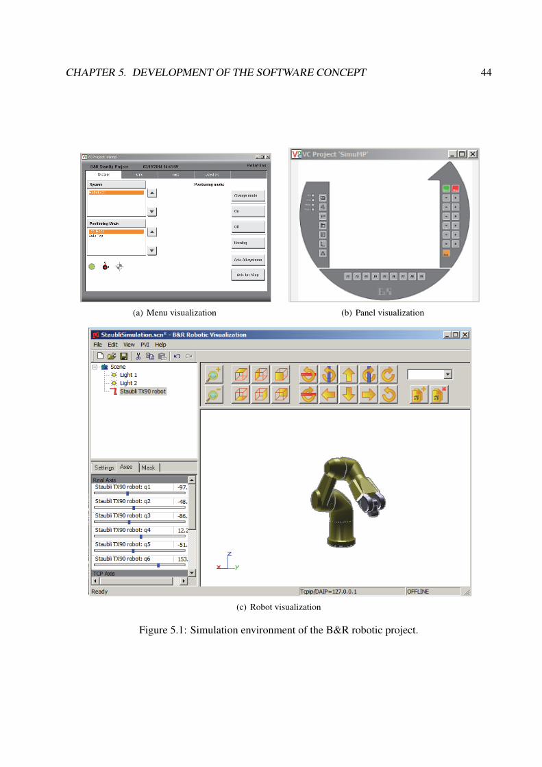
software and helped to develop new code1 before the hardware was available. Figure 5.1 shows
the simulation environment of the robotic project. The robotic project is divided into two main
parts. The first part is the Human-Machine-Interface block and is used to control the graphical
user interface. The second block is the Motion-Handling block, which takes care of path planning
and the control of the motion. Both blocks are designed to be reusable. Therefore, they are also
applied in other B&R applications. The Motion-Handling block can be divided into three tasks.
The first task is called the system task and is in charge of controlling states of the system, such as
homing or power up all axes. The next task is the CNC task and is used for path planning and to
coordinate the axes states. The last task is the Axes task and is applied to control the state of the
single axes.
5.1.1 Important Robot Specific NC Commands
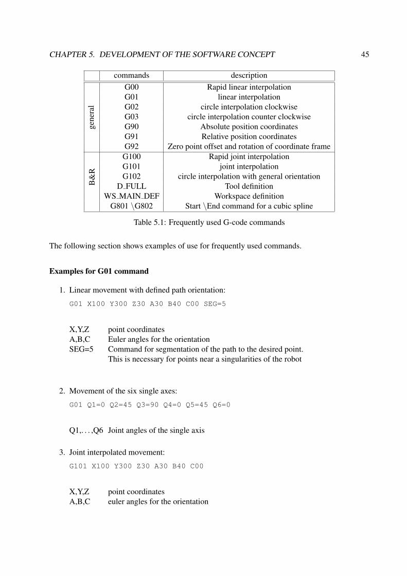
The robotic project of B&R uses G-code to control the different robot tasks. G-code is the standard
code for programming numerical controlled (NC) machines, such as CNC mills or CNC lathes.
Most of the commands are equal to the standardized G-code commands, but there are also some
machine specific commands. The most important commands are listed in the following list.
1The whole robotic project itself was developed with these simulation tools
43
CHAPTER 5. DEVELOPMENT OF THE SOFTWARE CONCEPT 44
(a) Menu visualization (b) Panel visualization
(c) Robot visualization
Figure 5.1: Simulation environment of the B&R robotic project.
CHAPTER 5. DEVELOPMENT OF THE SOFTWARE CONCEPT 45
commands description
gen
eral
G00 Rapid linear interpolation
G01 linear interpolation
G02 circle interpolation clockwise
G03 circle interpolation counter clockwise
G90 Absolute position coordinates
G91 Relative position coordinates
G92 Zero point offset and rotation of coordinate frame
B&
R
G100 Rapid joint interpolation
G101 joint interpolation
G102 circle interpolation with general orientation
D FULL Tool definition
WS MAIN DEF Workspace definition
G801 \G802 Start \End command for a cubic spline
Table 5.1: Frequently used G-code commands
The following section shows examples of use for frequently used commands.
Examples for G01 command
1. Linear movement with defined path orientation:
G01 X100 Y300 Z30 A30 B40 C00 SEG=5
X,Y,Z point coordinates
A,B,C Euler angles for the orientation
SEG=5 Command for segmentation of the path to the desired point.
This is necessary for points near a singularities of the robot
2. Movement of the six single axes:
G01 Q1=0 Q2=45 Q3=90 Q4=0 Q5=45 Q6=0
Q1,. . . ,Q6 Joint angles of the single axis
3. Joint interpolated movement:
G101 X100 Y300 Z30 A30 B40 C00
X,Y,Z point coordinates
A,B,C euler angles for the orientation

CHAPTER 5. DEVELOPMENT OF THE SOFTWARE CONCEPT 46
Examples for G02
1. Circle interpolation
G02 X7.5 Y40 I-30 J-22.5
X,Y coordinates of the end point
I,J coordinates of the circle center
2. Helix
G02 I50 H2160 Z100 (6 full rotations)
X,Y coordinates of the end point
I,J coordinates of the circle center
H Rotation in angle
Splines command
Cubic Spline:
G801 CE=0.01 BC1 X-1 Y1G1 Y0 Y0 (interpolation point 1)G1 X10 Y10 (interpolation point 2)G1 X20 Y10 (interpolation point 3)G1 X30 Y0 (interpolation point 4)
G802 BC1 X-1 Y0
X,Y,Z interpolation point coordinates
BC1 Boundary condition for the first point defined as first derivative
CE Chord error of the spline
Example for Workspace and Tool definition
1. Definition of the tool offset and orientation
D_FULL DX=20 DY=0 DZ=5 PHI=0 THETA=0 PSI=0
DX,DY,DZ Distance to the tool coordinate system
PHI,THETA,PSI Orientation angles of the tool coordinate system
CHAPTER 5. DEVELOPMENT OF THE SOFTWARE CONCEPT 47
2. Definition of the workspace border cuboid
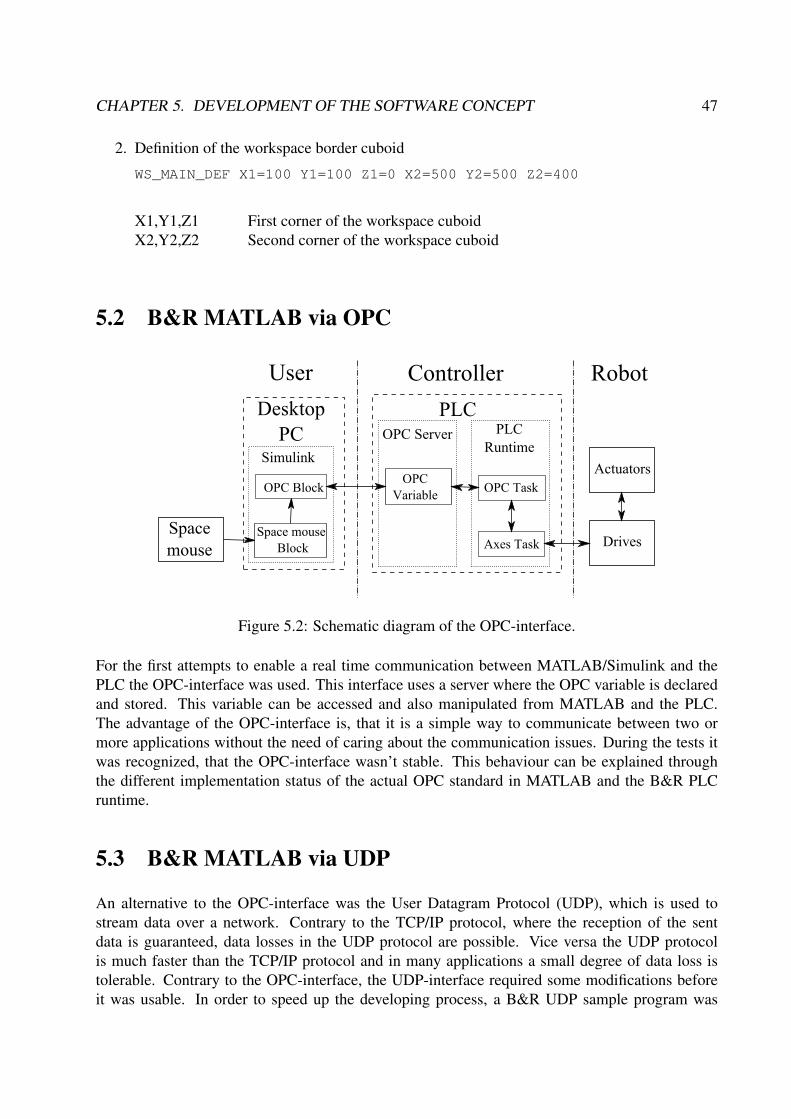
WS_MAIN_DEF X1=100 Y1=100 Z1=0 X2=500 Y2=500 Z2=400
X1,Y1,Z1 First corner of the workspace cuboid
X2,Y2,Z2 Second corner of the workspace cuboid
5.2 B&R MATLAB via OPC
Figure 5.2: Schematic diagram of the OPC-interface.
For the first attempts to enable a real time communication between MATLAB/Simulink and the
PLC the OPC-interface was used. This interface uses a server where the OPC variable is declared
and stored. This variable can be accessed and also manipulated from MATLAB and the PLC.
The advantage of the OPC-interface is, that it is a simple way to communicate between two or
more applications without the need of caring about the communication issues. During the tests it
was recognized, that the OPC-interface wasn’t stable. This behaviour can be explained through
the different implementation status of the actual OPC standard in MATLAB and the B&R PLC
runtime.
5.3 B&R MATLAB via UDP
An alternative to the OPC-interface was the User Datagram Protocol (UDP), which is used to
stream data over a network. Contrary to the TCP/IP protocol, where the reception of the sent
data is guaranteed, data losses in the UDP protocol are possible. Vice versa the UDP protocol
is much faster than the TCP/IP protocol and in many applications a small degree of data loss is
tolerable. Contrary to the OPC-interface, the UDP-interface required some modifications before
it was usable. In order to speed up the developing process, a B&R UDP sample program was
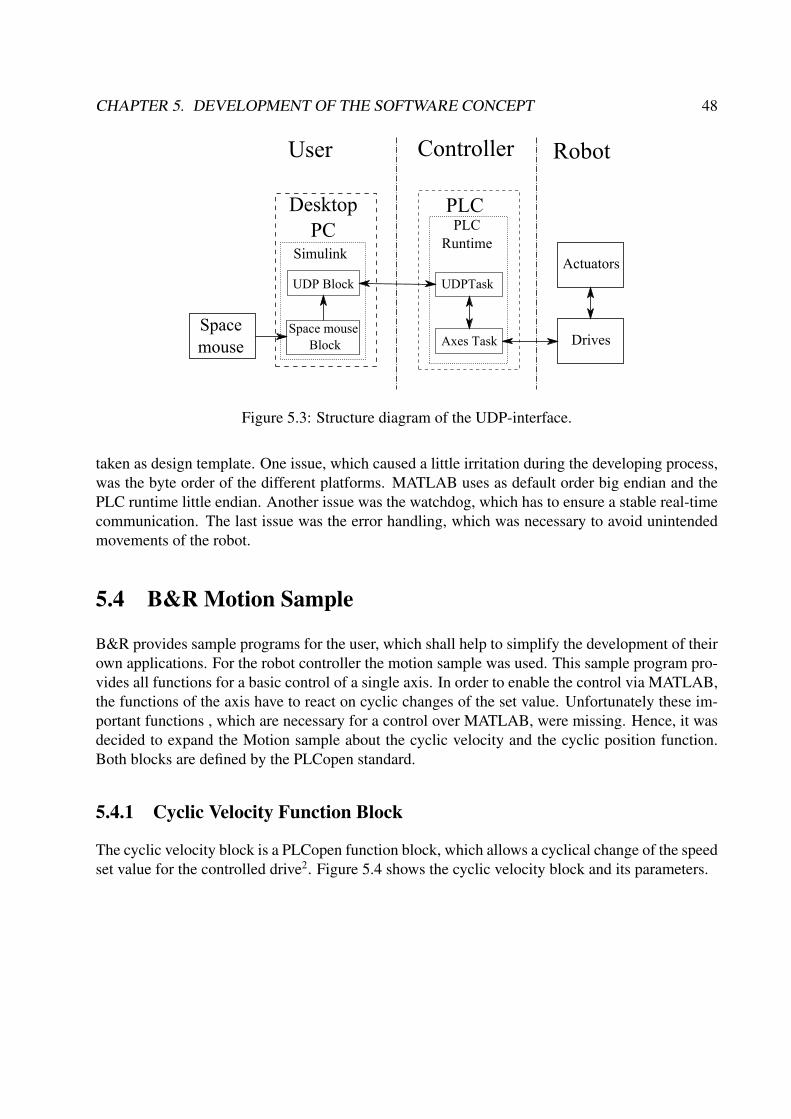
CHAPTER 5. DEVELOPMENT OF THE SOFTWARE CONCEPT 48
Figure 5.3: Structure diagram of the UDP-interface.
taken as design template. One issue, which caused a little irritation during the developing process,
was the byte order of the different platforms. MATLAB uses as default order big endian and the
PLC runtime little endian. Another issue was the watchdog, which has to ensure a stable real-time
communication. The last issue was the error handling, which was necessary to avoid unintended
movements of the robot.
5.4 B&R Motion Sample
B&R provides sample programs for the user, which shall help to simplify the development of their
own applications. For the robot controller the motion sample was used. This sample program pro-
vides all functions for a basic control of a single axis. In order to enable the control via MATLAB,
the functions of the axis have to react on cyclic changes of the set value. Unfortunately these im-
portant functions , which are necessary for a control over MATLAB, were missing. Hence, it was
decided to expand the Motion sample about the cyclic velocity and the cyclic position function.
Both blocks are defined by the PLCopen standard.
5.4.1 Cyclic Velocity Function Block
The cyclic velocity block is a PLCopen function block, which allows a cyclical change of the speed
set value for the controlled drive2. Figure 5.4 shows the cyclic velocity block and its parameters.
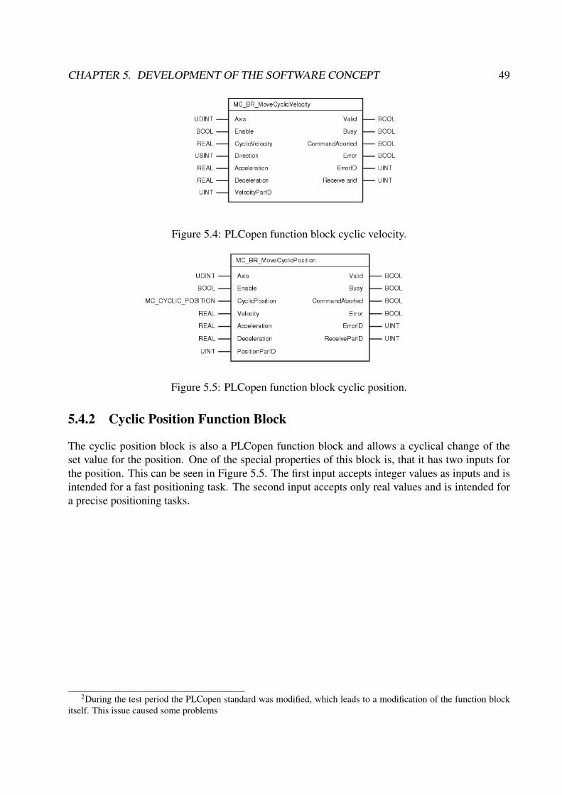
CHAPTER 5. DEVELOPMENT OF THE SOFTWARE CONCEPT 49
Figure 5.4: PLCopen function block cyclic velocity.
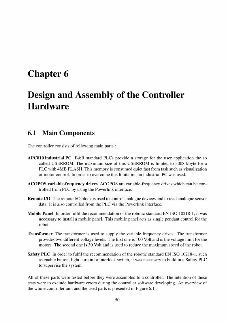
Figure 5.5: PLCopen function block cyclic position.
5.4.2 Cyclic Position Function Block
The cyclic position block is also a PLCopen function block and allows a cyclical change of the
set value for the position. One of the special properties of this block is, that it has two inputs for
the position. This can be seen in Figure 5.5. The first input accepts integer values as inputs and is
intended for a fast positioning task. The second input accepts only real values and is intended for
a precise positioning tasks.
2During the test period the PLCopen standard was modified, which leads to a modification of the function block
itself. This issue caused some problems
Chapter 6
Design and Assembly of the ControllerHardware
6.1 Main Components
The controller consists of following main parts :
APC810 industrial PC B&R standard PLCs provide a storage for the user application the so
called USERROM. The maximum size of this USERROM is limited to 3008 kbyte for a
PLC with 4MB FLASH. This memory is consumed quiet fast from task such as visualization
or motor control. In order to overcome this limitation an industrial PC was used.
ACOPOS variable-frequency drives ACOPOS are variable-frequency drives which can be con-
trolled from PLC by using the Powerlink interface.
Remote I/O The remote I/O block is used to control analogue devices and to read analogue sensor
data. It is also controlled from the PLC via the Powerlink interface.
Mobile Panel In order fulfil the recommendation of the robotic standard EN ISO 10218-1, it was
necessary to install a mobile panel. This mobile panel acts as single pendant control for the
robot.
Transformer The transformer is used to supply the variable-frequency drives. The transformer
provides two different voltage levels. The first one is 100 Volt and is the voltage limit for the
motors. The second one is 30 Volt and is used to reduce the maximum speed of the robot.
Safety PLC In order to fulfil the recommendation of the robotic standard EN ISO 10218-1, such
as enable button, light curtain or interlock switch, it was necessary to build in a Safety PLC
to supervise the system.
All of these parts were tested before they were assembled to a controller. The intention of these
tests were to exclude hardware errors during the controller software developing. An overview of
the whole controller unit and the used parts is presented in Figure 6.1.
50
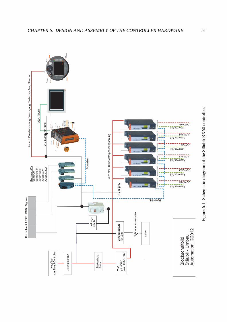
CHAPTER 6. DESIGN AND ASSEMBLY OF THE CONTROLLER HARDWARE 51
Fig
ure
6.1
:S
chem
atic
dia
gra
mof
the
Sta
ubli
RX
60
contr
oll
er.
CHAPTER 6. DESIGN AND ASSEMBLY OF THE CONTROLLER HARDWARE 52
(a) Frontside (b) Backside
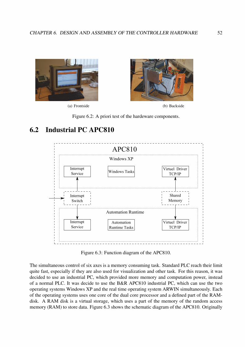
Figure 6.2: A priori test of the hardeware components.
6.2 Industrial PC APC810
Figure 6.3: Function diagram of the APC810.
The simultaneous control of six axes is a memory consuming task. Standard PLC reach their limit
quite fast, especially if they are also used for visualization and other task. For this reason, it was
decided to use an industrial PC, which provided more memory and computation power, instead
of a normal PLC. It was decide to use the B&R APC810 industrial PC, which can use the two
operating systems Windows XP and the real time operating system ARWIN simultaneously. Each
of the operating systems uses one core of the dual core processor and a defined part of the RAM-
disk. A RAM disk is a virtual storage, which uses a part of the memory of the random access
memory (RAM) to store data. Figure 6.3 shows the schematic diagram of the APC810. Originally

CHAPTER 6. DESIGN AND ASSEMBLY OF THE CONTROLLER HARDWARE 53
it was intended to run MATLAB on the industrial PC, but MATLAB was too resource hungry to
allow a stable operation of the ARWIN system.
6.3 Safety PLC
The standard EN ISO 10218-1 demands some special safety features from the robot. One of the
requirements was, that the robot only can be switched on if a enabling button was pressed. Another
requirement is the emergency stop of the robot if the light curtain or alternatively the interlock
switch of the robot cage door is activated. The robot Staubli RX60 has a holding brake, which is
used to hold the robot arm in position if the power is lost. This brake is lifted if power is available.
In the case of power loss, the brake is activated and stops the system. In order to reduce the braking
torque in case of an emergency stop, it was decided to slow down the arm first with the motors and
use the holding brake to bring the arm to a complete stop. This behaviour was realized by a switch
off delay of 300 ms and a quick stop command which is send to the drives. After the delay time
the drive controllers are disabled
6.4 Estimation of the Gear Ratio
The Staubli RX60 uses synchron servomotors to rotate its joints. Servomotors have a rotary en-
coder mounted on the motor shaft. This encoder allows a control of the position and the speed of
the motor shaft. The robot designer tried to reduce the mass of the moved parts to achieve a good
dynamical behaviour. Therefore, they used small motors with a small moment of inertia. This
motor are to weak to drive the joint directly and therefore a gear is needed. In order to reduce the
cost, the designer the motor used encoder to determine the actual joint angle. This task is simple
if the joints are driven directly, where the joint angle is equal with the motor angle. In case of gear
driven joint, the joint angle has to be calculated by multiplying the motor angle with the gear ratio.
Unfortunately,the data sheets of the Staubli RX60 didn’t provide the gear ratio. Therefore the gear
ratio had to be estimated. For this purpose the single joints were rotated about a known or easy
measurable angle, for example 180 degrees. Afterwards the gear ratio was calculated by using the
measured value of the encoder.
i =θoutθin
(6.1)
For an easier handling is θin substituted by
θin = c θ′in, (6.2)
i =θoutc θ′in
. (6.3)
with:

CHAPTER 6. DESIGN AND ASSEMBLY OF THE CONTROLLER HARDWARE 54
i . . . Gear ratio
θout . . . Rotation angle of the joint (gear output)
θin . . . Rotation angle of the motor (gear input)
θ′in . . . Rotation angle of the motor in encoder increments
c . . . Conversation factor
The B&R system uses motor revolution per one joint revolution to describe the gear ratio. For this
purpose the gear ratio has to be inverted.
motor revolution =1
ijoint revolution (6.4)
Chapter 7
Programming of the Axis Controller
One of the main issues was the simultaneous control of the six robot axes. The control task for a
single axis was developed during the test phase; therefore, by utilizing the already existing code,
the development effort for the multi axes control task is reduced. This particular task supervises
the individual single axis control tasks. Figure 7.1 gives an overview of the controller concept.
7.1 Single Axis Task
The Single Axis Task controls the basic function of one axis. In order to achieve a clear com-
mand structure, four structured variables, that can be used for hierarchical structures, were defined.
Structured variables can be explained as objects of a class, which only contains attributes but no
functions. This four variables are:
Commands These variables enable the particular drive modes.
Parameters These variables contain the set-values for the particular drive mode.
Status These variables display the actual drive status, such as actual position, actual velocity and
also error messages.
Axis state These variables display the actual state of the axis.
The single axis task is based on a finite state machine, which controls the modes of the axis.
7.2 Robot Control Task
The aim of the Robot Control Task is to coordinate the six single axes of the robot. This task also
uses structured variables as command structure and is equivalent to the one described in single axis
task. Also the structure finite state machine is similar. The idea behind this finite state machine is
that a state of the Robot Control task leads the same action as the same state in the Single axis task
55

CHAPTER 7. PROGRAMMING OF THE AXIS CONTROLLER 56
Figure 7.1: Overview of the controller concept.

CHAPTER 7. PROGRAMMING OF THE AXIS CONTROLLER 57
but only with six axes. The state diagram of this finite state machine can be found in the appendix.
The following examples code shows the power on state and how all six axes are handled.
Listing 7.1: First solution for conjoining the status variables
1
2 POWERON:3 ActualState := ’POWERON’;4 //Send global command only ONCE5
6 // Switch on of the controller of the single axes7 IF (cycle = 0) THEN8 FOR axes_index := 0 TO (max_loopcount) DO9 GlobalControl[axes_index].Command.Power := TRUE
;10 PowerCheck[axes_index] := 0;11 END_FOR12 cycle := 1;13 END_IF14
15 // Check if all axes controller are switched on16 FOR axes_index := 0 TO (max_loopcount) DO17 IF (axes_index = 0) THEN18 Merker := TRUE;19 END_IF20 // Conjoin all status variables by using Merker21 Merker := GlobalControl[axes_index].Status.DriveStatus.
ControllerStatus AND Merker;22 END_FOR23
24
25 // Exit state26 IF (Merker = TRUE) AND (axes_index = max_index) THEN27 RobStatus.VisuDrivesEnabled := TRUE;28 STATE := READY;29 END_IF
In this example code the for-loop was used to reduce the code and combine the status variables
of the axis to one variable. Therefore the variable Merkeris conjoined with the status variable
by AND. The result is stored again in the variable Merker. If all status variables of the axis are
TRUE, then the variable Merker is also TRUE. If one of the status variables is FALSE then the
variable Merker is also FALSE. Alternatively the same result could be achieved by conjoining
all status variables with AND. This is shown in the following example code.
Listing 7.2: Second solution for conjoining the status variables
1 //Check if all Axes are homed...2 RobStatus.Homed:= GlobalControl[0].Status.DriveStatus.HomingOk3 AND GlobalControl[1].Status.DriveStatus.
HomingOk

CHAPTER 7. PROGRAMMING OF THE AXIS CONTROLLER 58
4 AND GlobalControl[2].Status.DriveStatus.HomingOk
5 AND GlobalControl[3].Status.DriveStatus.HomingOk
6 AND GlobalControl[4].Status.DriveStatus.HomingOk
7 AND GlobalControl[5].Status.DriveStatus.HomingOk;
7.3 Interpolation Concept
In the first attempt, it was tried to move along a path by using the cyclic position function block.
This block didn’t allow a smooth movement. This behaviour can be explained by the acceleration
and deceleration ramp, which is applied after and before the desired point. If the distance between
the points is too short, there is a permanent acceleration and decelerating motion, which leads to
vibrations. Therefore it was decided to use the cyclic velocity function block instead. This block
has the disadvantage, that an interpolation controller is necessary to reach the desired position.
Figure 7.2: Interpolation concept for the Staubli RX60 .
The following equations show, that the behaviour of the interpolation concept in Figure 7.2 is
equivalent to the behaviour of a first order system.
θi =1
s(θref − θi) k, (7.1)
s θi = k θref − k θi, (7.2)
s θi + k θi = k θref , (7.3)
θi (s+ k) = k θref , (7.4)
θiθref
=k
k + s=
1sk+ 1
. (7.5)

CHAPTER 7. PROGRAMMING OF THE AXIS CONTROLLER 59
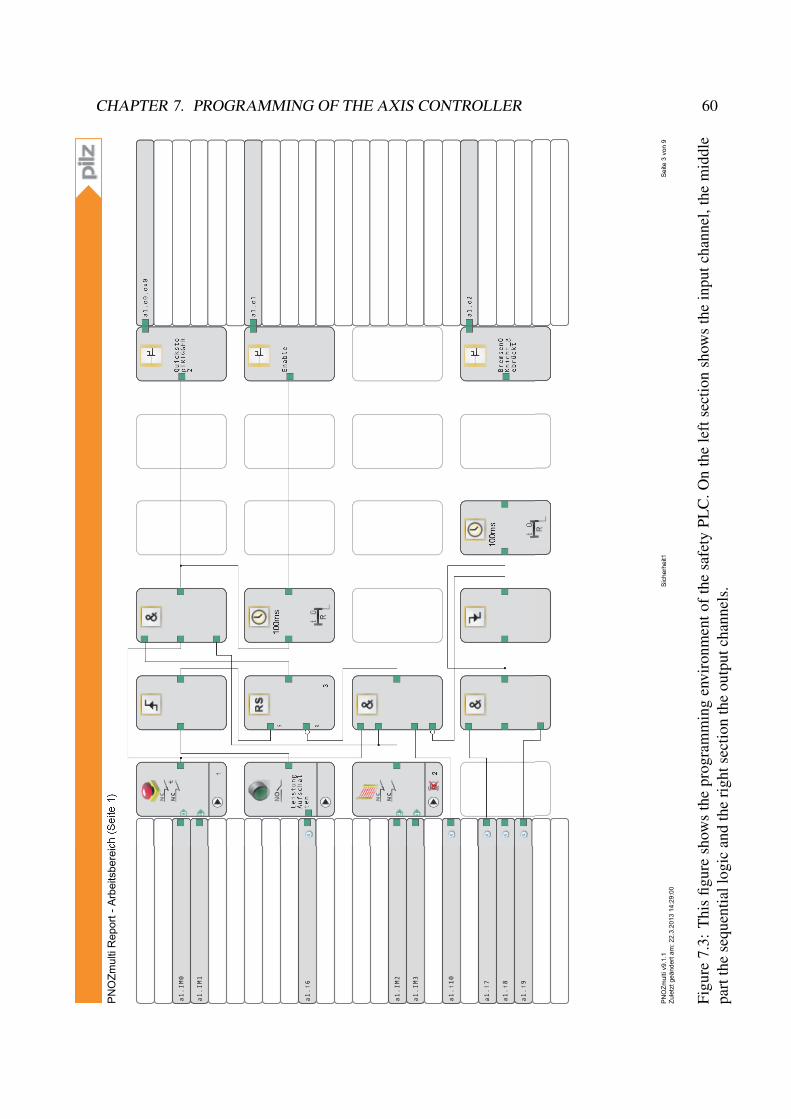
7.4 Programming of the Safety PLC
The safety PLC has a simple programming environment, which is diagram based. The program-
ming environment always uploads the actual program for the storage of the safety PLC. This fea-
ture was very useful to deal with the version problem. The safety PLC has to take care of the
following tasks:
1. Enable all drive controllers.
2. Force robot to stop, if the light curtain of the robot cage or the interlock switch of the cage
door is activated.
3. Control the emergency stop buttons and force the robot to stop. This stop is performed by an
electrical brake. The final stop is achieved by the holding brake, which has a release delay
of 300 ms to allow an electrical braking before.
Figure 7.3 shows the program for the Staubli RX60 .
CHAPTER 7. PROGRAMMING OF THE AXIS CONTROLLER 60
Fig
ure
7.3
:T
his
figure
show
sth
epro
gra
mm
ing
envir
onm
ent
of
the
safe
tyP
LC
.O
nth
ele
ftse
ctio
nsh
ow
sth
ein
put
chan
nel
,th
em
iddle
par
tth
ese
quen
tial
logic
and
the
right
sect
ion
the
outp
ut
chan
nel
s.
Chapter 8
Implementation of Robot Kinematics
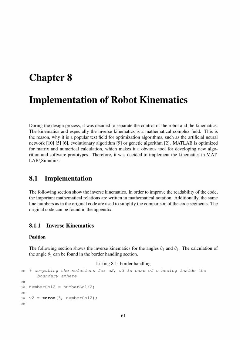
During the design process, it was decided to separate the control of the robot and the kinematics.
The kinematics and especially the inverse kinematics is a mathematical complex field. This is
the reason, why it is a popular test field for optimization algorithms, such as the artificial neural
network [10] [5] [6], evolutionary algorithm [9] or genetic algorithm [2]. MATLAB is optimized
for matrix and numerical calculation, which makes it a obvious tool for developing new algo-
rithm and software prototypes. Therefore, it was decided to implement the kinematics in MAT-
LAB\Simulink.
8.1 Implementation
The following section show the inverse kinematics. In order to improve the readability of the code,
the important mathematical relations are written in mathematical notation. Additionally, the same
line numbers as in the original code are used to simplify the comparison of the code segments. The
original code can be found in the appendix.
8.1.1 Inverse Kinematics
Position
The following section shows the inverse kinematics for the angles θ2 and θ3. The calculation of
the angle θ1 can be found in the border handling section.
Listing 8.1: border handling
200 % computing the solutions for u2, u3 in case of o beeing inside theboundary sphere
201
202 numberSol2 = numberSol/2;203
204 v2 = zeros(3, numberSol2);205
61
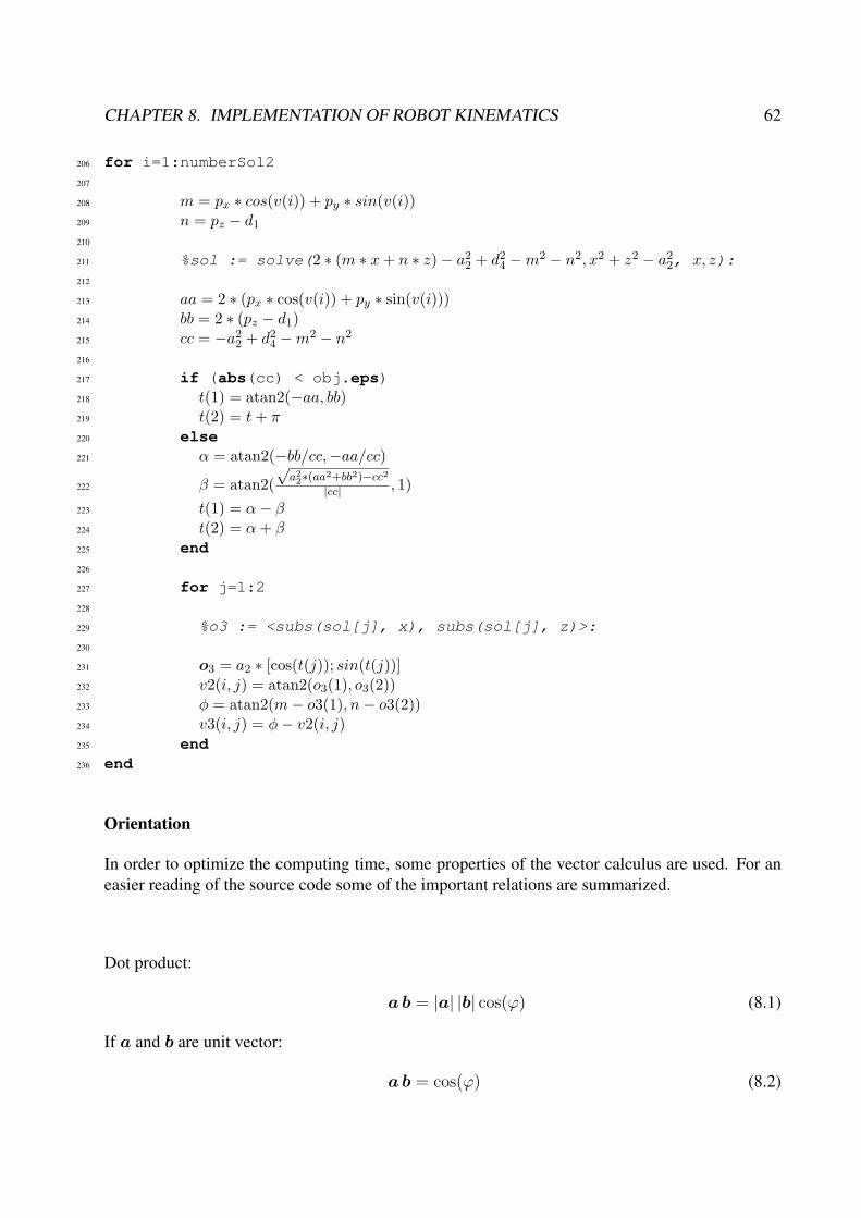
CHAPTER 8. IMPLEMENTATION OF ROBOT KINEMATICS 62
206 for i=1:numberSol2207
208 m = px ∗ cos(v(i)) + py ∗ sin(v(i))209 n = pz − d1210
211 %sol := solve(2 ∗ (m ∗ x+ n ∗ z)− a22 + d24 −m2 − n2, x2 + z2 − a22, x, z):212
213 aa = 2 ∗ (px ∗ cos(v(i)) + py ∗ sin(v(i)))214 bb = 2 ∗ (pz − d1)215 cc = −a22 + d24 −m2 − n2
216
217 if (abs(cc) < obj.eps)218 t(1) = atan2(−aa, bb)219 t(2) = t+ π220 else221 α = atan2(−bb/cc,−aa/cc)
222 β = atan2(
√a22∗(aa2+bb2)−cc2
|cc| , 1)
223 t(1) = α− β224 t(2) = α+ β225 end226
227 for j=1:2228
229 %o3 := <subs(sol[j], x), subs(sol[j], z)>:230
231 o3 = a2 ∗ [cos(t(j)); sin(t(j))]232 v2(i, j) = atan2(o3(1), o3(2))233 φ = atan2(m− o3(1), n− o3(2))234 v3(i, j) = φ− v2(i, j)235 end236 end
Orientation
In order to optimize the computing time, some properties of the vector calculus are used. For an
easier reading of the source code some of the important relations are summarized.
Dot product:
ab = |a| |b| cos(ϕ) (8.1)
If a and b are unit vector:
ab = cos(ϕ) (8.2)

CHAPTER 8. IMPLEMENTATION OF ROBOT KINEMATICS 63
Cross product:
|a× b| = |a| |b| sinϕ (8.3)
If a and b are unit vector:
|a× b| = sinϕ (8.4)
normalizing of vectors:
anorm =a
|a| (8.5)
Listing 8.2: orienation
245 nos = 2*nos123246 U = zeros(6,nos)247
248 % Normalizing of the input vectors and calculation of the threeorientation vectors.
249
250 n6 = f1/|f1|251 a6 = f1× f2252 a6 = a6/|a6|253 s6 = a6 × n6
254
255 for j=1:nos123256 j2 = 2*j257 j1 = j2-1258
259 for i=1:3260 U(i,j1) = U123(i,j)261 U(i,j2) = U123(i,j)262 end263
264 % Calculation of the orientation vector of the third joint265
266 sn1 = sin(U123(1,j))267 cs1 = cos(U123(1,j))268 sn23 = sin(U123(2,j)+U123(3,j))269 cs23 = cos(U123(2,j)+U123(3,j))270
271 a3 = [sn1; cs1; 0]272
273
274 a4 = [cs1 sn23; sn1 sn23; cs23]275
276 % Calculation of cos θ5

CHAPTER 8. IMPLEMENTATION OF ROBOT KINEMATICS 64
277
278 cs5 = a4,a6
279
280 % Exactly two different solution triples for u4, u5, u6 for everysolution triple of u1, u2, u3
281
282 if (abs(abs(cs5) - 1.0) > obj.eps)283
284 a5 = a4 × a6
285 denom = |a5|286 fak = 1/denom287 a5 = fak a5
288 sn5 = fak ∗ (1.0− cs52)289
290 % Calculation of the two solutions for the angle θ4291 cs4 = a3 a5
292 sn4 = fak ∗ (a3 a6)293 U(4, j1) = atan2(sn4, cs4)294 U(4, j2) = atan2(−sn4,−cs4)295
296 % Calculation of the two solutions for the angle θ6297 cs6 = a5 s6298 sn6 = fak (a4 s6)299 U(6, j1) = atan2(sn6, cs6)300 U(6, j2) = atan2(−sn6,−cs6)301 else302 .303 .304 .305 end306 % Calculation of the two solutions for the angle θ4307
308 U(5,j1) = atan2(sn5, cs5);309 U(5,j2) = - U(5,j1);
8.1.2 Border Handling
The points in space, which are reachable with the robot, are limited by the physical properties of
the robot, such as arm length. This is an important issue which has to be dealt with inside the
kinematics because the boundaries are singularities of the robot. As Figure 8.1 shows, the Staubli
RX60 has a spherical outer workspace boundary and a cylindrical inner workspace boundary. As
mentioned in chapter two, the design engineer tries to avoid singularities by design of the robot.
This design leads to an inner cylindrical border of the workspace.
Listing 8.3: border handling
142

CHAPTER 8. IMPLEMENTATION OF ROBOT KINEMATICS 65
(a) Isometric view (b) Front view
Figure 8.1: Theoretical workspace of the Staubli RX60 (axis limits are not reconsidered).
143 dist12 = p2x + p2y144 dist22 = p2x + p2y + (pz − d1)
2
145
146 % Point is in workspace147 if(dist12 > r2in)&&(dist2
2 < R2out)
148 % Point lies on the boundary cylinder149 if((dist12 < r2in)150 % Point lies on lower or upper boundary circle151 if(dist22 > R2
out)152 numberSol=1153 θ1 = atan2(−px, py)154 % Point lies on the upper boundary circle155 if(|pz − d1 − a3 − d4|<tolerance)156 θ2 = 0157 % Point lies on the lower boundary circle158 else159 θ2 = π160 end161 θ3 = 0162 % Point lies on the boundary cylinder and inside the boundary sphere163 else164 numberSol=2165 v(1) = atan2(−px, py)166 θ1(1) = v(1)167 θ1(2) = θ1(1)168 end169 % Point lies outside the boundary cylinder170 else171 α = atan2(−px, py)
172 β = atan2(√
dist12 − d22, d2)

CHAPTER 8. IMPLEMENTATION OF ROBOT KINEMATICS 66
173
174 v(1) = α− β175 v(2) = α+ β176 for j=1:2177 if(v(j) > π)178 v(j) = v(j)− 2π179 end180 if(v(j) < −π)181 v(j) = v(j) + 2π182 end183 end184 % Point lies on the boundary sphere185 if(dist22 > R2)186 numberSol=2187 θ1(1) = v(1)188 θ1(2) = v(2)189 for j=1:2190 θ2(j) = atan2(px cos v(j) + py sin v(j), pz − d1)191 θ3(j) = 0192 end193 end194 % Point lies inside the boundary sphere and out side the boundary
cylinder195 else196 numberSol=4197 θ1(1) = v(1)198 θ1(2) = v(1)199 θ1(3) = v(2)200 θ1(4) = v(2)201 end
8.1.3 Implementation in MATLAB
The first version of the kinematic was written as MATLAB class. This class contains two functions
beside the robot parameters. The first function is called DK and calculates the transformation
matrix of the forward kinematics. The second function is called IK and calculates the possible
solutions and evaluates the closest solution to the actual configuration. Just as the B&RRobotic
Project this kinematic was developed with a simulation tool, which leads to problems with the
rotation direction. Not all assumed rotation directions of simulation did fit with rotation directions
of the robot axes.
Closest Solution
In the general case the inverse kinematic of Staubli RX60 has eight solutions, but the robot can ex-
ecute only one of them. Therefore an algorithm is needed to find the most suitable of the solutions.
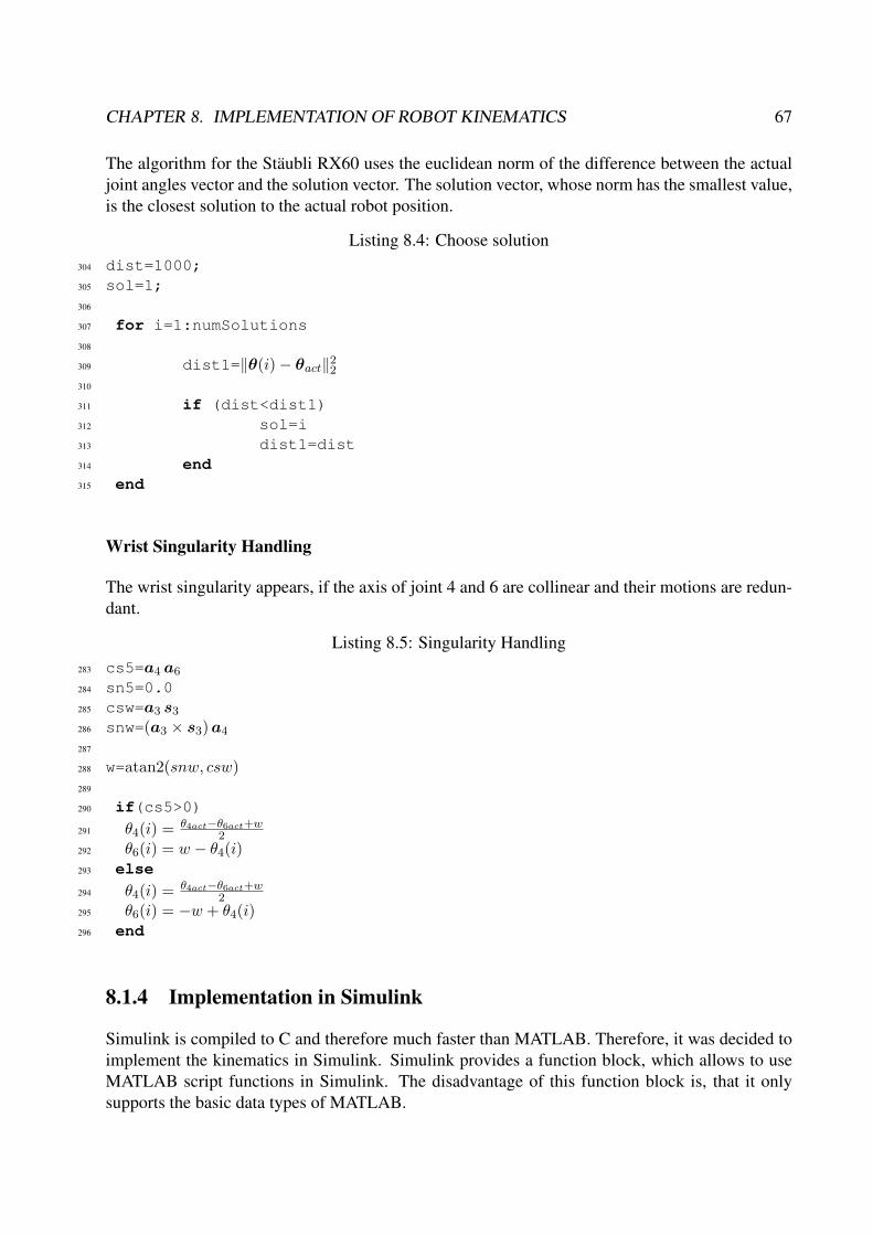
CHAPTER 8. IMPLEMENTATION OF ROBOT KINEMATICS 67
The algorithm for the Staubli RX60 uses the euclidean norm of the difference between the actual
joint angles vector and the solution vector. The solution vector, whose norm has the smallest value,
is the closest solution to the actual robot position.
Listing 8.4: Choose solution
304 dist=1000;305 sol=1;306
307 for i=1:numSolutions308
309 dist1=‖θ(i)− θact‖22310
311 if (dist<dist1)312 sol=i313 dist1=dist314 end315 end
Wrist Singularity Handling
The wrist singularity appears, if the axis of joint 4 and 6 are collinear and their motions are redun-
dant.
Listing 8.5: Singularity Handling
283 cs5=a4 a6
284 sn5=0.0285 csw=a3 s3286 snw=(a3 × s3)a4
287
288 w=atan2(snw, csw)289
290 if(cs5>0)291 θ4(i) =
θ4act−θ6act+w2
292 θ6(i) = w − θ4(i)293 else294 θ4(i) =
θ4act−θ6act+w2
295 θ6(i) = −w + θ4(i)296 end
8.1.4 Implementation in Simulink
Simulink is compiled to C and therefore much faster than MATLAB. Therefore, it was decided to
implement the kinematics in Simulink. Simulink provides a function block, which allows to use
MATLAB script functions in Simulink. The disadvantage of this function block is, that it only
supports the basic data types of MATLAB.

CHAPTER 8. IMPLEMENTATION OF ROBOT KINEMATICS 68
Real-time in Simulink
MATLAB\Simulink doesn’t operate in real time.1 A communication with a real time system
requires a synchronisation of MATLAB\Simulink with the real time. This is achieved with the
MATLAB function waitfortreal, which keeps MATLAB in busy wait state till the set time is over.
8.1.5 Test of the Kinematics
In order to test the functionality of the kinematics two different test programs were written. The
first program was written in MATLAB and the second one in Simulink.
MATLAB
The original kinematics was written as MATLAB class and therefore it was obvious to write a test
script in MATLAB. The MATLAB script is suitable to define a path and let it be executed from the
robot. During the test the following difficulties appeared:
1. In case, that the script is aborted, the UDP-connecting has to be closed manually via com-
mand line, which is sometimes forgotten. Therefore an error handling routine is necessary.
2. The calculation in MATLAB aren’t executed in real-time. In case, that MATLAB sends the
points of the path too fast for the PLC, data gets lost. Therefore a synchronization with the
real-time is necessary.
3. The standard user interaction are limited. Therefore a controlled program flow would be
necessary.
The test showed, that it is possible to control the robot via MATLAB but it is more effort necessary
to deal with the difficulties than in Simulink.
Simulink
The kinematics was also tested in Simulink. Simulink provides for many common input devices,
such as joysticks or cameras, function block to read their values. Therefore, a standard 3D-mouse
was used to generate the path and perform the test. In order to achieve a real-time behaviour some
changes in the solver parameters were necessary. Instead of the default variable-steps time of the
solver were a fixed-steps time of 0.01 s was used and the simulation time was set to infinity.
1Depending on the task, it is faster or slower than real-time.

Chapter 9
Conclusion and Future Work
This thesis presented the development and engineering of a control unit for a 6 DOF industrial
robot. The new controller concept provides a transparent framework and enables a separation of
the robot kinematics from the control hardware. For this purpose a generic network interface for the
PLC has been developed, which enables the real-time execution of remote positioning commands.
The network interface allows the use of more powerful PC and the scientific computation plat-
form MATLAB. Therefore, MATLAB is used as platform for the robot kinematics computations.
Due to the use of standard industrial components the maintenance is simplified. The transparent
framework simplifies the embedding and parametrizing of new sensors.
For standard application, the robot interprets G-codes stored in CNC files, that are generated with
several tools. A direct control from MATLAB/Simulink was implemented successfully and opens
new facilities for future applications. Research on methods for robot calibration and registration
may be done with the actual equipment.
It would be interesting to test, whether real-time control would be possible with the use of WLAN
instead of LAN. This implies the application of mobile devices, such as phones and tablets, for
controlling the robot. In future cyber-physical systems, this techniques will become more impor-
tant.
For educational purposes it is possible to integrate the control of the robot into student projects. For
example, during writing this thesis a project was carried out successfully, where students controlled
the robot with a KinectTMmotion sensor. Integration of such sensors is possible without the need
of downloading software to the robot controller.
A further new idea is to use the robot for 3D printing on surfaces of arbitrary geometry. A dedicated
printing head for this purpose is already under construction.
69
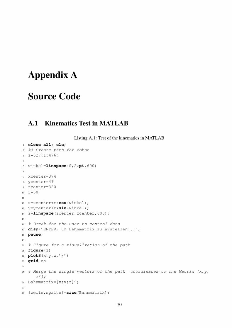
Appendix A
Source Code
A.1 Kinematics Test in MATLAB
Listing A.1: Test of the kinematics in MATLAB
1 close all; clc;2 %% Create path for robot3 z=327:1:476;4
5 winkel=linspace(0,2*pi,600)6
7 xcenter=3748 ycenter=499 zcenter=320
10 r=5011
12 x=xcenter+r*cos(winkel);13 y=ycenter+r*sin(winkel);14 z=linspace(zcenter,zcenter,600);15
16 % Break for the user to control data17 disp(’ENTER, um Bahnmatrix zu erstellen...’)18 pause;19
20 % Figure for a visualization of the path21 figure(1)22 plot3(x,y,z,’*’)23 grid on24
25 % Merge the single vectors of the path coordinates to one Matrix [x,y,z’];
26 Bahnmatrix=[x;y;z]’;27
28 [zeile,spalte]=size(Bahnmatrix);
70

APPENDIX A. SOURCE CODE 71
29
30 zaehler=0;31
32 %% Setup a connetion to PLC via UDP-Object33
34 u = udp(’10.43.70.10’, 25000, ’LocalPort’,30000, ’ByteOrder’, ’littleEndian’);
35
36 fopen(u);37
38 pause(0.2)39
40 % Create object of the class which deals with the kinematic41 my_robot = StaeubliRX60(290.0, 341.0, 49.0, 310.0);42
43 actAnglegrd(1)=0;44
45 % Create data to enable the comunictation with the PLC. The PLC waitstill
46 % it recives from the remote PC, therefore it is necesssary to senddata
47 % first48 data(1) = 11;49
50 % Convert value to Integer51 senddata = int32(data);52
53 fwrite(u,senddata, ’int32’);54
55 pause(0.2);56
57 actAnglegrd = fread(u,6,’single’);58
59 sendactAnglegrd = int32(actAnglegrd);60
61 disp(’ENTER, um Initialposition zu ubergeben... (RICHTIGKEIT PRUFEN!!!’)
62 pause;63
64 fwrite(u,sendactAnglegrd, ’int32’);65
66 %%67
68 disp(’ENTER, um Bahn abzuarbeiten...’)69 pause;70
71 for zahl=1:zeile72
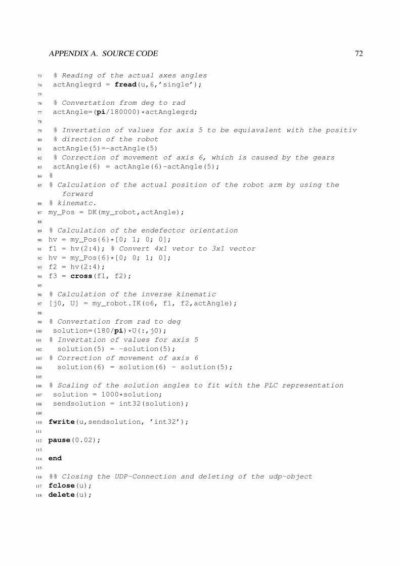
APPENDIX A. SOURCE CODE 72
73 % Reading of the actual axes angles74 actAnglegrd = fread(u,6,’single’);75
76 % Convertation from deg to rad77 actAngle=(pi/180000)*actAnglegrd;78
79 % Invertation of values for axis 5 to be equiavalent with the positiv80 % direction of the robot81 actAngle(5)=-actAngle(5)82 % Correction of movement of axis 6, which is caused by the gears83 actAngle(6) = actAngle(6)-actAngle(5);84 %85 % Calculation of the actual position of the robot arm by using the
forward86 % kinematc.87 my_Pos = DK(my_robot,actAngle);88
89 % Calculation of the endefector orientation90 hv = my_Pos{6}*[0; 1; 0; 0];91 f1 = hv(2:4); % Convert 4x1 vetor to 3x1 vector92 hv = my_Pos{6}*[0; 0; 1; 0];93 f2 = hv(2:4);94 f3 = cross(f1, f2);95
96 % Calculation of the inverse kinematic97 [j0, U] = my_robot.IK(o6, f1, f2,actAngle);98
99 % Convertation from rad to deg100 solution=(180/pi)*U(:,j0);101 % Invertation of values for axis 5102 solution(5) = -solution(5);103 % Correction of movement of axis 6104 solution(6) = solution(6) - solution(5);105
106 % Scaling of the solution angles to fit with the PLC representation107 solution = 1000*solution;108 sendsolution = int32(solution);109
110 fwrite(u,sendsolution, ’int32’);111
112 pause(0.02);113
114 end115
116 %% Closing the UDP-Connection and deleting of the udp-object117 fclose(u);118 delete(u);

APPENDIX A. SOURCE CODE 73
A.2 Kinematics Test in Simulink
Fig
ure
A.1
:S
imuli
nk
model
for
the
test
of
the
kin
emat
ics.
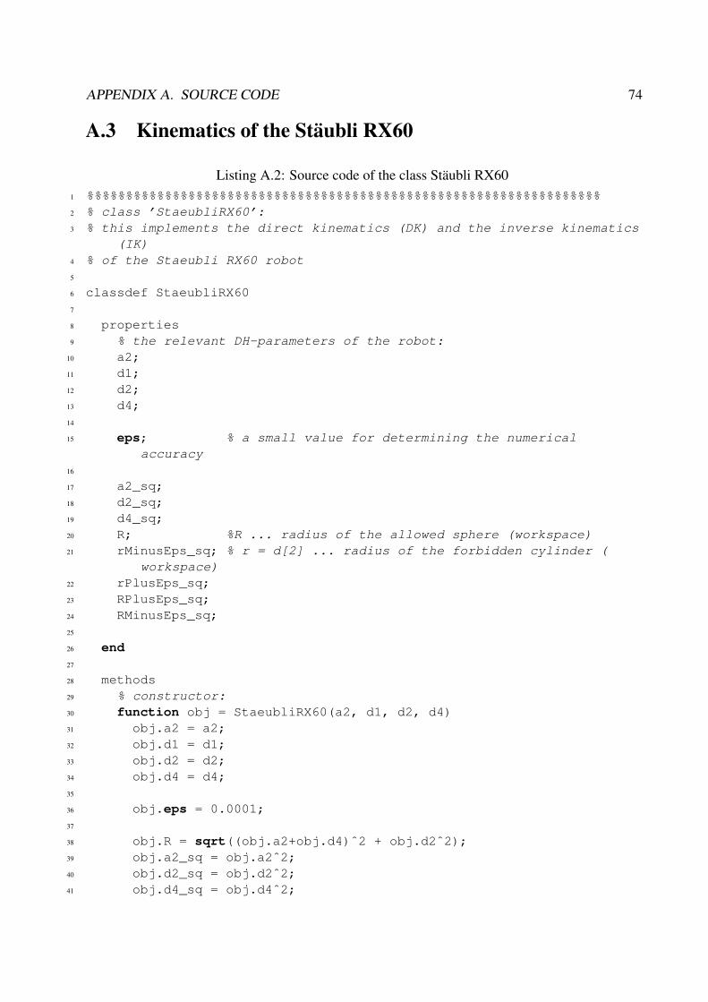
APPENDIX A. SOURCE CODE 74
A.3 Kinematics of the Staubli RX60
Listing A.2: Source code of the class Staubli RX60
1 %%%%%%%%%%%%%%%%%%%%%%%%%%%%%%%%%%%%%%%%%%%%%%%%%%%%%%%%%%%%%%%%%%2 % class ’StaeubliRX60’:3 % this implements the direct kinematics (DK) and the inverse kinematics
(IK)4 % of the Staeubli RX60 robot5
6 classdef StaeubliRX607
8 properties9 % the relevant DH-parameters of the robot:
10 a2;11 d1;12 d2;13 d4;14
15 eps; % a small value for determining the numericalaccuracy
16
17 a2_sq;18 d2_sq;19 d4_sq;20 R; %R ... radius of the allowed sphere (workspace)21 rMinusEps_sq; % r = d[2] ... radius of the forbidden cylinder (
workspace)22 rPlusEps_sq;23 RPlusEps_sq;24 RMinusEps_sq;25
26 end27
28 methods29 % constructor:30 function obj = StaeubliRX60(a2, d1, d2, d4)31 obj.a2 = a2;32 obj.d1 = d1;33 obj.d2 = d2;34 obj.d4 = d4;35
36 obj.eps = 0.0001;37
38 obj.R = sqrt((obj.a2+obj.d4)ˆ2 + obj.d2ˆ2);39 obj.a2_sq = obj.a2ˆ2;40 obj.d2_sq = obj.d2ˆ2;41 obj.d4_sq = obj.d4ˆ2;

APPENDIX A. SOURCE CODE 75
42 obj.rMinusEps_sq = (obj.d2-obj.eps)ˆ2;43 obj.rPlusEps_sq = (obj.d2+obj.eps)ˆ2;44 obj.RPlusEps_sq = (obj.R+obj.eps)ˆ2;45 obj.RMinusEps_sq = (obj.R-obj.eps)ˆ2;46 end47
48 %%49 % function ’DK’:50 % computes the transformation matrices B(i)51 % belonging to the input angles (u1, u2, u3, u4, u5, u6)52 % INPUT: u ... vector of the 6 rotation angles:53 % u = (u1, u2, u3, u4, u5, u6);54 % OUTPUT: the matrices B55 function B = DK(obj, u)56 %local cs, sn, Rz, B;57
58 B = cell(6, 1);59
60 % transformation matrix B{1}61 % for the rotation around axis number 162 % (i.e., the motion Sigma1/Sigma0):63 cs = cos(u(1));64 sn = sin(u(1));65 B{1} = [ 1.0 0.0 0.0 0.0;66 0.0 cs -sn 0.0;67 0.0 sn cs 0.0;68 obj.d1 0.0 0.0 1.0];69
70
71 % transformation matrix B{2}72 % for the combination of the first two rotations (axis number 1
and 2);73 % (i.e., the motion Sigma2/Sigma0):74 cs = cos(u(2));75 sn = sin(u(2));76 B{2} = B{1}*[ 1.0 0.0 0.0 0.0;77 0.0 sn cs 0.0;78 obj.d2 0.0 0.0 1.0;79 0.0 cs -sn 0.0];80
81 % transformation matrix B{3}82 % for the combination of the first three rotations (axis number
1, 2 and 3);83 % (i.e., the motion Sigma3/Sigma0):84 cs = cos(u(3));85 sn = sin(u(3));86 B{3} = B{2}*[ 1.0 0.0 0.0 0.0;87 obj.a2 -sn -cs 0.0;
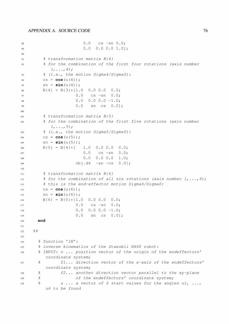
APPENDIX A. SOURCE CODE 76
88 0.0 cs -sn 0.0;89 0.0 0.0 0.0 1.0];90
91 % transformation matrix B{4}92 % for the combination of the first four rotations (axis number
1,...,4);93 % (i.e., the motion Sigma4/Sigma0):94 cs = cos(u(4));95 sn = sin(u(4));96 B{4} = B{3}*[1.0 0.0 0.0 0.0;97 0.0 cs -sn 0.0;98 0.0 0.0 0.0 -1.0;99 0.0 sn cs 0.0];
100
101 % transformation matrix B{5}102 % for the combination of the first five rotations (axis number
1,...,5);103 % (i.e., the motion Sigma5/Sigma0):104 cs = cos(u(5));105 sn = sin(u(5));106 B{5} = B{4}*[ 1.0 0.0 0.0 0.0;107 0.0 cs -sn 0.0;108 0.0 0.0 0.0 1.0;109 obj.d4 -sn -cs 0.0];110
111 % transformation matrix B{6}112 % for the combination of all six rotations (axis number 1,...,6);113 % this is the end-effector motion Sigma6/Sigma0:114 cs = cos(u(6));115 sn = sin(u(6));116 B{6} = B{5}*[1.0 0.0 0.0 0.0;117 0.0 cs -sn 0.0;118 0.0 0.0 0.0 -1.0;119 0.0 sn cs 0.0];120 end121
122 %%123
124 % function ’IK’:125 % inverse kinematics of the Staeubli RX60 robot:126 % INPUT: o ... position vector of the origin of the endeffectors’
coordinate system;127 % f1... direction vector of the x-axis of the endeffectors’
coordinate system;128 % f2... another direction vector parallel to the xy-plane129 % of the endeffectors’ coordinate system;130 % u ... a vector of 6 start values for the angles u1, ...,
u6 to be found

APPENDIX A. SOURCE CODE 77
131 % OUTPUT: 6x(nos)-matrix U (nos = number of solutions),132 % each of its columns contains a solution133 % 6-tupel u_1, ..., u_6 for the rotation angles";134 % integer value j0, index of the solution 6-tupel closest
to u135 function [j0, U] = IK(obj, o, f1, f2, u)136
137 % local U123, U, nos123, nos1232, nos, dist1_sq, dist2_sq, indic,138 % i, j, j0, j1, j2, insideSphere, m, n, phi, o3, sol, v1, v2,
v3,139 % sn1, cs1, sn23, cs23, sn4, cs4, sn5, cs5, sn6, cs6,140 % e, denom, fak, csw, snw, w, dist, dist1, res;141
142 dist1_sq = o(1)ˆ2 + o(2)ˆ2;143 dist2_sq = dist1_sq + (o(3)-obj.d1)ˆ2;144
145 if (dist1_sq > obj.rMinusEps_sq) && (dist2_sq < obj.RPlusEps_sq)% point o is in workspace
146 insideSphere = false;147 if (dist1_sq < obj.rPlusEps_sq) % o lies on the boundary
cylinder148 if (dist2_sq > obj.RMinusEps_sq) % o lies on the upper or
lower boundary circle149 nos123 = 1;150 U123 = zeros(3, 1);151 U123(1,1) = atan2(-o(1), o(2));152 if (abs(o(3) - obj.d1 - obj.a2 - obj.d4) < 0.001) % o lies
on the upper boundary circle153 U123(2,1) = 0.0;154 else % o lies on
the lower boundary circle155 U123(2,1) = pi;156 end157 U123(3,1) = 0.0;158 else % o lies on the boundary cylinder AND inside
the boundary sphere159 v1(1) = atan2(-o(1), o(2));160 nos123 = 2;161 U123 = zeros(3, nos123);162 U123(1,1) = v1(1);163 U123(1,2) = U123(1,1);164 insideSphere = true;165 end166 else % o lies outside the boundary cylinder167 %v1 = solve(o(1)*sin(u1) - o(2)*cos(u1) + d(2), u1);168 alph = atan2(-o(1), o(2));169 bet = atan2(sqrt(dist1_sq - obj.d2_sq), obj.d2);170 v1(1) = alph - bet;
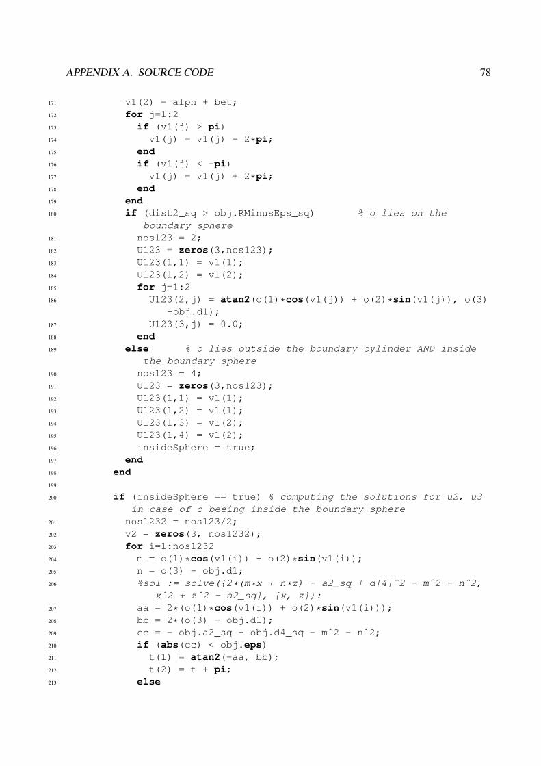
APPENDIX A. SOURCE CODE 78
171 v1(2) = alph + bet;172 for j=1:2173 if (v1(j) > pi)174 v1(j) = v1(j) - 2*pi;175 end176 if (v1(j) < -pi)177 v1(j) = v1(j) + 2*pi;178 end179 end180 if (dist2_sq > obj.RMinusEps_sq) % o lies on the
boundary sphere181 nos123 = 2;182 U123 = zeros(3,nos123);183 U123(1,1) = v1(1);184 U123(1,2) = v1(2);185 for j=1:2186 U123(2,j) = atan2(o(1)*cos(v1(j)) + o(2)*sin(v1(j)), o(3)
-obj.d1);187 U123(3,j) = 0.0;188 end189 else % o lies outside the boundary cylinder AND inside
the boundary sphere190 nos123 = 4;191 U123 = zeros(3,nos123);192 U123(1,1) = v1(1);193 U123(1,2) = v1(1);194 U123(1,3) = v1(2);195 U123(1,4) = v1(2);196 insideSphere = true;197 end198 end199
200 if (insideSphere == true) % computing the solutions for u2, u3in case of o beeing inside the boundary sphere
201 nos1232 = nos123/2;202 v2 = zeros(3, nos1232);203 for i=1:nos1232204 m = o(1)*cos(v1(i)) + o(2)*sin(v1(i));205 n = o(3) - obj.d1;206 %sol := solve({2*(m*x + n*z) - a2_sq + d[4]ˆ2 - mˆ2 - nˆ2,
xˆ2 + zˆ2 - a2_sq}, {x, z}):207 aa = 2*(o(1)*cos(v1(i)) + o(2)*sin(v1(i)));208 bb = 2*(o(3) - obj.d1);209 cc = - obj.a2_sq + obj.d4_sq - mˆ2 - nˆ2;210 if (abs(cc) < obj.eps)211 t(1) = atan2(-aa, bb);212 t(2) = t + pi;213 else

APPENDIX A. SOURCE CODE 79
214 alph = atan2(-bb/cc, -aa/cc);215 bet = atan2(sqrt(obj.a2_sq*(aaˆ2 + bbˆ2) - ccˆ2)/abs(cc),
1);216 t(1) = alph-bet;217 t(2) = alph+bet;218 end219
220 for j=1:2221 %o3 := <subs(sol[j], x), subs(sol[j], z)>:222 o3 = obj.a2*[cos(t(j)); sin(t(j))];223 v2(i,j) = atan2(o3(1), o3(2));224 phi = atan2(m-o3(1), n-o3(2));225 v3(i,j) = phi - v2(i,j);226 end227 end228 U123(2,1) = v2(1,1);229 U123(2,2) = v2(1,2);230 U123(3,1) = v3(1,1);231 U123(3,2) = v3(1,2);232 if (nos123 == 4)233 U123(2,3) = v2(2,1);234 U123(2,4) = v2(2,2);235 U123(3,3) = v3(2,1);236 U123(3,4) = v3(2,2);237 end238 end239
240
241 %%%%%%%%%%%%%%%%%%%%%%%%%%%%%%%%%%%%%%%%%%%%%%%242 %%% Berechnung der Loesungen fuer u_4, u_5, u_6;243 %%%%%%%%%%%%%%%%%%%%%%%%%%%%%%%%%%%%%%%%%%%%%%%244
245 nos = 2*nos123;246 U = zeros(6,nos);247
248 e61 = f1/norm(f1);249 e63 = cross(f1, f2);250 e63 = e63/norm(e63);251 e62 = cross(e63, e61);252 for j=1:nos123253 j2 = 2*j;254 j1 = j2-1;255 for i=1:3256 U(i,j1) = U123(i,j);257 U(i,j2) = U123(i,j);258 end259 sn1 = sin(U123(1,j));260 cs1 = cos(U123(1,j));
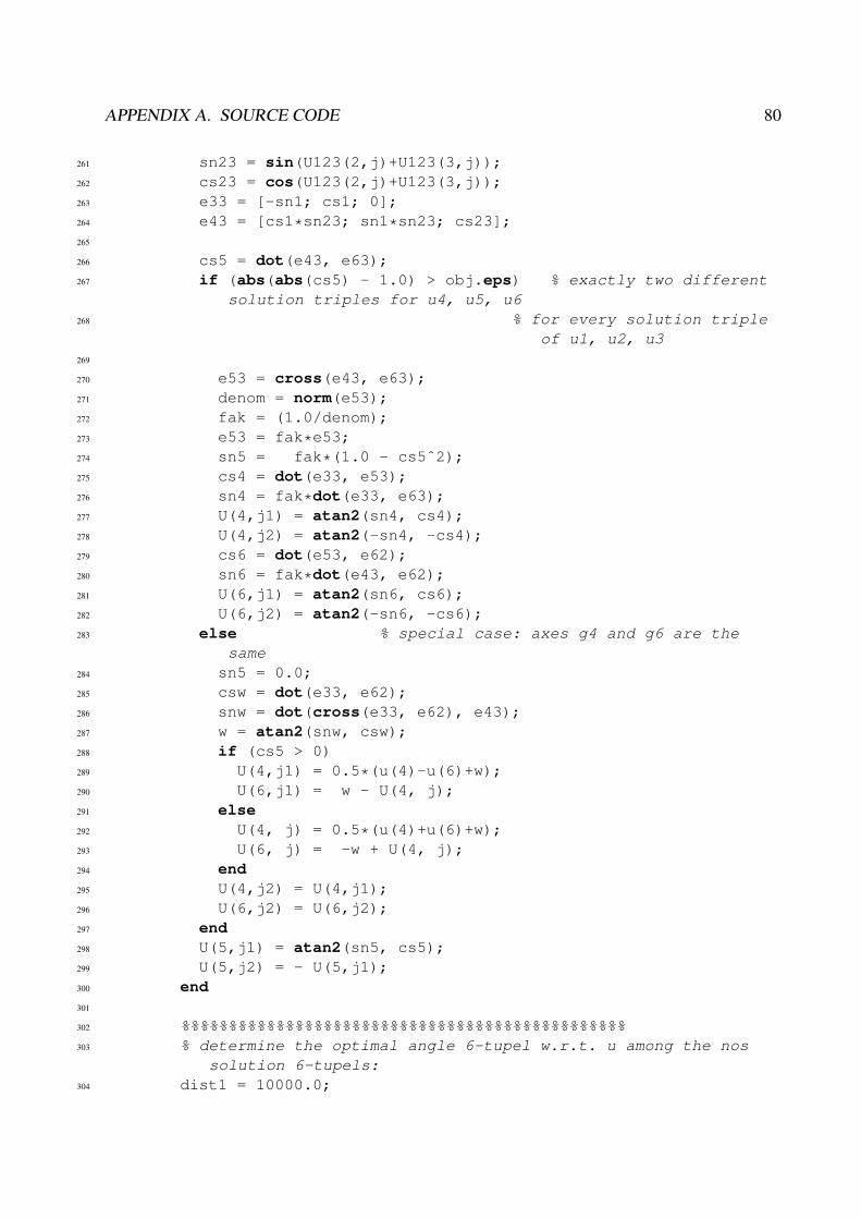
APPENDIX A. SOURCE CODE 80
261 sn23 = sin(U123(2,j)+U123(3,j));262 cs23 = cos(U123(2,j)+U123(3,j));263 e33 = [-sn1; cs1; 0];264 e43 = [cs1*sn23; sn1*sn23; cs23];265
266 cs5 = dot(e43, e63);267 if (abs(abs(cs5) - 1.0) > obj.eps) % exactly two different
solution triples for u4, u5, u6268 % for every solution triple
of u1, u2, u3269
270 e53 = cross(e43, e63);271 denom = norm(e53);272 fak = (1.0/denom);273 e53 = fak*e53;274 sn5 = fak*(1.0 - cs5ˆ2);275 cs4 = dot(e33, e53);276 sn4 = fak*dot(e33, e63);277 U(4,j1) = atan2(sn4, cs4);278 U(4,j2) = atan2(-sn4, -cs4);279 cs6 = dot(e53, e62);280 sn6 = fak*dot(e43, e62);281 U(6,j1) = atan2(sn6, cs6);282 U(6,j2) = atan2(-sn6, -cs6);283 else % special case: axes g4 and g6 are the
same284 sn5 = 0.0;285 csw = dot(e33, e62);286 snw = dot(cross(e33, e62), e43);287 w = atan2(snw, csw);288 if (cs5 > 0)289 U(4,j1) = 0.5*(u(4)-u(6)+w);290 U(6,j1) = w - U(4, j);291 else292 U(4, j) = 0.5*(u(4)+u(6)+w);293 U(6, j) = -w + U(4, j);294 end295 U(4,j2) = U(4,j1);296 U(6,j2) = U(6,j2);297 end298 U(5,j1) = atan2(sn5, cs5);299 U(5,j2) = - U(5,j1);300 end301
302 %%%%%%%%%%%%%%%%%%%%%%%%%%%%%%%%%%%%%%%%%%%%%%%303 % determine the optimal angle 6-tupel w.r.t. u among the nos
solution 6-tupels:304 dist1 = 10000.0;
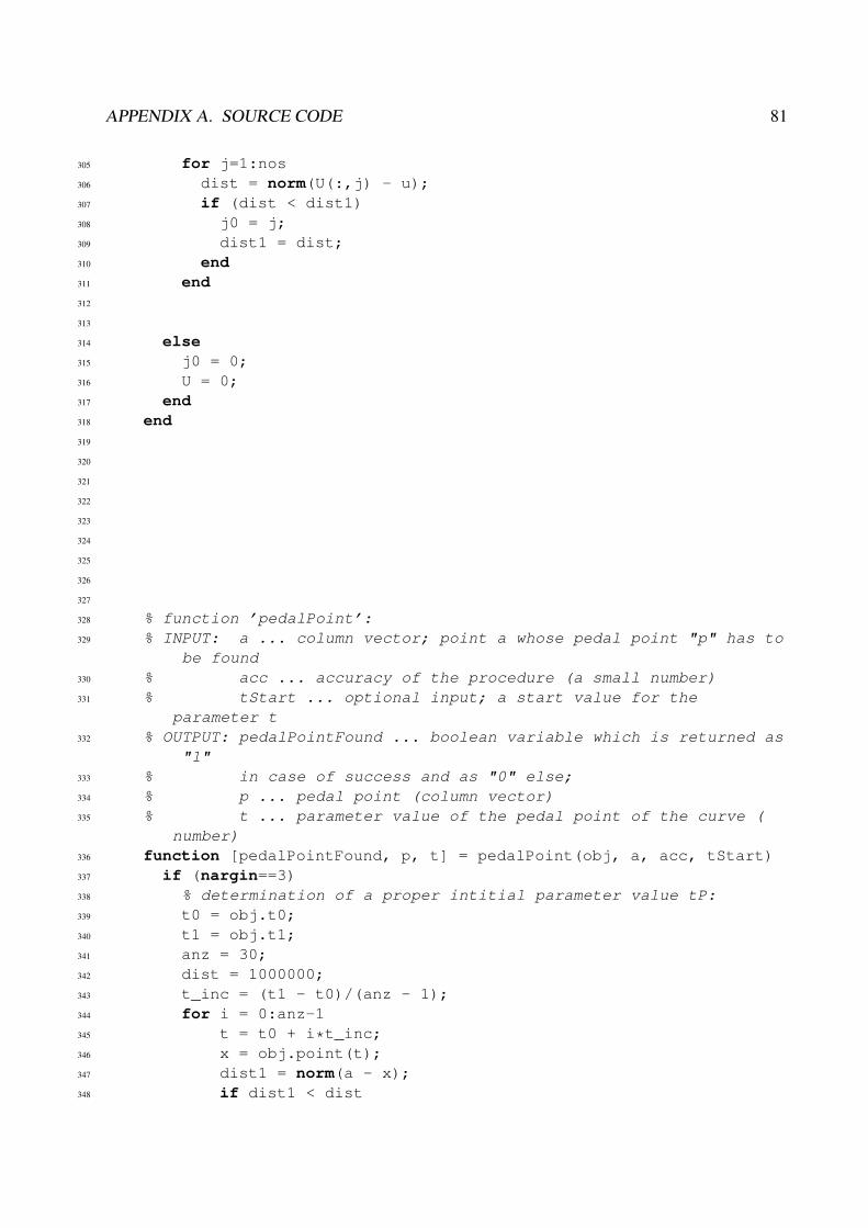
APPENDIX A. SOURCE CODE 81
305 for j=1:nos306 dist = norm(U(:,j) - u);307 if (dist < dist1)308 j0 = j;309 dist1 = dist;310 end311 end312
313
314 else315 j0 = 0;316 U = 0;317 end318 end319
320
321
322
323
324
325
326
327
328 % function ’pedalPoint’:329 % INPUT: a ... column vector; point a whose pedal point "p" has to
be found330 % acc ... accuracy of the procedure (a small number)331 % tStart ... optional input; a start value for the
parameter t332 % OUTPUT: pedalPointFound ... boolean variable which is returned as
"1"333 % in case of success and as "0" else;334 % p ... pedal point (column vector)335 % t ... parameter value of the pedal point of the curve (
number)336 function [pedalPointFound, p, t] = pedalPoint(obj, a, acc, tStart)337 if (nargin==3)338 % determination of a proper intitial parameter value tP:339 t0 = obj.t0;340 t1 = obj.t1;341 anz = 30;342 dist = 1000000;343 t_inc = (t1 - t0)/(anz - 1);344 for i = 0:anz-1345 t = t0 + i*t_inc;346 x = obj.point(t);347 dist1 = norm(a - x);348 if dist1 < dist

APPENDIX A. SOURCE CODE 82
349 tP = t;350 dist = dist1;351 end352 end353 else354 % using the intial parameter value "tStart" prescribed by the
user:355 tP = tStart;356 end357
358 t = tP;359 x = obj.point(t);360 c = a - x;361
362 delta = 0.0001;363 xt = obj.tangentVector(t, delta);364
365 cs = dot(c, xt);366
367 eps = abs(cs);368
369 zaehler = 1;370 maxSteps = 20;371 while (eps > acc) && (zaehler < maxSteps)372 % 2nd derivative vector373 xtt = obj.derivativeVector(t, 2, delta);374
375 % 1st derivative of the function cs(t) = <a - x(t), xt(t)>376 % to find the root of this function:377 cst = - dot(xt, xt) + dot(c, xtt);378
379 epsilon = 0.0001;380 if abs(cst) < epsilon381 if cst < 0382 cst = -epsilon;383 else384 cst = epsilon;385 end386 end387
388 % new t389 t = t - cs/cst;390 x = obj.point(t);391 c = a - x;392 xt = obj.tangentVector(t, delta);393 cs = dot(c, xt);394
395 eps = abs(cs);

APPENDIX A. SOURCE CODE 83
396
397 p = x;398 zaehler = zaehler + 1;399 end400 if zaehler == maxSteps401 pedalPointFound = false;402 else403 pedalPointFound = true;404 end405 end406
407 end408 end

APPENDIX A. SOURCE CODE 84
A.4 Statediagram of the RobotControl Task
Fig
ure
A.2
:S
tate
dia
gra
mfo
rth
eR
obot
Contr
ol
Tas
k
List of Figures
1.1 Derivation of rotation matrix . . . . . . . . . . . . . . . . . . . . . . . . . . . . . 10
1.2 Rotation of the coordinate frame Σ about z axis. . . . . . . . . . . . . . . . . . . . 12
1.3 Euler-rotation in zyx order . . . . . . . . . . . . . . . . . . . . . . . . . . . . . . 14
1.4 Roll-pitch-yaw-Rotation in ZYX order . . . . . . . . . . . . . . . . . . . . . . . . 17
1.5 Axis angle rotation . . . . . . . . . . . . . . . . . . . . . . . . . . . . . . . . . . 18
1.6 Axis of the axis angle rotation . . . . . . . . . . . . . . . . . . . . . . . . . . . . 19
1.7 Graphical representation of the homogeneous coordinates . . . . . . . . . . . . . . 22
1.8 Similarity transform for Staubli RX60 with tool . . . . . . . . . . . . . . . . . . . 23
1.9 Screw . . . . . . . . . . . . . . . . . . . . . . . . . . . . . . . . . . . . . . . . . 24
1.10 Plucker-coordinates for a screw . . . . . . . . . . . . . . . . . . . . . . . . . . . . 25
2.1 Definition of the Denavit-Hartenberg paramter . . . . . . . . . . . . . . . . . . . . 28
2.2 Denavit-Hartenberg parameters of Staubli RX60 . . . . . . . . . . . . . . . . . . 29
3.1 Home position of the Staubli RX60 . . . . . . . . . . . . . . . . . . . . . . . . . . 33
4.1 Overview of solution methods for the inverse kinematics. . . . . . . . . . . . . . . 34
4.2 Robot configurations of the geometric solution . . . . . . . . . . . . . . . . . . . . 36
5.1 Simulation environment of the B&R robotic project. . . . . . . . . . . . . . . . . . 44
5.2 Schematic diagram of the OPC-interface. . . . . . . . . . . . . . . . . . . . . . . 47
5.3 Structure diagram of the UDP-interface. . . . . . . . . . . . . . . . . . . . . . . . 48
5.4 PLCopen function block cyclic velocity. . . . . . . . . . . . . . . . . . . . . . . . 49
5.5 PLCopen function block cyclic position. . . . . . . . . . . . . . . . . . . . . . . . 49
6.1 Schematic diagram of the Staubli RX60 controller. . . . . . . . . . . . . . . . . . 51
6.2 A priori test of the hardeware components. . . . . . . . . . . . . . . . . . . . . . . 52
6.3 Function diagram of the APC810. . . . . . . . . . . . . . . . . . . . . . . . . . . 52
85

LIST OF FIGURES 86
7.1 Overview of the controller concept. . . . . . . . . . . . . . . . . . . . . . . . . . 56
7.2 Interpolation concept for the Staubli RX60 . . . . . . . . . . . . . . . . . . . . . . 58
7.3 Safety PLC diagram . . . . . . . . . . . . . . . . . . . . . . . . . . . . . . . . . . 60
8.1 Theoretical workspace of the Staubli RX60 . . . . . . . . . . . . . . . . . . . . . 65
A.1 Simulink model for the test of the kinematics. . . . . . . . . . . . . . . . . . . . . 73
A.2 Statediagram for the Robot Control Task . . . . . . . . . . . . . . . . . . . . . . . 84

List of Tables
2.1 Denavit-Hartenberg-parameters for Staubli RX60 . . . . . . . . . . . . . . . . . . 31
5.1 Frequently used G-code commands . . . . . . . . . . . . . . . . . . . . . . . . . . 45
87
Bibliography
[1] J. Angeles. Fundaments of Robotic Mechanical Systems. Springer-Verlag, Berlin, 1997.
[2] F. Chappelle and P. Bidaud. Closed form solution for inverse kinematics approximation of
general 6R manipulators. Mechanism and Machine Theory, 39(1):323–338, 2004.
[3] J. Craig. Intruduction to Robotics. Addison-Wesely Publishing Company, second edition,
1989.
[4] R. Goldman. Understanding quaterions. Graphical Models, 73(1):21–49, 2011.
[5] A.T. Hasan, A.M.S. Hamouda, N. Ismail, and H.M.A.A. Al-Assadi. An adaptiv-learning
algorithm to solve the inverse kinematics problem of a 6 d.o.f serial robot manipulator. Ad-vances in Engineering Software, 37(1):432–438, 2006.
[6] A.T. Hasan, N. Ismail, A.M.S. Hamouda, I. Aris, M.H. Marhaban, and H.M.A.A Al-Assadi.
Artificial neural network-based kinematics Jacobian solution for serial manipulatar passing
through singular configurations. Advances in Engineering Software, 41(1):359–367, 2010.
[7] K.H. Hunt. Don’t cross-thread the screw. Journal of Robotic Systems, 20(7):317–339, 2003.
[8] M. Husty, A. Karger, H. Sachs, and W. Steinhilper. Kinematik und Robotik. Springer-Verlag,
Berlin, 1997.
[9] P. Kalra, P.B. Mahapatra, and D.K. Aggarwal. An evolutionary approach for solving the mul-
timodal inverse kinematics problem of industrial robots. Mechanism and Machine Theory,
41(1):1213–1229, 2006.
[10] B. Karlik and S. Aydin. An improved approach to the solution of inverse kinematics problem
for robot manipulators. Engineering Applications or Artificial Intelligence, 13(1):159–164,
2000.
[11] R. Murray. A Mathematical Introduction to Robotic Manipulation. CRC Press, second edi-
tion, 1994.
[12] S.B. Niku. Intruduction to Robotics:Analysis,Control,Applications. John Wiley and Sons,
second edition, 2010.
[13] S. Qiao, Q. Liao, S. Wei, and H. Su. Inverse kinematic analysis of the general serial ma-
nipulators based on douple quaternions. Mechanism and Machine Theory, 45(1):193–199,
2010.
88

BIBLIOGRAPHY 89
[14] C.R. Rocha, C.P. Tonetto, and A. Dias. A comparison between the Denavit-Hartenber and
the screw-based methods used in kinematic modeling of robot manipulators. Robotics andComputer-Integrated Manifacturing, 27(1):723–728, 2011.
[15] L. Scilavicco and B. Siciliano. Modelling and control of robot manipulators. Springer-Verlag,
London, second edition, 2000.
[16] M.W. Spong, S. Hutchinson, and M. Vidyasagar. Robot Modeling and Control. John Wiley
and Sons,Inc, New Jersey,Hoboken, 2005.
[17] James M Van Verth and Lars M Bishop. Essential mathematics for games and interactiveapplications: a programmer’s Guide. CRC Press, 2008.