Development of a material with reproducible emission of ... Michael Nohr... · emission test...
142
Development of a material with reproducible emission of selected volatile organic compounds Dissertation zur Erlangung des Doktorgrades der Naturwissenschaften (Dr. rer. nat.) der Naturwissenschaftlichen Fakultät II Chemie, Physik und Mathematik der Martin-Luther-Universität Halle-Wittenberg vorgelegt von Herrn Dipl.-Chem. (FH) Michael Nohr geb. am 03.06.1984 in Schkeuditz Gutachter: 1. Prof. Dr. Lorenz, Wilhelm Georg 2. Prof. Dr. Greif, Dieter Verteidigt am 07.11.2014 Halle (Saale), 2015
Transcript of Development of a material with reproducible emission of ... Michael Nohr... · emission test...
Development of a material with reproducible emissio n of
selected volatile organic compounds
Dissertation
zur Erlangung des Doktorgrades der Naturwissenschaften
(Dr. rer. nat.)
der Naturwissenschaftlichen Fakultät II
Chemie, Physik und Mathematik
der
Martin-Luther-Universität
Halle-Wittenberg
vorgelegt
von Herrn Dipl.-Chem. (FH) Michael Nohr
geb. am 03.06.1984 in Schkeuditz
Gutachter:
1. Prof. Dr. Lorenz, Wilhelm Georg
2. Prof. Dr. Greif, Dieter
Verteidigt am 07.11.2014
Halle (Saale), 2015

Für Kristin.
Manchmal sind Umwege der schönere Weg zum Ziel.

Die vorliegende Arbeit entstand an der BAM Bundesanstalt für Materialforschung und
-prüfung.
Veröffentlichungen
IV
Veröffentlichungen
Ergebnisse dieser Arbeit wurden in folgenden Beiträgen veröffentlicht:
M. Nohr, K. Wiegner, M. Richter, W. Horn (2012)
„Development of a reference material for the measurement of (S)VOC in emission
test chambers“
Beitrag zu Tagungsband: HEALTHY BUILDINGS 2012 in Brisbane, Australien
M. Nohr, K. Wiegner, M. Richter, W. Horn (2012)
„Development of a reference material for the measurement of (S)VOC in emission
test chambers“
Poster: HEALTHY BUILDINGS 2012 in Brisbane, Australien
W. Horn (Vortragender), M. Nohr, M. Richter (2013)
„Generation of reproducible chamber concentrations for round robin tests based on
reference materials “
Vortrag: EMISSIONS AND ODOURS FROM MATERIALS 2013 in Brüssel, Belgien
M. Nohr, M. Richter (Vortragender), W. Horn (2013)
„Approach to the Improvement of the traceability for (S)VOC-measurement“
Vortrag: GAS 2013 in Rotterdam, Niederlande
M. Nohr (Vortragender), W. Horn, M. Richter, (2013)
„Entwicklung eines Referenzmaterials mit konstanter Emission flüchtiger organischer
Verbindungen“
Vortrag: 20. WaBoLu Innenraumtage Berlin, Deutschland
Veröffentlichungen
V
M. Nohr, K. Wiegner, M. Richter, W. Horn, W. Lorenz (2014)
„Development of a material with reproducible emission of selected volatile organic
compounds – µ-Chamber study”
Publikation: Chemosphere, Volume 107, July 2014, Pages 224-229
O. Jann (Vortragender), O. Wilke, W. Horn, B. Mull, M. Nohr (2014)
„Materials emissions testing - Measurements for healthy living”
Vortrag: MACPoll Workshop: "Novel (S)VOC gas standards for indoor air monitoring"
2014 Berlin, Deutschland
M. Nohr, M. Richter, W. Horn, B. Mull (2014)
„Development of a reference material for emission testing based on lacquer mixtures”
Poster: MACPoll Final Conference 2014 Delft, Niederlande
M. Nohr, M. Richter, W. Horn, B. Mull (2014)
„Development of a reference material for emission testing based on lacquer mixtures”
Poster: INDOOR AIR 2014 Hong Kong
M. Nohr, W. Horn, O. Jann, M. Richter, W. Lorenz (2014)
„Development of a multi-VOC reference material for quality assurance in materials
emission testing”
Publikation: Analytical and Bioanalytical Chemistry, available online, DOI:
10.1007/s00216-014-8387-2
Danksagung
VI
Danksagung
Ich möchte mich an dieser Stelle bei allen Personen bedanken, die dazu beigetragen
haben, dass diese Arbeit entstehen konnte.
Auf dem steinigen Weg Richtung Promotionsstelle gehört mein erster Dank Prof. Dr.
Wilhelm Georg Lorenz. Ohne sein schnelles Einverständnis zur Übernahme der
Betreuung seitens der Martin-Luther-Universität Halle-Wittenberg wäre das
Promotionsvorhaben schon vorab gescheitert.
Im gleichen Atemzug möchte ich Dr. Oliver Jann, Dr. Katharina Wiegner, Dr.
Wolfgang Horn und Dr. Matthias Richter seitens der BAM Bundesanstalt für
Materialforschung und -prüfung dafür danken, dass sie das Thema, die Finanzierung
und den Arbeitsplatz bereitgestellt haben. Selbst als es aus mehreren
Gesichtspunkten schlecht um eine Promotionsstelle aussah, haben sie sich
aufopferungsvoll weiter darum gekümmert.
Ebenfalls möchte ich mich bei allen Mitarbeitern der Fachgruppe 4.2 der BAM für das
gute Arbeitsklima bedanken. Besonders hervorheben möchte ich dabei Lars Pyza,
der auf alle technischen und physikalischen Fragen in kürzester Zeit praktikable
Antworten und Lösungen bereitstellte - viele davon werde ich wohl nie verstehen.
Sabine Kalus und Doris Brödner seien dafür gedankt, dass sie mich in analytischen
Problemstellungen stets unterstützt, und meine Messgeräte mit manch
hervorgezauberten Ersatzteilen am Leben erhalten haben. Schlussendlich möchte
ich noch meiner Büronachbarin Frau Dr. Birte Mull dafür danken, dass Sie stets
meine organisatorischen und raumklimatischen Unzulänglichkeiten ausgebügelt hat.
Prof. Dr. Dieter Greif von der Hochschule Zittau/Görlitz möchte ich für die
Übernahme der Zweitkorrektur danken. Ebenfalls verdanke ich der Hochschule ein
breites Fachwissen, dass ich während meiner Ausbildung zum Dipl.-Chem. (FH)
erhalten habe. Hier sei auch die Team Umweltanalytik GmbH (Ebersbach, Sa.) und
die Arbeitsgruppe organische Analytik des Helmholtz Zentrum für Umweltforschung
(UFZ, Leipzig) erwähnt, die mir in Praxis- und Diplomsemester ein sehr gutes
analytisches Fundament für meinen weiteren Werdegang vermittelt haben.
Danksagung
VII
Frau Heather Dickens danke ich dafür, dass sie mir geholfen hat, mein Vorhaben die
Dissertation in Englisch zu verfassen, umzusetzen. Für die Zweitkorrektur sei
ebenfalls Marc Leopold genannt.
Vielen Dank auch an Kai Meine und Hendrik Rönnfeldt von der Firma KEYENCE für
die kurzfristige Bereitstellung des VR 3000 Digitalmakroskops für die Vermessung
der Lackoberflächen.
Natürlich möchte ich mich auch bei meinen Freunden außerhalb der Universität
bedanken, die mich auf meinem Weg begleitet haben. Für die vielen Hinweise sei Dr.
Christian Albrecht hier gesondert genannt.
Meinen Eltern gehört mein tiefster Dank dafür, dass sie für meine Bildung sehr viel
Geld, Nerven und Zeit investiert haben. Ohne ihr Engagement wäre an eine
Promotion nie zu denken gewesen.
Schlussendlich danke ich meiner Frau Kristin. Durch ihre positive Art hat sie mich nie
am Gelingen dieser Arbeit zweifeln lassen und mich jeden Tag, auch wenn ich dem
Wahnsinn nahe war, motiviert und unterstützt.
Abstract
VIII
Abstract
Building products and furniture are sources for indoor air pollutants. They emit
volatile organic compounds (VOCs) which can affect human health. To investigate,
the emission potential test specimens of building products are loaded into chambers
which provide climate conditions close to that of indoor air. Here the samples emit
VOCs which can be analysed by sampling air from the chamber onto adsorbent
tubes and transferring them onto a measurement device.
To gain reliable results for this complex testing method reference materials are
necessary. To address the lack of such references in emission testing, the present
study focussed on the development of an artificial material with reproducible VOC
emissions. Therefore a lacquer was mixed with the substances of interest.
Afterwards, the mixture was cured under constant conditions and loaded into
emission test chambers.
The emissions in the different chambers showed variations in the range of 10 % for
common indoor air pollutants like hexanal, styrene, decane, naphthalene, limonene
and hexadecane.
Zusammenfassung
IX
Zusammenfassung
Bauprodukte und Möbel sind Quellen für Schadstoffe im Innenraum. Sie emittieren
leichtflüchtige organische Verbindungen (volatile organic compounds VOCs), welche
einen negativen Einfluss auf die menschliche Gesundheit haben können. Um dieses
Gefahrenpotential einschätzen zu können, werden Materialproben von Bauprodukten
und Möbeln in Testkammern beladen, die konstante klimatische Bedingung bieten,
die auch im Innenraum vorherrschen. In diesen Kammern emittieren die Proben
VOCs, welche auf Adsorbentien gefangen und in Messgeräten analysiert werden
können.
Um bei dieser komplexen Testmethode verlässliche Werte zu generieren, werden
Referenzmaterialen benötigt. Da es aktuell in diesem Feld nur sehr wenig
Referenzmaterialen gibt, befasst sich die vorliegende Arbeit mit der Entwicklung
eines künstlichen Materials, welches VOCs reproduzierbar emittiert. Dafür wird ein
flüssiger Lack mit ausgewählten Luftschadstoffen verrührt. Danach wird die
Mischung unter konstanten Bedingungen ausgehärtet und in
Emissionsmesskammern beladen.
Für typische Schadstoffe wie Hexanal, Styren, Decan, Naphthalin, Limonen und
Hexadecan zeigt die Emission des Materials in verschiedenen Kammern
Abweichungen im Bereich von 10 %.
Table of contents
X
Table of contents Veröffentlichungen ..................................................................................................... IV
Danksagung .............................................................................................................. VI Abstract ................................................................................................................... VIII Zusammenfassung .................................................................................................... IX
Table of contents ........................................................................................................ X
1 Introduction .......................................................................................................... 1
2 Motivation and theoretical background ................................................................ 2
2.1 Material emission........................................................................................... 2
2.1.1 General aspects ...................................................................................... 2
2.1.2 Emission modelling ................................................................................. 3
2.2 Emission testing ............................................................................................ 5
2.3 Challenges in emission testing ...................................................................... 9
2.3.1 Reference materials in emission testing - state of the art ..................... 10
2.3.2 Problem-solving approach .................................................................... 12
3 Materials, chemicals and methods .................................................................... 13
3.1 Materials and chemicals .............................................................................. 13
3.1.1 TD-GC/MS ............................................................................................ 13
3.1.2 Emission test chambers ........................................................................ 14
3.1.3 Lacquers ............................................................................................... 18
3.1.4 Chemicals ............................................................................................. 20
3.2 Methods ....................................................................................................... 22
3.2.1 TD-GC/MS ............................................................................................ 22
3.2.2 Calibration ............................................................................................. 26
3.2.3 Quantification ........................................................................................ 26
3.2.4 Lacquer preparation .............................................................................. 27
3.2.5 Sampling ............................................................................................... 30
3.2.6 Uncertainty ............................................................................................ 30
4 Experimental ..................................................................................................... 35
4.1 Preliminary testing ....................................................................................... 35
4.1.1 Chamber selection ................................................................................ 35
4.1.2 Lacquer selection .................................................................................. 37
4.1.3 Increasing the SVOC emission ............................................................. 39
4.1.4 Optimisation of the lindane-spiking ....................................................... 39
4.1.5 Influence of methanol ............................................................................ 40
4.1.6 Stability testing I .................................................................................... 41
4.2 Optimisation of the curing process .............................................................. 42
4.2.1 Curing process in the µ-CTE ................................................................. 42
4.2.2 Curing process for the desiccator ......................................................... 44
4.2.3 Stability testing II ................................................................................... 45
4.2.4 Influence on emissions at different chamber flows ................................ 46
4.2.5 Influence on emission at different humidities ........................................ 47
4.3 Round robin test optimisation ...................................................................... 48
4.3.1 Additional analytes and optimal spiking amounts.................................. 49
4.3.2 Shipping and storage ............................................................................ 49
4.3.3 Stability testing III .................................................................................. 50
5 Results and Discussion ..................................................................................... 53
5.1 Preliminary testing ....................................................................................... 53
5.1.1 Chamber selection ................................................................................ 53
Table of contents
XI
5.1.2 Lacquer selection .................................................................................. 54
5.1.3 Increasing the SVOC emission ............................................................. 59
5.1.4 The influence of methanol ..................................................................... 61
5.1.5 Interim conclusion I ............................................................................... 66
5.1.6 First stability testing .............................................................................. 67
5.2 Curing .......................................................................................................... 69
5.2.1 Curing process in the µ-CTE ................................................................. 69
5.2.2 Curing process for the desiccator ......................................................... 72
5.2.3 Stability testing II ................................................................................... 75
5.2.4 Curing at different chamber flows ......................................................... 77
5.2.5 Curing at different humidities ................................................................ 80
5.2.6 Interim conclusion II .............................................................................. 83
5.3 Round robin test optimisation ...................................................................... 86
5.3.1 Optimal Spiking ..................................................................................... 86
5.3.2 Shipping and storage ............................................................................ 87
5.3.3 Stability testing III .................................................................................. 89
6 Conclusion and Outlook .................................................................................... 92
7 Literature ........................................................................................................... 94
8 Appendix ........................................................................................................... 98
8.1 Abbreviations ............................................................................................... 98
8.2 List of figures ............................................................................................. 100
8.3 List of tables .............................................................................................. 103
8.4 Additional measurement data .................................................................... 105
8.4.1 Calibration data ................................................................................... 105
8.4.2 Chapter 4.1.1 ...................................................................................... 112
8.4.3 Chapter 4.1.2 ...................................................................................... 113
8.4.4 Chapter 4.1.3 ...................................................................................... 116
8.4.5 Chapter 4.1.4 ...................................................................................... 117
8.4.6 Chapter 5.2.1 ...................................................................................... 120
8.4.7 Chapter 5.2.2 ...................................................................................... 122
8.4.8 Chapter 5.2.4 ...................................................................................... 124
8.4.9 Chapter 5.2.5 ...................................................................................... 126
9 Eidesstattliche Erklärung ................................................................................. 128
10 Lebenslauf .................................................................................................... 129


1 Introduction
1
1 Introduction Several investigations indicate that building products and furniture can emit harmful
substances called volatile organic compounds (VOC). As between 15 and 16 hours
per day [1] is spent indoors it is thought that this could cause a significant impact on
human health.
To assess whether or not this risk is significant, identification of harmful substances
from building products is essential. Therefore, specialised environmental laboratories
analyse organic air pollutants either by investigating the room in question directly or
by analysing emissions from several building products and furnishings. As the
composition of every room is unique the latter method is more practical. The results
of such measurements are important to identify sources of harmful emissions and to
categorise products according to their emission behaviour.
The performance of environmental laboratories is usually controlled by round robin
tests. Reference materials with identical properties are sent to the participants who
analyse the samples under prescribed conditions. The results from the different
laboratories are collected and statistical evaluated. In the case of emission testing
from building materials and furnishing there is a lack of applicable references.
To solve this issue, an artificial reference material based on a lacquer will be
investigated in this study. To ensure the homogeneity of the material, the liquid
lacquer will be mixed with the investigated substances. After a certain amount of
time, the lacquer-analyte-system changes its physical condition from liquid to solid
and after loading it into emission test chambers it should show a reproducible
emission profile.
2 Motivation and theoretical background
2
2 Motivation and theoretical background This chapter introduces the need for reference materials in emission testing. In order
to facilitate comprehension of the following experiments and discussion some
theoretical background is given.
In chapter 2.1.1 and 2.1.2 the process of emission is introduced in general. Part 2.2
turns the focus on the complex process of emission testing. The effect of possible
sources deteriorating the method reproducibility is also described.
In chapter 2.3.1 reference materials as an essential tool to improve the quality of
emission testing are described. Part 2.3.2 presents the innovative approach for a
new material as central focus of this study.
Finally chapter 3.1.2 to 3.1.3 provide a theoretical overview of the analytical
equipment and lacquers used.
2.1 Material emission
2.1.1 General aspects An emission is the release of substances or radiation of a material. In the context of
the present study this means the exhalation of mostly organic substances. These
pollutants can be natural compounds of the material itself, like terpenes from wood.
In addition they can have their origin in the manufacturing process like plasticisers or
solvents in synthetic materials.
Beside these primary pollutant emissions secondary emissions may occur over time.
For example, the emission of alcohols, aldehydes and carboxylic acids are oxidation
products from the material itself in the presence of oxygen or ozone (see Wolkoff [2]).
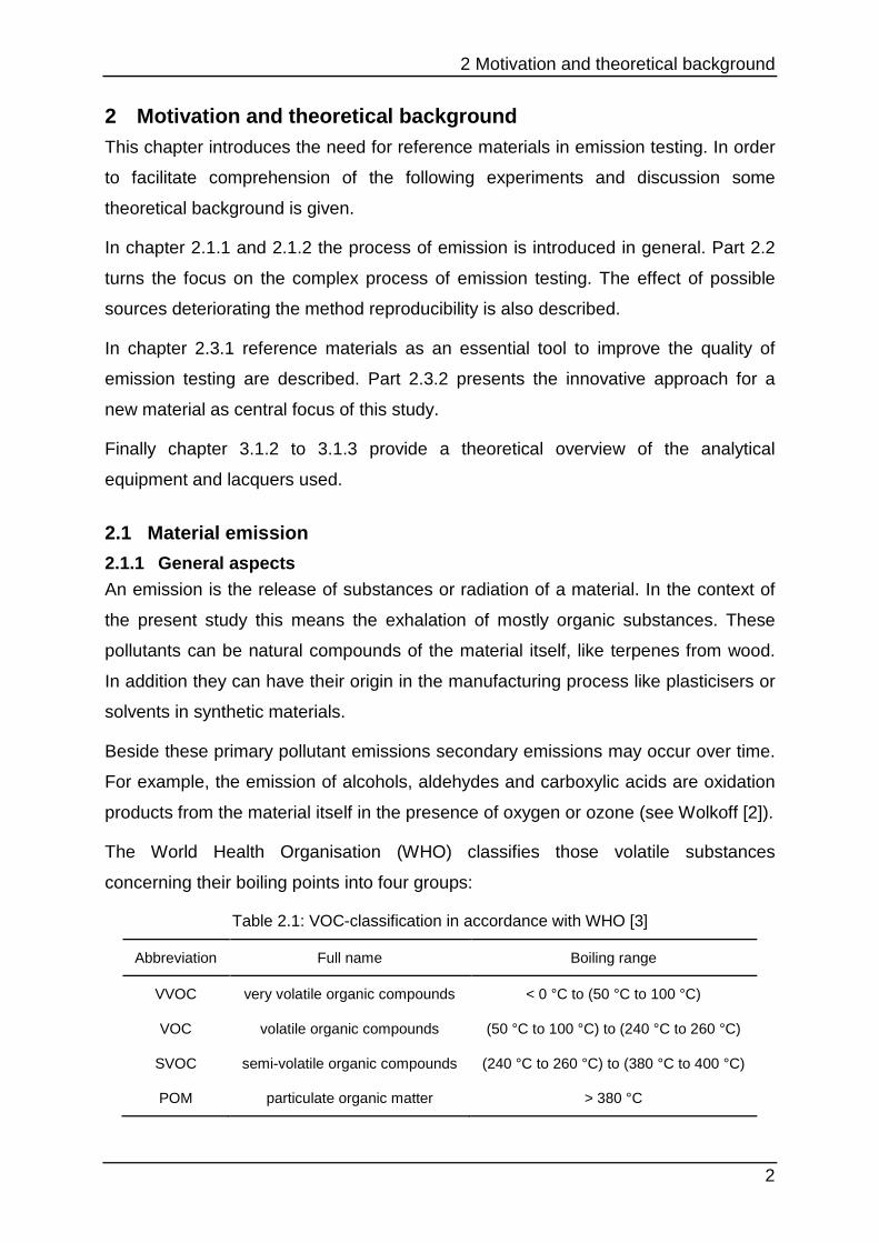
The World Health Organisation (WHO) classifies those volatile substances
concerning their boiling points into four groups:
Table 2.1: VOC-classification in accordance with WHO [3]
Abbreviation Full name Boiling range
VVOC very volatile organic compounds < 0 °C to (50 °C to 100 °C)
VOC volatile organic compounds (50 °C to 100 °C) to (240 °C to 260 °C)
SVOC semi-volatile organic compounds (240 °C to 260 °C) to (380 °C to 400 °C)
POM particulate organic matter > 380 °C
2 Motivation and theoretical background
3
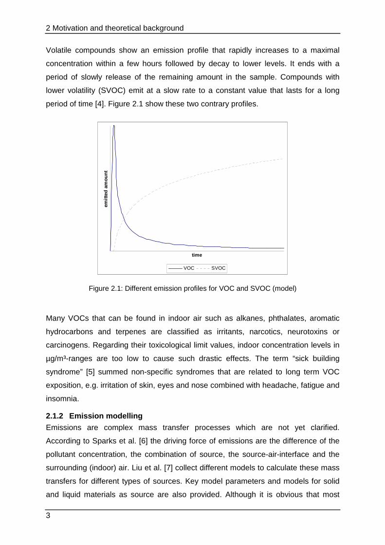
Volatile compounds show an emission profile that rapidly increases to a maximal
concentration within a few hours followed by decay to lower levels. It ends with a
period of slowly release of the remaining amount in the sample. Compounds with
lower volatility (SVOC) emit at a slow rate to a constant value that lasts for a long
period of time [4]. Figure 2.1 show these two contrary profiles.
time
emitt
ed a
mou
nt
VOC SVOC
Figure 2.1: Different emission profiles for VOC and SVOC (model)
Many VOCs that can be found in indoor air such as alkanes, phthalates, aromatic
hydrocarbons and terpenes are classified as irritants, narcotics, neurotoxins or
carcinogens. Regarding their toxicological limit values, indoor concentration levels in
µg/m³-ranges are too low to cause such drastic effects. The term “sick building
syndrome” [5] summed non-specific syndromes that are related to long term VOC
exposition, e.g. irritation of skin, eyes and nose combined with headache, fatigue and
insomnia.
2.1.2 Emission modelling
Emissions are complex mass transfer processes which are not yet clarified.
According to Sparks et al. [6] the driving force of emissions are the difference of the
pollutant concentration, the combination of source, the source-air-interface and the
surrounding (indoor) air. Liu et al. [7] collect different models to calculate these mass
transfers for different types of sources. Key model parameters and models for solid
and liquid materials as source are also provided. Although it is obvious that most
2 Motivation and theoretical background
4
building materials are solid, liquid forms also exist, such as wood stains, varnishes
and paints.
As key model parameters for the emission process Liu et al. [7] state the diffusion of
the pollutant inside the source and the partition coefficient of the pollutant
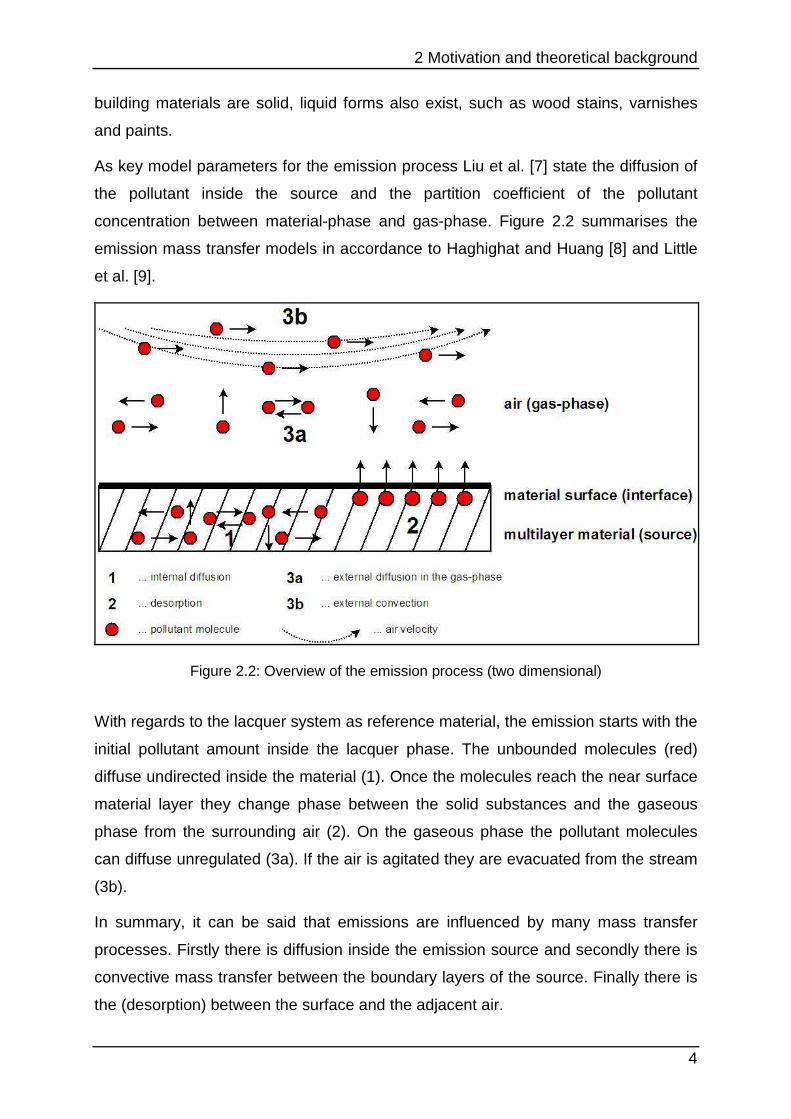
concentration between material-phase and gas-phase. Figure 2.2 summarises the
emission mass transfer models in accordance to Haghighat and Huang [8] and Little
et al. [9].
Figure 2.2: Overview of the emission process (two dimensional)
With regards to the lacquer system as reference material, the emission starts with the
initial pollutant amount inside the lacquer phase. The unbounded molecules (red)
diffuse undirected inside the material (1). Once the molecules reach the near surface
material layer they change phase between the solid substances and the gaseous
phase from the surrounding air (2). On the gaseous phase the pollutant molecules
can diffuse unregulated (3a). If the air is agitated they are evacuated from the stream
(3b).
In summary, it can be said that emissions are influenced by many mass transfer
processes. Firstly there is diffusion inside the emission source and secondly there is
convective mass transfer between the boundary layers of the source. Finally there is
the (desorption) between the surface and the adjacent air.
2 Motivation and theoretical background
5
Howard-Reed et al. [10] classify two types of sources of chemical emissions. On the
one hand there is a diffusion-controlled (“dry”) source whereby the emission is mainly
limited by the diffusivity of the pollutant molecules combined with the temperature
and the structure inside the material (see also Meininghaus and Uhde [11]). On the
other hand there are evaporation-controlled (“wet”) sources. In this case the
emissions are mainly limited by the transfer of pollutant molecules from the material
surface to the adjacent air. Here the volatility combined with the air velocity and
turbulence is an important factor.
2.2 Emission testing VOC-exhalations from building materials can be investigated with test chambers
under predefined conditions. The ISO 16000-9 [12] provides standards to determine
emissions from building products and furnishings.
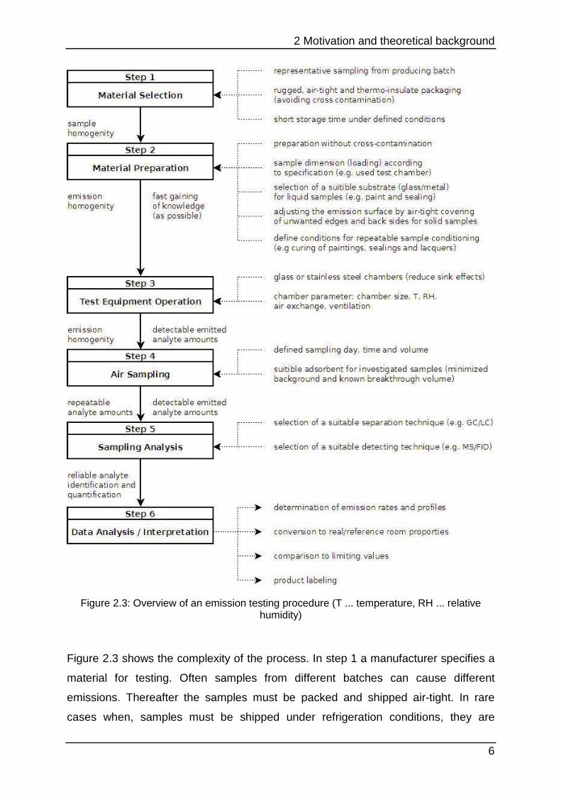
According to Oppl [13] and Howard-Reed et al. [10] emission testing of building
products consists of six main steps. Figure 2.3 shows these steps on the right hand
side. On the left, the important influences are listed. Between the main steps
important requests are shown.
2 Motivation and theoretical background
6
Figure 2.3: Overview of an emission testing procedure (T ... temperature, RH ... relative humidity)
Figure 2.3 shows the complexity of the process. In step 1 a manufacturer specifies a
material for testing. Often samples from different batches can cause different
emissions. Thereafter the samples must be packed and shipped air-tight. In rare
cases when, samples must be shipped under refrigeration conditions, they are
2 Motivation and theoretical background
7
thermo-insulated. This preserves the characteristics of the material, avoids
premature outgoing and cross contamination from the environment. Once the
samples have reached the laboratory they have to be stored under defined
conditions (e.g. refrigerating or at 23 °C and 50 % RH). These requirements ensure
that a representative sample is taken from the manufactured batch.
In step 2 the material has to be prepared for the analysis. This step is closely
associated to step 3 because the dimension of the investigated sample is strictly
related to the size of the desired test chambers in relation to its real room amount.
According to step 1 a clean working environment is necessary to avoid cross
contaminations.
Afterwards the emission surface has to be adjusted. Emission surface is an essential
parameter for emission testing. The loading factor as quotient of the surface (facing
the room) and the room volume shall represent indoor properties. Solid materials like
floorings or wooden particleboards are cut to size. Resulting emitting edges are
sealed (e.g. with aluminium tape). Oppl [13] reported that emission of edges can
differ significantly compared to the top surface. The treatment of liquid materials like
lacquers, paints and sealants are more difficult. Defined amounts of the selected
samples must be applied on a neutral substrate. Zhang and Niu [14] reported that the
substrate can delay and change emissions. They first act as sink and adsorb
analytes from the sample. The bounded substances can then be reemitted from the
substrate (secondary emission). Hence, less-adsorptive substrates like glass or
stainless steel are used. After applying the liquid sample onto a selected substrate
the material must be cured under defined conditions. This process can be realised in
emission test chambers because they provide constant climatic parameters.
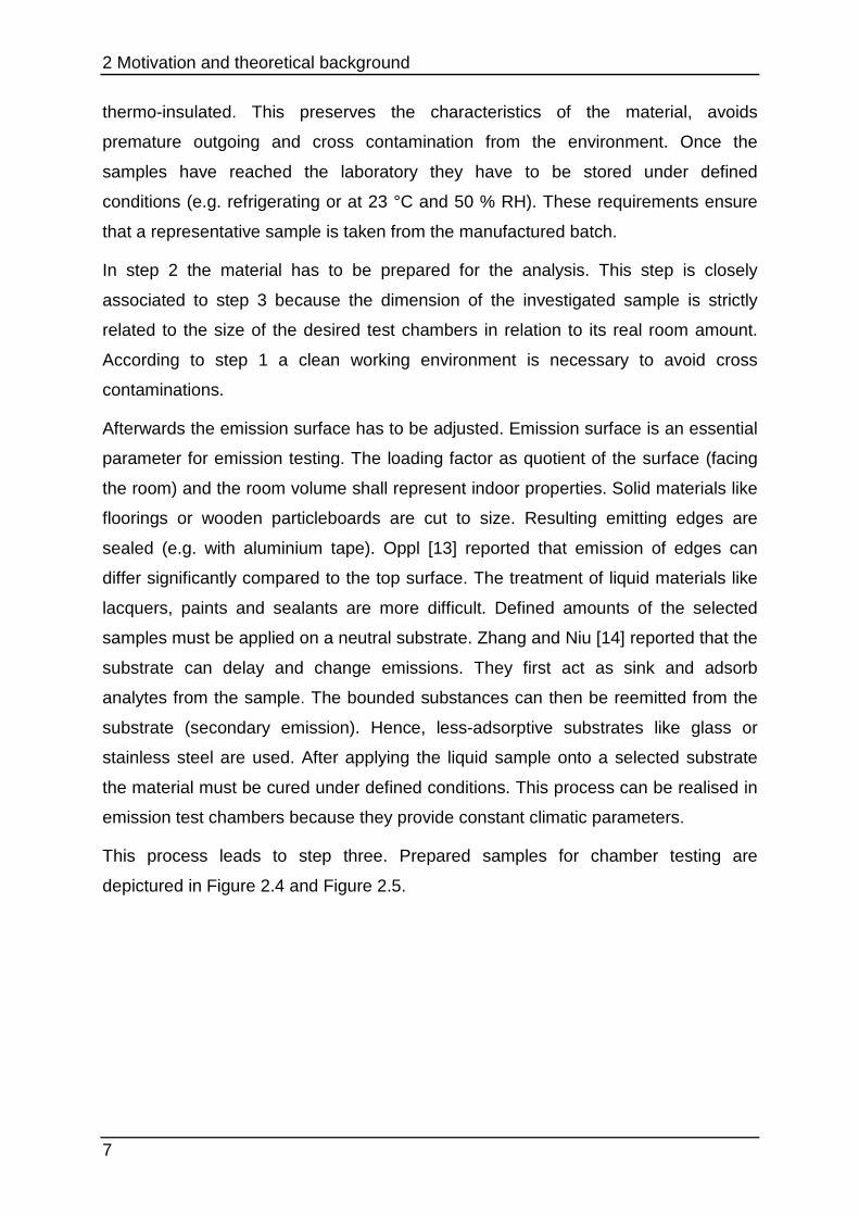
This process leads to step three. Prepared samples for chamber testing are
depictured in Figure 2.4 and Figure 2.5.
2 Motivation and theoretical background
8
Figure 2.4: Test specimen of a carpet with sealed cutting edges (left) and suitable glue
applied on glass (right)
Figure 2.5: Oriented strand boards with sealed cutting edges
Emission test chambers will be discussed further in chapter 3.1.2. They provide a
defined environment for testing. To reduce sink effects they are made of glass or
stainless steel [15]. For the test chamber parameters like humidity, temperature,
ventilation and air change rate can be adjusted to predefined values close to indoor
conditions.
After loading the test specimen into the chamber various substances are emitted.
Under static conditions (without any air exchange) a partition-equilibrium between the
sample and air are established over time for each substance. The concentration
increases steadily until equilibrium is reached. Usually such tests are used to
estimate the maximal air pollutant concentration in a real room without air change
[16]. In reality air change must be taken into consideration. All rooms exchange air
through windows, doors and air conditioning. Dynamic tests with defined chamber-
flows are widely used. In this case the partition equilibrium is interrupted permanently
and the substances emit consecutively from the sample.
Step 4 deals with the air sampling. ISO 16000-9 requires at least two sampling
points. After three days samples are taken for early exposure tests. Long-term
exposure can be investigated from sampling after 28 days. Gas analysis is usually
carried out using gas chromatography (GC, later introduced in chapter 3.1.1).
Sampling tubes with specific adsorbents are used for analyte collection. They
concentrate the organic contaminants by separating them from the inorganic air
compounds. It is a requirement for the adsorbent material to maximise the
2 Motivation and theoretical background
9
accumulation of pollutants on the tube without breakthrough of the compounds in
several litres of air. The tubes are desorbed thermally and the pollutants are
separated from each other in the GC-column.
In step 6 the measurement data are assembled and interpreted. From the air
concentrations at different times emission profiles and rates can be calculated. The
manufacturer needs the outcome of the emission testing process to license their
products if the results undercut limit values outlined in the legislation. The emission
rates and concentrations are also the basis for the evaluation of products like the
“Blue Angel”. Such labels advertise their products against other competitors.
2.3 Challenges in emission testing Comparative measurements on emission testing have previously resulted in
significant variations. Howard-Reed et al. [17] and Horn et al. [18] report coefficient of
variations up to 284 % with an average of greater than 40 % from seven studies that
uses different indoor materials.
There are two main factors inducing these high variations. Firstly there is the
complexity of the emission testing, as described in chapter 2.2. By modifying several
parameters in the process, comparability to other tests are influenced significantly.
For example, this includes different manufacturers and dimensions of the test
chambers or different analysis methods. To address this, standardisation is an
essential tool. It is impractical to develop regulations that match to all existing
materials, chambers and analytes. Hence common standardisation focuses on single
products with defined testing devices and specific compounds. One example is the
“Standard Practice for Determination of Volatile Organic Compounds (Excluding
Formaldehyde) Emissions from Wood-Based Panels Using Small Environmental
Chambers Under Defined Test Conditions” (ASTM D6330 [19]).
The second main influential factor deteriorating the reproducibility of emission testing
is the lack of reference materials. Round robin tests are comparative measurements
between different laboratories evaluating their performance. Reference materials are
necessary to provide all participants with a homogeneous sample with constant
properties. This ensures comparability. As described in chapter 2.2 heterogeneity at
the steps of material selection and preparation affect the testing results significantly.
Therefore, identical samples for every laboratory participating in round robin tests are

2 Motivation and theoretical background
10
desirable. While there are various reference materials in other sectors of
environmental analysis (see [20]), they are missing for emission testing with the
exception of the two approaches introduced below.
Another problem that should be addressed by a reference material is that the
measured values should be traceable to SI units. In the case of emission testing this
issue is displayed in Figure 2.6. Usually the chemical composition of the building
materials is unknown. This means that the true amount of the analytes inside the
sample is unknown and only the evaporated part is measurable. The amount,
trapped on a sampling tube, is traceable with reference gas standard mixtures. They
are based on evaporated weighed analyte amounts. The equilibrium between the air
and sample concentration can only be assessed when a material with known
composition is used. Hence it is possible to calculate losses of analyte amounts
through wall adsorption and leakage of the test chambers.
Figure 2.6: Overview of the traceability of emission testing
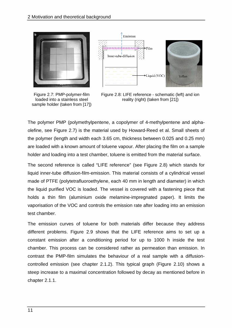
2.3.1 Reference materials in emission testing - sta te of the art There are two basic approaches for reference materials for VOC-emission-testing,
published by Wei at al. [21] and Howard-Reed et al. [17]. Both of them use only
toluene as the investigated VOC. In 2014 Wei at al. [22] reported that they enable
their reference material for the emission of formaldehyde. For both materials model
calculations for predicting the emitted amounts are publicised.
2 Motivation and theoretical background
11
Figure 2.7: PMP-polymer-film loaded into a stainless steel
sample holder (taken from [17])
Figure 2.8: LIFE reference - schematic (left) and ion reality (right) (taken from [21])
The polymer PMP (polymethylpentene, a copolymer of 4-methylpentene and alpha-
olefine, see Figure 2.7) is the material used by Howard-Reed et al. Small sheets of
the polymer (length and width each 3.65 cm, thickness between 0.025 and 0.25 mm)
are loaded with a known amount of toluene vapour. After placing the film on a sample
holder and loading into a test chamber, toluene is emitted from the material surface.
The second reference is called “LIFE reference” (see Figure 2.8) which stands for
liquid inner-tube diffusion-film-emission. This material consists of a cylindrical vessel
made of PTFE (polytetrafluoroethylene, each 40 mm in length and diameter) in which
the liquid purified VOC is loaded. The vessel is covered with a fastening piece that
holds a thin film (aluminium oxide melamine-impregnated paper). It limits the
vaporisation of the VOC and controls the emission rate after loading into an emission
test chamber.
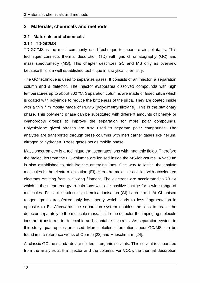
The emission curves of toluene for both materials differ because they address
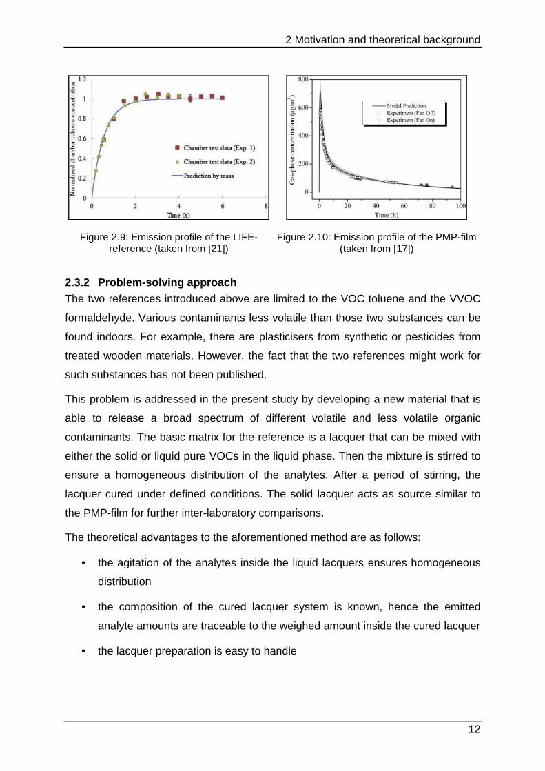
different problems. Figure 2.9 shows that the LIFE reference aims to set up a
constant emission after a conditioning period for up to 1000 h inside the test
chamber. This process can be considered rather as permeation than emission. In
contrast the PMP-film simulates the behaviour of a real sample with a diffusion-
controlled emission (see chapter 2.1.2). This typical graph (Figure 2.10) shows a
steep increase to a maximal concentration followed by decay as mentioned before in
chapter 2.1.1.
2 Motivation and theoretical background
12
Figure 2.9: Emission profile of the LIFE-reference (taken from [21])
Figure 2.10: Emission profile of the PMP-film (taken from [17])
2.3.2 Problem-solving approach The two references introduced above are limited to the VOC toluene and the VVOC
formaldehyde. Various contaminants less volatile than those two substances can be
found indoors. For example, there are plasticisers from synthetic or pesticides from
treated wooden materials. However, the fact that the two references might work for
such substances has not been published.
This problem is addressed in the present study by developing a new material that is
able to release a broad spectrum of different volatile and less volatile organic
contaminants. The basic matrix for the reference is a lacquer that can be mixed with
either the solid or liquid pure VOCs in the liquid phase. Then the mixture is stirred to
ensure a homogeneous distribution of the analytes. After a period of stirring, the
lacquer cured under defined conditions. The solid lacquer acts as source similar to
the PMP-film for further inter-laboratory comparisons.
The theoretical advantages to the aforementioned method are as follows:
• the agitation of the analytes inside the liquid lacquers ensures homogeneous
distribution
• the composition of the cured lacquer system is known, hence the emitted
analyte amounts are traceable to the weighed amount inside the cured lacquer
• the lacquer preparation is easy to handle
3 Materials, chemicals and methods
13
3 Materials, chemicals and methods
3.1 Materials and chemicals
3.1.1 TD-GC/MS TD-GC/MS is the most commonly used technique to measure air pollutants. This
technique connects thermal desorption (TD) with gas chromatography (GC) and
mass spectrometry (MS). This chapter describes GC and MS only as overview
because this is a well established technique in analytical chemistry.
The GC technique is used to separates gases. It consists of an injector, a separation
column and a detector. The Injector evaporates dissolved compounds with high
temperatures up to about 300 °C. Separation columns are made of fused silica which
is coated with polyimide to reduce the brittleness of the silica. They are coated inside
with a thin film mostly made of PDMS (polydimethylsiloxane). This is the stationary
phase. This polymeric phase can be substituted with different amounts of phenyl- or
cyanopropyl groups to improve the separation for more polar compounds.
Polyethylene glycol phases are also used to separate polar compounds. The
analytes are transported through these columns with inert carrier gases like helium,
nitrogen or hydrogen. These gases act as mobile phase.
Mass spectrometry is a technique that separates ions with magnetic fields. Therefore
the molecules from the GC-columns are ionised inside the MS-ion-source. A vacuum
is also established to stabilise the emerging ions. One way to ionise the analyte
molecules is the electron ionisation (EI). Here the molecules collide with accelerated
electrons emitting from a glowing filament. The electrons are accelerated to 70 eV
which is the mean energy to gain ions with one positive charge for a wide range of
molecules. For labile molecules, chemical ionisation (CI) is preferred. At CI ionised
reagent gases transferred only low energy which leads to less fragmentation in
opposite to EI. Afterwards the separation system enables the ions to reach the
detector separately to the molecule mass. Inside the detector the impinging molecule
ions are transferred in detectable and countable electrons. As separation system in
this study quadrupoles are used. More detailed information about GC/MS can be
found in the reference works of Oehme [23] and Hübschmann [24].
At classic GC the standards are diluted in organic solvents. This solvent is separated
from the analytes at the injector and the column. For VOCs the thermal desorption
3 Materials, chemicals and methods
14
(TD) enables the GC to analyse the substances directly in the gaseous phase.
Therefore defined amounts of contaminated air must be trapped on special
adsorbent tubes with sampling pumps at ambient conditions. The volatility of the
contaminants defines the adsorbent material used inside the tubes. For VVOC mostly
modified activated carbon is used while SVOC are usually sampled on glass wool
materials. TENAX® TA is usually used to sample wide ranges of analytes with
different volatilities. This polymer is based on 2,6-diphenyl-p-phenylene oxide.
The bounded analytes can be desorbed from the adsorbent material at higher
temperatures inside a TD-oven. The maximum temperature of desorption is adjusted
to the stability of the material and the analyte itself. Mostly temperatures between
280 and 340 °C are used. While with desorption the tubes are flushed with the carrier
gas of the GC. The gas flow transports the analytes from the heated sampling tube to
the GC. There the substances are desorbed from the material according to their
volatility. First high volatile compounds evaporates from the material at lower than the
less volatile at higher temperatures. Directly coupled to a GC the subsequent
desorption and transport of the analytes from the TD-oven to the GC-column would
lead to spreading peaks on the chromatogram. GC needs retention of the analytes at
the column start for a good separation. Therefore the analytes are trapped at low
temperature on a material at the GC-liner of the injector. This injector is equipped
with a special adsorbent material (activated carbon, Tenax, glass wool). From this
cold trap the analytes are desorbed simultaneously when the material is heated up
quickly.
In the present study two different thermal desorption systems (TDS) were used. The
system “Asterix” (GERTSEL/AGILENT) was used in part 4.1, while part 4.2 and 4.3
were analysed with “Idefix” (MARKES/AGILENT). Both systems are introduced in
Table 3.3
3.1.2 Emission test chambers
Usually climate chambers are used to analyse samples under defined conditions.
They keep the temperature, humidity, air flow and air change at constant values
which is close to indoor air properties.
Principal test chamber systems consist of the following parts: clean air generation,
humidification, test chamber with a temperature control and ventilation (air mixing),
control- and monitoring system.
3 Materials, chemicals and methods
15
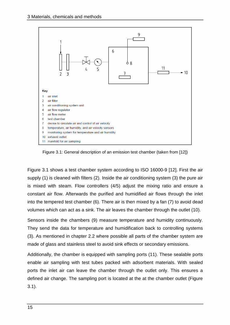
Figure 3.1: General description of an emission test chamber (taken from [12])
Figure 3.1 shows a test chamber system according to ISO 16000-9 [12]. First the air
supply (1) is cleaned with filters (2). Inside the air conditioning system (3) the pure air
is mixed with steam. Flow controllers (4/5) adjust the mixing ratio and ensure a
constant air flow. Afterwards the purified and humidified air flows through the inlet
into the tempered test chamber (6). There air is then mixed by a fan (7) to avoid dead
volumes which can act as a sink. The air leaves the chamber through the outlet (10).
Sensors inside the chambers (9) measure temperature and humidity continuously.
They send the data for temperature and humidification back to controlling systems
(3). As mentioned in chapter 2.2 where possible all parts of the chamber system are
made of glass and stainless steel to avoid sink effects or secondary emissions.
Additionally, the chamber is equipped with sampling ports (11). These sealable ports
enable air sampling with test tubes packed with adsorbent materials. With sealed
ports the inlet air can leave the chamber through the outlet only. This ensures a
defined air change. The sampling port is located at the at the chamber outlet (Figure
3.1).
3 Materials, chemicals and methods
16
Beside conventional test chambers with volumes in cubic meter ranges, there are
various smaller chambers which are often custom made. This reduces the sample
amount that has to be loaded. It can be said that those chambers are more economic
because they need less space, conditioned air and amount of material samples. On
the other hand their results must be correlated to bigger chambers because they are
often prescribed in different standards.
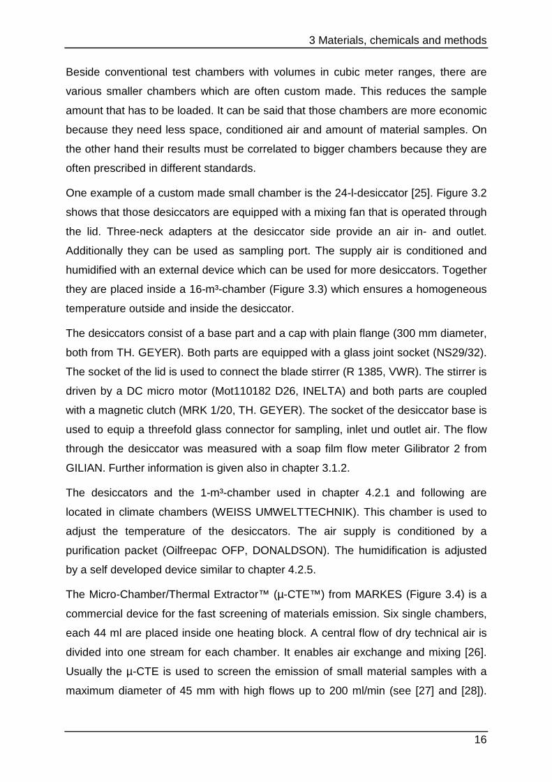
One example of a custom made small chamber is the 24-l-desiccator [25]. Figure 3.2
shows that those desiccators are equipped with a mixing fan that is operated through
the lid. Three-neck adapters at the desiccator side provide an air in- and outlet.
Additionally they can be used as sampling port. The supply air is conditioned and
humidified with an external device which can be used for more desiccators. Together
they are placed inside a 16-m³-chamber (Figure 3.3) which ensures a homogeneous
temperature outside and inside the desiccator.
The desiccators consist of a base part and a cap with plain flange (300 mm diameter,
both from TH. GEYER). Both parts are equipped with a glass joint socket (NS29/32).
The socket of the lid is used to connect the blade stirrer (R 1385, VWR). The stirrer is
driven by a DC micro motor (Mot110182 D26, INELTA) and both parts are coupled
with a magnetic clutch (MRK 1/20, TH. GEYER). The socket of the desiccator base is
used to equip a threefold glass connector for sampling, inlet und outlet air. The flow
through the desiccator was measured with a soap film flow meter Gilibrator 2 from
GILIAN. Further information is given also in chapter 3.1.2.
The desiccators and the 1-m³-chamber used in chapter 4.2.1 and following are
located in climate chambers (WEISS UMWELTTECHNIK). This chamber is used to
adjust the temperature of the desiccators. The air supply is conditioned by a
purification packet (Oilfreepac OFP, DONALDSON). The humidification is adjusted
by a self developed device similar to chapter 4.2.5.
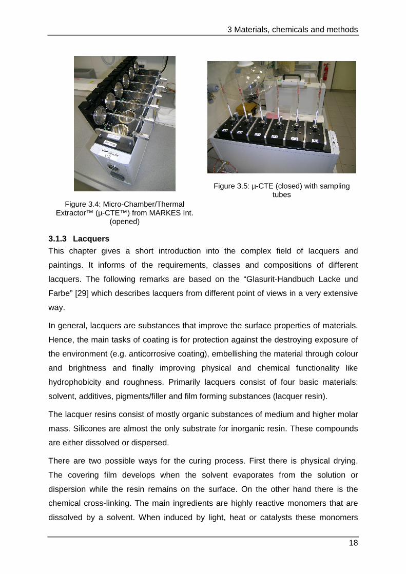
The Micro-Chamber/Thermal Extractor™ (µ-CTE™) from MARKES (Figure 3.4) is a
commercial device for the fast screening of materials emission. Six single chambers,
each 44 ml are placed inside one heating block. A central flow of dry technical air is
divided into one stream for each chamber. It enables air exchange and mixing [26].
Usually the µ-CTE is used to screen the emission of small material samples with a
maximum diameter of 45 mm with high flows up to 200 ml/min (see [27] and [28]).

3 Materials, chemicals and methods
17
The emission process can also be accelerated for low volatile substances by
increasing the temperature up to a maximum of 120 °C. As it exhibits high air
exchange, the sampling tube on the lid of each of the six chambers can be loaded
passively without pumps (Figure 3.5).
Beginning with experiment part 4.2 they were equipped with Mass flow controllers
(MFCs, 4800 Series, BROOKS) to reduce the variation of the flow. For the
investigations they operated at 25 °C. The flow was controlled with a flow meter
(35806ML, ANALYT-MTC).
Figure 3.2: 24-l-chamber (desiccator) loaded with wooden sample
Figure 3.3: Several 24-l-chambers inside a 16-m³-chamber
3 Materials, chemicals and methods
18
Figure 3.4: Micro-Chamber/Thermal Extractor™ (µ-CTE™) from MARKES Int.
(opened)
Figure 3.5: µ-CTE (closed) with sampling tubes
3.1.3 Lacquers
This chapter gives a short introduction into the complex field of lacquers and
paintings. It informs of the requirements, classes and compositions of different
lacquers. The following remarks are based on the “Glasurit-Handbuch Lacke und
Farbe” [29] which describes lacquers from different point of views in a very extensive
way.
In general, lacquers are substances that improve the surface properties of materials.
Hence, the main tasks of coating is for protection against the destroying exposure of
the environment (e.g. anticorrosive coating), embellishing the material through colour
and brightness and finally improving physical and chemical functionality like
hydrophobicity and roughness. Primarily lacquers consist of four basic materials:
solvent, additives, pigments/filler and film forming substances (lacquer resin).
The lacquer resins consist of mostly organic substances of medium and higher molar
mass. Silicones are almost the only substrate for inorganic resin. These compounds
are either dissolved or dispersed.
There are two possible ways for the curing process. First there is physical drying.
The covering film develops when the solvent evaporates from the solution or
dispersion while the resin remains on the surface. On the other hand there is the
chemical cross-linking. The main ingredients are highly reactive monomers that are
dissolved by a solvent. When induced by light, heat or catalysts these monomers
3 Materials, chemicals and methods
19
polymerise to form a resin which covers the surface. The solvent then evaporates
because the developing polymer loses solubility. Primary the process of curing does
not depend on the chemical structure of the resin itself but on the presence of
reactive chemical functional groups that provides polymerisation.
Pigments are necessary to cover the underground and colour the surface. The colour
is based on either different inorganic salts or oxides like Ti2O or organic substances
with many conjugated double bonds. Additionally, inorganic pigments can increase
the resistance against corrosion by deactivating the surface, for example on steel.
Mineral fillers are used to fill the dispersion and sustain the cured lacquer.
Additionally they can improve the adhesion on the substrate and linkage following
layers of lacquer as well as decreasing the surface brightness.
The group of additives is dominated by plasticisers. They act as non-evaporative
solvents for the resins and control the hardness and brittleness of the cured lacquer.
Other additives have the following functions: adjusting the viscosity of the mixture,
prevent foaming, biocidal properties, anti-fouling properties and improving dispersion,
wettability, curing and UV-absorption.
The main task for solvents or mixtures is to dissolve the other three main
compounds. They turn the lacquer into one matrix and adjust the viscosity, flow
properties and wetting. Besides water there are a lot of organic solvents in use, like
aliphatic hydrocarbons (e.g. benzine), aromatic hydrocarbons (e.g. styrene, toluene,
xylene), glycol-ethers and -esters, alcohols (glycerine), ketones (e.g. Methyl isobutyl
ketone, MIBK ) and other special solvents like N-methylpyrrolidone.
The lacquers used in chapter 4.1.2 were produced by the manufacturer MEFFERT.
Six of them were acrylic based (incorporating water as solvent) and six were based
on alkyd polymers (incorporating organic solvents). The acrylic lacquers contained
water, a dispersion of acrylat and polyurethane, glycols, additives, preservatives
(methyl-, benzyl- and chlor-isothiazolinone) and pigments (if it is a coloured lacquer).
These lacquers are labelled with the Blue Angel eco-label for low emissions. The
alkyd lacquers contained the alkyd resin, additives, white spirit and pigments (if
coloured).
3 Materials, chemicals and methods
20
3.1.4 Chemicals For the investigation the five VOCs styrene (100-42-5, ALFA AESAR, 99.5 %), N-
methyl-α-pyrrolidone (872-50-4, NMP, FLUKA, > 99.9 %), 2-ethyl-1-hexanol (104-76-
7, E.H., ALDRICH, 99.6 %), 1,2-dimethyl-phthalate (131-11-3, DMP, ALFA AESAR,
99 %), n-hexadecane (544-76-3, C16, ALDRICH, 99 %) and the two SVOC lindane
(58-89-9, ALDRICH, 99.8 %) and 1,2-di-n-butyl-phthalate (131-11-3, DBP, ALDRICH
> 98 %) were selected.
All of these substances can be found in indoor air as they are emitted from different
building materials like flooring. C16 is the link between VOC and SVOC according to
the standard ISO 16000-6 [30]. NMP and DBP (a plasticiser like DMP) are
“substances of very high concern” according to the ECHA (European Chemical
Agency) - candidate list because of their toxicity for reproduction [31]. E.H. and
styrene are reactants for many synthetic materials. For example E.H. is an important
reactant for the synthesis of the widely used plasticiser bis(2-ethylhexyl) phthalate
(DEHP) [32].
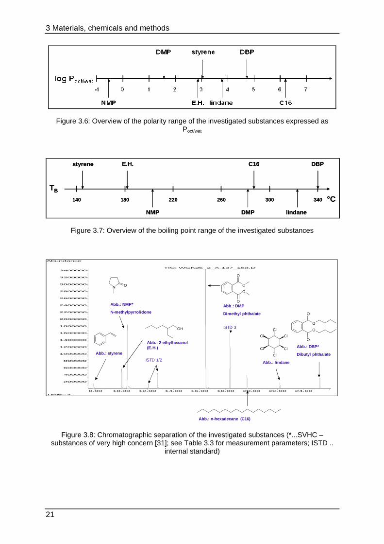
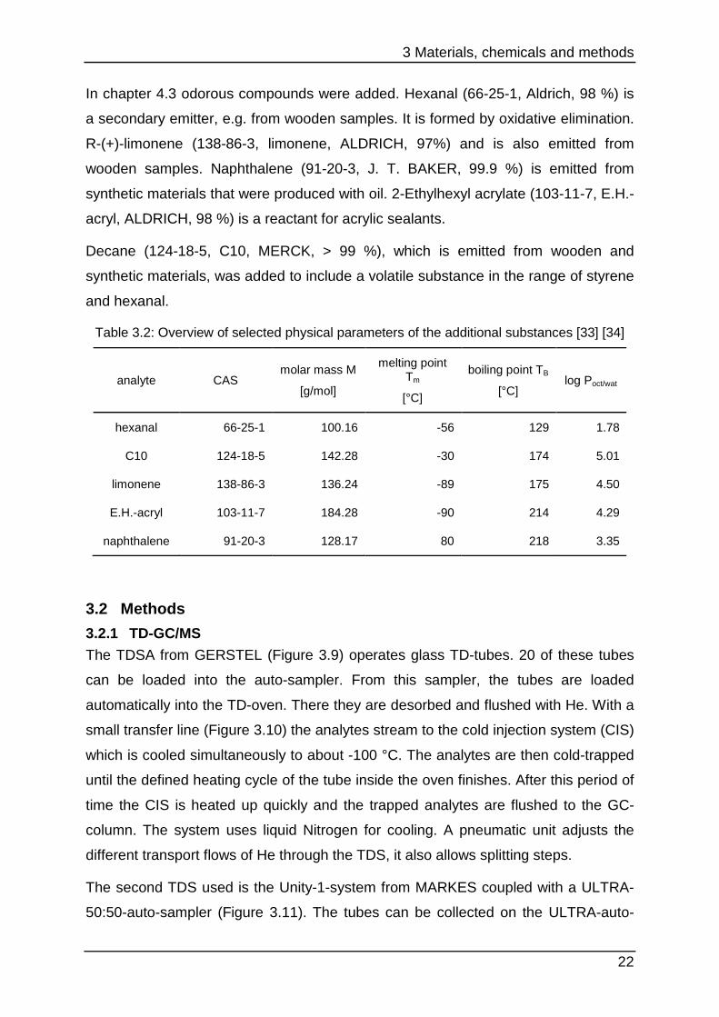
The spectrum of the polarity expressed as partition coefficient log Poct/wat can be seen
in Figure 3.6. Figure 3.7 shows the range of volatility of the investigated substances
expressed as boiling point TB. Table 3.1 shows additional selected physical
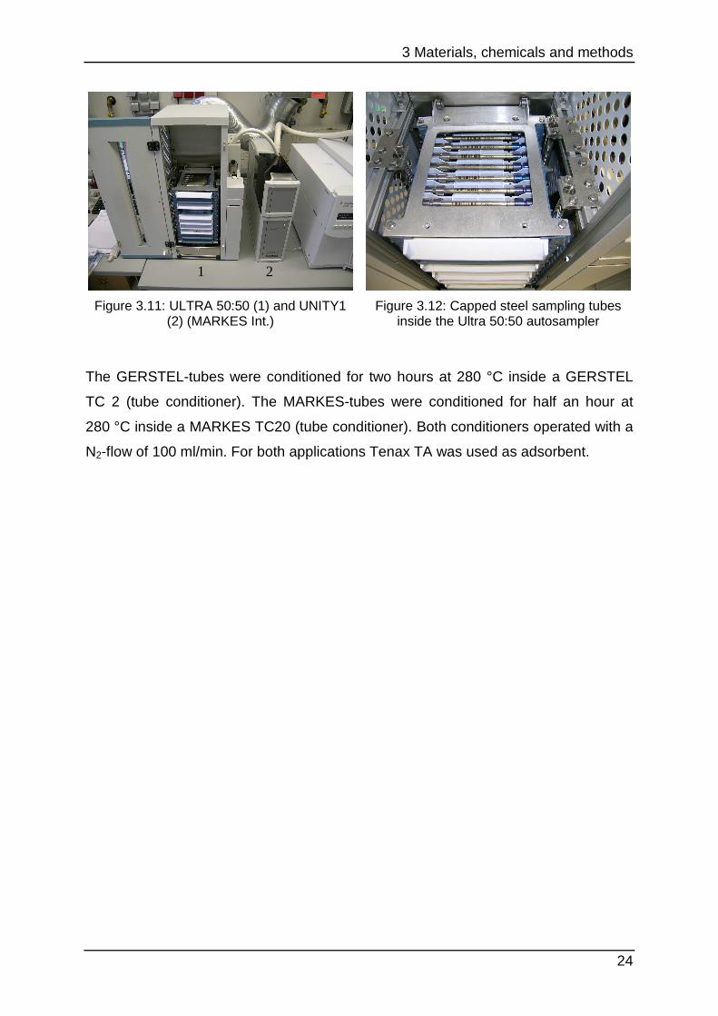
parameters. The chromatographic separation of the investigated substances is
shown in Figure 3.8.
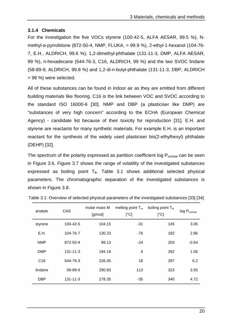
Table 3.1: Overview of selected physical parameters of the investigated substances [33] [34]
analyte CAS molar mass M
[g/mol]
melting point Tm
[°C]
boiling point TB
[°C] log Poct/wat
styrene 100-42-5 104.15 -31 145 3.05
E.H. 104-76-7 130.23 -76 182 2.86
NMP 872-50-4 99.13 -24 203 -0.54
DMP 131-11-3 194.19 6 282 1.56
C16 544-76-3 226.45 18 287 6.2
lindane 58-89-9 290.83 113 323 3.55
DBP 131-11-3 278.35 -35 340 4.72
3 Materials, chemicals and methods
21
Figure 3.6: Overview of the polarity range of the investigated substances expressed as Poct/wat
140 340180 220 260 300
styrene
NMP DMP
E.H.
lindane
DBPC16
TB
°C140 340180 220 260 300
styrene
NMP DMP
E.H.
lindane
DBPC16
TB
°C
Figure 3.7: Overview of the boiling point range of the investigated substances
8.00 10.00 12.00 14.00 16.00 18.00 20.00 22.00 24.00
200000
400000
600000
800000
1000000
1200000
1400000
1600000
1800000
2000000
2200000
2400000
2600000
2800000
3000000
3200000
3400000
Time-->
Abundance
TIC: WGK25_2_X-137_16d.D
O
O
O
ON O
O
O
O
O
Cl
ClCl
Cl
Cl
Cl
OH
Abb.: styrene
Abb.: 2-ethylhexanol (E.H.)
Abb.: NMP*
N-methylpyrrolidoneAbb.: DMP
Dimethyl phthalate
Abb.: lindane
Abb.: DBP*
Dibutyl phthalate
Abb.: n-hexadecane (C16)
ISTD 1/2
ISTD 3
Figure 3.8: Chromatographic separation of the investigated substances (*...SVHC – substances of very high concern [31]; see Table 3.3 for measurement parameters; ISTD ..
internal standard)
3 Materials, chemicals and methods
22
In chapter 4.3 odorous compounds were added. Hexanal (66-25-1, Aldrich, 98 %) is
a secondary emitter, e.g. from wooden samples. It is formed by oxidative elimination.
R-(+)-limonene (138-86-3, limonene, ALDRICH, 97%) and is also emitted from
wooden samples. Naphthalene (91-20-3, J. T. BAKER, 99.9 %) is emitted from
synthetic materials that were produced with oil. 2-Ethylhexyl acrylate (103-11-7, E.H.-
acryl, ALDRICH, 98 %) is a reactant for acrylic sealants.
Decane (124-18-5, C10, MERCK, > 99 %), which is emitted from wooden and
synthetic materials, was added to include a volatile substance in the range of styrene
and hexanal.
Table 3.2: Overview of selected physical parameters of the additional substances [33] [34]
analyte CAS molar mass M
[g/mol]
melting point Tm
[°C]
boiling point TB
[°C] log Poct/wat
hexanal 66-25-1 100.16 -56 129 1.78
C10 124-18-5 142.28 -30 174 5.01
limonene 138-86-3 136.24 -89 175 4.50
E.H.-acryl 103-11-7 184.28 -90 214 4.29
naphthalene 91-20-3 128.17 80 218 3.35
3.2 Methods
3.2.1 TD-GC/MS
The TDSA from GERSTEL (Figure 3.9) operates glass TD-tubes. 20 of these tubes
can be loaded into the auto-sampler. From this sampler, the tubes are loaded
automatically into the TD-oven. There they are desorbed and flushed with He. With a
small transfer line (Figure 3.10) the analytes stream to the cold injection system (CIS)
which is cooled simultaneously to about -100 °C. The analytes are then cold-trapped
until the defined heating cycle of the tube inside the oven finishes. After this period of
time the CIS is heated up quickly and the trapped analytes are flushed to the GC-
column. The system uses liquid Nitrogen for cooling. A pneumatic unit adjusts the
different transport flows of He through the TDS, it also allows splitting steps.
The second TDS used is the Unity-1-system from MARKES coupled with a ULTRA-
50:50-auto-sampler (Figure 3.11). The tubes can be collected on the ULTRA-auto-

3 Materials, chemicals and methods
23
sampler. The tubes are heated up and flushed with carrier gas and they stream over
a heated transfer line into the ultra. The analytes then become trapped on a cold trap
tube which is equipped with an adsorbent material. As the trapping temperature is
usually no lower than -5 °C, only gaseous Nitrogen and Peltier elements are needed
for cooling. After quickly heating the trap, the analytes are flushed together into the
GC-column. The complex pressure control of the UNITY allows splitting the analyte-
flow at every part of the TDS. For example, it is possible to divide the flow from the
TD-oven or the trap and transport a portion of it back to the sampling tube. This can
be used to analyse a sample from one tube for a second time. On the contrary the
TDS from GERSTEL desorbs the analytes from one tube completely, therefore the
sample cannot be analysed again from the same tube. To enable the recollection of
samples, the UNITY needs a complex pneumatic system with high pressures, thus
the TD-tubes are made mostly on stainless steel and they must be tightened with
caps before loading them into the ULTRA-50:50 (Figure 3.12).
Figure 3.9: TDSA with glass sampling tubes inside the autosampler (GERSTEL)
Figure 3.10: Transfer line of the TDSA (GERSTEL)
3 Materials, chemicals and methods
24
Figure 3.11: ULTRA 50:50 (1) and UNITY1 (2) (MARKES Int.)
Figure 3.12: Capped steel sampling tubes inside the Ultra 50:50 autosampler
The GERSTEL-tubes were conditioned for two hours at 280 °C inside a GERSTEL
TC 2 (tube conditioner). The MARKES-tubes were conditioned for half an hour at
280 °C inside a MARKES TC20 (tube conditioner). Both conditioners operated with a
N2-flow of 100 ml/min. For both applications Tenax TA was used as adsorbent.
1 2
3 Materials, chemicals and methods
25
Table 3.3: Measurement parameters of the TD-GC/MS system "Asterix" and "Idefix" (see chapter 3.1.1)
Asterix Idefix
GC model AGILENT 6890 AGILENT 6890
column RESTEK Rxi 5-ms (60 m, 25 mm, 0.25 µm)
column flow
1.4 ml/min (constant flow)
1.5 ml/min (constant flow)
carrier gas helium (ALPHAGAZ AIR LIQUIDE)
oven temperature program
40 °C for 4 min;
with 10 °C/min to 150 °C for 1 min;
with 8 °C/min to 300 °C for 5 min
60 °C for 2 min;
with 10 °C/min to 300 °C for 5 min
MS model AGILENT 5973N AGILENT 5975B
transfer line 300 °C 300 °C
ion source EI, 230 °C
quadrupole 150 °C
mode full scan: 40 – 440 amu
TDS model
GERSTEL TDS A + GERSTEL CIS 4
MARKES UNITY 1
tube desorption program
30 °C for 1 min;
with 30 °C/min to 260 °C for 5 min
flow: 50 ml/min (splitless)
290 °C for 10 min
flow: 50 ml/min (splitless)
CIS/cold trap
program
-120 °C for 0.05 min;
with 12 °C/s to 300 °C for 3 min
flow: 1.4 ml/min (splitless)
5 °C;
with 12 °C/s to 300 °C for 5 min
flow: 1.5 ml/min + 6 ml/min split flow (ratio: 1:5)
liner glass wool Tenax TA
transfer line 300 °C 180 °C
3 Materials, chemicals and methods
26
3.2.2 Calibration The substances were externally calibrated. From each substance weighed amounts
were diluted in methanol (MeOH, for organic residue analysis, J.T. Baker) in
volumetric flasks of 10 ml. Depending on the purity of the substances the final
concentrations were all approximately 10 µg/µl. From these stock solutions defined
amounts were transferred to a volumetric flask of 10 ml and filled up with MeOH. The
adjusted concentration of the mix was approximately 200 ng/µl. This methanolic
solution was diluted according to the following steps: 180, 160, 140, 120, 100, 80, 60,
50, 40, 20, 10, 4, 2 and 1 ng/µl.
From each of these 15 levels 1 µl was spiked with glass syringes of 5 µl (HAMILTON)
onto adsorbent tubes. 1 µl of an internal standard (ISTD) was also added. This ISTD
consisted of 20 ng/µl of cyclodecane (293-96-9, ALDRICH, 95 %) and naphthalene-
d8 (1146-65-2, ALDRICH, 99 %) as well as 51.5 ng/µl of 2,4,6-tribromophenol (118-
79-6, ALDRICH, 99 %). Afterwards MeOH was flushed with a 1 l of N2 (ALPHAGAZ
AIR LIQUIDE) on a GERSTEL TSPS (standard tube preparation system).
The tubes that were spiked with the 15 levels were subsequently analysed with the
TD-GC/MS. The measured area counts calculated from the chromatograms were
linked with the mass of analyte on the tube with linear regression. The calibration
data can be found in Table 8.1 to Table 8.6.
3.2.3 Quantification The internal standard was used to calculate differences in the adsorption
performance of the sampling tubes. Therefore the measured ISTD-area-counts from
each tube of one measurement sequence were averaged. For each tube the ratio of
the ISTD amount on the associated tube and the ISTD-average was calculated. This
factor was multiplied with the measured analyte amounts.
Furthermore, the concentrations were calculated based on ISO 16000-9 [12]. The
analyte amount trapped onto the sampling tube (mS) in relation to the sampled
volume (VS) results in the mass concentration (ρX). This parameter is often
expressed as µg/m³.
As there is a wide spectrum of commercially available and self build emission test
chambers with different volumes and operating flows the parameter L and q are often
used to correlate results from different chambers. For comparison SERA is more
3 Materials, chemicals and methods
27
practical than ρX because it considers important chamber parameters like air change,
emission surface and flow.
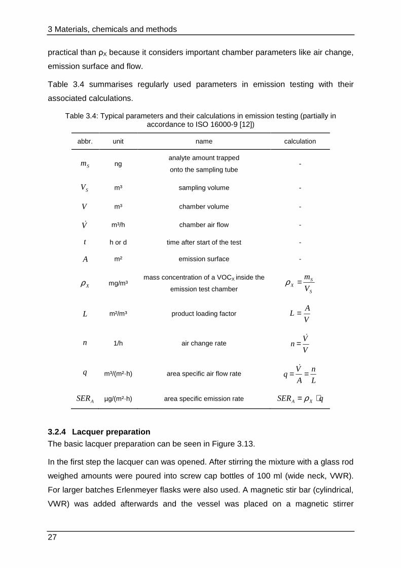
Table 3.4 summarises regularly used parameters in emission testing with their
associated calculations.
Table 3.4: Typical parameters and their calculations in emission testing (partially in accordance to ISO 16000-9 [12])
abbr. unit name calculation
Sm ng analyte amount trapped
onto the sampling tube -
SV m³ sampling volume -
V m³ chamber volume -
V& m³/h chamber air flow -
t h or d time after start of the test -
A m² emission surface -
Xρ mg/m³ mass concentration of a VOCX inside the
emission test chamber S
SX V
m=ρ
L m²/m³ product loading factor V
AL =
n 1/h air change rate V
Vn
&
=
q m³/(m²·h) area specific air flow rate L
n
A
Vq ==
&
ASER µg/(m²·h) area specific emission rate qSER XA ⋅= ρ
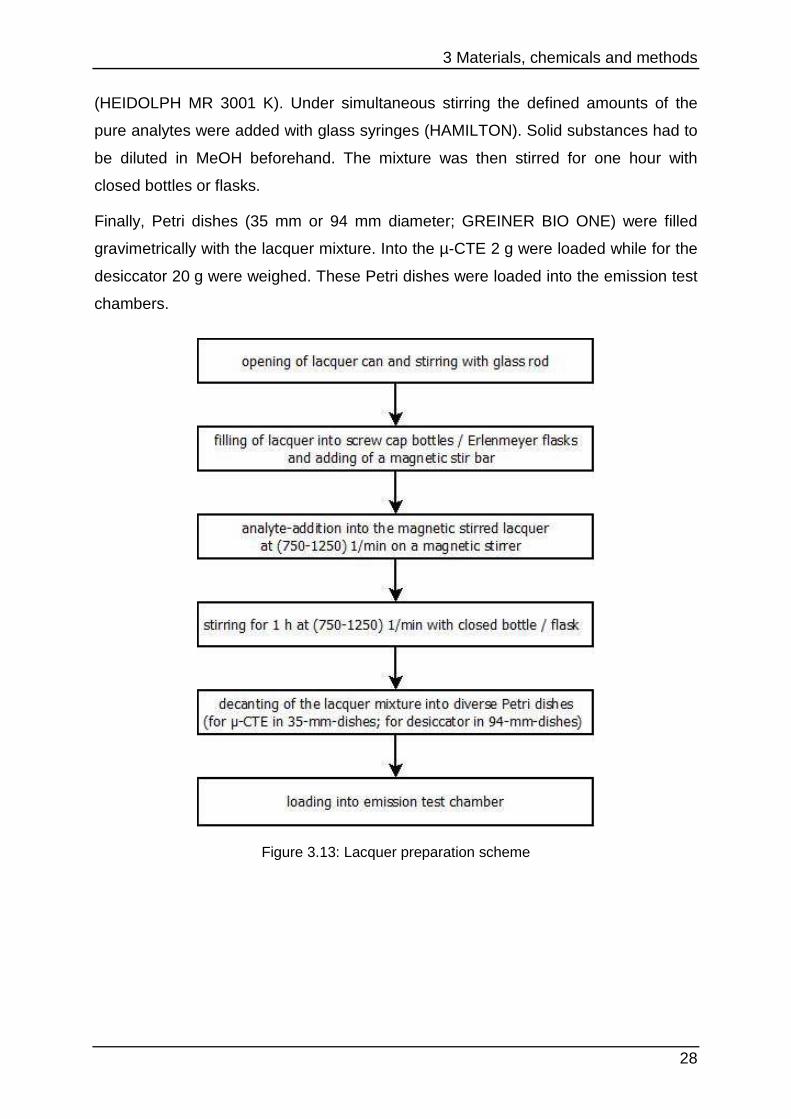
3.2.4 Lacquer preparation The basic lacquer preparation can be seen in Figure 3.13.
In the first step the lacquer can was opened. After stirring the mixture with a glass rod
weighed amounts were poured into screw cap bottles of 100 ml (wide neck, VWR).
For larger batches Erlenmeyer flasks were also used. A magnetic stir bar (cylindrical,
VWR) was added afterwards and the vessel was placed on a magnetic stirrer
3 Materials, chemicals and methods
28
(HEIDOLPH MR 3001 K). Under simultaneous stirring the defined amounts of the
pure analytes were added with glass syringes (HAMILTON). Solid substances had to
be diluted in MeOH beforehand. The mixture was then stirred for one hour with
closed bottles or flasks.
Finally, Petri dishes (35 mm or 94 mm diameter; GREINER BIO ONE) were filled
gravimetrically with the lacquer mixture. Into the µ-CTE 2 g were loaded while for the
desiccator 20 g were weighed. These Petri dishes were loaded into the emission test
chambers.
Figure 3.13: Lacquer preparation scheme
3 Materials, chemicals and methods
29
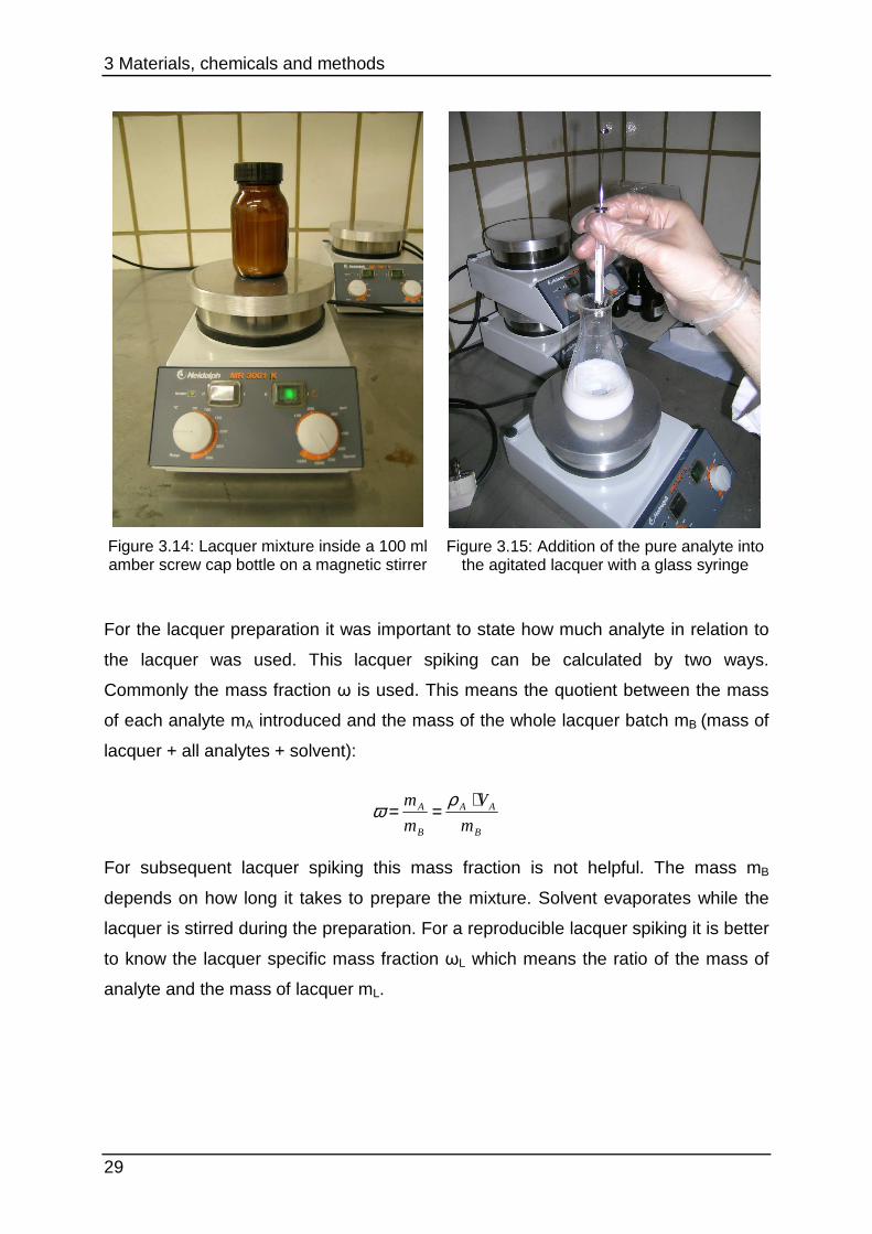
Figure 3.14: Lacquer mixture inside a 100 ml amber screw cap bottle on a magnetic stirrer
Figure 3.15: Addition of the pure analyte into the agitated lacquer with a glass syringe
For the lacquer preparation it was important to state how much analyte in relation to
the lacquer was used. This lacquer spiking can be calculated by two ways.
Commonly the mass fraction ω is used. This means the quotient between the mass
of each analyte mA introduced and the mass of the whole lacquer batch mB (mass of
lacquer + all analytes + solvent):
B
AA
B
A
m
V
m
m ⋅==
ρω
For subsequent lacquer spiking this mass fraction is not helpful. The mass mB
depends on how long it takes to prepare the mixture. Solvent evaporates while the
lacquer is stirred during the preparation. For a reproducible lacquer spiking it is better
to know the lacquer specific mass fraction ωL which means the ratio of the mass of
analyte and the mass of lacquer mL.
3 Materials, chemicals and methods
30
L
AA
L
AL m
V
m
m ⋅==
ρω
For liquid analytes in both mass fractions mA can be expressed as a product between
the spiked analyte volume VA multiplied by the associated density ρA.
3.2.5 Sampling
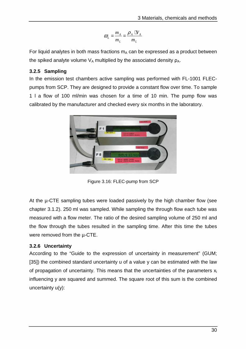
In the emission test chambers active sampling was performed with FL-1001 FLEC-
pumps from SCP. They are designed to provide a constant flow over time. To sample
1 l a flow of 100 ml/min was chosen for a time of 10 min. The pump flow was
calibrated by the manufacturer and checked every six months in the laboratory.
Figure 3.16: FLEC-pump from SCP
At the µ-CTE sampling tubes were loaded passively by the high chamber flow (see
chapter 3.1.2). 250 ml was sampled. While sampling the through flow each tube was
measured with a flow meter. The ratio of the desired sampling volume of 250 ml and
the flow through the tubes resulted in the sampling time. After this time the tubes
were removed from the µ-CTE.
3.2.6 Uncertainty According to the “Guide to the expression of uncertainty in measurement” (GUM;
[35]) the combined standard uncertainty u of a value y can be estimated with the law
of propagation of uncertainty. This means that the uncertainties of the parameters xi
influencing y are squared and summed. The square root of this sum is the combined
uncertainty u(y):
3 Materials, chemicals and methods
31
( ) ( ) ( )22
1 ...
⋅∂∂++
⋅∂∂= nxu
x
yxu
x
yyu
For the lacquer system, y stands for the measured air concentration ρx inside the test
chamber. According to Table 3.4 ρx stands for the quotient of the analyte amount
trapped onto the sampling tube mS and the sampled air volume VS. Therefore the
combined relative uncertainty can be summarised as:
( ) ( ) ( )SrelSrelXrel Vumuu 22 +=ρ
The uncertainty of VS is mainly determined by the deviation of the sampling pump
performance. This uncertainty was calculated from the relative standard deviation of
repetitive sampling of 1 l with 100 ml/min. The sampled volume was measured with a
gas meter (BRAND Germany).
For µ-CTE-sampling the tubes were loaded passively by the chamber flow over a
specific amount of time. The deviation of the stopwatch combined with the time that
was needed to pull the tubes from the sampling port could not be calculated.
However, compared to the deviation of the chamber flow it was negligible. The
deviation of the flow through the µ-CTE was calculated as relative standard deviation
of the flow, measured while sampling and randomly over the whole loading cycle.
With equipped mass flow controller the deviation of the flow could be lowered from 5
to 1 %.
The uncertainty of mS is influenced by the stability of the measurement system (TD-
GC/MS), the adsorption performance of the sampling tubes and the variance in the
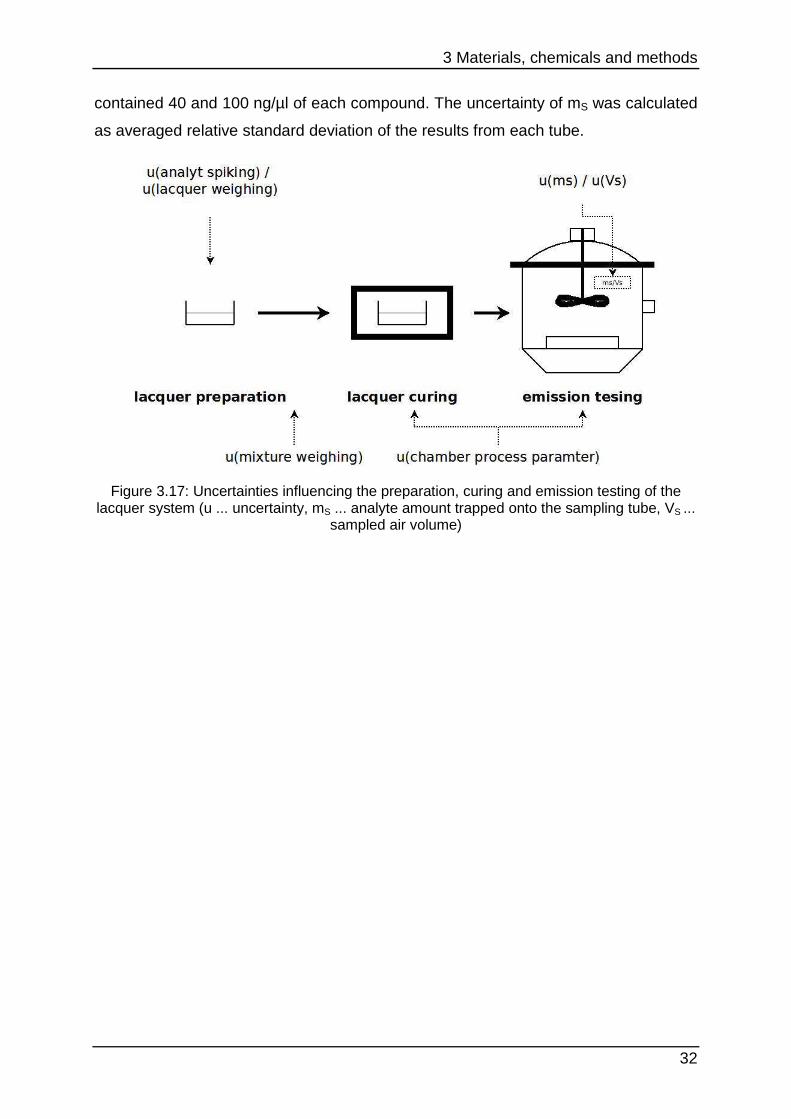
lacquer emission. Figure 3.17 shows that this last variance is determined by the
process parameter of the chamber while curing and emission testing as well as by
the variation of the lacquer preparation. In this study the lacquer system as a
reference material was under development. Hence not enough data was available to
develop models calculation the influence of the process parameters and the
variations in the sample preparation on the emission performance. Therefore these
parameters are shown but cannot be included in the uncertainty of mS.
The performance of the measurement system and the adsorption performance can
be estimated with repetitive analysis of sampling tubes spiked with equal analyte
amounts. Therefore each of the six sampling tubes were spiked with a solution that
3 Materials, chemicals and methods
32
contained 40 and 100 ng/µl of each compound. The uncertainty of mS was calculated
as averaged relative standard deviation of the results from each tube.
Figure 3.17: Uncertainties influencing the preparation, curing and emission testing of the lacquer system (u ... uncertainty, mS ... analyte amount trapped onto the sampling tube, VS ...
sampled air volume)
3 Materials, chemicals and methods
33
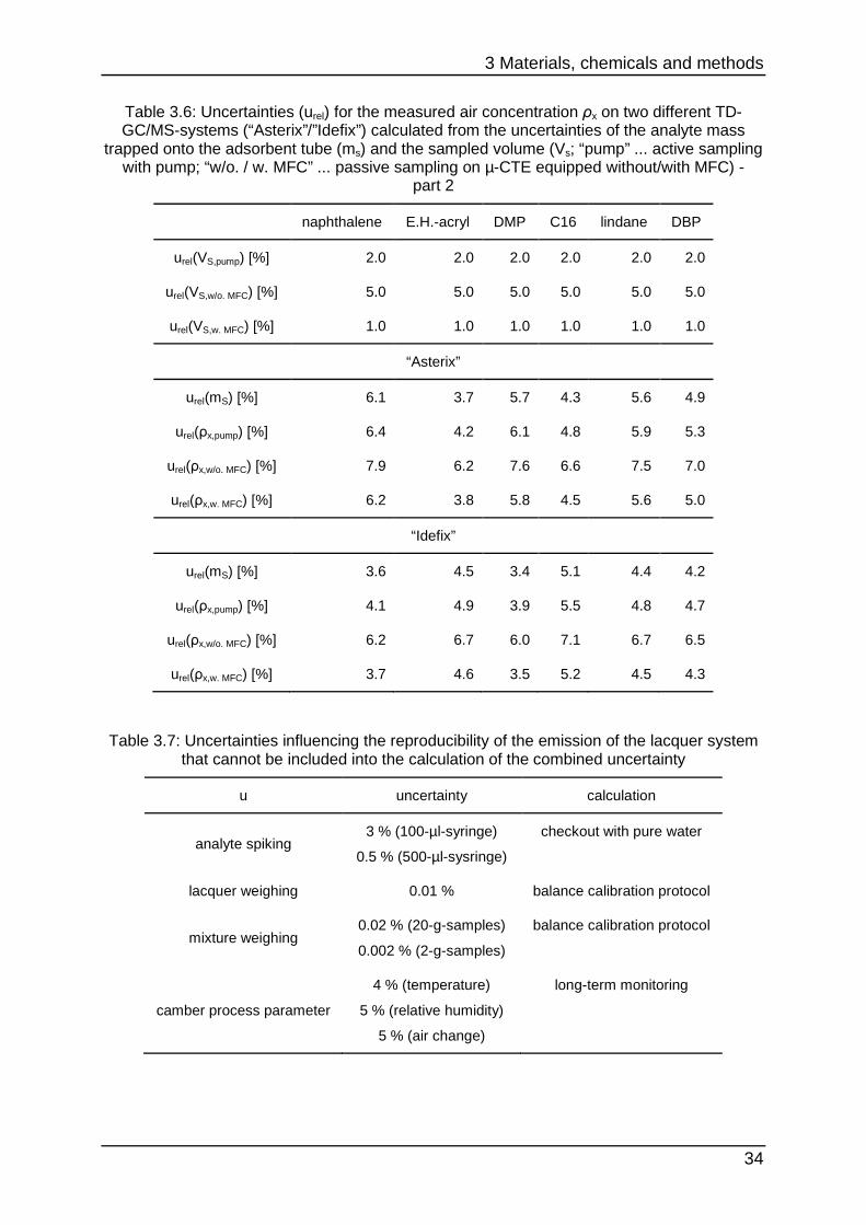
Table 3.5: Uncertainties (urel) for the measured air concentration ρx on two different TD-GC/MS-systems (“Asterix”/”Idefix”) calculated from the uncertainties of the analyte mass
trapped onto the adsorbent tube (ms) and the sampled volume (Vs; “pump” ... active sampling with pump; “w/o. / w. MFC” ... passive sampling on µ-CTE equipped without/with MFC) -
part 1
hexanal styrene C10 E.H. limonene NMP
urel(VS,pump) [%] 2.0 2.0 2.0 2.0 2.0 2.0
urel(VS,w/o. MFC) [%] 5.0 5.0 5.0 5.0 5.0 5.0
urel(VS,w. MFC) [%] 1.0 1.0 1.0 1.0 1.0 1.0
“Asterix”
urel(mS) [%] 5.5 6.8 4.3 6.4 4.9 8.9
urel(ρx,pump) [%] 5.8 7.0 4.8 6.7 5.3 9.1
urel(ρx,w/o. MFC) [%] 7.4 8.4 6.6 8.1 7.0 10.2
urel(ρx,w. MFC) [%] 5.6 6.8 4.4 6.5 5.0 8.9
“Idefix”
urel(mS) [%] 7.6 5.6 4.8 5.8 5.3 6.7
urel(ρx,pump) [%] 7.9 5.9 5.2 6.1 5.7 7.0
urel(ρx,w/o. MFC) [%] 9.1 7.5 6.9 7.7 7.3 8.4
urel(ρx,w. MFC) [%] 7.7 5.7 4.9 5.9 5.4 6.8
3 Materials, chemicals and methods
34
Table 3.6: Uncertainties (urel) for the measured air concentration ρx on two different TD-GC/MS-systems (“Asterix”/”Idefix”) calculated from the uncertainties of the analyte mass
trapped onto the adsorbent tube (ms) and the sampled volume (Vs; “pump” ... active sampling with pump; “w/o. / w. MFC” ... passive sampling on µ-CTE equipped without/with MFC) -
part 2
naphthalene E.H.-acryl DMP C16 lindane DBP
urel(VS,pump) [%] 2.0 2.0 2.0 2.0 2.0 2.0
urel(VS,w/o. MFC) [%] 5.0 5.0 5.0 5.0 5.0 5.0
urel(VS,w. MFC) [%] 1.0 1.0 1.0 1.0 1.0 1.0
“Asterix”
urel(mS) [%] 6.1 3.7 5.7 4.3 5.6 4.9
urel(ρx,pump) [%] 6.4 4.2 6.1 4.8 5.9 5.3
urel(ρx,w/o. MFC) [%] 7.9 6.2 7.6 6.6 7.5 7.0
urel(ρx,w. MFC) [%] 6.2 3.8 5.8 4.5 5.6 5.0
“Idefix”
urel(mS) [%] 3.6 4.5 3.4 5.1 4.4 4.2
urel(ρx,pump) [%] 4.1 4.9 3.9 5.5 4.8 4.7
urel(ρx,w/o. MFC) [%] 6.2 6.7 6.0 7.1 6.7 6.5
urel(ρx,w. MFC) [%] 3.7 4.6 3.5 5.2 4.5 4.3
Table 3.7: Uncertainties influencing the reproducibility of the emission of the lacquer system that cannot be included into the calculation of the combined uncertainty
u uncertainty calculation
analyte spiking 3 % (100-µl-syringe)
0.5 % (500-µl-sysringe)
checkout with pure water
lacquer weighing 0.01 % balance calibration protocol
mixture weighing 0.02 % (20-g-samples)
0.002 % (2-g-samples)
balance calibration protocol
camber process parameter
4 % (temperature)
5 % (relative humidity)
5 % (air change)
long-term monitoring
4 Experimental
35
4 Experimental In this chapter the experimental design is described. Preparation schemes
summarise the lacquer preparations with the respective analyte composition. The
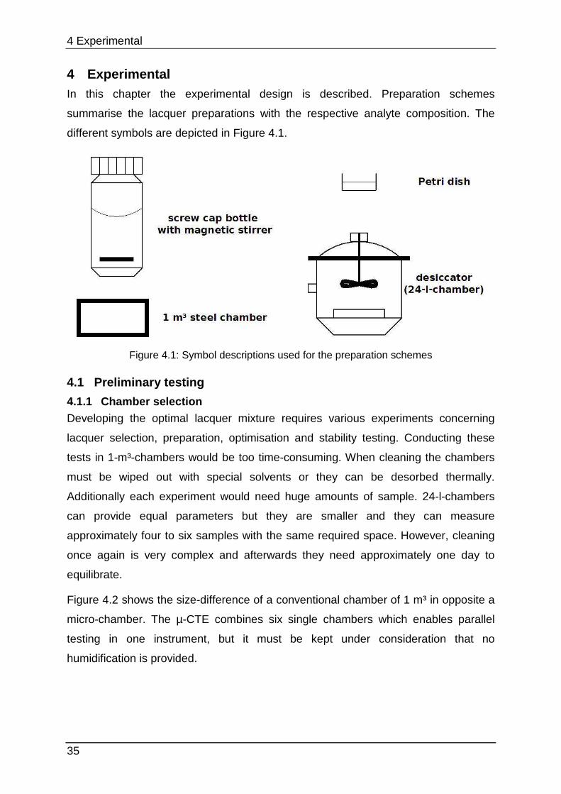
different symbols are depicted in Figure 4.1.
Figure 4.1: Symbol descriptions used for the preparation schemes
4.1 Preliminary testing
4.1.1 Chamber selection Developing the optimal lacquer mixture requires various experiments concerning
lacquer selection, preparation, optimisation and stability testing. Conducting these
tests in 1-m³-chambers would be too time-consuming. When cleaning the chambers
must be wiped out with special solvents or they can be desorbed thermally.
Additionally each experiment would need huge amounts of sample. 24-l-chambers
can provide equal parameters but they are smaller and they can measure
approximately four to six samples with the same required space. However, cleaning
once again is very complex and afterwards they need approximately one day to
equilibrate.
Figure 4.2 shows the size-difference of a conventional chamber of 1 m³ in opposite a
micro-chamber. The µ-CTE combines six single chambers which enables parallel
testing in one instrument, but it must be kept under consideration that no
humidification is provided.
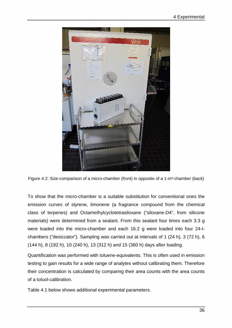
4 Experimental
36
Figure 4.2: Size-comparison of a micro-chamber (front) in opposite of a 1-m³-chamber (back)
To show that the micro-chamber is a suitable substitution for conventional ones the
emission curves of styrene, limonene (a fragrance compound from the chemical
class of terpenes) and Octamethylcyclotetrasiloxane (“siloxane-D4”, from silicone
materials) were determined from a sealant. From this sealant four times each 3.3 g
were loaded into the micro-chamber and each 16.2 g were loaded into four 24-l-
chambers (“desiccator”). Sampling was carried out at intervals of 1 (24 h), 3 (72 h), 6
(144 h), 8 (192 h), 10 (240 h), 13 (312 h) and 15 (360 h) days after loading.
Quantification was performed with toluene-equivalents. This is often used in emission
testing to gain results for a wide range of analytes without calibrating them. Therefore
their concentration is calculated by comparing their area counts with the area counts
of a toluol-calibration.
Table 4.1 below shows additional experimental parameters.
4 Experimental
37
Table 4.1: Operating parameters of the µ-CTE and 24-l-chamber (“desiccator”)
Value µ-CTE µ-CTE desiccator desiccator desiccator
Experiment section 4.1; 4.2.4 4.2 4.1; 4.2.2 4.2.3 4.3
V (chamber volume) [m³] 0.000044 0.000044 0.024 0.024 0.024
d (dish diameter) [m] 0.035 0.035 0.094 0.094 0.094
A (emission surface) [m²] 0.001 0.001 0.007 0.007 0.007
V* (Chamber-flow) [l/h] 1.8 0.9 127 108 100
L (product loading factor) [m²/m³]
21.87 21.87 0.3 0.3 0.3
n (air change rate) [1/h] 40.91 20.45 5.3 4.5 4.2
q (area specific air flow rate) [m³/(m²h)]
1.87 0.94 18.3 15.6 14.4
T (temperature) [°C] 25 25 23 23 23
RH (relative humidity) [%] - - 50 50 50
4.1.2 Lacquer selection 12 lacquers from one manufacturer (this improves comparability) were purchased
from a local building supplies store. Six of them are based on acrylic (water as
solvent) and six on alkyd (organic solvents) polymers. From the two main groups
lacquers with equal colours and surface designs were selected. Figure 4.3 shows the
nomenclature that consists of three letters for each pre-chosen lacquer:
Figure 4.3: Nomenclature of the tested lacquers (w…acrylic, o…alkyd)
The following lacquers were purchased (WGI is similar to WGW, but WGW is not
available): WGC, WGI, WGR, WMC, WMW, WMR, OGC, OGW, OGR, OMC, OMW
and OMR.
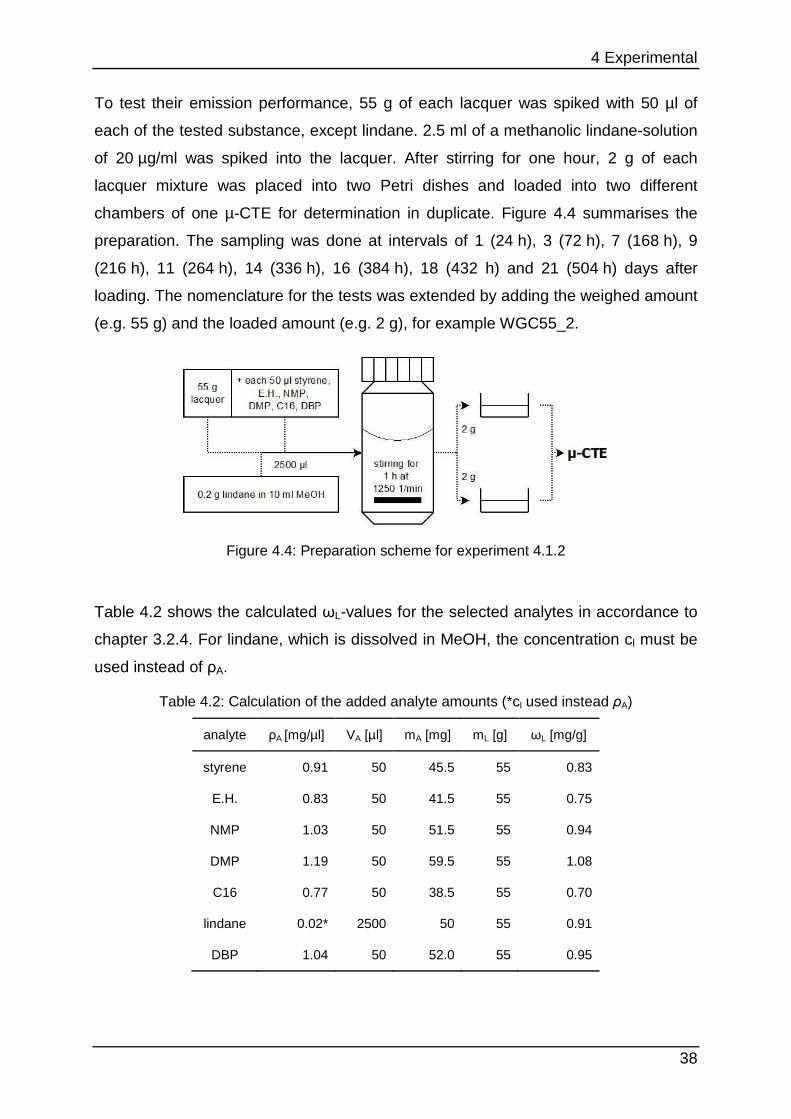
4 Experimental
38
To test their emission performance, 55 g of each lacquer was spiked with 50 µl of
each of the tested substance, except lindane. 2.5 ml of a methanolic lindane-solution
of 20 µg/ml was spiked into the lacquer. After stirring for one hour, 2 g of each
lacquer mixture was placed into two Petri dishes and loaded into two different
chambers of one µ-CTE for determination in duplicate. Figure 4.4 summarises the
preparation. The sampling was done at intervals of 1 (24 h), 3 (72 h), 7 (168 h), 9
(216 h), 11 (264 h), 14 (336 h), 16 (384 h), 18 (432 h) and 21 (504 h) days after
loading. The nomenclature for the tests was extended by adding the weighed amount
(e.g. 55 g) and the loaded amount (e.g. 2 g), for example WGC55_2.
Figure 4.4: Preparation scheme for experiment 4.1.2
Table 4.2 shows the calculated ωL-values for the selected analytes in accordance to
chapter 3.2.4. For lindane, which is dissolved in MeOH, the concentration cl must be
used instead of ρA.
Table 4.2: Calculation of the added analyte amounts (*cl used instead ρA)
analyte ρA [mg/µl] VA [µl] mA [mg] mL [g] ωL [mg/g]
styrene 0.91 50 45.5 55 0.83
E.H. 0.83 50 41.5 55 0.75
NMP 1.03 50 51.5 55 0.94
DMP 1.19 50 59.5 55 1.08
C16 0.77 50 38.5 55 0.70
lindane 0.02* 2500 50 55 0.91
DBP 1.04 50 52.0 55 0.95
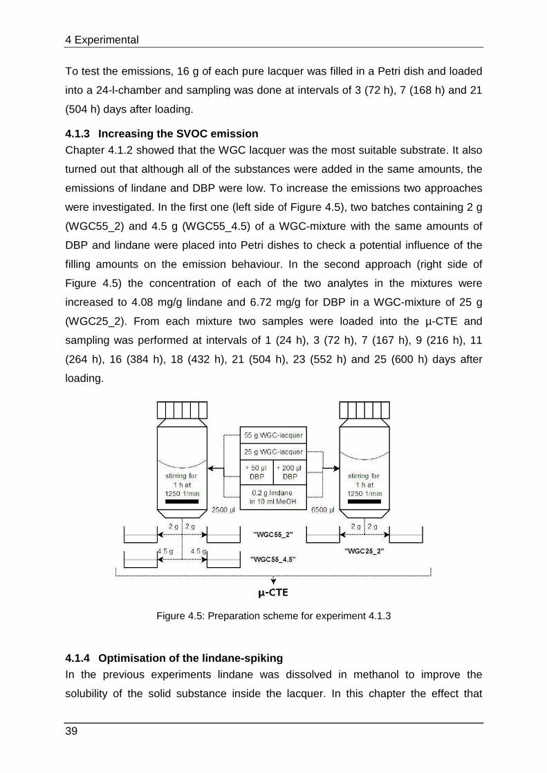
4 Experimental
39
To test the emissions, 16 g of each pure lacquer was filled in a Petri dish and loaded
into a 24-l-chamber and sampling was done at intervals of 3 (72 h), 7 (168 h) and 21
(504 h) days after loading.
4.1.3 Increasing the SVOC emission
Chapter 4.1.2 showed that the WGC lacquer was the most suitable substrate. It also
turned out that although all of the substances were added in the same amounts, the
emissions of lindane and DBP were low. To increase the emissions two approaches
were investigated. In the first one (left side of Figure 4.5), two batches containing 2 g
(WGC55_2) and 4.5 g (WGC55_4.5) of a WGC-mixture with the same amounts of
DBP and lindane were placed into Petri dishes to check a potential influence of the
filling amounts on the emission behaviour. In the second approach (right side of
Figure 4.5) the concentration of each of the two analytes in the mixtures were
increased to 4.08 mg/g lindane and 6.72 mg/g for DBP in a WGC-mixture of 25 g
(WGC25_2). From each mixture two samples were loaded into the µ-CTE and
sampling was performed at intervals of 1 (24 h), 3 (72 h), 7 (167 h), 9 (216 h), 11
(264 h), 16 (384 h), 18 (432 h), 21 (504 h), 23 (552 h) and 25 (600 h) days after
loading.
Figure 4.5: Preparation scheme for experiment 4.1.3
4.1.4 Optimisation of the lindane-spiking In the previous experiments lindane was dissolved in methanol to improve the
solubility of the solid substance inside the lacquer. In this chapter the effect that
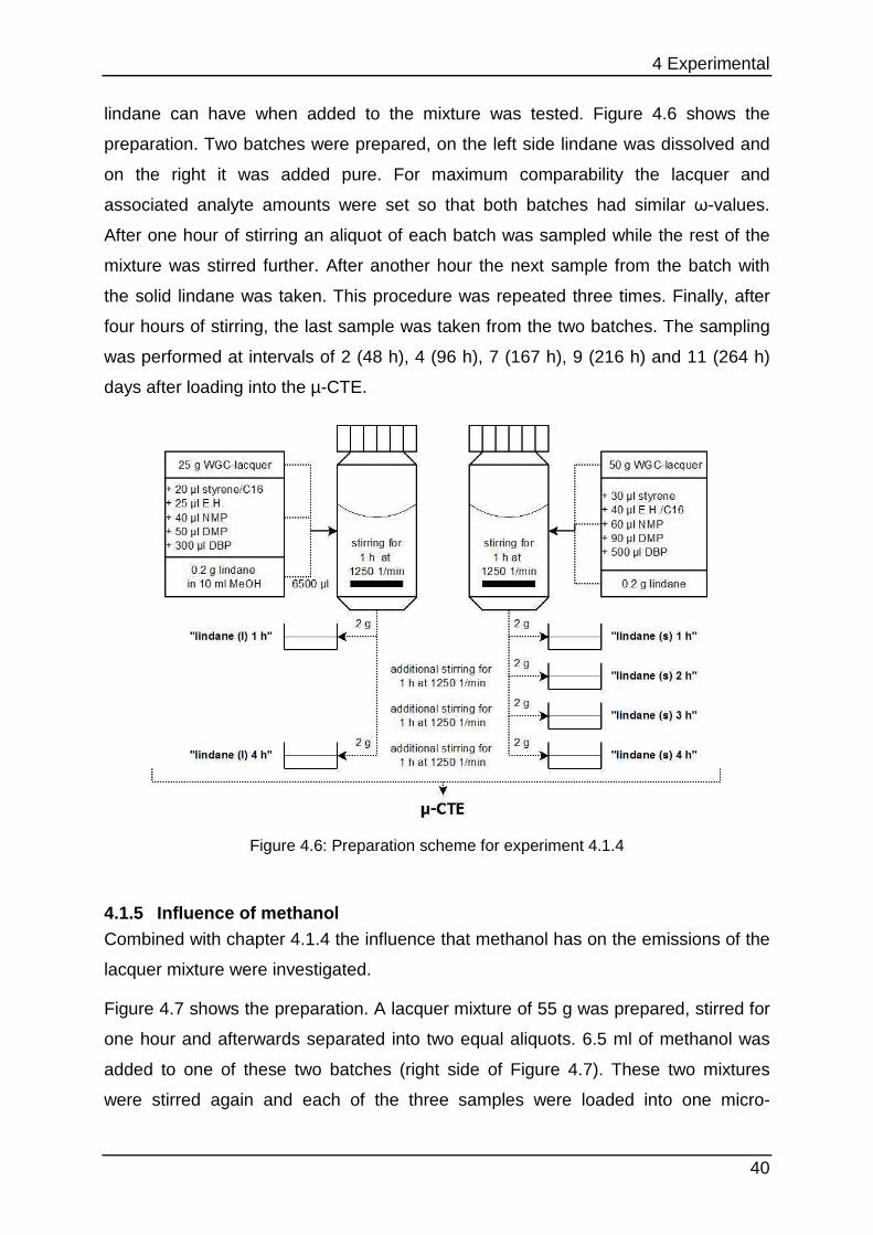
4 Experimental
40
lindane can have when added to the mixture was tested. Figure 4.6 shows the
preparation. Two batches were prepared, on the left side lindane was dissolved and
on the right it was added pure. For maximum comparability the lacquer and
associated analyte amounts were set so that both batches had similar ω-values.
After one hour of stirring an aliquot of each batch was sampled while the rest of the
mixture was stirred further. After another hour the next sample from the batch with
the solid lindane was taken. This procedure was repeated three times. Finally, after
four hours of stirring, the last sample was taken from the two batches. The sampling
was performed at intervals of 2 (48 h), 4 (96 h), 7 (167 h), 9 (216 h) and 11 (264 h)
days after loading into the µ-CTE.
Figure 4.6: Preparation scheme for experiment 4.1.4
4.1.5 Influence of methanol Combined with chapter 4.1.4 the influence that methanol has on the emissions of the
lacquer mixture were investigated.
Figure 4.7 shows the preparation. A lacquer mixture of 55 g was prepared, stirred for
one hour and afterwards separated into two equal aliquots. 6.5 ml of methanol was
added to one of these two batches (right side of Figure 4.7). These two mixtures
were stirred again and each of the three samples were loaded into one micro-
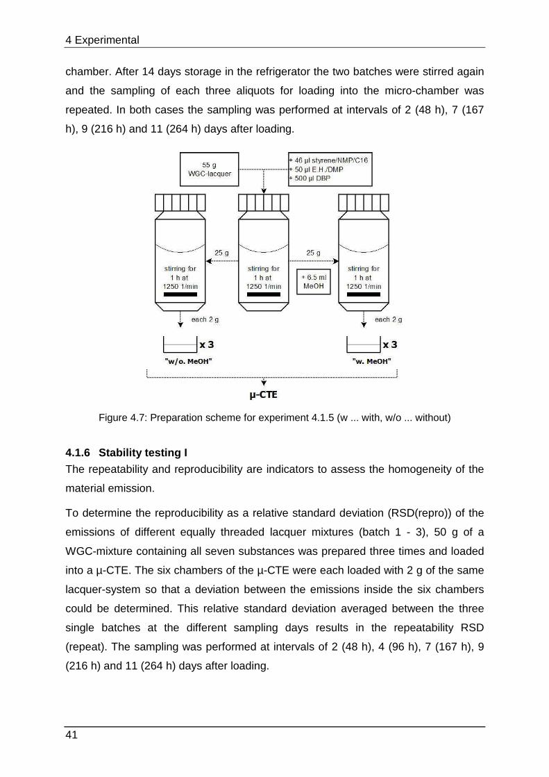
4 Experimental
41
chamber. After 14 days storage in the refrigerator the two batches were stirred again
and the sampling of each three aliquots for loading into the micro-chamber was
repeated. In both cases the sampling was performed at intervals of 2 (48 h), 7 (167
h), 9 (216 h) and 11 (264 h) days after loading.
Figure 4.7: Preparation scheme for experiment 4.1.5 (w ... with, w/o ... without)
4.1.6 Stability testing I
The repeatability and reproducibility are indicators to assess the homogeneity of the
material emission.
To determine the reproducibility as a relative standard deviation (RSD(repro)) of the
emissions of different equally threaded lacquer mixtures (batch 1 - 3), 50 g of a
WGC-mixture containing all seven substances was prepared three times and loaded
into a µ-CTE. The six chambers of the µ-CTE were each loaded with 2 g of the same
lacquer-system so that a deviation between the emissions inside the six chambers
could be determined. This relative standard deviation averaged between the three
single batches at the different sampling days results in the repeatability RSD
(repeat). The sampling was performed at intervals of 2 (48 h), 4 (96 h), 7 (167 h), 9
(216 h) and 11 (264 h) days after loading.
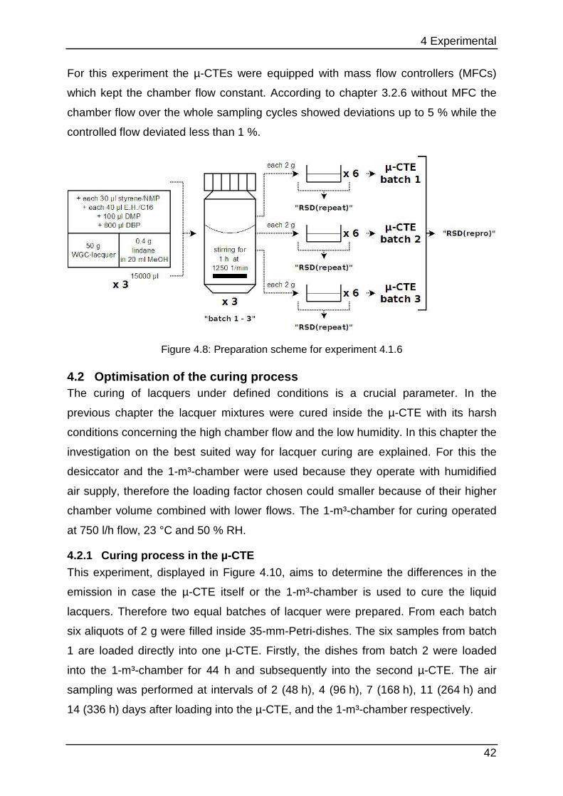
4 Experimental
42
For this experiment the µ-CTEs were equipped with mass flow controllers (MFCs)
which kept the chamber flow constant. According to chapter 3.2.6 without MFC the
chamber flow over the whole sampling cycles showed deviations up to 5 % while the
controlled flow deviated less than 1 %.
Figure 4.8: Preparation scheme for experiment 4.1.6
4.2 Optimisation of the curing process The curing of lacquers under defined conditions is a crucial parameter. In the
previous chapter the lacquer mixtures were cured inside the µ-CTE with its harsh
conditions concerning the high chamber flow and the low humidity. In this chapter the
investigation on the best suited way for lacquer curing are explained. For this the
desiccator and the 1-m³-chamber were used because they operate with humidified
air supply, therefore the loading factor chosen could smaller because of their higher
chamber volume combined with lower flows. The 1-m³-chamber for curing operated
at 750 l/h flow, 23 °C and 50 % RH.
4.2.1 Curing process in the µ-CTE
This experiment, displayed in Figure 4.10, aims to determine the differences in the
emission in case the µ-CTE itself or the 1-m³-chamber is used to cure the liquid
lacquers. Therefore two equal batches of lacquer were prepared. From each batch
six aliquots of 2 g were filled inside 35-mm-Petri-dishes. The six samples from batch
1 are loaded directly into one µ-CTE. Firstly, the dishes from batch 2 were loaded
into the 1-m³-chamber for 44 h and subsequently into the second µ-CTE. The air
sampling was performed at intervals of 2 (48 h), 4 (96 h), 7 (168 h), 11 (264 h) and
14 (336 h) days after loading into the µ-CTE, and the 1-m³-chamber respectively.
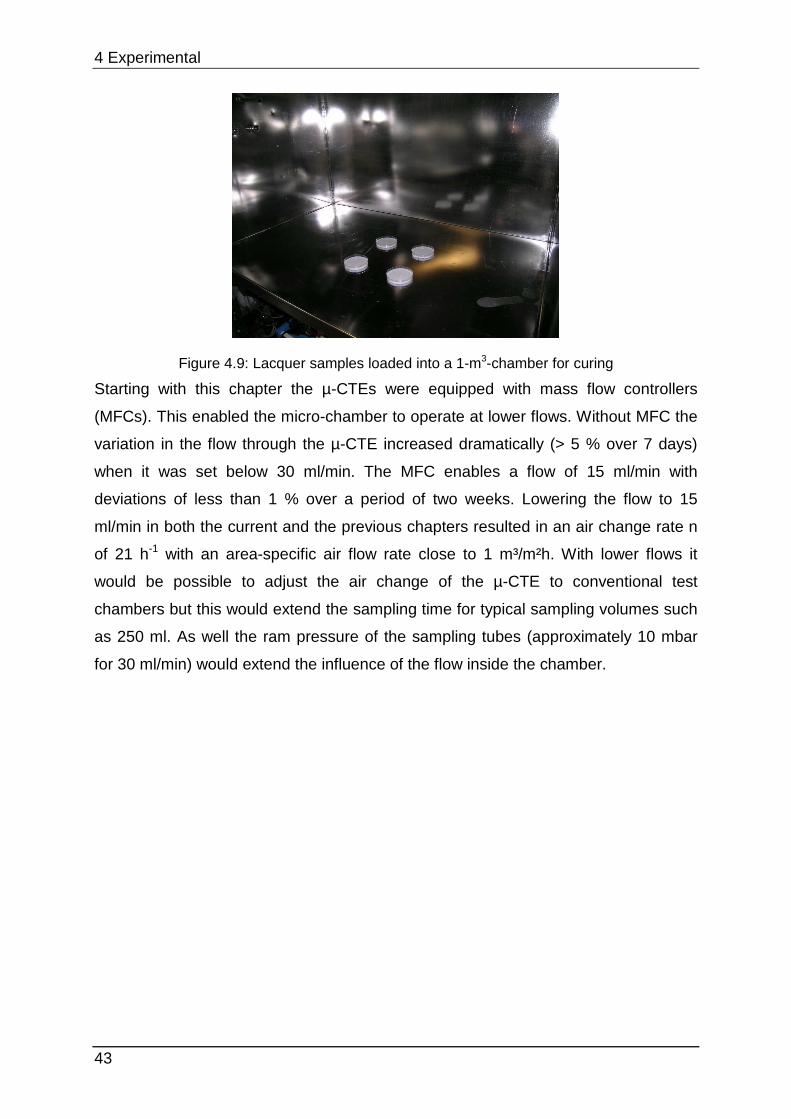
4 Experimental
43
Figure 4.9: Lacquer samples loaded into a 1-m3-chamber for curing
Starting with this chapter the µ-CTEs were equipped with mass flow controllers
(MFCs). This enabled the micro-chamber to operate at lower flows. Without MFC the
variation in the flow through the µ-CTE increased dramatically (> 5 % over 7 days)
when it was set below 30 ml/min. The MFC enables a flow of 15 ml/min with
deviations of less than 1 % over a period of two weeks. Lowering the flow to 15
ml/min in both the current and the previous chapters resulted in an air change rate n
of 21 h-1 with an area-specific air flow rate close to 1 m³/m²h. With lower flows it
would be possible to adjust the air change of the µ-CTE to conventional test
chambers but this would extend the sampling time for typical sampling volumes such
as 250 ml. As well the ram pressure of the sampling tubes (approximately 10 mbar
for 30 ml/min) would extend the influence of the flow inside the chamber.
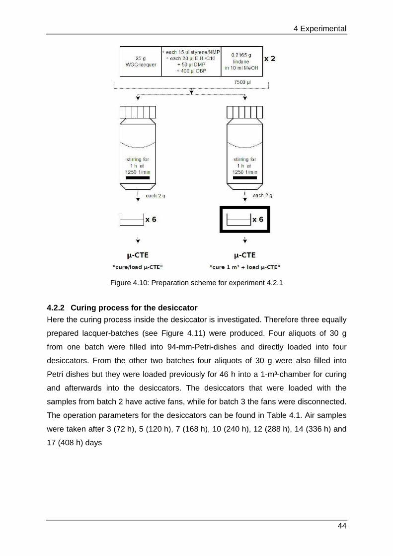
4 Experimental
44
Figure 4.10: Preparation scheme for experiment 4.2.1
4.2.2 Curing process for the desiccator
Here the curing process inside the desiccator is investigated. Therefore three equally
prepared lacquer-batches (see Figure 4.11) were produced. Four aliquots of 30 g
from one batch were filled into 94-mm-Petri-dishes and directly loaded into four
desiccators. From the other two batches four aliquots of 30 g were also filled into
Petri dishes but they were loaded previously for 46 h into a 1-m³-chamber for curing
and afterwards into the desiccators. The desiccators that were loaded with the
samples from batch 2 have active fans, while for batch 3 the fans were disconnected.
The operation parameters for the desiccators can be found in Table 4.1. Air samples
were taken after 3 (72 h), 5 (120 h), 7 (168 h), 10 (240 h), 12 (288 h), 14 (336 h) and
17 (408 h) days
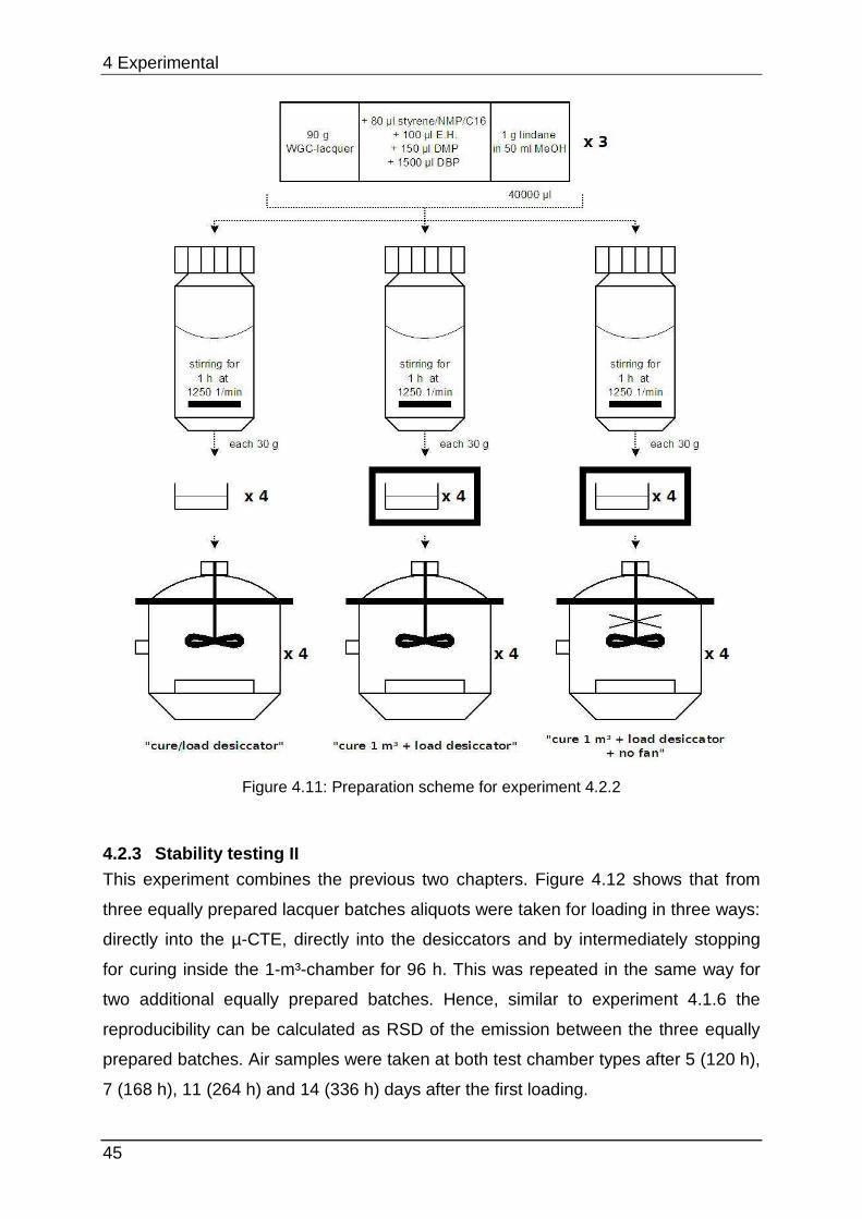
4 Experimental
45
Figure 4.11: Preparation scheme for experiment 4.2.2
4.2.3 Stability testing II This experiment combines the previous two chapters. Figure 4.12 shows that from
three equally prepared lacquer batches aliquots were taken for loading in three ways:
directly into the µ-CTE, directly into the desiccators and by intermediately stopping
for curing inside the 1-m³-chamber for 96 h. This was repeated in the same way for
two additional equally prepared batches. Hence, similar to experiment 4.1.6 the
reproducibility can be calculated as RSD of the emission between the three equally
prepared batches. Air samples were taken at both test chamber types after 5 (120 h),
7 (168 h), 11 (264 h) and 14 (336 h) days after the first loading.
4 Experimental
46
Figure 4.12: Preparation scheme for experiment 4.2.3
4.2.4 Influence on emissions at different chamber f lows In this experiment the emissions of the lacquer system were analysed using different
flows through the µ-CTE. As it can be seen in Figure 4.13 two aliquots of 2 g from a
mixture were loaded either into a µ-CTE that was operated at 30 ml/min or two
aliquots were loaded into a µ-CTE that was operated at 15 ml/min. To observe the
emission from both the liquid and the cured lacquer, samples were taken after 1 h, 2
h, 3 h, 4 h, 5 h, 6 h, 24 h, 26 h, 28 h, 30 h, 48 h, 50 h, 52 h, 54 h, 72 h, 76 h, 78 h, 98
h, 100 h, 168 h, 192 h after loading.
4 Experimental
47
Figure 4.13: Preparation scheme for experiment 4.2.4
Figure 4.14: Preparation scheme for experiment 4.2.5
4.2.5 Influence on emission at different humidities In the following experiment 4.2.4, the emissions of the same mixture were measured
under different humidities. Figure 4.14 shows that two aliquots of 2 g were loaded
into a µ-CTE that was operated at 0 % RH and also two aliquots into a µ-CTE that
was operated at 55 % RH. In accordance with experiment 4.2.4, the curing process
and the emissions afterwards should be observed. Therefore samples were taken
after 1 h, 2 h, 3 h, 4 h, 5 h, 24 h, 26 h, 28 h, 50 h, 52 h, 72 h, 76 h, 168 h, 192 h, 240
h, 264 h after loading. The flow was set to 15 ml/min for both µ-CTEs.
As previously mentioned in chapter 4.1.1 the µ-CTE does not provide humidification.
To humidify the air supply of the µ-CTE a simple humidification device was
developed (see Figure 4.15). Figure 4.16 shows the construction set-up. Dry air from
the MFC was split into two streams by a T-piece (1). With a needle valve (2) the split
ratio of dry and saturated air was adjusted. One part of the air was led through a
water reservoir (3) where the air is saturated with water. At a second T-piece (4) the
humidified air was mixed with dry air from the first T-piece and flows to the µ-CTE. A
sensor (ALMEMO 2890-9 data logger with a FHA646-R climate sensor both from
AHLBORN) measures and records the relative humidity of the µ-CTE supplying air.
4 Experimental
48
Figure 4.15: Improvised humidification device (1 ... T-piece; 2 ... needle valve; 3 ... water
reservoir; 4 ... T-piece)
Figure 4.16: Systematic scheme of the improvised humidification device
(1 ... T-piece; 2 ... needle valve; 3 ... water reservoir; 4 ... T-piece)
4.3 Round robin test optimisation The developed lacquer should be used as reference material for a round robin test
on emission testing with climate chambers according to ISO 16000-9 [12]. These
tests are organised by Federal Institute for Material Research and Testing
(Bundesanstalt für Materialforschung und -prüfung BAM, Germany) every two years
with about 50 participants all over the world.
Before the lacquer system could be used as reference some additional tests had to
be performed. Firstly odorous compounds were added. Afterwards a mixture was
developed where all substances emit quantifiable amounts at sampling day 3 and 7
after loading. It should be tested in which packaging the lacquer should be sent to the
participants. Finally the homogeneity of one of the lacquer batch inside desiccators
and a 1-m3-chamber was investigated.
4 Experimental
49
4.3.1 Additional analytes and optimal spiking amoun ts Additional analytes hexanal, n-decane (C10), 2-ethylhexyl acrylate (E.H.-acryl) and
naphthalene were added to the mixture. The substances were spiked in amounts that
are comparable to styrene, E.H. and C16 because they show similarity in both boiling
points and polarity (see Table 3.1 and Table 3.2).
Common used TD-GC/MS (thermal desorption) systems have their linear calibration
range between 1 ng to 150 ng depending on the substance. With a sampling volume
of 1 l this results in air concentrations of 1 - 150 µg/m³. Different lacquer mixtures
were prepared. After curing inside the 1-m³-chamber and loading into desiccators the
emissions after three and seven days were analysed. These are typical sampling
points in emission testing. The measured air concentration should range between 10
to 120 µg/m³.
4.3.2 Shipping and storage
At round robin tests it is important to ensure that the samples reach the participants
without any changes in their properties. With this step it should be ensured that all
laboratories receive comparable samples.
The lacquer mixture cannot be shipped in liquid. Chapter 4.2 shows that the curing
process is the crucial parameter that defines the emissions of the lacquer system.
Slight differences in the parameters while the mixture cures can lead to poor
emission reproducibility. Moreover, several regulations restrict the shipping liquids to
other countries. This leads to extending transfer times and possibly changing the
sample. Therefore it is more feasible to ship the solid lacquers which were cured
previously in bigger chambers.
In this experiment a lacquer mixture was prepared (see 4.3.1) and poured into six
Petri dishes and loaded into a µ-CTE (15 ml/min; 0 % RH). There were cured for four
days. After this time all Petri dishes were sealed with a lid and three were covered in
aluminium foil. The other three were packed in a LDPE-bag (low density
polyethylene, 0.1 mm thickness), vacuumed and sealed. The vacuum prevents
additional emission by eliminating the air. The six samples were stored for three days
in the laboratory at 21 °C. They were then unpacked and loaded into a µ-CTE which
operated at 15 ml/min chamber flow of dry air. Samples were taken one, two and four
days after the loading.
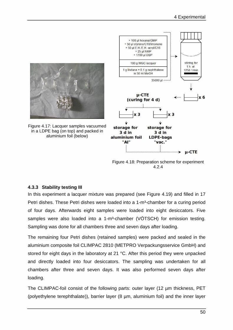
4 Experimental
50
Figure 4.17: Lacquer samples vacuumed in a LDPE bag (on top) and packed in
aluminium foil (below)
Figure 4.18: Preparation scheme for experiment 4.2.4
4.3.3 Stability testing III In this experiment a lacquer mixture was prepared (see Figure 4.19) and filled in 17
Petri dishes. These Petri dishes were loaded into a 1-m³-chamber for a curing period
of four days. Afterwards eight samples were loaded into eight desiccators. Five
samples were also loaded into a 1-m³-chamber (VÖTSCH) for emission testing.
Sampling was done for all chambers three and seven days after loading.
The remaining four Petri dishes (retained samples) were packed and sealed in the
aluminium composite foil CLIMPAC 2810 (METPRO Verpackungsservice GmbH) and
stored for eight days in the laboratory at 21 °C. After this period they were unpacked
and directly loaded into four desiccators. The sampling was undertaken for all
chambers after three and seven days. It was also performed seven days after
loading.
The CLIMPAC-foil consist of the following parts: outer layer (12 µm thickness, PET
(polyethylene terephthalate)), barrier layer (8 µm, aluminium foil) and the inner layer
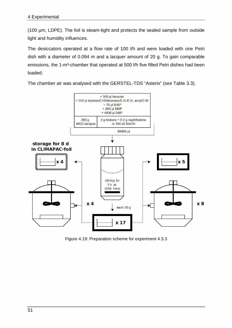
4 Experimental
51
(100 µm, LDPE). The foil is steam-tight and protects the sealed sample from outside
light and humidity influences.
The desiccators operated at a flow rate of 100 l/h and were loaded with one Petri
dish with a diameter of 0.094 m and a lacquer amount of 20 g. To gain comparable
emissions, the 1-m³-chamber that operated at 500 l/h five filled Petri dishes had been
loaded.
The chamber air was analysed with the GERSTEL-TDS “Asterix” (see Table 3.3).
Figure 4.19: Preparation scheme for experiment 4.3.3
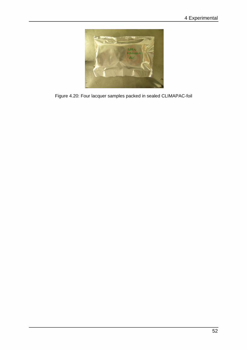
4 Experimental
52
Figure 4.20: Four lacquer samples packed in sealed CLIMAPAC-foil
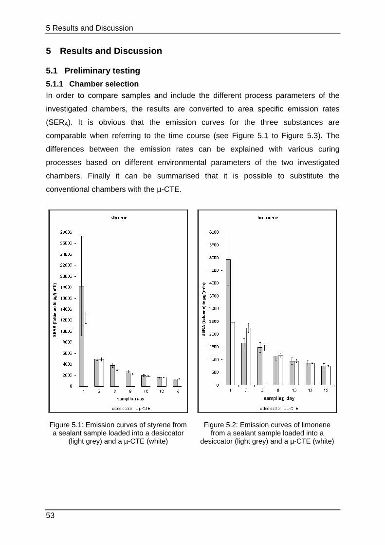
5 Results and Discussion
53
5 Results and Discussion
5.1 Preliminary testing
5.1.1 Chamber selection In order to compare samples and include the different process parameters of the
investigated chambers, the results are converted to area specific emission rates
(SERA). It is obvious that the emission curves for the three substances are
comparable when referring to the time course (see Figure 5.1 to Figure 5.3). The
differences between the emission rates can be explained with various curing
processes based on different environmental parameters of the two investigated
chambers. Finally it can be summarised that it is possible to substitute the
conventional chambers with the µ-CTE.
Figure 5.1: Emission curves of styrene from a sealant sample loaded into a desiccator
(light grey) and a µ-CTE (white)
Figure 5.2: Emission curves of limonene from a sealant sample loaded into a
desiccator (light grey) and a µ-CTE (white)
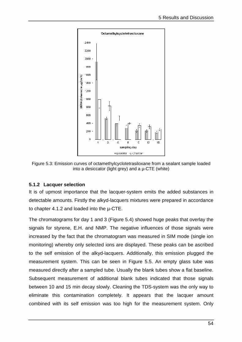
5 Results and Discussion
54
Figure 5.3: Emission curves of octamethylcyclotetrasiloxane from a sealant sample loaded into a desiccator (light grey) and a µ-CTE (white)
5.1.2 Lacquer selection It is of upmost importance that the lacquer-system emits the added substances in
detectable amounts. Firstly the alkyd-lacquers mixtures were prepared in accordance
to chapter 4.1.2 and loaded into the µ-CTE.
The chromatograms for day 1 and 3 (Figure 5.4) showed huge peaks that overlay the
signals for styrene, E.H. and NMP. The negative influences of those signals were
increased by the fact that the chromatogram was measured in SIM mode (single ion
monitoring) whereby only selected ions are displayed. These peaks can be ascribed
to the self emission of the alkyd-lacquers. Additionally, this emission plugged the
measurement system. This can be seen in Figure 5.5. An empty glass tube was
measured directly after a sampled tube. Usually the blank tubes show a flat baseline.
Subsequent measurement of additional blank tubes indicated that those signals
between 10 and 15 min decay slowly. Cleaning the TDS-system was the only way to
eliminate this contamination completely. It appears that the lacquer amount
combined with its self emission was too high for the measurement system. Only
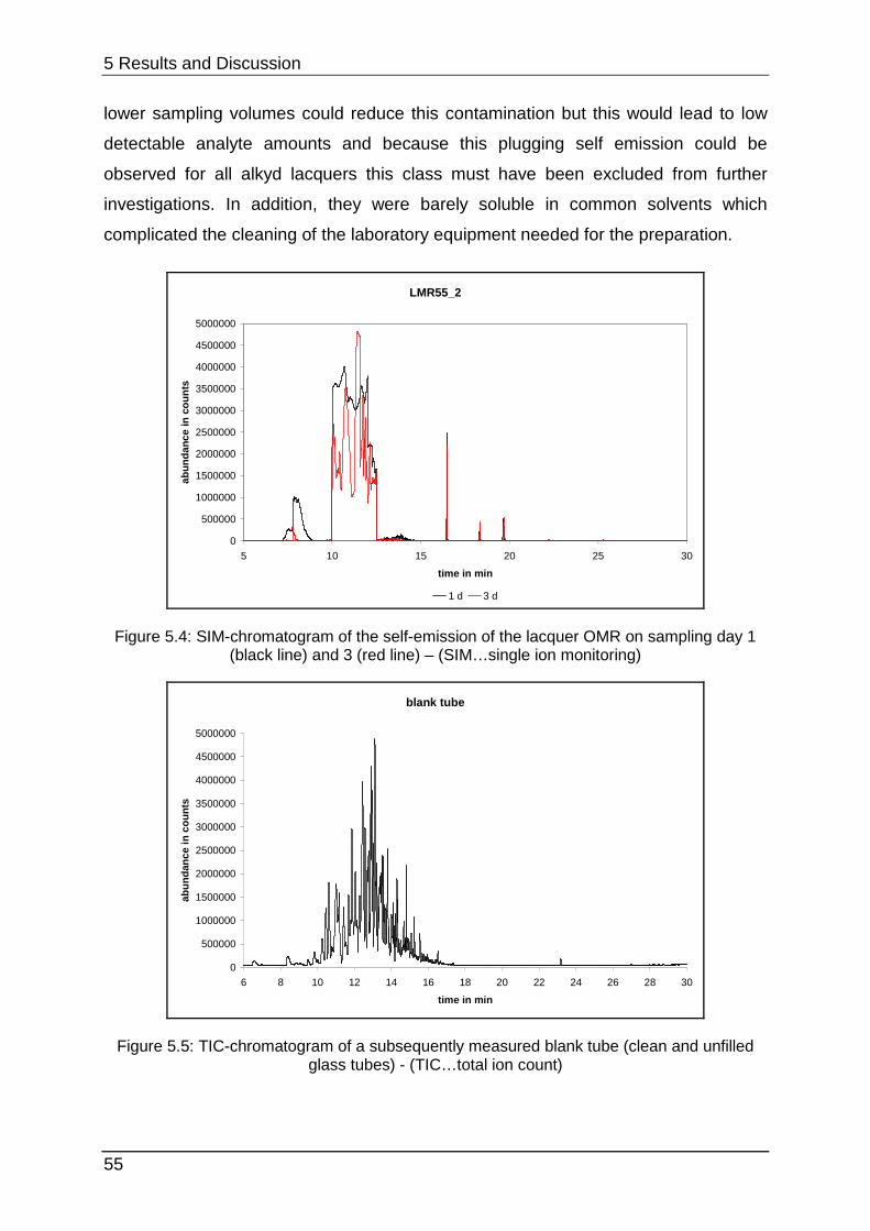
5 Results and Discussion
55
lower sampling volumes could reduce this contamination but this would lead to low
detectable analyte amounts and because this plugging self emission could be
observed for all alkyd lacquers this class must have been excluded from further
investigations. In addition, they were barely soluble in common solvents which
complicated the cleaning of the laboratory equipment needed for the preparation.
LMR55_2
0
500000
1000000
1500000
2000000
2500000
3000000
3500000
4000000
4500000
5000000
5 10 15 20 25 30
time in min
abun
danc
e in
cou
nts
1 d 3 d
Figure 5.4: SIM-chromatogram of the self-emission of the lacquer OMR on sampling day 1 (black line) and 3 (red line) – (SIM…single ion monitoring)
blank tube
0
500000
1000000
1500000
2000000
2500000
3000000
3500000
4000000
4500000
5000000
6 8 10 12 14 16 18 20 22 24 26 28 30
time in min
abun
danc
e in
cou
nts
Figure 5.5: TIC-chromatogram of a subsequently measured blank tube (clean and unfilled glass tubes) - (TIC…total ion count)
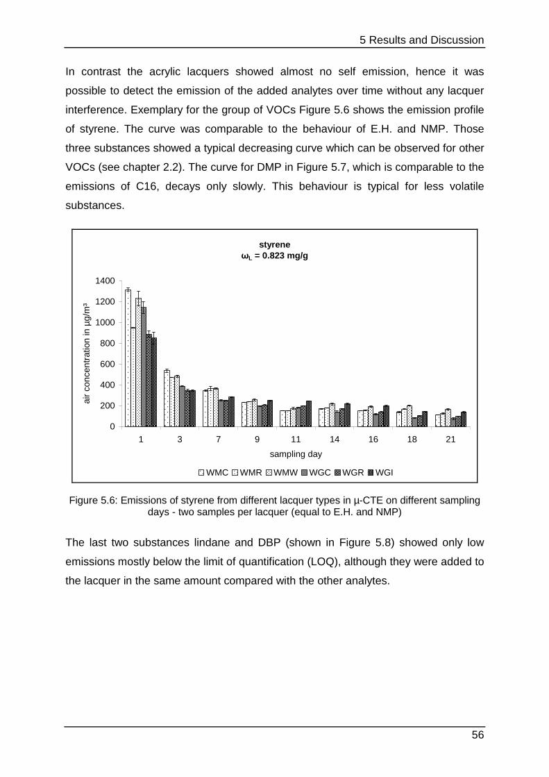
5 Results and Discussion
56
In contrast the acrylic lacquers showed almost no self emission, hence it was
possible to detect the emission of the added analytes over time without any lacquer
interference. Exemplary for the group of VOCs Figure 5.6 shows the emission profile
of styrene. The curve was comparable to the behaviour of E.H. and NMP. Those
three substances showed a typical decreasing curve which can be observed for other
VOCs (see chapter 2.2). The curve for DMP in Figure 5.7, which is comparable to the
emissions of C16, decays only slowly. This behaviour is typical for less volatile
substances.
styrene ωL = 0.823 mg/g
0
200
400
600
800
1000
1200
1400
1 3 7 9 11 14 16 18 21
sampling day
air
conc
entr
atio
n in
µg/
m³
WMC WMR WMW WGC WGR WGI
Figure 5.6: Emissions of styrene from different lacquer types in µ-CTE on different sampling days - two samples per lacquer (equal to E.H. and NMP)
The last two substances lindane and DBP (shown in Figure 5.8) showed only low
emissions mostly below the limit of quantification (LOQ), although they were added to
the lacquer in the same amount compared with the other analytes.
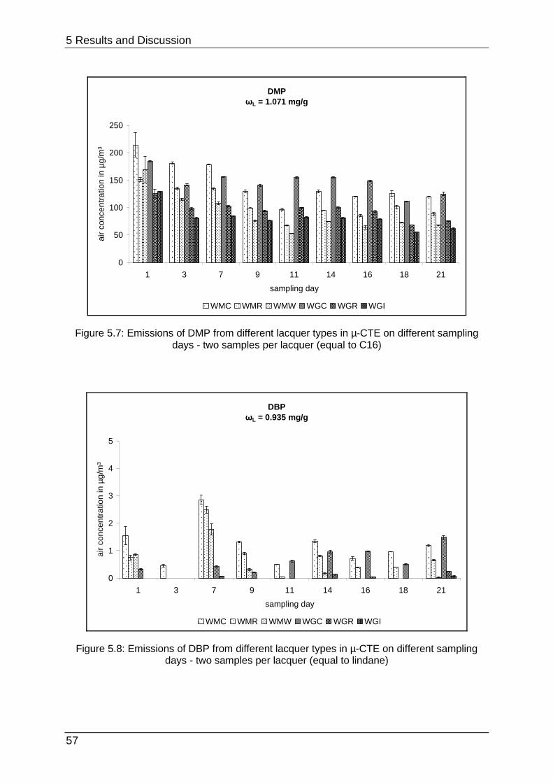
5 Results and Discussion
57
DMP ωL = 1.071 mg/g
0
50
100
150
200
250
1 3 7 9 11 14 16 18 21
sampling day
air
conc
entr
atio
n in
µg/
m³
WMC WMR WMW WGC WGR WGI
Figure 5.7: Emissions of DMP from different lacquer types in µ-CTE on different sampling days - two samples per lacquer (equal to C16)
DBP ωL = 0.935 mg/g
0
1
2
3
4
5
1 3 7 9 11 14 16 18 21
sampling day
air
conc
entr
atio
n in
µg/
m³
WMC WMR WMW WGC WGR WGI
Figure 5.8: Emissions of DBP from different lacquer types in µ-CTE on different sampling days - two samples per lacquer (equal to lindane)
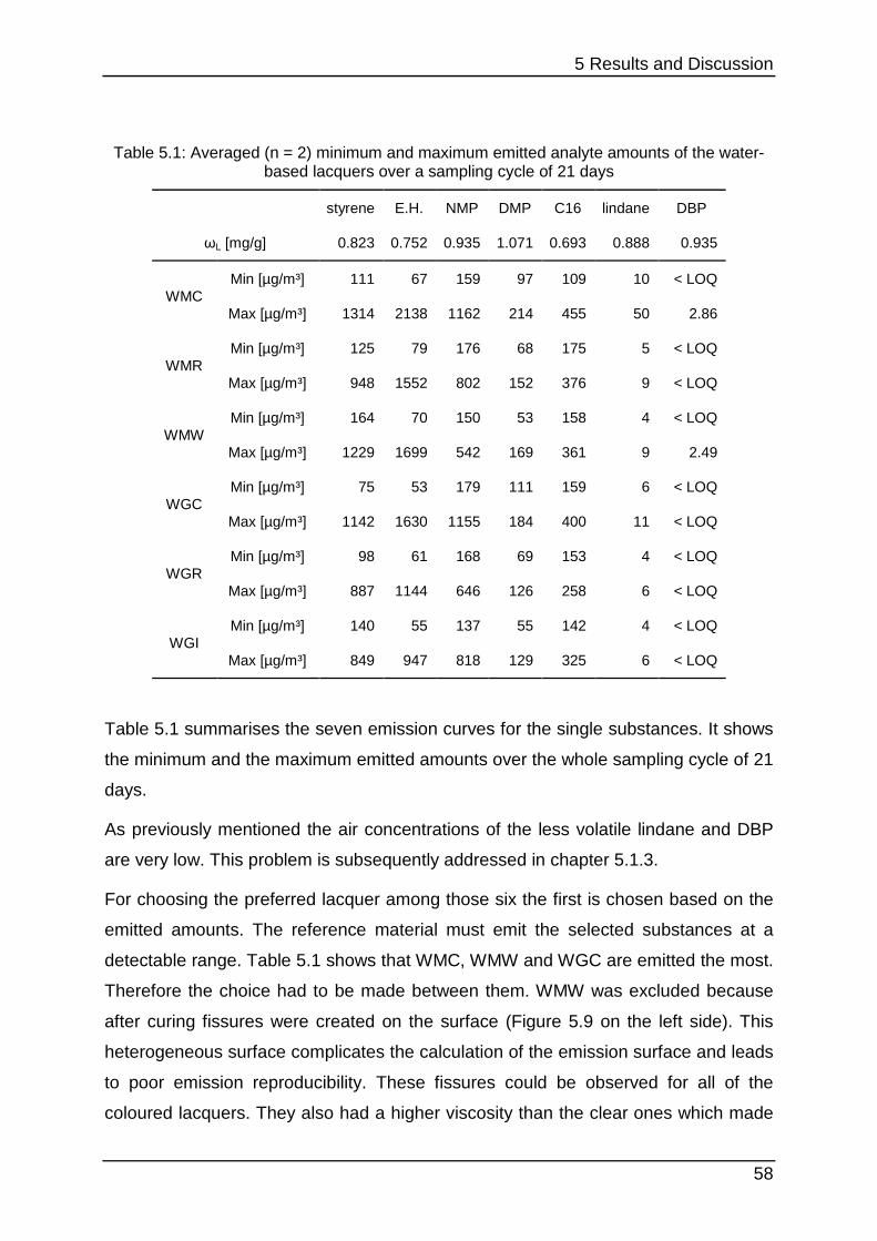
5 Results and Discussion
58
Table 5.1: Averaged (n = 2) minimum and maximum emitted analyte amounts of the water-based lacquers over a sampling cycle of 21 days
styrene E.H. NMP DMP C16 lindane DBP
ωL [mg/g] 0.823 0.752 0.935 1.071 0.693 0.888 0.935
WMC Min [µg/m³] 111 67 159 97 109 10 < LOQ
Max [µg/m³] 1314 2138 1162 214 455 50 2.86
WMR Min [µg/m³] 125 79 176 68 175 5 < LOQ
Max [µg/m³] 948 1552 802 152 376 9 < LOQ
WMW Min [µg/m³] 164 70 150 53 158 4 < LOQ
Max [µg/m³] 1229 1699 542 169 361 9 2.49
WGC Min [µg/m³] 75 53 179 111 159 6 < LOQ
Max [µg/m³] 1142 1630 1155 184 400 11 < LOQ
WGR Min [µg/m³] 98 61 168 69 153 4 < LOQ
Max [µg/m³] 887 1144 646 126 258 6 < LOQ
WGI Min [µg/m³] 140 55 137 55 142 4 < LOQ
Max [µg/m³] 849 947 818 129 325 6 < LOQ
Table 5.1 summarises the seven emission curves for the single substances. It shows
the minimum and the maximum emitted amounts over the whole sampling cycle of 21
days.
As previously mentioned the air concentrations of the less volatile lindane and DBP
are very low. This problem is subsequently addressed in chapter 5.1.3.
For choosing the preferred lacquer among those six the first is chosen based on the
emitted amounts. The reference material must emit the selected substances at a
detectable range. Table 5.1 shows that WMC, WMW and WGC are emitted the most.
Therefore the choice had to be made between them. WMW was excluded because
after curing fissures were created on the surface (Figure 5.9 on the left side). This
heterogeneous surface complicates the calculation of the emission surface and leads
to poor emission reproducibility. These fissures could be observed for all of the
coloured lacquers. They also had a higher viscosity than the clear ones which made
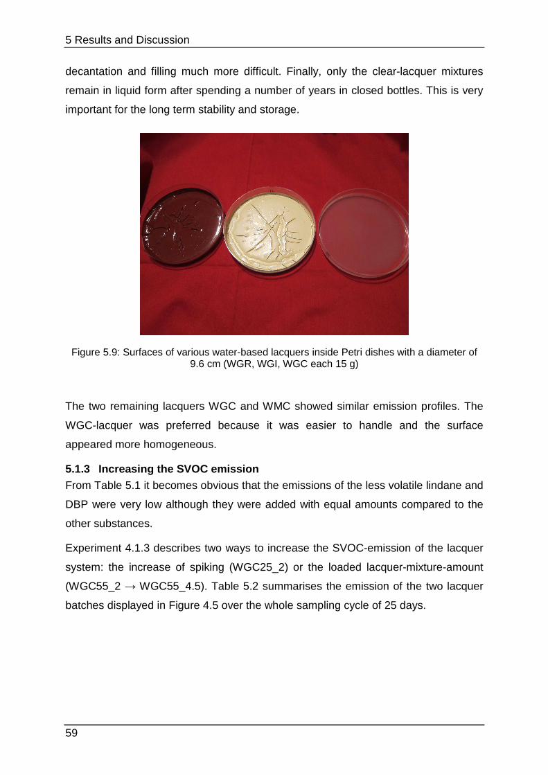
5 Results and Discussion
59
decantation and filling much more difficult. Finally, only the clear-lacquer mixtures
remain in liquid form after spending a number of years in closed bottles. This is very
important for the long term stability and storage.
Figure 5.9: Surfaces of various water-based lacquers inside Petri dishes with a diameter of 9.6 cm (WGR, WGI, WGC each 15 g)
The two remaining lacquers WGC and WMC showed similar emission profiles. The
WGC-lacquer was preferred because it was easier to handle and the surface
appeared more homogeneous.
5.1.3 Increasing the SVOC emission From Table 5.1 it becomes obvious that the emissions of the less volatile lindane and
DBP were very low although they were added with equal amounts compared to the
other substances.
Experiment 4.1.3 describes two ways to increase the SVOC-emission of the lacquer
system: the increase of spiking (WGC25_2) or the loaded lacquer-mixture-amount
(WGC55_2 → WGC55_4.5). Table 5.2 summarises the emission of the two lacquer
batches displayed in Figure 4.5 over the whole sampling cycle of 25 days.
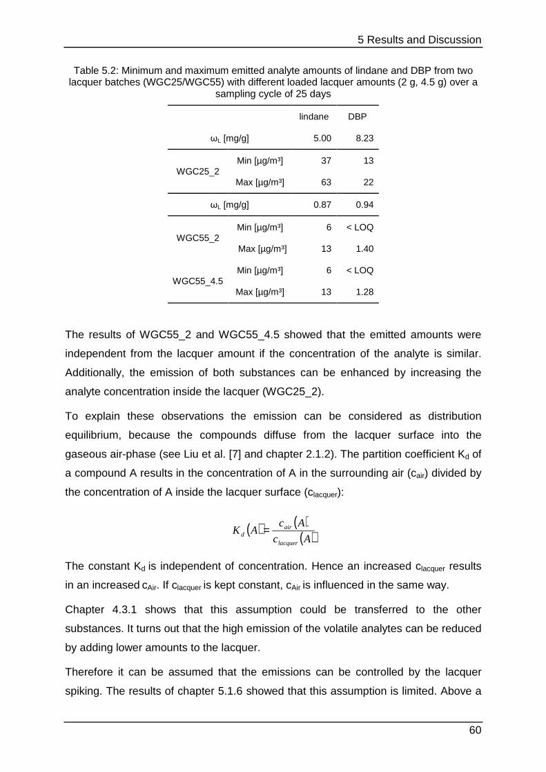
5 Results and Discussion
60
Table 5.2: Minimum and maximum emitted analyte amounts of lindane and DBP from two lacquer batches (WGC25/WGC55) with different loaded lacquer amounts (2 g, 4.5 g) over a
sampling cycle of 25 days
lindane DBP
ωL [mg/g] 5.00 8.23
WGC25_2 Min [µg/m³] 37 13
Max [µg/m³] 63 22
ωL [mg/g] 0.87 0.94
WGC55_2 Min [µg/m³] 6 < LOQ
Max [µg/m³] 13 1.40
WGC55_4.5 Min [µg/m³] 6 < LOQ
Max [µg/m³] 13 1.28
The results of WGC55_2 and WGC55_4.5 showed that the emitted amounts were
independent from the lacquer amount if the concentration of the analyte is similar.
Additionally, the emission of both substances can be enhanced by increasing the
analyte concentration inside the lacquer (WGC25_2).
To explain these observations the emission can be considered as distribution
equilibrium, because the compounds diffuse from the lacquer surface into the
gaseous air-phase (see Liu et al. [7] and chapter 2.1.2). The partition coefficient Kd of
a compound A results in the concentration of A in the surrounding air (cair) divided by
the concentration of A inside the lacquer surface (clacquer):
( ) ( )( )Ac
AcAK
lacquer
aird =
The constant Kd is independent of concentration. Hence an increased clacquer results
in an increased cAir. If clacquer is kept constant, cAir is influenced in the same way.
Chapter 4.3.1 shows that this assumption could be transferred to the other
substances. It turns out that the high emission of the volatile analytes can be reduced
by adding lower amounts to the lacquer.
Therefore it can be assumed that the emissions can be controlled by the lacquer
spiking. The results of chapter 5.1.6 showed that this assumption is limited. Above a
5 Results and Discussion
61
certain concentration inside the lacquer the emissions of lindane and DBP could not
be enhanced by adding more substance into the mixture. The volatility of those two
substances limited an increased emission, hence the spiking of those two
substances was kept at about 10 - 20 mg/g.
5.1.4 The influence of methanol Experiment 4.1.4 aims to determine the influence of lindane and the associated
solvent methanol. It was the only solid substance among the analytes. Figure 5.10
shows the emission profile of lindane which was added as methanolic solution
(“lindane (l)”) or pure (“lindane (s)”) to the lacquer. The results showed that the
emissions from lindane are higher when it is dissolved in methanol. Hence MeOH
seemed to improve the solubility of lindane inside the lacquer mixture.
0
10
20
30
40
50
60
70
2 4 7 9 11
air
conc
ent
ratio
n in
µg/
m³
sampling day
lindane"lindane (l)": ωL = 4.068 mg/g"lindane (s)": ωL = 3.926 mg/g
lindane (l) stirred 1 h lindane (l) stirred 4 h lindane (s) stirred 1 h
lindane (s) stirred 2 h lindane (s) stirred 3 h lindane (s) stirred 4 h
Figure 5.10: Emitted lindane amounts, either dissolved in MeOH (“lindane (l)”) or added pure (“lindane (s)”), over a period of 11 days with different stirring times
The dotted columns show that the stirring time did not affect lindane emissions
significantly. It can be assumed that the less volatile lindane remained inside the
liquid mixture over the whole homogenisation process.
Figure 5.11 to Figure 5.22 compare the results for the compounds except lindane for
both experiments 4.1.4 and 4.1.5. Experiment 4.1.4 was designed in a way that the
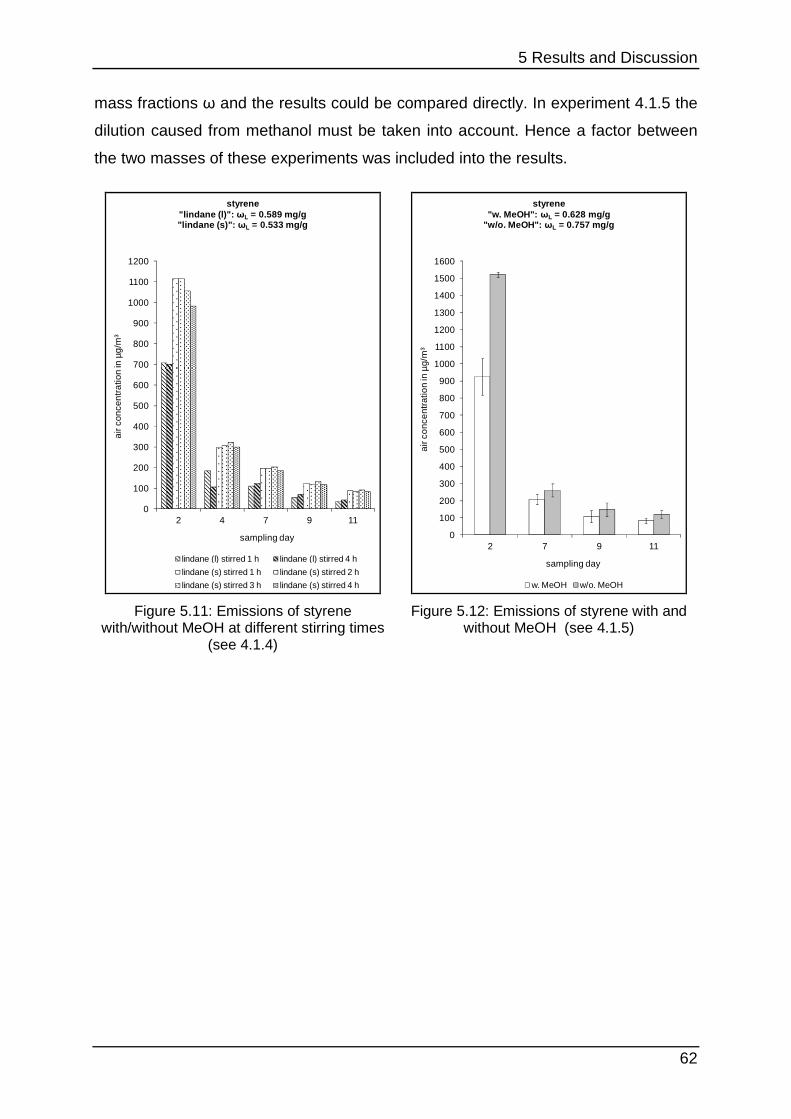
5 Results and Discussion
62
mass fractions ω and the results could be compared directly. In experiment 4.1.5 the
dilution caused from methanol must be taken into account. Hence a factor between
the two masses of these experiments was included into the results.
0
100
200
300
400
500
600
700
800
900
1000
1100
1200
2 4 7 9 11
air
con
cen
tra
tion
in µ
g/m
³
sampling day
styrene"lindane (l)": ωL = 0.589 mg/g"lindane (s)": ωL = 0.533 mg/g
lindane (l) stirred 1 h lindane (l) stirred 4 h
lindane (s) stirred 1 h lindane (s) stirred 2 h
lindane (s) stirred 3 h lindane (s) stirred 4 h
Figure 5.11: Emissions of styrene with/without MeOH at different stirring times
(see 4.1.4)
0
100
200
300
400
500
600
700
800
900
1000
1100
1200
1300
1400
1500
1600
2 7 9 11
air
co
nce
ntra
tion
in µ
g/m
³
sampling day
styrene"w. MeOH": ωL = 0.628 mg/g
"w/o. MeOH": ωL = 0.757 mg/g
w. MeOH w/o. MeOH
Figure 5.12: Emissions of styrene with and without MeOH (see 4.1.5)
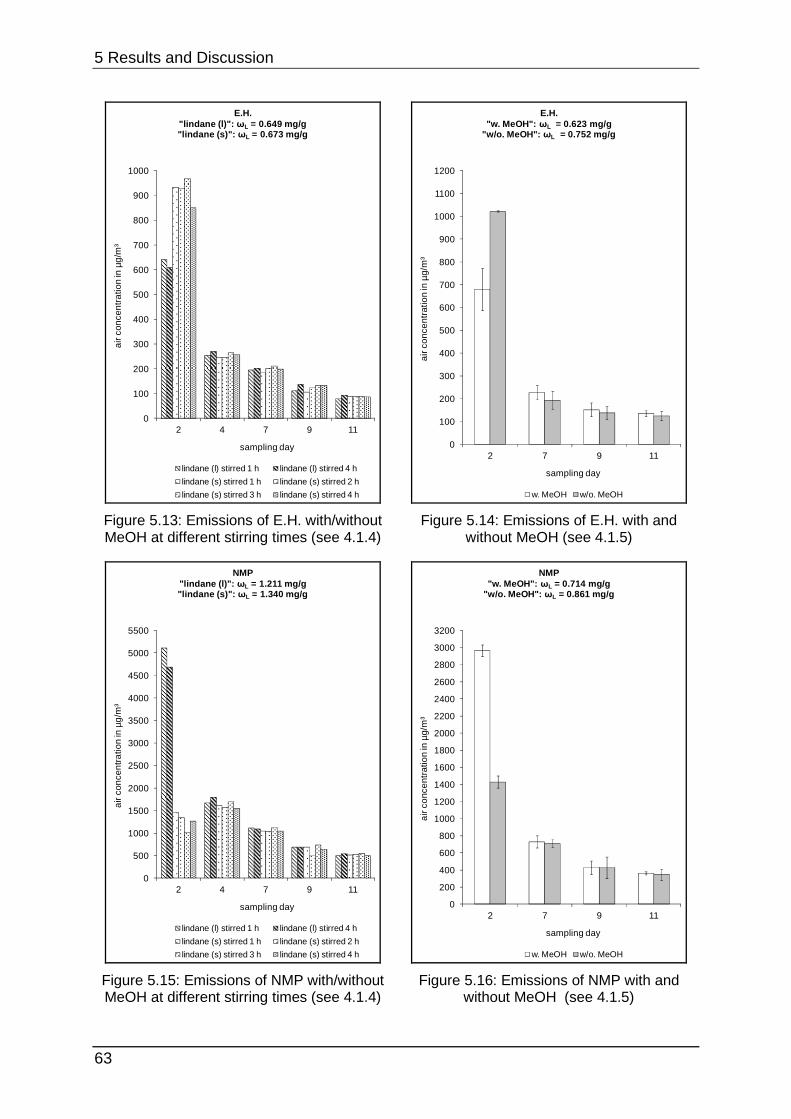
5 Results and Discussion
63
0
100
200
300
400
500
600
700
800
900
1000
2 4 7 9 11
air
con
cen
tra
tion
in µ
g/m
³
sampling day
E.H."lindane (l)": ωL = 0.649 mg/g"lindane (s)": ωL = 0.673 mg/g
lindane (l) stirred 1 h lindane (l) stirred 4 h
lindane (s) stirred 1 h lindane (s) stirred 2 h
lindane (s) stirred 3 h lindane (s) stirred 4 h
Figure 5.13: Emissions of E.H. with/without MeOH at different stirring times (see 4.1.4)
0
100
200
300
400
500
600
700
800
900
1000
1100
1200
2 7 9 11
air
co
nce
ntra
tion
in µ
g/m
³
sampling day
E.H."w. MeOH": ωL = 0.623 mg/g
"w/o. MeOH": ωL = 0.752 mg/g
w. MeOH w/o. MeOH
Figure 5.14: Emissions of E.H. with and without MeOH (see 4.1.5)
0
500
1000
1500
2000
2500
3000
3500
4000
4500
5000
5500
2 4 7 9 11
air
con
cen
tra
tion
in µ
g/m
³
sampling day
NMP"lindane (l)": ωL = 1.211 mg/g"lindane (s)": ωL = 1.340 mg/g
lindane (l) stirred 1 h lindane (l) stirred 4 h
lindane (s) stirred 1 h lindane (s) stirred 2 h
lindane (s) stirred 3 h lindane (s) stirred 4 h
Figure 5.15: Emissions of NMP with/without MeOH at different stirring times (see 4.1.4)
0
200
400
600
800
1000
1200
1400
1600
1800
2000
2200
2400
2600
2800
3000
3200
2 7 9 11
air
co
nce
ntra
tion
in µ
g/m
³
sampling day
NMP"w. MeOH": ωL = 0.714 mg/g
"w/o. MeOH": ωL = 0.861 mg/g
w. MeOH w/o. MeOH
Figure 5.16: Emissions of NMP with and without MeOH (see 4.1.5)
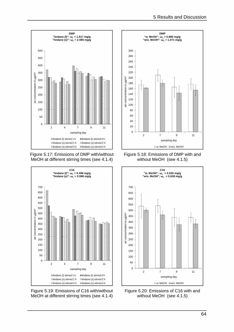
5 Results and Discussion
64
0
50
100
150
200
250
300
350
400
450
500
2 4 7 9 11
air
con
cen
tra
tion
in µ
g/m
³
sampling day
DMP"lindane (l)": ωL = 1.917 mg/g"lindane (s)": ωL = 2.080 mg/g
lindane (l) stirred 1 h lindane (l) stirred 4 h
lindane (s) stirred 1 h lindane (s) stirred 2 h
lindane (s) stirred 3 h lindane (s) stirred 4 h
Figure 5.17: Emissions of DMP with/without MeOH at different stirring times (see 4.1.4)
0
20
40
60
80
100
120
140
160
180
200
220
240
260
280
300
2 7 9 11
air
co
nce
ntra
tion
in µ
g/m
³
sampling day
DMP"w. MeOH": ωL = 0.889 mg/g
"w/o. MeOH": ωL = 1.071 mg/g
w. MeOH w/o. MeOH
Figure 5.18: Emissions of DMP with and without MeOH (see 4.1.5)
0
50
100
150
200
250
300
350
400
450
500
550
600
650
700
2 4 7 9 11
air
con
cen
tra
tion
in µ
g/m
³
sampling day
C16"lindane (l)": ωL = 0.496 mg/g"lindane (s)": ωL = 0.598 mg/g
lindane (l) stirred 1 h lindane (l) stirred 4 h
lindane (s) stirred 1 h lindane (s) stirred 2 h
lindane (s) stirred 3 h lindane (s) stirred 4 h
Figure 5.19: Emissions of C16 with/without MeOH at different stirring times (see 4.1.4)
0
50
100
150
200
250
300
350
400
450
500
550
600
650
700
2 7 9 11
air
co
nce
ntra
tion
in µ
g/m
³
sampling day
C16"w. MeOH": ωL = 0.529 mg/g
"w/o. MeOH": ωL = 0.638 mg/g
w. MeOH w/o. MeOH
Figure 5.20: Emissions of C16 with and without MeOH (see 4.1.5)
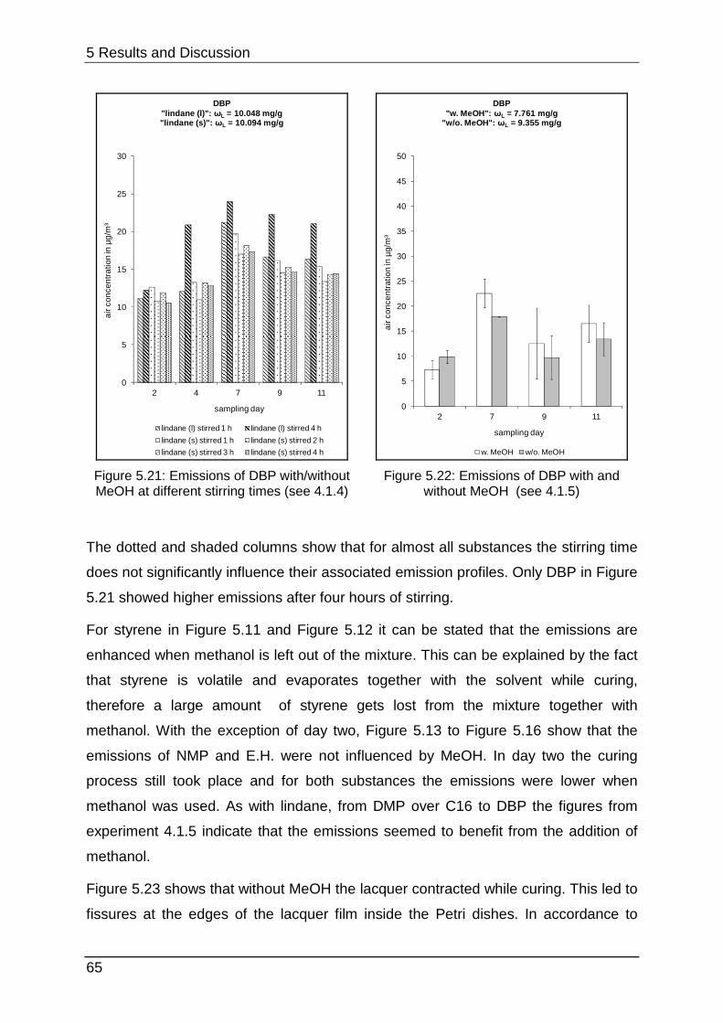
5 Results and Discussion
65
0
5
10
15
20
25
30
2 4 7 9 11
air
con
cen
tra
tion
in µ
g/m
³
sampling day
DBP"lindane (l)": ωL = 10.048 mg/g"lindane (s)": ωL = 10.094 mg/g
lindane (l) stirred 1 h lindane (l) stirred 4 h
lindane (s) stirred 1 h lindane (s) stirred 2 h
lindane (s) stirred 3 h lindane (s) stirred 4 h
Figure 5.21: Emissions of DBP with/without MeOH at different stirring times (see 4.1.4)
0
5
10
15
20
25
30
35
40
45
50
2 7 9 11
air
co
nce
ntra
tion
in µ
g/m
³
sampling day
DBP"w. MeOH": ωL = 7.761 mg/g
"w/o. MeOH": ωL = 9.355 mg/g
w. MeOH w/o. MeOH
Figure 5.22: Emissions of DBP with and without MeOH (see 4.1.5)
The dotted and shaded columns show that for almost all substances the stirring time
does not significantly influence their associated emission profiles. Only DBP in Figure
5.21 showed higher emissions after four hours of stirring.
For styrene in Figure 5.11 and Figure 5.12 it can be stated that the emissions are
enhanced when methanol is left out of the mixture. This can be explained by the fact
that styrene is volatile and evaporates together with the solvent while curing,
therefore a large amount of styrene gets lost from the mixture together with
methanol. With the exception of day two, Figure 5.13 to Figure 5.16 show that the
emissions of NMP and E.H. were not influenced by MeOH. In day two the curing
process still took place and for both substances the emissions were lower when
methanol was used. As with lindane, from DMP over C16 to DBP the figures from
experiment 4.1.5 indicate that the emissions seemed to benefit from the addition of
methanol.
Figure 5.23 shows that without MeOH the lacquer contracted while curing. This led to
fissures at the edges of the lacquer film inside the Petri dishes. In accordance to
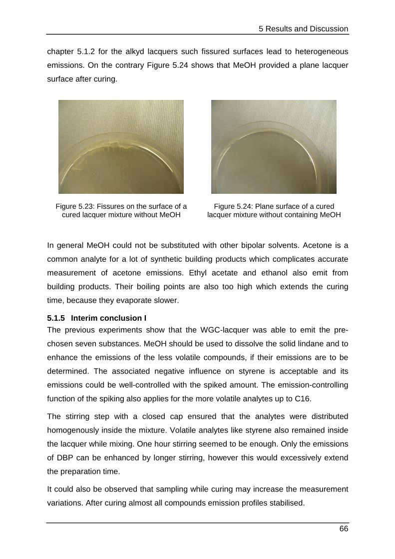
5 Results and Discussion
66
chapter 5.1.2 for the alkyd lacquers such fissured surfaces lead to heterogeneous
emissions. On the contrary Figure 5.24 shows that MeOH provided a plane lacquer
surface after curing.
Figure 5.23: Fissures on the surface of a cured lacquer mixture without MeOH
Figure 5.24: Plane surface of a cured lacquer mixture without containing MeOH
In general MeOH could not be substituted with other bipolar solvents. Acetone is a
common analyte for a lot of synthetic building products which complicates accurate
measurement of acetone emissions. Ethyl acetate and ethanol also emit from
building products. Their boiling points are also too high which extends the curing
time, because they evaporate slower.
5.1.5 Interim conclusion I The previous experiments show that the WGC-lacquer was able to emit the pre-
chosen seven substances. MeOH should be used to dissolve the solid lindane and to
enhance the emissions of the less volatile compounds, if their emissions are to be
determined. The associated negative influence on styrene is acceptable and its
emissions could be well-controlled with the spiked amount. The emission-controlling
function of the spiking also applies for the more volatile analytes up to C16.
The stirring step with a closed cap ensured that the analytes were distributed
homogenously inside the mixture. Volatile analytes like styrene also remained inside
the lacquer while mixing. One hour stirring seemed to be enough. Only the emissions
of DBP can be enhanced by longer stirring, however this would excessively extend
the preparation time.
It could also be observed that sampling while curing may increase the measurement
variations. After curing almost all compounds emission profiles stabilised.
5 Results and Discussion
67
Finally, it is difficult to optimise the emission profiles when considering of all analytes
equally as their physical and chemical properties differ substantially. The preparation
parameters described above are therefore a compromise between the different
effects.
5.1.6 First stability testing Table 5.3 summarises the results of experiment 4.1.6. The emissions of styrene,
DMP, C16 and lindane varied mostly below 10 %. In terms of emission testing this
indicated that both the emission of one mixture and equally prepared batches were
both repeatable and reproducible. The emissions of NMP were relatively stable with
deviations of less than 20 %. For E.H. up to day 7 there is a process that disturbs the
emission profile. This cannot currently be explained. The deviations for DBP stabilise
after one week below 20 %. The low air concentrations combined with the SVOC-
typical tendency to show sink effects lowers the repeatability and reproducibility of
the emission. Those sink effects cannot be described and controlled completely [36].
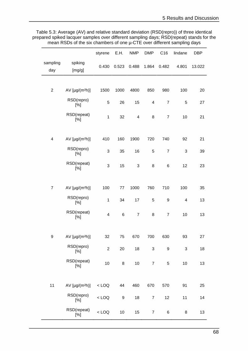
5 Results and Discussion
68
Table 5.3: Average (AV) and relative standard deviation (RSD(repro)) of three identical prepared spiked lacquer samples over different sampling days; RSD(repeat) stands for the
mean RSDs of the six chambers of one µ-CTE over different sampling days
styrene E.H. NMP DMP C16 lindane DBP
sampling
day
spiking
[mg/g] 0.430 0.523 0.488 1.864 0.482 4.801 13.022
2 AV [µg/(m²h)] 1500 1000 4800 850 980 100 20
RSD(repro)
[%] 5 26 15 4 7 5 27
RSD(repeat)
[%] 1 32 4 8 7 10 21
4 AV [µg/(m²h)] 410 160 1900 720 740 92 21
RSD(repro)
[%] 3 35 16 5 7 3 39
RSD(repeat)
[%] 3 15 3 8 6 12 23
7 AV [µg/(m²h)] 100 77 1000 760 710 100 35
RSD(repro)
[%] 1 34 17 5 9 4 13
RSD(repeat)
[%] 4 6 7 8 7 10 13
9 AV [µg/(m²h)] 32 75 670 700 630 93 27
RSD(repro)
[%] 2 20 18 3 9 3 18
RSD(repeat)
[%] 10 8 10 7 5 10 13
11 AV [µg/(m²h)] < LOQ 44 460 670 570 91 25
RSD(repro)
[%] < LOQ 9 18 7 12 11 14
RSD(repeat)
[%] < LOQ 10 15 7 6 8 13
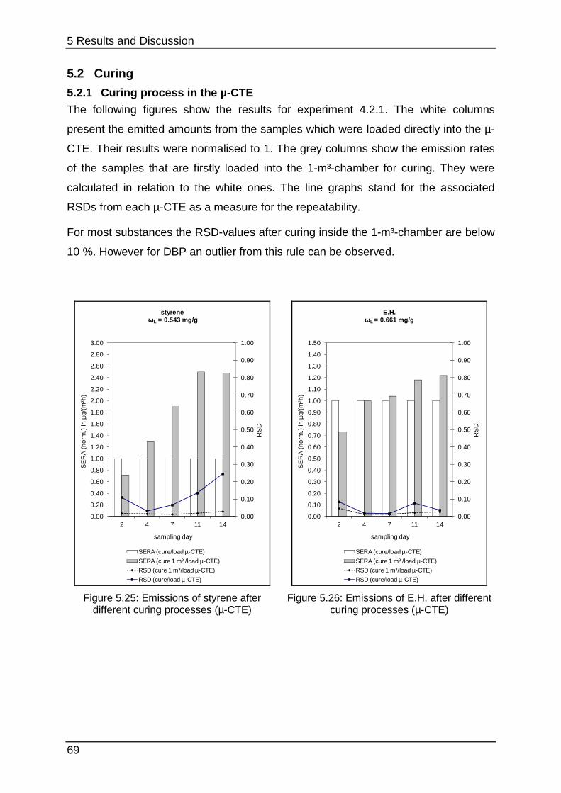
5 Results and Discussion
69
5.2 Curing
5.2.1 Curing process in the µ-CTE
The following figures show the results for experiment 4.2.1. The white columns
present the emitted amounts from the samples which were loaded directly into the µ-
CTE. Their results were normalised to 1. The grey columns show the emission rates
of the samples that are firstly loaded into the 1-m³-chamber for curing. They were
calculated in relation to the white ones. The line graphs stand for the associated
RSDs from each µ-CTE as a measure for the repeatability.
For most substances the RSD-values after curing inside the 1-m³-chamber are below
10 %. However for DBP an outlier from this rule can be observed.
0.00
0.10
0.20
0.30
0.40
0.50
0.60
0.70
0.80
0.90
1.00
0.00
0.20
0.40
0.60
0.80
1.00
1.20
1.40
1.60
1.80
2.00
2.20
2.40
2.60
2.80
3.00
2 4 7 11 14
RS
D
SE
RA
(no
rm.)
in µ
g/(m
²h)
sampling day
styreneωL = 0.543 mg/g
SERA (cure/load µ-CTE)
SERA (cure 1 m³ /load µ-CTE)
RSD (cure 1 m³/load µ-CTE)
RSD (cure/load µ-CTE)
Figure 5.25: Emissions of styrene after different curing processes (µ-CTE)
0.00
0.10
0.20
0.30
0.40
0.50
0.60
0.70
0.80
0.90
1.00
0.00
0.10
0.20
0.30
0.40
0.50
0.60
0.70
0.80
0.90
1.00
1.10
1.20
1.30
1.40
1.50
2 4 7 11 14
RS
D
SE
RA
(no
rm.)
in µ
g/(
m²h
)
sampling day
E.H.ωL = 0.661 mg/g
SERA (cure/load µ-CTE)
SERA (cure 1 m³ /load µ-CTE)
RSD (cure 1 m³/load µ-CTE)
RSD (cure/load µ-CTE)
Figure 5.26: Emissions of E.H. after different curing processes (µ-CTE)
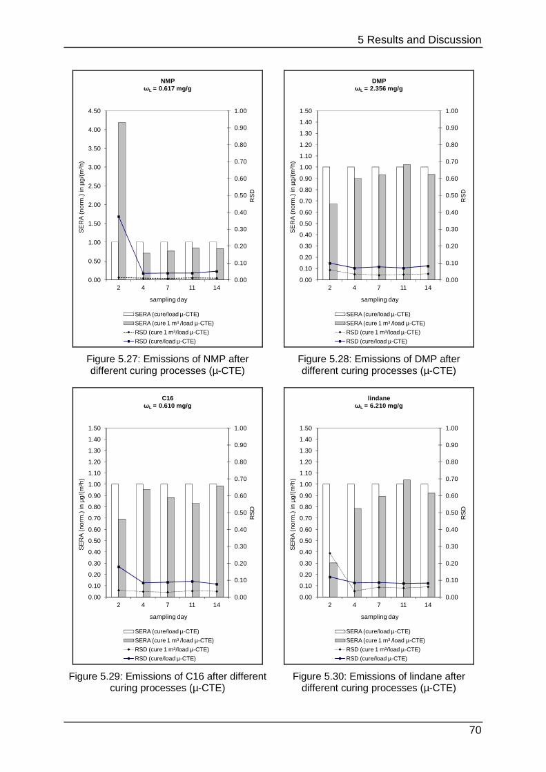
5 Results and Discussion
70
0.00
0.10
0.20
0.30
0.40
0.50
0.60
0.70
0.80
0.90
1.00
0.00
0.50
1.00
1.50
2.00
2.50
3.00
3.50
4.00
4.50
2 4 7 11 14
RS
D
SE
RA
(no
rm.)
in µ
g/(
m²h
)
sampling day
NMPωL = 0.617 mg/g
SERA (cure/load µ-CTE)
SERA (cure 1 m³ /load µ-CTE)
RSD (cure 1 m³/load µ-CTE)
RSD (cure/load µ-CTE)
Figure 5.27: Emissions of NMP after different curing processes (µ-CTE)
0.00
0.10
0.20
0.30
0.40
0.50
0.60
0.70
0.80
0.90
1.00
0.00
0.10
0.20
0.30
0.40
0.50
0.60
0.70
0.80
0.90
1.00
1.10
1.20
1.30
1.40
1.50
2 4 7 11 14
RS
D
SE
RA
(no
rm.)
in µ
g/(
m²h
) sampling day
DMPωL = 2.356 mg/g
SERA (cure/load µ-CTE)
SERA (cure 1 m³ /load µ-CTE)
RSD (cure 1 m³/load µ-CTE)
RSD (cure/load µ-CTE)
Figure 5.28: Emissions of DMP after different curing processes (µ-CTE)
0.00
0.10
0.20
0.30
0.40
0.50
0.60
0.70
0.80
0.90
1.00
0.00
0.10
0.20
0.30
0.40
0.50
0.60
0.70
0.80
0.90
1.00
1.10
1.20
1.30
1.40
1.50
2 4 7 11 14
RS
D
SE
RA
(no
rm.)
in µ
g/(
m²h
)
sampling day
C16ωL = 0.610 mg/g
SERA (cure/load µ-CTE)
SERA (cure 1 m³ /load µ-CTE)
RSD (cure 1 m³/load µ-CTE)
RSD (cure/load µ-CTE)
Figure 5.29: Emissions of C16 after different curing processes (µ-CTE)
0.00
0.10
0.20
0.30
0.40
0.50
0.60
0.70
0.80
0.90
1.00
0.00
0.10
0.20
0.30
0.40
0.50
0.60
0.70
0.80
0.90
1.00
1.10
1.20
1.30
1.40
1.50
2 4 7 11 14
RS
D
SE
RA
(no
rm.)
in µ
g/(
m²h
)
sampling day
lindaneωL = 6.210 mg/g
SERA (cure/load µ-CTE)
SERA (cure 1 m³ /load µ-CTE)
RSD (cure 1 m³/load µ-CTE)
RSD (cure/load µ-CTE)
Figure 5.30: Emissions of lindane after different curing processes (µ-CTE)
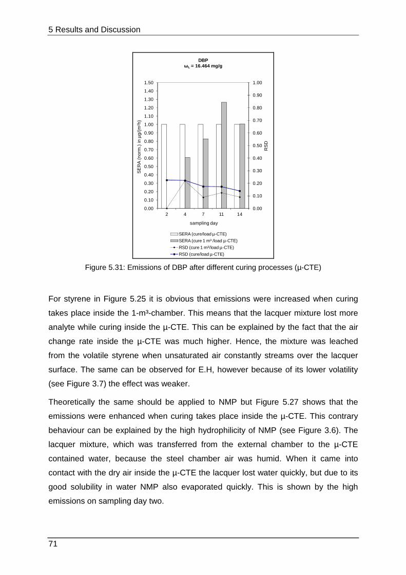
5 Results and Discussion
71
0.00
0.10
0.20
0.30
0.40
0.50
0.60
0.70
0.80
0.90
1.00
0.00
0.10
0.20
0.30
0.40
0.50
0.60
0.70
0.80
0.90
1.00
1.10
1.20
1.30
1.40
1.50
2 4 7 11 14
RS
D
SE
RA
(no
rm.)
in µ
g/(
m²h
)
sampling day
DBPωL = 16.464 mg/g
SERA (cure/load µ-CTE)
SERA (cure 1 m³ /load µ-CTE)
RSD (cure 1 m³/load µ-CTE)
RSD (cure/load µ-CTE)
Figure 5.31: Emissions of DBP after different curing processes (µ-CTE)
For styrene in Figure 5.25 it is obvious that emissions were increased when curing
takes place inside the 1-m³-chamber. This means that the lacquer mixture lost more
analyte while curing inside the µ-CTE. This can be explained by the fact that the air
change rate inside the µ-CTE was much higher. Hence, the mixture was leached
from the volatile styrene when unsaturated air constantly streams over the lacquer
surface. The same can be observed for E.H, however because of its lower volatility
(see Figure 3.7) the effect was weaker.
Theoretically the same should be applied to NMP but Figure 5.27 shows that the
emissions were enhanced when curing takes place inside the µ-CTE. This contrary
behaviour can be explained by the high hydrophilicity of NMP (see Figure 3.6). The
lacquer mixture, which was transferred from the external chamber to the µ-CTE
contained water, because the steel chamber air was humid. When it came into
contact with the dry air inside the µ-CTE the lacquer lost water quickly, but due to its
good solubility in water NMP also evaporated quickly. This is shown by the high
emissions on sampling day two.
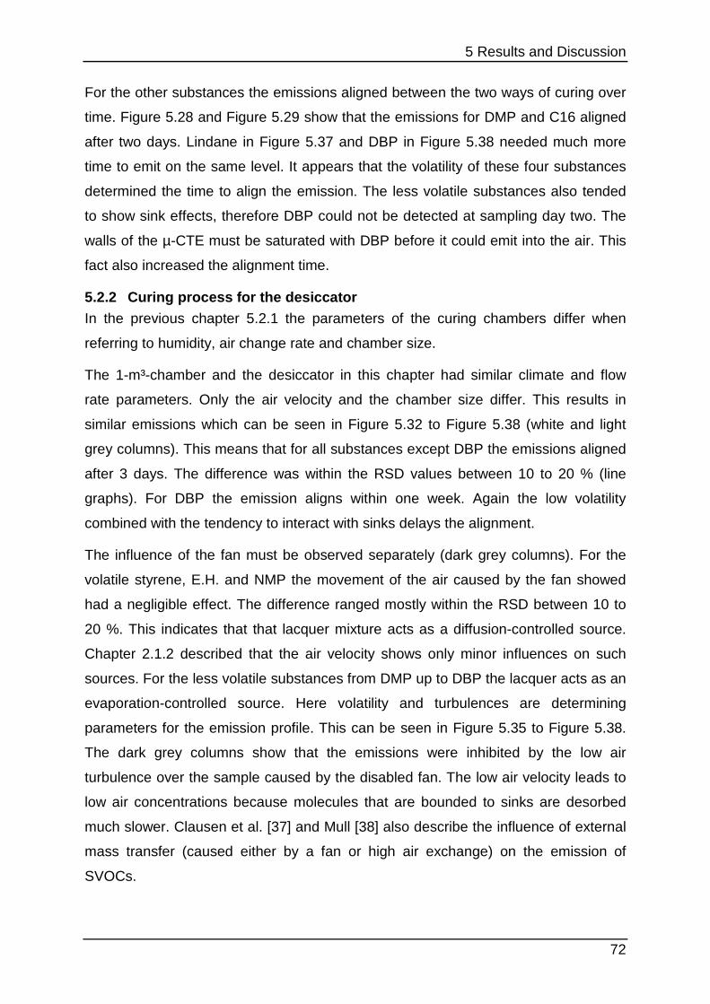
5 Results and Discussion
72
For the other substances the emissions aligned between the two ways of curing over
time. Figure 5.28 and Figure 5.29 show that the emissions for DMP and C16 aligned
after two days. Lindane in Figure 5.37 and DBP in Figure 5.38 needed much more
time to emit on the same level. It appears that the volatility of these four substances
determined the time to align the emission. The less volatile substances also tended
to show sink effects, therefore DBP could not be detected at sampling day two. The
walls of the µ-CTE must be saturated with DBP before it could emit into the air. This
fact also increased the alignment time.
5.2.2 Curing process for the desiccator In the previous chapter 5.2.1 the parameters of the curing chambers differ when
referring to humidity, air change rate and chamber size.
The 1-m³-chamber and the desiccator in this chapter had similar climate and flow
rate parameters. Only the air velocity and the chamber size differ. This results in
similar emissions which can be seen in Figure 5.32 to Figure 5.38 (white and light
grey columns). This means that for all substances except DBP the emissions aligned
after 3 days. The difference was within the RSD values between 10 to 20 % (line
graphs). For DBP the emission aligns within one week. Again the low volatility
combined with the tendency to interact with sinks delays the alignment.
The influence of the fan must be observed separately (dark grey columns). For the
volatile styrene, E.H. and NMP the movement of the air caused by the fan showed
had a negligible effect. The difference ranged mostly within the RSD between 10 to
20 %. This indicates that that lacquer mixture acts as a diffusion-controlled source.
Chapter 2.1.2 described that the air velocity shows only minor influences on such
sources. For the less volatile substances from DMP up to DBP the lacquer acts as an
evaporation-controlled source. Here volatility and turbulences are determining
parameters for the emission profile. This can be seen in Figure 5.35 to Figure 5.38.
The dark grey columns show that the emissions were inhibited by the low air
turbulence over the sample caused by the disabled fan. The low air velocity leads to
low air concentrations because molecules that are bounded to sinks are desorbed
much slower. Clausen et al. [37] and Mull [38] also describe the influence of external
mass transfer (caused either by a fan or high air exchange) on the emission of
SVOCs.

5 Results and Discussion
73
0.00
0.10
0.20
0.30
0.40
0.50
0.60
0.70
0.80
0.90
1.00
0.00
0.20
0.40
0.60
0.80
1.00
1.20
1.40
1.60
1.80
2.00
3 5 7 10 12 14 17
RS
D
SE
RA
(n
orm
.) in
µg
/(m
²h)
sampling day
styreneωL = 0.905 mg/g
SERA (cure/load desiccator)
SERA (cure 1 m³ + load desiccator)
SERA (cure 1 m³ + load desiccator + no fan)
RSD (cure/load desiccator)
RSD (cure 1 m³ + load desiccator)
RSD (cure 1 m³ + load desiccator + no fan)
Figure 5.32: Emission profile of styrene after different curing processes (desiccator)
0.00
0.10
0.20
0.30
0.40
0.50
0.60
0.70
0.80
0.90
1.00
0.00
0.40
0.80
1.20
1.60
2.00
2.40
2.80
3.20
3.60
4.00
3 5 7 10 12 14 17
RS
D
SE
RA
(n
orm
.) in
µg
/(m
²h)
sampling day
E.H.ωL = 0.827 mg/g
SERA (cure/load desiccator)
SERA (cure 1 m³ + load desiccator)
SERA (cure 1 m³ + load desiccator + no fan)
RSD (cure/load desiccator)
RSD (cure 1 m³ + load desiccator)
RSD (cure 1 m³ + load desiccator + no fan)
Figure 5.33: Emission profile of E.H. after different curing processes (desiccator)
0.00
0.10
0.20
0.30
0.40
0.50
0.60
0.70
0.80
0.90
1.00
0.00
0.40
0.80
1.20
1.60
2.00
2.40
2.80
3.20
3.60
4.00
3 5 7 10 12 14 17
RS
D
SE
RA
(n
orm
.) in
µg
/(m
²h)
sampling day
NMPωL = 1.029 mg/g
SERA (cure/load desiccator)
SERA (cure 1 m³ + load desiccator)
SERA (cure 1 m³ + load desiccator + no fan)
RSD (cure/load desiccator)
RSD (cure 1 m³ + load desiccator)
RSD (cure 1 m³ + load desiccator + no fan)
Figure 5.34: Emission profile of NMP after different curing processes (desiccator)
0.00
0.10
0.20
0.30
0.40
0.50
0.60
0.70
0.80
0.90
1.00
0.00
0.10
0.20
0.30
0.40
0.50
0.60
0.70
0.80
0.90
1.00
1.10
1.20
1.30
1.40
1.50
3 5 7 10 12 14 17
RS
D
SE
RA
(n
orm
.) in
µg
/(m
²h)
sampling day
DMPωL = 2.062 mg/g
SERA (cure/load desiccator)
SERA (cure 1 m³ + load desiccator)
SERA (cure 1 m³ + load desiccator + no fan)
RSD (cure/load desiccator)
RSD (cure 1 m³ + load desiccator)
RSD (cure 1 m³ + load desiccator + no fan)
Figure 5.35: Emission profile of DMP after different curing processes (desiccator)
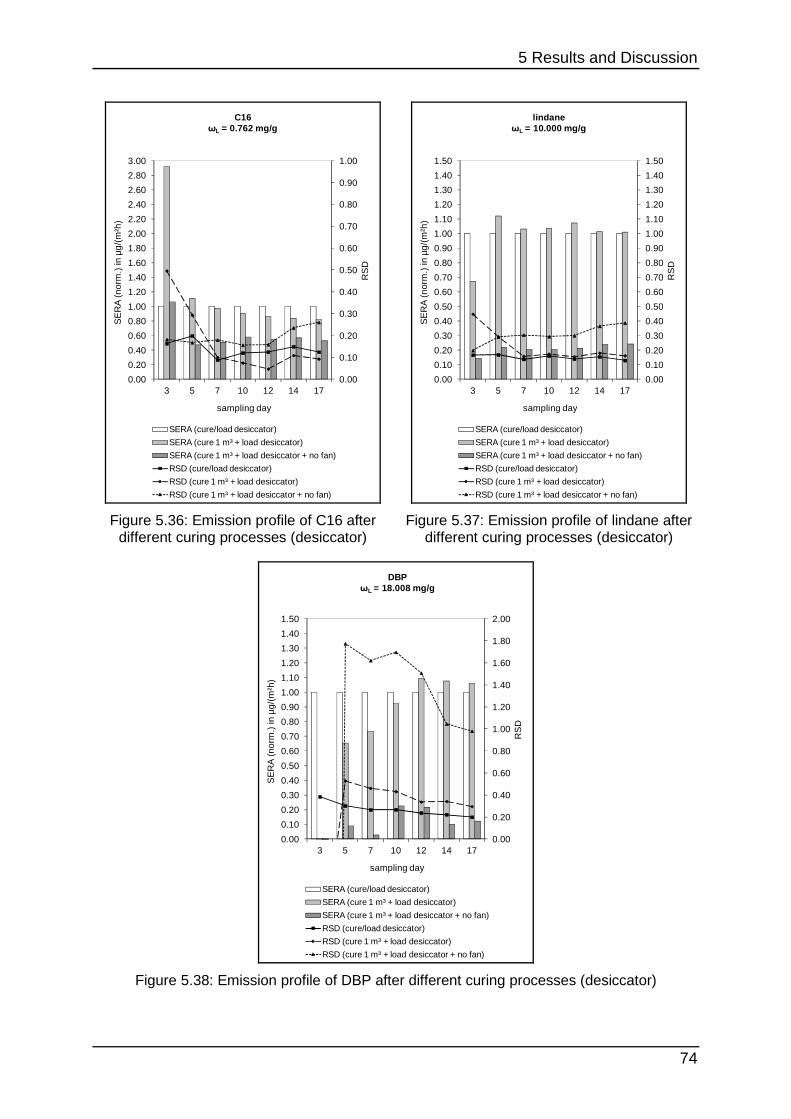
5 Results and Discussion
74
0.00
0.10
0.20
0.30
0.40
0.50
0.60
0.70
0.80
0.90
1.00
0.00
0.20
0.40
0.60
0.80
1.00
1.20
1.40
1.60
1.80
2.00
2.20
2.40
2.60
2.80
3.00
3 5 7 10 12 14 17
RS
D
SE
RA
(n
orm
.) in
µg
/(m
²h)
sampling day
C16ωL = 0.762 mg/g
SERA (cure/load desiccator)
SERA (cure 1 m³ + load desiccator)
SERA (cure 1 m³ + load desiccator + no fan)
RSD (cure/load desiccator)
RSD (cure 1 m³ + load desiccator)
RSD (cure 1 m³ + load desiccator + no fan)
Figure 5.36: Emission profile of C16 after different curing processes (desiccator)
0.00
0.10
0.20
0.30
0.40
0.50
0.60
0.70
0.80
0.90
1.00
1.10
1.20
1.30
1.40
1.50
0.00
0.10
0.20
0.30
0.40
0.50
0.60
0.70
0.80
0.90
1.00
1.10
1.20
1.30
1.40
1.50
3 5 7 10 12 14 17
RS
D
SE
RA
(n
orm
.) in
µg
/(m
²h)
sampling day
lindaneωL = 10.000 mg/g
SERA (cure/load desiccator)
SERA (cure 1 m³ + load desiccator)
SERA (cure 1 m³ + load desiccator + no fan)
RSD (cure/load desiccator)
RSD (cure 1 m³ + load desiccator)
RSD (cure 1 m³ + load desiccator + no fan)
Figure 5.37: Emission profile of lindane after different curing processes (desiccator)
0.00
0.20
0.40
0.60
0.80
1.00
1.20
1.40
1.60
1.80
2.00
0.00
0.10
0.20
0.30
0.40
0.50
0.60
0.70
0.80
0.90
1.00
1.10
1.20
1.30
1.40
1.50
3 5 7 10 12 14 17
RS
D
SE
RA
(no
rm.)
in µ
g/(m
²h)
sampling day
DBPωL = 18.008 mg/g
SERA (cure/load desiccator)
SERA (cure 1 m³ + load desiccator)
SERA (cure 1 m³ + load desiccator + no fan)
RSD (cure/load desiccator)
RSD (cure 1 m³ + load desiccator)
RSD (cure 1 m³ + load desiccator + no fan)
Figure 5.38: Emission profile of DBP after different curing processes (desiccator)
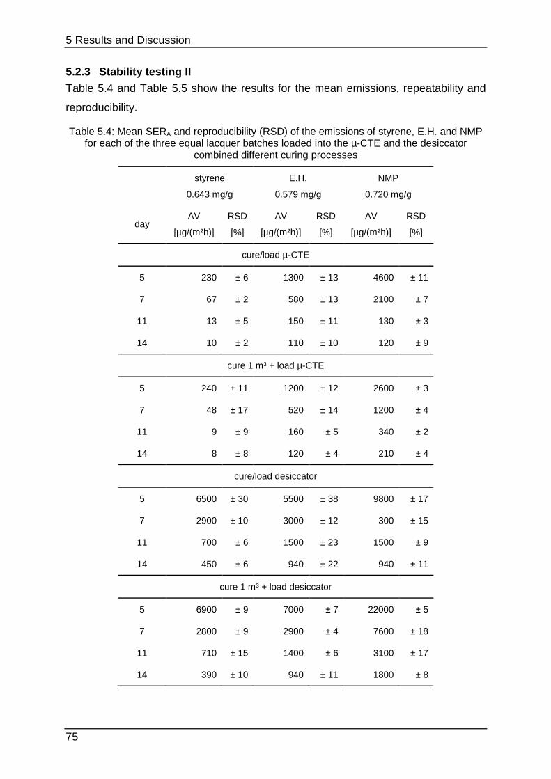
5 Results and Discussion
75
5.2.3 Stability testing II Table 5.4 and Table 5.5 show the results for the mean emissions, repeatability and
reproducibility.
Table 5.4: Mean SERA and reproducibility (RSD) of the emissions of styrene, E.H. and NMP for each of the three equal lacquer batches loaded into the µ-CTE and the desiccator
combined different curing processes
styrene
0.643 mg/g
E.H.
0.579 mg/g
NMP
0.720 mg/g
day AV
[µg/(m²h)]
RSD
[%]
AV
[µg/(m²h)]
RSD
[%]
AV
[µg/(m²h)]
RSD
[%]
cure/load µ-CTE
5 230 ± 6 1300 ± 13 4600 ± 11
7 67 ± 2 580 ± 13 2100 ± 7
11 13 ± 5 150 ± 11 130 ± 3
14 10 ± 2 110 ± 10 120 ± 9
cure 1 m³ + load µ-CTE
5 240 ± 11 1200 ± 12 2600 ± 3
7 48 ± 17 520 ± 14 1200 ± 4
11 9 ± 9 160 ± 5 340 ± 2
14 8 ± 8 120 ± 4 210 ± 4
cure/load desiccator
5 6500 ± 30 5500 ± 38 9800 ± 17
7 2900 ± 10 3000 ± 12 300 ± 15
11 700 ± 6 1500 ± 23 1500 ± 9
14 450 ± 6 940 ± 22 940 ± 11
cure 1 m³ + load desiccator
5 6900 ± 9 7000 ± 7 22000 ± 5
7 2800 ± 9 2900 ± 4 7600 ± 18
11 710 ± 15 1400 ± 6 3100 ± 17
14 390 ± 10 940 ± 11 1800 ± 8
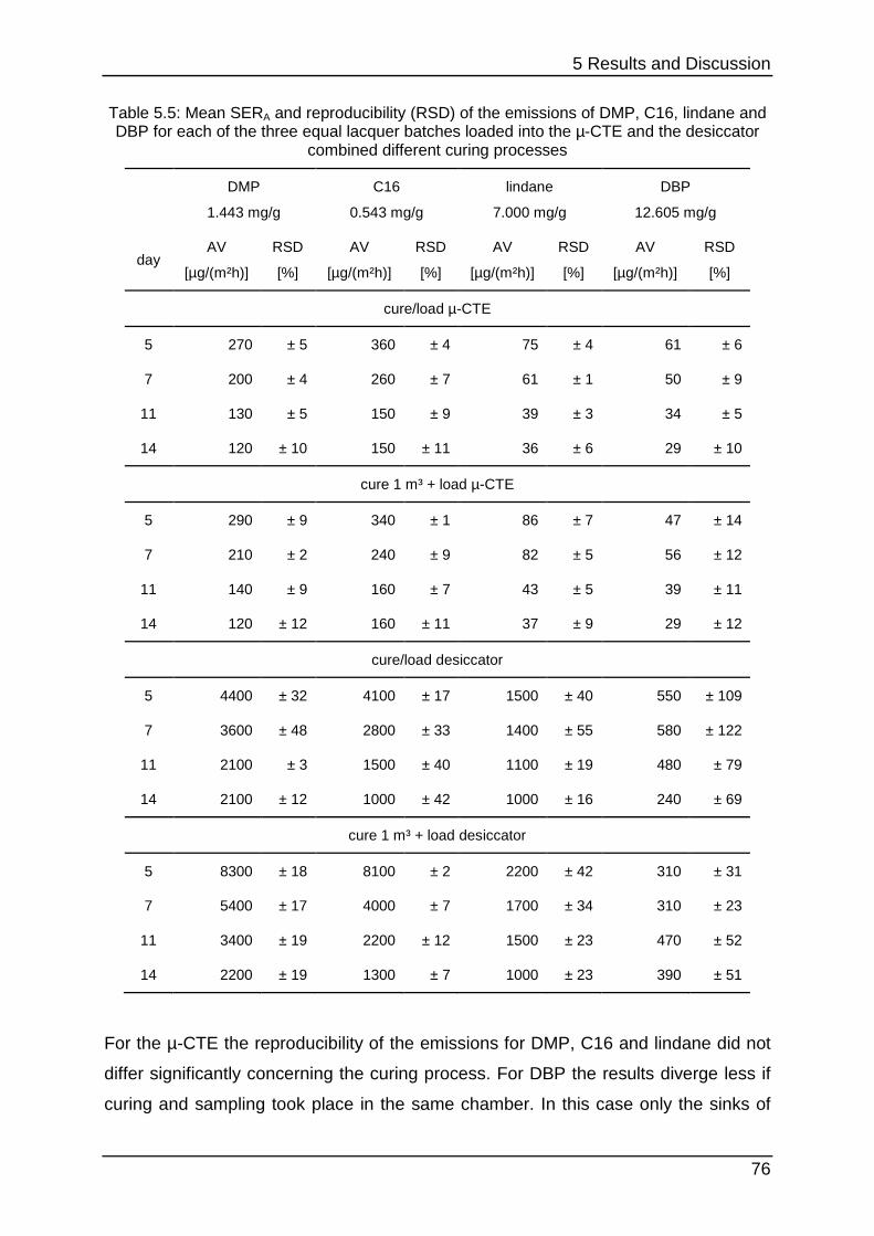
5 Results and Discussion
76
Table 5.5: Mean SERA and reproducibility (RSD) of the emissions of DMP, C16, lindane and DBP for each of the three equal lacquer batches loaded into the µ-CTE and the desiccator
combined different curing processes
DMP
1.443 mg/g
C16
0.543 mg/g
lindane
7.000 mg/g
DBP
12.605 mg/g
day AV
[µg/(m²h)]
RSD
[%]
AV
[µg/(m²h)]
RSD
[%]
AV
[µg/(m²h)]
RSD
[%]
AV
[µg/(m²h)]
RSD
[%]
cure/load µ-CTE
5 270 ± 5 360 ± 4 75 ± 4 61 ± 6
7 200 ± 4 260 ± 7 61 ± 1 50 ± 9
11 130 ± 5 150 ± 9 39 ± 3 34 ± 5
14 120 ± 10 150 ± 11 36 ± 6 29 ± 10
cure 1 m³ + load µ-CTE
5 290 ± 9 340 ± 1 86 ± 7 47 ± 14
7 210 ± 2 240 ± 9 82 ± 5 56 ± 12
11 140 ± 9 160 ± 7 43 ± 5 39 ± 11
14 120 ± 12 160 ± 11 37 ± 9 29 ± 12
cure/load desiccator
5 4400 ± 32 4100 ± 17 1500 ± 40 550 ± 109
7 3600 ± 48 2800 ± 33 1400 ± 55 580 ± 122
11 2100 ± 3 1500 ± 40 1100 ± 19 480 ± 79
14 2100 ± 12 1000 ± 42 1000 ± 16 240 ± 69
cure 1 m³ + load desiccator
5 8300 ± 18 8100 ± 2 2200 ± 42 310 ± 31
7 5400 ± 17 4000 ± 7 1700 ± 34 310 ± 23
11 3400 ± 19 2200 ± 12 1500 ± 23 470 ± 52
14 2200 ± 19 1300 ± 7 1000 ± 23 390 ± 51
For the µ-CTE the reproducibility of the emissions for DMP, C16 and lindane did not
differ significantly concerning the curing process. For DBP the results diverge less if
curing and sampling took place in the same chamber. In this case only the sinks of
5 Results and Discussion
77
the µ-CTE disturbed the homogeneity of the emissions. Changing the chamber for
the emission testing led to two possible sinks: sinks of the 1-m³-chamber (curing) and
the µ-CTE (testing). For E.H. and styrene the variations were distributed more
homogeneously if the chamber was not changed. On the contrary, the reproducibility
of the emissions of NMP benefited significantly if the lacquer mixture cured inside the
1-m³-chamber. The humidification inside this chamber appeared to improve the
reproducibility of the NMP-emissions. Lastly, it turned out that compared to chapter
5.1.6the variations for E.H., NMP and DBP could be improved significantly.
Concerning the desiccator, the reproducibility of almost all of the substances is
improved if curing took place inside the 1-m³-chamber. Therefore it is possible to
reproduce the emission profiles of the majority of the analytes with variations below
20 %. Only the results for lindane and DBP varied to a greater degree.
Compared to the results of the µ-CTE the reproducibility for all substances inside the
desiccator was poorer. For the less volatile lindane and DBP this can be explained
with the lower loading factor. Inside larger chambers there is more surface area that
can act as sink. This lowered the reproducibility of the additional low SVOC-
emissions. The emissions of the remaining more volatile substances were higher
compared to the µ-CTE because of the lower air change rate. This indicates that
small variations of the process parameters of the desiccators had a greater influence
on the homogeneity of the emissions.
5.2.4 Curing at different chamber flows Figure 5.39 to Figure 5.45 show the emission curves for the analytes at 15 and 30
ml/min chamber flow through the µ-CTE.
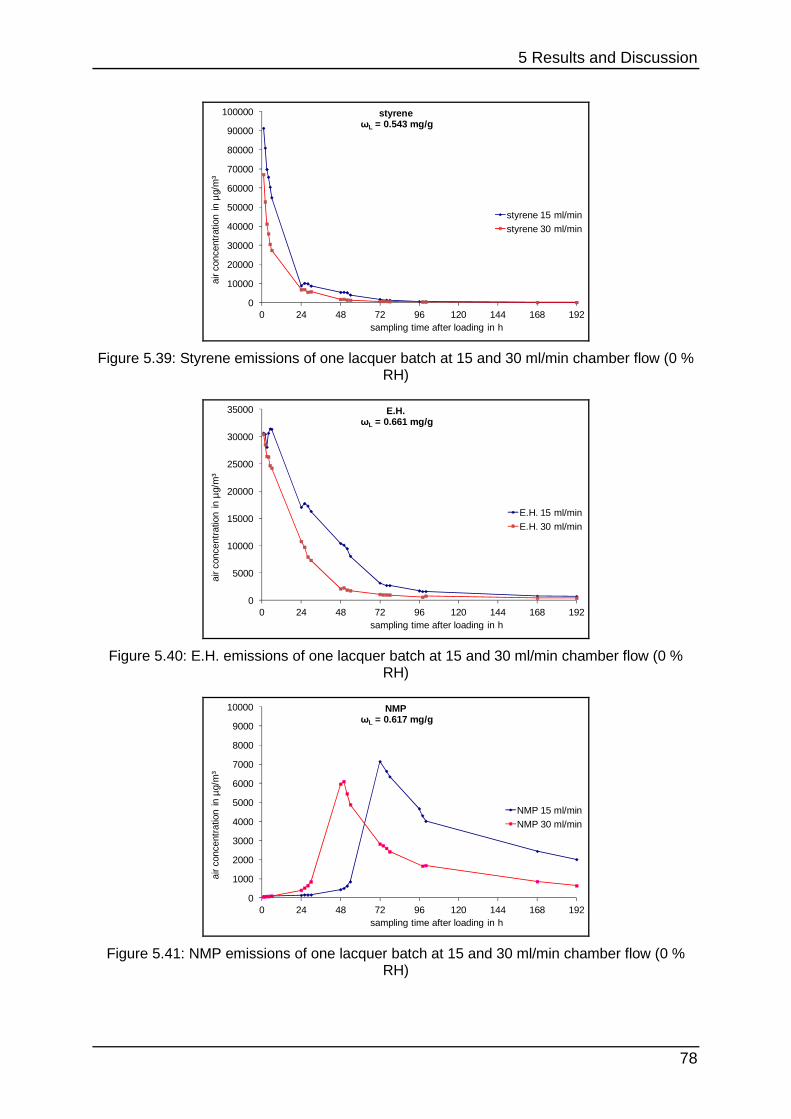
5 Results and Discussion
78
0
10000
20000
30000
40000
50000
60000
70000
80000
90000
100000
0 24 48 72 96 120 144 168 192
air
conc
entr
atio
n in
µg/
m³
sampling time after loading in h
styreneωL = 0.543 mg/g
styrene 15 ml/minstyrene 30 ml/min
Figure 5.39: Styrene emissions of one lacquer batch at 15 and 30 ml/min chamber flow (0 % RH)
0
5000
10000
15000
20000
25000
30000
35000
0 24 48 72 96 120 144 168 192
air
conc
entr
atio
n in
µg/
m³
sampling time after loading in h
E.H.ωL = 0.661 mg/g
E.H. 15 ml/minE.H. 30 ml/min
Figure 5.40: E.H. emissions of one lacquer batch at 15 and 30 ml/min chamber flow (0 % RH)
0
1000
2000
3000
4000
5000
6000
7000
8000
9000
10000
0 24 48 72 96 120 144 168 192
air
conc
entr
atio
n in
µg/
m³
sampling time after loading in h
NMPωL = 0.617 mg/g
NMP 15 ml/minNMP 30 ml/min
Figure 5.41: NMP emissions of one lacquer batch at 15 and 30 ml/min chamber flow (0 % RH)
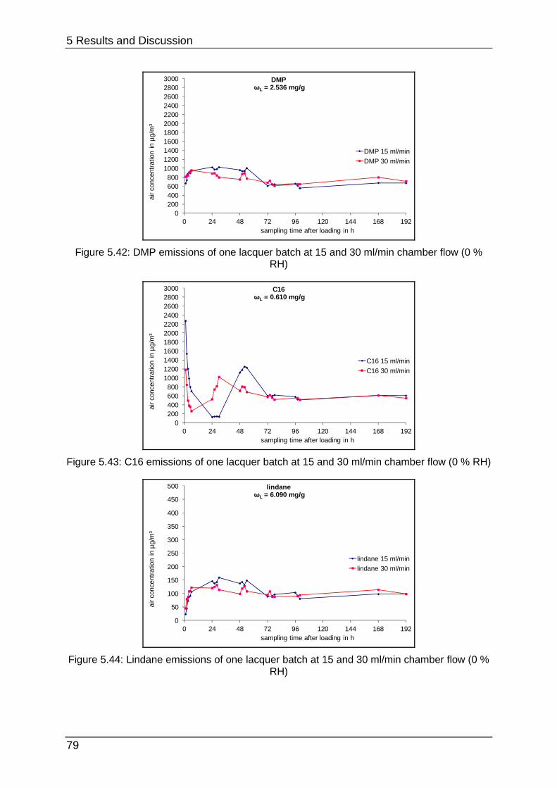
5 Results and Discussion
79
0200400600800
10001200140016001800200022002400260028003000
0 24 48 72 96 120 144 168 192
air
conc
entr
atio
n in
µg/
m³
sampling time after loading in h
DMPωL = 2.536 mg/g
DMP 15 ml/minDMP 30 ml/min
Figure 5.42: DMP emissions of one lacquer batch at 15 and 30 ml/min chamber flow (0 % RH)
0200400600800
10001200140016001800200022002400260028003000
0 24 48 72 96 120 144 168 192
air
conc
entr
atio
n in
µg/
m³
sampling time after loading in h
C16ωL = 0.610 mg/g
C16 15 ml/minC16 30 ml/min
Figure 5.43: C16 emissions of one lacquer batch at 15 and 30 ml/min chamber flow (0 % RH)
0
50
100
150
200
250
300
350
400
450
500
0 24 48 72 96 120 144 168 192
air
conc
entr
atio
n in
µg/
m³
sampling time after loading in h
lindaneωL = 6.090 mg/g
lindane 15 ml/minlindane 30 ml/min
Figure 5.44: Lindane emissions of one lacquer batch at 15 and 30 ml/min chamber flow (0 % RH)
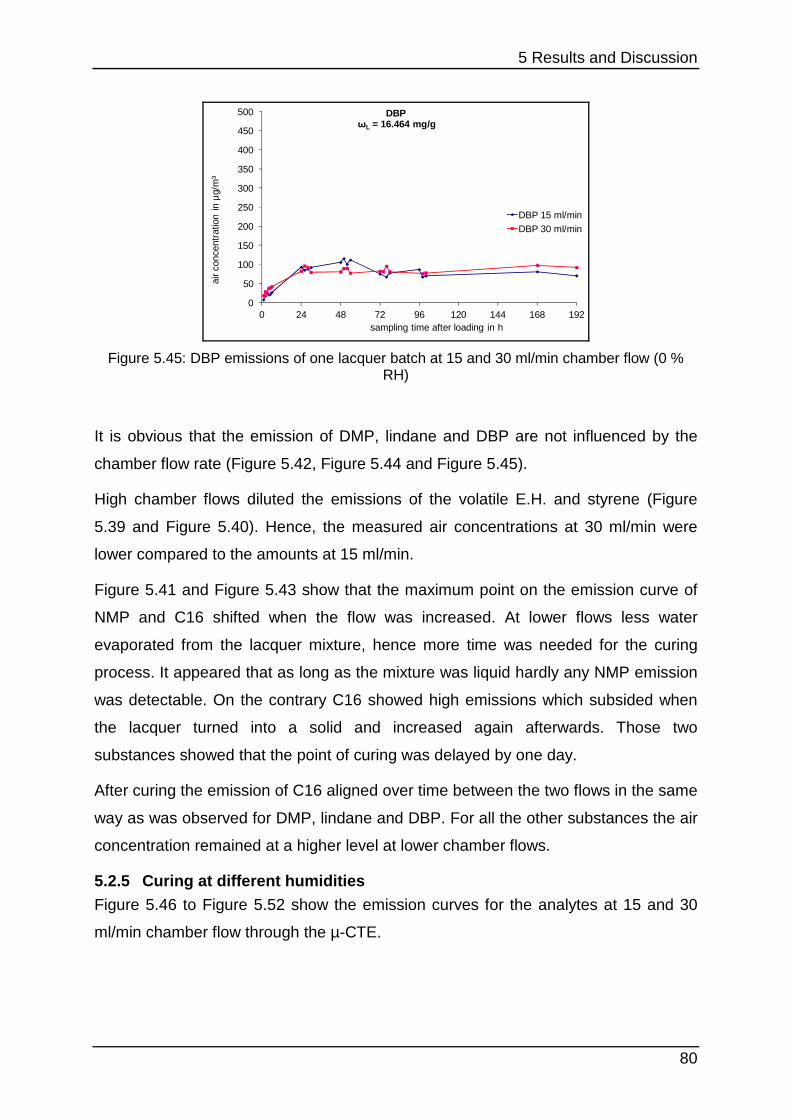
5 Results and Discussion
80
0
50
100
150
200
250
300
350
400
450
500
0 24 48 72 96 120 144 168 192
air
conc
entr
atio
n in
µg/
m³
sampling time after loading in h
DBPωL = 16.464 mg/g
DBP 15 ml/minDBP 30 ml/min
Figure 5.45: DBP emissions of one lacquer batch at 15 and 30 ml/min chamber flow (0 % RH)
It is obvious that the emission of DMP, lindane and DBP are not influenced by the
chamber flow rate (Figure 5.42, Figure 5.44 and Figure 5.45).
High chamber flows diluted the emissions of the volatile E.H. and styrene (Figure
5.39 and Figure 5.40). Hence, the measured air concentrations at 30 ml/min were
lower compared to the amounts at 15 ml/min.
Figure 5.41 and Figure 5.43 show that the maximum point on the emission curve of
NMP and C16 shifted when the flow was increased. At lower flows less water
evaporated from the lacquer mixture, hence more time was needed for the curing
process. It appeared that as long as the mixture was liquid hardly any NMP emission
was detectable. On the contrary C16 showed high emissions which subsided when
the lacquer turned into a solid and increased again afterwards. Those two
substances showed that the point of curing was delayed by one day.
After curing the emission of C16 aligned over time between the two flows in the same
way as was observed for DMP, lindane and DBP. For all the other substances the air
concentration remained at a higher level at lower chamber flows.
5.2.5 Curing at different humidities
Figure 5.46 to Figure 5.52 show the emission curves for the analytes at 15 and 30
ml/min chamber flow through the µ-CTE.
5 Results and Discussion
81
0
10000
20000
30000
40000
50000
60000
70000
0 24 48 72 96 120 144 168 192 216 240 264
air
conc
entr
atio
n in
µg/
m³
sampling time after loading in h
styreneωL = 0.543 mg/g
styrene 0 % RHstyrene 55 % RH
Figure 5.46: Styrene emissions of one lacquer batch at 0 and 55 % RH (15 ml/min flow)
0
5000
10000
15000
20000
25000
30000
0 24 48 72 96 120 144 168 192 216 240 264
air
conc
entr
atio
n in
µg/
m³
sampling time after loading in h
E.H.ωL = 0.661 mg/g
E.H. 0 % RHE.H. 55 % RH
Figure 5.47: E.H. emissions of one lacquer batch at 0 and 55 % RH (15 ml/min flow)
0
1000
2000
3000
4000
5000
6000
7000
8000
9000
10000
0 24 48 72 96 120 144 168 192 216 240 264
air
conc
entr
atio
n in
µg/
m³
sampling time after loading in h
NMPωL = 0.617 mg/g
NMP 0 % RHNMP 55 % RH
Figure 5.48: NMP emissions of one lacquer batch at 0 and 55 % RH (15 ml/min flow)
5 Results and Discussion
82
0
500
1000
1500
2000
2500
3000
0 24 48 72 96 120 144 168 192 216 240 264
air
conc
entr
atio
n in
µg/
m³
sampling time after loading in h
DMPωL = 2.356 mg/g
DMP 0 % RHDMP 55 % RH
Figure 5.49: DMP emissions of one lacquer batch at 0 and 55 % RH (15 ml/min flow)
0
500
1000
1500
2000
2500
3000
0 24 48 72 96 120 144 168 192 216 240 264
air
conc
entr
atio
n in
µg/
m³
sampling time after loading in h
C16ωL = 0.610 mg/g
C16 0 % RHC16 55 % RH
Figure 5.50: C16 emissions of one lacquer batch at 0 and 55 % RH (15 ml/min flow)
0
100
200
300
400
500
0 24 48 72 96 120 144 168 192 216 240 264
air
conc
entr
atio
n in
µg/
m³
sampling time after loading in h
lindaneωL = 6.090 mg/g
lindane 0 % RHlindane 55 % RH
Figure 5.51: Lindane emissions of one lacquer batch at 0 and 55 % RH (15 ml/min flow)
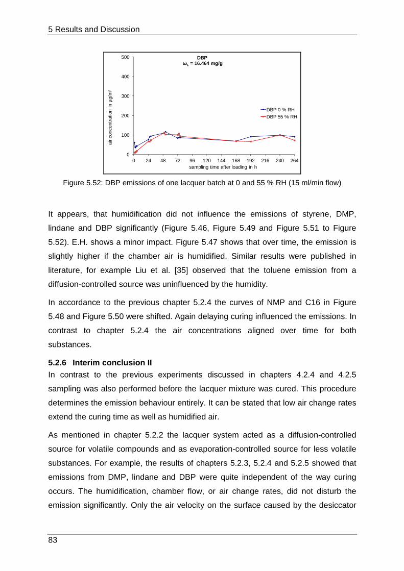
5 Results and Discussion
83
0
100
200
300
400
500
0 24 48 72 96 120 144 168 192 216 240 264
air
conc
entr
atio
n in
µg/
m³
sampling time after loading in h
DBPωL = 16.464 mg/g
DBP 0 % RHDBP 55 % RH
Figure 5.52: DBP emissions of one lacquer batch at 0 and 55 % RH (15 ml/min flow)
It appears, that humidification did not influence the emissions of styrene, DMP,
lindane and DBP significantly (Figure 5.46, Figure 5.49 and Figure 5.51 to Figure
5.52). E.H. shows a minor impact. Figure 5.47 shows that over time, the emission is
slightly higher if the chamber air is humidified. Similar results were published in
literature, for example Liu et al. [35] observed that the toluene emission from a
diffusion-controlled source was uninfluenced by the humidity.
In accordance to the previous chapter 5.2.4 the curves of NMP and C16 in Figure
5.48 and Figure 5.50 were shifted. Again delaying curing influenced the emissions. In
contrast to chapter 5.2.4 the air concentrations aligned over time for both
substances.
5.2.6 Interim conclusion II In contrast to the previous experiments discussed in chapters 4.2.4 and 4.2.5
sampling was also performed before the lacquer mixture was cured. This procedure
determines the emission behaviour entirely. It can be stated that low air change rates
extend the curing time as well as humidified air.
As mentioned in chapter 5.2.2 the lacquer system acted as a diffusion-controlled
source for volatile compounds and as evaporation-controlled source for less volatile
substances. For example, the results of chapters 5.2.3, 5.2.4 and 5.2.5 showed that
emissions from DMP, lindane and DBP were quite independent of the way curing
occurs. The humidification, chamber flow, or air change rates, did not disturb the
emission significantly. Only the air velocity on the surface caused by the desiccator
5 Results and Discussion
84
fan had a major impact on the emissions (chapter 5.2.2). As described in 5.1.3
increasing the analyte amount inside the lacquer results in higher air concentrations,
if evaporation does not limit the emissions produced. Reliable results for such
compounds can be achieved if the test chamber air is homogeneous and sinks
should be at best avoided or saturated.
On the contrary chapter 5.2.1 and 5.2.4 indicate that styrene and E.H. were
influenced significantly by the air change rate. As mentioned in chapter 5.2.2 the
lacquer acted as diffusion-controlled source. As long as the chamber air was not
saturated and the diffusion of the compound inside the lacquer was not limited those
analytes evaporated at a continuous rate. High air change rates diluted the VOC
concentration inside the chamber, hence the emitted amounts were lower at higher
flows inside the µ-CTE in 5.2.4. Therefore reliable results for such compounds can be
achieved if the air change is kept at best constant especially while curing, where the
lacquer loses the majority of volatile analytes.
In general humidity had a minor influence on the emissions of the lacquer system.
C16 and NMP were special cases. They are the most non-polar, respectively polar,
compounds among the investigated substances. Their emission is additionally
influenced significantly by the curing process which is influenced by the chamber
flow, mixing and humidity. Only after curing the lacquer acted as diffusion-controlled
source for NMP and as evaporation-controlled source for C16.
Finally Figure 5.53 to Figure 5.55 show that the homogeneity of the lacquer surface
could be improved by the chamber flow and its corresponding size. At 30 ml/min
(Figure 5.53) inside the µ-CTE the liquid mixture is pushed to one edge of the Petri
dish. There it cures while fissures develop on the opposite sides. At lower flows (e.g.
15 ml/min, Figure 5.54) the mixture is less influenced by the flow and the lacquer
distributes more evenly inside the Petri dish. This behaviour is enhanced inside the
1-m³-chamber with its low flow compared to the chamber size, which results in a
plane and homogeneous surface (Figure 5.55).
5 Results and Discussion
85
Figure 5.53: Surface of a lacquer sample cured inside the µ-CTE at 30 ml/min and 0 % RH (35-mm-Petri dish, measured with a VR 3000 from KEYENCE)
Figure 5.54: Surface of a lacquer sample cured inside the µ-CTE at 15 ml/min and 0 % RH (35-mm-Petri dish, measured with a VR 3000 from KEYENCE)
5 Results and Discussion
86
Figure 5.55: Surface of a lacquer sample cured inside an external 1-m³-chamber at 750 l/h and 50 % RH (35-mm-Petri dish, measured with a VR 3000 from KEYENCE)
5.3 Round robin test optimisation
5.3.1 Optimal Spiking It turned out that hexanal and naphthalene showed an emission behaviour that was
comparable to styrene (in comparison to Figure 5.39 at 15 ml/min). Their emission
decays constantly during and after curing of the mixture. The emissions of C10,
limonene and E.H.-acryl also decay, however similar to C16 while curing a maximum
in the emission developed over time (in comparison to Figure 5.43 at 15 ml/min).
According to the spiking, the emissions of C10, limonene, E.H.-acryl was comparable
to E.H. if they are added in the same amount to the mixture. Hexanal must be spiked
in the same way as DMP because its high volatility means large amounts are lost
while curing. Like lindane, naphthalene is a solid substance, therefore it was diluted
in MeOH together with lindane and added as a solution. As it is more volatile than
lindane only 10 % of the lindane amount was added to the MeOH-solution.
Table 5.6 and Table 5.7 depict a lacquer mixture whereby all substances are emitted
in quantifiable amounts.
5 Results and Discussion
87
Table 5.6: Air concentrations of a lacquer mixture three and seven days after loading into a 24-l-chamber (cured three days in a 1-m³-chamber) - part 1
hexanal styrene C10 E.H. limonene NMP
spiking ωL [mg/g] 0.79 0.45 0.36 0.41 0.41 0.26
amount after 3 d [µg/m³] 19 90 133 61 120 74
amount after 7 d [µg/m³] 12 36 67 40 74 41
Table 5.7: Air concentrations of a lacquer mixture three and seven days after loading into a 24-l-chamber (cured three days in a 1-m³-chamber) - part 2
naphthalene E.H.-acryl DMP C16 lindane DBP
spiking ωL [mg/g] 0.80 0.44 1.18 0.38 12.95 17.49
amount after 3 d [µg/m³] 201 95 121 107 55 23
amount after 7 d [µg/m³] 115 60 106 75 64 37
5.3.2 Shipping and storage
Table 5.8 below shows that the emitted amounts were lower when the samples were
stored in the evacuated bags. This difference between the two ways of storage was
lessened for the less volatile substances starting with DMP (see Table 5.9 and Table
5.10). The low emissions of these compounds were not affected by the suction of the
air from the bag, thereby making the emitted amounts comparable. While sucking the
vacuum the lacquer lost huge amounts of the more volatile analytes which lead to the
lower emissions afterwards.
5 Results and Discussion
88
Table 5.8: Mean SERA (AV) and RSD (n = 3) of six equal cured lacquer samples, three of which were stored in aluminium foil (“Al”) and three in an evacuated LDPE bag (vac.) over
four days - part 1
hexanal
0.79 mg/g
styrene
0.45 mg/g
C10
0.36 mg/g
E.H.
0.41 mg/g
d stor. AV
[µg/(m²h)]
RSD
[%]
AV
[µg/(m²h)]
RSD
[%]
AV
[µg/(m²h)]
RSD
[%]
AV
[µg/(m²h)]
RSD
[%]
1 vac. 18 ± 20 88 ± 6 337 ± 6 681 ± 2
Al 23 ± 21 244 ± 5 1118 ± 6 771 ± 8
2 vac. 9 ± 15 49 ± 12 224 ± 12 494 ± 6
Al 14 ± 36 129 ± 15 595 ± 14 587 ± 5
4 vac. 6 ± 23 21 ± 7 106 ± 8 339 ± 4
Al 8 ± 24 43 ± 18 226 ± 20 382 ± 2
Table 5.9: Mean SERA (AV) and RSD (n = 3) of six equal cured lacquer samples, three of which were stored in aluminium foil (“Al”) and three in an evacuated LDPE bag (vac.) over
four days - part 2
limonene
0.41 mg/g
NMP
0.26 mg/g
naphthalene
0.80 mg/g
E.H.-acryl
0.44 mg/g
d stor. AV
[µg/(m²h)]
RSD
[%]
AV
[µg/(m²h)]
RSD
[%]
AV
[µg/(m²h)]
RSD
[%]
AV
[µg/(m²h)]
RSD
[%]
1 vac. 627 ± 3 966 ± 1 1630 ± 2 878 ± 5
Al 1286 ± 3 1161 ± 7 2008 ± 8 924 ± 8
2 vac. 415 ± 7 755 ± 3 1288 ± 2 674 ± 4
Al 769 ± 5 902 ± 5 1537 ± 5 793 ± 7
4 vac. 246 ± 7 506 ± 9 925 ± 5 507 ± 7
Al 384 ± 13 613 ± 3 1055 ± 3 546 ± 6
5 Results and Discussion
89
Table 5.10: Mean SERA (AV) and RSD (n = 3) of six equal cured lacquer samples, three of which were stored in aluminium foil (“Al”) and three in an evacuated LDPE bag (vac.) over
four days - part 3
DMP
1.18 mg/g
C16
0.38 mg/g
lindane
12.95 mg/g
DBP
17.49 mg/g
d stor. AV
[µg/(m²h)]
RSD
[%]
AV
[µg/(m²h)]
RSD
[%]
AV
[µg/(m²h)]
RSD
[%]
AV
[µg/(m²h)]
RSD
[%]
1 vac. 116 ± 4 203 ± 7 37 ± 1 16 ± 9
Al 120 ± 8 193 ± 5 37 ± 6 18 ± 7
2 vac. 113 ± 3 192 ± 2 37 ± 2 24 ± 5
Al 115 ± 5 198 ± 4 38 ± 6 26 ± 6
4 vac. 120 ± 5 201 ± 5 41 ± 3 32 ± 9
Al 118 ± 8 196 ± 5 40 ± 6 34 ± 7
5.3.3 Stability testing III Table 5.11 to Table 5.13 below show the mean emissions of eight equal lacquer
samples loaded into eight desiccators with their associated deviations. The
emissions of five aliquots from the same mixture loaded into a 1-m³-chamber can be
seen. Finally, the averaged air concentration and the combined deviations are
calculated.
For all substances the emissions of the 1-m³-chamber were comparable to the
desiccators. The uncertainty of the emissions, expressed as RSD were uninfluenced
by either including or excluding the results from the 1-m³-chamber. The deviation
ranged for all analytes below 20 % at sampling day 7 except for DBP. In two of the
eight desiccators hardly any DBP could be detected which increased the uncertainty.
Sinks seemed to prevent stable emissions.
Table 5.11 to Table 5.13 also show the averaged emitted amounts of the retained
samples loaded into four desiccators. The percentage loss of the analytes emissions
are calculated from the quotient of the analyte concentration in the retained sample cr
and the total concentration ct of the nine different chambers:
5 Results and Discussion
90
−⋅=
t
r
c
closs 1%100
For almost all substances the loss ranged between 20 to 40 %. The exceptions were
styrene and C10, where about 60 % was unaccounted for. Based on their high
volatility higher amounts evaporate from the lacquer inside the foil. The same should
be applied to hexanal but the emissions from the retained samples ranged at LOQ,
therefore the calculated loss was not significant. For DBP the emissions of the
packed and sealed retained samples were very low which led to a higher loss.
Potentially the surface of the foil may act as an additional sink.
Table 5.11: Mean air concentration (AV) of eight desiccators (RSD, n = 8), one 1-m³-chamber and combined (total, RSD n = 9); retained samples from the same batch were
stored sealed in foil for eight days and loaded afterwards into four desiccators (n = 4) - part 1
hexanal
0.85 mg/g
styrene
0.45 mg/g
C10
0.36 mg/g
E.H.
0.41 mg/g
d chamber AV
[µg/m³]
RSD
[%]
AV
[µg/m³]
RSD
[%]
AV
[µg/m³]
RSD
[%]
AV
[µg/m³]
RSD
[%]
3 24 l 16 ± 10 76 ± 7 140 ± 7 63 ± 7
1 m³ 14 - 70 - 131 - 57 -
total 15 ± 10 76 ± 7 139 ± 7 63 ± 7
7 24 l 7 ± 11 25 ± 6 59 ± 6 30 ± 5
1 m³ 6 - 23 - 55 - 28 -
total 7 ± 11 25 ± 6 59 ± 6 30 ± 6
7 retained 5 ± 7 12 ± 7 25 ± 5 20 ± 6
loss [%] 31 52 58 33
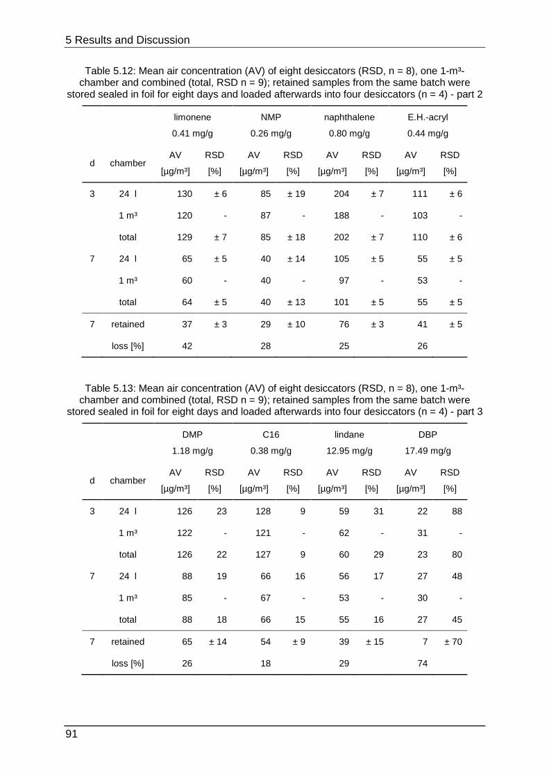
5 Results and Discussion
91
Table 5.12: Mean air concentration (AV) of eight desiccators (RSD, n = 8), one 1-m³-chamber and combined (total, RSD n = 9); retained samples from the same batch were
stored sealed in foil for eight days and loaded afterwards into four desiccators (n = 4) - part 2
limonene
0.41 mg/g
NMP
0.26 mg/g
naphthalene
0.80 mg/g
E.H.-acryl
0.44 mg/g
d chamber AV
[µg/m³]
RSD
[%]
AV
[µg/m³]
RSD
[%]
AV
[µg/m³]
RSD
[%]
AV
[µg/m³]
RSD
[%]
3 24 l 130 ± 6 85 ± 19 204 ± 7 111 ± 6
1 m³ 120 - 87 - 188 - 103 -
total 129 ± 7 85 ± 18 202 ± 7 110 ± 6
7 24 l 65 ± 5 40 ± 14 105 ± 5 55 ± 5
1 m³ 60 - 40 - 97 - 53 -
total 64 ± 5 40 ± 13 101 ± 5 55 ± 5
7 retained 37 ± 3 29 ± 10 76 ± 3 41 ± 5
loss [%] 42 28 25 26
Table 5.13: Mean air concentration (AV) of eight desiccators (RSD, n = 8), one 1-m³-chamber and combined (total, RSD n = 9); retained samples from the same batch were
stored sealed in foil for eight days and loaded afterwards into four desiccators (n = 4) - part 3
DMP
1.18 mg/g
C16
0.38 mg/g
lindane
12.95 mg/g
DBP
17.49 mg/g
d chamber AV
[µg/m³]
RSD
[%]
AV
[µg/m³]
RSD
[%]
AV
[µg/m³]
RSD
[%]
AV
[µg/m³]
RSD
[%]
3 24 l 126 23 128 9 59 31 22 88
1 m³ 122 - 121 - 62 - 31 -
total 126 22 127 9 60 29 23 80
7 24 l 88 19 66 16 56 17 27 48
1 m³ 85 - 67 - 53 - 30 -
total 88 18 66 15 55 16 27 45
7 retained 65 ± 14 54 ± 9 39 ± 15 7 ± 70
loss [%] 26 18 29 74
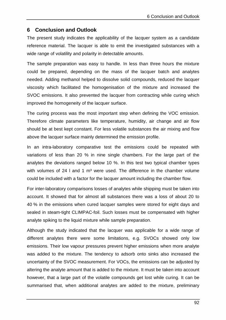
6 Conclusion and Outlook
92
6 Conclusion and Outlook The present study indicates the applicability of the lacquer system as a candidate
reference material. The lacquer is able to emit the investigated substances with a
wide range of volatility and polarity in detectable amounts.
The sample preparation was easy to handle. In less than three hours the mixture
could be prepared, depending on the mass of the lacquer batch and analytes
needed. Adding methanol helped to dissolve solid compounds, reduced the lacquer
viscosity which facilitated the homogenisation of the mixture and increased the
SVOC emissions. It also prevented the lacquer from contracting while curing which
improved the homogeneity of the lacquer surface.
The curing process was the most important step when defining the VOC emission.
Therefore climate parameters like temperature, humidity, air change and air flow
should be at best kept constant. For less volatile substances the air mixing and flow
above the lacquer surface mainly determined the emission profile.
In an intra-laboratory comparative test the emissions could be repeated with
variations of less than 20 % in nine single chambers. For the large part of the
analytes the deviations ranged below 10 %. In this test two typical chamber types
with volumes of 24 l and 1 m³ were used. The difference in the chamber volume
could be included with a factor for the lacquer amount including the chamber flow.
For inter-laboratory comparisons losses of analytes while shipping must be taken into
account. It showed that for almost all substances there was a loss of about 20 to
40 % in the emissions when cured lacquer samples were stored for eight days and
sealed in steam-tight CLIMPAC-foil. Such losses must be compensated with higher
analyte spiking to the liquid mixture while sample preparation.
Although the study indicated that the lacquer was applicable for a wide range of
different analytes there were some limitations, e.g. SVOCs showed only low
emissions. Their low vapour pressures prevent higher emissions when more analyte
was added to the mixture. The tendency to adsorb onto sinks also increased the
uncertainty of the SVOC measurement. For VOCs, the emissions can be adjusted by
altering the analyte amount that is added to the mixture. It must be taken into account
however, that a large part of the volatile compounds get lost while curing. It can be
summarised that, when additional analytes are added to the mixture, preliminary
6 Conclusion and Outlook
93
testing is needed to determine the analyte concentration resulting in detectable
emissions.
For further testing optimising the SVOC-emission is important. Their low vapour
pressure combined with the tendency to interact with sink complicated reliable
testing. The developed preparation method is a compromise between a wide range
of different substances. For low boiling compounds investigations according less
adsorptive surfaces and long-term testing is necessary to improve the emission
stability.
When working towards creating a certified reference material additional testing must
be undertaken. Homogeneity and traceability are the most important properties for a
reference material. For homogeneity inter-laboratory round robin tests are necessary.
The study showed that packing the cured lacquer into steam-tight CLIMPAC-foils
was the best way to ship the samples to the testing laboratories. Once the
homogeneity is determined, models predicting the emission profiles can be
developed. From these models parameters can be calculated that influence the
emission process. This will improve the quality of emission testing with its
fundamental role to protect human health from gaseous contaminants caused by
indoor materials.
7 Literature
94
7 Literature [1] W. Brasche and W. Bischof. Daily time spent indoors in german homes –
baseline data for the assessment of indoor exposure of german occupants.
International Journal of Hygiene and Environmental Health, 208:247–253, 2005.
[2] P. Wolkoff. How to measure and evaluate volatile organic compound
emissions from building products. a perspective. Science of The Total Environment,
227:197–213, 1999.
[3] World Health Organisation. Indoor air quality: organic pollutants. EURO
reports and studies, 111, 1989.
[4] W. Horn, O. Jann, and O. Wilke. Suitability of small environmental chambers
to test the emission of biocides from treated materials into the air. Atmospheric
Environment, 37:39–40, 2003.
[5] R. J. Laumbach. Sick building syndrome. International Encyclopedia of Public
Health, pages 4–8, 2008.
[6] L. E. Sparks, B. A. Tichenor, J. Chang, and Z. Guo. Gas-phase mass transfer
model for predicting volatile organic compound (voc) emission rates from indoor
pollutant sources. Indoor Air, 6:31–40, 1996.
[7] Z. Liu, W. Yea, and J. C. Little. Predicting emissions of volatile and
semivolatile organic compounds from building materials: A review. Building and
Environment, 64:7–25, 2013.
[8] F. Haghighat and H. Huang. Integrated iaq model for prediction of voc
emissions from building material. Building and Environment, 38:1007–1017, 2003.
[9] J. C. Little, A. T. Hodgson, and A. J. Gadgil. Modeling emissions of volatile
organic compounds from new carpets. Atmospheric Environment, 28:227–234, 1994.
[10] C. Howard-Reed, J. C. Little, E. Marand, S.S. Cox, S. J. Nabinger, and A. K.
Persily. Improving the reliability of voc emissions testing of building products.
ASHRAE IAQ Applications, pages 1–9, 2007.
[11] R. Meininghaus and E. Uhde. Diffusion studies of voc mixtures in a building
material. Indoor Air, 12:215–222, 2002.
7 Literature
95
[12] International Organization for Standardization. Iso 16000-9:2006 indoor air –
part 9: Determination of the emission of volatile organic compounds from building
products and furnishing – emission test chamber method. 2006.
[13] R. Oppl. Reliability of voc emission chamber testing – progress and remaining
challenges. Gefahrstoffe- Reinhaltung der Luft, 3:83–86, 2008.
[14] L. Z. Zhang and J. L. Niub. Effects of substrate parameters on the emissions
of volatile organic compounds from wet coating materials. Building and Environment,
38:939–946, 2003.
[15] T. Salthammer. Environmental Test Chambers and Cells. Wiley-VCH, 2009.
[16] S. Sollinger and K. Levsen. Indoor pollution by organic emissions from textile
floor coverings: Climate test chamber studies under static conditions. Atmospheric
Environment, 28:2369–2378, 1992.
[17] C. Howard-Reed, Z. Liu, J. Benning, S. S. Cox, D. Samarov, D. Leber, A. T.
Hodgson, S. Mason, D. Won, and J.C. Little. Diffusion-controlled reference material
for volatile organic compound emissions testing: Pilot inter-laboratory study. Building
and Environment, 46:1504–1511, 2011.
[18] W. Horn, O. Wilke, and K. Wiegner. Results of rr-voc-bam_2009, final report.
BAM: Federal Institute for Materials Research and Testing, Berlin, Germany (2010),
2010.
[19] ASTM International. Astm d6330 - 98(2008): Standard practice for
determination of volatile organic compounds (excluding formaldehyde) emissions
from wood-based panels using small environmental chambers under defined test
conditions. 2008.
[20] J. Namiesnik and B. Zygmunt. Role of reference materials in analysis of
environmental pollutants. Science of the Total Environment, 228:243–257, 1999.
[21] W. Wei, Y. Zhang, J. Xiong, and M. Li. A standard reference for chamber
testing of material voc emissions: Design principle and performance. Atmospheric
Environment, 47:381–388, 2012.
[22] W. Wei, J. Xiong, W. Zhao, and Y. Zhang. A framework and experimental
study of an improved voc/formaldehyde emission reference for environmental
chamber tests. Atmospheric Environment, 82:327–334, 2014.
7 Literature
96
[23] M. Oehme. Practical Introduction to GC-MS Analysis with Quadrupoles. Wiley-
VCH, 1998.
[24] H.-J. Hübschmann. Handbook of GC/MS. Wiley-VCH, 2008.
[25] E. Uhde. Vergleich von Emissionsprüfkammern : Untersuchungen unter
dynamischen Bedingungen. PhD thesis, Technische Universität Braunschweig, 1998.
[26] T. Schripp, B. Nachtwey, J. Toelke, T. Salthammer, E. Uhde, M. Wensing, and
M. Bahadir. A microscale device for measuring emissions from materials for indoor
use. Analytical and Bioanalytical Chemistry, 387:1907–1919, 2007.
[27] International Organization for Standardization. Iso 16000-25:2011 indoor air –
part 25: Determination of the emission of semi-volatile organic compounds by
building products – micro-chamber method. 2011.
[28] International Organization for Standardization. Iso 12219-3:2012 interior air of
road vehicles – part 3: Screening method for the determination of the emissions of
volatile organic compounds from vehicle interior parts and materials – micro-scale
chamber method. 2012.
[29] A. Goldschmidt, B. Hantschke, E. Knappe, and G.-F. Vock. Glasurit-Handbuch
Lacke und Farben. Curt R. Vincentz Verlag, Hannover, 1984.
[30] International Organization for Standardization. Iso 16000-6:2011 indoor air –
part 6: Determination of volatile organic compounds in indoor and test chamber air by
active sampling on tenax ta® sorbent, thermal desorption and gas chromatography
using ms or ms-fid. 2011.
[31] European Union. Regulation (ec) no 1907/2006 of the european parliament
and of the council of 18 december 2006 concerning the registration, evaluation,
authorisation and restriction of chemicals (reach), establishing a european chemicals
agency. 2006.
[32] S. Nalli, O. J. Horn, A. R. Grochowalski, D. G. Cooper, and J. A. Nicell. Origin
of 2-ethylhexanol as a voc. Environmental Pollution, 140:181–185, 2006.
[33] Institute for Occupational Safety and Health of the German Social Accident
Insurance IFA. GESTIS-database on hazardous substances.
http://www.dguv.de/ifa/Gefahrstoffdatenbanken/GESTIS-Stoffdatenbank/, last
checked: 2014-02-11.
7 Literature
97
[34] Georg Thieme Verlag KG. RÖMPP Online. http://www.roempp.com/prod3/,
last checked: 2014-02-11.
[35] Joint Committee for Guides in Metrology. Evaluation of measurement date -
guide to the expression of uncertainty in measurement. JCMG, 100, 2008.
[36] E. Uhde and T. Salthammer. Influence of molecular parameters on the sink
effect in test chambers. Indoor Air, 16:158–165, 2006.
[37] P. A. Clausen, Z. Liu, Y. Xu, V. Kofoed-Sørensena, and J. C. Little. Influence
of air flow rate on emission of dehp from vinyl flooring in the emission cell flec:
Measurements and cfd simulation. Atmospheric Environment, 44:2760–2766, 2010.
[38] B. Mull. Investigations of an active air sampling strategy for biocides, PCBs
and PAHs at low air change rates. PhD thesis, Technische Universität Berlin, 2013.
[39] German Institute for Standardization. Din 32645:2008-11 chemical analysis -
decision limit, detection limit and determination limit under repeatability conditions -
terms, methods, evaluation. 2008.
8 Appendix
98
8 Appendix
8.1 Abbreviations
µ-CTE Micro-Chamber/Thermal Extractor™
ASTM American Society for Testing and Materials
AV average
BAM Federal Institute for Material Research and Testing (Bundesanstalt für Materialforschung und -prüfung)
C10 n-decane
C16 n-hexadecane
CI chemical ionisation
CIS cold injection system
d sampling day
DBP dibutyl phthalate
DEHP di-2-ethylhexyl phthalate
DMP dimethyl phthalate
E.H. ethyl hexanol
E.H.-arcyl 2-ethylhexyl acrylate
ECHA European Chemical Agency
EI electron ionisation
FID flame ionization detector
GC gas chromatography
ISTD internal standard
ISO International Organization for Standardization
L product loading factor
LDPE low density polyethylene
LIFE liquid inner-tube diffusion-film-emission
LC liquid chromatography
LOQ limit of quantification
m slope
8 Appendix
99
MeOH methanol
MFC mass flow controller
MIBK methyl isobutyl ketone
MS mass spectrometry
n air change rate / number of samples or measurements
ny y-intercept
NMP N-methyl-2-pyrrolidone
OGC organic-solvent-based glossy clear lacquer
OGW organic-solvent-based glossy white lacquer
OGR organic-solvent-based glossy red lacquer
OMC organic-solvent-based matt clear lacquer
OMR organic-solvent-based matt red lacquer
OMW organic-solvent-based matt white lacquer
Poct/wat partition coefficient
PET polyethylene terephthalate
PMP polymethylpentene
POM particular organic matter
PTFE polytetrafluoroethylene
q area specific air flow rate
R² coefficient of correlation
RH relative humidity
(R)SD (relative) standard deviation
SERA area specific emission rate
SI International System of Units
SIM single ion monitoring
stor. storage
SVOC semi-volatile organic compounds
TD(S) thermal desorption (system)
TIC total ion chromatogram
8 Appendix
100
u uncertainty
VOC volatile organic compound
VVOC very volatile organic compound
w. with
w/o. without
WGC water-based glossy clear lacquer
WGI water-based glossy light-ivory lacquer
WGR water-based glossy red lacquer
WMC water-based matt clear lacquer
WMR water-based matt red lacquer
WMW water-based matt white lacquer
WHO World Health Organization
8.2 List of figures Figure 2.1: Different emission profiles for VOC and SVOC (model) ....................................... 3
Figure 2.2: Overview of the emission process (two dimensional) ............................................. 4 Figure 2.3: Overview of an emission testing procedure (T ... temperature, RH ... relative humidity) .................................................................................................................................... 6
Figure 2.4: Test specimen of a carpet with sealed cutting edges (left) and suitable glue applied on glass (right) ............................................................................................................................ 8
Figure 2.5: Oriented strand boards with sealed cutting edges .................................................... 8 Figure 2.6: Overview of the traceability of emission testing ................................................... 10 Figure 2.7: PMP-polymer-film loaded into a stainless steel sample holder (taken from [17]) 11
Figure 2.8: LIFE reference - schematic (left) and ion reality (right) (taken from [21]) ........... 11
Figure 2.9: Emission profile of the LIFE-reference (taken from [21]) .................................... 12
Figure 2.10: Emission profile of the PMP-film (taken from [17]) ........................................... 12 Figure 3.1: General description of an emission test chamber (taken from [12]) ..................... 15
Figure 3.2: 24-l-chamber (desiccator) loaded with wooden sample ........................................ 17
Figure 3.3: Several 24-l-chambers inside a 16-m³-chamber .................................................... 17 Figure 3.4: Micro-Chamber/Thermal Extractor™ (µ-CTE™) from MARKES Int. (opened) 18 Figure 3.5: µ-CTE (closed) with sampling tubes ..................................................................... 18 Figure 3.6: Overview of the polarity range of the investigated substances expressed as Poct/wat
.................................................................................................................................................. 21
Figure 3.7: Overview of the boiling point range of the investigated substances ..................... 21
Figure 3.8: Chromatographic separation of the investigated substances (*...SVHC – substances of very high concern [31]; see Table 3.3 for measurement parameters; ISTD .. internal standard) ...................................................................................................................... 21
Figure 3.9: TDSA with glass sampling tubes inside the autosampler (GERSTEL) ................ 23
Figure 3.10: Transfer line of the TDSA (GERSTEL) .............................................................. 23 Figure 3.11: ULTRA 50:50 (1) and UNITY1 (2) (MARKES Int.) .......................................... 24
8 Appendix
101
Figure 3.12: Capped steel sampling tubes inside the Ultra 50:50 autosampler ....................... 24
Figure 3.13: Lacquer preparation scheme ................................................................................ 28 Figure 3.14: Lacquer mixture inside a 100 ml amber screw cap bottle on a magnetic stirrer . 29
Figure 3.15: Addition of the pure analyte into the agitated lacquer with a glass syringe ........ 29
Figure 3.16: FLEC-pump from SCP ........................................................................................ 30 Figure 3.17: Uncertainties influencing the preparation, curing and emission testing of the lacquer system (u ... uncertainty, mS ... analyte amount trapped onto the sampling tube, VS ... sampled air volume) ................................................................................................................. 32
Figure 4.1: Symbol descriptions used for the preparation schemes ......................................... 35 Figure 4.2: Size-comparison of a micro-chamber (front) in opposite of a 1-m³-chamber (back) .................................................................................................................................................. 36
Figure 4.3: Nomenclature of the tested lacquers (w…acrylic, o…alkyd) ............................... 37
Figure 4.4: Preparation scheme for experiment 4.1.2 .............................................................. 38 Figure 4.5: Preparation scheme for experiment 4.1.3 .............................................................. 39 Figure 4.6: Preparation scheme for experiment 4.1.4 .............................................................. 40 Figure 4.7: Preparation scheme for experiment 4.1.5 (w ... with, w/o ... without) .................. 41
Figure 4.8: Preparation scheme for experiment 4.1.6 .............................................................. 42 Figure 4.9: Lacquer samples loaded into a 1-m3-chamber for curing ...................................... 43 Figure 4.10: Preparation scheme for experiment 4.2.1 ............................................................ 44 Figure 4.11: Preparation scheme for experiment 4.2.2 ............................................................ 45 Figure 4.12: Preparation scheme for experiment 4.2.3 ............................................................ 46 Figure 4.13: Preparation scheme for experiment 4.2.4 ............................................................ 47 Figure 4.14: Preparation scheme for experiment 4.2.5 ............................................................ 47 Figure 4.15: Improvised humidification device (1 ... T-piece; 2 ... needle valve; 3 ... water reservoir; 4 ... T-piece) ............................................................................................................. 48
Figure 4.16: Systematic scheme of the improvised humidification device (1 ... T-piece; 2 ... needle valve; 3 ... water reservoir; 4 ... T-piece) ...................................................................... 48 Figure 4.17: Lacquer samples vacuumed in a LDPE bag (on top) and packed in aluminium foil (below) ............................................................................................................................... 50
Figure 4.18: Preparation scheme for experiment 4.2.4 ............................................................ 50 Figure 4.19: Preparation scheme for experiment 4.3.3 ............................................................ 51 Figure 4.20: Four lacquer samples packed in sealed CLIMAPAC-foil ................................... 52
Figure 5.1: Emission curves of styrene from a sealant sample loaded into a desiccator (light grey) and a µ-CTE (white) ....................................................................................................... 53
Figure 5.2: Emission curves of limonene from a sealant sample loaded into a desiccator (light grey) and a µ-CTE (white) ....................................................................................................... 53
Figure 5.3: Emission curves of octamethylcyclotetrasiloxane from a sealant sample loaded into a desiccator (light grey) and a µ-CTE (white) .................................................................. 54 Figure 5.4: SIM-chromatogram of the self-emission of the lacquer OMR on sampling day 1 (black line) and 3 (red line) – (SIM…single ion monitoring) .................................................. 55 Figure 5.5: TIC-chromatogram of a subsequently measured blank tube (clean and unfilled glass tubes) - (TIC…total ion count) ........................................................................................ 55 Figure 5.6: Emissions of styrene from different lacquer types in µ-CTE on different sampling days - two samples per lacquer (equal to E.H. and NMP) ....................................................... 56 Figure 5.7: Emissions of DMP from different lacquer types in µ-CTE on different sampling days - two samples per lacquer (equal to C16) ........................................................................ 57 Figure 5.8: Emissions of DBP from different lacquer types in µ-CTE on different sampling days - two samples per lacquer (equal to lindane) ................................................................... 57 Figure 5.9: Surfaces of various water-based lacquers inside Petri dishes with a diameter of 9.6 cm (WGR, WGI, WGC each 15 g) .......................................................................................... 59
8 Appendix
102
Figure 5.10: Emitted lindane amounts, either dissolved in MeOH (“lindane (l)”) or added pure (“lindane (s)”), over a period of 11 days with different stirring times ..................................... 61 Figure 5.11: Emissions of styrene with/without MeOH at different stirring times (see 4.1.4) 62
Figure 5.12: Emissions of styrene with and without MeOH (see 4.1.5) ................................. 62
Figure 5.13: Emissions of E.H. with/without MeOH at different stirring times (see 4.1.4) .... 63
Figure 5.14: Emissions of E.H. with and without MeOH (see 4.1.5) ...................................... 63
Figure 5.15: Emissions of NMP with/without MeOH at different stirring times (see 4.1.4) ... 63
Figure 5.16: Emissions of NMP with and without MeOH (see 4.1.5) .................................... 63
Figure 5.17: Emissions of DMP with/without MeOH at different stirring times (see 4.1.4) ... 64
Figure 5.18: Emissions of DMP with and without MeOH (see 4.1.5) .................................... 64
Figure 5.19: Emissions of C16 with/without MeOH at different stirring times (see 4.1.4) ..... 64
Figure 5.20: Emissions of C16 with and without MeOH (see 4.1.5) ...................................... 64
Figure 5.21: Emissions of DBP with/without MeOH at different stirring times (see 4.1.4).... 65
Figure 5.22: Emissions of DBP with and without MeOH (see 4.1.5) ..................................... 65
Figure 5.23: Fissures on the surface of a cured lacquer mixture without MeOH .................... 66
Figure 5.24: Plane surface of a cured lacquer mixture without containing MeOH ................. 66
Figure 5.25: Emissions of styrene after different curing processes (µ-CTE) .......................... 69
Figure 5.26: Emissions of E.H. after different curing processes (µ-CTE) ............................... 69
Figure 5.27: Emissions of NMP after different curing processes (µ-CTE) ............................. 70
Figure 5.28: Emissions of DMP after different curing processes (µ-CTE) ............................. 70
Figure 5.29: Emissions of C16 after different curing processes (µ-CTE) ............................... 70
Figure 5.30: Emissions of lindane after different curing processes (µ-CTE) .......................... 70
Figure 5.31: Emissions of DBP after different curing processes (µ-CTE) .............................. 71
Figure 5.32: Emission profile of styrene after different curing processes (desiccator) ........... 73
Figure 5.33: Emission profile of E.H. after different curing processes (desiccator)................ 73
Figure 5.34: Emission profile of NMP after different curing processes (desiccator) .............. 73
Figure 5.35: Emission profile of DMP after different curing processes (desiccator) .............. 73
Figure 5.36: Emission profile of C16 after different curing processes (desiccator) ................ 74
Figure 5.37: Emission profile of lindane after different curing processes (desiccator) ........... 74
Figure 5.38: Emission profile of DBP after different curing processes (desiccator) ............... 74
Figure 5.39: Styrene emissions of one lacquer batch at 15 and 30 ml/min chamber flow (0 % RH) ........................................................................................................................................... 78
Figure 5.40: E.H. emissions of one lacquer batch at 15 and 30 ml/min chamber flow (0 % RH) .................................................................................................................................................. 78
Figure 5.41: NMP emissions of one lacquer batch at 15 and 30 ml/min chamber flow (0 % RH) ........................................................................................................................................... 78
Figure 5.42: DMP emissions of one lacquer batch at 15 and 30 ml/min chamber flow (0 % RH) ........................................................................................................................................... 79
Figure 5.43: C16 emissions of one lacquer batch at 15 and 30 ml/min chamber flow (0 % RH) .................................................................................................................................................. 79
Figure 5.44: Lindane emissions of one lacquer batch at 15 and 30 ml/min chamber flow (0 % RH) ........................................................................................................................................... 79
Figure 5.45: DBP emissions of one lacquer batch at 15 and 30 ml/min chamber flow (0 % RH) ........................................................................................................................................... 80
Figure 5.46: Styrene emissions of one lacquer batch at 0 and 55 % RH (15 ml/min flow) ..... 81
Figure 5.47: E.H. emissions of one lacquer batch at 0 and 55 % RH (15 ml/min flow) .......... 81
Figure 5.48: NMP emissions of one lacquer batch at 0 and 55 % RH (15 ml/min flow) ........ 81
Figure 5.49: DMP emissions of one lacquer batch at 0 and 55 % RH (15 ml/min flow) ........ 82
Figure 5.50: C16 emissions of one lacquer batch at 0 and 55 % RH (15 ml/min flow) .......... 82
Figure 5.51: Lindane emissions of one lacquer batch at 0 and 55 % RH (15 ml/min flow) .... 82
8 Appendix
103
Figure 5.52: DBP emissions of one lacquer batch at 0 and 55 % RH (15 ml/min flow) ......... 83
Figure 5.53: Surface of a lacquer sample cured inside the µ-CTE at 30 ml/min and 0 % RH (35-mm-Petri dish, measured with a VR 3000 from KEYENCE) ........................................... 85
Figure 5.54: Surface of a lacquer sample cured inside the µ-CTE at 15 ml/min and 0 % RH (35-mm-Petri dish, measured with a VR 3000 from KEYENCE) ........................................... 85
Figure 5.55: Surface of a lacquer sample cured inside an external 1-m³-chamber at 750 l/h and 50 % RH (35-mm-Petri dish, measured with a VR 3000 from KEYENCE) ........................... 86
8.3 List of tables Table 2.1: VOC-classification in accordance with WHO [3] .................................................... 2 Table 3.1: Overview of selected physical parameters of the investigated substances [33] [34] .................................................................................................................................................. 20
Table 3.2: Overview of selected physical parameters of the additional substances [33] [34] . 22
Table 3.3: Measurement parameters of the TD-GC/MS system "Asterix" and "Idefix" (see chapter 3.1.1) ............................................................................................................................ 25
Table 3.4: Typical parameters and their calculations in emission testing (partially in accordance to ISO 16000-9 [12]) ............................................................................................. 27 Table 3.5: Uncertainties (urel) for the measured air concentration ρx on two different TD-GC/MS-systems (“Asterix”/”Idefix”) calculated from the uncertainties of the analyte mass trapped onto the adsorbent tube (ms) and the sampled volume (Vs; “pump” ... active sampling with pump; “w/o. / w. MFC” ... passive sampling on µ-CTE equipped without/with MFC) - part 1 ......................................................................................................................................... 33
Table 3.6: Uncertainties (urel) for the measured air concentration ρx on two different TD-GC/MS-systems (“Asterix”/”Idefix”) calculated from the uncertainties of the analyte mass trapped onto the adsorbent tube (ms) and the sampled volume (Vs; “pump” ... active sampling with pump; “w/o. / w. MFC” ... passive sampling on µ-CTE equipped without/with MFC) - part 2 ......................................................................................................................................... 34
Table 3.7: Uncertainties influencing the reproducibility of the emission of the lacquer system that cannot be included into the calculation of the combined uncertainty ............................... 34
Table 4.1: Operating parameters of the µ-CTE and 24-l-chamber (“desiccator”) ................... 37
Table 4.2: Calculation of the added analyte amounts (*cl used instead ρA) ............................. 38
Table 5.1: Averaged (n = 2) minimum and maximum emitted analyte amounts of the water-based lacquers over a sampling cycle of 21 days ..................................................................... 58 Table 5.2: Minimum and maximum emitted analyte amounts of lindane and DBP from two lacquer batches (WGC25/WGC55) with different loaded lacquer amounts (2 g, 4.5 g) over a sampling cycle of 25 days ........................................................................................................ 60
Table 5.3: Average (AV) and relative standard deviation (RSD(repro)) of three identical prepared spiked lacquer samples over different sampling days; RSD(repeat) stands for the mean RSDs of the six chambers of one µ-CTE over different sampling days ........................ 68
Table 5.4: Mean SERA and reproducibility (RSD) of the emissions of styrene, E.H. and NMP for each of the three equal lacquer batches loaded into the µ-CTE and the desiccator combined different curing processes ........................................................................................ 75 Table 5.5: Mean SERA and reproducibility (RSD) of the emissions of DMP, C16, lindane and DBP for each of the three equal lacquer batches loaded into the µ-CTE and the desiccator combined different curing processes ........................................................................................ 76 Table 5.6: Air concentrations of a lacquer mixture three and seven days after loading into a 24-l-chamber (cured three days in a 1-m³-chamber) - part 1 ................................................... 87 Table 5.7: Air concentrations of a lacquer mixture three and seven days after loading into a 24-l-chamber (cured three days in a 1-m³-chamber) - part 2 ................................................... 87
8 Appendix
104
Table 5.8: Mean SERA (AV) and RSD (n = 3) of six equal cured lacquer samples, three of which were stored in aluminium foil (“Al”) and three in an evacuated LDPE bag (vac.) over four days - part 1 ...................................................................................................................... 88
Table 5.9: Mean SERA (AV) and RSD (n = 3) of six equal cured lacquer samples, three of which were stored in aluminium foil (“Al”) and three in an evacuated LDPE bag (vac.) over four days - part 2 ...................................................................................................................... 88
Table 5.10: Mean SERA (AV) and RSD (n = 3) of six equal cured lacquer samples, three of which were stored in aluminium foil (“Al”) and three in an evacuated LDPE bag (vac.) over four days - part 3 ...................................................................................................................... 89
Table 5.11: Mean air concentration (AV) of eight desiccators (RSD, n = 8), one 1-m³-chamber and combined (total, RSD n = 9); retained samples from the same batch were stored sealed in foil for eight days and loaded afterwards into four desiccators (n = 4) - part 1 ....................... 90
Table 5.12: Mean air concentration (AV) of eight desiccators (RSD, n = 8), one 1-m³-chamber and combined (total, RSD n = 9); retained samples from the same batch were stored sealed in foil for eight days and loaded afterwards into four desiccators (n = 4) - part 2 ....................... 91
Table 5.13: Mean air concentration (AV) of eight desiccators (RSD, n = 8), one 1-m³-chamber and combined (total, RSD n = 9); retained samples from the same batch were stored sealed in foil for eight days and loaded afterwards into four desiccators (n = 4) - part 3 ....................... 91
Table 8.1: Analyte amount and averaged area response (AV, n = 3) of a 15-point-calibration with slope (m), y-intercept (ny), coefficient of correlation (R²) and the limit of quantification (LOQ) calculated from a linear regression curve on the two measurement devices “Asterix” and “Idefix” - part 1 ............................................................................................................... 105
Table 8.2: Analyte amount and averaged area response (AV, n = 3) of a 15-point-calibration with slope (m), y-intercept (ny), coefficient of correlation (R²) and the limit of quantification (LOQ) calculated from a linear regression curve on the two measurement devices “Asterix” and “Idefix” - part 2 ............................................................................................................... 107
Table 8.3: Analyte amount and averaged area response (AV, n = 3) of a 15-point-calibration with slope (m), y-intercept (ny), coefficient of correlation (R²) and the limit of quantification (LOQ) calculated from a linear regression curve on the two measurement devices “Asterix” and “Idefix” - part 3 ............................................................................................................... 108
Table 8.4: Analyte amount and averaged area response (AV, n = 3) of a 15-point-calibration with slope (m), y-intercept (ny), coefficient of correlation (R²) and the limit of quantification (LOQ) calculated from a linear regression curve on the two measurement devices “Asterix” and “Idefix” - part 4 ............................................................................................................... 109
Table 8.5: Analyte amount and averaged area response (AV, n = 3) of a 15-point-calibration with slope (m), y-intercept (ny), coefficient of correlation (R²) and the limit of quantification (LOQ) calculated from a linear regression curve on the two measurement devices “Asterix” and “Idefix” - part 5 ............................................................................................................... 110
Table 8.6: Analyte amount and averaged area response (AV, n = 3) of a 15-point-calibration with slope (m), y-intercept (ny), coefficient of correlation (R²) and the limit of quantification (LOQ) calculated from a linear regression curve on the two measurement devices “Asterix” and “Idefix” - part 6 ............................................................................................................... 111
Table 8.7: Averaged area specific emission rates (n = 4) and RSD-values of styrene, octamethylcyclotetrasiloxane and limonene from a sealant sample loaded into four desiccators, respectively four chambers of a µ-CTE over a sampling cycle of 15 days ........ 112
Table 8.8: Averaged emissions (n = 2) of a water-based matt clear lacquer (WMC) prepared with seven substances over a sampling cycle of 21 days loaded into a µ-CTE ..................... 113
Table 8.9: Averaged emissions (n = 2) of a water-based matt red lacquer (WMR) prepared with seven substances over a sampling cycle of 21 days loaded into a µ-CTE ..................... 113
8 Appendix
105
Table 8.10: Averaged emissions (n = 2) of a water-based matt white lacquer (WMW) prepared with seven substances over a sampling cycle of 21 days loaded into a µ-CTE ...... 114
Table 8.11: : Averaged emissions (n = 2) of a water-based glossy clear lacquer (WGC) prepared with seven substances over a sampling cycle of 21 days loaded into a µ-CTE ...... 114
Table 8.12: Averaged emissions (n = 2) of a water-based glossy red lacquer (WGR) prepared with seven substances over a sampling cycle of 21 days loaded into a µ-CTE ..................... 115
Table 8.13: Averaged emissions (n = 2) of a water-based glossy light-ivory lacquer (WGI) prepared with seven substances over a sampling cycle of 21 days loaded into a µ-CTE ...... 115
Table 8.14: Emitted analyte amounts of lindane and DBP from two lacquer batches (WGC25/WGC55) with different loaded lacquer amounts (2 g, 4.5 g) over a sampling cycle of 25 days loaded into a µ-CTE ............................................................................................. 116 Table 8.15: Emission of a lacquer batch where lindane was added dissolved in MeOH stirred for one and four hours loaded into a µ-CTE .......................................................................... 117 Table 8.16: Emission of a lacquer batch where lindane without MeOH stirred for one, two, three and four hours loaded into a µ-CTE .............................................................................. 118 Table 8.17: Averaged (n = 3) emissions and SD-values of styrene, E.H. and NMP of lacquer batches with and without MeOH over a sampling cycle of 11 days loaded into a µ-CTE .... 119
Table 8.18: Averaged (n = 3) emissions and SD-values of DMP, C16 and DBP of lacquer batches with and without MeOH over a sampling cycle of 11 days loaded into a µ-CTE .... 119
Table 8.19: Averaged emissions (n = 6) and RSD-values of a lacquer batch loaded into µ-CTEs over a sampling cycle of 14 days that cured either directly inside the µ-CTE or for 44 h inside a 1-m³-chamber - part 1 ............................................................................................... 120 Table 8.20: Averaged emissions (n = 6) and RSD-values of a lacquer batch loaded into µ-CTEs over a sampling cycle of 14 days that cured either directly inside the µ-CTE or for 44 h inside a 1-m³-chamber - part 2 ............................................................................................... 121 Table 8.21: Averaged emissions (n = 4) and RSD-values of lacquer batches loaded into desiccators over a sampling cycle of 17 days that cured either directly inside the desiccator or for 46 h inside a 1-m³-chamber with switched on/off fan inside the testing chamber - part 1 ................................................................................................................................................ 122
Table 8.22: Averaged emissions (n = 4) and RSD-values of lacquer batches loaded into desiccators over a sampling cycle of 17 days that cured either directly inside the desiccator or for 46 h inside a 1-m³-chamber with switched on/off fan inside the testing chamber - part 2 ................................................................................................................................................ 123
Table 8.23: Emission rates of a lacquer batch loaded into a µ-CTE over a sampling cycle of 8 days that operated at 15 ml/min ............................................................................................. 124 Table 8.24: Emissions of a lacquer batch loaded into a µ-CTE over a sampling cycle of 8 days that operated at 30 ml/min ...................................................................................................... 125
Table 8.25: Emissions of a lacquer batch loaded into a µ-CTE over a sampling cycle of 11 days that operated at 0 % RH ................................................................................................. 126 Table 8.26: Emissions of a lacquer batch loaded into a µ-CTE over a sampling cycle of 11 days that operated at 55 % RH ............................................................................................... 127
8.4 Additional measurement data
8.4.1 Calibration data The values of slope (m), y-intercept (n), coefficient of correlation (R²) and the limit of
quantification (LOQ) were calculated based on DIN 32645 [39] with the EXCEL-
macro B.E.N. (ARVECON).
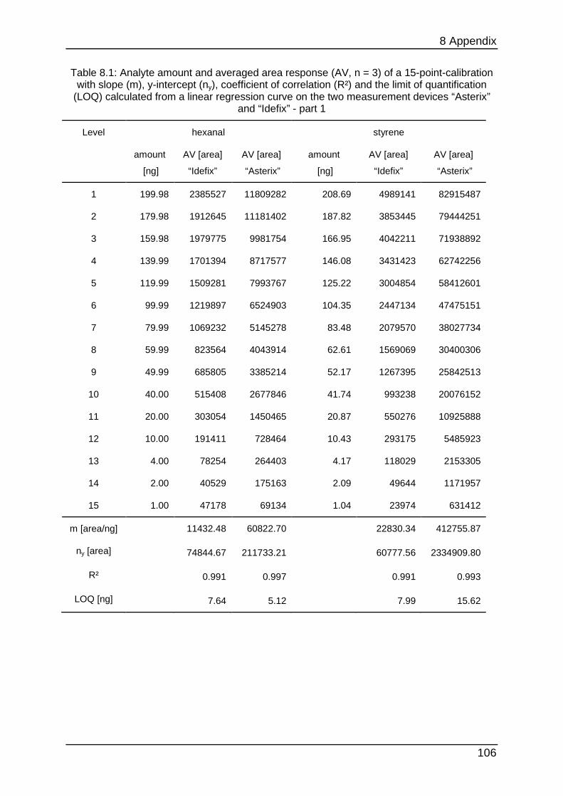
8 Appendix
106
Table 8.1: Analyte amount and averaged area response (AV, n = 3) of a 15-point-calibration with slope (m), y-intercept (ny), coefficient of correlation (R²) and the limit of quantification
(LOQ) calculated from a linear regression curve on the two measurement devices “Asterix” and “Idefix” - part 1
Level hexanal styrene
amount
[ng]
AV [area]
“Idefix”
AV [area]
“Asterix”
amount
[ng]
AV [area]
“Idefix”
AV [area]
“Asterix”
1 199.98 2385527 11809282 208.69 4989141 82915487
2 179.98 1912645 11181402 187.82 3853445 79444251
3 159.98 1979775 9981754 166.95 4042211 71938892
4 139.99 1701394 8717577 146.08 3431423 62742256
5 119.99 1509281 7993767 125.22 3004854 58412601
6 99.99 1219897 6524903 104.35 2447134 47475151
7 79.99 1069232 5145278 83.48 2079570 38027734
8 59.99 823564 4043914 62.61 1569069 30400306
9 49.99 685805 3385214 52.17 1267395 25842513
10 40.00 515408 2677846 41.74 993238 20076152
11 20.00 303054 1450465 20.87 550276 10925888
12 10.00 191411 728464 10.43 293175 5485923
13 4.00 78254 264403 4.17 118029 2153305
14 2.00 40529 175163 2.09 49644 1171957
15 1.00 47178 69134 1.04 23974 631412
m [area/ng] 11432.48 60822.70 22830.34 412755.87
ny [area] 74844.67 211733.21 60777.56 2334909.80
R² 0.991 0.997 0.991 0.993
LOQ [ng] 7.64 5.12 7.99 15.62
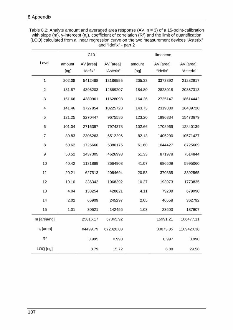
8 Appendix
107
Table 8.2: Analyte amount and averaged area response (AV, n = 3) of a 15-point-calibration with slope (m), y-intercept (ny), coefficient of correlation (R²) and the limit of quantification
(LOQ) calculated from a linear regression curve on the two measurement devices “Asterix” and “Idefix” - part 2
Level
C10 limonene
amount
[ng]
AV [area]
“Idefix”
AV [area]
“Asterix”
amount
[ng]
AV [area]
“Idefix”
AV [area]
“Asterix”
1 202.08 5412488 13186555 205.33 3373392 21282917
2 181.87 4396203 12669207 184.80 2828018 20357313
3 161.66 4389961 11628098 164.26 2725147 18614442
4 141.46 3727854 10225728 143.73 2319380 16439720
5 121.25 3270447 9675586 123.20 1996334 15473679
6 101.04 2716397 7974378 102.66 1708969 12840139
7 80.83 2306263 6512296 82.13 1405290 10571427
8 60.62 1725660 5380175 61.60 1044427 8725609
9 50.52 1437305 4626993 51.33 871978 7514844
10 40.42 1131889 3664903 41.07 686509 5995060
11 20.21 627513 2084694 20.53 370365 3392565
12 10.10 336342 1068392 10.27 193973 1773835
13 4.04 133254 428821 4.11 79208 679090
14 2.02 65909 245297 2.05 40558 362792
15 1.01 30621 142456 1.03 23603 187907
m [area/ng] 25816.17 67365.92 15991.21 106477.11
ny [area] 84499.79 672028.03 33873.85 1109420.38
R² 0.995 0.990 0.997 0.990
LOQ [ng] 8.79 15.72 6.88 29.58
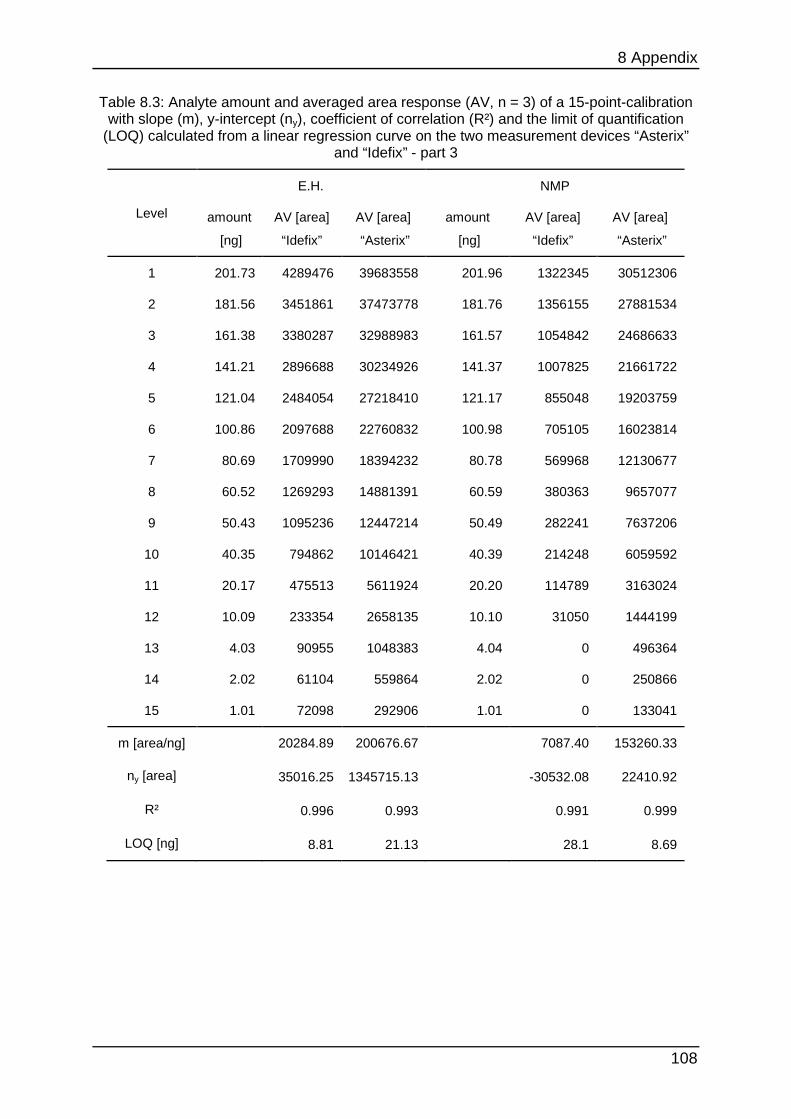
8 Appendix
108
Table 8.3: Analyte amount and averaged area response (AV, n = 3) of a 15-point-calibration with slope (m), y-intercept (ny), coefficient of correlation (R²) and the limit of quantification
(LOQ) calculated from a linear regression curve on the two measurement devices “Asterix” and “Idefix” - part 3
Level
E.H. NMP
amount
[ng]
AV [area]
“Idefix”
AV [area]
“Asterix”
amount
[ng]
AV [area]
“Idefix”
AV [area]
“Asterix”
1 201.73 4289476 39683558 201.96 1322345 30512306
2 181.56 3451861 37473778 181.76 1356155 27881534
3 161.38 3380287 32988983 161.57 1054842 24686633
4 141.21 2896688 30234926 141.37 1007825 21661722
5 121.04 2484054 27218410 121.17 855048 19203759
6 100.86 2097688 22760832 100.98 705105 16023814
7 80.69 1709990 18394232 80.78 569968 12130677
8 60.52 1269293 14881391 60.59 380363 9657077
9 50.43 1095236 12447214 50.49 282241 7637206
10 40.35 794862 10146421 40.39 214248 6059592
11 20.17 475513 5611924 20.20 114789 3163024
12 10.09 233354 2658135 10.10 31050 1444199
13 4.03 90955 1048383 4.04 0 496364
14 2.02 61104 559864 2.02 0 250866
15 1.01 72098 292906 1.01 0 133041
m [area/ng] 20284.89 200676.67 7087.40 153260.33
ny [area] 35016.25 1345715.13 -30532.08 22410.92
R² 0.996 0.993 0.991 0.999
LOQ [ng] 8.81 21.13 28.1 8.69
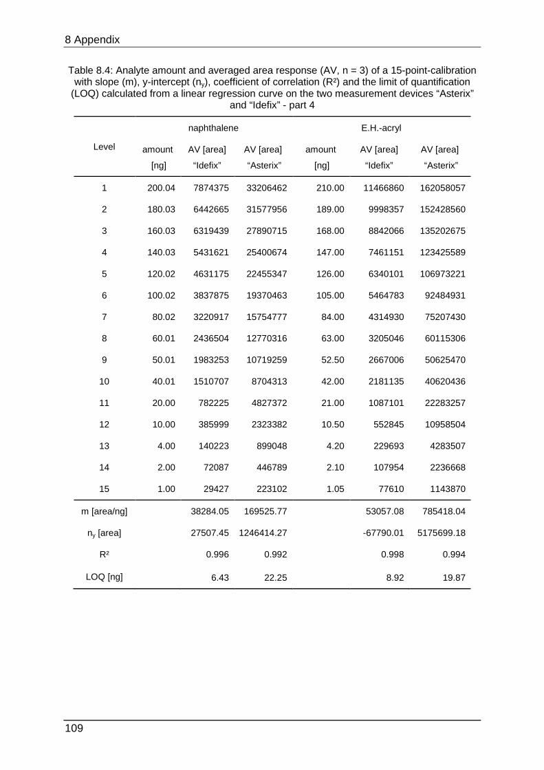
8 Appendix
109
Table 8.4: Analyte amount and averaged area response (AV, n = 3) of a 15-point-calibration with slope (m), y-intercept (ny), coefficient of correlation (R²) and the limit of quantification
(LOQ) calculated from a linear regression curve on the two measurement devices “Asterix” and “Idefix” - part 4
Level
naphthalene E.H.-acryl
amount
[ng]
AV [area]
“Idefix”
AV [area]
“Asterix”
amount
[ng]
AV [area]
“Idefix”
AV [area]
“Asterix”
1 200.04 7874375 33206462 210.00 11466860 162058057
2 180.03 6442665 31577956 189.00 9998357 152428560
3 160.03 6319439 27890715 168.00 8842066 135202675
4 140.03 5431621 25400674 147.00 7461151 123425589
5 120.02 4631175 22455347 126.00 6340101 106973221
6 100.02 3837875 19370463 105.00 5464783 92484931
7 80.02 3220917 15754777 84.00 4314930 75207430
8 60.01 2436504 12770316 63.00 3205046 60115306
9 50.01 1983253 10719259 52.50 2667006 50625470
10 40.01 1510707 8704313 42.00 2181135 40620436
11 20.00 782225 4827372 21.00 1087101 22283257
12 10.00 385999 2323382 10.50 552845 10958504
13 4.00 140223 899048 4.20 229693 4283507
14 2.00 72087 446789 2.10 107954 2236668
15 1.00 29427 223102 1.05 77610 1143870
m [area/ng] 38284.05 169525.77 53057.08 785418.04
ny [area] 27507.45 1246414.27 -67790.01 5175699.18
R² 0.996 0.992 0.998 0.994
LOQ [ng] 6.43 22.25 8.92 19.87
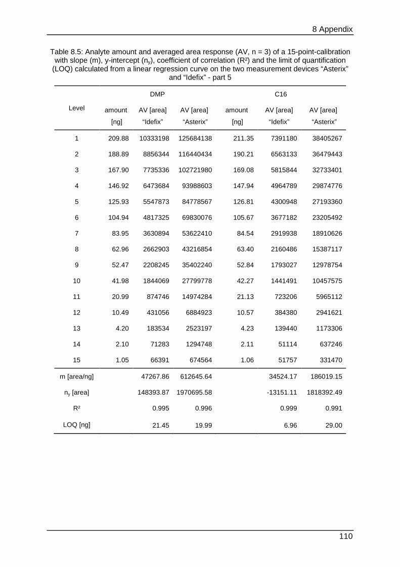
8 Appendix
110
Table 8.5: Analyte amount and averaged area response (AV, n = 3) of a 15-point-calibration with slope (m), y-intercept (ny), coefficient of correlation (R²) and the limit of quantification
(LOQ) calculated from a linear regression curve on the two measurement devices “Asterix” and “Idefix” - part 5
Level
DMP C16
amount
[ng]
AV [area]
“Idefix”
AV [area]
“Asterix”
amount
[ng]
AV [area]
“Idefix”
AV [area]
“Asterix”
1 209.88 10333198 125684138 211.35 7391180 38405267
2 188.89 8856344 116440434 190.21 6563133 36479443
3 167.90 7735336 102721980 169.08 5815844 32733401
4 146.92 6473684 93988603 147.94 4964789 29874776
5 125.93 5547873 84778567 126.81 4300948 27193360
6 104.94 4817325 69830076 105.67 3677182 23205492
7 83.95 3630894 53622410 84.54 2919938 18910626
8 62.96 2662903 43216854 63.40 2160486 15387117
9 52.47 2208245 35402240 52.84 1793027 12978754
10 41.98 1844069 27799778 42.27 1441491 10457575
11 20.99 874746 14974284 21.13 723206 5965112
12 10.49 431056 6884923 10.57 384380 2941621
13 4.20 183534 2523197 4.23 139440 1173306
14 2.10 71283 1294748 2.11 51114 637246
15 1.05 66391 674564 1.06 51757 331470
m [area/ng] 47267.86 612645.64 34524.17 186019.15
ny [area] 148393.87 1970695.58 -13151.11 1818392.49
R² 0.995 0.996 0.999 0.991
LOQ [ng] 21.45 19.99 6.96 29.00
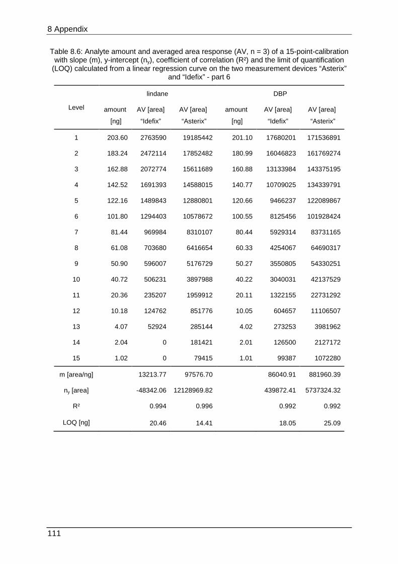
8 Appendix
111
Table 8.6: Analyte amount and averaged area response (AV, n = 3) of a 15-point-calibration with slope (m), y-intercept (ny), coefficient of correlation (R²) and the limit of quantification
(LOQ) calculated from a linear regression curve on the two measurement devices “Asterix” and “Idefix” - part 6
Level
lindane DBP
amount
[ng]
AV [area]
“Idefix”
AV [area]
“Asterix”
amount
[ng]
AV [area]
“Idefix”
AV [area]
“Asterix”
1 203.60 2763590 19185442 201.10 17680201 171536891
2 183.24 2472114 17852482 180.99 16046823 161769274
3 162.88 2072774 15611689 160.88 13133984 143375195
4 142.52 1691393 14588015 140.77 10709025 134339791
5 122.16 1489843 12880801 120.66 9466237 122089867
6 101.80 1294403 10578672 100.55 8125456 101928424
7 81.44 969984 8310107 80.44 5929314 83731165
8 61.08 703680 6416654 60.33 4254067 64690317
9 50.90 596007 5176729 50.27 3550805 54330251
10 40.72 506231 3897988 40.22 3040031 42137529
11 20.36 235207 1959912 20.11 1322155 22731292
12 10.18 124762 851776 10.05 604657 11106507
13 4.07 52924 285144 4.02 273253 3981962
14 2.04 0 181421 2.01 126500 2127172
15 1.02 0 79415 1.01 99387 1072280
m [area/ng] 13213.77 97576.70 86040.91 881960.39
ny [area] -48342.06 12128969.82 439872.41 5737324.32
R² 0.994 0.996 0.992 0.992
LOQ [ng] 20.46 14.41 18.05 25.09
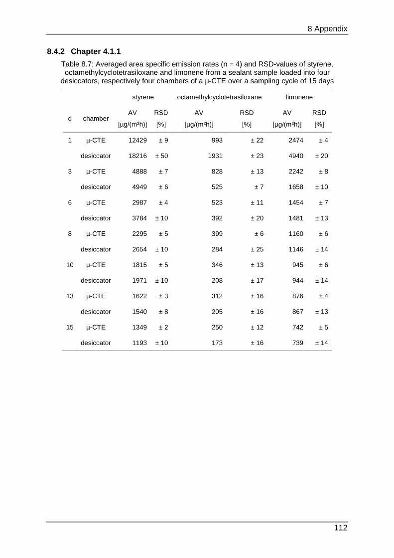
8 Appendix
112
8.4.2 Chapter 4.1.1
Table 8.7: Averaged area specific emission rates (n = 4) and RSD-values of styrene, octamethylcyclotetrasiloxane and limonene from a sealant sample loaded into four
desiccators, respectively four chambers of a µ-CTE over a sampling cycle of 15 days
styrene octamethylcyclotetrasiloxane limonene
d chamber AV
[µg/(m²h)]
RSD
[%]
AV
[µg/(m²h)]
RSD
[%]
AV
[µg/(m²h)]
RSD
[%]
1 µ-CTE 12429 ± 9 993 ± 22 2474 ± 4
desiccator 18216 ± 50 1931 ± 23 4940 ± 20
3 µ-CTE 4888 ± 7 828 ± 13 2242 ± 8
desiccator 4949 ± 6 525 ± 7 1658 ± 10
6 µ-CTE 2987 ± 4 523 ± 11 1454 ± 7
desiccator 3784 ± 10 392 ± 20 1481 ± 13
8 µ-CTE 2295 ± 5 399 ± 6 1160 ± 6
desiccator 2654 ± 10 284 ± 25 1146 ± 14
10 µ-CTE 1815 ± 5 346 ± 13 945 ± 6
desiccator 1971 ± 10 208 ± 17 944 ± 14
13 µ-CTE 1622 ± 3 312 ± 16 876 ± 4
desiccator 1540 ± 8 205 ± 16 867 ± 13
15 µ-CTE 1349 ± 2 250 ± 12 742 ± 5
desiccator 1193 ± 10 173 ± 16 739 ± 14
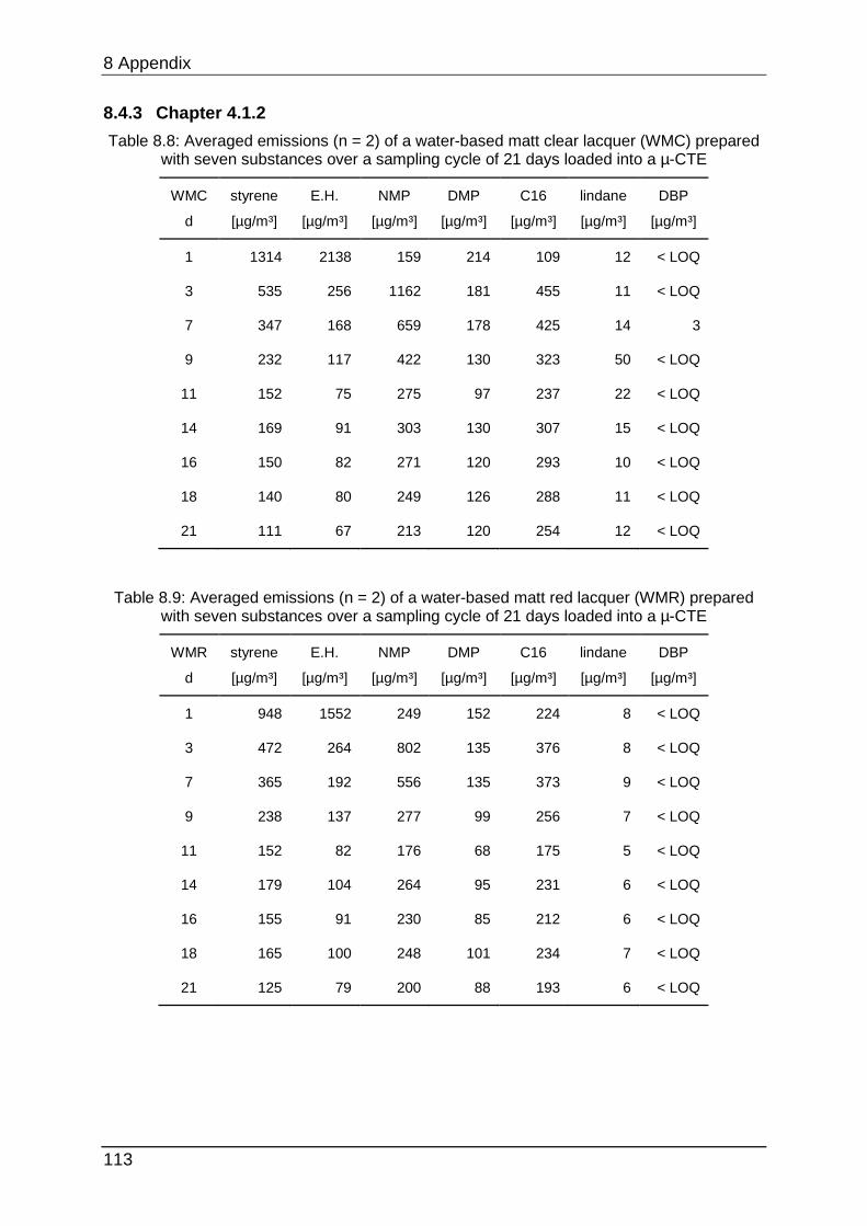
8 Appendix
113
8.4.3 Chapter 4.1.2
Table 8.8: Averaged emissions (n = 2) of a water-based matt clear lacquer (WMC) prepared with seven substances over a sampling cycle of 21 days loaded into a µ-CTE
WMC
d
styrene
[µg/m³]
E.H.
[µg/m³]
NMP
[µg/m³]
DMP
[µg/m³]
C16
[µg/m³]
lindane
[µg/m³]
DBP
[µg/m³]
1 1314 2138 159 214 109 12 < LOQ
3 535 256 1162 181 455 11 < LOQ
7 347 168 659 178 425 14 3
9 232 117 422 130 323 50 < LOQ
11 152 75 275 97 237 22 < LOQ
14 169 91 303 130 307 15 < LOQ
16 150 82 271 120 293 10 < LOQ
18 140 80 249 126 288 11 < LOQ
21 111 67 213 120 254 12 < LOQ
Table 8.9: Averaged emissions (n = 2) of a water-based matt red lacquer (WMR) prepared with seven substances over a sampling cycle of 21 days loaded into a µ-CTE
WMR
d
styrene
[µg/m³]
E.H.
[µg/m³]
NMP
[µg/m³]
DMP
[µg/m³]
C16
[µg/m³]
lindane
[µg/m³]
DBP
[µg/m³]
1 948 1552 249 152 224 8 < LOQ
3 472 264 802 135 376 8 < LOQ
7 365 192 556 135 373 9 < LOQ
9 238 137 277 99 256 7 < LOQ
11 152 82 176 68 175 5 < LOQ
14 179 104 264 95 231 6 < LOQ
16 155 91 230 85 212 6 < LOQ
18 165 100 248 101 234 7 < LOQ
21 125 79 200 88 193 6 < LOQ
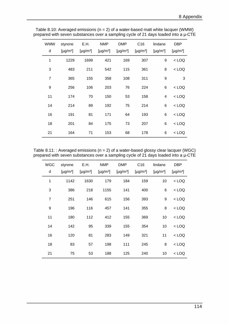
8 Appendix
114
Table 8.10: Averaged emissions (n = 2) of a water-based matt white lacquer (WMW) prepared with seven substances over a sampling cycle of 21 days loaded into a µ-CTE
WMW
d
styrene
[µg/m³]
E.H.
[µg/m³]
NMP
[µg/m³]
DMP
[µg/m³]
C16
[µg/m³]
lindane
[µg/m³]
DBP
[µg/m³]
1 1229 1699 421 169 307 9 < LOQ
3 483 211 542 115 361 8 < LOQ
7 365 155 358 108 311 9 3
9 256 106 203 76 224 6 < LOQ
11 174 70 150 53 158 4 < LOQ
14 214 89 192 75 214 6 < LOQ
16 191 81 171 64 193 6 < LOQ
18 201 84 175 73 207 6 < LOQ
21 164 71 153 68 178 6 < LOQ
Table 8.11: : Averaged emissions (n = 2) of a water-based glossy clear lacquer (WGC) prepared with seven substances over a sampling cycle of 21 days loaded into a µ-CTE
WGC
d
styrene
[µg/m³]
E.H.
[µg/m³]
NMP
[µg/m³]
DMP
[µg/m³]
C16
[µg/m³]
lindane
[µg/m³]
DBP
[µg/m³]
1 1142 1630 179 184 159 10 < LOQ
3 386 218 1155 141 400 6 < LOQ
7 251 146 615 156 393 9 < LOQ
9 196 116 457 141 355 8 < LOQ
11 180 112 412 155 369 10 < LOQ
14 142 95 339 155 354 10 < LOQ
16 120 81 283 149 321 11 < LOQ
18 83 57 198 111 245 8 < LOQ
21 75 53 188 125 240 10 < LOQ
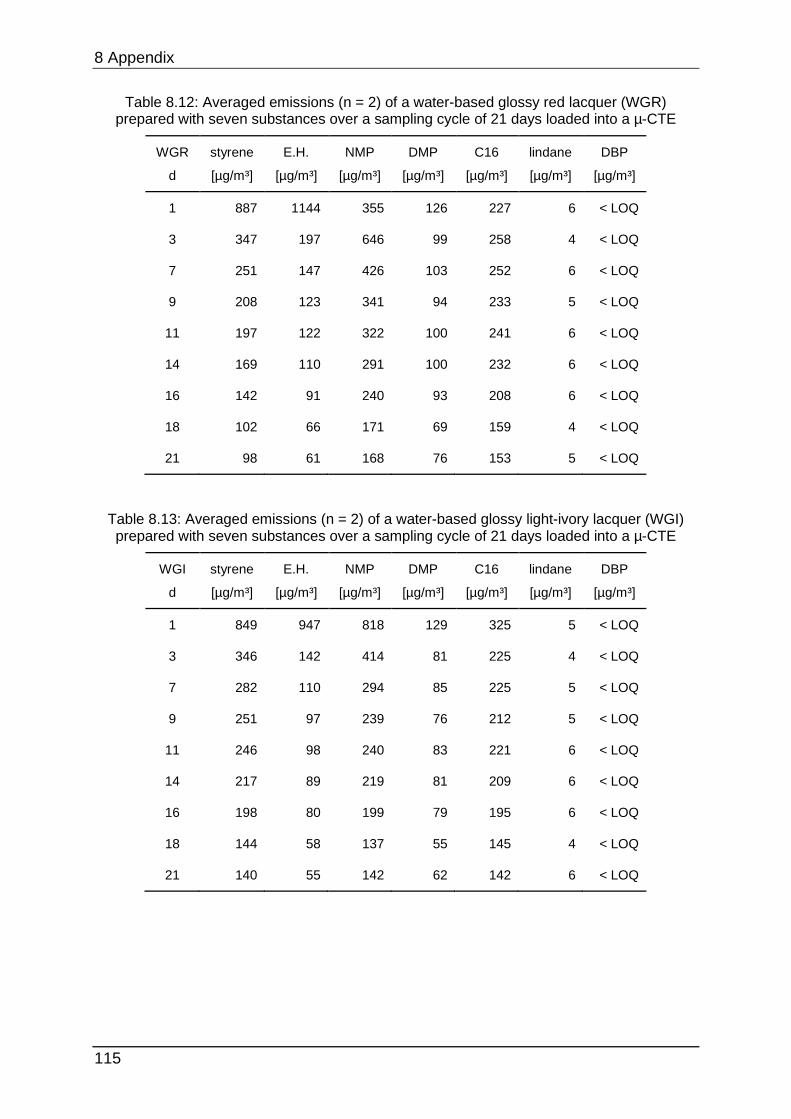
8 Appendix
115
Table 8.12: Averaged emissions (n = 2) of a water-based glossy red lacquer (WGR) prepared with seven substances over a sampling cycle of 21 days loaded into a µ-CTE
WGR
d
styrene
[µg/m³]
E.H.
[µg/m³]
NMP
[µg/m³]
DMP
[µg/m³]
C16
[µg/m³]
lindane
[µg/m³]
DBP
[µg/m³]
1 887 1144 355 126 227 6 < LOQ
3 347 197 646 99 258 4 < LOQ
7 251 147 426 103 252 6 < LOQ
9 208 123 341 94 233 5 < LOQ
11 197 122 322 100 241 6 < LOQ
14 169 110 291 100 232 6 < LOQ
16 142 91 240 93 208 6 < LOQ
18 102 66 171 69 159 4 < LOQ
21 98 61 168 76 153 5 < LOQ
Table 8.13: Averaged emissions (n = 2) of a water-based glossy light-ivory lacquer (WGI) prepared with seven substances over a sampling cycle of 21 days loaded into a µ-CTE
WGI
d
styrene
[µg/m³]
E.H.
[µg/m³]
NMP
[µg/m³]
DMP
[µg/m³]
C16
[µg/m³]
lindane
[µg/m³]
DBP
[µg/m³]
1 849 947 818 129 325 5 < LOQ
3 346 142 414 81 225 4 < LOQ
7 282 110 294 85 225 5 < LOQ
9 251 97 239 76 212 5 < LOQ
11 246 98 240 83 221 6 < LOQ
14 217 89 219 81 209 6 < LOQ
16 198 80 199 79 195 6 < LOQ
18 144 58 137 55 145 4 < LOQ
21 140 55 142 62 142 6 < LOQ
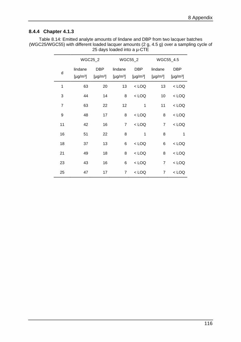
8 Appendix
116
8.4.4 Chapter 4.1.3
Table 8.14: Emitted analyte amounts of lindane and DBP from two lacquer batches (WGC25/WGC55) with different loaded lacquer amounts (2 g, 4.5 g) over a sampling cycle of
25 days loaded into a µ-CTE
WGC25_2 WGC55_2 WGC55_4.5
d lindane
[µg/m³]
DBP
[µg/m³]
lindane
[µg/m³]
DBP
[µg/m³]
lindane
[µg/m³]
DBP
[µg/m³]
1 63 20 13 < LOQ 13 < LOQ
3 44 14 8 < LOQ 10 < LOQ
7 63 22 12 1 11 < LOQ
9 48 17 8 < LOQ 8 < LOQ
11 42 16 7 < LOQ 7 < LOQ
16 51 22 8 1 8 1
18 37 13 6 < LOQ 6 < LOQ
21 49 18 8 < LOQ 8 < LOQ
23 43 16 6 < LOQ 7 < LOQ
25 47 17 7 < LOQ 7 < LOQ
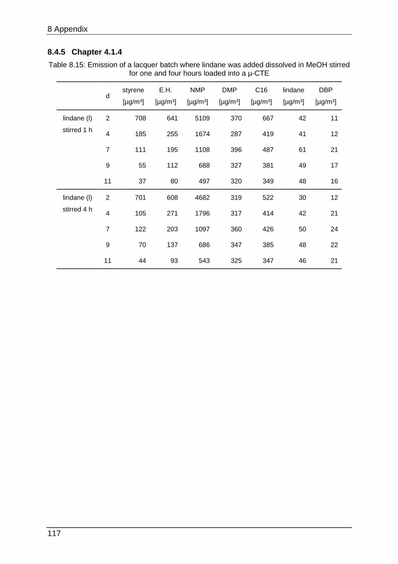
8 Appendix
117
8.4.5 Chapter 4.1.4
Table 8.15: Emission of a lacquer batch where lindane was added dissolved in MeOH stirred for one and four hours loaded into a µ-CTE
d
styrene
[µg/m³]
E.H.
[µg/m³]
NMP
[µg/m³]
DMP
[µg/m³]
C16
[µg/m³]
lindane
[µg/m³]
DBP
[µg/m³]
lindane (l)
stirred 1 h
2 708 641 5109 370 667 42 11
4 185 255 1674 287 419 41 12
7 111 195 1108 396 487 61 21
9 55 112 688 327 381 49 17
11 37 80 497 320 349 48 16
lindane (l)
stirred 4 h
2 701 608 4682 319 522 30 12
4 105 271 1796 317 414 42 21
7 122 203 1097 360 426 50 24
9 70 137 686 347 385 48 22
11 44 93 543 325 347 46 21
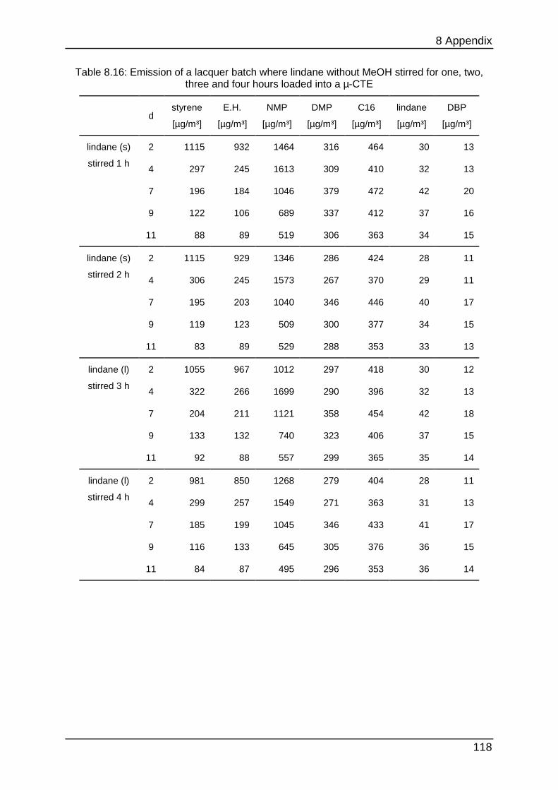
8 Appendix
118
Table 8.16: Emission of a lacquer batch where lindane without MeOH stirred for one, two, three and four hours loaded into a µ-CTE
d
styrene
[µg/m³]
E.H.
[µg/m³]
NMP
[µg/m³]
DMP
[µg/m³]
C16
[µg/m³]
lindane
[µg/m³]
DBP
[µg/m³]
lindane (s)
stirred 1 h
2 1115 932 1464 316 464 30 13
4 297 245 1613 309 410 32 13
7 196 184 1046 379 472 42 20
9 122 106 689 337 412 37 16
11 88 89 519 306 363 34 15
lindane (s)
stirred 2 h
2 1115 929 1346 286 424 28 11
4 306 245 1573 267 370 29 11
7 195 203 1040 346 446 40 17
9 119 123 509 300 377 34 15
11 83 89 529 288 353 33 13
lindane (l)
stirred 3 h
2 1055 967 1012 297 418 30 12
4 322 266 1699 290 396 32 13
7 204 211 1121 358 454 42 18
9 133 132 740 323 406 37 15
11 92 88 557 299 365 35 14
lindane (l)
stirred 4 h
2 981 850 1268 279 404 28 11
4 299 257 1549 271 363 31 13
7 185 199 1045 346 433 41 17
9 116 133 645 305 376 36 15
11 84 87 495 296 353 36 14
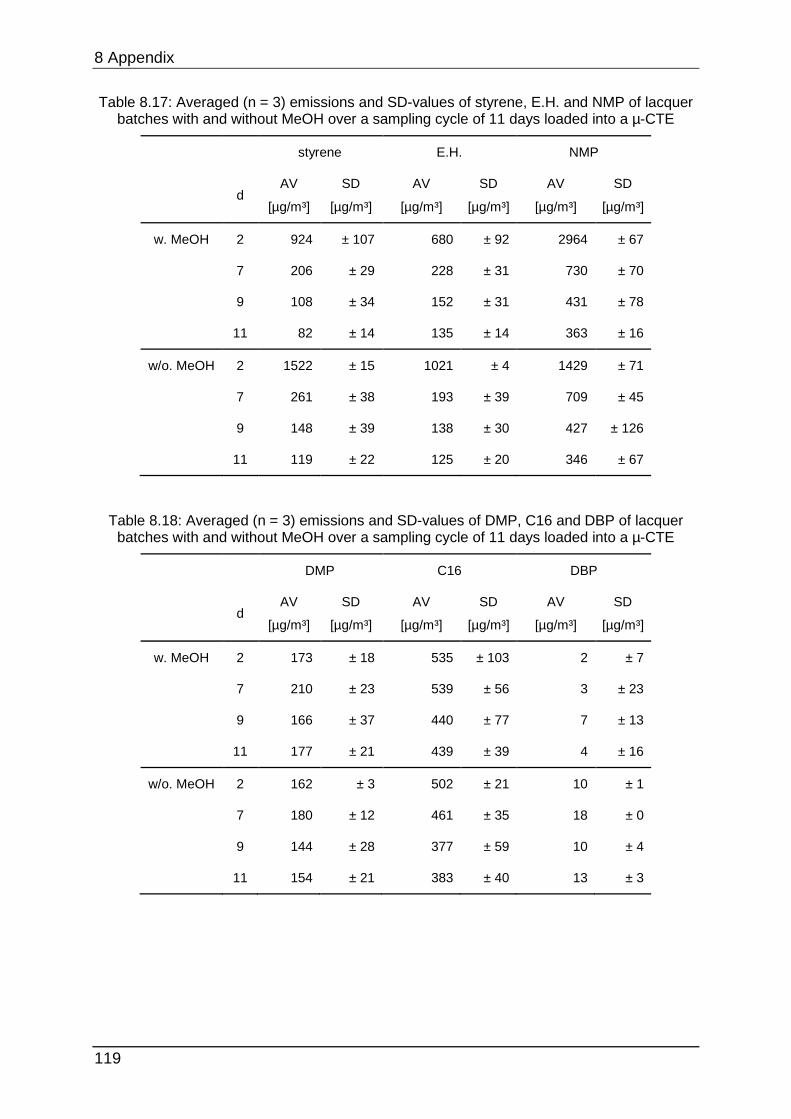
8 Appendix
119
Table 8.17: Averaged (n = 3) emissions and SD-values of styrene, E.H. and NMP of lacquer batches with and without MeOH over a sampling cycle of 11 days loaded into a µ-CTE
styrene E.H. NMP
d AV
[µg/m³]
SD
[µg/m³]
AV
[µg/m³]
SD
[µg/m³]
AV
[µg/m³]
SD
[µg/m³]
w. MeOH 2 924 ± 107 680 ± 92 2964 ± 67
7 206 ± 29 228 ± 31 730 ± 70
9 108 ± 34 152 ± 31 431 ± 78
11 82 ± 14 135 ± 14 363 ± 16
w/o. MeOH 2 1522 ± 15 1021 ± 4 1429 ± 71
7 261 ± 38 193 ± 39 709 ± 45
9 148 ± 39 138 ± 30 427 ± 126
11 119 ± 22 125 ± 20 346 ± 67
Table 8.18: Averaged (n = 3) emissions and SD-values of DMP, C16 and DBP of lacquer batches with and without MeOH over a sampling cycle of 11 days loaded into a µ-CTE
DMP C16 DBP
d AV
[µg/m³]
SD
[µg/m³]
AV
[µg/m³]
SD
[µg/m³]
AV
[µg/m³]
SD
[µg/m³]
w. MeOH 2 173 ± 18 535 ± 103 2 ± 7
7 210 ± 23 539 ± 56 3 ± 23
9 166 ± 37 440 ± 77 7 ± 13
11 177 ± 21 439 ± 39 4 ± 16
w/o. MeOH 2 162 ± 3 502 ± 21 10 ± 1
7 180 ± 12 461 ± 35 18 ± 0
9 144 ± 28 377 ± 59 10 ± 4
11 154 ± 21 383 ± 40 13 ± 3
8 Appendix
120
8.4.6 Chapter 5.2.1
Table 8.19: Averaged emissions (n = 6) and RSD-values of a lacquer batch loaded into µ-CTEs over a sampling cycle of 14 days that cured either directly inside the µ-CTE or for 44 h
inside a 1-m³-chamber - part 1
styrene E.H. NMP DMP
cure/
load d
AV
[µg/(m²h)]
RSD
[%]
AV
[µg/(m²h)]
RSD
[%]
AV
[µg/(m²h)]
RSD
[%]
AV
[µg/(m²h)]
RSD
[%]
µ-CTE
/
µ-CTE
2 1529 ± 11 2184 ± 8 616 ± 37 634 ± 10
4 509 ± 3 1291 ± 2 2625 ± 4 520 ± 7
7 134 ± 7 813 ± 2 1584 ± 4 504 ± 8
11 27 ± 14 501 ± 8 1003 ± 4 522 ± 7
14 7 ± 25 297 ± 4 657 ± 5 480 ± 8
1 m³
/
µ-CTE
2 1090 ± 5 1594 ± 7 2578 ± 6 427 ± 9
4 662 ± 5 1287 ± 2 1854 ± 4 468 ± 5
7 253 ± 4 845 ± 2 1205 ± 3 469 ± 4
11 68 ± 5 591 ± 3 845 ± 5 534 ± 5
14 18 ± 9 362 ± 4 546 ± 5 449 ± 5
8 Appendix
121
Table 8.20: Averaged emissions (n = 6) and RSD-values of a lacquer batch loaded into µ-CTEs over a sampling cycle of 14 days that cured either directly inside the µ-CTE or for 44 h
inside a 1-m³-chamber - part 2
C16 lindane DBP
d AV
[µg/(m²h)]
RSD
[%]
AV
[µg/(m²h)]
RSD
[%]
AV
[µg/(m²h)]
RSD
[%]
cure/load µ-CTE
2 1327 ± 33 128 ± 12 79 ± 22
7 771 ± 6 99 ± 8 59 ± 22
9 702 ± 7 89 ± 9 57 ± 17
11 653 ± 6 88 ± 8 68 ± 17
14 470 ± 34 77 ± 8 58 ± 14
cure 1 m³/
load µ-CTE
2 593 ± 29 39 ± 39 < LOQ -
7 628 ± 5 77 ± 5 36 ± 33
9 483 ± 35 79 ± 9 47 ± 13
11 614 ± 4 92 ± 8 87 ± 19
14 243 ± 3 71 ± 9 58 ± 14
8 Appendix
122
8.4.7 Chapter 5.2.2
Table 8.21: Averaged emissions (n = 4) and RSD-values of lacquer batches loaded into desiccators over a sampling cycle of 17 days that cured either directly inside the desiccator
or for 46 h inside a 1-m³-chamber with switched on/off fan inside the testing chamber - part 1
styrene E.H. NMP DMP
cure/
load d
AV
[µg/(m²h)]
RSD
[%]
AV
[µg/(m²h)]
RSD
[%]
AV
[µg/(m²h)]
RSD
[%]
AV
[µg/(m²h)]
RSD
[%]
24 l
/
24 l
3 4133 ± 6 1157 ± 15 5997 ± 6 2913 ± 12
5 3230 ± 6 1985 ± 23 3572 ± 3 2598 ± 12
7 2473 ± 1 1608 ± 24 2697 ± 5 2331 ± 7
10 1658 ± 3 1223 ± 23 1912 ± 7 2041 ± 8
12 1282 ± 6 1085 ± 22 1594 ± 11 1892 ± 6
14 999 ± 5 1041 ± 25 1379 ± 9 1770 ± 7
17 704 ± 7 866 ± 19 1133 ± 12 1634 ± 5
1 m³
/
24 l
3 6198 ± 35 2789 ± 60 19129 ± 46 3714 ± 45
5 3235 ± 19 1024 ± 29 5468 ± 20 2992 ± 25
7 2367 ± 2 1536 ± 20 3315 ± 4 2516 ± 8
10 1538 ± 2 1039 ± 20 2239 ± 2 2164 ± 8
12 1228 ± 2 934 ± 17 1968 ± 3 2059 ± 6
14 874 ± 5 729 ± 23 1547 ± 3 1829 ± 8
17 610 ± 2 650 ± 19 1264 ± 1 1705 ± 7
1 m³
/
24 l
no fan
3 4321 ± 4 4113 ± 22 1647 ± 48 610 ± 45
5 2942 ± 4 2229 ± 18 5511 ± 6 978 ± 21
7 2133 ± 2 1406 ± 16 3517 ± 4 877 ± 23
10 1526 ± 3 1147 ± 15 2740 ± 3 822 ± 22
12 1098 ± 4 939 ± 17 2210 ± 4 776 ± 20
14 899 ± 10 918 ± 26 2013 ± 14 819 ± 28
17 445 ± 10 709 ± 22 1443 ± 16 786 ± 29
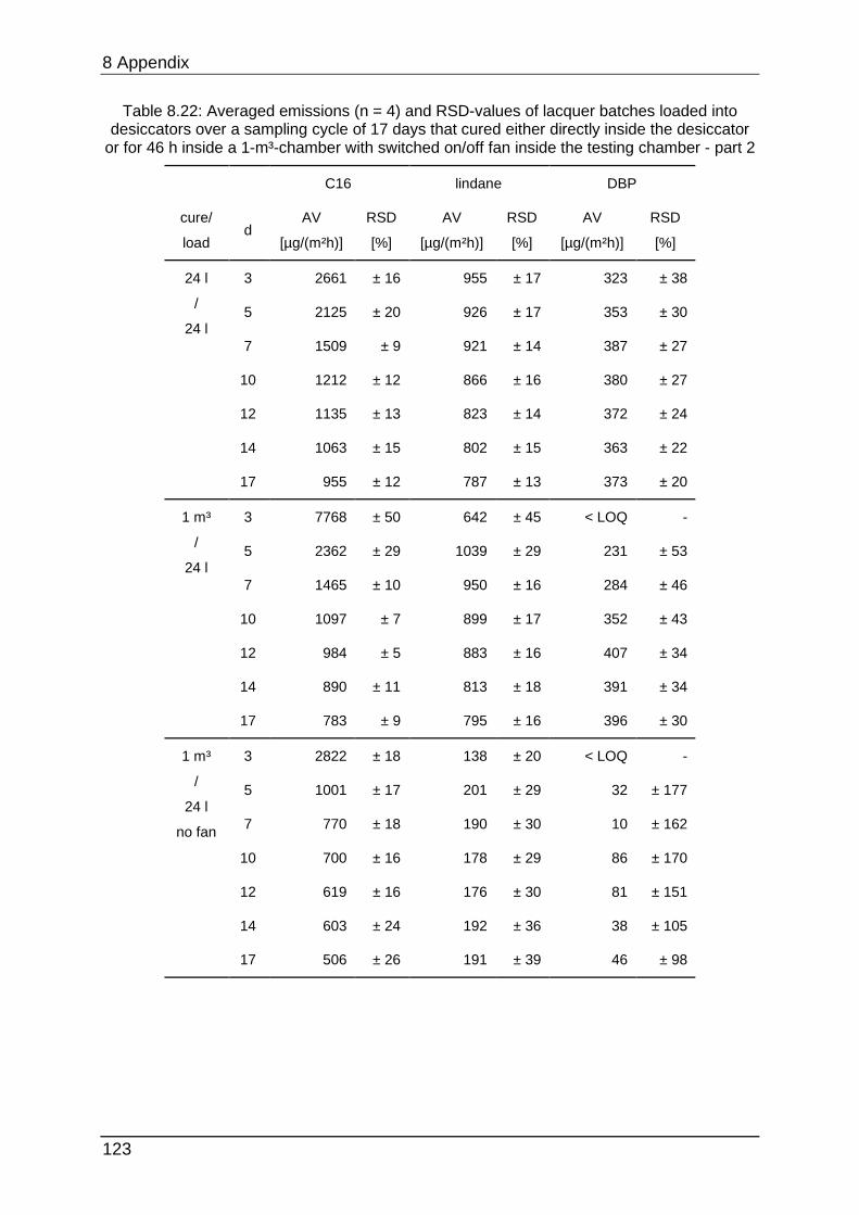
8 Appendix
123
Table 8.22: Averaged emissions (n = 4) and RSD-values of lacquer batches loaded into desiccators over a sampling cycle of 17 days that cured either directly inside the desiccator
or for 46 h inside a 1-m³-chamber with switched on/off fan inside the testing chamber - part 2
C16 lindane DBP
cure/
load d
AV
[µg/(m²h)]
RSD
[%]
AV
[µg/(m²h)]
RSD
[%]
AV
[µg/(m²h)]
RSD
[%]
24 l
/
24 l
3 2661 ± 16 955 ± 17 323 ± 38
5 2125 ± 20 926 ± 17 353 ± 30
7 1509 ± 9 921 ± 14 387 ± 27
10 1212 ± 12 866 ± 16 380 ± 27
12 1135 ± 13 823 ± 14 372 ± 24
14 1063 ± 15 802 ± 15 363 ± 22
17 955 ± 12 787 ± 13 373 ± 20
1 m³
/
24 l
3 7768 ± 50 642 ± 45 < LOQ -
5 2362 ± 29 1039 ± 29 231 ± 53
7 1465 ± 10 950 ± 16 284 ± 46
10 1097 ± 7 899 ± 17 352 ± 43
12 984 ± 5 883 ± 16 407 ± 34
14 890 ± 11 813 ± 18 391 ± 34
17 783 ± 9 795 ± 16 396 ± 30
1 m³
/
24 l
no fan
3 2822 ± 18 138 ± 20 < LOQ -
5 1001 ± 17 201 ± 29 32 ± 177
7 770 ± 18 190 ± 30 10 ± 162
10 700 ± 16 178 ± 29 86 ± 170
12 619 ± 16 176 ± 30 81 ± 151
14 603 ± 24 192 ± 36 38 ± 105
17 506 ± 26 191 ± 39 46 ± 98
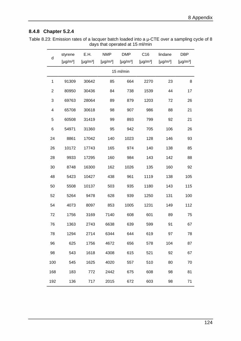
8 Appendix
124
8.4.8 Chapter 5.2.4
Table 8.23: Emission rates of a lacquer batch loaded into a µ-CTE over a sampling cycle of 8 days that operated at 15 ml/min
d styrene
[µg/m³]
E.H.
[µg/m³]
NMP
[µg/m³]
DMP
[µg/m³]
C16
[µg/m³]
lindane
[µg/m³]
DBP
[µg/m³]
15 ml/min
1 91309 30642 85 664 2270 23 8
2 80950 30436 84 738 1539 44 17
3 69763 28064 89 879 1203 72 26
4 65708 30618 98 907 986 88 21
5 60508 31419 99 893 799 92 21
6 54971 31360 95 942 705 106 26
24 8861 17042 140 1023 128 146 93
26 10172 17743 165 974 140 138 85
28 9933 17295 160 984 143 142 88
30 8748 16300 162 1026 135 160 92
48 5423 10427 438 961 1119 138 105
50 5508 10137 503 935 1180 143 115
52 5264 9478 628 939 1250 131 100
54 4073 8097 853 1005 1231 149 112
72 1756 3169 7140 608 601 89 75
76 1363 2743 6638 639 599 91 67
78 1294 2714 6344 644 619 97 78
96 625 1756 4672 656 578 104 87
98 543 1618 4308 615 521 92 67
100 545 1625 4020 557 510 80 70
168 183 772 2442 675 608 98 81
192 136 717 2015 672 603 98 71
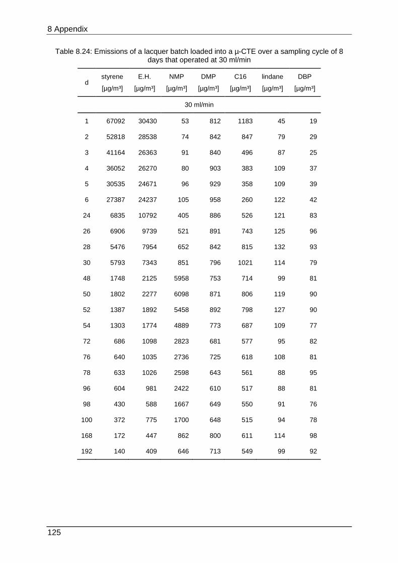
8 Appendix
125
Table 8.24: Emissions of a lacquer batch loaded into a µ-CTE over a sampling cycle of 8 days that operated at 30 ml/min
d styrene
[µg/m³]
E.H.
[µg/m³]
NMP
[µg/m³]
DMP
[µg/m³]
C16
[µg/m³]
lindane
[µg/m³]
DBP
[µg/m³]
30 ml/min
1 67092 30430 53 812 1183 45 19
2 52818 28538 74 842 847 79 29
3 41164 26363 91 840 496 87 25
4 36052 26270 80 903 383 109 37
5 30535 24671 96 929 358 109 39
6 27387 24237 105 958 260 122 42
24 6835 10792 405 886 526 121 83
26 6906 9739 521 891 743 125 96
28 5476 7954 652 842 815 132 93
30 5793 7343 851 796 1021 114 79
48 1748 2125 5958 753 714 99 81
50 1802 2277 6098 871 806 119 90
52 1387 1892 5458 892 798 127 90
54 1303 1774 4889 773 687 109 77
72 686 1098 2823 681 577 95 82
76 640 1035 2736 725 618 108 81
78 633 1026 2598 643 561 88 95
96 604 981 2422 610 517 88 81
98 430 588 1667 649 550 91 76
100 372 775 1700 648 515 94 78
168 172 447 862 800 611 114 98
192 140 409 646 713 549 99 92
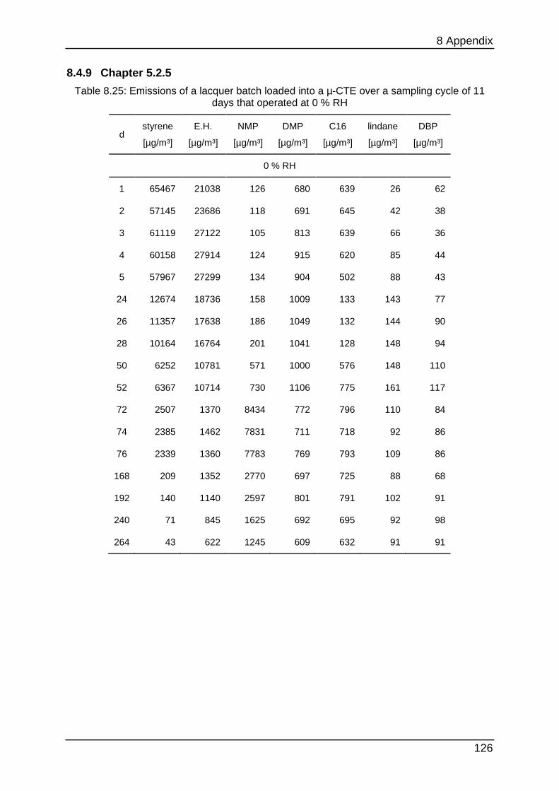
8 Appendix
126
8.4.9 Chapter 5.2.5
Table 8.25: Emissions of a lacquer batch loaded into a µ-CTE over a sampling cycle of 11 days that operated at 0 % RH
d styrene
[µg/m³]
E.H.
[µg/m³]
NMP
[µg/m³]
DMP
[µg/m³]
C16
[µg/m³]
lindane
[µg/m³]
DBP
[µg/m³]
0 % RH
1 65467 21038 126 680 639 26 62
2 57145 23686 118 691 645 42 38
3 61119 27122 105 813 639 66 36
4 60158 27914 124 915 620 85 44
5 57967 27299 134 904 502 88 43
24 12674 18736 158 1009 133 143 77
26 11357 17638 186 1049 132 144 90
28 10164 16764 201 1041 128 148 94
50 6252 10781 571 1000 576 148 110
52 6367 10714 730 1106 775 161 117
72 2507 1370 8434 772 796 110 84
74 2385 1462 7831 711 718 92 86
76 2339 1360 7783 769 793 109 86
168 209 1352 2770 697 725 88 68
192 140 1140 2597 801 791 102 91
240 71 845 1625 692 695 92 98
264 43 622 1245 609 632 91 91
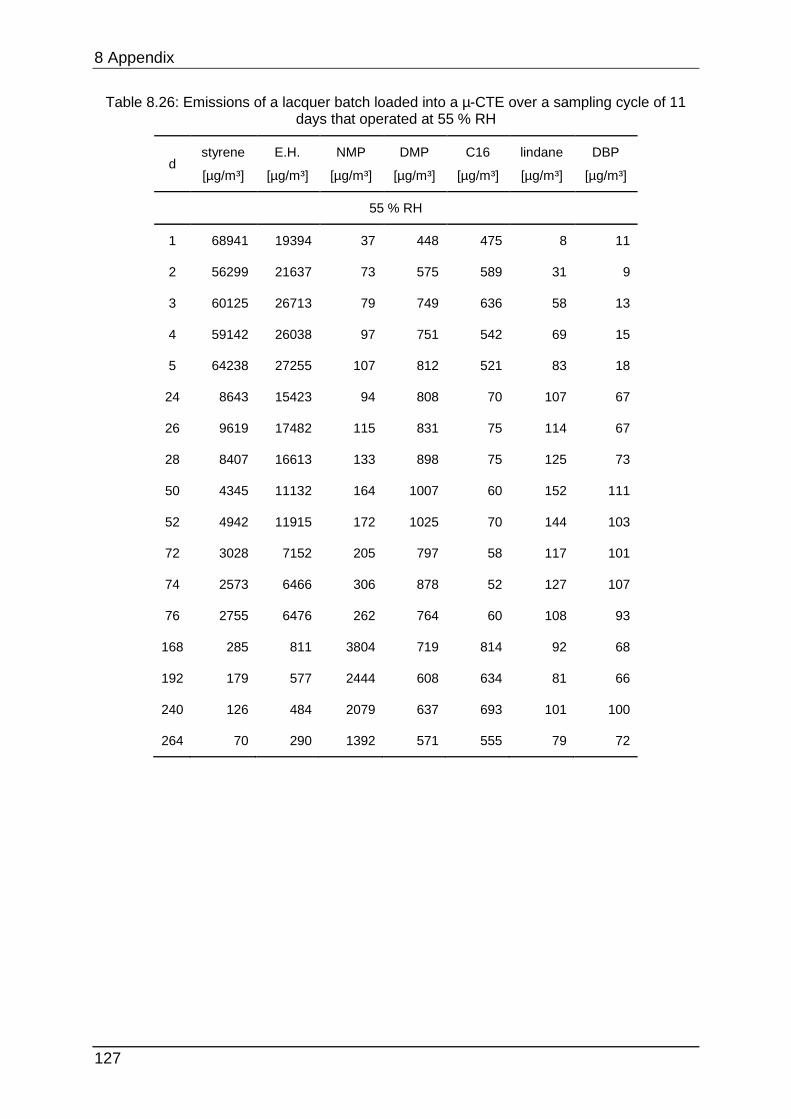
8 Appendix
127
Table 8.26: Emissions of a lacquer batch loaded into a µ-CTE over a sampling cycle of 11 days that operated at 55 % RH
d styrene
[µg/m³]
E.H.
[µg/m³]
NMP
[µg/m³]
DMP
[µg/m³]
C16
[µg/m³]
lindane
[µg/m³]
DBP
[µg/m³]
55 % RH
1 68941 19394 37 448 475 8 11
2 56299 21637 73 575 589 31 9
3 60125 26713 79 749 636 58 13
4 59142 26038 97 751 542 69 15
5 64238 27255 107 812 521 83 18
24 8643 15423 94 808 70 107 67
26 9619 17482 115 831 75 114 67
28 8407 16613 133 898 75 125 73
50 4345 11132 164 1007 60 152 111
52 4942 11915 172 1025 70 144 103
72 3028 7152 205 797 58 117 101
74 2573 6466 306 878 52 127 107
76 2755 6476 262 764 60 108 93
168 285 811 3804 719 814 92 68
192 179 577 2444 608 634 81 66
240 126 484 2079 637 693 101 100
264 70 290 1392 571 555 79 72
8 Appendix
128
9 Eidesstattliche Erklärung Ich erkläre hiermit an Eides statt, dass ich die vorliegende Arbeit selbständig und nur
unter Verwendung der angegebenen Quellen und Hilfsmittel angefertigt habe.
Die den Quellen wörtlich oder inhaltlich entnommenen Stellen sind als solche
kenntlich gemacht.
Berlin, den 21.1.2015 Michael Nohr
10 Lebenslauf
129
10 Lebenslauf
Persönliche Daten:
Name, Vorname: Nohr, Michael
Anschrift: Kleiststraße 71
38440 Wolfsburg
Geburtsdatum/-ort: 03.06.1984, Schkeuditz
Familienstand: ledig
Schulbildung:
12/1997 – 07/2003 Wiprecht Gymnasium Groitzsch,
Abschluss: Allgemeine Hochschulreife (Note: 2,4)
09/1995 – 11/1997 Evangelisches Schulzentrum Leipzig (Gymnasium)
Zivildienst:
08/2003 – 05/2004 Zivildienstleistender im Umweltschutz der Stadt Groitzsch (Bauhof)
Studium:
10/2004 – 02/2005
Studium der Chemie (Bachelor of Science, B.Sc), Universität Leipzig
09/2005 – 12/2009
Hochschule Zittau/Görlitz (FH)
Studiengang Chemie
Vertiefungsrichtung: Bioorganische Chemie
Abschluss: Dipl.-Chem. (FH) (Gesamtnote 1,0)
Vordiplom
16.07.2007
Vordiplomsprüfung im Studiengang Chemie
(Note: 1,7)
Praxissemester
09/2007 – 03/2008
„Der Einsatz der Festphasenmikroextraktion (SPME) in der Gaschromatographie zur Bestimmung ausgewählter organischer Spurenstoffe in Wasserproben“
Team Umweltanalytik GmbH, Ebersbach (Sa.)
Fachbetreuer:
Prof. Dr. Manfred Gey (HS Zittau/Görlitz (FH))
Dipl.-Ing. Ramona Bothmer (Team Umweltanalytik, Ebersbach)
(Note: 1,3)
10 Lebenslauf
130
Diplomarbeit
04/2009 – 12/2009
„Untersuchungen zum Abbauverhalten von Carbamazepin, Triclosan, N-Butylbenzolsulfonamid und Diclofenac unter Einsatz von drei verschiedenen Abwasserbehandlungsverfahren“,
Helmholtz Zentrum für Umweltforschung - UFZ, Leipzig
Fachbetreuer:
Prof. Dr. Annett Fuchs (HS Zittau/Görlitz (FH))
Dr. Monika Möder (UFZ Leipzig)
(Note: 1,3)
Beruflicher Werdegang:
01/2010 – 04/2010 Helmholtz-Zentrum für Umweltforschung – UFZ, Leipzig
Technischer Angestellter
seit 04/2010 Bundesanstalt für Materialforschung und –prüfung BAM, Berlin
Technischer Angestellter
Berlin, den 21.01.2015 Michael Nohr