
Diplomarbeit Christian Dolenz 0002982 IBW F - core.ac.uk motivation for choosing this actual...
141
DIPLOMARBEIT Titel der Diplomarbeit „Monetary Policy And Its Impact On The Linkage Between Short-Term And Long-Term Interest Rates“ - An Empirical Study - Verfasser Christian Dolenz Angestrebter akademischer Grad Magister der Sozial- und Wirtschaftswissenschaften (Mag. rer. soc. oec.) Wien, im April 2010 Studienkennzahl lt. Studienblatt: 157 Studienrichtung lt. Studienblatt: Internationale Betriebswirtschaft Betreuer/Betreuerin: Univ.-Prof. Dr. Erich W. Streissler
-
Upload
truongcong -
Category
Documents
-
view
220 -
download
0
Transcript of Diplomarbeit Christian Dolenz 0002982 IBW F - core.ac.uk motivation for choosing this actual...
DIPLOMARBEIT
Titel der Diplomarbeit
„Monetary Policy And Its Impact On The Linkage Between Short-Term And Long-Term Interest Rates“
- An Empirical Study -
Verfasser
Christian Dolenz
Angestrebter akademischer Grad
Magister der Sozial- und Wirtschaftswissenschaften (Mag. rer. soc. oec.)
Wien, im April 2010 Studienkennzahl lt. Studienblatt: 157 Studienrichtung lt. Studienblatt: Internationale Betriebswirtschaft Betreuer/Betreuerin: Univ.-Prof. Dr. Erich W. Streissler

Abstract
The basic aim of this work is to give a review of monetary policy and also to
distinguish between short-term and long-term interest rates. Monetary policy represents
the entirety of all instruments used by policy-makers following specific monetary goals.
In general, policy-makers are represented by central banks which have the power to
influence a nation’s economy. In this paper, different ways of targeting are discussed
and illustrated by dint of an empirical study which covers the last three decades and the
geographical areas of the United Stated of America, the United Kingdom and the Euro
Area. The short-term interest rate is the most basic and important factor in this work. It
is directly influenced by the monetary policy of any given central bank. Usually, these
policies are employed in order to react to certain events. Hence, a data analysis of the
different trends in certain areas shows specific goals. As far as the theoretical
framework of this thesis is concerned, I will combine the results of short-term interest
rates with long-term interest rate data, and round off this, in my opinion, precise survey,
with diagrams, which are meant to exemplify the linkage between short-term and long-
term interest rates.
Additionally, I would like to stress the fact that all the tables and figures used in
this thesis were developed and analyzed by myself. However, the different internet-
databases described in Appendix A and in the Bibliography provided the background
and the necessary tools for the data-acquisition for this work.


Acknowledgment
In the course of this work’s preparation I especially have to thank Prof. Dr. Erich
W. Streissler for inspiring in me the huge interest in this specific financial topic which
has its origin in the banking, financial and macroeconomics sector. “His course Money
and Banking opened up my eyes...”
Furthermore I want to thank my family, my parents and my brother outstanding,
for sustaining my tics during the work’s long creation which was not that easy to handle
from time to time.
I also have to give a special additional acknowledgement to all my close friends
who always pushed me forward in finishing my thesis and encouraged me all along –
you know who I mean.
“Thank you so much...”
Vienna, April 2010
Christian Dolenz

- 7 -
Contents
Abstract................................................................................................................. 3
Acknowledgment .................................................................................................. 5
Contents ................................................................................................................ 7
List of Figures..................................................................................................... 11
List of Formulas.................................................................................................. 13
List of Abbreviation............................................................................................ 15
1. Introduction.................................................................................................. 19
1.1. Motivation .......................................................................................... 19
1.2. Brief Overview...................................................................................19
2. The Basic Theory of Hicks..........................................................................21
2.1. The Conception of Marginal Utility................................................... 21
2.2. Preferences regarding the Holding of Money .................................... 22
2.3. Cost of Transfer, Duration and Net Advantage.................................. 23
2.4. People’s Expectations, Uncertainty and Upcoming Risk Factors...... 24
2.5. Total Risk, the Law of Large Numbers and the Relation between
Lenders and Borrowers ...................................................................... 25
2.6. Assets, Liabilities and the Banking Theory ....................................... 27
2.7. Wealth, Money and Prices ................................................................. 28
2.8. Sensitivity, Monetary Stability and the Dilemma .............................. 30
3. The Conception of the Taylor Rule ............................................................. 33
3.1. Real and Nominal Interest Rates........................................................ 33
3.2. Financial Markets............................................................................... 35
3.2.1. Money Market – German and International Point of View........... 36

CONTENTS
- 8 -
The English Definition of Money Market .................................................. 36
The German Definition of Money Market.................................................. 37
The Modern European Definition of Money Market ................................. 38
3.2.2. Money Market in the Euro Area.................................................... 39
3.2.3. Capital Market ............................................................................... 40
3.3. The Taylor Rule ................................................................................. 41
3.3.1. The Taylor Rule – Original Version.............................................. 42
The Equation............................................................................................... 43
Understanding the Model ........................................................................... 44
Suitable Weighting-Factors ........................................................................ 45
Critical Aspects........................................................................................... 46
3.3.2. The Taylor Rule – Forward-Looking Version............................... 46
The Equation................................................................................................... 47
4. Theory of Monetary Policy..........................................................................49
4.1. The New Consensus Macroeconomics – NCM ................................. 49
4.2. Instruments and Goals........................................................................ 50
4.3. Open Market Operations .................................................................... 51
4.3.1. Open Market Operations in the Money Market............................ 51
4.3.2. The Dilemma between Capital Market versus Money Market...... 51
4.3.3. Money Market and the Short-Term View ..................................... 53
4.3.4. Refinancing-operations.................................................................. 53
4.4. Monetary Policy Targets .................................................................... 54
4.4.1. Inflation Targeting......................................................................... 54
4.4.2. The Inflation Forecast as Target.................................................... 57
4.4.3. Nominal Income Targets ............................................................... 58
CONTENTS
- 9 -
4.4.4. Targeting an Index of Monetary Conditions ................................. 59
5. The Linkage between Short-Term and Long-Term Interest Rates and the
Impact of Monetary Policy .......................................................................... 61
5.1. Brief Overview...................................................................................61
5.2. Monetary Policy and the IS-LM Model ............................................. 62
5.3. The Feasible Malfunction of Monetary Policy .................................. 63
5.4. Interest Rates and the Term Structure ................................................ 64
5.5. Summary of Key Facts....................................................................... 64
6. Empirical Study A ....................................................................................... 67
6.1. Brief Overview...................................................................................67
6.1.1. Description of Long–Term Interest Rates ..................................... 68
6.1.2. Description of Short–Term Interest Rates ..................................... 68
6.2. Monetary Policy in the USA .............................................................. 69
6.2.1. Analysis of Data from 1979 - 1993 ............................................... 70
6.2.2. Analysis of Data from 1994 - 2008 ............................................... 72
6.2.3. Summary of Data from 1979 - 2008.............................................. 74
6.3. Monetary Policy in the UK ................................................................ 75
6.3.1. Analysis of Data from 1979 - 1993 ............................................... 75
6.3.2. Analysis of Data from 1994 - 2008 ............................................... 78
6.3.3. Summary of Data from 1979 - 2008............................................. 81
6.4. Monetary Policy in the Euro Area...................................................... 82
6.4.1. Analysis of Data from 1979 - 1993 ............................................... 83
6.4.2. Analysis of Data from 1994 - 2008 ............................................... 85
6.4.3. Summary of Data from 1979 - 2008.............................................. 88
6.5. Comparison of the Different Examined Monetary Policies ............... 89
CONTENTS
- 10 -
7. Empirical Study B........................................................................................ 91
7.1. Overview of Long-Term Interest Rates ............................................. 91
7.2. Short-Term vs. Long-Term Interest Rates in the USA ...................... 94
7.3. Short-Term vs. Long-Term Interest Rates in the UK......................... 97
7.4. Short-Term vs. Long-Term Interest Rates in Euro Area.................. 100
8. Conclusion ................................................................................................. 103
Appendix A....................................................................................................... 107
Datasets 1979 – 1993 (Annual Data)............................................................ 107
Datasets 1994 – 2008 (Monthly Data).......................................................... 112
Datasets 1979 – 2008 (Annual Data)............................................................ 127
Appendix B....................................................................................................... 133
Summary in German / Deutsche Zusammenfassung.................................... 133
Appendix C....................................................................................................... 135
References......................................................................................................... 137
Bibliography ................................................................................................. 137
Internet .......................................................................................................... 141

- 11 -
List of Figures
Figure 1: Basic Structure of the Money Market............................................................. 40
Figure 2: IS-LM Model (Original Source: Löchel, H. [2009] “Praxiswissen
Volkswirtschaft in Banking & Finance”, page 80)........................................................ 62
Figure 3: USA; Short-Term Rates; 1979 – 1993............................................................ 70
Figure 4: USA; Short-Term Rates; 1994 – 2008............................................................ 72
Figure 5: USA; Short-Term Rates; 1979 – 2008............................................................ 74
Figure 6: UK; Short-Term Rates; 1979 – 1993............................................................. 75
Figure 7: UK; Short-Term Rates; 1994 – 2008............................................................. 78
Figure 8: UK; Short-Term Rates; 1979 – 2008............................................................. 81
Figure 9: Euro Area; Short-Term Rates; 1979 – 1993.................................................. 83
Figure 10: Euro Area; Short-Term Rates; 1994 – 2008................................................ 85
Figure 11: Euro Area; Short-Term Rates; 1979 – 2008................................................ 88
Figure 12: Comparison of Short-Term Rates; 1979 – 1993.......................................... 89
Figure 13: Comparison of Short-Term Rates; 1994 – 2008.......................................... 90
Figure 14: Comparison of Short-Term Rates; 1979 – 2008.......................................... 90
Figure 15: Overview of Long-Term Rates; 1979 – 1993............................................... 92
Figure 16: Overview of Long-Term Rates; 1994 – 2008............................................... 92
Figure 17: Overview of Long-Term Rates; 1979 – 2008............................................... 93
Figure 18: USA; Short-Term vs. Long-Term Rates; 1979 – 1993................................. 94
Figure 19: USA; Short-Term vs. Long-Term Rates; 1994 – 2008................................. 95
Figure 20: USA; Short-Term vs. Long-Term Rates; 1979 – 2008................................. 96
Figure 21: UK; Short-Term vs. Long-Term Rates; 1979 – 1993................................... 97
Figure 22: UK; Short-Term vs. Long-Term Rates; 1994 – 2008................................... 98
LIST OF FIGURES
- 12 -
Figure 23: UK; Short-Term vs. Long-Term Rates; 1979 – 2008................................... 99
Figure 24: Euro Area; Short-Term vs. Long-Term Rates; 1979 – 1993...................... 100
Figure 25: Euro Area; Short-Term vs. Long-Term Rates; 1994 – 2008...................... 101
Figure 26: Euro Area; Short-Term vs. Long-Term Rates; 1979 – 2008...................... 102
- 13 -
List of Formulas
Formula 1: Nominal Rate of Interest............................................................................. 34
Formula 2: Real Rate of Interest.................................................................................... 34
Formula 3: Fisher’s Equation........................................................................................ 34
Formula 4: Nominal Return........................................................................................... 35
Formula 5: Real Return.................................................................................................. 35
Formula 6: Taylor rule – Original Equation................................................................. 43
Formula 7: Nominal Interest Rate.................................................................................. 44
Formula 8: Taylor Rule – Forward-Looking Equation................................................. 47
Formula 9: Loss Function.............................................................................................. 55

- 15 -
List of Abbreviation
(t+m) Time Period, Inflation-Gap
(t+n) Time Period, Production-Gap
(yt – yt*) Production-Gap
(πt – π*) Inflation-Gap
BoE Bank of England
CAPM Capital Asset Pricing Model
CPI Consumer Price Index
CPI-gap Consumer Price Index Gap
DBB Deutsche Bundesbank
DE Germany (Deutschland)
EA Euro Area
ECB European Central Bank
EMU European Monetary Union
EONIA Euro Overnight Index Average
ERM European Exchange Rate Mechanism
ESCB European System of Central Banks
Et Generated Expectations, Central Bank
EURIOBOR Euro Interbank Offered Rate
EuroStat Database, European Commission
FED Federal Reserve System
GDP Gross Domestic Product
I Investment
i Rate of Interest, Nominal

LIST OF ABBREVIATION
- 16 -
i* Rate of Interest, Nominal, Weighted, Observed Ex Post,
Time Period t
i0 Level of Interest Rate in Equilibrium
ir Rate of Interest, Real
i t Effective Rate of Interest, Nominal, Time Period t
L Demand of Money
M Supply of Money
NCM New Consensus Macroeconomics
OECD Organization for Economic Cooperation and Development
R Return, Nominal
Rr Return, Real
S Savings
t Time Period
UK United Kingdom
USA United States of America
Y National Income
Y0 Level of National Income in Equilibrium
yt Effective Gross Domestic Product, Real, Time Period t
yt* Potential Production of one nation's economy, Real, Time
Period t
ε* Normal Distributed Error, Not Correlated
θ Weighting Factor, Inflation-Gap
π* Rate of Inflation of Central Bank, Targeted
πe Inflation, Expected
πt Rate of Inflation, Time Period t

LIST OF ABBREVIATION
- 17 -
Φ Weighting Factor, Production-Gap
Ωt Bulk of Expectations

- 19 -
1. Introduction
1.1. Motivation
My motivation for choosing this actual financial topic with its origin in
macroeconomics and banking theory was a course in university held by Prof. Dr. Erich
W. Streissler named Money and Banking. He illustrated theoretical financial approaches
by means of actual financial events. Suddenly, frameworks and complicated formulas
became easy to understand, and with his long-lasting experience in this sector, he was
able to mesmerize each student, including myself.
Moreover, some critical incidences in the financial sector which occurred in the
last few years have also influenced my selection of this issue for my thesis. Worldwide
recession, the credit crunch and the sub-prime crisis, terror attacks and wars have
influenced the economy drastically. The basic question is how things are connected and
how they are regulated behind the curtains.
Why do the globalization and the credibility of banks play such an important
role nowadays? Why are some financial factors important in a certain decade and more
or less negligible in others? Why can interest rates reach a maximum of historical
importance at one point in time, and are then followed by an era of interest rate-levels in
the range of zero?
As I pointed out above, these issues will be analyzed and discussed in the
theoretical part and in the empirical study of this thesis.
1.2. Brief Overview
Chapter 2 of this work deals with the basic theory of Hicks. Although his ideas
have their origin in the early thirties of the last century, the conclusion of his
assumptions is up-to-date, so that contemporary events can be expressed by the meaning
of these results. Essentially, the influence of the interrelationship between different
financial and monetary factors on national economy is illustrated.
CHAPTER 1 INTRODUCTION
- 20 -
In chapter 3, the relation between short-term and long-term interest rates will be
discussed, and hence the Taylor Rule plays an important role in this chapter. Interest
rates depend on monetary policy and are regulated by central banks. The Taylor Rule is
very useful for a forecast of the behavior of central banks. The money and the capital
market, which constitute the stages of interest rate settlement, are also distinguished.
Monetary policy in theory is the topic of chapter 4. Central banks which
represent monetary policy-makers are the essential topic here. Basically, it will be
demonstrated which systems are used by the different banks, and which goals they are
trying to achieve by targeting specific factors via open market operation.
However, the most important sector is illustrated in chapter 5 – the connection
between short-term and long-term interest rates. Because policy-makers not only
regulate the short-term money market but also have influence on the capital market (on
a long-term basis), I will stress how special variables are interrelated and can be guided
by monetary policy.
Chapters 6 and 7 illustrate the theoretical rudiments on the basis of the empirical
study. It summarizes the last three decades and tries to point the differences in monetary
policy between the USA, the UK and the Euro Area. Due to the basis of the theoretical
chapters before the different kinds of targeting and implementing monetary policy by
the central banks are shown following the trends over specific time periods.
Finally, chapter 8 will provide a summary of the key findings from the data
analysis. Additionally, critical aspects will be addressed and thus this last chapter can be
read as a conclusion of my paper.
- 21 -
2. The Basic Theory of Hicks
The work of John R. Hicks with the name “A Suggestion for Simplifying the
Theory of Money” was published in London in 1935. It is based on the existence of the
theory of value, from which in turn the so-called theory of money is derived. In essence,
these theories deal with frameworks which serve to demonstrate how monetary systems
work. Even though Hicks was not an educated economist, he tried to express his own
view of the world of money, and how it can be influenced by various factors including
the behavior of individuals and by various risk factors. In general, his paper criticizes
the epoch’s monetary theory. In my opinion, it can serve as a useful reference for
contemporary economists. Especially in these turbulent times of financial crises and
crashes, economists can make good use of it to broaden their horizon in terms of
monetary understanding.
2.1. The Conception of Marginal Utility
Hicks first stresses that the general inability to understand what really should be
taken into account, in terms of theory of value, is the limited view of economists who
always only look at the same frameworks and equations that try to demonstrate how the
world of money is working. The most common equation of them, the quantity equation,
states that the price of goods multiplied by the quantity of goods equals the amount of
money which is spent on them [Hicks, J. R. (1935a)]. Derived in the century before the
paper of Hicks was published, this framework has evidently problems to adopt it, even
more in terms of present financial and economic observations. He alludes, taking the
marginal utility into account, is the only reasonable possibility to implement a
framework. This idea has been taken into considerations before1 but never been yielding
to any satisfying marginal utility theory of money. Since the research of Pareto and
Wicksteed, who derived a good working conception of marginal utility, it is clear that
money also must have a marginal utility [Hicks, J. R. (1935b)].
1 See Wicksell and Mises.
CHAPTER 2 THE BASIC THEORY OF HICKS
- 22 -
Later, Hicks picks up one of Keynes’ theories that represent the idea of a so
called price-level of investment goods. It evidently depends upon the relative preference
of the investor – to hold bank-deposits or securities [Hicks, J. R. (1935b)]. This is
supplemented by Hicks with the conception of marginal utility2 which leads to the
ability to form a theory of money.
2.2. Preferences regarding the Holding of Money
There exists a main recommendation concerning one individual’s choice. If
someone wants to reduce his holding of money he can do that like this:
• By spending, i.e. buying something;
• By lending money to someone else;
• By paying off debt which he owes to someone else.
For an increase of one individual’s holding of money there are also three
different ways to do so:
• By selling something else which he owes;
• By borrowing from someone else;
• By demanding repayment of money which is owed by someone else
[Hicks, J. R. (1935c)].
These explanations actually make sense and are encouraged by one simple case.
If one individual has a certain amount of money, or let me call it capital resource, he or
she has the choice to deplete it for present wants or hold it for future needs. It now
depends on the individual’s preference of how he or she wants to act in each specific
case. Usually, either one, or a combination of the above-mentioned potentials is
realized. Nevertheless, it has to be mentioned that the majority of people will not spend
all of their assets right away.
2 See Pareto and Wicksteed.
CHAPTER 2 THE BASIC THEORY OF HICKS
- 23 -
In addition, another interesting thing comes up when the rate of interest is taken
into account. On the one side, there is holding money, which is normally preferred, and
on the other side, there are capital goods. Here, it is curious to note that capital goods
have a positive rate of return, but money does not. In comparison to lending or paying
off debts, the act of holding money is not very profitable.
This now leads to one of the basic pillars in terms of a theory of money: “Why
do people prefer to hold their capital resources when it evidently does not yield to a
positive rate of return?”
2.3. Cost of Transfer, Duration and Net Advantage
Now I come to the point at which transferring assets from one to another
apparently indicates specific costs. These costs are the reason why individuals are
generally frightened of investing only for short periods. It is, in other words, because of
arising accumulating expenses. I think that a more detailed explanation is in order here.
The factor of most interest is the net advantage of a given amount of money
which is invested. It is derived from the means of interests of profit earned minus the
costs of investment. The transaction is only meaningful if the outcome is positive and
amounts to less than the cost of investment. Now let me assume:
• We neglect, or better keep unaffected, the amount of money invested and
the duration for which it is invested;
• We keep in mind that, with these two factors, we have increasing
expected interest and;
• That the costs of investment are thoroughly autonomous of the duration,
and they intensify as the amount of invested capital amplifies.
The result leads me straight to the claim that it is more profitable to hold a
relatively small amount of capital resources – money – for periods with short durations,
than to invest it. It is only worthwhile for investments for a specific level of invested
capital and for a specific duration (both will not be allowed to be undertaken).

CHAPTER 2 THE BASIC THEORY OF HICKS
- 24 -
There are various other important factors which influence this topic, however, I
am now able to point to the three main pillars through my observations: cost of
investment, expected rate of return on this investment, and the period of time until
payments are made – the duration.
To round off this part of the discussion, I would like to underline that in order to
yield a low demand of money the following equation can be applied:
• The further ahead the future payments;
• The lower the costs of investment and;
• The higher the expected rate of return on the investment.
2.4. People’s Expectations, Uncertainty and Upcoming Risk Factors
If one thinks about an individual’s behavior regarding his or her expectations of
the future, the probability that a person has precise notions of what could or should
happen to his or her money is rather low. In terms of risk, a secure position is replaced
by a bundle of risky ones, which might yield a much higher positive return but could
also lead into a negative one – a loss. On average, people cannot know beforehand when
or if they will need a specific amount of money at a specific date in the future. This is
exactly the stage where risk-factors are taken into account.
The uncertainty of a specific period can be increased or decreased, both by
objective facts, as well as by subjective ones. Generally, it can be said that uncertainty
inhibits an individual’s willingness for investments. Furthermore, the uncertainty of the
yield of investments has to be mentioned. This second factor also leads to a certain
feeling of inhibition for investments.
In the end it can be pointed out that these risk-factors, which act like a deterrent
for investments, generally yield an increasing demand for money at the present moment.
CHAPTER 2 THE BASIC THEORY OF HICKS
- 25 -
2.5. Total Risk, the Law of Large Numbers and the Relation between
Lenders and Borrowers
Until now, I have singled out and analyzed various risk-factors by themselves
But what about the total risk? In order to explain this point, it is useful to keep in mind
the law of large numbers3, which is also used to derive the total risk of portfolios4 in
terms of asset pricing theories. To invest into a portfolio with several titles, which all
have their own risks, will finally lead to a total portfolio-risk. This total risk can be
minimized through diversification effects. In other words, the more titles there are
inside a portfolio, the less the total risk of it, because the majority of titles with “good
risk” will intercept the few ones with “bad risk”.
In fact, however, it is not that simple to realize a reduction of total risk. The need
for a suitable amount of money for investments – only few people really have these
resources; and even then, the inability of individuals to diversify the total sum of it in a
qualified way by using the law of large numbers has to be taken into consideration –
limits the opportunities drastically. If one wants to reach a total risk-position that is
close to the preferred one of the individual, the capital resources should be divided into
two parts. The first one is devoted to more or less risky investments with diversification
effects, and the second one is devoted to secure investments. Therefore, only a good
objective sensitivity for secure and risky investments, and, on top of this, a sensitive
mind about preferences and distribution, can lead to satisfaction.
There are individuals who possess an extended amount of capital resources and
are able to diversify their total risk, in any form whatsoever. If these individuals decide
to become borrowers, they will suddenly be “safe” because of their ability to command
that specific amount of money. People without this ability will only choose to hold
money if they are not offered any safe possibilities of investments. My point is that
3 The mean of random variables in the long-term are defined through this rule. The sample mean will stay close to the expected value, if its values are repeatedly sampled, as the numbers of these observations increase, with given random variables with finite expected value.
4 See Markowitz and the Markowitz Efficient Portfolio Theory. Further the Capital Asset Pricing Model (CAPM).
CHAPTER 2 THE BASIC THEORY OF HICKS
- 26 -
holding money is the only real substitute for safe investments. Thus, it can be concluded
that as soon as safe investments turn into substitutes for holding money, the demand of
money is reduced.
This basic assumption is made use of by many institutions which compete in the
monetary world: banks, insurance companies, governments and other big firms. These
are what I call “safe” institutions, as they offer different kinds of financial substitutes
for holding capital. Normally, their promises to pay render this “circle” possible. Bank
deposits are, therefore, enabled to substitute money to a greater extent, because the cost
of investment is reduced by a general belief in the absence of risk [Hicks, J. R.
(1935d)]. But in the present situation of financial crises and crashes, one must be aware
of the inherent inability of the system to keep these promises.
That now leads me to the topic of bank credits and other contracts between
borrowers and lenders. If an individual deposits capital in a bank, this does not lead to
any change in his or her liquidity-position because this bank deposit is equivalent to
money. On the other hand, the deposit is mainly worthwhile for the bank because that
way, it can improve its liquidity-position. If one assumes that an individual with a credit
which is higher than the average – in terms of rating – wants to become a borrower it
only can be a more or less voluntary action, particularly if he does not really need a
loan. Subsequently, he or she has to pay interest on it which puts the individual in a
worse situation than without that loan. If this addressed rating of the borrower is
relatively high, the liquidity of the lender – the bank – will not be impeded much.
Another effect is that the demand of money by the lender – the bank – finally is less
than without having made the loan.
It can be said that for obtaining a specific lender’s liquidity-position, a so-called
purchase of capital goods by the borrower is the most important feature, more important
than a sale of capital goods by the lender on his own. This net effect of a loan is
generally described as inflationary5.
5 Inflation is the rate at which the general level of a good’s or service’s price is increasing.
CHAPTER 2 THE BASIC THEORY OF HICKS
- 27 -
On the other hand, it also has to be mentioned that a situation of deflation6 is
also possible. A deflation takes place if borrowers with relatively low credit – in terms
of rating – enter the monetary circle. The result leads to very high rates of interest for
loans offered by the lender – the bank – and this in turn causes an evident detraction of
the liquidity-position and, in order to re-establish this position, in a strongly reduced
offer of risky titles combined with a much higher amount of capital.
Simultaneously with this so-called voluntary borrowing and lending, which
manifests in monetary expansion accompanied by increasing prices, distressed
borrowing arises. This dubious policy is put into action when lenders force people to
make loans they actually do not need and want, with the main aim to restore their own
liquidity-position. Essentially, this method is applied during periods of world-
depression7.
2.6. Assets, Liabilities and the Banking Theory
I have already pointed out that the examined theory of money does, above all,
represent an extension of the known theory of value. Now, I will analyze the situation of
private individuals. The most important factors for my considerations are income and
expenditure account, both of which are influenced by the individual so that he or she
can attain his or her preferred position. Likewise, there is the production side with a
profit and loss account, which is more or less similar to the previous example. As far as
the theory of money is concerned, Hicks now argues that the only way to achieve a
framework is to apply equal factors, however, not for income accounts, but for capital
accounts. The fundamental point is to focus on the factors which affect assets and
liabilities.
6 Deflation is the extended reduction in prices that also has the potential to undermine the economy by stifling production and increasing unemployment.
7 Depression is a period when excess aggregate supply overwhelms aggregate demand, resulting in falling prices, unemployment and economic contraction. It is the superlative of a recession which represents a temporary downturn in economic activity, usually indicated by two consecutive quarters of a falling GDP (gross domestic product).
CHAPTER 2 THE BASIC THEORY OF HICKS
- 28 -
In fact, monetary policy can be seen as a form of banking theory, but more in a
general sense, as each individual is perceived as and treated like a small bank. The only
difference is that banking theory is limited through legally obligatory reserve ratios.
The analysis of assets and liabilities, which can be represented through a simple
balance sheet, entails an attempt to reach an equilibrium which is affected by
anticipation and risk. The first one influences assets and liabilities in the same way. The
second one, we already went through it before, is divided into risk influencing the
period of investment, and risk influencing the yield of investment. Speaking of the
factor of investment, it can be mentioned that any investment represents some sort of
starting-point for a production-process. This production-process can either obtain a
specific positive return if it is not interrupted or a huge negative return if an interruption
takes place. As far as risk is concerned, I am now able to stress that a short run
optimism will usually be enough to start a Stock Exchange boom, but for an industrial
boom, long run optimism is necessary [Hicks, J. R. (1935e)].
Finally it can be said that, in terms of equilibrium, we must distinguish
subjective factors which influence anticipation and objective ones that influence prices.
The gap between them leads us to the assumption that the theory of value must be much
more precise than the theory of money.
2.7. Wealth, Money and Prices
According to the theory of one individual’s equilibrium, we can emphasize some
factors that impair it: price, anticipation and a change in total wealth. In spite of the
fact that these terms are taken from the world of the theory of money, the last one in the
list, total wealth, does have an equal counterpart in terms of a theory of value, namely
total expenditure. But how does one individual’s demand for money react to a change in
total wealth – in terms of a theory of value to a change in total value of net assets?
In the past, there have been attempts to answer these questions by employing
basic assumptions, which are, I might add, quite interesting. Marrod8, for instance, came
8 See Marrod: “Expansion of the Bank Credit”.
CHAPTER 2 THE BASIC THEORY OF HICKS
- 29 -
up with the proposition that under certain theoretical conditions, the whole banking
system must have a more or less secure stability. In practice, however, this assumption
was promptly refuted because it is not that simple. One special factor has to be taken
into account here: wealth. Furthermore, it was claimed that the demand for money
increases in proportion to total net assets.
Consequently, Marrod’s idea of the theory of money was adopted. The attention
to anticipation, which now had been very strictly distinguished from prices which are
variables inside the theory of value framework, became more important. Finally, the
statement that the demand for money increases proportionally to the total net assets lost
its validity, because wealth can either lead to an increase, or a decrease in the demand of
money.
In order to demonstrate the sensitivity, but also the oddity of the whole system,
let me assume that the demand of money is set to be totally independent to changes in
wealth. For one individual who is trying to increase the holdings of money, prices will
decrease and drop down to zero, and on the other hand, an attempt to decrease the
holdings of money will increase the prices up to infinity. If there is also an extremely
high demand of money, this system can only work by continuous adjustments of the
supply of money.
In such a peculiar environment, a fast-acting increase in savings leads to:
• The provision of better-paying money accounts than expected on the
security owner’s side, and to;
• Smaller ones on the consumption-good producer’s side.
The exertion to restore these holdings of money will yield:
• A higher purchase of securities by security owners themselves;
• The reduction in purchasing consumption-goods on their producer’s side;
• A swing of prices;
• A price-reduction of consumption-goods and;
• Increasing prices of securities.
CHAPTER 2 THE BASIC THEORY OF HICKS
- 30 -
These extensive effects can only be stopped if:
• Security owners start buying goods of the producers or;
• Producers start selling securities.
According to the facts listed above, which close the gap between money and
prices, it becomes obvious that any prediction of points in time relating to an entering in
such a period is very difficult to handle.
2.8. Sensitivity, Monetary Stability and the Dilemma
Until now, I have analyzed two fundamentally different conceptions of
environment: a stable and an unstable one. What is really needed now is something in
between these two extremes. Thus, let me assume that an increase in wealth constantly
leads into an increase in demand of money. However, this time one will not be in direct
proportion to the other, as opposed to the case discussed above. Furthermore, one has to
bear in mind that there are two types of individuals: the sensitive and the insensitive
ones.
This entails a higher sensitivity to changes in anticipations for the former type.
Accordingly, an increase in wealth will lead to a decrease in demand of money. To
characterize the second type, one has to see that it holds the majority of the
community’s stock, which results in an insensitivity to changes in anticipation. This
implicates the absence of incentives to reduce the demand of money. In other words, an
increase in wealth yields an increase in demand of money, more or less proportionally,
and a decrease of it results in a reduction of that demand.
If this assumption is correct, price-fluctuations will be cranked up very easily,
and Stock Exchange booms will lead into industrial booms. Additionally, a depression
of Stock Exchange will then result in industrial depression. Accordingly, it can be
pointed out that periods of fluctuations are on the one side characterized by distribution
of sensitivity, and on the other side by a distribution of the production periods between
the different kinds of industrial units.
CHAPTER 2 THE BASIC THEORY OF HICKS
- 31 -
The appearance of these increasing fluctuations is the result of insensitive
individuals who keep whole circle stabile and who are trying to reduce the costs of
asset-transfer, in order to create capital. This cost-reduction can only be achieved
through the aid of institutions like banks, or by a more focused view of individuals on
lowering costs.
The inherent dilemma here is that these capitalistic factors are an adversary of
stability. An analysis of the present situation reveals that financial crises and crashes are
an unavoidable result of ill economic policies which are employed to keep monetary
stability, but evidently, they do not live up to that promise.
Hicks, for instance, suggests to implicate tariffs. These instruments create
relatively small losses for the majority of individuals, but at the same time generate
huge gains for a couple of recipients. One could call this practice unscrupulous, but in
fact it works.
To sum up my investigation, it can be said that economists are having a tough
time finding a relatively appropriate way to combine their conscience with the strong
will to find the right conception for obtaining monetary stability.

- 33 -
3. The Conception of the Taylor Rule
John B. Taylor, who was born in 1946, is a teaching professor at Stanford
University and indeed one of the most relevant economists of our times. He is an expert
regarding the subject of monetary policy, and has served in several governmental
institutions and administrations. In 1993, after years of service at the famous
universities of Princeton and Columbia, he published his paper about the so-called
“Taylor Rule”. The main idea of this work is to provide a specific framework for all
central banks which enables them to analyze monetary policy effects in terms of interest
rates.
In the following years of investigation and criticism, the original rule has been
adopted by some economists, but also continuously extended by others. As far as my
reflection is concerned, I will provide a few new ideas which should be taken into
account in my view, however, I will not go into detail with these. After all, the most
important point is to understand the main concept of the rule in terms of its effects on
interest rates.
First of all, it is important to understand how the Taylor rule is working.
3.1. Real and Nominal Interest Rates
In order to get a better understanding of the topic, the two basic types of interest
rates have to be distinguished first. However, inflation, which is the key to the
difference between real and nominal rates, will not be discussed into detail here.
The nominal rate of interest i is defined by the real rate of interest ir to which the
expected inflation πe is added. It represents the expected changes in price level.
Furthermore, the real rate is derived from the nominal rate i, from which the expected
inflation πe is subtracted. It can be expressed by the following formulas [Mishkin, F. S.
(2007b)]:
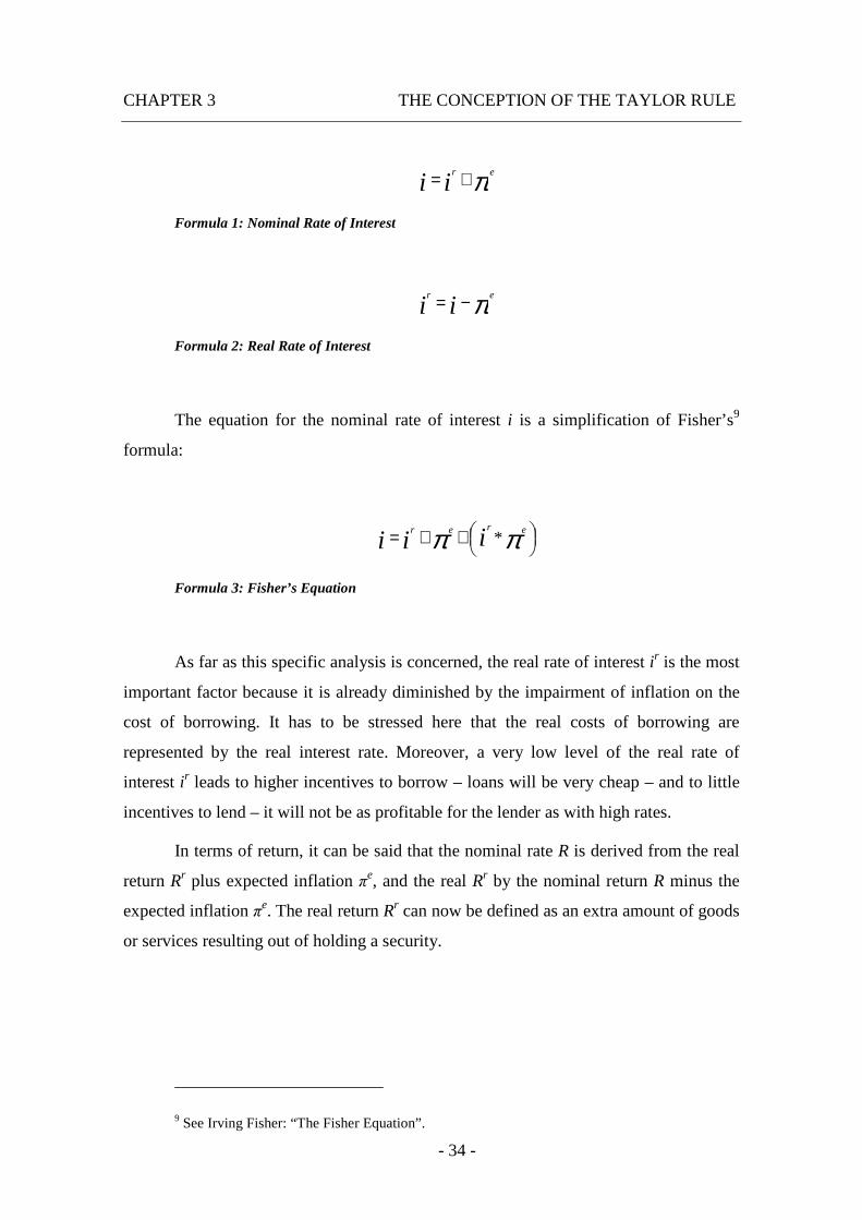
CHAPTER 3 THE CONCEPTION OF THE TAYLOR RULE
- 34 -
π er
ii +=
Formula 1: Nominal Rate of Interest
π er
ii −=
Formula 2: Real Rate of Interest
The equation for the nominal rate of interest i is a simplification of Fisher’s9
formula:
++= ππ erer iii *
Formula 3: Fisher’s Equation
As far as this specific analysis is concerned, the real rate of interest ir is the most
important factor because it is already diminished by the impairment of inflation on the
cost of borrowing. It has to be stressed here that the real costs of borrowing are
represented by the real interest rate. Moreover, a very low level of the real rate of
interest ir leads to higher incentives to borrow – loans will be very cheap – and to little
incentives to lend – it will not be as profitable for the lender as with high rates.
In terms of return, it can be said that the nominal rate R is derived from the real
return Rr plus expected inflation πe, and the real Rr by the nominal return R minus the
expected inflation πe. The real return Rr can now be defined as an extra amount of goods
or services resulting out of holding a security.
9 See Irving Fisher: “The Fisher Equation”.

CHAPTER 3 THE CONCEPTION OF THE TAYLOR RULE
- 35 -
π er
RR +=
Formula 4: Nominal Return
π er
RR −=
Formula 5: Real Return
Since the importance of the real rate of interest was underestimated in the United
Stated of the 1970s, only observations based on the nominal rate were carried out.
Unsurprisingly, this resulted in misinterpretations. For instance, an extremely high
nominal rate of interest led to a deterrence of borrowers, but in fact the real rate of
interest was very low. This was actually a huge advantage for the borrower’s side
because the loans were very cheap.
Only in the year 1997, after the introduction of new systems, the U.S.
government did start to close the gap of information, and began publishing the real rates
of interest on a current basis.
3.2. Financial Markets
According to Mishkin, financial markets perform the essential economic
function of channeling funds from households, firms and governments that have saved
surplus funds by spending less than their income or those that have a shortage of funds
because they wish to spend their income [Mishkin, F. S. (2007c)].
A differentiation of financial markets can be done in many ways. In terms of
maturity I discern between short-term securities with a time-horizon up to one year and
long-term securities which last more than one year.
In addition, one can distinguish between a primary and a secondary market. The
first is the financial market in which only new issues of securities, such as bonds and
stock, are offered to initial buyers. Normally, this type of business runs behind closed
CHAPTER 3 THE CONCEPTION OF THE TAYLOR RULE
- 36 -
doors. In the second market that has been mentioned, securities which have already
been issued can be resold. This is the market place where individuals buy and sell.
Through this observation, the most important distinction between the money and
the capital market is made visible. This difference is defined in the following way.
3.2.1. Money Market – German and International Point of View
Generally, the money market can be defined as a financial market in which only
short-term debt instruments are traded. This type of financial market is so important
because a monetary policy is executed through short-term operations which take place
in this very context.
In literature, several definitions from different points of view are given. Schinke
speaks about the English, the former German and the modern European definition
[Schinke, S. (2004a)].
The English Definition of Money Market
The English version has three main pillars.
Firstly, financial instruments which are traded in the money market only have
short maturities, a very good debtor’s validity and thus a very low exchange risk. One
result of these factors is that international transfers are followed by low transaction-
costs and are easy to handle [Wilson, J. S. G. (1992a)]. Usually these securities are
traded “over night” but also do have maturities of one day up to one year.
The second pillar relies on the different participants in the money market, which
are commercial banks, central banks, corporations, brokers, households and
governments [Cook, T. Q.; La Roche, R. K. (1993a)]. As far as these individuals are
concerned, commercial banks are the most important ones. They operate in the money
market and are responsible for the horizontal equalization of liquidity between
commercial banks, which means they establish the equilibrium between demand and
supply of federal funds. The determined equilibrium-price is called Federal Funds Rate.
Central banks, on the other hand, provide central bank-money to the money market.
They affect and control this market through central bank policy – which is in fact
CHAPTER 3 THE CONCEPTION OF THE TAYLOR RULE
- 37 -
monetary policy – by the use of open market operations to increase or decrease central
bank-money reserves. Finally, there are the governments. Through fixed or variable
interest-bearing obligations they borrow in the short run.
The third and ultimate pillar deals with the allocation function of the money
market. The hard competition between supply and demand is followed by a better
allocation of liquid funds. Furthermore, the loans traded are short-term ones, and have
the characteristic of same day money or over night money which means that they are
payable on the same day or in the same night [Wilson, J. S. G. (1992b)].
The German Definition of Money Market
In German literature, three different explanations are given: a narrow, a medium
and an extended one.
The narrow annotation is geographically limited to the national money market
and is defined as the mutual exchange of Reichsbankgeld-excess and -deficit between
commercial banks [Gestrich, H. (1957a)]. It is subject to severe criticism because the
role of central banks and non-banks is not taken into account. Moreover, the
classification of traded securities is difficult to handle and modern financial aspects are
completely disregarded.
The medium definition is characterized by operations between commercial
banks and central banks and represents the sum of all transactions between these two
actors. In the money market [Lipfert, H. (1975a)]. On the one hand, this specification
seems to be realistic, but on the other hand it also limits the geographical context to the
national market, which does not represent the actual modern situation.
Finally I would like to address the last and extend version of how the money
market is defined in German literature. Here, more participants act in the market and
operate via a wide range of transactions. Short-term bank-loans are given to customers,
short-term distributor-loans are given to retail and whole sale, and short-term central
bank-loans are given to government. Generally, it is defined as the market for short-tern
loans [Deppe, H. D. (1980a)]. This whole extend concept is based on the connection
between money and capital market regarding their time pattern. But it must be pointed
out here that this is not that helpful, neither for scientific nor for practical uses.
CHAPTER 3 THE CONCEPTION OF THE TAYLOR RULE
- 38 -
In essence, it can be stressed that the former German definitions of the money
market have their drawbacks. The main points in the explanation of the market serve as
a good basis, but must be extended in terms of limitations and, which is the most
important aspect, in terms of a modern and dynamic European thinking.
The Modern European Definition of Money Market
As regards the German definition, it is important to distinguish between the
Euro money market and the money market in the Euro Area. This second expression,
which is the more modern one, will be discussed later. The Euro money market,
however, is part of the whole Euro-market, which is further split up into the Euro-
capital market, and the Euro-credit market [Perridon, L.; Steiner, M. (1999a)]. It is
independent from governmental intervention and has short run characteristics. Primarily
U.S. Dollar deposits are traded in the Euro money market, the accumulation of interest
is only executed through supply and demand, and central banks did not intercede.
Generally speaking, specialist literature focuses on trading in which central banks are
excluded.
It must also be mentioned here that there is a compound of interest between
national money markets and the Euro money market. This leads to the individual’s
latitude concerning the right place for an execution of transactions. Debtors and
creditors perform both in the national money markets and in the Euro money market,
which is to say they conclude transactions in foreign currencies.
Let me stress my point with an example:
A German bank asks for a U.S. Dollar loan examining both, the U.S. and the
Euro money market. Since the Euro money market is not subject to strict regulations, as
it is the case in the U.S. market and the claimed interest on the loan is higher in the U.S.
market than in the Euro money market, the bank receives the loan much cheaper in
Europe than in the U.S.A. Generally I can quote here that U.S. interest on debt is a so-
called “upper limit” for U.S. Dollar loans in the Euro money market.
In addition, it can be pointed out that deposits in U.S. Dollars in the U.S. money
market are endued with lower interest than in the Euro money market. That leads to the
claim that interests on deposit are the “lower limit” for U.S. Dollar loans in the Euro
CHAPTER 3 THE CONCEPTION OF THE TAYLOR RULE
- 39 -
money market. In fact, European commercial banks do not need to conduct minimum
reserves on deposits to central banks however, banks in the U.S.A. do have to conduct
them to the Federal Reserve System (FED)10.
Finally, it can be claimed that the generation of interest in the U.S. money
market occurs through the interaction of supply and demand of liquidity which also has
wholesale-characteristics and a compound of interest.
3.2.2. Money Market in the Euro Area
In this chapter several definitions will be given to distinguish the money market
from the capital market. In terms of a broad modern disposition of a money market,
several branches have to be taken into account: money trade between commercial banks,
business between commercial banks and central banks, the issue of short-term
securities through commercial banks, corporations and governments and, last but not
least, trading with derivatives.
The European Central Bank has divided the money market into four categories:
the cash-sector, the sector in which money market securities are traded, the sector for
derivatives, and the regulation sector. Through this regulation sector, central banks are
able to intervene in the money market through monetary policy [European Central Bank
(2001a)].
For a better understanding of the matter, the money market will be defined
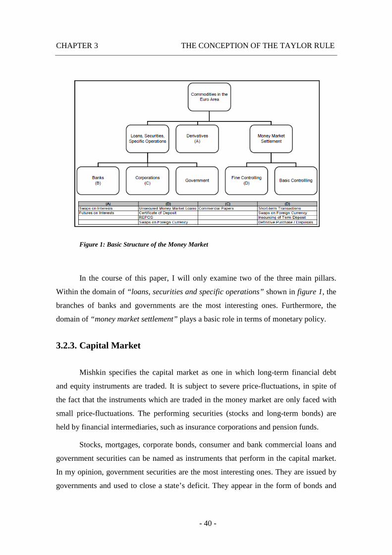
according to Schinke`s view, in which it is divided into three main parts which are
shown in the following illustration [Schinke, S. (2004b)].
10 FED: The Federal Reserve System is the central bank system of the U.S.
CHAPTER 3 THE CONCEPTION OF THE TAYLOR RULE
- 40 -
Figure 1: Basic Structure of the Money Market
In the course of this paper, I will only examine two of the three main pillars.
Within the domain of “loans, securities and specific operations” shown in figure 1, the
branches of banks and governments are the most interesting ones. Furthermore, the
domain of “money market settlement” plays a basic role in terms of monetary policy.
3.2.3. Capital Market
Mishkin specifies the capital market as one in which long-term financial debt
and equity instruments are traded. It is subject to severe price-fluctuations, in spite of
the fact that the instruments which are traded in the money market are only faced with
small price-fluctuations. The performing securities (stocks and long-term bonds) are
held by financial intermediaries, such as insurance corporations and pension funds.
Stocks, mortgages, corporate bonds, consumer and bank commercial loans and
government securities can be named as instruments that perform in the capital market.
In my opinion, government securities are the most interesting ones. They are issued by
governments and used to close a state’s deficit. They appear in the form of bonds and
CHAPTER 3 THE CONCEPTION OF THE TAYLOR RULE
- 41 -
are held by individuals like households, banks and a central bank, which makes them
the most liquid securities traded in the capital market.
Financial instruments in the capital market can be defined through three aspects
which are characterized by Chouldhry; Johannas; Pereira; Pienaar. The first one that is
mentioned is the maturity aspect, which is classified as “long-term” regarding maturities
of ten years and longer, “middle-term” if we speak about maturities of one year up to
ten, and “short-term” less than one year. The second aspect is the size of funding, which
is described as the amount of required capital. The last aspect combines the risk which
is borne by suppliers of financial instruments, and the return demanded by these
individuals as the cost of bearing this risk [Chouldhry, M.; Johannas. D.; Pereira, R.;
Pienaar, R. (2005a)].
Capital market instruments are, for example, stocks, mortgages, corporate bonds,
government bonds, government securities, consumer and bank commercial loans. In this
thesis, long-term government bonds – with a maturity of ten years – are the most
interesting instruments, and thus they are also taken into account in the empirical part of
this work.
3.3. The Taylor Rule
Generally, the rule developed by Taylor serves as a framework which provides
recommendations for central banks. In essence, the degree of intervention of monetary
policy into a state economy is represented. As I already pointed out above, this kind of
policy making only affects the short-term horizon, in other words short-term interest
rates. Besides the short-term goal of stabilizing the economy, the long-term goal of
reaching specific inflation levels is also considered.
According to Taylor, the real short-term interest rate is determined through three
factors:
• What is the actual level of inflation?
• How huge is the gap between economic activity and full employment
level?
CHAPTER 3 THE CONCEPTION OF THE TAYLOR RULE
- 42 -
• What would be the level of short-term interest rate in order to achieve a
situation of full employment?
These factors are addressed by different forms of monetary policy in the Taylor
Rule:
• Tight monetary policy: high interest rates if the inflation level is above
the target or if full employment is above the target; used in order to
reduce the inflationary pressure.
• Easy monetary policy: low interest rates if the inflation level is below the
target or if full employment is below the target; used in order to stimulate
output.
• If the conditions are not like this (e.g.: inflation level below and full
employment level above the target) the Taylor Rule advocates a support
of monetary policy-makers in order to reach a suitable level of interest
rate.
The Taylor Rule is not only an instrument to guide central bank decisions, but
also to evaluate one specific period’s monetary policy and to cede interest rate forecasts.
This reaction–function uncovers, through simple equations, how sensitive central banks
behave to macroeconomic parameters like economic booms and inflation. Essentially,
the rule deals with the coherency between short-term interest rates, economic boom and
inflation. The only problem was the implementation of the rule. In particular, it was the
imperfect information about one period’s data11.
3.3.1. The Taylor Rule – Original Version
In 1993, Taylor published his reaction-function which is basically a description
of the FED’s monetary policy. The most important pillar is the short-term interest rate
(Federal Funds Rate), which displays the basic parameter of the central bank to control
11 1993 - 2005: Use of the original Taylor Rule’s version by the FED that also entailed imperfect information because of the data’s historical point of view. Not until 2005 the FED invented the forward-looking Taylor Rule.
CHAPTER 3 THE CONCEPTION OF THE TAYLOR RULE
- 43 -
a nation’s economy by monetary policy instruments [Taylor, J. B. (1993a)]. In this
context it is vital to point out that the FED’s interest rate settlement reacts to two
factors:
• Deviation between effective inflation and targeted inflation12: inflation-
gap.
• Deviation between effective growth and targeted growth: production-
gap.
Now I will discuss the production-gap, or gross domestic product-gap (GDP-
gap) in greater detail. A national economy’s production-capability is defined through
the maximum production that can be reached without importing any additional
inflation-pressure. This macroeconomic production-capability depends on the quantity
of production-factors (capital, labor), and on the available production-technology.
A positive production-gap is only reached if the effective gross domestic product
(GDP) is above the potential growth. Similarly, a negative production-gap is reached if
the effective GDP is below the potential growth.
By taking a closer look at the inflation-gap, it can be pointed out that it shows
the difference between effective inflation and the targeted inflation through the central
bank. It is also named consumer price index-gap (CPI-gap) because it is measured
through the same.
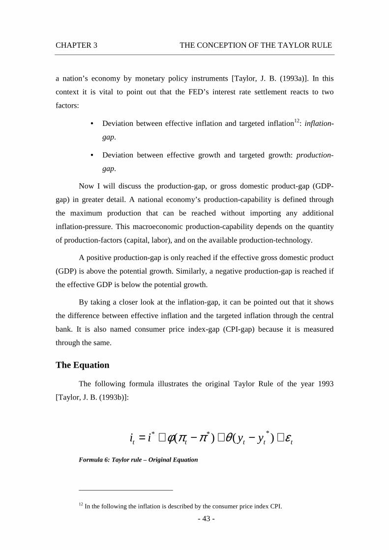
The Equation
The following formula illustrates the original Taylor Rule of the year 1993
[Taylor, J. B. (1993b)]:
ttttt yyii εθππφ +−+−+= )()( ***
Formula 6: Taylor rule – Original Equation
12 In the following the inflation is described by the consumer price index CPI.
CHAPTER 3 THE CONCEPTION OF THE TAYLOR RULE
- 44 -
The effective nominal interest rate in period t is defined by i t. The weighting-
factors [Sauer, S.; Sturm, J.-E. (2003a)] (Φ > 0) and (θ > 0) are flowing directly into the
inflation-gap (πt – π*) and into the production-gap respectively (yt – yt*). πt is the
inflation-rate of period t and π* represents the targeted inflation of the central bank, yt
stands for the effective real GDP in period t and yt* for the potential real production in
one nation’s economy during period t. Furthermore, the factor i* is integrated into
Taylor’s framework and stands for the weighted nominal interest rate of period t that is
observed ex post. For this framework published in the year 1993, Taylor used an
observed period of time prior to the year 1990, which led to the parameters of i*=2 and
ε*=2. The last element in the formula is εt. It is the not correlated normally distributed
error. The used distribution for εt is: εt ~ (0, σ2ε).
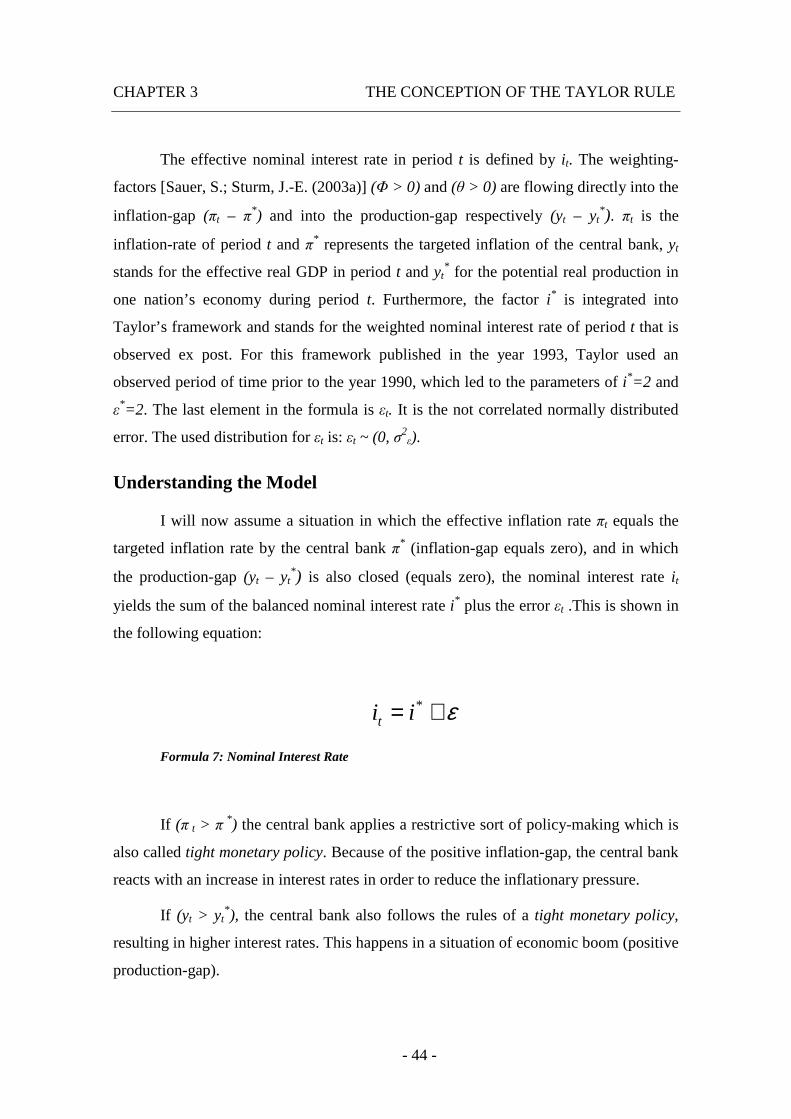
Understanding the Model
I will now assume a situation in which the effective inflation rate πt equals the
targeted inflation rate by the central bank π* (inflation-gap equals zero), and in which
the production-gap (yt – yt*) is also closed (equals zero), the nominal interest rate i t
yields the sum of the balanced nominal interest rate i* plus the error εt .This is shown in
the following equation:
ε+= *iit
Formula 7: Nominal Interest Rate
If (π t > π *) the central bank applies a restrictive sort of policy-making which is
also called tight monetary policy. Because of the positive inflation-gap, the central bank
reacts with an increase in interest rates in order to reduce the inflationary pressure.
If (yt > yt*), the central bank also follows the rules of a tight monetary policy,
resulting in higher interest rates. This happens in a situation of economic boom (positive
production-gap).
CHAPTER 3 THE CONCEPTION OF THE TAYLOR RULE
- 45 -
Suitable Weighting-Factors
The intensity of a central bank’s monetary policy with the aim of closing the
inflation- and the production-gap depends on the two weighting-factors Φ and θ. The
value of these factors is equivalent with the “aggressiveness” of a central bank. In other
words, the higher the weighting-factors, the bigger the steps in interest rates. In 1993,
Taylor suggested values of (Φ = θ = 0.50) for the weighting-factors.
As a result of various studies conducted in the late 1990s, the so-called “Taylor
Principle” was put forward [Taylor, J. B. (1999a)]. According to this principle, the
weighting-factor for the inflation-gap (πt – π*) in the Taylor Rule framework was settled
with (Φ > 1). This is based on the following facts: if a central bank administrates a
stabilizing force on the economic progress in a situation of an effective inflation which
is higher than the targeted inflation, it has to increase the nominal interest rate by an
amount higher than the positive inflation-gap. Because economic subjects react on real
interest rates, this really is the only possibility to increase the real interest rate inside a
national economy.
If central banks increase the nominal interest rate by an amount smaller than the
inflation-gap, the real interest rate would decrease because of the increased inflation
compared to the nominal interest rate. This leads into further inflationary dynamics
which do not create a stable equilibrium.
This emphasizes that only the real interest rate, as opposed to the nominal
interest rate, is crucial for the economy’s evolution in the real-economic sector. The
nominal interest rate can be seen as a variable in the monetary policy through which an
economy can keep its equilibrium.
In the context of the weighting-factor for the production-gap (yt – yt*), it can be
claimed that it is (θ > 0). In various studies conducted by the FED, the weighting-factor
for the inflation-gap has constantly been higher than the factor for the production-gap.
CHAPTER 3 THE CONCEPTION OF THE TAYLOR RULE
- 46 -
Critical Aspects
The concept of the original Taylor Rule has had a positive impact on monetary
policy nevertheless it is interesting to note here that this framework is only based on a
variety of abstract assumptions.
As far as real GDP and inflation are concerned, real-time data must be available
and taken into account. In the early years, only so-called “flash estimations” had been
available which led to huge miscalculations and to wrong results. In some cases, data
from governmental institutions had to be revised several times, and seemingly accurate
data turned out to be wrong after years (in the U.S. it was refuted after two years).
According to Taylor, real-time estimations of monetary policy are an
impracticality. In other words, they cannot be done because of a misinterpretation of
historical policies. One basic assumption in the framework is that central banks only
orientate themselves by the means of historical and present data, which means that only
already available data is taken into account.
However, the key factor for monetary policy decisions is the orientation towards
the future. Incidentally, aspects such as expectations regarding a future economic
progress were dealt with by Clarida et al., and these finally led to the “forward-looking
version of the Taylor Rule” [Clarida, R. J. et al (1998a)].
Another valuable piece of criticism regarding Taylor`s rule is the fact that
Taylor’s original version concentrated on a nation’s domestic economy, a so-called
closed economy. As far as an open economy is concerned, it must be taken into account
that factors like foreign interest rates and foreign exchange rates, which tend to have a
great impact on central bank decisions, need to be mentioned and kept in mind.
3.3.2. The Taylor Rule – Forward-Looking Version
Caused by the criticism and by the shortcomings of the original Taylor Rule,
Clarida et al. developed a forward-looking framework, which was, however, grounded
on the historically-orientated rule. The aim of this was to close the gap of information
which led into misinterpretations.
CHAPTER 3 THE CONCEPTION OF THE TAYLOR RULE
- 47 -
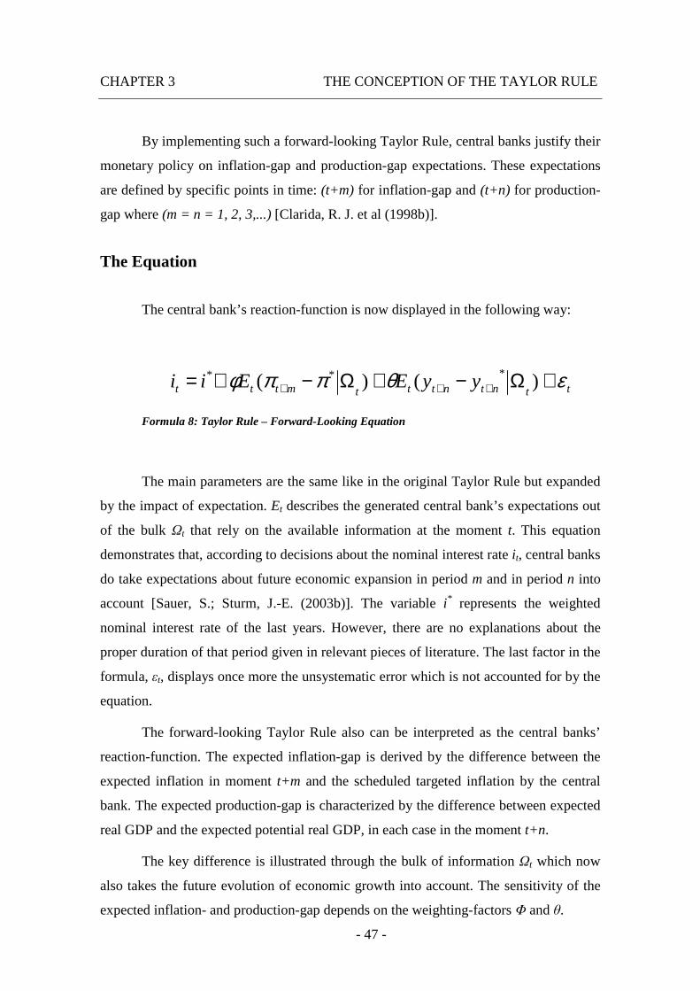
By implementing such a forward-looking Taylor Rule, central banks justify their
monetary policy on inflation-gap and production-gap expectations. These expectations
are defined by specific points in time: (t+m) for inflation-gap and (t+n) for production-
gap where (m = n = 1, 2, 3,...) [Clarida, R. J. et al (1998b)].
The Equation
The central bank’s reaction-function is now displayed in the following way:
ttntntttmttt yyEEii εθππφ +Ω−+Ω−+= +++ )()( ***
Formula 8: Taylor Rule – Forward-Looking Equation
The main parameters are the same like in the original Taylor Rule but expanded
by the impact of expectation. Et describes the generated central bank’s expectations out
of the bulk Ωt that rely on the available information at the moment t. This equation
demonstrates that, according to decisions about the nominal interest rate i t, central banks
do take expectations about future economic expansion in period m and in period n into
account [Sauer, S.; Sturm, J.-E. (2003b)]. The variable i* represents the weighted
nominal interest rate of the last years. However, there are no explanations about the
proper duration of that period given in relevant pieces of literature. The last factor in the
formula, εt, displays once more the unsystematic error which is not accounted for by the
equation.
The forward-looking Taylor Rule also can be interpreted as the central banks’
reaction-function. The expected inflation-gap is derived by the difference between the
expected inflation in moment t+m and the scheduled targeted inflation by the central
bank. The expected production-gap is characterized by the difference between expected
real GDP and the expected potential real GDP, in each case in the moment t+n.
The key difference is illustrated through the bulk of information Ωt which now
also takes the future evolution of economic growth into account. The sensitivity of the
expected inflation- and production-gap depends on the weighting-factors Φ and θ.


- 49 -
4. Theory of Monetary Policy
This chapter deals with the question of how central banks can affect economies,
and also with which instruments they can reach their targets. The first important step is
to select and evaluate the targets. During the decision-making process, central banks
should not act unsuspectingly. After all, they are only a small constituent in a
democracy, and therefore they cannot act irresponsibly in the decision-making-process
in terms of monetary policy. A central bank’s degree of political independence
influences the relative targets’ significance in terms of monetary stability and full
employment.
One of the key objectives is the creation of money which has an immense impact
on the development of prices. In recent times, the modern interest rate policy has
displaced the monetary aggregate policy. Central banks try to stimulate prices and
output directly via specific interest rate instruments.
Monetary policy is constantly competing with other factors, such as political and
economic concerns. On the one side, central banks strive to improve their reputation and
plausibility continuously in order to prevent labor unions from imposing expansive
wage-politics. After all, the constant fear of possible real wage reductions could lead to
inflationary pressure. On the other side, financial politics could be interested in
inflationary pressure in order to reduce state indebtedness. On top of this, one is
confronted with the assent holder’s request for stable monetary value.
4.1. The New Consensus Macroeconomics – NCM
In order to push my considerations forward and endow them with a state-of-the-
art character, let me now turn to the “New Consensus Macroeconomics” (NCM) [Bean,
C. (2007a)]. It was invented by Bean in the year 2007, and it deals with the following
basic issues [Bain, K.; Howells P. (2009a)]:
• In the long run, monetary policy has no real effects;
• In the short run, nominal rigidities create a trade-off between output and
inflation;
CHAPTER 4 THEORY OF MONETARY POLICY
- 50 -
• Monetary policy is the principal mean of influencing aggregate demand,
and policy is linked to inflation through its ability to influence the
pressure of demand;
• Policy outcomes are improved under an independent central bank, and
further improved if the central bank operates in an open and transparent
manner;
• Ends (a specific inflation target) matter more than means (intermediate
targets);
• The management of expectations is critical;
• The policy instrument is the short run nominal interest rate set by the
central bank in supply and refinancing of banks’ reserves.
4.2. Instruments and Goals
Targets are quantified objectives (or quantified goals), and the achievement of
them increases the material well-being of the population [Bain, K.; Howells P. (2009b)].
In the following chapters, the empirical study will demonstrate how monetary goals and
targeting have changed their character over the past three decades until the present.
Instruments of monetary policy are variables which the policy authorities control
directly, and their value is determined independently from other variables in the system
[Bain, K.; Howells P. (2009c)]. The short-term interest rate through which central banks
try to stimulate the economy, are of particular importance here. Generally, it can be
stressed that the longer the term of interest, the less central banks are able to influence
it. Of course, the monetary base also can be put under control but as far as this paper is
concerned, only the effect of monetary policy on interest rates will be explored.
One of the main challenges for central banks is the establishment of a connection
between one specific instrument and the respective targets to obtain the best results. In
the so-called “principle of effective market classification”, Mundell applied himself to
this problem and generated a technique to approach an optimal result. According to him,
the main pillars are external (balance in the balance of payments) and internal (full
CHAPTER 4 THEORY OF MONETARY POLICY
- 51 -
employment with low inflation) balances, which describe the targets and the basic
instruments consist of the monetary (interest rates), as well as the fiscal policy (budget
balance) [Mundell, R. A. (1962a)]. He focused on the use of a fiscal policy to obtain
internal balance and a monetary policy to obtain an external one in a fixed exchange
rate system.
4.3. Open Market Operations
With the assistance of open market operations, central banks try to fulfill their
monetary policy. Financial instruments are employed to control and guide the supply of
money in order to achieve specific targets13 (interest rates, exchange rates). These
operations appear in both, the money market and the capital market14. As my
professional expertise is limited, I will focus on the money market in the analysis,
simply because the effect on interest rates in connection with the different policies is
clearly visible in this context.
4.3.1. Open Market Operations in the Money Market
In modern monetary policy, open market operations are more important in the
money market than in the capital market. The reason for this can be found in the higher
significance of supply of money than supply of credit.
In terms of supply of money, I have to mention that this topic deals with the
satisfaction of the want from banks and private economic subjects to hold money. This
can be done via central banks which have the money supply monopoly.
4.3.2. The Dilemma between Capital Market versus Money Market
When talking about long-term financing activities, one problem suddenly
emerges: “How is it possible to create and strengthen the position of creditor and
debtor in the capital market, which is locally controlled by the long-term interest rate?"
13 See chapter 4.4. 14 See chapter 3.2.

CHAPTER 4 THEORY OF MONETARY POLICY
- 52 -
As money supply and credit supply take place in two different markets, they should be
observed in terms of monetary policy.
If central banks operated the supply of liquidity trough the capital market,
technical errors and fluctuations could negatively influence the allocation-function of
the interest rate of the capital market. Even short-term actions could accidentally emit
signals that would have impacts on long-term investment decisions.
The central bank is one basic player in the capital market and therefore
influences the supply-demand-constellation. Thus, the information-function of the
capital market could be disturbed heavily. Interest rate effects could override aspects
like inflation-expectations. This illustrates the dilemma between the general aim for
relatively undistorted information, and the aim for direct control of interest rate
constrained demand rulings for goods.
If central banks intervened directly in the capital market, the interest rate in that
market would turn into a political price. Therefore, central banks are likely to be faced
with a situation of political pressure, as they are able to influence the cost of interest
rates.
To sum up the arguments above, one has to say that central bank money is
regulated in a money market in which central banks generally follow three basic pillars:
• The liquidity of the whole banking sector has to be maintained
which assures that the sector is able to operate, and is not breaking down
in crisis. Central banks also can appear as “lenders of last resort”.
• Liquidity-constraints have to be employed because of efficiency-
matters. Central banks must conduct solvency checks, out of own
concerns, to implement some sort of selection in the economy.
• If central banks want to influence the evolution of the business
circle via reactions in the banking sector, the funding-conditions have to
be adjusted in correct way, and also diversified.
CHAPTER 4 THEORY OF MONETARY POLICY
- 53 -
4.3.3. Money Market and the Short-Term View
As regards the points above, I am now able to maintain that short-term interest
rates are the main variable in the efforts of central banks to conduct monetary policy.
The short-term interest rate is the rate which central banks claim from commercial
banks in the refinancing-business. Operations in this sector are called “open market
operations”. Usually they are defined as short-term inter-bank loans which are verified
through securities that are deposited by commercial banks at central banks. This short
maturity increases the flexibility of the whole monetary policy, which implies that
conditions of refinancing-operations can be adjusted quickly.
4.3.4. Refinancing-operations
Generally, there are two different refinancing-operations that are distinguished
between [Spahn, H. P. (2009a)]:
• “Fixed interest tender or quantity tender”: Central banks fix the
interest and cede the choice of money supply to commercial banks.
Fluctuations in money demand do not lead to changes in interest. If
central banks determine a specific upper limit for the whole business-
volume, this results in a so-called “oversubscription”, and this leads to
the fact that commercial banks only get a fraction of the desired amount
of money.
• “Interest tender”: Central banks fix an upper limit for the volume
of the refinancing loans and usually a minimum interest. On the one side,
this implicates that a specific amount of money is auctioned, and on the
other side this causes increasing interest rates for an increasing demand
of money. There are various types of interest tenders, like the Dutch and
the American, for example [Spahn, H. P. (2009b)].
If there is no apparent need for central banks to intervene via stabilizing
monetary policy actions, they will choose an action known as “quantity tender”, which
denotes an elastic refinancing of commercial banks for a fixed interest. Therefore, a
change in the policy of a central bank to the “interest tender” implicates a restrictive
money supply with increasing interest rates. In practice, the difference between the two
CHAPTER 4 THEORY OF MONETARY POLICY
- 54 -
kinds of policies does not have a drastic impact on the shortage of central bank money.
In connection with this, one important point for central banks is to estimate the
commercial banks’ need for central bank money in an accurate way. Because the
demand of money tends to fluctuate ambiguously, the minimum reserve-obligation
stabilizes the demand for central bank money. Therefore, the minimum reserve-
obligation assists a better forecast of central bank money. Hence, liquidity is not a prime
issue in monetary policy anymore.
4.4. Monetary Policy Targets
In this chapter, several targeting-techniques will be explored. For this paper, the
most important one is inflation targeting, and thus I will refer to this technique in
greater detail. In fact, this alternative intervention of the central bank plays a major role
in many countries since the beginning of the 1990s. I will now introduce the advantages
and disadvantages of the different techniques of targeting.
4.4.1. Inflation Targeting
Within the scope of policy-making, central banks set a specific level (specific
numerical value) for the inflation over an upcoming period in time. Already in the late
1800s, economists like Marshall and Wicksell developed a system with which they
wanted to bring the purchasing power of the currency close to an absolute standard.
In the 1990s, the UK implemented this system and it was followed by other
countries in Europe. Inflation targeting generally obeys the characteristics below:
• The most important issue is the focus of policy-makers on what they
want to achieve, rather than the question of which critical parameters
could influence the system or might lead to conflicts. In other words, it is
established that a clear aim has to be formulated.
• The specification of an inflation target entails that policy-makers must
have a clear notion of their expectations. They can only act under this
proposition. Generally, it can be said that decisions which rely on
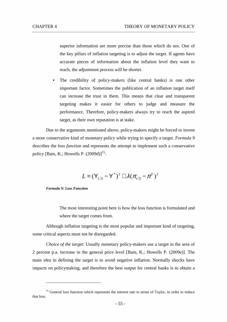
CHAPTER 4 THEORY OF MONETARY POLICY
- 55 -
superior information are more precise than those which do not. One of
the key pillars of inflation targeting is to adjust the target. If agents have
accurate pieces of information about the inflation level they want to
reach, the adjustment process will be shorter.
• The credibility of policy-makers (like central banks) is one other
important factor. Sometimes the publication of an inflation target itself
can increase the trust in them. This means that clear and transparent
targeting makes it easier for others to judge and measure the
performance. Therefore, policy-makers always try to reach the aspired
target, as their own reputation is at stake.
Due to the arguments mentioned above, policy-makers might be forced to invent
a more conservative kind of monetary policy while trying to specify a target. Formula 9
describes the loss function and represents the attempt to implement such a conservative
policy [Bain, K.; Howells P. (2009d)]15:
21
2*1 )()( T
ttL ππλ −+Υ−Υ= ++
Formula 9: Loss Function
The most interesting point here is how the loss function is formulated and
where the target comes from.
Although inflation targeting is the most popular and important kind of targeting,
some critical aspects must not be disregarded.
Choice of the target: Usually monetary policy-makers use a target in the area of
2 percent p.a. increase in the general price level [Bain, K.; Howells P. (2009e)]. The
main idea in defining the target is to avoid negative inflation. Normally shocks have
impacts on policymaking, and therefore the best output for central banks is to obtain a
15 General loss function which represents the interest rate in terms of Taylor, in order to reduce that loss.
CHAPTER 4 THEORY OF MONETARY POLICY
- 56 -
means, for a certain period of time, that is more or less equal to the target. In order not
to change the price level, it is clear that policy-makers therefore try to target a positive
inflation rate, as they also have to keep the existence of variance in mind.
However, extreme situations are likely to arise if the target is set too close to
zero. This then leads to falling prices, which is particularly bad, since prices should not
be changed. This fact has its origin in the monitoring of the index and in the use of
different update periods. For instance, an increase in the price of specific goods or
services affects the cost of living in the way the weights are set prior to the price rise.
Another problem emerges in the context of labor market thoughts. Normally the
market has a clearing function when it is in equilibrium. If one assumes that a decrease
in nominal wages is not possible this will lead into a situation in which the equilibrium
in real wages is not given. The effect is that the market is not cleaned. Therefore, prices
have to be increased, as this is practically the only way to handle the problem, dealing
with a low level of positive inflation.
If policy-makers yield a positive inflation, negative real rates of interest can be
established. Therefore, if prices are decreasing, with a zero nominal bound of interest
rate, the whole monetary policy-making can become ineffective. In terms of the present
economic situation, and the fact that we are in a deep recession, negative real rates are
needed but cannot be obtained.
Choice of the measure-index of inflation: The biggest challenge is to find an
index, which represents the changes in the level of prices of individuals most precisely.
Each index represents change in a different way, and comparing one to another also
poses problems. Most central banks use the CPI16 because it is the most common
measure of inflation worldwide.
Characteristic of the target: The last basic issue is whether to use a specific
point of target or a specific range in which the target should be bordered. Generally
speaking, a point sounds more plausible, but central banks like the ECB17 operate by
means of ranges because the loss of specific points of targets always entails additional
16 CPI: Consumer Price Index. 17 ECB: European Central Bank.
CHAPTER 4 THEORY OF MONETARY POLICY
- 57 -
expenses, and harms the reputation of central banks. For instance, the ECB dictates
“below but close to 2 percent” and the BoE18 a range “between 1 and 3 percent”.
At this point, another aspect which I will not discuss in greater detail has to be
mentioned: symmetry. It does not matter if the BoE overshoots or undershoots a target
by 1 percent point, and here one has to keep in mind that I am talking about a range, in
both cases the same penalty will be executed. Nevertheless, in case the ECB
undershoots a target, no execution will be induced. As a result, it can be stressed that
the ECB follows a monetary policy with a downward tendency, and it also leads to a
lower inflation target than the BoE.
4.4.2. The Inflation Forecast as Target
Svensson [Svensson, L. (1997a)] described inflation targeting as inflation
forecast targeting because of the long reaction time in the monetary policy sector and
the huge delays regarding the publication of reliable data. Here, the basic idea is to
establish an accurate way to define the policy-making instrument for a forward-looking
point of view, based on a forecast horizon for the expected inflation.
For instance, the Bank of England freely defines the target horizon. This entails
some sort of independence in terms of performance measure of the bank itself, because
it chooses the horizon ex ante and then it is judged ex post. However, even if central
banks are not constricted regarding the choice of their policy horizons, it is a tough
topic, as accurate definitions and forecasts of inflation are difficult to make. The most
hazardous errors in this respect are over- and underestimations of future prospects.
The Bank of England has made several mistakes in the settlement of assigned
forecasts over the last three decades. In the time period between 1971 and 1996, their
forecast was too low and, between 1993 and 1996, the forecasts were too high, reaching
an error for eight quarters ahead of +3.31 and -1.04 respectively. So the question arises
if central banks should be inspected by independent institutions in defining targets by
18 BoE: Bank of England.
CHAPTER 4 THEORY OF MONETARY POLICY
- 58 -
objective handling. Another sensible point is whether to include the private sector or
not.
The FED generally outperforms the private sector forecasts. This brings up
another critical fact. If the private sector cannot or does not trust the FED’s data
forecast, there is no second opinion and errors are obligatory. The provision of accurate
forecasts and data are the main incentives for central banks because their own
credibility is measured by these parameters. Slight errors denote an accurate policy, in
contrast to huge ones, which reveal policy-makers inaccurate forecasts over periods of
time. It also has to be pointed out here that the divergence of the forecast from the target
can be seen as a means of measure for the credibility of a central bank.
4.4.3. Nominal Income Targets
The act of targeting a specific nominal income also serves as an alternative to
the implementation of monetary policy. Although there are some advantages, the
disadvantages prevail. Some of them are specified below:
• For exact forecasts, a monthly basis should be a premise, but nominal
income targeting is connected with quarterly available datasets. This
makes it difficult to respond for monetary policy-makers.
• The invention of this kind of monetary policy is followed by giving equal
percentage weights to real output and to the divergence of prices from
the price level target [Hall, R.E. (1986a)]. Hall also addresses the
advantages of including the parameters of unemployment and price level
instability, in terms of a social welfare function.
• One of the basic problems, as far as nominal income targets are
concerned, is the conflict between monetary policy-makers – the central
banks – and governments.
• Nominal income is also influenced by fiscal policies. This kind of policy-
making is not subject to the central bank’s supervision.

CHAPTER 4 THEORY OF MONETARY POLICY
- 59 -
• The major problem in targeting a nominal income is expressed by the
fact that it is not easy to influence two parameters at the same time.
Balancing a decrease in output could therefore cause an increase of
prices.
4.4.4. Targeting an Index of Monetary Conditions
The act of targeting an index of monetary policy conditions is characterized by
taking more variables, for instance the exchange rate, into account. Making use of the
exchange rate is, on the one hand, a very thoughtful thing to do, but on the other hand, it
raises the question of who should be in charge of this index on global scale. Who should
be responsible for changes in this factor?
The main problems in the invention or formation of a policy which targets an
index of monetary conditions are the selection of variables which should be taken into
account, and finding responsible institutions that are able to control them. At the
moment, there seem to be no answers to these questions.

- 61 -
5. The Linkage between Short-Term and Long-Term
Interest Rates and the Impact of Monetary Policy
5.1. Brief Overview
If the risk of inflation is manageable, the majority of central banks follow a
monetary policy strategy with the goal to stimulate the economic growth and therefore
employment. This real effect can be illustrated in connection with the Phillips Curve19
discussion:
• Expansive monetary policy in short-term concerns is able to increase
national economy’s GDP20.
• However, in the long run this is accompanied by inflation.
Expansive monetary policy in the short run is expressed by several points of
view. On the one side, if the nominal GDP increases, the increase in value of money is
likely to be followed by expectations about inflation. On the other side, the circulating
value of money inside a national economy could be held short by individuals
themselves in order to escape the danger of inflation. This argument has already been
addressed in chapter 2 in connection with the Theory of Hicks.
The most important point here is that short-term monetary policy does have an
impact on real and nominal growth and therefore influences employment. The Taylor
Rule, which is discussed in chapter 3, is able to give the right explanation here. It is
used to give the participators in the market the ability to forecast the future monetary
policy of central banks.
19 Phillips Curve illustrates the inverse relationship of inflation rate and unemployment in an economy. In the sort run a tradeoff between inflation and unemployment can be observed which does not appear in the long run. In general it can be stressed that the lower the rate of unemployment, the huger the increases in nominal wages.
20 Gross Domestic Product: GDP.
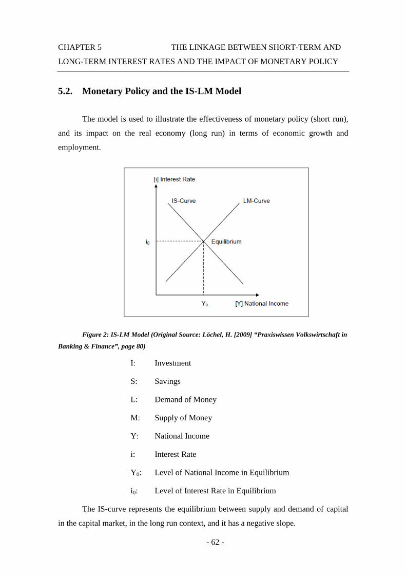
CHAPTER 5 THE LINKAGE BETWEEN SHORT-TERM AND
LONG-TERM INTEREST RATES AND THE IMPACT OF MONETARY POLICY
- 62 -
5.2. Monetary Policy and the IS-LM Model
The model is used to illustrate the effectiveness of monetary policy (short run),
and its impact on the real economy (long run) in terms of economic growth and
employment.
Figure 2: IS-LM Model (Original Source: Löchel, H. [2009] “Praxiswissen Volkswirtschaft in
Banking & Finance”, page 80)
I: Investment
S: Savings
L: Demand of Money
M: Supply of Money
Y: National Income
i: Interest Rate
Y0: Level of National Income in Equilibrium
i0: Level of Interest Rate in Equilibrium
The IS-curve represents the equilibrium between supply and demand of capital
in the capital market, in the long run context, and it has a negative slope.
CHAPTER 5 THE LINKAGE BETWEEN SHORT-TERM AND
LONG-TERM INTEREST RATES AND THE IMPACT OF MONETARY POLICY
- 63 -
The LM-curve represents the equilibrium between supply and demand of money
in the money market, which equals the short run, and has a positive slope. It can be said
that a rise in short-term interest rates in the money market leads to an increase in
national income, because of the higher inflation rate, and vice versa.
The model combines the two different curves and brings them together. The
interception between the IS-curve and the LM-curve expresses the equilibrium between
the money (short-term) and capital market (long-term). Thus, the national economy can
be said to be characterized by the level of national income and the level of interest rate
in the equilibrium. This is underlined by the fact that a reduction in interest rates leads
to an increase in national income followed by an increase in investment. This illustrates
the positive impact of expansionary monetary policy.
5.3. The Feasible Malfunction of Monetary Policy
As far as the expansionary monetarism of central banks is concerned, two
problems arise: the appearance of the investment and the liquidity trap.
The investment trap emerges when the investment of firms is no longer elastic in
terms of interest rates. This is illustrated by situations in which no reactions to interest
rate cuttings become apparent. The reason for this is the bad expectation by companies.
Big companies argue that the fear of high interest rates accompanied by a high cost of
capital is outperformed by problems regarding the value of business circle, return and
benefit.
Generally this can be stressed via an extreme example. If short-term interest-
rates decrease, interest rates in the long-term increase. However, the important long-
term interest rate in the capital market, which is relevant for the real economy, does not
increase as sharply as the short-term interest rates in the money market.
If monetary policy loses its power to impair economy, this is called the liquidity
trap. This liquidity trap is characterized by situations where interest rates cannot be
decreased any longer because they have already reached a very low level. An example
is the credit crunch, with its origin in the sub-prime crises in 2007. The level of short-
term interest rates had already reached a level ranged between 1.00 and 0.00 percent. So
CHAPTER 5 THE LINKAGE BETWEEN SHORT-TERM AND
LONG-TERM INTEREST RATES AND THE IMPACT OF MONETARY POLICY
- 64 -
the real effect on national income remains absent. Especially in relatively uncertain
periods of time, such effects might appear because neither households nor firms spend
money for consumption or for savings. Basically, their only goal is to hold liquidity.
However, these issues have already been discussed in chapter 2 by dint of
Hicks’ theory.
5.4. Interest Rates and the Term Structure
Interest rates are a crucial variable within a national economy because they
combine the money market (financial market) with the capital market (real market)
accompanied by the assignation of investment and consumption costs. It has already
been pointed out that central banks always aim to have a specific influence on the
capital market in the long run, mostly by regulating the short-term rates in the money
market. The accurate interest rates in the capital market are determined via supply and
demand in the bond market, but guided by settlements in the short run. Bonds are
defined to be the long-term financial products with durations longer than one year.
5.5. Summary of Key Facts
Short-term interest rates which are settled by central banks in the money market
have a specific impact on long-term rates in the capital market and this is expressed by
the bond market in this work. Long run factors like economic growth, rate of inflation
and the expectation about benefits are affected.
Generally, it can be stated that a rise in short-term interest rates leads to an
increase in economic growth because of higher investment, and vice versa.
If short-term interest rates decrease, stock prices increase, and vice versa. The
bond market is also influenced by short run interest rate changes in the money market.
Bond prices rise with decreasing short-term interest rates and vice versa. Thus, with
diminishing short-term interest rates the yield on bonds and long-term interest rates are
decreasing and vice versa.

CHAPTER 5 THE LINKAGE BETWEEN SHORT-TERM AND
LONG-TERM INTEREST RATES AND THE IMPACT OF MONETARY POLICY
- 65 -
Keynes` invention of the IS-LM model combines the capital market of the
national economy with the money market. The impact of monetary policy is
exemplified by the argument that relatively low interest rates lead to an increase in
investment into real capital, as well as to a higher growth in employment, and vice
versa.
The danger of the liquidity and investment trap also has to be mentioned here.
The best example in this context is the sub-prime crisis with its origin in the year 2007,
subsequently followed by a worldwide recession. Monetary policy was not able to react
to this outstanding event sufficiently. The reason for this is grounded in the low short-
term interest rate level, which was at that time in a range between 1,00 and 0,00 percent.
Therefore, a cut in short-term interest rates was not possible at that point.

- 67 -
6. Empirical Study A
6.1. Brief Overview
The basis of this paper is an empirical study. The main idea is to show how
interest rates, particularly long–term and short–term interest rates, react over a specific
period of time. At first, I intended to portray and analyze a time span of 15 years,
however, I soon realized that in order to gain a better insight into the dynamics of
interest rates, so to say, it is necessary to look at a longer period of time. This is why I
decided to focus on a time period of 30 years instead. In essence, it can be said that it is
easier to identify changes in a 30-year period than in a 15-year period.
Nevertheless, I decided to split the total time in two 15-year periods. For the first
period, I analyzed data from 1979 to 1993, and here it is important to note that this data
consists of yearly observations. The second part of data, covering the time between
1994 and 2008, is based on monthly observations because of the enormous importance
in this time.
For the present study, I chose three different geographical areas: the United
States of America, the United Kingdom and the Euro Area. The last area on the list has
to be explained in greater detail. The reason why I will not deal with the development of
the Euro area in this work is the fact that an analysis of data from a changing number of
member states is quite difficult. In consequence, I chose to obtain data from available
databases for the so-called Euro Area21.
The following analysis of data is divided into three main parts. At the beginning,
I will deal with the whole span of time, all in all three decades, followed by a more
detailed portrayal of the first 15 years from 1979 to 1993. The second half of the time
series analysis, ranging from 1994 to 2008, will be discussed in the end.
At this point, I would like to stress that this main chapter 6 (Empirical Study A)
will deal with the differences in Monetary Policy in the three geographic areas
mentioned above. This means that only short-term rates are observed in this context.
21 Euro area: EA11-2000, EA12-2006, EA13-2007, EA15-2008, EA16.
CHAPTER 6 EMPIRICAL STUDY A
- 68 -
However, in chapter 7, I will focus on the connection between short-term and long-term
rates.
6.1.1. Description of Long–Term Interest Rates
Maastricht Criterion22 bond yields are long-term interest rates, used as a
convergence criterion for the European Economic and Monetary Union (EMU)23
(central government bond yields on the secondary market24, gross of tax, with around 10
years residual maturity). In the available data set, one can find 10-year government
bond yields, which are reference rates, based on government bonds with a maturity
close to ten years. These bonds used for the calculation of the yields can only be issued
by governments itself.
In specialist literature, long-term interest rates are defined as interest rates with a
maturity of ten years or longer [Mishkin, F. S. (2007a)].
6.1.2. Description of Short–Term Interest Rates
The short–term interest rates used in this work are day–to–day money market
interest rates25 which are defined as average rates for the Euro Area. The time horizon
which was taken for the analysis stretches over 3–month periods. This is due to the
22 The Maastricht criteria (also known as the euro convergence criteria) are essential for European Union member states to enter the third stage of European Monetary Union. Third stage’s main scope of duties is to adopt the euro as the single official currency. The four main criteria are laid down in the European Community Treaty: inflation rate, government finance (annual government deficit, government debt), exchange rate, long–term interest rates.
23 European Monetary Union (EMU): All European Union member states have to be a part of the EMU. Its aim is to adopt the euro as a single official currency and covers over three stages (1 July 1990 to 31 December 1993, 1 January 1994 to 31 December 1998, 1 January 1999 and continuing).
24 The secondary market is a financial market in which securities that have been previously issued can be resold [Mishkin, F. S. (2007a)].
25 Day–to–day money market interest rate represents the average for the Euro Area (Euro Overnight Index Average – EONIA): 1-, 2-, 3-, 6- and 12-month interest rate averages for the Euro Area (EURIBOR).
CHAPTER 6 EMPIRICAL STUDY A
- 69 -
restraint of data availability in the United States of America and the United Kingdom
(EURIBOR)26.
Once again, I would like to point out that interest rates are short-term if the
maturity is less than a year. Long-term interest rates have already been discussed above.
However, in case the maturity is between one and ten years, one speaks of intermediate-
term interest rates [Mishkin, F. S. (2007a)].
6.2. Monetary Policy in the USA
The Federal Reserve System (FED)27 is the central bank of the United States and
the most powerful central bank in the whole world. In the last chapters, I elaborated on
monetary policy and on its definition. Now, I would like to take a closer look at the last
three decades, and particularly at the different aims the FED was trying to achieve.
In the context of this work, I am mainly interested in short-term and long-term
interest rates as main parameters. Firstly, I will analyze the short-term data because this
data is a vital aspect of monetary policy. Afterwards, I will take a closer look at the
combination of short-term and long-term rates.
In terms of U.S. short-term rates, there is the Federal Funds Rate or the Fed
Funds Rate. It has a huge effect on all other short-term rates.
26 Euro Interbank Offered Rate (EURIBOR): daily updated rate based on the average rates at which banks lend other banks funds in the interbank money market.
27 Federal Reserve System: FED is the central bank of the USA.

CHAPTER 6 EMPIRICAL STUDY A
- 70 -
6.2.1. Analysis of Data from 1979 - 1993
Figure 3: USA; Short-Term Rates; 1979 – 1993
Since the beginning of the 1980s, the FED’s monetary policy was characterized
by one specific aim: price stability. In comparison to other central banks this was not
encouraged through a certain level of a target rate of inflation. In 1979, the FED started
to operate employing a theory that was later called practical monetarism [Fazzari, S.;
Minsky, H.P. (1984a)]. Within this theory, the medium-term target of monetary policy
is defined through the quantity and the rate of change of monetary aggregate. As a result
of this, the known interest rate targets were replaced by reserves targets. The idea
behind this was that an increase in the demand of reserves, which was no longer
restricted by interest rates targets, would be accompanied by an increase in the Federal
Funds Rate (in terms of this work in short-term interest rates). For outsiders, this shift in
the FED’s monetary policy heralded a trend of monetary base control. However, the
FED still had a huge problem to solve: how to handle the reserve growth.
CHAPTER 6 EMPIRICAL STUDY A
- 71 -
In 1982, an attempt to avoid the effects of this problem by targeting borrowed
reserves was made – but it failed. The FED’s Funds Rate was decreasing because of the
increase in demand of the reserves. As a result, they turned back to interest rate
targeting.
Even in 1984, when the FED picked up the idea of contemporaneous reserve
accounting, the problem of handling the reserve growth was not solved. Through this
inability, short-term interest rates rose up and the FED tried to react through changing
their monetary policy strategy in terms of controlling banks once more, by the
replacement of quantities by prices. Some economists call it the era of experimental
monetarism because the first and foremost aim of the FED in terms of monetary policy
was to convince the public and the government to accept higher interest rates.
In 1989, and in the early 1990s, short-term interest rates (Federal Funds Rate)
had a higher level than in the 1980s, with 8.15 percent. The beginning of the 1990s was
characterized by several rate-cuttings by the FED because of the overall economic
slump in all branches. In 1991, the Federal Open Market Committee (FOMC)28 cut the
rates to 3.68 percent, leading to a minimum of 3.17 percent in the year 1993.
28 Federal Open Market Committee: FOMC.
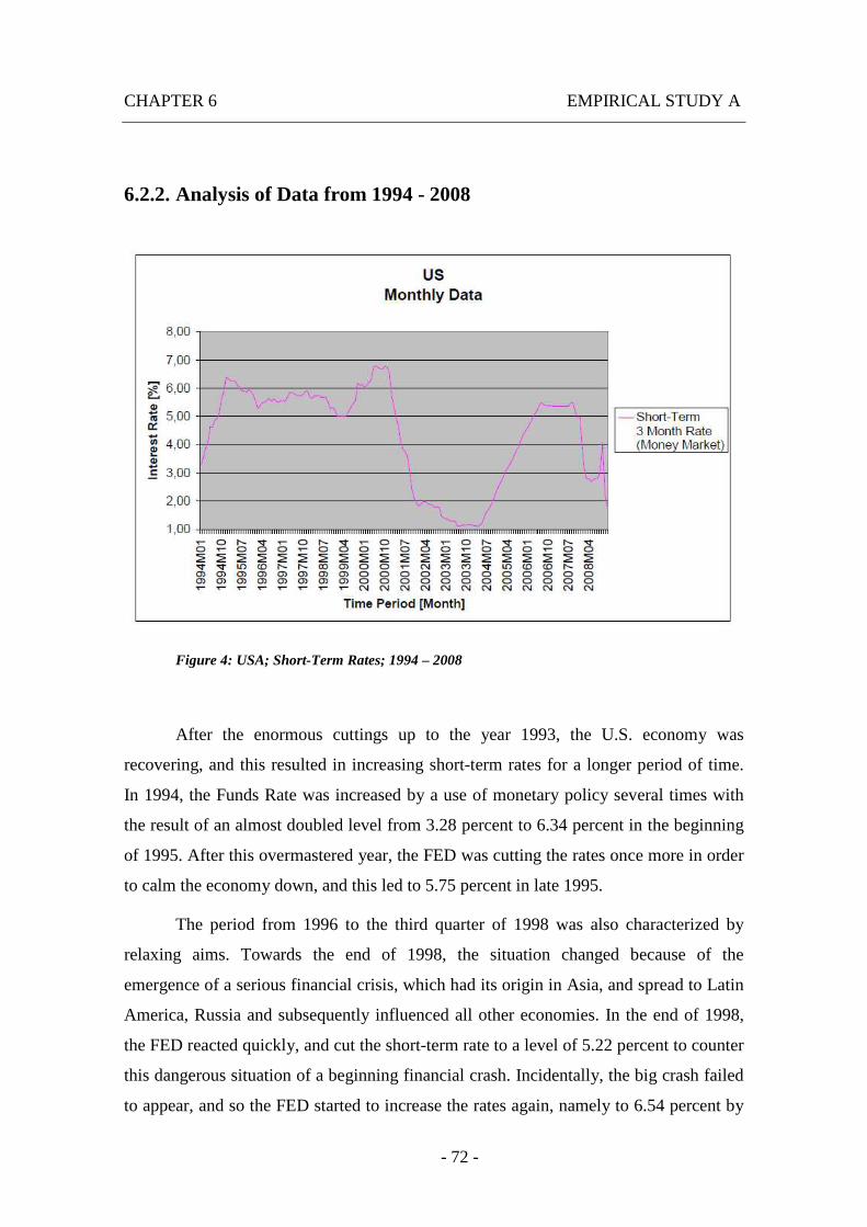
CHAPTER 6 EMPIRICAL STUDY A
- 72 -
6.2.2. Analysis of Data from 1994 - 2008
Figure 4: USA; Short-Term Rates; 1994 – 2008
After the enormous cuttings up to the year 1993, the U.S. economy was
recovering, and this resulted in increasing short-term rates for a longer period of time.
In 1994, the Funds Rate was increased by a use of monetary policy several times with
the result of an almost doubled level from 3.28 percent to 6.34 percent in the beginning
of 1995. After this overmastered year, the FED was cutting the rates once more in order
to calm the economy down, and this led to 5.75 percent in late 1995.
The period from 1996 to the third quarter of 1998 was also characterized by
relaxing aims. Towards the end of 1998, the situation changed because of the
emergence of a serious financial crisis, which had its origin in Asia, and spread to Latin
America, Russia and subsequently influenced all other economies. In the end of 1998,
the FED reacted quickly, and cut the short-term rate to a level of 5.22 percent to counter
this dangerous situation of a beginning financial crash. Incidentally, the big crash failed
to appear, and so the FED started to increase the rates again, namely to 6.54 percent by
CHAPTER 6 EMPIRICAL STUDY A
- 73 -
the end of 2000. The impact of increasing oil prices, as well as of increasing energy
costs resulted in a general fear of a possible overall economic recession, and thus the
FED implemented extreme interest rate cuttings to 3.85 percent by the middle of 2001.
In spite of the fact that the FED’s only aim was to keep the economy out of a
huge recession, this dangerous downward-sloping trend was unavoidable since it was
accompanied by the attack on the World Trade Center and the Pentagon in September
2001, and followed by rates under 3.00 percent to 1.92 percent by the end of 2001. In
the following two years, the U.S.-led invasion of Afghanistan, and the Second Gulf War
reduced the rates once more to a historical minimum of 1.11 percent in August 2003.
Once again, I would like to stress here that this paper deals with short-term
interest rates, which are led by the Federal Funds Rate, which is a short-term rate itself.
This explains the gap between the original Funds Rate of 1.00 percent and the short-
term rate of 1.11 percent, which is also used in this paper, in August 2003. The
difference between these two rates is based on the idea of this work, which is to
compare the short-term rates of three aspiring geographic areas which all have the same
characteristics.
Until the end of the second quarter of 2004, the FED tried to stabilize the rate
around 1.00 percent, and this action was subject to disapproval, but nevertheless
followed by a period of high increase. The reason for this was the change in the housing
market. Prices increased dramatically in relation to people’s income which was guarded
by high interest rates. The housing boom continued until July 2006, and was followed
by increasing interest rates with a maximum of 5.50 percent. The FED foresaw the
cooling down of the housing market and therefore did not increase the target rate for the
following month.
The sub-prime crisis already announced itself in early 2007 however the FED
did not decrease the short-term rates because the economy still seemed to grow in a
modest way. Thus, short-term interest rates amounted to about 5.30 percent. After
September 2007, rates fell because suddenly the adverse effect of the sub-prime market
on economic growth destroyed the future expectations of investors. This resulted in the
anticipation of a short-term interest cutting. After September 2007, the FED finally
reacted with a series of enormous cuttings, from a rate of 5.49 percent to a temporary
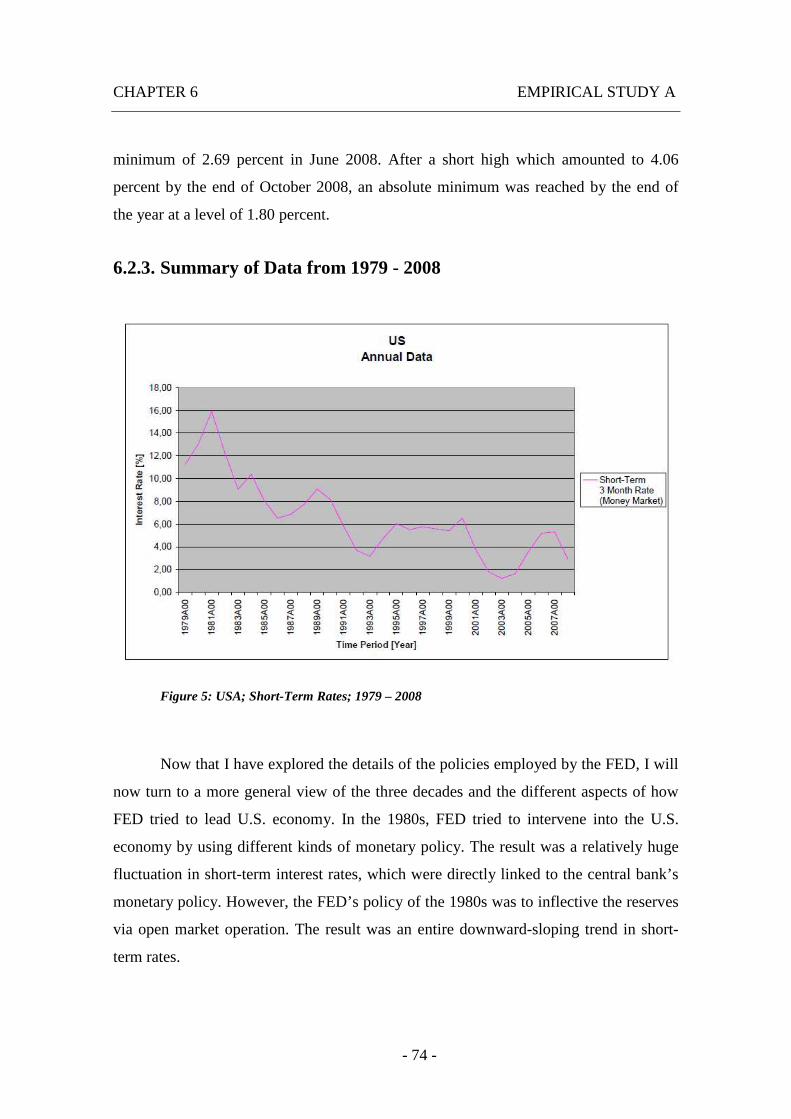
CHAPTER 6 EMPIRICAL STUDY A
- 74 -
minimum of 2.69 percent in June 2008. After a short high which amounted to 4.06
percent by the end of October 2008, an absolute minimum was reached by the end of
the year at a level of 1.80 percent.
6.2.3. Summary of Data from 1979 - 2008
Figure 5: USA; Short-Term Rates; 1979 – 2008
Now that I have explored the details of the policies employed by the FED, I will
now turn to a more general view of the three decades and the different aspects of how
FED tried to lead U.S. economy. In the 1980s, FED tried to intervene into the U.S.
economy by using different kinds of monetary policy. The result was a relatively huge
fluctuation in short-term interest rates, which were directly linked to the central bank’s
monetary policy. However, the FED’s policy of the 1980s was to inflective the reserves
via open market operation. The result was an entire downward-sloping trend in short-
term rates.
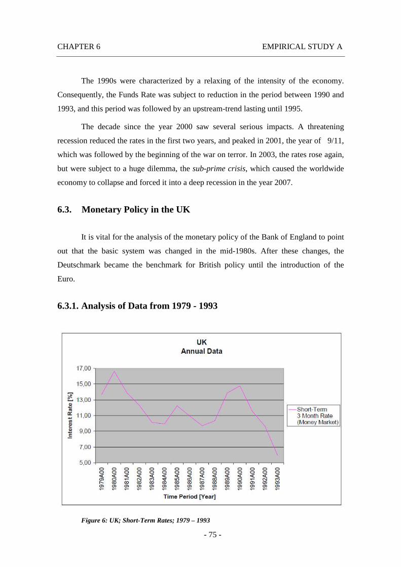
CHAPTER 6 EMPIRICAL STUDY A
- 75 -
The 1990s were characterized by a relaxing of the intensity of the economy.
Consequently, the Funds Rate was subject to reduction in the period between 1990 and
1993, and this period was followed by an upstream-trend lasting until 1995.
The decade since the year 2000 saw several serious impacts. A threatening
recession reduced the rates in the first two years, and peaked in 2001, the year of 9/11,
which was followed by the beginning of the war on terror. In 2003, the rates rose again,
but were subject to a huge dilemma, the sub-prime crisis, which caused the worldwide
economy to collapse and forced it into a deep recession in the year 2007.
6.3. Monetary Policy in the UK
It is vital for the analysis of the monetary policy of the Bank of England to point
out that the basic system was changed in the mid-1980s. After these changes, the
Deutschmark became the benchmark for British policy until the introduction of the
Euro.
6.3.1. Analysis of Data from 1979 - 1993
Figure 6: UK; Short-Term Rates; 1979 – 1993
CHAPTER 6 EMPIRICAL STUDY A
- 76 -
Monetary policy in the UK had not been subject to dramatic changes since
World War II. The main goal in the period until the mid-1980s was to lead and control
the monetary aggregates. The idea was to have suitable aggregates with the desired
effect on the economy in general. Moreover, the quantity of money was to be regulated
via monetary policy. However, it was known that factors like exchange rates,
availability of credit and interest rates also had an enormous significance in this context.
One basic aim in early 1980 was to target a specific monetary growth rate via the
increase of the short-term interest rate up to a level of 16.62 percent in the year 1980.
However, the Bank of England was not certain if factors like nominal income and
monetary growth were that closely connected, and if interest rates would be able to
inhibit monetary growth. During the 1980s, exchange rates were very high. The reason
for this was the fact that there was a relatively high level of interest rates at the
beginning of that decade, and the fact that the UK became a crucial oil producer. By the
end of 1980, short-term rates were reduced to 14.00 percent as a result of decreasing
inflationary pressure. During the year 1982, interest rates fell again to a level of 12.29
percent because of exchange rate concerns and a strictly deflationary budget. In order to
make the whole system more efficient, monetary policy-makers invented a new plan
with the aim to characterize monetary institutions more precisely. The monetary sector
was born. Just like in the U.S. system, all members had to deposit some sort of reserve
into the Bank of England in order to boost the influence over short-term interest rates.
In December 1982, the approaching political elections resulted in short-term interest
rates with a level of 10.13 percent. In the following years, concerns about the value of
specific targets were voiced, and in 1985, it became apparent that monetary policy-
makers were no longer able to target a certain money stock by the use of interest rates.
A reduction in the velocity of money was the result. Finally, in 1986, the Bank of
England declared the period of formal targeting to be finished with accompanying
short-term interest rates of 9.70 percent. It is interesting to note here that the idea of
targeting the rate of growth of money stock by the use of short-term interest rates had its
origin in the 1970s, but was already abandoned in the mid-1980s. The reason for this
CHAPTER 6 EMPIRICAL STUDY A
- 77 -
was the inability of monetary policy-makers to control interest rates efficiently in order
to have a positive impact on the aggregates of money.
There are two different factors which are often used to explain the proceedings
in the first half of the 1980s, and why monetary policy failed in that period: financial
innovation and liability management. I will now turn to the second term for further
elaborations on the matter.
Until the middle of the 1980s, the basic aim consisted of the desire to control the
aggregates of money. This was done via quantity control (direct control) or price
control (market control). Both incentives were meant to influence the desire of the
community to hold deposits, to limit the demand in borrowing, and to restrict the ability
of banks to lend [Bain, K.; Howells P. (2009f)]. The all-overlapping keyword was
deregulation which was characterized by the entry of banks into the mortgage market in
1981.
The then following chapter in this so-called era of monetary targeting was
characterized by deregulation. It began in the year 1981, when banks were entering the
mortgage sector, accompanied by decreasing short-term interest rates with a minimum
of 9.94 percent in 1984. In 1986, the Building Society Act was established, in which
guidelines for funds and their channels were set up. Financial institutions, especially
banks, were entertained which had to pay interest on selected check accounts in the time
between 1983 and the intervention of the act. By the implementation of the act, policy-
makers started to have greater influence on monetary aggregates. Now, however, the
Bank of England wanted to diminish the connection between short-term interest rates
and deposits, yielding a rate of 10.94 percent in 1986.
The basic goal was to eliminate targets which had become irrelevant. Now, the
main aims of policy-makers were declared to be price stability and the minimization of
inflation. In this process, one factor became very prominent in the period to follow: the
exchange rate. Because of the strength of the British Pound, the Bank of England
started a policy which granted a greater extent of independence to the British currency.
As I already pointed out above, the Pound had been linked to the Deutschmark before.
Since 1985, British short-term interest rates were applied on the basis of the connection
between these two currencies, and this was expressed through the exchange rate.

CHAPTER 6 EMPIRICAL STUDY A
- 78 -
Exchange rate targeting was the conception for the following years. Until the year 1987,
the Bank of England was continuously cutting short-term interest rates as far as to the
minimum of 9.70 percent, in order to react to various events like the stock market crash
of October 1987. The problem of inflationary pressure and increasing prices in the
housing sector resulted in an increase of rates, although the British Pound remained to
be a strong currency.
In 1990, the UK became a member in the European Exchange Rate Mechanism
(ERM)29 and the short-term rates reached a maximum of 14.77 percent. In the following
year, an incipient recession emerged accompanied by a cut of the rate to a level of 11.52
percent. Once again, the authenticity of the British Pound in the ERM and the falling
house prices were the origin of the problems. These were represented by decreasing
rates of 9.62 percent in 1992 – the crisis started.
6.3.2. Analysis of Data from 1994 - 2008
Figure 7: UK; Short-Term Rates; 1994 – 2008
29 European Exchange Rate Mechanism: ERM.
CHAPTER 6 EMPIRICAL STUDY A
- 79 -
As I pointed out before, the crisis had its origin in the year 1992, and the
problems which arose after that were the reason why the UK left the ERM. The years
from 1994 to 1996 can be termed the first period of inflation targeting with relatively
big fluctuations in short-term interest rate. In 1997, the need for a greater extent of
independence of the Bank of England led to the establishment of the Bank of England
Act in 1998. Due to the establishment of the act the responsibility of setting interest
rates was given from the Bank of England to a so called Monetary Policy Committee.
In the year 1997, which was characterized by increasing short-term interest rates
up to a level of 7.72 percent, the need for a general European Monetary Union became
apparent. The time from 1998 until 2008, which marks the end of my empirical study,
will be discussed in the following chapter about the Euro Area, as the aims of monetary
policy, as well as the challenges that it was confronted with, were tightly interwoven
with this general topic.
The first big step was the introduction of the Euro currency in 1999, based on
the Maastricht Treaty from 1992, after which it became the only currency inside the
Euro Area resulting in temporarily increasing short-term interest rates in the UK. The
only countries which did not accept the Euro were the UK, Sweden and Denmark. The
UK bargained for special conditions, so to say, with the objective that the British Pound
would persist as official domestic currency. The reason for this can be found in the UK
Treasury evaluation from 1997 to 1998. Generally speaking, the UK was willing to join
the European monetary system, but the results of the five different tests during that
evaluation caused concerns regarding the compatibility of the different systems.
Basically, the skepticism was based on the era of the UK membership in the European
Exchange Rate Mechanism between 1990 and 1992. During that time, the UK economy
went into recession various interest cuttings followed. In the year 1992, the former
Deutsche Bundesbank increased their short-term interest rates and the Bank of England
had to follow in order to hold up the exchange rate of the British Pound against the
Deutschmark because of its exchange rate targeting. This boost in interest rates by the
Deutsche Bundesbank led to worries about an increase of inflation after the German
reunification towards the end of 1989. Thus, the 1997 UK Treasury evaluation reached
CHAPTER 6 EMPIRICAL STUDY A
- 80 -
the conclusion that the British economy seemed to be extremely different from the
remaining European one. That was finally represented by UK short-term interest rates
of 7 to 8 percent in contrast to the European rates between 3 and 4 percent. These
different levels of short-term interest rates seemed to confirm the UK’s fear that
European rates might be too low for the British domestic economy. Moreover, the
following inflationary boom discouraged an entry into the European system.
Between 2002 and 2003, another evaluation was carried out by the UK Treasury.
Once again, the predominating argument by the British was that the domestic economy
as a whole might be incompatible to the economies from other member-states regarding
variables like taxes, wages, production and selling. However, critics argued that the
British evaluation did not take some important geographic areas of their own country
into account, and therefore they advocated an observation from another point of view.
In connection with the British labor market flexibility, one particular result came to the
surface: “The slower the progress in flexibility within the rest of the Euro Area, the
more important a high level of domestic labor market flexibility in the UK.” [Bain, K.;
Howells P. (2009g)].
In 2001, the huge impact of the terror attacks in the USA left its traces in the
UK, as short-term interest rates achieved a level of 4.05 percent towards the end of that
year, but were then followed by a short recovery.
There had not been another evaluation since 2003, but the situation remained the
same: the Bank of England still competed against the European Central Bank in terms
of monetary policy. In 2008, the Bank of England announced that a new evaluation of
the business cycle through the UK Treasury would lead to the result that British
economy now tended to be closer to the European one. This proximity would be
expressed via UK inflation rates which came closer to European inflation rates, and by a
British growth rate of more or less the same level as in the year 2004.
Nevertheless, there was a serious problem in short-term interest rates. As I
already mentioned before, the UK rates had levels higher than those in the rest of the
Euro Area. European supporters in the UK stressed that this was the result of the
credibility-problem of the monetary policy of the Bank of England, and that an entrance

CHAPTER 6 EMPIRICAL STUDY A
- 81 -
into the Euro Area would lead to a remaining inflation rate, but at the same time to a
lower level of interest rates.
Some argued that the British Pound was too high against the Euro, and that an
entrance into the Euro Area at such an exchange rate would lead to problems in terms
of a long-term development in the UK.
Finally it can be mentioned that for the supporters of an inclusion of the UK in
the Euro Area, the year 2008 would have been the best year ever with a UK short-term
interest rate of 4.25 percent towards the end of that year – not that far away from the
European rate of 4.24 percent.
6.3.3. Summary of Data from 1979 - 2008
Figure 8: UK; Short-Term Rates; 1979 – 2008
In order to summarize my analysis of the UK data, I would like to point out
some of my findings. Prior to the 1980s, the plan of fixed income regimes failed and
was followed by a so-called active monetarism. This incentive was characterized by the
aim to control money.
CHAPTER 6 EMPIRICAL STUDY A
- 82 -
In the early 1980s, up until 1985, the limitation of monetary growth was a big
challenge. It was conducted by scheduling target rates in order to give more credibility
to commitment. The consequence was the insufficiency of interest rate instruments.
In 1986, the system changed its priorities and turned into an exchange rate
targeting system, but only until 1992, when the UK left the European Exchange Rate
Mechanism. The current goal in this modern period of monetarism is inflation rate
targeting. In 1997, first indications towards a European Monetary Union with a system
based on the one by the Deutsche Bundesbank appeared.
What is most important in this context, however, is that since 2003, UK short-
term interest rates were always kept at a higher level than the European rates in order to
defend the exchange rate risk of the British Pound. This exchange rate risk was
measured via the connection to the Deutschmark, and later to the Euro. An entry of the
Euro Area would have led to a decrease of the cost of capital for British companies
however the critics had always been stronger than the supporters.
At the end of the decade, even Euro-pessimists had to admit that an entrance into
the Euro Area with all its regulations would lead, with a relatively high probability, to
an increase in quality and quantity of investment in the UK.
6.4. Monetary Policy in the Euro Area
Before I start my analysis of the Euro Area, I would like to point to the fact that
the data related to events before 1993 was obtained from the former Deutsche
Bundesbank and therefore relates primarily to Germany. For the remaining data from
the years 1994 to 2008, I based my analysis on the European Area and the European
Central Bank. Furthermore, this period of time is dealt with in a more detailed manner
because of the topicality of my findings.
After the Euro Area was born, the introduction of the Euro as the unitary
currency followed in 1999. Generally speaking, the European System of Central Banks
(ESCB)30 consists of the central banks of all member states, which are guided and led
30 European System of Central Banks: ESCB.
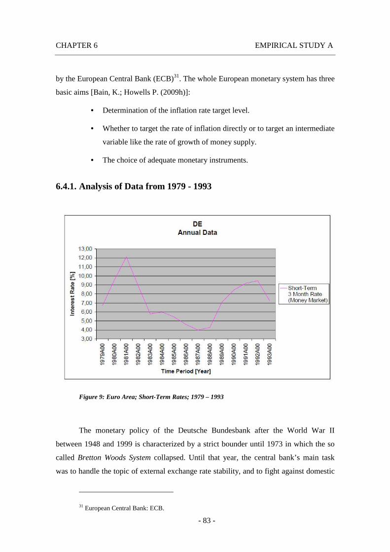
CHAPTER 6 EMPIRICAL STUDY A
- 83 -
by the European Central Bank (ECB)31. The whole European monetary system has three
basic aims [Bain, K.; Howells P. (2009h)]:
• Determination of the inflation rate target level.
• Whether to target the rate of inflation directly or to target an intermediate
variable like the rate of growth of money supply.
• The choice of adequate monetary instruments.
6.4.1. Analysis of Data from 1979 - 1993
Figure 9: Euro Area; Short-Term Rates; 1979 – 1993
The monetary policy of the Deutsche Bundesbank after the World War II
between 1948 and 1999 is characterized by a strict bounder until 1973 in which the so
called Bretton Woods System collapsed. Until that year, the central bank’s main task
was to handle the topic of external exchange rate stability, and to fight against domestic
31 European Central Bank: ECB.
CHAPTER 6 EMPIRICAL STUDY A
- 84 -
inflation. Since 1973, the new aim of the Deutsche Bundesbank was the control and
guidance of domestic price stability.
From the mid-1970s onwards, German policy-makers had to counter the rising
inflation by an increase of the short-term interest rate. At that time, monetary policy was
quite successful, and the German government supported the Bundesbank in its policies
with the result of minimizing inflation. The oil crisis in the late 1970s was the reason for
the establishment of a tougher monetary policy. Moreover, criticism regarding the
alleged boost of the recession of 1980 to 1981 arose. In those years the short-term
interest level reaches a level of 12.11 percent. By the end of 1981, the interest rate level
was dropping even more.
The following period was characterized by decreasing interest rates. They fell
until they reached a minimum of 3.99 percent in 1987. The second half of the 1980s
was characterized by a cagey slow-down of the business cycle and by a reduction of
pressure on inflation. The Bundesbank reformed its monetary policy system and open
market instruments became more important.
By the end of the 1980s, the level of short-term interest rates increased, and
reached 8.43 percent in the year 1990. The German reunification also had a deep impact
on the increase of interest rates in 1989 and in 1990.
As I already pointed out in the last chapter, the Maastricht Act was designed in
1992. Its basic objective was to guarantee and support the European Union with a
unified economy and a common currency. This is represented by a 1992 short-term
interest rate of 9.46 percent.
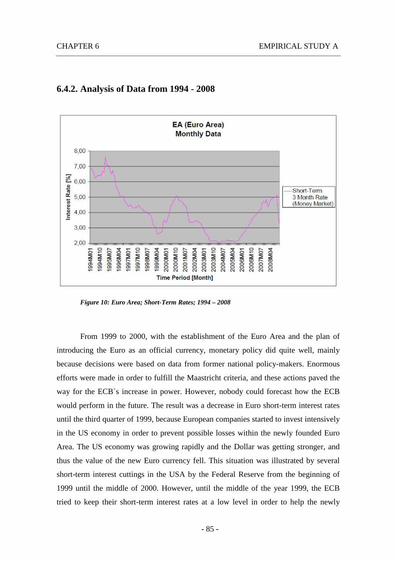
CHAPTER 6 EMPIRICAL STUDY A
- 85 -
6.4.2. Analysis of Data from 1994 - 2008
Figure 10: Euro Area; Short-Term Rates; 1994 – 2008
From 1999 to 2000, with the establishment of the Euro Area and the plan of
introducing the Euro as an official currency, monetary policy did quite well, mainly
because decisions were based on data from former national policy-makers. Enormous
efforts were made in order to fulfill the Maastricht criteria, and these actions paved the
way for the ECB`s increase in power. However, nobody could forecast how the ECB
would perform in the future. The result was a decrease in Euro short-term interest rates
until the third quarter of 1999, because European companies started to invest intensively
in the US economy in order to prevent possible losses within the newly founded Euro
Area. The US economy was growing rapidly and the Dollar was getting stronger, and
thus the value of the new Euro currency fell. This situation was illustrated by several
short-term interest cuttings in the USA by the Federal Reserve from the beginning of
1999 until the middle of 2000. However, until the middle of the year 1999, the ECB
tried to keep their short-term interest rates at a low level in order to help the newly

CHAPTER 6 EMPIRICAL STUDY A
- 86 -
united European economy in its starting phase. The rates decreased from initially 3.14
percent to 2.63 percent by July in that year. In October the rates started to increase
rapidly although the inflation rate lasted unchanged
In 2000, the ECB also increased their short-term rates, and was willing to
support the Euro currency with the aid of Japan and the USA. The effect, however, was
minimal, and thus the rates did not change dramatically over the next short period. In
October 2000, the US became aware of a threatening recession, which could have
affected the economy on a global scale. The inflation rates were under pressure and the
situation in the oil market deteriorated, and so the Federal Reserve started to cut down
interest rates in an aggressive manner. The reactions of the ECB were slow, but it
followed via a monetary policy in the end.
In 2001, the FED cut down its rates, however, the ECB did nothing and kept its
rates untouched because monetary growth rose with a short-term interest rate of 4.35
percent in August. The terror attacks of September 2001 functioned as a catalyst for a
worldwide recession. The ECB reacted and decreased the rates to a level of 3.98
percent. It was argued by critics that in comparison to US monetary policy-makers, the
ECB reacted too slowly to the fear of a world-wide recession after 9/11. The September
rates amounted to 3.56 percent in the USA and 5.00 percent in the UK. Even the Bank
of England reacted to the new situation although the domestic economy was better off
than the European one.
The year 2002 did not bring any interesting changes in the policy making
strategy of the ECB. However, European rates were cut down to a level of 2.94 percent
by the end of December, but this decrease did not have the desired impact on the
economic situation. The Euro followed its upward trend in value.
In 2003, further cuttings were conducted, and this was illustrated by rates of 2.15
percent in the Euro Area, and 1.11 percent in the USA. The Federal Funds Rate was
close to 1.00 percent for the very first time in its history, and the Euro still increased its
value.
The year 2004 brought little difference in the situation. Now the interest rates
increased again, the US rates increased by 1.50 percent, the UK rates by 4.79 percent,
and in continental Europe by 2.11 percent. Once again, the ECB did not follow the
CHAPTER 6 EMPIRICAL STUDY A
- 87 -
policy of other central banks in a sufficient way, and only kept its rates in a range
between 2.09 and 2.17 percent with no extensive upward movements. Although the
FED increased the short-term interest rates, the US Dollar was weak. In October 2004,
for the first time in history, the US rate became higher than the European one, and this
resulted in November-levels of 2.31 percent in the USA and only 2.17 percent in the
Euro Area. The ECB reacted to these developments, and argued that further upward
movements of short-term interest rate levels would only put pressure on the Euro
currency.
This situation continued in 2005. The political pressure on the ECB’s strategy
related to its monetary policy increased dramatically by the end of that year, and led to
several interest rate mark-ups with a level of 3.68 percent by December 2005.
This trend continued in 2006 and in 2007. Both the ECB and the FED increased
their rates, which were framed by a weak Dollar and a strong Euro. In June 2007 (with
an Euro rate of 4.15 percent) another serious problem arose: the sub-prime crisis and the
credit crunch, with its origin in the US system, emerged. Suddenly, the fear of a
worldwide recession spread from Europe to the rest of the world. The FED tried to
react, and cut down its short-term rate resulting in a huge pressure on the US Dollar
and, once more, in an increase in the value of the Euro. In January 2008, the European
short-term interest rate with a level of 4.48 percent exceeded the US rate of 3.92 percent
for the first time. Other demographic effects were, for example, the rising prices in the
food and oil sector.
Of all these events and implemented measures, the trend of inflation targeting set
by the ECB was, and still is, the most important of all actions. Moreover, the worldwide
recession with its origin in the US financial sector had, and also still has, a huge
influence on the behavior of central banks.
The trend of European short-term interest rates was dramatically sloping
downward during the 1990s, and until the introduction of the Euro as the official
currency in Europe.
In 2001, the terror attacks on the World Trade Center and on the Pentagon were
followed by a worldwide recession which lasted until 2004, when monetary policy tried
to calm down the economy. Consequently, the interest rate increased. Then the sub-
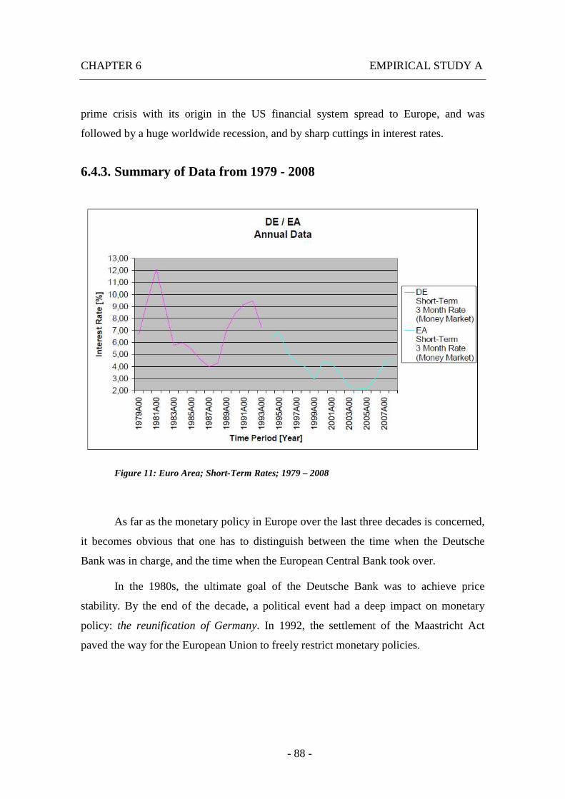
CHAPTER 6 EMPIRICAL STUDY A
- 88 -
prime crisis with its origin in the US financial system spread to Europe, and was
followed by a huge worldwide recession, and by sharp cuttings in interest rates.
6.4.3. Summary of Data from 1979 - 2008
Figure 11: Euro Area; Short-Term Rates; 1979 – 2008
As far as the monetary policy in Europe over the last three decades is concerned,
it becomes obvious that one has to distinguish between the time when the Deutsche
Bank was in charge, and the time when the European Central Bank took over.
In the 1980s, the ultimate goal of the Deutsche Bank was to achieve price
stability. By the end of the decade, a political event had a deep impact on monetary
policy: the reunification of Germany. In 1992, the settlement of the Maastricht Act
paved the way for the European Union to freely restrict monetary policies.
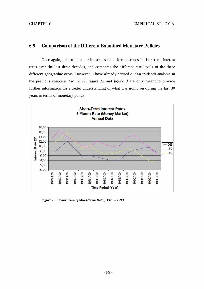
CHAPTER 6 EMPIRICAL STUDY A
- 89 -
6.5. Comparison of the Different Examined Monetary Policies
Once again, this sub-chapter illustrates the different trends in short-term interest
rates over the last three decades, and compares the different rate levels of the three
different geographic areas. However, I have already carried out an in-depth analysis in
the previous chapters. Figure 11, figure 12 and figure13 are only meant to provide
further information for a better understanding of what was going on during the last 30
years in terms of monetary policy.
Figure 12: Comparison of Short-Term Rates; 1979 – 1993
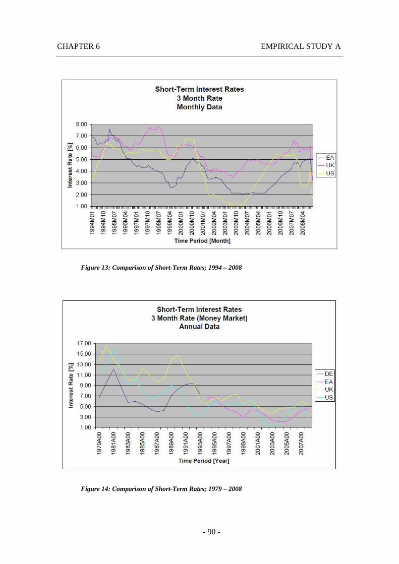
CHAPTER 6 EMPIRICAL STUDY A
- 90 -
Figure 13: Comparison of Short-Term Rates; 1994 – 2008
Figure 14: Comparison of Short-Term Rates; 1979 – 2008

- 91 -
7. Empirical Study B
7.1. Overview of Long-Term Interest Rates
As I already mentioned in chapter 5, the connection between short-term and
long-term interest rates is quite obvious. In the money market (financial market), short-
term interest rates are regulated by central banks through monetary policy. In the capital
market (real market), the long-term interest rates are influenced by the equilibrium
between the supply and demand in the bond market.
In figure 17, the declining trend illustrates the situation during the three
decades. As I already illustrated, short-term interest rates have an impact on economic
growth, on the rate of inflation and on benefit, which is illustrated by the long-term 10-
year government bond.
In 2009 Löchel explained some important facts which are also shown in the
following three figures [Löchel, H. (2009a)]:
• An increase of households in wealth and income leads to an increase in
demand of bonds. Therefore a given bond supply rises the prices and
reduces the return and vice versa.
• Expectations of benefits by firms increase the supply of bonds which
leads into deflation and a higher return because more capital is needed
and vice versa.
• An increase in the expectations of interest rates is accompanied by a
reduction in the bond demand, by falling prices and by a rising demand
of bonds and vice versa.
• The result of rising expectations in inflation rate are followed by a
reduction in demand of bonds and the resulting cheap refinancing costs
yield an increase in the supply of bonds and vice versa.
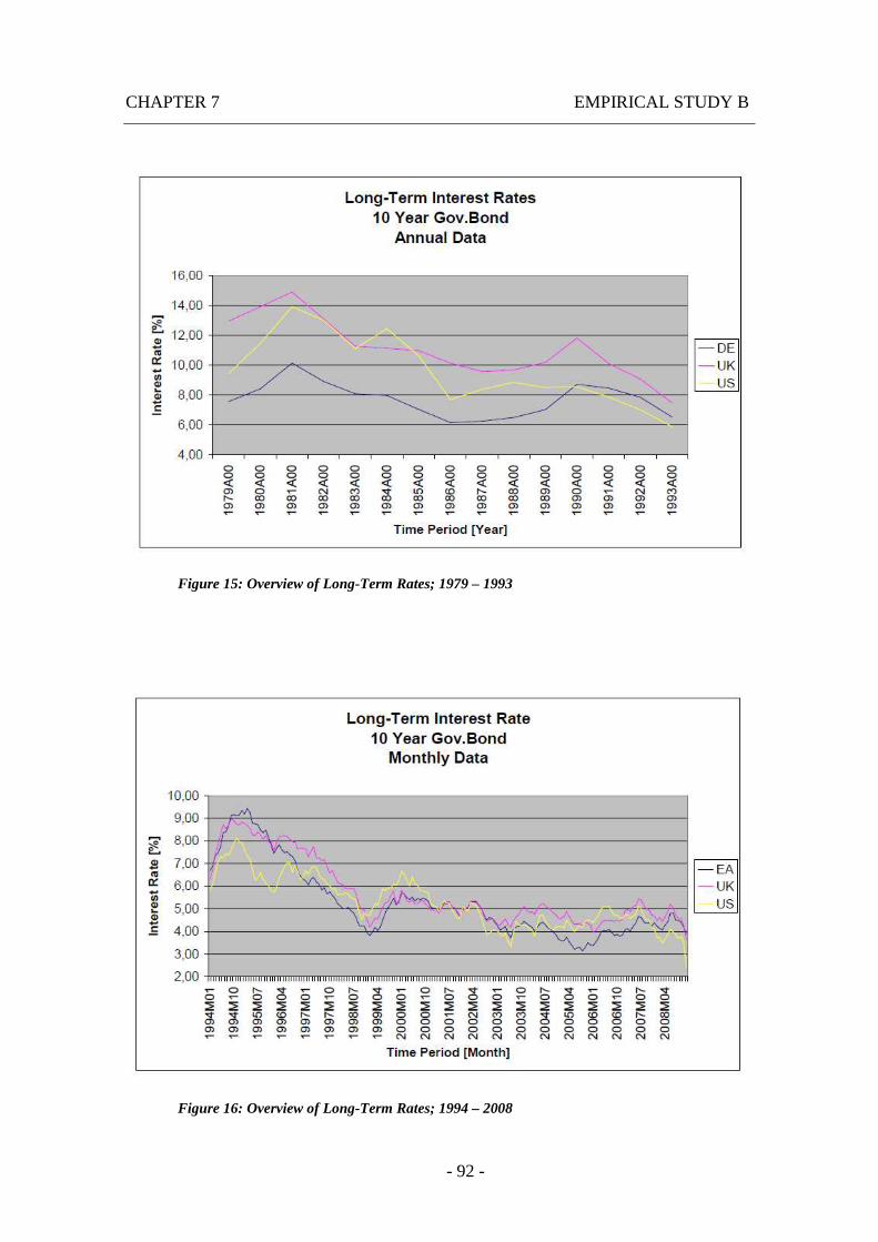
CHAPTER 7 EMPIRICAL STUDY B
- 92 -
Figure 15: Overview of Long-Term Rates; 1979 – 1993
Figure 16: Overview of Long-Term Rates; 1994 – 2008
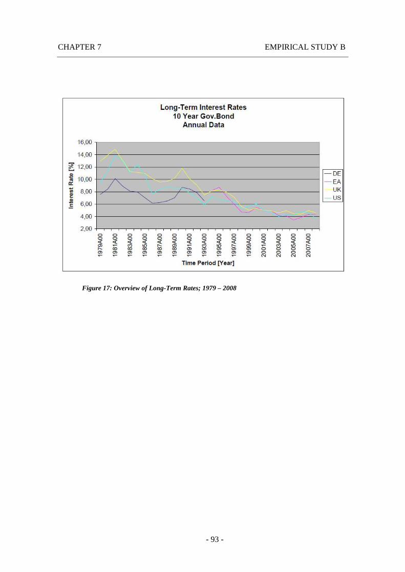
CHAPTER 7 EMPIRICAL STUDY B
- 93 -
Figure 17: Overview of Long-Term Rates; 1979 – 2008

CHAPTER 7 EMPIRICAL STUDY B
- 94 -
7.2. Short-Term vs. Long-Term Interest Rates in the USA
Figure 18: USA; Short-Term vs. Long-Term Rates; 1979 – 1993
Figure 18 shows the development of short-term and long-term interest rates
during the 1980s. In terms of short-term interest rates, this era was characterized by
relatively high fluctuations in the rate and various level cuts.
Generally, it can be stressed that increasing short-term interest rates in the
money market lead to increasing long-term interest rates in the capital market. This is
followed by rising prices for capital, and these also increase the demand in the goods
market with congruent effects for the price level, and vice versa.
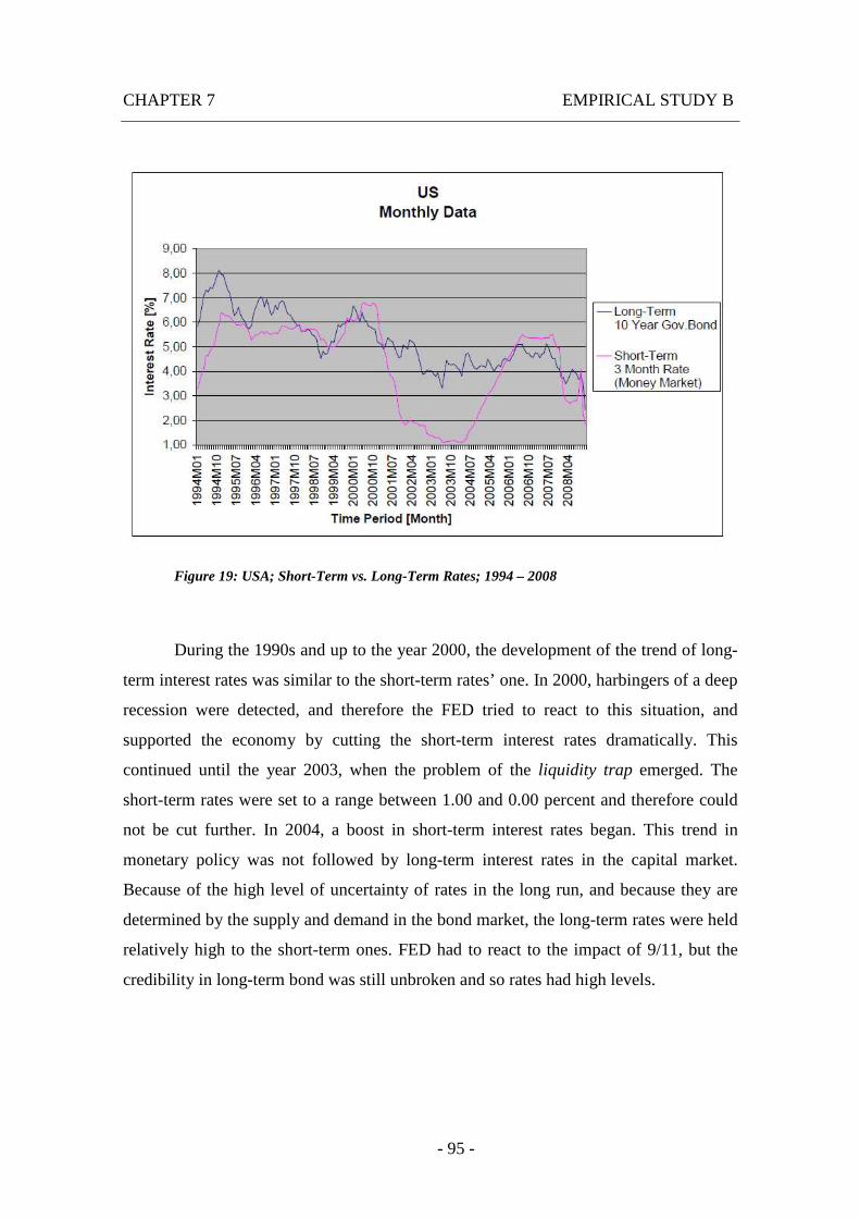
CHAPTER 7 EMPIRICAL STUDY B
- 95 -
Figure 19: USA; Short-Term vs. Long-Term Rates; 1994 – 2008
During the 1990s and up to the year 2000, the development of the trend of long-
term interest rates was similar to the short-term rates’ one. In 2000, harbingers of a deep
recession were detected, and therefore the FED tried to react to this situation, and
supported the economy by cutting the short-term interest rates dramatically. This
continued until the year 2003, when the problem of the liquidity trap emerged. The
short-term rates were set to a range between 1.00 and 0.00 percent and therefore could
not be cut further. In 2004, a boost in short-term interest rates began. This trend in
monetary policy was not followed by long-term interest rates in the capital market.
Because of the high level of uncertainty of rates in the long run, and because they are
determined by the supply and demand in the bond market, the long-term rates were held
relatively high to the short-term ones. FED had to react to the impact of 9/11, but the
credibility in long-term bond was still unbroken and so rates had high levels.
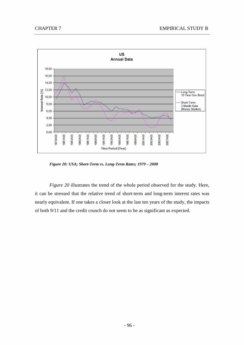
CHAPTER 7 EMPIRICAL STUDY B
- 96 -
Figure 20: USA; Short-Term vs. Long-Term Rates; 1979 – 2008
Figure 20 illustrates the trend of the whole period observed for the study. Here,
it can be stressed that the relative trend of short-term and long-term interest rates was
nearly equivalent. If one takes a closer look at the last ten years of the study, the impacts
of both 9/11 and the credit crunch do not seem to be as significant as expected.
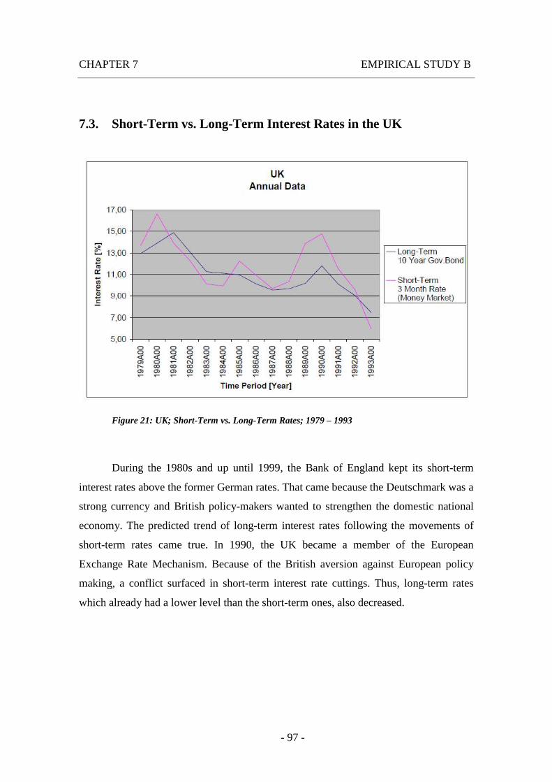
CHAPTER 7 EMPIRICAL STUDY B
- 97 -
7.3. Short-Term vs. Long-Term Interest Rates in the UK
Figure 21: UK; Short-Term vs. Long-Term Rates; 1979 – 1993
During the 1980s and up until 1999, the Bank of England kept its short-term
interest rates above the former German rates. That came because the Deutschmark was a
strong currency and British policy-makers wanted to strengthen the domestic national
economy. The predicted trend of long-term interest rates following the movements of
short-term rates came true. In 1990, the UK became a member of the European
Exchange Rate Mechanism. Because of the British aversion against European policy
making, a conflict surfaced in short-term interest rate cuttings. Thus, long-term rates
which already had a lower level than the short-term ones, also decreased.
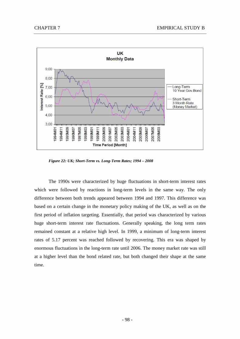
CHAPTER 7 EMPIRICAL STUDY B
- 98 -
Figure 22: UK; Short-Term vs. Long-Term Rates; 1994 – 2008
The 1990s were characterized by huge fluctuations in short-term interest rates
which were followed by reactions in long-term levels in the same way. The only
difference between both trends appeared between 1994 and 1997. This difference was
based on a certain change in the monetary policy making of the UK, as well as on the
first period of inflation targeting. Essentially, that period was characterized by various
huge short-term interest rate fluctuations. Generally speaking, the long term rates
remained constant at a relative high level. In 1999, a minimum of long-term interest
rates of 5.17 percent was reached followed by recovering. This era was shaped by
enormous fluctuations in the long-term rate until 2006. The money market rate was still
at a higher level than the bond related rate, but both changed their shape at the same
time.
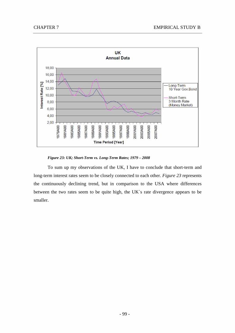
CHAPTER 7 EMPIRICAL STUDY B
- 99 -
Figure 23: UK; Short-Term vs. Long-Term Rates; 1979 – 2008
To sum up my observations of the UK, I have to conclude that short-term and
long-term interest rates seem to be closely connected to each other. Figure 23 represents
the continuously declining trend, but in comparison to the USA where differences
between the two rates seem to be quite high, the UK`s rate divergence appears to be
smaller.
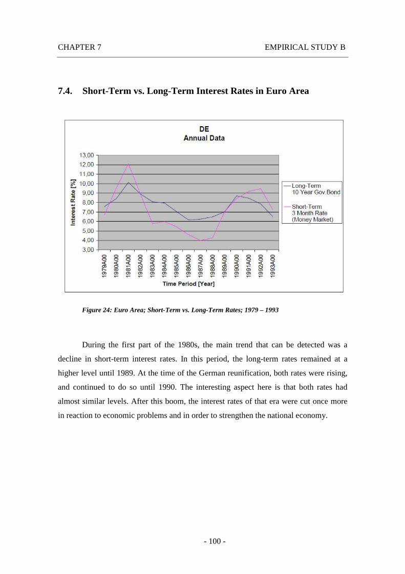
CHAPTER 7 EMPIRICAL STUDY B
- 100 -
7.4. Short-Term vs. Long-Term Interest Rates in Euro Area
Figure 24: Euro Area; Short-Term vs. Long-Term Rates; 1979 – 1993
During the first part of the 1980s, the main trend that can be detected was a
decline in short-term interest rates. In this period, the long-term rates remained at a
higher level until 1989. At the time of the German reunification, both rates were rising,
and continued to do so until 1990. The interesting aspect here is that both rates had
almost similar levels. After this boom, the interest rates of that era were cut once more
in reaction to economic problems and in order to strengthen the national economy.
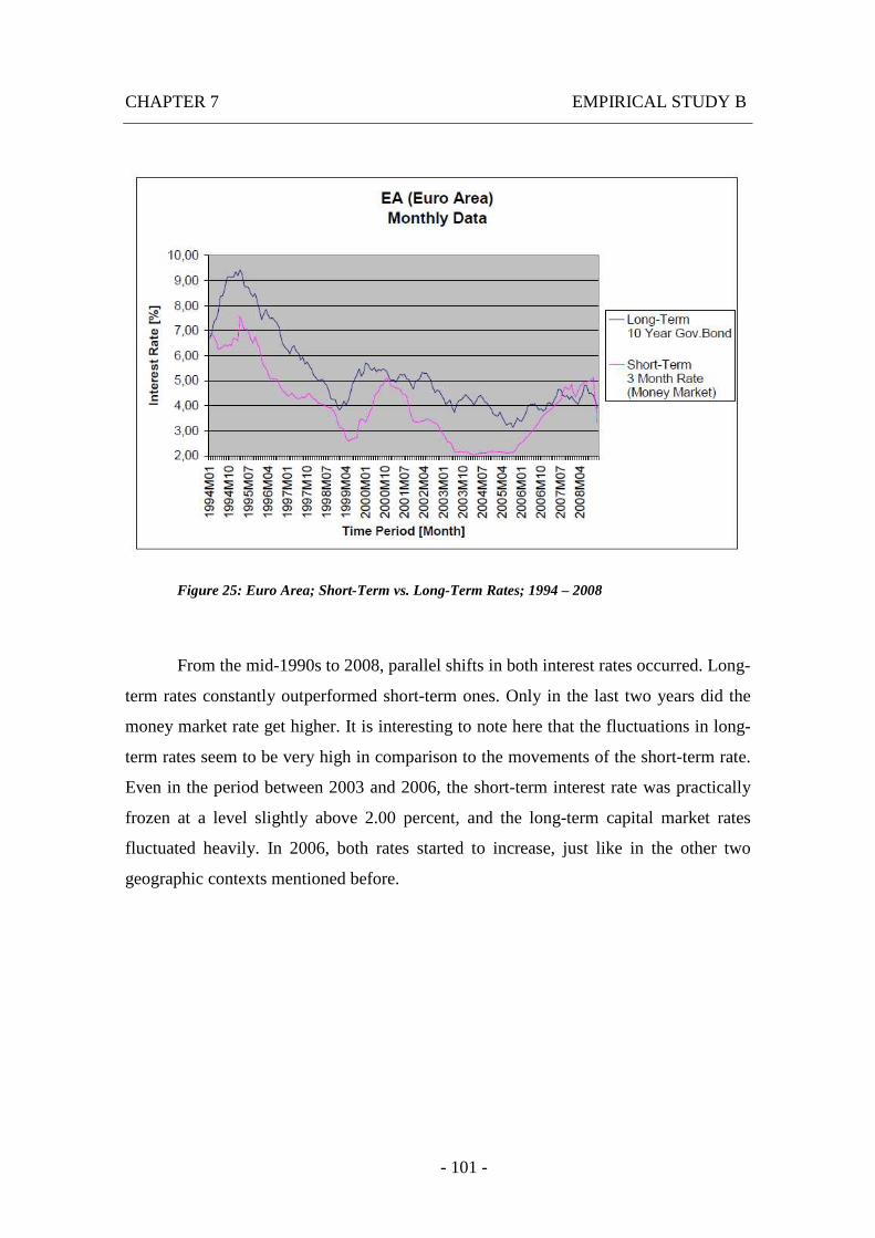
CHAPTER 7 EMPIRICAL STUDY B
- 101 -
Figure 25: Euro Area; Short-Term vs. Long-Term Rates; 1994 – 2008
From the mid-1990s to 2008, parallel shifts in both interest rates occurred. Long-
term rates constantly outperformed short-term ones. Only in the last two years did the
money market rate get higher. It is interesting to note here that the fluctuations in long-
term rates seem to be very high in comparison to the movements of the short-term rate.
Even in the period between 2003 and 2006, the short-term interest rate was practically
frozen at a level slightly above 2.00 percent, and the long-term capital market rates
fluctuated heavily. In 2006, both rates started to increase, just like in the other two
geographic contexts mentioned before.
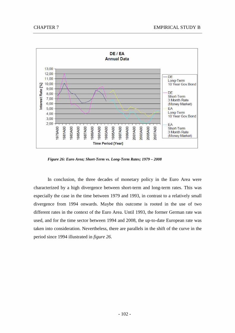
CHAPTER 7 EMPIRICAL STUDY B
- 102 -
Figure 26: Euro Area; Short-Term vs. Long-Term Rates; 1979 – 2008
In conclusion, the three decades of monetary policy in the Euro Area were
characterized by a high divergence between short-term and long-term rates. This was
especially the case in the time between 1979 and 1993, in contrast to a relatively small
divergence from 1994 onwards. Maybe this outcome is rooted in the use of two
different rates in the context of the Euro Area. Until 1993, the former German rate was
used, and for the time sector between 1994 and 2008, the up-to-date European rate was
taken into consideration. Nevertheless, there are parallels in the shift of the curve in the
period since 1994 illustrated in figure 26.
- 103 -
8. Conclusion
In the context of this work, I tried to give an overview of monetary policy in
three main geographic areas, and I attempted to combine my results with theoretical
approaches. The main challenges were the collection of data for the empirical study, the
difference between short-term and long-term interest rates, and the question of rate
selection. I have to admit that the collection of data turned out to be tougher than I
thought, mainly because data sets about the time prior to 1985 are very difficult to
obtain. The first challenge was to browse the internet for websites of central banks, and
to collect enough material for my work. After I had obtained the basic data for my
empirical study, I still had to do research concerning the topic of monetary policy. Here,
I primarily focused on the article by Hicks from 1935. It is interesting to note that he
thought about issues like the connection between economic factors and their interaction
within a national economy as early as in 1935.
The Taylor rule is the second pillar of this work so to speak. First, I learned
about the original one, and then I discovered the more modern and future-oriented
theory, which argues that severe mistakes were made for decades. To me, it seems a bit
blue-eyed to base a framework like the original version of the Taylor Rule only on
historical data, as we live in a world of a dynamic economy nowadays. Thus, I
concentrated on the future-oriented theory, which takes more factors into account.
Chapter 4 serves as a basis for my work, as it explains the structure of monetary
policy, and therefore helps the reader to gain some insight into the topic. To me, it
seemed impossible to be able to distinguish between short-term and long-term interest
rates without knowing anything about monetary policy-makers. Once I was able to
differentiate between money market and capital market, it was easy to understand how
short-term and long-term interest rates interact.
In my view, another important aspect is in which markets the different rates are
settled. The short-term interest rate is connected to the money market (financial market)
and is constituted by the central bank. The long-term interest rate belongs to the capital
market in which the supply and demand for bonds determine the level of the rate.
CHAPTER 8 CONCLUSION
- 104 -
The empirical data analysis underlines the effects of different targeting within
monetary policy making. I pointed out in my work that nearly each period had its own
targets, and I demonstrated that central banks used to experiment with their policies.
Moreover, I believe that the figures in the last two chapters enhanced my explanations
even more. Important events in the 30-year period covered by this paper were, for
example, the UK membership in the European Exchange Rate Mechanism, the
implementation of the Maastricht Act, the German reunification, the introduction of the
Euro as an official currency, 9/11, and finally the worldwide recession.
To me, monetary policy seems to be a valuable instrument to influence a
national economy. But I think it cannot be the only tool to set interest rates because its
limits have already been reached. For instance, in 2003 when the level of short-term
interest rate was near zero percent in the USA, the FED was unable to react. I believe an
option model should be implemented to support and control the activities of central
banks.
Furthermore, an exact definition of the connection between long-term and short-
term interest rates is also a tough challenge. Generally speaking, long-term rates tend to
follow the trend of short-term rates, but in certain periods they act differently. In
Chapter 7, I portrayed several approaches which deal with the way variables interact
within a national economy. Via the IS-LM model, the interception between the two
curves can be classified.
On a personal level, central banks and their monetary policies bear a frightful
potential. The consequences of their business, whether successful or not, cannot be
estimated so easily. On the one hand, central banks are seemingly able to improve the
economies of countries, but on the other hand, they are unable to react and remain
passive. This dilemma is expressed by the liquidity trap and by the investment trap.
Finally I have to admit that this thesis does not provide any new information on
monetary policy, but rather illustrates the policy of central banks of the last three
decades. Essentially, my paper consists of discussions of dependencies of financial
variables.
CHAPTER 8 CONCLUSION
- 105 -
I hope my thesis contributes to the work that has already been published in order
to provide a valuable interpretation of monetary policy, and the connection between
short-term a long-term interest rates.

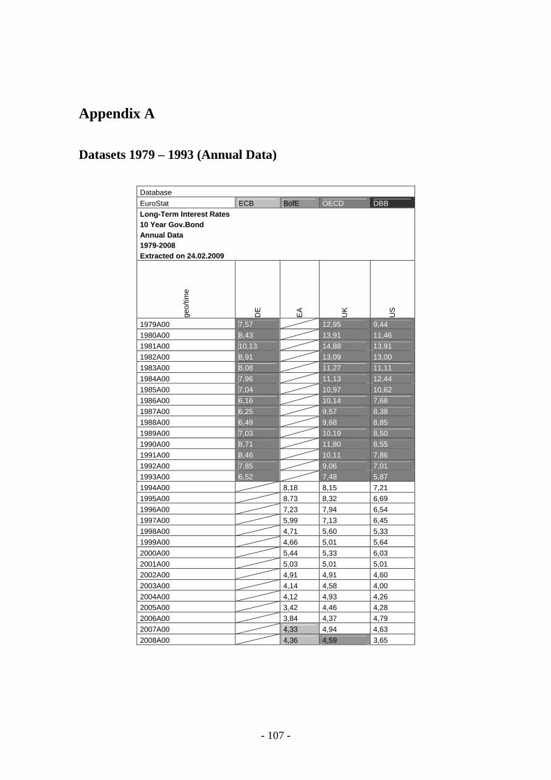
- 107 -
Appendix A
Datasets 1979 – 1993 (Annual Data)
Database
EuroStat ECB BofE OECD DBB
Long-Term Interest Rates 10 Year Gov.Bond Annual Data 1979-2008 Extracted on 24.02.2009
geo/
time
DE
EA
UK
US
1979A00 7,57 12,95 9,44
1980A00 8,43 13,91 11,46
1981A00 10,13 14,88 13,91
1982A00 8,91 13,09 13,00
1983A00 8,08 11,27 11,11
1984A00 7,96 11,13 12,44
1985A00 7,04 10,97 10,62
1986A00 6,16 10,14 7,68
1987A00 6,25 9,57 8,38
1988A00 6,49 9,68 8,85
1989A00 7,03 10,19 8,50
1990A00 8,71 11,80 8,55
1991A00 8,46 10,11 7,86
1992A00 7,85 9,06 7,01
1993A00 6,52 7,48 5,87
1994A00 8,18 8,15 7,21
1995A00 8,73 8,32 6,69
1996A00 7,23 7,94 6,54
1997A00 5,99 7,13 6,45
1998A00 4,71 5,60 5,33
1999A00 4,66 5,01 5,64
2000A00 5,44 5,33 6,03
2001A00 5,03 5,01 5,01
2002A00 4,91 4,91 4,60
2003A00 4,14 4,58 4,00
2004A00 4,12 4,93 4,26
2005A00 3,42 4,46 4,28
2006A00 3,84 4,37 4,79
2007A00 4,33 4,94 4,63
2008A00 4,36 4,59 3,65
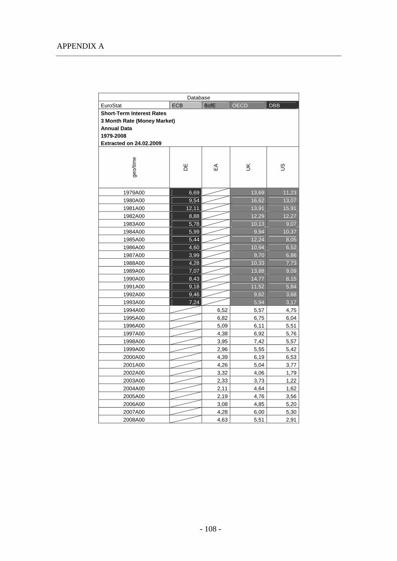
APPENDIX A
- 108 -
Database
EuroStat ECB BofE OECD DBB
Short-Term Interest Rates 3 Month Rate (Money Market) Annual Data 1979-2008 Extracted on 24.02.2009
geo/
time
DE
EA
UK
US
1979A00 6,69 13,69 11,23
1980A00 9,54 16,62 13,07
1981A00 12,11 13,91 15,91
1982A00 8,88 12,29 12,27
1983A00 5,78 10,13 9,07
1984A00 5,99 9,94 10,37
1985A00 5,44 12,24 8,05
1986A00 4,60 10,94 6,52
1987A00 3,99 9,70 6,86
1988A00 4,28 10,33 7,73
1989A00 7,07 13,88 9,09
1990A00 8,43 14,77 8,15
1991A00 9,18 11,52 5,84
1992A00 9,46 9,62 3,68
1993A00 7,24 5,94 3,17
1994A00 6,52 5,57 4,75
1995A00 6,82 6,75 6,04
1996A00 5,09 6,11 5,51
1997A00 4,38 6,92 5,76
1998A00 3,95 7,42 5,57
1999A00 2,96 5,55 5,42
2000A00 4,39 6,19 6,53
2001A00 4,26 5,04 3,77
2002A00 3,32 4,06 1,79
2003A00 2,33 3,73 1,22
2004A00 2,11 4,64 1,62
2005A00 2,19 4,76 3,56
2006A00 3,08 4,85 5,20
2007A00 4,28 6,00 5,30
2008A00 4,63 5,51 2,91
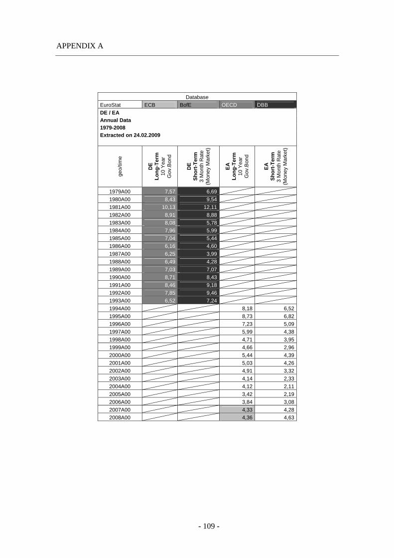
APPENDIX A
- 109 -
Database
EuroStat ECB BofE OECD DBB
DE / EA Annual Data 1979-2008 Extracted on 24.02.2009
geo/
time
DE
L
on
g-T
erm
10
Yea
r G
ov.B
ond
DE
S
ho
rt-T
erm
3
Mon
th R
ate
(Mon
ey M
arke
t)
EA
L
on
g-T
erm
10
Yea
r G
ov.B
ond
EA
S
ho
rt-T
erm
3
Mon
th R
ate
(Mon
ey M
arke
t)
1979A00 7,57 6,69
1980A00 8,43 9,54
1981A00 10,13 12,11
1982A00 8,91 8,88
1983A00 8,08 5,78
1984A00 7,96 5,99
1985A00 7,04 5,44
1986A00 6,16 4,60
1987A00 6,25 3,99
1988A00 6,49 4,28
1989A00 7,03 7,07
1990A00 8,71 8,43
1991A00 8,46 9,18
1992A00 7,85 9,46
1993A00 6,52 7,24
1994A00 8,18 6,52
1995A00 8,73 6,82
1996A00 7,23 5,09
1997A00 5,99 4,38
1998A00 4,71 3,95
1999A00 4,66 2,96
2000A00 5,44 4,39
2001A00 5,03 4,26
2002A00 4,91 3,32
2003A00 4,14 2,33
2004A00 4,12 2,11
2005A00 3,42 2,19
2006A00 3,84 3,08
2007A00 4,33 4,28
2008A00 4,36 4,63
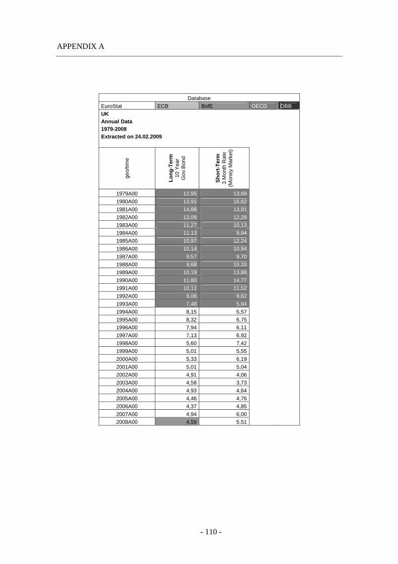
APPENDIX A
- 110 -
Database
EuroStat ECB BofE OECD DBB
UK Annual Data 1979-2008 Extracted on 24.02.2009
geo/
time
Lo
ng
-Ter
m
10 Y
ear
Gov
.Bon
d
Sh
ort
-Ter
m
3 M
onth
Rat
e (M
oney
Mar
ket)
1979A00 12,95 13,69
1980A00 13,91 16,62
1981A00 14,88 13,91
1982A00 13,09 12,29
1983A00 11,27 10,13
1984A00 11,13 9,94
1985A00 10,97 12,24
1986A00 10,14 10,94
1987A00 9,57 9,70
1988A00 9,68 10,33
1989A00 10,19 13,88
1990A00 11,80 14,77
1991A00 10,11 11,52
1992A00 9,06 9,62
1993A00 7,48 5,94
1994A00 8,15 5,57
1995A00 8,32 6,75
1996A00 7,94 6,11
1997A00 7,13 6,92
1998A00 5,60 7,42
1999A00 5,01 5,55
2000A00 5,33 6,19
2001A00 5,01 5,04
2002A00 4,91 4,06
2003A00 4,58 3,73
2004A00 4,93 4,64
2005A00 4,46 4,76
2006A00 4,37 4,85
2007A00 4,94 6,00
2008A00 4,59 5,51
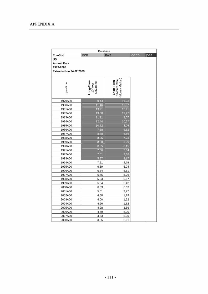
APPENDIX A
- 111 -
Database
EuroStat ECB BofE OECD DBB
US Annual Data 1979-2008 Extracted on 24.02.2009
geo/
time
Lo
ng
-Ter
m
10 Y
ear
Gov
.Bon
d
Sh
ort
-Ter
m
3 M
onth
Rat
e (M
oney
Mar
ket)
1979A00 9,44 11,23
1980A00 11,46 13,07
1981A00 13,91 15,91
1982A00 13,00 12,27
1983A00 11,11 9,07
1984A00 12,44 10,37
1985A00 10,62 8,05
1986A00 7,68 6,52
1987A00 8,38 6,86
1988A00 8,85 7,73
1989A00 8,50 9,09
1990A00 8,55 8,15
1991A00 7,86 5,84
1992A00 7,01 3,68
1993A00 5,87 3,17
1994A00 7,21 4,75
1995A00 6,69 6,04
1996A00 6,54 5,51
1997A00 6,45 5,76
1998A00 5,33 5,57
1999A00 5,64 5,42
2000A00 6,03 6,53
2001A00 5,01 3,77
2002A00 4,60 1,79
2003A00 4,00 1,22
2004A00 4,26 1,62
2005A00 4,28 3,56
2006A00 4,79 5,20
2007A00 4,63 5,30
2008A00 3,65 2,91
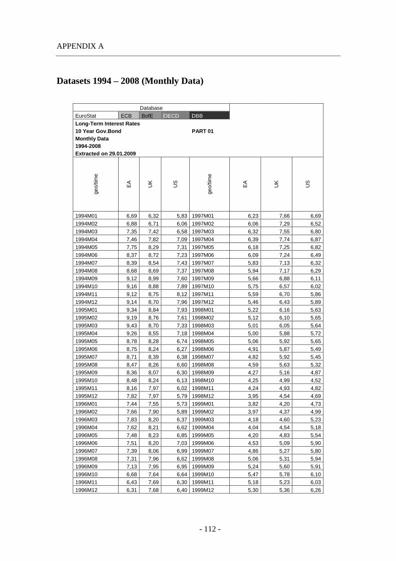
APPENDIX A
- 112 -
Datasets 1994 – 2008 (Monthly Data)
Database
EuroStat ECB BofE OECD DBB
Long-Term Interest Rates 10 Year Gov.Bond PART 01 Monthly Data 1994-2008 Extracted on 29.01.2009
geo/
time
EA
UK
US
geo/
time
EA
UK
US
1994M01 6,69 6,32 5,83 1997M01 6,23 7,66 6,69
1994M02 6,88 6,71 6,06 1997M02 6,06 7,29 6,52
1994M03 7,35 7,42 6,58 1997M03 6,32 7,55 6,80
1994M04 7,46 7,82 7,09 1997M04 6,39 7,74 6,87
1994M05 7,75 8,29 7,31 1997M05 6,18 7,25 6,82
1994M06 8,37 8,72 7,23 1997M06 6,09 7,24 6,49
1994M07 8,39 8,54 7,43 1997M07 5,83 7,13 6,32
1994M08 8,68 8,69 7,37 1997M08 5,94 7,17 6,29
1994M09 9,12 8,99 7,60 1997M09 5,66 6,88 6,11
1994M10 9,16 8,88 7,89 1997M10 5,75 6,57 6,02
1994M11 9,12 8,75 8,12 1997M11 5,59 6,70 5,86
1994M12 9,14 8,70 7,96 1997M12 5,46 6,43 5,89
1995M01 9,34 8,84 7,93 1998M01 5,22 6,16 5,63
1995M02 9,19 8,76 7,61 1998M02 5,12 6,10 5,65
1995M03 9,43 8,70 7,33 1998M03 5,01 6,05 5,64
1995M04 9,26 8,55 7,18 1998M04 5,00 5,88 5,72
1995M05 8,78 8,28 6,74 1998M05 5,06 5,92 5,65
1995M06 8,75 8,24 6,27 1998M06 4,91 5,87 5,49
1995M07 8,71 8,39 6,38 1998M07 4,82 5,92 5,45
1995M08 8,47 8,26 6,60 1998M08 4,59 5,63 5,32
1995M09 8,36 8,07 6,30 1998M09 4,27 5,16 4,87
1995M10 8,48 8,24 6,13 1998M10 4,25 4,99 4,52
1995M11 8,16 7,97 6,02 1998M11 4,24 4,93 4,82
1995M12 7,82 7,97 5,79 1998M12 3,95 4,54 4,69
1996M01 7,44 7,55 5,73 1999M01 3,82 4,20 4,73
1996M02 7,66 7,90 5,89 1999M02 3,97 4,37 4,99
1996M03 7,83 8,20 6,37 1999M03 4,18 4,60 5,23
1996M04 7,62 8,21 6,62 1999M04 4,04 4,54 5,18
1996M05 7,48 8,23 6,85 1999M05 4,20 4,83 5,54
1996M06 7,51 8,20 7,03 1999M06 4,53 5,09 5,90
1996M07 7,39 8,06 6,99 1999M07 4,86 5,27 5,80
1996M08 7,31 7,96 6,62 1999M08 5,06 5,31 5,94
1996M09 7,13 7,95 6,95 1999M09 5,24 5,60 5,91
1996M10 6,68 7,64 6,64 1999M10 5,47 5,78 6,10
1996M11 6,43 7,69 6,30 1999M11 5,18 5,23 6,03
1996M12 6,31 7,68 6,40 1999M12 5,30 5,36 6,26

APPENDIX A
- 113 -
Database
EuroStat ECB BofE OECD DBB
Long-Term Interest Rates 10 Year Gov.Bond PART 02 Monthly Data 1994-2008 Extracted on 29.01.2009
geo/
time
EA
UK
US
geo/
time
EA
UK
US
2000M01 5,70 5,83 6,66 2003M01 4,27 4,31 4,02
2000M02 5,66 5,63 6,52 2003M02 4,06 4,29 3,90
2000M03 5,49 5,34 6,26 2003M03 4,13 4,41 3,79
2000M04 5,41 5,30 6,00 2003M04 4,23 4,56 3,94
2000M05 5,52 5,41 6,42 2003M05 3,92 4,31 3,56
2000M06 5,35 5,21 6,10 2003M06 3,72 4,19 3,32
2000M07 5,45 5,24 6,04 2003M07 4,06 4,47 3,93
2000M08 5,40 5,32 5,83 2003M08 4,20 4,64 4,44
2000M09 5,47 5,38 5,80 2003M09 4,23 4,76 4,29
2000M10 5,42 5,20 5,74 2003M10 4,31 4,96 4,27
2000M11 5,34 5,11 5,72 2003M11 4,44 5,10 4,29
2000M12 5,07 4,95 5,23 2003M12 4,36 4,94 4,26
2001M01 5,01 4,94 5,14 2004M01 4,26 4,84 4,13
2001M02 5,02 4,95 5,10 2004M02 4,18 4,88 4,06
2001M03 4,94 4,82 4,89 2004M03 4,02 4,76 3,81
2001M04 5,10 5,03 5,13 2004M04 4,19 4,99 4,32
2001M05 5,26 5,21 5,37 2004M05 4,35 5,15 4,70
2001M06 5,21 5,30 5,26 2004M06 4,41 5,24 4,73
2001M07 5,25 5,30 5,23 2004M07 4,31 5,14 4,48
2001M08 5,06 5,07 4,97 2004M08 4,15 5,03 4,27
2001M09 5,04 5,02 4,76 2004M09 4,11 4,95 4,13
2001M10 4,82 4,86 4,55 2004M10 3,98 4,81 4,08
2001M11 4,67 4,67 4,61 2004M11 3,86 4,74 4,19
2001M12 4,96 4,94 5,07 2004M12 3,66 4,58 4,23
2002M01 5,02 5,02 5,00 2005M01 3,60 4,60 4,21
2002M02 5,07 5,04 4,90 2005M02 3,59 4,66 4,16
2002M03 5,32 5,34 5,28 2005M03 3,75 4,87 4,49
2002M04 5,30 5,33 5,21 2005M04 3,54 4,67 4,34
2002M05 5,30 5,35 5,15 2005M05 3,39 4,45 4,14
2002M06 5,16 5,19 4,90 2005M06 3,22 4,31 4,00
2002M07 5,03 5,02 4,62 2005M07 3,28 4,31 4,16
2002M08 4,73 4,67 4,24 2005M08 3,30 4,34 4,26
2002M09 4,52 4,45 3,88 2005M09 3,14 4,25 4,19
2002M10 4,62 4,53 3,91 2005M10 3,30 4,40 4,45
2002M11 4,59 4,55 4,04 2005M11 3,51 4,37 4,53
2002M12 4,41 4,49 4,03 2005M12 3,40 4,27 4,46

APPENDIX A
- 114 -
Database
EuroStat ECB BofE OECD DBB
Long-Term Interest Rates 10 Year Gov.Bond PART 03 Monthly Data 1994-2008 Extracted on 29.01.2009
geo/
time
EA
UK
US
2006M01 3,38 3,97 4,41
2006M02 3,54 4,05 4,56
2006M03 3,72 4,19 4,72
2006M04 3,99 4,37 4,99
2006M05 4,05 4,49 5,10
2006M06 4,05 4,50 5,10
2006M07 4,08 4,49 5,10
2006M08 3,96 4,49 4,88
2006M09 3,83 4,44 4,72
2006M10 3,87 4,51 4,73
2006M11 3,79 4,45 4,60
2006M12 3,85 4,54 4,57
2007M01 4,09 4,94 4,76
2007M02 4,12 4,97 4,73
2007M03 4,02 4,88 4,56
2007M04 4,23 5,10 4,69
2007M05 4,37 5,15 4,75
2007M06 4,66 5,43 5,11
2007M07 4,63 5,41 5,01
2007M08 4,43 5,15 4,68
2007M09 4,37 4,99 4,51
2007M10 4,40 4,96 4,52
2007M11 4,25 4,73 4,16
2007M12 4,38 4,69 4,10
2008M01 4,23 4,49 3,73
2008M02 4,14 4,62 3,73
2008M03 4,07 4,44 3,49
2008M04 4,28 4,64 3,65
2008M05 4,42 4,87 3,87
2008M06 4,81 5,21 4,09
2008M07 4,81 5,05 3,98
2008M08 4,50 4,73 3,89
2008M09 4,50 4,57 3,68
2008M10 4,42 4,58 3,79
2008M11 4,20 4,26 3,52
2008M12 3,89 3,62 2,42

APPENDIX A
- 115 -
Database
EuroStat ECB BofE OECD DBB
Short-Term Interest Rates 3 Month Rate (Money Market) PART 01 Monthly Data 1994-2008 Extracted on 04.02.2009
geo/
time
EA
UK
US
geo/
time
EA
UK
US
1994M01 6,91 5,44 3,28 1997M01 4,39 6,42 5,57
1994M02 6,86 5,26 3,55 1997M02 4,43 6,29 5,53
1994M03 6,75 5,23 3,88 1997M03 4,50 6,30 5,67
1994M04 6,57 5,29 4,11 1997M04 4,39 6,45 5,85
1994M05 6,24 5,23 4,64 1997M05 4,30 6,53 5,84
1994M06 6,30 5,19 4,64 1997M06 4,29 6,76 5,81
1994M07 6,34 5,27 4,86 1997M07 4,30 7,04 5,76
1994M08 6,43 5,58 4,92 1997M08 4,36 7,24 5,73
1994M09 6,38 5,77 5,13 1997M09 4,31 7,30 5,74
1994M10 6,43 5,97 5,63 1997M10 4,44 7,36 5,78
1994M11 6,40 6,13 5,88 1997M11 4,49 7,63 5,89
1994M12 6,69 6,43 6,39 1997M12 4,37 7,72 5,90
1995M01 6,66 6,64 6,34 1998M01 4,26 7,59 5,67
1995M02 6,59 6,80 6,26 1998M02 4,24 7,54 5,64
1995M03 7,58 6,73 6,27 1998M03 4,11 7,57 5,74
1995M04 7,29 6,74 6,24 1998M04 4,09 7,54 5,74
1995M05 7,04 6,78 6,11 1998M05 4,06 7,49 5,73
1995M06 7,08 6,71 6,01 1998M06 4,02 7,71 5,69
1995M07 6,92 6,88 5,90 1998M07 3,95 7,81 5,69
1995M08 6,66 6,88 5,90 1998M08 3,93 7,73 5,68
1995M09 6,50 6,80 5,86 1998M09 3,93 7,47 5,50
1995M10 6,75 6,82 5,94 1998M10 3,81 7,22 5,27
1995M11 6,45 6,72 5,88 1998M11 3,69 6,97 5,32
1995M12 6,32 6,55 5,75 1998M12 3,37 6,46 5,22
1996M01 5,81 6,45 5,55 1999M01 3,14 5,92 5,01
1996M02 5,58 6,25 5,28 1999M02 3,09 5,53 5,00
1996M03 5,50 6,14 5,39 1999M03 3,05 5,40 5,01
1996M04 5,27 6,08 5,49 1999M04 2,70 5,32 5,00
1996M05 5,06 6,12 5,50 1999M05 2,58 5,35 5,02
1996M06 5,08 5,93 5,57 1999M06 2,63 5,22 5,18
1996M07 5,06 5,82 5,64 1999M07 2,68 5,17 5,31
1996M08 5,08 5,84 5,53 1999M08 2,70 5,25 5,45
1996M09 4,86 5,86 5,62 1999M09 2,73 5,41 5,57
1996M10 4,69 6,02 5,54 1999M10 3,38 6,03 6,18
1996M11 4,57 6,39 5,50 1999M11 3,47 5,87 6,10
1996M12 4,50 6,43 5,55 1999M12 3,44 6,06 6,13
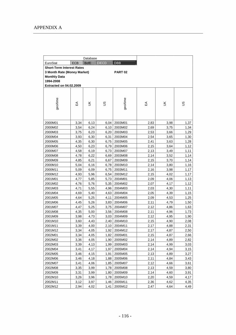
APPENDIX A
- 116 -
Database
EuroStat ECB BofE OECD DBB
Short-Term Interest Rates 3 Month Rate (Money Market) PART 02 Monthly Data 1994-2008 Extracted on 04.02.2009
geo/
time
EA
UK
US
geo/
time
EA
UK
US
2000M01 3,34 6,13 6,04 2003M01 2,83 3,98 1,37
2000M02 3,54 6,24 6,10 2003M02 2,69 3,75 1,34
2000M03 3,75 6,23 6,20 2003M03 2,53 3,66 1,29
2000M04 3,93 6,30 6,31 2003M04 2,54 3,65 1,30
2000M05 4,35 6,30 6,75 2003M05 2,41 3,63 1,28
2000M06 4,50 6,23 6,79 2003M06 2,15 3,64 1,12
2000M07 4,58 6,19 6,73 2003M07 2,13 3,49 1,11
2000M08 4,78 6,22 6,69 2003M08 2,14 3,52 1,14
2000M09 4,85 6,21 6,67 2003M09 2,15 3,70 1,14
2000M10 5,04 6,16 6,78 2003M10 2,14 3,80 1,16
2000M11 5,09 6,09 6,75 2003M11 2,16 3,98 1,17
2000M12 4,93 5,96 6,54 2003M12 2,15 4,02 1,17
2001M01 4,77 5,85 5,73 2004M01 2,09 4,06 1,13
2001M02 4,76 5,76 5,35 2004M02 2,07 4,17 1,12
2001M03 4,71 5,55 4,96 2004M03 2,03 4,30 1,11
2001M04 4,69 5,40 4,63 2004M04 2,05 4,39 1,15
2001M05 4,64 5,25 4,11 2004M05 2,09 4,53 1,25
2001M06 4,45 5,26 3,83 2004M06 2,11 4,79 1,50
2001M07 4,47 5,25 3,75 2004M07 2,12 4,86 1,63
2001M08 4,35 5,00 3,56 2004M08 2,11 4,96 1,73
2001M09 3,98 4,73 3,03 2004M09 2,12 4,95 1,90
2001M10 3,60 4,43 2,40 2004M10 2,15 4,90 2,08
2001M11 3,39 4,00 2,10 2004M11 2,17 4,88 2,31
2001M12 3,34 4,05 1,92 2004M12 2,17 4,87 2,50
2002M01 3,34 4,05 1,82 2005M01 2,15 4,87 2,66
2002M02 3,36 4,05 1,90 2005M02 2,14 4,89 2,82
2002M03 3,39 4,13 1,99 2005M03 2,14 4,99 3,03
2002M04 3,41 4,17 1,97 2005M04 2,14 4,94 3,15
2002M05 3,46 4,15 1,91 2005M05 2,13 4,89 3,27
2002M06 3,46 4,18 1,88 2005M06 2,11 4,84 3,43
2002M07 3,41 4,06 1,85 2005M07 2,12 4,66 3,61
2002M08 3,35 3,99 1,78 2005M08 2,13 4,59 3,80
2002M09 3,31 3,99 1,80 2005M09 2,14 4,60 3,91
2002M10 3,26 3,96 1,78 2005M10 2,20 4,59 4,17
2002M11 3,12 3,97 1,46 2005M11 2,36 4,62 4,35
2002M12 2,94 4,02 1,41 2005M12 2,47 4,64 4,49
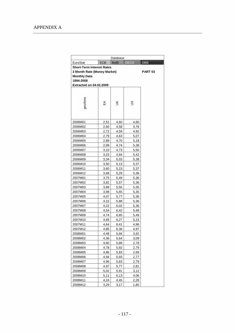
APPENDIX A
- 117 -
Database
EuroStat ECB BofE OECD DBB
Short-Term Interest Rates 3 Month Rate (Money Market) PART 03 Monthly Data 1994-2008 Extracted on 04.02.2009
geo/
time
EA
UK
US
2006M01 2,51 4,60 4,60
2006M02 2,60 4,58 4,76
2006M03 2,72 4,59 4,92
2006M04 2,79 4,63 5,07
2006M05 2,89 4,70 5,18
2006M06 2,99 4,74 5,38
2006M07 3,10 4,73 5,50
2006M08 3,23 4,94 5,42
2006M09 3,34 5,03 5,38
2006M10 3,50 5,13 5,37
2006M11 3,60 5,23 5,37
2006M12 3,68 5,29 5,36
2007M01 3,75 5,49 5,36
2007M02 3,82 5,57 5,36
2007M03 3,89 5,55 5,35
2007M04 3,98 5,65 5,35
2007M05 4,07 5,77 5,36
2007M06 4,15 5,88 5,36
2007M07 4,22 6,02 5,36
2007M08 4,54 6,42 5,48
2007M09 4,74 6,65 5,49
2007M10 4,69 6,27 5,15
2007M11 4,64 6,41 4,96
2007M12 4,85 6,36 4,97
2008M01 4,48 5,66 3,92
2008M02 4,36 5,64 3,09
2008M03 4,60 5,89 2,78
2008M04 4,78 5,92 2,79
2008M05 4,86 5,83 2,69
2008M06 4,94 5,93 2,77
2008M07 4,96 5,83 2,79
2008M08 4,97 5,77 2,81
2008M09 5,02 5,91 3,12
2008M10 5,11 6,13 4,06
2008M11 4,24 4,45 2,28
2008M12 3,29 3,17 1,80
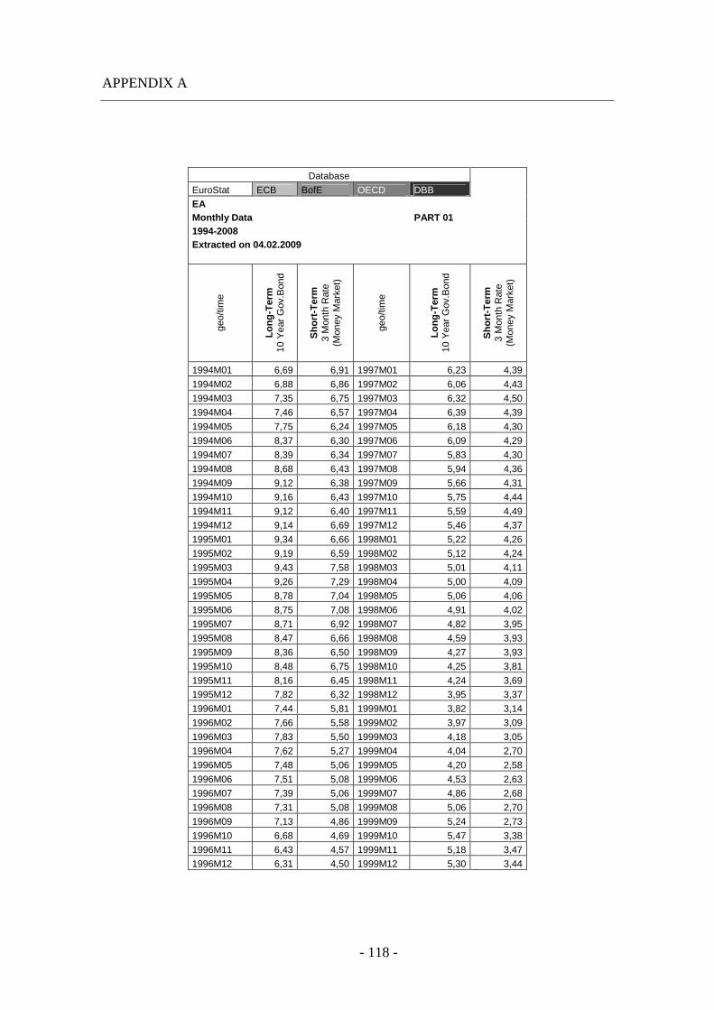
APPENDIX A
- 118 -
Database
EuroStat ECB BofE OECD DBB
EA Monthly Data PART 01 1994-2008 Extracted on 04.02.2009
geo/
time
Lo
ng
-Ter
m
10 Y
ear
Gov
.Bon
d
Sh
ort
-Ter
m
3 M
onth
Rat
e (M
oney
Mar
ket)
geo/
time
Lo
ng
-Ter
m
10 Y
ear
Gov
.Bon
d
Sh
ort
-Ter
m
3 M
onth
Rat
e (M
oney
Mar
ket)
1994M01 6,69 6,91 1997M01 6,23 4,39
1994M02 6,88 6,86 1997M02 6,06 4,43
1994M03 7,35 6,75 1997M03 6,32 4,50
1994M04 7,46 6,57 1997M04 6,39 4,39
1994M05 7,75 6,24 1997M05 6,18 4,30
1994M06 8,37 6,30 1997M06 6,09 4,29
1994M07 8,39 6,34 1997M07 5,83 4,30
1994M08 8,68 6,43 1997M08 5,94 4,36
1994M09 9,12 6,38 1997M09 5,66 4,31
1994M10 9,16 6,43 1997M10 5,75 4,44
1994M11 9,12 6,40 1997M11 5,59 4,49
1994M12 9,14 6,69 1997M12 5,46 4,37
1995M01 9,34 6,66 1998M01 5,22 4,26
1995M02 9,19 6,59 1998M02 5,12 4,24
1995M03 9,43 7,58 1998M03 5,01 4,11
1995M04 9,26 7,29 1998M04 5,00 4,09
1995M05 8,78 7,04 1998M05 5,06 4,06
1995M06 8,75 7,08 1998M06 4,91 4,02
1995M07 8,71 6,92 1998M07 4,82 3,95
1995M08 8,47 6,66 1998M08 4,59 3,93
1995M09 8,36 6,50 1998M09 4,27 3,93
1995M10 8,48 6,75 1998M10 4,25 3,81
1995M11 8,16 6,45 1998M11 4,24 3,69
1995M12 7,82 6,32 1998M12 3,95 3,37
1996M01 7,44 5,81 1999M01 3,82 3,14
1996M02 7,66 5,58 1999M02 3,97 3,09
1996M03 7,83 5,50 1999M03 4,18 3,05
1996M04 7,62 5,27 1999M04 4,04 2,70
1996M05 7,48 5,06 1999M05 4,20 2,58
1996M06 7,51 5,08 1999M06 4,53 2,63
1996M07 7,39 5,06 1999M07 4,86 2,68
1996M08 7,31 5,08 1999M08 5,06 2,70
1996M09 7,13 4,86 1999M09 5,24 2,73
1996M10 6,68 4,69 1999M10 5,47 3,38
1996M11 6,43 4,57 1999M11 5,18 3,47
1996M12 6,31 4,50 1999M12 5,30 3,44
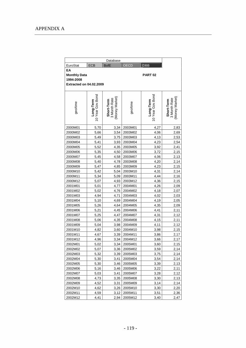
APPENDIX A
- 119 -
Database
EuroStat ECB BofE OECD DBB
EA Monthly Data PART 02 1994-2008 Extracted on 04.02.2009
geo/
time
Lo
ng
-Ter
m
10 Y
ear
Gov
.Bon
d
Sh
ort
-Ter
m
3 M
onth
Rat
e (M
oney
Mar
ket)
geo/
time
Lo
ng
-Ter
m
10 Y
ear
Gov
.Bon
d
Sh
ort
-Ter
m
3 M
onth
Rat
e (M
oney
Mar
ket)
2000M01 5,70 3,34 2003M01 4,27 2,83
2000M02 5,66 3,54 2003M02 4,06 2,69
2000M03 5,49 3,75 2003M03 4,13 2,53
2000M04 5,41 3,93 2003M04 4,23 2,54
2000M05 5,52 4,35 2003M05 3,92 2,41
2000M06 5,35 4,50 2003M06 3,72 2,15
2000M07 5,45 4,58 2003M07 4,06 2,13
2000M08 5,40 4,78 2003M08 4,20 2,14
2000M09 5,47 4,85 2003M09 4,23 2,15
2000M10 5,42 5,04 2003M10 4,31 2,14
2000M11 5,34 5,09 2003M11 4,44 2,16
2000M12 5,07 4,93 2003M12 4,36 2,15
2001M01 5,01 4,77 2004M01 4,26 2,09
2001M02 5,02 4,76 2004M02 4,18 2,07
2001M03 4,94 4,71 2004M03 4,02 2,03
2001M04 5,10 4,69 2004M04 4,19 2,05
2001M05 5,26 4,64 2004M05 4,35 2,09
2001M06 5,21 4,45 2004M06 4,41 2,11
2001M07 5,25 4,47 2004M07 4,31 2,12
2001M08 5,06 4,35 2004M08 4,15 2,11
2001M09 5,04 3,98 2004M09 4,11 2,12
2001M10 4,82 3,60 2004M10 3,98 2,15
2001M11 4,67 3,39 2004M11 3,86 2,17
2001M12 4,96 3,34 2004M12 3,66 2,17
2002M01 5,02 3,34 2005M01 3,60 2,15
2002M02 5,07 3,36 2005M02 3,59 2,14
2002M03 5,32 3,39 2005M03 3,75 2,14
2002M04 5,30 3,41 2005M04 3,54 2,14
2002M05 5,30 3,46 2005M05 3,39 2,13
2002M06 5,16 3,46 2005M06 3,22 2,11
2002M07 5,03 3,41 2005M07 3,28 2,12
2002M08 4,73 3,35 2005M08 3,30 2,13
2002M09 4,52 3,31 2005M09 3,14 2,14
2002M10 4,62 3,26 2005M10 3,30 2,20
2002M11 4,59 3,12 2005M11 3,51 2,36
2002M12 4,41 2,94 2005M12 3,40 2,47
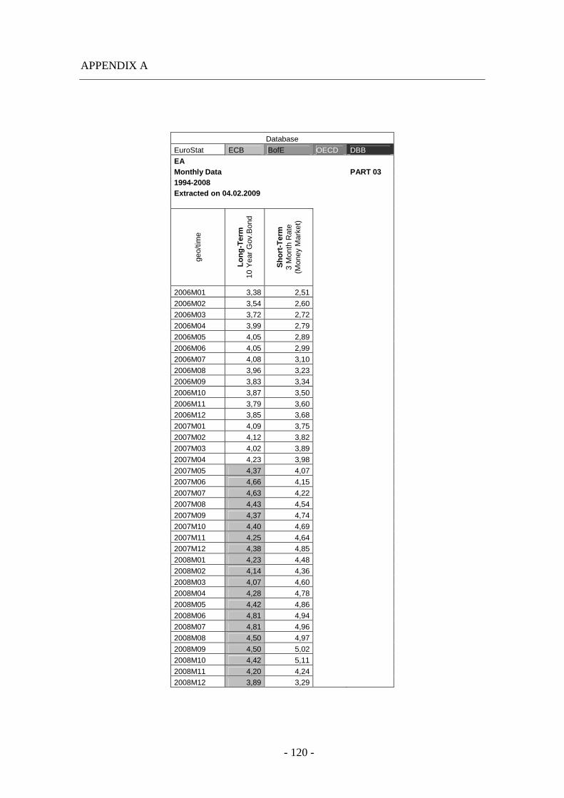
APPENDIX A
- 120 -
Database
EuroStat ECB BofE OECD DBB
EA Monthly Data PART 03 1994-2008 Extracted on 04.02.2009
geo/
time
Lo
ng
-Ter
m
10 Y
ear
Gov
.Bon
d
Sh
ort
-Ter
m
3 M
onth
Rat
e (M
oney
Mar
ket)
2006M01 3,38 2,51
2006M02 3,54 2,60
2006M03 3,72 2,72
2006M04 3,99 2,79
2006M05 4,05 2,89
2006M06 4,05 2,99
2006M07 4,08 3,10
2006M08 3,96 3,23
2006M09 3,83 3,34
2006M10 3,87 3,50
2006M11 3,79 3,60
2006M12 3,85 3,68
2007M01 4,09 3,75
2007M02 4,12 3,82
2007M03 4,02 3,89
2007M04 4,23 3,98
2007M05 4,37 4,07
2007M06 4,66 4,15
2007M07 4,63 4,22
2007M08 4,43 4,54
2007M09 4,37 4,74
2007M10 4,40 4,69
2007M11 4,25 4,64
2007M12 4,38 4,85
2008M01 4,23 4,48
2008M02 4,14 4,36
2008M03 4,07 4,60
2008M04 4,28 4,78
2008M05 4,42 4,86
2008M06 4,81 4,94
2008M07 4,81 4,96
2008M08 4,50 4,97
2008M09 4,50 5,02
2008M10 4,42 5,11
2008M11 4,20 4,24
2008M12 3,89 3,29
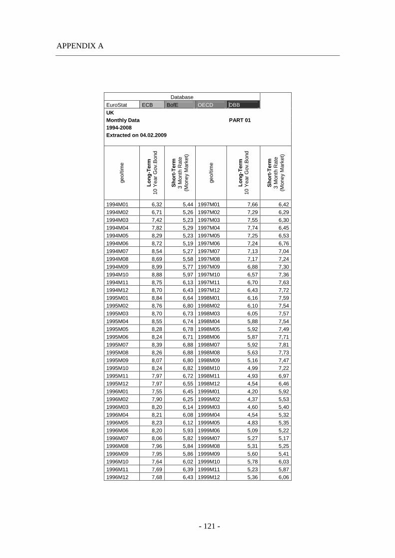
APPENDIX A
- 121 -
Database
EuroStat ECB BofE OECD DBB
UK Monthly Data PART 01 1994-2008 Extracted on 04.02.2009
geo/
time
Lo
ng
-Ter
m
10 Y
ear
Gov
.Bon
d
Sh
ort
-Ter
m
3 M
onth
Rat
e (M
oney
Mar
ket)
geo/
time
Lo
ng
-Ter
m
10 Y
ear
Gov
.Bon
d
Sh
ort
-Ter
m
3 M
onth
Rat
e (M
oney
Mar
ket)
1994M01 6,32 5,44 1997M01 7,66 6,42
1994M02 6,71 5,26 1997M02 7,29 6,29
1994M03 7,42 5,23 1997M03 7,55 6,30
1994M04 7,82 5,29 1997M04 7,74 6,45
1994M05 8,29 5,23 1997M05 7,25 6,53
1994M06 8,72 5,19 1997M06 7,24 6,76
1994M07 8,54 5,27 1997M07 7,13 7,04
1994M08 8,69 5,58 1997M08 7,17 7,24
1994M09 8,99 5,77 1997M09 6,88 7,30
1994M10 8,88 5,97 1997M10 6,57 7,36
1994M11 8,75 6,13 1997M11 6,70 7,63
1994M12 8,70 6,43 1997M12 6,43 7,72
1995M01 8,84 6,64 1998M01 6,16 7,59
1995M02 8,76 6,80 1998M02 6,10 7,54
1995M03 8,70 6,73 1998M03 6,05 7,57
1995M04 8,55 6,74 1998M04 5,88 7,54
1995M05 8,28 6,78 1998M05 5,92 7,49
1995M06 8,24 6,71 1998M06 5,87 7,71
1995M07 8,39 6,88 1998M07 5,92 7,81
1995M08 8,26 6,88 1998M08 5,63 7,73
1995M09 8,07 6,80 1998M09 5,16 7,47
1995M10 8,24 6,82 1998M10 4,99 7,22
1995M11 7,97 6,72 1998M11 4,93 6,97
1995M12 7,97 6,55 1998M12 4,54 6,46
1996M01 7,55 6,45 1999M01 4,20 5,92
1996M02 7,90 6,25 1999M02 4,37 5,53
1996M03 8,20 6,14 1999M03 4,60 5,40
1996M04 8,21 6,08 1999M04 4,54 5,32
1996M05 8,23 6,12 1999M05 4,83 5,35
1996M06 8,20 5,93 1999M06 5,09 5,22
1996M07 8,06 5,82 1999M07 5,27 5,17
1996M08 7,96 5,84 1999M08 5,31 5,25
1996M09 7,95 5,86 1999M09 5,60 5,41
1996M10 7,64 6,02 1999M10 5,78 6,03
1996M11 7,69 6,39 1999M11 5,23 5,87
1996M12 7,68 6,43 1999M12 5,36 6,06
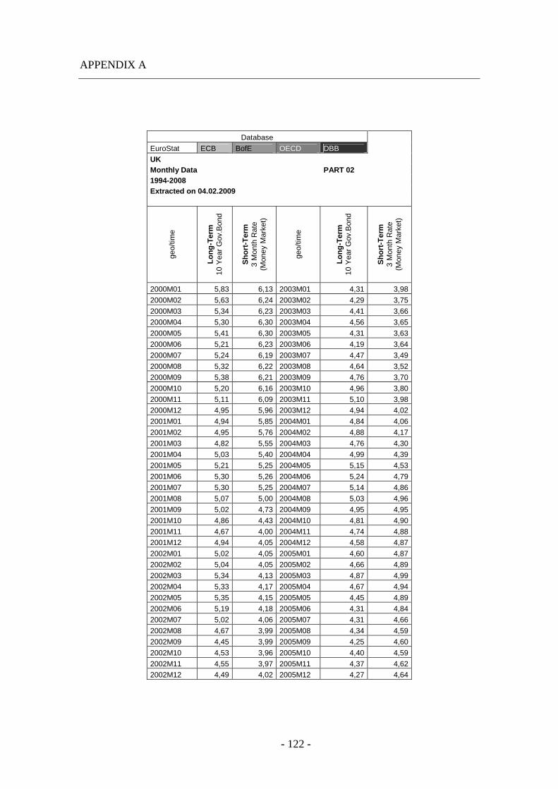
APPENDIX A
- 122 -
Database
EuroStat ECB BofE OECD DBB
UK Monthly Data PART 02 1994-2008 Extracted on 04.02.2009
geo/
time
Lo
ng
-Ter
m
10 Y
ear
Gov
.Bon
d
Sh
ort
-Ter
m
3 M
onth
Rat
e (M
oney
Mar
ket)
geo/
time
Lo
ng
-Ter
m
10 Y
ear
Gov
.Bon
d
Sh
ort
-Ter
m
3 M
onth
Rat
e (M
oney
Mar
ket)
2000M01 5,83 6,13 2003M01 4,31 3,98
2000M02 5,63 6,24 2003M02 4,29 3,75
2000M03 5,34 6,23 2003M03 4,41 3,66
2000M04 5,30 6,30 2003M04 4,56 3,65
2000M05 5,41 6,30 2003M05 4,31 3,63
2000M06 5,21 6,23 2003M06 4,19 3,64
2000M07 5,24 6,19 2003M07 4,47 3,49
2000M08 5,32 6,22 2003M08 4,64 3,52
2000M09 5,38 6,21 2003M09 4,76 3,70
2000M10 5,20 6,16 2003M10 4,96 3,80
2000M11 5,11 6,09 2003M11 5,10 3,98
2000M12 4,95 5,96 2003M12 4,94 4,02
2001M01 4,94 5,85 2004M01 4,84 4,06
2001M02 4,95 5,76 2004M02 4,88 4,17
2001M03 4,82 5,55 2004M03 4,76 4,30
2001M04 5,03 5,40 2004M04 4,99 4,39
2001M05 5,21 5,25 2004M05 5,15 4,53
2001M06 5,30 5,26 2004M06 5,24 4,79
2001M07 5,30 5,25 2004M07 5,14 4,86
2001M08 5,07 5,00 2004M08 5,03 4,96
2001M09 5,02 4,73 2004M09 4,95 4,95
2001M10 4,86 4,43 2004M10 4,81 4,90
2001M11 4,67 4,00 2004M11 4,74 4,88
2001M12 4,94 4,05 2004M12 4,58 4,87
2002M01 5,02 4,05 2005M01 4,60 4,87
2002M02 5,04 4,05 2005M02 4,66 4,89
2002M03 5,34 4,13 2005M03 4,87 4,99
2002M04 5,33 4,17 2005M04 4,67 4,94
2002M05 5,35 4,15 2005M05 4,45 4,89
2002M06 5,19 4,18 2005M06 4,31 4,84
2002M07 5,02 4,06 2005M07 4,31 4,66
2002M08 4,67 3,99 2005M08 4,34 4,59
2002M09 4,45 3,99 2005M09 4,25 4,60
2002M10 4,53 3,96 2005M10 4,40 4,59
2002M11 4,55 3,97 2005M11 4,37 4,62
2002M12 4,49 4,02 2005M12 4,27 4,64

APPENDIX A
- 123 -
Database
EuroStat ECB BofE OECD DBB
UK Monthly Data PART 03 1994-2008 Extracted on 04.02.2009
geo/
time
Lo
ng
-Ter
m
10 Y
ear
Gov
.Bon
d
Sh
ort
-Ter
m
3 M
onth
Rat
e (M
oney
Mar
ket)
2006M01 3,97 4,60
2006M02 4,05 4,58
2006M03 4,19 4,59
2006M04 4,37 4,63
2006M05 4,49 4,70
2006M06 4,50 4,74
2006M07 4,49 4,73
2006M08 4,49 4,94
2006M09 4,44 5,03
2006M10 4,51 5,13
2006M11 4,45 5,23
2006M12 4,54 5,29
2007M01 4,94 5,49
2007M02 4,97 5,57
2007M03 4,88 5,55
2007M04 5,10 5,65
2007M05 5,15 5,77
2007M06 5,43 5,88
2007M07 5,41 6,02
2007M08 5,15 6,42
2007M09 4,99 6,65
2007M10 4,96 6,27
2007M11 4,73 6,41
2007M12 4,69 6,36
2008M01 4,49 5,66
2008M02 4,62 5,64
2008M03 4,44 5,89
2008M04 4,64 5,92
2008M05 4,87 5,83
2008M06 5,21 5,93
2008M07 5,05 5,83
2008M08 4,73 5,77
2008M09 4,57 5,91
2008M10 4,58 6,13
2008M11 4,26 4,45
2008M12 3,62 3,17

APPENDIX A
- 124 -
Database
EuroStat ECB BofE OECD DBB
US Monthly Data PART 01 1994-2008 Extracted on 04.02.2009
geo/
time
Lo
ng
-Ter
m
10 Y
ear
Gov
.Bon
d
Sh
ort
-Ter
m
3 M
onth
Rat
e (M
oney
Mar
ket)
geo/
time
Lo
ng
-Ter
m
10 Y
ear
Gov
.Bon
d
Sh
ort
-Ter
m
3 M
onth
Rat
e (M
oney
Mar
ket)
1994M01 5,83 3,28 1997M01 6,69 5,57
1994M02 6,06 3,55 1997M02 6,52 5,53
1994M03 6,58 3,88 1997M03 6,80 5,67
1994M04 7,09 4,11 1997M04 6,87 5,85
1994M05 7,31 4,64 1997M05 6,82 5,84
1994M06 7,23 4,64 1997M06 6,49 5,81
1994M07 7,43 4,86 1997M07 6,32 5,76
1994M08 7,37 4,92 1997M08 6,29 5,73
1994M09 7,60 5,13 1997M09 6,11 5,74
1994M10 7,89 5,63 1997M10 6,02 5,78
1994M11 8,12 5,88 1997M11 5,86 5,89
1994M12 7,96 6,39 1997M12 5,89 5,90
1995M01 7,93 6,34 1998M01 5,63 5,67
1995M02 7,61 6,26 1998M02 5,65 5,64
1995M03 7,33 6,27 1998M03 5,64 5,74
1995M04 7,18 6,24 1998M04 5,72 5,74
1995M05 6,74 6,11 1998M05 5,65 5,73
1995M06 6,27 6,01 1998M06 5,49 5,69
1995M07 6,38 5,90 1998M07 5,45 5,69
1995M08 6,60 5,90 1998M08 5,32 5,68
1995M09 6,30 5,86 1998M09 4,87 5,50
1995M10 6,13 5,94 1998M10 4,52 5,27
1995M11 6,02 5,88 1998M11 4,82 5,32
1995M12 5,79 5,75 1998M12 4,69 5,22
1996M01 5,73 5,55 1999M01 4,73 5,01
1996M02 5,89 5,28 1999M02 4,99 5,00
1996M03 6,37 5,39 1999M03 5,23 5,01
1996M04 6,62 5,49 1999M04 5,18 5,00
1996M05 6,85 5,50 1999M05 5,54 5,02
1996M06 7,03 5,57 1999M06 5,90 5,18
1996M07 6,99 5,64 1999M07 5,80 5,31
1996M08 6,62 5,53 1999M08 5,94 5,45
1996M09 6,95 5,62 1999M09 5,91 5,57
1996M10 6,64 5,54 1999M10 6,10 6,18
1996M11 6,30 5,50 1999M11 6,03 6,10
1996M12 6,40 5,55 1999M12 6,26 6,13
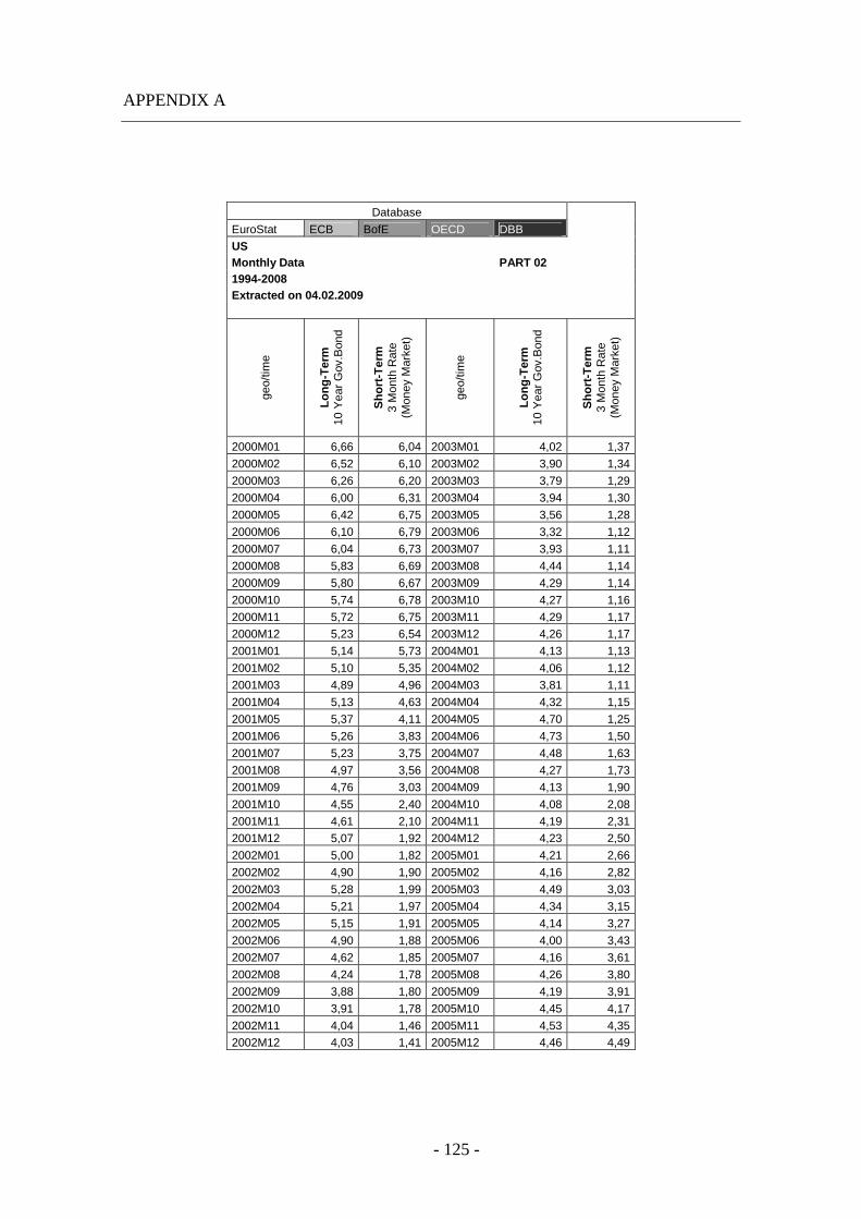
APPENDIX A
- 125 -
Database
EuroStat ECB BofE OECD DBB
US Monthly Data PART 02 1994-2008 Extracted on 04.02.2009
geo/
time
Lo
ng
-Ter
m
10 Y
ear
Gov
.Bon
d
Sh
ort
-Ter
m
3 M
onth
Rat
e (M
oney
Mar
ket)
geo/
time
Lo
ng
-Ter
m
10 Y
ear
Gov
.Bon
d
Sh
ort
-Ter
m
3 M
onth
Rat
e (M
oney
Mar
ket)
2000M01 6,66 6,04 2003M01 4,02 1,37
2000M02 6,52 6,10 2003M02 3,90 1,34
2000M03 6,26 6,20 2003M03 3,79 1,29
2000M04 6,00 6,31 2003M04 3,94 1,30
2000M05 6,42 6,75 2003M05 3,56 1,28
2000M06 6,10 6,79 2003M06 3,32 1,12
2000M07 6,04 6,73 2003M07 3,93 1,11
2000M08 5,83 6,69 2003M08 4,44 1,14
2000M09 5,80 6,67 2003M09 4,29 1,14
2000M10 5,74 6,78 2003M10 4,27 1,16
2000M11 5,72 6,75 2003M11 4,29 1,17
2000M12 5,23 6,54 2003M12 4,26 1,17
2001M01 5,14 5,73 2004M01 4,13 1,13
2001M02 5,10 5,35 2004M02 4,06 1,12
2001M03 4,89 4,96 2004M03 3,81 1,11
2001M04 5,13 4,63 2004M04 4,32 1,15
2001M05 5,37 4,11 2004M05 4,70 1,25
2001M06 5,26 3,83 2004M06 4,73 1,50
2001M07 5,23 3,75 2004M07 4,48 1,63
2001M08 4,97 3,56 2004M08 4,27 1,73
2001M09 4,76 3,03 2004M09 4,13 1,90
2001M10 4,55 2,40 2004M10 4,08 2,08
2001M11 4,61 2,10 2004M11 4,19 2,31
2001M12 5,07 1,92 2004M12 4,23 2,50
2002M01 5,00 1,82 2005M01 4,21 2,66
2002M02 4,90 1,90 2005M02 4,16 2,82
2002M03 5,28 1,99 2005M03 4,49 3,03
2002M04 5,21 1,97 2005M04 4,34 3,15
2002M05 5,15 1,91 2005M05 4,14 3,27
2002M06 4,90 1,88 2005M06 4,00 3,43
2002M07 4,62 1,85 2005M07 4,16 3,61
2002M08 4,24 1,78 2005M08 4,26 3,80
2002M09 3,88 1,80 2005M09 4,19 3,91
2002M10 3,91 1,78 2005M10 4,45 4,17
2002M11 4,04 1,46 2005M11 4,53 4,35
2002M12 4,03 1,41 2005M12 4,46 4,49
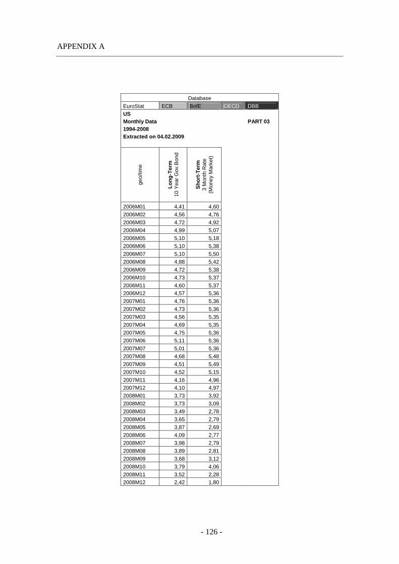
APPENDIX A
- 126 -
Database
EuroStat ECB BofE OECD DBB
US Monthly Data PART 03 1994-2008 Extracted on 04.02.2009
geo/
time
Lo
ng
-Ter
m
10 Y
ear
Gov
.Bon
d
Sh
ort
-Ter
m
3 M
onth
Rat
e (M
oney
Mar
ket)
2006M01 4,41 4,60
2006M02 4,56 4,76
2006M03 4,72 4,92
2006M04 4,99 5,07
2006M05 5,10 5,18
2006M06 5,10 5,38
2006M07 5,10 5,50
2006M08 4,88 5,42
2006M09 4,72 5,38
2006M10 4,73 5,37
2006M11 4,60 5,37
2006M12 4,57 5,36
2007M01 4,76 5,36
2007M02 4,73 5,36
2007M03 4,56 5,35
2007M04 4,69 5,35
2007M05 4,75 5,36
2007M06 5,11 5,36
2007M07 5,01 5,36
2007M08 4,68 5,48
2007M09 4,51 5,49
2007M10 4,52 5,15
2007M11 4,16 4,96
2007M12 4,10 4,97
2008M01 3,73 3,92
2008M02 3,73 3,09
2008M03 3,49 2,78
2008M04 3,65 2,79
2008M05 3,87 2,69
2008M06 4,09 2,77
2008M07 3,98 2,79
2008M08 3,89 2,81
2008M09 3,68 3,12
2008M10 3,79 4,06
2008M11 3,52 2,28
2008M12 2,42 1,80
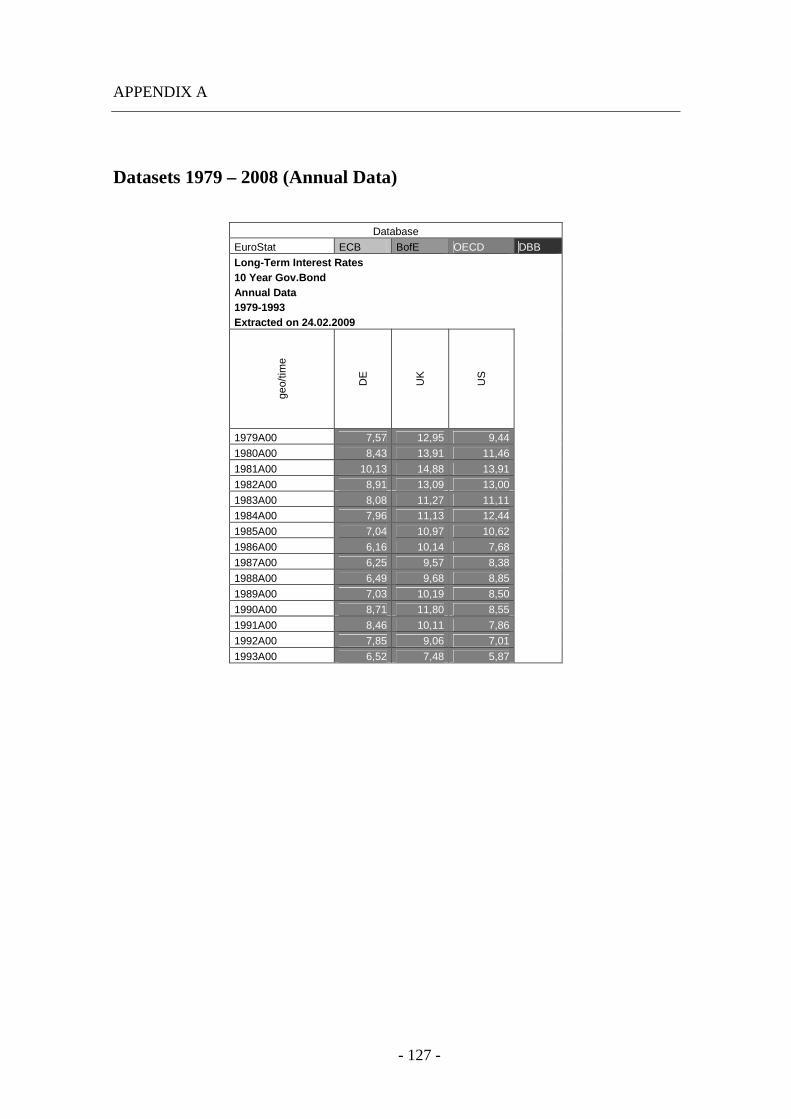
APPENDIX A
- 127 -
Datasets 1979 – 2008 (Annual Data)
Database
EuroStat ECB BofE OECD DBB
Long-Term Interest Rates 10 Year Gov.Bond Annual Data 1979-1993 Extracted on 24.02.2009
geo/
time
DE
UK
US
1979A00 7,57 12,95 9,44
1980A00 8,43 13,91 11,46
1981A00 10,13 14,88 13,91
1982A00 8,91 13,09 13,00
1983A00 8,08 11,27 11,11
1984A00 7,96 11,13 12,44
1985A00 7,04 10,97 10,62
1986A00 6,16 10,14 7,68
1987A00 6,25 9,57 8,38
1988A00 6,49 9,68 8,85
1989A00 7,03 10,19 8,50
1990A00 8,71 11,80 8,55
1991A00 8,46 10,11 7,86
1992A00 7,85 9,06 7,01
1993A00 6,52 7,48 5,87
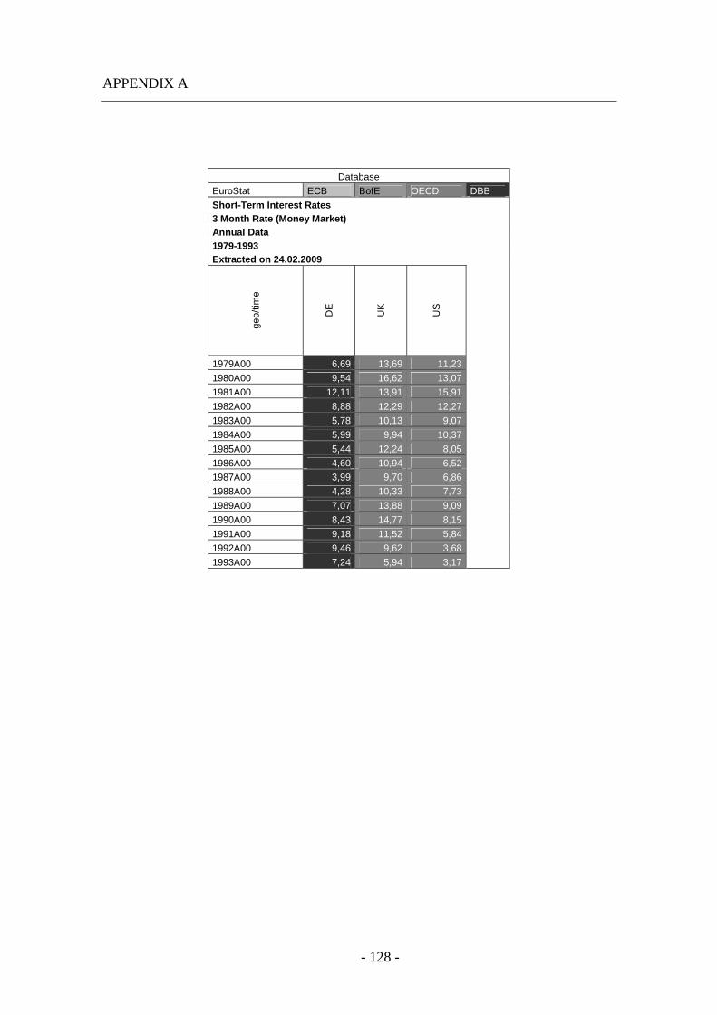
APPENDIX A
- 128 -
Database
EuroStat ECB BofE OECD DBB
Short-Term Interest Rates 3 Month Rate (Money Market) Annual Data 1979-1993 Extracted on 24.02.2009
geo/
time
DE
UK
US
1979A00 6,69 13,69 11,23
1980A00 9,54 16,62 13,07
1981A00 12,11 13,91 15,91
1982A00 8,88 12,29 12,27
1983A00 5,78 10,13 9,07
1984A00 5,99 9,94 10,37
1985A00 5,44 12,24 8,05
1986A00 4,60 10,94 6,52
1987A00 3,99 9,70 6,86
1988A00 4,28 10,33 7,73
1989A00 7,07 13,88 9,09
1990A00 8,43 14,77 8,15
1991A00 9,18 11,52 5,84
1992A00 9,46 9,62 3,68
1993A00 7,24 5,94 3,17
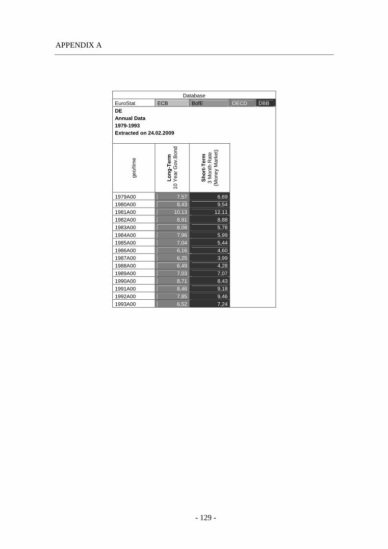
APPENDIX A
- 129 -
Database
EuroStat ECB BofE OECD DBB
DE Annual Data 1979-1993 Extracted on 24.02.2009
geo/
time
Lo
ng
-Ter
m
10 Y
ear
Gov
.Bon
d
Sh
ort
-Ter
m
3 M
onth
Rat
e (M
oney
Mar
ket)
1979A00 7,57 6,69
1980A00 8,43 9,54
1981A00 10,13 12,11
1982A00 8,91 8,88
1983A00 8,08 5,78
1984A00 7,96 5,99
1985A00 7,04 5,44
1986A00 6,16 4,60
1987A00 6,25 3,99
1988A00 6,49 4,28
1989A00 7,03 7,07
1990A00 8,71 8,43
1991A00 8,46 9,18
1992A00 7,85 9,46
1993A00 6,52 7,24

APPENDIX A
- 130 -
Database
EuroStat ECB BofE OECD DBB
UK Annual Data 1979-1993 Extracted on 24.02.2009
geo/
time
Lo
ng
-Ter
m
10 Y
ear
Gov
.Bon
d
Sh
ort
-Ter
m
3 M
onth
Rat
e (M
oney
Mar
ket)
1979A00 12,95 13,69
1980A00 13,91 16,62
1981A00 14,88 13,91
1982A00 13,09 12,29
1983A00 11,27 10,13
1984A00 11,13 9,94
1985A00 10,97 12,24
1986A00 10,14 10,94
1987A00 9,57 9,70
1988A00 9,68 10,33
1989A00 10,19 13,88
1990A00 11,80 14,77
1991A00 10,11 11,52
1992A00 9,06 9,62
1993A00 7,48 5,94
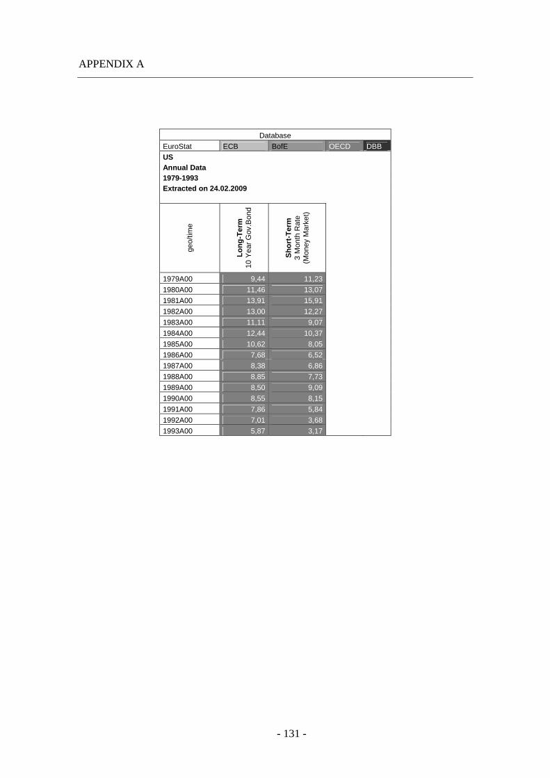
APPENDIX A
- 131 -
Database
EuroStat ECB BofE OECD DBB
US Annual Data 1979-1993 Extracted on 24.02.2009
geo/
time
Lo
ng
-Ter
m
10 Y
ear
Gov
.Bon
d
Sh
ort
-Ter
m
3 M
onth
Rat
e (M
oney
Mar
ket)
1979A00 9,44 11,23
1980A00 11,46 13,07
1981A00 13,91 15,91
1982A00 13,00 12,27
1983A00 11,11 9,07
1984A00 12,44 10,37
1985A00 10,62 8,05
1986A00 7,68 6,52
1987A00 8,38 6,86
1988A00 8,85 7,73
1989A00 8,50 9,09
1990A00 8,55 8,15
1991A00 7,86 5,84
1992A00 7,01 3,68
1993A00 5,87 3,17

- 133 -
Appendix B
Summary in German / Deutsche Zusammenfassung
Die Hauptaufgabe der vorliegenden Arbeit liegt einerseits darin den Überblick
über die Geldmarktpolitik zu schaffen und andererseits eine Unterscheidung zwischen
kurz- und langfristigen Zinssätzen zu ermöglichen.
Geldmarktpolitik repräsentiert die Summe aller finanzwirtschaftlichen
Instrumente, welche von bestimmten Entscheidungsträgern zur Verfolgung und
letztendlichen Erlangung monetärer Ziele eingesetzt werden. Diese Entscheidungsträger
sind keine Geringeren als die Zentralbanken der jeweiligen Staaten, in derer Macht es
steht durch bestimmte politische Interventionen die Geschicke einer gesamten
Volkswirtschaft zu lenken und zu beeinflussen. Anhand der, in der Arbeit dargestellten
empirischen Studie welche den Zeitraum der letzten drei Dekaden und die drei
geographischen Gebiete der Vereinigten Staaten von Amerika, Großbritannien und der
Euro Zone umfasst, werden verschiedene Ansätze und Zielsetzungen von
Geldmarktpolitik besprochen und bildlich dargestellt.
Die in der Arbeit besprochenen, kurzfristigen Zinssätze sind jene mit der größten
Bedeutung im Hinblick auf die Politik der Zentralbanken, da sie im direkten
Zusammenhang mit den angestrebten Zielsetzungen stehen und darüber hinaus als
direktes Steuerungselement dienen. Durch ihre Anpassung reagieren Zentralbanken auf
bestimmte Ereignisse und können somit die Volkswirtschaft einer gesamten Nation
effizient und produktiv halten. Durch die Analyse der Daten werden somit bestimmte
Trends der jeweiligen Zeitperioden und geographischen Gebiete dargestellt.
Diese Ergebnisse, beruhend auf der Auswertung der kurzfristigen Daten, werden
nun, unter Berücksichtigung von theoretischen Ansätzen, den langfristigen Zinssätzen
gegenübergestellt. Durch die Zuhilfenahme von Diagrammen können letztendlich
Aussagen getroffen werden, inwieweit langfristige Zinssätze von kurzfristigen und
somit direkt von der Geldmarktpolitik der Zentralbanken beeinflusst werden.
Abschließend muss noch erläutert werden, dass alle, in der Arbeit dargestellten
und verwendeten Daten-Tabellen und Diagramme vom Verfasser selbiger erstellt und

APPENDIX B
- 134 -
ausgewertet wurden. Als Grundlage zur Datenerfassung dienten lediglich die im
Appendix A und in der Bibliography angeführten Internet-Databases der jeweiligen
Institutionen.

- 135 -
Appendix C

APPENDIX C
- 136 -
- 137 -
References
Bibliography
[Bain, K.; Howells P. (2009a)] “Monetary Economics – Policy and its
Theoretical Basis”. Second Edition, London, Palgrave, page 222.
[Bain, K.; Howells P. (2009b)] “Monetary Economics – Policy and its
Theoretical Basis”. Second Edition, London, Palgrave, page 223.
[Bain, K.; Howells P. (2009c)] “Monetary Economics – Policy and its
Theoretical Basis”. Second Edition, London, Palgrave, page 224.
[Bain, K.; Howells P. (2009d)] “Monetary Economics – Policy and its
Theoretical Basis”. Second Edition, London, Palgrave, page 130.
[Bain, K.; Howells P. (2009e)] “Monetary Economics – Policy and its
Theoretical Basis”. Second Edition, London, Palgrave, page 229.
[Bain, K.; Howells P. (2009f)] “Monetary Economics – Policy and its
Theoretical Basis”. Second Edition, London, Palgrave, page 319.
[Bain, K.; Howells P. (2009g)] “Monetary Economics – Policy and its
Theoretical Basis”. Second Edition, London, Palgrave, page 347.
[Bain, K.; Howells P. (2009h)] “Monetary Economics – Policy and its
Theoretical Basis”. Second Edition, London, Palgrave, page 358.
[Bean, C. (2007a)] “Is There a New Consensus in Monetary Policy?”. In Arestis
P. (2007) Is There a New Consensus on Macroeconomics?, London, Palgrave.
[Bodie, Kane, Marcus (2005a)] “Investments”. Six Edition, Mc Graw Hill,
International Edition.
[Chouldhry, M.; Johannas. D.; Pereira, R.; Pienaar, R. (2005a)] “Capital Market
Instruments – Analysis and Valuation”, second edition. Palgrave McMillan, Great
Britain, pages 3-9.
[Clarida, R. J. et al (1998a)] “Monetary Policy Rules in Practice: some
International Evidence”. European Economic Review, vol. 42, pages 1033-1068.
REFERENCES
- 138 -
[Clarida, R. J. et al (1998b)] “Monetary Policy Rules in Practice: some
International Evidence”. European Economic Review, vol. 42, page 1036.
[Cook, T. Q.; La Roche, R. K. (1993a)] “The Money Market”. Cook, Timothy;
La Roche, Robert. Instruments of the Money Market, pages 1-6.
[Deppe, H. D. (1980a)] “Geldmarkt und Geldmarktkonzepte”. Kredit und
Kapital, 13, Jahrgang 1980, Seite 289-322, page 304.
[European Central Bank (2001a)] “The Monetary Policy of the ECB”. European
Central Bank, Frankfurt am Main, pages 26f.
[Fazzari, S.; Minsky, H.P. (1984a)] “Domestic Monetary Policy; if not
Monetarism, what?”. Journal of Economic Issues, 18 (1), page 101-16.
[Fendel, R. (2007a)] “Monetary Policy, Interest Rate Rules and the Term
Structure of Interest Rates”. Peter Lang GmbH, Frankfurt am Main, pages 106-172.
[Gestrich, H. (1957a)] “Kredit und Sparen”. Walter Eucken, Düsseldorf und
München, page 59.
[Hall, R.E. (1986a)] “Optimal Monetary Institutions and Policy”. Alternative
Monetary Regimes, Campbell C. and Dougan W. (eds), John Hopkins Press.
[Hicks, J. R. (1935a)] “A Suggestion for Simplifying the Theory of Money”.
Economica, February 1935. page 1.
[Hicks, J. R. (1935b)] “A Suggestion for Simplifying the Theory of Money”.
Economica, February 1935. page 3.
[Hicks, J. R. (1935c)] “A Suggestion for Simplifying the Theory of Money”.
Economica, February 1935. page 5.
[Hicks, J. R. (1935d)] “A Suggestion for Simplifying the Theory of Money”.
Economica, February 1935. page 11.
[Hicks, J. R. (1935e)] “A Suggestion for Simplifying the Theory of Money”.
Economica, February 1935. page 13.
REFERENCES
- 139 -
[Holtfrerich, C.L. (2008a)] “Monetary Policy in Germany since 1948: National
Tradition, International Best Practice or Ideology?”. In Central Banks as Economic
Institutions, Edward Elgar, Cheltenham, UK, pages 22-51.
[Lipfert, H. (1975a)] “Der Geldmarkt im Eurogeldmarkt”, 8, neu bearb. Aufl.
Fritz knapp Verlag, Frankfurt am Main, page 23.
[Löchel, H. (2009a)] “Praxiswissen Volkswirtschaft in Banking & Finance”. 3.
vollständig überarbeitete Auflage Frankfurt School Verlag, page 113.
[Mishkin, F. S. (2007a)] “The Economics of Money, Banking and Financial
Markets”, eighth edition. Pearson, Addison, Wesley, pages 25-28.
[Mishkin, F. S. (2007b)] “The Economics of Money, Banking and Financial
Markets”, eighth edition. Pearson, Addison, Wesley, pages 87-90.
[Mishkin, F. S. (2007c)] “The Economics of Money, Banking and Financial
Markets”, eighth edition. Pearson, Addison, Wesley, page 23.
[Mundell, R. A. (1962a)] “The Appropriate Use of Monetary and Fiscal Policy
for Internal and External Stability". International Monetary Fund Staff Papers, IX.
[Perridon, L.; Steiner, M. (1999a)] “Finanzwirtschaft der Unternehmung”, 10,
überarb. Aufl. Verlag Franz Vahlen, München, page 170.
[Sauer, S.; Sturm, J.-E. (2003a)] “ECB Monetary Policy: How well does the
Taylor Rule describe it?”. Discussion Paper, ifo-Institute for Economic Research and
CES-ifo, München, page 3.
[Sauer, S.; Sturm, J.-E. (2003b)] “ECB Monetary Policy: How well does the
Taylor Rule describe it?”. Discussion Paper, ifo-Institute for Economic Research and
CES-ifo, München, page 14.
[Schäfer, C.H. (2006a)] “Empirische Analyse der Geldpolitik des Federal
Reserve Boards der USA”. Wissenschaftlicher Verlag Berlin, Olaf Gauding & Peter
Veit GbR.
[Schinke, S. (2004a)] “Der Geldmarkt im Euro-Währungsraum.
Geldmarktgeschäfte, Zinsbildung und die Taylor-Rule”. Peter Lang, Europäischer
Verlag der Wissenschaften, pages 23-50.
REFERENCES
- 140 -
[Schinke, S. (2004b)] “Der Geldmarkt im Euro-Währungsraum.
Geldmarktgeschäfte, Zinsbildung und die Taylor-Rule”. Peter Lang, Europäischer
Verlag der Wissenschaften, page 55.
[Sounders, A.; Cornett, M.M. (2003a)] “Financial Institutions Management”.
Fourth Edition, Mc Graw Hill, International Edition.
[Spahn, H. P. (2009a)] “Geldpolitik – Finanzmärkte, neue Makroökonomie und
zinspolitische Strategien”. Zweite überarbeitete Auflage,Verlag Franz Vahlen,
München, page 96.
[Spahn, H. P. (2009b)] “Geldpolitik – Finanzmärkte, neue Makroökonomie und
zinspolitische Strategien”. Zweite überarbeitete Auflage,Verlag Franz Vahlen,
München, page 97.
[Svensson, L. (1997a)] “Inflation Forecast Targeting: Implementing and
Monitoring Targets”. European Economic Review, 41, pages 1111-1146.
[Taylor, J. B. (1999a)] “A Historical Analysis of Monetary Policy”. In John B.
Taylor (ed.) Monetary Policy Rules, Chicago University Press, Chicago, pages 319-
341.
[Taylor, J. B. (1993a)] “Discretion versus policy rules in practice”. Carnegie-
Rochester Conference Series on Public Policy, 39, pages 195-214.
[Taylor, J. B. (1993b)] “Discretion versus policy rules in practice”. Carnegie-
Rochester Conference Series on Public Policy, 39, page 202.
[Varian, H.R. (1996a)] “Intermediate Microeconomics – A Modern Approach”.
Fourth Edition, W.W.Norton & Company, New York.
[Wilson, J. S. G. (1992a)] “Money Markets”. Newman, Murray, Eatwell. The
New Palgrave Dictionary of Money and Finance, vol. 2, pages 797-801.
[Wilson, J. S. G. (1992b)] “Money Markets”. Newman, Murray, Eatwell. The
New Palgrave Dictionary of Money and Finance, vol. 2, page 799.
REFERENCES
- 141 -
Internet
http://epp.eurostat.ec.europa.eu/portal/page/portal/eurostat/home/
http://www.bankofengland.co.uk/
http://www.bundesbank.de/
http://www.bundesfinanzministerium.de/
http://www.ecb.eu/home/html/index.en.html
http://www.economist.com/
http://www.federalreserve.gov/
http://www.fma.gv.at/cms/site/DE/
http://www.ft.com/home/europe
http://www.imf.org/external/index.htm
http://www.marketoracle.co.uk/
http://www.oecd.org/home/
http://www.oenb.at/
http://www.wienerborse.at/
https://www.bmf.gv.at/