
Creating Innovative Services with Mobile and Ubiquitous Computing - Drei innovative neue Ideen

DIPLOMARBEIT
Titel der Diplomarbeit
The ubiquitous role of Linear Algebra within AppliedMathematics
Verfasser
Bayram ÜLGEN
angestrebter akademischer Grad
Magister der Naturwissenschaften (Mag. rer. nat.)
Wien, im August 2011
Studienkennzahl lt. Studienbuchblatt: A 190 406 313
Matrikel-Nummer: 0602262
Studienrichtung lt. Studienbuchblatt: UF Mathematik. UF Geschichte, Sozialkunde,
Politische Bildung
Betreuer: Univ.-Prof. Dr. Hans Georg Feichtinger

2
Contents
Preface 5
1 The backbone of Linear Algebra: The Four Subspaces 7
1.1 Motivation . . . . . . . . . . . . . . . . . . . . . . . . . . . . . . . . . . . . 7
1.2 The Four Subspaces and Kircho�'s Laws . . . . . . . . . . . . . . . . . . . . 8
2 Eigenvalues 19
2.1 Markov chains . . . . . . . . . . . . . . . . . . . . . . . . . . . . . . . . . . 19
2.2 Image compression . . . . . . . . . . . . . . . . . . . . . . . . . . . . . . . . 25
2.3 Minimal Norm Least Squares MNLSQ . . . . . . . . . . . . . . . . . . . . . 29
3 An introduction to Signal (and Image) Processing 39
3.1 Basics . . . . . . . . . . . . . . . . . . . . . . . . . . . . . . . . . . . . . . . 39
3.2 Fourier series . . . . . . . . . . . . . . . . . . . . . . . . . . . . . . . . . . . 41
3.3 Fourier transform and signals . . . . . . . . . . . . . . . . . . . . . . . . . . 48
4 �Applicable� Mathematics and Didactics 55
4.1 General part . . . . . . . . . . . . . . . . . . . . . . . . . . . . . . . . . . . 55
4.2 Syllabi . . . . . . . . . . . . . . . . . . . . . . . . . . . . . . . . . . . . . . 56
4.3 Ingenieur Mathematik 4 - An analysis . . . . . . . . . . . . . . . . . . . . . 57
4.4 Comments, ideas, remarks and questions . . . . . . . . . . . . . . . . . . . . 58
Appendix 61
Bibliography 66
List of Figures 69
List of Tables 70
Abstract 71
3

Contents
Zusammenfassung 72
Curriculum Vitae 73
4
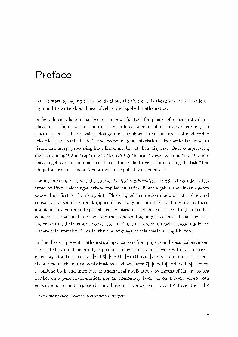
Preface
Let me start by saying a few words about the title of this thesis and how I made up
my mind to write about linear algebra and applied mathematics.
In fact, linear algebra has become a powerful tool for plenty of mathematical ap-
plications. Today, we are confronted with linear algebra almost everywhere, e.g., in
natural sciences, like physics, biology and chemistry, in various areas of engineering
(electrical, mechanical, etc.) and economy (e.g., statistics). In particular, modern
signal and image processing have linear algebra at their disposal. Data compression,
digitizing images and �repairing� defective signals are representative examples where
linear algebra comes into action. This is the explicit reason for choosing the title:�The
ubiquitous role of Linear Algebra within Applied Mathematics�.
For me personally, it was the course Applied Mathematics for SSTAP1-students lec-
tured by Prof. Feichtinger, where applied numerical linear algebra and linear algebra
exposed me �rst to the viewpoint. This original inspiration made me attend several
consolidation seminars about applied (linear) algebra until I decided to write my thesis
about linear algebra and applied mathematics in English. Nowadays, English has be-
come an international language and the standard language of science. Thus, scientists
prefer writing their papers, books, etc. in English in order to reach a broad audience.
I share this intention. This is why the language of this thesis is English, too.
In this thesis, I present mathematical applications from physics and electrical engineer-
ing, statistics and demography, signal and image processing. I work with both more el-
ementary literature, such as [Str03], [OS06], [Bro91] and [Usm87], and more technical-
theoretical mathematical contributions, such as [Dem97], [Goc10] and [Sad08]. Hence,
I combine both and introduce mathematical applications by means of linear algebra
neither on a pure mathematical nor an elementary level but on a level, where both
coexist and are not neglected. In addition, I worked with MATLAB and the TikZ
1Secondary School Teacher Accreditation Program
5
Preface
environment in order to generate both the �gures and tables. The whole typesetting
was done in LATEX.
The �rst chapter combines physics and electrical engineering and presents three funda-
mental laws of Kirchho� and Ohm, respectively, which combine into the fundamental
network equation. Therefore, we consider the four subspaces, graphs and incidence
matrices.
The second chapter is all about applications to eigenvalues and eigenvectors. We
consider statistics and demographic processes by introducing Markov chains, image
compression by introducing the singular value decomposition, and (minimal norm)
least squares applications.
The third chapter deals with basics of signal and image processing. We provide an
introduction to Fourier analysis and discuss some important tools for signal processing,
e.g., �lters.
The last chapter constitutes an attempt to review our work with respect to mathe-
matics education, teaching and, in general, didactics.
At this point, I would like to express my sincere gratitude to my supervisor Prof.
Hans Georg Feichtinger. First and foremost, I thank him for inspiring me to write
this thesis with his courses and seminars. I learned from him that the interplay of
pure mathematics and applied sciences is possible and (more than) important.
Next, I would like to thank Dr. Kayhan Ince for several discussions about the �rst
chapter, in particular about Kirchho�, Ohm and electrical circuits, and how linear
algebra contributes to electrical engineering, in general. Further, I thank my friends
and colleagues from software engineering, technical mathematics, pedagogy and edu-
cational studies for motivating me with new ideas, comments and questions.
Finally, I wish to thank my parents, who have supported me in many ways, for their
patience and understanding.
6
1 The backbone of Linear Algebra:
The Four Subspaces
1.1 Motivation
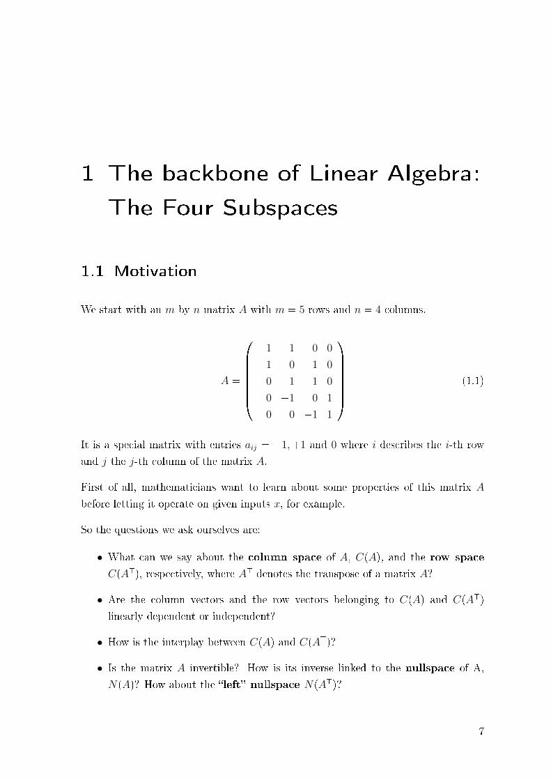
We start with an m by n matrix A with m � 5 rows and n � 4 columns.
A �
���������1 1 0 0
�1 0 1 0
0 �1 1 0
0 �1 0 1
0 0 �1 1
������� (1.1)
It is a special matrix with entries aij � �1,�1 and 0 where i describes the i-th row
and j the j-th column of the matrix A.
First of all, mathematicians want to learn about some properties of this matrix A
before letting it operate on given inputs x, for example.
So the questions we ask ourselves are:
• What can we say about the column space of A, CpAq, and the row space
CpAJq, respectively, where AJ denotes the transpose of a matrix A?
• Are the column vectors and the row vectors belonging to CpAq and CpAJqlinearly dependent or independent?
• How is the interplay between CpAq and CpAJq?
• Is the matrix A invertible? How is its inverse linked to the nullspace of A,
NpAq? How about the �left� nullspace NpAJq?
7
1 The backbone of Linear Algebra: The Four Subspaces
• What about the rankpAq � rpAq, dim CpAq, dim CpAJq?
• . . .
The series of questions can be continued. In principle they shall help revealing all the
properties of the matrix A. Now we are ready for mathematical operations.
1.2 The Four Subspaces and Kircho�'s Laws
The reader might wonder where there is a connection between the subspaces and
Kircho�. Well, it exactly is the matrix A we introduced above. Just wait and see.
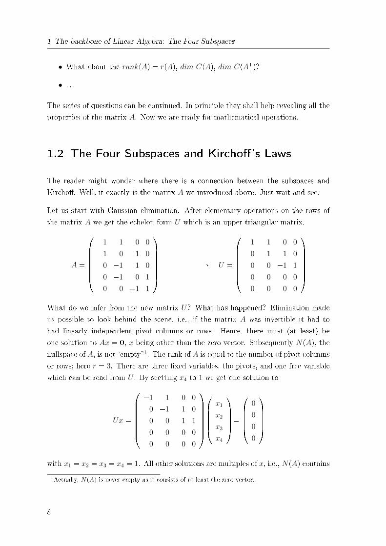
Let us start with Gaussian elimination. After elementary operations on the rows of
the matrix A we get the echelon form U which is an upper triangular matrix.
A �
���������1 1 0 0
�1 0 1 0
0 �1 1 0
0 �1 0 1
0 0 �1 1
������� ÝÝÝÝÝÝÝÝÝÑ U �
���������1 1 0 0
0 �1 1 0
0 0 �1 1
0 0 0 0
0 0 0 0
������� What do we infer from the new matrix U? What has happened? Elimination made
us possible to look behind the scene, i.e., if the matrix A was invertible it had to
had linearly independent pivot columns or rows. Hence, there must (at least) be
one solution to Ax � 0, x being other than the zero vector. Subsequently NpAq, thenullspace of A, is not �empty�1. The rank of A is equal to the number of pivot columns
or rows; here r � 3. There are three �xed variables, the pivots, and one free variable
which can be read from U . By seetting x4 to 1 we get one solution to
Ux �
���������1 1 0 0
0 �1 1 0
0 0 �1 1
0 0 0 0
0 0 0 0
�������
������x1
x2
x3
x4
����� �
������0
0
0
0
����� with x1 � x2 � x3 � x4 � 1. All other solutions are multiples of x, i.e., NpAq contains1Actually, NpAq is never empty as it consists of at least the zero vector.
8
1.2 The Four Subspaces and Kircho�'s Laws
all the vectors of the form c � p1, 1, 1, 1qJ.
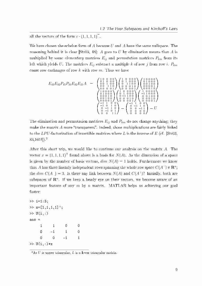
We have chosen the echelon form of A because U and A have the same nullspace. The
reasoning behind it is clear [Str03, 48]: A goes to U by elimination means that A is
multiplied by some elementary matrices Eij and permutation matrices Pkm from its
left which yields U . The matrices Eij subtract a multiple k of row j from row i. Pkmcause row exchanges of row k with row m. Thus we have
E43E32P45P34E32E21A ��
1 0 0 0 00 1 0 0 00 0 1 0 00 0 �1 1 00 0 0 0 1
��1 0 0 0 00 1 0 0 00 �1 1 0 00 0 0 1 00 0 0 0 1
��1 0 0 0 00 1 0 0 00 0 1 0 00 0 0 0 10 0 0 1 0
��
1 0 0 0 00 1 0 0 00 0 0 1 00 0 1 0 00 0 0 0 1
��1 0 0 0 00 1 0 0 00 �1 1 0 00 0 0 1 00 0 0 0 1
��1 0 0 0 0�1 1 0 0 00 0 1 0 00 0 0 1 00 0 0 0 1
�� �1 1 0 0
�1 0 1 00 �1 1 00 �1 0 10 0 �1 1
��� �1 1 0 0
0 �1 1 00 0 �1 10 0 0 00 0 0 0
�� U
The elimination and permutation matrices Eij and Pkm do not change anything; they
make the matrix A more �transparent�. Indeed, those multiplications are fairly linked
to the LPU -factorization of invertible matrices where L is the inverse of E (cf. [Str03,
83,101f]).2
After this short trip, we would like to continue our analysis on the matrix A. The
vector x � p1, 1, 1, 1qJ found above is a basis for NpAq. As the dimension of a space
is given by the number of basis vectors, dim NpAq � 1 holds. Furthermore we know
that A has three linearly independent rows spanning the whole row space CpAJq P Rn;
the dim CpAJq � 3. Is there any link between NpAq and CpAJq? Initially, both are
subspaces of Rn. If we keep a beady eye on their vectors, we become aware of an
important feature of any m by n matrix. MATLAB helps us achieving our goal
faster:
>> i=1:3;
>> x=[1,1,1,1]';
>> U(i,:)
ans =
-1 1 0 0
0 -1 1 0
0 0 -1 1
>> U(i,:)*x
2As U is upper triangular, L is a lower triangular matrix.
9
1 The backbone of Linear Algebra: The Four Subspaces
ans =
0
0
0
We just multiplied each row i by x � p1, 1, 1, 1qJ which yielded 0 every single time. We
conclude that any x P NpAq is perpendicular or orthogonal to any vector w P CpAJq.Hence the subspaces NpAq and CpAJq are orthogonal.
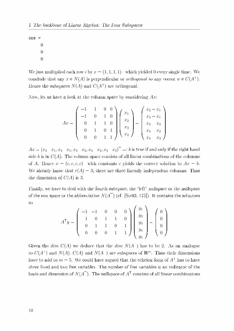
Now, let us have a look at the column space by considering Ax:
Ax �
���������1 1 0 0
�1 0 1 0
0 �1 1 0
0 �1 0 1
0 0 �1 1
�������
������x1
x2
x3
x4
����� �
��������x2 � x1
x3 � x1
x3 � x2
x4 � x2
x4 � x3
������� Ax � px2�x1, x3�x1, x3�x2, x4�x2, x4�x3qJ �: b is true if and only if the right hand
side b is in CpAq. The column space consists of all linear combinations of the columns
of A. Hence x � pc, c, c, cqJ with constants c yields the correct solution to Ax � b.
We already know that rpAq � 3; there are three linearly independent columns. Thus
the dimension of CpAq is 3.
Finally, we have to deal with the fourth subspace, the �left� nullspace or the nullspace
of the row space or the abbreviation NpAJq (cf. [Str03, 175]). It contains the solutionsto
AJy �
�������1 �1 0 0 0
1 0 �1 �1 0
0 1 1 0 �1
0 0 0 1 1
�����
��������y1
y2
y3
y4
y5
������� �
������0
0
0
0
����� Given the dim CpAq we deduce that the dim NpAJq has to be 2. As an analogue
to CpAJq and NpAq, CpAq and NpAJq are subspaces of Rm. Thus their dimensions
have to add to m � 5. We could have argued that the echelon form of AJ has to have
three �xed and two free variables. The number of free variables is an indicator of the
basis and dimension of NpAJq. The nullspace of AJ consists of all linear combinations
10
1.2 The Four Subspaces and Kircho�'s Laws
satisfying AJy � p0q, i.e.,
NpAJq �
$''''''''''''&''''''''''''%c
���������1
1
0
�1
1
������� looomooon
yα
� d
��������1
�1
1
0
0
������� looomooon
yβ
where c, d P R
,////////////.////////////-Special about yα and yβ is that they are orthogonal to b P CpAq. Any multiples of yαand yβ are perpendicular to b. Hence, the subspaces NpAJq and CpAq are orthogonal.
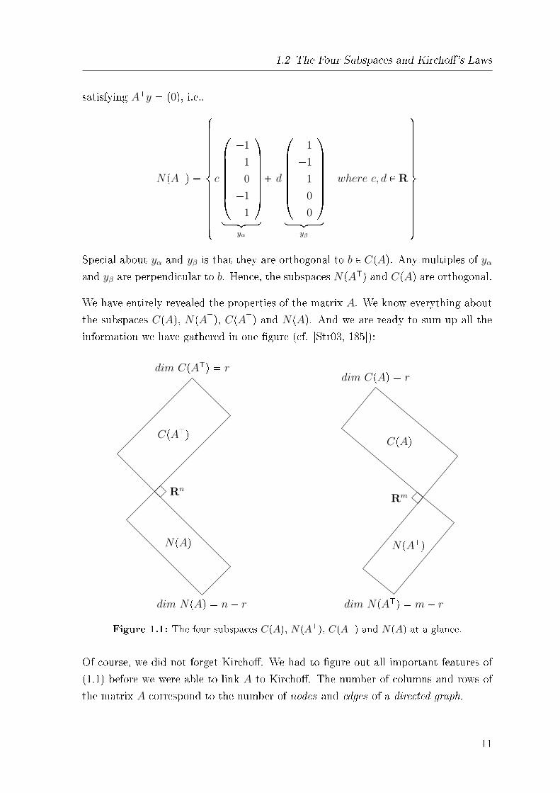
We have entirely revealed the properties of the matrix A. We know everything about
the subspaces CpAq, NpAJq, CpAJq and NpAq. And we are ready to sum up all the
information we have gathered in one �gure (cf. [Str03, 185]):
Rn
CpAJq
dim CpAJq � r
NpAq
dim NpAq � n� r
CpAq
dim CpAq � r
NpAJq
dim NpAJq � m� r
Rm
Figure 1.1: The four subspaces CpAq, NpAJq, CpAJq and NpAq at a glance.
Of course, we did not forget Kircho�. We had to �gure out all important features of
(1.1) before we were able to link A to Kircho�. The number of columns and rows of
the matrix A correspond to the number of nodes and edges of a directed graph.
11
1 The backbone of Linear Algebra: The Four Subspaces
De�nition 1. [Dem97, 288] A directed graph is a �nite collection of nodes connected
by a �nite collection of directed edges, i.e., arrows from one node to another. A path
in a directed graph is a sequence of nodes n1, . . . , nm with an edge from each ni to
ni�1. A self edge is an edge from a node to itself.
Graphs are crucial in discrete mathematics (cf. [Goc10, p.168]). They serve as an
abstract representation of interconnections of objects belonging to a certain set. For
example, we could think of a set of websites and how some of them are linked to
each other. Another example is a genealogical tree depicting a set of people and their
relationships. Actually, this is a graph without any loops and is called - not by chance
- a tree. What we want to do is to study such types abstractly. Therefore we assign
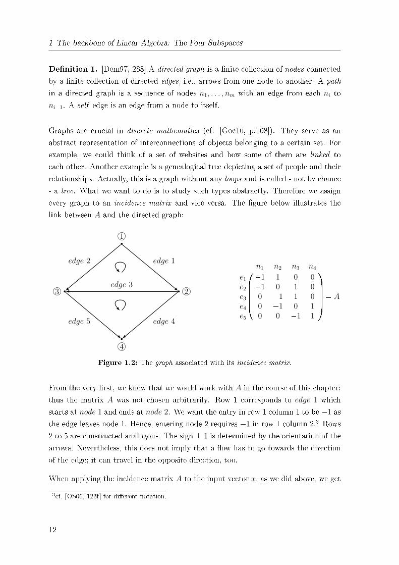
every graph to an incidence matrix and vice versa. The �gure below illustrates the
link between A and the directed graph:
1
4
23
edge 1edge 2
edge 3
edge 5 edge 4
������
n1 n2 n3 n4
e1 �1 1 0 0e2 �1 0 1 0e3 0 �1 1 0e4 0 �1 0 1e5 0 0 �1 1
����� � A
Figure 1.2: The graph associated with its incidence matrix.
From the very �rst, we knew that we would work with A in the course of this chapter;
thus the matrix A was not chosen arbitrarily. Row 1 corresponds to edge 1 which
starts at node 1 and ends at node 2. We want the entry in row 1 column 1 to be �1 as
the edge leaves node 1. Hence, entering node 2 requires �1 in row 1 column 2.3 Rows
2 to 5 are constructed analogous. The sign � 1 is determined by the orientation of the
arrows. Nevertheless, this does not imply that a �ow has to go towards the direction
of the edge; it can travel in the opposite direction, too.
When applying the incidence matrix A to the input vector x, as we did above, we get
3cf. [OS06, 123f] for di�erent notation.
12
1.2 The Four Subspaces and Kircho�'s Laws
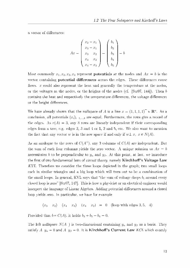
a vector of di�erences:
Ax �
��������x2 � x1
x3 � x1
x3 � x2
x4 � x2
x4 � x3
������� �
��������b1
b2
b3
b4
b5
������� � b
Most commonly x1, x2, x3, x4 represent potentials at the nodes and Ax � b is the
vector containing potential di�erences across the edges. These di�erences cause
�ows. x could also represent the heat and generally the temperature at the nodes,
or the voltages at the nodes, or the heights of the nodes (cf. [Str07, 144]). Then b
contains the heat and respectively the temperature di�erences, the voltage di�erences
or the height di�erences.
We have already shown that the nullspace of A is a line x � p1, 1, 1, 1qJ P Rn. As a
conclusion, all potentials pxiqi�1,...,4 are equal. Furthermore, the rows give a record of
the edges. As rpAq � 3, any 3 rows are linearly independent if their corresponding
edges form a tree, e.g. edges 2, 3 and 4 or 1, 2 and 5, etc. We also want to mention
the fact that any vector w is in the row space if and only if wK x, x P NpAq.
As an analogue to the rows of CpAJq, any 3 columns of CpAq are independent. Butthe sum of each four columns yields the zero vector. A unique solution to Ax � b
necessitates b to be perpendicular to yα and yβ. At this point, at last, we introduce
the �rst of two fundamental laws of circuit theory, namely Kirchho�'s Voltage Law
KVL. Therefore we consider the three loops depicted in the graph; two small loops
each in similar triangles and a big loop which will turn out to be a combination of
the small loops. In general, KVL says that �the sum of voltage drops bi around every
closed loop is zero� [Str07, 147]. This is how a physicist or an electrical engineer would
interpret the language of Linear Algebra. Adding potential di�erences around a closed
loop yields zero. In particular, we have for example
px3 � x2q � px4 � x3q � px4 � x2q � 0 (loop with edges 3, 5,�4)
Provided that b P CpAq, it holds b3 � b5 � b4 � 0.
The left nullspace NpAJq is two-dimensional containing yα and yβ as a basis. They
satisfy AJyα � 0 and AJyβ � 0. It is Kirchho�'s Current Law KCL which exactly
13
1 The backbone of Linear Algebra: The Four Subspaces
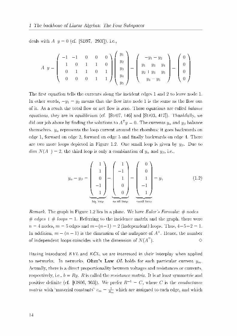
deals with AJy � 0 (cf. [SB97, 293f]), i.e.,
AJy �
�������1 �1 0 0 0
1 0 �1 �1 0
0 1 1 0 �1
0 0 0 1 1
�����
��������y1
y2
y3
y4
y5
������� �
�������y1 � y2
y1 � y3 � y4
y2 � y3 � y5
y4 � y5
����� �
������0
0
0
0
����� The �rst equation tells the currents along the incident edges 1 and 2 to leave node 1.
In other words, �y1 � y2 means that the �ow into node 1 is the same as the �ow out
of it. As a result the total �ow or net �ow is zero. These equations are called balance
equations, they are in equilibrium (cf. [Str07, 146] and [Str03, 417]). Thankfully, we
did our job above by �nding the solutions to AJy � 0. The currents yα and yβ balance
themselves. yα represents the loop current around the rhombus; it goes backwards on
edge 1, forward on edge 2, forward on edge 5 and �nally backwards on edge 4. There
are two more loops depicted in Figure 1.2. One small loop is given by yβ. Due to
dim NpAJq � 2, the third loop is only a combination of yα and yβ, i.e.,
yα � yβ �
���������1
1
0
�1
1
������� looomooonbig loop
�
��������1
�1
1
0
0
������� looomooonsmall loop
�
��������0
0
1
�1
1
������� looomooonsmall loop
� yγ (1.2)
Remark. The graph in Figure 1.2 lies in a plane. We have Euler's Formula: # nodes�# edges�# loops � 1. Referring to the incidence matrix and the graph, there were
n � 4 nodes, m � 5 edges andm�pn�1q � 2 (independent) loops. Thus, 4�5�2 � 1.
In addition, m� pn� 1q is the dimension of the nullspace of AJ. Hence, the number
of independent loops coincides with the dimension of NpAJq. 3
Having introduced KVL and KCL, we are interested in their interplay when applied
to networks. In networks, Ohm's Law OL holds for each particular current ym.
Actually, there is a direct proportionality between voltages and resistances or currents,
respectively, i.e., b � Ry. R is called the resistance matrix. It is at least symmetric and
positive de�nite (cf. [OS06, 303]). We prefer R�1 � C, where C is the conductance
matrix with �material constants� cm � 1Rm
which are assigned to each edge, and which
14
1.2 The Four Subspaces and Kircho�'s Laws
measure the physical properties of the edges (cf. [Str86, 88]). Rewriting the equation
above yields y � �Cb. We had to change the sign of Ax. In circuit theory a �ow
goes from higher potential to lower potential. The potential di�erence across edge 1 is
given by x1 � x2 ¡ 0 providing positive current (cf. [Str03, 419]). With OL, we have
�gured out three fundamental laws of electricity. Combining �Ax � b, y � Cb and
AJy � 0, we get AJCAx � 0. We have put those equations together but, furthermore,
we want some external powers such as current sources f and voltage sources p, e.g.,
batteries, to put something into action. Thus, we change �Ax � b to p�Ax � b and
KCL from AJy � 0 to AJy � f . There are batteries pm along the edges and current
sources fn at the nodes. The modi�ed formulas combine into following fundamental
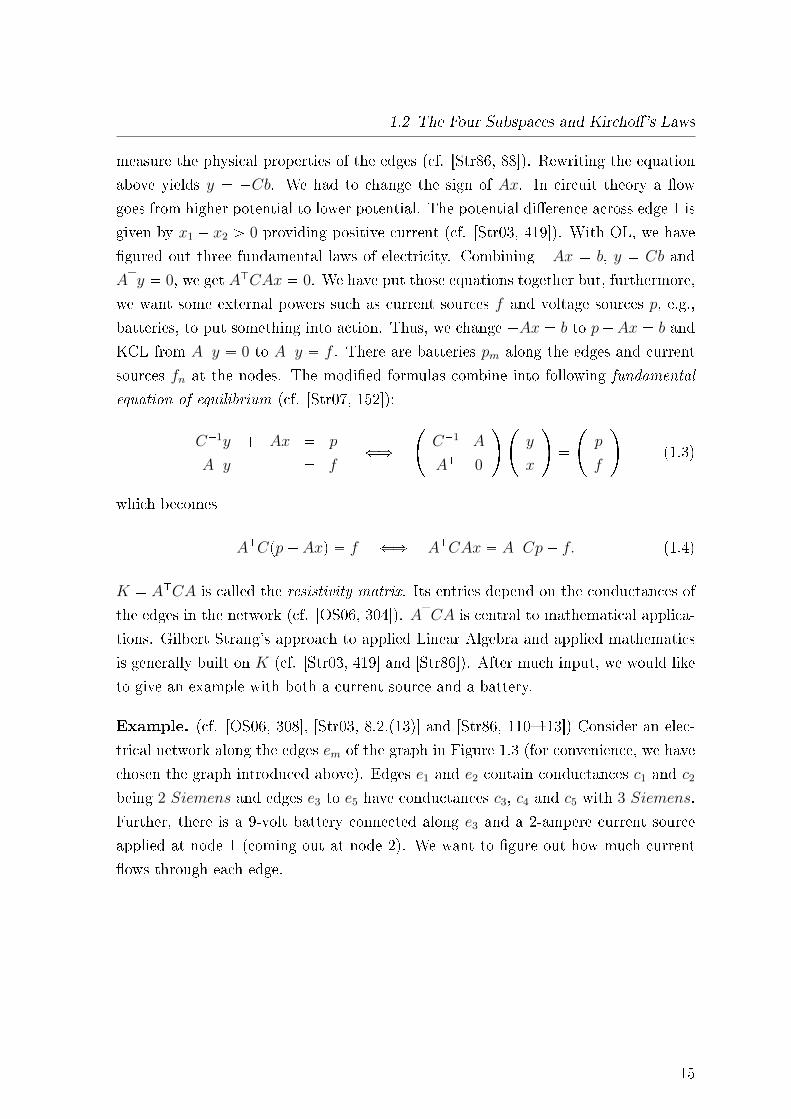
equation of equilibrium (cf. [Str07, 152]):
C�1y � Ax � p
AJy � fðñ
�C�1 A
AJ 0
��y
x
���p
f
�(1.3)
which becomes
AJCpp� Axq � f ðñ AJCAx � AJCp� f. (1.4)
K � AJCA is called the resistivity matrix. Its entries depend on the conductances of
the edges in the network (cf. [OS06, 304]). AJCA is central to mathematical applica-
tions. Gilbert Strang's approach to applied Linear Algebra and applied mathematics
is generally built on K (cf. [Str03, 419] and [Str86]). After much input, we would like
to give an example with both a current source and a battery.
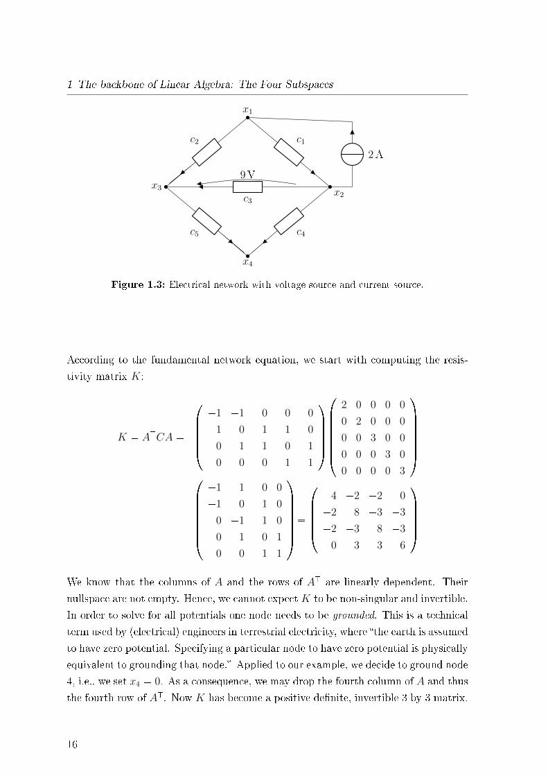
Example. (cf. [OS06, 308], [Str03, 8.2.(13)] and [Str86, 110�113]) Consider an elec-
trical network along the edges em of the graph in Figure 1.3 (for convenience, we have
chosen the graph introduced above). Edges e1 and e2 contain conductances c1 and c2
being 2 Siemens and edges e3 to e5 have conductances c3, c4 and c5 with 3 Siemens.
Further, there is a 9-volt battery connected along e3 and a 2-ampere current source
applied at node 1 (coming out at node 2). We want to �gure out how much current
�ows through each edge.
15
1 The backbone of Linear Algebra: The Four Subspaces
c1c2
c5 c4
c3
9V
2A
x1
x2x3
x4
Figure 1.3: Electrical network with voltage source and current source.
According to the fundamental network equation, we start with computing the resis-
tivity matrix K:
K � AJCA �
�������1 �1 0 0 0
1 0 �1 �1 0
0 1 1 0 �1
0 0 0 1 1
�����
��������2 0 0 0 0
0 2 0 0 0
0 0 3 0 0
0 0 0 3 0
0 0 0 0 3
������� ��������
�1 1 0 0
�1 0 1 0
0 �1 1 0
0 �1 0 1
0 0 �1 1
������� �
������4 �2 �2 0
�2 8 �3 �3
�2 �3 8 �3
0 �3 �3 6
����� We know that the columns of A and the rows of AJ are linearly dependent. Their
nullspace are not empty. Hence, we cannot expectK to be non-singular and invertible.
In order to solve for all potentials one node needs to be grounded. This is a technical
term used by (electrical) engineers in terrestrial electricity, where �the earth is assumed
to have zero potential. Specifying a particular node to have zero potential is physically
equivalent to grounding that node.� Applied to our example, we decide to ground node
4, i.e., we set x4 � 0. As a consequence, we may drop the fourth column of A and thus
the fourth row of AJ. Now K has become a positive de�nite, invertible 3 by 3 matrix.
16
1.2 The Four Subspaces and Kircho�'s Laws
We are ready to solve the right hand side of the equation AJCAx � AJCp� f :
AJCp� f �
��� �1 �1 0 0 0
1 0 �1 �1 0
0 1 1 0 �1
�� ��������
2 0 0 0 0
0 2 0 0 0
0 0 3 0 0
0 0 0 3 0
0 0 0 0 3
�������
��������0
0
9
0
0
������� �
��� �2
2
0
�� �
��� 0
�27
27
�� ���� �2
2
0
�� �
��� 2
�29
27
�� The rest is done via MATLAB:
>> rhs=A'*C*p-f %rhs abbr. for right hand side;
>> x=inv(K)*rhs
x =
1/2
-28/11
28/11
Having �gured out the potentials or node voltages x1, x2 and x3, OL y � Cb �Cpp� Axq yields the currents:
>> y=C*(p-A*x)
y =
67/11
-45/11
129/11
-84/11
84/11
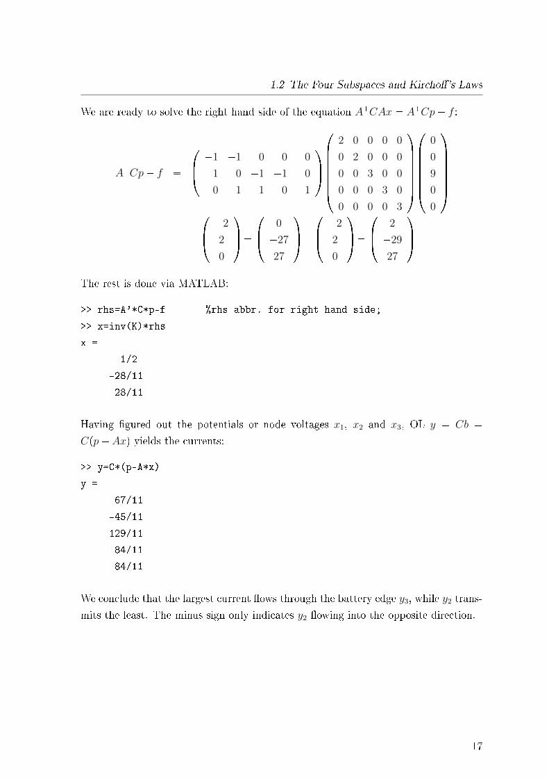
We conclude that the largest current �ows through the battery edge y3, while y2 trans-
mits the least. The minus sign only indicates y2 �owing into the opposite direction.
17
1 The backbone of Linear Algebra: The Four Subspaces
Following network records our results for potentials xn and currents ym:
6711A�45
11A
8411A �84
11A
12911A
9V
2A
x1 � 12V
x2 � �2811V
2811V� x3
(grounded)
D
Summary. (cf. [Str03, 417]) Basic features of Linear Algebra made us possible to
look into the world of physics and engineering. Here is a record of central ideas of the
�rst chapter:
1. The key to applied Linear Algebra: (understanding) the four subspaces CpAq,CpAJq, NpAq and NpAJq.
2. Each graph has its corresponding incidence matrix and vice versa.
3. dim CpAq � dim CpAJq � n�1, dim NpAq � 1 with NpAq containing constantvectors pc, c, . . . , cqJ (cf. [OS06, Prop. 2.51]). and dim NpAJq � m� pn� 1q.
4. Kirchho�'s Voltage Law: Potential di�erences Ax add to zero around each
closed loop.
5. Ohm's Law: y � Cb, i.e., Current � Conductance� voltage drop.
6. Kirchho�'s Current Law: Consider AJy � 0. Flows balance themselves at
each node, i.e., �ow in equals �ow out.
7. Combining KVL, OL and KCL generates the fundamental network equation:
AJCAx � AJCp� f with voltage sources p and current sources f .
18
2 Eigenvalues
This section is devoted to sample applications of eigenvalues and eigenvectors. We
present Markov chains and stochastic processes, elementary image compression with
the SVD, the pseudo-inverse and applications to (minimal norm) least squares.
2.1 Markov chains
De�nition 2. (cf. [Sen81, 113], [FW79, 1] and [Beh00, Chapt. 1]) Given a �nite set
S � s0, s1, . . . , sn�1, the state space with n states, with the conditional probability
ppsk�1|sk, sk�1, . . . , s1, s0q � ppsk�1|skq. This probability property is called Markov
property. Further, let ρ denote a probability vector with entries ppiqiPS where pi ¥0 @j and
°pi � 1, and let T � ppijqi,jPS be a transition matrix where pij ¥ 0 and°
i pij � 1 @j. The tuple pS, T q endowed with the Markov property constitutes a �nite
Markov chain.
Informally (cf. [Bro91, 5,181]), we consider a system with a countable number of
states and assume that the state of the system tomorrow only depends on the current
state of the system (and not on the past, i.e., it has no memory) (cf. [Sad08, 126]).
The system moves from state i to one of the n states, say j, with the probability pij.
In addition, each column of the stochastic matrix T is represented by a probability
vector pi.
Actually, we do not want to know what happens with the system after a single step
or two steps. More generally, we are interested in the case after k steps, i.e., what is
the conditional probability ppsk|s0q? Before introducing an example, we would like to
remind the reader of some crucial facts about eigenvectors and eigenvalues which will
facilitate a lot.
19
2 Eigenvalues
Initially, if we know the eigenvalues and eigenvectors of a square matrix A, we can
easily deal with its powers, Ak, by diagonalizing A. Although not every n by n matrix
is diagonalizable, we can �nd some matrix M such that M�1AM � J . Then A is �as
nearly diagonal as possible� (cf. [Str03, 346]). J denotes the Jordan canonical form.
Nevertheless, we will work with diagonalizable matrices throughout this section.
De�nition 3. (cf. [OS06, 410] and [Str03, 288]) A square matrix A is called diago-
nalizable if there exists a matrix S, where each of its columns is represented by exactly
one of n linearly independent eigenvectors of A, such that
S�1AS � Λ �
����λ1
. . .
λn
��� or, equivalently we have A � SΛS�1.
Λ is a diagonal matrix with entries λ1, . . . , λn, the eigenvalues of A.
Proof. See [OS06, 410f] or [Str03, 288f].
The de�nition above holds for square matrices. We want the matrix A to be symmetric,
too, i.e., we consider A � AJ.
Theorem 1. (cf. [OS06, 413] and [Str03, 318f]) Let A be real and symmetric. Then
following holds:
1. All the eigenvalues are real.
2. Eigenvectors corresponding to di�erent eigenvalues are orthogonal.
Proof. See [OS06, 415f] or [Str03, 320f].
Furthermore, A � SΛS�1 becomes A � QΛQ�1 for symmetric matrices:
Theorem 2. Given a real, symmetric matrix A. Then there exists an orthogonal
matrix Q and a real diagonal matrix Λ such that
A � QΛQ�1 with Q�1 � QJ.
Proof. See [Str03, 319�322].
20
2.1 Markov chains
Remark. (cf. [OS06, 418f] and [Str03, 319]) We are talking about the spectral fac-
torization of A and, more generally, the Spectral Theorem in mathematics and the
Principal Axis Theorem in physics. The columns of the orthogonal matrix Q corre-
spond to eigenvectors of A which we can choose orthonormal. Hence, the columns of
Q form an orthonormal basis of Rn. 3
Being aware of how diagonalization of a matrix is possible, we approach Ak. Let us
start with k � 2. Therefore, we have
A2 � SΛS�1SΛS�1 � SΛ2S�1
and by iteration
Ak � SΛS�1 � � �SΛS�1looooooooomooooooooonk�times
� SΛkS�1.
Obviously, the eigenvectors of A do not change and the eigenvalues are squared and
taken to the k-th power, respectively. Analogous, if we have a real, symmetric matrix
A, the above equations hold true for S � Q.
Now, we are given the conditions which make us possible to deal with a �rst order
linear iterative system, i.e., uk�1 � Tuk, representing a Markov chain.
Example. [OS06, Problem 10.4.2] A study has determined that, on average, the
occupation of a boy depends on that of his father. If the father is a farmer, there is
a 30% chance that the son will be a blue color laborer, a 30% chance he will be a
white color professional, and a 40% chance he will also be a farmer. If the father is a
laborer, there is a 30% chance that the son will also be one, a 60% chance he will be
a professional, and a 10% chance he will be a farmer. If the father is a professional,
there is a 70% chance that the son will also be one, a 25% chance he will be a laborer,
and a 5% chance he will be a farmer.
1. What is the probability that the grandson of a farmer will also be a farmer?
2. In the long run, what proportion of the male population will be farmers?
The information from above is recorded in following �gure:
21
2 Eigenvalues
XXXXXXXXXXXXSONFATHER
farmer laborer professional
farmer 0.4 0.1 0.05
laborer 0.3 0.3 0.25
professional 0.3 0.6 0.7
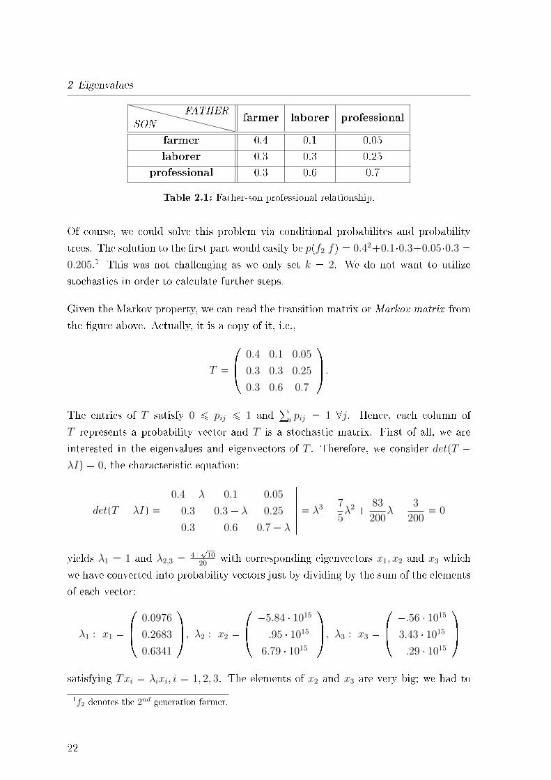
Table 2.1: Father-son professional relationship.
Of course, we could solve this problem via conditional probabilites and probability
trees. The solution to the �rst part would easily be ppf2|fq � 0.42�0.1�0.3�0.05�0.3 �0.205.1 This was not challenging as we only set k � 2. We do not want to utilize
stochastics in order to calculate further steps.
Given the Markov property, we can read the transition matrix or Markov matrix from
the �gure above. Actually, it is a copy of it, i.e.,
T �
��� 0.4 0.1 0.05
0.3 0.3 0.25
0.3 0.6 0.7
�� .The entries of T satisfy 0 ¤ pij ¤ 1 and
°i pij � 1 @j. Hence, each column of
T represents a probability vector and T is a stochastic matrix. First of all, we are
interested in the eigenvalues and eigenvectors of T . Therefore, we consider detpT �λIq � 0, the characteristic equation:
detpT � λIq �
�������0.4� λ 0.1 0.05
0.3 0.3� λ 0.25
0.3 0.6 0.7� λ
������� � λ3 � 7
5λ2 � 83
200λ� 3
200� 0
yields λ1 � 1 and λ2,3 � 4�?1020
with corresponding eigenvectors x1, x2 and x3 which
we have converted into probability vectors just by dividing by the sum of the elements
of each vector:
λ1 : x1 �
��� 0.0976
0.2683
0.6341
�� , λ2 : x2 �
��� �5.84 � 1015
�.95 � 1015
6.79 � 1015
�� , λ3 : x3 �
��� �.56 � 1015
3.43 � 1015
�.29 � 1015
�� satisfying Txi � λixi, i � 1, 2, 3. The elements of x2 and x3 are very big; we had to
1f2 denotes the 2nd generation farmer.
22
2.1 Markov chains
shorten them. Actually, we knew that one root of the characteristic equation would
be 1. T is a regular stochastic matrix with entries pij � 0 and following theorem tells
us more about it:
Theorem 3. (cf. [Sad08, 128] and [OS06, 542]) If T is a regular stochastic matrix,
then
1. λ1 � 1 is an eigenvalue of T . The entries of the corresponding eigenvector x1
are all non-negative. We can normalize x1 such that it becomes a probability
vector.
2. T has no eigenvalue of magnitude greater than 1.
3. Any Markov chain with coe�cient matrix T converges to the probability eigen-
vector: uk Ñ x1 pk Ñ 8q.
Proof. See [Sad08, 128�130] and [OS06, 543].
Provided that the father is a farmer, the initial state vector is given by u0 � p1, 0, 0qJ.Additionally, we can diagonalize T and thus have a look at T k. The initial vector is
just a combination of the eigenvectors x1, x2 and x3 with coe�cients c1 � 1, c2 and c3:
u0 �
��� 1
0
0
�� �
��� 0.0976
0.2683
0.6341
�� � c2
��� �5.84 � 1015
�.95 � 1015
6.79 � 1015
�� � c3
��� �.56 � 1015
3.43 � 1015
�.29 � 1015
�� c2 and c3 are very small negative numbers. The columns of S contain the eigenvectors
of T . MATLAB �nds it quite exhausting to calculate u0 � Sc ô c � S�1u0, where
c � pc1, c2, c3qJ, due to the large condition number of T which indicates that detpT qis approximately zero and T is nearly singular.
Formally, multiplying c1x1 � � � � � cnxn by the kth powers of the eigenvalues yields
uk � c1λk1x1 � � � � � cnλ
knxn �
��� | |x1 � � � xn| |
�� ����λ1
. . .
λn
��� ����c1
...
cn
��� � SΛkc.
Obviously, we have SΛkc � SΛkS�1u0 � T ku0. Hence, the solution to the di�erence
23
2 Eigenvalues
system uk�1 � Tuk is uk � T ku0.
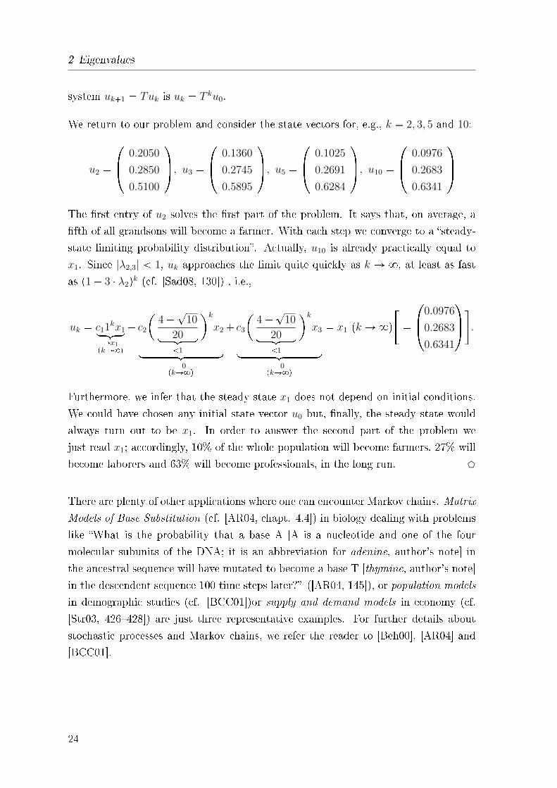
We return to our problem and consider the state vectors for, e.g., k � 2, 3, 5 and 10:
u2 �
��� 0.2050
0.2850
0.5100
�� , u3 �
��� 0.1360
0.2745
0.5895
�� , u5 �
��� 0.1025
0.2691
0.6284
�� , u10 �
��� 0.0976
0.2683
0.6341
�� The �rst entry of u2 solves the �rst part of the problem. It says that, on average, a
�fth of all grandsons will become a farmer. With each step we converge to a �steady-
state limiting probability distribution�. Actually, u10 is already practically equal to
x1. Since |λ2,3| 1, uk approaches the limit quite quickly as k Ñ 8, at least as fast
as p1� 3 � λ2qk (cf. [Sad08, 130]) , i.e.,
uk � c11kx1loomoonÑx1pkÑ8q
� c2
�4�?
10
20looomooon 1
k
x2
loooooooooomoooooooooon�0
pkÑ8q
� c3
�4�?
10
20looomooon 1
k
x3
loooooooooomoooooooooon�0
pkÑ8q
� x1 pk Ñ 8q��
���0.0976
0.2683
0.6341
�� �.
Furthermore, we infer that the steady state x1 does not depend on initial conditions.
We could have chosen any initial state vector u0 but, �nally, the steady state would
always turn out to be x1. In order to answer the second part of the problem we
just read x1; accordingly, 10% of the whole population will become farmers, 27% will
become laborers and 63% will become professionals, in the long run. D
There are plenty of other applications where one can encounter Markov chains. Matrix
Models of Base Substitution (cf. [AR04, chapt. 4.4]) in biology dealing with problems
like �What is the probability that a base A [A is a nucleotide and one of the four
molecular subunits of the DNA; it is an abbreviation for adenine, author's note] in
the ancestral sequence will have mutated to become a base T [thymine, author's note]
in the descendent sequence 100 time steps later?� ([AR04, 145]), or population models
in demographic studies (cf. [BCC01])or supply and demand models in economy (cf.
[Str03, 426�428]) are just three representative examples. For further details about
stochastic processes and Markov chains, we refer the reader to [Beh00], [AR04] and
[BCC01].
24
2.2 Image compression
2.2 Image compression
We consider an m by n image as an m by n matrix. When digitizing an image we
want to read its details by dividing it into pieces, i.e., a lattice with small rectangulars
(=pixels). Each rectangular is assigned a number indicating the brightness of a pixel.
Hence, the more pixels exist, i.e., the �smoothier� the lattice is, the more numbers
we need. These numbers are stored in a matrix. A 320 by 200 lattice equivalently
necessitates a matrix with the same size. Thus it stores 320 � 200 � 64000 numbers
which must not be underestimated. Data processing by a computer is not appropriate
if there is a vast amount of inputs to deal with. The hard disk does not only assign big
data to a bigger storage, it is not sparse with regard to processing time at all. So, we
want to compress the original image by replacing its corresponding matrix such that
the initial image can be reconstructed from many few numbers without much loss of
quality of the image. Therefore, we consider the Singular Value Decomposition (SVD)
(cf. [Gra04, 106], [Dem97, 114] and [Str03, 352]):
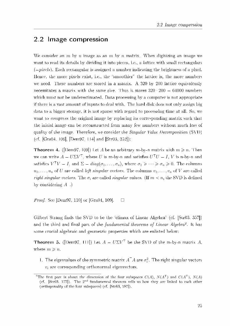
Theorem 4. ([Dem97, 109]) Let A be an arbitrary m-by-n matrix with m ¥ n. Then
we can write A � UΣV J, where U is m-by-n and satis�es UJU � I, V is n-by-n and
satis�es V JV � I, and Σ � diagpσ1, . . . , σnq, where σ1 ¥ � � � ¥ σn ¥ 0. The columns
u1, . . . , un of U are called left singular vectors. The columns v1, . . . , vn of V are called
right singular vectors. The σi are called singular values. (If m n, the SVD is de�ned
by considering AJ.)
Proof. See [Dem97, 110] or [Gra04, 109].
Gilbert Strang �nds the SVD to be the �climax of Linear Algebra� (cf. [Str03, 357])
and the third and �nal part of the fundamental theorems of Linear Algebra2. It has
some crucial algebraic and geometric properties which are enlisted below:
Theorem 5. ([Dem97, 111]) Let A � UΣV J be the SVD of the m-by-n matrix A,
where m ¥ n.
1. The eigenvalues of the symmetric matrix AJA are σ2i . The right singular vectors
vi are corresponding orthonormal eigenvectors.
2The �rst part is about the dimension of the four subspaces CpAq, NpAJq and CpAJq, NpAq(cf. [Str03, 177]). The 2nd fundamental theorem tells us how they are linked to each other(orthogonality of the four subspaces) (cf. [Str03, 187]).
25
2 Eigenvalues
2. The eigenvalues of the symmetric matrix AAJ are σ2i . The left singular vectors
ui are corrseponding orthonormal eigenvectors for the eigenvalues σ2i .
3. Suppose σ1 ¥ � � � ¥ σr ¡ σr�1 � � � � � σn � 0. Then the rank of A is r. The
null space of A is the space spanned by columns r � 1 through n of V , i.e.,
spanpvr�1, . . . , vnq. The column space of A is the space spanned by columns 1
through r of U , i.e., spanpu1, . . . , urq.
4. Let Sn�1 be the unit sphere in Rn: Sn�1 � tx P Rn : ‖x‖2 � 1u. Let A � Sn�1 �tAx, x P Rnand‖x‖2 � 1u. Then A � Sn�1 is an ellipsoid centered at the origin
of Rm, with principal axes σiui.
5. Write V � tv1, . . . , vnu and U � tu1, . . . , unu, so A � UΣV J � °ni�1 σiuiv
Ji (a
sum of rank-1 matrices). Then a matrix of rank k n closest to A (measured
with ‖�‖2) is Ak �°ki�1 σiuiv
Ji , and ‖A � Ak‖2 � σk�1. We may also write
Ak � UΣkVJ, where Σk � diagpσ1, . . . , σk, 0, . . . , 0q.
Proof. (cf. [Dem97, 111f])
1. AJA � pUΣV JqJUΣV J � V ΣUJUΣV J � V Σ2V J. We have diagonalized AJA
where V is an orthogonal matrix with eigenvectors of AJA and Σ2 contains the
eigenvalues σ2i on its diagonal.
2. Analogous to 1.
3. We split U up into U � rU1, U2s where U1 ism-by-n and U2 ism-by-pm�nq. SinceU and V are regular, A and UJAV � rΣ1,0sJ � Σ, where Σ1 is n-by-n and 0 is
pm� nq-by-n, have the same rank. Further, we infer from A � UΣV J ô AV �UΣ that Avi is a multiple of the left singular vectors ui, i.e., Avi � σiui. By
assumption, σr�1 � � � � � σn � 0 and thus Av1�� � ��Avr�Avr�1�� � ��Avn �σ1u1 � � � � � σrur. Hence, Avi � 0 for i � r � 1, . . . , n and Avi � σiui for
i � 1, . . . , r. So the nullspace of A is spanned by vr�1, . . . , vn and the column
space of A is spanned by u1, . . . , ur.
4. We start by multiplying Sn�1 by V J. Since V is orthogonal, it maps unit vectors
to other unit vectors and thus does not change the shape of Sn�1. Hence,
V JSn�1 � Sn�1. Next, since v P Sn�1 if and only if ‖v‖2 � 1, x P ΣSn�1 if and
only if ‖Σ�1x‖2 � 1 which is the same as°ni�1 pxiσi q2 � 1. This is the well known
equation for an ellipsoid with principal axes σiei, where ei is the ith column of I.
26
2.2 Image compression
Finally, we multiply x � Σv by U such that each ei becomes ui, the ith column
of U .
5. By construction, the rank of Ak is k. Further,
‖A� Ak‖2 � ‖n
i�k�1
σiuivJi ‖2 � σmax � σk�1.
Next, we have to show that Ak is the matrix closest to A with respect to the
rank. Therefore, we consider an arbitrary matrix B with rankpBq � k. Hence,
the dimension of its nullspace is n� k. The dimension of the space spanned by
tv1, . . . , vk�1u is k � 1. Since pn � kq � pk � 1q ¡ n, we choose a unit vector h
which is in their intersection. We have
‖A�B‖22 ¥ ‖pA�Bqh‖2
2 � ‖Ah‖22
� ‖UΣV Jh‖22 � ‖ΣpV Jhq‖2
2
¥ σ2k�1‖V Jh‖2
2 � σ2k�1.
Remark. (cf. [Gra04, 103] and [OS06, 428]) Let A be symmetric. According to the
theorem about orthogonal factorization, A decomposes to A � QΛQJ with Q � U �V . We can write A � λiqiq
Ji , equivalently. This is a linear combination of rank-1
matrices or projection matrices qiqJi , respectively. Thus, we interpret the SVD as a
�generalization of the spectral factorization to non-symmetric matrices� ([OS06, 427]).
Next, we conclude from (3) that the orthogonal matrices U and V contain orthonormal
bases for the four subspaces. In addition to (3), tv1, . . . , vru is a basis for the row space
and tur�1, . . . , unu is a basis for the left nullspace.
(4) gives a geometric interpretation of the SVD. Provided that A is a non-singular n-
by-n matrix, U, V and Σ are square, too. U and V represent rotations and re�ections,
whereas Σ represents an orthogonal stretching transformation.
Finally, (5) tells us how to reconstruct A only by considering k singular values. In
short, this is the reduced singular value decomposition (rSVD) giving an optimal low-
rank approximation to A (cf. [Str03, 352]). In applications, we can ignore very small
singular values which do not have any importance with regard to the reconstruction
of A. 3
27
2 Eigenvalues
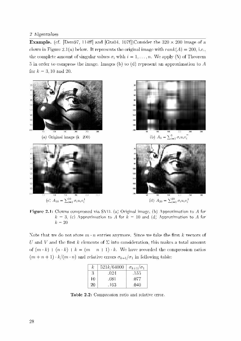
Example. (cf. [Dem97, 114�] and [Gra04, 107f])Consider the 320 � 200 image of a
clown in Figure 2.1(a) below. It represents the original image with rankpAq � 200, i.e.,
the complete amount of singular values σi with i � 1, . . . , n. We apply (5) of Theorem
5 in order to compress the image. Images (b) to (d) represent an approximation to A
for k � 3, 10 and 20.
(a) Original image (k=200) (b) A3 �°3
i�1 σiuivJ
i
(c) A10 �°10
i�1 σiuivJ
i (d) A20 �°20
i�1 σiuivJ
i
Figure 2.1: Clowns compressed via SVD. (a) Original image, (b) Approximation to A for
k � 3, (c) Approximation to A for k � 10 and (d) Approximation to A for
k � 20
Note that we do not store m � n entries anymore. Since we take the �rst k vectors of
U and V and the �rst k elements of Σ into consideration, this makes a total amount
of pm � kq � pn � kq � k � pm � n � 1q � k. We have recorded the compression ratios
pm� n� 1q � k{pm � nq and relative errors σk�1{σ1 in following table:
k 521k{64000 σk�1{σ1
3 .024 .15510 .081 .07720 .163 .040
Table 2.2: Compression ratio and relative error.
28
2.3 Minimal Norm Least Squares MNLSQ
The images were produced in MATLAB by following commands:
load clown
[U,S,V]=svd(X) % MATLAB assigns the matrix X to the image.
colormap('gray')
image(U(:,1:k)*S(1:k,1:k)*V(:,1:k)') % set k=3,10,20
One can use the command svds(X,k) which just computes the �rst k entries of Σ
where σi are in decreasing order. The command lines become
load clown
[U,S,V]=svds(X,k)
colormap('gray')
image(U*S*V').
D
Remark. The SVD has remarkable properties but it is not an ideal choice in applica-
tions like image processing and image compression respectively, statistics and �nance.
Computing the orthogonal matrices U and V are expensive. We need sparse matrices
where computation is faster and cheaper. Therefore, we will introduce �lters when
dealing with elements of Fourier-Analysis in the course of this paper. For further
details about Limitations of the SVD (cf. [Str07, 96f]). 3
2.3 Minimal Norm Least Squares MNLSQ
A linear system of equations, i.e., Ax � b, has either no solution, a unique solution
or in�nitely many solutions. We try to read CpAq properly and often want to know
if b P CpAq. In applications, we face overdetermined systems with more rows than
columns where the right-hand side b does not constitute a linear combination of the
columns of A. Thus, we look for the closest vector in the subspace, say p, with respect
to b. Following �gure illustrates the idea of what we are aiming at:
29
2 Eigenvalues
b
a1
a2p
e � b� p
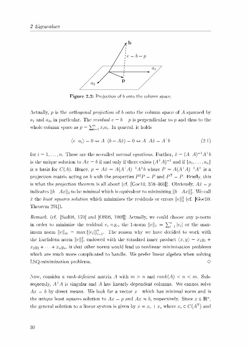
Figure 2.2: Projection of b onto the column space.
Actually, p is the orthogonal projection of b onto the column space of A spanned by
a1 and a2, in particular. The residual e � b� p is perpendicular to p and thus to the
whole column space as p � °ni�1 xiai. In general, it holds
xe | aiy � 0 ô AJpb� Axq � 0 ô AJAx � AJb (2.1)
for i � 1, . . . , n. These are the so-called normal equations. Further, x � pAJAq�1AJb
is the unique solution to Ax � b if and only if there exists pAJAq�1 and if ta1, . . . , anuis a basis for CpAq. Hence, p � Ax � ApAJAq�1AJb where P � ApAJAq�1AJ is a
projection matrix acting on b with the properties P 2P � P and PJ � P . Brie�y, this
is what the projection theorem is all about (cf. [Goc10, 358�360]). Obviously, Ax � p
indicates ‖b�Ax‖2 to be minimal which is equivalent to minimizing ‖b�Ax‖22. We call
x the least squares solution which minimizes the residuals or errors ‖e‖22 (cf. [Goc10,
Theorem 291]).
Remark. (cf. [Sad08, 170] and [OS06, 196f]) Actually, we could choose any p-norm
in order to minimize the residual e, e.g., the 1-norm ‖e‖1 � °ni�1 |ei| or the max-
imum norm ‖e‖8 � max t|ei|uni�1. The reason why we have decided to work with
the Euclidean norm ‖e‖22, endowed with the standard inner product xx, yy � x1y1 �
x2y2 � � � � � xnyn, is that other norms would lead to nonlinear minimization problems
which are much more complicated to handle. We prefer linear algebra when solving
LSQ-minimization problems. 3
Now, consider a rank-de�cient matrix A with m ¡ n and rankpAq n m. Sub-
sequently, AJA is singular and A has linearly dependent columns. We cannot solve
Ax � b by direct means. We look for a vector x� which has minimal norm and is
the unique least squares solution to Ax � p and Ax � b, respectively. Since x P Rn,
the general solution to a linear system is given by x � xr � xs where xr P CpAJq and
30
2.3 Minimal Norm Least Squares MNLSQ
xs P NpAq. The system Axr � p is uniquely solvable due to Axs � 0. Moreover, it
follows from the pythagorean formula for right triangles that ‖x‖22 � ‖xr‖2
2 � ‖xs‖22.
By setting ‖xs‖22 � 0 ô ‖xs‖2 � 0 ô xs � 0, we obtain the minimal norm solution
denoted by x� � xr. It remains to �nd a way to compute x� satisfying Ax� � p.
We have already introduced how to deal with rectangular, ill-conditioned matrices.
The SVD of such a matrix is the key to the right solution:
De�nition 4. (cf. [Dem97, 126f]) Suppose that A is a rectangular matrix withm ¡ n
and rankpAq � r n m, with A � UΣV J being the SVD of A, respectively. If
r n, the SVD reduces to A � UΣV J � UrΣrVJr where Σr is r-by-r and nonsingular
and Ur and Vr have r columns. Then
A� � Vr�1r UJ
r (2.2)
is called the Moore-Penrose pseudoinverse of a rank-de�cient matrix A. We may also
write A� � V J�U where � ��
Σr 00 0
���
Σ�1r 00 0
.
Remark. (cf. [Usm87, 84]) Let A be any m-by-n matrix. An n-by-m matrix A�
is called the generalized inverse of A if and only if A� satis�es one or more of the
following properties:
1. AA�A = A2. A�AA� = A�
3. pAA�qJ = AA�
4. pA�AqJ = A�A
Furthermore, A� is said to be the pseudoinverse of A if and only if A� satis�es all the
four enlisted properties. 3
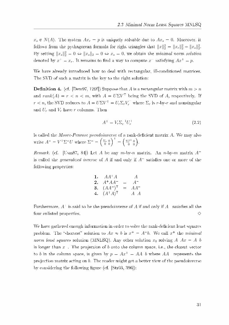
We have gathered enough information in order to solve the rank-de�cient least squares
problem. The �shortest� solution to Ax � b is x� � A�b. We call x� the minimal
norm least squares solution (MNLSQ). Any other solution x0 solving AJAx � AJb
is longer than x�. The projection of b onto the column space, i.e., the closest vector
to b in the column space, is given by p � Ax� � AA�b where AA� represents the
projection matrix acting on b. The reader might get a better view of the pseudoinverse
by considering the following �gure (cf. [Str03, 396]):
31
2 Eigenvalues
0
x�
Rn
CpAJq
NpAq
0b
e � b� p
p � Ax�
Rm
CpAq
NpAJq
A�
A�
A�
A
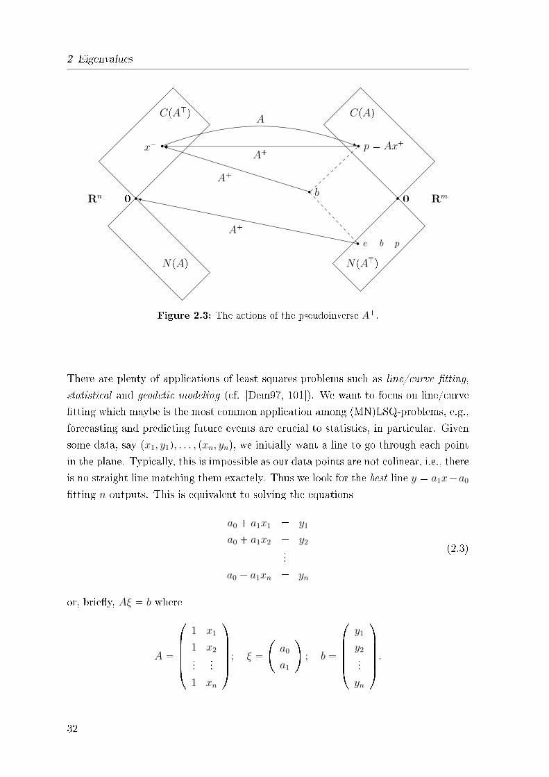
Figure 2.3: The actions of the pseudoinverse A�.
There are plenty of applications of least squares problems such as line/curve �tting,
statistical and geodetic modeling (cf. [Dem97, 101]). We want to focus on line/curve
�tting which maybe is the most common application among (MN)LSQ-problems, e.g.,
forecasting and predicting future events are crucial to statistics, in particular. Given
some data, say px1, y1q, . . . , pxn, ynq, we initially want a line to go through each point
in the plane. Typically, this is impossible as our data points are not colinear, i.e., there
is no straight line matching them exactely. Thus we look for the best line y � a1x�a0
�tting n outputs. This is equivalent to solving the equations
a0 � a1x1 � y1
a0 � a1x2 � y2
...
a0 � a1xn � yn
(2.3)
or, brie�y, Aξ � b where
A �
������1 x1
1 x2
......
1 xn
����� ; ξ ��a0
a1
�; b �
������y1
y2
...
yn
����� .
32
2.3 Minimal Norm Least Squares MNLSQ
By the equations given in (2.1), we compute
AJA ��
1 1 . . . 1
x1 x2 . . . xn
�������1 x1
1 x2
......
1 xn
����� ��
n°xi°
xi° pxiq2
�� n
�1 x
x x2
�,
AJb ��
1 1 . . . 1
x1 x2 . . . xn
�������y1
y2
...
yn
����� �� °
yi°xiyi
�� n
�y�xy� (2.4)
with
x � 1
n
n°i�1
xi , y � 1
n
n°i�1
yi , x2 � 1
n
n°i�1
x2i , �xy � 1
n
n°i�1
xiyi (2.5)
denoting the mean values of the indicated variables (cf. [Sad08, 172f]). Finally, we
have to solve a 2-by-2 system of equations with two unknowns a0 and a1. The solution
(cf. [OS06, 198]) is
a0 � y � a1x and a1 � �xy � xy
x2 � x2�
° pxi � xqyi° pxi � xq2 . (2.6)
We have �gured out ξ which minimizes the least-squares error ‖e‖22 � ‖Aξ � b‖2
2.
Hence, the best straight line �tting the given data in the least squares sense is
y � a1px� xq � y. (2.7)
The slope of the line is given in (2.6) (cf. [OS06, 198]).
Remark. (cf. [Bos10, 161�164]) In statistics this phenomenon is called linear regres-
sion. Provided that pX, Y q is a two-dimensional stochastic variable, the regression
line of y with respect to x is given by (2.7). We call a1 the (empirical) regression
coe�cient of y with respect to x where sxy �° pxi � xqyi denotes the covariance and
s2x � 1
n
° pxi � xq2 is the variance of a random sample of n observations x1, . . . , xn.
The residual ‖e‖22 becomes pn�1qp1�r2qs2
y (cf. [Bos10, 163]), where s2y � 1
n
° pyi � yq2and r � sxy
sxsyis called correlation coe�cient of x and y. Obviously, r lies in the interval
r�1; 1s. For further properties of r (cf. [Bos10, 134]). 3
One might be dissatis�ed with a simple linear model. We could replace the linear
33
2 Eigenvalues
function y � a1x�a0 by a parabola y � a2x2�a1x�a0 or, generally, by a polynomial
of nth degree, i.e., y � anxn � . . . � a1x � a0. Now, the best curve �tting the data
points is obtained by solving following system of equations:
a0 � a1x1 � . . .� anx � y1
a0 � a1x2 � . . .� anx2 � y2
...
a0 � a1xn � . . .� anxn � yn.
(2.8)
In matrix notation, we have V ξ � b with
V �
������1 x1 x2
1 � � � xn1
1 x2 x22 � � � xn2
......
.... . .
...
1 xn x2n � � � xnn
����� ; ξ �
������a0
a1
...
an
����� ; b �
������y1
y2
...
yn
����� . (2.9)
The n � pn � 1q coe�cient matrix V is called Vandermonde matrix. By setting n :�n� 1, V becomes square and invertible for distinct x1, . . . , xn�1. In this case, V ξ � b
has a unique solution indicating ‖e‖22 to be zero. The solution is an interpolating
polynomial which �ts the data exactly (cf. [OS06, 201f]). Interpolation and LSQ-
methods are useful means to approximate functions like?x, sinx or ex by polynomials.
Nevertheless, high-degree polynomials might be badly behaved which could have a
negative impact on the columns of the Vandermonde matrix V . They consitute a poor
basis and V often is ill-conditioned, albeit we divide each column vector by its norm
and make them unit vectors (cf. [Str07, 441,587f]). Hence, high-degree polynomial
interpolation is not used in practical applications (cf. [OS06, 205]).
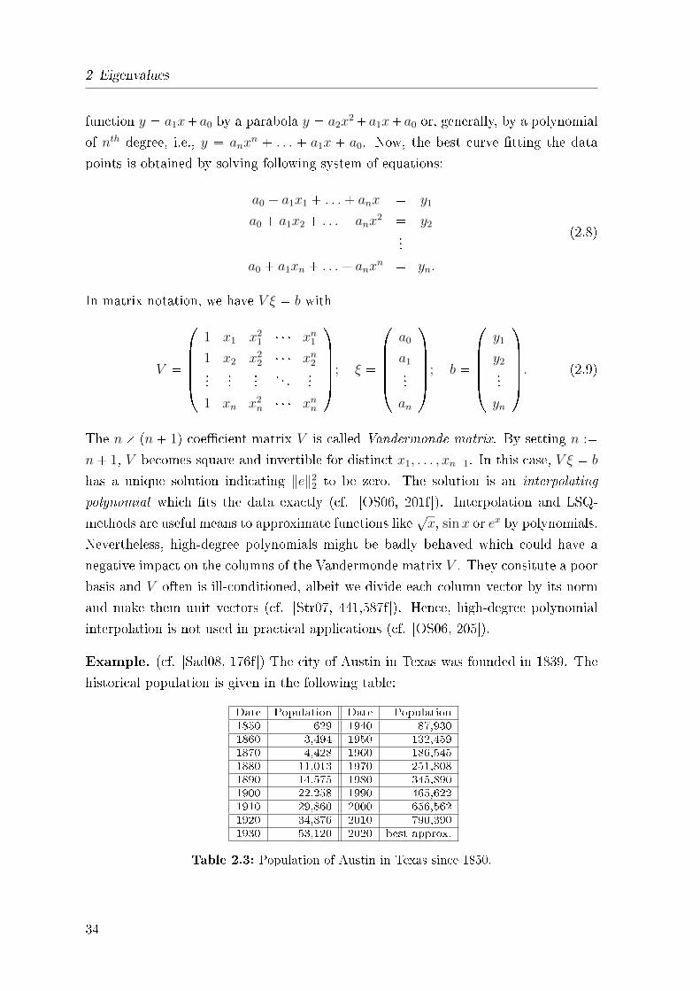
Example. (cf. [Sad08, 176f]) The city of Austin in Texas was founded in 1839. The
historical population is given in the following table:
Date Population Date Population1850 629 1940 87,9301860 3,494 1950 132,4591870 4,428 1960 186,5451880 11,013 1970 251,8081890 14,575 1980 345,8901900 22,258 1990 465,6221910 29,860 2000 656,5621920 34,876 2010 790,3901930 53,120 2020 best approx.
Table 2.3: Population of Austin in Texas since 1850.
34
2.3 Minimal Norm Least Squares MNLSQ
Throughout this example, we will work with MATLAB by analyzing the measured
data. We will use the data from 1850 through 1950 to �nd a model for Austin's
population growth, and use the data from 1960 through 2010 to test our models.
Initially, we want the best linear �t and are interested in estimating the population
from 1960 to 2010. The typical approach to �nding the best line is given by the normal
equations in (2.4) and (2.1), respectively. Thus
AJAξ ��
11 20900
20900 39721000
��a0
a1
���
394642
761879610
�� AJb
where A contains two linearly independent vectors with ones(11,1) generating an
11-by-1 column vector with ones on the one hand and the �rst 11 data entries (until
1950) from the table on the other hand. Hence, the LSQ-solution is
ξ � pAJAq�1AJb ���2047181.5455
1096.3464
�(2.10)
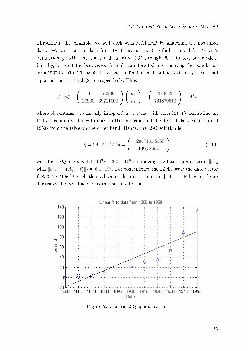
with the LSQ-line y � 1.1 � 103x � 2.05 � 106 minimizing the total squared error ‖e‖2
with ‖e‖2 � ‖pAξ � bq‖2 � 6.1 � 104. For convenience, me might scale the date vector
(1850:10:1950)' such that all values lie in the interval r�1; 1s. Following �gure
illustrates the best line versus the measured data:
Figure 2.4: Linear LSQ-approximation.
35
2 Eigenvalues
There are some convenient commands in MATLAB generating the best line in a least-
squares sense, anyway. The commands can be found in the appendix. Actually, the
command polyfit is based on vander(x), i.e., the Vandermonde matrix V in (2.9)
with respect to the basis BV � t1, x, . . . , xn�1, xnu. If we want to �t a line to some
data, we just take the last two columns of V , i.e., V1=V(:,n-1:n) where n=length(x).
The solution of the overdetermined system V 1ξ � b is obtained by the backslash
operator \ or by the pseudoinverse of V 1,respectively. The poylnomials represented
by tppxq � a1x � a0 with ppxq P PpRqu constitute a two-dimensional subspace of
R11 [cf. lecture notes: applied mathematics for SSTAP]. Hence, we have to solve the
system in a LSQ-sense.
Referring to Figure 2.4, we are not satis�ed with this linear model with respect
to predicting future data. For the period from 1960 to 2010 it yields the vector
p1.0166, 1.1262, 1.2358, 1.3455, 1.4551, 1.5647q � 105. By comparing the sample values
with the measured values, we notice the huge gap between them. And we conclude
that linear growth is not a good model for Austin's population. Thus, we seek for the
best curve beginning with a parabola. Further, we would like to consider polynomials
of higher degree (n ¡ 2).
Let us start with a polynomial of degree n � 2. Therefore, we repeat the commands
above and just substitute 2 for n. Indeed, the parabola turns out to be a better �t in
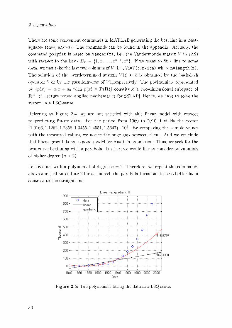
contrast to the straight line:
Figure 2.5: Two polynomials �tting the data in a LSQ-sense.
36
2.3 Minimal Norm Least Squares MNLSQ
Well, it is better with respect to the estimated population for the year 2020 which we
can read from the �gure directly. We, however, �nd the quadratic model rather unre-
liable for future prediction as 415, 680 does not even reach the data from 1990. Thus,
we wonder what happens if we allow more parameters, i.e., we consider polynomials
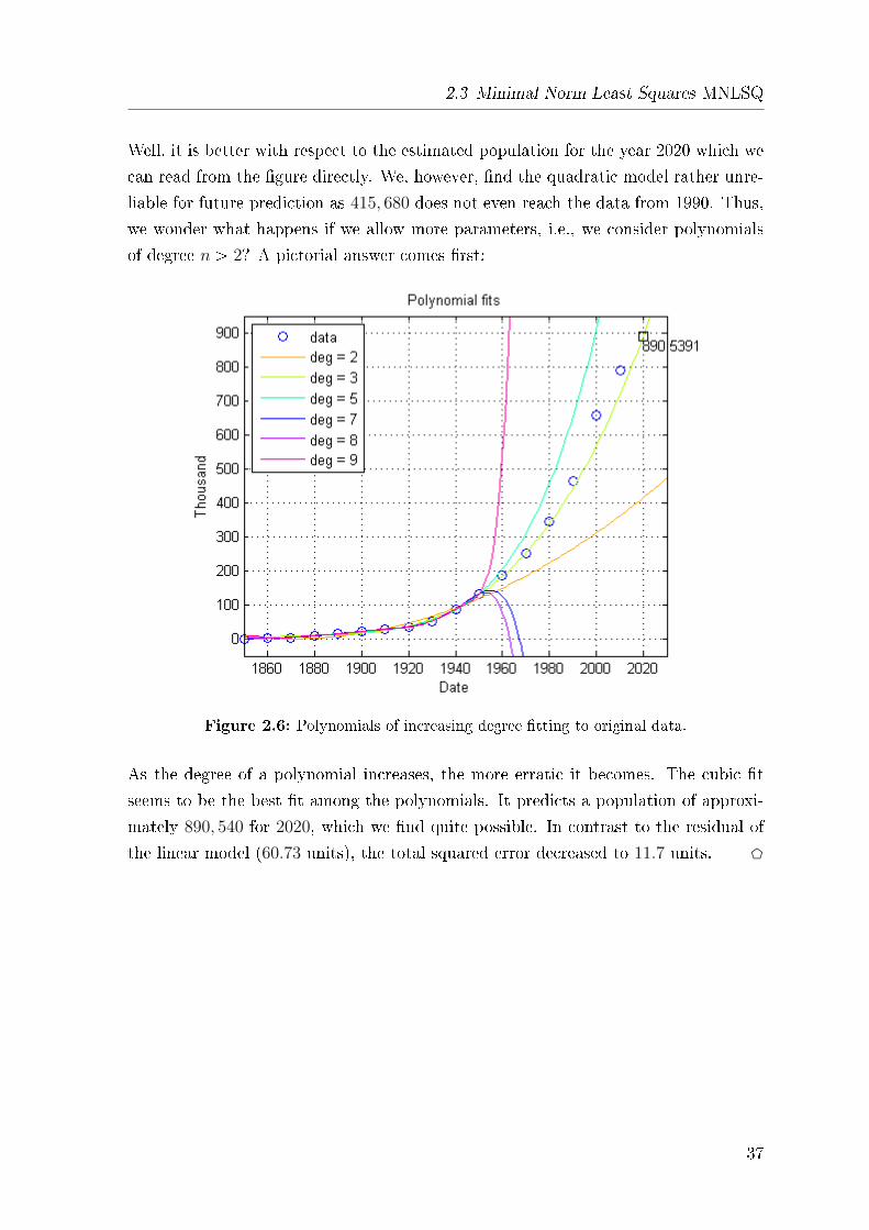
of degree n ¡ 2? A pictorial answer comes �rst:
Figure 2.6: Polynomials of increasing degree �tting to original data.
As the degree of a polynomial increases, the more erratic it becomes. The cubic �t
seems to be the best �t among the polynomials. It predicts a population of approxi-
mately 890, 540 for 2020, which we �nd quite possible. In contrast to the residual of
the linear model (60.73 units), the total squared error decreased to 11.7 units. D
37

38
3 An introduction to Signal (and
Image) Processing
This section is devoted to an elementary introduction to signal (and image) processing.
Initially, we provide some basics of (complex) vector and function spaces (`2, L2), show
their interconnection and say some words about �nite and in�nite dimensional spaces.
Next, we introduce three types of Fourier series and go into detail by considering some
crucial properties of their (partial) sums and coe�cients, respectively. This leads us
to the Discrete Fourier Transform, DFT, and the fast DFT, i.e., the Fast Fourier
Transform, FFT.
Finally, we work on function spaces when dealing with the Fourier integral fpxq and theFourier transform fpωq. Further, we provide fundamental examples and applications
and �nish this section with a competitor to Fourier integral & Co., i.e., wavelets.
Throughout this section, our work is mainly based on [Sad08], [Str07], [Str03] and
[OS06]. We recommend [Str07] to interested readers, who just aim at getting some
idea about Fourier analysis, its applications, wavelets and how all of them contribute
to signal and image processing (cf. [Str07, Chapt. 4]). [Str03] and [OS06] provide
basics, whereas [OS06] confronts the reader with Fourier analysis from a view of point
of signal processing from the very beginning. [Sad08] combines all three references
but goes further by considering important properties of introduced subjects.
3.1 Basics
We have been working with euclidean norms and standard inner products onRn, which
wholly ful�lled our purpose above. Nevertheless, we need to extend our �operation
space� in order to introduce, e.g., (complex) Fourier series.
39
3 An introduction to Signal (and Image) Processing
We obtain the complex norm of a complex vector z by multiplying by its conjugate
transpose, i.e., ‖z‖2 � zJz � zHz � |z1|2, |z2|2, . . . , |zn|2 equipped with the standard
complex inner product xu, vy � uHv � u1v1 � . . .� unvn. The standard inner product
on Cn is a sesquilinear form which is conjugate-symmetric and positive. It is called a
positive Hermitian form (cf. [Sad08, 150]).
Analogous to (real) orthogonal matrices, there exist special complex matrices, i.e.,
Hermitian matrices, A � AJ � AH and unitary matrices U , respectively. A unitary
matrix U has orthonormal columns.
When dealing with Fourier analysis, we will have to operate on in�nite dimensional
spaces. Therefore, we introduce the spaces `2 and L2.
De�nition 5. `2pRq is the space of in�nte sequences of real scalars x1, x2, x3, . . ., such
that the in�nite sum°i |xi|2 converges.
The in�nite dimensional real vector space is denoted by `2pRq. The inner product on`2pRq is given by xx, yy � °8
i�0 xiyi (cf. [Sad08, Theorem 6.8]). The space of in�nite
sequences of complex scalars xi, `2pCq, is de�ned similarly with inner product xx, yy �°8i�0 xisyi. Since `2 is an in�nite dimensional vector space where
b°i|xi|
2 8, we
can take in�nite linear combinations (as long as they converge) from which we bene�t
a lot (see below).
Next, we consider a space of functions on real and complex subsets, denoted by
L2pI,Rq and L2pI,Cq, respectively, or even just L2, �where an orthonormal basis
makes the space look like `2� ([Sad08, 179]). The orthonormal basis will be sine and
cosine functions and complex exponentials, and �the conversion from a function (in
L2) to an in�nite set of coe�cients (in `2) is called Fourier series� ([Sad08, 179]). This
is what we discuss below.
De�nition 6. Let I be a subset of R. Then L2pI,Rq is the space of real-valued
functions fpxq on I sucht that³I|fpxq|2 dx 8. L2pI,Rq is a real inner product
space with inner product xf, gy � ³Ifpxqgpxq dx. Analogous, we de�ne L2pI,Cq, the
space of complex valued functions fpxq on I such that³I|fpxq|2 dx 8. Its inner
product is xf, gy � ³I�fpxqgpxq dx.
Spaces such as `2 and L2, where the norm comes from an inner product, are called
Hilbert spaces (cf. [Sad08, 178]).
40
3.2 Fourier series
3.2 Fourier series
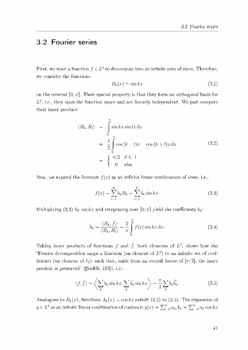
First, we want a function f P L2 to decompose into an in�nite sum of sines. Therefore,
we consider the functions
Bkpxq � sin kx (3.1)
on the interval r0, πs. Their special property is that they form an orthogonal basis for
L2, i.e., they span the function space and are linearly independent. We just compute
their inner product:
xBk, Bly �π»
0
sin kx sin lx dx
� 1
2
π»0
cos pk � lqx� cos pk � lqx dx
�"π{2 if k=l
0 else.
(3.2)
Now, we expand the function fpxq as an in�nite linear combination of sines, i.e.,
fpxq �8
i�1
bkBk �8
i�1
bk sin kx. (3.3)
Multiplying (3.3) by sin kx and integrating over r0, πs yield the coe�cients bk:
bk � xBk, fyxBk, Bly �
2
π
π»0
fpxq sin kx dx. (3.4)
Taking inner products of functions f and f , both elements of L2, shows how the
�Fourier decomposition maps a function (an element of L2) to an in�nite set of coef-
�cients (an element of `2), such that, aside from an overall factor of [π/2], the inner
prodcut is preserved� ([Sad08, 183]), i.e.,
xf, fy �B¸
k
bk sin kx,¸k
bk sin kx
F� π
2
¸k
sbk rbk. (3.5)
Analogous to Bkpxq, functions Akpxq � cos kx satisfy (3.2) to (3.5). The expansion of
g P L2 as an in�nite linear combination of cosines is gpxq � °8i�0 akAk �
°8i�0 ak cos kx
41
3 An introduction to Signal (and Image) Processing
with coe�cients
a0 � 1
π
π»0
gpxq dx and ak � 2
π
π»0
gpxq cos kx dx. (3.6)
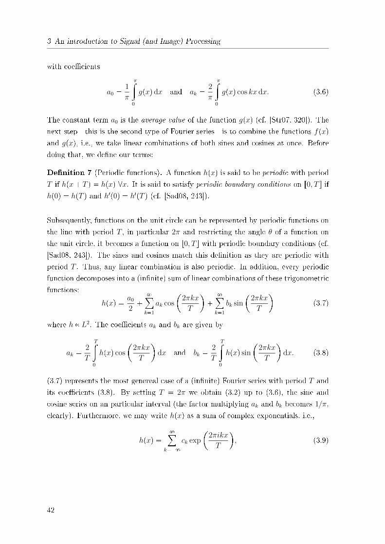
The constant term a0 is the average value of the function gpxq (cf. [Str07, 320]). Thenext step - this is the second type of Fourier series - is to combine the functions fpxqand gpxq, i.e., we take linear combinations of both sines and cosines at once. Before
doing that, we de�ne our terms:
De�nition 7 (Periodic functions). A function hpxq is said to be periodic with period
T if hpx� T q � hpxq @x. It is said to satisfy periodic boundary conditions on r0, T s ifhp0q � hpT q and h1p0q � h1pT q (cf. [Sad08, 243]).
Subsequently, functions on the unit circle can be represented by periodic functions on
the line with period T , in particular 2π and restricting the angle θ of a function on
the unit circle, it becomes a function on r0, T s with periodic boundary conditions (cf.
[Sad08, 243]). The sines and cosines match this de�nition as they are periodic with
period T . Thus, any linear combination is also periodic. In addition, every periodic
function decomposes into a (in�nite) sum of linear combinations of these trigonometric
functions:
hpxq � a0
2�
8
k�1
ak cos
�2πkx
T
�
8
k�1
bk sin
�2πkx
T
(3.7)
where h P L2. The coe�cients ak and bk are given by
ak � 2
T
T»0
hpxq cos
�2πkx
T
dx and bk � 2
T
T»0
hpxq sin
�2πkx
T
dx. (3.8)
(3.7) represents the most genereal case of a (in�nite) Fourier series with period T and
its coe�cients (3.8). By setting T � 2π we obtain (3.2) up to (3.6), the sine and
cosine series on an particular interval (the factor multiplying ak and bk becomes 1{π,clearly). Furthermore, we may write hpxq as a sum of complex exponentials, i.e.,
hpxq �8
k��8ck exp
�2πikx
T
, (3.9)
42
3.2 Fourier series
where
ck � 1
T
T»0
hpxq exp
��2πikx
T
dx. (3.10)
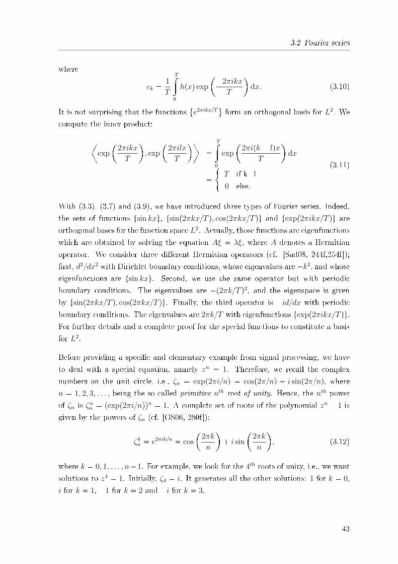
It is not surprising that the functions e2πikx{T( form an orthogonal basis for L2. We
compute the inner product:
Bexp
�2πikx
T
, exp
�2πilx
T
F�
T»0
exp
�2πipk � lqx
T
dx
�#T if k=l
0 else.
(3.11)
With (3.3), (3.7) and (3.9), we have introduced three types of Fourier series. Indeed,
the sets of functions tsin kxu, tsinp2πkx{T q, cosp2πkx{T qu and texpp2πikx{T qu are
orthogonal bases for the function space L2. Actually, those functions are eigenfunctions
which are obtained by solving the equation Aξ � λξ, where A denotes a Hermitian
operator. We consider three di�erent Hermitian operators (cf. [Sad08, 244f,254f]);
�rst, d2{dx2 with Dirichlet boundary conditions, whose eigenvalues are �k2, and whose
eigenfunctions are tsin kxu. Second, we use the same operator but with periodic
boundary conditions. The eigenvalues are �p2πk{T q2, and the eigenspace is given
by tsinp2πkx{T q, cosp2πkx{T qu. Finally, the third operator is �id{dx with periodic
boundary conditions. The eigenvalues are 2πk{T with eigenfunctions texpp2πikx{T qu.For further details and a complete proof for the special functions to constitute a basis
for L2.
Before providing a speci�c and elementary example from signal processing, we have
to deal with a special equation, namely zn � 1. Therefore, we recall the complex
numbers on the unit circle, i.e., ζn � expp2πi{nq � cosp2π{nq � i sinp2π{nq, wheren � 1, 2, 3, . . . , being the so called primitive nth root of unity. Hence, the nth power
of ζn is ζnn � pexpp2πi{nqqn � 1. A complete set of roots of the polynomial zn � 1 is
given by the powers of ζn (cf. [OS06, 280f]):
ζkn � e2πik{n � cos
�2πk
n
� i sin
�2πk
n
, (3.12)
where k � 0, 1, . . . , n�1. For example, we look for the 4th roots of unity, i.e., we want
solutions to z4 � 1. Initially, ζ4 � i. It generates all the other solutions: 1 for k � 0,
i for k � 1, �1 for k � 2 and �i for k � 3.
43
3 An introduction to Signal (and Image) Processing
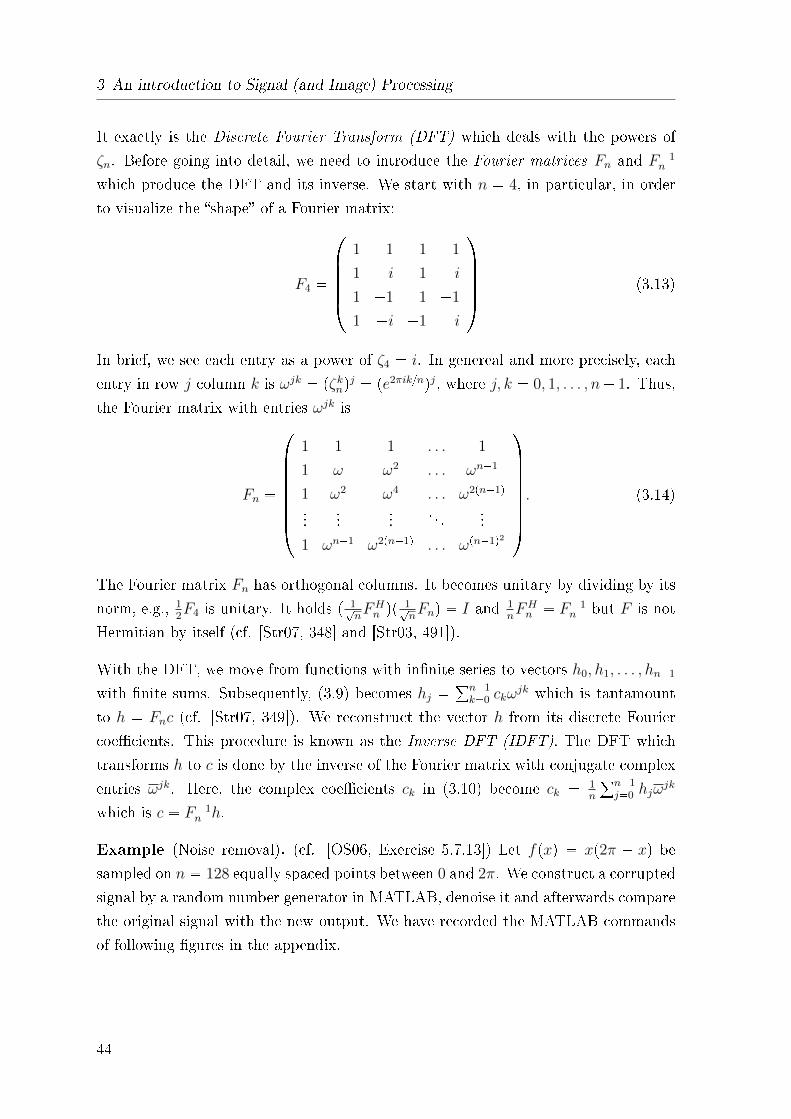
It exactly is the Discrete Fourier Transform (DFT) which deals with the powers of
ζn. Before going into detail, we need to introduce the Fourier matrices Fn and F�1n
which produce the DFT and its inverse. We start with n � 4, in particular, in order
to visualize the �shape� of a Fourier matrix:
F4 �
������1 1 1 1
1 i �1 �i1 �1 1 �1
1 �i �1 i
����� (3.13)
In brief, we see each entry as a power of ζ4 � i. In genereal and more precisely, each
entry in row j column k is ωjk � pζknqj � pe2πik{nqj, where j, k � 0, 1, . . . , n� 1. Thus,
the Fourier matrix with entries ωjk is
Fn �
���������
1 1 1 . . . 1
1 ω ω2 . . . ωn�1
1 ω2 ω4 . . . ω2pn�1q...
......
. . ....
1 ωn�1 ω2pn�1q . . . ωpn�1q2
�������� . (3.14)
The Fourier matrix Fn has orthogonal columns. It becomes unitary by dividing by its
norm, e.g., 12F4 is unitary. It holds p 1?
nFHn qp 1?
nFnq � I and 1
nFHn � F�1
n but F is not
Hermitian by itself (cf. [Str07, 348] and [Str03, 491]).
With the DFT, we move from functions with in�nite series to vectors h0, h1, . . . , hn�1
with �nite sums. Subsequently, (3.9) becomes hj �°n�1k�0 ckω
jk which is tantamount
to h � Fnc (cf. [Str07, 349]). We reconstruct the vector h from its discrete Fourier
coe�cients. This procedure is known as the Inverse DFT (IDFT). The DFT which
transforms h to c is done by the inverse of the Fourier matrix with conjugate complex
entries ωjk. Here, the complex coe�cients ck in (3.10) become ck � 1n
°n�1j�0 hjω
jk
which is c � F�1n h.
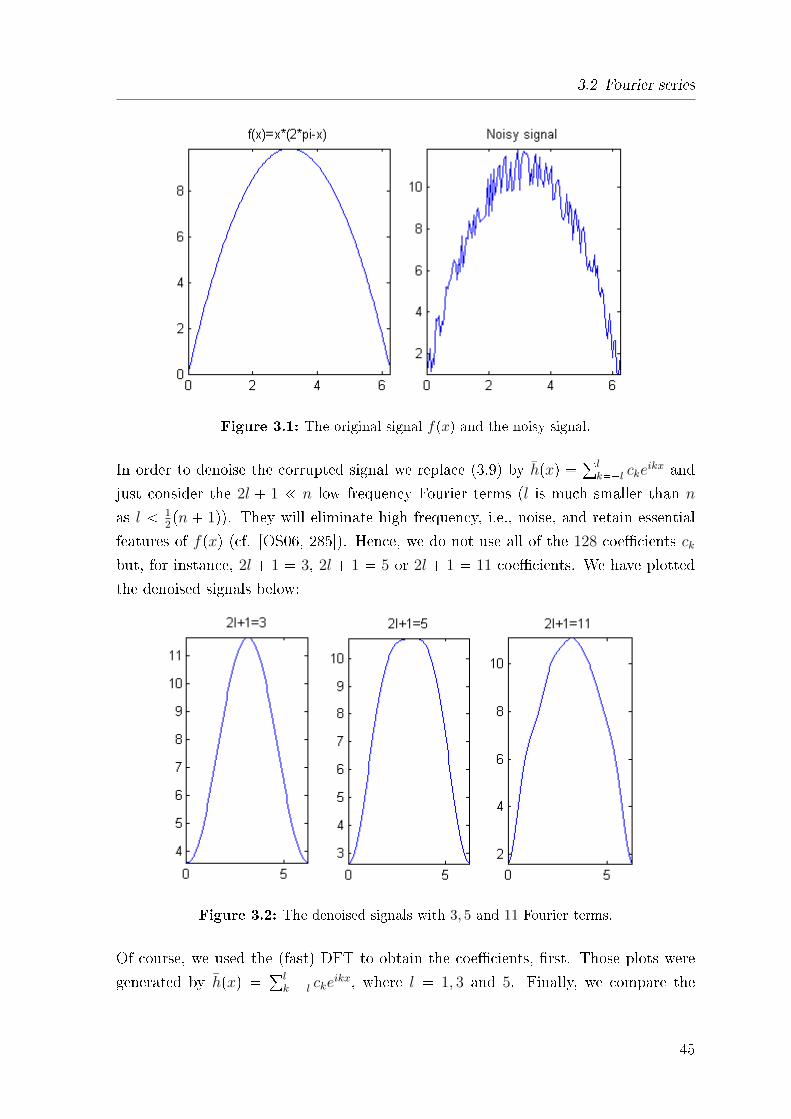
Example (Noise removal). (cf. [OS06, Exercise 5.7.13]) Let fpxq � xp2π � xq besampled on n � 128 equally spaced points between 0 and 2π. We construct a corrupted
signal by a random number generator in MATLAB, denoise it and afterwards compare
the original signal with the new output. We have recorded the MATLAB commands
of following �gures in the appendix.
44
3.2 Fourier series
Figure 3.1: The original signal fpxq and the noisy signal.
In order to denoise the corrupted signal we replace (3.9) by hpxq � °lk��l cke
ikx and
just consider the 2l � 1 ! n low frequency Fourier terms (l is much smaller than n
as l 12pn � 1q). They will eliminate high frequency, i.e., noise, and retain essential
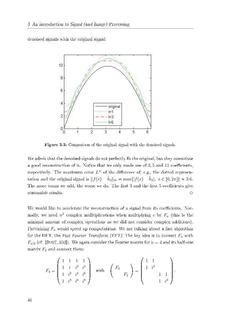
features of fpxq (cf. [OS06, 285]). Hence, we do not use all of the 128 coe�cients ckbut, for instance, 2l � 1 � 3, 2l � 1 � 5 or 2l � 1 � 11 coe�cients. We have plotted
the denoised signals below:
Figure 3.2: The denoised signals with 3, 5 and 11 Fourier terms.
Of course, we used the (fast) DFT to obtain the coe�cients, �rst. Those plots were
generated by hpxq � °lk��l cke
ikx, where l � 1, 3 and 5. Finally, we compare the
45
3 An introduction to Signal (and Image) Processing
denoised signals with the original signal:
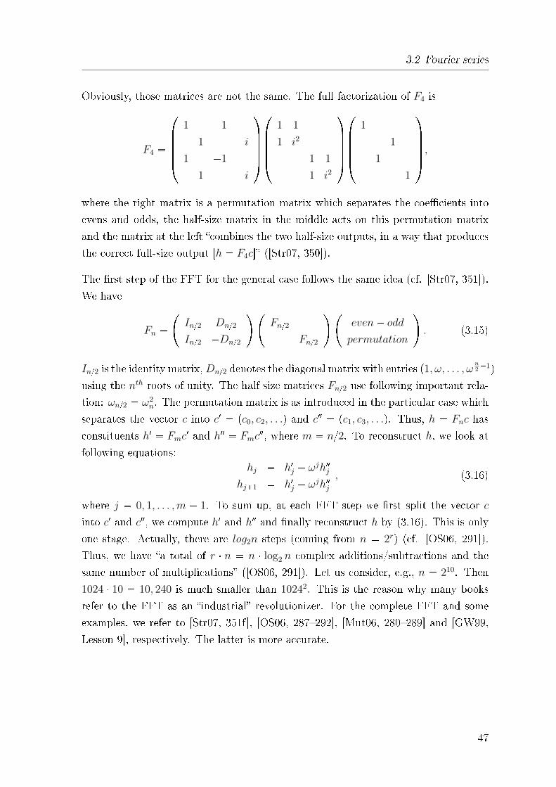
Figure 3.3: Comparison of the original signal with the denoised signals.
We admit that the denoised signals do not perfectly �t the original, but they constitute
a good reconstruction of it. Notice that we only made use of 3, 5 and 11 coe�cients,
respectively. The maximum error L8 of the di�erence of, e.g., the dotted represen-
tation and the original signal is ‖fpxq � h3‖8 � maxt|fpxq � h3|, x P r0, 2πsu � 3.6.
The more terms we add, the worse we do. The �rst 3 and the �rst 5 coe�cients give
reasonable results. D
We would like to accelerate the reconstruction of a signal from its coe�cients. Nor-
mally, we need n2 complex mulitiplications when multiplying c by Fn (this is the
minimal amount of complex operations as we did not consider complex additions).
Factorizing Fn would speed up computations. We are talking about a fast algorithm
for the DFT, the Fast Fourier Transform (FFT). The key idea is to connect Fn with
Fn{2 (cf. [Str07, 350]). We again consider the Fourier matrix for n � 4 and its half-size
matrix F2 and connect them:
F4 �
������1 1 1 1
1 i i2 i3
1 i2 i4 i6
1 i3 i6 i9
����� with
�F2
F2
��
������1 1
1 i2
1 1
1 i2
����� .
46
3.2 Fourier series
Obviously, those matrices are not the same. The full factorization of F4 is
F4 �
������1 1
1 i
1 �1
1 �i
����� ������
1 1
1 i2
1 1
1 i2
����� ������
1
1
1
1
����� ,
where the right matrix is a permutation matrix which separates the coe�cients into
evens and odds, the half-size matrix in the middle acts on this permutation matrix
and the matrix at the left �combines the two half-size outputs, in a way that produces
the correct full-size output [h � F4c]� ([Str07, 350]).
The �rst step of the FFT for the general case follows the same idea (cf. [Str07, 351]).
We have
Fn ��In{2 Dn{2In{2 �Dn{2
��Fn{2
Fn{2
��even� odd
permutation
�. (3.15)
In{2 is the identity matrix,Dn{2 denotes the diagonal matrix with entries p1, ω, . . . , ω n2�1q
using the nth roots of unity. The half size matrices Fn{2 use following important rela-
tion: ωn{2 � ω2n. The permutation matrix is as introduced in the particular case which
separates the vector c into c1 � pc0, c2, . . .q and c2 � pc1, c3, . . .q. Thus, h � Fnc has
constituents h1 � Fmc1 and h2 � Fmc
2, where m � n{2. To reconstruct h, we look at
following equations:hj � h1j � ωjh2j
hj�1 � h1j � ωjh2j, (3.16)
where j � 0, 1, . . . ,m � 1. To sum up, at each FFT step we �rst split the vector c
into c1 and c2, we compute h1 and h2 and �nally reconstruct h by (3.16). This is only
one stage. Actually, there are log2n steps (coming from n � 2r) (cf. [OS06, 291]).
Thus, we have �a total of r � n � n � log2 n complex additions/subtractions and the
same number of multiplications� ([OS06, 291]). Let us consider, e.g., n � 210. Then
1024 � 10 � 10, 240 is much smaller than 10242. This is the reason why many books
refer to the FFT as an �industrial� revolutionizer. For the complete FFT and some
examples, we refer to [Str07, 351f], [OS06, 287�292], [Mut06, 280�289] and [GW99,
Lesson 9], respectively. The latter is more accurate.
47
3 An introduction to Signal (and Image) Processing
3.3 Fourier transform and signals
We want to decompose a function f into its basic constituents, i.e., sines and cosines,
or complex exponentials, respectively, on the entire real line R. It is not completely
di�erent from what we introduced above, however, it is more general (cf. [Sad08,
281]).
De�nition 8. Let f P L2pRq. Then
fptq � 1?2π
8»�8
fpωqeiωt dω, (3.17)
where
fpωq � 1?2π
8»�8
fptqe�iωt dt. (3.18)
The decomposition of a signal in the time domain (3.17) is called Fourier integral. The
complex valued function fpωq is called the Fourier transform of the function fptq. Insignal processing fpωq describes the frequency behavior of the signal fptq. Here, we
speak of working in the frequency domain (cf. [Sad08, 287]).
There are some properties (without proofs) of Fourier transforms which need to be
considered. We start with a proposition which says to treat the function fptq and its
corresponding tranfsorm fpωq on an equal footing (cf. [Sad08, 287], [GW99, 193]).
Proposition (The Plancherel-Parseval equality). Let f, g P L2pRq. Then following
equations hold:8»
�8
�fptqgptq dt �8»
�8
fpωqgpωq dω (3.19)
and 8»�8
|fptq|2 dt �8»
�8
|fpωq|2 dω. (3.20)
Theorem 6. (cf. [Str07, 370], [Sad08, 287] and [Pau07, 4f]) Let f P L2pRq, letfaptq � fpt � aq be the translated function, let gbptq � eibtfptq be the modulated
48
3.3 Fourier transform and signals
function, and let mptq � δf{δt. Then following holds:
fapωq � e�iωafpωqgbpωq � fpω � bqmpωq � iωfpωq.
(3.21)
In words, translating a function by a is tantamount to multiplying its transform by
e�iωa, or, to put it more concrete, � shift of f changes phase of f � ([Str07, 371]). Next,
a phase change of f causes f to shift. Third, the derivative of a function is the same
as multiplying the transform by iω.
Example (Gaussian). (cf. [Sad08, 282f], [Str07, 371]) Let fptq � expp�t2{2q. The
transform is
fpωq � 1?2π
8»�8
e�t2{2e�iωt dt
� 1?2π
8»�8
e�pt2�2ωitq{2 dt
� 1?2π
8»�8
e�pt�iωq2{2e�ω
2{2 dt
� e�ω2{2
?2π
8»�8
e�u2{2 dt
� e�ω2{2,
(3.22)
where u � t � ωi. We put this fascinating result into words: �the Fourier transform
of a standard normal distribution is a standard normal distribution� ([Sad08, 283]).
We could have computed the transform by using, e.g., the third property of Theorem
6 (cf. [Str07, 371]). D
In the discrete case, one might be interested in the Fourier coe�cients of the product
of two functions f and g. It is not the product of ck and dk, however, it is the
convolution of those coe�cients, i.e.,°ckdn�k (cf. [Str07, 357]). Below, we introduce
the convolution for functions f and g (from R to C) and their transforms.
De�nition 9. The convolution of two functions f and g is the function f � g de�nedby
f � gptq �8»
�8
fpt� yqgpyq dy. (3.23)
49
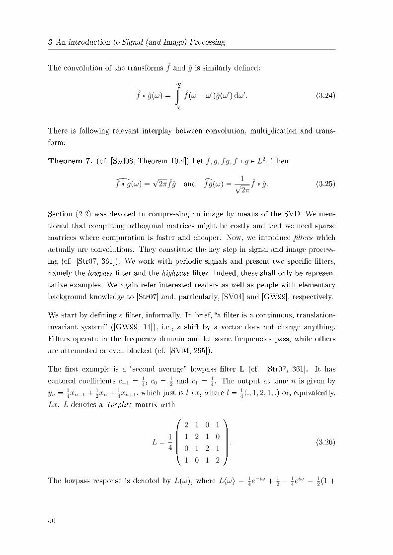
3 An introduction to Signal (and Image) Processing
The convolution of the transforms f and g is similarly de�ned:
f � gpωq �8»
�8
fpω � ω1qgpω1q dω1. (3.24)
There is following relevant interplay between convolution, multiplication and trans-
form:
Theorem 7. (cf. [Sad08, Theorem 10.4]) Let f, g, fg, f � g P L2. Then
zf � gpωq � ?2πf g and xfgpωq � 1?
2πf � g. (3.25)
Section (2.2) was devoted to compressing an image by means of the SVD. We men-
tioned that computing orthogonal matrices might be costly and that we need sparse
matrices where computation is faster and cheaper. Now, we introduce �lters which
actually are convolutions. They constitute the key step in signal and image process-
ing (cf. [Str07, 361]). We work with periodic signals and present two speci�c �lters,
namely the lowpass �lter and the highpass �lter. Indeed, these shall only be represen-
tative examples. We again refer interested readers as well as people with elementary
background knowledge to [Str07] and, particularly, [SV04] and [GW99], respectively.
We start by de�ning a �lter, informally. In brief, �a �lter is a continuous, translation-
invariant system� ([GW99, 14]), i.e., a shift by a vector does not change anything.
Filters operate in the frequency domain and let some frequencies pass, while others
are attenuated or even blocked (cf. [SV04, 295]).
The �rst example is a �second average� lowpass �lter L (cf. [Str07, 361]. It has
centered coe�cients c�1 � 14, c0 � 1
2and c1 � 1
4. The output at time n is given by
yn � 14xn�1 � 1
2xn � 1
4xn�1, which just is l � x, where l � 1
4p., 1, 2, 1, .q or, equivalently,
Lx. L denotes a Toeplitz matrix with
L � 1
4
������2 1 0 1
1 2 1 0
0 1 2 1
1 0 1 2
����� . (3.26)
The lowpass response is denoted by Lpωq, where Lpωq � 14e�iω � 1
2� 1
4eiω � 1
2p1 �
50
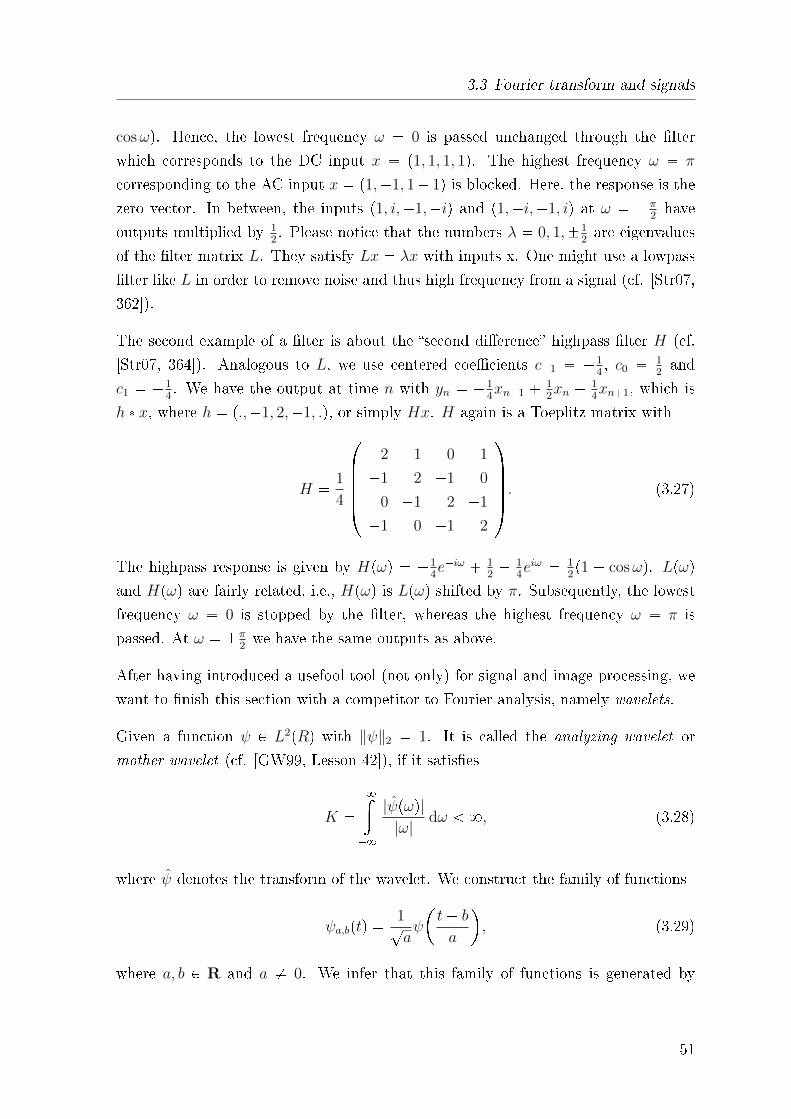
3.3 Fourier transform and signals
cosωq. Hence, the lowest frequency ω � 0 is passed unchanged through the �lter
which corresponds to the DC input x � p1, 1, 1, 1q. The highest frequency ω � π
corresponding to the AC input x � p1,�1, 1� 1q is blocked. Here, the response is thezero vector. In between, the inputs p1, i,�1,�iq and p1,�i,�1, iq at ω � �π
2have
outputs multiplied by 12. Please notice that the numbers λ � 0, 1,�1
2are eigenvalues
of the �lter matrix L. They satisfy Lx � λx with inputs x. One might use a lowpass
�lter like L in order to remove noise and thus high frequency from a signal (cf. [Str07,
362]).
The second example of a �lter is about the �second di�erence� highpass �lter H (cf.
[Str07, 364]). Analogous to L, we use centered coe�cients c�1 � �14, c0 � 1
2and
c1 � �14. We have the output at time n with yn � �1
4xn�1 � 1
2xn � 1
4xn�1, which is
h � x, where h � p.,�1, 2,�1, .q, or simply Hx. H again is a Toeplitz matrix with
H � 1
4
������2 �1 0 �1
�1 2 �1 0
0 �1 2 �1
�1 0 �1 2
����� . (3.27)
The highpass response is given by Hpωq � �14e�iω � 1
2� 1
4eiω � 1
2p1 � cosωq. Lpωq
and Hpωq are fairly related, i.e., Hpωq is Lpωq shifted by π. Subsequently, the lowest
frequency ω � 0 is stopped by the �lter, whereas the highest frequency ω � π is
passed. At ω � �π2we have the same outputs as above.
After having introduced a usefool tool (not only) for signal and image processing, we
want to �nish this section with a competitor to Fourier analysis, namely wavelets.
Given a function ψ P L2pRq with ‖ψ‖2 � 1. It is called the analyzing wavelet or
mother wavelet (cf. [GW99, Lesson 42]), if it satis�es
K �8»
�8
|ψpωq||ω|
dω 8, (3.28)
where ψ denotes the transform of the wavelet. We construct the family of functions
ψa,bptq � 1?aψ
�t� b
a
, (3.29)
where a, b P R and a � 0. We infer that this family of functions is generated by
51
3 An introduction to Signal (and Image) Processing
translations and dilations.
De�nition 10. Fix ψ and let f P L2pRq. The Wavelet transform of f with respect
to ψ denoted by Wψf is
Wψfpa, bq � xf, ψa,by �8»
�8
fptq�ψa,bptq dt. (3.30)
The functionWψf is continuous and bounded. The numberWψfpa, bq is called waveletcoe�cient of f with respect to ψ in pa, bq. The signal fptq is reconstructed by the
Inverse Wavelet transform:
fptq � 1
K
»R
»R
1
a2Wψfpa, bqψ
�t� b
a
da db. (3.31)
We do not further go into detail by introducing other theorems, propositions and
examples. What we want to do is to explain why wavelets have become a very usefull
mathematical tool in applications and why it was, to our mind, necessary to give a
faint idea of it.
The main idea underlying the Fourier transform is to �transform� a signal from its
time domain to its frequency domain. The inverse is obtained by the Fourier integral.
Thus, we consider a signal either in the t-domain or in the ω-domain. We cannot
have it both ways (cf. Heisenberg's Uncertainty Principle, e.g., in [GW99, 197f]). In
addition, the Fourier bases are global and only have a locality in the frequency domain.
Moreover, they give a poor approximation at a jump (cf. Gibbs phenomenon, e.g., in
[Str07, 318f]). To put it more concrete: if we want to represent signals and images �in
a sparse and piecewise smooth way� ([Str07, 389]), we need to choose bases which are
local, easily re�ned, fast to compute, and which yield a good approximation by a few
terms (cf. [Str07, 389]). Wavelets achieve all of them. They represent signals in time
and frequency. They capture high frequencies over short times and lower frequencies
over longer times (cf. [Str07, 390]).
The most common application to wavelets is data compression. For instance, the FBI
preferred wavelet methods for compressing digital �ngerprints instead of a proposal
based on JPEG (Joint Photographic Experts Group). For more information and details
we again refer to some literature: [Str07, Chapt. 4.7], [Fra99], [MMP07], [SV04] and
52

3.3 Fourier transform and signals
[GW99]. [Fra99] introduces wavelets by (not necessarily) elementary linear algebra,
[MMP07] and [SV04] provide many applications worked with MAPLE and MATLAB,
especially [SV04], without going to deep into mathematical questions. [GW99] is all
about fundamentals of signal processing.
53

54
4 �Applicable� Mathematics and
Didactics
In this short section, we �rst introduce some general results of an empirical survey
about �Teaching applications in mathematics education�, which were presented by
J. Humenberger in his habilitation thesis (in 1997). Afterwards, we have a look at
syllabi of secondary academic schools (Allgemeinbildende Höhere Schule, AHS) and
technichal high schools (Höhere Technische Lehranstalt, HTL) and want to know to
which extent linear algebra and its applications are prevalent. Next, we focus on the
math-textbook �Ingenieur-Mathematik 4�, which is commonly used in technical high
schools. We �nish this section with some thoughts, ideas, comments and questions
concerning the teaching and didactics of mathematical applications at (technical) high
schools.
4.1 General part
J. Humenberger wrote his dissertation about �Fundamental ideas of Applied Mathe-
matics�, which was extended to a scienti�c contribution, i.e., a book with the same
title (cf. [HR95]). According to the authors, this book constitutes a �rst approach
to fundamental ideas of applied mathematics as a complete subject (cf. [HR95, V])
(at least restricted to the German area). This is the reason why we have explicitely
chosen this author. In his habilitation thesis, Humenberger presents the results of an
empirical investigation, where teachers, mathematics students and pupils were asked
questions about �applications in mathematics teaching� (cf. [Hum97, 3]). We do not
intend to present all of it, however, we are interested in following problems:
• Applicable and non-applicable mathematical topis (opinions of students and
pupils).
55
4 �Applicable� Mathematics and Didactics
• Computer use at school.
• Teachers' and pupils' opinion on teaching and resp. learning applied mathemat-
ics.
Both students as well as pupils have similar point of views about the �rst issue. They
�nd percent calculation and stochastics (= probability theory + statistics) usefull,
while integral and di�erential calculus, complex numbers and curve sketching and
vector calculus, respectively, are among the least applicable mathematical topics.
Moreover, 74% of pupils never worked with computers in their math-lessons. Only a
quarter of the teachers �sometimes/occasionally� ([Hum97, 45]) let their pupils work
at a computer.
Third; almost 71% of invesitaged teachers �nd mathematical applications useful as
these help pupils to better realize the purpose and essence of mathematics. But they
complain about the complexity of �non-mathematical areas�, i.e., physics, engineering,
biology, etc., that even they themselves do not know much about non-mathematical
contents.
What is interesting - and almost clear - is the pupils' reply to following question:
�What do you like most at mathematics?�. They answered: �Problems, where you can
see how math is applicable� (55%).
4.2 Syllabi
We consider two di�erent kinds of syllabi; �rst, the syllabus of secondary academic
schools (AHS) and second, the syllabus of technical high schools (HTL). According to
the homepage of the Austrian Federal Ministry for Education, Arts and Culture, there
are 14 subject areas pupils might attend (HTL). We are interested in the syllabus of
electronics and electrical engineering as this contains the most amount of mathematics
hours (16 distributed over �ve years). We start with the �rst.
The AHS-syllabus does not explicitely distinguish between linear algebra and other
mathematical topics (analysis, etc.). Following topics (9th � 12th grades) can be as-
signed to linear algebra: (systems of) equations, trigonometry (9thgrade); vector cal-
culus in R2 and R3 (9th and 10th grades); complex numbers and conic section (11th
56
4.3 Ingenieur Mathematik 4 - An analysis
grade). The 12th grade syllabus for math does not contain any topics of linear algebra
and geometry.
The HTL-syllabus is more rich in content with respect to linear algebra. The 9th
and 10th grades math contains vector calculus (R2 and R3), linear (in)equations and
systems of equations, trigonometry and complex numbers. There is a logical reason
behind introducing complex numbers that early. Since the subject area is electrical
engineering, the complex number j in electronics (engineering, in genereal) which is i
in mathematics has an overriding importance (especially for engineers).
The 11th grade students are presented error propagation and estimation, numerical
methods for solving equations, interpolation and di�erence equations. The next grade
contains Fourier sums, matrices, conic section and algebraic structures. Analogous to
the AHS-syllabus, there is no linear algebra content in the 13th grade at all.
For more and detailed information visit the homepage of the Ministry for Education,
Arts and Culture, which is provided in the Bibliography below.
4.3 Ingenieur Mathematik 4 - An analysis
�Ingenieur-Mathematik 4� (ger., �mathematics for engineers�) is a mathematical text-
book which is commonly used at technical high schools. We have analysed its approach
to Fourier analysis.
It starts by introducing in�nite sums (chapter 3) and thus Fourier sums (cf. [TK05,
101]). The authors provide coe�cient properties and decay rates of Fourier coe�cients
and even say a word about the Gibbs phenomenon without explicitely mentioning it
(cf. [TK05, 105f]).
Further, the book presents �Numerical Fourier Analysis� beginning with Shannon's
Sampling Theorem. It provides formulas for the numerical computation of Fourier
coe�cients and introduces the FFT. This chapter ends here but chapter 4 is all about
an important application of Fourier analysis, namely di�erential equations.
Chapter 5 is wholly devoted to �Transforms and Signals� and constitutes an introduc-
tion to signal processing (especially with examples from electrical engineering). We
encounter basic signals like the step function σptq and the Delta impulse δptq. The
57
4 �Applicable� Mathematics and Didactics
Fourier transform and some of its properties, and the Laplace transform follow next.
Di�erential equations and electrical circuits (cf. [TK05, 223�232]) are introduced as
applications to the Laplace transform.
We see that this approach to Fourier analysis is not completely elementary anymore.
This book does not only contain formulas but provides essential explanations to in-
troduced subjects. In fact, it intends at educating young engineers who become an
asset for companies. Actually, each student of a technical high school was granted
an �Ingenieur�-title along with the diploma until recently. Now, they need to work
three years in a �eld which matches their subject area they attended at school (elec-
trical engineering, mechanical engineering, mechatronics, etc.) in order to become an
engineer.
4.4 Comments, ideas, remarks and questions
At this place, we want to review this work including the survey of J. Humenberger, the
syllabi and the mathematical textbook analysed above with respect to mathematics
education.
Almost 15 years have passed since the empirical investigation of Humenberger was
carried out. Indeed, this is a long period of time and we wonder to which extent the
inclusion of mathematical applications into math lessons has happened (in Austria).
While the number in 1997 of computer using students was 74%, we are convinced
that this number has decreased as new-generation teachers make use of computers in
their classes and lessons (this is an assumption as we lack any scienti�c statistics).
For instance, the mathematical software GeoGebra has become a popular computer
algebra system. It particularly appeals to students of secondary academic schools.
Furthermore, we know from some students of technical high schools of various subject
areas that they use MATLAB and Maple in order to cope with complex computations
and simulate physical, electrical, etc. processes.
When considering the mathematical contents of both syllabi, we realize a huge gap in
between. One might take this for granted as AHS provides general and HTL speci�c
(technical) education. While the overwhelming majority of AHS-students enrols at
university, HTL-students prefer working in their subject area. However, the situation
of latter students has started to change since the labor market has become more com-
58
4.4 Comments, ideas, remarks and questions
petitive. Nowadays, companies do not wholly prefer HTL-students with a technical
high school diploma anymore. More and more HTL-students continue their studies
at university in their subject area. They often have a great background knowledge
(referring to the syllabus and, e.g., �Ingenieur Mathematik 4�) which facilitates a lot
- at least in the �rst year after enrolment. The reader might wonder why we write
about this. We think of AHS-students who want to study mathematics, electrical
engineering, and other technical courses who actually are at disadvantage compared
to their colleagues from a technical high scholl. We want to end this series of thoughts
with some (provocative) questions: What is the ideal syllabus which does not neglect
both the AHS-syllabus and the HTL-syllabus? Do HTL-students really need that
much math, nowadays, where so much students with a high school diploma enrol at
university? How about workshops, courses, introductory seminars, etc. in holidays
for future mathematics students, especially about applied mathematics?.
Back to the survey: it is interesting that mathematics students and pupils found
integral, di�erential and vector calculus and complex numbers not applicable. Indeed,
this applies more to AHS-students than HTL-students. To our mind, this is a serious
issue which needs to be considered properly. High school students often wonder where
they need math and for which purpose �something mathematical� is introduced. This
is due to the abstract world of mathematics which causes students trouble as they
cannot �feel� mathematical abstractions.
From our vantage point, it is indispensable to incorporate technology, i.e., hand-held
devices, CAS, etc., into math lessons. Further, we do not think that applied mathe-
matics is a subject to be introduced only in special, time-consuming projects and other
organisations. The adequate education for teachers, the ideal syllabus, the technical
environment in classes (schools) and motivated students are the only prerequisites to
make mathematics fun and interesting.
59

60
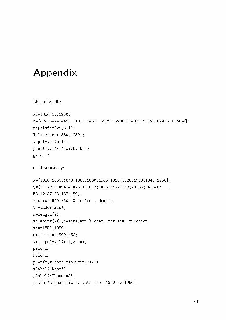
Appendix
Linear LSQ�t:
xi=1850:10:1950;
b=[629 3494 4428 11013 14575 22258 29860 34876 53120 87930 132459];
p=polyfit(xi,b,1);
l=linspace(1850,1950);
v=polyval(p,l);
plot(l,v,'k-',xi,b,'bo')
grid on
or alternatively:
x=[1850;1860;1870;1880;1890;1900;1910;1920;1930;1940;1950];
y=[0.629;3.494;4.428;11.013;14.575;22.258;29.86;34.876; ...
53.12;87.93;132.459];
xsc=(x-1900)/50; % scaled x domain
V=vander(xsc);
n=length(V);
xil=pinv(V(:,n-1:n))*y; % coef. for lin. function
xin=1850:1950;
sxin=(xin-1900)/50;
vxin=polyval(xil,sxin);
grid on
hold on
plot(x,y,'bo',xin,vxin,'k-')
xlabel('Date')
ylabel('Thousand')
title('Linear fit to data from 1850 to 1950')
61
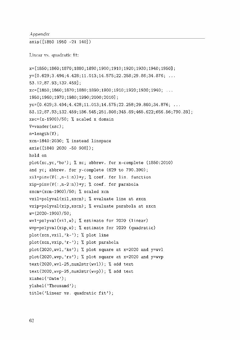
Appendix
axis([1850 1950 -21 140])
Linear vs. quadratic �t:
x=[1850;1860;1870;1880;1890;1900;1910;1920;1930;1940;1950];
y=[0.629;3.494;4.428;11.013;14.575;22.258;29.86;34.876; ...
53.12;87.93;132.459];
xc=[1850;1860;1870;1880;1890;1900;1910;1920;1930;1940; ...
1950;1960;1970;1980;1990;2000;2010];
yc=[0.629;3.494;4.428;11.013;14.575;22.258;29.860;34.876; ...
53.12;87.93;132.459;186.545;251.808;345.89;465.622;656.56;790.39];
xsc=(x-1900)/50; % scaled x domain
V=vander(xsc);
n=length(V);
xcn=1840:2030; % instead linspace
axis([1840 2030 -50 900]);
hold on
plot(xc,yc,'bo'); % xc; abbrev. for x-complete (1850:2010)
and yc; abbrev. for y-complete (629 to 790.390);
xil=pinv(V(:,n-1:n))*y; % coef. for lin. function
xip=pinv(V(:,n-2:n))*y; % coef. for parabola
sxcn=(xcn-1900)/50; % scaled xcn
vxil=polyval(xil,sxcn); % evaluate line at sxcn
vxip=polyval(xip,sxcn); % evaluate parabola at sxcn
w=(2020-1900)/50;
wvl=polyval(xil,w); % estimate for 2020 (linear)
wvp=polyval(xip,w); % estimate for 2020 (quadratic)
plot(xcn,vxil,'k-'); % plot line
plot(xcn,vxip,'r-'); % plot parabola
plot(2020,wvl,'ks'); % plot square at x=2020 and y=wvl
plot(2020,wvp,'rs'); % plot square at x=2020 and y=wvp
text(2020,wvl-25,num2str(wvl)); % add text
text(2020,wvp-25,num2str(wvp)); % add text
xlabel('Date');
ylabel('Thousand');
title('Linear vs. quadratic fit');
62
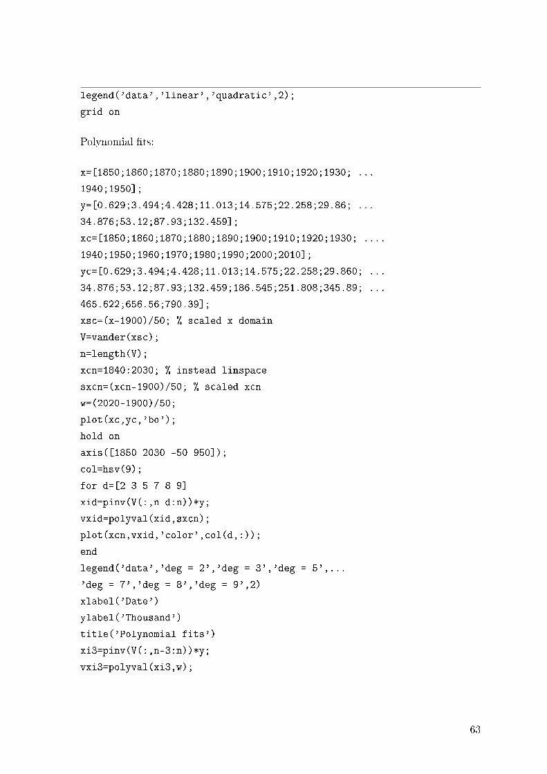
legend('data','linear','quadratic',2);
grid on
Polynomial �ts:
x=[1850;1860;1870;1880;1890;1900;1910;1920;1930; ...
1940;1950];
y=[0.629;3.494;4.428;11.013;14.575;22.258;29.86; ...
34.876;53.12;87.93;132.459];
xc=[1850;1860;1870;1880;1890;1900;1910;1920;1930; ....
1940;1950;1960;1970;1980;1990;2000;2010];
yc=[0.629;3.494;4.428;11.013;14.575;22.258;29.860; ...
34.876;53.12;87.93;132.459;186.545;251.808;345.89; ...
465.622;656.56;790.39];
xsc=(x-1900)/50; % scaled x domain
V=vander(xsc);
n=length(V);
xcn=1840:2030; % instead linspace
sxcn=(xcn-1900)/50; % scaled xcn
w=(2020-1900)/50;
plot(xc,yc,'bo');
hold on
axis([1850 2030 -50 950]);
col=hsv(9);
for d=[2 3 5 7 8 9]
xid=pinv(V(:,n-d:n))*y;
vxid=polyval(xid,sxcn);
plot(xcn,vxid,'color',col(d,:));
end
legend('data','deg = 2','deg = 3','deg = 5',...
'deg = 7','deg = 8','deg = 9',2)
xlabel('Date')
ylabel('Thousand')
title('Polynomial fits')
xi3=pinv(V(:,n-3:n))*y;
vxi3=polyval(xi3,w);
63
Appendix
plot(2020,vxi3,'ks');
text(2020,vxi3-30,num2str(vxi3));
grid on
Original signal, corrupted signal, denoised signals, and comparison:
%original signal%
t=0:pi/64:127*pi/64;
f=2*pi*t-t.^2;
%corrupted signal%
fn=f+2*rand(size(t));
%plot of original signal and corrupted signal%
hold on
subplot(1,2,1)
plot(t,f,'b-')
axis tight
title('f(x)=x*(2*pi-x)')
subplot(1,2,2)
plot(t,fn,'b-')
axis tight
title('Noisy signal')
%denoised signals with coefficients%
c=fft(eye(128))*fn';
fd3=c(128)*exp(-i*t)+c(1)+c(2)*exp(i*t);
fd5=c(128)*exp(-i*t)+c(127)*exp(-2*i*t)+c(1)+c(2)*...
exp(i*t)+c(3)*exp(2*i*t);
fd11=c(128)*exp(-i*t)+c(127)*exp(-2*i*t)+c(126)*...
exp(-3*i*t)+c(125)*exp(-4*i*t)+...
64
c(124)*exp(-5*i*t)+c(1)+c(2)*exp(i*t)+c(3)*exp(2*i*t)+...
c(4)*exp(3*i*t)+c(5)*exp(4*i*t)+c(6)*exp(5*i*t);
%subplot of denoised signals%
hold on
subplot(1,3,1)
plot(t,fd3,'b-')
title('2l+1=3')
axis tight
subplot(1,3,2)
plot(t,fd5,'b-')
axis tight
title('2l+1=5')
subplot(1,3,3)
plot(t,fd11,'b-')
axis tight
title('2l+1=11')
hold off
%comparison of denoised signal with original signal%
hold on
plot(t,f,'k-',t,fd3,'b:',t,fd5,'r-.',t,fd11,'g-')
axis tight
legend('original','l=1','l=3','l=5')
65
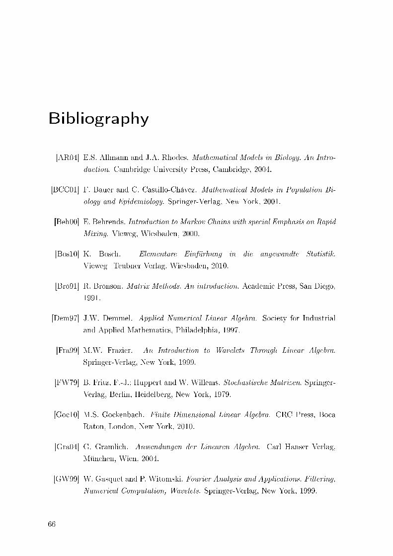
Bibliography
[AR04] E.S. Allmann and J.A. Rhodes. Mathematical Models in Biology. An Intro-
duction. Cambridge University Press, Cambridge, 2004.
[BCC01] F. Bauer and C. Castillo-Chávez. Mathematical Models in Population Bi-
ology and Epidemiology. Springer-Verlag, New York, 2001.
[Beh00] E. Behrends. Introduction to Markov Chains with special Emphasis on Rapid
Mixing. Vieweg, Wiesbaden, 2000.
[Bos10] K. Bosch. Elementare Einfürhung in die angewandte Statistik.
Vieweg+Teubner Verlag, Wiesbaden, 2010.
[Bro91] R. Bronson. Matrix Methods. An introduction. Academic Press, San Diego,
1991.
[Dem97] J.W. Demmel. Applied Numerical Linear Algebra. Society for Industrial
and Applied Mathematics, Philadelphia, 1997.
[Fra99] M.W. Frazier. An Introduction to Wavelets Through Linear Algebra.
Springer-Verlag, New York, 1999.
[FW79] B. Fritz, F.-J.; Huppert and W. Willems. Stochastische Matrizen. Springer-
Verlag, Berlin, Heidelberg, New York, 1979.
[Goc10] M.S. Gockenbach. Finite-Dimensional Linear Algebra. CRC Press, Boca
Raton, London, New York, 2010.
[Gra04] G. Gramlich. Anwendungen der Linearen Algebra. Carl Hanser Verlag,
München, Wien, 2004.
[GW99] W. Gasquet and P. Witomski. Fourier Analysis and Applications. Filtering,
Numerical Computation, Wavelets. Springer-Verlag, New York, 1999.
66
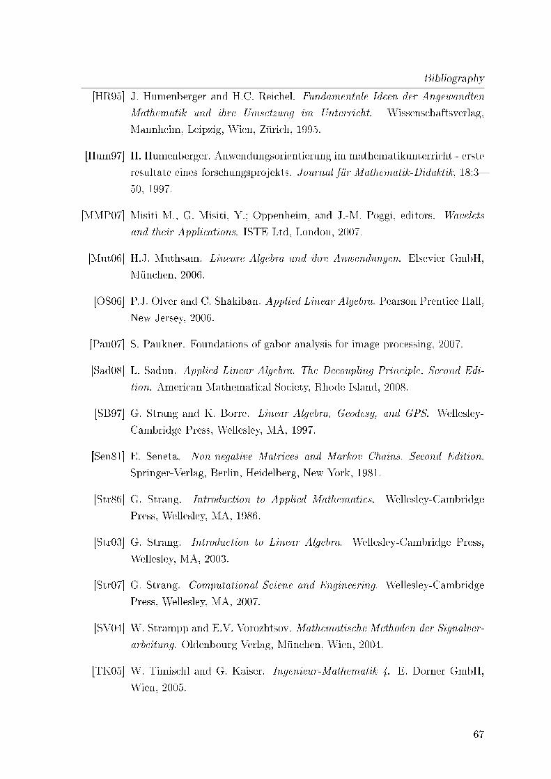
Bibliography
[HR95] J. Humenberger and H.C. Reichel. Fundamentale Ideen der Angewandten
Mathematik und ihre Umsetzung im Unterricht. Wissenschaftsverlag,
Mannheim, Leipzig, Wien, Zürich, 1995.
[Hum97] H. Humenberger. Anwendungsorientierung im mathematikunterricht - erste
resultate eines forschungsprojekts. Journal für Mathematik-Didaktik, 18:3�
50, 1997.
[MMP07] Misiti M., G. Misiti, Y.; Oppenheim, and J.-M. Poggi, editors. Wavelets
and their Applications. ISTE Ltd, London, 2007.
[Mut06] H.J. Muthsam. Lineare Algebra und ihre Anwendungen. Elsevier GmbH,
München, 2006.
[OS06] P.J. Olver and C. Shakiban. Applied Linear Algebra. Pearson Prentice Hall,
New Jersey, 2006.
[Pau07] S. Paukner. Foundations of gabor analysis for image processing, 2007.
[Sad08] L. Sadun. Applied Linear Algebra. The Decoupling Principle. Second Edi-
tion. American Mathematical Society, Rhode Island, 2008.
[SB97] G. Strang and K. Borre. Linear Algebra, Geodesy, and GPS. Wellesley-
Cambridge Press, Wellesley, MA, 1997.
[Sen81] E. Seneta. Non-negative Matrices and Markov Chains. Second Edition.
Springer-Verlag, Berlin, Heidelberg, New York, 1981.
[Str86] G. Strang. Introduction to Applied Mathematics. Wellesley-Cambridge
Press, Wellesley, MA, 1986.
[Str03] G. Strang. Introduction to Linear Algebra. Wellesley-Cambridge Press,
Wellesley, MA, 2003.
[Str07] G. Strang. Computational Sciene and Engineering. Wellesley-Cambridge
Press, Wellesley, MA, 2007.
[SV04] W. Strampp and E.V. Vorozhtsov. Mathematische Methoden der Signalver-
arbeitung. Oldenbourg Verlag, München, Wien, 2004.
[TK05] W. Timischl and G. Kaiser. Ingenieur-Mathematik 4. E. Dorner GmbH,
Wien, 2005.
67

[Usm87] R.A. Usmani. Applied Linear Algebra. Marcel Dekker, New York, Basel,
1987.
Austrian Federal Ministry for Education, Arts and Culture:
http://www.bmukk.gv.at
http://www.bmukk.gv.at/medienpool/11859/lp_neu_ahs_07.pdf
http://www.bmukk.gv.at/schulen/bw/bbs/Berufsbildende_Schulen_H1745.xml
List of Figures
1.1 The four subspaces CpAq, NpAJq, CpAJq and NpAq at a glance. . . . . 11
1.2 The graph associated with its incidence matrix. . . . . . . . . . . . . . 12
1.3 Electrical network with voltage source and current source. . . . . . . . 16
2.1 Clowns compressed via SVD. (a) Original image, (b) Approximation to
A for k � 3, (c) Approximation to A for k � 10 and (d) Approximation
to A for k � 20 . . . . . . . . . . . . . . . . . . . . . . . . . . . . . . . 28
2.2 Projection of b onto the column space. . . . . . . . . . . . . . . . . . . 30
2.3 The actions of the pseudoinverse A�. . . . . . . . . . . . . . . . . . . . 32
2.4 Linear LSQ-approximation. . . . . . . . . . . . . . . . . . . . . . . . . 35
2.5 Two polynomials �tting the data in a LSQ-sense. . . . . . . . . . . . . 36
2.6 Polynomials of increasing degree �tting to original data. . . . . . . . . 37
3.1 The original signal fpxq and the noisy signal. . . . . . . . . . . . . . . . 45
3.2 The denoised signals with 3, 5 and 11 Fourier terms. . . . . . . . . . . . 45
3.3 Comparison of the original signal with the denoised signals. . . . . . . . 46

List of Tables
2.1 Father-son professional relationship. . . . . . . . . . . . . . . . . . . . . 22
2.2 Compression ratio and relative error. . . . . . . . . . . . . . . . . . . . 28
2.3 Population of Austin in Texas since 1850. . . . . . . . . . . . . . . . . . 34
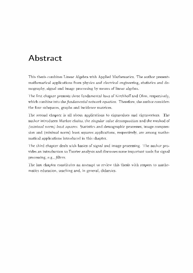
Abstract
This thesis combines Linear Algebra with Applied Mathematics. The author presents
mathematical applications from physics and electrical engineering, statistics and de-
mography, signal and image processing by means of linear algebra.
The �rst chapter presents three fundamental laws of Kirchho� and Ohm, respectively,
which combine into the fundamental network equation. Therefore, the author considers
the four subspaces, graphs and incidence matrices.
The second chapter is all about applications to eigenvalues and eigenvectors. The
author introduces Markov chains, the singular value decomposition and the method of
(minimal norm) least squares. Statistics and demographic processes, image compres-
sion and (minimal norm) least squares applications, respectively, are among mathe-
matical applications introduced in this chapter.
The third chapter deals with basics of signal and image processing. The author pro-
vides an introduction to Fourier analysis and discusses some important tools for signal
processing, e.g., �lters.
The last chapter constitutes an attempt to review this thesis with respect to mathe-
matics education, teaching and, in general, didactics.

Zusammenfassung
Die vorliegende Diplomarbeit kombiniert elementare Methoden der Linearen Algebra
mit der Angewandten Mathematik. Die Lineare Algebra wird dabei als unverzicht-
bares Werkzeug der modernen Anwendungsgebiete der Mathematik verstanden.
Das erste Kapitel beschäftigt sich mit drei fundamentalen Gesetzen der Physik und
Elektrotechnik von Kirchho� beziehungsweise Ohm, die sich zu einer Gleichung zusam-
menfassen lassen, nämlich der Netzwerkgleichung. Hierfür werden die vier Teilräume,
Graphen und Inzidenzmatrizen in Betracht gezogen.
Das zweite Kapitel widmet sich der Eigenwerte und Eigenvektoren. Markov Ket-
ten, die Singulärwertzerlegung und die Methode der kleinsten Quadrate (minimaler
Länge) werden vorgestellt. Statistik und demographische Prozesse, Bildkompression
beziehungsweise Anwendungen der kleinsten Quadrate (minimaler Länge) sind unter
den mathematischen Anwendungen, die hier zutrage kommen.
Das dritte Kapitel beschäftigt sich mit Grundlagen der Bild- und Signalverarbeitung.
Es wird in die Fourier-Analysis eingeleitet und einige wichtige Elemente der Signalver-
arbeitung, wie Filter, besprochen.
Das letzte Kapitel unternimmt einen Versuch diese Arbeit in die Diskussion über
Angewandte Mathematik in der Schule einzubinden.
Curriculum Vitae
Name: Bayram ÜLGEN
Born: August 17th, 1986
Nationality: Austria
E-mail: [email protected]
1992�1996: Primary school (Gasserg. 46)
1996�2005: Secondary academic school (Haydn Bundesrealgymnasium),
high school diploma (Matura) with distinction
2005�2006: Community service
2006�2011: Study of Secondary School Teacher Accreditation Program
in Mathematics (major) and History (minor) at the
University of Vienna