Dissertation Wolfgang Lahmann-22Jan12-V21-29Jun12 ...
256
Technische Universität München Lehrstuhl für Finanzmanagement und Kapitalmärkte Univ.-Prof. Dr. Christoph Kaserer SYSTEMIC RISK, SYSTEMIC IMPORTANCE AND BANKING SECTOR RISK CONTAGION DEPENDENCIES Wolfgang Lahmann Vollständiger Abdruck der von der Fakultät für Wirtschaftswissenschaften der Technischen Universität München zur Erlangung des akademischen Grades eines Doktors der Wirtschaftswissenschaften (Dr. rer. pol.) genehmigten Dissertation Vorsitzender: Univ.-Prof. Dr. Martin Grunow Prüfer der Dissertation: 1. Univ.-Prof. Dr. Christoph Kaserer 2. Univ.-Prof. Dr. Bernd Rudolph (Ludwig- Maximilians-Universität München) Die Dissertation wurde am 28.02.2012 bei der Technischen Universität München eingereicht und durch die Fakultät für Wirtschaftswissenschaften am 13.06.2012 angenommen.
Transcript of Dissertation Wolfgang Lahmann-22Jan12-V21-29Jun12 ...
Technische Universität München
Lehrstuhl für Finanzmanagement und Kapitalmärkte
Univ.-Prof. Dr. Christoph Kaserer
SYSTEMIC RISK, SYSTEMIC IMPORTANCE AND BANKING SECTOR
RISK CONTAGION DEPENDENCIES
Wolfgang Lahmann
Vollständiger Abdruck der von der Fakultät für Wirtschaftswissenschaften der Technischen
Universität München zur Erlangung des akademischen Grades eines Doktors der
Wirtschaftswissenschaften (Dr. rer. pol.) genehmigten Dissertation
Vorsitzender: Univ.-Prof. Dr. Martin Grunow
Prüfer der Dissertation: 1. Univ.-Prof. Dr. Christoph Kaserer
2. Univ.-Prof. Dr. Bernd Rudolph (Ludwig-
Maximilians-Universität München)
Die Dissertation wurde am 28.02.2012 bei der Technischen Universität München
eingereicht und durch die Fakultät für Wirtschaftswissenschaften am 13.06.2012
angenommen.

I
ABSTRACT
The 2007-2009 financial crisis rigorously exposed the relevance of systemic risk and
systemically important financial institutions (SIFIs) for financial market stability. While both
notions are ubiquitous in the analysis of the financial crisis and in the discourse on banking
sector regulation, there is still no consensus on adequate measurement approaches.
In this thesis we develop the ‘expected systemic shortfall’ (ESS) methodology which facilitates
both the measurement of aggregate systemic risk and the assessment of a bank’s relative
systemic risk contribution. The ESS-indicator is derived transparently using standard measures
from financial institutions risk management and represents the product of the probability of a
systemic default event in the banking sector and the expected loss when this systemic event
occurs. The measure is computed using a credit portfolio simulation model whose input
parameters are estimated from market CDS spreads and equity return correlations. In addition to
these methodological contributions we conduct the most comprehensive analysis of systemic risk
and systemic importance in global and regional financial markets to date.
Our empirical results show that the ESS-indicator responds adequately to both the financial crisis
events with global importance and to specific events in the regional sub-samples. The ESS-
indicator reaches its peak in September 2008 and remains elevated at the end of the sample
period in all samples and especially in the European sub-sample. The relative systemic risk
contribution of individual banking groups is mainly driven by their size, corroborating the
common ‘too big to fail’ statement. We contribute to the ongoing discourse concerning the
regulation of systemically important financial institutions by suggesting the use of the relative
contributions to the ESS-indicator as a measure for a bank’s systemic importance. By applying a
relative systemic risk contribution threshold of one percent, our empirical results show that there
are 23 globally systemically important banks.
The recent financial crisis and the ensuing sovereign debt crisis also exposed the relevance of
banking sector risk contagion dependencies. Specifically, inter-regional systemic risk contagion,
bank vs. sovereign sector as well as bank vs. non-bank corporate sector risk contagion effects are
mentioned frequently both in academia and among practitioners. However, there are only very
few empirical investigations of these dependencies to date. In fact, to our best knowledge only
the interdependencies between bank and sovereign credit spreads on the country level have been
the focus of previous research. In the present thesis we add to this rather unexplored field of
II
financial research and conduct a comprehensive empirical analysis of banking sector risk
contagion effects. In particular, we employ state-of-the-art time series methods in order to
examine three types of banking sector risk contagion dependencies. Firstly, we analyze inter-
regional systemic risk contagion dependencies using the regional ESS-indicator developed in
this thesis (as measure of systemic risk) and alternatively regional bank credit spreads. Secondly,
we examine interdependencies between sovereign and bank credit spreads for intra-/inter-
regional and intra-country relations. Thirdly, we analyze the interdependencies between bank
and non-bank corporate sector credit spreads and alternatively equity returns on the intra-
regional level.
For the inter-regional systemic risk contagion effects we find that the systemic risk in the
American financial system is contagious for the systemic risk in the other regions since the
subprime crisis period. Moreover, the analysis shows new inter-regional systemic risk
dependencies which have not been described previously. The analysis of sovereign vs. banking
sector risk contagion exhibits a strong increase of the interdependencies between sovereign and
banking sector credit spreads since the financial crisis. The impact of sovereign vs. bank default
risk even increased during the sovereign debt crisis period. The analysis of bank vs. non-bank
corporate risk contagion effects exposed that changes in the default risk of banks depend changes
in the default risk of the corporate sector during the financial crisis period in all regions,
corroborating the claim that banking sector risk impacts the real economy. The analysis of the
bank vs. non-bank corporate equity returns shows interestingly that the bank equity returns are
led by the corporate equity returns whereas the opposite dependency is only rarely observed.

III
TABLE OF CONTENTS
ABSTRACT ....................................................................................................................................... I
TABLE OF CONTENTS ................................................................................................................... III
LIST OF ABBREVIATIONS ............................................................................................................ VII
LIST OF SYMBOLS ........................................................................................................................ IX
1 INTRODUCTION ........................................................................................................................ 1
1.1 MOTIVATION ..................................................................................................................... 1
1.2 RESEARCH QUESTIONS AND CONTRIBUTION ..................................................................... 2
1.3 STRUCTURE OF ANALYSIS AND UNDERLYING WORKING PAPERS ..................................... 4
2 RELATED LITERATURE ............................................................................................................ 5
2.1 SYSTEMIC RISK AND SYSTEMIC IMPORTANCE ................................................................... 5
2.1.1 Definition ............................................................................................................ 5
2.1.2 Measurement approaches .................................................................................... 6
2.2 BANKING SECTOR RISK CONTAGION DEPENDENCIES........................................................ 9
2.2.1 Inter-regional systemic risk contagion .............................................................. 10
2.2.2 Sovereign risk vs. banking sector risk contagion.............................................. 11
2.2.3 Banking sector risk vs. corporate sector risk contagion ................................... 13
3 HYPOTHESES FOR BANKING SECTOR RISK CONTAGION ANALYSIS .................................... 14
3.1 INTER-REGIONAL SYSTEMIC RISK CONTAGION .............................................................. 14
3.2 SOVEREIGN RISK VS. BANKING SECTOR RISK CONTAGION ............................................. 15
3.3 BANKING SECTOR RISK VS. CORPORATE SECTOR RISK CONTAGION............................... 17

IV
4 METHODOLOGY ..................................................................................................................... 19
4.1 THE EXPECTED SYSTEMIC SHORTFALL (ESS) METHODOLOGY ....................................... 19
4.1.1 Estimating asset return correlations from equity returns .................................. 19
4.1.2 Calculating risk-neutral probabilities from CDS spreads ................................. 20
4.1.3 Constructing the systemic risk indicator ........................................................... 22
4.1.4 Technical comparison with other systemic risk measures ................................ 24
4.2 MEASURING CONTAGION EFFECTS IN FINANCIAL MARKETS .......................................... 27
5 EMPIRICAL DATA .................................................................................................................. 31
5.1 ESS-ANALYSIS ............................................................................................................... 31
5.1.1 Global sample ................................................................................................... 32
5.1.2 American sub-sample........................................................................................ 34
5.1.3 Asian-Pacific sub-sample .................................................................................. 35
5.1.4 European sub-sample ........................................................................................ 36
5.1.5 Middle Eastern and Russian sub-sample .......................................................... 37
5.1.6 Comparative analysis ........................................................................................ 38
5.2 BANKING SECTOR RISK CONTAGION DEPENDENCIES...................................................... 41
5.2.1 Inter-regional systemic risk contagion .............................................................. 41
5.2.2 Sovereign risk vs. banking sector risk contagion.............................................. 42
5.2.3 Banking sector risk vs. corporate sector risk contagion ................................... 43
6 EMPIRICAL RESULTS ............................................................................................................. 46
6.1 EXPECTED SYSTEMIC SHORTFALL INDICATOR ................................................................ 46
6.1.1 The aggregate ESS-indicator ............................................................................ 46
6.1.1.1 Global sample ..................................................................................... 46
6.1.1.2 American sub-sample ......................................................................... 49
6.1.1.3 Asian-Pacific sub-sample ................................................................... 51
6.1.1.4 European sub-sample ......................................................................... 53
6.1.1.5 Middle Eastern and Russian sub-sample ............................................ 55

V
6.1.1.6 Comparative analysis ......................................................................... 57
6.1.2 Risk premium determinants of the ESS-indicator ............................................ 60
6.1.2.1 Global sample ..................................................................................... 61
6.1.2.2 American sub-sample ......................................................................... 62
6.1.2.3 Asian-Pacific sub-sample ................................................................... 63
6.1.2.4 European sub-sample ......................................................................... 64
6.1.2.5 Middle Eastern and Russian sub-sample ............................................ 64
6.1.2.6 Comparative analysis ......................................................................... 65
6.1.3 Relative contribution to the ESS-indicator ....................................................... 66
6.1.3.1 Global sample ..................................................................................... 66
6.1.3.2 American sub-sample ......................................................................... 68
6.1.3.3 Asian-Pacific sub-sample ................................................................... 69
6.1.3.4 European sub-sample ......................................................................... 70
6.1.3.5 Middle Eastern and Russian sub-sample ............................................ 71
6.1.3.6 Comparative analysis ......................................................................... 72
6.1.4 Discussion in the context of related research .................................................... 73
6.1.5 Policy implications and recommendations ....................................................... 74
6.2 BANKING SECTOR RISK CONTAGION DEPENDENCIES...................................................... 78
6.2.1 Inter-regional systemic risk contagion .............................................................. 78
6.2.1.1 Econometric results ............................................................................ 78
6.2.1.2 Evaluation of initial hypotheses ......................................................... 81
6.2.2 Sovereign risk vs. banking sector risk contagion.............................................. 82
6.2.2.1 Region-level analysis ......................................................................... 82
6.2.2.2 Country-level analysis ........................................................................ 86
6.2.3 Banking sector risk vs. corporate sector risk contagion ................................... 91
6.2.3.1 Econometric results ............................................................................ 91
6.2.3.2 Evaluation of initial hypotheses ......................................................... 97
7 CONCLUSION ........................................................................................................................ 103
7.1 SUMMARY AND IMPLICATIONS ...................................................................................... 103
7.2 OUTLOOK ...................................................................................................................... 105

VI
LIST OF FIGURES......................................................................................................................... 107
LIST OF TABLES .......................................................................................................................... 149
BIBLIOGRAPHY ........................................................................................................................... 199
APPENDIX .................................................................................................................................... 208

VII
LIST OF ABBREVIATIONS
Abbreviation Definition
ADF Augmented Dickey/Fuller (1979) test
AIC Akaike (1974) information criterion
AIG American International Group
CDO Collateralized debt obligation
CDS Credit default swap
CoVaR Conditional value at risk
DIP Distress insurance premium
EC Error correction
EFSM European Financial Stabilization Mechanism
EL Expected loss
ESM European Stability Mechanism
ESS Expected systemic shortfall
ETL Expected tail loss
GIRF Generalized impulse response function
IFRS International financial reporting standards
KPSS Kwiatkowski et al. (1992)
IMF International Monetary Fund
IRF Impulse response function
LGD Loss given default
MER Middle East& Russia
OLS Ordinary least squares
PP Phillips/Perron (1988)
PD Probability of default
VIII
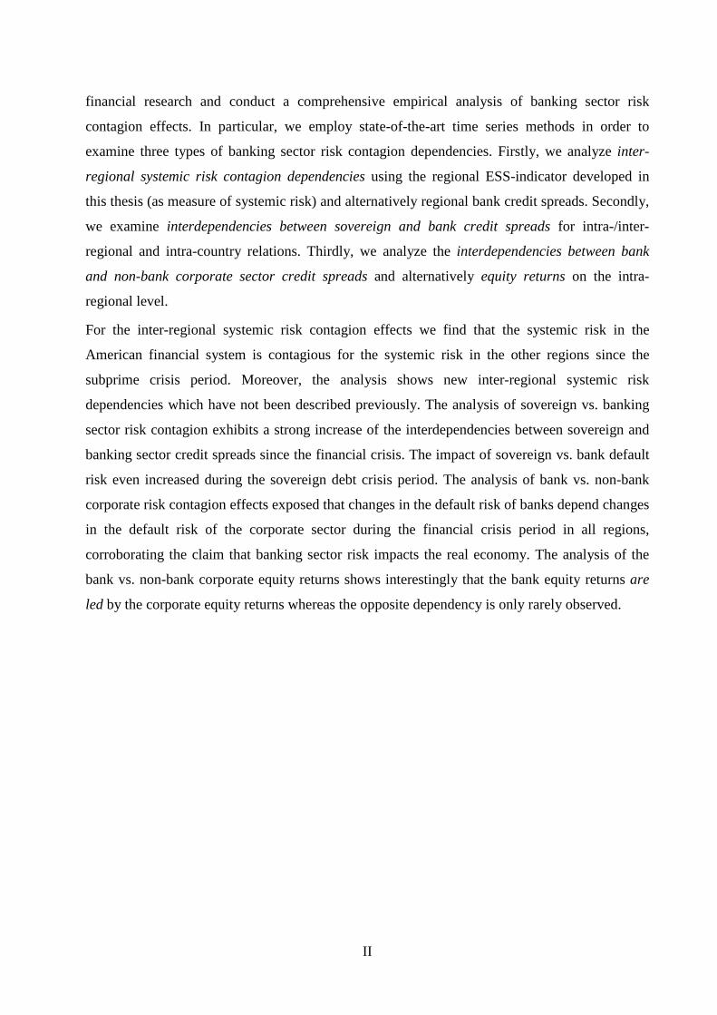
Abbreviation Definition
PSD Probability of systemic default
SBIC Schwarz (1978) Bayesian information criterion
SES Systemic expected shortfall of Acharya et al. (2010)
SIFI Systemically important financial institution
SLT Systemic loss threshold
TARP Troubled Asset Relief Program
UAE United Arab Emirates
VaR Value at risk
VAR Vector autoregressive
VEC Vector error correction
IX
LIST OF SYMBOLS
Symbol Definition
,i tc Systemic loss contribution of bank i at time t
k Simulation iteration in ESS analysis
K Number of simulation iterations in ESS analysis
, ,i k tl Loss in ESS simulation for bank i
,k tL Portfolio loss in ESS simulation
tΛ Portfolio loss distribution at time t
M Common risk factor in Vasicek (1987) model
N Number of sample banks in ESS analysis
tP Correlation matrix
( )Pr ⋅ Probability of
( )1−Φ ⋅ Quantile of the standard normal distribution
q Annualized default intensity
r Risk-free rate of return
ρ Correlation
s CDS spread
,Tτ Maturity
V Value of bank assets in Vasicek (1987) model
Y Variable vector in the VAR model
,i tY Sample value in ESS Monte Carlo simulation
Z Idiosyncratic risk factor in Vasicek (1987) model

1
1 INTRODUCTION
1.1 MOTIVATION
The 2007-2009 financial crisis exposed the relevance of systemic risk in the financial sector
which denotes the likelihood of the occurrence of a systemic event that would have serious
detrimental effects not only on the stability of financial markets but also on the real economy.
Systemically important financial institutions (SIFIs) are a related concept discussed
extensively since the recent financial crisis. A financial institution is commonly regarded to
be systemically important, if its failure would represent a systemic event. As a consequence of
this, SIFIs are often considered to benefit from an implicit bailout guarantee since
governments would never risk their failure. The notions ‘too big to fail’ and ‘too
interconnected to fail’ are mentioned frequently in this respect and it is argued that the
implicit guarantee may lead to inefficient incentives and negative externalities.
The existing banking sector regulatory architecture ‘Basel II’ has turned out to be insufficient
to prevent the recent financial crisis and additionally several shortcomings of this regulatory
framework were exposed during the crisis. These deficiencies were on the one hand
microprudential in nature as the capital and funding liquidity standards for individual
institutions did not prevent banks from failing or requiring government assistance. On the
other hand, the financial crisis exposed a lack of macroprudential regulation which takes a
system-wide perspective in order to ensure the stability of the financial system as a whole.
Therefore, one guiding principle in the elaboration of the new banking sector regulatory
regime ‘Basel III’ is the consideration of this macroprudential dimension aimed at mitigating
systemic risk and ensuring efficient incentives as well as sufficient risk-bearing capacity of
SIFIs amongst others.
Consequently, an adequate understanding of and measurement approaches for systemic risk
and systemic importance are highly relevant for both the analysis of the recent financial crisis
as well as the design and implementation of the future banking sector regulatory architecture.
This relevance may also explain the recent growth of the literature on systemic risk and SIFIs
and the advancement of this rather new finance research field. While the current literature
provides several proposals for the measurement of either systemic risk or systemic
importance, there are only very few approaches for the consistent measurement of both of
these ubiquitous concepts. This may explain why there is still no consensus on the

1 INTRODUCTION 2
methodologies for measuring systemic risk and assessing systemic importance. In this thesis
we add to this literature and develop the ‘expected systemic shortfall’ (ESS) methodology
which facilitates both the measurement of aggregate systemic risk and the assessment of a
bank’s relative systemic risk contribution as a measure of its systemic importance.
The financial crisis and the ensuing sovereign debt crisis also exposed the relevance of
banking sector risk contagion effects. Firstly, it is frequently mentioned that there are inter-
regional systemic risk contagion effects, i.e., spillover of systemic risk in one region onto the
systemic risk in other regions (particularly in times of crisis). Secondly, it stands to reason
that interdependencies between sovereign and banking sector default risk have increased due
to i) government interventions in the financial sector during the crisis and ii) the increase in
sovereign credit spreads since the onset of the euro zone sovereign debt crisis. Thirdly, the
financial crisis also highlighted the contagious effects of banking sector risk for the real
economy which materialized in severe economic recessions in the aftermath of the crisis
(amongst others). Although these banking sector risk contagion effects are mentioned
frequently, there are only very few empirical investigations of these dependencies to date. The
analysis of the banking sector risk dependencies in this thesis will not only facilitate an
evaluation of their presumed existence but may also provide an analytical starting point for
potential regulatory measures in order to mitigate certain detrimental effects.
1.2 RESEARCH QUESTIONS AND CONTRIBUTION
This thesis aims to derive an analytical framework for measuring systemic financial sector
risk and consistently assessing systemic importance of financial institutions which we name
the expected systemic shortfall (ESS) methodology. In addition, the ESS-methodology shall
be applied in a comprehensive empirical analysis of systemic risk and systemic importance in
global and regional financial markets. Moreover, this thesis seeks to conduct a comprehensive
analysis of the relevant banking sector risk dependencies. Specifically, the following research
questions are addressed in this thesis:
1. How can systemic risk in the financial sector be measured? What are the
determinants of systemic risk and which differences exist between regions?
a) Derivation of an analytical framework for measuring aggregate systemic risk
using a credit portfolio simulation methodology whose input parameters are
estimated from capital market data.

1 INTRODUCTION 3
b) Application of the systemic risk measurement framework to a global bank
sample and regional sub-samples during the sample period between October
2005 and April 2011 and analysis of the resulting systemic risk indicators.
c) Analysis of the input factor and risk premium determinants of the sample-
specific systemic risk indicators.
2. How can the systemic importance of a financial institution be assessed consistently
with its contribution to systemic risk?
a) Derivation of the relative contribution of individual financial institutions to the
aggregate systemic risk measure within the analytical systemic risk
measurement framework.
b) Analysis of the systemic risk contributions by individual banks and
examination of the input factor determinants.
c) Translation of a financial institution’s systemic risk contribution into a measure
of its systemic importance.
3. Is there empirical evidence for banking sector risk contagion effects? Are these
effects also observed when general macroeconomic conditions are controlled for?
a) Derivation of an econometric model for measuring risk contagion effects
between financial variables and controlling for macroeconomic factors.
b) Analysis of inter-regional risk contagion effects of i) the regional systemic risk
measures and ii) regional banking sector credit spreads.
c) Analysis of contagion effects between banking sector and sovereign sector
default risk on the intra-/inter-regional level and intra-country level.
d) Analysis of intra-regional risk contagion effects between banking sector and
non-bank corporate sector credit spreads and equity returns.
As mentioned earlier, these topics are highly relevant for academia and practitioners alike.
The aggregate measure of systemic risk derived in this thesis can be employed in the
continuous monitoring and steering of financial market stability by regulatory authorities.
Similarly, an objective assessment of systemic importance is a necessary precondition for
applying specific regulatory measures to systemically important financial institutions which is
envisioned in the ‘Basel III’ banking sector regulatory framework. Hence, this thesis adds to
the literature and regulatory discussion on measuring systemic risk and assessing systemic
importance of financial institutions by suggesting the ESS-methodology as a consistent

1 INTRODUCTION 4
analytical framework for these purposes. In addition to the methodological enhancements, this
thesis provides the most comprehensive empirical analysis of systemic risk and systemic
importance conducted to date.
The analysis of banking sector risk contagion dependencies is a research area which has so far
received very little attention. In fact, to our best knowledge only the interdependencies
between bank and sovereign credit spreads on the country level have been the focus of
previous research. Therefore, we add to this rather unexplored field of financial research in
the present thesis and conduct a comprehensive empirical analysis of banking sector risk
contagion effects.
1.3 STRUCTURE OF ANALYSIS AND UNDERLYING WORKING PAPERS
In the remainder of this thesis we proceed as follows. Chapter 2 provides a definition of
systemic risk and systemic importance and surveys the related literature on these concepts and
on the banking sector risk contagion dependencies. The hypotheses which are examined in the
banking sector risk contagion analysis are elaborated in chapter 3. In chapter 4 we derive our
ESS-methodology for measuring systemic risk and assessing systemic importance. Also, the
econometric model for analyzing financial market contagion effects is elaborated. In chapter 5
we describe the empirical data analyzed in this thesis. The results from applying the
methodology to the empirical data are elaborated in chapter 6. Chapter 7 summarizes the
previous chapters, concludes and outlines areas for future research.
This dissertation represents the consolidation of the following working papers by the author
on the sub-topics of this thesis: Lahmann/Kaserer (2011a), Lahmann/Kaserer (2011b),
Lahmann/Kaserer (2012), Lahmann (2012a) and Lahmann (2012b). The content from these
working papers is used in this thesis also literally and corresponding references are made
using footnotes at the beginning of the respective sections. Quotations from these working
papers in the abstract, introduction and conclusion of this thesis are not stated expressly for
expositional convenience.
5
2 RELATED LITERATURE
2.1 SYSTEMIC RISK AND SYSTEMIC IMPORTANCE1
2.1.1 Definition
Systemic risk in the financial sector is commonly described as the risk of correlated defaults
of financial institutions which would not only affect the stability of the banking sector but
also its ability to act as intermediary between depositors and borrowers with potentially
serious consequences for the economy as a whole.2 Systemically important financial
institutions (SIFIs) are a related concept. A bank is generally considered to be systemically
important if its bankruptcy would represent a trigger event for a series of correlated defaults in
the sense of the above description of systemic risk.3
In the present dissertation we generalize the above descriptions of systemic financial sector
risk and systemically important banks and employ the following definitions:
Definition D1 ‘Systemic risk’ in the financial sector denotes the likelihood of the
occurrence of a ‘systemic event’ which would not only have severe
implications for the stability of the financial system but also
detrimentally affect the real economy.
Definition D2 A financial institution is considered as ‘systemically important’ if its
failure represents a ‘systemic event’.
The main difference in our definition is that the trigger event of a systemic financial crisis is
defined more broadly as ‘systemic event’ which comprises (but is not limited to) a correlated
default event in the financial sector. This definition is consistent with the derivation of the
expected systemic shortfall (ESS) indicator in this thesis which defines the systemic event as
the loss of a certain percentage of the sample banks’ total liabilities.
1 The elaborations in this section are (also literally) based on Lahmann/Kaserer (2011a). 2 Cf. Lehar (2005), p.2578 and Adrian/Brunnermeier (2011), p. 2 (amongst others). 3 Cf. Huang/Zhou/Zhu (2010b), p. 3 and FSB (2009), pp. 5-6 (amongst others).
2 RELATED LITERATURE 6
2.1.2 Measurement approaches
Approaches for the measurement of systemic risk and the assessment of systemic importance
in the financial sector have been developed even before the financial crisis. The importance of
this subject has grown significantly due to the recent financial crisis which is reflected in the
sustained growth of literature on this topic. The approaches for the measurement of systemic
risk and assessing systemic importance can be classified with respect to the underlying data
used: financial statement-based measures, exposure-based network models and measures
based on capital market data.
The first type of approaches uses financial statement data such as the share of non-performing
loans, profitability, liquidity and capital adequacy measures. The disadvantage of this
approach type is that financial statement data is available only with a relatively low
frequency, is published only with a substantial delay and information in financial statements
is backward-looking despite IFRS accounting.4 Drehmann/Tarashev (2011) find that while
market data and model based approaches are usually favorable, ‘simple indicators’ based on
financial statement and regulatory data (such as bank size, interbank borrowing and lending)
can offer a handy approximation in the assessment of bank’s systemic importance whereas the
aggregate systemic risk cannot be adequately determined by this approach.
Network models usually rely on mutual bank exposure data and model the direct connections
among the banks to simulate the effects of a default event on the banks within the network.
IMF (2009) and Espinosa-Vega/Sole (2010) apply a network model using the mutual bank
exposures and the bank equity to model the effects of an initial default of one of the network
banks on the other banks in the system. The systemic importance of a bank is derived based
on the cumulated capital impairments which its initial default causes in the system.5
Aggregate systemic risk can be measured using this approach by means of the cumulated
exposure losses. Pokutta/Schmaltz/Stiller (2011) develop a similar network model that also
facilitates the derivation of optimal bail-out strategies. As network models are usually based
on confidential exposure data, their application is reserved for regulatory authorities and will
– for the time being – be limited to the application within a country due to confidentiality
restrictions. Besides, the required data are available only with a relatively low frequency.6
4 Cf. Huang/Zhou/Zhu (2009), p. 2036-2037. 5 An extension of the model considers the effects of lost funding sources and consequent fire sales. 6 E.g., the large exposure reporting in the European Union is carried out on a quarterly basis.

2 RELATED LITERATURE 7
Systemic risk measurement approaches based on capital market-data have three key
advantages vis-à-vis measures based on balance sheet and exposure data: they can be updated
more frequently (usually daily), are forward-looking by nature and can be implemented by all
interested parties. These approaches are described in the following.
Lehar (2005) computes the probability of default of several financial institutions as a measure
for aggregate systemic risk based on the asset return correlations which are estimated using
the Merton (1974) contingent claims analysis. Gray/Merton/Bodie (2007a) also pursue a
contingent claims approach and develop a systemic risk measure which accounts for
sovereign risk. Gray/Merton/Bodie (2007b) follow the same analytical approach and derive a
regulatory policy framework aimed at mitigating systemic macrofinancial risks.
Chan-Lau/Gravelle (2005) and Avesani/Pascual/Li (2006) consider the banks in the sphere of
competence of a regulator as portfolio and compute the probability of default of n portfolio
banks (nth-to-default probability) as measure of systemic risk in the portfolio. Billio et al.
(2010) analyze the correlations and dependencies prevailing in equity returns of different
types of financial institutions in order to obtain the aggregate systemic risk. Kim/Giesecke
(2010) use Moody’s US default data together with capital market parameters7 to derive an
aggregate systemic risk measure and its term structure.
While the above approaches based on market data can be used to measure aggregate financial
sector risk, they are not appropriate to assess systemic importance. To this end, Acharya et al.
(2010) measure systemic risk using the “systemic expected shortfall” (SES) measure which
they define as the probability of an individual bank being undercapitalized when the whole
system is undercapitalized. Adrian/Brunnermeier (2008) examine the systemic importance of
banks based on equity data using the “Conditional Value at Risk” (CoVaR) metric which
measures the value at risk of the whole financial system when one of the financial institutions
experiences a distress situation. CoVaR can be used to assess the systemic importance of
individual banks whereas it cannot be aggregated to measure aggregate systemic risk.
Huang/Zhou/Zhu (2009) employ a credit portfolio risk model using equity return correlations
and CDS spreads to compute a risk-neutral measure of aggregate systemic risk, the distress
insurance premium (DIP) for the US financial system. This measure represents the
hypothetical insurance premium against the losses of a certain share of the total banking
sector liabilities. Huang/Zhou/Zhu (2010a) extend the DIP approach by an importance
7 Such as S&P 500, TED spread, the US yield curve.

2 RELATED LITERATURE 8
sampling methodology to determine the marginal DIP contribution of individual institutions
which facilitates the assessment of systemic importance and apply it to the Asian-Pacific
banking system. Huang/Zhou/Zhu (2010b) employ the same approach in analyzing the US
financial sector.
The use of a credit portfolio simulation approach based on capital market data to derive the
aggregate expected systemic shortfall (ESS) indicator in this thesis is inspired by
Huang/Zhou/Zhu (2009). There are, however, three important differences between the two
approaches. Firstly, we define the systemic default event as a portfolio loss of the sample
bank liabilities which exceeds a percentage of the total liabilities of the sample banks whereas
Huang/Zhou/Zhu (2009) define the loss threshold relative to the total banking sector
liabilities. This difference makes our approach also appropriate for banking systems in which
a major portion of the banks is not exchange-listed. Secondly, we derive the ESS-indicator in
a transparent manner using standard measures from financial institutions risk management,
namely the probability of (systemic) default and the expected shortfall, which facilitates the
application of our indicator by other parties. Thirdly, the relative systemic risk contributions
in our ESS-methodology are computed in a transparent fashion as byproduct of the credit
portfolio simulation as opposed to using an additional importance sampling procedure as in
Huang/Zhou/Zhu (2010a) and Huang/Zhou/Zhu (2010b). This feature facilitates the use of our
methodology as an intuitive measure of a bank’s systemic importance.
Apart from the methodological enhancements in measuring systemic risk and assessing
systemic importance, this thesis also contributes on the empirical side as it is the first truly
global analysis of systemic financial sector risk which also accounts for regional differences
by separately analyzing four regional sub-samples. By contrast, the above publications
consider only individual regions or countries. Due to the global perspective in the present
thesis we also to contribute to the ongoing discourse on the identification and regulation of
systemically important financial institutions as our results can be used to identify those banks
which are systemically important on a global scale.

2 RELATED LITERATURE 9
2.2 BANKING SECTOR RISK CONTAGION DEPENDENCIES8
There is a vast literature concerning contagion in financial markets which is surveyed
comprehensively by Dornbusch/Park/Claessens (2000) and Kaminsky/Reinhart/Vegh (2003).
While most publications focus on cross-country market contagious effects it should be noted
that contagion can take place between any sort of financial markets, e.g., between debt and
equity capital markets.9 We define contagion consistent with Dornbusch/Park/Claessens
(2000) and Bae/Karolyi/Stulz (2003) as an elevation of market interconnection subsequent to
a shock event in one market.10 The literature distinguishes at least three channels by which
contagion can be transmitted through financial markets.11
The liquidity channel describes a mechanism where a shock event in one financial market
detrimentally impacts market liquidity of certain or even all financial markets with potential
consequences for asset prices and investor conduct. Further consequences in case of a
liquidity channel contagion may be elevated trading activity in other markets affected by the
initial shock and diminished credit availability which may become fully effective first after an
extended period. Allen/Gale (2000), Kodres/Pritsker (2002) and Brunnermeier/Pedersen
(2009) describe relevant models for this contagion propagation channel.
In the risk-premium channel of financial market contagion an initial shock event in one
market affects investors’ risk-bearing willingness in other markets whereby changes in
equilibrium risk premiums affect asset prices in all markets. Consequently, shock-induced
return changes to the affected security may impact the returns on securities in other markets
which also provides a rationale for the predictive power of distressed asset returns for other
asset classes. Due to feedback effects, the implications of this propagation channel may first
fully materialize after several periods. Consequently, the measurement of contagion via the
risk-premium channel can be conducted in a vector autoregressive (VAR) framework
provided that adequate data frequencies and lag lengths are chosen. Acharya/Pedersen (2005)
and Vayanos (2004) present relevant models for this contagion transmission channel.
In the correlated-information channel a jolt to one financial market represents new economic
information which is relevant also for asset prices in other markets, e.g., because the
8 The elaborations in this section are (also literally) based on Lahmann (2012b). 9 Cf. Longstaff (2010), p. 438. 10 Cf. Dornbusch/Park/Claessens (2000), p. 177 and Bae/Karolyi/Stulz (2003), p. 720. 11 The subsequent elaboration of the three contagion propagation channels is based on Longstaff (2010), p. 438.

2 RELATED LITERATURE 10
information pertains to economic factors which drive multiple markets. A common feature of
the literature describing the correlated-information channel is the assumption that the
contagion takes place via the price discovery mechanism. Therefore, one would expect to
observe immediate price reactions in the affected financial markets especially when these are
more liquid than the market where the initial shock occurred. Therefore, contagion propagated
by means of the correlated-information channel can be tested using a VAR framework.
Theoretical models for this contagion propagation channel are described by
Dornbusch/Park/Claessens (2000), Kiyotaki/Moore (2002) and King/Wadhwani (1990).
Longstaff (2010) points out that while the three contagion channels affect security prices in
specific ways, there are also similarities between the channels, an example of which is the
relation between credit risk and liquidity during the recent financial crisis: while the subprime
crisis of 2007 was characterized by ‘credit-risk-induced illiquidity’ (attributable to the risk-
premium and/or correlated information channel), a critical determinant of the 2008 global
financial crisis was ‘illiquidity-induced credit risk’ (attributable to the liquidity channel).12
The recent financial crisis exposed the relevance of systemic risk in the banking sector as
defined in definition D1. It suggests itself that systemic risk in the banking sector can also be
contagious for other parts of the financial market and it stands to reason that it could also be
propagated by way of the above contagion transmission channels.13 In the following we
elaborate the systemic banking sector risk contagion effects which are the focus of this thesis
along with the related literature.
2.2.1 Inter-regional systemic risk contagion14
The 2007-2009 global financial crisis evolved from a subprime mortgage and CDO market
crisis in the United States and the subsequent crisis events in the US – such as the Bear
Stearns takeover and the Lehman Brothers default – were contagious for other regional
financial markets and also led to increased systemic risk in these markets.15 Additionally, one
could observe inter-regional dependencies between regional crisis events and market reactions
in other regions. Specifically, our results in section 6.1.1 show that since the onset of the euro
12 Cf. Longstaff (2010), p. 438. 13 To the best of our knowledge there are no publications concerning the contagion transmission channels of
systemic risk, though. We outline the presumed contagion transmission channels for the analyzed dependencies in chapter 3.
14 The elaborations in this section are (also literally) based on Lahmann (2012b). 15 Cf. Acharya et al. (2009), p. 1.

2 RELATED LITERATURE 11
zone sovereign debt crisis the systemic risk increases not only in Europe but also in other
regions.
While the observation of inter-regional systemic risk contagion has been described
frequently, there is – to the best of our knowledge – currently no published research analyzing
the inter-regional contagion effects of systemic risk as measured by a systemic risk measure
(or alternatively bank CDS16) available. This thesis fills this gap by analyzing the inter-
regional systemic risk contagion effects between the relative ESS-indicator (and alternatively
regional bank CDS) of the American, Asian-Pacific, European as well as the Middle Eastern
and Russian sub-samples by means of Granger-causality tests and impulse response functions
in VAR frameworks during four sub-periods between October 2005 and April 2011.
2.2.2 Sovereign risk vs. banking sector risk contagion17
In the course of the recent global financial crisis several financial institutions were supported
by government interventions in order to avert their failure because a default event by a major
financial institution was considered to represent a systemic event which could have further
destabilized the financial system and the real economy.18 While these financial stability
measures substantially altered the size and structure of governments’ balance sheets, Gray
(2009) points out that the impact of this new interconnectedness between banking and
sovereign sector and its effects for other economic sectors are largely unexplored.
One may wonder why systemic risk in the financial sector or – more generally – bank default
risk is related with sovereign default risk. Gray/Merton/Bodie (2008) point out that there are
several linkages between these two risk types which are influenced by the explicit and
implicit guarantees of the sovereign to the banks. They also find that the presence of an
elevated level of systemic risk in the financial sector entails recessionary tendencies in the
real economy which strains public finances and shifts distress to the government which is
even reinforced when there are state guarantees for the financial sector. Furthermore, banks
and other owners of sovereign debt are affected by the decreased quality of the sovereign’s
credit risk and write-downs on their sovereign debt holdings.19 Acharya/Drechsler/Schnabl
16 We find in section 6.1.1 that bank CDS spreads are a first-order approximation for the relative ESS-indicator. 17 The elaborations in this section are (also literally) based on Lahmann (2012a). 18 Additionally, governments introduced large-scale economic stimulus packages for the ‘real economy’ in order
to alleviate the impact of the economic downturn. 19 Cf. Alter/Schueler (2011), p. 2.

2 RELATED LITERATURE 12
(2011) describe this interdependency as ‘two-way feedback’ and derive a theoretical model to
capture the linkages between government bailouts of financial firms and the sovereign risk.
Recent research on the financial crisis effects also established empirical evidence for the
linkage between financial and sovereign sector risk. Dieckmann/Plank (2010) find evidence
for a risk transfer from the private to the public sector in Western Europe during the financial
crisis and particularly for countries which introduced financial stability measures. Moreover,
they find that the linkage of country-level bank and sovereign CDS spreads increased which
they attribute to the fact that banks own significant amounts of sovereign debt and
governments have large contingent liabilities for their banking systems.
Gerlach/Schulz/Wolff (2010) find that CDS spreads of Western European countries affected
by sovereign debt issues are positively related with the countries’ bank CDS spreads whereas
no lead-lag relationships are analyzed. Moreover, they observe that sovereign and banking
sector risk became more interlinked when governments started to guarantee some of the
banks’ liabilities. In addition to their above theoretical contributions
Acharya/Drechsler/Schnabl (2011) find that government bailout programs to the financial
sector increased the linkage between the credit risk of banks and sovereigns on the country-
level. By analyzing the lead-lag dependencies between a country’s sovereign CDS spread and
the CDS spreads of two of the country’s financial institutions Alter/Schueler (2011) show that
in the period prior to the financial sector bailouts changes in bank credit risk mostly preceded
changes in sovereign credit risk whereas in the post-bailout period the opposite effect
occurred in the majority of the seven examined euro zone countries.20
In this thesis we contribute to the literature on the contagion effects between sovereign risk
and banking sector risk by analyzing the interlinkages between sovereign and bank CDS
spreads as proxy measure of systemic risk16 on the regional and country level. On the regional
level we analyze both inter- and intra-regional interlinkages between sovereign and bank
CDS spreads of the sample regions America, Asia-Pacific, Europe as well as Middle East and
Russia which has not been covered in previous research. On the country level we analyze the
interlinkages between the country’s sovereign CDS spread and the average CDS spread of the
country’s banking groups which has so far only been analyzed for certain euro zone countries
by Alter/Schueler (2011). To the best of our knowledge, this is the most comprehensive
analysis of sovereign and bank credit risk interlinkages conducted so far.
20 They consider the seven countries France, Germany, Ireland, Italy, Netherlands, Portugal and Spain.
2 RELATED LITERATURE 13
2.2.3 Banking sector risk vs. corporate sector risk contagion21
The banking sector is interconnected with the non-bank corporate sector in several ways.
Firstly, banks provide lending to firms and consequently a deterioration of the funding
conditions in the financial sector should also spill over to the non-bank corporate sector.
Secondly, a deterioration of the credit quality of corporate obligors in bank loan portfolios
should also detrimentally affect the earnings of the lending financial institutions. Moreover,
the 2007-2009 financial crisis exposed the relevance of systemic banking sector risk for the
non-bank corporate sectors and it is argued frequently that systemic risk in the financial sector
detrimentally impacts the real economy.22
Contagion effects between the credit spreads or equity returns of banking vs. non-bank
corporate sector have to our best knowledge not yet been analyzed in the scientific literature.
However, there are studies which cover somewhat related topics. Claessens/Tong/Wei (2011)
analyze the importance of transmission channels on the performance of manufacturing firms
and find that the financial linkages are relevant in explaining the decrease in profitability and
equity performance during the global financial crisis. Raunig/Scheicher (2009) analyze the
pricing of default risk of banks vs. non-bank firms using CDS data and find that the
importance of common factors in explaining the CDS spreads has increased during the crisis.
In this thesis we analyze the interdependencies between bank and non-bank corporate23 CDS
spreads and equity returns. We account for regional differences by separately analyzing
American, Asian-Pacific and European samples. Industry-specific peculiarities are accounted
for by examining both the overall corporate sample as well as nine industry clusters for each
region. To the best of our knowledge this is the first analysis of the interdependencies
between bank and non-bank corporate CDS spreads and equity returns conducted so far.
21 The elaborations in this section are (also literally) based on Lahmann/Kaserer (2012). 22 This is consistent with our definition of systemic risk which we define as the likelihood of the occurrence of a
systemic event which would not only have effects for the stability of financial markets but also the affect the real economy.
23 In the following we also refer simply to ‘corporate’ firms when referring to non-bank corporate entities for expositional convenience.

14
3 HYPOTHESES FOR BANKING SECTOR RISK CONTAGION ANALYSIS
In this chapter we elaborate the hypotheses concerning the banking sector risk contagion
dependencies which are analyzed empirically in this thesis.
3.1 INTER-REGIONAL SYSTEMIC RISK CONTAGION24
Before the 2007-2009 financial crisis the concept of systemic risk in the financial system was
discussed primarily from an academic viewpoint whereas the crisis actually exposed the
relevance of this topic for financial markets. Moreover, there is so far no evidence of inter-
regional systemic risk contagion before the crisis. Therefore, we formulate:
Hypothesis A1 Before the financial crisis there are no contagion effects between the
systemic risk in the sample regions.
As the financial crisis originated in the subprime mortgage market of the Unite States and the
financial crisis events in the US affected financial markets around the globe, we test:
Hypothesis A2 During the subprime and financial crisis periods the systemic risk in the
United States was contagious for the systemic risk in other regions.
In the course of the financial crisis the mutual sensitivity of bank CDS spreads25 and equity
prices to events affecting banks in other regions increased as markets increasingly perceived
banks’ asset- and liability-side risks to be highly correlated.26 Consequently, we analyze
Hypothesis A3 During the financial crisis period the feedback relations between the
regional systemic risk increased.
Due to the systemic component and particularly the high correlation of asset- and funding-
side risks in the financial sector exposed during the crisis, we expect persistence of the
observed inter-regional systemic risk contagion after the financial crisis and posit:
Hypothesis A4 After the end of the financial crisis the systemic risk interdependencies
observed during the financial crisis persist.
24 The elaborations in this section are (also literally) based on Lahmann (2012b). 25 For expositional convenience we refer synonymously to CDS (spreads), credit risk, credit spreads and default
risk when denoting the market CDS spreads which we employ in the empirical analysis. 26 Cf. Acharya et al. (2009), pp. 2-4.

3 HYPOTHESES FOR BANKING SECTOR RISK CONTAGION ANALYSIS 15
We operationalize the analysis of these inter-temporal hypotheses by conducting the
econometric analysis for four sub-periods which we specify in chapter 5. Regarding the
contagion transmission channels involved, it stands to reason that during the financial crisis
the inter-regional systemic risk transmission may have occurred via all three transmission
channels of financial market contagion described in the preceding classification.
3.2 SOVEREIGN RISK VS. BANKING SECTOR RISK CONTAGION27
The sovereign and banking sector are interlinked in a multitude of ways. For example,
financial institutions often hold sovereign debt as it is considered a ‘low-risk’ investment
providing a stable source of income, it receives a favorable regulatory treatment and because
sovereign debt represents a comparatively liquid asset also in times of strained markets.28
Changes in the default risk of sovereigns should hence lead to changes in the default risk of
banks in case the respective sovereign debt holding represents a significant share of the total
assets. As the information regarding the composition of bank balance sheets is not publicly
available, market participants need to conjecture the impact of changes in sovereign credit
risk on a particular financial institution.29
Apart from the relative size of banks’ sovereign asset holding, one would expect that the level
and volatility of sovereign CDS spreads also influences the susceptibility of bank credit risk
to changes in sovereign credit risk. Given the low level and volatility of sovereign CDS
spreads in America and Europe before the ‘core’ financial crisis materialized as shown in
Figure 830, it is likely that bank CDS spreads were not affected by the American and European
sovereign CDS spreads before this period. Therefore, we analyze:
Hypothesis B1 Before the financial crisis period the sovereign default risk of America
and Europe does not impact bank default risk.
By contrast, the CDS spreads of the Asia-Pacific and Middle East & Russian sovereigns are
elevated and volatile even before the financial crisis. Therefore, we would expect that the
sovereign risk in these regions impacts the bank default risk and examine
27 The elaborations in this section are (also literally) based on Lahmann (2012a). 28 Cf. Panizza/Sturzenegger/Zettelmeyer (2009), pp. 1-2 and Acharya/Drechsler/Schnabl (2011), pp. 2-4. 29 Cf. Arteta/Hale (2008), pp. 54-55. 30 The low level and volatility reflects the low default expectations associated with these countries.

3 HYPOTHESES FOR BANKING SECTOR RISK CONTAGION ANALYSIS 16
Hypothesis B2 Before the financial crisis period the sovereign default risk in the
regions Asia-Pacific, Middle East and Russia impacts bank default risk.
During the sovereign debt crisis period, the level and volatility of all sovereign spreads
increased significantly. We suspect that this change in sovereign CDS spread characteristics
also impacted on bank credit spreads and, therefore, analyze:
Hypothesis B3 Since the sovereign debt crisis period changes in the sovereign default
risk lead changes in bank default risk.
In the analysis of intra-regional and intra-country sovereign vs. bank default risk
dependencies, additional perspectives are to be taken into account. During the financial crisis
several financial institutions were supported by their home countries’ governments as their
failure may have constituted a ‘systemic event’ with potentially disastrous consequences for
financial markets and the real economy. The implicit guarantee by the state for ‘systemically
important financial institutions’ is a frequently discussed notion in this regard. The support
measures for banks altered the size and structure of governments’ balance sheets and due to
the implicit guarantee changes in the banking sector credit risk should also impact the
sovereign debt in the same country.31 Accordingly, the following hypothesis will be analyzed:
Hypothesis B4 Since the financial crisis period, there is an intra-regional/-country
lead-lag relation between changes in bank and sovereign default risk.
In order to analyze these hypotheses we employ market CDS spreads as these are the most
widely used market-based measure for credit risk. It should be noted that CDS spreads not
only reflect the actual default risk, as measured by the physical default probability, but also
risk-premium components.32 The analysis of the inter-temporal hypotheses is operationalized
by conducting the econometric analysis during four the sub-periods described in chapter 5.
With regard to the above financial market contagion channels we argue that the transmission
of sovereign risk to the financial system occurs predominantly through the risk-premium
channel and the correlated-information channel. In case of the risk-premium channel,
increases in the risk-premiums of sovereign debt securities may also spill over to bank debt
and thereby affect systemic risk (the reciprocal relation can be explained similarly). The
correlated-information contagion channel applies when information pertaining to sovereign
debt affect also the asset side of bank balance sheets or – equivalently – increases in banking
31 Cf. Acharya/Drechsler/Schnabl (2011) and Alter/Schueler (2011). 32 Cf. Longstaff/Mithal/Neis (2005) and Forte/Pena (2009).

3 HYPOTHESES FOR BANKING SECTOR RISK CONTAGION ANALYSIS 17
sector risk elevate the contingent liability of countries to bail out their financial sectors which
may in turn detrimentally impact sovereign credit risk.
3.3 BANKING SECTOR RISK VS. CORPORATE SECTOR RISK CONTAGION33
Banks provide lending to non-bank corporate firms and hence a deterioration in the
refinancing conditions of banks should translate into increased funding costs of non-bank
firms. The effective contagion transmission mechanism according to our classification can be
due to the risk-premium channel, when the increase in bank credit spreads is due to an overall
increase in risk premiums, or alternatively, due to the liquidity channel, when the deteriorated
funding conditions can be attributed to an overall decrease in market liquidity for the
respective funding instruments.34 This dependence of non-bank corporate funding on bank
funding conditions should also apply when firms can directly access debt capital markets
(e.g., by issuing bonds) as these are also impacted by the conditions on bank funding
markets.35 Therefore, we examine:
Hypothesis C1 Changes in the bank default risk affect changes in the default risk of
non-bank corporates.
Apart from the above funding relation between bank and corporate refinancing, the financial
crisis has exposed the importance of bank (or systemic) risk for the real economy. With
regard to the inter-temporal validity of hypothesis C1 we would hence assume that the
dependency became more pronounced during the financial crisis. In order to analyze the
hypothesis concerning the default risk we employ market CDS spreads as these are the most
widely used market-based measure for credit risk. In this respect it should be noted that CDS
spreads not only reflect the actual default risk, as measured by the physical default
probability, but also risk-premium components.32
The quality of a bank’s loan portfolio – and thereby its future earnings – is mainly determined
by the credit quality of the firms to which the bank provides lending. Moreover, a company’s
ability to meet its payment obligations is also determined by its business prospects. A firm’s
business prospects should in turn be reflected in its equity prices since good business
33 The elaborations in this section are (also literally) based on Lahmann/Kaserer (2012). 34 For expositional convenience we refer synonymously to CDS (spreads), credit risk, credit spreads and default
risk when denoting the market CDS spreads which we employ in the empirical analysis. 35 This is due to the fact that bank funding markets are usually very liquid and dislocations in bank funding
markets spread to non-bank funding markets (cf. Beck/Demirguc-Kunt/Maksimovic (2002)).

3 HYPOTHESES FOR BANKING SECTOR RISK CONTAGION ANALYSIS 18
prospects usually translate into higher earnings and future dividends.36 Moreover, the assets of
banks also often comprise the shares of other non-bank corporate firms in the shape of long-
term investments or as speculative instruments. Following this line of argument we
hypothesize that the equity returns of non-bank firms should lead the equity returns of banks
due to the correlated-information contagion transmission channel and analyze
Hypothesis C2 Changes in the equity returns of non-bank corporates lead changes in
the equity returns of banks.
It should be noted that the argument of hypothesis C2 could be made equally well for a
dependency in the other direction for similar reasons as described above for the dependency
between bank and non-bank corporate default risk. Also, it could be argued that the opposite
of the dependency described in C1 could be plausible, e.g., when an increase in the credit risk
of corporate borrowers (as a whole or from certain industries) leads to increased default risk
for the lending financial institution. In the empirical analysis we will test the stated
hypotheses, though, as we consider them more plausible. Obviously, the formulation of the
hypotheses does not impact the empirical results.
While there may exist industry-specific differences with respect to the existence or extent of
the above hypothesized dependencies it is difficult to formulate industry-specific hypotheses
ex ante and we will consider this aspect again in the analysis of the empirical results.
36 In fact, several rating models, such as Moody’s KMV, use public equity prices as one determinant in modeling a firm’s credit risk (cf. Bharath/Shumway (2004)). In this respect, the equity price is relevant for its level (inverse relation between equity prices and default risk) and its volatility (for modeling the volatility of the firm’s assets).

19
4 METHODOLOGY
4.1 THE EXPECTED SYSTEMIC SHORTFALL (ESS) METHODOLOGY37
In this chapter we elaborate the ESS-methodology. In deriving our indicator we follow the
approach by Huang/Zhou/Zhu (2009) and construct a hypothetical credit portfolio comprising
the total liabilities of the banks in the sample and estimate the two key determinants for the
credit portfolio risk, the asset return correlations and the default probabilities from capital
market data. Based on these inputs we use an asset value model of portfolio credit risk in a
Monte Carlo simulation to model the portfolio losses over time. The resulting loss distribution
is used to derive the ESS-indicator as the product of the probability of a systemic default
event and the expected loss in case this default event occurs. We also provide a methodology
to determine the relative ESS-contributions of individual institutions.
4.1.1 Estimating asset return correlations from equity returns
In order to model the default correlations of assets in a credit portfolio there are two
predominant procedures. The first uses historical default data and is described in Jarrow
(2001), Das et al. (2007) and Duffie et al. (2009), amongst others. While being theoretically
appropriate, this procedure may result in severe estimation errors in practice as defaults are
rare events, especially for high-rated obligors, such as major banking groups.38
The second approach uses credit or equity market data to estimate the default correlations
indirectly by following the contingent claims approach in Merton (1974) and interpreting
equity as a call option and debt as a put option on the underlying firm’s assets. The
correlations of the market equity returns (or CDS spreads) of the firms under research are thus
used as proxy for the asset return correlations. Tarashev/Zhu (2008b) obtain the asset return
correlation by means of CDS spreads, Moody’s Global Correlation model estimates the
underlying asset value from equity market data and balance sheet parameters before
calculating the asset return correlations, Hull/White (2004) suggest to use equity return
correlations as proxy for asset return correlations for practical implementations.
37 The elaborations in this section are (also literally) based on Lahmann/Kaserer (2011a). 38 Cf. Huang/Zhou/Zhu (2009), p. 2038.
4 METHODOLOGY 20
In this thesis we use the second approach and follow the suggestion by Hull/White (2004) to
estimate the asset return correlations from the equity return correlations. Correlations derived
from equity returns benefit from the high liquidity of exchange-traded equity shares which –
under ideal market conditions – ensures that changes in the firm’s default risk or overall
market conditions are incorporated instantaneously in the firm’s equity market price. The
rationale for employing equity return correlations as proxy for the asset return correlations
results from the fact that under constant firm leverage it can be shown the asset and equity
return correlations are equal.39
As the assumption of constant leverage is more likely to hold in the short-run, we estimate the
correlations based on the equity returns from the past 50 trading days whereby we construct
the symmetrical matrix of the pairwise equity return correlations of the banks under research
for each day during the observation period. This correlation estimation methodology ensures
that only the equity returns from a defined period of time are included in the correlation
estimation so that the constant-leverage assumption at least approximately tends to hold.40
4.1.2 Calculating risk-neutral probabilities from CDS spreads
We estimate the other relevant determinant of portfolio credit risk, the probability of default
(PD), from single-name credit default swap (CDS) spreads. A CDS is a contract which
provides insurance against the default of a reference entity in exchange for a continuous
payment of the CDS spread on the underlying notional value. The CDS market has grown
substantially since the turn of the millennium41 and CDS spreads are considered to be better
measures of credit risk than bond spreads or loan spreads.42
Under the standard assumption that the present value of the indemnification payments in case
of default (numerator of the subsequent equation) equals the present value of the CDS
insurance payments (the denominator), the market CDS spread ,i ts of bank i can be written as
39 The derivation for this rationale is provided in Appendix A. 40 By conducting robustness checks we find that the empirical results are also robust when equity returns from
other time lags or alternative correlation estimation methods are employed. 41 Cf. Jakola (2006) for a discussion of the growth and importance of the CDS market. 42 Cf. Longstaff/Mithal/Neis (2005) and Forte/Pena (2009) for a discussion of the advantages of CDS vs. bond
spreads and Norden/Wagner (2008) for a discussion of the advantages of CDS vs. loan spreads.
4 METHODOLOGY 21
( ), ,
,
,01
t T ri t it
i t t T ri ut
LGD e q ds
e q du d
τ
τ
ττ
ττ
τ
τ
+ −
+ −
⋅=
−
∫
∫ ∫ (1)
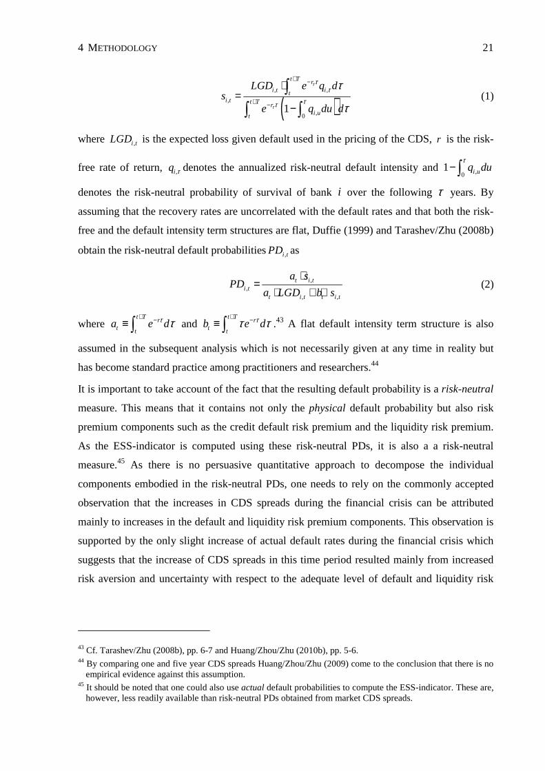
where ,i tLGD is the expected loss given default used in the pricing of the CDS, r is the risk-
free rate of return, ,iq τ denotes the annualized risk-neutral default intensity and ,01 i uq du
τ− ∫
denotes the risk-neutral probability of survival of bank i over the following τ years. By
assuming that the recovery rates are uncorrelated with the default rates and that both the risk-
free and the default intensity term structures are flat, Duffie (1999) and Tarashev/Zhu (2008b)
obtain the risk-neutral default probabilities ,i tPD as
,,
, ,
t i ti t
t i t t i t
a sPD
a LGD b s
⋅=
⋅ + ⋅ (2)
where t T r
t ta e dτ τ
+ −≡ ∫ and t T r
t tb e dττ τ
+ −≡ ∫ .43 A flat default intensity term structure is also
assumed in the subsequent analysis which is not necessarily given at any time in reality but
has become standard practice among practitioners and researchers.44
It is important to take account of the fact that the resulting default probability is a risk-neutral
measure. This means that it contains not only the physical default probability but also risk
premium components such as the credit default risk premium and the liquidity risk premium.
As the ESS-indicator is computed using these risk-neutral PDs, it is also a a risk-neutral
measure.45 As there is no persuasive quantitative approach to decompose the individual
components embodied in the risk-neutral PDs, one needs to rely on the commonly accepted
observation that the increases in CDS spreads during the financial crisis can be attributed
mainly to increases in the default and liquidity risk premium components. This observation is
supported by the only slight increase of actual default rates during the financial crisis which
suggests that the increase of CDS spreads in this time period resulted mainly from increased
risk aversion and uncertainty with respect to the adequate level of default and liquidity risk
43 Cf. Tarashev/Zhu (2008b), pp. 6-7 and Huang/Zhou/Zhu (2010b), pp. 5-6. 44 By comparing one and five year CDS spreads Huang/Zhou/Zhu (2009) come to the conclusion that there is no
empirical evidence against this assumption. 45 It should be noted that one could also use actual default probabilities to compute the ESS-indicator. These are,
however, less readily available than risk-neutral PDs obtained from market CDS spreads.

4 METHODOLOGY 22
premiums.46 We further analyze the risk premium determinants of the ESS-indicator in
section 6.1.2.
Another feature of the resulting default probability is that it is – similarly as the above equity
return correlations – a market-based forward-looking measure in the sense that it contains an
average of the expected default probability during the life of the CDS. In that respect it stands
in clear contrast to backward-looking measures (e.g., based on financial statement data),
which only state what has occurred in the past as opposed to what will occur in the future.
4.1.3 Constructing the systemic risk indicator
The estimated equity return correlations and risk-neutral default probabilities are used as
inputs for the Monte Carlo simulation using the single-risk-factor portfolio credit risk
methodology of Gibson (2004) and Tarashev/Zhu (2008a), which we apply to the
hypothetical credit portfolio comprising the total liabilities of the sample banks to obtain our
expected systemic shortfall indicator. The methodology is elaborated in the following.
We assume that the asset values of the sample banks in the hypothetical debt portfolio are
characterized by the Vasicek (1987) single-risk-factor model, which postulates that a firm
defaults when its assets fall below a certain threshold and that the asset values are determined
by a single common risk factor:
2, ,1
ii T i T i TV M Zρ ρ= + − ⋅ (3)
where ,i TV denotes the asset value of bank i at time T , TM is the common risk factor and iρ
represents bank i ’s exposure to the common factor. ,i TZ denotes the idiosyncratic factor of
bank i . The correlation between banks i and j is consequently given by i jρ ρ .47 In order to
facilitate the model’s implementation, we follow standard practice and assume that the
common risk factor follows a standard normal distribution so that the default threshold of
bank i contingent on the realization of the common factor TM can be shown to equal
( )1,i TPD−Φ where 1−Φ denotes the quantile of the standard normal distribution.48
46 Cf. Huang/Zhou/Zhu (2009), p. 2038. 47 Cf. Vasicek (1987), pp. 1-2. 48 Cf. Tarashev/Zhu (2008a), pp. 135-137.

4 METHODOLOGY 23
In order to implement the Monte Carlo simulation for the N banks in the sample we first
estimate the symmetrical N N× correlation matrix tP and compute the 1 N× vector of the 1-
year risk-neutral default probabilities tPD for every day t in the sample period. We then draw
a 1 N× vector tY of standard-normally distributed variables whose correlation matrix is tP .
This procedure is repeated for K simulation iterations, resulting in a K N× matrix of
correlated normally distributed sample values for each day in the sample period.
A default for bank i at the end of the one-year period under consideration occurs when the
sampled value is below the default threshold, i.e., ( )1, ,i t i tY PD−< Φ . When default occurs for
bank i , we sample an LGD from a symmetrical triangular distribution with a mean of 0.55 in
the range [0.1, 1] which is a widely-used distribution assumption for LGDs.49 Multiplying this
sample LGD with the total liabilities of bank i outstanding on day t results in the
corresponding loss , ,i k tl of bank i . Summing over the losses of all N banks in a particular
simulation iteration k , we obtain the total portfolio loss ,k tL which we use to construct the
portfolio loss distribution tΛ for each observation day t .
We define the ‘systemic loss threshold’ (SLT) as a share of the total liabilities of the sample
banks. When the total portfolio loss ,k tL exceeds the tSLT we assume the occurrence of the
systemic default event. Within the meaning of ‘systemic event’ in definition D1, we interpret
this default event as a situation in which the stability of the financial system is severely
endangered due to the default of a substantial share of the banking sector liabilities. In our
analysis we use a value of 10 percent for the relative systemic loss threshold, i.e.,
10%relSLT = .50 We define the ‘probability of systemic default’ (PSD) as the probability of
the occurrence of the systemic default event, i.e., ( )Pr t tL SLT> , which we obtain from the
portfolio loss distribution tΛ for each day t in the sample period.
From the portfolio loss distribution tΛ we further derive the expected tail loss (ETL), which
we define as the expected value of the total portfolio loss given that the portfolio loss exceeds
49 Cf. Tarashev/Zhu (2008a), pp. 145-146. In a robustness check exercise we use a Beta distribution for the LGD as suggested by Loeffler/Posch (2010).
50We also used 5% and 15% as relative systemic loss thresholds and find that the ESS over time shows the same trajectory as for 10% albeit – of course – on a different level. The definition of the relative SLT depends on the specific application.

4 METHODOLOGY 24
the systemic loss threshold, i.e., ( )|t t t tETL E L L SLT= > . This definition is consistent with
the common definition of expected shortfall in the financial risk management literature.
We obtain the absolute expected systemic shortfall indicator by multiplying the probability of
systemic default by the expected tail loss:
( )Pr( ) |t t t t t t t tESS L SLT E L L SLT PSD ETL= > ⋅ > = ⋅ (4)
The interpretation of the ESS-indicator is straightforward: it represents the product of the
probability of a severe default event in the financial system multiplied by the expected value
of the losses in case this default event materializes. It is also possible to evaluate the PSD and
ETL individually in order to understand the drivers of the aggregate ESS-indicator.
Furthermore we also compute the relative ESS-indicator by dividing tESS by the total
liabilities of the sample banks outstanding at time t in order to facilitate inter-sample
comparability of the empirical results.
The ESS-indicator is an aggregate measure of systemic risk in the financial system
accounting for all sample banks. However, it is also important to understand the relative
contribution of individual banks to the aggregate systemic risk as macroprudential measures
need to be introduced at the level of the individual institution. To this end we compute the
relative systemic loss contribution51 ,i tc of bank i when the total portfolio loss ,t kL exceeds
the systemic loss threshold in a simulation iteration. Summing over all K iterations yields the
contribution of each bank to the systemic risk indicator on sample day t
, ,, ,
1 ,
Ki t k
i t t k tk t k
lc when L SLT
L=
= >∑ (5)
Calculating this measure over the whole or parts of the sample period results in the systemic
risk contribution ic of bank i which can be evaluated either by considering individual banks
or groups of banks (e.g., all banks from a specific country).
4.1.4 Technical comparison with other systemic risk measures
While the usage of a credit portfolio approach and the estimation of its input parameters from
capital market data to measure systemic risk was inspired by Huang/Zhou/Zhu (2009), there
51 In the subsequent elaboration we will refer to the (relative) systemic loss contribution synonymously as (relative) systemic risk contribution and (relative) ESS contribution.

4 METHODOLOGY 25
are a few, but important differences to their distress insurance premium (DIP).
Huang/Zhou/Zhu (2009) assume the systemic loss threshold (SLT) as a percentage of the total
liabilities of the banking system. While this may be adequate for the US banking system,
where most relevant banks are exchange-listed (and consequently the sample banks’ liability
portfolio covers a larger share of the total banking system liabilities), it would be
inappropriate for countries where a significant number of banks are not listed as is in many
European countries.52 Therefore, we define the SLT as a share of total liabilities of the sample
banks in our analysis.
The DIP-indicator measures the cost of insurance against distress losses in excess of the SLT.
While the computation methodology is not stated expressly by the authors, we conjecture that
the DIP-indicator is computed by discounting the expected portfolio loss in excess of the
SLT. As we derive our ESS-indicator using standard measures from financial institution risk
management, it may have certain advantages in terms of transparency and usability vis-à-vis
the DIP-indicator. Besides, Huang/Zhou/Zhu (2009) consider a three-month time horizon
while we compute the portfolio loss at the end of a one-year time period. The relative risk
contributions to the ESS-measure are computed in a transparent fashion as byproduct of our
credit portfolio simulation as opposed to an auxiliary importance sampling procedure in
Huang/Zhou/Zhu (2010a) which facilitates the application of our methodology to measure the
systemic importance of individual institutions.
Moreover, we compute the ESS-measure for each day during the observation period which
ensures that the indicator can respond immediately to financial market events. By contrast,
Huang/Zhou/Zhu (2009), Huang/Zhou/Zhu (2010a), Huang/Zhou/Zhu (2010b) compute the
DIP measure only on a weekly basis which leads to some delay in the indicator’s response to
financial market events. However, this is no drawback of the DIP per se but rather a
disadvantage of the chosen implementation.
An important similarity is that both the DIP and the ESS-indicator are risk-neutral measures
as they are derived from risk-neutral default probabilities obtained from market CDS spreads.
This is also a distinguishing feature with respect to other measures of systemic risk described
in the following. Besides, both the DIP and the ESS-indicator are coherent risk measures
according to the definition by Artzner et al. (1999).
52 The importance of state banks (“Landesbanken”) in Germany but also the savings banks in several European countries supports this statement.

4 METHODOLOGY 26
The systemic expected shortfall (SES) of Acharya et al. (2010) considers the probability of an
individual bank to be undercapitalized when the system as a whole is undercapitalized. The
marginal expected shortfall of individual banks is obtained by computing the expected loss of
individual banks when the whole system is in distress. The SES-indicator is derived using
equity market data, whereas the most important input for the ESS-indicator are CDS spreads
which by construction are better predictors of credit risk.53 The SES measure is also a
coherent risk measure but differs from the ESS-indicator in that it defines the occurrence of a
systemic event as percentile of the portfolio loss distribution, whereas we define it as
percentage of the sample banks’ total liabilities.
The Adrian/Brunnermeier (2008) Conditional Value at Risk (CoVaR) measure computes the
value at risk of the financial system conditional on one bank being in distress. Our ESS-
measure takes the opposite approach by considering the contribution of an individual bank
when the system as a whole is in distress. CoVaR can be used to determine the systemic
importance of individual institutions, whereas it cannot be aggregated to measure the level of
aggregate systemic financial sector risk. The CoVaR measure suffers from the general
shortcomings of VaR-based measures as it is not a coherent measure of risk according to the
Artzner et al. (1999) definition.
53 Cf. Longstaff/Mithal/Neis (2005), pp. 2216-2217.

4 METHODOLOGY 27
4.2 MEASURING CONTAGION EFFECTS IN FINANCIAL MARKETS54
The analysis of contagion and interdependencies in financial markets is most frequently
conducted by analyzing the mutual predictive power of the relevant market variables by
means of Granger-causality tests in vector autoregressive (VAR) or vector error correction
(VEC) models and by interpreting the respective impulse response functions.55 In this thesis
we pursue the same methodological pathway and employ VAR and VEC frameworks in order
to test the described hypotheses. We derive the methodology in the following.
Macroeconomic and financial variables often exhibit the unit root property which according
to Nelson/Plosser (1982) can lead to incorrect conclusions in time series econometrics
hypothesis testing when it is left unaccounted for. In this thesis we employ the three most
common unit root (stationarity) tests in order to examine the relevant variables:
1. Augmented Dickey and Fuller (ADF) test as suggested by Dickey/Fuller (1979),
2. Philips and Perron (PP) test proposed in Phillips/Perron (1988),
3. Kwiatkowski, Phillips, Schmidt and Shin (KPSS) test elaborated in Kwiatkowski et al.
(1992).
We conclude that the time series under research has a unit root, i.e., is integrated of order one
(formalized as ( )1I ), when at least two of these tests suggest the presence of a unit root at the
five percent significance level. If we find a variable to be non-stationary we employ the first
differences of the respective variable in the analysis. When analyzing ( )1I variables one
needs to test the variables for cointegration, i.e., a common stochastic trend, as described by
Engle/Granger (1987) in order to avoid false inferences. This study employs the
Engle/Granger (1987) ADF test as well as the Johansen (1995) trace and maximum
eigenvalue tests in order to analyze the bivariate time series for common stochastic trends. We
conclude that two series are cointegrated if at least two of these tests suggest the presence of
cointegration at the five percent significance level.
When the variables are ( )1I but no cointegration is found between the variables we use the
following VAR model for the analysis
54 The elaborations in this section are (also literally) based on Lahmann (2012b). 55 The theoretical background for this methodological proceeding is described in section 2.2. Examples for
corresponding empirical implementations are Alter/Schueler (2011), Huang/Yang/Hu (2000), Longstaff (2010) and Roll/Schwarz/Suess (2007).

4 METHODOLOGY 28
1, 1,1, 1,2, 1,
12, 2,1, 2,2, 2,
pt i i t i
tit i i t i
y yu
y y
α αν
α α−
= −
∆ ∆ = + + ∆ ∆ ∑ (6)
where 1,ty and 2,ty are the variables under research, ∆ denotes the first difference, ν is a
vector of intercepts, p denotes the lag order of the VAR system and tu denotes a white noise
error term. 56 We follow standard practice and estimate the VAR model using ordinary least
squares (OLS). Accepting the first null hypothesis 0,1 1,2,1 1,2,2 1,2,: ... 0pH α α α= = = = implies
that 2,ty does not Granger-cause 1,ty and equivalently 1,ty Granger-causes 2,ty when one fails
to reject 0,2 2,1,1 2,1,2 2,1,: ... 0pH α α α= = = = . When both null hypotheses are rejected, there
exists a feedback relation between 1,ty and 2,ty . Hypothesis tests are conducted using a Wald
test based on the F-statistic against the one, five and ten percent critical values.
In case cointegration is found between 1,ty and 2,ty an error correction (EC) term needs to be
included in the Granger causality regression equation as follows:
( )1, 1, 1,1, 1,2, 1,
1 1, 1 2 2, 1 012, 1, 2,1, 2,2, 2,
pt t i i t i
t t tit t i i t i
y yy y u
y y
δ α αβ β γ β
δ α α−
− −= −
∆ ∆ = − + + + ∆ ∆
∑ (7)
where 1δ and 2δ represent the speed of adjustment to the long-run equilibrium. The EC part
of the model is estimated using the Johansen (1995) maximum likelihood procedure whereas
the VAR part is estimated using OLS. Rejecting the first null hypothesis
0,1 1,2,1 1,2,2 1,2,: ... 0pH α α α= = = = and 1 0δ = implies that 2,ty Granger-causes 1,ty whereas a
rejection of the second null hypothesis 0,2 2,1,1 2,1,2 2,1,: ... 0pH α α α= = = = and 2 0δ = denotes
that 1,ty Granger-causes 2,ty . When both null hypotheses are rejected, there exists a feedback
relation between 1,ty and 2,ty . Hypothesis tests are conducted using a Wald test based on the
F-statistic against the one, five and ten percent critical values. The regression residuals are
examined for auto-correlation by means of the Ljung/Box (1978) Q-test.57
The data variables actually used for 1,ty and 2,ty in the above VAR models for the contagion
analysis in this thesis are described in the next chapter on the employed empirical data. All
variables are transformed to natural logarithms as suggested by Forte/Pena (2009) and
56 We do not provide separate equations for stationary variables as we do not observe stationary variable pairs in our sample.
57 Cf. Lütkepohl (2007), pp. 316-318.
4 METHODOLOGY 29
Granger/Huangb/Yang (2000).58 In order to determine the lag length p we follow common
practice and employ the Akaike (1974) information criterion (AIC) and the Schwarz (1978)
Bayesian information criterion (SBIC).59 In case the AIC and the SBIC suggest different lag
lengths we use the smaller lag length for the sake of parsimony.60
Including control variables to ensure result robustness
Macroeconomic and financial variables are often affected by common economic factors and
shocks. This commonality may lead to erroneous conclusions in causality analysis when the
actual causality relationship does not exist directly between the variables under research but
rather ‘via’ the common factor.61 In order to control for this commonality and to ensure
robustness of the findings we conduct the analyses in the VAR and VEC frameworks both
without and with control variables as exogenous variables. To this end, we include a relevant
stock market index as proxy for market expectations of overall economic conditions.
Specifically we use the MSCI World in the inter-regional analysis, the S&P 500 index for the
analysis of the American sample, the MSCI Asia-Pacific for Asia-Pacific and the MSCI
Europe for the European sample. Besides, as daily economic variables are only scarcely
available, we additionally employ the federal funds rate as a measure of macroeconomic
shocks. We include the control variables both separately and together as exogenous variables
in the regression equations.62
Trading time adjustments in the lag structure
In the inter-regional analyses we account for differences in trading times between the regions
where necessary and perform the necessary trading time adjustments in the lag structure of the
variables used in the VAR framework as proposed by Huang/Yang/Hu (2000) in order to
ensure that the analyzed variables reflect the same level of information.63
Capturing the model dynamics by means of impulse response analysis
In addition to the above Granger causality tests of the lead-lag relationships in the bivariate
setting we employ impulse response analysis in order to analyze the full dynamics of the
58 This step is further motivated by comparatively low values of the research variables at the beginning of the observation period compared to rather high values at the end of the period.
59 Cf. Huang/Yang/Hu (2000), Granger/Huangb/Yang (2000) and Hiemstra/Jones (1994) (amongst others). 60 This proceeding is consistent with the proposal of Roll/Schwarz/Suess (2007), p. 2216. 61 Cf. Granger (2003), pp. 69-70. 62 This proceeding is motivated by Granger/Huangb/Yang (2000), pp. 349-350. 63 Cf. Huang/Yang/Hu (2000), p.292.

4 METHODOLOGY 30
VAR model in case a Granger causality relationship has been identified. Specifically we
analyze the effect of a one standard deviation ‘shock’64 in one variable on the other variable
over time. Following the seminal thesis of Sims (1980), the dynamics analysis of VAR
models is conducted frequently by computing the orthogonalized impulse responses using the
Cholesky decomposition.65 Koop/Pesaran/Potter (1996) and Pesaran/Shin (1998) find two
shortcomings of this approach, though. Firstly, the impulse response functions are not unique
as they depend on the ordering of the variables in the VAR model. Secondly, the restriction of
uncorrelated contemporaneous shocks is imposed.66 However, in the present analysis theory
does neither suggest an ordering of the research variables nor that contemporaneous shocks to
the variables are uncorrelated.67 Therefore, we employ the generalized impulse response
(GIR) analysis suggested by Pesaran/Shin (1998) because it overcomes the mentioned
shortcomings of the orthogonalized impulse responses. This choice is consistent with the
methodological implementations in recent research (e.g., Chordia/Sarkar/Subrahmanyam
(2005), Griffin/Nardari/Stulz (2007) and Kavussanos/Visvikis (2004)). In order to facilitate
the comparison and interpretation of the results, we follow Griffin/Nardari/Stulz (2007) and
scale the impulse responses by the standard deviation of the residual of the variable’s
regression equation.68
Correlations of the research variables
In order to complement the results obtained from the Granger-causality and impulse response
analysis we analyze the correlations of the research variables by employing a moving-window
correlation estimation methodology using the past month’s values. While the correlations do
not provide additional insights with respect to the lead-lag dependencies between the
variables, they facilitate the analysis of the direction and magnitude of the linear relationship.
64 In the following the terms impulse and innovation are used synonymously. 65 Cf. Pesaran/Shin (1998), p. 17. 66 Cf. Griffin/Nardari/Stulz (2007), p. 918. 67 In fact, a correlation of shocks is rather likely for several variables (e.g., sovereign and bank CDS). 68 Cf. Griffin/Nardari/Stulz (2007), p. 918 as well as Lütkepohl (2007), pp. 51-54 and pp. 321-322.

31
5 EMPIRICAL DATA
In this chapter we describe the empirical data analyzed in this thesis. Firstly, we describe the
bank sample used in the empirical application of the ESS-methodology and, secondly, the
data employed in the analysis of banking sector risk contagion dependencies is specified. The
observation horizon of the analyses in this thesis comprises the time period between October
1st, 2005 and April 30th, 2011.69 In order to facilitate an intertemporal analysis of the data and
analysis results we divide the overall sample period into the following four sub-periods which
are subsequently referenced: the ‘pre-crisis’ period 1 ranges from October 1st, 2005 to
February 28th, 2007; the ‘subprime and beginning financial crisis’ period 2 ranges from
March 1st, 2007 to July 31st, 2008; ‘the core financial crisis’ period 3 ranges from August 1st,
2008 to December 31st, 2009; ‘the sovereign debt crisis’ period 4 ranges from January 1st,
2010 to April 30th, 2011.
5.1 ESS-ANALYSIS70
The ESS-methodology described in the previous chapter can in principle be applied to any
portfolio of companies with publicly traded equity and available CDS data. As the focus of
the present analysis is the measurement of systemic risk and the assessment of systemic
importance in global and regional financial markets, we select bank holding companies
according to the following data availability criteria: (I) available CDS spreads, (II) publicly
available equity prices, (III) publicly available liability data. By applying these data
availability criteria we obtain a global sample of 83 banks from 28 countries covering the
following four regional sub-samples: America (12 banks), Asia-Pacific (24 banks), Europe
(38 banks), Middle East and Russia71 (9 banks).
We compute equity returns from equity market prices provided by Thomson Datastream in
order to estimate the equity return correlations required in the computation of the ESS-
indicator. CDS spreads are obtained from CMA Market Data and Thomson Reuters using the
mid-spread of the 5-year senior unsecured CDS spread to compute the corresponding risk-
69 A longer sample period was not feasible due to data limitations. 70 The elaborations in this section are (also literally) based on Lahmann/Kaserer (2011a). 71 We summarize these two regions as one ‘region’ as neither of them could be unambiguously allocated to any
of the other regions and because they are individually too small in terms of available sample data.

5 EMPIRICAL DATA 32
neutral default probabilities.72 As the LGDs used by market participants for pricing the CDS
are not available in these databases we assume an LGD of 55% to compute the risk-neutral
default probabilities.73 Total liabilities of the sample bank holding companies are obtained
from the Thomson Worldscope database. A linear gradient is assumed between available
liability dates to obtain the amount of total liabilities per day during the observation period.
We conduct the analysis both for the global sample and for the four regional sub-samples
individually which is also reflected in the subsequent elaboration: we first describe the data
for the global sample and then proceed with the regional sub-samples before conducting a
comparative analysis between the individual samples. The elaboration is structured so that the
reader can also focus on specific samples only without loss of continuity.
5.1.1 Global sample
The lower panel of Table 1 shows the 28 countries of the banks in the global sample as well
as the total liabilities of the sample banks per country and their average (liability-weighted)
CDS spreads. The total liabilities of the banks covered in the analysis amount to 35.8 trillion
EUR with an average of 1.3 trillion EUR per country. The countries with the highest total
bank liabilities are France, Germany, Switzerland, the United Kingdom and the United States.
From period 1 to period 4 the average CDS spread of all banks increases from 13 to 139 basis
points. In period 4 the countries with the highest average bank CDS spreads are Greece,
Ireland, Kazakhstan and Portugal whereas Denmark, Malaysia, Singapore and Sweden have
the lowest bank CDS spreads. The ranking of the countries with respect to their banks’ CDS
spreads changes over time and the changes from period 3 to period 4 reflect the impact of the
euro zone sovereign debt crisis (e.g., the Greek banks’ average CDS spread increases more
than ten-fold from 72 to 778 basis points).
Table 2 shows the same parameters as Table 1 on a bank level. The total liabilities per bank
average 431 billion EUR. The largest banking groups in terms of total liabilities are Barclay’s,
BNP Paribas, Deutsche Bank and Royal Bank of Scotland. In period 4 Greece’s Alpha Bank
and EFG Eurobank, Ireland’s Allied Irish Banks and Kazakhstan’s Kazkommertsbank have
the highest CDS spreads whereas the three Singaporean banks and Sweden’s Svenska
72 We use the 5-year senior unsecured CDS spread as this is the most frequently traded CDS type (cf. Hull/Predescu/White (2004), p. 2794).
73 The empirical results are robust to alternative assumptions for the LGD.

5 EMPIRICAL DATA 33
Handelsbanken have the lowest CDS spreads. The ranking of the banks according to their
CDS spreads is time-variant with the biggest changes occurring from period 3 to period 4.
Table 3 shows the sample banks’ equity return correlations74 as well as their end-2008
shareholder’s equity on a country-level. The total equity of the sample banks adds up to 1.5
trillion EUR with a country average of 54 billion EUR. The countries with the highest average
correlation of their sample banks’ equity returns are France, Germany, Italy and Switzerland.
On a bank level, Barclay’s, BNP Paribas, Crédit Agricole and Societé Generale have the
highest correlation as shown in Table 4. The evolution of the equity return correlation of the
global sample is shown in the lower panel of Figure 1. It averages 24 percent in the period
before August 2007. In August 2007 the correlation increases significantly to an average
value of 37 percent in the period until November 2008. In addition to the elevated level of the
average correlation, the standard deviation of the correlation also increases considerably.
From December 2008 until April 2010 the average equity return correlation decreases to an
average of 28 percent before rising to an average of 33 percent in May 2010. From June 2010
until the end of the observation period average correlations decrease to 26 percent, slightly
above the pre-crisis average.
The upper panel of Figure 1 shows the liability-weighted average risk-neutral default
probabilities of the banking groups in the global sample during the observation period. Before
July 2007 the average risk-neutral default PDs are below 0.5 percent. Following the freezing
of three investment funds by BNP Paribas in August 2007 the default probabilities are
elevated before reaching a local maximum of 2.9 percent after the takeover of Bear Stearns by
JP Morgan in March 2008. In the aftermath of the collapse of Lehman Brothers in September
2008, average risk-neutral PDs reach a second peak at 3.6 percent on September 29th, 2008.
Following the financial stability measures in Europe and the United States taken in early
October 2008, the default probabilities decline to a lower level before reaching an
observation-period maximum of 4.4 percent on March 09th, 2009. After the G20 Summit in
London in April 2009, the risk-neutral default probabilities fall again below two percent on
average. At the time of the aggravation of the euro sovereign debt crisis in May 2010 the
average PDs increase again sharply and remain at two percent until the end of the observation
period which is significantly above pre-crisis levels.
74 Computed as the mean of the daily pairwise stock return correlations between the respective bank and all other banks.

5 EMPIRICAL DATA 34
5.1.2 American sub-sample
The American sub-sample is represented by 12 banks from the United States as no other bank
from the American continent meets the described data availability criteria. The total liabilities
of the American banks amount to 6.9 trillion EUR with an average of 577 billion EUR as
shown in Table 1. Table 2 shows that the largest US sample banks in terms of total liabilities
are Bank of America, Citigroup and JP Morgan. The average CDS spreads of the American
sample increased from 16 basis points in period 1 to 214 basis points in period 3 and
decreased to 134 basis points in period 4. The US banks with the highest CDS spreads in
period 4 are MetLife, Morgan Stanley and Citigroup whereas American Express, JP Morgan
and Wells Fargo have the lowest CDS spreads.
Table 5 shows the equity as of end-2008 and the average correlations of the American sample
banks. In total, the US sample banks have a combined equity of 465 billion EUR with a mean
of 39 billion EUR. In period 4 Bank of America, JP Morgan and Wells Fargo are the banks
with the highest correlation. The lower panel of Figure 2 shows the average equity return
correlation of the American sub-sample during the observation horizon. From October 2005
until July 2007 the average correlation is 62 percent. During the financial crisis period
between August 2007 and July 2009 equity return correlations in the US sub-sample hike to
an average of 76 percent and return to a lower level of 59 percent from August 2009 until
April 2010. Thereafter, average correlations increase by ten percentage points and maintain
this level until the end of the observation period.
The upper panel of Figure 2 shows the liability-weighted average risk-neutral default
probabilities of the US sample banks during the observation period. In the period between
October 2005 and July 2007 the average risk-neutral default PDs are below 0.5 percent. The
default probabilities are significantly elevated as of August 2007 and reach a local maximum
of 3.7 percent in March 2008. In the aftermath of the collapse of Lehman Brothers in
September 2008, the mean PD of the US sample banks reaches two local maxima on
September, 17th 2008 (5.9 percent) and on October, 10th, 2008 (6.0 percent). At a level of 6.6
percent the US banks reach their observation-period maximum on March 09th, 2009.
Thereafter, the average PD decreases to a value of 2 percent in end-April 2010. Afterwards it
begins to rise again and reaches a local maximum on June 10th, 2010 at 3.3 percent. Until the
end of the observation period, the default probability averages 2.3 percent which is the

5 EMPIRICAL DATA 35
quintuplicate of the pre-crisis average. In addition to the elevated level of the PDs during the
financial crisis period, the dispersion75 of the PDs is higher during this period.
5.1.3 Asian-Pacific sub-sample
The total liabilities of the Asian-Pacific banks amount to 5.2 trillion EUR with an average of
218 billion EUR per bank as shown in Table 1. The Australian, Chinese and Japanese banks
have the highest total liabilities in this sub-sample. The average CDS spreads of the banks in
the Asian-Pacific sample increase from 19 basis points in period 1 to 169 basis points in
period 3 before decreasing to 108 basis points in period 4. In period 4 the countries with the
highest average CDS spreads are China, India and Kazakhstan. The ranking of the countries
with respect to their average CDS spreads is rather stable over time. Table 2 shows that Bank
of China, Mizuho Financial Group and Sumitomo Mitsui Bank have the highest total
liabilities in this sample. The Asian-Pacific banks with the highest CDS spreads in period 4
are India’s ICICI Bank as well as Kazakhstan’s Halyk Bank and Kazkommertsbank whereas
the three Singaporean sample banks have the lowest CDS spreads.
Table 6 shows the end-2008 equity and the average correlations of the Asian-Pacific sub-
sample on a country and bank level. The Asian-Pacific banks have a combined equity of 264
billion EUR with a mean of 11 billion EUR. In period 4 the countries with the highest average
correlation are Australia, Korea and Singapore. On a bank-level Australia’s Commonwealth
Bank, Macquarie Bank and National Australia Bank and Korea’s Kookmin Bank have the
highest average correlation. The equity return correlation of the Asian-Pacific sub-sample
banks during the sample period are shown in the lower panel of Figure 3. The average
correlation is 26 percent in the period between October 2005 and June 2007. During the crisis
period between July 2007 and July 2009 equity return correlations increase to an average of
33 percent. From August 2009 until the end of the observation period, the average
correlations decrease to 24 percent which is even below the pre-crisis average.
The average risk-neutral default probabilities of the banks from the Asia-Pacific region during
the observation period are shown in the upper panel of Figure 3. Before August 2007 the risk-
neutral PDs average 0.3 percent. The default probabilities are elevated as of August 2007 and
reach a local maximum of 2.7 percent in March 2008. Until mid-September 2008 average PDs
amount to 1.8 percent and reach a local maximum of 4.7 percent on October 29th, 2008. The
75 We measure dispersion as the standard deviation of all observations at a particular point in time.

5 EMPIRICAL DATA 36
observation period maximum of 4.8 percent is reached on March 10th, 2009 and until the end
of the observation period the risk-neutral PDs average 1.9 percent.
5.1.4 European sub-sample
The total liabilities of the banks in European sub-sample amount to 23.3 trillion EUR with an
average of 613 billion EUR per country as shown in Table 1.76 The largest European countries
in terms of their sample banks’ total liabilities are France, Germany and the United Kingdom.
The average CDS spreads of all sample banks increase markedly from 10 basis points in
period 1 to 145 basis points in period 4. The countries with the highest average bank CDS
spreads in period 4 are Greece, Ireland and Portugal. These countries also show the strongest
increase in their bank CDS spreads from period 3 to period 4 reflecting the impact of the euro
zone sovereign debt crisis (e.g., Greece’ average bank CDS spreads increase from 72 to 778
basis points). The largest banking groups in the European sample in terms of total liabilities
are Barclay’s, BNP Paribas, Deutsche Bank and Royal Bank of Scotland as shown in Table 2.
The banks with the highest CDS spreads in period 4 are Greece’s Alpha Bank and EFG
Eurobank, Ireland’s Allied Irish Banks and Portugal’s Banco Commercial and Espirito Santo.
Table 7 shows the end-2008 total equity of the European sample banks and their average
correlations during the four sample periods on a country level. The European sample banks
have a combined equity of 744 billion EUR with an average of 53 billion EUR per country.
The sample countries with the highest average equity return correlations in period 4 are
France, Italy and Spain. Table 8 shows that the equity per bank averages 20 billion EUR and
that the banks with the highest average correlations in period 4 are France’s BNP Paribas and
Societé Generale as well as Spain’s Grupo Santander. The progress of the equity return
correlation of the European sample banks is shown in the lower panel of Figure 4. It averages
41 percent in the period before August 2007. In August 2007 the correlation increases
significantly to a mean value of 61 percent in the period until November 2008. In addition to
the elevated level of the average correlation, the standard deviation of the correlation also
increases considerably.77 From December 2008 until April 2010 the average equity return
correlation decreases to 49 percent before rising again to a higher level as the euro sovereign
76The majority of the banks from the European Union were also covered in the stress test conducted by the Committee of European Banking Supervisors published in July 2010 which applied stress scenarios to the positions of individual institutions.
77 This conclusion is drawn by considering the underlying data of Figure 4.

5 EMPIRICAL DATA 37
debt crisis materializes in May 2010. From October 2010 until the end of the observation
period the average correlations decrease again to the pre-crisis average.
The upper panel of Figure 4 shows the average risk-neutral default probabilities of the sample
banks during the observation period. Before July 2007 the average risk-neutral default PDs
are low at below 0.5 percent. After the freezing of three investment funds by BNP Paribas in
August 2007 the default probabilities are elevated before reaching a local maximum of 2.7
percent after the takeover of Bear Stearns by JP Morgan in March 2008. Subsequent to the
collapse of Lehman Brothers in September 2008, average risk-neutral PDs reach a second
peak at 3.3 percent on September 29th, 2008. Afterwards, the default probabilities decline to a
lower level before reaching an observation-period maximum of 3.6 percent on March 12th,
2009. From April 2009 to April 2010 the average PDs average out 1.9 percent. Due to the
aggravation of the euro sovereign debt crisis in May 2010 the average PDs increase again
sharply to an average of 2.6 percent until the end of the observation period.
5.1.5 Middle Eastern and Russian sub-sample
The Middle Eastern and Russian (MER) sub-sample consists of nine banks, six from the
Middle Eastern region and three banks from Russia as shown in Table 2.78 We summarize
these two regions in our analysis as neither of them could be unambiguously allocated to any
of the other regions and because they are individually too small in terms of available sample
data. The total liabilities of the MER banks amount to 354 billion EUR with an average of 39
billion EUR per bank (Table 1). Russia’s WTB and Sberbank and the UAE’s79 Abu Dhabi
Commercial bank are the largest banks in terms of total liabilities in this sub-sample.
The average CDS spreads in the MER sub-sample increase from 69 basis points in period 1 to
526 basis points in period 3 but decrease again to an average of 279 basis points in period 4.
The banks with the highest CDS spreads in period 4 are Russia’s Bank of Moscow and the
UAE’s Dubai Islamic Bank and Mashreqbank. Table 9 shows the end-2008 equity and the
average correlations of the banks in the sub-sample. The total equity in this sample amounts
to 40.6 billion EUR and averages 4.5 billion EUR per bank. The banks with the highest
correlation in the last period are Bank of Moscow, Commercial Bank of Qatar and National
Bank of Abu Dhabi. The lower panel of Figure 5 shows the average equity return correlation
78 Due to the small sample size a country level analysis is not conducted for this sub-sample. 79 UAE = United Arab Emirates.

5 EMPIRICAL DATA 38
of the MER sub-sample during the observation period. The average correlation is 21 percent
in the period between October 2005 and June 2007. During the crisis period between July
2007 and July 2009 equity return correlations decrease to an average of 17 percent. From
August 2009 until the end of the observation period, the average correlations increase slightly
to 19 percent which is still below the pre-crisis average.
The average risk-neutral default probabilities of the banks from the Middle East and Russia
sub-sample during the observation period are shown in the upper panel of Figure 5. Before
July 2007 the risk-neutral PDs average 1.1 percent. Between July 2007 and August 2008 the
default probabilities rise to an average of 2.6 percent and reach an observation-period
maximum of 14.2 percent on October 24th, 2008. After this extreme hike, the risk-neutral PDs
remain elevated until April 2009 (10 percent on average) and then return to lower levels until
the end of the observation horizon (5 percent on average).
5.1.6 Comparative analysis
Following the above description of the global sample and the four regional sub-samples we
conduct a comparative analysis of the liability size, default probabilities and average
correlations between the samples in this section.
From Table 1 it can be gathered that from the 37.8 trillion EUR total liabilities of the global
sample, Europe is the largest sub-sample with a total of 23.3 trillion EUR (65 percent of total)
followed by the American sample with total liabilities of 6.9 trillion EUR (19 percent). The
Asian-Pacific sub-sample ranks third with 5.2 trillion EUR (15 percent) and the Middle
Eastern and Russian sample is the smallest sub-sample with 354 billion EUR (1 percent). Due
to these significant size differences of the sub-samples we focus the comparison of the
sample-specific results on the relative ESS-indicator and relative changes over time.
The upper panel of Figure 6 shows the average risk-neutral default probabilities of the global
sample and the four sub-samples. The MER sub-sample has the highest average default-
probability of all samples over time (3.7 percent), followed by the American (1.8 percent), the
global and Asian-Pacific samples (both 1.5 percent) and the European (1.4 percent) sub-
samples. It is interesting to note that all samples except for the MER sub-sample reach their
observation period maximum in March 2009 after the stock-market low and not – as one may
have expected – following the Lehman bankruptcy and the subsequent events in September
and October 2008. It can further be observed that the default-probability (and respectively the
CDS spreads) of the American sample banks exhibit the highest volatility between September

5 EMPIRICAL DATA 39
2008 and September 2009. The default probabilities of the European and Asian-Pacific sub-
samples move closely together from October 2005 until September 2008. The default
probabilities of the banks from the Asia-Pacific region react more strongly and are more
elevated than the PDs of the European banks between October 2008 and June 2009. From
July 2009 until April 2010 the Asian-Pacific and European default probabilities move again
together and the American banks’ average default probability is slightly higher. As the euro
sovereign debt crisis aggravated in May 2010, the European banks’ default probabilities
upswing strongly and also the PDs from the other sub-samples increase slightly. The PD
increase of the non-European sub-samples can probably be explained by the market
uncertainty with respect to the global effects of the euro sovereign debt crisis and the extent of
exposure of banks around the globe to debt from financially frail euro zone countries. The
euro zone sovereign debt crisis also has another notable impact: the European sub-sample is
the only sample whose average default probabilities increase in period 4with respect to the
average in period 3.80
The lower panel of Figure 6 shows the average correlations of the global sample and the four
sub-samples. At an average level of 68 percent, the banks from the American sample have the
highest average correlation of all sub-samples during the observation period. This is no
surprise, however, because the American sample is the most homogeneous sub-sample as it is
composed of major US banks exclusively. The average correlation of the American banks is
always above that of the European banks except for the time between May 11th, 2010 and
June 18th, 2010 where the comovement of European banks’ equity prices was particularly
strong due to the market dislocations caused by the euro zone sovereign debt crisis.
The European banks’ average equity return correlations are at an average level of 50 percent
the second highest of all sub-samples and are above the average correlations of the Asian-
Pacific banks (28 percent) which applies also on a daily level except for six outlier days in
March 2011. As the European sub-sample comprises mainly banks from an integrated
economic and currency area (however with varying differences between the member
countries), the ordering of its average correlations below the homogeneous American sub-
sample and above the heterogeneous Asia-Pacific sub-sample appears adequate. The Middle
East & Russia sample has the lowest average correlation among the sub-samples (19 percent)
80 This conclusion is more obvious when the respective CDS spreads tables are compared.

5 EMPIRICAL DATA 40
which is amongst others due to the fact that the sample banks are heterogeneous and stem
from emerging markets with specific characteristics.
There is a strong comovement in the equity return correlations of the American, Asian-Pacific
and European sub-samples whereas the European and (particularly) Asian-Pacific sub-
samples’ correlations respond with more delay to the financial crisis events than the American
correlations. The correlations of these three sub-samples increase even jointly in May 2010 in
response to the European sovereign debt problems whereas the increase of the European
sample’s correlations is strongest. However, from June 2010 until the end of the observation
period the comovement relationship breaks down and correlations appear to be determined
mainly by region-specific factors.
The global sample has an average correlation of 29 percent during the observation period. As
the average correlations are computed from the average of the correlations of one bank with
all other banks and bearing in mind the number and heterogeneity of the banks and countries
covered in the global sample it is obvious that high average correlations are rare. In fact, the
global sample’s average correlation reaches a value of 50 percent only once in the observation
period on September 22nd, 2008. The average correlation of the global sample has a strong
comovement with the American, Asian-Pacific and European sub-samples, particularly in the
time period before June 2010.

5 EMPIRICAL DATA 41
5.2 BANKING SECTOR RISK CONTAGION DEPENDENCIES
In this section we discuss the empirical data employed in the analysis of banking sector risk
contagion dependencies.
5.2.1 Inter-regional systemic risk contagion81
In order to analyze the inter-regional systemic risk contagion we employ the relative ESS-
indicator elaborated in section 6.1 for the regional sub-samples America, Asia-Pacific, Europe
as well as Middle East and Russia. In a separate analysis we employ the liability-weighted
average bank CDS spreads of these four sample regions. In terms of the notation employed in
the elaborated VAR model we use the relative ESS-indicator and respectively the weighted
bank CDS spreads of one region as 1,ty (‘caused systemic risk’) and the relative ESS-
indicator and respectively the weighted bank CDS spreads of the other regions as 2,ty
(‘causing systemic risk’) so as to capture all possible regional combinations.
The evolution of the ESS-indicator in Figure 22 shows that the indicator is at a very low level
in all regions before the crisis and that it adequately captures the financial crisis events with
‘global importance’ as well as the region-specific crisis events. In particular, the ESS-
indicator shows peaks for all samples in March 2008 after the Bear Stearns takeover, in
September 2008 after the Lehman default, in March 2009 after the stock market low and in
May 2010 at the time of the aggravation of the euro debt crisis. On the regional level, the
ESS-indicator captures the region-specific crisis events such as the Russian bank funding
crisis in October 2008 and the natural disaster in Japan in March 2011.
Figure 7 shows the evolution of the weighted82 CDS spreads of the sample banks for each
sample region. The peaks of the curves reflect the financial crisis events with global
importance as well as the regional events. During the full observation period the European
bank sample has the lowest average CDS spreads followed by the Asia-Pacific, American and
MER samples. However, at the end of the observation period, the European banks have the
second highest CDS spreads due to the euro zone sovereign debt crisis. Table 1 shows the
average bank CDS spreads on the regional and country level during the four sub-periods. In
period 4 the sample banks from Portugal, Ireland, Kazakhstan and Greece have the highest
81 The elaborations in this section are (also literally) based on Lahmann (2012b). 82 We use the banks’ total liabilities weights in order to weight the CDS spreads. We find that the empirical
results are also robust when unweighted bank CDS spreads are used.

5 EMPIRICAL DATA 42
CDS spreads whereas the banks from Singapore, Malaysia and Sweden have the lowest CDS
spreads.
5.2.2 Sovereign risk vs. banking sector risk contagion83
In the analysis of inter- and intra-regional sovereign risk vs. systemic risk contagion we use
the weighted82 bank CDS spreads for the four regional samples America, Asia-Pacific, Europe
and Middle East & Russia described in the previous section as a (proxy) measure of regional
systemic risk.84 The sovereign sector credit risk is measured by CDS spreads as these are
superior measures of credit risk compared to bond and loan spreads.85 Consistent with the
bank CDS spreads, we use the spreads of the 5-year senior unsecured sovereign CDS as this
is the most liquid and most frequently studied CDS type.86 We employ the sovereign CDS
spreads from the same 28 countries covered in the bank sample and compute the weighted
average of these CDS spreads for the four sample regions.87 In terms of the notation of the
elaborated VAR model we use the regional bank CDS spreads as 1,ty and the regional
sovereign CDS spreads as 2,ty for all possible combinations of regional bank and sovereign
CDS spreads. For the analysis of country-specific sovereign risk vs. banking sector risk we
use the country-level weighted average bank CDS spread as 1,ty and the corresponding
sovereign CDS spread as 2,ty .
Table 10 shows the average sovereign CDS spreads of the countries covered in the analysis
during the respective sub-periods. In period 4 Greece, Ireland and Portugal have the highest
sovereign CDS spreads whereas Denmark, Singapore and Sweden are the countries with the
lowest CDS spreads. Figure 8 shows the evolution of the sovereign CDS spreads per region
over time. The countries in the MER sample exhibit the highest average sovereign CDS
spreads during the observation period followed by the Asia-Pacific, European and American
83 The elaborations in this section are (also literally) based on Lahmann (2012a). 84 This step is motivated by the finding in section 6.1 that the bank CDS spreads are a first-order approximation
of the relative ESS-indicator. 85 See section 4.1.2 for related references. 86 Cf. Hull/Predescu/White (2004), pp. 2790-2792. 87 We use the country’s sample banks‘ liability weights to compute the weighted average in order to ensure
consistency with the weighting of the bank CDS. We find that the empirical results are also robust when unweighted sovereign (or bank) CDS spreads are used.

5 EMPIRICAL DATA 43
sample. In period 4, the European countries have the second-highest average sovereign CDS
spreads due to the euro zone sovereign debt crisis.
5.2.3 Banking sector risk vs. corporate sector risk contagion88
In the analysis of banking vs. non-bank corporate sector risk contagion we consider both the
credit and equity side of the sample entities in the regions America, Asia-Pacific and Europe
within an intra-regional analysis.89 In order to analyze the contagion effects in credit markets
we employ CDS spreads as these are superior measures of credit risk compared to bond and
loan spreads.85 Consistent with the bank CDS, we use the spreads of the 5-year senior
unsecured CDS of the non-bank corporate sample firms as this is the most liquid and most
frequently studied CDS type.86 For the analysis of banking vs. corporate sector contagion
effects in equity markets we employ market equity prices. In terms of the notation employed
in the elaborated VAR framework we use the corporate CDS spreads (equity returns) as 1,ty
and the weighted90 bank CDS spreads (equity returns) of the same region as 2,ty .
The bank sample comprises the regional sub-samples America, Asia-Pacific and Europe
described in the previous section.89 Figure 11 shows the indexed regional bank equity prices
used in the analysis which exhibit a high degree of comovement before and during the crisis .
After the crisis, the recovery is strongest for the stocks of the Asia-Pacific banks whereas the
American and particularly the European banks’ equity prices are significantly below their pre-
crisis levels. The stock prices of the banks in the Middle East & Russia sample exhibit the
highest volatility of all regional samples and the decline during the crisis as well as the post-
crisis increase is strongest for this sample.91
We select all non-bank corporate sample entities subject to available CDS and equity data in
Thomson Reuters Datastream during the sample period. Each entity is unambiguously
assigned to one of the three sample regions and one of nine industry clusters. Table 11 shows
the composition of the non-bank corporate sample as well as the average daily CDS spreads
88 The elaborations in this section are (also literally) based on Lahmann/Kaserer (2012). 89 The region Middle East and Russia is not considered due to lack of available data for the non-bank corporate
firms in this sample. 90 We use the banks’ total liabilities weights in order to weight the CDS spreads. We find that the empirical
results are also robust when unweighted bank CDS spreads are used. 91 The stock prices for the MER sample shown in the figure are not considered in this analysis and are included
only for comparison and reference purposes.

5 EMPIRICAL DATA 44
per region and industry cluster.92 Across all regions and industry clusters we cover 352 firms,
of which 157 are from the (North) American continent, 68 from the Asia-Pacific region and
127 from Europe.93 In the American sample the automotive firms have the highest average
CDS spreads (424 bps) whereas the firms in the ‘industrial’ cluster have the lowest CDS
spreads (63 bps) in period 4. In the Asia-Pacific sample the firms in the construction and
logistics cluster have the highest average CDS spreads (183 bps) whereas the automotive
firms have the lowest CDS spreads (73 bps) in period 4. The automotive firms in the
European sample exhibit the highest CDS spreads (163 bps) whereas the firms in the
chemicals, healthcare and pharma cluster have the lowest CDS spreads (60 bps) in period 4.
These differences in industry- and region-specific firm CDS spread levels provide further
reasoning for the separate analysis of industry and regional samples.
The upper panel of Figure 9 shows the evolution of the corporate CDS spreads per industry
across all regions. It is striking that the automotive firms have by far the highest average CDS
level. For the financial crisis period this reflects the severe impact of the financial crisis on
this industry: The large peaks for the automotive cluster result mainly from the high CDS
spreads of the US automotive firms (e.g., Ford Motors’ average CDS spread in December
2008 amounted to a stunning 68 percent). The CDS of companies from the industry clusters
basic materials and financial services (excl. banking) were also particularly affected by the
financial crisis whereas the firms from the other industries show a high degree of
comovement at comparatively low CDS levels. The lower panel of Figure 9 shows the
evolution of the average corporate CDS spreads per region across all industries. It shows that
the average corporate CDS spreads in the American sample are the highest followed by the
Asian-Pacific and the European sample. At the end of the sample period, the firms in the
European sample have the highest average CDS spread.
The upper panel of Figure 10 shows the indexed equity prices of the sample entities for each
industry across all regions. The equity prices of firms from the automotive and basic materials
industries show a high degree of independent movement relative to the other industries which
have a high degree of comovement.94 The stock prices of the financial services (excl.
92 The averages for the non-bank corporate sample (CDS spreads and equity returns) are computed as unweighted averages due to the differences in balance sheet structure across industries. We find that the empirical results are also robust when the values are weighted by total liabilities (similarly as for banks).
93 A list of the sample entities is shown in Appendix B. 94 The extreme hike in the automotive industry cluster on October 28th, 2008 is due to the speculation-induced
share price increase of the Volkswagen stock (attempted takeover by Porsche Group).
5 EMPIRICAL DATA 45
banking) companies were hit most by the crisis and are the lowest at the end of the
observation period whereas the basic materials companies’ stocks show the highest relative
post-crisis level. The lower panel of Figure 10 shows the evolution of the regional cross-
industry indexed equity prices. Compared to their pre-crisis peaks, the stock prices of the
Asian-Pacific and European companies show the strongest declines. By contrast, the stock
prices of the American sample are lowest at the end of the sample period relative to the initial
level. Table 12 shows the industry-specific equity returns for the sample regions during the
four sub-periods. In period 4 the equity prices of the companies in the American sample
increased strongest and on a cross-regional industry basis the Automotive companies’ equity
return was highest in this period.
46
6 EMPIRICAL RESULTS
6.1 EXPECTED SYSTEMIC SHORTFALL INDICATOR95
The ESS-methodology is applied separately to the global sample and the four regional sub-
samples to obtain the expected systemic shortfall indicator which is then analyzed with
respect to its input variable determinants (section 6.1.1).96 As the ESS-indicator is a risk-
neutral measure, we further analyze its risk premium determinants in section 6.1.2. The
relative systemic risk contributions of individual countries and banks are elaborated in section
6.1.3. In each section of this chapter we describe the global sample as well as the four sub-
samples and conduct a comparative analysis at the end of each section. As in the previous
chapter, the elaboration is structured such that the reader can also focus on specific samples
without loss of continuity.
6.1.1 The aggregate ESS-indicator
In this section we describe the results from applying the ESS-methodology as well as the
input factor determinants of the ESS-indicator for each sample before comparing the sample-
specific results. As outlined in section 4.1.3 the absolute ESS-indicator represents the
probability of the portfolio losses exceeding the systemic loss threshold multiplied by the
expected tail loss in case this systemic default event occurs. The relative ESS-indicator
denotes the ratio of the absolute ESS-indicator to the total liabilities outstanding. In order to
determine the end of the international financial crisis effects by means of the ESS-indicator
for each sample we define the end of the financial crisis period as the time period when the
relative ESS-indicator is below a third of its crisis peak for three consecutive months.97
6.1.1.1 Global sample
The evolution of the ESS-indicator of the global sample over time is shown in Figure 12.
Before the first indication of the sub-prime and financial crisis became evident in July 2007
95 The elaborations in this section are (also literally) based on Lahmann/Kaserer (2011a). 96 The robustness of the results is confirmed by repeating the simulation using the Beta distribution suggested by
Loeffler/Posch (2010) for the LGD instead of the triangular distribution. 97 It should be noted that this definition is somewhat arbitrary but facilitates an approximate assessment of the
crisis end which is defined as a period rather than a point in time.
6 EMPIRICAL RESULTS 47
the ESS-indicator was at a very low level, i.e., below 10 billion EUR (0.1 percent of total
liabilities).98 The indicator increased sharply to 59 billion EUR (0.2 percent) after the freezing
of the BNP Paribas funds on August 16th, 2007. Thereafter the indicator rose steadily until it
reached a first local maximum of 255 billion EUR (0.7 percent) on March 17th, 2008 after the
arranged takeover of Bear Stearns by JP Morgan. Reflecting the crisis response of central
banks and governments around the globe, the indicator decreased again to a local minimum of
86 billion EUR (0.3 percent) on May 2nd, 2008 when the central banks of the European
Union, Switzerland and the United States jointly announced an expansion of liquidity-
enhancing measures.99
On September 17th, 2008 – two days after the collapse of Lehman Brothers – the ESS-
indicator jumps to a level of 413 billion EUR (1.1 percent). The sample period maximum is
reached on September 29th, 2008 at a level of 446 billion EUR (1.2 percent) which reflects the
market uncertainty and dislocation after the Lehman default. In the fourth quarter 2008 frail
financial institutions around the globe were supported or rescued by unprecedented
government measures: amongst others the US government introduced the troubled asset relief
program (TARP), France approved a 360 billion EUR rescue package, the German
government rescued Hypo Real Estate and Her Majesty’s Treasury forced capital injections
into major UK banking groups. Subsequent to these measures the ESS-indicator decreased to
223 billion EUR (0.6 percent) on average until February 2009.
The systemic risk in the global sample reaches another local maximum of 368 billion EUR
(1.0 percent) on March 9th, 2009, three days after global stock markets hit their crisis lows. In
the subsequent 12 months after the G20 summit in London on April 2nd, 2009 the indicator
decreased to an average value of 128 billion EUR (0.4 percent) which is only slightly above
the average during the 12 months before the Lehman default.
Along with the exacerbation of the euro zone sovereign debt crisis in May 2010, the absolute
ESS-indicator of the global financial system reached its second highest value during the
observation period on June 8th, 2010 at 379 billion EUR (1.0 percent). After the EU
government interventions, the global ESS-indicator returned to an average level of 234 billion
EUR (0.6 percent) in the third quarter 2010. In the fourth quarter 2010 the ESS-measure
decreased further to 110 billion EUR (0.3 percent) on November 15th, 2010 before rising
98 Relative ESS values are shown in brackets in the subsequent text. 99 Cf. US Federal Reserve (2008).

6 EMPIRICAL RESULTS 48
again sharply to 238 billion EUR (0.6 percent) in response to market uncertainty regarding the
solvency of additional euro member states (Ireland, Portugal, Spain).
By applying our definition for the end of the financial crisis, we come to the conclusion that
the financial crisis effects in the global financial system abated in the fourth quarter 2009.
However, at the end of the observation period, the global systemic risk remains significantly
elevated (relative ESS of 0.4 percent compared to 0.01 percent at the beginning of the sample
period) which reflects a high degree of remaining market uncertainty regarding the prospects
of financial institutions around the world in the face of unsolved sovereign problems in the
euro zone and an overarching re-assessment with respect to the risk associated with financial
institutions debt amongst others.
The development of the factors constituting the ESS-indicator, the probability of systemic
default (PSD) and the expected tail loss (ETL), of the global sample during the observation
period are shown in Figure 13. The PSD reaches its peaks at the same points in time as the
ESS-indicator whereas the ranking of the peaks differs slightly. The PSD increases from 0.1
percent at the beginning of the period to 6.1 percent in March 2009. At the end of the sample
period, the PSD of the global sample amounts to 23 times its initial average value. The ETL
denotes the expected loss in case the systemic default event occurs and hence is an absolute
measure. At the beginning of the sample period the ETL amounts to 3.4 trillion EUR and
increases to 7.8 trillion EUR on September 22nd, 2008. From April 2009 to April 2010 the
ETL averages 5.5 trillion EUR and increases markedly again in July 2010 to an average of 7.6
trillion EUR. The evolution of the ETL shows that the expected loss in case of a systemic
default event increased significantly during the financial crisis and euro zone’s sovereign debt
crisis. At the end of the observation period it has about twice its initial value.
As a further step, we conduct regression analysis to identify the input factor determinants of
the relative ESS-indicator as shown in Table 13. Not surprisingly, the average risk neutral
default probability is the most relevant single variable explaining 89 percent of the total
variation of the indicator. Average correlation alone does not explain sufficiently the variation
in the ESS-indicator (R² of 0.23). However, when added as explanatory variable to the risk-
neutral default probability, the correlation improves the explanatory power of the regression
equation whereas the PD remains the dominant explanatory variable: a PD increase by one
percentage point raises the relative ESS-indicator by 21 basis points, whereas the same
increase in average correlations only leads to a two basis points increase. The dispersion in
risk-neutral default probabilities has a negative coefficient which means that a larger

6 EMPIRICAL RESULTS 49
heterogeneity in the default probabilities of the sample banks leads ceteris paribus to a lower
level of systemic risk. The regressions show that the default probabilities (or CDS spreads)
could be used as a ‘quick’ approximation of the aggregate systemic risk measure.
6.1.1.2 American sub-sample
Figure 14 shows the evolution of the ESS-measure for the American sub-sample. The
absolute ESS-indicator has an average value of 6 billion EUR (0.1 percent of total liabilities)
until June 2007. From July 2007 it rises steadily until it reaches a local maximum of 32 billion
EUR (0.5 percent) on August 16th, 2007 after the subprime-related freezing of BNP Paribas
funds. From this local peak the ESS-indicator rises continuously with minor interruptions
until it reaches another local maximum of 100 billion EUR (1.7 percent) on March 14th, 2008
amid market rumors about the financial difficulties of major US investment banks and just
before the arranged takeover of Bear Stearns by JP Morgan. From April through June 2008
the ESS-indicator decreases to an average of 49 billion EUR (0.3 percent) with a local
minimum of 37 billion EUR (0.6 percent) on May 2nd, 2008 as the Federal Reserve and other
central banks announced the expansion of their measures aimed at enhancing market liquidity
for certain asset types.97
Despite the coordinated actions by central banks and governments around the world, the ESS-
indicator for the American sample increases steadily until it culminates on September 17th,
2008 at a level of 178 billion EUR (2.7 percent) two days after the collapse of Lehman
Brothers and amid news about a potential bankruptcy of American International Group
(AIG).100 After a slight decrease, the indicator peaks again on October 10th, 2008 at a level of
163 billion EUR (2.4 percent) and on November 21st, 2008 at 155 billion EUR (2.3 percent)
reflecting the market uncertainty and an increased risk aversion with respect to exposures to
financial institutions. In the aftermath of these peaks, the ESS-indicator remains elevated and
reaches its observation period maximum of 222 billion EUR (3.1 percent) on March 9th, 2009
just after the Dow Jones Industrial Average and the S&P 500 reach their crisis lows.
After another peak on March 31st, 2009 and the financial stability measures decided at the
G20 summit in London on April 2nd, 2009, the ESS-indicator in the American sub-sample
decreases to an average of 82 billion EUR (1.2 percent) in the period until April 2010 with the
lowest post-crisis ESS value reached at 48 billion EUR (0.6 percent) on April 14th, 2010. The
100 The AIG default was averted on the same evening by a liquidity facility from the Federal Reserve Bank of New York as the US government became AIG’s largest shareholder.

6 EMPIRICAL RESULTS 50
increase of the ESS-indicator in May 2010 and the local maximum of 113 billion EUR (1.4
percent) reached on June 10th, 2010 are most likely to be explained by the euro zone
sovereign debt problems, especially the market uncertainty with respect to the exposure of US
banks to debt originating from euro zone crisis countries.101
According to our definition of the end of the financial crisis period, the curve of the ESS-
indicator permits the conclusion that the financial crisis effects in the American sample
subsided in the last quarter 2009. However, the elevated level of the ESS-indicator at the end
of the observation period (relative ESS of 0.8 percent vs. 0.1 percent at the beginning) points
to a persisting increased level of systemic risk, a reassessment with respect to the risk posed
by debt issued by banks and potentially also an uncertainty regarding effects of the European
sovereign debt crisis on US banks.
The development of the factors constituting the ESS-indicator, the probability of systemic
default (PSD) and the expected tail loss (ETL), in the American financial system during the
observation period are shown in Figure 15. The PSD reaches its peaks at the same points in
time as the ESS-indicator whereas the ranking of the peaks differs slightly, especially in
September 2008: while the ESS-indicator reaches its highest value on September 29th, 2008
the PSD observed after the Lehman default on September 17th, 2008 is higher than the PSD
on September 29th, 2008. The PSD at the beginning of the period averages 0.6 percent which
compares to an observation period maximum of 12 percent on March 9th, 2009. The PSD at
the end of the sample period amounts to the sixfold of its initial value. The ETL of the
American sub-sample averages around one trillion EUR until February 2007. Interestingly,
the ETL increases already during March 2007 and reaches a value of 1.5 trillion EUR on
April 11th, 2007 at a time when the PSD is only slightly elevated. At a level of 2.1 trillion
EUR, the ETL reaches its maximum on July 2nd, 2010. At the end of the sample period, the
ETL is about 60 percent higher than at the beginning.
In order to identify the input factor determinants of the relative ESS-indicator we conduct
regression analysis as shown in Table 13. The average risk-neutral default probability is the
most relevant single variable explaining 99 percent of the ESS-indicator’s total variation for
the American sub-sample. Average correlation alone does not explain sufficiently the
variation in the ESS-indicator (R² of 0.17) and only has a negligible positive coefficient when
included in the regression equation with the PD. The dispersion in risk-neutral default
101 This presumption is analyzed in the banking sector risk contagion analysis in this thesis.

6 EMPIRICAL RESULTS 51
probabilities has a negative coefficient which means that a larger heterogeneity in the default
probabilities of the sample banks leads ceteris paribus to a lower level of systemic risk. The
regression results show that the default probabilities (or CDS spreads) could be used as a first
order approximation of the systemic risk measure.
6.1.1.3 Asian-Pacific sub-sample
The development of the ESS-indicator in the Asian sub-sample over time is shown in Figure
16. The ESS-measure averages 2.8 billion EUR (0.1 percent of total liabilities) until June
2007. In July 2007 the indicator starts to rise which culminates in a peak of 6.1 billion EUR
(0.2 percent) on August 21st, 2007 after BNP Paribas announces the closing of three funds due
to subprime-related problems. In the time after this peak the ESS-indicator rises steadily with
few interruptions and reaches a local maximum of 29.7 billion EUR (0.6 percent) on March
18th, 2008 after the government-mediated acquisition of Bear Stearns by JP Morgan. In the
aftermath of the Bear Stearns takeover the indicator first declined and then increased as of
July 2008 in spite of the international financial market support measures.
After the Lehman Brothers bankruptcy and government support measures for the banks in the
Asia-Pacific region102 the ESS-indicator has multiple peaks in October 2008 at levels of
around 65 billion EUR (1.3 percent), culminating at a level of 69 billion EUR (1.4 percent) on
October 29th, 2008. Until the end of the year 2008, the trajectory of the ESS-indicator is
highly erratic and elevated with peaks at levels of around 67 billion EUR (1.3 percent). These
elevated ESS levels in the fourth quarter 2008 reflect the global market uncertainty and risk
aversion in the aftermath of the Lehman Brothers default but also the specific events in the
Asia-Pacific region as major banks in the region announced large layoffs and regional
economies slid into recession. The observation period maximum of the ESS-indicator in the
Asia-Pacific sample is observed on March 10th, 2009 at a level of 75 billion EUR (1.5
percent) briefly after the Hang Seng as well as other Asian and global stock markets hit their
financial crisis lows.
Subsequent to the announcement of comprehensive measures to stabilize the global financial
system at the G20 summit on April 2nd, 2009 the ESS-indicator in Asia-Pacific decreases to
an average of 24 billion EUR (0.4 percent) until early May 2010. On June 9th, 2010 the ESS-
indicator increases strongly to a value of 47 billion EUR (0.7 percent) which is presumably in
102 E.g., China cut its interest rate on September 15th, 2008 for the first time since 2002 and other APAC countries also provided liquidity support to their banks.

6 EMPIRICAL RESULTS 52
response to the European sovereign debt crisis and the market uncertainty regarding the
exposure of Asian-Pacific banks to affected euro zone countries and their banks.101 After
returning again to 22 billion EUR (0.3 percent) in November 2010, the indicator increases
again whereas it is unclear if this increase is also due to the European debt crisis events. The
devastation and market uncertainty caused by the earthquake and tsunami hitting Japan on
March 11th, 2011 is reflected in the ESS-indicator as of March 15th, 2011 when the indicator
increased substantially by 23 percent to 46 billion EUR (1 percent) and climbed even further
as the disaster of Japan’s Fukushima nuclear plant evolved and the severe impact of the
natural and nuclear catastrophes on Japan’s economy became palpable.103
By interpreting the curve of the relative ESS-indicator using our definition of the financial
crisis end we conclude that the financial crisis effects in the Asian-Pacific sub-sample
subsided in the last quarter 2009. The elevated level of the ESS-measure at the end of the
observation period (relative ESS of 0.7 vs. 0.1 percent at the beginning) represents a
persisting increased level of systemic risk in the Asian-Pacific financial sector which is
among other things explained by the imponderables resulting from the impact of the natural
and nuclear disaster on Japan’s economy and financial markets.
The gradient of the probability of systemic default (PSD) and the expected tail loss (ETL) in
the Asian-Pacific sample during the observation period are shown in Figure 17. The PSD
reaches its peaks at the same points in time as the ESS-indicator whereas the ranking of the
peaks differs slightly, especially in October 2008 and April 2011. The PSD increases from an
initial value of 0.4 percent to an observation period maximum of 8.4 percent on March 11th,
2009. The PSD at the end of the sample period equals more than seven times of its initial
value. The ETL first increases after the Lehman Brothers default in September 2008 from 800
billion EUR to 1 trillion EUR. Afterwards, the ETL decreases slightly and remains relatively
constant before increasing further in the fourth quarter 2010. It hikes to its sample period
maximum above 1.2 trillion EUR in March 2011 after Japan’s tsunami. At the end of the
sample period, the ETL is about 60 percent higher than at the beginning.
We conduct regression analysis to identify the input factor determinants of the relative ESS-
indicator as shown in Table 13. The average risk-neutral default probability is the most
important single variable explaining 97 percent of the total variation of the indicator for the
103 As Japan is the largest country in the Asian-Pacific sub-sample in terms of total liabilities, changes of its banks’ CDS spreads and equity return correlations have a significant impact on the whole sub-sample.
6 EMPIRICAL RESULTS 53
American sub-sample. Average correlation alone does not explain sufficiently the variation in
the ESS-indicator (R² of 0.12). When the correlation is included in the regression equation
together with the PD, it only has a negligible positive coefficient. The dispersion in risk-
neutral default probabilities has a negative coefficient which means that a larger heterogeneity
in the default probabilities of the sample banks leads – other things being equal – to a reduced
level of systemic risk. According to the regression results, the default probabilities (or CDS
spreads) could be used as a first order approximation of the systemic risk measure.
6.1.1.4 European sub-sample
The evolution of the ESS-indicator of the European sample is shown in Figure 18. Before the
first indication of the sub-prime and financial crisis became evident the ESS-indicator is at a
very low level, i.e., below 10 billion EUR (0.1 percent of total liabilities). The indicator
increased sharply to 57 billion EUR (0.3 percent) after the freezing of the BNP Paribas funds
on August 16th, 2007. Thereafter the indicator rose steadily until it reached first a local
maximum of 254 billion EUR (1.1 percent) on March 17th, 2008 following the arranged
takeover of Bear Stearns by JP Morgan. Reflecting the crisis response of central banks and
governments around the globe, the indicator decreased again to about 120 billion EUR (0.5
percent) in mid-July 2008.
Two weeks after the collapse of Lehman Brothers the indicator hikes to an observation period
maximum of 343 billion EUR (1.4 percent) on September 29th, 2008. This sharp increase
reflects the post-Lehman market anxiety and uncertainty, which led globally to increased risk
aversion especially towards debt issued by banks. In the fourth quarter 2008 frail financial
institutions in Europe were supported or rescued by unprecedented government measures:
amongst others France approved a 360 billion EUR rescue package, the German government
rescued Hypo Real Estate and Her Majesty’s Treasury forced capital injections into major UK
banking groups. After these measures the ESS-indicator decreased to 150 billion EUR (0.6
percent) on average until February 2009. It reached another local maximum of 261 billion
EUR (1.2 percent) on March 12th, 2009, one week after the Eurostoxx 50 and other global
stock markets hit rock bottom. In the subsequent 13 months after the G20 summit in London
on April 2nd, 2009 the ESS-indicator in the European sample decreased to an average value of
before the Lehman Brothers default.
The curve of the relative ESS-indicator shows that according to our definition the effects of
the international financial crisis in the European financial system subsided in the fourth

6 EMPIRICAL RESULTS 54
quarter 2009. However, subsequent to the exacerbation of the euro zone sovereign debt crisis
in general and the support measures for Greece in particular the European financial system
experienced its specific financial crisis: the absolute ESS-indicator reached its second highest
value in the observation period on June 8th, 2010 at 341 billion EUR and the relative ESS-
measure even marginally exceeded the value reached on September 29th, 2008 (1.43 vs. 1.41
percent). After markets were reassured by euro zone government measures to stabilize frail
member countries by means of the provisional European Financial Stabilization Mechanism
(EFSM), the ESS-indicator returned to an average level of 200 billion EUR (0.8 percent) in
the third quarter 2010. In the fourth quarter 2010 the ESS-measure decreased further to 121
billion EUR (0.5 percent) on November 15th, 2010 before rising again sharply to 264 billion
EUR (1.1 percent) in response to market uncertainty regarding the solvency of additional euro
member states (Ireland, Portugal, Spain) and the sufficiency of the provisional EFSM to
stabilize additional needy euro zone countries.
As euro zone governments prepared the implementation of a permanent EFSM which was
agreed upon by the euro zone finance ministers on March 21st, 2011, the ESS-measure
declined again while remaining at a substantially elevated level towards the end of the
observation period (relative ESS-indicator of 0.6 versus 0.03 percent at the beginning) which
most likely embodies the sustained market uncertainty with respect to the stability of the euro
currency and the solvency of certain euro zone countries.101
The development of the factors constituting the ESS-indicator, the probability of systemic
default (PSD) and the expected tail loss (ETL), during the observation period are shown in
Figure 19. The PSD reaches its peaks at the same points in time as the ESS-indicator whereas
the ranking of the peaks differs slightly. While the absolute ESS-measure reaches its
maximum in September 2008, the PSD in June 2010 is slightly higher than the PSD values
observed in September 2008 and March 2009. Initially, the average PSD equals 0.2 percent
and it reaches its observation period maximum at a level of 5.8 percent on May 7th, 2010. At
the end of the observation period the PSD amounts to the twentyfold of its initial value. The
ETL averages below 3 trillion EUR until July 2007 and increases to a peak of 6.3 trillion EUR
on September 26th, 2008. . The curve of the ETL shows that the expected loss in case of a
systemic default event increased significantly during the financial crisis period and the euro
zone’s sovereign debt crisis. At the end of the observation period the ETL is about 80 percent
higher than initially.

6 EMPIRICAL RESULTS 55
As a further step, we analyze the input factor determinants of the relative ESS-indicator by
means of regression analysis whose results are presented in Table 13. As expected, the
average risk neutral default probability is the most relevant single variable explaining 92
percent of the total variation of the indicator. Average correlation alone does not explain
sufficiently the variation in the ESS-indicator (R² of 0.29). When added as explanatory
variable to the risk-neutral default probability, the correlation improves the explanatory power
of the regression equation whereas the PD remains the dominant explanatory variable: a PD
increase by one percentage point raises the relative ESS-indicator by 32 basis points, whereas
the same increase in average correlations only leads to a one basis point increase. The
coefficient of the dispersion in risk-neutral default probabilities is slightly negative which
means that a larger heterogeneity in the default probabilities of the sample banks leads ceteris
paribus to a lower level of systemic risk. The regressions show that the default probabilities
(or CDS spreads) could be used as a first order approximation of the ESS-indicator.
6.1.1.5 Middle Eastern and Russian sub-sample
Figure 20 shows the evolution of the ESS-indicator for the Middle Eastern and Russian
(MER) sample. From October 2005 until October 2007, the indicator averages below 1 billion
EUR (0.5 percent of total liabilities). The indicator begins to rise in November 2007 and
reaches a local maximum of 4.4 billion EUR (1.6 percent) on March 31st, 2008 – first two
weeks after the arranged takeover of Bear Stearns by JP Morgan. In the period until June 2008
the ESS-indicator decreases again along with the calming of the global market sentiment at
the time.
Thereafter, the indicator rises continuously and jumps to 9 billion EUR (2.6 percent) after the
Lehman Brothers default on September 17th, 2008 before reaching an observation period
maximum of 23.7 billion EUR (6.9 percent) on October 24th, 2008. The gradient of the ESS-
indicator and the high average level of 15 billion EUR (4 percent) from September 2008 to
March 2009 reflect both the global financial crisis events and – even more so – the specific
events in Russia (the largest country in this this sub-sample): Trading on Russian exchanges
was suspended repeatedly in September and October 2008 due to extraordinary declines of the
main Russian stock indices, the Russian government saw itself forced to provide several
emergency liquidity facilities to Russian banks; on October 23rd, 2008 Standard & Poor’s
(S&P) changed its rating outlook for Russia’s sovereign rating from stable to negative (amid
worries that the support measures for the banking sector could overburden the financial
6 EMPIRICAL RESULTS 56
capacity of the Russian government) and on December 8th, 2008 S&P downgraded Russia’s
currency rating.104
The MER ESS-indicator has a local maximum on March 9th, 2009 at 17 billion EUR (4.9
percent) after global stock markets reached their financial crisis lows. Following the
announcement of comprehensive financial stability measures at the G20 summit on April 2nd,
2009 the ESS-indicator decreases to an average value of 8 billion EUR (2.4 percent) until
early September 2009 and reaches a local minimum of 4.5 billion EUR (1.3 percent) on
October 16th, 2009. At the end of November 2009, the indicator rises again as a result of the
debt problems of the Emirate Dubai which also increases the risk premiums for debt of
entities from other Middle Eastern countries. Following a decline until April 2010, the ESS-
indicator rises again in May 2010 (likely in response to the euro zone sovereign debt crisis)
and remains heightened (5 billion EUR, 1.2 percent) at the end of the observation period.
By applying our definition of the crisis end to the relative ESS curve of the MER sample we
conclude that the financial crisis effects in this region abated in the fourth quarter 2009. The
elevated level of the ESS-measure at the end of the observation period (relative ESS of 1.2
percent vs. 0.5 percent at the beginning) points to a slightly increased level of systemic risk in
the MER banking sector.
The gradient of the probability of systemic default (PSD) and the expected tail loss (ETL) in
the MER financial system during the observation period are shown in Figure 21. The PSD
reaches its peaks at the same points in time as the ESS-indicator and also the rankings of the
peak heights are largely consistent. At the beginning of the sample period the PSD amounts to
2.3 percent and increases tenfold to a dramatic 23 percent at the peak of the crisis in October
2008. The PSD at the end of the sample period equals about three times its initial value. The
ETL increases from its initial value of 40 billion EUR with minor interruptions until it reaches
a peak of 102 billion EUR in October 2010. At the end of the sample period, the ETL is about
twice as high as at the beginning.
We conduct regression analysis to identify the input factor determinants of the relative ESS-
indicator in the MER sample as shown in Table 13. The risk-neutral default probability is the
most important single variable and explains 97 percent of the total variation of the relative
ESS-indicator. Average correlation alone does not explain sufficiently the variation in the
MER ESS-indicator. When correlation is included in the regression equation together with the
104 Cf. Fidrmuc/Suess (2009) for a detailed elaboration of the financial crisis impacts on Russia.
6 EMPIRICAL RESULTS 57
PD, it slightly increases the explanatory power of the regression equation and the correlation
has a marginally positive coefficient. The dispersion in risk-neutral default probabilities has a
coefficient of -0.2 which means that a larger heterogeneity in the default probabilities of the
sample banks leads ceteris paribus to a reduced level of systemic risk. According to the
regression results, the default probabilities (or CDS spreads) could be used as a first order
approximation of the systemic risk measure.
6.1.1.6 Comparative analysis
In the following we conduct the comparative analysis between the above ESS results for the
individual samples.
Level and evolution of the ESS-indicator
Figure 22 shows the development of the absolute and relative ESS-indicator for all samples
over time. The ranking of the average absolute ESS-indicator reflects as expected the ranking
of the total liabilities of the respective samples. What is more remarkable is that the level of
the absolute ESS-indicator of the European sub-sample for certain time periods is equal to or
slightly greater than the absolute ESS-indicator of the global sample (e.g., March till July
2008 and November 2010 till March 2011). This can be explained by the different levels of
correlations and risk-neutral default probabilities as shown in Figure 6: During the whole
sample period, the average correlations of the European sub-sample are significantly higher
than the correlations of the global sample (50 vs. 29 percent) which also leads to a higher
correlation of the samples drawn in the ESS simulation and consequently to more correlated
outcomes (particularly in times of elevated default probabilities). This effect is even increased
when the average risk-neutral PDs of the European sub-sample are higher than the average
PDs of the global sample which is the case for the last nine months of the observation period
as the analysis in section 5.1.6 has shown. This impact of the correlations shows that the ESS-
methodology adequately captures the ‘benefits of diversification’ resulting from a more
heterogeneous ‘sample bank portfolio’ and that a more heterogeneous financial system is
favorable versus a more homogeneous financial system with respect to the resulting level of
systemic risk.
In order to ensure comparability, we use the results of the relative ESS-indicator to describe
the differences in the evolution of the systemic risk in the samples over time. The MER
sample has the highest average relative ESS level (1.4 percent), followed by the American
sample (0.8 percent), the European sample (0.4 percent), the Asian-Pacific sample (0.35
6 EMPIRICAL RESULTS 58
percent) and the global sample (0.3 percent). This ranking applies also to the relative ESS
levels of the samples at the end of the observation period. A closer examination of the default
probabilities shows, however, that this ranking can only partly be explained on grounds of the
PDs: While the MER as well as the American sub-samples have the highest average PDs, the
default probability of the European sample is lower than the PDs of the global and Asia-
Pacific sample which again reflects the impact of correlations on the ESS-indicator.
The evolution of the relative ESS for the MER sample appears somewhat decoupled from the
other samples’ ESS-indicator until March 2008. As of September 2008 the gradient of the
curve shows the Russia-specific effects of the financial crisis on the systemic risk in the MER
sample. A closer look at the data underlying Figure 22 shows that the global financial crisis
effects are first observed in the American sample which provides a tentative confirmation for
the observation that the global financial crisis spread out from the US financial system. 105 The
relative ESS-indicator of the Asia-Pacific sample exhibits a high degree of comovement with
the European and global samples apart from a few outliers which are observed mainly in the
fourth quarter 2008.
While a casual look at Figure 22 may suggest that the Middle Eastern and Russian as well as
the American financial systems were most affected by the financial crisis, Figure 24 (which
shows the relative change of the ESS-indicator with respect to its initial three months average
for all samples) contradicts this conclusion. It shows that - relative to the sample period
average - the European and global financial systems were affected most by the financial
crisis: at the peak of the crisis the relative ESS-indicator of the global (European) sample
equals 85 times (46 times) its initial value which compares to a multiple of 24 for the
American, 17 for the Asian-Pacific and only 13 for the MER sub-sample (the averages of the
relative change over time have the same ranking). The ‘repricing of systemic financial sector
risk’ was particularly strong for the global sample because the ESS-indicator for this sample
was particularly low at the beginning of the sample (among other things due to very low
correlations) so that the relative impact of the subsequent financial crisis (on correlations and
PDs) was all the more pronounced.
We observe that the financial crisis effects subside in all samples in the fourth quarter 2009
according to our definition of the crisis end. It is noteworthy that the relative ESS-indicator
has returned to lower levels (albeit not pre-crisis levels) at the end of the observation period
105 This presumption is analyzed in the banking sector risk contagion analysis in this thesis.

6 EMPIRICAL RESULTS 59
only for the American, Asian-Pacific and MER samples (2-8 times initial average) whereas it
is still strongly elevated for the European sub-sample and the global sample (about twentyfold
of initial average).106 The strong relative increase and the sustained elevated level of systemic
risk in the European and global financial system may suggest that the systemic risk in these
financial systems was particularly ‘underpriced’ before the financial crisis. This conclusion is
not meant to overshadow the fact that the systemic risk in the MER and the American
financial systems (measured in terms of the relative ESS-indicator) is still the most elevated of
all samples at the end of the sample period.
Level and evolution of the probability of systemic default and the expected tail loss
Figure 23 shows the evolution of the components of the ESS-indicator, the probability of
systemic default (PSD) and the expected tail loss (ETL) for all samples over time. The
ranking of the PSD values (average and end of period) of the samples is consistent with the
ranking of the relative ESS-indicator, i.e., the PSD of the MER and the American samples are
highest (average value of 5.9 and 3.4 percent), followed by the European (2.1 percent), Asia-
Pacific (2.2 percent) and global sample (1.7 percent). The upper panel of Figure 25 shows that
the relative change of the PSD is the main driver of the strong relative change of the ESS-
indicator over time. At the end of the sample period, the PSDs of the European and the global
samples amount to the twentyfold of their initial value whereas the relative increase of the
other samples is below the factor eight.
The development of the ETL is shown for all samples in the lower panel of Figure 23. As the
absolute values are strongly determined by the sample’s total liabilities it is more insightful to
consider the relative changes of the ETL in the lower panel of Figure 25. At a multiple of 2.3
with respect to its initial average value, the MER sub-sample shows the highest increase at the
end of the sample period whereas the expected tail loss of the other samples are at about 1.5 to
1.7 times of their initial average value. This sustained elevated level of the ETL shows that
the expected loss in case of a systemic default event increased significantly during the sample
period. In conjunction with the elevated level of the PSD this finding also explains the
persistent increased level of the ESS-indicator.
106 The elevated level in the global sample is of course driven by the increased level in the European sample.

6 EMPIRICAL RESULTS 60
Input factor determinants
A comparison of the regression results in Table 13 shows that the average risk-neutral default
probability is the single variable with the highest ‘positive’ impact on the relative ESS-
indicator for all samples, i.e., the higher the average PD, the higher the systemic risk measure.
Another feature of all sample regressions is that the dispersion in default probabilities has a
significant negative coefficient which means that the higher the heterogeneity of the sample
banks’ risk-neutral PDs (or their CDS spreads), the lower is the relative ESS-indicator.
Average correlation alone does not have sufficient explanatory power for the relative ESS-
indicator whereas when it is included in the regression equation together with other variables
it has a significant positive coefficient which suggests that a higher correlation leads ceteris
paribus to a higher level of systemic risk.
6.1.2 Risk premium determinants of the ESS-indicator
As described in section 4.1 the default probabilities computed from CDS spreads are risk-
neutral, i.e., they contain not only the expectation about the actual probability of default but
also risk premium components such as the default risk premium and the liquidity risk
premium. Since the ESS-indicator is computed using these risk-neutral default probabilities, it
is by construction also a risk-neutral measure of systemic financial sector risk. Therefore, it is
worthwhile to further analyze the individual risk premium determinants of the ESS-indicator.
As the default risk premiums on credit markets are not directly observable, adequate proxy
measures need to be employed in this analysis. We use Moody’s seasoned Baa-Aaa bond
index spread and the TED spread as proxies for the credit default risk premium. Moody’s
Baa-Aaa bond spread is the difference between the average yields of Moody’s seasoned Baa
and Aaa corporate bond indices. The TED spread is the difference between the 3-month
LIBOR rate and the yield of a 3-month US Treasury Bill. While both spreads are a market-
based measure of the risk premiums for differences in credit quality, Moody’s Baa-Aaa bond
spread measures the credit spread differences between corporate bond ratings of higher and
lower quality107, whereas the TED spread measures the differences in credit quality between
debt issued by major financial institutions and the – by assumption – riskless US Treasury
107Cf. Chen/Collin-Dufresne/Goldstein (2009), p. 3367-3368.
6 EMPIRICAL RESULTS 61
Bills.108 In the following we refer, therefore, to the Baa-Aaa spread also as ‘corporate default
risk premium’ and to the TED spread also as ‘bank default risk premium’.109
In order to proxy the liquidity risk premium component we use the term spread which we
define as the difference between the market yields of the 10-year and the 3-month US
Treasury Bills. The term spread provides a market assessment for the compensation, which
market participants require for holding a long-maturity versus a short-maturity asset with the
same underlying characteristics. For the expected actual default rates, Moody’s Expected
Default Frequencies (EDF) or physical default probabilities from company ratings would be
adequate proxy measures. However, as these measures are proprietary products which were
unavailable for the present research, a measure for the expected actual default rates cannot be
included in our analysis.
We perform regression analysis separately for each sample using the relative ESS-indicator as
dependent variable and the Baa-Aaa spread, the TED spread and the term spread both
individually and together as independent variables (Table 14). In order to further analyze the
time-varying impact of the three spreads on the ESS-indicator we insert the actual values of
the spreads into the estimated regression equation comprising all variables and obtain a
specific area diagram for each sample (Figure 26).
In the following sections we elaborate the analysis results for each sample separately and
conduct a comparative analysis among all sample-specific results in the last section.
6.1.2.1 Global sample
The regression results for the global sample in Table 14 show that the corporate default risk
premium has a significant positive coefficient of 27 basis points and it explains 46 percent of
the variation in the relative ESS-indicator. By contrast, the bank default risk premium alone
does not have sufficient explanatory power (R²=0.19) whereas its coefficient is also positive.
The liquidity risk premium is the risk premium component with the highest explanatory
power of the spreads in the regression analysis and shows as expected a positive coefficient.
By including all risk premium components in the regression equation, the explanatory power
is significantly increased (adjusted R² of 0.72) and the corporate default risk and the liquidity
risk premiums turn out to be the risk premium components with the highest impact on the
108The TED spread is also used as a measure for the availability of bank wholesale funding. 109 These notions are somewhat stereotypical because the Baa-Aaa spread also includes debt issued by financial
institutions (amongst others).

6 EMPIRICAL RESULTS 62
relative ESS-indicator (coefficient of 0.16 and 0.10, respectively) whereas the bank default
risk premium also has a significant positive coefficient of two basis points.
The global sample chart of Figure 26 shows the time-varying impact of the risk premium
determinants on the relative ESS-indicator for the global sample. Until July 2007 the Baa-Aaa
spread is the component with the highest impact on the relative ESS-measure and the other
spreads are of minor importance. From August 2007 until April 2009, the impact of the other
risk premium components increases whereas the corporate default risk premium remains the
variable with the strongest influence. Interestingly, the bank default risk component has a
significant impact on the relative ESS-indicator only during the ‘core’ financial crisis period,
i.e., from August 2007 until April 2009. From May 2009 until the end of the observation
period, the liquidity risk premium has the dominant impact on the relative ESS-indicator
whereas the importance of the corporate default risk premium decreases to its pre-crisis level.
The time-varying impact of the corporate default and liquidity risk premium components
shows a relative increase of the liquidity risk aversion and a relative decrease in the default
risk aversion among market participants during the financial crisis which persists at the end of
the observation period.
6.1.2.2 American sub-sample
The risk premium determinants regression results for the American sample are shown in
Table 14. The corporate default risk premium alone has the highest coefficient (0.76) and the
highest explanatory power (R²=0.62) of all individual risk premium components. The
liquidity risk premium has the second highest coefficient (0.32) and explanatory power
(R²=0.65) of the single variables whereas the bank default risk premium alone has no
sufficient explanatory power (R²=0.18) although its coefficient is still significantly positive.
Regression 4 shows the results obtained by including all risk premium components in the
regression equation: The corporate default risk and the liquidity risk premium influence the
relative ESS-indicator most strongly (coefficient of 0.54 and 0.22, respectively) whereas the
bank default risk premium coefficient is only marginally positive (0.02).
The area diagram for the American sample in Figure 26 shows that in the period until August
2007, the impact of the bank default risk and liquidity risk premium is negligible while the
corporate default risk premium exerts the strongest influence on the relative ESS-indicator.
The impact of the liquidity risk premium increases as of October 2007 and exceeds even the
impact of the corporate default risk premium at the end of the sample period. The impact of

6 EMPIRICAL RESULTS 63
the bank default risk premium is only discernible in the time period between August 2007 and
March 2009. The increase of the liquidity risk premium’s impact relative to the corporate
default risk premium’s impact during the financial crisis (which is sustained at the end of the
observation period) reflects a change in risk aversion by market participants during the
financial crisis.
6.1.2.3 Asian-Pacific sub-sample
The regression results for the Asian-Pacific sample in Table 14 show that the corporate
default risk premium has a significant positive coefficient of 0.41 and it explains alone 71
percent of the variation in the relative ESS-indicator. By contrast, the bank default risk
premium alone does not have sufficient explanatory power (R²=0.17) whereas its coefficient
is also significantly positive (0.09). The liquidity risk premium alone has a coefficient of 0.15
and explains 45 percent of the variation of the relative ESS-indicator. By including all risk
premium components in the regression equation, the explanatory power is significantly
increased (adjusted R² of 0.84) and the corporate default risk and the liquidity risk premiums
are the only risk premium components which impact the relative ESS-indicator (coefficient of
0.33 and 0.09, respectively) while the coefficient of the bank default risk premium is not
significantly different from zero.
The Asian-Pacific sample chart of Figure 26 shows the time-varying impact of the risk
premium determinants on the relative ESS-indicator. Until July 2007 the Baa-Aaa spread is
the component with the highest impact on the relative ESS-measure and additionally only the
liquidity risk premium has some impact. From August 2007 until April 2009, the impact of
the liquidity risk premium component increases whereas the corporate default risk premium
remains the variable with the strongest influence. Interestingly, the bank default risk premium
has a significant impact on the relative ESS-indicator only during the ‘core’ financial crisis
period. From May 2009 until the end of the observation period, the impact of the liquidity risk
premium increases while the corporate default risk premium decreases so that both premium
components have roughly the same impact at the end of the observation period. The bank
default risk premium has no discernible impact in the Asian-Pacific sample. The time-varying
impact of the corporate default and liquidity risk premium components shows a relative
increase of the market’s liquidity risk aversion and a decrease in the default risk aversion
between the beginning and the end of the financial crisis which persists at the end of the
observation period.

6 EMPIRICAL RESULTS 64
6.1.2.4 European sub-sample
The risk premium determinants regression results for the European sample are shown in Table
14. In the single-variable regressions, the liquidity risk premium has the highest explanatory
power (R²=0.55) and a regression coefficient of 0.19. The corporate default risk premium has
the highest coefficient (0.26) and an explanatory power of 26 percent whereas the bank
default risk premium alone has no sufficient explanatory power (R²=0.11) while its coefficient
is positive (0.08). Regression 4 shows the results from including all risk premium components
in the regression equation: The liquidity risk premium and the corporate default risk premium
influence the relative ESS-indicator most strongly (coefficient of 0.16 and 0.09, respectively)
whereas the bank default risk premium coefficient is at 0.02 only slightly positive.
The area diagram for the European sample in Figure 26 shows the time-varying impact of the
risk premium components during the observation period: While the corporate default risk
premium has the largest average impact on the relative ESS-indicator until July 2007, the
impact of the liquidity risk premium increased considerably since August 2007 and exceeds
the impact of the default risk components as of April 2008. Notably, the bank default risk
premium is only significant during the financial crisis period. The increase of the liquidity
risk premium’s impact relative to the corporate default risk premium’s effect during the
financial crisis period reflects a change in risk aversion by market participants.
6.1.2.5 Middle Eastern and Russian sub-sample
The regression results for the MER sample in Table 14 show that the corporate default risk
premium has a strongly positive coefficient of 1.67 and it explains alone 83 percent of the
variation in the relative ESS-indicator. By contrast, the bank default risk premium alone does
not have sufficient explanatory power (R²=0.15) whereas its coefficient is also significantly
positive. The liquidity risk premium alone has a coefficient of 0.50 and explains 37 percent of
the variation in the relative ESS-indicator. By including all risk premium components in the
regression equation, the explanatory power is significantly increased (adjusted R² of 0.90) and
the corporate default risk and the liquidity risk premiums turn out to be the only risk premium
components which positively impact the relative ESS-indicator (coefficient of 1.49 and 0.24,
respectively). The bank default risk premium’s coefficient is marginally negative at -0.04.
Figure 26 shows the time-varying impact of the risk premium determinants on the relative
ESS-indicator for the MER sample. Until August 2007 only the corporate default risk
premium significantly impacts the relative ESS-indicator. From September 2007 until the end

6 EMPIRICAL RESULTS 65
of the observation period the impact of the liquidity risk premium increases. The area diagram
shows that the bank default risk premium has no discernible impact on the ESS-indicator.
While the corporate default risk premium still has the largest impact during the last months of
the sample period, it can be noted that the liquidity risk premium increased substantially over
time. This time-varying impact of the risk premium components shows a relative increase of
the liquidity risk aversion and a relative decrease of the default risk aversion among market
participants during the observation period.
6.1.2.6 Comparative analysis
In the following we compare the risk premium analysis results of the individual samples. Due
to the different levels of the relative ESS-indicator across the samples we will focus the
comparison on the ranking of the respective risk premium proxy coefficients and the
comparison of the risk premium impact over time as shown in Figure 26.110
A comparison of the regional results in Table 14 shows that the corporate default risk
premium is the risk premium component which has the highest explanatory power for the
relative ESS-indicator and the largest average regression coefficient across all samples except
for the European relative ESS-indicator which is best explained by the liquidity risk premium.
The liquidity risk premium ranks second in terms of explanatory power and average
regression coefficient across all samples. By contrast, the regression results for the bank
default risk premium show that this variable alone has no sufficient explanatory power for the
relative ESS-indicator and in combination with the other risk premium components, the
resulting coefficients are only marginally positive (if at all).
The area diagrams in Figure 26 emphasize the dominant impact of the corporate default risk
premium over time for all samples with the exception of the European sample for which the
liquidity risk premium is more dominant. A pattern which is observable in all area charts is
the increased importance and level of the liquidity risk premium since the beginning of the
financial crisis and the relative decrease of the corporate default risk from the peak of the
financial crisis until the end of the observation period. This observation is tantamount to an
increase of the liquidity risk aversion and a decrease of the credit risk aversion among market
participants. While further research is required to explain this effect in more detail, this
development may be due to two common observations from the financial crisis: firstly, during
110 By contrast, a comparison of the level values of the coefficients will not be conducted due to the significant differences between the samples’ coefficients.

6 EMPIRICAL RESULTS 66
the financial crisis market participants were most concerned with credit defaults which in fact
did not occur as strongly as suggested by the increase in CDS spreads;111 secondly, the
financial crisis exposed the importance of asset liquidity in a drastic fashion as markets for
certain assets dried up in a matter of days which increased the demand for liquid assets and is
reflected in the sustained elevated level of the liquidity risk premium.112
6.1.3 Relative contribution to the ESS-indicator
While the ESS-indicator measures the aggregate systemic risk prevailing in the respective
banking sector, the understanding of the relative contributions of countries and individual
institutions to this aggregate financial sector risk is also highly relevant not least from a
regulatory point of view. As described in section 4.1.3 we compute the contribution of
individual banking groups to the ESS-indicator by determining the share of the total portfolio
loss by individual banking groups when the portfolio loss exceeds the systemic loss threshold.
By aggregating the bank-specific systemic loss contributions on a country level we obtain the
measure for a country’s systemic risk contribution over time. In order to understand the
drivers for the relative systemic risk contribution by banks we conduct regression analysis
using bank-specific parameters (e.g., risk-neutral default probability, correlation, liability
weight and interaction terms) as explanatory variables. In the following we describe the
results for each sample individually and conduct a comparative analysis in the last section.
6.1.3.1 Global sample
Table 15 shows the relative systemic loss contributions on a country level for the global
sample. The results show that the systemic risk contributions are time-variant whereas the
ranking is relatively stable over time. The countries with the highest average systemic loss
contributions during the sample period are France, the United States and the United Kingdom
(in ascending order of the systemic loss share). In period 4 France even has a higher systemic
loss contribution than the United States. By considering Table 1 and Table 3 it becomes
evident that these results are consistent with the CDS spreads, correlations and liabilities of
these countries: while the US banks have the highest total liabilities and their average CDS
spreads are slightly above those of their UK counterparts, their average equity return
111 Cf. Huang/Zhou/Zhu (2010a), pp. 18-19. 112 Cf. Taylor (2009), p. 18; Moessner/Allen (2011), pp. 2-3.

6 EMPIRICAL RESULTS 67
correlations are significantly lower than the correlations of the British and French banks.
Kazakhstan, Malaysia, Singapore, Bahrain, Qatar and the UAE have a relative systemic loss
contribution of below 0.3 percent which is in fact negligible.
A few notable observations can be made by considering the changes in the systemic loss
contributions between period 3 and period 4. Among the countries with total liabilities above
two trillion EUR, Germany, Switzerland and the US have reduced their systemic loss
contributions whereas France and the UK increased theirs. The countries whose systemic loss
contribution increased by at least 40 percent from period 3 to period 4 are China, Greece,
Portugal and Spain. While in China’s case this is due to an increase of total liabilities and
correlations, the increase for the European countries can be explained by the severe increase
in CDS spreads due to the euro sovereign debt crisis (e.g., the share of Greece increased
fivefold, albeit on a low level). The fact that the systemic risk contribution of Ireland has not
increased from period 3 to period 4 despite the increase of its CDS spreads can be explained
by a decrease in Ireland’s total liabilities and its correlations in this period. Korea, Malaysia
and Singapore are the countries which decreased their systemic risk contributions most from
period 3 to period 4 (relative decrease by 60-65 percent).
The relative systemic loss contributions for the individual banks in the global sample are
shown in Table 16 which shows that the above general conclusions for the country level also
apply on the bank level. The banks with the highest relative systemic risk contribution in
period 4 are Barclay’s, Deutsche Bank, Royal Bank of Scotland, Lloyds Banking Group and
BNP Paribas. It should be noted that the strong increase in the systemic risk contribution of
Bank of America in period 3 is due to its takeover of Merrill Lynch and the increase in the
systemic risk share of Lloyds Banking Group in period 4 is due to its acquisition of HBOS.
The actuality that no US banks are among the top five can be explained on grounds of the
relatively low correlations of the US banks vis-à-vis their European counterparts.
The banks with the strongest increase in systemic loss contributions from period 3 to period 4
are the banks from euro zone countries with sovereign debt issues. All banking groups with
total liabilities exceeding one trillion EUR have decreased their relative contribution from
period 3 to period 4 with the notable exceptions of the French banks BNP Paribas, Crédit
Agricole and Societé Generale. By defining systemic loss contribution thresholds of

6 EMPIRICAL RESULTS 68
one/three/five percent one can conclude that 23/12/6 banking groups in the global sample
exceed this threshold in period 4.113
Table 24 shows the regression results for the determinants of the relative systemic risk
contribution in the global sample. The liability weight turns out to be the single variable with
the highest impact on a bank’s systemic risk contribution. In regressions 2, 3 and 4 the
estimated coefficient for the liability weight is even above one, which means that a one
percentage-point increase of a bank’s liability weight leads to a disproportionate increase in
its relative contribution to the systemic risk. This finding corroborates the common concern
that a bank’s size is the main driver for the risk it poses to the financial system (‘too big to
fail’). Regression 4 exposes that correlations also have a ‘positive’ impact on banks’ systemic
risk contribution which confirms the previous descriptions. Regression 1 shows that the bank-
specific risk-neutral default probability alone has no sufficient explanatory power for the
relative systemic risk contributions. Regressions 5 and 6 expose, however, that the interaction
between liability weight and risk-neutral PD has a significant positive coefficient as does the
interaction between the average correlation and the liability weight.114
6.1.3.2 American sub-sample
Table 17 shows the relative systemic loss contributions for the bank holding companies in the
American sample. The results show that the systemic risk contributions vary over time
whereas the ranking is largely constant. The banks with the highest ESS-contribution in
period 4 and during the whole sample period are JP Morgan, Bank of America and Citigroup
(in ascending order of their systemic loss share). It should be noted that the strong increase in
the systemic risk contribution of Bank of America in period 3 is due to its acquisition of
Merrill Lynch. The banks which increased their systemic loss share most from period 3 to
period 4 are Bank of America, JP Morgan and Wells Fargo (multiple of 1.1–1.3) whereas
American Express, Goldman Sachs and PNC Financial Services significantly decreased their
systemic risk contribution (factor of 0.6–0.8). By defining systemic loss contribution
thresholds of five (ten) percent we conclude that seven (three) banking groups in the
American sample exceed this threshold in period 4.
113 This result will be revisited in the next section concerning the policy implications of the empirical results. 114 The conclusions from regression 6 need to be interpreted with some caution, however, as the variance
inflation factors indicate the presence of multicollinearity.

6 EMPIRICAL RESULTS 69
Table 25 shows the regression results for the determinants of the relative systemic risk
contribution in the American sample. The liability weight is the single variable with the
highest impact on a bank’s systemic risk contribution. The estimated coefficient for the
liability weight is even above one in regressions 2 to 6, which means that a one percentage-
point increase of a bank’s liability weight causes a disproportionate increase in its relative
contribution to systemic risk. This conclusion confirms common opinion that a bank’s size
strongly determines the risk it poses to the financial system. Regression 6 exposes that
correlations also have a ‘positive’ impact on banks’ systemic risk contribution whilst the
negative coefficient for the correlation in regression 4 is likely caused by an omitted variable
bias. The bank-specific risk-neutral default probability alone has no sufficient explanatory
power for the relative systemic risk contributions which is shown by regression 1. However,
regressions 5 and 6 expose that the interaction between liability weight and risk-neutral PD
has a significant positive coefficient.
6.1.3.3 Asian-Pacific sub-sample
Table 18 shows the relative systemic loss contributions on a country level for the Asian-
Pacific sample. The results show that the systemic risk contributions are time-variant whereas
the ranking is relatively constant over time. The countries with the highest average systemic
loss contributions during the observation period are China, Australia and Japan (in ascending
order of the systemic risk contribution). In period 4 China ranks even ahead of Australia
which is due to a strong relative increase of its total liabilities in this period. The countries
with the lowest systemic risk contribution are Kazakhstan, Malaysia and Hong Kong.
Interestingly, China and Australia are also the countries which increased their systemic risk
contribution most from period 3 to period 4 which is driven by the growth of the total bank
liabilities of these two countries (multiple of 1.4 and 1.3, respectively). By contrast, the
relative systemic loss contribution of Hong Kong, Korea and Singapore halved from period 3
to period 4. Overall, these changes increased the combined systemic loss share of Australia,
China and Japan from 80 percent in period 3 to 90 percent in period 4.
The relative systemic loss contributions for the banks in the Asian-Pacific sample are shown
in Table 19. In period 4 the banks with the highest systemic risk contribution are the
Commonwealth Bank, Westpac Banking Corp, Sumitomo Mitsui Banking, Bank of China and
Mizuho Financial Group. ANZ Banking Group, Westpac Banking Corp and Bank of China
increased their systemic loss contribution most from period 3 to period 4 (multiple of 1.4-1.5)
6 EMPIRICAL RESULTS 70
whereas India’s ICICI Bank, Halyk Bank of Kazakhstan and Korea’s Shinhan Group
decreased their systemic risk contribution most (relative decrease of 60 percent). By defining
systemic loss contribution thresholds of five (ten) percent the results show that six (three)
banking groups in the Asian-Pacific sub-sample exceed this threshold in period 4.
Table 26 shows the regression results for the determinants of the relative systemic risk
contribution in the Asian-Pacific sample. The liability weight turns out to be the single
variable with the highest impact on a bank’s systemic risk contribution. In all regressions
where the liability weight is included, its estimated coefficient is even above one, which
means that an increase of a bank’s liability weight leads to a disproportionate increase in its
systemic risk contribution. This finding confirms the common proposition that a bank’s size is
the main driver for the risk it poses. Regression 1 shows that the bank-specific risk-neutral
default probability alone has no sufficient explanatory power for the relative systemic risk
contributions whereas in conjunction with the liability weight and the average correlation it
has a significant positive coefficient as does the correlation. The coefficients of the interaction
terms in regressions 5 and 6 need to be interpreted with some caution as the variance inflation
factors indicate the presence of multicollinearity.
6.1.3.4 European sub-sample
The relative systemic loss contributions by country for the European sample are shown in
Table 20. The systemic risk contributions vary over time, the ranking is rather constant.
Switzerland, Germany, France and the UK are the countries with the highest average systemic
loss contribution during the observation period (in ascending order of systemic risk
contribution). However, in period 4 Germany, Spain, France and the UK have the highest
systemic risk contributions with a combined total of 74 percent. The Netherlands, Denmark
and Greece have the lowest systemic loss contribution.
The countries which increased their relative systemic loss share most from period 3 to period
4 are Spain, Portugal and Greece due to their sovereign debt issues (multiplier of 1.4 to 3.5).
One may wonder why Ireland’s share even decreased slightly in period 4 despite the increase
of its average CDS spreads: this can be explained by the reduction of its total liabilities115 and
the decrease in Ireland’s correlations which may be due to the fact that the Irish government
acquired major stakes in its banks during the financial crisis which ‘decoupled’ the Irish
115 The reduction in total liabilities is also caused by a deleveraging of the Irish sample banks.

6 EMPIRICAL RESULTS 71
banks’ stock prices somewhat from equity prices of other European banks. Denmark, Sweden
and Switzerland are the countries which decreased their systemic risk contributions most from
period 3 to period 4.
Table 21 shows the systemic risk contributions of the banks in the European sample. Crédit
Agricole, Royal Bank of Scotland, BNP Paribas and Lloyds Banking Group are the banks
with the highest systemic risk contributions in period 4. From period 3 to period 4 the banks
which increased their systemic risk contributions most are the Greek and Portuguese banks.
The strong increase in systemic risk contribution of Lloyds Banking Group in period 4 is due
to its takeover of HBOS. The banks which decreased their systemic risk contributions most
from period 3 to period 4 are Germany’s IKB, Denmark’s Danske Bank and Switzerland’s
UBS. By applying systemic loss contribution thresholds of one (five) percent the results show
that 18 (9) banking groups in the European sub-sample exceed this threshold in period 4.
The regression results for the determinants of the relative systemic risk contribution in the
European sample are shown in Table 27. The liability weight is the single variable with the
highest impact on a bank’s systemic risk contribution. In regressions 3 and 4 the estimated
coefficient for the liability weight is even above one, which means that an increase of a bank’s
liability weight leads to a disproportionate increase in its systemic risk contribution. This
finding confirms the common claim that a bank’s size is the main driver for the risk it poses to
the financial system. Regression 1 shows that the bank-specific risk-neutral default
probability alone has no sufficient explanatory power for the relative systemic risk
contributions whereas in conjunction with the liability weight and the average correlation it
has a significant positive coefficient as does the correlation. The interaction terms of default
probability, correlation and liability weight also have as expected significant positive
coefficients in regressions 5 and 6.116
6.1.3.5 Middle Eastern and Russian sub-sample
Table 22 shows the relative systemic loss contributions by country for the MER sample. The
systemic risk contributions are time-variant whereas the ranking is relatively stable over time.
Russia and the United Arab Emirates are the countries with the highest systemic risk
contribution (combined share of 98 percent), Bahrain and Qatar only have minor systemic risk
shares. The Middle Eastern countries have the strongest increase in systemic risk contribution
116 The conclusions from regression 6 need to be interpreted with some caution, however, as the variance inflation factors indicate the presence of multicollinearity.
6 EMPIRICAL RESULTS 72
from period 3 to period 4 (relative increase from 14 to 28 percent) while the share of Russia
slightly decreases in this time. This can also be explained by the sustained high CDS levels of
the UAE banks since Dubai’s sovereign debt problems in the fourth quarter of 2009.
The systemic risk contributions of the individual banks in the MER sample are shown Table
23. Bank of Moscow, WTB and Sberbank have the highest systemic loss contribution in
period 4 whereas the Commercial Bank of Qatar, Arab Banking Corp and Mashreqbank
contribute least to the systemic risk in this sub-sample. The largest increase in the systemic
risk contributions from period 3 to 4 are observed for Arab Banking Corp, Abu Dhabi
Commercial Bank and Mashreqbank whereas WTB, Bank of Moscow and Dubai Islamic
bank reduce their systemic loss contribution in period 4.
Table 28 shows the regression results for the determinants of the relative systemic risk
contribution in the MER sample. The liability weight is the single variable with the highest
impact on a bank’s systemic risk contribution. In all regressions where the liability weight is
included, its estimated coefficient is even above unity, which means that an increase of a
bank’s liability weight leads to a disproportionate increase in its systemic risk contribution.
This finding confirms the claim that the size of a bank determines its riskiness for the
aggregate financial system. Regression 1 shows that the bank-specific risk-neutral default
probability alone has no sufficient explanatory power for the relative systemic risk
contributions whereas in conjunction with the liability weight and the average correlation it
has a significant positive coefficient as does the average correlation. The coefficients of the
interaction terms in regressions 5 and 6 are to be interpreted with some caution, though, as the
variance inflation factors indicate the presence of multicollinearity.
6.1.3.6 Comparative analysis
Across all samples we observe that the banks with the highest (smallest) relative systemic loss
contribution are also the largest (smallest) in their sample in terms of total liabilities.
Furthermore, at a similar level of relative liability share, the banks with the higher CDS
spreads contribute more to the systemic risk. The strongest increase in systemic risk
contribution from period 3 to period 4 is observed for the banks affected by ‘special
circumstances’ such as the euro zone sovereign debt crisis which strongly increased the risk
contribution of Greece, Portugal and Spain as well as Dubai’s sovereign debt problems which
substantially increased the systemic risk contributions of the UAE (amongst other reasons).
6 EMPIRICAL RESULTS 73
The above observations are confirmed by comparing the regression analysis results
concerning the determinants of the relative systemic risk contributions in Table 24 to Table
28. We find that the risk-neutral default probability alone has no sufficient explanatory power
whereas together with the liability weight and the average correlation it has as expected a
positive coefficient. The liability weight has the strongest impact on the relative ESS-
contribution with an average coefficient of even above one. This finding confirms the
common concern that the higher a bank’s size, the greater is the risk it poses to the financial
system (‘too big too fail’). A higher average equity return correlation also increases the bank’s
systemic risk contribution in all samples except for the American sample. The coefficients of
the interaction terms between average correlation, risk-neutral probability and liability weight
are positive on average whereas the interpretation of the results of regression 5 and 6 needs to
be conducted with some caution due to the presence of multicollinearity.
6.1.4 Discussion in the context of related research
As this is the first published study of systemic risk in the global financial system,
comparisons can be drawn only for sub-samples of our analysis. To this end we compare the
analysis of systemic risk in the US banking sector by Huang/Zhou/Zhu (2010b) with our
results for the American sample and the analysis by Huang/Zhou/Zhu (2010a) of bank
holding companies in the Asia-Pacific region with our results for the Asian-Pacific sample.117
A comparison of the trajectory of the distress insurance premium (DIP) systemic risk measure
for the US financial system in Figure 2 of Huang/Zhou/Zhu (2010b) with the gradient of the
ESS-indicator of the American sample in Figure 14 between October 2005 and December
2009 exposes a consistency for both the peak points in time as well as for the ranking of the
peak heights for the absolute and relative measures alike. With respect to the input factor
determinants regression, the results for the American sub-sample in Table 13 are consistent
with the regression results of Huang/Zhou/Zhu (2010b) in Table 2. As for the determinants of
the systemic risk contributions by individual institutions, the results (in terms of estimated
117 While there are also other studies of systemic risk in the American financial sector, Huang/Zhou/Zhu (2010b) provide the only comprehensive results which are comparable to our findings.

6 EMPIRICAL RESULTS 74
coefficients and coefficient rankings) from regressions 4 and 6 in Table 25 are consistent with
the results of regression 1 and 3 in Table 5 of Huang/Zhou/Zhu (2010b).118
By comparing the gradient of the DIP measure for the Asian-Pacific banks in Figure 3 of
Huang/Zhou/Zhu (2010a) with the ESS results for the Asian-Pacific sub-sample in Figure 16
between October 2005 and May 2009 we observe that the peaks are at the same points in time
whereas the ranking of the peak heights differs slightly: the peaks of the ESS-indicator in
November and December 2008 are stronger than the DIP peaks in Huang/Zhou/Zhu (2010a).
As regards the input factor determinants, our results for the Asian-Pacific sub-sample in Table
13 are consistent with the results in Table 3 of Huang/Zhou/Zhu (2010a) in terms of
coefficient rankings.119 With respect to the determinants of the relative systemic risk
contributions by individual institutions we find that our results of regression 4 in Table 26 are
consistent with regression 1 in Table 6 of Huang/Zhou/Zhu (2010a) whereas the results differ
between our regression 6 and the relative-term DIP regression 3 (while the reasons cannot be
explored further, multicollinearity in both regression equations is a likely cause120).
In summary we can state that the our ESS results for the American and Asian-Pacific sub-
samples are consistent with the findings of Huang/Zhou/Zhu (2010b) and Huang/Zhou/Zhu
(2010a), respectively. As the ESS-indicator is computed on a daily basis whereas the DIP is
computed on a weekly basis only, the gradient of the ESS-indicator is more erratic and reacts
faster to the financial crisis events then the DIP measure. Minor differences exist with respect
to certain regression results which is not surprising as the methodologies and input parameters
employed in the studies are different.121
6.1.5 Policy implications and recommendations
The recent financial crisis has exposed the need for macroprudential regulation, which seeks
to enhance the stability of the overall financial system in addition to microprudential
measures which focus on the stability of individual institutions. The Basel III regulatory
118 Minor differences apply as Huang/Zhou/Zhu (2010b) also include the recovery rates in the regressions. Also, Huang/Zhou/Zhu (2010b) apply a different methodology to compute marginal risk contributions using importance sampling techniques.
119 As Huang/Zhou/Zhu (2010a) use the absolute DIP as dependent variable, the levels of the coefficients are naturally hardly comparable.
120 Unfortunately Huang/Zhou/Zhu (2010a) do not provide variance inflation factors in their regressions in order to further analyze this claim.
121 A comparison of our results from the regression analysis of the risk premium determinants was not feasible due to different proxy measures for the risk premium components.

6 EMPIRICAL RESULTS 75
framework released in December 2010 was devised bearing in mind this guiding principle.
Therefore, the extended and new regulatory measures such as increased capital requirements,
countercyclical capital buffers and the liquidity standard serve both macroprudential and
microprudential purposes.122 Regarding the treatment of SIFIs, the Basel III standard contains
so far no specific provisions but states that the work on an “integrated approach” for the
regulation of these entities is in progress.123 The proposals under discussion comprise bail-in
debt, capital surcharges, conditional capital and resolution mechanisms as potential measures
for regulating systemically important banks.124
Irrespective of the precise measures taken to regulate SIFIs, the first step in regulating these
entities is to adequately identify them. Among the current proposals for the identification of
SIFIs one can discern an inclination to asses a bank’s systemic importance based on its
ranking in terms of size (an example of this is BIS (2011)). However, the use of a transparent,
well-defined and accepted metric based on capital market data has obvious advantages. We
suggest the use of the relative contribution to the ESS-indicator in order to assess a bank’s
systemic importance. We consider the measure to be a suitable indicator for systemic
importance as it directly incorporates the bank’s size and also its interconnectedness and
overall risk-profile are reflected as the ESS-indicator is based on capital market data.125
The implementation could be conducted in a binary fashion by declaring all banking groups
systemically important whose relative ESS-contribution exceeds a certain threshold. For
instance, by setting the relative ESS-contribution threshold at 1 (3) percent on the global
level, our analysis in Table 16 shows that during period 4 of the observation period 23 (12)
out of the 83 banking groups are globally systemically important.126 Moreover, the ESS-
contribution could be translated into a discrete or continuous measure of systemic importance
to facilitate the differentiation of degrees of systemic importance and a corresponding
differentiation of regulatory measures. Applying this concept to the empirical results for the
global sample could mean, for instance, that the 12 banks whose systemic risk contribution
122 Cf. BIS (2010), pp. 1-4. 123 While specific provisions for systemically important financial institutions are yet pending, certain new capital
requirements decrease the incentive of mutual exposures among global financial institutions. 124 Cf. BIS (2010), pp. 6-8. 125 As the availability of capital market data is a precondition for the application of the ESS methodology our
recommendation is based on the assumption that the relevant data is available for systemically important financial institutions.
126 Period 4 ranges from January 1st, 2010 to April 30th, 2011.

6 EMPIRICAL RESULTS 76
exceeds 3 percent could be subjected to additional regulatory measures (discrete approach) or
that the capital surcharges are scaled by the extent of which a bank’s relative ESS-
contribution exceeds 1 percent (continuous approach). Under the latter approach, systemically
important banks could take measures to mitigate their systemic importance, e.g., by reducing
their balance sheet or overall risk profile, in order to achieve a more favorable regulatory
treatment. As the continuous implementation approach would lead to efficient risk-taking
incentives for the subjected financial institutions we consider this a particularly favorable
implementation for regulating systemically important banks.
In assessing the systemic importance of banks we suggest to distinguish different layers of
systemic importance and apply the ESS methodology to the geographical focus of interest in
the way we analyzed the regional sub-samples. While the current regulatory discourse is
focused on banking groups with systemic importance for the global financial system, regional
and national systemically important banking groups should potentially be considered as well.
The reasoning behind this proposal is that certain banks may be highly important for the
functioning of regional or national financial sub-systems, while not being necessarily
considered systemically important on a global scale.127 Applying this proposal to our
empirical results could take the following shape: while none of the banking groups from the
Asian-Pacific region are systemically important on the global scale according to the above
exemplary one percent threshold, Bank of China as well as Japan’s Mizuho Financial Group
and Sumitomo Mitsui Banking should be considered systemically important in the Asia-
Pacific region and their countries of residence as their systemic loss contribution in the Asian-
Pacific sub-sample lies above 15 percent.
Our analysis of the determinants of the relative risk contributions shows that a bank’s size is
the most important determinant of a bank’s systemic importance. While the size is already
captured in the bank’s relative contribution to the ESS-indicator (and hence in our proposed
approach for the assessment of systemic importance), regulators may want to consider
additional limitations on the maximum size of banking groups. In fact, such a provision was
made in the Dodd-Frank Act (“Wall Street Reform”) by stating that an acquisition or merger
127 As our ESS-indicator can be implemented only for banks with publicly traded CDS spreads and equity the implementation of this proposal may require the use of additional metrics. This would be the case, e.g., for state banks (“Landesbanken”) in Germany.

6 EMPIRICAL RESULTS 77
of financial companies shall not be permitted if the resulting entity would have more than
10% of the total financial sector liabilities.128
The development of the ESS-indicator during the observation period shows that the aggregate
level of risk in the financial system varies significantly over time. Consequently, central banks
and regulators could use the ESS-indicator with a relevant geographical focus in order to
enhance their ongoing financial stability monitoring and early warning systems.
Consequently, both the ESS-indicator and the relative ESS contribution can be helpful in the
context of macroprudential regulation whereas further work is necessary to elaborate an
operational policy framework.
128 Cf. SEC (2010), section 622 (b), p. 258.

6 EMPIRICAL RESULTS 78
6.2 BANKING SECTOR RISK CONTAGION DEPENDENCIES
In this chapter we describe the results from analyzing the banking sector risk contagion
dependencies. The results from the unit-root and cointegration tests are shown in the
appendix. In the subsequent elaboration we assume the presence of a dependency between
two variables if the corresponding F-Statistic is significant at least at the five percent level.
6.2.1 Inter-regional systemic risk contagion129
6.2.1.1 Econometric results
Inter-regional ESS-indicator
The upper panel of Table 29 shows the Granger-causality test results for the inter-regional
systemic risk (regional ESS-indicator) analysis excluding control variables. We find that in
period 1, i.e., before the crisis, there is evidence for a lead-lag relationship between the
relative ESS-indicators of Europe and Asia-Pacific as well as between Middle East & Russia
(MER) and Europe. During the subprime crisis period 2 the systemic risk in America
Granger-causes the systemic risk in Europe and there is a feedback relation between the
systemic risk in Asia-Pacific and Europe. Moreover, the relative ESS-indicator in the
European sample Granger-causes the systemic risk in MER.
In the ‘core financial crisis’ period 3 we find that the lead-lag relationships between the
relative ESS-indicators of the individual regions became more pronounced. The systemic risk
in the American sample Granger-causes the systemic risk in all other regions. By contrast, the
American relative ESS-indicator is only led by the MER relative ESS-indicator in this period
which is likely due to the UAE’s sovereign debt crisis. Moreover, we find that the MER
systemic risk leads the Asian-Pacific systemic risk and that the European systemic risk is
informative for the MER systemic risk. Apart from the dependency between the regional
ESS-indicator in MER and America, the same dependencies found in period 3 apply also in
period 4 whereas the F-statistics and p-values vary.
Figure 27 shows the generalized impulse response functions (GIRFs) for four inter-regional
relative ESS combinations for which we find significant Granger-causality relations at least
during two sub-periods. We follow standard practice and exhibit the four possible impulse
response functions for each bivariate dependency between the impulse and response variables
129 The elaborations in this section are (also literally) based on Lahmann (2012b).
6 EMPIRICAL RESULTS 79
in one panel. Each sub-panel exhibits four lines referring to the GIRFs scaled by the standard
deviation of the impulse variable’s regression equation during the four sub-periods observed
over 10 trading days (the contemporaneous response is captured in period 1 and the ensuing
responses are traced in subsequent periods).
The results of the GIRF analysis are consistent with the findings in the Granger-causality
analysis.130 Specifically, the GIRF analysis confirms that innovations in the American relative
ESS-indicator have a positive and lasting effect on the systemic risk in all other regions since
the subprime crisis whereas the opposite relation is only observed for MER in period 3. Also,
the lasting positive impact of shocks in the European relative ESS-indicator on the Asian-
Pacific systemic risk can be observed. The effects of the impulse decay over time which is
consistent with the stationarity of the variables found in the unit root tests.131
The upper panel of Figure 29 shows the average correlations of the regional relative ESS-
indicator with the relative ESS-indicator in other regions. In periods 1 and 2 the correlations
were at a comparatively low level (0.12). Since period 3 the correlations more than doubled
(0.27) at which the systemic risk in the US exhibits the highest average correlation (0.41),
followed by Europe (0.29), MER (0.23) and Asia-Pacific (0.16). Not surprisingly, the
correlations exhibit a high degree of comovement since the subprime crisis period.
Inter-regional bank CDS
The upper panel of Table 30 shows the Granger-causality test results for the inter-regional
bank CDS analysis excluding control variables. In period 1 we find evidence that the bank
CDS in Europe lead the bank CDS in America and MER. Moreover, changes in the American
bank CDS Granger-cause the bank CDS in MER and there is a feedback relation between
Asia-Pacific and European bank CDS. In period 2 we find evidence that the American bank
CDS are informative for both the Asia-Pacific and European bank CDS and that there is a
feedback relation between the bank CDS of Asia-Pacific and Europe.132
During the ‘core financial crisis’ period 3 the American bank CDS Granger-cause the bank
CDS of Asia-Pacific and Europe. Moreover, there are feedback relations between i) the bank
CDS of America and MER, ii) the bank CDS of Asia-Pacific and Europe and iii) the bank
130 Additionally, the dependency between American vs. Asia-Pacific systemic risk is observed already during period 2 in the GIRF analysis whereas it is significant only periods 3 and 4 in the Granger-causality test.
131 This interpretation is consistent with the conclusion in Roll/Schwarz/Suess (2007), pp. 2217-2218. 132 We reach the conclusion concerning the feedback relation by considering the results excluding and including
control variables.

6 EMPIRICAL RESULTS 80
CDS of Europe and MER. Besides, the bank CDS of the European sample Granger-cause the
bank CDS of the MER sample. Moreover, the MER bank CDS lead the Asia-Pacific bank
CDS in period 3. During the sovereign debt crisis period the same causality relations apply
with the following exceptions: The MER bank CDS no longer Granger-cause the bank CDS
in America whereas there is an additional lead-lag relationship between the European and the
American bank CDS.
Figure 28 shows the generalized impulse response functions (GIRFs) for four inter-regional
bank CDS combinations for which we find significant Granger-causality relations at least
during two sub-periods. The results from the GIRF analysis are consistent with the findings in
the Granger-causality analysis. Specifically, the GIRF analysis confirms that innovations in
the American bank CDS have a positive and lasting effect on the bank CDS in all other
regions since the subprime crisis period. The same holds for the feedback relation between the
bank CDS in Asia-Pacific and Europe since period 2. The effects of the impulses decay over
time which is consistent with the stationarity of the variables found in the unit root tests.131
The lower panel of Figure 29 shows the average correlations of the regional bank CDS
spreads with the bank CDS spreads in other regions. In periods 1 and 2 the average
correlations across all regions were at a comparatively low level (0.29). Since period 3 the
correlations increased markedly (0.51) at which the US exhibits the highest average
correlation (0.57), followed by Europe (0.54), Middle East & Russia (0.50) and Asia-Pacific
(0.43). Not surprisingly, the correlations exhibit a high degree of comovement since the
subprime crisis period.
The lower panels of Table 29 and respectively Table 30 shows the Granger-causality test
results for the inter-regional systemic risk analysis and respectively inter-regional bank CDS
analysis where the global stock index and the federal funds rate are included as exogenous
control variables. The findings are consistent with the results excluding control variables
whereas the strength of the dependency (as measured by the p-value of the F-statistic) varies
slightly. Minor deviations133 exist only in the controlled results for the bank CDS spreads in
periods 1 and 2 (Asia-Pacific vs. Europe) and period 3 (Europe vs. America). The same
133 Minor deviations describe the case when dependencies observed with control variables are significant at a significance level up to five percent higher than dependencies found without control variables (or equivalently five percent lower when the controlled results show dependencies not observed without control variables).

6 EMPIRICAL RESULTS 81
applies to the results obtained when only one control variable, i.e., stock index or federal
funds rate, is included in the regression.134
6.2.1.2 Evaluation of initial hypotheses
In this section we evaluate our initial hypotheses based on the econometric results using first
the relative ESS-indicator and then outlining differences from analyzing the regional bank
CDS. We can largely confirm hypothesis A1 since before the financial crisis the inter-regional
systemic risk dependencies are negligible. The hypothesis A2 concerning the lead-lag relation
between the systemic risk in America and the other regions is fully confirmed first in period 3
while in period 2 the American systemic risk depends only the European systemic risk. This
may be explained by the more intensive linkages between the American and the European
financial systems. However, the systemic risk in America is not led by other regions before
period 4 which shows that the US banking sector risk leads the systemic risk in other regions
while itself being not susceptible to banking sector risk in other regions. Additionally, the
systemic risk in Europe leads the MER systemic risk as of period 2.
The feedback relations postulated in hypothesis A3 are only observed for the inter-regional
relative ESS-indicator between America and MER which is likely due to the UAE’s sovereign
debt crisis in period 3. Consequently, hypothesis A3 is rejected by the empirical results. By
comparing the results between periods 3 and 4 we note that the lead-lag relations observed in
period 3 are indeed persistent in period 4 (with the exception of the dependency between
MER and America) which reflects the enduring impact of the financial crisis on the inter-
regional banking sector sensitivities and confirms hypothesis A4.
The findings for the inter-regional bank CDS largely confirm the results for the inter-regional
relative ESS-indicator whereas a few exceptions apply. In period 1 five inter-regional
dependencies in the bank CDS are observed which contradicts hypothesis A1 stronger than
for the regional ESS-indicator. Hypothesis A2 is additionally verified for the America vs.
Asia-Pacific bank CDS dependency in period 2. The feedback dependencies hypothesized in
A3 are in fact found for all inter-regional bank CDS dependencies except for Asia-Pacific vs.
America and Asia-Pacific vs. MER in period 3. In period 4, hypothesis A4 concerning the
persistence of the effects observed since period 3 is confirmed for all dependencies except for
MER vs. America bank CDS spreads. This is likely due to the fact that this dependency was
134 These results are omitted due to space considerations.

6 EMPIRICAL RESULTS 82
caused by the severe bank funding crisis in Russia and the sovereign debt crisis in the UAE
and the associated difficulties for Arab banks in the fourth quarter 2008.
Discussion in the context of related research
As pointed out in the literature review there is yet no research concerning the inter-regional
contagion effects of regional systemic financial sector risk or alternatively regional banking
sector CDS spreads. Therefore, a discussion of our results in the context of findings by other
authors is unfortunately not feasible.
6.2.2 Sovereign risk vs. banking sector risk contagion135
In this chapter we describe the results from applying the econometric methodology to the
region- and country-level sovereign and bank CDS data.
6.2.2.1 Region-level analysis
6.2.2.1.1 Econometric results
The upper panel of Table 31 shows the Granger causality test results for the intra- and inter-
regional sovereign CDS and bank CDS analysis excluding control variables.
For the American sovereign credit risk, i.e., the sovereign CDS of the United States, we find
feedback relationships with the American and European bank CDS in period 1. Moreover, we
find that the American sovereign risk Granger-causes the Asia-Pacific bank CDS in the pre-
crisis period. We observe a lead-lag relationship between the American bank CDS and the
American sovereign CDS in periods 2, 3 and 4. In period 3, there is a feedback dependency
between the American sovereign CDS and the Asia-Pacific bank CDS. During the sovereign
debt crisis period, the American sovereign risk Granger-causes the Asian-Pacific, European
and Middle East & Russia (MER) bank CDS.
The Asia-Pacific sovereign risk leads the bank CDS in Europe and is Granger-caused by the
MER bank CDS spreads in period 1. In period 2, we observe feedback relationships between
the Asia-Pacific sovereign risk and the Asia-Pacific bank CDS. Moreover, the Asia-Pacific
sovereign risk is led by the American and European bank CDS spreads during the subprime
crisis period. In period 3, the same dependencies as in period 2 are observed whereas
additionally the Asia-Pacific sovereign CDS spreads exhibit a feedback relation with the
135 The elaborations in this section are (also literally) based on Lahmann (2012a).

6 EMPIRICAL RESULTS 83
MER bank CDS.136 During the sovereign debt crisis period the same dependencies as in
period 3 are observed with the following exceptions: the dependency between Asia-Pacific
bank vs. sovereign CDS spreads is no longer found and a new dependency between Asia-
Pacific sovereign and European bank CDS is observed.
The European sovereign risk exhibits no interdependencies with bank CDS spreads in period
1. In period 2 there is a feedback dependency between the European sovereign risk and the
MER bank CDS. During the financial crisis period the European sovereign credit spreads
Granger-causes the Asia-Pacific bank credit spreads. Furthermore, the European bank CDS
lead the European sovereign risk in this period. In period 4 there are feedback relationships
between the European sovereign and the American and European bank CDS. Additionally the
European sovereign CDS lead both the Asia-Pacific and MER bank CDS.
For the Middle East & Russian sovereign CDS spreads we find these to be Granger-caused by
the American and European bank CDS in period 1. Besides, the MER sovereign CDS are
informative for the MER bank CDS. In period 2 the same lead-lag relationships as in period 1
are observed whereas the dependency between the European bank vs. MER sovereign CDS is
no longer significant. In period 3 we observe feedback dependencies between the MER
sovereign CDS and the American and MER bank CDS and also the MER sovereign CDS
Granger-cause the Asia-Pacific bank CDS and are led by the European bank CDS spreads.
During the sovereign debt crisis period the MER sovereign CDS lead the Asia-Pacific and the
MER bank CDS. Besides, the American bank CDS Granger-cause the MER sovereign CDS.
The lower panel of Table 31 shows the Granger-causality test results for the inter- and intra-
regional sovereign vs. bank CDS analysis where the global stock index and the federal funds
rate are included as exogenous control variables. The findings are consistent with the results
excluding control variables whereas the strength of the dependency (as measured by the p-
value of the F-statistic) varies slightly. Minor deviations137 exist for the American sovereign
risk in period 2, for the Asia-Pacific sovereign risk in periods 1 and 4, for the European
sovereign CDS in period 4 and for the MER sovereign risk in period 3. The same applies to
136 The dependency between Asia-Pacific bank and sovereign risk is only significant at the 6 percent level. 137 Minor deviations describe the case when dependencies observed with control variables are significant at a
significance level up to five percent higher than dependencies found without control variables (or equivalently five percent lower when the controlled results show dependencies not observed without control variables).
6 EMPIRICAL RESULTS 84
the results obtained when only one control variable, i.e., stock index or federal funds rate, is
included in the regression.138
Figure 30 shows the generalized impulse response functions (GIRFs) for four inter-regional
sovereign CDS vs. bank CDS combinations for which we find significant Granger-causality
relations at least during two sub-periods. We follow standard practice and exhibit the four
possible impulse response functions for each bivariate dependency between the impulse and
response variables in one panel. Each sub-panel exhibits four lines referring to the GIRFs
scaled by the standard deviation of the impulse variable’s regression equation during the four
sub-periods observed over 10 trading days (the contemporaneous response is captured in
period 1 and the ensuing responses are traced in subsequent periods).
The results from the GIRF analysis are consistent with the findings in the Granger-causality
analysis. Specifically, innovations in the Asia-Pacific sovereign CDS have a positive and
lasting influence on the Asia-Pacific bank CDS since period 3. Also, shocks in the European
sovereign CDS have a positive and enduring impact on European bank CDS in period 4. The
lasting impact of impulses in the American bank CDS on the MER sovereign CDS is
confirmed during all periods. Moreover, the feedback relation between MER sovereign and
bank risk in period 3 is confirmed in the GIRF analysis. The effects of the impulse decay over
time which is consistent with the stationarity of the variables found in the unit root tests.131
Figure 31 shows the average correlations between the regional sovereign CDS spreads and the
cross-regional bank CDS spreads. In periods 1 and 2 the correlations are at a relatively low
level with an average value of 0.15. Since the financial crisis period the correlations increase
markedly to an average of 0.49 and the MER sovereign CDS has the highest correlation
(0.58), followed by Asia-Pacific (0.53), Europe (0.48) and America (0.38).139 This ordering
may be explained by the fact that risk premiums for emerging market debt are driven by
similar factors determining banking sector credit spreads whereas risk premiums for debt of
large industrialized countries do not share this feature.140 Further research is necessary in
order to adequately explain this finding, though.
Table 32 provides a more granular view on the correlations between sovereign and bank CDS
during the four sub-periods. The highest correlations are observed for the regions where
138 These results are omitted due to space considerations. 139 The same ordering applies for periods 1 and 2 whereas the average values are correspondingly lower. 140 This assessment is somewhat simplifying as the Asia-Pacific sample also includes Australia and Japan.

6 EMPIRICAL RESULTS 85
sovereign debt problems materialized, i.e., for Middle East & Russia in period 3 and Europe
in period 4. Apart from these prominent results it can be noted that the average correlations
increased substantially over time and that there is a strong variation between the intra-regional
correlations across the sample regions.
6.2.2.1.2 Evaluation of initial hypotheses and overarching considerations
The econometric results confirm hypothesis B1 which states that the sovereign risk in
America and Europe does not impact the bank default risk before the crisis whereas few
exceptions apply: in period 1 the American sovereign risk impacts the bank credit risk in
America, Asia-Pacific and Europe. Moreover, the European sovereign risk impacts the MER
bank CDS (in period 2). The lead-lag relation between the ‘emerging market’141 sovereign
and bank credit risk formulated in B2 cannot be considered as confirmed: the hypothesized
dependency is found only with respect to few bank CDS spreads in periods 2 and 3.
Since the sovereign debt crisis the impact of sovereign default risk on bank credit risk has
increased substantially and hypothesis B3 applies fully for Asia-Pacific and Europe as the
sovereign risk in these regions depends the bank CDS in all other regions in period 4. This
finding confirms the common perception that the euro sovereign debt crisis impacts financial
sector risk around the globe.142 For the American sovereign risk we find the hypothesized
dependency for all regions except for the American bank default risk. The MER sovereign
risk exhibits the dependency only with respect to the Asia-Pacific and MER bank CDS.
Hypothesis B4 which states that the bank CDS lead the sovereign CDS in the same region
since period 3 applies only to America and Europe whereas for MER this dependency is only
found in period 3 and it does not apply at all for Asia-Pacific. This finding appears plausible
as government bail out of the financial sector during the crisis relative to GDP143 has been
indeed larger in America and Europe than in the other regions. Hence, the contingent liability
of the sovereign for the banking sector is likely higher in these countries which is reflected in
the higher sensitivity of sovereign default risk to changes in bank default risk.
In addition to the evaluation of the initial hypotheses we discuss overarching observations in
the following. While we hypothesized an intra-regional dependency between bank and
141 The term ‚emerging market‘ refers to the sample countries from Asia-Pacific and Middle East & Russia which is simplifying since sample countries such as Australia and Japan do not meet this classification.
142 This hypothesis is formulated amongst others in Lahmann/Kaserer (2011a). 143 Cf. Taylor (2009).

6 EMPIRICAL RESULTS 86
sovereign CDS since the financial crisis, this dependency is observed in the US already since
the first sub-period. This finding may reflect the major importance of the financial sector for
the US economy as well as a pre-crisis market assessment of the contingent liability which the
state would bear for the banking sector. Moreover, the strong lead-lag relation between the
bank default risk in America and Europe and the Asia-Pacific sovereign risk since the
subprime crisis period is remarkable. A possible explanation for this dependency is a market
anticipation of the detrimental impact which the financial crisis in America and Europe would
have on the world economy, exports from the Asia-Pacific region and thereby eventually
affect the credit risk of the region’s sovereign debt. Alternatively, the reason for this
dependency may be a market anticipation of the impact of the American and European
financial crises on the Asia-Pacific banking sector, potential government support measures for
the banking sector and ensuing sovereign credit risk debilitations. For the dependency
between the American bank CDS and the MER sovereign CDS since period 2 similar
arguments can be applied. Further research is necessary to adequately classify these
dependencies, though.
Discussion in the context of related research
As pointed out in the literature review there is yet no research concerning the inter- or intra-
regional contagion effects between sovereign and banking sector CDS spreads. Therefore, a
discussion of the above results in the context of findings by other authors is not feasible.
6.2.2.2 Country-level analysis
In this section we elaborate the country-level sovereign vs. bank CDS analysis which
represents a more granular analysis of the intra-regional analysis in the preceding section.
6.2.2.2.1 Econometric results
The upper panel of Table 33 shows the Granger causality test results for the intra-country
sovereign CDS and bank CDS analysis excluding control variables.
For the United States we find a feedback relation between the sovereign and bank CDS in
period 1 and during the subsequent periods the bank CDS Granger-cause the sovereign CDS.
In Australia the sovereign CDS Granger-cause bank CDS in periods 2, 3, and 4. For China,
the results are more mixed: The bank CDS Granger-cause the sovereign CDS in period 1; in
period 2 and 4, there is a lead-lag relation between the sovereign and bank CDS in addition to
a feedback relation in period 3. For the Hong Kong market, feedback interdependence exists

6 EMPIRICAL RESULTS 87
in period 3 and a lead-lag relation between bank and sovereign CDS is found in period 4. In
India, a feedback relation is found between sovereign and bank CDS in period 1 and in
periods 2 and 3 there are lead-lag relationships between the bank CDS and the sovereign
CDS. In the Japanese market a Granger-causality dependence between bank and sovereign
CDS is present in period 3 and in period 4 the sovereign CDS spreads lead the bank CDS.
With respect to the Kazakhstan sovereign risk it is found that it depends the bank default risk
in period 2. In Korea we observe that the sovereign CDS Granger-cause the bank CDS in
periods 1, 2 and 4 and that in period 3 there is a feedback interdependence between the
variables. For the Malaysian market a lead-lag relation between sovereign and bank CDS is
found in periods 1 and 3 and the reverse dependence is observed in period 4. In Singapore we
find a feedback dependence between sovereign and bank CDS in period 1 and also the bank
CDS Granger-cause the sovereign CDS in periods 2 and 3.
For Austria we find feedback relationships between the sovereign and bank CDS in periods 3
and 4 whereby the effect of the sovereign on the bank CDS is stronger than vice versa. No
significant lead-lag relationships are found for Belgium. In Denmark we find a lead-lag
relation between bank and sovereign CDS in period 1 whilst in period 3 the opposite effect is
observed. During the sovereign debt crisis period, a feedback relation between sovereign and
bank CDS is found. A lead-lag relationship between sovereign vs. bank CDS is found in
France in period 4. For Germany we note that the sovereign CDS are informative for bank
CDS in periods 1 and 3 whereas in period 4 the opposite dependence occurs. Feedback
interdependence is observed for Greece in period 1 while in period 4 we find that the bank
CDS Granger-cause the sovereign CDS. The Irish bank CDS exhibit a lead-lag relationship
with the sovereign CDS in period 3 whereas the opposite effect occurs in period 4. In Italy we
find that the bank CDS lead the sovereign CDS in periods 2 and 3 whereas a feedback relation
exists in period 4. For the Netherlands, sovereign risk Granger-causes bank default risk in
period 1 and feedback relation between both variables is found in period 4. In Portugal the
bank CDS show a lead-lag relationship with the sovereign CDS in period 2 and a feedback
interdependence is found between sovereign and bank CDS in period 4. The Spanish bank
CDS lead the sovereign CDS in periods 1 and 3 whereas during the sovereign debt crisis the
reverse dependence is highly significant. For Sweden we find that the sovereign CDS lead the
bank CDS in periods 3 and 4. The bank CDS in Switzerland are informative for the Swiss
sovereign CDS spreads in periods 3 and 4. The UK bank CDS Granger-cause the sovereign
CDS in period 1 and during the financial crisis period a feedback relationship is observed.

6 EMPIRICAL RESULTS 88
The bank CDS in Bahrain lead the sovereign CDS in period 1 and the opposite effect is
observed in period 3. Moreover, a feedback relation between sovereign and bank CDS is
found during the sovereign debt crisis period in Bahrain. In Qatar, the bank CDS lead the
sovereign CDS in period 2 and in period 4 the opposite effect occurs. For the UAE we find
that the sovereign CDS lead the bank CDS in periods 3 and 4. In Russia the sovereign CDS
are informative for the bank CDS in periods 1 and 4 whereas there is a feedback
interdependence in period 3.144
The lower panel of Table 33 shows the Granger-causality test results for the country-level
sovereign vs. bank CDS analysis where the global stock index and the federal funds rate are
included as exogenous control variables. The findings are largely consistent with the results
excluding control variables whereas the strength of the dependency (as measured by the p-
value of the F-statistic) varies slightly. The same applies to the results obtained when only one
control variable, i.e., stock index or federal funds rate, is included in the regression.145
6.2.2.2.2 Evaluation of initial hypothesis and overarching considerations
In this section we consider the country-level sovereign vs. bank default risk results as a
further level of granularity of the above intra-regional results. The focus of the subsequent
elaboration is on the results in periods 3 and 4.
For Asia-Pacific we find that five of the nine countries (Australia, China, Hong Kong, Korea
and Malaysia) exhibit the lead-lag relation between sovereign and bank default risk also
observed on the regional level in period 3. However, six countries (China, Hong Kong, India,
Japan, Korea and Singapore) also show a lead-lag relationship between bank and sovereign
CDS in period 3 as postulated in hypothesis B4. We attribute this finding to the market’s
perception of the contingent liability of the state towards the banking sector in these countries
which in turn may have been caused by a more dominant banking sector in these countries
(relative to the other countries). During the sovereign debt crisis period we find the (strong)
lead-lag relation between sovereign and bank default risk (observed on the regional level) in
Australia, China, Japan and Korea which confirms hypothesis B3. The opposite dependency
is only observed in Hong Kong and Malaysia (for Kazakhstan and Singapore no
interdependencies between sovereign and bank default risk are observed). These results show
144 The findings from the generalized impulse response functions are consistent with the results of the Granger-causality analysis. Due to space considerations the GIRFs are not shown on the country level.
145 These results are omitted due to space considerations.

6 EMPIRICAL RESULTS 89
that the impact of sovereign risk on bank default risk clearly increased in period 4 also for the
Asia-Pacific countries which is likely the result of an overall reevaluation of sovereign debt
risk premiums due to the euro zone sovereign debt crisis. Additional research is necessary to
validate these explanations, though.
For the European sample we find the impact of bank default risk on sovereign default risk
observed on the regional level in period 3 for six European countries, namely Austria,
Germany, Ireland, Italy, Spain, Switzerland and the UK which reflect the substantial
contingent liability of these countries for their banking sectors and confirming hypothesis B3.
In fact, all of these countries apart from Italy and Spain provided massive financial support to
their financial institutions. The banks in Italy and Spain were not so much directly affected by
the financial crisis than by the crisis’ ‘collateral damage’ such as the bursting of housing
bubbles due to strained funding markets (amongst others).
The European country level analysis also exposes that during the financial crisis period the
bank default risk became more sensitive with respect to sovereign default risk in Austria,
Denmark, Sweden and the UK. The resulting feedback relations between sovereign and bank
default risk in Austria and the UK reflect two dimensions of the relation between
governments and banks during the crisis: firstly the banking sectors in these countries was
safeguarded by government support and hence a decrease in the government’s capacity to bail
out the financial sector (as measured by its sovereign CDS spread) would also lead to
increased default risk of the country’s banks. Secondly, an increase in the banks’ default risk
entails an increased likelihood of state intervention due to the reluctance of governments to let
their financial institutions fail which in turn increases sovereign default risk.
During the sovereign debt crisis period the feedback relation between sovereign and bank
default risk observed on the regional level is found for the countries Austria, Denmark, Italy,
the Netherlands and Portugal. For these feedback relations it should be noted that the effect of
changes in the sovereign default risk on the bank default risk is far stronger than the opposite
dependency (measured in terms of the F-Statistic). Moreover, sovereign risk impacts bank
default risk in France, Germany, Ireland, Spain and Sweden (confirming hypothesis B4)
whereas the opposite dependency is observed for Greece and Switzerland in period 4. Given
the effects of the euro zone sovereign debt crisis on global financial markets it is plausible
that a euro zone country’s sovereign risk also impacts on the default risk of its banks. By
contrast, the factors that determine in which of these countries the bank default risk also
affects the sovereign risk (in addition to the aforementioned contingent liability) are not fully

6 EMPIRICAL RESULTS 90
transparent and require further research. Similarly, further research is necessary to understand
why the bank default risk in Greece actually leads the sovereign risk during the sovereign
debt crisis period (as the opposite dependency would likely have been expected). The
unidirectional dependency between bank vs. sovereign default risk for Switzerland can be
explained by the size of Swiss banks and the bank rescue packages relative to the Swiss
economy whilst the Swiss sovereign risk has been largely unaffected during the financial and
sovereign debt crises as markets perceived Switzerland (and the Swiss franc) as a safe haven.
In Middle East & Russia, the feedback relationship between sovereign and bank default risk
on the regional level in period 3 is also significant for Russia on the country level which can
be explained along the same lines as for the feedback relations in Austria and the UK above.
By contrast, in Bahrain and the UAE the sovereign default risk leads the bank default risk
(and not vice versa) in period 3 which is most likely due to the UAE’s sovereign debt
problems. During the sovereign debt crisis period the region-level finding that the sovereign
risk leads the bank default risk applies to all MER sample countries which corroborates
hypothesis B3.146
Discussion in the context of related research
Among the research described in the literature review only the Granger-causality analysis of
sovereign and individual bank CDS spreads in Alter/Schueler (2011) is approximately
comparable to our findings for the seven euro zone countries147 covered in their analysis. The
overall tendency observed by Alter/Schueler (2011), namely that in the period prior to the
financial sector bailouts changes in bank credit risk mostly affected changes in sovereign
credit risk whereas in the post-bailout period the opposite effect occurred, is confirmed in our
analysis for the respective countries.148
146 In Bahrain even a feedback relationship is observed the reasons for which require further explanation. 147 Alter/Schueler (2011) analyze France, Germany, Ireland, Italy, Netherlands, Portugal and Spain. 148 This conclusion is obtained by comparing the findings in Alter/Schueler (2011), p.28 (Table 2), with our
country-level Granger-causality results.

6 EMPIRICAL RESULTS 91
6.2.3 Banking sector risk vs. corporate sector risk contagion149
In this chapter we describe the results from analyzing the bank vs. non-bank corporate risk
contagion dependencies.
6.2.3.1 Econometric results
6.2.3.1.1 CDS spreads
The upper panel of Table 34 shows the test results for the banking vs. non-bank corporate
sector CDS Granger causality analysis excluding control variables.
In the American sample we find that the banking sector CDS lead the overall non-bank
corporate sector CDS since in period 2, whereas in period 1 the opposite dependence is
observed. In the following we describe the specific industry-level results which deviate from
this cross-industry finding. For the automotive firms, no lead-lag relationship is observed in
period 1. The CDS of the firms in the basic materials industry cluster are Granger-caused by
bank CDS in period 1 (and not vice versa) and additionally a feedback relation is observed in
period 4. In the case of the chemicals, healthcare and pharma as well as the construction and
logistics firms’ CDS we do not observe that these Granger-cause the bank CDS in period 1.
For the energy and utilities firms’ CDS we find feedback relationships with the bank CDS in
periods 2 and 3 whereas the lead-lag relationship in period 1 is not observed. The CDS of
financial services firms do not Granger-cause the bank CDS in period 1 and in period 3 there
is a feedback interdependence. The results for the ‘industrial’ firms’ CDS are consistent with
the overall results except for period 4 where a feedback relation exists. The CDS of
telecommunications, media and technology (TMT) firms are led by the bank CDS in period 1
whereas in period 3 no interdependence is observed.
In the Asia-Pacific sample we observe that the bank CDS lead the overall corporate sector
CDS in period 2. In period 3 there is a feedback dependency between the corporate and bank
CDS whereas the impact of bank default risk on corporate default risk is stronger than vice
versa. By contrast, in period 4 the corporate CDS lead the bank CDS. On the industry-level
the results are more heterogeneous than in the American sample and the deviations from the
cross-industry findings are described in the following. For the automotive firms’ CDS we find
these not to be Granger-caused by bank CDS in period 3. The CDS of the basic materials
companies are informative for the bank CDS in period 1 and in period 4 the bank CDS
149 The elaborations in this section are (also literally) based on Lahmann/Kaserer (2012).

6 EMPIRICAL RESULTS 92
Granger-cause this industry’s CDS. The chemical, healthcare and pharma firms’ CDS show
no interdependence with the bank CDS except for period 4 where they lead the bank CDS.
The results for the commerce and consumer, construction and logistics as well as the energy
and utilities firms’ CDS deviate from the overall results only in period 4 where they are led by
the bank CDS (and not vice versa). The financial services industry CDS deviate from the
overall results as they have a feedback dependence with the bank CDS in period 4. The
industrial firms’ CDS deviate from the overall results in period 4 where they are Granger-
caused by the bank CDS. The CDS of the TMT firms differ from the overall results in period
4 because the Granger-causality relation with respect to the bank CDS is not significant.
The cross-industry result in the European sample shows that the non-bank corporate CDS
lead the bank CDS in period 1 and 2 whereas the opposite dependence occurs in period 3. In
period 4 a feedback interdependence between bank and corporate CDS is observed. In the
following we describe the deviations from this cross-industry finding for the respective
industries. For the automotive firms’ CDS the dependence with respect to bank CDS is not
observed in period 1. The basic materials firms’ CDS results deviate significantly from the
overall results as they exhibit only one Granger-causality relation versus the bank CDS in
period 2. The findings for the chemicals, healthcare and pharma as well as the commerce and
consumer firms’ CDS are consistent with the overall findings except for period 3 where no
dependence is found. The CDS of the construction and logistics firms deviate from the overall
results in period 1 as no corresponding dependence is found. The energy and utilities firms’
CDS Granger-cause the bank CDS in periods 1 and 2 whereas no dependence is found in
periods 3 and 4. The financial services firms’ CDS have feedback relations with the bank
CDS in periods 1 and 3 whereas the results for the other sub-periods are consistent with the
cross-industry perspective. The results for the (other) ‘industrial’ firms deviate from the
overall results in period 1 where the industry CDS are Granger-caused by the bank CDS.
TMT firms’ vs. bank CDS dependencies are consistent with the overall results only in period
2 as no other interdependencies are found for this industry cluster.
The lower panel of Table 34 shows the Granger-causality test results for intra-regional
banking vs. corporate CDS analysis where the global stock index and the federal funds rate
are included as exogenous control variables. The findings are consistent with the results
excluding control variables whereas the strength of the dependency (as measured by the p-
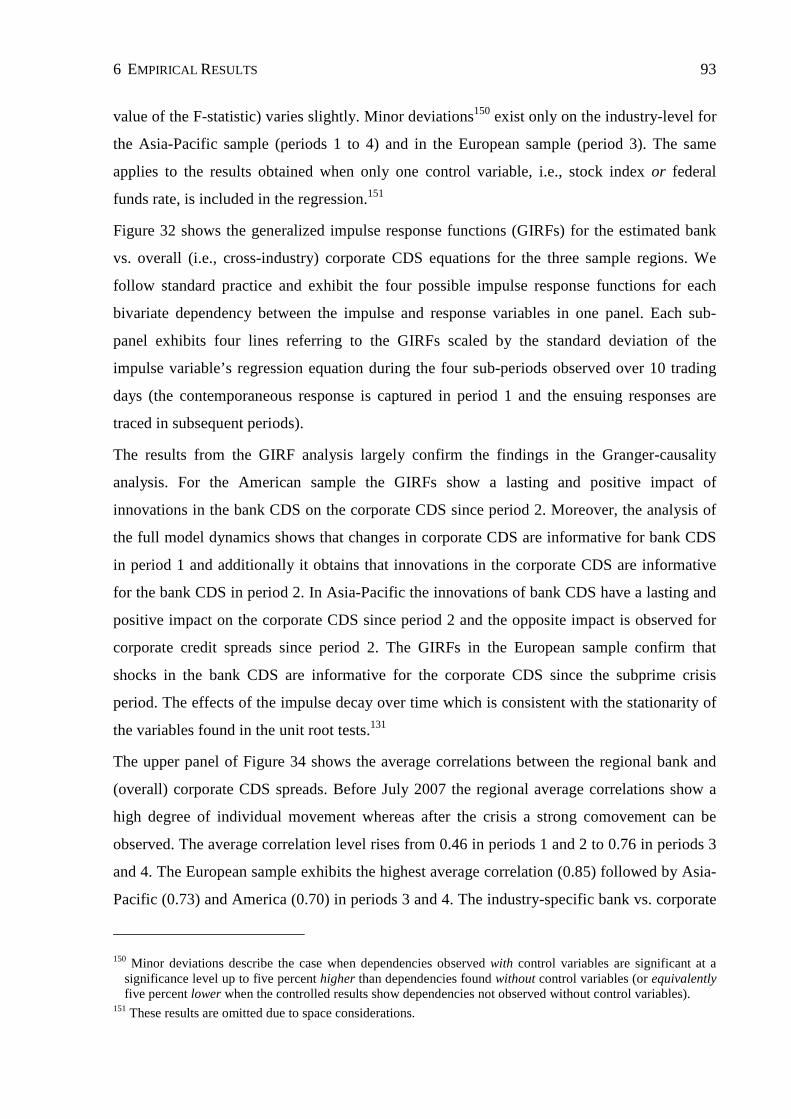
6 EMPIRICAL RESULTS 93
value of the F-statistic) varies slightly. Minor deviations150 exist only on the industry-level for
the Asia-Pacific sample (periods 1 to 4) and in the European sample (period 3). The same
applies to the results obtained when only one control variable, i.e., stock index or federal
funds rate, is included in the regression.151
Figure 32 shows the generalized impulse response functions (GIRFs) for the estimated bank
vs. overall (i.e., cross-industry) corporate CDS equations for the three sample regions. We
follow standard practice and exhibit the four possible impulse response functions for each
bivariate dependency between the impulse and response variables in one panel. Each sub-
panel exhibits four lines referring to the GIRFs scaled by the standard deviation of the
impulse variable’s regression equation during the four sub-periods observed over 10 trading
days (the contemporaneous response is captured in period 1 and the ensuing responses are
traced in subsequent periods).
The results from the GIRF analysis largely confirm the findings in the Granger-causality
analysis. For the American sample the GIRFs show a lasting and positive impact of
innovations in the bank CDS on the corporate CDS since period 2. Moreover, the analysis of
the full model dynamics shows that changes in corporate CDS are informative for bank CDS
in period 1 and additionally it obtains that innovations in the corporate CDS are informative
for the bank CDS in period 2. In Asia-Pacific the innovations of bank CDS have a lasting and
positive impact on the corporate CDS since period 2 and the opposite impact is observed for
corporate credit spreads since period 2. The GIRFs in the European sample confirm that
shocks in the bank CDS are informative for the corporate CDS since the subprime crisis
period. The effects of the impulse decay over time which is consistent with the stationarity of
the variables found in the unit root tests.131
The upper panel of Figure 34 shows the average correlations between the regional bank and
(overall) corporate CDS spreads. Before July 2007 the regional average correlations show a
high degree of individual movement whereas after the crisis a strong comovement can be
observed. The average correlation level rises from 0.46 in periods 1 and 2 to 0.76 in periods 3
and 4. The European sample exhibits the highest average correlation (0.85) followed by Asia-
Pacific (0.73) and America (0.70) in periods 3 and 4. The industry-specific bank vs. corporate
150 Minor deviations describe the case when dependencies observed with control variables are significant at a significance level up to five percent higher than dependencies found without control variables (or equivalently five percent lower when the controlled results show dependencies not observed without control variables).
151 These results are omitted due to space considerations.

6 EMPIRICAL RESULTS 94
CDS correlations are shown in Table 36 and exhibit the same trends as described for the
overall corporate data. Moreover, it can be noted that the cross-industry variation of the
correlations is particularly low during periods 2 and 3.
Impact of systemic risk on the strength of the causality relation
As a further step we examine the explanatory power of the regional ESS-indicator for the
strength of the Granger-causality relation between bank and corporate CDS. To this end we
conduct our previous Granger-causality time series regression analysis for the regional bank
and corporate CDS spreads using an estimation window of 250 trading days which we roll
forward from the beginning until the end of the sample period. As before, the resulting p-
values of the F-statistic measure the strength of the observed Granger-causality dependency.
We employ the p-values for each region as dependent variables in linear regressions using as
independent variables the regional relative ESS-indicator (as measure of systemic risk) alone
and together with the regional stock index and the federal funds rate as control variables.
The results of this regression are shown in Table 38. In the American and European sample
we find that the coefficient of the regional relative ESS-indicator has a strongly significant
negative sign both without and with control variables. This translates into the following
relation in these two regions: When the systemic risk increases, the significance of the
Granger-causality between bank and corporate CDS spreads also increases (because the p-
value of the F-statistic decreases). For Asia-Pacific the coefficient of the regional relative
ESS-indicator is only significantly negative when no control variables are included whereas
the coefficient is no longer significant when control variables are included in the regression.
While the results for Asia-Pacific are mixed it can be noted that the findings for America and
Europe clearly validate the claim that systemic risk impacts the real economy.
6.2.3.1.2 Equity prices
Table 35 shows the results for the banking vs. non-bank corporate sector equity return
Granger causality analysis excluding control variables. For the American sample we find that
the non-bank corporate equity returns lead the bank equity returns in periods 2 and 3. In the
following we describe the industry-specific deviations from this cross-industry result. For the
automotive as well as the construction and logistics firms we find no significant
interdependency with the bank equity returns. The equity returns of the basic materials firms
do not Granger-cause the bank equity returns in period 3 but in period 4. For the chemicals,
healthcare and pharma as well as for the commerce and consumer companies we find that

6 EMPIRICAL RESULTS 95
their equity returns lead the bank equity returns in period 3 (but not in period 2). The results
for the equity returns of the energy and utilities firms differ from the overall findings in period
3 where they are led by the bank equity returns. Regarding the other industrial firms’ equity
returns we find these do not depend the bank equity returns in period 3.
Among the Asia-Pacific firms we find that the corporate equity returns lead the bank equity
returns in periods 2 and 3 and in period 4 a feedback relation between bank and non-bank
equity prices exists. In the following we describe the deviations from this cross-industry
finding for the respective industry clusters. For the automotive firms’ equity returns we find
them to be Granger-caused by bank equity returns in period 2 whereas they do not lead the
bank equity returns in any period. The equity returns of the basic materials firms’ have a
feedback relation with the bank equity returns in period 3. Concerning the chemicals,
healthcare and pharma equity returns it can be noted that these Granger-cause the bank equity
returns only in period 3. By contrast, the commerce and consumer firms’ equity returns are
informative for the bank equity returns in periods 3 and 4 (but not in period 2). The equity
returns of the construction and logistics firms have predictive power for the bank equity
returns in period 1 (but not in periods 2 and 3). The results for the energy and utilities firms
deviate from the cross-industry results in that a lead-lag relation between the industries’ and
bank equity returns is found in period 1 and a feedback relation is observed in period 3. The
equity returns of the financial services firms lead the banks’ equity returns in period 1
whereas no other lead-lag relation is observed for this industry cluster. Concerning the other
industrial firms’ equity returns, a feedback relationship with the bank equity returns is
observed in period 2; in period 3 the bank equity returns lead the industrial firms’ equity
returns. The results for the TMT firms are largely consistent whereas in period 4 only the
TMT firm equity returns are informative for the bank equity returns (but not vice versa).
In Europe we observe that the non-bank corporate equity returns Granger-cause the bank
equity returns in period 2 whereas no other dependencies are observed. The industry-level
deviations from these overall results are elaborated in the following. The results for the
following industry-clusters deviate from the overall results as they do not show any
dependencies with the bank equity returns: automotive, chemicals, healthcare and pharma,
construction and logistics, energy and utilities as well as financial services. The equity returns
of the commerce and consumer firms lead the bank equity returns in period 4 (however not in
periods 2 and 3). The equity returns of the (other) industrial firms are Granger-caused by the

6 EMPIRICAL RESULTS 96
bank equity returns in period 3. With respect to the TMT firms we find their equity returns to
lead the bank equity returns in period 4 (however not in period 3).
The lower panel of Table 35 shows the Granger-causality test results for intra-regional bank
vs. corporate equity returns analysis where the global stock index and the federal funds rate
are included as exogenous control variables. The main findings are consistent with the results
excluding control variables whereas the strength of the dependency (as measured by the p-
value of the F-statistic) varies slightly. Minor deviations150 exist in the American sample
(periods 1 to 3), Asia-Pacific and Europe (both period 3). The same applies to the results
obtained when only one control variable, i.e., stock index or federal funds rate, is included in
the regression.152
Figure 33 shows the generalized impulse response functions (GIRFs) for the bank vs. overall
(i.e., cross-industry) corporate equity returns equations for the three sample regions. The
results from the GIRF analysis largely confirm the findings in the Granger-causality analysis.
For the American sample the GIRFs confirm that innovations in corporate equity returns are
informative for bank equity returns in periods 2 and 3. In Asia-Pacific the GIRF analysis
confirms that shocks in bank equity returns have predictive power for the corporate equity
returns in period 4 and that the opposite relation exists since period 2. The GIRFs for the
European sample show that innovations in corporate equity returns are (slightly) informative
for bank equity returns. The effects of the impulse decay over time which is consistent with
the stationarity of the variables found in the unit root tests.131
The lower panel of Figure 34 shows the average correlations between the regional bank and
(overall) corporate equity returns. The average correlation level decreases slightly from 0.84
in periods 1 and 2 to 0.80 in periods 3 and 4. This decrease may reflect the market’s
perception during the crisis that banks have somewhat decoupled from the ‘real economy’
whereas further research is necessary to explain this observation. At a level of 0.80 the
correlations in Asia-Pacific and Europe are highest in periods 3 and 4 compared to 0.76 in
America. Table 37 shows the industry-level bank vs. corporate equity return correlations. In
America and Europe the financial services industry cluster firms’ equity returns have the
highest correlations with the bank equity returns whereas in Asia-Pacific the TMT firms’
equity prices exhibit the highest correlations with the bank equity returns.
152 These results are omitted due to space considerations.

6 EMPIRICAL RESULTS 97
6.2.3.2 Evaluation of initial hypotheses
In this section we evaluate the initial hypotheses based on the preceding econometric results.
6.2.3.2.1 CDS spreads
In the American sample we find that the bank default risk does indeed lead corporate default
risk since period 2 as posited in hypothesis C1 and that the strength of this dependency
increased during the financial and sovereign debt crisis periods. By contrast, in period 1 the
corporate CDS lead the bank CDS. A possible explanation for the change in the bank vs.
corporate default risk dependency in period 2 may be that before the financial crisis the ‘real
economy’ (represented by the non-bank corporate firms) played a larger role for the American
banking sector whereas since the onset of the subprime crisis, markets noticed that the
banking sector has become somewhat decoupled from the real economy because of its
exposure to structured assets and derivatives (rather than loans) as well as the high correlation
of banks’ asset and funding risks. In this sense, the American banking sector itself became a
potential risk for the non-bank corporate sector which is also reflected by the economic crisis
which followed the financial crisis. Moreover, the results could provide evidence for the
impact of the crisis-related increase in bank funding costs on non-bank corporate firms and
their default risk. Further research is necessary, though, to adequately classify this finding.
A closer examination of the industry-level results shows that the observed dependency
between corporate and bank default risk in period 1 results from the commerce and consumer
as well as the industrial firms whereas the CDS of firms in other industries have either no
dependency with the bank CDS or are actually impacted on by the bank CDS (basic materials
and TMT). As of period 2 the industry-level results are largely consistent with the overall
findings whereas in some periods the credit risk of certain industries also impacts on the
banking sector risk (energy and utilities, financial services, industrial) or no dependency is
observed (TMT). While the feedback relation between the default risk of banks and other
financial services firms can be explained by the close mutual dependency of these sectors due
to similarities in financing and investment activities, further research is necessary to
understand the industry-specific determinants for the sensitivity of firm default risk to bank
default risk in the American sample. The default risk of the firms from the automotive,
commerce and consumer, financial services as well as the other industry clusters are affected
most by the bank default risk in periods 3 and 4 (measured in terms of the F-statistics).
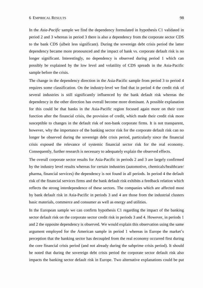
6 EMPIRICAL RESULTS 98
In the Asia-Pacific sample we find the dependency formulated in hypothesis C1 validated in
period 2 and 3 whereas in period 3 there is also a dependency from the corporate sector CDS
to the bank CDS (albeit less significant). During the sovereign debt crisis period the latter
dependency became more pronounced and the impact of bank vs. corporate default risk is no
longer significant. Interestingly, no dependency is observed during period 1 which can
possibly be explained by the low level and volatility of CDS spreads in the Asia-Pacific
sample before the crisis.
The change in the dependency direction in the Asia-Pacific sample from period 3 to period 4
requires some classification. On the industry-level we find that in period 4 the credit risk of
several industries is still significantly influenced by the bank default risk whereas the
dependency in the other direction has overall become more dominant. A possible explanation
for this could be that banks in the Asia-Pacific region focused again more on their core
function after the financial crisis, the provision of credit, which made their credit risk more
susceptible to changes in the default risk of non-bank corporate firms. It is not transparent,
however, why the importance of the banking sector risk for the corporate default risk can no
longer be observed during the sovereign debt crisis period, particularly since the financial
crisis exposed the relevance of systemic financial sector risk for the real economy.
Consequently, further research is necessary to adequately explain the observed effects.
The overall corporate sector results for Asia-Pacific in periods 2 and 3 are largely confirmed
by the industry level results whereas for certain industries (automotive, chemicals/healthcare/
pharma, financial services) the dependency is not found in all periods. In period 4 the default
risk of the financial services firms and the bank default risk exhibits a feedback relation which
reflects the strong interdependence of these sectors. The companies which are affected most
by bank default risk in Asia-Pacific in periods 3 and 4 are those from the industrial clusters
basic materials, commerce and consumer as well as energy and utilities.
In the European sample we can confirm hypothesis C1 regarding the impact of the banking
sector default risk on the corporate sector credit risk in periods 3 and 4. However, in periods 1
and 2 the opposite dependency is observed. We would explain this observation using the same
argument employed for the American sample in period 1 whereas in Europe the market’s
perception that the banking sector has decoupled from the real economy occurred first during
the core financial crisis period (and not already during the subprime crisis period). It should
be noted that during the sovereign debt crisis period the corporate sector default risk also
impacts the banking sector default risk in Europe. Two alternative explanations could be put

6 EMPIRICAL RESULTS 99
forward for this observation. Firstly, it could be that the change of banks’ business models
towards more stable and politically desired lending activities153 after the crisis exposed it
stronger to the credit risk of corporate firms. Secondly, the euro zone sovereign debt crisis
may have contributed to a higher mutual sensitivity between bank and corporate default risk
(which should be observed particularly on a cross-country basis between banks in stable euro
zone countries versus firms in euro zone countries with sovereign debt problems). A
validation of these explanations requires further research, though.
The overall corporate results for the European sample in period 2 are fully confirmed on the
industry level and in period 4 only three industries (basic materials, energy and utilities,
TMT) do not exhibit the feedback interdependency with the bank default risk. The largest
deviations between the overall corporate results and the industry-level results default risk
dependencies are observed in periods 1 and 3. The default risk of the firms from the
automotive, construction and logistics, financial services and industrial segments is affected
most by the bank default risk in Europe in periods 3 and 4.
In the following we compare the overall bank vs. corporate default risk dependency results for
the respective sample regions. Before the onset of the subprime crisis the corporate default
risk impacted on the banking sector CDS in America and Europe whereas in Asia-Pacific no
significant dependency is observed. In period 2 the bank default risk leads the corporate
default risk in America and Asia-Pacific whereas in Europe the opposite relation exists.
During the financial crisis period 3, the bank CDS lead the corporate CDS in all regions
which confirms the common perception that during the financial crisis the banking sector risk
spread to the real economy.154 By contrast, the results are mixed in period 4: while the
American sample still exhibits the bank vs. corporate default risk dependency, the opposite
relation is observed in Asia-Pacific and in Europe a feedback relation between bank and non-
bank corporate default risk exists.
On a cross-regional basis we compare the bank vs. corporate default risk dependencies for the
respective industries. In periods 3 and 4 the sensitivity of the corporate default risk with
respect to the bank default risk is highest for the automotive, commerce and consumer,
financial services and industrial industry segments across all regions as measured by the
153 In fact, after the crisis governments and regulators in Europe (but also in other countries) pushed banks to provide more lending to the economy and refocus their business models.
154 Further evidence for this is provided in the above regression using the p-values and the regional relative ESS-indicators.

6 EMPIRICAL RESULTS 100
average p-values of the F-statistics. By contrast, for periods 1 and 2, a consistent cross-
regional industry ranking with respect to the sensitivity of the firm’s default risk to the bank
default risk is not feasible. The financial services firms’ default risk exhibits the most
feedback relations with the banking sector default risk in all regions which can be explained
by the common exposures and financing channels pertinent to all financial services firms.
6.2.3.2.2 Equity prices
In the American sample we find that hypothesis C2, according to which the corporate equity
returns lead the bank equity returns, does indeed apply in periods 2 and 3. By contrast, in
period 1 no dependency is observed and in period 4 the lead-lag relation only applies for the
basic materials industry cluster. One may wonder why the dependency between corporate and
bank equity returns is only observed during the subprime and financial crisis periods. It could
be argued that during the crisis when financial institutions faced substantial losses from their
investment banking activities already, the additional deterioration in the business prospects of
corporates (as measured amongst others by corporate equity prices) increased the loss
potential for financial institutions and hence affected their equity prices. However, additional
research needs to be conducted to adequately explain this observation.
On the industry level we find that the equity returns of firms from four industries (automotive,
basic materials, construction and logistics, industrial) show no interdependency with bank
equity returns in period 2. In period 3 we observe no dependency between corporate and bank
equity returns in five industries (automotive, basic materials, commerce and consumer,
construction and logistics, industrial) and additionally we find that the bank equity returns
impact the equity returns of energy and utilities firms.
In the Asia-Pacific sample we find that the corporate equity returns impact on the bank equity
returns in periods 2, 3 and 4, thereby confirming hypothesis C2. In period 4 we observe an
additional dependency between bank and corporate equity prices. By contrast, in period 1 no
dependency between bank and corporate equity returns can be observed.
A closer examination of the Asia-Pacific industry-level results reveals that the overall results
are observed only for few industries in periods 2 and 4. In period 2, only the equity returns for
the industrial and TMT firms do actually lead the bank equity returns whereas the other
industries’ firms do not exhibit this dependency. Moreover, the automotive and industrial
firms exhibit a dependency in the opposite direction in period 2. In period 4 the equity returns
of commerce and consumer, industrial and TMT firms impact the bank equity returns whereas

6 EMPIRICAL RESULTS 101
the opposite dependency is observed for industrial firms. The industry-level results in period 3
largely confirm the overall findings whereas for the basic materials and the energy and
utilities firms feedback interdependencies are found and the industrial firms’ equity returns
are led by bank equity returns.
In the European sample we find that the overall corporate sector equity prices lead the bank
equity returns confirming hypothesis C2 only in period 2. On the industry-level these results
are also found for the firms from the basic materials, industrial and TMT industry clusters.155
During the other periods we find no significant overall dependencies between banking and
corporate sector equity returns. Exceptions apply at the industry-level, though: in period 3
bank equity returns depend corporate equity returns and in period 4 the opposite dependency
applies for the commerce and consumer as well as the TMT firms.
By comparing the regional results one can note a substantial deviation in the overall regional
results. Corporate equity returns lead bank equity returns in all regions in period 2 whereas in
period 3 only America and Asia-Pacific share this property. While the bank and corporate
equity returns in Asia-Pacific have feedback interdependencies in period 4, no significant
dependencies are observed for America and Europe in this period. The industry-specific
results across all regions show that the equity returns of the industrial and TMT firms have the
highest impact on the bank equity returns (in terms of the average p-values of the F-statistics)
whereas for the other industries no clear pattern can be observed.
Comparative discussion
A comparison of the causality test results for bank vs. non-bank corporate sector
dependencies shows the opposite dependencies for CDS and equity prices: while the banking
sector CDS spreads mostly lead the non-bank corporate CDS spreads, the opposite
dependency is found for equity prices in most periods. For the CDS spreads this dependency
can be explained amongst others by the funding channel since banks provide lending to firms
and thus changes in funding costs of banks should impact on the funding costs of non-bank
corporate firms. In case of the equity returns, the analysis of the results is more ambiguous:
while the observed dependency can be explained by the relationship between a bank’s
profitability and the credit quality of its loan portfolio (a possible measure for which is the
corporate sector equity performance) the opposite dependency could also be argued as well by
155 At the six percent significance level this result also applies to the commerce and consumer as well as the energy and utilities firms.

6 EMPIRICAL RESULTS 102
the role of the banking sector for the overall economy. This ambiguity is also reflected in the
fact that the average strength of the dependency (as measured by the average p-values of the
F-statistic) is higher for the CDS spread analysis than for the equity return analysis.
Another striking feature of the CDS and equity banking vs. corporate sector time series
analyses alike is that the overall findings are most pronounced for the American market
whereas for Asia-Pacific and Europe the results are more heterogeneous. On the industry-
level the cross-regional analysis for the CDS spreads shows that the automotive, commerce
and consumer, financial services and industrial industry clusters are affected most by the bank
CDS spreads whereas for the equity analysis a consistent conclusion for the industry-specific
sensitivity cannot be drawn.
Discussion in the context of related research
As pointed out in the literature review there is yet no research concerning the contagion
effects between the banking sector and non-bank corporate sector CDS spreads or
respectively equity returns. Therefore, a discussion of our results in the context of findings by
other authors is unfortunately not feasible.

103
7 CONCLUSION
7.1 SUMMARY AND IMPLICATIONS
In this thesis we developed a new framework for measuring systemic risk and assessing
systemic importance, the ‘expected systemic shortfall’ (ESS) methodology. We applied the
ESS-methodology in a comprehensive empirical analysis of systemic risk and systemic
importance in global and regional financial markets. Moreover, we conducted a
comprehensive analysis of banking sector risk contagion effects using state-of-the-art
econometric time series methods.
In chapter 2 we described the related literature on the topics covered in this thesis. Firstly, we
defined systemic risk and systemic importance in the context of the related literature and
provided a structured elaboration of the existing measurement approaches for these concepts.
Also, we elaborated the contribution of our ESS-methodology to the existing literature.
Secondly, we presented the relevant literature on contagion transmission channels in financial
markets and on the relevant banking sector risk contagion effects. The hypotheses examined
in the analysis of banking sector risk contagion dependencies were elaborated in chapter 3.
In chapter 4 we presented the methodology employed in this thesis. Firstly, we derived our
ESS-framework by constructing a hypothetical bank liability portfolio and described the
employed credit portfolio model whose input parameters are estimated from capital market
data. Using standard measures from financial institution risk management, we obtained the
aggregate ESS-indicator which represents the probability of a systemic default event in the
financial sector and the expected loss when this event occurs. Also, we derived the relative
ESS-contribution by individual institutions. A technical comparison of the ESS-methodology
with other measures of systemic risk concluded our description of the ESS-indicator.
Secondly, we elaborated the econometric methods employed for measuring banking sector
risk contagion effects which involve Granger-causality tests and the analysis of generalized
impulse response functions in vector autoregressive frameworks.
Chapter 5 described the empirical data analyzed in this thesis which covers the observation
horizon between October 1st, 2005 and April 30th, 2011. The global bank sample comprises 83
banking groups from 28 countries and is the most comprehensive data set ever considered in
an analysis of systemic risk and systemic importance. We divided the global sample into the
four regional sub-samples America, Asia-Pacific, Europe and Middle East & Russia. CDS

7 CONCLUSION 104
spreads and equity returns are used to estimate the input parameters of the ESS-methodology,
the risk-neutral default probability and the equity return correlation, for each sample. The
sovereign sample comprises the CDS spreads of the 28 origin countries of the sample banks.
The non-bank corporate sample covers the CDS spreads and equity returns of 352 companies
from the regions America, Asia-Pacific and Europe.
In chapter 6 we presented the results of the empirical analysis. Firstly, we described the
results from applying the ESS methodology. The evolution of the ESS-indicator captures both
the crisis events with global importance as well as region-specific crisis events. An analysis of
the input factor determinants showed that the default probability is the most important
explanatory variable of the ESS-indicator. Regarding the risk premium determinants of the
ESS-indicator we found that the corporate default risk premium and the liquidity risk
premium exhibit the highest explanatory power across all samples. The analysis of the relative
ESS-contribution by individual institutions showed that this varies over time whereas the
ranking is relatively stable. We found a confirmation of the ‘too big to fail’ claim because the
size of the bank’s total liabilities was found to be the most important explanatory variable for
its relative systemic risk contribution. Based on the empirical results we derived the policy
implications and outlined how the ESS-methodology can be used to monitor systemic risk and
to assess the systemic importance of banking groups.
Secondly, we described the results from analyzing the banking sector risk contagion
dependencies. For the inter-regional systemic risk contagion effects we found that the
systemic risk in the American financial system mostly leads the systemic risk in the other
regions since the subprime crisis period. Moreover, the analysis exposed new inter-regional
systemic risk dependencies which have not been described previously. The analysis of
sovereign vs. banking sector risk contagion showed a strong increase of the interdependencies
between sovereign and banking sector credit spreads since the financial crisis. The impact of
sovereign on bank default risk even increased during the sovereign debt crisis period. The
analysis of bank vs. non-bank corporate risk contagion effects exposed that changes in the
banks’ default risk depend changes in the default risk of the corporate sector during the
financial crisis period in all regions, corroborating the claim that banking sector risk impacts
the real economy. By contrast, the analysis of bank vs. non-bank corporate equity returns
showed that bank equity returns are mostly led by corporate equity returns whereas the
opposite dependency is only rarely observed.

7 CONCLUSION 105
7.2 OUTLOOK
We derived the ESS-methodology as a new approach for measuring systemic risk and
assessing systemic importance in the financial sector. The derivation and technical
implementation of the ESS-framework employs standard methods for credit risk modeling
which are also used in the current literature and by practitioners. While we confirmed the
adequacy and robustness of the empirical results, the ESS-methodology can be enhanced on
the modeling side and also alternative empirical analyses could be considered.
Modeling aspects
In the modeling of portfolio credit risk, different models could be employed to model the
credit risk of the hypothetical debt portfolio used in the derivation of the ESS-methodology.
In particular, the recent advances in credit risk modeling by means of enhanced structural
models and reduced-form models offer potential pathways for future extensions. A
comprehensive survey on the current work and open topics in credit risk modeling is provided
by Hao/Alam/Carling (2009).
The estimation of asset return correlations within the credit risk model of the ESS-framework
can be developed further in two directions. Firstly, the estimation of asset return correlations
from equity returns can be extended by enhancements in correlation estimation methodology.
Engle (2009) exhibits an extensive survey on the available models and areas for future
research in this econometric field. Secondly, estimation methodologies which are based not
only on equity returns but also on credit spreads to estimate the asset return correlations could
offer a means for enhancing asset correlation estimates.156 However, corresponding
methodologies are to our best knowledge not yet available. Furthermore, different approaches
for the estimation of default probabilities could be considered. For instance, the ESS-indicator
could be computed using real-world default probabilities obtained from debt rating models.
Similarly, the computation of physical default probabilities from credit spreads by isolating
risk premium components is an interesting area for future research.
Empirical analyses
As we conducted the most comprehensive analysis of systemic risk and systemic importance
in global and regional financial markets to date, an extension of the empirical analysis by
including more sample banks is likely only feasible at the expense of shortening the
156 This is due to the fact that under constant leverage both equity and debt returns can be used to proxy asset returns (as shown in Appendix A).

7 CONCLUSION 106
observation horizon. However, the concept of systemic financial sector risk could be analyzed
using the ESS-framework in a broader perspective by also including other relevant types of
financial market participants, such as asset management and insurance companies, in the
analysis. In so doing, the comparability and consistency of the results due to different
business practices and balance sheet structures of the sample companies would need to be
ensured, though. In addition, further research could focus on applying the concept of systemic
risk to other industries.
Although we have shown the robustness of the results in our analysis of banking sector risk
contagion effects by conducting several robustness tests, there are opportunities for future
research using upcoming econometric methodology and conducting additional empirical
analyses in this rather new field of financial research.
Econometric methodology
The banking sector risk contagion effects were analyzed using the latest methods from time
series econometrics. As econometric methodology is evolving continuously along with the
advances in analytical frameworks and computational capacities (amongst others), an update
of the analyses in this thesis by means of future econometric methods appears worthwhile.
Empirical analyses
While the conducted empirical analyses of banking sector risk contagion effects are quite
extensive, further research is necessary to extend this rather new area of financial research.
For instance, future empirical implementations could consider a higher granularity of the
sample data, e.g., by analyzing country- and firm-level data in addition to region- and
industry-level data. Moreover, along with the development of financial markets, further
sample data should become available, e.g., from emerging markets, which could be included
in future empirical analyses on banking sector risk contagion effects.
Besides, we already outlined in the description of the empirical results that an adequate
explanation of certain observed dependencies (e.g., industry-level deviations from overall
corporate results) provides a large field for future research. Moreover, further research is
required in order to better understand the channels by which the observed banking sector risk
contagion dependencies are actually transmitted. In a related strain of research, potential
regulatory measures aimed at mitigating certain banking sector risk contagion effects could be
developed theoretically and evaluated empirically.

107
LIST OF FIGURES
Figure 1: Input variables for the ESS-indicator (Global) ....................................................... 109
Figure 2: Input variables for the ESS-indicator (America) .................................................... 110
Figure 3: Input variables for the ESS-indicator (Asia-Pacific) .............................................. 111
Figure 4: Input variables for the ESS-indicator (Europe)....................................................... 112
Figure 5: Input variables for the ESS-indicator (Middle East and Russia) ............................ 113
Figure 6: Input variables for the ESS-indicator (Comparative analysis)................................ 114
Figure 7: Bank CDS spreads .................................................................................................. 115
Figure 8: Sovereign CDS spreads ........................................................................................... 115
Figure 9: CDS spreads of non-bank corporate firms .............................................................. 116
Figure 10: Indexed equity prices for non-bank corporate sample firms................................. 117
Figure 11: Regional weighted indexed bank equity prices..................................................... 118
Figure 12: Absolute and relative expected systemic shortfall (Global) ................................. 119
Figure 13: Probability of systemic default and expected tail loss (Global)............................ 120
Figure 14: Absolute and relative expected systemic shortfall (America) .............................. 121
Figure 15: Probability of systemic default and expected tail loss (America) ......................... 122
Figure 16: Absolute and relative expected systemic shortfall (Asia-Pacific) ........................ 123
Figure 17: Probability of systemic default and expected tail loss (Asia-Pacific) ................... 124
Figure 18: Absolute and relative expected systemic shortfall (Europe) ................................. 125
Figure 19: Probability of systemic default and expected tail loss (Europe) ........................... 126
Figure 20: Absolute and relative expected systemic shortfall (Middle East and Russia) ...... 127
Figure 21: Probability of systemic default and expected tail loss (Middle East and Russia). 128
Figure 22: Absolute and relative expected systemic shortfall (Comparative analysis) .......... 129
Figure 23: Probability of systemic default and expected tail loss (Comparative analysis) .... 130
Figure 24: Relative change of absolute and relative ESS-indicator with respect to initial
average (Comparative analysis).............................................................................................. 131
Figure 25: Relative change of probability of systemic default (PSD) and expected tail loss
(ETL) with respect to initial average (Comparative analysis) ................................................ 132
Figure 26: Risk premium determinants of the relative ESS-indicator.................................... 133
Figure 27: Generalized impulse responses for inter-regional relative ESS analysis .............. 136
Figure 28: Generalized impulse responses for inter-regional bank CDS spreads analysis .... 138
Figure 29: Correlation of regional relative ESS-indicator and regional bank CDS spreads .. 140

108
Figure 30: Generalized impulse responses for regional sovereign vs. bank CDS spreads ..... 141
Figure 31: Correlation of regional sovereign and bank CDS spreads .................................... 143
Figure 32: Generalized impulse responses for regional bank vs. corporate CDS spreads ..... 144
Figure 33: Generalized impulse responses for regional bank vs. corporate equity returns .... 146
Figure 34: Correlation between bank and corporate CDS spreads and equity returns ........... 148

109
Figure 1: Input variables for the ESS-indicator (Global)
Notes: The upper panel shows the average risk-neutral default probabilities during the observation period (weighted by total liabilities). The lower panel shows the average correlations of the sample banks (computed from the correlations of one bank with all other banks, weighted by total liabilities). The dashed lines represent selected financial crisis events.
0%
5%
10%
15%
20%
25%
10-2005 04-2006 10-2006 04-2007 10-2007 04-2008 10-2008 04-2009 10-2009 04-2010 10-2010 04-2011
Risk-neutral default probability
MinMean
Max
-40%
-30%
-20%
-10%
0%
10%
20%
30%
40%
50%
60%
70%
10-2005 04-2006 10-2006 04-2007 10-2007 04-2008 10-2008 04-2009 10-2009 04-2010 10-2010 04-2011
Average correlation
BNP Paribas funds freeze
Bear Stearns takeover
Lehman Brothers failure
Stock market low
Euro debt crisis aggravates
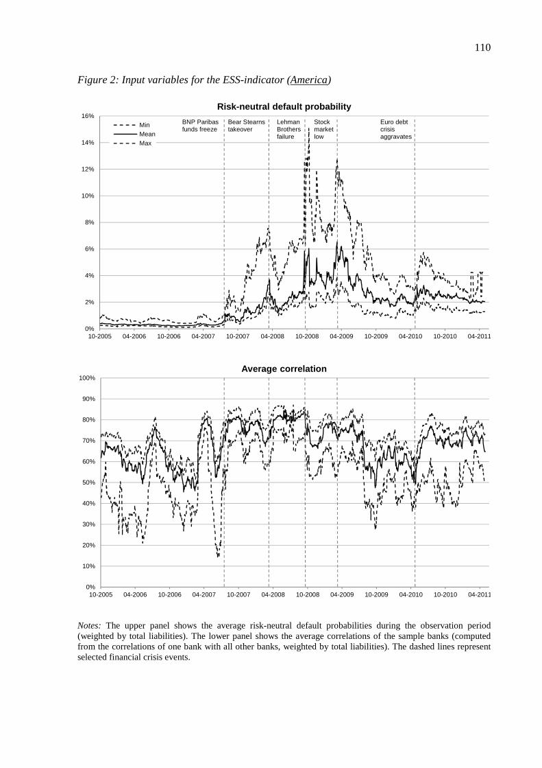
110
Figure 2: Input variables for the ESS-indicator (America)
Notes: The upper panel shows the average risk-neutral default probabilities during the observation period (weighted by total liabilities). The lower panel shows the average correlations of the sample banks (computed from the correlations of one bank with all other banks, weighted by total liabilities). The dashed lines represent selected financial crisis events.
0%
2%
4%
6%
8%
10%
12%
14%
16%
10-2005 04-2006 10-2006 04-2007 10-2007 04-2008 10-2008 04-2009 10-2009 04-2010 10-2010 04-2011
Risk-neutral default probability
MinMeanMax
0%
10%
20%
30%
40%
50%
60%
70%
80%
90%
100%
10-2005 04-2006 10-2006 04-2007 10-2007 04-2008 10-2008 04-2009 10-2009 04-2010 10-2010 04-2011
Average correlation
BNP Paribas funds freeze
Bear Stearns takeover
Lehman Brothers failure
Stock market low
Euro debt crisis aggravates

111
Figure 3: Input variables for the ESS-indicator (Asia-Pacific)
Notes: The upper panel shows the average risk-neutral default probabilities during the observation period (weighted by total liabilities). The lower panel shows the average correlations of the sample banks (computed from the correlations of one bank with all other banks, weighted by total liabilities). The dashed lines represent selected financial crisis events.
0%
5%
10%
15%
20%
25%
10-2005 04-2006 10-2006 04-2007 10-2007 04-2008 10-2008 04-2009 10-2009 04-2010 10-2010 04-2011
Risk-neutral default probability
MinMeanMax
-30%
-20%
-10%
0%
10%
20%
30%
40%
50%
60%
70%
10-2005 04-2006 10-2006 04-2007 10-2007 04-2008 10-2008 04-2009 10-2009 04-2010 10-2010 04-2011
Average correlation
BNP Paribas funds freeze
Bear Stearns takeover
Lehman Brothers failure
Stock market low
Euro debt crisis aggravates
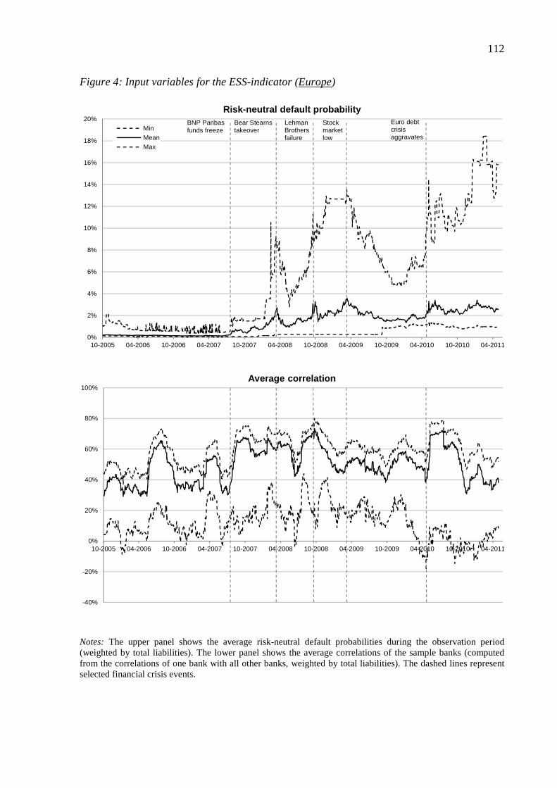
112
Figure 4: Input variables for the ESS-indicator (Europe)
Notes: The upper panel shows the average risk-neutral default probabilities during the observation period (weighted by total liabilities). The lower panel shows the average correlations of the sample banks (computed from the correlations of one bank with all other banks, weighted by total liabilities). The dashed lines represent selected financial crisis events.
0%
2%
4%
6%
8%
10%
12%
14%
16%
18%
20%
10-2005 04-2006 10-2006 04-2007 10-2007 04-2008 10-2008 04-2009 10-2009 04-2010 10-2010 04-2011
Risk-neutral default probability
MinMeanMax
-40%
-20%
0%
20%
40%
60%
80%
100%
10-2005 04-2006 10-2006 04-2007 10-2007 04-2008 10-2008 04-2009 10-2009 04-2010 10-2010 04-2011
Average correlation
BNP Paribas funds freeze
Bear Stearns takeover
Lehman Brothers failure
Stock market low
Euro debt crisis aggravates

113
Figure 5: Input variables for the ESS-indicator (Middle East and Russia)
Notes: The upper panel shows the average risk-neutral default probabilities during the observation period (weighted by total liabilities). The lower panel shows the average correlations of the sample banks (computed from the correlations of one bank with all other banks, weighted by total liabilities). The dashed lines represent selected financial crisis events.
0%
5%
10%
15%
20%
25%
10-2005 04-2006 10-2006 04-2007 10-2007 04-2008 10-2008 04-2009 10-2009 04-2010 10-2010 04-2011
Risk-neutral default probability
MinMeanMax
-30%
-20%
-10%
0%
10%
20%
30%
40%
50%
60%
10-2005 04-2006 10-2006 04-2007 10-2007 04-2008 10-2008 04-2009 10-2009 04-2010 10-2010 04-2011
Average correlation
BNP Paribas funds freeze
Bear Stearns takeover
Lehman Brothers failure
Stock market low
Euro debt crisis aggravates

114
Figure 6: Input variables for the ESS-indicator (Comparative analysis)
Notes: The upper panel shows the average risk-neutral default probabilities during the observation period (weighted by total liabilities). The lower panel shows the average correlations of the sample banks (computed from the correlations of one bank with all other banks, weighted by total liabilities). The dashed lines represent selected financial crisis events.
0%
2%
4%
6%
8%
10%
12%
14%
16%
10-2005 04-2006 10-2006 04-2007 10-2007 04-2008 10-2008 04-2009 10-2009 04-2010 10-2010 04-2011
Risk-neutral default probability
Global
America
Asia-Pacific
Europe
Middle East and Russia
0%
10%
20%
30%
40%
50%
60%
70%
80%
90%
10-2005 04-2006 10-2006 04-2007 10-2007 04-2008 10-2008 04-2009 10-2009 04-2010 10-2010 04-2011
Average correlation
BNP Paribas funds freeze
Bear Stearns takeover
Lehman Brothers failure
Stock market low
Euro debt crisis aggravates

115
Figure 7: Bank CDS spreads
Notes: The panel shows the liability-weighted bank CDS spreads per region.
Figure 8: Sovereign CDS spreads
Notes: The panel shows the sovereign CDS spreads per region. The country sovereign CDS spreads are weighted using the total liabilities of the sample banks per country (in order to ensure comparability with the bank CDS).
0
200
400
600
800
1,000
1,200
1,400
1,600
10-2005 04-2006 10-2006 04-2007 10-2007 04-2008 10-2008 04-2009 10-2009 04-2010 10-2010 04-2011
Average bank CDS spreads (bps)
Global
America
Asia-Pacific
Europe
Middle East and Russia
0
100
200
300
400
500
600
700
800
900
1,000
10-2005 04-2006 10-2006 04-2007 10-2007 04-2008 10-2008 04-2009 10-2009 04-2010 10-2010 04-2011
Average sovereign CDS spreads (bps)
Global
America
Asia-Pacific
Europe
Middle East and Russia
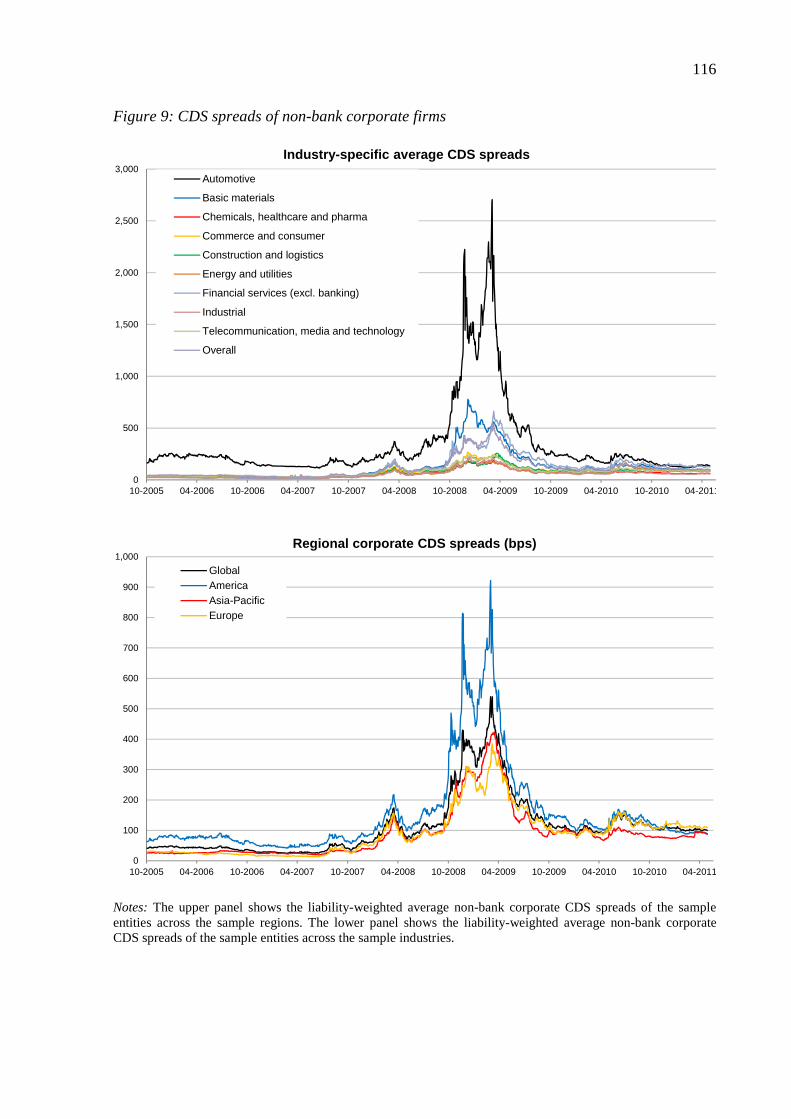
116
Figure 9: CDS spreads of non-bank corporate firms
Notes: The upper panel shows the liability-weighted average non-bank corporate CDS spreads of the sample entities across the sample regions. The lower panel shows the liability-weighted average non-bank corporate CDS spreads of the sample entities across the sample industries.
0
500
1,000
1,500
2,000
2,500
3,000
10-2005 04-2006 10-2006 04-2007 10-2007 04-2008 10-2008 04-2009 10-2009 04-2010 10-2010 04-2011
Industry-specific average CDS spreads
Automotive
Basic materials
Chemicals, healthcare and pharma
Commerce and consumer
Construction and logistics
Energy and utilities
Financial services (excl. banking)
Industrial
Telecommunication, media and technology
Overall
0
100
200
300
400
500
600
700
800
900
1,000
10-2005 04-2006 10-2006 04-2007 10-2007 04-2008 10-2008 04-2009 10-2009 04-2010 10-2010 04-2011
Regional corporate CDS spreads (bps)
GlobalAmericaAsia-PacificEurope

117
Figure 10: Indexed equity prices for non-bank corporate sample firms
Notes: The upper panel shows the liability-weighted average non-bank corporate indexed equity prices per industry across all sample regions. The extreme hike in the automotive industry cluster on October 28th, 2008 is due to the speculation-induced share price increase of the Volkswagen stock (attempted takeover by Porsche Group). The lower panel shows the same data across all industries for each sample region. The stock prices on October 3rd, 2005 are indexed to 100 points.
0
50
100
150
200
250
300
10-2005 04-2006 10-2006 04-2007 10-2007 04-2008 10-2008 04-2009 10-2009 04-2010 10-2010 04-2011
Indexed equity prices per industry cross-region
AutomotiveBasic materialsChemicals, healthcare and pharmaCommerce and consumerConstruction and logisticsEnergy and utilitiesFinancial services (excl. banking)IndustrialTelecommunication, media and technologyOverall
0
20
40
60
80
100
120
140
160
10-2005 04-2006 10-2006 04-2007 10-2007 04-2008 10-2008 04-2009 10-2009 04-2010 10-2010 04-2011
Indexed non-bank corporate equity prices per region
GlobalAmericaAsia-PacificEurope

118
Figure 11: Regional weighted indexed bank equity prices
Notes: The panel shows the liability-weighted indexed bank equity prices for the sample regions. The stock prices on October 3rd, 2005 are indexed to 100 points.
0
50
100
150
200
250
10-2005 04-2006 10-2006 04-2007 10-2007 04-2008 10-2008 04-2009 10-2009 04-2010 10-2010 04-2011
Regional weighted indexed bank equity prices
Global AmericaAsia-Pacific EuropeMiddle East and Russia

119
Figure 12: Absolute and relative expected systemic shortfall (Global)
Notes: The upper panel shows the absolute ESS-indicator and the lower panel shows the relative ESS-indicator in the observation period. The dashed lines represent selected financial crisis events.
0
50
100
150
200
250
300
350
400
450
500
10-2005 04-2006 10-2006 04-2007 10-2007 04-2008 10-2008 04-2009 10-2009 04-2010 10-2010 04-2011
Expected systemic shortfall (bn EUR)
0.0%
0.2%
0.4%
0.6%
0.8%
1.0%
1.2%
1.4%
10-2005 04-2006 10-2006 04-2007 10-2007 04-2008 10-2008 04-2009 10-2009 04-2010 10-2010 04-2011
Expected systemic shortfall relative to total liabilities
BNP Paribas funds freeze
Bear Stearns takeover
Lehman Brothers failure
Stock market low
Euro debt crisis aggravates

120
Figure 13: Probability of systemic default and expected tail loss (Global)
Notes: The upper panel shows the probability of the systemic default event and the lower panel shows the expected loss in case of a systemic default event during the observation period. The product of these two factors yields the expected systemic shortfall indicator.
0.0%
1.0%
2.0%
3.0%
4.0%
5.0%
6.0%
7.0%
10-2005 04-2006 10-2006 04-2007 10-2007 04-2008 10-2008 04-2009 10-2009 04-2010 10-2010 04-2011
Probability of systemic default
1,000
2,000
3,000
4,000
5,000
6,000
7,000
8,000
9,000
10-2005 04-2006 10-2006 04-2007 10-2007 04-2008 10-2008 04-2009 10-2009 04-2010 10-2010 04-2011
Expected tail loss (bn EUR)

121
Figure 14: Absolute and relative expected systemic shortfall (America)
Notes: The upper panel shows the absolute ESS-indicator and the lower panel shows the relative ESS-indicator in the observation period. The dashed lines represent selected financial crisis events.
0
50
100
150
200
250
10-2005 04-2006 10-2006 04-2007 10-2007 04-2008 10-2008 04-2009 10-2009 04-2010 10-2010 04-2011
Expected systemic shortfall (bn EUR)
0.0%
0.5%
1.0%
1.5%
2.0%
2.5%
3.0%
3.5%
10-2005 04-2006 10-2006 04-2007 10-2007 04-2008 10-2008 04-2009 10-2009 04-2010 10-2010 04-2011
Expected systemic shortfall relative to total liabilities
BNP Paribas funds freeze
Bear Stearns takeover
Lehman Brothers failure
Stock market low
Euro debt crisis aggravates

122
Figure 15: Probability of systemic default and expected tail loss (America)
Notes: The upper panel shows the probability of the systemic default event and the lower panel shows the expected loss in case of a systemic default event during the observation period. The product of these two factors yields the expected systemic shortfall indicator.
0.0%
2.0%
4.0%
6.0%
8.0%
10.0%
12.0%
14.0%
10-2005 04-2006 10-2006 04-2007 10-2007 04-2008 10-2008 04-2009 10-2009 04-2010 10-2010 04-2011
Probability of systemic default
500
1,000
1,500
2,000
2,500
10-2005 04-2006 10-2006 04-2007 10-2007 04-2008 10-2008 04-2009 10-2009 04-2010 10-2010 04-2011
Expected tail loss (bn EUR)

123
Figure 16: Absolute and relative expected systemic shortfall (Asia-Pacific)
Notes: The upper panel shows the absolute ESS-indicator and the lower panel shows the relative ESS-indicator in the observation period. The dashed lines represent selected financial crisis events.
0
10
20
30
40
50
60
70
80
10-2005 04-2006 10-2006 04-2007 10-2007 04-2008 10-2008 04-2009 10-2009 04-2010 10-2010 04-2011
Expected systemic shortfall (bn EUR)
0.0%
0.2%
0.4%
0.6%
0.8%
1.0%
1.2%
1.4%
1.6%
10-2005 04-2006 10-2006 04-2007 10-2007 04-2008 10-2008 04-2009 10-2009 04-2010 10-2010 04-2011
Expected systemic shortfall relative to total liabilities
BNP Paribas funds freeze
Bear Stearns takeover
Lehman Brothers failure
Stock market low
Euro debt crisis aggravates
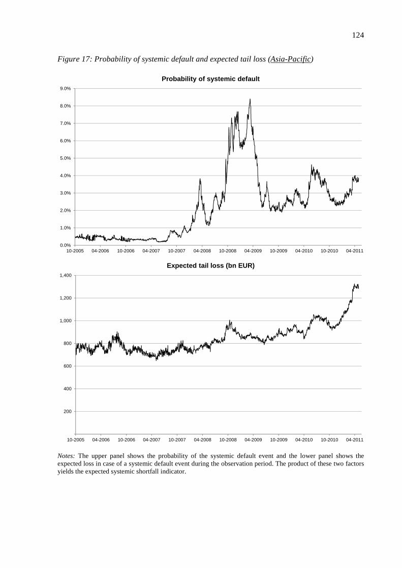
124
Figure 17: Probability of systemic default and expected tail loss (Asia-Pacific)
Notes: The upper panel shows the probability of the systemic default event and the lower panel shows the expected loss in case of a systemic default event during the observation period. The product of these two factors yields the expected systemic shortfall indicator.
0.0%
1.0%
2.0%
3.0%
4.0%
5.0%
6.0%
7.0%
8.0%
9.0%
10-2005 04-2006 10-2006 04-2007 10-2007 04-2008 10-2008 04-2009 10-2009 04-2010 10-2010 04-2011
Probability of systemic default
200
400
600
800
1,000
1,200
1,400
10-2005 04-2006 10-2006 04-2007 10-2007 04-2008 10-2008 04-2009 10-2009 04-2010 10-2010 04-2011
Expected tail loss (bn EUR)

125
Figure 18: Absolute and relative expected systemic shortfall (Europe)
Notes: The upper panel shows the absolute ESS-indicator and the lower panel shows the relative ESS-indicator in the observation period. The dashed lines represent selected financial crisis events.
0
50
100
150
200
250
300
350
400
10-2005 04-2006 10-2006 04-2007 10-2007 04-2008 10-2008 04-2009 10-2009 04-2010 10-2010 04-2011
Expected systemic shortfall (bn EUR)
0.0%
0.2%
0.4%
0.6%
0.8%
1.0%
1.2%
1.4%
1.6%
10-2005 04-2006 10-2006 04-2007 10-2007 04-2008 10-2008 04-2009 10-2009 04-2010 10-2010 04-2011
Expected systemic shortfall relative to total liabilities
BNP Paribas funds freeze
Bear Stearns takeover
Lehman Brothers failure
Stock market low
Euro debt crisis aggravates

126
Figure 19: Probability of systemic default and expected tail loss (Europe)
Notes: The upper panel shows the probability of the systemic default event and the lower panel shows the expected loss in case of a systemic default event during the observation period. The product of these two factors yields the expected systemic shortfall indicator.
0.00%
1.00%
2.00%
3.00%
4.00%
5.00%
6.00%
7.00%
10-2005 04-2006 10-2006 04-2007 10-2007 04-2008 10-2008 04-2009 10-2009 04-2010 10-2010 04-2011
Probability of systemic default
1,000
2,000
3,000
4,000
5,000
6,000
7,000
10-2005 04-2006 10-2006 04-2007 10-2007 04-2008 10-2008 04-2009 10-2009 04-2010 10-2010 04-2011
Expected tail loss (bn EUR)

127
Figure 20: Absolute and relative expected systemic shortfall (Middle East and Russia)
Notes: The upper panel shows the absolute ESS-indicator and the lower panel shows the relative ESS-indicator in the observation period. The dashed lines represent selected financial crisis events.
0
5
10
15
20
25
10-2005 04-2006 10-2006 04-2007 10-2007 04-2008 10-2008 04-2009 10-2009 04-2010 10-2010 04-2011
Expected systemic shortfall (bn EUR)
0.0%
1.0%
2.0%
3.0%
4.0%
5.0%
6.0%
7.0%
8.0%
10-2005 04-2006 10-2006 04-2007 10-2007 04-2008 10-2008 04-2009 10-2009 04-2010 10-2010 04-2011
Expected systemic shortfall relative to total liabilities
BNP Paribas funds freeze
Bear Stearns takeover
Lehman Brothers failure
Stock market low
Euro debt crisis aggravates

128
Figure 21: Probability of systemic default and expected tail loss (Middle East and Russia)
Notes: The upper panel shows the probability of the systemic default event and the lower panel shows the expected loss in case of a systemic default event during the observation period. The product of these two factors yields the expected systemic shortfall indicator.
0.0%
5.0%
10.0%
15.0%
20.0%
25.0%
10-2005 04-2006 10-2006 04-2007 10-2007 04-2008 10-2008 04-2009 10-2009 04-2010 10-2010 04-2011
Probability of systemic default
20
40
60
80
100
120
10-2005 04-2006 10-2006 04-2007 10-2007 04-2008 10-2008 04-2009 10-2009 04-2010 10-2010 04-2011
Expected tail loss (bn EUR)

129
Figure 22: Absolute and relative expected systemic shortfall (Comparative analysis)
Notes: The upper panel shows the absolute ESS-indicator and the lower panel shows the relative ESS-indicator in the observation period. The dashed lines represent selected financial crisis events.
0
50
100
150
200
250
300
350
400
450
500
10-2005 04-2006 10-2006 04-2007 10-2007 04-2008 10-2008 04-2009 10-2009 04-2010 10-2010 04-2011
Expected systemic shortfall (bn EUR)
Global
America
Asia-Pacific
Europe
Middle East and Russia
0.0%
1.0%
2.0%
3.0%
4.0%
5.0%
6.0%
7.0%
8.0%
10-2005 04-2006 10-2006 04-2007 10-2007 04-2008 10-2008 04-2009 10-2009 04-2010 10-2010 04-2011
Expected systemic shortfall relative to total liabilities
BNP Paribas funds freeze
Bear Stearns takeover
Lehman Brothers failure
Stock market low
Euro debt crisis aggravates

130
Figure 23: Probability of systemic default and expected tail loss (Comparative analysis)
Notes: The upper panel shows the probability of the systemic default event and the lower panel shows the expected loss in case of a systemic default event during the observation period. The product of these two factors yields the expected systemic shortfall indicator.
0.0%
5.0%
10.0%
15.0%
20.0%
25.0%
10-2005 04-2006 10-2006 04-2007 10-2007 04-2008 10-2008 04-2009 10-2009 04-2010 10-2010 04-2011
Probability of systemic default
Global
America
Asia-Pacific
Europe
Middle East and Russia
1,000
2,000
3,000
4,000
5,000
6,000
7,000
8,000
9,000
10-2005 04-2006 10-2006 04-2007 10-2007 04-2008 10-2008 04-2009 10-2009 04-2010 10-2010 04-2011
Expected tail loss (bn EUR)
BNP Paribas funds freeze
Bear Stearns takeover
Lehman Brothers failure
Stock market low
Euro debt crisis aggravates

131
Figure 24: Relative change of absolute and relative ESS-indicator with respect to initial average (Comparative analysis)
Notes: The upper (lower) panel shows the relative change of the absolute ESS-indicator (relative ESS-indicator) with respect to its three-month average at the beginning of the observation period over time.
0
20
40
60
80
100
120
140
10-2005 04-2006 10-2006 04-2007 10-2007 04-2008 10-2008 04-2009 10-2009 04-2010 10-2010 04-2011
Relative change of absolute ESS-indicator with respect to initial average
Global
America
Asia-Pacific
Europe
Middle East and Russia
0
10
20
30
40
50
60
70
80
90
10-2005 04-2006 10-2006 04-2007 10-2007 04-2008 10-2008 04-2009 10-2009 04-2010 10-2010 04-2011
Relative change of relative ESS-indicator with respect to initial average
BNP Paribas funds freeze
Bear Stearns takeover
Lehman Brothers failure
Stock market low
Euro debt crisis aggravates
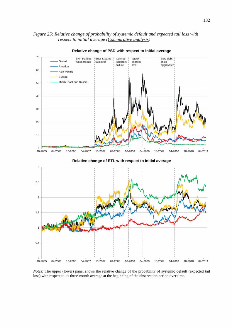
132
Figure 25: Relative change of probability of systemic default and expected tail loss with respect to initial average (Comparative analysis)
Notes: The upper (lower) panel shows the relative change of the probability of systemic default (expected tail loss) with respect to its three-month average at the beginning of the observation period over time.
0
10
20
30
40
50
60
70
10-2005 04-2006 10-2006 04-2007 10-2007 04-2008 10-2008 04-2009 10-2009 04-2010 10-2010 04-2011
Relative change of PSD with respect to initial average
Global
America
Asia-Pacific
Europe
Middle East and Russia
0
0.5
1
1.5
2
2.5
3
10-2005 04-2006 10-2006 04-2007 10-2007 04-2008 10-2008 04-2009 10-2009 04-2010 10-2010 04-2011
Relative change of ETL with respect to initial average
BNP Paribas funds freeze
Bear Stearns takeover
Lehman Brothers failure
Stock market low
Euro debt crisis aggravates

133
Figure 26: Risk premium determinants of the relative ESS-indicator
Global
America
0.0%
0.2%
0.4%
0.6%
0.8%
1.0%
1.2%
10-2005 04-2006 10-2006 04-2007 10-2007 04-2008 10-2008 04-2009 10-2009 04-2010 10-2010 04-2011
Term spread TED spread Baa-Aaa spread
0.0%
0.5%
1.0%
1.5%
2.0%
2.5%
3.0%
10-2005 04-2006 10-2006 04-2007 10-2007 04-2008 10-2008 04-2009 10-2009 04-2010 10-2010 04-2011

134
Asia-Pacific
Europe
0.0%
0.2%
0.4%
0.6%
0.8%
1.0%
1.2%
1.4%
1.6%
10-2005 04-2006 10-2006 04-2007 10-2007 04-2008 10-2008 04-2009 10-2009 04-2010 10-2010 04-2011
Term spread TED spread Baa-Aaa spread
0.0%
0.2%
0.4%
0.6%
0.8%
1.0%
1.2%
10-2005 04-2006 10-2006 04-2007 10-2007 04-2008 10-2008 04-2009 10-2009 04-2010 10-2010 04-2011

135
Middle East and Russia
Notes: The graph shows the contribution of the risk premium proxy spreads to the relative expected systemic shortfall indicator. The graph is obtained by inserting the daily values of the respective spreads into the estimated respective regression equation from Regression 4 in Table 14 during the observation period.
0.0%
1.0%
2.0%
3.0%
4.0%
5.0%
6.0%
10-2005 04-2006 10-2006 04-2007 10-2007 04-2008 10-2008 04-2009 10-2009 04-2010 10-2010 04-2011
Term spread TED spread Baa-Aaa spread

136
Figure 27: Generalized impulse responses for inter-regional relative ESS analysis
2 4 6 8 10
0
1
2
America → America
2 4 6 8 10
0
1
2
America → Asia-Pacific
2 4 6 8 10
0
1
2
Asia-Pacific → America
2 4 6 8 10
0
1
2
Asia-Pacific → Asia-Pacific
Inter-regional relative ESS
2 4 6 8 10
0
1
2
America → America
2 4 6 8 10
0
1
2
America → Europe
2 4 6 8 10
0
1
2
Europe → America
2 4 6 8 10
0
1
2
Europe → Europe
Inter-regional relative ESS
Period 1 Period 2 Period 3 Period 4
Period 1 Period 2 Period 3 Period 4
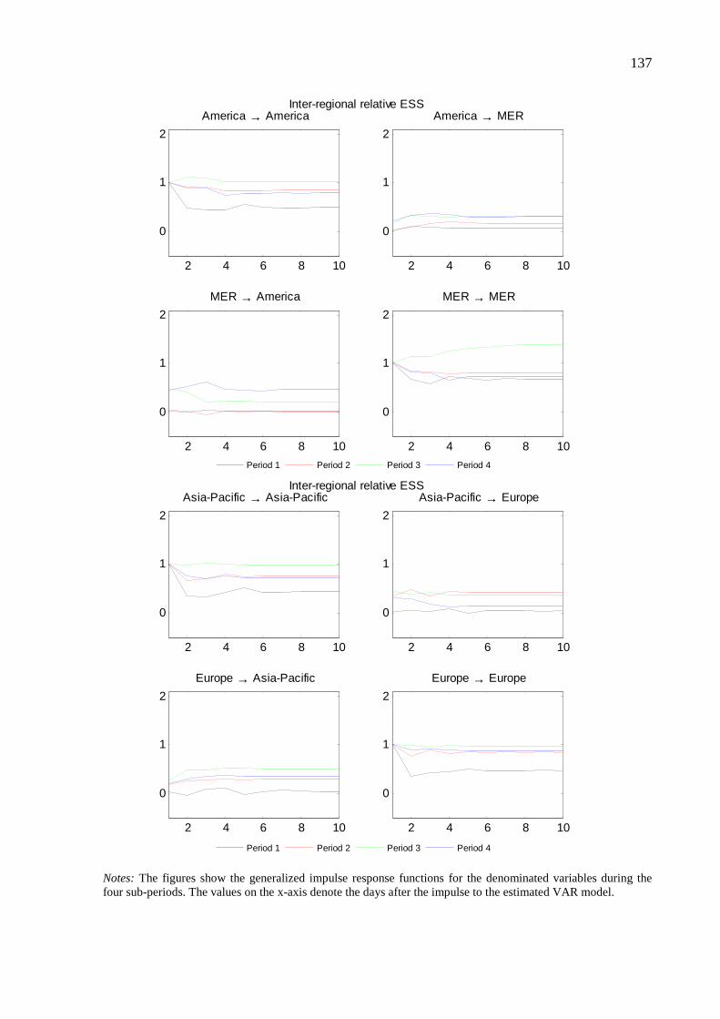
137
Notes: The figures show the generalized impulse response functions for the denominated variables during the four sub-periods. The values on the x-axis denote the days after the impulse to the estimated VAR model.
2 4 6 8 10
0
1
2
America → America
2 4 6 8 10
0
1
2
America → MER
2 4 6 8 10
0
1
2
MER → America
2 4 6 8 10
0
1
2
MER → MER
Inter-regional relative ESS
2 4 6 8 10
0
1
2
Asia-Pacific → Asia-Pacific
2 4 6 8 10
0
1
2
Asia-Pacific → Europe
2 4 6 8 10
0
1
2
Europe → Asia-Pacific
2 4 6 8 10
0
1
2
Europe → Europe
Inter-regional relative ESS
Period 1 Period 2 Period 3 Period 4Period 1 Period 2 Period 3 Period 4
Period 1 Period 2 Period 3 Period 4

138
Figure 28: Generalized impulse responses for inter-regional bank CDS spreads analysis
2 4 6 8 10
0
1
2
America → America
2 4 6 8 10
0
1
2
America → Asia-Pacific
2 4 6 8 10
0
1
2
Asia-Pacific → America
2 4 6 8 10
0
1
2
Asia-Pacific → Asia-Pacific
Inter-regional bank CDS
2 4 6 8 10
0
1
2
America → America
2 4 6 8 10
0
1
2
America → Europe
2 4 6 8 10
0
1
2
Europe → America
2 4 6 8 10
0
1
2
Europe → Europe
Inter-regional bank CDS
Period 1 Period 2 Period 3 Period 4
Period 1 Period 2 Period 3 Period 4
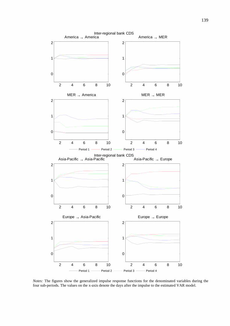
139
Notes: The figures show the generalized impulse response functions for the denominated variables during the four sub-periods. The values on the x-axis denote the days after the impulse to the estimated VAR model.
2 4 6 8 10
0
1
2
America → America
2 4 6 8 10
0
1
2
America → MER
2 4 6 8 10
0
1
2
MER → America
2 4 6 8 10
0
1
2
MER → MER
Inter-regional bank CDS
2 4 6 8 10
0
1
2
Asia-Pacific → Asia-Pacific
2 4 6 8 10
0
1
2
Asia-Pacific → Europe
2 4 6 8 10
0
1
2
Europe → Asia-Pacific
2 4 6 8 10
0
1
2
Europe → Europe
Inter-regional bank CDS
Period 1 Period 2 Period 3 Period 4
Period 1 Period 2 Period 3 Period 4

140
Figure 29: Correlation of regional relative ESS-indicator and regional bank CDS spreads
Notes: The upper panel shows the (average) correlations between the regional relative ESS-indicator in the shown regions (lines) and the regional ESS-indicator in all other regions (cross-regional average of bivariate estimation using the past month's returns. The lower panel shows the (average) correlations between the regional bank CDS spreads in the shown regions (lines) and the regional bank CDS spreads in all other regions (cross-regional average of bivariate estimation using the past month's returns).
-0.5
0.0
0.5
1.0
10-2005 04-2006 10-2006 04-2007 10-2007 04-2008 10-2008 04-2009 10-2009 04-2010 10-2010 04-2011
Average correlation between regional relative ESS-indicator
America Asia-Pacific Europe Middle East and Russia
-0.5
0.0
0.5
1.0
10-2005 04-2006 10-2006 04-2007 10-2007 04-2008 10-2008 04-2009 10-2009 04-2010 10-2010 04-2011
Average correlation between regional bank CDS spreads
America Asia-Pacific Europe Middle East and Russia
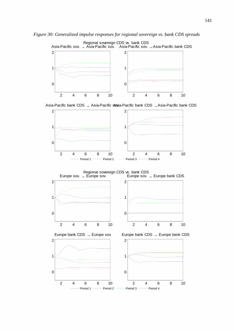
141
Figure 30: Generalized impulse responses for regional sovereign vs. bank CDS spreads
2 4 6 8 10
0
1
2
Asia-Pacific sov. → Asia-Pacific sov.
2 4 6 8 10
0
1
2
Asia-Pacific sov. →Asia-Pacific bank CDS
2 4 6 8 10
0
1
2
Asia-Pacific bank CDS → Asia-Pacific sov.
2 4 6 8 10
0
1
2
Asia-Pacific bank CDS →Asia-Pacific bank CDS
Regional sovereign CDS vs. bank CDS
2 4 6 8 10
0
1
2
Europe sov. → Europe sov.
2 4 6 8 10
0
1
2
Europe sov. → Europe bank CDS
2 4 6 8 10
0
1
2
Europe bank CDS → Europe sov.
2 4 6 8 10
0
1
2
Europe bank CDS → Europe bank CDS
Regional sovereign CDS vs. bank CDS
Period 1 Period 2 Period 3 Period 4
Period 1 Period 2 Period 3 Period 4
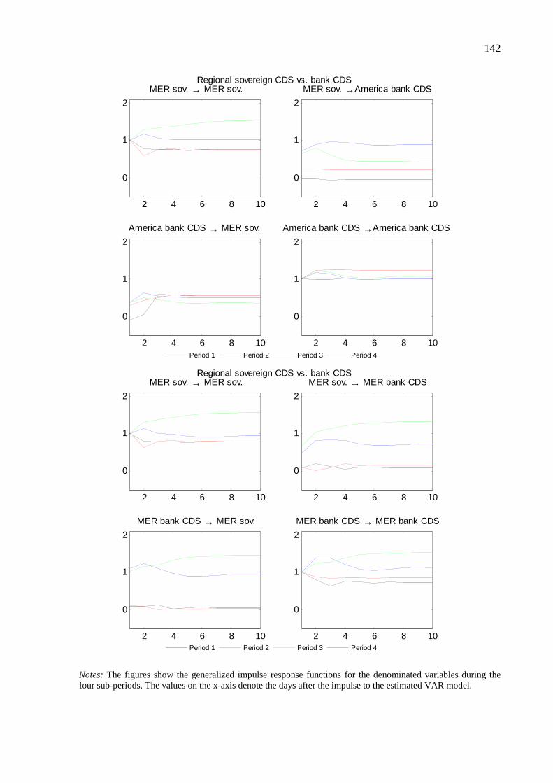
142
Notes: The figures show the generalized impulse response functions for the denominated variables during the four sub-periods. The values on the x-axis denote the days after the impulse to the estimated VAR model.
2 4 6 8 10
0
1
2
MER sov. → MER sov.
2 4 6 8 10
0
1
2
MER sov. →America bank CDS
2 4 6 8 10
0
1
2
America bank CDS → MER sov.
2 4 6 8 10
0
1
2
America bank CDS →America bank CDS
Regional sovereign CDS vs. bank CDS
2 4 6 8 10
0
1
2
MER sov. → MER sov.
2 4 6 8 10
0
1
2
MER sov. → MER bank CDS
2 4 6 8 10
0
1
2
MER bank CDS → MER sov.
2 4 6 8 10
0
1
2
MER bank CDS → MER bank CDS
Regional sovereign CDS vs. bank CDS
Period 1 Period 2 Period 3 Period 4Period 1 Period 2 Period 3 Period 4
Period 1 Period 2 Period 3 Period 4

143
Figure 31: Correlation of regional sovereign and bank CDS spreads
Notes: The figure shows the (average) correlations between the regional sovereign CDS spreads and the bank CDS spreads of all other regions (cross-regional average of bivariate correlations).
-1.0
-0.5
0.0
0.5
1.0
10-2005 04-2006 10-2006 04-2007 10-2007 04-2008 10-2008 04-2009 10-2009 04-2010 10-2010 04-2011
Average correlation betweeen sovereign and the cross-regional bank CDS
America Asia-Pacific Europe Middle East and Russia
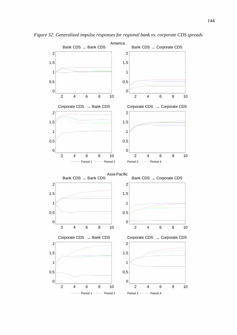
144
Figure 32: Generalized impulse responses for regional bank vs. corporate CDS spreads
2 4 6 8 100
0.5
1
1.5
2
Bank CDS → Bank CDS
2 4 6 8 100
0.5
1
1.5
2
Bank CDS → Corporate CDS
2 4 6 8 100
0.5
1
1.5
2
Corporate CDS → Bank CDS
2 4 6 8 100
0.5
1
1.5
2
Corporate CDS → Corporate CDS
America
2 4 6 8 100
0.5
1
1.5
2
Bank CDS → Bank CDS
2 4 6 8 100
0.5
1
1.5
2
Bank CDS → Corporate CDS
2 4 6 8 100
0.5
1
1.5
2
Corporate CDS → Bank CDS
2 4 6 8 100
0.5
1
1.5
2
Corporate CDS → Corporate CDS
Asia-Pacific
Period 1 Period 2 Period 3 Period 4
Period 1 Period 2 Period 3 Period 4

145
Notes: The figures show the generalized impulse response functions for the denominated variables during the four sub-periods. The values on the x-axis denote the days after the impulse to the estimated VAR model.
2 4 6 8 100
0.5
1
1.5
2
Bank CDS → Bank CDS
2 4 6 8 100
0.5
1
1.5
2
Bank CDS → Corporate CDS
2 4 6 8 100
0.5
1
1.5
2
Corporate CDS → Bank CDS
2 4 6 8 100
0.5
1
1.5
2
Corporate CDS → Corporate CDS
Europe
Period 1 Period 2 Period 3 Period 4

146
Figure 33: Generalized impulse responses for regional bank vs. corporate equity returns
2 4 6 8 100
0.5
1
1.5
2
Bank equity → Bank equity
2 4 6 8 100
0.5
1
1.5
2
Bank equity → Corporate equtiy
2 4 6 8 100
0.5
1
1.5
2
Corporate equtiy → Bank equity
2 4 6 8 100
0.5
1
1.5
2
Corporate equtiy → Corporate equtiy
America
2 4 6 8 100
0.5
1
1.5
2
Bank equity → Bank equity
2 4 6 8 100
0.5
1
1.5
2
Bank equity → Corporate equtiy
2 4 6 8 100
0.5
1
1.5
2
Corporate equtiy → Bank equity
2 4 6 8 100
0.5
1
1.5
2
Corporate equtiy → Corporate equtiy
Asia-Pacific
Period 1 Period 2 Period 3 Period 4
Period 1 Period 2 Period 3 Period 4

147
Notes: The figures show the generalized impulse response functions for the denominated variables during the four sub-periods. The values on the x-axis denote the days after the impulse to the estimated VAR model.
2 4 6 8 100
0.5
1
1.5
2
Bank equity → Bank equity
2 4 6 8 100
0.5
1
1.5
2
Bank equity → Corporate equtiy
2 4 6 8 100
0.5
1
1.5
2
Corporate equtiy → Bank equity
2 4 6 8 100
0.5
1
1.5
2
Corporate equtiy → Corporate equtiy
Europe
Period 1 Period 2 Period 3 Period 4

148
Figure 34: Correlation between bank and corporate CDS spreads and equity returns
Notes: The upper panel shows the correlation between the regional bank CDS spreads and the overall (i.e., cross-industry) corporate CDS spreads in the respective region. The lower panel shows the correlation between the regional bank equity returns and the overall (i.e., cross-industry) corporate equity returns in the respective region.
-0.5
0.0
0.5
1.0
10-2005 04-2006 10-2006 04-2007 10-2007 04-2008 10-2008 04-2009 10-2009 04-2010 10-2010 04-2011
Correlation between bank and overall non-bank corporate CDS spreads
America Asia-Pacific Europe
0.0
0.5
1.0
10-2005 04-2006 10-2006 04-2007 10-2007 04-2008 10-2008 04-2009 10-2009 04-2010 10-2010 04-2011
Correlation between bank and overall non-bank corporate equity returns
America Asia-Pacific Europe

149
LIST OF TABLES
Table 1: Liabilities and CDS spreads by region and country ................................................. 151
Table 2: Liabilities and CDS spreads by bank ....................................................................... 152
Table 3: Equity and average equity return correlation by country (Global) .......................... 154
Table 4: Equity and average equity return correlation by bank (Global) ............................... 155
Table 5: Equity and average equity return correlation by bank (America) ............................ 157
Table 6: Equity and average equity return correlation (Asia-Pacific) .................................... 158
Table 7: Equity and average equity return correlation by country (Europe) .......................... 159
Table 8: Equity and average equity return correlation by bank (Europe) .............................. 160
Table 9: Equity and average equity return correlation by bank (Middle East and Russia) .... 161
Table 10: Sovereign CDS spreads by country ........................................................................ 162
Table 11: CDS spreads of non-bank corporates by region and industry ................................ 163
Table 12: Corporate equity return by region and industry ..................................................... 164
Table 13: Input variable determinants of the ESS-indicator .................................................. 165
Table 14: Risk premium determinants of the ESS-indicator .................................................. 167
Table 15: Relative systemic loss contribution by country (Global) ....................................... 169
Table 16: Relative systemic loss contribution by bank (Global)............................................ 170
Table 17: Relative systemic loss contribution by bank (America) ......................................... 172
Table 18: Relative systemic loss contribution by country (Asia-Pacific) .............................. 172
Table 19: Relative systemic loss contribution by bank (Asia-Pacific) ................................... 173
Table 20: Relative systemic loss contribution by country (Europe) ...................................... 174
Table 21: Relative systemic loss contribution by bank (Europe) ........................................... 175
Table 22: Relative systemic loss contribution by country (Middle East and Russia) ............ 176
Table 23: Relative systemic loss contribution by bank (Middle East and Russia)................. 176
Table 24: Determinants of the relative contributions to the ESS-indicator (Global) ............. 177
Table 25: Determinants of the relative contributions to the ESS-indicator (America) .......... 178
Table 26: Determinants of the relative contributions to the ESS-indicator (Asia-Pacific) .... 179
Table 27: Determinants of the relative contributions to the ESS-indicator (Europe) ............ 180
Table 28: Determinants of the relative contributions to the ESS-indicator (Middle East and
Russia) .................................................................................................................................... 181
Table 29: Granger causality test results for inter-regional relative ESS analysis .................. 182
Table 30: Granger causality test results for inter-regional bank CDS analysis ...................... 183
Table 31: Granger causality test results for regional sovereign risk vs. bank CDS analysis . 184

150
Table 32: Correlation between regional sovereign and bank CDS ........................................ 186
Table 33: Granger causality test results for country sovereign CDS vs. bank CDS analysis 187
Table 34: Granger causality test results for regional bank vs. non-bank corporate CDS....... 190
Table 35: Granger causality test results for regional bank vs. non-bank corporate equity .... 193
Table 36: Correlation between bank and corporate CDS spreads .......................................... 196
Table 37: Correlation between bank and corporate equity returns ......................................... 197
Table 38: Regression of relative ESS-indicator on p-value of F-statistic .............................. 198

151
Table 1: Liabilities and CDS spreads by region and country
By region
Liabilities1 Average daily CDS spread2 Region Total Mean³ Period 1 Period 2 Period 3 Period 4
America 6,919.7 576.6 15.9 69.7 213.5 133.7 Asia-Pacific 5,222.6 217.6 19.2 57.3 168.6 108.3 Europe 23,287.7 612.8 9.6 47.1 124.4 145.1 Middle East and Russia 353.6 39.3 69.2 127.1 526.2 279.0 Global 35,783.5 431.1 12.8 53.8 152.1 138.8
By country
Average daily CDS spread2 Region Country Liability1 Period 1 Period 2 Period 3 Period 4
America US 6,919.7 15.9 69.7 213.5 133.7 Asia-Pacific Australia 1,204.7 8.7 47.3 125.3 110.3 Asia-Pacific China 679.5 21.9 67.5 206.3 130.4 Asia-Pacific Hong Kong 291.7 11.0 49.5 146.5 89.1 Asia-Pacific India 247.0 65.7 148.4 314.8 183.4 Asia-Pacific Japan 1,844.3 16.7 34.9 116.9 88.3 Asia-Pacific Kazakhstan 22.4 192.8 449.0 1,509.9 762.5 Asia-Pacific Korea 604.2 28.0 92.4 306.6 126.0 Asia-Pacific Malaysia 48.1 20.2 49.2 138.6 75.9 Asia-Pacific Singapore 280.7 9.6 44.8 98.6 47.2 Europe Austria 189.5 21.5 52.4 208.2 148.3 Europe Belgium 979.3 9.0 66.6 250.7 229.2 Europe Denmark 462.8 6.0 22.1 122.4 87.9 Europe France 4,700.4 7.2 41.1 83.4 114.0 Europe Germany 2,810.2 13.0 51.8 113.8 112.0 Europe Greece 139.9 21.2 20.7 71.8 777.7 Europe Ireland 362.0 7.7 69.9 285.9 568.9 Europe Italy 1,862.7 13.7 43.9 104.6 148.4 Europe Netherlands 118.7 10.8 44.5 294.5 212.8 Europe Portugal 199.4 13.0 50.7 110.2 462.7 Europe Spain 1,740.4 10.9 46.0 119.1 203.0 Europe Sweden 1,017.1 16.2 26.4 122.4 79.2 Europe Switzerland 2,080.3 8.6 55.3 144.9 101.2 Europe UK 6,625.1 7.6 49.3 127.6 133.1 Middle East Bahrain 18.6 35.3 114.1 457.3 354.3 Middle East Qatar 10.1 17.5 56.8 221.1 182.9 Middle East UAE 87.2 22.5 72.3 345.7 315.1 Russia Russia 237.6 91.1 151.2 610.9 263.9 Mean 1,278.0 12.8 53.8 152.1 138.8 Total 35,783.5 0.0% 0.0% 0.0% 0.0%
Notes: 1. Total liabilities as of 31.12.2008 in billion EUR. 2. Mean of daily CDS spread in basis points. 3. Mean computed per bank in region. Period 1 ranges from October 1st, 2005 to February 28th, 2007, Period 2 ranges from March 1st, 2007 to July 31st, 2008, Period 3 ranges from August 1st, 2008 to December 31st, 2009, Period 4 ranges from January 1st, 2010 to April 30th, 2011. The mean of the CDS spreads is obtained by weighting the period CDS spreads with the liabilities as of 31.12.2008.

152
Table 2: Liabilities and CDS spreads by bank
Average daily CDS spread2
No. Bank name Region Country Liability1 Period 1 Period 2 Period 3 Period 4 1 American Express America US 79.7 16.7 85.4 291.5 88.62 Bank of America America US 1,180.4 11.5 54.6 172.4 150.13 Bank of New York Mellon America US 150.7 14.5 80.3 221.0 133.94 Capital One Financial America US 100.2 34.4 205.7 267.1 116.55 Citigroup America US 1,292.6 11.0 72.0 298.0 161.86 Goldman Sachs America US 638.5 22.9 79.2 207.5 135.97 JPMorgan Chase & Co. America US 1,444.6 17.9 57.0 111.4 83.48 MetLife America US 331.1 20.2 64.3 451.4 208.39 Morgan Stanley America US 479.1 23.0 103.5 302.9 169.210 PNC Financial Services America US 189.5 22.8 119.0257.5 137.911 US Bancorp America US 172.4 20.4 74.9 288.6 159.412 Wells Fargo America US 860.9 10.2 53.9 137.6 103.513 ANZ Banking Group Asia-Pacific Australia 249.4 8.0 43.2 109.9 103.014 Commonwealth Bank Asia-Pacific Australia 281.0 8.1 42.7 105.4 103.015 Macquarie Bank Asia-Pacific Australia 90.1 16.7 99.3 340.4 171.716 National Australia Bank Asia-Pacific Australia 348.8 8.1 43.6 110.6 104.917 Westspac Banking Corp Asia-Pacific Australia 235.4 7.9 42.6 104.8 111.218 Bank of China Asia-Pacific China 679.5 21.9 67.5 206.3 130.419 Standard Chartered Bank Asia-Pacific Hong Kong 291.7 11.0 49.5 146.5 89.120 Bank of India Asia-Pacific India 26.5 81.1 140.2 249.1 175.621 ICICI Bank Asia-Pacific India 68.9 71.9 191.6 446.0213.722 State Bank of India Asia-Pacific India 151.5 60.1130.2 266.6 171.123 Mizuho Financial Group Asia-Pacific Japan 939.1 18.5 24.4 101.9 94.824 Resona Holdings Asia-Pacific Japan 234.7 22.1 68.8266.9 82.525 Sumitomo Mitsui Banking Asia-Pacific Japan 670.5 12.5 37.8 85.4 81.226 Halyk Bank of Kazakhstan Asia-Pacific Kazakhstan 8.7 180.3 336.5 1,369.1 481.827 Kazkommertsbank Asia-Pacific Kazakhstan 13.7 200.8 520.4 1,599.3 940.728 Hana Bank Asia-Pacific Korea 84.8 27.6 93.4 309.8 126.229 Industrial Bank of Korea Asia-Pacific Korea 78.1 23.1 74.1 279.1 118.230 Kookmin Bank Asia-Pacific Korea 143.6 24.0 81.3 292.4 120.931 Shinhan Financial Group Asia-Pacific Korea 140.1 27.7 94.9 308.0 124.232 Woori Bank Asia-Pacific Korea 157.7 34.4 108.8 330.1 135.933 Malayan Banking Berhad Asia-Pacific Malaysia 48.1 20.2 49.2 138.6 75.934 DBS Bank Asia-Pacific Singapore 116.1 9.0 44.9 98.846.535 Oversea Chinese Banking Asia-Pacific Singapore 81.3 9.5 44.7 98.0 46.236 United Overseas Bank Asia-Pacific Singapore 83.310.7 44.6 98.9 49.337 Erste Group Bank Europe Austria 189.5 21.5 52.4 208.2 148.338 Dexia Europe Belgium 641.4 9.1 67.7 274.6 269.039 KBC Bank Europe Belgium 337.9 9.0 64.5 205.4 153.640 DANSKE Bank Europe Denmark 462.8 6.0 22.1 122.4 87.941 BNP Paribas Europe France 2,012.6 7.0 35.1 69.6 96.442 Crédit Agricole Europe France 1,601.7 7.1 46.7 91.8130.843 Societé Generale Europe France 1,086.2 7.6 43.9 96.9 121.744 Commerzbank Europe Germany 599.3 12.9 52.3 90.3 115.145 Deutsche Bank Europe Germany 2,162.0 12.7 49.1 107.9 105.246 IKB - Deutsche Industriebank Europe Germany 48.922.6 164.5 664.7 374.747 Alpha Bank Europe Greece 61.9 21.4 27.4 92.4 756.348 EFG Eurobank Europe Greece 78.0 21.1 15.4 55.6 794.649 Allied Irish Banks Europe Ireland 171.2 7.7 67.1 278.5 725.9
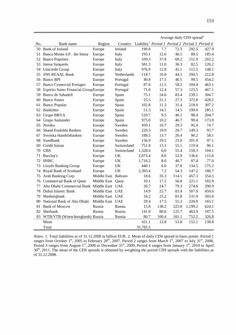
153
Average daily CDS spread2
No. Bank name Region Country Liability1 Period 1 Period 2 Period 3 Period 4 50 Bank of Ireland Europe Ireland 190.8 7.7 72.3 292.5427.951 Banca Monte d.P. die Siena Europe Italy 195.1 12.6 46.5 89.5 185.452 Banco Popolare Europe Italy 109.3 37.8 68.2 151.9 202.253 Intesa Sanpaolo Europe Italy 581.3 11.0 36.3 82.5 126.254 Unicredit Group Europe Italy 976.9 12.8 45.1 115.5 148.155 SNS REAAL Bank Europe Netherlands 118.7 10.8 44.5 294.5 212.856 Banco BPI Europe Portugal 40.8 17.5 40.5 99.5 454.257 Banco Comercial Portuges Europe Portugal 87.6 11.5 50.2 104.4 463.158 Espirito Santo Financial Group Europe Portugal 71.0 12.4 57.3 123.5 467.159 Banco de Sabadell Europe Spain 75.1 24.6 83.4 239.1304.760 Banco Pastor Europe Spain 25.5 21.1 27.3 372.8 428.261 Banco Popular Europe Spain 102.8 11.3 31.4 218.0 307.262 Bankinter Europe Spain 51.3 14.1 14.5 199.0 285.163 Grupo BBVA Europe Spain 510.7 9.5 46.1 98.4 204.764 Grupo Santander Europe Spain 975.0 10.2 46.7 99.4 173.065 Nordea Europe Sweden 450.1 10.7 29.3 95.4 74.766 Skand Enskilda Banken Europe Sweden 220.5 19.9 29.7 149.3 93.767 Svenska Handelsbanken Europe Sweden 189.5 13.7 20.4 90.2 58.168 Swedbank Europe Sweden 156.9 29.5 21.0 201.0 97.169 Crédit Suisse Europe Switzerland 751.9 13.1 55.1 119.4 96.170 UBS Europe Switzerland 1,328.4 6.0 55.4 159.3 104.171 Barclay's Europe UK 2,075.4 8.0 52.9 136.6 115.672 HSBC Europe UK 1,716.2 8.0 40.7 87.4 77.073 Lloyds Banking Group Europe UK 440.1 6.0 37.8 134.5175.274 Royal Bank of Scotland Europe UK 2,393.4 7.2 54.3 147.2 180.775 Arab Banking Corp Middle East Bahrain 18.6 35.3 114.1 457.3 354.376 Commercial Bank of Qatar Middle East Qatar 10.1 17.5 56.8 221.1 182.977 Abu Dhabi Commercial Bank Middle East UAE 26.7 24.7 79.3 274.6 290.978 Dubai Islamic Bank Middle East UAE 14.9 25.7 83.4 507.8 450.679 Mashreqbank Middle East UAE 16.2 25.2 81.8 531.9 503.680 National Bank of Abu Dhabi Middle East UAE 29.4 17.5 55.2 226.0 165.181 Bank of Moscow Russia Russia 15.8 138.2 225.8 1,199.2 624.182 Sberbank Russia Russia 141.0 80.6 125.7 463.9 187.583 WTB/VTB (Wneschtorgbank) Russia Russia 80.7 100.4 181.1 752.2 326.8
Mean 431.1 12.8 53.8 152.1 138.8 Total 35,783.5 0.0% 0.0% 0.0% 0.0%
Notes: 1. Total liabilities as of 31.12.2008 in billion EUR. 2. Mean of daily CDS spread in basis points. Period 1 ranges from October 1st, 2005 to February 28th, 2007, Period 2 ranges from March 1st, 2007 to July 31st, 2008, Period 3 ranges from August 1st, 2008 to December 31st, 2009, Period 4 ranges from January 1st, 2010 to April 30th, 2011. The mean of the CDS spreads is obtained by weighting the period CDS spreads with the liabilities as of 31.12.2008.

154
Table 3: Equity and average equity return correlation by country (Global)
Average equity return correlation²
Region Country Equity1 Period 1 Period 2 Period 3 Period 4 America US 464.5 19.2% 26.4% 27.1% 24.4% Asia-Pacific Australia 60.3 17.5% 23.9% 28.5% 22.0% Asia-Pacific China 48.9 9.4% 10.3% 1.5% 4.6% Asia-Pacific Hong Kong 15.7 25.6% 39.9% 36.1% 28.5% Asia-Pacific India 18.3 13.3% 21.5% 24.7% 16.2% Asia-Pacific Japan 55.2 15.6% 12.9% 13.1% 3.2% Asia-Pacific Kazakhstan 3.0 6.3% 8.3% 7.6% 5.6% Asia-Pacific Korea 34.9 15.8% 22.8% 22.4% 16.9% Asia-Pacific Malaysia 3.7 10.4% 19.0% 20.1% 10.7% Asia-Pacific Singapore 23.5 19.2% 28.2% 28.5% 18.5% Europe Austria 8.1 19.0% 34.0% 36.4% 28.5% Europe Belgium 19.8 25.0% 37.2% 32.5% 31.3% Europe Denmark 13.2 20.5% 35.8% 36.2% 22.3% Europe France 132.5 28.8% 39.8% 39.4% 34.1% Europe Germany 51.7 29.0% 39.1% 37.7% 32.5% Europe Greece 6.6 15.2% 25.5% 30.0% 18.8% Europe Ireland 15.7 18.5% 36.1% 27.4% 21.1% Europe Italy 128.6 23.5% 35.6% 38.9% 31.6% Europe Netherlands 4.8 21.4% 30.3% 35.9% 29.9% Europe Portugal 11.4 10.5% 26.1% 30.5% 27.0% Europe Spain 97.9 26.5% 34.0% 37.1% 30.1% Europe Sweden 39.8 24.6% 35.3% 36.5% 29.0% Europe Switzerland 44.0 27.2% 38.7% 38.0% 32.3% Europe UK 169.5 27.4% 38.8% 36.0% 30.3% Middle East Bahrain 1.3 7.0% 6.2% -5.3% 3.5% Middle East Qatar 2.0 6.6% 7.7% 12.3% 12.0% Middle East UAE 8.7 3.3% 8.0% 10.7% 4.3% Russia Russia 28.7 17.2% 25.2% 29.7% 23.9% Mean 54.0 23.5% 32.7% 32.3% 27.0% Total 1,512.3 0.0% 0.0% 0.0% 0.0%
Notes: 1. Total equity as of 31.12.2008 in billion EUR. 2. Mean of daily pairwise stock return correlations between the bank and all other banks. Period 1 ranges from October 1st, 2005 to February 28th, 2007, Period 2 ranges from March 1st, 2007 to July 31st, 2008, Period 3 ranges from August 1st, 2008 to December 31st, 2009, Period 4 ranges from January 1st, 2010 to April 30th, 2011. The mean of the correlations is obtained by weighting the period correlations with the liabilities as of 31.12.2008.

155
Table 4: Equity and average equity return correlation by bank (Global)
Average equity return correlation²
No. Bank name Region Country Equity1 Period 1 Period 2 Period 3 Period 4 1 American Express America US 8.5 18.9% 24.1% 26.5% 21.1%2 Bank of America America US 99.1 19.1% 27.0% 30.7% 27.4%3 Bank of New York Mellon America US 20.2 18.6% 25.3% 23.0% 22.7%4 Capital One Financial America US 16.6 18.1% 23.5% 26.7% 22.4%5 Citigroup America US 51.1 20.4% 29.4% 27.7% 22.9%6 Goldman Sachs America US 36.5 20.1% 28.0% 28.1% 17.9%7 JPMorgan Chase & Co. America US 97.1 20.6% 24.6% 25.8% 26.4%8 MetLife America US 24.6 15.6% 25.5% 27.1% 26.6%9 Morgan Stanley America US 25.0 22.7% 27.8% 28.4% 24.7%10 PNC Financial Services America US 18.3 15.4% 23.9% 20.8% 21.8%11 US Bancorp America US 18.9 16.8% 25.2% 22.2% 23.7%12 Wells Fargo America US 48.7 15.7% 23.6% 25.1% 24.9%13 ANZ Banking Group Asia-Pacific Australia 14.4 14.4% 21.2% 27.3% 20.7%14 Commonwealth Bank Asia-Pacific Australia 15.0 18.3% 26.6% 30.7% 22.7%15 Macquarie Bank Asia-Pacific Australia 5.1 16.3% 25.0% 25.4% 19.0%16 National Australia Bank Asia-Pacific Australia 15.8 18.9% 22.6% 28.1% 22.7%17 Westspac Banking Corp Asia-Pacific Australia 10.0 18.2% 24.9% 29.1% 22.4%18 Bank of China Asia-Pacific China 48.9 9.4% 10.3% 1.5% 4.6%19 Standard Chartered Bank Asia-Pacific Hong Kong 15.7 25.6% 39.9% 36.1% 28.5%20 Bank of India Asia-Pacific India 1.7 13.4% 16.1% 20.7% 9.4%21 ICICI Bank Asia-Pacific India 7.0 13.7% 23.1% 27.8% 17.1%22 State Bank of India Asia-Pacific India 9.6 13.2% 21.7% 24.0% 16.9%23 Mizuho Financial Group Asia-Pacific Japan 18.5 16.6% 13.2% 13.9% 2.6%24 Resona Holdings Asia-Pacific Japan 16.3 16.4% 12.5% 6.5% 1.4%25 Sumitomo Mitsui Banking Asia-Pacific Japan 20.4 13.9% 12.8% 14.4% 4.8%26 Halyk Bank of Kazakhstan Asia-Pacific Kazakhstan 1.1 6.9% 8.4% 13.2% 5.7%27 Kazkommertsbank Asia-Pacific Kazakhstan 1.9 5.8% 8.3% 4.1% 5.6%28 Hana Bank Asia-Pacific Korea 5.1 15.2% 22.9% 21.2% 13.1%29 Industrial Bank of Korea Asia-Pacific Korea 4.0 14.6% 22.2% 23.7% 16.4%30 Kookmin Bank Asia-Pacific Korea 9.0 16.6% 24.1% 22.0% 18.9%31 Shinhan Financial Group Asia-Pacific Korea 9.8 15.4% 24.1% 22.9% 16.4%32 Woori Bank Asia-Pacific Korea 7.0 16.5% 20.6% 22.3% 17.7%33 Malayan Banking Berhad Asia-Pacific Malaysia 3.7 10.4% 19.0% 20.1% 10.7%34 DBS Bank Asia-Pacific Singapore 9.9 20.4% 29.0% 28.3% 18.4%35 Oversea Chinese Banking Asia-Pacific Singapore 7.0 19.0% 28.6% 29.2% 17.0%36 United Overseas Bank Asia-Pacific Singapore 6.7 17.6% 26.7% 28.1% 20.2%37 Erste Group Bank Europe Austria 8.1 19.0% 34.0% 36.4% 28.5%38 Dexia Europe Belgium 14.2 25.2% 36.1% 30.2% 30.3%39 KBC Bank Europe Belgium 5.6 24.5% 39.3% 36.8% 33.3%40 DANSKE Bank Europe Denmark 13.2 20.5% 35.8% 36.2% 22.3%41 BNP Paribas Europe France 53.2 29.8% 40.9% 39.3% 34.4%42 Crédit Agricole Europe France 41.7 26.6% 39.3% 39.8% 33.5%43 Societé Generale Europe France 37.5 30.1% 38.4% 38.9% 34.3%44 Commerzbank Europe Germany 19.2 25.3% 37.8% 34.3% 29.7%45 Deutsche Bank Europe Germany 30.7 30.2% 39.9% 39.1% 34.0%46 IKB - Deutsche Industriebank Europe Germany 1.8 22.8% 21.5% 17.7% 0.9%47 Alpha Bank Europe Greece 3.0 15.8% 26.6% 29.2% 18.2%48 EFG Eurobank Europe Greece 3.6 14.7% 24.6% 30.6% 19.2%49 Allied Irish Banks Europe Ireland 9.3 23.1% 37.8% 28.0% 21.4%

156
Average equity return correlation²
No. Bank name Region Country Equity1 Period 1 Period 2 Period 3 Period 4 50 Bank of Ireland Europe Ireland 6.4 14.5% 34.6% 26.9% 20.8%51 Banca Monte d.P. die Siena Europe Italy 14.8 21.4% 33.4% 35.8% 29.5%52 Banco Popolare Europe Italy 9.8 17.2% 30.7% 33.4% 29.7%53 Intesa Sanpaolo Europe Italy 49.0 19.1% 34.3% 39.6% 31.6%54 Unicredit Group Europe Italy 55.0 27.3% 37.4% 39.7% 32.1%55 SNS REAAL Bank Europe Netherlands 4.8 21.4% 30.3% 35.9% 29.9%56 Banco BPI Europe Portugal 1.5 8.0% 19.8% 33.2% 26.2%57 Banco Comercial Portuges Europe Portugal 6.0 12.9% 24.9% 30.9% 27.4%58 Espirito Santo Financial Group Europe Portugal 3.9 8.9% 31.1% 28.3% 27.0%59 Banco de Sabadell Europe Spain 4.4 23.3% 36.1% 39.4% 26.7%60 Banco Pastor Europe Spain 1.5 16.1% 30.9% 24.7% 16.7%61 Banco Popular Europe Spain 6.8 23.8% 37.6% 41.2% 28.3%62 Bankinter Europe Spain 2.0 22.8% 36.2% 29.2% 29.2%63 Grupo BBVA Europe Spain 25.7 23.4% 21.9% 27.8% 27.6%64 Grupo Santander Europe Spain 57.6 29.1% 39.8% 42.2% 32.2%65 Nordea Europe Sweden 17.5 25.1% 35.9% 36.9% 29.0%66 Skand Enskilda Banken Europe Sweden 7.6 24.8% 37.0% 37.4% 30.0%67 Svenska Handelsbanken Europe Sweden 6.8 24.2% 31.7% 35.6% 29.0%68 Swedbank Europe Sweden 7.8 23.3% 35.4% 35.1% 27.6%69 Crédit Suisse Europe Switzerland 21.8 26.7% 39.5% 37.2% 33.1%70 UBS Europe Switzerland 22.2 27.5% 38.3% 38.4% 31.8%71 Barclay's Europe UK 34.1 26.9% 39.8% 36.8% 34.3%72 HSBC Europe UK 64.8 31.0% 38.3% 40.3% 30.1%73 Lloyds Banking Group Europe UK 9.7 26.4% 39.3% 31.9% 26.9%74 Royal Bank of Scotland Europe UK 60.9 25.3% 38.1% 33.0% 27.5%75 Arab Banking Corp Middle East Bahrain 1.3 7.0% 6.2% -5.3% 3.5%76 Commercial Bank of Qatar Middle East Qatar 2.0 6.6% 7.7% 12.3% 12.0%77 Abu Dhabi Commercial Bank Middle East UAE 2.2 4.5% 9.5% 11.5% 7.2%78 Dubai Islamic Bank Middle East UAE 1.7 0.4% 10.7% 15.0% 8.0%79 Mashreqbank Middle East UAE 2.0 6.0% 6.7% -4.9% -5.5%80 National Bank of Abu Dhabi Middle East UAE 2.8 2.2% 6.1% 16.5% 5.1%81 Bank of Moscow Russia Russia 1.6 10.3% 20.6% 21.2% 11.7%82 Sberbank Russia Russia 17.6 20.2% 28.4% 30.5% 25.5%83 WTB/VTB (Wneschtorgbank) Russia Russia 9.5 13.3% 20.6% 30.1% 23.5%
Mean 18.2 23.5% 32.7% 32.3% 27.0% Total 1,512.3 0.0% 0.0% 0.0% 0.0%
Notes: 1. Total equity as of 31.12.2008 in billion EUR. 2. Mean of daily pairwise stock return correlations between the bank and all other banks. Period 1 ranges from October 1st, 2005 to February 28th, 2007, Period 2 ranges from March 1st, 2007 to July 31st, 2008, Period 3 ranges from August 1st, 2008 to December 31st, 2009, Period 4 ranges from January 1st, 2010 to April 30th, 2011. The mean of the correlations is obtained by weighting the period correlations with the liabilities as of 31.12.2008.
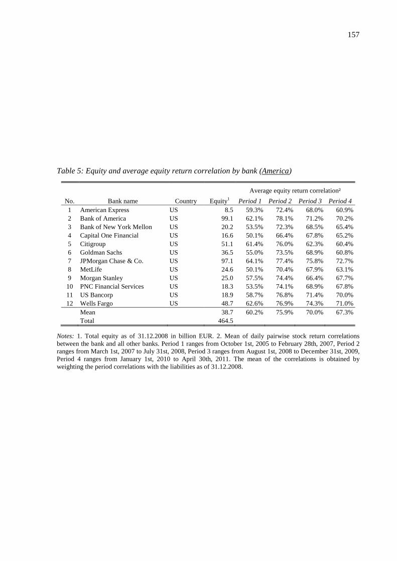
157
Table 5: Equity and average equity return correlation by bank (America)
Average equity return correlation²
No. Bank name Country Equity1 Period 1 Period 2 Period 3 Period 4 1 American Express US 8.5 59.3% 72.4% 68.0% 60.9% 2 Bank of America US 99.1 62.1% 78.1% 71.2% 70.2% 3 Bank of New York Mellon US 20.2 53.5% 72.3% 68.5% 65.4% 4 Capital One Financial US 16.6 50.1% 66.4% 67.8% 65.2% 5 Citigroup US 51.1 61.4% 76.0% 62.3% 60.4% 6 Goldman Sachs US 36.5 55.0% 73.5% 68.9% 60.8% 7 JPMorgan Chase & Co. US 97.1 64.1% 77.4% 75.8% 72.7% 8 MetLife US 24.6 50.1% 70.4% 67.9% 63.1% 9 Morgan Stanley US 25.0 57.5% 74.4% 66.4% 67.7% 10 PNC Financial Services US 18.3 53.5% 74.1% 68.9% 67.8% 11 US Bancorp US 18.9 58.7% 76.8% 71.4% 70.0% 12 Wells Fargo US 48.7 62.6% 76.9% 74.3% 71.0%
Mean 38.7 60.2% 75.9% 70.0% 67.3% Total 464.5 0.0% 0.0% 0.0% 0.0%
Notes: 1. Total equity as of 31.12.2008 in billion EUR. 2. Mean of daily pairwise stock return correlations between the bank and all other banks. Period 1 ranges from October 1st, 2005 to February 28th, 2007, Period 2 ranges from March 1st, 2007 to July 31st, 2008, Period 3 ranges from August 1st, 2008 to December 31st, 2009, Period 4 ranges from January 1st, 2010 to April 30th, 2011. The mean of the correlations is obtained by weighting the period correlations with the liabilities as of 31.12.2008.

158
Table 6: Equity and average equity return correlation (Asia-Pacific)
By country
Average equity return correlation²
Region Country Equity1 Period 1 Period 2 Period 3 Period 4 Asia-Pacific Australia 60.3 28.6% 35.6% 35.1% 35.5% Asia-Pacific China 48.9 14.8% 17.1% 13.2% 16.1% Asia-Pacific Hong Kong 15.7 14.6% 25.6% 24.7% 11.6% Asia-Pacific India 18.3 22.1% 27.3% 29.3% 22.9% Asia-Pacific Japan 55.2 29.3% 29.8% 27.8% 18.3% Asia-Pacific Kazakhstan 3.0 7.1% 8.7% 13.5% 15.2% Asia-Pacific Korea 34.9 29.4% 36.8% 39.6% 34.6% Asia-Pacific Malaysia 3.7 16.5% 27.0% 27.2% 25.3% Asia-Pacific Singapore 23.5 28.5% 38.1% 39.2% 33.6% Mean 29.3 25.8% 30.2% 29.4% 24.6% Total 263.7 0.0% 0.0% 0.0% 0.0%
By bank
Average equity return correlation²
No. Bank name Country Equity1 Period 1 Period 2 Period 3 Period 4 1 ANZ Banking Group Australia 14.4 20.7% 27.2% 27.0% 33.7% 2 Commonwealth Bank Australia 15.0 31.5% 38.4% 36.9% 36.6% 3 Macquarie Bank Australia 5.1 26.5% 40.1% 35.8% 36.1% 4 National Australia Bank Australia 15.8 32.2% 36.9% 37.7% 36.1% 5 Westspac Banking Corp Australia 10.0 29.1% 37.3% 37.7% 35.0% 6 Bank of China China 48.9 14.8% 17.1% 13.2% 16.1% 7 Standard Chartered Bank Hong Kong 15.7 14.6% 25.6% 24.7% 11.6% 8 Bank of India India 1.7 20.9% 23.0% 25.3% 19.0% 9 ICICI Bank India 7.0 24.3% 31.2% 33.7% 25.6% 10 State Bank of India India 9.6 21.4% 26.2% 27.9% 22.3% 11 Mizuho Financial Group Japan 18.5 30.4% 31.1% 28.2% 17.0% 12 Resona Holdings Japan 16.3 29.5% 28.1% 20.0% 13.7% 13 Sumitomo Mitsui Banking Japan 20.4 27.6% 28.5% 30.0% 21.7% 14 Halyk Bank of Kazakhstan Kazakhstan 1.1 8.5% 9.9% 19.9% 15.3% 15 Kazkommertsbank Kazakhstan 1.9 6.2% 8.0% 9.5% 15.2% 16 Hana Bank Korea 5.1 29.7% 35.9% 36.7% 32.8% 17 Industrial Bank of Korea Korea 4.0 28.0% 34.7% 39.7% 33.4% 18 Kookmin Bank Korea 9.0 31.2% 39.0% 40.9% 36.7% 19 Shinhan Financial Group Korea 9.8 28.2% 38.1% 41.0% 35.2% 20 Woori Bank Korea 7.0 29.3% 35.1% 38.6% 33.9% 21 Malayan Banking Berhad Malaysia 3.7 16.5% 27.0% 27.2% 25.3% 22 DBS Bank Singapore 9.9 31.1% 40.3% 40.1% 34.5% 23 Oversea Chinese Banking Singapore 7.0 27.7% 37.8% 38.9% 33.1% 24 United Overseas Bank Singapore 6.7 25.8% 35.2% 38.1% 32.7%
Mean 11.0 25.8% 30.2% 29.4% 24.6% Total 263.7 0.0% 0.0% 0.0% 0.0%
Notes: 1. Total equity as of 31.12.2008 in billion EUR. 2. Mean of daily pairwise stock return correlations between the bank and all other banks. Period 1 ranges from October 1st, 2005 to February 28th, 2007, Period 2 ranges from March 1st, 2007 to July 31st, 2008, Period 3 ranges from August 1st, 2008 to December 31st, 2009, Period 4 ranges from January 1st, 2010 to April 30th, 2011. The mean of the correlations is obtained by weighting the period correlations with the liabilities as of 31.12.2008.

159
Table 7: Equity and average equity return correlation by country (Europe)
Average equity return correlation²
Region Country Equity1 Period 1 Period 2 Period 3 Period 4 Europe Austria 8.1 28.7% 49.1% 53.2% 51.9% Europe Belgium 19.8 40.6% 54.8% 46.5% 54.7% Europe Denmark 13.2 30.2% 50.5% 51.5% 39.3% Europe France 132.5 46.0% 59.3% 57.6% 59.6% Europe Germany 51.7 44.5% 56.0% 53.1% 51.2% Europe Greece 6.6 23.9% 36.0% 41.9% 35.6% Europe Ireland 15.7 32.0% 51.2% 40.1% 35.0% Europe Italy 128.6 38.1% 53.5% 55.1% 57.3% Europe Netherlands 4.8 19.6% 44.5% 51.9% 46.3% Europe Portugal 11.4 16.8% 37.0% 43.5% 52.0% Europe Spain 97.9 42.0% 49.7% 51.9% 56.2% Europe Sweden 39.8 40.3% 54.0% 54.7% 47.9% Europe Switzerland 44.0 42.5% 56.7% 55.1% 48.5% Europe UK 169.5 39.6% 55.1% 51.4% 45.1% Mean 53.1 41.1% 55.1% 53.2% 51.2% Total 743.5 0.0% 0.0% 0.0% 0.0%
Notes: 1. Total equity as of 31.12.2008 in billion EUR. 2. Mean of daily pairwise stock return correlations between the bank and all other banks. Period 1 ranges from October 1st, 2005 to February 28th, 2007, Period 2 ranges from March 1st, 2007 to July 31st, 2008, Period 3 ranges from August 1st, 2008 to December 31st, 2009, Period 4 ranges from January 1st, 2010 to April 30th, 2011. The mean of the correlations is obtained by weighting the period correlations with the liabilities as of 31.12.2008.

160
Table 8: Equity and average equity return correlation by bank (Europe)
Average equity return correlation²
No. Bank name Country Equity1 Period 1 Period 2 Period 3 Period 4 1 Erste Group Bank Austria 8.1 28.7% 49.1% 53.2% 51.9%2 Dexia Belgium 14.2 40.6% 53.6% 44.4% 53.7%3 KBC Bank Belgium 5.6 40.5% 57.1% 50.7% 56.5%4 DANSKE Bank Denmark 13.2 30.2% 50.5% 51.5% 39.3%5 BNP Paribas France 53.2 47.9% 61.3% 57.6% 60.2%6 Crédit Agricole France 41.7 41.6% 58.8% 58.5% 58.8%7 Societé Generale France 37.5 49.1% 56.4% 56.3% 59.7%8 Commerzbank Germany 19.2 38.6% 55.1% 48.4% 48.3%9 Deutsche Bank Germany 30.7 46.4% 56.9% 55.0% 53.1%10 IKB - Deutsche Industriebank Germany 1.8 33.8% 30.0% 25.6% 0.8%11 Alpha Bank Greece 3.0 25.3% 38.0% 41.1% 34.7%12 EFG Eurobank Greece 3.6 22.9% 34.4% 42.7% 36.3%13 Allied Irish Banks Ireland 9.3 37.9% 53.3% 41.2% 34.6%14 Bank of Ireland Ireland 6.4 26.6% 49.4% 39.2% 35.3%15 Banca Monte d.P. die Siena Italy 14.8 34.4% 50.3%50.8% 54.7%16 Banco Popolare Italy 9.8 29.7% 47.0% 47.4% 52.7%17 Intesa Sanpaolo Italy 49.0 32.9% 51.2% 55.7% 57.8%18 Unicredit Group Italy 55.0 42.9% 56.3% 56.5% 58.0%19 SNS REAAL Bank Netherlands 4.8 19.6% 44.5% 51.9% 46.3%20 Banco BPI Portugal 1.5 14.4% 29.4% 47.4% 49.3%21 Banco Comercial Portuges Portugal 6.0 19.3% 35.4% 43.5% 52.9%22 Espirito Santo Financial Group Portugal 3.9 15.0%43.3% 41.1% 52.5%23 Banco de Sabadell Spain 4.4 37.6% 53.6% 57.0% 54.1%24 Banco Pastor Spain 1.5 26.5% 46.0% 35.3% 32.9%25 Banco Popular Spain 6.8 39.4% 55.5% 59.2% 56.2%26 Bankinter Spain 2.0 37.1% 52.8% 43.9% 56.4%27 Grupo BBVA Spain 25.7 36.1% 29.8% 35.2% 48.2%28 Grupo Santander Spain 57.6 46.4% 59.1% 60.3% 61.1%29 Nordea Sweden 17.5 41.0% 54.3% 55.7% 49.6%30 Skand Enskilda Banken Sweden 7.6 41.2% 56.9% 55.0% 48.0%31 Svenska Handelsbanken Sweden 6.8 39.6% 49.7% 54.0% 45.5%32 Swedbank Sweden 7.8 38.3% 54.4% 52.4% 45.9%33 Crédit Suisse Switzerland 21.8 40.7% 57.2% 53.1% 49.3%34 UBS Switzerland 22.2 43.5% 56.4% 56.3% 48.1%35 Barclay's UK 34.1 41.9% 57.3% 53.3% 51.2%36 HSBC UK 64.8 38.6% 53.5% 53.7% 42.2%37 Lloyds Banking Group UK 9.7 38.0% 56.8% 46.9% 41.2%38 Royal Bank of Scotland UK 60.9 38.6% 54.1% 48.8% 42.6%
Mean 19.6 41.1% 55.1% 53.2% 51.2% Total 743.5 0.0% 0.0% 0.0%
Notes: 1. Total equity as of 31.12.2008 in billion EUR. 2. Mean of daily pairwise stock return correlations between the bank and all other banks. Period 1 ranges from October 1st, 2005 to February 28th, 2007, Period 2 ranges from March 1st, 2007 to July 31st, 2008, Period 3 ranges from August 1st, 2008 to December 31st, 2009, Period 4 ranges from January 1st, 2010 to April 30th, 2011. The mean of the correlations is obtained by weighting the period correlations with the liabilities as of 31.12.2008.

161
Table 9: Equity and average equity return correlation by bank (Middle East and Russia)
Average equity return correlation²
No. Bank name Country Equity1 Period 1 Period 2 Period 3 Period 4 1 Arab Banking Corp Bahrain 1.3 13.9% 7.1% 5.0% 17.0% 2 Commercial Bank of Qatar Qatar 2.0 12.4% 12.3% 18.7% 21.5% 3 Abu Dhabi Commercial Bank UAE 2.2 24.6% 19.1% 22.9% 19.4% 4 Dubai Islamic Bank UAE 1.7 19.4% 17.9% 22.4% 20.7% 5 Mashreqbank UAE 2.0 11.0% 11.3% 3.2% 18.6% 6 National Bank of Abu Dhabi UAE 2.8 21.7% 19.3% 24.8% 24.2% 7 Bank of Moscow Russia 1.6 14.9% 17.4% 17.2% 22.5% 8 Sberbank Russia 17.6 14.8% 17.6% 15.7% 20.8% 9 WTB/VTB (Wneschtorgbank) Russia 9.5 43.4% 22.8% 17.4% 20.7%
Mean 4.5 22.6% 18.0% 16.7% 20.7% Total 40.6 0.0% 0.0% 0.0% 0.0%
Notes: 1. Total equity as of 31.12.2008 in billion EUR. 2. Mean of daily pairwise stock return correlations between the bank and all other banks. Period 1 ranges from October 1st, 2005 to February 28th, 2007, Period 2 ranges from March 1st, 2007 to July 31st, 2008, Period 3 ranges from August 1st, 2008 to December 31st, 2009, Period 4 ranges from January 1st, 2010 to April 30th, 2011. The mean of the correlations is obtained by weighting the period correlations with the liabilities as of 31.12.2008.

162
Table 10: Sovereign CDS spreads by country
Average daily CDS spread
Region Country Period 1 Period 2 Period 3 Period 4 America US 3.1 6.7 40.9 44.5
Asia-Pacific
Australia 9.8 18.9 68.4 46.6 China 18.6 35.9 121.5 72.5 Hong Kong 8.5 21.8 81.2 45.1 India 60.1 130.2 266.6 171.1 Japan 4.3 13.2 51.3 69.2 Kazakhstan 59.8 148.2 570.2 175.4 Korea 23.5 50.3 223.3 101.5 Malaysia 25.2 50.8 165.0 87.4 Singapore 4.1 9.1 40.7 42.3
Europe
Austria 1.9 5.8 95.3 76.5 Belgium 2.1 10.7 60.6 120.0 Denmark 14.7 8.6 59.1 39.3 France 1.9 6.3 38.5 73.1 Germany 2.0 4.8 33.8 45.0 Greece 11.5 24.0 158.1 748.9 Ireland 5.5 14.8 171.0 371.8 Italy 10.1 20.2 104.0 164.1 Netherlands 4.8 6.5 50.8 45.1 Portugal 6.8 18.3 76.6 348.5 Spain 3.0 17.1 86.4 217.5 Sweden 11.0 24.2 67.3 34.6 Switzerland 3.7 8.8 63.6 45.7 UK 2.7 7.9 76.1 69.5
Middle East and Russia
Bahrain 30.3 75.1 323.5 196.4 Qatar 21.7 32.5 166.4 90.3 UAE 28.2 66.1 326.6 277.9 Russia 57.5 83.7 407.5 152.0
Mean (unweighted) 15.6 32.9 142.7 141.8
Notes: Period 1 ranges from October 1st, 2005 to February 28th, 2007, Period 2 ranges from March 1st, 2007 to July 31st, 2008, Period 3 ranges from August 1st, 2008 to December 31st, 2009, Period 4 ranges from January 1st, 2010 to April 30th, 2011.

163
Table 11: CDS spreads of non-bank corporates by region and industry
Average daily CDS spread1
Region Industry Sample
size Period 1 Period 2 Period 3 Period 4
Global
Automotive 19 193.7 199.0 765.4 172.0Basic materials 17 29.1 65.0 295.6 112.5Chemicals, healthcare and pharma 40 23.3 43.5 108.1 67.2Commerce and consumer 76 32.7 55.3 143.2 87.0Construction and logistics 13 23.9 45.8 127.7 86.4Energy and utilities 49 19.4 39.0 112.7 92.6Financial services (excl. banking) 30 18.6 63.4 267.5 139.7Industrial 46 27.5 40.0 111.3 62.7Telecommunication, media and tech. 62 38.6 64.0 137.0 89.0Overall 352 38.7 66.4 231.0 110.8
America
Automotive 3 699.3 763.0 3,101.4 424.2Basic materials 7 30.7 59.9 331.0 132.3Chemicals, healthcare and pharma 22 21.3 41.3 108.6 70.2Commerce and consumer 35 34.0 55.3 129.1 82.9Construction and logistics 5 18.0 45.4 112.8 61.4Energy and utilities 22 25.1 40.2 120.3 78.2Financial services (excl. banking) 16 30.4 94.4 431.5 196.0Industrial 23 24.4 26.6 63.3 31.4Telecommunication, media and tech. 24 34.4 66.5 126.0 82.4Overall 157 67.6 95.0 329.3 116.7
Asia-Pacific
Automotive 7 10.8 27.7 164.8 73.2Basic materials 6 23.6 59.3 240.5 84.3Chemicals, healthcare and pharma 3 32.9 76.7 190.4 78.2Commerce and consumer 11 29.2 53.0 234.9 89.3Construction and logistics 3 33.7 103.8 489.5 182.9Energy and utilities 8 25.4 52.3 165.6 89.6Financial services (excl. banking) 3 30.2 52.1 137.6 134.6Industrial 9 20.3 48.0 172.1 89.6Telecommunication, media and tech. 18 39.3 60.2 177.5 78.3Overall 68 26.7 51.7 187.3 85.9
Europe
Automotive 9 55.2 69.2 299.6 162.5Basic materials 4 33.8 76.6 340.4 138.3Chemicals, healthcare and pharma 15 23.6 38.5 88.6 60.3Commerce and consumer 30 32.5 56.1 126.3 89.9Construction and logistics 5 24.4 43.2 101.3 84.1Energy and utilities 19 15.3 36.7 101.9 99.4Financial services (excl. banking) 11 14.3 54.6 214.0 118.2Industrial 14 42.1 71.4 208.4 130.2Telecommunication, media and tech. 20 43.4 63.9 119.3 106.3Overall 127 22.9 53.6 181.5 113.1
Notes: 1. The average CDS spreads of the non-bank corporates were obtained by weighting with the total liabilities of the respective firm. Period 1 ranges from October 1st, 2005 to February 28th, 2007, Period 2 ranges from March 1st, 2007 to July 31st, 2008, Period 3 ranges from August 1st, 2008 to December 31st, 2009, Period 4 ranges from January 1st, 2010 to April 30th, 2011.

164
Table 12: Corporate equity return by region and industry
Average daily equity return1
Region Industry Sample
size Period 1 Period 2 Period 3 Period 4
Global
Automotive 19 0.03% -0.09% -0.01% 0.09%Basic materials 17 0.09% 0.02% -0.06% 0.03%Chemicals, healthcare and pharma 40 0.03% -0.06% 0.01% 0.05%Commerce and consumer 76 0.04% -0.06% 0.00% 0.03%Construction and logistics 13 0.06% -0.11% -0.04% 0.02%Energy and utilities 49 0.02% -0.02% -0.04% 0.01%Financial services (excl. banking) 30 0.07% -0.13% -0.06% 0.04%Industrial 46 0.02% -0.07% -0.08% 0.08%Telecommunication, media and tech. 62 0.02% -0.07% -0.02% 0.02%Overall 352 0.04% -0.09% -0.04% 0.04%
America
Automotive 3 -0.08% -0.16% 0.20% 0.11%Basic materials 7 0.04% 0.05% -0.10% 0.06%Chemicals, healthcare and pharma 22 0.00% -0.09% 0.02%0.05%Commerce and consumer 35 0.01% -0.06% 0.01% 0.03%Construction and logistics 5 0.00% -0.07% 0.01% 0.06%Energy and utilities 22 -0.01% -0.01% -0.03% 0.06%Financial services (excl. banking) 16 0.02% -0.13% -0.08% 0.06%Industrial 23 0.01% -0.07% -0.10% 0.09%Telecommunication, media and tech. 24 0.02% -0.08% -0.01% 0.04%Overall 157 0.01% -0.09% -0.04% 0.06%
Asia-Pacific
Automotive 7 0.04% -0.14% 0.02% 0.00%Basic materials 6 0.09% 0.06% -0.04% -0.01%Chemicals, healthcare and pharma 3 0.08% -0.09% -0.05%0.06%Commerce and consumer 11 0.05% -0.05% -0.04% 0.04%Construction and logistics 3 -0.01% -0.20% -0.06% 0.06%Energy and utilities 8 0.07% -0.07% -0.02% 0.01%Financial services (excl. banking) 3 0.10% -0.10% 0.05% -0.02%Industrial 9 0.02% -0.03% -0.02% 0.06%Telecommunication, media and tech. 18 0.03% -0.05% -0.05% 0.03%Overall 68 0.05% -0.06% -0.02% 0.02%
Europe
Automotive 9 0.08% -0.03% -0.09% 0.13%Basic materials 4 0.12% -0.05% -0.05% 0.05%Chemicals, healthcare and pharma 15 0.04% -0.02% 0.01%0.04%Commerce and consumer 30 0.08% -0.06% 0.01% 0.03%Construction and logistics 5 0.07% -0.11% -0.04% 0.00%Energy and utilities 19 0.03% -0.02% -0.04% -0.01%Financial services (excl. banking) 11 0.08% -0.13% -0.05% 0.03%Industrial 14 0.07% -0.06% -0.04% 0.07%Telecommunication, media and tech. 20 0.01% -0.06% -0.02% 0.01%Overall 127 0.07% -0.09% -0.04% 0.03%
Notes: The average equity returns of the non-bank corporates were obtained by weighting with the total liabilities of the respective firm. Period 1 ranges from October 1st, 2005 to February 28th, 2007, Period 2 ranges from March 1st, 2007 to July 31st, 2008, Period 3 ranges from August 1st, 2008 to December 31st, 2009, Period 4 ranges from January 1st, 2010 to April 30th, 2011.
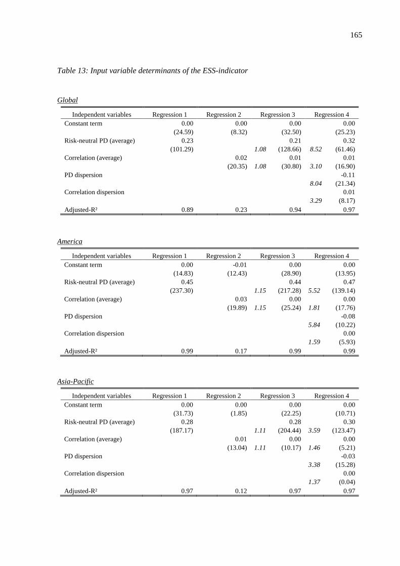
165
Table 13: Input variable determinants of the ESS-indicator
Global
Independent variables Regression 1 Regression 2 Regression 3 Regression 4 Constant term 0 0.00 0 0.00 0 0.00 0 0.00
0.00 (24.59) 0.00 (8.32) 0.00 (32.50) 0.00 (25.23) Risk-neutral PD (average) 0 0.23 0 0.00 0 0.21 0 0.32
0.00 (101.29) 0.00 (0.00) 1.08 (128.66) 8.52 (61.46) Correlation (average) 0 0.00 0 0.02 0 0.01 0 0.01
0.00 (0.00) 0.00 (20.35) 1.08 (30.80) 3.10 (16.90) PD dispersion 0 0.00 0 0.00 0 0.00 0 -0.11
0.00 (0.00) 0.00 (0.00) 0.00 (0.00) 8.04 (21.34) Correlation dispersion 0 0.00 0 0.00 0 0.00 0 0.01
0.00 (0.00) 0.00 (0.00) 0.00 (0.00) 3.29 (8.17) Adjusted-R² 0.00 0.89 0.00 0.23 0.00 0.94 0.00 0.97
America
Independent variables Regression 1 Regression 2 Regression 3 Regression 4 Constant term 0 0.00 0 -0.01 0 0.00 0 0.00
0.00 (14.83) 0.00 (12.43) 0.00 (28.90) 0.00 (13.95) Risk-neutral PD (average) 0 0.45 0 0.00 0 0.44 0 0.47
0.00 (237.30) 0.00 (0.00) 1.15 (217.28) 5.52 (139.14) Correlation (average) 0 0.00 0 0.03 0 0.00 0 0.00
0.00 (0.00) 0.00 (19.89) 1.15 (25.24) 1.81 (17.76) PD dispersion 0 0.00 0 0.00 0 0.00 0 -0.08
0.00 (0.00) 0.00 (0.00) 0.00 (0.00) 5.84 (10.22) Correlation dispersion 0 0.00 0 0.00 0 0.00 0 0.00
0.00 (0.00) 0.00 (0.00) 0.00 (0.00) 1.59 (5.93) Adjusted-R² 0.00 0.99 0.00 0.17 0.00 0.99 0.00 0.99
Asia-Pacific
Independent variables Regression 1 Regression 2 Regression 3 Regression 4 Constant term 0 0.00 0 0.00 0 0.00 0 0.00
0.00 (31.73) 0.00 (1.85) 0.00 (22.25) 0.00 (10.71) Risk-neutral PD (average) 0 0.28 0 0.00 0 0.28 0 0.30
0.00 (187.17) 0.00 (0.00) 1.11 (204.44) 3.59 (123.47) Correlation (average) 0 0.00 0 0.01 0 0.00 0 0.00
0.00 (0.00) 0.00 (13.04) 1.11 (10.17) 1.46 (5.21) PD dispersion 0 0.00 0 0.00 0 0.00 0 -0.03
0.00 (0.00) 0.00 (0.00) 0.00 (0.00) 3.38 (15.28) Correlation dispersion 0 0.00 0 0.00 0 0.00 0 0.00
0.00 (0.00) 0.00 (0.00) 0.00 (0.00) 1.37 (0.04) Adjusted-R² 0.00 0.97 0.00 0.12 0.00 0.97 0.00 0.97

166
Europe
Independent variables Regression 1 Regression 2 Regression 3 Regression 4 Constant term 0 0.00 0 0.00 0 0.00 0 0.00
0.00 (12.31) 0.00 (8.65) 0.00 (31.80) 0.00 (22.92) Risk-neutral PD (average) 0 0.32 0 0.00 0 0.30 0 0.34
0.00 (110.65) 0.00 (0.00) 1.09 (157.02) 11.28 (46.81) Correlation (average) 0 0.00 0 0.01 0 0.01 0 0.01
0.00 (0.00) 0.00 (20.13) 1.09 (32.28) 1.76 (27.03) PD dispersion 0 0.00 0 0.00 0 0.00 0 -0.04
0.00 (0.00) 0.00 (0.00) 0.00 (0.00) 11.25 (6.06) Correlation dispersion 0 0.00 0 0.00 0 0.00 0 0.01
0.00 (0.00) 0.00 (0.00) 0.00 (0.00) 1.47 (5.12) Adjusted-R² 0.00 0.92 0.00 0.22 0.00 0.96 0.00 0.96
Middle East and Russia
Independent variables Regression 1 Regression 2 Regression 3 Regression 4 Constant term 0 0.00 0 0.01 0 0.00 0 0.00
0.00 (15.96) 0.00 (11.94) 0.00 (13.66) 0.00 (18.10) Risk-neutral PD (average) 0 0.43 0 0.00 0 0.43 0 0.51
0.00 (122.64) 0.00 (0.00) 1.00 (134.76) 4.23 (160.73) Correlation (average) 0 0.00 0 0.00 0 0.01 0 0.00
0.00 (0.00) 0.00 (0.28) 1.00 (9.31) 1.15 (5.49) PD dispersion 0 0.00 0 0.00 0 0.00 0 -0.20
0.00 (0.00) 0.00 (0.00) 0.00 (0.00) 4.23 (38.95) Correlation dispersion 0 0.00 0 0.00 0 0.00 0 0.03
0.00 (0.00) 0.00 (0.00) 0.00 (0.00) 1.15 (18.07) Adjusted-R² 0.00 0.97 0.00 0.00 0.00 0.97 0.00 0.99
Notes: The dependent variable in the regression is the relative ESS-indicator of the banks in the sample. Average PD and average correlation denote the risk-neutral default probability of all banks and the correlation between the bank and all other banks at a particular point in time, respectively. Dispersion denotes the standard deviation of the respective variable at a particular point in time for all sample banks. Variance inflation factors are provided in italics. Heteroskedacity-consistent t-statistics are shown in parenthesis. Critical values for the t-statistic at the ten, five and one percent significance level are respectively 1.28, 1.65 and 2.33.

167
Table 14: Risk premium determinants of the ESS-indicator
Global
Independent variables Regression 1 Regression 2 Regression 3 Regression 4
Constant term 0 0.00 0.00 0.00 0.00 0.00 0.00 0.00
0 (5.66) (0.00) (23.98) (0.00) (21.85) 0.00 (16.00)
Baa-Aaa spread 0 0.27 0.00 0.00 0.00 0.00 0.00 0.16
0 (34.57) (0.00) (0.00) (0.00) (0.00) 1.44 (20.87)
Ted spread 0 0.00 0.00 0.08 0.00 0.00 0.00 0.02
0 (0.00) (0.00) (21.72) (0.00) (0.00) 1.27 (6.99)
Term spread 0 0.00 0.00 0.00 0.00 0.13 0.00 0.10
0 (0.00) (0.00) (0.00) (0.00) (45.19) 1.20 (38.93)
Adjusted-R² 0 0.46 0.00 0.19 0.00 0.53 0.00 0.72
America
Independent variables Regression 1 Regression 2 Regression 3 Regression 4
Constant term 0 0.00 0.00 0.01 0.00 0.00 0.00 0.00
0 (7.45) (0.00) (30.91) (0.00) (32.36) 0.00 (15.86)
Baa-Aaa spread 0 0.76 0.00 0.00 0.00 0.00 0.00 0.54
0 (33.67) (0.00) (0.00) (0.00) (0.00) 1.44 (23.43)
Ted spread 0 0.00 0.00 0.18 0.00 0.00 0.00 0.02
0 (0.00) (0.00) (23.64) (0.00) (0.00) 1.27 (3.26)
Term spread 0 0.00 0.00 0.00 0.00 0.32 0.00 0.22
0 (0.00) (0.00) (0.00) (0.00) (50.29) 1.20 (60.34)
Adjusted-R² 0 0.62 0.00 0.18 0.00 0.55 0.00 0.84
Asia-Pacific
Independent variables Regression 1 Regression 2 Regression 3 Regression 4
Constant term 0 0.00 0.00 0.00 0.00 0.00 0.00 0.00
0 (18.37) (0.00) (29.44) (0.00) (28.71) 0.00 (31.80)
Baa-Aaa spread 0 0.41 0.00 0.00 0.00 0.00 0.00 0.33
0 (54.78) (0.00) (0.00) (0.00) (0.00) 1.44 (38.41)
Ted spread 0 0.00 0.00 0.09 0.00 0.00 0.00 0.00
0 (0.00) (0.00) (16.46) (0.00) (0.00) 1.27 (1.19)
Term spread 0 0.00 0.00 0.00 0.00 0.15 0.00 0.09
0 (0.00) (0.00) (0.00) (0.00) (42.35) 1.20 (38.64)
Adjusted-R² 0 0.71 0.00 0.17 0.00 0.45 0.00 0.84

168
Europe
Independent variables Regression 1 Regression 2 Regression 3 Regression 4
Constant term 0 0.00 0.00 0.00 0.00 0.00 0.00 0.00
0 (4.26) (0.00) (26.35) (0.00) (22.92) 0.00 (3.42)
Baa-Aaa spread 0 0.26 0.00 0.00 0.00 0.00 0.00 0.09
0 (28.11) (0.00) (0.00) (0.00) (0.00) 1.44 (11.74)
Ted spread 0 0.00 0.00 0.08 0.00 0.00 0.00 0.02
0 (0.00) (0.00) (17.12) (0.00) (0.00) 1.27 (5.29)
Term spread 0 0.00 0.00 0.00 0.00 0.19 0.00 0.16
0 (0.00) (0.00) (0.00) (0.00) (56.11) 1.20 (45.22)
Adjusted-R² 0 0.26 0.00 0.11 0.00 0.65 0.00 0.69
Middle East and Russia
Independent variables Regression 1 Regression 2 Regression 3 Regression 4
Constant term 0 -0.01 0.00 0.01 0.00 0.01 0.00 -0.01
0 (21.25) (0.00) (36.22) (0.00) (43.04) 0.00 (28.58)
Baa-Aaa spread 0 1.67 0.00 0.00 0.00 0.00 0.00 1.49
0 (55.05) (0.00) (0.00) (0.00) (0.00) 1.44 (43.83)
Ted spread 0 0.00 0.00 0.31 0.00 0.00 0.00 -0.04
0 (0.00) (0.00) (13.61) (0.00) (0.00) 1.27 (3.58)
Term spread 0 0.00 0.00 0.00 0.00 0.50 0.00 0.24
0 (0.00) (0.00) (0.00) (0.00) (38.00) 1.20 (57.77)
Adjusted-R² 0 0.83 0.00 0.15 0.00 0.37 0.00 0.90
Notes: The dependent regression variable is the relative ESS-indicator of the European banks in the sample during the observation period. Baa-Aaa spread is the spread between Moody's Baa and Aaa bond indices, Ted spread is the spread between the 3-month LIBOR and the yield of a 3-month T-Bill, Term spread is the spread between the yields of 10-year and 3-month maturity T-Bills. Variance inflation factors are provided in italics. Heteroskedacity-consistent t-statistics are shown in parenthesis. Critical values for the t-statistic at the ten, five and one percent significance level are respectively 1.28, 1.65 and 2.33.

169
Table 15: Relative systemic loss contribution by country (Global)
Relative systemic loss contribution
Region Country Period 1 Period 2 Period 3 Period 4 Average America US 20.8% 19.0% 22.1% 16.5% 19.6% Asia-Pacific Australia 0.4% 0.6% 1.6% 1.4% 1.0% Asia-Pacific China 0.2% 0.2% 0.3% 0.4% 0.3% Asia-Pacific Hong Kong 0.5% 0.7% 0.8% 0.7% 0.7% Asia-Pacific India 0.2% 0.3% 0.5% 0.3% 0.3% Asia-Pacific Japan 1.8% 0.4% 1.1% 0.6% 1.0% Asia-Pacific Kazakhstan 0.0% 0.0% 0.0% 0.0% 0.0% Asia-Pacific Korea 0.4% 0.5% 0.9% 0.4% 0.5% Asia-Pacific Malaysia 0.0% 0.0% 0.0% 0.0% 0.0% Asia-Pacific Singapore 0.1% 0.2% 0.3% 0.1% 0.2% Europe Austria 0.3% 0.3% 0.7% 0.5% 0.4% Europe Belgium 2.4% 2.9% 3.1% 3.6% 3.0% Europe Denmark 0.3% 0.5% 1.1% 0.5% 0.6% Europe France 19.3% 15.2% 14.5% 18.9% 17.0% Europe Germany 10.1% 11.8% 9.0% 8.1% 9.8% Europe Greece 0.1% 0.1% 0.1% 0.5% 0.2% Europe Ireland 0.4% 0.9% 1.0% 0.9% 0.8% Europe Italy 5.0% 4.7% 5.3% 6.7% 5.4% Europe Netherlands 0.1% 0.1% 0.5% 0.4% 0.3% Europe Portugal 0.1% 0.2% 0.3% 0.9% 0.4% Europe Spain 6.2% 3.8% 5.2% 7.3% 5.6% Europe Sweden 2.6% 1.6% 2.9% 2.0% 2.3% Europe Switzerland 9.8% 8.5% 6.6% 4.5% 7.4% Europe UK 18.5% 27.2% 21.4% 24.3% 22.9% Middle East Bahrain 0.0% 0.0% 0.0% 0.0% 0.0% Middle East Qatar 0.0% 0.0% 0.0% 0.0% 0.0% Middle East UAE 0.0% 0.0% 0.1% 0.1% 0.0% Russia Russia 0.3% 0.3% 0.9% 0.5% 0.5%
Notes: Relative systemic loss contribution is defined as the relative loss share of a bank when the total portfolio loss exceeds the systemic loss threshold. Period 1 ranges from October 1st, 2005 to February 28th, 2007, Period 2 ranges from March 1st, 2007 to July 31st, 2008, Period 3 ranges from August 1st, 2008 to December 31st, 2009, Period 4 ranges from January 1st, 2010 to April 30th, 2011.
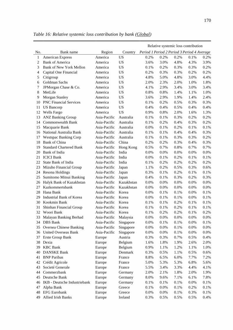
170
Table 16: Relative systemic loss contribution by bank (Global)
Relative systemic loss contribution
No. Bank name Region Country Period 1 Period 2 Period 3 Period 4 Average 1 American Express America US 0.2% 0.2% 0.2% 0.1% 0.2%2 Bank of America America US 3.6% 3.0% 4.8% 4.3% 3.9%3 Bank of New York Mellon America US 0.1% 0.2% 0.3% 0.3% 0.2%4 Capital One Financial America US 0.2% 0.3% 0.3% 0.2% 0.2%5 Citigroup America US 4.8% 5.0% 4.8% 3.0% 4.4%6 Goldman Sachs America US 2.0% 2.3% 2.0% 1.0% 1.8%7 JPMorgan Chase & Co. America US 4.1% 2.9% 3.4% 3.0% 3.4%8 MetLife America US 0.8% 0.8% 1.4% 1.1% 1.0%9 Morgan Stanley America US 3.6% 2.9% 1.9% 1.4% 2.4%10 PNC Financial Services America US 0.1% 0.2% 0.5% 0.3% 0.3%11 US Bancorp America US 0.4% 0.4% 0.5% 0.4% 0.4%12 Wells Fargo America US 0.9% 0.8% 2.0% 1.6% 1.3%13 ANZ Banking Group Asia-Pacific Australia 0.1% 0.1% 0.3% 0.2% 0.2%14 Commonwealth Bank Asia-Pacific Australia 0.1% 0.2% 0.4% 0.3% 0.2%15 Macquarie Bank Asia-Pacific Australia 0.0% 0.1% 0.2% 0.1% 0.1%16 National Australia Bank Asia-Pacific Australia 0.1% 0.1% 0.4% 0.4% 0.3%17 Westspac Banking Corp Asia-Pacific Australia 0.1% 0.1% 0.3% 0.3% 0.2%18 Bank of China Asia-Pacific China 0.2% 0.2% 0.3% 0.4% 0.3%19 Standard Chartered Bank Asia-Pacific Hong Kong 0.5% 0.7% 0.8% 0.7% 0.7%20 Bank of India Asia-Pacific India 0.0% 0.0% 0.0% 0.0% 0.0%21 ICICI Bank Asia-Pacific India 0.0% 0.1% 0.2% 0.1% 0.1%22 State Bank of India Asia-Pacific India 0.1% 0.2% 0.2% 0.2% 0.2%23 Mizuho Financial Group Asia-Pacific Japan 1.1% 0.2% 0.5% 0.3% 0.6%24 Resona Holdings Asia-Pacific Japan 0.3% 0.1% 0.2% 0.1% 0.1%25 Sumitomo Mitsui Banking Asia-Pacific Japan 0.4% 0.1% 0.3% 0.2% 0.3%26 Halyk Bank of Kazakhstan Asia-Pacific Kazakhstan 0.0% 0.0% 0.0% 0.0% 0.0%27 Kazkommertsbank Asia-Pacific Kazakhstan 0.0% 0.0% 0.0% 0.0% 0.0%28 Hana Bank Asia-Pacific Korea 0.0% 0.1% 0.1% 0.0% 0.1%29 Industrial Bank of Korea Asia-Pacific Korea 0.0%0.1% 0.1% 0.0% 0.1%30 Kookmin Bank Asia-Pacific Korea 0.1% 0.1% 0.2% 0.1% 0.1%31 Shinhan Financial Group Asia-Pacific Korea 0.1% 0.1% 0.2% 0.1% 0.1%32 Woori Bank Asia-Pacific Korea 0.1% 0.2% 0.2% 0.1% 0.2%33 Malayan Banking Berhad Asia-Pacific Malaysia 0.0% 0.0% 0.0% 0.0% 0.0%34 DBS Bank Asia-Pacific Singapore 0.0% 0.1% 0.1% 0.0% 0.1%35 Oversea Chinese Banking Asia-Pacific Singapore 0.0% 0.0% 0.1% 0.0% 0.0%36 United Overseas Bank Asia-Pacific Singapore 0.0%0.0% 0.1% 0.0% 0.0%37 Erste Group Bank Europe Austria 0.3% 0.3% 0.7% 0.5% 0.4%38 Dexia Europe Belgium 1.6% 1.8% 1.9% 2.6% 2.0%39 KBC Bank Europe Belgium 0.9% 1.1% 1.2% 1.1% 1.0%40 DANSKE Bank Europe Denmark 0.3% 0.5% 1.1% 0.5% 0.6%41 BNP Paribas Europe France 8.8% 6.5% 6.0% 7.7% 7.2%42 Crédit Agricole Europe France 5.0% 5.3% 5.3% 6.8% 5.6%43 Societé Generale Europe France 5.5% 3.4% 3.3% 4.4% 4.1%44 Commerzbank Europe Germany 2.0% 2.1% 1.8% 2.0% 1.9%45 Deutsche Bank Europe Germany 8.0% 9.6% 7.1% 6.1% 7.8%46 IKB - Deutsche Industriebank Europe Germany 0.1%0.1% 0.1% 0.0% 0.1%47 Alpha Bank Europe Greece 0.1% 0.0% 0.1% 0.2% 0.1%48 EFG Eurobank Europe Greece 0.0% 0.0% 0.1% 0.3% 0.1%49 Allied Irish Banks Europe Ireland 0.3% 0.5% 0.5% 0.5% 0.4%

171
Relative systemic loss contribution
No. Bank name Region Country Period 1 Period 2 Period 3 Period 4 Average 50 Bank of Ireland Europe Ireland 0.1% 0.4% 0.5% 0.4% 0.4%51 Banca Monte d.P. die Siena Europe Italy 0.3% 0.4% 0.4% 0.8% 0.5%52 Banco Popolare Europe Italy 0.2% 0.2% 0.3% 0.4% 0.3%53 Intesa Sanpaolo Europe Italy 0.5% 1.1% 1.4% 2.1% 1.3%54 Unicredit Group Europe Italy 4.0% 2.9% 3.2% 3.4% 3.4%55 SNS REAAL Bank Europe Netherlands 0.1% 0.1% 0.5% 0.4% 0.3%56 Banco BPI Europe Portugal 0.0% 0.0% 0.1% 0.2% 0.1%57 Banco Comercial Portuges Europe Portugal 0.0% 0.1% 0.1% 0.4% 0.2%58 Espirito Santo Financial Group Europe Portugal 0.0% 0.1% 0.1% 0.3% 0.1%59 Banco de Sabadell Europe Spain 0.2% 0.2% 0.3% 0.3% 0.3%60 Banco Pastor Europe Spain 0.0% 0.0% 0.1% 0.1% 0.0%61 Banco Popular Europe Spain 0.2% 0.2% 0.5% 0.5% 0.3%62 Bankinter Europe Spain 0.1% 0.1% 0.1% 0.2% 0.1%63 Grupo BBVA Europe Spain 0.7% 0.4% 0.7% 1.4% 0.8%64 Grupo Santander Europe Spain 4.8% 2.9% 3.5% 4.8% 4.0%65 Nordea Europe Sweden 0.9% 0.7% 1.2% 0.9% 0.9%66 Skand Enskilda Banken Europe Sweden 0.7% 0.4% 0.7% 0.4% 0.6%67 Svenska Handelsbanken Europe Sweden 0.5% 0.2% 0.4% 0.3% 0.4%68 Swedbank Europe Sweden 0.5% 0.3% 0.5% 0.3% 0.4%69 Crédit Suisse Europe Switzerland 4.0% 3.1% 2.2% 1.9% 2.8%70 UBS Europe Switzerland 5.8% 5.4% 4.4% 2.5% 4.6%71 Barclay's Europe UK 7.2% 8.7% 6.6% 6.0% 7.2%72 HSBC Europe UK 5.6% 5.5% 4.9% 4.3% 5.1%73 Lloyds Banking Group Europe UK 1.1% 1.5% 2.5% 7.7% 3.1%74 Royal Bank of Scotland Europe UK 4.7% 11.6% 7.4% 6.2% 7.5%75 Arab Banking Corp Middle East Bahrain 0.0% 0.0% 0.0% 0.0% 0.0%76 Commercial Bank of Qatar Middle East Qatar 0.0% 0.0% 0.0% 0.0% 0.0%77 Abu Dhabi Commercial Bank Middle East UAE 0.0% 0.0% 0.0% 0.0% 0.0%78 Dubai Islamic Bank Middle East UAE 0.0% 0.0% 0.0% 0.0% 0.0%79 Mashreqbank Middle East UAE 0.0% 0.0% 0.0% 0.0% 0.0%80 National Bank of Abu Dhabi Middle East UAE 0.0% 0.0% 0.0% 0.0% 0.0%81 Bank of Moscow Russia Russia 0.0% 0.0% 0.1% 0.0% 0.0%82 Sberbank Russia Russia 0.3% 0.3% 0.5% 0.3% 0.3%83 WTB/VTB (Wneschtorgbank) Russia Russia 0.0% 0.1% 0.3% 0.2% 0.1%
Notes: Relative systemic loss contribution is defined as the relative loss share of a bank when the total portfolio loss exceeds the systemic loss threshold. Period 1 ranges from October 1st, 2005 to February 28th, 2007, Period 2 ranges from March 1st, 2007 to July 31st, 2008, Period 3 ranges from August 1st, 2008 to December 31st, 2009, Period 4 ranges from January 1st, 2010 to April 30th, 2011.
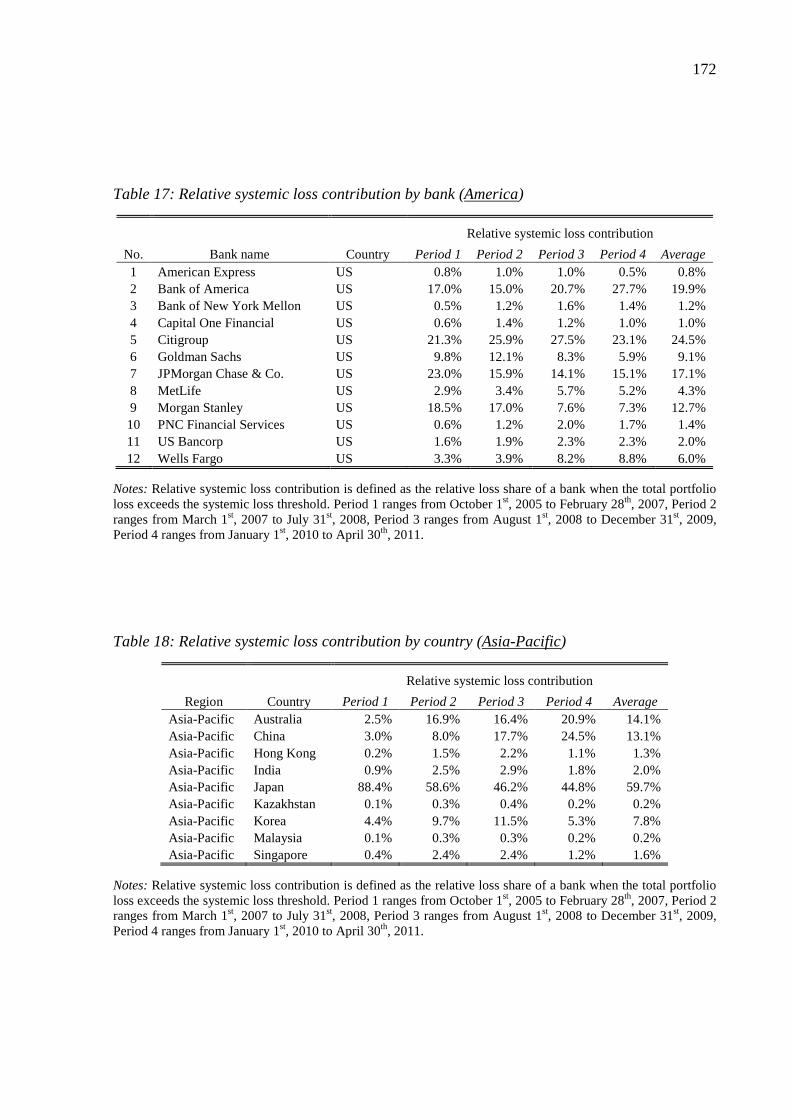
172
Table 17: Relative systemic loss contribution by bank (America)
Relative systemic loss contribution
No. Bank name Country Period 1 Period 2 Period 3 Period 4 Average 1 American Express US 0.8% 1.0% 1.0% 0.5% 0.8% 2 Bank of America US 17.0% 15.0% 20.7% 27.7% 19.9% 3 Bank of New York Mellon US 0.5% 1.2% 1.6% 1.4% 1.2% 4 Capital One Financial US 0.6% 1.4% 1.2% 1.0% 1.0% 5 Citigroup US 21.3% 25.9% 27.5% 23.1% 24.5% 6 Goldman Sachs US 9.8% 12.1% 8.3% 5.9% 9.1% 7 JPMorgan Chase & Co. US 23.0% 15.9% 14.1% 15.1% 17.1% 8 MetLife US 2.9% 3.4% 5.7% 5.2% 4.3% 9 Morgan Stanley US 18.5% 17.0% 7.6% 7.3% 12.7% 10 PNC Financial Services US 0.6% 1.2% 2.0% 1.7% 1.4% 11 US Bancorp US 1.6% 1.9% 2.3% 2.3% 2.0% 12 Wells Fargo US 3.3% 3.9% 8.2% 8.8% 6.0%
Notes: Relative systemic loss contribution is defined as the relative loss share of a bank when the total portfolio loss exceeds the systemic loss threshold. Period 1 ranges from October 1st, 2005 to February 28th, 2007, Period 2 ranges from March 1st, 2007 to July 31st, 2008, Period 3 ranges from August 1st, 2008 to December 31st, 2009, Period 4 ranges from January 1st, 2010 to April 30th, 2011.
Table 18: Relative systemic loss contribution by country (Asia-Pacific)
Relative systemic loss contribution
Region Country Period 1 Period 2 Period 3 Period 4 Average Asia-Pacific Australia 2.5% 16.9% 16.4% 20.9% 14.1% Asia-Pacific China 3.0% 8.0% 17.7% 24.5% 13.1% Asia-Pacific Hong Kong 0.2% 1.5% 2.2% 1.1% 1.3% Asia-Pacific India 0.9% 2.5% 2.9% 1.8% 2.0% Asia-Pacific Japan 88.4% 58.6% 46.2% 44.8% 59.7% Asia-Pacific Kazakhstan 0.1% 0.3% 0.4% 0.2% 0.2% Asia-Pacific Korea 4.4% 9.7% 11.5% 5.3% 7.8% Asia-Pacific Malaysia 0.1% 0.3% 0.3% 0.2% 0.2% Asia-Pacific Singapore 0.4% 2.4% 2.4% 1.2% 1.6%
Notes: Relative systemic loss contribution is defined as the relative loss share of a bank when the total portfolio loss exceeds the systemic loss threshold. Period 1 ranges from October 1st, 2005 to February 28th, 2007, Period 2 ranges from March 1st, 2007 to July 31st, 2008, Period 3 ranges from August 1st, 2008 to December 31st, 2009, Period 4 ranges from January 1st, 2010 to April 30th, 2011.

173
Table 19: Relative systemic loss contribution by bank (Asia-Pacific)
Relative systemic loss contribution
No. Bank name Country Period 1 Period 2 Period 3 Period 4 Average 1 ANZ Banking Group Australia 0.2% 2.1% 2.2% 3.2% 1.9% 2 Commonwealth Bank Australia 0.7% 4.2% 3.9% 5.3% 3.5% 3 Macquarie Bank Australia 0.2% 1.5% 1.6% 1.0% 1.1% 4 National Australia Bank Australia 1.0% 5.6% 5.1% 6.1% 4.4% 5 Westspac Banking Corp Australia 0.4% 3.5% 3.6% 5.2% 3.2% 6 Bank of China China 3.0% 8.0% 17.7% 24.5% 13.1% 7 Standard Chartered Bank Hong Kong 0.2% 1.5% 2.2% 1.1% 1.3% 8 Bank of India India 0.1% 0.2% 0.2% 0.2% 0.2% 9 ICICI Bank India 0.2% 1.0% 1.1% 0.4% 0.7% 10 State Bank of India India 0.5% 1.3% 1.6% 1.1% 1.2% 11 Mizuho Financial Group Japan 58.1% 35.1% 27.4% 27.1% 37.1% 12 Resona Holdings Japan 8.5% 5.8% 4.5% 2.2% 5.3% 13 Sumitomo Mitsui Banking Japan 21.8% 17.7% 14.3% 15.5% 17.3% 14 Halyk Bank of Kazakhstan Kazakhstan 0.0% 0.1% 0.2% 0.1% 0.1% 15 Kazkommertsbank Kazakhstan 0.1% 0.2% 0.2% 0.1% 0.1% 16 Hana Bank Korea 1.0% 1.1% 1.4% 0.7% 1.1% 17 Industrial Bank of Korea Korea 0.4% 1.0% 1.4% 0.7% 0.9% 18 Kookmin Bank Korea 1.1% 2.4% 2.8% 1.3% 1.9% 19 Shinhan Financial Group Korea 0.8% 2.4% 2.9% 1.2% 1.8% 20 Woori Bank Korea 1.0% 2.8% 3.0% 1.5% 2.1% 21 Malayan Banking Berhad Malaysia 0.1% 0.3% 0.3% 0.2% 0.2% 22 DBS Bank Singapore 0.2% 1.1% 1.1% 0.5% 0.7% 23 Oversea Chinese Banking Singapore 0.1% 0.7% 0.7% 0.4% 0.5% 24 United Overseas Bank Singapore 0.1% 0.6% 0.7% 0.3% 0.5%
Notes: Relative systemic loss contribution is defined as the relative loss share of a bank when the total portfolio loss exceeds the systemic loss threshold. Period 1 ranges from October 1st, 2005 to February 28th, 2007, Period 2 ranges from March 1st, 2007 to July 31st, 2008, Period 3 ranges from August 1st, 2008 to December 31st, 2009, Period 4 ranges from January 1st, 2010 to April 30th, 2011.

174
Table 20: Relative systemic loss contribution by country (Europe)
Relative systemic loss contribution
Country Period 1 Period 2 Period 3 Period 4 Average Austria 0.4% 0.4% 0.9% 0.7% 0.6% Belgium 3.2% 3.7% 4.3% 4.7% 4.0% Denmark 0.4% 0.6% 1.5% 0.6% 0.8% France 25.7% 19.6% 20.2% 23.2% 22.2% Germany 13.5% 13.5% 11.9% 9.4% 12.1% Greece 0.1% 0.1% 0.2% 0.6% 0.3% Ireland 0.5% 1.1% 1.3% 1.4% 1.0% Italy 6.7% 5.9% 7.0% 8.7% 7.0% Netherlands 0.1% 0.1% 0.7% 0.5% 0.3% Portugal 0.1% 0.3% 0.5% 1.2% 0.5% Spain 8.0% 4.8% 7.1% 9.8% 7.4% Sweden 3.5% 2.1% 3.9% 2.4% 3.0% Switzerland 13.7% 11.1% 9.1% 5.3% 9.9% UK 24.3% 36.8% 31.6% 31.4% 31.1%
Notes: Relative systemic loss contribution is defined as the relative loss share of a bank when the total portfolio loss exceeds the systemic loss threshold. Period 1 ranges from October 1st, 2005 to February 28th, 2007, Period 2 ranges from March 1st, 2007 to July 31st, 2008, Period 3 ranges from August 1st, 2008 to December 31st, 2009, Period 4 ranges from January 1st, 2010 to April 30th, 2011.
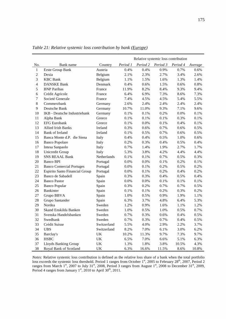
175
Table 21: Relative systemic loss contribution by bank (Europe)
Relative systemic loss contribution
No. Bank name Country Period 1 Period 2 Period 3 Period 4 Average 1 Erste Group Bank Austria 0.4% 0.4% 0.9% 0.7% 0.6% 2 Dexia Belgium 2.1% 2.3% 2.7% 3.4% 2.6% 3 KBC Bank Belgium 1.1% 1.5% 1.6% 1.3% 1.4% 4 DANSKE Bank Denmark 0.4% 0.6% 1.5% 0.6% 0.8% 5 BNP Paribas France 11.9% 8.2% 8.4% 9.3% 9.4% 6 Crédit Agricole France 6.4% 6.9% 7.3% 8.6% 7.3% 7 Societé Generale France 7.4% 4.5% 4.5% 5.4% 5.5% 8 Commerzbank Germany 2.6% 2.4% 2.4% 2.4% 2.4% 9 Deutsche Bank Germany 10.7% 11.0% 9.3% 7.1% 9.6% 10 IKB - Deutsche Industriebank Germany 0.1% 0.1% 0.2% 0.0% 0.1% 11 Alpha Bank Greece 0.1% 0.1% 0.1% 0.3% 0.1% 12 EFG Eurobank Greece 0.1% 0.0% 0.1% 0.4% 0.1% 13 Allied Irish Banks Ireland 0.3% 0.6% 0.7% 0.6% 0.5% 14 Bank of Ireland Ireland 0.1% 0.5% 0.7% 0.6% 0.5% 15 Banca Monte d.P. die Siena Italy 0.4% 0.4% 0.5% 1.0% 0.6% 16 Banco Popolare Italy 0.2% 0.3% 0.4% 0.5% 0.4% 17 Intesa Sanpaolo Italy 0.7% 1.4% 1.9% 2.7% 1.7% 18 Unicredit Group Italy 5.3% 3.8% 4.2% 4.4% 4.4% 19 SNS REAAL Bank Netherlands 0.1% 0.1% 0.7% 0.5% 0.3% 20 Banco BPI Portugal 0.0% 0.0% 0.1% 0.2% 0.1% 21 Banco Comercial Portuges Portugal 0.0% 0.1% 0.2% 0.5% 0.2% 22 Espirito Santo Financial Group Portugal 0.0% 0.1% 0.2% 0.4% 0.2% 23 Banco de Sabadell Spain 0.3% 0.3% 0.4% 0.5% 0.4% 24 Banco Pastor Spain 0.0% 0.0% 0.1% 0.1% 0.1% 25 Banco Popular Spain 0.3% 0.2% 0.7% 0.7% 0.5% 26 Bankinter Spain 0.1% 0.1% 0.2% 0.3% 0.2% 27 Grupo BBVA Spain 1.0% 0.5% 0.9% 1.9% 1.1% 28 Grupo Santander Spain 6.3% 3.7% 4.8% 6.4% 5.3% 29 Nordea Sweden 1.2% 0.9% 1.6% 1.1% 1.2% 30 Skand Enskilda Banken Sweden 1.0% 0.5% 1.0% 0.5% 0.7% 31 Svenska Handelsbanken Sweden 0.7% 0.3% 0.6% 0.4% 0.5% 32 Swedbank Sweden 0.7% 0.3% 0.7% 0.4% 0.5% 33 Crédit Suisse Switzerland 5.5% 4.0% 2.9% 2.2% 3.7% 34 UBS Switzerland 8.2% 7.0% 6.1% 3.0% 6.2% 35 Barclay's UK 10.2% 11.3% 9.7% 7.3% 9.7% 36 HSBC UK 6.5% 7.0% 6.6% 5.1% 6.3% 37 Lloyds Banking Group UK 1.3% 1.8% 3.8% 10.5% 4.3% 38 Royal Bank of Scotland UK 6.3% 16.6% 11.5% 8.6% 10.8%
Notes: Relative systemic loss contribution is defined as the relative loss share of a bank when the total portfolio loss exceeds the systemic loss threshold. Period 1 ranges from October 1st, 2005 to February 28th, 2007, Period 2 ranges from March 1st, 2007 to July 31st, 2008, Period 3 ranges from August 1st, 2008 to December 31st, 2009, Period 4 ranges from January 1st, 2010 to April 30th, 2011.

176
Table 22: Relative systemic loss contribution by country (Middle East and Russia)
Relative systemic loss contribution
Country Period 1 Period 2 Period 3 Period 4 Average Bahrain 0.8% 0.7% 1.0% 1.3% 1.0% Qatar 0.1% 0.2% 0.5% 0.6% 0.3% UAE 3.5% 3.0% 8.0% 10.2% 6.1% Russia 95.6% 96.1% 90.5% 88.0% 92.6%
Notes: Relative systemic loss contribution is defined as the relative loss share of a bank when the total portfolio loss exceeds the systemic loss threshold. Period 1 ranges from October 1st, 2005 to February 28th, 2007, Period 2 ranges from March 1st, 2007 to July 31st, 2008, Period 3 ranges from August 1st, 2008 to December 31st, 2009, Period 4 ranges from January 1st, 2010 to April 30th, 2011.
Table 23: Relative systemic loss contribution by bank (Middle East and Russia)
Relative systemic loss contribution
No. Bank name Country Period 1 Period 2 Period 3 Period 4 Average 1 Arab Banking Corp Bahrain 0.8% 0.7% 1.0% 1.3% 1.0% 2 Commercial Bank of Qatar Qatar 0.1% 0.2% 0.5% 0.6% 0.3% 3 Abu Dhabi Commercial Bank UAE 1.1% 0.9% 2.5% 3.4% 1.9% 4 Dubai Islamic Bank UAE 0.8% 0.5% 1.7% 1.7% 1.2% 5 Mashreqbank UAE 0.2% 0.5% 0.9% 1.4% 0.7% 6 National Bank of Abu Dhabi UAE 1.4% 1.1% 2.9% 3.7% 2.3% 7 Bank of Moscow Russia 1.4% 2.6% 4.6% 4.5% 3.2% 8 Sberbank Russia 73.5% 67.3% 49.3% 53.3% 61.0% 9 WTB/VTB (Wneschtorgbank) Russia 20.7% 26.2% 36.6% 30.2% 28.4%
Notes: Relative systemic loss contribution is defined as the relative loss share of a bank when the total portfolio loss exceeds the systemic loss threshold. Period 1 ranges from October 1st, 2005 to February 28th, 2007, Period 2 ranges from March 1st, 2007 to July 31st, 2008, Period 3 ranges from August 1st, 2008 to December 31st, 2009, Period 4 ranges from January 1st, 2010 to April 30th, 2011.

177
Table 24: Determinants of the relative contributions to the ESS-indicator (Global)
Independent variables Regression 1 Regression 2 Regression 3
Constant term 0 0.01 0.00 0.00 0.00 0.00
0 (172.74) 0.00 (105.11) 0.00 (119.41)
Risk-neutral PD 0 -0.11 0.00 0.00 0.00 0.05
0 (75.77) 0.00 (0.00) 1.05 (80.01)
Liability weight 0 0.00 0.00 1.26 0.00 1.28
0 (0.00) 0.00 (302.20) 1.05 (307.16)
Average correlation 0 0.00 0.00 0.00 0.00 0.00
0 (0.00) 0.00 (0.00) 0.00 (0.00)
Adjusted-R² 0 0.02 0.00 0.77 0.00 0.78 Regression 4 Regression 5 Regression 6
Constant term 0.00 -0.01 0.00 0.00 0.00 0.00
0.00 (135.50) 0.00 (82.15) 0.00 (52.66)
Risk-neutral PD 0.00 0.06 0.00 0.00 0.00 0.04
1.05 (86.93) 0.00 (0.00) 1.29 (43.23)
Liability weight 0.00 1.23 0.00 0.59 0.00 0.63
1.16 (282.42) 6.28 (58.55) 8.20 (54.76)
Average correlation 0.00 0.02 0.00 0.00 0.00 0.00
1.12 (80.50) 0.00 (0.00) 1.64 (4.24)
Risk-neutral PD*liability weight 0.00 0.00 0.00 2.06 0.00 0.38
0.00 (0.00) 1.75 (7.81) 2.11 (1.25)
Average correlation*liability weight 0.00 0.00 0.00 1.98 0.00 1.99
0.00 (0.00) 5.97 (81.40) 8.66 (70.22)
Adjusted-R² 0.00 0.79 0.00 0.81 0.00 0.82
Notes: The dependent regression variable is the relative contribution to the ESS-indicator of each bank i (in percentage terms) over time. Independent variables are the risk-neutral default probability, the percentage weight (share) of total liabilities, the bank-specific correlations (average of bilateral correlations of one bank with all other banks) as well as interaction terms of each bank i over time. Variance inflation factors are provided in italics. Heteroskedacity-consistent t-statistics are shown in parenthesis. Critical values for the t-statistic at the ten, five and one percent significance level are respectively 1.28, 1.65 and 2.33.

178
Table 25: Determinants of the relative contributions to the ESS-indicator (America)
Independent variables Regression 1 Regression 2 Regression 3
Constant term 0 0.09 0.00 -0.01 0.00 -0.02
0 (90.89) 0.00 (53.60) 0.00 (54.11)
Risk-neutral PD 0 -0.17 0.00 0.00 0.00 0.40
0 (4.86) 0.00 (0.00) 1.02 (33.93)
Liability weight 0 0.00 0.00 1.13 0.00 1.14
0 (0.00) 0.00 (258.94) 1.02 (265.76)
Average correlation 0 0.00 0.00 0.00 0.00 0.00
0 (0.00) 0.00 (0.00) 0.00 (0.00)
Adjusted-R² 0 0.00 0.00 0.87 0.00 0.87 Regression 4 Regression 5 Regression 6
Constant term 0.00 0.00 0.00 -0.01 0.00 -0.05
0.00 (1.17) 0.00 (67.50) 0.00 (41.44)
Risk-neutral PD 0.00 0.46 0.00 0.00 0.00 -0.07
1.10 (35.19) 0.00 (0.00) 2.56 (7.27)
Liability weight 0.00 1.15 0.00 1.52 0.00 1.81
1.05 (263.91) 18.78 (77.47) 38.44 (75.61)
Average correlation 0.00 -0.04 0.00 0.00 0.00 0.06
1.10 (14.68) 0.00 (0.00) 2.58 (32.53)
Risk-neutral PD*liability weight 0.00 0.00 0.00 6.31 0.00 6.74
0.00 (0.00) 1.47 (36.90) 3.37 (29.29)
Average correlation*liability weight 0.00 0.00 0.00 -0.70 0.00 -1.15
0.00 (0.00) 18.95 (25.64) 43.79 (33.68)
Adjusted-R² 0.00 0.88 0.00 0.89 0.00 0.89
Notes: The dependent regression variable is the relative contribution to the ESS-indicator of each bank i (in percentage terms) over time. Independent variables are the risk-neutral default probability, the percentage weight (share) of total liabilities, the bank-specific correlations (average of bilateral correlations of one bank with all other banks) as well as interaction terms of each bank i over time. Variance inflation factors are provided in italics. Heteroskedacity-consistent t-statistics are shown in parenthesis. Critical values for the t-statistic at the ten, five and one percent significance level are respectively 1.28, 1.65 and 2.33.
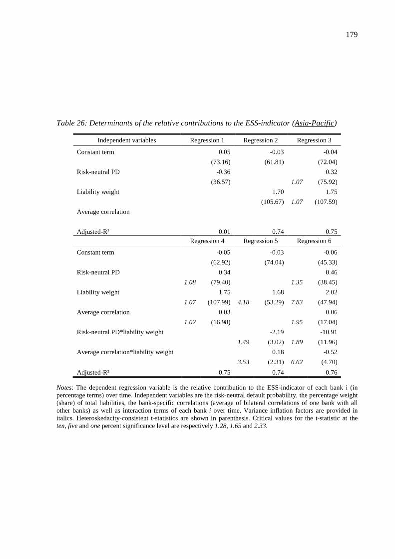
179
Table 26: Determinants of the relative contributions to the ESS-indicator (Asia-Pacific)
Independent variables Regression 1 Regression 2 Regression 3
Constant term 0 0.05 0.00 -0.03 0.00 -0.04
0 (73.16) 0.00 (61.81) 0.00 (72.04)
Risk-neutral PD 0 -0.36 0.00 0.00 0.00 0.32
0 (36.57) 0.00 (0.00) 1.07 (75.92)
Liability weight 0 0.00 0.00 1.70 0.00 1.75
0 (0.00) 0.00 (105.67) 1.07 (107.59)
Average correlation 0 0.00 0.00 0.00 0.00 0.00
0 (0.00) 0.00 (0.00) 0.00 (0.00)
Adjusted-R² 0 0.01 0.00 0.74 0.00 0.75 Regression 4 Regression 5 Regression 6
Constant term 0.00 -0.05 0.00 -0.03 0.00 -0.06
0.00 (62.92) 0.00 (74.04) 0.00 (45.33)
Risk-neutral PD 0.00 0.34 0.00 0.00 0.00 0.46
1.08 (79.40) 0.00 (0.00) 1.35 (38.45)
Liability weight 0.00 1.75 0.00 1.68 0.00 2.02
1.07 (107.99) 4.18 (53.29) 7.83 (47.94)
Average correlation 0.00 0.03 0.00 0.00 0.00 0.06
1.02 (16.98) 0.00 (0.00) 1.95 (17.04)
Risk-neutral PD*liability weight 0.00 0.00 0.00 -2.19 0.00 -10.91
0.00 (0.00) 1.49 (3.02) 1.89 (11.96)
Average correlation*liability weight 0.00 0.00 0.00 0.18 0.00 -0.52
0.00 (0.00) 3.53 (2.31) 6.62 (4.70)
Adjusted-R² 0.00 0.75 0.00 0.74 0.00 0.76
Notes: The dependent regression variable is the relative contribution to the ESS-indicator of each bank i (in percentage terms) over time. Independent variables are the risk-neutral default probability, the percentage weight (share) of total liabilities, the bank-specific correlations (average of bilateral correlations of one bank with all other banks) as well as interaction terms of each bank i over time. Variance inflation factors are provided in italics. Heteroskedacity-consistent t-statistics are shown in parenthesis. Critical values for the t-statistic at the ten, five and one percent significance level are respectively 1.28, 1.65 and 2.33.

180
Table 27: Determinants of the relative contributions to the ESS-indicator (Europe)
Independent variables Regression 1 Regression 2 Regression 3
Constant term 0 0.03 0.00 0.00 0.00 -0.01
0 (153.83) 0.00 (76.04) 0.00 (86.89)
Risk-neutral PD 0 -0.22 0.00 0.00 0.00 0.08
0 (52.40) 0.00 (0.00) 1.04 (54.93)
Liability weight 0 0.00 0.00 1.17 0.00 1.18
0 (0.00) 0.00 (313.41) 1.04 (319.04)
Average correlation 0 0.00 0.00 0.00 0.00 0.00
0 (0.00) 0.00 (0.00) 0.00 (0.00)
Adjusted-R² 0 0.02 0.00 0.85 0.00 0.85 Regression 4 Regression 5 Regression 6
Constant term 0.00 -0.01 0.00 0.00 0.00 -0.01
0.00 (72.23) 0.00 (74.41) 0.00 (39.30)
Risk-neutral PD 0.00 0.08 0.00 0.00 0.00 0.07
1.04 (57.53) 0.00 (0.00) 1.36 (37.40)
Liability weight 0.00 1.16 0.00 0.85 0.00 0.90
1.11 (297.29) 9.05 (62.55) 12.84 (56.95)
Average correlation 0.00 0.01 0.00 0.00 0.00 0.00
1.07 (36.78) 0.00 (0.00) 1.69 (6.79)
Risk-neutral PD*liability weight 0.00 0.00 0.00 2.07 0.00 0.13
0.00 (0.00) 1.76 (8.23) 2.30 (0.44)
Average correlation*liability weight 0.00 0.00 0.00 0.57 0.00 0.53
0.00 (0.00) 9.24 (26.31) 14.40 (20.40)
Adjusted-R² 0.00 0.86 0.00 0.86 0.00 0.86
Notes: The dependent regression variable is the relative contribution to the ESS-indicator of each bank i (in percentage terms) over time. Independent variables are the risk-neutral default probability, the percentage weight (share) of total liabilities, the bank-specific correlations (average of bilateral correlations of one bank with all other banks) as well as interaction terms of each bank i over time. Variance inflation factors are provided in italics. Heteroskedacity-consistent t-statistics are shown in parenthesis. Critical values for the t-statistic at the ten, five and one percent significance level are respectively 1.28, 1.65 and 2.33.
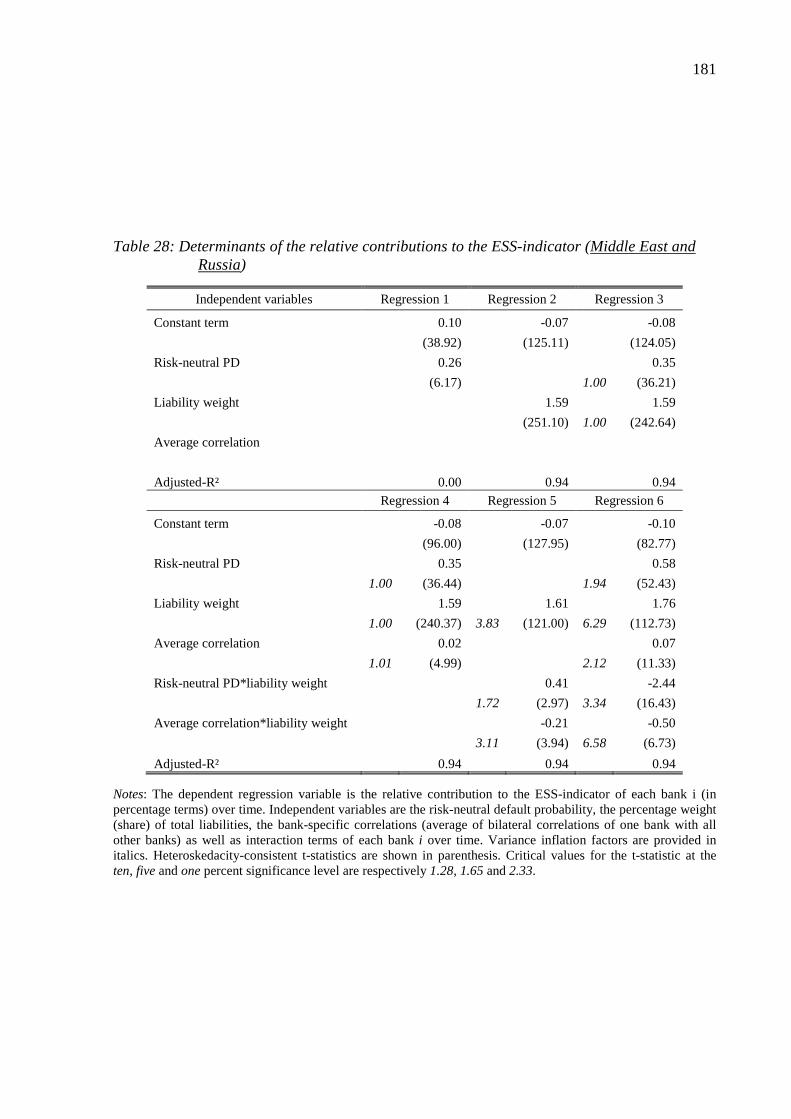
181
Table 28: Determinants of the relative contributions to the ESS-indicator (Middle East and Russia)
Independent variables Regression 1 Regression 2 Regression 3
Constant term 0 0.10 0.00 -0.07 0.00 -0.08
0 (38.92) 0.00 (125.11) 0.00 (124.05)
Risk-neutral PD 0 0.26 0.00 0.00 0.00 0.35
0 (6.17) 0.00 (0.00) 1.00 (36.21)
Liability weight 0 0.00 0.00 1.59 0.00 1.59
0 (0.00) 0.00 (251.10) 1.00 (242.64)
Average correlation 0 0.00 0.00 0.00 0.00 0.00
0 (0.00) 0.00 (0.00) 0.00 (0.00)
Adjusted-R² 0 0.00 0.00 0.94 0.00 0.94 Regression 4 Regression 5 Regression 6
Constant term 0.00 -0.08 0.00 -0.07 0.00 -0.10
0.00 (96.00) 0.00 (127.95) 0.00 (82.77)
Risk-neutral PD 0.00 0.35 0.00 0.00 0.00 0.58
1.00 (36.44) 0.00 (0.00) 1.94 (52.43)
Liability weight 0.00 1.59 0.00 1.61 0.00 1.76
1.00 (240.37) 3.83 (121.00) 6.29 (112.73)
Average correlation 0.00 0.02 0.00 0.00 0.00 0.07
1.01 (4.99) 0.00 (0.00) 2.12 (11.33)
Risk-neutral PD*liability weight 0.00 0.00 0.00 0.41 0.00 -2.44
0.00 (0.00) 1.72 (2.97) 3.34 (16.43)
Average correlation*liability weight 0.00 0.00 0.00 -0.21 0.00 -0.50
0.00 (0.00) 3.11 (3.94) 6.58 (6.73)
Adjusted-R² 0.00 0.94 0.00 0.94 0.00 0.94
Notes: The dependent regression variable is the relative contribution to the ESS-indicator of each bank i (in percentage terms) over time. Independent variables are the risk-neutral default probability, the percentage weight (share) of total liabilities, the bank-specific correlations (average of bilateral correlations of one bank with all other banks) as well as interaction terms of each bank i over time. Variance inflation factors are provided in italics. Heteroskedacity-consistent t-statistics are shown in parenthesis. Critical values for the t-statistic at the ten, five and one percent significance level are respectively 1.28, 1.65 and 2.33.

182
Table 29: Granger causality test results for inter-regional relative ESS analysis
Without control variables
Period 1 Period 2 Period 3 Period 4 Systemic risk causality direction F-Stat p-val F-Stat p-val F-Stat p-val F-Stat p-val
America ~→ Asia-Pacific 1.080% 0.36 1.400% 0.24 17.83*** 0.00 15.30*** 0.00Asia-Pacific ~→ America 1.630% 0.18 0.430% 0.73 0.630% 0.60 0.020% 1.00America ~→ Europe 0.050% 0.99 5.44*** 0.00 12.38*** 0.00 5.26*** 0.00Europe ~→ America 1.240% 0.29 1.330% 0.26 0.710% 0.55 0.940% 0.42America ~→ Middle East & Russia 0.610% 0.61 0.230% 0.88 7.72*** 0.00 7.09*** 0.00Middle East & Russia ~→ America 0.190% 0.90 2.11* 0.10 2.84** 0.04 1.640% 0.18Asia-Pacific ~→ Europe 0.900% 0.44 3.63** 0.01 1.000% 0.39 1.420% 0.24Europe ~→ Asia-Pacific 3.32** 0.02 4.23*** 0.01 11.17*** 0.00 6.45*** 0.00Asia-Pacific ~→ Middle East & Russia 1.030% 0.38 0.630% 0.60 1.460% 0.23 2.15* 0.09Middle East & Russia ~→ Asia-Pacific 1.340% 0.26 0.120% 0.95 8.87*** 0.00 2.93** 0.03Europe ~→ Middle East & Russia 0.470% 0.70 4.07*** 0.01 3.27** 0.02 8.82*** 0.00Middle East & Russia ~→ Europe 4.29*** 0.01 0.390% 0.76 0.340% 0.79 0.970% 0.41
Incl. stock index and federal funds rate
Period 1 Period 2 Period 3 Period 4 Systemic risk causality direction F-Stat p-val F-Stat p-val F-Stat p-val F-Stat p-val
America ~→ Asia-Pacific 0.950% 0.42 1.360% 0.26 16.85*** 0.00 13.53*** 0.00Asia-Pacific ~→ America 1.900% 0.13 0.340% 0.80 0.730% 0.54 0.100% 0.96America ~→ Europe 0.190% 0.90 3.76** 0.01 12.34*** 0.00 5.98*** 0.00Europe ~→ America 0.770% 0.51 1.270% 0.29 1.290% 0.28 0.810% 0.49America ~→ Middle East & Russia 0.440% 0.72 0.530% 0.66 7.04*** 0.00 5.88*** 0.00Middle East & Russia ~→ America 0.150% 0.93 1.990% 0.11 2.91** 0.03 1.390% 0.25Asia-Pacific ~→ Europe 1.040% 0.37 3.90*** 0.01 0.920% 0.43 1.680% 0.17Europe ~→ Asia-Pacific 2.90** 0.03 6.04*** 0.00 10.11*** 0.00 4.74*** 0.00Asia-Pacific ~→ Middle East & Russia 0.580% 0.63 0.740% 0.53 1.620% 0.19 0.720% 0.54Middle East & Russia ~→ Asia-Pacific 1.280% 0.28 0.100% 0.96 8.75*** 0.00 3.03** 0.03Europe ~→ Middle East & Russia 0.320% 0.81 4.55*** 0.00 4.16*** 0.01 8.94*** 0.00Middle East & Russia ~→ Europe 5.04*** 0.00 0.340% 0.80 0.320% 0.81 0.920% 0.43
Notes: We evaluate the null hypothesis that the relative ESS-indicator in region i does not impact the relative ESS-indicator in region j, i.e.,
0 : ~rel reli jH ESS ESS→
using the F-Statistic. *, **, *** denotes significance at the
10%, 5% and 1% significance level, respectively. Period 1 ranges from October 1st, 2005 to February 28th, 2007, Period 2 ranges from March 1st, 2007 to July 31st, 2008, Period 3 ranges from August 1st, 2008 to December 31st, 2009, Period 4 ranges from January 1st, 2010 to April 30th, 2011.

183
Table 30: Granger causality test results for inter-regional bank CDS analysis
Without control variables
Period 1 Period 2 Period 3 Period 4 Regional bank CDS causality direction F-Stat p-val F-Stat p-val F-Stat p-val F-Stat p-val
America ~→ Asia-Pacific 0.810% 0.49 24.89*** 0.00 40.02*** 0.00 43.73*** 0.00Asia-Pacific ~→ America 0.770% 0.51 2.14* 0.09 1.070% 0.36 1.570% 0.20America ~→ Europe 0.270% 0.85 33.00*** 0.00 5.80*** 0.00 17.66*** 0.00Europe ~→ America 6.59*** 0.00 0.700% 0.55 2.11* 0.10 3.01** 0.03America ~→ Middle East & Russia 3.00** 0.03 1.600% 0.19 8.26*** 0.00 13.02*** 0.00Middle East & Russia ~→ America 0.970% 0.41 1.340% 0.26 6.39*** 0.00 0.800% 0.50Asia-Pacific ~→ Europe 3.96*** 0.01 2.40* 0.07 3.66** 0.01 6.50*** 0.00Europe ~→ Asia-Pacific 2.87** 0.04 4.44*** 0.00 25.88*** 0.00 15.53*** 0.00Asia-Pacific ~→ Middle East & Russia 0.180% 0.91 0.770% 0.51 1.030% 0.38 0.460% 0.71Middle East & Russia ~→ Asia-Pacific 0.280% 0.84 0.230% 0.87 4.82*** 0.00 4.80*** 0.00Europe ~→ Middle East & Russia 4.49*** 0.00 0.540% 0.65 6.65*** 0.00 10.04*** 0.00Middle East & Russia ~→ Europe 0.560% 0.64 0.270% 0.85 3.95*** 0.01 2.87** 0.04
Incl. stock index and federal funds rate
Period 1 Period 2 Period 3 Period 4
Regional bank CDS causality direction F-Stat p-val F-Stat p-val F-Stat p-val F-Stat p-val America ~→ Asia-Pacific 0.550% 0.65 30.62*** 0.00 42.09*** 0.00 39.14*** 0.00Asia-Pacific ~→ America 0.860% 0.46 2.31* 0.08 1.990% 0.12 1.540% 0.20America ~→ Europe 1.420% 0.24 38.69*** 0.00 5.99*** 0.00 17.61*** 0.00Europe ~→ America 7.16*** 0.00 0.830% 0.48 3.61** 0.01 3.07** 0.03America ~→ Middle East & Russia 4.07*** 0.01 1.690% 0.17 7.51*** 0.00 12.61*** 0.00Middle East & Russia ~→ America 1.900% 0.13 0.680% 0.56 6.51*** 0.00 0.720% 0.54Asia-Pacific ~→ Europe 3.63** 0.01 2.66** 0.05 3.58** 0.01 6.48*** 0.00Europe ~→ Asia-Pacific 2.25* 0.08 5.14*** 0.00 24.79*** 0.00 15.16*** 0.00Asia-Pacific ~→ Middle East & Russia 0.190% 0.90 0.670% 0.57 1.170% 0.32 0.400% 0.75Middle East & Russia ~→ Asia-Pacific 0.320% 0.81 0.170% 0.92 3.90*** 0.01 4.58*** 0.00Europe ~→ Middle East & Russia 4.56*** 0.00 1.280% 0.28 7.22*** 0.00 10.35*** 0.00Middle East & Russia ~→ Europe 0.490% 0.69 0.370% 0.77 3.62** 0.01 4.49*** 0.00
Notes: We evaluate the null hypothesis that the average regional bank CDS in region i do not impact the bank CDS in region j, i.e.,
0 : ~bank banki jH CDS CDS→ using the F-Statistic. *, **, *** denotes significance at the 10%,
5% and 1% significance level, respectively. Period 1 ranges from October 1st, 2005 to February 28th, 2007, Period 2 ranges from March 1st, 2007 to July 31st, 2008, Period 3 ranges from August 1st, 2008 to December 31st, 2009, Period 4 ranges from January 1st, 2010 to April 30th, 2011.

184
Table 31: Granger causality test results for regional sovereign risk vs. bank CDS analysis
Without control variables
Period 1 Period 2 Period 3 Period 4 Causality direction F-Stat p-val F-Stat p-val F-Stat p-val F-Stat p-val
America sovereign ~→ America bank CDS 18.90*** 0.00 0.740 0.53 0.300 0.83 1.960 0.12America bank CDS ~→ America sovereign 7.66*** 0.00 2.86** 0.04 5.68*** 0.00 5.51*** 0.00America sovereign ~→ Asia-Pacific bank CDS 3.86*** 0.01 2.34* 0.07 5.19*** 0.00 9.71*** 0.00Asia-Pacific bank CDS ~→ America sovereign 1.630 0.18 0.380 0.76 3.29** 0.02 1.710 0.17America sovereign ~→ Europe bank CDS 16.26*** 0.00 1.990 0.11 0.720 0.54 7.19*** 0.00Europe bank CDS ~→ America sovereign 6.40*** 0.00 0.740 0.53 1.820 0.14 1.260 0.29America sovereign ~→ Middle East & Russia bank CDS 0.660 0.58 0.190 0.90 0.500 0.68 3.61** 0.01Middle East & Russia bank CDS ~→ America sovereign 0.140 0.94 0.150 0.93 0.990 0.40 1.230 0.30Asia-Pacific sovereign ~→ America bank CDS 2.43* 0.06 0.190 0.91 2.45* 0.06 2.88** 0.04America bank CDS ~→ Asia-Pacific sovereign 0.760 0.52 6.29*** 0.00 13.23*** 0.00 30.17*** 0.00Asia-Pacific sovereign ~→ Asia-Pacific bank CDS 1.660 0.17 3.91*** 0.01 6.31*** 0.00 12.42*** 0.00Asia-Pacific bank CDS ~→ Asia-Pacific sovereign 1.090 0.35 5.65*** 0.00 2.47* 0.06 1.960 0.12Asia-Pacific sovereign ~→ Europe bank CDS 2.77** 0.04 1.880 0.13 1.710 0.16 4.95*** 0.00Europe bank CDS ~→ Asia-Pacific sovereign 0.710 0.54 2.98** 0.03 10.54*** 0.00 6.34*** 0.00Asia-Pacific sovereign ~→ Middle East & Russia bank CDS 0.900 0.44 0.360 0.78 4.38*** 0.00 2.87** 0.04Middle East & Russia bank CDS ~→ Asia-Pacific sovereign 2.95** 0.03 0.560 0.64 5.00*** 0.00 5.22*** 0.00Europe sovereign ~→ America bank CDS 1.810 0.15 0.270 0.85 2.18* 0.09 2.69** 0.05America bank CDS ~→ Europe sovereign 0.780 0.50 0.120 0.95 2.22* 0.09 3.25** 0.02Europe sovereign ~→ Asia-Pacific bank CDS 0.820 0.48 0.290 0.83 7.30*** 0.00 17.13*** 0.00Asia-Pacific bank CDS ~→ Europe sovereign 1.170 0.32 0.130 0.94 0.060 0.98 1.800 0.15Europe sovereign ~→ Europe bank CDS 0.400 0.75 0.050 0.98 1.160 0.32 12.10*** 0.00Europe bank CDS ~→ Europe sovereign 2.47* 0.06 0.070 0.98 3.87*** 0.01 5.60*** 0.00Europe sovereign ~→ Middle East & Russia bank CDS 1.250 0.29 5.74*** 0.00 1.010 0.39 10.60*** 0.00Middle East & Russia bank CDS ~→ Europe sovereign 2.14* 0.10 3.08** 0.03 0.930 0.43 1.980 0.12Middle East & Russia sovereign ~→ America bank CDS 0.870 0.46 0.290 0.83 2.65** 0.05 1.200 0.31America bank CDS ~→ Middle East & Russia sovereign risk 4.42*** 0.00 3.83** 0.01 3.32** 0.02 13.19*** 0.00Middle East & Russia sovereign ~→ Asia-Pacific bank CDS 1.220 0.30 0.870 0.46 12.60*** 0.00 16.96*** 0.00Asia-Pacific bank CDS ~→ Middle East & Russia sovereign 0.440 0.72 0.590 0.62 1.870 0.13 0.990 0.40Middle East & Russia sovereign ~→ Europe bank CDS 1.130 0.34 1.010 0.39 0.960 0.41 0.180 0.91Europe bank CDS ~→ Middle East & Russia sovereign 5.91*** 0.00 0.450 0.72 4.99*** 0.00 0.680 0.57Middle East & Russia sovereign ~→ Middle East & Russia bank CDS 2.98** 0.03 3.50** 0.02 25.05*** 0.00 14.13*** 0.00Middle East & Russia bank CDS ~→ Middle East & Russia sovereign 1.290 0.28 2.34* 0.07 9.82*** 0.00 1.820 0.14

185
Incl. stock index and federal funds rate
Period 1 Period 2 Period 3 Period 4
Causality direction F-Stat p-val F-Stat p-val F-Stat p-val F-Stat p-val America sovereign ~→ America bank CDS 16.47*** 0.00 0.650 0.58 0.360 0.78 1.840 0.14America bank CDS ~→ America sovereign 8.82*** 0.00 2.61* 0.05 4.92*** 0.00 5.46*** 0.00America sovereign ~→ Asia-Pacific bank CDS 3.61** 0.01 2.92** 0.03 4.05*** 0.01 9.45*** 0.00Asia-Pacific bank CDS ~→ America sovereign 1.690 0.17 0.520 0.67 3.08** 0.03 1.660 0.18America sovereign ~→ Europe bank CDS 13.21*** 0.00 1.670 0.17 0.620 0.60 7.02*** 0.00Europe bank CDS ~→ America sovereign 5.76*** 0.00 1.560 0.20 2.28* 0.08 1.320 0.27America sovereign ~→ Middle East & Russia bank CDS 1.020 0.38 0.110 0.96 0.370 0.78 3.60** 0.01Middle East & Russia bank CDS ~→ America sovereign 0.150 0.93 0.040 0.99 0.720 0.54 1.590 0.19Asia-Pacific sovereign ~→ America bank CDS 2.40* 0.07 0.730 0.53 2.50* 0.06 2.010 0.11America bank CDS ~→ Asia-Pacific sovereign 0.800 0.49 8.93*** 0.00 12.52*** 0.00 30.36*** 0.00Asia-Pacific sovereign ~→ Asia-Pacific bank CDS 1.860 0.14 4.40*** 0.00 4.21*** 0.01 8.14*** 0.00Asia-Pacific bank CDS ~→ Asia-Pacific sovereign 1.340 0.26 7.17*** 0.00 1.860 0.14 0.480 0.69Asia-Pacific sovereign ~→ Europe bank CDS 2.84** 0.04 2.45* 0.06 1.760 0.15 4.84*** 0.00Europe bank CDS ~→ Asia-Pacific sovereign 0.560 0.64 2.86** 0.04 9.80*** 0.00 6.20*** 0.00Asia-Pacific sovereign ~→ Middle East & Russia bank CDS 0.660 0.58 0.310 0.82 3.51** 0.02 3.32** 0.02Middle East & Russia bank CDS ~→ Asia-Pacific sovereign 1.800 0.15 0.820 0.48 4.28*** 0.01 5.09*** 0.00Europe sovereign ~→ America bank CDS 1.960 0.12 0.210 0.89 1.770 0.15 2.51* 0.06America bank CDS ~→ Europe sovereign 1.220 0.30 0.170 0.92 1.980 0.12 3.22** 0.02Europe sovereign ~→ Asia-Pacific bank CDS 1.860 0.14 0.320 0.81 5.32*** 0.00 15.99*** 0.00Asia-Pacific bank CDS ~→ Europe sovereign 1.010 0.39 0.170 0.91 0.040 0.99 1.600 0.19Europe sovereign ~→ Europe bank CDS 0.570 0.64 0.060 0.98 1.250 0.29 11.35*** 0.00Europe bank CDS ~→ Europe sovereign 2.36* 0.07 0.220 0.88 3.76** 0.01 4.79*** 0.00Europe sovereign ~→ Middle East & Russia bank CDS 1.790 0.15 6.92*** 0.00 0.280 0.84 10.80*** 0.00Middle East & Russia bank CDS ~→ Europe sovereign 2.040 0.11 3.96*** 0.01 0.450 0.72 3.72** 0.01Middle East & Russia sovereign ~→ America bank CDS 0.830 0.48 0.140 0.93 3.08** 0.03 0.950 0.42America bank CDS ~→ Middle East & Russia sovereign risk 5.93*** 0.00 3.23** 0.02 4.10*** 0.01 13.22*** 0.00Middle East & Russia sovereign ~→ Asia-Pacific bank CDS 1.630 0.18 1.350 0.26 10.57*** 0.00 16.73*** 0.00Asia-Pacific bank CDS ~→ Middle East & Russia sovereign 0.310 0.82 0.860 0.46 3.23** 0.02 1.250 0.29Middle East & Russia sovereign ~→ Europe bank CDS 0.980 0.40 1.220 0.30 2.12* 0.10 0.160 0.92Europe bank CDS ~→ Middle East & Russia sovereign 5.18*** 0.00 0.540 0.65 5.66*** 0.00 0.630 0.59Middle East & Russia sovereign ~→ Middle East & Russia bank CDS 2.96** 0.03 3.52** 0.02 21.11*** 0.00 12.44*** 0.00Middle East & Russia bank CDS ~→ Middle East & Russia sovereign 1.810 0.14 1.980 0.12 8.16*** 0.00 1.720 0.16
Notes: We evaluate the null hypothesis that the sovereign CDS in region i does not impact the bank CDS in in region j, i.e.,
0 : ~sov banki jH CDS CDS→ , using the F-Statistic. *, **, *** denotes significance at the 10%, 5% and
1% significance level, respectively.

186
Table 32: Correlation between regional sovereign and bank CDS
Average correlation
Sovereign CDS Banking sector CDS Period 1 Period 2 Period 3 Period 4
America
America 4.68% 22.52% 23.16% 42.29%Asia-Pacific 10.94% 29.64% 28.97% 33.56%Europe -4.19% 30.63% 44.08% 57.29%Middle East and Russia 12.03%19.40% 32.89% 46.81%
Asia-Pacific
America -2.55% 11.57% 29.32% 38.09%Asia-Pacific 4.93% 11.96% 63.98% 63.01%Europe -8.76% 13.81% 58.23% 53.18%Middle East and Russia 11.18%14.47% 56.09% 61.07%
Europe
America -1.75% 12.93% 37.01% 44.63%Asia-Pacific 0.28% 14.40% 46.93% 26.40%Europe 6.24% 21.73% 62.51% 71.52%Middle East and Russia 2.38%16.32% 51.15% 45.36%
Middle East and Russia
America 7.08% 41.23% 51.83% 52.85%Asia-Pacific -0.43% 38.38% 43.76% 42.93%Europe 5.68% 53.18% 64.82% 61.60%Middle East and Russia 16.48%40.13% 73.87% 69.24%
Notes: The table shows the correlation between regional sovereign CDS and regional banking sector CDS during
the four sub-periods. Period 1 ranges from November 1st, 2005 to February 28
th, 2007, Period 2 ranges from
March 1st, 2007 to July 31
st, 2008, Period 3 ranges from August 1
st, 2008 to December 31
st, 2009, Period 4
ranges from January 1st, 2010 to April 30
th, 2011.

187
Table 33: Granger causality test results for country sovereign CDS vs. bank CDS analysis
Without control variables
Period 1 Period 2 Period 3 Period 4
Causality direction F-Stat p-val F-Stat p-val F-Stat p-val F-Stat p-val US sovereign CDS ~→ US bank CDS 18.90*** 0.00 0.740 0.53 0.300 0.83 1.960 0.12US bank CDS ~→ US sovereign CDS 7.66*** 0.00 2.86** 0.04 5.68*** 0.00 5.51*** 0.00Australia sovereign CDS ~→ Australia bank CDS 0.570 0.64 3.13** 0.03 5.73*** 0.00 10.10*** 0.00Australia bank CDS ~→ Australia sovereign CDS 0.810 0.49 1.780 0.15 1.950 0.12 1.330 0.26China sovereign CDS ~→ China bank CDS 2.39* 0.07 14.41*** 0.00 5.02*** 0.00 13.64*** 0.00China bank CDS ~→ China sovereign CDS 11.68*** 0.00 1.440 0.23 3.53** 0.02 1.020 0.38Hong Kong sovereign CDS ~→ Hong Kong bank CDS 1.260 0.29 0.410 0.75 3.24** 0.02 0.680 0.56Hong Kong bank CDS ~→ Hong Kong sovereign CDS 0.460 0.71 0.550 0.65 10.95*** 0.00 5.19*** 0.00India sovereign CDS ~→ India bank CDS 7.93*** 0.00 2.33* 0.07 1.540 0.20 0.230 0.88India bank CDS ~→ India sovereign CDS 3.22** 0.02 4.21*** 0.01 3.13** 0.03 0.750 0.52Japan sovereign CDS ~→ Japan bank CDS 0.290 0.83 1.140 0.33 1.700 0.17 5.02*** 0.00Japan bank CDS ~→ Japan sovereign CDS 0.640 0.59 1.590 0.19 3.53** 0.02 1.110 0.34Kazakhstan sovereign CDS ~→ Kazakhstan bank CDS 0.570 0.64 13.15*** 0.00 1.020 0.38 1.140 0.33Kazakhstan bank CDS ~→ Kazakhstan sovereign CDS 0.410 0.74 0.290 0.84 1.380 0.25 2.51* 0.06Korea sovereign CDS ~→ Korea bank CDS 3.94*** 0.01 9.15*** 0.00 20.60*** 0.00 5.01*** 0.00Korea bank CDS ~→ Korea sovereign CDS 1.190 0.31 0.410 0.74 4.07*** 0.01 2.19* 0.09Malaysia sovereign CDS ~→ Malaysia bank CDS 2.82** 0.04 1.050 0.37 3.91*** 0.01 1.750 0.16Malaysia bank CDS ~→ Malaysia sovereign CDS 0.520 0.67 2.090 0.10 2.090 0.10 8.32*** 0.00Singapore sovereign CDS ~→ Singapore bank CDS 12.46*** 0.00 1.250 0.29 1.760 0.15 0.250 0.86Singapore bank CDS ~→ Singapore sovereign CDS 2.71** 0.05 3.52** 0.02 4.10*** 0.01 0.780 0.50Austria sovereign CDS ~→ Austria bank CDS 1.500 0.21 2.36* 0.07 14.47*** 0.00 9.24*** 0.00Austria bank CDS ~→ Austria sovereign CDS 1.280 0.28 2.25* 0.08 6.27*** 0.00 3.84*** 0.01Belgium sovereign CDS ~→ Belgium bank CDS 0.910 0.43 0.130 0.94 0.620 0.60 2.050 0.11Belgium bank CDS ~→ Belgium sovereign CDS 0.480 0.69 0.920 0.43 1.220 0.30 0.900 0.44Denmark sovereign CDS ~→ Denmark bank CDS 0.180 0.91 0.840 0.47 5.45*** 0.00 5.73*** 0.00Denmark bank CDS ~→ Denmark sovereign CDS 3.18** 0.02 0.180 0.91 1.020 0.39 3.11** 0.03France sovereign CDS ~→ France bank CDS 1.050 0.37 0.570 0.64 0.530 0.66 8.37*** 0.00France bank CDS ~→ France sovereign CDS 2.020 0.11 0.480 0.69 1.910 0.13 2.050 0.11Germany sovereign CDS ~→ Germany bank CDS 0.480 0.70 0.780 0.51 0.140 0.94 3.73** 0.01Germany bank CDS ~→ Germany sovereign CDS 2.79** 0.04 1.780 0.15 8.60*** 0.00 0.090 0.96Greece sovereign CDS ~→ Greece bank CDS 3.94*** 0.01 0.470 0.70 0.120 0.95 1.490 0.22Greece bank CDS ~→ Greece sovereign CDS 3.45** 0.02 0.110 0.96 0.040 0.99 7.26*** 0.00Ireland sovereign CDS ~→ Ireland bank CDS 0.440 0.73 1.770 0.15 0.800 0.49 8.66*** 0.00Ireland bank CDS ~→ Ireland sovereign CDS 0.230 0.88 0.740 0.53 6.44*** 0.00 1.640 0.18Italy sovereign CDS ~→ Italy bank CDS 0.610 0.61 1.750 0.16 0.420 0.74 11.89*** 0.00Italy bank CDS ~→ Italy sovereign CDS 1.660 0.17 7.77*** 0.00 3.16** 0.02 5.78*** 0.00Netherlands sovereign CDS ~→ Netherlands bank CDS 4.19*** 0.01 0.470 0.70 1.940 0.12 3.02** 0.03Netherlands bank CDS ~→ Netherlands sovereign CDS 1.510 0.21 0.130 0.94 1.560 0.20 6.31*** 0.00Portugal sovereign CDS ~→ Portugal bank CDS 0.290 0.83 0.060 0.98 0.770 0.51 16.24*** 0.00Portugal bank CDS ~→ Portugal sovereign CDS 0.870 0.46 6.15*** 0.00 1.340 0.26 3.52** 0.02Spain sovereign CDS ~→ Spain bank CDS 0.400 0.75 1.930 0.12 0.780 0.51 10.07*** 0.00Spain bank CDS ~→ Spain sovereign CDS 3.25** 0.02 0.530 0.66 4.97*** 0.00 0.950 0.41

188
Sweden sovereign CDS ~→ Sweden bank CDS 1.590 0.19 1.110 0.34 13.70*** 0.00 6.82*** 0.00Sweden bank CDS ~→ Sweden sovereign CDS 1.880 0.13 0.940 0.42 0.500 0.68 1.320 0.27Switzerland sovereign CDS ~→ Switzerland bank CDS 0.230 0.87 0.150 0.93 0.200 0.90 1.490 0.22Switzerland bank CDS ~→ Switzerland sovereign CDS 1.630 0.18 0.110 0.96 4.61*** 0.00 4.59*** 0.00UK sovereign CDS ~→ UK bank CDS 0.710 0.55 0.160 0.92 4.76*** 0.00 2.22* 0.09UK bank CDS ~→ UK sovereign CDS 3.26** 0.02 0.940 0.42 8.37*** 0.00 1.700 0.17Bahrain sovereign CDS ~→ Bahrain bank CDS 0.860 0.46 0.550 0.65 11.70*** 0.00 3.57** 0.01Bahrain bank CDS ~→ Bahrain sovereign CDS 3.04** 0.03 0.220 0.88 1.270 0.29 2.66** 0.05Qatar sovereign CDS ~→ Qatar bank CDS 0.280 0.84 1.730 0.16 1.690 0.17 4.32*** 0.01Qatar bank CDS ~→ Qatar sovereign CDS 0.560 0.64 2.94** 0.03 0.400 0.76 1.240 0.30UAE sovereign CDS ~→ UAE bank CDS 0.820 0.48 0.790 0.50 12.66*** 0.00 3.81** 0.01UAE bank CDS ~→ UAE sovereign CDS 2.070 0.10 0.140 0.93 1.650 0.18 0.590 0.62Russia sovereign CDS ~→ Russia bank CDS 3.33** 0.02 1.370 0.25 23.85*** 0.00 15.65*** 0.00Russia bank CDS ~→ Russia sovereign CDS 0.620 0.60 2.57* 0.05 7.59*** 0.00 2.30* 0.08
Incl. stock index and federal funds rate
Period 1 Period 2 Period 3 Period 4
Causality direction F-Stat p-val F-Stat p-val F-Stat p-val F-Stat p-val US sovereign CDS ~→ US bank CDS 16.47*** 0.00 0.650 0.58 0.360 0.78 1.840 0.14US bank CDS ~→ US sovereign CDS 8.82*** 0.00 2.61* 0.05 4.92*** 0.00 5.46*** 0.00Australia sovereign CDS ~→ Australia bank CDS 1.900 0.13 3.50** 0.02 3.45** 0.02 11.10*** 0.00Australia bank CDS ~→ Australia sovereign CDS 0.960 0.41 2.56* 0.05 2.19* 0.09 1.710 0.17China sovereign CDS ~→ China bank CDS 3.06** 0.03 18.62*** 0.00 3.86*** 0.01 11.09*** 0.00China bank CDS ~→ China sovereign CDS 11.41*** 0.00 1.430 0.24 3.19** 0.02 0.870 0.46Hong Kong sovereign CDS ~→ Hong Kong bank CDS 1.030 0.38 0.290 0.83 3.44** 0.02 0.780 0.50Hong Kong bank CDS ~→ Hong Kong sovereign CDS 0.550 0.65 0.520 0.67 10.02*** 0.00 5.27*** 0.00India sovereign CDS ~→ India bank CDS 7.56*** 0.00 2.090 0.10 1.710 0.17 0.400 0.75India bank CDS ~→ India sovereign CDS 3.13** 0.03 4.05*** 0.01 3.51** 0.02 0.450 0.72Japan sovereign CDS ~→ Japan bank CDS 0.530 0.66 1.100 0.35 0.880 0.45 4.62*** 0.00Japan bank CDS ~→ Japan sovereign CDS 0.930 0.43 1.660 0.18 3.45** 0.02 1.070 0.36Kazakhstan sovereign CDS ~→ Kazakhstan bank CDS 0.510 0.67 14.93*** 0.00 0.710 0.54 0.920 0.43Kazakhstan bank CDS ~→ Kazakhstan sovereign CDS 0.960 0.41 0.290 0.84 2.050 0.11 3.02** 0.03Korea sovereign CDS ~→ Korea bank CDS 3.38** 0.02 10.21*** 0.00 17.64*** 0.00 3.59** 0.01Korea bank CDS ~→ Korea sovereign CDS 0.780 0.50 0.790 0.50 2.99** 0.03 2.15* 0.09Malaysia sovereign CDS ~→ Malaysia bank CDS 0.670 0.57 1.150 0.33 3.35** 0.02 1.560 0.20Malaysia bank CDS ~→ Malaysia sovereign CDS 0.400 0.75 2.080 0.10 2.62* 0.05 8.36*** 0.00Singapore sovereign CDS ~→ Singapore bank CDS 15.51*** 0.00 1.540 0.20 1.480 0.22 0.520 0.67Singapore bank CDS ~→ Singapore sovereign CDS 2.41* 0.07 3.12** 0.03 3.69** 0.01 0.830 0.48Austria sovereign CDS ~→ Austria bank CDS 2.36* 0.07 2.31* 0.08 13.84*** 0.00 7.80*** 0.00Austria bank CDS ~→ Austria sovereign CDS 0.600 0.61 2.43* 0.07 6.99*** 0.00 3.16** 0.02Belgium sovereign CDS ~→ Belgium bank CDS 1.040 0.38 0.180 0.91 0.610 0.61 1.920 0.13Belgium bank CDS ~→ Belgium sovereign CDS 0.630 0.60 1.010 0.39 1.490 0.22 0.650 0.58Denmark sovereign CDS ~→ Denmark bank CDS 0.060 0.98 0.920 0.43 3.94*** 0.01 5.16*** 0.00Denmark bank CDS ~→ Denmark sovereign CDS 4.51*** 0.00 0.320 0.81 1.650 0.18 3.12** 0.03France sovereign CDS ~→ France bank CDS 1.760 0.15 0.900 0.44 0.470 0.71 8.39*** 0.00France bank CDS ~→ France sovereign CDS 2.65** 0.05 0.390 0.76 1.920 0.13 2.21* 0.09

189
Germany sovereign CDS ~→ Germany bank CDS 0.500 0.68 0.900 0.44 0.190 0.90 3.64** 0.01Germany bank CDS ~→ Germany sovereign CDS 3.00** 0.03 1.670 0.17 7.41*** 0.00 0.070 0.98Greece sovereign CDS ~→ Greece bank CDS 4.65*** 0.00 0.480 0.70 0.170 0.92 1.510 0.21Greece bank CDS ~→ Greece sovereign CDS 3.34** 0.02 0.130 0.94 0.040 0.99 7.29*** 0.00Ireland sovereign CDS ~→ Ireland bank CDS 1.230 0.30 2.12* 0.10 0.270 0.84 9.63*** 0.00Ireland bank CDS ~→ Ireland sovereign CDS 1.000 0.39 0.760 0.52 7.43*** 0.00 1.730 0.16Italy sovereign CDS ~→ Italy bank CDS 0.620 0.60 1.810 0.14 0.620 0.60 11.85*** 0.00Italy bank CDS ~→ Italy sovereign CDS 1.790 0.15 7.30*** 0.00 3.05** 0.03 6.28*** 0.00Netherlands sovereign CDS ~→ Netherlands bank CDS 4.42*** 0.00 0.090 0.96 1.930 0.12 3.08** 0.03Netherlands bank CDS ~→ Netherlands sovereign CDS 1.090 0.36 0.020 1.00 0.390 0.76 6.26*** 0.00Portugal sovereign CDS ~→ Portugal bank CDS 0.270 0.85 0.080 0.97 0.880 0.45 14.46*** 0.00Portugal bank CDS ~→ Portugal sovereign CDS 1.140 0.33 5.70*** 0.00 1.030 0.38 3.30** 0.02Spain sovereign CDS ~→ Spain bank CDS 0.220 0.88 2.17* 0.09 0.810 0.49 12.98*** 0.00Spain bank CDS ~→ Spain sovereign CDS 3.63** 0.01 1.690 0.17 5.30*** 0.00 1.230 0.30Sweden sovereign CDS ~→ Sweden bank CDS 4.84*** 0.00 0.820 0.48 12.56*** 0.00 6.70*** 0.00Sweden bank CDS ~→ Sweden sovereign CDS 1.240 0.29 0.840 0.47 0.620 0.60 1.250 0.29Switzerland sovereign CDS ~→ Switzerland bank CDS 0.200 0.89 0.170 0.91 0.110 0.96 1.570 0.20Switzerland bank CDS ~→ Switzerland sovereign CDS 1.540 0.20 0.120 0.95 3.97*** 0.01 5.03*** 0.00UK sovereign CDS ~→ UK bank CDS 0.510 0.68 0.140 0.94 4.69*** 0.00 2.26* 0.08UK bank CDS ~→ UK sovereign CDS 2.46* 0.06 1.020 0.38 7.59*** 0.00 1.750 0.16Bahrain sovereign CDS ~→ Bahrain bank CDS 0.970 0.41 0.630 0.59 12.48*** 0.00 3.70** 0.01Bahrain bank CDS ~→ Bahrain sovereign CDS 3.37** 0.02 0.230 0.87 0.960 0.41 2.28* 0.08Qatar sovereign CDS ~→ Qatar bank CDS 0.760 0.52 1.380 0.25 2.27* 0.08 4.32*** 0.01Qatar bank CDS ~→ Qatar sovereign CDS 0.630 0.60 4.60*** 0.00 0.380 0.77 1.170 0.32UAE sovereign CDS ~→ UAE bank CDS 0.870 0.46 0.820 0.48 6.40*** 0.00 3.43** 0.02UAE bank CDS ~→ UAE sovereign CDS 2.56* 0.06 0.360 0.78 1.580 0.20 0.480 0.69Russia sovereign CDS ~→ Russia bank CDS 3.33** 0.02 1.630 0.18 21.03*** 0.00 14.19*** 0.00Russia bank CDS ~→ Russia sovereign CDS 0.990 0.40 1.270 0.28 6.20*** 0.00 2.34* 0.07
Notes: We evaluate the null hypothesis that the sovereign CDS in country i does not impact the bank CDS in the same country, i.,e.,
0 : ~sov banki iH CDS CDS→ , using the F-Statistic. *, **, *** denotes significance at the 10%,
5% and 1% significance level, respectively. Period 1 ranges from October 1st, 2005 to February 28th, 2007, Period 2 ranges from March 1st, 2007 to July 31st, 2008, Period 3 ranges from August 1st, 2008 to December 31st, 2009, Period 4 ranges from January 1st, 2010 to April 30th, 2011.

190
Table 34: Granger causality test results for regional bank vs. non-bank corporate CDS
Without control variables
America
Period 1 Period 2 Period 3 Period 4
Causality direction F-Stat p-val F-Stat p-val F-Stat p-val F-Stat p-val Bank CDS ~→ Automotive 0.13 0 0.94 7.90*** 0.00 6.12*** 0.00 10.82*** 0.00Automotive ~→ Bank CDS 0.90 0 0.44 1.200 0.31 1.130 0.34 2.16* 0.09Bank CDS ~→ Basic materials 4.14 *** 0.01 7.07*** 0.00 5.63*** 0.00 9.32*** 0.00Basic materials ~→ Bank CDS 0.26 0 0.86 0.610 0.61 0.200 0.89 2.66** 0.05Bank CDS ~→ Chemicals, healthcare and pharma 1.67 0 0.17 7.25*** 0.00 4.72*** 0.00 7.63*** 0.00Chemicals, healthcare and pharma ~→ Bank CDS 0.03 0 0.99 0.680 0.56 0.150 0.93 1.530 0.21Bank CDS ~→ Commerce and consumer 0.76 0 0.52 3.51** 0.02 4.46*** 0.00 12.08*** 0.00Commerce and consumer ~→ Bank CDS 5.63 *** 0.00 1.350 0.26 0.180 0.91 2.35* 0.07Bank CDS ~→ Construction and logistics 2.37 * 0.07 8.25*** 0.00 4.17*** 0.01 11.90*** 0.00Construction and logistics ~→ Bank CDS 0.56 0 0.64 0.840 0.47 0.240 0.87 1.150 0.33Bank CDS ~→ Energy and utilities 2.04 0 0.11 10.86*** 0.00 3.69** 0.01 11.69*** 0.00Energy and utilities ~→ Bank CDS 0.82 0 0.48 3.67** 0.01 5.44*** 0.00 0.950 0.42Bank CDS ~→ Financial services (excl. banking) 0.23 0 0.88 8.42*** 0.00 7.23*** 0.00 8.66*** 0.00Financial services (excl. banking) ~→ Bank CDS 1.28 0 0.28 1.030 0.38 3.49** 0.02 0.180 0.91Bank CDS ~→ Industrial 2.56 * 0.05 10.58*** 0.00 3.27** 0.02 12.41*** 0.00Industrial ~→ Bank CDS 4.03 *** 0.01 2.28* 0.08 0.400 0.76 3.54** 0.01Bank CDS ~→ Telecommunication, media and tech. 2.86 ** 0.04 5.06*** 0.00 1.870 0.13 9.13*** 0.00Telecommunication, media and tech. ~→ Bank CDS 1.85 0 0.14 0.620 0.61 0.110 0.96 1.610 0.19Bank CDS ~→ Overall corporate sector 2.48 * 0.06 6.10*** 0.00 6.37*** 0.00 12.18*** 0.00Overall corporate sector ~→ Bank CDS 4.32 *** 0.01 1.480 0.22 1.550 0.20 1.590 0.19
Asia-Pacific
Period 1 Period 2 Period 3 Period 4
Causality direction F-Stat p-val F-Stat p-val F-Stat p-val F-Stat p-val Bank CDS ~→ Automotive 0.84 0 0.47 6.27*** 0.00 1.680 0.17 1.610 0.19Automotive ~→ Bank CDS 1.68 0 0.17 0.580 0.63 2.48* 0.06 14.38*** 0.00Bank CDS ~→ Basic materials 2.27 * 0.08 9.30*** 0.00 5.20*** 0.00 5.34*** 0.00Basic materials ~→ Bank CDS 2.68 ** 0.05 1.200 0.31 2.28* 0.08 0.670 0.57Bank CDS ~→ Chemicals, healthcare and pharma 2.00 0 0.11 0.430 0.73 1.450 0.23 1.680 0.17Chemicals, healthcare and pharma ~→ Bank CDS 1.16 0 0.32 0.380 0.77 0.490 0.69 4.72*** 0.00Bank CDS ~→ Commerce and consumer 1.15 0 0.33 3.17** 0.02 3.09** 0.03 7.85*** 0.00Commerce and consumer ~→ Bank CDS 0.58 0 0.63 1.230 0.30 0.540 0.66 0.530 0.66Bank CDS ~→ Construction and logistics 0.42 0 0.74 15.46*** 0.00 5.31*** 0.00 4.77*** 0.00Construction and logistics ~→ Bank CDS 0.11 0 0.95 0.990 0.40 1.790 0.15 0.340 0.80Bank CDS ~→ Energy and utilities 1.32 0 0.27 8.82*** 0.00 9.43*** 0.00 4.44*** 0.00Energy and utilities ~→ Bank CDS 0.67 0 0.57 1.380 0.25 2.13* 0.10 1.110 0.35Bank CDS ~→ Financial services (excl. banking) 0.62 0 0.60 1.690 0.17 0.610 0.61 10.89*** 0.00Financial services (excl. banking) ~→ Bank CDS 0.08 0 0.97 0.190 0.90 1.480 0.22 6.20*** 0.00Bank CDS ~→ Industrial 2.47 * 0.06 5.86*** 0.00 3.57** 0.01 2.71** 0.05Industrial ~→ Bank CDS 1.54 0 0.20 2.31* 0.08 0.860 0.46 0.700 0.55Bank CDS ~→ Telecommunication, media and tech. 0.92 0 0.43 3.42** 0.02 2.93** 0.03 0.890 0.45Telecommunication, media and tech. ~→ Bank CDS 0.27 0 0.85 1.930 0.12 0.350 0.79 2.51* 0.06Bank CDS ~→ Overall corporate sector 0.54 0 0.66 6.92*** 0.00 8.32*** 0.00 1.780 0.15Overall corporate sector ~→ Bank CDS 0.82 0 0.48 1.360 0.26 3.21** 0.02 4.00*** 0.01
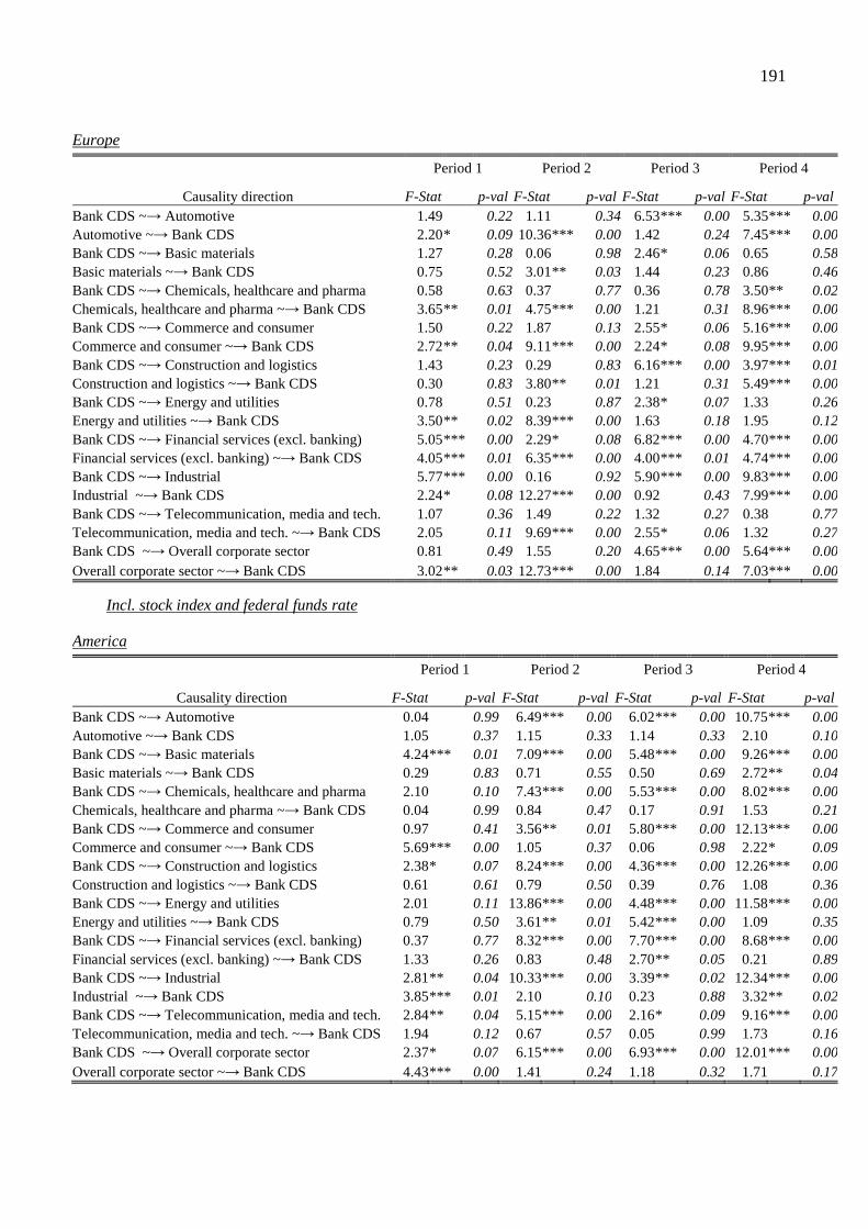
191
Europe
Period 1 Period 2 Period 3 Period 4
Causality direction F-Stat p-val F-Stat p-val F-Stat p-val F-Stat p-val Bank CDS ~→ Automotive 1.49 0 0.22 1.110 0.34 6.53*** 0.00 5.35*** 0.00Automotive ~→ Bank CDS 2.20 * 0.09 10.36*** 0.00 1.420 0.24 7.45*** 0.00Bank CDS ~→ Basic materials 1.27 0 0.28 0.060 0.98 2.46* 0.06 0.650 0.58Basic materials ~→ Bank CDS 0.75 0 0.52 3.01** 0.03 1.440 0.23 0.860 0.46Bank CDS ~→ Chemicals, healthcare and pharma 0.58 0 0.63 0.370 0.77 0.360 0.78 3.50** 0.02Chemicals, healthcare and pharma ~→ Bank CDS 3.65 ** 0.01 4.75*** 0.00 1.210 0.31 8.96*** 0.00Bank CDS ~→ Commerce and consumer 1.50 0 0.22 1.870 0.13 2.55* 0.06 5.16*** 0.00Commerce and consumer ~→ Bank CDS 2.72 ** 0.04 9.11*** 0.00 2.24* 0.08 9.95*** 0.00Bank CDS ~→ Construction and logistics 1.43 0 0.23 0.290 0.83 6.16*** 0.00 3.97*** 0.01Construction and logistics ~→ Bank CDS 0.30 0 0.83 3.80** 0.01 1.210 0.31 5.49*** 0.00Bank CDS ~→ Energy and utilities 0.78 0 0.51 0.230 0.87 2.38* 0.07 1.330 0.26Energy and utilities ~→ Bank CDS 3.50 ** 0.02 8.39*** 0.00 1.630 0.18 1.950 0.12Bank CDS ~→ Financial services (excl. banking) 5.05 *** 0.00 2.29* 0.08 6.82*** 0.00 4.70*** 0.00Financial services (excl. banking) ~→ Bank CDS 4.05 *** 0.01 6.35*** 0.00 4.00*** 0.01 4.74*** 0.00Bank CDS ~→ Industrial 5.77 *** 0.00 0.160 0.92 5.90*** 0.00 9.83*** 0.00Industrial ~→ Bank CDS 2.24 * 0.08 12.27*** 0.00 0.920 0.43 7.99*** 0.00Bank CDS ~→ Telecommunication, media and tech. 1.07 0 0.36 1.490 0.22 1.320 0.27 0.380 0.77Telecommunication, media and tech. ~→ Bank CDS 2.05 0 0.11 9.69*** 0.00 2.55* 0.06 1.320 0.27Bank CDS ~→ Overall corporate sector 0.81 0 0.49 1.550 0.20 4.65*** 0.00 5.64*** 0.00Overall corporate sector ~→ Bank CDS 3.02 ** 0.03 12.73*** 0.00 1.840 0.14 7.03*** 0.00
Incl. stock index and federal funds rate
America
Period 1 Period 2 Period 3 Period 4
Causality direction F-Stat p-val F-Stat p-val F-Stat p-val F-Stat p-val Bank CDS ~→ Automotive 0.040 0.99 6.49*** 0.00 6.02*** 0.00 10.75*** 0.00Automotive ~→ Bank CDS 1.050 0.37 1.150 0.33 1.140 0.33 2.100 0.10Bank CDS ~→ Basic materials 4.24*** 0.01 7.09*** 0.00 5.48*** 0.00 9.26*** 0.00Basic materials ~→ Bank CDS 0.290 0.83 0.710 0.55 0.500 0.69 2.72** 0.04Bank CDS ~→ Chemicals, healthcare and pharma 2.100 0.10 7.43*** 0.00 5.53*** 0.00 8.02*** 0.00Chemicals, healthcare and pharma ~→ Bank CDS 0.040 0.99 0.840 0.47 0.170 0.91 1.530 0.21Bank CDS ~→ Commerce and consumer 0.970 0.41 3.56** 0.01 5.80*** 0.00 12.13*** 0.00Commerce and consumer ~→ Bank CDS 5.69*** 0.00 1.050 0.37 0.060 0.98 2.22* 0.09Bank CDS ~→ Construction and logistics 2.38* 0.07 8.24*** 0.00 4.36*** 0.00 12.26*** 0.00Construction and logistics ~→ Bank CDS 0.610 0.61 0.790 0.50 0.390 0.76 1.080 0.36Bank CDS ~→ Energy and utilities 2.010 0.11 13.86*** 0.00 4.48*** 0.00 11.58*** 0.00Energy and utilities ~→ Bank CDS 0.790 0.50 3.61** 0.01 5.42*** 0.00 1.090 0.35Bank CDS ~→ Financial services (excl. banking) 0.370 0.77 8.32*** 0.00 7.70*** 0.00 8.68*** 0.00Financial services (excl. banking) ~→ Bank CDS 1.330 0.26 0.830 0.48 2.70** 0.05 0.210 0.89Bank CDS ~→ Industrial 2.81** 0.04 10.33*** 0.00 3.39** 0.02 12.34*** 0.00Industrial ~→ Bank CDS 3.85*** 0.01 2.100 0.10 0.230 0.88 3.32** 0.02Bank CDS ~→ Telecommunication, media and tech. 2.84** 0.04 5.15*** 0.00 2.16* 0.09 9.16*** 0.00Telecommunication, media and tech. ~→ Bank CDS 1.940 0.12 0.670 0.57 0.050 0.99 1.730 0.16Bank CDS ~→ Overall corporate sector 2.37* 0.07 6.15*** 0.00 6.93*** 0.00 12.01*** 0.00Overall corporate sector ~→ Bank CDS 4.43*** 0.00 1.410 0.24 1.180 0.32 1.710 0.17

192
Asia-Pacific
Period 1 Period 2 Period 3 Period 4
Causality direction F-Stat p-val F-Stat p-val F-Stat p-val F-Stat p-val Bank CDS ~→ Automotive 1.020 0.38 9.22*** 0.00 2.100 0.10 1.590 0.19Automotive ~→ Bank CDS 1.000 0.39 1.030 0.38 2.25* 0.08 14.28*** 0.00Bank CDS ~→ Basic materials 1.510 0.21 9.19*** 0.00 4.88*** 0.00 4.89*** 0.00Basic materials ~→ Bank CDS 1.650 0.18 1.250 0.29 1.830 0.14 0.730 0.54Bank CDS ~→ Chemicals, healthcare and pharma 1.920 0.13 0.810 0.49 1.290 0.28 1.470 0.22Chemicals, healthcare and pharma ~→ Bank CDS 0.600 0.61 0.460 0.71 0.110 0.95 5.12*** 0.00Bank CDS ~→ Commerce and consumer 0.810 0.49 3.16** 0.02 2.83** 0.04 7.38*** 0.00Commerce and consumer ~→ Bank CDS 0.730 0.54 1.230 0.30 0.480 0.70 0.700 0.55Bank CDS ~→ Construction and logistics 0.370 0.77 15.79*** 0.00 4.08*** 0.01 4.59*** 0.00Construction and logistics ~→ Bank CDS 0.040 0.99 1.250 0.29 1.770 0.15 0.180 0.91Bank CDS ~→ Energy and utilities 1.240 0.29 9.30*** 0.00 10.60*** 0.00 5.72*** 0.00Energy and utilities ~→ Bank CDS 0.720 0.54 1.270 0.28 1.470 0.22 1.080 0.36Bank CDS ~→ Financial services (excl. banking) 0.620 0.60 2.45* 0.06 0.580 0.63 10.55*** 0.00Financial services (excl. banking) ~→ Bank CDS 0.200 0.89 0.240 0.87 1.880 0.13 6.12*** 0.00Bank CDS ~→ Industrial 1.560 0.20 8.81*** 0.00 2.77** 0.04 2.56* 0.05Industrial ~→ Bank CDS 1.250 0.29 2.77** 0.04 0.190 0.90 0.810 0.49Bank CDS ~→ Telecommunication, media and tech. 0.930 0.42 4.54*** 0.00 2.36* 0.07 0.760 0.52Telecommunication, media and tech. ~→ Bank CDS 0.300 0.82 2.64** 0.05 0.650 0.58 2.59* 0.05Bank CDS ~→ Overall corporate sector 0.450 0.72 7.61*** 0.00 9.26*** 0.00 1.640 0.18Overall corporate sector ~→ Bank CDS 0.500 0.68 2.62* 0.05 3.06** 0.03 4.53*** 0.00
Europe
Period 1 Period 2 Period 3 Period 4
Causality direction F-Stat p-val F-Stat p-val F-Stat p-val F-Stat p-val Bank CDS ~→ Automotive 1.410 0.24 1.110 0.35 8.07*** 0.00 5.05*** 0.00Automotive ~→ Bank CDS 2.12* 0.10 10.39*** 0.00 1.660 0.18 5.31*** 0.00Bank CDS ~→ Basic materials 0.900 0.44 0.020 1.00 2.22* 0.09 0.580 0.63Basic materials ~→ Bank CDS 0.840 0.47 2.97** 0.03 3.37** 0.02 0.820 0.48Bank CDS ~→ Chemicals, healthcare and pharma 0.600 0.62 0.330 0.80 0.790 0.50 3.54** 0.01Chemicals, healthcare and pharma ~→ Bank CDS 4.50*** 0.00 4.98*** 0.00 1.590 0.19 7.28*** 0.00Bank CDS ~→ Commerce and consumer 1.650 0.18 1.890 0.13 3.51** 0.02 5.05*** 0.00Commerce and consumer ~→ Bank CDS 3.97*** 0.01 9.09*** 0.00 2.64** 0.05 9.50*** 0.00Bank CDS ~→ Construction and logistics 1.100 0.35 0.410 0.75 6.60*** 0.00 5.60*** 0.00Construction and logistics ~→ Bank CDS 0.310 0.82 3.89*** 0.01 1.240 0.30 4.70*** 0.00Bank CDS ~→ Energy and utilities 0.790 0.50 0.320 0.81 3.24** 0.02 1.270 0.29Energy and utilities ~→ Bank CDS 2.74** 0.04 8.36*** 0.00 1.630 0.18 1.900 0.13Bank CDS ~→ Financial services (excl. banking) 5.22*** 0.00 2.18* 0.09 6.97*** 0.00 4.85*** 0.00Financial services (excl. banking) ~→ Bank CDS 3.51** 0.02 6.15*** 0.00 4.08*** 0.01 4.62*** 0.00Bank CDS ~→ Industrial 5.89*** 0.00 0.190 0.90 6.42*** 0.00 9.88*** 0.00Industrial ~→ Bank CDS 2.12* 0.10 11.91*** 0.00 1.000 0.39 8.06*** 0.00Bank CDS ~→ Telecommunication, media and tech. 1.060 0.36 1.480 0.22 1.940 0.12 0.350 0.79Telecommunication, media and tech. ~→ Bank CDS 2.10* 0.10 9.56*** 0.00 2.39* 0.07 1.230 0.30Bank CDS ~→ Overall corporate sector 0.630 0.60 1.580 0.19 5.41*** 0.00 5.03*** 0.00Overall corporate sector ~→ Bank CDS 3.10** 0.03 12.73*** 0.00 1.930 0.12 5.34*** 0.00
Notes: We evaluate the null hypothesis that the bank CDS in region i does not impact the corporate CDS in the same region, i.e.,
0 : ~bank corpi iH CDS CDS→ , using the F-Statistic. *, **, *** denotes significance at the 10%, 5%
and 1% significance level, respectively.

193
Table 35: Granger causality test results for regional bank vs. non-bank corporate equity
Without control variables
America
Period 1 Period 2 Period 3 Period 4
Causality direction F-Stat p-val F-Stat p-val F-Stat p-val F-Stat p-val Bank equity ~→ Automotive 1.67 0 0.17 0.200 0.90 0.800 0.49 1.300 0.27Automotive ~→ Bank equity 0.85 0 0.47 0.070 0.98 1.740 0.16 1.270 0.28Bank equity ~→ Basic materials 0.16 0 0.93 2.48* 0.06 2.23* 0.08 0.640 0.59Basic materials ~→ Bank equity 2.40 * 0.07 12.21*** 0.00 0.120 0.95 3.18** 0.02Bank equity ~→ Chemicals, healthcare and pharma 1.69 0 0.17 0.350 0.79 2.22* 0.09 0.220 0.89Chemicals, healthcare and pharma ~→ Bank equity 0.53 0 0.66 0.370 0.78 4.45*** 0.00 0.830 0.48Bank equity ~→ Commerce and consumer 0.71 0 0.55 1.680 0.17 2.40* 0.07 0.580 0.63Commerce and consumer ~→ Bank equity 0.10 0 0.96 1.860 0.14 3.26** 0.02 0.150 0.93Bank equity ~→ Construction and logistics 0.52 0 0.67 0.640 0.59 1.140 0.33 0.270 0.85Construction and logistics ~→ Bank equity 0.11 0 0.95 1.300 0.27 1.290 0.28 0.670 0.57Bank equity ~→ Energy and utilities 0.28 0 0.84 0.730 0.53 2.67** 0.05 0.860 0.46Energy and utilities ~→ Bank equity 2.27 * 0.08 7.26*** 0.00 1.880 0.13 1.460 0.23Bank equity ~→ Financial services (excl. banking) 1.79 0 0.15 0.620 0.60 0.310 0.82 0.820 0.48Financial services (excl. banking) ~→ Bank equity 0.65 0 0.58 3.41** 0.02 2.70** 0.05 1.410 0.24Bank equity ~→ Industrial 0.40 0 0.75 2.21* 0.09 2.14* 0.09 0.460 0.71Industrial ~→ Bank equity 1.15 0 0.33 3.18** 0.02 1.780 0.15 0.570 0.63Bank equity ~→ Telecommunication, media and tech. 0.13 0 0.94 1.090 0.35 0.920 0.43 0.540 0.66Telecommunication, media and tech. ~→ Bank equity 0.31 0 0.82 5.57*** 0.00 2.91** 0.03 0.350 0.79Bank equity ~→ Overall corporate sector 1.85 0 0.14 0.510 0.67 0.280 0.84 0.730 0.53Overall corporate sector ~→ Bank equity 0.60 0 0.61 3.43** 0.02 2.70** 0.05 1.400 0.24
Asia-Pacific
Period 1 Period 2 Period 3 Period 4
Causality direction F-Stat p-val F-Stat p-val F-Stat p-val F-Stat p-val Bank equity ~→ Automotive 0.18 0 0.91 3.32** 0.02 2.45* 0.06 1.220 0.30Automotive ~→ Bank equity 0.60 0 0.61 1.360 0.25 2.29* 0.08 1.170 0.32Bank equity ~→ Basic materials 0.09 0 0.96 0.490 0.69 7.75*** 0.00 1.660 0.17Basic materials ~→ Bank equity 0.41 0 0.75 1.290 0.28 7.71*** 0.00 0.820 0.48Bank equity ~→ Chemicals, healthcare and pharma 0.14 0 0.94 0.480 0.70 1.520 0.21 1.000 0.39Chemicals, healthcare and pharma ~→ Bank equity 0.53 0 0.66 0.590 0.62 3.38** 0.02 1.840 0.14Bank equity ~→ Commerce and consumer 1.97 0 0.12 0.790 0.50 0.270 0.85 2.40* 0.07Commerce and consumer ~→ Bank equity 0.92 0 0.43 2.13* 0.10 5.10*** 0.00 2.88** 0.04Bank equity ~→ Construction and logistics 0.18 0 0.91 0.380 0.77 0.630 0.60 2.060 0.11Construction and logistics ~→ Bank equity 3.10 ** 0.03 0.680 0.57 0.770 0.51 0.860 0.46Bank equity ~→ Energy and utilities 0.37 0 0.77 1.240 0.30 6.36*** 0.00 1.670 0.17Energy and utilities ~→ Bank equity 2.99 ** 0.03 1.630 0.18 6.07*** 0.00 1.920 0.13Bank equity ~→ Financial services (excl. banking) 1.58 0 0.19 1.060 0.37 1.380 0.25 0.330 0.80Financial services (excl. banking) ~→ Bank equity 3.69 ** 0.01 2.30* 0.08 2.29* 0.08 1.070 0.36Bank equity ~→ Industrial 2.27 * 0.08 4.77*** 0.00 5.73*** 0.00 5.10*** 0.00Industrial ~→ Bank equity 1.16 0 0.33 10.17*** 0.00 1.980 0.12 2.80** 0.04Bank equity ~→ Telecommunication, media and tech. 1.23 0 0.30 1.110 0.35 0.670 0.57 2.54* 0.06Telecommunication, media and tech. ~→ Bank equity 1.08 0 0.36 4.10*** 0.01 12.00*** 0.00 3.66** 0.01Bank equity ~→ Overall corporate sector 1.96 0 0.12 0.550 0.65 0.290 0.83 5.14*** 0.00Overall corporate sector ~→ Bank equity 0.67 0 0.57 3.71** 0.01 11.19*** 0.00 5.01*** 0.00

194
Europe
Period 1 Period 2 Period 3 Period 4
Causality direction F-Stat p-val F-Stat p-val F-Stat p-val F-Stat p-val Bank equity ~→ Automotive 1.68 0 0.17 1.560 0.20 1.540 0.20 1.490 0.22Automotive ~→ Bank equity 0.11 0 0.95 2.44* 0.06 1.000 0.39 0.510 0.67Bank equity ~→ Basic materials 0.98 0 0.40 0.640 0.59 1.320 0.27 1.660 0.18Basic materials ~→ Bank equity 2.14 * 0.09 7.30*** 0.00 0.190 0.91 1.340 0.26Bank equity ~→ Chemicals, healthcare and pharma 0.17 0 0.91 0.210 0.89 1.610 0.19 1.210 0.30Chemicals, healthcare and pharma ~→ Bank equity 1.58 0 0.19 1.880 0.13 1.150 0.33 2.24* 0.08Bank equity ~→ Commerce and consumer 2.20 * 0.09 0.420 0.74 2.17* 0.09 0.820 0.48Commerce and consumer ~→ Bank equity 0.31 0 0.82 2.46* 0.06 0.650 0.58 3.65** 0.01Bank equity ~→ Construction and logistics 1.52 0 0.21 0.590 0.62 0.330 0.81 1.980 0.12Construction and logistics ~→ Bank equity 0.89 0 0.45 0.900 0.44 0.310 0.82 0.930 0.43Bank equity ~→ Energy and utilities 1.52 0 0.21 2.30* 0.08 2.49* 0.06 1.230 0.30Energy and utilities ~→ Bank equity 1.34 0 0.26 2.23* 0.08 0.430 0.73 2.50* 0.06Bank equity ~→ Financial services (excl. banking) 0.61 0 0.61 0.430 0.73 1.090 0.35 2.30* 0.08Financial services (excl. banking) ~→ Bank equity 0.29 0 0.83 0.910 0.43 1.560 0.20 1.680 0.17Bank equity ~→ Industrial 1.35 0 0.26 0.440 0.73 3.35** 0.02 0.600 0.62Industrial ~→ Bank equity 1.36 0 0.26 3.47** 0.02 0.430 0.73 1.310 0.27Bank equity ~→ Telecommunication, media and tech. 1.15 0 0.33 1.050 0.37 1.610 0.19 0.990 0.40Telecommunication, media and tech. ~→ Bank equity 1.98 0 0.12 7.05*** 0.00 0.810 0.49 3.09** 0.03Bank equity ~→ Overall corporate sector 0.15 0 0.93 0.980 0.40 1.300 0.27 0.630 0.60Overall corporate sector ~→ Bank equity 0.92 0 0.43 3.69** 0.01 0.290 0.83 2.50* 0.06
Incl. stock index and federal funds rate
America
Period 1 Period 2 Period 3 Period 4
Causality direction F-Stat p-val F-Stat p-val F-Stat p-val F-Stat p-val Bank equity ~→ Automotive 1.640 0.18 0.130 0.94 0.890 0.45 1.170 0.32Automotive ~→ Bank equity 0.720 0.54 0.130 0.94 1.690 0.17 1.240 0.29Bank equity ~→ Basic materials 0.140 0.94 1.270 0.28 1.680 0.17 0.630 0.60Basic materials ~→ Bank equity 2.42* 0.07 12.35*** 0.00 0.080 0.97 2.93** 0.03Bank equity ~→ Chemicals, healthcare and pharma 1.630 0.18 0.270 0.85 1.900 0.13 0.180 0.91Chemicals, healthcare and pharma ~→ Bank equity 0.490 0.69 0.160 0.92 4.04*** 0.01 1.050 0.37Bank equity ~→ Commerce and consumer 0.730 0.54 1.770 0.15 2.000 0.11 0.520 0.67Commerce and consumer ~→ Bank equity 0.080 0.97 1.600 0.19 3.46** 0.02 0.190 0.90Bank equity ~→ Construction and logistics 0.530 0.66 0.750 0.52 0.700 0.55 0.230 0.87Construction and logistics ~→ Bank equity 0.130 0.94 1.230 0.30 1.220 0.30 0.700 0.55Bank equity ~→ Energy and utilities 0.060 0.98 0.880 0.45 1.750 0.16 0.900 0.44Energy and utilities ~→ Bank equity 3.88*** 0.01 6.46*** 0.00 1.720 0.16 1.450 0.23Bank equity ~→ Financial services (excl. banking) 1.660 0.17 0.710 0.55 0.500 0.68 1.080 0.36Financial services (excl. banking) ~→ Bank equity 0.610 0.61 3.10** 0.03 2.24* 0.08 1.720 0.16Bank equity ~→ Industrial 0.430 0.73 1.980 0.12 1.650 0.18 0.430 0.73Industrial ~→ Bank equity 1.350 0.26 2.15* 0.09 1.610 0.19 0.610 0.61Bank equity ~→ Telecommunication, media and tech. 0.010 1.00 1.080 0.36 0.650 0.58 0.580 0.63Telecommunication, media and tech. ~→ Bank equity 0.500 0.68 4.03*** 0.01 2.83** 0.04 0.530 0.66Bank equity ~→ Overall corporate sector 1.730 0.16 0.600 0.62 0.480 0.69 0.970 0.41Overall corporate sector ~→ Bank equity 0.560 0.64 3.11** 0.03 2.25* 0.08 1.710 0.16
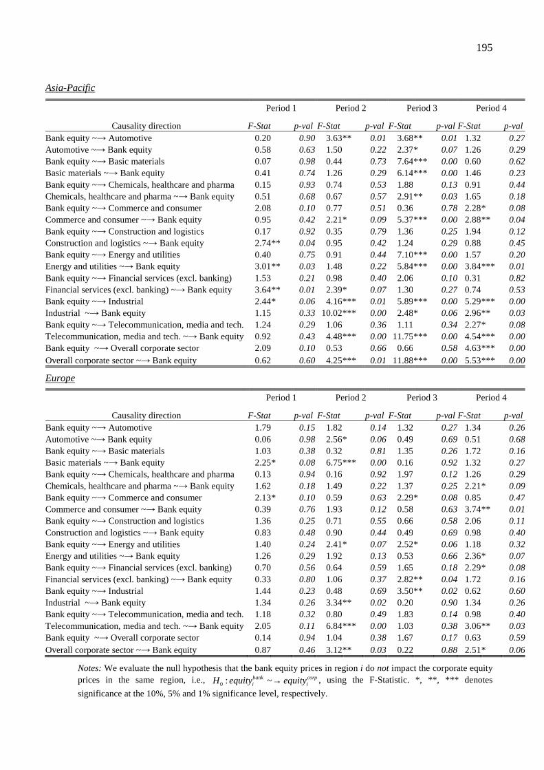
195
Asia-Pacific
Period 1 Period 2 Period 3 Period 4
Causality direction F-Stat p-val F-Stat p-val F-Stat p-val F-Stat p-val Bank equity ~→ Automotive 0.200 0.90 3.63** 0.01 3.68** 0.01 1.320 0.27Automotive ~→ Bank equity 0.580 0.63 1.500 0.22 2.37* 0.07 1.260 0.29Bank equity ~→ Basic materials 0.070 0.98 0.440 0.73 7.64*** 0.00 0.600 0.62Basic materials ~→ Bank equity 0.410 0.74 1.260 0.29 6.14*** 0.00 1.460 0.23Bank equity ~→ Chemicals, healthcare and pharma 0.150 0.93 0.740 0.53 1.880 0.13 0.910 0.44Chemicals, healthcare and pharma ~→ Bank equity 0.510 0.68 0.670 0.57 2.91** 0.03 1.650 0.18Bank equity ~→ Commerce and consumer 2.080 0.10 0.770 0.51 0.360 0.78 2.28* 0.08Commerce and consumer ~→ Bank equity 0.950 0.42 2.21* 0.09 5.37*** 0.00 2.88** 0.04Bank equity ~→ Construction and logistics 0.170 0.92 0.350 0.79 1.360 0.25 1.940 0.12Construction and logistics ~→ Bank equity 2.74** 0.04 0.950 0.42 1.240 0.29 0.880 0.45Bank equity ~→ Energy and utilities 0.400 0.75 0.910 0.44 7.10*** 0.00 1.570 0.20Energy and utilities ~→ Bank equity 3.01** 0.03 1.480 0.22 5.84*** 0.00 3.84*** 0.01Bank equity ~→ Financial services (excl. banking) 1.530 0.21 0.980 0.40 2.060 0.10 0.310 0.82Financial services (excl. banking) ~→ Bank equity 3.64** 0.01 2.39* 0.07 1.300 0.27 0.740 0.53Bank equity ~→ Industrial 2.44* 0.06 4.16*** 0.01 5.89*** 0.00 5.29*** 0.00Industrial ~→ Bank equity 1.150 0.33 10.02*** 0.00 2.48* 0.06 2.96** 0.03Bank equity ~→ Telecommunication, media and tech. 1.240 0.29 1.060 0.36 1.110 0.34 2.27* 0.08Telecommunication, media and tech. ~→ Bank equity 0.920 0.43 4.48*** 0.00 11.75*** 0.00 4.54*** 0.00Bank equity ~→ Overall corporate sector 2.090 0.10 0.530 0.66 0.660 0.58 4.63*** 0.00Overall corporate sector ~→ Bank equity 0.620 0.60 4.25*** 0.01 11.88*** 0.00 5.53*** 0.00
Europe
Period 1 Period 2 Period 3 Period 4
Causality direction F-Stat p-val F-Stat p-val F-Stat p-val F-Stat p-val Bank equity ~→ Automotive 1.790 0.15 1.820 0.14 1.320 0.27 1.340 0.26Automotive ~→ Bank equity 0.060 0.98 2.56* 0.06 0.490 0.69 0.510 0.68Bank equity ~→ Basic materials 1.030 0.38 0.320 0.81 1.350 0.26 1.720 0.16Basic materials ~→ Bank equity 2.25* 0.08 6.75*** 0.00 0.160 0.92 1.320 0.27Bank equity ~→ Chemicals, healthcare and pharma 0.130 0.94 0.160 0.92 1.970 0.12 1.260 0.29Chemicals, healthcare and pharma ~→ Bank equity 1.620 0.18 1.490 0.22 1.370 0.25 2.21* 0.09Bank equity ~→ Commerce and consumer 2.13* 0.10 0.590 0.63 2.29* 0.08 0.850 0.47Commerce and consumer ~→ Bank equity 0.390 0.76 1.930 0.12 0.580 0.63 3.74** 0.01Bank equity ~→ Construction and logistics 1.360 0.25 0.710 0.55 0.660 0.58 2.060 0.11Construction and logistics ~→ Bank equity 0.830 0.48 0.900 0.44 0.490 0.69 0.980 0.40Bank equity ~→ Energy and utilities 1.400 0.24 2.41* 0.07 2.52* 0.06 1.180 0.32Energy and utilities ~→ Bank equity 1.260 0.29 1.920 0.13 0.530 0.66 2.36* 0.07Bank equity ~→ Financial services (excl. banking) 0.700 0.56 0.640 0.59 1.650 0.18 2.29* 0.08Financial services (excl. banking) ~→ Bank equity 0.330 0.80 1.060 0.37 2.82** 0.04 1.720 0.16Bank equity ~→ Industrial 1.440 0.23 0.480 0.69 3.50** 0.02 0.620 0.60Industrial ~→ Bank equity 1.340 0.26 3.34** 0.02 0.200 0.90 1.340 0.26Bank equity ~→ Telecommunication, media and tech. 1.180 0.32 0.800 0.49 1.830 0.14 0.980 0.40Telecommunication, media and tech. ~→ Bank equity 2.050 0.11 6.84*** 0.00 1.030 0.38 3.06** 0.03Bank equity ~→ Overall corporate sector 0.140 0.94 1.040 0.38 1.670 0.17 0.630 0.59Overall corporate sector ~→ Bank equity 0.870 0.46 3.12** 0.03 0.220 0.88 2.51* 0.06
Notes: We evaluate the null hypothesis that the bank equity prices in region i do not impact the corporate equity prices in the same region, i.e.,
0 : ~bank corpi iH equity equity→ , using the F-Statistic. *, **, *** denotes
significance at the 10%, 5% and 1% significance level, respectively.

196
Table 36: Correlation between bank and corporate CDS spreads
Average correlation with bank CDS spreads
Region Industry Period 1 Period 2 Period 3 Period 4
America
Automotive 24.60% 59.95% 59.57% 59.73%Basic materials 6.63% 49.93% 62.48% 51.10%Chemicals, healthcare and pharma 16.69% 57.73% 63.18% 49.90%Commerce and consumer 26.47% 64.41% 70.52% 56.91%Construction and logistics 11.81% 47.94% 54.06% 41.62%Energy and utilities 24.45% 59.71% 64.67% 56.39%Financial services (excl. banking) 34.32% 63.88% 71.25% 68.48%Industrial 16.92% 59.59% 67.41% 59.71%Telecommunication, media and technology 27.13% 62.95% 67.41% 60.68%Overall 32.72% 68.65% 73.95% 66.25%
Asia-Pacific
Automotive 5.75% 39.94% 51.21% 54.09%Basic materials 2.17% 48.85% 60.68% 66.98%Chemicals, healthcare and pharma -3.19% 25.48% 52.80% 44.64%Commerce and consumer 15.61% 51.53% 57.21% 59.57%Construction and logistics 10.80% 32.21% 46.24% 52.91%Energy and utilities 13.50% 32.50% 48.06% 53.50%Financial services (excl. banking) 9.53% 29.88% 48.35% 56.36%Industrial 8.23% 42.49% 56.19% 52.13%Telecommunication, media and technology 13.63% 51.97% 60.73% 65.10%Overall 16.11% 56.17% 73.90% 71.25%
Europe
Automotive 17.17% 66.39% 71.12% 77.47%Basic materials 9.29% 60.72% 69.34% 71.25%Chemicals, healthcare and pharma 1.81% 64.79% 73.87% 70.73%Commerce and consumer 17.82% 66.92% 81.13% 77.60%Construction and logistics 4.73% 60.31% 65.58% 52.98%Energy and utilities 12.71% 67.84% 79.22% 75.76%Financial services (excl. banking) 26.66% 69.94% 76.88% 85.08%Industrial 11.57% 66.37% 78.58% 76.58%Telecommunication, media and technology 15.13% 66.87% 76.73% 80.54%Overall 24.15% 73.60% 84.53% 84.63%
Notes: The table shows the correlation between banking sector CDS spreads and the CDS spreads of the non-
bank corporate firms during the four sub-periods. Period 1 ranges from November 1st, 2005 to February 28
th,
2007, Period 2 ranges from March 1st, 2007 to July 31
st, 2008, Period 3 ranges from August 1
st, 2008 to
December 31st, 2009, Period 4 ranges from January 1
st, 2010 to April 30
th, 2011.

197
Table 37: Correlation between bank and corporate equity returns
Average correlation with bank equity returns
Region Industry Period 1 Period 2 Period 3 Period 4
America
Automotive 55.81% 69.62% 52.82% 56.14%Basic materials 34.59% 39.58% 50.21% 53.42%Chemicals, healthcare and pharma 70.60% 72.28% 62.26% 66.41%Commerce and consumer 81.66% 84.17% 68.73% 69.96%Construction and logistics 63.68% 77.09% 67.87% 62.78%Energy and utilities 39.68% 57.76% 61.65% 66.82%Financial services (excl. banking) 75.07% 85.74% 82.68% 77.52%Industrial 74.21% 80.83% 73.99% 71.61%Telecommunication, media and technology 79.23% 78.81% 71.81% 73.81%Overall 81.54% 84.72% 77.17% 75.70%
Asia-Pacific
Automotive 62.60% 68.06% 62.43% 65.15%Basic materials 62.10% 64.55% 69.11% 72.38%Chemicals, healthcare and pharma 57.82% 64.71% 59.40% 62.07%Commerce and consumer 69.29% 72.07% 71.29% 74.05%Construction and logistics 57.66% 65.95% 56.90% 64.77%Energy and utilities 56.91% 61.71% 64.14% 68.57%Financial services (excl. banking) 53.81% 65.93% 66.03% 61.52%Industrial 71.26% 69.08% 74.54% 74.19%Telecommunication, media and technology 72.95% 74.58% 75.68% 73.60%Overall 79.60% 80.76% 81.69% 81.66%
Europe
Automotive 71.27% 76.87% 76.83% 63.40%Basic materials 69.71% 70.14% 76.19% 65.25%Chemicals, healthcare and pharma 75.21% 76.20% 72.67% 60.78%Commerce and consumer 79.33% 80.57% 75.11% 62.42%Construction and logistics 60.98% 66.73% 75.25% 71.69%Energy and utilities 66.85% 62.49% 70.18% 75.28%Financial services (excl. banking) 84.62% 88.72% 88.80% 83.05%Industrial 78.11% 78.46% 81.05% 69.54%Telecommunication, media and technology 74.73% 76.09% 75.07% 73.73%Overall 89.60% 85.68% 85.91% 77.54%
Notes: The table shows the correlation between banking sector equity returns and the equity returns of the non-
bank corporate firms during the four sub-periods. Period 1 ranges from November 1st, 2005 to February 28
th,
2007, Period 2 ranges from March 1st, 2007 to July 31
st, 2008, Period 3 ranges from August 1
st, 2008 to
December 31st, 2009, Period 4 ranges from January 1
st, 2010 to April 30
th, 2011.

198
Table 38: Regression of relative ESS-indicator on p-value of F-statistic
Regression 1 Regression 2 Region Independent variables Coeff P-val Coeff P-val
America
Constant 0.08 0.0% 1.16 0.0%
Regional_rel_ESS -2.79 0.0% -2.50 0.3%
Stock_index 0.00 0.0% -0.14 0.0%
Federal_funds_rate 0.00 0.0% 0.02 0.0%
Adjusted_R² 0.19 0.0% 0.45 0.0%
Asia-Pacific
Constant 0.18 0.0% -2.24 0.0%
Regional_rel_ESS -1.66 0.0% 6.05 8.5%
Stock_index 0.00 0.0% 0.51 0.0%
Federal_funds_rate 0.00 0.0% -0.01 4.2%
Adjusted_R² 0.30 0.0% 0.38 0.0%
Europe
Constant 0.53 0.0% 0.55 5.0%
Regional_rel_ESS -5.89 0.0% -2.92 0.0%
Stock_index 0.00 0.0% 0.03 38.5%
Federal_funds_rate 0.00 0.0% 0.08 0.0%
Adjusted_R² 0.49 0.0% 0.63 0.0%
Notes: The table shows the results from the regressions of the p-value of the F-Statistic from the banking vs. cross-industry (i.e., overall) corporate CDS Granger-causality analysis using the regional relative ESS-indicator (and control variables) as explanatory variables. Coeff denotes the value of the estimated coefficient and P-val denotes the p-value of the coefficient's t-statistic. The regression equation is estimated using White (1980) heteroskedasticity-consistent estimators.
199
BIBLIOGRAPHY
Acharya, V.; Philippon, T.; Richardson, M.; Roubini, N. (2009): The Financial Crisis of 2007
2009: Causes and Remedies, Financial Markets, Institutions & Instruments, Vol. 18, pp.
89-137.
Acharya, V.V.; Drechsler, I.; Schnabl, P. (2011): A Pyrrhic Victory? - Bank Bailouts and
Sovereign Credit Risk, Working Paper.
Acharya, V.V.; Pedersen, L.H. (2005): Asset pricing with liquidity risk, Journal of Financial
Economics, Vol. 77, pp. 375-410.
Acharya, V.V.; Pedersen, L.H.; Philippon, T.; Richardson, M.P. (2010): Measuring systemic
risk, Working Paper.
Adrian, T.; Brunnermeier, M. (2008): CoVaR, Federal Reserve Bank of New York Staff
Reports, Vol. 348, pp. 1-8.
Adrian, T.; Brunnermeier, M. (2011): CoVaR, Working Paper, Vol. 348, pp. 1-8.
Akaike, H. (1974): A new look at the statistical model identification, Automatic Control,
IEEE Transactions on, Vol. 19, pp. 716-723.
Allen, F.; Gale, D. (2000): Financial contagion, Journal of political economy, pp. 1-33.
Alter, A.; Schueler, Y.S. (2011): Credit Spread Interdependencies of European States and
Banks During the Financial Crisis, SSRN eLibrary.
Arteta, C.; Hale, G. (2008): Sovereign debt crises and credit to the private sector, Journal of
International Economics, Vol. 74, pp. 53-69.
Artzner, P.; Delbaen, F.; Eber, J.M.; Heath, D. (1999): Coherent measures of risk,
Mathematical Finance, Vol. 9, pp. 203-228.

200
Avesani, R.; Pascual, A.G.; Li, J. (2006): A new risk indicator and stress testing tool: A
multifactor Nth-to-default CDS basket, IMF Working Paper.
Bae, K.H.; Karolyi, G.A.; Stulz, R.M. (2003): A new approach to measuring financial
contagion, Review of Financial Studies, Vol. 16, pp. 717.
Beck, T.; Demirguc-Kunt, A.; Maksimovic, V. (2002): Funding growth in bank-based and
market-based financial systems: evidence from firm-level data, Journal of Financial
Economics, Vol. 65, pp. 337-363.
Bharath, S.T.; Shumway, T. (2004): Forecasting default with the KMV-Merton model, AFA
2006 Boston Meetings Paper, pp. 48109.
Billio, M.; Getmansky, M.; Lo, A.W.; Pelizzon, L. (2010): Measuring Systemic Risk in the
Finance and Insurance Sectors, Working Paper.
BIS (2010): Basel III: A global regulatory framework for more resilient banks and banking
systems, Bank for International Settelements.
BIS (2011): Assessment methodology and the additional loss absorbency requirement for
global systemically important banks - consultative document issued by the Basel
Committee, Bank for International Settelements.
Brunnermeier, M.K.; Pedersen, L.H. (2009): Market liquidity and funding liquidity, Review of
Financial Studies, Vol. 22, pp. 2201.
Chan-Lau, J.A.; Gravelle, T. (2005): The END: A new indicator of financial and nonfinancial
corporate sector vulnerability, IMF Working Paper.
Chen, L.; Collin-Dufresne, P.; Goldstein, R.S. (2009): On the relation between the credit
spread puzzle and the equity premium puzzle, Review of Financial Studies, Vol. 22, pp.
3367-3381.

201
Chordia, T.; Sarkar, A.; Subrahmanyam, A. (2005): An empirical analysis of stock and bond
market liquidity, Review of Financial Studies, Vol. 18, pp. 85-129.
Claessens, S.; Tong, H.; Wei, S.J. (2011): From the Financial Crisis to the Real Economy:
Using Firm-Level Data to Identify Transmission Channels, SSRN eLibrary.
Das, S.R.; Duffie, D.; Kapadia, N.; Saita, L. (2007): Common failings: How corporate
defaults are correlated, The Journal of Finance, Vol. 62, pp. 93-117.
Dickey, D.A.; Fuller, W.A. (1979): Distribution of the estimators for autoregressive time
series with a unit root, Journal of the American Statistical Association, pp. 427-431.
Dieckmann, S.; Plank, T. (2010). Default risk of advanced economies: An empirical analysis
of credit default swaps during the financial crisis Mimeo, Wharton School.
Dornbusch, R.; Park, Y.C.; Claessens, S. (2000): Contagion: Understanding how it spreads,
The World Bank Research Observer, Vol. 15, pp. 177.
Drehmann, M.; Tarashev, N. (2011): Systemic importance: some simple indicators, BIS
Quarterly Review.
Duffie, D. (1999): Credit swap valuation, Financial Analysts Journal, Vol. 55, pp. 73-87.
Duffie, D.; Eckner, A.; Horel, G.; Saita, L. (2009): Frailty correlated default, The Journal of
Finance, Vol. 64, pp. 2089-2123.
Engle, R. (2009): Anticipating correlations: a new paradigm for risk management Princeton
University Press.
Engle, R.F.; Granger, C.W.J. (1987): Co-integration and error correction: representation,
estimation, and testing, Econometrica: journal of the Econometric Society, pp. 251-276.
Espinosa-Vega, M.; Sole, J. (2010): Cross-border financial surveillance: a network
perspective, IMF Working Papers, Vol. 105, pp. 1-27.

202
Fidrmuc, J.; Suess, K. (2009): The Outbreak of the Russian Banking Crisis, University of
Munich Discussion Paper.
Forte, S.; Pena, J.I. (2009): Credit spreads: An empirical analysis on the informational content
of stocks, bonds, and CDS, Journal of Banking & Finance, Vol. 33, pp. 2013-2025.
FSB (2009): Guidance to Assess the Systemic Importance of Financial Institutions, Markets
and Instruments: Initial Considerations, Report to the G-20 Finance Ministers and Central
Bank Governors, IMF and FSB, October.
Gerlach, S.; Schulz, A.; Wolff, G.B. (2010): Banking and sovereign risk in the euro area,
Deutsche Bundesbank.
Gibson, M.S. (2004): Understanding the risk of synthetic CDOs, Working Paper.
Granger, C.W.J. (2003): Some aspects of causal relationships, Journal of Econometrics, Vol.
112, pp. 69-71.
Granger, C.W.J.; Huangb, B.N.; Yang, C.W. (2000): A bivariate causality between stock
prices and exchange rates: evidence from recent Asianflu, The Quarterly Review of
Economics and Finance, Vol. 40, pp. 337-354.
Gray, D.; Merton, R.; Bodie, Z. (2008). A Contingent Claims Analysis of the Subprime Credit
Crisis of 2007-2008. In (pp. 22-23).
Gray, D.F. (2009): Modeling financial crises and sovereign risks, Annu.Rev.Financ.Econ.,
Vol. 1, pp. 117-144.
Gray, D.F.; Merton, R.C.; Bodie, Z. (2007a): Contingent claims approach to measuring and
managing sovereign credit risk, Journal of Investment Management, Vol. 5, pp. 5.
Gray, D.F.; Merton, R.C.; Bodie, Z. (2007b): New framework for measuring and managing
macrofinancial risk and financial stability, NBER Working Paper.

203
Griffin, J.M.; Nardari, F.; Stulz, R.M. (2007): Do investors trade more when stocks have
performed well? Evidence from 46 countries, Review of Financial Studies, Vol. 20, pp.
905-951.
Hao, C.; Alam, M.M.; Carling, K. (2009): Review of the literature on credit risk modeling.
Hiemstra, C.; Jones, J.D. (1994): Testing for linear and nonlinear Granger causality in the
stock price-volume relation, Journal of Finance, pp. 1639-1664.
Huang, B.N.; Yang, C.W.; Hu, J.W.-S. (2000): Causality and cointegration of stock markets
among the United States, Japan and the South China Growth Triangle, International
Review of Financial Analysis, Vol. 9, pp. 281-297.
Huang, X.; Zhou, H.; Zhu, H. (2009): A framework for assessing the systemic risk of major
financial institutions, Journal of Banking & Finance, Vol. 33, pp. 2036-2049.
Huang, X.; Zhou, H.; Zhu, H. (2010a): Assessing the systemic risk of a heterogeneous
portfolio of banks during the recent financial crisis Bank for International Settlements,
Monetary and Economic Department.
Huang, X.; Zhou, H.; Zhu, H. (2010b): Systemic Risk Contributions, Working Paper.
Hull, J.; Predescu, M.; White, A. (2004): The relationship between credit default swap
spreads, bond yields, and credit rating announcements, Journal of Banking & Finance, Vol.
28, pp. 2789-2811.
Hull, J.C.; White, A.D. (2004): Valuation of a CDO and an n-th to default CDS without
Monte Carlo simulation, The Journal of Derivatives, Vol. 12, pp. 8-23.
IMF (2009): Responding to the Financial Crisis and Measuring Systemic Risks, Global
Financial Stability Report April 2009.
Jakola, M. (2006). Credit Default Swap Index Options Working Paper.

204
Jarrow, R. (2001): Default parameter estimation using market prices, Financial Analysts
Journal, Vol. 57, pp. 75-92.
Johansen, S. (1995): Likelihood-based inference in cointegrated vector autoregressive models
Oxford University Press, USA.
Kaminsky, G.L.; Reinhart, C.M.; Vegh, C.A. (2003): The unholy trinity of financial
contagion, Working Paper.
Kavussanos, M.G.; Visvikis, I.D. (2004): Market interactions in returns and volatilities
between spot and forward shipping freight markets, Journal of Banking & Finance,
Vol. 28, pp. 2015-2049.
Kim, B.; Giesecke, K. (2010). Systemic Risk: What Defaults Are Telling Us Working Paper,
Stanford University.
King, M.A.; Wadhwani, S. (1990): Transmission of volatility between stock markets, Review
of Financial Studies, Vol. 3, pp. 5.
Kiyotaki, N.; Moore, J. (2002): Evil is the root of all money, American Economic Review, pp.
62-66.
Kodres, L.E.; Pritsker, M. (2002): A rational expectations model of financial contagion, The
Journal of Finance, Vol. 57, pp. 769-799.
Koop, G.; Pesaran, M.H.; Potter, S.M. (1996): Impulse response analysis in nonlinear
multivariate models, Journal of Econometrics, Vol. 74, pp. 119-147.
Kwiatkowski, D.; Phillips, P.; chmidt, P.; hin, Y. (1992): Testing the null hypothesis of
stationarity against the alternative of a unit root* 1:: How sure are we that economic time
series have a unit root?, Journal of Econometrics, Vol. 54, pp. 159-178.

205
Lahmann, W. (2012a): Contagion Effects between Sovereign and Bank Credit Spreads - A
Global Analysis of Interdependencies between Sovereign and Bank CDS Spreads, Working
Paper.
Lahmann, W. (2012b): Is there Inter-Regional Systemic Risk Contagion? An Investigation of
Inter-Regional Systemic Risk Spillover Effects using the ESS-indicator and Bank CDS
Spreads, Working Paper.
Lahmann, W.; Kaserer, C. (2011a): Measuring Systemic Risk and Assessing Systemic
Importance in Global and Regional Financial Markets using the ESS-Indicator, Working
Paper.
Lahmann, W.; Kaserer, C. (2011b): The ESS-Indicator: A New Measure of Systemic Risk
Applied to the European Financial Sector, Working Paper.
Lahmann, W.; Kaserer, C. (2012): Does Banking Sector Risk Really Affect the Real
Economy? An Analysis of Dependencies Between Bank and Non-Bank Corporate CDS
Spreads and Equity Returns in America, Asia-Pacific and Europe., Working Paper.
Lehar, A. (2005): Measuring systemic risk: A risk management approach, Journal of Banking
& Finance, Vol. 29, pp. 2577-2603.
Ljung, G.M.; Box, G.E.P. (1978): On a measure of lack of fit in time series models,
Biometrika, Vol. 65, pp. 297-303.
Loeffler, G.; Posch, P.N. (2010): Credit risk modeling using Excel and VBA, 2nd ed., New
York: John Wiley & Sons Inc.
Longstaff, F.A. (2010): The subprime credit crisis and contagion in financial markets, Journal
of Financial Economics, Vol. 97, pp. 436-450.
Longstaff, F.A.; Mithal, S.; Neis, E. (2005): Corporate yield spreads: Default risk or liquidity?
New evidence from the credit default swap market, The Journal of Finance, Vol. 60, pp.
2213-2253.

206
Lütkepohl, H. (2007): New introduction to multiple time series analysis, Berlin: Springer.
Merton, R.C. (1974): On the Pricing of Corporate Debt: The Risk Structure of Interest Rates,
The Journal of Finance, Vol. 29, pp. 449-470.
Moessner, R.; Allen, W.A. (2011): The international propagation of the financial crisis of
2008 and a comparison with 1931, Bank for International Settelements.
Nelson, C.R.; Plosser, C.R. (1982): Trends and random walks in macroeconmic time series::
Some evidence and implications, Journal of Monetary economics, Vol. 10, pp. 139-162.
Norden, L.; Wagner, W. (2008): Credit derivatives and loan pricing, Journal of Banking &
Finance, Vol. 32, pp. 2560-2569.
Panizza, U.; Sturzenegger, F.; Zettelmeyer, J. (2009): The economics and law of sovereign
debt and default, Journal of Economic Literature, Vol. 47, pp. 651-698.
Pesaran, H.H.; Shin, Y. (1998): Generalized impulse response analysis in linear multivariate
models, Economics Letters, Vol. 58, pp. 17-29.
Phillips, P.C.B.; Perron, P. (1988): Testing for a unit root in time series regression,
Biometrika, Vol. 75, pp. 335.
Pokutta, S.; Schmaltz, C.; Stiller, S. (2011): Measuring Systemic Risk and Contagion in
Financial Networks, SSRN eLibrary.
Raunig, B.; Scheicher, M. (2009): Are Banks Different?: Evidence from the CDS Market,
Working Paper.
Roll, R.; Schwarz, K.; Suess, K. (2007): Liquidity and the Law of One Price: The Case of the
Futures-Cash Basis, The Journal of Finance, Vol. 62, pp. 2201-2234.
Schwarz, G. (1978): Estimating the dimension of a model, The annals of statistics, pp. 461-
464.

207
SEC (2010): Dodd-Frank Wall Street Reform and Consumer Protection, Securities and
Exchange Commission.
Sims, C.A. (1980): Macroeconomics and Reality, Econometrica, Vol. 48, pp. 1-48.
Tarashev, N.; Zhu, H. (2008a): Specification and calibration errors in measures of portfolio
credit risk: The case of the ASRF model, International Journal of Central Banking, Vol. 4,
pp. 129-173.
Tarashev, N.A.; Zhu, H. (2008b): The pricing of portfolio credit risk, Journal of Fixed
Income, Vol. 18, pp. 5-24.
Taylor, J.B. (2009): The financial crisis and the policy responses: An empirical analysis of
what went wrong, NBER Working Paper.
US Federal Reserve (2008): Press release concerning the expansion of liquidity measures,
http://www.federalreserve.gov/newsevents/press/monetary/20080502a.htm.
Vasicek, O. (1987): Probability of loss on loan portfolio, KMV Corporation, Vol. 12.
Vayanos, D. (2004): Flight to quality, flight to liquidity, and the pricing of risk, Working
Paper.

208
APPENDIX
Appendix A: Relationship between asset and equity correlations ......................................... 209
Appendix B: Sample entities in the non-bank corporate sample............................................ 210
Appendix C: Unit root test results for the regional relative ESS-indicator ............................ 218
Appendix D: Unit root test results for regional bank CDS spreads ........................................ 219
Appendix E: Cointegration test results for regional relative ESS-indicator ........................... 220
Appendix F: Cointegration test results for regional bank CDS spreads ................................. 221
Appendix G: Unit root test results for regional sovereign CDS spreads ................................ 222
Appendix H: Cointegration test for regional sovereign and bank CDS spreads .................... 223
Appendix I: Unit root test results for country sovereign CDS spreads .................................. 225
Appendix J: Unit root test results for country bank CDS spreads .......................................... 228
Appendix K: Cointegration test for country sovereign and bank CDS spreads ..................... 231
Appendix L: Unit-root test for regional corporate CDS spreads ............................................ 234
Appendix M: Cointegration test for regional bank and corporate CDS spreads .................... 237
Appendix N: Unit-root test for regional bank equity prices ................................................... 240
Appendix O: Unit-root test for regional corporate equity prices ........................................... 241
Appendix P: Cointegration test for regional bank and corporate equity prices...................... 244

209
Appendix A: Relationship between asset and equity correlations157
In the Merton (1974) framework, the market value of the firm’s assets are characterized by
the following stochastic process:
dV Vdt VdWµ σ= + (8)
with V denoting the firm’s asset value, µ and σ are the drift rate and volatility of the
stochastic process, respectively. W denotes a Wiener process. The liability side of the firm’s
balance sheet consists of only two liabilities, namely equity and debt. The debt has a book
value of X and a matures at time T . By interpreting the equity as a call option on the firm’s
assets, Merton (1974) applies the well-known Black-Scholes-Merton equation for pricing
European options to show that he equity value is determined by
( ) ( )1 2rTE VN d e XN d−= − (9)
where ( ) ( )2
1
ln 2V X r Td
T
σσ+ +
≡ , ( ) ( )2
2
ln 21
V X r Td d T
T
σσ
σ+ −
= − = and r denotes
the risk-free interest rate.
Under the assumption of constant risk-free interest rate, volatility and constant leverage V X
it can be easily seen that the value of the equity is proportional to the asset value since 1d and
2d are constant and V is proportional to X . Consequently, it must hold that
( )( ) ( )( )ln lnfd E fd V= with fd denoting the first difference. Under this condition the
equity return correlation is equal to the asset return correlation:
( )( ) ( )( ) ( )( ) ( )( )1 2 1 2ln , ln ln , lncor fd E fd E cor fd V fd V = . (10)
157 This appendix is based on Huang/Zhou/Zhu (2009), p. 2047 (Appendix A).
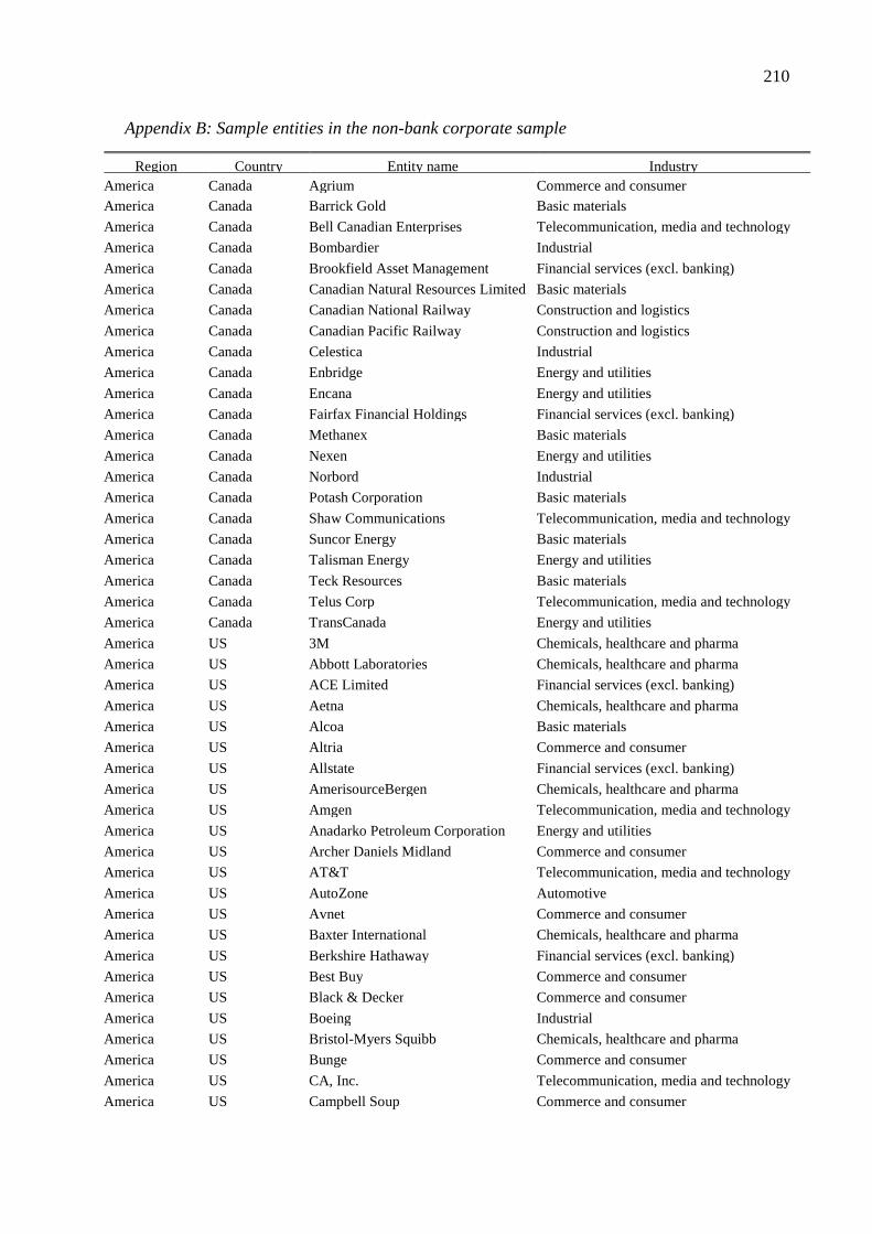
210
Appendix B: Sample entities in the non-bank corporate sample
Region Country Entity name Industry America Canada Agrium Commerce and consumer America Canada Barrick Gold Basic materials
America Canada Bell Canadian Enterprises Telecommunication, media and technology
America Canada Bombardier Industrial
America Canada Brookfield Asset Management Financial services (excl. banking)
America Canada Canadian Natural Resources Limited Basic materials
America Canada Canadian National Railway Construction and logistics
America Canada Canadian Pacific Railway Construction and logistics
America Canada Celestica Industrial
America Canada Enbridge Energy and utilities
America Canada Encana Energy and utilities
America Canada Fairfax Financial Holdings Financial services (excl. banking)
America Canada Methanex Basic materials
America Canada Nexen Energy and utilities
America Canada Norbord Industrial
America Canada Potash Corporation Basic materials
America Canada Shaw Communications Telecommunication, media and technology
America Canada Suncor Energy Basic materials
America Canada Talisman Energy Energy and utilities
America Canada Teck Resources Basic materials
America Canada Telus Corp Telecommunication, media and technology
America Canada TransCanada Energy and utilities
America US 3M Chemicals, healthcare and pharma
America US Abbott Laboratories Chemicals, healthcare and pharma
America US ACE Limited Financial services (excl. banking)
America US Aetna Chemicals, healthcare and pharma
America US Alcoa Basic materials
America US Altria Commerce and consumer
America US Allstate Financial services (excl. banking)
America US AmerisourceBergen Chemicals, healthcare and pharma
America US Amgen Telecommunication, media and technology
America US Anadarko Petroleum Corporation Energy and utilities
America US Archer Daniels Midland Commerce and consumer
America US AT&T Telecommunication, media and technology
America US AutoZone Automotive
America US Avnet Commerce and consumer
America US Baxter International Chemicals, healthcare and pharma
America US Berkshire Hathaway Financial services (excl. banking)
America US Best Buy Commerce and consumer
America US Black & Decker Commerce and consumer
America US Boeing Industrial
America US Bristol-Myers Squibb Chemicals, healthcare and pharma
America US Bunge Commerce and consumer
America US CA, Inc. Telecommunication, media and technology
America US Campbell Soup Commerce and consumer

211
Region Country Entity name Industry America US Cardinal Health Chemicals, healthcare and pharma
America US Carnival Corporation Construction and logistics
America US Caterpillar Industrial
America US CBS Corporation Telecommunication, media and technology
America US Chevron Energy and utilities
America US Chubb Corp Financial services (excl. banking)
America US Cigna Chemicals, healthcare and pharma
America US Cisco Telecommunication, media and technology
America US Coca Cola Commerce and consumer
America US Comcast Telecommunication, media and technology
America US ConAgra Foods Commerce and consumer
America US Constellation Energy Energy and utilities
America US Costco Wholesale Commerce and consumer
America US CSX Corporation Industrial
America US CVS Caremark Chemicals, healthcare and pharma
America US Darden Restaurants Commerce and consumer
America US Deere & Company Industrial
America US Dell Telecommunication, media and technology
America US Devon Energy Energy and utilities
America US DIRECTV Holdings Telecommunication, media and technology
America US Dominion Resources Energy and utilities
America US Dow Chemical Chemicals, healthcare and pharma
America US Duke Energy Carolinas Energy and utilities
America US Du Pont Chemicals, healthcare and pharma
America US Eastman Chemical Company Chemicals, healthcare and pharma
America US Enterprise Products Energy and utilities
America US Express Scripts Chemicals, healthcare and pharma
America US Exxon Mobil Energy and utilities
America US FedEx Construction and logistics
America US FirstEnergy Energy and utilities
America US Ford Automotive
America US Fortune Brands Commerce and consumer
America US General Dynamics Industrial
America US General Electric Industrial
America US General Mills Commerce and consumer
America US Goodrich Industrial
America US Halliburton Energy and utilities
America US Hartford Financial Services Financial services (excl. banking)
America US Hess Energy and utilities
America US Hewlett-Packard Telecommunication, media and technology
America US Home Depot Commerce and consumer
America US Honeywell Industrial
America US Humana Chemicals, healthcare and pharma
America US IBM Telecommunication, media and technology
America US Ingersoll-Rand Industrial
America US International Paper Industrial
America US Johnson & Johnson Chemicals, healthcare and pharma

212
Region Country Entity name Industry America US Johnson Controls Industrial
America US Kinder Morgan Energy and utilities
America US Kraft Foods Commerce and consumer
America US Kroger Automotive
America US Liberty Mutual Financial services (excl. banking)
America US Lockheed Martin Industrial
America US Loews Corporation Financial services (excl. banking)
America US Lowe's Commerce and consumer
America US Marathon Oil Energy and utilities
America US Marriott International Commerce and consumer
America US Marsh & McLennan Financial services (excl. banking)
America US McDonalds Commerce and consumer
America US McKesson Chemicals, healthcare and pharma
America US MedCo Health Chemicals, healthcare and pharma
America US Merck & Co Chemicals, healthcare and pharma
America US Motorola Telecommunication, media and technology
America US Newell Rubbermaid Commerce and consumer
America US Norfolk Southern Industrial
America US Northrop Grumman Industrial
America US Omnicom Group Telecommunication, media and technology
America US PepsiCo Commerce and consumer
America US Pfizer Chemicals, healthcare and pharma
America US Pitney Bowes Telecommunication, media and technology
America US Procter & Gamble Commerce and consumer
America US Progress Energy Energy and utilities
America US Prudential Financial Financial services (excl. banking)
America US Quest Diagnostics Chemicals, healthcare and pharma
America US R.R. Donneley Telecommunication, media and technology
America US Raytheon Company Industrial
America US Reynolds American Commerce and consumer
America US Ryder System Industrial
America US Safeway Inc. Commerce and consumer
America US Sara Lee Commerce and consumer
America US Sears Commerce and consumer
America US Sempra Energy Energy and utilities
America US Sherwin-Williams Industrial
America US Simon Property Financial services (excl. banking)
America US SLM Corp Financial services (excl. banking)
America US Southwest Airlines Commerce and consumer
America US Sprint Nextel Telecommunication, media and technology
America US Sunoco Energy and utilities
America US Supervalu Commerce and consumer
America US Sysco Commerce and consumer
America US Target Corp Commerce and consumer
America US Time Warner Telecommunication, media and technology
America US TJX Companies Commerce and consumer
America US Toll Brothers Industrial

213
Region Country Entity name Industry America US Transocean Telecommunication, media and technology
America US Travellers Companies Financial services (excl. banking)
America US Tyson Foods Commerce and consumer
America US UnitedHealth Group Chemicals, healthcare and pharma
America US United Technologies Industrial
America US Union Pacific Industrial
America US United Parcel Service Construction and logistics
America US Valero Energy Corporation Energy and utilities
America US Verizon Telecommunication, media and technology
America US Viacom Telecommunication, media and technology
America US Vornado Realty Financial services (excl. banking)
America US Wal-Mart Commerce and consumer
America US Walt Disney Telecommunication, media and technology
America US Wellpoint Chemicals, healthcare and pharma
America US Whirlpool Commerce and consumer
America US Xerox Telecommunication, media and technology
America US XL Group Financial services (excl. banking)
America US YUM! Brands Commerce and consumer
Asia-Pacific Australia Amcor Industrial
Asia-Pacific Australia AMP Limited Financial services (excl. banking)
Asia-Pacific Australia BHP Billiton Basic materials
Asia-Pacific Australia CSR Limited Industrial
Asia-Pacific Australia Fairfax Media Telecommunication, media and technology
Asia-Pacific Australia Foster's Group Commerce and consumer
Asia-Pacific Australia GPT Group Construction and logistics
Asia-Pacific Australia Lend Lease Group Construction and logistics
Asia-Pacific Australia Qantas Commerce and consumer
Asia-Pacific Australia QBE Insurance Financial services (excl. banking)
Asia-Pacific Australia Rio Tinto Basic materials
Asia-Pacific Australia Telstra Chemicals, healthcare and pharma
Asia-Pacific Australia Wesfarmers Commerce and consumer
Asia-Pacific Australia Woodside Petroleum Energy and utilities
Asia-Pacific Australia Woolworths Commerce and consumer
Asia-Pacific China China Mobile Limited Telecommunication, media and technology
Asia-Pacific Hong Kong Hutchison Whampoa Industrial
Asia-Pacific Hong Kong Noble Group Basic materials
Asia-Pacific India Reliance Industries Energy and utilities
Asia-Pacific India Tata Group Industrial
Asia-Pacific Japan Aeon Commerce and consumer
Asia-Pacific Japan All Nippon Airways Commerce and consumer
Asia-Pacific Japan Bridgestone Automotive
Asia-Pacific Japan Canon Telecommunication, media and technology
Asia-Pacific Japan Chubu Electric Power Energy and utilities
Asia-Pacific Japan East Japan Railway Commerce and consumer
Asia-Pacific Japan Fujitsu Telecommunication, media and technology
Asia-Pacific Japan Hitachi Telecommunication, media and technology
Asia-Pacific Japan Honda Motor Automotive

214
Region Country Entity name Industry Asia-Pacific Japan Itochu Commerce and consumer
Asia-Pacific Japan Japan Tobaccco Commerce and consumer
Asia-Pacific Japan JFE Steel Basic materials
Asia-Pacific Japan Kansai Electric Power Energy and utilities
Asia-Pacific Japan Kawasaki Heavy Industries Industrial
Asia-Pacific Japan Komatsu Industrial
Asia-Pacific Japan KDDI Corporation Telecommunication, media and technology
Asia-Pacific Japan Mazda Automotive
Asia-Pacific Japan Marubeni Commerce and consumer
Asia-Pacific Japan Mitsubishi Group Industrial
Asia-Pacific Japan Mitsui Industrial
Asia-Pacific Japan NEC Telecommunication, media and technology
Asia-Pacific Japan Nippon Paper Group Industrial
Asia-Pacific Japan Nippon Steel Basic materials
Asia-Pacific Japan Nippon Telegraph & Telephone Telecommunication, media and technology
Asia-Pacific Japan Nissan Motor Automotive
Asia-Pacific Japan Sharp Telecommunication, media and technology
Asia-Pacific Japan Softbank Telecommunication, media and technology
Asia-Pacific Japan Sony Telecommunication, media and technology
Asia-Pacific Japan Sumitomo Chemicals Chemicals, healthcare and pharma
Asia-Pacific Japan Suzuki Automotive
Asia-Pacific Japan Taisei Corporation Construction and logistics
Asia-Pacific Japan Tokyo Gas Energy and utilities
Asia-Pacific Japan Toshiba Telecommunication, media and technology
Asia-Pacific Japan Toyota Automotive
Asia-Pacific Korea GS Caltex Energy and utilities
Asia-Pacific Korea Hyundai Motor Automotive
Asia-Pacific Korea Hynix Chemicals, healthcare and pharma
Asia-Pacific Korea Korea Electric Power Energy and utilities
Asia-Pacific Korea KT Corp Telecommunication, media and technology
Asia-Pacific Korea LG Electronics Telecommunication, media and technology
Asia-Pacific Korea POSCO Basic materials
Asia-Pacific Korea Samsung Telecommunication, media and technology
Asia-Pacific Korea SK Holdings Energy and utilities
Asia-Pacific Malaysia Telekom Malaysia Telecommunication, media and technology
Asia-Pacific Singapore CapitaLand Financial services (excl. banking)
Asia-Pacific Singapore Flextronics Telecommunication, media and technology
Asia-Pacific Singapore Genting Group Commerce and consumer
Asia-Pacific Singapore Singapore Telecommunications Telecommunication, media and technology
Europe Austria Telekom Austria Telecommunication, media and technology
Europe Belgium Anheuser-Busch InBev Commerce and consumer
Europe Belgium Solvay Chemicals, healthcare and pharma
Europe Denmark Carlsberg Commerce and consumer
Europe Finnland Fortum Energy and utilities
Europe Finnland Metso Industrial
Europe Finnland M-Real Industrial
Europe Finnland Nokia Telecommunication, media and technology

215
Region Country Entity name Industry Europe Finnland Stora Enso Industrial
Europe France Air France KLM Group Commerce and consumer
Europe France Air Liquide-SA Chemicals, healthcare and pharma
Europe France Alstom Industrial
Europe France Axa Financial services (excl. banking)
Europe France Bouygues Construction and logistics
Europe France Carrefour Commerce and consumer
Europe France Compagnie de Saint-Gobain Basic materials
Europe France Danone Commerce and consumer
Europe France France Telecom Telecommunication, media and technology
Europe France GDF Suez Commerce and consumer
Europe France Groupe Casino Commerce and consumer
Europe France L'Oreal Commerce and consumer
Europe France LVMH Commerce and consumer
Europe France Peugeot Automotive
Europe France PPR Commerce and consumer
Europe France Publicis Telecommunication, media and technology
Europe France Renault Automotive
Europe France Sanofi-Aventis Chemicals, healthcare and pharma
Europe France Schneider Electric Industrial
Europe France Total Energy and utilities
Europe France Unibail-Rodamco Financial services (excl. banking)
Europe France Veolia Environnement Energy and utilities
Europe France Vinci Construction and logistics
Europe France Vivendi Telecommunication, media and technology
Europe Germany Adidas Commerce and consumer
Europe Germany Allianz Financial services (excl. banking)
Europe Germany BASF Chemicals, healthcare and pharma
Europe Germany Bayer Chemicals, healthcare and pharma
Europe Germany BMW Automotive
Europe Germany Continental Automotive
Europe Germany Daimler Automotive
Europe Germany Deutsche Lufthansa Commerce and consumer
Europe Germany Deutsche Post Construction and logistics
Europe Germany Deutsche Telekom Telecommunication, media and technology
Europe Germany E.ON Energy and utilities
Europe Germany ENBW Energy and utilities
Europe Germany Fresenius Medical Chemicals, healthcare and pharma
Europe Germany Hannover Re Financial services (excl. banking)
Europe Germany Henkel Chemicals, healthcare and pharma
Europe Germany Lanxess Chemicals, healthcare and pharma
Europe Germany Linde Chemicals, healthcare and pharma
Europe Germany Metro Commerce and consumer
Europe Germany RWE Energy and utilities
Europe Germany Siemens Industrial
Europe Germany Suedzuckker Commerce and consumer
Europe Germany ThyssenKrupp Industrial

216
Region Country Entity name Industry Europe Germany Volkswagen Automotive
Europe Greece Hellenic Telecom Telecommunication, media and technology
Europe Italy Assicurazioni Generali Financial services (excl. banking)
Europe Italy ENI Energy and utilities
Europe Italy Enel Energy and utilities
Europe Italy Fiat Automotive
Europe Italy Finmeccanica Industrial
Europe Italy Telecom Italia Telecommunication, media and technology
Europe Netherlands Aegon Financial services (excl. banking)
Europe Netherlands Ahold Commerce and consumer
Europe Netherlands AkzoNobel Chemicals, healthcare and pharma
Europe Netherlands EADS Industrial
Europe Netherlands DSM Chemicals, healthcare and pharma
Europe Netherlands KPN Telecommunication, media and technology
Europe Netherlands Philips Telecommunication, media and technology
Europe Netherlands TNT Construction and logistics
Europe Netherlands WoltersKluwer Telecommunication, media and technology
Europe Norway Norske Skog Industrial
Europe Norway Statoil Energy and utilities
Europe Norway Telenor Telecommunication, media and technology
Europe Portugal Brisa-Auto-Estradas Construction and logistics
Europe Portugal Energias de Portugal Energy and utilities
Europe Portugal Portugal Telecom Telecommunication, media and technology
Europe Spain Endesa Energy and utilities
Europe Spain Gas Natural Energy and utilities
Europe Spain Iberdrola Energy and utilities
Europe Spain Repsol YPF Energy and utilities
Europe Spain Telefonica Telecommunication, media and technology
Europe Sweden Electrolux Commerce and consumer
Europe Sweden Svenska Cellulosa Commerce and consumer
Europe Sweden TeliaSonera Telecommunication, media and technology
Europe Sweden Volvo Automotive
Europe Switzerland ABB Industrial
Europe Switzerland Adecco Industrial
Europe Switzerland Holcim Basic materials
Europe Switzerland Nestlé Commerce and consumer
Europe Switzerland Novartis Chemicals, healthcare and pharma
Europe Switzerland Roche Chemicals, healthcare and pharma
Europe Switzerland STMicroelectronics Telecommunication, media and technology
Europe Switzerland Swiss Reinsurance Financial services (excl. banking)
Europe Switzerland Xstrata Basic materials
Europe UK AngloAmerican Basic materials
Europe UK AstraZeneca Chemicals, healthcare and pharma
Europe UK Aviva Financial services (excl. banking)
Europe UK BAE Systems Industrial
Europe UK BP Energy and utilities
Europe UK British American Tobacco Commerce and consumer

217
Region Country Entity name Industry Europe UK British Telecommunications Telecommunication, media and technology
Europe UK Centrica Energy and utilities
Europe UK Compass Group Commerce and consumer
Europe UK Diageo Commerce and consumer
Europe UK GlaxoSmithKline Chemicals, healthcare and pharma
Europe UK Imperial Tobacco Commerce and consumer
Europe UK J. Sainsbury's Commerce and consumer
Europe UK Kingfisher PLC Commerce and consumer
Europe UK Legal & General Financial services (excl. banking)
Europe UK Marks and Spencer Commerce and consumer
Europe UK National Grid Energy and utilities
Europe UK Next PLC Commerce and consumer
Europe UK Old Mutual Financial services (excl. banking)
Europe UK Pearson Telecommunication, media and technology
Europe UK Prudential Financial services (excl. banking)
Europe UK Reed Elsevier Telecommunication, media and technology
Europe UK Rentokil Initial Industrial
Europe UK Rolls-Royce Automotive
Europe UK Royal Dutch Shell Energy and utilities
Europe UK Safeway / WM Morrisons Commerce and consumer
Europe UK Tate & Lyle Commerce and consumer
Europe UK Tesco Commerce and consumer
Europe UK Unilever Commerce and consumer
Europe UK United Utilities Energy and utilities
Europe UK Vodafone Telecommunication, media and technology

218
Appendix C: Unit root test results for the regional relative ESS-indicator
Log Values Log Differences Period Relative ESS-Indicator ADF PP KPSS ADF PP KPSS
Period 1
America -0.200.00 -0.19 0.00 1.53 *** -28.81*** -30.91*** 0.02 0%
Asia-Pacific -0.130.00 0.09 0.00 0.36 *** -30.74*** -35.44*** 0.00 0%
Europe -0.220.00 -0.11 0.00 2.91 *** -32.21*** -35.93*** 0.01 0%
Middle East & Russia -0.070.00 0.01 0.00 3.25 *** -24.80*** -25.65*** 0.01 0%
Period 2
America -1.410.00 -1.50 0.00 2.72 *** -21.97*** -21.94*** 0.05 0%
Asia-Pacific -1.130.00 -1.38 0.00 1.50 *** -26.13*** -26.43*** 0.05 0%
Europe -1.560.00 -1.76* 4.45 *** -25.27*** -25.03*** 0.05 0%
Middle East & Russia -0.750.00 -0.81 0.00 4.22 *** -22.68*** -22.77*** 0.03 0%
Period 3
America 0.180.00 0.15 0.00 6.29 *** -17.16*** -17.14*** 0.03 0%
Asia-Pacific -0.180.00 -0.18 0.00 4.57 *** -19.50*** -19.50*** 0.22***
Europe 0.030.00 0.04 0.00 3.11 *** -19.45*** -19.45*** 0.04 0%
Middle East & Russia -0.530.00 -0.50 0.00 5.25 *** -16.89*** -16.88*** 0.24***
Period 4
America -0.260.00 -0.26 0.00 4.22 *** -20.15*** -20.17*** 0.02 0%
Asia-Pacific -0.610.00 -0.69 0.00 2.88 *** -22.46*** -22.67*** 0.08 0%
Europe -0.370.00 -0.38 0.00 3.50 *** -20.56*** -20.55*** 0.05 0%
Middle East & Russia 0.460.00 0.54 0.00 1.30 *** -21.86*** -21.92*** 0.02 0% Notes: The table shows the test-statistics from applying the ADF, PP and KPSS unit root tests. ADF and PP examines the null hypothesis of a unit root. By contrast, the KPSS test examines the null hypothesis of stationarity. *, **, *** denotes significance at the 10%, 5% and 1% significance level, respectively. Period 1 ranges from October 1st, 2005 to February 28th, 2007, Period 2 ranges from March 1st, 2007 to July 31st, 2008, Period 3 ranges from August 1st, 2008 to December 31st, 2009, Period 4 ranges from January 1st, 2010 to April 30th, 2011.

219
Appendix D: Unit root test results for regional bank CDS spreads
Log Values Log Differences Period Regional bank CDS spread ADF PP KPSS ADF PP KPSS
Period 1
America 0.22 0.00 0.22 0.00 1.52*** -19.99*** -20.00*** 0.10 0%
Asia-Pacific 0.19 0.00 0.34 0.00 1.85*** -29.02*** -31.06*** 0.01 0%
Europe 0.78 0.00 1.02 0.00 1.45*** -22.18*** -22.51*** 0.01 0%
Middle East & Russia 0.12 0.00 0.20 0.00 3.77*** -21.56*** -21.82*** 0.02 0%
Period 2
America -1.86 * -1.66* 2.87*** -15.49*** -15.48*** 0.08 0%
Asia-Pacific -2.54 ** -2.12** 2.37*** -13.52*** -13.48*** 0.17**
Europe -2.28 ** -2.07** 4.30*** -15.50*** -15.49*** 0.09 0%
Middle East & Russia -1.14 0.00-1.24 0.00 4.92*** -21.31*** -21.33*** 0.07 0%
Period 3
America 0.10 0.00 0.05 0.00 5.70*** -15.12*** -15.08*** 0.03 0%
Asia-Pacific 0.11 0.00 0.06 0.00 5.09*** -14.24*** -14.22*** 0.25***
Europe -0.17 0.00-0.18 0.00 5.96*** -15.09*** -15.03*** 0.04 0%
Middle East & Russia -0.94 0.00-0.84 0.00 5.25*** -14.60*** -14.54*** 0.28***
Period 4
America -0.31 0.00-0.30 0.00 4.34*** -15.58*** -15.54*** 0.03 0%
Asia-Pacific -0.55 0.00-0.49 0.00 2.03*** -14.68*** -14.65*** 0.09 0%
Europe -0.85 0.00-0.79 0.00 2.46*** -16.23*** -16.23*** 0.04 0%
Middle East & Russia 1.09 0.00 0.90 0.00 1.56*** -15.38*** -15.39*** 0.04 0%
Notes: The table shows the test-statistics from applying the ADF, PP and KPSS unit root tests. ADF and PP examines the null hypothesis of a unit root. By contrast, the KPSS test examines the null hypothesis of stationarity. *, **, *** denotes significance at the 10%, 5% and 1% significance level, respectively. Period 1 ranges from October 1st, 2005 to February 28th, 2007, Period 2 ranges from March 1st, 2007 to July 31st, 2008, Period 3 ranges from August 1st, 2008 to December 31st, 2009, Period 4 ranges from January 1st, 2010 to April 30th, 2011.
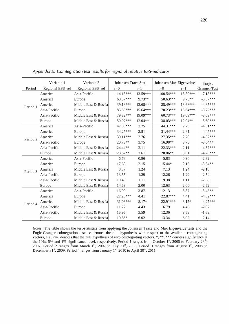
220
Appendix E: Cointegration test results for regional relative ESS-indicator
Variable 1 Variable 2 Johansen Trace Stat. Johansen Max Eigenvalue Engle- Granger-Test Period Regional ESS_rel Regional ESS_rel r=0 r=1 r=0 r=1
Period 1
America Asia-Pacific 114.13*** 13.59*** 100.54*** 13.59*** -7.18***
America Europe 60.37*** 9.73** 50.63*** 9.73** -6.57***
America Middle East & Russia 39.18*** 13.68*** 25.49*** 13.68*** -4.35***
Asia-Pacific Europe 85.86*** 15.64*** 70.23*** 15.64*** -8.72***
Asia-Pacific Middle East & Russia 79.82*** 19.09*** 60.73*** 19.09*** -8.09***
Europe Middle East & Russia 50.07*** 12.04** 38.03*** 12.04** -5.60***
Period 2
America Asia-Pacific 47.06*** 2.75 ## 44.31*** 2.75 ## -4.51***
America Europe 34.25*** 2.81 ## 31.44*** 2.81 ## -4.45***
America Middle East & Russia 30.11*** 2.76 ## 27.35*** 2.76 ## -4.87***
Asia-Pacific Europe 20.73** 3.75 ## 16.98** 3.75 ## -3.64**
Asia-Pacific Middle East & Russia 24.44** 2.11 ## 22.33*** 2.11 ## -4.57***
Europe Middle East & Russia 23.67** 3.61 ## 20.06** 3.61 ## -4.28***
Period 3
America Asia-Pacific 6.78 ## 0.96 ## 5.83 ## 0.96 ## -2.32 ##
America Europe 17.60 ## 2.15 ## 15.44* 2.15 ## -3.64**
America Middle East & Russia 8.37 ## 1.24 ## 7.13 ## 1.24 ## -2.18 ##
Asia-Pacific Europe 13.55 ## 1.29 ## 12.26 ## 1.29 ## -2.54 ##
Asia-Pacific Middle East & Russia 10.49 ## 1.11 ## 9.38 ## 1.11 ## -2.63 ##
Europe Middle East & Russia 14.63 ## 2.00 ## 12.63 ## 2.00 ## -2.52 ##
Period 4
America Asia-Pacific 16.00 ## 3.87 ## 12.13 ## 3.87 ## -3.45**
America Europe 27.28*** 4.41 ## 22.87*** 4.41 ## -4.82***
America Middle East & Russia 31.08*** 8.17* 22.91*** 8.17* -4.27***
Asia-Pacific Europe 11.22 0.0 4.43 0.0 6.79 0.0 4.43 0.0 -2.07 0
Asia-Pacific Middle East & Russia 15.95 0.0 3.59 0.0 12.36 0.0 3.59 0.0 -1.69 0
Europe Middle East & Russia 19.36* 6.02 0.0 13.34 0.0 6.02 0.0 -2.14 0
Notes: The table shows the test-statistics from applying the Johansen Trace and Max Eigenvalue tests and the Engle-Granger cointegration tests. r denotes the null hypothesis with respect to the available cointegrating vectors, e.g., r=0 denotes that the null hypothesis of zero cointegrating vectors. *, **, *** denotes significance at the 10%, 5% and 1% significance level, respectively. Period 1 ranges from October 1st, 2005 to February 28th, 2007, Period 2 ranges from March 1st, 2007 to July 31st, 2008, Period 3 ranges from August 1st, 2008 to December 31st, 2009, Period 4 ranges from January 1st, 2010 to April 30th, 2011.

221
Appendix F: Cointegration test results for regional bank CDS spreads
Variable 1 Variable 2 Johansen Trace Stat. Johansen Max Eigenvalue Engle- Granger-Test Period Regional bank CDS Regional bank CDS r=0 r=1 r=0 r=1
Period 1
America Asia-Pacific 48.59*** 3.11 ## 45.48*** 3.11 ## -4.13*** America Europe 24.22** 3.50 ## 20.71*** 3.50 ## -2.72 ## America Middle East & Russia 25.27*** 3.89 ## 21.37*** 3.89 ## -1.99 ## Asia-Pacific Europe 69.70*** 3.11 ## 66.59*** 3.11 ## -8.50***
Asia-Pacific Middle East & Russia 43.37*** 10.40** 32.98*** 10.40** -5.79***
Europe Middle East & Russia 18.12* 3.06 ## 15.06* 3.06 ## -2.52 ##
Period 2
America Asia-Pacific 87.61*** 2.91 ## 84.70*** 2.91 ## -3.52**
America Europe 73.61*** 2.71 ## 70.90*** 2.71 ## -4.98***
America Middle East & Russia 29.93*** 3.71 ## 26.22*** 3.71 ## -4.26***
Asia-Pacific Europe 26.95*** 4.95 ## 22.00*** 4.95 ## -2.55 ##
Asia-Pacific Middle East & Russia 25.56*** 6.79 ## 18.77** 6.79 ## -4.27***
Europe Middle East & Russia 28.55*** 6.03 ## 22.51*** 6.03 ## -4.39***
Period 3
America Asia-Pacific 6.53 ## 0.35 ## 6.18 ## 0.35 ## -2.46 ##
America Europe 14.48 ## 2.78 ## 11.70 ## 2.78 ## -3.09*
America Middle East & Russia 12.10 ## 1.97 ## 10.13 ## 1.97 ## -1.94 ##
Asia-Pacific Europe 5.91 ## 0.28 ## 5.62 ## 0.28 ## -1.49 ##
Asia-Pacific Middle East & Russia 12.67 ## 0.57 ## 12.10 ## 0.57 ## -2.06 ##
Europe Middle East & Russia 9.05 ## 3.63 ## 5.42 ## 3.63 ## -2.08 ##
Period 4
America Asia-Pacific 20.39** 7.53 ## 12.86 ## 7.53 ## -2.83 ##
America Europe 12.45 ## 3.84 ## 8.61 ## 3.84 ## -2.49 ## America Middle East & Russia 21.32** 3.86 0.0 17.46** 3.86 0.0 -3.06*
Asia-Pacific Europe 23.98** 9.24** 14.74* 9.24** -1.81 0
Asia-Pacific Middle East & Russia 12.70 0.0 4.90 0.0 7.79 0.0 4.90 0.0 -2.01 0
Europe Middle East & Russia 25.15*** 5.98 0.0 19.17** 5.98 0.0 -2.74 0
Notes: The table shows the test-statistics from applying the Johansen Trace and Max Eigenvalue tests and the Engle-Granger cointegration tests. r denotes the null hypothesis with respect to the available cointegrating vectors, e.g., r=0 denotes that the null hypothesis of zero cointegrating vectors. *, **, *** denotes significance at the 10%, 5% and 1% significance level, respectively. Period 1 ranges from October 1st, 2005 to February 28th, 2007, Period 2 ranges from March 1st, 2007 to July 31st, 2008, Period 3 ranges from August 1st, 2008 to December 31st, 2009, Period 4 ranges from January 1st, 2010 to April 30th, 2011.

222
Appendix G: Unit root test results for regional sovereign CDS spreads
Log Values Log Differences Period Regional sovereign CDS spread ADF PP KPSS ADF PP KPSS
Period 1
America 0.13 0.00 0.24 0.00 3.34*** -31.16 *** -31.63*** 0.01 0%
Asia-Pacific 0.07 0.00 0.15 0.00 0.52*** -27.17 *** -28.65*** 0.00 0%
Europe -0.16 0.00 -0.08 0.00 2.90*** -23.49 *** -23.89*** 0.01 0%
Middle East & Russia 0.05 0.00 0.10 0.00 1.23*** -24.45 *** -24.82*** 0.01 0%
Period 2
America -1.20 0.00 -1.37 0.00 2.89*** -23.10 *** -23.19*** 0.03 0%
Asia-Pacific -0.96 0.00 -1.08 0.00 1.82*** -22.03 *** -22.46*** 0.02 0%
Europe -0.61 0.00 -0.72 0.00 1.85*** -26.19 *** -26.41*** 0.02 0%
Middle East & Russia -0.70 0.00 -0.84 0.00 3.50*** -27.26 *** -27.15*** 0.04 0%
Period 3
America -0.97 0.00 -1.01 0.00 6.38*** -20.26 *** -20.27*** 0.18**
Asia-Pacific -0.55 0.00 -0.50 0.00 5.83*** -15.11 *** -15.20*** 0.23***
Europe -1.93 * -1.58 0.00 6.65*** -13.26 *** -13.25*** 0.37***
Middle East & Russia -1.06 0.00 -0.94 0.00 5.79*** -14.13 *** -14.10*** 0.29***
Period 4
America -0.47 0.00 -0.45 0.00 1.38*** -16.77 *** -16.80*** 0.03 0%
Asia-Pacific -0.05 0.00 -0.05 0.00 2.27*** -17.23 *** -17.24*** 0.06 0%
Europe -0.55 0.00 -0.51 0.00 2.34*** -14.51 *** -14.51*** 0.04 0%
Middle East & Russia 0.58 0.00 0.55 0.00 1.05*** -16.62 *** -16.56*** 0.03 0% Notes: The table shows the test-statistics from applying the ADF, PP and KPSS unit root tests. ADF and PP examines the null hypothesis of a unit root. By contrast, the KPSS test examines the null hypothesis of stationarity. *, **, *** denotes significance at the 10%, 5% and 1% significance level, respectively. Period 1 ranges from October 1st, 2005 to February 28th, 2007, Period 2 ranges from March 1st, 2007 to July 31st, 2008, Period 3 ranges from August 1st, 2008 to December 31st, 2009, Period 4 ranges from January 1st, 2010 to April 30th, 2011.

223
Appendix H: Cointegration test for regional sovereign and bank CDS spreads
Variable 1 Variable 2 Johansen Trace Stat. Johansen Max Eigenvalue Engle- Granger-Test Period Sovereign CDS Bank CDS r=0 r=1 r=0 r=1
Period 1
America
America 43.91*** 2.91 ## 41.00*** 2.91 ## -5.72*** Asia-Pacific 94.87*** 12.49** 82.38*** 12.49** -8.64*** Europe 56.73*** 2.67 ## 54.06*** 2.67 ## -7.53*** Middle East & Russia 53.48*** 7.88* 45.61*** 7.88* -6.67***
Asia-Pacific
America 75.25*** 3.02 ## 72.23*** 3.02 ## -8.51*** Asia-Pacific 104.39*** 19.10*** 85.29*** 19.10*** -9.34*** Europe 100.66*** 3.10 ## 97.56*** 3.10 ## -10.54*** Middle East & Russia 50.92*** 10.76** 40.15*** 10.76** -6.42***
Europe
America 38.79*** 3.06 ## 35.73*** 3.06 ## -6.10*** Asia-Pacific 53.36*** 20.37*** 32.99*** 20.37*** -5.44*** Europe 39.20*** 3.22 ## 35.97*** 3.22 ## -6.13*** Middle East & Russia 36.44*** 11.02** 25.42*** 11.02** -5.11***
Middle East & Russia
America 30.19*** 3.00 ## 27.19*** 3.00 ## -5.11*** Asia-Pacific 52.03*** 9.26** 42.77*** 9.26** -5.22*** Europe 35.30*** 2.93 ## 32.37*** 2.93 ## -5.77*** Middle East & Russia 29.81*** 7.49 ## 22.32*** 7.49 ## -4.36***
Period 2
America
America 47.80*** 3.10 ## 44.70*** 3.10 ## -5.13*** Asia-Pacific 32.77*** 6.13 ## 26.64*** 6.13 ## -4.98*** Europe 32.72*** 5.67 ## 27.05*** 5.67 ## -4.71*** Middle East & Russia 36.73*** 2.80 ## 33.92*** 2.80 ## -5.88***
Asia-Pacific
America 33.19*** 2.80 ## 30.38*** 2.80 ## -4.11*** Asia-Pacific 32.35*** 5.97 ## 26.38*** 5.97 ## -4.90*** Europe 20.80** 5.40## 15.40* 5.40 ## -3.60** Middle East & Russia 22.14** 2.53 ## 19.61** 2.53 ## -4.21***
Europe
America 63.38*** 3.91 ## 59.48*** 3.91 ## -7.97*** Asia-Pacific 80.86*** 6.47 ## 74.39*** 6.47 ## -8.96*** Europe 61.43*** 5.95 ## 55.48*** 5.95 ## -7.67*** Middle East & Russia 53.11*** 2.33 ## 50.79*** 2.33 ## -7.28***
Middle East & Russia
America 49.35*** 3.56 ## 45.79*** 3.56 ## -5.93*** Asia-Pacific 41.12*** 6.23 ## 34.89*** 6.23 ## -5.91*** Europe 52.54*** 6.00 ## 46.54*** 6.00 ## -7.02*** Middle East & Russia 36.55*** 2.33 ## 34.22*** 2.33 ## -5.96***
Period 3
America
America 6.79 ## 2.23 ## 4.56 ## 2.23 ## -1.75 ## Asia-Pacific 10.03 ## 0.90 ## 9.13 ## 0.90 ## -1.86 ## Europe 9.62 ## 4.40 ## 5.23 ## 4.40 ## -2.02 ## Middle East & Russia 13.27 ## 3.62 ## 9.65 ## 3.62 ## -2.06 ##
Asia-Pacific
America 7.36 ## 1.69 ## 5.67 ## 1.69 ## -2.00 ## Asia-Pacific 9.39 ## 0.70 ## 8.69 ## 0.70 ## -2.18 ## Europe 7.40 ## 2.46 ## 4.94 ## 2.46 ## -1.83 ## Middle East & Russia 10.99 ## 3.49 ## 7.50 ## 3.49 ## -2.40 ##
Europe
America 11.97 ## 2.15 ## 9.82 ## 2.15 ## -1.72 ## Asia-Pacific 18.33* 3.85## 14.48* 3.85 ## -2.05 ## Europe 13.17 ## 3.31 ## 9.85 ## 3.31 ## -1.75 ## Middle East & Russia 22.20** 4.39 ## 17.81** 4.39 ## -1.11 ##
Middle East & Russia
America 10.37 ## 1.98 ## 8.38 ## 1.98 ## -2.14 ## Asia-Pacific 11.99 ## 0.68 ## 11.31 ## 0.68 ## -2.63 ## Europe 10.25 ## 4.12 ## 6.13 ## 4.12 ## -1.97 ## Middle East & Russia 14.69 ## 4.81 ## 9.88 ## 4.81 ## -3.14*
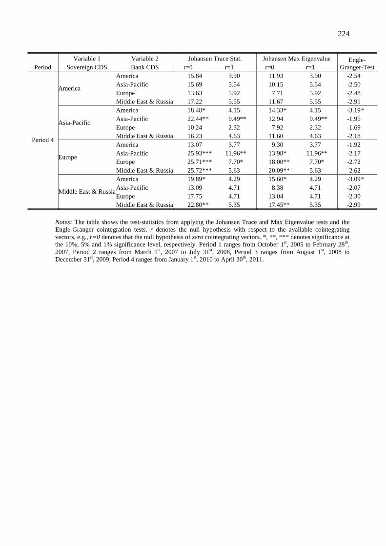
224
Variable 1 Variable 2 Johansen Trace Stat. Johansen Max Eigenvalue Engle- Granger-Test Period Sovereign CDS Bank CDS r=0 r=1 r=0 r=1
Period 4
America
America 15.84 ## 3.90 ## 11.93 ## 3.90 ## -2.54 ## Asia-Pacific 15.69 ## 5.54 ## 10.15 ## 5.54 ## -2.50 ## Europe 13.63 ## 5.92 ## 7.71 ## 5.92 ## -2.48 ## Middle East & Russia 17.22 ## 5.55 ## 11.67 ## 5.55 ## -2.91 ##
Asia-Pacific
America 18.48* 4.15## 14.33* 4.15 ## -3.19* Asia-Pacific 22.44** 9.49** 12.94 ## 9.49** -1.95 ## Europe 10.24 ## 2.32 ## 7.92 ## 2.32 ## -1.69 ## Middle East & Russia 16.23 ## 4.63 ## 11.60 ## 4.63 ## -2.18 ##
Europe
America 13.07 ## 3.77 ## 9.30 ## 3.77 ## -1.92 ## Asia-Pacific 25.93*** 11.96** 13.98* 11.96** -2.17## Europe 25.71*** 7.70* 18.00** 7.70* -2.72## Middle East & Russia 25.72*** 5.63 ## 20.09** 5.63 ## -2.62 ##
Middle East & Russia
America 19.89* 4.29## 15.60* 4.29 ## -3.09* Asia-Pacific 13.09 ## 4.71 ## 8.38 ## 4.71 ## -2.07 ## Europe 17.75 ## 4.71 ## 13.04 ## 4.71 ## -2.30 ## Middle East & Russia 22.80** 5.35 ## 17.45** 5.35 ## -2.99 ##
Notes: The table shows the test-statistics from applying the Johansen Trace and Max Eigenvalue tests and the Engle-Granger cointegration tests. r denotes the null hypothesis with respect to the available cointegrating vectors, e.g., r=0 denotes that the null hypothesis of zero cointegrating vectors. *, **, *** denotes significance at the 10%, 5% and 1% significance level, respectively. Period 1 ranges from October 1st, 2005 to February 28th, 2007, Period 2 ranges from March 1st, 2007 to July 31st, 2008, Period 3 ranges from August 1st, 2008 to December 31st, 2009, Period 4 ranges from January 1st, 2010 to April 30th, 2011.
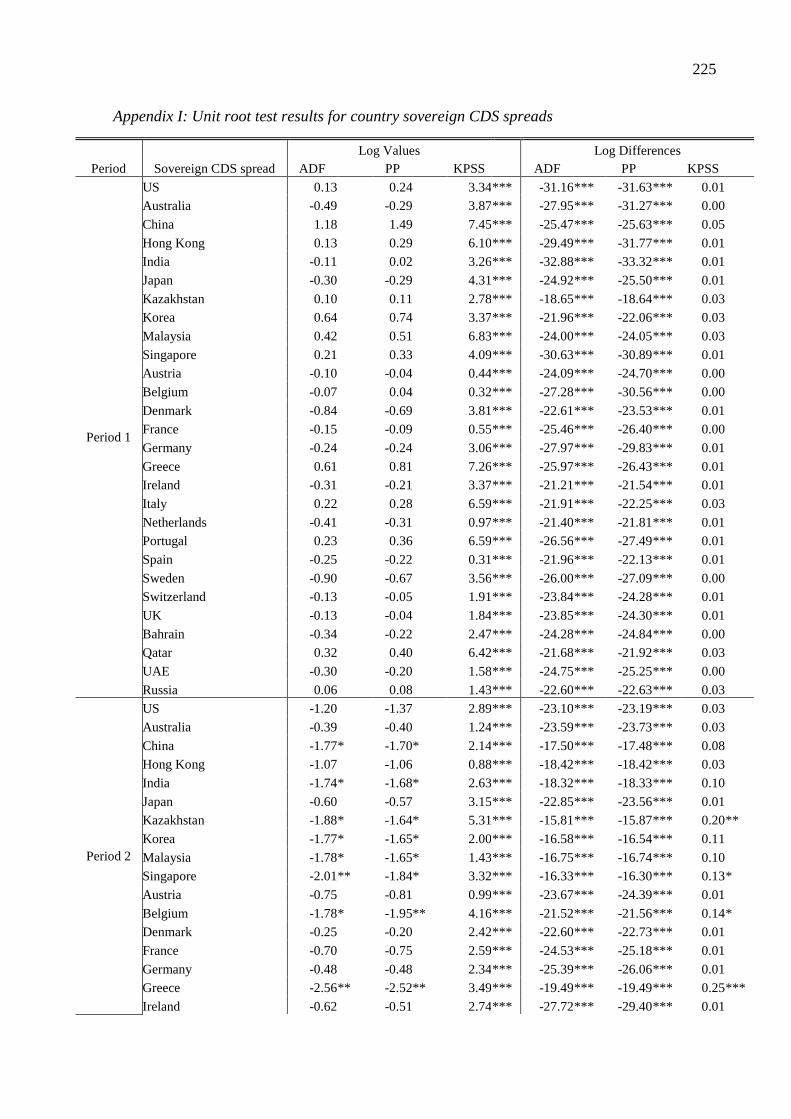
225
Appendix I: Unit root test results for country sovereign CDS spreads
Log Values Log Differences Period Sovereign CDS spread ADF PP KPSS ADF PP KPSS
Period 1
US 0.13 0.00 0.24 0.00 3.34*** -31.16*** -31.63*** 0.01 0%
Australia -0.49 0.00 -0.29 0.00 3.87*** -27.95*** -31.27*** 0.00 0%
China 1.18 0.00 1.49 0.00 7.45*** -25.47*** -25.63*** 0.05 0%
Hong Kong 0.13 0.00 0.29 0.00 6.10*** -29.49*** -31.77*** 0.01 0%
India -0.11 0.00 0.02 0.00 3.26*** -32.88*** -33.32*** 0.01 0%
Japan -0.30 0.00 -0.29 0.00 4.31*** -24.92*** -25.50*** 0.01 0%
Kazakhstan 0.100.00 0.11 0.00 2.78*** -18.65*** -18.64*** 0.03 0%
Korea 0.64 0.00 0.74 0.00 3.37*** -21.96*** -22.06*** 0.03 0%
Malaysia 0.42 0.00 0.51 0.00 6.83*** -24.00*** -24.05*** 0.03 0%
Singapore 0.21 0.00 0.33 0.00 4.09*** -30.63*** -30.89*** 0.01 0%
Austria -0.10 0.00 -0.04 0.00 0.44*** -24.09*** -24.70*** 0.00 0%
Belgium -0.07 0.00 0.04 0.00 0.32*** -27.28*** -30.56*** 0.00 0%
Denmark -0.84 0.00 -0.69 0.00 3.81*** -22.61*** -23.53*** 0.01 0%
France -0.15 0.00 -0.09 0.00 0.55*** -25.46*** -26.40*** 0.00 0%
Germany -0.24 0.00 -0.24 0.00 3.06*** -27.97*** -29.83*** 0.01 0%
Greece 0.61 0.00 0.81 0.00 7.26*** -25.97*** -26.43*** 0.01 0%
Ireland -0.31 0.00 -0.21 0.00 3.37*** -21.21*** -21.54*** 0.01 0%
Italy 0.22 0.00 0.28 0.00 6.59*** -21.91*** -22.25*** 0.03 0%
Netherlands -0.41 0.00 -0.31 0.00 0.97*** -21.40*** -21.81*** 0.01 0%
Portugal 0.23 0.00 0.36 0.00 6.59*** -26.56*** -27.49*** 0.01 0%
Spain -0.25 0.00 -0.22 0.00 0.31*** -21.96*** -22.13*** 0.01 0%
Sweden -0.90 0.00 -0.67 0.00 3.56*** -26.00*** -27.09*** 0.00 0%
Switzerland -0.13 0.00 -0.05 0.00 1.91*** -23.84*** -24.28*** 0.01 0%
UK -0.13 0.00 -0.04 0.00 1.84*** -23.85*** -24.30*** 0.01 0%
Bahrain -0.34 0.00 -0.22 0.00 2.47*** -24.28*** -24.84*** 0.00 0%
Qatar 0.32 0.00 0.40 0.00 6.42*** -21.68*** -21.92*** 0.03 0%
UAE -0.30 0.00 -0.20 0.00 1.58*** -24.75*** -25.25*** 0.00 0%
Russia 0.06 0.00 0.08 0.00 1.43*** -22.60*** -22.63*** 0.03 0%
Period 2
US -1.20 0.00 -1.37 0.00 2.89*** -23.10*** -23.19*** 0.03 0%
Australia -0.39 0.00 -0.40 0.00 1.24*** -23.59*** -23.73*** 0.03 0%
China -1.77* -1.70* 2.14*** -17.50*** -17.48*** 0.08 0%
Hong Kong -1.07 0.00 -1.06 0.00 0.88*** -18.42*** -18.42*** 0.03 0%
India -1.74* -1.68* 2.63*** -18.32*** -18.33*** 0.10 0%
Japan -0.60 0.00 -0.57 0.00 3.15*** -22.85*** -23.56*** 0.01 0%
Kazakhstan -1.88* -1.64* 5.31*** -15.81*** -15.87*** 0.20**
Korea -1.77* -1.65* 2.00*** -16.58*** -16.54*** 0.11 0%
Malaysia -1.78* -1.65* 1.43*** -16.75*** -16.74*** 0.10 0%
Singapore -2.01** -1.84* 3.32*** -16.33*** -16.30*** 0.13*
Austria -0.75 0.00 -0.81 0.00 0.99*** -23.67*** -24.39*** 0.01 0%
Belgium -1.78* -1.95** 4.16*** -21.52*** -21.56*** 0.14*
Denmark -0.25 0.00 -0.20 0.00 2.42*** -22.60*** -22.73*** 0.01 0%
France -0.70 0.00 -0.75 0.00 2.59*** -24.53*** -25.18*** 0.01 0%
Germany -0.48 0.00 -0.48 0.00 2.34*** -25.39*** -26.06*** 0.01 0%
Greece -2.56** -2.52** 3.49*** -19.49*** -19.49*** 0.25***
Ireland -0.62 0.00 -0.51 0.00 2.74*** -27.72*** -29.40*** 0.01 0%
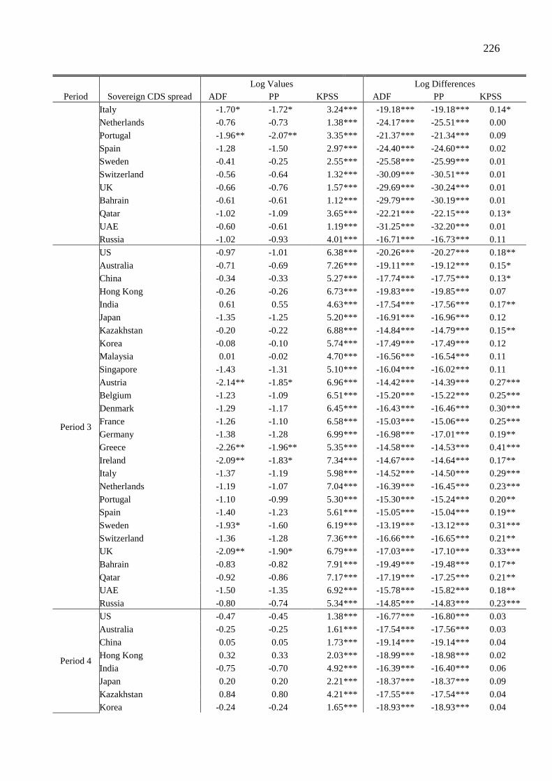
226
Log Values Log Differences Period Sovereign CDS spread ADF PP KPSS ADF PP KPSS
Italy -1.70* -1.72* 3.24*** -19.18*** -19.18*** 0.14*
Netherlands -0.76 0.00 -0.73 0.00 1.38*** -24.17*** -25.51*** 0.00 0%
Portugal -1.96** -2.07** 3.35*** -21.37*** -21.34*** 0.09 0%
Spain -1.28 0.00 -1.50 0.00 2.97*** -24.40*** -24.60*** 0.02 0%
Sweden -0.41 0.00 -0.25 0.00 2.55*** -25.58*** -25.99*** 0.01 0%
Switzerland -0.56 0.00 -0.64 0.00 1.32*** -30.09*** -30.51*** 0.01 0%
UK -0.66 0.00 -0.76 0.00 1.57*** -29.69*** -30.24*** 0.01 0%
Bahrain -0.61 0.00 -0.61 0.00 1.12*** -29.79*** -30.19*** 0.01 0%
Qatar -1.02 0.00 -1.09 0.00 3.65*** -22.21*** -22.15*** 0.13*
UAE -0.60 0.00 -0.61 0.00 1.19*** -31.25*** -32.20*** 0.01 0%
Russia -1.02 0.00 -0.93 0.00 4.01*** -16.71*** -16.73*** 0.11 0%
Period 3
US -0.97 0.00 -1.01 0.00 6.38*** -20.26*** -20.27*** 0.18**
Australia -0.71 0.00 -0.69 0.00 7.26*** -19.11*** -19.12*** 0.15*
China -0.34 0.00 -0.33 0.00 5.27*** -17.74*** -17.75*** 0.13*
Hong Kong -0.26 0.00 -0.26 0.00 6.73*** -19.83*** -19.85*** 0.07 0%
India 0.61 0.00 0.55 0.00 4.63*** -17.54*** -17.56*** 0.17**
Japan -1.35 0.00 -1.25 0.00 5.20*** -16.91*** -16.96*** 0.12 0%
Kazakhstan -0.200.00 -0.22 0.00 6.88*** -14.84*** -14.79*** 0.15**
Korea -0.08 0.00 -0.10 0.00 5.74*** -17.49*** -17.49*** 0.12 0%
Malaysia 0.01 0.00 -0.02 0.00 4.70*** -16.56*** -16.54*** 0.11 0%
Singapore -1.43 0.00 -1.31 0.00 5.10*** -16.04*** -16.02*** 0.11 0%
Austria -2.14** -1.85* 6.96*** -14.42*** -14.39*** 0.27***
Belgium -1.23 0.00 -1.09 0.00 6.51*** -15.20*** -15.22*** 0.25***
Denmark -1.29 0.00 -1.17 0.00 6.45*** -16.43*** -16.46*** 0.30***
France -1.26 0.00 -1.10 0.00 6.58*** -15.03*** -15.06*** 0.25***
Germany -1.38 0.00 -1.28 0.00 6.99*** -16.98*** -17.01*** 0.19**
Greece -2.26** -1.96** 5.35*** -14.58*** -14.53*** 0.41***
Ireland -2.09** -1.83* 7.34*** -14.67*** -14.64*** 0.17**
Italy -1.37 0.00 -1.19 0.00 5.98*** -14.52*** -14.50*** 0.29***
Netherlands -1.19 0.00 -1.07 0.00 7.04*** -16.39*** -16.45*** 0.23***
Portugal -1.10 0.00 -0.99 0.00 5.30*** -15.30*** -15.24*** 0.20**
Spain -1.40 0.00 -1.23 0.00 5.61*** -15.05*** -15.04*** 0.19**
Sweden -1.93* -1.600.00 6.19*** -13.19*** -13.12*** 0.31***
Switzerland -1.36 0.00 -1.28 0.00 7.36*** -16.66*** -16.65*** 0.21**
UK -2.09** -1.90* 6.79*** -17.03*** -17.10*** 0.33***
Bahrain -0.83 0.00 -0.82 0.00 7.91*** -19.49*** -19.48*** 0.17**
Qatar -0.92 0.00 -0.86 0.00 7.17*** -17.19*** -17.25*** 0.21**
UAE -1.50 0.00 -1.35 0.00 6.92*** -15.78*** -15.82*** 0.18**
Russia -0.80 0.00 -0.74 0.00 5.34*** -14.85*** -14.83*** 0.23***
Period 4
US -0.47 0.00 -0.45 0.00 1.38*** -16.77*** -16.80*** 0.03 0%
Australia -0.25 0.00 -0.25 0.00 1.61*** -17.54*** -17.56*** 0.03 0%
China 0.05 0.00 0.05 0.00 1.73*** -19.14*** -19.14*** 0.04 0%
Hong Kong 0.32 0.00 0.33 0.00 2.03*** -18.99*** -18.98*** 0.02 0%
India -0.75 0.00 -0.70 0.00 4.92*** -16.39*** -16.40*** 0.06 0%
Japan 0.20 0.00 0.20 0.00 2.21*** -18.37*** -18.37*** 0.09 0%
Kazakhstan 0.840.00 0.80 0.00 4.21*** -17.55*** -17.54*** 0.04 0%
Korea -0.24 0.00 -0.24 0.00 1.65*** -18.93*** -18.93*** 0.04 0%

227
Log Values Log Differences Period Sovereign CDS spread ADF PP KPSS ADF PP KPSS
Malaysia 0.11 0.00 0.12 0.00 1.02*** -18.60*** -18.62*** 0.03 0%
Singapore -0.80 0.00 -0.88 0.00 5.51*** -22.64*** -22.48*** 0.10 0%
Austria 0.48 0.00 0.42 0.00 2.52*** -15.69*** -15.68*** 0.07 0%
Belgium -1.13 0.00 -1.04 0.00 3.78*** -15.71*** -15.73*** 0.06 0%
Denmark -0.20 0.00 -0.19 0.00 1.46*** -16.46*** -16.46*** 0.06 0%
France -1.02 0.00 -0.88 0.00 3.28*** -13.70*** -13.75*** 0.05 0%
Germany -0.61 0.00 -0.60 0.00 1.18*** -18.03*** -18.03*** 0.05 0%
Greece -1.82* -1.69* 4.34*** -15.41*** -15.39*** 0.06 0%
Ireland -1.69* -1.54 0.00 2.93*** -15.40*** -15.40*** 0.06 0%
Italy -0.33 0.00 -0.33 0.00 4.49*** -14.42*** -14.37*** 0.03 0%
Netherlands -0.26 0.00 -0.25 0.00 3.25*** -15.76*** -15.75*** 0.04 0%
Portugal -1.92* -1.72* 1.61*** -14.11*** -14.09*** 0.04 0%
Spain -0.81 0.00 -0.76 0.00 3.76*** -14.94*** -14.93*** 0.03 0%
Sweden 1.04 0.00 1.15 0.00 0.97*** -19.81*** -19.88*** 0.03 0%
Switzerland 0.55 0.00 0.52 0.00 1.20*** -16.95*** -16.95*** 0.05 0%
UK 0.55 0.00 0.53 0.00 0.90*** -17.43*** -17.43*** 0.02 0%
Bahrain -0.65 0.00 -0.63 0.00 5.61*** -17.29*** -17.28*** 0.08 0%
Qatar 0.22 0.00 0.23 0.00 1.55*** -18.70*** -18.71*** 0.03 0%
UAE 0.66 0.00 0.59 0.00 0.53*** -15.38*** -15.34*** 0.05 0%
Russia 0.50 0.00 0.50 0.00 2.00*** -17.16*** -17.12*** 0.03 0%
Notes: The table shows the test-statistics from applying the ADF, PP and KPSS unit root tests. ADF and PP examines the null hypothesis of a unit root. By contrast, the KPSS test examines the null hypothesis of stationarity. *, **, *** denotes significance at the 10%, 5% and 1% significance level, respectively. Period 1 ranges from October 1st, 2005 to February 28th, 2007, Period 2 ranges from March 1st, 2007 to July 31st, 2008, Period 3 ranges from August 1st, 2008 to December 31st, 2009, Period 4 ranges from January 1st, 2010 to April 30th, 2011.

228
Appendix J: Unit root test results for country bank CDS spreads
Log Values Log Differences Period Bank CDS spread ADF PP KPSS ADF PP KPSS
Period 1
US 0.22 0.00 0.22 0.00 1.52*** -19.36*** -19.36*** 0.11 0%
Australia 0.610.00 0.77 0.00 1.90*** -22.92*** -23.38*** 0.01 0%
China 0.660.00 0.78 0.00 5.62*** -23.33*** -23.38*** 0.05 0%
Hong Kong 0.710.00 1.18 0.00 2.04*** -30.96*** -33.37*** 0.01 0%
India -0.09 0.00 -0.01 0.00 2.69*** -29.38*** -29.51*** 0.01 0%
Japan -0.050.00 0.13 0.00 0.72*** -30.27*** -33.09*** 0.00 0%
Kazakhstan -0.150.00 -0.14 0.00 1.87*** -21.85*** -21.90*** 0.01 0%
Korea 0.020.00 0.07 0.00 1.72*** -24.63*** -25.27*** 0.01 0%
Malaysia 0.430.00 0.68 0.00 6.89*** -26.92*** -28.38*** 0.01 0%
Singapore 0.510.00 0.64 0.00 6.89*** -22.78*** -23.16*** 0.03 0%
Austria -1.04 0.00 -0.62 0.00 0.59*** -28.68*** -33.53*** 0.00 0%
Belgium 0.58 0.00 0.82 0.00 1.02*** -26.37*** -27.43*** 0.01 0%
Denmark 0.510.00 0.74 0.00 4.23*** -24.36*** -25.71*** 0.01 0%
France 0.450.00 0.63 0.00 1.13*** -25.01*** -25.92*** 0.01 0%
Germany 0.510.00 0.67 0.00 1.57*** -24.55*** -25.00*** 0.01 0%
Greece 0.090.00 0.18 0.00 1.98*** -25.04*** -25.41*** 0.02 0%
Ireland 0.260.00 0.36 0.00 3.47*** -23.30*** -23.96*** 0.01 0%
Italy 1.16 0.00 1.33 0.00 2.25*** -21.36*** -21.49*** 0.03 0%
Netherlands 0.18 0.00 0.27 0.00 1.10*** -25.86*** -26.38*** 0.01 0%
Portugal 0.170.00 0.27 0.00 1.36*** -25.56*** -26.28*** 0.01 0%
Spain 0.340.00 0.44 0.00 3.46*** -23.05*** -23.50*** 0.02 0%
Sweden 0.060.00 0.12 0.00 3.47*** -22.64*** -23.50*** 0.03 0%
Switzerland 0.750.00 1.05 0.00 1.42*** -26.07*** -27.04*** 0.01 0%
UK 0.76 0.00 0.95 0.00 1.72*** -23.25*** -23.61*** 0.02 0%
Bahrain 0.490.00 0.56 0.00 2.60*** -22.81*** -22.77*** 0.02 0%
Qatar 0.500.00 0.56 0.00 2.60*** -22.81*** -22.77*** 0.02 0%
UAE 0.54 0.00 0.61 0.00 2.47*** -22.74*** -22.70*** 0.03 0%
Russia 0.030.00 0.11 0.00 3.78*** -22.15*** -22.55*** 0.02 0%
Period 2
US -1.86* -1.66* 2.87*** -15.39*** -15.38*** 0.08 0%
Australia -2.71*** -2.31** 3.77*** -14.56*** -14.55*** 0.18**
China -1.93* -1.87* 1.91*** -18.71*** -18.72*** 0.08 0%
Hong Kong -2.06** -1.93* 5.90*** -16.66*** -16.64*** 0.09 0%
India -1.82* -1.72* 3.17*** -17.30*** -17.29*** 0.13*
Japan -1.400.00 -1.25 0.00 1.10*** -15.97*** -15.99*** 0.08 0%
Kazakhstan -1.76* -1.80* 6.39*** -20.47*** -20.45*** 0.05 0%
Korea -1.510.00 -1.84* 3.13*** -24.86*** -25.20*** 0.08 0%
Malaysia -1.210.00 -1.26 0.00 3.15*** -20.35*** -20.36*** 0.05 0%
Singapore -1.80* -1.70* 4.94*** -16.93*** -16.90*** 0.10 0%
Austria -1.43 0.00 -0.91 0.00 1.28*** -32.68*** -38.79*** 0.00 0%
Belgium -2.89*** -2.66*** 5.69*** -16.66*** -16.69*** 0.10 0%
Denmark -1.260.00 -1.26 0.00 3.97*** -19.11*** -19.11*** 0.07 0%
France -1.97** -1.80* 3.97*** -16.42*** -16.43*** 0.10 0%
Germany -1.79* -1.69* 4.14*** -16.81*** -16.76*** 0.06 0%
Greece -0.310.00 -0.35 0.00 0.66*** -23.69*** -23.74*** 0.03 0%
Ireland -2.76*** -2.56** 5.71*** -16.17*** -16.13*** 0.09 0%
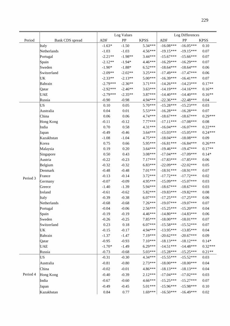
229
Log Values Log Differences Period Bank CDS spread ADF PP KPSS ADF PP KPSS
Italy -1.63* -1.50 0.00 5.34*** -16.08*** -16.05*** 0.10 0%
Netherlands -1.03 0.00 -1.03 0.00 4.56*** -19.15*** -19.15*** 0.07 0%
Portugal -2.21** -1.98** 3.44*** -15.67*** -15.66*** 0.07 0%
Spain -2.12** -1.94* 4.46*** -16.29*** -16.29*** 0.07 0%
Sweden -1.90* -1.88* 6.52*** -18.64*** -18.64*** 0.06 0%
Switzerland -2.09** -2.02** 3.25*** -17.49*** -17.47*** 0.06 0%
UK -2.33** -2.13** 5.00*** -16.39*** -16.41*** 0.07 0%
Bahrain -2.79*** -2.36** 3.71*** -14.26*** -14.23*** 0.17**
Qatar -2.92*** -2.46** 3.63*** -14.19*** -14.16*** 0.16**
UAE -2.79*** -2.35** 3.87*** -14.40*** -14.40*** 0.16**
Russia -0.900.00 -0.98 0.00 4.94*** -22.36*** -22.48*** 0.04 0%
Period 3
US 0.10 0.00 0.05 0.00 5.70*** -15.28*** -15.23*** 0.03 0%
Australia 0.040.00 0.01 0.00 5.53*** -16.28*** -16.28*** 0.07 0%
China 0.060.00 0.06 0.00 4.74*** -18.67*** -18.67*** 0.29***
Hong Kong -0.110.00 -0.12 0.00 7.77*** -17.11*** -17.08*** 0.08 0%
India 0.70 0.00 0.58 0.00 4.31*** -16.04*** -16.07*** 0.22***
Japan -0.490.00 -0.46 0.00 3.64*** -15.03*** -15.05*** 0.24***
Kazakhstan -1.080.00 -1.04 0.00 4.75*** -18.04*** -18.08*** 0.09 0%
Korea 0.750.00 0.66 0.00 5.95*** -16.81*** -16.84*** 0.26***
Malaysia 0.190.00 0.20 0.00 3.64*** -19.46*** -19.47*** 0.17**
Singapore 0.500.00 0.43 0.00 3.08*** -17.04*** -17.09*** 0.14*
Austria -0.22 0.00 -0.23 0.00 7.17*** -17.83*** -17.85*** 0.06 0%
Belgium -0.32 0.00 -0.32 0.00 6.83*** -22.09*** -22.02*** 0.05 0%
Denmark -0.480.00 -0.48 0.00 7.01*** -18.91*** -18.91*** 0.07 0%
France -0.130.00 -0.14 0.00 3.72*** -17.72*** -17.72*** 0.02 0%
Germany -0.070.00 -0.09 0.00 4.95*** -15.09*** -15.07*** 0.03 0%
Greece -1.400.00 -1.39 0.00 5.94*** -18.67*** -18.67*** 0.03 0%
Ireland -0.610.00 -0.62 0.00 5.82*** -19.83*** -19.82*** 0.08 0%
Italy -0.39 0.00 -0.38 0.00 6.07*** -17.25*** -17.25*** 0.06 0%
Netherlands -0.68 0.00 -0.68 0.00 7.26*** -19.07*** -19.07*** 0.07 0%
Portugal -0.040.00 -0.06 0.00 2.56*** -15.25*** -15.20*** 0.04 0%
Spain -0.190.00 -0.19 0.00 4.46*** -14.80*** -14.83*** 0.06 0%
Sweden -0.260.00 -0.25 0.00 7.85*** -18.00*** -18.01*** 0.07 0%
Switzerland 0.230.00 0.18 0.00 6.07*** -15.58*** -15.52*** 0.07 0%
UK -0.15 0.00 -0.17 0.00 4.94*** -13.95*** -13.85*** 0.04 0%
Bahrain -1.370.00 -1.47 0.00 7.19*** -20.62*** -20.67*** 0.09 0%
Qatar -0.950.00 -0.93 0.00 7.10*** -18.13*** -18.12*** 0.14*
UAE -1.70* -1.49 0.00 6.29*** -14.51*** -14.48*** 0.32***
Russia -0.730.00 -0.68 0.00 5.03*** -15.28*** -15.25*** 0.21**
Period 4
US -0.31 0.00 -0.30 0.00 4.34*** -15.55*** -15.52*** 0.03 0%
Australia -0.810.00 -0.80 0.00 2.73*** -18.00*** -18.00*** 0.04 0%
China -0.020.00 -0.01 0.00 4.86*** -18.13*** -18.13*** 0.04 0%
Hong Kong -0.400.00 -0.39 0.00 2.12*** -17.04*** -17.02*** 0.03 0%
India -0.67 0.00 -0.60 0.00 4.66*** -15.25*** -15.27*** 0.07 0%
Japan -0.490.00 -0.45 0.00 5.01*** -15.96*** -15.98*** 0.10 0%
Kazakhstan 0.840.00 0.77 0.00 1.69*** -16.50*** -16.49*** 0.02 0%

230
Log Values Log Differences Period Bank CDS spread ADF PP KPSS ADF PP KPSS
Korea -0.260.00 -0.24 0.00 2.74*** -13.64*** -13.66*** 0.07 0%
Malaysia -0.160.00 -0.16 0.00 2.38*** -19.83*** -19.85*** 0.04 0%
Singapore -0.610.00 -0.58 0.00 4.38*** -16.11*** -16.08*** 0.09 0%
Austria 0.03 0.00 0.01 0.00 3.54*** -16.64*** -16.65*** 0.02 0%
Belgium -0.68 0.00 -0.63 0.00 2.08*** -15.29*** -15.27*** 0.09 0%
Denmark -0.700.00 -0.75 0.00 4.41*** -20.10*** -20.19*** 0.09 0%
France -0.690.00 -0.65 0.00 3.02*** -16.37*** -16.37*** 0.03 0%
Germany -0.500.00 -0.48 0.00 2.66*** -15.89*** -15.86*** 0.04 0%
Greece -1.80* -1.68* 3.94*** -15.91*** -15.89*** 0.04 0%
Ireland -1.69* -1.66* 1.70*** -19.39*** -19.37*** 0.09 0%
Italy -0.89 0.00 -0.84 0.00 2.21*** -16.21*** -16.20*** 0.04 0%
Netherlands -0.52 0.00 -0.50 0.00 3.89*** -17.14*** -17.14*** 0.02 0%
Portugal -2.70*** -2.31** 3.03*** -14.25*** -14.30*** 0.09 0%
Spain -1.090.00 -1.01 0.00 2.73*** -15.69*** -15.70*** 0.04 0%
Sweden 0.220.00 0.26 0.00 2.38*** -21.25*** -21.34*** 0.04 0%
Switzerland -0.350.00 -0.34 0.00 3.87*** -16.52*** -16.53*** 0.06 0%
UK -0.53 0.00 -0.52 0.00 2.69*** -17.70*** -17.70*** 0.03 0%
Bahrain -0.040.00 -0.05 0.00 5.22*** -17.15*** -17.17*** 0.06 0%
Qatar 0.230.00 0.25 0.00 2.50*** -19.33*** -19.36*** 0.03 0%
UAE 0.66 0.00 0.60 0.00 0.92*** -16.80*** -16.82*** 0.04 0%
Russia 1.130.00 0.92 0.00 1.64*** -12.84*** -12.87*** 0.03 0%
Notes: The table shows the test-statistics from applying the ADF, PP and KPSS unit root tests. ADF and PP examines the null hypothesis of a unit root. By contrast, the KPSS test examines the null hypothesis of stationarity. *, **, *** denotes significance at the 10%, 5% and 1% significance level, respectively. Period 1 ranges from October 1st, 2005 to February 28th, 2007, Period 2 ranges from March 1st, 2007 to July 31st, 2008, Period 3 ranges from August 1st, 2008 to December 31st, 2009, Period 4 ranges from January 1st, 2010 to April 30th, 2011.
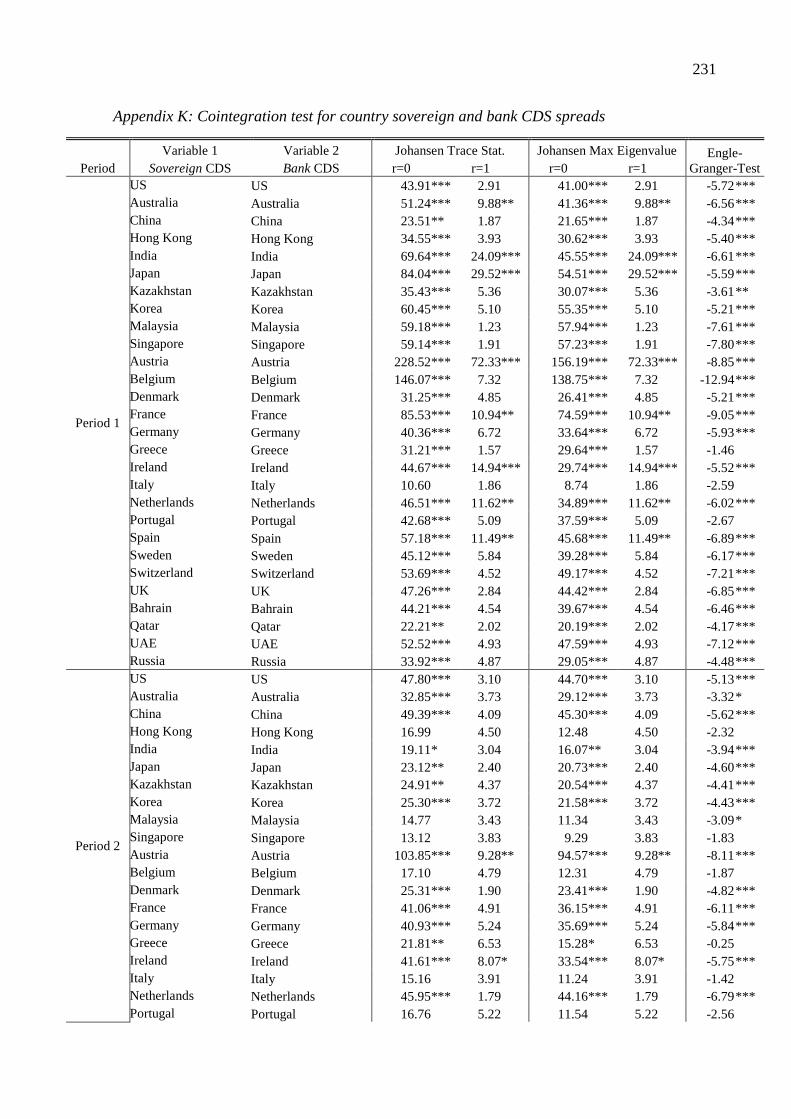
231
Appendix K: Cointegration test for country sovereign and bank CDS spreads
Variable 1 Variable 2 Johansen Trace Stat. Johansen Max Eigenvalue Engle- Granger-Test Period Sovereign CDS Bank CDS r=0 r=1 r=0 r=1
Period 1
US US 43.91*** 2.91 ## 41.00*** 2.91 ## -5.72 *** Australia Australia 51.24*** 9.88** 41.36*** 9.88** -6.56 *** China China 23.51** 1.87## 21.65*** 1.87 ## -4.34 *** Hong Kong Hong Kong 34.55*** 3.93## 30.62*** 3.93 ## -5.40 *** India India 69.64*** 24.09*** 45.55*** 24.09*** -6.61 *** Japan Japan 84.04*** 29.52*** 54.51*** 29.52*** -5.59 *** Kazakhstan Kazakhstan 35.43*** 5.36## 30.07*** 5.36 ## -3.61 ** Korea Korea 60.45*** 5.10 ## 55.35*** 5.10 ## -5.21 *** Malaysia Malaysia 59.18*** 1.23## 57.94*** 1.23 ## -7.61 *** Singapore Singapore 59.14*** 1.91## 57.23*** 1.91 ## -7.80 *** Austria Austria 228.52*** 72.33*** 156.19*** 72.33*** -8.85 *** Belgium Belgium 146.07*** 7.32 ## 138.75*** 7.32 ## -12.94 *** Denmark Denmark 31.25*** 4.85## 26.41*** 4.85 ## -5.21 *** France France 85.53*** 10.94** 74.59*** 10.94** -9.05 *** Germany Germany 40.36*** 6.72## 33.64*** 6.72 ## -5.93 *** Greece Greece 31.21*** 1.57## 29.64*** 1.57 ## -1.46 ## Ireland Ireland 44.67*** 14.94*** 29.74*** 14.94*** -5.52 *** Italy Italy 10.60 ## 1.86 ## 8.74 ## 1.86 ## -2.59 ## Netherlands Netherlands 46.51*** 11.62** 34.89*** 11.62** -6.02 *** Portugal Portugal 42.68*** 5.09## 37.59*** 5.09 ## -2.67 ## Spain Spain 57.18*** 11.49** 45.68*** 11.49** -6.89 *** Sweden Sweden 45.12*** 5.84## 39.28*** 5.84 ## -6.17 *** Switzerland Switzerland 53.69*** 4.52## 49.17*** 4.52 ## -7.21 *** UK UK 47.26*** 2.84 ## 44.42*** 2.84 ## -6.85 *** Bahrain Bahrain 44.21*** 4.54## 39.67*** 4.54 ## -6.46 *** Qatar Qatar 22.21** 2.02## 20.19*** 2.02 ## -4.17 *** UAE UAE 52.52*** 4.93 ## 47.59*** 4.93 ## -7.12 *** Russia Russia 33.92*** 4.87## 29.05*** 4.87 ## -4.48 ***
Period 2
US US 47.80*** 3.10 ## 44.70*** 3.10 ## -5.13 *** Australia Australia 32.85*** 3.73 ## 29.12*** 3.73 ## -3.32 * China China 49.39*** 4.09 ## 45.30*** 4.09 ## -5.62 *** Hong Kong Hong Kong 16.99## 4.50 ## 12.48 ## 4.50 ## -2.32 ## India India 19.11* 3.04## 16.07** 3.04 ## -3.94 *** Japan Japan 23.12** 2.40## 20.73*** 2.40 ## -4.60 *** Kazakhstan Kazakhstan 24.91** 4.37## 20.54*** 4.37 ## -4.41 *** Korea Korea 25.30*** 3.72 ## 21.58*** 3.72 ## -4.43 *** Malaysia Malaysia 14.77## 3.43 ## 11.34 ## 3.43 ## -3.09 * Singapore Singapore 13.12## 3.83 ## 9.29 ## 3.83 ## -1.83 ## Austria Austria 103.85*** 9.28** 94.57*** 9.28** -8.11 *** Belgium Belgium 17.10 ## 4.79 ## 12.31 ## 4.79 ## -1.87 ## Denmark Denmark 25.31*** 1.90## 23.41*** 1.90 ## -4.82 *** France France 41.06*** 4.91## 36.15*** 4.91 ## -6.11 *** Germany Germany 40.93*** 5.24## 35.69*** 5.24 ## -5.84 *** Greece Greece 21.81** 6.53## 15.28* 6.53 ## -0.25 ## Ireland Ireland 41.61*** 8.07* 33.54*** 8.07* -5.75 *** Italy Italy 15.16 ## 3.91 ## 11.24 ## 3.91 ## -1.42 ## Netherlands Netherlands 45.95*** 1.79 ## 44.16*** 1.79 ## -6.79 *** Portugal Portugal 16.76## 5.22 ## 11.54 ## 5.22 ## -2.56 ##

232
Variable 1 Variable 2 Johansen Trace Stat. Johansen Max Eigenvalue Engle- Granger-Test Period Sovereign CDS Bank CDS r=0 r=1 r=0 r=1
Spain Spain 27.29*** 5.57## 21.72*** 5.57 ## -4.19 *** Sweden Sweden 23.57** 3.71## 19.86** 3.71 ## -4.48 *** Switzerland Switzerland 59.60*** 5.50## 54.10*** 5.50 ## -7.54 *** UK UK 51.84*** 6.37 ## 45.46*** 6.37 ## -6.93 *** Bahrain Bahrain 68.96*** 7.76* 61.21*** 7.76* -8.07 *** Qatar Qatar 33.15*** 5.05## 28.10*** 5.05 ## -2.73 ## UAE UAE 71.66*** 7.66* 64.01*** 7.66* -8.23 *** Russia Russia 24.41** 2.26## 22.15*** 2.26 ## -4.43 ***
Period 3
US US 6.79 ## 2.23 ## 4.56 ## 2.23 ## -1.75 ## Australia Australia 11.89## 1.79 ## 10.10 ## 1.79 ## -2.28 ## China China 14.50## 0.57 ## 13.93* 0.57 ## -3.49 ** Hong Kong Hong Kong 16.65## 1.18 ## 15.47* 1.18 ## -3.92 ** India India 14.17 ## 0.56 ## 13.61 ## 0.56 ## -3.66 ** Japan Japan 10.10## 2.66 ## 7.44 ## 2.66 ## -1.61 ## Kazakhstan Kazakhstan 28.17*** 2.16## 26.01*** 2.16 ## -1.36 ## Korea Korea 15.86## 0.58 ## 15.28* 0.58 ## -3.90 ** Malaysia Malaysia 17.09## 0.62 ## 16.46** 0.62 ## -4.02 *** Singapore Singapore 20.99** 4.33## 16.66** 4.33 ## -3.38 ** Austria Austria 13.78 ## 1.62 ## 12.16 ## 1.62 ## -1.68 ## Belgium Belgium 10.29 ## 3.46 ## 6.84 ## 3.46 ## -1.75 ## Denmark Denmark 10.38## 4.51 ## 5.88 ## 4.51 ## -1.89 ## France France 14.65## 5.51 ## 9.14 ## 5.51 ## -1.90 ## Germany Germany 14.42## 4.65 ## 9.77 ## 4.65 ## -1.98 ## Greece Greece 9.16## 1.31 ## 7.85 ## 1.31 ## -1.71 ## Ireland Ireland 25.01** 6.30## 18.71** 6.30 ## -2.39 ## Italy Italy 12.06 ## 5.17 ## 6.89 ## 5.17 ## -2.19 ## Netherlands Netherlands 26.02*** 4.29 ## 21.73*** 4.29 ## -2.91 ## Portugal Portugal 14.49## 3.08 ## 11.40 ## 3.08 ## -1.70 ## Spain Spain 10.72## 2.09 ## 8.63 ## 2.09 ## -1.44 ## Sweden Sweden 12.11## 1.20 ## 10.90 ## 1.20 ## -1.49 ## Switzerland Switzerland 10.30## 1.38 ## 8.91 ## 1.38 ## -1.76 ## UK UK 17.14 ## 4.55 ## 12.59 ## 4.55 ## -2.26 ## Bahrain Bahrain 26.03*** 1.92## 24.11*** 1.92 ## -2.77 ## Qatar Qatar 34.91*** 3.75## 31.16*** 3.75 ## -3.73 ** UAE UAE 29.22*** 8.87* 20.35*** 8.87* -3.97 *** Russia Russia 18.12* 3.40## 14.72* 3.40 ## -3.63 **
Period 4
US US 15.84 ## 3.90 ## 11.93 ## 3.90 ## -2.54 ## Australia Australia 30.59*** 6.89 ## 23.70*** 6.89 ## -3.38 ** China China 13.93## 4.38 ## 9.55 ## 4.38 ## -2.82 ## Hong Kong Hong Kong 16.92## 5.96 ## 10.95 ## 5.96 ## -2.73 ## India India 30.62*** 5.73 ## 24.88*** 5.73 ## -4.67 *** Japan Japan 3.08## 0.89 ## 2.19 ## 0.89 ## -1.14 ## Kazakhstan Kazakhstan 11.30## 3.82 ## 7.49 ## 3.82 ## -2.15 ## Korea Korea 65.64*** 6.84 ## 58.80*** 6.84 ## -5.60 *** Malaysia Malaysia 23.22** 4.55## 18.67** 4.55 ## -4.13 *** Singapore Singapore 19.39* 7.23## 12.15 ## 7.23 ## -1.25 ## Austria Austria 23.90** 5.44## 18.46** 5.44 ## -3.22 * Belgium Belgium 25.19*** 6.64 ## 18.55** 6.64 ## -2.54 ## Denmark Denmark 8.88## 1.44 ## 7.45 ## 1.44 ## -2.70 ##

233
Variable 1 Variable 2 Johansen Trace Stat. Johansen Max Eigenvalue Engle- Granger-Test Period Sovereign CDS Bank CDS r=0 r=1 r=0 r=1
France France 23.86** 9.08* 14.78* 9.08* -3.45 ** Germany Germany 13.64## 5.73 ## 7.91 ## 5.73 ## -2.38 ## Greece Greece 41.15*** 4.36## 36.79*** 4.36 ## -4.14 *** Ireland Ireland 28.26*** 2.73 ## 25.53*** 2.73 ## -3.16 * Italy Italy 18.41* 6.85 ## 11.56 ## 6.85 ## -2.13 ## Netherlands Netherlands 20.43** 4.59 ## 15.84* 4.59 ## -3.29 * Portugal Portugal 35.71*** 5.04## 30.67*** 5.04 ## -2.27 ## Spain Spain 27.27*** 5.08## 22.19*** 5.08 ## -3.12 * Sweden Sweden 16.21## 4.69 ## 11.52 ## 4.69 ## -3.01 ## Switzerland Switzerland 15.66## 4.56 ## 11.10 ## 4.56 ## -2.61 ## UK UK 16.86 ## 5.47 ## 11.39 ## 5.47 ## -2.04 ## Bahrain Bahrain 9.24## 0.80 ## 8.44 ## 0.80 ## -1.99 ## Qatar Qatar 21.05** 6.10## 14.96* 6.10 ## -3.72 ** UAE UAE 30.78*** 2.81 ## 27.97*** 2.81 ## -4.50 *** Russia Russia 20.11* 5.37## 14.74* 5.37 ## -2.84 ##
Notes: The table shows the test-statistics from applying the Johansen Trace and Max Eigenvalue tests and the Engle-Granger cointegration tests. r denotes the null hypothesis with respect to the available cointegrating vectors, e.g., r=0 denotes that the null hypothesis of zero cointegrating vectors. *, **, *** denotes significance at the 10%, 5% and 1% significance level, respectively. Period 1 ranges from October 1st, 2005 to February 28th, 2007, Period 2 ranges from March 1st, 2007 to July 31st, 2008, Period 3 ranges from August 1st, 2008 to December 31st, 2009, Period 4 ranges from January 1st, 2010 to April 30th, 2011.

234
Appendix L: Unit-root test for regional corporate CDS spreads
America
Log Values Log Differences Period Industry CDS spreads ADF PP KPSS ADF PP KPSS
Period 1
Automotive 0.140.00 0.130.00 5.68*** -18.46*** -18.46*** 0.08 0%
Basic materials 1.110.00 1.230.00 3.26*** -24.24*** -23.99*** 0.07 0%
Chemicals, healthcare and pharma 0.850.00 0.770.00 3.06*** -20.18*** -20.16*** 0.03 0%
Commerce and consumer 2.200.00 2.010.00 2.63*** -19.57*** -19.57*** 0.04 0%
Construction and logistics 1.160.00 1.330.00 1.44*** -24.33*** -24.67*** 0.02 0%
Energy and utilities 2.440.00 2.180.00 3.87*** -24.83*** -24.84*** 0.04 0%
Financial services (excl. banking) 2.370.00 2.140.00 7.60*** -20.53*** -20.49*** 0.12*
Industrial -0.470.00 -0.370.00 1.50*** -25.04*** -26.13*** 0.00 0%
Telecommunication, media and tech. 1.050.00 0.960.00 3.79*** -18.48*** -18.50*** 0.11 0%
Overall 0.570.00 0.630.00 6.88*** -24.87*** -25.75*** 0.01 0%
Period 2
Automotive -1.510.00 -1.580.00 1.14*** -19.97*** -19.97*** 0.03 0%Basic materials -2.60*** -2.42** 2.57*** -16.33*** -16.32*** 0.09 0%Chemicals, healthcare and pharma -1.97** -1.73* 2.15*** -15.07*** -15.12*** 0.12* Commerce and consumer -2.09** -1.76* 2.25*** -15.45*** -15.49*** 0.10 0%Construction and logistics -2.30** -2.08** 2.48*** -16.41*** -16.43*** 0.07 0%Energy and utilities -2.22** -1.93* 2.56*** -16.28*** -16.29*** 0.11 0%Financial services (excl. banking) -3.01*** -2.39** 2.94*** -13.30*** -13.31*** 0.13* Industrial -0.440.00 -0.380.00 3.66*** -29.55*** -31.08*** 0.01 0%Telecommunication, media and tech. -2.37** -2.02** 2.42*** -14.64*** -14.63*** 0.15** Overall -1.72* -1.70* 1.53*** -21.94*** -21.87*** 0.05 0%
Period 3
Automotive 0.550.00 0.550.00 6.68*** -18.63*** -18.63*** 0.15** Basic materials -0.070.00 -0.100.00 7.53*** -11.95*** -11.88*** 0.54*** Chemicals, healthcare and pharma -0.050.00 -0.070.00 6.02*** -13.26*** -13.25*** 0.30*** Commerce and consumer 0.200.00 0.140.00 5.23*** -14.38*** -14.38*** 0.29*** Construction and logistics 0.710.00 0.550.00 6.06*** -14.57*** -14.58*** 0.18** Energy and utilities -0.010.00 -0.040.00 5.59*** -13.26*** -13.29*** 0.24*** Financial services (excl. banking) -0.290.00 -0.290.00 6.24*** -15.06*** -15.01*** 0.11 0%Industrial 0.470.00 0.360.00 6.92*** -16.59*** -16.59*** 0.19** Telecommunication, media and tech. 0.430.00 0.310.00 4.94*** -13.30*** -13.27*** 0.25*** Overall 0.380.00 0.340.00 6.68*** -13.82*** -13.76*** 0.23***
Period 4
Automotive 1.520.00 1.330.00 3.56*** -15.06*** -15.05*** 0.08 0%Basic materials 0.120.00 0.080.00 6.37*** -14.70*** -14.71*** 0.06 0%Chemicals, healthcare and pharma -0.040.00 -0.040.00 5.41*** -14.66*** -14.68*** 0.09 0%Commerce and consumer -0.260.00 -0.240.00 2.21*** -15.00*** -14.94*** 0.05 0%Construction and logistics -0.590.00 -0.550.00 4.70*** -17.45*** -17.46*** 0.11 0%Energy and utilities -0.040.00 -0.050.00 6.37*** -15.07*** -15.09*** 0.17** Financial services (excl. banking) 0.440.00 0.350.00 6.15*** -13.80*** -13.79*** 0.09 0%Industrial -0.190.00 -0.170.00 4.58*** -16.03*** -16.00*** 0.04 0%Telecommunication, media and tech. -0.120.00 -0.120.00 4.38*** -14.43*** -14.43*** 0.12* Overall 0.530.00 0.420.00 5.70*** -13.65*** -13.63*** 0.08 0%
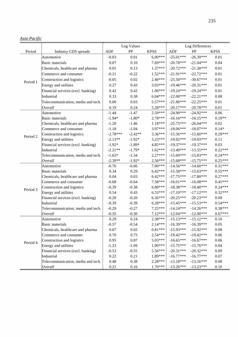
235
Asia-Pacific
Log Values Log Differences Period Industry CDS spreads ADF PP KPSS ADF PP KPSS
Period 1
Automotive -0.030.00 0.010.00 6.00*** -25.01*** -26.39*** 0.01 0%
Basic materials 0.070.00 0.100.00 7.69*** -20.78*** -21.04*** 0.04 0%
Chemicals, healthcare and pharma 0.010.00 0.130.00 1.37*** -20.72*** -21.30*** 0.01 0%
Commerce and consumer -0.210.00 -0.220.00 1.52*** -21.91*** -22.72*** 0.01 0%
Construction and logistics -0.050.00 0.020.00 2.40*** -25.50*** -30.67*** 0.01 0%
Energy and utilities 0.270.00 0.430.00 3.03*** -19.46*** -20.31*** 0.01 0%
Financial services (excl. banking) 0.420.00 0.420.00 1.06*** -19.24*** -19.24*** 0.01 0%
Industrial 0.330.00 0.380.00 6.04*** -22.00*** -22.21*** 0.08 0%
Telecommunication, media and tech. 0.000.00 0.030.00 5.57*** -21.80*** -22.25*** 0.01 0%
Overall 0.190.00 0.240.00 5.28*** -20.17*** -20.78*** 0.01 0%
Period 2
Automotive -1.440.00 -1.470.00 2.59*** -24.90*** -24.92*** 0.06 0%Basic materials -1.94* -1.80* 2.78*** -16.16*** -16.15*** 0.19** Chemicals, healthcare and pharma -1.200.00 -1.460.00 1.18*** -25.75*** -26.04*** 0.02 0%Commerce and consumer -1.180.00 -1.040.00 3.97*** -18.06*** -18.07*** 0.14* Construction and logistics -2.78*** -2.42** 3.36*** -15.56*** -15.60*** 0.29*** Energy and utilities -2.13** -1.92* 3.23*** -19.92*** -19.93*** 0.11 0%Financial services (excl. banking) -1.92* -1.89* 4.85*** -19.37*** -19.37*** 0.03 0%Industrial -2.21** -1.79* 1.62*** -13.49*** -13.55*** 0.22*** Telecommunication, media and tech. -1.63* -1.340.00 2.27*** -15.69*** -15.83*** 0.24*** Overall -2.39** -1.92* 2.56*** -15.68*** -15.75*** 0.25***
Period 3
Automotive -0.760.00 -0.660.00 7.00*** -14.56*** -14.60*** 0.31*** Basic materials 0.340.00 0.290.00 6.42*** -15.58*** -15.63*** 0.55*** Chemicals, healthcare and pharma 0.040.00 0.030.00 6.42*** -17.75*** -17.80*** 0.27*** Commerce and consumer -0.680.00 -0.640.00 7.58*** -16.01*** -16.08*** 0.45*** Construction and logistics -0.390.00 -0.380.00 6.80*** -18.38*** -18.40*** 0.24*** Energy and utilities 0.540.00 0.430.00 6.53*** -17.10*** -17.12*** 0.32*** Financial services (excl. banking) -0.200.00 -0.200.00 6.36*** -20.25*** -20.23*** 0.09 0%Industrial -0.390.00 -0.390.00 6.28*** -15.45*** -15.53*** 0.54*** Telecommunication, media and tech. -0.290.00 -0.270.00 7.25*** -14.24*** -14.26*** 0.38*** Overall -0.350.00 -0.300.00 7.12*** -12.04*** -12.00*** 0.67***
Period 4
Automotive 0.290.00 0.240.00 2.38*** -15.13*** -15.12*** 0.10 0%Basic materials -0.570.00 -0.540.00 2.14*** -16.39*** -16.39*** 0.05 0%Chemicals, healthcare and pharma 0.670.00 0.650.00 0.81*** -15.93*** -15.92*** 0.08 0%Commerce and consumer 0.700.00 0.750.00 2.54*** -19.42*** -19.42*** 0.06 0%Construction and logistics 0.950.00 0.870.00 5.03*** -16.65*** -16.67*** 0.06 0%Energy and utilities -1.230.00 -1.090.00 1.00*** -15.75*** -15.76*** 0.04 0%Financial services (excl. banking) -0.530.00 -0.550.00 5.56*** -20.31*** -20.32*** 0.09 0%Industrial 0.220.00 0.210.00 1.89*** -16.77*** -16.77*** 0.07 0%Telecommunication, media and tech. 0.480.00 0.380.00 2.28*** -13.18*** -13.16*** 0.08 0%Overall 0.210.00 0.160.00 1.70*** -13.26*** -13.23*** 0.10 0%

236
Europe
Log Values Log Differences Period Industry CDS spreads ADF PP KPSS ADF PP KPSS
Period 1
Automotive 2.470.00 2.250.00 1.65*** -17.12*** -17.15*** 0.05 0%Basic materials 0.940.00 1.010.00 5.62*** -20.78*** -20.83*** 0.03 0%Chemicals, healthcare and pharma 0.900.00 0.830.00 4.93*** -21.45*** -21.43*** 0.09 0%Commerce and consumer 1.360.00 1.210.00 1.43*** -21.31*** -21.23*** 0.08 0%Construction and logistics 0.060.00 0.110.00 1.03*** -26.80*** -27.44*** 0.01 0%Energy and utilities 0.910.00 0.890.00 2.32*** -25.03*** -25.30*** 0.05 0%Financial services (excl. banking) 1.860.00 2.050.00 2.93*** -21.33*** -21.35*** 0.03 0%Industrial 1.850.00 1.740.00 2.79*** -19.54*** -19.54*** 0.05 0%Telecommunication, media and tech. 0.350.00 0.340.00 3.02*** -18.82*** -18.83*** 0.04 0%Overall 2.550.00 2.310.00 1.67*** -19.55*** -19.55*** 0.04 0%
Period 2
Automotive -1.520.00 -1.350.00 1.95*** -15.21*** -15.18*** 0.12* Basic materials -2.31** -2.08** 2.36*** -15.96*** -15.96*** 0.14* Chemicals, healthcare and pharma -1.68* -1.500.00 3.38*** -15.27*** -15.29*** 0.15** Commerce and consumer -1.610.00 -1.440.00 1.93*** -15.29*** -15.29*** 0.10 0%Construction and logistics -1.560.00 -1.410.00 2.37*** -16.21*** -16.21*** 0.08 0%Energy and utilities -1.78* -1.520.00 4.49*** -14.10*** -14.08*** 0.19** Financial services (excl. banking) -2.30** -2.10** 3.96*** -15.81*** -15.75*** 0.11 0%Industrial -2.27** -1.99** 2.32*** -15.03*** -15.02*** 0.15** Telecommunication, media and tech. -1.330.00 -1.240.00 2.35*** -16.65*** -16.65*** 0.13* Overall -2.06** -1.82* 3.10*** -14.72*** -14.64*** 0.13*
Period 3
Automotive -0.180.00 -0.190.00 6.73*** -15.01*** -14.99*** 0.10 0%Basic materials 0.410.00 0.280.00 6.50*** -13.07*** -13.07*** 0.32*** Chemicals, healthcare and pharma 0.260.00 0.200.00 6.13*** -14.21*** -14.18*** 0.21** Commerce and consumer 0.310.00 0.240.00 5.12*** -13.83*** -13.76*** 0.15** Construction and logistics 0.060.00 0.040.00 6.64*** -15.54*** -15.51*** 0.08 0%Energy and utilities -0.240.00 -0.230.00 6.26*** -14.44*** -14.42*** 0.22*** Financial services (excl. banking) -0.190.00 -0.190.00 8.03*** -15.10*** -15.08*** 0.12* Industrial 0.200.00 0.130.00 6.22*** -13.65*** -13.63*** 0.27*** Telecommunication, media and tech. 0.430.00 0.380.00 5.02*** -15.46*** -15.36*** 0.10 0%Overall -0.060.00 -0.080.00 7.70*** -14.33*** -14.29*** 0.15**
Period 4
Automotive -0.070.00 -0.070.00 4.66*** -17.57*** -17.58*** 0.06 0%Basic materials -0.110.00 -0.120.00 5.96*** -15.93*** -15.92*** 0.04 0%Chemicals, healthcare and pharma -0.300.00 -0.290.00 6.16*** -16.67*** -16.69*** 0.07 0%Commerce and consumer -0.500.00 -0.480.00 4.63*** -17.29*** -17.29*** 0.05 0%Construction and logistics -0.610.00 -0.580.00 6.78*** -17.10*** -17.10*** 0.05 0%Energy and utilities -0.810.00 -0.750.00 6.13*** -15.60*** -15.60*** 0.07 0%Financial services (excl. banking) -0.440.00 -0.410.00 2.50*** -16.31*** -16.34*** 0.04 0%Industrial -0.070.00 -0.080.00 4.92*** -16.79*** -16.80*** 0.10 0%Telecommunication, media and tech. -0.740.00 -0.700.00 5.67*** -16.57*** -16.56*** 0.03 0%Overall -0.460.00 -0.430.00 4.30*** -16.31*** -16.33*** 0.04 0%
Notes: The table shows the test-statistics from applying the ADF, PP and KPSS unit root tests. ADF and PP examines the null hypothesis of a unit root. By contrast, the KPSS test examines the null hypothesis of stationarity. *, **, *** denotes significance at the 10%, 5% and 1% significance level, respectively. Period 1 ranges from October 1st, 2005 to February 28th, 2007, Period 2 ranges from March 1st, 2007 to July 31st, 2008, Period 3 ranges from August 1st, 2008 to December 31st, 2009, Period 4 ranges from January 1st, 2010 to April 30th, 2011.
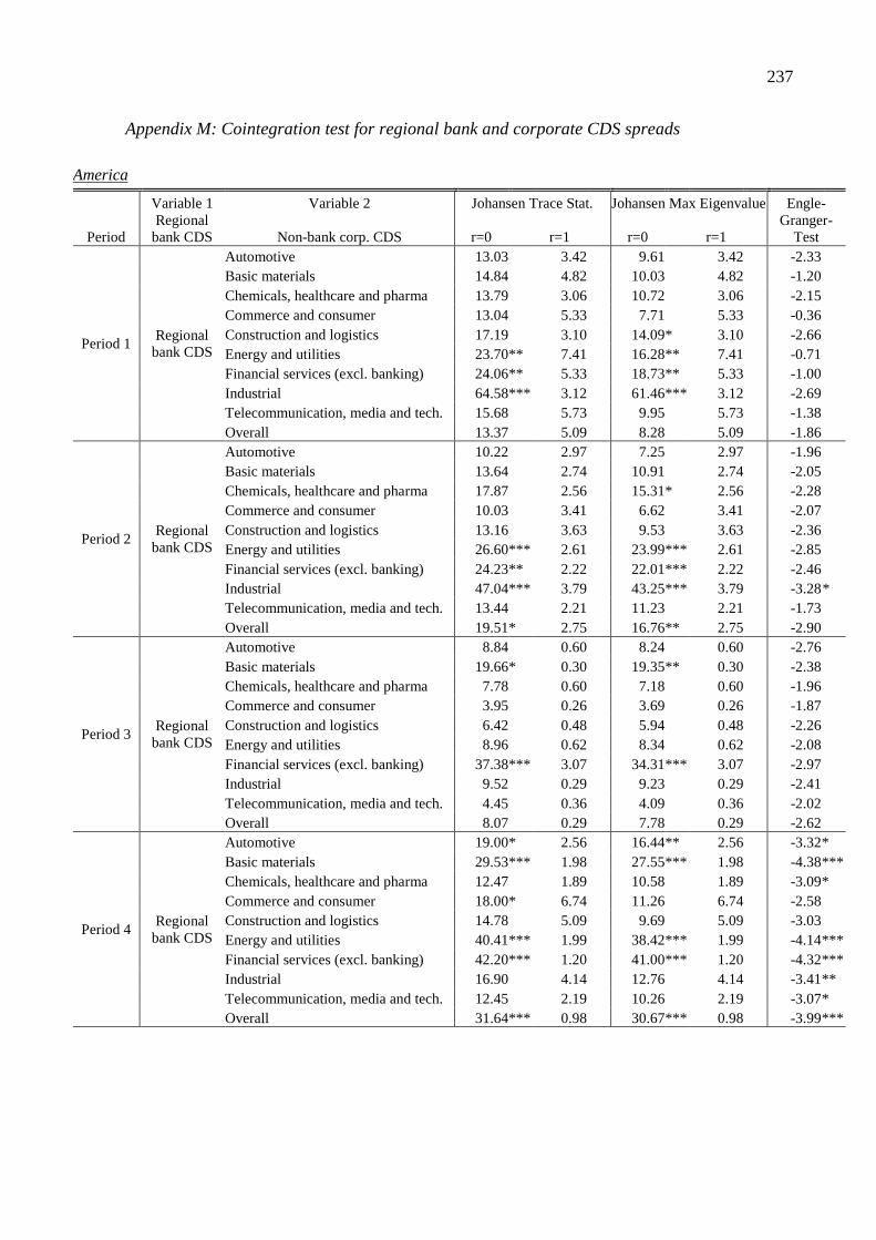
237
Appendix M: Cointegration test for regional bank and corporate CDS spreads
America
Variable 1 Variable 2 Johansen Trace Stat. Johansen Max Eigenvalue Engle- Granger-
Test Period Regional bank CDS Non-bank corp. CDS r=0 r=1 r=0 r=1
Period 1 Regional bank CDS
Automotive 13.03## 3.42## 9.61## 3.42## -2.33 ## Basic materials 14.84## 4.82## 10.03## 4.82## -1.20 ## Chemicals, healthcare and pharma 13.79## 3.06## 10.72## 3.06## -2.15 ## Commerce and consumer 13.04## 5.33## 7.71## 5.33## -0.36 ## Construction and logistics 17.19## 3.10## 14.09* 3.10## -2.66 ## Energy and utilities 23.70** 7.41## 16.28** 7.41## -0.71 ## Financial services (excl. banking) 24.06** 5.33## 18.73** 5.33## -1.00 ## Industrial 64.58*** 3.12## 61.46*** 3.12## -2.69 ## Telecommunication, media and tech. 15.68## 5.73## 9.95## 5.73## -1.38 ## Overall 13.37## 5.09## 8.28## 5.09## -1.86 ##
Period 2 Regional bank CDS
Automotive 10.22## 2.97## 7.25## 2.97## -1.96 ## Basic materials 13.64## 2.74## 10.91## 2.74## -2.05 ## Chemicals, healthcare and pharma 17.87## 2.56## 15.31* 2.56## -2.28 ## Commerce and consumer 10.03## 3.41## 6.62## 3.41## -2.07 ## Construction and logistics 13.16## 3.63## 9.53## 3.63## -2.36 ## Energy and utilities 26.60*** 2.61## 23.99*** 2.61## -2.85 ## Financial services (excl. banking) 24.23** 2.22## 22.01*** 2.22## -2.46 ## Industrial 47.04*** 3.79## 43.25*** 3.79## -3.28* Telecommunication, media and tech. 13.44## 2.21## 11.23## 2.21## -1.73 ## Overall 19.51* 2.75## 16.76** 2.75## -2.90 ##
Period 3 Regional bank CDS
Automotive 8.840.0 0.60 0.0 8.24 0.0 0.60 0.0 -2.76 0Basic materials 19.66* 0.300.0 19.35** 0.300.0 -2.38 0Chemicals, healthcare and pharma 7.780.0 0.60 0.0 7.18 0.0 0.60 0.0 -1.96 0Commerce and consumer 3.950.0 0.26 0.0 3.69 0.0 0.26 0.0 -1.87 0Construction and logistics 6.420 0.48 0 5.94 0 0.48 0 -2.26 0Energy and utilities 8.96 0 0.62 0 8.34 0 0.62 0 -2.08 0Financial services (excl. banking) 37.38*** 3.07 0 34.31*** 3.07 0 -2.97 0Industrial 9.52 0 0.29 0 9.23 0 0.29 0 -2.41 0Telecommunication, media and tech. 4.450 0.36 0 4.09 0 0.36 0 -2.02 0Overall 8.07 0 0.29 0 7.78 0 0.29 0 -2.62 0
Period 4 Regional bank CDS
Automotive 19.00* 2.56 0 16.44** 2.56 0 -3.32* Basic materials 29.53*** 1.98 0 27.55*** 1.98 0 -4.38*** Chemicals, healthcare and pharma 12.470 1.89 0 10.58 0 1.89 0 -3.09* Commerce and consumer 18.00* 6.740 11.26 0 6.74 0 -2.58 0Construction and logistics 14.780 5.09 0 9.69 0 5.09 0 -3.03 0Energy and utilities 40.41*** 1.99 0 38.42*** 1.99 0 -4.14*** Financial services (excl. banking) 42.20*** 1.20 0 41.00*** 1.20 0 -4.32*** Industrial 16.90 0 4.14 0 12.76 0 4.14 0 -3.41** Telecommunication, media and tech. 12.450 2.19 0 10.26 0 2.19 0 -3.07* Overall 31.64*** 0.98 0 30.67*** 0.98 0 -3.99***

238
Asia-Pacific
Variable 1 Variable 2 Johansen Trace Stat. Johansen Max Eigenvalue Engle- Granger-
Test Period Regional bank CDS Non-bank corp. CDS r=0 r=1 r=0 r=1
Period 1 Regional bank CDS
Automotive 42.27*** 10.91** 31.35*** 10.91** -5.51*** Basic materials 46.94*** 4.22## 42.71*** 4.22## -6.62*** Chemicals, healthcare and pharma 88.23*** 21.57*** 66.67*** 21.57*** -6.59***
Commerce and consumer 42.82*** 13.09*** 29.73*** 13.09*** -5.21***
Construction and logistics 82.80*** 18.39*** 64.41*** 18.39*** -7.23***
Energy and utilities 100.06*** 11.43** 88.62*** 11.43** -9.79***
Financial services (excl. banking) 47.38*** 5.38## 42.00*** 5.38## -6.64***
Industrial 33.61*** 2.96## 30.65*** 2.96## -5.62***
Telecommunication, media and tech. 32.56*** 7.40## 25.16*** 7.40## -5.03***
Overall 36.25*** 7.12## 29.14*** 7.12## -5.45***
Period 2 Regional bank CDS
Automotive 35.58*** 3.33## 32.25*** 3.33## -2.84 ##
Basic materials 12.85## 5.16## 7.69## 5.16## -2.28 ##
Chemicals, healthcare and pharma 35.15*** 5.16## 29.99*** 5.16## -4.53***
Commerce and consumer 24.41** 7.04## 17.37** 7.04## -1.91 ##
Construction and logistics 25.36*** 3.97## 21.39*** 3.97## -1.77 ## Energy and utilities 15.23## 3.35## 11.88## 3.35## -1.92 ## Financial services (excl. banking) 20.68** 2.65## 18.03** 2.65## -1.65 ## Industrial 23.68** 3.05## 20.63*** 3.05## -2.13 ## Telecommunication, media and tech. 23.59** 4.48## 19.12** 4.48## -1.71 ## Overall 27.49*** 4.47## 23.02*** 4.47## -1.61 ##
Period 3 Regional bank CDS
Automotive 37.53*** 7.09 0.0 30.44*** 7.09 0.0 -1.02 0Basic materials 31.30*** 2.13 0.0 29.16*** 2.13 0.0 -2.01 0Chemicals, healthcare and pharma 6.950.0 0.78 0.0 6.17 0.0 0.78 0.0 -1.50 0Commerce and consumer 31.98*** 5.13 0.0 26.85*** 5.13 0.0 -1.01 0Construction and logistics 20.52** 2.360 18.16** 2.36 0 -1.37 0Energy and utilities 22.68** 1.24 0 21.43*** 1.24 0 -2.41 0Financial services (excl. banking) 33.72*** 2.10 0 31.62*** 2.10 0 -2.23 0Industrial 15.49 0 0.76 0 14.73* 0.76 0 -2.13 0Telecommunication, media and tech. 35.65*** 4.94 0 30.71*** 4.94 0 -1.23 0Overall 57.07*** 5.94 0 51.14*** 5.94 0 -1.22 0
Period 4 Regional bank CDS
Automotive 8.61 0 2.18 0 6.43 0 2.18 0 -2.24 0Basic materials 16.12 0 4.79 0 11.33 0 4.79 0 -2.75 0Chemicals, healthcare and pharma 70.98*** 4.23 0 66.75*** 4.23 0 -6.26*** Commerce and consumer 15.470 3.73 0 11.75 0 3.73 0 -2.12 0Construction and logistics 20.08* 4.050 16.03** 4.05 0 -2.06 0Energy and utilities 15.37 0 5.28 0 10.09 0 5.28 0 -2.16 0Financial services (excl. banking) 10.330 3.14 0 7.19 0 3.14 0 -1.78 0Industrial 23.72** 5.31 0 18.41** 5.31 0 -3.54** Telecommunication, media and tech. 14.140 2.96 0 11.17 0 2.96 0 -2.42 0Overall 25.34*** 4.82 0 20.51*** 4.82 0 -3.08*

239
Europe
Variable 1 Variable 2 Johansen Trace Stat. Johansen Max Eigenvalue Engle- Granger-
Test Period Regional bank CDS Non-bank corp. CDS r=0 r=1 r=0 r=1
Period 1 Regional bank CDS
Automotive 27.95*** 6.08## 21.87*** 6.08## -4.61*** Basic materials 14.42## 1.42## 13.00## 1.42## -3.59** Chemicals, healthcare and pharma 17.78## 1.30## 16.49** 1.30## -3.89**
Commerce and consumer 25.88*** 2.89## 22.99*** 2.89## -4.70***
Construction and logistics 31.42*** 3.17## 28.25*** 3.17## -2.47 ##
Energy and utilities 17.51## 1.42## 16.09** 1.42## -3.99***
Financial services (excl. banking) 63.31*** 4.35## 58.96*** 4.35## -7.71***
Industrial 22.63** 3.50## 19.13** 3.50## -4.27***
Telecommunication, media and tech. 11.65## 1.01## 10.64## 1.01## -2.96 ##
Overall 43.31*** 5.71## 37.60*** 5.71## -5.88***
Period 2 Regional bank CDS
Automotive 13.01## 4.72## 8.29## 4.72## -2.34 ##
Basic materials 11.89## 5.11## 6.78## 5.11## -1.99 ##
Chemicals, healthcare and pharma 12.47## 3.52## 8.95## 3.52## -2.55 ##
Commerce and consumer 11.18## 3.59## 7.59## 3.59## -2.26 ##
Construction and logistics 11.94## 3.97## 7.97## 3.97## -1.78 ## Energy and utilities 15.83## 6.10## 9.73## 6.10## -2.92 ## Financial services (excl. banking) 25.01** 6.64## 18.37** 6.64## -4.17*** Industrial 13.76## 6.15## 7.61## 6.15## -2.38 ## Telecommunication, media and tech. 11.96## 3.99## 7.97## 3.99## -2.23 ## Overall 15.77## 6.11## 9.66## 6.11## -2.92 ##
Period 3 Regional bank CDS
Automotive 5.730.0 1.04 0.0 4.69 0.0 1.04 0.0 -2.14 0Basic materials 6.030.0 0.33 0.0 5.71 0.0 0.33 0.0 -2.31 0Chemicals, healthcare and pharma 7.040.0 0.52 0.0 6.52 0.0 0.52 0.0 -2.20 0Commerce and consumer 5.430.0 0.46 0.0 4.97 0.0 0.46 0.0 -1.97 0Construction and logistics 6.190 1.33 0 4.86 0 1.33 0 -2.12 0Energy and utilities 5.57 0 0.82 0 4.75 0 0.82 0 -2.02 0Financial services (excl. banking) 30.01*** 1.86 0 28.16*** 1.86 0 -2.83 0Industrial 5.10 0 0.25 0 4.85 0 0.25 0 -2.12 0Telecommunication, media and tech. 6.410 0.91 0 5.50 0 0.91 0 -2.08 0Overall 14.16 0 0.83 0 13.33 0 0.83 0 -2.52 0
Period 4 Regional bank CDS
Automotive 11.95 0 1.22 0 10.74 0 1.22 0 -1.98 0Basic materials 8.77 0 0.99 0 7.79 0 0.99 0 -1.75 0Chemicals, healthcare and pharma 10.720 1.04 0 9.68 0 1.04 0 -1.79 0Commerce and consumer 13.620 2.29 0 11.33 0 2.29 0 -1.45 0Construction and logistics 11.920 3.83 0 8.09 0 3.83 0 -1.75 0Energy and utilities 9.19 0 2.92 0 6.28 0 2.92 0 -1.60 0Financial services (excl. banking) 17.040 7.11 0 9.93 0 7.11 0 -2.61 0Industrial 9.13 0 0.96 0 8.17 0 0.96 0 -1.88 0Telecommunication, media and tech. 8.740 2.01 0 6.73 0 2.01 0 -1.39 0Overall 12.71 0 2.10 0 10.61 0 2.10 0 -1.21 0
Notes: The table shows the test-statistics from applying the Johansen Trace and Max Eigenvalue tests and the Engle-Granger cointegration tests. r denotes the null hypothesis with respect to the available cointegrating vectors, e.g., r=0 denotes that the null hypothesis of zero cointegrating vectors. *, **, *** denotes significance at the 10%, 5% and 1% significance level, respectively. Period 1 ranges from October 1st, 2005 to February 28th, 2007, Period 2 ranges from March 1st, 2007 to July 31st, 2008, Period 3 ranges from August 1st, 2008 to December 31st, 2009, Period 4 ranges from January 1st, 2010 to April 30th, 2011.

240
Appendix N: Unit-root test for regional bank equity prices
Log Values Log Differences Period Regional bank equity prices ADF PP KPSS ADF PP KPSS
Period 1
America 0.22 0.00 0.22 0.00 1.52 *** -19.99 *** -19.99*** 0.10 0%
Asia-Pacific 0.19 0.00 0.19 0.00 1.85 *** -29.02 *** -29.02*** 0.01 0%
Europe 0.78 0.00 0.78 0.00 1.45 *** -22.18 *** -22.18*** 0.01 0%
Middle East & Russia 0.12 0.00 0.12 0.00 3.77 *** -21.56 *** -21.56*** 0.02 0%
Period 2
America -1.86 * -1.86* 2.87 *** -15.49 *** -15.49*** 0.08 0%
Asia-Pacific -2.54 ** -2.54** 2.37 *** -13.52 *** -13.52*** 0.17**
Europe -2.28 ** -2.28** 4.30 *** -15.50 *** -15.50*** 0.09 0%
Middle East & Russia -1.14 0.00 -1.14 0.00 4.92 *** -21.31 *** -21.31*** 0.07 0%
Period 3
America 0.10 0.00 0.10 0.00 5.70 *** -15.12 *** -15.12*** 0.03 0%
Asia-Pacific 0.11 0.00 0.11 0.00 5.09 *** -14.24 *** -14.24*** 0.25***
Europe -0.17 0.00 -0.17 0.00 5.96 *** -15.09 *** -15.09*** 0.04 0%
Middle East & Russia -0.94 0.00 -0.94 0.00 5.25 *** -14.60 *** -14.60*** 0.28***
Period 4
America -0.31 0.00 -0.31 0.00 4.34 *** -15.58 *** -15.58*** 0.03 0%
Asia-Pacific -0.55 0.00 -0.55 0.00 2.03 *** -14.68 *** -14.68*** 0.09 0%
Europe -0.85 0.00 -0.85 0.00 2.46 *** -16.23 *** -16.23*** 0.04 0%
Middle East & Russia 1.09 0.00 1.09 0.00 1.56 *** -15.38 *** -15.38*** 0.04 0%
Notes: The table shows the test-statistics from applying the ADF, PP and KPSS unit root tests. ADF and PP examines the null hypothesis of a unit root. By contrast, the KPSS test examines the null hypothesis of stationarity. *, **, *** denotes significance at the 10%, 5% and 1% significance level, respectively. Period 1 ranges from October 1st, 2005 to February 28th, 2007, Period 2 ranges from March 1st, 2007 to July 31st, 2008, Period 3 ranges from August 1st, 2008 to December 31st, 2009, Period 4 ranges from January 1st, 2010 to April 30th, 2011.
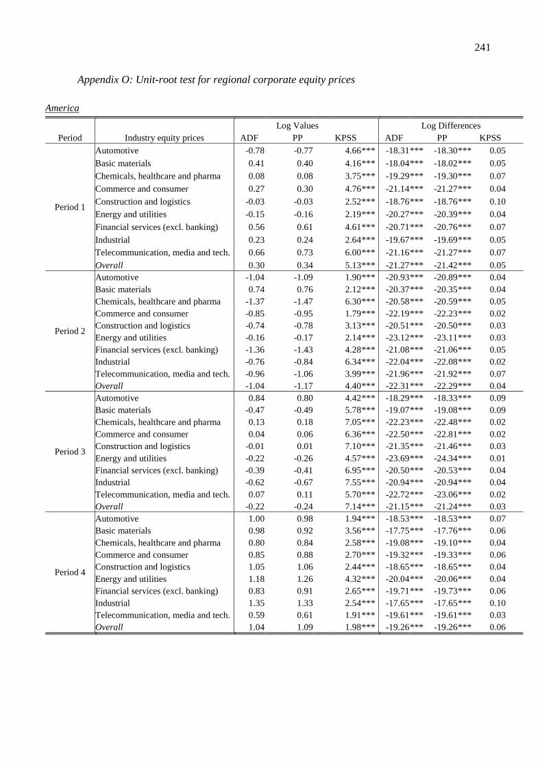
241
Appendix O: Unit-root test for regional corporate equity prices
America
Log Values Log Differences Period Industry equity prices ADF PP KPSS ADF PP KPSS
Period 1
Automotive -0.780.00 -0.770.00 4.66*** -18.31*** -18.30*** 0.05 0%
Basic materials 0.410.00 0.400.00 4.16*** -18.04*** -18.02*** 0.05 0%
Chemicals, healthcare and pharma 0.080.00 0.080.00 3.75*** -19.29*** -19.30*** 0.07 0%
Commerce and consumer 0.270.00 0.300.00 4.76*** -21.14*** -21.27*** 0.04 0%
Construction and logistics -0.030.00 -0.030.00 2.52*** -18.76*** -18.76*** 0.10 0%
Energy and utilities -0.150.00 -0.160.00 2.19*** -20.27*** -20.39*** 0.04 0%
Financial services (excl. banking) 0.560.00 0.610.00 4.61*** -20.71*** -20.76*** 0.07 0%
Industrial 0.230.00 0.240.00 2.64*** -19.67*** -19.69*** 0.05 0%
Telecommunication, media and tech. 0.660.00 0.730.00 6.00*** -21.16*** -21.27*** 0.07 0%
Overall 0.300.00 0.340.00 5.13*** -21.27*** -21.42*** 0.05 0%
Period 2
Automotive -1.040.00 -1.090.00 1.90*** -20.93*** -20.89*** 0.04 0%Basic materials 0.740.00 0.760.00 2.12*** -20.37*** -20.35*** 0.04 0%Chemicals, healthcare and pharma -1.370.00 -1.470.00 6.30*** -20.58*** -20.59*** 0.05 0%Commerce and consumer -0.850.00 -0.950.00 1.79*** -22.19*** -22.23*** 0.02 0%Construction and logistics -0.740.00 -0.780.00 3.13*** -20.51*** -20.50*** 0.03 0%Energy and utilities -0.160.00 -0.170.00 2.14*** -23.12*** -23.11*** 0.03 0%Financial services (excl. banking) -1.360.00 -1.430.00 4.28*** -21.08*** -21.06*** 0.05 0%Industrial -0.760.00 -0.840.00 6.34*** -22.04*** -22.08*** 0.02 0%Telecommunication, media and tech. -0.960.00 -1.060.00 3.99*** -21.96*** -21.92*** 0.07 0%Overall -1.040.00 -1.170.00 4.40*** -22.31*** -22.29*** 0.04 0%
Period 3
Automotive 0.840.00 0.800.00 4.42*** -18.29*** -18.33*** 0.09 0%Basic materials -0.470.00 -0.490.00 5.78*** -19.07*** -19.08*** 0.09 0%Chemicals, healthcare and pharma 0.130.00 0.180.00 7.05*** -22.23*** -22.48*** 0.02 0%Commerce and consumer 0.040.00 0.060.00 6.36*** -22.50*** -22.81*** 0.02 0%Construction and logistics -0.010.00 0.010.00 7.10*** -21.35*** -21.46*** 0.03 0%Energy and utilities -0.220.00 -0.260.00 4.57*** -23.69*** -24.34*** 0.01 0%Financial services (excl. banking) -0.390.00 -0.410.00 6.95*** -20.50*** -20.53*** 0.04 0%Industrial -0.620.00 -0.670.00 7.55*** -20.94*** -20.94*** 0.04 0%Telecommunication, media and tech. 0.070.00 0.110.00 5.70*** -22.72*** -23.06*** 0.02 0%Overall -0.220.00 -0.240.00 7.14*** -21.15*** -21.24*** 0.03 0%
Period 4
Automotive 1.000.00 0.980.00 1.94*** -18.53*** -18.53*** 0.07 0%Basic materials 0.980.00 0.920.00 3.56*** -17.75*** -17.76*** 0.06 0%Chemicals, healthcare and pharma 0.800.00 0.840.00 2.58*** -19.08*** -19.10*** 0.04 0%Commerce and consumer 0.850.00 0.880.00 2.70*** -19.32*** -19.33*** 0.06 0%Construction and logistics 1.050.00 1.060.00 2.44*** -18.65*** -18.65*** 0.04 0%Energy and utilities 1.180.00 1.260.00 4.32*** -20.04*** -20.06*** 0.04 0%Financial services (excl. banking) 0.830.00 0.910.00 2.65*** -19.71*** -19.73*** 0.06 0%Industrial 1.350.00 1.330.00 2.54*** -17.65*** -17.65*** 0.10 0%Telecommunication, media and tech. 0.590.00 0.610.00 1.91*** -19.61*** -19.61*** 0.03 0%Overall 1.040.00 1.090.00 1.98*** -19.26*** -19.26*** 0.06 0%

242
Asia-Pacific
Log Values Log Differences Period Industry equity prices ADF PP KPSS ADF PP KPSS
Period 1
Automotive 0.680.00 0.690.00 2.74*** -18.55*** -18.55*** 0.05 0%
Basic materials 1.020.00 1.110.00 3.01*** -20.20*** -20.25*** 0.04 0%
Chemicals, healthcare and pharma 1.040.00 1.070.00 2.92*** -19.21*** -19.21*** 0.09 0%
Commerce and consumer 0.810.00 0.840.00 2.80*** -19.87*** -19.87*** 0.08 0%
Construction and logistics -0.050.00 -0.050.00 3.42*** -18.25*** -18.23*** 0.10 0%
Energy and utilities 1.460.00 1.550.00 3.40*** -20.72*** -20.71*** 0.07 0%
Financial services (excl. banking) 1.640.00 1.790.00 3.16*** -19.65*** -19.67*** 0.02 0%
Industrial 0.350.00 0.360.00 3.10*** -19.25*** -19.25*** 0.09 0%
Telecommunication, media and tech. 0.560.00 0.580.00 3.20*** -19.20*** -19.20*** 0.07 0%
Overall 0.970.00 1.010.00 3.31*** -19.56*** -19.56*** 0.07 0%
Period 2
Automotive -1.460.00 -1.560.00 1.37*** -21.45*** -21.43*** 0.02 0%Basic materials 0.450.00 0.470.00 3.27*** -19.52*** -19.53*** 0.03 0%Chemicals, healthcare and pharma -1.010.00 -1.130.00 2.48*** -20.93*** -21.07*** 0.05 0%Commerce and consumer -0.670.00 -0.760.00 4.84*** -21.93*** -22.11*** 0.03 0%Construction and logistics -1.99** -1.95** 4.76*** -18.73*** -18.73*** 0.02 0%Energy and utilities -0.150.00 -0.150.00 7.60*** -20.05*** -20.04*** 0.04 0%Financial services (excl. banking) -0.900.00 -0.900.00 5.23*** -18.92*** -18.92*** 0.03 0%Industrial -0.290.00 -0.310.00 3.01*** -21.24*** -21.35*** 0.03 0%Telecommunication, media and tech. -0.510.00 -0.540.00 3.84*** -21.33*** -21.36*** 0.02 0%Overall -0.590.00 -0.640.00 4.47*** -21.82*** -21.90*** 0.02 0%
Period 3
Automotive 0.080.00 0.110.00 4.09*** -21.71*** -21.85*** 0.04 0%Basic materials -0.190.00 -0.200.00 6.12*** -19.15*** -19.16*** 0.07 0%Chemicals, healthcare and pharma -0.420.00 -0.420.00 3.28*** -18.47*** -18.46*** 0.04 0%Commerce and consumer -0.230.00 -0.260.00 6.21*** -22.10*** -22.26*** 0.04 0%Construction and logistics -0.120.00 -0.120.00 2.60*** -19.26*** -19.26*** 0.04 0%Energy and utilities -0.380.00 -0.380.00 3.22*** -19.67*** -19.68*** 0.02 0%Financial services (excl. banking) 0.200.00 0.210.00 7.22*** -20.88*** -20.84*** 0.03 0%Industrial -0.230.00 -0.230.00 5.50*** -19.25*** -19.25*** 0.07 0%Telecommunication, media and tech. -0.430.00 -0.460.00 5.80*** -21.42*** -21.49*** 0.04 0%Overall -0.260.00 -0.270.00 5.90*** -20.65*** -20.70*** 0.05 0%
Period 4
Automotive 0.110.00 0.130.00 2.28*** -19.52*** -19.66*** 0.05 0%Basic materials 0.360.00 0.360.00 2.97*** -18.56*** -18.56*** 0.05 0%Chemicals, healthcare and pharma 0.670.00 0.700.00 1.35*** -18.78*** -18.80*** 0.04 0%Commerce and consumer 0.800.00 0.850.00 2.07*** -18.42*** -18.45*** 0.06 0%Construction and logistics 0.450.00 0.530.00 3.87*** -21.12*** -21.31*** 0.05 0%Energy and utilities 0.560.00 0.590.00 4.00*** -18.27*** -18.28*** 0.03 0%Financial services (excl. banking) -0.350.00 -0.350.00 3.82*** -18.19*** -18.19*** 0.02 0%Industrial 0.820.00 0.850.00 3.49*** -18.27*** -18.27*** 0.07 0%Telecommunication, media and tech. 0.190.00 0.210.00 1.67*** -19.38*** -19.48*** 0.05 0%Overall 0.510.00 0.540.00 1.81*** -19.06*** -19.13*** 0.05 0%

243
Europe
Log Values Log Differences Period Industry equity prices ADF PP KPSS ADF PP KPSS
Period 1
Automotive 1.590.00 1.610.00 4.00*** -18.93*** -18.93*** 0.06 0%Basic materials 1.490.00 1.540.00 2.27*** -19.97*** -19.96*** 0.03 0%Chemicals, healthcare and pharma 1.100.00 1.110.00 2.03*** -19.45*** -19.45*** 0.03 0%Commerce and consumer 2.210.00 2.270.00 4.10*** -19.76*** -19.75*** 0.05 0%Construction and logistics 1.200.00 1.170.00 3.95*** -19.28*** -19.29*** 0.07 0%Energy and utilities 0.790.00 0.790.00 2.43*** -18.98*** -18.98*** 0.06 0%Financial services (excl. banking) 1.430.00 1.510.00 3.58*** -20.50*** -20.50*** 0.08 0%Industrial 1.350.00 1.390.00 3.99*** -20.37*** -20.35*** 0.12 0%Telecommunication, media and tech. 0.450.00 0.450.00 7.36*** -18.59*** -18.59*** 0.06 0%Overall 1.510.00 1.610.00 3.95*** -20.66*** -20.66*** 0.07 0%
Period 2
Automotive 0.530.00 0.510.00 4.90*** -19.56*** -19.56*** 0.05 0%Basic materials -0.210.00 -0.220.00 2.51*** -21.28*** -21.25*** 0.03 0%Chemicals, healthcare and pharma -0.200.00 -0.200.00 2.92*** -20.61*** -20.57*** 0.07 0%Commerce and consumer -0.840.00 -0.880.00 2.49*** -20.89*** -20.87*** 0.03 0%Construction and logistics -1.550.00 -1.490.00 3.11*** -18.90*** -18.93*** 0.07 0%Energy and utilities -0.300.00 -0.300.00 5.01*** -20.59*** -20.55*** 0.05 0%Financial services (excl. banking) -1.370.00 -1.410.00 2.87*** -20.36*** -20.34*** 0.02 0%Industrial -0.130.00 -0.130.00 4.73*** -21.39*** -21.32*** 0.03 0%Telecommunication, media and tech. -0.740.00 -0.790.00 7.72*** -21.22*** -21.22*** 0.04 0%Overall -1.010.00 -1.050.00 3.77*** -21.04*** -21.00*** 0.03 0%
Period 3
Automotive -0.500.00 -0.510.00 2.29*** -17.92*** -17.90*** 0.06 0%Basic materials -0.430.00 -0.430.00 7.06*** -18.27*** -18.26*** 0.05 0%Chemicals, healthcare and pharma -0.040.00 -0.030.00 7.94*** -20.07*** -20.11*** 0.02 0%Commerce and consumer 0.070.00 0.080.00 7.35*** -19.02*** -19.05*** 0.04 0%Construction and logistics 0.190.00 0.190.00 4.97*** -18.09*** -18.06*** 0.03 0%Energy and utilities -0.440.00 -0.480.00 7.01*** -20.03*** -20.15*** 0.02 0%Financial services (excl. banking) -0.380.00 -0.380.00 6.81*** -18.52*** -18.51*** 0.05 0%Industrial -0.460.00 -0.460.00 5.89*** -18.45*** -18.44*** 0.05 0%Telecommunication, media and tech. -0.140.00 -0.150.00 7.60*** -20.42*** -20.58*** 0.02 0%Overall -0.390.00 -0.410.00 6.91*** -18.87*** -18.87*** 0.05 0%
Period 4
Automotive 1.580.00 1.500.00 2.71*** -16.09*** -16.02*** 0.08 0%Basic materials 0.520.00 0.510.00 4.09*** -17.55*** -17.53*** 0.03 0%Chemicals, healthcare and pharma 0.960.00 0.950.00 2.69*** -18.19*** -18.19*** 0.03 0%Commerce and consumer 0.570.00 0.600.00 2.81*** -18.78*** -18.79*** 0.03 0%Construction and logistics 0.060.00 0.060.00 4.32*** -17.44*** -17.42*** 0.02 0%Energy and utilities -0.280.00 -0.270.00 6.34*** -17.41*** -17.40*** 0.05 0%Financial services (excl. banking) 0.350.00 0.340.00 3.95*** -17.61*** -17.60*** 0.02 0%Industrial 1.030.00 1.020.00 3.90*** -16.98*** -16.94*** 0.02 0%Telecommunication, media and tech. 0.220.00 0.230.00 1.76*** -18.90*** -18.92*** 0.04 0%Overall 0.560.00 0.560.00 4.06*** -17.54*** -17.53*** 0.03 0%
Notes: The table shows the test-statistics from applying the ADF, PP and KPSS unit root tests. ADF and PP examines the null hypothesis of a unit root. By contrast, the KPSS test examines the null hypothesis of stationarity. *, **, *** denotes significance at the 10%, 5% and 1% significance level, respectively. Period 1 ranges from October 1st, 2005 to February 28th, 2007, Period 2 ranges from March 1st, 2007 to July 31st, 2008, Period 3 ranges from August 1st, 2008 to December 31st, 2009, Period 4 ranges from January 1st, 2010 to April 30th, 2011.

244
Appendix P: Cointegration test for regional bank and corporate equity prices
America
Variable 1 Variable 2 Johansen Trace Stat. Johansen Max Eigenvalue Engle-
Granger-Test Period Regional
bank equity Non-bank corp. equity r=0 r=1 r=0 r=1
Period 1 Regional
bank equity
Automotive 14.30## 2.99 ## 11.31 ## 2.99 ## -1.56 ## Basic materials 8.64## 2.92 ## 5.71 ## 2.92 ## -1.65 ## Chemicals, healthcare and pharma 6.50## 3.06 ## 3.44 ## 3.06 ## -1.74 ## Commerce and consumer 10.01## 3.10 ## 6.91 ## 3.10 ## -2.10 ## Construction and logistics 7.11## 2.89 ## 4.22 ## 2.89 ## -1.78 ## Energy and utilities 23.47** 2.96## 20.50*** 2.96 ## -3.44** Financial services (excl. banking) 9.66## 2.77 ## 6.90 ## 2.77 ## -1.61 ## Industrial 10.84## 3.08 ## 7.77 ## 3.08 ## -1.87 ## Telecommunication, media and tech. 8.63 ## 2.71 ## 5.92 ## 2.71 ## -2.09 ## Overall 9.22 ## 3.28 ## 5.93 ## 3.28 ## -1.96 ##
Period 2 Regional
bank equity
Automotive 12.89## 3.79 ## 9.10 ## 3.79 ## -2.51 ## Basic materials 21.78** 4.55## 17.23** 4.55 ## -1.43 ## Chemicals, healthcare and pharma 11.16## 4.43 ## 6.73 ## 4.43 ## -1.72 ## Commerce and consumer 16.42## 3.87 ## 12.55 ## 3.87 ## -3.31* Construction and logistics 10.50## 3.97 ## 6.53 ## 3.97 ## -2.09 ## Energy and utilities 26.01*** 6.07## 19.94** 6.07 ## -2.32 ## Financial services (excl. banking) 9.99## 3.83 ## 6.16 ## 3.83 ## -2.20 ## Industrial 9.62 ## 4.23 ## 5.39 ## 4.23 ## -1.91 ## Telecommunication, media and tech. 14.14 ## 4.73 ## 9.40 ## 4.73 ## -2.31 ## Overall 12.40 ## 4.63 ## 7.77 ## 4.63 ## -2.24 ##
Period 3 Regional
bank equity
Automotive 10.74 0.0 1.66 0.0 9.08 0.0 1.66 0.0 -2.80 0Basic materials 10.640.0 2.43 0.0 8.20 0.0 2.43 0.0 -1.63 0Chemicals, healthcare and pharma 12.380.0 2.58 0.0 9.81 0.0 2.58 0.0 -2.30 0Commerce and consumer 13.270.0 3.29 0.0 9.98 0.0 3.29 0.0 -1.61 0Construction and logistics 7.74 0 2.13 0 5.61 0 2.13 0 -1.89 0Energy and utilities 17.59 0 2.51 0 15.08* 2.51 0 -1.33 0Financial services (excl. banking) 7.44 0 2.18 0 5.26 0 2.18 0 -1.38 0Industrial 8.07 0 2.80 0 5.28 0 2.80 0 -1.28 0Telecommunication, media and tech. 13.02 0 2.45 0 10.57 0 2.45 0 -2.15 0Overall 8.64 0 2.60 0 6.04 0 2.60 0 -1.59 0
Period 4 Regional
bank equity
Automotive 16.86 0 4.40 0 12.47 0 4.40 0 -3.02 0Basic materials 14.74 0 3.68 0 11.06 0 3.68 0 -3.23* Chemicals, healthcare and pharma 18.64* 5.330 13.31 0 5.33 0 -3.11* Commerce and consumer 18.12* 7.090 11.04 0 7.09 0 -2.81 0Construction and logistics 16.95 0 5.13 0 11.81 0 5.13 0 -2.88 0Energy and utilities 14.69 0 2.74 0 11.96 0 2.74 0 -3.25* Financial services (excl. banking) 20.59** 7.390 13.20 0 7.39 0 -2.84 0Industrial 23.39** 3.55 0 19.84** 3.55 0 -3.22* Telecommunication, media and tech. 13.65 0 4.73 0 8.92 0 4.73 0 -2.89 0Overall 18.42* 4.87 0 13.55 0 4.87 0 -3.01 0

245
Asia-Pacific
Variable 1 Variable 2 Johansen Trace Stat. Johansen Max Eigenvalue Engle-
Granger-Test Period Regional
bank equity Non-bank corp. equity r=0 r=1 r=0 r=1
Period 1 Regional
bank equity
Automotive 40.75*** 2.89## 37.87*** 2.89 ## -6.25*** Basic materials 41.92*** 1.70## 40.22*** 1.70 ## -6.51*** Chemicals, healthcare and pharma 32.83*** 3.66## 29.16*** 3.66 ## -5.50*** Commerce and consumer 31.79*** 6.62## 25.16*** 6.62 ## -5.08*** Construction and logistics 30.40*** 2.51## 27.89*** 2.51 ## -5.27*** Energy and utilities 47.35*** 2.54## 44.81*** 2.54 ## -6.89*** Financial services (excl. banking) 58.44*** 3.00## 55.44*** 3.00 ## -7.69*** Industrial 29.29*** 3.76## 25.53*** 3.76 ## -5.08*** Telecommunication, media and tech. 31.14*** 5.94 ## 25.21*** 5.94 ## -5.06*** Overall 35.58*** 3.30## 32.28*** 3.30 ## -5.79***
Period 2 Regional
bank equity
Automotive 27.11*** 1.98## 25.14*** 1.98 ## -2.79 ## Basic materials 23.63** 5.29## 18.34** 5.29 ## -1.13 ## Chemicals, healthcare and pharma 24.49** 3.78## 20.72*** 3.78 ## -2.91 ## Commerce and consumer 33.70*** 4.58## 29.12*** 4.58 ## -2.37 ## Construction and logistics 16.55## 3.05 ## 13.50 ## 3.05 ## -1.51 ## Energy and utilities 24.71** 6.14## 18.57** 6.14 ## -1.39 ## Financial services (excl. banking) 13.48## 5.41 ## 8.07 ## 5.41 ## -2.32 ## Industrial 25.38*** 3.67## 21.72*** 3.67 ## -1.45 ## Telecommunication, media and tech. 30.26*** 3.92 ## 26.35*** 3.92 ## -2.27 ## Overall 32.01*** 4.13## 27.89*** 4.13 ## -2.14 ##
Period 3 Regional
bank equity
Automotive 14.78 0.0 0.62 0.0 14.16* 0.62 0.0 -2.38 0Basic materials 14.240.0 1.15 0.0 13.09 0.0 1.15 0.0 -1.94 0Chemicals, healthcare and pharma 22.80** 0.640.0 22.17*** 0.64 0.0 -1.59 0Commerce and consumer 25.10*** 1.360.0 23.74*** 1.36 0.0 -1.58 0Construction and logistics 14.82 0 0.39 0 14.43* 0.39 0 -1.43 0Energy and utilities 11.63 0 0.36 0 11.27 0 0.36 0 -1.42 0Financial services (excl. banking) 14.80 0 1.99 0 12.82 0 1.99 0 -1.48 0Industrial 19.96* 0.96 0 19.00** 0.96 0 -2.28 0Telecommunication, media and tech. 18.40* 1.01 0 17.39** 1.01 0 -1.23 0Overall 18.21* 1.17 0 17.05** 1.17 0 -1.72 0
Period 4 Regional
bank equity
Automotive 22.60** 10.47** 12.13 0 10.47** -2.00 0Basic materials 8.92 0 3.92 0 4.99 0 3.92 0 -1.99 0Chemicals, healthcare and pharma 20.64** 8.77* 11.87 0 8.77* -1.97 0Commerce and consumer 13.63 0 4.46 0 9.17 0 4.46 0 -1.97 0Construction and logistics 14.79 0 6.63 0 8.16 0 6.63 0 -1.97 0Energy and utilities 15.95 0 4.68 0 11.26 0 4.68 0 -2.09 0Financial services (excl. banking) 14.40 0 4.01 0 10.40 0 4.01 0 -2.00 0Industrial 11.82 0 3.33 0 8.49 0 3.33 0 -2.00 0Telecommunication, media and tech. 22.20** 9.86** 12.34 0 9.86** -1.97 0Overall 15.69 0 6.66 0 9.03 0 6.66 0 -2.00 0

246
Europe
Variable 1 Variable 2 Johansen Trace Stat. Johansen Max Eigenvalue Engle-
Granger-Test Period Regional
bank equity Non-bank corp. equity r=0 r=1 r=0 r=1
Period 1 Regional
bank equity
Automotive 20.12* 4.03## 16.10** 4.03 ## -4.05*** Basic materials 32.19*** 3.21## 28.98*** 3.21 ## -5.10*** Chemicals, healthcare and pharma 32.95*** 3.17## 29.78*** 3.17 ## -5.07*** Commerce and consumer 40.09*** 5.61## 34.48*** 5.61 ## -5.90*** Construction and logistics 12.96## 2.41 ## 10.55 ## 2.41 ## -3.20* Energy and utilities 24.87** 2.11## 22.76*** 2.11 ## -4.49*** Financial services (excl. banking) 19.42* 3.80## 15.62* 3.80## -3.85** Industrial 11.81## 3.21 ## 8.60 ## 3.21 ## -2.83 ## Telecommunication, media and tech. 11.24 ## 1.08 ## 10.16 ## 1.08 ## -2.74 ## Overall 20.71** 3.41## 17.30** 3.41 ## -4.11***
Period 2 Regional
bank equity
Automotive 15.20## 4.03 ## 11.17 ## 4.03 ## -1.43 ## Basic materials 20.19* 7.59* 12.59## 7.59* -2.49 ## Chemicals, healthcare and pharma 18.10* 6.68## 11.42 ## 6.68 ## -3.12* Commerce and consumer 12.43## 3.35 ## 9.08 ## 3.35 ## -2.65 ## Construction and logistics 9.63## 2.98 ## 6.64 ## 2.98 ## -1.43 ## Energy and utilities 17.09## 6.98 ## 10.11 ## 6.98 ## -2.35 ## Financial services (excl. banking) 10.62## 3.63 ## 6.99 ## 3.63 ## -2.21 ## Industrial 16.96## 7.28 ## 9.67 ## 7.28 ## -2.32 ## Telecommunication, media and tech. 11.86 ## 3.59 ## 8.27 ## 3.59 ## -1.96 ## Overall 11.34 ## 4.36 ## 6.98 ## 4.36 ## -2.37 ##
Period 3 Regional
bank equity
Automotive 27.54*** 3.74 0.0 23.81*** 3.74 0.0 -2.42 0Basic materials 10.880.0 3.53 0.0 7.35 0.0 3.53 0.0 -2.18 0Chemicals, healthcare and pharma 13.400.0 3.25 0.0 10.15 0.0 3.25 0.0 -2.45 0Commerce and consumer 9.570.0 2.07 0.0 7.50 0.0 2.07 0.0 -2.65 0Construction and logistics 7.56 0 1.36 0 6.20 0 1.36 0 -2.33 0Energy and utilities 14.82 0 3.94 0 10.88 0 3.94 0 -2.10 0Financial services (excl. banking) 8.38 0 3.56 0 4.82 0 3.56 0 -1.91 0Industrial 10.37 0 3.51 0 6.86 0 3.51 0 -2.00 0Telecommunication, media and tech. 13.44 0 3.89 0 9.55 0 3.89 0 -2.48 0Overall 9.40 0 3.37 0 6.03 0 3.37 0 -1.94 0
Period 4 Regional
bank equity
Automotive 12.19 0 4.13 0 8.06 0 4.13 0 -2.65 0Basic materials 10.21 0 2.73 0 7.48 0 2.73 0 -2.61 0Chemicals, healthcare and pharma 10.830 2.02 0 8.81 0 2.02 0 -2.54 0Commerce and consumer 14.96 0 3.89 0 11.07 0 3.89 0 -2.85 0Construction and logistics 11.41 0 3.76 0 7.66 0 3.76 0 -1.86 0Energy and utilities 8.10 0 1.46 0 6.64 0 1.46 0 -1.58 0Financial services (excl. banking) 9.75 0 2.87 0 6.89 0 2.87 0 -2.30 0Industrial 11.12 0 4.55 0 6.57 0 4.55 0 -2.55 0Telecommunication, media and tech. 10.96 0 3.60 0 7.35 0 3.60 0 -2.34 0Overall 10.14 0 2.69 0 7.45 0 2.69 0 -2.52 0
Notes: The table shows the test-statistics from applying the Johansen Trace and Max Eigenvalue tests and the Engle-Granger cointegration tests. r denotes the null hypothesis with respect to the available cointegrating vectors, e.g., r=0 denotes that the null hypothesis of zero cointegrating vectors. *, **, *** denotes significance at the 10%, 5% and 1% significance level, respectively. Period 1 ranges from October 1st, 2005 to February 28th, 2007, Period 2 ranges from March 1st, 2007 to July 31st, 2008, Period 3 ranges from August 1st, 2008 to December 31st, 2009, Period 4 ranges from January 1st, 2010 to April 30th, 2011.