Electricity system optimization in

the EUMENA region

Technical Report

Technische Universität München,

Lehrstuhl für Energiewirtschaft und Anwendungstechnik

2012/01/18

Authors:

Matthias Huber

Johannes Dorfner

Thomas Hamacher

2

3

INDEX

1 Summary ........................................................................................................................ 9

2 Model description .........................................................................................................11

2.1 Time and space ......................................................................................................11

2.2 Electricity conversion ..............................................................................................11

2.2.1 Must-run power plants ....................................................................................11

2.2.2 Controllable power plants ...............................................................................12

2.2.3 Concentrating solar power ..............................................................................12

2.2.4 Dam storage hydro power plants ....................................................................12

2.3 Transmission ..........................................................................................................13

2.4 Storage ...................................................................................................................13

2.5 Model structure ......................................................................................................13

2.6 Optimization ...........................................................................................................14

3 Scenario definitions .......................................................................................................15

3.1 Main scenarios .......................................................................................................15

3.2 Sensitivities.............................................................................................................16

4 Main scenario results ....................................................................................................18

4.1 Costs ......................................................................................................................18

4.2 Electricity production ..............................................................................................20

4.3 Generation capacities .............................................................................................25

4.4 CO2 emissions ........................................................................................................27

4.5 Role of CSP ............................................................................................................28

4.6 Generation time series ............................................................................................32

4.7 Transmission ..........................................................................................................39

4.8 Market ....................................................................................................................41

5 Sensitivities ...................................................................................................................43

5.1 Technology cost variations .....................................................................................44

5.1.1 CSP .................................................................................................................45

5.1.2 Wind offshore ..................................................................................................46

4

5.1.3 Wind onshore ..................................................................................................47

5.1.4 Photovoltaic ....................................................................................................48

5.2 Cost of grid connection ..........................................................................................49

5.3 WACC variation ......................................................................................................51

5.4 Availability of Nuclear & CCS ..................................................................................53

5.5 CO2 price instead of CO2 limit .................................................................................57

5.6 Grid restrictions & autarky ......................................................................................58

6 Input parameters ...........................................................................................................61

6.1 Commodities ..........................................................................................................61

6.1.1 Demand in detail .............................................................................................61

6.1.2 Fuels in detail ..................................................................................................63

6.1.3 CO2 in detail ....................................................................................................64

6.2 Generation technologies .........................................................................................64

6.3 Transmission technologies .....................................................................................70

6.4 Storage technologies ..............................................................................................71

6.5 Weather data ..........................................................................................................75

ANNEX A 1. Electricity production ....................................................................................................77

A 1.1 Scenario 01 Base — Electricity production (GWh) .................................................77

A 1.2 Scenario 02 High demand — Electricity production (GWh) ....................................78

A 1.3 Scenario 03 Disconnected — Electricity production (GWh) ....................................79

A 1.4 Scenario 04 Disconnected/High demand — Electricity production (GWh) .............80

A 2. Production capacities....................................................................................................81

A 2.1 Scenario 01 Base ...................................................................................................81

A 2.2 Scenario 02 High demand ......................................................................................82

A 2.3 Scenario 03 Disconnected systems .......................................................................83

A 2.4 Scenario 04 Disconnected systems/High demand .................................................84

A 3. Transport capacities between regions ..........................................................................85

5

A 3.1 Scenario 01 Base ...................................................................................................85

A 3.2 Scenario 02 High demand ......................................................................................85

A 3.3 Scenario 03 Disconnected systems .......................................................................86

A 3.4 Scenario 04 Disconnected systems/High demand .................................................86

A 4. Capacity factors ............................................................................................................87

A 4.1 Hydro — energy input for dam storage hydro power plants ...................................88

A 4.2 SunDirect — energy input for CSP collectors ........................................................89

A 4.3 SunGlobal — energy input for photovoltaic............................................................90

A 4.4 Offshore wind — energy input for offshore wind turbines ......................................91

A 4.5 Onshore wind — energy input for onshore wind turbines ......................................92

6

Definitions

AAGR Average Annual Growth Rate

ADEREE Agency for Development of Renewable Energy and Energy Efficiency

AfDB African Development Bank

AUPDTE Arab Union of Electricity

AUPTDE Arab Union of Producers, Transporters and Distributors of Electricity

BODC British Oceanographic Data Centre

CAPEX Capital Expenditure

CCGT Combined Cycle Gas Turbine

CCS Carbon Capture and Storage

CFADS Cash Flow Available for Debt Service

CORINE Coordination of Information on the Environment Land Cover

CPV Concentrating Photovoltaic

CSP Concentrating Solar Power

CSR Corporate Social Responsibility

CTF Clean Technology Fund (World Bank)

Dii Dii GmbH

DLR Deutsches Zentrum für Luft- und Raumfahrt

DNI Direct Normal Irradiation

DSCR Debt Service Coverage Ratio

DSRA Debt Service Reserve Account

EC European Commission

EIB European Investment Bank

EIRR Equity Internal Rate of Return

ENTSO-E European Network of Transmission System Operators for Electricity

EPIA European Photovoltaic Industry Association

ESPI European Space Policy Institute

ETP Energy Technology Perspectives, a publication by the IEA (2008)

EU European Union

EUMENA Europe, the Middle East and North Africa

EURIBOR Euro Interbank Offered Rate

EWEA European Wind Energy Association

GCC Gulf Co-operation Council

GEBCO General Bathymetric Chart of the Oceans

GHG Greenhouse Gas

GHI Global Horizontal Irradiation

GIS Geographic Information System

GW Gigawatt

GWEC Global Wind Energy Council

HDI Human Development Index

HSBC Hong Kong and Shanghai Banking Corporation

HTF Heat Transfer Fluid (of a CSP plant)

HV High voltage

HVDC High Voltage Direct Current

IEA International Energy Agency

IIF Institute of International Finance

7

IKI Internationale Klimaschutzinitiative

IKLU Initiative für Klima und Umweltschutz

IMF International Monetary Fund

IPP Independent Power Producer

IRR Internal Rate of Return

IUCN International Union for Conservation of Nature

KfW Kreditanstalt für Wiederaufbau (German Development Bank)

LCOE Levelized Cost of Energy

LIBOR London Interbank Offered Rate

MASEN Moroccan Agency for Solar Energy

ME Middle East

MEMEE Moroccan Ministry of Energy, Mines, Water and Environment

MENA Middle East and North Africa

MODIS Moderate Resolution Imaging Spectroradiometer

MoU Memorandum of Understanding

Mt Co2-eq. Metric ton Carbon Dioxide equivalent

MW Megawatt

MWe/kWe Mega/Kilowatt electric, referring to the turbine capacity of a CSP plant

MWh Megawatt hour

MWp/kWp Mega/Kilowatt peak, referring to the nameplate capacity of a PV plant

NA North Africa

NREAP National Renewable Energy Action Plan

NREL National Renewable Energy Laboratory

NUTS 3 Nomenclature des unités territoriales statistiques – Statistical area unit

applied in the European Union

O&M Operation and maintenance

OCGT Open Cycle Gas Turbine

OHL Overhead Line

OME Observatoire Méditerranéen de l’Energie

OMEL Operador del Mercado Ibérico de Electricidad - Polo Español S.A.

ONE Office National d’Électricité

OPEX Operating Expenses

PPA Power Purchase Agreement

PPP Purchasing Power Parity

PV Photovoltaic

PwC PricewaterhouseCoopers

RE Renewable Energy

REE Red Eléctrica de España

RES Renewable Energy Sources

RES-E Renewable Energy Share - Electricity

ROE Return on Equity

RoP Rollout Plan

SAM System Advisory Model (software for CSP performance simulation)

SCPC Supercritical Pulverized Coal

SEGS Solar Energy Generating System

SPV Special Purpose Vehicle

SRTM Space Radar Topographic Mission

8

STC Standard Testing Conditions

TSO Transport System Operator

TWh Terawatt hour

UBS Merged Union Bank of Switzerland (UBS) and Swiss Bank Corporation (SBC)

UDI UmweltDirektInvest Beratungsgesellschaft mbH

UfM Union for the Mediterranean

UNDP United Nations Development Programme

UNFCCC United Nations Framework Convention on Climate Change

USGS U.S. Geological Survey

USSR Union of Soviet Socialist Republics

WACC Weighted Average Cost of Capital

WEO World Energy Outlook

WGG Working Group Generation

WGM Working Group Markets

9

1 Summary

This report describes results of a techno-economic model optimizing a potential electricity

generation system in the EUMENA region for the year 2050. In 32 scenarios, cost optimal

systems for electricity generation, transmission and storage are calculated. The optimization

goal is minimization of total system cost for annualized investment, operation and

maintenance costs as well as fuel costs for the complete system. This includes cost

elements for power plants, transmission networks and large-scale hydro as well as thermal

storage. Costs for the national distribution grid are not included in this model.

The optimized systems must satisfy a strict CO2 reduction goal of 95 % compared specific

emissions (gCO2/kWhel) in the year 1990. In some scenarios, this requirement is replaced by a

fixed CO2 price that increases costs for use of fossil fuels (Coal, Gas). All solutions are

compared by contribution of energy resources to electricity generation and by the resulting

cost of electricity.

Cost optimality together with the goal to reduce greenhouse gas emission renders the

optimal solution in the Base scenario a mix of all available renewable energy sources, with an

emphasis on onshore wind power. Major contributors are offshore wind, photovoltaic,

concentrating solar power, biomass and hydro power; remaining fluctuations are regulated

using combined cycle power plants fueled by natural gas, as far as the CO2 reduction goal

allows.

The possibility to connect EU and MENA is exploited in order to balance the power input of

fluctuating renewable sources. In scenario Base, more than 25 % of European electricity

demand is imported from MENA countries. The interconnectors between the two regions

have a summed capacity of 188 GW and annual full load hours from 3100 to 7100. These

values are significantly higher than other transport lines that have mean full load hours of

2200.

Annual total system cost – excluding national distribution – in the base scenario are as high

as 324 B€, corresponding to electricity costs of 73.0 €/MWh consumed. This means 5 %

lower system costs compared to disconnected EU and MENA systems (scenario 03).

Approximately 77 % of the costs are dedicated to generation. Only 9 % are for transport

network (neglecting the distribution grids) and 14 % for storage. These shares are quite

stable for all investigated scenarios. For comparison, in the cheapest simulated scenario 22

(without restriction on CO2 emissions and no CO2 price), total system cost are as low as

243 B€ or 25 % below base scenario.

Wind power is dominating source for electricity production with a share on overall electricity

production of around 50 % in all main scenarios. PV accounts for another 10-15 %,

whereas the share of CSP is about 3-10 % in main scenarios. The remaining electricity is

provided through hydro, biomass and gas fired power plants. Wind power is dominating

because of its comparatively low investment costs as well as very good balancing of wind

power between regions in a huge and connected power system.

Existing hydro storage capacities in European countries, in total 206 TWh from pumped

storage and dam lakes, are sufficient to create feasible solutions in all scenarios; flexible

CSP is thus used to a relatively small amount, indicating only a minor need for additional

10

storage capacities. In disconnected systems however, more CSP is used for stabilizing the

local energy balance in MENA.

A sensitivity analysis shows major changes in the optimized system configuration. Changed

investment costs for renewable energy technologies increase or decrease their share in the

optimal electricity generation mix. Consequently, onshore wind exhibits the biggest absolute

changes in the electricity generation. Availability of nuclear power dominates the electricity

generation in all countries. CCS has only minor impact on the optimal solution. In scenarios

without CO2 limits and low CO2 prices (0, 50 €/t), coal fired power plants provide major

shares of electricity, while high CO2 prices (100, 150 €/t) lead to solutions comparable to the

base scenario with CO2 limit.

The first four main scenarios investigate the influence of high and low future electricity

demand and compare a connected EUMENA system with two separated systems in Europe

and North African/Middle East countries without interconnections. The remaining 28

scenarios are about sensitivities to changed input parameters. In chapter 2, the model is

briefly described. Chapter 3 describes all modeled scenarios. In chapter 4, results of the

four main scenarios are discussed in detail. Chapter 5 then highlights the key changes in the

system caused by the parameter changes in the remaining scenarios, grouped by scenario

types: these are cost variations for technologies (wind onshore and offshore, PV, CSP),

availability of technology (nuclear power and CCS), economic parameters (WACC) and

political restrictions (grid restrictions, autarky). Parameters and data sources are presented

in chapter 6.

11

2 Model description

The TUM energy system design model finds a minimum-cost system configuration among a

set of technologies to meet a predetermined electricity demand. It works on a time

resolution of one hour and a spatial resolution of countries. Optimized are capacities for

production and transport of electrical energy and the time schedule for their operation.

Optimization goal is minimum total costs for electricity generation, transmission and

storage.

2.1 Time and space

Modeled countries are the 27 member states of the European Union1, Norway, Switzerland

and Turkey for the European area. In addition, Morocco, Algeria, Tunisia, Libya, Egypt,

Syria, Jordan and Saudi Arabia are included to model Middle East and North Africa (MENA).

Italy and Spain are split into two and three separate regions to better model the spatial

distribution of desert power input from MENA countries.

The time span covered consists of 12 weeks, equal to 2016 time steps. Each week

represents one month of the year. The model is fully deterministic, meaning that unforeseen

events like power plant breakdowns or errors of wind or demand forecasts are not

considered, i.e. balancing requirements as well as reserve margins for generation are not

covered by the model.

2.2 Electricity conversion

Energy conversion is modeled as processes that convert a so-called input commodity (e.g.

solar energy, natural gas) to an output commodity (electric energy) with a certain efficiency.

Both electricity generation and storage are processes. For storage processes, input and

output commodity are identical.

These process chains are also divided by whether their hourly output power is pre-

determined (e.g. hydro, solar, wind) or can be controlled by the model (e.g. coal, gas). Pre-

determined commodities rely on time series of data (so-called capacity factors) that are

derived from measured climate data. Each country has its own time series, reflecting the

highly different availability of renewable energy sources per country.

2.2.1 Must-run power plants

Power generation from must-run power plants is predetermined through the weather

situation in each hour of the year. Technologies that are modeled as must-run power plants

in this model are: wind power onshore, wind power offshore, photovoltaic, run-of-river

hydro power and geothermal power plants. Geothermal power plants are assumed to run at

constant value during the whole year. All predefined time series are normalized to an annual

sum of one. Each value is thus the percentage of energy produced within a year that is

produced in this hour. These time series are calculated from weather data for each

technology in a separated step before the optimization process. Section 6.5 lists the

weather data sources.

1 Austria, Belgium, Bulgaria, Cyprus, Czech Republic, Denmark, Estonia, Finland, France, Germany, Greece, Hungary, Ireland, Italy, Latvia, Lithuania, Luxembourg, Malta, Netherlands, Poland, Portugal, Romania, Slovakia, Slovenia, Spain, Sweden, United Kingdom

12

For wind power, measured hourly mean wind speeds are transformed to electric output

power by applying a typical characteristic curve of a wind turbine. Photovoltaic power

output is derived linearly from hourly global horizontal irradiation. Output of run-of-river

hydro power is derived from monthly data on hydro power production per country that is

then smoothed to an hourly time series through spline interpolation.

2.2.2 Controllable power plants

Controllable power plants are all fossil, biomass or nuclear fired power plants. In each hour,

the model can decide how much electricity should be produced by each technology.

Restrictions are the global limit for CO2 emissions and a maximum potential for biomass

production per country.

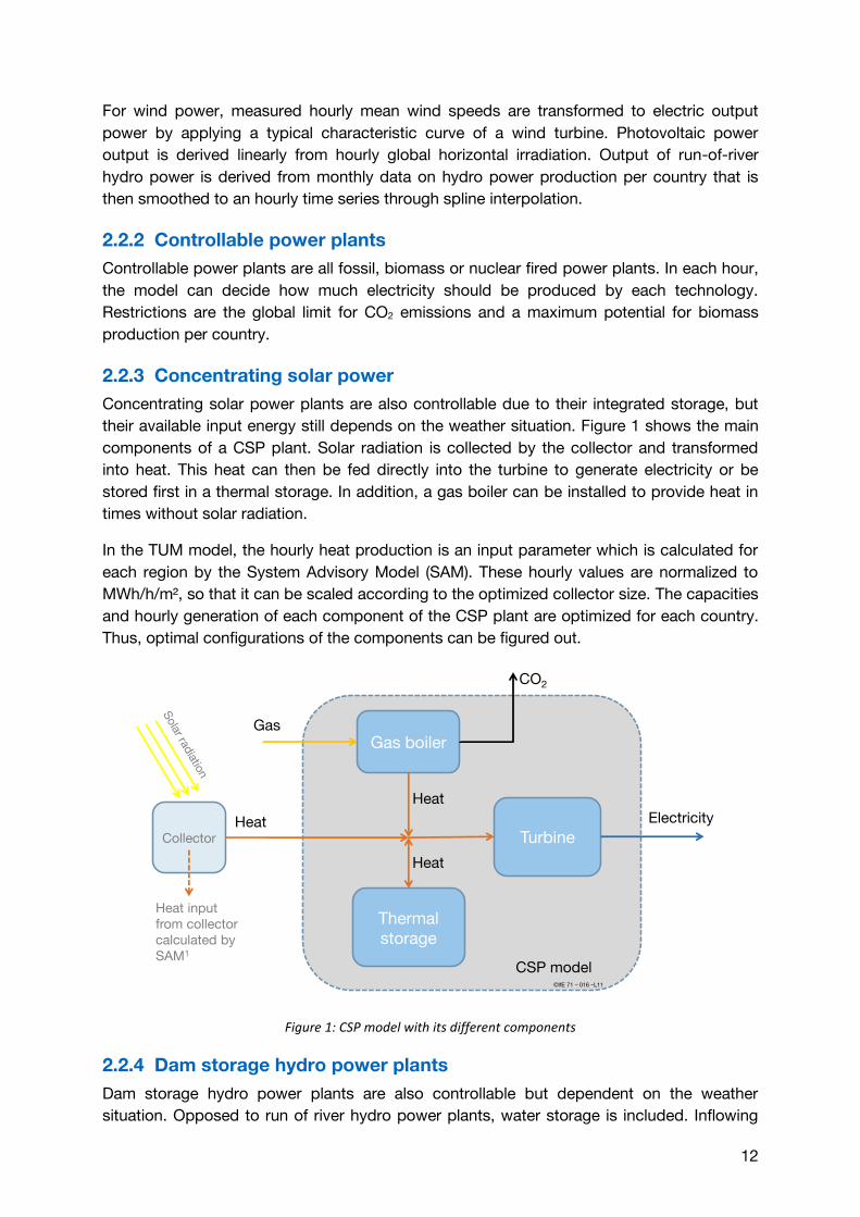
2.2.3 Concentrating solar power

Concentrating solar power plants are also controllable due to their integrated storage, but

their available input energy still depends on the weather situation. Figure 1 shows the main

components of a CSP plant. Solar radiation is collected by the collector and transformed

into heat. This heat can then be fed directly into the turbine to generate electricity or be

stored first in a thermal storage. In addition, a gas boiler can be installed to provide heat in

times without solar radiation.

In the TUM model, the hourly heat production is an input parameter which is calculated for

each region by the System Advisory Model (SAM). These hourly values are normalized to

MWh/h/m², so that it can be scaled according to the optimized collector size. The capacities

and hourly generation of each component of the CSP plant are optimized for each country.

Thus, optimal configurations of the components can be figured out.

Figure 1: CSP model with its different components

2.2.4 Dam storage hydro power plants

Dam storage hydro power plants are also controllable but dependent on the weather

situation. Opposed to run of river hydro power plants, water storage is included. Inflowing

Thermalstorage

Turbine

Gas boiler

Collector

Electricity

Gas

Heat input from collector calculated by SAM1

CSP model

Heat

CO2

Heat

Heat

©IfE 71 – 016 –L11

13

water can thus be stored first in this reservoir or fed directly to the turbine. The hourly water

inflow is determined through monthly production of hydro plants according to data

published by [3]. Full load hours of these time series can be seen in appendix A 4. All

storage is initialized 50 % filled and must reach the same level at the end of the simulation

timespan. In this model, capacity for dam storage is fixed and cannot be influenced through

optimization.

2.3 Transmission

Electricity transmission among Europe is modeled using a country-to-country transport

model, including losses according to the distance between two country’s geographical

center points. Transport model means that no load flow is simulated, but energy is allocated

and transported like a physical good. Electricity transmission between MENA and Europe is

modeled through designated DC power lines between certain countries, e.g. Morocco–

Spain (south), Tunisia–Italy (north) or Algeria–France.

Distribution within a country is accounted for by 7.5 % losses. However, costs for the

distribution network are not included in this model. For a discussion about costs for

transmission vs. distribution networks, see chapter 5 in [17].

2.4 Storage

The model includes three different types of storage: Pumped hydro storage, dam storage,

and thermal storage. The modeling approach for dam and thermal is described in the

generation section as this storage only allows postponing electricity generation. In contrast,

pumped hydro storage is the only possibility to feed with electricity from the grid, then store

it and use it later. A pumped hydro storage consists of two processes: The pump transforms

electricity to gravitational energy and the turbine transforms it back to electricity. Both

processes have a specific efficiency as well as a maximum capacity assigned. In addition,

the maximum energy content of the reservoir is limited. In the model, the reservoir level is

half filled at the beginning of the optimization period and has to be half filled at the end

again.

2.5 Model structure

The model itself consists of a huge set of parameters, variables and linear equations. Each

parameter is a numeric value representing one aspect of the model, like availability of a

renewable commodity, its costs, CO2 emissions or efficiency. Each variable is a quantity

whose value must be determined by the optimization algorithm. These are capacities of

installed power plants and activity of controllable power plants for each country, process

chain and time step.

Equations finally represent the connections between parameters and variables, thus forming

the model structure. While some equations are used to calculate derived quantities (e.g.

total electric energy generated per time step and country), other equations ensure that

boundary conditions (e.g. emission limits, capacity constraints for power plants) are fulfilled.

14

2.6 Optimization

Each aspect of the model has costs attached to it. Installing capacities for any of the

available processes causes investment costs, fixed annual costs for maintenance. Use of

some power plants causes variable costs for actually converting energy (operating costs +

fuel costs where applicable). Goal of the optimization is to find a system configuration of

installed capacities and operation of plants, transmission, and storage so that total costs

are minimized, while satisfying all boundary conditions. Considering storage, only the

capacity of thermal storage can be optimized, capacities of other storage possibilities are

set to a fixed level. The hourly operation however, can be optimized for all types of storage.

15

3 Scenario definitions

3.1 Main scenarios

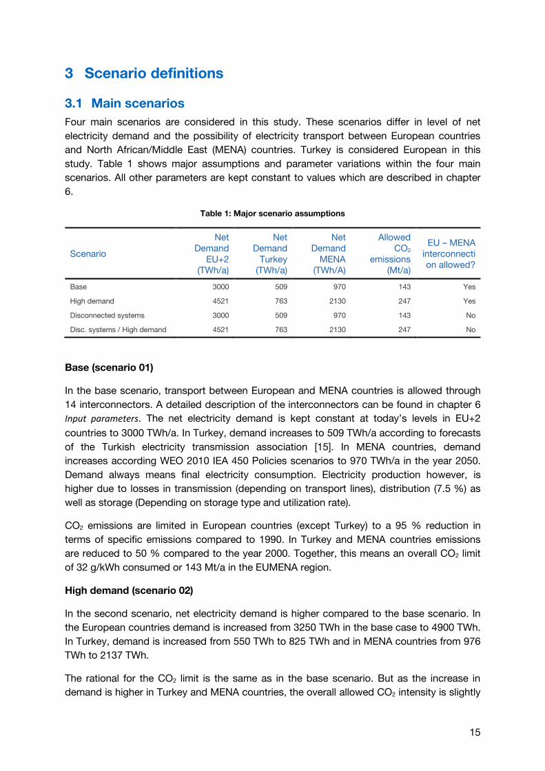
Four main scenarios are considered in this study. These scenarios differ in level of net

electricity demand and the possibility of electricity transport between European countries

and North African/Middle East (MENA) countries. Turkey is considered European in this

study. Table 1 shows major assumptions and parameter variations within the four main

scenarios. All other parameters are kept constant to values which are described in chapter

6.

Table 1: Major scenario assumptions

Scenario

Net Demand

EU+2 (TWh/a)

Net Demand

Turkey (TWh/a)

Net Demand

MENA (TWh/A)

Allowed CO2

emissions (Mt/a)

EU – MENA interconnection allowed?

Base 3000 509 970 143 Yes

High demand 4521 763 2130 247 Yes

Disconnected systems 3000 509 970 143 No

Disc. systems / High demand 4521 763 2130 247 No

Base (scenario 01)

In the base scenario, transport between European and MENA countries is allowed through

14 interconnectors. A detailed description of the interconnectors can be found in chapter 6

Input parameters. The net electricity demand is kept constant at today’s levels in EU+2

countries to 3000 TWh/a. In Turkey, demand increases to 509 TWh/a according to forecasts

of the Turkish electricity transmission association [15]. In MENA countries, demand

increases according WEO 2010 IEA 450 Policies scenarios to 970 TWh/a in the year 2050.

Demand always means final electricity consumption. Electricity production however, is

higher due to losses in transmission (depending on transport lines), distribution (7.5 %) as

well as storage (Depending on storage type and utilization rate).

CO2 emissions are limited in European countries (except Turkey) to a 95 % reduction in

terms of specific emissions compared to 1990. In Turkey and MENA countries emissions

are reduced to 50 % compared to the year 2000. Together, this means an overall CO2 limit

of 32 g/kWh consumed or 143 Mt/a in the EUMENA region.

High demand (scenario 02)

In the second scenario, net electricity demand is higher compared to the base scenario. In

the European countries demand is increased from 3250 TWh in the base case to 4900 TWh.

In Turkey, demand is increased from 550 TWh to 825 TWh and in MENA countries from 976

TWh to 2137 TWh.

The rational for the CO2 limit is the same as in the base scenario. But as the increase in

demand is higher in Turkey and MENA countries, the overall allowed CO2 intensity is slightly

16

higher with 31.4 g/kWh produced. Sum of allowed CO2 emission for the EUMENA region is

247 Mt/a, equal to specific emission of 33.3 g/kWh consumed.

Disconnected systems (scenario 03)

In this scenario, transportation between MENA and European countries through

interconnectors is completely forbidden. Electricity cannot be transported between

continents. The electricity demand as well as the limit for CO2 emissions is identical to

scenario 01 Base. That means both EU and MENA share one common CO2 limit.

Disconnected systems / High demand (scenario 04)

This scenario is a combination of scenarios 02 and 03. Transportation between MENA and

European countries is forbidden. The electricity demand as well as the limit for CO2-

Emissions is the same as in scenario 02 High demand.

3.2 Sensitivities

In the four main scenarios, only demand and allowed transmission lines are variable. In the

following 28 sensitivity scenarios, the influence of other parameter variations is investigated.

If not noted otherwise, electricity demand and CO2 restrictions from scenario 01 Base is

used. This section briefly lists the parameter changes in each scenario. Results are

presented and discussed in chapter 5.

Technology cost variations (scenarios 05-09, 23, 28-31)

In scenario 05, investment and fixed costs for CSP (collector, cofiring, turbine and storage

capacity) are at today’s higher values. In scenario 28, all costs are decreased by 30 %

compared to scenario 01. Investment and fixed costs for wind offshore are increased by

50 % in scenario 06 and decreased by 30 % in scenario 29. Investment and fixed costs for

photovoltaic are increased by 50 % in scenario 07 and decreased by 30 % in scenario 30.

Investment and fixed costs for wind onshore are increased by 50 % in scenario 08 and

decreased by 30 % in scenario 31. Investment costs for transmission lines are increased by

50 % in scenario 09 and increased by 100 % in scenario 23.

WACC variation (scenarios 10-12)

WACC is 7 % in scenario 01 Base. It is decreased to 5 % in scenario 10 and increased to

9 % in scenario 11. In scenario 12, WACC is increased to 9 % only in MENA countries.

Availability of Nuclear & CCS (scenarios 13-18, 32)

In these scenarios, either construction of nuclear or CCS capacities is allowed. In scenario

13, nuclear power may be installed with investment cost of 3000 €/kW. This value is

increased by 50 % in scenario 14, by 100 % in scenario 15 and by 150 % in scenario 32. In

scenario 16, CCS (gas & coal) power may be installed with investment costs of 1500 €/kW

(gas) and 2900 €/kW (coal). These values are increased by 50 % in scenario 17 and

increased by 100 % in scenario 18.

17

CO2 price instead of CO2 limit (scenarios 19-21, 27)

No limit on CO2 emissions is imposed in these scenarios. Instead, a CO2 price increased

variable costs for emitting processes. A price of 0 €/t is used in scenario 27, 50 €/t in

scenario 20, 100 €/t in scenario 19 and 150 €/t in scenario 21.

Grid restrictions & autarky (scenarios 22, 24-26)

In scenario 22, European transmission capacities may only be increased to three times of

today’s NTCs. In scenarios 24-26, electricity demand per country must be satisfied in each

hour by local electricity production with a share of 30, 50 and 70 %, respectively.

18

4 Main scenario results

4.1 Costs

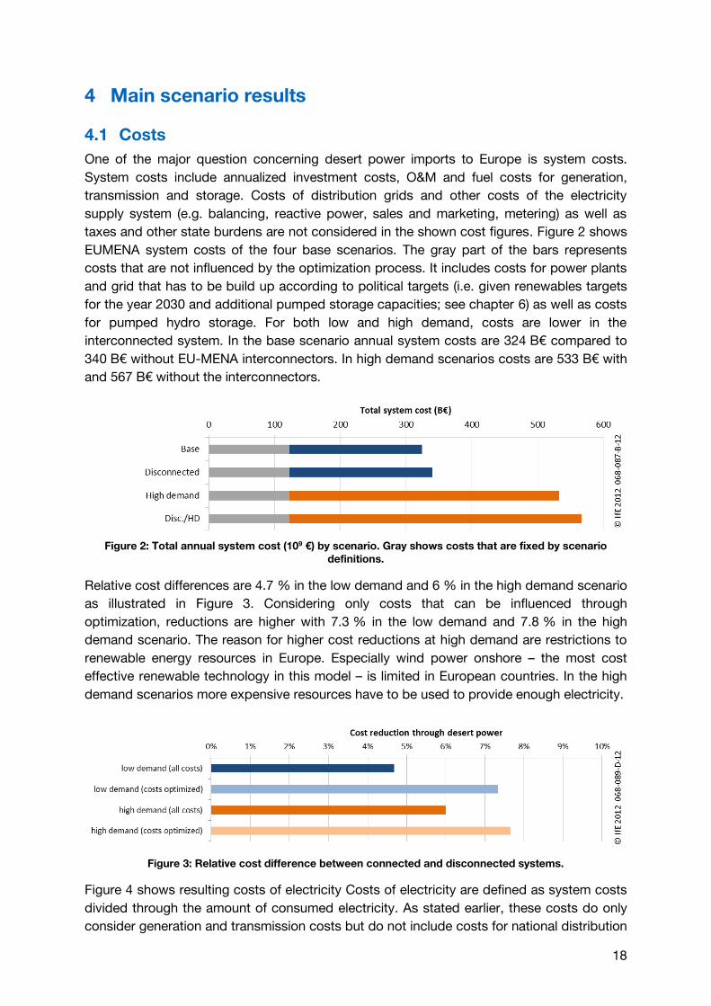
One of the major question concerning desert power imports to Europe is system costs.

System costs include annualized investment costs, O&M and fuel costs for generation,

transmission and storage. Costs of distribution grids and other costs of the electricity

supply system (e.g. balancing, reactive power, sales and marketing, metering) as well as

taxes and other state burdens are not considered in the shown cost figures. Figure 2 shows

EUMENA system costs of the four base scenarios. The gray part of the bars represents

costs that are not influenced by the optimization process. It includes costs for power plants

and grid that has to be build up according to political targets (i.e. given renewables targets

for the year 2030 and additional pumped storage capacities; see chapter 6) as well as costs

for pumped hydro storage. For both low and high demand, costs are lower in the

interconnected system. In the base scenario annual system costs are 324 B€ compared to

340 B€ without EU-MENA interconnectors. In high demand scenarios costs are 533 B€ with

and 567 B€ without the interconnectors.

Figure 2: Total annual system cost (109 €) by scenario. Gray shows costs that are fixed by scenario

definitions.

Relative cost differences are 4.7 % in the low demand and 6 % in the high demand scenario

as illustrated in Figure 3. Considering only costs that can be influenced through

optimization, reductions are higher with 7.3 % in the low demand and 7.8 % in the high

demand scenario. The reason for higher cost reductions at high demand are restrictions to

renewable energy resources in Europe. Especially wind power onshore – the most cost

effective renewable technology in this model – is limited in European countries. In the high

demand scenarios more expensive resources have to be used to provide enough electricity.

Figure 3: Relative cost difference between connected and disconnected systems.

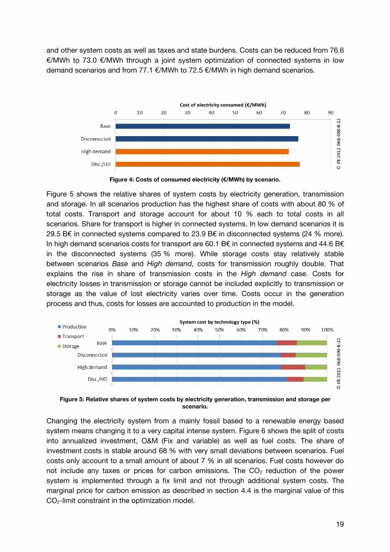
Figure 4 shows resulting costs of electricity Costs of electricity are defined as system costs

divided through the amount of consumed electricity. As stated earlier, these costs do only

consider generation and transmission costs but do not include costs for national distribution

19

and other system costs as well as taxes and state burdens. Costs can be reduced from 76.6

€/MWh to 73.0 €/MWh through a joint system optimization of connected systems in low

demand scenarios and from 77.1 €/MWh to 72.5 €/MWh in high demand scenarios.

Figure 4: Costs of consumed electricity (€/MWh) by scenario.

Figure 5 shows the relative shares of system costs by electricity generation, transmission

and storage. In all scenarios production has the highest share of costs with about 80 % of

total costs. Transport and storage account for about 10 % each to total costs in all

scenarios. Share for transport is higher in connected systems. In low demand scenarios it is

29.5 B€ in connected systems compared to 23.9 B€ in disconnected systems (24 % more).

In high demand scenarios costs for transport are 60.1 B€ in connected systems and 44.6 B€

in the disconnected systems (35 % more). While storage costs stay relatively stable

between scenarios Base and High demand, costs for transmission roughly double. That

explains the rise in share of transmission costs in the High demand case. Costs for

electricity losses in transmission or storage cannot be included explicitly to transmission or

storage as the value of lost electricity varies over time. Costs occur in the generation

process and thus, costs for losses are accounted to production in the model.

Figure 5: Relative shares of system costs by electricity generation, transmission and storage per

scenario.

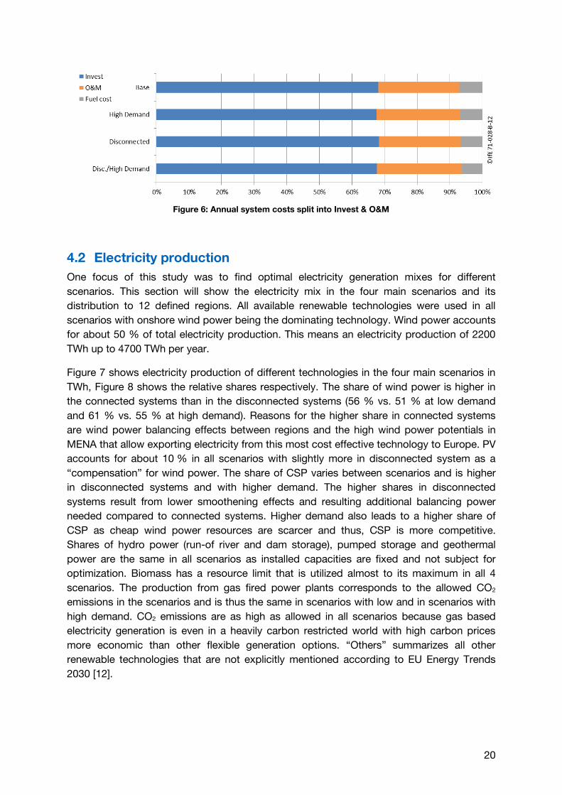
Changing the electricity system from a mainly fossil based to a renewable energy based

system means changing it to a very capital intense system. Figure 6 shows the split of costs

into annualized investment, O&M (Fix and variable) as well as fuel costs. The share of

investment costs is stable around 68 % with very small deviations between scenarios. Fuel

costs only account to a small amount of about 7 % in all scenarios. Fuel costs however do

not include any taxes or prices for carbon emissions. The CO2 reduction of the power

system is implemented through a fix limit and not through additional system costs. The

marginal price for carbon emission as described in section 4.4 is the marginal value of this

CO2-limit constraint in the optimization model.

20

Figure 6: Annual system costs split into Invest & O&M

4.2 Electricity production

One focus of this study was to find optimal electricity generation mixes for different

scenarios. This section will show the electricity mix in the four main scenarios and its

distribution to 12 defined regions. All available renewable technologies were used in all

scenarios with onshore wind power being the dominating technology. Wind power accounts

for about 50 % of total electricity production. This means an electricity production of 2200

TWh up to 4700 TWh per year.

Figure 7 shows electricity production of different technologies in the four main scenarios in

TWh, Figure 8 shows the relative shares respectively. The share of wind power is higher in

the connected systems than in the disconnected systems (56 % vs. 51 % at low demand

and 61 % vs. 55 % at high demand). Reasons for the higher share in connected systems

are wind power balancing effects between regions and the high wind power potentials in

MENA that allow exporting electricity from this most cost effective technology to Europe. PV

accounts for about 10 % in all scenarios with slightly more in disconnected system as a

“compensation” for wind power. The share of CSP varies between scenarios and is higher

in disconnected systems and with higher demand. The higher shares in disconnected

systems result from lower smoothening effects and resulting additional balancing power

needed compared to connected systems. Higher demand also leads to a higher share of

CSP as cheap wind power resources are scarcer and thus, CSP is more competitive.

Shares of hydro power (run-of river and dam storage), pumped storage and geothermal

power are the same in all scenarios as installed capacities are fixed and not subject for

optimization. Biomass has a resource limit that is utilized almost to its maximum in all 4

scenarios. The production from gas fired power plants corresponds to the allowed CO2

emissions in the scenarios and is thus the same in scenarios with low and in scenarios with

high demand. CO2 emissions are as high as allowed in all scenarios because gas based

electricity generation is even in a heavily carbon restricted world with high carbon prices

more economic than other flexible generation options. “Others” summarizes all other

renewable technologies that are not explicitly mentioned according to EU Energy Trends

2030 [12].

21

Figure 7: Generated electricity (TWh) by input commodity and scenario.

Figure 8: Relative shares of generated electricity by input commodity and scenario.

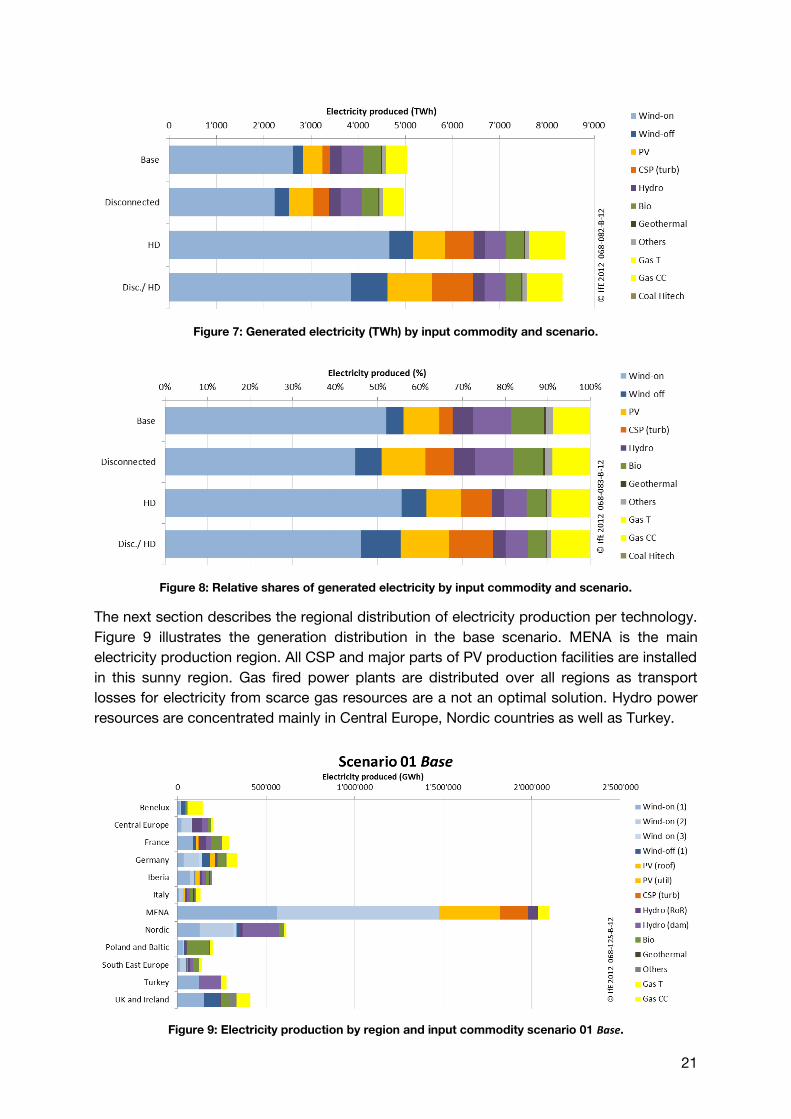
The next section describes the regional distribution of electricity production per technology.

Figure 9 illustrates the generation distribution in the base scenario. MENA is the main

electricity production region. All CSP and major parts of PV production facilities are installed

in this sunny region. Gas fired power plants are distributed over all regions as transport

losses for electricity from scarce gas resources are a not an optimal solution. Hydro power

resources are concentrated mainly in Central Europe, Nordic countries as well as Turkey.

Figure 9: Electricity production by region and input commodity scenario 01 Base.

22

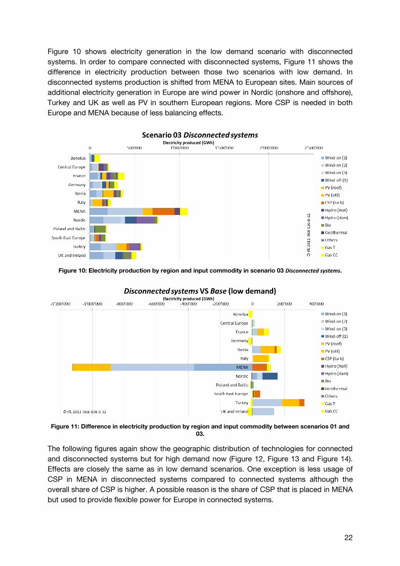
Figure 10 shows electricity generation in the low demand scenario with disconnected

systems. In order to compare connected with disconnected systems, Figure 11 shows the

difference in electricity production between those two scenarios with low demand. In

disconnected systems production is shifted from MENA to European sites. Main sources of

additional electricity generation in Europe are wind power in Nordic (onshore and offshore),

Turkey and UK as well as PV in southern European regions. More CSP is needed in both

Europe and MENA because of less balancing effects.

Figure 10: Electricity production by region and input commodity in scenario 03 Disconnected systems.

Figure 11: Difference in electricity production by region and input commodity between scenarios 01 and

03.

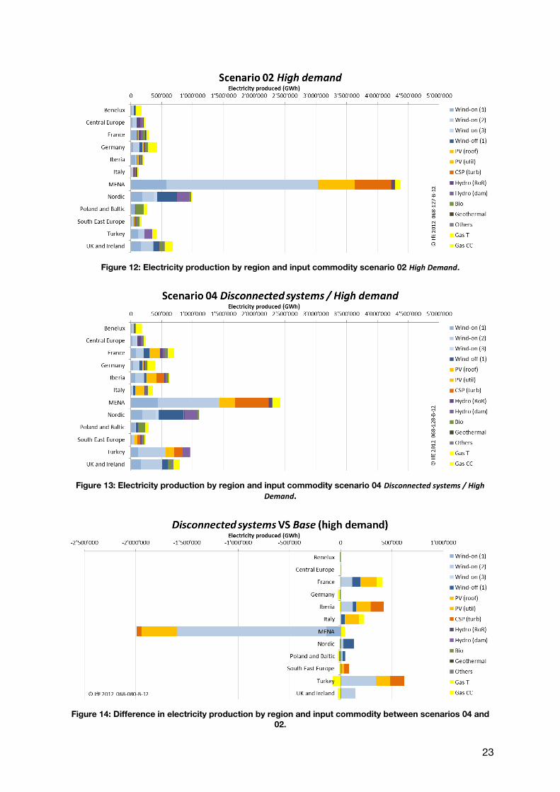
The following figures again show the geographic distribution of technologies for connected

and disconnected systems but for high demand now (Figure 12, Figure 13 and Figure 14).

Effects are closely the same as in low demand scenarios. One exception is less usage of

CSP in MENA in disconnected systems compared to connected systems although the

overall share of CSP is higher. A possible reason is the share of CSP that is placed in MENA

but used to provide flexible power for Europe in connected systems.

23

Figure 12: Electricity production by region and input commodity scenario 02 High Demand.

Figure 13: Electricity production by region and input commodity scenario 04 Disconnected systems / High

Demand.

Figure 14: Difference in electricity production by region and input commodity between scenarios 04 and

02.

24

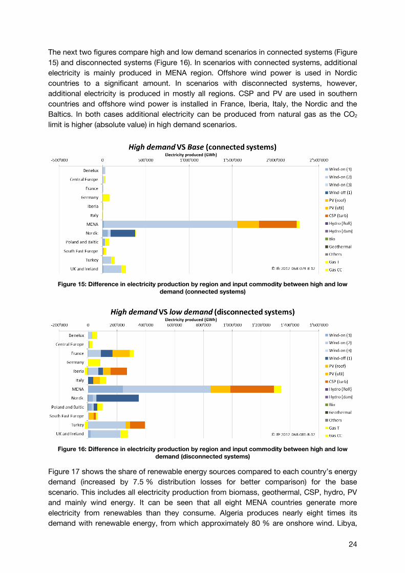
The next two figures compare high and low demand scenarios in connected systems (Figure

15) and disconnected systems (Figure 16). In scenarios with connected systems, additional

electricity is mainly produced in MENA region. Offshore wind power is used in Nordic

countries to a significant amount. In scenarios with disconnected systems, however,

additional electricity is produced in mostly all regions. CSP and PV are used in southern

countries and offshore wind power is installed in France, Iberia, Italy, the Nordic and the

Baltics. In both cases additional electricity can be produced from natural gas as the CO2

limit is higher (absolute value) in high demand scenarios.

Figure 15: Difference in electricity production by region and input commodity between high and low

demand (connected systems)

Figure 16: Difference in electricity production by region and input commodity between high and low

demand (disconnected systems)

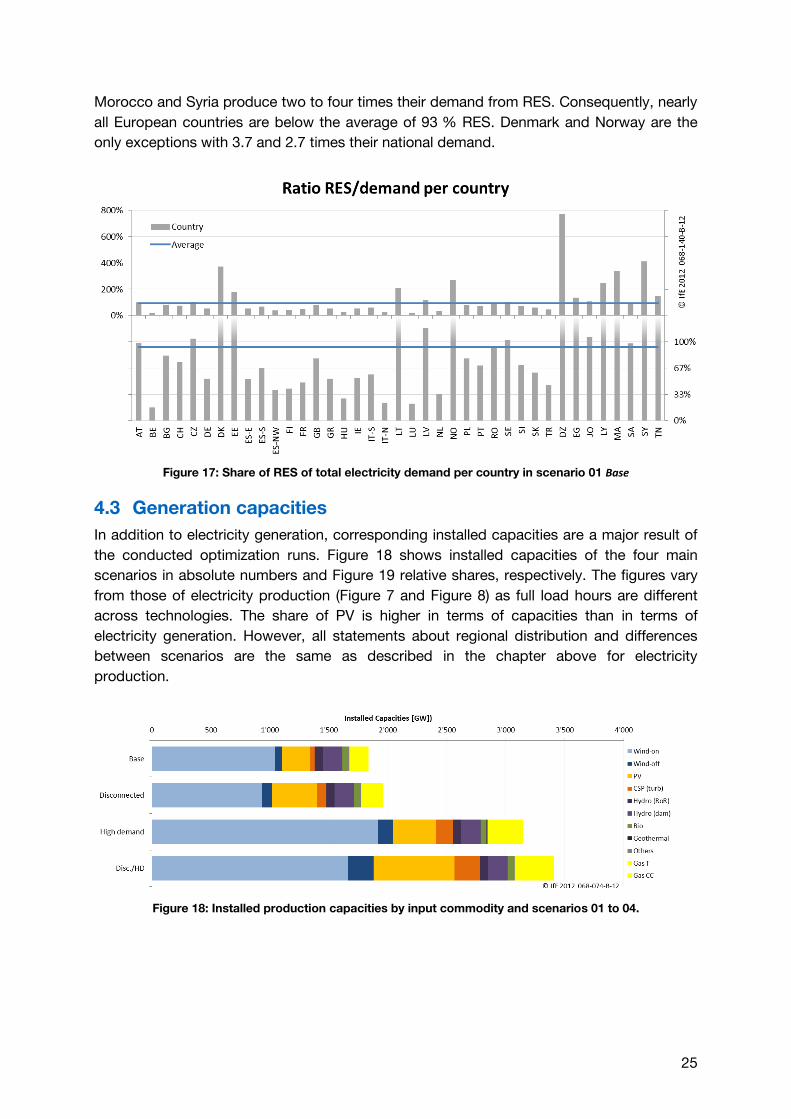
Figure 17 shows the share of renewable energy sources compared to each country’s energy

demand (increased by 7.5 % distribution losses for better comparison) for the base

scenario. This includes all electricity production from biomass, geothermal, CSP, hydro, PV

and mainly wind energy. It can be seen that all eight MENA countries generate more

electricity from renewables than they consume. Algeria produces nearly eight times its

demand with renewable energy, from which approximately 80 % are onshore wind. Libya,

25

Morocco and Syria produce two to four times their demand from RES. Consequently, nearly

all European countries are below the average of 93 % RES. Denmark and Norway are the

only exceptions with 3.7 and 2.7 times their national demand.

Figure 17: Share of RES of total electricity demand per country in scenario 01 Base

4.3 Generation capacities

In addition to electricity generation, corresponding installed capacities are a major result of

the conducted optimization runs. Figure 18 shows installed capacities of the four main

scenarios in absolute numbers and Figure 19 relative shares, respectively. The figures vary

from those of electricity production (Figure 7 and Figure 8) as full load hours are different

across technologies. The share of PV is higher in terms of capacities than in terms of

electricity generation. However, all statements about regional distribution and differences

between scenarios are the same as described in the chapter above for electricity

production.

Figure 18: Installed production capacities by input commodity and scenarios 01 to 04.

26

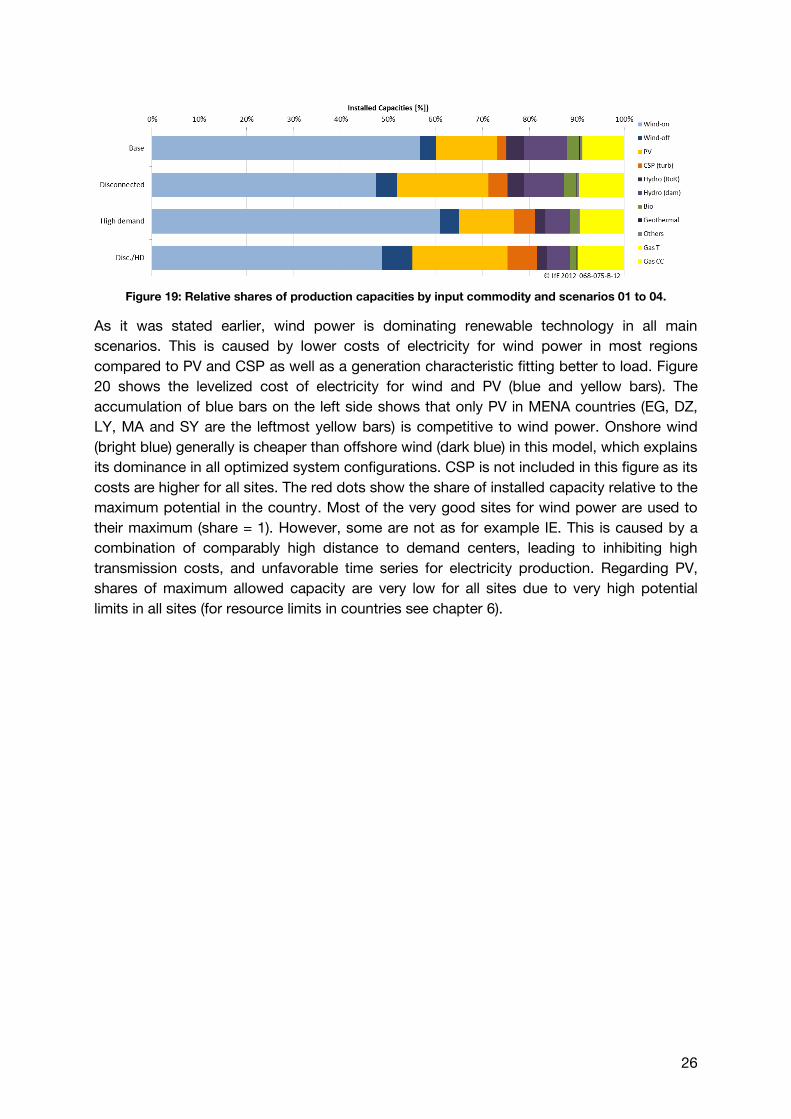
Figure 19: Relative shares of production capacities by input commodity and scenarios 01 to 04.

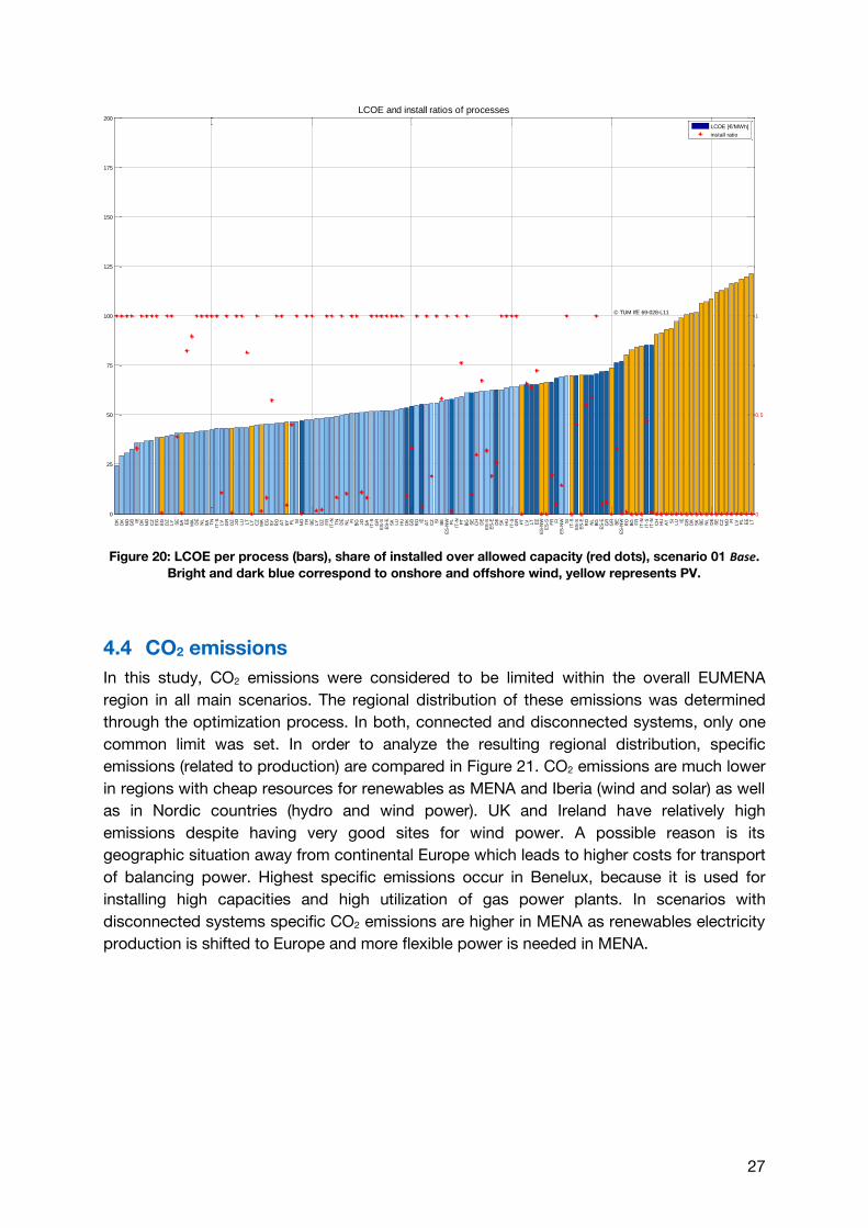
As it was stated earlier, wind power is dominating renewable technology in all main

scenarios. This is caused by lower costs of electricity for wind power in most regions

compared to PV and CSP as well as a generation characteristic fitting better to load. Figure

20 shows the levelized cost of electricity for wind and PV (blue and yellow bars). The

accumulation of blue bars on the left side shows that only PV in MENA countries (EG, DZ,

LY, MA and SY are the leftmost yellow bars) is competitive to wind power. Onshore wind

(bright blue) generally is cheaper than offshore wind (dark blue) in this model, which explains

its dominance in all optimized system configurations. CSP is not included in this figure as its

costs are higher for all sites. The red dots show the share of installed capacity relative to the

maximum potential in the country. Most of the very good sites for wind power are used to

their maximum (share = 1). However, some are not as for example IE. This is caused by a

combination of comparably high distance to demand centers, leading to inhibiting high

transmission costs, and unfavorable time series for electricity production. Regarding PV,

shares of maximum allowed capacity are very low for all sites due to very high potential

limits in all sites (for resource limits in countries see chapter 6).

27

Figure 20: LCOE per process (bars), share of installed over allowed capacity (red dots), scenario 01 Base.

Bright and dark blue correspond to onshore and offshore wind, yellow represents PV.

4.4 CO2 emissions

In this study, CO2 emissions were considered to be limited within the overall EUMENA

region in all main scenarios. The regional distribution of these emissions was determined

through the optimization process. In both, connected and disconnected systems, only one

common limit was set. In order to analyze the resulting regional distribution, specific

emissions (related to production) are compared in Figure 21. CO2 emissions are much lower

in regions with cheap resources for renewables as MENA and Iberia (wind and solar) as well

as in Nordic countries (hydro and wind power). UK and Ireland have relatively high

emissions despite having very good sites for wind power. A possible reason is its

geographic situation away from continental Europe which leads to higher costs for transport

of balancing power. Highest specific emissions occur in Benelux, because it is used for

installing high capacities and high utilization of gas power plants. In scenarios with

disconnected systems specific CO2 emissions are higher in MENA as renewables electricity

production is shifted to Europe and more flexible power is needed in MENA.

0

25

50

75

100

125

150

175

200

LCOE and install ratios of processes

D

KD

KN

OG

B IED

KN

OC

ZE

GE

GD

ZLY SE

SA EE

MA

DE

NL

SA TN

IT-S LV

GR

DZ

JO

LU LT

LY

CZ

MA

EG

SY

RO

AT

SY PL SI

NO

TR

BE

LY

DZ

FR

IT-N TN

DE

NL FI

BG JO

SA

IT-S

GR

ES

-SE

S-E SK

LU

HU

DK

GB

RO IE

AT

CZ SI

BE

ES

-NW PL

IT-N PT

BG SE

CH

DE

ES

-SE

S-E DE

SK

HU

IT-S

GR

PT

LV LT

EE

ES

-NW

ES

-S FR FI

ES

-NW SI

IT-S

ES

-SE

S-E

RO

NL

BG

ES

-EG

RG

RB

EE

S-N

WR

OB

G FR

IT-N

IT-S

IT-N CH

HU

AT SI

LU IE

GB

DK

SK

BE

NL

DE

SE

CZ

NO FI

LV PL

EE

LT

© TUM IfE 69-028-L11

0

0.5

1

LCOE [€/MWh]

install ratio

28

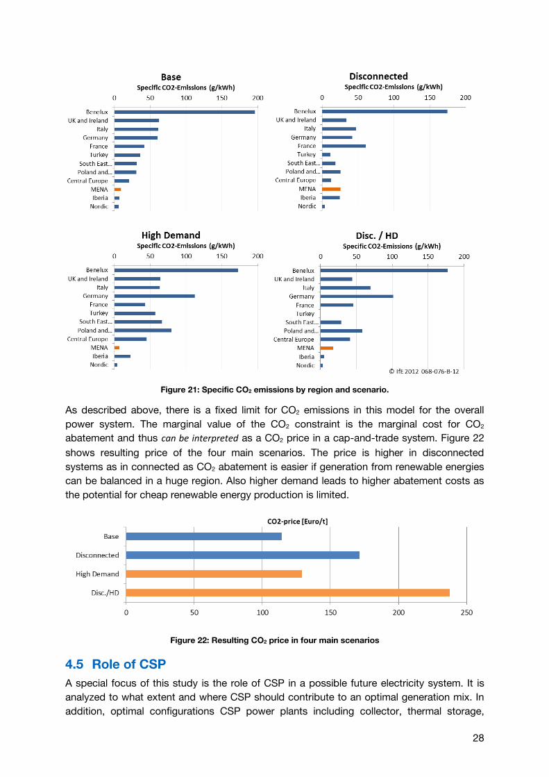
Figure 21: Specific CO2 emissions by region and scenario.

As described above, there is a fixed limit for CO2 emissions in this model for the overall

power system. The marginal value of the CO2 constraint is the marginal cost for CO2

abatement and thus can be interpreted as a CO2 price in a cap-and-trade system. Figure 22

shows resulting price of the four main scenarios. The price is higher in disconnected

systems as in connected as CO2 abatement is easier if generation from renewable energies

can be balanced in a huge region. Also higher demand leads to higher abatement costs as

the potential for cheap renewable energy production is limited.

Figure 22: Resulting CO2 price in four main scenarios

4.5 Role of CSP

A special focus of this study is the role of CSP in a possible future electricity system. It is

analyzed to what extent and where CSP should contribute to an optimal generation mix. In

addition, optimal configurations CSP power plants including collector, thermal storage,

29

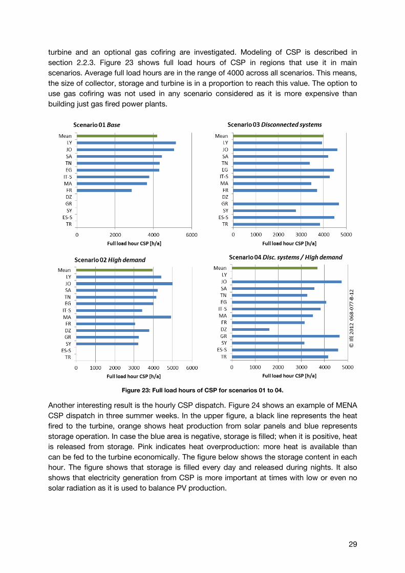
turbine and an optional gas cofiring are investigated. Modeling of CSP is described in

section 2.2.3. Figure 23 shows full load hours of CSP in regions that use it in main

scenarios. Average full load hours are in the range of 4000 across all scenarios. This means,

the size of collector, storage and turbine is in a proportion to reach this value. The option to

use gas cofiring was not used in any scenario considered as it is more expensive than

building just gas fired power plants.

Figure 23: Full load hours of CSP for scenarios 01 to 04.

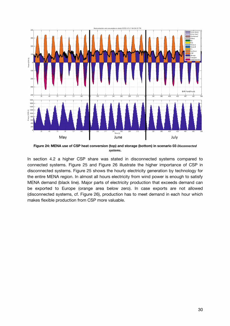
Another interesting result is the hourly CSP dispatch. Figure 24 shows an example of MENA

CSP dispatch in three summer weeks. In the upper figure, a black line represents the heat

fired to the turbine, orange shows heat production from solar panels and blue represents

storage operation. In case the blue area is negative, storage is filled; when it is positive, heat

is released from storage. Pink indicates heat overproduction: more heat is available than

can be fed to the turbine economically. The figure below shows the storage content in each

hour. The figure shows that storage is filled every day and released during nights. It also

shows that electricity generation from CSP is more important at times with low or even no

solar radiation as it is used to balance PV production.

30

Figure 24: MENA use of CSP heat conversion (top) and storage (bottom) in scenario 03 Disconnected

systems.

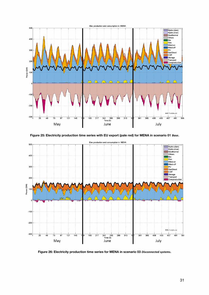
In section 4.2 a higher CSP share was stated in disconnected systems compared to

connected systems. Figure 25 and Figure 26 illustrate the higher importance of CSP in

disconnected systems. Figure 25 shows the hourly electricity generation by technology for

the entire MENA region. In almost all hours electricity from wind power is enough to satisfy

MENA demand (black line). Major parts of electricity production that exceeds demand can

be exported to Europe (orange area below zero). In case exports are not allowed

(disconnected systems, cf. Figure 26), production has to meet demand in each hour which

makes flexible production from CSP more valuable.

31

Figure 25: Electricity production time series with EU export (pale red) for MENA in scenario 01 Base.

Figure 26: Electricity production time series for MENA in scenario 03 Disconnected systems.

32

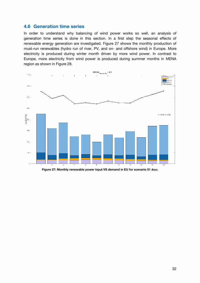
4.6 Generation time series

In order to understand why balancing of wind power works so well, an analysis of

generation time series is done in this section. In a first step the seasonal effects of

renewable energy generation are investigated. Figure 27 shows the monthly production of

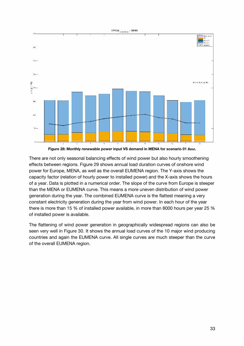
must-run renewables (hydro run of river, PV, and on- and offshore wind) in Europe. More

electricity is produced during winter month driven by more wind power. In contrast to

Europe, more electricity from wind power is produced during summer months in MENA

region as shown in Figure 28.

Figure 27: Monthly renewable power input VS demand in EU for scenario 01 Base.

33

Figure 28: Monthly renewable power input VS demand in MENA for scenario 01 Base.

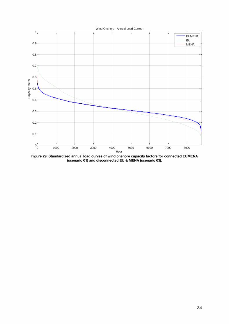
There are not only seasonal balancing effects of wind power but also hourly smoothening

effects between regions. Figure 29 shows annual load duration curves of onshore wind

power for Europe, MENA, as well as the overall EUMENA region. The Y-axis shows the

capacity factor (relation of hourly power to installed power) and the X-axis shows the hours

of a year. Data is plotted in a numerical order. The slope of the curve from Europe is steeper

than the MENA or EUMENA curve. This means a more uneven distribution of wind power

generation during the year. The combined EUMENA curve is the flattest meaning a very

constant electricity generation during the year from wind power. In each hour of the year

there is more than 15 % of installed power available, in more than 8000 hours per year 25 %

of installed power is available.

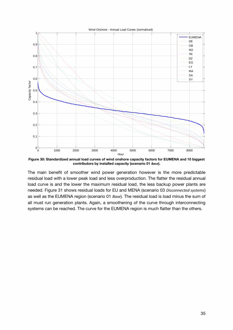
The flattening of wind power generation in geographically widespread regions can also be

seen very well in Figure 30. It shows the annual load curves of the 10 major wind producing

countries and again the EUMENA curve. All single curves are much steeper than the curve

of the overall EUMENA region.

34

Figure 29: Standardized annual load curves of wind onshore capacity factors for connected EUMENA

(scenario 01) and disconnected EU & MENA (scenario 03).

0 1000 2000 3000 4000 5000 6000 7000 80000

0.1

0.2

0.3

0.4

0.5

0.6

0.7

0.8

0.9

1

Hour

Capacity f

acto

rWind Onshore - Annual Load Curves

EUMENA

EU

MENA

35

Figure 30: Standardized annual load curves of wind onshore capacity factors for EUMENA and 10 biggest

contributors by installed capacity (scenario 01 Base).

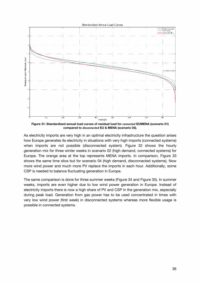
The main benefit of smoother wind power generation however is the more predictable

residual load with a lower peak load and less overproduction. The flatter the residual annual

load curve is and the lower the maximum residual load, the less backup power plants are

needed. Figure 31 shows residual loads for EU and MENA (scenario 03 Disconnected systems)

as well as the EUMENA region (scenario 01 Base). The residual load is load minus the sum of

all must run generation plants. Again, a smoothening of the curve through interconnecting

systems can be reached. The curve for the EUMENA region is much flatter than the others.

0 1000 2000 3000 4000 5000 6000 7000 80000

0.1

0.2

0.3

0.4

0.5

0.6

0.7

0.8

0.9

1

Hour

Capacity f

acto

rWind Onshore - Annual Load Curves (normalised)

EUMENA

DE

GB

NO

TR

DZ

EG

LY

MA

SA

SY

36

Figure 31: Standardized annual load curves of residual load for connected EUMENA (scenario 01)

compared to disconnected EU & MENA (scenario 03).

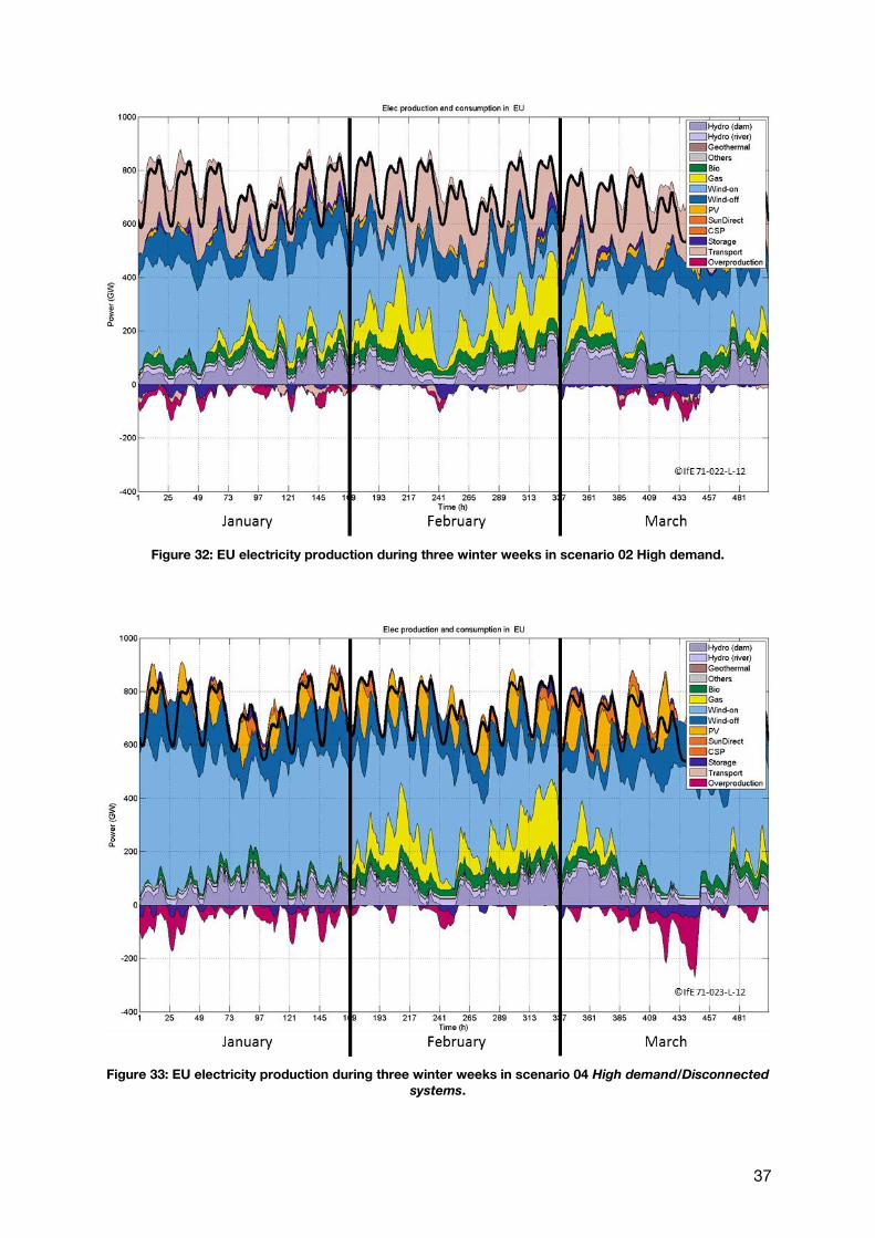
As electricity imports are very high in an optimal electricity infrastructure the question arises

how Europe generates its electricity in situations with very high imports (connected systems)

when imports are not possible (disconnected system). Figure 32 shows the hourly

generation mix for three winter weeks in scenario 02 (high demand, connected systems) for

Europe. The orange area at the top represents MENA imports. In comparison, Figure 33

shows the same time slice but for scenario 04 (high demand, disconnected systems). Now

more wind power and much more PV replace the imports in each hour. Additionally, some

CSP is needed to balance fluctuating generation in Europe.

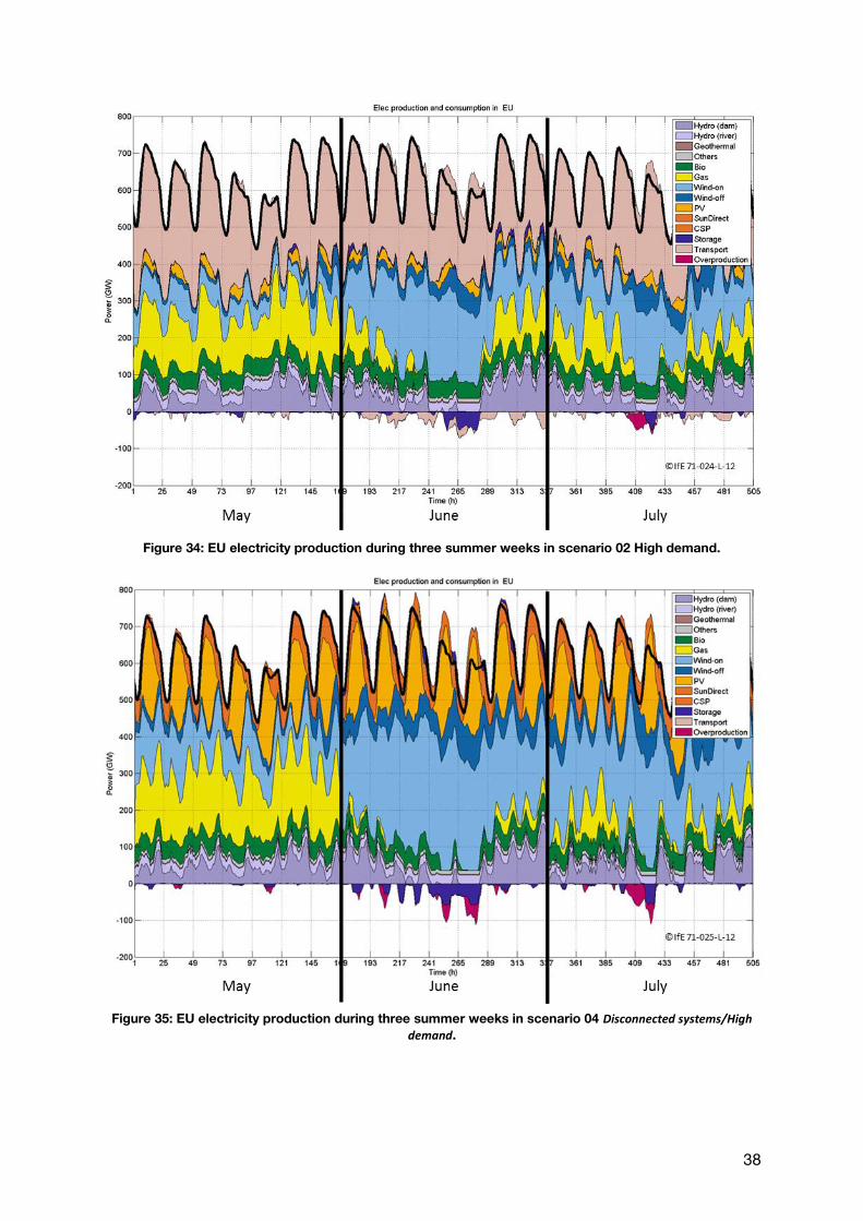
The same comparison is done for three summer weeks (Figure 34 and Figure 35). In summer

weeks, imports are even higher due to low wind power generation in Europe. Instead of

electricity imports there is now a high share of PV and CSP in the generation mix, especially

during peak load. Generation from gas power has to be used concentrated in times with

very low wind power (first week) in disconnected systems whereas more flexible usage is

possible in connected systems.

37

Figure 32: EU electricity production during three winter weeks in scenario 02 High demand.

Figure 33: EU electricity production during three winter weeks in scenario 04 High demand/Disconnected

systems.

38

Figure 34: EU electricity production during three summer weeks in scenario 02 High demand.

Figure 35: EU electricity production during three summer weeks in scenario 04 Disconnected systems/High

demand.

39

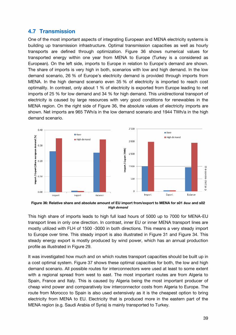
4.7 Transmission

One of the most important aspects of integrating European and MENA electricity systems is

building up transmission infrastructure. Optimal transmission capacities as well as hourly

transports are defined through optimization. Figure 36 shows numerical values for

transported energy within one year from MENA to Europe (Turkey is a considered as

European). On the left side, imports to Europe in relation to Europe’s demand are shown.

The share of imports is very high in both, scenarios with low and high demand. In the low

demand scenario, 26 % of Europe’s electricity demand is provided through imports from

MENA. In the high demand scenario even 35 % of electricity is imported to reach cost

optimality. In contrast, only about 1 % of electricity is exported from Europe leading to net

imports of 25 % for low demand and 34 % for high demand. This unidirectional transport of

electricity is caused by large resources with very good conditions for renewables in the

MENA region. On the right side of Figure 36, the absolute values of electricity imports are

shown. Net imports are 965 TWh/a in the low demand scenario and 1944 TWh/a in the high

demand scenario.

Figure 36: Relative share and absolute amount of EU import from/export to MENA for s01 Base and s02

High demand

This high share of imports leads to high full load hours of 5000 up to 7000 for MENA-EU

transport lines in only one direction. In contrast, inner EU or inner MENA transport lines are

mostly utilized with FLH of 1500 -3000 in both directions. This means a very steady import

to Europe over time. This steady import is also illustrated in Figure 31 and Figure 34. This

steady energy export is mostly produced by wind power, which has an annual production

profile as illustrated in Figure 29.

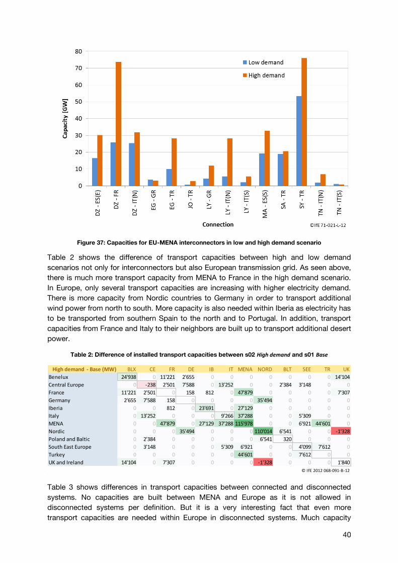
It was investigated how much and on which routes transport capacities should be built up in

a cost optimal system. Figure 37 shows these optimal capacities for both, the low and high

demand scenario. All possible routes for interconnectors were used at least to some extent

with a regional spread from west to east. The most important routes are from Algeria to

Spain, France and Italy. This is caused by Algeria being the most important producer of

cheap wind power and comparatively low interconnector costs from Algeria to Europe. The

route from Morocco to Spain is also used extensively as it is the cheapest option to bring

electricity from MENA to EU. Electricity that is produced more in the eastern part of the

MENA region (e.g. Saudi Arabia of Syria) is mainly transported to Turkey.

40

Figure 37: Capacities for EU-MENA interconnectors in low and high demand scenario

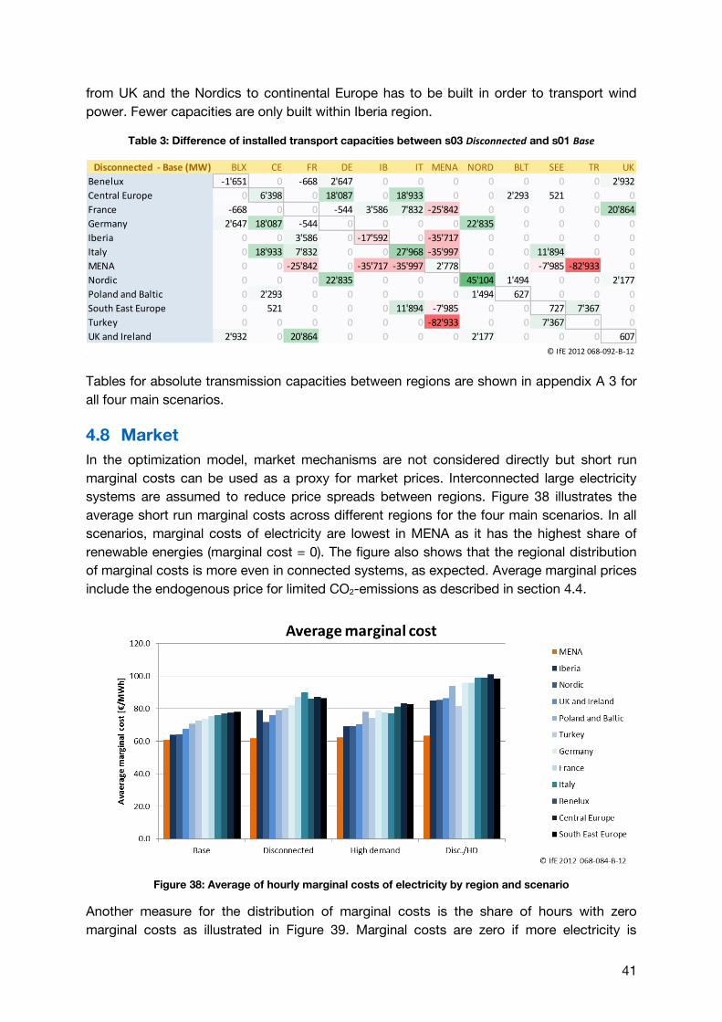
Table 2 shows the difference of transport capacities between high and low demand

scenarios not only for interconnectors but also European transmission grid. As seen above,

there is much more transport capacity from MENA to France in the high demand scenario.

In Europe, only several transport capacities are increasing with higher electricity demand.

There is more capacity from Nordic countries to Germany in order to transport additional

wind power from north to south. More capacity is also needed within Iberia as electricity has

to be transported from southern Spain to the north and to Portugal. In addition, transport

capacities from France and Italy to their neighbors are built up to transport additional desert

power.

Table 2: Difference of installed transport capacities between s02 High demand and s01 Base

Table 3 shows differences in transport capacities between connected and disconnected

systems. No capacities are built between MENA and Europe as it is not allowed in

disconnected systems per definition. But it is a very interesting fact that even more

transport capacities are needed within Europe in disconnected systems. Much capacity

High demand - Base (MW) BLX CE FR DE IB IT MENA NORD BLT SEE TR UK

Benelux 24'938 0 11'221 2'655 0 0 0 0 0 0 0 14'104

Central Europe 0 -238 2'501 7'588 0 13'252 0 0 2'384 3'148 0 0

France 11'221 2'501 0 158 812 0 47'879 0 0 0 0 7'307

Germany 2'655 7'588 158 0 0 0 0 35'494 0 0 0 0

Iberia 0 0 812 0 23'691 0 27'129 0 0 0 0 0

Italy 0 13'252 0 0 0 9'266 37'288 0 0 5'309 0 0

MENA 0 0 47'879 0 27'129 37'288 115'978 0 0 6'921 44'601 0

Nordic 0 0 0 35'494 0 0 0 110'014 6'541 0 0 -1'328

Poland and Baltic 0 2'384 0 0 0 0 0 6'541 320 0 0 0

South East Europe 0 3'148 0 0 0 5'309 6'921 0 0 4'099 7'612 0

Turkey 0 0 0 0 0 0 44'601 0 0 7'612 0 0

UK and Ireland 14'104 0 7'307 0 0 0 0 -1'328 0 0 0 1'840

© IfE 2012 068-091-B-12

41

from UK and the Nordics to continental Europe has to be built in order to transport wind

power. Fewer capacities are only built within Iberia region.

Table 3: Difference of installed transport capacities between s03 Disconnected and s01 Base

Tables for absolute transmission capacities between regions are shown in appendix A 3 for

all four main scenarios.

4.8 Market

In the optimization model, market mechanisms are not considered directly but short run

marginal costs can be used as a proxy for market prices. Interconnected large electricity

systems are assumed to reduce price spreads between regions. Figure 38 illustrates the

average short run marginal costs across different regions for the four main scenarios. In all

scenarios, marginal costs of electricity are lowest in MENA as it has the highest share of

renewable energies (marginal cost = 0). The figure also shows that the regional distribution

of marginal costs is more even in connected systems, as expected. Average marginal prices

include the endogenous price for limited CO2-emissions as described in section 4.4.

Figure 38: Average of hourly marginal costs of electricity by region and scenario

Another measure for the distribution of marginal costs is the share of hours with zero

marginal costs as illustrated in Figure 39. Marginal costs are zero if more electricity is

Disconnected - Base (MW) BLX CE FR DE IB IT MENA NORD BLT SEE TR UK

Benelux -1'651 0 -668 2'647 0 0 0 0 0 0 0 2'932

Central Europe 0 6'398 0 18'087 0 18'933 0 0 2'293 521 0 0

France -668 0 0 -544 3'586 7'832 -25'842 0 0 0 0 20'864

Germany 2'647 18'087 -544 0 0 0 0 22'835 0 0 0 0

Iberia 0 0 3'586 0 -17'592 0 -35'717 0 0 0 0 0

Italy 0 18'933 7'832 0 0 27'968 -35'997 0 0 11'894 0 0

MENA 0 0 -25'842 0 -35'717 -35'997 2'778 0 0 -7'985 -82'933 0

Nordic 0 0 0 22'835 0 0 0 45'104 1'494 0 0 2'177

Poland and Baltic 0 2'293 0 0 0 0 0 1'494 627 0 0 0

South East Europe 0 521 0 0 0 11'894 -7'985 0 0 727 7'367 0

Turkey 0 0 0 0 0 0 -82'933 0 0 7'367 0 0

UK and Ireland 2'932 0 20'864 0 0 0 0 2'177 0 0 0 607

© IfE 2012 068-092-B-12

42

produced through must run technologies than consumed. (Marginal) higher electricity

consumption would not cause additional costs in these situations. The share of hours with

marginal costs of zero is highest in MENA as the share of renewables is highest there.

Fewer situations with zero marginal costs occur in connected systems, i.e. renewable

energy is better used. This again is a measure for a better balancing of prices throughout

the system.

Figure 39: Relative count of hours with marginal cost equal to zero by region and scenario

43

5 Sensitivities

Having established a firm understanding of the simulation results in the previous chapter, in

the following the influence of changed input parameter values is investigated. For that

purpose, many additional scenarios are derived from Scenario 01 Base by changing only one

parameter per scenario. This chapter highlights the changes caused by those changes on

the optimal system configuration and total system costs. The main comparison method is

electricity production by region and input commodity (wind, hydro, gas). Electricity

production (MWh) is preferred to installed capacities (MW), because it better reflects the

true contribution of a technology to the electricity mix.

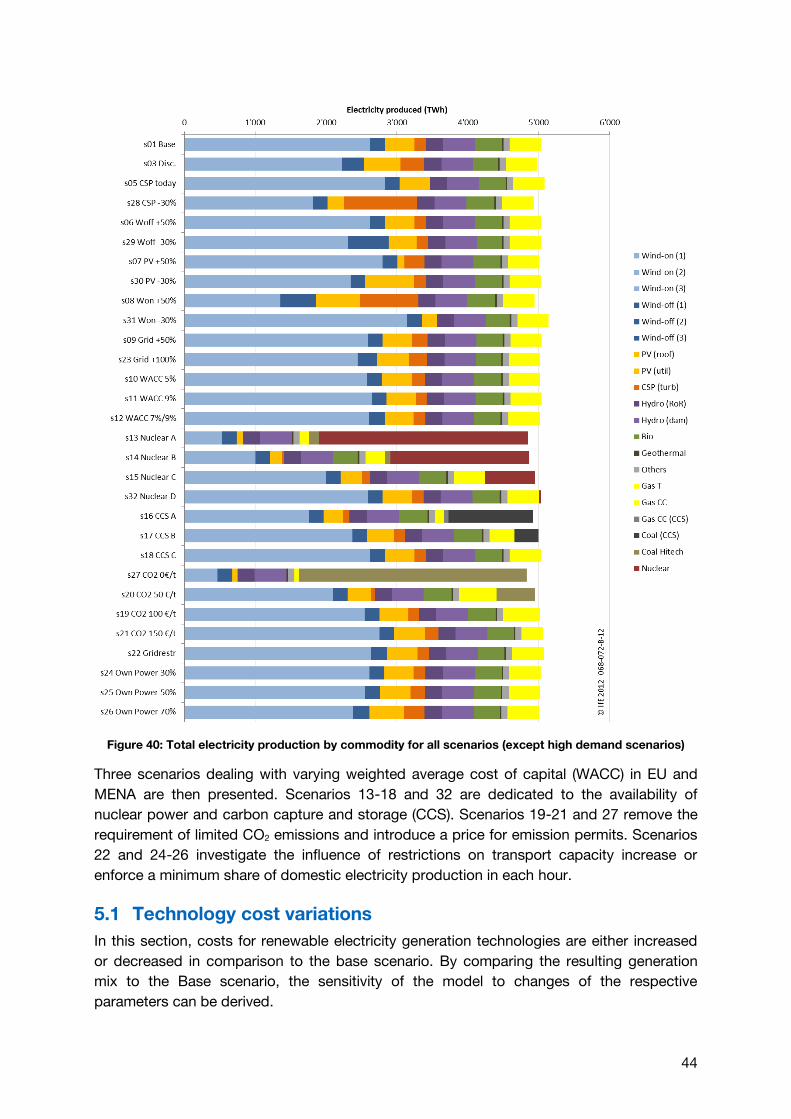
Figure 40 first gives an overview on all scenarios, sorted by scenario groups. After the two

main scenarios 01 and 03 with low demand (s02 and s04 are the corresponding high

demand scenarios), the following ten scenarios are dedicated to changes in costs of

electricity generation and transmission technologies.

44

Figure 40: Total electricity production by commodity for all scenarios (except high demand scenarios)

Three scenarios dealing with varying weighted average cost of capital (WACC) in EU and

MENA are then presented. Scenarios 13-18 and 32 are dedicated to the availability of

nuclear power and carbon capture and storage (CCS). Scenarios 19-21 and 27 remove the

requirement of limited CO2 emissions and introduce a price for emission permits. Scenarios

22 and 24-26 investigate the influence of restrictions on transport capacity increase or

enforce a minimum share of domestic electricity production in each hour.

5.1 Technology cost variations

In this section, costs for renewable electricity generation technologies are either increased

or decreased in comparison to the base scenario. By comparing the resulting generation

mix to the Base scenario, the sensitivity of the model to changes of the respective

parameters can be derived.

45

5.1.1 CSP

In scenario Base, CSP contributes 160 TWh to the total electricity generation of 5035 TWh.

This equals a share of 3.2 %, compared to 8.4 % provided by photovoltaic. However, this

comparison neglects the ability of CSP to balance daily fluctuations, comparable to natural

gas. Table 4 lists investment costs that are changed between scenarios. Fixed operation

costs (€/kW/a) are scaled accordingly.

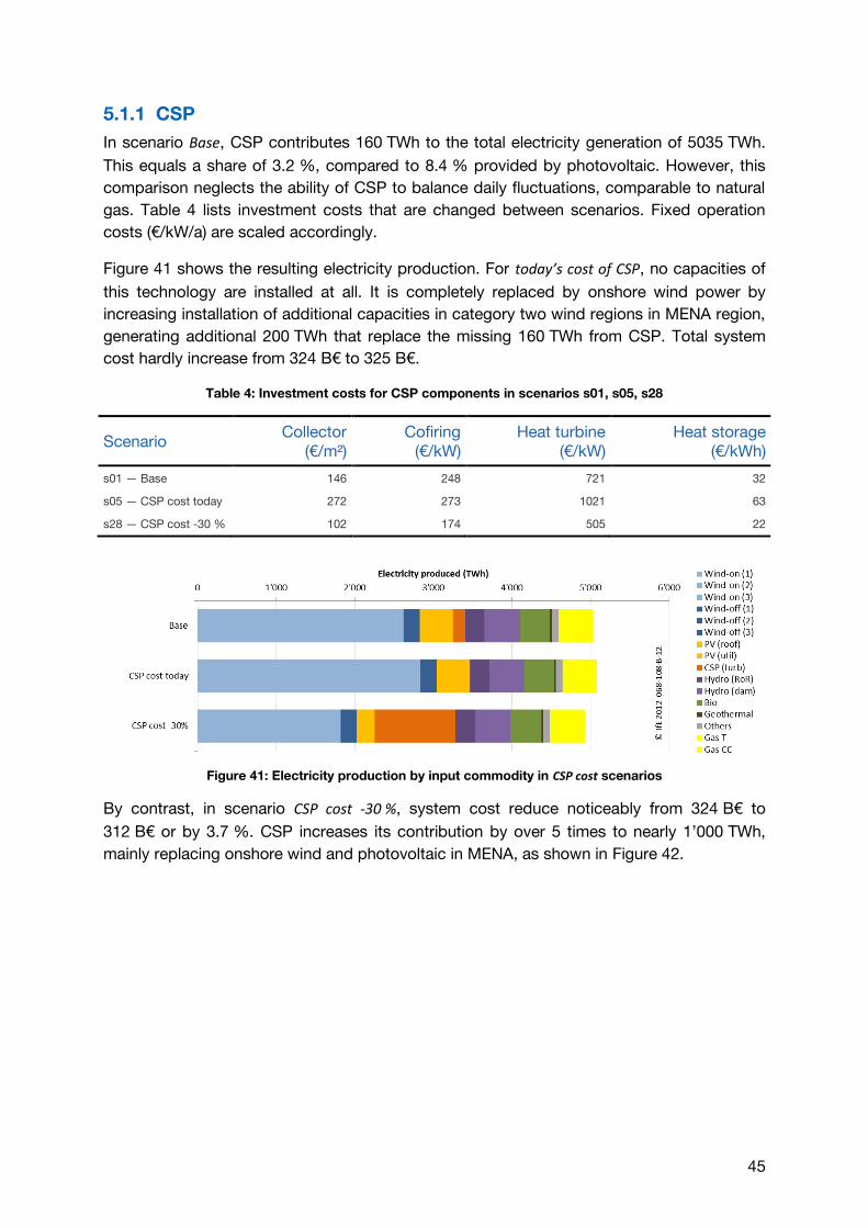
Figure 41 shows the resulting electricity production. For today’s cost of CSP, no capacities of

this technology are installed at all. It is completely replaced by onshore wind power by

increasing installation of additional capacities in category two wind regions in MENA region,

generating additional 200 TWh that replace the missing 160 TWh from CSP. Total system

cost hardly increase from 324 B€ to 325 B€.

Table 4: Investment costs for CSP components in scenarios s01, s05, s28

Scenario Collector

(€/m²) Cofiring

(€/kW) Heat turbine

(€/kW) Heat storage

(€/kWh)

s01 — Base 146 248 721 32

s05 — CSP cost today 272 273 1021 63

s28 — CSP cost -30 % 102 174 505 22

Figure 41: Electricity production by input commodity in CSP cost scenarios

By contrast, in scenario CSP cost -30 %, system cost reduce noticeably from 324 B€ to

312 B€ or by 3.7 %. CSP increases its contribution by over 5 times to nearly 1’000 TWh,

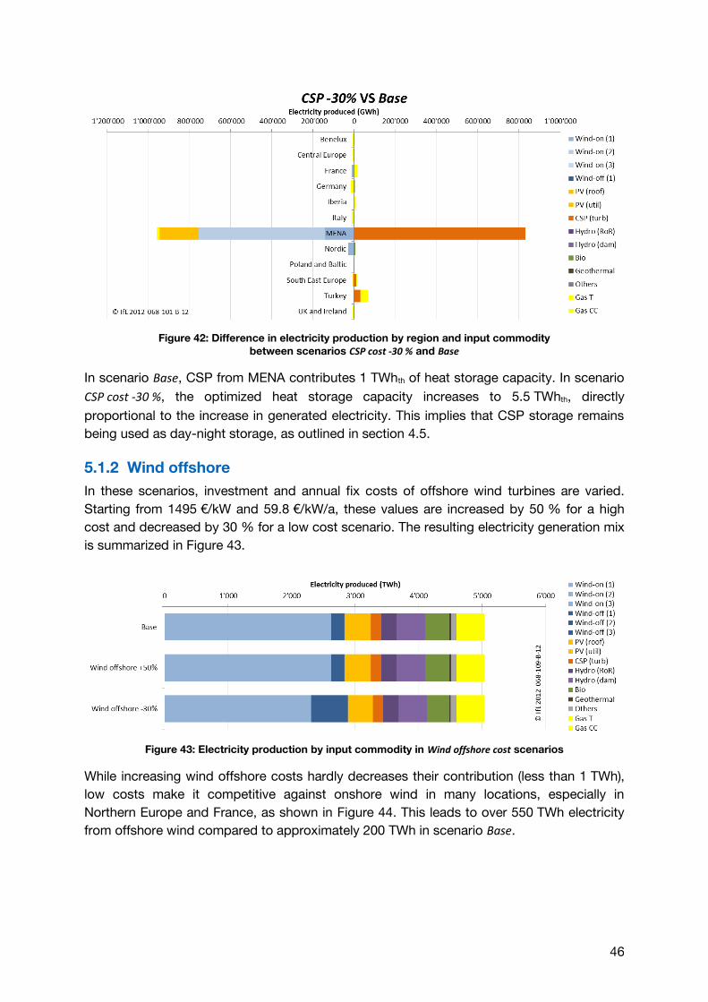
mainly replacing onshore wind and photovoltaic in MENA, as shown in Figure 42.

46

Figure 42: Difference in electricity production by region and input commodity

between scenarios CSP cost -30 % and Base

In scenario Base, CSP from MENA contributes 1 TWhth of heat storage capacity. In scenario

CSP cost -30 %, the optimized heat storage capacity increases to 5.5 TWhth, directly

proportional to the increase in generated electricity. This implies that CSP storage remains

being used as day-night storage, as outlined in section 4.5.

5.1.2 Wind offshore

In these scenarios, investment and annual fix costs of offshore wind turbines are varied.

Starting from 1495 €/kW and 59.8 €/kW/a, these values are increased by 50 % for a high

cost and decreased by 30 % for a low cost scenario. The resulting electricity generation mix

is summarized in Figure 43.

Figure 43: Electricity production by input commodity in Wind offshore cost scenarios

While increasing wind offshore costs hardly decreases their contribution (less than 1 TWh),

low costs make it competitive against onshore wind in many locations, especially in

Northern Europe and France, as shown in Figure 44. This leads to over 550 TWh electricity

from offshore wind compared to approximately 200 TWh in scenario Base.

47

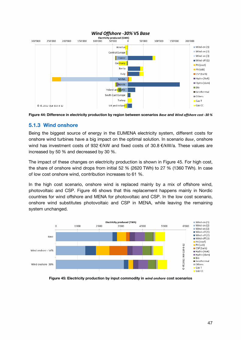
Figure 44: Difference in electricity production by region between scenarios Base and Wind offshore cost -30 %

5.1.3 Wind onshore

Being the biggest source of energy in the EUMENA electricity system, different costs for

onshore wind turbines have a big impact on the optimal solution. In scenario Base, onshore

wind has investment costs of 932 €/kW and fixed costs of 30.8 €/kW/a. These values are

increased by 50 % and decreased by 30 %.

The impact of these changes on electricity production is shown in Figure 45. For high cost,

the share of onshore wind drops from initial 52 % (2620 TWh) to 27 % (1360 TWh). In case

of low cost onshore wind, contribution increases to 61 %.

In the high cost scenario, onshore wind is replaced mainly by a mix of offshore wind,

photovoltaic and CSP. Figure 46 shows that this replacement happens mainly in Nordic

countries for wind offshore and MENA for photovoltaic and CSP. In the low cost scenario,

onshore wind substitutes photovoltaic and CSP in MENA, while leaving the remaining

system unchanged.

Figure 45: Electricity production by input commodity in wind onshore cost scenarios

48

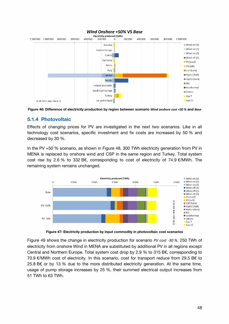
Figure 46: Difference of electricity production by region between scenario Wind onshore cost +50 % and Base

5.1.4 Photovoltaic

Effects of changing prices for PV are investigated in the next two scenarios. Like in all

technology cost scenarios, specific investment and fix costs are increased by 50 % and

decreased by 30 %.

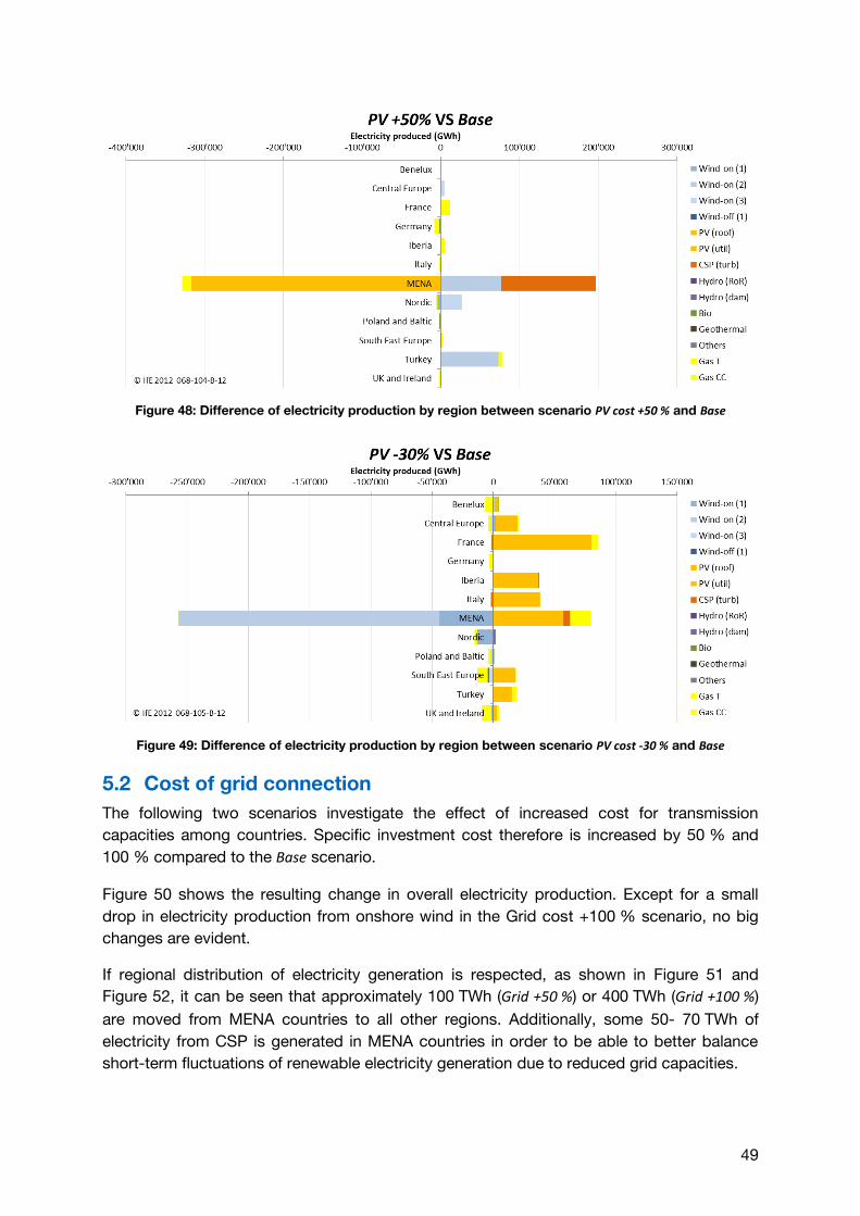
In the PV +50 % scenario, as shown in Figure 48, 300 TWh electricity generation from PV in

MENA is replaced by onshore wind and CSP in the same region and Turkey. Total system

cost rise by 2.6 % to 332 B€, corresponding to cost of electricity of 74.9 €/MWh. The

remaining system remains unchanged.

Figure 47: Electricity production by input commodity in photovoltaic cost scenarios

Figure 49 shows the change in electricity production for scenario PV cost -30 %. 250 TWh of

electricity from onshore Wind in MENA are substituted by additional PV in all regions except

Central and Northern Europe. Total system cost drop by 2.9 % to 315 B€, corresponding to

70.9 €/MWh cost of electricity. In this scenario, cost for transport reduce from 29.5 B€ to

25.8 B€ or by 13 % due to the more distributed electricity generation. At the same time,

usage of pump storage increases by 25 %, their summed electrical output increases from

51 TWh to 63 TWh.

49

Figure 48: Difference of electricity production by region between scenario PV cost +50 % and Base

Figure 49: Difference of electricity production by region between scenario PV cost -30 % and Base

5.2 Cost of grid connection

The following two scenarios investigate the effect of increased cost for transmission

capacities among countries. Specific investment cost therefore is increased by 50 % and

100 % compared to the Base scenario.

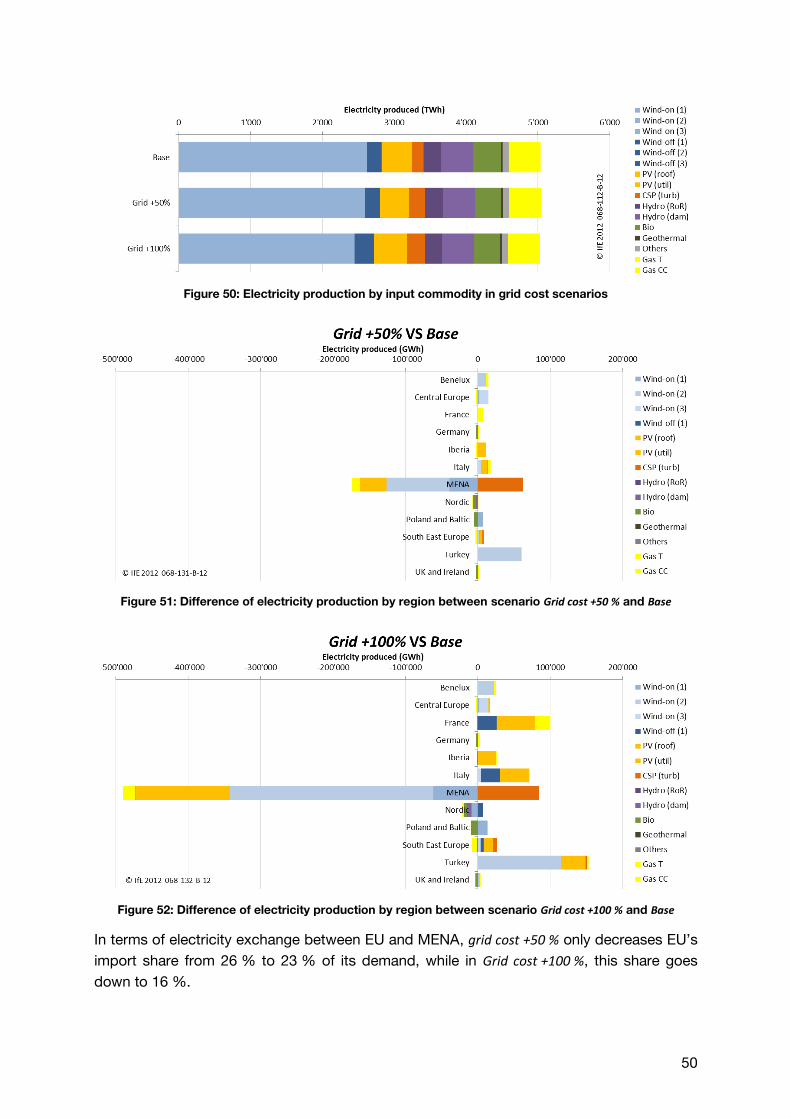
Figure 50 shows the resulting change in overall electricity production. Except for a small

drop in electricity production from onshore wind in the Grid cost +100 % scenario, no big

changes are evident.

If regional distribution of electricity generation is respected, as shown in Figure 51 and

Figure 52, it can be seen that approximately 100 TWh (Grid +50 %) or 400 TWh (Grid +100 %)

are moved from MENA countries to all other regions. Additionally, some 50- 70 TWh of

electricity from CSP is generated in MENA countries in order to be able to better balance

short-term fluctuations of renewable electricity generation due to reduced grid capacities.

50

Figure 50: Electricity production by input commodity in grid cost scenarios

Figure 51: Difference of electricity production by region between scenario Grid cost +50 % and Base

Figure 52: Difference of electricity production by region between scenario Grid cost +100 % and Base

In terms of electricity exchange between EU and MENA, grid cost +50 % only decreases EU’s

import share from 26 % to 23 % of its demand, while in Grid cost +100 %, this share goes

down to 16 %.

51

5.3 WACC variation

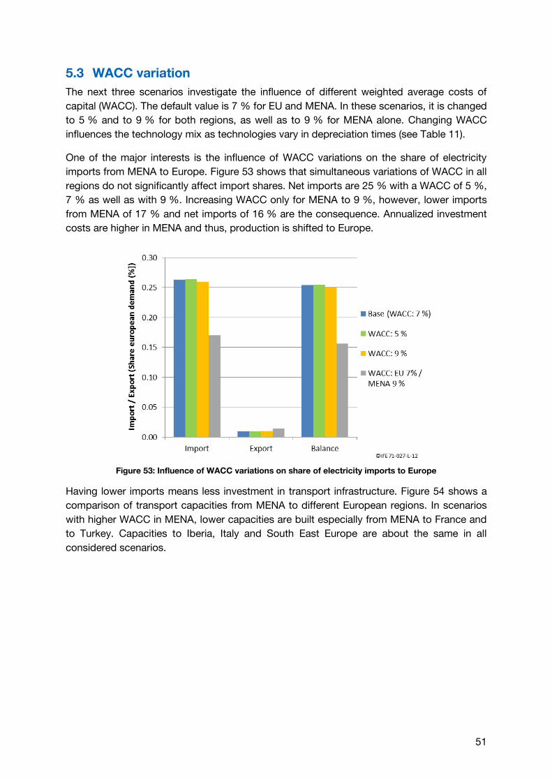
The next three scenarios investigate the influence of different weighted average costs of

capital (WACC). The default value is 7 % for EU and MENA. In these scenarios, it is changed

to 5 % and to 9 % for both regions, as well as to 9 % for MENA alone. Changing WACC

influences the technology mix as technologies vary in depreciation times (see Table 11).

One of the major interests is the influence of WACC variations on the share of electricity

imports from MENA to Europe. Figure 53 shows that simultaneous variations of WACC in all

regions do not significantly affect import shares. Net imports are 25 % with a WACC of 5 %,

7 % as well as with 9 %. Increasing WACC only for MENA to 9 %, however, lower imports

from MENA of 17 % and net imports of 16 % are the consequence. Annualized investment

costs are higher in MENA and thus, production is shifted to Europe.

Figure 53: Influence of WACC variations on share of electricity imports to Europe

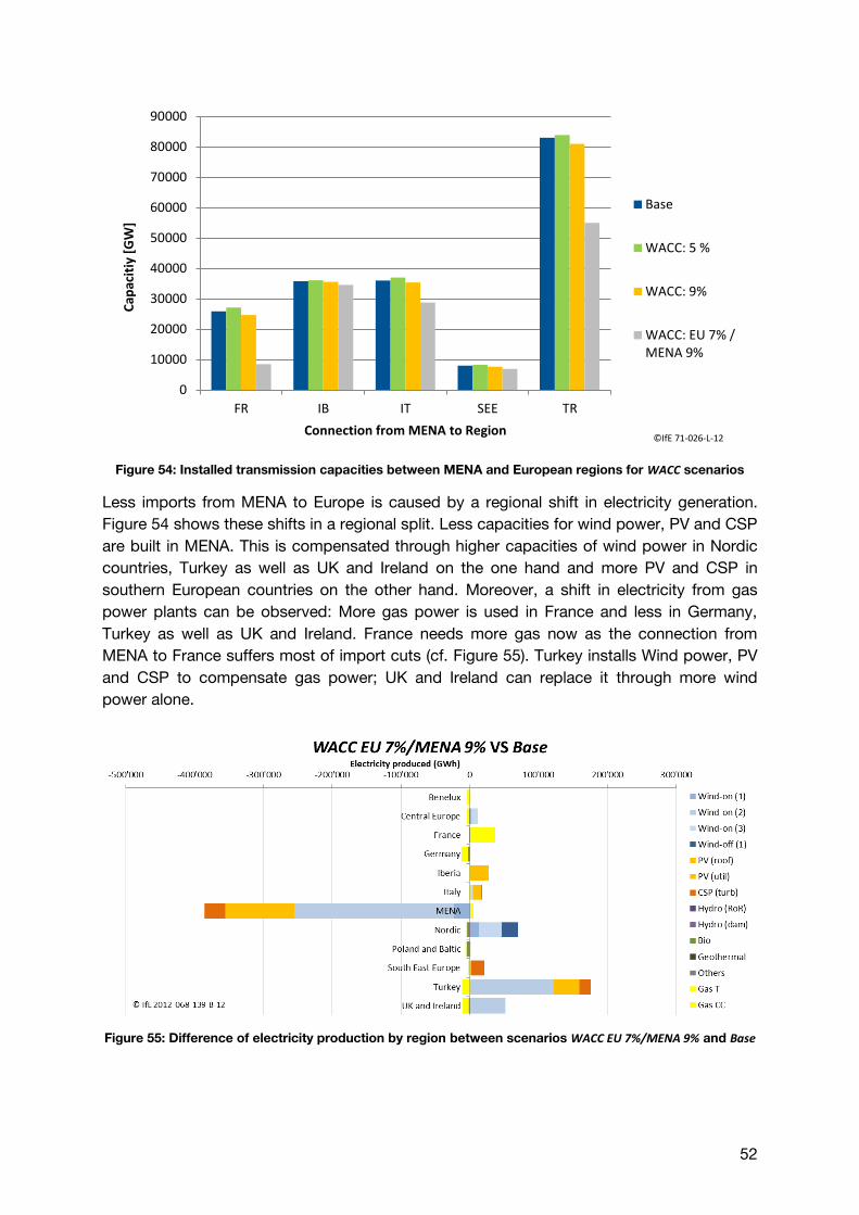
Having lower imports means less investment in transport infrastructure. Figure 54 shows a

comparison of transport capacities from MENA to different European regions. In scenarios

with higher WACC in MENA, lower capacities are built especially from MENA to France and

to Turkey. Capacities to Iberia, Italy and South East Europe are about the same in all

considered scenarios.

52

Figure 54: Installed transmission capacities between MENA and European regions for WACC scenarios

Less imports from MENA to Europe is caused by a regional shift in electricity generation.

Figure 54 shows these shifts in a regional split. Less capacities for wind power, PV and CSP

are built in MENA. This is compensated through higher capacities of wind power in Nordic

countries, Turkey as well as UK and Ireland on the one hand and more PV and CSP in

southern European countries on the other hand. Moreover, a shift in electricity from gas

power plants can be observed: More gas power is used in France and less in Germany,

Turkey as well as UK and Ireland. France needs more gas now as the connection from

MENA to France suffers most of import cuts (cf. Figure 55). Turkey installs Wind power, PV

and CSP to compensate gas power; UK and Ireland can replace it through more wind

power alone.

Figure 55: Difference of electricity production by region between scenarios WACC EU 7%/MENA 9% and Base

0

10000

20000

30000

40000

50000

60000

70000

80000

90000

FR IB IT SEE TR

Cap

acit

iy [

GW

]

Connection from MENA to Region

Base

WACC: 5 %

WACC: 9%

WACC: EU 7% /MENA 9%

©IfE 71-026-L-12

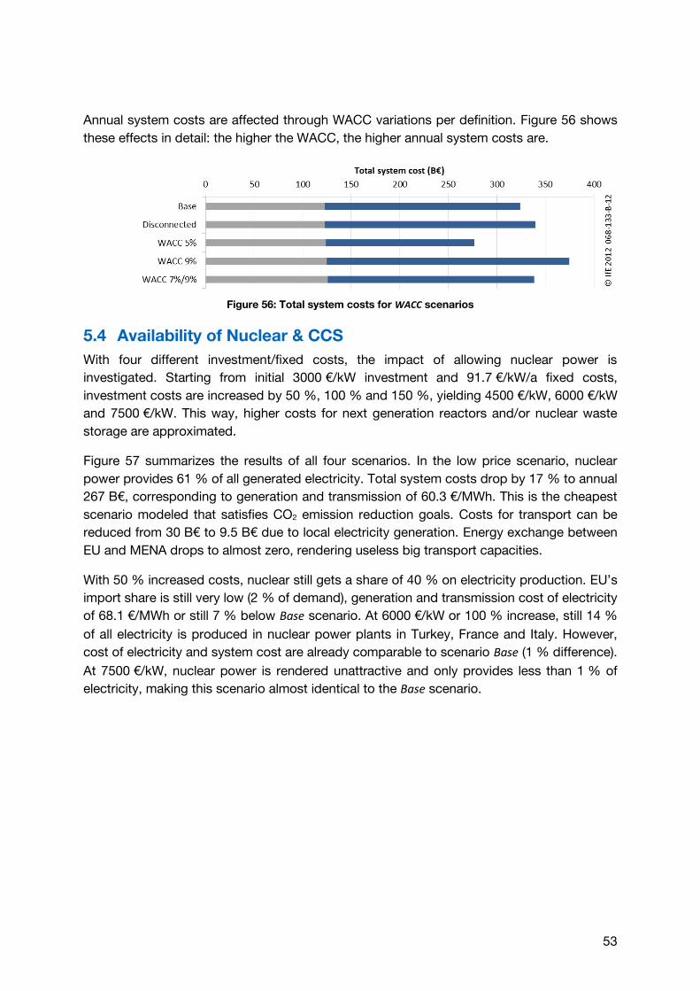
53

Annual system costs are affected through WACC variations per definition. Figure 56 shows

these effects in detail: the higher the WACC, the higher annual system costs are.

Figure 56: Total system costs for WACC scenarios

5.4 Availability of Nuclear & CCS

With four different investment/fixed costs, the impact of allowing nuclear power is

investigated. Starting from initial 3000 €/kW investment and 91.7 €/kW/a fixed costs,

investment costs are increased by 50 %, 100 % and 150 %, yielding 4500 €/kW, 6000 €/kW

and 7500 €/kW. This way, higher costs for next generation reactors and/or nuclear waste

storage are approximated.

Figure 57 summarizes the results of all four scenarios. In the low price scenario, nuclear

power provides 61 % of all generated electricity. Total system costs drop by 17 % to annual

267 B€, corresponding to generation and transmission of 60.3 €/MWh. This is the cheapest

scenario modeled that satisfies CO2 emission reduction goals. Costs for transport can be

reduced from 30 B€ to 9.5 B€ due to local electricity generation. Energy exchange between

EU and MENA drops to almost zero, rendering useless big transport capacities.

With 50 % increased costs, nuclear still gets a share of 40 % on electricity production. EU’s

import share is still very low (2 % of demand), generation and transmission cost of electricity

of 68.1 €/MWh or still 7 % below Base scenario. At 6000 €/kW or 100 % increase, still 14 %

of all electricity is produced in nuclear power plants in Turkey, France and Italy. However,

cost of electricity and system cost are already comparable to scenario Base (1 % difference).

At 7500 €/kW, nuclear power is rendered unattractive and only provides less than 1 % of

electricity, making this scenario almost identical to the Base scenario.

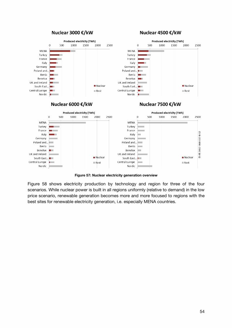
54

Figure 57: Nuclear electricity generation overview

Figure 58 shows electricity production by technology and region for three of the four

scenarios. While nuclear power is built in all regions uniformly (relative to demand) in the low

price scenario, renewable generation becomes more and more focused to regions with the

best sites for renewable electricity generation, i.e. especially MENA countries.

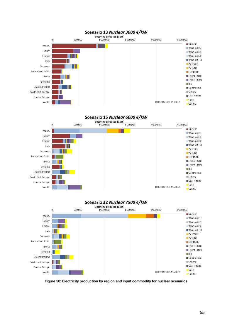
55

Figure 58: Electricity production by region and input commodity for nuclear scenarios

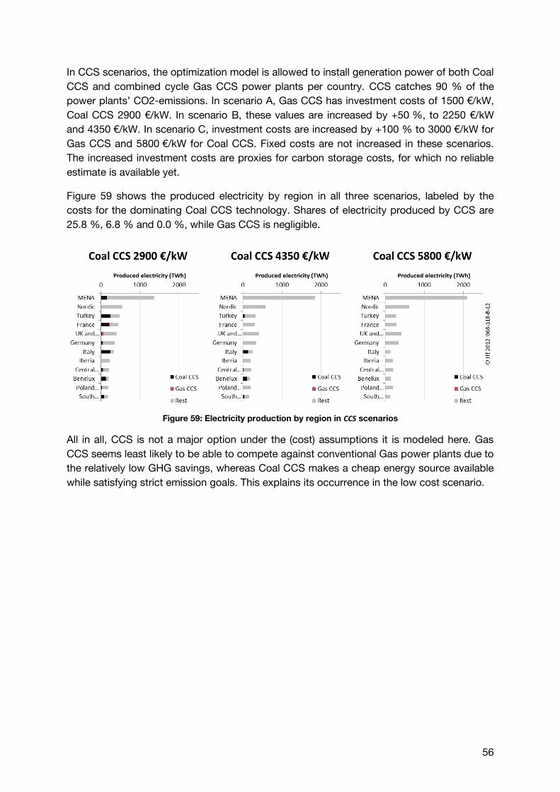
56

In CCS scenarios, the optimization model is allowed to install generation power of both Coal

CCS and combined cycle Gas CCS power plants per country. CCS catches 90 % of the

power plants’ CO2-emissions. In scenario A, Gas CCS has investment costs of 1500 €/kW,

Coal CCS 2900 €/kW. In scenario B, these values are increased by +50 %, to 2250 €/kW

and 4350 €/kW. In scenario C, investment costs are increased by +100 % to 3000 €/kW for

Gas CCS and 5800 €/kW for Coal CCS. Fixed costs are not increased in these scenarios.

The increased investment costs are proxies for carbon storage costs, for which no reliable

estimate is available yet.

Figure 59 shows the produced electricity by region in all three scenarios, labeled by the

costs for the dominating Coal CCS technology. Shares of electricity produced by CCS are

25.8 %, 6.8 % and 0.0 %, while Gas CCS is negligible.

Figure 59: Electricity production by region in CCS scenarios

All in all, CCS is not a major option under the (cost) assumptions it is modeled here. Gas

CCS seems least likely to be able to compete against conventional Gas power plants due to

the relatively low GHG savings, whereas Coal CCS makes a cheap energy source available

while satisfying strict emission goals. This explains its occurrence in the low cost scenario.

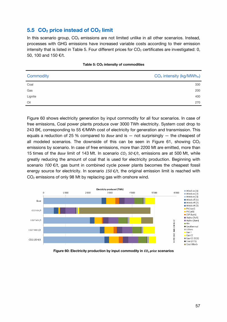
57

5.5 CO2 price instead of CO2 limit

In this scenario group, CO2 emissions are not limited unlike in all other scenarios. Instead,

processes with GHG emissions have increased variable costs according to their emission

intensity that is listed in Table 5. Four different prices for CO2 certificates are investigated: 0,

50, 100 and 150 €/t.

Table 5: CO2 intensity of commodities

Commodity CO2 intensity (kg/MWhth)

Coal 330

Gas 200

Lignite 400

Oil 270

Figure 60 shows electricity generation by input commodity for all four scenarios. In case of

free emissions, Coal power plants produce over 3000 TWh electricity. System cost drop to

243 B€, corresponding to 55 €/MWh cost of electricity for generation and transmission. This

equals a reduction of 25 % compared to Base and is — not surprisingly — the cheapest of

all modeled scenarios. The downside of this can be seen in Figure 61, showing CO2

emissions by scenario. In case of free emissions, more than 2200 Mt are emitted, more than

15 times of the Base limit of 143 Mt. In scenario CO2 50 €/t, emissions are at 500 Mt, while

greatly reducing the amount of coal that is used for electricity production. Beginning with

scenario 100 €/t, gas burnt in combined cycle power plants becomes the cheapest fossil

energy source for electricity. In scenario 150 €/t, the original emission limit is reached with

CO2 emissions of only 98 Mt by replacing gas with onshore wind.

Figure 60: Electricity production by input commodity in CO2 price scenarios

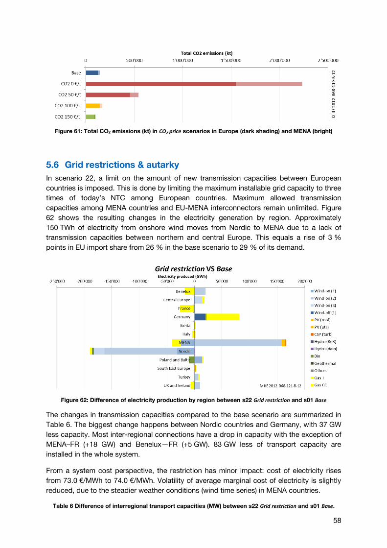
58

Figure 61: Total CO2 emissions (kt) in CO2 price scenarios in Europe (dark shading) and MENA (bright)

5.6 Grid restrictions & autarky

In scenario 22, a limit on the amount of new transmission capacities between European

countries is imposed. This is done by limiting the maximum installable grid capacity to three

times of today’s NTC among European countries. Maximum allowed transmission

capacities among MENA countries and EU-MENA interconnectors remain unlimited. Figure

62 shows the resulting changes in the electricity generation by region. Approximately

150 TWh of electricity from onshore wind moves from Nordic to MENA due to a lack of

transmission capacities between northern and central Europe. This equals a rise of 3 %

points in EU import share from 26 % in the base scenario to 29 % of its demand.

Figure 62: Difference of electricity production by region between s22 Grid restriction and s01 Base

The changes in transmission capacities compared to the base scenario are summarized in

Table 6. The biggest change happens between Nordic countries and Germany, with 37 GW

less capacity. Most inter-regional connections have a drop in capacity with the exception of

MENA–FR (+18 GW) and Benelux—FR (+5 GW). 83 GW less of transport capacity are

installed in the whole system.

From a system cost perspective, the restriction has minor impact: cost of electricity rises

from 73.0 €/MWh to 74.0 €/MWh. Volatility of average marginal cost of electricity is slightly

reduced, due to the steadier weather conditions (wind time series) in MENA countries.

Table 6 Difference of interregional transport capacities (MW) between s22 Grid restriction and s01 Base.

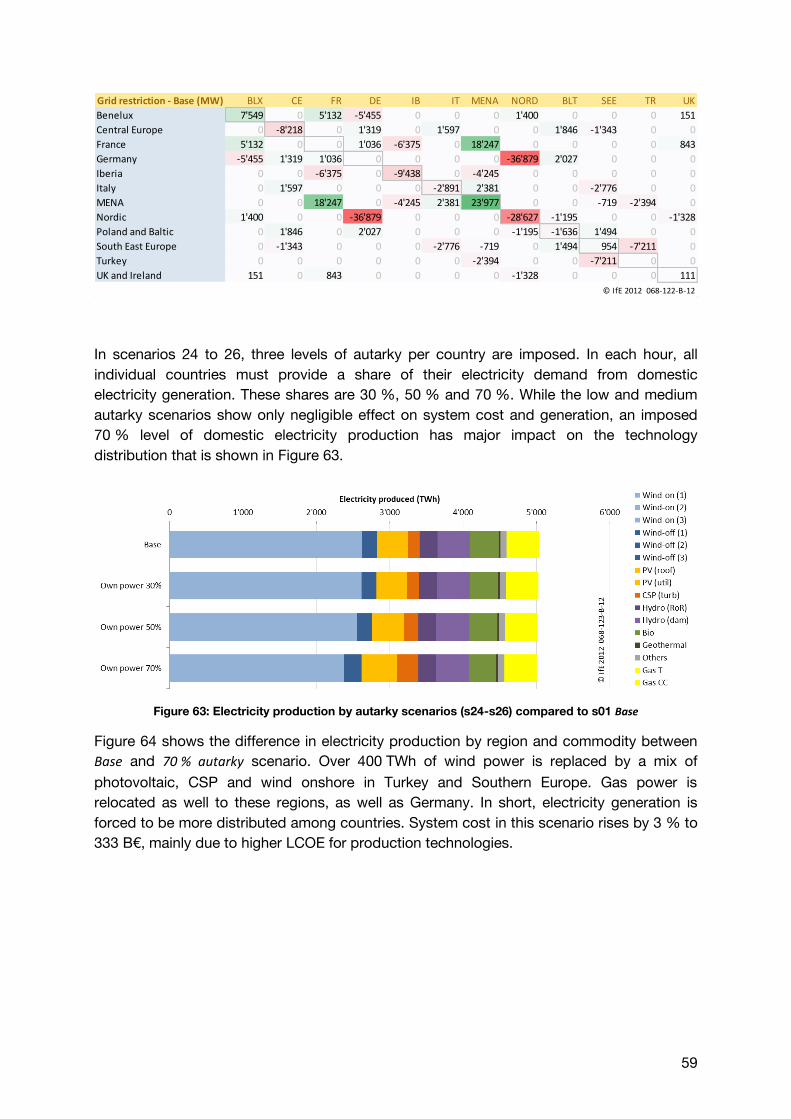
59

In scenarios 24 to 26, three levels of autarky per country are imposed. In each hour, all

individual countries must provide a share of their electricity demand from domestic

electricity generation. These shares are 30 %, 50 % and 70 %. While the low and medium

autarky scenarios show only negligible effect on system cost and generation, an imposed

70 % level of domestic electricity production has major impact on the technology

distribution that is shown in Figure 63.

Figure 63: Electricity production by autarky scenarios (s24-s26) compared to s01 Base

Figure 64 shows the difference in electricity production by region and commodity between

Base and 70 % autarky scenario. Over 400 TWh of wind power is replaced by a mix of

photovoltaic, CSP and wind onshore in Turkey and Southern Europe. Gas power is

relocated as well to these regions, as well as Germany. In short, electricity generation is

forced to be more distributed among countries. System cost in this scenario rises by 3 % to

333 B€, mainly due to higher LCOE for production technologies.

Grid restriction - Base (MW) BLX CE FR DE IB IT MENA NORD BLT SEE TR UK

Benelux 7'549 0 5'132 -5'455 0 0 0 1'400 0 0 0 151

Central Europe 0 -8'218 0 1'319 0 1'597 0 0 1'846 -1'343 0 0

France 5'132 0 0 1'036 -6'375 0 18'247 0 0 0 0 843

Germany -5'455 1'319 1'036 0 0 0 0 -36'879 2'027 0 0 0

Iberia 0 0 -6'375 0 -9'438 0 -4'245 0 0 0 0 0

Italy 0 1'597 0 0 0 -2'891 2'381 0 0 -2'776 0 0

MENA 0 0 18'247 0 -4'245 2'381 23'977 0 0 -719 -2'394 0

Nordic 1'400 0 0 -36'879 0 0 0 -28'627 -1'195 0 0 -1'328

Poland and Baltic 0 1'846 0 2'027 0 0 0 -1'195 -1'636 1'494 0 0

South East Europe 0 -1'343 0 0 0 -2'776 -719 0 1'494 954 -7'211 0

Turkey 0 0 0 0 0 0 -2'394 0 0 -7'211 0 0

UK and Ireland 151 0 843 0 0 0 0 -1'328 0 0 0 111

© IfE 2012 068-122-B-12

60

Figure 64: Difference of electricity production by region between s26 Own power 70% and s01 Base

In terms of energy exchange between EU and MENA countries, the 70 % autarky scenario

has major impact: EU import share drops from 26 % to 14 % of its electricity demand.

Crucial for reaching the 70 % requirement is the use of existing pump storage capacities.

The total electrical output of pump storage is 126 TWh which is more than twice as much as

in the Base scenario (51 TWh). CSP heat storage fulfills the same purpose in MENA

countries.

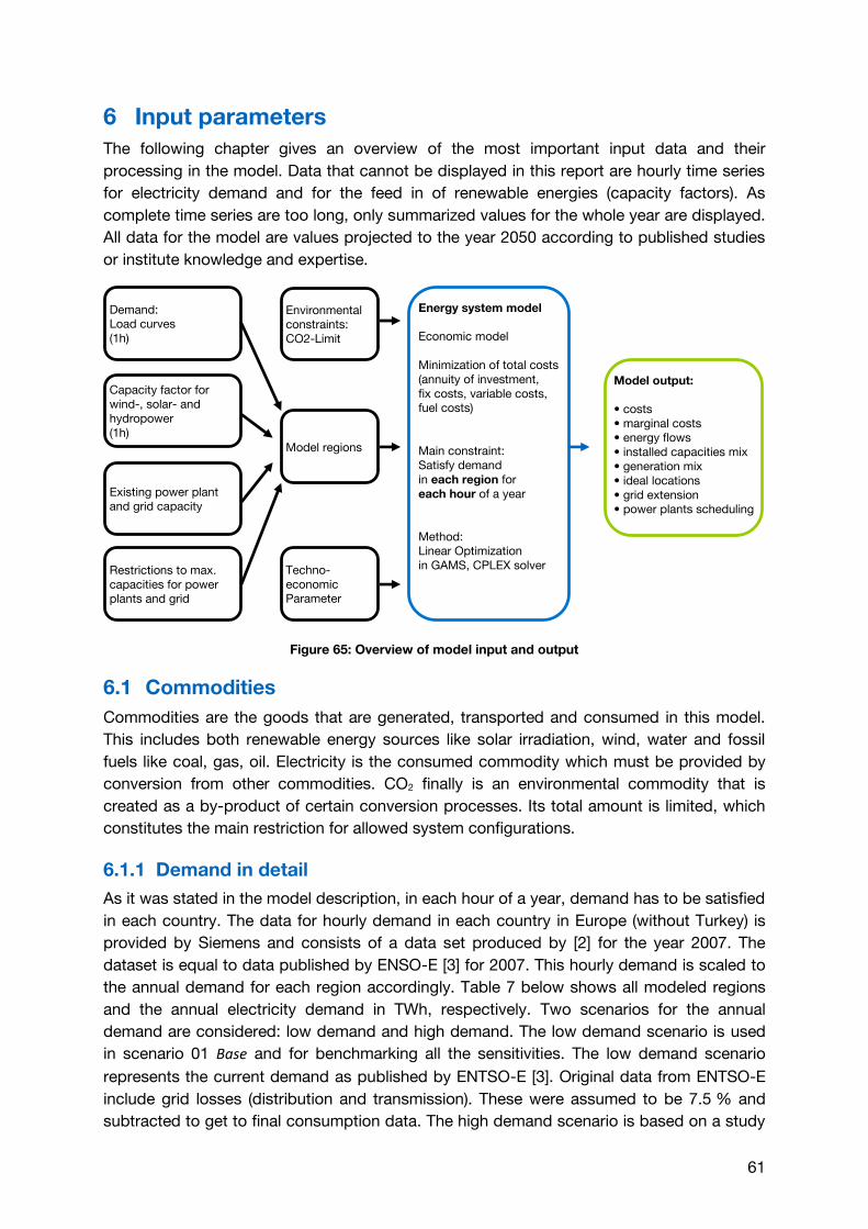
61

6 Input parameters

The following chapter gives an overview of the most important input data and their

processing in the model. Data that cannot be displayed in this report are hourly time series

for electricity demand and for the feed in of renewable energies (capacity factors). As

complete time series are too long, only summarized values for the whole year are displayed.

All data for the model are values projected to the year 2050 according to published studies

or institute knowledge and expertise.

Figure 65: Overview of model input and output

6.1 Commodities

Commodities are the goods that are generated, transported and consumed in this model.

This includes both renewable energy sources like solar irradiation, wind, water and fossil

fuels like coal, gas, oil. Electricity is the consumed commodity which must be provided by

conversion from other commodities. CO2 finally is an environmental commodity that is

created as a by-product of certain conversion processes. Its total amount is limited, which

constitutes the main restriction for allowed system configurations.

6.1.1 Demand in detail

As it was stated in the model description, in each hour of a year, demand has to be satisfied

in each country. The data for hourly demand in each country in Europe (without Turkey) is

provided by Siemens and consists of a data set produced by [2] for the year 2007. The

dataset is equal to data published by ENSO-E [3] for 2007. This hourly demand is scaled to

the annual demand for each region accordingly. Table 7 below shows all modeled regions

and the annual electricity demand in TWh, respectively. Two scenarios for the annual

demand are considered: low demand and high demand. The low demand scenario is used

in scenario 01 Base and for benchmarking all the sensitivities. The low demand scenario

represents the current demand as published by ENTSO-E [3]. Original data from ENTSO-E

include grid losses (distribution and transmission). These were assumed to be 7.5 % and

subtracted to get to final consumption data. The high demand scenario is based on a study

Techno-economicParameter

Demand:Load curves(1h)

Capacity factor for wind-, solar- and hydropower(1h)

Existing power plant and grid capacity

Restrictions to max. capacities for powerplants and grid

Energy system model

Economic model

Minimization of total costs(annuity of investment, fix costs, variable costs, fuel costs)

Main constraint:Satisfy demand in each region for each hour of a year

Method: Linear Optimization in GAMS, CPLEX solver

Model regions

Environmentalconstraints: CO2-Limit

Model output:

• costs• marginal costs• energy flows• installed capacities mix• generation mix• ideal locations• grid extension• power plants scheduling

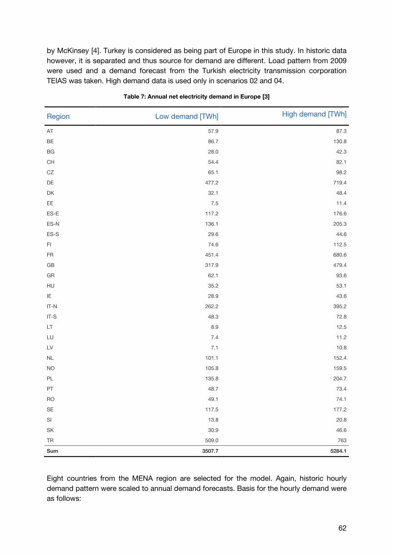
62

by McKinsey [4]. Turkey is considered as being part of Europe in this study. In historic data

however, it is separated and thus source for demand are different. Load pattern from 2009

were used and a demand forecast from the Turkish electricity transmission corporation

TEIAS was taken. High demand data is used only in scenarios 02 and 04.

Table 7: Annual net electricity demand in Europe [3]

Region Low demand [TWh] High demand [TWh]

AT 57.9 87.3

BE 86.7 130.8

BG 28.0 42.3

CH 54.4 82.1

CZ 65.1 98.2

DE 477.2 719.4

DK 32.1 48.4

EE 7.5 11.4

ES-E 117.2 176.6

ES-N 136.1 205.3

ES-S 29.6 44.6

FI 74.6 112.5

FR 451.4 680.6

GB 317.9 479.4

GR 62.1 93.6

HU 35.2 53.1

IE 28.9 43.6

IT-N 262.2 395.2

IT-S 48.3 72.8

LT 8.9 12.5

LU 7.4 11.2

LV 7.1 10.8

NL 101.1 152.4

NO 105.8 159.5

PL 135.8 204.7

PT 48.7 73.4

RO 49.1 74.1

SE 117.5 177.2

SI 13.8 20.8

SK 30.9 46.6

TR 509.0 763

Sum 3507.7 5284.1

Eight countries from the MENA region are selected for the model. Again, historic hourly

demand pattern were scaled to annual demand forecasts. Basis for the hourly demand were

as follows:

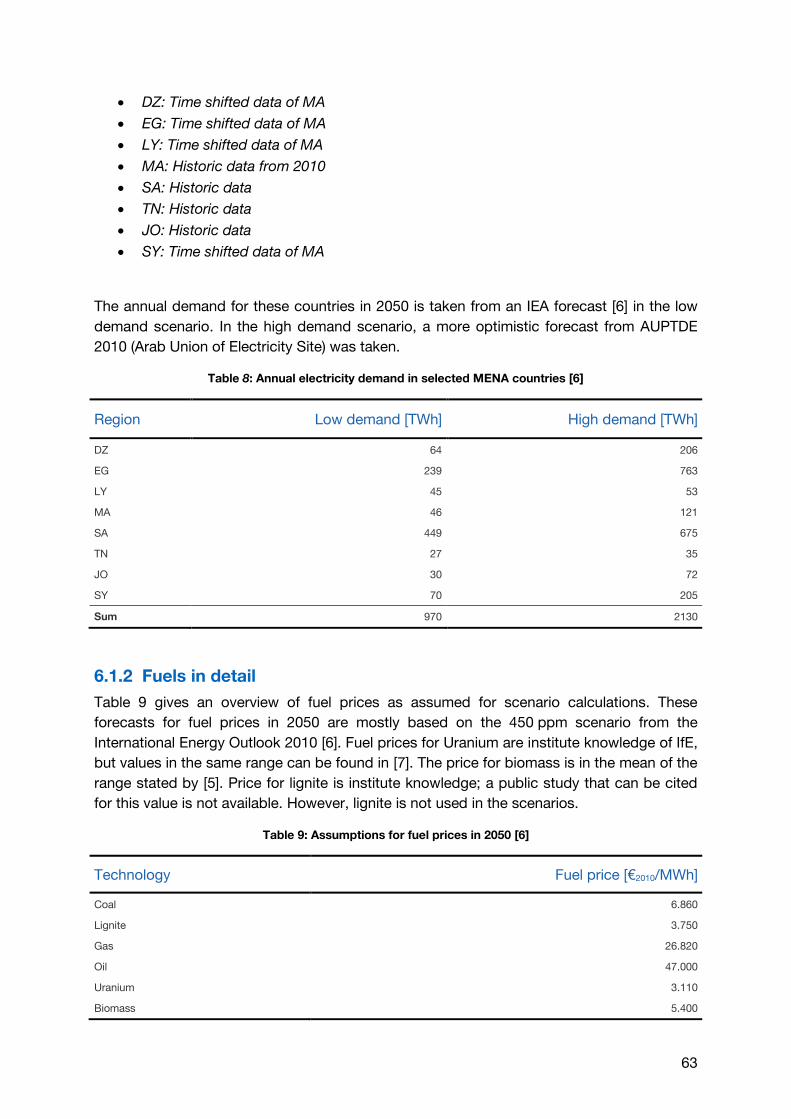
63

DZ: Time shifted data of MA

EG: Time shifted data of MA

LY: Time shifted data of MA

MA: Historic data from 2010

SA: Historic data

TN: Historic data

JO: Historic data

SY: Time shifted data of MA

The annual demand for these countries in 2050 is taken from an IEA forecast [6] in the low

demand scenario. In the high demand scenario, a more optimistic forecast from AUPTDE

2010 (Arab Union of Electricity Site) was taken.

Table 8: Annual electricity demand in selected MENA countries [6]

Region Low demand [TWh] High demand [TWh]

DZ 64 206

EG 239 763

LY 45 53

MA 46 121

SA 449 675

TN 27 35

JO 30 72

SY 70 205

Sum 970 2130

6.1.2 Fuels in detail

Table 9 gives an overview of fuel prices as assumed for scenario calculations. These

forecasts for fuel prices in 2050 are mostly based on the 450 ppm scenario from the

International Energy Outlook 2010 [6]. Fuel prices for Uranium are institute knowledge of IfE,

but values in the same range can be found in [7]. The price for biomass is in the mean of the

range stated by [5]. Price for lignite is institute knowledge; a public study that can be cited

for this value is not available. However, lignite is not used in the scenarios.

Table 9: Assumptions for fuel prices in 2050 [6]

Technology Fuel price [€2010/MWh]

Coal 6.860

Lignite 3.750

Gas 26.820

Oil 47.000

Uranium 3.110

Biomass 5.400

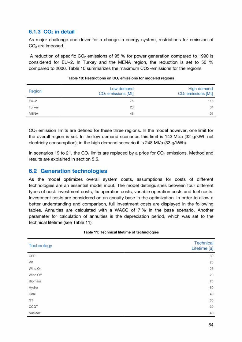
64

6.1.3 CO2 in detail

As major challenge and driver for a change in energy system, restrictions for emission of

CO2 are imposed.

A reduction of specific CO2 emissions of 95 % for power generation compared to 1990 is

considered for EU+2. In Turkey and the MENA region, the reduction is set to 50 %

compared to 2000. Table 10 summarizes the maximum CO2-emissions for the regions

Table 10: Restrictions on CO2 emissions for modeled regions

Region Low demand

CO2 emissions [Mt] High demand

CO2 emissions [Mt]

EU+2 75 113

Turkey 23 34

MENA 46 101

CO2 emission limits are defined for these three regions. In the model however, one limit for

the overall region is set. In the low demand scenarios this limit is 143 Mt/a (32 g/kWh net

electricity consumption); in the high demand scenario it is 248 Mt/a (33 g/kWh).

In scenarios 19 to 21, the CO2 limits are replaced by a price for CO2 emissions. Method and

results are explained in section 5.5.

6.2 Generation technologies

As the model optimizes overall system costs, assumptions for costs of different

technologies are an essential model input. The model distinguishes between four different

types of cost: investment costs, fix operation costs, variable operation costs and fuel costs.

Investment costs are considered on an annuity base in the optimization. In order to allow a

better understanding and comparison, full Investment costs are displayed in the following

tables. Annuities are calculated with a WACC of 7 % in the base scenario. Another

parameter for calculation of annuities is the depreciation period, which was set to the

technical lifetime (see Table 11).

Table 11: Technical lifetime of technologies

Technology Technical

Lifetime [a]

CSP 30

PV 25

Wind On 25

Wind Off 20

Biomass 25

Hydro 50

Coal 40

GT 30

CCGT 30

Nuclear 40

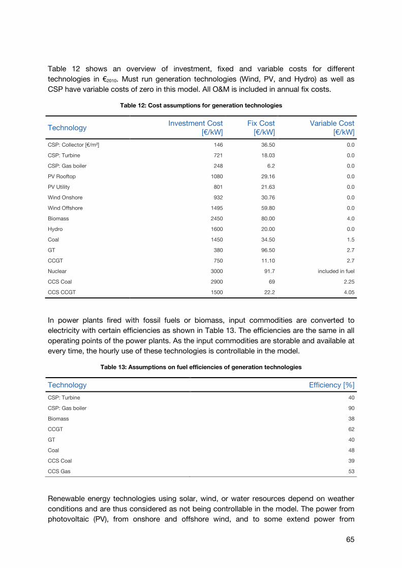
65

Table 12 shows an overview of investment, fixed and variable costs for different

technologies in €2010. Must run generation technologies (Wind, PV, and Hydro) as well as

CSP have variable costs of zero in this model. All O&M is included in annual fix costs.

Table 12: Cost assumptions for generation technologies

Technology Investment Cost

[€/kW] Fix Cost

[€/kW] Variable Cost

[€/kW]

CSP: Collector [€/m²] 146 36.50 0.0

CSP: Turbine 721 18.03 0.0

CSP: Gas boiler 248 6.2 0.0

PV Rooftop 1080 29.16 0.0

PV Utility 801 21.63 0.0

Wind Onshore 932 30.76 0.0

Wind Offshore 1495 59.80 0.0

Biomass 2450 80.00 4.0

Hydro 1600 20.00 0.0

Coal 1450 34.50 1.5

GT 380 96.50 2.7

CCGT 750 11.10 2.7

Nuclear 3000 91.7 included in fuel

CCS Coal 2900 69 2.25

CCS CCGT 1500 22.2 4.05

In power plants fired with fossil fuels or biomass, input commodities are converted to

electricity with certain efficiencies as shown in Table 13. The efficiencies are the same in all

operating points of the power plants. As the input commodities are storable and available at

every time, the hourly use of these technologies is controllable in the model.

Table 13: Assumptions on fuel efficiencies of generation technologies

Technology Efficiency [%]

CSP: Turbine 40

CSP: Gas boiler 90

Biomass 38

CCGT 62

GT 40

Coal 48

CCS Coal 39

CCS Gas 53

Renewable energy technologies using solar, wind, or water resources depend on weather

conditions and are thus considered as not being controllable in the model. The power from

photovoltaic (PV), from onshore and offshore wind, and to some extend power from

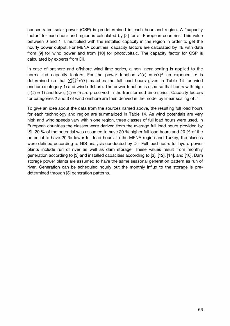
66

concentrated solar power (CSP) is predetermined in each hour and region. A “capacity

factor” for each hour and region is calculated by [2] for all European countries. This value

between 0 and 1 is multiplied with the installed capacity in the region in order to get the

hourly power output. For MENA countries, capacity factors are calculated by IfE with data

from [9] for wind power and from [10] for photovoltaic. The capacity factor for CSP is

calculated by experts from Dii.

In case of onshore and offshore wind time series, a non-linear scaling is applied to the

normalized capacity factors. For the power function an exponent is

determined so that ∑ matches the full load hours given in Table 14 for wind

onshore (category 1) and wind offshore. The power function is used so that hours with high

( ) and low ( ) are preserved in the transformed time series. Capacity factors

for categories 2 and 3 of wind onshore are then derived in the model by linear scaling of .

To give an idea about the data from the sources named above, the resulting full load hours

for each technology and region are summarized in Table 14. As wind potentials are very

high and wind speeds vary within one region, three classes of full load hours were used. In

European countries the classes were derived from the average full load hours provided by

ISI. 20 % of the potential was assumed to have 20 % higher full load hours and 20 % of the

potential to have 20 % lower full load hours. In the MENA region and Turkey, the classes

were defined according to GIS analysis conducted by Dii. Full load hours for hydro power

plants include run of river as well as dam storage. These values result from monthly

generation according to [3] and installed capacities according to [3], [12], [14], and [16]. Dam

storage power plants are assumed to have the same seasonal generation pattern as run of

river. Generation can be scheduled hourly but the monthly influx to the storage is pre-

determined through [3] generation patterns.

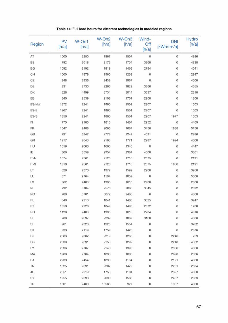
67

Table 14: Full load hours for different technologies in modeled regions

Region PV

[h/a] W-On1

[h/a]

W-On2 [h/a]

W-On3 [h/a]

Wind-Off

[h/a]

DNI [kWh/m2/a]

Hydro [h/a]

AT 1000 2250 1867 1507 0 0 4886

BE 792 2618 2173 1754 3260 0 4838

BG 1092 2192 1819 1468 2784 0 4041

CH 1000 1879 1560 1259 0 0 2947

CZ 848 2936 2439 1967 0 0 4000

DE 831 2730 2266 1829 3366 0 4055

DK 828 4499 3734 3014 3637 0 2818

EE 840 2539 2108 1701 2900 0 1800

ES-NW 1372 2241 1860 1501 2907 0 1503

ES-E 1267 2241 1860 1501 2907 0 1503

ES-S 1356 2241 1860 1501 2907 1977 1503

FI 775 2185 1813 1464 2952 0 4469

FR 1047 2488 2065 1667 3456 1838 5150

GB 791 3347 2778 2242 4021 0 2986

GR 1217 2643 2193 1771 2987 1924 4000

HU 1019 2000 1660 1340 0 0 4447

IE 809 3559 2954 2384 4000 0 3361

IT-N 1074 2561 2125 1716 2575 0 2191

IT-S 1310 2561 2125 1716 2575 1850 2191

LT 828 2376 1972 1592 2900 0 3268

LU 871 2764 1194 1852 0 0 5000

LV 862 2403 1995 1610 2900 0 2300

NL 792 3104 2576 2080 3345 0 2622

NO 786 3701 3072 2480 0 0 4000

PL 848 2218 1841 1486 3325 0 3947

PT 1350 2228 1849 1493 2872 0 1280

RO 1126 2403 1995 1610 2784 0 4816

SE 786 2697 2239 1807 3168 0 4000

SI 981 2320 1925 1554 0 0 3782

SK 933 2119 1759 1420 0 0 2676

DZ 2083 2882 2219 1265 0 2246 759

EG 2339 2691 2153 1292 0 2248 4302

LY 2036 2787 2146 1395 0 2330 4000

MA 1988 2784 1893 1003 0 2698 2636

SA 2239 2454 1890 1134 0 2121 4000

TN 1625 2691 2207 1479 0 2231 2584

JO 2051 2219 1753 1104 0 2397 4000

SY 1955 2090 2090 1588 0 2487 2083

TR 1501 2480 16586 927 0 1907 4000

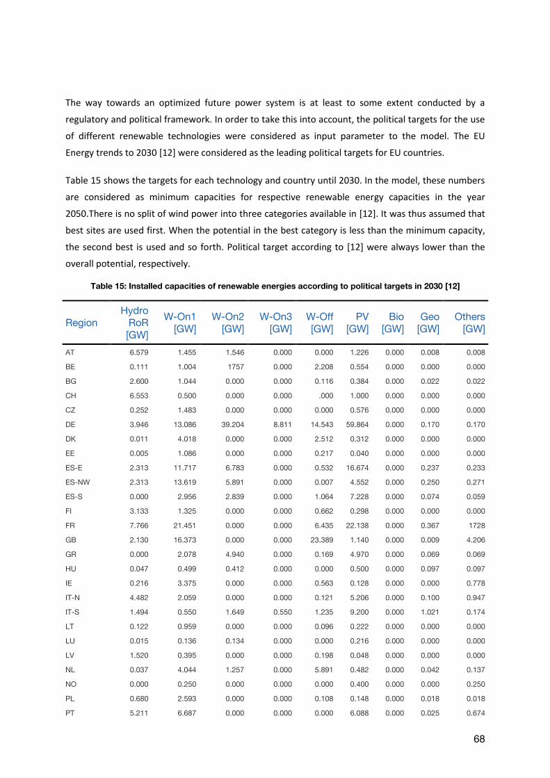
68

The way towards an optimized future power system is at least to some extent conducted by a

regulatory and political framework. In order to take this into account, the political targets for the use

of different renewable technologies were considered as input parameter to the model. The EU

Energy trends to 2030 [12] were considered as the leading political targets for EU countries.

Table 15 shows the targets for each technology and country until 2030. In the model, these numbers

are considered as minimum capacities for respective renewable energy capacities in the year

2050.There is no split of wind power into three categories available in [12]. It was thus assumed that

best sites are used first. When the potential in the best category is less than the minimum capacity,

the second best is used and so forth. Political target according to [12] were always lower than the

overall potential, respectively.

Table 15: Installed capacities of renewable energies according to political targets in 2030 [12]

Region Hydro

RoR [GW]

W-On1 [GW]

W-On2 [GW]

W-On3 [GW]

W-Off [GW]

PV [GW]

Bio [GW]

Geo [GW]

Others [GW]

AT 6.579 1.455 1.546 0.000 0.000 1.226 0.000 0.008 0.008

BE 0.111 1.004 1757 0.000 2.208 0.554 0.000 0.000 0.000

BG 2.600 1.044 0.000 0.000 0.116 0.384 0.000 0.022 0.022

CH 6.553 0.500 0.000 0.000 .000 1.000 0.000 0.000 0.000

CZ 0.252 1.483 0.000 0.000 0.000 0.576 0.000 0.000 0.000

DE 3.946 13.086 39.204 8.811 14.543 59.864 0.000 0.170 0.170

DK 0.011 4.018 0.000 0.000 2.512 0.312 0.000 0.000 0.000

EE 0.005 1.086 0.000 0.000 0.217 0.040 0.000 0.000 0.000

ES-E 2.313 11.717 6.783 0.000 0.532 16.674 0.000 0.237 0.233

ES-NW 2.313 13.619 5.891 0.000 0.007 4.552 0.000 0.250 0.271

ES-S 0.000 2.956 2.839 0.000 1.064 7.228 0.000 0.074 0.059

FI 3.133 1.325 0.000 0.000 0.662 0.298 0.000 0.000 0.000

FR 7.766 21.451 0.000 0.000 6.435 22.138 0.000 0.367 1728

GB 2.130 16.373 0.000 0.000 23.389 1.140 0.000 0.009 4.206

GR 0.000 2.078 4.940 0.000 0.169 4.970 0.000 0.069 0.069

HU 0.047 0.499 0.412 0.000 0.000 0.500 0.000 0.097 0.097

IE 0.216 3.375 0.000 0.000 0.563 0.128 0.000 0.000 0.778

IT-N 4.482 2.059 0.000 0.000 0.121 5.206 0.000 0.100 0.947

IT-S 1.494 0.550 1.649 0.550 1.235 9.200 0.000 1.021 0.174

LT 0.122 0.959 0.000 0.000 0.096 0.222 0.000 0.000 0.000

LU 0.015 0.136 0.134 0.000 0.000 0.216 0.000 0.000 0.000

LV 1.520 0.395 0.000 0.000 0.198 0.048 0.000 0.000 0.000

NL 0.037 4.044 1.257 0.000 5.891 0.482 0.000 0.042 0.137

NO 0.000 0.250 0.000 0.000 0.000 0.400 0.000 0.000 0.250

PL 0.680 2.593 0.000 0.000 0.108 0.148 0.000 0.018 0.018

PT 5.211 6.687 0.000 0.000 0.000 6.088 0.000 0.025 0.674

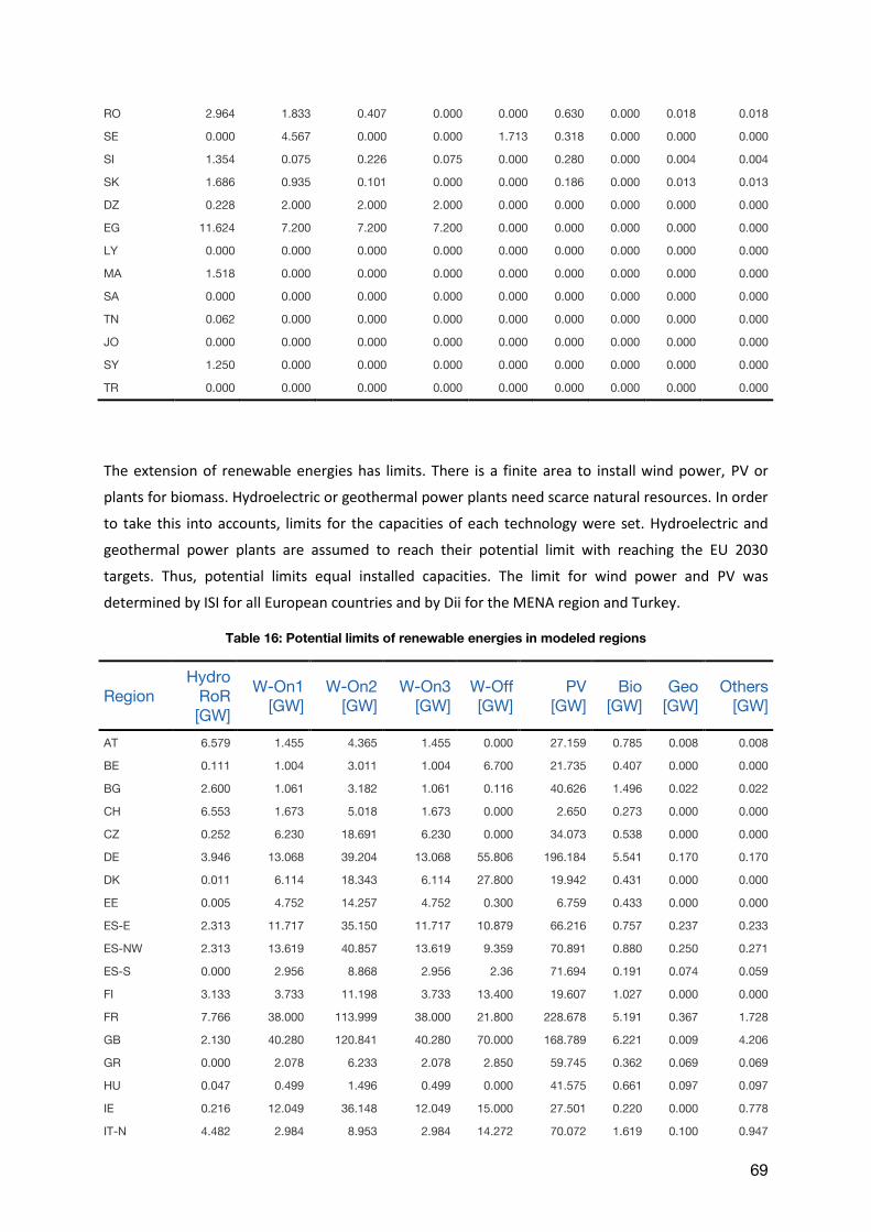
69

RO 2.964 1.833 0.407 0.000 0.000 0.630 0.000 0.018 0.018

SE 0.000 4.567 0.000 0.000 1.713 0.318 0.000 0.000 0.000

SI 1.354 0.075 0.226 0.075 0.000 0.280 0.000 0.004 0.004

SK 1.686 0.935 0.101 0.000 0.000 0.186 0.000 0.013 0.013

DZ 0.228 2.000 2.000 2.000 0.000 0.000 0.000 0.000 0.000

EG 11.624 7.200 7.200 7.200 0.000 0.000 0.000 0.000 0.000

LY 0.000 0.000 0.000 0.000 0.000 0.000 0.000 0.000 0.000

MA 1.518 0.000 0.000 0.000 0.000 0.000 0.000 0.000 0.000

SA 0.000 0.000 0.000 0.000 0.000 0.000 0.000 0.000 0.000

TN 0.062 0.000 0.000 0.000 0.000 0.000 0.000 0.000 0.000

JO 0.000 0.000 0.000 0.000 0.000 0.000 0.000 0.000 0.000

SY 1.250 0.000 0.000 0.000 0.000 0.000 0.000 0.000 0.000

TR 0.000 0.000 0.000 0.000 0.000 0.000 0.000 0.000 0.000

The extension of renewable energies has limits. There is a finite area to install wind power, PV or

plants for biomass. Hydroelectric or geothermal power plants need scarce natural resources. In order

to take this into accounts, limits for the capacities of each technology were set. Hydroelectric and

geothermal power plants are assumed to reach their potential limit with reaching the EU 2030

targets. Thus, potential limits equal installed capacities. The limit for wind power and PV was

determined by ISI for all European countries and by Dii for the MENA region and Turkey.

Table 16: Potential limits of renewable energies in modeled regions

Region Hydro

RoR [GW]

W-On1 [GW]

W-On2 [GW]

W-On3 [GW]

W-Off [GW]

PV [GW]

Bio [GW]

Geo [GW]

Others [GW]

AT 6.579 1.455 4.365 1.455 0.000 27.159 0.785 0.008 0.008

BE 0.111 1.004 3.011 1.004 6.700 21.735 0.407 0.000 0.000

BG 2.600 1.061 3.182 1.061 0.116 40.626 1.496 0.022 0.022

CH 6.553 1.673 5.018 1.673 0.000 2.650 0.273 0.000 0.000

CZ 0.252 6.230 18.691 6.230 0.000 34.073 0.538 0.000 0.000

DE 3.946 13.068 39.204 13.068 55.806 196.184 5.541 0.170 0.170

DK 0.011 6.114 18.343 6.114 27.800 19.942 0.431 0.000 0.000

EE 0.005 4.752 14.257 4.752 0.300 6.759 0.433 0.000 0.000

ES-E 2.313 11.717 35.150 11.717 10.879 66.216 0.757 0.237 0.233

ES-NW 2.313 13.619 40.857 13.619 9.359 70.891 0.880 0.250 0.271

ES-S 0.000 2.956 8.868 2.956 2.36 71.694 0.191 0.074 0.059

FI 3.133 3.733 11.198 3.733 13.400 19.607 1.027 0.000 0.000

FR 7.766 38.000 113.999 38.000 21.800 228.678 5.191 0.367 1.728

GB 2.130 40.280 120.841 40.280 70.000 168.789 6.221 0.009 4.206

GR 0.000 2.078 6.233 2.078 2.850 59.745 0.362 0.069 0.069

HU 0.047 0.499 1.496 0.499 0.000 41.575 0.661 0.097 0.097

IE 0.216 12.049 36.148 12.049 15.000 27.501 0.220 0.000 0.778

IT-N 4.482 2.984 8.953 2.984 14.272 70.072 1.619 0.100 0.947

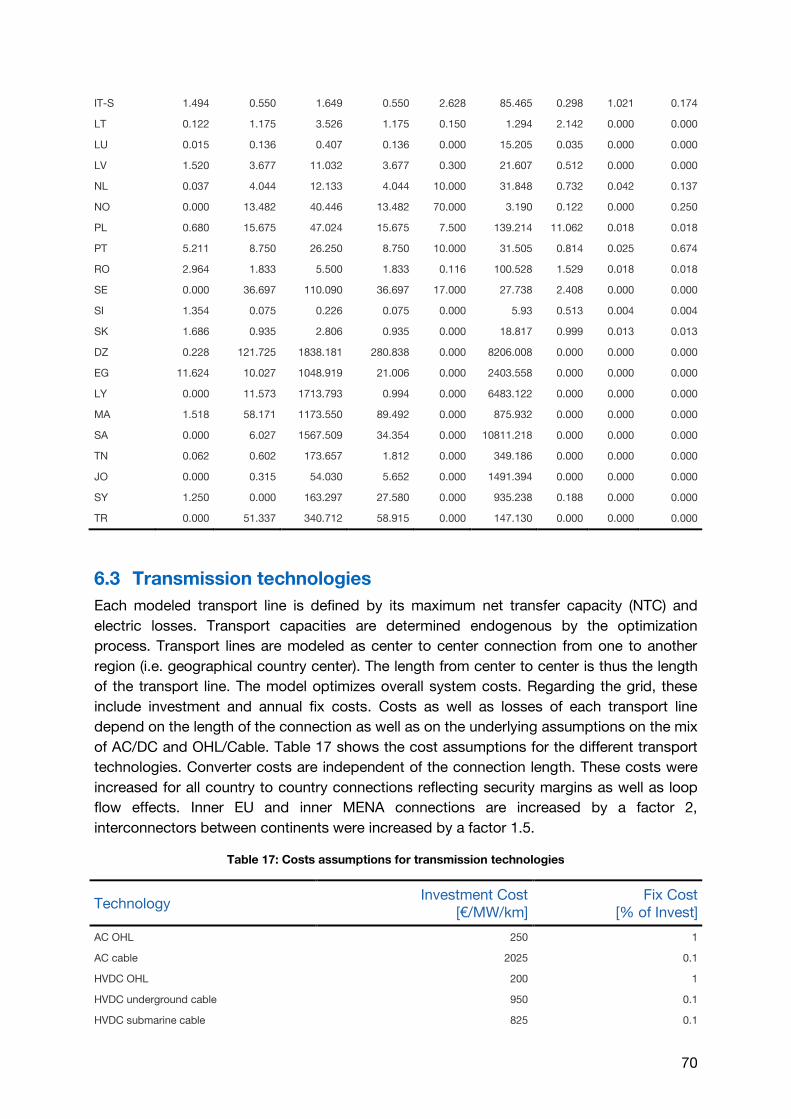
70

IT-S 1.494 0.550 1.649 0.550 2.628 85.465 0.298 1.021 0.174

LT 0.122 1.175 3.526 1.175 0.150 1.294 2.142 0.000 0.000

LU 0.015 0.136 0.407 0.136 0.000 15.205 0.035 0.000 0.000

LV 1.520 3.677 11.032 3.677 0.300 21.607 0.512 0.000 0.000

NL 0.037 4.044 12.133 4.044 10.000 31.848 0.732 0.042 0.137

NO 0.000 13.482 40.446 13.482 70.000 3.190 0.122 0.000 0.250

PL 0.680 15.675 47.024 15.675 7.500 139.214 11.062 0.018 0.018

PT 5.211 8.750 26.250 8.750 10.000 31.505 0.814 0.025 0.674

RO 2.964 1.833 5.500 1.833 0.116 100.528 1.529 0.018 0.018

SE 0.000 36.697 110.090 36.697 17.000 27.738 2.408 0.000 0.000

SI 1.354 0.075 0.226 0.075 0.000 5.93 0.513 0.004 0.004

SK 1.686 0.935 2.806 0.935 0.000 18.817 0.999 0.013 0.013

DZ 0.228 121.725 1838.181 280.838 0.000 8206.008 0.000 0.000 0.000

EG 11.624 10.027 1048.919 21.006 0.000 2403.558 0.000 0.000 0.000

LY 0.000 11.573 1713.793 0.994 0.000 6483.122 0.000 0.000 0.000

MA 1.518 58.171 1173.550 89.492 0.000 875.932 0.000 0.000 0.000

SA 0.000 6.027 1567.509 34.354 0.000 10811.218 0.000 0.000 0.000

TN 0.062 0.602 173.657 1.812 0.000 349.186 0.000 0.000 0.000

JO 0.000 0.315 54.030 5.652 0.000 1491.394 0.000 0.000 0.000

SY 1.250 0.000 163.297 27.580 0.000 935.238 0.188 0.000 0.000

TR 0.000 51.337 340.712 58.915 0.000 147.130 0.000 0.000 0.000

6.3 Transmission technologies

Each modeled transport line is defined by its maximum net transfer capacity (NTC) and

electric losses. Transport capacities are determined endogenous by the optimization

process. Transport lines are modeled as center to center connection from one to another

region (i.e. geographical country center). The length from center to center is thus the length

of the transport line. The model optimizes overall system costs. Regarding the grid, these

include investment and annual fix costs. Costs as well as losses of each transport line

depend on the length of the connection as well as on the underlying assumptions on the mix

of AC/DC and OHL/Cable. Table 17 shows the cost assumptions for the different transport

technologies. Converter costs are independent of the connection length. These costs were

increased for all country to country connections reflecting security margins as well as loop

flow effects. Inner EU and inner MENA connections are increased by a factor 2,

interconnectors between continents were increased by a factor 1.5.

Table 17: Costs assumptions for transmission technologies

Technology Investment Cost

[€/MW/km] Fix Cost

[% of Invest]

AC OHL 250 1

AC cable 2025 0.1

HVDC OHL 200 1

HVDC underground cable 950 0.1

HVDC submarine cable 825 0.1

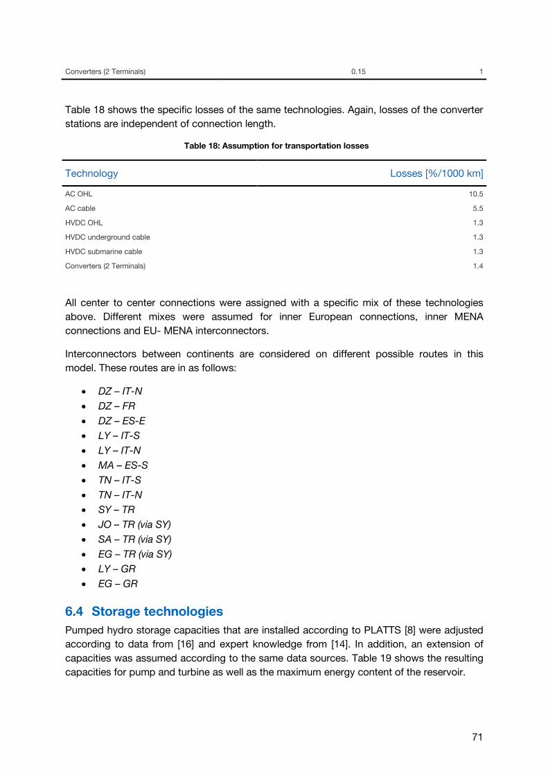
71

Converters (2 Terminals) 0.15 1

Table 18 shows the specific losses of the same technologies. Again, losses of the converter

stations are independent of connection length.

Table 18: Assumption for transportation losses

Technology Losses [%/1000 km]

AC OHL 10.5

AC cable 5.5

HVDC OHL 1.3

HVDC underground cable 1.3

HVDC submarine cable 1.3

Converters (2 Terminals) 1.4

All center to center connections were assigned with a specific mix of these technologies

above. Different mixes were assumed for inner European connections, inner MENA

connections and EU- MENA interconnectors.

Interconnectors between continents are considered on different possible routes in this

model. These routes are in as follows:

DZ – IT-N

DZ – FR

DZ – ES-E

LY – IT-S

LY – IT-N

MA – ES-S

TN – IT-S

TN – IT-N

SY – TR

JO – TR (via SY)

SA – TR (via SY)

EG – TR (via SY)

LY – GR

EG – GR

6.4 Storage technologies

Pumped hydro storage capacities that are installed according to PLATTS [8] were adjusted

according to data from [16] and expert knowledge from [14]. In addition, an extension of

capacities was assumed according to the same data sources. Table 19 shows the resulting

capacities for pump and turbine as well as the maximum energy content of the reservoir.

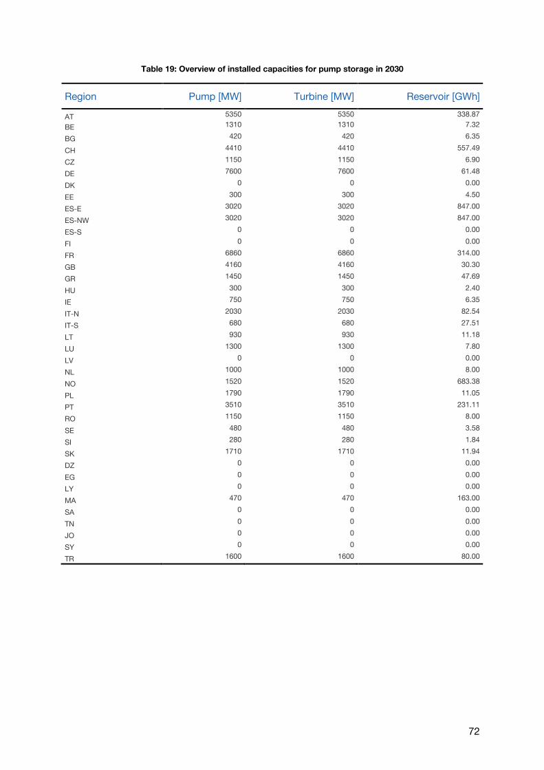
72

Table 19: Overview of installed capacities for pump storage in 2030

Region Pump [MW] Turbine [MW] Reservoir [GWh]

AT 5350 5350 338.87

BE 1310 1310 7.32

BG 420 420 6.35

CH 4410 4410 557.49

CZ 1150 1150 6.90

DE 7600 7600 61.48

DK 0 0 0.00

EE 300 300 4.50

ES-E 3020 3020 847.00

ES-NW 3020 3020 847.00

ES-S 0 0 0.00

FI 0 0 0.00

FR 6860 6860 314.00

GB 4160 4160 30.30

GR 1450 1450 47.69

HU 300 300 2.40

IE 750 750 6.35

IT-N 2030 2030 82.54

IT-S 680 680 27.51

LT 930 930 11.18

LU 1300 1300 7.80

LV 0 0 0.00

NL 1000 1000 8.00

NO 1520 1520 683.38

PL 1790 1790 11.05

PT 3510 3510 231.11

RO 1150 1150 8.00

SE 480 480 3.58

SI 280 280 1.84

SK 1710 1710 11.94

DZ 0 0 0.00

EG 0 0 0.00

LY 0 0 0.00

MA 470 470 163.00

SA 0 0 0.00

TN 0 0 0.00

JO 0 0 0.00

SY 0 0 0.00

TR 1600 1600 80.00

73

Table 20 shows installed capacity and maximum energy content of the reservoir of dam

storage power plants. Dam storage power plants don’t have pumps by definition. Only

natural influx of water can be stored in a reservoir and used to produce electricity time

shifted.

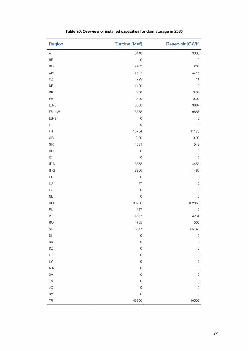
74

Table 20: Overview of installed capacities for dam storage in 2030

Region Turbine [MW] Reservoir [GWh]

AT 5418 3063

BE 0 0

BG 2462 209

CH 7547 8746

CZ 729 11

DE 1400 10

DK 0.00 0.00

EE 0.00 0.00

ES-E 8868 9887

ES-NW 8868 9887

ES-S 0 0

FI 0 0

FR 13734 11175

GB 0.00 0.00

GR 4531 548

HU 0 0

IE 0 0

IT-N 8868 4458

IT-S 2956 1486

LT 0 0

LU 17 3

LV 0 0

NL 0 0

NO 30700 102850

PL 167 10

PT 4337 3231

RO 4765 500

SE 16317 35148

SI 0 0

SK 0 0

DZ 0 0

EG 0 0

LY 0 0

MA 0 0

SA 0 0

TN 0 0

JO 0 0

SY 0 0

TR 43800 10500

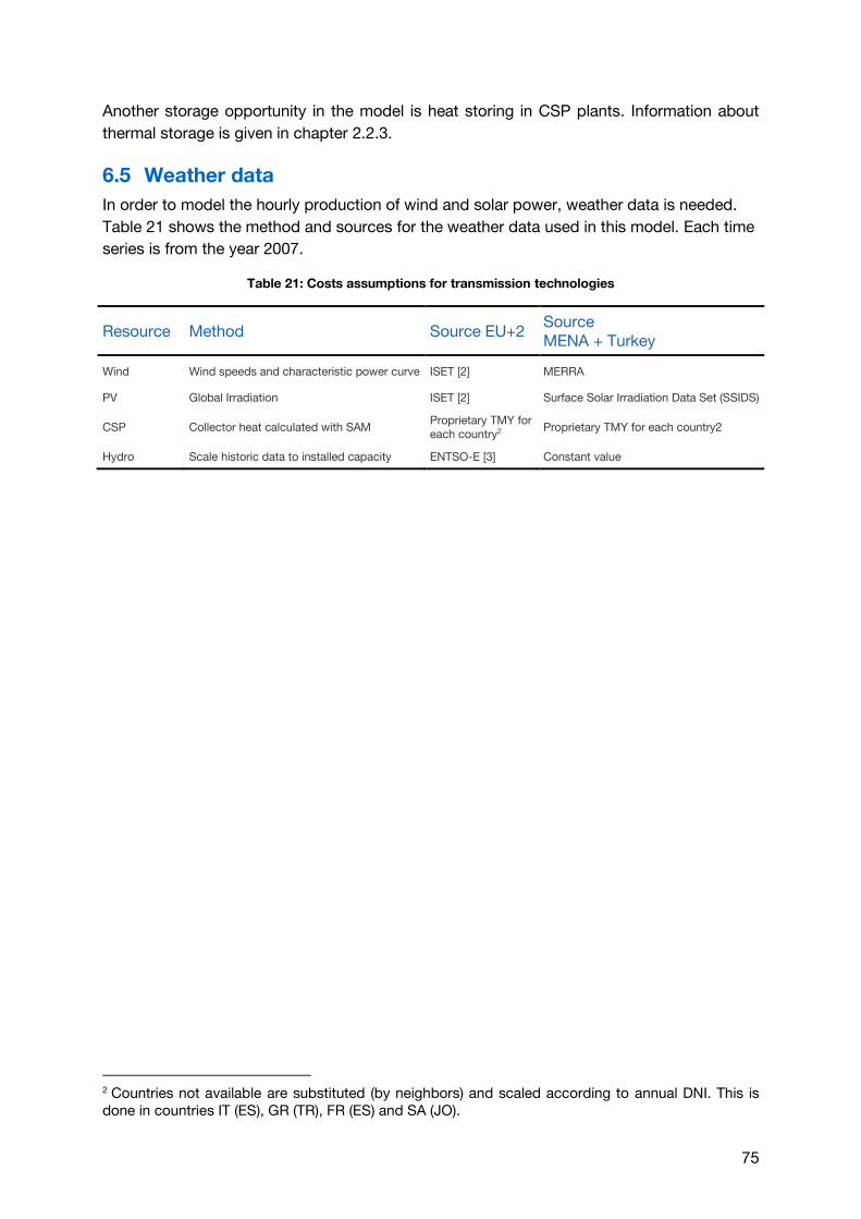
75

Another storage opportunity in the model is heat storing in CSP plants. Information about

thermal storage is given in chapter 2.2.3.

6.5 Weather data

In order to model the hourly production of wind and solar power, weather data is needed.

Table 21 shows the method and sources for the weather data used in this model. Each time

series is from the year 2007.

Table 21: Costs assumptions for transmission technologies

Resource Method Source EU+2 Source MENA + Turkey

Wind Wind speeds and characteristic power curve ISET [2] MERRA

PV Global Irradiation ISET [2] Surface Solar Irradiation Data Set (SSIDS)

CSP Collector heat calculated with SAM Proprietary TMY for each country2

Proprietary TMY for each country2

Hydro Scale historic data to installed capacity ENTSO-E [3] Constant value

2 Countries not available are substituted (by neighbors) and scaled according to annual DNI. This is done in countries IT (ES), GR (TR), FR (ES) and SA (JO).

76

BIBLIOGRAPHY [1] Schaber, Katrin: European Energy System Model URBS-EU Documentation.

München, 2010 [2] Stefan Bofinger, Lüder von Bremen, Kaspar Knorr, Katharina Lesch, Kurt Rohrig,

Yves-Marie Saint-Drenan, and Markus Speckmann. Raum-zeitliche Erzeugungsmuster von Wind- und Solarenergie in der UCTE-Region und deren Einfluss auf elektrische Transportnetze: Abschlussbericht für Siemens Zentraler Forschungsbereich. Institut für Solare Energieversorgungstechnik, ISET e.V., Kassel, 2008

[3] ENTSO-E European Network of Transmission System Operators for Electricity: Statistical data.

[4] McKinsey: Transformation of Europe’s power system until 2050. [5] International Energy Agency IEA. Interactive renewable energy calculator: Recabs;

htto://www.recabs.org/, 2010 [6] International Energy Ageny, editor: World Energy Outlook 2009. Paris, 2009.

Organisation for Economic Co-operation and Development OECD. [7] Prognos AG: Kurzstudie – Kosten neuer Kernkraftwerke. Basel, 2008 [8] Platts, data base description and research methodology: Udi world electric power

plant data base (wepp). 2009. [9] Sander & Partner GmbH: World wind atlas, http://sander-partner.ch [10] Bishop, J.K:B., Potylitsina T., Rossow, W.B.: Documentation and Desciption of

Surface Solar Irradiance Data Set Produced for SeaWiFS, NASA Grant, Department of Applied Physics, Columbia University, 2000

[11] Greenhouse Gas Inventory Data; http://unfccc.int/di/DetailedByParty.do, requested on 2011/05/05

[12] European Commision: EU energy trends to 2030 – Update 2009. Luxembourg 2010 [13] Fraunhofer ISI [14] Dii GmbH [15] TEIAS: Turkish Electricity Transmission Corporation [16] Eurelectric Key Statistics – 2011 Edition [17] International Energy Agency. World Energy Outlook 2011. Paris, 2011. Organisation

for Economic Cooperation and Development (OECD)

77

A 1. Electricity production The following tables contain annual electricity production per country by process for the four main scenarios.

A 1.1 Scenario 01 Base — Electricity production (GWh) Produced electricity (GWh) Bio Gas T Gas CC Geothermal CSP (turb) Hydro (RoR) Hydro (dam) Others PV (roof) PV (util) Wind-off (1) Wind-on (1) Wind-on (2) Wind-on (3) Total Overprod AT 6'713 0 0 70 0 32'061 9'941 70 595 0 0 3'494 8'732 0 61'676 0 BE 3'330 0 40'459 0 0 532 0 0 235 0 5'811 2'338 3'408 0 56'114 0 BG 12'201 0 0 193 0 1'044 2'892 193 210 0 331 2'308 5'767 0 25'137 0 CH 2'328 0 3'111 0 0 19'304 20'680 0 498 0 0 900 0 0 46'821 0 CZ 4'448 0 8'852 0 0 984 586 0 231 0 0 18'497 46'224 2'351 82'172 9 DE 42'869 0 63'640 1'489 0 15'921 3'994 1'489 24'895 0 46'711 34'975 87'403 15'799 339'185 12 DK 3'005 0 0 0 0 31 0 0 139 0 9'416 27'917 69'764 18'704 128'976 64 EE 3'235 0 442 0 0 9 0 0 15 0 669 10'584 0 0 14'953 0 ES-E 5'508 0 0 2'079 0 3'514 6'486 2'042 10'579 0 1'487 24'929 12'022 0 68'646 7 ES-NW 6'429 0 4'192 2'193 0 3'514 6'487 2'374 3'120 0 19 26'126 9'414 0 63'868 21 ES-S 1'296 0 0 651 0 0 0 515 4'922 0 3'057 6'307 5'045 0 21'793 50 FI 8'622 0 10'945 0 0 13'944 0 0 116 0 1'941 8'142 0 0 43'710 0 FR 42'468 0 37'394 3'215 1'062 39'777 31'553 15'137 11'884 0 19'438 86'700 0 0 288'628 0 GB 41'598 0 70'503 79 0 6'450 0 36'845 512 0 86'548 136'725 0 0 379'259 2'285 GR 2'807 0 0 604 0 0 6'612 604 3'048 0 470 5'333 13'326 3'573 36'377 0 HU 5'784 0 11'453 850 0 210 0 850 247 0 0 1'041 2'602 0 23'036 0 IE 1'461 17 9'228 0 0 772 0 6'815 59 0 2'043 12'400 0 0 32'795 341 IT-N 13'465 0 24'849 877 0 9'876 13'881 8'293 2'773 0 285 6'769 16'916 0 97'983 0 IT-S 2'422 0 0 8'943 1'800 1'097 1'542 1'527 5'956 0 2'914 1'412 3'529 946 32'090 0 LT 17'017 0 0 0 0 397 0 0 83 0 295 2'434 0 0 20'225 0 LU 283 0 3'046 0 0 75 50 0 100 0 0 345 861 0 4'761 0 LV 3'830 0 0 0 0 3'621 0 0 19 0 609 1'015 0 0 9'093 0 NL 5'792 0 42'310 368 0 101 0 1'200 203 0 16'876 10'705 2'772 0 80'327 1 NO 672 0 0 0 0 0 136'968 2'190 159 0 1'070 48'727 121'770 0 311'556 523 PL 95'448 0 11'449 158 0 2'641 505 158 56 0 375 16'761 0 0 127'552 0 PT 5'615 0 0 219 0 6'812 7'542 5'904 4'223 0 0 12'503 0 0 42'818 31 RO 13'249 0 1'840 158 0 14'106 5'425 158 355 1'149 183 4'450 11'121 0 52'193 0 SE 16'583 0 0 0 0 0 68'326 0 128 0 5'621 38'955 0 0 129'613 2 SI 4'426 0 1'139 35 0 5'162 0 35 135 0 0 179 448 120 11'680 0 SK 8'742 0 7'219 114 0 4'446 0 114 83 0 0 1'985 4'961 0 27'663 0 TR 0 0 30'942 0 0 0 126'007 0 0 0 0 119'662 0 0 276'611 65 DZ 0 0 0 0 0 173 0 0 0 99'959 0 344'262 90'015 0 534'409 7'392 EG 0 0 0 0 23'935 50'000 0 0 0 34'727 0 28'877 211'681 0 349'221 3'014 JO 0 0 0 0 20'587 0 0 0 0 0 0 802 12'901 0 34'290 5 LY 0 0 0 0 9'505 0 0 0 0 11'155 0 32'143 66'906 0 119'710 518 MA 0 0 0 0 45 3'963 0 0 0 23'647 0 140'450 0 0 168'105 4'025 SA 0 2'851 56'376 0 93'710 0 0 0 0 95'833 0 15'792 270'635 0 535'197 3'460 SY 1'264 0 0 0 0 2'604 0 0 0 79'989 0 0 228'653 0 312'509 4'893 TN 0 0 0 0 9'390 160 0 0 0 0 0 1'566 32'993 0 44'109 234

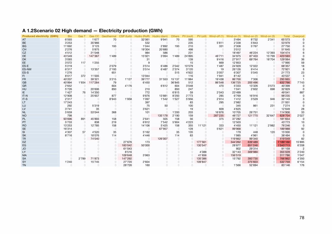
78

A 1.2 Scenario 02 High demand — Electricity production (GWh) Produced electricity (GWh) Bio Gas T Gas CC Geothermal CSP (turb) Hydro (RoR) Hydro (dam) Others PV (roof) PV (util) Wind-off (1) Wind-on (1) Wind-on (2) Wind-on (3) Total Overprod AT 6'593 0 1'677 70 0 32'061 9'941 70 595 0 0 3'494 8'732 2'341 65'573 0 BE 3'253 0 35'966 0 0 532 0 0 235 0 5'811 2'338 5'843 0 53'979 0 BG 11'692 0 3'123 193 0 1'044 2'892 193 210 0 331 2'308 5'767 0 27'750 0 CH 2'276 0 5'875 0 0 19'304 20'680 0 498 0 0 3'012 0 0 51'645 0 CZ 4'512 0 21'048 0 0 984 586 0 231 0 0 18'497 46'224 12'393 104'474 6 DE 43'549 0 147'367 1'489 0 15'921 3'994 1'489 24'895 0 46'711 34'975 87'403 15'799 423'593 0 DK 3'093 0 0 0 0 31 0 0 139 0 9'416 27'917 69'764 18'704 129'064 36 EE 3'072 117 1'255 0 0 9 0 0 15 0 669 12'853 0 0 17'990 59 ES-E 5'219 0 0 2'079 0 3'514 6'486 2'042 10'579 0 1'487 24'929 12'022 0 68'357 18 ES-NW 6'317 0 13'357 2'193 0 3'514 6'487 2'374 3'120 0 19 26'126 9'414 0 72'921 8 ES-S 1'276 0 0 651 0 0 0 515 4'922 0 3'057 6'307 5'045 0 21'773 23 FI 8'017 372 11'005 0 0 13'944 0 0 116 0 1'941 8'142 0 0 43'537 3 FR 40'207 0 39'321 3'215 1'127 39'777 31'553 15'137 11'884 0 19'438 86'700 7'306 0 295'665 1 GB 40'894 1'934 117'284 79 0 6'450 0 36'845 512 0 86'548 136'725 205'496 0 632'766 7'743 GR 2'652 0 0 604 4'176 0 6'612 604 3'048 0 470 5'333 13'326 3'573 40'399 0 HU 5'726 0 20'606 850 0 210 0 850 247 0 0 1'041 2'602 698 32'829 0 IE 1'427 76 14'350 0 0 772 0 6'815 59 0 2'043 23'499 0 0 49'041 887 IT-N 12'908 0 25'657 877 0 9'876 13'881 8'293 2'773 0 285 6'769 16'916 0 98'235 0 IT-S 2'317 0 0 8'943 1'958 1'097 1'542 1'527 5'956 0 2'914 1'412 3'529 946 32'143 3 LT 17'243 0 0 0 0 397 0 0 83 0 295 2'982 0 0 21'001 0 LU 292 0 5'319 0 0 75 50 0 100 0 0 345 861 231 7'274 0 LV 3'741 0 35 0 0 3'621 0 0 19 0 609 4'625 0 0 12'649 28 NL 5'659 0 53'044 368 0 101 0 1'200 203 0 16'876 10'705 26'751 0 114'906 33 NO 798 0 0 0 0 0 135'178 2'190 159 0 287'235 48'727 121'770 32'647 628'704 2'027 PL 93'696 891 45'893 158 0 2'641 505 158 56 0 375 37'282 0 0 181'654 0 PT 5'733 0 838 219 0 6'812 7'542 5'904 4'223 0 0 12'503 0 0 43'773 10 RO 13'253 0 12'785 158 0 14'106 5'425 158 355 11'121 333 4'450 11'121 2'982 76'246 0 SE 16'314 0 0 0 0 0 67'957 0 128 0 5'621 99'968 0 0 189'988 92 SI 4'307 57 4'520 35 0 5'162 0 35 135 0 0 179 448 120 15'000 0 SK 8'716 0 18'076 114 0 4'446 0 114 83 0 0 1'985 4'961 0 38'494 0 TR 0 0 74'040 0 0 0 126'007 0 0 0 0 119'662 99'340 0 419'049 82 DZ 0 0 0 0 27'676 173 0 0 0 177'561 0 344'262 639'489 0 1'189'160 15'895 EG 0 0 0 0 183'042 50'000 0 0 0 130'547 0 28'877 651'246 0 1'043'713 6'208 JO 0 0 0 0 61'043 0 0 0 0 0 0 802 29'314 0 91'159 2 LY 0 0 0 0 8'516 0 0 0 0 4'388 0 32'143 309'980 0 355'028 2'240 MA 0 0 0 0 109'648 3'963 0 0 0 41'656 0 156'519 0 0 311'786 1'047 SA 0 2'789 71'873 0 147'292 0 0 0 0 135'386 0 15'792 393'730 0 766'862 4'350 SY 1'240 0 15'745 0 27'720 2'604 0 0 0 109'847 0 0 375'603 0 532'759 6'154 TN 0 0 0 0 28'726 160 0 0 0 0 0 1'566 52'694 0 83'146 176

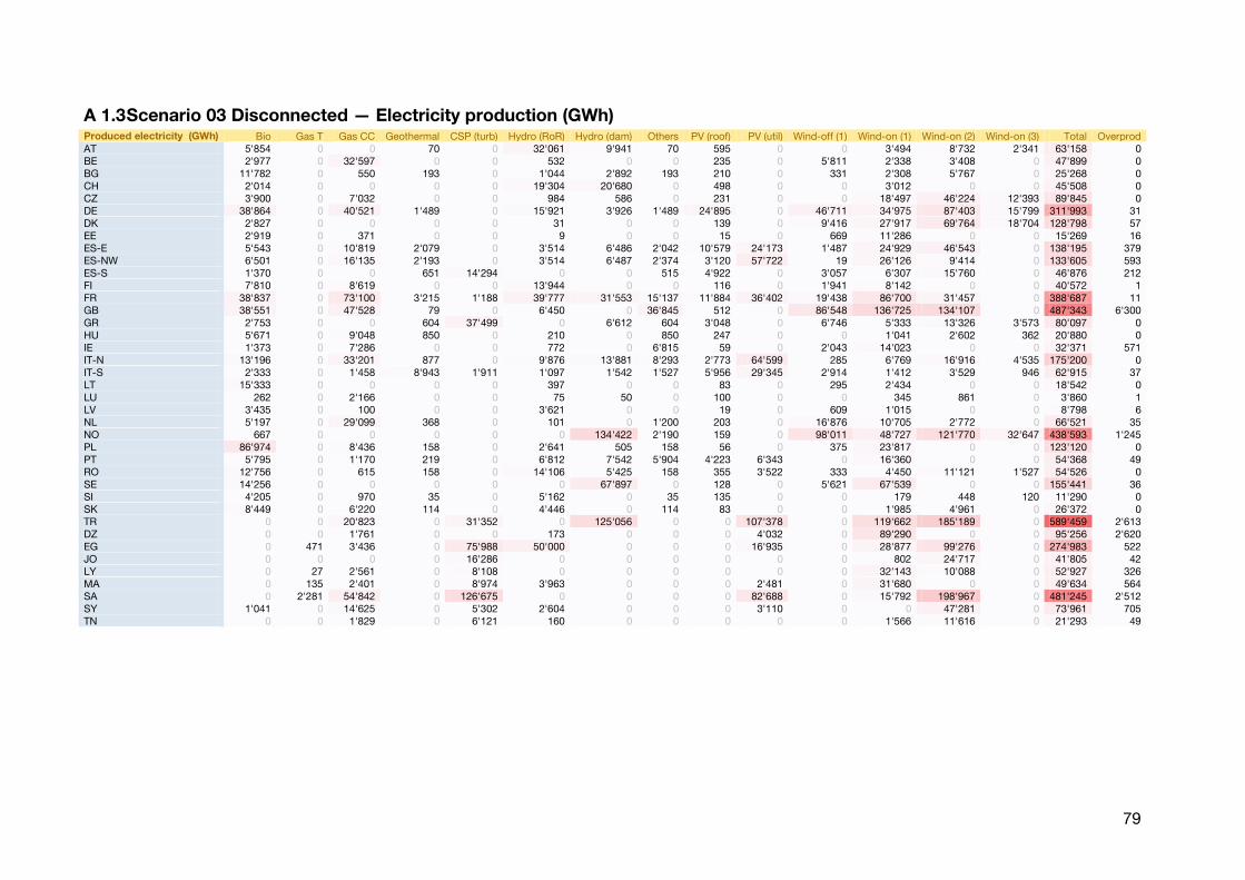
79

A 1.3 Scenario 03 Disconnected — Electricity production (GWh) Produced electricity (GWh) Bio Gas T Gas CC Geothermal CSP (turb) Hydro (RoR) Hydro (dam) Others PV (roof) PV (util) Wind-off (1) Wind-on (1) Wind-on (2) Wind-on (3) Total Overprod AT 5'854 0 0 70 0 32'061 9'941 70 595 0 0 3'494 8'732 2'341 63'158 0 BE 2'977 0 32'597 0 0 532 0 0 235 0 5'811 2'338 3'408 0 47'899 0 BG 11'782 0 550 193 0 1'044 2'892 193 210 0 331 2'308 5'767 0 25'268 0 CH 2'014 0 0 0 0 19'304 20'680 0 498 0 0 3'012 0 0 45'508 0 CZ 3'900 0 7'032 0 0 984 586 0 231 0 0 18'497 46'224 12'393 89'845 0 DE 38'864 0 40'521 1'489 0 15'921 3'926 1'489 24'895 0 46'711 34'975 87'403 15'799 311'993 31 DK 2'827 0 0 0 0 31 0 0 139 0 9'416 27'917 69'764 18'704 128'798 57 EE 2'919 0 371 0 0 9 0 0 15 0 669 11'286 0 0 15'269 16 ES-E 5'543 0 10'819 2'079 0 3'514 6'486 2'042 10'579 24'173 1'487 24'929 46'543 0 138'195 379 ES-NW 6'501 0 16'135 2'193 0 3'514 6'487 2'374 3'120 57'722 19 26'126 9'414 0 133'605 593 ES-S 1'370 0 0 651 14'294 0 0 515 4'922 0 3'057 6'307 15'760 0 46'876 212 FI 7'810 0 8'619 0 0 13'944 0 0 116 0 1'941 8'142 0 0 40'572 1 FR 38'837 0 73'100 3'215 1'188 39'777 31'553 15'137 11'884 36'402 19'438 86'700 31'457 0 388'687 11 GB 38'551 0 47'528 79 0 6'450 0 36'845 512 0 86'548 136'725 134'107 0 487'343 6'300 GR 2'753 0 0 604 37'499 0 6'612 604 3'048 0 6'746 5'333 13'326 3'573 80'097 0 HU 5'671 0 9'048 850 0 210 0 850 247 0 0 1'041 2'602 362 20'880 0 IE 1'373 0 7'286 0 0 772 0 6'815 59 0 2'043 14'023 0 0 32'371 571 IT-N 13'196 0 33'201 877 0 9'876 13'881 8'293 2'773 64'599 285 6'769 16'916 4'535 175'200 0 IT-S 2'333 0 1'458 8'943 1'911 1'097 1'542 1'527 5'956 29'345 2'914 1'412 3'529 946 62'915 37 LT 15'333 0 0 0 0 397 0 0 83 0 295 2'434 0 0 18'542 0 LU 262 0 2'166 0 0 75 50 0 100 0 0 345 861 0 3'860 1 LV 3'435 0 100 0 0 3'621 0 0 19 0 609 1'015 0 0 8'798 6 NL 5'197 0 29'099 368 0 101 0 1'200 203 0 16'876 10'705 2'772 0 66'521 35 NO 667 0 0 0 0 0 134'422 2'190 159 0 98'011 48'727 121'770 32'647 438'593 1'245 PL 86'974 0 8'436 158 0 2'641 505 158 56 0 375 23'817 0 0 123'120 0 PT 5'795 0 1'170 219 0 6'812 7'542 5'904 4'223 6'343 0 16'360 0 0 54'368 49 RO 12'756 0 615 158 0 14'106 5'425 158 355 3'522 333 4'450 11'121 1'527 54'526 0 SE 14'256 0 0 0 0 0 67'897 0 128 0 5'621 67'539 0 0 155'441 36 SI 4'205 0 970 35 0 5'162 0 35 135 0 0 179 448 120 11'290 0 SK 8'449 0 6'220 114 0 4'446 0 114 83 0 0 1'985 4'961 0 26'372 0 TR 0 0 20'823 0 31'352 0 125'056 0 0 107'378 0 119'662 185'189 0 589'459 2'613 DZ 0 0 1'761 0 0 173 0 0 0 4'032 0 89'290 0 0 95'256 2'620 EG 0 471 3'436 0 75'988 50'000 0 0 0 16'935 0 28'877 99'276 0 274'983 522 JO 0 0 0 0 16'286 0 0 0 0 0 0 802 24'717 0 41'805 42 LY 0 27 2'561 0 8'108 0 0 0 0 0 0 32'143 10'088 0 52'927 326 MA 0 135 2'401 0 8'974 3'963 0 0 0 2'481 0 31'680 0 0 49'634 564 SA 0 2'281 54'842 0 126'675 0 0 0 0 82'688 0 15'792 198'967 0 481'245 2'512 SY 1'041 0 14'625 0 5'302 2'604 0 0 0 3'110 0 0 47'281 0 73'961 705 TN 0 0 1'829 0 6'121 160 0 0 0 0 0 1'566 11'616 0 21'293 49

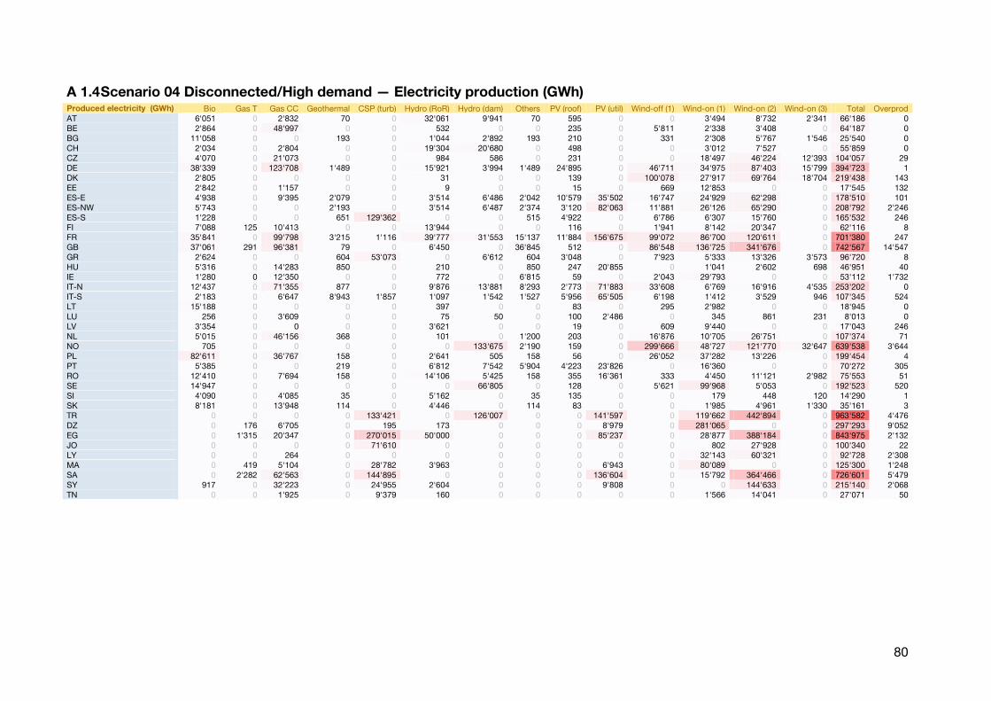
80

A 1.4 Scenario 04 Disconnected/High demand — Electricity production (GWh) Produced electricity (GWh) Bio Gas T Gas CC Geothermal CSP (turb) Hydro (RoR) Hydro (dam) Others PV (roof) PV (util) Wind-off (1) Wind-on (1) Wind-on (2) Wind-on (3) Total Overprod AT 6'051 0 2'832 70 0 32'061 9'941 70 595 0 0 3'494 8'732 2'341 66'186 0 BE 2'864 0 48'997 0 0 532 0 0 235 0 5'811 2'338 3'408 0 64'187 0 BG 11'058 0 0 193 0 1'044 2'892 193 210 0 331 2'308 5'767 1'546 25'540 0 CH 2'034 0 2'804 0 0 19'304 20'680 0 498 0 0 3'012 7'527 0 55'859 0 CZ 4'070 0 21'073 0 0 984 586 0 231 0 0 18'497 46'224 12'393 104'057 29 DE 38'339 0 123'708 1'489 0 15'921 3'994 1'489 24'895 0 46'711 34'975 87'403 15'799 394'723 1 DK 2'805 0 0 0 0 31 0 0 139 0 100'078 27'917 69'764 18'704 219'438 143 EE 2'842 0 1'157 0 0 9 0 0 15 0 669 12'853 0 0 17'545 132 ES-E 4'938 0 9'395 2'079 0 3'514 6'486 2'042 10'579 35'502 16'747 24'929 62'298 0 178'510 101 ES-NW 5'743 0 0 2'193 0 3'514 6'487 2'374 3'120 82'063 11'881 26'126 65'290 0 208'792 2'246 ES-S 1'228 0 0 651 129'362 0 0 515 4'922 0 6'786 6'307 15'760 0 165'532 246 FI 7'088 125 10'413 0 0 13'944 0 0 116 0 1'941 8'142 20'347 0 62'116 8 FR 35'841 0 99'798 3'215 1'116 39'777 31'553 15'137 11'884 156'675 99'072 86'700 120'611 0 701'380 247 GB 37'061 291 96'381 79 0 6'450 0 36'845 512 0 86'548 136'725 341'676 0 742'567 14'547 GR 2'624 0 0 604 53'073 0 6'612 604 3'048 0 7'923 5'333 13'326 3'573 96'720 8 HU 5'316 0 14'283 850 0 210 0 850 247 20'855 0 1'041 2'602 698 46'951 40 IE 1'280 0 12'350 0 0 772 0 6'815 59 0 2'043 29'793 0 0 53'112 1'732 IT-N 12'437 0 71'355 877 0 9'876 13'881 8'293 2'773 71'883 33'608 6'769 16'916 4'535 253'202 0 IT-S 2'183 0 6'647 8'943 1'857 1'097 1'542 1'527 5'956 65'505 6'198 1'412 3'529 946 107'345 524 LT 15'188 0 0 0 0 397 0 0 83 0 295 2'982 0 0 18'945 0 LU 256 0 3'609 0 0 75 50 0 100 2'486 0 345 861 231 8'013 0 LV 3'354 0 0 0 0 3'621 0 0 19 0 609 9'440 0 0 17'043 246 NL 5'015 0 46'156 368 0 101 0 1'200 203 0 16'876 10'705 26'751 0 107'374 71 NO 705 0 0 0 0 0 133'675 2'190 159 0 299'666 48'727 121'770 32'647 639'538 3'644 PL 82'611 0 36'767 158 0 2'641 505 158 56 0 26'052 37'282 13'226 0 199'454 4 PT 5'385 0 0 219 0 6'812 7'542 5'904 4'223 23'826 0 16'360 0 0 70'272 305 RO 12'410 0 7'694 158 0 14'106 5'425 158 355 16'361 333 4'450 11'121 2'982 75'553 51 SE 14'947 0 0 0 0 0 66'805 0 128 0 5'621 99'968 5'053 0 192'523 520 SI 4'090 0 4'085 35 0 5'162 0 35 135 0 0 179 448 120 14'290 1 SK 8'181 0 13'948 114 0 4'446 0 114 83 0 0 1'985 4'961 1'330 35'161 3 TR 0 0 0 0 133'421 0 126'007 0 0 141'597 0 119'662 442'894 0 963'582 4'476 DZ 0 176 6'705 0 195 173 0 0 0 8'979 0 281'065 0 0 297'293 9'052 EG 0 1'315 20'347 0 270'015 50'000 0 0 0 85'237 0 28'877 388'184 0 843'975 2'132 JO 0 0 0 0 71'610 0 0 0 0 0 0 802 27'928 0 100'340 22 LY 0 0 264 0 0 0 0 0 0 0 0 32'143 60'321 0 92'728 2'308 MA 0 419 5'104 0 28'782 3'963 0 0 0 6'943 0 80'089 0 0 125'300 1'248 SA 0 2'282 62'563 0 144'895 0 0 0 0 136'604 0 15'792 364'466 0 726'601 5'479 SY 917 0 32'223 0 24'955 2'604 0 0 0 9'808 0 0 144'633 0 215'140 2'068 TN 0 0 1'925 0 9'379 160 0 0 0 0 0 1'566 14'041 0 27'071 50

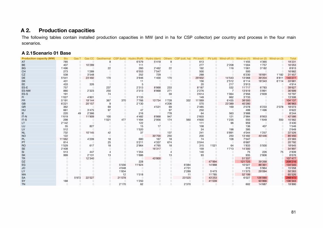
81

A 2. Production capacities The following tables contain installed production capacities in MW (and in ha for CSP collector) per country and process in the four main

scenarios.

A 2.1 Scenario 01 Base Production capacity (MW) Bio Gas T Gas CC Geothermal CSP (turb) Hydro (RoR) Hydro (dam) Others CSP (coll, ha) PV (roof) PV (util) Wind-off (1) Wind-on (1) Wind-on (2) Wind-on (3) Total AT 785 0 0 8 0 6'579 5'418 8 0 613 0 0 1'455 4'365 0 19'231 BE 407 0 10'289 0 0 111 0 0 0 277 0 2'208 1'004 1'757 0 16'053 BG 1'496 0 0 22 0 260 2'462 22 0 192 0 116 1'061 3'182 0 8'813 CH 273 0 1'289 0 0 6'553 7'547 0 0 500 0 0 500 0 0 16'662 CZ 538 0 3'548 0 0 252 729 0 0 288 0 0 6'230 18'691 1'182 31'457 DE 5'541 0 23'492 170 0 3'946 1'400 170 0 29'932 0 14'543 13'068 39'204 8'811 140'277 DK 431 0 0 0 0 11 0 0 0 156 0 2'512 6'114 18'343 6'114 33'681 EE 433 0 326 0 0 5 0 0 0 20 0 217 3'913 0 0 4'914 ES-E 757 0 0 237 0 2'313 8'868 233 0 8'187 0 532 11'717 6'783 0 39'627 ES-NW 880 0 2'323 250 0 2'313 8'868 271 0 2'276 0 7 13'619 5'891 0 36'699 ES-S 191 0 0 74 0 0 0 59 0 3'614 0 1'064 2'956 2'839 0 10'797 FI 1'027 0 4'801 0 0 3'133 0 0 0 149 0 662 3'733 0 0 13'506 FR 5'191 0 19'144 367 370 7'766 13'734 1'728 332 11'069 0 6'435 38'000 0 0 104'137 GB 6'221 0 20'157 9 0 2'130 0 4'206 0 570 0 23'389 40'280 0 0 96'963 GR 362 0 0 69 0 0 4'531 69 0 2'485 0 169 2'078 6'233 2'078 18'073 HU 661 0 3'475 97 0 47 0 97 0 250 0 0 499 1'496 0 6'622 IE 220 49 2'366 0 0 216 0 778 0 64 0 563 3'988 0 0 8'244 IT-N 1'619 0 11'909 100 0 4'482 8'868 947 0 2'603 0 121 2'984 8'953 0 42'586 IT-S 298 0 0 1'021 477 1'494 2'956 174 560 4'600 0 1'235 550 1'649 550 15'562 LT 2'142 0 0 0 0 122 0 0 0 111 0 96 959 0 0 3'430 LU 35 0 827 0 0 15 17 0 0 108 0 0 136 407 0 1'546 LV 512 0 0 0 0 1'520 0 0 0 24 0 198 395 0 0 2'649 NL 732 0 10'145 42 0 37 0 137 0 241 0 5'891 4'044 1'257 0 22'526 NO 122 0 0 0 0 0 30'700 250 0 200 0 250 13'482 40'446 0 85'450 PL 11'062 0 4'209 18 0 680 167 18 0 74 0 108 7'047 0 0 23'383 PT 814 0 0 25 0 5'211 4'337 674 0 3'044 0 0 6'687 0 0 20'792 RO 1'529 0 617 18 0 2'964 4'765 18 0 315 1'021 64 1'833 5'500 0 18'645 SE 2'408 0 0 0 0 0 16'317 0 0 159 0 1'713 14'300 0 0 34'897 SI 513 0 447 4 0 1'354 0 4 0 140 0 0 75 226 75 2'839 SK 999 0 2'131 13 0 1'686 0 13 0 93 0 0 935 2'806 0 8'676 TR 0 0 12'340 0 0 0 43'800 0 0 0 0 0 51'337 0 0 107'477 DZ 0 0 0 0 0 228 0 0 0 0 47'994 0 121'725 39'268 0 209'216 EG 0 0 0 0 5'556 11'624 0 0 6'084 0 14'888 0 10'027 86'361 0 134'540 JO 0 0 0 0 4'048 0 0 0 4'731 0 0 0 315 5'964 0 15'058 LY 0 0 0 0 1'834 0 0 0 2'289 0 5'473 0 11'573 29'094 0 50'263 MA 0 0 0 0 12 1'518 0 0 11 0 11'785 0 52'199 0 0 65'526 SA 0 5'972 22'527 0 21'078 0 0 0 23'525 0 43'253 0 6'027 126'090 0 248'472 SY 188 0 0 0 0 1'250 0 0 0 0 41'039 0 0 93'866 0 136'343 TN 0 0 0 0 2'170 62 0 0 2'370 0 0 0 602 14'687 0 19'890

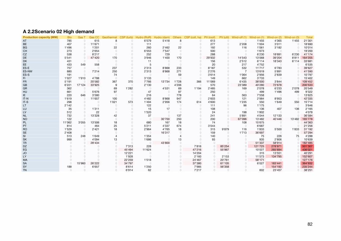
82

A 2.2 Scenario 02 High demand Production capacity (MW) Bio Gas T Gas CC Geothermal CSP (turb) Hydro (RoR) Hydro (dam) Others CSP (coll, ha) PV (roof) PV (util) Wind-off (1) Wind-on (1) Wind-on (2) Wind-on (3) Total AT 785 0 615 8 0 6'579 5'418 8 0 613 0 0 1'455 4'365 1'455 21'301 BE 407 0 11'671 0 0 111 0 0 0 277 0 2'208 1'004 3'011 0 18'690 BG 1'496 0 1'201 22 0 260 2'462 22 0 192 0 116 1'061 3'182 0 10'014 CH 273 0 2'654 0 0 6'553 7'547 0 0 500 0 0 1'673 0 0 19'200 CZ 538 0 8'217 0 0 252 729 0 0 288 0 0 6'230 18'691 6'230 41'174 DE 5'541 0 47'420 170 0 3'946 1'400 170 0 29'932 0 14'543 13'068 39'204 8'811 164'205 DK 431 0 0 0 0 11 0 0 0 156 0 2'512 6'114 18'343 6'114 33'681 EE 433 549 558 0 0 5 0 0 0 20 0 217 4'752 0 0 6'535 ES-E 757 0 0 237 0 2'313 8'868 233 0 8'187 0 532 11'717 6'783 0 39'627 ES-NW 880 0 7'214 250 0 2'313 8'868 271 0 2'276 0 7 13'619 5'891 0 41'590 ES-S 191 0 0 74 0 0 0 59 0 3'614 0 1'064 2'956 2'839 0 10'797 FI 1'027 1'910 4'788 0 0 3'133 0 0 0 149 0 662 3'733 0 0 15'402 FR 5'191 0 20'582 367 370 7'766 13'734 1'728 366 11'069 0 6'435 38'000 3'844 0 109'452 GB 6'221 17'124 33'925 9 0 2'130 0 4'206 0 570 0 23'389 40'280 72'678 0 200'533 GR 362 0 0 69 1'282 0 4'531 69 1'194 2'485 0 169 2'078 6'233 2'078 20'549 HU 661 0 5'676 97 0 47 0 97 0 250 0 0 499 1'496 499 9'322 IE 220 646 3'580 0 0 216 0 778 0 64 0 563 7'558 0 0 13'625 IT-N 1'619 0 11'657 100 0 4'482 8'868 947 0 2'603 0 121 2'984 8'953 0 42'335 IT-S 298 0 0 1'021 573 1'494 2'956 174 614 4'600 0 1'235 550 1'649 550 15'714 LT 2'142 0 0 0 0 122 0 0 0 111 0 96 1'175 0 0 3'646 LU 35 0 1'311 0 0 15 17 0 0 108 0 0 136 407 136 2'165 LV 512 0 22 0 0 1'520 0 0 0 24 0 198 1'802 0 0 4'078 NL 732 0 13'328 42 0 37 0 137 0 241 0 5'891 4'044 12'133 0 36'584 NO 122 0 0 0 0 0 30'700 250 0 200 0 67'096 13'482 40'446 13'482 165'778 PL 11'062 3'055 13'506 18 0 680 167 18 0 74 0 108 15'675 0 0 44'363 PT 814 0 464 25 0 5'211 4'337 674 0 3'044 0 0 6'687 0 0 21'256 RO 1'529 0 2'421 18 0 2'964 4'765 18 0 315 9'879 116 1'833 5'500 1'833 31'192 SE 2'408 0 0 0 0 0 16'317 0 0 159 0 1'713 36'697 0 0 57'294 SI 513 248 1'649 4 0 1'354 0 4 0 140 0 0 75 226 75 4'288 SK 999 0 4'094 13 0 1'686 0 13 0 93 0 0 935 2'806 0 10'639 TR 0 0 28'434 0 0 0 43'800 0 0 0 0 0 51'337 58'914 0 182'485 DZ 0 0 0 0 7'313 228 0 0 7'816 0 85'254 0 121'725 278'971 0 501'307 EG 0 0 0 0 45'494 11'624 0 0 47'216 0 55'967 0 10'027 265'694 0 436'021 JO 0 0 0 0 12'221 0 0 0 14'204 0 0 0 315 13'551 0 40'291 LY 0 0 0 0 1'928 0 0 0 2'160 0 2'153 0 11'573 134'795 0 152'607 MA 0 0 0 0 22'259 1'518 0 0 24'467 0 20'761 0 58'171 0 0 127'176 SA 0 15'960 26'222 0 34'797 0 0 0 37'380 0 61'105 0 6'027 183'441 0 364'932 SY 188 0 6'657 0 8'614 1'250 0 0 7'985 0 56'358 0 0 154'192 0 235'244 TN 0 0 0 0 6'914 62 0 0 7'217 0 0 0 602 23'457 0 38'251

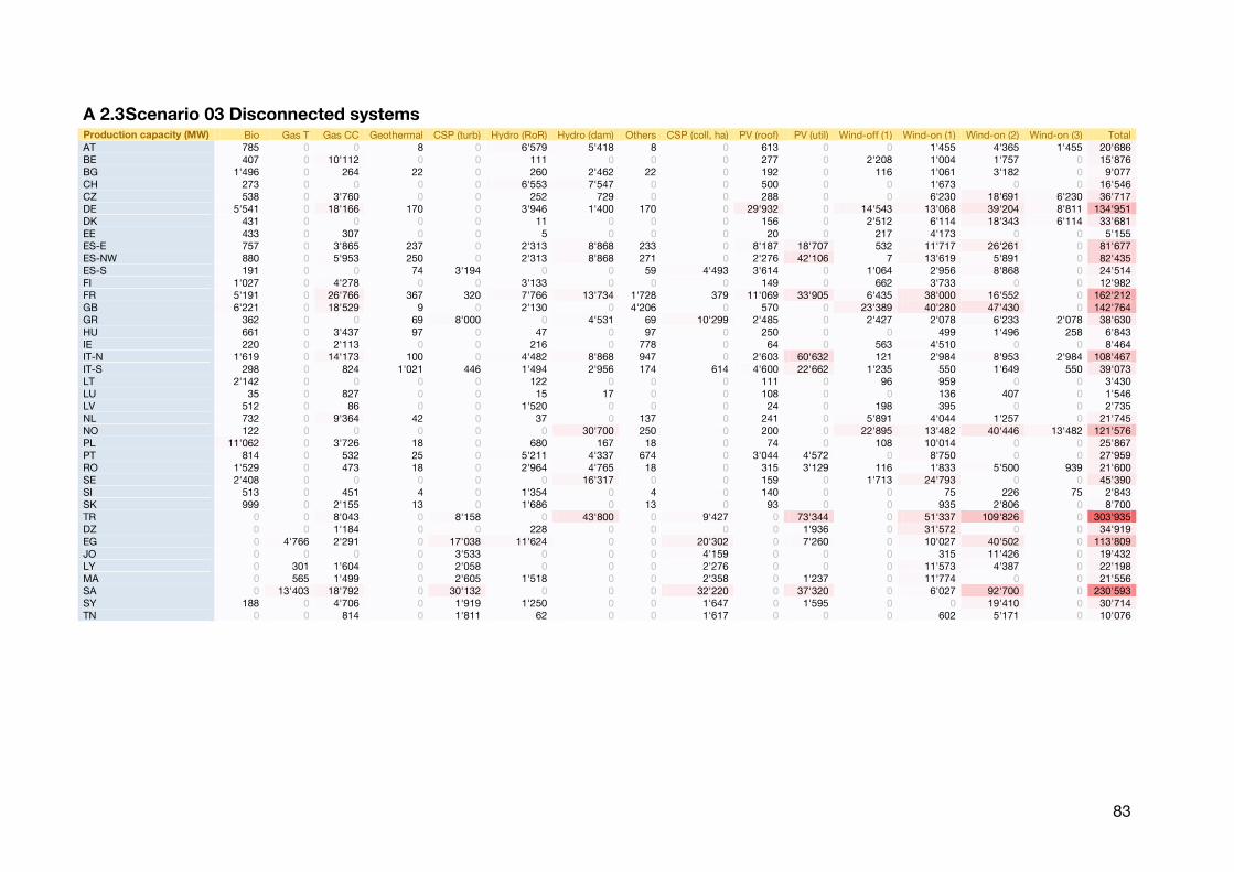
83

A 2.3 Scenario 03 Disconnected systems Production capacity (MW) Bio Gas T Gas CC Geothermal CSP (turb) Hydro (RoR) Hydro (dam) Others CSP (coll, ha) PV (roof) PV (util) Wind-off (1) Wind-on (1) Wind-on (2) Wind-on (3) Total AT 785 0 0 8 0 6'579 5'418 8 0 613 0 0 1'455 4'365 1'455 20'686 BE 407 0 10'112 0 0 111 0 0 0 277 0 2'208 1'004 1'757 0 15'876 BG 1'496 0 264 22 0 260 2'462 22 0 192 0 116 1'061 3'182 0 9'077 CH 273 0 0 0 0 6'553 7'547 0 0 500 0 0 1'673 0 0 16'546 CZ 538 0 3'760 0 0 252 729 0 0 288 0 0 6'230 18'691 6'230 36'717 DE 5'541 0 18'166 170 0 3'946 1'400 170 0 29'932 0 14'543 13'068 39'204 8'811 134'951 DK 431 0 0 0 0 11 0 0 0 156 0 2'512 6'114 18'343 6'114 33'681 EE 433 0 307 0 0 5 0 0 0 20 0 217 4'173 0 0 5'155 ES-E 757 0 3'865 237 0 2'313 8'868 233 0 8'187 18'707 532 11'717 26'261 0 81'677 ES-NW 880 0 5'953 250 0 2'313 8'868 271 0 2'276 42'106 7 13'619 5'891 0 82'435 ES-S 191 0 0 74 3'194 0 0 59 4'493 3'614 0 1'064 2'956 8'868 0 24'514 FI 1'027 0 4'278 0 0 3'133 0 0 0 149 0 662 3'733 0 0 12'982 FR 5'191 0 26'766 367 320 7'766 13'734 1'728 379 11'069 33'905 6'435 38'000 16'552 0 162'212 GB 6'221 0 18'529 9 0 2'130 0 4'206 0 570 0 23'389 40'280 47'430 0 142'764 GR 362 0 0 69 8'000 0 4'531 69 10'299 2'485 0 2'427 2'078 6'233 2'078 38'630 HU 661 0 3'437 97 0 47 0 97 0 250 0 0 499 1'496 258 6'843 IE 220 0 2'113 0 0 216 0 778 0 64 0 563 4'510 0 0 8'464 IT-N 1'619 0 14'173 100 0 4'482 8'868 947 0 2'603 60'632 121 2'984 8'953 2'984 108'467 IT-S 298 0 824 1'021 446 1'494 2'956 174 614 4'600 22'662 1'235 550 1'649 550 39'073 LT 2'142 0 0 0 0 122 0 0 0 111 0 96 959 0 0 3'430 LU 35 0 827 0 0 15 17 0 0 108 0 0 136 407 0 1'546 LV 512 0 86 0 0 1'520 0 0 0 24 0 198 395 0 0 2'735 NL 732 0 9'364 42 0 37 0 137 0 241 0 5'891 4'044 1'257 0 21'745 NO 122 0 0 0 0 0 30'700 250 0 200 0 22'895 13'482 40'446 13'482 121'576 PL 11'062 0 3'726 18 0 680 167 18 0 74 0 108 10'014 0 0 25'867 PT 814 0 532 25 0 5'211 4'337 674 0 3'044 4'572 0 8'750 0 0 27'959 RO 1'529 0 473 18 0 2'964 4'765 18 0 315 3'129 116 1'833 5'500 939 21'600 SE 2'408 0 0 0 0 0 16'317 0 0 159 0 1'713 24'793 0 0 45'390 SI 513 0 451 4 0 1'354 0 4 0 140 0 0 75 226 75 2'843 SK 999 0 2'155 13 0 1'686 0 13 0 93 0 0 935 2'806 0 8'700 TR 0 0 8'043 0 8'158 0 43'800 0 9'427 0 73'344 0 51'337 109'826 0 303'935 DZ 0 0 1'184 0 0 228 0 0 0 0 1'936 0 31'572 0 0 34'919 EG 0 4'766 2'291 0 17'038 11'624 0 0 20'302 0 7'260 0 10'027 40'502 0 113'809 JO 0 0 0 0 3'533 0 0 0 4'159 0 0 0 315 11'426 0 19'432 LY 0 301 1'604 0 2'058 0 0 0 2'276 0 0 0 11'573 4'387 0 22'198 MA 0 565 1'499 0 2'605 1'518 0 0 2'358 0 1'237 0 11'774 0 0 21'556 SA 0 13'403 18'792 0 30'132 0 0 0 32'220 0 37'320 0 6'027 92'700 0 230'593 SY 188 0 4'706 0 1'919 1'250 0 0 1'647 0 1'595 0 0 19'410 0 30'714 TN 0 0 814 0 1'811 62 0 0 1'617 0 0 0 602 5'171 0 10'076

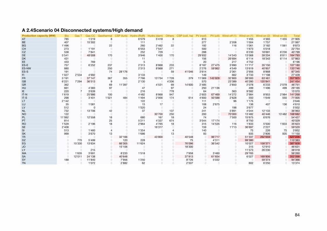
84

A 2.4 Scenario 04 Disconnected systems/High demand Production capacity (MW) Bio Gas T Gas CC Geothermal CSP (turb) Hydro (RoR) Hydro (dam) Others CSP (coll, ha) PV (roof) PV (util) Wind-off (1) Wind-on (1) Wind-on (2) Wind-on (3) Total AT 785 0 1'219 8 0 6'579 5'418 8 0 613 0 0 1'455 4'365 1'455 21'905 BE 407 0 15'302 0 0 111 0 0 0 277 0 2'208 1'004 1'757 0 21'067 BG 1'496 0 0 22 0 260 2'462 22 0 192 0 116 1'061 3'182 1'061 9'873 CH 273 0 1'191 0 0 6'553 7'547 0 0 500 0 0 1'673 5'018 0 22'754 CZ 538 0 7'841 0 0 252 729 0 0 288 0 0 6'230 18'691 6'230 40'799 DE 5'541 0 48'008 170 0 3'946 1'400 170 0 29'932 0 14'543 13'068 39'204 8'811 164'793 DK 431 0 0 0 0 11 0 0 0 156 0 26'694 6'114 18'343 6'114 57'863 EE 433 0 769 0 0 5 0 0 0 20 0 217 4'752 0 0 6'196 ES-E 757 0 6'252 237 0 2'313 8'868 233 0 8'187 27'475 5'990 11'717 35'150 0 107'180 ES-NW 880 0 0 250 0 2'313 8'868 271 0 2'276 59'862 4'549 13'619 40'857 0 133'746 ES-S 191 0 0 74 28'176 0 0 59 41'046 3'614 0 2'361 2'956 8'868 0 87'345 FI 1'027 2'534 4'992 0 0 3'133 0 0 0 149 0 662 3'733 11'198 0 27'428 FR 5'191 0 37'147 367 355 7'766 13'734 1'728 379 11'069 145'928 32'800 38'000 63'461 0 357'925 GB 6'221 7'294 36'513 9 0 2'130 0 4'206 0 570 0 23'389 40'280 120'841 0 241'454 GR 362 0 0 69 11'397 0 4'531 69 14'600 2'485 0 2'850 2'078 6'233 2'078 46'751 HU 661 0 4'383 97 0 47 0 97 0 250 21'136 0 499 1'496 499 29'165 IE 220 7 3'639 0 0 216 0 778 0 64 0 563 9'582 0 0 15'070 IT-N 1'619 0 25'986 100 0 4'482 8'868 947 0 2'603 67'469 14'272 2'984 8'953 2'984 141'268 IT-S 298 0 3'401 1'021 484 1'494 2'956 174 614 4'600 50'588 2'628 550 1'649 550 71'005 LT 2'142 0 0 0 0 122 0 0 0 111 0 96 1'175 0 0 3'646 LU 35 0 1'081 0 0 15 17 0 0 108 2'675 0 136 407 136 4'610 LV 512 0 0 0 0 1'520 0 0 0 24 0 198 3'677 0 0 5'932 NL 732 0 13'706 42 0 37 0 137 0 241 0 5'891 4'044 12'133 0 36'963 NO 122 0 0 0 0 0 30'700 250 0 200 0 70'000 13'482 40'446 13'482 168'682 PL 11'062 0 12'558 18 0 680 167 18 0 74 0 7'500 15'675 6'676 0 54'427 PT 814 0 0 25 0 5'211 4'337 674 0 3'044 17'174 0 8'750 0 0 40'029 RO 1'529 0 2'196 18 0 2'964 4'765 18 0 315 14'535 116 1'833 5'500 1'833 35'623 SE 2'408 0 0 0 0 0 16'317 0 0 159 0 1'713 36'697 2'227 0 59'520 SI 513 0 1'460 4 0 1'354 0 4 0 140 0 0 75 226 75 3'852 SK 999 0 3'670 13 0 1'686 0 13 0 93 0 0 935 2'806 935 11'150 TR 0 0 0 0 32'166 0 43'800 0 40'548 0 96'717 0 51'337 262'659 0 527'226 DZ 0 770 5'499 0 120 228 0 0 75 0 4'311 0 99'380 0 0 110'383 EG 0 15'330 13'634 0 66'305 11'624 0 0 76'096 0 36'542 0 10'027 158'371 0 387'928 JO 0 0 0 0 15'106 0 0 0 18'300 0 0 0 315 12'910 0 46'631 LY 0 0 215 0 0 0 0 0 0 0 0 0 11'573 26'230 0 38'018 MA 0 1'635 3'691 0 8'233 1'518 0 0 7'958 0 3'460 0 29'765 0 0 56'260 SA 0 12'011 24'138 0 40'648 0 0 0 37'813 0 61'654 0 6'027 169'806 0 352'098 SY 188 0 11'840 0 7'956 1'250 0 0 8'726 0 5'032 0 0 59'374 0 94'366 TN 0 0 1'072 0 2'882 62 0 0 2'507 0 0 0 602 6'250 0 13'374

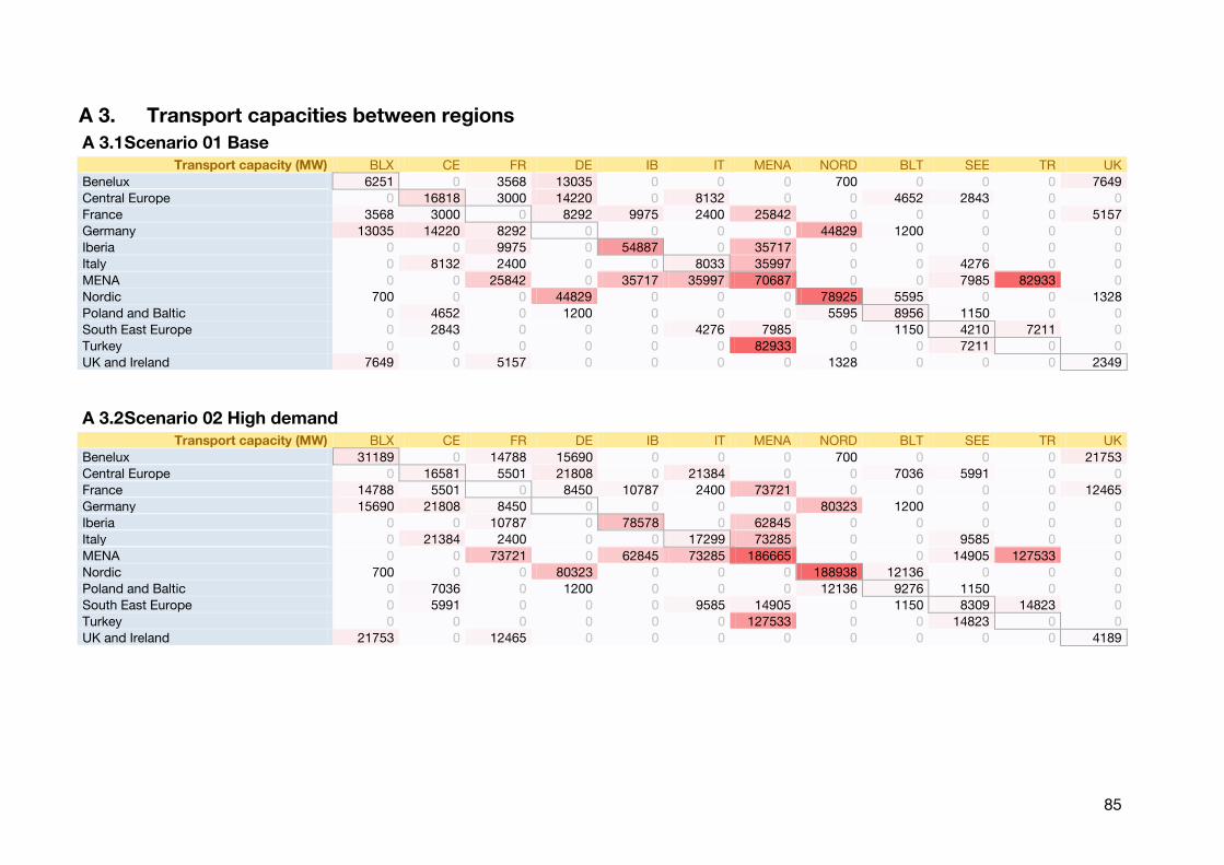
85

A 3. Transport capacities between regions

A 3.1 Scenario 01 Base Transport capacity (MW) BLX CE FR DE IB IT MENA NORD BLT SEE TR UK

Benelux 6251 0 3568 13035 0 0 0 700 0 0 0 7649

Central Europe 0 16818 3000 14220 0 8132 0 0 4652 2843 0 0

France 3568 3000 0 8292 9975 2400 25842 0 0 0 0 5157

Germany 13035 14220 8292 0 0 0 0 44829 1200 0 0 0

Iberia 0 0 9975 0 54887 0 35717 0 0 0 0 0

Italy 0 8132 2400 0 0 8033 35997 0 0 4276 0 0

MENA 0 0 25842 0 35717 35997 70687 0 0 7985 82933 0

Nordic 700 0 0 44829 0 0 0 78925 5595 0 0 1328

Poland and Baltic 0 4652 0 1200 0 0 0 5595 8956 1150 0 0

South East Europe 0 2843 0 0 0 4276 7985 0 1150 4210 7211 0

Turkey 0 0 0 0 0 0 82933 0 0 7211 0 0

UK and Ireland 7649 0 5157 0 0 0 0 1328 0 0 0 2349

A 3.2 Scenario 02 High demand Transport capacity (MW) BLX CE FR DE IB IT MENA NORD BLT SEE TR UK

Benelux 31189 0 14788 15690 0 0 0 700 0 0 0 21753

Central Europe 0 16581 5501 21808 0 21384 0 0 7036 5991 0 0

France 14788 5501 0 8450 10787 2400 73721 0 0 0 0 12465

Germany 15690 21808 8450 0 0 0 0 80323 1200 0 0 0

Iberia 0 0 10787 0 78578 0 62845 0 0 0 0 0

Italy 0 21384 2400 0 0 17299 73285 0 0 9585 0 0

MENA 0 0 73721 0 62845 73285 186665 0 0 14905 127533 0

Nordic 700 0 0 80323 0 0 0 188938 12136 0 0 0

Poland and Baltic 0 7036 0 1200 0 0 0 12136 9276 1150 0 0

South East Europe 0 5991 0 0 0 9585 14905 0 1150 8309 14823 0

Turkey 0 0 0 0 0 0 127533 0 0 14823 0 0

UK and Ireland 21753 0 12465 0 0 0 0 0 0 0 0 4189

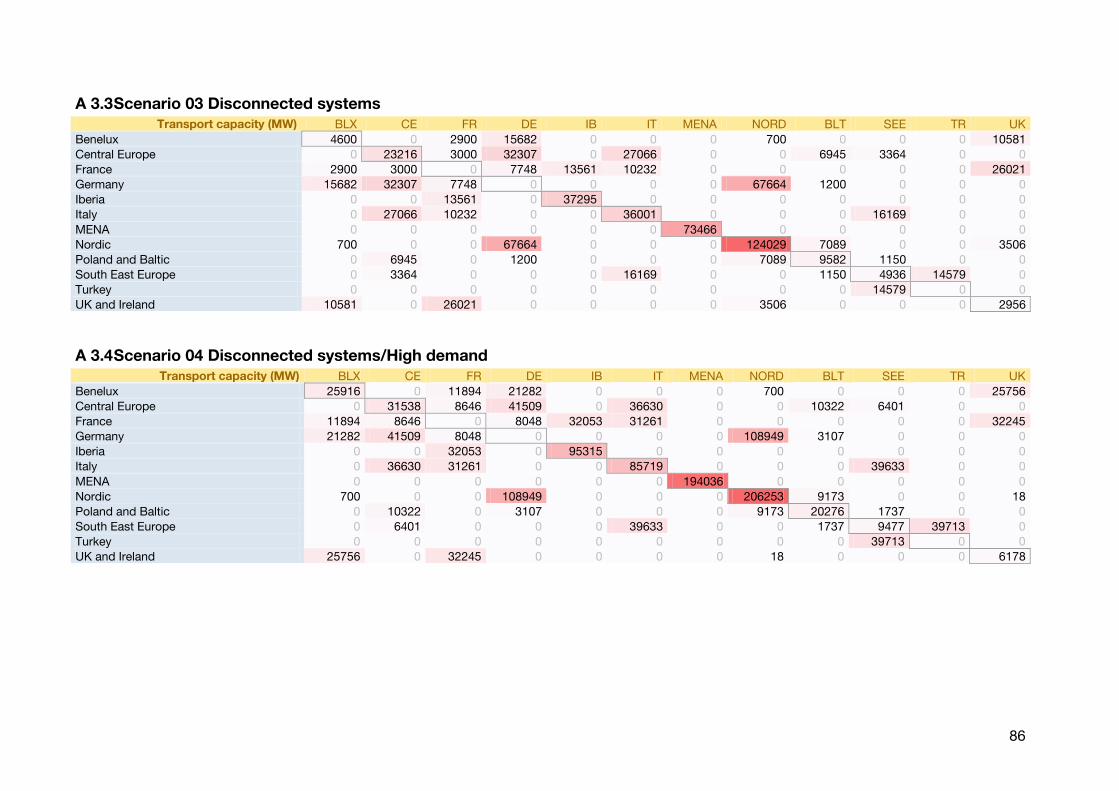
86

A 3.3 Scenario 03 Disconnected systems Transport capacity (MW) BLX CE FR DE IB IT MENA NORD BLT SEE TR UK

Benelux 4600 0 2900 15682 0 0 0 700 0 0 0 10581

Central Europe 0 23216 3000 32307 0 27066 0 0 6945 3364 0 0

France 2900 3000 0 7748 13561 10232 0 0 0 0 0 26021

Germany 15682 32307 7748 0 0 0 0 67664 1200 0 0 0

Iberia 0 0 13561 0 37295 0 0 0 0 0 0 0

Italy 0 27066 10232 0 0 36001 0 0 0 16169 0 0

MENA 0 0 0 0 0 0 73466 0 0 0 0 0

Nordic 700 0 0 67664 0 0 0 124029 7089 0 0 3506

Poland and Baltic 0 6945 0 1200 0 0 0 7089 9582 1150 0 0

South East Europe 0 3364 0 0 0 16169 0 0 1150 4936 14579 0

Turkey 0 0 0 0 0 0 0 0 0 14579 0 0

UK and Ireland 10581 0 26021 0 0 0 0 3506 0 0 0 2956

A 3.4 Scenario 04 Disconnected systems/High demand Transport capacity (MW) BLX CE FR DE IB IT MENA NORD BLT SEE TR UK

Benelux 25916 0 11894 21282 0 0 0 700 0 0 0 25756

Central Europe 0 31538 8646 41509 0 36630 0 0 10322 6401 0 0

France 11894 8646 0 8048 32053 31261 0 0 0 0 0 32245

Germany 21282 41509 8048 0 0 0 0 108949 3107 0 0 0

Iberia 0 0 32053 0 95315 0 0 0 0 0 0 0

Italy 0 36630 31261 0 0 85719 0 0 0 39633 0 0

MENA 0 0 0 0 0 0 194036 0 0 0 0 0

Nordic 700 0 0 108949 0 0 0 206253 9173 0 0 18

Poland and Baltic 0 10322 0 3107 0 0 0 9173 20276 1737 0 0

South East Europe 0 6401 0 0 0 39633 0 0 1737 9477 39713 0

Turkey 0 0 0 0 0 0 0 0 0 39713 0 0

UK and Ireland 25756 0 32245 0 0 0 0 18 0 0 0 6178

87

A 4. Capacity factors The following pages show normalized hourly time series derived from measured weather data from the year 2007. They are used as input data for

renewable energy power plants.

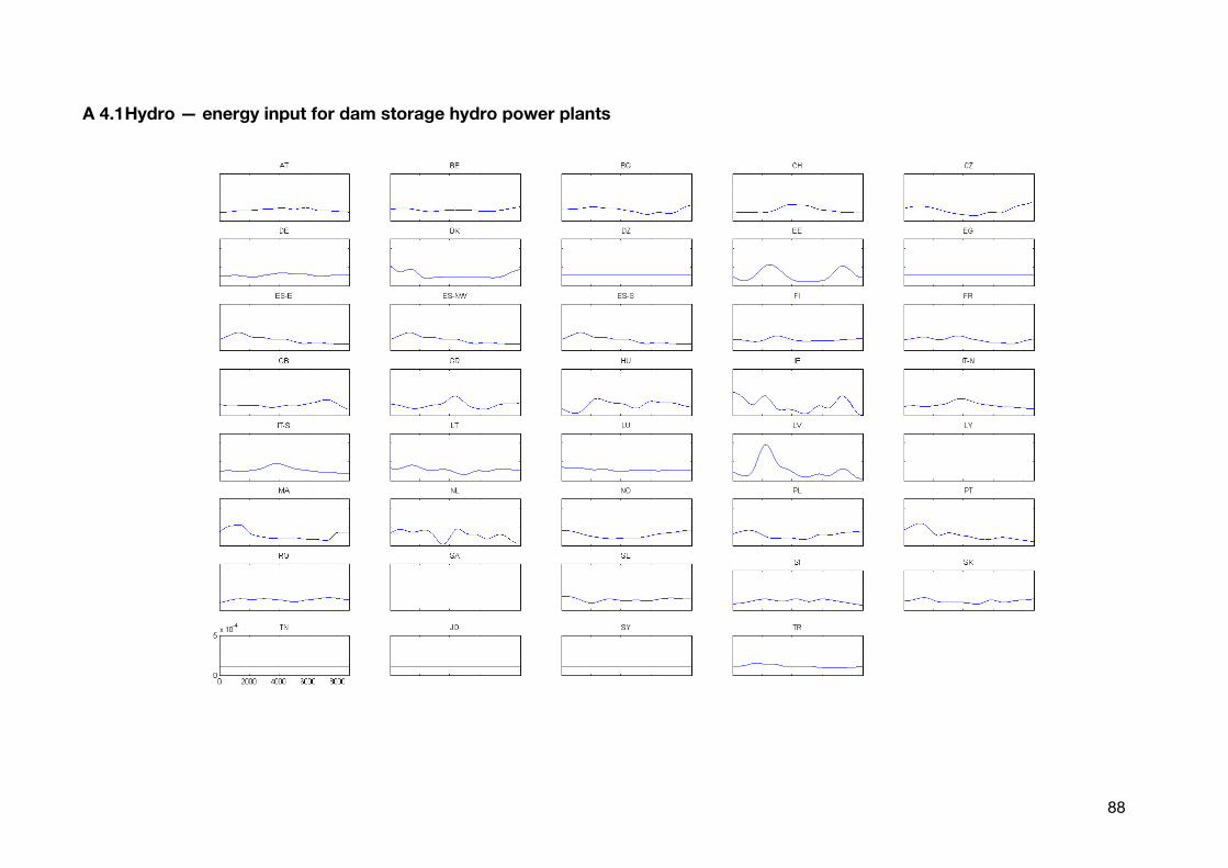
88

A 4.1 Hydro — energy input for dam storage hydro power plants

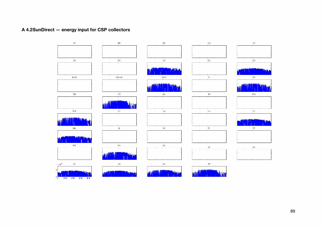
89

A 4.2 SunDirect — energy input for CSP collectors

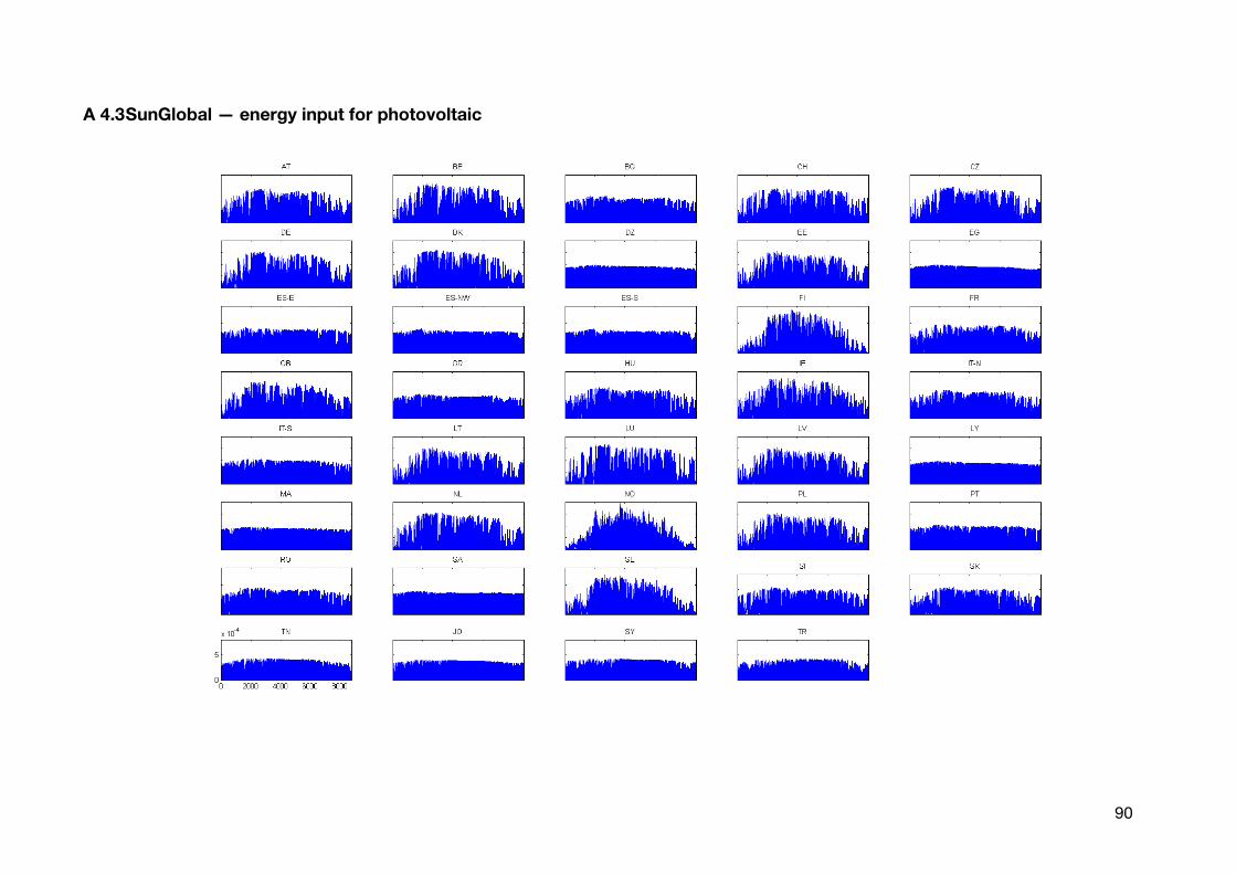
90

A 4.3 SunGlobal — energy input for photovoltaic

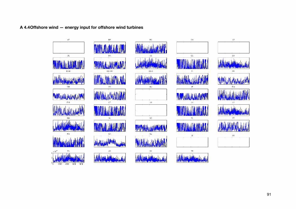
91

A 4.4 Offshore wind — energy input for offshore wind turbines

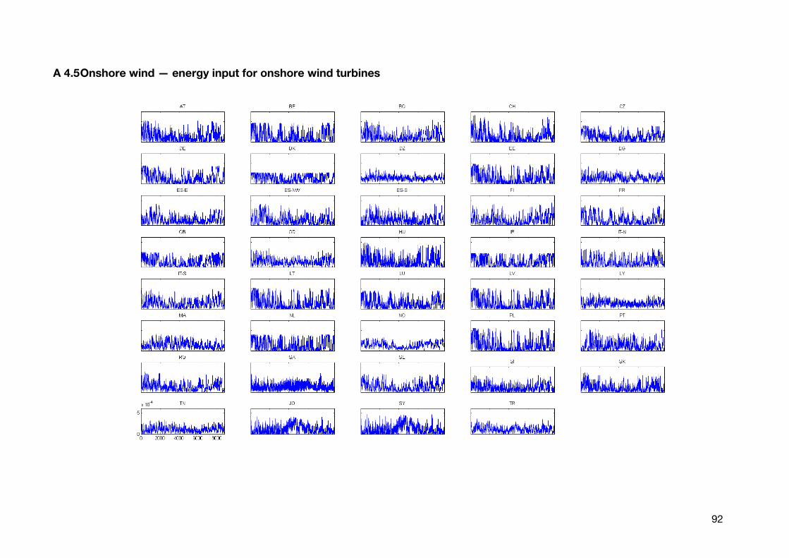
92

A 4.5 Onshore wind — energy input for onshore wind turbines