Essays on Industrial andSocietal Organization:

Certification, Variety andConcern for Face

Inauguraldissertationzur Erlangung des akademischen Grades

Doktor rerum politicarumder Technischen Universitat Dortmund

Yiquan Gu

August 2009

Supervisor: Prof. Wolfgang Leininger, Ph.D

Location: Dortmund

Faculty: Technische Universitat Dortmund

Wirtschafts- und Sozialwissenschaftliche Fakultat

Volkswirtschaftlehre (Mikrookonomie)

Candidate: Yiquan Gu, M.A.

Title: Essays on Industrial and Societal Organization: Cer-tification, Variety and Concern for Face

Date: August 19, 2009

Abstract

In this dissertation I report three doctoral research projects: the appli-cation of imperfect certification in markets with asymmetric information,the impact of elastic demand on market supplied product variety in dif-ferentiated product markets and a microeconomic analysis of gift givingwhen individuals are concerned with social approval (face). It consists ofsix chapters including a general introduction, four research papers and anoutlook for further projects.

Chapter 2 proposes a model for a certification market with an imperfecttesting technology. Such a technology only assures that whenever twoproducts are tested the higher quality product is more likely to pass thanthe lower quality one. When only one certifier with such testing technol-ogy is present in the market, it is found that this monopoly certifier canbe completely ignored in equilibrium, in contrast to the prediction of amodel with perfect testing technology. A separating equilibrium is alsosupported in which only relatively high quality types (products) choose topay for the certification service. It is true that in such an equilibrium hav-ing a certificate is better than not. The exact value of a certificate, however,depends both on the prior distribution of product quality and the natureof the testing technology. Welfare accounting shows that the monopolycertifier’s profit maximizing conduct can lead to under or over supplyof certification service depending on model specification. Socially opti-mal certification fee is always positive and such that it makes all positivetypes choose to test. In the case of two competing certifiers with identicaltesting technologies, the intuition of Bertrand competition does not neces-sarily hold. Segmentation equilibrium wherein higher seller types choosethe more expensive certification service and not so high types choose theless expensive service can be supported. As an application, we argue that

i

the fee differentiation between major and non-major auditing firms neednot be a result of any differences in their auditing technologies.

Chapter 3 revisits the excess entry theorem in spatial models a la Vickrey(1964) and Salop (1979) while relaxing the assumption of inelastic de-mand. Using a demand function with a constant demand elasticity, weshow that the number of firms that enter a market decreases with thedegree of demand elasticity. We find that the excess entry theorem doesonly hold when demand is sufficiently inelastic. Otherwise, there is in-sufficient entry. In the limiting case of unit elastic demand, the marketis monopolized. We point out when and how a public policy can be de-sirable and broaden our results with a more general transportation costfunction. Chapter 4 generalizes on Chapter 3. We introduce consumerswith a generic quasi-linear utility function in the framework of the Salop(1979) model. In addition to the results found in Chapter 3, we are able topin down conditions for efficient variety in entry cost and transportationcost. A proof for the existence and uniqueness of symmetric equilibriumwhen price elasticity of demand is increasing in price is also provided.

Chapter 5 studies further into the warm-glow that donors may benefit fromtheir act of giving. Within the framework of concern for social approval,we emphasize an individual’s relative position in social network and in-troduce the concept of face. When individuals are concerned with face, thewealthier will need to contribute more than the poorer in order to gain anequal level of social approval. In aggregate, other things being equal, themore individuals are concerned with face, the more they tend to donate.While this approach is proposed in the context of social acceptance, it isalso applicable in morally motivated situations.

ii

Publications and Presentations

Publications

Earlier versions of three chapters of this dissertation appeared in RuhrEconomic Papers series as Number 78 , 33 and 92. Chapter 3, “A Noteon the Excess Entry Theorem in Spatial Models with Elastic Demand”,coauthored with Tobias Wenzel, is now published in the InternationalJournal of Industrial Organization.1

Presentations

Presentations based on various chapters were given in the Brown Bag Sem-inar series in Dortmund from 2007 to 2009. The following is a summaryof various national and international conference presentations.

Imperfect Certification

The second chapter on “Imperfect Certification” was presented at

∙ the 7th Annual International Industrial Organization Conference inBoston, U.S.A. (2009),

∙ the 35th Annual Conference of the European Association for Re-search in Industrial Economics (EARIE) in Toulouse, France (2008),

∙ the XIII. Spring Meeting of Young Economists in Lille, France (2008),

∙ and the Doctoral Workshop on Game Theory in Konstanz (2008),

∙ and will be presented at the 2009 Econometric Society EuropeanMeeting (ESEM) in Barcelona, Spain.

1Gu and Wenzel (2009a) in the Bibliography

iii

A Note on the Excess Entry Theorem in Spatial Models with ElasticDemand

I presented the third chapter on “A Note on the Excess Entry Theorem inSpatial Models with Elastic Demand” at

∙ the Jahrestagung 2008 des Vereins fur Socialpolitik (VfS) in Graz,Austria (2008),

∙ and the All China Economics (ACE) International Conference inHong Kong, China (2007).

Product Variety, Price Elasticity of Demand and Fixed Cost in SpatialModels

I presented the forth chapter on “Product Variety, Price Elasticity of De-mand and Fixed Cost in Spatial Models” at

∙ the 2009 Econometric Society Australasian Meeting (ESAM) in Can-berra, Australia,

∙ and will present it at the 36th Annual Conference of the EuropeanAssociation for Research in Industrial Economics (EARIE) in Ljubl-jana, Slovenia (2009).

Gift Giving and Concern for Face

Finally, the fifth chapter on “Gift Giving and Concern for Face” was pre-sented at

∙ the PGPPE (Public Goods, Public Projects, Externalities) Workshopin Bonn (2008)

which was organized by the Max-Planck-Institut zur Erforschung vonGemeinschaftsgutern in Bonn.

iv

Acknowledgments

This dissertation is based on the research that I have undertaken whileholding a scholarship from the Ruhr Graduate School in Economics (RGS)and afterwards working as an assistant at the chair of microeconomic the-ory at the Technische Universitat Dortmund. I would like to acknowledgeboth institutions for providing excellent research environments and finan-cial support. I would also like to thank professors, colleagues and fellowstudents both in Essen and Dortmund who have offered me their valuableadvices, suggestions and comments.

In particular, I would like to take this opportunity to acknowledge the con-stant support I received from my supervisor, Professor Wolfgang Leininger,to whom my gratitude can never be adequately expressed by words. With-out his continuous encouragement and numerous pieces of constructiveadvice on earlier versions of my work, this dissertation would not havebeen possible.

I also benefited greatly from collaborations and discussions with manyfriends. Specifically, I would like to thank Tobias Wenzel with whom Iworked on two joint research papers on Product Differentiation. Overthe years when I studied and worked in Dortmund, discussions withJan Heufer on various research topics have always been both inspiringand entertaining. My thanks also go to Leilanie Basilio, Tobias Guse,Burkhard Hehenkamp and Stefanie Neimann who helped me on my workin different ways.

Finally, I would like to thank my parents for their understanding andsupport.

v

Contents

1 Introduction 1

1.1 Asymmetric information and imperfect certification . . . . . 1

1.2 Production differentiation and the excess entry theorem . . 5

1.3 Charitable giving and concern for face . . . . . . . . . . . . 9

2 Imperfect Certification 13

2.1 Introduction . . . . . . . . . . . . . . . . . . . . . . . . . . . . 13

2.2 Related literature . . . . . . . . . . . . . . . . . . . . . . . . . 16

2.3 The model . . . . . . . . . . . . . . . . . . . . . . . . . . . . . 18

2.4 Monopoly: bypassing . . . . . . . . . . . . . . . . . . . . . . 22

2.5 Monopoly: separating equilibrium . . . . . . . . . . . . . . . 24

2.6 Monopoly: market performance . . . . . . . . . . . . . . . . 30

2.7 Duopoly . . . . . . . . . . . . . . . . . . . . . . . . . . . . . . 38

2.8 Conclusion . . . . . . . . . . . . . . . . . . . . . . . . . . . . . 43

2.9 Appendix . . . . . . . . . . . . . . . . . . . . . . . . . . . . . 44

3 A Note on the Excess Entry Theorem in Spatial Models withElastic Demand 56

3.1 Introduction . . . . . . . . . . . . . . . . . . . . . . . . . . . . 56

3.2 The model . . . . . . . . . . . . . . . . . . . . . . . . . . . . . 58

vi

3.3 Analysis . . . . . . . . . . . . . . . . . . . . . . . . . . . . . . 61

3.4 Welfare . . . . . . . . . . . . . . . . . . . . . . . . . . . . . . . 64

3.5 Power transportation costs . . . . . . . . . . . . . . . . . . . . 66

3.6 Conclusion . . . . . . . . . . . . . . . . . . . . . . . . . . . . . 67

3.7 Appendix . . . . . . . . . . . . . . . . . . . . . . . . . . . . . 68

4 Product Variety, Price Elasticity of Demand and Fixed Cost inSpatial Models 70

4.1 Introduction . . . . . . . . . . . . . . . . . . . . . . . . . . . . 70

4.2 The model . . . . . . . . . . . . . . . . . . . . . . . . . . . . . 73

4.3 Analysis . . . . . . . . . . . . . . . . . . . . . . . . . . . . . . 77

4.4 Welfare . . . . . . . . . . . . . . . . . . . . . . . . . . . . . . . 82

4.5 Example . . . . . . . . . . . . . . . . . . . . . . . . . . . . . . 84

4.6 Conclusion . . . . . . . . . . . . . . . . . . . . . . . . . . . . . 85

4.7 Appendix . . . . . . . . . . . . . . . . . . . . . . . . . . . . . 86

5 Gift Giving and Concern for Face 93

5.1 Introduction . . . . . . . . . . . . . . . . . . . . . . . . . . . . 93

5.2 An economy with concern for face . . . . . . . . . . . . . . . 97

5.3 An extension with public policy . . . . . . . . . . . . . . . . 105

5.4 Concluding remarks . . . . . . . . . . . . . . . . . . . . . . . 108

6 Further Research 111

6.1 Capturable certifiers and umbrella branding . . . . . . . . . 111

6.2 Elastic demand in the Hotelling model and empirical inves-tigation of spatial models . . . . . . . . . . . . . . . . . . . . 112

6.3 An experimental investigation of concern for relative socialapproval (face): a research proposal . . . . . . . . . . . . . . 113

vii

Bibliography 116

viii

Chapter 1

Introduction

This dissertation centers on three research topics: the application of im-perfect certification in markets with asymmetric information, the impactof elastic demand on market supplied product variety in differentiatedproduct markets and a microeconomic analysis of gift giving when indi-viduals are concerned with social approval.

1.1 Asymmetric information and imperfect certifica-tion

1.1.1 Asymmetric information and information intermediaries

The problem of asymmetric information in product quality was first brou-ght to attention by George Akerlof (1970)’s classic paper of “The Marketfor ‘Lemons’ ”. Since then this topic has grown into a large literature ineconomics.1 Akerlof’s paper points out that when buyers have less knowl-edge of product quality than sellers do, for example in a used car market,because buyers are only willing to pay up to the value of the expectedquality of a product, sellers of high quality (reservation price) will opt outfrom trading. Following this logic, in the end only low quality products

1According to Wikipedia, this paper has been citied more than 4,800 times in academicpapers as of October 2008. This data was retrieved from Google Scholar search on October24, 2008.

1

will remain in the market and if no one finds low quality products thatare worth buying, the market then breaks down.

This phenomenon at that time posed an enormous challenge to the classictheory of general equilibrium which assumes full information and per-fect competition. Subsequent periods have therefore witnessed a changeof style in which researches in economics are conducted: more papersstarted looking at specific markets at hand. Observing that to varyingextents information asymmetry exists in virtually every market yet mar-kets are still functioning, several explanations have been suggested in theliterature. There are models that allow sellers to signal product qualityvia price, to build reputation in the long run, to provide quality insurancethrough warranty, etc. Some others feature intermediaries. Particularly re-lated to Chapter 2 are information intermediaries. In this type of models,product quality in principle can be tested by a third party possibly withcosts. Depending on market characteristics, quality testing may mitigateinformation asymmetry and improve market efficiency.

1.1.2 Perfect and imperfect certification

Several papers have studied markets with the presence of informationintermediaries, specifically, certifiers.2 Many of them, however, do notinvestigate certifiers’ behavior. For instance, they are modeled as a publicauthority providing quality tests for free. Such tests, however, can beand in many cases are provided by private organizations. Therefore, theinvestigation of certifiers’ incentives and conducts and the efficiency ofboth product and certification markets will be the theme of Chapter 2. Themodel that I am proposing is based on Lizzeri (1999). The difference and acontribution of my work is the modeling of imperfect testing technologies.Previous literature on strategic certifiers has been mainly interested incertifiers with perfect testing technologies. However, tests that are proneto mistakes are not only more realistic but also have consequential impactson certifiers and market performance.

With respect to the nature of certification results, I assume that a productcan either be certified or not. This is a simplification of the observationthat real life certification outcomes are normally discrete signals. Product

2A detailed literature review is provided in Chapter 2.

2

quality, however, more often takes a value from a continuous interval. Animperfect testing technology in this model is proposed in a way such thatit approves a higher quality product with a higher probability. It capturesthe idea that certifiers with certain abilities or experiences in differenti-ating product quality inevitably make honest but poor judgments. Thestrategic aspect of imperfect certification comes in when certifiers try toset a profit maximizing certification fee. Therefore, in the model there isan endogenous price formation for both the product and the certificationservice.

If we maintained everything in Chapter 2’s model except that certifiersare assumed to have access to a perfect testing technology, i.e. they areable to know the exact quality of a tested product, a summary of marketoutcome would be as follows: In the monopoly certification service case,the certifier only certifies products of positive qualities and charges a priceequal to the expected value of a certified product. Since buyers are payingthe same expected value to the sellers, the certifier, by exerting its powerof monopoly and ability of perfect testing, is able to obtain the entiresurplus generated in the product market and leave sellers and buyersindifferent between trading and not trading. This result is completelyreverted when there are more than one certifier in the certification servicemarket. Competition between certifiers will drive market certification feeto the marginal cost of testing or zero in this model. In the end, allpositive quality products get traded and sellers now enjoy the surplusfrom product trading.

1.1.3 Main results in imperfect certification

Results when imperfect testing is introduced are no longer as extremeas in the case of perfect testing. The main message from Chapter 2 isthat a little noise in the testing technology changes the certifier’s behaviordramatically. Starting from a technology that only assures whenever twoproducts are tested, the higher quality product is more likely to passthan the lower quality one, it is found that a monopoly certifier can becompletely ignored in equilibrium, in contrast to the enormous power aperfect testing technology monopoly certifier has. It is also shown that aseparating equilibrium is supported wherein only relatively high quality

3

types (products) choose to pay for the certification service. Hence, suchan imperfect testing technology can be useful in reducing informationasymmetry.

It is true that in a separating equilibrium having a certificate is better thannot. The exact value of a certificate, however, depends both on the priordistribution of product quality and the nature of the testing technology.With respect to market efficiency, analysis shows that the monopolisticcertifier’s profit maximizing conduct may lead to under- or oversupply ofcertification service depending on model specification. A socially optimalcertification fee is always positive and such that it makes all positive typeschoose to test.

In the case of two competing certifiers with identical testing technologies,the intuition of Bertrand competition does not necessarily hold. A seg-mentation equilibrium is found wherein higher seller types choose themore expensive certification service and not so high types choose the lessexpensive service can be supported. Finally, we apply this finding to thefinancial auditing industry and argue that the fee differentiation betweenmajor and non-major auditing firms need not be a result of any differencesin their auditing technologies. Our theoretical model sheds light on thepuzzle that quality difference in auditing services between high fee firmsand others is hard to identify empirically.

The model provided in Chapter 2 is fairly general yet it nevertheless leadsus to several concrete predictions. Arguably every test is imperfect andit is realistic that anyone who looks at a quality certificate would havedoubts about the accuracy of the signal and sometimes even have a hardtime in understanding what such a certificate means. By constructing sucha model, I would like to emphasize the power of strategic thinking andequilibrium analysis. By putting themselves in sellers’ shoes, consumersknow in a separating equilibrium that it does not pay for low qualityproducts to be tested. Therefore, a possibility of an imperfect certificationwill at least exclude the really bad quality products. Certifiers, however,understand that they need to keep certification price high to deter lowquality products yet are aware of the negative impact of a high price,i.e. a low demand for certification service. Hence, only in equilibriumwill consumers and indeed certifiers have a refined knowledge of product

4

quality. It is my hope that my model will help us understand more abouthow tests that do not provide clear cut results and are prone to mistakeshave such a widespread use in real life. Its prediction in the duopoly caseis surprising yet reasonable. It offers a new perspective when we look atthe certification industry.

1.2 Production differentiation and the excess entrytheorem

1.2.1 Production differentiation

Equally important as market provided product quality is product variety.Products that serve a common purpose can be very different in details.3

In general, differentiated products are provided in the market as a resultof producers catering to consumers with heterogeneous preferences. Forexample, in the automobile market, two cars can be identical except one isblack and the other is red. Some consumers like the black car better thanthe red one. Others have the opposite preference. There are, however,many more colors in the color spectrum that some consumers may findpreferable to both black and red. A natural question to ask is how manydifferent colors (varieties) the market will provide. What are the mostimportant parameters that determine the market provided level of variety?And of classic economic interests is to compare this level to the sociallyefficient benchmark of product differentiation.

To answer the above questions and many more, three different modelingapproaches have been suggested in the literature. There are representa-tive consumer models by Spence (1976) and Dixit and Stiglitz (1977), anddiscrete choice models by Anderson, de Palma, and Thisse (1989). Theformer relies on a representative consumer whose utility function encom-passes all provided varieties. The latter takes a viewpoint of the producersand model consumer choice of differentiated products as a random pro-cess. With respect to the above mentioned questions, both approachespin down several variables including variables related to consumer pref-

3Commonly accepted in competition policy literature is that whether two productsbelong to a single market is an empirical question of cross product price elasticities. Inthis thesis, we follow the more traditional theoretical approach of product differentiation.

5

erences and production costs. As expected, both market provided varietyand socially optimal level depend on model parameters and in generaleither of these two may take a higher level.

There is another widely used approach of product differentiation with aneven longer history. Originally as a remedy to the instability of Bertrandprice competition, Hotelling (1929) first suggested a model with two firmslocated in different positions on a line where consumers are uniformly dis-tributed. Because almost all consumers have to incur transportation costswhen purchasing a product, a slight price variation only translates intoa small demand variation faced by the firms. As exemplified by manysubsequent papers, physical locations and transportation costs can be in-terpreted as product characteristics and disutilities in consuming a lesspreferred variety. In this sense, chocolates with different cacao levels canbe seen as if they are located at different locations along the line betweenthe lowest and highest cacao levels. Consumers may have different pref-erences over chocolates with different cacao levels and consuming a lessfavorite level incurs some disutility in taste.4 This approach is known aslocation or address models.

In his 1979 article, Salop presented the ingenious idea of transforming theunit Hotelling line into a unit circle to avoid boundary complexities. Thisframework quickly found its power in analyzing firms’ entry decisions, atopic the original Hotelling model finds difficult to address. In this model,the basic ingredients of the Hotelling model remain except when there aremore than two firms in the market, firms located closest to the two endsof the Hotelling line are now in principle no more different than any otherfirms. If we look at a Salop circle with uniformly distributed consumersand equidistantly located single variety firms, for a given number of firms,we can calculate their profits in the price equilibrium. A firm then onlyenters if the profit it expects to earn outweighs its cost of entry. Applyingzero profit condition under free entry, we will then have an endogenousmarket provided level of product variety.

4Here, an important assumption with respect to consumer preference is its unimod-ularity. That is, if a consumer has his most preferred variety at location xm, then to theleft of xm he prefers x2 over x1 as long as x1 < x2 < xm and to the right of xm he prefersx3 over x4 as long as xm < x3 < x4.

6

1.2.2 The excess entry theorem

Determinants of the market level of product variety are the parametersthat represent consumer disutility in consuming a less preferred variety,also known as the transportation cost, and firms’ entry cost, commonlymodeled as the fixed cost of establishing a new business. As the onlytwo major exogenous parameters in the original Salop model, the sociallyefficient level of product variety depends only on consumer transportationcost and the fixed cost of entry. As shown in Tirole (1988), in this modelmarket provided product variety is always larger than the socially efficientlevel. In other words, there is always an excess of entry into the market.A similar point was raised by Vickrey (1964). The intuition of this resultis that competition between firms are localized and firms will not stopentering until even with their local monopoly power they can only makea profit just to cover their fixed cost of entry. This also explains why theother two approaches are able to produce insufficient entry as in thesemodels competition is global.5

Several papers have checked the robustness of this excess entry theorem.Already shown in Anderson, de Palma, and Thisse (1992) is that the excessentry result is quite robust against different functional forms of the trans-portation cost. For example, it holds under power transportation cost.With respect to the production cost, Matsumura and Okamura (2006) findthe result holds for quite general cost structures. Given its robustness,it seems that if a researcher decides to use a Salop model, he/she also“decides” that there is excess entry. Are spatial models then incapable ofconducting welfare analyses?

1.2.3 Elastic demand in spatial models

Chapter 3 and 4, coauthored with Tobias Wenzel, weigh in on this longestablished theorem of excess entry. We argue that it is inadequate torepresent consumer preferences only by transportation costs, a seeminglytrivial point. By focusing only on transportation cost, one assumes eachconsumer only demands a fixed amount of the differentiated product, nomatter what the price is. But for many products, consumer demanded

5See, for instance, Anderson and de Palma (2000).

7

quantity responses to price changes, hence, demand is generally elastic.6

Examples include chocolates, beer and many other consumer products.Therefore, we revisit the classic spatial model by introducing elastic con-sumer demand. The main impact of elastic demand is on market compe-tition of firms, that is, on their pricing behavior. In turn, it impacts onfirms’ profits and ultimately their entry decisions.

To implement this idea, in chapter 3 we first propose a demand functionwith constant elasticity. This allows us to bring in one more parameterinto the model in a tractable manner. With elastic demand, when firmschoose their product price, they not only compete for a larger marketshare but also have to consider their own customers’ individual demands.A low price then increases both a firm’s market share and its customers’individual demands. We found that in the price equilibrium of any givennumber of competing firms, each firm makes a lower profit than it wouldhave under inelastic demand. Hence under free entry, there are less firmsin the market. Indeed, the higher the demand elasticity is, the lower theequilibrium number of firms in the market. However, since the sociallyoptimal number of firms under the first best benchmark is independent ofprice elasticity, it remains unchanged.7 In consequence, it is shown thatthere exists a threshold level of demand elasticity below which there isexcess entry in the market while above which there is insufficient entry.When the demand elasticity approaches zero, we then of course go backto the classic Salop model and as expected there is always excess entry.

We believe that the insight in chapter 3 also applies in much more generalcases. Constant elasticity is a very unrealistic and restrictive assumptionand, in principle, demand elasticity should be found in price equilibria forgeneral demand functions. Thus, we are interested in finding out whatreally determines market entry without assuming an exogenously givendemand elasticity. Chapter 4 does exactly that. We start with a very gen-eral demand function and identify price equilibrium demand elasticity

6For lacking of a better term, by “elastic” we mean consumer demand varies in productprice instead of being fixed. We are aware that commonly in industrial organizationliterature, a level of demand is called elastic if the demand elasticity evaluated at thislevel is found to be larger than 1 and inelastic when it is less than 1.

7Under first best benchmark, the optimal level of entry is found when a regulatorcan also control product price besides the number of firms. We also do a second bestbenchmark comparison in which the regulator can only control market entry leavingproduct price endogenously determined in a price equilibrium.

8

and the associated firms’ profits by implicit functions. We then pin downthe endogenous equilibrium number of firms under free entry by trans-portation cost and fixed cost. We show that there are cases in which whenthe fixed cost is low enough there is excess entry and when high enoughthere is insufficient entry. Reformulated in terms of transportation cost,there is excess entry when it is high enough and insufficient entry whenit is low enough. These results are quite intuitive but previously eludedresearchers.

As we have shown, once elastic demand is considered, market entry ormarket provided product varieties can be either excessive or insufficient,depending on model parameters. This finding closes the gap betweenspatial models and the other two approaches in the literature of productdifferentiation when efficient level variety is considered. Our model inchapter 4 also provides a framework for researchers in search of a spatialmodel suitable for the market at hand and who would like to investigatewelfare issues. As we notice in the literature, the traditional Salop modelis used in several welfare analyses, we would like to call for more attentionto consumer demand structure before such analyses are carried out.8

1.3 Charitable giving and concern for face

1.3.1 Motivations of charitable giving

Departing from topics in industrial economics, Chapter 5 covers a subjectthat has relevance both in economics and sociology: charitable giving.There are several theories offered in the economics literature on volun-tary contribution to charities. When charity is viewed as a public good,some individuals may have a preference on the level of the good thatis provided. As long as the amount of provided public good remainsunchanged, they may not care who contributes how much. Along withthis pure altruism theory, there is the impure altruism theory in whichindividuals also care about whether he himself has contributed or not.Within this impure altruism theory, a distinction of “prestige benefit” ver-sus “intrinsic benefit” of one’s own act of giving, based on whether such

8Reference to previous welfare analyses in spatial models is given in chapter 4.

9

an act is visible to others or not, has been proposed in recent works. In-tuitively, if one is after the “prestige benefit”, other individuals shouldat least be able to know about his donation. If visibility does not matterfor a donor, then the motivation behind his impure altruistic behavior ismore likely to be the “intrinsic benefit” from donating. Various empiricalfindings based on statical, survey or experiment data have supported thehypothesis of impure altruism, although most of them do not differentiatebetween “prestige benefit” and “intrinsic benefit”. A more comprehensiveliterature review is provided in the introduction section of chapter 5.

Although most researchers agree that individuals’ enjoyment of “joy ofgiving” is an important incentive to make voluntary donations, the na-ture of this “joy” or “warm glow” is relatively underinvestigated. UsingMRI scans of subjects’ brains, Harbaugh, Mayr, and Burghart (2007) findthat voluntary financial transfers to public goods increase neural activi-ties in areas linked to reward processing. Compared to a consumptionof a physical good, there is less understanding of such a consumption of“voluntary donation” that triggers reward process in a brain. More likely,this reward process is influenced by many more factors than a rewardprocess triggered by a consumption of gourmet food or narcotics. Manyof these factors are very subjective. What is the minimal level of dona-tion that would trigger such a process? By how much more donation acertain measure of such activity in a brain will be increased? How aboutinformation? Will we observe a higher level of activity when the subjectis told he is the most generous donor than otherwise?

1.3.2 Concern for face

Chapter 5 presents a theory of how different donations are translated intoindividual utilities and gives predictions on human behavior based onequilibrium analysis. I introduce the concept of “face” from sociology lit-erature which, in economics terms, is a case of interdependent preference.Each individual according to his ranking of wealth occupies a relativeposition in his social network. At a given position, the more he donatesthe more he enjoys “joy of giving”. A key point is, nominal donationsfrom different positions have different “exchange rates” or “prices” forsubjective hedonic enjoyment. The same amount of donation by a poor

10

individual gives him a higher level of “reward” than it gives a wealthyperson. Presumably, neural activities in a brain is influenced by this per-son’s information of own wealth. Another important point is that sucha production of “joy of giving” is also interdependent. When others aredonating generously, the same amount of donation gives an individual ata given position less enjoyment than when others’ donations are smaller.This idea is represented by an average donation/income ratio which isdetermined in equilibrium. In summary, in a model of individuals withconcern for face, the average donation/income ratio functions as a refer-ence point but is adjusted by individuals’ relative positions in the socialnetwork. In equilibrium, richer individuals donate more in terms of abso-lute amount and have higher donation/income ratio since they are alreadyexpected to donate more.

The negative externality of one individual’s donation to others’ enjoymentof “warm glow” was studied in Glazer and Konrad (1996) in a signalingmodel in which a higher donation level can be seen as a signal of higherincome in equilibrium. Therefore, when others are donating generously,a rich individual needs to donate even more to signal his income. Inthe current model, externality comes from individuals’ concern for face.When others are donating more, it will make one look bad or lose face.This negative externality explains the model predictions on governmentsubsidy for donation expenses, for instance via a tax refund. It is foundin chapter 5 a government subsidy will increase the aggregate amount ofdonation more than the cost to the government. In this case, real cost ofdonation for individuals decreases so every one donates more. But higherindividual donation also generates negative externalities to others and inthe end every one donates much more. Individuals will also have a lowerutility level because of a much lower level of other consumptions. Bya similar reasoning, government tax of individual donation will increasetheir utility.9

Chapter 5 is a new explanation of charitable giving with a special intereston the interactions of individual giving. With a few exceptions, the liter-ature so far is mainly interested in modeling, theorizing, confirming and

9In the model, individual utilities from aggregate supply of donated public goods areabsent. Therefore, these results with respect to public policies should be interpreted withcaution.

11

estimating the “demand” for “warm glow”. My model attempts to pro-vide us with a better understanding of the “supply” side of “warm glow”,hence to have a better understanding of individuals’ charitable behavior.

After the above introduced chapters, this thesis concludes with a chapteron an outlook for future research projects.

12

Chapter 2

Imperfect Certification

2.1 Introduction

Consider a market in which sellers know more about product qualitythan buyers do as in Akerlof (1970). It is well understood that seriousconsequences including market breakdown may result from informationasymmetry in this fashion. Other than building up reputation (Klein andLeffler, 1981) and providing warranty (Grossman, 1981), sellers sometimesresort to third-party intermediaries. This chapter studies such marketsfeaturing one type of pure information intermediaries known as certi-fiers.1 By using a testing technology certifiers normally are able to assessthe quality of tested products. After the assessment, a certifier decideswhether to grant the tested product a certificate. With the additionalinformation of a product’s certification status, buyers should then knowmore about its quality. Examples of such certification services are numer-ous. Laboratories test and certify consumer products; credit rating agen-cies assign credit ratings to issuers of debt obligations; universities issuediploma to students who meet their graduation criteria; educational test-ing services carry out tests evaluating testees’ scholastic aptitudes;2 many

1Intermediaries who buy and sell products may also improve buyers’ information onproduct quality. This point is studied in Biglaiser (1993) and Biglaiser and Friedman(1994).

2The Educational Testing Service (ETS) is, of course, one of such institutions.

13

software solution companies also run certification programs of technicalexpertise through which job applicants can obtain relevant credentials.3

In studies of certification markets, more significantly so in those withstrategic certifiers, it is often assumed that a perfect testing technology isavailable to the certifiers. That is, they are able to know the exact qualityof each tested product without a single mistake. Though this simplifica-tion is helpful to many other research topics, it is of both practical andtheoretical interest to see how certifiers set prices and how markets per-form when testing technologies are imperfect. Justifications for imperfect-ness in testing technologies are as many as the applications. Laboratoriesmake honest mistakes in certifying consumer products; credit rating agen-cies only have imperfect knowledge about debt issuers’ credit worthiness;there are cases that students fail to graduate because of non-productivityrelated factors; and luck plays a role in any expertise certification process.Yet, real life experiences indicate that those certification services are help-ful in reducing information asymmetry. For example, a university degreeusually is a good signal of a worker’s ability although some students mayhave obtained their degrees just out of luck and some high ability studentsfailed to graduate.

Many certification services are imperfect but effective in differentiatingproducts of different qualities. This chapter attempts to model such cer-tification technologies in a general way. Our main assumption is the fol-lowing: tested by such a technology, a product may or may not pass butfor any two products the higher quality one has a higher probability thanthe lower quality one to pass. In the context of education, it amountsto say that a student may or may not graduate from a university but forany two students the one of the higher ability is more likely to succeedin earning a diploma than the other. As shown in the following, whenutilized, such a testing technology is sufficient to render a certificationservice informative although only to a limited extent.

3Currently Microsoft runs four such certification programs: Microsoft Certified Tech-nology Specialist (MCTS), Professional Developer (MCPD), IT Professional (MCITP) andArchitect (MAC). Many other software companies such as Sun, Cisco, Oracle, etc., providetheir own certification service.

14

2.1.1 Main results

The deviation from perfect certification generates new results. For ex-ample, a monopoly certifier with an imperfect technology can now becompletely ignored, in contrast to the prediction of a model with perfecttesting technology. A certificate is informative in a separating equilibriumin which only relatively high quality types (products) choose to pay forthe certification service. Though having a certificate is preferable, the ex-act value of a certificate depends both on the product quality distributionand the nature of the testing technology. Welfare accounting shows thatthe monopolistic certifier’s profit maximizing conduct can lead to underor over supply of certification service depending on model specification.Optimal certification fee is always positive and such that it makes all pos-itive types choose to test.

In the duopoly case, the intuition of Bertrand competition between twoidentical suppliers (of certificates) need not hold. Facing two certifierswith identical but imperfect testing technologies, higher seller types maychoose the certifier who charges the higher fee and not so high typeschoose the other. In such a segmentation equilibrium, neither the lowerfee certifier nor the higher fee one monopolizes the entire market of test-ing. Moreover, lowering one’s certification fee does not necessarily gen-erate a higher demand nor a higher profit. This observation suggests thepossibility of positive profits for both certifiers even when their testingtechnologies are essentially identical. Consequently, competition need notdrive the certification fee to zero which would be the case if both certifiershad perfect testing technologies (see Lizzeri 1999). Applied to the case offinancial auditing services, we cannot rule out the possibility that auditorscharging vastly different fees may have similar auditing abilities.

The rest of the chapter is organized as follows. Section 2.2 reviews therelated literature and section 2.3 sets up the model. Section 2.4, 2.5 and 2.6investigate the monopoly case and section 2.7 the duopoly case. Section2.8 concludes. All proofs are relegated to the Appendix.

15

2.2 Related literature

There are a few studies of strategic certifiers, but mostly with perfect test-ing technologies. Lizzeri (1999) builds up a canonical model of certifiersupon which our model is constructed. In that paper the model is used tostudy certifiers’ strategic behavior in information revelation assuming thatthey are able to know the exact value of every tested product’s quality.Based on a similar model, Albano and Lizzeri (2001) investigate sellers’incentive in quality provision when the possibility of certification is avail-able and the certifier may reveal the quality information in a strategic way.Strausz (2005) studies another important aspect of certification service,namely the credibility of certifiers. Our model on the other hand, focuseson certifier’s testing technology. We propose a general representation ofimperfect testing technology that only requires a few basic assumptions.By constructing our model on Lizzeri (1999)’s perfect testing model, we’llbe able to do a direct comparison of respective results and highlight theimplication of imperfectness in testing technologies.4

Imperfect testing technology is studied in some other papers of certifica-tion markets. In this strand of literature, however, certifiers do not strate-gically set their prices and there are normally only two possible levels ofproduct quality, either high or low. These papers include, for example,Heinkel (1981), De and Nabar (1991), and Mason and Sterbenz (1994).Heinkel (1981) investigates sellers’ incentive in improving product qualityin a setup with exogenously provided imperfect tests. Mason and Ster-benz (1994) analyze how imperfect test affects market size. Compared toDe and Nabar’s (1991) paper, which like ours also studies the equilibriaof certification markets with imperfect testing technologies, we introducestrategic certifiers and allow product quality to be drawn from a contin-uous interval. A shortcoming of limiting quality space to a binary set inmodeling imperfect certification is that in an information-revealing sepa-rating equilibrium the testing technology becomes “perfect”.

Hvide (2005) models strategic certifiers and introduces a zero-mean, nor-mally distributed error term into testing technology. When a product istested by this technology, a certifier observes the sum of its true quality

4It has to be noted that in this chapter we are mainly interested in testing technologies.We do not model certifier’s strategic behavior in information revelation.

16

and the realization of a white noise. If this reading exceeds the certifier’spassing score, the tested product will be awarded a certificate. Modeledin this way, as it is in Hvide (2005), for any given passing score sucha technology exhibits the property of our approach, namely, the higherthe tested product quality is, the more likely it passes. This “measure-ment error” approach hence amounts to a special case of our modeling ofimperfect testing technology.5

In a setting of rating agencies, Boom (2001) assumes an investment project’sprobability of getting a favorable rating is the same as its success prob-ability.6 With this rating technology, she shows that in a market witha monopolistic rating agency there can be over or under supply of rat-ing services compared to the socially optimal level. Though differing indetails, our work shows that both market provision and socially optimallevel of certification service depend on product quality distribution andthe testing technology; we also establish a necessary condition for mar-ket equilibrium to be socially optimal and show that when this conditionis not satisfied market either undersupplies or oversupplies certificationservice depending on model specification.

To explain the significant fee differentiation between major and non-majorauditing firms in financial service market, Hvide (2005) argues major au-diting firms adopt stricter test standards (higher passing scores in the“measurement error” approach) than non-major auditing firms. With thehelp of the stricter standards, major auditing firms are then able to chargehigher auditing fees and make higher profits. In this chapter we providean alternative explanation. In our model, we need not assume differencesin their auditing processes. Even with identical standards, i.e., identicaltests, Bertrand Competition need not happen and segmentation equilib-rium may be supported in which firms charge different prices.

5Note that the reading gives the expected quality of the tested product. The certifiershave incentive to reveal more information than just the certificate. For instance, revealingthe reading itself can attract testees. In our current model, however, this information isnot available to the certifiers.

6It will become clear in the following that this is also a special case of our modelingof imperfect testing technology, namely G(t) = t. See Equation (2.1) in Section 2.3.

17

2.3 The model

Following the setup of Lizzeri (1999), we analyze the market situation asa non-cooperative game with incomplete information.

2.3.1 Players

We have four players in the model, one seller, one certifier and two buyers.The seller wants to sell a product to the buyers. The product has a valueequal to its quality t (type) to both of the buyers but is worth nothingto the seller and the certifier. The type t is originally only known to theseller; the buyers and the certifier, however, know the prior distribution oft represented by cumulative distribution function, F(t). F(t) is assumedto be continuous, differentiable and strictly increasing on interval [a, b],where a < 0 < b.7 The associated density function is denoted f (t). Theseller has the possibility to get the product tested by the certifier.

The certifier has a testing technology. When it is used to test the product,it prints out a certificate (C) with probability

Pr(C ∣ t) = G(t), (2.1)

conditional on t. G(t) is also assumed to be continuous, differentiable andstrictly increasing on [a, b] with first derivative denoted g(t). Tested bythis technology, the higher a product’s quality is the higher its probabilityof receiving a certificate will be. Naturally the probability of no certificate(NC) is Pr(NC ∣ t) = 1 − G(t). This setup requires function G(t) tobe bounded below by 0 and above by 1. For convenience, we assumeG(a) = 0 and G(b) = 1, i.e., it is not possible for the lowest type to passthe test while the highest type always passes when tested.8 It is alsoassumed that the certifier does not manipulate the test result producedby the technology. The certifier can charge a certification fee P for the testand the cost associated with testing is normalized to zero.

Both buyers observe whether a product possesses a certificate or not andbid simultaneously based on their beliefs. They, however, cannot distin-

7When product quality is negative, consumption of such goods harms the buyers.8This assumption does not change our results qualitatively.

18

guish the event that the product was not tested from the event that theproduct failed the test. That is, they observe if a product has a certificate,θ : θ ∈ C, NC, but not what the seller did.

2.3.2 Timing

Stage 1 The certifier announces its certification fee, P, for the test.

Stage 2 At the beginning, the seller learns his type t (chosen by natureaccording to F(⋅)) and the announced certification fee, P; the sellerthen decides whether or not to get the product tested by paying thecertifier the certification fee.

Stage 3 If the seller chooses to test, then the certifier employs the testingtechnology and the seller receives a certificate with probability G(t),receives no certificate with probability 1− G(t).

Stage 4 Both buyers observe P and if the product has a certificate or not.

Stage 5 Buyers bid independently and simultaneously for the product.The product is sold to the buyer who bids higher than the other atthe price of the winning bid. Buyers get the product equally likelyin case of a tie. When both bids are zero, the product is not sold.

2.3.3 Strategies

The certifier’s strategy is simply the choice of certification fee, P ∈ R+.

The seller’s strategy specifies his decision for all combinations of ownquality type and certification fee level. Namely, it is a functionρ(P, t), from R+ × [a, b] to TS, NTS, that maps the vector (P, t)into a set of two elements, to test or not to test.

A strategy for a buyer is a function β(P, θ), from R+ × C, NC to R+,

that maps the announced certification fee and the product’s certifi-cation status to a bid for that product. Buyers’ beliefs are denoted byµ(t ∣ C, P) for a certified product and µ(t ∣ NC, P) for a non-certifiedproduct. Since buyers have identical information, when beliefs areBayesian updatable they are identical. Note that competition will

19

make them both bid up to their common belief. Therefore, no sub-scripts are used for individual buyers.

2.3.4 Payoffs

All players are assumed to be risk neutral. Hence, they maximize theirpayoffs in expected terms.

A buyer’s payoff function, in the following three types of outcomes, reads

U(t, β) =

⎧⎨⎩t− β(P, NC) when the buyer gets a non-certified product,

t− β(P, C) when the buyer gets a certified product,

0 when the buyer does not get the product.

The seller receives buyers’ bids for a non-certified product when theproduct is not tested. If the seller chooses to test, he has a prob-ability of G(t) getting a certificate and receiving buyers’ bids fora certified product. In other cases (1− G(t)), he does not get thecertificate and receives bids for a non-certified product. Taking thecertification fee into account, the seller’s payoff is

V(ρ, t, P, β) =

⎧⎨⎩ β(P, NC) not to test,

[1− G(t)]β(P, NC) + G(t)β(P, C)− P to test.

The certifier’s payoff is the product of the certification fee and the de-mand for the certification service, i.e.,

Π(P, ρ) = P ⋅ Pr(the event that the seller tests),

orΠ(P, ρ) = P ⋅

∫T

dF(t), where T = t ∣ ρ(P, t) = TS.

2.3.5 Equilibrium notion

The equilibrium notion employed in this chapter is Perfect Bayesian Equi-librium. As we argued before competition between the buyers will force

20

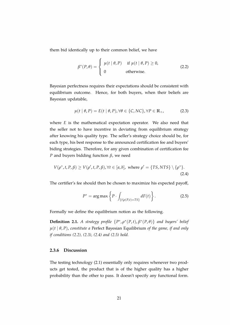
them bid identically up to their common belief, we have

β∗(P, θ) =

⎧⎨⎩ µ(t ∣ θ, P) if µ(t ∣ θ, P) ≥ 0,

0 otherwise.(2.2)

Bayesian perfectness requires their expectations should be consistent withequilibrium outcome. Hence, for both buyers, when their beliefs areBayesian updatable,

µ(t ∣ θ, P) = E(t ∣ θ, P), ∀θ ∈ C, NC, ∀P ∈ R+, (2.3)

where E is the mathematical expectation operator. We also need thatthe seller not to have incentive in deviating from equilibrium strategyafter knowing his quality type. The seller’s strategy choice should be, foreach type, his best response to the announced certification fee and buyers’biding strategies. Therefore, for any given combination of certification feeP and buyers bidding function β, we need

V(ρ∗, t, P, β) ≥ V(ρ′, t, P, β), ∀t ∈ [a, b], where ρ′ = TS, NTS ∖ ρ∗.(2.4)

The certifier’s fee should then be chosen to maximize his expected payoff,

P∗ = arg max

P ⋅∫t∣ρ(P,t)=TS

dF(t)

. (2.5)

Formally we define the equilibrium notion as the following.

Definition 2.1. A strategy profile P∗, ρ∗(P, t), β∗(P, θ) and buyers’ beliefµ(t ∣ θ, P), constitute a Perfect Bayesian Equilibrium of the game, if and onlyif conditions (2.2), (2.3), (2.4) and (2.5) hold.

2.3.6 Discussion

The testing technology (2.1) essentially only requires whenever two prod-ucts get tested, the product that is of the higher quality has a higherprobability than the other to pass. It doesn’t specify any functional form.

21

2.4 Monopoly: bypassing

In the situation depicted in section 2.3, without certification service infor-mation asymmetry leads to market breakdown when the prior expectationof product quality is below zero, E(t) < 0. When E(t) > 0, however, theproduct is traded with probability one. From social welfare point of view,there is over-trading since there are cases trading results in a loss to thesociety.9

With perfect testing technology, for example, as in Lizzeri (1999), it isfound that a monopoly certifier will only certify non-negative seller types;hence, only those certified types will be traded in equilibrium. This isan efficient outcome since all positive types are traded while none of thenegative types will be. It is also shown that the mere existence of thisperfect testing possibility grants the certifier the power to take away theentire market surplus leaving the seller a payoff of zero. Consequently,the monopolist’s interest is coincident with social welfare.10 This explainswhy the monopolist’s profit maximizing conduct is also socially optimal.

When the testing technology is imperfect, however, the game changesdramatically with respect to both the monopoly certifier’s power and themarket outcome. Although with perfect testing technology the certifiercan always guarantee itself the demand for certification service by offeringto the seller that it will reveal the exact quality type of a tested product,when testing technology is imperfect the certifier may even be completelybypassed.

Proposition 2.1. Any of the following strategy profiles, such that,

1. for all levels of the certification fee, all seller types choose not to test,

2. for all levels of certification fee, buyers bid for a non-certified product eitherthe ex ante expected quality when it is positive or zero when non-positive,bid for a certified product either the belief for a certified product when it ispositive or zero when non-positive,

3. the certifier charges any non-negative fee,9The lowest type a is assumed to be less than 0. Therefore, some negative types will

be traded. When a ≥ 0, full trading is efficient.10Note that buyers always end up with zero payoff because they engage in Bertrand

bidding competition.

22

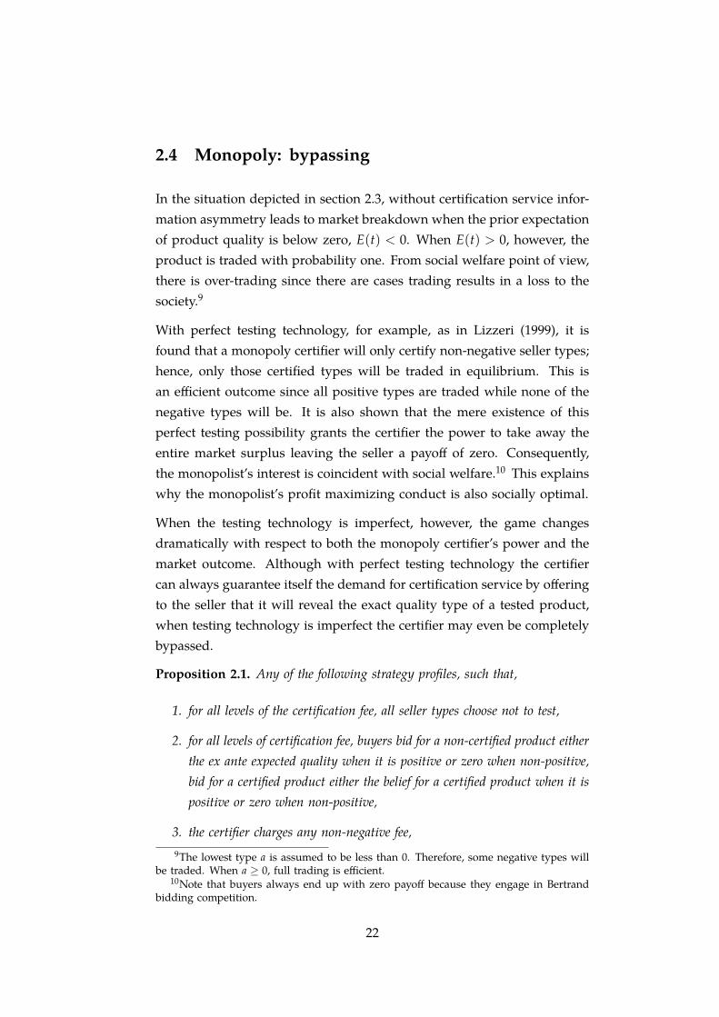
4. and the buyers’ belief being that the quality of a certified product is nohigher than the ex ante expected quality,

constitutes an equilibrium. That is,

P∗ = P ∈ R+

ρ∗(P, t) = NTS, ∀t ∈ [a, b], ∀P ∈ R+

β∗(P, NC) = maxE(t), 0, ∀P ∈ R+

β∗(P, C) = maxµ(t ∣ C, P), 0, ∀P ∈ R+

µ(t ∣ NC, P) = E(t), ∀P ∈ R+

µ(t ∣ C, P) = µ ∈ (a, E(t)], ∀P ∈ R+.

Proof. See Appendix.

One direct implication of Proposition 2.1 is the following remark.

Remark 2.1. When testing technology is imperfect, it’s possible for the seller tobypass the monopoly certifier.

The main underlying reason for this result is the strictly positive probabil-ity that lower types may pass the test. This leaves the buyers the scope offorming the beliefs that are required for the equilibria in Proposition 2.1.In the perfect testing technology case, such beliefs cannot be supported;consequently, bypassing is not possible.

This difference between perfect and imperfect testing technology is notonly of theoretical interest but also of practical importance. Consider “a”seller in the literal sense. Before nature’s draw, there are collective interestsamong seller types. We can think of a monopoly seller or an industry inaggregation. From this perspective, when E(t) ≤ 0, it is not in the seller’sinterest to bypass the certification service because there would then beno trading. When E(t) > 0, however, the seller makes maximal profitE(t) without the certification service. Given that the testing technology isimperfect, it’s at least possible for the seller to bypass the certifier.

We are aware that buyers’ belief in Proposition 2.1 seems irregular. Itessentially says that a certificate does not serve a signal of high qualityeven though buyers know that when tested higher types are more likely

23

to obtain a certificate than lower types. First of all, when the certificationservice is not used, the beliefs stated in Proposition 2.1 are not exactlyirrational. Second, the reason we present Proposition 2.1 in this chapteris to show the difference in feasible equilibria when testing technology isperfect versus when it is imperfect. Although we can put more restrictionson buyers’ beliefs by adopting other equilibrium notions, this possibilityresult signifies the decrease of certifier’s power caused by imperfectnessin testing technology.

2.5 Monopoly: separating equilibrium

In the following we search out those equilibria in which there is a positivemeasure of seller types paying for the test. This is of particularly impor-tance when E(t) ≤ 0 since in this case the market would break down ifthere were no certification service available. To focus on this issue and tosimplify the analysis, we assume the prior expected product quality to benegative.11

Assumption 2.1. The prior expected product quality is less than zero, i.e.,E(t) ≤ 0.

As an example, consider the labor market for IT specialists. If there are noother signals available and the average potential worker does not qualify,then a certificate for such expertise would be crucial both to job applicantsand to employers. Yet, we need to find out for a given imperfect testingtechnology what a certificate could mean and how the market for thecertification service performs.

We solve the game by investigating first the subgames induced by differentcertification fees. Not surprisingly, when the certification fee is set toohigh, it does not pay for the seller to get the product tested. The followingproposition states.

Proposition 2.2. In subgames induced by the certifier’s fee setting P, it is truethat:

11Again, this assumption does not change the result on separating equilibrium quali-tatively.

24

1. if the certifier charges a fee higher than the highest type, then any strategyprofile such that all seller types choosing not to test, buyers bidding zero fora non-certified, bidding for a certified product the belief for such a productwhen it is positive or zero when non-positive, and buyers’ beliefs for acertified product being no higher than b, constitutes an equilibrium in thesubgame induced by P; that is, in subgames where P > b,

ρ∗(t ∣ P > b) = NTS, ∀t ∈ [a, b]

β∗(NC ∣ P > b) = 0

β∗(C ∣ P > b) = maxµ(t ∣ C, P > b), 0

µ(t ∣ NC, P > b) = E(t)

µ(t ∣ C, P > b) = µ ∈ (a, b];

2. if the certifier charges a fee equal to the highest type, there is only oneequilibrium in the subgame other than bypassing, in which only the highestseller type chooses to test and buyers bid the value of the highest type for acertified product, zero for a non-certified product and buyers’ beliefs beingthe ex ante expectation for a non-certified product and b for a certifiedproduct; that is, in the subgame where P = b,

ρ∗(t = b ∣ P = b) = TS and ρ∗(t ∣ P = b) = NTS, ∀t ∈ [a, b)

β∗(C ∣ P = b) = b and β∗(NC ∣ P = b) = 0

µ(C ∣ P = b) = b and µ(NC ∣ P = b) = E(t).

Proof. See the Appendix.

This result can be interpreted as the following. When the price for test istoo high, there is intuitively not much demand for it. As a preparation forsolving the whole game, we establish the following corollary with respectto the certifier’s profit. The result is immediate from Proposition 2.2.

Corollary 2.1. The certifier makes zero profit by setting P ≥ b, or P = 0.

25

2.5.1 Separating equilibrium

We now turn to the more interesting subgames induced by intermediatecertification fees. Before proceeding to the result, the following definitionis useful in simplifying notation.

Definition 2.2. Denote

Ω(m, n) =

∫ nm tG(t)dF(t)∫ nm G(t)dF(t)

for a ≤ m < n ≤ b.

Function Ω(m, n) gives type expectation of a product with a certificate if andonly if all types from the interval (m, n] (or (m, n), [m, n), [m, n]) choose to test.

Further we introduce the following tie-breaking rule.

Assumption 2.2. When a seller type is indifferent between to test and not totest, we assume he chooses to test.

Proposition 2.3 (Separating). In each subgame induced by 0 < P < b, thereis a unique subgame equilibrium other than bypassing the certifier completely.Moreover, the set of seller types, which strictly prefer testing, is of the form(x, b] and type x is indifferent between testing and not testing, where x solvesG(x)Ω(x, b) = P. Buyers bid β(P, C) = Ω(x, b) for a certified product andβ(P, NC) = 0 for a non-certified product. That is,

the seller’s strategies:

⎧⎨⎩ ρ∗(t ∣ P) = TS, ∀t ∈ [x, b],

ρ∗(t ∣ P) = NTS, ∀t ∈ [a, x),

buyer’s strategies:

⎧⎨⎩ β∗(C ∣ P) = Ω(x, b),

β∗(NC ∣ P) = 0,

and buyer’s expectation:

⎧⎨⎩ µ(t, C ∣ P) = Ω(x, b),

µ(t, NC ∣ P) < 0.

constitute the equilibrium in the subgame induced by P ∈ (0, b).

Proof. See Appendix.

This result states that for each positive certification fee that is less thanthe highest quality type, there is a unique subgame equilibrium in which

26

those relatively high types choose to test by paying the certification feewhile relatively low types choose not to.12 Since only those higher typeschoose to test, after taking the imperfectness in the testing technologyinto account, buyers still bid more for a product that has a certificate.This bidding difference justifies the fee that high seller types pay for thetest. The probability of a type passing the test is critical to the type’swillingness to pay. Even high types have a certain probability failing atest. But the nature of the testing technology ensures that in expectedterms higher types are better off by paying for the test while lower typesare better off by choosing not to test.

For ease of exposition and motivated by the proof of Proposition 2.3 inAppendix 2.9.3, we introduce the next definition.

Definition 2.3. Denote κ(P) = x such that G(x)Ω(x, b) = P where 0 < P < b.

For a given P, κ(P) gives the unique type who is indifferent between to test andnot to test in the equilibrium identified in Proposition 2.3.

Proposition 2.3 states that in equilibrium all types higher than κ(P) preferpaying for the test and playing the certification lottery over not to test. Thedifference for any type t between these two options can be represented byfunction Γ(t), 13

Γ(t) = G(t)Ω (κ(P), b)− P.

While Γ(κ(P)) = 0,

Γ(t ∣ t > κ(P)) = G(t ∣ t > κ(P))Ω(κ(P), b)− P

> G(κ(P))Ω(κ(P), b)− P = Γ(κ(P)) = 0.

This explains that the set of the seller types who pay for the test is al-ways connected. Whenever a certain type finds it worthwhile paying forthe test, any type above would find it so as well. For the same fee, ahigher type gets a better lottery than a lower type. On the other hand,this guarantees the existence of the separating equilibrium by preventinglower types from applying the test. A certification service provides a de-vice by which relatively high seller types can separate themselves from

12Note that bypassing is still possible but in this section we focus on the cases whenthe certification service is used.

13See also Equation (2.17) in 2.9.3.

27

relatively low types. They also need to pool together to induce buyers toform a quality expectation that is positive. In the case of perfect testingtechnology, however, pooling is not necessarily needed since a certifiercan certify a seller’s true type. From the perspective of the seller, we havethe following remark.

Remark 2.2. 1. When there is no testing technology, seller types’ interestsare all pooled together without choice;

2. when there is a perfect testing technology, an individual seller type has theopportunity to perfectly identify itself unilaterally;

3. when there is an imperfect testing technology, seller types depend on eachother to a certain degree.

Recall that in the case of perfect testing technology the certifier is able tomake all tested types indifferent between testing and not testing and takeaway the entire market surplus. The certifier chooses a minimum qualitystandard, say κ′ = 0, and charges P′ = E(t ∣ t ≥ 0) for the test. It turnsout that types above 0 are all indifferent between testing and not testing.Note that even though each seller type is left with zero surplus, this isthe unique equilibrium when perfect testing technology is available in themonopoly certifier case.14

Suppose that a certifier with an imperfect technology wants to employsuch a strategy. The certifier claims that all types higher than κ′ willpass the test while all types below will not. Since the certifier is unableto make sure that every low type does not pass and every high typepasses, the expected quality of a certified product is not assured to be atE(t ∣ t ≥ κ′). Therefore, buyers will not bid as much as E(t ∣ t ≥ κ′) andneither will the seller types pay as much for the test. So it is clear thatwhen testing technology is imperfect, a monopoly certifier cannot takeaway the entire market surplus. Indeed most of the testing seller typesderive strictly positive payoff in a separating equilibrium. The followingremark summaries.

14For a formal reasoning, the reader is referred to Lizzeri (1999). This situation re-sembles the observation that in the unique subgame perfect equilibrium of a 2-playerUltimatum game, the proposer gets all and the other gets nothing even though she canreject.

28

Remark 2.3. When imperfect certification service is used in equilibrium, themonopoly certifier’s power in taking up market surplus against the seller is limitedcompared to the case in which a perfect testing technology is available.

2.5.2 Value of a certificate

It is worth noting how buyers form their expectations towards a certifiedproduct. Without equilibrium analysis a certificate does not give a defini-tive meaning in terms of product quality. Proposition 2.3, however, saysonly types higher than or equal to κ(P) go to the certifier in equilibriumat the cost of a positive fee. By successfully attracting a positive measureof seller types, the certification service practically blocks away types lowerthan κ(P) in the original population and filters the remaining into a newpopulation of those with a certificate. The new population is distributedon [κ(P), b] with density G(t) f (t)∫ b

κ(P) G(t)dF(t)where f (t) is the density function of

the original distribution. Thus buyers form their expectations of a certifiedproduct as ∫ b

κ(P) tG(t)dF(t)∫ bκ(P) G(t)dF(t)

= Ω (κ(P), b) .

First, this observation further emphasizes the idea that buyers are onlyable to attribute a value to a certificate for equilibrium outcomes but not foroff-equilibrium incidences. Second, in an equilibrium of the form statedin Proposition 2.3, the value of a certificate directly depends both on thepopulation of the seller types who choose to test and on the nature ofthe testing technology. This implies that to be able to assess a certificate,a buyer first needs to understand what types of products are likely tochoose to test and how difficult it is to pass such a test. Third, note thatthe value of the certificate Ω (κ(P), b) for a given type distribution anda given testing technology is a function of the certification fee P. Hence,when the certification fee changes, the value of the certificate also changes.

Compared to the case in which a perfect testing technology is available, thedependence on the test takers’ population is crucial in imperfect testing. Inthe former case, a certifier can always identify the type when a product istested. The meaning of such a test can be made independent of the seller’stype distribution. In our imperfect testing case, the certifier has to rely

29

on a positive measure of seller types to make the certificate meaningful.This dependence is responsible for the limited ability of the certifier bothin ensuring demand for the test (Remark 2.1) and in taking up marketsurplus against the seller (Remark 2.3).

2.5.3 Free certification

There is one subgame yet to be discussed, the one induced by P = 0. It isof additional importance because we are also interested in the case whentests are provided for free to the seller, for instance, through a publicpolicy program.

Proposition 2.4. In the subgame induced by P = 0, buyers make positive bidsfor a certified product if and only if Ω(a, b) > 0.

Proof. See Appendix.

Free certification produces two contrasting outcomes with respect to trad-ing probabilities. It gives the maximum probability of

∫ ba G(t)dF(t) when

Ω(a, b) > 0 since all seller types have already chosen to test and there isno other way to increase the probability of having a certified product. IfΩ(a, b) < 0, the product will for sure not be traded. However, neither ofthese two is necessarily desirable compared to the socially optimal leveldiscussed in subsection 2.6.3 below.

2.6 Monopoly: market performance

2.6.1 Equilibrium of the game

After having investigated all subgames, we are now ready to solve thegame in its entirety. At the first stage, the certifier chooses the certificationfee for the test, P ∈ R+. Since we put aside bypassing equilibria, the nextresult follows.

30

Proposition 2.5. In equilibrium, a monopoly certifier sets P to maximize profitΠ(P) = P[1− F(κ(P))]. That is,

P∗ = arg maxP∈(0,b)

P[1− F(κ(P))]. (2.6)

It can also be represented as to choose the indifferent type x, such that it maximizesthe certifier’s profit. Formally,

x∗ = arg maxx∈(a,b)

G(x)Ω(x, b)[1− F(x)]. (2.7)

Proof. See Appendix.

The monopoly certifier’s trade-off resembles that of many other monopolyproducers who face a downward sloping demand curve. Demand de-creases when the fee (price) increases. The difference, however, is thatwhile the negative slope of the demand function of consumer productsis normally a result of consumers’ descending willingness to pay for theunit-by-unit-identical product, here the value of the certificate that is be-ing offered is actually evolving along with participating seller types. Thevalue of a certificate deteriorates in the participation of lower seller types.When a certifier lowers its certification fee, it lowers the value of its cer-tificate too.

2.6.2 An example

To have a better understanding of the equilibrium outcome, we present afully specified numerical example.

Example 2.1. Suppose seller types are uniformly distributed on the interval[−2, 1], that is, F(t) = t+2

3 . The testing technology G(t) follows a power func-tion, G(t) =

( t+23

)2 on [−2, 1]. Under this model specification, as stated inEquation (2.22), the monopoly certifier solves the following problem,

max−2<x<1

(1− x + 2

3

)(x + 2

3

)2 ∫ 1x t 1

3

( t+23

)2 dt∫ 1x

13

( t+23

)2 dt.

31

The solution to this problem is x = 0.3154. This means the fee the certifier chargesis

P = G(x)Ω(x, 1) =(

0.3154 + 23

)2 ∫ 10.3154 t 1

3

( t+23

)2 dt∫ 10.3154

13

( t+23

)2 dt= 0.4092.

It turns out that seller types in [0.3154, 1] choose to test while the rest choose notto. Buyers bid

β(C ∣ P = 0.4092) = Ω(0.3154, 1) =

∫ 10.3154 t 1

3

( t+23

)2 dt∫ 10.3154

13

( t+23

)2 dt= 0.6870

for a certified product and 0 for a non-certified. The expected profit the certifiermakes is

Π(0.4092) = P(1− F(x))) = 0.4092∫ 1

0.3154

13

dt = 0.0934,

which is less than the amount it would have made,

Π′ =∫ 1

0

13

tdt = 0.1667,

if a perfect testing technology were available.15 This point can indeed be general-ized.

Remark 2.4. A monopoly certifier with an imperfect testing technology makes asmaller profit than a monopoly certifier with a perfect testing technology underotherwise identical circumstances.

The explanation is the following. With perfect testing technology, a certi-fier is able to take away the entire trading surplus in the market leavingnothing to the seller. Consequently, the certifier will seek to reach thehighest possible market surplus. In contrast, with imperfect testing tech-nology, the surplus generated in the product market is shared betweenthe certifier and the seller.16 From the perspective of the certifier, withperfect testing technology it achieves first best outcome; while in the case

15The profit under perfect testing technology is found when the certifier only certifiestypes above zero and charges E(t ∣ t ≥ 0).

16Note that the set of seller types who strictly prefer paying for the test obtain positiveexpected payoffs. See subsection 2.5.1.

32

t−2 −1.5 −1 −0.5 0 0.5 1

0

0.5

1

1.5

2

f (t) = 13

G(t) =(

t+23

)2

f c(t) = G(t) f (t)∫ bx G(t)dF(t)

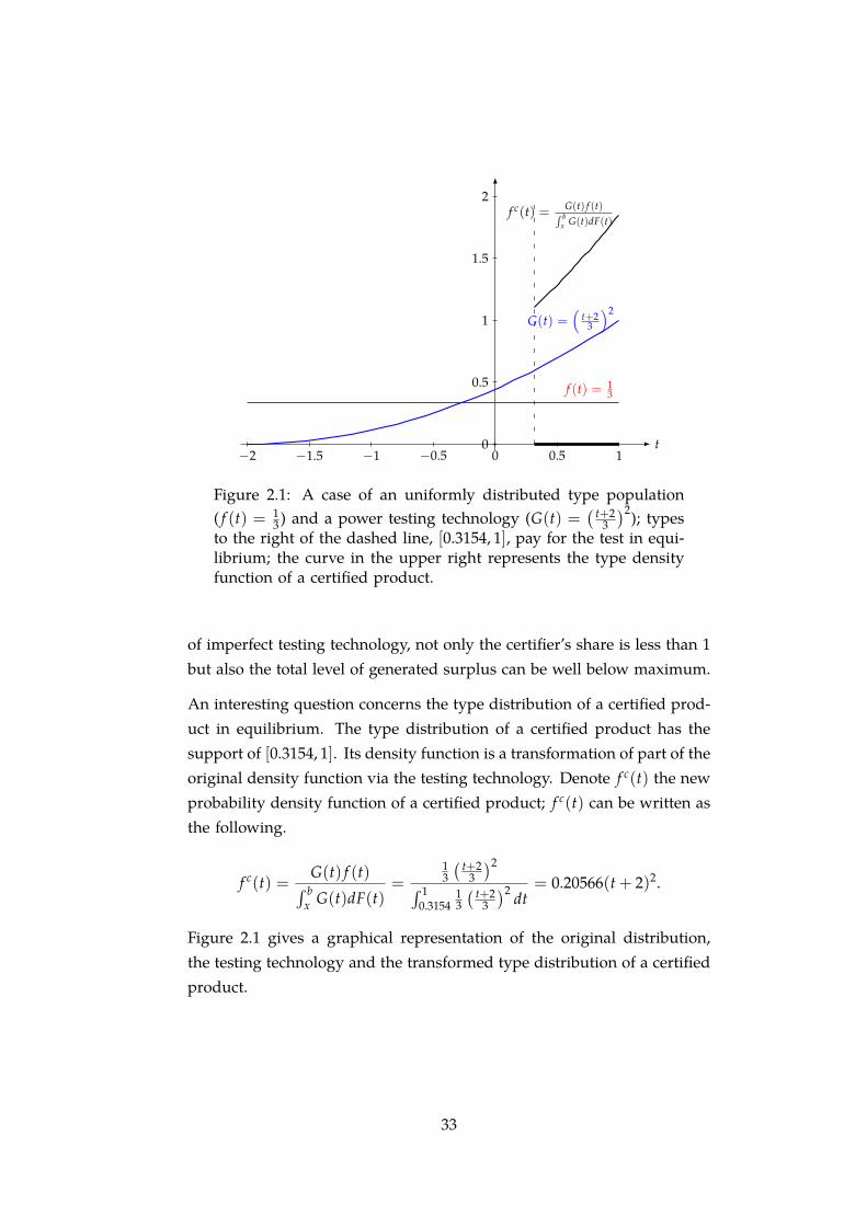
Figure 2.1: A case of an uniformly distributed type population( f (t) = 1

3 ) and a power testing technology (G(t) =( t+2

3

)2); typesto the right of the dashed line, [0.3154, 1], pay for the test in equi-librium; the curve in the upper right represents the type densityfunction of a certified product.

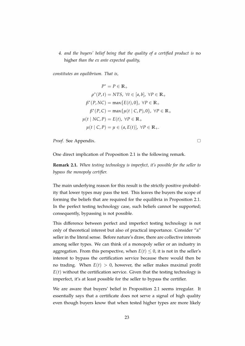
of imperfect testing technology, not only the certifier’s share is less than 1but also the total level of generated surplus can be well below maximum.

An interesting question concerns the type distribution of a certified prod-uct in equilibrium. The type distribution of a certified product has thesupport of [0.3154, 1]. Its density function is a transformation of part of theoriginal density function via the testing technology. Denote f c(t) the newprobability density function of a certified product; f c(t) can be written asthe following.

f c(t) =G(t) f (t)∫ b

x G(t)dF(t)=

13

( t+23

)2∫ 10.3154

13

( t+23

)2 dt= 0.20566(t + 2)2.

Figure 2.1 gives a graphical representation of the original distribution,the testing technology and the transformed type distribution of a certifiedproduct.

33

2.6.3 Welfare

An important issue in markets with asymmetric information is marketperformance in terms of social welfare. The next result gives the conditionfor welfare maximization.

Proposition 2.6. In the separating equilibrium of subgames induced by 0 <

P < b, market surplus is represented by∫ b

κ(P) tG(t)dF(t). It is maximized whenκ(P∗∗) = 0, i.e., when type 0 is made indifferent between testing and not testing.Therefore, the welfare maximizing certification fee is P∗∗ = G(0)Ω(0, b).

Proof. See Appendix.

The intuition is the following. For a product to be traded in a separatingequilibrium, it has to obtain a certificate. Note that trading of positivetypes increases while trading of negative types decreases social welfare.So the ideal outcome is that all positive types obtain a certificate whileall negative types are uncertified. But given the nature of the imperfecttesting technology, this is not achievable. Also note that once a give typedecides to test, the probability of getting a certificate is governed by thetesting technology. The second best is then to set the certification fee toa level such that it is low enough for all positive types to pay for the testwhile it is still high enough to discourage negative types from using thetest. Hence, the optimal certification fee should make type 0 the indifferenttype. Note that G(0)Ω(0, b) is strictly positive, we emphasize the resultas a corollary to Proposition 2.6.

Corollary 2.2. The social welfare maximizing certification fee P∗∗ is strictlypositive.

Apparently, free certification under imperfect testing technology is notan optimal policy. Because of the inability of the testing technology inblocking negative types from getting a certificate, we need a positive cer-tification fee to function as a self-selection mechanism.

34

We can also see the difference between social welfare and the certifier’sprofit in a comparison of the following two expressions.

Social welfare :∫ b

κ(P)tG(t)dF(t)

Certifier’s profit : P[1− F(κ(P))]

= [1− F(κ(P))]G(κ(P))Ω(κ(P), b)

=

⎧⎨⎩∫ b

κ(P) G(κ(P))dF(t)∫ bκ(P) G(t)dF(t)

⎫⎬⎭∫ b

κ(P)tG(t)dF(t). (2.8)

They differ by the part in the curly brackets in equation (2.8). Note thatG(t ∣ t > κ(P)) > G(κ(P)), the part in the curly brackets is less than 1.

Hence, not all of the total market surplus is taken by the certifier. Part ofit is shared by the seller. But for a certifier equipped with a perfect testingtechnology, G(t ∣ t ≥ κ′) could be set to 1 and G(t ∣ t < κ′) to 0. The partin the curly brackets hence vanishes and the monopoly certifier’s profitis equal to the entire social surplus. When such a certifier maximizes itsprofit it as well maximizes social welfare. This comparison tells us thatthe inability of taking up all market surplus leads to a lower level of socialwelfare, i.e., inefficiency.

Boom (2001) shows that in a market with a monopolistic rating agencythere can be over or under supply of rating services in equilibrium com-pared to socially optimal level. In the next proposition we establish thenecessary condition for profit maximizing conduct to be welfare maxi-mizing. When this condition does not hold, market either oversupplies orundersupplies certification service depending on model specification.

Proposition 2.7. A necessary condition for the profit maximizing certifier to setthe welfare maximizing certification fee P∗∗ = G(0)Ω(0, b) is,

f (0)1− F(0)

=g(0)G(0)

+G(0) f (0)∫ b

0 G(t) f (t)dt. (2.9)

Moreover, when P[1− F(κ(P))] is concave for P ∈ (0, b), there is oversupply(undersupply) of certification service if

f (0)1− F(0)

> (<)g(0)G(0)

+G(0) f (0)∫ b

0 G(t) f (t)dt. (2.10)

35

Proof. See the Appendix.

This necessary condition requires the Hazard rate of the original typedistribution when evaluated at type 0 has to be equal to the sum of a valuerelated to the testing technology (G(t)) and certified product’s density attype 0. When condition (2.9) doesn’t hold, socially optimal certificationfee will not be achieved by profit maximizing monopoly certifier.

Further, with additional information of certifier’s profit function concav-ity, we can identify conditions for over and under supply of certificationservice. When

f (0)1− F(0)

<g(0)G(0)

+G(0) f (0)∫ b

0 G(t) f (t)dt, (2.11)

the first derivative of profit is positive at type 0. Therefore, the certifierwill have an incentive to raise the certification fee from the socially optimallevel P∗∗ = G(0)Ω(0, b) and the indifferent type will be strictly higherthan type 0. Because there are strictly positive types find the certificationfee too high and do not apply the test, there is under utilization of thecertification service. Social welfare could be improved by lowering thecertification fee. Similarly, when the reverse of condition (2.11) holds, theindifferent type will be strictly lower than 0 and some negative types willbe traded. Hence there will be oversupply of certification service.

2.6.4 Example 2.1 continued

In the above numerical example, the indifferent type is 0.3154. Socialwelfare would be higher if types in [0, 0.3154] applied the test. Hence,the certification fee 0.4092 is too high. By lowering the fee, more sellertypes will use the certification service and the product will have a higherprobability to be traded. To be exact, the socially optimal fee is

P∗∗ = G(0)Ω(0, 1) =(

23

)2 ∫ 10 t 1

3

( t+23

)2 dt∫ 10

13

( t+23

)2 dt= 0.2515.

So that types in [0, 1] choose to test while types in [−2, 0] choose not to.

In Table 2.1 we compare social welfare and the product’s trading proba-bility in example 2.1 under three different scenarios: perfect testing tech-

36

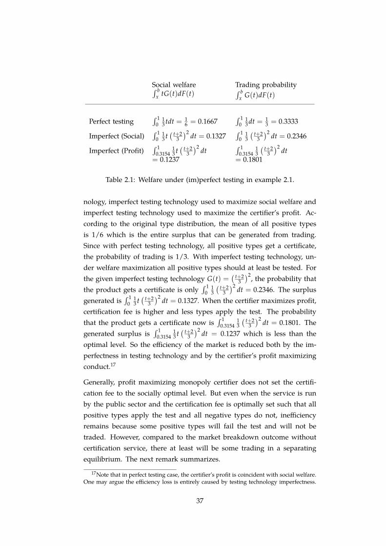
Social welfare∫ bx tG(t)dF(t)

Trading probability∫ bx G(t)dF(t)

Perfect testing∫ 1

013 tdt = 1

6 = 0.1667∫ 1

013 dt = 1

3 = 0.3333

Imperfect (Social)∫ 1

013 t( t+2

3

)2 dt = 0.1327∫ 1

013

( t+23

)2 dt = 0.2346

Imperfect (Profit)∫ 1

0.315413 t( t+2

3

)2 dt= 0.1237

∫ 10.3154

13

( t+23

)2 dt= 0.1801

Table 2.1: Welfare under (im)perfect testing in example 2.1.

nology, imperfect testing technology used to maximize social welfare andimperfect testing technology used to maximize the certifier’s profit. Ac-cording to the original type distribution, the mean of all positive typesis 1/6 which is the entire surplus that can be generated from trading.Since with perfect testing technology, all positive types get a certificate,the probability of trading is 1/3. With imperfect testing technology, un-der welfare maximization all positive types should at least be tested. Forthe given imperfect testing technology G(t) =

( t+23

)2, the probability thatthe product gets a certificate is only

∫ 10

13

( t+23

)2 dt = 0.2346. The surplusgenerated is

∫ 10

13 t( t+2

3

)2 dt = 0.1327. When the certifier maximizes profit,certification fee is higher and less types apply the test. The probabilitythat the product gets a certificate now is

∫ 10.3154

13

( t+23

)2 dt = 0.1801. Thegenerated surplus is

∫ 10.3154

13 t( t+2

3

)2 dt = 0.1237 which is less than theoptimal level. So the efficiency of the market is reduced both by the im-perfectness in testing technology and by the certifier’s profit maximizingconduct.17

Generally, profit maximizing monopoly certifier does not set the certifi-cation fee to the socially optimal level. But even when the service is runby the public sector and the certification fee is optimally set such that allpositive types apply the test and all negative types do not, inefficiencyremains because some positive types will fail the test and will not betraded. However, compared to the market breakdown outcome withoutcertification service, there at least will be some trading in a separatingequilibrium. The next remark summarizes.

17Note that in perfect testing case, the certifier’s profit is coincident with social welfare.One may argue the efficiency loss is entirely caused by testing technology imperfectness.

37

Remark 2.5. An imperfect testing technology solves the asymmetric informationproblem imperfectly. The market is not as efficient as it is with perfect test-ing technology but it does improve buyers’ information on product quality inequilibrium.

2.7 Duopoly

In this section we investigate a market with two certifiers. The mainpurpose of this section is to provide a new perspective for the study ofcompeting certifiers. To this aim, we are interested in market behaviorwith given certification fees. The seller now can choose which certifierto go for a test or not to test at all. We do not consider the possibilitythat a seller type applies both tests. Hence, the seller’s decision ρ mapsR2

+ × [a, b] to TS1, TS2, NTS. TS1 is to test at Certifier 1 and TS2 isto test at Certifier 2. When a seller type fails a test, the type is pooledwith those who do not test. For buyers, β is now a function from R2

+ ×C1, C2, NC to R+, which specifies their bids for a product conditionalon which certificate it has or none at all. Here, C1 stands for a certificatefrom Certifier 1 and C2 a certificate from Certifier 2. As a tie-breaking rule,in the analysis of equilibrium strategies, when a seller type is indifferentbetween two options, he makes the same decision as the type slightlyhigher than he is.

2.7.1 Segmentation in identical tests

We consider a case in which these two certifiers employ identical testingtechnologies. Formally, we have G1(t) = G2(t) = G(t) for all t ∈ [a, b]. Thissetup is to say these two certifiers are providing identical tests and they areidentical except that they charge different certification fees. The next resultreveals that the usual intuition of Bertrand competition between certifiersneed not hold. Even with different certification fees, both certifiers canattract positive measures of seller types in equilibrium.

Proposition 2.8 (Segmentation). Assume two certifiers charge different certifi-cation fees and, without loss of generality, the certifier who charges the higher fee isnamed Certifier 1 and the one charges the lower fee, Certifier 2, 0 < P2 < P1 < b.

38

If there exist x1 and x2 such that a < x2 < x1 < b and

P1 − P2 = G(x1)[Ω(x1, b)−Ω(x2, x1)] (2.12)

P2 = G(x2)Ω(x2, x1), (2.13)

then x1 and x2 identify a subgame equilibrium in which types in (x1, b] strictlyprefer testing at Certifier 1, type x1 is indifferent between testing at either ofthese two certifiers, types in (x2, x1) strictly prefer testing at Certifier 2, type x2

is indifferent between testing at Certifier 2 and not to test at all, types below x2

strictly prefer not to test, buyers bid Ω(x1, b) for a product with Certificate 1,Ω(x2, x1) for a product with Certificate 2 and 0 for a non-certified product. Thatis,

ρ∗(t ∣ P1, P2) = TS1, ∀t ∈ [x1, b]

ρ∗(t ∣ P1, P2) = TS2, ∀t ∈ [x2, x1)

ρ∗(t ∣ P1, P2) = NTS, ∀t ∈ [a, x2)

β∗(C1 ∣ P1, P2) = µ(C1 ∣ P1, P2) = Ω(x1, b)

β∗(C2 ∣ P1, P2) = µ(C2 ∣ P1, P2) = Ω(x2, x1)

β∗(NC ∣ P1, P2) = 0, µ(NC ∣ P1, P2) < 0.

Proof. See appendix.

When the equilibrium identified in Proposition 2.8 exists, for instance inour example in subsection 2.7.2, we call such equilibrium segmentationequilibrium. The existence of segmentation equilibrium suggests that itis possible for both certifiers to attract positive measures of seller typeswhile charging different fees. Since the testing technologies are identical,they are providing supposedly identical certification service. One mayexpect that the lower fee certifier takes up entire market demand for thecertification service and competition would drive the certification fee tomarginal cost as in normal Bertrand competition. In the current setup,this means free certification service.18 Proposition 2.8, however, showsthis line of reasoning need not hold. When segmentation equilibriumexists, certifiers need not engage in Bertrand competition because loweringone’s certification fee does not necessarily increase the demand for its

18Proposition 2.4 finds free certification is generally not socially optimal.

39

certification service nor its profit. Being a higher fee certifier does notmean having zero demand either.

This result can be understood in light of the endogeneity of a certificate’svalue. (Subsection 2.5.2) When the certifiers charge different fees, theircertificates have different values in a segmentation equilibrium. Hence,although they have identical testing processes, their end products (certifi-cates) are differentiated.

In the monopoly certifier case, a certification service provides a devicethat higher types can differentiate themselves from lower types by payingfor the test. With two certifiers providing imperfect certification services,those really high types choose the higher fee certifier to differentiate them-selves from moderate types.

Remark 2.6. 1. A higher certification fee can serve as a signal of higherproduct quality.

2. Even with identical imperfect testing technology, duopoly certifiers neednot to engage in Bertrand Competition.

2.7.2 An example in duopoly

We work through an example to verify the existence of segmentation equi-librium.

Example 2.2. Suppose seller types are distributed on the interval [−1, 1] follow-ing a power function F(t) =

( t+12

) 12 . The testing technology G(t) is represented

by this power distribution function as well, G(t) = F(t) =( t+1

2

) 12 on [−1, 1].

The type expectation function Ω(m, n) is, after simple algebra, simply m+n2 .

Equations (2.12) and (2.13) then read

P1 − P2 =

(x1 + 1

2

) 12 1− x2

2and

P2 =

(x2 + 1

2

) 12 x1 + x2

2.

Suppose Certifier 1 charges P1 = 0.6 and Certifier 2 charges P2 = 0.1. In thiscase, the above system obtains a unique solution, x1 = 0.4742, x2 = −0.1648.

40

Seller types in [0.4742, 1] choose Certifier 1, types in [−0.1648, 0.4742) chooseCertifier 2, types in [−1,−0.1648) choose not to test. Type 0.4742 is indeedindifferent between choosing either of these two certifiers and type −0.1648 isindifferent between choosing Certifier 2 or not to test at all. Buyers in this casebid Ω(0.4742, 1) = (0.4742 + 1)/2 = 0.7371 for a product with Certificate 1,bid Ω(−0.1648, 0.4742) = (−0.1648 + 0.4742)/2 = 0.1547 for a product withCertificate 2 and bid zero for a non-certified product.

The profits the certifiers make are

Π1(P1 = 0.6, P2 = 0.1) = P1 (1− F(x1)) = 0.084873

andΠ2(P2 = 0.1, P1 = 0.6) = P2 (F(x1)− F(x2)) = 0.021233.

So in this example the higher fee certifier earns a higher profit than the lower feecertifier.

In the perfect testing case studied in Lizzeri (1999), competition of cer-tifiers will drive the certification fee to zero. When testing technologyis imperfect, even if both certifiers provide identical testing technology,the current analysis shows fee differentiation is possible and BertrandCompetition is not guaranteed. The point is that when certifiers chargedifferent fees, there can be subgame equilibria in which high seller typeschoose the high fee certifier to signal their type. Hence certifiers neednot to lower their certification fee to the marginal cost level. In example2.2, each certifier has a positive profit and lowering one’s certification feedoesn’t necessarily increase one’s demand nor profit.

Remark 2.7. Although imperfect testing technology limits certifiers’ power incollecting generated surplus from the seller, it does help to soften competitionamong certifiers.

2.7.3 An alternative explanation to auditing fee differences

The significant fee differentiation between major and non-major auditingfirms has long been documented in the accounting literature (e.g., Simu-nic (1980)). See also more recent evidence like Hay, Knechel, and Wong

41

(2006).19 It is also known that in Initial Public Offerings and debt financ-ing, firms audited by major auditors generally receive more favorable bidsthan those audited by other auditors. Evidences include Teoh and Wong(1993) and Mansi, Maxwell, and Miller (2004) among others. The empir-ical observation here is, in other words, the positive correlation betweenauditing fees and bids received.

DeAngelo (1981), Titman and Trueman (1986) and in a context similarto our work, Hvide (2005), suggest that the differences in auditors’ au-diting qualities or standards are responsible for this observation.20 Yet,as acknowledged in Hay, Knechel, and Wong (2006), differences in au-diting qualities are hard to identify. Here we suggest a new perspectiveto this question, namely identical imperfect testing technology. We showin Example 2.2 that even two identical testing technologies can supportfee differentiation in equilibrium and those who choose the higher feecertifier receive higher bids from the buyers. Applied to the auditingcontext, those major auditing firms (Certifier 1 in Proposition 2.8) mayhave exactly the same ability in identifying audited companies’ financialsoundness as other auditing firms (Certifier 2 in Proposition 2.8). If seg-mentation equilibrium is supported, by paying a higher audition fee, acompany of higher quality receives higher bids in equilibrium. Auditedby a non-major auditing firm, however, signals a lower quality. Note alsothat moderate quality companies will not try major auditing firms sincethose are too expensive and they are very likely to get unfavorable au-diting reports. They try non-major firms nevertheless since the fee is lowenough to justify their relatively small probability of getting favorable au-diting reports. To apply the above analysis, we only need to assume thatauditing processes are imperfect, that is, auditing firms are not able toknow exactly the financial situation of each audited firm and yet are ableto ensure better companies have a higher probability receiving favorablefinancial reports.

That major auditing firms make more profits than the rest is also predictedin Example 2.2. Though we have argued that different certification fees

19Major auditing firms here refer to the few largest auditing firms. The exact numbervaries from time to time.

20Additional references on this topic can be found in Hvide (2005).

42

P1, P2 are possible in equilibrium, we leave solving the entire duopolygame to future research.

2.8 Conclusion

In this chapter, we propose a general model of imperfect testing tech-nology in certification services. The main assumption of our suggestedmodel is that whenever two products get tested the higher quality productis more likely to pass than the lower quality one. The model also admitscontinuous quality types and strategic certifiers.

The analysis provided in this chapter aims to improve our understandingof imperfect certification. It’s not always clear what a certificate meansin real life. Yet, we have seen a large number of successful certificationservices that are of practical uses. This chapter takes a formal theoreticalapproach and proves that when a certification service can ensure thathigher quality products stand a better chance obtaining a certificate thanlower quality products, such certification service can reduce informationasymmetry and facilitate trading.

Monopoly certifiers with imperfect testing technologies are not as pow-erful as they would be if perfect testing technologies were available. Ac-cording to the analysis, a certifier with an imperfect technology can becompletely bypassed. This is in sharp contrast to the case of perfect test-ing technology.

A separating equilibrium is also supported in which only high qualityseller types (products) utilize the certification service. By paying the cer-tification fee a seller type in principle obtains the right to play a lottery.The lottery, however, is type dependent and is in favor of higher typessince higher types are more likely to get a certificate for the same certi-fication fee. The value of a certificate is determined jointly by the typedistribution and the nature of the testing technology. Welfare accountingshows that the monopolistic certifier’s profit maximizing conduct can leadto under or over supply of certification service depending on model spec-ification. The welfare maximizing certification fee is always positive andsuch that it makes all positive types choose to test. Hence, free certificationis not recommended under imperfect testing technology.

43

When there are two certifiers with identical testing technologies offeringcertification services in the market, intuition suggests Bertrand competi-tion of the certifiers. While this is true in the perfect testing case studiedin Lizzeri (1999), the arguments for Bertrand competition are not valid inimperfect testing cases. Segmentation equilibrium in which higher sellertypes choose the more expensive certification service and not so high typeschoose the less expensive service can be supported. In this case, keepingon lowering one’s certification fee is not necessarily the best response. Inthe context of auditing industry, we show that to explain the fee differ-entiation between major and non-major auditing firms we do not have toassume differences in auditing processes.

2.9 Appendix

2.9.1 Proof of Proposition 2.1

Proof. If no seller types choose to get the product tested, the type popu-lation of a non-certified product is exactly the original one. Hence, it isoptimal for the buyers to bid maxE(t), 0 for a non-certified product. Aslong as the buyers believe the type of a certified product µ(t ∣ C, P) ≤ E(t),that is, it is not above the population mean, any bid

β(P, C) = maxµ(t ∣ C, P), 0

for a certified product is one of the best responses (Condition 2.2).

Because a certificate is an off-equilibrium incidence and any type excepttype a could get a certificate with a strictly positive probability, buyers’beliefs for a certified product can be supported (Condition 2.3).21,22

If buyers’ bids for a certified product are no higher than those for a non-certified product, no seller types choose to test. Note also that a single

21Given that there is a positive probability for low types to pass, buyers’ belief are notirrational. For perfect Bayesian equilibrium, any not exactly impossible off-equilibriumbelief will do. In other words, there is no prior to be updated.

22Here buyers can hold different beliefs so long as they satisfy the specified conditions,i.e., their beliefs for a non-certified product are both no higher than the ex ante typeexpectation.

44

type choosing to test does not convince the buyers to bid higher, so theseller will not pay for the test after learning his own type (Condition 2.4).

Given the strategies of the seller and the buyers, the certifier’s action isirrelevant (Condition 2.5).

2.9.2 Proof of Proposition 2.2

Proof. With respect to the certification fee P, we have the following twocases.

P > b: It is obvious that in no cases buyers will bid above b. All sellertypes will make a loss by paying for the test. Since E(t) ≤ 0, buyersbid zero for a non-certified and up to their belief for a certifiedproduct. So any of the stated strategy pair constitutes an equilibriumin these subgames. Note that buyers’s out of equilibrium belief a <

µ(t ∣ C, P > b) ≤ b can be supported.

P = b: Note that any combination of seller types other than type b alonechoosing to test will result buyers’ belief for a certified product beingless than b, µ(t ∣ C) < b. In turn their bids β(C ∣ P) < b. Choosingto test makes a loss for all seller types in such a situation.

When type b alone chooses to test, however, we have µ(t ∣ C) = b.

Because type b for sure gets the certificate by choosing to test, typeb is indifferent between testing

β(C ∣ P)− P = b− b = 0,

and not testing (also 0). Types other than b has a strictly positivepossibility of getting no certificate. Consequently, if choose to test,seller types t < b will receive a negative payoff G(t)b− b < 0. Theonly equilibrium other than bypassing when P = b is then the one inwhich type b alone chooses to test and all others not to. The buyersthen bid b for a certified product and 0 for a non-certified productin this equilibrium. Since type b alone is of zero measure, buyers’belief for a non-certified product remains to be the product’s priorexpectation E(t) which is less than zero.

45

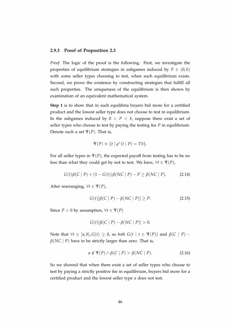
2.9.3 Proof of Proposition 2.3

Proof. The logic of the proof is the following. First, we investigate theproperties of equilibrium strategies in subgames induced by P ∈ (0, b)with some seller types choosing to test, when such equilibrium exists.Second, we prove the existence by constructing strategies that fulfill allsuch properties. The uniqueness of the equilibrium is then shown byexamination of an equivalent mathematical system.

Step 1 is to show that in such equilibria buyers bid more for a certifiedproduct and the lowest seller type does not choose to test in equilibrium.In the subgames induced by 0 < P < b, suppose there exist a set ofseller types who choose to test by paying the testing fee P in equilibrium.Denote such a set Ψ(P). That is,

Ψ(P) ≡ t ∣ ρ∗(t ∣ P) = TS.

For all seller types in Ψ(P), the expected payoff from testing has to be noless than what they could get by not to test. We have, ∀t ∈ Ψ(P),

G(t)β(C ∣ P) + (1− G(t))β(NC ∣ P)− P ≥ β(NC ∣ P). (2.14)

After rearranging, ∀t ∈ Ψ(P),

G(t)[β(C ∣ P)− β(NC ∣ P)] ≥ P. (2.15)

Since P > 0 by assumption, ∀t ∈ Ψ(P)

G(t)[β(C ∣ P)− β(NC ∣ P)] > 0.

Note that ∀t ∈ [a, b], G(t) ≥ 0, so both G(t ∣ t ∈ Ψ(P)) and β(C ∣ P) −β(NC ∣ P) have to be strictly larger than zero. That is,

a /∈ Ψ(P) ∧ β(C ∣ P) > β(NC ∣ P). (2.16)

So we showed that when there exist a set of seller types who choose totest by paying a strictly positive fee in equilibrium, buyers bid more for acertified product and the lowest seller type a does not test.

46

Step 2 is to prove when buyers bid more for a certified product the set ofseller types that pay for the test exists and is of the form [x, b].Let’s denote Γ(t) the difference in expected payoffs for type t between totest and not to.

Γ(t) ≡ G(t)[β(C ∣ P)− β(NC ∣ P)]− P. (2.17)

Apparently, t ∈ Ψ(P) if and only if Γ(t) ≥ 0. Note that for any given Pand β such that 0 < P < b and β(C ∣ P) > β(NC ∣ P), Γ(t) is continuousand strictly increasing in t; Γ(b) ≥ Γ(t) ∀t ∈ [a, b]. Hence, if any typeschoose to test, type b must be one of them, b ∈ Ψ(P).

1. Suppose type b is the only element of Ψ(P), that is Ψ = b. FromProposition 2.2, β(C ∣ P) = b and β(NC ∣ P) = 0. Therefore, com-bined with G(b) = 1 and P < b, we have Γ(b) = G(b)b− P > 0.

Solving the equation G(t)b− P = 0, we have t = G−1(P/b) whereG−1 is the inverse of G. Because G(t) is strictly increasing, for thetypes t ∈ (G−1(P/b), b), their expected payoff of testing G(t)b− P isstrictly larger than zero. These types will also choose to test. Hencewe prove that when 0 < P < b, the supposition that Ψ(P) has onlyone element is false.

2. Now we know Ψ(P), when it exists, contains more elements thanjust type b alone. Note also G(t) is strictly increasing and β(C ∣P) > β(NC ∣ P). Therefore, if a type t′ other than b is in Ψ(P),that is, if the expression (2.15) holds for t′, it also must hold withstrict inequality for any t > t′. Hence, all t such that t > t′ shouldbe in Ψ(P) as well. Moreover, these types strictly prefer testing. Inequilibrium, the set of seller types strictly prefer testing must be ofthe form (x, b] or [x, b] for some x < b.

3. For type b, we have

Γ(b) = G(b)[β(C ∣ P)− β(NC ∣ P)]− P > 0.

This inequality holds strictly because type b obtains a higher payoffthan type inf Ψ(P). For type a, G(a) = 0,

Γ(a) = −P < 0.

47

By the continuity and monotonicity of function Γ(t), there is a uniquesolution for Γ(t) = 0 in the domain of (a, b). Suppose x = Γ−1(0),for type x, it is indifferent between to test and not to test. For t > x,Γ(t) > 0. Consequently, when buyers bid more for a certified prod-uct the set of seller types that pay for the test exists in each subgameinduced by 0 < P < b and, by the tie-breaking rule, is of the form[x, b].

Step 3 is to construct the required buyers’ optimal bids.In this part we search out compatible buyers’ strategies, β(⋅ ∣ P) that willsatisfy

β(C ∣ P) > β(NC ∣ P) ≥ 0.

Buyers bid positively for a certified product (β(C ∣ P) > 0), only whentheir beliefs for a certified product is positive (µ(t ∣ C) > 0). In equilib-rium, µ(t ∣ C) requires to be consistent with rational expectation,

µ(t ∣ C) = E(t ∣ C).

Further, by the following identity

Pr(C)E(t ∣ C) + (1− Pr(C))E(t ∣ NC) ≡ E(t) < 0, (2.18)

it cannot be true that both conditional expectations are non-negative.Hence, to have E(t ∣ C) > 0, E(t ∣ NC) has to be less than zero. Inturn, µ(t ∣ NC) < 0 and β(NC ∣ P) = 0. Since the set of seller types thatchoose to test is of the form [x, b], the buyers’ Bayesian updated beliefshould be,

E(t ∣ C) =

∫ bx tG(t)dF(t)∫ bx G(t)dF(t)

= Ω(x, b). (2.19)

The bid for a certified product is, therefore, β(C ∣ P) = E(t ∣ C) = Ω(x, b).To find indifferent type x, we need to solve

G(x)[Ω(x, b)− 0] = P.

The existence and uniqueness of the solution is established in the nextstep. Note that if G(x)Ω(x, b) = P holds, then Ω(x, b) = P

G(x) . Sinceboth P and G(t), ∀t ∈ (a, b] are larger than zero, Ω(x, b) is also large than

48

zero. Hence we constructed feasible buyers’ strategies and their beliefs.For 0 < P < b, buyers bid

β(C ∣ P) = µ(t ∣ C) = E(t ∣ C) = Ω(x, b)

and β(NC ∣ P) = 0 with belief µ(t ∣ NC) < 0. These bidding strategiesare compatible to the seller’s strategy.

Step 4 is to prove the existence and uniqueness of the indifferent type xfor each 0 < P < b.

The existence and uniqueness of the equilibrium in the subgames boilsdown to the existence and uniqueness of the solution to Γ(t) = 0 or

G(x)Ω(x, b) = P. (2.20)

Note that Ω(x, b) is bounded, it is clear that

limx→a

G(x)Ω(x, b) = 0 and

limx→b

G(x)Ω(x, b) = b.

Note also function Ω(x, b) and G(x)Ω(x, b) are continuous,23 G(x)Ω(x, b) =P obtains at least one solution when 0 < P < b.

To prove the uniqueness, we first derive the derivative of the functionΩ(x, b),

dΩ(x, b)dx

=G(x) f (x)

∫ bx (t− x)G(t)dF(t)(∫ b

x G(t)dF(t))2 .

It’s easy to verify that all parts in the right hand side are positive. HencedΩ(x,b)

dx > 0 and Ω(x, b) increases in x.

According to the value of Ω(a, b), we discuss two cases.

1. When Ω(a, b) ≥ 0, then Ω(x, b) ≥ 0, ∀x ∈ (a, b]. Since the derivativeof the function G(x)Ω(x, b) is as the following:

d (G(x)Ω(x, b))dx

= g(x)Ω(x, b) + G(x)dΩ(x, b)

dx. (2.21)

23The continuity of Ω(x, b) follows from the theorem that the quotient of two contin-uous functions is continuous. That the divisor

∫ bx G(t)dF(t) is non-zero for x ∈ (a, b) is

checked.

49

All parts are positive and G(x)Ω(x, b) increases monotonically form0 to b. Hence Equation 2.20 only obtains one solution when 0 < P <

b.

2. When Ω(a, b) < 0, because of continuity and monotonicity of Ω(x, b),we first find x such that Ω(x, b) = 0. For any x < x, Ω(x, b) < 0

hence Equation (2.20) has no solution. Within the interval of [x, b],G(x)Ω(x, b) increases monotonically form 0 to b. Hence Equation(2.20) only obtains one solution in [x, b] when 0 < P < b.

This proves the existence and uniqueness of the indifferent type x foreach 0 < P < b. Together with above steps, all conditions required byequilibrium notion (Definition 2.1) for the subgames are satisfied and wehave established uniqueness.

2.9.4 Proof of Proposition 2.4

Proof. 1. If Ω(a, b) > 0, it’s easy to verify that all types choose to testand buyers bid Ω(a, b) for a certified product and zero for a non-certified product is an equilibrium.

2. On the other hand, if buyers make positive bids for a certified prod-uct, all types above a will choose to test. This is because there issimply no cost involved in testing for the seller and there is a certainprobability receiving positive bids. Hence, to test is the dominantstrategy except for the lowest type. Suppose Ω(a, b) ≤ 0, then buy-ers’ belief for a certified product is non-positive and consequentlywill bid zero for a certified product. This contradicts the suppositionthat buyers make positive bids. Hence when buyers make positivebids, Ω(a, b) > 0.

2.9.5 Proof of Proposition 2.5

Proof. According to Corollary 2.1, if P ≥ b or P = 0 the seller’s profit willbe zero. Note as well that according to the proof of the uniqueness of thesubgame equilibrium when 0 < P < b, G(t)Ω(t, b) is a continuous and

50

strictly increasing function in (a, b) or (x, b) where x is find by solvingΩ(x, b) = 0 when Ω(a, b) < 0.24 Hence, its inverse function κ(P) from(0, b) to (a, b) or (x, b) is also strictly increasing in (0, b). Consequently, thecertifier can also maximize his profit by optimally choosing the indifferenttype x. The certification fee P is then G(x)Ω(x, b). From Proposition 2.3,the demand for certification service will be 1− F(x). The product of thesetwo components give the profit,25

Π(x) = (1− F(x))G(x)Ω(x, b), x ∈ (a, b). (2.22)

Since the extreme points in Corollary 2.1 are dominated, the maximum isobtained inside the interval. The certifier’s best response to the equilibriumstrategies of the seller and the buyers is hence P∗ defined in Equation (2.6).This, together with Proposition 2.3, concludes the proof.

2.9.6 Proof of Proposition 2.6

Proof. Because buyer always bid up to the expected value of a certifiedproduct, they do not derive positive gains. Social welfare is then the sumof the payoff of the certifier and the payoff of the seller. Moreover, thesum is exactly what buyers pay for the product in equilibrium, becausethis is the only source for the revenues of both the certifier and the seller.

Since buyers bid zero for a non-certified product, trading only takes placewhen the product has a certificate. The total surplus is then, for a givencertification fee, the result of multiplying buyers’ bid for a certified productand the probability of the product getting a certificate,

Ω(κ(P), b)∫ b

κ(P)G(t)dF(t) =

∫ b

κ(P)tG(t)dF(t).

Taking derivative of this expression gives us,

d(∫ b

κ(P) tG(t)dF(t))

d (κ(P))= −κ(P)G(κ(P)) f (κ(P)). (2.23)

24See 2.9.3, especially Step 4 and Equation (2.21).25Note that when Ω(x, b) < 0 when x ∈ (a, x), Π(x) < 0 on this interval too. This

allows us to represent the problem as Equation (2.22) without explicitly write the case for(x, b).

51

It is then obvious that the right hand side of equation (2.23) is strictlynegative when κ(P) > 0, strictly positive when κ(P) < 0 and equal tozero when κ(P) = 0. Maximization of

∫ bκ(P) tG(t)dF(t) with a < κ(P) < b

requires κ(P) = 0. The welfare maximizing certification fee is hence P∗∗ =G(0)Ω(0, b).

2.9.7 Proof of Proposition 2.7

Proof. In the proof of Proposition 2.5 we show that the certifier can setthe indifferent type x to maximize profit. The first order derivative ofΠ(x) = G(x)Ω(x, b)[1− F(x)] is

g(x)Ω(x, b)[1− F(x)] + G(x)[1− F(x)]dΩ(x, b)

dx− G(x)Ω(x, b) f (x)

=g(x)Ω(x, b)([1− F(x)]

(1 +

G(x)g(x)Ω(x, b)

dΩ(x, b)dx

)− G(x)

g(x)f (x)

).

(2.24)

Since g(x) > 0 and Ω(x, b) > 0, when 0 < P < 0 a necessary conditionfor profit maximization is

[1− F(x)](

1 +G(x)

g(x)Ω(x, b)dΩ(x, b)

dx

)− G(x)

g(x)f (x) = 0

⇒ [1− F(x)](

1 +G(x)

g(x)Ω(x, b)dΩ(x, b)

dx

)=

G(x)g(x)

f (x)

⇒ f (x)1− F(x)

=g(x)G(x)

+dΩ(x, b)

dx1

Ω(x, b). (2.25)

Hence if profit maximizing x is socially optimal, i.e., x∗ = 0, the nextcondition has to hold,

f (0)1− F(0)

=g(0)G(0)

+1

Ω(0, b)dΩ(x, b)

dx

∣∣∣x=0

.

Note that

dΩ(x, b)dx

=d

dx

(∫ bx tG(t) f (t)dt∫ bx G(t) f (t)dt

)

=G(x) f (x)

∫ bx tG(t) f (t)dt− xG(x) f (x)

∫ bx G(t) f (t)dt(∫ b

x G(t) f (t)dt)2

52

hencedΩ(x, b)

dx

∣∣∣x=0

=G(0) f (0)

∫ b0 tG(t) f (t)dt(∫ b

0 G(t) f (t)dt)2 .

Consequently,

f (0)1− F(0)

=g(0)G(0)

+1

Ω(0, b)dΩ(x, b)

dx

∣∣∣x=0

=g(0)G(0)

+

( ∫ b0 G(t) f (t)dt∫ b0 tG(t) f (t)dt

)G(0) f (0)

∫ b0 tG(t) f (t)dt(∫ b

0 G(t) f (t)dt)2

=g(0)G(0)

+G(0) f (0)∫ b

0 G(t) f (t)dt.

This proves the first part of Proposition 2.7. With the additional conditionof profit function concavity, we know the second derivative is negative andthe first order condition (2.25) becomes sufficient for profit maximization.However, we are interested in the value of the first derivative (2.24) atx = 0. When it is larger than 0, the monopoly certifier will increase Pin order to increase x and because of the profit function concavity theprofit maximizing x∗ is larger than 0. Consequently, some positive typesfind it too expensive to test and the certification service is under supplied.Hence, the condition for undersupply is

g(x)Ω(x, b)([1− F(x)]

(1 +

G(x)g(x)Ω(x, b)

dΩ(x, b)dx

)− G(x)

g(x)f (x)

) ∣∣∣x=0

> 0

⇒([1− F(x)]

(1 +

G(x)g(x)Ω(x, b)

dΩ(x, b)dx

)− G(x)

g(x)f (x)

) ∣∣∣x=0

> 0

⇒ g(0)G(0)

+G(0) f (0)∫ b

0 G(t) f (t)dt>

f (0)1− F(0)

.

Likewise, when

f (0)1− F(0)

>g(0)G(0)

+G(0) f (0)∫ b

0 G(t) f (t)dt

there is oversupply of certification service. So we proved the second partof Proposition 2.7.

53

2.9.8 Proof of Proposition 2.8

Proof. The following is to prove when a < x2 < x1 < b solve the systemof equations (2.12) and (2.13), we claim the strategies profile in Proposi-tion 2.8 constitutes a perfect Bayesian equilibrium. This is done in thefollowing steps.

1. First, for given 0 < P2 < P1 < b when a < x2 < x1 < b solves

P1 − P2 = G(x1)[ Ω(x1, b)−Ω(x2, x1)]

P2 = G(x2)Ω(x2, x1),

we have Ω(x1, b) > Ω(x2, x1) > 0. This is because G(t) > 0, ∀t > a.

2. Suppose types in [x1, b] choose Certifier 1, types in [x2, x1) chooseCertifier 2 and types in [a, x2) chooses not to test, then buyers ex-pectation for a product certified by Certifier 1 µ(C1 ∣ P1, P2) =

E(C1 ∣ P1, P2) is Ω(x1, b) and for a product certified by Certifier2 µ(C2 ∣ P1, P2) = E(C2 ∣ P1, P2) is Ω(x2, x1). Because the priorexpectation of the product is negative, the expectation for a nonecertified product µ(NC ∣ P1, P2) is less than zero.

3. Then buyers bids are β(C1 ∣ P1, P2) = Ω(x1, b) for a product certifiedby Certifier 1, β(C2 ∣ P1, P2) = Ω(x2, x1) for a product certified byCertifier 2 and 0 for a non-certified product.

4. Since P1 − P2 = G(x1)[ Ω(x1, b)−Ω(x2, x1)] , P2 = G(x2)Ω(x2, x1)

and G(t) strictly increases in t, we have for all x1 < t ≤ b,

G(t)[ Ω(x1, b)−Ω(x2, x1)] > P1 − P2

G(t)Ω(x2, x1) > P2

=⇒ G(t) Ω(x1, b)− P1 > G(t) Ω(x2, x1)− P2 > 0;

for all x2 < t < x1,

G(t)[ Ω(x1, b)−Ω(x2, x1)] < P1 − P2

G(t)Ω(x2, x1) > P2

=⇒ G(t) Ω(x2, x1)− P2 > G(t) Ω(x1, b)− P1

G(t) Ω(x2, x1)− P2 > 0;

54

for all a ≤ t < x2,

G(t)[ Ω(x1, b)−Ω(x2, x1)] < P1 − P2

G(t)Ω(x2, x1) < P2

=⇒ 0 > G(t) Ω(x2, x1) > P2.G(t) Ω(x1, b)− P1.

Hence we compared the expected payoffs for different choices fortypes in [a, b]. Employing also the tie break rule, we conclude that itis true that types in [x1, b] choose Certifier 1, types in [x2, x1) chooseCertifier 2 and types in [a, x2) choose not to test.

5. In summary, if there exist such x1, x2 that satisfy a < x2 < x1 <

b and solve the system of equations (2.12) and (2.13), the aboveconstruction proves that the strategy combinations in Proposition2.8 constitute an equilibrium for the given P1, P2.

55

Chapter 3

A Note on the Excess EntryTheorem in Spatial Modelswith Elastic Demand1

3.1 Introduction

Three main frameworks have been widely used to study product differ-entiation and monopolistic competition: representative consumer, discretechoice and spatial models. In representative consumer and discrete choicemodels, it is understood that equilibrium product variety could either beexcessive or insufficient or optimal depending on the model configura-tion.2 In spatial models such as Vickrey (1964) and Salop (1979), however,analysis shows that there is always excessive entry. This result becameknown as the excess entry theorem. Matsumura and Okamura (2006)extend this result for a large set of transportation costs and productiontechnologies.3

One drawback of standard spatial models such as Hotelling (1929) andSalop (1979) is that consumer demand is completely inelastic. Each con-

1This chapter is coauthored with Tobias Wenzel and has been published in the Inter-national Journal of Industrial Organization.

2See, for example, Dixit and Stiglitz (1977), Pettengill (1979), Lancaster (1975), Sattinger(1984), Hart (1985) among many others.

3They do point out that there are also some situations in which entry can be insuffi-cient.

56

sumer demands a single unit of a differentiated product.4 In this chapterwe lift this restrictive assumption in the context of the Salop model andinvestigates the implications of price-dependent demand for the excessentry theorem.

To this aim, we incorporate a demand function with a constant elastic-ity into the Salop framework. We find that the number of entrants in afree-entry equilibrium is the lower the more elastic demand is. We alsofind that only when demand is sufficiently inelastic, there is excess entry.Otherwise, entry is insufficient. In the limiting case when the demandelasticity approaches unity, the market becomes a monopoly. Thus, theexcess entry theorem is only valid for sufficiently inelastic demand andhence, the assumption of inelastic demand, typically employed, is not aninnocuous one. This result is independent of whether we use a first-bestor a second-best welfare benchmark. As a consequence of our welfareanalysis we point out when and how a public policy can be desirable. Inan extension, we broaden our result with a more general transportationcost function.

Our model setup is closely related to Anderson and de Palma (2000).The purpose of their paper is to develop a model that integrates fea-tures of spatial models where competition is localized and representativeconsumer models where competition between firms is global. The formu-lation of the individual demand function is the same as in Anderson andde Palma (2000).5 They also consider a constant elasticity demand func-tion. However, the difference lies in the perspectives of the works. Theirfocus is on the interaction between local and global competition, whilethe present work focuses on the implications of price-dependent demandon the excess entry result in spatial models.

Other approaches to introduce price-dependent demand into spatial mod-els are Boeckem (1994), Rath and Zhao (2001) and Peitz (2002).6 The first

4The assumption of inelastic demand can be a realistic one in the case of some durablegoods, e.g. houses, etc. However, in case of nondurables, e.g. groceries, etc, the assump-tion seems less plausible.

5Our model is the special case of Anderson and de Palma (2000) when eliminatingthe taste component in their utility function. Thus, in this chapter we consider a purespatial model, while Anderson and de Palma (2000) analyze a model that has features ofspatial and representative consumer models.

6A recent paper by Peng and Tabuchi (2007) combines a model of spatial competitionwith taste for variety in the spirit of Dixit and Stiglitz (1977). In their setup, the quantity

57

two papers consider variants of the Hotelling framework. Boeckem (1994)introduces heterogenous consumers with respect to reservation prices.Depending on the price charged by firms some consumers choose notto buy a product. The paper by Rath and Zhao (2001) introduces elasticdemand in the Hotelling framework by assuming that the quantity de-manded by each consumer depends on the price charged. The authorspropose a utility function that is quadratic in the quantity of the differen-tiated product leading to a linear demand function. In contrast to thosetwo models we build on the Salop model as we are interested in therelationship between price-dependent demand and entry into the mar-ket. Our approach is closer to Rath and Zhao (2001) as we also assumethat each consumer has a downward sloping demand for the differenti-ated good. However, our demand function takes on a different functionalform which has the advantage of yielding tractable results. Peitz (2002)features unit-elastic demand both in Hotelling and Salop settings but fo-cuses on conditions for existence of Nash equilibrium in prices. He doesnot consider entry decisions.

This chapter is organized as follows. Section 3.2 sets up the model. Section3.3 presents the analysis of the model. Section 3.4 analyzes the welfareoutcome and policy implications. An extension with more general trans-portation cost functions is provided in section 3.5. Section 3.6 summarizes.

3.2 The model

There is a unit mass of consumers who are located on a circle with cir-cumference one. The location of a consumers is denoted by x. In contrastto Salop (1979), consumers are not limited to buy a single unit of the dif-ferentiated good. The amount they purchase depends on the price. Wepropose the following utility function which leads to a demand functionwith a constant elasticity of ε. We assume that this utility function isidentical for all consumers:

demanded also depends on the price. However, their focus is a different one. They studythe incentives of how much variety to offer and how many stores to establish. A paper byHamilton, Klein, Sheshinski, and Slutsky (1994) analyzes elastic demand in a model withquantity competition. In contrast to the present note the authors employ a transportationcosts per unit of quantity purchased.

58

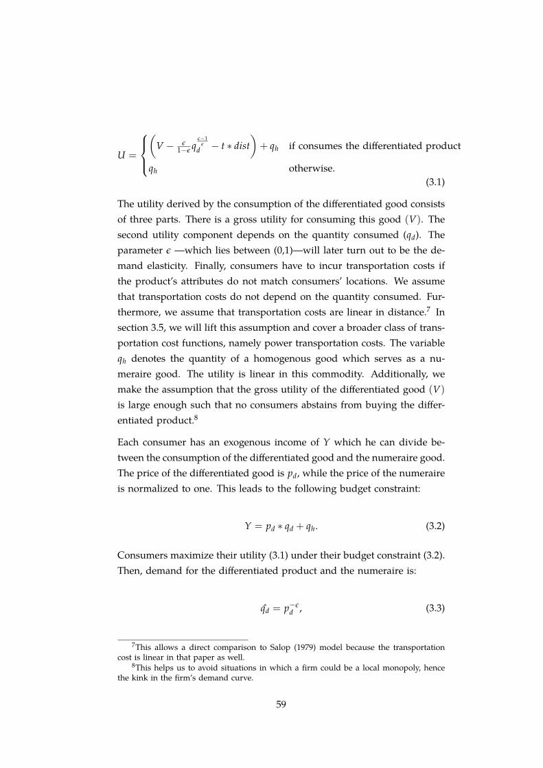
U =

⎧⎨⎩(

V − ε1−ε q

ε−1ε

d − t ∗ dist)+ qh if consumes the differentiated product

qh otherwise.(3.1)

The utility derived by the consumption of the differentiated good consistsof three parts. There is a gross utility for consuming this good (V). Thesecond utility component depends on the quantity consumed (qd). Theparameter ε —which lies between (0,1)—will later turn out to be the de-mand elasticity. Finally, consumers have to incur transportation costs ifthe product’s attributes do not match consumers’ locations. We assumethat transportation costs do not depend on the quantity consumed. Fur-thermore, we assume that transportation costs are linear in distance.7 Insection 3.5, we will lift this assumption and cover a broader class of trans-portation cost functions, namely power transportation costs. The variableqh denotes the quantity of a homogenous good which serves as a nu-meraire good. The utility is linear in this commodity. Additionally, wemake the assumption that the gross utility of the differentiated good (V)

is large enough such that no consumers abstains from buying the differ-entiated product.8

Each consumer has an exogenous income of Y which he can divide be-tween the consumption of the differentiated good and the numeraire good.The price of the differentiated good is pd, while the price of the numeraireis normalized to one. This leads to the following budget constraint:

Y = pd ∗ qd + qh. (3.2)

Consumers maximize their utility (3.1) under their budget constraint (3.2).Then, demand for the differentiated product and the numeraire is:

qd = p−εd , (3.3)

7This allows a direct comparison to Salop (1979) model because the transportationcost is linear in that paper as well.

8This helps us to avoid situations in which a firm could be a local monopoly, hencethe kink in the firm’s demand curve.

59

qh = Y− p1−εd . (3.4)

The demand for the differentiated good exhibits a constant demand elas-ticity of ε. A higher value of ε corresponds to more elastic demand. Thelimit case of ε→ 0 corresponds to completely inelastic demand. Insertingthese demand functions into equation (3.1) gives the indirect utility a con-sumer derives from consuming the differentiated product from a certainfirm:

U = V + Y− 11− ε

p1−εd − t ∗ dist. (3.5)

There are n firms that offer the differentiated product. We assume thatthese firms are located equidistantly on the circle. Hence, the distancebetween two neighboring firms is 1

n . Consumers choose to buy the dif-ferentiated product from the firm which offers them the highest utility.Given the symmetric structure of the model, we seek for a symmetricequilibrium. Therefore we derive demand of a representative firm i. Themarginal consumer is the consumer who is indifferent between choosingfirm i and an adjacent firm. When firm i charges a price pi while the re-maining firms charge a price p, the marginal consumer is implicitly givenby

V + Y− 11− ε

p1−εi − tx = V + Y− 1

1− εp1−ε − t

(1n− x)

, (3.6)

or explicitly by

x =1

2n+

p1−ε − p1−εi

2(1− ε)t. (3.7)

As each firm faces two adjacent firms, the number of consumers choosingto buy from firm i is 2x. According to equation (3.3), each consumer buysan amount of qi = p−ε

i . Hence total demand at firm i is:

Di = 2x ∗ p−εi . (3.8)

60

In contrast to the Salop model, total demand consists now of two parts:market share and quantity per consumer.

3.3 Analysis

This section analyzes the equilibrium. We start by deriving equilibriumprices for a given number of firms in the market. In a second step, weseek to determine the number of firms that enter.

3.3.1 Price equilibrium

We look for a symmetric equilibrium in which all firms charge the sameprice. Assuming zero production costs, the profit of a representative firmi when this firm charges a price pi and all remaining firms charge a pricep is given by:

Πi =

[1n+

p1−ε − p1−εi

(1− ε)t

]p−ε

i pi. (3.9)

Maximizing profits with respect to the price pi and assuming symmetryamong all firms leads to the following equilibrium price:9

p∗ =[(1− ε)

tn

] 11−ε

. (3.10)

The corresponding quantity purchased by each consumer then is

q∗ =[(1− ε)

tn

]− ε1−ε

. (3.11)

As in the Salop model, the equilibrium price increases in transportationcosts and decreases in the number of firms in the market. Conversely, thequantity purchased by each consumer rises with the number of firms anddecreases with transportation costs. More interesting is the impact of the

9For the proof of the existence of a symmetric price equilibrium, the reader is referredto Anderson and de Palma (2000).

61

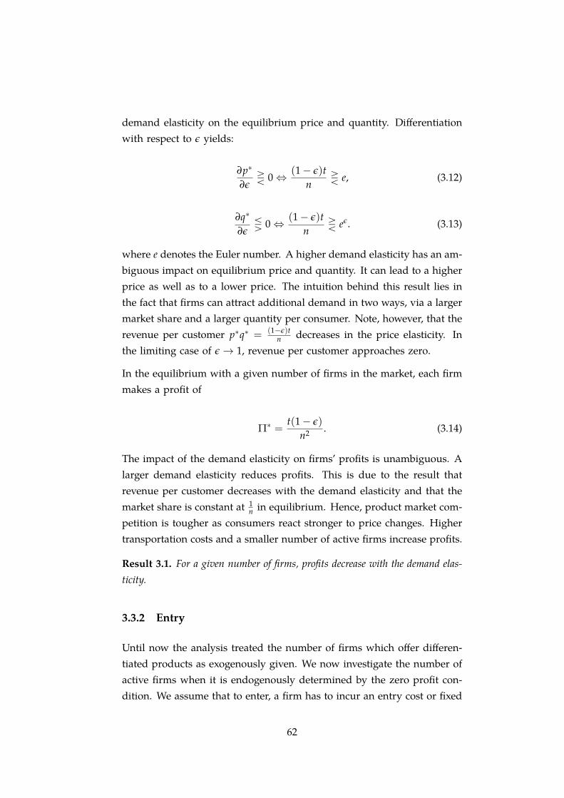
demand elasticity on the equilibrium price and quantity. Differentiationwith respect to ε yields:

∂p∗

∂ε⋛ 0⇔ (1− ε)t

n⋛ e, (3.12)

∂q∗

∂ε⋚ 0⇔ (1− ε)t

n⋛ eε. (3.13)

where e denotes the Euler number. A higher demand elasticity has an am-biguous impact on equilibrium price and quantity. It can lead to a higherprice as well as to a lower price. The intuition behind this result lies inthe fact that firms can attract additional demand in two ways, via a largermarket share and a larger quantity per consumer. Note, however, that therevenue per customer p∗q∗ = (1−ε)t

n decreases in the price elasticity. Inthe limiting case of ε→ 1, revenue per customer approaches zero.

In the equilibrium with a given number of firms in the market, each firmmakes a profit of

Π∗ =t(1− ε)

n2 . (3.14)

The impact of the demand elasticity on firms’ profits is unambiguous. Alarger demand elasticity reduces profits. This is due to the result thatrevenue per customer decreases with the demand elasticity and that themarket share is constant at 1

n in equilibrium. Hence, product market com-petition is tougher as consumers react stronger to price changes. Highertransportation costs and a smaller number of active firms increase profits.

Result 3.1. For a given number of firms, profits decrease with the demand elas-ticity.

3.3.2 Entry

Until now the analysis treated the number of firms which offer differen-tiated products as exogenously given. We now investigate the number ofactive firms when it is endogenously determined by the zero profit con-dition. We assume that to enter, a firm has to incur an entry cost or fixed

62

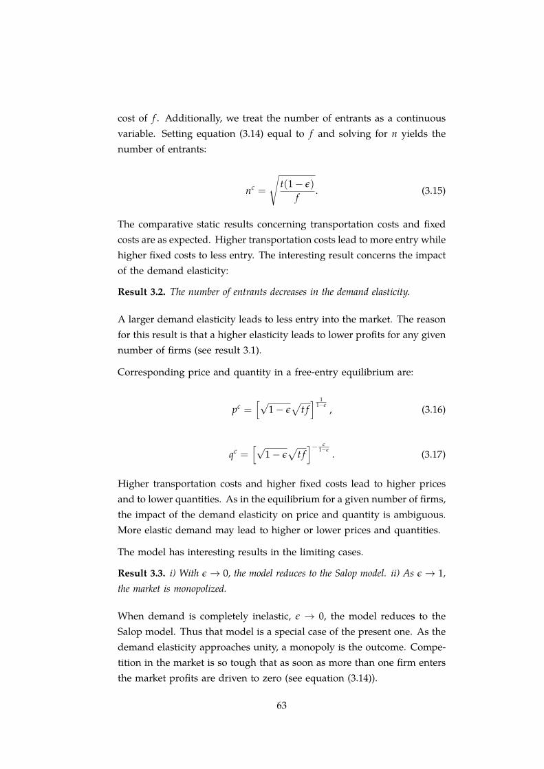
cost of f . Additionally, we treat the number of entrants as a continuousvariable. Setting equation (3.14) equal to f and solving for n yields thenumber of entrants:

nc =

√t(1− ε)

f. (3.15)

The comparative static results concerning transportation costs and fixedcosts are as expected. Higher transportation costs lead to more entry whilehigher fixed costs to less entry. The interesting result concerns the impactof the demand elasticity:

Result 3.2. The number of entrants decreases in the demand elasticity.

A larger demand elasticity leads to less entry into the market. The reasonfor this result is that a higher elasticity leads to lower profits for any givennumber of firms (see result 3.1).

Corresponding price and quantity in a free-entry equilibrium are:

pc =[√

1− ε√

t f] 1

1−ε, (3.16)

qc =[√

1− ε√

t f]− ε

1−ε. (3.17)

Higher transportation costs and higher fixed costs lead to higher pricesand to lower quantities. As in the equilibrium for a given number of firms,the impact of the demand elasticity on price and quantity is ambiguous.More elastic demand may lead to higher or lower prices and quantities.

The model has interesting results in the limiting cases.

Result 3.3. i) With ε→ 0, the model reduces to the Salop model. ii) As ε→ 1,the market is monopolized.

When demand is completely inelastic, ε → 0, the model reduces to theSalop model. Thus that model is a special case of the present one. As thedemand elasticity approaches unity, a monopoly is the outcome. Compe-tition in the market is so tough that as soon as more than one firm entersthe market profits are driven to zero (see equation (3.14)).

63

3.4 Welfare

This section considers the welfare and policy implications. We ask whetherthere is excess entry into the market as it is the case in models with in-elastic demand.

In contrast to models with inelastic demand, we have to consider pricesin our welfare analysis as they have an impact on the quantity purchasedand hence on welfare. We define social welfare as the sum of consumerutility and industry profits:

W = V + Y− 11− ε

p1−ε − 2n∫ 1

2n

0tx dx︸ ︷︷ ︸

Consumer welfare

+ p1−ε − f n︸ ︷︷ ︸Industry profits

. (3.18)

We consider two different welfare benchmarks, a first-best benchmark inwhich the social planner chooses both the level of entry and the pricecharged by firms, and a second-best benchmark in which the social plan-ner can only control the level of entry, but not prices. Our result arequalitatively independent of the choice of the welfare benchmark.

3.4.1 First-best benchmark

In the first-best benchmark, the social planner can control prices and levelof entry, that is he maximizes total welfare with respect to p and n. Fromequation (3.18), we see that the optimal price set by the regulator is equalto marginal cost, in this case, p = 0. Inserting this into equation (3.18)yields

W = V + Y− 2n∫ 1

2n

0tx dx− f n. (3.19)

The problem for the social planner is then identical to the case with in-elastic demand, hence reduced to a trade-off between transportation costsand fixed costs. The optimal number of entrants is

n f =

√t

4 f. (3.20)

64

Comparison with the free-entry level, nc, leads to the following result:

Result 3.4. Compared to the first-best benchmark, there is excess entry whenε < 3

4 , insufficient entry when ε > 34 , and optimal entry when ε = 3

4 .

The previous result shows that the result of excess entry in the Salopmodel does not hold when demand is elastic. In the model with elas-tic demand whether there is too much entry or not enough depends onthe demand elasticity. Whenever demand is sufficiently inelastic, thereis excess entry as is the case in the Salop model (ε → 0). However, ifthe demand elasticity exceeds 3

4 , there is insufficient entry into the mar-ket. Only when ε = 3

4 , entry coincides with the socially optimal number.Thus, the excess entry theorem in spatial models depends crucially on theassumption of inelastic demand.

3.4.2 Second-best benchmark

Here we derive the welfare-maximizing number of firms given their pric-ing behavior after entry. Inserting equation (3.10) into (3.18) gives

W = V + Y− tn− 2n

∫ 12n

0tx dx +

t(1− ε)

n− f n. (3.21)

Maximizing total welfare (3.21) with respect to n yields the optimal num-ber of firms:10

ns =

√t(1 + 4ε)

4 f. (3.22)

Comparing the optimal number of firms, ns, with the outcome under freeentry, nc, the following result can be established:

Result 3.5. Compared to the second-best benchmark, there is excess entry whenε < 3

8 , insufficient entry when ε > 38 , and optimal entry when ε = 3

8 .

Using the second-best benchmark, our result has the same structure aswith the first-best benchmark. For sufficiently inelastic demand, we getexcess entry and for sufficiently elastic demand, we get insufficient entry.

10The second-order condition for maximization is satisfied: − t(1+4ε)2n3 < 0.

65

3.4.3 Policy implications

Here we derive some policy implications of our welfare analysis focus-ing on the case of the second-best welfare benchmark. Suppose that agovernment agency may either charge a fee against or grant a subsidy toeach entry, e.g. license fee or start-up funds, respectively. Let s denotethe value of such a transfer. When s < 0 we call it a subsidy, and whens > 0 we call it an entry fee.

Hence the number of firms under such an otherwise “Free Entry” policynow is:

nc′ =

√t(1− ε)

f + s. (3.23)

This, of course, follows directly from equation (3.15) by adjusting the fixedcost term accordingly. By setting equation (3.23) equal to (3.22), we candetermine the value of s that induces optimal entry into the market. Thisvalue is

s = f3− 8ε

1 + 4ε. (3.24)

The following corollary then immediately follows from result 3.5.

Corollary 3.1. i) When ε < 38 , a government agency should charge an entry fee

to reduce excess entry; ii) when ε > 38 , a government agency should subsidize

entry.

By such a transfer scheme, a government agency could effectively influ-ence the number of active firms.

3.5 Power transportation costs

This section reconsiders the analysis assuming a more general transporta-tion cost function. Instead of linear transportation costs, we now assumepower transportation costs txβ with β ≥ 1. This functional form is alsoconsidered by Anderson, de Palma, and Thisse (1992) and Matsumura andOkamura (2006) which both show that the excess entry theorem always

66

holds in the case of inelastic demand.11 Our analysis will show that theirresult depends very much on the assumption of inelastic demand.

Following the same steps as in section 3.3, we can derive the number ofentrants in a free-entry equilibrium and the socially optimal number. Thederivation of these results is given in appendix 3.7.

The number of entrants in a free-entry equilibrium is

nc =

[(1− ε)tβ21−β

f

] 11+β

, (3.25)

and the optimal number of firms—using the second-best welfare benchmark—is

nw =

[tβ2−β(2βε + 1

1+β )

f

] 11+β

. (3.26)

We denote by ε = 1+2β2(1+β)2 the demand elasticity such that optimal and

competitive entry coincides. This leads to the following result:

Result 3.6. Suppose that transportation costs are of the power function form txβ.Then we have that i) there is excess entry if ε < ε(β) and insufficient entry ifε > ε(β), and ii) ε(β) decreases in β.

The first part of the result generalizes result 3.5 for the case of a moregeneral transportation cost function. It states that as long as demand issufficiently inelastic the excess entry theorem still holds. Otherwise itdoes not hold. The second part of the result, follows directly as ∂ε

∂β =

− β(1+β)3 < 0. It says that the interval of demand elasticities for which the

excess entry theorem holds shrinks with β.

3.6 Conclusion

In this chapter, we introduce elastic demand in the Salop (1979) modeland investigate if the excess entry theorem still holds. We feature a utility

11Note that existence of price equilibrium is not ensured if β is too high. See Anderson,de Palma, and Thisse (1992, Ch. 6).

67

function that leads to a demand function with constant elasticity. Wefind that a larger demand elasticity leads to less entry into the market.This is a hypothesis that can be tested empirically. Markets with higherdemand elasticity should offer less product variety. In the limiting case ofa unit demand elasticity the market outcome is a monopoly. Turning towelfare analysis, we show that when demand is sufficiently inelastic thereis excess entry. However, when demand is sufficiently elastic the numberof entrants is lower than the socially optimal number. Further, we provideconditions on when and how a government intervention can be desirable.We also show that our results hold with more general transportation costfunctions.

3.7 Appendix

Here we provide the derivation of the results for the model with powertransportation costs. The derivation follows Anderson, de Palma, andThisse (1992, Ch. 6), but extended to price-dependent demand.

With power transportation costs, the marginal consumer is implicitly givenby

− 11− ε

p1−εi − txβ = − 1

1− εp1−ε − t

(1n− x)β

. (3.27)

In contrast to the case of linear transportation costs, it is not possible togive a closed form for the marginal consumer. However, by total differ-entiation it is possible to calculate the impact of a price change on themarginal consumer, which is

dxdpi

= −p−ε

i

tβ(xβ−1 + ( 1n − x)β−1)

. (3.28)

As we are interested in a symmetric equilibrium we can evaluate thisexpression at the symmetric equilibrium, that is at x = 1

2n . Then, we get

dxdpi

∣∣∣x= 12n

= −p−ε

i

2tβ( 12n )

β−1. (3.29)

68

Profits for the representative firm i is Πi = 2xp1−εi . The first-order condi-

tion for profit maximization and assuming symmetry gives the followingequilibrium prices for a given number of firms in the market:

p =

[(1− ε)

tβ21−β

nβ

] 11−ε

. (3.30)

For β = 1, this gives the results of our base model, and for ε = 0, we getthe results of Anderson, de Palma, and Thisse (1992, Ch. 6). Each firmearns a profit of

(1− ε)tβ21−β

nβ+1 − f . (3.31)

The number of firms that enter in a free-entry equilibrium is determinedvia the zero-profit condition. This leads to the following number of en-trants:

nc =

[(1− ε)tβ21−β

f

] 11+β

. (3.32)

With power transportation costs the second-best welfare benchmark canbe expressed as:

W = V + Y− tβ21−β

nβ− t

(1 + β)nβ2β+

(1− ε)tβ21−β

nβ− f n. (3.33)

The number of firms that maximizes total welfare is then

nw =

[tβ2−β(2βε + 1

1+β )

f

] 11+β

. (3.34)

Comparison with the number of firms in a free-entry equilibrium showsthat there is excess entry if ε < 1+2β

2(1+β)2 .

69

Chapter 4

Product Variety, PriceElasticity of Demand andFixed Cost in Spatial Models1

4.1 Introduction

Spatial models of product differentiation in the spirit of Hotelling (1929)and Salop (1979) have been a popular tool in Industrial Organization andRegional Science. They have been used to study competition in a largevariety of markets and issues.2 Typically, the Hotelling model has beenused to study location decisions by firms while the Salop model has beenused to study entry decisions and market structure. Concerning the Salopmodel, one prominent result is the so-called excess entry theorem. It statesthat in a free-entry equilibrium, there are always more firms entering intothe market than would be desirable from a welfare point of view. That is,there is excessive entry into the market. As firms are usually assumed tobe single product firms, the result can also be interpreted as an excess ofproduct variety provided in the market.3

1This chapter is coauthored with Tobias Wenzel. An earlier version of this chapter isGu and Wenzel (2009b).

2E.g., Anderson and Coate (2005) on media markets, Friedman and Thisse (1993) oncollusion, Armstrong (2006) for a study on two-sided markets, and many more.

3With respect to variants of the standard Salop model, Matsumura and Okamura(2006) find this excess entry result holds for a broad class of transport and productioncost functions.

70

However, one underlying, and quite restrictive assumption in the Salopmodel, is that consumer demand does not depend on the price of theproduct. Each consumer demands a single unit of a differentiated prod-uct. In consequence, the price then constitutes a mere transfer betweenconsumers and firms and thus has no impact on total welfare. It is theaim of the present chapter to lift this assumption of completely inelasticdemand and investigate the consequences of this modification on the va-lidity of the excess entry theorem. In contrast to a version of the modelwith completely inelastic demand, the price of the differentiated productis no longer a mere transfer between consumer and firm, but has a realwelfare impact by influencing the quantity the consumer demands of thedifferentiated product. A higher price now leads to a lower quantity ofthe differentiated product and to lower total welfare.

The present chapter explores the relationship between price-dependentdemand and the excess entry theorem in a quite general setting. Westudy a setup in which consumer preferences can be represented by aquasi-linear utility function. We make a mild restriction on the resultingconsumer demand function for the differentiated product, namely we as-sume that the price elasticity is increasing in the price. This assumptionis satisfied by many demand functions, for instance, linear demand func-tions.4 In this setup, we establish existence and uniqueness of a symmetricprice equilibrium.

Our main objective is to characterize the welfare properties of the free-entry equilibrium. We show that unlike the standard Salop model withcompletely inelastic demand, the free-entry equilibrium may exhibit ex-cessive, insufficient or optimal entry. The intuition behind this result is thefollowing. When setting the price of the product firms have to take twoeffects into account. An increase in the price reduces the market shareas well as the quantity sold to each consumer. This second effect—notpresent in the standard Salop model with completely inelastic demand—makes firms more careful when setting the price, and hence leads to alower equilibrium price than in the standard model. This, in turn, leadsto lower profits and reduces the incentives to enter the market. Thus,considering price-dependent demand leads to a downward correction of

4It is also a common assumption in the business literature. See, e.g., Lariviere andPorteus (2001) and Ziya, Ayhan, and Foley (2003).

71

the number of firms which are active in the market. Whether we obtainexcessive or insufficient entry now depends on the strength of consumerreactions to a price increase. If consumers react only mildly to a priceincrease, the downward correction of the equilibrium price and profit issmall, and hence, we still get excessive entry. On the other hand, if con-sumers react strongly on a price increase the downward correction is large,and equilibrium price and profit are largely reduced and, in consequence,we obtain insufficient entry. This chapter obtains conditions for each ofthe possible welfare outcomes.

The central message of this chapter is that considering price-dependentdemand is a decisive factor for the welfare results. The excess entry resultmay not hold when consumers react to prices by adjusting the quantitiesthey demand. As the Salop is used as a building block in many applica-tions, we think one should be careful in interpreting these welfare resultswhich rely on the assumption of completely inelastic demand. When con-sidering price-dependent demand these results may change.

In Chapter 3, we provided an example of the issue by considering a spe-cific functional form for the consumer demand. We employ a demandfunction with a constant demand elasticity which enables us to expressequilibrium solutions in closed form. This has the advantage to provide asimple formulation that is suitable for use in applications. In contrast, thepresent chapter aims to study the issue at a general level without relyingon specific forms of consumer demand.

Our result also closes, at least partially, the gap between different ap-proaches of modeling competition in differentiated product markets. Inrepresentative consumer models, such as Dixit and Stiglitz (1977), or indiscrete choice models of product differentiation, for instance see theoverview in Anderson, de Palma, and Thisse (1992), equilibrium entrycan be excessive, insufficient, or optimal depending on the exact modelconfiguration.

This chapter contributes to a recent literature that introduces price-dependentdemand into spatial models. Related contributions are Boeckem (1994),Rath and Zhao (2001), Peitz (2002) and Anderson and de Palma (2000).The first two papers consider variants of the Hotelling framework. Boeckem(1994) introduces heterogenous consumers with respect to reservation

72

prices. Depending on the price charged by firms some consumers choosenot to buy a product. The paper by Rath and Zhao (2001) introduceselastic demand in the Hotelling framework by assuming that the quantitydemanded by each consumer depends on the price charged. The authorspropose a utility function that is quadratic in the quantity of the differenti-ated product leading to a linear demand function. In contrast to those twomodels we build on the Salop model as we are interested in the relation-ship between price-dependent demand and entry into the market. Ourapproach is closer to Rath and Zhao (2001) as we also assume that eachconsumer has a downward sloping demand for the differentiated goodalthough we do not postulate a specific functional form. Peitz (2002) fea-tures unit-elastic demand both in Hotelling and Salop settings but focuseson conditions for existence of Nash equilibrium in prices. He does notconsider entry decisions. Anderson and de Palma (2000) propose a modelthat integrates features of spatial models where competition is localizedand representative consumer models where competition is global. In thismodel, consumer demand is elastic with a constant demand elasticity. Thestudy focuses on the interaction between local and global competition.

The remainder of the chapter is structured as follows. Section 4.2 outlinesour model. Section 4.3 establishes the existence and uniqueness of thesymmetric price equilibrium and analyzes its properties both for a givennumber of firms and under free entry condition. In Section 4.4 we comparethe market equilibrium with the welfare optimal outcomes. Section 4.6concludes.

4.2 The model

Here we set up our model. Our aim is to stay close to the original Salopmodel as, for instance, outlined in Tirole (1988). The only modificationwe make is to introduce price-dependent demand.

4.2.1 Model setup

There is a unit mass of consumers who are uniformly located on a cir-cle with circumference one. The location of a consumer is denoted by x.

73

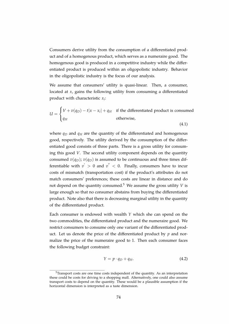
Consumers derive utility from the consumption of a differentiated prod-uct and of a homogenous product, which serves as a numeraire good. Thehomogenous good is produced in a competitive industry while the differ-entiated product is produced within an oligopolistic industry. Behaviorin the oligopolistic industry is the focus of our analysis.

We assume that consumers’ utility is quasi-linear. Then, a consumer,located at x, gains the following utility from consuming a differentiatedproduct with characteristic xi:

U =

⎧⎨⎩V + v(qD)− t∣x− xi∣+ qH if the differentiated product is consumed

qH otherwise,(4.1)

where qD and qH are the quantity of the differentiated and homogenousgood, respectively. The utility derived by the consumption of the differ-entiated good consists of three parts. There is a gross utility for consum-ing this good V. The second utility component depends on the quantityconsumed v(qD); v(qD) is assumed to be continuous and three times dif-ferentiable with v

′> 0 and v

′′< 0. Finally, consumers have to incur

costs of mismatch (transportation cost) if the product’s attributes do notmatch consumers’ preferences; these costs are linear in distance and donot depend on the quantity consumed.5 We assume the gross utility V islarge enough so that no consumer abstains from buying the differentiatedproduct. Note also that there is decreasing marginal utility in the quantityof the differentiated product.

Each consumer is endowed with wealth Y which she can spend on thetwo commodities, the differentiated product and the numeraire good. Werestrict consumers to consume only one variant of the differentiated prod-uct. Let us denote the price of the differentiated product by p and nor-malize the price of the numeraire good to 1. Then each consumer facesthe following budget constraint:

Y = p ⋅ qD + qH. (4.2)

5Transport costs are one time costs independent of the quantity. As an interpretationthese could be costs for driving to a shopping mall. Alternatively, one could also assumetransport costs to depend on the quantity. These would be a plausible assumption if thehorizontal dimension is interpreted as a taste dimension.

74

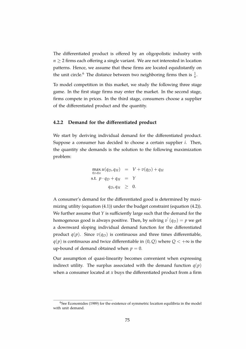
The differentiated product is offered by an oligopolistic industry withn ≥ 2 firms each offering a single variant. We are not interested in locationpatterns. Hence, we assume that these firms are located equidistantly onthe unit circle.6 The distance between two neighboring firms then is 1

n .

To model competition in this market, we study the following three stagegame. In the first stage firms may enter the market. In the second stage,firms compete in prices. In the third stage, consumers choose a supplierof the differentiated product and the quantity.

4.2.2 Demand for the differentiated product

We start by deriving individual demand for the differentiated product.Suppose a consumer has decided to choose a certain supplier i. Then,the quantity she demands is the solution to the following maximizationproblem:

maxqD ,qH

u(qD, qH) = V + v(qD) + qH

s.t. p ⋅ qD + qH = Y

qD, qH ≥ 0.

A consumer’s demand for the differentiated good is determined by maxi-mizing utility (equation (4.1)) under the budget constraint (equation (4.2)).We further assume that Y is sufficiently large such that the demand for thehomogenous good is always positive. Then, by solving v

′(qD) = p we get

a downward sloping individual demand function for the differentiatedproduct q(p). Since v(qD) is continuous and three times differentiable,q(p) is continuous and twice differentiable in (0, Q) where Q < +∞ is theup-bound of demand obtained when p = 0.

Our assumption of quasi-linearity becomes convenient when expressingindirect utility. The surplus associated with the demand function q(p)when a consumer located at x buys the differentiated product from a firm

6See Economides (1989) for the existence of symmetric location equilibria in the modelwith unit demand.

75

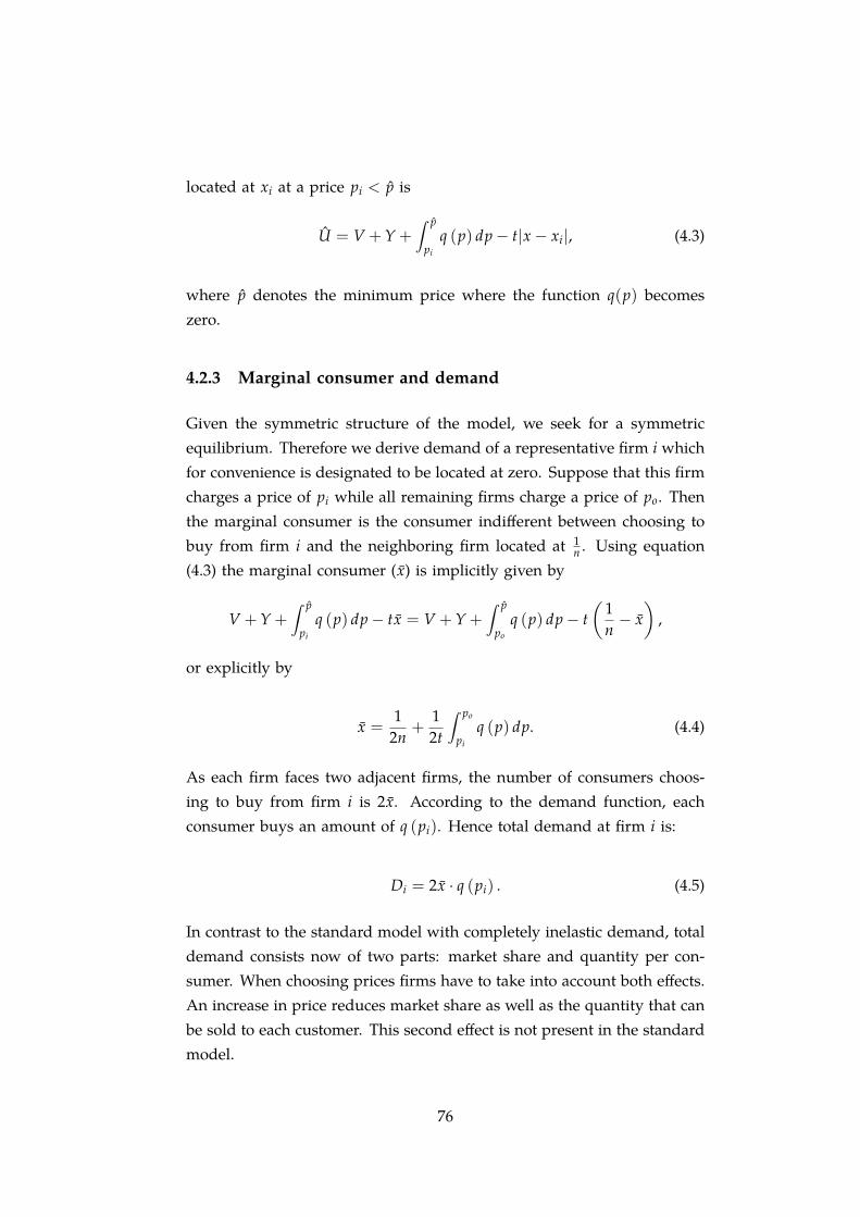
located at xi at a price pi < p is

U = V + Y +∫ p

pi

q (p) dp− t∣x− xi∣, (4.3)

where p denotes the minimum price where the function q(p) becomeszero.

4.2.3 Marginal consumer and demand

Given the symmetric structure of the model, we seek for a symmetricequilibrium. Therefore we derive demand of a representative firm i whichfor convenience is designated to be located at zero. Suppose that this firmcharges a price of pi while all remaining firms charge a price of po. Thenthe marginal consumer is the consumer indifferent between choosing tobuy from firm i and the neighboring firm located at 1

n . Using equation(4.3) the marginal consumer (x) is implicitly given by

V + Y +∫ p

pi

q (p) dp− tx = V + Y +∫ p

po

q (p) dp− t(

1n− x)

,

or explicitly by

x =1

2n+

12t

∫ po

pi

q (p) dp. (4.4)

As each firm faces two adjacent firms, the number of consumers choos-ing to buy from firm i is 2x. According to the demand function, eachconsumer buys an amount of q (pi). Hence total demand at firm i is:

Di = 2x ⋅ q (pi) . (4.5)

In contrast to the standard model with completely inelastic demand, totaldemand consists now of two parts: market share and quantity per con-sumer. When choosing prices firms have to take into account both effects.An increase in price reduces market share as well as the quantity that canbe sold to each customer. This second effect is not present in the standardmodel.

76

4.3 Analysis

This section analyzes the equilibrium. In a first step we characterize theprice equilibrium for a given number of firms and provide conditions forthe existence. In a second step, we seek to determine the number of firmsthat enter.

4.3.1 Price equilibrium

We look for a symmetric equilibrium in which all firms charge the sameprice. Assuming zero production costs, the profit of a representative firmi when this firm charges a price pi and all remaining firms charge a pricepo is given by:

Πi = Di ⋅ pi =

[1n+

1t

∫ po

pi

q (p) dp]

q (pi) pi. (4.6)

To find profit maximizing price pi, we first derive the first order derivative,

dΠi

dpi= −1

tpi [q (pi)]

2 +

[1n+

1t

∫ po

pi

q (p) dp] [

q (pi) + pidq (p)

dp

∣∣∣p=pi

].

(4.7)By setting equation (4.7) to zero we obtain the following necessary condi-tion,

[q (pi)]2 pi

1t=

[1n+

1t

∫ po

pi

q (p) dp] [

q (pi) + pidq (p)

dp

∣∣∣p=pi

]. (4.8)

For the moment let us suppose that a symmetric price equilibrium exists.Later we will turn to this issue and provide existence conditions. Applyingsymmetry to the first-order condition, a symmetric price equilibrium ischaracterized by:

q (p∗) p∗ =tn

[1 +

p∗

q (p∗)dq (p)

dp

∣∣∣p=p∗

]. (4.9)

Note that the last part of equation (4.9) includes the price elasticity ofindividual demand evaluated at the equilibrium price. After the follow-

77

ing definition, we express this equilibrium condition in terms of priceelasticity of demand.

Definition 4.1. Denote the absolute value of price elasticity of demand ε as

ε = − pq(p)

dq(p)dp

.

Equation (4.9) now can be rewritten as

q (p∗) p∗ =tn[1− ε∗] . (4.10)

We use this condition to state corresponding equilibrium profits. Insertingequation (4.9) into equation (4.6) we get

Π∗ =t

n2

[1 +

p∗

q (p∗)dq (p)

dp

∣∣∣p=p∗

]=

tn2 [1− ε∗] . (4.11)

It can be seen immediately that there is a negative relationship betweenequilibrium demand elasticity and equilibrium profit.

4.3.2 Equilibrium existence

Now we provide conditions that ensure existence of a symmetric priceequilibrium as stated in equation (4.10). We start with a preliminaryresult:

Lemma 4.1. In equilibrium, demand is inelastic, that is, ε∗ < 1.

Proof. see appendix.

This result reveals that analogous to a monopolist who sets the price toreach unit elasticity, a firm in the current model will only set price at theinelastic segment of the demand function.

To ensure existence, we have to impose some additional structure on thedemand function. We introduce the following assumption:7

7This assumption is sufficient but not necessary for the existence of a symmetric priceequilibrium.

78

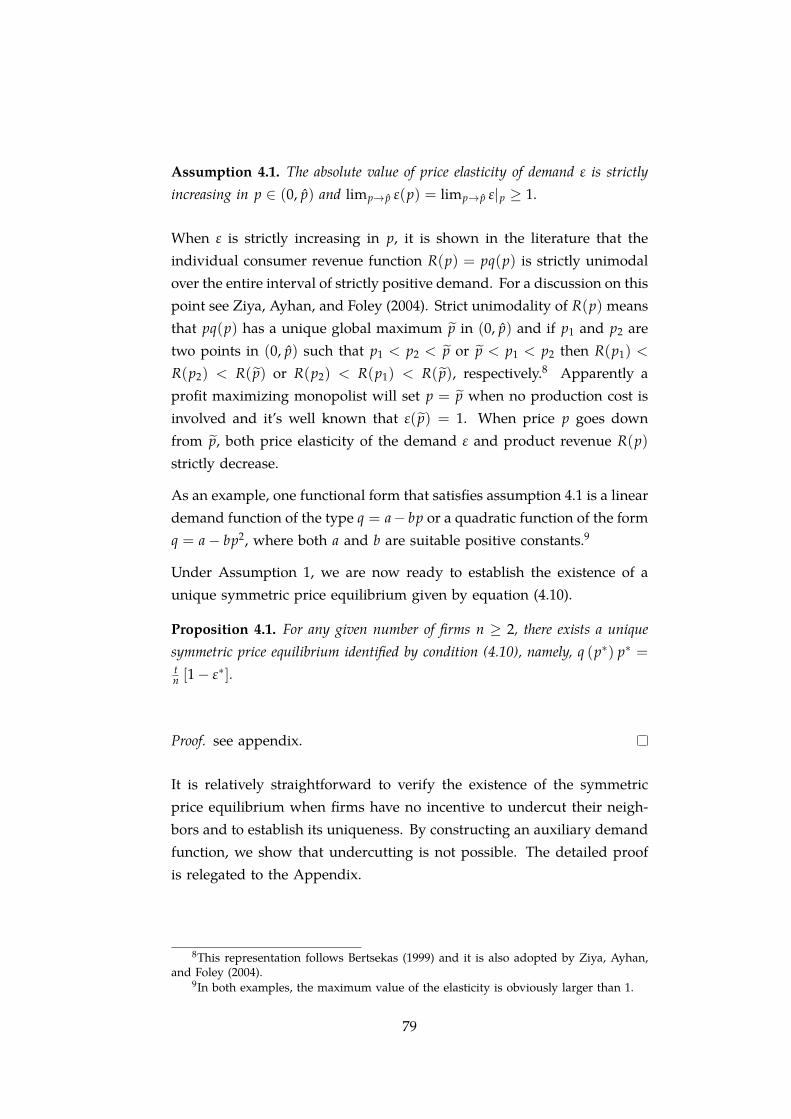
Assumption 4.1. The absolute value of price elasticity of demand ε is strictlyincreasing in p ∈ (0, p) and limp→ p ε(p) = limp→ p ε∣p ≥ 1.

When ε is strictly increasing in p, it is shown in the literature that theindividual consumer revenue function R(p) = pq(p) is strictly unimodalover the entire interval of strictly positive demand. For a discussion on thispoint see Ziya, Ayhan, and Foley (2004). Strict unimodality of R(p) meansthat pq(p) has a unique global maximum p in (0, p) and if p1 and p2 aretwo points in (0, p) such that p1 < p2 < p or p < p1 < p2 then R(p1) <

R(p2) < R( p) or R(p2) < R(p1) < R( p), respectively.8 Apparently aprofit maximizing monopolist will set p = p when no production cost isinvolved and it’s well known that ε( p) = 1. When price p goes downfrom p, both price elasticity of the demand ε and product revenue R(p)strictly decrease.

As an example, one functional form that satisfies assumption 4.1 is a lineardemand function of the type q = a− bp or a quadratic function of the formq = a− bp2, where both a and b are suitable positive constants.9

Under Assumption 1, we are now ready to establish the existence of aunique symmetric price equilibrium given by equation (4.10).

Proposition 4.1. For any given number of firms n ≥ 2, there exists a uniquesymmetric price equilibrium identified by condition (4.10), namely, q (p∗) p∗ =tn [1− ε∗].

Proof. see appendix.

It is relatively straightforward to verify the existence of the symmetricprice equilibrium when firms have no incentive to undercut their neigh-bors and to establish its uniqueness. By constructing an auxiliary demandfunction, we show that undercutting is not possible. The detailed proofis relegated to the Appendix.

8This representation follows Bertsekas (1999) and it is also adopted by Ziya, Ayhan,and Foley (2004).

9In both examples, the maximum value of the elasticity is obviously larger than 1.

79

4.3.3 Properties of price equilibrium

We can now study the properties of the price equilibrium. Lemma 4.2below states the comparative statics effect of the number of firms whichare active in the market and of transportation costs on equilibrium price,equilibrium price elasticity and firm profit.

Lemma 4.2. Comparative statics.

1. Equilibrium price, price elasticity of demand and firm profit decrease in thenumber of entrants, that is, dp∗

dn < 0, dε∗

dn < 0 and dΠ∗dn < 0.

2. Equilibrium price, price elasticity of demand and firm profit increase intransportation costs, that is, dp∗

dt > 0, dε∗

dt > 0 and dΠ∗dt > 0.

Proof. see appendix.

Unsurprisingly, the larger the number of firms the lower the price. Profitsalso decrease with the number of firms in the market. Additionally, thedemand elasticity decreases with the number of firms in the market. Thisfollows from our assumption that the demand elasticity increases in theprice. The impact of transportation costs on prices and profits is thesame as in standard location models. Prices and profits increase withtransportation costs.

4.3.4 Entry

Until now the analysis has treated the number of firms which offer differ-entiated products as exogenously given. We now investigate the numberof active firms when it is endogenously determined by a zero profit con-dition. We assume that to enter, a firm has to incur an entry cost or fixedcost of f . Additionally, we treat the number of entrants as a continu-ous variable. Setting equation (4.11) equal to f determines implicitly thenumber of firms that enter. We denote this number by nc:

t(nc)2 (1− ε∗nc) = f . (4.12)

80

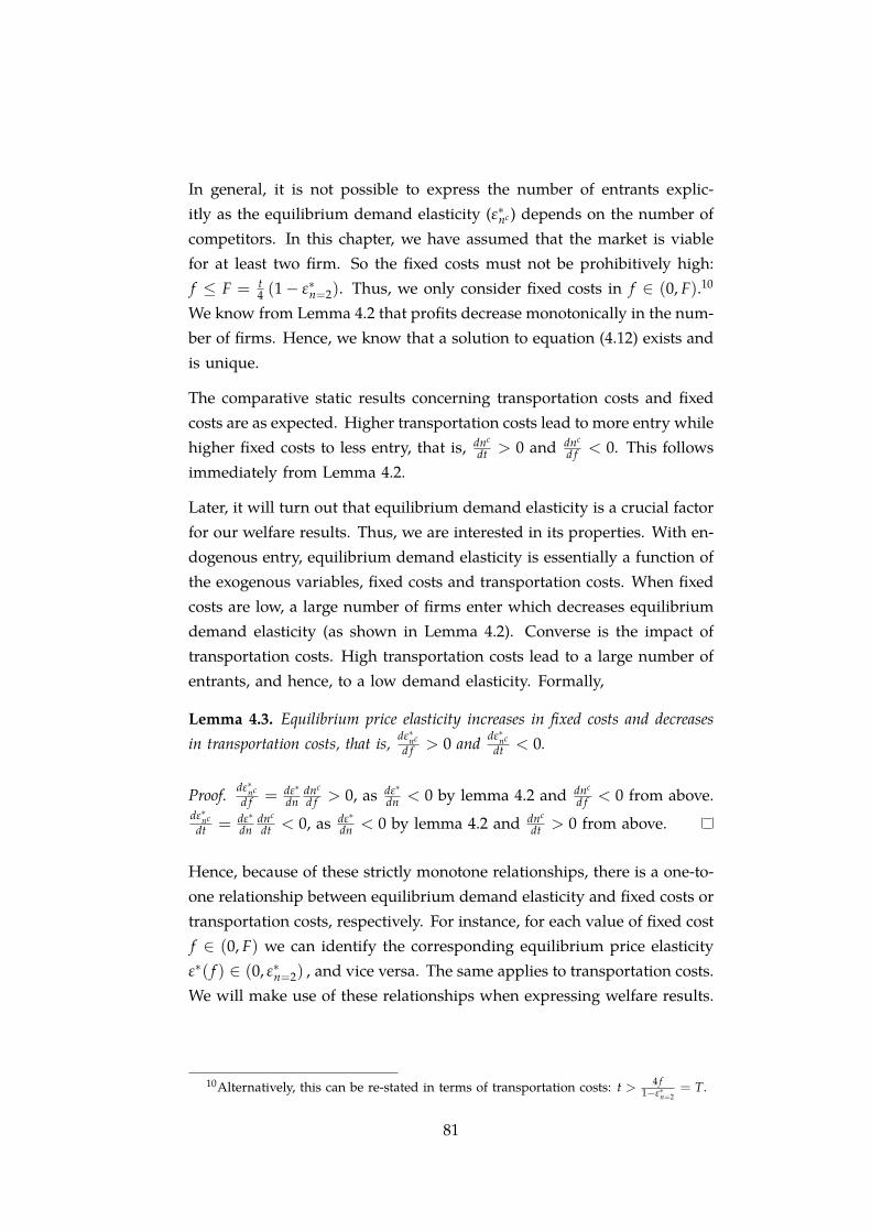
In general, it is not possible to express the number of entrants explic-itly as the equilibrium demand elasticity (ε∗nc) depends on the number ofcompetitors. In this chapter, we have assumed that the market is viablefor at least two firm. So the fixed costs must not be prohibitively high:f ≤ F = t

4 (1− ε∗n=2). Thus, we only consider fixed costs in f ∈ (0, F).10

We know from Lemma 4.2 that profits decrease monotonically in the num-ber of firms. Hence, we know that a solution to equation (4.12) exists andis unique.

The comparative static results concerning transportation costs and fixedcosts are as expected. Higher transportation costs lead to more entry whilehigher fixed costs to less entry, that is, dnc

dt > 0 and dnc

d f < 0. This followsimmediately from Lemma 4.2.

Later, it will turn out that equilibrium demand elasticity is a crucial factorfor our welfare results. Thus, we are interested in its properties. With en-dogenous entry, equilibrium demand elasticity is essentially a function ofthe exogenous variables, fixed costs and transportation costs. When fixedcosts are low, a large number of firms enter which decreases equilibriumdemand elasticity (as shown in Lemma 4.2). Converse is the impact oftransportation costs. High transportation costs lead to a large number ofentrants, and hence, to a low demand elasticity. Formally,

Lemma 4.3. Equilibrium price elasticity increases in fixed costs and decreasesin transportation costs, that is, dε∗nc

d f > 0 and dε∗ncdt < 0.

Proof. dε∗ncd f = dε∗

dndnc

d f > 0, as dε∗

dn < 0 by lemma 4.2 and dnc

d f < 0 from above.dε∗ncdt = dε∗

dndnc

dt < 0, as dε∗

dn < 0 by lemma 4.2 and dnc

dt > 0 from above.

Hence, because of these strictly monotone relationships, there is a one-to-one relationship between equilibrium demand elasticity and fixed costs ortransportation costs, respectively. For instance, for each value of fixed costf ∈ (0, F) we can identify the corresponding equilibrium price elasticityε∗( f ) ∈ (0, ε∗n=2) , and vice versa. The same applies to transportation costs.We will make use of these relationships when expressing welfare results.

10Alternatively, this can be re-stated in terms of transportation costs: t > 4 f1−ε∗n=2

= T.

81

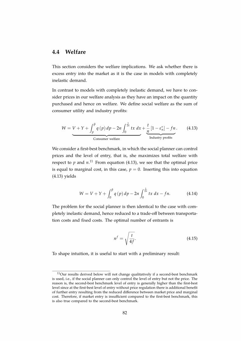
4.4 Welfare

This section considers the welfare implications. We ask whether there isexcess entry into the market as it is the case in models with completelyinelastic demand.

In contrast to models with completely inelastic demand, we have to con-sider prices in our welfare analysis as they have an impact on the quantitypurchased and hence on welfare. We define social welfare as the sum ofconsumer utility and industry profits:

W = V + Y +∫ p

pq (p) dp− 2n

∫ 12n

0tx dx︸ ︷︷ ︸

Consumer welfare

+tn[1− ε∗n]− f n︸ ︷︷ ︸

Industry profits

. (4.13)

We consider a first-best benchmark, in which the social planner can controlprices and the level of entry, that is, she maximizes total welfare withrespect to p and n.11 From equation (4.13), we see that the optimal priceis equal to marginal cost, in this case, p = 0. Inserting this into equation(4.13) yields

W = V + Y +∫ p

0q (p) dp− 2n

∫ 12n

0tx dx− f n. (4.14)

The problem for the social planner is then identical to the case with com-pletely inelastic demand, hence reduced to a trade-off between transporta-tion costs and fixed costs. The optimal number of entrants is

n f =

√t

4 f. (4.15)

To shape intuition, it is useful to start with a preliminary result:

11Our results derived below will not change qualitatively if a second-best benchmarkis used, i.e., if the social planner can only control the level of entry but not the price. Thereason is, the second-best benchmark level of entry is generally higher than the first-bestlevel since at the first-best level of entry without price regulation there is additional benefitof further entry resulting from the reduced difference between market price and marginalcost. Therefore, if market entry is insufficient compared to the first-best benchmark, thisis also true compared to the second-best benchmark.

82

Lemma 4.4. There is excess entry if ε∗nc < 34 , insufficient entry if ε∗nc > 3

4 , andoptimal entry if ε∗nc = 3

4 .

Lemma 4.4 can easily be derived by comparing equations (4.12) and (4.15).This lemma provides conditions for the existence of excessive, insufficient,and optimal entry. If the equilibrium demand elasticity is sufficiently lowwe get excess entry as in the standard model with completely inelasticdemand. If, on the other hand, equilibrium demand elasticity exceeds 3

4 ,there is insufficient entry into the market. The intuition behind the resultcan be seen in equation (4.11). The higher equilibrium demand elasticityis, the lower the profits are; and hence the smaller the incentives to enterthe market will be.

However, the equilibrium demand elasticity is endogenous in this model.Thus, our aim is to state the welfare result in terms of exogenous variables.Now we can make use of the monotone relationship between equilibriumdemand elasticity and fixed costs of entry. Entry is excessive (insufficient)if fixed costs are such that ε∗nc < 3

4 (ε∗nc > 34 ). This leads to:

Proposition 4.2. Welfare result.

1. Suppose ε∗n=2 ≥ 34 and define f as the fixed cost level that leads to equi-

librium price elasticity ε∗nc = 34 . Then there is excess entry if f < f ,

insufficient entry if f > f and optimal entry if f = f .

2. Suppose ε∗n=2 < 34 , then there is excess entry for all f ∈ (0, F].

Proof. see appendix.

Proposition 4.2 contains the main contribution of the chapter. When ac-counting for price-dependent demand the excess entry result of the stan-dard model with completely inelastic demand needs not hold. In theproposition we have to consider two cases. First, if the demand functionis such that ε∗n=2 ≥ 3

4 . Then, if fixed costs of entry are high such that thecorresponding equilibrium demand elasticity is high, entry into the mar-ket is insufficient. Conversely, if fixed costs are low, the number of firmsthat enter is high which leads to a low demand elasticity. And hence,entry into the market is excessive. The second case we have to consideris a demand function which has the property such that ε∗n=2 < 3

4 . As ε∗nc

83

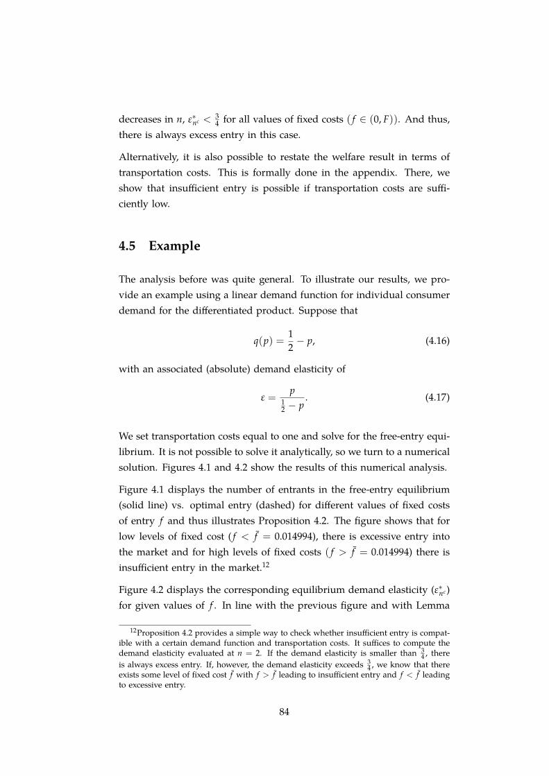
decreases in n, ε∗nc < 34 for all values of fixed costs ( f ∈ (0, F)). And thus,

there is always excess entry in this case.

Alternatively, it is also possible to restate the welfare result in terms oftransportation costs. This is formally done in the appendix. There, weshow that insufficient entry is possible if transportation costs are suffi-ciently low.

4.5 Example

The analysis before was quite general. To illustrate our results, we pro-vide an example using a linear demand function for individual consumerdemand for the differentiated product. Suppose that

q(p) =12− p, (4.16)

with an associated (absolute) demand elasticity of

ε =p

12 − p

. (4.17)

We set transportation costs equal to one and solve for the free-entry equi-librium. It is not possible to solve it analytically, so we turn to a numericalsolution. Figures 4.1 and 4.2 show the results of this numerical analysis.

Figure 4.1 displays the number of entrants in the free-entry equilibrium(solid line) vs. optimal entry (dashed) for different values of fixed costsof entry f and thus illustrates Proposition 4.2. The figure shows that forlow levels of fixed cost ( f < f = 0.014994), there is excessive entry intothe market and for high levels of fixed costs ( f > f = 0.014994) there isinsufficient entry in the market.12

Figure 4.2 displays the corresponding equilibrium demand elasticity (ε∗nc)for given values of f . In line with the previous figure and with Lemma

12Proposition 4.2 provides a simple way to check whether insufficient entry is compat-ible with a certain demand function and transportation costs. It suffices to compute thedemand elasticity evaluated at n = 2. If the demand elasticity is smaller than 3

4 , thereis always excess entry. If, however, the demand elasticity exceeds 3

4 , we know that thereexists some level of fixed cost f with f > f leading to insufficient entry and f < f leadingto excessive entry.

84

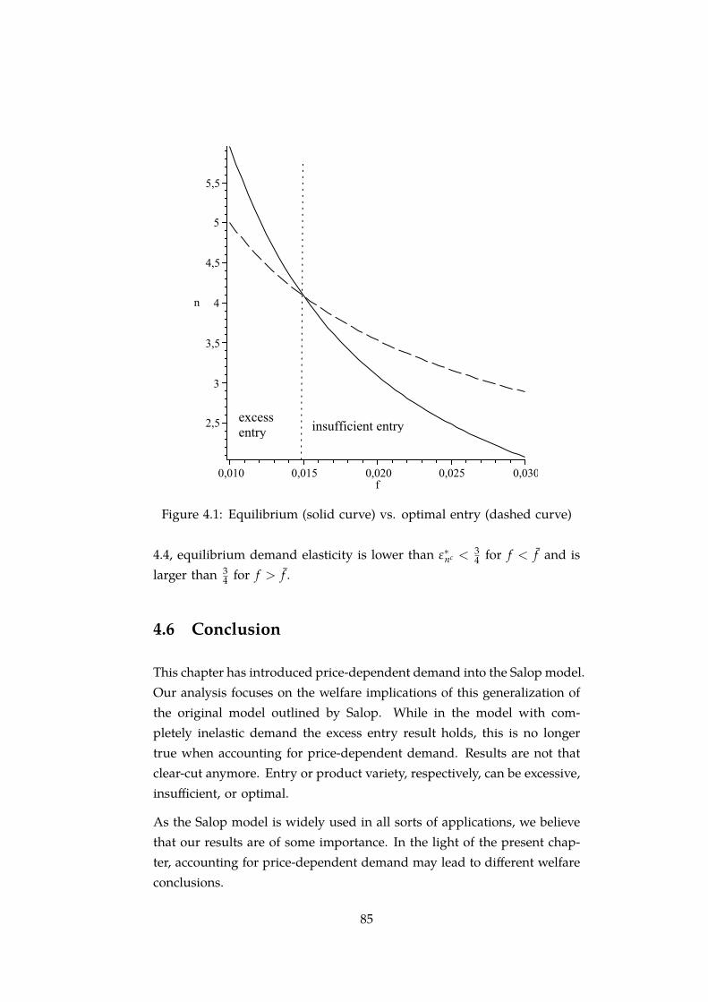
Figure 4.1: Equilibrium (solid curve) vs. optimal entry (dashed curve)

4.4, equilibrium demand elasticity is lower than ε∗nc < 34 for f < f and is

larger than 34 for f > f .

4.6 Conclusion

This chapter has introduced price-dependent demand into the Salop model.Our analysis focuses on the welfare implications of this generalization ofthe original model outlined by Salop. While in the model with com-pletely inelastic demand the excess entry result holds, this is no longertrue when accounting for price-dependent demand. Results are not thatclear-cut anymore. Entry or product variety, respectively, can be excessive,insufficient, or optimal.

As the Salop model is widely used in all sorts of applications, we believethat our results are of some importance. In the light of the present chap-ter, accounting for price-dependent demand may lead to different welfareconclusions.

85

Figure 4.2: Equilibrium demand elasticity

4.7 Appendix

4.7.1 Proof of Lemma 4.1

Proof: Note when ε ≥ 1 i.e., dq(p)dp

pq(p) ≤ −1, the first order derivative (4.7)

dΠi

dpi= − [q (pi)]

2 pi1t︸ ︷︷ ︸

negative

+

[1n+

1t

∫ po

pi

q (p) dp]

q (pi)︸ ︷︷ ︸positive

[1 +

pi

q (pi)

dq (p)dp

∣∣∣p=pi

]︸ ︷︷ ︸

non-positive(4.18)

obtains a strictly negative value. The middle part in the right-hand sideof (4.18) is positive because we are interested in symmetric equilibrium(pi = po). With dΠi

dpibeing negative, whenever demand elasticity exceeds

or is equal to 1, a firm wants to reduce price in order to boost demand.

86

In equilibrium, whenever it exists, however, the F.O.C. (4.9) holds,

1 +p∗

q (p∗)dq (p)

dp

∣∣∣p=p∗

> 0

=⇒ p∗

q (p∗)dq (p)

dp

∣∣∣p=p∗

> −1

=⇒ ε∗ < 1.

This concludes the proof.

4.7.2 Proof of Proposition 4.1

Proof: The structure of the proof is the following. We first show that thenecessary first order condition (4.10) admits a unique solution. Second,we prove that under the condition of symmetric price and without under-cutting, firm profit is quasi-concave in the strategy variable pi. Last weshow that firms have no incentive to undercut neighbors when they arein the situation identified by the first order condition.

1) Define ∆(p) = q (p) p− tn [1− ε(p)]. Because v(qD) is continuous and

three times differentiable, q(p) and ε(p) are continuous and differen-tiable. Hence, ∆(p) is continuous. Note that

limp→0

∆(p) = 0− tn

[1− lim

p→0ε(p)

]= 0− t

n< 0

and for the individual consumer (R(p) = pq(p)) revenue-maximizingp,

∆( p) = q ( p) p > 0.

Because of continuity, ∆(p) = 0 obtains solution(s) for p ∈ (0, p). Takethe derivative of ∆(p),

d∆(p)dp

=dR(p)

dp+

tn

dε(p)dp

.

Following Assumption 4.1, dε(p)dp > 0; since R(p) is strictly unimodal, for

p ∈ (0, p), dR(p)dp > 0 as well. Hence, we conclude d∆(p)

dp > 0. Because ofthis monotonicity, ∆(p) = 0 obtains a unique solution in (0, p). Whenp ∈ [ p, p), we know ε(p) ≥ 1 which means ∆(p) > 0 for [ p, p). So

87

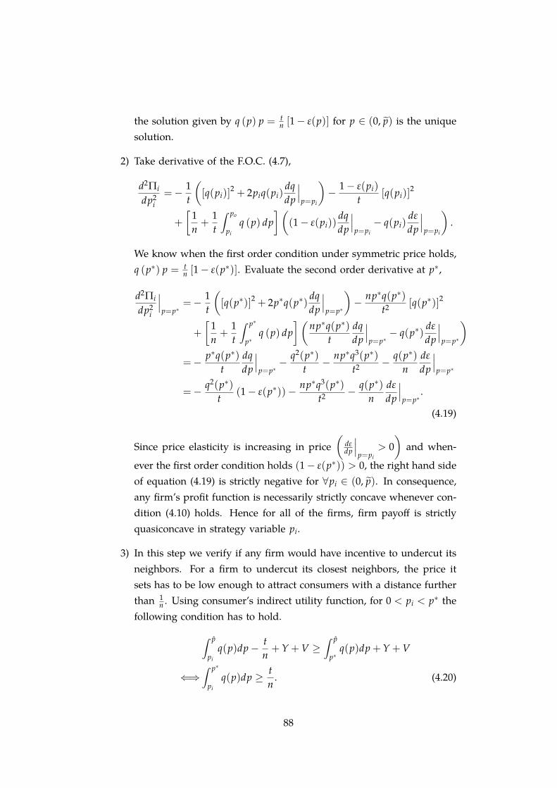
the solution given by q (p) p = tn [1− ε(p)] for p ∈ (0, p) is the unique

solution.

2) Take derivative of the F.O.C. (4.7),

d2Πi

dp2i

=− 1t

([q(pi)]

2 + 2piq(pi)dqdp

∣∣∣p=pi

)− 1− ε(pi)

t[q(pi)]

2

+

[1n+

1t

∫ po

pi

q (p) dp] (

(1− ε(pi))dqdp

∣∣∣p=pi

− q(pi)dε

dp

∣∣∣p=pi

).

We know when the first order condition under symmetric price holds,q (p∗) p = t

n [1− ε(p∗)]. Evaluate the second order derivative at p∗,

d2Πi

dp2i

∣∣∣p=p∗

=− 1t

([q(p∗)]2 + 2p∗q(p∗)

dqdp

∣∣∣p=p∗

)− np∗q(p∗)

t2 [q(p∗)]2

+

[1n+

1t

∫ p∗

p∗q (p) dp

] (np∗q(p∗)

tdqdp

∣∣∣p=p∗− q(p∗)

dε

dp

∣∣∣p=p∗

)=− p∗q(p∗)

tdqdp

∣∣∣p=p∗− q2(p∗)

t− np∗q3(p∗)

t2 − q(p∗)n

dε

dp

∣∣∣p=p∗

=− q2(p∗)t

(1− ε(p∗))− np∗q3(p∗)t2 − q(p∗)

ndε

dp

∣∣∣p=p∗

.

(4.19)

Since price elasticity is increasing in price(

dεdp

∣∣∣p=pi

> 0)

and when-

ever the first order condition holds (1− ε(p∗)) > 0, the right hand sideof equation (4.19) is strictly negative for ∀pi ∈ (0, p). In consequence,any firm’s profit function is necessarily strictly concave whenever con-dition (4.10) holds. Hence for all of the firms, firm payoff is strictlyquasiconcave in strategy variable pi.

3) In this step we verify if any firm would have incentive to undercut itsneighbors. For a firm to undercut its closest neighbors, the price itsets has to be low enough to attract consumers with a distance furtherthan 1

n . Using consumer’s indirect utility function, for 0 < pi < p∗ thefollowing condition has to hold.

∫ p

pi

q(p)dp− tn+ Y + V ≥

∫ p

p∗q(p)dp + Y + V

⇐⇒∫ p∗

pi

q(p)dp ≥ tn

. (4.20)

88

To investigate condition (4.20), we first prepare an additional result(i.e., inequality (4.23) below) for further use. By solving (4.10) we willhave equilibrium price p∗, the corresponding demand q∗ = q(p∗) andprice elasticity ε∗ = ε(p∗). Define constant

ϕ =q∗

(p∗)−ε∗ .

We construct an auxiliary demand function with constant elasticity ε∗,

q†(p) = ϕp−ε∗

which also passes through the point (p∗, q∗). With this demand func-tion we can obtain the following closed form formula for 0 < pi < p∗,

∫ p∗

pi

ϕp−ε∗dp =ϕ

1− ε∗p1−ε∗

∣∣∣p∗pi

. (4.21)

Applying the necessary condition for symmetric equilibrium 1− ε∗ =nt p∗q (p∗), equation (4.21) becomes

∫ p∗

pi

ϕp−ε∗dp =q∗

(p∗)−ε∗t

np∗q∗((p∗)1−ε∗ − (pi)

1−ε∗)

=tn(p∗)1−ε∗ − (pi)

1−ε∗

(p∗)1−ε∗

=tn

(1−

(pi

p∗

)1−ε∗)

.

Since 0 ≤ 1− ε∗ < 1 and 0 < pi < p∗, we have

∫ p∗

pi

ϕp−ε∗dp <tn

, ∀ pi ∈ (0, p∗). (4.22)

Note also that q†(p) = ϕp−ε∗ has a constant elasticity ε∗ while q(p)obtains elasticity ε∗ at the point (p∗, q∗) but strictly lower elasticityε < ε∗ when price decreases. That is, for the same percentage decreaseof price, although q(p) and q†(p) start out at the same point (p∗, q∗),

89

q(p) increase less than q†(p) does. Hence,

q(p) < ϕp−ε∗ , for ∀ p ∈ (0, p∗)

=⇒∫ p∗

pi

q(p)dp <∫ p∗

pi

ϕp−ε∗dp, for ∀ pi ∈ (0, p∗).

By condition (4.22) we have the next result,

∫ p∗

pi

q(p)dp <tn

for ∀ pi ∈ (0, p∗). (4.23)

Now we are ready to discuss the undercutting strategy for firm i facingconsumer demand function q(p). To undercut its neighbors who arecharging the symmetric equilibrium price p∗, condition (4.20) has tohold. Because of the result we established in (4.23), there exists nopositive price that satisfies condition (4.20). Hence there is no firmwho is able to take over neighbor’s business without losing money.

4) We have shown that for any n ≥ 2, there exists a unique solution tocondition (4.10). Moreover, the strategy profile characterized by thiscondition is indeed an equilibrium because firms’ payoffs are strictlyquasiconcave in own strategy and there is no incentive for firms toundercut neighbors. This concludes the proof.

4.7.3 Proof of Lemma 4.2

Proof:

1. Take total differentiation of equation (4.10) with respect to the num-ber of firms,

dq∗

dpdp∗

dnp∗ + q∗

dp∗

dn=

tn

(−dε∗

dpdp∗

dn

)− (1− ε∗)

tn2

=⇒(

dq∗

dpp∗ + q∗

)dp∗

dn= − t

ndε∗

dpdp∗

dn− t

n2 (1− ε∗)

=⇒dp∗

dn

(q∗(1− ε∗) +

tn

dε∗

dp

)= − t

n2 (1− ε∗)

=⇒dp∗

dn=

− tn2 (1− ε∗)

q(1− ε∗) + tn

dε∗dp

.

90

Since (1− ε∗) > 0 by Lemma 4.1 and dε∗

dp > 0, in equilibrium dp∗dn < 0.

Also from Assumption 4.1

dε∗

dn=

dε∗

dpdp∗

dn< 0.

Differentiate equation (4.11) with respect to n:

dΠ∗

dn=− 2t

n3 (1− ε∗)− tn2

dε∗

dn

=− tn3 (1− ε∗)

[2− t

ndε∗

dp

(1

q∗(1− ε∗) + tn

dε∗dp

)]

=− tn3 (1− ε∗)

2q∗(1− ε∗) + tn

dε∗

dp

q∗(1− ε∗) + tn

dε∗dp

< 0.

2. Take total differentiation of equation (4.10) with respect to trans-portation costs,

dq∗

dpdp∗

dtp∗ + q∗

dp∗

dt= − t

n

(dε∗

dpdp∗

dt

)+ (1− ε∗)

1n

=⇒dp∗

dt

(q∗(1− ε∗) +

tn

dε∗

dp

)=

1n(1− ε∗)

=⇒dp∗

dt=

1n (1− ε∗)

q∗(1− ε∗) + tn

dε∗dp

> 0.

It follows:

dε∗

dt=

dε

dpdp∗

dt

=dε

dp

1n (1− ε∗)

q∗(1− ε∗) + tn

dε∗dp

> 0.

Differentiate equation (4.11) with respect to transportation costs:

dΠ∗

dt=

1n2 (1− ε∗)− t

n2dε∗

dt

=1n2 (1− ε∗)

[1− t

ndε

dp

(1

q∗(1− ε∗) + tn

dεdp

)]

=1n2 (1− ε∗)

q∗(1− ε∗)

q∗(1− ε∗) + tn

dε∗dp

> 0.

91

4.7.4 Proof of Proposition 4.2

Proof: From Lemma 4.3, we know that equilibrium elasticity under freeentry increases in fixed cost. From Lemma 4.4, we know that nc > n f

when ε∗nc < 34 , nc = n f when ε∗nc = 3

4 , and nc < n f when ε∗nc > 34 .

We have to consider two cases:

1. ε∗n=2 ≥ 34 . Then, there exists a fixed cost f such that the resulting

equilibrium demand elasticity is equal to 34 . Since ε∗nc increases in

f , for f < f , ε∗nc < 34 which leads to excessive entry by Lemma 4.4.

Conversely, for f > f , ε∗nc > 34 which means insufficient entry.

2. ε∗n=2 < 34 . Then, since ε∗nc decreases in n, ε∗nc < 3

4 for all values of f .And hence, there is excess entry.

We can also reformulate Proposition 4.2 in terms of transportation costs.What we need first is to show that there is a monotone relationship be-tween equilibrium demand elasticity and transportation costs. This isdε∗ncdt = dε

dndndt < 0, as dε

dn < 0 from Lemma 4.2 and dndt > 0.

Again, we must distinguish the two cases:

1. ε∗n=2 ≥ 34 . Then, there exists a transportation cost t such that the

resulting equilibrium demand elasticity is equal to 34 . Since ε∗nc de-

creases in t, for t > t, ε∗nc < 34 which leads to excessive entry by

Lemma 4.4. Conversely, for t < t, ε∗nc > 34 which means insufficient

entry.

2. ε∗n=2 < 34 . Then, since ε∗nc decreases in n, ε∗nc < 3

4 for all values of t.And hence, there is excess entry.

We state the result formally as a corollary:

Corollary 4.1. Welfare result in terms of transportation costs.

1. Suppose ε∗n=2 ≥ 34 and define t as the transportation cost level that leads

to equilibrium price elasticity ε∗ of 34 . Then there is excess entry if t > t,

insufficient entry if t < t and optimal entry if t = t.

2. Suppose ε∗n=2 < 34 , then there is excess entry for all t > T.

92

Chapter 5

Gift Giving and Concern forFace

The Widow’s OfferingAnd he called unto him his disciples, and saith unto them, Verily Isay unto you, That this poor widow hath cast more in, than all theywhich have cast into the treasury: For all they did cast in of theirabundance; but she of her want did cast in all that she had, even allher living. — Mark 12: 43–44

5.1 Introduction

5.1.1 Theories of gift giving

People voluntarily contribute to public goods, make charitable transfers tothe needy and give gifts to others. Explanations for such behavior are notapparent from the point of view of neoclassical economic theory. A rea-sonable attempt was to admit the total provision of public goods into indi-vidual preferences together with private consumptions (see, for example,McGuire (1974), Warr (1982), Roberts (1984) and Bergstrom, Blume, andVarian (1986)). However, Andreoni (1988) shows that such a pure altruismmodel typically leads to prevailing of free-riding in large economies. Thisframework also predicts that government spending on public goods willcrowd out equal amount of private donation while empirical studies find

93

such crowding out is rather small.1 These issues can be addressed by theinclusion of the act of giving into individual preferences. The argumentis that private donation may also be motivated by social or psychologicalconcerns such as esteem, prestige, social pressure or simply a feeling of awarm glow. A large body of sociological, psychological, and anthropolog-ical research supports this view and important contributions employingthis impure altruism approach in economic studies have been presentedby, for example, Arrow (1972), Margolis (1981), Andreoni (1989, 1990),McClelland (1989) among many others.

5.1.2 Warm glow

Harbaugh (1998a, 1998b) further differentiates two distinctive types of“joy of giving” that may be derived from the act of donation. The firstis the “intrinsic benefit” which a donor enjoys because of her own moralconcerns and only requires her own knowledge of the act of giving. Forinstance, a donor is happier after a donation because only then she feelsshe is entitled to think herself as a good person. The other is the “prestigebenefit” which comes from a donor’s social concerns and is only obtainedwhen the act of giving is publicly recognized. In this case, a donor’sdecision is influenced by how others think about himself. See, for example,Deci and Ryan (1985), Brekke, Kverndokk, and Nyborg (2003) for studiesof moral motivation and Hollander (1990), Lindbeck (1997) for studies ofsocial acceptance.

Though the literature of warm glow has convincingly argued and exten-sively studied the relevance of the demand for warm glow, what remainsless investigated is the supply or the production technology of it. In the so-cial concern case obviously, from the same $100 donation to a charity, the“prestige” one enjoys when he is the only donor differs to what one wouldclaim, if any, when he was just one of the one hundred $100-donors. Inother words, how much prestige one could enjoy from his own donationdepends also on how much others have given. Moreover, same amountof donation also tends to be judged differently when it comes from differ-

1Theoretical prediction on crowding-out is shown in, for example, Warr (1982), Roberts(1984), Bernheim (1986) and Bergstrom, Blume, and Varian (1986); empirical evidenceshave been provided by Abrams and Schmitz (1978), Khanna, Posnett, and Sandler (1995),Payne (1998) and more recently Garrett and Rhine (2007), among others.

94

ent donors. A $100 donation from a poor person will usually be praisedhigher than a $100 donation from a wealthy person.

Parallel arguments can also be made even when only internal intrinsicbenefit is relevant. In this case, the one who “judges” is not the “society”but one’s own moral. It’s not uncommon when people make voluntarycontributions they acknowledge the reason being “doing my bit”. Thenthe question is, how much is a “bit”? One story could be like this: Supposethere is a way a person can find out the total income and total charitabledonation of all of his fellow countrymen, then he will be able to computethe aggregate donation-income ratio.2 If a person treats such a ratio asa reasonable reference point or the “bit”, the higher his own donation-income ratio above this reference point, the better he may look to himselfin the mirror. Likewise, if one knows others have donated so much outof their own moderate income, esteem might not be a very significantmotivation for his one penny donation.

5.1.3 The concept of face

When donations are visible to the public, each of them is seen differ-ently by the society and comparison of individual donations is inevitablein many situations. The motivation of private donation identified hereinfalls into the warm glow approach since a donor directly benefits fromthe act of giving, but it differs from what prestige, honor, esteem, dignity,social status or social norm may refer to. It is, therefore, conceptually ap-pealing to introduce the concept of face to the analysis of current situationalthough it is arguably more relevant in some communities than others.

“Face is the respectability and/or deference which a person canclaim for himself from others, by virtue of the relative positionhe occupies in his social network and the degree to which he isjudged to have functioned adequately in that position as wellas acceptably in his general conduct;......” — Ho (1976), page883, American Journal of Sociology, 81(4)

2Such statistics of national income and national charitable donation are published inmany countries.

95

Face is important for an individual to function properly within the com-munity though the degree of the importance varies from one part of theworld to another. The idea is that each one has a face which can either beimproved or lost to a certain extent depending on, for example, whetherone has donated sufficiently compared to what ought to be contributedbased on the position he occupies in our context. If the relative posi-tions are assigned according to individual’s income, individual donationswill be judged along with the donor’s income level. However, the exactamount that ought to be contributed for each position is not a written rule.It depends on how much others have donated. In this sense, concern forface is not strictly a social norm since it does not prescribe what one hasto do (see, Elster (1989)). Indeed, the criteria based on which individual’sbehavior is judged are endogenously determined. Face is also not status.If an individual “functioned adequately” in his relatively low status, hecan still be possessing a sound face.

Though by definition face is a social concept, the approach proposed inthis chapter is also capable of addressing entirely morally motivated do-nations. It therefore does not require that each donation has to be seenby others nor individuals have to care about what others think aboutthemselves so long as they do care whether themselves have functionedadequately according to a certain type of standards. This chapter henceextends and complements studies of both intrinsic and prestige type ofbenefits by investigating what kind of warm glow it could be and how itinfluences individual decision making.

Glazer and Konrad (1996)’s signaling explanation for charity is the closestpaper to the present work for the fact that both place interests primarilyon the impact of one donor’s donation on others’ enjoyment of warmglow.3 In their paper, donations are observable and in equilibrium amore “generous” donation signals a higher income level of that donor.Hence the benefit one derives from the act of giving comes from the factthat others get to know the donor’s income level and to be known tohave high income is important. While their model addresses situations inwhich individual income is completely unobservable, this chapter refers to

3Hopkins and Kornienko (2004) is a more elaborated and general contribution to theproblem of game of status and positional consumption. When donation is seen as a specialcase of positional consumption, their model supports Glazer and Konrad (1996).

96

situations in which individuals’ income is directly or indirectly observablealong with individual donations, when the relevant concern is face. In thecase of pure moral concerns, both individual income level and donationcan be completely unobservable.

The rest of the chapter proceeds as follows. Section 5.2 introduces themodel and derives the main implications. Section 5.3 extends the model tothe analysis of potential public policies. Finally, some concluding remarksare presented in Section 5.4.

5.2 An economy with concern for face

5.2.1 The model

Suppose a single good economy with individuals i ∈ I of mass 1. Eachindividual is initially endowed with wi amount of that good, 0 < w ≤wi ≤ w. Each individual also has the possibility of making a charitablegiving gi ≥ 0 and is aware that gi, ∀i ∈ I, will be publicly reported af-ter they simultaneously decided their own giving. Moreover, wi, ∀i ∈ I,is also common knowledge.4 The utility that one derives from privateconsumption xi and donation gi is

u(gi, xi) =

(f + gi −

G−i

W−iwi

)α

(xi)1−α, (5.1)

where G−i (W−i) represents the total donation from (endowment of) allother individuals except i, i.e.,

G−i =∫

j∈I, j ∕=igjdj

(W−i =

∫j∈I, j ∕=i

wjdj)

.

α ∈ (0, 1) and f > 0 (further conditions specified below in inequality (5.8))are two constants.

4Endowment level wi may be observed directly or inferred in an equilibrium of a sig-naling game of conspicuous consumption. Further, the complete knowledge assumptionsboth of individual donation and endowment are stronger than necessary. In the currentmodel, as long as the average donation and average endowment are known after the do-nation and people who are relevant to one’s concern of face know his information, theargument of face will be valid and the results still hold.

97

The first part of the utility function is an individual’s concern for face.It specifies the degree of face individual i can claim from others, judgedby whether he has functioned adequately on his relative position (wi) inhis social network. An adequate amount of donation for i is formulatedby the product of donation-endowment ratio of all others (G−i/W−i) andi’s own endowment (wi). Therefore, wiG−i/W−i gives what individuali should do if he appears at least as “generous” as the average.5 Thedifference of individual i’s donation and his “adequate amount” then de-termines whether i enjoys a gain of face or suffers from losing it. Initiallyall individuals are assumed having the same level of “face” f but howmuch individuals care about face when they make consumption-donationdecisions is specified by the parameter α. In an economy, the more indi-viduals care about face, the higher α is. In the extreme case when α goesto 1, individuals almost only care about face.

The second part of the utility function is an individual’s private consump-tion. Note that the utility that an individual might derive from the publicgoods supplied, G =

∫gidi, is completely absent. Evidence has shown

that both pure altruistic and warm glow motivations are important for theunderstanding of private donation.6 However, since the primary tasks inthis chapter are to investigate the direct benefits from the act of giving andto provide alternative explanations for the behavior of voluntary donation,we leave out this pure altruistic motivation.7

5.2.2 Analysis

Each individual maximizes utility (5.1) subject to budget constraint. Theproblem reads,

maxxi ,gi

(f + gi −

G−i

W−iwi

)α

(xi)1−α

5In this chapter, we do not discuss the relationship between individual behavior andindividual character, hence how much one donates in the current context does not helpto know his personal quality of ”generosity”.

6See, for instance, evidence from neuroscience reported in Harbaugh, Mayr, andBurghart (2007).

7A similar treatment is also used in Glazer and Konrad (1996) and Harbaugh (1998a,1998b).

98

s.t. xi + gi = wi

xi, gi ≥ 0.

Simply substituting xi by the budget constraint,

maxgi

(f + gi −

G−i

W−iwi

)α

(wi − gi)1−α

and solving the first order condition gives

gi =

[α + (1− α)

G−i

W−i

]wi − (1− α) f . (5.2)

Because individuals are from a population of mass 1,

G−i =∫

j∈I, j ∕=igjdj =

∫j∈I

gjdj ≡ G

which is the total donation. Similarly

W−i =∫

j∈I, j ∕=iwjdj =

∫j∈I,

wjdj ≡W

which is the total endowment of the population. Apparently,

G−i

W−i=

GW

, ∀i ∈ I.

Equation (5.2) can now be written as

gi =

[α + (1− α)

GW

]wi − (1− α) f . (5.3)

Integrate equation (5.3) over the population,

G =∫

j∈Igjdj (5.4)

=∫

j∈I

[α + (1− α)

GW

]wjdj−

∫j∈I

(1− α) f dj

=

[α + (1− α)

GW

]W − (1− α) f

= αW + (1− α)G− (1− α) f .

99

Solving it for G we have

G = W − 1− α

αf

andGW

= 1− 1− α

α

fW

. (5.5)

Substituting equation (5.5) back to individual decision (5.3), we obtain

gi =

[1− (1− α)2

α

fW

]wi − (1− α) f (5.6)

which pins down individual donation level in equilibrium.

To ensure that each individual chooses a positive and feasible amount ofdonation in equilibrium, which has been assumed so far, gi has to fulfill

0 < gi < wi, ∀i ∈ I.

That is,

0 <

[1− (1− α)2

α

fW

]wi − (1− α) f < wi, ∀i ∈ I. (5.7)

The second part of inequality (5.7) can be easily verified and the first partcan be reduced to

f <

((1− α)

wi+

(1− α)2

α

1W

)−1

, ∀i ∈ I.

Observe that the right hand side of the inequality increases in wi, so if

0 < f <

((1− α)

1w

+(1− α)2

α

1W

)−1

(5.8)

then 0 < gi < wi, ∀i ∈ I.

Proposition 5.1. In an economy with a mass 1 population of individuals whoseutility functions are represented by equation (5.1) and condition (5.8) satis-fied,there exists a unique equilibrium wherein individuals’ charitable giving and

100

private consumptions are, ∀i ∈ I,

g∗i =

[1− (1− α)2

α

fW

]wi − (1− α) f (5.9)

and

x∗i =(1− α)2

α

fW

wi + (1− α) f (5.10)

respectively.

Proof. The above construction proves the existence of equilibrium. Forthe uniqueness, note first that the cases in which only zero measure ofindividuals donate positively do not qualify as equilibrium. Since if thatis the case, the donation from the highest wi can be found by substitutingG = 0 into equation (5.2).

g∗w = αw− (1− α) f

> αw− (1− α)

((1− α)

1w

+(1− α)2

α

1W

)−1

= αw− αWwαW + (1− α)w

= α

(w (αW + (1− α)w)−Ww

αW + (1− α)w

)> α

(Ww−Ww

αW + (1− α)w

)= 0.

Therefore, a positive measure of individuals whose endowments are closeto the highest level w will have incentive to donate positive amounts,contradicting to the assumption that there are only zero measure of indi-viduals donate positively.

When there is a positive measure of individuals who donate positiveamounts, the form of individual strategies can only be βwi − (1 − α) fwhere β is a constant. Since the construction in equation (5.4) admits oneand only one solution, there are no other possible strategy combinationsthat qualify as equilibrium.

101

5.2.3 Comparative statics

Individual donation takes the form of equation (5.9). Given the assump-tion placed on f in inequality (5.8),

β ≡ 1− (1− α)2

α

fW

can be easily verified to be strictly positive. Not surprisingly, individualdonation increases in the endowment level (∂g∗i /∂wi > 0). The more anindividual possesses, the more he is expected to donate and the more hedonates. With own endowment level unchanged, one donates more whenthe average endowment (W) of the population increases (∂g∗i /∂W > 0). Inthis case, when the society gets richer and others donate more, individuali catches up with an increase in donation even when his own incomeremained constant. The impact of others’ donation can be understoodintuitively as others’ generous donation makes one look bad.

The derivative ∂g∗i /∂α is also larger than zero which means individualdonation increases in α, the parameter which governs how strongly indi-viduals care about “face”. The more they care, the tougher the contest ofdonation gets. The derivative ∂g∗i /∂ f is less than 0 so that private dona-tion decreases with initial level of face. In many situations, f is relatedto the nature of the fund raising’s purpose. When resources are raised tofeed starving people or to provide relief to victims of major natural dis-asters, the situations speak for themselves and very likely will put eachand every individual in a low level of initial face. In contrast, if someadditional money needs to be raised to build a second football stadium ofa university, then a high level of f can be expected.

The individual donation endowment ratio, defined as

g∗iwi

=

[1− (1− α)2

α

fW

]− (1− α) f

wi,

is also increasing in individual wealth. Rich people tend to donate largerproportions of their endowments to charity in our simple model. Techni-cally, this is a result of the constant term f and the structure of the utilityfunction. The intuition is, for poor individuals, private consumption ismore important given that there is an initial level of “face”, while for

102

∂wi ∂W ∂α ∂ f

∂g∗i ; ∂(

g∗iwi

)+ + + −

∂x∗i + − − +∂G∗; ∂(G∗

W ) + + −∂X∗ 0 0 − +

Table 5.1: Comparative Statics: the signs represent the direction of changeof a row variable when a column variable increases

richer ones, to increase their overall as well as marginal benefit of privateconsumption, a larger proportion of additional wealth will go to charitablegiving. There are real world observations of wealthy individuals donatingmost of their wealth.

Both, total donationG∗ = W − 1− α

αf

and total donation endowment ratio

G∗

W= 1− 1− α

α

fW

increase in total endowment W and the parameter α but decreases in f .The proportion of total wealth that a society donates for charitable purposeincreases in total wealth and in the relevance of “face” to individualsutility. Total private consumption

X∗ = W − G∗ =1− α

αf

which is surprisingly independent of the level of wealth. In other words,when society is getting richer, increased wealth will be entirely transferredto donation. Above results are summarized in Table 5.1 and Result 5.1.

Result 5.1. Ceteris paribus

i) When an individual’s wealth is increased, his donation level, donation incomeratio and private consumption increase.

ii) When society’s wealth is increased, an individual with original wealth levelwill increase his donation level which in turn increases his donation incomeratio and decreases his private consumption; Society’s donation level anddonation income ratio will also increase.

103

iii) When individuals are more concerned with face, individual donation leveland donation income ratio increase and private consumption decreases. Sameeffects apply to the society level.

iv) When initial face level is increased, individual donation level and donationincome ratio decrease and private consumption increases. Same effects applyto the society level.

5.2.4 Wealth, donation and happiness

With increased wealth and increased donation, will individuals be hap-pier? In equilibrium, individual utility is

u(g∗i , x∗i ) =(

f + g∗i −G−i

W−iwi

)α

(x∗i )1−α

= (1− α) f[

α

(1− α)+

wi

W

]α [1− α

α

(wi

W

)+ 1]1−α

= u(wi

W; α, f

). (5.11)

Consequently, the relative endowment (wi/W) determines individual util-ity. If each and every individual is endowed 50% more of wealth, theresulting relative wealth ratio remains the same for all, so does everyone’sutility. But in aggregation,

G∗′= 1.5W − 1− α

αf

which is a 0.5W increase compared to original donation and also is theentire wealth increase. Therefore, they donate more but consume thesame and end up with an unchanged utility despite the fact that each has50% more of endowment. This observation, like results of other models ofinterdependent preferences, helps to understand the Easterlin (1974) Para-dox, namely average happiness seems not to be increasing with averagewealth once basic needs (X∗) are fulfilled.

Result 5.2. i) Individual utility is determined by the ratio of one’s own wealthto the average wealth (5.11).

104

ii) When each individual’s wealth is changed with a same proportion, providedthat condition (5.8) is satisfied, individuals’ equilibrium utility remain un-changed.

5.3 An extension with public policy

We will not discuss government funds’ crowding out effect using ourmuch simplified model. Individuals do not derive direct utility from thetotal supply of public good and their engagement in charity is solely mo-tivated by their own personal reasons i.e., to gain or not to lose face. Adirect transfer from government to charity has no impact to the individualutility; equilibrium donation remains the same.

5.3.1 Proportional subsidy

The policy of proportional subsidy, however, is relevant. Suppose for eachdollar donated by an individual, the government reimburses a fraction oft, 0 < t < 1. Then for the same utility function (5.1), the budget constraintnow reads

xi + (1− t)gi = wi.

After similar steps, we obtain the equilibrium donation

g∗i (t) =

[1

1− t− (1− α)2

α

fW

]wi − (1− α) f . (5.12)

Equation (5.12) differs from the original solution (5.9) by an increase inmarginal spending on donation.8 Private consumption in equilibrium now

8The condition that has to be put on f to insure interior solution, which we assumeis satisfied, is now

0 < f <

[(1− t)

((1− α)

1w

+(1− α)2

α

1W

)]−1

.

105

is

x∗i (t) = wi − (1− t)g∗i (t)

= (1− t)

[(1− α)2

α

fW

wi + (1− α) f

].

Clearly, with government subsidy donation becomes “cheaper” and peo-ple donate more. However, what it is perhaps surprising is that privateconsumption is now only a fraction (1− t) of what is consumed withoutthe subsidy. Hence, government subsidy did not help individuals to saveon charitable giving instead it increased their donation level.

As a result of increased individual donation, aggregate donation

G∗(t) =W

1− t− 1− α

αf

increases with the cost to the government being

tG∗(t) =Wt

1− t− 1− α

αf t. (5.13)

Is it well spent from the point of view of the total supply of public goods?The increased donation is

∆G(t) = G∗(t)− G∗(t = 0) =Wt

1− t

which exceeds the government spending (5.13) by f t(1− α)/α. This isexactly the difference between private consumptions with and withoutthe government subsidy since

∆X(t) = X∗(t)− X∗(t = 0)

= (1− t)1− α

αf − 1− α

αf

= −1− α

αf t.

Result 5.3. A proportional subsidy rate of t costs the government

Wt1− t

− 1− α

αf t

106

but increases total donation by Wt/(1− t). The difference f t(1− α)/α is cov-ered by a reduction in individuals’ private consumption.

Public subsidy for donation seems to be a beneficial policy for individualsbecause it in effect lowers the price of donation. A closer look reveals theopposite. In equilibrium, individuals donate even more than what theyused to donate before the subsidy. The reason is the following. Supposeevery one else donates the original amount, an individual will place someof the money saved from the subsidy to donation while still have someleft for private consumption. This, however, is not an equilibrium. Whenevery one donates more, which has a negative impact on an individual’slevel of face, this individual will catch up in donation to equalize hismarginal rate of substitution to the price ratio.

In equilibrium, we found that individuals increase the same percentageof individual wealth to donation compared the case without subsidy. Inthe end, however, they all obtain the same level of face as they do in theoriginal case. One can verify that the final levels are both

α f + (1− α)f

Wwi

by using the results we obtained before. Therefore, in aggregate, increasedindividual donations will not bring any one any increase in face. The de-crease in private consumption, however, results an unambiguous decreaseof utility to all individuals. The utility with subsidy can be written as

u(g∗i , x∗i ; t) = (1− t)1−αu(g∗i , x∗i ; t = 0). (5.14)

So the higher the subsidy is the lower individual utility will be.

Result 5.4. Excluding the benefits from the provided public goods, a governmentsubsidy for individual donation reduces individual utility.

To summarize, a government subsidy encourages individuals engaging inface gaining activities. Had the subsidy only applied to one individual,it’s true that this individual would have benefited from this subsidy sincehis budget set would have expanded; he would also have donated more toobtain a higher level of face. But the subsidy applies to all individuals, thenegative externalities of donation to each other render individuals’ higher

107

level of donation completely ineffective in face improving. The concept ofequilibrium also excludes the possibility for the individuals to maintainthe original non-subsidized donation level.

5.3.2 A welcomed tax

If the proportional subsidy rate t is set to be negative (t < 0), the gov-ernment then in fact levies on each dollar donated a tax of −t. In thiscase, donation gets more “expensive” and indeed the amount donatedwill decrease, see equation (5.12). Private consumption will increase sincenow people save on donation even though they have to pay tax for it. Aswe can see from individual utility level (5.14), individuals are better offwhen t decreases (lower subsidy or higher tax). Hence, the more severelythe government taxes donation, the higher individual utility will be. Notethat the benefit from the supply of total donation is not modeled. If themoney raised is wasted, for instance, when the transfers are not donationsto charity but contributions to wasteful consumption in the occasion of afestival or the like. Taxation on this type of gift giving is beneficial toall. Individuals enjoy higher utilities while the government can also raisemoney.

The logic behind this perverse result, namely taxation on private “con-sumption” of gift giving can lead to higher utilities of the individuals, isin line with Mill (1848)’s argument for taxation of conspicuous consump-tion.

5.4 Concluding remarks

The argument for face builds on the importance of social acceptance to anindividual’s all other activities. It is also crucial that individual donationsare publicly observable for “face” to be a relevant motivation. Both pointshave more significant relevance in the East, especially East Asian countriesthan in the West. Face in some places is such an important concept andbeing referred to “no face” is an outright insult. The loss of face “makesit impossible for him to function properly within the community” (Ho(1976)). Indeed some researchers suggest that “face” should be accepted

108

as an important theoretical concept in the literature. For example, Kimand Nam (1998) in management literature. To a lesser extent, the idea of“face” is also relevant in Western countries where individualism is moreprominent.

Though it’s true that donation should be and in many communities is aprivate conduct. In some other communities where people tend to openlydiscuss all kinds of information it is practically public. In those commu-nities, individual wealth level is quite often also commonly known bothbecause individuals signal out the information to obtain their relative po-sitions in the social network and because those communities also are morestratified which makes the inference of wealth level easier. Note that aslong as people who are relevant to a person know that person’s conductand wealth, the face argument is valid. It does not need all individualsin a society know every donation and wealth level. In the West, theorieson conspicuous consumption and status game support that individualincome is at least partially observable. Charitable activities that attractpublic attention are also quite common.

The approach presented here is based on a story of concern for face. It’sby nature a social concept. The model, however, can also address purelymoral motivations of donation. In this context, individuals compare whatthey’ve done to what they “should” have done. An outdoing would gen-erally make one to feel being more than a responsible person and aninsufficient conduct would make one less comfortable. The assumptionsthat each individual ascribes to the same reference rule and shares thesame value of αand f are admittedly strong. Nevertheless, the “nega-tive externality” of one’s donation to others’ enjoyment of “being a goodperson” is robust and the current work maybe helpful for future research.

In an economy with concern for face, a publicly reported charitable fundraising is a big contest.9 Because when individuals making their deci-sions they do not take the negative externality to others into account, inequilibrium a large part of donations from each individual does not giveanyone any measure of benefit. This observation is similar to the resultsof status games wherein a large part of spending on positional goods is

9In moral context, instead of competing directly with each other, each individualcompetes with the fictional self whose characteristic is prescribed collectively by all otherindividuals.

109

simply wasted. The difference here is, the resources that are raised bya charity can be put into good uses rather than being wasted. The cur-rent model does not allow a complete analysis of welfare implications.However, when the gifts that individuals give end up with festivals andunnecessary conspicuous consumptions, taxation on this type of gift giv-ing is favorable.

An interesting finding is the total private consumption of an economydoes not change with aggregate income. Such economies consume morewhen there is no situation that induces a low level of initial face ( f ) andwhen individuals care less about face (α). When a “gift” tax is levied,individuals actually consume more and attain higher utility levels thanwithout the tax.

In conclusion, in this chapter we present concern for face as one possi-ble motivation behind visible conducts, especially in charitable donations.The policy analysis should be interpreted with caution since we have notincluded individuals’ preference for the provided public goods. When thevisible conduct in question is beneficial to no one, individuals’ sacrifice ofprivate consumption is inefficient.

110

Chapter 6

Further Research

In this chapter, I discuss several possible future research projects for eachof the previously presented topics.

6.1 Capturable certifiers and umbrella branding

6.1.1 Capturable certifiers

In Chapter 2, certifiers are assumed to only passively use their testingtechnology. Therefore, the strategic aspect of manipulating testing resultsis absent. It is nevertheless an important research topic. In the caseof perfect testing technology, Strausz (2005) employs a repeated gameframework and finds that a monopoly certifier is less likely to be capturedsince it has more profit to lose than competitive certifiers. This insight wasfirst put forward in Klein and Leffler (1981)’s seminal work on reputation.

Whether certifiers will honestly reveal testing results and under what cir-cumstances will they do so when their testing technology is imperfect?This will be a natural direction for future research. Presumably, the like-lihood that a certifier is captured is linked to the underlying quality typedistribution and the nature of the imperfect testing technology. A moresubtle point is how to differentiate the case where a certifier manipulatesa testing result from the case in which it makes an honest mistake. Anidea is to model consumers’ trust on a certifier being depreciating onlygradually when they observe bad quality products being certified. Con-

111

sumers will also take the nature of the testing technology into account insuch a way that when the testing technology is more precise, they will beless tolerant of certified bad quality products. A more interesting case iswhen there are multiple certifiers on the market.

6.1.2 Umbrella branding

Chapter 2 is concerned with an asymmetric information model with anadverse selection problem. In many situations, market provision of qualityis also a moral hazard problem. Brand name products are often associatedwith high quality and in consequence are charged with a quality premium.This is an example of mitigating asymmetric information problem by es-tablishing reputation. It is also a common practice to leverage reputationof one product to others via umbrella branding. With emphases beingput on consumer belief and punishment strategy, a new research projectwill explore additional possible yet relevant equilibria other than thosealready treated in the literature (Cabral 2009, Hakenes and Peitz 2008).

Both certification and umbrella branding can be seen as practices intend-ing to reduce information asymmetry. Hakenes and Peitz (2009) studyto which extent umbrella branding can replace outside certification. Thispaper, however, proposes only a one-period model. Drawing on my re-searches in certification and umbrella branding, I plan to investigate theinteraction of these two practices in a repeated game setting, hoping touncover the underlying long-run relationship.

6.2 Elastic demand in the Hotelling model and em-pirical investigation of spatial models

6.2.1 Elastic demand in the Hotelling model

The Salop model has been widely used to address entry issues in prod-uct differentiation while the Hotelling model is often used to investigatefirms’ location decision. Since traditionally both models mainly featureproducts of unit demand, our initiative of considering general elastic de-mand can be applied in the Hotelling model as well. Our main interest

112

is to revisit previous results on “minimum” versus “maximum” productdifferentiation under elastic demand. Rath and Zhao (2001) introduce alinear demand function and quadratic transportation cost in a Hotellingmodel and find both minimal and maximal differentiation are possible.Our approach in Chapter 4 is more general and we expect our findingwill encompass their result as a special case.

6.2.2 Empirical investigation of spatial models

As we have argued, once elastic demand is included efficiency issues canbe properly addressed in spatial models. In many situations, however,a real answer to a specific market can only be provided by a carefullyconducted empirical investigation. To test whether our work in Chapter 4provides a good framework for empirical studies of spatial models, I aminterested in carrying out an empirical research of bottled and canned beermarket.1 Following the theoretical guidance, an estimation of consumerdemand function of beer based on market data will be the first step. Ofcourse, a good estimation of transportation or taste parameter is hard tograsp but data on variety switch caused by price changes might be veryhelpful in this regard. In the end, I hope I will be able to provider betteranswers to efficiency questions.

6.3 An experimental investigation of concern for rel-ative social approval (face): a research proposal

In Chapter 5, I presented a theoretical explanation of charitable givingand introduced individuals’ concern for face as a case of interdependentpreferences. In the following, I present a self contained research proposalof an experiment. I first review the relevant theories then proceed toexperiment design.

1Beer is an idea example for our theoretical model in Chapter 4 since normally eachconsumer has a small number of preferred variety of beer or even only one favorite varietyof beer.

113

6.3.1 Theories

Andreoni (1989, 1990) differentiates pure altruism and impure altruism inprivate provision of public goods. While the former denotes a donor’spreference for the well-being of others, the latter is defined to high-light private benefits of giving. The nature of private benefits or warm-glow is, however, less well understood. Besides internal moral concerns(Brekke, Kverndokk, and Nyborg, 2003), “prestige benefit” (Harbaugh1998a, 1998b) and signaling motivations (Glazer and Konrad, 1996), Gu(2008b)2 argues that an individual’s concern for social approval is alsoan important motivation for making positive contributions. This concerntherefore, constitutes one form of impure altruism. Differing from othermodels of social acceptance (Hollander 1990, Lindbeck 1997), Gu (2008b)emphasizes an individual’s relative position in the social network and intro-duces the concept of “face” (Ho, 1976). When individuals are concernedwith “face”, the wealthier will need to contribute more than the poorer inorder to gain an equal level of social approval. In the current project, weintend to empirically investigate this relative-position-adjusted concern.

6.3.2 Experiment design

To investigate this concern for relative social approval, we use a linearPublic Goods Game (hereafter PGG, for a survey see Ledyard 1995) withtwo modifications. First, we introduce the opportunity of receiving socialapproval into the otherwise anonymous PGG. Since Laury, Walker, andWilliams (1995), there have been a few studies of social approval usingPGGs with subjects’ identity observable. Gachter and Fehr (1999) allowsubjects to express and receive social approval after the game and Regeand Telle (2004) create a situation in which their subjects present theirown contribution level in front of all subjects. The results of these exper-iments are mixed but we leave detailed analysis to future development ofthis project. By social approval, we also mean non-pecuniary sanctions.Therefore, we do not discuss the approach of Fehr and Gachter (2000).

Our second modification to the game is on the distribution of endow-ments. In normal PGGs, subjects are endowed equally. To investigate if

2Also Chapter 5 of this thesis

114

the concern for social approval will make wealthier subjects contributemore, we assign, say, the ten integers from 21 to 30 randomly (withoutreplacement) to ten subjects as their initial endowment levels. The impactof endowment heterogeneity in public goods experiments is studied inChan, Mestelman, Moir, and Muller (1999), Cherry, Kroll, and Shogren(2005) and Kroll, Cherry, and Shogren (2007).

We intend to run our experiment with the following three treatments:

1. Normal anonymous PGG but with heterogeneous endowments (purealtruism, preference for fairness, intrinsic benefits of giving)

2. Let individual contributions be observable but not endowment levels(social approval, prestige effect)

3. Let both individual contributions and endowment levels be observ-able (relative social approval/ concern for ”face”)

Cited in parentheses are the related theories. Observed experiment re-sults will also be compared to the findings in normal PGGs, PGGs withendowment heterogeneity (Cherry, Kroll, and Shogren 2005) and PGGswith social approval treatment (Gachter and Fehr 1999, Rege and Telle2004). The proposed experiment will investigate if the concern for “face”is relevant in individuals’ decision-making processes and will attempt toshed light on both the nature of social approval and its impact on coop-erative behavior in communities.

115

Bibliography

Abrams, B., and M. Schmitz (1978): “The crowding-out effect of gov-ernmental transfers on private charitable contributions,” Public Choice,33(1), 29–39.

Akerlof, G. A. (1970): “Market for Lemons: Quality Uncertainty and theMarket Mechanism,” Quarterly Journal of Economics, 84(3), 488–500.

Albano, G. L., and A. Lizzeri (2001): “Strategic Certification and Provisionof Quality,” International Economic Review, 42(1), 267–283.

Anderson, S. P., and S. Coate (2005): “Market Provision of Broadcasting:A Welfare Analysis,” Review of Economic Studies, 72(4), 947–972.

Anderson, S. P., and A. de Palma (2000): “From Local to Global Compe-tition,” European Economic Review, 44(3), 423–448.

Anderson, S. P., A. de Palma, and J.-F. Thisse (1989): “Demand for Dif-ferentiated Products, Discrete Choice Models, and the CharacteristicsApproach,” Review of Economic Studies, 56(1), 21–35.

Anderson, S. P., A. de Palma, and J.-F. Thisse (1992): Discrete Choice Theoryof Product Differentiation. MIT Press.

Andreoni, J. (1988): “Privately provided public goods in a large economy:The limits of altruism,” Journal of Public Economics, 35(1), 57–73.

Andreoni, J. (1989): “Giving with Impure Altruism: Applications to Char-ity and Ricardian Equivalence,” Journal of Political Economy, 97(6), 1447.

Andreoni, J. (1990): “Impure Altruism and Donations to Public Goods: ATheory of Warm-Glow Giving,” Economic Journal, 100(401), 464–477.

116

Armstrong, M. (2006): “Competition in Two-Sided Markets,” Rand Journalof Economics, 37(3), 668–691.

Arrow, K. (1972): “Gifts and Exchanges,” Philosophy and Public Affairs, 1(4),343–362.

Bergstrom, T., L. Blume, and H. Varian (1986): “On the private provisionof public goods,” Journal of Public Economics, 29(1), 25–49.

Bernheim, B. D. (1986): “On the Voluntary and Involuntary Provision ofPublic Goods,” American Economic Review, 76(4), 789–93.

Bertsekas, D. (1999): Nonlinear programming. Athena Scientific Belmont,Mass.

Biglaiser, G. (1993): “Middlemen as Experts,” RAND Journal of Economics,24, 212–223.

Biglaiser, G., and J. W. Friedman (1994): “Middlemen as Guarantors ofQuality,” International Journal of Industrial Organization, 12, 509–531.

Boeckem, S. (1994): “A Generalized Model of Horizontal Product Differ-entiation,” Journal of Industrial Economics, 42(3), 287–298.

Boom, A. (2001): “A Monopolistic Credit Rating Agency,” Revised Ver-sion of Diskussionsbeitrage des Fachbereichs Wirtschaftswissenschaftder Freien Universitat Berlin; 1999/27: Volkswirtschaftliche Reihe.

Brekke, K. A., S. Kverndokk, and K. Nyborg (2003): “An economic modelof moral motivation,” Journal of Public Economics, 87(9-10), 1967–1983.

Cabral, L. M. (2009): “Umbrella branding with imperfect observabilityand moral hazard,” International Journal of Industrial Organization, 27(2),206 – 213.

Chan, K., S. Mestelman, R. Moir, and R. Muller (1999): “Heterogeneityand the Voluntary Provision of Public Goods,” Experimental Economics,2(1), 5–30.

Cherry, T. L., S. Kroll, and J. F. Shogren (2005): “The impact of endow-ment heterogeneity and origin on public good contributions: evidencefrom the lab,” Journal of Economic Behavior & Organization, 57(3), 357–365.

117

De, S., and P. Nabar (1991): “Economic implications of imperfect qualitycertification,” Economics Letters, 37(4), 333–337.

DeAngelo, L. (1981): “Audit Size and Audit Quality,” Journal of Accountingand Economics, 3, 183–200.

Deci, E., and R. Ryan (1985): Intrinsic Motivation and Self-Determination inHuman Behavior. Springer.

Dixit, A. K., and J. E. Stiglitz (1977): “Monopolistic Competition andOptimum Product Diversity,” American Economic Review, 67(3), 297–308.

Easterlin, R. (1974): “Does Economic Growth Improve the Human Lot?Some Empirical Evidence,” Nations and Households in Economic Growth:Essays in Honor of Moses Abramovitz, pp. 89–125.

Economides, N. (1989): “Symmetric equilibrium existence and optimalityin differentiated product markets,” Journal of Economic Theory, 47(1),178–194.

Elster, J. (1989): “Social Norms and Economic Theory,” Journal of EconomicPerspectives, 3(4), 99–117.

Fehr, E., and S. Gachter (2000): “Cooperation and Punishment in PublicGoods Experiments,” American Economic Review, 90(4), 980–994.

Friedman, J. W., and J.-F. Thisse (1993): “Partial Collusion Fosters Mini-mum Product Differentiation,” Rand Journal of Economics, 24(4), 631–645.

Gachter, S., and E. Fehr (1999): “Collective action as a social exchange,”Journal of Economic Behavior & Organization, 39(4), 341–369.

Garrett, T. A., and R. M. Rhine (2007): “Does government spending reallycrowd out charitable contributions? new time series evidence,” WorkingPapers 2007-012, Federal Reserve Bank of St. Louis.

Glazer, A., and K. A. Konrad (1996): “A Signaling Explanation for Char-ity,” American Economic Review, 86(4), 1019–28.

Grossman, S. J. (1981): “The Informational Role of Warranties and PrivateDisclosure About Product Quality,” Journal of Law and Economics, 24(3),461–483.

118

Gu, Y. (2008a): “Imperfect Certification,” Ruhr Economic Papers0078, Rheinisch-Westfälisches Institut für Wirtschaftsforschung, Ruhr-Universität Bochum, Technischen Universität Dortmund, UniversitätDuisburg-Essen.

(2008b): “On Gift Giving and Concern for Face,” Unpublishedmanuscript, Technischen Universität Dortmund.

Gu, Y., and T. Wenzel (2007): “A Note on the Excess Entry Theo-rem in Spatial Models with Elastic Demand,” Ruhr Economic Papers0033, Rheinisch-Westfälisches Institut für Wirtschaftsforschung, Ruhr-Universität Bochum, Technischen Universität Dortmund, UniversitätDuisburg-Essen.

(2009a): “A note on the excess entry theorem in spatial mod-els with elastic demand,” International Journal of Industrial Organization,27(5), 567 – 571.

(2009b): “Product Variety, Price Elasticity of Demand and FixedCost in Spatial Models,” Ruhr Economic Papers 0092, RWI Essen, Ruhr-Universität Bochum, Technischen Universität Dortmund, UniversitätDuisburg-Essen.

Hakenes, H., and M. Peitz (2008): “Umbrella branding and the provisionof quality,” International Journal of Industrial Organization, 26(2), 546 –556.

(2009): “Umbrella branding and external certification,” EuropeanEconomic Review, 53(2), 186 – 196.

Hamilton, J., J. Klein, E. Sheshinski, and S. Slutsky (1994): “QuantityCompetition in a Spatial Model,” Canadian Journal of Economics, 27(4),903–917.

Harbaugh, W., U. Mayr, and D. Burghart (2007): “Neural Responses toTaxation and Voluntary Giving Reveal Motives for Charitable Dona-tions,” Science, 316(5831), 1622.

Harbaugh, W. T. (1998a): “The Prestige Motive for Making CharitableTransfers,” American Economic Review, 88(2), 277–82.

119

Harbaugh, W. T. (1998b): “What do donations buy? A model of philan-thropy based on prestige and warm glow,” Journal of Public Economics,67(2), 269–284.

Hart, O. D. (1985): “Monopolistic Competition in the Spirit of Chamberlin:A General Model,” Review of Economic Studies, 52(4), 529–46.

Hay, D., W. R. Knechel, and N. Wong (2006): “Audit Fees: A Meta-Analysis of the Effect of Supply and Demand Attributes,” ContemporaryAccounting Research, 23, 141–191.

Heinkel, R. (1981): “Uncertain Product Quality: The Market for Lemonswith an Imperfect Testing Technology,” The Bell Journal of Economics,12(2), 625–636.

Ho, D. (1976): “On the Concept of Face,” American Journal of Sociology,81(4), 867.

Hollander, H. (1990): “A Social Exchange Approach to Voluntary Coop-eration,” American Economic Review, 80(5), 1157–67.

Hopkins, E., and T. Kornienko (2004): “Running to Keep in the Same Place:Consumer Choice as a Game of Status,” American Economic Review, 94(4),1085–1107.

Hotelling, H. (1929): “Stability in Competition,” Economic Journal, 39, 41–57.

Hvide, H. K. (2005): “A Theory of Certification with an Application to theMarket for Auditing Services,” The B. E. Journal of Theoretical Economics.

Khanna, J., J. Posnett, and T. Sandler (1995): “Charity donations in theUK: New evidence based on panel data,” Journal of Public Economics,56(2), 257–272.

Kim, J., and S. Nam (1998): “The concept and dynamics of face: impli-cations for organizational behavior in Asia,” Organization Science, 9(4),522–534.

Klein, B., and K. B. Leffler (1981): “The Role of Market Forces in AssuringContractual Performance,” Journal of Political Economy, 89(4), 615–641.

120

Kroll, S., T. Cherry, and J. Shogren (2007): “The impact of endow-ment heterogeneity and origin on contributions in best-shot public goodgames,” Experimental Economics, 10(4), 411–428.

Lancaster, K. (1975): “Socially Optimal Product Differentiation,” AmericanEconomic Review, 65(4), 567–85.

Lariviere, M., and E. Porteus (2001): “Selling to the Newsvendor: AnAnalysis of Price-Only Contracts,” Manufacturing & Service OperationsManagement, 3(4), 293.

Laury, S. K., J. M. Walker, and A. W. Williams (1995): “Anonymity andthe voluntary provision of public goods,” Journal of Economic Behavior &Organization, 27(3), 365–380.

Ledyard, J. (1995): “Public Goods: A Survey of Experimental Research,”The Handbook of Experimental Economics, pp. 111–194.

Lindbeck, A. (1997): “Incentives and Social Norms in Household Behav-ior,” American Economic Review, 87(2), 370–77.

Lizzeri, A. (1999): “Information Revelation and Certification Intermedi-aries,” RAND Journal of Economics, 30(2), 214–231.

Mansi, S. A., W. F. Maxwell, and D. P. Miller (2004): “Does Auditor Qual-ity and Tenure Matter to Investors? Evidence from the Bond Market.,”Journal of Accounting Research, 42, 755–793.

Margolis, H. (1981): “A New Model of Rational Choice,” Ethics, 91(2),265.

Mason, C. F., and F. P. Sterbenz (1994): “Imperfect Product Testing andMarket Size,” International Economic Review, 35(1), 61–86.

Matsumura, T., and M. Okamura (2006): “A Note on the Excess Entry The-orem in Spatial Markets,” International Journal of Industrial Organization,24(5), 1071–1076.

McClelland, R. (1989): “Voluntary Donations and Public Expendituresin a Federalist System: Comment and Extension,” American EconomicReview, 79(5), 1291–96.

121

McGuire, M. (1974): “Group size, group homo-geneity, and the aggregateprovision of a pure public good under cournot behavior,” Public Choice,18(1), 107–126.

Mill, J. (1848): “Principles of political economy, 2 vols,” London: John W.Parker.

Payne, A. A. (1998): “Does the government crowd-out private donations?New evidence from a sample of non-profit firms,” Journal of Public Eco-nomics, 69(3), 323–345.

Peitz, M. (2002): “Price equilibrium in address models of product differ-entiation: unit-elastic demand,” Economic Theory, 20(4), 849–860.

Peng, S.-K., and T. Tabuchi (2007): “Spatial Competition in Variety andNumber of Stores,” Journal of Economics and Management Strategy, 16(1),227–250.

Pettengill, J. S. (1979): “Monopolistic Competition and Optimum ProductDiversity: Comment,” American Economic Review, 69(5), 957–60.

Rath, K., and G. Zhao (2001): “Two Stage Equilibrium and Product Choicewith Elastic Demand,” International Journal of Industrial Organization,19(9), 1441–1455.

Rege, M., and K. Telle (2004): “The impact of social approval and framingon cooperation in public good situations,” Journal of Public Economics,88(7-8), 1625–1644.

Roberts, R. D. (1984): “A Positive Model of Private Charity and PublicTransfers,” Journal of Political Economy, 92(1), 136–48.

Salop, S. (1979): “Monopolistic Competition with Outside Goods,” BellJournal of Economics, 10, 141–156.

Sattinger, M. (1984): “Value of an Additional Firm in Monopolistic Com-petition,” Review of Economic Studies, 51(2), 321–332.

Simunic, D. (1980): “The Pricing of Audit Services: Theory and Evidence,”Journal of Accounting Research, 18, 161–190.

Spence, M. (1976): “Product Selection, Fixed Costs, and MonopolisticCompetition,” Review of Economic Studies, 43(2), 217–35.

122

Strausz, R. (2005): “Honest Certification and the Threat of Capture,” In-ternational Journal of Industrial Organization, 23, 45–62.

Teoh, S. H., and T. J. Wong (1993): “Perceived Auditor Quality and theEarnings Response Coefficient,” The Accounting Review, pp. 346–366.

Tirole, J. (1988): The Theory of Industrial Organization. MIT Press.

Titman, S., and B. Trueman (1986): “Information Quality and the Valuationof New Issues,” Journal of Accounting and Economics, 8, 159–172.

Vickrey, W. S. (1964): Microstatics. Harcourt, Brace and World, New York.

Warr, P. G. (1982): “Pareto optimal redistribution and private charity,”Journal of Public Economics, 19(1), 131–138.

Ziya, S., H. Ayhan, and R. Foley (2003): “Optimal Pricing for a ServiceFacility,” Discussion paper, Working paper, School of Industrial andSystems Engineering, Georgia Institute of Technology, Atlanta, GA.

(2004): “Relationships Among Three Assumptions in RevenueManagement,” Operations Research, 52(5), 804–809.

123

Erklarung

Ich versichere, dass ich diese Dissertation selbststandig verfasst habe. Beider Erstellung der Arbeit habe ich mich ausschließlich der angegebenenHilfsmittel bedient. Die Dissertation ist nicht bereits Gegenstand eines er-folgreich abgeschlossenen Promotions- oder sonstigen Prufungsverfahrensgewesen.

Dortmund,

Yiquan Gu

124