Essays on Matching Markets

Inaugural-Dissertation

zur Erlangung des Grades eines Doktors

der Wirtschafts- und Gesellschaftswissenschaften

durch die

Rechts- und Staatswissenschaftliche Fakultat

der Rheinischen Friedrich-Wilhelms-Universitat

Bonn

vorgelegt von

Alexander Westkamp

aus Bonn

Bonn 2009

Dekan: Prof. Dr. Christian Hilgruber

Erstreferent: Prof. Dr. Benny Moldovanu

Zweitreferent: Prof. Paul Heidhues, Ph. D.

Tag der mundlichen Prufung: 21.07.2009

Diese Dissertation ist auf dem Hochschulschriftenserver der ULB Bonn

(http://hss.ulb.uni-bonn.de/diss online) elektronisch publiziert.

Acknowledgments

In writing this thesis I have greatly benefited from the help and encouragement from a number

of people.

First and foremost, I appreciate the guidance and support of Benny Moldovanu who has

been a great supervisor. Without him this thesis would not have come into being as it is.

I want to thank him for valuable perspectives on my work and economic theory in general.

Paul Heidhues agreed to be the second supervisor of this thesis (Thank You!) and I hope it

is sufficiently well written to make it an enjoyable read for him. Konrad Mierendorff has been

my office mate for several years and I owe special thanks to him for enduring earlier drafts

of parts of this thesis, many insightful discussions, and companionship during my graduate

student years. Furthermore, at Bonn I want to thank Urs Schweizer, for his enduring support

and his continuous efforts to manage and run the graduate school, and Thomas Gall, for a

helpful discussion about the second chapter of this thesis.

Outside of Bonn, I am very grateful to Al Roth for many discussions and his support during

my academic year at Harvard and beyond. During my stay abroad I also met Lars Ehlers,

who has become not only a co-author (the second chapter of this thesis is based on a joint

project), but also a friend. It was a great pleasure to work with him on our joint projects and

I benefitted a great deal from his comments on my other research projects. Other economists

that I had the pleasure to talk to and discuss my as well as their work with are Peter Coles,

Itay Fainmesser, Bettina Klaus, Fuhito Kojima, Markus Mobius, and Utku Unver.

Outside of the academic world I am most grateful to my parents, my wonderful wife, and

my grandparents who have always supported me in all I do. Whenever I had doubts about my

work, they encouraged me and gave me the firm belief that somehow “everything would come

together”. I guess the completion of this thesis proves them right.

Finally, I want to thank my fellow students in the BGSE and my friends for making life

outside academics worthwile.

Contents

Introduction 1

I.1 The College Admissions Problem with Responsive Preferences . . . . . . . . . . . 5

I.2 The School Choice Problem with Strict Priorities . . . . . . . . . . . . . . . . . . 10

1 An Analysis of the German University Admissions System 15

1.1 Introduction . . . . . . . . . . . . . . . . . . . . . . . . . . . . . . . . . . . . . . 15

1.2 The German University Admissions System . . . . . . . . . . . . . . . . . . . . 19

1.2.1 An example . . . . . . . . . . . . . . . . . . . . . . . . . . . . . . . . . . 21

1.3 Analysis of the assignment procedure: Strategic Incentives . . . . . . . . . . . . 23

1.3.1 Complete Information . . . . . . . . . . . . . . . . . . . . . . . . . . . . 25

1.3.2 Incomplete Information . . . . . . . . . . . . . . . . . . . . . . . . . . . . 30

1.4 Towards a New Design . . . . . . . . . . . . . . . . . . . . . . . . . . . . . . . . 35

1.4.1 The College Admissions Problem with Substitutable Preferences . . . . . 37

1.4.2 Proposal for a Redesign . . . . . . . . . . . . . . . . . . . . . . . . . . . 38

1.5 Conclusion and Discussion . . . . . . . . . . . . . . . . . . . . . . . . . . . . . . 44

1.5.1 Efficiency, Stability, and the Welfare of Universities . . . . . . . . . . . . 45

1.5.2 The Evaluation Process . . . . . . . . . . . . . . . . . . . . . . . . . . . 46

1.5.3 Floating Quotas and Affirmative Action Constraints . . . . . . . . . . . . 47

2 Breaking Ties in School Choice: (Non-)Specialized Schools 49

2.1 Introduction . . . . . . . . . . . . . . . . . . . . . . . . . . . . . . . . . . . . . . 49

2.2 The School Choice Problem with Weak Priorities . . . . . . . . . . . . . . . . . 53

2.3 Motivating Preference Based Tie-Breaking . . . . . . . . . . . . . . . . . . . . . 55

2.4 The (Non-)Specialized Schools Model . . . . . . . . . . . . . . . . . . . . . . . . 57

2.4.1 Unit capacities - Necessary Conditions . . . . . . . . . . . . . . . . . . . 59

2.4.2 General Capacities - Sufficient Conditions . . . . . . . . . . . . . . . . . 61

2.5 Conclusion and Discussion . . . . . . . . . . . . . . . . . . . . . . . . . . . . . . 70

i

2.5.1 Uniqueness of the Tie-Breaking Rule . . . . . . . . . . . . . . . . . . . . 71

2.5.2 Full Characterization for General Capacities . . . . . . . . . . . . . . . . 72

2.5.3 Beyond Non-specialized schools environments . . . . . . . . . . . . . . . 73

3 Market Structure and Matching with Contracts 75

3.1 Introduction . . . . . . . . . . . . . . . . . . . . . . . . . . . . . . . . . . . . . . 75

3.2 An Example . . . . . . . . . . . . . . . . . . . . . . . . . . . . . . . . . . . . . . 79

3.3 The Supply Chain Model . . . . . . . . . . . . . . . . . . . . . . . . . . . . . . . 81

3.3.1 Preferences . . . . . . . . . . . . . . . . . . . . . . . . . . . . . . . . . . 82

3.3.2 Networks and Solution Concepts . . . . . . . . . . . . . . . . . . . . . . 82

3.4 Main Results . . . . . . . . . . . . . . . . . . . . . . . . . . . . . . . . . . . . . 85

3.5 Further results on the Core . . . . . . . . . . . . . . . . . . . . . . . . . . . . . 91

3.6 Conclusion . . . . . . . . . . . . . . . . . . . . . . . . . . . . . . . . . . . . . . . 94

Appendices 103

A.1 Appendix to Chapter 1 . . . . . . . . . . . . . . . . . . . . . . . . . . . . . . . . 103

A.2 Appendix to Chapter 2 . . . . . . . . . . . . . . . . . . . . . . . . . . . . . . . . 111

A.3 Appendix to Chapter 3 . . . . . . . . . . . . . . . . . . . . . . . . . . . . . . . . 127

ii

Introduction

Matching is a central problem to economics: Workers need to be matched to firms, objects

need to be allocated to bidders in multi-object auctions, students need to be matched to public

schools or universities, and so on. Following the seminal paper of Gale and Shapley (1962),

theoretical models have provided important, practically relevant, insights into the strategic

structure of matching markets and have uncovered important links between the above problems.

While the literature has long moved beyond Gale and Shapley’s famous model of a monogamous

marriage market, their ideas have remained central to the literature. The central element of

theoretical matching models is the cooperative solution concept of pairwise stability. Roughly

speaking, this postulates that a matching of agents can persist in a market of self-interested

agents if and only if there is no pair of agents who are not matched to each other but who

would mutually prefer to form a partnership. Empirical and experimental evidence, Roth and

Sotomayor (1991) is an excellent survey, suggests that stability may be a key determinant for

the success and longevity of market mechanisms. Thus, an important practical question is

how market rules have to be designed in order to achieve stable outcomes. For an important

class of matching models, a simple and intuitive class of procedures, the deferred acceptance

algorithms,1 always find stable matchings and can thus be seen as a blueprint for stable market

rules.

In recent years, this theory has been successfully applied to the design of centralized match-

ing institutions.2 Following the advice of matching theorists some of these markets have replaced

malfunctioning (centralized) assignment procedures with variants of the deferred acceptance al-

gorithms. Within the realm of the theoretical models that had been studied, these algorithms

ensured not only that the outcome was stable with respect to the reported preferences, but also

that revealing preferences truthfully was a dominant strategy for (some of the) agents. However,

although the markets to which the theory was supposed to be applied seemed reasonably close

1For a survey of the theoretical and applied history of these algorithms see Roth (2008).2For a survey of earlier design efforts see Roth (2002). A more recent survey, which includes the design of

school choice systems and centralized exchanges for live donor organ transplants, is Sonmez and Unver (2008).

1

to existing theoretical models, the applied literature has often encountered complex constraints

and problems that had largely been ignored by the theoretical literature. For example, one

of the major challenges in Roth and Peranson (1999)’s effort to redesign the matching market

for medical students in the United States was to adopt the deferred acceptance algorithm to

take into account that some students are in a relationship with each other and desire a pair of

positions not too far apart.3 This is one of many examples - we will encounter more below -

showing that applied matching-market design often requires tailoring the simple and intuitive

concepts of theoretical models to the complex realities at hand. As Roth (2002) [p.1342] argues,

[...] we need to foster a still unfamiliar kind of design literature in economics, whose focus will

be different than traditional game theory and theoretical mechanism design In particular the

first two chapters of this thesis contribute to this research agenda.

The first chapter of this thesis analyzes the German university admissions system, where

places for medicine and related subjects are assigned via a centralized clearinghouse. The

system has to deal with three conflicting goals that are dictated by policymakers and legal

constraints: First, applicants who did exceptionally well in high-school should be given relative

freedom in choosing a university. Secondly, applicants who have unsuccessfully participated

in the procedure several times must be given a chance of admission. Finally, universities

should be able to evaluate applicants according to their own criteria. The current assignment

procedure adapts to these goals by dividing the capacity of each university into three parts

and assigning places sequentially starting with those places reserved for excellent high-school

graduates. Interestingly, the procedure is based on the well known Boston and College Optimal

Stable Matching Mechanisms. We argue that this system induces a very complicated revelation

game for applicants. In particular, some applicants face a difficult trade-off between securing a

match early in the procedure and taking the risk of participating in later parts of the procedure

to obtain a more preferred university. Assuming that universities do not act strategically

we derive a characterization of complete information Nash equilibrium outcomes. Our main

result is that the set of equilibrium outcomes coincides with the set of matchings that satisfy

a notion of stability adapted to the constraints of the German admissions system. A major

problem of the current procedure is that it supports outcomes which are Pareto dominated with

respect to applicants’ preferences. As a response we develop a variant of the student proposing

deferred acceptance algorithm that allocates all places simultaneously while maintaining the

3This couples problem, for which the set of stable matchings can be empty, has spawned a literature of itsown. For example, Klaus and Klijn (2005) derive conditions under which existence of a stable matching isguaranteed in couples problems.

2

three quotas of the current system. This algorithm relies on a transformation of the German

admissions system to a related college admissions problem. We show that despite the complex

institutional constraints this related problem is “well behaved” so that known results from the

theory of two-sided matching apply. In particular, our version of the student proposing deferred

acceptance algorithm is strategy-proof for applicants, i.e. makes it a dominant strategy for them

to report their preferences truthfully, and Pareto dominates any equilibrium outcome of the

current procedure with respect to the true preferences of applicants. Outside the specific context

of the German system, we discuss how our approach can be used to implement affirmative action

constraints in school choice problems.

In the second chapter, which is based on joint work with Lars Ehlers, we study the school

choice problem with indifferences in priority orders. In this problem a set of students has to be

assigned among a set of public schools. Each school has an exogenously given priority ordering

of students that e.g. represents political or social preferences about who should be given

prioritized access to the school. In this context, stability (with respect to student preferences

and school priorities) can be understood as a fairness criterion which ensures that no student

ever envies another student for a school at which she has higher priority. If students can never

have identical priority for a given school, as is likely if priorities are based on e.g. scores from

centralized exams, the student proposing deferred acceptance algorithm produces a student

optimal stable matching and is strategy-proof (Gale and Shapley (1962),Dubins and Freedman

(1981),Roth (1982)). However, large indifference classes in priority structures are the rule rather

than an exception in real-life school choice problems. For these problems, a matching mechanism

has to specify how ties between equal priority students are broken. The main problem here is

that tie-breaking introduces additional stability constraints to the problem which can lead to

decreased student welfare. A counterexample in Erdil and Ergin (2008) shows that, in some

instances, any strategy-proof and stable mechanism incurs additional welfare loss due to tie-

breaking. An important question is whether this negative result is an exception or the rule

in school choice problems with indifferences in priority orders. We call a priority structure

solvable, if there is a strategy-proof (for students) matching mechanism that never incurs any

welfare loss due to tie-breaking. In the second chapter we introduce a model in which schools

are either completely indifferent between all students or have a strict ordering of students.

One interpretation of this model is that strict orderings arise from subject tests at specialized

schools, while non-specialized schools offer general educational training and therefore do not

discriminate between students. The model is a natural starting point for analyzing matching

3

with indifferences and provides important insights into problems with large indifference classes.

Furthermore, this model presents a unified perspective on two problems that have been studied

extensively in the literature. Within the (non-)specialized schools model, we analyze when a

strategy-proof and stable matching mechanism exists that never incurs any welfare loss due to

tie-breaking. Our main results relate the existence of such mechanisms to the priority structure

of specialized schools. For the case where no school can admit more than one student, we

provide a full characterization of solvable priority structures. Of course, schools can typically

admit more than one student and we derive weaker sufficient conditions for solvability in case

of general capacity vectors. The conditions are easy to test and connect the capacity vector

with the amount of allowable variability in the priority structure of specialized schools. Our

existence proofs are constructive and are based on a new version of the student proposing

deferred acceptance algorithm with preference-based tie-breaking. In particular, our results

show that there is often scope for preference based tie-breaking and it is not sufficient to

restrict attention to exogenous tie-breaking rules.

The first two chapters of this thesis are concerned with a class of two-sided matching markets

in which only one side of the market (universities/schools) can be matched to more than

one partner. Abstracting from the above applications, the theory of these many-to-one two-

sided matching markets excludes a wealth of interesting applications that one might want to

study using the tools of matching theory. For example, in labor markets it is not uncommon

that workers are looking for several jobs, i.e. not all two-sided matching markets of interest

need to be many-to-one. Furthermore, in many matching markets intermediaries facilitate

exchange or partnership formation between agents, i.e. markets may fail to be two-sided.

Recently, Ostrovsky (2008) introduced the supply chain model, which allows for these features.

In this model agents are located in an exogenously given vertically ordered network4 and have

preferences over sets of trading relationships, or contracts, with their neighbors. Ostrovsky

showed that a generalized notion of pairwise stability, called chain stability, can be satisfied

for a natural domain of preferences. This existence result suggests that this new stability

concept could play an important role in extending the theory of two-sided matching markets.

However, unlike pairwise stable matchings in the two-sided models considered above, chain

stable allocations may not be immune to all coordinated deviations and can even fail to be

efficient. This is a major obstacle for extending the theory of two-sided matching since it

questions the cooperative foundation of Ostrovsky’s stability concept. In the third chapter, we

4Here, a vertically ordered network means a directed graph of connections between the agents that has nodirected cycles.

4

take his basic model as given and analyze the relationship between chain stability, efficiency,

and some important competing concepts of stability. In a first step, we characterize the largest

class of supply chain models for which chain stable allocations are efficient and immune to all

coalitional deviations. The characterization is based on properties of the exogenously given

network structure that agents interact in and our main condition rules out certain kinds of

trading cycles. A major difference to most other papers in the literature is that we do not impose

additional restrictions on preferences but work with the most general domain of preferences for

which the existence of a chain stable allocation is known. A major benefit of our approach is that

we are able to derive two justifications for the use of chain stability in the unrestricted model:

First, whenever a minimal stability requirement can (always) be reconciled with efficiency, chain

stable outcomes are also guaranteed to be efficient. Second, if chain stable outcomes fail to be

immune to some coalitional deviations, there does not (in general) exist any outcome that is

immune to all coalitional deviations. The relationship between chain stability and the classical

(cooperative) solution concept of the core is also studied. We characterize the largest class of

supply chain models for which these two concepts yield identical predictions. Examples show

that this class is strictly smaller than the class for which chain stable outcomes are efficient

and immune to any coalitional deviation. Before proceeding, it is important to stress that in

contrast to the first two chapters, the third chapter takes an entirely cooperative game theory

view of the economy. However, we believe that our results lay the foundation for future studies

that focus on the non-cooperative implementation of chain stable allocations as they provide a

cooperative rationale for using this stability concept.

Before proceeding to our contributions to the literature, the next two sections formally

introduce the basic language and terminology of (two-sided) matching theory, and summarize

most of the classical results. Readers proficient in this theory may want to skip these sections

but we hope that they provide useful compendium to the three main chapters of this thesis.

I.1 The College Admissions Problem with Responsive Preferences

In a college admissions problem (Gale and Shapley (1962)) two finite sets of students and

colleges have to be matched to each other. Each student is interested in receiving a place at

one of the colleges. Each college has a fixed upper bound on the maximal number of students

it can admit. Students have preferences over available colleges and the option of not attending

a college. Colleges have preferences over entering classes of students. In this section we assume

that college preferences over groups of students are responsive (Roth (1985)) to a ranking of

5

individual students. More formally, a college admissions problem with responsive preferences

consists of

• a finite set of students I

• a finite set of colleges C,

• a capacity vector (qc)c∈C

• a profile of strict student preferences RI = (Ri)i∈I5 and

• a profile of strict college preferences RC = (Rc)c∈C .

We write cRic′ if i weakly prefers college c over college c′ and cPic

′ denotes that i strictly prefers

c over c′ (i.e. cRic′ and c 6= c′). We denote by cPii that i strictly prefers being assigned to c

over not receiving a place at any university. In this case we say that college c is acceptable to

student i. Sometimes we write preferences in the form Pi : c1, . . . , ck, which means that clPicl′

for all l < l′ ≤ k and that i finds only colleges c1, . . . , ck acceptable.

The notation for preferences of colleges is exactly the same as for the students. Apart from

having a strict preference relation Rc over individual students (and the option of leaving a place

unfilled), college c has a strict ranking R#c over subsets of I. For this section we assume that

R#c is responsive (Roth (1985)) to its ranking of individual students Rc: If J ⊂ I and i, j ∈ I \J

then

(i) J ∪ {i}P#c J ∪ {j} if and only if iPcj, and

(ii) J ∪ {i}P#c J if and only if iPcc.

Note that there may be several preferences over groups of students that are responsive to the

same ranking of individual students. However, for our purpose it does not matter which re-

sponsive extension of the ranking of individual students is used. This is the reason for including

the ranking of individual students and not the preferences over groups in the formulation of

the problem.

A matching is an assignment of students to colleges that respects capacity constraints of

colleges. More formally, a matching is a mapping µ from I ∪ C into itself such that (i) µ(i) ∈

C ∪ {i} for all i ∈ I, (ii) µ(c) ⊆ I and |µ(c)| ≤ qc for all c ∈ C, and (iii) i ∈ µ(c) if and

only if µ(i) = c. Student i is unassigned under matching µ if µ(i) = i. We assume throughout

that agents only care about their own partner(s) in a matching so that their preferences over

5More formally, for all students i ∈ I, Ri is a complete, reflexive, transitive, and antisymmetric binaryrelation on C ∪ {i}. The same remark applies to college preferences.

6

matchings are congruent with their preferences over potential partners.6 The sets of students

and colleges as well as the capacity vector are assumed to be fixed so that we can think of a

college admissions problem with responsive preferences as being given by a profile of student

and college preferences R = (RI , RC).

A main interest of matching theory is to predict which matchings will occur when self-

interested agents form partnerships. The key concept in the literature in this respect is (pair-

wise) stability as introduced by Gale and Shapley (1962). Given a college admissions problem

R, a matching µ is pairwise stable if

(i) no student is matched to an unacceptable college, that is, µ(i)Rii for all i ∈ I,

(ii) no college prefers to reject some of its assigned students, that is, for all c ∈ C, iPcc for

all i ∈ µ(c), and

(iii) there is no student-college pair that blocks µ, that is, there is no pair (i, c) such that

cPiµ(i) and either iPcj for some j ∈ µ(c) or iPcc and |µ(c)| < qc.

If a matching was not stable, we would expect agents to act upon their incentives to form

new partnerships and block the matching. Note that stability is a cooperative solution concept

which remains agnostic as to how the market is supposed to reach such an equilibrium. For

the domain of responsive preferences a stable matching always exists. Furthermore, pairwise

stability is equivalent to core stability (Roth and Sotomayor (1991)) so that there is no group of

agents who can block a pairwise stable matching.7 In particular, a stable matching is efficient

with respect to the preferences of students and colleges. Two stable matchings are of central

interest to matching theory which can be found by applying the two variants of the deferred

acceptance algorithm introduced by Gale and Shapley (1962). This class of algorithms is central

to the theory of two-sided matching and also provides an important point of departure for the

first two chapters of this thesis.8

The Student Proposing Deferred Acceptance Algorithm

Given a profile of student and college preferences the student proposing deferred acceptance

algorithm (SDA) proceeds as follows.

In the first round, every student applies to her favorite acceptable college. For each

6For matching models with externalities see Dutta and Masso (1997) and Echenique and Yenmez (2007).7More precisely, the set of pairwise stable matchings coincides with the core defined by weak domination.

Here, a matching is in the core, if there is no group of agents who can obtain a matching that all agents involvedweakly (and at least one strictly) prefer(s) by forming partnerships only among themselves.

8An excellent survey of the theoretical and applied history of the deferred acceptance algorithms is Roth(2008).

7

college c, the qc most preferred acceptable students (or all acceptable students if

there are fewer than qa) are placed on the waiting list of c and the rest are rejected.

In the tth round, those applicants who were rejected in round t − 1 apply to their

next best acceptable college. For each college c, the qc most preferred acceptable

students among the new applicants and those in the waiting list are placed on the

new waiting list of c and the rest are rejected.

The algorithm ends when all unmatched students have proposed to all acceptable colleges.

Only at this point are assignments finalized (hence the term deferred acceptance). Given a

college admissions problem R, let f I(R) denote the matching chosen by the SDA. As shown by

Gale and Shapley (1962) the matching f I(R) is the unanimously most preferred stable matching

for students and the unanimously least preferred stable matching for colleges: If µ is any other

stable matching for the college admissions problem R, then f Ii (R)Riµ(i) for all students i ∈ I,

and µ(c)R#c f

Ic (R) for all colleges c ∈ C.9 The next algorithm reverses the roles of students and

colleges in the deferred acceptance procedure.

The College Proposing Deferred Acceptance Algorithm

Given a profile of student and college preferences the college proposing deferred acceptance

algorithm (CDA) proceeds as follows

In the first round, every college offers admission to its qc most preferred acceptable

students. Each student i temporarily holds on to her most preferred offer and rejects

all other offers.

In the tth round, every college that had k of its offers rejected in round t− 1 offers

admission to the qc − k most preferred acceptable students that have not rejected

one of its offers in earlier rounds. Each student i temporarily holds on to her most

preferred offer among the one she was holding at the end of round t − 1 and the

ones she receives in round t.

The algorithm ends when all colleges with unfilled capacity have offered admittance to all

acceptable students. Only at this point are assignments finalized. Let fC(R) denote the match-

ing chosen by the CDA for the college admissions problem R. This matching has diametrically

9It does not matter which responsive extension of Rc is used in this comparison since they all yield the sameranking of stable matchings (Roth and Sotomayor (1989)).

8

opposed properties to the SDA in the sense that fC(R) is the college optimal and student

pessimal stable matching given R.

An important strand of the matching literature is concerned with the design of centralized

clearinghouses for matching markets. A centralized matching institution can be thought of as

a (deterministic) matching mechanism that collects preferences from the agents to determine

a matching. More formally, a matching mechanism is a mapping f that associates a matching

to each college admissions problem R.10 Given a college admissions problem R, fi(R) denotes

the college assigned to student i ∈ I by f (if any). Similarly, fc(R) denotes the set of students

assigned to college c ∈ C. A matching mechanism is stable, if it selects a stable matching for

each college admissions problem. We have already encountered two stable matching mechanisms

above: f I is the student optimal stable matching mechanism (SOSM) and fC is the college

optimal stable matching mechanism (COSM).

Given that preferences about potential partners are typically private information, a match-

ing mechanism has to provide participants with the right incentives to reveal their private

information. Ideally, it should be in a participant’s best interest to submit her true preferences

irrespective of her expectations about the behavior of others. A mechanism f is strategy-proof

if there is no college admissions problem for which some student or college can benefit from mis-

representing preferences. More formally, this requires that for all college admissions problems

R, fi(R)Rifi(R′i, R−i) for all i ∈ I and all R′i, and fc(R)R#

c fc(R′c, R−c)) for all c ∈ C and all R′c.

Unfortunately, a result by Roth (1982) shows that a stable mechanism cannot always provide all

participants with dominant strategy incentives to reveal their true preferences.1112 However, in

some applications the abilities to misrepresent preferences are not symmetric between the two

market sides. For example, colleges often base their admission decisions on verifiable student

characteristics, e.g. performance in standardized tests, and thus have little scope for strategic

manipulation once their admission criteria have been announced. For such applications, the

following result by Dubins and Freedman (1981) and Roth (1982) is particularly useful: The

student optimal stable mechanism f I is strategy-proof for students, that is, for all college admis-

10Note that we restrict attention to mechanisms that elicit only a ranking of individual students from colleges.Given that we concentrate on stable mechanisms and the case of responsive preferences, this restriction isinnocuous since the set of stable matchings only depends on the ranking of individual students.

11For a general class of matching problems that includes the marriage model as a special case, Sonmez (1999)shows that a strategy-proof and stable matching mechanism exists if and only if the set of stable matchings isa singleton.

12Several authors have studied weaker incentive compatibility concepts: See Kara and Sonmez (1996), Karaand Sonmez (1997), and Sonmez (1997) as well as the references therein for results on the Nash implementabilityof (subsolutions of) the stable rule. See Alcalde and Romero-Medina (2000) for two simple sequential mechanismthat implement the set of stable matchings in subgame perfect equilibrium.

9

sions problems R, f Ii (R)RifI(R′i, R−i) for all i ∈ I and all R′i.

13 Roth (1985) shows that there

is no analogous result for colleges. In particular, it may sometimes be beneficial for colleges to

submit a false ranking of individual students to the COSM.14

I.2 The School Choice Problem with Strict Priorities

A school choice problem (Abdulkadiroglu and Sonmez (2003)) is conceptually almost identical

to the college admissions problem. The main and only difference is that instead of having

preferences over entering classes of students, colleges, or schools as they will be called from now

on, are exogenously assigned a priority ordering of students. This priority ordering may result

for example from test scores or social criteria such as distance from a school. More formally, a

school choice problem consists of

• a finite set of students I,

• a finite set of schools S,

• a vector of capacities q = (qc)c∈C ,15

• a profile of strict priority orders of schools �= (�s)s∈S, and

• a profile of strict student preferences R = (Ri)i∈I .16

Everything but the priority orderings has exactly the same interpretation as in the college

admissions problem. The priority ordering of school s, �s, is a strict ordering of I. For two

students i, i′ ∈ I, i �s i′ denotes that i has strictly higher priority for s than i′. For example,

if schools assign priorities according to distance then i �s i′ means that i lives closer to s than

i′. The sets of students and schools, the capacity vector, and the priority structure of schools

are assumed to be fixed so that we can think of a school choice problem as being given by a

profile of student preferences R. A matching is defined precisely as in the college admissions

problem17 and a matching mechanism is a mapping that assigns a matching to each school

13Alcalde and Barbera (1994) show that the SOSM is the only stable mechanism that is strategy-proof forstudents.

14For these results it does not matter whether colleges are allowed to state their full preferences over subsetsof students or only their ranking of individual students. The counterexample in Roth (1985) shows that collegescan manipulate even when a mechanism elicits only rankings of individual students.

15Many authors require that the total available capacity is greater than the number of students (cf Abdulka-diroglu and Sonmez (2003)). It is inconsequential for the results below whether this assumption is satisfied ornot.

16It will be clear from context whether we are dealing with a college admissions or a school choice problem.For economy of notation we will thus denote a preference profile of students in the school choice problem by R.

17Most authors prefer to define a matching as a mapping from I to S in the school choice problems toemphasize that schools are objects here. However, we find that using the same formulation as for the collegeadmissions problem leads to a more compact notation.

10

choice problem/profile of student preferences. Since only students possess private information,

a mechanism is strategy-proof if it is strategy-proof for students.

As in the college admissions problem, a major goal of the literature on school choice prob-

lems is to design matching mechanisms that satisfy certain desirable properties. There is an

important difference to the college admissions problem, where stability was identified as a con-

straint that a matching mechanism has to satisfy in order to ensure orderly participation. In

the school choice problem, there are several competing desirable properties that have been

proposed in the literature.

First of all, given a school choice problem R a matching µ is efficient, if there is no other

matching µ such that µ(i)Riµ(i) for all students i ∈ I and µ(i)Piµ(i) for at least one i ∈ I. Note

that since schools are objects, efficiency only conditions on students’ preferences. A matching

mechanism is efficient, if it selects an efficient matching for each school choice problem. One of

the most commonly used efficient mechanisms in school choice problems is the so called Boston

mechanism that determines a matching using the following algorithm.18

The Boston mechanism

Givn a profile of student preferences (and the fixed priority structure), the Boston mecha-

nism proceeds as follows

In the first round, only students’ top choices are considered. Each school s admits

the qs highest priority students who have it as their top choice (or all students if

there are fewer than qs). All other students are rejected.

In the tth round, only students’ tth choice schools are considered. Each school s

admits the qts highest priority students who have it as their tth choice (or all students

if there are fewer than qts), where qts is the number of empty places at s after round

t− 1. All other students are rejected.

Let fBOS(R) denote the outcome this algorithm chooses for the school choice problem R.

This mechanism was used to assign students to public schools in Boston until 2005 (Abdulka-

diroglu, Pathak, Roth, and Sonmez (2006)) and also has an important role in the German

university admissions system that will be analyzed in Chapter 1. A major problem of the

18The term Boston mechanism usually refers to the below algorithm with a particular priority structure usedfor Boston public schools (Abdulkadiroglu and Sonmez (2003)). However, for the properties of this mechanismit is inconsequential which priority structure is used and we use the same term in our description.

11

Boston mechanism is that students lose their priority for a school unless they rank it suffi-

ciently high (Abdulkadiroglu and Sonmez (2003)) so that students sometimes have an incentive

to submit a false preference relation to the mechanism.

There are other efficient mechanisms which provide straightforward incentives to students,

the most prominent being the top trading cycles mechanism originally developed by Shapley

and Scarf (1974).19 However, depending on the priority structure, there can exist school choice

problems R such that for any efficient matching µ there is a student i and a school s such that

sPiµ(i) and i �s i′ for some i′ ∈ µ(s). If a student’s priority for a school is an absolute right

to be admitted to the school before any student with lower priority can be admitted, student

i (or her parents) could take legal actions to enforce her priority for school s. Furthermore,

while priorities cannot be interpreted as measuring the welfare of schools, they often formally

represent social or political preferences about the admission process. For these reasons, honoring

the stability constraints imposed by the priority structure is an important goal in school choice

problems. A matching µ is called stable for the school choice problem R (with the priority

structure �), if

(i) is individually rational, if µ(i)Rii for all students i ∈ I,

(ii) eliminates justified envy, if there is no student school pair (i, s) such that sPiµ(i) and

i �s i′ for some i′ ∈ µ(s), and

(iii) is non-wasteful, if there is no student school pair (i, s) such that sPiµ(i) and |µ(s)| < qs.

Clearly, this notion of stability is equivalent to stability in a college admissions problem (with

responsive preferences) where �s is taken to be school s’ ranking of individual students. For

the case of strict priorities, this implies in particular that the SOSM (of the associated college

admissions problem) is strategy-proof and constrained efficient in the sense that for all school

choice problems all students weakly prefer its outcome to any other stable matching.20

A problem that we will return to in Chapter 2 is that equal priorities at schools are not

necessarily a knife-edge case in the school choice problem. For example, cities are sometimes

partitioned into walking zones and students have higher priority for any school in their walking

zone than any student living in another part of the city. Here, it is not the political will

to discriminate between students within the same walking zone and we have to be careful in

breaking ties between students in order to prevent additional welfare loss due to unnecessary

stability constraints. In other cases, for example if priorities are at least partly determined by

19A comprehensive recent survey that includes these mechanisms and also discusses potential applications tomarkets for organ transplants is Sonmez and Unver (2008).

20See Ergin (2002) for an elegant characterization of priority structures for which the SOSM achieves fullefficiency.

12

test scores as in the first chapter of this thesis, ties in priority orders are much less likely.

13

14

Chapter 1

An Analysis of the German University

Admissions System

1.1 Introduction

According to German legislation, every student who obtains the Abitur (i.e., successfully fin-

ishes secondary school) or some equivalent qualification is entitled to study any subject at any

public university. In accordance with this principle of free choice university admission was a

completely decentralized process prior to the 1960s: a student with the appropriate qualifi-

cation could just enroll at the university of her choice. Problems emerged in the early 1960s

when some universities had to reject a substantial number of applicants for medicine and den-

tistry. Rejections were usually based on some measure of the quality of the Abitur, mostly

the average degree. This often led to a threshold for average grades, called Numerus Clausus,

such that applicants with higher averages were not admitted.1 The problem quickly spread to

other disciplines and many universities had to establish local admission criteria. This resulted

in a very complicated decentralized admission procedure that forced students to spend more

time on maximizing their chances of admission than to figure out which university fitted their

needs.2 To solve these problems a centralized clearinghouse, the Zentralstelle fur die Vergabe

von Studienplatzen (ZVS), was established in 1973. Ever since its introduction the ZVS has

been subject to immense public scrutiny and political debates. These debates led to gradual

changes in the assignment procedure, with the last major revision in 2005.

In this chapter we analyze the most recent version of the ZVS procedure that is used to

1In Germany average grades range from 1.0 to 6.0, with 1.0 representing the best possible average grade.Hence, high average grades indicate a bad performance in secondary school.

2In a study of the admission procedures at 40 universities, Scheer (1999) finds that 70 different admissioncriteria were used.

15

allocate places for medicine and related subjects. The procedure consists of three steps that

sequentially allocate parts of total capacity: In step one twenty percent of available places

at each university can be allocated among applicants with exceptional average grades. This

is implemented by first using average grades to select as many applicants as places can be

allocated in step one and then assigning selected applicants (henceforth top-grade applicants)

to universities using the Boston mechanism. In this mechanism the priority of a top-grade

applicant for a university is determined by average grade and subordinated social criteria such

as distance between hometown and the university. In step two a completely analogous procedure

is used to allocate up to twenty percent of available places at each university among applicants

who have unsuccessfully participated in previous assignment procedures (henceforth wait-time

applicants) on basis of average grades and social criteria. In the third step all remaining places -

this includes in particular all places that could have been but were not allocated in the first two

steps - are assigned among remaining applicants according to criteria chosen by the universities

using the college (university) proposing deferred acceptance algorithm (CDA). In a sense, the

ZVS procedure tries to have the best of both worlds by using the applicant proposing Boston

mechanism for the priority based steps of the procedure (steps 1 and 2) and letting universities

take an active role in the last step of the procedure, where they are able to evaluate applicants

themselves.

With respect to reported preferences, the ZVS procedure can lead to very undesirable allo-

cations. For example, an applicant assigned in the first step may prefer a university at which

she could have been admitted in the third step. However, the procedure is highly manipulable

so that reported need not correspond to true preferences. In particular, prospective students

can submit one ranking for each step of the procedure which allows them to condition their

reports on the different admission criteria and assignment mechanisms used in the three steps

of the procedure. In general, applicants have to make a difficult trade-off between securing a

match in an early step and staying in the procedure in hope of obtaining a better assignment

in a later step. We argue that given the structure of the German university admissions system

it is reasonable to assume that universities do not act strategically. Under this assumption

we show that the set of (complete information) equilibrium outcomes coincides with the set of

matchings that are stable with respect to the true preferences of applicants and the admissions

environment. Here, stability roughly means that if an applicant prefers some university to the

assignment received, she could not have been admitted at that university no matter which of

the three different admission criteria are considered. Using well known results from the theory

of two-sided matching, we show that the ZVS procedure supports equilibrium outcomes that

16

are Pareto dominated with respect to applicants’ preferences. We also briefly consider the case

of incomplete information. Two simple examples point out the problems associated with (i) the

sequential allocation of places, and (ii) allowing universities to use their position in applicants’

preference rankings as an admission criterion for the last step of the procedure.

Given the deficiencies of the existing procedure, we develop a proposal for a redesign of the

current system in the second part of the paper. The approach is to take the basic university

admissions environment, in particular the legal constraints, as given and look for better alter-

natives within this environment. The main idea is to assign all places simultaneously while

keeping the three quota system of the current ZVS procedure. We introduce a version of Gale

and Shapley (1962)’s student proposing deferred acceptance algorithm (SDA) in which places

initially reserved for top-grade and wait-time applicants stay open for qualifying applicants

throughout the procedure. As in the current ZVS procedure, if in some round of the algo-

rithm, the supply of places for top-grade applicants exceeds demand at a particular university,

the excess capacity can be allocated on basis of the admission criteria chosen by this university

among all interested applicants. In contrast to the current procedure top-grade applicants may,

however, reclaim any place that was initially reserved for them in later rounds of the modified

SDA. Thus, quotas are floating in the sense that the number of places allocated according to

fixed priorities and universities’ own admission criteria, respectively, may vary across different

rounds of the procedure. We show that the SDA with floating quotas produces a matching

that is as favorable as possible to applicants subject to the stability constraints of the German

university admissions environment. A major benefit of the new procedure is that it provides

applicants with dominant strategy incentives to submit their true preferences if universities are

not allowed to use their position in applicants’ rankings. If universities are not strategic, the

outcome chosen by the modified SDA thus (weakly) Pareto dominates any equilibrium outcome

of the current ZVS procedure with respect to the true preferences of applicants. Outside the

context of the German system, we discuss how the proposed procedure can be used to imple-

ment affirmative action plans in school choice problems while ensuring a non-wasteful allocation

of school places.

This chapter is structured as follows: After discussing the related literature, we describe the

current ZVS procedure and illustrate it by means of a simple example in section 1.2. In section

1.3 we analyze the revelation game induced by the ZVS procedure under the assumption that

universities do not act strategically. In section 1.4 we develop advice for a potential redesign

of the current system. In section 1.5 we conclude and discuss our results. Some proofs, further

details about the current procedure, data on the evaluation process, and a short history of the

17

ZVS procedure are relegated to Appendix A.1.

Related Literature

Since the assignment procedure analyzed in this paper combines the Boston mechanism with

the college optimal stable matching mechanism, the theoretical and applied literature concerned

with these two algorithms is closely related.

There are three incidents of real-life matching procedures that were found to be equivalent to

(one of the versions of) a deferred acceptance algorithm: Roth (1984a) showed that the matching

algorithm used to match graduating medical students to their first professional position in the

US from 1951 until the late 1990s was equivalent to the CDA. In a similar vein, Balinski and

Sonmez (1999) showed that the mechanism used to assign Turkish high school graduates to

public universities, the multi-category serial dictatorship, was also equivalent to this mechanism.

More recently, Guillen and Kesten (2008) have shown that the mechanism used to allocate on

campus housing among students of the Massachusetts Institute of Technology is equivalent

to the SDA. Our study contributes to this literature by reporting another case of a real-life

assignment procedure that uses the CDA. However, in the German system this mechanism is

combined with the well known Boston mechanism which, to the best of our knowledge, is the

first time a combined use of these two popular mechanisms has been observed and analyzed.

The Boston mechanism has been extensively studied in the matching literature since Ab-

dulkadiroglu and Sonmez (2003)’s influential study of school choice systems. Ergin and Sonmez

(2006) analyze the preference revelation game between students induced by the Boston mech-

anism. They show that the set of pure strategy equilibrium outcomes coincides with the set of

stable matchings for the school choice problem. Hence, strategic incentives of students “correct”

the instabilities of the Boston mechanism.3 Well known results from the theory of two-sided

matching markets then imply that the SDA outcome weakly dominates any equilibrium out-

come of the Boston mechanism with respect to the true preferences of students. In an empirical

investigation of the Boston mechanism, Abdulkadiroglu, Pathak, Roth, and Sonmez (2006) find

strong evidence that many students try to manipulate the mechanism. They argue that the

strategic choices of some families hurt other families who strategize suboptimally.4 In an ex-

3Kojima (2008) shows that this result also holds for generalized priority structures, which are formallyequivalent to substitutable preferences over subsets of students. These generalized priority structures canaccommodate e.g. affirmative action constraints, which are often present in real-life applications of the schoolchoice problem.

4A theoretical argument in this vein is provided by Pathak and Sonmez (2008). They consider a model inwhich students are either fully strategic or naive in the sense that they always submit their true ranking ofschools. The main result is that the equilibrium outcomes of the Boston mechanism correspond to the set of

18

perimental comparison of school choice mechanism, Chen and Sonmez (2006) found that the

student optimal stable matching mechanism outperformed the Boston mechanism in terms of

efficiency. According to Abdulkadiroglu, Pathak, Roth, and Sonmez (2006) these theoretical,

empirical, and experimental results were instrumental in convincing school choice authorities in

Boston to replace their assignment procedure with the student optimal stable matching mech-

anism.5 In our study we show that Ergin and Sonmez (2006)’s equilibrium characterization

has a natural extension to the more complicated German admission system. Furthermore, it

is shown that the SDA can be accommodated to the specific constraints of the German mar-

ket. The associated matching mechanism always selects an applicant optimal stable (for the

German market) matching and is strategy-proof for applicants. This shows that at least the

theoretical arguments in favor of deferred acceptance algorithms remain valid despite the com-

plex constraints in Germany. We view this as an important initial step in convincing German

authorities to change their assignment procedure.

Another study of the German university admissions system is Braun, Dwenger, and Kubler

(2008). Using data for the winter term 2006/2007 they find considerable support for the

hypothesis that applicants try to manipulate the ZVS procedure.6 Our paper, which was drafted

independently of this empirical study, complements this research since it shows precisely how

these findings can be explained by applicants’ strategic incentives. A major benefit of the more

theoretical approach is that we are not only able to design a promising alternative but can also

compare it directly to the equilibrium outcomes of the current procedure.

1.2 The German University Admissions System

The ZVS assigns places for medicine and related subjects.7 There is a separate assignment

procedure for each course of study and applicants have to decide in which one of these procedures

to participate prior to their application. The assignment of places in all courses of studies

proceeds in three sequential steps.

1. In the first step, Step E, (up to) one fifth of total places at each university are allocated

among applicants with an exceptional qualification, that is, an excellent, or very low,

stable matchings for a modified school choice problem in which strategic students have higher priority thannaive students.

5For a more positive perspective on the Boston mechanism in some special symmetric environments seeMiralles (2008) and Featherstone and Niederle (2008).

6There have been some minor changes in the procedure since then, which we detail in Appendix A.1.7For biology and psychology, only those universities that still offer a diploma certificate allocate places via

the centralized ZVS procedure.

19

average grade in school leaving examinations.

2. In the second step, Step W, (up to) one fifth of total places at each university are allocated

among applicants with an exceptionally long waiting time, that is, a long time since

obtaining their high-school degree.

3. In the third step, Step U, all remaining places are allocated among applicants not assigned

in steps E and W on basis of universities’ preferences.

In the following, let A be the set of applicants interested in a particular course of studies and

let U denote the set of universities offering this course. In order to participate in the centralized

assignment procedure applicants have to submit an ordered (preference) list of universities for

each step of the procedure. There is no consistency requirement on the three lists and the

list submitted for step i ∈ {E,W,U} is used only to determine assignments in step i. All

three preference lists are submitted simultaneously. For step W, applicants can rank as many

universities as they want. For steps E and U at most six universities can be ranked. Let

Qa = (QEa , Q

Wa , Q

Ua ) denote the preference lists that a ∈ A submitted to the ZVS. An applicant

applies for a place in step i if she ranks at least one university for step i of the procedure. Let

qu denote the total number of places that university u has to offer. Let qEu = qWu = 15qu and

qE = qW = 15

∑u∈U qu denote the number of places at university u and the total number of

places available in steps E and W, respectively. To avoid integer problems we assume that, for

all u ∈ U , qu is a multiple of five. With these preparations, the ZVS procedure can be described

as follows.8

Step E: Assignment for excellent applicants

(Selection) Select qE applicants from those that applied for a place in step E. If there are

more than qE such applicants, order applicants lexicographically according to (i) average

grade, (ii) time since obtaining qualification, (iii) completion of military or civil service,

(iv) lottery. Select the qE highest ranked applicants in this ordering.

(Assignment) Apply the Boston mechanism to determine assignments of selected applicants.

University u can admit at most qEu applicants, the preference relation of a selected appli-

cant a is QEa , and an applicant’s priority for a university is determined lexicographically

by (i) average grade, (ii) social criteria,9 (iii) lottery. Denote the matching produced in

step E by fZV SE(QE).

8The main reference for this description are the Vergabeverordnung ZVS, Stand: WS 2008/2009 and Merk-blatt M1 - M10 , which can be found at www.zvs.de. The following is a simplified version of the actualassignment procedure and some omitted details can be found in Appendix A.1.

9In this category, applicants are ordered lexicographically according to the following criteria: 1. Beingseverely disabled. 2. Main residence with spouse or child in the district or a district-free city associated to this

20

Step W: Assignment for wait-time applicants

(Selection) Select qW applicants from those that applied for a place in this step and have

not been assigned in step E. If there are more than qW such applicants, order applicants

lexicographically according to (i) time since obtaining qualification, (ii) average grade,

(iii) completion of military or civil service, (iv) lottery. Select the qW highest ranked

applicants in this ordering.

(Assignment) Apply the Boston mechanism to determine assignments of selected applicants.

University u can admit at most qWu applicants, the preference relation of a selected appli-

cant a is QWa , and an applicant’s priority for a university is determined lexicographically

by (i) social criteria, (ii) average grade, (iii) lottery. Denote the matching produced in

step W by fZV SW (QW ).

Step U: Assignment according to universities’ preferences

For each university u ∈ U , all remaining places are allocated in this step. Let qUu =

qu −∣∣fZV SEu (QE)

∣∣ − ∣∣fZV SWu (QW )∣∣, that is, the total capacity of this university minus

places assigned in steps E and W.

(Preference Formation) Each university u evaluates applicants who have not been assigned

in the two previous steps and listed u in their preference list for step U. Each university u

submits the results of this evaluation in form of a strict ranking Ru of individual applicants

and the option of leaving a place unfilled.

(Assignment) Apply the college proposing deferred acceptance algorithm to determine an

assignment of applicants to universities. University u can admit at most qUu applicants,

the preference relation of an applicant a is given by QUa , and the preference relation of

university u over individual applicants is given by Ru. Denote the matching produced in

this step of the procedure by fZV SU(QU , RU).

1.2.1 An example

In the following, we illustrate the ZVS procedure by calculating the chosen assignment in a

simple example. This will also serve as a first step in the analysis of the procedure since the

example already highlights some of the problems.

place of study. 3. Granted request for preferred consideration of top choice. 4. Main residence with parents inthe area associated with this place of study. Note that, in contrast to the selection stage, an applicant’s prioritymay thus differ across universities.

21

Suppose that A = {a1, . . . , a9} and U = {u1, u2, u3}. For simplicity, assume that each

university has three places to allocate among students and that one place at each university

is available in all three steps of the ZVS procedure.10 Applicants are indexed in increasing

order of their average grades, so that ai has the ith best average grade among a1, . . . , a9. The

applicants with the longest waiting time are a7, a8, a9. Assume that applicants rank available

universities as follows:11

RA Ra1 Ra2 Ra3 Ra4 Ra5 Ra6 Ra7 Ra8 Ra9

u1 u1 u3 u2 u2 u3 u2 u2 u1

u2 u3 u2 u1 u3 u2 u1 u1 u2

u3 u2 u1 u3 u1 u1 u3 u3 u3

.

We now calculate the assignment chosen by the ZVS procedure under the assumption that

all applicants submit their preferences truthfully for each step of the procedure.

In Step E, applicants a1, a2, a3 are selected since they have the best average grades. The

Boston mechanism produces the following assignment

fZV SE(RA) =u1 u2 u3

a1 a2 a3

.

Since the Boston mechanism is used to determine assignments this matching is efficient with

respect to the preferences of a1, a2, a3. Note that this assignment is not stable: a2 would strictly

prefer a place at u3, has a better average grade than a3 and yet a3 was assigned a place at

u3. Applicant a2 would have been assigned a place at u3 if she had ranked this university first

(since she has a better average grade), but she loses her priority over student a3 by ranking u3

second. Thus, a2 has an incentive to overreport her preference for u3 in this example.

Next, we calculate the assignment in step W. Given the above description, a7, a8, and a9 are

eligible for a place in this step. To pin down assignments, assume that the priority ordering in

the assignment stage of step W is a8, a7, a9 at university u1 (applicants are listed in decreasing

order of priority), a9, a7, a8 at u2, and a7, a8, a9 at u3.12 In this case, the Boston mechanism

10It is unproblematic to let each universities’ capacity be some multiple of five if one includes more applicantsto take the additional places. Larger examples do not facilitate the understanding of the mechanism and allthe points made below apply equally well to larger, more realistic settings. This point applies to all examplesconsidered in this chapter.

11This notation means that e.g. applicant a1 strictly prefers u1 over u2 over u3 and that only these universitiesare acceptable to her.

12This ranking could result e.g. if a8 lives in the vicinity of u1 and a9 lives in the vicinity of u2.

22

produces the following assignment

fZV SW (RA) =u1 u2 u3

a9 a7 a8

.

As in step E the matching is efficient with respect to the preferences of a7, a8, a9. Similar to

above, a8 would have been better off claiming that her most preferred university is u1. In

addition, a8 and a2 would both benefit if they were allowed to trade their places.13 Hence, the

matchings chosen in the first two steps of the ZVS procedure are not necessarily efficient with

respect to the preferences of all applicants selected in steps E and W.

Finally, we calculate the assignment in step U. To pin down assignments, assume that

Ru1 : a4, a5, a6, Ru2 : a6, a5, a4, and Ru3 : a4, a5, a6. The college proposing deferred acceptance

algorithm in step U produces the following assignment

fZV SU(RA, RU) =u1 u2 u3

a4 a6 a5

.

Note that this is the college/university optimal stable matching in a college admissions problem

with participants {a4, a5, a6, u1, u2, u3} and preferences as given above if universities’ preferences

are responsive to RU .

1.3 Analysis of the assignment procedure: Strategic In-

centives

The example in the last section showed that applicants sometimes have an incentive to manip-

ulate the ZVS procedure by submitting a ranking of universities that does not correspond to

their true preferences. Strategic behavior is encouraged by the ability to submit three different

preference lists. In its official information brochures the ZVS makes it very clear to applicants

that they should choose submitted preference lists carefully in order to maximize their chances

of admission. These materials, available at www.zvs.de, even contain examples where profitable

manipulations are explicitly calculated. Braun, Dwenger, and Kubler (2008) provide empiri-

cal evidence showing that applicants do act upon the incentives to manipulate the assignment

procedure. In order to evaluate the performance of the university admissions system it is thus

13One argument against this trade is that it would mean that university u2 is stuck with two of the threeapplicants with the worst average grades.

23

important to analyze the strategic incentives induced by the ZVS mechanism.

An important question is whether universities are strategic players or not. Given that

universities take a passive role in steps E and W, the only possibility for strategizing is the

evaluation process in step U that we now describe in some detail. Prior to the application

deadline, each university has to decide on the criteria that it will use to rank applicants in

step U. A university can use detailed information about applicants that is provided by the

ZVS. This information includes its position in the preference rankings submitted by applicants

for step U, average grades, waiting time, and so on. A university may also gather additional

information about applicants for example by conducting interviews or evaluating letters of

motivation. If a university has announced that it will use only “objective” criteria such as its

rank in applications or average grades, there is no scope for manipulation since unrightfully

(according to the criteria set by the university) rejected applicants could sue the university.14

If a university uses “subjective” criteria such as performance in interviews, there might be

some scope for strategic manipulation. However, we will assume that universities do not act

strategically and always submit their ranking of applicants truthfully. This is not without loss

of generality, but (i) only a limited number of universities use subjective criteria,15 and (ii) there

have not been reports about universities strategically manipulating their lists of applicants in

step U. For these reasons the assumption of non-strategic universities is a useful approximation

and we will concentrate on the strategic incentives of applicants in the following. This is not

to say that universities do not act strategically at all. Rather, the game induced by the ZVS

procedure can be viewed as a two-stage game where in the first stage universities (strategically)

announce their evaluation criteria and in the second stage applicants submit their rankings of

universities. In this paper we focus for the most part on the game between applicants.

Before proceeding to the analysis, it is useful to formally summarize those factors that will

be taken as fixed and to define a few terms that will be used throughout the whole remainder

of this chapter. The university admission environment consists of the sets of applicants A, the

set of universities U , the vector of universities’ capacities q, and the criteria which determine

applicants’ priorities in steps E and W. For our purpose these criteria can be summarized as

follows: Let A ⊆ A be the set of applicants who would be selected in step E if all applicants

applied for a place in step E. Remember that selection is related to submitted preference lists

only in so far that no applicant is considered who did not rank any university for step E. For

14This is quite likely given that the assignment procedure is subject to immense public scrutiny. The infor-mation brochure of the ZVS actually includes many advertisements for lawyers specialized in suing universitiesover their admission decisions.

15In Pharmacy for example, only 2 out of 22 universities employ subjective criteria. See Appendix A.1.

24

u ∈ U , let �Eu denote the ordering of A that results by applying the criteria of the assignment

stage in step E. In this chapter we assume that this ordering is strict so that no two top-grade

applicants have equal (top-grade) priority for some university. This can be extended to an

ordering of all applicants by setting u �Eu a for all a /∈ A. Let �E be the resulting profile

of orderings. The profile of orderings for step W is defined analogously and is denoted by

�W . As above, we assume that no two wait-time applicants have equal (wait-time) priority

for any university. The admissions environment can thus be summarized by (A,U , q,�E,�W )

and it is taken to be fixed throughout the analysis. Applicant a ∈ A is a top-grade (wait-

time) applicant if a �Eu u (a �Wu u) for all u ∈ U . Next, we define feasible assignments for

the university admissions environment. Since the total capacity is divided into three parts, a

matching has to specify not only to which university an applicant is matched, but also which

of the three types of places she receives. More formally, we have the following.

Definition 1. A matching for the university admission environment is a three-tuple

of matchings µ = (µE, µW , µU) that respects capacity constraints for all three steps and assigns

at most one place to each applicant, that is,

(i) for all i ∈ {E,W,U} and all a ∈ A, µi(a) ∈ U ∪ {a}

(ii) |(µE(a) ∪ µW (a) ∪ µU(a)) ∩ U| ≤ 1 for all a ∈ A,

(iii) for i ∈ {E,W} and all u ∈ U , |µi(u)| ≤ qiu,

(iv) for all u ∈ U , |µU(u)| ≤ qUu (µE, µW ) = qu −∣∣µE(u)

∣∣− ∣∣µW (u)∣∣, and

(v) for all i ∈ {E,W,U}, all a ∈ A, and all u ∈ U , a ∈ µi(u) if and only if µi(a) = u.

We usually suppress the dependency of qUu on µE and µW . Applicant a’s assignment under

matching µ is u if for some i ∈ {E,W,U}, µi(a) = u, and it is a if for all i ∈ {E,W,U},

µi(a) = a. We denote a’s assignment under µ by µ(a) and a is unassigned if µ(a) = a.

1.3.1 Complete Information

In this section we assume that the admissions environment, applicants’ true preferences, and

the rankings of universities to be used for step U are all common knowledge among applicants.

While the assumption of complete information might seem strong, applicants can often rely on

the outcomes of past assignment procedures to estimate their chances of admission. If univer-

sities rely solely on objective criteria such as average grade, these estimates are usually quite

25

reliable so that complete information is a reasonable approximation to the actual information

structure in this case. However, in case a university uses subjective criteria this means that

an applicant knows exactly how she would perform e.g. in an interview at some university,

irrespective of whether the interview took place or not. We will return to this point in the next

section. In order to simplify the analysis and to be able to characterize complete information

equilibrium outcomes we make four additional assumptions.

Strict University Rankings: The ZVS procedure allows universities to restrict attention

to applicants who have ranked them sufficiently high. We assume that the criteria a

university uses apart from such ranking constraints induce a strict ordering �Uu of A ∪

{u}.16 For example, a university u might consider only applicants who ranked it first and

order these applicants according to their average grades. In this case, �Uu would simply

list applicants in increasing order of their average grades.

No Empty Lists: All applicants always rank at least one university for each part of the

procedure. Without this assumption the set of applicants selected in steps E and W would

depend on the profile of submitted rankings. The empirical evidence in Braun, Dwenger,

and Kubler (2008) offers strong support in favor of the assumption. The assumption is

restrictive, since it can be shown that it may - in very rare cases - be in an applicant’s

best interest to manipulate the set of students eligible for a place in steps E or W. An

example demonstrating this point can be found in Appendix A.1.

Disjoint Sets: No applicant who is selected in step E can also be selected in step W. Without

this assumption the set of applicants selected in step W would depend on the assignment

in step E. The assumption is reasonable since applicants with very good average grades

are typically assigned a place of study before they could become eligible for step W.17

Strict Preferences and Early Assignment: If an applicant could be matched to the same

university in steps E/W and U, she prefers to be assigned in E/W. This assumption makes

sense since assignments in steps E/W are determined more than one month before step

U is conducted (to give universities enough time to evaluate applicants). The additional

time an applicant gains by receiving a place in steps E/W is valuable extra time to search

16We use the same notation as for priority orderings here to point out that this ordering is taken to be fixedthroughout.

17For example, in medicine an applicant needed an average grade of at least 1.3 to be selected in step E,while an applicant must have waited at least 5 full years in order to be considered in step W. At 18 out of the34 universities offering medicine, a student with an average grade of 1.3 would have been guaranteed to receivea place in step U for the winter term 2008/2009. This data is publicly available at www.zvd.de.

26

for an apartment, move, and so on. Formally, we assume that each applicant a has a

(true) strict ranking Ra of U ∪ {a} and a preference ranking Ra over (three tuples of)

matchings such that she strictly prefers µ over µ, denoted by µPaµ, if and only if either

µ(a)Paµ(a), or for some i ∈ {E,W} and u ∈ U , µi(a) = µU(a) = u .

We now describe the revelation game between applicants induced by the ZVS mechanism.

For each applicant a, the set of admissible strategies consists of three-tuples of rankings Qa =

(QEa , Q

Wa , Q

Ua ), such that, for i ∈ {E,U}, Qi

a is an ordered list containing at least one and at

most six universities in decreasing preference, and QWa is an ordered list containing at least one

university. Let Q denote the set of admissible strategies and let Q|A| be the set of all possible

strategy profiles. Given a profile of applicant reports Q ∈ Q|A|, the admissions environment

(A,U , q,�E,�W ), and the preferences of universities �U , let fZV S(Q) be the outcome of the

ZVS procedure. Denote by fZV Sa (Q) the assignment that applicant a receives. Given a profile

of strict applicant preferences R, the game induced by the ZVS mechanism is denoted by

ΓZV S(R) = (A,Q|A|, fZV S, R). A strategy profile Q is a Nash equilibrium of ΓZV S(R) if there

is no profitable unilateral deviation, that is, for all a ∈ A, fZV Sa (Q)RafZV Sa (Q′a, Q−a), for all

Q′a ∈ Q. We now define a notion of stability for matchings that is adapted to the specific nature

of the German admission environment and that will turn out to be crucial in characterizing

equilibrium outcomes. First of all, a university admissions problem is given by an admissions

environment, a profile of universities’ preferences, and a profile of applicants’ preferences. Since

everything else is assumed to be fixed, we will think of an admissions problem as being given

by a profile of student preferences.

Definition 2. Let R be a profile of strict applicant preferences. A matching µ = (µA, µW , µH) is

stable with respect to the university admissions problem R if the following conditions

are satisfied.

(i) No university is assigned an unacceptable applicant for one of its quotas, that is, a �iu u

for all i ∈ {E,W,U}, all u ∈ U , and all a ∈ µi(u).

(ii) No applicant is matched to an unacceptable university, that is, µ(a)Raa for all a ∈ A,.

(iii) Applicants are matched as early as possible, that is, if µU(a) = u for some university u

then there is no i ∈ {E,W} such that either (a �iu u and |µi(u)| < qiu), or (a �iu a for

some applicant a ∈ µi(u)).

27

(iv) There is no blocking pair within and across quotas, that is, there is no applicant-university

pair (a, u) such that uPaµ(a) and, for some i ∈ {E,W,U}, either (a �iu u and |µi(u)| <

qiu) or (a �iu a for some a ∈ µi(u)).

This definition of stability takes into account that different criteria are used to regulate

admissions in the three different steps of the assignment procedure. Part (iii) of this definition

ensures that in case of multiple possibilities of admission at a university applicants take the

place that was intended for them. The following is the main result of this section.

Theorem 1. Let R be a profile of strict applicant preferences. The set of pure strategy Nash

equilibrium outcomes of ΓZV S(R) coincides with the set of stable matchings for the university

admissions problem R.

The proof of this result is deferred to Appendix A.1. We now briefly sketch why fZV S(Q)

has to be stable in the sense of Definition 2 if Q is a Nash equilibrium. The intuition for the

stability of fZV SE(QE) with respect to the preferences of all applicants matched in step E of the

ZVS procedure is very similar to the intuition for Ergin and Sonmez (2006)’s characterization

for the Boston mechanism: A top-grade applicant takes into account that she loses her priority

for a university in step E to other top-grade applicants unless she ranks it first and thus

strategically overreports her preference for certain universities if necessary. However, here it is

not necessarily optimal to be matched in step E by all means since there is another chance to

be assigned a more preferred university in step U. If a top-grade applicant a is matched in step

E but blocks fZV SU(QU ,�U) together with some university u (according to Definition 2), she

could profitably deviate by ranking only u for all steps of the procedure: If a did not receive a

place at u in step E for this alternative report Qa, only a subset of applicants would have had to

wait for step U (compared to Q). This implies that all applicants apart from a receive weakly

more offers in step U of the ZVS procedure under Q = (Qa, Q−a). This implies in particular

that all applicants who rejected an offer by u in the CDA under Q will continue to do so when

the profile of preferences is Q. But then if a and u blocked fZV SU(QU ,�U), a must obtain a

place at u in step U of the ZVS procedure under Q; contradiction. At this point it is illustrative

to calculate the set of stable matchings and thus the set of equilibrium outcomes for a simple

example.

Example 1. Consider the example of section 1.2.1. To calculate the set of stable matchings,

we first need to complete the preferences of universities for step U to a ranking of all applicants.

We assume that

28

�Uu1: a1, a4, a5, a2, a3, a6, a7, a8, a9

�Uu2: a1, a6, a2, a3, a5, a4, a7, a8, a9

�Uu3: a1, a4, a5, a2, a3, a6, a7, a8, a9

Note that restricted to a4, a5, a6 these orderings coincide with the preferences of universities

given in section 3.1. Preferences of applicants and the priority structures for steps E and W

are as given in section 3.1. For this specification, there are exactly two stable matchings.

µE1 =u1 u2 u3

a1 ∅ a3

, µW1 =u1 u2 u3

a8 a9 a7

, µU1 =u1 u2 u3

a2 {a4, a5} a6

, and

µE2 =u1 u2 u3

a1 a3 a2

, µW2 =u1 u2 u3

a8 a9 a7

, µU2 =u1 u2 u3

a4 a6 a5

.

The proof that these are the only stable matchings can be found in Appendix A.1. By The-

orem 1, there are thus two pure strategy equilibrium outcomes of the revelation game among

applicants. Note that all applicants weakly prefer µ1 over µ2. One strategy profile that imple-

ments the first matching is the following: All top-grade applicants rank only their most preferred

university for step E and submit their true ranking for step U. Wait-time applicants rank only

their assignment under the stable matching µ1 for step W. The remaining three applicants rank

only their most preferred university for step U. For a2 this means that she truncates her true

preferences so that she will stay in the procedure until step U, where she can be assigned a

place at her most preferred university u1 given the reports of the others. Applicants with a long

waiting-time on the other hand, overreport their preferences in fear of falling through the cracks

in the Boston mechanism of step W and knowing that their chances of obtaining a preferred

university in step U are slim.18

However, note that a2 is guaranteed to obtain a place at u3 in step E if she ranks this

university first - irrespective of the reports of the other applicants. On the other hand, a2 has

to rely on others to follow the right equilibrium strategy in order to reach the Pareto dominant

equilibrium. In this sense, the Pareto dominant equilibrium is more risky for a2 so that she

might be inclined to use the safe strategy of overreporting her preference for u3 in step E.

18This is roughly in accordance with the empirical analysis in Braun, Dwenger, and Kubler (2008) who notethat (i) about 28 percent of the places available to top-grade applicants are not filled in step E because selectedapplicants submit very short preference lists, and that (ii) there are almost no places reserved for but not filledin step W.

29

Theorem 1 shows that the potential instabilities of ZVS procedure we saw in the example

of section 1.2.1 are “corrected” by the strategic behavior of applicants. It can be viewed

as an extension of Ergin and Sonmez (2006)’s result about the equilibrium outcomes of the

Boston mechanism to the more complicated ZVS procedure. The characterization of complete

information outcomes of the ZVS procedure is a useful benchmark for comparing the current

procedure with our proposal for a redesign in the next section.

We will later see that the set of stable matchings for the university admissions problem

coincides with the set of stable matchings for a related college admissions problem with sub-

stitutable preferences. It is known (Roth (1984b)) that for such problems there always exists a

student optimal stable matching that all students weakly prefer to any other stable matching.

This result implies that the ZVS procedure supports Pareto dominated outcomes, a fact that

we have already seen in the above example.

An interesting corollary of the result is that neither the constraint that applicants can rank

at most six universities for steps E and U, nor universities’ use of their rank in applications

has any effect on the set of matchings that are attainable as equilibrium outcomes. To see

this note that in order to achieve an arbitrary stable matching, applicants rank just their

assigned university (if any) for each part of the procedure. Conversely, if a matching fails to be

stable, an applicant involved in a blocking pair with some university u can profitably deviate by

ranking only this university for each step of the procedure. Thus, the ranking constraints set by

universities never come into play in a complete information equilibrium. The just mentioned

strategies are, of course, very risky since they entail a potentially high probability of being

left unassigned by the end of the procedure if applicants are only slightly mistaken about the

preferences of universities and other applicants. The discussion is meant to point out that if

applicants had a very reliable estimate of their chances of admission at each university then

constraints would be irrelevant.

1.3.2 Incomplete Information

The last section considered the case of complete information. This informational environment

is a reasonable approximation if universities mostly rely on objective measures such as average

grades to evaluate applicants. However, calculating chances of admission is significantly harder

for universities using subjective criteria such as interviews: First, there is usually very little

to no data available on past admission decisions (for step U). Secondly, applicants may find it

hard to estimate their potential performance in an interview. Assuming complete information

30

is thus more appropriate when relatively few universities use subjective criteria. In particular,

the applicability of the results in the last section may depend on the course of study under

consideration: In the assignment procedure for pharmacy, only 2 out of 22 universities used

subjective criteria to assign at least part of their capacity. On the other hand, 10 out of 34

universities in the assignment procedure for medicine gathered additional information about

applicants by conducting interviews (see Appendix A.1). In this case, a full answer to the

question of which outcomes can be expected from the ZVS procedure would require modeling

applicant expectations about the interviewing process, about other applicants’ preferences, and

so on. Given the complexities of the ZVS procedure the problem of characterizing incomplete

information equilibria can quickly become very difficult or even intractable. Instead of aiming

for general results, we use two very simple examples to point out the possible complications

caused by (i) the sequential allocation of places, and (ii) the possibility that universities use

ranking constraints for step U. These features will be abolished in our proposal for a redesign

in the next section.

As before, we assume that applicants know the preferences and average grades of their

peers. Applicant a’s average grade is denoted by g(a). In contrast to the last section, however,

applicants are uncertain about their performance in interviews and thus their chances of ad-

mission at a university in step U: Applicant a’s performance in interviews is the same across

universities and is summarized by a one-dimensional random variable θa with realizations in

some finite set Θ ⊂ R. Interview performance is identically and independently distributed

across applicants. All universities rank applicants on basis of the sum of average grade and

performance in the interview: Applicant a ranks higher in u’s preferences than applicant a′ if

and only if g(a) + θa < g(a′) + θa′ . Note that high realized values of θ are thus associated with

bad performance in an interview. The first example outlines the problems of the sequential

nature of the ZVS procedure.

Example 2 (The Problems of Sequential Allocation). Suppose there are seven applicants

a1, . . . , a7 and three universities u1, u2, u3. Applicants are ordered in increasing order of their

average grades, that is, g(ai) < g(aj) for i < j. For simplicity we concentrate on the assignment

procedures for steps E and U in this example and assume that each university has only one seat

to allocate in each part of the procedure. Hence, a1, a2, a3 are the top-grade applicants. For this

example, we assume that Θ = {−x, 0, x}, where x > g(a5)− g(a2).19 Let p := Prob(θa = −x),

19This is not an unrealistic assumption when g(a5)−g(a2) is not too large. In the ZVS procedure universitiesoften use weighted averages of average grades and performance in interviews. It is not uncommon that a gradedifference of, say, 0.3 points is reversed by performances in interviews.

31

q := Prob(θa = 0), and r := Prob(θa = x). Ordinal preferences of applicants are given by (only

acceptable universities are listed)

R Ra1 Ra2 Ra3 Ra4 Ra5 Ra6 Ra7

u1 u1 u2 u1 u2 u3 u3

u2

.

For all applicants except a2 it is optimal to rank their only acceptable university for each

step of the procedure.20 Applicant a2’s utilities for obtaining a place at u1 and u2 are given

by A and B with A > B > 0, respectively. The utility of not being assigned a university is

normalized to zero and the utility of being assigned to u3 is negative. It is easy to see that a2

should either try to secure a match in step E by ranking u2 as her first choice for step E, or

should rank only u1 as acceptable for step E and then submit her true ranking for step U. The

last statement follows since interview performance is the same across universities so that for

any realization u1 and u2 have the same preferences over applicants.

Suppose first that a2 decides to wait for step U and ranks only u1 for step E. Then the

probability of obtaining a place at u1 is p + q(1 − p) + r2 and the probability of obtaining a

place at u2, conditional on not obtaining a place at u1, is qp(1− p) + r2(1− r) (remember that

interview performance was assumed to be the same across universities). Hence, a2’s expected

value of waiting for step U is [p+ q(1− p) + r2]A+ [qp(1− p) + r2(1− r)]B. On the other hand,

she will be matched to u2 for sure if she ranks it as her first choice for step E. Hence, a2 will

wait for step U if and only if [p+ q(1− p) + r2]A+ [qp(1− p) + r2(1− r)]B > B. This can be

rearranged to yield

A

B>

1− [qp(1− p) + r2(1− r)]p+ q(1− p) + r2

. (1.1)

Note first that if the utility difference between obtaining first and second choice university is

big, a2 is willing to accept a non-negligible risk of being left unassigned in step U. For example,

if A = 3B and p = q = r, a2 prefers to wait for assignment in step U even though there is a

probability of qp2 +r(1−r)2 ≈ 0.2 that she ends up unassigned. Thus, the sequential assignment

procedure undermines the idea that top-grade applicants should not suffer too much from having

a bad interview since they sometimes have to accept risky gambles in order to maximize their

expected payoff from participating in the ZVS procedure.21

20The other applicants can also be interpreted as representing a2’s beliefs about her competitors.21Braun, Dwenger, and Kubler (2008) report the case of an applicant with an average grade of 1.1 who did

not receive a place in step E and who was subsequently rejected by all four universities he listed for step U. Anapplicant with an average grade of 1.1 is usually among the top 2 percent of high school graduates. Thus, even

32

Secondly, if the utility difference between obtaining first and second choice university is

small, a2 will often prefer the safe option of taking a place at u2 in step E. Note that if a2

refrains from taking part in step U, p+ q(1− p) + r2 is the probability that a2 would have been

u1’s top candidate had she not been assigned in step E. This can be interpreted as the probability

that u1 ends up with the “wrong” applicant in step U. Now suppose that A/B = 5/4, p = 0.5,

and r = q = 0.25. From (1.1) we see that a2 (weakly) prefers the safe option even though there

is a chance of almost 70 percent that she receives a place at her most preferred university in

step U. Put differently, the probability that u1 ends up with the wrong applicant in step U is

close to 70 percent! This shows that from an ex-ante perspective the current ZVS procedure

may produce outcomes that are very undesirable for universities.

Note that the problems outlined in example 2 are not peculiar to the precise form of the

assignment procedure used in the sequential steps of the ZVS procedure. For example, the

same problems would occur if instead the SDA procedure would be used in each step. In

this sense, the above problems are direct consequences of the decision to allocate places in

the three different quotas sequentially. The next example illustrates the problems associated

with allowing universities to use ranking constraints which force applicants to rank a university

sufficiently high if they want to be considered.

Example 3 (The problems of Ranking Constraints). There are three applicants a1, a2, a3

and two universities u1 and u2. As above, applicants are ordered in increasing order of average

grades. For simplicity we consider only step U and assume that both universities have only one

place to assign among applicants. We assume that Θ = {−y, 0, y}, where y > g(a3)−g(a1). Let

p := Prob(θ = −y), q := Prob(θ = 0), and r = Prob(θ = y). Ordinal preferences of applicants

are given by (as above only acceptable universities are listed)

R Ra1 Ra2 Ra3

u1 u1 u2

u2

.

Applicant a1’s utilities for u1 and u2 are A and B with A > B > 0. Note that if no

university uses ranking constraints then it is optimal for a1 to submit her true ordinal ranking

of universities for step U. As above this follows from the assumption that interview performance

is the same at all universities. This implies that if no university uses its rank in applications

the outcome of step U must be stable with respect to the true preferences of participants. In this

for top-grade applicants there is a non-negligible risk of being left unassigned by the procedure if they fail tosecure a place early in the procedure.

33

case the probability that u2 is assigned its most preferred applicant (among the two applicants

a1 and a2 it interviews) is q(1 − p)p + r2(1 − r), while u1 always obtains its most preferred

applicant (among a1 and a3). To see this note that (i) if θa1 = −y then a1 is the top candidate

of both universities with probability one so that u2 will not get its most preferred applicant, (ii)

if θa1 = 0 then a1 is the top candidate of u2 if θa3 ≥ 0 but u2 is assigned a1 only if θa2 = −y, and

(iii) if θa1 = y then a1 is the top candidate of u2 if θa3 = y but u2 is assigned a1 only if θa2 ≤ 0.

Note that the expected utility of applicant a1 is given [p+q(1−p)+r2]A+[qp(1−p)+r2(1−r)]B

as in Example 2.

Now suppose u2 declares that it only considers applicants who ranked it first. In this case a2

has to decide whether to report her first choice truthfully and thus forsake chances of admission

at u2, or to rank u2 as her first choice university. Note that a2’s expected utility of (truthfully)

ranking u1 first is now [p+q(1−p)+r2]A, since she would not be considered by u2 if she fails to

secure a place at u1. On the other hand her expected utility for misrepresenting her first choice

and ranking u2 first is [p+ q(1−p) + r2]B+ [qp(1−p) + r2(1− r)]A. She will thus misrepresent

her first choice if and only if [p+q(1−p)+r2]A < [p+q(1−p)+r2]B+[qp(1−p)+r2(1−r)]A.

This is satisfied for example if p = q = r and A/B = 5/4. For this parameter constellation,

u2 would increase the probability that it receives its most preferred applicant from 4/27 to one

by forcing a1 to rank it first. Hence, u2 has a strict incentive to employ this tool if we assume

that u2 has a strictly higher utility for obtaining its most preferred applicant. Note that for the

above parameter constellation this means that ex-post there is a blocking pair (a1 and u2) for

the ZVS outcome with probability p+ q(1− p)2 + r3 ≈ 0.5.

There is one major benefit of allowing universities to use ranking constraints: If a university

only considers applicants who ranked it first, its evaluation efforts are never wasted since any

offer it makes must be accepted. Without ranking constraints, universities would potentially

have to evaluate many more candidates to fill their places. This is problematic if the marginal

cost of evaluating an additional candidate is not negligible as in the case of rankings that

are based on interviews. Nevertheless, ranking constraints can hardly be seen as a satisfactory

solution since they force applicants to forsake valuable chances of admission. For example, six of

the universities offering medicine only consider applicants who ranked them first (see Appendix

A.1). Thus, an applicant interested in only these universities effectively has to decide on

one university to rank for step U of the ZVS procedure. Furthermore, note that there were no

explicit interviewing costs in the above example and yet u2 had an incentive to restrict attention

to applicants who ranked it first. This shows that it is not necessarily a cost saving motive that

34

drives universities’ incentives to employ ranking constraints. There is empirical evidence that

universities make excessive use of such constraints: Many universities use mechanical evaluation

procedures where the ranking of applicants can be easily computed from characteristics such

as average grade. The marginal cost of “evaluating” an additional candidate is thus negligible.

Still, many of the universities with mechanical evaluation procedures use ranking constraints.

In medicine, for example, 12 out of the 34 universities have a mechanical evaluation procedure

and accept only applicants who ranked them “sufficiently” high (see Appendix A.1). Here,

the ability to use ranking constraints lets universities take unduly advantage of the centralized

procedure in the sense that they are able to elicit binding commitments from applicants that

would not be possible in a decentralized procedure.

1.4 Towards a New Design

The main goal of this section is to propose a redesign of the German university admissions

system. Our approach is to keep the university admissions environment as defined in section

3 fixed and to construct an alternative mechanism within this environment. More specifically,

we maintain the following features of the current assignment procedure.

(i) Each university’s capacity is divided into three parts: One for top-grade applicants, one

for wait-time applicants, and one for which universities can evaluate candidates.

(ii) Places not taken by top-grade and wait-time applicants can be allocated on basis of

university criteria among all applicants.

(iii) Places for top-grade and wait-time applicants are allocated on basis of �E and �W ,

respectively.

The division of capacities into three parts makes sense since it represents the political will

that some places should be reserved for top-grade and wait-time applicants. Without places

reserved for wait-time applicants, these applicants would typically not have a chance to be ad-

mitted at popular universities due to their high average grades. Braun, Dwenger, and Kubler

(2008) mention that the quota for wait-time students is generally seen to be necessary to fulfill

the constitutional requirement that any student with the appropriate qualification should have

a chance of being admitted at any university. One motivation for reserving some places for

top-grade applicants is that they should not suffer too much from having a couple of bad inter-

views which would dampen admission chances in step U. The second requirement ensures that

seats are not wasted because of insufficient demand from top-grade and wait-time applicants.

Finally, the admission criteria used in steps E and W are taken to represent the preferences of

35

policymakers that are not subject to discussion.

In our redesign we focus on the welfare and incentives of applicants and continue to assume

that universities do not act strategically. The goal will be to design a stable, in the sense of

Definition 2, and strategy-proof procedure that is as favorable as possible to applicants. Stabil-

ity ensures that top-grade and wait-time applicants never lose their priority for a place in their

quota, and that universities’ preferences are respected. The requirement that applicants should

be matched as early as possible can be understood as the desire to reach a 1:1:3 distribution

of students admitted through the top-grade, wait-time, and the university quota, respectively.

An important argument in favor of stability is that it offers a clear explanation for rejections:

An applicant rejected by u can be told that this was because there were other applicants who

ranked higher with respect to (all of) the admission criteria at u. This feature could signifi-

cantly increase public acceptance of the centralized procedure, which is important given that

it is subject to immense public scrutiny. A practical reason for requiring the assignment to

be as favorable as possible to applicants is that some universities allow applicants to exchange

places assigned by the ZVS. These exchanges are not conducted by a centralized procedure22

and there is a chance that due to lack of information some mutually beneficial exchanges are

not carried out. It thus makes sense to minimize the number of mutually advantageous ex-

changes in advance (subject to stability constraints) and this can be achieved by implementing

an applicant optimal stable matching. Apart from these arguments, Theorem 1 shows that the

currently employed ZVS procedure achieves a stable matching in equilibrium. Hence, even in

the current procedure any deviation from stability is either due to suboptimal strategizing or

informational frictions.

In the current ZVS procedure there are three major impediments to non-manipulability

that will need to be abolished:

1. The sequential allocation of places in the three quotas,

2. universities’ ability to impose ranking constraints, and

3. the limited length of preference lists for steps E and U.

The problems associated with 1. and 2. were discussed in the last section. Similar to ranking

constraints, the restriction to rank no more than six universities for steps E and U forces some

applicants to forsake valuable chances of admission. Dropping 3. should not lead to a significant

increase in the complexity of the assignment procedure. Furthermore, the ZVS already handles

lists of arbitrary length in step W, where applicants are allowed to rank as many universities

22Regional newspapers often publish student requests and there are a number of websites, such aswww.studienplatztausch.de, that offer to organize exchanges.

36

as they want.23

Given this discussion, we propose that the evaluation process should take place before the

application deadline. We present some ideas on how the evaluation process can be organized

efficiently in section 1.5. After evaluations have been completed, universities and applicants

submit their rankings simultaneously to the centralized procedure. Since we are interested in

a procedure that is non-manipulable by applicants, we consider assignment procedures that

elicit a single ranking from applicants. The redesign is based on the student proposing deferred

acceptance algorithm adapted to handle the three quota system of the German university

admissions environment. For this application, we require a more general domain of preferences

than the domain of responsive preferences that we now introduce.

1.4.1 The College Admissions Problem with Substitutable Prefer-

ences

In the general college admissions problem each college c has a strict ranking Rc of subsets of I.

Given Rc and a subset J ⊂ I, we can define c’s choice from J as the subset Chc(J) of J such

that for all subsets J ′ ⊆ J with Chc(J) 6= J ′, Chc(J)PcJ′. A matching µ is pairwise stable, if

(i) no student is matched to an unacceptable college, that is, µ(i)Rii for all i ∈ I,

(ii) no college prefers to reject some of the students assigned to it, that is, Chc(µ(c)) = µ(c)

for all c ∈ C, and

(iii) there is no student-college pair (i, c) such that cPiµ(i) and i ∈ Chc(µ(c) ∪ {i}).

Note that this reduces to the definition of stability given in Chapter I.1. when college preferences

are responsive.

We assume that college c’s preferences are substitutable: If i ∈ Chc(J) for some i ∈ J ⊂ I

then i ∈ Chc(J′) for all J ′ ⊆ J containing i. Kelso and Crawford (1982) show that the

set of stable matchings is non-empty if all colleges have substitutable preferences. Under the

same assumption, Roth (1984b) shows that there is a student optimal stable matching that all

students weakly prefer to any other stable matching. As in the case of responsive preferences,

this matching can be found by applying the student proposing deferred acceptance algorithm

(SDA). We briefly describe the appropriate reformulation of the algorithm for the case of

substitutable preferences.

23If there are binding constraints on the length of preference lists, the SOSM is not strategy-proof for students(Romero-Medina (1998)). Haeringer and Klijn (2008) show that there can even be unstable Nash equilibriumoutcomes of the preference revelation game induced by the SOSM in this case.

37

The Student Proposing Deferred Acceptance Algorithm

Given a profile of student preferences over colleges and a profile of college preferences over

groups of students, the student proposing deferred acceptance algorithm proceeds as follows

In the first round each student applies to her most preferred college. Each college

temporarily admits its choice from the set of students who applied to it.

In the tth round each student who was rejected in round t − 1 proposes to her

best acceptable college among those that have not rejected her in any of the earlier

rounds. Each college temporarily admits its choice from the set of students who

applied to it in this step and the set of students it had temporarily admitted by the

end of step t− 1.

The algorithm ends when all unmatched students have proposed to all acceptable colleges.

Let the direct mechanism that associates the outcome of this algorithm to each preference

profile be denoted by f I .

We now consider students’ strategic incentives when face with this mechanism. Assume

that, in addition to substitutability, college preferences satisfy the law of aggregate demand :

If J ′ ⊆ J ⊆ I then |Chc(J ′)| ≤ |Chc(J)|. Hatfield and Milgrom (2005) show that if this

assumption is satisfied and college preferences are substitutable, the SDA as a direct mechanism

is strategy-proof for students. In fact, Hatfield and Kojima (2009) show that the SDA as a

direct mechanism is even group strategy-proof for students in the sense that there is no group

of students that can make all of its members strictly better off by a joint misrepresentation of

preferences. These results show that the SDA is a very desirable allocation procedure in the

college admissions problem with substitutable preferences if the law of aggregate demand is

satisfied and the goal is to achieve a stable matching.

1.4.2 Proposal for a Redesign

In the following, the university admissions environment is taken as given and we continue to

assume that universities are non-strategic. For each university u ∈ U , we fix a ranking �Uu of

A ∪ {u} which is meant to represent the outcome of the evaluation process of university u. In

order to compare the outcome of my proposed alternative with the current ZVS procedure, we

assume that this is the same ranking as the one that would be used in the current procedure if

universities ignored their rank in applications (see the discussion in section 1.3.1).

38

As in the analysis of the current assignment procedure, a university admissions problem is

given by a profile of applicant preferences. The main idea is to construct an associated college

admissions problem such that the student optimal stable matching for this problem is the

applicant optimal matching among those that are stable for the university admissions problem.

In the associated college admissions problem, the set of students is identified with the set of

applicants and we associate to each university u a college c(u) whose preferences over groups

of students are determined by applying the three different admission criteria of the university.

Since only the choice function of a college is important in order to apply the deferred acceptance

algorithm, we directly construct the choice function of c(u) without explicitly specifying the

preferences over groups of applicants. Given a set of applicants A ⊂ A, university u’s choice

from A, denoted by Chc(u)(A), is constructed in three steps which use the three different

admission criteria.

Step E: Let ChEc(u)(A) be the set of the qEu top-grade applicants in A who have the highest

priorities according to �Eu , or the set of all top-grade applicants if there are no more than

qEu top-grade applicants in A.

Step W: Let ChWc(u)(A) be the set of the qWu wait-time applicants in A who have the highest

priorities according to �Wu , or the set of all wait-time applicants if there are no more than

qWu wait-time applicants in A.

Step U: Let qUu (A) = qu− |ChEc(u)(A)| − |ChWc(u)(A)| denote the remaining capacity after steps

E and W. Let ChUc(u)(A) be the set of the qUu (A) highest ranking acceptable applicants in

A \ (ChEc(u)(A) ∪ ChWc(u)(A)) according to �Uu , or all acceptable applicants if there are no

more than qUu (A) acceptable applicants in A \ (ChEc(u)(A) ∪ ChWc(u)(A)).

Let Chc(u)(A) = ChEc(u)(A)∪ChWc(u)(A)∪ChUc(u)(A) denote the resulting choice of c(u) from

A ⊆ A. This construction mimics the current ZVS procedure in the sense that we first check

whether an applicant can be admitted as a top-grade applicant, then check whether she can

be admitted as a wait-time applicant, and, finally, consider the applicant’s chances of being

admitted on basis of the criteria chosen by universities. Note that these choice functions cannot

in general be rationalized by responsive preferences since different admission criteria are used

to order top-grade, wait-time, and other applicants, respectively.

The idea is to determine an assignment for the university admissions problem by applying

the SDA to the associated college admissions problem. The above construction of choice func-

tions ensures that in any round in which a university u receives only few proposals by top-grade

39

applicants, remaining places can be allocated according to the admission criteria set by u. If a

top-grade applicant proposes to u in some later round of the SDA procedure, she can still claim

one of the places that are reserved for exceptional applicants. This floating quota system is in

sharp contrast to the current ZVS procedure, where a top-grade who does not claim a place

early in the procedure loses her top-grade priority since places are irreversibly converted to

places that are allocated on basis of universities’ preferences. Note that through the course of

the algorithm the number of places a university allocates according to its own criteria decreases:

If at some point of the algorithm a top-grade applicant takes one of the places reserved for her,

she will keep this place unless another top-grade applicant with higher priority applies in one

of the later rounds. In the following, fA(R) will denote the matching chosen by the SDA for

the associated college admissions problem when applicant preferences are R (remember that we

assume everything but applicants’ preferences to be fixed). The following example illustrates

the construction of college preferences and the SDA procedure.

Example 4. Consider again the university admissions problem of section 1.2.1 and Example 1.

For the convenience of the reader, we briefly summarize priorities and preferences. Remember

that each university was assumed to have one place to allocate for each step of the ZVS procedure.

Preferences of students are given by

R Ra1 Ra2 Ra3 Ra4 Ra5 Ra6 Ra7 Ra8 Ra9

u1 u1 u3 u2 u2 u3 u2 u2 u1

u2 u3 u2 u1 u3 u2 u1 u1 u2

u3 u2 u1 u3 u1 u1 u3 u3 u3

.

Applicants are indexed in increasing order of average grades so that a1, a2, a3 are top-grade

applicants. We assumed that applicants a7, a8, a9 were wait-time applicants and that the priority

structure for step W was (we only list wait-time applicants here)

�Wu1: a8, a7, a9

�Wu2: a9, a7, a8

�Wu3: a7, a8, a9

The preferences of universities for step U were given by the following

�Uu1: a1, a4, a5, a2, a3, a6, a7, a8, a9

�Uu2: a1, a6, a2, a3, a5, a4, a7, a8, a9

�Uu3: a1, a4, a5, a2, a3, a6, a7, a8, a9

40

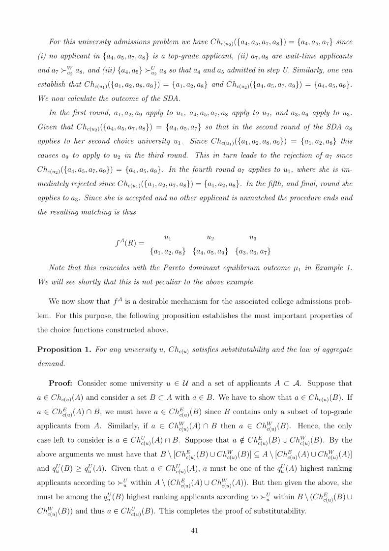
For this university admissions problem we have Chc(u2)({a4, a5, a7, a8}) = {a4, a5, a7} since

(i) no applicant in {a4, a5, a7, a8} is a top-grade applicant, (ii) a7, a8 are wait-time applicants

and a7 �Wu2a8, and (iii) {a4, a5} �Uu2

a8 so that a4 and a5 admitted in step U. Similarly, one can

establish that Chc(u1)({a1, a2, a8, a9}) = {a1, a2, a8} and Chc(u2)({a4, a5, a7, a9}) = {a4, a5, a9}.

We now calculate the outcome of the SDA.

In the first round, a1, a2, a9 apply to u1, a4, a5, a7, a8 apply to u2, and a3, a6 apply to u3.

Given that Chc(u2)({a4, a5, a7, a8}) = {a4, a5, a7} so that in the second round of the SDA a8

applies to her second choice university u1. Since Chc(u1)({a1, a2, a8, a9}) = {a1, a2, a8} this

causes a9 to apply to u2 in the third round. This in turn leads to the rejection of a7 since

Chc(u2)({a4, a5, a7, a9}) = {a4, a5, a9}. In the fourth round a7 applies to u1, where she is im-

mediately rejected since Chc(u1)({a1, a2, a7, a8}) = {a1, a2, a8}. In the fifth, and final, round she

applies to a3. Since she is accepted and no other applicant is unmatched the procedure ends and

the resulting matching is thus

fA(R) =u1 u2 u3

{a1, a2, a8} {a4, a5, a9} {a3, a6, a7}

Note that this coincides with the Pareto dominant equilibrium outcome µ1 in Example 1.

We will see shortly that this is not peculiar to the above example.

We now show that fA is a desirable mechanism for the associated college admissions prob-

lem. For this purpose, the following proposition establishes the most important properties of

the choice functions constructed above.

Proposition 1. For any university u, Chc(u) satisfies substitutability and the law of aggregate

demand.

Proof: Consider some university u ∈ U and a set of applicants A ⊂ A. Suppose that

a ∈ Chc(u)(A) and consider a set B ⊂ A with a ∈ B. We have to show that a ∈ Chc(u)(B). If

a ∈ ChEc(u)(A) ∩ B, we must have a ∈ ChEc(u)(B) since B contains only a subset of top-grade

applicants from A. Similarly, if a ∈ ChWc(u)(A) ∩ B then a ∈ ChWc(u)(B). Hence, the only

case left to consider is a ∈ ChUc(u)(A) ∩ B. Suppose that a /∈ ChEc(u)(B) ∪ ChWc(u)(B). By the

above arguments we must have that B \ [ChEc(u)(B) ∪ChWc(u)(B)] ⊆ A \ [ChEc(u)(A) ∪ChWc(u)(A)]

and qUu (B) ≥ qUu (A). Given that a ∈ ChUc(u)(A), a must be one of the qUu (A) highest ranking

applicants according to �Uu within A \ (ChEc(u)(A) ∪ ChWc(u)(A)). But then given the above, she

must be among the qUu (B) highest ranking applicants according to �Uu within B \ (ChEc(u)(B)∪

ChWc(u)(B)) and thus a ∈ ChUc(u)(B). This completes the proof of substitutability.

41

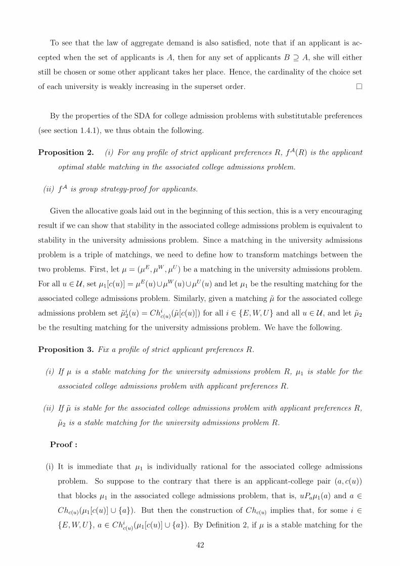
To see that the law of aggregate demand is also satisfied, note that if an applicant is ac-

cepted when the set of applicants is A, then for any set of applicants B ⊇ A, she will either

still be chosen or some other applicant takes her place. Hence, the cardinality of the choice set

of each university is weakly increasing in the superset order.

By the properties of the SDA for college admission problems with substitutable preferences

(see section 1.4.1), we thus obtain the following.

Proposition 2. (i) For any profile of strict applicant preferences R, fA(R) is the applicant

optimal stable matching in the associated college admissions problem.

(ii) fA is group strategy-proof for applicants.

Given the allocative goals laid out in the beginning of this section, this is a very encouraging

result if we can show that stability in the associated college admissions problem is equivalent to

stability in the university admissions problem. Since a matching in the university admissions

problem is a triple of matchings, we need to define how to transform matchings between the

two problems. First, let µ = (µE, µW , µU) be a matching in the university admissions problem.

For all u ∈ U , set µ1[c(u)] = µE(u)∪µW (u)∪µU(u) and let µ1 be the resulting matching for the

associated college admissions problem. Similarly, given a matching µ for the associated college

admissions problem set µi2(u) = Chic(u)(µ[c(u)]) for all i ∈ {E,W,U} and all u ∈ U , and let µ2

be the resulting matching for the university admissions problem. We have the following.

Proposition 3. Fix a profile of strict applicant preferences R.

(i) If µ is a stable matching for the university admissions problem R, µ1 is stable for the

associated college admissions problem with applicant preferences R.

(ii) If µ is stable for the associated college admissions problem with applicant preferences R,

µ2 is a stable matching for the university admissions problem R.

Proof :

(i) It is immediate that µ1 is individually rational for the associated college admissions

problem. So suppose to the contrary that there is an applicant-college pair (a, c(u))

that blocks µ1 in the associated college admissions problem, that is, uPaµ1(a) and a ∈

Chc(u)(µ1[c(u)] ∪ {a}). But then the construction of Chc(u) implies that, for some i ∈

{E,W,U}, a ∈ Chic(u)(µ1[c(u)] ∪ {a}). By Definition 2, if µ is a stable matching for the

42

university admissions problem it has to match applicants as early as possible. This im-

plies that, for all universities u ∈ U , µE(u) (µW (u)) contains the qEu (qWu ) highest priority

top-grade (wait-time) applicants w.r.t. �Eu (�Wu ) within µE(u) ∪ µW (u) ∪ µU(u). Hence,

ChEc(u)(µ1[c(u)]) = µE(u), ChWc(u)(µ1[c(u)]) = µW (u), and ChUc(u)(µ1[c(u)]) = µU(u). If

a ∈ ChEc(u)(µ1[c(u)] ∪ {a}) we would thus have that either (|µE(u)| < qEu and a �Eu u), or

(a �Eu a, for some a ∈ µE(u)). In both cases we obtain a contradiction to point (iv) of

Definition 2 for i = E. The other cases are handled similarly and we obtain that µ1 is

stable in the associated college admissions problem.

(ii) Let µ be a stable matching in the associated college admissions problem with applicant

preferences R. Since, for all i ∈ {E,W,U}, µi2(u) = Chic(u)(µ[c(u)]), µE2 (u) (µW2 (u))

contains the qEu (qWu ) highest priority top-grade (wait-time) applicants w.r.t. �Eu (�Wu )

within µ[c(u)]. This implies in particular that µ2 matches applicants as early as possible.

Furthermore, if uPaµ2(a) and either (|µE2 (u)| < qEu and a �Eu u), or (a �Eu a, for some

a ∈ µ2(u)), we would also have that a ∈ ChEc(u)(µ[c(u)]∪ {a}). Thus, µ2 must satisfy (iv)

with respect to i = E. The argument that µ2 satisfies (iv) with respect to i ∈ {W,U} is

similar and omitted here.

This implies that for all profiles of applicant preferences R, fA(R) is the applicant optimal

stable matching for the university admissions problem R. This follows directly from Proposition

3 and the corresponding property of the set of stable matchings in a college admissions prob-

lem with substitutable preferences (see section 1.4.1). Given the characterization of complete

information equilibrium outcomes in Theorem 1, we obtain the following.24

Proposition 4. Let R be a university admissions problem and let ΓZV S(R) denote the set of

Nash equilibrium outcomes of the game induced by the ZVS mechanism. Then for all Q ∈

ΓZV S(R), all applicants weakly prefer the outcome chosen by the SDA with floating quotas, that

is, fAa (R)RafZV Sa (Q) for all a ∈ A.

In case there are multiple stable matchings under the current procedure, our redesign elim-

inates the possibility that applicants coordinate on welfare inferior equilibria. Furthermore,

24This result parallels Ergin and Sonmez (2006)’s result comparing equilibrium outcomes of the Bostonmechanism and the student optimal stable mechanism. The main differences to their result are the sequentialstructure of the ZVS procedure and the special construction of college preferences in the associated collegeadmissions problem.

43

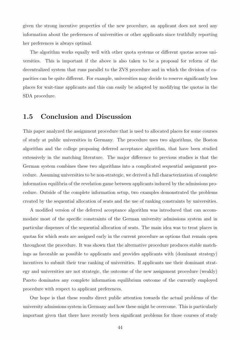
given the strong incentive properties of the new procedure, an applicant does not need any

information about the preferences of universities or other applicants since truthfully reporting

her preferences is always optimal.

The algorithm works equally well with other quota systems or different quotas across uni-

versities. This is important if the above is also taken to be a proposal for reform of the

decentralized system that runs parallel to the ZVS procedure and in which the division of ca-

pacities can be quite different. For example, universities may decide to reserve significantly less

places for wait-time applicants and this can easily be adapted by modifying the quotas in the

SDA procedure.

1.5 Conclusion and Discussion

This paper analyzed the assignment procedure that is used to allocated places for some courses

of study at public universities in Germany. The procedure uses two algorithms, the Boston

algorithm and the college proposing deferred acceptance algorithm, that have been studied

extensively in the matching literature. The major difference to previous studies is that the

German system combines these two algorithms into a complicated sequential assignment pro-

cedure. Assuming universities to be non-strategic, we derived a full characterization of complete

information equilibria of the revelation game between applicants induced by the admissions pro-

cedure. Outside of the complete information setup, two examples demonstrated the problems

created by the sequential allocation of seats and the use of ranking constraints by universities.

A modified version of the deferred acceptance algorithm was introduced that can accom-

modate most of the specific constraints of the German university admissions system and in

particular dispenses of the sequential allocation of seats. The main idea was to treat places in

quotas for which seats are assigned early in the current procedure as options that remain open

throughout the procedure. It was shown that the alternative procedure produces stable match-

ings as favorable as possible to applicants and provides applicants with (dominant strategy)

incentives to submit their true ranking of universities. If applicants use their dominant strat-

egy and universities are not strategic, the outcome of the new assignment procedure (weakly)

Pareto dominates any complete information equilibrium outcome of the currently employed

procedure with respect to applicant preferences.

Our hope is that these results direct public attention towards the actual problems of the

university admissions system in Germany and how these might be overcome. This is particularly

important given that there have recently been significant problems for those courses of study

44

that are not part of the centralized procedure.25 A big problem of these decentralized procedure

that the market often fails to clear since some applicants hold multiple offers and this leads

to congestion. We think that the widespread refusal of a centralized procedure is rooted in

a wrong assessment of the benefits and disadvantages of a decentralized system and that a

well designed centralized procedure, possibly along the lines of what has been proposed in this

chapter, is capable of addressing many of the concerns about the current system.

We now discuss a number of important issues with the alternative design proposed in the

last section. In some instances, these questions present important avenues for future research.

1.5.1 Efficiency, Stability, and the Welfare of Universities

Given that the allocation of places among top-grade and wait-time applicants is based on a

priority structure that is exogenously assigned to universities, one may also be interested in

achieving a matching that is efficient with respect to applicant preferences for this part of total

capacity. This is not in general guaranteed by the procedure proposed in the last section: In

Example 4 the procedure assigns applicants a8 and a9 places reserved for wait-time applicants

which they would prefer to exchange with each other.26 The problem with this approach is that

there is no matching mechanism that is strategy-proof for applicants and satisfies efficiency for

the priority based as well as stability for the two-sided part of the procedure.27 Since stability is

important in the sense that it ensures that universities’ preferences play a role in the assignment

process, we chose to impose stability as the main allocative criterion.

A problem of the new design is that political authorities might perceive it as favoring

applicants too much since it chooses the worst stable matching for universities. However, it

is easy to show that for any stable matching mechanism there is always an equilibrium which

yields the applicant optimal stable matching. Hence, welfare gains of universities relative to

the applicant optimal stable matching cannot be guaranteed. 28

25See e.g. http://www.spiegel.de/unispiegel/studium/0,1518,610971,00.html.26It is easy to see that stability uniquely pins down the allocation for places in the wait-time quota so that

for this example there is a conflict between stability and efficiency. This problem is well known and Ergin(2002) has characterized the class of priority structures for which there is no such conflict between efficiencyand stability.

27This is an adaption of a result by Papai (2009), who studies a hybrid model of school choice and collegeadmission problems.

28Furthermore, some papers in the literature have argued that the differences between student and collegeoptimal stable matching are “small” if the matching market is “large”. This is found as an empirical fact instudies of the matching programs for American doctors (Roth and Peranson (1999)) and the Boston schoolchoice program (Pathak and Sonmez (2008)). Kojima and Pathak (2009) show analytically that the set ofstable matchings converges to a singleton if the number of participants becomes very large.

45

1.5.2 The Evaluation Process

For the redesign we assumed that the evaluation of applicants takes place before the application

deadline. If a university has a non-mechanical evaluation procedure, for which the marginal

cost of considering an additional applicant is not negligible, there are two problems with this

approach:

(i) The university may evaluate an applicant who would have received a place at the univer-

sity anyway through the top-grade or the wait-time quota.

(ii) The university may interview an applicant who ends up ranking the university low.

As a consequence, universities’ incentives to invest in a costly evaluation of applicants might

decrease. On the other hand, the cost of the evaluation process might increase since more

applicants need to be considered to fill available places. While a theoretical investigation of

universities’ investment incentives is an interesting avenue for future research, it is beyond the

scope of this study and we now informally discuss some ideas about the evaluation process.

For concreteness, we will talk about interviews whenever we mean non-mechanical evaluation

procedures.

The new assignment procedure could be implemented as a two-stage mechanism where in

the first stage applicants are evaluated and the second stage determines assignments using the

SDA with floating quotas. For the evaluation stage, applicants report a set (not a ranking)

of acceptable universities. Similar to the current ZVS procedure, universities could set upper

bounds on the number of applicants they are willing to interview and criteria according to which

interviewees are selected. It might also be sensible to limit the number of interviews an applicant

can have. In this case, an applicant would be required to report not only a set of acceptable

universities, but would also have to specify at which universities she would like to interview.

Prospective students may still have a chance of being assigned to a university at which they

did not interview through the top-grade/wait-time quota, or because the university allocates

only part of its places on basis of interviews. Once all interviews have taken place, universities

and applicants submit their rankings to the centralized clearinghouse. While choosing where

to apply for interviews is a difficult decision, submitting the true ranking of universities is still

a dominant strategy once the evaluation process of universities is completed (provided that

universities are not allowed to use ranking constraints).

46

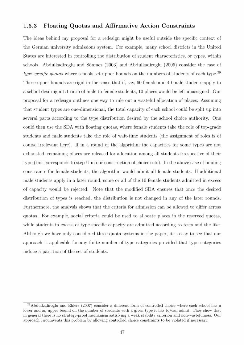
1.5.3 Floating Quotas and Affirmative Action Constraints

The ideas behind my proposal for a redesign might be useful outside the specific context of

the German university admissions system. For example, many school districts in the United

States are interested in controlling the distribution of student characteristics, or types, within

schools. Abdulkadiroglu and Sonmez (2003) and Abdulkadiroglu (2005) consider the case of

type specific quotas where schools set upper bounds on the numbers of students of each type.29

These upper bounds are rigid in the sense that if, say, 60 female and 40 male students apply to

a school desiring a 1:1 ratio of male to female students, 10 places would be left unassigned. Our

proposal for a redesign outlines one way to rule out a wasteful allocation of places: Assuming

that student types are one-dimensional, the total capacity of each school could be split up into

several parts according to the type distribution desired by the school choice authority. One

could then use the SDA with floating quotas, where female students take the role of top-grade

students and male students take the role of wait-time students (the assignment of roles is of

course irrelevant here). If in a round of the algorithm the capacities for some types are not

exhausted, remaining places are released for allocation among all students irrespective of their

type (this corresponds to step U in our construction of choice sets). In the above case of binding

constraints for female students, the algorithm would admit all female students. If additional

male students apply in a later round, some or all of the 10 female students admitted in excess

of capacity would be rejected. Note that the modified SDA ensures that once the desired

distribution of types is reached, the distribution is not changed in any of the later rounds.

Furthermore, the analysis shows that the criteria for admission can be allowed to differ across

quotas. For example, social criteria could be used to allocate places in the reserved quotas,

while students in excess of type specific capacity are admitted according to tests and the like.

Although we have only considered three quota systems in the paper, it is easy to see that our

approach is applicable for any finite number of type categories provided that type categories

induce a partition of the set of students.

29Abdulkadiroglu and Ehlers (2007) consider a different form of controlled choice where each school has alower and an upper bound on the number of students with a given type it has to/can admit. They show thatin general there is no strategy-proof mechanism satisfying a weak stability criterion and non-wastefulness. Ourapproach circumvents this problem by allowing controlled choice constraints to be violated if necessary.

47

48

Chapter 2

Breaking Ties in School Choice:

(Non-)Specialized Schools

2.1 Introduction

Recently, the school choice problem has received a lot of attention in the theoretical and applied

matching literature starting with Abdulkadiroglu and Sonmez (2003). In this problem, a set

of students has to be assigned among a set of public schools. Each school has an exogenously

given priority ordering of students. A central allocative criterion in the literature is stability,

which requires that no student should envy another student for a school that she has strictly

higher priority for. If students cannot have equal priority at schools, the student proposing

deferred acceptance algorithm (SDA) produces a student optimal stable matching and provides

students with dominant strategy incentives to submit their preferences over schools truthfully.

This is not only of theoretical interest, as school choice authorities in Boston and New York

have recently decided to adopt a variant of this mechanism (Abdulkadiroglu, Pathak, Roth,

and Sonmez (2006) and Abdulkadiroglu, Pathak, and Roth (2009)). A problem that has not

received much attention in the theoretical literature until the recent work by Erdil and Ergin

(2008) is that in most real-life applications students may have the same priority at a given

school. In the Boston public school choice system, for example, a major determinant for the

priority of a student is whether she lives in the walk zone of a school, that is, not further away

from the school than some fixed distance. Of course, a walk zone inherits (much) more than one

student in a densely populated city so that schools’ priority orderings have large indifference

classes. This seemingly small change in the model changes results dramatically. The major

problem is that ties between equal priority students have to be broken in order to determine

49

an assignment. This induces additional stability constraints that can lead to a substantial

decrease in student welfare (Abdulkadiroglu, Pathak, and Roth (2009)). We call a mechanism

constrained efficient, if it is stable with respect to the original weak priority structure and never

incurs welfare loss due to tie-breaking. Unfortunately, Erdil and Ergin (2008) show that there

are priority structures for which a constrained efficient and strategy-proof mechanism fails to

exist.

A natural question that is at the heart of the present study is whether this is an exception

or the rule in school choice problems with weak priority orders. We call a priority structure

solvable, if there exists a strategy-proof and constrained efficient mechanism. In this paper we

make important initial progress in characterizing the class of solvable priority structures. We

introduce a model of (non-)specialized schools in which a school is either specialized and has

a strict priority ranking of students, or a school is non-specialized and all students have the

same priority. While it cannot be expected that this assumption is exactly satisfied in real-life

applications, we view the analysis of this model as a useful first step since it provides important

insights into how we can deal with large indifference classes in the priority structure. Further-

more, this model is interesting in its own right since it unifies the school choice problem with

strict priority orders of Abdulkadiroglu and Sonmez (2003) and the house allocation problem

of Hylland and Zeckhauser (1979).

For the case that no school can admit more than one student, we fully characterize solvable

priority structures by two simple and intuitive conditions. These conditions ensure that most

of the ties can be broken exogenously, that is, without referring to student preferences. Since

the conditions required for solvability are very restrictive, our results for the unit capacity case

have the flavor of an impossibility result. This is in line with Gibbard (1973) and Satterthwaite

(1979)’s classical negative results concerning dominant strategy implementation. However, our

negative results critically depend on the assumption that no school can admit more than one

student. In a second step we then consider general capacity vectors and show that significantly

weaker conditions are sufficient for solvability. As for the unit capacity case, our conditions

connect the capacity vector with the amount of allowable variability across the priority order-

ings of specialized schools. Most importantly, our results show that there is some scope for

breaking ties according to student preferences and we introduce a new version of the SDA with

endogenous tie-breaking (SDA-ETB). For solvable priority structures the associated matching

mechanism is strategy-proof for students even though tie-breaking is (partly) based on elicited

preferences. Interestingly, increasing capacities substantially enlarges the scope for preference

based tie-breaking.

50

This chapter is organized as follows: After discussing the related literature we introduce the

school choice problem with weak priorities and relevant existing results in section 2.2. In section

2.3 we motivate the need for preference based tie-breaking by means of a simple example. In

section 2.4 we introduce the (non-)specialized schools model. This section contains the main

results of this chapter. In section 2.5 we conclude and discuss our results as well as possible

extensions. All proofs are relegated to Appendix A.2.

Related Literature

Ehlers (2007) was the first to study the problem of indifferences in priority orders. In particular

he considered a simple three student example (that does not belong to our (non-)specialized

schools environment) for which no exogenous tie-breaking rule guaranteed the constrained ef-

ficiency of the SDA. Nevertheless, he showed by construction that a strategy-proof and con-

strained efficient matching mechanism existed. We are the first to systematically study the

possibility of preference based tie-breaking in school choice problems with indifferences in pri-

ority orders.

Apart from the above paper, the literature on the school choice problem with indifferences

has mainly focused on exogenous tie-breaking. Here, a central question has been whether there

should be a single lottery that is used to break ties at all schools, or whether there should be

a separate lottery for each school. Pathak (2008) considers a random assignment problem in

which all students initially have the same priority for each school. He shows that a market based

approach, in which a priority structure for each school is randomly selected and students are

then allowed to trade their priorities, is equivalent to the random serial dictatorship, in which

a single lottery is conducted and students then choose schools in the order determined by the

lottery, in the sense that both produce exactly the same lottery over outcomes.1 In a similar

vein, Abdulkadiroglu, Pathak, and Roth (2009) show that for any school choice problem, any

constrained efficient matching can be reached by first using a single lottery to break all ties

and then running the deferred acceptance algorithm. The focus of both of these papers is to

give a rationale for using a single lottery to break all ties for all schools instead of multiple

lotteries. They do not discuss how one can elicit the information about student preferences

that is necessary to break ties in a way that avoids additional welfare loss, which is the main

focus of our study.

1This is an extension of a classical result by Abdulkadiroglu and Sonmez (1998) who show that in the houseallocation problem the random serial dictatorship is equivalent to the core from random endowments, whichconducts a single lottery to determine an initial allocation of indivisible objects and then lets agents tradetowards a core outcome.

51

More related in focus is the main theoretical result in Abdulkadiroglu, Pathak, and Roth

(2009), which shows that no strategy-proof matching mechanism can dominate student optimal

stable matching mechanism with any fixed tie-breaking rule. The dominance relation they

consider is very strong since it requires that all students weakly prefer the outcome of the

dominating mechanism to the outcome of the dominate mechanism for all preference profiles,

with at least one strict preference for at least one profile. This already suggests that the class

of mechanisms that is not dominated by another strategy-proof mechanism is quite large. Our

results show that it is not sufficient to restrict attention to the class of SDAs resulting from fixed

tie-breaking rules if one is interested in strategy-proof and constrained efficient mechanisms.

Of course, our SDA-ETB does not dominate the SDA with an arbitrary fixed tie-breaking rule

for all preference profiles in the above sense. However, in contrast to the latter mechanism it

guarantees that there is never additional welfare loss due to tie-breaking if the priority structure

is solvable.

Another closely related paper is Erdil and Ergin (2008). They show that a matching is

constrained efficient if and only if there is no stable improvement cycle, that is, no cyclical

sequence of trades that respects stability constraints and makes all students involved better

off. This motivates a simple constrained efficient procedure: Calculate the SDA outcome

using an arbitrary tie-breaking rule. If the outcome is inefficient, successively eliminate stable

improvement cycles until a constrained efficient outcome is reached. We will see that there exist

solvable priority structures for which the stable improvement cycles procedure is not strategy-

proof no matter how ties are broken initially and no matter how stable improvement cycles are

selected. In particular, it is not sufficient to restrict attention to the stable improvement cycles

procedure if one is interested in strategy-proof and constrained efficient mechanisms.

For the case of strict priorities, a number of papers have studied the relation between proper-

ties of the priority structure and the existence of mechanisms with certain desirable properties.

Most prominently, Ergin (2002) studies the relationship between efficiency (with respect to stu-

dent preferences) and stability. He introduces a simple but restrictive acyclicity condition that is

shown to be necessary and sufficient for the compatibility of efficiency and stability.2 Note that

for the problem with strict priorities, the compatibility of strategy-proofness and constrained

efficiency follows from the strategy-proofness of the SDA. At least for the unit capacity case we

can formally show that Ergin’s conditions are more restrictive than the conditions required for

2Another example is Kesten (2006) who derives conditions under which the SDA coincides with the toptrading cycles algorithm, which has been one of SDA’s main competitors in applications to the school choiceproblem.

52

solvability.3

Finally, we mention the recent paper by Abdulkadiroglu, Che, and Yasuda (2008) who study

the school choice problem with equal priorities from an ex-ante cardinal welfare perspective.

They introduce a “choice augmented deferred acceptance algorithm” (CADA) in which students

submit an ordinal ranking of schools and also specify a target school. The auxiliary message is

used as a tie-breaking device and can be interpreted as allowing a student to signal the intensity

of her preference for the target school. In a model with a continuum of students, the CADA

is shown to improve upon the SDA with fixed tie-breaking from an ex-ante perspective. The

approach of Abdulkadiroglu, Che, and Yasuda (2008) differs from ours as we concentrate on

the classical ex-post welfare perspective in a model with a finite number of students.

2.2 The School Choice Problem with Weak Priorities

A School Choice Problem with Weak Priorities is given by

• a finite set of students I,

• a finite set of schools S,

• a vector of capacities q = (qs)s∈S,

• a profile of weak priority orders of schools �= (�s)s∈S, and

• a profile of strict student preferences R = (Ri)i∈I .

The only difference to the school choice problem with strict priorities introduced in Chapter

I.2 is that two distinct students i and i′ can now have equal priority for a school s, denoted

by i ∼s i′. Remember that i �s i′ means that i has strictly higher priority for school s than

student i′. For two subsets J, J ′ ⊂ I, we denote by J �s J ′ that i �s i′ for all i ∈ J and

i′ ∈ J ′. Note that we continue to assume students can never be indifferent between two distinct

schools. As everything else is fixed, we will think of a (school choice) problem as being given by

a profile R of student preferences. A rule, or matching mechanism, is a function that assigns

a matching to each problem. A correspondence is a function that assigns a non-empty set of

3Although Ergin (2002)’s conditions are for the case of strict priorities, it is easy to see that they guaranteethe compatibility of efficiency and stability when imposed on the priority structure of specialized schools inour model. If one demands that all constrained efficient matchings should be constrained efficient, strongerconditions are required (Ehlers and Erdil (2009)).

53

matchings to each problem and rule f is a selection from correspondence F , if f(R) ∈ F (R)

for all problems R.

Remember that a matching µ is stable (or fair) for the school choice problem R, , if it

(i) is individually rational, that is, µ(i)Rii for all students i ∈ I,

(ii) eliminates justified envy, that is, there is no student school pair (i, s) such that sPiµ(i)

and i �s i′ for some i′ ∈ µ(s), and

(iii) is non-wasteful, that is, there is no student school pair (i, s) such that sPiµ(i) and |µ(s)| <

qs.

At this point it is important to note that stability only depends on strict rankings in the priority

structure. It is known (cf example 2.15 in Roth and Sotomayor (1991)) that in the presence of

ties in the priority structure there may not exist a stable matching µ that all students weakly

prefer to any other stable matching. However, given the finiteness of the problem there always

exists (at least one) stable assignment which is not Pareto dominated by any other stable

matching with respect to student welfare. We call a matching with this property constrained

efficient and given some profile of strict student preferences R we denote by OS�(R) the set

of constrained efficient matchings.

If priorities are strict, OS�(R) contains exactly one matching which can be found by ap-

plying the SDA. However, if there are ties in the priority structure the SDA cannot be applied

unless we specify some rule for breaking ties. Formally, a fixed tie-breaking rule, or strict trans-

formation, of � is a strict priority structure �′ that preservers the strict ranking of �, that is,

i �′s j whenever i �s j. Let ST (�) denote the set of all strict transformations of �. Given some

�′∈ ST (�), let f�′

denote the matching mechanism that associates the outcome of the SDA

with strict priority structure �′ to each problem. It is known (Dubins and Freedman (1981),

Roth (1982)) that for all �′∈ ST (�), f�′

is strategy-proof and stable with respect to �. Erdil

and Ergin (2008) note that f�′

may, however, fail to be constrained efficient. Abdulkadiroglu,

Pathak, and Roth (2009) aim to provide a rationale for the SDA with a fixed tie-breaking rule

and show that no strategy-proof mechanism can dominate f�′for any �′∈ ST (�), that is, there

is no strategy-proof mechanism g such that for all problems R, gi(R)Rif�′(R) for all i ∈ I,

with at least one strict preference for at least one problem and at least one student. Of course,

this dominance relation is very strong so that the set of mechanisms that are undominated in

this sense is very large.

54

Recently, Erdil and Ergin (2008) introduced an algorithm that always produces a con-

strained efficient matching for weak priority structures. The main idea is that whenever a

stable matching is not constrained efficient, then it is possible to increase student welfare via a

cyclical exchange that respects stability constraints. More formally, let µ be a stable matching

for some R. Then student i desires school s at µ if sPiµ(i). For each school s, let Ds(µ) denote

the set of highest �s-priority students among those who desire s at µ. A stable improvement

cycle (SIC) at µ and R consists of m distinct students i1, . . . , im such that for all l = 1, . . . ,m,

il ∈ Dµ(il+1)(µ) (where m+ 1 := 1). Erdil and Ergin (2008) show that µ ∈ OS�(R) if and only

if µ admits no stable improvement cycle (SIC) at µ and PI . This leads them to suggest the

following procedure to achieve a constrained efficient outcome.

The Stable Improvement Cycles Algorithm

Select a fixed single tie-breaking rule and compute the associated SDA outcome given the

submitted preferences of students.

If the outcome is not constrained efficient, allow students involved in a SIC to realize

the corresponding cyclical exchange. Continue with this procedure until we arrive at a

constrained efficient matching.

As shown in Erdil and Ergin (2008), this procedure is not, in general, strategy-proof. This

is not necessarily a fault of the stable improvement cycles as the same authors show that there

exist weak priority structures � which do not admit any strategy-proof selection from OS�.

Motivated by this result, we call a priority structure � solvable, if there exists a strategy-

proof and constrained efficient selection from OS�. Our main goal is to characterize the class

of solvable priority structures. In the next section we start with a motivating example.

2.3 Motivating Preference Based Tie-Breaking

We consider the following school choice environment with three students 1, 2, 3: There are six

schools s1, . . . , s6 at which all three students have different priorities and one school s7 at which

all students have equal priority. All schools can admit at most one student. The priority

orderings of the various schools are summarized in the following table.4

4This notation means that e.g. at s1, 1 has the highest, 2 has the second highest, and 3 has the lowestpriority.

55

�s1 �s2 �s3 �s4 �s5 �s6 �s71 1 2 2 3 3 1, 2, 3

2 3 1 3 1 2

3 2 3 1 2 1

To implement the Erdil-Ergin procedure, we have to choose a fixed tie-breaking rule. Due

to the symmetries of the example, we may assume without loss of generality that the strict

transformation �′s7 : 1, 2, 3 was chosen. Consider the following preference profile:5

R R1 R2 R3

s4 s7 s7

s7

For this school choice problem the outcome of the SDA with the above fixed tie-breaking

rule is constrained efficient: 1 obtains her first choice school s4 and 2 obtains her first choice

school s7. Student 3 does not receive a place at some school since she did not rank enough

schools. Now suppose that instead of ranking only s7, 3 declares s4 to be her second choice,

i.e. claims that her preferences are R′3 : s7, s4. If all other students submit the same ranking

as before, the SDA outcome is not constrained efficient for the above fixed tie-breaking rule: 1

obtains s7, since she was randomly given the highest priority for this school, and 3 obtains s4,

since she has higher priority for this school than 1 but (randomly chosen) lower priority for s7

than 2. There is a unique stable improvement cycle in this example since 1 and 3 would prefer to

trade places, which cannot be vetoed by student 2. But this means that the stable improvement

cycles procedure would now assign 3 a place at s7, her true top choice school (under R3). Hence,

3 has a strict incentive to manipulate the procedure at the original preference profile R. Since

the ordering was chosen at random, this shows that no matter which fixed tie-breaking rule is

used, there does not exist a strategy proof rule for selecting stable improvement cycles. The

following procedure, however, is strategy-proof and constrained efficient:

Calculate the SDA outcome assuming that s7 has unlimited capacity and let µ1 be the

resulting temporary assignment. If µ1(s7) = {1, 2, 3}, reject 3. If µ1(s7) = {i1, i2} with i1 < i2,

reject i1 if and only if the third student, i3, is temporarily matched to a school s such that

i2 �s i1 and i3 �s i1. Now continue with the SDA in which students propose down their

lists starting with their most preferred school that has not rejected them yet. Should another

5Remember that the above notation means that agent 1 strictly prefers school s3 to school s7, and that s4and s7 are the only schools which agent 1 prefers to not being assigned to any school.

56

tie-breaking become necessary, apply the same rules as above.

An exact proof of strategy-proofness and constrained efficiency of this rule is deferred to the

next sections. Note that the above tie-breaking rule takes the indexing of students as a baseline,

which is only modified if two students are matched to s7 while the third student is matched to a

school in s1, . . . , s6 at which she does not have lowest priority. This rule ensures that a student

can affect the tie-breaking decision only if she changes her own temporary assignment prior to

tie-breaking. By the strategy-proofness of the SDA procedure with fixed tie-breaking, it is clear

that such a manipulation can, by itself, not be profitable. But the rule for tie-breaking ensures

that if a student affects the tie-breaking decision, she will be matched to the new temporary

assignment. The intuition for constrained efficiency is similar. This shows - a formal proof is

deferred to later sections - that if we are interested in identifying the class of solvable priority

structures, it is not sufficient to restrict attention to the stable improvement cycles procedure.

2.4 The (Non-)Specialized Schools Model

In this paper we consider a restricted class of school choice environments with two types of

schools: Specialized schools have a strict priority ranking, while non-specialized schools assign

the same priority to every student. More formally, we have the following.

Definition 3. The priority structure � is a (non-)specialized schools environment, if

there exists a partition of S into two non-empty sets S0 and S1 such that

(i) S0 comprises the set of non-specialized schools, that is, for all s ∈ S0 and all i, j ∈ I,

i ∼s j, and

(ii) S1 comprises the set of specialized schools, that is, for all s ∈ S1 and all i, j ∈ I such that

i 6= j, i �s j or j �s i.

In this language schools s1, . . . , s6 in the example of section 3 were specialized, while s7 was

the only non-specialized school. One interpretation of this model is that a specialized school’s

priority ordering result from subject test(s) in the discipline(s) relevant for this school, e.g. a

sports oriented school makes admission contingent on sports trials. Non-specialized schools on

the other hand offer general educational training and therefore do not discriminate between

students. Apart from this interpretation, our motivation for studying the (non-)specialized

schools model is twofold.

First, our analysis is an important initial step towards a characterization of solvable priority

structures in the school choice problem with indifferences in priority orders. We consider the

57

extreme situation where a school’s priority order has either one or |I| indifference classes.

However, it will become clear that our results also have important implications for the general

school choice problem whenever some or all schools assign equal priority to a group of students

which is sufficiently large, but at the same time potentially much smaller than |I|.

Secondly, our model bridges the gap between two important environments, which have been

studied extensively in the literature.

(i) If S1 = ∅, then all students have equal priority at all schools. This case is known as

the house allocation problem.6 Among others, Svensson (1999), Papai (2000), and Pycia

and Unver (2009), are interested in identifying rules which satisfy strategy-proofness and

efficiency.7 Since all students have equal priority at all schools, stability is vacuously

satisfied by any rule and constrained efficiency is equivalent to efficiency. The class of

strategy-proof and efficient rules is very large and has not been characterized in the

literature.

(ii) If S0 = ∅, then no two students have equal priority at a school and we are back to the

school choice problem with strict priorities from Chapter I.2. For this problem the student

optimal stable rule is the only strategy-proof and constrained efficient rule.8

In the presence of both specialized and non-specialized schools a strategy-proof and constrained

efficient mechanism does not always exist and we derive tractable conditions under which a

priority structure is solvable.

For the remainder of this paper we restrict attention to the (non-)specialized schools envi-

ronment. It is important to keep in mind that stability constraints only come from the priority

orders of specialized schools. In the following, we will denote the priority ordering of a spe-

cialized school s ∈ S1 by �s instead of �s to emphasize that no two students can have equal

priority. Let �1= (�s)s∈S1 be the priority structure of specialized schools. It is easy to see

that the conditions for solvability can only concern �1. We assume throughout that there are

at least two specialized schools and at least two non-specialized schools.9 We first consider

the case of unit capacity at all schools to develop intuition for the requirements imposed by

solvability.

6This problem was first studied by Hylland and Zeckhauser (1979).7In fact, all these papers derive characterizations of rules that satisfy strategy-proofness, efficiency, and

different sets of additional axioms.8In fact, the student optimal stable rule is also the only strategy-proof and stable rule (Alcalde and Barbera

(1994)).9If there is only one specialized school, solvability is trivial. If there is only one non-specialized school, the

sufficient conditions for solvability are slightly different as we discuss below.

58

2.4.1 Unit capacities - Necessary Conditions

Throughout this section we consider the case where all schools can admit at most one student,

i.e. where qs = 1 for all s ∈ S. Of course, schools can usually admit more than one student

and the reader may prefer to think of the allocation of tasks in a society rather than the school

choice problem for this section. Society has a strict preference over who takes on specialized

tasks, while it is indifferent as to who takes on a non-specialized task.

The example in Section 2.3 suggests that strategy-proofness and constrained efficiency are

always compatible if there are at most three students (a formal proof can be found below).

Not surprisingly, this positive result does not extend to the case of four or more students as we

will shortly see. In this section we identify two related sources for the incompatibility between

strategy-proofness and constrained efficiency. The first source is introduced in the following

definition.

Definition 4. Let � be a non-specialized schools environment with unit capacities. Then �1

contains an ambiguous 1-tie if there exist two specialized schools s1, s2 ∈ S1 and four distinct

students i1, i2, i3, i4 ∈ I such that both i1 �s1 i3 �s1 i2 and i2 �s2 i4 �s2 i1.

To see the problems associated with ambiguous 1-ties, consider the smallest example where

it can be violated: There are four students 1, . . . , 4, two specialized schools s1, s2, and one

non-specialized school s3. The priority structure �1 is such that (the remaining rankings are

irrelevant)

1 �s1 3 �s1 2 and 2 �s2 4 �s2 1.

Now consider the preference profile

R R1 R2 R3 R4

s2 s1 s3 s3

s3 s3

s1 s2

.

For this profile, 1 and 2 would prefer to exchange their priorities for s1 and s2. Here, this

is not problematic since neither 3 nor 4 are interested in these schools. However, either 3 or 4

will have to remain unassigned since s3 cannot admit more than one student. A strategy-proof

procedure has to ensure in particular that 3 and 4 cannot profit by claiming that s1 and/or s2

are acceptable, respectively. We show in Appendix A.2 that this cannot be achieved by any

59

constrained efficient mechanism, thus proving the following result.

Proposition 5. Let � be a (non-)specialized schools environment with unit capacities. Then

� is solvable only if �1 does not contain an ambiguous 1-tie.

The absence of ambiguous 1-ties is a strong restriction. Suppose for example that s1 is

a music oriented school while s2 is a sports oriented school. Both schools assign priorities

according to performance in auditions. Typically, there will be allrounders who do relatively

well in both specializations. At the same time, there will also be specialists who have a musical

talent but are not very sportive (and the other way around). If there are at least two allrounders

and two specialists, the priority structure is not solvable since it contains an ambiguous 1-tie.

However, there is still some scope for different priority orderings across specialized schools as

the next example demonstrates.

Example 5. There are four students 1, . . . , 4, six specialized schools s1, . . . , s6, and one non-

specialized school s7. The priority structure at specialized schools is as follows.

�s1 �s2 �s3 �s4 �s5 �s61 2 1 1 2 2

3 3 2 2 1 1

2 1 4 3 4 3

4 4 3 4 3 4

Note that �1 does not contain an ambiguous 1-tie. Thus, in principle the door remains open

for possibility results.

However, it is easy to see that any fixed tie breaking rule leads to violations of constrained

efficiency for some preference profiles so that some or all of the ties have to broken preference

based. A natural candidate for a constrained efficient assignment procedure is the following:

Set 1 ∼0 2 �0 3 �0 4 and break ties at the non-specialized school s7 according to this ordering.

Thus, only the tie between 1 and 2 remains to be broken endogenously. Now if 1 and 2 apply

to s7 in some round of the SDA procedure, temporarily ignore the capacity constraint at s7. If

3 is temporarily matched to s2 by the end of the SDA procedure, 1 is rejected by s7. In any

other case 2 is rejected. While this certainly guarantees a constrained efficient allocation, 4 can

manipulate the tie breaking decision to her benefit. To see this consider the profile

60

R R1 R2 R3 R4

s7 s7 s3 s1

s3 s1 s2

.

Here, 4 would be left unmatched while 3 obtains a place at s3. However, if she claims that

R′4 : s3, s1, 3 would be rejected by s3 and would subsequently apply to s2. But then 1 would be

rejected by s7, causes 4 to be rejected at s3, and 4 ultimately obtains a place at her true top

choice (under R4) school s1. Hence, the above procedure is not strategy-proof.

The following definition formalizes one problematic feature of the priority structure in this

example.

Definition 5. Let � be a (non-)specialized schools environment with unit capacities. Then �1

contains ambiguity at the top if there are four distinct students i1, i2, i3, i4 and three distinct

specialized schools s1, s2, s3 ∈ S1 such that i1 �s1 i3 �s1 i2 �s1 i4, i2 �s2 i3 �s2 i1 �s2 i4, and

{i1, i2} �s3 i4 �s3 i3.

In the above example there was ambiguity at the top concerning �s1 ,�s2 , and �s3 . In order

to avoid ambiguity at the top, at least one of the schools’ priority orderings needs to be changed.

For example, we could set �s2 equal to any of the priority orderings of the other specialized

schools to obtain a priority structure that contains no ambiguous 1-ties and no ambiguity at the

top. The following shows that ambiguity at the top is the second source for the incompatibility

of strategy-proofness and constrained efficiency.

Proposition 6. Let � be a (non-)specialized schools environment with unit capacities. Then

� is solvable only if �1 does not contain no ambiguity at the top.

Above we showed that our intuitive idea for achieving a constrained efficient matching does

not provide students with the right incentives. Note that the statement of Proposition 6 is much

stronger since it says that any assignment procedure has to sacrifice either strategy-proofness

or constrained efficiency.

2.4.2 General Capacities - Sufficient Conditions

The results in the last section support a pessimistic view about the possibilities of obtaining

strategy-proof and constrained efficient mechanisms. It is important to keep in mind that we

assumed that all schools could admit at most one student. In this section we turn to the case of

61

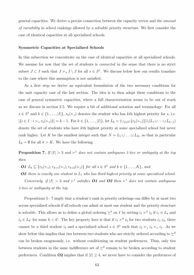
general capacities. We derive a precise connection between the capacity vector and the amount

of variability in school rankings allowed by a solvable priority structure. We first consider the

case of identical capacities at all specialized schools.

Symmetric Capacities at Specialized Schools

In this subsection we concentrate on the case of identical capacities at all specialized schools.

We assume for now that the set of students is connected in the sense that there is no strict

subset J ⊂ I such that J �s I \ J for all s ∈ S1. We discuss below how our results translate

to the case where this assumption is not satisfied.

As a first step we derive an equivalent formulation of the two necessary conditions for

the unit capacity case of the last section. The idea is to then adapt these conditions to the

case of general symmetric capacities, where a full characterization seems to be out of reach

as we discuss in section 2.5. We require a bit of additional notation and terminology: For all

s ∈ S1 and k ∈ {1, . . . , |I|}, rk(�s) denotes the student who has kth highest priority for s, i.e.

|{i ∈ I : i �s rk(�s)}| = k− 1. For k ∈ {1, . . . , |I|}, let Lk = (∪s∈S1{rk(�s)})\(L1∪ · · · ∪Lk−1)

denote the set of students who have kth highest priority at some specialized school but never

rank higher. Let K be the smallest integer such that N = L1 ∪ . . . ∪ LK , so that in particular

Lk = ∅ for all k > K. We have the following.

Proposition 7. If |I| > 3 and �1 does not contain ambiguous 1-ties or ambiguity at the top

then

O1 Lk ⊆ {rk(�s), rk+1(�s), rk+2(�s)} for all s ∈ S1 and k ∈ {1, . . . , K}, and

O2 there is exactly one student in L1 who has third highest priority at some specialized school.

Conversely, if |I| > 3 and �1 satisfies O1 and O2 then �1 does not contain ambiguous

1-ties or ambiguity at the top.

Propositions 5 - 7 imply that a student’s rank in priority orderings can differ by at most two

across specialized schools if all schools can admit at most one student and the priority structure

is solvable. This allows us to define a global ordering �0 on I by setting i1 �0 i2 if i1 ∈ Lk and

i2 ∈ Lk′ for some k < k′. The key property here is that if i1 �0 i2 for two students i1, i2, there

cannot be a third student i3 and a specialized school s ∈ S1 such that i2 �s i3 �s i1. As we

show below this implies that ties between two students who are strictly ordered according to �0

can be broken exogenously, i.e. without conditioning on student preferences. Thus, only ties

between students in the same indifference set of �0 remain to be broken according to student

preferences. Condition O2 implies that if |I| ≥ 4, we never have to consider the preferences of

62

lower priority students in L2 ∪ . . . ∪ LK in order to break the tie between the two students in

L1. Note that since |L1| = 2 this basically means that the tie between the two students at the

top can be broken exogenously if |I| ≥ 4.

Intuitively, it is clear that increasing capacities should enlarge the scope for preference based

tie breaking and should increase the allowable variability in priority orderings of specialized

schools. The important task here is to identify the exact form of this relationship. We now

show how the conditions for solvability from the unit capacity case can be adapted to the

capacity vector. For the following, we fix a capacity vector for schools with the property that

all specialized schools have the same capacity. Let q1 be the common capacity of all specialized

schools, let q0(1) be the lowest capacity of any non-specialized school, and q0

(2) ≥ q0(1) be the

second lowest capacity.10

First of all, the priority structure is solvable if the number of students is sufficiently small

compared to available capacities. Here, the critical value turns out to be p = q1 + q0(1) +

min{q1, q0(2)}. To see that any priority structure is solvable if |I| ≤ p note that if tie-breaking

becomes necessary, i.e. at least q0(1) + 1 students are interested in the same non-specialized

school s1 ∈ S0, at most one specialized school can have filled its capacity. Furthermore, if some

specialized school s2 ∈ S1 has filled its capacity, there cannot be a third school s3 ∈ S \{s1, s2}

that has to reject any student. We show below how the priority ordering of s2 can be used to

determine who should be rejected by s1. Secondly, if |I| > p the variability of priority orders

across specialized schools has to be restricted. The next definition formally summarizes our

requirements in this case.

Definition 6. Suppose that I is connected and that |I| > p. Then �1 satisfies limited p-

variability if

O1(p) Lk ⊂ {rk(�s), . . . , rp(�s)} for all k ≤ p− 2 and all s ∈ S1,

O2(p) Lk ⊂ {rk(�s), rk+1(�s), rk+2(�s)} for all p− 2 < k and all s ∈ S1, and

O3(p) there is exactly one student in L1 ∪ . . . ∪ Lp−2 who has pth highest priority at some

specialized school.

The idea behind this condition is that we want to assign high priority for non-specialized

schools to students who have high, i.e. at least (p − 2)nd highest, priority for specialized

schools. Note that the amount of allowable variability declines as we move down the rankings

of specialized schools. This is because the demands of students with higher priority could

effectively lead to a reduction of the number of seats at some schools. Eventually, everything

10Remember that we assumed |S0| ≥ 2.

63

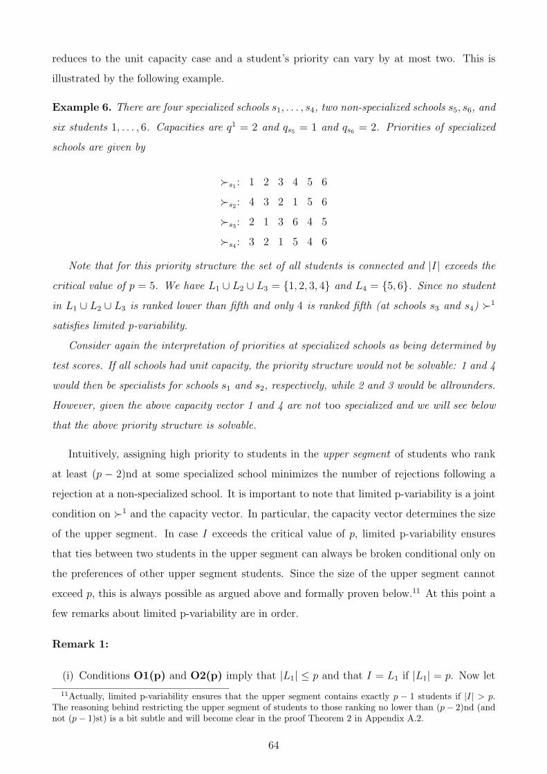
reduces to the unit capacity case and a student’s priority can vary by at most two. This is

illustrated by the following example.

Example 6. There are four specialized schools s1, . . . , s4, two non-specialized schools s5, s6, and

six students 1, . . . , 6. Capacities are q1 = 2 and qs5 = 1 and qs6 = 2. Priorities of specialized

schools are given by

�s1 : 1 2 3 4 5 6

�s2 : 4 3 2 1 5 6

�s3 : 2 1 3 6 4 5

�s4 : 3 2 1 5 4 6

Note that for this priority structure the set of all students is connected and |I| exceeds the

critical value of p = 5. We have L1 ∪ L2 ∪ L3 = {1, 2, 3, 4} and L4 = {5, 6}. Since no student

in L1 ∪ L2 ∪ L3 is ranked lower than fifth and only 4 is ranked fifth (at schools s3 and s4) �1

satisfies limited p-variability.

Consider again the interpretation of priorities at specialized schools as being determined by

test scores. If all schools had unit capacity, the priority structure would not be solvable: 1 and 4

would then be specialists for schools s1 and s2, respectively, while 2 and 3 would be allrounders.

However, given the above capacity vector 1 and 4 are not too specialized and we will see below

that the above priority structure is solvable.

Intuitively, assigning high priority to students in the upper segment of students who rank

at least (p − 2)nd at some specialized school minimizes the number of rejections following a

rejection at a non-specialized school. It is important to note that limited p-variability is a joint

condition on �1 and the capacity vector. In particular, the capacity vector determines the size

of the upper segment. In case I exceeds the critical value of p, limited p-variability ensures

that ties between two students in the upper segment can always be broken conditional only on

the preferences of other upper segment students. Since the size of the upper segment cannot

exceed p, this is always possible as argued above and formally proven below.11 At this point a

few remarks about limited p-variability are in order.

Remark 1:

(i) Conditions O1(p) and O2(p) imply that |L1| ≤ p and that I = L1 if |L1| = p. Now let

11Actually, limited p-variability ensures that the upper segment contains exactly p − 1 students if |I| > p.The reasoning behind restricting the upper segment of students to those ranking no lower than (p− 2)nd (andnot (p− 1)st) is a bit subtle and will become clear in the proof Theorem 2 in Appendix A.2.

64

K be the minimal integer such that N = L1 ∪ . . . ∪ LK so that in particular Lk = ∅ for

all k > K. If |I| > p, O1(p) and O2(p) imply that

· |L1 ∪ . . . ∪ Lp−2| = p− 1,

· |Lk| = 1 for all p− 2 < k ≤ K − 1, and

· |LK | ∈ {1, 2}.

In particular we must have |I| ∈ {K + 1, K + 1} if |I| > p.

(ii) A major benefit of limited p-variability is that it is tractable and very easy to verify. If

|I| > p, we first need to check that L1 ⊂ {r1(�s), . . . , rp(�s)} for all specialized schools

s ∈ S1. This can be implemented as follows: Take an arbitrary specialized school s ∈ S1.

Then check whether r1(�s) ∈ {r1(�s′), . . . , rp(�s′)} for all s′ ∈ S1 \ {s}. This requires at

most (|S1| − 1)p steps. Proceeding in this fashion, we can test whether no student in L1

is ever ranked lower than pth in at most |S1|(|S1| − 1)p < (|S1|)2|I| steps.

Now, the conditions for the remaining Lk sets can be verified completely analogously so

that checking O1(p) and O2(p) requires at most K|S1|(|S1| − 1)p < (|I|)2(|S1|)2 steps.

Note that O3(p) can be tested at (almost) no additional computational cost: As soon as

we find a student in L1 ∪ . . .∪Lp−2 who is ranked pth at some specialized school we have

to check that all other students in this segment of the priority structure rank no lower

than (p− 1)st.

We now design an assignment procedure that is strategy-proof and constrained efficient

provided that limited p-variability is satisfied. For the following we fix a capacity vector as

well as the priority structure �1 of specialized schools and assume that �1 satisfies limited

p-variability. The procedure consists of two steps: In the first step we define an ordering �0 as

in the unit capacity case. In the second step, we introduce a new version of the SDA algorithm

which uses this ordering as the common priority ordering of all non-specialized schools. The

procedure breaks ties between students in the same indifference class of �0 endogenously on

basis of temporary assignments.

Step 1: Ordering Students

• If |I| ≤ p, set i ∼0 j for all i, j ∈ I.

• If |I| > p, set

65

(i) i ∼0 j for all i, j ∈ L1 ∪ . . . ∪ Lp−2

(ii) i �0 j if i ∈ Lk and j ∈ Lk′ with k < k′ ≤ K and k′ ≥ p

(iii) i ∼0 j if i, j ∈ LK

As in the unit capacity case this ordering has the property that if i1 �0 i2 there cannot be

a third student i3 and a specialized school s ∈ S1 such that i2 �s i3 �s i1. We show below

that this implies that the tie between i1 and i2 can be broken exogenously without violating

constrained efficiency. All remaining ties can be broken endogenously. By Remark 1.(i) there

are at most two non-singleton indifference sets of �0 if |I| > p (and one indifference set if

|I| ≤ p): An upper segment consisting of p − 1 students who have at least (p − 2)nd highest

priority for some specialized school and, possibly, a lower segment consisting of two students

in LK . For the purpose of breaking ties in these two segments endogenously we label students

according to their position in �0. Within an indifference class, the label is arbitrary with the

exception that if |I| > p we assign the highest label p − 1 (remember Remark 1.(i)) in the

upper indifference set of �0 to the only student in L1 ∪ . . .∪Lp−2 who has pth highest priority

at some specialized school. 12 Labels will be used as a baseline for endogenous tie breaking.

This baseline is modified only if a specialized school has filled its capacity. In the following

we abuse notation slightly and identify a student with her label. Thus, if |I| > p we write

I = {1, . . . , K + 1} if |LK | = 1 and I = {1, . . . , K + 2} if |LK | = 2, where the labeling adheres

to the rules above. We are now ready to describe the SDA procedure with endogenous tie

breaking (SDA-ETB).

Step 2: The SDA with Endogenous Tie Breaking

The algorithm takes as inputs the (relevant portion of the) capacity vector (q1, q0(1), q

0(2)), the

priority structure of specialized schools �1, the ordering �0 calculated in Step 1, and a profile

of student preferences.

Round 1: Each student applies to her most preferred school. Each specialized school s ∈ S1

admits the q1 highest priority students according to �s. Each non-specialized school s ∈

S0 admits the qs students with the lowest labels among those who aply to it. If necessary,

12More formally, the labeling can be described as follows: If |I| ≤ p choose a permutation πI : I → {1, . . . , |I|}at random. If |I| > p let i be the unique student in L1 ∪ . . . ∪ Lp−2 who can have pth highest priority at somespecialized school and set πI (i) = p− 1.

(i) Choose a permutation πI : (L1 ∪ . . . ∪ Lp−2) \ {i} → {1, . . . , p− 2} at random.(ii) For k ∈ {p− 1, . . . ,K − 1} and i ∈ Lk set πI(i) = k + 1.(iii) If |LK | = 2 randomly pick a student i ∈ LK and set πI(i) = K + 1. Set πI(i′) = K + 2 for the other

student i′ in LK .

66

it admits all students in the same indifference class of �0 as the qsth highest labeled

student who was admitted in addition. Let µ1 be the resulting temporary assignment.

If one of the rejected students has not yet applied to all acceptable schools, go to Round

2. If all rejected students have applied to all acceptable schools and there is a non-

specialized s ∈ S0 such that |µ1(s)| > qs, use subroutine TB(µ1) to determine a rejection

and go to Round 2. Else, stop.

...

Round t: Each student rejected in Round t − 1 applies to her most preferred school among

those that have not yet rejected one of her proposals. Each specialized school s ∈ S1

admits the q1 highest priority students according to �s. Each non-specialized school s ∈

S0 admits the qs students with the lowest labels among those who aply to it. If necessary,

it admits all students in the same indifference class of �0 as the qsth highest labeled

student who was admitted in addition. Let µt be the resulting temporary assignment.

If one of the rejected students has not yet applied to all acceptable schools, go to Round

t + 1. If all rejected students have applied to all acceptable schools and there is a non-

specialized school s ∈ S0 such that |µt(s)| > qs, use subroutine TB(µt) to determine a

rejection and go to Round t+ 1. Else, stop.

The crucial ingredient of this algorithm is the tie-breaking subroutine which is applied to

determine a rejection at non-specialized schools. The subroutine is applied only if nothing else

moves in the sense that there is no other way for the algorithm to proceed than to break a tie

within an indifference class of �0.

Subroutine TB(µt): If there is a non-specialized school s ∈ S0 such that |µt(s)| > qs and

i ∼0 j for all i, j ∈ µt(s), set s0 := s and go to Step TB(µt).1. Else, let s0 ∈ S0 be the

non-specialized school such that LK ⊂ µt(s0) and go to Step TB(µt).2.

Step TB(µt).1: If there is a specialized school s1 ∈ S1 s.t. |µt(s1)| = q1 and i ∼0 j for

all i, j ∈ µt(s1) ∪ µt(s0) let i1 be the student with the lowest priority according to

�s1 among students in µt(s0). School s0 rejects i1 if µt(s1) �s1 i1.

In any other case s0 rejects student with the highest label among students in µt(s0).

Step TB(µt).2: Let s1 := µt(K). If K + 2 �s1 K + 1, s0 rejects K + 1.

In any other case, s0 rejects K + 2.

67

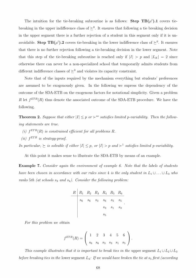
The intuition for the tie-breaking subroutine is as follows: Step TB(µt).1 covers tie-

breaking in the upper indifference class of �0. It ensures that following a tie breaking decision

in the upper segment there is a further rejection of a student in this segment only if it is un-

avoidable. Step TB(µt).2 covers tie-breaking in the lower indifference class of �0. It ensures

that there is no further rejection following a tie-breaking decision in the lower segment. Note

that this step of the tie-breaking subroutine is reached only if |I| > p and |LK | = 2 since

otherwise there can never be a non-specialized school that temporarily admits students from

different indifference classes of �0 and violates its capacity constraint.

Note that of the inputs required by the mechanism everything but students’ preferences

are assumed to be exogenously given. In the following we supress the dependency of the

outcome of the SDA-ETB on the exogenous factors for notational simplicity. Given a problem

R let fETB(R) thus denote the associated outcome of the SDA-ETB procedure. We have the

following.

Theorem 2. Suppose that either |I| ≤ p or �ss satisfies limited p-variability. Then the follow-

ing statements are true.

(i) fETB(R) is constrained efficient for all problems R.

(ii) fETB is strategy-proof.

In particular, � is solvable if either |I| ≤ p, or |I| > p and �1 satisfies limited p-variability.

At this point it makes sense to illustrate the SDA-ETB by means of an example.

Example 7. Consider again the environment of example 6. Note that the labels of students

have been chosen in accordance with our rules since 4 is the only student in L1 ∪ . . . ∪ L3 who

ranks 5th (at schools s3 and s4). Consider the following problem:

R R1 R2 R3 R4 R5 R6

s6 s6 s3 s6 s5 s5

s3 s1 s3

s5

.

For this problem we obtain

fETB(R) =

1 2 3 4 5 6

s6 s6 s3 s3 s1 s5

.

This example illustrates that it is important to break ties in the upper segment L1 ∪L2 ∪L3

before breaking ties in the lower segment L4: If we would have broken the tie at s5 first (according

68

to our rules for tie breaking), 6 would have been rejected. In subsequent rounds of SDA-ETB,

student 4 would then have been rejected by s6 and s3. Since 4 �0 5, 4 would have subsequently

obtained a place at s5. But then there would be a stable improvement cycle consisting of 4 and

6. The main reason for breaking ties in the lower segment last is that this way we can ensure

that there are no further rejections after tie-breaking. A similar example can be used to show

that it is important to wait with endogenous tie-breaking until nothing else moves.

Asymmetric Capacities

In this section we turn to the case of general capacity vectors. In the following, let q1(1) be

the minimal capacity of specialized schools, q0(1) and q0

(2) be defined as in the last section, and

p = q1(1) + q0

(1) + min{q1(1), q

0(2)} be the modified critical value. It is easy to see that our previous

results imply that if the set of students is connected and �1 satisfies limited p-variability

whenever |I| > p then � is solvable.13

We now discuss how our results extend to the case where I is not connected. Since we are

dealing with a finite problem there has to exist a minimal set J1 such that for any s ∈ S1,

J1 �s I \J1. We call J1 the minimal top set of I with respect to �1. Proceeding inductively, let

Jt be the minimal top set of I \ (J1∪ . . .∪Jt−1) with respect to �1. We call (Jt)t≥1 the minimal

top set partition of I with respect to �1. Suppose for the sake of clarity that I = J1 ∪ J2. Let

fETB|J1 denote the SDA-ETB mechanism when we make all places at all schools available to

students in J1. Since J1 is connected, our previous analysis implies that fETB|J1 is strategy-

proof and constrained efficient provided that �1 |J1 satisfies limited p-variability. In principle,

there are two ways to guarantee that there is a strategy-proof and constrained efficient procedure

for students in J2 which we now discuss. In both cases, we assign all students in J1 with higher

priority for non-specialized schools than all students in J2. This ensures in particular that a

student in J1 can never envy a student in J2.

(i) In some instances it might be feasible to elicit reports from students in J2 after assign-

ments for students in J1 have been determined. In this case given a profile RJ1 elicited

from students in J1, we can reduce capacities at schools according to fETB|J1(RJ1). Let

p1 be the resulting modified critical value and let fETB|J2 denote the SDA-ETB that

allocates remaining places among students in J2. Again, our analysis from the connected

case implies that fETB|J2 is strategy-proof and constrained efficient provided that �1 |J2

satisfies limited p1-variability.

13One just needs to replace q1 with the actual capacities of specialized schools in the formulation of theSDA-ETB. Everything else remains exactly the same.

69

(ii) If we restrict attention to assignment procedures that simultaneously elicit a report from

all students, the restrictions for solvability in J2 become more restrictive. We have to

require solvability for the lowest possible critical value that could be induced by the

demands of students in J1. For example, consider the case q1(1) = 4, q0

(1) = q0(2) = 2, and

|J1| = 3. Here, the worst case would be if all students in J1 were interested in the minimal

capacity specialized school leading to a new critical value of 4.

From the above discussion it is clear that even when all specialized schools initially have

identical capacities, we have to consider the case of asymmetric capacities if I is not connected

since the demands of students in J1 may lead to a problem with asymmetric capacities for the

remaining student population.

However, note that in the unit capacity case the critical value is always 3. This implies that

the same conditions guaranteeing solvability for the connected case also guarantee solvability

for the general case. Hence, we obtain the following theorem as a corollary to Propositions 5

-7 and Theorem 2.

Theorem 3. Suppose � is a (non-)specialized schools environment with unit capacities. Then

� is solvable if and only if �1 does not contain ambiguous 1-ties or ambiguity at the top.

To conclude this section note that it could be the case that even though � is not solvable,

there is a strategy-proof and constrained efficient procedure for a subpopulation of students.

To see this consider again the case of unit capacities and suppose that I = J1 ∪ J2. If �1 |J1

satisfies limited 3-variability, but �1 |J2 does not, there is a strategy-proof and constrained

efficient mechanism for students in J1 but not for students in J2.

2.5 Conclusion and Discussion

This chapter derived a full characterization of solvable priority structures in (non-)specialized

schools environments with unit capacity. Significantly weaker sufficient conditions were in-

troduced for the case of general capacity vectors. Our conditions show precisely how much

variability in priority orderings across specialized schools can be allowed in order to guarantee

existence of a constrained efficient and strategy-proof mechanism. The proof of sufficiency was

constructive and used a modified deferred acceptance procedure with (potentially) preference

based tie-breaking. The results show that it is not sufficient to concentrate on fixed tie-breaking

rules if one is interested in strategy-proof and constrained efficient school choice systems. Fur-

70

thermore, the scope for preference based tie-breaking increases in the number of slots available

at schools. We now discuss several important open questions.

2.5.1 Uniqueness of the Tie-Breaking Rule

In this chapter we introduced tractable conditions that guarantee solvability of a priority struc-

ture. Given that these conditions are satisfied we introduced the strategy-proof and constrained

efficient SDA-ETB procedure. One important idea of this mechanism was to assign those stu-

dents who have high priority at specialized school also high priority for all non-specialized

schools. This could be considered problematic from an equity perspective and school choice au-

thorities might be interested in knowing whether there are other strategy-proof and constrained

efficient mechanisms. In the following we discuss whether there could be other ways to break

ties. In this section we concentrate on the case of unit capacities at all schools, assume that I

is connected, and fix a solvable environment �.

First, suppose we have set i1 �0 i2 for two students i1, i2 ∈ I so that i2 can never obtain

a non-specialized school desired by i1. Can there be strategy-proof and constrained efficient

procedure that exogenously breaks ties at non-specialized schools in favor of i2? To see that

this is impossible, note that the construction of �0 ensures that there exists a specialized school

s ∈ S1 and a third student i3 such that i1 �s i3 �s i2. Let s ∈ S0 be one of the non-specialized

schools.14 Now let f be a strategy-proof and constrained efficient mechanism such that i2

always has higher priority for s than i1. Consider first the problem

R1 R1i1

R1i2

R1i3

s s s

s s

.

We must have fi1(R1) = 1, fi2(R

1) = s, and fi3 = s. Otherwise there would be a stable

improvement cycle given that i2 can never envy i1 for s. Now suppose that R2i3

: s and consider

R2 = (R1i1, R1

i2, R2

i3). By strategy-proofness we must have f(R2) = f(R1). Next, let R2

i1: s, s

and R3 = (R2i1, R1

i2, R2

i3). By strategy-proofness and stability, we must have fi1(R

3) = s.

Constrained efficiency then implies fi2(R3) = i2 and fi3(R

3) = s. Finally, let R3i3

= s, s and

consider R4 = (R2i1, R1

i2, R3

i3). Since i2 cannot envy i1 for a place at s and i2 cannot obtain

a place at s given R3i3

, it is not possible that fi3(R4) = s. But if fi3(R

4) = s, we must

have fi1(R4) = s so that i1 and i3 form a stable improvement cycle. Hence, we must have

14Note that we must have |I| ≥ 4 if we exogenously break any tie. For the following we assume that nostudent in I \ {i1, i2, i3} is interested in s or s.

71

fi3(R4) = i3. But then i3 has an incentive to submit R2

i3when the other students submit R2

i1

and R1i2

!

More generally, we would like to know whether strategy-proofness and constrained efficiency

require us to always follow the ordering �0 for the case of solvable priority structures. That

is, if f is a strategy-proof and constrained efficient mechanism can it be the case that for some

problem R we have sPifi(R), i �0 j, and fj(R) = s for some non-specialized school s ∈ S0? To

see that this is possible let R = {R : |{i ∈ I : A(Ri) 6= ∅}| ≤ 2} denote the set of profiles where

at most two students i ∈ I have a non-empty set of acceptable schools A(Ri). Let �′∈ ST (�)

be an arbitrary strict transformation. Now we can modify the rule fETB as follows: for any

profile R, (i) if R /∈ R, then f(R) = fETB(R); and (ii) if R ∈ R, then f(R) = f�′(R). It is

easy to see that f is strategy-proof and constrained efficient. An important open question is

whether we can allow such violations of �0 on more interesting domains of preferences.

2.5.2 Full Characterization for General Capacities

Beyond the case of unit capacities we have only derived sufficient conditions for solvability. An

important question is whether these conditions can be weakened further. We first illustrate the

additional problems for designing strategy-proof and constrained efficient mechanisms when

our conditions are not satisfied using a simple example.

There are two specialized schools s1, s2 and two non-specialized schools s3, s4. Both spe-

cialized schools can admit three students while the two non-specialized schools can only admit

one student. There are six students 1, . . . , 6 and the priority ordering is given by

�s1 : 1 2 3 4 5 6

�s2 : 6 5 4 3 2 1

Note that in this example the critical value is p = 5 and that the priority structure does

not satisfy limited p-variability. Now consider the preference profile

R R1 R2 R3 R4 R5 R6

s3 s2 s4 s4 s2 s3

s7 s3 s2 s2

.

Now suppose we were to use the SDA-ETB with the tie-breaking procedure we defined above

for this example assuming that i ∼0 j for all i, j ∈ {1, . . . , 6}. Then µ1(s1) = ∅, µ1(s2) = {2, 5},

µ1(s3) = {1, 6}, and µ1(s4) = {3, 4}. Now 6 would be rejected in the first round and 4 would

72

be rejected by s4 in the second round. In the third round, 4 applies to s2 so that 2 would be

rejected and applies to s3. Since s2 has filled its capacity and 1 is the lowest priority student

at s2, SDA-ETB would break the resulting tie in favor of 2. But then 2 and 6 form a stable

improvement cycle. The problem in this example is that there are two non-specialized schools

(s3 and s4) that have to reject students. If �1 had satisfied limited p-variability, it would

have been irrelevant which student is rejected by s3 or s4 since there could not have been a

subsequent rejection at some specialized school. Here, in contrast it is important to condition

tie-breaking on the priority ranking of school s2 in the first place even though this school has

not filled its capacity in round 1 of SDA-ETB. Nevertheless, we do not have a counterexample

showing that the above priority structure is not solvable so that the door remains open for

further possibility results despite the just mentioned complications.15

Secondly, consider the case of identical capacity q ≥ 2 at all schools so that p = 3q (and the

above issue does not arise). Is limited p-variability necessary for solvability here? While we do

believe that this is true, potential counterexamples needed to show necessity quickly become

intractable. The main problem here is that it is very hard to pin down assignments in case

non-specialized schools can admit more than one student. We view the weakening of sufficient

conditions for solvability to be substantially more important than extending our impossibility

results and have thus not worked towards obtaining a full characterization for the case of general

capacities at non-specialized schools.

2.5.3 Beyond Non-specialized schools environments

In this paper we have concentrated on the (non-)specialized schools environment. To see that

there is room for positive results outside this environment, we now consider an easy example.

There are three schools s1, s2, s3 and three students 1, 2, 3. All schools have a capacity of

one and the priority structure is as follows

�s1 �s2 �s31 2 3

{2, 3} {1, 3} {1, 2}

To see that this priority structure is solvable, note that the above environment is isomor-

15We do expect the tie-breaking rule to be somewhat more complicated to describe. In general, we conjecturethat a critical value of 2q1 + q0(1) could work in case of identical capacities at specialized schools. This is easilyseen to be true when there is just one non-specialized school. However, we have not (yet) been able to provethat this critical value works in the general case. A similar remark applies to the case of asymmetric capacities,where there also seems to be some additional room for solvability.

73

phic to a house allocation with existing tenants problem as introduced by Abdulkadiroglu and

Sonmez (1999): Student i is an existing tenant for school si. Their version of the top-trading

cycles algorithm is strategy-proof and constrained efficient for such problems.16

In general, it will not be possible to rely on the top-trading cycles algorithm since it is known

that it may lead to unstable allocations. Furthermore, the above approach is not applicable, for

example, when the set of students with top priority for some school is larger than the school’s

capacity (as in the (non-)specialized schools environment). However, the above shows that the

door in principal remains open for possibility results and a (partial) characterization of solvable

priority structures in the general case is an important question for future research.

16This is a special case of the hierarchical exchange rules introduced by Papai (2000). She shows that this classof rules exhaust the class of rules that are group strategy-proof, efficient, and satisfy a notion of reallocation-proofness. Recently, Pycia and Unver (2009) have characterized the (slightly) larger class of group strategy-proofand efficient rules.

74

Chapter 3

Market Structure and Matching with

Contracts

3.1 Introduction

Theoretical models of network formation and matching markets are concerned with predicting

which outcomes are likely to emerge when self-interested agents interact. An important strand

of this literature belongs to the area of cooperative game theory and “likely outcomes” are

not defined by writing down an explicit negotiation protocol, but rather by postulating a set

of stability constraints that one perceives to be relevant in the problem under study. In the

previous chapters we discussed several examples where such constraints have been an important

guideline for the design of real-life mechanisms for two-sided matching problems in which a group

of workers (students) has to be assigned among a set of firms (universities/schools). This

literature has focused on the pairwise stability concept, which only considers the possibility of

coordinated deviations by pairs of players. One might worry that a pairwise stable matching

could be susceptible to deviations by larger coalitions. However, as long as workers can take

at most one job and firms have substitutable preferences, a pairwise stable matching not only

exists (Kelso and Crawford (1982)), but is also group stable (Roth and Sotomayor (1991)):

There is no group of agents who can obtain a strictly preferred matching by forming new

partnerships only among themselves, possibly dropping some previously held partnerships. In

particular, a pairwise stable matching is efficient.

While these are encouraging results for a restricted class of assignment problems, many

interesting applications do not fit the assumptions above: Some workers may demand multiple

75

jobs in a labor market,1 firms may not view workers as substitutes,2 and markets are often not

two-sided.3

Recently, Ostrovsky (2008) introduced a model of matching in vertically ordered networks

which allows for some of these features. The location of an agent in the (directed) network is

exogenously given and agents have preferences over sets of trading relationships, or contracts,

with their neighbors. A set of contracts is chain stable if (i) no agent would prefer to drop

some of her contracts, and (ii) there is no downstream sequence of agents who can obtain a

strictly preferred set of contracts by forming new contracts only with their direct neighbors in

the sequence, possibly dropping some of their previously held contracts. Ostrovsky shows that

chain stable outcomes exist as long as agents’ preferences satisfy same side substitutability and

cross side complementarity. However, unlike pairwise stable matchings in the simple matching

models above, chain stable allocations may not be group stable. In fact, chain stable outcomes

may even be inefficient and thus fail to be in the core.4 Thus, even when deviating agents are

not allowed to maintain relationships with outsiders there can be profitable deviations from

a chain stable allocation. We characterize the conditions under which these problems cannot

occur. Furthermore, we show how the use of the chain stability concept can be justified even

though the positive results from two-sided matching markets have no direct extension to the

more general supply chain model.

A main contribution of this study is methodological. Unlike most of the literature we will not

try to guarantee efficiency and group stability of chain stable outcomes by (directly) restricting

the class of allowed preferences. Rather, we take the domain of preferences introduced by

Ostrovsky (2008) as given and develop restrictions on the exogenously given network structure.

The main structural restriction in the paper is an acyclicity notion which rules out certain kinds

of trading cycles. We show that this condition is necessary and sufficient for (i) the equivalence

of group and chain stability, (ii) the core stability of chain stable outcomes, (iii) the efficiency of

chain stable outcomes, (iv) the existence of a group stable outcome, and (v) the existence of an

efficient and individually stable outcome.5 The equivalences provide two justifications for the use

1For example, Echenique and Oviedo (2006) mention that 35 % of teachers in Argentina work for more thanone school.

2Many tasks can only be accomplished by the combined workforce of a set of specialized workers. Theconstruction of a building, for example, requires a structural engineer, a carpenter, and so on, so that comple-mentarities between individual workers are likely.

3Brokers act as intermediaries between owners and potential tenants in housing markets, temporary employ-ment agencies supply firms with short-term labor, some stores (e.g. Gamestop) allow customers to trade inused goods which they then sell to other customers, and so on.

4An outcome is in the core (defined by weak domination), if no group of agents can obtain a weakly preferredoutcome for all involved by trading only among themselves.

5An outcome is individually stable, if no agent refrains from taking her part of the outcome.

76

of chain stability in the unrestricted model: First, whenever the minimal stability requirement

of individual stability can be reconciled with efficiency, chain stable outcomes are also efficient.

Thus, imposing the stronger chain stability concept does not lead to any additional efficiency

loss. Second, if chain stable networks fail to be group stable, the very existence of a group

stable outcome cannot be guaranteed. In this sense chain stable allocations are as stable as it

gets.

The above acyclicity condition is not sufficient for the equivalence of chain stability and the

core, one of the most important solution concepts in cooperative game theory. In the second part

of the paper we introduce a stronger acyclicity condition which is then shown to characterize the

class of supply chain models for which the equivalence obtains. The characterization subsumes

a number of important existing results.

This chapter is organized as follows: After discussing the related literature we motivate

the main ideas of this chapter by means of a simple example in section 3.2. In section 3.3 we

introduce Ostrovsky’s supply chain model. In section 3.4 we present the main results of this

chapter in detail. In section 3.5 we present some further results on the core. In section 3.6

we conclude. All proofs, a discussion of the main results, and an extension are relegated to

Appendix A.3.

Related Literature

From a methodological perspective, the paper most closely related to the present study is

Abeledo and Isaak (1992). They start from a fixed structure of potential partnerships in a simple

one-to-one matching model represented by an undirected graph that contains edges between

mutually acceptable pairs of agents. Their main result is that a pairwise stable matching

will exist for all preference profiles if and only if the market is two-sided. In this chapter we

restrict attention to the model introduced by Ostrovsky (2008) for which the existence of a

chain stable allocation is guaranteed. In contrast to Abeledo and Isaak (1992) our focus is

the relationship between cooperative solution concepts. Furthermore, their methodology has

no direct extension to the model we consider since the acceptability of a trade depends on

the whole set of available trades. In particular the set of acceptable allocations cannot be

summarized by a simple undirected graph.

More closely related in focus is a line of research that has been concerned with stability

concepts for two-sided many-to-many matching markets. If all preferences are substitutable,

this model is a special case of the supply chain model so that existence of a pairwise stable

77

allocation follows from Ostrovsky (2008).6 Blair (1988) was the first to note that in such

markets the core can be empty. This implies in particular that (i) group stable allocations may

fail to exist, and (ii) the set of pairwise stable allocations may be disjoint from both, the core

and the set of group stable allocations. In light of these problems, most studies have focused on

stability concepts which limit the set of allowable coalitional deviations. Roth (1984b) considers

the restriction that all members of a deviating coalition should obtain a subset of their most

preferred set of contracts out of previously held and newly formed contracts. He shows that if

all preferences are substitutable, there is no such coalitional deviation from a pairwise stable

allocation. In a matching model without contracts, Konishi and Unver (2006) consider the

restriction that deviations have to be pairwise stable themselves. A matching that is not

susceptible to such a deviation is called credibly group stable. They show that if one side of the

market has responsive preferences and the other side of the market has categorywise responsive

preferences,7 pairwise stability is equivalent to credible group stability. Echenique and Oviedo

(2006) consider the restriction that deviations have to be individually stable in the sense that no

deviating agent wants to drop some of her partners after the deviation. A matching that is not

susceptible to such a deviation is called setwise stable.8 They show that if one side of the market

has substitutable preferences and the other side has strongly substitutable preferences, pairwise

and setwise stability are equivalent.9 There are two important differences between this line of

research and our study: First, all these papers study stability notions that restrict the set of

allowable coalitional deviations. A problem with this approach is that none of these concepts

guarantee efficiency of the outcome. This leaves open the question whether there are other

natural stability concepts compatible with efficiency. The results of our paper apply equally

well to many-to-many matching models and, to the best of our knowledge, this is the first

systematic study of the relationship between pairwise stability, group stability, the core, and

efficiency. A second difference is that most of the above papers introduce stronger restrictions

on preferences than those needed to guarantee existence of a pairwise stable allocation. Thus,

while they provide insightful foundations for pairwise stability in these restricted models, their

results do not explain why this is a desirable property when all substitutable preferences are

6The existence of a pairwise stable allocation in this model had been established earlier by Roth (1984b).7An agent has categorywise responsive preferences, if there is partition of the set of available partners such

that her preferences restricted to any element of this partition are responsive. Konishi and Unver (2006) showthat this is a stronger restriction than substitutability.

8Setwise stability was introduced by Sotomayor (1999).9Strong substitutability requires that if an agent i chooses another agent j when the set of available partners

is A ∪ {j} and prefers A to B, then i must still choose j when the set of available partners is B ∪ {j}. Theresults of Echenique and Oviedo (2006) have recently been generalized to matching models with contracts byKlaus and Walzl (2008).

78

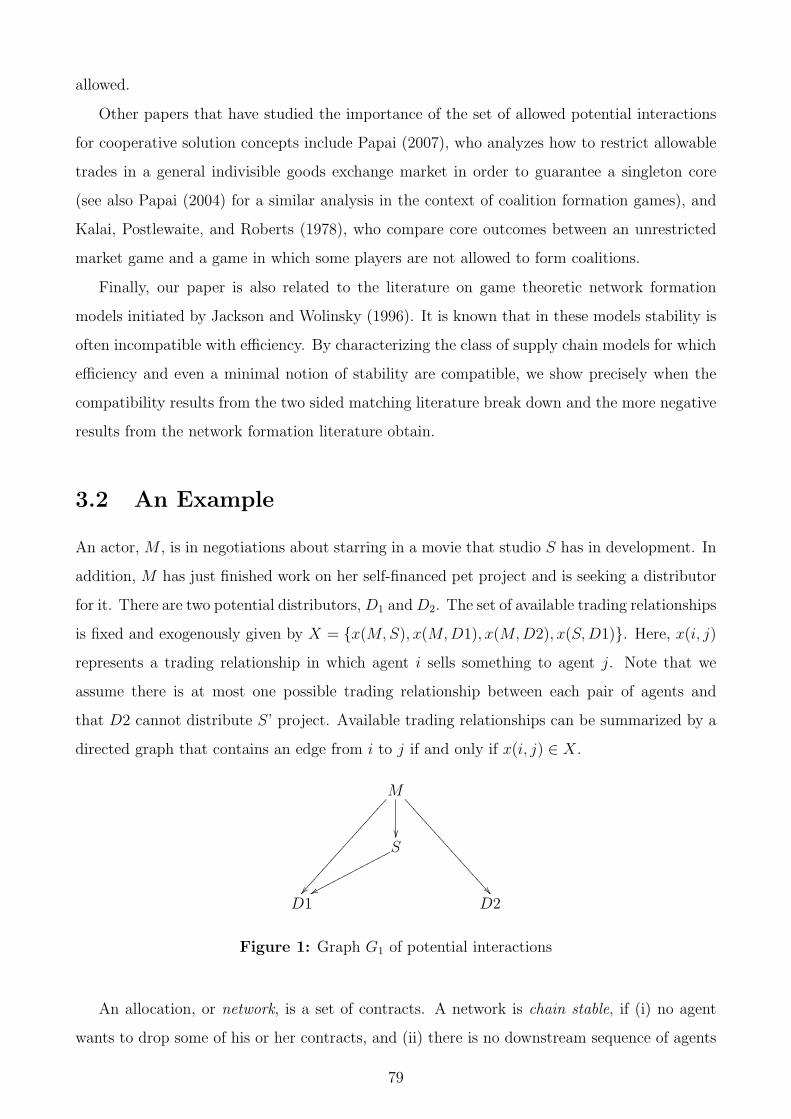
allowed.

Other papers that have studied the importance of the set of allowed potential interactions

for cooperative solution concepts include Papai (2007), who analyzes how to restrict allowable

trades in a general indivisible goods exchange market in order to guarantee a singleton core

(see also Papai (2004) for a similar analysis in the context of coalition formation games), and

Kalai, Postlewaite, and Roberts (1978), who compare core outcomes between an unrestricted

market game and a game in which some players are not allowed to form coalitions.

Finally, our paper is also related to the literature on game theoretic network formation

models initiated by Jackson and Wolinsky (1996). It is known that in these models stability is

often incompatible with efficiency. By characterizing the class of supply chain models for which

efficiency and even a minimal notion of stability are compatible, we show precisely when the

compatibility results from the two sided matching literature break down and the more negative

results from the network formation literature obtain.

3.2 An Example

An actor, M , is in negotiations about starring in a movie that studio S has in development. In

addition, M has just finished work on her self-financed pet project and is seeking a distributor

for it. There are two potential distributors, D1 andD2. The set of available trading relationships

is fixed and exogenously given by X = {x(M,S), x(M,D1), x(M,D2), x(S,D1)}. Here, x(i, j)

represents a trading relationship in which agent i sells something to agent j. Note that we

assume there is at most one possible trading relationship between each pair of agents and

that D2 cannot distribute S’ project. Available trading relationships can be summarized by a

directed graph that contains an edge from i to j if and only if x(i, j) ∈ X.

M

��S

<<<<<<<<<<<<<<<<<<<<

��D1 D2

pppppppppppppp

ww��������������������

��

Figure 1: Graph G1 of potential interactions

An allocation, or network, is a set of contracts. A network is chain stable, if (i) no agent

wants to drop some of his or her contracts, and (ii) there is no downstream sequence of agents

79

who, by signing new contracts only with immediate neighbors in the sequence while possibly

dropping some previously held contracts, can obtain a strictly preferred outcome. Consider the

following exemplary profile of preferences:

R RM RS RD1 RD2

{x(M,D1)} {x(M,S), x(S,D1)} {x(S,D1)} {x(M,D2)}

{x(M,D1), x(M,S)}

{x(M,D2)}

This notation has the following interpretation: {x(M,D1)} is the most preferred (set

of) contract(s) for M , {x(M,D1), x(M,S)} is the second most preferred set of contracts,

{x(M,D2)} is the third most preferred set of contracts, and no other set of contracts is ac-

ceptable to M . The other formulas have analogous interpretations. It is easy to verify that

{x(M,D2)} is the unique chain stable allocation. While this allocation is also efficient, it

is vulnerable to a joint deviation by M,S, and D1 since they all strictly prefer the network

{x(M,S), x(S,D1), x(M,D1)}. This deviation is not considered by chain stability since it

would require M to sign contracts with both S and D1. What are the conditions under which

chain stable networks are not susceptible to such a deviation?

Suppose that each agent is characterized by her location in the network of figure 1 and

a capacity vector which contains an exogenously given upper bound on the number of con-

tracts she can sign. In the example above, D1’s capacity would then have to be at least two

since she would, in principle, be willing to sign the two contracts x(S,D1) and x(M,D1) (as

{x(S,D1), x(M,D1)}PD1∅). Suppose now that D1 cannot distribute both projects. This obvi-

ously rules out the above example, but what about an arbitrary profile of preferences? We now

show that if each agent views two contracts in which she is the seller (buyer) as substitutes,

there cannot be a profitable deviation from a chain stable network.

Suppose to the contrary that for some substitutable preference profile agents S, M , D1

strictly prefer some network µ′ over a chain stable network µ, and can obtain µ′ by signing

new contracts only among themselves. Then either x(M,D1) ∈ µ′ \ µ or x(S,D1) ∈ µ′ \ µ

since D1 can sign at most one contract. Suppose the former case applies (the latter case is

analogous). Since M strictly prefers µ′ over µ her most preferred subset out of all her contracts

in µ and µ′ must include at least one contract in µ′ \ µ by revealed preference. If x(M,D1) is

in M ’s most preferred subset, M and D1 block µ using x(M,D1) in the sense of chain stability

since (i) M would still want to sign x(M,D1) even when she can only choose from contracts in

µ∪{x(M,D1)} by substitutability, and (ii) D1 must prefer x(M,D1) over her contract (if any)

80

in µ given that she can sign at most one contract. If x(M,D1) is not in M ’s most preferred

subset of µ ∪ µ′, we must have x(M,S) ∈ µ′ \ µ. Since D1 can sign at most one contract,

x(M,S) must be S’ only contract in µ′. But then M and S block µ in the sense of chain

stability and we again obtain a contradiction.

Since the above argument is valid for any potential block of a chain stable allocation, we

see that if D1 can sign at most one contract, chain stable allocations have to be immune to any

coalitional deviation. In the next section we show that this is a special case of a much more

general result.

3.3 The Supply Chain Model

This section briefly describes Ostrovsky (2008)’s supply chain model. The presentation here is

self contained, but readers interested in a more detailed introduction may want to consult the

original article.

Consider a market consisting of a finite set of agents V . Agents trade discrete units of

indivisible goods and trading relationships are represented by bilateral contracts. Each contract

is of the form (s, b, a, p) and represents a sale of one (unit of a) good a ∈ N from seller s ∈ V

to buyer b ∈ V at a price p ∈ R.10 The set of all possible contracts, denoted by X, is assumed

to be exogenously given and finite. For x ∈ X, let sx denote the seller in contract x and let bx

denote the buyer in contract x. It is assumed that there are no directed trading cycles in X,

that is, there is no sequence of agents v1, . . . , vn such that, for all i ∈ {1, . . . , n}, there exists

a contract xi such that sxi= vi and bxi

= vi+1 (where n + 1 := 1).11 A supply chain model

is given by the pair (V,X), with the assumption that there are no directed trading cycles in

X. For future reference we now introduce some more terminology and notation: A contract in

which agent v is the seller is called a downstream contract for v. A contract in which agent v

is the buyer is called an upstream contract for v. Given a set of contracts Y ⊆ X, let Dv(Y )

denote the set of contracts (in Y ) in which v is a seller, Uv(Y ) denote the set of contracts in

which v is a buyer, and Y (v) denote the set of all contracts involving v. An agent v ∈ V with

Uv(X) 6= ∅ and Dv(X) 6= ∅ is an intermediary. For each pair v, w ∈ V , X(v, w) denotes the set

of all possible contracts between v and w.

10This formulation of contracts follows Ostrovsky (2008) and is chosen for concreteness. Our results do notdepend on the exact nature of the set of contracts apart from the assumption that each contract is bilateral.For example, a labor market contract could specify wage, days of leave, retirement plans, and so on.

11This assumption corresponds to Ostrovsky (2008)’s assumption that agents are located in a verticallyordered network.

81

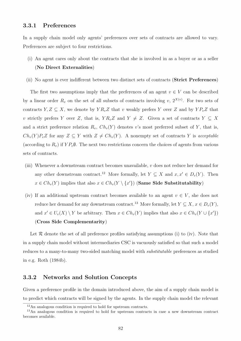
3.3.1 Preferences

In a supply chain model only agents’ preferences over sets of contracts are allowed to vary.

Preferences are subject to four restrictions.

(i) An agent cares only about the contracts that she is involved in as a buyer or as a seller

(No Direct Externalities)

(ii) No agent is ever indifferent between two distinct sets of contracts (Strict Preferences)

The first two assumptions imply that the preferences of an agent v ∈ V can be described

by a linear order Rv on the set of all subsets of contracts involving v, 2X(v). For two sets of

contracts Y, Z ⊆ X, we denote by Y RvZ that v weakly prefers Y over Z and by Y PvZ that

v strictly prefers Y over Z, that is, Y RvZ and Y 6= Z. Given a set of contracts Y ⊆ X

and a strict preference relation Rv, Chv(Y ) denotes v’s most preferred subset of Y , that is,

Chv(Y )PvZ for any Z ⊆ Y with Z 6= Chv(Y ). A nonempty set of contracts Y is acceptable

(according to Rv) if Y Pv∅. The next two restrictions concern the choices of agents from various

sets of contracts.

(iii) Whenever a downstream contract becomes unavailable, v does not reduce her demand for

any other downstream contract.12 More formally, let Y ⊆ X and x, x′ ∈ Dv(Y ). Then

x ∈ Chv(Y ) implies that also x ∈ Chv(Y \ {x′}) (Same Side Substitutability)

(iv) If an additional upstream contract becomes available to an agent v ∈ V , she does not

reduce her demand for any downstream contract.13 More formally, let Y ⊆ X, x ∈ Dv(Y ),

and x′ ∈ Uv(X) \ Y be arbitrary. Then x ∈ Chv(Y ) implies that also x ∈ Chv(Y ∪ {x′})

(Cross Side Complementarity)

Let R denote the set of all preference profiles satisfying assumptions (i) to (iv). Note that

in a supply chain model without intermediaries CSC is vacuously satisfied so that such a model

reduces to a many-to-many two-sided matching model with substitutable preferences as studied

in e.g. Roth (1984b).

3.3.2 Networks and Solution Concepts

Given a preference profile in the domain introduced above, the aim of a supply chain model is

to predict which contracts will be signed by the agents. In the supply chain model the relevant

12An analogous condition is required to hold for upstream contracts.13An analogous condition is required to hold for upstream contracts in case a new downstream contract

becomes available.

82

outcomes are sets of contracts, or networks.14 Networks will usually be denoted by µ and agent

v’s set of contracts under µ will be denoted by µ(v). Predictions take the form of (cooperative)

solution concepts which require a network to be robust against certain deviations of individuals

or groups.

A network is individually rational if no agent is assigned an unacceptable set of contracts.

This assumes that if an individual wanted to deviate she has to discontinue all of her existing

relationships. A network µ is individually stable if no agent v wants to drop some of her

contracts in µ(v), that is, Chv(µ(v)) = µ(v) for all v ∈ V . In contrast to individual rationality,

individual stability thus allows an individual to delete some but also to keep other contracts.

Next, we consider stability notions that rule out coordinated deviations by groups of agents.

The core (defined by weak domination) considers deviations by arbitrary groups of players,

but deviating agents are not allowed to maintain existing relationships with “outsiders”. More

formally, a network µ′ weakly dominates network µ via coalition A if (i) no member of A trades

with an outsider under µ′, that is, x ∈ µ′ implies that either {sx, bx} ⊆ A or {sx, bx} ∩ A = ∅,

(ii) µ′(a)Raµ(a) for all a ∈ A, and (iii) µ′(a)Paµ(a) for at least one agent a ∈ A. A network µ

is in the core (defined by weak domination) (or core stable), if it is not weakly dominated by

any other network.15

Group stability, on the other hand, considers any deviation that a coalition can implement

by forming new contracts only among themselves while possibly dropping some previously held

contracts. Coalition A can obtain µ′ from µ if (i) additional contracts are formed only between

members of A, that is, x ∈ µ′ \ µ implies that {sx, bx} ⊆ A, and (ii) only agents in A drop

some of their contracts, that is, x ∈ µ \ µ′ implies that {sx, bx} ∩ A 6= ∅. Network µ is blocked

by coalition A via network µ′ if (i) A can obtain µ from µ′, and (ii) µ′(a)Paµ(a) for all a ∈ A.

A network is group stable if it is not blocked by any coalition. Note that group stability is a

stronger solution concept than the core.

A major problem is that group and core stable networks can fail to exist even under quite

restrictive assumptions about preferences.16 Thus, in order to guarantee existence the set

of coalitional deviations has to be restricted. Ostrovsky (2008) introduces a new stability

criterion which generalizes the idea of pairwise stability in the sense that it considers (some)

14Here, networks take the role of matchings from the other two chapters of this thesis. The above formulationfacilitates the analysis in this chapter.

15Analogously, one can define the core by strong domination by requiring that all members of the coalition Ahave to be strictly better off. Roth and Sotomayor (1991) (Chapter 5) show that even in many-to-one matchingmarkets with responsive preferences, this core concept allows for matchings that are not pairwise stable.

16See e.g. Klaus and Walzl (2008) and Konishi and Unver (2006), who show that even when preferencesare strongly substitutable and responsive, respectively, there may not exist a group or even a core stablenetwork/matching.

83

coordinated deviations by downstream sequences of agents instead of only deviations by pairs.

A chain is a downstream sequence of contracts {x1, . . . , xn} ⊆ X such that for all i < n,

bxi= sxi+1

. Network µ is blocked by the chain x1, . . . , xn /∈ µ if (i) x1 ∈ Chsx1(µ(sx1) ∪ {x1}),

(ii) {xi, xi+1} ⊆ Chsxi+1(µ(sxi+1

)∪{xi, xi+1}) for all i < n, and (iii) xn ∈ Chbxn(µ(bxn)∪{xn}).

A network µ is chain stable, if it is individually stable and if it is not blocked by any chain.

One of the main results in Ostrovsky (2008) is that chain stable networks exist for all profiles

in the domain R introduced in 3.3.1. Note that if there are no intermediaries chain stability

reduces to pairwise stability so that his result generalizes the existence results from two-sided

matching models with substitutable preferences.

To justify the use of chain stability, Ostrovsky (2008) argues that it is reasonable to assume

that a downstream sequence of agents is able to coordinate a deviation since a customer need

only pick up the phone and call a potential supplier [. . .]; the potential supplier [. . .] calls one

of his potential suppliers, and so on. (p. 911). On the other hand he argues that coalitions

involving several competing firms require much more coordination and information exchange

between the agents (p. 911). There are two caveats to this justification: First, as we saw in the

example of section 3.2, chain stability does not generally rule out any profitable manipulation

by downstream sequences of agents. So it is not necessarily true that any deviation from a chain

stable network has to involve competing agents or firms. Second, requiring robustness against

any possible chain block in complex supply chain models means that coordinated deviations

by large groups of agents are thought to be possible. Given that, as we saw in the example,

coalitions consisting of as few as three agents might have a profitable joint deviation from

a chain stable network it is not clear why robustness against chain blocks is important while

robustness against the latter type of deviation is not. Finally, requiring robustness against chain

blocks may come at the expense of efficiency. If some of the deviations considered by chain

stability are implausible due to e.g. the size of the coalitions involved, less demanding stability

concepts may reduce the efficiency loss while still being satisfactorily robust. To summarize,

Ostrovsky (2008)’s results do not provide a firm foundation for the concept of chain stability.

In many-to-one two-sided matching markets with substitutable preferences pairwise stable

matchings are always efficient and both, core and group stability, reduce to pairwise stability

(see Roth and Sotomayor (1991)). These results can be seen as a justification for the use of

pairwise stability as the leading concept of stability in such models. The purpose of this paper

is to (a) characterize the largest class of supply chain models for which chain stable networks

are efficient and group or core stable, and (b) to derive a foundation for the use of chain stability

in the unrestricted model.

84

3.4 Main Results

This section develops conditions under which chain stable networks are efficient as well as

core and group stable. Instead of introducing further restrictions on preferences, we restrict

potential interactions between agents. These restrictions concern who can contract with whom

and how many relationships an agent can form. Such assumptions are common in two-sided

matching models, where an agent cannot contract with another agent on her side of the market

and it is often assumed that agents on one side of the market can all engage in at most

one relationship. The restrictions that we develop can be interpreted as restricting the sets

of acceptable contracts. However, unlike the usual preference restrictions in the matching

literature, such as responsiveness or strong substitutability, our conditions do not place further

restrictions on the ranking of acceptable (or unacceptable) sets of contracts.

For our analysis it is useful to work with a graphical representation of the supply chain

model. Let GX be the simple directed graph that contains an edge from agent v to agent w if

and only if X contains some contract x with sx = v and bx = w. This is the graph of potential

interactions that describes who can contract with whom. Note that even though there may

be more than one possible contract between a pair of agents, GX contains at most one edge

between each pair of agents. Given that the set of available contracts is assumed to be fixed,

agents are not allowed to choose their location in the network. The graph is not necessarily

complete so that some pairs of agents may not be able to trade with each other at all. For

example, two agents may not know each other, or a trade embargo forbids them to engage in a

contractual relationship. If there are no directed trading cycles in X, GX contains no directed

cycles,17 and vice versa.

We restrict attention to supply chain models in which agents face fixed upper bounds on

the number of contracts they can sign. First of all, for each pair of agents v, w ∈ V with

(v, w) ∈ GX , there is an integer c(v, w) ∈ {1, . . . , |X(v, w)|} representing the maximum number

of contracts v and w can sign with each other. If X(v, w) = ∅, so that v and w cannot directly

trade with each other, we set c(v, w) = 0. One interpretation is that c(v, w) represents the

capacity of the unique distribution channel between v and w. Furthermore, each agent v ∈ V

has an upper bound on the number of agents she can trade with: v can sign contracts with at

most qDv downstream agents and at most qUv upstream agents. For example, an agent who owns

k indivisible goods and whose only interest is to sell these goods can sign contracts with at most

k agents. A set of contracts Y ⊆ X violates v’s capacity constraints, if either |{w ∈ V \ {v} :

17A directed cycle in GX is a sequence of agents v1, . . . , vn such that, for all i ∈ {1, . . . , n}, (vi, vi+1) ∈ GX

(where we set n+ 1 := 1).

85

sx = w for some x ∈ Y (v)}| > qUv , |{w ∈ V \{v} : bx = w for some x ∈ Y (v)}| > qDv , or if there

is an agent w ∈ V \{v} such that |Y ∩X(v, w)| > c(v, w). We assume that preferences conform

to capacities : No agent finds a set of contracts acceptable that violates (one of) her capacity

constraints.18 In the following, R(c,q) ⊆ R denotes the set of all preference profiles conforming

to capacities and satisfying the assumptions of the supply chain model. Given V and X, the

unrestricted model is obtained by setting c(v, w) = qUv = qDv = |X|, for all v, w ∈ V .

The triple (GX , c, q) is the market structure induced by the supply chain model (V,X) and

the capacity constraints (c, q). The market structure is taken to be fixed throughout so that,

in particular, we do not consider location or capacity choice.

The example in Section 3.2 suggests that the presence or absence of certain cycles in the

market structure is key to the relationship between the solution concepts studied in this paper.

Note that the assumptions made so far ruled out only directed, but not undirected cycles in

GX .19 The market structure in the example contained exactly one undirected cycle: M , S, D1.

Such cycles by themselves cannot be the problem: Even a marriage market permits cycles (of

even length) and yet most stability concepts collapse to pairwise stability. However, a crucial

difference to the unrestricted supply chain model is that in a marriage market cycles cannot

actually be realized since each agent can have at most one partner. The following definition

introduces the notion of capacity constraints on cycles.

Definition 7. Let v1, . . . , vn be an undirected cycle in GX . Agent vi is capacity constrained

on cycle v1, . . . , vn if

(i) vi is a source, that is, {(vi, vi+1), (vi, vi−1)} ⊂ GX , and qDvi≤ 1,

(ii) vi is a sink, that is, {(vi−1, vi), (vi+1, vi)} ⊂ GX , and qUvi≤ 1, and

(iii) vi is a passing node, that is, either {(vi−1, vi), (vi, vi+1)} ⊂ GX or {(vi+1, vi), (vi, vi−1)} ⊂

GX , and min{qDvi, qUvi} = 0.

A 2 cycle in (GX , c, q) is an undirected cycle such that no agent is capacity constrained on it.

If v is a capacity constrained passing node, either all incoming or all outgoing edges in

GX relative to v are irrelevant. For example, v could be a firm that has signed an exclusive

long-term contract with a supplier. The example of section 2 contained a unique cycle in which

M was a source, S was a passing node, and D1 was a sink. According to the first preference

profile (RM , RS, RD1, RD2) we considered in this example, no agent was capacity constrained

18Instead of requiring preferences to conform to the capacity vector, one could place feasibility restrictionson the set of networks. We discuss this approach in Appendix A.3.

19An undirected cycle in GX is a sequence of distinct agents v1, . . . , vn such that, for all i ∈ {1, . . . , n}, either(vi, vi+1) ∈ GX or (vi+1, vi) ∈ GX (where n+ 1 := 1).

86

so that M , S, D1 was a 2 cycle. Note that by the definition of GX an undirected cycle has to

contain at least three agents. Thus, a supply chain model with only two agents can never have

a 2 cycle. The following example shows that even when there are only two agents the set of

chain stable networks, the core, and the set of group stable networks can all be disjoint.

Example 8. Consider a supply chain model with two agents v and w in which v possesses two

indivisible goods A and B. The only available contracts are xA and xB, where xi represents

the sale of good i ∈ {A,B} to agent w at some fixed price. Selling both goods is efficient but

agents differ in their evaluation of the most preferred outcome: {xA}Pw{xA, xB}Pw∅Pw{xB}

and {xB}Pv{xA, xB}Pv∅Pv{xA}. It is easy to see that this profile of preferences satisfies SSS

and CSC. However, (i) the unique chain stable network is the empty network, (ii) there is no

group stable network, and (iii) the unique core network is {xA, xB}.

Now suppose that a sale of both objects has to be implemented by a single contract xA,B

instead of the two independent contracts xA and xB. In this case, {xA,B} is the unique chain

stable network. This network is also the unique core and group stable network.

In order to guarantee that chain stable networks are efficient as well as core and group stable

we thus need to assume that each pair of agents signs at most one contract with each other.

As the example shows this does not mean that an agent can sell at most one good to any given

neighbor. Rather, it requires that all trading relationships between a given pair of agents can

be bundled into one contract. We now introduce the concept of acyclic market structures that

will play a crucial role in our analysis.

Definition 8. The market structure (GX , c, q) is weakly acyclic if it contains no 2 cycles

and c(v, w) ≤ 1 for all v, w ∈ V .

Some further notation facilitates the statement of our results: Given a preference profile

R ∈ R(c,q), let CS(R) denote the set of all chain stable networks, IS(R) denote the set of all

individually stable networks, GS(R) denote the set of all group stable networks, C(R) denote

the core, and E(R) denote the set of all efficient networks. With these preparations the first

main result reads as follows.

Theorem 4. The following are equivalent:

(i) The market structure (GX , c, q) is weakly acyclic.

(ii) Chain stable networks are always group stable, that is, CS(R) = GS(R) for all R ∈ R(c,q).

(iii) Chain stable networks are always in the core, that is, CS(R) ⊆ C(R) for all R ∈ R(c,q).

(iv) Chain stable networks are always efficient, that is, CS(R) ⊆ E(R) for all R ∈ R(c,q).

87

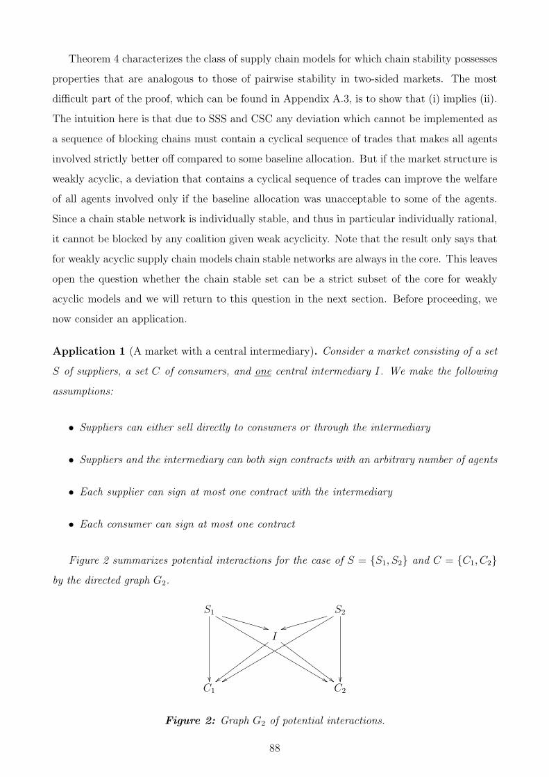
Theorem 4 characterizes the class of supply chain models for which chain stability possesses

properties that are analogous to those of pairwise stability in two-sided markets. The most

difficult part of the proof, which can be found in Appendix A.3, is to show that (i) implies (ii).

The intuition here is that due to SSS and CSC any deviation which cannot be implemented as

a sequence of blocking chains must contain a cyclical sequence of trades that makes all agents

involved strictly better off compared to some baseline allocation. But if the market structure is

weakly acyclic, a deviation that contains a cyclical sequence of trades can improve the welfare

of all agents involved only if the baseline allocation was unacceptable to some of the agents.

Since a chain stable network is individually stable, and thus in particular individually rational,

it cannot be blocked by any coalition given weak acyclicity. Note that the result only says that

for weakly acyclic supply chain models chain stable networks are always in the core. This leaves

open the question whether the chain stable set can be a strict subset of the core for weakly

acyclic models and we will return to this question in the next section. Before proceeding, we

now consider an application.

Application 1 (A market with a central intermediary). Consider a market consisting of a set

S of suppliers, a set C of consumers, and one central intermediary I. We make the following

assumptions:

• Suppliers can either sell directly to consumers or through the intermediary

• Suppliers and the intermediary can both sign contracts with an arbitrary number of agents

• Each supplier can sign at most one contract with the intermediary

• Each consumer can sign at most one contract

Figure 2 summarizes potential interactions for the case of S = {S1, S2} and C = {C1, C2}

by the directed graph G2.

S1

I

S2

C1 C2

�� ��

VVVVVVVVVVV

** hhhhhhhhhhhtt

wwwwwwwwwwwwwww

{{ GGGGGGGGGGGGGGG

##LLLLLLLLLLLLLLLLLLLLLLLLLLLLL

&&rrrrrrrrrrrrrrrrrrrrrrrrrrrrr

xx

Figure 2: Graph G2 of potential interactions.

88

The underlying market structure is weakly acyclic since any undirected cycle must contain at

least one consumer, who, by assumption, signs at most one contract. If every agents’ preferences

satisfy SSS and CSC chain stable networks not only exist but are also efficient and group

stable by Theorem 4. If there is more than one intermediary, chain stable networks may be

neither group stable nor efficient. The reason is that there could be cycles consisting exclusively

of suppliers and intermediaries. Without further restrictions on capacities or the pattern of

connections, the market structure would fail to be weakly acyclic.

Theorem 4 identifies weak acyclicity as a necessary and sufficient condition to guarantee

efficiency and group stability of chain stable networks. This condition is quite restrictive and

we now derive a foundation for chain stability in the unrestricted model. The following result is

key to this foundation since it relates weak acyclicity to the existence of group stable networks

and to the existence of efficient individually stable networks.

Theorem 5. The following are equivalent:

(i) The market structure (GX , c, q) is weakly acyclic.

(ii) A group stable network always exists, that is, GS(R) 6= ∅ for all P ∈ R(c,q).

(iii) An efficient and individually stable network always exists, that is, E(R) ∩ IS(R) 6= ∅ for

all R ∈ R(c,q).

Theorem 5 is related to the literature on network formation models since the supply chain

model is a special case of the general network formation models studied in e.g. Jackson and

Wolinsky (1996). For these models the incompatibility between efficiency and stability is well

known. On the other hand, the supply chain model contains most of the matching models pre-

viously studied in the literature as a special case. As mentioned above efficiency and stability

are compatible in these models. Theorem 5 thus identifies a point at which the positive results

from the two sided matching literature break down and the general incompatibility results from

the network formation literature obtain since even the minimal requirement of individual sta-

bility cannot in general be reconciled with efficiency.20 The following is an immediate corollary

of Theorems 4 and 5.

Corollary 1. An efficient and individually stable network always exists if and only if chain

stable networks are always efficient.

20Individual stability is often viewed as a minimal stability requirement in the matching literature. Forexample, except for the core all stability concepts considered by Echenique and Oviedo (2006), Konishi andUnver (2006), and Klaus and Walzl (2008) require individual stability.

89

This can be seen as a justification for chain stability from an efficiency perspective: The

only reason for a chain stable network to fail the efficiency criterion is that even the minimal

requirement of individual stability cannot, in general, be reconciled with efficiency. This implies

that there is no additional efficiency loss from imposing the stronger chain stability concept.

The following is another immediate corollary of Theorems 4 and 5.

Corollary 2. A group stable network always exists if and only if chain stable networks are

always group stable.

This can be seen as a justification for chain stability from a robustness perspective: The

only reason for a chain stable network to fail the group stability criterion is that the existence

of a group stable network cannot, in general, be guaranteed. In this sense a chain stable

network is as stable to coordinated deviations as it gets. The following corollary summarizes all

equivalences derived in this section.

Corollary 3. The following are equivalent:

(i) The market structure (GX , c, q) is weakly acyclic.

(ii) CS(R) = GS(R) for all R ∈ R(c,q)

(iii) CS(R) ⊆ C(R) for all R ∈ R(c,q)

(iv) CS(R) ⊆ E(R) for all R ∈ R(c,q)

(v) GS(R) 6= ∅ for all R ∈ R(c,q)

(vi) E(R) ∩ IS(R) 6= ∅ for all R ∈ R(c,q).

It is important to bear in mind that the above results are about solution concepts. As

we show in Appendix A.3 the non-trivial of the above implications do not hold without the

quantifiers. For example, it is not true that if for some profile R ∈ R(c,q) an efficient and

individually stable network exists, then all chain stable networks are efficient. In the appendix

we construct an example in which all chain stable networks are strongly inefficient even though

efficiency and individual stability are compatible. This may lead some readers to question the

efficiency justification for chain stability given above. After all, we might achieve a better

compromise between efficiency and stability considerations if we settle for individual stability

whenever it is compatible with efficiency but chain stability is not, and otherwise require chain

stability. Apart from the question whether such a concept is descriptively appealing, such

a solution concept is (computationally) infeasible as one would need to check that given a

particular problem, (a) there is an individually stable and efficient network, and (b) any chain

stable network is inefficient. Ostrovsky (2008) provides a reasonably fast algorithm to compute

90

chain stable allocations so that chain stability is immune to this type of criticism. A similar

remark applies for the robustness justification of chain stability.

3.5 Further results on the Core

In this section we direct attention to the core, which has been one of the most important

solution concepts in cooperative game theory.21 The last section, and in particular Corollaries

1 and 2, showed how the chain stability concept can be motivated on basis of efficiency and

stability considerations. The main questions of this section are:

(a) Is there a similarly strong justification for the core?

(b) When do core and chain stability coincide?

First, we focus on the relationship between individual stability and the core. It is easy to see

that the core does not, in general, satisfy individual stability: The unique core allocation in the

example of section 2 is {x(M,S), x(S,D1), x(M,D1)}. This is not individually stable since M

and D1 both want to drop one of their contracts.22 The plausibility of the core allocation thus

rests on the assumptions that all contracts are signed simultaneously and that renegotiation

is impossible. If the agents would try to implement the allocation sequentially, one of the

deviators will defect. The next result shows that the same conditions which guaranteed that

chain stable networks are always in the core characterize the class of supply chain models for

which core networks are always individually stable.

Theorem 6. The following are equivalent:

(i) The market structure (GX , c, q) is weakly acyclic.

(ii) Core allocations are always individually stable, that is, C(R) ⊆ IS(R) for all R ∈ R(c,q).

An immediate corollary of Theorems 5 and 6 is that the core sacrifices individual stabil-

ity only if efficiency cannot in general be reconciled with individual stability. The following

variation of the example in Section 3.2 shows that chain stability has an edge over the core in

weakly acyclic supply chain models.

Example 9. Suppose that capacities are qUM = 0, qDM = 2, qUS = qDS = 1, qUD1 = 1, and qDD1 = 0.

Consider the following preference profile (D2’s preferences and capacities are not specified since

they are irrelevant for the example)

21A good, albeit technical, introduction to the cooperative game theory is Peleg and Sudholter (2003).22That core allocations can fail to be individually stable in many-to-many matching markets has previously

been shown by Echenique and Oviedo (2006) and Konishi and Unver (2006).

91

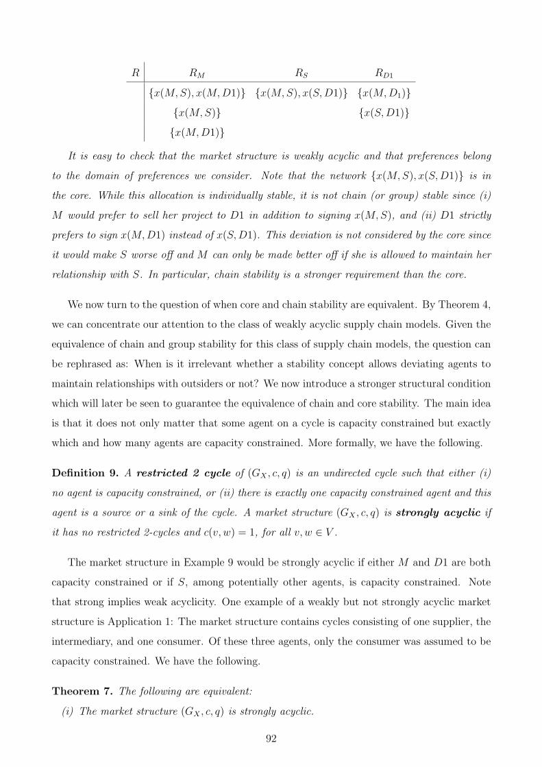
R RM RS RD1

{x(M,S), x(M,D1)} {x(M,S), x(S,D1)} {x(M,D1)}

{x(M,S)} {x(S,D1)}

{x(M,D1)}

It is easy to check that the market structure is weakly acyclic and that preferences belong

to the domain of preferences we consider. Note that the network {x(M,S), x(S,D1)} is in

the core. While this allocation is individually stable, it is not chain (or group) stable since (i)

M would prefer to sell her project to D1 in addition to signing x(M,S), and (ii) D1 strictly

prefers to sign x(M,D1) instead of x(S,D1). This deviation is not considered by the core since

it would make S worse off and M can only be made better off if she is allowed to maintain her

relationship with S. In particular, chain stability is a stronger requirement than the core.

We now turn to the question of when core and chain stability are equivalent. By Theorem 4,

we can concentrate our attention to the class of weakly acyclic supply chain models. Given the

equivalence of chain and group stability for this class of supply chain models, the question can

be rephrased as: When is it irrelevant whether a stability concept allows deviating agents to

maintain relationships with outsiders or not? We now introduce a stronger structural condition

which will later be seen to guarantee the equivalence of chain and core stability. The main idea

is that it does not only matter that some agent on a cycle is capacity constrained but exactly

which and how many agents are capacity constrained. More formally, we have the following.

Definition 9. A restricted 2 cycle of (GX , c, q) is an undirected cycle such that either (i)

no agent is capacity constrained, or (ii) there is exactly one capacity constrained agent and this

agent is a source or a sink of the cycle. A market structure (GX , c, q) is strongly acyclic if

it has no restricted 2-cycles and c(v, w) = 1, for all v, w ∈ V .

The market structure in Example 9 would be strongly acyclic if either M and D1 are both

capacity constrained or if S, among potentially other agents, is capacity constrained. Note

that strong implies weak acyclicity. One example of a weakly but not strongly acyclic market

structure is Application 1: The market structure contains cycles consisting of one supplier, the

intermediary, and one consumer. Of these three agents, only the consumer was assumed to be

capacity constrained. We have the following.

Theorem 7. The following are equivalent:

(i) The market structure (GX , c, q) is strongly acyclic.

92

(ii) Chain stability is equivalent to core stability, that is, CS(R) = C(R) for all R ∈ R(c,q).

The intuition for this result is that in a weakly but not strongly acyclic market structure

there could be an undirected cycle v1, . . . , vn such that (i) agents v1, . . . , vj can reach some

core allocation µ by signing contracts only with their direct neighbor(s) in {v1, . . . , vj}, and (ii)

there is a blocking chain of µ involving vj+1, . . . , vn as well as v1 and vj. This is possible, if e.g.

v1 is a source and is the only capacity constrained agent on the cycle. The above is impossible

if there are no restricted 2 cycles: If v1 was the only capacity constrained agent on the cycle

she would have to be a passing node. But then v1 would never agree to sign a contract with vn

if µ was individually rational. The following is an application of Theorems 4 and 7.

Application 2 (Many-to-Many (One) Matching). Consider a labor market with at least two

firms and at least two workers. All firms can hire arbitrarily many workers, while some or all

of the workers are constrained to work for at most one firm. We assume that all workers are

connected to all firms and that firms’ as well as agents’ preferences satisfy substitutability. This

is a special case of a supply chain models in which the graph of potential interactions contains

edges from all workers to all firms.23 Note that chain stability reduces to pairwise stability here,

since there are no intermediaries and a chain can thus involve at most two agents. How many

workers can be allowed to demand multiple contracts if we want the market structure to be

weakly and strongly acyclic, respectively?

In order to satisfy weak acyclicity we need to guarantee that every cycle contains at least one

capacity constrained agent. Note that for any pair of workers there exists a cycle that contains

only these two workers and a pair of firms. Since only workers can be capacity constrained,

weak acyclicity thus requires us to assume that at most one worker can work for multiple firms.

In order to satisfy strong acyclicity, both workers would have to be capacity constrained so

the market has to be a many-to-one matching market. As a corollary to Theorem 7 we thus

obtain that the core of a many-to-many matching market is equivalent to the set of pairwise

stable matchings for all substitutable preference profiles if and only if the market is actually

many-to-one.24

To conclude, we now discuss three (independent) corollaries of Theorem 7.

23The direction of the edges is arbitrary and we could also direct the edges from firms to workers. A directionof edges has to be chosen to embed this two-sided matching model in a supply chain model.

24The interested reader may note that if there are no intermediaries, as in Application 2, the preferences incounterexample used to prove that (ii)⇒ (i) of Theorem 7 are responsive in the sense of Roth (1985). Hence,the statements apply equally well to the class of all responsive preferences. We thank Lars Ehlers for pointingthis out.

93

As previously mentioned, the core coincides with the set of pairwise stable matchings in

many-to-one matching models with substitutable preferences (Roth and Sotomayor (1991)).

Note that this is a special case of our result since (i) chain reduces to pairwise stability if there

are no intermediaries, (ii) agents on one side of the market can sign at most one contract, and

(iii) each cycle must contain at least two agents from each of the two market sides and thus at

least two capacity constrained agents.

Next, consider the unit capacity model in which each agent can sign at most one upstream

and at most one downstream contract. Ostrovsky (2008) shows that in the unit capacity

model the core coincides with the set of chain stable networks. To see that this is a direct

consequence of Theorem 7 note that in the absence of directed cycles any undirected cycle

must contain at least one source and at least one sink. In the unit capacity model sources and

sinks of a cycle are always capacity constrained. Hence, any undirected cycle must have at

least two capacity constrained agents and the market structure is strongly acyclic. Note that

Ostrovsky’s result does not in general imply core equivalence for the many-to-one matching

model with substitutable preferences.

Finally, consider a many-to-one matching model with substitutes and complements. We

assume that firms can hire an arbitrary number of workers, while workers can work for at most

one firm. Assume that it is possible to decompose the set of workers into two sets W1 and W2

such that all firms view two workers from the same set as substitutes (in the sense of SSS)

and workers from different sets as complements (in the sense of CSC). This is a variant of the

model studied in Sun and Yang (2006) and Sun and Yang (2009). Ostrovsky (2008) discusses

how this can be formulated as a supply chain model in which the set of sellers of basic inputs

comprises W1, the set of consumers of final products comprises W2, and the set of intermediaries

comprises all firms. Note that since there are no edges connecting two firms or two workers, any

undirected cycle must contain at least two workers. Since all workers are capacity constrained

the market structure is strongly acyclic so that the core coincides with the set of chain stable

networks. Hence, we obtain the non-emptiness of a core network as a corollary to the existence

of a chain stable network for this model.

3.6 Conclusion

This paper showed that the structural properties of supply chain models are important for

the relationship between (cooperative) solution concepts. Weak acyclicity was shown to be

necessary and sufficient for (i) the equivalence of chain and group stability, (ii) the core stability

94

of chain stable networks, (iii) the efficiency of chain stable networks, (iv) the existence of group

stable networks, and (iv) the existence of efficient individually stable networks. In the second

part of the paper we derived some further results on the competing stability concept of the core.

In particular, it was shown that strong acyclicity is necessary and sufficient for core equivalence

to obtain. We have argued that our results can be interpreted as a justification of chain stability

on basis of efficiency and robustness considerations. The cooperative foundation shows that

this stability concept is a reasonable allocative goal for markets that fit the assumptions of

the supply chain model. An important open question for future research is how such markets

would have to be organized in order to reach this goal when agents act strategically.

95

96

Bibliography

Abdulkadiroglu, A. (2005): “College Admissions with Affirmative Action,” International

Journal of Game Theory, 33(4), 535 – 549.

Abdulkadiroglu, A., Y.-K. Che, and Y. Yasuda (2008): “Expanding ”Choice” in School

Choice,” Working Paper, Columbia University.

Abdulkadiroglu, A., and L. Ehlers (2007): “Controlled School Choice,” Working Paper,

Montreal University.

Abdulkadiroglu, A., P. Pathak, and A. Roth (2009): “Strategy-proofness versus Effi-

ciency in Matching with Indifferences: Redesigning the NYC High School Match,” American

Economic Review.

Abdulkadiroglu, A., P. Pathak, A. Roth, and T. Sonmez (2006): “Changing the

Boston School Choice Mechanism,” Working Paper, Harvard University.

Abdulkadiroglu, A., and T. Sonmez (2003): “School Choice - A Mechanism Design

Approach,” American Economic Review, 93(3), 729 – 747.

Abdulkadiroglu, A., and T. Sonmez (1998): “Random Serial Dictatorship and the Core

from Random Endowments in House Allocation Problems,” Econometrica, 66, 689 – 701.

(1999): “House Allocation with Existing Tenants,” Journal of Economic Theory, 88,

233 – 260.

Abeledo, H., and G. Isaak (1992): “A characterization of graphs that ensure the existence

of stable matchings,” Mathematical Social Sciences, pp. 93 – 96.

Alcalde, J., and S. Barbera (1994): “Top Dominance and the Possibility of Strategy-Proof

Stable Solutions to Matching Problems,” Economic Theory, 4, 417 – 435.

97

Alcalde, J., and A. Romero-Medina (2000): “Simple Mechanisms to Implement the Core

of College Admissions Problems,” Games and Economic Behavior, pp. 294 – 302.

Balinski, M., and T. Sonmez (1999): “A Tale of Two Mechanisms: Student Placement,”

Journal of Economic Theory, 84(1), 73 – 94.

Blair, C. (1988): “The Lattice Structure of the Set of Stable Matchings with Multiple Part-

ners,” Mathematics of Operations Research, pp. 619 – 628.

Braun, S., N. Dwenger, and D. Kubler (2008): “Telling the Truth May Not Pay Off:

An Empirical Study of Centralised University Admissions in Germany,” Working Paper,

Technical University of Berlin.

Chen, Y., and T. Sonmez (2006): “School Choice: An experimental study,” Journal of

Economic Theory, 127(1), 202 – 231.

Dubins, L., and D. Freedman (1981): “Machiavelli and the Gale-Shapley algorithm,” Amer-

ican Mathematical Monthly, 88, 485 494.

Dutta, B., and J. Masso (1997): “Stability of Matchings When Individuals Have Preferences

over Colleagues,” Journal of Economic Theory, 75, 464 – 475.

Echenique, F., and J. Oviedo (2006): “A theory of stability in many-to-many matching

markets,” Theoretical Economics, pp. 233 – 273.

Echenique, F., and B. Yenmez (2007): “A solution to matching with preferences over

colleagues,” Games and Economic Behavior, 59, 46 – 71.

Ehlers, L. (2007): “Respecting Priorities when Assigning Students to Schools,” Working

Paper, Universite de Montreal.

Ehlers, L., and A. Erdil (2009): “Efficient Assignment Respecting Priorities,” Working

Paper, Universite de Montreal.

Erdil, A., and H. Ergin (2008): “What’s the Matter with Tie-Breaking? Improving Effi-

ciency in School Choice,” American Economic Review, pp. 669 – 689.

Ergin, H. (2002): “Efficient resource allocation on the basis of priorities,” Econometrica,

70(6), 2489 – 2497.

98

Ergin, H., and T. Sonmez (2006): “Games of School Choice under the Boston Mechanism,”

Journal of Public Economics, 90, 215 – 237.

Featherstone, C., and M. Niederle (2008): “Ex Ante Efficiency in School Choice Mech-

anisms: An Experimental Investigation,” Working Paper, Stanford University.

Gale, D., and L. Shapley (1962): “College Admissions and the Stability of Marriage,”

American Mathematical Monthly, 69, 9–15.

Gibbard, A. (1973): “Manipulation of Voting Schemes: A General Result,” Econometrica,

41, 587 – 601.

Guillen, P., and O. Kesten (2008): “On-Campus Housing: Theory vs. Experiment,” Work-

ing Paper, Tepper School of Business, Carnegie Mellon University.

Haeringer, G., and F. Klijn (2008): “Constrained School Choice,” Working Paper, Uni-

versitat Autonoma de Barcelona.

Hatfield, J., and P. Milgrom (2005): “Matching with Contracts,” American Economic

Review, pp. 913 – 935.

Hatfield, J. W., and F. Kojima (2009): “Group incentive compatibility for matching with

contracts,” Games and Economic Behavior.

Hylland, A., and R. Zeckhauser (1979): “The Efficient Allocation of Individuals to Po-

sitions,” Journal of Political Economy, 87, 293 – 314.

Jackson, M., and A. Wolinsky (1996): “A Strategic Model of Social and Economic Net-

works,” Journal of Economic Theory, pp. 44 – 74.

Kalai, E., A. Postlewaite, and J. Roberts (1978): “Barriers to Trade and Disadvan-

tageous Middlemen: Nonmonotonicity of the core,” Journal of Economic Theory, pp. 200 –

209.

Kara, T., and T. Sonmez (1996): “Nash Implementation of Matching Rules,” Journal of

Economic Theory, 68, 425 – 439.

(1997): “Implementation of College Admission Rules,” Economic Theory, 9, 197 –

218.

99

Kelso, A., and V. Crawford (1982): “Job matching, coalition formation, and gross sub-

stitutes,” Econometrica, pp. 1483 – 1503.

Kesten, O. (2006): “On two competing mechanisms for priority-based allocation problems,”

Journal of Economic Theory, 127(1), 155 – 171.

Klaus, B., and F. Klijn (2005): “Stable Matchings and the Preferences of Couples,” Journal

of Economic Theory, 121, 75 – 106.

Klaus, B., and M. Walzl (2008): “Stable Many-to-Many Matchings with Contracts,” Har-

vard Business School Working Paper 09-046.

Kojima, F. (2008): “Games of school choice under the Boston mechanism with general priority

structures,” Social Choice and Welfare, pp. 357–365.

Kojima, F., and P. Pathak (2009): “Incentives and Stability in Large Matching Markets,”

American Economic Review.

Konishi, H., and M. U. Unver (2006): “Credible group stability in many-to-many matching

problems,” Journal of Economic Theory, pp. 57 – 80.

Miralles, A. (2008): “School Choice: The Case for the Boston Mechanism,” Working Paper,

Boston University.

Ostrovsky, M. (2008): “Stability in Supply Chain Networks,” American Economic Review,

pp. 897 – 923.

Papai, S. (2000): “Strategy-proof Assignment by Hierarchical Exchange,” Econometrica, 68,

1403 – 1433.

(2004): “Unique stability in simple coalition formation games,” Games and Economic

Behavior, pp. 337 – 354.

(2007): “Exchange in a general market with indivisible goods,” Journal of Economic

Theory, pp. 208 – 235.

(2009): “Mixed Priority Matching,” Working Paper, Concordia University Montreal.

Pathak, P. (2008): “Lotteries in Student Assignment: The Equivalence of Queueing and a

Market-Based Approach,” Working Paper, MIT.

100

Pathak, P., and T. Sonmez (2008): “Leveling the Playing Field: Sincere and Sophisticated

Players in the Boston Mechanism,” American Economic Review, pp. 1636 – 1652.

Peleg, B., and P. Sudholter (2003): Introduction to Theory of Cooperative Games. Kluwer

Academic.

Pycia, M., and U. Unver (2009): “A Theory of House Allocation and Exchange Mecha-

nisms,” Working Paper, Boston College.

Romero-Medina (1998): “Implementation of Stable Solutions in a Restricted Matching Mar-

ket,” Review of Economic Design, 3, 137 – 147.

Roth, A. (1982): “The Economics of Matching: Stability and Incentives,” Mathematics of

Operations Research, 7, 617 – 628.

(1984a): “The Evolution of the Labor Market for Medical Interns and Residents: A

Case Study in Game Theory,” Journal of Political Economy, 92, 991 – 1016.

(1984b): “Stability and Polarization of Interests in Job Matching,” Econometrica, pp.

47 – 57.

(1985): “The College Admissions Problem is not equivalent to the Marriage Problem,”

Journal of Economic Theory, 36, 277 – 288.

(2002): “The Economist as Engineer: Game Theory, Experimentation, and Compu-

tation as Tools for Design Economics,” Econometrica, 70, 1341 – 1378.

(2008): “Deferred Acceptance Algorithms: History, Theory, Practice, and Open Ques-

tions,” International Journal of Game Theory, 36, 537 – 569.

Roth, A., and E. Peranson (1999): “The redesign of the Matching Market for American

Physicians: Some Engineering Aspects of Economic Design,” American Economc Review,

89(4), 748 – 780.

Roth, A., and M. Sotomayor (1989): “The College Admissions Problem Revisited,” Econo-

metrica, pp. 559–570.

Roth, A., and M. Sotomayor (1991): Two Sided Markets - A Study in Game Theoretic

modeling. Cambridge University Press.

101

Satterthwaite, M. (1979): “Strategy-proofness and Arrow’s conditions: Existence and Cor-

respondence Theorems for Voting Procedures and Social Welfare Functions,” Journal of Eco-

nomic Theory, 10, 187 – 217.

Scheer, e. (1999): Zentralstelle fur die Vergabe von Studienplatzen 1973 - 1998. Informations-

und Pressestelle der ZVS.

Shapley, L., and H. Scarf (1974): “On Cores and Indivisibility,” Journal of Mathematical

Economics, 1, 23 – 37.

Sonmez, T. (1997): “Games of Manipulation in Marriage Problems,” Games and Economic

Behavior, 20, 169 – 176.

(1999): “Strategy-Proofness and Essentially Single-Valued Cores,” Econometrica, 67,

677 – 689.

Sonmez, T., and U. Unver (2008): “Matching, Allocation, and Exchange of Discrete Re-

sources,” Working Paper, Boston College.

Sotomayor, M. (1999): “Three remarks on the many-to-many stable matching problem,”

Mathematical Social Sciences, pp. 55 – 70.

Sun, N., and Z. Yang (2006): “Equilibria and Indivisibilities,” Econometrica, pp. 1385 –

1402.

(2009): “A Double-Track Adjustment Process for Discrete Markets with Substitutes

and Complements,” Econometrica.

Svensson, L.-G. (1999): “Strategy-proof allocation of indivisible goods,” Social Choice and

Welfare, 16, 557–567.

102

Appendices

A.1 Appendix to Chapter 1

Proof of Theorem 1

We show first that for any profile of strict applicant preferences R, if Q is a pure strategy Nash

equilibrium of ΓZV S(R) then fZV S(Q) must be a stable matching for the university admissions

problem R. For economy of notation let fZV S(Q) = (µEZV S, µWZV S, µ

UZV S) and qU be the capacity

vector in step U. Condition (i) is satisfied irrespective of whether Q is a Nash equilibrium or

not, since only top-grade applicants can receive a place in step E, only wait-time applicants

can obtain a place in step W, and a university never makes an offer to an unacceptable student

in the college proposing deferred acceptance algorithm of step U. If an applicant a is matched

to an unacceptable (w.r.t. R) university she could profitably deviate by ranking just her most

preferred university (w.r.t. R) for each step of the procedure: The worst thing that could

happen is to be left unassigned if she submits the alternative report. Since aPafZV Sa (Q) this

is profitable so that Q could not have been a Nash equilibrium of ΓZV S(R). This shows that

fZV S(Q) has to satisfy (ii).

Suppose to the contrary that fZV S(Q) does not match applicants as early as possible and

that there is a top-grade applicant a such that µU(a) = u and either |µE(u)| < qEu or πEu (a) <

πEu (a) for some a ∈ µE(u). If a had ranked u as her most preferred university for step E,

she would have been matched to u in step E since in the first case at most qEu − 1 top-grade

applicants could have applied to u in the course of the Boston mechanism under Q and in the

second case at most qEu − 1 other (top-grade) applicants with higher πEu priority than a could

have listed u as their top choice in QE (and thus in QE). Since applicants prefer to be matched

as early as possible, this would be a profitable deviation for a. The argument in case of a

wait-time applicant matched too late is completely analogous. Hence, fZV S(Q) has to satisfy

condition (iii).25

25These parts of the proof that concern the Boston mechanisms of steps E and W are similar to the arguments

103

Next, suppose that fZV S(Q) satisfies (i) to (iii) but that there is an applicant-university

pair (a, u) such that (iv) is violated for some i ∈ {E,W,U}. Let Qa be an alternative report

for applicant a that lists only u for each step of the procedure. Let Q = (Qa, Q−a), fZV S(Q) =

(µE, µW , µU), and qU be the corresponding quota vector in step U. For i ∈ {E,W} the same

argument used to show that fZV S(Q) satisfies (iii) can be used to establish that µi(a) = u. So

suppose that i = U . Let AU and AU denote the sets of applicants apart from a who remain in

the procedure by the beginning of step U under Q and Q, respectively. It is clear that unless

µ(a) = a, Qa is a profitable deviation for a. So suppose that µ(a) = a. Note that this implies

AU ⊆ AU , qUu = qUu , as well as |µU(u)| = qU : If a does not receive a place at u in steps E or

W under Q, there are (weakly) less rejections in steps E and W under Q than under Q. In

particular the set of applicants who are assigned a place at u in steps E and W must be the

same under Q and Q. Furthermore, since (a, u) is a pair such that (iv) is violated for i = U it

has to be the case that a �Uu u. But then u would always make an offer to a before leaving a

place unassigned so that we must have |µU(u)| = qUu . This implies that if a has not received

an offer by u in the first t rounds of the CDA under Q then all applicants in AU must have

received weakly more offers in rounds 1 through t than they received in the first t rounds of the

CDA under Q. Hence, if a does not receive an offer by u in the course of the CDA under Q, all

applicants in AU receive a weakly better assignment (wrt to QU−a) than under Q. In particular,

any applicant in AU who rejected an offer by u in the CDA under Q will also reject an offer

by u in the CDA under Q. But then we must have |µU(u)| = qUu and, since (iv) is violated,

there has to be an applicant a ∈ µU(u) such that a �Uu a. By the above this implies that if

a′ /∈ µU(u) and a′ �Uu a then a′ will reject an offer by u in the CDA under Q. But then µU(u)

has to contain at least one applicant a′′ with a �Uu a′′. Hence, u must have made an offer to

a in the CDA under Q (which a would have accepted). This contradicts the assumption that

µ(a) = a and shows that fZV S(Q) has to satisfy (iv).

Now let µ be a stable matching in the university admissions problem R. We construct a

Nash equilibrium Q such that fZV S(Q) = µ. Let a be an arbitrary applicant. If µ(a) = a, let

a rank her six most preferred acceptable universities according to Ra steps E and W, and all

acceptable universities for step U. If µ(a) = u, let a rank only u for all parts of the procedure.

Let Q be the resulting strategy profile.

We show first that fZV S(Q) = µ. Let fZV S(Q) = (µE, µW , µU). Suppose a is such that

µ(a) = a but µE(a) = u ∈ U . By construction of Q, all applicants in µE(u) rank u first in their

in Ergin and Sonmez (2006).

104

submitted ranking for step E. Since a ranks only acceptable universities, uPaµ(a) so that we

obtain a contradiction to (iv). If a is such that µU(a) = u ∈ U , then the only possibility for

µE(a) 6= µE(a) is that a receives a place at u in step E of the ZVS procedure under Q. This is a

contradiction to (iii). Hence, µE(a) = a if µE(a) = a. Given the construction of Q, this implies

that any applicant who receives a place at some university u under µE must be assigned to u

in step E of the ZVS procedure for Q. Hence, µE = µE and a completely analogous argument

can be used to establish that µW = µW . To see that µU = µU , note that, by the above, any

applicant a with µU(a) ∈ U will not be assigned in steps E or W of the ZVS procedure under Q.

All of these applicants rank only their assigned university under µU for step U while all other

unassigned applicants rank their six most preferred acceptable universities (w.r.t. R). If one of

the unassigned applicants received a place in step U of the ZVS procedure under Q, (iv) would

be violated.

Next, we show that no applicant has an incentive to deviate from the proposed strategy-

profile. Let Qa be an alternative report for applicant a, Q = (Qa, Q−a), and fZV S(Q) =

(µE, µW , µU). Note that the sets of top-grade and wait-time applicants are the same as under

Q since, for i ∈ {E,W}, Qia contains at least one university by the no empty lists assumption.

Now suppose to the contrary that µ(a)Paµ(a). It cannot be the case that µE(a) = u = µU(a)

or µW (a) = u = µU(a), since all applicants in µE(u) and µW (u) apply to u in the first round of

the Boston mechanism under Q so that µ could not satisfy (iii) otherwise. We can show in a

similar fashion that a cannot obtain a university strictly preferred to µ(a) (w.r.t. Ra) in steps

E or W. Hence, it remains to be shown that a cannot prefer µU(a) over µ(a). Consider first

an applicant a such that µE(a) = µW (a) = a. Given (iii) and (iv), no alternative report Qa

that leads to different assignments in steps E or W can be profitable for a. Suppose then that

contrary to what we want to show, Qa is a profitable deviation for a. We can assume w.l.o.g.

that QEa = QE

a and QWa = QW

a by the above. But then the set of applicants who are unmatched

by the beginning of step U of the ZVS procedure under Q contains in particular all applicants

who are matched to some university under µU . By assumption, µU(a)Paµ(a) so that there must

be some university u ∈ U such that µU(a) = u. But all applicants in µU(u) were “available” to

u in step U of the ZVS procedure under Q since they all ranked only u. Hence, u must prefer a

to at least one of the applicants assigned to it under µU or must have had some unfilled capacity

in µU(u) even though a is acceptable (w.r.t. �Uu ). This is a contradiction to (iv). Now consider

an applicant a such that for some u ∈ U , µE(a) = u. By the disjoint sets assumption, a can

never obtain a place at some university in step W. By (iv) and the construction of Q, there is

no alternative report for a such that she obtains a strictly preferred (w.r.t. Ra) university in

105

step E. Thus the only way that a could potentially improve upon her assignment under µ is

that µE(a) = a(= µW (a)). But the only applicants who could take the leftover seat at u in step

E are those who are either unassigned under µ or who are matched to u under µU . In any case,

for all universities u′ 6= u, all applicants in µU(u′) remain in the procedure by the beginning of

step U under Q. If µU(a)Pau, we must thus obtain a contradiction to (iv). This completes the

proof.

An example showing that No Empty Lists is Restrictive

The following example shows that the No Empty Lists assumption is restrictive. There are seven

applicants a1, a2, a3, a4, a5, a6, a7 indexed in order of increasing average grades. For simplicity,

we assume that there are only two universities u and u′ who have one place to allocate in each

of the three steps of the ZVS procedure. Preferences of applicants are as follows:

RA Ra1 Ra2 Ra3 Ra4 Ra5 Ra6 Ra7

u u u′ u′ u′ u u′

u

Assuming that a5 and a6 are the applicants with the longest waiting time, a3 �Uu a2 as well

as a5 �Uu a4 �Uu a3, and that all applicants submit their true ranking of universities for each

step of the procedure, the outcome of the ZVS procedure is

fZV SE(R) =u u′

a1 ∅, fZV SW (R) =

u u′

a6 a7

, fZV SU(R,�U) =u u′

a3 {a4, a5}.

Note that if we keep the profile of reports by everyone but a2 fixed, a2 cannot obtain a place

at u if she applies for a place in step E. Suppose then that she decides to apply only for step

U and submits QUa2

= u. If everyone else submits the same preferences as before, a3 would be

a top-grade applicant and could obtain a place at her most preferred university u′ in step E of

the ZVS procedure. But then a2 would receive a place at u in step U of the procedure since no

one else will apply to u in that step. Thus, she benefits from not applying for a place in step

E.

106

Proof that µ1 and µ2 are the only stable matchings in Example 2

Note first that a1 has to be assigned to u1 in step E by (iii) and (iv). This implies that if a2

is matched in step E, she must receive a place at u3 by (iv) for i = E. Now note that if a2

is matched in step E, a3 must be matched to u2 in step E. Otherwise, one place at u2 would

remain empty and a3 would have to receive a place at u3 in step U by (iii). But then a4 and a5

would take the two places at u2 in step U. But this implies that a1 must have strictly higher

priority according �Uu1than one of the applicants assigned a place at u1 in step U (or u1 does

not fill its capacity reserved for U). Hence, a3 must be matched to u2 in step E if a3 receives

a place at u2 in step E. It is easy to see that wait-time applicants cannot do better than being

assigned a place in step W and that there is a unique stable matching for this subproblem.

This is easily seen to imply that there is a unique stable matching where a2 is matched in step

E.

If on the other hand, a2 is not matched in step E, she must receive a place at u1 in step

U by (iii). This implies directly that a4 and a5 must both obtain a place at u2 in step U and

that a3 must be assigned to a3 in step E. It is again easy to see that the wait-time applicants

cannot do better than being assigned a place in step W.

Omitted details of the ZVS Procedure

This appendix lists some of the more substantial simplifications made in the main body of the

text. Readers interested in all details of the current ZVS procedure may still want to consult

the Vergabeverordnung ZVS [Stand: WS 2008/2009] (available at www.zvs.de).

Capacities: The total number of places at each university is determined by the application

of federal laws. For each state there is a so called Kapazit”atsverodnung (KaPVO) which

prescribes a formula for calculating the number of applicants a university can admit on

basis of the number of professors, available teaching facilities, and so on.26

Special Quotas: Up to approximately fifteen percent of total available places are allocated in

advance among foreign applicants, applicants pursuing a second university degree, and so

on. These applicants are not allowed to participate in the regular assignment procedure.

26There has been some discussion about the KaPVO in recent years, see e.g. Die fiese Formel in Die Zeit,Nr. 39(2007).

107

Step E: The education system in Germany is federalized and the general opinion is that av-

erage grades are not directly comparable across federal states. For this reason, there are

actually sixteen separate assignment procedures in step E, one for each federal state. This

is achieved by splitting the 20 percent of (remaining) capacity available in step E into

sixteen parts. In the assignment procedure of a given federal state only those applicants

are considered who have received their high school diploma in this state.

Step U: – Once assignments are determined by the ZVS procedure described in section 2,

successful applicants have to enroll at their assigned university. If some applicants

fail to do so, their places are allocated according to the rules of step U. Here, only

those applicants are considered who did not receive a place in previous rounds of the

assignment procedure. Again, students have to enroll at their assigned university (if

any) and if they fail to do so, another round of step U is used to allocate remaining

places (again only students who were not previously assigned a place are considered).

Any places that remain after all of this are allocated via lottery by universities.

– In order to prevent multiple rounds of the assignment procedure in step U, a uni-

versity can demand the ZVS to overbook its capacities. Thus, a university with, say

100 places, may ask the ZVS to be assigned 150 applicants since it expects some

students not to accept their assigned places.

Lotteries: If a university does not fill its capacity in the ZVS procedure, remaining places are

allocated on basis of lottery. Each university conducts its own lottery and applicants have

to apply to universities directly in order to participate.

Evaluation Procedures in the current ZVS procedure

In this Appendix we provide some further details on the different evaluation procedures used

by universities in step U. All of the below concerns the ZVS procedure for the winter term

2008/2009. The evaluation process takes place after assignments in steps E and W have been

determined and only those applicants who did not receive a place in these steps are considered.

In principle, the ZVS informs each university about all remaining applicants who have listed

the university in their ranking for step U.

A university may, however, limit the set of applicants it will consider for step U in advance

on basis of its rank in the preference lists submitted for step U, average grades, or a combination

of the two criteria. For example, a university with, say, a hundred seats to be allocated in step

108

U may consider only the 300 applicants with the best average grades among those who ranked

it first. This practice is called pre-selection and the ZVS informs each university only about

those applicants who “survived” its pre-selection process.

In case an applicant is not rejected in the pre-selection process of a university, the ZVS

provides the university with detailed information including its rank in the submitted preference

list, average grade, waiting-time, and so on. Universities can then use average grades, inter-

views, statements of purpose, completion of on-the-job training in a relevant field, prizes in

scientific competition, and so on, to evaluate remaining applicants. Furthermore, universities

are allowed to split their capacity into several parts and to apply different admission crite-

ria across these parts. For example, a university may decide to allocate 50 percent of places

according to average grade and 50 percent on basis of performance in an interview. In this

case, the university has to specify which place an applicant receives if she could be admitted in

more than one of these quotas. The official information brochure of the ZVS states that in the

determination of an applicant’s rank average grade has to be a decisive factor,27 although the

exact requirement that needs to be fulfilled is not specified.

A university uses a mechanical evaluation procedure if the marginal cost of evaluating an

additional candidate according to its criteria is negligible. Under this label we summarize

all universities who do not use “subjective” criteria such as performance in interviews or the

evaluation of statements of purpose. While such universities may still require to elicit additional

information from applicants, computing the rank of an applicant is completely mechanical.

In this category, we also include universities who use standardized tests in their evaluation

procedure. For example, several universities offering medical subjects use the outcome of a

standardized medical subject test in their evaluation. Applicants have to pay a fixed fee in order

to take the test and tests are graded by an independent company. If, for example, a university

uses some weighted average of average grade and performance in the standardized test to rank

applicants, its cost of considering one additional applicant amounts to the (computational) cost

of calculating the weighted average of two numbers.

In the first table, #U lists the number of universities, #Prek lists the number of universities

that consider only applicants who ranked them at least kth (k = 1, . . . , 4), #M lists the number

of universities who use a mechanical evaluation procedure, and #M + Pre lists the number

of universities who have a mechanical evaluation procedure but only consider applicants who

rank them sufficiently high.

In the second table, #INT is the number of universities that use interviews to allocate at

27Merkblatt M09: Auswahlverfahren der Hochschulen, available at www.zvs.de. Translation by the author.

109

Subject # U #Pre 1 #Pre 2 #Pre 3 #Pre 4 # M # M+PreBiology 2 0 1 0 0 2 1Psychology 11 2 1 1 0 11 4Vet. Med. 5 3 0 0 0 2 0Pharmacy 22 0 2 3 0 20 5Dentistry 29 4 3 6 1 22 8Medicine 34 6 4 9 1 24 12

Table 1: Preselection and Mechanical Evaluation

Subject #INT #INT>0.5 #INT≤0.5

Biology 0 0 0Psychology 0 0 0Vet. Med. 3 3 0Pharmacy 2 2 0Dentistry 7 2 5Medicine 10 3 7

Table 2: Interviews in the Evaluation Process

least part of their capacity, #INT>0.5 is the number of universities who assign more than half

of their seats on basis of interviews, and #INT≤0.5 is the number of universities who assign at

most half (but at least one) of their seats on basis of interviews.

A short history of the ZVS mechanism

The last major revision of the ZVS procedure took place in the winter term 2005/2006 where

the three part (steps E, W and U) assignment procedure was introduced. There have been a

number of changes from this procedure to the one currently employed procedure. The following

is a list of the most important changes.

Floating Quotas Initially, places not taken in step E were allocated in step W (in addition

to the 20 percent of places reserved for wait-time applicants). As Braun, Dwenger, and

Kubler (2008) mention, this led to some universities allocating far more than 20 percent

of their places to wait-time applicants since very few top-grade applicants demanded

places in step E. Presumably, this one of the main reasons for changing the procedure

and moving unused places directly from step E to step U.

Preference Reversals in step U Applicants were allowed to reverse their preferences in step

U once the evaluation process of universities was complete. Initially, applicants who could

be admitted at several universities in the first round of the assignment procedure of step

U were allowed to take the offer of a university other than the one in highest reported

110

preference. At some point between 2005/2006 and 2008/2009 applicants were even allowed

to reorder their whole ranking of universities in step U after the evaluation process. We

conjecture that one of the main reasons for abandoning this practice is that universities

could not guarantee that a candidate they interviewed would accept an offer.28

Algorithm in Step U Previous versions of the description of the assignment procedure have

been relatively vague concerning the exact form of the assignment procedure in step U.

It was not exactly clear whether a version of the Boston mechanism in which universities

made the offers or the college/university proposing deferred acceptance algorithm were

used. The current version of the official description of the assignment procedure says

that at each point an applicant can be admitted at multiple universities, only the offer

of the most preferred university remains valid.29 Thus, the ZVS algorithm looks at the

lists submitted by universities to check whether an applicant can be admitted at more

than one university. If this is the case, the applicant is deleted from the lists of all but

her most preferred university among those that offered admission. If this procedure is

iterated until no applicants are left, we arrive at exactly the description of the college

proposing deferred acceptance algorithm.

A.2 Appendix to Chapter 2

Proof of Proposition 5

Suppose to the contrary that �1 contains an ambiguous 1-tie but that f is a strategy-proof and

constrained efficient selection from the stable correspondence. W.l.o.g. we can assume that

there are exactly four students 1, 2, 3, 4 and two specialized schools s1, s2 such that

1 �s1 3 �s1 2 and 2 �s2 4 �s2 1. (1)

Let s3 be one of the non-specialized schools. To derive a contradiction, we consider six

preference profiles which define a cycle in the space of preference profiles. The following diagram

summarizes the preference profiles used in our proof. Arrows indicate how we move between

the profiles.

28Given that a couple of universities considered only applicants who ranked them first, it still guaranteed thatan applicant could not have interviewed at some of the other universities.

29Vergabeverordnung ZVS, Stand: WS 2008/2009 §10.(5), which can be found at www.zvs.de. Translationby the author.

111

R2 R11 R1

2 R23 R1

4

s2 s1 s1 s3

s3 s3 s3

s1 s2

↓

←

R1 R11 R1

2 R13 R1

4

s2 s1 s3 s3

s3 s3

s1 s2

←

R6 R11 R1

2 R13 R2

4

s2 s1 s3 s3

s3 s3 s2

s1 s2

↑

R3 R11 R3

2 R23 R1

4

s2 s1 s1 s3

s3 s3 s3

s1

→

R4 R11 R3

2 R23 R2

4

s2 s1 s1 s3

s3 s3 s3 s2

s1

→

R5 R11 R1

2 R23 R2

4

s2 s1 s1 s3

s3 s3 s3 s2

s1 s2

We start with the profile R1. Let

µ =

1 2 3 4

s2 s1 s3 4

and µ =

1 2 3 4

s2 s1 3 s3

.

It is straightforward that these are the only constrained efficient matchings for the profile R1.

Thus, we must have f(R1) = µ or f(R1) = µ. By the symmetries of the example, we can

assume f(R1) = µ without loss of generality.

Now let R23 : s1, s3 and R2 = (R2

3, R1−3). By strategy-proofness, f3(R

2) 6= 3. Note that

for R2 there is no constrained efficient matching that assigns 3 to s3. Hence, we must have

f3(R2) = s1. It is easy to see that this in conjunction with constrained efficiency implies

f(R2) =

1 2 3 4

s2 s3 s1 4

. (2)

Next, suppose 2 declares s2 unacceptable, that is, consider R32 : s1, s3 and the profile R3 =

(R11, R

32, R

23, R

14). By strategy-proofness we must have f2(R

3) = s3 so that constrained efficiency

implies f(R3) = f(R2).

Now consider the profile R4 = (R11, R

32, R

23, R

24). By strategy-proofness, f4(R

4) 6= s3. Since

4 �s2 1 and 1 and 4 are the only students who would like to be assigned to s2, we have

f1(R4) 6= s2 = f4(R

4). If f1(R4) = s3, 1 and 4 would form a SIC under f(R4) - a contradiction

to constrained efficiency. Thus, f1(R4) = s1. But then f3(R

4) 6= s3 since otherwise by 3 �s1 2,

1 and 3 would form a SIC. Thus, f3(R4) = 3 so that

f(R4) =

1 2 3 4

s1 s3 3 s2

. (3)

112

Now consider the profile R5 = (R11, R

12, R

23, R

24). By strategy-proofness, f2(R

5) = s3 and simi-

larly to above, f(R5) = f(R4).

Finally, consider the profile R6 = (R11, R

12, R

13, R

24). By strategy-proofness, f3(R

6) = 3.

Since the first choices of the other three agents are compatible, constrained efficiency implies

f(R6) = f(R5).

This yields the desired contradiction since s3 = f4(R24, R

1−4)P

14 f4(R

1) = 4. Hence, there is

no strategy-proof and constrained efficient mechanism. �

Proof of Proposition 6

Consider a �1 that contains ambiguity at the top. Let s1, s2, s3 be three specialized schools

and 1, 2, 3, 4 ∈ I be four distinct students such that30

�s1 �s2 �s31 2 1

3 3 2

2 1 4

4 4 3

Let s4 be one of the non-specialized schools. Suppose to the contrary that there exists a

strategy-proof and constrained efficient rule f .

The main part of the proof considers four preference profiles, which are summarized in the

following diagram. As in the proof of Proposition 5, arrows indicate how we move between

preference profiles.

R1 R11 R1

2 R13 R1

4

s4 s1 s4 s3

s4 s3

s1

↓

R2 R21 R2

2 R23 R1

4

s2 s4 s4 s3

s4 s3

s2

↓

R3 R11 R3

2 R13 R2

4

s4 s4 s4 s1

s3 s3 s3

s1 s2

↔

R4 R11 R3

2 R23 R2

4

s4 s4 s4 s1

s3 s3 s3

s2 s2

30Note that due to the symmetries of the definition it is without loss of generality to assume that 1 �s3 2.

113

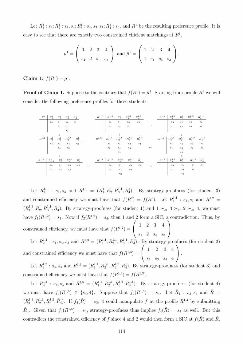
Let R11 : s4;R

12 : s1, s4;R

13 : s4, s3, s1;R

14 : s3, and R1 be the resulting preference profile. It is

easy to see that there are exactly two constrained efficient matchings at R1,

µ1 =

1 2 3 4

s4 2 s1 s3

and µ1 =

1 2 3 4

1 s1 s4 s3

.

Claim 1: f(R1) = µ1.

Proof of Claim 1. Suppose to the contrary that f(R1) = µ1. Starting from profile R1 we will

consider the following preference profiles for these students:

R1 R11 R1

2 R13 R1

4

s4 s1 s4 s3

s4 s3

s1

↓

R1,7 R1,11 R1

2 R1,23 R

1,34

s4 s1 s3 s4

s1 s4 s4

↑

→

R1,8 R1,11 R1

2 R1,23 R

1,14

s4 s1 s3 s4

s1 s4 s4 s3

↓

R1,1 R11 R1

2 R1,13 R1

4

s4 s1 s4 s3

s4 s3

↓

R1,6 R1,11 R

1,12 R

1,23 R

1,34

s4 s1 s3 s4

s1 s4 s4

s3

←

R1,5 R1,11 R

1,12 R

1,23 R

1,14

s4 s1 s3 s4

s1 s4 s4 s3

s3

↑

R1,2 R11,1 R1

2 R1,13 R1

4

s4 s1 s4 s3

s1 s4 s3→

R1,3 R1,11 R

1,12 R

1,13 R1

4

s4 s1 s4 s3

s1 s4 s3

s3

→

R1,4 R1,11 R

1,12 R

1,23 R1

4

s4 s1 s3 s3

s1 s4 s4

s3

Let R1,13 : s4, s3 and R1,1 = (R1

1, R12, R

1,13 , R1

4). By strategy-proofness (for student 3)

and constrained efficiency we must have that f(R2) = f(R1). Let R1,11 : s4, s1 and R1,2 =

(R1,11 , R1

2, R1,13 , R1

4). By strategy-proofness (for student 1) and 1 �s1 3 �s1 2 �s1 4, we must

have f1(R1,2) = s1. Now if f2(R

1,2) = s4, then 1 and 2 form a SIC, a contradiction. Thus, by

constrained efficiency, we must have that f(R1,2) =

1 2 3 4

s1 2 s4 s3

.

Let R1,12 : s1, s4, s3 and R1,3 = (R1,1

1 , R1,12 , R1,1

3 , R14). By strategy-proofness (for student 2)

and constrained efficiency we must have that f(R1,3) =

1 2 3 4

s1 s3 s4 4

.

Let R1,23 : s3, s4 and R1,4 = (R1,1

1 , R1,12 , R1,2

3 , R14). By strategy-proofness (for student 3) and

constrained efficiency we must have that f(R1,4) = f(R1,3).

Let R1,14 : s4, s3 and R1,5 = (R1,1

1 , R1,12 , R1,2

3 , R1,14 ). By strategy-proofness (for student 4)

we must have f4(R1,5) ∈ {s4, 4}. Suppose that f4(R

1,5) = s4. Let R4 : s3, s4 and R =

(R1,11 , R1,1

2 , R1,23 , R4). If f4(R) = s3, 4 could manipulate f at the profile R1,4 by submitting

R4. Given that f4(R1,5) = s4, strategy-proofness thus implies f4(R) = s4 as well. But this

contradicts the constrained efficiency of f since 4 and 2 would then form a SIC at f(R) and R.

114

This contradiction shows that we must have f4(R1,5) = 4 and f(R1,5) = f(R1,3) as well.

Let R1,34 : s4 and R1,6 = (R1,1

1 , R1,12 , R1,2

3 , R1,34 ). By strategy-proofness we must have

f4(R1,6) = 4. Since the top choices of the other students are compatible, constrained efficiency

implies that f(R1,6) =

1 2 3 4

s4 s1 s3 4

.

Let R1,7 = (R1,11 , R1

2, R1,23 , R1,3

4 ). By strategy-proofness we must have that f2(R1,7) = s1.

Stability implies that f1(R1,7) = s4 and hence f(R1,7) = f(R1,6).

Let R1,8 = (R1,11 , R1

2, R1,23 , R1,1

4 ). By strategy-proofness and constrained efficiency we must

have f4(R1,8) = s3 and f3(R

1,8) = 3. Thus f(R1,8) =

1 2 3 4

s4 s1 3 s3

.

Since f2(R1,5) = s3 and f2(R

1,8) = s1, this implies that 2 is strictly better off reporting R12

rather than her true preference R1,12 when the other students submit R1,1

1 , R1,23 , and R1,1

4 . This

contradicts strategy-proofness and completes the proof of Claim 1. �

Now let R21 : s2, s4, R

22 : s4, R

23 : s4, s3, s2, and R2 = (R2

1, R22, R

23, R

14). Similar to above,

there are exactly two constrained efficient matchings at R2,

µ2 =

1 2 3 4

s2 2 s4 s3

and µ2 =

1 2 3 4

1 s4 s2 s3

.

Claim 2: f(R2) = µ2

Proof of Claim 2. The proof is analogous to the proof of Claim 1. One just needs to switch

the roles of 1 and 2 as well as s1 and s2 and note that at any profile in the proof of Claim 1,

school s3 is never acceptable for both 1 and 2 (and the proof only uses the fact {1, 2} �s3 4 �s3 3

and not how students 1 and 2 are ranked under �s3). �

Now let R32 : s4, s3, R

24 : s1, s3, s2, and R3 = (R1

1, R32, R

13, R

24). Let µ3 =

1 2 3 4

s4 s3 s1 s2

.

Claim 3: f(R3) = µ3.

Proof of Claim 3. By Claim 1 we have that f(R1) = µ1. Now let R3,12 : s1, s4, s3 and

R3,1 = (R11, R

3,12 , R1

3, R14). Since f2(R

1) = 2, strategy-proofness and stability imply f2(R3,1) =

s3. Constrained efficiency then implies f3(R3,1) = s1 so that f(R3,1) =

1 2 3 4

s4 s3 s1 4

.

Now let R3,14 : s3, s1 and R3,2 = (R1

1, R3,12 , R1

3, R3,14 ). By strategy-proofness, f4(R

3,2) 6= s3 so

that constrained efficiency implies f(R3,2) = f(R3,1).

Let R3,24 : s1, s3, s2 and R3,3 = (R1

1, R3,12 , R1

3, R3,24 ). By strategy-proofness and f4(R

3,2) = 4,

115

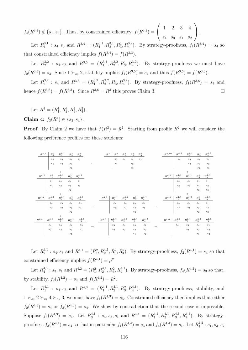
f4(R3,3) /∈ {s1, s3}. Thus, by constrained efficiency, f(R3,3) =

1 2 3 4

s4 s3 s1 s2

.

Let R3,11 : s4, s3 and R3,4 = (R3,1

1 , R3,12 , R1

3, R3,24 ). By strategy-proofness, f1(R

3,4) = s4 so

that constrained efficiency implies f(R3,4) = f(R3,3).

Let R3,22 : s4, s3 and R3,5 = (R3,1

1 , R3,22 , R1

3, R3,24 ). By strategy-proofness we must have

f2(R3,5) = s3. Since 1 �s3 2, stability implies f1(R

3,5) = s4 and thus f(R3,5) = f(R3,3).

Let R3,21 : s4 and R3,6 = (R3,2

1 , R3,22 , R1

3, R3,24 ). By strategy-proofness, f1(R

3,6) = s4 and

hence f(R3,6) = f(R3,3). Since R3,6 = R3 this proves Claim 3. �

Let R4 = (R11, R

32, R

23, R

24).

Claim 4: f3(R4) ∈ {s3, s4}.

Proof. By Claim 2 we have that f(R2) = µ2. Starting from profile R2 we will consider the

following preference profiles for these students:

R4,1 R21 R

4,12 R2

3 R24

s2 s4 s4 s3

s4 s3 s3

s2

↓

←

R2 R21 R2

2 R23 R2

4

s2 s4 s4 s3

s4 s3

s2

R4,10 R4,21 R

4,12 R2

3 R4,34

s4 s4 s4 s1

s3 s3 s3

s2 s2

↑

R4,2 R21 R

4,12 R2

3 R4,14

s2 s4 s4 s3

s4 s3 s3 s1

s2

↓

R4,9 R4,11 R

4,12 R2

3 R4,34

s4 s4 s3 s1

s3 s3 s4 s3

s2 s2

↑

R4,3 R4,11 R

4,12 R2

3 R4,14

s4 s4 s4 s3

s3 s3 s3 s1

s2

↓

→

R4,7 R4,11 R

4,22 R2

3 R4,14

s4 s4 s4 s3

s3 s1 s3 s1

s2

→

R4,8 R4,11 R

4,22 R2

3 R4,34

s4 s4 s4 s1

s3 s1 s3 s3

s2 s2

R4,4 R4,11 R

4,12 R

4,13 R

4,14

s4 s4 s4 s3

s3 s3 s3 s1

s1

→

R4,5 R4,11 R

4,12 R

4,13 R

4,24

s4 s4 s4 s1

s3 s3 s3 s3

s1 s2

→

R4,6 R4,21 R

4,12 R

4,13 R

4,24

s4 s4 s4 s1

s3 s3 s3

s1 s2

Let R4,12 : s4, s3 and R4,1 = (R2

1, R4,12 , R2

3, R24). By strategy-proofness, f2(R

4,1) = s4 so that

constrained efficiency implies f(R4,1) = µ2

Let R4,14 : s3, s1 and R4,2 = (R2

1, R4,12 , R2

3, R4,14 ). By strategy-proofness, f4(R

4,2) = s3 so that,

by stability, f2(R4,2) = s4 and f(R4,2) = µ2.

Let R4,11 : s4, s3 and R4,3 = (R4,1

1 , R4,12 , R2

3, R4,14 ). By strategy-proofness, stability, and

1 �s3 2 �s3 4 �s3 3, we must have f1(R4,3) = s3. Constrained efficiency then implies that either

f2(R4,3) = s4 or f3(R

4,3) = s4. We show by contradiction that the second case is impossible.

Suppose f3(R4,3) = s4. Let R4,1

3 : s4, s3, s1 and R4,4 = (R4,11 , R4,1

2 , R4,13 , R4,1

4 ). By strategy-

proofness f3(R4,4) = s4 so that in particular f1(R

4,4) = s3 and f4(R4,4) = s1. Let R4,2

4 : s1, s3, s2

116

and R4,5 = (R4,11 , R4,1

2 , R4,13 , R4,2

4 ). By strategy-proofness we must have f4(R4,5) = s1. This is

compatible with stability only if f3(R4,5) = s4 and f1(R

4,5) = s3 so that f(R4,5) = f(R4,4). Let

R4,21 : s4 and R4,6 = (R4,2

1 , R4,12 , R4,1

3 , R4,24 ). By strategy-proofness f1(R

4,6) = 1. But note that

R4,6 = R3 and, by Claim 3 above, f1(R3) = s4. This is a contradiction and hence we must have

that f2(R4,3) = s4. Constrained efficiency then implies f(R4,3) =

1 2 3 4

s3 s4 s2 s1

.

Let R4,22 : s4, s1 and R4,7 = (R4,1

1 , R4,22 , R2

3, R4,14 ). By strategy-proofness, f2(R

4,7) = s4 so

that by stability f(R4,7) = f(R4,3).

Let R4,34 : s4, s3, s2 and R4,8 = (R4,1

1 , R4,22 , R2

3, R4,34 ). By strategy-proofness, f4(R

4,8) = s1.

Stability then implies f2(R4,8) = s4 and f(R4,8) = f(R4,3).

Let R4,9 = (R4,11 , R4,1

2 , R23, R

4,34 ). Strategy-proofness implies f2(R

4,9) = s4 so that, by stabil-

ity, f(R4,9) = f(R4,3).

Let R4,10 = (R4,21 , R4,1

2 , R23, R

4,34 ) and note that R4,10 = R4. By strategy-proofness f1(R

4) =

1. But then constrained efficiency implies f3(R4) ∈ {s4, s3} since either f2(R

4) = s4 or

f3(R4) = s4, and if f2(R

4) = s4 then f3(R4) = s3. �

Combining Claim 3 and Claim 4 we see that student 3 has an incentive to submit R23 when

other students submit their preferences from the profile R3 since f3(R4)P 1

3 f3(R3) = s1 given

that f3(R3) = s1 by Claim 3 and f3(R

4) ∈ {s3, s4} by Claim 4. This contradicts strategy-

proofness of f and completes the proof. �

Proof of Proposition 7

We show first that no ambiguos 1-ties and no ambiguity at the top imply that O1 and O2 are

satisfied. Fix some k ≤ K and i ∈ Lk. Suppose to the contrary that there exists a specialized

school s1 ∈ S1 such that rk+l(�s1) = i for some l ≥ 3. On the other hand since i ∈ Lk

there exists a specialized school s2 ∈ S1 \ {s1} such that rk(�s2) = i. For any l′ ∈ {1, . . . , l} let

il′ = rk+l′(�s2). Now if there is a student j such that il �s1 j �s1 i we have found an ambiguous

1-tie since l ≥ 3 so that at least two distinct students rank between i and il with respect to

�s2 . If il = rk+l−1(�s1) and il−1 �s1 il we obtain a contradiction since i �s2 il−2 �s2 il−1. If

il �s1 i �s1 il−1, there has to be a student j such that il �s2 j and j �s1 il yielding another

contradiction. Hence, we must have i �s1 il. But then there has to exist a student j such that

il �s2 j and j �s1 i. No matter whether j �s1 il−1 or il−1 �s1 j we obtain an ambiguous 1-tie.

This shows that O1 has to be satisfied.

117

To see that O2 must be satisfied note that if O1 is satisfied we must have |L1| = 2 if |I| > 3:

If |L1| = 1 we must have |I| = 1 and if |L1| = 3 we must have I = L1 since otherwise one of

the students in L1 would have to rank fourth at some specialized school. By similar arguments

we must have |L2| ∈ {1, 2} and K = 2 if |L2| = 2. Let L1 = {1, 2}. If L2 = {3, 4} but there

exist two specialized schools s1, s2 ∈ S1 such that r3(�s1) = 1 and r3(�s2) = 2 we obtain an

ambiguous 1-tie. If L2 = {3}, let 4 be one of the students in L3. Suppose there exist two

specialized schools s1, s2 ∈ S1 such that r3(�s1) = 1 and r3(�s1) = 2. By O1 we must have

2 �s1 3 �s1 1 �s1 4 and 1 �s2 3 �s2 2 �s2 4. Now since 4 ∈ L3 and |L1 ∪ L2| = 3, at least

one agent in {1, 2, 3} must have lower priority than 4 for some specialized school. By O1 this

agent cannot be 1 or 2. This implies that there exists a third specialized school s3 such that

{1, 2} �s3 4 �s3 3. Hence, �1 contains ambiguity at the top (with respect to schools s1, s2, s3).

Now suppose that �1 satisfies O1 and O2. Note that if |I| > 3, we must have |L1| = 2,

|Lk| = 1, for all k ∈ {1, . . . , K − 1}, and |LK | ∈ {1, 2}. Now by O2 there cannot be an

ambiguous 1-tie involving the two students in L1 since at most one of them can rank third.

By O1 there cannot be an ambiguous 1-tie between an agent i ∈ Lk and an agent j ∈ Lk′ for

k < k′ ≤ K since i always has at least (k+ 2)nd highest priority at specialized schools. Lastly,

there cannot be an ambiguous 1-tie between two students in LK (if |LK | = 2) since only one

student in LK−1 can rank in between these two agents by O1 and O2.

Now suppose that there exist four distinct students i1, i2, i3, i4 and three specialized schools

s1, s2, s3 such that i1 �s1 i3 �s1 i2 �s1 i4, i2 �s2 i3 �s2 i1 �s2 i4, and {i1, i2} �s3 i4 �s3 i3.

Clearly, we cannot have i1, i2 ∈ LK since this would imply i4 ∈ L1 ∪ . . . ∪ LK−1 while i4 /∈

{r1(�s1), . . . , rK+2(�s1)}, contradicting O1. By O1, we can also not have that i1, i2 ∈ L1 and

it is easy to see that i1 and i2 cannot belong to different Lks. This completes the proof.

�

Proof of Theorem 2

(i) Fix an arbitrary school choice problem R and let µ := fETB(R) be the matching produced

by the SDA-ETB algorithm. Let (µt)t≥1 be the sequence of temporary assignments in the

SDA-ETB. We show that there are no stable improvement cycles (SICs) at µ and R by

contradiction.

Suppose that i1, . . . , im is a SIC at µ and R, and let sl := µ(il) for all l ≤ m. We

assume in the following that the cycle is minimal in the sense that no strict subset of

118

students i1, . . . , im forms a SIC. Note that since sl+1Pilsl, il must have applied to sl+1

before applying to sl in the SDA-ETB. We start with a few preliminary observations

about SICs that are summarized in the following Lemma.

Lemma 1. (i) sl 6= sl′ for all l 6= l′.

(ii) sl ∈ S0 for at least one l ≤ m.

(iii) sl ∈ S1 for at least one l ≤ m.

Proof.

(i) It is clear that no specialized school can appear more than once on a SIC since Ds(µ)

contains at most one student if s ∈ S1. If sl = sl′ = s ∈ S0, i1, . . . , il−1, il′ , . . . , im is

a SIC of smaller size which contradicts the assumed minimality of the cycle.

(ii) Suppose to the contrary that {s1, . . . , sm} ⊆ S1 and let t1 be the first round of the

SDA-ETB (under R)31 in which a student il is rejected by sl+1. But then, there

must be a student j ∈ µt1(sl+1) \ µ(sl+1) such that j �sl+1il. Since sl+1 ∈ S1, this

implies that il /∈ Dsl+1(µ); contradiction.

(iii) Suppose to the contrary that {s1, . . . , sm} ⊆ S0.

Consider first the case |I| ≤ p and note that m ≥ 2. Again, let t1 be the first round

of the SDA-ETB in which a student il is rejected by sl+1. If there was a specialized

school s ∈ S1 such that |µt1(s)| = q1, there could not have been a round t′ > t1 in

which a student il′ 6= il was rejected by sl′+1 given |I| ≤ p; contradiction. Now let

t′′ > t1 be some round of the SDA-ETB in which a student il′ 6= il is rejected by

sl′+1. Since |µt′′(sl+1)| ≥ qsl+1and |µt′′(sl′+1)| > qsl′+1, there could not have been a

specialized school s ∈ S1 such that |µt′′(s)| = qs given that |I| ≤ p. This implies

that all rejections by non-specialized schools on the SIC were based on the labeling

of students so that i1 > i2 > . . . > im > i132; contradiction.

If |I| > p note that the construction of �0 and the just completed argument imply

that no student on the SIC belongs to the upper segment L1∪. . .∪Lp−2. Furthermore,

the cycle cannot consist exclusively of students who are strictly ordered according

to �0. This implies that the only remaining possibility for a SIC consisting only

of non-specialized schools is m = 2 and i1, i2 ∈ LK . The proof is completed by

noting that, by construction of �0, no student in LK can cause a student in Lk to

be rejected by a non-specialized school for all k < K.

31This qualifying statement will henceforth be omitted and we will speak of the SDA-ETB. There is noambiguity involved here since the problem R is fixed throughout.

32Remember that we identify students with their labels.

119

�

Now consider the case of |I| ≤ p. By Lemma 1 we can assume w.l.o.g. that s1 ∈ S0 and

s2 ∈ S1. Since |I| ≤ p, we must have m ≤ 3. Suppose first that m = 3 and that s3 ∈ S1 so

that s1 is the only non-specialized school on the SIC. Note that i3 must have been rejected

by s1 before i2 was rejected by s3: Otherwise i2 /∈ Ds3(µ) since at least one higher priority

student must have been rejected by s3 in the course of SDA-ETB. Similarly, i2 must have

been rejected by s3 before i1 was rejected by s2. But this implies that at the point where

i1 was supposedly rejected by s2, at least q0(1) students were temporarily matched to s1

and q1 students were temporarily matched to s3. Since |I| ≤ p, i1 could not have been

rejected by s2; contradiction. Now suppose that s3 ∈ S0. As in the previous case, i2

must have been rejected by s3 before i1 was rejected by s2. This implies that there is a

round t of SDA-ETB such that i2 ∈ µt(s3), µt(i1)Ri1s2, and s3Pi2µ

t+1(i2). Now in some

round t′ > t, i1 must have been rejected by s2. If s1Pi3µt′(i3), we obtain an immediate

contradiction since at the point were i1 was supposedly rejected by s2, at least q0(1) + q0

(2)

students must have been matched to s1 and s3 so that there could not have been q1

students apart from i1 applying to s2 in round t′. If µt′(i3)Ri3s1, we similarly obtain a

contradiction to the assumption that i3 was rejected by s1 in some later round of SDA-

ETB. Hence, we must have m = 2. As in the previous cases, i2 must have been rejected

by s1 before i1 was rejected by s2. This implies that there is a round t of the SDA-ETB

such that i2 ∈ µt(s1), µt(i1)Ri1s2, and s1Pi2µ

t+1(i2). If µt(i1)Pi1s2, i1 could not have been

rejected by µt(i1) and s2 in subsequent rounds of SDA-ETB given that |I| ≤ p. Hence,

we must have µt(i1) = s2 by strict preferences. If i1 /∈ µt+1(s2), it has to be the case that

µt(s1) �s2 i1 since i2 would not have been rejected in TB(µt) otherwise. But then i1 could

not have subsequently obtained a place at s1; contradiction. If i1 ∈ µt+1(s2), there must

be a student j ∈ µ(s2) such that µt(j)Pjs2. If µt(j) 6= s1, let t′ be the round where j was

rejected by µt(j). Given |I| ≤ p, there cannot be a round t′′ > t′ in which i1 was rejected

by s2. But then i2 must have been rejected by s2 before round t′ so that in particular

i2 /∈ Ds2(µ); contradiction. Hence, we must have µt(j) = s1 for any j ∈ µ(s2) such that

µt(j)Pjs2. Iterating this argument it is easy to see that there must be a round t′ > t of

SDA-ETB such that |µt′(s2)| = q1, i1 ∈ µt′(s2), |µt

′(s1)| ≥ qs1 + 1, and µt

′(s1) �s2 i1.

But then i1 could not have obtained a place at s1 subsequently to being rejected by s2;

contradiction.

120

Now we consider the case that |I| > p. Note that we can assume w.l.o.g. that i1 is the

student with the lowest label among all students on the SIC. We distinguish two subcases.

Case 1: i1 ≥ p.

We assume for now that |LK | = 2. It will become clear from our arguments that

there cannot be SIC in case |LK | = 1 either.

If s2 ∈ S0, we must have i1, i2 ∈ LK by the construction of �0 and the assumption

that p ≤ i1 < i2. This implies in particular that L = 2, i1 = K + 1, i2 = K + 2, and

s1 ∈ S1. By exogenous tie-breaking in the SDA-ETB at most qs2 − 1 students with

lower labels than K + 1 could have applied to s2. If more than q1 − 1 students with

lower labels than K + 1 applied to s1, stability of µ and limited p-variability imply

that K must have been rejected by s1 in the SDA-ETB and K+ 1 �s1 K �s1 K+ 2.

But then we cannot have that K + 2 ∈ Ds1(µ). Hence, at most q1− 1 students with

lower labels than K + 1 could have applied to s1. But then SDA-ETB would have

assigned K + 1 to s2 and K + 2 to s1; contradiction. Hence, we must have s2 ∈ S1.

Now suppose that s2 ∈ S1 and i2 = i1 + 2. Since s2 ∈ S1, the stability of µ w.r.t.

�1 and limited p-variability imply that i1 = K, i2 = K + 2, and K + 2 �s2 K. If

m = 2 we must have s1 ∈ S0 by Lemma 1. Given exogenous tie-breaking in the

SDA-ETB and µ(K) = s1, at most qs1 − 1 students with labels lower than K could

have applied to s1. As above, K + 2 must have been rejected by s1 before K was

rejected by s2. It is easy to see that we obtain a contradiction unless K + 1 applied

to s1 in the SDA-ETB. Since ties in the lower segment are broken last, this implies

that there is a round t of the SDA-ETB procedure such that {K+1, K+2} ⊂ µt(s1)

and i1 ∈ µt(s2). Since K+ 2 �s2 K by the stability of µ, we must have K �s2 K+ 1

by limited p-variability. But then K + 1, and not K + 2, would have been rejected

by s1. Since there are no further rejections after tie-breaking in the lower segment

this is a contradiction. If m = 3, i3 = K + 1 (this is the only possibility given the

definition of i1), and s3 ∈ S0, i2 must have been rejected by s3 before i1 was rejected

by s2. Suppose first that s1 ∈ S0. By exogenous tie-breaking in the SDA-ETB and

limited p-variability at most qs1 − 1 students with lower labels than K could have

applied to s1. Similarly, at most qs3− 1 lower labeled students could have applied to

s3. Furthermore, it cannot be the case that s1PK+2s3 since there would be a SIC of

size 2 otherwise. But then neither i3 nor i2 would have been rejected by s1 and s3,

respectively; contradiction. If s1 ∈ S1, it is easy to see that there must have been

121

a round t of the SDA-ETB such that {i2, i3} ⊂ µt(s3) and i1 ∈ µt(s2). But then,

i2 would not have been rejected by s3 since i2 �s2 i1 �s2 i3 given the stability of µ

and limited p-variability. An analogous argument can be used to show that m = 3,

i3 = K + 1, and s3 ∈ S1 is also impossible. Hence, we must have i2 = i1 + 1.

Now suppose we have shown that, for some l ≤ m, il′ = il′−1 + 1 and sl′ ∈ S1, for

all l′ ∈ {2, . . . , l}. We now establish that m > l, il+1 = il + 1, and sl+1 ∈ S1. This

inductive argument completes the proof since it contradicts the finiteness of the set

of students.

Suppose first that m = l. Since there has to be at least one non-specialized school

on the SIC by Lemma 1, we must have s1 ∈ S0. Note that it has to be the case that

im ∈ {K + 1, K + 2}. Otherwise we could use exactly the same argument used to

establish that a SIC cannot contain only specialized schools to derive a contradiction

since we assumed i1 ≥ p − 1. Suppose first that im = K + 1 so that im−1 = K.

By minimality of the cycle, we must have sl+1Pils1 for all l < m. Furthermore, at

most qs1 − 1 students indexed lower than i1 could have applied to s1 by exogenous

tie-breaking in the SDA-ETB. Since all schools except s1 are specialized, im must

have been rejected by s1 before il was rejected by sl+1 for all l ≤ m − 1. Similar

to above this implies that there must have been a round t of SDA-ETB such that

{K+ 1, K+ 2} ⊂ µt(s1) and K ∈ µt(sm). By stability of µ and limited p-variability,

we must have K+1 �sm K �sm K+2. This implies again that K+2, and not K+1,

would have been rejected by s1. Since there are no rejections after tie-breaking in

the lower segment this is a contradiction. If im = K + 2, we obtain an immediate

contradiction since it is easy to see that the minimality of the cycle implies that at

most qs1 − 1 other students could have applied to s1 in the SDA-ETB. Hence, im

could not have been rejected by s1 in the SDA-ETB; contradiction.

The proofs that sl+1 ∈ S1 and il+1 = il + 1 are virtually identical to the proofs that

s2 ∈ S1 and i2 = i1 + 1. The details are omitted.

Case 2: i1 < p.

Note first that there has to exist an l ≤ m − 1 such that il = p − 1 and il+1 ∈

Lp−1∪. . .∪LK . Otherwise, the SIC would consist entirely of students in L1∪. . .∪Lp−2.

The proof that this is impossible is completely analogous to the proof for the case

of |I| ≤ p.

Hence, there has to exist an index l with the above mentioned properties. Note that

122

in particular sl+1 ∈ S1 since il cannot envy a student in Lp−1 for a non-specialized

school. Furthermore, by limited p-variability il+1 is the only student in Lp−1∪. . .∪LKwho can rank higher at sl+1 than il. This implies |µ(sl+1)∩(L1∪ . . .∪Lp−2)| = q1−1.

For all l′ ∈ {2, . . . , l} we must have µ(sl) ⊂ L1 ∪ . . . ∪ Lp−1 and |µ(sl)| = qsl. Now

note that |I| > p implies |L1 ∪ . . . ∪ Lp−2| = p− 1 so that we must have l ≤ 2.

Now let l ≤ 2, il = p− 1 and il+1 ∈ Lp−1. Note that there cannot be an l < l′ ≤ m

such that il′ ∈ L1 ∪ . . . ∪ Lp−2: Otherwise, we would have that {il′ , . . . , im} ⊂

L1 ∪ . . . ∪ Lp−2. If l = 1, this yields a contradiction to the assumption that i1 was

the lowest labeled agent on the SIC. If l = 2, we would have that µ(sl′+1) ∪ . . . ∪

µ(s1) ⊂ L1 ∪ . . .∪Lp−2. Since |µ(sl+1)∩ (L1 ∪ . . .∪Lp−2)| = q1− 1, this contradicts

|L1 ∪ . . . ∪ Lp−2| = p− 1. By construction of �0 and limited p-variability, we must

thus have il′+1 = il′ + 1 for all l′ ∈ {l, . . . ,m − 3}, and {sl+1, . . . , sm−1} ⊂ S1. If

sm ∈ S0, it has to be the case that {im−1, im} = LK . As above, im−1 must have

been rejected by sm before im−2 = K was rejected by sm−1 ∈ S1. Since we break

ties in the lower segment last and im ∈ µ(sm), there must have been a round t of the

SDA-ETB such that {im−1, im} ⊂ µt(sm), |µt(sm)| = qsm + 1, and im−2 ∈ µt(sm−1).

But then im−1 could not have been rejected by sm; contradiction. Hence, we must

have {sl+1, . . . , sm} ⊂ S1.

Now suppose that l = 2, s1 ∈ S1, and s2 ∈ S0. It has to be the case that i1 was

rejected by s2 before il was rejected by sl+1 for all l ∈ {2, . . . , L}. Let t be the round

of SDA-ETB in which i1 was rejected by s2 and let t′ > t be the round of SDA-ETB

in which i2 applied to s2. By limited p-variability we must have |µt′(s3)∩ (L1∪ . . .∪

Lp−2)| ≥ q1−1 and since t′ > t it has to be the case that µt′(s2)\{i2} ⊂ L1∪. . .∪Lp−2,

|µt′(s2)| ≥ q0(1) +1, and i1 /∈ µt

′(s3)∪µt

′(s2). But since |L1∪ . . .∪Lp−2| = p−1, there

cannot be a specialized school s ∈ S1 \ {s3} such that µt′(s) ⊂ L1 ∪ . . . ∪ Lp−2 and

|µt′(s)| = q1. Since i2 is the highest indexed student in the upper segment, she could

not have obtained a place at s2; contradiction. Next, consider the case s1 ∈ S0,

s2 ∈ S1. As above, im must have been rejected by s1 before il was rejected by sl+1

for all l ≤ m− 1. Let t be the round of the SDA-ETB in which im was rejected by

s1. If µt(s1) ⊂ L1 ∪ . . . ∪ Lp−2, it is easy to see that i1 could not have been rejected

by s2 given that |L1 ∪ . . . ∪ Lp−2| = p− 1 since i2 must have been rejected by s3 in

some earlier round. By minimality of the cycle, we must have slPils1 for all l 6= m.

This implies that there is an agent j ∈ I \ (L1 ∪ . . . ∪ Lp−2 ∪ {i1, . . . , im}) such that

123

µt+1(j) = µt(j) = s1. Given the above the only possibility is that {im, j} = LK .

Since ties in the lower segment are broken last, we must have µt(im−1) = sm. As

usual, stability and limited p-variability imply that im would not have been rejected

by s1; contradiction. The only remaining case to consider for l = 2 is s1, s2 ∈ S0.

Here, im must have been rejected by s1 in particular before i2 was rejected by s3. If

i1 was rejected by s2 before i2 was rejected by s3, i2 could not have been rejected

by s3 in a subsequent round. If i2 was rejected by s3 before i1 was rejected by s2, i1

could not have been rejected by s2 in a subsequent round. The details are similar to

the previous cases and omitted.

Thus, the only remaining case is l = 1 and s1 ∈ S0 (by Lemma 1). As usual, im must

have been rejected by s1 before il was rejected by sl+1 for all l ≤ m− 1. Similar to

the proof that l = 2, s1 ∈ S0, s2 ∈ S1, we can show that if t is the round in which im

was rejected by s1 we must have µt(s1)\{im} ⊂ L1∪ . . .∪Lp−2. If t′ > t is the round

in which i1 is rejected by s2, we must have |µt′(s2)∩ (L1∪ . . .∪Lp−2)| = q1−1. Since

|I| ≤ p − 1, this implies that if t′′ > t′ denotes the round of SDA-ETB in which i2

applies to s1, we must have µt′′(s1) ⊂ L1 ∪ . . .∪Lp−2 and there could not have been

a specialized school s 6= s2 such that µt′′(s2) ⊂ L1 ∪ . . . ∪ Lp−2 and |µt′′(s2)| = q1.

But then i2 could not have obtained a place at s2; contradiction.

(ii) We first consider the case |I| ≤ p. Let i ∈ I be a student and Ri be an arbitrary

strict preference relation for this student. Let topj(Ri) be the jth most preferred school

according to Ri if Ri contains at least j acceptable schools, and topj(Ri) = i if Ri contains

less than j acceptable schools.

Note that if fETBi (R) /∈ {top(Ri), top2(Ri), top3(Ri)} for some i ∈ I, student i cannot

manipulate at the profile R:33 Let s1 = top(Ri), s2 = top2(Ri), and s3 = top3(Ri). Given

that |I| ≤ p, we must have s1, s2, s3 ∈ S0 and any specialized school s must have at least

qs1 + qs2 + qs3 free places in the matching fETB(R). But then, no matter which preference

relation i submits, no specialized school can ever fill its capacity. By the rules of the

tie-breaking subroutine, tie-breaking decisions will thus always be based on the (fixed)

labels of students. By strategy-proofness of the SDA for fixed tie-breaking rules, i cannot

manipulate the SDA-ETB.

Now consider a profile R and a student i such that fETBi (R) ∈ {top2(Ri), top3(Ri)}.33It is obvious that the SDA-ETB never assigns a student to an unacceptable school. This implies in particular

that {top(Ri), top2(Ri), top3(Ri)} ⊂ S in the above situation.

124

Suppose there was an alternative report R′i for i such that fETBi (R′i, R−i) = top(Ri) =: s1.

Let s2 := top(R′i) and note that we must have s1 6= s2. Denote by (µt)t≥1 and (µt)t≥1 the

sequences of temporary assignments of the SDA-ETB under R and R′, respectively. Let t1

be the round of the SDA-ETB under R in which i is rejected by s1 and let t2 be the round

of the SDA-ETB under R′ in which i is rejected by s2. Consider first the case s1 ∈ S0

and s2 ∈ S1. We must have |µt1(s1)| = qs1 + l for some l ≥ 1. If there was a specialized

school s such that |µt1(s)| = qs, it would have to be the case that |µt(s2)| ≤ qs2 − l. But

this would imply that in the SDA-ETB under R no student is ever rejected by s2, so that

fETBi (R′) = s2. Continuing this line of reasoning it is easy to see that all tie-breaking

decisions in the SDA-ETB under R must have been made conditional on the fixed labeling

of students and no specialized school could have rejected any student in the course of this

algorithm. But the same statements must hold for the SDA-ETB under R′ since i was

rejected by s1 in the SDA-ETB under R. Now there must be at least qs1 students with

lower labels than i who applied to s1 in the SDA-ETB under R. But all of these students

will apply to s1 in the SDA-ETB under R′ given the above so that i cannot obtain a place

at s1. Next, consider the case s1 ∈ S0 and s2 ∈ S1. Note that if t2 = 1, i cannot end up

matched to s1 in the SDA-ETB under R′ if top2(R′i) = s1 since there must be a round of

this procedure in which the temporary assignment is exactly the same as in round t1 of the

SDA-ETB under R. If top2(R′i) 6= s1, we must have fETBi (R′) = top2(R

′i) given |I| ≤ p.

Thus, t2 > 1 and there has to be a school s 6= s2 that has to reject a student in some

round t < t2 of the SDA-ETB under R′. If s 6= s1, s1 could not have rejected any student

in the SDA-ETB under R and R′ given that |I| ≤ p which contradicts fETBi (R) 6= s1.

Hence, s = s1 and we must have |µt2(s1)| > qs1 . But then subroutine TB(µt2) ensures

that all students in µt2(s1) have higher priority for s2 than i and that i could not have

obtained a place at s1 in one of the subsequent rounds. Now suppose s1 ∈ S1 and note

that i could not obtain s1 by any misrepresentation if µ1(i) 6= s1. Hence, there must

be school s 6= s1 that had to reject at least one student prior to t1. Since |I| ≤ p, i is

matched to top(R′i) if top(R′i) ∈ S \ {s1, s}. Hence, we must have s = s2 and s1, s2 are

the only schools who had to reject a student in the SDA-ETB under R′. If s2 ∈ S1 and

fETBi (R′) = s1, i could also manipulate if s1 and s2 were the only schools available. This

contradicts strategy-proofness of the SDA when S0 = ∅. So suppose that s2 ∈ S0. Since

i was rejected subsequently to a rejection at s2 in the SDA-ETB under R, all students in

µt1(s2) must have had higher priority for s1 than i. This implies that in the SDA-ETB

under R′ ultimately the same set of students will be rejected by s2 as in the SDA-ETB

125

under R. Since all students who have applied to s1 prior to t1 in the SDA-ETB under R

also apply to s1 in some round of the SDA-ETB under R′, we cannot have fETBi (R′) = s1.

It remains to be shown that i cannot obtain top2(Ri) if fETBi (R) = top3(Ri). Given

|I| ≤ p, it is easy to see that the only potentially profitable manipulation is for i to rank

top2(Ri) first. The proof can be completed using a similar case distinction as above and

the details are omitted.

Next, we prove the statement for the case of |I| ≥ p+ 1. Note first that students outside

the upper segment L1∪ . . .∪Lp−2 cannot influence tie breaking in the upper segment. To

see this note that the only possible effect such a student could have on this tie-breaking

decision is to initiate a rejection chain leading to the rejection of the student indexed p−1

by some specialized school s. Since there cannot be more than one student from Lp−1

who has higher priority for s than p− 1, this implies that there are q1 − 1 students from

the upper segment temporarily matched to s. Now remember that we only use temporary

assignments for tie-breaking in the upper segment if some specialized school has filled all

of its places with students from the upper segment. But if p− 1 is temporarily matched

to some specialized school s′ ∈ S1 \ {s} together with q1 − 1 other students from the

upper segment, no student from the upper segment is rejected by a non-specialized school

given that |I| ≤ p.34 The proof that no student in the upper segment can manipulate

tie-breaking in the upper segment to her benefit is completely analogous to the proof for

the case of |I| ≤ p and the details are omitted.

It remains to be shown that no student can profitable manipulate the tie-breaking decision

in the lower segment. In particular, the proof is complete unless |LK | = 2. Now note that

the endogenous tie-breaking of the SDA-ETB in the lower segment ensures that there are

no additional rejections after the tie-breaking stage since (i) only student K can ever rank

lower than one of K + 1 and K + 2, and (ii) K cannot rank below both of these students

at some specialized school. Hence, a student can profitably manipulate tie-breaking in

the lower segment only if she obtains a better school prior to tie-breaking. Now suppose

that contrary to what we want to show some student i can profitably manipulate the tie-

breaking procedure when the profile of (true) preferences is R by submitting R′i. Note that

it has to be the case that the tie between K+1 and K+2 needs to be broken endogenously

under R and R′ = (R′i, R−i): Otherwise we could use the same strict priority structure

34It is precisely at this point where we need that the upper segment contains p−1 students and not p studentsif |I| ≥ p+ 1.

126

under R and R′ so that we obtain a contradiction to the strategy-proofness of SDA for

a fixed strict priority structure. This already implies that neither K + 1 nor K + 2 can

manipulate the SDA-ETB procedure to their benefit. Let s and s′ be the schools to which

K+ 1 and K+ 2 are temporarily matched before tie-breaking in the lower segment under

R and R′, respectively. By the exogenous tie-breaking of the SDA-ETB exactly qs − 1

students in I \ {K + 1, K + 2} apply to s in the course of SDA-ETB under R and exactly

qs′ − 1 students in I \ {K + 1, K + 2} apply to s′ in the course of SDA-ETB under R′.

Note that s = s′ unless i applies to s′ (prior to tie-breaking) under R′i but not under

Ri. Since there are no rejections after tie-breaking in the lower segment, s 6= s′ would

imply that s′ = fETBi (R′) and thus s = fETBi (R)RifETBi (R′) = s′. So we may assume

that s = s′. But then we would obtain the same final matching for students outside the

lower segment (under both R and R′), if we assumed (contrary to fact) that s could admit

qs + 1 students and has a strict priority ranking of students (by arbitrarily breaking the

remaining ties in �0). This is again a contradiction to strategy-proofness of the SDA for

a fixed strict priority structure and completes the proof.

�

A.3 Appendix to Chapter 3

Proof of Theorem 4

(i)⇒ (ii) For agent v ∈ V and a contract x ∈ X(v), let Sx,v denote the direction of the contract

relative to v, that is, Sx,v = Uv if and only if x is an upstream contract for v. Let Sx,v

denote the complementary direction, that is, Sx,v = Dv if and only if Sx,v = Uv.

The proof is by contradiction: Suppose that (GX , c, q) is weakly acyclic but for some

preference profile R ∈ R(c,q) there exists a chain stable matching µ which is not group

stable. By the definition of group stability there must then be a coalition A that blocks

µ via network µ′. We show that µ′ \ µ contains a blocking chain of µ. The following

procedure, which we call the chain algorithm, will be key to the proof.

Step 1: Let v1 ∈ A and x ∈ Chv1(µ(v1) ∪ µ′(v1)) \ µ(v1) be arbitrary.

If x ∈ Chv1(µ(v1) ∪ {x}), set x1 := x and B1 := ∅.

Else let x1 ∈ Chv1[µ(v1) ∪ {x} ∪ Sx,v1(µ′(v1))

]\ (µ(v1) ∪ {x}) be arbitrary.

127

If x1 ∈ Chv1(µ(v1) ∪ {x1}), set B1 := ∅.

Else set B1 := {v1}....

Step k + 1: Let vk+1 6= vk be the other node involved with xk.

If xk ∈ Chvk+1(µ(vk+1) ∪ {xk}), stop.

If xk ∈ Chvk+1(µ(vk+1) ∪ µ′(vk+1)) but xk /∈ Chvk+1

(µ(vk+1) ∪ {xk}), let xk+1 ∈

Chvk+1[µ(vk+1) ∪ {xk} ∪ Sxk,vk+1

(µ′(vk+1))] \ (µ(vk+1) ∪ {xk}) be arbitrary and set

Bk+1 := Bk.

If xk /∈ Chvk+1(µ(vk+1) ∪ µ′(vk+1)), let x ∈ Chvk+1

(µ(vk+1) ∪ µ′(vk+1)) \ µ(vk+1) be

arbitrary.

If x ∈ Chvk+1(µ(vk+1) ∪ {x}) set xk+1 := x and Bk+1 := Bk.

Else let xk+1 ∈ Chvk+1[µ(vk+1) ∪ {x} ∪ Sx,vk+1

(µ′(vk+1))] \ (µ(vk+1) ∪ {x}) be

arbitrary.

If xk+1 ∈ Chvk+1(µ(vk+1) ∪ {xk+1}), set Bk+1 := Bk.

Else set Bk+1 := Bk ∪ {vk+1}....

The sequence {Bk} produced by the algorithm is a stack of agents who are marked for

later processing. In order to show that this algorithm is well defined and terminates after

a finite number of rounds we need the following lemma.

Lemma 2. Let v ∈ A be arbitrary.

(i) There exists a contract x ∈ Chv(µ(v) ∪ µ′(v)) \ µ(v).

(ii) If x ∈ Chv(µ(v) ∪ µ′(v)) \ µ(v) and x /∈ Chv(µ(v) ∪ {x}) then Chv[µ(v) ∪ {x} ∪

Sx,v(µ′(v))] \ (µ(v) ∪ {x}) 6= ∅.

(iii) If x ∈ Chv(µ(v)∪µ′(v))\µ(v), x /∈ Chv(µ(v)∪{x}), y ∈ Chv[µ(v)∪{x}∪Sx,v(µ′(v))]\

(µ(v) ∪ {x}), and y /∈ Chv(µ(v) ∪ {y}) then {x, y} ⊆ Chv(µ(v) ∪ {x, y}).

Proof of Lemma 2:

(i) Let v ∈ A be arbitrary. Since µ ∈ CS(R) ⊆ IS(R) it cannot be the case that

Chv(µ(v)∪µ′(v)) ⊆ µ(v). Otherwise revealed preference would imply that Chv(µ(v)∪

µ′(v)) = µ(v) so that µ(v)Rvµ′(v). This contradicts the assumption that µ is blocked

by coalition A via µ′.

128

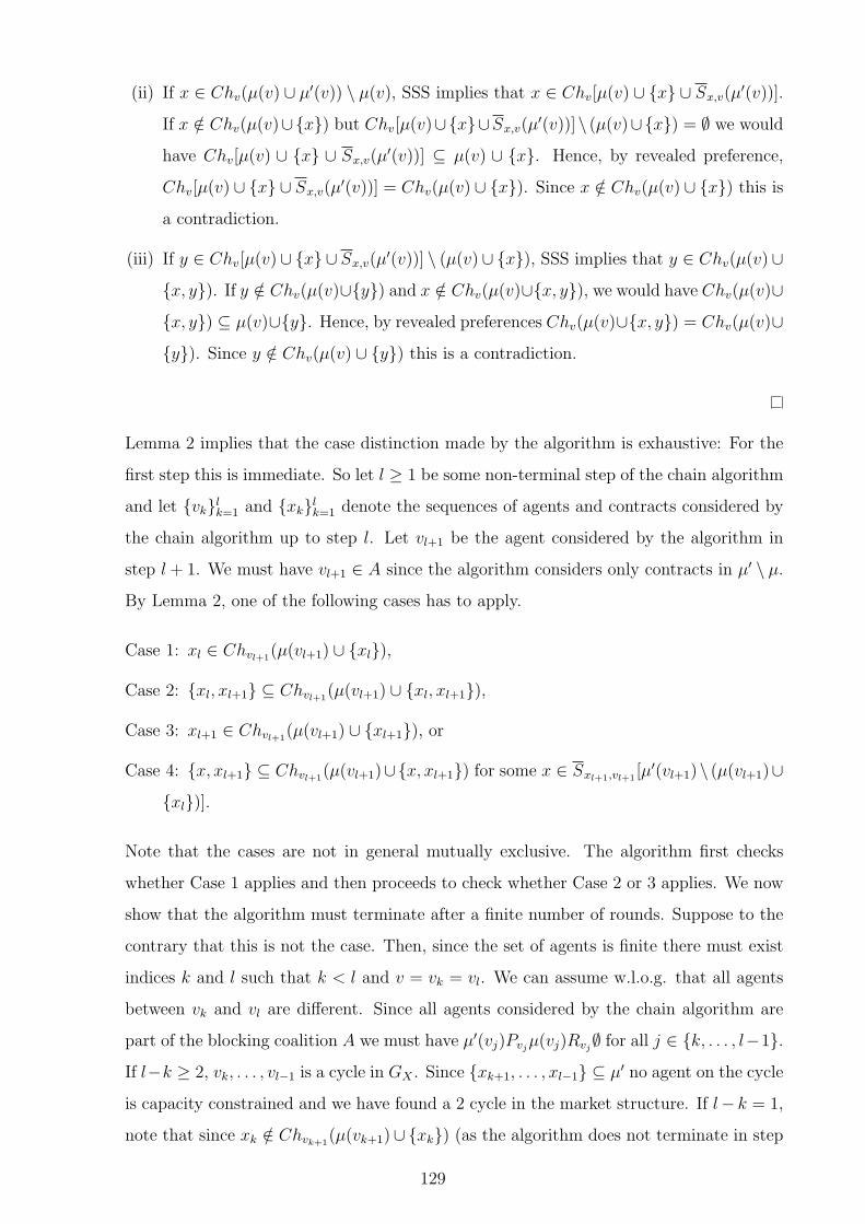
(ii) If x ∈ Chv(µ(v) ∪ µ′(v)) \ µ(v), SSS implies that x ∈ Chv[µ(v) ∪ {x} ∪ Sx,v(µ′(v))].

If x /∈ Chv(µ(v)∪{x}) but Chv[µ(v)∪{x}∪Sx,v(µ′(v))]\ (µ(v)∪{x}) = ∅ we would

have Chv[µ(v) ∪ {x} ∪ Sx,v(µ′(v))] ⊆ µ(v) ∪ {x}. Hence, by revealed preference,

Chv[µ(v) ∪ {x} ∪ Sx,v(µ′(v))] = Chv(µ(v) ∪ {x}). Since x /∈ Chv(µ(v) ∪ {x}) this is

a contradiction.

(iii) If y ∈ Chv[µ(v)∪ {x} ∪ Sx,v(µ′(v))] \ (µ(v)∪ {x}), SSS implies that y ∈ Chv(µ(v)∪

{x, y}). If y /∈ Chv(µ(v)∪{y}) and x /∈ Chv(µ(v)∪{x, y}), we would have Chv(µ(v)∪

{x, y}) ⊆ µ(v)∪{y}. Hence, by revealed preferences Chv(µ(v)∪{x, y}) = Chv(µ(v)∪

{y}). Since y /∈ Chv(µ(v) ∪ {y}) this is a contradiction.

Lemma 2 implies that the case distinction made by the algorithm is exhaustive: For the

first step this is immediate. So let l ≥ 1 be some non-terminal step of the chain algorithm

and let {vk}lk=1 and {xk}lk=1 denote the sequences of agents and contracts considered by

the chain algorithm up to step l. Let vl+1 be the agent considered by the algorithm in

step l + 1. We must have vl+1 ∈ A since the algorithm considers only contracts in µ′ \ µ.

By Lemma 2, one of the following cases has to apply.

Case 1: xl ∈ Chvl+1(µ(vl+1) ∪ {xl}),

Case 2: {xl, xl+1} ⊆ Chvl+1(µ(vl+1) ∪ {xl, xl+1}),

Case 3: xl+1 ∈ Chvl+1(µ(vl+1) ∪ {xl+1}), or

Case 4: {x, xl+1} ⊆ Chvl+1(µ(vl+1)∪{x, xl+1}) for some x ∈ Sxl+1,vl+1

[µ′(vl+1)\ (µ(vl+1)∪

{xl})].

Note that the cases are not in general mutually exclusive. The algorithm first checks

whether Case 1 applies and then proceeds to check whether Case 2 or 3 applies. We now

show that the algorithm must terminate after a finite number of rounds. Suppose to the

contrary that this is not the case. Then, since the set of agents is finite there must exist

indices k and l such that k < l and v = vk = vl. We can assume w.l.o.g. that all agents

between vk and vl are different. Since all agents considered by the chain algorithm are

part of the blocking coalition A we must have µ′(vj)Pvjµ(vj)Rvj

∅ for all j ∈ {k, . . . , l−1}.

If l−k ≥ 2, vk, . . . , vl−1 is a cycle in GX . Since {xk+1, . . . , xl−1} ⊆ µ′ no agent on the cycle

is capacity constrained and we have found a 2 cycle in the market structure. If l− k = 1,

note that since xk /∈ Chvk+1(µ(vk+1)∪ {xk}) (as the algorithm does not terminate in step

129

k + 1) we must have xk 6= xk+1. But then |µ ∩ X(vk, vk+1)| ≥ 2 and since preferences

conform to capacities, c(vk, vk+1) ≥ 2. In both cases we thus obtain a contradiction to

weak acyclicity.

In the following we use the chain algorithm as a subroutine for another algorithm that

finds a chain block of µ given weak acyclicity. This completes the proof since µ was

assumed to be chain stable. The algorithm uses a special version of the chain algorithm

that starts from a given agent-contract pair: Taking v ∈ V and x ∈ µ′(v) \ µ(v) as given,

the algorithm proceeds as if the first step of the chain algorithm yielded v1 := v, x1 := x

and B1 = ∅ (so that v2 is the other agent involved with x). The chain block algorithm

works as follows.

Step 1: Run the chain algorithm and let the resulting sequence of agents, contracts, and

stacks be denoted by {v1k, x

1k, B

1k}k≥1. Let K1 be the last step of the algorithm. If

B1K1

= ∅ stop. Otherwise let j1 be the highest index j such that v1j ∈ B1

K1. Set

v21 := v1

j1and proceed with step 2.

...

Step t+ 1: Let xt+11 ∈ Sxt

jt,vt+1

1[µ′(vt+1

1 ) \ (µ(vt+11 ) ∪ {xtjt−1})] be such that {xtjt , x

t+11 } ⊆

Chvt+11

(µ(vt+11 )∪{xtjt , x

t+11 }). Run the chain algorithm starting at (vt+1

1 , xt+11 ) and let

the resulting sequence of agents, contracts and stacks be denoted by {vt+1k , xt+1

k , Bt+1k }k≥1.

Let Kt+1 be the last step of the algorithm. If Bt+1Kt+1

= ∅ stop. Otherwise let jt+1 be

the highest index j such that vtj ∈ Bt+1Kt+1

. Set vt+21 := vt+1

jt+1and proceed with step

t+ 2....

Note that the algorithm is well defined since an agent is put on the stack if and only if

only Case 4 applies. The proof that the algorithm terminates in finite time is analogous

to the corresponding proof for the chain algorithm and the details are omitted.

Let T be the last iteration of the chain algorithm. We now show how to find a blocking

chain of µ. Since KT is the last step of this iteration we have xTKT−1 ∈ ChvTKT

(µ(vTKT) ∪

{xTKT−1}). Since BTKT

= ∅ one of the Cases 1-3 holds for each step of the last (T th)

iteration of the chain algorithm. If there is a step of the T th iteration for which Case 3

holds, let j be the last step with this property. Then xTj , . . . , xTKT−1 is a blocking chain

if vTj = sxTj. To see this note that by the definition of j, Case 2 must hold for all steps

k ∈ {j+ 1, . . . , KT − 1} and Case 1 holds for step KT . Furthermore, vTk = bxTk−1

= sxTk

for

all k ∈ {j+ 1, . . . , KT − 1}. If vTj = bxTj, the sequence in reverse order is a blocking chain.

130

If there is no step of the T th iteration such that Case 3 holds consider the sequence of

agents and contracts in the T − 1st iteration of the chain algorithm starting at vT−1jT−1

. By

definition of jT−1 there is no step i > jT−1 such that only Case 4 applies. If there is a step

i > jT−1 of the T − 1st iteration such that Case 3 applies, let l be the largest index with

this property. Then xT−1l , . . . , xT−1

KT−1−1 is a blocking chain. If there is no step for which

Case 3 applies, xT−1KT−1−1, . . . , x

T−1jT−1

, xT1 , . . . , xTKT−1 must be a blocking chain. In both cases

it might be necessary to reverse the order of the sequence to obtain a blocking chain as

above.

Thus, the above algorithm finds a chain block of µ within µ′ \ µ. This contradicts the

assumption that µ is chain stable and completes the proof that (i)⇒ (ii).

(ii)⇒ (iii) This follows immediately from the observation that GS(R) ⊆ C(R), for all R ∈

R(c,q).

(iii)⇒ (iv) Suppose that (iii) holds but that there exists a preference profile R ∈ R(c,q) and a

network µ ∈ CS(R) \ E(R). By definition, this means that there exists a network µ′ that

all agents weakly and some strictly prefer over µ. But then µ′ weakly dominates µ via V ,

which contradicts (iii).

(iv)⇒ (i) This will follow from the proof that (iii) ⇒ (i) in Theorem 5 since chain stable

networks exist for all profiles in R(c,q).

Proof of Theorem 5

(i)⇒ (ii) This follows from the implication (i) ⇒ (ii) of Theorem 1 that was proven above

and the existence of chain stable networks on the domain R(c,q).

(ii)⇒ (iii) Since a group stable network is efficient and individually stable, this implication is

again immediate.

(iii)⇒ (i) Suppose first that there is a 2 cycle v1, . . . , vn in (GX , c, q). We show that there

exists a profile R ∈ Rq such that E(R) ∩ IS(R) = ∅. Since we can always construct

the preference profile in such a way that no agent on the cycle wants to sign a contract

with the outside world and vice versa, we can assume that V = {v1, . . . , vn}. Let xi ∈ X

denote some contract between vi and vi+1 for i ∈ {1, . . . , n}. The preferences of agents

131

on the cycle are defined as follows: For all i ∈ {1, . . . , n}, Agent vi strictly prefers signing

only contract xi over signing the set of contracts {xi−1, xi}, over signing no contracts at

all. These are the only acceptable sets of contracts. It is easy to check that the resulting

profile R ∈ R(c,q).

We show that for this profile any individually stable network must assign the empty set

of contracts to all agents. By construction of the preference profile, individual stability

demands that v1 is assigned either the empty set of contracts or only x1. So suppose that

there is an individually stable network µ that includes x1. But v2 must be assigned either

the empty set of contracts or only contract x2 in an individually stable network. Hence,

any individually stable network must assign the empty set of contracts to agent v1. A

simple repetition of this argument establishes that the unique individually stable network

is the empty network. But this network is (strictly) Pareto dominated by the complete

network.

Now consider the case that there is some pair of agents v, w such that (v, w) ∈ GX

and c(v, w) ≥ 2. Take two contracts x, y ∈ X(v, w). Let {x}Pv{x, y}Pv∅Pv{y} and

{y}Pw{x, y}Pw∅Pw{x}, and assume that no other sets of contracts are acceptable to either

v or w. As above only the empty network is individually stable but Pareto dominated by

the network {x, y}. This completes the proof that (iii)⇒ (i).

Proof of Theorem 6

(i)⇒ (ii) Suppose to the contrary that (GX , c, q) is weakly acyclic but that for some preference

profile R ∈ R(c,q) there exists a core stable network µ which is not individually stable.

Let v0 ∈ V be an agent who would like to drop some of the contracts in µ(v0), that is,

Chv0(µ(v0)) 6= µ(v0). This implies in particular that µ(v0) 6= ∅. But then it has to be the

case that Chv0(µ(v0)) 6= ∅ since µ is at least individually rational. We denote by µ′ the

network that results from µ when contracts in µ(v0) \ Chv0(µ(v0)) are deleted. For the

following let V0 := {v0}.

Let V1 ⊂ V \ V0 be the (nonempty) set of agents who are involved with some contract in

Chv0(µ(v0)) and let W be the set of agents who are involved with one of the contracts v0

wants to drop, that is, with one of the contracts in µ(v0) \ Chv0(µ(v0)). We must have

V1∩W = ∅ since c(v, w) ≤ 1 for all v, w ∈ V and µ is individually rational. Furthermore, µ

132

cannot contain a contract between a pair of agents in V1×(W ∪V1) if the market structure

is weakly acyclic. Otherwise, there would be two agents w1 ∈ V1 and w2 ∈ W ∪ V1 such

that µ contains a contract between w1 and w2. By definition of V1 and W , µ also contains

contracts between v0 and both, w1 and w2. Since µ is individually rational, none of the

three agents can be capacity constrained. Hence, we have found a 2 cycle in (GX , c, q),

a contradiction. On the other hand, µ has to contain at least one contract between an

agent in V1 and an agent in V \ (W ∪ V0 ∪ V1). Otherwise µ′ weakly dominates µ via the

coalition V0∪V1 since (i) all agents in V1 would be indifferent between these two networks,

(ii) v0 strictly prefers µ′ over µ, and (iii) no agent in V0∪V1 signs a contract with an agent

in V \ (V0 ∪ V1). Thus, there has to be a nonempty set of agents V2 ⊂ V \ (W ∪ V0 ∪ V1)

who sign a contract with some agent in V1 under µ.

Now suppose that for some k ≥ 2 we have shown that there is a sequence of sets of

agents V1, . . . , Vk such that, for all l ∈ {2, . . . , k}, Vl ⊂ V \ (W ∪ V0 ∪ . . . ∪ Vl−1) and

the set of all agents who sign a contract with agents in Vl−1 under µ is Vl−2 ∪ Vl. If the

market structure is weakly acyclic, µ cannot contain a contract between a pair of agents

in Vk× (W ∪ V0 . . .∪ Vk). The argument is similar to above. On the other hand, µ has to

contain at least one contract between an agent in Vk and an agent in V \ (W ∪V0 . . .∪Vk).

Otherwise µ′ weakly dominates µ via the coalition V0 ∪ . . . ∪ Vk since (i) all agents in

V1 ∪ . . . ∪ Vk would be indifferent between these two networks, (ii) v0 strictly prefers µ′

over µ, and (iii) no agent in V0∪. . .∪Vk signs a contract with an agent in V \(V0∪. . .∪Vk−1).

Thus, there has to be a nonempty set of agents Vk+1 ⊂ V \ (W ∪ V0 ∪ . . . ∪ Vk) who sign

a contract with some agent in Vk under µ.

The above argument is valid for any k and the procedure would thus run forever, contra-

dicting the finiteness of V . This completes the proof that (i)⇒ (ii).

(ii)⇒ (i) Note that C(R) ⊆ IS(R) for all R ∈ R(c,q) implies that an efficient and individually

stable network always exists. Hence, the statement follows from (iii) ⇒ (i) in Theorem

5.

Proof of Theorem 7

(i)⇒ (ii) Before going to the details of the proof, note that any network µ with |µ∩X(v, w)| ≤

1 for all v, w ∈ V defines a (unique) subgraph Gµ of GX that includes an edge from v to

133

w if and only if µ contains a x with sx = v and bx = w.

By Theorem 4 we know that, for all R ∈ R(c,q), CS(R) ⊆ C(R) if the market structure is

weakly acyclic. Hence, we only need to show that C(R) ⊆ CS(R) if the market structure

is strongly acyclic. The proof will be by contradiction: Assume that for some R ∈ R(c,q)

there exists a network µ ∈ C(R)\CS(R). Since strong implies weak acyclicity we have that

C(R) ⊆ IS(R) by Theorem 6. Hence, there must be a chain x1, . . . , xn /∈ µ that blocks

µ. Consider the network µ′ that results from µ when we add the contracts x1, . . . , xn

and delete contracts in µ(sx1) \ Chsx1(µ(sx1) ∪ {x1}), µ(bxn) \ Chbxn

(µ(bxn) ∪ {xn}), and

µ(bxi) \ Chbxi

(µ(bxi) ∪ {xi, xi+1}) for all i < n. Note that µ′ and µ can both contain

at most one contract between each pair of agents since the market structure is strongly

acyclic and (i) µ′(v)Pvµ(v)Rv∅, for all v ∈ {sx1 , bx1 , . . . , bxn}, (ii) µ′(v) ⊆ µ(v), for all

v ∈ V \ {sx1 , bx1 , . . . , bxn}, as well as (iii) µ(v)Rv∅, for all v ∈ V . Now let A be the set of

agents who are in the same connected component of Gµ′ as sx1 .35 We claim that µ′ weakly

dominates µ via A. As noted above, all agents involved with some contract in the blocking

chain strictly prefer µ′ over µ. Now suppose there is an agent v ∈ A \ {sx1 , bx1 , . . . , bxn}

such that µ(v)Pvµ′(v). Since we have only deleted some contracts involving agents on

the blocking chain this means that there is a contract x ∈ µ \ µ′ which involves v and an

agent v ∈ {sx1 , bx1 . . . , bxn}. Since µ′(v) = µ(v) \ {x} and µ(v)Rv∅, µ′ cannot contain a

contract between v and v. Given that v is in the same connected component of Gµ′ as

sx1 , Gµ′∪{x} contains a cycle v1, . . . , vn with {v, v} ⊂ {v1, . . . , vn}. We now show that this

must be a restricted 2 cycle. This contradiction shows that µ′ must dominate µ via A so

that µ could not have been in the core.

Note that the following two cases cannot occur: (i) v = sx1 and x is an upstream contract

for v, and (ii) v = bxn and x is a downstream contract for v. In case (i) we would have

that x ∈ Chv(µ(v)), due to the individual stability of µ, and x /∈ Chv(µ(v) ∪ {x1}). But

then CSC would be violated since x1 is a downstream contract for v and x is an upstream

contract for v. Case (ii) can be handled similarly. This shows that if v is a passing

node of the cycle v1, . . . , vn, she must be one of the intermediate agents in the blocking

chain. But this means that v signs an upstream and a downstream contract in µ′. Since

µ′(v)Pvµ(v)Rv∅, v cannot be capacity constrained on the cycle if she is a passing node.

But v is the only potentially capacity constrained agent on the cycle. To see this, note

that all agents in {v1, . . . , vn} \ {v, v} sign contracts with both of their neighbors under

35Two nodes v and w are in the same connected component of a directed graph G if there is a sequence ofedges connecting v and w.

134

µ′ and that µ(v) contains contracts between v and v as well as her other neighbor on

the cycle. For each agent v ∈ ({sx1 , bx1 , . . . , bxn} ∩ {v1, . . . , vn}) \ {v}, µ′(v)Pvµ(v)Rv∅

so that µ′(v) is an acceptable set of contracts and v is not capacity constrained. For

each agent v ∈ {v1, . . . , vn} \ {sx1 , bx1 , . . . , bxn} we have µ′(v) ⊆ µ(v) and, since µ is a

core allocation, µ(v)Pv∅ so that v is not capacity constrained. In both cases v cannot be

capacity constrained on the cycle.

(ii)⇒ (i) If weak acyclicity is not satisfied, consider the counterexamples used to prove that

(iii) ⇒ (i) in Theorem 5. In both types of examples it is easy to check that the core

consists of the complete network while the empty network is the unique chain stable

network. Now suppose that weak acyclicity is satisfied but that there is a restricted 2

cycle v1, . . . , vn for which only the source v1 is capacity constrained (the case where v1 is a

sink can be handled similarly). Let x1, . . . , xn be an accompanying sequence of contracts,

that is, xk is a contract between agents vk and vk+1 (where n+1 := 1). As in the proof that

(iii)⇒ (i) in Theorem 5 we can assume that V = {v1, . . . , vn}. We now define a preference

profile for the agents starting with Rv1 = {x1}, {xn}. Let k ∈ {2, . . . , n} be arbitrary and

set Rvk= {xk−1, xk} if vk is a passing node, and Rvk

= {xk−1, xk}, {xk}, {xk−1} in any

other case. Let the resulting profile be denoted by R and note that R ∈ R(c,q) since v1 is

the only capacity constrained agent among v1, . . . , vn.

Now let j be the smallest index in {2, . . . , n} such that vj is a sink. Note that such an

index must exist since GX contains no directed cycles and all agents between v1 and vj

are passing nodes. Consider the network µ = {xj, . . . , xn}. Clearly, µ /∈ CS(R) since it is

blocked by the chain x1, . . . , xj−1. We now show that µ ∈ C(R).

Suppose to the contrary that µ is weakly dominated by some network µ′ via a coali-

tion A. Since agents vj+1, . . . , vn get their most preferred set of contracts under µ,

A∩{v1, . . . , vj} 6= ∅. Since agents v2, . . . , vj−1 are all passing nodes by the definition of j,

the construction of R implies {x1, . . . , xj−1} ⊆ µ′. Hence, we must have {v1, . . . , vj} ⊆ A.

Since {xj}Pvj{xj−1} this implies xj ∈ µ′ and thus vj+1 ∈ A. Continuing with this line

of reasoning it is easy to see that we must have µ′ = {x1, . . . , xn} and A = {v1, . . . , vn}.

But then v1 is worse off compared to µ since ∅Pv1{x1, xn}. Hence, it has to be the case

that µ ∈ C(R).

135

Discussion of the main results

For this Appendix we assume that there are no capacity constraints and let R denote the

set of all preference profiles satisfying strict preferences, no externalities, SSS, and CSC. The

following statements are easily seen to be true for any given R ∈ R.

CS(R) = GS(R)⇒ CS(R) ⊆ C(R), CS(R) ⊆ E(R),GS(R) 6= ∅, E(R) ∩ IS(R) 6= ∅

CS(R) ⊆ C(R)⇒ CS(R) ⊆ E(R), E(R) ∩ IS(R) 6= ∅

CS(R) ⊆ E(R)⇒ E(R) ∩ IS(R) 6= ∅

GS(R) 6= ∅ ⇒ E(R) ∩ IS(R) 6= ∅

In this Appendix we show that all other implications of Corollary 3 are not necessarily true

for any given preference profile. Chain stable networks in the examples can be calculated using

the T-algorithm of Ostrovsky (2008). All counterexamples except example 3 use a supply chain

model with five agents and the following graph of potential interactions:

v1

v2

v3 v5

v4

��

rrrrrrrrrrrrrrrrr

yy

WWWWWWWWW++ �������������

�� ������������

?????????????????????

�� /////////////

�� ############

��

Figure 3: Graph G3 of potential interactions.

Throughout the Appendix we use the following notation: xji denotes some contract in which

agent i sells something to agent j. Agent v5 will only be needed for the last example.

1. There exist profiles R ∈ R such that CS(R) ⊆ C(R), CS(R) ⊆ E(R), and E(R)∩IS(R) 6=

∅, but CS(R) 6= GS(R) and GS(R) = ∅.

Suppose preferences of the agents are36

R1 R1v1

R1v2

R1v3

R1v4

{x21} {x2

1, x32} {x3

1, x43} {x4

1, x43}

{x21, x

31} {x3

1, x32, x

43} {x4

1}

{x41} {x4

3} {x43}

36As in all examples that follow it is easy to check that SSS and CSC are indeed satisfied.

136

Using the T-Algorithm it is easy to show that the unique chain stable network is given

by µ = {x41, x

43}.

To see that µ ∈ C(R1) note that v4 cannot be made better off and the only network which

makes v1 and v3 better off without hurting v2 is {x21, x

31, x

32, x

43}. This network would make

v4 worse off and thus does not weakly dominate µ in the sense of the core. Hence, µ is in

the core and thus in particular efficient.

On the other hand, µ is blocked by {v1, v2, v3} via {x21, x

31, x

32, x

43} so that µ is not group

stable. The only other nonempty individually stable network is {x43} which is not even

chain stable. Since a group stable matching has to be individually stable, this shows that

GS(P ) = ∅.

2. There exist preference profiles R ∈ R such that IS(R)∩E(R) 6= ∅ , but CS(R)∩C(R) = ∅

and CS(R) ∩ E(R) = ∅.

Consider the following preference profile

R2 R2v1

R2v2

R2v3

R2v4

{x41, x

31} {x2

1, x32, x

42} {x3

1, x32, x

43} {x4

1, x42}

{x21, x

31} {x3

2} {x32} {x4

2, x43}

{x41} {x4

2} {x31} {x4

1}

{x21} {x4

3}

{x31} {x4

2}

The unique chain stable network is given by µ = {x41, x

32}. But the network µ′ =

{x21, x

31, x

32, x

42, x

43} is individually stable as well as efficient, and makes all agents better

off (note that this network is blocked by the chain x41).

3. There exist preference profiles R ∈ R such that CS(R) ⊆ E(R) but CS(R) ∩ C(R) = ∅.

In the example of section 3.2 the unique chain stable network is the efficient network

{x(M,D2)}. The unique core network is given by {x(M,S), x(S,D1), x(M,D1)}.

4. There exist preference profiles R ∈ R such that GS(R) 6= ∅ but CS(R) \ E(R) 6= ∅,

CS(R) \ GS(R) 6= ∅, and CS(R) \ C(R) 6= ∅.

Preferences are given by:

137

R2 R3v1

R3v2

R3v3

R3v4

R3v5

{x41} {x2

1, x42} {x3

1, x43} {x4

5} {x51, x

45}

{x21} {x4

2, x43, x

45}

{x21, x

31, x

51} {x4

3}

{x31} {x4

1}

For this profile there are two chain stable networks: {x41} and {x3

1, x43}.

The first network is also group stable, but the second is not even efficient as the network

{x21, x

31, x

51, x

42, x

43, x

45} makes all agents (weakly) better off.

Feasibility Restrictions on Networks

Instead of requiring preferences to conform to an exogenously given capacity vector, one could

also restrict the set of feasible networks. Given a capacity vector (c, q), the set of feasible

networks M(c,q) can be defined as follows: µ ∈ M(c,q) if and only if µ does not violate the

capacity constraints, that is, for all v ∈ V , (i) |{w ∈ V \{v} : sx = w for some x ∈ µ(v)}| ≤ qUv ,

(ii) |{w ∈ V \{v} : bx = w for some x ∈ µ(v)}| ≤ qDv , and (iii) |µ(v)∩X(v, w)| ≤ c(v, w), for all

w ∈ V \ {v}. Given some network µ ∈M(c,q) let Gµ be the directed graph which contains one

edge from v to w for each contract x ∈ µ such that sx = v and bx = w. Note that in contrast

to GX and Gµ used in the main text, this graph may contain multiple edges between a given

pair of agents. The following shows how the acyclicity condition developed in Chapter 3 can

be expressed in this framework.

Proposition 8. The market structure (GX , c, q) is weakly acyclic if and only if Gµ is a forest

for all µ ∈M(c,q).37

The proof is straightforward and omitted here. It is not clear, how strong acyclicity could

have been formulated in this framework. This is the main reason for requiring preferences to

conform to capacities instead.

Beyond the Supply Chain Model

Some of the main results of chapter continue to hold without the CSC assumption. Let (GX , c, q)

be a market structure and let R(c,q) be the set of all preference profiles that satisfy strict prefer-

ences, no externalities, and SSS, and conform to capacities. The following theorem summarizes

37A forest is a directed graph containing no directed or undirected cycles.

138

the results that carry over to this more general setting (in which the existence of chain stable

networks cannot be guaranteed).

Theorem 8. 1. The following are equivalent:

(i) (GX , c, q) is weakly acyclic.

(ii) CS(R) = GS(R) for all R ∈ R(c,q).

(iii) CS(R) ⊆ C(R) for all R ∈ R(c,q).

(iv) CS(R) ⊆ E(R) for all R ∈ R(c,q).

2. If GS(R) 6= ∅ for all R ∈ R(c,q) then (GX , c, q) is weakly acyclic.

3. If IS(R) ∩ E(R) 6= ∅ for all R ∈ R(c,q) then (GX , c, q) is weakly acyclic.

4. (GX , c, q) is weakly acyclic if and only if C(R) ⊆ IS(R) for all R ∈ R(c,q).

The proof of this Theorem follows directly from the proofs of Theorems 4,5, and 6: The

proof of Theorem 4 does not use the CSC assumption. The counterexample used in the proof

that (iii) ⇒ (i) in Theorem 5 belongs to the larger domain R(c,q). The proof of Theorem 6

does not use CSC to prove sufficiency of weak acyclicity. The proof of necessity uses the same

counterexample as Theorem 5. Weak acyclicity may not be sufficient for the existence of a

group stable or efficient and individually stable network since the existence of a chain stable

network is not guaranteed by Ostrovsky (2008)’s existence result.

One application of Theorem 8 is the roommate problem introduced in Gale and Shapley

(1962). In this problem 2n agents have to be assigned among n rooms that each have place for

2 agents. Each agent can share a room with any other agent, has a strict preference relation

over potential roommates, and does not care about which room she is assigned to (only the

roommate matters). If we want to allow agents to have any (rational) preference relation over

potential roommates, this model does not belong to the class of supply chain models with same

side substitutable and cross side complementary preferences: In order to write this problem as a

supply chain model, we would have to define a directed graph of potential trading relationships.

In order to allow all potential roommate combinations we would need to introduce an arbitrarily

directed edge between all pairs of agents. It is easy to see that if n ≥ 2, at least one agent

has to be an intermediary if we require the market structure to be free of directed cycles.

The preferences of such an agent would be severely restricted by the assumption of CSC: The

intermediary would be required to either declare all upstream or all downstream agents as

unacceptable roommates. Given that the direction of the edges introduced is arbitrary, this is

139

not a satisfactory embedding of the roommate problem. If we dispense with the assumption

that preferences satisfy the CSC condition this problem does not occur since it is easy to see

that SSS does not restrict the set of allowed preference relations. Hence, any roommate problem

can be formulated as a supply chain model in which agents’ preferences satisfy SSS (but are

allowed to violate CSC). Note that since each agent is looking for at most one partner chain

stability reduces to pairwise stability and (any) market structure is weakly acyclic. The above

theorem then implies that in the roommate problem any pairwise stable matching lies in the

core. Since it is a trivial fact that any core matching is pairwise stable in the roommate problem

we obtain the following corollary to Theorem 8.

Corollary 4. For roommate problems the set of pairwise stable matchings coincides with the

core.

140