Evaluation of Analytical Methods to Study Aquifer …...Evaluation of Pumping Test Analytical...
17
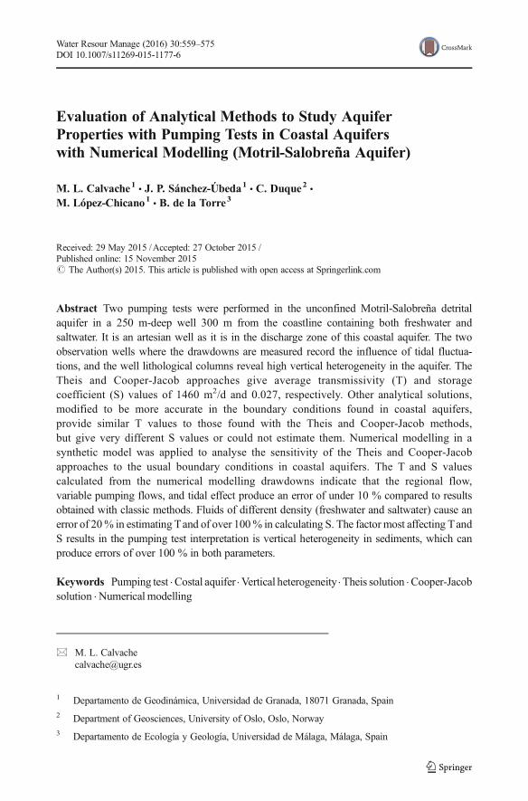
Evaluation of Analytical Methods to Study Aquifer Properties with Pumping Tests in Coastal Aquifers with Numerical Modelling (Motril-Salobreña Aquifer) M. L. Calvache 1 & J. P. Sánchez-Úbeda 1 & C. Duque 2 & M. López-Chicano 1 & B. de la Torre 3 Received: 29 May 2015 /Accepted: 27 October 2015 / Published online: 15 November 2015 # The Author(s) 2015. This article is published with open access at Springerlink.com Abstract Two pumping tests were performed in the unconfined Motril-Salobreña detrital aquifer in a 250 m-deep well 300 m from the coastline containing both freshwater and saltwater. It is an artesian well as it is in the discharge zone of this coastal aquifer. The two observation wells where the drawdowns are measured record the influence of tidal fluctua- tions, and the well lithological columns reveal high vertical heterogeneity in the aquifer. The Theis and Cooper-Jacob approaches give average transmissivity (T) and storage coefficient (S) values of 1460 m 2 /d and 0.027, respectively. Other analytical solutions, modified to be more accurate in the boundary conditions found in coastal aquifers, provide similar T values to those found with the Theis and Cooper-Jacob methods, but give very different S values or could not estimate them. Numerical modelling in a synthetic model was applied to analyse the sensitivity of the Theis and Cooper-Jacob approaches to the usual boundary conditions in coastal aquifers. The T and S values calculated from the numerical modelling drawdowns indicate that the regional flow, variable pumping flows, and tidal effect produce an error of under 10 % compared to results obtained with classic methods. Fluids of different density (freshwater and saltwater) cause an error of 20 % in estimating T and of over 100 % in calculating S. The factor most affecting T and S results in the pumping test interpretation is vertical heterogeneity in sediments, which can produce errors of over 100 % in both parameters. Keywords Pumping test . Costal aquifer . Vertical heterogeneity . Theis solution . Cooper-Jacob solution . Numerical modelling Water Resour Manage (2016) 30:559–575 DOI 10.1007/s11269-015-1177-6 * M. L. Calvache [email protected] 1 Departamento de Geodinámica, Universidad de Granada, 18071 Granada, Spain 2 Department of Geosciences, University of Oslo, Oslo, Norway 3 Departamento de Ecología y Geología, Universidad de Málaga, Málaga, Spain
Transcript of Evaluation of Analytical Methods to Study Aquifer …...Evaluation of Pumping Test Analytical...
Evaluation of Analytical Methods to Study AquiferProperties with Pumping Tests in Coastal Aquiferswith Numerical Modelling (Motril-Salobreña Aquifer)
M. L. Calvache1 & J. P. Sánchez-Úbeda1 & C. Duque2 &
M. López-Chicano1& B. de la Torre3
Received: 29 May 2015 /Accepted: 27 October 2015 /Published online: 15 November 2015# The Author(s) 2015. This article is published with open access at Springerlink.com
Abstract Two pumping tests were performed in the unconfined Motril-Salobreña detritalaquifer in a 250 m-deep well 300 m from the coastline containing both freshwater andsaltwater. It is an artesian well as it is in the discharge zone of this coastal aquifer. The twoobservation wells where the drawdowns are measured record the influence of tidal fluctua-tions, and the well lithological columns reveal high vertical heterogeneity in the aquifer. TheTheis and Cooper-Jacob approaches give average transmissivity (T) and storagecoefficient (S) values of 1460 m2/d and 0.027, respectively. Other analytical solutions,modified to be more accurate in the boundary conditions found in coastal aquifers,provide similar T values to those found with the Theis and Cooper-Jacob methods,but give very different S values or could not estimate them. Numerical modelling in asynthetic model was applied to analyse the sensitivity of the Theis and Cooper-Jacobapproaches to the usual boundary conditions in coastal aquifers. The T and S valuescalculated from the numerical modelling drawdowns indicate that the regional flow,variable pumping flows, and tidal effect produce an error of under 10 % compared to resultsobtained with classic methods. Fluids of different density (freshwater and saltwater) cause anerror of 20% in estimating Tand of over 100% in calculating S. The factor most affecting TandS results in the pumping test interpretation is vertical heterogeneity in sediments, which canproduce errors of over 100 % in both parameters.
Keywords Pumping test . Costal aquifer . Vertical heterogeneity. Theis solution . Cooper-Jacobsolution . Numerical modelling
Water Resour Manage (2016) 30:559–575DOI 10.1007/s11269-015-1177-6
* M. L. [email protected]
1 Departamento de Geodinámica, Universidad de Granada, 18071 Granada, Spain2 Department of Geosciences, University of Oslo, Oslo, Norway3 Departamento de Ecología y Geología, Universidad de Málaga, Málaga, Spain
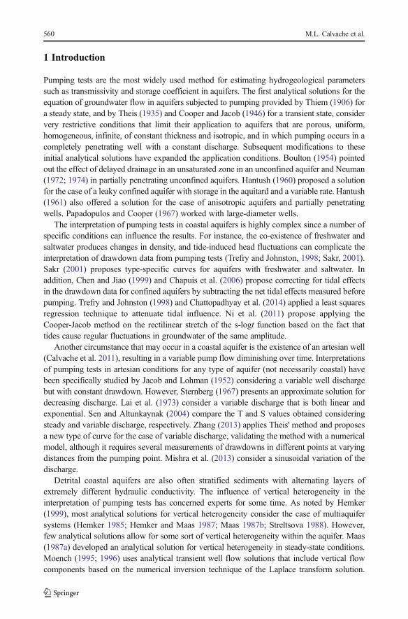
1 Introduction
Pumping tests are the most widely used method for estimating hydrogeological parameterssuch as transmissivity and storage coefficient in aquifers. The first analytical solutions for theequation of groundwater flow in aquifers subjected to pumping provided by Thiem (1906) fora steady state, and by Theis (1935) and Cooper and Jacob (1946) for a transient state, considervery restrictive conditions that limit their application to aquifers that are porous, uniform,homogeneous, infinite, of constant thickness and isotropic, and in which pumping occurs in acompletely penetrating well with a constant discharge. Subsequent modifications to theseinitial analytical solutions have expanded the application conditions. Boulton (1954) pointedout the effect of delayed drainage in an unsaturated zone in an unconfined aquifer and Neuman(1972; 1974) in partially penetrating unconfined aquifers. Hantush (1960) proposed a solutionfor the case of a leaky confined aquifer with storage in the aquitard and a variable rate. Hantush(1961) also offered a solution for the case of anisotropic aquifers and partially penetratingwells. Papadopulos and Cooper (1967) worked with large-diameter wells.
The interpretation of pumping tests in coastal aquifers is highly complex since a number ofspecific conditions can influence the results. For instance, the co-existence of freshwater andsaltwater produces changes in density, and tide-induced head fluctuations can complicate theinterpretation of drawdown data from pumping tests (Trefry and Johnston, 1998; Sakr, 2001).Sakr (2001) proposes type-specific curves for aquifers with freshwater and saltwater. Inaddition, Chen and Jiao (1999) and Chapuis et al. (2006) propose correcting for tidal effectsin the drawdown data for confined aquifers by subtracting the net tidal effects measured beforepumping. Trefry and Johnston (1998) and Chattopadhyay et al. (2014) applied a least squaresregression technique to attenuate tidal influence. Ni et al. (2011) propose applying theCooper-Jacob method on the rectilinear stretch of the s-logt function based on the fact thattides cause regular fluctuations in groundwater of the same amplitude.
Another circumstance that may occur in a coastal aquifer is the existence of an artesian well(Calvache et al. 2011), resulting in a variable pump flow diminishing over time. Interpretationsof pumping tests in artesian conditions for any type of aquifer (not necessarily coastal) havebeen specifically studied by Jacob and Lohman (1952) considering a variable well dischargebut with constant drawdown. However, Sternberg (1967) presents an approximate solution fordecreasing discharge. Lai et al. (1973) consider a variable discharge that is both linear andexponential. Sen and Altunkaynak (2004) compare the T and S values obtained consideringsteady and variable discharge, respectively. Zhang (2013) applies Theis' method and proposesa new type of curve for the case of variable discharge, validating the method with a numericalmodel, although it requires several measurements of drawdowns in different points at varyingdistances from the pumping point. Mishra et al. (2013) consider a sinusoidal variation of thedischarge.
Detrital coastal aquifers are also often stratified sediments with alternating layers ofextremely different hydraulic conductivity. The influence of vertical heterogeneity in theinterpretation of pumping tests has concerned experts for some time. As noted by Hemker(1999), most analytical solutions for vertical heterogeneity consider the case of multiaquifersystems (Hemker 1985; Hemker and Maas 1987; Maas 1987b; Streltsova 1988). However,few analytical solutions allow for some sort of vertical heterogeneity within the aquifer. Maas(1987a) developed an analytical solution for vertical heterogeneity in steady-state conditions.Moench (1995; 1996) uses analytical transient well flow solutions that include vertical flowcomponents based on the numerical inversion technique of the Laplace transform solution.
560 M.L. Calvache et al.
Hemker (1999) provides a solution of the general issue of computing well flow in verticallyheterogeneous aquifers by integrating both analytical and numerical techniques. Alam andOlsthoorn (2014) use Hemker and Maas' (1987) numerical and analytical approaches to assessthe benefits of using multidepth pumping tests in the analysis of deep layered and anisotropicaquifers. In most cases, a pumping test in aquifers with some vertical heterogeneity is resolvedwith numerical modelling (Hemker 1999; Riva et al. 2001; Kollet and Zlotnik 2005; Chenet al. 2014).
Despite these steps forward and the many modifications to the initial analytical solutions,there are still many unresolved limitations in interpreting pumping tests in coastal aquifers.Many studies on coastal aquifers consider it acceptable to use the T and S results obtainedapplying classic methods (Theis 1935; Cooper and Jacob 1946). Such is the case of Capuanoand Jan (1996) and Vouillamoz et al. (2006), who apply the Theis and Cooper-Jacob solutionsto a coastal detrital aquifer. Park et al. (2012) use Theis' solution for a fissured aquifer withfreshwater and saltwater. Chachadi and Gawas (2012), Sabtan and Shehata (2003), Mohantyet al. (2012), and Lee et al. (2014) also apply Theis' solution in detrital coastal aquifers. Barlowet al. (1996) and Ni et al. (2011) noticed a tidal effect in their drawdown curves but did notconsider it for evaluating T and S. Keith et al. (2006) and Mastrocicco et al. (2013) apply theCooper-Jacob method to interpret pumping tests in detrital coastal aquifers. Diamantopoulouand Voudouris (2008) apply the Theis and the Cooper-Jacob methods to a multilayer coastalaquifer.
It can therefore be concluded that there are still uncertainties in the analytical solutionsapplied in interpreting pumping tests in coastal aquifers. In addition, the classic analyticalsolutions are applied even when the theoretical conditions required by those solutions are notmet.
This study presents the case of two pumping tests carried out in a deep well penetrating theMotril-Salobreña coastal aquifer (southern Spain), which has a series of specific circumstancestypical of coastal aquifers that make it difficult to interpret drawdowns from the pumping tests.It is an artesian well with a decreasing variable flow drilled in a detrital aquifer with a layeredseries having different hydraulic conductivity and with significant flow to the sea. In addition,the well intersects the freshwater-saltwater mixing zone and is affected by tidal fluctuationsdue to its proximity to the coastline. The main objective of this paper is to determine the errorof the T and S values obtained applying the classic methods of Theis and of Cooper-Jacob dueto these specific characteristics of coastal aquifers. This objective is approached with numericalmodelling, which allows a quantification of the impact on the theoretical results.
2 Study Area and Hydrogeological Setting
The unconfined detrital Motril-Salobreña aquifer, located on the Mediterranean coast insouthern Spain (Fig. 1), covers a surface area of 42 km2 and comprises alluvial sedimentssupplied by the Guadalfeo River and other minor streams. The aquifer’s main recharge sourceis the Guadalfeo River, providing direct infiltration in the 8 km of its course over the aquiferand indirect infiltration from irrigation water deriving from the same river (Calvache et al.2009; Duque et al. 2011).
The Motril-Salobreña aquifer is one of the few on the Spanish Mediterranean coastline thathas of yet shown no signs of marine intrusion in contrast to the usual case for aquifers insemi-arid coastal zones (Kourakos and Mantoglou, 2011; Doulgeris and Zissis, 2014; Zekri
Evaluation of Pumping Test Analytical Methods in Coastal Aquifers 561
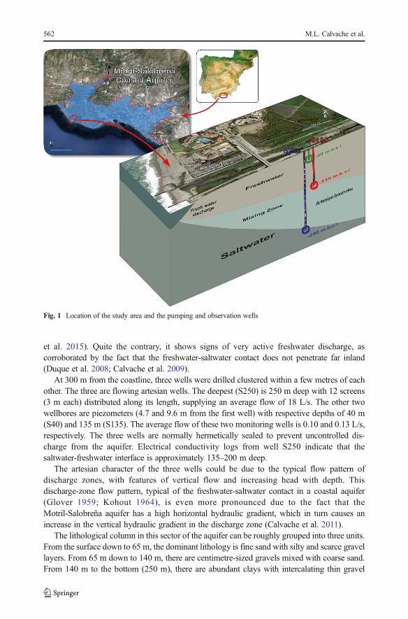
et al. 2015). Quite the contrary, it shows signs of very active freshwater discharge, ascorroborated by the fact that the freshwater-saltwater contact does not penetrate far inland(Duque et al. 2008; Calvache et al. 2009).
At 300 m from the coastline, three wells were drilled clustered within a few metres of eachother. The three are flowing artesian wells. The deepest (S250) is 250 m deep with 12 screens(3 m each) distributed along its length, supplying an average flow of 18 L/s. The other twowellbores are piezometers (4.7 and 9.6 m from the first well) with respective depths of 40 m(S40) and 135 m (S135). The average flow of these two monitoring wells is 0.10 and 0.13 L/s,respectively. The three wells are normally hermetically sealed to prevent uncontrolled dis-charge from the aquifer. Electrical conductivity logs from well S250 indicate that thesaltwater-freshwater interface is approximately 135–200 m deep.
The artesian character of the three wells could be due to the typical flow pattern ofdischarge zones, with features of vertical flow and increasing head with depth. Thisdischarge-zone flow pattern, typical of the freshwater-saltwater contact in a coastal aquifer(Glover 1959; Kohout 1964), is even more pronounced due to the fact that theMotril-Salobreña aquifer has a high horizontal hydraulic gradient, which in turn causes anincrease in the vertical hydraulic gradient in the discharge zone (Calvache et al. 2011).
The lithological column in this sector of the aquifer can be roughly grouped into three units.From the surface down to 65 m, the dominant lithology is fine sand with silty and scarce gravellayers. From 65 m down to 140 m, there are centimetre-sized gravels mixed with coarse sand.From 140 m to the bottom (250 m), there are abundant clays with intercalating thin gravel
Fig. 1 Location of the study area and the pumping and observation wells
562 M.L. Calvache et al.
layers. The latest studies on the aquifer, using numerical modelling calibration, provideaverage transmissivity and specific yield values of 5000 m2/d and 0.12, respectively, nottaking into account vertical changes (Duque 2009).
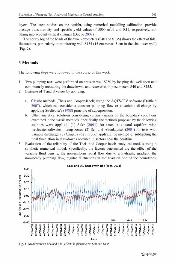
The hourly log of the heads of the two piezometers (S40 and S135) shows the effect of tidalfluctuations, particularly in monitoring well S135 (15 cm versus 5 cm in the shallower well)(Fig. 2).
3 Methods
The following steps were followed in the course of this work:
1. Two pumping tests were performed on artesian well S250 by keeping the well open andcontinuously measuring the drawdowns and recoveries in piezometers S40 and S135.
2. Estimate of T and S values by applying:
a. Classic methods (Theis and Cooper-Jacob) using the AQTSOLV software (Duffield2007), which can consider a constant pumping flow or a variable discharge byapplying Streltsova’s (1988) principle of superposition.
b. Other analytical solutions considering certain variants on the boundary conditionsexamined in the classic methods. Specifically, the methods proposed by the followingauthors were applied: (1) Sakr (2001) for tests in coastal aquifers withfreshwater-saltwater mixing zones. (2) Sen and Altunkaynak (2004) for tests withvariable discharge. (3) Chapius et al. (2006) applying the method of subtracting thetidal fluctuation in drawdowns obtained in sectors near the coastline.
3. Evaluation of the reliability of the Theis and Cooper-Jacob analytical models using asynthetic numerical model. Specifically, the factors determined are the effect of thevariable fluid density, the non-uniform radial flow due to a hydraulic gradient, thenon-steady pumping flow, regular fluctuations in the head on one of the boundaries,
Fig. 2 Mediterranean tide and tidal effects in piezometers S40 and S135
Evaluation of Pumping Test Analytical Methods in Coastal Aquifers 563
and the vertical heterogeneity of the hydraulic conductivity. The conceptual modelconsidered is a simplification of the real study case since the objective is to determinethe margin of error that the T and S values obtained with the classic methods can havewhen the boundary conditions considered by Theis and Cooper-Jacob are not met (case 1).To do so, the T and S values (Ti, Si) are estimated from the drawdowns for each simulatedscenario, and the error with regard to case 1 (Ti, Si) is calculated as
ErrorT ¼ Ti−T 1
T1; ErrorS ¼ Si−S1
S1
3.1 Pumping Tests Description
Two pumping tests were performed consisting in measuring the heads in the monitoring wellsS40 and S135 after a prolonged opening of well S250. In the first test (PT1), well S250 waskept open for 23 h and 35 min, allowing a recovery time of 3 h and 30 min after well S250 wassealed. In the second test (PT2), well S250 was opened for 26 h and 7 min, allowing a recoverytime of 23 h and 43 min (Table 1).
Throughout the two tests, the well discharge was measured at variable intervals, noting aprogressive drop in flow. In PT1, discharge was between 20 and 16.7 L/s and in PT2 it was17.7 to 16 L/s. The average discharge for the two tests was taken as 18.2 and 16.8 L/s,respectively (Table 2).
In PT1, although the recovery time allowed was very short (3.5 h), the static water level wasnearly reached, with a residual decrease of just 0.01 m in S40. In PT2, the recovery time waslonger (almost 24 h), allowing complete recovery of the water level.
In both tests, the effect of tidal fluctuations is noted, although it is much more noticeable inS135 than in S40.
3.2 Numerical Modelling
A finite-difference 3D model (SEAWAT) has been developed simulating a theoretical pumpingtest where the boundary conditions were modified in a total of seven different cases: (1) Theisand Cooper-Jacob conditions, (2) with a hydraulic gradient on the X axis, (3) with a variablepumping rate, (4) with a boundary with tidal fluctuations, (5) with vertical heterogeneity, (6)with fluids of different density (freshwater and saltwater), and (7) with all the above condi-tions. The size of the model is large enough to ensure a completely theoretical pumping, inwhich there is no border impact on the shape of the drawdown cones.
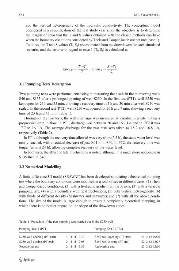
Table 1 Procedure of the two pumping tests carried out in the S250 well
Pumping Test 1 (PT1) Pumping Test 2 (PT2)
S250 well opening (PT start) 1–11-11 12:30 S250 well opening (PT start) 21–2-12 10:20
S250 well closing (PT end) 2–11-11 12:05 S250 well closing (PT end) 22–2-12 12:27
Recovering end 2–11-11 15:35 Recovering end 23–2-12 12:10
564 M.L. Calvache et al.
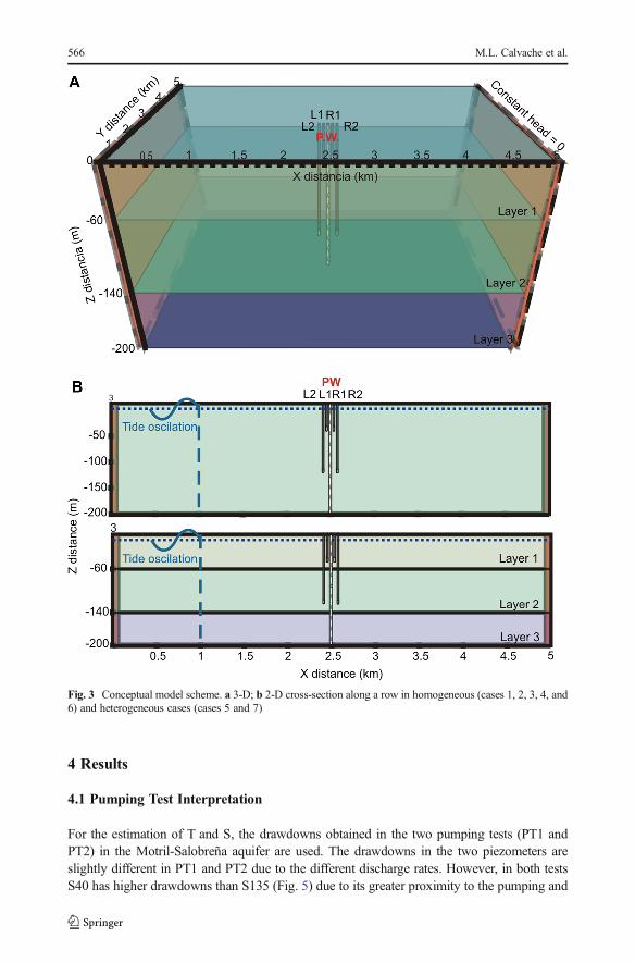
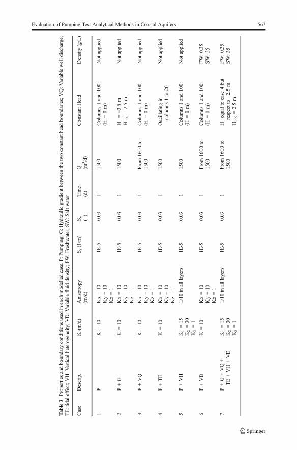
Accordingly, the model dimension (Fig. 3) was set to 5 km long (X dimension) by 5 kmwide (Y dimension) by 200 m deep (Z dimension), considering the ground surface at 3 mabove sea level. Cells are 50 m × 50 m and of variable depth in accordance with the two mainsituations: one layer (cases 1, 2, 3, 4, and 6) as a homogeneous aquifer and three layers (cases 5and 7) to include heterogeneity in the aquifer (Fig. 3).
The main features for each scenario are listed in Table 3. The gradient defined between thetwo constant head boundaries is 0.001 in cases 2 and 7. The tide condition imposed in cases 4and 7 is described as a constant sinusoidal oscillation head boundary condition (Fig. 3B) on theleft border from 0 to 1 km, with the aim to produce a detectable disturbance in the records ofthe head observation wells. The expression used to define the tide oscillation is:
H ¼ A*sin2πT
*t� φ
� �
where H is the tide elevation [L], A is the semi-amplitude of the tide [L], T is the period oftide oscillation [T], t is the time [T], and φ is the phase of the tide [°]. In this case, tidal valuessimilar to those in the Mediterranean Sea were considered. The semi-diurnal tide fluctuationfor a 24-h period has been adjusted, with an amplitude of 2 m, a frequency of 0.082 cycles/h,and a period of 12.2 h. Another variation (applied in cases 6 and 7) is added with the aim ofevaluating the implication of variable density on the simulated pumping test. The considereddensity values are 0.35 g/L (freshwater) and 35 g/L (saltwater). A 10 m-thick layer in thelowest level was considered, with a constant salinity of 35 g/L.
The pumping well is situated in the centre of the model domain (2.5 × 2.5 km2), and fullypenetrating, from 3 m to −200 m depth (along the Z axis). The casing of the pumping well wasassigned as fully screened. The variable pumping rate in cases 3 and 7 has been imposed with alinear decrease from 1600 m3/d to 1500 m3/d, throughout one day of pumping. In other cases,the pumping rate is constant and equal to 1500 m3/d.
Finally, eight head observation points were added in order to assess the symmetry of thedrawdown cone produced by the pumping and the changes in heads with depth. They weredistributed symmetrically on both the right and left sides of the well (R1-RS1-L1-LS1 50 mand R2-RS2-L2-LS2 100 m from the pumping well, respectively), as shown in Fig. 3B. Thedepths of the head observation points are:
– RS1, RS2, LS1, and LS2: - 5 m (below top of the model)– R1 and L1: - 40 m (below top of the model)– R2 and L2: - 135 m (below top of the model)
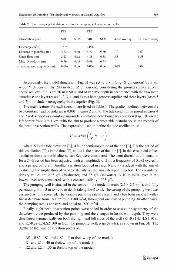
Table 2 Some pumping test data related to the pumping and observation wells
PT1 PT2
Observation point S40 S135 S40 S135 S40 recovering S135 recovering
Discharge (m3/d) 1576 1451
Distance to pumping (m) 4.72 9.60 4.72 9.60 4.72 9.60
Static Head (m) 5.23 6.62 4.88 6.58 4.88 6.58
Max. Drawdown (m) 0.79 0.45 0.49 0.44
Tidal-induced amplitude (m) 0.008 0.06 0.006 0.06 0.028 0.09
Evaluation of Pumping Test Analytical Methods in Coastal Aquifers 565
4 Results
4.1 Pumping Test Interpretation
For the estimation of T and S, the drawdowns obtained in the two pumping tests (PT1 andPT2) in the Motril-Salobreña aquifer are used. The drawdowns in the two piezometers areslightly different in PT1 and PT2 due to the different discharge rates. However, in both testsS40 has higher drawdowns than S135 (Fig. 5) due to its greater proximity to the pumping and
Fig. 3 Conceptual model scheme. a 3-D; b 2-D cross-section along a row in homogeneous (cases 1, 2, 3, 4, and6) and heterogeneous cases (cases 5 and 7)
566 M.L. Calvache et al.
Tab
le3
Propertiesandboundary
conditionsused
ineach
modelledcase.P
:Pum
ping;G
:Hydraulicgradient
betweenthetwoconstant
head
boundaries;V
Q:V
ariablewelld
ischarge;
TE:tid
aleffect;VH:Verticalheterogeneity;VD:Variablefluiddensity
;FW
:Freshw
ater;SW
:Saltwater
Case
Descrip.
K(m
/d)
Anisotropy
(m/d)
S s(1/m
)S y (−)
Tim
e(d)
Q (m3/d)
ConstantHead
Density(g/L)
1P
K=10
Kx=10
Ky=10
Kz=1
1E-5
0.03
11500
Colum
ns1and100:
(H=0m)
Not
applied
2P+G
K=10
Kx=10
Ky=10
Kz=1
1E-5
0.03
11500
H1=−2
.5m
H100
=2.5m
Not
applied
3P+VQ
K=10
Kx=10
Ky=10
Kz=1
1E-5
0.03
1From
1600
to1500
Colum
ns1and100:
(H=0m)
Not
applied
4P+TE
K=10
Kx=10
Ky=10
Kz=1
1E-5
0.03
11500
Oscillatingin
columns
1to
20Not
applied
5P+VH
K1=15
K2=30
K3=1
1/10
inalllayers
1E-5
0.03
11500
Colum
ns1and100:
(H=0m)
Not
applied
6P+VD
K=10
Kx=10
Ky=10
Kz=1
1E-5
0.03
1From
1600
to1500
Colum
ns1and100:
(H=0m)
FW:0.35
SW:35
7P+G
+VQ
+TE+VH
+VD
K1=15
K2=30
K3=1
1/10
inalllayers
1E-5
0.03
1From
1600
to1500
H1equaltocase
4but
respectto
−2.5
mH100
=2.5m
FW:0.35
SW:35
Evaluation of Pumping Test Analytical Methods in Coastal Aquifers 567
to the shallower measurement. The highest drawdown in S40 during PT1 was 0.79 m and 0.49during PT2 (Table 2). In the case of S135, the differences in drawdowns are slight in both tests,never exceeding 0.02 m.
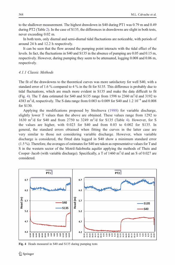
In both tests, only diurnal and semi-diurnal tidal fluctuations are noticeable, with periods ofaround 24 h and 12.2 h respectively.
It can be seen that the flow around the pumping point interacts with the tidal effect of thelevels. In fact, the fluctuations in S40 and S135 in the absence of pumping are 0.05 and 0.15 m,respectively. However, during pumping they seem to be attenuated, logging 0.008 and 0.06 m,respectively.
4.1.1 Classic Methods
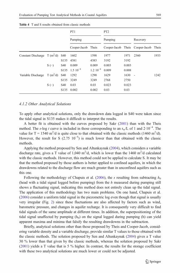
The fit of the drawdowns to the theoretical curves was more satisfactory for well S40, with astandard error of 1.6 % compared to 4 % in the fit for S135. This difference is probably due totidal fluctuations, which are much more evident in S135 and make the data difficult to fit(Fig. 4). The T data estimated for S40 and S135 range from 1598 to 2360 m2/d and 3192 to4383 m2/d, respectively. The S data range from 0.003 to 0.009 for S40 and 1.2 10−4 and 0.008for S130.
Applying the modifications proposed by Streltsova (1988) for variable discharge,slightly lower T values than the above are obtained. These values range from 1292 to1630 m2/d for S40 and from 2750 to 3249 m2/d for S135 (Table 4). However, for Sthe values are higher, with 0.023 for S40 and from 0.03 to 0.002 for S135. Ingeneral, the standard errors obtained when fitting the curves in the latter case arevery similar to those not considering variable discharge. However, when variabledischarge is considered, the fitted data logged in S40 show a minimum standard error(1.5%). Therefore, the averages of estimates for S40 are taken as representative values for TandS in the western sector of the Motril-Salobreña aquifer applying the methods of Theis andCooper–Jacob (with variable discharge). Specifically, a T of 1460 m2/d and an S of 0.027 areconsidered.
Fig. 4 Heads measured in S40 and S135 during pumping tests
568 M.L. Calvache et al.
4.1.2 Other Analytical Solutions
To apply other analytical solutions, only the drawdown data logged in S40 were taken sincethe tidal signal in S135 makes it difficult to interpret the results.
A better fit is obtained with the curves proposed by Sakr (2001) than with the Theismethod. The s-log t curve is included in those corresponding to an rw/L of 1 and 2·10−4. Thevalue for T = 1540 m2/d is quite close to that obtained with the classic methods (1460 m2/d).However, the result for S (2.75 10−5) is much lower than that obtained with the classicmethods.
Applying the method proposed by Sen and Altunkaynak (2004), which considers a variabledischarge rate, gives a T value of 1,040 m2/d, which is lower than the 1460 m2/d calculatedwith the classic methods. However, this method could not be applied to calculate S. It may bethat the method proposed by those authors is better applied to confined aquifers, in which thedrawdowns related to the discharge flow are much greater than in unconfined aquifers such asthis one.
Following the methodology of Chapuis et al. (2006), the s resulting from subtracting h0(head with a tidal signal logged before pumping) from the h measured during pumping stillshows a fluctuating signal, indicating this method does not entirely clean up the tidal signal.The application of this methodology has two main problems. On one hand, Chapuis et al.(2006) consider a uniform tidal signal in the piezometric log even though that signal is usuallyvery irregular (Fig. 2) since these fluctuations are also affected by factors such as wind,barometric pressure, and changes in aquifer recharge. It is consequently very difficult to findtidal signals of the same amplitude at different times. In addition, the superpositioning of thetidal signal unaffected by pumping (h0) on the signal logged during pumping (h) can yieldapparent maxima and minima that falsify the resulting drawdowns in the subtraction.
Briefly, analytical solutions other than those proposed by Theis and Cooper-Jacob, consid-ering variable density and a variable discharge, provide similar T values to those obtained withthe classic methods. The solution proposed by Sen and Altunkaynak (2004) gives a T value30 % lower than that given by the classic methods, whereas the solution proposed by Sakr(2001) yields a T value that is 5 % higher. In contrast, the results for the storage coefficientwith these two analytical solutions are much lower or could not be adjusted.
Table 4 T and S results obtained from classic methods
PT1 PT2
Pumping Pumping Recovery
Cooper-Jacob Theis Cooper-Jacob Theis Cooper-Jacob Theis
Constant Discharge T (m2/d) S40 1602 1598 1977 1971 2360 1933
S135 4381 4383 3192 3192
S (−) S40 0.009 0.009 0.003 0.003
S135 1.5 10−4 1.2 10−4 0.009 0.008
Variable Discharge T (m2/d) S40 1292 1290 1629 1630 - 1242
S135 3249 3249 2768 2750
S (−) S40 0.03 0.03 0.023 0.023
S135 0.002 0.002 0.03 0.03
Evaluation of Pumping Test Analytical Methods in Coastal Aquifers 569
4.2 Evaluation of Reliability of Theis and Cooper-Jacob Methods
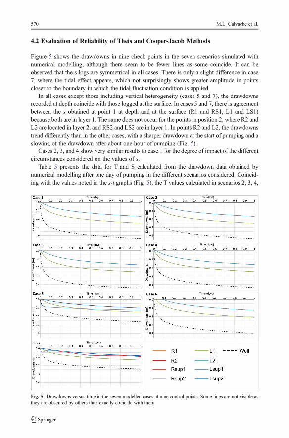
Figure 5 shows the drawdowns in nine check points in the seven scenarios simulated withnumerical modelling, although there seem to be fewer lines as some coincide. It can beobserved that the s logs are symmetrical in all cases. There is only a slight difference in case7, where the tidal effect appears, which not surprisingly shows greater amplitude in pointscloser to the boundary in which the tidal fluctuation condition is applied.
In all cases except those including vertical heterogeneity (cases 5 and 7), the drawdownsrecorded at depth coincide with those logged at the surface. In cases 5 and 7, there is agreementbetween the s obtained at point 1 at depth and at the surface (R1 and RS1, L1 and LS1)because both are in layer 1. The same does not occur for the points in position 2, where R2 andL2 are located in layer 2, and RS2 and LS2 are in layer 1. In points R2 and L2, the drawdownstrend differently than in the other cases, with a sharper drawdown at the start of pumping and aslowing of the drawdown after about one hour of pumping (Fig. 5).
Cases 2, 3, and 4 show very similar results to case 1 for the degree of impact of the differentcircumstances considered on the values of s.
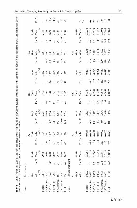
Table 5 presents the data for T and S calculated from the drawdown data obtained bynumerical modelling after one day of pumping in the different scenarios considered. Coincid-ing with the values noted in the s-t graphs (Fig. 5), the T values calculated in scenarios 2, 3, 4,
Fig. 5 Drawdowns versus time in the seven modelled cases at nine control points. Some lines are not visible asthey are obscured by others than exactly coincide with them
570 M.L. Calvache et al.
Tab
le5
TandSvalues
foreach
ofthecasesmodelledfrom
each
oneof
thedraw
downrecordsfrom
thedifferentobservationpointsof
thenumericalmodelandestim
ationerrors
regardingcase
1.Valuesrepeated
dueto
symmetry
have
been
elim
inated
Cases
Transmissivity
R1
R2
RS1
RS2
Theis
Jacob
Theis
Jacob
Theis
Jacob
Theis
Jacob
Value m2/d
Err.%
Value m2/d
Err.%
Value m2/d
Err.%
Value m2 /d
Err.%
Value m2/d
Err.%
Value m2/d
Err.%
Value m2/d
Err.%
Value m2/d
Err.%
1Ideal
1958
-2014
-1994
-2133
-1937
-2032
-1994
-2133
-
2H.G
radient
1959
0.0
2066
2.6
1995
0.1
2066
−3.1
1959
1.1
2026
−0.3
1995
0.1
2185
2.4
3V.D
isch.
1944
−0.7
2009
−0.2
1985
−0.5
2170
1.7
1944
0.4
2053
1.0
1985
−0.5
2078
−2.6
4TidalEff.
1958
0.0
2077
3.1
1994
0.0
2133
0.0
1958
1.1
2029
−0.2
1994
0.0
2100
−1.5
5V.H
eterog.
2517
282639
318806
342
5295
148
2517
302653
312518
262749
29
6V.D
ensity
1810
−7.5
1945
−3.4
1583
−20.6
2170
1.7
1810
−6.5
1953
−3.9
1583
−20.6
2170
1.8
7All
2863
462827
402314
16.1
3579
682863
482827
392812
412943
38
Cases
Storagecoefficient
R1
R2
RS1
RS2
Theis
Jacob
Theis
Jacob
Theis
Jacob
Theis
Jacob
Value
Err.%
Value
Err.%
Value
Err.%
Value
Err.%
Value
Err.%
Value
Err.%
Value
Err.%
Value
Err.
%
1Ideal
0.0292
-0.0263
-0.0288
-0.0237
-0.0301
0.0264
-0.0288
-0.0234
-
2H.G
radient
0.0292
0.0
0.0254
−3.4
0.0288
−0.1
0.0254
7.2
0.0292
−3.0
0.0256
−2.9
0.0288
−0.1
0.0234
0.0
3V.D
isch.
0.0300
2.7
0.0262
−0.4
0.0291
1.0
0.0235
−1.1
0.0300
−0.3
0.0263
−0.4
0.0291
1.0
0.0253
7.9
4TidalEff.
0.0292
0.1
0.0254
−3.4
0.0288
−0.2
0.0243
2.4
0.0292
−2.9
0.0261
−1.1
0.0288
−0.2
0.0252
7.5
5V.H
eterog.
0.0970
232
0.0843
220
0.0002
−99
0.0043
−82
0.0970
222
0.0847
220
0.0723
151
0.0602
157
6V.D
ensity
0.0664
127
0.0558
112
0.0707
145
0.0494
108
0.0664
121
0.0555
110
0.0707
145
0.0494
110
7All
0.1072
267
0.1039
256
0.0609
108
0.0526
800.1072
267
0.1039
256
0.0945
223
0.0800
174
Evaluation of Pumping Test Analytical Methods in Coastal Aquifers 571
and 6 are quite similar to those obtained with the Theis and Cooper-Jacobmethods (case 1). Theerror tends to be below 10 %, and only in the case of s measured at the points farthest from thepumping point considering different densities (R2, RS2) does it reach an error of 20 % (case 6).
Vertical heterogeneity is the most important factor impacting the applicability of classicmethods in interpreting pumping tests. In that scenario (case 5), the T values obtained show ahigher error percentage, although there is a great difference between the values calculated atthe points located in layer 1 (R1, RS1, RS2), with errors of around 30 %, and the values inlayer 2 (R2), with errors of over 100 %.
It is worth noting that, considering all the factors combined (case 7), the percentage of errordrops down to 40–50 % in most cases, probably because certain effects compensate for theeffects of other factors.
The S is much more sensitive to changes with respect to the reference case. Acceptableresults have only been found for cases taking into account a hydraulic gradient, variablewithdrawal rate, and single-layer tidal effects (cases 2, 3, and 4), with errors generally under3 %. In the other cases, the S values are much higher than the value calculated in case 1, witherrors of around 100–300 %.
As occurs with T, the S values obtained for case 7 (in which all the variables are consideredjointly) show a lower error than in case 5. The fluid’s variable density affects the estimation ofS (errors of over 100 %) more than that of T (errors of 1.7–20.6 %).
5 Discussion
Applying the analytical solution proposed by Sen and Altunkaynak (2004) to theMotril-Salobreña aquifer to determine the effect of pumping with a variable discharge revealsa T value 28 % lower than when estimated with the classic methods. In contrast, the results ofthe numerical modelling (case 3) considering a decrease of 10 % in the pumping rate over thecourse of the test yielded a difference of less than 2.6 % compared to the values from the Theisand Cooper-Jacob methods.
The other analytical solution applied in this work, proposed by Sakr (2001), considers theeffect of two fluids of different density and yields T values 5 % higher than the values of theclassic methods for the Motril-Salobreña aquifer. In this case, in contrast, the results of thenumerical modelling (case 6) indicate that this factor has more impact on the results andinversely to the form suggested by Sakr (2001), with T values up to 20 % lower than thosefound with the classic methods.
When considering layers with different hydraulic conductivity (case 5), vertical flows occurthat deform the equipotentials, losing their verticality. This occurs because the supply of waterto the pumping well is proportional to the hydraulic conductivity and, therefore, is higher inlayer 2, which has the highest K of the three. In fact, layer 2 supplied 71 %, layer 1 27 %, andlayer 3 2 % of the withdrawal volume. This causes a greater loss of head at the beginning inlayer 2 and the appearance of a vertical hydraulic gradient from layers 1 and 3 towards layer 2.This is why, in case 5, the drawdowns in L2 and R2 are much sharper at the start and graduallystabilize due to the supply of water from the other two layers.
Consequently, the s values measured in the different layers do not correspond to the directeffect of the volume pumped and explains why they do not provide good results using theclassic methods. Therefore, and in agreement with Alam and Olsthoorn (2014), the traditionalmethods tend to mask the effect in stratified aquifers with vertical flow.
572 M.L. Calvache et al.
In case 5, it has been considered that the effect could be similar to what happens in a leakyconfined aquifer, and we therefore opted to use the analytical solution proposed by Hantush(1960). The resulting T values are closer than with traditional methods, but the errors are stillquite large (around 100 %).
The effect of tidal fluctuations on drawdowns is minimal when only one layer is considered(case 4 in Fig. 5), but is notable when several layers are taken into account (case 7 in Fig. 5).Specifically, the s logged in the shallower points (R1, L1) show no fluctuation; however,deeper points (R2, L2) do show a clear effect of tidal fluctuations. This circumstance is inagreement with the effect found in the two monitoring wells for the Motril-Salobreña aquifer(S40 and S135), where a much sharper tidal fluctuation is found in the deeper piezometer(Fig. 2).
6 Conclusions
Synthetic numerical modelling has shown that estimating the transmissivity values and thestorage coefficient calculated by Theis and Cooper-Jacob in a detrital aquifer can yield an errorof under 10 % when there is regional flow (hydraulic gradient), when the volume pumpedvaries up to 10 % throughout the test, and when the levels show a tidal effect on the order of1 % of the total head.
A saltwater-freshwater interface can cause an error of 20 % in the transmissivity results andof over 100 % in the storage coefficient.
Vertical heterogeneity causes the greatest errors in the T and S results using classic methods.Layers with variations in hydraulic conductivity of 1–30 m/d produce errors in both parametersof over 100 %.
The Theis and Cooper-Jacob methods can be applied in coastal aquifers to interpretpumping tests and obtain T and S values as long as the aquifers are uniform, withoutsignificant vertical heterogeneity, and in a sector without variable density (saline wedge).
If the Theis or Cooper-Jacob methods are used in stratified aquifers with variable verticalhydraulic conductivity or in which pumping is carried out in the saline wedge, the S datacannot be considered valid and the T values should be viewed as approximate andover-estimated.
In the specific case of the Motril-Salobreña aquifer, in fact, the T value (1460 m2/d)obtained from applying the Theis and Cooper-Jacob methods on the pumping tests is probablyoverestimated as well. The storage coefficient value is uncertain and other methods will needto be used to determine it.
Acknowledgments This research has been financed by Project CGL2012-32892 (Ministerio de Economía yCompetitividad of Spain) and by the Research Group Sedimentary Geology and Groundwater (RNM-369) of theJunta de Andalucía. Christine Laurin is thanked for the English version of the text.
Open Access This article is distributed under the terms of the Creative Commons Attribution 4.0 InternationalLicense (http://creativecommons.org/licenses/by/4.0/), which permits unrestricted use, distribution, and repro-duction in any medium, provided you give appropriate credit to the original author(s) and the source, provide alink to the Creative Commons license, and indicate if changes were made.
Evaluation of Pumping Test Analytical Methods in Coastal Aquifers 573
References
Alam N, Olsthoorn TN (2014) Multidepth pumping tests in deep aquifers. Groundwater 52:148–160. doi:10.1111/gwat.12155
Barlow PM, Masterson JP, Walter DA (1996) Hydrogeology and analysis of ground-water-flow system,sagamore marsh area, Southern Massachusetts USGS Water-Resources Investigations Report 96-4200
Boulton NS (1954) The drawdown of the water-table under non-steady conditions near a pumped well in anunconfined formation. Proc Inst Civil Eng 3:564–579
Calvache ML, Duque C, Gomez-Fontalva JM, Crespo F (2011) Processes affecting groundwater temperaturepatterns in a coastal aquifer. Int J Environ Sci Technol 8(2):223–236
Calvache ML, Ibáñez SP, Duque C, et al. (2009) Numerical modelling of the potential effects of a dam on acoastal aquifer in S. Spain. Hydrol Process 23:1268–1281
Capuano RM, Jan RZ (1996) In situ hydraulic conductivity of clay and silty-clay fluvial-deltaic sediments, Texasgulf coast. Ground Water 34:545–551. doi:10.1111/j.1745-6584.1996.tb2036.x
Chachadi AG, Gawas PD (2012) Correlation study between geoelectrical and aquifer parameters in West coastlaterites. Int J Earth Sci Eng 5(2):282–287
Chapuis RP, Belanger C, Chenaf D (2006) Pumping test in a confined aquifer under tidal influence. Groundwater44(2):300–305
Chattopadhyay PB, Vedanti N, Singh VS (2014) A conceptual numerical model to simulate aquifer parameters.Water Resour Manag 29:771–784. doi:10.1007/s11269-014-0841-6
Chen C, Jiao JJ (1999) Numerical simulation of pumping tests in multilayer well with non-darcian flow in thewell-bore. Ground Water 37(3):465–474
Chen F, Wiese B, Zhou Q, Kowalsky MB, Norden B, Kempka T, Birkholzer JT (2014) Numerical modeling ofthe pumping tests at the ketzin pilot site for CO2 injection: model calibration and heterogeneity effects. Int JGreenh Gas Con 22:200–212
Cooper HH, Jacob CE (1946) A generalized graphical method for evaluating formation constants and summa-rizing well field history. Trans Am Geophys Union 27:526–534
Diamantopoulou P, Voudouris K (2008) Optimization of water resources management using SWOT analysis: thecase of Zakynthos island, Ionian sea, Greece. Environ Geol 54(1):197–211
Doulgeris C, Zissis T (2014) 3D variable density flow simulation to evaluate pumping schemes in coastalaquifers. Water Resour Manag 28(4):4943–4956
Duffield GM (2007) AQTESOLV for Vindows, Version 4.5, HydroSOLVE Inc, Reston, VirginiaDuque C (2009) Influencia antrópica sobre la hidrogeología del acuífero Motril-Salobreña [Anthropogenic
influence on the hydrogeology of the Motril-Salobreña Aquifer. PhD Thesis, University of GranadaDuque C, Calvache ML, Pedrera A, Martín-Rosales W, López-Chicano M (2008) Combined time domain
electromagnetic soundings and gravimetry to determine marine intrusion in a detrital coastal aquifer(southern Spain). J Hydrol 349(3–4):536–547
Duque C, López-Chicano M, Calvache ML, Martin-Rosales W, Gómez-Fontalva JM, Crespo F (2011) Rechargesources and hydrogeological effects of irrigation and an influent river identified by stable isotopes in themotril-salobreña aquifer (southern Spain). Hydrol Process 25(4):2261–2274
Glover RE (1959) The pattern of fresh-water flow in a coastal aquifer. J Geophys Res 64(4):457–459Hantush MS (1960) Modification of the theory of leaky aquifers. J Geophys Res 65(11):3713–3725Hantush MS (1961) Aquifer test in partially penetrating wells. J Hyd Div, Proc Am Soc Civil Eng 87:171–194Hemker CJ (1985) Transient well flow in a leaky multiple-aquifer systems. J Hydrol 81:111–126Hemker CJ (1999) Transient well flow in vertically heterogeneous aquifers. J Hydrol 225:1–18Hemker CJ, Maas C (1987) Unsteady flow to wells in layered and fissured aquifer systems. J Hydrol 90:231–249Jacob CE, Lohman SW (1952) Non steady flow to a well of constant drawdown in an extensive aquifer. Trans
Am Geophys Union 33(4):559–569Keith JH, Willis DW, Robert PS (2006) Interpretation of transmissivity estimates from single-well pumping
aquifer tests. Groundwater 44(3):467–471Kohout FA (1964) The flow of fresh water and salt water in the Biscayne aquifer of the Miami area, Florida. In:
sea water in coastal aquifers: U.S. Geological Survey Water-Supply Paper 1613-C:12–32Kollet J, Zlotnik VA (2005) Influence of aquifer heterogeneity and return flow on pumping test data interpre-
tation. J Hydrol 300(1–4):267–285. doi:10.1016/j.jhydrol.2004.06.011Kourakos G, Mantoglou A (2011) Simulation and multi-objective management of coastal aquifers in semi-arid
regions. Water Resour Manag 25(4):1063–1074Lai RY, Karadi GM, Williams RA (1973) Drawdown at time-dependent flowrate. Water Resour Bull 9(5):892–
900Lee BS, Song SH, Kim JS, Um JY, Nam K (2014) Availability of coastal groundwater discharge as an alternative
water resource in a large-scale reclaimed land, Korea. Environ Earth Sci 71(4):1521–1532
574 M.L. Calvache et al.
Maas C (1987a) Groundwater flow to a well in a layered porous medium 1. Steady flow. Water Resour Res 23:1675–1681
Maas C (1987b) Groundwater flow to a well in a layered porous medium 2. Nonsteady multiple-aquifer flow.Water Resour Res 23:1683–1688
Mastrocicco M, Sbarbati C, Colombani N, Petitta M (2013) Efficiency verification of a horizontal flow barriervia flowmeter tests and multilevel sampling. Hydrol Process 27:2414–2421
Mishra PK, Vessilinov V, Gupta H (2013) On simulation and analysis of variable-rate pumping tests.Groundwater 51(3):469–473
Moench AF (1995) Combining the neuman and boulton models for flow to a well in an unconfined aquifer.Groundwater 33:378–384
Moench AF (1996) Flow to a well in a water-table aquifer: an improved Laplace transform solution.Groundwater 34:593–596
Mohanty S, Jha MK, Kumar A, Jena SK (2012) Hydrologic and hydrogeologic characterization of a deltaicaquifer system inOrissa, eastern India.Water ResourManag 26:1899–1928. doi:10.1007/s11269-012-9993-4
Neuman SP (1972) Theory of flow in unconfined aquifers considering delayed response of the water table. WaterResour Res 8(4):1031–1045
Neuman SP (1974) Effects of partial penetration on flow in unconfined aquifers considering delayed aquiferresponse. Water Resour Res 10(2):303–312
Ni JC, Cheng WC, Ge L (2011) A case history of field pumping tests in a deep gravel formation in the Taipeibasin, Taiwan. Eng Geol 117:17–28. doi:10.1013/j.enggeo.2010.10.001
Papadopulos IS, Cooper HH (1967) Drawdown in a well of large diameter. Water Resour Res 3:241–244Park HY, Jang K, Ju JW, Yeo JW (2012) Hydrogeological characterization of seawater intrusion in tidally-forced
coastal fractured bedrock aquifer. J Hydrol 446–447:77–89Riva M, Guadagnini A, Neuman SP, Franzetti S (2001) Radial flow in a bounded randomly heterogeneous
aquifer. Transp Porous Media 45(1):139–193Sabtan AA, Shehata WM (2003) Hydrogeology of Al-lith sabkha, Saudi Arabia. J Asian Earth Sci 21(4):423–
429Sakr SA (2001) Type curves for pumping test analysis in coastal aquifers. Ground Water 39(1):5–9Sen Z, Altunkaynak A (2004) Variable discharge type curve solutions for confined aquifers. J Am Water Resour
Assoc Res 40(5):1189–1196Sternberg YM (1967) Transmissibility determination from variable discharge pumping tests. Groundwater 5(4):
27–29Streltsova TD (1988) Well testing in heterogeneous formations. John Willey & sons, New YorkThiem G (1906) Hydrologische methoden. Gebhardt, LeipzigTheis CV (1935) The relation between the lowering of the piezometric surface and the rate and duration of
discharge of well using groundwater storage. Trans Am Geophys Union 2:519–524Trefry MG, Johnston CD (1998) Pumping test analysis for a tidally forced aquifer. Groundwater 36(3):427–433Vouillamoz JM, Chatenoux B, Mathieu F, Baltassat JM, Legchenko A (2006) Efficiency of joint use of MRS and
VES to characterize coastal aquifer in Myanmar. J Appl Geophys 61:142–154Zekri S, Triki C, Al-Maktoumi A, Bazargan-Lari MR (2015) An optimization-simulation approach for ground-
water abstraction under recharge uncertainty. Water Resour Manag 29:3681–3695. doi:10.1007/s11269-015-1023-x
Zhang G (2013) Type curve and numerical solutions for estimation os transmisivity and storage coefficient withvariable discharge condition. J Hydrol 476:345–351
Evaluation of Pumping Test Analytical Methods in Coastal Aquifers 575