FAKULTAT FUR INFORMATIK

DER TECHNISCHEN UNIVERSITAT MUNCHEN

Bachelor’s Thesis in Informatics

Efficient Trajectory Modelling for SpaceDebris Evolution

Oliver Bosing

FAKULTAT FUR INFORMATIK

DER TECHNISCHEN UNIVERSITAT MUNCHEN

Bachelor’s Thesis in Informatics

Efficient Trajectory Modelling for Space DebrisEvolution

Effiziente Modellierung zur Vorausberechnung vonWeltraumschrott Flugbahnen

Author: Oliver Bosing

Supervisor: Univ.-Prof. Dr. Hans-Joachim Bungartz

Advisor: Fabio Alexander Gratl, M.Sc. and Pablo Gomez, Dr.-Ing.

Date: 15.09.2021

I confirm that this bachelor’s thesis is my own work and I have documented all sources andmaterial used.

Munich, 15.09.2021 Oliver Bosing

Acknowledgements

I thank Fabio and Pablo for their supervision and guidance during the writing of thisthesis.

Special thanks also go to my friends Moe and Freddy for our bad habit of sooner or laterstarting to talk about mathematics, physics, and computer science until nobody around ushas an idea what’s wrong with us.

And at last, I thank my parents for being patient with me, even when I changed mydegree program for the second time.

iv

Abstract

The number of objects orbiting Earth is increasing and will continue to do so in thefuture. With the increasing amount of these objects, collisions become more probable. Thesecollisions produce space debris orbiting Earth without an opportunity to manipulate itstrajectories.

For this thesis a software solution to model the trajectories of such objects, was developed,using C++. This software solution uses numerical integration, namely the leapfrog integrationmethod, to solve a system of differential equations. These differential equations model thetwo-body problem of the orbiting object and the Earth and uses Cowell’s formulation toadd perturbations to the two-body equations. The modeled perturbations are caused by thegravitation of the Sun and the Moon, the aspherical gravitational potential of the Earth,solar radiation pressure, and atmospheric drag.

The software solution is planned to be used as a part of larger space debris simulationssystems, developed and used by the European Space Agency’s Advanced Concept Team. Itis open source and can be found on GitHub1

1https://github.com/Wombatwarrior/BAspacedebris

v

Summary

The goal of the following Bachelor’s thesis Efficient Trajectory Modelling for Space DebrisEvolution is developing a software solution in C++, that can be used to simulate thetrajectories of a large number of objects orbiting Earth. This software is planned to be usedas part of bigger simulation programs for space debris evolution.

In the Theoretical Background chapter of this thesis, first, the equations of motions, thatare part of the model used to describe the forces acting on an object near the Earth, areintroduced. Next, the used integration method is explained.

The second part of the thesis focuses on the implementation aspects of the developedsoftware. Starting with the used data structures to represent the simulated system. Themain focus of the Implementation chapter lies in the calculation of the accelerations, neededto determine the trajectories of the simulated particles. At the end of the chapter theimplementation details of the leapfrog integration method and some aspects concerning I/Oare explained.

Part three analyzes some experiments conducted. First, the error convergence of thedeveloped software is analyzed. Additionally, the number of particle updates per second ismeasured for different amounts of simulated particles. To get a better idea of possible waysto increase simulation speed, the consumption of computation time during the simulation isdetermined. In the last section, the contributions of the different accelerations used in thesimulation are compared for different orbit altitudes.

As result of this thesis, the developed software can simulate hundreds of thousandsof particles, performing around 2 million particle updates per second. The error of thesimulations achieves convergence for reasonable integration time steps. But because the usedintegration method is only second-order, this convergence is rather slow. To improve theperformance of the software a higher-order integration method could be used in the future.Another promising approach could be parallelization because the performed calculations areindependent per particle.

vi

Contents

Acknowledgements iv

Abstract v

Summary vi

I. Introduction and Background 1

1. Introduction 2

2. Theoretical Background 42.1. The J2000 reference frame . . . . . . . . . . . . . . . . . . . . . . . . . . . . 42.2. Equations Of Motion . . . . . . . . . . . . . . . . . . . . . . . . . . . . . . . 5

2.2.1. Two-body equation . . . . . . . . . . . . . . . . . . . . . . . . . . . . 52.2.2. Third-Body Equation . . . . . . . . . . . . . . . . . . . . . . . . . . 52.2.3. Spherical Harmonics . . . . . . . . . . . . . . . . . . . . . . . . . . . 82.2.4. Solar Radiation Pressure . . . . . . . . . . . . . . . . . . . . . . . . . 112.2.5. Atmospheric Drag . . . . . . . . . . . . . . . . . . . . . . . . . . . . 122.2.6. Cowell’s Formulation . . . . . . . . . . . . . . . . . . . . . . . . . . . 13

2.3. Integration . . . . . . . . . . . . . . . . . . . . . . . . . . . . . . . . . . . . 13

3. Related Work 15

II. Implementation 16

4. Implementation 174.1. Data Structures . . . . . . . . . . . . . . . . . . . . . . . . . . . . . . . . . . 174.2. Acceleration Calculation . . . . . . . . . . . . . . . . . . . . . . . . . . . . . 174.3. Numerical Integration . . . . . . . . . . . . . . . . . . . . . . . . . . . . . . 204.4. I/O . . . . . . . . . . . . . . . . . . . . . . . . . . . . . . . . . . . . . . . . . 21

4.4.1. File Input . . . . . . . . . . . . . . . . . . . . . . . . . . . . . . . . . 214.4.2. File Output . . . . . . . . . . . . . . . . . . . . . . . . . . . . . . . . 22

III. Results 23

5. Results 245.1. Used Hardware and Software . . . . . . . . . . . . . . . . . . . . . . . . . . 24

vii

5.2. Error Analysis . . . . . . . . . . . . . . . . . . . . . . . . . . . . . . . . . . 245.3. Calculation Speed . . . . . . . . . . . . . . . . . . . . . . . . . . . . . . . . 265.4. Integration profiling . . . . . . . . . . . . . . . . . . . . . . . . . . . . . . . 28

5.4.1. Integration Time Compared to Main Simulation Loop . . . . . . . . 285.4.2. Computation Time Distribution Inside integrate . . . . . . . . . . 285.4.3. Computation Time Distribution Inside applyComponents . . . . . . 30

5.5. Acceleration Component Influences . . . . . . . . . . . . . . . . . . . . . . . 31

IV. Conclusion 35

6. Conclusion 36

V. Appendix 37

A. Constants 38

Bibliography 41

Part I.

Introduction and Background

1

1. Introduction

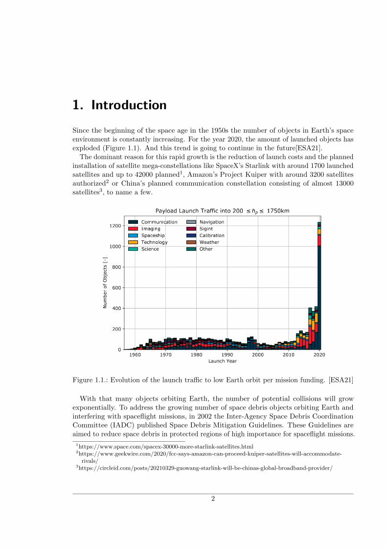
Since the beginning of the space age in the 1950s the number of objects in Earth’s spaceenvironment is constantly increasing. For the year 2020, the amount of launched objects hasexploded (Figure 1.1). And this trend is going to continue in the future[ESA21].

The dominant reason for this rapid growth is the reduction of launch costs and the plannedinstallation of satellite mega-constellations like SpaceX’s Starlink with around 1700 launchedsatellites and up to 42000 planned1, Amazon’s Project Kuiper with around 3200 satellitesauthorized2 or China’s planned communication constellation consisting of almost 13000satellites3, to name a few.

Figure 1.1.: Evolution of the launch traffic to low Earth orbit per mission funding. [ESA21]

With that many objects orbiting Earth, the number of potential collisions will growexponentially. To address the growing number of space debris objects orbiting Earth andinterfering with spaceflight missions, in 2002 the Inter-Agency Space Debris CoordinationCommittee (IADC) published Space Debris Mitigation Guidelines. These Guidelines areaimed to reduce space debris in protected regions of high importance for spaceflight missions.

1https://www.space.com/spacex-30000-more-starlink-satellites.html2https://www.geekwire.com/2020/fcc-says-amazon-can-proceed-kuiper-satellites-will-accommodate-rivals/

3https://circleid.com/posts/20210329-guowang-starlink-will-be-chinas-global-broadband-provider/

2

1. Introduction

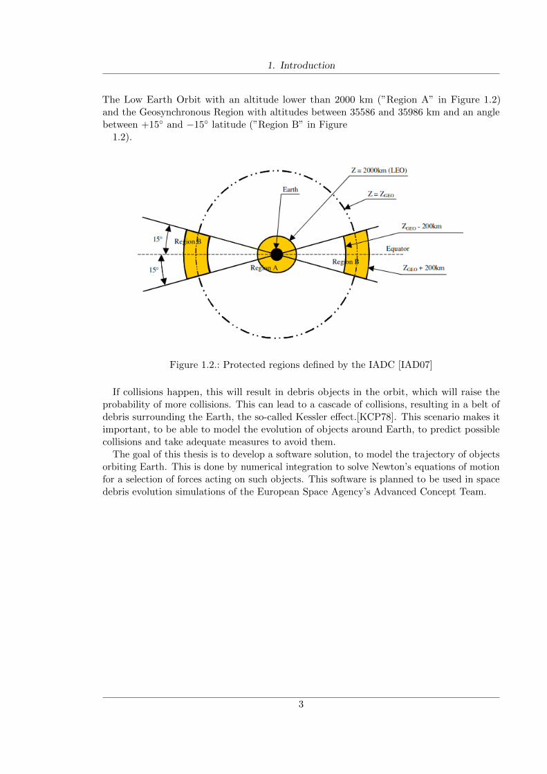
The Low Earth Orbit with an altitude lower than 2000 km (”Region A” in Figure 1.2)and the Geosynchronous Region with altitudes between 35586 and 35986 km and an anglebetween +15 and −15 latitude (”Region B” in Figure

1.2).

Figure 1.2.: Protected regions defined by the IADC [IAD07]

If collisions happen, this will result in debris objects in the orbit, which will raise theprobability of more collisions. This can lead to a cascade of collisions, resulting in a belt ofdebris surrounding the Earth, the so-called Kessler effect.[KCP78]. This scenario makes itimportant, to be able to model the evolution of objects around Earth, to predict possiblecollisions and take adequate measures to avoid them.

The goal of this thesis is to develop a software solution, to model the trajectory of objectsorbiting Earth. This is done by numerical integration to solve Newton’s equations of motionfor a selection of forces acting on such objects. This software is planned to be used in spacedebris evolution simulations of the European Space Agency’s Advanced Concept Team.

3

2. Theoretical Background

2.1. The J2000 reference frame

As the main source to develop the model used in this thesis the book ”Fundamentals ofAstrodynamics and Applications” by Vallado and McClain is used[VM97e].

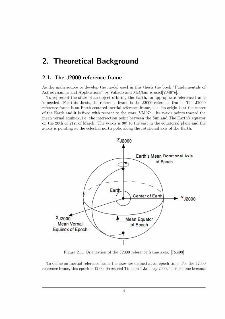
To represent the state of an object orbiting the Earth, an appropriate reference frameis needed. For this thesis, the reference frame is the J2000 reference frame. The J2000reference frame is an Earth-centered inertial reference frame, i. e. its origin is at the centerof the Earth and it is fixed with respect to the stars [VM97c]. Its x-axis points toward themean vernal equinox, i.e. the intersection point between the Sun and The Earth’s equatoron the 20th or 21st of March. The y-axis is 90° to the east in the equatorial plane and thez-axis is pointing at the celestial north pole, along the rotational axis of the Earth.

Figure 2.1.: Orientation of the J2000 reference frame axes. [Ros98]

To define an inertial reference frame the axes are defined at an epoch time. For the J2000reference frame, this epoch is 12:00 Terrestrial Time on 1 January 2000. This is done because

4

2. Theoretical Background

the above definitions change over time, due to periodic changes of the Earth’s orbit withrespect to the stars i. e. precession and nutation[Ros98].

2.2. Equations Of Motion

The motion of an object can be calculated knowing its position ~p and its position’s first andsecond derivative with respect to time i.e. its velocity ~v and acceleration ~a. The model usedfor this thesis combines several accelerations applied to its objects and uses the resultingaccelerations to calculate their positions and velocities.

2.2.1. Two-body equation

For objects orbiting Earth inside the protected regions depicted in Figure 1.2 by far the mostimportant acceleration to take into account is the gravitational acceleration caused by theEarth itself. The basis to calculate this acceleration is Newton’s Law of Gravitation. Thislaw describes the attraction between two bodies and can be used to formulate an equationto calculate the acceleration acting on an object orbiting the Earth following an elliptic orbitdescribed by Kepler’s Laws.

~aKep = −G(m⊕ +mobj)

|~p|3~p (2.1)

Where G is the gravitational constant, m⊕ is the mass of the Earth, and mobj is the massof the object. Considering that m⊕ is many magnitudes greater than mobj for satellites ordebris, the object’s mass can be neglected. This results in the equations

~aKep = −Gm⊕|~p|3

~p (2.2)

Where Gm⊕ = 3.986004407799724× 105km3sec−2 [VM97i].

2.2.2. Third-Body Equation

The last subsection considered only the Earth as an object gravitationally acting on anobject in its proximity. But since gravitation is acting on large distances, the accelerationacting on an object, caused by a third body must be taken into account. As described byVallado [VM97h] a general equation to calculate the gravitational acceleration on an objectobj in a three-body system with Earth and the third body b is

~a⊕,b = ~aKep +Gmb

(~pb − ~pobj|~pb − ~pobj |3

− ~pb − ~p⊕|~pb − ~p⊕|3

)(2.3)

The first term is the acceleration acting on the object, due to Earth’s gravity, describedin the last subsection. To get an equation to calculate the acceleration caused only bythe body b the second term is examined further. Since the used J2000 reference frame isEarth-centered the term can be simplified to

5

2. Theoretical Background

~ab = Gmb

(~pb − ~pobj|~pb − ~pobj |3

− ~pb

|~pb|3

)(2.4)

Using ~pb − ~pobj = −(~pobj − ~pb) and |~pb − ~pobj | = |~pobj − ~pb| [Esc65] the result is

~ab = −Gmb

(~pobj − ~pb|~pobj − ~pb|3

+~pb

|~pb|3

)(2.5)

The needed variables mb and ~pb have to be determined for an arbitrary body to calculateits influence on an object. For relevant bodies mb is constant and known but a body’sposition has to be calculated and changes over time. The model used in this thesis takesinto account the Sun and the Moon as third bodies and has to determine their position.

Sun as The Third Body

Because the Sun’s mass makes up over 99% of the complete mass of the solar system it isdominating the solar system with its gravity. Its effect on an object orbiting Earth is takeninto account by the model used in this thesis. To calculate the position of the Sun ~p at agiven point in time t, first its mean anomaly `, ecliptic longitude λ and the distance rbetween Sun and Earth are calculated.

` = ϕ,0 + νtλ = Ω + ω + ` +

(68923600 sin ` + 72

3600 sin 2`)

r = 1− 0.0167024241573 cos ` − 0.0001403565055 cos 2`

(2.6)

Where ϕ,0 = 357.5256 is the mean anomaly at t = 0, ν = 1.1407410259335311× 10−5 sis the mean angular motion, Ω + ω = 282.94 is the sum of the longitude of ascendingnode and the argument of periapsis of the Sun orbiting the Earth.

To obtain the vector ~p between Sun and Earth, the equation

~p =

r cosλr sinλ cos εr sinλ sin ε

AU (2.7)

is used. With the obliquity of the ecliptic ε = 23.4392911.Now this position can be substituted into the general third body equation 2.5

~aSol = −Gm

(~pobj − ~p|~pobj − ~p|3

+~p

|~p|3

)(2.8)

Where Gm = 1.32712440018× 1011km3sec−2.

Moon as The Third Body

Compared to the Sun the Moon has an almost neglectable mass. But compared to the Sunthe Moon is significantly closer to the Earth i.e. objects orbiting the Earth. Because ofthis proximity, the Moon’s gravitational perturbation is also incorporated into the model.The calculation of the Moon’s position ~pM at a given point in time t, requires additional

6

2. Theoretical Background

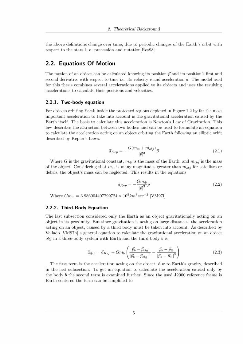
Figure 2.2.: Lunar orbit and orientation with respect to the ecliptica

ahttps://upload.wikimedia.org/wikipedia/commons/4/46/LunarOrbitandOrientationwithrespecttotheEcliptic.svg

calculations. Reason for this is the complex motion of the Moon. The inclination of theMoon’s orbit of about 5 to the ecliptic (Figure 2.2), the third body perturbation, causedby the Sun, and periodic variations of the Moon’s orbit around the Earth, must be takeninto account.

To do this the four time dependent angles ϕM , ϕMa , ϕMpand ϕMSare needed.

ϕM = νtϕMa = νMatϕMp = νMptϕMS

= νMst

(2.9)

Based on these angles the mean anomaly of the Moon lM, the mean elongation from theSun DM, the mean argument of latitude of the Moon, measured on the ecliptic from themean equinox of date FM and the Moon’s longitude L0 can be calculated with

lM = ϕMa + 134.96292

DM = ϕMp + ϕMa − ϕM + 297.85027

FM = ϕMp + ϕMa + ϕMS+ 93.27283

L0 = ϕMp + ϕMa + 218.31617

(2.10)

[VM97g]Using series expansion to calculate the position of the Moon, the values of its ecliptic

latitude λM, its ecliptic longitude βM and the magnitude of its position vector rM aredetermined.

7

2. Theoretical Background

λM = L0 + 13600(22640 sin(lM) + 769 sin(2lM)− 4856 sin(lM − 2DM) + 2370 sin(2DM)

−668 sin(`)− 412 sin(2FM)− 212 sin(2lM − 2DM)− 206 sin(lM + ` − 2DM)+192 sin(lM + 2DM)− 165 sin(` − 2DM) + 148 sin(lM − `)−125 sin(DM)− 110 sin(lM + `)− 55 sin(2FM − 2DM))

(2.11)

βM = 13600(18520 sin

(FM + λM − L0 + 1

3600(412 sin(2FM) + 541 sin(`)))

−526 sin(FM − 2DM) + 44 sin(lM + FM − 2DM)−31 sin(−lM + FM − 2DM)− 25 sin(−2lM + FM)−23 sin(` + FM − 2DM) + 21 sin(−lM + FM)+11 sin(−` + FM − 2DM))

(2.12)

rM = 385000− 20905 cos(lM)− 3699 cos(2DM − lM)−2956 cos(2DM)− 570 cos(2lM) + 246 cos(2lM − 2DM)−205 cos(` − 2DM)− 171 cos(lM + 2DM)− 152 cos(lM + ` − 2DM)

(2.13)

To obtain the position vector ~pM in the J2000 reference frame the equation

~pM =

1 0 00 cos(ε) − sin(ε)0 sin(ε) cos(ε)

·rM cos(λM) cos(βM)rM sin(λM) cos(βM)

rM sin(βM)

(2.14)

is used [VM97a].Now this position can be substituted into the general third body equation 2.5

~aLun = −GmM

(~pobj − ~pM|~pobj − ~pM|3

+~pM

|~pM|3

)(2.15)

Where GmM = 4.9028× 103km3sec−2.

2.2.3. Spherical Harmonics

The Two-Body Equation 2.2 discussed in the subsection 2.2.1 makes assumptions. Oneof these assumptions about the two bodies in question is that they are both sphericallysymmetric and their density is uniform. Because of this assumption, the bodies can betreated as point masses [VM97i]. But this assumption is not true for the Earth. Due to itsrotation, the shape of the Earth is flattened along its rotational axis. Additionally, its densityis not constant. This results in a gravitational potential that is not spherical. Because ofthis, the used model incorporates perturbing accelerations, due to the Earth’s nonsphericalnature and mass distribution, using spherical harmonics.

To calculate accelerations caused by this nonspherical potential, first, the potential Uitself is defined as

U =Gm⊕|~p|

[1 +

∞∑l=2

l∑m=0

(R⊕|~p|

)lPlm[sin(φgc)]Clm cos(mλ) + Slm sin(mλ)

](2.16)

8

2. Theoretical Background

Where the magnitude of the position vector |~p|, the geocentric latitude φgc and the geocentriclongitude λgc are the polar coordinates of the location of the object. Plm[sin(φgc)] are theassociated Legendre functions for the geocentric latitude. The coefficients Clm and Slm areapproximated by analyzing observation data of satellites orbiting the Earth [LPL+89]. Tocalculate the acceleration due to this potential partial derivatives of the potential functionare needed. Resulting in the equation for the acceleration

~aharmonics =∂U

∂|~p|

(∂|~p|∂~p

)T+

∂U

∂φgc

(∂φgc∂~p

)T+

∂U

∂λgc

(∂λgc∂~p

)T(2.17)

.The terms in the equation 2.17 are

∂U∂|~p| = −Gm⊕

|~p|2∞∑l=2

l∑m=0

(R⊕|~p|

)l(l + 1)Plm[sin(φgc)]Clm cos(mλgc) + Slm sin(mλgc)

∂U∂φgc

= Gm⊕|~p|2

∞∑l=2

l∑m=0

(R⊕|~p|

)lPl,m+1[sin(φgc)]−m tan(φgc)Plm[sin(φgc)]

×Clm cos(mλgc) + Slm sin(mλgc)∂U∂λgc

= Gm⊕|~p|2

∞∑l=2

l∑m=0

(R⊕|~p|

)lmPlm[sin(φgc)]Slm cos(mλgc) + Clm sin(mλgc)

∂|~p|∂~p = ~pT

|~p|∂φgc∂~p = 1

p2x+p2y

(− ~pT pz|~p|2 + ∂pz

∂~p

)∂λgc∂~p = 1

p2x+p2y

(px

∂py∂~p − py

∂px∂~p

)(2.18)

Putting these terms together the resulting equations for the components of the acceleration~aharmonics are

aharmonicsx =

(1|~p|

∂U∂|~p| −

pz|~p|2√p2x+p

2y

∂U∂φgc

)px −

(1

p2x+p2y

∂U∂λgc

)py

aharmonicsy =

(1|~p|

∂U∂|~p| + pz

|~p|2√p2x+p

2y

∂U∂φgc

)py −

(1

p2x+p2y

∂U∂λgc

)px

aharmonicsz = 1|~p|

∂U∂|~p|pz +

√p2x+p

2y

|~p|2∂U∂

(2.19)

[VM97f]

Zonal Harmonics

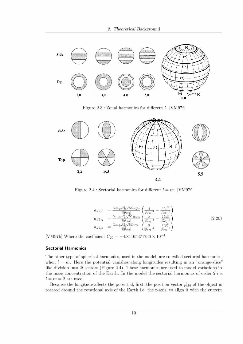
If m = 0, the dependency on longitudinal potential vanishes completely. This results in asymmetrical potential w.r.t. the polar axis i.e. bands of latitude (Figure 2.3). The resultingspherical harmonics are called zonal harmonics. Zonal harmonics are named Jl. In themodel used in this thesis, the J2 i.e. l = 2 is used, because it is the most significant one andis used to simulate the oblateness of the Earth due to its rotation. Using l = 2 and m = 0,equation 2.19 can be converted into

9

2. Theoretical Background

Figure 2.3.: Zonal harmonics for different l. [VM97f]

Figure 2.4.: Sectorial harmonics for different l = m. [VM97f]

aJ2,x =Gm⊕R2

E

√5C20px

2|~pobj |

(3

|~pobj |4− 15p2z|~pobj |6

)aJ2,y =

Gm⊕R2E

√5C20py

2|~pobj |

(3

|~pobj |4− 15p2z|~pobj |6

)aJ2,z =

Gm⊕R2E

√5C20pz

2|~pobj |

(9

|~pobj |4− 15p2z|~pobj |6

) (2.20)

[VM97b] Where the coefficient C20 = −4.84165371736× 10−4.

Sectorial Harmonics

The other type of spherical harmonics, used in the model, are so-called sectorial harmonics,when l = m. Here the potential vanishes along longitudes resulting in an ”orange-slice”like division into 2l sectors (Figure 2.4). These harmonics are used to model variations inthe mass concentration of the Earth. In the model the sectorial harmonics of order 2 i.e.l = m = 2 are used.

Because the longitude affects the potential, first, the position vector ~pobj of the object isrotated around the rotational axis of the Earth i.e. the z-axis, to align it with the current

10

2. Theoretical Background

orientation of the Earth. Where the angle θG + νEt is the angle the Earth rotated sincet = 0.

~d =

cos(θG + νEt) sin(θG + νEt) 0− sin(θG + νEt) cos(θG + νEt) 0

0 0 1

~pobj (2.21)

Using l = m = 2 in the equation 2.19 the vectors ~c22 and ~s22 can be calculated.

c22,x =5Gm⊕R2

⊕√15C22dx(d2y−d2x)2|~d|7

+Gm⊕R2

⊕√15C22dy

|~d|5

c22,y =5Gm⊕R2

⊕√15C22dy(d2y−d2x)2|~d|7

− Gm⊕R2⊕√15C22dx

|~d|5

c22,z =5Gm⊕R2

⊕√15C22dz(d2y−d2x)2|~d|7

(2.22)

With the coefficient C22 = 2.43914352398× 10−6.

s22,x = −5Gm⊕R2⊕√15S22d2xdy

|~d|7+

Gm⊕R2⊕√15S22dx

|~d|5

s22,y = −5Gm⊕R2⊕√15S22dxd2y

|~d|7+

Gm⊕R2⊕√15S22dy

|~d|5

s22,z = −5Gm⊕R2⊕√15S22dxdydz

|~d|7

(2.23)

Where S22 = −1.40016683654× 10−6.To rotate the results back to the actual position, the Matrix M is defined as

M =

cos(θG + νEt) − sin(θG + νEt) 0sin(θG + νEt) cos(θG + νEt) 0

0 0 1

(2.24)

Now the two vectors can be rotated around the z-axis resulting in the two accelerationvectors

~aC22 = M~c22 (2.25)

~aS22 = M~s22 (2.26)

The sum of ~aC22 and ~aS22 is a solution of equation 2.19 with l = m = 2.

2.2.4. Solar Radiation Pressure

After discussing gravitational effects and their resulting accelerations for an object in orbit,there are other sources of acceleration that are integrated into the model. The first one ofthem is the solar radiation pressure, caused by the impulse of the Sun’s radiation that istransferred on an object if the object is hit by it. The acceleration aused by this pressurecan be calculated using

~aSRP = −PSRP cRAm

(~p− ~p|~p− ~p|

)(2.27)

. Where PSRP = 4.56 × 10−6N/m2 is the solar radiation pressure at the distance of oneastronomical unit from the Sun. A is the surface of the object exposed to the Sun’s

11

2. Theoretical Background

radiation, cR is the reflectivity of the object, ~p−~p is the connecting vector between the Sunand the object, and m is the mass of the object. The Sun’s position ~p can be calculatedusing Equation 2.7.

The used model is not using A, cr and m directly. Instead, it introduces the factorAOM , which combines A and m for a given object and is given before the calculation andcr is assumed to be 1. This results in the equation

~aSRP = PSRPAOM~p− ~p|~p− ~p|

(2.28)

This equation assumes the distance between the Sun and the object is exactly oneastronomical unit. To get a better approximation of the acceleration the scaling factorAU2

|~p−~p|2 is introduced. The result is the used equation

~aSRP = AU2PSRPAOM~p− ~p|~p− ~p|3

(2.29)

2.2.5. Atmospheric Drag

The second non-conservative acceleration included in the model is the one caused by thefriction between the Earth’s atmosphere and an orbiting object.

Because the density of the Earth’s atmosphere p (not to be confused with the positionvector ~p) decreases with the distance from the Earth, near the Earth, the influence ofatmospheric drag is extremely strong compared to other perturbing effects, but at higheraltitudes effects like third bodies or the solar radiation pressure become more dominant.The drag effect retards the object’s motion i.e. the direction of the acceleration is oppositeof the object’s velocity w.r.t. to the atmosphere ~vrel, resulting in a loss of altitude.

The general equation to calculate the acceleration caused by the drag is

~aDrag = −1

2

cDA

mp|~vrel|2

~vrel|~vrel|

(2.30)

Where cD is the coefficient of drag. This value reflects how strong the influence of thedrag effect is on an object. Spheres approximately have a cD ∼ 2 to 2.1, a flat plate oneof cD ∼ 2.2. A is the cross-section area normal to the object’s velocity vector. Because todetermine A the orientation of the object is needed with a high, almost impossible to know,accuracy, its value is approximated and constant in the used model. Calculating Equation2.30 requires the values for p and ~vrel, that must be determined. To get the velocity relativeto the atmosphere, a model of the motion of the atmosphere itself must be chosen.

The chosen model is only using the Earth’s rotation and the position of the object,neglecting other factors like wind.

~vrel = ~vobj − ~ω⊕ × ~pobj =

vobjx − ω⊕pobjyvobjy + ω⊕pobjxvobjz

(2.31)

Where

~ω⊕ =

00ω⊕

(2.32)

12

2. Theoretical Background

is the rotational vector of the Earth and ω⊕ = 7.292115 × 10−5 rads . Determining theatmospheric density p can be arbitrarily complex, because the number of factors influencingit is high, and many of them are themselves highly complex to model and interact with eachother.

For example one can consider [VM07]:

• The temperature of the atmosphere

• The magnetic field of the Earth

• Latitudinal and longitudinal variations of the atmosphere

• The influence of the Sun’s activity on the atmosphere

• Winds

• Tides

The chosen model of the atmosphere is very simple. It assumes the density of theatmosphere decreases exponentially with the distance from the Earth’s surface.

p = p0 exp

(−|~pobj | −R⊕

H

)(2.33)

Where p0 = 1.3kgm−3 is the atmospheric density at ground level and H = 8.5km is theatmospheric scale factor [Fit12].

2.2.6. Cowell’s Formulation

As mentioned above, ~aKep is by far the main acceleration acting on an object near theEarth. The other described effects cause perturbations on this acceleration. To formulatetotal equations of motion to be integrated using numerical methods like in this thesis, theperturbing accelerations of n sources can be added linearly to ~aKep to get the acceleration

~a = ~aKep +n∑i=1

~apertubredi (2.34)

This formulation is known as Cowell’s formulation. Advantageous about this formulationis the fact, that perturbations can be added or removed easily, without affecting thecalculations of any of the other ones [VM97d]. Substituting all accelerations, describedabove, into Cowell’s formulation the result is

~a = ~aKep + ~aSol + ~aLun + ~aJ2 + ~aC22 + ~aS22 + ~aSRP + ~aDrag (2.35)

This equation is used in this thesis.

2.3. Integration

To determine the motion of an object, the state of the object i.e. its position ~pi and itsderivatives ~pi and ~pi a.k.a its velocity ~vi and acceleration ~ai, is calculated along a grid ofpoints in time ti = t0 + ∆t ∗ i, with i = 1, 2, 3..., the step size ∆t and starting time t0.

13

2. Theoretical Background

This leads to the problem of determining the state at the next time step i+ 1. To solvethis problem numerical integration is used. The used numerical integration method for thisthesis is the leapfrog method. This method defines the equations

~vi+1/2 = ~vi−1/2 + ~ai∆t

~pi+1 = ~pi + ~vi+1/2∆t(2.36)

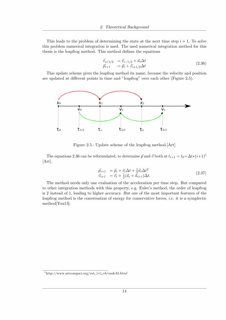
This update scheme gives the leapfrog method its name, because the velocity and positionare updated at different points in time and ”leapfrog” over each other (Figure 2.5).

Figure 2.5.: Update scheme of the leapfrog method.[Art]

The equations 2.36 can be reformulated, to determine ~p and ~v both at ti+1 = t0+∆t∗(i+1)1

[Art].

~pi+1 = ~pi + ~vi∆t+ 12~ai∆t

2

~vi+1 = ~vi + 12(~ai + ~ai+1)∆t.

(2.37)

The method needs only one evaluation of the acceleration per time step. But comparedto other integration methods with this property, e.g. Euler’s method, the order of leapfrogis 2 instead of 1, leading to higher accuracy. But one of the most important features of theleapfrog method is the conversation of energy for conservative forces, i.e. it is a symplecticmethod[You13].

1http://www.artcompsci.org/vol1/v1web/node34.html

14

3. Related Work

There are lots of software solutions, that are used for orbit propagation. One of the oldestgroups of them is the Simplified General Perturbations (SGP) model series. The developmentof these orbit propagators began in the 1960s and one of them that is used by NASA andother organizations is the Simplified General Perturbations-4 (SGP4) propagator publishedin 1980[VCHK06].

Because the SGP4 model produces an error of more than 1 km per day, it is not suited tosimulate large amounts of time into the future. It is used to track objects orbiting Earth,but due to the error in the predicted trajectories, the state of the objects frequently has tobe corrected using observation data.

Another software developed and used by the ESA is the pykep library. The pykep libraryconsists of highly specialized and optimized modules, that are used for mission planning andresearch. But no module for trajectory propagation of a great number of particles orbitingEarth is available yet1.

Because the goal of this thesis is to build a software solution, that can efficiently calculatethe trajectory of an object orbiting Earth, a state of the art tool is needed to compare thedeveloped solution’s performance. For this purpose, the heyoka tool is used. This is a C++library, developed to integrate systems of ordinary differential equations, using Taylor’smethod. Taylor’s method, in short, uses Taylor expansion around the point in time t = t0to determine the solution xt1 at a point in time t1, using the starting condition x0.

xt1 = x0 + x′(t0)h+1

2x′′(t0)h

2 + ...+xp(t0)

p!hp (3.1)

Where h = t1 − t0 is the time step, p is the order of the Taylor method and xn(t) is the nth

derivative of x(t) [BI21].By increasing p the integration error ε of the method can be reduced. On the other hand,

the required calculations grow quadratic with respect to p, resulting in a trade-off betweenprecision and speed. Because of this, heyoka can be used to calculate solutions of a givensystem of ordinary differential equations with ε being smaller than machine precision.

In this thesis heyoka is used to calculate solutions for the model derived in Section 2.2 withmachine precision. These solutions are used as ground truth in Section 5.2. The softwaredeveloped for this thesis tries to achieve a better error behavior than propagators like SGP4for a large number of simulated particles, without being as computational demanding as ahigh order Taylor integrator like heyoka.

1https://esa.github.io/pykep/documentation/index.html

15

Part II.

Implementation

16

4. Implementation

As a practical part of this thesis, a C++ software solution is developed to use numericalintegration, to efficiently model the trajectories of a great number of objects, followingNewton’s Laws of motion based on the acceleration model explained in Section 2.2.

4.1. Data Structures

To develop software to determine the trajectory of a particle using the model described inSection 2.2, first, a data structure to store the state of a particle is needed.

Since the leapfrog method described in Section 2.3 is used for integration, this datastructure has to store the values used in Equation 2.37. Other required properties of theobjects are the factors needed to calculate the solar radiation pressure using Equation 2.29and the atmospheric drag using Equation 2.30. The first one uses the factor AOM thatrepresents the ratio between the object’s area affected by the solar radiation and the object’smass. The second one contains the factor cDA

m , i.e. the inverse of the so-called ballisticcomponent m

cDtimes the cross-section area A of the object. Both of these values are assumed

constant in the used model and are saved in the object’s data structure.The used data object is the Debris class with the following data members:

• The 3D position vector of the object of the current time step in km

• The 3D velocity vector of the object of the current time step in kms

• The 3D acceleration vector of the last time step acc t0 in kms2

• The 3D acceleration vector of the current time step acc t1 kms2

• The object’s area over mass factor aom in km2

kg

• The object’s inverse ballistic component times the object’s cross section area bc inv

in kgm2

Because the developed software is designed to simulate multiple objects in parallel, theDebrisContainer class is introduced. The purpose of a DebrisContainer object is to holda vector object of Debris objects and managing access to these Debris objects.

4.2. Acceleration Calculation

The developed software uses a pattern of linearly adding up accelerations due to differentperturbation forces. This calculation scheme is an implementation of Cowell’s formulationdescribed in Section 2.2.6.

The AccelerationAccumulator class is responsible for managing the calculations of theseaccelerations. To achieve this an AccelerationAccumulator object holds the current time

17

4. Implementation

of the simulation and a reference to a central DebrisContainer object, holding the Debris

objects to simulate. Objects of this class can be configured to toggle the calculation of thedifferent acceleration sources. This is done using the confi array of boolean values indexedby an enumeration of the AccelerationComponents.

The eight AccelerationComponents and their corresponding accelerations are:

• KepComponent : aKep Equation 2.2

• J2Component : aJ2 Equation 2.20

• C22Component : aC22 Equation 2.25

• S22Component : aS22 Equation 2.26

• LunComponent : aLun Equation 2.15

• SolComponent : aSol Equation 2.8

• SRPComponent : aSRP Equation 2.29

• DragComponent : aDrag Equation 2.30

The calculation of the accelerations per time step can be divided into two parts:

1. Determine the object independent state of the simulated system.

2. Calculate the activated acceleration components for all particles. Per particle this canbe divided into two sub steps by itself:

a) Calculate values needed for more than one component.

b) Calculate the actual component accelerations.

During step 1. some values needed for the calculation of the accelerations can be determinedand reused for all particles to reduce the number of calculations per particle. The two termscos(θG + νEt) and sin(θG + νEt) needed for the spherical harmonics components J2, C22 andS22 are both independent of the particle and constant for one time step. The calculations ofthe Sun’s and Moon’s position relative to the reference frame, and terms depending onlyon them, are also independent of the particle and constant for one time step. These valuesare calculated in the setUp method of the corresponding AccelerationComponent. At thebeginning of each time step, the AccelerationAccumulator object calls these methods forall activated components and passes references to the results as parameters for the actualcalculations done per particle.

During step 2. the AccelerationAccumulator iterates over all Debris objects, managedby the central DebrisContainer, and applies all activated components by accumulating theaccelerations returned by the components apply method. For a given particle and a giventime step, there are again some values, that can be calculated once and used in multiplecalculations for different components. In particular, the calculations of aSun and aSRP bothdepend on the distance between the particle and the Sun. So if both components have to becalculated the value is only calculated once and passed as a parameter to the apply methodsof the SRPComponent after being calculated by the SolComponent.

18

4. Implementation

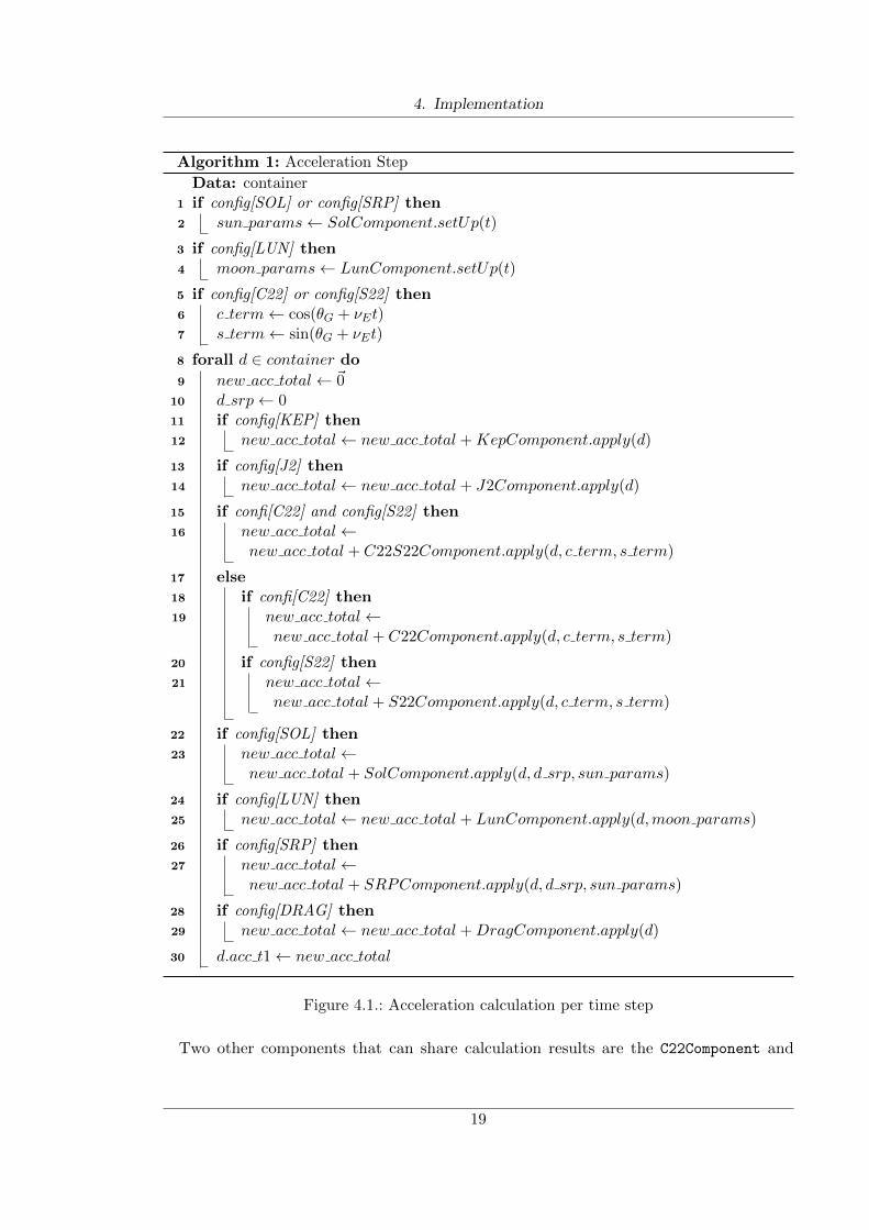
Algorithm 1: Acceleration Step

Data: container1 if config[SOL] or config[SRP] then2 sun params← SolComponent.setUp(t)

3 if config[LUN] then4 moon params← LunComponent.setUp(t)

5 if config[C22] or config[S22] then6 c term← cos(θG + νEt)7 s term← sin(θG + νEt)

8 forall d ∈ container do

9 new acc total← ~010 d srp← 011 if config[KEP] then12 new acc total← new acc total +KepComponent.apply(d)

13 if config[J2] then14 new acc total← new acc total + J2Component.apply(d)

15 if confi[C22] and config[S22] then16 new acc total←

new acc total + C22S22Component.apply(d, c term, s term)

17 else18 if confi[C22] then19 new acc total←

new acc total + C22Component.apply(d, c term, s term)

20 if config[S22] then21 new acc total←

new acc total + S22Component.apply(d, c term, s term)

22 if config[SOL] then23 new acc total←

new acc total + SolComponent.apply(d, d srp, sun params)

24 if config[LUN] then25 new acc total← new acc total + LunComponent.apply(d,moon params)

26 if config[SRP] then27 new acc total←

new acc total + SRPComponent.apply(d, d srp, sun params)

28 if config[DRAG] then29 new acc total← new acc total +DragComponent.apply(d)

30 d.acc t1← new acc total

Figure 4.1.: Acceleration calculation per time step

Two other components that can share calculation results are the C22Component and

19

4. Implementation

S22Component. Because the Equations 2.25 and 2.26 share a lot of terms, an extraAccelerationComponent C22S22Component is introduced. This new component calculatesthe sum aC22 + aS22 in one apply method, taking advantage of the similarity between thesecomponents. As the last step for each particle, the accumulated acceleration is written tothe Debris object. The resulting algorithm is depicted in Figure 4.1 for one time step. Toachieve better calculation performance, some basic optimizations are made for all componentswhenever possible.

Calculate constants up front If the equations to calculate the acceleration contain termsthat can be precalculated at compile time, the AccelerationComponent provides constantmethods to avoid recalculating these terms.

Replace divisions with multiplications For many architectures the division operation issignificantly slower than the multiplication operation. If the divisions b

a and ca must be

calculated, the number of division operations can be reduced by calculating the inversea−1 = 1

a once and replacing all divisions by a with a multiplication with a−1 to ba−1 andca−1.

Factorize terms and calculate factors once If two terms a and b can be factorized intothe form a = cd and b = ce the shared factor c is calculated only once.

Use multiplication instead of std::pow method To avoid overhead when using the stan-dard library std::pow, all powers are hardcoded as multiplications.

To avoid numerical errors, due to rounding errors, when adding to numbers of differentmagnitude, the operations are ordered in such a way, that numbers are added in ascendingorder. This is mainly used for the series expansions in Equations 2.11., 2.12 and 2.13 whilecalculating aLun.

4.3. Numerical Integration

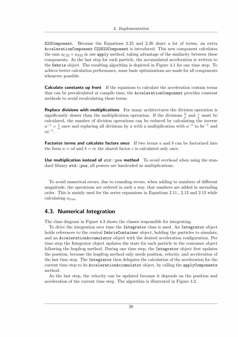
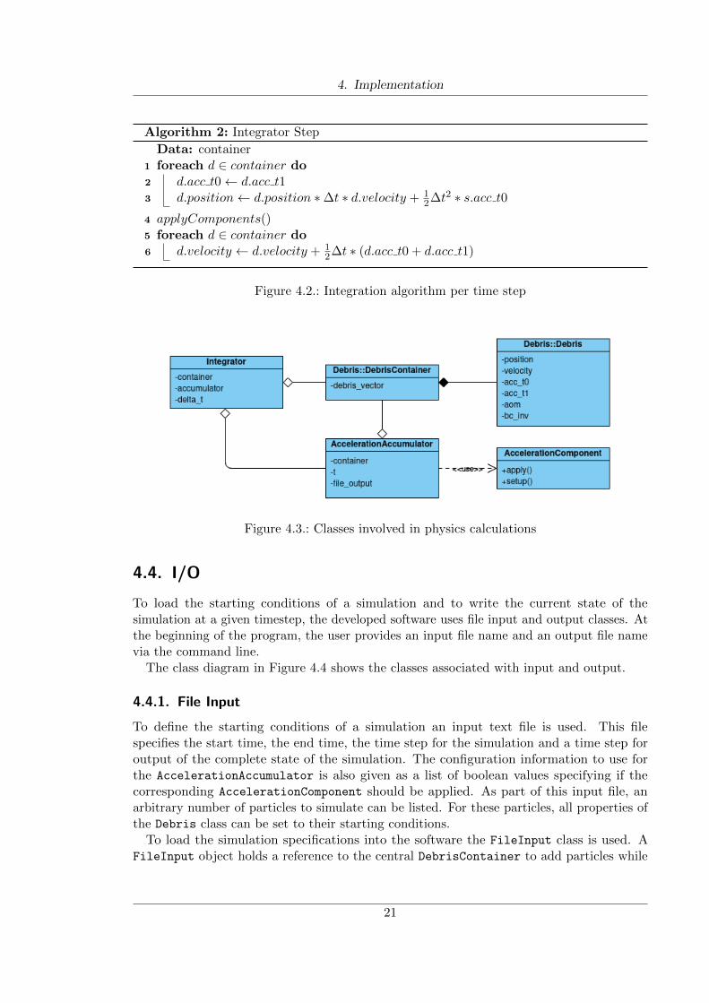
The class diagram in Figure 4.3 shows the classes responsible for integrating.To drive the integration over time the Integrator class is used. An Integrator object

holds references to the central DebrisContainer object, holding the particles to simulate,and an AccelerationAccumulator object with the desired acceleration configuration. Pertime step the Integrator object updates the state for each particle in the container objectfollowing the leapfrog method. During one time step, the Integrator object first updatesthe position, because the leapfrog method only needs position, velocity, and acceleration ofthe last time step. The Integrator then delegates the calculation of the acceleration for thecurrent time step to its AccelerationAccumulator object, by calling the applyComponentsmethod.

As the last step, the velocity can be updated because it depends on the position andacceleration of the current time step. The algorithm is illustrated in Figure 4.2.

20

4. Implementation

Algorithm 2: Integrator Step

Data: container1 foreach d ∈ container do2 d.acc t0← d.acc t13 d.position← d.position ∗∆t ∗ d.velocity + 1

2∆t2 ∗ s.acc t04 applyComponents()5 foreach d ∈ container do6 d.velocity ← d.velocity + 1

2∆t ∗ (d.acc t0 + d.acc t1)

Figure 4.2.: Integration algorithm per time step

Figure 4.3.: Classes involved in physics calculations

4.4. I/O

To load the starting conditions of a simulation and to write the current state of thesimulation at a given timestep, the developed software uses file input and output classes. Atthe beginning of the program, the user provides an input file name and an output file namevia the command line.

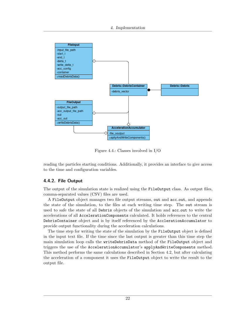
The class diagram in Figure 4.4 shows the classes associated with input and output.

4.4.1. File Input

To define the starting conditions of a simulation an input text file is used. This filespecifies the start time, the end time, the time step for the simulation and a time step foroutput of the complete state of the simulation. The configuration information to use forthe AccelerationAccumulator is also given as a list of boolean values specifying if thecorresponding AccelerationComponent should be applied. As part of this input file, anarbitrary number of particles to simulate can be listed. For these particles, all properties ofthe Debris class can be set to their starting conditions.

To load the simulation specifications into the software the FileInput class is used. AFileInput object holds a reference to the central DebrisContainer to add particles while

21

4. Implementation

Figure 4.4.: Classes involved in I/O

reading the particles starting conditions. Additionally, it provides an interface to give accessto the time and configuration variables.

4.4.2. File Output

The output of the simulation state is realized using the FileOutput class. As output files,comma-separated values (CSV) files are used.

A FileOutput object manages two file output streams, out and acc out, and appendsthe state of the simulation, to the files at each writing time step. The out stream isused to safe the state of all Debris objects of the simulation and acc out to write theaccelerations of all AccelerationComponents calculated. It holds references to the centralDebrisContainer object and is by itself referenced by the AcclerationAccumulator toprovide output functionality during the acceleration calculations.

The time step for writing the state of the simulation by the FileOutput object is definedin the input text file. If the time since the last output is greater than this time step themain simulation loop calls the writeDebrisData method of the FileOutput object andtriggers the use of the AccelerationAccumulator’s applyAndWriteComponents method.This method performs the same calculations described in Section 4.2, but after calculatingthe acceleration of a component it uses the FileOutput object to write the result to theoutput file.

22

Part III.

Results

23

5. Results

5.1. Used Hardware and Software

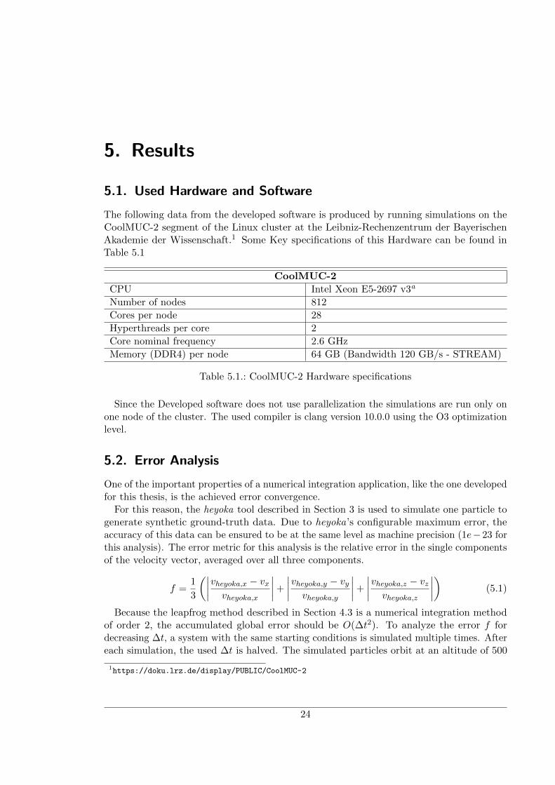
The following data from the developed software is produced by running simulations on theCoolMUC-2 segment of the Linux cluster at the Leibniz-Rechenzentrum der BayerischenAkademie der Wissenschaft.1 Some Key specifications of this Hardware can be found inTable 5.1

CoolMUC-2

CPU Intel Xeon E5-2697 v3a

Number of nodes 812

Cores per node 28

Hyperthreads per core 2

Core nominal frequency 2.6 GHz

Memory (DDR4) per node 64 GB (Bandwidth 120 GB/s - STREAM)

Table 5.1.: CoolMUC-2 Hardware specifications

Since the Developed software does not use parallelization the simulations are run only onone node of the cluster. The used compiler is clang version 10.0.0 using the O3 optimizationlevel.

5.2. Error Analysis

One of the important properties of a numerical integration application, like the one developedfor this thesis, is the achieved error convergence.

For this reason, the heyoka tool described in Section 3 is used to simulate one particle togenerate synthetic ground-truth data. Due to heyoka’s configurable maximum error, theaccuracy of this data can be ensured to be at the same level as machine precision (1e−23 forthis analysis). The error metric for this analysis is the relative error in the single componentsof the velocity vector, averaged over all three components.

f =1

3

(∣∣∣∣vheyoka,x − vxvheyoka,x

∣∣∣∣+

∣∣∣∣vheyoka,y − vyvheyoka,y

∣∣∣∣+

∣∣∣∣vheyoka,z − vzvheyoka,z

∣∣∣∣) (5.1)

Because the leapfrog method described in Section 4.3 is a numerical integration methodof order 2, the accumulated global error should be O(∆t2). To analyze the error f fordecreasing ∆t, a system with the same starting conditions is simulated multiple times. Aftereach simulation, the used ∆t is halved. The simulated particles orbit at an altitude of 500

1https://doku.lrz.de/display/PUBLIC/CoolMUC-2

24

5. Results

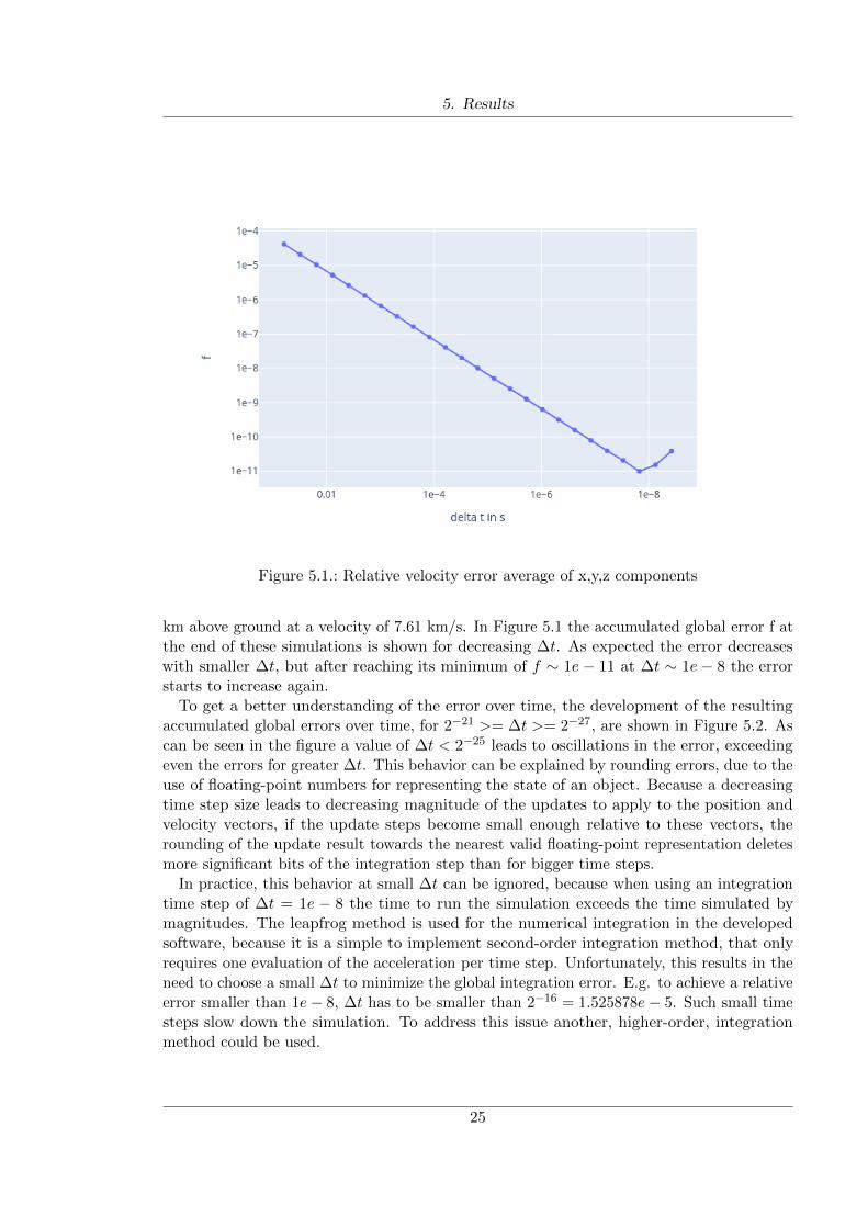
Figure 5.1.: Relative velocity error average of x,y,z components

km above ground at a velocity of 7.61 km/s. In Figure 5.1 the accumulated global error f atthe end of these simulations is shown for decreasing ∆t. As expected the error decreaseswith smaller ∆t, but after reaching its minimum of f ∼ 1e− 11 at ∆t ∼ 1e− 8 the errorstarts to increase again.

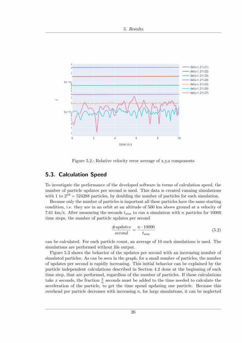
To get a better understanding of the error over time, the development of the resultingaccumulated global errors over time, for 2−21 >= ∆t >= 2−27, are shown in Figure 5.2. Ascan be seen in the figure a value of ∆t < 2−25 leads to oscillations in the error, exceedingeven the errors for greater ∆t. This behavior can be explained by rounding errors, due to theuse of floating-point numbers for representing the state of an object. Because a decreasingtime step size leads to decreasing magnitude of the updates to apply to the position andvelocity vectors, if the update steps become small enough relative to these vectors, therounding of the update result towards the nearest valid floating-point representation deletesmore significant bits of the integration step than for bigger time steps.

In practice, this behavior at small ∆t can be ignored, because when using an integrationtime step of ∆t = 1e − 8 the time to run the simulation exceeds the time simulated bymagnitudes. The leapfrog method is used for the numerical integration in the developedsoftware, because it is a simple to implement second-order integration method, that onlyrequires one evaluation of the acceleration per time step. Unfortunately, this results in theneed to choose a small ∆t to minimize the global integration error. E.g. to achieve a relativeerror smaller than 1e− 8, ∆t has to be smaller than 2−16 = 1.525878e− 5. Such small timesteps slow down the simulation. To address this issue another, higher-order, integrationmethod could be used.

25

5. Results

Figure 5.2.: Relative velocity error average of x,y,z components

5.3. Calculation Speed

To investigate the performance of the developed software in terms of calculation speed, thenumber of particle updates per second is used. This data is created running simulationswith 1 to 219 = 524288 particles, by doubling the number of particles for each simulation.

Because only the number of particles is important all these particles have the same startingcondition, i.e. they are in an orbit at an altitude of 500 km above ground at a velocity of7.61 km/s. After measuring the seconds tsim to run a simulation with n particles for 10000time steps, the number of particle updates per second

#updates

second=n · 10000

tsim(5.2)

can be calculated. For each particle count, an average of 10 such simulations is used. Thesimulations are performed without file output.

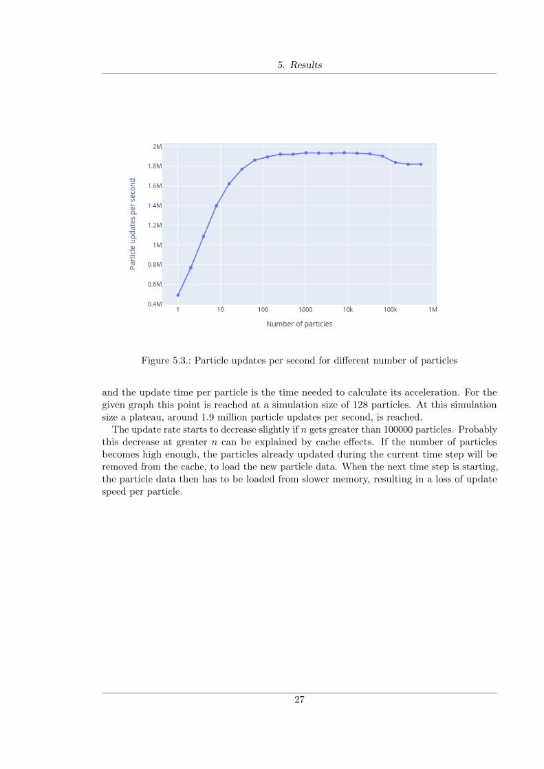
Figure 5.3 shows the behavior of the updates per second with an increasing number ofsimulated particles. As can be seen in the graph, for a small number of particles, the numberof updates per second is rapidly increasing. This initial behavior can be explained by theparticle independent calculations described in Section 4.2 done at the beginning of eachtime step, that are performed, regardless of the number of particles. If these calculationstake x seconds, the fraction x

n seconds must be added to the time needed to calculate theacceleration of the particle, to get the time spend updating one particle. Because thisoverhead per particle decreases with increasing n, for large simulations, it can be neglected

26

5. Results

Figure 5.3.: Particle updates per second for different number of particles

and the update time per particle is the time needed to calculate its acceleration. For thegiven graph this point is reached at a simulation size of 128 particles. At this simulationsize a plateau, around 1.9 million particle updates per second, is reached.

The update rate starts to decrease slightly if n gets greater than 100000 particles. Probablythis decrease at greater n can be explained by cache effects. If the number of particlesbecomes high enough, the particles already updated during the current time step will beremoved from the cache, to load the new particle data. When the next time step is starting,the particle data then has to be loaded from slower memory, resulting in a loss of updatespeed per particle.

27

5. Results

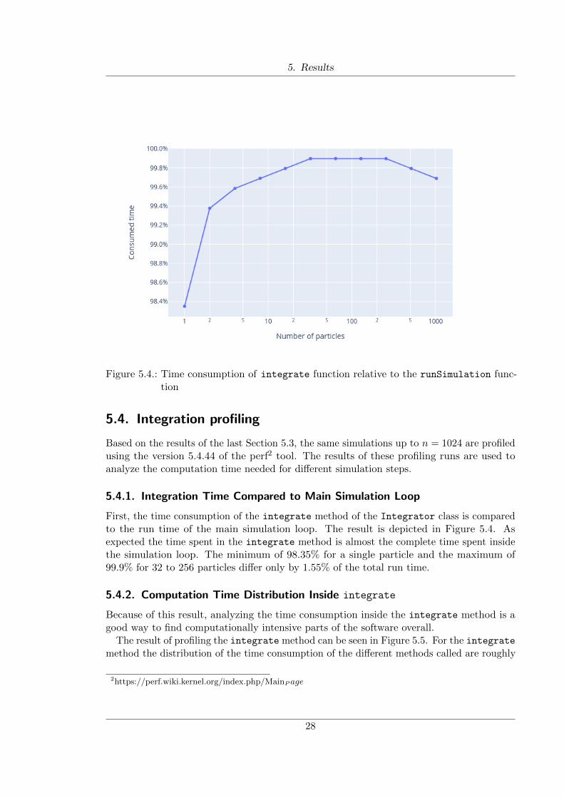
Figure 5.4.: Time consumption of integrate function relative to the runSimulation func-tion

5.4. Integration profiling

Based on the results of the last Section 5.3, the same simulations up to n = 1024 are profiledusing the version 5.4.44 of the perf2 tool. The results of these profiling runs are used toanalyze the computation time needed for different simulation steps.

5.4.1. Integration Time Compared to Main Simulation Loop

First, the time consumption of the integrate method of the Integrator class is comparedto the run time of the main simulation loop. The result is depicted in Figure 5.4. Asexpected the time spent in the integrate method is almost the complete time spent insidethe simulation loop. The minimum of 98.35% for a single particle and the maximum of99.9% for 32 to 256 particles differ only by 1.55% of the total run time.

5.4.2. Computation Time Distribution Inside integrate

Because of this result, analyzing the time consumption inside the integrate method is agood way to find computationally intensive parts of the software overall.

The result of profiling the integrate method can be seen in Figure 5.5. For the integratemethod the distribution of the time consumption of the different methods called are roughly

2https://perf.wiki.kernel.org/index.php/MainP age

28

5. Results

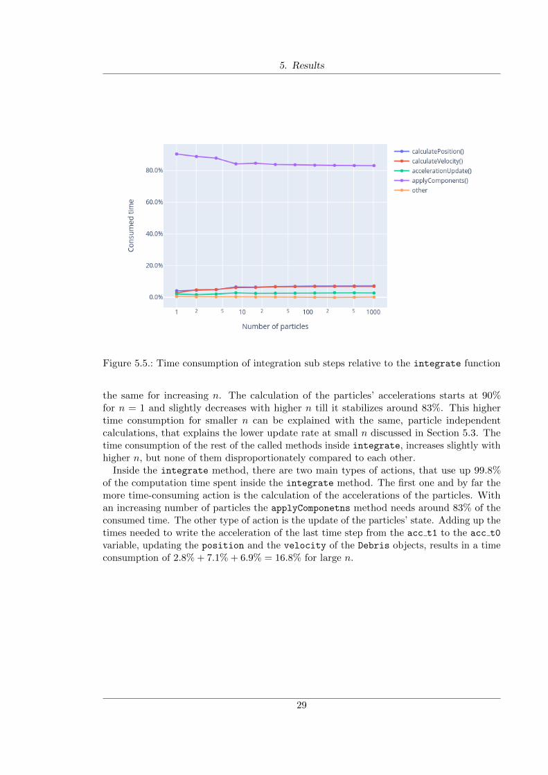
Figure 5.5.: Time consumption of integration sub steps relative to the integrate function

the same for increasing n. The calculation of the particles’ accelerations starts at 90%for n = 1 and slightly decreases with higher n till it stabilizes around 83%. This highertime consumption for smaller n can be explained with the same, particle independentcalculations, that explains the lower update rate at small n discussed in Section 5.3. Thetime consumption of the rest of the called methods inside integrate, increases slightly withhigher n, but none of them disproportionately compared to each other.

Inside the integrate method, there are two main types of actions, that use up 99.8%of the computation time spent inside the integrate method. The first one and by far themore time-consuming action is the calculation of the accelerations of the particles. Withan increasing number of particles the applyComponetns method needs around 83% of theconsumed time. The other type of action is the update of the particles’ state. Adding up thetimes needed to write the acceleration of the last time step from the acc t1 to the acc t0

variable, updating the position and the velocity of the Debris objects, results in a timeconsumption of 2.8% + 7.1% + 6.9% = 16.8% for large n.

29

5. Results

5.4.3. Computation Time Distribution Inside applyComponents

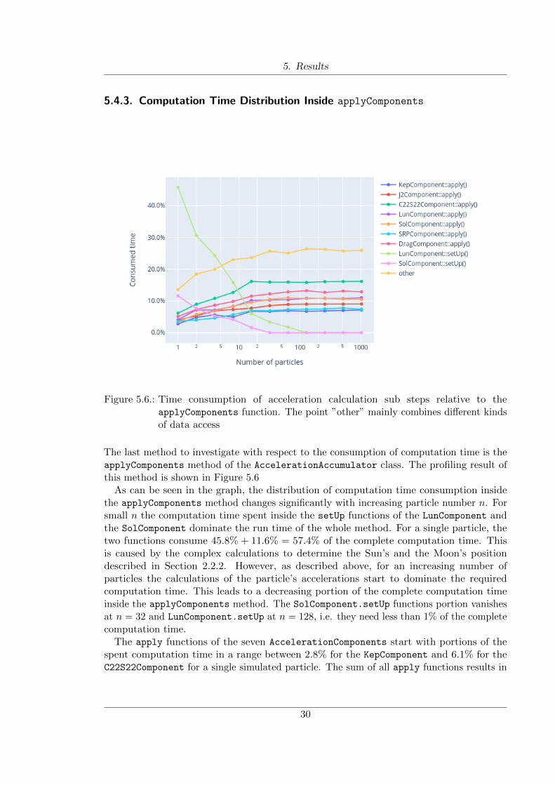
Figure 5.6.: Time consumption of acceleration calculation sub steps relative to theapplyComponents function. The point ”other” mainly combines different kindsof data access

The last method to investigate with respect to the consumption of computation time is theapplyComponents method of the AccelerationAccumulator class. The profiling result ofthis method is shown in Figure 5.6

As can be seen in the graph, the distribution of computation time consumption insidethe applyComponents method changes significantly with increasing particle number n. Forsmall n the computation time spent inside the setUp functions of the LunComponent andthe SolComponent dominate the run time of the whole method. For a single particle, thetwo functions consume 45.8% + 11.6% = 57.4% of the complete computation time. Thisis caused by the complex calculations to determine the Sun’s and the Moon’s positiondescribed in Section 2.2.2. However, as described above, for an increasing number ofparticles the calculations of the particle’s accelerations start to dominate the requiredcomputation time. This leads to a decreasing portion of the complete computation timeinside the applyComponents method. The SolComponent.setUp functions portion vanishesat n = 32 and LunComponent.setUp at n = 128, i.e. they need less than 1% of the completecomputation time.

The apply functions of the seven AccelerationComponents start with portions of thespent computation time in a range between 2.8% for the KepComponent and 6.1% for theC22S22Component for a single simulated particle. The sum of all apply functions results in

30

5. Results

a total portion of 29.1% of the complete computation time. For n = 1024 these values spanfrom 7.1% for the KepComponent, 16.1% for the C22S22Component and a total of 74.0% forall AccelerationComponents.

In contrast to Figures 5.4 and 5.5, a great portion of computation time is spent to accessdata. The different types of data access during the applyComponents method are responsiblefor almost the complete portion of computation time labeled ”other” in Figure 5.6. Foran increasing number of particles this fraction makes up between 13.6% for n = 1 andaround 26% for n > 128. The fact that data access is responsible for such a great amount ofcomputation time, makes it a promising starting point to optimize the used data structuresfor faster data access. This approach would also reduce the time needed to access the particledata during updating their state inside the integrate method analyzed in the last section.

5.5. Acceleration Component Influences

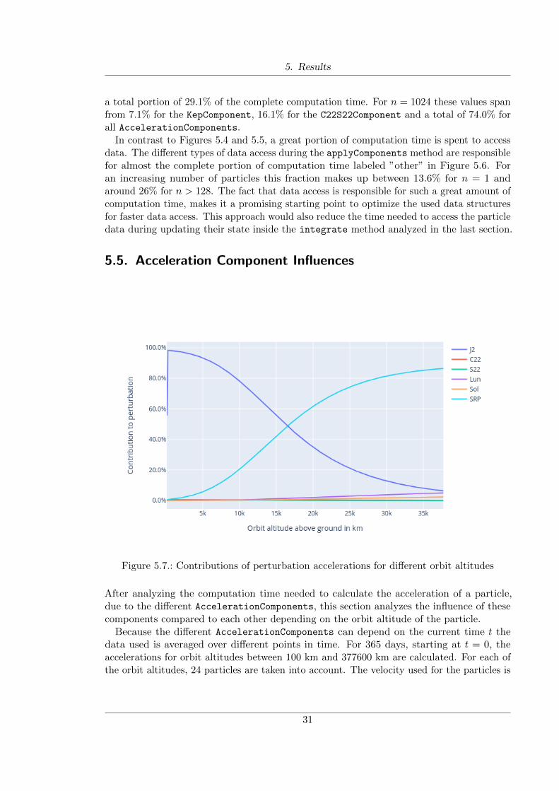
Figure 5.7.: Contributions of perturbation accelerations for different orbit altitudes

After analyzing the computation time needed to calculate the acceleration of a particle,due to the different AccelerationComponents, this section analyzes the influence of thesecomponents compared to each other depending on the orbit altitude of the particle.

Because the different AccelerationComponents can depend on the current time t thedata used is averaged over different points in time. For 365 days, starting at t = 0, theaccelerations for orbit altitudes between 100 km and 377600 km are calculated. For each ofthe orbit altitudes, 24 particles are taken into account. The velocity used for the particles is

31

5. Results

the orbital velocity vorbit determined using the equation3

vorbit =

√398600.5

R⊕ + altitude(5.3)

.These particles cover both protected regions depicted in Figure 1.2Because the acceleration caused by the DragComponent quickly vanishes with the orbit

altitude, additional data for orbit altitudes between 10 km and 1100 km is used to analyzethe DragComponent separately.

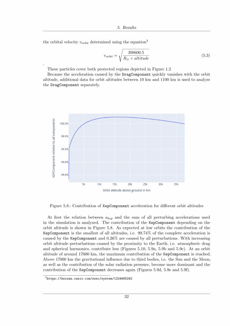
Figure 5.8.: Contribution of KepComponent acceleration for different orbit altitudes

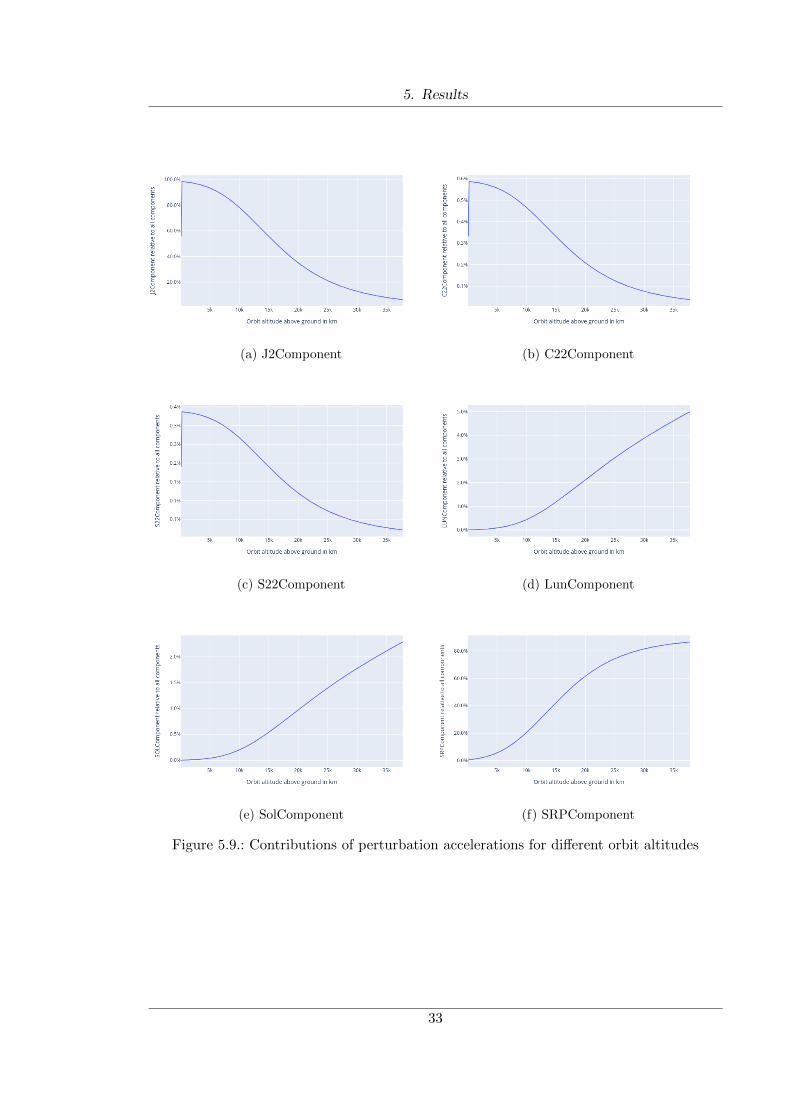
At first the relation between akep and the sum of all perturbing accelerations usedin the simulation is analyzed. The contribution of the KepComponent depending on theorbit altitude is shown in Figure 5.8. As expected at low orbits the contribution of theKepComponent is the smallest of all altitudes, i.e. 99.74% of the complete acceleration iscaused by the KepComponent and 0.26% are caused by all perturbations. With increasingorbit altitude perturbations caused by the proximity to the Earth, i.e. atmospheric dragand spherical harmonics, contribute less (Figures 5.10, 5.9a, 5.9b and 5.9c). At an orbitaltitude of around 17000 km, the maximum contribution of the KepComponent is reached.Above 17000 km the gravitational influence due to third bodies, i.e. the Sun and the Moon,as well as the contribution of the solar radiation pressure, become more dominant and thecontribution of the KepComponent decreases again (Figures 5.9d, 5.9e and 5.9f).

3https://keisan.casio.com/exec/system/1224665242

32

5. Results

(a) J2Component (b) C22Component

(c) S22Component (d) LunComponent

(e) SolComponent (f) SRPComponent

Figure 5.9.: Contributions of perturbation accelerations for different orbit altitudes

33

5. Results

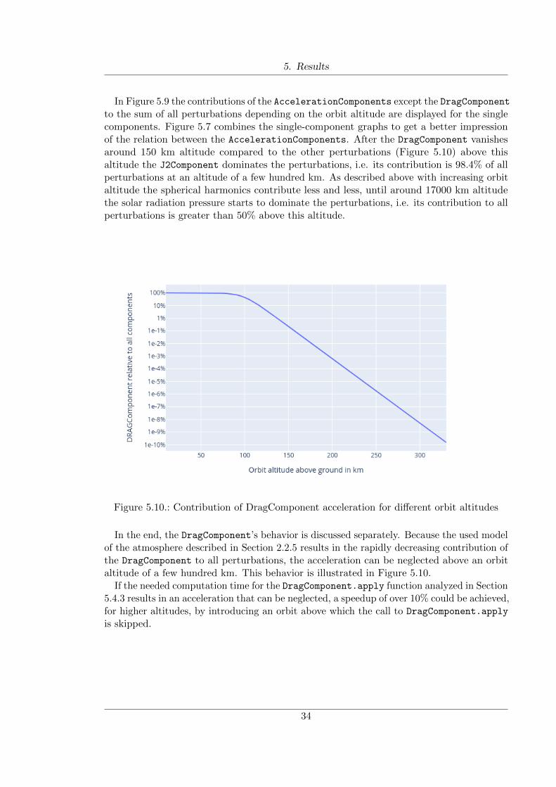
In Figure 5.9 the contributions of the AccelerationComponents except the DragComponentto the sum of all perturbations depending on the orbit altitude are displayed for the singlecomponents. Figure 5.7 combines the single-component graphs to get a better impressionof the relation between the AccelerationComponents. After the DragComponent vanishesaround 150 km altitude compared to the other perturbations (Figure 5.10) above thisaltitude the J2Component dominates the perturbations, i.e. its contribution is 98.4% of allperturbations at an altitude of a few hundred km. As described above with increasing orbitaltitude the spherical harmonics contribute less and less, until around 17000 km altitudethe solar radiation pressure starts to dominate the perturbations, i.e. its contribution to allperturbations is greater than 50% above this altitude.

Figure 5.10.: Contribution of DragComponent acceleration for different orbit altitudes

In the end, the DragComponent’s behavior is discussed separately. Because the used modelof the atmosphere described in Section 2.2.5 results in the rapidly decreasing contribution ofthe DragComponent to all perturbations, the acceleration can be neglected above an orbitaltitude of a few hundred km. This behavior is illustrated in Figure 5.10.

If the needed computation time for the DragComponent.apply function analyzed in Section5.4.3 results in an acceleration that can be neglected, a speedup of over 10% could be achieved,for higher altitudes, by introducing an orbit above which the call to DragComponent.apply

is skipped.

34

Part IV.

Conclusion

35

6. Conclusion

As result of this thesis, the developed software can simulate hundreds of thousands of particles,without slowing down the simulation, due to the large number of particles, achieving anupdate rate of around 2 million particle updates per second. But the number of updatesalone doesn’t say much about the performance of the software, because if the used integrationtime step is small, the total simulated time is smaller too. At this point the order of the usedintegration method must be considered, because a higher-order method allows for biggertime steps. The error of the simulations achieves convergence for reasonable integrationtime steps. But because the used integration method is only second-order, this convergenceis rather slow.

Building upon the software solution developed for this thesis, multiple approaches couldbe followed, to further improve the performance of the software.

Optimizing the used data structures to allow faster data access while iterating over allparticles, could enhance simulation speed. One approach could be the use of a structureof arrays in contrast to the used array of structures. This approach could achieve betterperformance while looping over the particles to simulate, because for most calculations doneduring the simulation only one property of the particles is needed. Using a structure ofarrays to represent the particles could lead to faster memory access because with the firstparticle loaded of each cache line the needed values for the next particles would be cachedand loaded faster in the future.

Incorporating another numerical integration method, that has higher order than the usedleapfrog method, could result in a better error behavior of the software. This would allowincreasing the time steps used for integration, to speed up simulations, without increasingthe integration error of the result.

The developed software solution does not take advantage of possible parallelization.Because the calculations performed per particle are completely independent, parallelizationis probably the best place to start to achieve higher simulation speed. As long as theparticles do not interact, this approach would result in a simply scalable software solutionfor simulating large numbers of particles. If the trajectory calculations of the particles areembedded into bigger software solutions, that needs the simulated particles to interact, i.e.collisions must be handled, parallelization can become harder to exploit, but still worth theefforts.

36

Part V.

Appendix

37

A. Constants

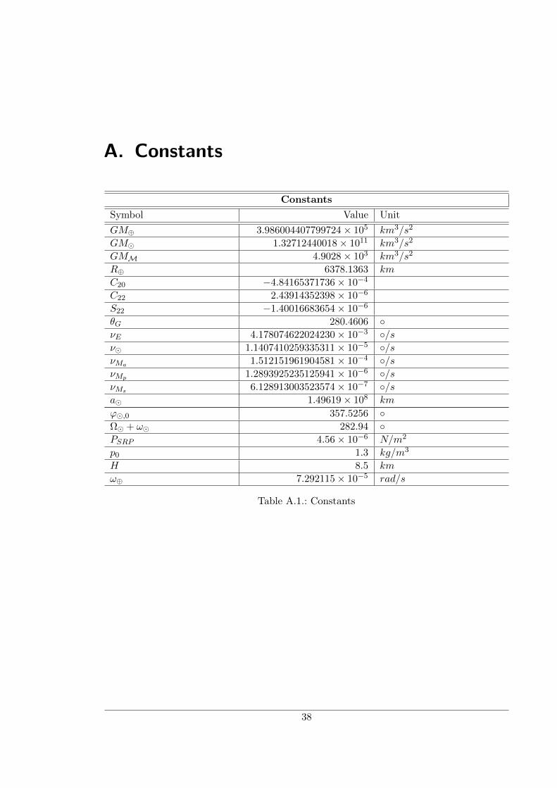
Constants

Symbol Value Unit

GM⊕ 3.986004407799724× 105 km3/s2

GM 1.32712440018× 1011 km3/s2

GMM 4.9028× 103 km3/s2

R⊕ 6378.1363 km

C20 −4.84165371736× 10−4

C22 2.43914352398× 10−6

S22 −1.40016683654× 10−6

θG 280.4606 νE 4.178074622024230× 10−3 /sν 1.1407410259335311× 10−5 /sνMa 1.512151961904581× 10−4 /sνMp 1.2893925235125941× 10−6 /sνMs 6.128913003523574× 10−7 /sa 1.49619× 108 km

ϕ,0 357.5256 Ω + ω 282.94 PSRP 4.56× 10−6 N/m2

p0 1.3 kg/m3

H 8.5 km

ω⊕ 7.292115× 10−5 rad/s

Table A.1.: Constants

38

List of Figures

1.1. Launch traffic . . . . . . . . . . . . . . . . . . . . . . . . . . . . . . . . . . . 21.2. IADC protected regions . . . . . . . . . . . . . . . . . . . . . . . . . . . . . 3

2.1. J2000 reference frame . . . . . . . . . . . . . . . . . . . . . . . . . . . . . . 42.2. Moon’s orbital plane . . . . . . . . . . . . . . . . . . . . . . . . . . . . . . . 72.3. Zonal harmonics . . . . . . . . . . . . . . . . . . . . . . . . . . . . . . . . . 102.4. Sectorial harmonics . . . . . . . . . . . . . . . . . . . . . . . . . . . . . . . . 102.5. Leapfrog scheme . . . . . . . . . . . . . . . . . . . . . . . . . . . . . . . . . 14

4.1. Acceleration calculation per time step . . . . . . . . . . . . . . . . . . . . . 194.2. Integration algorithm per time step . . . . . . . . . . . . . . . . . . . . . . . 214.3. Physics class diagram . . . . . . . . . . . . . . . . . . . . . . . . . . . . . . 214.4. I/O class diagram . . . . . . . . . . . . . . . . . . . . . . . . . . . . . . . . 22

5.1. Relative velocity error . . . . . . . . . . . . . . . . . . . . . . . . . . . . . . 255.2. Relative velocity error . . . . . . . . . . . . . . . . . . . . . . . . . . . . . . 265.3. Particle updates . . . . . . . . . . . . . . . . . . . . . . . . . . . . . . . . . 275.4. Integration time consumption . . . . . . . . . . . . . . . . . . . . . . . . . . 285.5. integrate profile . . . . . . . . . . . . . . . . . . . . . . . . . . . . . . . . . 295.6. applyComponents() profile . . . . . . . . . . . . . . . . . . . . . . . . . . . . 305.7. AcelerationComponents contribution combined . . . . . . . . . . . . . . . . 315.8. Kepler contribution . . . . . . . . . . . . . . . . . . . . . . . . . . . . . . . . 325.9. Acceleration contributions . . . . . . . . . . . . . . . . . . . . . . . . . . . . 335.10. Drag contribution . . . . . . . . . . . . . . . . . . . . . . . . . . . . . . . . . 34

39

List of Tables

5.1. CoolMUC-2 . . . . . . . . . . . . . . . . . . . . . . . . . . . . . . . . . . . . 24

A.1. Constants . . . . . . . . . . . . . . . . . . . . . . . . . . . . . . . . . . . . . 38

40

Bibliography

[Art] Two ways to write the leapfrog,http://www.artcompsci.org/vol 1/v1 web/node34.html

(Date accessed 22. 08. 2021).

[BI21] Francesco Biscani and Dario Izzo. Revisiting high-order Taylor methods forastrodynamics and celestial mechanics, volume 504. 04 2021.

[ESA21] ESA’s annual space environment report. Number 5.0. ESA, 2021.

[Esc65] P.R. Escobal. Methods of Orbit Determination. J. Wiley, 1965.

[Fit12] R. Fitzpatrick. An Introduction to Celestial Mechanics. Cambridge UniversityPress, 2012.

[IAD07] IADC Space Debris Mitigation Guidelines. Number 1. IADC, 2007.

[KCP78] Donald J. Kessler and Burton G. Cour-Palais. Collision frequency of artificialsatellites: The creation of a debris belt. Journal of Geophysical Research: SpacePhysics, 83(A6):2637–2646, 1978.

[LPL+89] A.C. Long, R. Pajerski, R. Luczak, United States. National Aeronautics, SpaceAdministration, and Goddard Space Flight Center. Goddard Trajectory Deter-mination System (GTDS): Mathematical Theory. Goddard Space Flight Center,1989.

[Ros98] D. Rose. International space station familiarization. NASA, 1998.

[VCHK06] David Vallado, Paul Crawford, Ricahrd Hujsak, and T.S. Kelso. Revisitingspacetrack report 3. volume 3, 08 2006.

[VM97a] D.A. Vallado and W.D. McClain. Application: Moon Position Vector, chapter3.6. Primis, 1997.

[VM97b] D.A. Vallado and W.D. McClain. Application: Simplified Acceleration Model,chapter 7.7.1. Primis, 1997.

[VM97c] D.A. Vallado and W.D. McClain. Coordinate Systems, chapter 1.4. Primis, 1997.

[VM97d] D.A. Vallado and W.D. McClain. Cowell’s Formulation, chapter 7.4. Primis,1997.

[VM97e] D.A. Vallado and W.D. McClain. Fundamentals of Astrodynamics and Applica-tions. Primis, 1997.

41

Bibliography

[VM97f] D.A. Vallado and W.D. McClain. Gravity Field of a Central Body, chapter 7.6.1.Primis, 1997.

[VM97g] D.A. Vallado and W.D. McClain. Nutation (J2000), chapter 1.7.2. Primis, 1997.

[VM97h] D.A. Vallado and W.D. McClain. Three-body and n-body Equations, chapter 2.3.Primis, 1997.

[VM97i] D.A. Vallado and W.D. McClain. Two-body Equation, chapter 2.2. Primis, 1997.

[VM07] D.A. Vallado and W.D. McClain. Atmospheric Drag, chapter 8.6.2. MicrocosmPress/Springer, 2007.

[You13] P. Young. The leapfrog method and other “symplectic” algorithms for integratingnewton’s laws of motion. UC Santa Cruz, 2013.

42