Feinstein 2003 Economica

8/17/2019 Feinstein 2003 Economica

http://slidepdf.com/reader/full/feinstein-2003-economica 1/25

Inequality in the Early Cognitive Development of British Children in the 1970 Cohort

By LEON FEINSTEIN

London School of Economics

Final version received 24 September 2001.

This paper develops an index of development for British children in the 1970 cohort, assessed

at 22 months, 42 months, 5 years and 10 years. The score at 22 months predicts educational

qualifications at age 26 and is related to family background. The children of educated or

wealthy parents who scored poorly in the early tests had a tendency to catch up, whereas

children of worse-off parents who scored poorly were extremely unlikely to catch up and are

shown to be an at-risk group. There is no evidence that entry into schooling reverses thispattern.

INTRODUCTION

Tony Blair has famously made education the priority of his government, and it

is clear that human capital production plays a central role in the government’s

thinking about inequality. It is well understood that the government wishes to

reduce income inequality by reducing educational inequality. However, social

and family background factors influence or are associated with the

development of children before they have entered school or, even pre-school.

Liaw and Brooks-Gunn (1994), for example, show that ‘at-risk factors’, such asfamily mental health or problem behaviours related to poverty, influence the

IQ of children as young as age 3. Klebanov et al . (1998) show that these risk

factors influence the development of North American one-year olds and that,

moreover, poverty significantly affects children by age two. By age 5, even

neighbourhood effects have played a significant role.

At face value, this evidence suggests that educational interventions after

children have already entered school may come too late. Family background or

genetic factors may have already played an irreversible role in generating

intergenerational inequality. However, such a conclusion would place a strong

weight on early IQ and developmental scores, and it is important to know to what

extent early measures of ability are correlated with later ability and qualifications.This paper, therefore, attempts to answer three questions: (1) whether indicators

of pre-school development are associated with final, adult educational outcomes;

(2) whether performance in these pre-school indicators is stratified by social class;

and (3) how this stratification changes as children mature.

There are many studies in the literatures of developmental psychology,

psychometrics and behavioural genetics that have sought to consider the

descriptive questions addressed here, but none of which I am aware that have

sought to do all three in a single, large and representative data-set. The

majority of early development studies, such as those of the High=Scope

programme in the United States, have been based on specially selected, non-

random samples (Berrueta-Clement et al . 1984 and Schweinhart et al . 1986,among others). There have been no equivalent, large-scale studies of UK

Economica (2003) 70, 73–97

# The London School of Economics and Political Science 2003



children. This paper exploits the 1970 Birth Cohort Survey (BCS), a

longitudinal data-set with unparalleled cross-sectional and longitudinal

richness. Particularly useful are the tests of development given in two subsamples when the children were 22 and 42 months old. Selection was random

subject to attrition and to the important restriction that all the children in these

early sub-samples were from two-parent families. This restriction is important

but, none the less, the sample is wider and more representative than those

mentioned above. Children from the full income range are included and the

sample is national.

The results of this study would not surprise those working in the disciplines

mentioned, but the objective of this paper is to report these results to

economists. One may ask why economists should be interested. I have already

pointed to an important policy question, but, more broadly, human capital is

an essential aspect of many current issues in economics, from explaining

individual differences in wages to explaining growth at the macroeconomic

level. It is likely that complexities in the process of human capital formation

account for the failure of many human capital models of growth to be

empirically validated. Human capital is not just the result of schooling

investments but is formed through a series of genetic, parenting and wider

social institutions. Better understanding of these issues might lead to more

successful modelling. This paper describes one of the complexities in the

formation of human capital, namely the stability and meaning of tests of

human capital through childhood.

The answers given by this paper are descriptive; the paper does not make

the excessively strong assumptions necessary to attempt clarification of the

nature of the causal mechanisms underlying the patterns of association in thedata. The reasons for this are given in Section I, which also describes the data

and addresses the issue of the meaning of indices of childhood development

and discusses how the scores are to be modelled. Section II assesses the

stability of the development index as children mature. Section III assesses the

extent of social stratification. Family background variables may pick up

genetic or environmental effects, so to facilitate interpretation of the meaning

of stratification Section III includes a brief discussion of the wider evidence for

each. Section IV concludes and offers some avenues for future research.

I. THE DATA

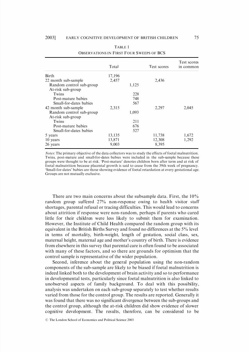
Table 1 reports the ages at which the 1970 cohort was sampled, together with

sample numbers. Of particular value are the data collected when the children

were 22 and 42 months old. Owing to medical concerns about the effect of

foetal malnutrition on brain cell proliferation, a sub-sample of BCS children

was studied at these ages. A 10% random sample of all births was taken

together with those children who were considered to be most at risk from foetal

malnutrition. Numbers from each of these sub-groups within the 22 and 42

month sub-sample are given in Table 1.

Although there were over 17,000 children in the full cohort, this paper

makes use of the information only about children in the pre-school subsample,

2457 children. There is information about test scores at all four ages for 1292 of these children, and this is the sample frame for the paper.


74 ECONOMICA [FEBRUARY



There are two main concerns about the subsample data. First, the 10%

random group suffered 27% non-response owing to health visitor staff

shortages, parental refusal or tracing difficulties. This would lead to concerns

about attrition if response were non-random, perhaps if parents who cared

little for their children were less likely to submit them for examination.

However, the Institute of Child Health compared the random group with its

equivalent in the British Births Survey and found no differences at the 5% level

in terms of mortality, birth-weight, length of gestation, social class, sex,

maternal height, maternal age and mother’s country of birth. There is evidence

from elsewhere in this survey that parental care is often found to be associatedwith many of these factors, and so there are grounds for optimism that the

control sample is representative of the wider population.

Second, inference about the general population using the non-random

components of the sub-sample are likely to be biased if foetal malnutrition is

indeed linked both to the development of brain activity and so to performance

in developmental tests, particularly since foetal malnutrition is also linked to

unobserved aspects of family background. To deal with this possibility,

analysis was undertaken on each sub-group separately to test whether results

varied from those for the control group. The results are reported. Generally it

was found that there was no significant divergence between the sub-groups and

the control group, although the at-risk children did show evidence of slower

cognitive development. The results, therefore, can be considered to be

TABLE 1

OBSERVATIONS IN FIRST FOUR SWEEPS OF BCS

Total Test scoresTest scoresin common

Birth 17,19622 month sub-sample 2,457 2,436

Random control sub-group 1,125At-risk sub-group

Twins 228Post-mature babies 748Small-for-dates babies 567

42 month sub-sample 2,315 2,297 2,045Random control sub-group 1,093At-risk sub-group

Twins 211Post-mature babies 676Small-for-dates babies 527

5 years 13,135 11,738 1,67210 years 13,871 12,308 1,29226 years 9,003 8,395

Notes: The primary objective of the data collectors was to study the effects of foetal malnutrition.Twins, post-mature and small-for-dates babies were included in the sub-sample because thesegroups were thought to be at risk. ‘Post-mature’ denotes children born after term and at risk of foetal malnutrition because placental growth is said to cease from the 39th week of pregnancy.‘Small-for-dates’ babies are those showing evidence of foetal retardation at every gestational age.Groups are not mutually exclusive.


2003] EARLY COGNITIVE DEVELOPMENT OF BRITISH CHILDREN 75



representative of the educational development of the wider population of

children.

One remaining sampling issue cannot be overcome. Only children fromtwo-parent families were included in the subsample. This seriously limits the

representativeness of these results, particularly for those concerned with family

breakdown. None the less, bearing this exclusion in mind, analysis of these

data still sheds light on the questions of the importance and explanation of

early ability differences between children of different backgrounds. Twenty-

four children who were in special schools at age 10 were also excluded from the

subsequent analysis on the assumption that they represent particular

educational problems.

Test scores

At each age BCS children were assessed by a wide range of tests of

intellectual, emotional and personal development. The full list of tests is given

in the Appendix, Table A1. At 22 months the children were asked by the

health visitors administering the survey to complete a range of different tasks,

for example, pointing to their eyes to illustrate understanding of language;

putting on their shoes, as an indication of personal development; stacking

cubes and drawing lines as tests of locomotor ability. These tests, together

with those at 42 months, were intended to indicate the general development of

children based on the tests used for screening in child health clinics

(Chamberlain and Davey 1976). A pilot study found high correlation

between the BCS tests and similar, standard tests of development such as the

Bayley Scale of Infant Behaviour or the Newcastle Survey (Neligan andPrudham 1969). At 42 months counting and speaking could be tested, and

further copying tests were administered such as drawing simple geometrical

shapes. At age 5 copying was again assessed, together with tests of basic

vocabulary. Harris (1963) and Koppitz (1968) show these scores to have good

properties of discrimination and reliability. Standard age 10 scores for maths

and reading are also available. All these scores are appropriate for the age of

the children being tested.

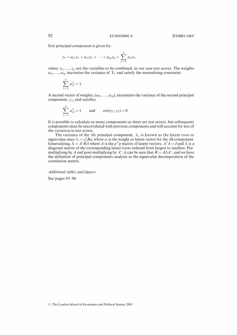
Principal components analysis and the development of an ability index at

each age

In order to maximize the information available at each age while reducing the

number of dependent variables, test scores at each age were combined by

principal components analysis. This technique is common in most behavioural

and social sciences but is perhaps less well known in economics, so a brief

review is provided in the Appendix. Broadly, principal components analysis is

the eigenvalue decomposition of the correlation matrix, R. The first principal

component is given by

y1 ¼ a11x1 þ a12x2 þ ::: þ a1 px p ¼

XP

i ¼ 1

a1i xi ;

where x1; :::; x p are the variables to be combined, in our case test scores. The





weights a11; :::; a1 p maximize the variance of y1 and satisfy the normalizing

constraint

X p

i ¼ 1

a 21i ¼ 1

It is possible to calculate as many components as there are test scores, but

subsequent components must be uncorrelated with previous components and

will account for less of the variation in test scores.

This method has the virtue of combining scores into a single index of

development at each age, which is easier to understand and use in subsequent

analysis than the full set of scores. It is appropriate here because, as Table A1

shows, the test scores are sufficiently correlated to support the hypothesis that

they are measuring manifestations of a similar process, but sufficiently distinct

that each contributes valuable information when they are combined.There is no assumption here that this index identifies any biological entity

or that intelligence is uni-dimensional in the manner of Spearman’s g.1 Rather,

principal components analysis is used to maximize the variance of the

underlying data, in other words its signal, and so to give the early scores the

best chance to predict later outcomes.

Modelling the distributions of abilities

It used to be thought that cognitive development could not be tested before

children were 5 years old (Bayley 1949). In fact, recent tests of attention or

response to novelty in the first six months of life have been shown to becorrelated with cognitive test scores in later childhood (Bornstein and Sigman

1986). None the less, intelligence changes qualitatively over early maturation.

In a review of psychiatric research, Zeanah et al . (1997) emphasize three

periods of major structural reorganizations in infancy. The last of these

qualitative shifts, involving entry into verbal and symbolic representation, ends

at around 20 months, after which changes can be more easily characterized

quantitatively. At 22 months children will still be consolidating after the most

recent shift, but by 42 months they will have the skills much more firmly at

their disposal. More stability from 42 months might, therefore, be expected,

and development can be more readily assessed quantitatively.

There is still considerable instability in scores, because very young childrendo not stay on-task for long, because of qualitative changes in the ability being

proxied at different stages of development, and because the growth rate for

cognitive abilities is not common for all children. A child whose IQ score

remains the same throughout childhood does not exhibit the same performance

at ages 6 and 16. Steady gains in ability will be observed, but the relative

performance is constant. Conducting analysis on rank position rather than

actual scores increases stability, and that is the procedure followed here. This

also makes sense, because our concern is with educational inequality. The

children are ranked in normalized reverse order, a rank of 1 for the lowest

scoring child and 100 for the child scoring highest. This gives four outcome

variables that reflect children’s position in the distribution of observeddevelopment at the ages of 22, 42, 60 and 120 months. Although the rank





varies between 1 and 100 there are potentially as many positions within this

range as there are children in each sweep who completed the tests.

We can write:

(1) Rm ¼ 0

mF m þ "m m ¼ 22; 42; 60; 120;

where F m is a matrix of family inputs and the rank positions are subscripted m

rather than t to emphasize that, even when combined through the use of

principal components, the scores do not represent movement along a single

axis of ability over time. The development of attainment through childhood is

clearly not akin to a time-series of, for example, individual wages, because the

variable itself changes as children mature. Intellectual and behavioural

development is qualitatively different at each age. Different abilities are tested,

and these are not necessarily functionally equivalent. It would be uninforma-

tive to test, say, reading skills at 22 months or, conversely, block stacking at 60

months, because of the qualitative change in children’s abilities. Functional

equivalence for reading would demand tests of abilities at 22 months that fed

particularly into reading ability, but the tests used here have not been devised

in that way (see Table 2 and related discussion).

Thus, although the rank positions at different ages are related, this paper

does not attempt a parametric estimation of such relationships, considering

instead the mobility of rank positions and the association at each age with the

elements of F m. It may be econometrically tempting to employ panel data

techniques that treat rank positions at different ages analogous to, say, a

panel of wages and to ignore the qualitative change in development in

childhood. Such an approach would beg the question of what was undergoingchange, and in these circumstances it is not clear that inference would be

meaningful.

Instead, the Rm are treated as samples of observations of four different

random variables so that (1), therefore, describes four different equations. The

position in the distribution of abilities at each age is commonly thought of as a

linear function of family inputs, including genetic and environmental inputs,

proxied by F m. This is standard in the economics of education following the

Coleman report (Coleman et al . 1966), based on the theoretical foundation of

the education production function.

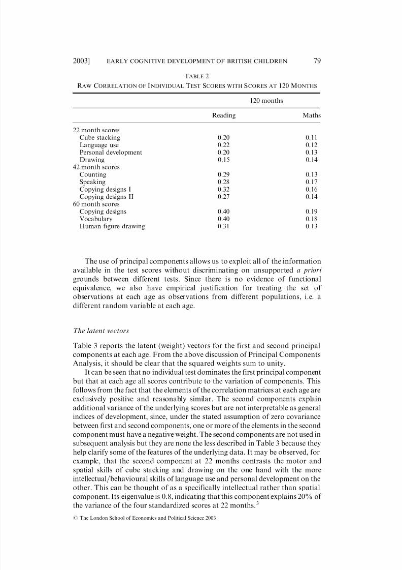
The relations between underlying test scores at different ages

Table 2 reports the raw correlation of each early test score with test results at

age 10. It can be seen that early test scores, particularly those at 42 months, are

associated with later ability but that there is no particular connection between

scores in tests of specific abilities at early ages and subsequent performance in

more demanding tests of the same abilities. For example, cube stacking and

language scores at 22 months are equally associated with reading at age ten.2

Similarly, age 10 reading is associated with the age 5 copying designs test and

with the age 5 vocabulary score. There is, therefore, no evidence of any

functional equivalence or that any single test score is an obvious candidate toproxy development by itself.





The use of principal components allows us to exploit all of the information

available in the test scores without discriminating on unsupported a priori

grounds between different tests. Since there is no evidence of functional

equivalence, we also have empirical justification for treating the set of

observations at each age as observations from different populations, i.e. adifferent random variable at each age.

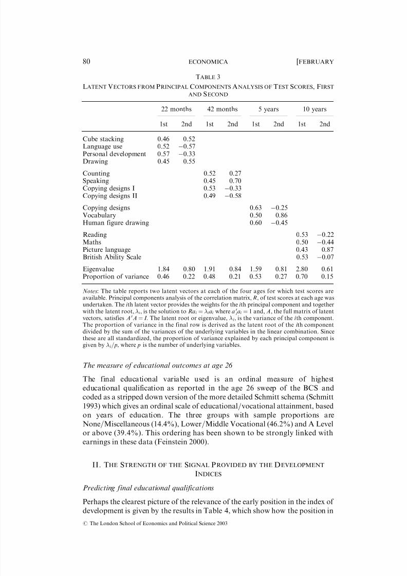
The latent vectors

Table 3 reports the latent (weight) vectors for the first and second principal

components at each age. From the above discussion of Principal Components

Analysis, it should be clear that the squared weights sum to unity.

It can be seen that no individual test dominates the first principal component

but that at each age all scores contribute to the variation of components. This

follows from the fact that the elements of the correlation matrices at each age are

exclusively positive and reasonably similar. The second components explainadditional variance of the underlying scores but are not interpretable as general

indices of development, since, under the stated assumption of zero covariance

between first and second components, one or more of the elements in the second

component must have a negative weight. The second components are not used in

subsequent analysis but they are none the less described in Table 3 because they

help clarify some of the features of the underlying data. It may be observed, for

example, that the second component at 22 months contrasts the motor and

spatial skills of cube stacking and drawing on the one hand with the more

intellectual=behavioural skills of language use and personal development on the

other. This can be thought of as a specifically intellectual rather than spatial

component. Its eigenvalue is 0.8, indicating that this component explains 20% of the variance of the four standardized scores at 22 months.3

TABLE 2

RAW CORRELATION OF INDIVIDUAL TEST SCORES WITH SCORES AT 120 MONTHS

120 months

Reading Maths

22 month scoresCube stacking 0.20 0.11Language use 0.22 0.12Personal development 0.20 0.13Drawing 0.15 0.14

42 month scoresCounting 0.29 0.13Speaking 0.28 0.17Copying designs I 0.32 0.16

Copying designs II 0.27 0.1460 month scoresCopying designs 0.40 0.19Vocabulary 0.40 0.18Human figure drawing 0.31 0.13





The measure of educational outcomes at age 26

The final educational variable used is an ordinal measure of highest

educational qualification as reported in the age 26 sweep of the BCS and

coded as a stripped down version of the more detailed Schmitt schema (Schmitt

1993) which gives an ordinal scale of educational=vocational attainment, basedon years of education. The three groups with sample proportions are

None=Miscellaneous (14.4%), Lower=Middle Vocational (46.2%) and A Level

or above (39.4%). This ordering has been shown to be strongly linked with

earnings in these data (Feinstein 2000).

II. THE STRENGTH OF THE SIGNAL PROVIDED BY THE DEVELOPMENT

INDICES

Predicting final educational qualifications

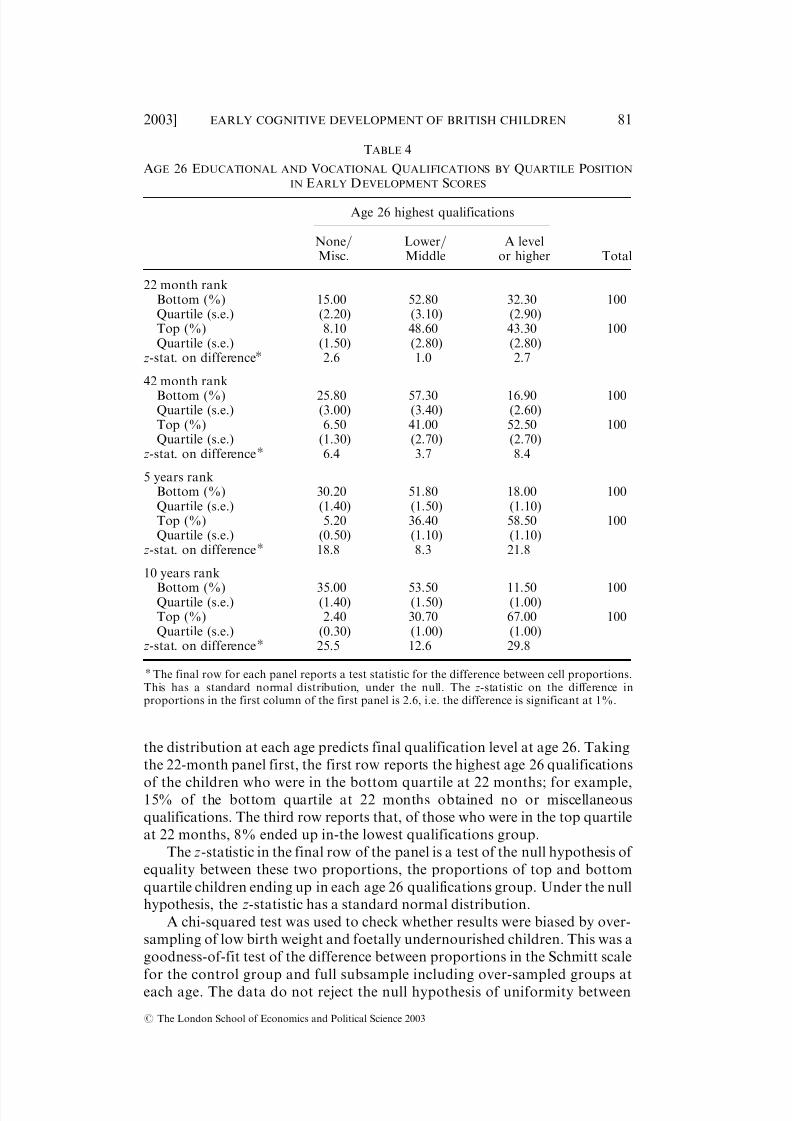
Perhaps the clearest picture of the relevance of the early position in the index of development is given by the results in Table 4, which show how the position in

TABLE 3

LATENT VECTORS FROM PRINCIPAL COMPONENTS ANALYSIS OF TEST SCORES, FIRST

AND SECOND

22 months 42 months 5 years 10 years

1st 2nd 1st 2nd 1st 2nd 1st 2nd

Cube stacking 0.46 0.52Language use 0.52 0.57Personal development 0.57 0.33Drawing 0.45 0.55

Counting 0.52 0.27Speaking 0.45 0.70Copying designs I 0.53 0.33Copying designs II 0.49 0.58

Copying designs 0.63 0.25Vocabulary 0.50 0.86Human figure drawing 0.60 0.45

Reading 0.53 0.22Maths 0.50 0.44Picture language 0.43 0.87British Ability Scale 0.53 0.07

Eigenvalue 1.84 0.80 1.91 0.84 1.59 0.81 2.80 0.61Proportion of variance 0.46 0.22 0.48 0.21 0.53 0.27 0.70 0.15

Notes: The table reports two latent vectors at each of the four ages for which test scores areavailable. Principal components analysis of the correlation matrix, R, of test scores at each age was

undertaken. The i th latent vector provides the weights for the i th principal component and togetherwith the latent root, i , is the solution to Rai ¼ i ai where a 0

i ai ¼ 1 and, A, the full matrix of latentvectors, satisfies A 0A ¼ I . The latent root or eigenvalue, i , is the variance of the i th component.The proportion of variance in the final row is derived as the latent root of the i th componentdivided by the sum of the variances of the underlying variables in the linear combination. Sincethese are all standardized, the proportion of variance explained by each principal component isgiven by i = p, where p is the number of underlying variables.





the distribution at each age predicts final qualification level at age 26. Taking

the 22-month panel first, the first row reports the highest age 26 qualifications

of the children who were in the bottom quartile at 22 months; for example,15% of the bottom quartile at 22 months obtained no or miscellaneous

qualifications. The third row reports that, of those who were in the top quartile

at 22 months, 8% ended up in-the lowest qualifications group.

The z-statistic in the final row of the panel is a test of the null hypothesis of

equality between these two proportions, the proportions of top and bottom

quartile children ending up in each age 26 qualifications group. Under the null

hypothesis, the z-statistic has a standard normal distribution.

A chi-squared test was used to check whether results were biased by over-

sampling of low birth weight and foetally undernourished children. This was a

goodness-of-fit test of the difference between proportions in the Schmitt scale

for the control group and full subsample including over-sampled groups at

each age. The data do not reject the null hypothesis of uniformity between

TABLE 4

AGE 26 EDUCATIONAL AND VOCATIONAL QUALIFICATIONS BY QUARTILE POSITION

IN EARLY DEVELOPMENT SCORES

Age 26 highest qualifications

None=Misc.

Lower=Middle

A levelor higher Total

22 month rankBottom (%) 15.00 52.80 32.30 100Quartile (s.e.) (2.20) (3.10) (2.90)Top (%) 8.10 48.60 43.30 100Quartile (s.e.) (1.50) (2.80) (2.80)

z-stat. on difference* 2.6 1.0 2.7

42 month rank

Bottom (%) 25.80 57.30 16.90 100Quartile (s.e.) (3.00) (3.40) (2.60)Top (%) 6.50 41.00 52.50 100Quartile (s.e.) (1.30) (2.70) (2.70)


5 years rankBottom (%) 30.20 51.80 18.00 100Quartile (s.e.) (1.40) (1.50) (1.10)Top (%) 5.20 36.40 58.50 100Quartile (s.e.) (0.50) (1.10) (1.10)


10 years rank

Bottom (%) 35.00 53.50 11.50 100Quartile (s.e.) (1.40) (1.50) (1.00)Top (%) 2.40 30.70 67.00 100Quartile (s.e.) (0.30) (1.00) (1.00)


*The final row for each panel reports a test statistic for the difference between cell proportions.This has a standard normal distribution, under the null. The z-statistic on the difference inproportions in the first column of the first panel is 2.6, i.e. the difference is significant at 1%.





samples at any age. It is striking that, even measured at 22 months, children in

the bottom quartile of this development index are significantly less likely to get

any qualifications than those in the top quartile. Moreover, more than threetimes as many of those in the top quartile at 42 months as those in the bottom

quartile go on to get A-level qualifications or above. Given the young age of

the children tested, these are strong findings, suggesting that the index picks up

clear signals of educational development; before children have even entered

school, very substantial signals about educational progress are contained in

standard tests of development.

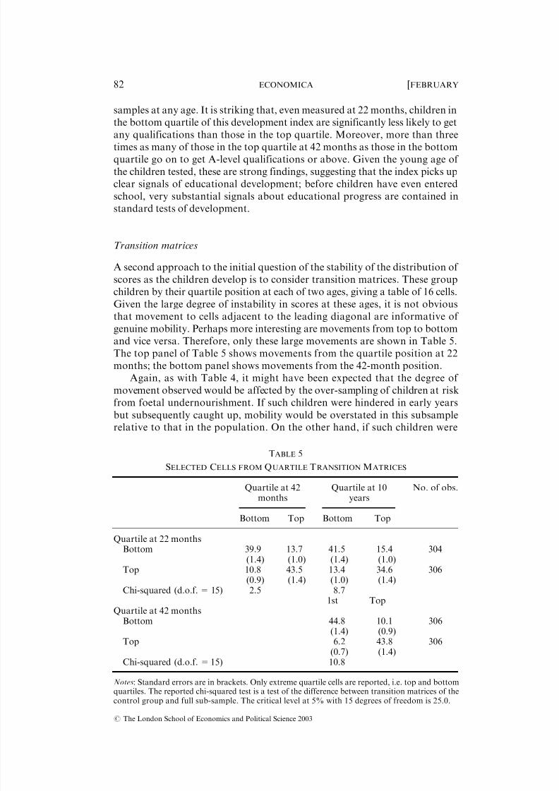
Transition matrices

A second approach to the initial question of the stability of the distribution of

scores as the children develop is to consider transition matrices. These groupchildren by their quartile position at each of two ages, giving a table of 16 cells.

Given the large degree of instability in scores at these ages, it is not obvious

that movement to cells adjacent to the leading diagonal are informative of

genuine mobility. Perhaps more interesting are movements from top to bottom

and vice versa. Therefore, only these large movements are shown in Table 5.

The top panel of Table 5 shows movements from the quartile position at 22

months; the bottom panel shows movements from the 42-month position.

Again, as with Table 4, it might have been expected that the degree of

movement observed would be affected by the over-sampling of children at risk

from foetal undernourishment. If such children were hindered in early years

but subsequently caught up, mobility would be overstated in this subsamplerelative to that in the population. On the other hand, if such children were

TABLE 5

SELECTED CELLS FROM QUARTILE TRANSITION MATRICES

Quartile at 42months

Quartile at 10years

No. of obs.

Bottom Top Bottom Top

Quartile at 22 monthsBottom 39.9 13.7 41.5 15.4 304

(1.4) (1.0) (1.4) (1.0)Top 10.8 43.5 13.4 34.6 306

(0.9) (1.4) (1.0) (1.4)Chi-squared (d.o.f. = 15) 2.5 8.7

1st TopQuartile at 42 months

Bottom 44.8 10.1 306(1.4) (0.9)

Top 6.2 43.8 306(0.7) (1.4)

Chi-squared (d.o.f. = 15) 10.8

Notes: Standard errors are in brackets. Only extreme quartile cells are reported, i.e. top and bottom

quartiles. The reported chi-squared test is a test of the difference between transition matrices of thecontrol group and full sub-sample. The critical level at 5% with 15 degrees of freedom is 25.0.





persistently affected, mobility might be understated. Chi-squared tests for

contingency tables have been applied and are presented in Table 5. These

suggest, as before, that there is no significant difference between the transitionmatrices for the full subsample and those for the control group. Other

experiments were undertaken with mobility indices such as those of

Bartholomew (1973), which weights cells by their distance from the leading

diagonal, a high overall score indicating a large degree of mobility; or of

Shorrocks (1978). These also showed that the mobility results described in the

text are not substantially altered by over-sampling.

The first row shows that, of the 25% children scoring lowest at 22 months,

39.9% were still in the lowest quartile at 42 months. On the other hand, 13.7%

had entered the top quartile. Clearly, there is considerable movement within

the distribution over these twenty months. By 120 months, even more children

had made large movements across the distribution. From these sample data, a

child in the bottom quartile at 22 months would have a probability of 0.42 of

being in the bottom quartile at 10 years but a probability of 0.15 of reaching

the top quartile by then.

There is more clear persistence of scores between 42 months and 10 years,

particularly in terms of the proportion of large movements. Thus, as expected,

the position at 42 months seems to be more firmly fixed than that at 22 months.

However, 10% of the bottom group at 42 months had reached the top quartile

by age 10. This emphasizes the interpretation of the development indices as

signals of development and not as stronger classifying mechanisms. Plenty of

scope remains for children to catch up and overtake other children who may be

out-performing them early on. (As we see, below, high SES children who

under-perform early on are very likely to catch up in this way.) None the less,the 22 and 42-month scores provide a meaningful guide to subsequent

performance. The development index at 42 months is the preferred indicator.

Other experiments have shown that for girls it is slightly more stable than for

boys.

III. THE ASSOCIATION OF TEST RANK WITH SOCIAL CLASS

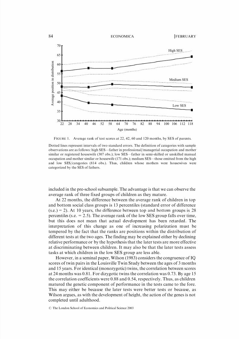
Figure l maps the average position of children from different social

backgrounds in the distribution of test ranks at the four survey ages. Social

class classifications are made here on the basis of both parents’ occupationalclassification (socioeconomic status, or SES) at the child’s birth. It should be

remembered that all the children in this sample are from two-parent families.

Details of categorization are given in the notes to the figure. No allowance is

made for changing occupational classifications over time, because it is not

possible to differentiate between genuine changes and miscoding. In any case,

social class at birth provides a good enough indicator of the material, genetic

and educational inputs that the children can be expected to receive through

childhood.

Observations are only made at 22, 42, 60 and 120 months. As noted above,

the sample is restricted to those 1292 observations for whom test scores are

available at all ages. This increases the standard errors of difference betweengroups, because we discard all age 5 and age 10 observations that are not





included in the pre-school subsample. The advantage is that we can observe the

average rank of three fixed groups of children as they mature.

At 22 months, the difference between the average rank of children in top

and bottom social class groups is 13 percentiles (standard error of difference

(s.e.) = 2). At 10 years, the difference between top and bottom groups is 28

percentiles (s.e. = 2.5). The average rank of the low SES group falls over time,

but this does not mean that actual development has been retarded. The

interpretation of this change as one of increasing polarization must be

tempered by the fact that the ranks are positions within the distribution of

different tests at the two ages. The finding may be explained either by decliningrelative performance or by the hypothesis that the later tests are more effective

at discriminating between children. It may also be that the later tests assess

tasks at which children in the low SES group are less able.

However, in a seminal paper, Wilson (1983) considers the congruence of IQ

scores of twin pairs in the Louisville Twin Study between the ages of 3 months

and 15 years. For identical (monozygotic) twins, the correlation between scores

at 24 months was 0.81. For dizygotic twins the correlation was 0.73. By age 15

the correlation coefficients were 0.88 and 0.54, respectively. Thus, as children

matured the genetic component of performance in the tests came to the fore.

This may either be because the later tests were better tests or because, as

Wilson argues, as with the development of height, the action of the genes is notcompleted until adulthood.

30

35

40

45

50

55

60

65

70

22 28 34 40 46 52 58 64 70 76 82 88 94 100 106 112 118

Age (months)

A v e r a g e p o s i t i o n i n d i s t r i b u t i o n

High SES

Medium SES

Low SES

FIGURE 1. Average rank of test scores at 22, 42, 60 and 120 months, by SES of parents.

Dotted lines represent intervals of two standard errors. The definition of categories with sample

observations are as follows: high SES—father in professional=managerial occupation and mother

similar or registered housewife (307 obs.); low SES—father in semi-skilled or unskilled manual

occupation and mother similar or housewife (171 obs.); medium SES—those omitted from the high

and low SES=categories (814 obs.). Thus, children whose mothers were housewives were

categorized by the SES of fathers.





The pattern of polarization here, therefore, is not surprising whether one

tends towards a genetic or environmental explanation. Crucially, the graph

clearly shows that, although children are already stratified by social class instandard tests of intellectual and personal development at 22 months, this

stratification has become more extreme by 10 years, as assessed by the standard

tests for academic development appropriate at that age. There is certainly no

evidence here that entry into schooling in any way overcame the polarization of

children in the late 1970s. The most generous statement that may be made for

schooling is that it may or may not have minimized the deepening effects of

parental background.

It should be remembered, however, that Figure 1 shows the mean rank

positions within each of three groups of children, as they mature. There is,

however, considerable and important within-group variation. This is brought

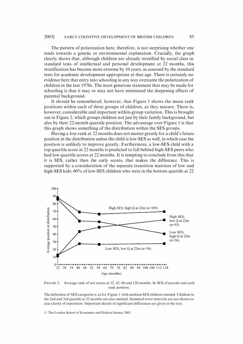
out in Figure 2, which groups children not just by their family background, but

also by their 22-month quartile position. The advantage over Figure 1 is that

this graph shows something of the distribution within the SES groups.

Having a low rank at 22 months does not matter greatly for a child’s future

position in the distribution unless the child is low-SES as well, in which case the

position is unlikely to improve greatly. Furthermore, a low-SES child with a

top quartile score at 22 months is predicted to fall behind high-SES peers who

had low quartile scores at 22 months. It is tempting to conclude from this that

it is SES, rather than the early scores, that makes the difference. This is

supported by a consideration of the separate transition matrices of low and

high-SES kids: 60% of low-SES children who were in the bottom quartile at 22

High SES, high Q at 22m (n=105)

Low SES, low Q at 22m (n=54)

Low SES,high Q at 22m

(n=36)

High SES,low Q at 22m(n=55)

0

20

40

10

30

60

50

70

80

90

100

22 28 34 40 46 52 58 64 70 76 82 88 94 100 106 112 118

Age (months)

A v e r a g e

p o s i t i o n i n d i s t r i b u t i o n

FIGURE 2. Average rank of test scores at 22, 42, 60 and 120 months, by SES of parents and early

rank position.

The definition of SES categories is as for Figure 1 with medium SES children omitted. Children in

the 2nd and 3rd quartile at 22 months are also omitted. Standard error intervals are not shown to

ease clarity of exposition. Important details of significant differences are given in the text.





months were still there at age 10. On the other hand, high-SES kids who

happened to be in the bottom quartile at 22 months were more likely to be in

the top quartile at 10 years than to still be in the bottom quartile!Does this suggest that early scores don’t matter? The answer is no, for two

reasons. First, from Figure 2, it is still the case that children within each of the

SES groups who are in the top quartile at 22 months score better at 10 years

than children in the same SES group who were in the bottom quartile at 22

months. The difference is still 13 points at age 10 for the low-SES group and 11

for the high-SES group, differences that are significant at 1%. For the omitted

middle SES group, there is also some convergence over time for the high and

low quartile groups at 22 months, but, although by 42 months the difference

had fallen to 26 points in the distribution, at age 10 it was still 22 points.

Second, we can also reconsider Table 5. This showed the probabilities of

obtaining final educational qualifications in the abridged Schmitt range on the

basis of quartile position at the different ages. For the middle SES group (the

majority of children), children in the bottom quartile at 22 months are

significantly more likely to get no qualifications than children in the top

quartile, and significantly less likely to get A levels or higher qualifications. For

the top and bottom SES groups, differences at 42 months predict final

educational qualifications. So, conditioning on SES, the pre-school score still

matters. None the less, as well as influencing early ability, family background

clearly plays a tremendously important role in determining the continued

development of ability of UK children.

It might appear to be a natural extension of the conditioning process to

consider an ordered probit regression of the age 26 Schmitt variable on the

rank at 22 months and SES dummies and other family background variables.However, we expect from equation (1) that the Schmitt position be indicated

by 22-month rank partly because the 22-month rank picks up SES effects.

Since the intention is to test whether or not the 22-month score is an indicator

of real development, that is precisely the point. Even if the 22-month rank

picked up only SES effects and nothing else, it would still indicate

development. The problem would, rather, be in the opposite direction if the

rank position did not pick up SES effects at all, which would suggest that it was

a poor indicator.4

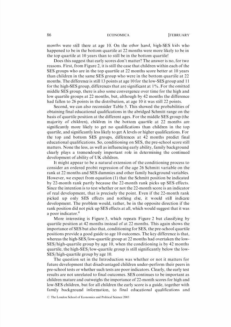
More interesting is Figure 3, which repeats Figure 2 but classifying by

quartile position at 42 months instead of at 22 months. This again shows the

importance of SES but also that, conditioning for SES, the pre-school quartilepositions provide a good guide to age 10 outcomes. The key difference is that,

whereas the high-SES=low-quartile group at 22 months had overtaken the low-

SES=high-quartile group by age 10, when the conditioning is by 42 months

quartile, the high-SES=low-quartile group is still significantly below the low-

SES=high-quartile group by age 10.

The question set in the Introduction was whether or not it matters for

future development that disadvantaged children under-perform their peers in

pre-school tests or whether such tests are poor indicators. Clearly, the early test

results are not unrelated to final outcomes. SES continues to be important as

children mature and outweighs the importance of 22-month scores for high and

low-SES children, but for all children the early score is a guide, together withfamily background information, to final educational qualifications and





academic performance. The lesson for policy-makers is clear from Figures 2

and 3. There is mobility (as one would expect) after 22 or 42 months, but this is

mainly for high or medium-SES children. Low-SES children do not, on

average, overcome the hurdle of lower initial attainment combined with

continued low input. Even high-SES children find it hard to escape from poor

performance at 42 months.

The importance of different aspects of social class

The ability trajectories show that, as children mature and do more

discriminating tests, the family background association strengthens. Figures

A1–A3 in the Appendix show that this result does not appear to depend on

which conditioning variable is selected from the matrix of family background

variables F . It remains when children are grouped by the education rather thanSES of their parents, or when they are grouped by the backgrounds of one

parent only.

It would be interesting to know which aspect of family background

dominates, either as a genetic marker or as a proxy for key environmental

inputs. However, given the strong correlations between the elements of F , there

is no unambiguous way to identify separate contributions to the variation of

test scores. If the independent variables were continuous, one approach would

be to consider the partial correlation coefficients. Together with simple

coefficients, this would give a guide to the relative importance of each variable.

In the current case, however, the regressors are a set of dummy variables, and

so the netting-out process introduces further ambiguities that are not obviouslyresolved.

0

20

40

10

30

60

50

70

80

90

100

22 28 34 40 46 52 58 64 70 76 82 88 94 100 106 112 118Age (months)

A v e r a g e p o s i t i o n i n d i s t r i b u t i o n High SES, high Q at 42m (n=103)

Low SES, low Q at 42m (n=62)

Low SES, high Q at 42m (n=30)

High SES, low Q at 42m (n=48)

FIGURE 3. Average rank of test scores at 22, 42, 60 and 120 months, by SES of parents and

42-month rank.

Notes: as Figure 2.





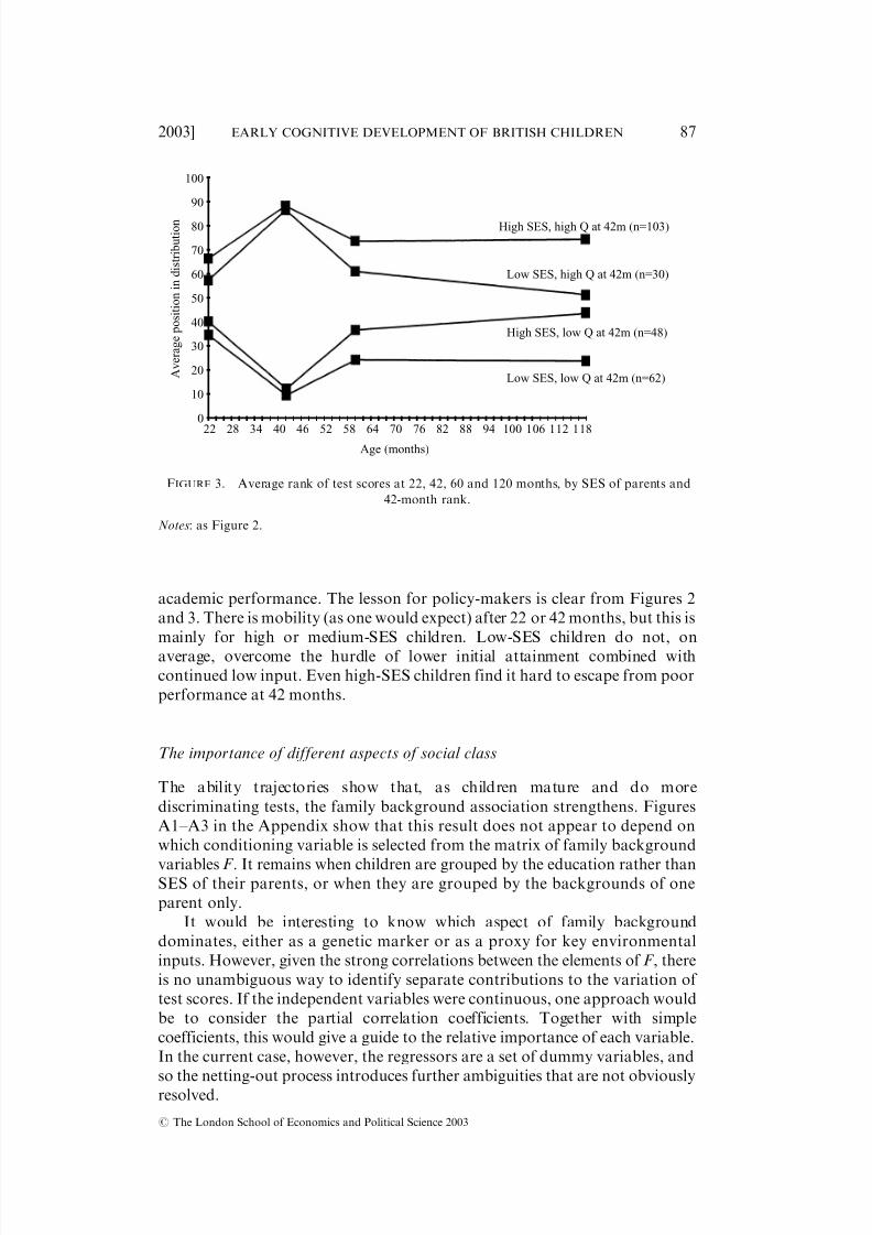
Neglecting, therefore, the importance of partial correlations, Table 6

reports OLS estimates of the am vectors from equation (1), which is reproduced

here:(1) Rm ¼ 0

mF m þ "m; m ¼ 22; 42; 60; 120:

Weighted OLS is used to reduce the importance of over-sampled observations,

but none of the conclusions described depend on sampling bias, transforma-

tions of the data or problems of discreteness or censoring.5 For the reported

regressions, observations were grouped across genders. Experiments with

running separate regressions did not bring to light any differences that are

important to the conclusions here.

In this regression framework, children of parents without qualifications

were 38 points lower in the distribution at age 10 than children whose parents

TABLE 6

TEST RANKS REGRESSED ON BACKGROUND VARIABLES AT BIRTH

22 months 42 months 5 years 10 years

Est. t Est. t Est. t Est. t

Father’s SES 3, 4, 5 2.4 0.8 2.9 1.1 0.4 0.1 7.2 2.96 2.1 0.4 1.4 0.3 5.9 1.1 12.1 2.6

Father’s highest qualificationVocational or other 3.0 1.0 3.4 1.1 0.5 0.2 0.1 0.0

O=A level, SRN or Cert. Ed. 3.0 1.0 3.9 1.4 7.3 2.7 8.4 3.4Degree 5.1 1.5 3.5 1.0 9.0 2.5 12.8 4.3

Mother’s SES 3,4,5 1.3 0.3 1.9 0.5 6.1 1.5 5.0 1.56 0.9 0.1 19.9 2.8 12.8 1.5 22.0 4.5Housewife 1.9 0.5 1.5 0.4 5.0 1.2 3.0 0.8

Mother’s highest qualificationVocational or other 3.1 1.0 4.3 1.4 1.7 0.6 4.2 1.6O=A level, SRN or Cert. Ed. 7.9 2.8 7.9 2.9 8.0 3.0 13.1 5.5Degree 21.4 3.4 20.5 2.6 19.8 2.8 25.2 4.2

Siblings1 older 4.1 1.4 0.8 0.3 3.9 1.4 8.9 3.52 older 4.3 1.2 5.5 1.5 8.7 2.4 13.9 4.2

3 or more older 7.3 1.7 13.3 3.0 9.7 2.3 18.2 4.91 younger 3.0 1.1 4.7 1.9 3.7 1.62 or more younger 14.2 2.1 9.5 2.2 6.9 1.5

Girl 7.1 3.3 5.7 2.7 0.7 0.3 1.8 1.0Mother’s age 0.2 0.6 0.4 1.5 0.5 1.9 0.7 3.4Constant 27.5 1.0 82.4 2.0 37.7 4.7 38.9 5.3

Obs 1194 1194 1194 1194R2 0.08 0.13 0.12 0.25

Notes: Observations are re-weighted by the formula wi ¼ ssi =si for i =1,2 where w1 and w2 are theweights of the control and at-risk groups in the early sub-sample, ssi is the number of observationsof type i in the sub-sample predicted on the basis of the full sample proportions and si is the actualnumber of observations of type i . Controls for reason for inclusion in the sub-sample and precise

age when test was taken are also included but are not reported here. Summary statistics arereported in Table A2.





both had degrees. Add in a couple of older siblings, and the effect rises to 52

points.6 Even at 22 months the effect of two parents with degrees is 26 points.

This compares with negligible effects of SES until age 10. From 42 months, theassociation of mother’s social class group 6 and rank positions is strongly

negative, but it must be borne in mind that this is, in fact, the average

association for a group of only 15 women.

The association with mother’s education is particularly striking early on

and dominates the effect of paternal education; but, again, this is due partly to

the smaller numbers of women than men with degrees (13% of men as opposed

to 2% of women). However, the mother’s education variables are jointly

significant at 1%, while those of fathers are not jointly significant even at 20%.

The father’s education variables do not become significant at 5% until age 5,

and the father’s SES variables not until age 10. In fact, the father’s SES and

education variables are not jointly significant at 5% until age 5.

Overall, it appears that for this sample the education of mothers is the best

indicator of expected development and so may be most the useful variable in

determining at-risk groups. The effect is attenuated marginally if controls for

foetal health such as birth weight are introduced, but the overall result is robust

to this, suggesting that the underlying cause is not confined to the care taken

during pregnancy but relates to the general level of inputs received by the child

during pregnancy and the early years.

IV. DISCUSSION

This paper finds, first, that there were significant differences in the educationalperformance of children from different social groups in these data, even at 22

months. In this sense there was pre-school educational inequality in the UK

between 1970 and 1975. Second, performance in tests of ability at 22 months

are correlated with ultimate schooling outcomes at age 26, although the 42-

month scores provide a better guide than those at 22 months. The pre-school

scores are, therefore, meaningful measures of development in the sense that

they provide real signals of development.

Third, family background plays a large role in influencing the mobility of

children within the distributions of ability at different ages. Most low-SES

children who are in the bottom quartile at 22 months are still there at age 10.

High-SES children show considerably more upward mobility and are morelikely to be in the top quartile than the lowest by age 10, even if they were in the

bottom quartile at 22 months. These results bring out the extent to which the

formation of human capital in the UK is influenced by family background. It

would be very interesting to know how much these associations are reproduced

elsewhere, in countries with perhaps less, or more, social inequality.

Fourth, the early differences in attainment are not appreciably reduced by

entry into the schooling system. It is not possible to conclude from this that by

the time children enter school the position is irreversible. The test instruments

change as children mature and the degree of stratification may be affected by

this. It is not sensible, therefore, to consider changes in the rank position

between stages of development as standard first differences. However, thetrajectories do demonstrate the extent of the challenge facing the UK





government if it wishes to reverse economic inequality through the education

system.

In a sense, though, the key policy question cannot be addressed by thispaper, and that is: at what point should the government intervene? In order to

address this question, one would want to know (a) the extent to which the

correlation between school-age ability and pre-school ability was due to

dependence of the former on the latter or to individual heterogeneity

underlying both, and (b) the extent to which interventions could improve

performance or reduce inequality at each age. There is currently little evidence

on either of these questions. In the absence of experimental evidence, answers

to the first of these research questions might be attempted by treating the

scores at different ages as a panel which, with tests at sufficient ages, would

allow one to include and instrument a lagged dependent variable in the

education production function. For the reasons given above, that has not been

thought possible with the scores available in these data. However, such an

approach may be possible where tests are of a single entity such as maths skills;

this is left to future research.

Despite the lack of evidence, however, there is a widespread perception that

there are strong advantages to early intervention, so that, for example, the Blair

administration in the UK has developed the £540 million Sure-Start programme.

This will bring together child-care organizations, so that communities have

access to organized and coordinated systems of support. Professionals and carers

are provided with evidence-based guidance about practice. The non-coverage of

those who do not choose to get involved in programmes, or do so only indirectly,

will clearly be a concern. It is also important to note that Sure-Start is an area-

based intervention and will, therefore, completely miss those families thathappen to live outside targeted areas and so are excluded from the programme.

This suggests that, in addition to Sure-Start, such skills might be taught at

school, rather than waiting until the period of compulsory schooling is over.

Research summarized by Waldfogel (1999) suggests that there is consider-

able room for optimism about intervention programmes, but that success

cannot be had cheaply. A well replicated set of randomized experiments in the

USA (Ramey and Ramey 2000) suggest that to be successful interventions

must pay top salaries in order to recruit well qualified staff and to keep staff

turnover to a minimum. They must also follow children over time, because the

benefits of programmes that start in pre-school but do not continue for at least

the first two years of school are highly liable to decay.However, other kinds of programmes about which there was considerable

optimism, such as two-generation interventions or programmes targeted at

entire families, have not produced the hoped-for gains. For example, Barnett

(1995) shows that, if interventions do have positive effects on the performance

of children, this is not due to effects on parents. This conclusion has been

replicated in many other studies, suggesting that programmes that target

resources directly on children are most successful. This evidence suggests that

Sure-Start in its current design will not be very successful in reducing the level

of early educational inequality.

Turning to the implications of these results for macroeconomics referred to

in the Introduction, it would also be interesting to build on the tentative findingthat parental learning is a key factor in the formation of the human capital of





children. It may prove beneficial to model human capital by the variables that

explain performance in Table 6, rather than by years of schooling, which has

been shown to be a poor measure of genuine educational investment because of the wide differences in the quality of the schooling received. At the individual

level, these results also show why family background explains earnings above

and beyond that part explained by years of schooling. For individuals with no or

low levels of qualification, years of schooling provides no guide to formed

human capital. Models incorporating family background as proxies of human

capital formation may sometimes be more informative.

ACKNOWLEDGMENTS

I would like to thank the ESRC Data Archive at Essex University for permission to usethe BCS data, and three anonymous referees for many helpful comments. Barbara

Maugham of the Institute of Psychiatry made many interesting and helpful points, and Iwould also like to thank James Symons, Steve Machin, Pamela Klebanov, CostasMeghir and Marco Manacorda, as well as participants at the Labour EconomicsSeminar at the CEP, the Econometrics Workshop, UCL, and the Economics SubjectGroup seminar, Sussex University.

NOTES

1. Spearman (1904) noted that people who scored well on intelligence tests usually did well in allcognitive areas—whether verbal, mathematical or spatial. He hypothesized that some general or g factor contributes to this success. While some neuro-scientists are attempting to locate the partof the brain responsible for success in tasks of g-intelligence, others are concerned that thepsychometric model describes the results of statistical analyses without explaining what the

abilities are. The answer to the question, what is g? is that it is that which correlates with lots of different tests of intelligence. Modern theories of intelligence are more concerned withunderstanding the relations between different aspects of intelligence.

2. This is not due to differences in the variance of the two 22-month variables.3. It may be noted that the second component is not significant in regressions of the first principal

component factor at age 10 on age 22 months factors. In fact, of the second factors at 22, 42 and60 months, only the age 5 second factor, which emphasizes vocabulary at the expense of humanfigure drawing tests, is a significant predictor of age 10 development. This is unsurprising, giventhat second components have lower variance than first components.

4. The reader might nevertheless be interested to note that, in fact, even conditioning on all thebackground variables in Table 6 rank at 22 months is still significant at 5% in the ordered probitprediction of the age 26 final educational qualification.

5. If variation in the control group is higher than for the foetally undernourished groups, thenparameter estimates based on the latter groups might be biased downwards, but the pattern of results described below changes very little if only control group observations are used. Inferences

are also unchanged if the rank score dependent variable is replaced by the continuous test scorevariables using Tobit regression to correct for some evident lower censoring which might alsohave caused downward bias.

6. Summing the coefficients on mother’s and father’s degrees in the age 10 regression (ignoring thepossibility of an interaction term) gives a boost of 38 points relative to the position of a child inthe default groups of no qualifications. If the child whose parents have no qualifications isassumed to have two siblings, an additional 14 points are lost relative to a single child whoseparents both have degrees, hence 52 points.

APPENDIX

A brief summary of principal components analysis

Principal components analysis is the eigenvalue decomposition of the covariance matrix,C , or, where the variables are standardized as here, of the correlation matrix, R. The





first principal component is given by:

y1¼

a11x1þ

a12x2þ þ

a1px p¼X

p

i ¼ 1 a1i xi ;

where x1, ..., x p are the variables to be combined, in our case test scores. The weightsa11, ..., a1 p maximize the variance of Y 1 and satisfy the normalizing constraint:

X p

i ¼ 1

a 21i ¼ 1:

A second vector of weights, (a21; :::; a2 p), maximizes the variance of the second principalcomponent, y2, and satisfies

X p

i ¼ 1

a 21i ¼ 1 and cov( y1; y2) ¼ 0:

It is possible to calculate as many components as there are test scores, but subsequentcomponents must be uncorrelated with previous components and will account for less of the variation in test scores.

The variance of the i th principal component, i , is known as the latent root oreigenvalue since i ¼ a 0

i Rai where ai is the weight or latent vector for the i th component.Generalizing, ¼ A 0RA where A is the p* p matrix of latent vectors, A 0A ¼ I and is adiagonal matrix of the corresponding latent roots ordered from largest to smallest. Pre-multiplying by A and post-multiplying by A 0, it can be seen that R ¼ AA 0, and we havethe definition of principal components analysis as the eigenvalue decomposition of thecorrelation matrix.

Additional tables and figures

See pages 93–96.





TABLE A1

TESTS UNDERTAKEN BY CHES, WITH CORRELATION MATRICES

22 monthsCube stacking 1.00Language use 0.27 1.00Personal development I 0.34 0.46 1.00Personal development II 0.20 0.29 0.31 1.00Drawing 0.31 0.22 0.30 0.25 1.00Gross Locomotor 0.19 0.31 0.27 0.32 0.27 1.00

42 monthsCounting 1.00Speaking 0.40 1.00Copying designs I 0.35 0.31 1.00Copying designs II 0.28 0.19 0.38 1.00Building 0.30 0.26 0.35 0.19 1.00

Cube stacking 0.16 0.16 0.17 0.08 0.34 1.00Picture test I 0.26 0.43 0.23 0.11 0.29 0.26 1.00Picture test II 0.35 0.50 0.33 0.19 0.34 0.24 0.57 1.00Line drawing 0.25 0.31 0.26 0.11 0.29 0.19 0.27 0.38 1.00Gross Locomotor 0.22 0.32 0.24 0.11 0.22 0.15 0.24 0.29 0.19 1.00Parts of the body 0.26 0.48 0.27 0.14 0.28 0.26 0.43 0.48 0.29 0.35 1.00

5 yearsCopying designs 1.00Vocabulary 0.30 1.00Human Figure Drawing I 0.39 0.22 1.00Human Figure Drawing II 0.39 0.22 0.81 1.00Profile drawing 0.20 0.19 0.23 0.23 1.00

10 years

Reading 1.00Maths 0.49 1.00Picture language test 0.53 0.34 1.00British Ability Scales 0.74 0.48 0.57 1.00

Notes: Two human figure drawing tests are reported here for the children at age 5. These are bothbased on the same test but weighted by different procedures developed in the educational literature(Koppitz 1968, and Harris 1963). The HFD score used in the text is the average of these twodifferent measures of HFD This avoids the need for assumptions about which weighting procedureis preferable. In any case, the correlation between the two scores is 0.81, perhaps too high forseparate entry in the principal components analysis.





TABLE A2

BASIC STATISTICS FOR BACKGROUND INFORMATION IN TABLE 6

No. obs. Mean s.d. Min. Max

Girl 1194 0.46 0.50 0 1Father in SES 1, 2 1194 0.16 0.37 0 1Father in SES 3m, 3nm, 4a 1194 0.78 0.41 0 1Father in SES 5 1194 0.06 0.23 0 1Father has no qualifications 1194 0.47 0.50 0 1Father has low qualifications 1194 0.14 0.35 0 1Father has medium qualifications 1194 0.23 0.42 0 1Father has high qualifications 1194 0.13 0.33 0 1Mother has no qualifications 1194 0.54 0.50 0 1Mother has low qualifications 1194 0.17 0.37 0 1Mother has medium qualifications 1194 0.27 0.44 0 1

Mother has high qualifications 1194 0.02 0.14 0 1Mother in SES 1, 2 1194 0.10 0.30 0 1Mother in SES 3m, 3nm, 4a 1194 0.55 0.50 0 1Mother in SES 5 1194 0.01 0.11 0 1Mother is housewife 1194 0.34 0.47 0 1Mother’s age 1194 26.2 5.3 16 44No older siblings 1194 0.39 0.49 0 1One older siblings 1194 0.35 0.48 0 1Two older siblings 1194 0.15 0.36 0 1More than two older siblings 1194 0.11 0.32 0 1No younger siblings at 42 months 1194 0.65 0.48 0 1One younger siblings at 42 months 1194 0.33 0.47 0 1Two or more younger siblings at 42 months 1194 0.02 0.15 0 1No younger siblings at 5 years 1194 0.57 0.50 0 1

One younger siblings at 5 years 1194 0.38 0.49 0 1Two or more younger siblings at 5 years 1194 0.05 0.23 0 1

a SES 3m= 3 manual; SES 3nm= 3 nonmanual.





30

35

40

45

50

55

60

65

75

70

22 28 34 40 46 52 58 64 70 76 82 88 94 100 106 112 118

Age (months)

A v e r a g e p

o s i t i o n i n d i s t r i b u t i o n

Fathers in high SES with high schooling

Medium SES/schooling

Fathers in low SES with low schooling

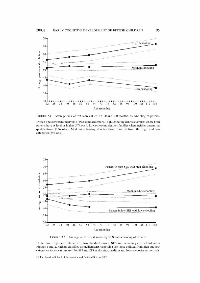
FIGURE A2. Average rank of test scores by SES and schooling of fathers.

Dotted lines represent intervals of two standard errors. SES and schooling are defined as in

Figures 1 and 2. Fathers classified as medium SES=schooling are those omitted from high and lowcategories. Observations are 176, 897 and 219 in the high, medium and low categories respectively.

30

35

40

45

50

55

60

65

70

22 28 34 40 46 52 58 64 70 76 82 88 94 100 106 112 118

Age (months)


High schooling

Medium schooling

Low schooling

FIGURE A1. Average rank of test scores at 22, 42, 60 and 120 months, by schooling of parents.

Dotted lines represent intervals of two standard errors. High schooling denotes families where both

parents have A level or higher (474 obs.). Low schooling denotes families where neither parent has

qualifications (226 obs.). Medium schooling denotes those omitted from the high and low

categories (592 obs.).





REFERENCES

BARNETT, W. S. (1995). Long-term effects of early childcare programs on cognitive and school

outcomes. The Future of Children, 5(3), 25 –50. Los Altos, Cal.: Center for the Future of

Children, The David and Lucile Packard Foundation.

BARTHOLOMEW, D. (1973). Stochastic Model for Social Processes. Chichester: John Wiley.

BAYLEY, N. (1949). Consistency and variability in the growth of intelligence from birth to eighteen

Years. Journal of Genetic Psychology, 75, 165–196.

BERRUETA-CLEMENT, J., SCHWEINHART, L. J., BARNETT, W. S., EPSTEIN, A. S. and WEIKART,

D. P. (1984). Changed lives: the effects of the Perry pre-school programme on youths through

age nineteen. Monograph of the High=Scope Educational Research Foundation, no. 8. Ypsilanti,

Mich.: High=Scope Press.

BORNSTEIN, M. H. and SIGMAN, M. D. (1986). Continuity in mental development from infancy.

Child Development, 57, 251–74.

CHAMBERLAIN, R. and DAVEY, A. (1976). Cross-sectional study of developmental test items in

children aged 94–97 weeks: report of the British Births Child Study. Developmental Medicine

and Child Neurology, 18, 54–70.

COLEMAN, J. S. et al . (1966). Equality of Educational Opportunity, 2 vols. Washington DC: US

Government Printing Office.

DfEE (1999). Sure-Start: A Guide for Trailblazers. London: DfEE.

DOUGHERTY, T. M. and HAITH, M. M. (1997). Infant expectations and reaction time as predictors

of childhood speed of processing and IQ. Developmental Psychology, 33, 146–55.

FEINSTEIN, L. (2000). The relative economic importance of academic, psychological and

behavioural attributes developed in childhood. Centre for Economic Performance Discussion

Paper, no. 443, 209–34.

——, ROBERTSON, D. and SYMONS, J. (1999). Pre-school education and attainment in the NCDS

and BCS. Education Economics, 7(3).

HANUSHEK, E. A. (1986). The economics of schooling: production and efficiency in public schools.Journal of Economic Literature, 24, 1141–77

30

35

40

45

50

55

60

65

70

22 28 34 40 46 52 58 64 70 76 82 88 94 100 106 112 118

Age (months)


Mothers in high SES with high schooling

Medium SES/schooling

Mothers in low SES with low schooling

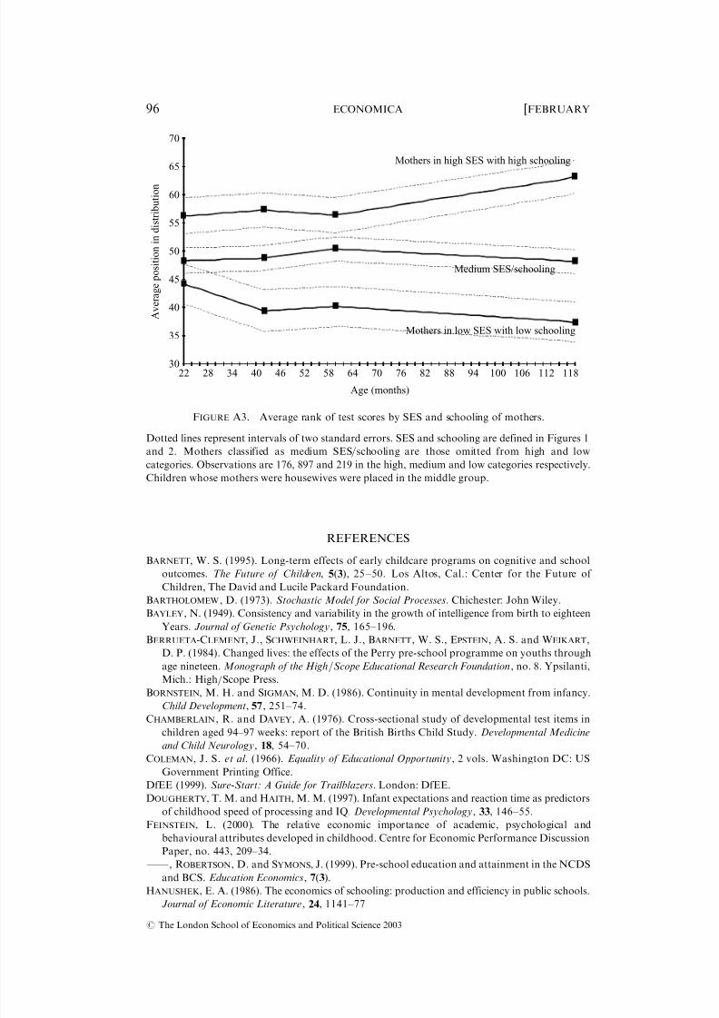
FIGURE A3. Average rank of test scores by SES and schooling of mothers.

Dotted lines represent intervals of two standard errors. SES and schooling are defined in Figures 1

and 2. Mothers classified as medium SES=schooling are those omitted from high and low

categories. Observations are 176, 897 and 219 in the high, medium and low categories respectively.

Children whose mothers were housewives were placed in the middle group.





HARRIS, D. B. (1963). Children’s Drawings as Measures of Intellectual Maturity. New York:

Harcourt, Brace & World.

KLEBANOV, K. B., BROOKS-GUNN, J., MCCARTON, C. and MCCORMICK, M. C. (1998). The

contribution of neighbourhood and family income to developmental test scores over the firstthree years of life. Child Development, 96, 1420–36.

KOPPITZ, E. M. (1968). Psychological evaluation of children’s human figure drawings. New York:

Grure & Stratton.

LIAW, F. and BROOKS-GUNN, J. (1994). Cumulative familial risks and low birth-weight children’s

cognitive and behavioural development. Journal of Child Psychology, 23, 360–72.

LIEBOWITZ, A. (1974). Home investments in children. Journal of Political Economy, 82, 111–31.

NELIGAN, G. A. and PRUDHAM, D. (1969). Norms for four standard development milestones by

sex, social class and place in family. Developmental Medicine and Child Neurologs, 11, 413.

RAMEY, S . L . a n d RAMEY, C. T. (2000). Early childhood experiences and developmental

competence. In J. Waldfogel and S. Danziger (eds.), Securing the Future: Investing in Children

from Birth to College. New York: Russell Sage Foundation, pp. 122–50.

SCHMITT, J. (1993). The changing structure of male earnings in Britain, 1974–1988. Centre for

Economic Performance Discussion Paper, no. 122, March.

SCHWEINHART, L., WEIKART, C. and LARNER, M. (1986). Consequences of three pre-school

curriculum models through age fifteen. Early Education Research Quarterly, 1, 15–45.

SHORROCKS, A. (1978). The measurement of mobility. Econometrica, 46, 1013– 24.

SPEARMAN, C. (1904). General intelligence, objectively determined and measured. American

Journal of Psychology, 15, 201–93.

Waldfogel, J. (1999) Early childhood interventions and outcomes. CASE paper 21, Centre for the

Analysis of Social Exclusion, London School of Economics.

WILSON, R. S. (1983). The Louisville Twin Study: developmental synchronies in behaviour. Child

Development, 54, 298–316.

ZEANAH, C. H., BORIS, N. W. and LARRIEU, J. A. (1997). Infant development and developmental

risk: a review of the past ten years. Journal of the American Academv of Child and Adolescent

Psychiatry, 36(2), 165– 78.



Feinstein 2003 Economica

Documents

Transcript of Feinstein 2003 Economica