FEM-with-UG-NX

FEM WITH UG-NX

NARENDRA KOMARLA

M-CME

MENTOR

Prof. Dr – Ing. H-B. Woyand

Fachgebiet Maschinenbau-Informatik

FEM WITH UG-NX

MASCHINENBAU-INFORMATIK 2 | P a g e

CONTENTS

1. Introduction ..................................................................... 03

2. Entering the Module .......................................................... 04

3. Creating the Mesh ............................................................. 08

4. Assigning Material Properties ........................................... 10

5. Boundary Conditions ......................................................... 11

6. Defining the force ............................................................. 14

7. Results and Post-processing ............................................. 16

FEM WITH UG-NX


1. Introduction

The purpose of this guide is to familiarize the user with the Structural analysis solver in Siemens-NX. Structural analysis using NX is strong and comprehensive, as it uses “NX Nastran Design” as the solver.

An indispensable example of the structural analysis of a cantilever beam is demonstrated here. The analysis demonstrates only basic functions. The main intention of the manual is to familiarize the user with the environment, so that it could be used for practical purposes.

FEM WITH UG-NX


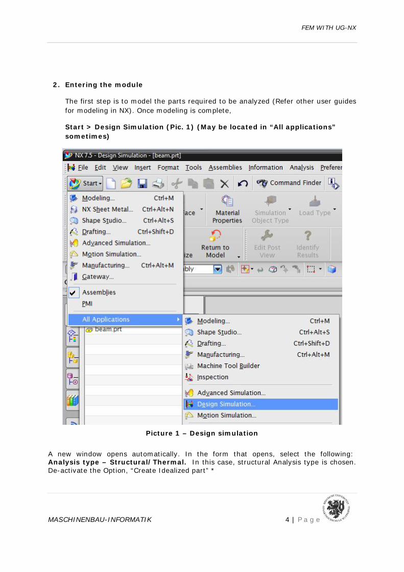
2. Entering the module

The first step is to model the parts required to be analyzed (Refer other user guides for modeling in NX). Once modeling is complete,

Start > Design Simulation (Pic. 1) (May be located in “All applications” sometimes)

Picture 1 – Design simulation

A new window opens automatically. In the form that opens, select the following: Analysis type – Structural/Thermal. In this case, structural Analysis type is chosen. De-activate the Option, “Create Idealized part” *

FEM WITH UG-NX


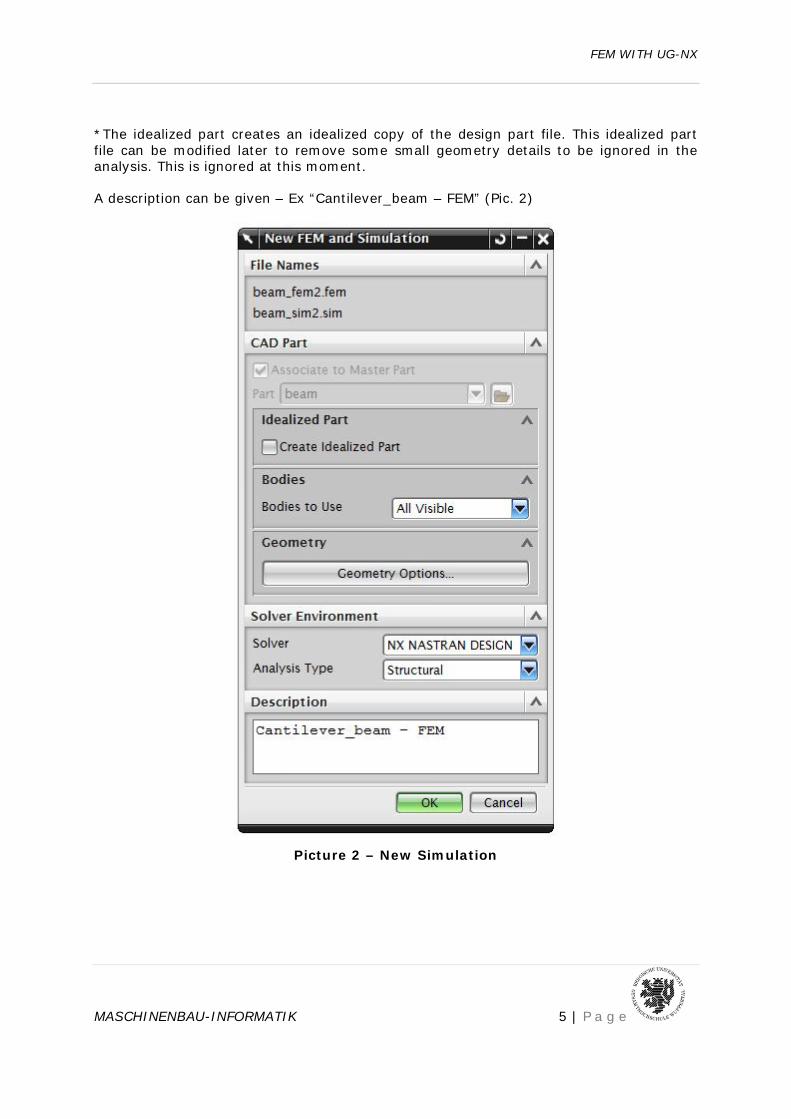
*The idealized part creates an idealized copy of the design part file. This idealized part file can be modified later to remove some small geometry details to be ignored in the analysis. This is ignored at this moment. A description can be given – Ex “Cantilever_beam – FEM” (Pic. 2)

Picture 2 – New Simulation

FEM WITH UG-NX


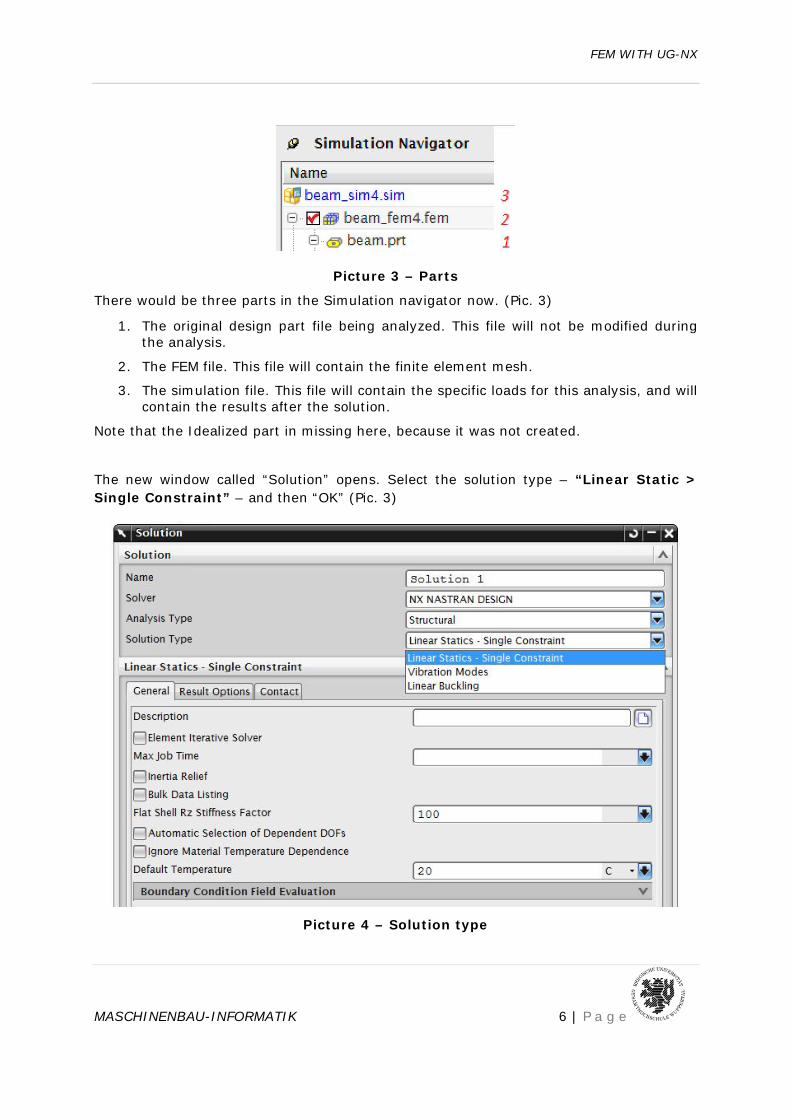
Picture 3 – Parts

There would be three parts in the Simulation navigator now. (Pic. 3)

1. The original design part file being analyzed. This file will not be modified during the analysis.

2. The FEM file. This file will contain the finite element mesh.

3. The simulation file. This file will contain the specific loads for this analysis, and will contain the results after the solution.

Note that the Idealized part in missing here, because it was not created.

The new window called “Solution” opens. Select the solution type – “Linear Static > Single Constraint” – and then “OK” (Pic. 3)

Picture 4 – Solution type

FEM WITH UG-NX


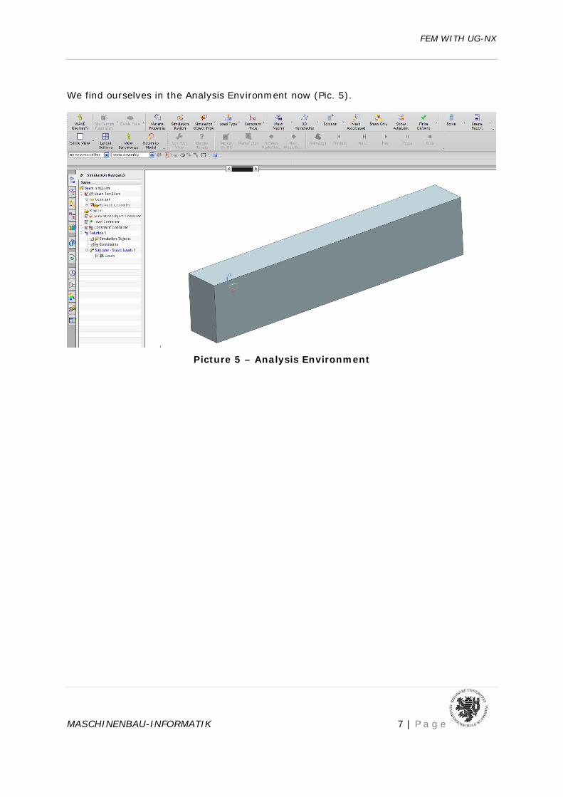
We find ourselves in the Analysis Environment now (Pic. 5).

Picture 5 – Analysis Environment

FEM WITH UG-NX


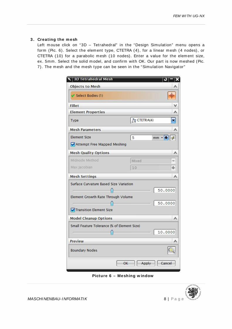
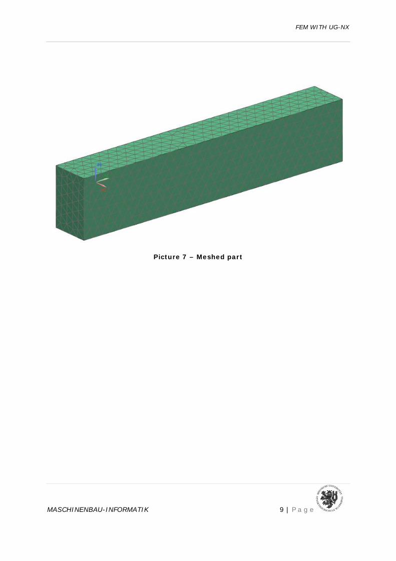
3. Creating the mesh Left mouse click on “3D – Tetrahedral” in the “Design Simulation” menu opens a form (Pic. 6). Select the element type, CTETRA (4), for a linear mesh (4 nodes), or CTETRA (10) for a parabolic mesh (10 nodes). Enter a value for the element size, ex. 5mm. Select the solid model, and confirm with OK. Our part is now meshed (Pic. 7). The mesh and the mesh type can be seen in the “Simulation Navigator”

Picture 6 – Meshing window

FEM WITH UG-NX


Picture 7 – Meshed part

FEM WITH UG-NX


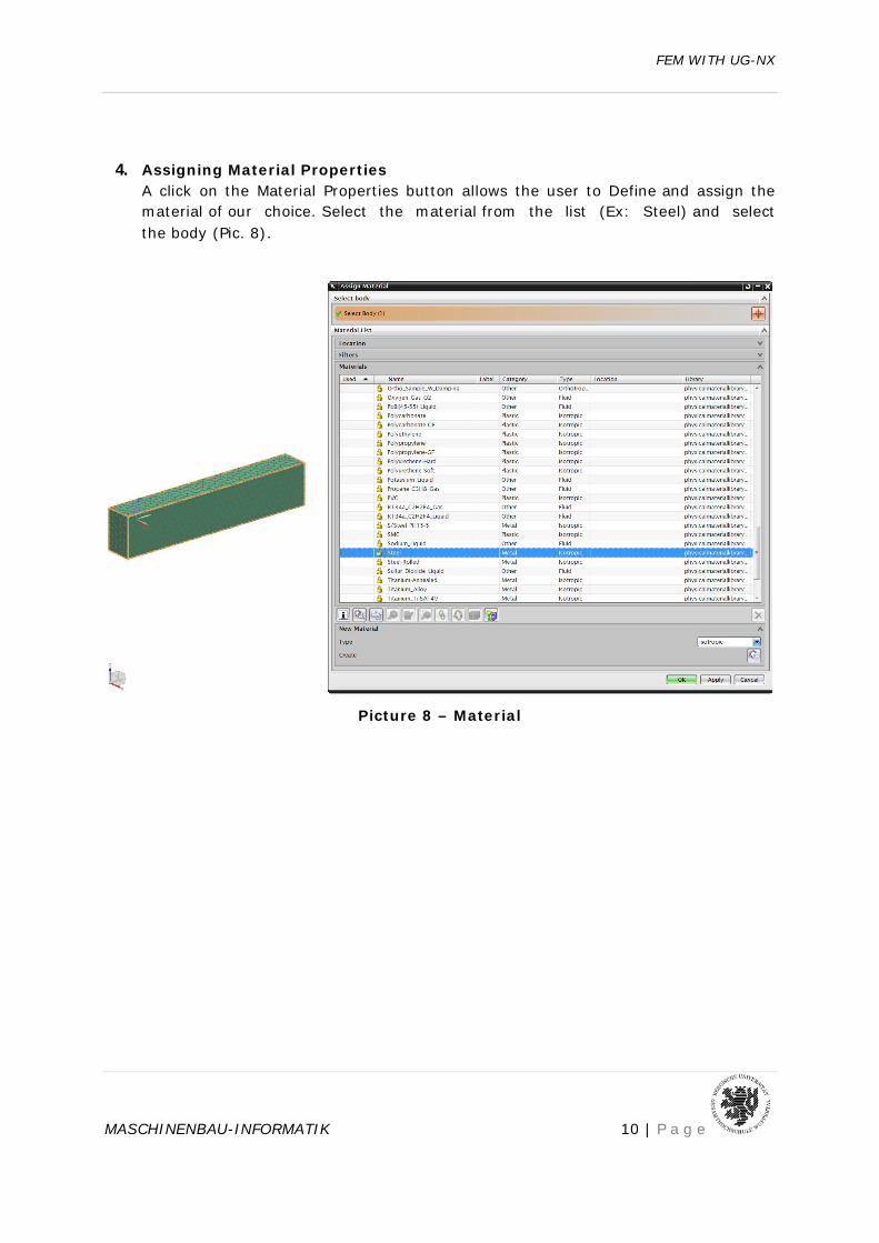
4. Assigning Material Properties

A click on the Material Properties button allows the user to Define and assign the material of our choice. Select the material from the list (Ex: Steel) and select the body (Pic. 8).

Picture 8 – Material

FEM WITH UG-NX


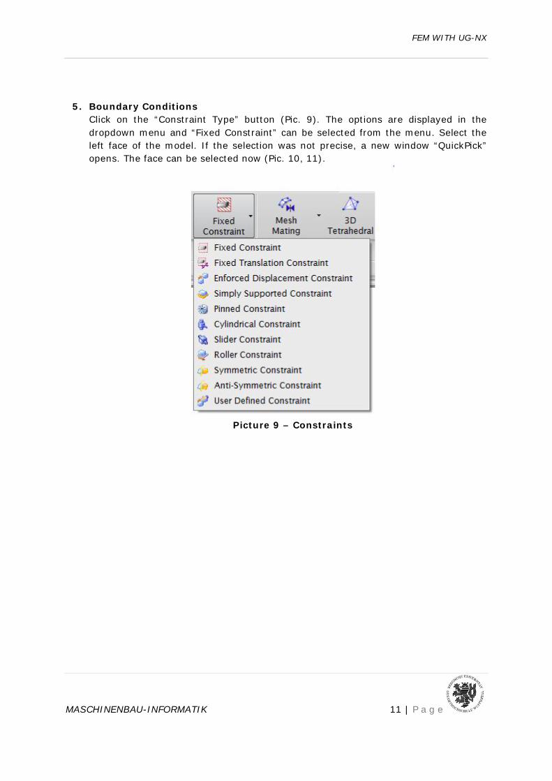
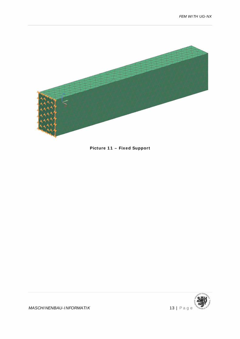
5. Boundary Conditions

Click on the “Constraint Type” button (Pic. 9). The options are displayed in the dropdown menu and “Fixed Constraint” can be selected from the menu. Select the left face of the model. If the selection was not precise, a new window “QuickPick” opens. The face can be selected now (Pic. 10, 11).

Picture 9 – Constraints

FEM WITH UG-NX


Picture 10 – Fixed Boundary Conditions

FEM WITH UG-NX


Picture 11 – Fixed Support

FEM WITH UG-NX


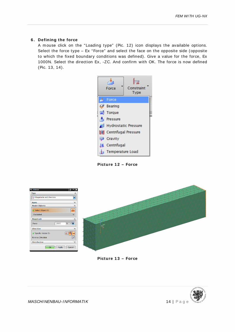
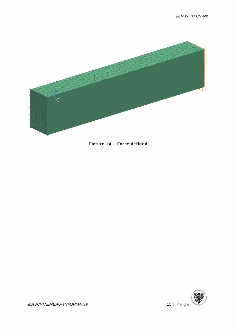
6. Defining the force A mouse click on the “Loading type” (Pic. 12) icon displays the available options. Select the force type – Ex “Force” and select the face on the opposite side (opposite to which the fixed boundary conditions was defined). Give a value for the force, Ex 1000N. Select the direction Ex, -ZC. And confirm with OK. The force is now defined (Pic. 13, 14).

Picture 12 – Force

Picture 13 – Force

FEM WITH UG-NX


Picture 14 – Force defined

FEM WITH UG-NX


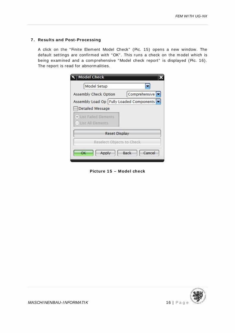
7. Results and Post-Processing

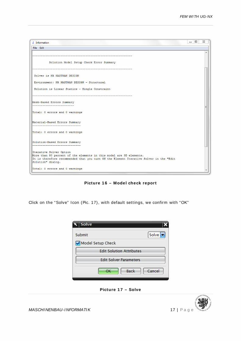
A click on the “Finite Element Model Check” (Pic. 15) opens a new window. The default settings are confirmed with “OK”. This runs a check on the model which is being examined and a comprehensive “Model check report” is displayed (Pic. 16). The report is read for abnormalities.

Picture 15 – Model check

FEM WITH UG-NX


Picture 16 – Model check report

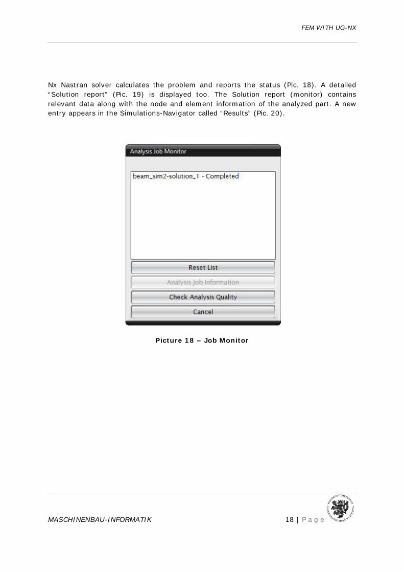
Click on the “Solve” Icon (Pic. 17), with default settings, we confirm with “OK”

Picture 17 – Solve

FEM WITH UG-NX


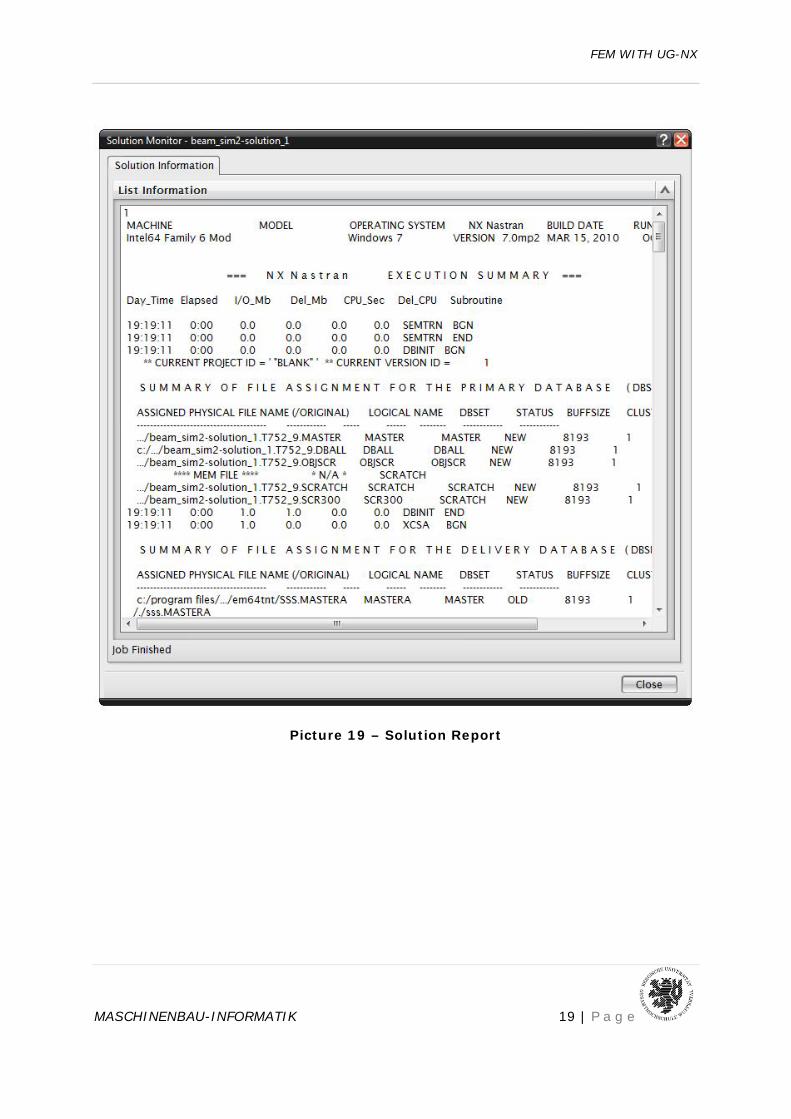
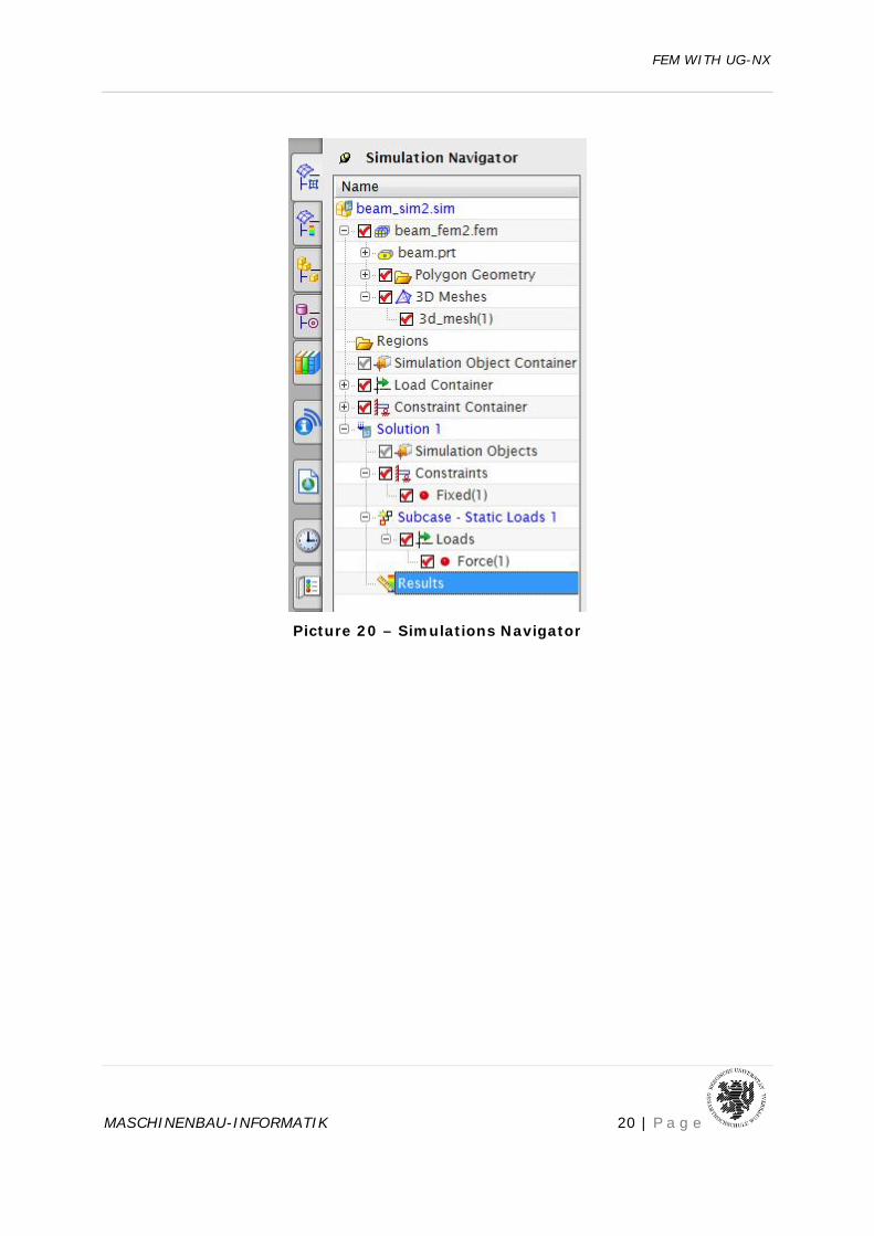
Nx Nastran solver calculates the problem and reports the status (Pic. 18). A detailed “Solution report” (Pic. 19) is displayed too. The Solution report (monitor) contains relevant data along with the node and element information of the analyzed part. A new entry appears in the Simulations-Navigator called “Results” (Pic. 20).

Picture 18 – Job Monitor

FEM WITH UG-NX


Picture 19 – Solution Report

FEM WITH UG-NX


Picture 20 – Simulations Navigator

FEM WITH UG-NX


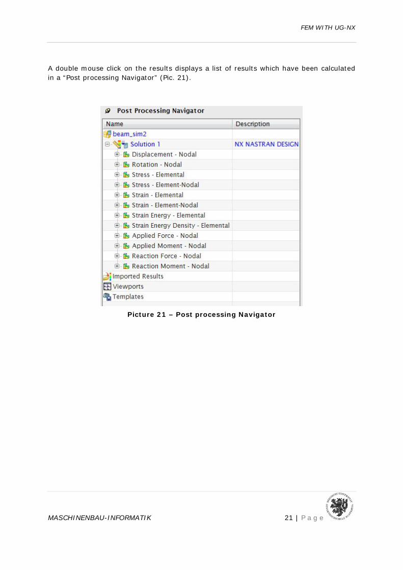
A double mouse click on the results displays a list of results which have been calculated in a “Post processing Navigator” (Pic. 21).

Picture 21 – Post processing Navigator

FEM WITH UG-NX


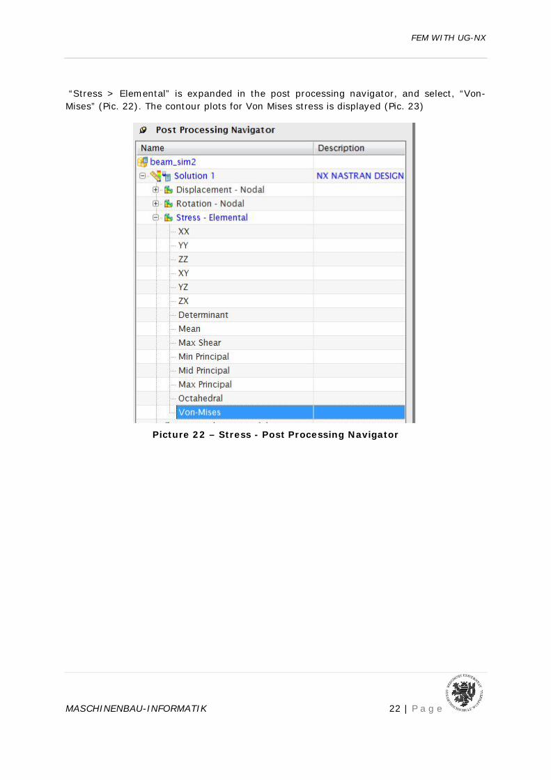
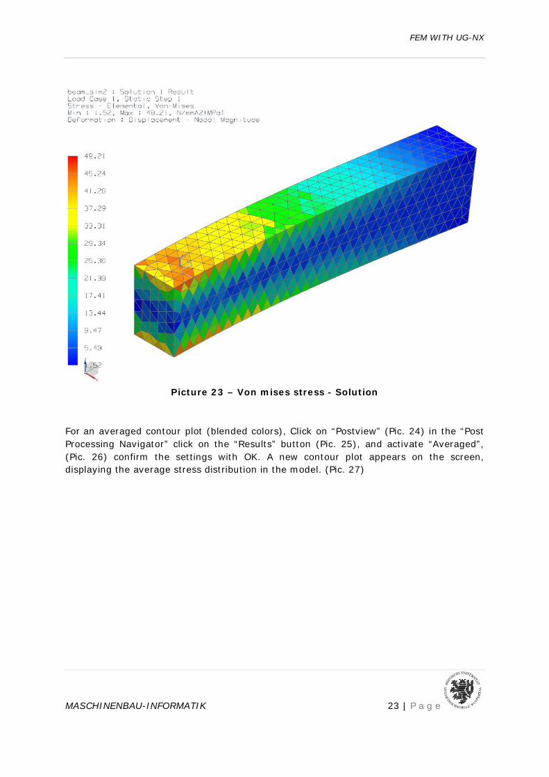
“Stress > Elemental” is expanded in the post processing navigator, and select, “Von-Mises” (Pic. 22). The contour plots for Von Mises stress is displayed (Pic. 23)

Picture 22 – Stress - Post Processing Navigator

FEM WITH UG-NX


Picture 23 – Von mises stress - Solution

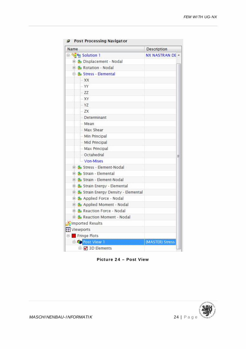
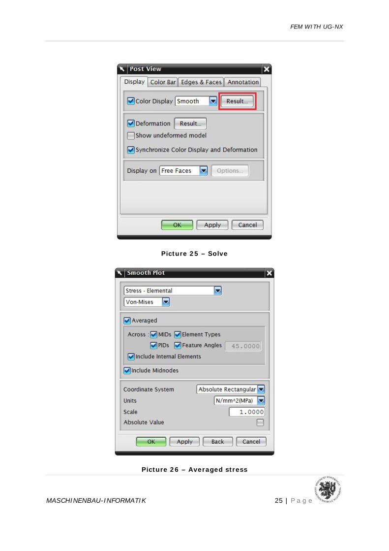
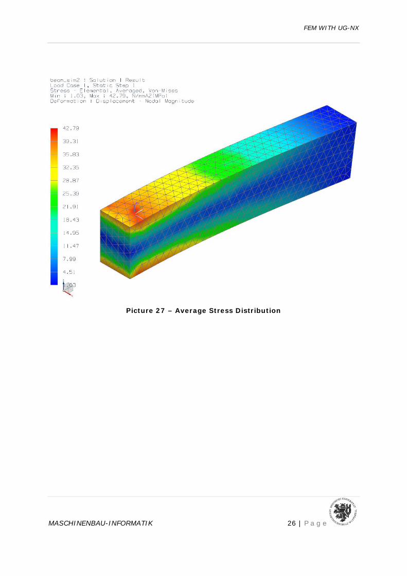
For an averaged contour plot (blended colors), Click on “Postview” (Pic. 24) in the “Post Processing Navigator” click on the “Results” button (Pic. 25), and activate “Averaged”, (Pic. 26) confirm the settings with OK. A new contour plot appears on the screen, displaying the average stress distribution in the model. (Pic. 27)

FEM WITH UG-NX


Picture 24 – Post View

FEM WITH UG-NX


Picture 25 – Solve

Picture 26 – Averaged stress

FEM WITH UG-NX


Picture 27 – Average Stress Distribution

FEM-with-UG-NX

Documents

Transcript of FEM-with-UG-NX