Geschwindigkeitsmessung in einer turbulenten Strömung ... · W Q I2 R hAT w or replacing h with...

8. November 2012 | 1

Geschwindigkeitsmessung in einer turbulentenStrömung mittels Hitzdrahtanemometrie

Messtechnik Vorlesung

8. November 2012

How to measure turbulence with hot-wire

anemometers- a practical guide

Finn E. Jørgensen - 2005


Motivation - Turbulenz

Die Hitzdrahtanemometrie ermöglicht

• die Messung der lokalen Geschwindigkeit und• der sehr feinskaligen Fluktuationsgeschwindigkeiten.

Der Student soll in der Lage sein (Praktikum),

• ein CTA-Setup festzulegen• Messungen zur Bestimmung grundlegender turbulenter

Eigenschaften auszuführen,• die notwendigen Vorbereitungen zu treffen• die Datenerfassung und -auswertung durchzuführen.• Fehler einzuschätzen.


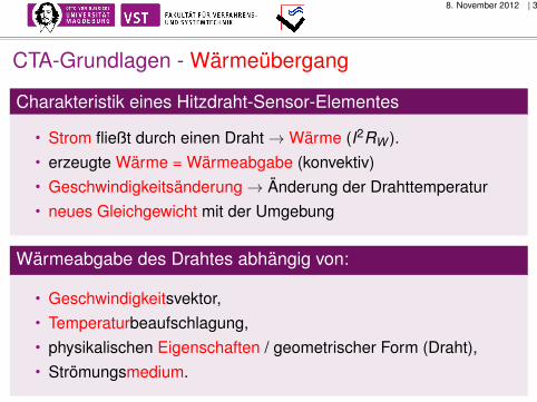
CTA-Grundlagen - Wärmeübergang

Charakteristik eines Hitzdraht-Sensor-Elementes

• Strom fließt durch einen Draht→Wärme (I2RW ).• erzeugte Wärme = Wärmeabgabe (konvektiv)• Geschwindigkeitsänderung→ Änderung der Drahttemperatur• neues Gleichgewicht mit der Umgebung

Wärmeabgabe des Drahtes abhängig von:

• Geschwindigkeitsvektor,• Temperaturbeaufschlagung,• physikalischen Eigenschaften / geometrischer Form (Draht),• Strömungsmedium.


Dynamische Charakteristik, Grenzfrequenz

Reaktion des Hitzdrahtes

• instationäre Wärmebilanzgleichung• thermische Trägheit, Fluktuationen gedämpft• Kompensationen mit Hilfe der Elektronik notwendig• Konstant-Temperatur-Anemometer• Erhöhung der Grenzfrequenz auf das bis zu 1000-fache [1,2].

Kalibrierung

• Spannung - Geschwindigkeit• Potenzgesetzbeziehung• Einflussgrößen: Re, Nu und Pr [3]


Grundlegende Gleichung

Für einen dünnen erwärmtenDraht, der einer Geschwindigkeitausgesetzt wird

W = Q +dQi

dt

48

Governing equation:Consider a thin heated wire mounted to supports and exposed to a velocity U.

dt

idQQW ��

W = power generated by Joule heating W = I2 Rw , recall Rw = Rw(Tw)Q = heat transferred to surroundings Qi = CwTw =thermal energy stored in wireCw = heat capacity of wireTw = wire temperature

Static characteristics –stationary heat transfer:Heat storage in the wire is zero:

� �02 TThARIQW w ��

or replacing h with Nu:

� �02 TTNuk

dARI wfw ��

h = film coefficient of heat transferA = heat transfer aread = wire diameterkf = heat conductivity of fluidNu = dimensionless heat transfer coefficient

In the forced convection regime (0.02<Re<140):

Reynolds number: �

� dU ��

�Re , ��= air density, U= velocity and ��= air dynamic viscosity.

Nu = A1 + B1 · Ren = A2+ B2 Un

I2Rw2 = E2 = (Tw –T0)(A + BUn) “King’s law” �15�. The voltage is a measure of velocity U.

Dynamic characteristics- frequency limit:Heat storage term added to the stationary heattransfer equation:

� �� dt

wdTwCnBUARwRwRI �� 0

2

or expressing Tw in terms of Rw and temperature coefficient of resistance �0:

� �� dt

dRR

CBUARRRI wwn

ww00

02

�

��

This differential equation has the time constant �:

� �21100 IUBAR

Cn

w

��

�

�

�

Frequency limit (3 dB amplitude damping):

��21

�cpf

Abbildung: Sensor

W Energie, die durch Erwärmung entstehtW = I2Rw wobei Rw = Rw (Tw )Q an die Umgebung abgeführte WärmeQi = CwTw im Draht gespeicherte thermische EnergieCw Wärmekapazität des DrahtesTw Drahttemperatur


Statische Charakteristiken - stationärer Wärmeübergang

Die Wärmespeicherung im Draht ist Null:

W = Q = I2Rw = hA(Tw − T0)

oder wenn h durch Nu ersetzt wird:

I2Rw =Ad

Nukf (Tw − T0)

h Film-Koeffizient des WärmeübergangsA Wärmeübertragungsfläched Drahtdurchmesserkf Wärmeleitfähigkeit des FluidsNu dimensionsloser Wärmeübergangskoeffizient


Charakterisierung der Dynamik - Frequenzgrenze:

Den Wärmespeicher-Term hinzu addiert zur stationärenWärmeübertragungsgleichung ergibt

I2Rw = (Rw − R0)(A + BUn) + CwdTw

dtoder Tw ausgedrückt durch Rw und denWärmeübergangskoeffizienten α

I2Rw = (Rw − R0)(A + BUn) +Cw

α0R0

dRw

dtDiese Differentialgleichung hat die Zeitkonstante τ :

τ =Cw

α0R0(A1 + B1Un − I2)

Das Frequenzlimit (3 dB Amplitudendämpfung)

fcp =1

2πτ


Sondenkonstruktion

50

Probe design:

Tungsten wire is spot-welded to stainless steel prongs embedded in a ceramic tube.Gold-plated probes have plated wire ends inorder to minimise prong effects.

Spatial resolution:

Hot-wire resolution lx in streamwise direction:

cp

meanx f

Ul

2� �5�.

Umean = mean velocityfcp = frequency limit

High spatial resolution at high velocity requires high bandwidth

Directional sensitivity:

Finite wire response includes yaw and pitch Sensitivity �24�, �29�.:

� � � � � ��22222 sincos0 kUU �� θ = 0

� � � � � ��22222 sincos0 hUU �� = 0

General response in 3-D flows:222222

zUhyUkxUeffU ��

U(0): actual velocity in the flowUeff: effective cooling velcoity

(calculated from velocity calibration)�: yaw angle (angle between velocity

and wire normal)θ: pitch angle (agle between velocity

and wire wire-prong plane)k: yaw factorh: pitch factor(x,y,z): probe oriented coordinate system

Abbildung: Sondenaufbau


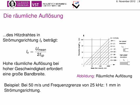
Die räumliche Auflösung

...des Hitzdrahtes inStrömungsrichtung lx beträgt:

lx =Umean

2fcp

Hohe räumliche Auflösung beihoher Geschwindigkeit erforderteine große Bandbreite.

50

Probe design:


Spatial resolution:


cp

meanx f

Ul

2� �5�.





� � � � � ��22222 sincos0 kUU �� θ = 0

� � � � � ��22222 sincos0 hUU �� = 0


zUhyUkxUeffU ��





Abbildung: Räumliche Auflösung

Beispiel: Bei 50 m/s und Frequenzgrenze von 25 kHz: 1 mm inStrömungsrichtung.

8. November 2012 | 10

Richtungsempfindlichkeit (2/3-D Sonden) [4,5]

U2eff = U2

x + k2U2y + h2U2

z

50

Probe design:


Spatial resolution:


cp

meanx f

Ul

2� �5�.





� � � � � ��22222 sincos0 kUU �� θ = 0

� � � � � ��22222 sincos0 hUU �� = 0


zUhyUkxUeffU ��





50

Probe design:


Spatial resolution:


cp

meanx f

Ul

2� �5�.





� � � � � ��22222 sincos0 kUU �� θ = 0

� � � � � ��22222 sincos0 hUU �� = 0


zUhyUkxUeffU ��





U(α)2 = U(0)2(cos2α + k2sin2α), mit θ = 0

U(θ)2 = U(0)2(cos2θ + h2sin2θ), mit α = 0

8. November 2012 | 11

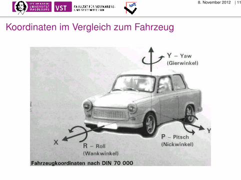
Koordinaten im Vergleich zum Fahrzeug

Page 1/1

8. November 2012 | 12

Blockschaltbild eines CTA

Page 1/1

8. November 2012 | 13

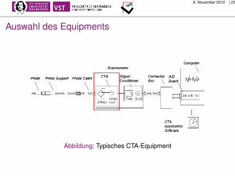
Auswahl des Equipments

6

1. SELECTING MEASUREMENT EQUIPMENT

1.1 Measuring chain

Fig. 1. Typical CTA measuring chain.

The measuring equipment constitutes a measuring chain. It consists typically of aProbe with Probe support and Cabling, a CTA anemometer, a Signal Conditioner, anA/D Converter, and a Computer. Very often a dedicated Application soft-ware for CTAsetup, data acquisition and data analysis is part of the CTA anemometer. A traversesystem may be added for probe traverse, when profiles have to be investigated. Adedicated probe calibrator may speed up an experiment and reduce the total costs, as itcuts down expensive wind-tunnel time.

1.2 Probe selectionProbes are primarily selected on basis of:

� Fluid medium

� Number of velocity components to be measured (1-, 2- or 3)

� Expected velocity range

� Quantity to be measured (velocity, wall shear strees etc.)

� Required spatial resolution

� Turbulence intensity and fluctuation frequency in the flow

� Temperature variations

� Contamination risk

� Available space around the measuring point (free flow, boundary layer flows,confined flows).

Abbildung: Typisches CTA-Equipment

8. November 2012 | 14



8. November 2012 | 15

Sondenauswahl

...richtet sich nach:

• dem Strömungsmedium• der Anzahl der zu messenden Geschwindigkeitskomponenten• dem erwarteten Geschwindigkeitsbereich• der Größen, die gemessen werden sollen (U, τ usw.)• der erforderlichen räumlichen Auflösung• der Turbulenzintensität und Frequenz der

Geschwindigkeitsschwankungen• den Temperaturverhältnissen• der Verschmutzungsgefahr• den räumlichen Bedingungen um den Messpunkt herum (freie

Strömung, Grenzschichtströmung, räumliche Beschränkungen)

8. November 2012 | 16

Schnelleinstieg in die Sondenauswahl

7

1.2.1 Quick guide to probe selection

Free and Confined Flows

Type of flow Medium Recommended Probes1-Dimensional

Uni-directional Gas Single sensor Wire Single sensor Fiber, thin coat.Wedge-shaped Film, thin coat.Conical Film, thin coat.

Liquid Single sensor Fiber, heavy coat.Wedge-shaped Film, heavy coat.Conical Film, heavy coat.

Bi-directional Gas Split-fibers, thin coat.Liquid Split-fibers, heavy coat.

2-DimensionalOne Quadrant Gas X-array Wires

X-array Fibers, thin coat.V-wedge Film, thin coat.

Liquids X-array Fibers, heavy coat.V-wedge Film, heavy coat.

Half Plane Gas Split-fibers, thin coat.Liquids Split-fibers, heavy coat.

Full Plane Gas Triple-split Fibers, thin coat.X-array Wire, flying hot-wire

Liquids Triple-split Fibers, special

3-DimensionalOne Octant(70� Cone) Gas Tri-axial Wire

Tri-axial Fiber, thin coat.Liquids Tri-axial Fiber, Special

90� Cone Gas Slanted Wire, rotated probeLiquids Slanted Fiber, heavy coat.

Full Space Gas Omnidirectional FilmWall Flows(Shear Stress)Type of flow Medium Recommended Probes

1-DimensionalUnidirectional Gas Flush-mounting Film, thin coat.

Glue-on Film, thin coat.Liquids Flush-mounting Film, heavy coat.

Glue-on Film, special

8. November 2012 | 17

Drahtsonden

Miniaturdrähte

• Für Anwendungen in Luft• Tu bis zu 5-10%• höchster Frequenzgang• können repariert werden• am häufigsten angewendet

mit Goldummantelung

• Für Anwendungen in Luft• Tu bis hin zu 20-25%• Frequenzgang ist dem von

Miniatursonden unterlegen• können repariert werden

8. November 2012 | 18

Fiber-Filmsonden

mit dünnem Quartz-Überzug

• Für Anwendungen in Luft• Frequenzgang ist dem von

Drähten unterlegen• robuster als Drahtsonden• für weniger reine Luft• können repariert werden

mit stabilem Quartz-Überzug

• Für Anwendungen in Wasser• Frequenzgang ist dem von

Miniatursonden unterlegen• können repariert werden

8. November 2012 | 19

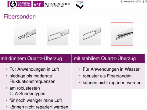
Fibersonden

mit dünnem Quartz-Überzug

• Für Anwendungen in Luft• niedrige bis moderate

Fluktuationsfrequenzen• am robustesten

CTA-Sondentypen• für noch weniger reine Luft• können nicht repariert werden

mit stabilem Quartz-Überzug

• Für Anwendungen in Wasser• robuster als Fibersonden• können nicht repariert werden

8. November 2012 | 20

Eindrahtsonden

normale EindrahtsondenFür eindimensionale beliebig gerichtete Strömungen. Verschiedenangeordneten Haltestiften, die es erlauben, den Fühldraht genausenkrecht und die Stifte parallel zur Strömung auszurichten.

schräg angeordnete Eindrahtsonden (45◦)

Für dreidimensionale stationäre Strömungen, bei denen derGeschwindigkeitsvektor innerhalb eines Kegels von 90◦ auftritt.Während der Messungen muss die Sonde gedreht werden.

8. November 2012 | 21

Zweidrahtsonden

X-Draht-SondeFür zweidimensionale Strömungen mit einem Geschwindigkeitsvektorinnerhalb von ±45◦ bezüglich der Sondenachse.

Split-Fiber-Sonde

Für zweidimensionale Strömungen mit einem Geschwindigkeitsvektorinnerhalb von ±90◦ bezüglich der Sondenachse. Die kreuzweiseräumliche Auflösung beträgt 0,2 mm und ist für Scherschichten bessergeeignet als X-Draht-Sonden.

8. November 2012 | 22

Dreidrahtsonden

Dreiachsige Sonde

Für zweidimensionale Strömungen, mit einem Geschwindigkeitsvektorinnerhalb eines Kegels von 70◦ Öffnungswinkel um die Sondenachse.Die räumliche Auflösung ist durch eine Kugel mit einem Durchmesservon 1,3 mm definiert.

Dreifach-Split-Filmsonde

Für vollständig umkehrbare zweidimensionale Strömungen mit einemakzeptierten Winkel von ±180◦.

8. November 2012 | 23



8. November 2012 | 24

CTA-Anemometer

CTA für Forschungszwecke (Streamline)

• typische Bandbreite: 100-250 kHz (max. 400 kHz).• typisches Rauschen: 0,005% (bei 0,1%@10 kHz).• typische Drift: 0,5µV/◦C (Verstärkereingang)

CTA-Brücke

• 1:20-Brücke für allgemeine Zwecke bei Anwendung inLuftströmungen bei einer Bandbreite bis etwa 250 kHz.

• 1:20-Brücke für allgemeine Zwecke bei hoher Brückenleistungund Anwendung in Wasserströmungen.

• 1:1-symmetrische Brücke für Bandbreiten bis 400 kHz oder fürlange Sondenkabel bis zu 100 m (reduziert auf 50 kHz).

8. November 2012 | 25



8. November 2012 | 26

Signalaufbereitung - Auswahl

Offset:• sollte den Eingangsbereich des A/D-Wandlers überdecken,• Praxis: den Bereich des CTA-Ausgangsignals (z.B. 0-5 V)

Verstärkung:• verbessert die Auflösung des A/D-Wandlers• Verstärkung von 16: 12→16-bit-Wandler

Hochpassfilter:• beseitigt den Gleichanteil des Signals• zum Entfernen geringer Frequenz-Fluktuationen

Tiefpassfilter:• beseitigt elektronisches Rauschen und beugt dem Aliasing vor• sollte so steil wie möglich sein

8. November 2012 | 27



8. November 2012 | 28

Auswahl des A/D-WandlersAnzahl der Kanäle

• Anzahl der CTA-Kanäle• plus zusätzliche Kanäle für Temperatur- und andere Messungen

Input-Bereich• mindestens den Spannungsbereich des CTA überdecken• 0-10 V für die meisten Anemometer und Anwendungen

Input-Auflösung• erforderliche Auflösung der Daten...• 12-bit-Wandler: Auflösung von 0,025%.

8. November 2012 | 29

Auswahl des A/D-WandlersSampling-Rate

• mehr als zweimal so hoch sein wie die maximale Frequenz in derStrömung

• wird durch die Anzahl der im Gebrauch befindlichen Kanäle nreduziert

• Ein 100 kHz Wandler deckt die meisten niedrigen bis mittlerenGeschwindigkeiten ab (<100 m/s).

Simultanaufnahme• zur Korrelation zwischen schnell aufgenommenen Kanälen

(z.B. Reynolds´sche Schubspannung)Externe Triggerung

• für Messungen, die einem bestimmten Ereignis zugeordnetwerden sollen

8. November 2012 | 30



8. November 2012 | 31

12

1.5 ComputerThe choice of computer to be used for CTA measurements is normally not critical.Speed and memory storage are normally more than sufficient for most applications. Itis, however, important to ensure that the CTA controller, the A/D board driver and thetraverse driver are compatible, i.e. runs under the same operative system and can becalled from the same application software. Also that the required number of com portsfor communication with the CTA anemometer and the traverse system is available.

1.6 CTA application softwareCommercially available CTA anemometers are normally delivered together with anapplication software. Advanced software packages control the anemometer and carryout automatic setup of both CTA bridge and signal conditioner �14�. They also performautomatic velocity and directional calibrations and they can be programmed to performautomatic experiments with probe traversing and data equisition. Finally data areconverted into engineering units and reduced to relevant statistical quantities: moments,spectra etc. Application software for manually operated anemometers is also available.Except for the anemometer and calibrator drivers, they have by and large the samefunctionality as the advanced packages.

Note: It is highly recommended to use professional CTA application software when at allpossible in order to reduce the time and costs it otherwise takes to start up. In special cases,where the CTA is part of a large measurement system with input from many other types ofinstruments including the control of windtunnels and traverses, it may be worthwhileconsidering writing ones own software. Even then, it may be sensible to use the velocity anddirectional calibration routines offered by a professional application software.

Abbildung: Screenshot mit Programmteilen (links) und einem E(t)-Verlauf

8. November 2012 | 32

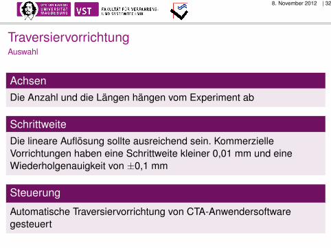
TraversiervorrichtungAuswahl

AchsenDie Anzahl und die Längen hängen vom Experiment ab

SchrittweiteDie lineare Auflösung sollte ausreichend sein. KommerzielleVorrichtungen haben eine Schrittweite kleiner 0,01 mm und eineWiederholgenauigkeit von ±0,1 mm

Steuerung

Automatische Traversiervorrichtung von CTA-Anwendersoftwaregesteuert

8. November 2012 | 33

KalibrierungKalibriervorrichtung

zugehörige Kalibriervorrichtung

Geschwindigkeitsbereich von wenigen cm/s bis zu einigen 100 m/s.Genauigkeit typischerweise ±0,5% vom Messwert,

oberhalb 5 m/s.Zusatzausstattung Richtungskalibrierungen

von Mehrdrahtsonden

Windkanal mit PitotrohrGeschwindigkeitsbereich von ca.2 m/s bis zu typischerweise 50 m/s.Genauigkeit typischerweise ±1,0% vom Messwert,

oberhalb 5 m/s (abhängig vomDruckmessgerät, starke Abnahmebei kleineren Geschwindigkeiten.

8. November 2012 | 34

Versuchsplanung

• Was soll gemessen werden? Welche physikalischen Variablen, welchestatistischen Funktionen werden benötigt? Darstellung?

• Sensoren: Messempfindlichkeit, potentielle Probleme

• Die zu erwartenden Ergebnisse vorher abschätzen, eventuellTestmessungen (auch mit anderen Geräten) durchführen.

• Den Messaufbau zusammenstellen.

• Bestimmung der optimalen Datenrate, der Messzeit und der Anzahl dererforderlichen Messwerte.

• Die Funktion des Messsystems bei variierenden Parametern überprüfen.Ist das System unempfindlich gegen kleine Änderungen imMessbereich, Verstärkung usw.?

• Ergebnisse online anzeigen, es kann Veränderungen geben z.B. derTemperatur, oder anderer Bedingungen während der Traversierung.

8. November 2012 | 35

Checkliste

• Festlegung der Größen, die zu messen sind• Momente höherer Ordnung, Frequenzverteilung, Wirbelgrößen

• Festlegung der Verteilung der Messpunkte• Einpunktmessung, Profil (Traversierung), an mehreren Punkten

• Auswahl des Equipments und der Software• Strömungsmedium, Dimensionen, zu messende Größen, usw.

• Festlegung des Versuchsablaufs• Art des Strömungsfeldes, Datenauswertung

• Festlegung der Datenanalyse auf der Grundlage von• erforderlichen Ergebnissen gegenüber gemessenen Ergebnissen• Setup des Equipments und der Datenverarbeitung

8. November 2012 | 36

Schritt-für-Schritt-Anleitung

Hardware-Setup

1 Festlegung des Überhitzungsgrades.2 Messung der vorliegenden Temperatur, wenn

Temperaturänderungen zu erwarten sind.3 Falls notwendig, Test der Ansprechempfindlichkeit des Systems

mit einem Rechteckwellentest4 Festlegung des Tiefpass-Filters

Geschwindigkeitskalibrierung

5 Beaufschlage die Sonde mit einer Reihe von bekanntenGeschwindigkeiten und lege die Übertragungsfunktion fest.

8. November 2012 | 37

Richtungskalibrierung

6 Nur für 2- und 3-Drahtsonden und nur, wenn hohe Genauigkeiterforderlich ist. Andererseits können die vom Herstellerempfohlenen Gier- und Nickkoeffizienten verwendet werden.

Datenumwandlung und Datenreduzierung

7 Die Übertragungsfunktion liefert die Kalibrierung derGeschwindigkeiten

8 Die Aufteilung der Geschwindigkeiten mittels Gier- undNickkoeffizienten liefert die Geschwindigkeitskomponenten

9 Das Datenauswertungsmodul liefert die reduzierten Daten

8. November 2012 | 38

Festlegung des Experimentes

10 Wähle das Hardware-Setup aus.• Option 1: Regelung des Überhitzungsgrades, wenn

Temperaturänderungen zu erwarten sind.• Option 2: Konstanthalten des Überhitzungswiderstandes (erfordert

Temperaturkompensation wenn Temperaturänderungen auftreten)

11 Sondenbewegung: Festlegung eines Traversier-Gitters

Festlegung der Datenerfassung

12 Datenrate und Anzahl der Messwerte

8. November 2012 | 39

Testdurchlauf

13 Sonde in der Strömung unterbringen und Messwerte aufnehmen.Überprüfung der reduzierten Daten (mittlere Geschwindigkeit,Standardabweichung usw.) im Vergleich zu erwarteten Werten.

Versuchsdurchführung

14 Sonde an den Messort bewegen, Hardwareeinstellungenüberprüfen, Sondenspannung messen.

Datenumwandlung und -reduzierung

15 Daten einladen und ausgewählte Umwandlungs-/Reduzierungs-Routinen anwenden.

8. November 2012 | 40

Präsentation der Daten

16 grafische Darstellung der Daten oder Export.

8. November 2012 | 41

Sondenmontage und -orientierung

Die Sonde wird wie bei der Kalibrierung, in die Strömung montiert(Draht senkrecht und Haltestiften parallel zur Strömung).

16

4. SYSTEM CONFIGURATIONSystem configuration is the process of mounting and interconnecting the selected

probes, cables, CTA anemometers, signal conditioners and A/D channels. Theconfiguration may also include a Traverse system for the probe.

4.1 Probe mounting and cabling

4.1.1 Probe mounting and orientationThe probe is mounted in the flow with the same orientation as it had during calibration.Preferably with the wire perpendicular to the flow and the prongs parallel with the flow.

Fig. 2. Probe orientation with respect to laboratory coordinate system.

Straight probes are mounted with the probe axis parallel with the dominant velocitydirection. It is recommended that the probe coordinate system (X,Y,Z) coincides with thelaboratory coordinate system (U,V,W).

The probe is mounted in a probe support, which is equipped with a cable andBNC connector, one for each sensor on the probe. Film probes are equipped with fixedcables and need no supports. Probe bodies and the probe support are designed so thattheir outer surfaces are electrically insulated from the electrical circuitry of the probe oranemometer circuit. They can therefore be mounted directly to any metal part of the testrig without the risk of ground loops.

It is important to note that the BNC connectors do not make electrical contact with any metalparts of the rig or elsewhere. The BNC connectors represent the signal ground and maytherefore carry ground loops. It is also important that the BNC connectors on dual- or triple-sensor supports do not touch each other, as it will influence the floating amplifiers in the CTA.

It is therefore recommended to cover all BNC connectors with a length of plastic tube.

Important: The probe should only be mounted in its support or removed from it,when the CTA is switched to Stand- by or the power to the CTA is disconnected.

Abbildung: Sondenorientierung bezüglich des Labor-Koordinatensystems

8. November 2012 | 42

Verbindungskabel

17

4.1.2 Cabling

Fig. 3. Avoiding ground loops and noise pickup.

The distance between the probe and the CTA should be kept as small as possible.The standard cable length is 4 meters probe cable plus 1 meter support cable, and thiscombination should be used if at all possible in order to obtain maximum bandwidthand in order to avoid picking up more noise than need be. If longer cables are necessary,it is important to follow the lengths recommended by the manufacturer for the actualCTA bridge (normally 20 or 100 m).

4.1.3 Liquid grounding Film probes mounted in liquids may be damaged, if a voltage difference between

the sensor film and the liquid builds up by electric charges in the flowing medium. Ifsuch charge build up occurs, the insulating quartz coating may break down and the thin-film will be etched away due to electrolysis. The liquid must therefore be grounded tothe anemometer’s signal ground as close to the probe as possible.

Fig. 4. Grounding of liquid to Signal ground near film probe.

It is recommended to use the BNC-BNC cables delivered together with the CTA by themanufacturer in order to match the cable-compensating network in the bridge.If this is not done, the bridge may become unstable and deliver a useless oscillating voltageoutput or, in the worst case, burn the sensor.

Abbildung: Vermeidung von Erdungsschleifen und Geräuschaufnahme

8. November 2012 | 43

Erdung bei Messungen in Flüssigkeit

17

4.1.2 Cabling

Fig. 3. Avoiding ground loops and noise pickup.

The distance between the probe and the CTA should be kept as small as possible.The standard cable length is 4 meters probe cable plus 1 meter support cable, and thiscombination should be used if at all possible in order to obtain maximum bandwidthand in order to avoid picking up more noise than need be. If longer cables are necessary,it is important to follow the lengths recommended by the manufacturer for the actualCTA bridge (normally 20 or 100 m).

4.1.3 Liquid grounding Film probes mounted in liquids may be damaged, if a voltage difference between

the sensor film and the liquid builds up by electric charges in the flowing medium. Ifsuch charge build up occurs, the insulating quartz coating may break down and the thin-film will be etched away due to electrolysis. The liquid must therefore be grounded tothe anemometer’s signal ground as close to the probe as possible.

Fig. 4. Grounding of liquid to Signal ground near film probe.

It is recommended to use the BNC-BNC cables delivered together with the CTA by themanufacturer in order to match the cable-compensating network in the bridge.If this is not done, the bridge may become unstable and deliver a useless oscillating voltageoutput or, in the worst case, burn the sensor.

Abbildung: Erdung der Flüssigkeit

8. November 2012 | 44

Konfiguration der CTA-Brücke

Standard-CTA-BrückeBrückenverhältnis 1:20 Widerstände in Reihe mit der Sonde: normal20 Ohm. Diese Brückenkonfiguration kann für die meistenAnwendungen genutzt werden.

Symmetrische CTA-Brücke (für wissenschaftliche Zwecke)

Brückenverhältnis 1:1. Widerstände in Reihe mit der Sonde: normal 20Ohm. Diese Brücke wird für sehr niedrige Turbulenzintensitätenempfohlen (typischerweise kleiner 0,1%) oder sehr hoheFluktuationsfrequenzen (typischerweise über 200-300 kHz), oder wennlange Kabel zwischen Sonde und CTA benötigt werden. Sie weist einniedrigeres Rauschen auf und kann auf eine größere Bandbreiteabgeglichen werden als der 1:20-Typ.

8. November 2012 | 45

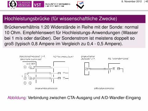
Hochleistungsbrücke (für wissenschaftliche Zwecke)

Brückenverhältnis 1:20 Widerstände in Reihe mit der Sonde: normal10 Ohm. Empfehlenswert für Hochleistungs-Anwendungen (Wasserbei 1 m/s oder darüber). Der Sondenstrom ist meistens doppelt sogroß (typisch 0,8 Ampere im Vergleich zu 0,4 - 0,5 Ampere).

18

4.2 CTA configuration

4.2.1 CTA bridgeThe CTA bridge configuration is selected on the basis of the required bandwidth,

the required power to the probe (related to fluid medium, velocity and probe type) andon basis of the distance between probe and the CTA.

4.2.2 Connecting CTA output to A/D board input channels.

It is important to follow the manufacturer’s instructions when connecting the CTAoutput to the A/D board input. Research anemometers where the CTA modules haveseparate power supplies and common signal ground may be connected single-endedreferenced (i.e. with common ground). Dedicated anemometers in separate housingsshould normally be connected differentially in order to avoid cross-talk betweenchannels. The cable length between the CTA output and the A/D board input should bekept as short as possible, preferably a few meters. The configuration of the A/D board isdone in the manufacturer’s application software.

Standard CTA bridge:Bridge ratio 1:20Resistor in series with the probe: normally 20 ohms.This bridge configuration can be used in the most applications.

Symmetrical CTA bridge (research type anemometers):Bridge ratio 1:1Resistor in series with the probe: normally 20 ohms.This bridge is recommended for very low turbulence intensities (typically less than0.1%) or very high fluctuation frequencies (typically above 200-300 kHz).Or when long cables between probe and CTA are needed.It has lower noise and can be balanced to a higher bandwidth than the 1:20 bridge.

High power CTA bridge (research type anemometers):Bridge ratio 1:20Resistor in series with the probe: 10 ohms.Recommended for high power applications (water at high speeds, e.g. 1 m/s or above).Probe current is almost doubled (typically 0.8 amps. compared with 0.4-0.5 amps.)

Abbildung: Verbindung zwischen CTA-Ausgang und A/D-Wandler-Eingang

8. November 2012 | 46

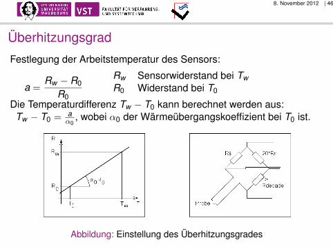
Überhitzungsgrad

Festlegung der Arbeitstemperatur des Sensors:

a =Rw − R0

R0

Rw Sensorwiderstand bei TwR0 Widerstand bei T0

Die Temperaturdifferenz Tw − T0 kann berechnet werden aus:Tw − T0 = a

α0, wobei α0 der Wärmeübergangskoeffizient bei T0 ist.

Abbildung: Einstellung des Überhitzungsgrades

8. November 2012 | 47

Brückenausgleich

• Messung des Gesamtwiderstandes Rtot bei T0 und Berechnungdes Sensorwiderstandes:

R0 = Rtot ,0 − (Rl + Rs + Rc)

• Auswahl eines geeigneten Überhitzungsgrades a.• a = 0,8 für Luft (Tue ≈ 220◦C)• a = 0,1 in Wasser (Tue ≈ 30◦C).

• Berechnung des Dekadenwiderstandes:

Rdec = BR[(1 + a)R0 + Rl + Rs + Rc]

BR: Brückenverhältnis = 20 (in den meisten Fällen)• Einstellen des Dekadenwiderstandes auf Rdec .

8. November 2012 | 48

8. November 2012 | 49

Einstellung des Überhitzungsgrades

Abhängig vom Temperaturverhalten

• Die Temperatur bleibt konstant (Tvar < ±0,5◦C):• Überhitzungsgrad wird einmalig eingestellt• Automatic overheat adjust - OFF

• Die Temperatur verändert sich (Kalibrierung/Experiment):1 Einstellung des Überhitzungsgrades:

• Der Sondenwiderstand wird gemessen und der Überhitzungsgrad vorder Kalibrierung und vor jeder Messung neu eingestellt.

• Automatic overheat adjust - ON.2 Temperaturkorrektur:

• Der Überhitzungsgrad wird einmalig eingestellt.• Die Temperatur wird während der Kalibrierung gemessen und• für die Korrektur der Anemometerspannung benutzt

8. November 2012 | 50

Rechteckwellentest - dynamische Brückenabstimmung

Durchführung des Rechteckwellentests

• Verstärkungsfilter und Verstärkung regulieren, wenn• Anwortfunktion ca. 15% überschwingt; glatt ohne Schwingungen

• ∆t bestimmen• auf ca. 3% des Maximalwertes herunterregulieren

• Bandbreite des Systems (cut-off frequency) berechnen [6]:fc = 1

C∆t Drahtsonden: C = 1.3, Fiber-Filmsonden: C = 1

Correct Too high gain Too long cable

Abbildung: Rechteckwellentest

8. November 2012 | 51

TiefpassfilterungRauschen beseitigen; Aliasing verhindern

• Höchste Frequenz bestimmen: fmax• Aufnahmefrequenz wählen: fcutoff = 2fmax• Filtereinstellungen in der Nähe der Aufnahmefrequenz wählen

22

Most CTA manufacturer’s are recommending default settings for gain and filter, whichcan be used in most applications. Dedicated CTA anemometers often have fixed setupfor the servo-loop, which works within the bandwidth stated for them without furtheradjustment by the user.

5.2 Signal Conditioner setupThe signal conditioner provides facilities for the filtering and the amplification of

the CTA signal prior to digitizing by the A/D converter.

5.2.1 Low-pass filtering.Low-pass filtering is used in order to remove noise and to prevent higher

frequencies from folding back (anti-aliasing). The setting of the low-pass filter relates tothe highest frequency in the flow.

If low-pass filtering is not performed, the energy at frequencies lower than fcut-offwill be contaminated by higher frequencies if the Nyquist sampling criteria is applied.This appears as a false energy peak in the power spectrum.

5.2.2 High-pass filteringHigh-pass filtering is used to clean the signal, if FFT spectra calculation is

required. When the CTA signal fluctuates on a timescale longer than the total length ofthe data record, it will give unwanted high frequency contributions in an FFT-basedspectrum. Otherwise it should not be applied.

Low-pass filtering:Estimate the highest frequency: fmax.Select the cut-off, frequency: max2 ff offcut ��

�

Select the filter setting closestto the cut-off frequency.

High-pass filtering:

Select the data record length, trecord.

Calculate the high-pass cut-off

frequency: record

offcut tf

�

�� 2

5

This eliminates waves with a wavelength larger than 2/5 of the record length. Shorter waveswill not be interpreted as erroneous non-stationary contributions to the signal.

Abbildung: Tiefpass-Filterung

8. November 2012 | 52

HochpassfilterungBereinigung des Signals

Nur, wenn tSchwankung > trecord , sonst nicht!

• Datenaufnahmelänge trecord wählen• Hochpass-Aufnahmefrequenz berechnen: fcutoff = 5

2·trecord

22

Most CTA manufacturer’s are recommending default settings for gain and filter, whichcan be used in most applications. Dedicated CTA anemometers often have fixed setupfor the servo-loop, which works within the bandwidth stated for them without furtheradjustment by the user.

5.2 Signal Conditioner setupThe signal conditioner provides facilities for the filtering and the amplification of

the CTA signal prior to digitizing by the A/D converter.

5.2.1 Low-pass filtering.Low-pass filtering is used in order to remove noise and to prevent higher

frequencies from folding back (anti-aliasing). The setting of the low-pass filter relates tothe highest frequency in the flow.

If low-pass filtering is not performed, the energy at frequencies lower than fcut-offwill be contaminated by higher frequencies if the Nyquist sampling criteria is applied.This appears as a false energy peak in the power spectrum.

5.2.2 High-pass filteringHigh-pass filtering is used to clean the signal, if FFT spectra calculation is

required. When the CTA signal fluctuates on a timescale longer than the total length ofthe data record, it will give unwanted high frequency contributions in an FFT-basedspectrum. Otherwise it should not be applied.

Low-pass filtering:Estimate the highest frequency: fmax.Select the cut-off, frequency: max2 ff offcut ��

�

Select the filter setting closestto the cut-off frequency.

High-pass filtering:

Select the data record length, trecord.

Calculate the high-pass cut-off

frequency: record

offcut tf

�

�� 2

5

This eliminates waves with a wavelength larger than 2/5 of the record length. Shorter waveswill not be interpreted as erroneous non-stationary contributions to the signal.

8. November 2012 | 53

DC-OffsetSenkung des Niveaus des CTA-Signals

Vorgehensweise

• den minimalen Wert Emin des zu messenden CTA-Signalsbestimmen

• den DC-offset an der Signalbearbeitungseinheit aufEoffset = Emin

stellen

HinweisDC-offsets wenn möglich vermeiden

8. November 2012 | 54

Signalverstärkung (Gain)Verbesserung der Auflösung

Vorgehensweise

• Notwendige Auflösung der Geschwindigkeit ∆U in m/s bestimmen• Mittleren Anstieg der Sonden-Kalibrierkurve in dem

interessierenden Geschwindigkeitsbereich bestimmen:dEdU = E(U2)−E(U1)

U2−U1, wobei E(U) ist die CTA-Spannung bei U

• erforderliche Auflösung der Spannung berechnen:∆E = ∆U dE

dU• die Verstärkung G berechnen:

G = ∆EAD∆E , wobei ∆EAD ist die Auflösung des A/D-Wandlers

8. November 2012 | 55

Durchführung der Geschwindigkeitskalibrierung

24

6. VELOCITY CALIBRATION, CURVE FITTINGCalibration establishes a relation between the CTA output and the flow velocity. It

is performed by exposing the probe to a set of known velocities, U, and then record thevoltages, E. A curve fit through the points (E,U) represents the transfer function to beused when converting data records from voltages into velocities. Calibration may eitherbe carried out in a dedicated probe calibrator, which normally is a free jet, or in a wind-tunnel with for example a pitot-static tube as the velocity reference. It is important tokeep track of the temperature during calibration. If it varies from calibration tomeasurement, it may be necessary to correct the CTA data records for temperaturevariations.

Research type anemometers may be delivered with automatic calibrators andcalibration routines in their application software, thus offering fully automaticcalibrations inclusive of curve fitting.

Velocity calibration procedure:

Mount the probe in the calibration rig with the same wire-prong orientation as will beused during the experiment.

- Single-sensor probes: with the prongs parallel with the flow.

- X-probes and Tri-axial probes: with the probe axis parallel with the flow.

Record the ambient conditions: Temperature, Ta , and barometric pressure, Pb.

Setting to operate:

1) Calibration with temperature correction:

Switch the anemometer to Operate with the previously established overheat setup.

2) Calibration with overheat adjustment:

Balance the bridge immediately before calibration and establish a new overheatsetup using the same overheat ratio a.

Choose min. and max. calibration velocity, Umin,cal and Umax,cal ,

Choose number of calibration points (a minimum of 10 points is recommended).

Choose velocity distribution (logarithmic distribution is recommended).

Create the velocities and acquire the CTA voltage together with velocity and ambienttemperature in all points.

Abbildung: Referenzmessgeräte für Geschwindigkeitskalibrierung

8. November 2012 | 56

Durchführung der Geschwindigkeitskalibrierung

• Kalibriergeschwindigkeitsbereich (Umin, Umax ) wählen• Anzahl der Kalibrierpunkte (min. 10) wählen• Geschwindigkeitsverteilung (logarithmische empfohlen) wählen• Geschwindigkeiten mit Hilfe des Referenz-Messgerätes einstellen• E zusammen mit U (ev. T ) aufzeichen.

25

CTA application software packages contain curve fitting procedures, whichcorrect the voltages and calculates the transfer functions on basis of advanced curvefitting methods eliminating the need for any data manipulations by the user.

Curve fitting of calibration data (manual procedure):

Arrange the probe data in a table, for example in Excel, containing velocity U, CTA voltage E,fluid temperature Ta and pressure Pb.

Correct the voltages E for temperature variations during calibration, see Chapter 7.1.2.

Polynomial curve fitting:

Plot U as function of Ecorr

Create a polynomial trend line in 4th order:4

43

32

210 corrcorrcoorcorr ECECECECCU �� , Co to C4 are calibration constants.

The polynomial curve fit is normally recommended, as it makes very good fits withlinearisation errors often less than 1%.

Note: Polynomial curve fits may oscillate, if the velocity is outside the calibration velocityrange.

Power law curve fitting:

Plot E2 as function of Un in double logarithmic scale (n=0.45 is a good starting value forwire probes).

Create a linear trend line. This will give the calibration constants A and B in the function:nUBAE ��

2 (King’s law �15�)

Vary n and repeat the trend line until the curve fit errors are acceptable.

Power law curve fits are less accurate than polynomial fits, especially over wide velocityranges, as n is slightly velocity dependent.

Velocity calibration of X-probes and Tri-axial probes:The calibration velocity range must be expanded with respect to the velocity limitsexpected during the experiment thus making sure that the curve fit is valid over thefull angular acceptance range of the probes. Umin,exp and Umax,exp are peak values.

Umin,cal Umax,cal

X-probes 0.1· Umin,exp 1.5· Umax,exp

Tri-axial probes 0.15· Umin,exp 1.6· Umax,exp

8. November 2012 | 57

Anpassung mittels Polynom - für sehr gute Anpassungen

• U(Ekorr ) darstellen• Trendlinie mit einem Polynom 4. Grades erzeugen:

U = C0 + C1Ekorr + C2Ekorr2 + C3Ekorr3 + C4Ekorr4

Anpassung mittels Potenzgesetz

• E2(Un) doppelt logarithmisch darstellen (n = 0.45)• lineare Trendlinie festlegen:→ A und B für E2 = A + B · Un (King’sches Gesetz [3]).

• n variieren und Trendlinie wiederholen bis Fehler akzeptabel . . .

8. November 2012 | 58

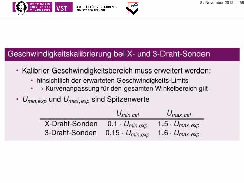
Geschwindigkeitskalibrierung bei X- und 3-Draht-Sonden

• Kalibrier-Geschwindigkeitsbereich muss erweitert werden:• hinsichtlich der erwarteten Geschwindigkeits-Limits• → Kurvenanpassung für den gesamten Winkelbereich gilt

• Umin,exp und Umax ,exp sind Spitzenwerte

Umin,cal Umax ,cal

X-Draht-Sonden 0.1 · Umin,exp 1.5 · Umax ,exp3-Draht-Sonden 0.15 · Umin,exp 1.6 · Umax ,exp

8. November 2012 | 59

X-Draht-Sonden

26

7. DIRECTIONAL CALIBRATIONDirectional calibration of multi-sensor probes provides the individual directional

sensitivity coefficients (yaw factor k and pitch-factor h) for the sensors, which are usedto decompose calibration velocities into velocity components.

7.1.1 X-array probesThe yaw coefficients, k1 and k2, are used in order to decompose the calibration

velocities Ucal1 and Ucal2 from an X-probe into the U and V components.

Directional calibration of X-probes requires a rotation unit, where the probe can berotated on an axis through the crossing point of the wires perpendicular to the wireplane. Calculation of the yaw coefficients requires that a probe coordinate system isdefined with respect to the wires (see the sketch below), and that the probe has beencalibrated against velocity.

Advanced CTA application software packages contain routines for automaticdirectional calibration and evaluation of the yaw coefficients.

X-probe calibration procedure:Define probe coordinate system (X,Y) with respect to wire 1 and 2 as shown below:

Mount the probe in the rotating holder oriented as shown above.

Estimate the maximum angle �max , which is expected in the experiment between thevelocity vector U� and the probe axis. In most cases �max is selected to =40�.

Select the number of angular positions for the calibration.

Expose the probe to the middle calibration velocity Udir,cal = 1/2·(Umin,cal+Umax,cal)

Rotate the probe to the -�max position and acquire the voltages E1 and E2 from the twosensors.

Check that E1 is bigger than E2 and that E1 increases, while E2 decreases, when the probeis moved to next angular position. If not turn the probe180� around its X-axis and startagain.

Read E1 and E2 in each angular position.

Calculate the squared yaw factor k12 and k2

2 for sensor 1 and sensor 2 in each positionusing the equations in Chapter 8.1.4.

Calculate the average of the k12 and k2

2 ,respectively, factors and use them as sensitivityfactors for the two sensors.

Note: In many situations, where optimal accuracy is not needed, the manufacturer’s defaultvalues for k and h can be used, eliminating the need for individual directional calibration.

Abbildung: Winkeldefinitionen im X-Draht-Sonden-Koordinatensystem undKalibrierdaten

8. November 2012 | 60

Drei-Draht-Sonden

27

7.1.2 Tri-axial probesThe directional sensitivity of tri-axial probes is characterised by both a yaw and a

pitch coefficient, k and h, for each sensor. Calibration of tri-axial probes requires aholder, where the probe axis (X-direction) can be tilted with respect to the flow andthereafter rotated 360� around its axis. Proper evaluation of the coefficient requires thata probe coordinate system is defined with respect to the sensor-orientation. Directionalcalibration is made on the basis of a velocity calibration.

Note: Directional calibration normally only needs to be carried out once in a probe’slifetime, as it depends only on the geometry, which will not change in use.

Tri-axial probe calibration procedure:Define a probe coordinate system (normally use the manufacturer’s suggestion):

Mount the probe in the rotating holder with the probe axis in the flow direction and wireno. 3 in the XZ plane of the calibration unit system, corresponding to �=0.

Estimate the maximum angle �max , which is expected in the experiment between thevelocity vector and the probe axis. In most cases �max is selected to 30�.

Select the number of angular positions � for the calibration, normally 24 corresponding to15� steps.

Expose the probe to the mid calibration velocity range Udir,cal = 1/2·(Umin,cal+Umax,cal) andacquire the voltages E1 , E2 and E3 from the three sensors.

Tilt the probe to the �max position with �=0 and acquire E1 , E2 and E3.

Rotate the probe and acquire E1 , E2 and E3 in all �-positions.

Calculate the squared yaw factor k12 , k2

2 and k32 and pitch factors for sensor 1 , 2 and 3 in

each position using the equations in the Theoretical part, chapter YY.

Calculate the average of the k2- and h2-factors and use them as sensitivity factors for thethree sensors.

Abbildung: Winkeldefinitionen im 3-Draht-Sonden-Koordinatensystem undKalibrierdaten

8. November 2012 | 61

Datenumwandlung

• Skalierung der gemessenen CTA-Spannungen (raw signal)• nur bei Verstärkung oder Offset: E = Ea

G − Eoffset

• Temperaturkorrektur• Nur bei Temperaturänderungen• wenn der Überhitzungsgrad nicht korrigiert wurde• Temperaturaufnahme nötig

Ecorr =(

Tw−T0Tw−Ta

)0.5· Ea

• Linearisierung• Nur wenn Datenreduzierung im Amplitudenbereich erforderlich ist• Polynom / Potenzgesetz

• Aufteilung in Geschwindigkeitskomponenten• Nur bei X- oder 3-Draht-Sonden

8. November 2012 | 62

Beispiel für 3D-Sonden

Zerlegung:

31

8.1.5 Tri-axial probe decomposition into velocity components U, V and WIn a 3-D flows measured with a Tri-axial probe the calibration velocities are used

together with the yaw and pitch coefficients k2 and h2 to calculate the three velocitycomponents U, V and W in the probe coordinate system (X,Y,Z).

The yaw and pitch coefficients for the three sensors may be the manufacturer’sdefault values, or if higher accuracy is required they are determined by directionalcalibration of the individual sensors.

Decomposition of Tri-axial probe voltages into U, V and W:

Calculate the calibration velocities Ucal1 , Ucal2 Ucal3 using the linearisation functions for sensor1, 2 and 3.

Decomposition with individual yaw and pitch coefficients:Calculate the velocities U1 , U2 and U3 in the wire-coordinate system (1,2,3) defined by thesensors using the three quations:

� � 21

221

21

23

21

22

21

21 74.54cos1 calUhkUhUUk ��

� � 22

222

22

23

22

22

21

22 74.54cos1 calUhkUUkUh ��

� � 23

223

23

23

23

22

23

21 74.54cos1 calUhkUkUhU ��

With the k2=0.0225 and , h2=1.04 default values for a tri-axial wire probe, the velocities U1, U2and U3 in the wire coordinate system becomes:

23

22

211 3266.03544.03477.0 calcalcal UUUU ��

23

22

212 3544.03477.03266.0 calcalcal UUUU ��

23

22

213 3477.032663.03544.0 calcalcal UUUU ��

Calculate the U, V and W in the probe coordinate system:

74.54cos74.54cos74.54cos 321 �� UUUU90cos135cos45cos 321 �� UUUV

26.35cos09.114cos09.114cos 321 �� UUUW

Manufacturer’s (Dantec Dynamics) default values for k2 and h2:

k2 h2

Gold-plated wire sensors: 0.0225 1.04Fiber-film sensors for air: 0.04 1.20

Geschwindigkeitskomponente:

31







� � 21

221

21

23

21

22

21


� � 22

222

22

23

22

22

21


� � 23

223

23

23

23

22

23



23

22

211 3266.03544.03477.0 calcalcal UUUU ��

23

22

212 3544.03477.03266.0 calcalcal UUUU ��

23

22

213 3477.032663.03544.0 calcalcal UUUU ��



26.35cos09.114cos09.114cos 321 �� UUUW


k2 h2


in Sonden-Koordinatensystem:

31







� � 21

221

21

23

21

22

21


� � 22

222

22

23

22

22

21


� � 23

223

23

23

23

22

23



23

22

211 3266.03544.03477.0 calcalcal UUUU ��

23

22

212 3544.03477.03266.0 calcalcal UUUU ��

23

22

213 3477.032663.03544.0 calcalcal UUUU ��



26.35cos09.114cos09.114cos 321 �� UUUW


k2 h2


8. November 2012 | 63

Datenerfassung

CTA-Signal - kontinuierliche analoge Spannung

→ Digital/Analog-Wandler• Datenrate SR und• Anzahl der Messwerte N• Zusammen legen sie die Messzeit T = N

SR fest.

Parameter, die die Datenerfassung definieren

• Experiment• verfügbares Speichervolumen des Computers• die akzeptable Messunsicherheit• erforderlichen Datenanalyse (zeitgemittelt oder frequenzgemittelt)

8. November 2012 | 64

Zeitgemittelte Auswertung

• erwartete Werte abschätzen: U [m/s], Tu [%], T1 [s]• gewünschte Messunsicherheit u [%] von der mittleren

Geschwindigkeit Umean und den Vertrauensbereich (1-a) [%]auswählen.

• Datenrate berechnen: SR ≤ 12T1

• Anzahl der Messwerte berechnen: N =( 1

u ·za2 · Tu

)2

32

9. DATA ACQUISITIONThe CTA signal is a continuos analogue voltage. In order to process it digitally it

has to be sampled as a time series consisting of discrete values digitized by an analogue-to-digital converter (A/D board).

The parameters defining the data acquisition are the sampling rate SR and thenumber of samples, N. Together they determine the sampling time as T=N/SR. Thevalues for SR and N depend primarily on the specific experiment, the required dataanalysis (time-averaged or spectral analysis), the available computer memory and theacceptable level of uncertainty. Time-averaged analysis, such as mean velocity and rmsof velocity, requires non-correlated samples, which can be achieved when the timebetween samples is at least two times larger than the integral time scale of the velocityfluctuations. Spectral analysis requires the sampling rate to be at least two times thehighest occurring fluctuation frequency in the flow. The number of samples depends onthe required uncertainty and confidence level of the results.

Time avaraged analysis:

Estimate the following expected quantities in the flow:

velocity U �m/s � , turbulence intensity Tu � %� , andintegral time-scale T1 � seconds� (see Chapter 10.2).

Select the wanted uncertainty and confidence level:

uncertainty u, %, in Umean

confidence level (1-a), %

Calculate the sampling rate SR:

121T

SR � (gives uncorrelated samples)

Calculate the number of samples N:

2

21

��

��

��

�

��

�� Tu

zu

N a

where za/2 is a variable related to confidence level (1-a) of the Gaussian probability densityfunction p(z).

Sampling rate SR for time spectral analysis:


max2 fSR �� (Nyquist critrium with fmax based onan oversampled time series.), or

offcutfSR�

�� 2 (based on low-pass filter setup), or

offcutfSR�

�� 5.2 (the factor 2.5 adopts to a non-ideal low-pass filter, which does not set the signal tozero at the cut-off frequency �57�).

za/2 (1-a) %1.65 901.96 952.33 98

32











121T



2

21

��

��

��

�

��

�� Tu

zu

N a





offcutfSR�


offcutfSR�


za/2 (1-a) %1.65 901.96 952.33 98

8. November 2012 | 65

Datenrate bei zeitlicher Spektralanalyse

Datenrate berechnen:• Nyquist-Kriterium mit fmax basierend auf einer zu stark

abgetasteten (oversampled) Zeitreihe: SR ≥ 2fmax

• auf Grund einer Tiefpassfilter-Einstellung: SR = 2fcutoff

• der Faktor 2,5 wird bei einem nicht idealen Tiefpass-Filterverwendet, der das Signal bei der cut-off-Frequenz nicht auf Nullsetzt: SR = 2.5fcutoff

32











121T



2

21

��

��

��

�

��

�� Tu

zu

N a





offcutfSR�


offcutfSR�


za/2 (1-a) %1.65 901.96 952.33 98

8. November 2012 | 66

Datenanalyse

stochastische Natur des CTA-Signal einer turbulenten Strömung

→ eine statistische Beschreibung des Signals notwendig

Die Zeitreihe kann analysiert oder reduziert werden:• im Wertebereich der Amplitude,• der Zeit oder• der Frequenz.

Die reduzierten Daten können• in dem Projekt gespeichert,• grafisch dargestellt,• exportiert werden.

8. November 2012 | 67

Datenanalyse im Amplitudenbereich

37

37

4.11 Datenanalyse

Wegen der stochastischen Natur des CTA-Signal einer turbulenten Strömung, ist eine statistische Beschreibung des Signals notwendig. Die Zeitreihe kann entweder im Wertebereich der Amplitude, der zeit oder der Frequenz analysiert oder reduziert werden. Die folgenden Prozeduren verlangen alle eine stationäre ortsfeste Zufallsdaten. Die CTA-Anwendersoftware enthält Module, die die gebräuchlichsten Datenanalysen, wie nachfolgend beschrieben, ausführen. Im Allgemeinen wird ein Analyseverfahren ausgesucht und auf die Zeitreihe angewendet. Die reduzierten Daten werden dann in dem Projekt gespeichert und können dann grafisch dargestellt oder exportiert werden. 4.11.1 Datenanalyse im Amplitudenbereich Sie liefert Informationen über die Amplitudenverteilung im Signal. Sie basiert auf einer oder mehreren Zeitserien auf der Grundlage einer einfachen integralen Zeitskala in der Strömung. Die Zeitserie der Geschwindigkeit enthält Daten eines Sensors, umgewandelt in eine Geschwindigkeitskomponente. Eine einfache Geschwindigkeits-Zeitserie liefert Mittelwerte, mittlere Quadrate und Momente höherer Ordnung. Auf einer einfachen Zeitserie basierende Momente:

mittlere Geschwindigkeit: ∑=N

imean UN

U1

1

Standardabweichung der Geschwindigkeit:

( )5.0

1

2

11

⎟⎠

⎞⎜⎝

⎛−

−= ∑

N

meanirms UUN

U

Turbulenzgrad: mean

rms

UUTu =

Schiefe (skewness): ( )∑ ⋅

−=

Nmeani

NUUS

13

3

σ

Flachheit (flatness): ( )∑ ⋅

−=

Nmeani

NUUK

14

4

σ

wobei die Varianz σ definiert ist als:

( ) 5.0

1

2

1 ⎟⎟⎠

⎞⎜⎜⎝

⎛−

−= ∑

Nmeani

NUUσ

Die Schiefe ist ein Maß für das Fehlen einer statistischen Symmetrie in der Strömung, während die Flachheit ein Maß für die Amplitudenverteilung ist.

8. November 2012 | 68

Datenanalyse im Amplitudenbereich

37

37

4.11 Datenanalyse

Wegen der stochastischen Natur des CTA-Signal einer turbulenten Strömung, ist eine statistische Beschreibung des Signals notwendig. Die Zeitreihe kann entweder im Wertebereich der Amplitude, der zeit oder der Frequenz analysiert oder reduziert werden. Die folgenden Prozeduren verlangen alle eine stationäre ortsfeste Zufallsdaten. Die CTA-Anwendersoftware enthält Module, die die gebräuchlichsten Datenanalysen, wie nachfolgend beschrieben, ausführen. Im Allgemeinen wird ein Analyseverfahren ausgesucht und auf die Zeitreihe angewendet. Die reduzierten Daten werden dann in dem Projekt gespeichert und können dann grafisch dargestellt oder exportiert werden. 4.11.1 Datenanalyse im Amplitudenbereich Sie liefert Informationen über die Amplitudenverteilung im Signal. Sie basiert auf einer oder mehreren Zeitserien auf der Grundlage einer einfachen integralen Zeitskala in der Strömung. Die Zeitserie der Geschwindigkeit enthält Daten eines Sensors, umgewandelt in eine Geschwindigkeitskomponente. Eine einfache Geschwindigkeits-Zeitserie liefert Mittelwerte, mittlere Quadrate und Momente höherer Ordnung. Auf einer einfachen Zeitserie basierende Momente:

mittlere Geschwindigkeit: ∑=N

imean UN

U1

1

Standardabweichung der Geschwindigkeit:

( )5.0

1

2

11

⎟⎠

⎞⎜⎝

⎛−

−= ∑

N

meanirms UUN

U

Turbulenzgrad: mean

rms

UUTu =

Schiefe (skewness): ( )∑ ⋅

−=

Nmeani

NUUS

13

3

σ

Flachheit (flatness): ( )∑ ⋅

−=

Nmeani

NUUK

14

4

σ

wobei die Varianz σ definiert ist als:

( ) 5.0

1

2

1 ⎟⎟⎠

⎞⎜⎜⎝

⎛−

−= ∑

Nmeani

NUUσ

Die Schiefe ist ein Maß für das Fehlen einer statistischen Symmetrie in der Strömung, während die Flachheit ein Maß für die Amplitudenverteilung ist.

8. November 2012 | 69

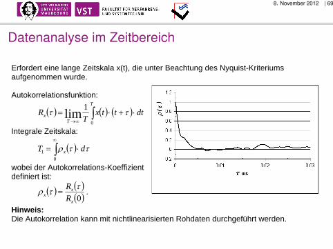
Datenanalyse im Zeitbereich

39

39

Autokorrelationsfunktion und integrale Zeitskala: Erfordert eine lange Zeitskala x(t), die unter Beachtung des Nyquist-Kriteriums aufgenommen wurde. Autokorrelationsfunktion:

( ) ( ) ( )∫ ⋅+⋅=∞→

T

Tx dtttx

TR

0

1lim ττ

Integrale Zeitskala:

( )∫∞

⋅=0

1 ττρ dT x

wobei der Autokorrelations-Koeffizient definiert ist:

( ) ( )( )0x

xx R

R ττρ = .

Hinweis: Die Autokorrelation kann mit nichtlinearisierten Rohdaten durchgeführt werden. 4.11.3 Datenanalyse im Spektralbereich Die Spektralanalyse kann verwendet werden, um Informationen darüber zu erhalten, wie die Energie des Signals hinsichtlich ihrer Frequenz verteilt ist.

Leistungsspektrum der Strömung hinter einem Kreiszylinder Die Analyse kann mit nichtlinearisierten Rohdaten durchgeführt werden, vorausgesetzt, dass das Nyquist-Kriterium eingehalten wurde. Die Genauigkeit des Spektrums hängt von dem verwendeten Algorithmus und der Anzahl der Messwerte ab, die normalerweise hoch sein muss. Es gibt eine Reihe von unterschiedlichen Algorithmen für die Berechnung des Spektrums, die meistens auf der Fourier-Transformation beruhen, die Werte für diskrete Frequenzen erzeugt. CTA-Anwendersoftware enthält normalerweise solche Routinen. 4.12 Störeinflüsse Die Messungen mit einem CTA-Anemometer werden von einer Reihe von Störeinflüssen begleitet. Einige Änderungen der Parameter, die in den Mechanismus der Wärmeübertragung vom Draht an die Umgebung eingreifen, stellen Störeffekte dar und

8. November 2012 | 70

Datenanalyse im Spektralbereich

39

39

Autokorrelationsfunktion und integrale Zeitskala: Erfordert eine lange Zeitskala x(t), die unter Beachtung des Nyquist-Kriteriums aufgenommen wurde. Autokorrelationsfunktion:

( ) ( ) ( )∫ ⋅+⋅=∞→

T

Tx dtttx

TR

0

1lim ττ

Integrale Zeitskala:

( )∫∞

⋅=0

1 ττρ dT x

wobei der Autokorrelations-Koeffizient definiert ist:

( ) ( )( )0x

xx R

R ττρ = .

Hinweis: Die Autokorrelation kann mit nichtlinearisierten Rohdaten durchgeführt werden. 4.11.3 Datenanalyse im Spektralbereich Die Spektralanalyse kann verwendet werden, um Informationen darüber zu erhalten, wie die Energie des Signals hinsichtlich ihrer Frequenz verteilt ist.

Leistungsspektrum der Strömung hinter einem Kreiszylinder Die Analyse kann mit nichtlinearisierten Rohdaten durchgeführt werden, vorausgesetzt, dass das Nyquist-Kriterium eingehalten wurde. Die Genauigkeit des Spektrums hängt von dem verwendeten Algorithmus und der Anzahl der Messwerte ab, die normalerweise hoch sein muss. Es gibt eine Reihe von unterschiedlichen Algorithmen für die Berechnung des Spektrums, die meistens auf der Fourier-Transformation beruhen, die Werte für diskrete Frequenzen erzeugt. CTA-Anwendersoftware enthält normalerweise solche Routinen. 4.12 Störeinflüsse Die Messungen mit einem CTA-Anemometer werden von einer Reihe von Störeinflüssen begleitet. Einige Änderungen der Parameter, die in den Mechanismus der Wärmeübertragung vom Draht an die Umgebung eingreifen, stellen Störeffekte dar und

8. November 2012 | 71

Störeinflüsse

Durch die Strömung

• Temperatur - sehr wichtig!• Druck - vernachlässigbar

• Druckänderungen• Druckbereich

• Zusammensetzung - vernachlässigbar

Sensorbedingungen

• Verschmutzung - neue Kalibrierung• Sensorstabilität - Empfindlichkeit betrachten• Sensororientierung - Kalibrierung=Messung!!!

8. November 2012 | 72

Unsicherheiten bei CTA-Messungen (1)

44

44

Quelle der Unsicher-heit

Ein-gangsgröße

Typi-scher Wert

Relative Ausgangsgröße Typi-scher Wert

Über-dek-kungs-faktor

Relative Standard- Unsicher-heit

ixΔ ixΔ

iyU

Δ⋅1

iyU

Δ⋅1

k iy

UkΔ⋅⋅

11

Kalibrier-vorrichtung calUΔ 1% ( )calUSTDV Δ⋅⋅ 1002 0.02 2 0.01

Lineari-sierung fitUΔ 0.5% ( )fitUSTDV Δ⋅⋅ 1002 0.01 2 0.005

A/D-Auflösung ADE

n 10 volts

12 bit EUE

U nAD

∂∂⋅⋅

21

0.0008 3 0.0013

Sonden- positio-nierung

θ 1° θcos1− 0.00015

3 0≈

8. November 2012 | 73

Unsicherheiten bei CTA-Messungen (2)

45

45

Quelle der Unsicher-heit

Ein-gangsgröße

Typi-scher Wert

Relative Ausgangsgröße Typi-scher Wert

Über-dek-kungs-faktor

Relative Standard- Unsicher-heit

Temperaturänderungen1)

TΔ 1°C

( ) ⎟⎠⎞

⎜⎝⎛ +⋅⋅

−Δ

⋅ − 11 5,0

0

UBA

TTT

U w

0.013 3 0.008

Temperaturänderungen2)

TΔ 1°C

273TΔ

0.004 3 0.002

Umgebungs-druck

PΔ 10kPa

PPPΔ+0

0 0.01 3 0.006

Feuchtigkeit wvPΔ 1 kPa

wvwv

PPU

UΔ⋅

∂∂

⋅1

0.0006 3 0≈

Relative erweiterte Unsicherheit3) : U(Usample)= ∑ ⎟⎠⎞

⎜⎝⎛ Δ⋅⋅⋅

2112 iyUk

=0.030=3%

8. November 2012 | 74

Weiterführende Aufgabenstellungen

• Sehr langsame Geschwindigkeiten: Der Einfluss der natürlichenKonvektion beginnt bei ca. 0.2 m/s und ist vollständig ausgeprägtbei 0,03 bis 0,04 m/s. In diesem Bereich ist es wichtig, dass dieSonde bei der Kalibrierung und bei der Messung die gleicheOrientierung zum Geschwindigkeitsfeld hat.

• Hohe Geschwindigkeiten, kompressible Strömungen:Geschwindigkeit und Druck müssen simultan gemessen werden.Die Korrektur ist ziemlich kompliziert und wird oft vernachlässigt[33, 48, 55].

• Niedriger Druck: Wenn die Knudsen-Zahl sich über 0,1 erhöht,wird der Wärmeübergang eine Funktion sowohl derGeschwindigkeit als auch der Knudsen-Zahl (oder Druck). Beieiner 5 µm-Sonde beträgt die Knudsen-Zahl etwa 0,02 unteratmosphärischen Bedingungen.

8. November 2012 | 75

Weiterführende Aufgabenstellungen

• Wandeinflüsse: Der Wandeinfluss beginnt bei y+ ≤ y Uτ = 3,5 (y= Wandabstand, Uτ = Reibungsgeschwindigkeit). Der kritischeWandabstand beträgt typischerweise 0,1 bis 0,2 mm und istabhängig von der Geschwindigkeit in der freien Strömung.

• Sehr hohe Turbulenzen, Rückströmungen:→ fliegendeSensorsysteme.

• Wandschubspannung: wandschlüssig angeordnete Filmsonden.• Zweiphasenströmungen: jeweilige Phase bestimmbar.• Gemische: Gemischanteile können bestimmt werden.

Geschwindigkeitsmessung in einer turbulenten Strömung ... · W Q I2 R hAT w or replacing h with...

Documents

Transcript of Geschwindigkeitsmessung in einer turbulenten Strömung ... · W Q I2 R hAT w or replacing h with...