Harald Tauchmann, Silja Göhlmann, Till Requate … · Harald Tauchmann, Silja Göhlmann, Till...

Harald Tauchmann, Silja Göhlmann, Till Requateand Christoph M. Schmidt

A Statistical Guinea Pig Approach

No. 52

RWIESSEN

RWI:

Dis

cuss

ion

Pape

rs

Rheinisch-Westfälisches Institutfür WirtschaftsforschungBoard of Directors:Prof. Dr. Christoph M. Schmidt, Ph.D. (President),Prof. Dr. Thomas K. BauerProf. Dr. Wim Kösters

Governing Board:Dr. Eberhard Heinke (Chairman);Dr. Dietmar Kuhnt, Dr. Henning Osthues-Albrecht, Reinhold Schulte

(Vice Chairmen);Prof. Dr.-Ing. Dieter Ameling, Manfred Breuer, Christoph Dänzer-Vanotti,Dr. Hans Georg Fabritius, Prof. Dr. Harald B. Giesel, Dr. Thomas Köster, HeinzKrommen, Tillmann Neinhaus, Dr. Torsten Schmidt, Dr. Gerd Willamowski

Advisory Board:Prof. David Card, Ph.D., Prof. Dr. Clemens Fuest, Prof. Dr. Walter Krämer,Prof. Dr. Michael Lechner, Prof. Dr. Till Requate, Prof. Nina Smith, Ph.D.,Prof. Dr. Harald Uhlig, Prof. Dr. Josef Zweimüller

Honorary Members of RWI EssenHeinrich Frommknecht, Prof. Dr. Paul Klemmer †

RWI : Discussion PapersNo. 52Published by Rheinisch-Westfälisches Institut für Wirtschaftsforschung,Hohenzollernstrasse 1/3, D-45128 Essen, Phone +49 (0) 201/81 49-0All rights reserved. Essen, Germany, 2006Editor: Prof. Dr. Christoph M. Schmidt, Ph.D.ISSN 1612-3565 – ISBN 3-936454-79-5ISBN-13 978-3-936454-79-6

The working papers published in the Series constitute work in progresscirculated to stimulate discussion and critical comments. Views expressedrepresent exclusively the authors’ own opinions and do not necessarilyreflect those of the RWI Essen.

RWI : Discussion PapersNo. 52

Harald Tauchmann, Silja Göhlmann, Till Requateand Christoph M. Schmidt

RWIESSEN

Bibliografische Information Der Deutschen BibliothekDie Deutsche Bibliothek verzeichnet diese Publikation in der DeutschenNationalbibliografie; detaillierte bibliografische Daten sind im Internetüber http://dnb.ddb.de abrufbar.

ISSN 1612-3565ISBN 3-936454-79-5ISBN-13 978-3-936454-79-6

Harald Tauchmann, Silja Göhlmann, Till Requateand Christoph M. Schmidt*

Tobacco and Alcohol: Complements or Substitutes? –A Statistical Guinea Pig Approach

AbstractThe question of whether two drugs – namely alcohol and tobacco – are used ascomplements or substitutes is of crucial interest if side-effects of anti-drug pol-icies are considered. Numerous papers have empirically addressed this issueby estimating demand systems for alcohol and tobacco and subsequently cal-culating cross-price effects. However, this traditional approach often is seri-ously hampered by insufficient price-variation observed in survey data. We,therefore, suggest an alternative instrumental variables approach that statisti-cally mimics an experimental study and does not rely on prices as explanatoryvariables. This approach is applied to German survey data. Our estimationresults suggest that a reduction in tobacco consumption results in a reductionin alcohol consumption, too. It is shown theoretically that this implies thatalcohol and tobacco are complements. Hence, we conclude that successfulantismoking policies will not result in the unintended side-effect of an in-creased (ab)use of alcohol.

JEL Classification: C31, D12, I12

Keywords: Interdependence in consumption, tobacco and alcohol,instrumental variables approach

November 2006

*Harald Tauchmann, RWI Essen; Silja Göhlmann, RWI Essen; Till Requate, University Kiel;Christoph M. Schmidt, RWI Essen and Ruhr University Bochum. All correspondence to HaraldTauchmann, Rheinisch-Westfälisches Institut für Wirtschaftsforschung (RWI Essen), Hohenzol-lernstr. 1-3, 45128 Essen, Germany. Fax: +49-201-8149-200. Email: [email protected] would like to thank Boris Augurzky and Lars Siemers as well as participants at the ScottishEconomic Society Annual Conference 2006, the European Society for Population Economics20th Annual Conference, and the Verein für Socialpolitik Annual Conference 2006 for many use-ful comments. Any errors are our own.

1 Introduction

The consumption of psychoactive substances has been subject to regulation for cen-

turies. While numerous drugs like opium, cocaine, marihuana, and ecstasy nowadays

are completely banned in almost any western society, others are still legally consumed

on a widespread basis, most prominently alcohol and tobacco. Nevertheless, in most

western economies consumption is penalized by taxes and often restricted, e.g. pur-

chase is subject to a minimum age. In general, regulation seems to be well justified

from the perspective of economic theory. The consumption of alcohol and tobacco –

and of course the consumption of many illicit drugs as well – may involve external ef-

fects to other individuals and the society as a whole. In many cases, these are unlikely

to be internalized via bilateral bargaining because of transaction costs and ill-defined

or non-enforceable property rights. Annoyance, health problems, and even death by

second-hand smoking, alcohol related violence and crime, road accidents caused by

drug abuse involving other parties1 and extra costs to the social security systems2

may serve as examples for such externalities.

Yet, the question of how to design measures aiming at the reduction of drug usage

remains controversial. This especially applies to so called soft (illicit) drugs and licit

psychoactive substances. At the one hand, it is often argued that consumption of ‘soft’

and even legal drugs serves as ‘gateway’ to drug usage in general and, therefore, as

potential gateway to extremely harmful substances. If this argument is correct, it may

be appropriate to apply tough measures even to soft drugs in order to hit drug usage

in general. Others argue that drug usage is a – maybe unfavorable – yet inevitable

phenomenon in any society. Restricting the access to ‘soft’ drugs may therefore only

encourage potential drug users to turn to other, probably more harmful, substances.

If this argument applies, designing optimal policies for the regulation of drug usage is

more complex, since inter-drug substitution has to be considered an important issue.

Currently, in Germany a heated debate on restricting the consumption of legal

drugs is going on. Namely, smoking bans are discussed with respect to bars and pubs,

1In many cases, e.g. in case of accidental death, statutory compensation for immaterial damage islikely to be incomplete and, therefore, fails to internalize external costs properly.

2The question of whether smokers do decrease total health care expenditures because of dying earlyrather than actually increase expenditures, is still subject to an ongoing debate, e.g. Warschburger(2000).

4

schools, and even motorists. Analyzing the effect of such bans is of great interest and

research has been carried out for other countries, where bans have already become

implemented; see for example Wasserman et al. (1991), Chaloupka & Grossman (1996)

and Tauras & Chaloupka (1999). These studies come to the conclusion that smoking

restrictions in fact do reduce tobacco consumption. In this paper, we condition on

the effectiveness of anti-drug policies and address the question of whether a reduced

tolerance against smoking will ultimately lead to less overall drug usage or whether it

may encourage smokers to turn to drugs other than tobacco.

From the perspective of economic theory, in order to answer this question one has

to determine whether tobacco and other drugs are consumed as substitutes or comple-

ment goods. Correspondingly, our analysis addresses this question using econometric

techniques. In doing this, we focus on the interdependence of tobacco and alcohol,

namely because these two substances are by far the most commonly consumed drugs

in Germany, and therefore are likely to be the most relevant ones. Moreover, data

concerning the consumption of alcohol and tobacco are available through several sur-

veys and are probably more reliable than data concerning the consumption of illicit

psychoactive substances.

2 Literature

The question of whether two goods are consumed as complements or substitutes lies

within the core of micro-economic consumer theory. The sign of the cross-price deriva-

tives derived from Hicksian demand functions precisely answers this question. Corre-

spondingly, the vast majority of econometric analyses that has so far addressed the

question of substitutability with respect to tobacco and alcohol is based on estimating

demand functions and calculating cross-price effects from estimated price-coefficients.3

Yet, the majority of empirical studies fail to distinguish Hicksian from Marshallian de-

mand properly.

Jones (1989), Florkowski & McNamara (1992) and Goel & Morey (1995) rely on

aggregate data at state or national level. Several more recent studies use survey data

at individual consumer level from several different countries; e.g. Jimenez & Labeaga

(1994), Decker & Schwarz (2000), Cameron & Williams (2001), Zhao & Harris (2004),

3As an extension to basic consumer theory, lagged endogenous variables are often additionallyincluded as regressors in order to account for the addictive nature of both drugs and to test forBecker & Murphy’s (1988) rational addiction hypothesis.

5

and Picone et al. (2004).4 Irrespective of the level of aggregation and the country

considered, most of these studies find cross-price effects being negative and therefore

conclude that alcohol and tobacco are complements. As the only exception, Goel &

Morey (1995) find positive and significant cross-price elasticities.

Despite its rigorous derivation from micro-economic theory, the well-established

cross-price approach, however, suffers from severe shortcomings when applied to survey

data at the level of individual consumers. More specifically, for the identification

of cross-price effects this approach critically relies on high-quality price data that

is both exogenous and displays sufficient variation. Unfortunately, prices in general

are not consumer specific. That is, the same price should apply to any individual

consumer in the same market. Therefore, such analyses typically have to rely solely on

price-variation across periods (e.g. Jimenez & Labeaga (1994)) and/or across regions

(e.g. Zhao & Harris (2004) or Picone et al. (2004)), though price-variation often seems

to be rather limited.

Yet, consumption patterns are likely to vary across periods and regions for other rea-

sons than different prices alone. Even worse, price-differences might even reflect vary-

ing consumption patterns rather than the other way round. Quite regularly the lack

of individual specific price data does not allow for or, at least, seriously hampers con-

trolling for period- and region-specific heterogeneity.5 Hence, it seems to be strongly

disputable whether the corresponding price-coefficients capture true price effects but

not time or regional effects. Jimenez & Labeaga (1994: 235) quite tellingly exemplify

this problem by characterizing the price variables employed in their analysis “as a

group of quarterly dummies with restriction”. Others (e.g. Picone et al. 2004: 1068)

complain about prices and time effects being highly collinear, almost equally well re-

vealing the problem of price data being barely sufficient for identifying substitutability

or complementarity.

4Chaloupka & Laixuthai (1997), DiNardo & Lemieux (2001), and Williams et al. (2001), addressthe interdependency of the consumption of alcohol and drugs others than tobacco, for instance,marijuana. Moreover, several related papers do not use prices as explanatory variables and, therefore,are concerned with correlation of drinking and smoking rather than interdependency, e.g. Su & Yen(2000), Lee & Abdel-Gahny (2004), and Yen (2005).

5If price variation is either exclusively across time or exclusively across regions, correspondingsets of period- or region-specific dummies obviously are not identified. If, instead, prices vary acrosstime and regions, in theory two sets of dummies could be included along with prices. In practice,however, this will often not be feasible because of severe collinearity. Moreover, random effects is justa feigned alternative to time- or regional dummies, since the implicit assumption that period- andregion-specific effects are uncorrelated with period- and region-specific prices is rather implausible.

6

In the light of this rather general problem we suggest a different approach that is not

based on prices6 but directly estimates effects from the consumption of one drug to the

consumption of the other. In fact, explaining the consumption of two drugs mutually

by each other is not completely new to the literature. One recent analysis (Bask &

Melkersson 2004), which is based on aggregate data from Sweden, uses consumption

levels of tobacco as an explanatory variable for contemporaneous alcohol consumption

and vice versa. Nevertheless, Bask & Melkersson (2004) still critically rely on price data

that serve as instrumental variables and the analysis still ultimately aims at estimating

cross-price effects. In contrast, the approach presented by the following section does

not rely on – presumably insufficient – price data altogether. Moreover, our work

contributes to the existing literature as, to our knowledge, it is the first econometric

application where German micro-data is used to analyze the interdependency in the

consumption of alcohol and tobacco. In Germany, prices of alcohol and tobacco display

only minimal variation over time as well as across regions. Therefore our approach

seems to be particularly well suited to the German case.

3 The Econometric Framework

3.1 A Statistical Guinea Pig approach

If we were biologists rather than economists and if we were interested in the behavior

of guinea pigs rather than human beings we would typically not consider estimating

demand functions with prices serving as explanatory variables.7 Nevertheless, we still

could examine whether our test animals consumed two kinds of feed as complements

or substitutes. In order to do this, we would treat them with certain doses of one

feed and measure the intake of the other. As a matter of course, in the context of

drug (ab)use it is not possible or, at least, it is highly questionable in ethical terms to

carry out such an experiment with human beings.8 Nevertheless, we can mimic such

an experiment by applying statistical procedures to survey data. Hence, we express

6Picone et al. (2004) do not exclusively rely on price data, since they employ a “smoking banindex” as additional explanatory variable for both tobacco and alcohol consumption.

7Yet, one may consider using implicit prices – such as the effort that is necessary to collect certainkinds of feed – instead of obviously inexistent market prices.

8A clinical study which tried to address the research question of this paper at least had to excludenon-smokers from the experiment, in order to avoid exposing them to a substance that is known tobe addictive and noxious.

7

the (latent) demand for one good – say alcohol – a∗it as a function of the (latent)

consumption of tobacco c∗it and common explanatory variables xit as well as alcohol-

specific ones zait, and vice versa. Time and regional effects, including those due to

temporal and regional price variation, are accounted for by including sets of dummy

variables in the vector xit.

a∗it = γac

∗it + β′

axit + δ′azait + εait (1)

c∗it = γca∗it + β′

cxit + δ′czcit + εcit (2)

This structural model that explains the demand for one good by the consumption

level of the other stays in line with micro-economic theory if the individual consumers’

optimization problem is subject to a fixed consumption constraint concerning the lat-

ter good. This exactly holds for an experimental situation. In this representation

the coefficient γa measures what would happen to the (latent) consumption of alcohol

if the (latent) consumption of tobacco were exogenously reduced by one unit; i.e. γa

represents the derivative of the Marshallian demand for alcohol with respect to the

restricted consumption of tobacco.9 This analogously applies to γc. In this study we

use these coefficients as a measure of complementarity in consumption which exactly

answers the question which often is relevant when thinking about side-effects of drug

related regulation: “Imagine the regulator could manage to reduce smoking by a cer-

tain amount, how would this affect the consumption of alcohol?” As the equations

(1) and (2) describe (hypothetical) experiments they can be both interpreted in terms

of a causal relationship and the “autonomy requirement” (cf. Wooldridge 2002: 209)

is satisfied, even though both structural equations explain the behavior of the same

economic unit.

Obviously, the coefficients γ originate from restricted Marshallian demand and do

not coincide with cross-price derivatives of Hicksian demand functions. However, it is

shown in Appendix A that for any regular utility function our proposed measures of

complementarity γa and γc necessarily show the opposite sign than the corresponding

cross-price derivatives of Hicksian demand functions do, given restricted Marshallian

demand is evaluated at the unrestricted consumer’s optimum.10 Therefore, if the

qualitative question of whether alcohol and tobacco are consumed as complements or

substitutes is addressed, our empirical approach that mimics an experimental study –

9If feedback-effects are taken into account, one might think of (1 − γaγc)−1γa as the more appro-priate measure. For model stability, the condition 1 − γaγc > 0 needs to be satisfied.

10This condition holds as we analyze survey data collected from a situation with consumptionrestrictions not yet in place.

8

in terms of micro-economic theory – is fully equivalent to estimating Hicksian cross-

price effects.

However, the survey data used for this study are not gathered from an experiment.

Therefore, results from naively estimating (1) and (2) are severely biased because of

c∗it and a∗it being endogenous regressors. Nonetheless, the coefficients θ of the corre-

sponding reduced form representation

a∗it = θ′a1xit + θ′a2zait + θ′a3zcit + υait (3)

c∗it = θ′c1xit + θ′c3zait + θ′c2zcit + υcit (4)

θa1 ≡ γaβc + βa

1 − γaγc

, θa2 ≡ δa

1 − γaγc

, θa3 ≡ γaδc

1 − γaγc

, υait ≡ γaεcit + εait

1 − γaγc

θc1, θc2, θc3, and υcit analogously

can be estimated consistently. If zait and zcit were empty, that is, if we had no instru-

ments for alcohol and tobacco consumption respectively, estimates for θ would be of no

value to our research question. However, with valid instruments zait and zcit in hand

one can calculate any structural coefficients including γ, since γa = θa3k

θc2kand γc = θc3k

θa2k

hold.11 As a more efficient alternative, one can employ the classical two stage instru-

mental variables estimator. That is, fitted values obtained from estimating the reduced

form equations serve as regressors in the structural equations and the parameters γ

are directly estimated as regression coefficients. Evidently, this two-step approach still

relies on valid instruments. Our reported results are based on the two-step approach.

Fortunately, the data comprises variables which can be expected to be well suited

instruments both for the consumption of alcohol and tobacco. Drinking as well as

smoking habits at parental home are likely to have a strong effect on children’s later

consumption habits. For instance, Bantle & Haisken-DeNew (2002) find significant

correlations between parental smoking behavior and children’s tobacco consumption

for Germany. In order to use parental consumption habits as instruments, we argue

that parents’ smoking habits do influence children’s later tobacco consumption, but

conditional on children’s later smoking behavior, they will not have an effect on their

drinking habits, vice versa. That is, even though parents’ tobacco consumption and

11The subscript k indicates the kth element of the corresponding vector. I.e. if the vectors za

and zc consist of more than one element, several different estimates for γa and γc can be calculated.However, because of the two-step approach estimated in this paper, there is just one estimator of γa

and γc.

9

children’s later alcohol use are possibly correlated, the correlation purely operates

through children’s own smoking habits (and other observables) but does not capture

a direct effect. Fortunately, with respect to the validity of our identifying assumptions

we do not have to rely on intuition alone but we have the opportunity of testing

them. Consumption habits of both mothers and fathers serve as instruments. Thus,

the vectors zait and zcit consist of more than one element.12 Hence, the structural

coefficients γ are over-identified and one can apply tests of over-identifying restrictions.

3.2 Estimation

The consumption patterns of both alcohol and tobacco are characterized by large

shares of corner solutions as observed in the data used for this study. That is, many

consumers do not drink or smoke at all. To account for this, the linear equations (1)

and (2) are formulated in terms of latent consumption, rather than actual demand.

Latent consumption, i.e. the inclination to consume, might well fall below zero if an

individual dislikes tobacco or alcohol. In contrast, actual consumption is always non-

negative and zero consumption is observed regardless how strong the disgust at alcohol

or nicotine might ever be. Since negative latent consumption is observed as zero actual

consumption, the dependent variables are censored and if one accepts the assumption

of normally distributed errors, the Tobit model is the obvious estimation procedure

both for the reduced form and the structural model13, cf. Maddala (1983: 245) and

Nelson & Olsen (1978).

Employing a two-step estimation procedure requires some caution in calculating

valid standard errors. Either an appropriate correction procedure, cf. Murphy & Topel

(1985), is required or bootstrapping, which encompasses both stages of the estimation

procedure. We chose the latter strategy and report bootstrapped standard errors for

the structural model parameters. Because of censoring in the dependent variables,

one cannot calculate regression residuals on which to base tests for over-identifying

restrictions. We therefore use an alternative representation of the usual test procedure

that is not based on residuals but compares fitted values obtained from estimating

12In addition, consumption habits of mothers and fathers (expressed in different consumption levels)are parameterized as sets of dummy-variables not as two single variables.

13We do not account for correlated errors by estimating the equations of the systems simultane-ously. Potential gains in efficiency that might be achieved by using a system estimator seem to berather limited since both equations share all/most of the explanatory variables and no cross-equationrestrictions are imposed.

10

the reduced form and the structural model, see McFadden (1999: 8). In addition,

we test whether the different estimates for γa and γc that can be calculated from

the reduced form model using coefficients attached to different instrumental-variables

do significantly differ. These tests can be regarded as quasi-tests for the validity of

over-identifying restrictions.

It is important to note that in a two-step approach not var(εa) but instead

var(γaυc + εa) = var(υa) is estimated as second-step regression variance. Clearly, this

analogously applies to var(εc). As long as we are exclusively interested in the model

coefficients this is of no relevance to our analysis. Yet, if we were interested in marginal

effects on actual, not latent, consumption an approach would be required that would

allow for the identification of var(εa), cf. Smith & Blundell (1986).

4 The Data

4.1 Data Sources

This analysis uses data from the “Population Survey on the Consumption of Psy-

choactive Substances in Germany”14 collected by IFT15 Munich; see Kraus & Augustin

(2001) for a detailed description. The data is not a panel but consists of seven sepa-

rate cross sections at the level of individual consumers. Additionally, five significantly

smaller supplementary surveys were conducted primarily to address sampling issues.

The (regular) surveys were carried out by mail at irregular intervals in the years 1980,

1986, 1990, 1992, 1995, 1997, and 2000. The sample size varies significantly from

4455 in 1992 to 21632 in 1990. While the first two surveys concentrate solely on West

Germany the one carried out in 1992 exclusively deals with the former East German

GDR. All other waves cover Germany as a whole. Until 1992 only German citizens

but no immigrants without the German citizenship were interviewed. Later on, the

whole German speaking population was included in the survey. The data comprises

comprehensive information with respect to various legal as well as illicit drugs so also

on prevalence, frequency and intensity of consumption, consumption habits and age

at first use. Additionally, detailed information on socioeconomic characteristics is

provided along with attitudes towards several drug-related issues.

Unfortunately, the questionnaire and the study’s target population have changed

14Bundesstudie “Reprasentativerhebung zum Gebrauch psychoaktiver Substanzen in Deutschland”15Institute for Therapy Research (Institut fur Therapieforschung)

11

over time. The first wave focuses on teens and young adults aged 12 to 24. Later on

the upper age limit was successively raised up to 39 in 1990. Since 1995 the target

population solely consists of adults aged 18 to 59. As a consequence, consumers’

family background increasingly became a minor issue and therefore smoking as well

as drinking habits at parental home are not reported in waves more recent than 1992.

The recent waves therefore lack those instrumental variables that are decisive for our

econometric model and, consequently, our analysis has to rely on data collected in

1980, 1986, 1990, and 1992. We do not consider individuals younger than 16 years

for estimating the model. Though numerous people from this age group do report

having consumed alcohol or tobacco this often may reflect experimenting rather than

already settled consumption patterns. After excluding observations with missing data

the sample consists of 26516 individuals.16

4.2 Variables

In our analysis, the quantity of tobacco consumed is measured by the average number

of smoked cigarettes per day. The variable takes the value zero, if the individual

answers to be an ex- or never smoker. Alcohol consumption is defined as grams of

alcohol drunken per day which is calculated from the reported glasses of beer, wine

and spirits per week.17

Numerous consumers do report to be a drinker or smoker but do not report the

amount of alcohol or nicotine consumed. This, for instance, applies to all individuals

that smoke cigars, small cigars or pipes, since only cigarette consumers were asked

about frequency and amount of tobacco consumption. In our sample, quantitative

information regarding consumption is missing for 20 percent of all drinkers and for 17

percent of all smokers. Nevertheless, we do not exclude these observation from our

analysis but let the probability to either drink or smoke enter the overall likelihood

function being maximized.18

1625695 observations are used for estimating the equations explaining alcohol consumption and26353 are used for estimating the equations explaining tobacco consumption because of missinginformation about either dependent variable.

17We use standard values for beverages’ alcohol content: one glass of beer (0.3l) contains 12 gramsof alcohol, one glass of wine (0.25l) 20 grams, and one glass of spirits (0.02l) 5.6 grams.

18For the univariate Tobit model this can quite easily be implemented by recoding consumers withno information about quantitative consumption as non-consumers and multiplying the explanatoryvariables by minus one.

12

The variable average number of cigarettes smoked per day takes integer values only,

so one might think of estimating a classical count-data model rather than the Tobit

model proposed in this paper. However, we do not follow this modeling approach since

tobacco consumption is not a genuine count-data phenomenon. In fact, any amount of

tobacco can be consumed if cigarettes are partially smoked. Moreover, in the survey

that is used for our analysis – as in many similar ones – individuals were asked about

the average number of cigarettes smoked per day. Consequently, the correct answers

to this question would not necessarily take integer values even if cigarettes were always

completely smoked by individuals. In other words, the fact that cigarette consumption

is measured as an integer is a matter of imprecise reporting, i.e. rounding error, rather

than due to an underlying Poisson process. Parametric count-data models like the

Poisson or the negative binomial, therefore, are likely to misspecify the true data

generating process.

In our empirical analysis, we control for gender, age, age squared and a dummy

variable indicating living in West-Germany. Moreover, the vector xit includes parental

education, parental marital status, number of children at parents home as well as the

way individuals have grown up reflecting the social background of the family. For the

latter, we distinguish between having grown up with the mother, the father or both

captured by an interaction term. Parental education is included in the specification

in form of four dummies: parent has a “low schooling degree”, “a medium degree”,

“a high degree”, or a “university degree”. “Parent has no degree” serves as reference

group. By interacting parental education with dummy variables indicating having

grown up with the parent we allow parental education to have an effect only if the

respondent has grown up with the parent. Parental marital status is measured by one

dummy variable indicating whether parents are married. Variables often controlled for

by other authors – e.g. Chaloupka & Laixuthai (1997), Williams (2005), Yen (2005)

– like own education, marital and labor market status, number of children, current

living situation as well as income are not used as explanatory variables because of

their potential endogeneity. Notwithstanding, we also experimented with including

these variables in additional specifications but it turned out that this does not change

our main findings.19

As discussed, parental smoking and drinking habits serve as instruments zcit and zait.

Individuals that already have moved out from parental home are retrospectively asked

about these variables. For our regression analysis, each parent’s smoking behavior is

19See Table 7 and 8 in Appendix B for estimation results.

13

characterized by three categories: (i) smoker, (ii) ex- or (iii) never-smoker whereas the

last one serves as reference group. With regard to parents’ drinking habits instruments

are parameterized as three dummy variables for each parent: parent drinks (i) (almost)

daily, (ii) several times a week, (iii) several times a month. Parent (almost) never drinks

is chosen as reference group. We interacted parental consumption habits with having

grown up with this parent in order to make sure that only parental habits enter the

analysis that could have influenced children’s consumption behavior. See Tables 5 and

6 in Appendix B for descriptive statistics of all variables.

5 Estimation Results

Naively estimating equations (1) and (2) by a Tobit procedure, ignoring the endogene-

ity of the right hand side variables consumption of tobacco or alcohol respectively,

indicates a strong correlation between the consumption of both substances. The es-

timates of γa as well as γc are highly significant and take values of 0.37 and 0.28 re-

spectively. However, these results are certainly biased and do not tell anything about

the interdependence of alcohol and tobacco consumption. For this, the instrumental

variables approach is required.

5.1 Reduced Form Results

The corresponding results for the reduced form equations (3) and (4) are presented

in Table 1. In qualitative terms, the main result is that the chosen instruments are

highly correlated with the endogenous variables c∗it and a∗it. Thus, the parents’ smoking

habits have a significant effect on the smoking behavior of the children and this holds

for drinking behavior as well. The inclination to smoke increases with the intensity of

parental tobacco consumption and the propensity to drink increases with the frequency

a parent drinks. The findings of relevant instruments are confirmed by LR-tests, see

Davis & Kim (2002),20 and by tests of joint significance of instruments as well. For

smoking the corresponding F-statistics is as high as 272.6, for drinking it takes a

value of 104.9. Furthermore, results also exhibit “cross-correlations” between parental

drinking habits to individual’s smoking habits and vice versa. Surprisingly, while

20The χ2(1)-statistic takes a value of 2484.9 concerning parents’ smoking habits and 716.6 con-cerning parents’ drinking habits. Because of the absence of OLS-residuals Shea-Partial-R-Squaresare calculated using Tobit pseudo residuals instead.

14

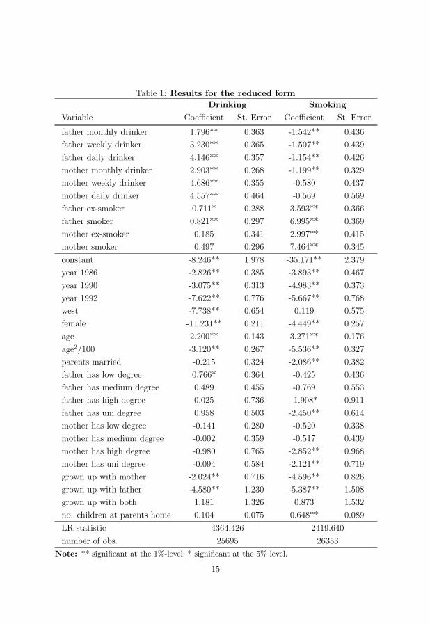
Table 1: Results for the reduced form

Drinking Smoking

Variable Coefficient St. Error Coefficient St. Error

father monthly drinker 1.796** 0.363 -1.542** 0.436

father weekly drinker 3.230** 0.365 -1.507** 0.439

father daily drinker 4.146** 0.357 -1.154** 0.426

mother monthly drinker 2.903** 0.268 -1.199** 0.329

mother weekly drinker 4.686** 0.355 -0.580 0.437

mother daily drinker 4.557** 0.464 -0.569 0.569

father ex-smoker 0.711* 0.288 3.593** 0.366

father smoker 0.821** 0.297 6.995** 0.369

mother ex-smoker 0.185 0.341 2.997** 0.415

mother smoker 0.497 0.296 7.464** 0.345

constant -8.246** 1.978 -35.171** 2.379

year 1986 -2.826** 0.385 -3.893** 0.467

year 1990 -3.075** 0.313 -4.983** 0.373

year 1992 -7.622** 0.776 -5.667** 0.768

west -7.738** 0.654 0.119 0.575

female -11.231** 0.211 -4.449** 0.257

age 2.200** 0.143 3.271** 0.176

age2/100 -3.120** 0.267 -5.536** 0.327

parents married -0.215 0.324 -2.086** 0.382

father has low degree 0.766* 0.364 -0.425 0.436

father has medium degree 0.489 0.455 -0.769 0.553

father has high degree 0.025 0.736 -1.908* 0.911

father has uni degree 0.958 0.503 -2.450** 0.614

mother has low degree -0.141 0.280 -0.520 0.338

mother has medium degree -0.002 0.359 -0.517 0.439

mother has high degree -0.980 0.765 -2.852** 0.968

mother has uni degree -0.094 0.584 -2.121** 0.719

grown up with mother -2.024** 0.716 -4.596** 0.826

grown up with father -4.580** 1.230 -5.387** 1.508

grown up with both 1.181 1.326 0.873 1.532

no. children at parents home 0.104 0.075 0.648** 0.089

LR-statistic 4364.426 2419.640

number of obs. 25695 26353

Note: ** significant at the 1%-level; * significant at the 5% level.

15

the correlation between the propensity to drink and parental smoking behavior is

positive, we find a significantly, negative correlation between the propensity to smoke

and parental drinking habits.

With regard to our control variables the results of the reduced forms exhibit a

trend of a decreasing inclination to smoke and drink over time as well as a lower

propensity to consume tobacco and alcohol for women compared to men. Moreover,

results indicate a significant negative correlation of the propensity to drink or smoke

with having grown up with at least one parent compared to individuals having grown

up with other persons. Yet, we find a significant positive (but diminishing) correlation

with age. Parental education has a significantly negative effect on the propensity to

smoke and the number of children at parents home as well as the parental marital

status are significant only for the inclination to smoke as well.

When including other, potentially endogenous variables, we find no significant cor-

relation of the inclination to drink and smoke with income; see Table 7 in Appendix B

for reduced form estimation results. Yet, the own education level is significantly and

negatively correlated as well as being married compared to being single. With regard

to the working status results exhibit that unemployed, full time workers as well as per-

sons doing military or community service have a larger propensity to drink and smoke

than individuals not participating at the labor market whereas pupils are less inclined.

Individuals working part-time or being in vocational training show a higher propen-

sity to smoke than non-participating individuals. Moreover, the higher the number of

children the higher is the inclination to smoke. Again, in our final specification we

omit these variables because the causal direction is not clear a priori.

5.2 Structural Model Results

Table 2 reports the results for the structural equations (1) and (2). Regarding γa

and γc, the parameters of primary interest, estimates exhibit that (i) smoking signifi-

cantly increases the propensity to drink but, in contrast, that (ii) drinking significantly

decreases the propensity to smoke. In conclusion, the first result argues in favor of

complementarity between smoking and drinking while the latter seems to indicate that

drinking and smoking were substitutes. The latter, apparently, mirrors the reduced

form result that exhibits a negative correlation between the propensity to smoke and

parental drinking habits.

16

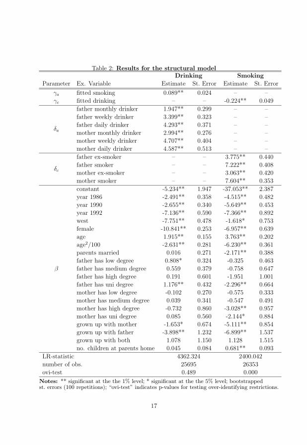
Table 2: Results for the structural modelDrinking Smoking

Parameter Ex. Variable Estimate St. Error Estimate St. Error

γa fitted smoking 0.089** 0.024 – –

γc fitted drinking – – -0.224** 0.049

father monthly drinker 1.947** 0.299 – –

father weekly drinker 3.399** 0.323 – –

father daily drinker 4.293** 0.371 – –δa mother monthly drinker 2.994** 0.276 – –

mother weekly drinker 4.707** 0.404 – –

mother daily drinker 4.587** 0.513 – –

father ex-smoker – – 3.775** 0.440

father smoker – – 7.222** 0.408δc mother ex-smoker – – 3.063** 0.420

mother smoker – – 7.604** 0.353

constant -5.234** 1.947 -37.053** 2.387

year 1986 -2.491** 0.358 -4.515** 0.482

year 1990 -2.655** 0.340 -5.649** 0.453

year 1992 -7.136** 0.590 -7.366** 0.892

west -7.751** 0.478 -1.618* 0.753

female -10.841** 0.253 -6.957** 0.639

age 1.915** 0.155 3.763** 0.202

age2/100 -2.631** 0.281 -6.230** 0.361

parents married 0.016 0.271 -2.171** 0.388

father has low degree 0.808* 0.324 -0.325 0.463

β father has medium degree 0.559 0.379 -0.758 0.647

father has high degree 0.191 0.601 -1.951 1.001

father has uni degree 1.176** 0.432 -2.296** 0.664


mother has medium degree 0.039 0.341 -0.547 0.491

mother has high degree -0.732 0.860 -3.028** 0.957

mother has uni degree 0.085 0.560 -2.144* 0.884

grown up with mother -1.653* 0.674 -5.111** 0.854


grown up with both 1.078 1.150 1.128 1.515


LR-statistic 4362.324 2400.042


ovi-test 0.489 0.000

Notes: ** significant at the the 1% level; * significant at the the 5% level; bootstrappedst. errors (100 repetitions); “ovi-test” indicates p-values for testing over-identifying restrictions.

17

As it is shown that γa and γc need to bear the opposite sign than Hicksian cross-

price derivatives do, which are well known to be symmetric, this asymmetry seems to

contradict theory, immediately raising the question whether we can trust this result. In

econometric terms, this means that we have to test if our identifying assumptions hold

that parental smoking habits do influence children’s later tobacco consumption but

do not affect their drinking behavior conditional on their smoking habits, vice versa.

Actually, the over-identification test as presented in Table 2 rejects the null hypothe-

sis for the smoking equation. In contrast, the test statistics for the drinking equation

indicate that parental smoking habits are valid instruments for smoking. These re-

sults are confirmed by “quasi-over-identification-tests”. With respect to smoking the

hypothesis is rejected that all different estimates for γ, which can be calculated from

the reduced form, coincide. Yet, the opposite holds for drinking.

These dissymmetric test results might be explained as follows. Apparently, our

empirical analysis supports the hypothesis that parental smoking habits do not have

effects on children’s future alcohol consumption that operate through unobserved chan-

nels. In contrast, the reverse does hold for parental drinking habits. Drinking at

parental home, therefore, seems to affect children’s future lives in a more general way

than parental smoking habits do. This result is quite plausible in the case of exces-

sive consumption. Severe alcohol abuse is likely to damage family live in general and,

therefore, might affect children through various channels, while excessive smoking –

though harmful to health – is not likely to have comparable effects. Yet, even beyond

this extreme case, drinking, which unlike smoking often is a collaborative activity,

might serve as an indicator for unobserved parental attributes like sociableness or

fun-lovingness. Such parental attributes potentially are of general importance to chil-

dren’s character building and therefore might be reflected in children’s future general

consumption behavior.

In consequence, we can trust the estimate for γa and, therefore, we can conclude that

alcohol and tobacco are consumed as complements rather than substitutes. This result

is in line with the main body of previous literature that comes to the same conclusion,

though applying approaches different to ours. In contrast, the estimate for γc is of

no value for any economic interpretation. Its negative sign that seemingly indicates

substitutability just represents a statistical artefact resting on invalid instruments.

At this point one may wonder why we have allowed γa and γc to exhibit opposite

signs rather than imposing the restriction sign(γa) = sign(γc) on the estimates. The

reason for this is the lack of valid instruments for the identification of γc. Since we

18

have not properly identified γc, estimates for this parameter cannot contribute to

our research question which, in turn, exclusively has to be answered on basis of the

estimate for γa. This problem is not solved by imposing cross-equation restrictions.

Yet, even worse, imposing such restrictions might render γa biased, too.21

6 Model Extensions

6.1 Non-Linear Specifications

In the model presented so far the degree of complementarity in the consumption of

alcohol and tobacco is captured by the fixed coefficients γ. Yet, the assumption that

the degree of complementarity in consumption does not depend on consumption levels

seems to be quite strong. One way to address this problem is specifying γ as a

function of endogenous variables, i.e. γa = γa(c∗it), γc analogously. In this case, even

if a simple linear relationship is assumed, a reduced form model representation does

not longer exist in closed form. Nevertheless, a linear instrumental variable estimator

that deals with non-linear functions of endogenous regressors as if they were additional

explanatory variables still can be applied in order to obtain estimates for the structural

parameters, see Wooldridge (2002: 232). For this approach additional instruments are

required. Interaction terms of the original instruments zit or, alternatively, squares and

higher order powers of a∗it and c∗it seem to be the most obvious choices, see Wooldridge

(2002: 237). Rather than a linear specification we chose a quadratic one

γa = γa1 + γa2(c∗it)

2

1000(5)

γc = γc1 + γc2(a∗

it)2

1000, (6)

which corresponds to cubic structural equations. This choice is for technical reasons.

Fitted values for (a∗it)

3 and (c∗it)3 still can be obtained from simple Tobit regressions

with (ait)3 and (cit)

3 serving as left hand side variables. In contrast – due to non-

negativeness – squares do not allow for this approach. Several versions of non-linear

model specifications are estimated, using (i) (a∗it)

3 and (c∗it)3, (ii) (a∗

it)2, (c∗it)

2, (a∗it)

3,

and (c∗it)3 and, (iii) interaction terms of the elements of zait and, respectively, zcit as

21Since the likelihood function of the Tobit model is globally concave, binding inequality constraintswill always result in corner solutions. In our case [γa γc] = [−0 − 0.224] maximizes the restrictedlikelihood function. I.e. the supposably biased estimator for γc prevails over the consistent one for γa

if the restriction sign(γa) = sign(γc) is imposed.

19

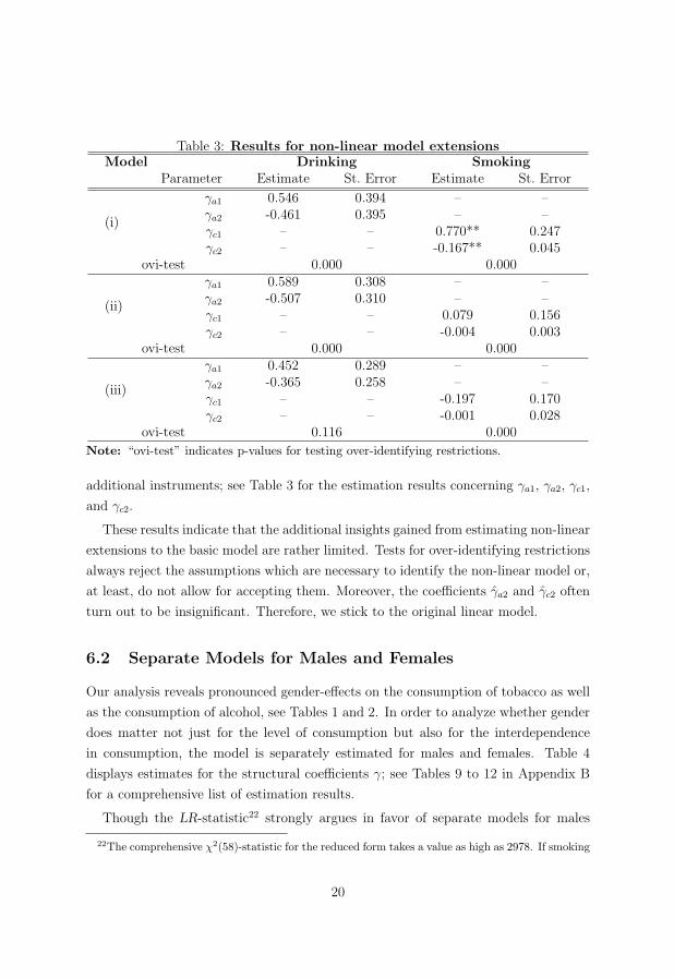
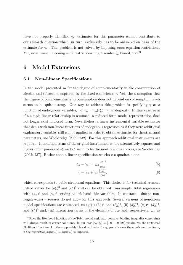
Table 3: Results for non-linear model extensionsModel Drinking Smoking

Parameter Estimate St. Error Estimate St. Error

γa1 0.546 0.394 – –γa2 -0.461 0.395 – –

(i)γc1 – – 0.770** 0.247γc2 – – -0.167** 0.045

ovi-test 0.000 0.000γa1 0.589 0.308 – –γa2 -0.507 0.310 – –

(ii)γc1 – – 0.079 0.156γc2 – – -0.004 0.003

ovi-test 0.000 0.000γa1 0.452 0.289 – –γa2 -0.365 0.258 – –

(iii)γc1 – – -0.197 0.170γc2 – – -0.001 0.028

ovi-test 0.116 0.000

Note: “ovi-test” indicates p-values for testing over-identifying restrictions.

additional instruments; see Table 3 for the estimation results concerning γa1, γa2, γc1,

and γc2.

These results indicate that the additional insights gained from estimating non-linear

extensions to the basic model are rather limited. Tests for over-identifying restrictions

always reject the assumptions which are necessary to identify the non-linear model or,

at least, do not allow for accepting them. Moreover, the coefficients γa2 and γc2 often

turn out to be insignificant. Therefore, we stick to the original linear model.

6.2 Separate Models for Males and Females

Our analysis reveals pronounced gender-effects on the consumption of tobacco as well

as the consumption of alcohol, see Tables 1 and 2. In order to analyze whether gender

does matter not just for the level of consumption but also for the interdependence

in consumption, the model is separately estimated for males and females. Table 4

displays estimates for the structural coefficients γ; see Tables 9 to 12 in Appendix B

for a comprehensive list of estimation results.

Though the LR-statistic22 strongly argues in favor of separate models for males

22The comprehensive χ2(58)-statistic for the reduced form takes a value as high as 2978. If smoking

20

Table 4: Results for separate models for males and females

Gender Drinking SmokingParameter Estimate St. Error Estimate St. Error

γa 0.135** 0.041 – –male

γc – – -0.159** 0.055ovi-test 0.379 0.000

γa 0.037 0.025 – –female

γc – – -0.337** 0.102ovi-test 0.920 0.061

Note: “ovi-test” indicates p-values for testing over-identifying restrictions.

and females, in qualitative terms the results are similar to those obtained from the

pooled model for either gender. For both men and women γc is negative, yet - as in the

pooled model - over-identification tests reject the identifying assumptions. In contrast,

γa takes positive values for both genders and its identification is not fundamentally

questioned for the males’ or for the females’ model by the relevant test-statistics.

The main difference to the results obtained from the split model, therefore, is a

quantitative one. While for males γa is of a substantially larger magnitude than in

the pooled model, the parameter takes a much smaller value for females and even

becomes insignificant. Therefore, the positive effect from smoking to drinking that is

found in this analysis is a males’ phenomenon while for females it seems to be of much

smaller magnitude and might even be non-existent. Thus, drinking habits seem to

differ between males and females even beyond the mere level of alcohol consumption.

This result might reflect gender-specific variation in preferences as well as differing

social conventions.

7 Conclusions

In this paper a new approach for analyzing the interdependence in the consumption

of alcohol and tobacco was proposed and applied to German survey data. We use

an alternative measure of complementarity which – in qualitative terms – is shown

to be equivalent to conventional Hicksian cross-price derivatives, yet it is not based

on the estimation of cross-price effects. In fact, the proposed instrumental variable

approach mimics an experimental study and therefore – in contrast to the main body

of the existing literature – does not rely on high-quality price data which often may

and drinking are treated separately, pooled models are rejected for either drug.

21

not be available. This makes it particularly well suited to the German case where price

variation for both goods is extremely limited. Moreover, the lack of price variation is

a frequent obstacle to survey data based analyses of consumers’ behavior, not unique

to the case of alcohol and tobacco. Instrumental variables approaches, similar to

the one proposed here, might therefore serve as a promising modeling strategy if

interdependence in consumption is analyzed and if sufficient price data for estimating

a conventional demand system is not available.

Our estimation results suggest that tobacco and alcohol are consumed as com-

plements. This result rests on a positive effect from the consumption of tobacco to

consumption of alcohol that is found in the data. From a policy perspective, this

can be interpreted as follows: if the government could achieve a reduction in smoking

or in the inclination to smoke by any anti-drug policy, this would also decrease the

propensity to consume alcohol. Thus, there would be no unintended side-effects in

form of an increased (ab)use of alcohol to compensate for the reduced level of nicotine

intake. Even the reverse, i.e. a reduction in the consumption of both drugs, seems to

be the consequence. Yet, this result is statistically firm only for males. For females

this effect seems to be much smaller and might even be non-existent.

22

References

Bantle, C. & J. Haisken-DeNew (2002): Smoke Signals: The Intergenerational

Transmission of Smoking Behavior, DIW Discussion Paper 277.

Bask, M. & M. Melkerson (2004): Rationally Addicted to Drinking and Smok-

ing? Applied Economics 36, 373-381.

Becker, G.S. & K.M. Murphy (1988): A theory of Rational Addiction, American

Economic Review 84, 396-418.

Cameron, L. & J. Williams (2001): Cannabis, Alcohol and Cigarettes: Substi-

tutes or Complements?, The Economic Record 77, 19-34.

Chaloupka, F.J. & M. Grossman (1996): Price, Tobacco Control Policies and

Youth Smoking, NBER Working Paper 5740.

Chaloupka, F.J. & A. Laixuthai (1997): Do Youths Substitute Alcohol and

Marijuana? Some Econometric Evidence, Eastern Economic Journal 23, 253-

276.

Davis, G.C. & S.Y. Kim (2002): Measuring Instrument Relevance in the Sin-

gle Endogenous Regressor – Multiple Instrument case: a simplifying procedure,

Economics Letters 74, 321-325.

Decker, S.L. & A.E. Schwartz (2000): Cigarettes and Alkohol: Substitutes or

Complements?, NBER Working Paper 7535.

DiNardo, J. & T. Lemieux (2001): Alcohol, Marijuana, and American Youth:

the Unintended Effects of Government Regulation, Journal of Health Economics

20, 991-1010.

Florkowski, W.J. & K.T. McNamara (1992): Policy Implications of Alcohol

and Tobacco Demand in Poland, Journal of Policy Modelling 14, 93-99.

Goel, R.K. & M.J. Morey (1995): The Interdependence of Cigarette and Liquor

Demand, Southern Economics Journal 62, 451-459.

Jimenez, S. & J.M. Labeaga (1994): It is Possible to Reduce Tobacco Consump-

tion via Alcohol Taxation, Health Economics 3, 231-241.

23

Jones, A.M. (1989): A System Approach to the Demand for Alcohol and Tobacco,

Bulletin of Economic Research 41, 85-106.

Kraus, L. & R. Augustin (2001): Population Survey on the Consumption of Py-

choactive Substances in the German Adult Population 2000, Sucht - Zeitschrift

fur Wissenschaft und Praxis 47, Sonderheft 1, 1-88.

Lee, Y.G. & M. Abdel-Ghany (2004): American Youth Consumption of Licit

and Illicit Substances, International Journal of Consumer Studies 28, 454-465.

Maddala, G.S. (1983): Limited-Dependent and Qualitative Variables in Econo-

metrics, Cambridge U.K., Cambridge University Press.

McFadden, D. (1999): Lecture Notes – Econometrics and Statistics, download:

http://emlab.berkeley.edu/users/mcfadden/e240b f01/ch6.pdf.

Murphy, K.M. & R.H. Topel (1985): Estimation and Inference in Two-Step

Econometric Models, Journal of Business & Economic Statistics 3, 370-379.

Nelson, F.D. & L. Olsen (1978): Specification and Estimation of a Simultane-

ous Equation Model with Limited Dependent Variables, International Economic

Review 19, 695-710.

Picone, G.A., F. Sloan & J.G. Trogdon (2004): The Effect on of the Tobacco

Settlement and Smoking Bans on Alcohol Consumption, Health Economics 13,

1063-1080.

Smith, R. & R. Blundell (1986): An Exogeneity Test for the Simultaneous

Equation Tobit Model with an Application to Labor Supply, Econometrica 54,

679-685.

Su, S.B. & S.T. Yen (2000): A Censored System of Cigarette and Alcohol Con-

sumption, Applied Economics 32, 729-737.

Tauras, J.A. & F.J. Chaloupka (1999): Price, Clean Indoor Air Laws, and

Cigarette Smoking: Evidence from Longitudinal Data for Young Adults, NBER

Working Paper 6937.

Warschburger, S. (2000): Rauchen und Sozialversicherung: Eine empirische Ana-

lyse der Konsequenzen veranderter Rauchgewohnheiten auf das bundesdeutsche

Rentensystem, Ph.D.-Thesis University of Dortmund.

24

Wasserman, J. , W.G. Manning, J.P. Newhouse & J.D. Winkler (1991):

The Effects of Excise Taxes and Regulations on Cigarette Smoking, Journal of

Health Economics 10, 43-64.

Williams, J., R.L. Pacula, F.J. Chloupka & H. Wechsler (2001): Alcohol and

Marijuana use among College Studens: Economic Complements or Substitutes?,

NBER Working Paper 8401.

Wooldridge, J.M. (2002): Econometric Analysis of Cross Section and Panel Data,

Cambridge Massachusetts, MIT Press.

Yen, S.T. (2005): A Multivariate Sample-Selection Model: Estimating Cigarette

and Alcohol demands with Zero Observations, American Journal of Agricultural

Economics 87, 453-466.

Zhao, X. & M.N. Harris (2004): Demand for Marijuana, Alcohol and Tobacco:

Participation, Levels of Consumption and Cross-equation Correlation, The Eco-

nomic Record 80, 394-410.

25

Appendix

A Equivalence of Measures of Complementarity

In this appendix we show that the cross price effect of increasing the price of tobacco

(alcohol) on the Hicksian demand for alcohol (tobacco) has always the opposite sign

of the effect resulting from increasing the consumption of tobacco (alcohol) on the

Marshiallian demand for alcohol (tobacco).

To see this, we write the consumer’s direct utility as U(a, c, w), where we denote by

a, c, and w the amounts of consumed alcohol, tobacco and a compound good consisting

of all other goods, respectively. For simplicity, any subscripts i and t denoting specific

individuals and periods are skipped. The corresponding prices are pa, pc, and pw.

Hicksian demand for alcohol is written as aH(pa, pc, pw, U), for some fixed utility level

U . Accordingly, the restricted Marshallian demand for alcohol, if the consumption of

tobacco c is given, is denoted by aM(pa, pc, pw, c, y) where y is income. We now state

the following result:

Proposition: If U is strictly quasi-concave, and both the Marshallian and the

Hicksian demand is characterized by interior solutions in a, c, and w, then

sign

[∂aH(pa, pc, pw, U)

∂pc

]= −sign

[∂aM(pa, pc, pw, c, y)

∂c

]. (7)

Proof: By definition aH(pa, pc, pw, U) is the solution of mina,c,w

{paa + pcc + pww}subject to

U(a, c, w) = U. (8)

The first-order necessary conditions for the expenditure minimum are given by

Ua(a, c, w) = λ−1pa ≡ µpa (9)

Uc(a, c, w) = λ−1pc ≡ µpc (10)

Uw(a, c, w) = λ−1pw ≡ µpw (11)

where λ is the Langrange multiplier with respect to (8) and µ = λ−1. In order to obtain

∂a/∂pc we differentiate the equation system (9)-(11) and (8) totally with respect to pc

to obtain: ⎡⎢⎢⎢⎢⎣

Uaa Uac Uaw −pa

Uac Ucc Ucw −pc

Uaw Ucw Uww −pw

µpa µpc µpw 0

⎤⎥⎥⎥⎥⎦ ×

⎡⎢⎢⎢⎢⎣

∂aH/∂pc

∂cH/∂pc

∂wH/∂pc

∂µ/∂pc

⎤⎥⎥⎥⎥⎦ =

⎡⎢⎢⎢⎢⎣

0

µ

0

0

⎤⎥⎥⎥⎥⎦ (12)

26

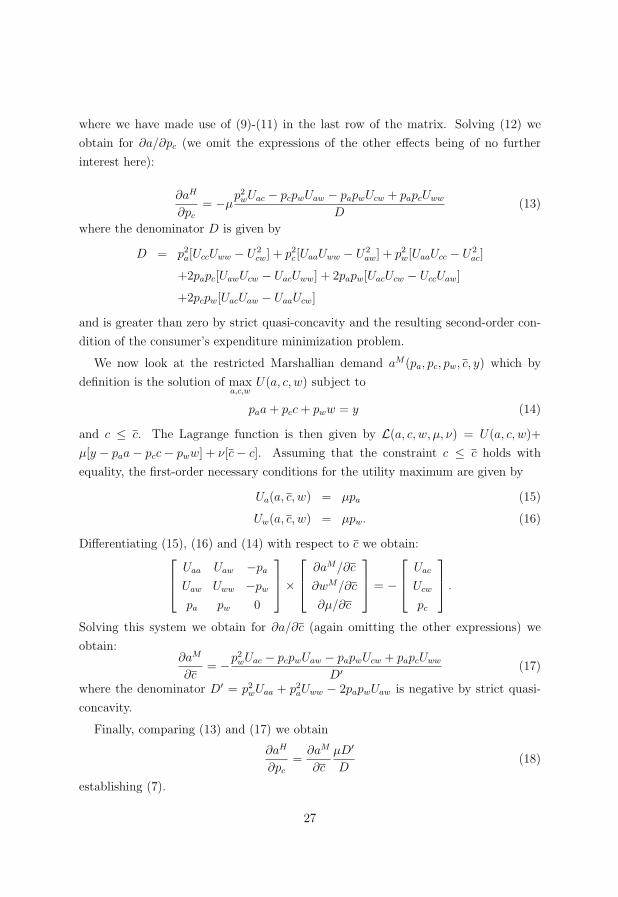
where we have made use of (9)-(11) in the last row of the matrix. Solving (12) we

obtain for ∂a/∂pc (we omit the expressions of the other effects being of no further

interest here):

∂aH

∂pc

= −µp2

wUac − pcpwUaw − papwUcw + papcUww

D(13)

where the denominator D is given by

D = p2a[UccUww − U2

cw] + p2c [UaaUww − U2

aw] + p2w[UaaUcc − U2

ac]

+2papc[UawUcw − UacUww] + 2papw[UacUcw − UccUaw]

+2pcpw[UacUaw − UaaUcw]

and is greater than zero by strict quasi-concavity and the resulting second-order con-

dition of the consumer’s expenditure minimization problem.

We now look at the restricted Marshallian demand aM(pa, pc, pw, c, y) which by

definition is the solution of maxa,c,w

U(a, c, w) subject to

paa + pcc + pww = y (14)

and c ≤ c. The Lagrange function is then given by L(a, c, w, µ, ν) = U(a, c, w)+

µ[y − paa − pcc − pww] + ν[c − c]. Assuming that the constraint c ≤ c holds with

equality, the first-order necessary conditions for the utility maximum are given by

Ua(a, c, w) = µpa (15)

Uw(a, c, w) = µpw. (16)

Differentiating (15), (16) and (14) with respect to c we obtain:⎡⎢⎣

Uaa Uaw −pa

Uaw Uww −pw

pa pw 0

⎤⎥⎦ ×

⎡⎢⎣

∂aM/∂c

∂wM/∂c

∂µ/∂c

⎤⎥⎦ = −

⎡⎢⎣

Uac

Ucw

pc

⎤⎥⎦ .

Solving this system we obtain for ∂a/∂c (again omitting the other expressions) we

obtain:∂aM

∂c= −p2

wUac − pcpwUaw − papwUcw + papcUww

D′ (17)

where the denominator D′ = p2wUaa + p2

aUww − 2papwUaw is negative by strict quasi-

concavity.

Finally, comparing (13) and (17) we obtain

∂aH

∂pc

=∂aM

∂c

µD′

D(18)

establishing (7).

27

B Supplementary Tables

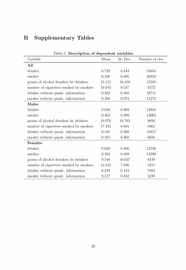
Table 5: Description of dependent variables

Variable Mean St. Dev. Number of obs.

All

drinker 0.729 0.444 25654

smoker 0.428 0.495 26353

grams of alcohol drunken by drinkers 15.112 16.418 15505

number of cigarettes smoked by smokers 16.043 8.547 9372

drinker without quant. information 0.203 0.402 18711

smoker without quant. information 0.169 0.374 11272

Males

drinker 0.838 0.369 12916

smoker 0.462 0.499 13063





Females

drinker 0.620 0.486 12738

smoker 0.394 0.489 13290





28

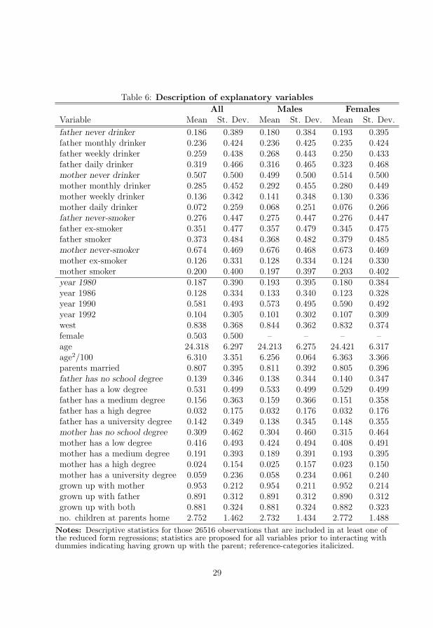
Table 6: Description of explanatory variables

All Males FemalesVariable Mean St. Dev. Mean St. Dev. Mean St. Dev.

father never drinker 0.186 0.389 0.180 0.384 0.193 0.395father monthly drinker 0.236 0.424 0.236 0.425 0.235 0.424father weekly drinker 0.259 0.438 0.268 0.443 0.250 0.433father daily drinker 0.319 0.466 0.316 0.465 0.323 0.468mother never drinker 0.507 0.500 0.499 0.500 0.514 0.500mother monthly drinker 0.285 0.452 0.292 0.455 0.280 0.449mother weekly drinker 0.136 0.342 0.141 0.348 0.130 0.336mother daily drinker 0.072 0.259 0.068 0.251 0.076 0.266father never-smoker 0.276 0.447 0.275 0.447 0.276 0.447father ex-smoker 0.351 0.477 0.357 0.479 0.345 0.475father smoker 0.373 0.484 0.368 0.482 0.379 0.485mother never-smoker 0.674 0.469 0.676 0.468 0.673 0.469mother ex-smoker 0.126 0.331 0.128 0.334 0.124 0.330mother smoker 0.200 0.400 0.197 0.397 0.203 0.402year 1980 0.187 0.390 0.193 0.395 0.180 0.384year 1986 0.128 0.334 0.133 0.340 0.123 0.328year 1990 0.581 0.493 0.573 0.495 0.590 0.492year 1992 0.104 0.305 0.101 0.302 0.107 0.309west 0.838 0.368 0.844 0.362 0.832 0.374female 0.503 0.500 – – – –age 24.318 6.297 24.213 6.275 24.421 6.317age2/100 6.310 3.351 6.256 0.064 6.363 3.366parents married 0.807 0.395 0.811 0.392 0.805 0.396father has no school degree 0.139 0.346 0.138 0.344 0.140 0.347father has a low degree 0.531 0.499 0.533 0.499 0.529 0.499father has a medium degree 0.156 0.363 0.159 0.366 0.151 0.358father has a high degree 0.032 0.175 0.032 0.176 0.032 0.176father has a university degree 0.142 0.349 0.138 0.345 0.148 0.355mother has no school degree 0.309 0.462 0.304 0.460 0.315 0.464mother has a low degree 0.416 0.493 0.424 0.494 0.408 0.491mother has a medium degree 0.191 0.393 0.189 0.391 0.193 0.395mother has a high degree 0.024 0.154 0.025 0.157 0.023 0.150mother has a university degree 0.059 0.236 0.058 0.234 0.061 0.240grown up with mother 0.953 0.212 0.954 0.211 0.952 0.214grown up with father 0.891 0.312 0.891 0.312 0.890 0.312grown up with both 0.881 0.324 0.881 0.324 0.882 0.323no. children at parents home 2.752 1.462 2.732 1.434 2.772 1.488

Notes: Descriptive statistics for those 26516 observations that are included in at least one ofthe reduced form regressions; statistics are proposed for all variables prior to interacting withdummies indicating having grown up with the parent; reference-categories italicized.

29

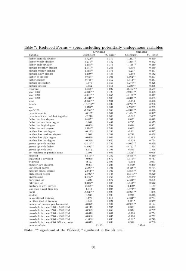
Table 7: Reduced Forms – spec. including potentially endogenous variablesDrinking Smoking


father monthly drinker 1.722** 0.379 -1.217** 0.450father weekly drinker 3.274** 0.382 -1.244** 0.452father daily drinker 4.108** 0.374 -1.146** 0.440mother monthly drinker 2.941** 0.281 -0.606 0.339mother weekly drinker 4.518** 0.371 -0.217 0.451mother daily drinker 4.409** 0.483 -0.159 0.582father ex-smoker 0.654* 0.301 3.562** 0.377father smoker 0.716* 0.312 6.413** 0.381mother ex-smoker 0.577 0.356 3.277** 0.426mother smoker 0.552 0.311 6.729** 0.356constant 6.896* 3.022 -21.458** 3.537year 1986 -2.300** 0.420 -2.904** 0.498year 1990 -2.618** 0.355 -4.167** 0.417year 1992 -7.431** 0.900 -6.317** 0.868west -7.888** 0.787 -0.414 0.696female -10.818** 0.239 -3.728** 0.286age 1.178** 0.201 2.596** 0.239age2/100 -1.259** 0.353 -4.342** 0.420parents married -0.167 0.341 -1.464** 0.397parents not married but together -2.210 1.903 -0.622 2.067father has low degree 0.817* 0.381 0.023 0.449father has medium degree 0.661 0.481 0.785 0.575father has high degree -0.068 0.784 0.684 0.951father has uni degree 1.414** 0.539 0.603 0.648mother has low degree -0.123 0.293 -0.111 0.347mother has medium degree 0.001 0.381 0.749 0.458mother has high degree -0.690 0.809 -0.962 1.008mother has uni degree -0.330 0.620 -0.429 0.754grown up with mother -2.119** 0.756 -4.067** 0.859grown up with father -4.892** 1.364 -5.722** 1.554grown up with both 1.572 1.391 0.599 1.578no. children at parents home 0.093 0.083 0.522** 0.096married -1.514** 0.382 -2.456** 0.440separated / divorced -0.050 0.672 3.916** 0.747widowed -2.177 2.595 -0.392 3.051number own children -0.201 0.225 0.642* 0.250low school degree -2.399** 0.701 -2.418** 0.764medium school degree -2.011** 0.707 -5.805** 0.776high school degree -2.107** 0.744 -10.319** 0.829unemployed 2.645** 0.766 5.578** 0.880part time job 0.226 0.677 2.333** 0.805full time job 2.116** 0.508 3.643** 0.612military or civil service 2.398* 0.967 2.449* 1.157less than a part time job 1.317 1.095 3.673** 1.249pupil -5.530** 0.920 -8.223** 1.065student 0.538 0.700 0.221 0.873in vocational training 0.170 0.614 2.934** 0.734in other kind of training 0.646 0.827 2.271* 0.957number of persons per household -0.027 0.104 -0.903** 0.124household income 1000 – 1499 DM -0.119 0.705 0.368 0.822household income 1500 – 1999 DM -0.999 0.653 0.334 0.767household income 2000 – 2499 DM -0.618 0.641 -0.168 0.754household income 2500 – 2999 DM -0.800 0.635 -0.160 0.752household income 3000 – 3999 DM -1.068 0.630 -0.387 0.749household income 4000 DM and more -0.073 0.638 0.399 0.760number of obs. 23195 23746


30

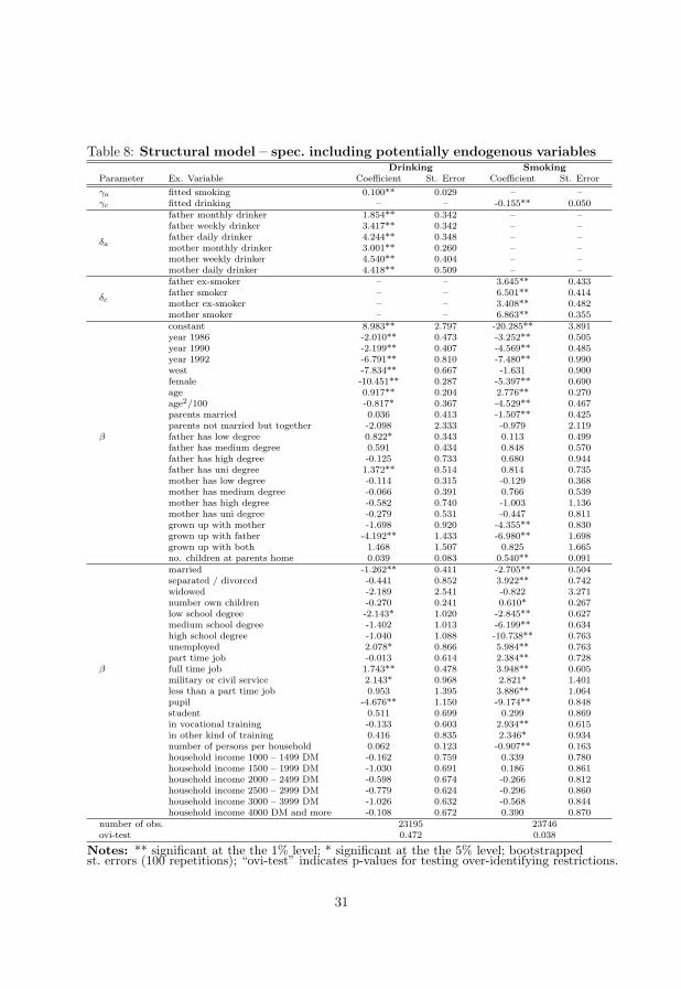
Table 8: Structural model – spec. including potentially endogenous variablesDrinking Smoking

Parameter Ex. Variable Coefficient St. Error Coefficient St. Error

γa fitted smoking 0.100** 0.029 – –γc fitted drinking – – -0.155** 0.050

father monthly drinker 1.854** 0.342 – –father weekly drinker 3.417** 0.342 – –father daily drinker 4.244** 0.348 – –

δamother monthly drinker 3.001** 0.260 – –mother weekly drinker 4.540** 0.404 – –mother daily drinker 4.418** 0.509 – –father ex-smoker – – 3.645** 0.433father smoker – – 6.501** 0.414

δcmother ex-smoker – – 3.408** 0.482mother smoker – – 6.863** 0.355constant 8.983** 2.797 -20.285** 3.891year 1986 -2.010** 0.473 -3.252** 0.505year 1990 -2.199** 0.407 -4.569** 0.485year 1992 -6.791** 0.810 -7.480** 0.990west -7.834** 0.667 -1.631 0.900female -10.451** 0.287 -5.397** 0.690age 0.917** 0.204 2.776** 0.270age2/100 -0.817* 0.367 -4.529** 0.467parents married 0.036 0.413 -1.507** 0.425parents not married but together -2.098 2.333 -0.979 2.119

β father has low degree 0.822* 0.343 0.113 0.499father has medium degree 0.591 0.434 0.848 0.570father has high degree -0.125 0.733 0.680 0.944father has uni degree 1.372** 0.514 0.814 0.735mother has low degree -0.114 0.315 -0.129 0.368mother has medium degree -0.066 0.391 0.766 0.539mother has high degree -0.582 0.740 -1.003 1.136mother has uni degree -0.279 0.531 -0.447 0.811grown up with mother -1.698 0.920 -4.355** 0.830grown up with father -4.192** 1.433 -6.980** 1.698grown up with both 1.468 1.507 0.825 1.665no. children at parents home 0.039 0.083 0.540** 0.091married -1.262** 0.411 -2.705** 0.504separated / divorced -0.441 0.852 3.922** 0.742widowed -2.189 2.541 -0.822 3.271number own children -0.270 0.241 0.610* 0.267low school degree -2.143* 1.020 -2.845** 0.627medium school degree -1.402 1.013 -6.199** 0.634high school degree -1.040 1.088 -10.738** 0.763unemployed 2.078* 0.866 5.984** 0.763part time job -0.013 0.614 2.384** 0.728

β full time job 1.743** 0.478 3.948** 0.605military or civil service 2.143* 0.968 2.821* 1.401less than a part time job 0.953 1.395 3.886** 1.064pupil -4.676** 1.150 -9.174** 0.848student 0.511 0.699 0.299 0.869in vocational training -0.133 0.603 2.934** 0.615in other kind of training 0.416 0.835 2.346* 0.934number of persons per household 0.062 0.123 -0.907** 0.163household income 1000 – 1499 DM -0.162 0.759 0.339 0.780household income 1500 – 1999 DM -1.030 0.691 0.186 0.861household income 2000 – 2499 DM -0.598 0.674 -0.266 0.812household income 2500 – 2999 DM -0.779 0.624 -0.296 0.860household income 3000 – 3999 DM -1.026 0.632 -0.568 0.844household income 4000 DM and more -0.108 0.672 0.390 0.870

number of obs. 23195 23746ovi-test 0.472 0.038


31

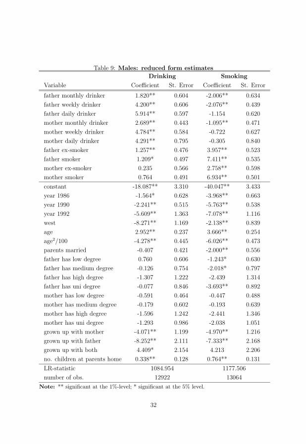
Table 9: Males: reduced form estimates

Drinking Smoking


father monthly drinker 1.820** 0.604 -2.006** 0.634

father weekly drinker 4.200** 0.606 -2.076** 0.439

father daily drinker 5.914** 0.597 -1.154 0.620




father ex-smoker 1.257** 0.476 3.957** 0.523

father smoker 1.209* 0.497 7.411** 0.535

mother ex-smoker 0.235 0.566 2.758** 0.598

mother smoker 0.764 0.491 6.934** 0.501

constant -18.087** 3.310 -40.047** 3.433

year 1986 -1.564* 0.628 -3.968** 0.663

year 1990 -2.241** 0.515 -5.763** 0.538

year 1992 -5.609** 1.363 -7.078** 1.116

west -8.271** 1.169 -2.138** 0.839

age 2.952** 0.237 3.666** 0.254

age2/100 -4.278** 0.445 -6.026** 0.473

parents married -0.407 0.421 -2.000** 0.556

father has low degree 0.760 0.606 -1.243* 0.630

father has medium degree -0.126 0.754 -2.018* 0.797

father has high degree -1.307 1.222 -2.439 1.314

father has uni degree -0.077 0.846 -3.693** 0.892



mother has high degree -1.596 1.242 -2.441 1.346

mother has uni degree -1.293 0.986 -2.038 1.051

grown up with mother -4.071** 1.199 -4.970** 1.216


grown up with both 4.409* 2.154 4.213 2.206

no. children at parents home 0.338** 0.128 0.764** 0.131

LR-statistic 1084.954 1177.506



32

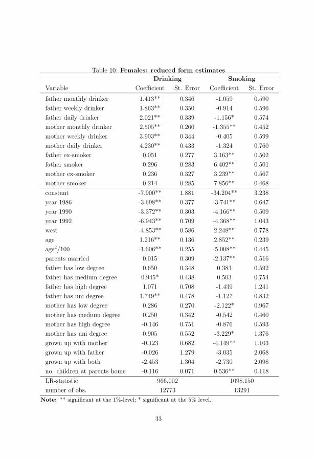
Table 10: Females: reduced form estimates

Drinking Smoking


father monthly drinker 1.413** 0.346 -1.059 0.590

father weekly drinker 1.863** 0.350 -0.914 0.596

father daily drinker 2.021** 0.339 -1.156* 0.574




father ex-smoker 0.051 0.277 3.163** 0.502

father smoker 0.296 0.283 6.402** 0.501

mother ex-smoker 0.236 0.327 3.239** 0.567

mother smoker 0.214 0.285 7.856** 0.468

constant -7.900** 1.881 -34.204** 3.238

year 1986 -3.698** 0.377 -3.741** 0.647

year 1990 -3.372** 0.303 -4.166** 0.509

year 1992 -6.943** 0.709 -4.368** 1.043

west -4.853** 0.586 2.248** 0.778

age 1.216** 0.136 2.852** 0.239

age2/100 -1.606** 0.255 -5.008** 0.445

parents married 0.015 0.309 -2.137** 0.516

father has low degree 0.650 0.348 0.383 0.592

father has medium degree 0.945* 0.438 0.503 0.754


father has uni degree 1.749** 0.478 -1.127 0.832

mother has low degree 0.286 0.270 -2.122* 0.967



mother has uni degree 0.905 0.552 -3.229* 1.376

grown up with mother -0.123 0.682 -4.149** 1.103

grown up with father -0.026 1.279 -3.035 2.068

grown up with both -2.453 1.304 -2.730 2.098

no. children at parents home -0.116 0.071 0.536** 0.118

LR-statistic 966.002 1098.150



33

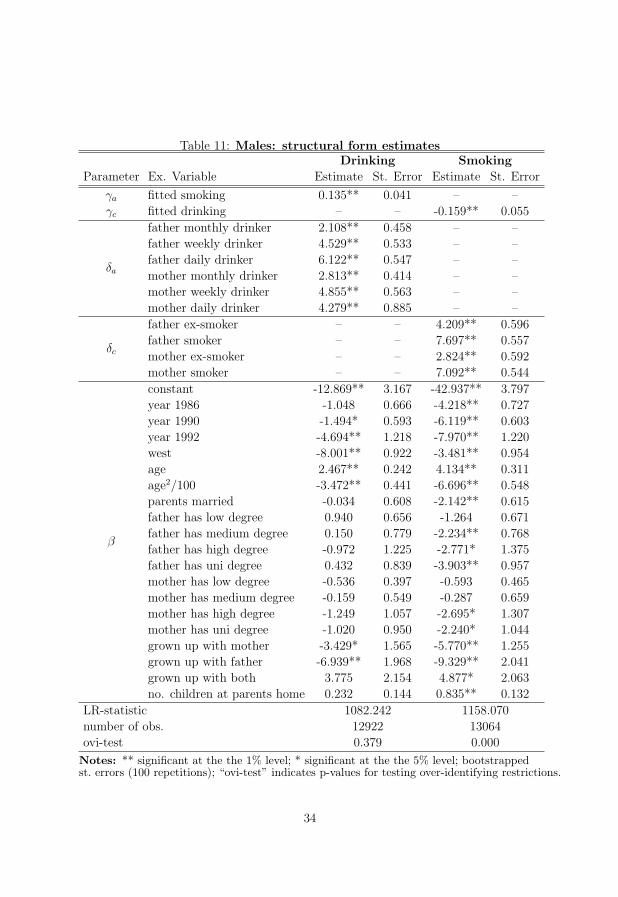
Table 11: Males: structural form estimatesDrinking Smoking


γa fitted smoking 0.135** 0.041 – –









mother smoker – – 7.092** 0.544

constant -12.869** 3.167 -42.937** 3.797

year 1986 -1.048 0.666 -4.218** 0.727

year 1990 -1.494* 0.593 -6.119** 0.603

year 1992 -4.694** 1.218 -7.970** 1.220

west -8.001** 0.922 -3.481** 0.954

age 2.467** 0.242 4.134** 0.311

age2/100 -3.472** 0.441 -6.696** 0.548

parents married -0.034 0.608 -2.142** 0.615

father has low degree 0.940 0.656 -1.264 0.671

father has medium degree 0.150 0.779 -2.234** 0.768β

father has high degree -0.972 1.225 -2.771* 1.375

father has uni degree 0.432 0.839 -3.903** 0.957



mother has high degree -1.249 1.057 -2.695* 1.307

mother has uni degree -1.020 0.950 -2.240* 1.044

grown up with mother -3.429* 1.565 -5.770** 1.255


grown up with both 3.775 2.154 4.877* 2.063


LR-statistic 1082.242 1158.070


ovi-test 0.379 0.000


34

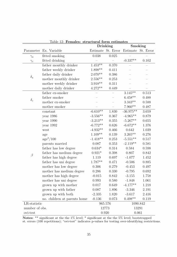
Table 12: Females: structural form estimatesDrinking Smoking


γa fitted smoking 0.038 0.025 – –









mother smoker – – 7.960** 0.487

constant -6.610** 1.830 -36.975** 3.659

year 1986 -3.556** 0.367 -4.965** 0.879

year 1990 -3.213** 0.355 -5.267** 0.655

year 1992 -6.772** 0.626 -6.672** 1.376

west -4.932** 0.466 0.642 1.039

age 1.109** 0.139 3.265** 0.276

age2/100 -1.418** 0.253 -5.551** 0.517

parents married 0.087 0.353 -2.119** 0.581

father has low degree 0.634* 0.314 0.584 0.598

father has medium degree 0.921* 0.398 0.807 0.842β


father has uni degree 1.787** 0.471 -0.506 0.885

mother has low degree 0.306 0.279 -0.453 0.497



mother has uni degree 0.993 0.580 -1.848 1.061

grown up with mother 0.017 0.649 -4.177** 1.218

grown up with father 0.087 1.896 -3.346 2.191

grown up with both -2.335 1.820 -3.617 2.416

no. children at parents home -0.136 0.073 0.498** 0.119

LR-statistic 965.576 1090.842


ovi-test 0.920 0.061


35

Harald Tauchmann, Silja Göhlmann, Till Requate … · Harald Tauchmann, Silja Göhlmann, Till...

Documents

Transcript of Harald Tauchmann, Silja Göhlmann, Till Requate … · Harald Tauchmann, Silja Göhlmann, Till...