
i Abstract - mediatum.ub.tum.de
212
Technische Universit¨at M¨ unchen Zentrum Mathematik - HVB-Stiftungsinstitut f¨ ur Finanzmathematik Valuation of mortgage products with stochastic prepayment-intensity models Andreas Kolbe Vollst¨andiger Abdruckderbei derFakult¨atf¨ ur Mathematik der Technischen Universit¨atM¨ unchen zur Erlangung des akademischen Grades eines Doktors der Naturwissenschaften (Dr. rer. nat.) genehmigten Dissertation. Vorsitzende: Univ.-Prof. Claudia Czado, Ph.D. Pr¨ ufer der Dissertation: 1. Univ.-Prof. Dr. Rudi Zagst 2. Prof. Frank J. Fabozzi, Ph.D. (Yale University, USA), schriftliche Beurteilung 3. Univ.-Prof. Dr. R¨ udiger Kiesel (Universit¨atUlm) Die Dissertation wurde am 13. November 2007 bei der Technischen Univer- sit¨at eingereicht und durch die Fakult¨at f¨ ur Mathematik am 30. Januar 2008 angenommen.
Transcript of i Abstract - mediatum.ub.tum.de
Technische Universitat MunchenZentrum Mathematik - HVB-Stiftungsinstitut fur Finanzmathematik
Valuation of mortgage products withstochastic prepayment-intensity
models
Andreas Kolbe
Vollstandiger Abdruck der bei der Fakultat fur Mathematik der TechnischenUniversitat Munchen zur Erlangung des akademischen Grades eines
Doktors der Naturwissenschaften (Dr. rer. nat.)
genehmigten Dissertation.
Vorsitzende: Univ.-Prof. Claudia Czado, Ph.D.
Prufer der Dissertation: 1. Univ.-Prof.Dr. Rudi Zagst
2. Prof. Frank J. Fabozzi, Ph.D.(Yale University, USA),schriftliche Beurteilung
3. Univ.-Prof.Dr. Rudiger Kiesel(Universitat Ulm)
Die Dissertation wurde am 13. November 2007 bei der Technischen Univer-sitat eingereicht und durch die Fakultat fur Mathematik am 30. Januar 2008angenommen.

2
i
Abstract
This thesis is concerned with the valuation of mortgage products with un-certain time of termination. In particular, we develop new valuation modelsfor agency mortgage-backed securities (MBS) as they are traded in the USmarket. Standard US mortgages feature a prepayment option which is oftennot exercised optimally. This causes uncertainty with respect to the time oftermination of a mortgage contract and makes the valuation of mortgage-backed securities a mathematically challenging task. Building on recentlyintroduced stochastic prepayment-intensity models for individual mortgagecontracts, we develop new mathematically consistent valuation models formortgage-backed securities. This modelling approach can also be consideredas an extension of the more traditional, purely econometric MBS valuationmodels which are very popular in practice.
The intensity-based modelling framework also allows us to develop aclosed-form approximation formula for the value of agency MBS. Comparedto existing MBS valuation approaches in the academic and practitioner-oriented literature, which usually rely on Monte-Carlo simulations or costlynumerical methods to solve multidimensional partial differential equations,our closed-form approximation approach offers a computationally highly effi-cient alternative. We apply this approach to some selected portfolio manage-ment applications with MBS, which require frequent product revaluationsunder different scenarios and thus computationally efficient valuation rou-tines.
Furthermore, we consider the valuation of reverse mortgages in this the-sis. Reverse mortgages also feature uncertainty with respect to the time oftermination of the contract and their mathematical valuation is thus non-trivial. We develop a consistent valuation model, again based on a stochastictermination-intensity, and illustrate our approach with some examples di-rected towards the German market, where reverse mortgages are not yetavailable.

ii

iii
Zusammenfassung
Die im amerikanischen Markt ublichen Hypothekenkredite beinhalten eineOption, die es dem Kreditnehmer erlaubt, den Kredit jederzeit vorzeitig undohne Vorfalligkeitsentschadigung zu tilgen (prepayment). Die Existenz derprepayment-Option und die Tatsache, dass viele Kreditnehmer die Optionsuboptimal ausuben, erzeugen Unsicherheit hinsichtlich des Terminierungs-zeitpunktes von Hypothekenkontrakten und machen die finanzmathemati-sche Bewertung von Hypothekendarlehen (mortgages) und Mortgage-BackedSecurities (MBS) zu einem anspruchsvollen Problem. Aufbauend auf inten-sitatsbasierten Modellen fur individuelle Hypthekenkredite, werden in dieserDissertation Bewertungsmodelle fur MBS entwickelt, die auch als Erweite-rung der in der Praxis gebrauchlichen, rein okonometrischen Modelle inter-pretiert werden konnen.
Der intensitatsbasierte Ansatz ermoglicht es zudem, eine approximative,geschlossene Bewertungsformel fur Mortgage-Backed Securities mit festemZinssatz herzuleiten. Im Vergleich zu bestehenden MBS-Bewertungsroutinen,die ublicherweise eine Monte-Carlo Simulation oder aufwandige numerischeVerfahren zur Losung mehrdimensionaler partieller Differentialgleichungenerfordern, bietet die entwickelte geschlossene Approximationsformel eine nu-merisch sehr effiziente Bewertungsalternative. Diese ermoglicht es auch, MBSim Rahmen einiger ausgewahlter Anwendungen im Portfoliomanagement zubetrachten, die eine wiederholte Produktbewertung unter verschiedenen Sze-narien erfordern.
Abschließend werden in dieser Dissertation Reverse Mortgages betrach-tet. Die mathematische Bewertung von Reverse Mortgages ist nicht-trivial,da deren Terminierungszeitpunkt ebenfalls zufallig ist. Der in dieser Arbeitentwickelte mathematisch konsistente Bewertungsansatz basiert, wie bereitsdie Bewertung von MBS, auf einer stochastischen Terminierungsintensitat.Das Bewertungsmodell wird schließlich mit einigen Beispielen fur den deut-schen Markt illustriert, in dem Reverse Mortgages bisher nicht erhaltlichsind.

iv
v
Acknowledgements
First of all, I would like to thank my supervisor Prof. Dr. Rudi Zagst. Heoffered me the possibility to do a dissertation at the HVB-Institute for Math-ematical Finance and significantly contributed to the success of this researchproject through his valuable ideas, advice, feedback and encouragement innumerous discussions. He provided the academically productive environmentand also gave me the opportunity to present my work at various conferences.Furthermore, I am grateful to Prof. Frank J. Fabozzi, Ph.D. and to Prof.Dr. Rudiger Kiesel for agreeing to serve as referees for this thesis and toProf. Dr. Claudia Czado for agreeing to chair the examination board of mydissertation.
I would also like to thank the Market Risk Control Division at BayerischeLandesbank (BayernLB), headed by Dr. Stefan Peiss, for the financial sup-port which made this research cooperation between BayernLB and the HVB-Institute for Mathematical Finance possible. I am particularly grateful toKai-Uwe Radde, former head of the Market Risk team at BayernLB Munich(now Allianz S.E.), who initiated the research cooperation and supported myapplication. He also contributed to the success of this dissertation throughhis ongoing interest, advice and encouragement during the last three years.I would also like to thank all colleagues in the Market Risk and Quantita-tive Analysis teams at BayernLB Munich and New York for the interestingprojects we jointly worked on and for the many discussions on prepaymentand mortgage-backed securities in particular, which greatly helped me to un-derstand the problems related to these topics from a practitioner’s point ofview.
Finally I would like to express my gratitude to my colleagues at theHVB-Institute for Mathematical Finance for many helpful discussions andthe always pleasant working atmosphere and to my family and friends formaking these last three years a highly enjoyable time.

vi
Contents
1 Introduction 1
1.1 Motivation . . . . . . . . . . . . . . . . . . . . . . . . . . . . . 1
1.2 Objectives and structure . . . . . . . . . . . . . . . . . . . . . 3
2 Mortgage products and prepayment 5
2.1 Prepayment and prepayment risk: A definition . . . . . . . . . 5
2.2 Mortgage-backed securities (MBS) . . . . . . . . . . . . . . . . 7
2.2.1 Subtypes of MBS and trading mechanics . . . . . . . . 7
2.2.2 Prepayment . . . . . . . . . . . . . . . . . . . . . . . . 10
2.2.3 Basic MBS cash flow conventions . . . . . . . . . . . . 13
2.3 Reverse mortgages . . . . . . . . . . . . . . . . . . . . . . . . 16
3 Mathematical preliminaries 19
3.1 The Cauchy problem . . . . . . . . . . . . . . . . . . . . . . . 19
3.2 Interest-rate markets . . . . . . . . . . . . . . . . . . . . . . . 22
3.2.1 General definitions . . . . . . . . . . . . . . . . . . . . 22
3.2.2 The Vasicek and Hull-White Models . . . . . . . . . . 25
3.2.3 The Cox-Ingersoll-Ross Model . . . . . . . . . . . . . . 29
3.3 Point processes and intensities . . . . . . . . . . . . . . . . . . 31
3.3.1 Theoretical overview . . . . . . . . . . . . . . . . . . . 31
3.3.2 Application to the pricing of contingent claims . . . . . 38
3.4 The Kalman filter . . . . . . . . . . . . . . . . . . . . . . . . . 40
4 Mortgage and MBS valuation 45
4.1 The different model classes . . . . . . . . . . . . . . . . . . . . 46
4.1.1 Econometric models . . . . . . . . . . . . . . . . . . . 46
4.1.2 Option-theoretic models . . . . . . . . . . . . . . . . . 48
4.1.3 Intensity-based models . . . . . . . . . . . . . . . . . . 51
4.2 Current frontiers and further challenges . . . . . . . . . . . . . 52
vii
viii CONTENTS
5 A new hybrid-form MBS valuation model 57
5.1 The model set-up for a fixed-rate MBS . . . . . . . . . . . . . 57
5.2 Application to market data . . . . . . . . . . . . . . . . . . . 62
5.2.1 Parameter estimation and model calibration . . . . . . 62
5.2.2 Prices and option-adjusted spreads . . . . . . . . . . . 74
5.2.3 Effective duration, convexity andparameter sensitivities . . . . . . . . . . . . . . . . . . 78
5.3 Adjustable-Rate MBS . . . . . . . . . . . . . . . . . . . . . . 84
5.4 Collateralized Mortgage Obligations . . . . . . . . . . . . . . . 88
6 A closed-form approximation for fixed-rate MBS 93
6.1 The model set-up . . . . . . . . . . . . . . . . . . . . . . . . . 94
6.2 Application to market data . . . . . . . . . . . . . . . . . . . 110
6.2.1 Parameter estimation and model calibration . . . . . . 110
6.2.2 Model performance, prices & sensitivities . . . . . . . . 114
7 The contribution of our MBS pricing models 123
7.1 A comparative assessment . . . . . . . . . . . . . . . . . . . . 123
7.2 Implications for the use in practice . . . . . . . . . . . . . . . 128
8 Optimal portfolios with MBS 129
8.1 The set-up: assets and scenarios . . . . . . . . . . . . . . . . . 130
8.2 Scenario-based portfolio optimisationwith MBS . . . . . . . . . . . . . . . . . . . . . . . . . . . . . 134
8.2.1 Expected utility approach . . . . . . . . . . . . . . . . 138
8.2.2 Portfolio optimisation with CVaR constraints . . . . . 143
9 Valuation and Pricing of Reverse Mortgages 151
9.1 The default-free modelling framework . . . . . . . . . . . . . . 152
9.1.1 Fixed-rate reverse mortgages . . . . . . . . . . . . . . . 157
9.1.2 Adjustable-rate reverse mortgages . . . . . . . . . . . . 158
9.2 Introducing default risk . . . . . . . . . . . . . . . . . . . . . . 162
9.3 Results and implications . . . . . . . . . . . . . . . . . . . . . 167
10 Summary and conclusion 177
A A Monte-Carlo algorithm 181
B The moving block bootstrap 185
C Discussion of approximation errors 189

CONTENTS ix
Bibliography 191
List of Figures 199

x CONTENTS
Chapter 1
Introduction
1.1 Motivation
Mortgage loans in general and mortgage-backed securities in particular con-stitute an important segment of any major debt market. The outstandingamount of all residential mortgage loans in the US market, on which we willprimarily focus in this thesis, was USD 10.9 trillion at the end of 20061. A to-tal of USD 6.4 trillion had been securitised and sold to the secondary marketin the form of mortgage-backed securities (MBS) and mortgage trusts (suchas, e.g., real estate investment trusts). The most important segment of thesecondary mortgage market are undoubtedly the so-called agency mortgage-backed securities, i.e. mortgage-backed securities issued and guaranteedby three agencies: The Government National Mortgage Association (Gin-nie Mae, GNMA), the Federal National Mortgage Association (Fannie Mae,FNMA) and the Federal Home Loan Mortgage Corporation (Freddie Mac,FHLMC). The cumulative outstanding principal of all agency-MBS addedup to USD 4.0 trillion at the end of 2006. The tremendous importance ofmortgage products in the US fixed-income market becomes even clearer if onecompares these amounts with the total amount of all (marketable, interest-bearing) outstanding US treasury debt, which equalled USD 4.6 trillion in2006.
Standard residential mortgages in the US feature full prepayment flexibil-ity, i.e. the mortgagors are allowed to prepay their mortgages at any time ata price of 100% of the outstanding notional. This prepayment option embed-ded in the mortgage contract causes uncertainty with respect to the time oftermination of the mortgage contract and makes the valuation of mortgage
1Source: Statistical Supplement to the Federal Reserve Bulletin, June 2007. Availableat www.federalreserve.gov
1
2 CHAPTER 1. INTRODUCTION
products a mathematically challenging task. This is particularly true for thevaluation of MBS where pools of mortgages have to be evaluated. The firstacademic and practitioner-oriented articles which were concerned with thepricing of mortgages, explicitly taking into account the prepayment option-ality, appeared in the early 1980s when mathematical finance and the pricingof financial derivatives had only just emerged as a field of research in its ownright. Since then, a vast body of literature and models on the pricing ofmortgage products has developed. These approaches can in general be clas-sified as econometric, option-theoretic or, rather recently, intensity-based.Since there is no consensus, neither in academia nor in practice, which ofthese general approaches is the ’best’ or most promising one, research in alldirections remains active.
While we will give a brief overview of the existing literature concernedwith each of the three approaches, we will focus on the intensity-based ap-proach in this thesis, which has been applied to the pricing of individualmortgage contracts recently, but not yet explicitly to the pricing of MBS(to the author’s best knowledge). The intensity-based approach will proveto be useful to tackle two major challenges regarding MBS valuation. Thefirst challenge is the mathematical pricing routine which should be consistentwith mathematical and financial theory and, at the same time, must be ableto take into account that mortgagors behave notoriously sub-optimal. Thesecond challenge is the computational burden associated with most existingMBS valuation techniques, which often causes problems in practice. Thisholds in particular for risk and portfolio management applications wherepossibly large portfolios of MBS have to be revaluated frequently under dif-ferent scenarios.
In addition to MBS, we will consider reverse mortgages in detail in thisthesis. Reverse mortgages are sold to older homeowners who receive either alump sum or a fixed annuity from the mortgage lender, for which no interestpayments have to be made during the lifetime of the contract. The reversemortgage contract is terminated when the mortgagor dies or sells the house.At this point of time, all outstanding debt including all accrued interest hasto be paid back, capped at the house sale proceeds. Since, of course, the timeof termination of the contract is random, reverse mortgages also fall into thecategory of mortgage products with uncertain time of termination for which amathematically consistent valuation model is non-trivial. Reverse mortgagesare still a niche product in the US and are not yet available in most Europeancountries, among them Germany. Yet, given the demographic developmentin these countries, the potential market for reverse mortgages in Europe ishuge. Despite the well-acknowledged potential of the product, the academicliterature on reverse mortgages, in particular concerning a mathematically

1.2. OBJECTIVES AND STRUCTURE 3
consistent valuation, remains scarce.
1.2 Objectives and structure
The main objective of this thesis is to develop new valuation approaches formortgage products with uncertain time of termination, based on stochasticintensity modelling. It is our aim to use this rather new concept in mathemat-ical finance, which has become popular in the context of credit risk modellingrecently, and to fine-tune it to the pricing of MBS and reverse mortgages.Concerning MBS, we want to improve on existing pricing models with re-spect to the challenges associated with MBS valuation as already stated inthe previous section. Concerning reverse mortgages, it is our aim to developa complete and consistent pricing model for different contract specifications,which has not been done before in the academic literature (to the author’sbest knowledge).
In addition to the theoretical development of the models, we will also ap-ply the model to real market data where possible. We will thus discuss andtake the reader through the whole model building process, from the theoret-ical formulation of the model to parameter estimation and calibration. Wewill also discuss the performance of our models where this is feasible and con-sider selected risk and portfolio optimisation topics. In the case of reversemortgages, we will provide empirical results directed towards the Germanmarket.
The remainder of this thesis is organised as follows: In Chapter 2 we de-fine how we understand the term ’prepayment’ in this thesis. Moreover, wegive a short overview of products with prepayment features in general and ofmortgage products in particular. In order to familiarise the reader with theproducts considered in this thesis, we will then introduce the basic character-istics of MBS as they are traded in the US market. Finally, we will introducereverse mortgages in more detail. Chapter 3 provides the reader with themathematical concepts which we need later in our MBS valuation models.This chapter is also intended to familiarise the reader with the mathemati-cal notation used in this thesis. While no substantial new contributions arecontained in Chapter 3 some calculations related to interest-rate theory arecarried out, which we will use in the subsequent chapters.
In Chapter 4 we provide an overview of the existing approaches for mort-gage and MBS valuation and give a detailed motivation for the need of furtherresearch in this field. Chapters 5 and 6 can be considered as the innovativecore of this thesis concerning MBS valuation. In Chapter 5 we develop a newMBS valuation model for fixed-rate MBS based on stochastic intensity mod-
4 CHAPTER 1. INTRODUCTION
elling. We explicitly consider the relation between option-adjusted spreads(an excess return measure commonly used in practice) and real-world andmarket implied prepayment speed patterns. The theoretical foundation forthis is Theorem 5.1 which adapts results from intensity models in other con-texts to the modelling of MBS. It offers the necessary mathematical rigourto extend ideas from previous mortgage and MBS modelling approaches andembeds them into a mathematically well-defined model framework. We giveempirical calibration examples, consider model sensitivities with respect toyield curve shifts and model parameters and discuss how the model can beused to price adjustable-rate mortgage-backed securities and collateralizedmortgage obligations (CMOs). This model, however, has one inconvenienceshared by many previous modelling approaches: the pricing requires a com-putationally expensive Monte-Carlo simulation. This problem is tackled inChapter 6, where we propose a closed-form approximation formula, basedon a slightly different model specification. This new closed-form approxima-tion formula presented in Theorem 6.6 offers an easy-to-compute alternativeto previous approaches in the literature concerned with MBS valuation inclosed-form. Compared to existing models, our approach has the advantagethat it does not require any numerically complex techniques. Again, we cal-ibrate and validate the model empirically with historically observed MBSmarket prices. Chapter 7 is intended to embed our models into the existingliterature and explicitly discusses the contribution of our MBS modelling ap-proaches, which naturally completes the discussion in Chapter 4.
In Chapter 8 we present some selected portfolio optimisation problems,based on simulated scenarios, and include fixed-rate MBS into the universeof available assets. In an empirical study we show how an asset alloca-tion strategy including MBS can outperform classical stock/bond portfolios.These empirical portfolio optimisation studies require a large number of MBSevaluations under different scenarios and have only become feasible due toour computationally highly efficient closed-form approximation approach.
Our pricing framework for reverse mortgages is presented in Chapter 9.We consider both, fixed-rate and adjustable-rate reverse mortgage contracts,explicitly take into account the possibility of losses for the lender (mainlyresulting from longevity risk) and discuss the maximum payments a home-owner can receive from the mortgage lender under certain constraints. Theresults are illustrated with data from the German market. Finally, Chapter10 concludes.

Chapter 2
Mortgage products andprepayment
In the first part of this chapter we will give an overview of the products withprepayment features, in particular with respect to the US market. Moreover,we will specify explicitly what we mean by ’prepayment’ and ’prepaymentrisk’. These terms are not always unambiguously used, neither in the aca-demic nor in the practitioner-oriented literature. The second part of thischapter is concerned with the most important asset class associated withprepayment risk: Mortgage-backed securities. While we can only provide anoverview of the product characteristics, the most important subtypes andtrading mechanics, this section is intended to familiarise the reader withthe securities for which we will develop valuation models in the subsequentchapters. Prominent examples of textbooks covering mortgage-backed secu-rities in a more detailed and extensive way include Fabozzi (2006) and Hu(1997), where legal, economic, structural, trading and pricing aspects of MBSare covered. Fabozzi (1998) features practitioner-oriented articles concernedwith various aspects of MBS valuation, while Young et al. (1999) providea detailed overview of MBS trading and settlement issues. Finally, reversemortgages are introduced in the last section of this chapter.
2.1 Prepayment and prepayment risk: A def-
inition
Prepayment is commonly understood as a borrower’s decision to exercise anearly repayment option in a financial contract. In order to price this option-ality, the borrower’s call policy must be anticipated correctly. This, however,is not always possible. The following definition formally establishes how we
5
6 CHAPTER 2. MORTGAGE PRODUCTS & PREPAYMENT
understand prepayment and prepayment risk in this thesis. It generalises thedefinition given by, e.g., Francois (2003) who exclusively considers callabledebt.
Definition 2.1. (Prepayments and prepayment risk)Prepayments are (contractually permitted) notional cash flows which occurearlier or later than expected, deviating from the anticipated call or put pol-icy of the counterparty in a financial contract. Prepayment risk is the riskresulting from these cash flow deviations.
This definition is very broad and it is able to accommodate both the prepay-ment risk in a bank’s assets and the prepayment risk in a bank’s liabilities.In the case of a liability, prepayment risk stems from a lender’s option towithdraw funds or to deposit money earlier or later than anticipated. Defi-nition 2.1 also makes clear that we understand prepayment risk exclusivelyas a special kind of market price risk resulting from the uncertain time oftermination (or partial termination) of the contract. Occasionally, the term’extension risk’ is used for the risk of cash flows which occur later than an-ticipated, increasing the duration of a financial product’s cash flow stream.The term ’prepayment risk’ is then used for the risk of cash flows which occurearlier than anticipated, decreasing the duration of the cash flow stream. Inthis thesis, however, we will not explicitly make this distinction and use theterm ’prepayment risk’ in its general form as defined in Definition 2.1. Thefact that a counterparty’s call or put policy can not be perfectly anticipatedfor some products may have various reasons. First, any prepayment modelwhich tries to capture the prepayment behaviour may be misspecified dueto, e.g., omission of factors or erroneous assumptions. Second, the counter-party may simply not behave optimally for lack of financial interest and/orsophistication.
The most important product class featuring prepayment risk are undoubt-edly mortgage-backed securities. Mortgage-backed securities (MBS) can beconsidered as a particular subtype of asset-backed securities (ABS) wherethe assets backing the security’s cash flows are mortgage loans. In general,ABS which feature call flexibility, e.g. ABS backed by Home-Equity or Re-tail Auto loans, also belong to the class of prepayment-sensitive assets. Ofcourse, beside interest-rate and prepayment risk, an ABS investor may alsobe exposed to credit risk, which is in many cases the major source of risk andthus very often the primary focus of an ABS investor. ABS and MBS inherittheir prepayment-sensitivity from the underlying loans. Prepayment risk ofindividual loans may in fact serve as the basis for assessing the prepaymentrisk of more complex products such as MBS. The prepayment risk in callable
2.2. MORTGAGE-BACKED SECURITIES (MBS) 7
bonds is explicitly addressed in Francois (2003), who discusses the theoreti-cal implications and provides empirical evidence. Yet, in most callable debtvaluation models it is assumed that the borrower does make the optimal calldecision which may be anticipated and priced by an adequate model (see,e.g., Artzner and Delbaen (1992) or Acharya and Carpenter (2002)).
In addition to the previously described prepayment-sensitive assets onemay also want to consider liabilities with put features in a prepaymentrisk context, i.e. products where the depositor has the right to withdrawfunds flexibly. An example are Municipal Guaranteed Investment Contracts(GICs). In the US, GICs are used by municipalities in conjunction withsocial or infrastructure projects. In order to finance these projects munici-palities issue bonds whose proceeds are then transferred into a GIC agree-ment to be used for the project development or as a reserve account for thebond issues. Furthermore, special GIC accounts are usually created for theproject’s proceeds which are then used for interest and principal repaymentsto the bondholders. Fund withdrawals and future deposits are often flexibleand may depend on various factors which are usually directly related to theproject which is being financed and to the call features of the correspondingbonds. As a consequence, the timing and sometimes also the amount of cashflows is hard to anticipate, which results in prepayment risk.
2.2 Mortgage-backed securities (MBS)
In this section we will briefly present the major structures and features ofmortgage-backed securities. Although MBS are one of the most importantasset classes in the US, they are a unique instrument whose valuation remainshighly complex. This is mainly caused by the prepayment feature inherent inthe mortgage loans underlying a MBS. In the last subsection we will shortlysummarise the basic loan and amortisation calculations for mortgages andMBS.
2.2.1 Subtypes of MBS and trading mechanics
Residential vs. Commercial MBS
The first criterion to classify the different subtypes of MBS in the US marketis the nature of the underlying mortgage loans. While we focus on securitiesbacked by residential mortgages in this thesis, securities backed by commer-cial mortgages (CMBS) also constitute an important part of the MBS market.However, the structure of a particular CMBS will largely be determined bythe individual characteristics of the underlying commercial mortgage(s) and,
8 CHAPTER 2. MORTGAGE PRODUCTS & PREPAYMENT
as a consequence, the prepayment behaviour and risk of these securities canoften be assessed only by taking into account these individual characteris-tics. Moreover, the primary concern of an investor in CMBS is usually thecredit risk component in view of which the prepayment risk often plays onlya minor or even negligible role.
Term and amortisation schedule
A second, natural classification criterion is the term of the underlying mort-gages and their amortisation schedule. While 30 year, fully amortising mort-gages are still the most common type of mortgage, mortgages and MBS withshorter maturities (e.g., 15 or 20 years) exist as well. More exotic amor-tisation structures include, for example, balloon mortgages and graduated-payment mortgages. Balloon mortgages have a 30 year amortisation sched-ule, but are due in just five or seven years, while the monthly payments ofa graduated-payment mortgage are lower during the first year of the loanand then rise gradually, so that the loan is fully amortised after the 30 yearterm. Because of the low initial payments, a graduated-payment mortgagemay feature negative amortisation in the early years.
Fixed-rate and adjustable-rate MBS
In the early 1980s adjustable-rate mortgages (ARMs) were introduced as analternative to the traditional fixed-rate mortgages. Adjustable-rate mort-gages and adjustable-rate MBS usually have a 6 month or 1 year floatingmoney market or treasury rate as reference index rate, such as the 6 monthLIBOR rate or the 1 year CMT (constant maturity treasury) rate. Yet, moreexotic indices such as the COFI (cost of fund index) are also common. Agreat majority of ARMs have periodic reset Caps and Floors as well as lifetime Caps, reducing the impact of interest-rate changes for the borrower.A combination of fixed-rate and adjustable-rate mortgages are the so-calledhybrids, which are adjustable-rate mortgages with an initial fixed-rate pe-riod of usually three, five, seven or ten years. For example, the notation5/1/30 is commonly used for a hybrid mortgage with maturity 30 years andan annually fixed adjustable rate after an initial tenor of five years.
Pass-throughs, Pay-throughs and CMOs
In a pass-through security, the monthly mortgage payments, which containinterest, scheduled principal and prepayments, are directly ’passed’ frommortgagors ’through’ the issuer to the investor. Usually these paymentsto the investor are delayed, e.g., by 14 or 19 days in the case of GNMA

2.2. MORTGAGE-BACKED SECURITIES (MBS) 9
securities (see Table 2.1). A delay of 14 means that the first payment tothe investor is made at the 15th (instead of the first) of the month follow-ing the record date and every month thereafter. In a pay-through security,mortgage payments are transformed by the issuer before they are passed onto the investor. Pay-through structures have particularly gained popular-ity in the form of collateralized mortgage obligations (CMOs). In a CMO,payments and especially prepayments of the underlying mortgage pool areassigned to different tranches. It is thus possible to create tranches withdifferent expected average lives, prepayment risk exposures and even interestrate agreements from one underlying pool. CMOs are thus able to satisfythe increasingly diversified risk appetite of investors. We will discuss someexemplary CMO structures in more detail in Chapter 5.4.
Agency and Private-label MBS
The Government National Mortgage Association (GNMA, Ginnie Mae) aswell as the government-sponsored Federal National Mortgage Association(FNMA, Fannie Mae) and the Federal Home Loan Mortgage Corporation(FHLMC, Freddie Mac) play a crucial role in the US MBS market. Theseinstitutions act as guarantor for mortgage pools, guaranteeing full and timelypayment of interest and principal to the investor. GNMA securities, whichfeature the full faith and credit of the US government, can thus be consid-ered default-free from the investor’s point of view since a possible default ofany of the mortgages in the underlying pool simply results in prepayment ofthe outstanding notional of the respective loan by GNMA. GNMA, FNMAand FHLMC securities are usually called agency MBS, have highly standard-ised structures, trading and settlement mechanics and constitute the largest,most liquid and most important part of the MBS market. Private-label MBShave individual characteristics with respect to structure, credit quality andliquidity. In the following we will particularly focus on the GNMA I andGNMA II programs, whose securities we will use in the following chaptersfor the empirical validation of our modelling approaches. Table 2.1, which isadapted from Hu (1997), p. 17 and p. 18, summarises the major features ofthese securities.
Trading mechanics
Trading in the US agency pass-through market can be divided into to-be-announced (TBA) trading and pool-specific trading. While in a pool-specifictrade both parties agree on the exact pool to be delivered, the seller in a

10 CHAPTER 2. MORTGAGE PRODUCTS & PREPAYMENT
Feature GNMA I GNMA II
Issuer Single lender Multiple lendersType of loans Newly originated, Newly originated,
backed by federal agencies backed by federal agencies(e.g., FHA2, VA3) (e.g., FHA, VA)
Minimum USD 1 mio USD 0.25 mio per lenderpool sizeMortgage Rate All must have Must be within 100 bpsRange the same rate of the lowest rate
in the poolServicing/ 50 bps 50-150 bpsGuarantee feePayment 14 days 19 daysdelay
Table 2.1: Major characteristics of GNMA I and GNMA II pass-throughMBS
TBA trade has the right to choose the pool(s), which must satisfy somerequirements of good delivery (see, e.g., Young et al. (1999) for details).The counterparties only agree on the crucial parameters, i.e. agency, term,coupon, par amount and price (for example, USD 20 mio of GNMA 30 year7% pass-throughs at a price of USD 0.9875 per USD 1 face amount). Inthe so-called TBA vintage-market, the buyer can also specify the originationyear of the pool(s). In 2005, USD 251 billion of agency MBS were traded ona daily average4. The market for TBA fixed-rate agency MBS remains themost liquid and most mature market segment.
2.2.2 Prepayment
As previously discussed, the mortgagors’ right to prepay is a crucial feature ofMBS. A MBS investor is always short the prepayment option which makesMBS highly complex instruments. The exercise of the prepayment optionby a mortgagor may have several reasons. The first, and most importantreason is usually called refinancing incentive. When mortgage refinancingrates drop, the mortgagor may have the possibility to refinance the mort-gage at a lower rate. In this sense, the prepayment option can be compared
2Federal Housing Administration3Department of Veterans Affairs4Source: The Bond Market Association (www.bondmarkets.com)
2.2. MORTGAGE-BACKED SECURITIES (MBS) 11
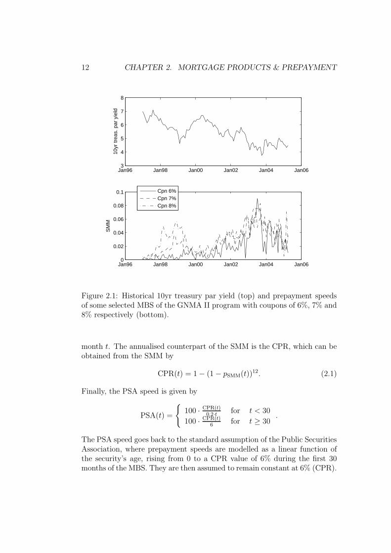
to an American-style interest-rate option. However, different mortgagors ina mortgage pool may experience different constraints regarding the abilityto refinance. These constraints may contain, for example, transaction costsor the opportunity costs that a mortgagor faces when he/she spends timerenegotiating mortgage conditions with possible lenders. These costs arecertainly a reason for the fact that refinancing related prepayment on poollevel is rather heterogeneous. Yet, the relationship between falling interestrates and rising prepayments is well-established and can also be confirmedwith the data which is available for this thesis. Figure 2.1 shows the develop-ment of the 10 year US treasury par yield together with prepayment speedsof some selected GNMA securities with different coupons. The prepaymentspeeds are expressed as single monthly mortalities (SMM).
Beside the refinancing incentive, prepayment may be caused by housesales due to relocation or death of the mortgagor. A mortgagor’s defaultequally leads to prepayment for the investor in the case of agency MBSand, finally, a change in personal wealth (e.g., by an inheritance, an unex-pected bonus payment, etc.) or simply new loan preferences of an individualmortgagor may prompt full or partial prepayment of a mortgage. Thesenon-refinancing related prepayments are usually subsumed under the term’turnover prepayment’ or ’baseline prepayment’.
Prepayment speeds are usually expressed as single monthly mortalityrates (SMM), as annualised constant prepayment rate (CPR) or as a per-centage of the Public Securities Association standard assumption (PSA).The SMM in month t simply measures the percentage of the outstandingnotional which is paid back to the investor after the interest and regularprincipal repayment of the corresponding month. Let A(t) be the outstand-ing notional (after scheduled repayments) of a MBS at time t according tothe original amortisation schedule without any prepayments and let PF (t)denote the pool factor at time t, i.e. the actual notional amount outstandingat time t. Then, given the mortgages prepayment history of the MBS up totime t − 1, we get5:
pSMM(t) =PF (t) − PF (t)
PF (t)
where
PF (t) := PF (t− 1) · A(t)
A(t − 1).
Note that, given the prepayment history up to month t− 1, PF (t) would bethe outstanding notional at time t if there were no further prepayments in
5We write pSMM for the single monthly mortality (SMM) due to notational consistencywith the subsequent chapters.
12 CHAPTER 2. MORTGAGE PRODUCTS & PREPAYMENT
Jan96 Jan98 Jan00 Jan02 Jan04 Jan063
4
5
6
7
8
10yr
trea
s. p
ar y
ield
Jan96 Jan98 Jan00 Jan02 Jan04 Jan060
0.02
0.04
0.06
0.08
0.1
SM
M
Cpn 6%Cpn 7%Cpn 8%
Figure 2.1: Historical 10yr treasury par yield (top) and prepayment speedsof some selected MBS of the GNMA II program with coupons of 6%, 7% and8% respectively (bottom).
month t. The annualised counterpart of the SMM is the CPR, which can beobtained from the SMM by
CPR(t) = 1 − (1 − pSMM(t))12. (2.1)
Finally, the PSA speed is given by
PSA(t) =
100 · CPR(t)
0.2·t for t < 30
100 · CPR(t)6
for t ≥ 30.
The PSA speed goes back to the standard assumption of the Public SecuritiesAssociation, where prepayment speeds are modelled as a linear function ofthe security’s age, rising from 0 to a CPR value of 6% during the first 30months of the MBS. They are then assumed to remain constant at 6% (CPR).
2.2. MORTGAGE-BACKED SECURITIES (MBS) 13
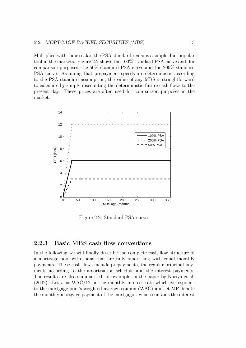
Multiplied with some scalar, the PSA standard remains a simple, but populartool in the markets. Figure 2.2 shows the 100% standard PSA curve and, forcomparison purposes, the 50% standard PSA curve and the 200% standardPSA curve. Assuming that prepayment speeds are deterministic accordingto the PSA standard assumption, the value of any MBS is straightforwardto calculate by simply discounting the deterministic future cash flows to thepresent day. These prices are often used for comparison purposes in themarket.
0 50 100 150 200 250 300 3500
2
4
6
8
10
12
14
MBS age (months)
CP
R (
in %
)
100% PSA200% PSA50% PSA
Figure 2.2: Standard PSA curves
2.2.3 Basic MBS cash flow conventions
In the following we will finally describe the complete cash flow structure ofa mortgage pool with loans that are fully amortising with equal monthlypayments. These cash flows include prepayments, the regular principal pay-ments according to the amortisation schedule and the interest payments.The results are also summarised, for example, in the paper by Kariya et al.(2002). Let i := WAC/12 be the monthly interest rate which correspondsto the mortgage pool’s weighted average coupon (WAC) and let MP denotethe monthly mortgage payment of the mortgagor, which contains the interest

14 CHAPTER 2. MORTGAGE PRODUCTS & PREPAYMENT
payment I(t) and the regular principal repayment RP (t), if we assume thatprepayments are not allowed. For a mortgage with T months to maturity attime t = 0, we obtain the defining equation for MP by using i as internalrate of return:
A(0) = MP/(1 + i)1 + MP/(1 + i)2 + ... + MP/(1 + i)T
= MP ·T∑
j=1
1
(1 + i)j
= MP ·1
1+i− 1
(1+i)T+1
1 − 11+i
= MP · 1 − (1 + i)−T
i. (2.2)
Thus,
MP = A(0) · i
1 − (1 + i)−T.
Equation (2.2) can of course be generalised, so that for any month t, 0 ≤ t ≤T , the outstanding notional according to the original amortisation scheduleis given by
A(t) = MP · 1 − (1 + i)−(T−t)
i.
The scheduled interest payment according to the amortisation schedule with-out any prepayments, which has to be made by the mortgagors in month t,1 ≤ t ≤ T , is given by
I(t) = A(t−1) · i = MP · (1− (1+ i)−(T−t+1)) = i ·A(0) · 1 − (1 + i)−(T−t+1)
1 − (1 + i)−T.
Finally, the regular principal payment is given by
RP (t) = MP − I(t) = i · A(0) · (1 + i)−(T−t+1)
1 − (1 + i)−T.
In a mortgage pool with prepayments, the difference between the outstandingnotional according to the original amortisation schedule without prepaymentsand the actual pool factor, i.e. A(t)−PF (t), can be considered as a quantitywhich reflects the magnitude of prepayments in the pool’s history up to timet. This difference, or alternatively the ratio PF (t)/A(t), is commonly referredto as the pool’s burnout. We will also use the burnout as an explanatoryvariable in our hybrid-form model presented in Chapter 5.
2.2. MORTGAGE-BACKED SECURITIES (MBS) 15
Now, let C denote the monthly coupon of the MBS with a pool of similarmortgages and let S be the monthly servicing and guarantee spread. Bymarket convention, the gross coupon i of the MBS is given by i = C + S.Defining by
I(t) := PF (t − 1) · i
the actual interest paid by the mortgagors in month t, the actual cash flowCF (t) paid to the investor in month t, 1 ≤ t ≤ T , is given by
CF (t) = (PF (t− 1) − PF (t)) +C
C + S· I(t)
=PF (t− 1)
A(t − 1)·(
A(t − 1) − PF (t)
PF (t − 1)· A(t − 1)
A(t)· A(t)
)
+C · PF (t − 1)
=PF (t− 1)
A(t − 1)·(
A(t − 1) − PF (t)
PF (t)· A(t)
)+ C · PF (t− 1)
=PF (t− 1)
A(t − 1)· (A(t − 1) − A(t) + A(t) · pSMM(t)) + C · PF (t− 1).
I.e. the cash flow paid to the investor at time t is given by the sum ofthe regular principal payment, prepayment and interest payment (with theservicing fee deducted).
Remark 2.2. (Monthly mortgage payment)Since in this thesis we are primarily interested in MBS from an investor’spoint of view, we will use the term ’monthly mortgage payment’ for the quan-tity
M(t)·∆t := A(t−1)−A(t)+C
C + S·I(t) = RP (t)+
C
C + S·I(t), 1 ≤ t ≤ T,
where ∆t = 112
unless explicitly specified otherwise. I.e., M(t) · ∆t is themonthly payment received by the investor without any prepayments. Thedifference between M(t) · ∆t and the earlier defined MP = RP (t) + I(t) isthe servicing spread which has to be paid by the mortgagors, but is not passedthrough to the investor. Note that, unlike MP , M(t) · ∆t is not constant.However, since the servicing spread is usually small (50 basis points in thecase of GNMA I securities), the changes of M(t) · ∆t over time are alsosmall.

16 CHAPTER 2. MORTGAGE PRODUCTS & PREPAYMENT
2.3 Reverse mortgages
Reverse mortgages were first introduced in the US in the late 1980s. While formost of the time demand for reverse mortgages remained low, the US reversemortgage market has experienced considerable growth in the last years andis now commonly viewed as a market with huge potential. In 2005, 43,131reverse mortgage contracts were originated in the US, compared to 6,640 in2001 (see Eschtruth et al. (2006)). A reverse mortgage allows home-rich,cash-poor older homeowners to access their housing wealth for consumptionwithout selling the house and without having to take a conventional homeequity mortgage which would require regular interest and loan amortisationpayments. The most popular reverse mortgage program in the US is theHome Equity Conversion Mortgage (HECM), which is available to home-owners over the age of 62 who fulfil certain eligibility criteria. In a HECMloan, payments to the mortgagor are made as a lump sum at origination ofthe reverse mortgage contract, as a lifetime income or as a flexible line ofcredit. A reverse mortgage loan has to be paid back including all accruedinterest when the mortgagor dies or sells the house or, depending on thecontract, when the mortgagor moves out of the house. The amount whichhas to be paid back is, however, capped at the house sale proceeds.
Despite the recent success in the US, reverse mortgages are still not avail-able in most European countries, among them Germany, on which we willfocus in the empirical examples in Chapter 9. This is particularly surprisingsince in Germany the demographic development implies that there will bemore and more elderly people in the near future without children. The accessto home equity for consumption after retirement seems even more attractivewithout any direct heirs. The US experience and the demographic develop-ment in Europe suggest that the potential market for reverse mortgages inGermany and in other European countries will be huge. The most apparentreason for the reluctance of financial institutions to offer reverse mortgagesmay be the risk of longevity. A mortgage lender experiences losses if at termi-nation of the contract the total outstanding loan amount exceeds the housevalue. This may obviously occur if the mortgagor attains a very high age.This risk must of course be taken into account for the pricing and subsequentvaluation of the reverse mortgage contract. The question of how to price areverse mortgage contract by adequately taking into account the risk thatthe total amount of the loan may exceed the house value at termination ofthe contract is not trivial. In a very recent paper, Wang et al. (2007) addressthis issue and consider survivor bonds and survivor swaps for reverse mort-gages within an actuarial approach. Apart from this recent contribution theacademic literature on the valuation of reverse mortgage contracts remains

2.3. REVERSE MORTGAGES 17
scarce.A further reason for the reluctance to offer reverse mortgages may be
the fear of adverse selection and moral hazard effects, which are discussed indetail in Davidoff and Welke (2005) and Shiller and Weiss (2000). Adverseselection means that mortgagors expecting an exceptionally long life, a par-ticularly low mobility or with houses which appreciate at particularly lowrates preferably enter into reverse mortgage contracts. Davidoff and Welke(2005) also give two dimensions of moral hazard. First, reverse mortgagesmay make it less attractive to sell the house. Second, a mortgagor with areverse mortgage has less incentive to invest in property maintenance. Whilethe latter issue is hard to measure empirically, Davidoff and Welke (2005)come to the conclusion that neither adverse selection nor moral hazard isguaranteed by the structure of the reverse mortgage industry in the US andeven give empirical evidence for advantageous selection. Advantageous se-lection means that reverse mortgagors on average move out of their housesfaster (by death or voluntarily) than older people without a reverse mortgagecontract. We thus do not further take adverse selection and moral hazardeffects into account.
Following Definition 2.1, the termination of the reverse mortgage contractby death or house sale can be considered as prepayment. We do not takeinto account the possibility of prepayment due to refinancing of the reversemortgage, i.e. the possibility to prepay a reverse mortgage contract in orderto get a new one with lower rates. There are two reasons why we do not con-sider refinancing prepayment for reverse mortgages. First, we concentrateon the German market. In Germany, it is still the market convention thatrefinancing-related prepayment of conventional mortgage loans is not per-mitted without penalty payments to compensate the mortgage lender. Thus,from a mortgage lender’s point of view, it makes little sense to introduce re-verse mortgages with refinancing-prepayment options as long as the standardmortgage products do not incorporate these options. Second, even in the USwhere mortgagors are used to having prepayment options in their mortgagecontracts, refinancing related prepayment of reverse mortgages is very rare(see Davidoff and Welke (2005)). This may be explained by the high closingfees (6.8% on average), which makes refinancing expensive, and by the verynature of reverse mortgages. Reducing a monthly payment of a conventionalmortgage by refinancing is certainly more attractive than reducing the ac-crued interest of a reverse mortgage which most of the mortgagors will neverpay back during their lifetime anyway. All prepayment risk associated withthe reverse mortgage contracts considered in this thesis therefore stems fromthe mortgagor’s death and mobility. It is important to notice that theserisks are unsystematic and may thus be considered diversifiable. We will,

18 CHAPTER 2. MORTGAGE PRODUCTS & PREPAYMENT
however, briefly comment on the modelling consequences which a systematicprepayment option would imply at the end of Chapter 9.

Chapter 3
Mathematical preliminaries
In this chapter we introduce the basic mathematical concepts which we needto develop valuation models for mortgage-backed securities and reverse mort-gages. The first two sections of this chapter are also intended to familiarisethe reader with the mathematical notation which will then be maintainedthroughout this thesis. While we cite original articles and further litera-ture sources where appropriate, notation and presentation of the necessarypreliminaries from interest-rate market theory are mainly based on Zagst(2002a). Beside Zagst (2002a), Bingham and Kiesel (2004) or Brigo andMercurio (2006) are two further examples of textbooks covering stochasticprocesses, financial market theory and, in particular, interest-rate theoryin a more detailed way. For the basics of point processes and, in particu-lar, intensity-based financial modelling the books by Bielecki and Rutkowski(2002), Schonbucher (2003), Schmid (2004) or Brigo and Mercurio (2006) aregood references where intensity-based models are applied in the context ofcredit risk. Schmid (2004) also treats the Kalman filtering method which wewill present in the last section of this chapter.
3.1 The Cauchy problem
While we assume that the basic concepts of probability theory, stochasticprocesses and stochastic calculus are known to the reader, we would like torecall shortly the so-called Cauchy problem and the Feynman-Kac represen-tation of the Cauchy problem since these concepts will be crucial in someproofs in the following parts of this thesis. For this purpose let us start withan n-dimensional Ito-process X(t) on a complete filtered probability space
19
20 CHAPTER 3. MATHEMATICAL PRELIMINARIES
(Ω,F , Ftt≥0, Q) defined by
X(t) = x0 +
∫ t
0
µ(s)ds +
∫ t
0
σ(t)dW (t) (3.1)
for which we write in the usual way
dX(t) = µ(t)dt + σ(t)dW (t) = µ(t)dt +m∑
j=1
σj(t)dWj(t).
W (t) = (W1(t), ..., Wm(t))′ is an m-dimensional Wiener process, X(0) is F0-measurable and µ, σ are progressively measurable stochastic processes with
∫ t
0
|µi(s)|ds < ∞ (3.2)
EQ
[∫ t
0
σ2ij(s)ds
]< ∞ (3.3)
Q-almost surely for all t ≥ 0, i = 1, ..., n, j = 1, ..., m.
If there exists an n-dimensional stochastic process X of the form (3.1) withµ(t) = µ(X(t), t) and σ(t) = σ(X(t), t) satisfying (3.2) and (3.3), the pro-cess X(t) is called the strong solution of the following stochastic differentialequation (see, e.g., Zagst (2002a), p. 36):
dX(t) = µ(X(t), t)dt + σ(X(t), t)dW (t), (3.4)
X(0) = x0.
Theorem 3.1. (Existence and uniqueness)Let µ and σ in (3.4) be continuous functions such that for all t ≥ 0, x, y ∈ R
and for some constant K > 0 the following conditions hold:
(i) Lipschitz condition:
||µ(x, t) − µ(y, t)||+ ||σ(x, t) − σ(y, t)|| ≤ K · ||x − y||
(ii) Growth condition:
||µ(x, t)||2 + ||σ(x, t)||2 ≤ K2 ·(1 + ||x||2
)
Then there exists a unique, continuous strong solution X of the stochasticdifferential equation (3.4) and a constant C, depending only on K and T ≥ 0,such that
EQ
[||X(t)||2
]≤ C ·
(1 + ||x||2
)· eC·t
3.1. THE CAUCHY PROBLEM 21
for all t ∈ [0, T ]. Moreover,
EQ
[sup0≤t≤T ||X(t)||2
]< ∞.
In Zagst (2002a), p. 36f., some special cases of this theorem are discussed. Aformal proof can be found, for example, in Korn and Korn (1999), p.127-133.
Definition 3.2. (Cauchy Problem)Let D : Rn → R, r : Rn × [0, T ] → R be continuous and T > 0 be arbitrarybut fixed. The problem to find a function v : Rn × [0, T ] → R which iscontinuously differentiable in t and twice continuously differentiable in x andsolves the partial differential equation
vt(x, t) +n∑
i=1
µi(x, t) · vxi(x, t)
+1
2
n∑
i=1
n∑
j=1
aij(x, t) · vxixj(x, t) = r(x, t) · v(x, t)
v(x, T ) = D(x)
for all x ∈ Rn, where aij :=∑m
k=1 σik(x, t) · σjk(x, t) and X is the uniquestrong solution of the stochastic differential equation (3.4), is called the Cauchyproblem.
Now, defineP0(t, s) := e
R st
r(X(u),u)du.
Under sufficient regularity conditions for µ, σ, v, r, D (for details on regularityconditions see, e.g., Karatzas and Shreve (1991) or Korn and Korn (1999)),it can be shown that
v(x, t) = EQ[P−10 (t, T ) · D(X(T ))|Ft] (3.5)
= EQ[e−R Tt
r(X(u),u)du · D(X(T ))|Ft]
is the solution of the Cauchy problem (see, e.g., Zagst (2002a), p. 38ff.). Therepresentation (3.5) is called the Feynman-Kac representation of the Cauchyproblem.
We have introduced the Cauchy problem and the Feynman-Kac represen-tation in its general form. Applied to interest-rate contingent claims this isa crucial result which we will frequently need and refer to in the rest of thisthesis.

22 CHAPTER 3. MATHEMATICAL PRELIMINARIES
3.2 Interest-rate markets
3.2.1 General definitions
We start our overview of interest-rate market theory with the most importantprimary asset, the zero-coupon bond. The zero-coupon bond price P (t, T )at the point of time t is the price one has to pay to get back 1 at maturityT . The zero-rate is defined in the usual way by
R(t, T ) := − ln P (t, T )
T − t
and its limit as T approaches t by
r(t) := R(t, t) := − lim∆t→0
ln P (t, t + ∆t)
∆t= − ∂
∂Tln P (t, T )
∣∣∣∣T=t
.
The interest rate r(t) is called the short rate. A contract in which two partiesat time t agree to exchange at a future point of time T1 a zero-coupon bondwith maturity T2−T1 is called a forward starting zero-coupon bond, denotedby P (t, T1, T2). Buying a number of P (t, T1, T2) zero-coupon bonds for a priceof P (t, T1) at time t and an obligation to reinvest the amount one receivesat T1 into a zero-coupon bond with maturity T2 − T1 results in an identicalportfolio as simply buying a zero-coupon bond P (t, T2) at time t. It is thuseasy to see that the price of the forward starting zero-coupon bond is givenby
P (t, T1, T2) =P (t, T2)
P (t, T1).
The forward zero-rate is given by
R(r, T1, T2) = − ln P (t, T1, T2)
T2 − T1= − ln P (t, T2) − ln P (t, T1)
T2 − T1
and the forward short rate by
f(t, T ) := R(t, T, T ) := − lim∆t→0
lnP (t, T + ∆t) − ln P (t, T )
∆t
= − ∂
∂Tln P (t, T ).
with f(t, t) = r(t). The next instrument we would like to introduce is thecash account, which is defined in the usual way by
P0(t) := eR t
0r(s)ds.
3.2. INTEREST-RATE MARKETS 23
I.e., the cash account describes a (random) payment of P0(t) which resultsfrom an investment of one dollar today (time 0) into infinitely many consec-utive forward starting zero-coupon bonds with infinitesimal time to maturitywhen the investment is made successively in time.
Our interest-rate market is modelled by a complete filtered probability space(Ω,F , Ftt≥0, Q) where the prices of the primary assets, the zero-couponbonds, are driven by an m-dimensional Wiener process W . The zero-couponbond prices are described by
dtP (t, T ) = µP (t, T )dt + σP (t)dW (t) = µ(t)dt +m∑
j=1
σP,j(t)dWj(t) (3.6)
for all t ∈ [0, T ] with progressively measurable stochastic processes µp andσP such that for all T
∫ T
0
|µP (s, T )|ds < ∞ Q − a.s. (3.7)
EQ
[∫ T
0
σ2P,j(s, T )ds
]< ∞ (3.8)
for all j = 1, ..., m. The discounted zero-coupon bond prices are given by
P (t, T ) := P−10 (t) · P (t, T ), 0 ≤ t ≤ T.
An important concept in interest-rate market theory and mathematical fi-nance in general is the concept of an equivalent martingale measure, i.e. aprobability measure Q on (Ω,F) equivalent to Q under which the discounted
price processes P (t, T ) are Q-martingales. A major characteristic of interest-rate markets is the existence of infinitely many primary assets, since thereare infinitely many maturities T with T ≤ T ∗, where T ∗ denotes the maxi-mum time horizon of our interest-rate market. A probability measure Q is anequivalent martingale measure if it is an equivalent martingale measure forany finite interest-rate market, i.e. for any interest-rate market with a finitenumber of zero-coupon bonds. The following theorem, which is adapted fromZagst (2002a), p. 103, states the conditions under which such an equivalentmartingale measure exists.
Theorem 3.3. (Existence of equivalent martingale measure) Suppose thatthere exists an m-dimensional progressively measurable stochastic process γsuch that:

24 CHAPTER 3. MATHEMATICAL PRELIMINARIES
(i) The following Novikov condition holds for γ:
EQ
[e
12·R T∗
t0||γ(s)||2ds
]< ∞.
(ii) The no-arbitrage condition
µP (t, T ) − σP (t, T )γ(t) = r(t) · P (t, T )
holds for all t0 ≤ t ≤ T ≤ T ∗.
Furthermore let the probability measure Q on (Ω,FT ∗) = (Ω,F) be definedby
dQ
dQ= L(γ, T ). (3.9)
with L(γ, t) := e−
R t
t0γ(s)′dW (s)− 1
2·R t
t0||γ(s)||2ds
. Then, the stochastic process Wdefined by
dW := γ(t)dt + dW (t), t ∈ [t0, T∗] (3.10)
is a Q-Wiener process and the discounted price processes P (t, T ) have the
following representation in terms of W :
dP0(t) = 0
dP (t, T ) = σP (t, T )dW (t)
for t0 ≤ t ≤ T ≤ T ∗. Furthermore,
dP (t, T ) = r(t) · P (t, T )dt + σP (t, T )dW (t).
If the martingale condition
E eQ
[∫ T ∗
t0
||σP (s, T )||2ds
]< ∞
is satisfied for all t0 ≤ T ≤ T ∗, then Q is an equivalent martingale measure.
Proof. See Zagst (2002a), p. 104f.
The existence of an equivalent martingale measure is important for the pric-ing of contingent claims. A (European) contingent claim (with maturity
T ) is a random variable D(T ), with e−R Tt
r(s)ds · D(T ) lower bounded for allt ∈ [0, T ], on (Ω,FT ).
3.2. INTEREST-RATE MARKETS 25
In this thesis we will assume that the interest market is complete and that theequivalent martingale measure Q is unique. Thus, every contingent claim inour interest-rate market is attainable (i.e. for each contingent claim there ex-ists a hedging strategy replicating the contingent claim) and the price VD(t)of the contingent claim D with maturity TD is given by the risk-neutralvaluation formula (see, e.g., Zagst (2002a), p. 107):
VD(t) = P0(t) · E eQ[P−1
0 (t) · D(TD)|Ft
].
3.2.2 The Vasicek and Hull-White Models
In interest-rate market theory, one of the major challenges is to find a modelwhich is able to describe the price movements of the universe of zero-couponbonds with different maturities, i.e. to find a model which adequately cap-tures the dynamics of the term structure of interest rates. One-factor modelslike the Vasicek model and the Hull-White model, which we present in thissection, or the Cox-Ingersoll-Ross (CIR) model, which will be the topic of thefollowing section, still play a key role in interest-rate theory. A particularlyappealing feature of these one-factor models is their analytical tractabilitywhich makes it possible to price interest-rate derivatives such as bond op-tions, Caps and Floors in closed form. This is often not the case in morecomplex multi-factor models. The Vasicek model was originally developedin Vasicek (1977) and extended in Hull and White (1990) to the Hull-Whitemodel. The original paper concerned with the CIR model is Cox et al. (1985).For a more complete overview of one and multi-factor interest rate models,also with respect to tests and implementations, see, e.g., Rebonato (1998) orBrigo and Mercurio (2006).
In the Hull-White model the (risk-free) short rate is given by the dynam-ics (under the real-world measure Q):
dr(t) = (θr(t) − arr(t))dt + σrdWr(t)
where ar, σr are some positive constants, Wr is a 1-dimensional Wiener pro-cess and θr(t) is a deterministic function. If θr(t) is a constant, the Hull-Whitemodel reduces to the model considered by Vasicek (1977).
Now assume that there exists a progressively measurable stochastic pro-cess γ(t) such that
dQ
dQ
∣∣∣∣∣Ft
= e−R t
0γ(s)′dW (s)− 1
2·R t
0||γ(s)||2ds.

26 CHAPTER 3. MATHEMATICAL PRELIMINARIES
Further assume that γ(t) satisfies the Novikov condition (i) in Theorem 3.3and that there exists a constant λr ∈ R such that
γ(t) = λrσrr(t).
Then, according to Theorem 3.3,
dWr := γ(t)dt + dWr(t), t ∈ [t0, T∗]
is a Q-Wiener process. Defining ar := ar + λrσ2r the dynamics of the short
rate under the equivalent martingale measure Q, also called the risk-neutralmeasure, are given by:
dr(t) = (θr(t) − arr(t))dt + σrdWr.
The function θr(t) in the Hull-White model is given by
θr(t) := fT (0, T )|T=t + ar · f(0, t) +σ2
r
2ar(1 − e−2art). (3.11)
This choice of θr(t) ensures that the Hull-White model is arbitrage-free, i.e.that the model prices of the zero-coupon bonds replicate the currently ob-served market prices. In fact, the initial yield curve is a model input for theHull-White model via the market forward rates f(0, t) and θr(t) is fitted tothis input yield curve. For a constant θr, as in the Vasicek model, the yieldcurve is a model output.
In both the Vasicek model and the Hull-White model the price of a zero-coupon bond P (t, T ) is given by (see, e.g., Zagst (2002a), p. 136f.)
P (t, T ) = eA(t,T )−B(t,T )·r(t) (3.12)
with
A(t, T ) =
∫ T
t
(1
2σ2
r B(l, T ) − θr(l)B(l, T ))dl,
B(t, T ) =1
ar(1 − e−ar(T−t)),
which yields in the Vasicek case with a constant θr (see, e.g., Zagst (2002a),p. 126 or Brigo and Mercurio (2006), p. 59)
A(t, T ) =
(θr
ar− σ2
2a2r
)[B(t, T ) − T + t] − σ2
4ar· B(t, T )2 (3.13)
3.2. INTEREST-RATE MARKETS 27
and in the Hull-White case (see, e.g., Zagst (2002a), p. 139)
A(t, T ) = ln
(P (0, T )
P (0, t)
)+ B(t, T ) · f(0, t)
−1
2· B(t, T ) ·
√σ2
r
2ar
· (1 − e−2ar ·t). (3.14)
Finally, we want to discuss some distributional properties of the short rateunder the real-world measure Q, which we will need explicitly in Chapter 9.Since a linear stochastic differential equation (SDE)
dX(t) = (H · X(t) + J(t))dt + V dW (t) (3.15)
with an m-dimensional stochastic process X, H ∈ Rm×m, V ∈ Rm×m, J :[0,∞)m → Rm continuous, has the unique strong solution
X(t) = eH·tX(0) +
∫ t
0
eH·(t−l)J(l)dl +
∫ t
0
eH·(t−l)V dW (l)
(see, e.g., Karatzas and Shreve (1991), [5.6]), we get by defining m = 1,X(t) = r(t), H = −ar, J(t) = θr(t) and V = σr:
r(t) = e−ar ·tr(0) +
∫ t
0
e−ar(t−l)θr(l)dl +
∫ t
0
e−ar(t−l)σrdWr(l). (3.16)
In the Vasicek case, (3.16) simplifies to
r(t) = e−ar ·t[r(0) +
θr
ar· (ear ·t − 1) +
∫ t
0
ear ·lσrdWr(l)
].
Obviously, the distribution of both r(t) and∫ T
0r(t)dt is normal and a straight-
forward calculation yields the formulas for the expectation and variance of∫ T
0r(t)dt in the Vasicek model, given F0 (see, e.g., Mamon (2004) for a de-
tailed derivation):
EQ
[∫ T
0
r(t)dt|F0
]=
(r(0) − θr
ar
)· B(0, T ) +
θr
ar
· T,
V arQ
[∫ T
0
r(t)dt|F0
]= V (0, T )
with
B(0, T ) :=1
ar(1 − e−ar ·T ) (3.17)
V (0, T ) :=σ2
r
a2r
(T +
2
are−arT − 1
2are−2arT ) − 3
2ar
). (3.18)

28 CHAPTER 3. MATHEMATICAL PRELIMINARIES
In the Hull-White model, (3.16) can be written in the form (see Brigo andMercurio (2006), p. 73)
r(t) = α(t) +
∫ t
0
e−ar(t−l)σrdWr(l), (3.19)
where
α(t) := f(0, t) +σ2
r
2a2r
· (1 − e−ar ·t)2.
As in the Vasicek model, the distribution of both r(t) and∫ T
0r(t)dt in the
Hull-White model is obviously normal and from (3.19) we can calculate the
expectation and variance of∫ T
0r(t)dt given F0 under the real-world measure
Q.
Lemma 3.4. In the Hull-White model as previously introduced it holds thatunder the real-world measure Q
∫ T
0
r(t)dt ∼ N(aT ; V (0, T )), (3.20)
where
aT := − ln P (0, T ) +σ2
r
a2r
· [T − 2B(0, T )
+1
2ar· (1 − e−2ar ·T )] (3.21)
and B(0, T ), V (0, T ) are as defined in (3.17) and (3.18), respectively.
Proof. The fact that∫ T
0r(t)dt is normally distributed follows directly from
(3.19), as previously stated. For the expectation, given F0, we obtain from(3.19):
EQ
[∫ T
0
r(t)dt
]= − ln P (0, T ) +
σ2r
2a2r
·∫ T
0
(1 − e−ar ·t)2dt
= − ln P (0, T ) +σ2
r
2a2r
·[T − 2 ·
∫ T
0
e−ar ·tdt
+
∫ T
0
e−2·ar ·tdt
]
A straightforward calculation of the integrals yields
EQ
[∫ T
0
r(t)dt
]= − ln P (0, T ) +
σ2r
2a2r
·[T − 2
ar
· (1 − e−ar ·T )
+1
2ar· (1 − e−2ar ·T )
],
3.2. INTEREST-RATE MARKETS 29
from which (3.21) follows with the definition of B(0, T ).
Moreover, we can calculate the variance of∫ T
0r(t)dt from (3.19), using
Fubini’s theorem:
V arQ
[∫ T
0
r(t)dt
]= V arQ
[∫ T
0
∫ t
0
e−ar(t−l)σrdWr(l)dt
]
= V arQ
[σr ·
∫ T
0
e−ar ·t ·∫ t
0
ear ·ldWr(l)dt
]
= V arQ
[σr ·
∫ T
0
ear ·l ·(∫ T
l
e−ar ·tdt
)dWr(l)
]
= V arQ
[σr ·
∫ T
0
1
ar· (1 − e−ar ·(T−t))dWr(t)
]
=σ2
r
a2r
· V arQ
[ ∫ T
0
(1 − e−ar ·(T−t))dWr(t)
].
Due to the Ito isometry (see, e.g., Zagst (2002a), p.24) we finally obtain
V arQ
[∫ T
0
r(t)dt
]=
σ2r
a2r
·∫ T
0
(e−ar ·(T−t) − 1)2dt
=σ2
r
a2r
·[ ∫ T
0
e−2ar ·(T−t)dt − 2
∫ T
0
e−ar ·(T−t)dt + T
]
=σ2
r
a2r
·[T +
1
2ar·(1 − e−2ar ·T )− 2
ar·(1 − e−ar ·T)
]
= V (0, T )
3.2.3 The Cox-Ingersoll-Ross Model
One major inconvenience of the Hull-White model, as introduced in the pre-vious section, is the fact that interest rates may become negative, which isoften considered unrealistic. This is not the case in the model developed byCox et al. (1985), which is known as the CIR model. Yet, in its originalversion, this model is not able to provide an exact fit of the initially observedyield curve, similar to the Vasicek model. Arbitrage-free extensions of theCIR model have been proposed in the literature (see, e.g., Brigo and Mer-curio (2001) or Schmid (2004)). These efforts, however, lead in general to aloss in analytical tractability, significantly complicate numerical calculations,and closed-form pricing of common interest-rate derivatives may become in-feasible in arbitrage-free CIR extensions. We thus work with the original

30 CHAPTER 3. MATHEMATICAL PRELIMINARIES
CIR model in this thesis.
In the CIR model the (non-defaultable) short rate is given by the dynamics(under the real-world measure Q):
dr(t) = (θr − arr(t))dt + σr
√r(t)dWr(t), (3.22)
where θr, ar, σr are some positive constants with 2θr > σ2r and Wr(t) is a 1-
dimensional Wiener process. Assuming again that there exists a progressivelymeasurable stochastic process γ(t) such that
dQ
dQ
∣∣∣∣∣Ft
= e−R t
0γ(s)′dW (s)− 1
2·R t
0||γ(s)||2ds,
that γ(t) satisfies the Novikov condition (i) in Theorem 3.3 and that thereexists a constant λr ∈ R such that
γ(t) = λrσr
√r(t),
then, according to Theorem 3.3,
dWr := γ(t)dt + dWr(t), t ∈ [0, T ∗]
is a Q-Wiener process and
dr(t) = (θr − arr(t))dt + σr
√r(t)dWr(t)
are the dynamics of the short rate under the risk-neutral measure Q withar := ar + λrσ
2r .
The CIR model is, as well as the Hull-White model, a short-rate modelwith affine term structure and the zero-coupon bond prices in the CIR modelare given by (see Cox et al. (1985))
P (t, T ) = eA(t,T )−B(t,T )·r(t) (3.23)
with
A(t, T ) =2θr
σ2r
· ln[
γ · eκ2·(T−t)
κ1 − e−γ·(T−t)
]
B(t, T ) =1 − e−γ(T−t)
κ1 − κ2e−γ(T−t)
and γ :=√
a2r + 2σ2
r , κ1 := ar
2+ γ
2, κ2 := ar
2− γ
2. While in the Vasicek
and Hull-White models, the distribution of the short rate is Gaussian, as
3.3. POINT PROCESSES AND INTENSITIES 31
discussed in the previous section, the distribution of the short rate in theCIR model is the non-central χ2-distribution. More precisely, if we considerthe distribution under the risk-neutral measure, it holds that given F0 (seeCox et al. (1985))
2 · c · r(t) ∼ χ2(2q + 2, 2u),
where
c :=2ar
σ2r · (1 − e−ar ·t)
, (3.24)
u := c · r(0) · e−ar ·t, (3.25)
q :=2θr
σ2r
− 1
and χ2(a, b) denotes the non-central χ2-distribution with degrees of freedomparameter a and non-centrality parameter b. Of course, if we replace ar byar in (3.24) and (3.25) we obtain the short-rate distribution under the real-world measure Q.
We conclude this section by remarking that, despite the analytical incon-veniences of the non-central χ2-distribution compared to the normal distribu-tion, it is possible to derive closed-form formulas for options on zero-couponbonds in the CIR model, as well as in the Vasicek and Hull-White models.(see, e.g., Brigo and Mercurio (2006)). Thus, many common interest-ratederivatives such as Caps and Floors can conveniently be priced in all short-rate models which we use in this thesis.
3.3 Point processes and intensities
Since we will need the concepts of point processes and intensities in ourvaluation models in the following chapters, we give a brief overview of thebasic ideas and theorems in this section. Applied to financial modelling,intensity-based models are often labelled ’reduced-form’ models and havebecome a popular tool, particularly in the context of credit risk modelling.
3.3.1 Theoretical overview
We start with a point or counting process N(t) which we define on the prob-ability space (Ω,G, Q) by
N(t) =∑
i
1τi≤t,
32 CHAPTER 3. MATHEMATICAL PRELIMINARIES
where τi, i ∈ N is a collection of stopping times with respect to somefiltration FN
t t≥0, indexed in ascending order. Throughout this thesis, wewill also assume that τi 6= τj for i 6= j (i.e. τi < τi+1 for all i) and that thepoint process is nonexplosive, i.e. limn→∞ τn = ∞. The process N(t) can thusbe considered a stochastic process, counting the number of events associatedwith the stopping times τi. We assume that (Ω,G, Q) is equipped with threefiltrations Gtt≥0, Ftt≥0, FN
t t≥0. Let FNt t≥0 be the filtration generated
by the counting process N(t) and let Ftt≥0 be the filtration generated by allother considered processes, excluding the counting process. Let furthermore
Gtt≥0 = Ftt≥0 ∨ FNt t≥0.
The filtration Ftt≥0 is called ’background filtration’ by Schonbucher (2003).We will assume throughout that for any t ∈ (0, T ∗] the σ-fields FT ∗ and FN
t
are conditionally independent (under the martingale measure Q) given Ft.This is equivalent to the assumption that Ftt≥0 has the so-called martingale
invariance property with respect to Gtt≥0 and for any t ∈ (0, T ∗] and any Q-integrable FT ∗-measurable random variable X we have E eQ[X|Gt] = E eQ[X|Ft](see, e.g., Bielecki and Rutkowski (2002), p. 242 for details). The followingdefinition introduces the concept of intensity.
Definition 3.5. (Intensity)Let N(t) be a point process as previously introduced, adapted to the filtrationFN
t t≥0 and let γ(t) be a nonnegative Ft-progressively measurable processwith ∫ t
0
γ(s)ds < ∞
Q-a.s. for all t. If for all nonnegative Ft-predictable processes C(t) theequality
EQ
[∫ ∞
0
C(s)dN(s)
]= EQ
[∫ ∞
0
C(s)γ(s)ds
]
holds, the point process N(t) is said to admit the (Q,Ft)-intensity γ(t).
The following theorems are adapted from Schmid (2004), p.60, and are con-cerned with crucial properties, existence and uniqueness of intensities.
Theorem 3.6. (Martingale Characterisation)If N(t) admits the (Q,Ft)-intensity γ(t), then N(t) is nonexplosive and
M(t) := N(t) −∫ t
0
γ(s)ds (3.26)
3.3. POINT PROCESSES & INTENSITIES 33
is a (Gt-local) martingale. Conversely, let N(t) be a nonexplosive point pro-cess adapted to FN
t , and suppose that for some nonnegative Ft-progressivelymeasurable process γ(t) and for all n ≥ 1,
N(t ∧ τn) −∫ t∧τn
0
γ(s)ds
is a (Q,Gt)-martingale. Then, γ(t) is the (Q,Ft)-intensity of N(t).
Proof. See Schmid (2004), p. 60, and Bremaud (1981), p.27f.
The integral
Γ(t) :=
∫ t
0
γ(s)ds (3.27)
is usually called the compensator of N(t).
Theorem 3.7. (Existence and Uniqueness of Predictable Intensity)Let N(t) be a point process with a (Q,Ft)-intensity γ(t). Then one can finda (Q,Ft)-intensity γ(t) which is Ft-predictable. Now, let γ(t) and γ(t) betwo (Q,Ft)-intensities of N(t) which are Ft-predictable. Then γ(t) = γ(t)Q(dω)dN(t, ω) almost everywhere.
Proof. See Schmid (2004), p. 60, and Bremaud (1981), p.31.
Let us assume for the moment that we have only one stopping time τ suchthat N(t) = 1τ≤t. I.e. N(t) is the indicator function associated with someevent τ , for example the prepayment time of a mortgage. Let us furtherassume that N(t) admits the (Q,Ft)-intensity γ(t). Then, recalling thatM(t) as defined in (3.26) is a martingale,
Mt∧τ := N(t) −∫ t∧τ
0
γ(s)ds
is also a martingale and it is straightforward to see that
EQ[N(t + ǫ) − N(t)|Gt] = EQ[M(t+ǫ)∧τ − Mt∧τ |Gt]
+EQ
[∫ t+ǫ
t
γ(s) · 1s<τds
]
= Mt∧τ (t) − Mt∧τ (t)
+EQ
[∫ t+ǫ
t
γ(s) · 1s<τds
]
= EQ
[∫ t+ǫ
t
γ(s) · 1s<τds
]. (3.28)
34 CHAPTER 3. MATHEMATICAL PRELIMINARIES
Furthermore, it can be shown (see, e.g., Schmid (2004), p.61) that
γ(t) · 1t≤τ = limǫ→0+
Qτ (t, t + ǫ)
ǫ, (3.29)
where
Qτ (t, t + ǫ) := Q(τ ∈ (t, t + ǫ]|Gt) = EQ[N(t + ǫ) − N(t)|Gt]
is the probability that the event τ occurs in the time period from t to t + ǫ.Thus, the intensity γ(t) can be considered as the arrival rate of the eventassociated with τ , given all information at time t. If, for example, τ isassociated with prepayment of a particular mortgage loan, we can concludethat the probability of prepayment over the next infinitesimal time intervalof length ǫ is approximately given by γ(t)·ǫ. From (3.28) and (3.29) it followsthat
Q(τ ∈ (t, T ]|Gt) = EQ
[∫ T
t
γ(s) · 1s<τds|Gt
].
Lemma 3.8. (Survival probability)Let τ be a stopping time with a bounded intensity γ or with an intensitysatisfying the integrability conditions as stated in, e.g., Duffie (1998), p. 5.Fixing some time T > 0, let for t < T
Yt := EQ
[e−
R Tt
γ(s)ds|Ft
].
Then, if Yτ − Yτ− is zero almost surely,
Q(τ ∈ (t, T ]|Gt) = (1 − Yt) · 1τ>t.
Proof. The lemma is taken from Schmid (2004), p. 62. A proof can be foundin Duffie (1998), p. 4f.
Thus the ’survival’ probability, i.e. the probability that the event associ-ated with τ has not occurred until time T , is given by:
Q(τ > T |Gt) = EQ
[e−
R Tt
γ(s)ds|Ft
]· 1τ>t. (3.30)
As a next step we generalise the previously introduced concept of point pro-cesses and attach a ’marker’ to each event τi. We consider the double se-quence (τi, Yi), i ∈ N, where the stopping times τi are responsible for thetiming of the event(s) and the marker variables Yi, drawn from a measurablespace (E, E), determine the magnitude. The double sequence (τi, Yi), i ∈ Nis called a marked point process. In order to formalise the concept of markedpoint processes we need to define jump measures, which are special cases ofthe more generally defined random measures.
3.3. POINT PROCESSES & INTENSITIES 35
Definition 3.9. (Random measure)ν : Ω × E × B(R+) → R+ is a random measure if for every ω ∈ Ω, ν(ω, ·, ·)is a measure on ((E × R+), E ⊗ B(R+)) and ν(ω, E, 0) = 0.
Definition 3.10. (Jump measure)The jump measure of a marked point process (τi, Yi), i ∈ N is a randommeasure on E × R+ such that for all E ′ ∈ E :
µ(ω, E′, [0, t]) =
∫ t
0
∫
E′
µ(ω, de, ds) :=
∞∑
i=1
1τi(ω)≤t1Yi(ω)∈E′
for all ω ∈ Ω.
Note at this point that with the previous definitions the counting processassociated with any marked point process, i.e. the number of jumps of amarked point process until a given time t, is given by:
N(t) =
∫ t
0
∫
E
1 · µ(de, ds).
Before we proceed with the definition of the compensator measure of amarked point process, we consider the special case more closely, where themarker space E contains only the element 1. In this case the marked pointprocess simply reduces to the earlier defined counting process N(t). If theintensity γ is constant, N(t) is usually called a Poisson process. If the in-tensity γ(t) is a (non-constant) deterministic function of time, the processis usually called a time-inhomogeneous Poisson process. The next step isthe incorporation of stochastic intensities. This yields a doubly stochasticPoisson process, also called Cox process, which can be defined as follows (seealso Schonbucher (2003), p. 121):
Definition 3.11. (Cox process)A point process N(t) with intensity process γ(t) is a Cox process if, condi-tional on the background filtration Ftt≥0, N(t) is a time-inhomogeneousPoisson process with intensity γ(t).
Note that this definition ensures that the Cox process can not be measurablewith respect to Ftt≥0. Thus, knowledge of the intensity process does notreveal any information about the realisation of N(t).
For the extension of the concept of the compensator (see (3.27)) frompoint processes to marked point processes, we need to define predictabilityin the context of random measures. The analogue to the Ft-predictabilityof the process C(s) in Definition 3.5 and of the intensity γ(t) (see Theorem3.7) is given in the following definition for stochastic functions and randommeasures.
36 CHAPTER 3. MATHEMATICAL PRELIMINARIES
Definition 3.12. (Predictable stochastic function, random measure)A predictable stochastic function f : (Ω×R+)×E → R is a function which ismeasurable with respect to the σ-algebra P⊗E , where P is the σ-algebra gen-erated by the adapted left-continuous processes on (Ω, Gtt≥0, Q). A randommeasure ν is called predictable if for every predictable stochastic function f ,the integral process
X(ω, t) :=
∫ t
0
∫
E
f(ω, e, s)ν(ω, de, ds)
is again a predictable process.
The compensator measure of the jump measure of a marked point processµ(ω, de, ds), whose existence and uniqueness has been proven by , e.g., Liptserand Shiryaev (2001), Chapter 18.3, is defined as follows:
Definition 3.13. (Compensator measure)Let f(ω, e, s) be a predictable stochastic function and let µ(ω, de, ds) be thejump measure of a marked point process. The compensator measure ν(ω, de, dt)is the unique (a.s.) predictable random measure with the following property:M(ω, t), defined by
M(ω, t) :=
∫ t
0
∫
E
f(ω, e, s)µ(ω, de, ds)−∫ t
0
∫
E
f(ω, e, s)ν(ω, de, ds),
is a martingale for all predictable stochastic functions f .
An easy, but at the same time the most important example for our pur-poses, is the Cox process which we will use in the following chapters for ourMBS valuation models. If µ(ω, de, ds) is the jump measure of a Cox processwith (stochastic) intensity process γ(t), it is straightforward to see that thecompensator measure of the Cox process is given by
ν(ω, de, ds) = δY =1(de)γ(t)dt,
where Y denotes the marker variable and δY =1 is defined by
δY =1 =
1 for Y = 10 otherwise
.
In Section 3.2 about interest-rate market theory we have already introducedthe concept of an equivalent martingale measure which we need as a pricingmeasure for interest-rate derivatives. Theorem 3.3 states how the Radon-Nikodym derivative (3.9) determines which processes become Wiener pro-cesses after a transition from the probability measure Q to the equivalent
3.3. POINT PROCESSES & INTENSITIES 37
martingale measure Q (see (3.10)). Considering marked point processes, itis evident that the compensator measure is, in general, affected by such achange of measure since the compensator measure describes the probabilitiesof the marked point process dynamics. So, the question arises which form thecompensator measure takes after the measure change. The answer is givenby the Girsanov theorem for marked point processes, which, in its generalform as given below, is valid for probability spaces supporting marked pointprocesses and diffusions.
Theorem 3.14. (Girsanov theorem for marked point processes)Let (Ω,G, Gtt≥0, Q) be a filtered probability space which supports an n-dimensional Q-Wiener process W (t) and a marked point process with jumpmeasure η(de, dt). The marker e of the marked point process is drawn fromthe mark space (E, E). The compensator measure of η(de, dt) is assumed totake the form νQ(de, dt) = KQ(t, de)γQ(t)dt under Q. Here γQ(t) is the Q-intensity of the arrivals of the point process and KQ(t, de) is the Q-conditionaldistribution of the marker on (E, E).Let φ be an n-dimensional predictable process and Φ(e, t) a non-negative pre-dictable function with
∫ t
0
|φi(s)|2ds < ∞,
∫ t
0
∫
E
|Φ(e, s)|KQ(t, de)γQ(s)ds < ∞
for any finite t. Define the process L by L(0) = 1 and
dL(t)
L(t−)= φ(t)dW (t) +
∫
E
(Φ(e, t) − 1)(η(de, dt) − νQ(de, dt)).
Assume that EQ(L(t)) = 1 for finite t. Define the probability measure Q with
dQ
dQ
∣∣∣∣∣Ft = L(t), ∀t ≥ 0.
Then:
(i) The process W with W (0) = 0 and
dW (t) := dW + φ(t)dt
is a Q-Wiener process.
(ii) The predictable compensator measure of η under Q is
νeQ(de, dt) = Φ(e, t)νQ(de, dt) (3.31)
38 CHAPTER 3. MATHEMATICAL PRELIMINARIES
(iii) Define µ(t) :=∫
EΦ(e, t)KQ(t, de) and LE(e, t) = Φ(e,t)
µ(t)for µ(t) > 0,
LE(e, t) = 1 otherwise. The intensity of the counting process of the
arrivals of the marked point process under Q is
γeQ(t) = µ(t)γQ(t). (3.32)
(iv) The conditional distribution of the marker under Q is
KeQ(t, de) = LE(e, t)KQ(t, de).
Proof. The theorem is taken from Schonbucher (2003), p. 108. A formalproof can be found in Jacod and Shiryaev (1987), Chapter III.3.
3.3.2 Application to the pricing of contingent claims
The concepts introduced in the previous subsection are particularly usefulfor the pricing of contingent claims whose payoffs depend on a random, ex-ogenously driven termination time associated with a particular event. Aspreviously mentioned, intensity-based models have become very popular inthe context of credit risk modelling. In particular, intensity-based models areoften used for the pricing of defaultable bonds and credit derivatives. In thisthesis, we will apply them to the modelling of prepayment. Both applica-tions have in common that if a particular event occurs a financial contract isterminated prior to its final maturity. Let us assume that we have a stoppingtime τ associated with the termination event and with the first jump of acounting process N(t) with (stochastic) intensity γ(t). We denote by D thepayoff received by the owner of the contingent claim at the final maturityT , if τ > t. Moreover, we denote by S(t) the stream of cash flows receivedby the owner of the claim until τ and by Z(t) the recovery payoff at τ , ifτ ≤ T . The following two definitions, adapted from Schmid (2004), p. 209f.,formalise the concept of a contingent claim which can be terminated prior toits final maturity.
Definition 3.15. (Non-terminable contingent claim)We call a triple (D,S,T) consisting of a cumulative dividend process S (any Ft
adapted process of integrable variation), the FT -measurable random variableD and the time T < T ∗ at which D is paid a (European) non-terminablecontingent claim.
Definition 3.16. (Terminable contingent claim)A (European) terminable contingent claim is a triple [(D, S, T ), Z, τ ] consist-ing of
3.3. POINT PROCESSES & INTENSITIES 39
• a non-terminable (European) contingent claim (D,S,T) yielding payoffs∫ T∧τ
0dS(u) over the time interval [0, T ∧ τ ], and a final payoff D at
time T , provided the event associated with the stopping time τ has notoccurred until time T .
• a Ft-predictable process Z describing the payoff upon occurrence of theevent which leads to termination of the contingent claim.
• a FNt t≥0 stopping time τ valued in [0,∞), describing the stochastic
structure of the arrival time of the event.
Theorem 3.17. (Value of a terminable contingent claim)If the stopping time τ admits the (stochastic) intensity γ, the value processV Cl(t) of a terminable contingent claim [(D, S, T ), Z, τ ] admits the followingrepresentation for t ∈ [0, T ]:
V Cl(t) = E eQ
[ ∫
(t,T ]
e−R ut
r(s)ds · 1τ>udS(u) +
∫
(t,T ]
e−R ut
r(s)ds · Z(u)d1τ≤u
+e−R T
tr(s)ds · D · 1τ>T
∣∣∣∣Gt
]
= 1τ>t · E eQ
[ ∫
(t,T ]
e−R u
t(r(s)+γ(s))ds(dS(u) + γ(u)Z(u)du)
∣∣∣∣Ft
]
+1τ>t · E eQ
[e−
R T
t(r(s)+γ(s))ds · D
∣∣∣∣Ft
]. (3.33)
Proof. The theorem is an adapted version of Theorem 8.2.1 in Bielecki andRutkowski (2002), p. 230f. See also Schmid (2004), p. 210.
Now, consider the example of a typical non-defaultable, fully amortisingmortgage, which can be prepaid at any time. The stopping time τ is thusassociated with the time of prepayment, the recovery process is equal tothe (deterministic) outstanding notional A(t) according to the amortisationschedule as defined in Chapter 2.2.3, and the payoff at the final maturityT of the contract, if τ > T , is equal to 0. Moreover, if we assume for themoment that the mortgage payment M(t), comprising interest and scheduledprincipal repayments, is made continuously, it follows that
dS(t) = M(t)dt.
According to (3.33), the value of the mortgage V Mo(t) is then given by:
V Mo(t) = 1τ>t · E eQ
[ ∫ T
t
(M(u) · e−
R u
t(r(s)+γ(s))ds
+A(u) · γ(u) · e−R ut
(r(s)+γ(s))ds
)du
∣∣∣∣Ft
]. (3.34)

40 CHAPTER 3. MATHEMATICAL PRELIMINARIES
If the mortgage payments M(tk) · ∆tk are made at discrete points of timet1,...,tK = T with ∆tk := tk − tk−1, it follows that the value of the mortgagecontract at time t0 ≤ t ≤ t1 is given by
V Mo(t) = 1τ>t · E eQ
[ K∑
k=1
e−R tkt (r(s)+γ(s))ds · M(tk) · ∆tk
+
∫ T
t
A(u) · γ(u) · e−R u
t(r(s)+γ(s))dsdu
∣∣∣∣Ft
]. (3.35)
If the mortgage payments are made at discrete points of time, the outstand-ing principal A(t) remains constant between to payment dates. If we thenapproximate the integral in (3.35) by sums we obtain
V Mo(t) = 1τ>t · E eQ
[ K∑
k=1
(e−
R tkt (r(s)+γ(s))ds · (M(tk) · ∆tk
+A(tk) · γ(tk) · ∆tk) + Rtk
) ∣∣∣∣Ft
], (3.36)
where Rtk are the error terms resulting from the approximation of the integralby sums. Note that Rtk is small if ∆tk is small and that Rtk → 0 for ∆tk → 0.We discuss the error term in more detail in the appendix. Neglecting the errorterms Rtk , we obtain the approximate value of a mortgage, which we denoteby
V Moapp (t) := 1τ>t · E eQ
[ K∑
k=1
e−R tk
t (r(s)+γ(s))ds · (M(tk) · ∆tk
+A(tk) · γ(tk) · ∆tk)
∣∣∣∣Ft
]. (3.37)
(3.34) and (3.37) are important and useful results which we will often referto in the remainder of this thesis.
3.4 The Kalman filter
This section is concerned with the Kalman filter and with maximum likeli-hood estimation for state space models, which goes back to Kalman (1960).For a more extensive and detailed discussion of Kalman filtering techniquessee, for example, Harvey (1989) or the paper by Koopman et al. (1999),where efficient algorithms for filtering, moment smoothing and simulation

3.4. THE KALMAN FILTER 41
smoothing in state space models are presented. Kalman filtering is also dis-cussed and applied to credit spread data in Schmid (2004).
In this thesis we only deal with linear Gaussian state space models, whichconsist of a transition equation and a measurement equation. The transitionequation describes the dynamics of an unobservable state vector, while themeasurement equation relates an observable variable to the state vector. Thelinear Gaussian state space model (in discrete time) is given by:
αt = ct + T · αt−1 + H · ǫt, t = 1, ..., T (transition equation) (3.38)
Yt = dt + Z · αt + G · ǫt, t = 1, ..., T (measurement equation)
(3.39)
where
αt is the unobservable m × 1 state vector at time t
Yt is the N × 1 observation vector at time t
ct, dt are unknown fixed effects at time t
with dimension N × 1 and m × 1 respectively
ǫt is the r × 1 disturbance vector, where usually r = m + N
T, Z, G, H are the deterministic system matrices
with dimensions m × m, N × m, m × r, N × r.
Here, we only consider the case where the matrices T, Z, G, H are constantover time. Furthermore, we assume that the disturbance vectors ǫtt=1,...,T
are independent identically distributed (iid) multivariate-normal random vec-tors with expectation 0 and with the identity matrix I as covariance, i.e.
ǫt ∼ Nr(0, I)
and that the initial state vector is drawn from a normal distribution withexpectation a0 and covariance P0, i.e.
α1 ∼ Nm(a0, P0).
When the initial conditions are not explicitly defined, one can assume thatthe initial state vector is fully diffuse and choose a0 = 0 and P0 = κ ·I, whereκ is some large scalar (see Koopman et al. (1999), p. 117). The maximumlikelihood estimation of the parameters in the state space model is based onthe Kalman filter which is given in the following:

42 CHAPTER 3. MATHEMATICAL PRELIMINARIES
Algorithm 1. (Kalman Filter)
(i) Set t = 0. Specify a0, P0
(ii) Set t = t + 1.Evaluate the prediction equations:
at|t−1 = T · at−1 + ct
Pt|t−1 = T · Pt−1 · T ′ + GG′
(iii) Evaluate the update equations:
at = at|t−1 + Pt|t−1 · Z ′ · F 1
t · (yt − Z · at|t−1 − dt)
Pt = Pt|t−1 − Pt|t−1 · Z ′ · F−1t · Z · Pt|t−1
with Ft := Z · Pt|t−1 · Z ′ + HH ′.
(iv) If t = T stop, else go back to (ii).
The following theorem states the distributional properties of the quantitiesin the Kalman filter.
Theorem 3.18. (Kalman Filter properties)For t = 1, ..., T it holds that
(αt
Yt
) ∣∣∣∣y1, ..., yt−1 ∼
Nm+N
((at|t−1
Z · at|t−1 + dt
),
(Pt|t−1 Pt|t−1 · Z ′
Z · Pt|t−1 Ft
))
and that
αt|y1, ..., yt ∼ Nm(at, Pt).
In particular, at is the minimum mean square estimate of αt, given the datay1, ..., yt.
Proof. A proof can be found, e.g., in Harvey (1989), p. 109f.
Theorem 3.18 delivers the necessary distributional properties for the cal-culation of the likelihood function of the model, which can be derived byprediction error decomposition (see, e.g., Harvey (1989), Chapter 3.4, for

3.4. THE KALMAN FILTER 43
details). With the observations y1, y2, ..., yT and the model parameter vectorφ, the log-likelihood, up to some constants, is given by
log l(y1, ..., yT ; φ) =
T∑
t=1
log p(yt|y1, ..., yt−1; φ) ∝ −T∑
t=1
(log |Ft| + v′tF
−1t vt).
(3.40)
Thus, maximum likelihood estimates of the parameters φ can be obtained bymaximising the expression
f(φ|y1, ..., yT ) = −T∑
t=1
(log |Ft| + v′tF
−1t vt).

44 CHAPTER 3. MATHEMATICAL PRELIMINARIES
Chapter 4
Mortgage and MBS valuation
Traditionally, the academic literature on the valuation of mortgage-backed se-curities could be divided into two general categories: The structural, option-based approach where prepayment is related to a mortgagor’s rational de-cision to exercise the prepayment option inherent in the mortgage contractand the econometric approach where an empirically estimated prepaymentfunction, often within a proportional hazard framework, is used to forecastprepayment cash flows. Recently, however, advances in the field of creditrisk modelling have motivated a series of new research papers which areconcerned with the valuation of mortgage loans and MBS using approachesborrowed from this field. While Nakagawa and Shouda (2005) define an un-observable prepayment cost process which they compare with the firm valueprocess in the default risk literature, intensity-based modelling approachesseem particularly suitable for prepayment modelling and thus for the pricingof mortgages and MBS. While intensity-based prepayment and mortgage val-uation models are closely related to the more traditional econometric models,they offer both mathematical rigour and the flexibility of econometric modelswith respect to explanatory factors and variables. Despite the fact that thepurely econometric models are still widely preferred in practice, they haveoften been subject to criticism for their lack of mathematical rigour (see, e.g.,Kagraoka (2002)).
In this chapter we will give an overview of existing mortgage and MBSvaluation models and explain the basic ideas underlying the econometric,the option-based and the intensity-based modelling approaches. We willthen comment on the shortcomings of the existing models and discuss thecurrent frontiers and further challenges, in particular concerning MBS valu-ation, which motivate the subsequent MBS chapters in this thesis.
45
46 CHAPTER 4. MORTGAGE AND MBS VALUATION
4.1 The different model classes
4.1.1 Econometric models
The traditional, econometric mortgage and MBS valuation models rely on apurely statistical modelling of prepayment rates. In this model class, the pre-payment speed is usually considered as response variable in some regressionmodel, where the most important explanatory variables are usually somefunction(s) of interest rates. Of course, the universe of further potentialexplanatory variables for prepayment is huge. The most common furtherexplanatory variables include loan age, loan size, seasonal and geographic ef-fects and, if prepayment is considered at pool level, the pool burnout effect.Spahr and Sunderman (1992) provide a good overview of the early economet-ric models which were first developed in the late 1980s. Schwartz and Torous(1989) and Richard and Roll (1989) remain two popular and frequently citedpapers dating back to this period. The Schwartz/Torous model is based ona proportional hazard framework. In their model, the prepayment speed p(t)is given by:
p(t; x(t), θ) = p0(t, γ, λ) · ex′
tβ, (4.1)
where t is the time from origination of the mortgage contract,
θ = (γ, λ, β1, β2, β3, β4)′
is the parameter vector which has to be estimated statistically from historicalprepayment data, p0(t, γ, λ) is the baseline hazard and xt = (x1(t), ..., x4(t))
′
contains the following explanatory variables:
x1(t) := c − l(t − s)
x2(t) := x1(t)3
x3(t) := lnPF (t)
A(t)
x4(t) :=
1 if t = May-August0 if t = September-April
.
Here, c is the mortgage contract rate, l is the default-free consol yield, saccounts for a time lag of three months and PF (t), A(t) are the pool fac-tor and the outstanding loan amount according to the original amortisationschedule as already specified in Chapter 2.2.3. The baseline hazard functionp0 is given by the log-logistic hazard function, i.e.
p0(t, γ, λ) =γλ(γt)λ−1
1 + (γt)λ,
4.1. THE DIFFERENT MODEL CLASSES 47
In order to value mortgage-backed securities the prepayment speed function(4.1) is used to simulate cash flows. First, the short rate and the consolyield are simulated under the risk-neutral pricing measure according to theinterest-rate model developed by Brennan and Schwartz (1979). Then, giventhe interest-rate scenario, the prepayment speed is calculated according to(4.1). Contractually obligatory and prepayment cash flows to the mortgage-backed security holder can then easily be determined (see Chapter 2.2.3).The present value of these cash flows gives a realisation of the security value.Finally, applying the Monte-Carlo principle, averaging over all simulated sce-narios yields the theoretical price of the mortgage-backed security.
Since the previously introduced early models of the late 1980s many otherstatistical specifications of the prepayment speed function (4.1) have beenproposed in the academic and practitioner-oriented literature. On the prac-titioner side, the available prepayment data and experience has increasedconsiderably during the last years, in line with the substantial growth of theMBS market. Nowadays, highly specialised commercial consultancies offereconometric prepayment models which include an ever-increasing universe ofexplanatory variables, in particular loan- and pool-level variables6. More-over, recent advances in statistics have motivated a series of papers with moresophisticated regression techniques for the prepayment speed function, par-ticularly in the academic literature. Two examples are Maxam and LaCour-Little (2001), who use a nonparametric kernel regression, and Popova et al.(2007), who specify a Bayesian mixture of regression models. Parameter es-timation in the latter model is carried out by Markov Chain Monte Carlotechniques.
Once the theoretical price of a MBS has been calculated (usually applyinga Monte-Carlo simulation as previously described), this theoretical price canbe compared to the market price of the respective security. Usually, it canbe observed for any specification of the empirical prepayment model thatMBS market prices are below the theoretical prices. This price differencecan be expressed as a spread on the benchmark interest-rate curve used fordiscounting. The spread is called option-adjusted spread (OAS) and is com-monly understood as a compensation for prepayment risk in practice. Fora given OAS (continuously compounded), the theoretical price of a MBS in
6Examples of commercial vendors in this field are Andrew Davidson & Co., Inc.(www.ad-co.com), Interactive Data Corp. (www.bondegde.com) and Applied FinancialTechnology (www.aftgo.com). Andrew Kalotay Associates, Inc. (www.kalotay.com) isanother consultancy offering an option-based prepayment model.
48 CHAPTER 4. MORTGAGE AND MBS VALUATION
one particular interest-rate and prepayment scenario is given by
VMBS(t0) =
J∑
j=1
CFtj ·j∏
l=1
e−(R(tl−1,tl−1+∆tl)+OAS)·∆tl, (4.2)
where CFtj are the MBS cash flows corresponding to the remaining paymentdates t1, ..., tJ , R(tl−1, tl−1 + ∆tl) is the (continuously compounded) interest-rate from time tl−1 to tl−1 + ∆tl as simulated at time tl−1 and ∆tl := tl −tl−1. The OAS is then adjusted iteratively until the theoretical price (afteraveraging over all scenarios) matches the market price of the security. Wewill discuss the theoretical justification and the implications of the existenceof the OAS later in Chapter 5.
4.1.2 Option-theoretic models
Option-theoretic models for mortgages and MBS were first introduced inthe early 1980s. The paper by Dunn and McConnell (1981) was the firstpublication which explicitly develops a pricing model for fixed-rate mortgagesand GNMA pass-throughs based on option-pricing techniques. The basicprinciple underlying the option-based approach is the observation that amortgage can be considered as a portfolio of a non-callable mortgage loanand an American-style call option on the underlying loan with a strike priceequal to par, which the mortgage lender/investor is short. Thus, the valueof a mortgage contract V Mo(t) is given by:
V Mo(t) = V MoNC (t) − VPrOp(t), (4.3)
where V MoNC (t) denotes the value of the non-callable mortgage and VPrOp(t) is
the value of the prepayment option.A first critical observation concerning (4.3) is the fact that if the prepay-
ment option is exercised optimally, as assumed in the common mathematicalmodels for American-style options, the option value will always be larger orequal to its intrinsic value. Thus, the mortgage value can never exceed par,assuming that there are no transaction costs. This fact was already notedin Dunn and McConnell (1981), who allow for sub-optimal prepayment andare therefore able to obtain mortgage values exceeding par. A further crit-ical issue in option-theoretic models is the treatment of pool heterogeneityfor the pricing of mortgage pools and MBS. Theoretically, the value of amortgage pool (and thus of the corresponding MBS up to servicing fees)is given by the sum of the values of the individual mortgages in the pool.The early option-theoretic models commonly assumed that all homeowners
4.1. THE DIFFERENT MODEL CLASSES 49
behave identically. This assumption implies, however, that all prepaymentsof mortgages with similar characteristics occur simultaneously, which is, ofcourse, far from reality (see Chapter 2.2.2). This problem was explicitly ad-dressed in a couple of subsequent publications, e.g. in Stanton (1995) orKau and Slawson (2002) which are two examples of frequently cited papersconcerned with the option-based approach. In the Stanton (1995) model it isassumed that (1) mortgage holders face heterogeneous transaction costs andthat (2) they make prepayment decisions only at (random) discrete intervals.Heterogeneous transaction costs alone are not able to explain the empiricallyobserved prepayment behaviour as described in Chapter 2.2.2. Even withheterogeneous transaction costs, there would still be a critical level for eachtransaction cost at which all mortgagors with the corresponding transac-tion cost level would prepay immediately. If interest rates then rise and fallagain to this level, there would be no further refinancing-prepayment sinceall mortgage holders who would optimally prepay would already have doneso (see Stanton (1995)). Hence the need for the second assumption in orderto obtain a more realistic prepayment model.
Most option-theoretic models derive the price of the mortgage V Mo(t)at time t by solving the partial differential equation (PDE) for the mort-gage value with some finite difference, backward-induction method. In theStanton-model, interest rates are assumed to follow a 1-factor CIR model asintroduced in Chapter 3.2.3. It can be shown by standard argumentation(see, e.g., Dunn and McConnell (1981) or Stanton (1995) for details) thatV Mo(t) satisfies the PDE
1
2σ2
r · r ·∂2V Mo
∂r2+ (θr − arr) ·
∂V Mo
∂r+
∂V Mo
∂t+ C = r · V Mo,
subject to appropriate boundary conditions, where C(t) is the (continuouslypaid) coupon of the mortgage. The time boundary condition for a fullyamortising mortgage is, obviously V Mo(r, T ) = 0, since all principal has beenrepaid when the mortgage matures at time T . Moreover, it is optimal torefinance the mortgage if
V Mo(r, t) > A(t) · (1 + X),
where A(t) is the loan amount outstanding at time t and X are (proportional)transaction costs. This yields the typical boundary condition of a callablebond (see Dunn and McConnell (1981) and Stanton (1995) for further detailson boundary conditions).
Stanton (1995) assumes that the transaction costs X of a mortgagor in amortgage pool are random and follow a Beta-distribution. Furthermore, he
50 CHAPTER 4. MORTGAGE AND MBS VALUATION
assumes that each month there is a probability
pex = 1 − e−λ/12,
for some parameter λ > 0, that the mortgage is prepaid for exogenous rea-sons. This corresponds, in some sense, to the baseline prepayment in theempirical prepayment models. If it is optimal to prepay, the mortgagor doesso only with a probability of
pref = 1 − e−(λ+ρ)/12,
for a further parameter ρ > 0, corresponding to the idea that mortgagorsonly decide to refinance at (random) points of time. Denoting by V Mo,u(t)the value of the mortgage conditional on the prepayment option remainingunexercised and by x a realisation of X, the mortgage value (to the mortgagelender/investor) at time t can be calculated by:
V Mo(r, t) =
(1 − pex) · V Mo,u(r, t) + pex · A(t) if
V Mo,u(r, t) ≤ A(t) · (1 + x)
(1 − pref) · V Mo,u(r, t) + pref · A(t) otherwise(4.4)
The value V Mo(r, t) can be determined by (4.4) at any point of time t workingbackwards through the time grid from maturity t = T , once all parametershave been estimated from historical prepayment data. The value of a MBSon a pool of similar mortgages can be obtained from adding the values ofthe individual mortgages, which differ in their respective transaction costrealisation x.
Yet, the ability to explain market prices of most option-theoretic modelsand thus their success in practice has been limited so far. This fact is dis-cussed in detail in Kalotay et al. (2004). In this recent paper, it is pointedout that most option-based models are only able to explain market prices ofpremium securities (which clearly exceed par), by ’assigning artificially hightransaction costs to a fraction of the homeowners in the mortgage pool’. Theauthors suggest a new approach which, within the class of option-theoreticmodels, works with two different yield curves. One for discounting MBS cashflows and one to model the call strategy of homeowners. Pool heterogeneityis introduced by dividing the pool into financial engineers (who refinance op-timally), leapers (who refinance too early) and laggards (who refinance toolate).
4.1. THE DIFFERENT MODEL CLASSES 51
4.1.3 Intensity-based models
Intensity-based prepayment and mortgage valuation models are closely re-lated to the econometric models as introduced earlier in this chapter. Infact, they can be regarded as an extension of the hazard-based economet-ric models. Intensity-based prepayment models do not only consider theindividual risk that a loan will terminate given a statistically determinedhazard-rate, but allow for randomness of the hazard-rate itself (beyond thepossibly stochastic explanatory variables, such as interest rates, in a statis-tical prepayment model). This general concept is well known and widelyapplied in credit risk modelling (for some references see Chapter 3.3), wherethese models are usually called reduced-form models. While they offer thenecessary mathematical rigour, intensity-based models also offer flexibilitywith respect to the specification of the intensity process for applications inboth credit risk and prepayment risk modelling and are, in general, analyti-cally well tractable. Intensity-based prepayment modelling was first appliedto the pricing of mortgage contracts by Kau et al. (2004) and Kau et al.(2006). They develop a pricing model for individual mortgage contracts tak-ing into account both prepayment and the possibility of default. In Kau et al.(2004) the (stochastic) baseline prepayment and baseline default processesare explicitly specified as CIR processes as introduced in Chapter 3.2.3 inthe context of interest-rate modelling.
Another interesting publication concerned with an intensity-based ap-proach to the pricing of mortgage contracts is Goncharov (2005). Goncharov(2005) shows that the generic reduced-form pricing formula for a mortgagecontract (3.34) can be written in the form
V Mo(t) = 1τ>t ·(
A(t)
+E eQ
[∫ T
t
(m − r(u)) · A(u) · e−R u
t(r(s)+p(s))dsdu
]), (4.5)
where m is the (continuously compounded) mortgage rate and all other quan-tities are as previously defined. (4.5) can be used to derive the endogenousmortgage rate. The endogenous mortgage rate of a fixed-rate mortgage isthe rate m0 for which the mortgage value is equal to the loan amount atorigination of the contract, i.e. for which the mortgage is priced at par. Theendogenous mortgage rate is thus the mortgage rate implied by the current(at the time of origination) riskless yield curve and by the prepayment be-haviour of a representative mortgagor. The superscript t in mt denotes thepoint of time when the mortgage rate is fixed. From the par value condition
52 CHAPTER 4. MORTGAGE AND MBS VALUATION
V Mo(0) = A(0) it follows immediately from (4.5) that
E eQ
[∫ T
0
m0 · A(u) · e−R u
0(r(s)+p(s))dsdu
]=
E eQ
[∫ T
0
r(u) · A(u) · e−R u0
(r(s)+p(s))dsdu
],
which yields
m0 =E eQ
[∫ T
0r(u) · A(u) · e−
R u
0(r(s)+p(s))dsdu
]
E eQ
[∫ T
0·A(u) · e−
R u
0(r(s)+p(s))dsdu
] . (4.6)
Note, however, that (4.6) is not a formula, but a nonlinear equation sincethe outstanding loan amount A(s) (in any case) and p(s) (for any seriousprepayment model specification) depend on m0. In the most general case,p(s) may depend not only on the contract rate at origination m0, but alsoon the future mortgage rates ms. In this case, (4.6) is a functional equation.Goncharov (2005) also gives a theorem which guarantees the existence ofa solution within his general modelling framework. The calculation of thissolution is, however, numerically challenging. The question of how to calcu-late m0 in a numerically efficient way is addressed in two subsequent papers(Goncharov et al. (2006), Goncharov (2007)).
Further contributions in the field of intensity-based prepayment and mort-gage valuation were made recently (and independently of most of the researchpresented in this thesis) by Gorovoy and Linetsky (2007) and Rom-Poulsen(2007) who develop semi-analytical MBS pricing formulas which we will dis-cuss in more detail later.
4.2 Current frontiers and further challenges
In the previous section, we have already mentioned that the econometricmodels remain highly popular in practice and that the OAS, as defined in(4.2), is a common and broadly accepted quantity in the MBS markets. Itsinterpretation, however, has become subject to discussion. It is a commonview among practitioners that the OAS represents a risk premium for pre-payment risk. Levin and Davidson (2005) point out, however, that randomoscillations of actual prepayments around the model’s predictions should bediversifiable and should not lead to any additional risk compensation pre-mium. They thus interpret the OAS as a compensation for non-diversifiableuncertainty which is systematic in trend and unexplained by an otherwise
4.2. CURRENT FRONTIERS AND FURTHER CHALLENGES 53
best-guess prepayment model. Kupiec and Kah (1999) argue in a rathersimilar direction and attribute the existence of the OAS to the omissionof important prepayment factors in the risk-neutral Monte-Carlo simulationprocess. Indeed, in the risk-neutral pricing framework there is no scope foreconomic risk premia since under a risk-neutral pricing measure all tradedassets are expected to earn the risk-free rate. These recent considerationshave directed researchers’ attention to the probability measure associatedwith the prepayment process. Kagraoka (2002) points out that, ’surpris-ingly’, this has not been an issue before despite the fact that practitionershave been employing the OAS procedure for decades. He emphasizes that itis, of course, not sure that the prepayment process under the pricing measureis similar to that under the real-world measure.
The intensity-based modelling approach delivers the necessary mathemat-ical apparatus to deal with a change of measure for the pricing of mortgages.In fact, Kau et al. (2006) note that ’each source of randomness in the modelhas to be converted from real form to its risk-neutral form’. In their modelspecification in Kau et al. (2004), this leads to some additional model param-eters which they calibrate to a data sample of individual mortgage contracts.
When making the transition from the valuation of individual mortgagecontracts to MBS, however, some additional topics arise. The first aspectis credit quality. While for the valuation of individual mortgage contractsdefault risk is certainly an issue, agency-MBS are guaranteed by their respec-tive issuer. GNMA securities, as previously discussed, have the full faith andcredit of the US government so that they can be considered default-free forthe investor and the US treasury curve can be used as benchmark curve. ForFNMA and FHLMC securities a AAA corporate curve may the most appro-priate benchmark curve. The second aspect is liquidity. Since agency MBStraded on a TBA basis are highly liquid securities, liquidity effects can be ex-pected to be comparatively unimportant, while this may not be the case forthe pricing of potentially illiquid individual mortgages. Moreover, the treat-ment of mortgagor heterogeneity is an important issue, as already discussedin the previous section. While this is a crucial point for any option-theoreticmodel, it is an intrinsic feature of econometric and intensity-based modelsthat mortgagors with identical mortgages behave differently. This is causedby the fact that the specification of a prepayment probability/intensity auto-matically implies that, given a certain state of the economy, the prepaymentof an individual mortgage remains random. Yet, it is also a well observed factin the mortgage markets that past refinancing incentives due to low mortgagerefinancing rates affect prepayment speeds at pool level in the present and fu-ture. This effect is commonly referred to as ’burnout’ and called ’an essentialphenomenon of mortgage behaviour’ by Levin (2001). Levin’s model, which
54 CHAPTER 4. MORTGAGE AND MBS VALUATION
belongs to the class of econometric models, explicitly separates the pool’smortgagors into an active (ready-to-refinance) and a passive, pure turnoverpart (including those mortgagors that are not able or not willing to refinancetheir loans due to, e.g., individual transaction costs or simply lack of financialinterest). The incorporation of a burnout factor as an additional explana-tory variable into the prepayment model as, e.g., in the model developed bySchwartz and Torous (1989) (the variable x3(t) in (4.1)), is the traditionalway of accounting for burnout. This approach, which we will also take inour model in Chapter 5, has the advantage that a rather ad-hoc a priori as-sumption of mortgagor heterogeneity in a homogenous mortgage pool is notnecessary.
In addition to the pool heterogeneity and burnout considerations, an MBSpricing model should be able to establish some relation between OAS levelsand MBS market prices. In the option-theoretic model developed by Kalotayet al. (2004) the OAS of a MBS is a fixed input to the model, while it isan output in the common econometric models, calculated according to (4.2).However, following the argumentation outlined earlier in this section, theOAS itself is not a theoretically well justified quantity. To the author’s bestknowledge, the paper by Levin and Davidson (2005) is the only paper so far,where this argumentation is used to develop a prepayment-risk-neutral val-uation model for agency MBS, which directly targets market prices withoutany need for an OAS. They do this by introducing two additional stochasticprepayment risk factors for pricing purposes (called prepayment multipliers),which scale the historically estimated refinancing-prepayment and the base-line prepayment functions respectively. Mean-reverting Vasicek-processes forthese risk-factors are proposed (among other suggestions), with parameterswhich can then be calibrated to MBS market prices. While their model hasthe desirable feature that MBS market prices can be targeted directly, theintroduction of the two prepayment-risk factors seems rather ad-hoc and insome sense artificial. In fact, no mathematical connection is made betweenthe prepayment rates observed in real-world and the expected prepaymentrates implied from market prices. However, as we will show in our own mod-elling approaches in the subsequent chapters, their basic idea can well beembedded into an intensity-based model framework which delivers the nec-essary mathematical apparatus while maintaining all desirable features of theLevin/Davidson approach.
A further challenge is the computational burden associated with MBSvaluation. In general, this holds for option-based approaches as well as forintensity-based and traditional econometric approaches. In option-theoreticmodels most authors use backward induction valuation approaches on mul-tidimensional grids to solve the partial differential equation (PDE) which

4.2. CURRENT FRONTIERS AND FURTHER CHALLENGES 55
the mortgage/MBS value must satisfy, as already discussed in the previoussection. The grid dimension is determined by the number of factors whichenter into the prepayment modelling. Thus, the grid points grow exponen-tially with the number of factors, making most numerical PDE methodscomputationally costly. The computational burden for the pricing of MBSis particularly high for the econometric models where a computationally ex-pensive Monte-Carlo simulation is usually used for cash flow projection.
The computational burden of MBS valuation can constitute a seriousproblem, particularly when dealing with large portfolios of MBS which haveto be revaluated frequently, e.g. in a risk or portfolio management context.Yet, in such an environment, a fast-to-compute closed-form approximationof a security’s value would be sufficient for most purposes. This fact is alsodiscussed in the papers by Collin-Dufresne and Harding (1999) and Sharpet al. (2006), which are concerned with closed-form formulas for mortgagesand MBS. The previously mentioned papers by Gorovoy and Linetsky (2007)and Rom-Poulsen (2007) are two further recent contributions in this direc-tion. The Sharp et al. (2006) paper, however, only addresses the valuation ofa single fixed-rate mortgage contract by a purely option-theoretic approachfor which a closed-form approximation is derived by the use of singular per-turbation theory for PDEs. For a generalization of this approach to thevaluation of MBS one would still have to deal with the non-optimal and het-erogeneous prepayment behaviour of the different mortgagors in a (a priorihomogeneous) MBS pool.
The model developed by Collin-Dufresne and Harding (1999) was origi-nally set up as an option-theoretic model, too. Rom-Poulsen (2007) shows,however, that the Collin-Dufresne model can be embedded into an intensityframework. While with this model Collin-Dufresne and Harding are ableto explain most of the historical price variation of an exemplarily chosensecurity, their model has a couple of shortcomings. First, their modellingframework is limited to one stochastic factor (the risk-free short rate). Sec-ond, the relation between interest rates and prepayments is strictly linear,which is not in line with the empirically well established S-curve shape ofthe refinancing incentive (see, e.g., Levin and Daras (1998)). Finally, theirmodel does not allow for any path-dependent explanatory variables such asthe previously explained burnout effect. The intensity-based Rom-Poulsenmodel can be considered as an extension of the Collin-Dufresne/Hardingmodel, allowing for a quadratic interest rate/prepayment relationship whichis somewhat more flexible than a purely linear relationship. Both the Collin-Dufresne/Harding and the Rom-Poulsen model offer a semi-analytic formulafor the valuation of mortgages and MBS involving systems of partial differen-tial equations which have to be solved numerically. Numerical complexity is

56 CHAPTER 4. MORTGAGE AND MBS VALUATION
also a critical issue in the approach by Gorovoy and Linetsky (2007). Whilethe authors develop a closed-form formula for the valuation of mortgagesbased on eigenfunction expansion techniques, the computation of mortgageand MBS values requires numerically complex and parameter-sensitive tech-niques and should thus equally be considered as semi-analytic. We will ad-dress these issues explicitly in Chapter 6, where we develop a new, easy-to-compute closed-form approximation formula for the pricing of agency MBSwithin an intensity-based framework.
Chapter 5
A new hybrid-form MBSvaluation model
In this chapter we present a new prepayment-risk-neutral valuation model forMBS which basically extends the proportional hazard model for individualmortgage contracts presented by Kau et al. (2004). Yet, we use differentmean-reverting processes for the interest-rate and baseline prepayment fac-tors and explicitly account for the dependence between baseline turnoverprepayment and general economic conditions. This is done by adding a thirdfactor which is fitted to the quarterly GDP growth in the US, making ourmodel a hybrid-form model. We label our model ’prepayment-risk-neutral’since we directly target market prices in the spirit of Levin and Davidson(2005) without the need of any OAS input. The existence of the OAS is, aspreviously discussed, dubious from a theoretical point of view. Nevertheless,our model also allows for a traditional OAS analysis within the same mod-elling framework.
In the first section we present our model and provide the necessary math-ematical background. Details of the parameter estimation and calibrationprocess are discussed subsequently. We apply our model to data of GNMA30yr fixed-rate MBS-pass-throughs and discuss the empirical results and theireconomic implications. The final two sections in this chapter are concernedwith an extension of our model to the pricing of adjustable-rate MBS andCMOs.
5.1 The model set-up for a fixed-rate MBS
A crucial part of every valuation model for MBS is an adequate interest-ratemodel. We use a 1-factor Hull-White type model, as presented in Chapter
57
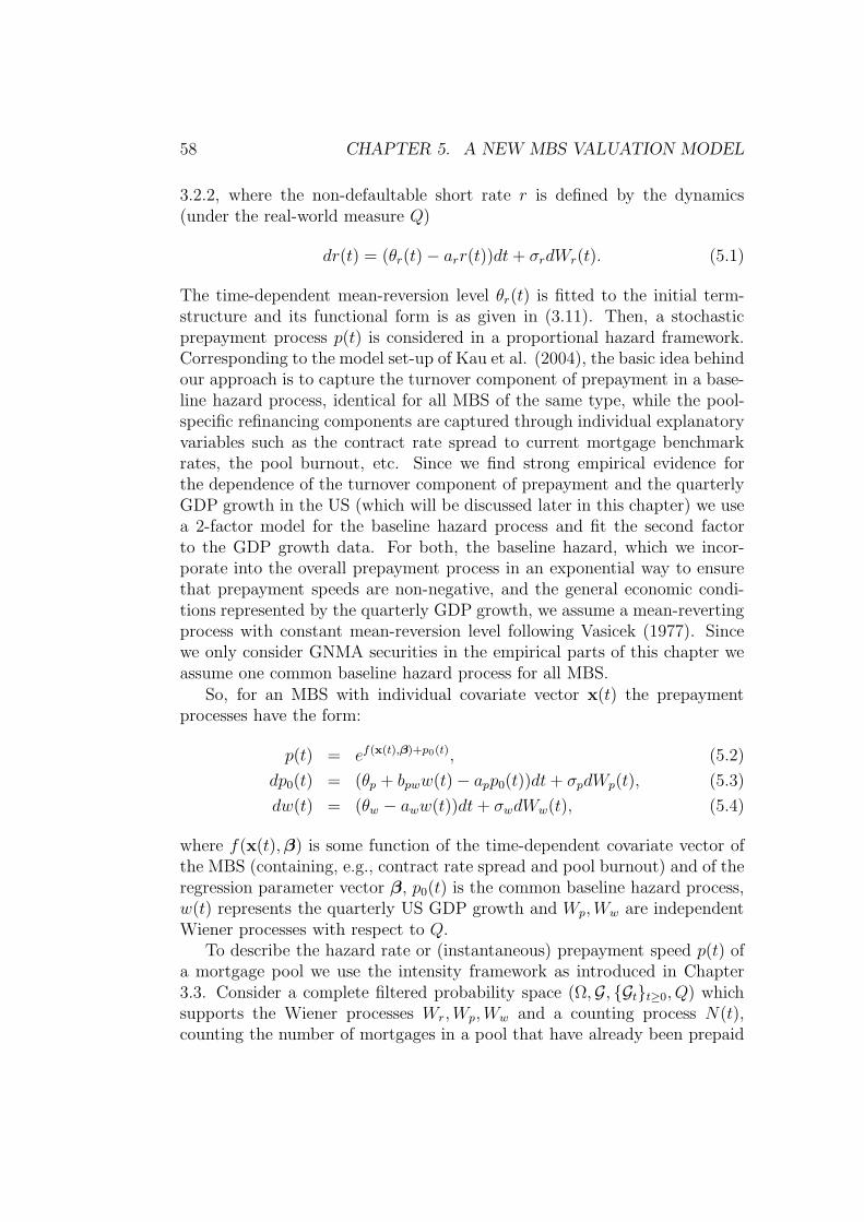
58 CHAPTER 5. A NEW MBS VALUATION MODEL
3.2.2, where the non-defaultable short rate r is defined by the dynamics(under the real-world measure Q)
dr(t) = (θr(t) − arr(t))dt + σrdWr(t). (5.1)
The time-dependent mean-reversion level θr(t) is fitted to the initial term-structure and its functional form is as given in (3.11). Then, a stochasticprepayment process p(t) is considered in a proportional hazard framework.Corresponding to the model set-up of Kau et al. (2004), the basic idea behindour approach is to capture the turnover component of prepayment in a base-line hazard process, identical for all MBS of the same type, while the pool-specific refinancing components are captured through individual explanatoryvariables such as the contract rate spread to current mortgage benchmarkrates, the pool burnout, etc. Since we find strong empirical evidence forthe dependence of the turnover component of prepayment and the quarterlyGDP growth in the US (which will be discussed later in this chapter) we usea 2-factor model for the baseline hazard process and fit the second factorto the GDP growth data. For both, the baseline hazard, which we incor-porate into the overall prepayment process in an exponential way to ensurethat prepayment speeds are non-negative, and the general economic condi-tions represented by the quarterly GDP growth, we assume a mean-revertingprocess with constant mean-reversion level following Vasicek (1977). Sincewe only consider GNMA securities in the empirical parts of this chapter weassume one common baseline hazard process for all MBS.
So, for an MBS with individual covariate vector x(t) the prepaymentprocesses have the form:
p(t) = ef(x(t),β)+p0(t), (5.2)
dp0(t) = (θp + bpww(t) − app0(t))dt + σpdWp(t), (5.3)
dw(t) = (θw − aww(t))dt + σwdWw(t), (5.4)
where f(x(t), β) is some function of the time-dependent covariate vector ofthe MBS (containing, e.g., contract rate spread and pool burnout) and of theregression parameter vector β, p0(t) is the common baseline hazard process,w(t) represents the quarterly US GDP growth and Wp, Ww are independentWiener processes with respect to Q.
To describe the hazard rate or (instantaneous) prepayment speed p(t) ofa mortgage pool we use the intensity framework as introduced in Chapter3.3. Consider a complete filtered probability space (Ω,G, Gtt≥0, Q) whichsupports the Wiener processes Wr, Wp, Ww and a counting process N(t),counting the number of mortgages in a pool that have already been prepaid
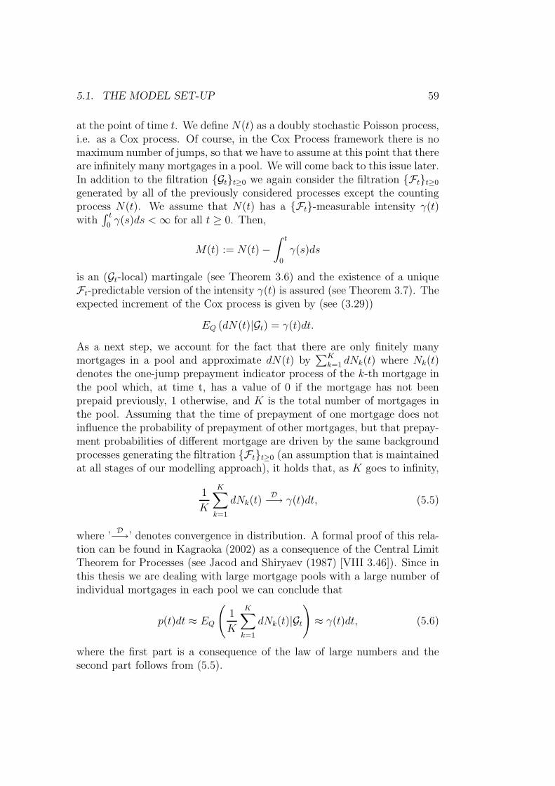
5.1. THE MODEL SET-UP 59
at the point of time t. We define N(t) as a doubly stochastic Poisson process,i.e. as a Cox process. Of course, in the Cox Process framework there is nomaximum number of jumps, so that we have to assume at this point that thereare infinitely many mortgages in a pool. We will come back to this issue later.In addition to the filtration Gtt≥0 we again consider the filtration Ftt≥0
generated by all of the previously considered processes except the countingprocess N(t). We assume that N(t) has a Ft-measurable intensity γ(t)with
∫ t
0γ(s)ds < ∞ for all t ≥ 0. Then,
M(t) := N(t) −∫ t
0
γ(s)ds
is an (Gt-local) martingale (see Theorem 3.6) and the existence of a uniqueFt-predictable version of the intensity γ(t) is assured (see Theorem 3.7). Theexpected increment of the Cox process is given by (see (3.29))
EQ (dN(t)|Gt) = γ(t)dt.
As a next step, we account for the fact that there are only finitely manymortgages in a pool and approximate dN(t) by
∑Kk=1 dNk(t) where Nk(t)
denotes the one-jump prepayment indicator process of the k-th mortgage inthe pool which, at time t, has a value of 0 if the mortgage has not beenprepaid previously, 1 otherwise, and K is the total number of mortgages inthe pool. Assuming that the time of prepayment of one mortgage does notinfluence the probability of prepayment of other mortgages, but that prepay-ment probabilities of different mortgage are driven by the same backgroundprocesses generating the filtration Ftt≥0 (an assumption that is maintainedat all stages of our modelling approach), it holds that, as K goes to infinity,
1
K
K∑
k=1
dNk(t)D−→ γ(t)dt, (5.5)
where ’D−→’ denotes convergence in distribution. A formal proof of this rela-
tion can be found in Kagraoka (2002) as a consequence of the Central LimitTheorem for Processes (see Jacod and Shiryaev (1987) [VIII 3.46]). Since inthis thesis we are dealing with large mortgage pools with a large number ofindividual mortgages in each pool we can conclude that
p(t)dt ≈ EQ
(1
K
K∑
k=1
dNk(t)|Gt
)≈ γ(t)dt, (5.6)
where the first part is a consequence of the law of large numbers and thesecond part follows from (5.5).
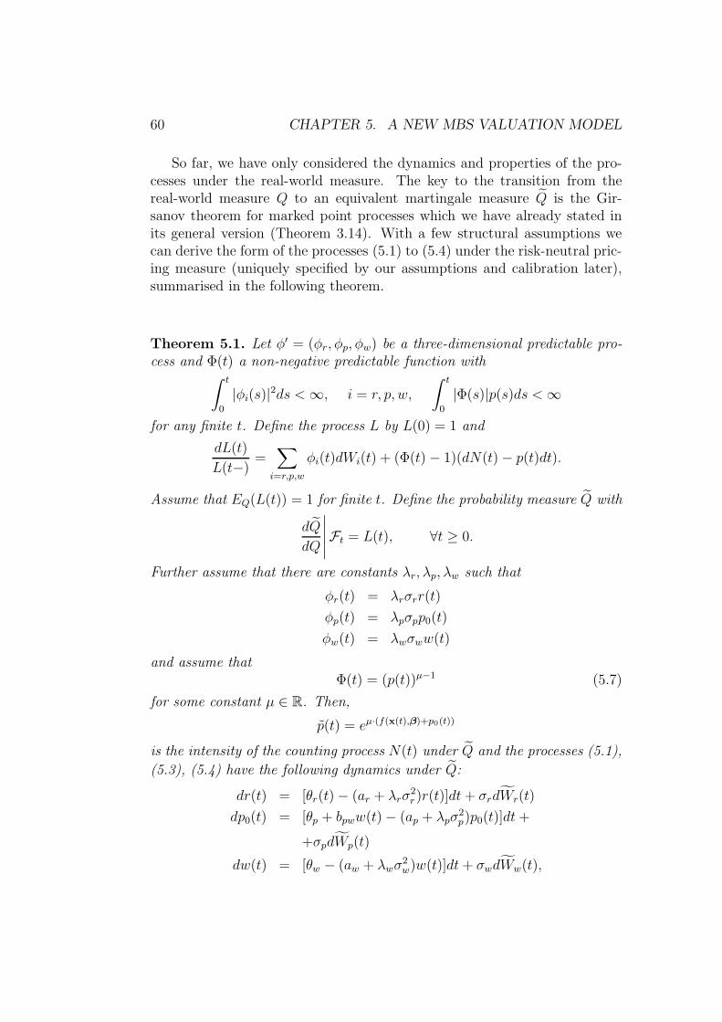
60 CHAPTER 5. A NEW MBS VALUATION MODEL
So far, we have only considered the dynamics and properties of the pro-cesses under the real-world measure. The key to the transition from thereal-world measure Q to an equivalent martingale measure Q is the Gir-sanov theorem for marked point processes which we have already stated inits general version (Theorem 3.14). With a few structural assumptions wecan derive the form of the processes (5.1) to (5.4) under the risk-neutral pric-ing measure (uniquely specified by our assumptions and calibration later),summarised in the following theorem.
Theorem 5.1. Let φ′ = (φr, φp, φw) be a three-dimensional predictable pro-cess and Φ(t) a non-negative predictable function with
∫ t
0
|φi(s)|2ds < ∞, i = r, p, w,
∫ t
0
|Φ(s)|p(s)ds < ∞
for any finite t. Define the process L by L(0) = 1 and
dL(t)
L(t−)=∑
i=r,p,w
φi(t)dWi(t) + (Φ(t) − 1)(dN(t) − p(t)dt).
Assume that EQ(L(t)) = 1 for finite t. Define the probability measure Q with
dQ
dQ
∣∣∣∣∣Ft = L(t), ∀t ≥ 0.
Further assume that there are constants λr, λp, λw such that
φr(t) = λrσrr(t)
φp(t) = λpσpp0(t)
φw(t) = λwσww(t)
and assume thatΦ(t) = (p(t))µ−1 (5.7)
for some constant µ ∈ R. Then,
p(t) = eµ·(f(x(t),β)+p0(t))
is the intensity of the counting process N(t) under Q and the processes (5.1),
(5.3), (5.4) have the following dynamics under Q:
dr(t) = [θr(t) − (ar + λrσ2r)r(t)]dt + σrdWr(t)
dp0(t) = [θp + bpww(t) − (ap + λpσ2p)p0(t)]dt +
+σpdWp(t)
dw(t) = [θw − (aw + λwσ2w)w(t)]dt + σwdWw(t),
5.1. THE MODEL SET-UP 61
where Wr, Wp, Ww are independent Q-Wiener processes.
Proof. The proposition follows from the Girsanov theorem as stated in The-orem 3.14. Recall that our marked point process N(t) is a Cox process withintensity p(t). Thus, the marker space E contains only the element 1 and,denoting the marker variable by Y , the compensator measure ν(de, dt) hasthe form:
ν(de, dt) = δY =1(de)p(t)dt.
The Girsanov theorem now yields that (see (3.31) and (3.32))
p(t) = Φ(t)p(t)
and by the structural assumption (5.7) we get
p(t) = eµ·(f(x(t),β)+p0(t)).
Furthermore, the Girsanov theorem ensures that, with dWi(t) := dWi(t) +
φi(t)dt, Wi is a Wiener-process under Q for i = r, p, w and we finally get the
dynamics of the processes r(t), p0(t), w(t) under the (martingale) measure Qby standard argumentation (see, e.g., Zagst (2002a) [4.4-4.5] for details).
Note at this point that the structural assumption (5.7) is a little uncon-ventional. In most other applications the assumption that Φ(t) = µ∗ forsome constant µ∗ is the norm. In our case, however, it is more convenient toassume a structure as in (5.7), since this leads to the (multiplicative) risk-adjustment parameter µ in the overall prepayment process which is clearlyidentifiable against the risk-adjustment parameters λp and λw in the base-line prepayment process p0(t). The convenience of the previously describedstructural assumption will become clear in the subsequent section where wediscuss the interaction of the risk-adjustment parameters in their economiccontext.
The value V (0) of the MBS at time t = 0 can finally be calculated asthe expectation of the security’s discounted future cash flows under the risk-neutral pricing measure Q. We denote by A(tk) the regular principal amountoutstanding on payment date tk according to the original amortisation sched-ule without any prepayments. Moreover, if we denote by M(tk) · ∆tk theoriginal monthly mortgage payment (i.e. the sum of interest and scheduledprincipal repayment) and by K the number of payment dates until final ma-turity of the MBS, we get the following cash flows at each payment datetk:
62 CHAPTER 5. A NEW MBS VALUATION MODEL
• The monthly mortgage payment M(tk) · ∆tk ·∏k−1
j=1(1 − pSMM(tj))
• The prepaid principal A(tk) · pSMM(tk) ·∏k−1
j=1(1 − pSMM(tj)).
Here pSMM(tk) denotes the prepayment speed expressed as single monthlymortality. The continuously compounded annual prepayment speed p(t) canbe converted to a (discrete) constant prepayment rate by
CPR(tk) = ep(t) − 1,
from which the single monthly mortality is obtained by the relation (2.1).We can conclude:
Theorem 5.2. The value V (0) of a fixed-rate MBS at time t = 0 is givenby:
V (0) = E eQ
[ K∑
k=1
ctk ·(
k−1∏
j=1
(1 − pSMM(tj))
)
· (pSMM(tk) · A(tk) + M(tk) · ∆t)
], (5.8)
where ctk = e−R tk0 r(s)ds.
Due to the path dependence introduced through the explanatory variables wehave no alternative to a computationally costly Monte-Carlo simulation toevaluate (5.8) at this point. Note that (5.8) is a version of (3.35) with discre-tised prepayment rates. In (5.8) the prepayment rates pSMM(tk) are expressedas single monthly mortalities, which is convenient for the Monte-Carlo eval-uation. If prepayment speeds were expressed as continuous annualised rates,the overall ’survival probability’ up to time tk−1 inside the expectation would
be given by e−R tk−10 p(s)ds instead of
∏k−1j=1(1− pSMM(tj)) and (5.8) would take
a form similar to (3.35). The Monte-Carlo algorithm used to evaluate (5.8)is given in the appendix.
5.2 Application to market data
5.2.1 Parameter estimation and model calibration
Interest rate and real-world prepayment model
The available data for this study consists of US treasury strip par ratesand monthly historical prepayment data for large issues of 30yr fixed-rate
5.2. APPLICATION TO MARKET DATA 63
mortgage-backed securities of the GNMA I and GNMA II programs. Weuse the historical pool data of a total of eight individual mortgage pools forthe empirical prepayment model (see Table 5.2 for the pool numbers). Thecorresponding MBS were issued between 1993 and 1996 with more than USD50m of residential mortgage loans in each of the eight pools and have couponsbetween 6% and 9%, so that both discounts and premiums are included inour sample. Discount MBS are securities with a low coupon which are tradedbelow 100% while premiums feature high coupons and market prices above100%. After the months of very high prepayment speeds in 2002-2004 (com-pare Figure 2.1) the mortgage pools considered for parameter estimationin this study were not large enough any more to maintain the assumptionsbased on large sample properties. We therefore discard the prepayment dataof these pools in 2005 for parameter estimation in the prepayment model.Weekly US treasury strip zero rates, obtained from the par rates by stan-dard bootstrapping, from 1993 to 2005 are used for the estimation of theparameters of the interest-rate process. Since the focus of our model is noton explanatory variables for prepayment, we restrict the set of covariates tothose that are usually stated as the most important ones: the spread betweenthe weighted-average coupon (WAC) of the mortgage pool and the 10yr trea-sury par yield which is commonly used as proxy for mortgage rates (see, e.g.,Goncharov (2005) for some discussion concerning this choice of proxy) andthe burnout which we define in line with the definition given in Schwartz andTorous (1989):
burnout(t) = ln
(PF (t)
A(t)
),
where PF (t) is the actual principal amount outstanding at time t and A(t)is the remaining principal amount according to the amortisation schedulewithout any prepayments, as previously defined. In order to account for theusual S-curve shape of the influence of the refinancing incentive (see, e.g.,Levin and Daras (1998) or Figure 5.1), expressed by the spread covariate,we choose the arc-tangent as functional form. The arc-tangent function wasalso used by Asay et al. (1987). Furthermore, our empirical results could beimproved by incorporating the burnout covariate as cubic term in additionto the linear term. Finally, our covariate function f has the form
f(x(t), β) = β1 · arctan(β2 · (spread(t) + β3)) +
+β4 · burnout(t) + β5 · burnout(t)3. (5.9)
Parameter estimation for the short-rate process.We estimate the parameters ar, σr, λr of the interest rate model with a
64 CHAPTER 5. A NEW MBS VALUATION MODEL
Kalman filter for state space models as introduced in Chapter 3.4 with mea-surement and transition equations as given in the following.
Recall that the price of a zero-coupon bond with maturity T at the pointof time t, denoted by P (t, T ), in the Hull-White type short-rate model (5.1)is given by (see Chapter 3.2.2 ):
P (t, T ) = eA(t,T )−B(t,T )r(t),
A(t, T ) =
∫ T
t
(1
2σ2
rB(l, T )2 − θr(l)B(l, T ))dl,
B(t, T ) =1
ar(1 − e−ar(T−t)),
where ar = ar + λr · σ2r . At the point of time tk we observe for maturities
τi, i = 1, ..., n, the treasury strip rates R(tk, tk + τi) = − lnP (tk ,tk+τi)(T−t)
. With
a(t, T ) = −A(t,T )T−t
, b(t, T ) = B(t,T )T−t
the measurement equation of the statespace model is then given by:
R(tk, tk + τ1)...
R(tk, tk + τn)
=
a(tk, tk + τ1)...
a(tk, tk + τn)
+
b(0, τ1)...
b(0, τn)
· r(tk) + ǫk, (5.10)
where we assume that the measurement error follows an n-dimensional Nor-mal distribution with expectation vector 0 and covariance matrix h2
r · In, i.e.ǫk ∼ Nn(0, h2
r ·In). The transition equation can be derived by the Hull-Whiteshort-rate dynamics which yield (see (3.16)):
rk+1 = e−ar ·∆tk+1rk +
∫ tk+1
tk
e−ar(tk+1−l)θr(l)dl +
∫ tk+1
tk
e−ar(tk+1−l)σrdW (l),
if we define rk := r(tk) and ∆tk+1 := tk+1 − tk. By approximating θr(l) byθr(tk) in the integral and defining
ηk+1 :=
∫ tk+1
tk
e−ar(tk+1−l)σrdW (l)
we finally get the transition equation of the state space model:
rk+1 = e−ar ·∆tk+1rk +
∫ ∆tk+1
0
e−ar ·lθr(tk)dl + ηk+1 (5.11)
with
ηk+1 ∼ N1
(0,
σ2r
2ar(1 − e−2ar∆tk+1)
).
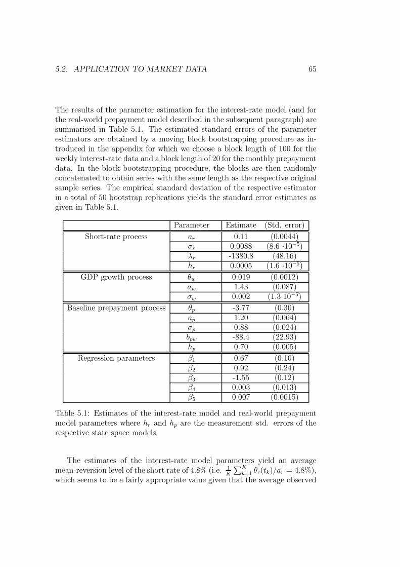
5.2. APPLICATION TO MARKET DATA 65
The results of the parameter estimation for the interest-rate model (and forthe real-world prepayment model described in the subsequent paragraph) aresummarised in Table 5.1. The estimated standard errors of the parameterestimators are obtained by a moving block bootstrapping procedure as in-troduced in the appendix for which we choose a block length of 100 for theweekly interest-rate data and a block length of 20 for the monthly prepaymentdata. In the block bootstrapping procedure, the blocks are then randomlyconcatenated to obtain series with the same length as the respective originalsample series. The empirical standard deviation of the respective estimatorin a total of 50 bootstrap replications yields the standard error estimates asgiven in Table 5.1.
Parameter Estimate (Std. error)
Short-rate process ar 0.11 (0.0044)σr 0.0088 (8.6 ·10−5)λr -1380.8 (48.16)hr 0.0005 (1.6 ·10−5)
GDP growth process θw 0.019 (0.0012)aw 1.43 (0.087)σw 0.002 (1.3·10−5)
Baseline prepayment process θp -3.77 (0.30)ap 1.20 (0.064)σp 0.88 (0.024)bpw -88.4 (22.93)hp 0.70 (0.005)
Regression parameters β1 0.67 (0.10)β2 0.92 (0.24)β3 -1.55 (0.12)β4 0.003 (0.013)β5 0.007 (0.0015)
Table 5.1: Estimates of the interest-rate model and real-world prepaymentmodel parameters where hr and hp are the measurement std. errors of therespective state space models.
The estimates of the interest-rate model parameters yield an averagemean-reversion level of the short rate of 4.8% (i.e. 1
K
∑Kk=1 θr(tk)/ar = 4.8%),
which seems to be a fairly appropriate value given that the average observed
66 CHAPTER 5. A NEW MBS VALUATION MODEL
3-month rate was 5.1% during the time horizon used for parameter estima-tion. For the estimation of the prepayment parameters we use a two-stageprocedure. We first estimate the parameters θw, aw, σw of the GDP growthprocess by Maximum-Likelihood and the parameters θp, ap, σp, bpw again bya Kalman filter for state space models with the historical prepayment speedsas observables.
Parameter estimation for the GDP growth process.The dynamics of the GDP growth process in (5.4) are again given by a SDEof the form (3.15). Thus, we get
w(tk+1) = e−aw∆tk+1w(tk) +
∫ tk+1
tk
e−aw(tk+1−l)θwdl +
+
∫ tk+1
tk
e−aw(tk+1−l)σwdWw(l)
and it follows that
w(tk+1)|w(tk) ∼ N1(c, d2),
c = e−aw∆tk+1w(tk) +θw
aw
(1 − e−aw∆tk+1),
d2 =σ2
w
2aw
(1 − e−2aw∆tk+1).
We obtain Maximum-Likelihood estimates of the parameters θw, aw, σw bymaximising the likelihood function
L(θw, aw, σw) =
K∏
k=1
ϕw(tk)|w(tk+1),
where ϕw(tk)|w(tk+1) denotes the p.d.f. of the Normal distribution with param-eters c and d2 as defined above.
Parameter estimation for the prepayment process.The measurement equation of the state space model is given by (5.2) withthe historically observed prepayment speeds (as SMM) and f as specified in(5.9):
ln(pSMM,1(tk))...
ln(pSMM,N(tk))
=
f(x1(tk), β)...
f(xN(tk), β)
+
1...1
· p0(tk) + ǫk, (5.12)
5.2. APPLICATION TO MARKET DATA 67
where we assume that ǫk ∼ NN
(0, h2
p · IN
). The transition equation for the
(unobservable) baseline prepayment hazard is given by (5.3). For stabilityreasons, we use w(t) as an external input to the model and define X(t) =p0(t), H = −ap, J(t) = θp +bpww(t), V = σp to get a SDE of the form (3.15).Similar to the derivation of the transition equation (5.11) of the interest-ratemodel the transition equation of the prepayment state space model is
p0(tk+1) = e−ap∆tk+1 · p0(tk) +θp + bpww(tk)
ap· (1 − e−ap∆tk+1) + ηk+1
with
ηk+1 ∼ N1
(0,
σ2p
2ap(1 − e−2ap∆tk+1)
).
The values for the estimates of the GDP growth process (see again Table 5.1)yield a mean-reversion level of θw/aw = 1.3% which is identical to the actuallyobserved average. For all optimisation steps we use a combined Downhill-Simplex/Simulated Annealing algorithm as described in Press et al. (1992).
Before we discuss the statistical properties of our estimates in the real-world prepayment state space model and proceed to the calibration and in-terpretation of the prepayment-risk-adjustment parameters λp, λw, µ in thefollowing subsection, we want to give some empirical justification for the in-corporation of the GDP growth rate as a second factor of the prepaymentmodel. While it is often recognised that the baseline component of prepay-ment is correlated to general economic conditions, nobody (to the author’sbest knowledge) has made the effort of explicitly modelling such a depen-dence structure by considering prepayment jointly with a factor such as thequarterly GDP growth. In order to investigate the value of such an economicfactor, we consider the differences di(t) between the actual, historically ob-served prepayment speeds pi(t) of the i-th MBS in the sample and thosepredicted by the covariates, i.e. not taking into account the baseline hazardin (5.2):
di(t) = ln pSMM,i(t) − f(xi(t), β), i = 1, ..., M. (5.13)
We consider the average difference d(t) := 1M
∑Mi=1 di(t) of the M different
MBS pools used for prepayment parameter estimation as an estimate forthe baseline hazard prepayment process p0(t) and investigate the correlationbetween the estimated baseline hazard prepayment and the quarterly GDPgrowth process (monthly data for the GDP growth process was obtainedby cubic spline interpolation). With the MatLab-function corr, the Pear-son correlation coefficient for a 6-month lag between GDP growth rates and
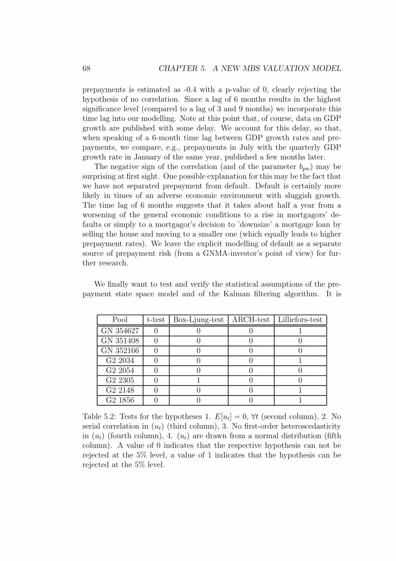
68 CHAPTER 5. A NEW MBS VALUATION MODEL
prepayments is estimated as -0.4 with a p-value of 0, clearly rejecting thehypothesis of no correlation. Since a lag of 6 months results in the highestsignificance level (compared to a lag of 3 and 9 months) we incorporate thistime lag into our modelling. Note at this point that, of course, data on GDPgrowth are published with some delay. We account for this delay, so that,when speaking of a 6-month time lag between GDP growth rates and pre-payments, we compare, e.g., prepayments in July with the quarterly GDPgrowth rate in January of the same year, published a few months later.
The negative sign of the correlation (and of the parameter bpw) may besurprising at first sight. One possible explanation for this may be the fact thatwe have not separated prepayment from default. Default is certainly morelikely in times of an adverse economic environment with sluggish growth.The time lag of 6 months suggests that it takes about half a year from aworsening of the general economic conditions to a rise in mortgagors’ de-faults or simply to a mortgagor’s decision to ’downsize’ a mortgage loan byselling the house and moving to a smaller one (which equally leads to higherprepayment rates). We leave the explicit modelling of default as a separatesource of prepayment risk (from a GNMA-investor’s point of view) for fur-ther research.
We finally want to test and verify the statistical assumptions of the pre-payment state space model and of the Kalman filtering algorithm. It is
Pool t-test Box-Ljung-test ARCH-test Lilliefors-test
GN 354627 0 0 0 1GN 351408 0 0 0 0GN 352166 0 0 0 0G2 2034 0 0 0 1G2 2054 0 0 0 0G2 2305 0 1 0 0G2 2148 0 0 0 1G2 1856 0 0 0 1
Table 5.2: Tests for the hypotheses 1. E[ut] = 0, ∀t (second column), 2. Noserial correlation in (ut) (third column), 3. No first-order heteroscedasticityin (ut) (fourth column), 4. (ut) are drawn from a normal distribution (fifthcolumn). A value of 0 indicates that the respective hypothesis can not berejected at the 5% level, a value of 1 indicates that the hypothesis can berejected at the 5% level.
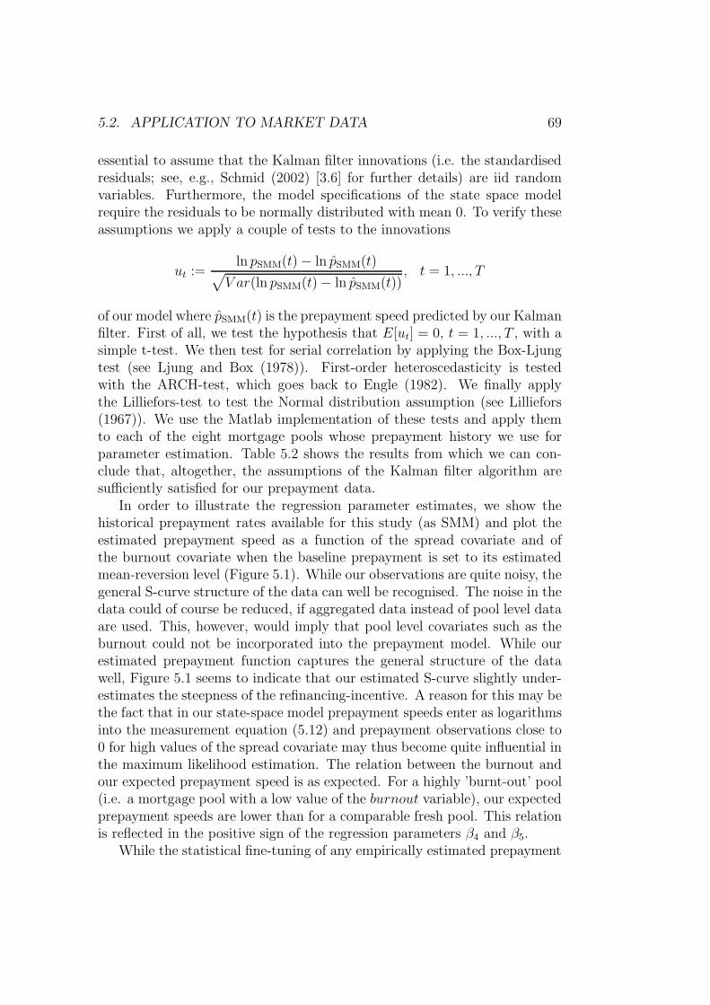
5.2. APPLICATION TO MARKET DATA 69
essential to assume that the Kalman filter innovations (i.e. the standardisedresiduals; see, e.g., Schmid (2002) [3.6] for further details) are iid randomvariables. Furthermore, the model specifications of the state space modelrequire the residuals to be normally distributed with mean 0. To verify theseassumptions we apply a couple of tests to the innovations
ut :=ln pSMM(t) − ln pSMM(t)√
V ar(ln pSMM(t) − ln pSMM(t)), t = 1, ..., T
of our model where pSMM(t) is the prepayment speed predicted by our Kalmanfilter. First of all, we test the hypothesis that E[ut] = 0, t = 1, ..., T , with asimple t-test. We then test for serial correlation by applying the Box-Ljungtest (see Ljung and Box (1978)). First-order heteroscedasticity is testedwith the ARCH-test, which goes back to Engle (1982). We finally applythe Lilliefors-test to test the Normal distribution assumption (see Lilliefors(1967)). We use the Matlab implementation of these tests and apply themto each of the eight mortgage pools whose prepayment history we use forparameter estimation. Table 5.2 shows the results from which we can con-clude that, altogether, the assumptions of the Kalman filter algorithm aresufficiently satisfied for our prepayment data.
In order to illustrate the regression parameter estimates, we show thehistorical prepayment rates available for this study (as SMM) and plot theestimated prepayment speed as a function of the spread covariate and ofthe burnout covariate when the baseline prepayment is set to its estimatedmean-reversion level (Figure 5.1). While our observations are quite noisy, thegeneral S-curve structure of the data can well be recognised. The noise in thedata could of course be reduced, if aggregated data instead of pool level dataare used. This, however, would imply that pool level covariates such as theburnout could not be incorporated into the prepayment model. While ourestimated prepayment function captures the general structure of the datawell, Figure 5.1 seems to indicate that our estimated S-curve slightly under-estimates the steepness of the refinancing-incentive. A reason for this may bethe fact that in our state-space model prepayment speeds enter as logarithmsinto the measurement equation (5.12) and prepayment observations close to0 for high values of the spread covariate may thus become quite influential inthe maximum likelihood estimation. The relation between the burnout andour expected prepayment speed is as expected. For a highly ’burnt-out’ pool(i.e. a mortgage pool with a low value of the burnout variable), our expectedprepayment speeds are lower than for a comparable fresh pool. This relationis reflected in the positive sign of the regression parameters β4 and β5.
While the statistical fine-tuning of any empirically estimated prepayment
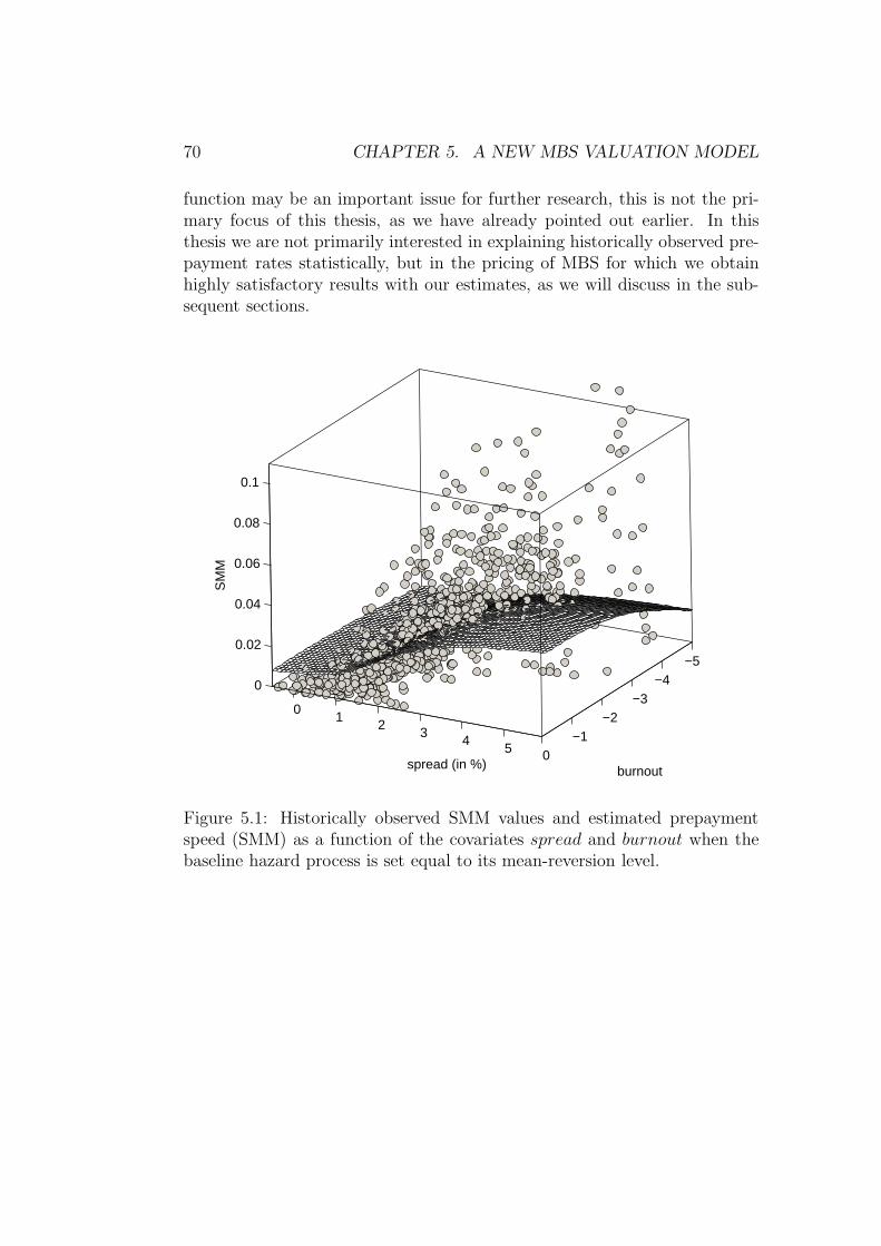
70 CHAPTER 5. A NEW MBS VALUATION MODEL
function may be an important issue for further research, this is not the pri-mary focus of this thesis, as we have already pointed out earlier. In thisthesis we are not primarily interested in explaining historically observed pre-payment rates statistically, but in the pricing of MBS for which we obtainhighly satisfactory results with our estimates, as we will discuss in the sub-sequent sections.
−5−4
−3−2
−10
01
23
45
0
0.02
0.04
0.06
0.08
0.1
burnoutspread (in %)
SM
M
Figure 5.1: Historically observed SMM values and estimated prepaymentspeed (SMM) as a function of the covariates spread and burnout when thebaseline hazard process is set equal to its mean-reversion level.
5.2. APPLICATION TO MARKET DATA 71
Prepayment-risk-neutral model
In general, there is no active and liquid market for an individual mort-gage pool. One obvious reason for this is the limited size of individualpools. For the calibration of the prepayment-risk-adjustment parameterswe therefore consider market prices of generic GNMA 30yr fixed-rate MBSas quoted in Bloomberg (Bloomberg ticker GNSF) for trading on a TBA(to-be-announced) basis. We consider coupons between 4.5% and 8%, sothat both discounts and premiums are included. GNMA securities which aretraded on a TBA basis are highly liquid securities, so that we do not have toworry about liquidity effects/premia. Even for those securities with a couponwell below or well above the current coupon, Bid-Ask spreads are usually nothigher than 2 ticks with a tick size of USD 1
32. When we speak of market
prices we refer to the Ask-prices.We estimate the prepayment-risk-adjustment parameters µ, λp, λw by min-
imising the Euclidean norm of the vector of differences between the marketprices and model prices of the securities on each sample day. All calculationsare carried out without accounting for any OAS, i.e. with an OAS equal to0 for all securities. By setting the OAS-target equal to 0, we price with thetreasury curve as benchmark curve, which seems to be the most appropriatecurve for GNMA securities since these securities feature the full faith andcredit of the US Government. Of course, any other curve could be used asbenchmark curve if desired. Once the parameters have been calibrated, onecan hardly expect all theoretical prices to match market prices exactly for allMBS securities. The OAS equivalent in a risk-neutral valuation framework(with a target of 0 in the calibration procedure) could be compared to the’prOAS’-measure recently introduced by Levin and Davidson (2005). We willalso use their ’prOAS’-term in the following and point out that the prOASshould not be regarded as any kind of risk premium, but simply as a measureof unsystematic residual pricing error.
Levin and Davidson (2005) emphasize the necessity of a two-risk factormodel in order to account for the two distinct market fears in the MBSmarket: refinancing understatement and turnover overstatement. These twodistinct market fears explain why, in the traditional OAS valuation approach,it is not uncommon to observe higher OAS levels for both discounts and pre-miums compared to MBS around the current-coupon level. On the one hand,an investor in discounts experiences losses if the turnover component is over-estimated and pure turnover-related prepayment is slower than expected. Inthis case the average life of the security is extended, decreasing the cash flowstream’s present value. On the other hand, the refinancing component isthe major concern of an investor in premiums since the average life of pre-
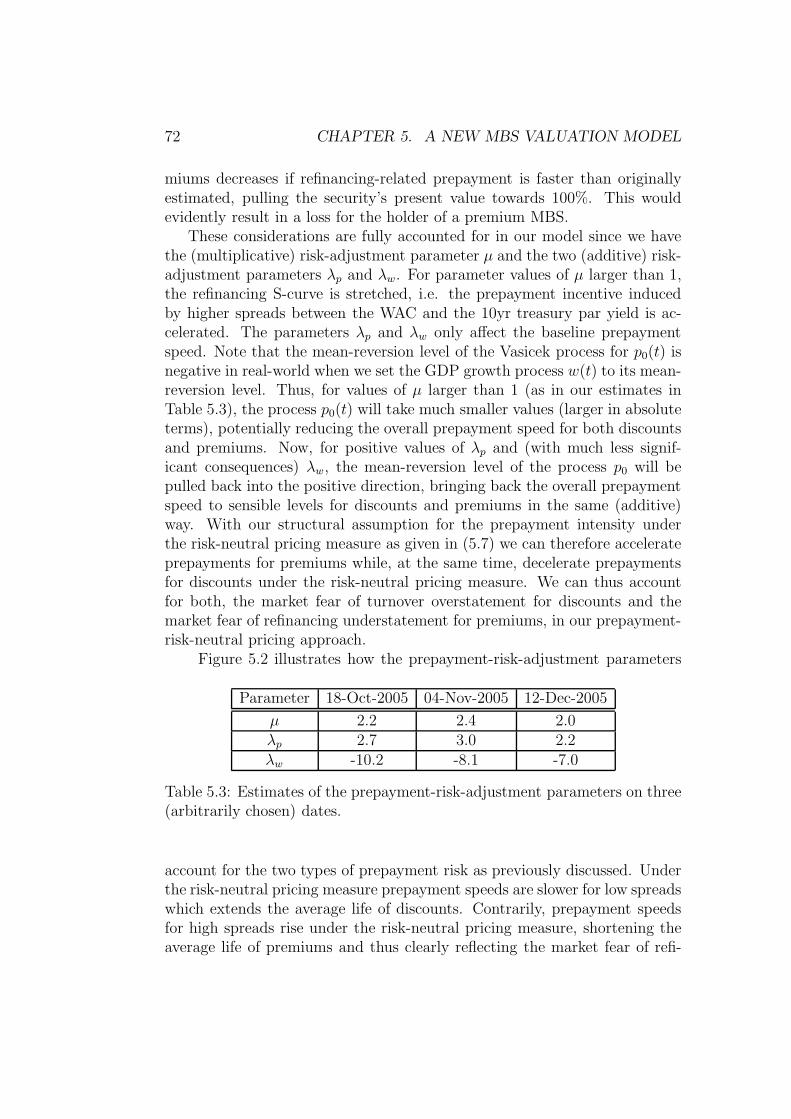
72 CHAPTER 5. A NEW MBS VALUATION MODEL
miums decreases if refinancing-related prepayment is faster than originallyestimated, pulling the security’s present value towards 100%. This wouldevidently result in a loss for the holder of a premium MBS.
These considerations are fully accounted for in our model since we havethe (multiplicative) risk-adjustment parameter µ and the two (additive) risk-adjustment parameters λp and λw. For parameter values of µ larger than 1,the refinancing S-curve is stretched, i.e. the prepayment incentive inducedby higher spreads between the WAC and the 10yr treasury par yield is ac-celerated. The parameters λp and λw only affect the baseline prepaymentspeed. Note that the mean-reversion level of the Vasicek process for p0(t) isnegative in real-world when we set the GDP growth process w(t) to its mean-reversion level. Thus, for values of µ larger than 1 (as in our estimates inTable 5.3), the process p0(t) will take much smaller values (larger in absoluteterms), potentially reducing the overall prepayment speed for both discountsand premiums. Now, for positive values of λp and (with much less signif-icant consequences) λw, the mean-reversion level of the process p0 will bepulled back into the positive direction, bringing back the overall prepaymentspeed to sensible levels for discounts and premiums in the same (additive)way. With our structural assumption for the prepayment intensity underthe risk-neutral pricing measure as given in (5.7) we can therefore accelerateprepayments for premiums while, at the same time, decelerate prepaymentsfor discounts under the risk-neutral pricing measure. We can thus accountfor both, the market fear of turnover overstatement for discounts and themarket fear of refinancing understatement for premiums, in our prepayment-risk-neutral pricing approach.
Figure 5.2 illustrates how the prepayment-risk-adjustment parameters
Parameter 18-Oct-2005 04-Nov-2005 12-Dec-2005
µ 2.2 2.4 2.0λp 2.7 3.0 2.2λw -10.2 -8.1 -7.0
Table 5.3: Estimates of the prepayment-risk-adjustment parameters on three(arbitrarily chosen) dates.
account for the two types of prepayment risk as previously discussed. Underthe risk-neutral pricing measure prepayment speeds are slower for low spreadswhich extends the average life of discounts. Contrarily, prepayment speedsfor high spreads rise under the risk-neutral pricing measure, shortening theaverage life of premiums and thus clearly reflecting the market fear of refi-
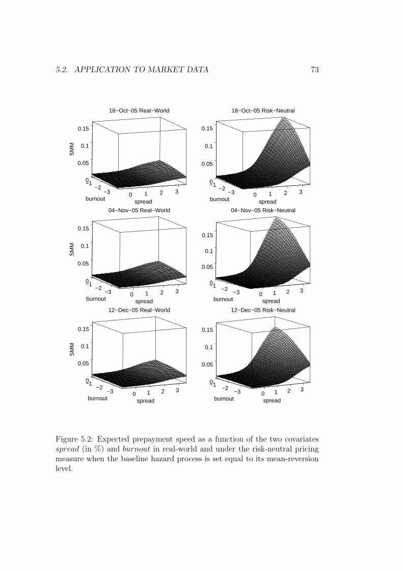
5.2. APPLICATION TO MARKET DATA 73
0 1 2 3−3−2
−10
0.05
0.1
0.15
spread
04−Nov−05 Real−World
burnout
SM
M
0 1 2 3−3−2−10
0.05
0.1
0.15
spread
04−Nov−05 Risk−Neutral
burnout
0 1 2 3−3−2
−10
0.05
0.1
0.15
spread
18−Oct−05 Real−World
burnout
SM
M
0 1 2 3−3−2
−10
0.05
0.1
0.15
spread
18−Oct−05 Risk−Neutral
burnout
0 1 2 3−3−2
−10
0.05
0.1
0.15
spread
12−Dec−05 Real−World
burnout
SM
M
0 1 2 3−3−2
−10
0.05
0.1
0.15
spread
12−Dec−05 Risk−Neutral
burnout
Figure 5.2: Expected prepayment speed as a function of the two covariatesspread (in %) and burnout in real-world and under the risk-neutral pricingmeasure when the baseline hazard process is set equal to its mean-reversionlevel.
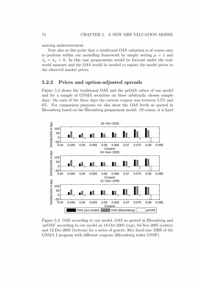
74 CHAPTER 5. A NEW MBS VALUATION MODEL
nancing understatement.Note also at this point that a traditional OAS valuation is of course easy
to perform within our modelling framework by simply setting µ = 1 andλp = λw = 0. In this case prepayments would be forecast under the real-world measure and the OAS would be needed to equate the model prices tothe observed market prices.
5.2.2 Prices and option-adjusted spreads
Figure 5.3 shows the traditional OAS and the prOAS values of our modeland for a sample of GNMA securities on three arbitrarily chosen sampledays. On each of the three days the current coupon was between 5.5% and6%. For comparison purposes we also show the OAS levels as quoted inBloomberg based on the Bloomberg prepayment model. Of course, it is hard
0.04 0.045 0.05 0.055 0.06 0.065 0.07 0.075 0.08 0.085−50
0
50
100
Coupon
OA
S/p
rOA
S in
bps 18−Oct−2005
0.04 0.045 0.05 0.055 0.06 0.065 0.07 0.075 0.08 0.085−50
0
50
100
Coupon
OA
S/p
rOA
S in
bps 12−Dec−2005
0.04 0.045 0.05 0.055 0.06 0.065 0.07 0.075 0.08 0.085−50
0
50
100
Coupon
OA
S/p
rOA
S in
bps 04−Nov−2005
OAS (our model) OAS (Bloomberg) prOAS
Figure 5.3: OAS according to our model, OAS as quoted in Bloomberg and’prOAS’ according to our model on 18-Oct-2005 (top), 04-Nov-2005 (centre)and 12-Dec-2005 (bottom) for a series of generic 30yr fixed-rate MBS of theGNMA I program with different coupons (Bloomberg ticker GNSF).
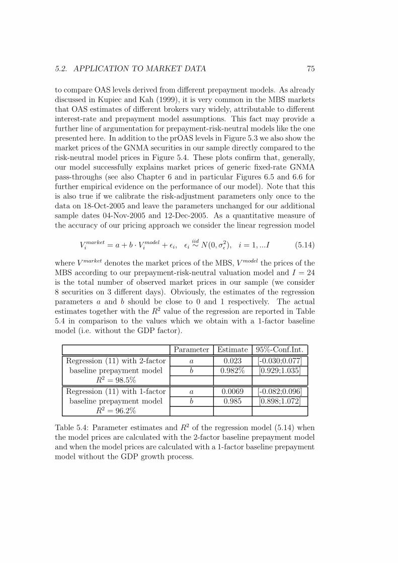
5.2. APPLICATION TO MARKET DATA 75
to compare OAS levels derived from different prepayment models. As alreadydiscussed in Kupiec and Kah (1999), it is very common in the MBS marketsthat OAS estimates of different brokers vary widely, attributable to differentinterest-rate and prepayment model assumptions. This fact may provide afurther line of argumentation for prepayment-risk-neutral models like the onepresented here. In addition to the prOAS levels in Figure 5.3 we also show themarket prices of the GNMA securities in our sample directly compared to therisk-neutral model prices in Figure 5.4. These plots confirm that, generally,our model successfully explains market prices of generic fixed-rate GNMApass-throughs (see also Chapter 6 and in particular Figures 6.5 and 6.6 forfurther empirical evidence on the performance of our model). Note that thisis also true if we calibrate the risk-adjustment parameters only once to thedata on 18-Oct-2005 and leave the parameters unchanged for our additionalsample dates 04-Nov-2005 and 12-Dec-2005. As a quantitative measure ofthe accuracy of our pricing approach we consider the linear regression model
V marketi = a + b · V model
i + ǫi, ǫiiid∼ N(0, σ2
ǫ ), i = 1, ...I (5.14)
where V market denotes the market prices of the MBS, V model the prices of theMBS according to our prepayment-risk-neutral valuation model and I = 24is the total number of observed market prices in our sample (we consider8 securities on 3 different days). Obviously, the estimates of the regressionparameters a and b should be close to 0 and 1 respectively. The actualestimates together with the R2 value of the regression are reported in Table5.4 in comparison to the values which we obtain with a 1-factor baselinemodel (i.e. without the GDP factor).
Parameter Estimate 95%-Conf.Int.
Regression (11) with 2-factor a 0.023 [-0.030;0.077]baseline prepayment model b 0.982% [0.929;1.035]
R2 = 98.5%
Regression (11) with 1-factor a 0.0069 [-0.082;0.096]baseline prepayment model b 0.985 [0.898;1.072]
R2 = 96.2%
Table 5.4: Parameter estimates and R2 of the regression model (5.14) whenthe model prices are calculated with the 2-factor baseline prepayment modeland when the model prices are calculated with a 1-factor baseline prepaymentmodel without the GDP growth process.
76 CHAPTER 5. A NEW MBS VALUATION MODEL
Since in the 2-factor baseline prepayment model the confidence intervals fora and b are narrower around 0 and 1 respectively and the R2 value is higher,these results indicate that the GDP growth factor adds explanatory powerto our prepayment-risk-neutral pricing model. The (in-sample) average ab-solute pricing error of our model, i.e. the mean of the absolute differencesbetween the model prices and the market prices, is 59 basis points in our sam-ple compared to 105 basis points for the 1-factor baseline prepayment model.When we consider out-of-sample prices, i.e. we use the risk-adjustment pa-rameters calibrated to the data of 18-Oct-2005 for pricing on the two othersample days, we obtain an average absolute pricing error of 61 basis pointsfor our model while the average absolute pricing error of the 1-factor baselineprepayment model is 76 basis points. These results provide further evidencefor the usefulness of the GDP growth rate factor.
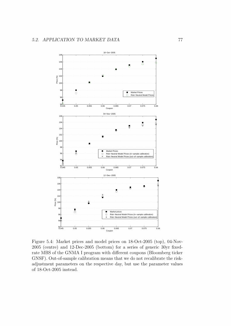
5.2. APPLICATION TO MARKET DATA 77
0.045 0.05 0.055 0.06 0.065 0.07 0.075 0.0894
96
98
100
102
104
106
108
Coupon
Pric
e (%
)
18−Oct−2005
Market PricesRisk−Neutral Model Prices
0.045 0.05 0.055 0.06 0.065 0.07 0.075 0.0892
94
96
98
100
102
104
106
108
Coupon
Pric
e (%
)
04−Nov−2005
Market PricesRisk−Neutral Model Prices (in−sample calibration)Risk−Neutral Model Prices (out−of−sample calibration)
0.045 0.05 0.055 0.06 0.065 0.07 0.075 0.0892
94
96
98
100
102
104
106
108
Coupon
Pric
e (%
)
12−Dec−2005
Market pricesRisk−Neutral Model Prices (in−sample calibration)Risk−Neutral Model Prices (out−of−sample calibration)
Figure 5.4: Market prices and model prices on 18-Oct-2005 (top), 04-Nov-2005 (centre) and 12-Dec-2005 (bottom) for a series of generic 30yr fixed-rate MBS of the GNMA I program with different coupons (Bloomberg tickerGNSF). Out-of-sample calibration means that we do not recalibrate the risk-adjustment parameters on the respective day, but use the parameter valuesof 18-Oct-2005 instead.
78 CHAPTER 5. A NEW MBS VALUATION MODEL
5.2.3 Effective duration, convexity and
parameter sensitivities
Effective duration and convexity are two important quantities to measurethe interest-rate risk exposure of a mortgage-backed security with respect toparallel shifts of the yield curve. Since these quantities are easy to determinethey are very popular in practice, particularly in the context of MBS portfoliomanagement. A regular bond’s duration is defined as the price sensitivityof the bond with respect to parallel shifts of the yield curve and can easilybe calculated as the weighted average of the times when payments are madewith the weights being equal to the proportion of the bond’s total presentvalue provided by the payment of the respective payment time (see, e.g., Hull(2003), p. 112f. for details). For a mortgage-backed security, however, thebasic duration concept can not be readily applied since a shift of the yieldcurve inevitably leads to changes in the prepayment behaviour and thereforechanges the cash flows of the security. The modified cash flows resultingfrom changes in interest rates are accounted for in the effective durationDeff which can be defined as follows (see, e.g. Hu (1997), p. 46):
Deff =V− − V+
2 · V · ∆y, (5.15)
where V is the security’s present value, V− is the security’s value after aparallel downward shift of the zero-rate curve of ∆y and V+ is the security’svalue after a parallel upward shift of the yield curve of the same size. Anal-ogously, the effective convexity Ceff , i.e. the second-order sensitivity of thevalue of a mortgage-backed security with respect to parallel shifts of the yieldcurve can be defined as (see again Hu (1997), p. 47):
Ceff =V− − 2 · V + V+
V · (∆y)2· 1%, (5.16)
where the scaling by 1% is done due to market convention. While the con-vexity of a regular bond is usually positive, most mortgage-backed securities(with the possible exception of very deep discounts and very high premiumsecurities) feature negative convexities. Negative convexity means that, withrespect to parallel shifts of the yield curve, an MBS has more downside riskin the case of rising interest rates than upside potential in the case of fallingrates. This can easily be explained by the prepayment feature inherent inMBS. If interest rates rise, prepayments tend to slow down, which extends thecash flow stream’s average life. Thus, the negative effect of the rising rates onthe present value of the security’s cash flow stream is intensified. Contrarily,
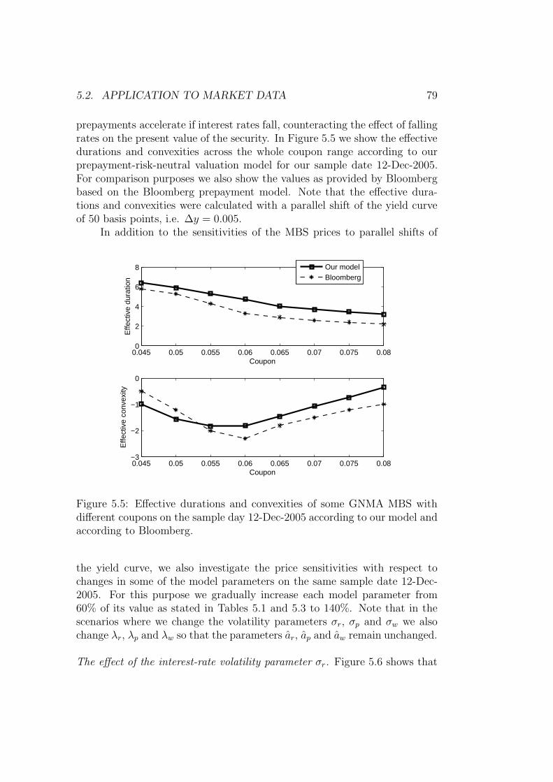
5.2. APPLICATION TO MARKET DATA 79
prepayments accelerate if interest rates fall, counteracting the effect of fallingrates on the present value of the security. In Figure 5.5 we show the effectivedurations and convexities across the whole coupon range according to ourprepayment-risk-neutral valuation model for our sample date 12-Dec-2005.For comparison purposes we also show the values as provided by Bloombergbased on the Bloomberg prepayment model. Note that the effective dura-tions and convexities were calculated with a parallel shift of the yield curveof 50 basis points, i.e. ∆y = 0.005.
In addition to the sensitivities of the MBS prices to parallel shifts of
0.045 0.05 0.055 0.06 0.065 0.07 0.075 0.080
2
4
6
8
Coupon
Effe
ctiv
e du
ratio
n
0.045 0.05 0.055 0.06 0.065 0.07 0.075 0.08−3
−2
−1
0
Coupon
Effe
ctiv
e co
nvex
ity
Our modelBloomberg
Figure 5.5: Effective durations and convexities of some GNMA MBS withdifferent coupons on the sample day 12-Dec-2005 according to our model andaccording to Bloomberg.
the yield curve, we also investigate the price sensitivities with respect tochanges in some of the model parameters on the same sample date 12-Dec-2005. For this purpose we gradually increase each model parameter from60% of its value as stated in Tables 5.1 and 5.3 to 140%. Note that in thescenarios where we change the volatility parameters σr, σp and σw we alsochange λr, λp and λw so that the parameters ar, ap and aw remain unchanged.
The effect of the interest-rate volatility parameter σr. Figure 5.6 shows that
80 CHAPTER 5. A NEW MBS VALUATION MODEL
MBS prices across the whole coupon range decrease if σr increases. Thiscan easily be explained by the prepayment option which an MBS investoris short. Consistent with basic option theory, the value of the mortgagors’prepayment option increases if the interest-rate volatility increases. Thus,MBS prices decrease.
The effect of the parameter ar. Figure 5.6 shows that changes of the meanreversion speed parameter ar within the analysed scope do not significantlyaffect MBS prices. Recall that the interest-rate model we use is a Hull-Whitemodel, where the function θr(t) ensures that for any parameter value of ar thecurrent term structure is perfectly fit. Thus, if ar changes, so does the func-tion θr(t), so that the model remains arbitrage-free as already discussed inChapter 3.2. Yet, if ar increases, the average speed with which the short-ratereverts to its mean reversion level increases. However, within the analysedscope, the effect of an increased mean-reversion speed of the short rate seemsnegligible.
The effect of the parameter µ. As already discussed in the previous para-graphs, the prepayment-risk adjustment parameter µ inversely scales theoverall prepayment intensity. Thus, the larger µ the lower the overall pre-payment intensity and the longer the average lives of the MBS. Hence, ingeneral, an increase in µ can be expected to increase the value of premiumsand, at the same time, decrease the value of discounts. Very large valuesof µ, however, imply that there is virtually no prepayment, i.e. that theprepayment option is never exercised and thus worthless. For large values ofµ, the MBS prices therefore equal the prices of a security without any pre-payment feature. These prices are, obviously, higher than the regular MBSprices across the whole coupon range. This explains the sensitivity patternas shown in Figure 5.6.
The effect of the parameter β1. Figure 5.6 shows that MBS prices acrossthe whole coupon range decrease if β1 increases. An increase of β1 meansthat the intensity of prepayment increases if rates rise. Thus, more peopleexercise their prepayment option when it is advantageous to do so, whichreduces the value of both discount and premium MBS.
The effect of the parameter β2. Figure 5.7 shows that MBS prices across thewhole coupon range decrease if β2 increases. The parameter β2 determinesthe shape of the refinancing S-curve, modelled via the arctangent-function inour model. If β2 increases, the S-curve is jolted. I.e., prepayment intensitiesreact more sensitively to changes in interest-rates and refinancing incentives,
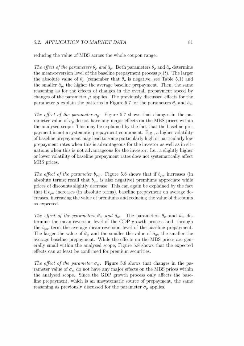
5.2. APPLICATION TO MARKET DATA 81
reducing the value of MBS across the whole coupon range.
The effect of the parameters θp and ap. Both parameters θp and ap determinethe mean-reversion level of the baseline prepayment process p0(t). The largerthe absolute value of θp (remember that θp is negative, see Table 5.1) andthe smaller ap, the higher the average baseline prepayment. Then, the samereasoning as for the effects of changes in the overall prepayment speed bychanges of the parameter µ applies. The previously discussed effects for theparameter µ explain the patterns in Figure 5.7 for the parameters θp and ap.
The effect of the parameter σp. Figure 5.7 shows that changes in the pa-rameter value of σp do not have any major effects on the MBS prices withinthe analysed scope. This may be explained by the fact that the baseline pre-payment is not a systematic prepayment component. E.g., a higher volatilityof baseline prepayment may lead to some particularly high or particularly lowprepayment rates when this is advantageous for the investor as well as in sit-uations when this is not advantageous for the investor. I.e., a slightly higheror lower volatility of baseline prepayment rates does not systematically affectMBS prices.
The effect of the parameter bpw. Figure 5.8 shows that if bpw increases (inabsolute terms; recall that bpw is also negative) premiums appreciate whileprices of discounts slightly decrease. This can again be explained by the factthat if bpw increases (in absolute terms), baseline prepayment on average de-creases, increasing the value of premiums and reducing the value of discountsas expected.
The effect of the parameters θw and aw. The parameters θw and aw de-termine the mean-reversion level of the GDP growth process and, throughthe bpw term the average mean-reversion level of the baseline prepayment.The larger the value of θw and the smaller the value of aw, the smaller theaverage baseline prepayment. While the effects on the MBS prices are gen-erally small within the analysed scope, Figure 5.8 shows that the expectedeffects can at least be confirmed for premium securities.
The effect of the parameter σw. Figure 5.8 shows that changes in the pa-rameter value of σw do not have any major effects on the MBS prices withinthe analysed scope. Since the GDP growth process only affects the base-line prepayment, which is an unsystematic source of prepayment, the samereasoning as previously discussed for the parameter σp applies.

82 CHAPTER 5. A NEW MBS VALUATION MODEL
0.050.060.070.6 0.8 1 1.2
0.9
1
1.1
Coupon
Parameter σr
Scaling factor0.050.060.070.6 0.8 1 1.2
0.9
1
1.1
Coupon
Parameter âr
Scaling factor
0.050.060.070.6 0.8 1 1.2
0.9
1
1.1
Coupon
Parameter µ
Scaling factor0.050.060.070.6 0.8 1 1.2
0.9
1
1.1
Coupon
Parameter β1
Scaling factor
Figure 5.6: MBS price sensitivities with respect to changes in model param-eters (I).
0.050.060.070.6 0.8 1 1.2
0.9
1
1.1
Coupon
Parameter β2
Scaling factor0.050.060.070.6 0.8 1 1.2
0.9
1
1.1
Coupon
Parameter θp
Scaling factor
0.050.060.070.6 0.8 1 1.2
0.9
1
1.1
1.2
Coupon
Parameter âp
Scaling factor0.050.060.070.6 0.8 1 1.2
0.9
1
1.1
Coupon
Parameter σp
Scaling factor
Figure 5.7: MBS price sensitivities with respect to changes in model param-eters II).
5.2. APPLICATION TO MARKET DATA 83
0.050.060.070.6 0.8 1 1.2
0.9
1
1.1
Coupon
Parameter bpw
Scaling factor0.050.060.070.6 0.8 1 1.2
0.9
1
1.1
Coupon
Parameter θw
Scaling factor
0.050.060.070.6 0.8 1 1.2
0.9
1
1.1
Coupon
Parameter âw
Scaling factor0.050.060.070.6 0.8 1 1.2
0.9
1
1.1
Coupon
Parameter σw
Scaling factor
Figure 5.8: MBS price sensitivities with respect to changes in model param-eters (III).
84 CHAPTER 5. A NEW MBS VALUATION MODEL
5.3 Adjustable-Rate MBS
Our model as introduced in the previous section for fixed-rate MBS can quiteeasily be extended to the pricing of adjustable-rate MBS. In Chapter 2.2.1we have already mentioned that adjustable-rate MBS usually have a 6 monthor 1 year floating money market or treasury rate as reference index and thatthey have periodic reset Caps and Floors as well as life time Caps, reducingthe impact of interest-rate changes for the borrower. In the case of GNMAadjustable-rate MBS, which we will focus on in this study, the reference in-dex is the 1 year constant maturity treasury (CMT) rate and the net margin(i.e. the spread above the index the adjustable-rate MBS adjusts to) is 150basis points. Moreover, all GNMA adjustable-rate MBS (GNMA ARMs inthe following) have a coupon reset frequency of 1 year, a lifetime Cap of5% above the initial rate and an annual periodic reset Cap and Floor of 1%.Thus, the coupon adjustment at any fixing date can never exceed 1%, neitherupward nor downward. Initial rates of adjustable-rate mortgages are oftenlower than the fully indexed rate. These low initial rates are usually labelled’teaser-rates’.
Evidently, a pure floating-rate mortgage does not feature any prepay-ment risk since the coupon of the mortgage always reflects current marketconditions and prepayment does not lead to any losses for the investor. Yet,GNMA ARMs are not pure floaters, as previously discussed. The embed-ded Caps and Floors, the long tenor and the existence of teaser rates arethe reasons why an investor in GNMA ARMs is exposed to prepayment riskwhich can not be neglected entirely (see also, e.g., Ambrose and LaCour-Little (2001)).
For the valuation of GNMA ARMs we can straightforwardly extend ourapproach for fixed-rate MBS as described in the previous section. The onlychange we have to make is the refinancing-prepayment function, as given in(5.9) for fixed-rate MBS, since reasons for prepayments of ARMs differ fromthose of fixed-rate mortgages. Following Davis (2004) we consider pool age,ARM-to-ARM refinancing incentive and ARM-to-FRM refinancing incentiveas possible explanatory variables. We do not consider seasonality effects,allow, however, for interaction effects between the ARM-to-ARM and theARM-to-FRM refinancing incentives. The data sample for the statisticalmodelling in this section consists of historical prepayment and coupon dataof a total of 18 GNMA ARMs during the time interval April 2001 to March2006.
Ambrose and LaCour-Little (2001) report that ARM prepayments arelow directly after origination, peak around the first rate reset date and re-main constant afterwards (with some smaller peaks around subsequent rate
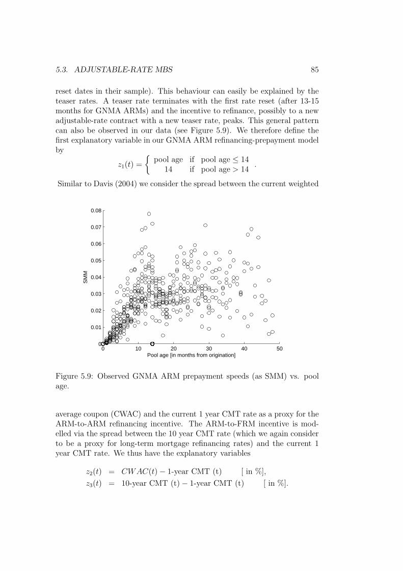
5.3. ADJUSTABLE-RATE MBS 85
reset dates in their sample). This behaviour can easily be explained by theteaser rates. A teaser rate terminates with the first rate reset (after 13-15months for GNMA ARMs) and the incentive to refinance, possibly to a newadjustable-rate contract with a new teaser rate, peaks. This general patterncan also be observed in our data (see Figure 5.9). We therefore define thefirst explanatory variable in our GNMA ARM refinancing-prepayment modelby
z1(t) =
pool age if pool age ≤ 14
14 if pool age > 14.
Similar to Davis (2004) we consider the spread between the current weighted
0 10 20 30 40 500
0.01
0.02
0.03
0.04
0.05
0.06
0.07
0.08
Pool age [in months from origination]
SM
M
Figure 5.9: Observed GNMA ARM prepayment speeds (as SMM) vs. poolage.
average coupon (CWAC) and the current 1 year CMT rate as a proxy for theARM-to-ARM refinancing incentive. The ARM-to-FRM incentive is mod-elled via the spread between the 10 year CMT rate (which we again considerto be a proxy for long-term mortgage refinancing rates) and the current 1year CMT rate. We thus have the explanatory variables
z2(t) = CWAC(t) − 1-year CMT (t) [ in %],
z3(t) = 10-year CMT (t) − 1-year CMT (t) [ in %].
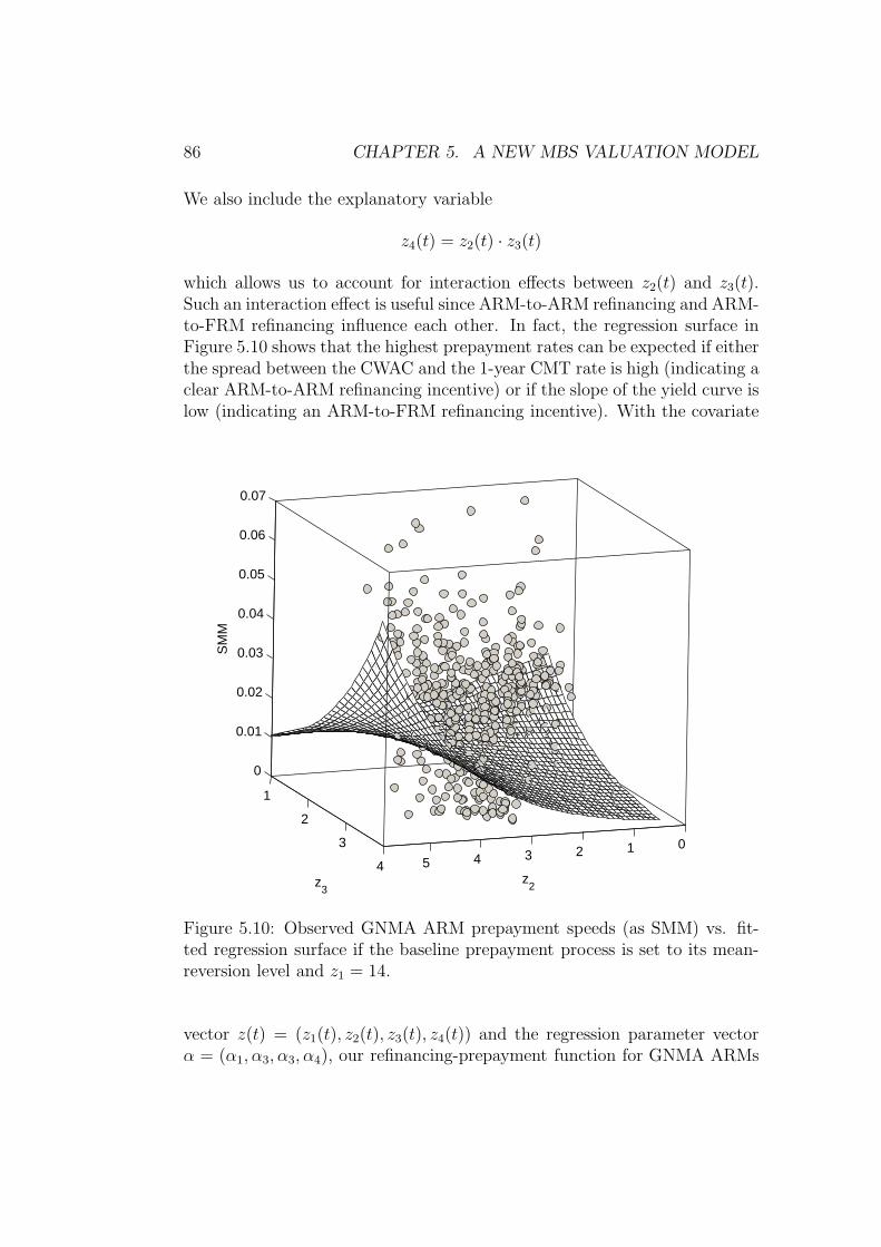
86 CHAPTER 5. A NEW MBS VALUATION MODEL
We also include the explanatory variable
z4(t) = z2(t) · z3(t)
which allows us to account for interaction effects between z2(t) and z3(t).Such an interaction effect is useful since ARM-to-ARM refinancing and ARM-to-FRM refinancing influence each other. In fact, the regression surface inFigure 5.10 shows that the highest prepayment rates can be expected if eitherthe spread between the CWAC and the 1-year CMT rate is high (indicating aclear ARM-to-ARM refinancing incentive) or if the slope of the yield curve islow (indicating an ARM-to-FRM refinancing incentive). With the covariate
012345
1
2
3
4
0
0.01
0.02
0.03
0.04
0.05
0.06
0.07
z2z
3
SM
M
Figure 5.10: Observed GNMA ARM prepayment speeds (as SMM) vs. fit-ted regression surface if the baseline prepayment process is set to its mean-reversion level and z1 = 14.
vector z(t) = (z1(t), z2(t), z3(t), z4(t)) and the regression parameter vectorα = (α1, α3, α3, α4), our refinancing-prepayment function for GNMA ARMs
5.3. ADJUSTABLE-RATE MBS 87
has the form
fARM(z(t), α) = α1z1(t) + α2z2(t) + α3z3(t) + α4z4(t). (5.17)
The overall prepayment speed is thus given by
pARM(t) = efARM (z(t),α)+p0(t),
where p0(t) is the baseline prepayment process as defined in (5.3). We assumefor simplicity that the baseline prepayment process is the same for fixed-rateand adjustable-rate mortgages. The components of the regression parametervector α can again be estimated by Kalman filtering techniques, as alreadydiscussed for our fixed-rate MBS model in the previous section. The resultsof the parameter estimation are shown in Table 5.5. Since regression pa-
Parameter Estimate
α1 0.1124α2 -0.4377α3 -1.0515α4 0.2697
Table 5.5: Estimates of the regression parameter vector in our GNMA ARMmodel.
rameters in a model with interaction effects between explanatory variables(reflected in our variable z4(t)) can not be interpreted directly, we illustratethem with respect to the spread covariates in Figure 5.10. For any givenvalue of the prepayment-risk-adjustment parameters µ, λp and λw, we cannow price GNMA ARMs by Monte-Carlo simulation. The Monte-Carlo esti-mation procedure, as described in the appendix for fixed-rate MBS, has to beadapted only slightly. Instead of the fixed-rate MBS refinancing-prepaymentfunction f(x(t), t) we have to use the function fARM (z(t), t) as given in (5.17).Furthermore, the weighted average coupon does of course not remain con-stant but has to be adjusted according to the simulated index rate, takinginto account the Caps and Floors embedded in the contract.
The prepayment-risk-adjustment parameters µ, λp and λw can again becalibrated to market data. In order to give an empirical example, we con-sider market data of 20-Aug-2006. On this particular day, prices for GNMAARMs with current coupons of 4%, 4.5% and 5% were actively quoted on aTBA basis. Calibrating the prepayment-risk-adjustment parameters to theprices of these securities (by minimising the Euclidean norm of differences
88 CHAPTER 5. A NEW MBS VALUATION MODEL
between model and market prices) yields the estimates as given in Table5.6. These results are line with the estimates obtained in our fixed-rate MBSmodel and the same interpretations apply. In Table 5.7 we show the market
Parameter Estimate
µ 2.7λp 3.1λw -14.4
Table 5.6: Prepayment-risk-adjustment parameters calibrated to GNMAARM prices on the sample day 20-Aug-2006.
prices and our model prices. These results indicate that our model is able toexplain market prices of GNMA ARMs successfully. Yet, further empiricalevidence, in particular with respect to parameter stability over time, wouldbe interesting. This is however, beyond the scope of this thesis and remainsa topic for further research.
Coupon 4% Coupon 4.5% Coupon 5%
Market price 0.9800 0.9841 1.0059Model price 0.9847 0.9912 0.9995
Rel. pricing error 0.5% 0.7% 0.6%
Table 5.7: GNMA ARM market and model prices according to ourprepayment-risk-neutral GNMA ARM pricing model on the sample day 20-Aug-2006.
5.4 Collateralized Mortgage Obligations
In this section we will apply our model to the pricing of Collateralized Mort-gage Obligations (CMOs). We have already introduced CMOs briefly inChapter 2 and have mentioned that the cash flows of the underlying mortgagepool are assigned to different tranches. Depending on the individual securi-tisation scheme, these tranches may have very different characteristics. Themost basic type of CMO is the sequential-pay CMO, sometimes also calledplain-vanilla or clean CMO. In a sequential-pay CMO each tranche receivesregular interest payments. Principal payments (scheduled payments and pre-payments) are, however, assigned sequentially to the different tranches, usu-ally labelled A-Tranche, B-Tranche, etc. I.e., principal payments are assigned
5.4. COLLATERALIZED MORTGAGE OBLIGATIONS 89
to the Tranche A alone until it is completely retired. Once this is the case,all principal payments are assigned to Tranche B, etc. Figure 5.12 illustratesthe cash flow pattern of a sequential-pay CMO with three tranches.
More complex CMO structure may include Planned Amortization Class(PAC) tranches and Targeted Amortization Class (TAC) tranches. PACtranches guarantee a fixed principal repayment schedule as long as prepay-ment rates remain in a certain corridor, e.g. 75% PSA to 300% PSA. TACtranches have a designated target speed. If prepayments are equal or abovethe target speed, e.g. 100% PSA, the principal allocation to the TAC tranchefollows a prespecified schedule. Thus, PAC tranches offer protection againstprepayment risk up to a certain degree. Unlike the PAC tranches, a TACtranche is not protected from extension if prepayments are slower than ex-pected and therefore offer only one-sided prepayment variability protection.Excess prepayments which are above the PAC and TAC tranche schedules areabsorbed by so-called companion or support tranches. These tranches featurea very high uncertainty with respect to cash flow timing and therefore beara large part of the prepayment risk associated with the underlying mortgagepool. In addition to PAC, TAC and support tranches, complex CMOs mayalso have accrual tranches (usually labelled Z-tranche), which do not receiveinterest payments during a certain lockout period, Interest-Only tranches,Principal-Only tranches, Floating-Rate Tranches and Inverse Floating-Ratetranches. Finally, residual tranches collect remaining cash flows from theunderlying pool after the obligations to the other tranches have been met.
The pricing of these tranches within our modelling framework is per-fectly possible. The Monte-Carlo simulation used to price the underlyingpass-through security according to (5.8) simply has to be changed to ac-commodate the cash flow structuring rules of the CMO. Since virtually ev-ery CMO features individual characteristics, liquid market prices of CMOtranches are not readily available. Since we do not have liquid market data,it is impossible at this stage to validate our model empirically using CMOmarket prices. We will however, briefly illustrate how our model works foran easy sequential-pay CMO structure with three tranches as illustrated inFigure 5.12. We assume that all tranches are equally large (i.e. 1/3 of theunderlying pool’s total notional amount) and that the underlying pool is theGNMA 5.5% generic pool on the sample day 12-Dec-2005 as already used inChapter 5.2.2. Furthermore, we assume that the coupon for each of the threetranches is equally 5.5%. Our prepayment-risk neutral model prices of thetranches (with respect to a notional of 1), as well as the respective expectedaverage lives, are given in Table 5.8.
In addition to the different expected average lives, CMO tranches alsodiffer with respect to their model risk exposure. The different model risk
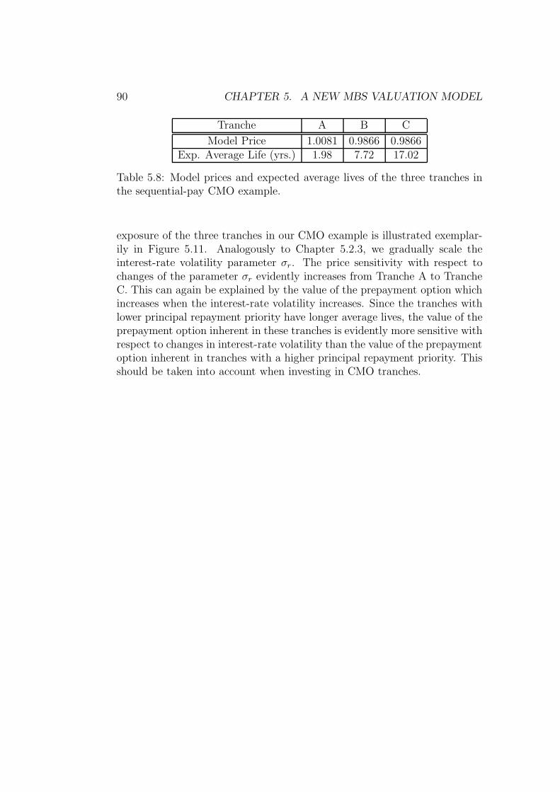
90 CHAPTER 5. A NEW MBS VALUATION MODEL
Tranche A B C
Model Price 1.0081 0.9866 0.9866Exp. Average Life (yrs.) 1.98 7.72 17.02
Table 5.8: Model prices and expected average lives of the three tranches inthe sequential-pay CMO example.
exposure of the three tranches in our CMO example is illustrated exemplar-ily in Figure 5.11. Analogously to Chapter 5.2.3, we gradually scale theinterest-rate volatility parameter σr. The price sensitivity with respect tochanges of the parameter σr evidently increases from Tranche A to TrancheC. This can again be explained by the value of the prepayment option whichincreases when the interest-rate volatility increases. Since the tranches withlower principal repayment priority have longer average lives, the value of theprepayment option inherent in these tranches is evidently more sensitive withrespect to changes in interest-rate volatility than the value of the prepaymentoption inherent in tranches with a higher principal repayment priority. Thisshould be taken into account when investing in CMO tranches.
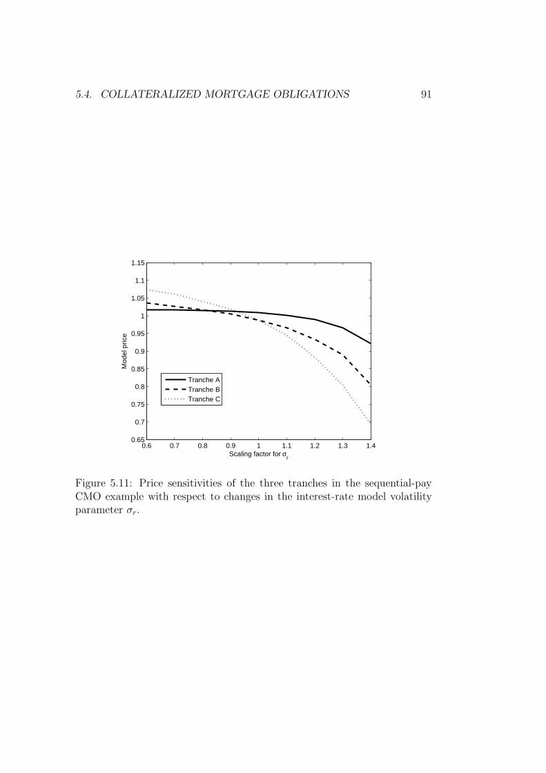
5.4. COLLATERALIZED MORTGAGE OBLIGATIONS 91
0.6 0.7 0.8 0.9 1 1.1 1.2 1.3 1.40.65
0.7
0.75
0.8
0.85
0.9
0.95
1
1.05
1.1
1.15
Scaling factor for σr
Mod
el p
rice
Tranche ATranche BTranche C
Figure 5.11: Price sensitivities of the three tranches in the sequential-payCMO example with respect to changes in the interest-rate model volatilityparameter σr.
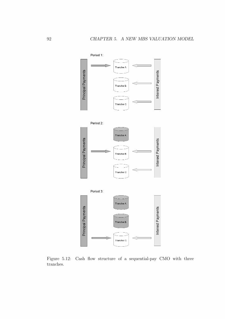
92 CHAPTER 5. A NEW MBS VALUATION MODEL
Figure 5.12: Cash flow structure of a sequential-pay CMO with threetranches.
Chapter 6
A closed-form approximationfor fixed-rate MBS
The valuation of mortgage-backed securities is usually considered a com-putationally expensive problem. This holds for both the option-theoreticapproaches and the traditional econometric approaches, as already discussedin Chapter 4. In this chapter we develop an approximate closed-form formulafor the value of fixed-rate (agency) MBS and, as corollaries, for Interest-Onlyand Principal-Only securities. The valuation is again based on a stochasticprepayment intensity approach similar in spirit to the approach presented inChapter 5.
In many intensity-based modelling approaches for the valuation of default-able bonds and credit derivatives closed-form pricing formulas are available.It is our aim in this chapter to apply these techniques to prepayment-sensitiveMBS. Interestingly, in our intensity-based model we find that a closed-formsolution of the MBS valuation problem leads to rather similar challengingcalculations as in the approach developed by Collin-Dufresne and Harding(1999). As already discussed in Chapter 4.2, the Collin-Dufresne/Hardingmodel, as well as its extension developed by Rom-Poulsen (2007), has a coupleof shortcomings. In our framework, however, we are able to address some ofthe previously mentioned shortcomings which may be problematic in certainsituations and for certain types of MBS. It is straightforward to incorporateadditional stochastic factors into our model. Similar to the approach takenin Chapter 5, we do this by modelling the (non refinancing-related) baselineprepayment process via two stochastic factors, where the second factor isfit to the GDP growth in the US. We thus account for the dependence be-tween general economic conditions and turnover-related prepayment in ourmodel. The baseline prepayment is also supposed to capture defaults which,in the case of agency MBS, simply result in prepayment for an investor. In
93
94 CHAPTER 6. A CLOSED-FORM APPROXIMATION
addition to this, we account for the usual S-curve shape of the refinancing-incentive/prepayment relation by a sectionwise linear approximation. Thisis quite similar to the approach presented in Gorovoy and Linetsky (2007)(which was developed independently from the research presented here). Wefind that this approximation does have an important effect across the wholecoupon range.
While in our modelling framework it is straightforward to conduct a clas-sical OAS valuation, we are again primarily interested in a prepayment-risk-neutral valuation. This also allows us to assess the performance of our modelquantitatively by directly comparing market to model prices.
6.1 The model set-up
Our starting point here is the valuation of a single mortgage contract. Weassume that the time of prepayment of one mortgage does not influence theprobability of prepayment of other mortgages and that the pool is homoge-neous (w.r.t. mortgage maturity, coupon, etc. and thus w.r.t. individualprepayment probabilities). Thus, the value of the MBS can be calculated asthe value of an individual mortgage multiplied with the number of mortgagesin the pool. While this assumption is problematic in option-based modelswhere one would have to establish some additional features accounting forheterogeneous prepayment-option exercise behaviour, this is not the case inthe reduced-form framework. We further assume that partial prepayment isnot possible.
Consider a mortgage contract with payment dates t1, ..., tK , define ∆tk :=tk − tk−1 (years) and set t0 = 0. On each payment date tk, k = 1, ..., K, themortgage payment M(tk) · ∆tk, containing both interest and regular repay-ments, has to be made until the time of prepayment. At the time of prepay-ment tτ (or at the final maturity of the mortgage), the remaining principalbalance according to the amortization schedule A(tτ ) is paid back in a lumpsum. Thus, all cash flows depend on the time of prepayment. Following(3.35) and (3.37), the approximate value V Mo
app (0) of the mortgage contractat time 0 admits the representation
V Moapp (0) = E eQ
[K∑
k=1
(M(tk) · ∆tk + A(tk) · π(tk) · ∆tk) · e−R tk0
(r(s)+π(s))ds
],
(6.1)
where r(t) is the (risk-free) short-rate process, π(t) is the (continuous, an-
nualised) prepayment intensity/prepayment speed process and Q is the risk-neutral pricing measure. Formula (6.1) can also be considered a discretised
6.1. THE MODEL SET-UP 95
version of the continuous time valuation formula in Goncharov (2005). Notethat (6.1) implies that A(tk) is to be understood here as the outstandingbalance according to the amortisation schedule before the regular principalrepayment has been made on the payment date tk. In the credit risk liter-ature, where formulas such as (6.1) are common, the process π(t) is usuallythe default intensity. If the default intensity process can be set up withina Gaussian framework, a closed-form representation of formula (6.1) is, ingeneral, possible. In many models and applications in practice the defaultintensity is modelled independently from r(t). In the case of prepaymentmodelling, however, the prepayment intensity process π(t) can not be as-sumed to be independent of the interest-rate process r(t) since it is a wellknown fact that mortgage borrowers are more likely to refinance their loansand thus prepay their mortgages when interest rates decline, as previouslydiscussed. In the following we will again decompose the overall prepaymentintensity into the two independent components refinancing-related prepay-ment πrefi(t) and baseline prepayment π0(t), i.e. we get for the continuous,annualised prepayment speed
π(t) = πrefi(t) + π0(t). (6.2)
Note that we have specified the prepayment intensity here in a slightly dif-ferent way than in the model presented in the previous chapter. The prepay-ment intensity π(t) in our closed-form model presented here is the analogueof ln p(t) in the previous chapter.
Following the argumentation in Chapter 5 based on the Girsanov theoremfor marked point processes, we again introduce a multiplicative prepayment-risk adjustment parameter µ so that, under the risk-neutral pricing measureQ, the prepayment process has the dynamics
dπ(t) = µ · (dπrefi(t) + dπ0(t)). (6.3)
Note that (6.3) implies that we assume that the intensity under the risk-
neutral pricing measure Q is given by the intensity under the real-worldmeasure, multiplied with some constant µ. I.e., we assume that
Φ(t) = µ
instead of Φ(t) = (p(t))µ−1 in Theorem 5.1. We will discuss the refinancingcomponent and the turnover component of prepayment separately in thefollowing before we finally put all components together for our closed-formformula.
96 CHAPTER 6. A CLOSED-FORM APPROXIMATION
The short-rate model and the refinancing component
A crucial component of every MBS valuation model is an adequate modelfor the interest-rate term structure. For our closed-form formula we use a1-factor CIR model as introduced in Chapter 3.2.3, which has proven tobe better suited for our closed-form approximation approach than the Hull-White model used in Chapter 5. While an extensions to a two-factor CIRmodel is possible in our modelling framework, we leave this for further re-search. Recall that in the basic CIR model, the risk-free short-rate dynamicsunder the risk-neutral measure Q are given by
dr(t) = (θr − arr(t))dt + σr
√r(t)dWr(t), (6.4)
where Wr is a Q-Wiener process, ar := ar + λrσ2r with the market price
of risk parameter λr and some positive constants θr, ar, σr with 2θr > σ2r .
Recall also that the zero-coupon bond prices in the CIR model can be calcu-lated analytically. They are comprised in the following, more general, lemma:
Lemma 6.1. In the CIR short-rate model and with rc(t) := c · r(t) for some
constant c ≥ − a2r
2σ2r, it holds that
P c(t, T ) := E eQ[e−R T
trc(s)ds|Ft] = eAc(t,T )−Bc(t,T )r(t) (6.5)
where
Bc(t, T ) = c · 1 − e−γc(T−t)
κ1 − κ2e−γc(T−t),
Ac(t, T ) =2θr
σ2r
log
[γceκ2·(T−t)
κ1 − κ2 · e−γc·(T−t)
]
with γc :=√
a2r + 2σ2
rc, κ1 := ar
2+ γc
2and κ2 := ar
2− γc
2.
Proof. For c = 1 we have the well-known formulas for zero-coupon bondprices in the CIR model. For c ≥ 0 in general, we get the dynamics of rc(t)
under Q by a simple application of the Ito-formula and obtain:
rc(t) = (θcr − arr
c(t))dt + σcr
√rc(t)dWr(t)
with
θcr = c · θr,
σcr =
√c · σr

6.1. THE MODEL SET-UP 97
and the statement follows directly from, e.g., Zagst (2002a), p.126/127. For
− a2r
2σ2r≤ c < 0, however, the result is less straightforward. We therefore
explicitly give the detailed proof in the following.From the Feynman-Kac representation of the Cauchy-Problem (see (3.5))
we know that P c(t, T ) must satisfy:
P ct + (θr − arr)P
cr +
1
2· σ2
r · r · P crr = c · r · P c (6.6)
with boundary condition P c(T, T ) = 1. Since
P cr = −Bc · P c,
P ct = P c · (Ac
t − r · Bct ),
P crr = (Bc)2 · P c,
it follows from (6.6) that
Act(t, T ) − θrB
c(t, T ) − r · (c − 1
2· σ2
r · (Bc(t, T ))2
+Bct (t, T ) − ar · Bc(t, T )) = 0
with Ac(T, T ) = Bc(T, T ) = 0. This leads to the Riccati-style equations
c − 1
2· σ2
r · (Bc(t, T ))2 + Bct (t, T ) − arB
c(t, T ) = 0
with Bc(T, T ) = 0 andAc
t(t, T ) = θrBc(t, T )
with Ac(T, T ) = 0. Thus, it remains to show that
Bc(t, T ) = c · 1 − e−γc(T−t)
κ1 − κ2e−γc(T−t),
Ac(t, T ) =2θr
σ2r
log
[γceκ2·(T−t)
κ1 − κ2 · e−γc·(T−t)
]
with γc :=√
a2r + 2σ2
rc, κ1 := ar
2+ γc
2and κ2 := ar
2− γc
2solve the Riccati
equations for c ≥ − a2r
2σ2r. Since (for c 6= 0)
12· σ2
r · (Bc(t, T ))2
c− Bc
t (t, T )
c+
arBc(t, T )
c=
12σ2
rc · (1 − e−γc(T−t))2
(κ1 − κ2e−γc(T−t))2
−(κ1 − κ2e−γc(T−t))(−γce−γc(T−t)) − (1 − e−γc(T−t))(−κ2γ
ce−γc(T−t))
(κ1 − κ2e−γc(T−t))2
+ar(1 − e−γc(T−t))(κ1 − κ2e
−γc(T−t))
(κ1 − κ2e−γc(T−t))2:=
Z
N

98 CHAPTER 6. A CLOSED-FORM APPROXIMATION
it remains to show that Z = N .
Z =1
2σ2
rc − σ2rce
−γc(T−t) +1
2σ2
rce−2γc(T−t) + κ1γ
ce−γc(T−t) −
κ2γce−2γc(T−t) − κ2γ
ce−γc(T−t) + κ2γce−2γc(T−t) + arκ1 −
arκ1e−γc(T−t) − arκ2e
−γc(T−t) + arκ2e−2γc(T−t)
=1
2σ2
rc − σ2rce
−γc(T−t) +1
2σ2
rce−2γc(T−t) +
ar
2γce−γc(T−t) +
1
2γc2e−γc(T−t) − ar
2γce−γc(T−t) +
1
2γc2e−γc(T−t) +
a2r
2+
ar
2γc − a2
r
2e−γc(T−t) − ar
2γce−γc(T−t) − a2
r
2e−γc(T−t) +
ar
2γce−γc(T−t) +
a2r
2e−2γc(T−t) − ar
2γce−2γc(T−t).
Simplifying further, we obtain:
Z =a2
r
2+
1
2arγ
c +1
2σ2
rc +
e−γc(T−t)(−σ2rc + (a2
r + 2σ2rc) − a2
r −ar
2γc +
ar
2γc)
e−2γc(T−t)(1
2σ2
rc +a2
r
2− ar
2γc)
=a2
r
2+
1
2arγ
c +1
2σ2
rc +
e−γc(T−t) · σ2rc + e−2γc(T−t)(
1
2σ2
rc +a2
r
2− ar
2γc).
Now, since
κ21 =
a2r
4+
1
2arγ
c +1
4(a2
r + 2σ2rc) =
a2r
2+
1
2arγ
c +1
2σ2
rc,
−2κ1κ2 = −2(a2
r
4− 1
4γc2) = − a2
r
2+
a2r
2+ σ2
rc = σ2rc;
κ22 =
a2r
4− 1
2arγ
c +1
4(a2
r + 2σ2rc) =
a2r
2− 1
2arγ
c +1
2σ2
rc,
we get:
N =a2
r
2+
1
2arγ
c +1
2σ2
rc
+e−γc(T−t) · σ2rc + e−2γc(T−t)(
1
2σ2
rc +a2
r
2− ar
2γc)
6.1. THE MODEL SET-UP 99
and thus Z = N .For Ac(t, T ) we get by comparing the original form of A(t, T ) in the CIR
model
Ac(t, T ) = −∫ T
t
θrBc(s, T )ds
= c · 2θr
σ2rc
log
[2γce
1
2(ar+γc)(T−t)
(ar + γc)(eγc(T−t) − 1) + 2γc
]
=2θr
σ2r
log
[2γce
12(ar+γc)(T−t)
(ar + γc)(eγc(T−t) − 1) + 2γc
],
which completes the proof.
If c = 1 in Lemma 6.1, P c(t, T ) is the price of a zero-coupon bond in the CIRmodel and we will write P (t, T ), γ, B(t, T ) and A(t, T ) instead of P c(t, T ),γc, Bc(t, T ) and Ac(t, T ) in this case.
As already mentioned earlier, the refinancing incentive is usually modelledas a function of the spread between a security’s weighted-average coupon(WAC) and current long-term interest rates which serve as a proxy for mort-gage refinancing rates. While in some models (e.g., Levin and Daras (1998)or our approach in Chapter 5) the 10yr par yield is used, we use the 10yr zeroyield here since this is a more convenient choice for our closed-form formula.Note that within the CIR framework the 10yr zero yield R10 is given by
R10(t) = −a10 + b10 · r(t), (6.7)
where a10 := A(t,t+10)10
and b10 := B(t,t+10)10
. Contrarily to Collin-Dufresne andHarding (1999) we do not use a purely linear functional form, but approxi-mate an S-curve shape by defining
πrefi(t) = β · max(min(WAC − R10(t), α), 0), (6.8)
for some constant α > 0, which results in a spread-refinancing prepaymentrelationship as shown in Figure 6.1. This functional form offers two majoradvantages compared to a purely linear functional form:
• The S-like relationship between the spread and the refinancing-drivenprepayment, which has been confirmed empirically by, e.g., Levin andDaras (1998), is accounted for.
• Refinancing-driven prepayment can never become negative.
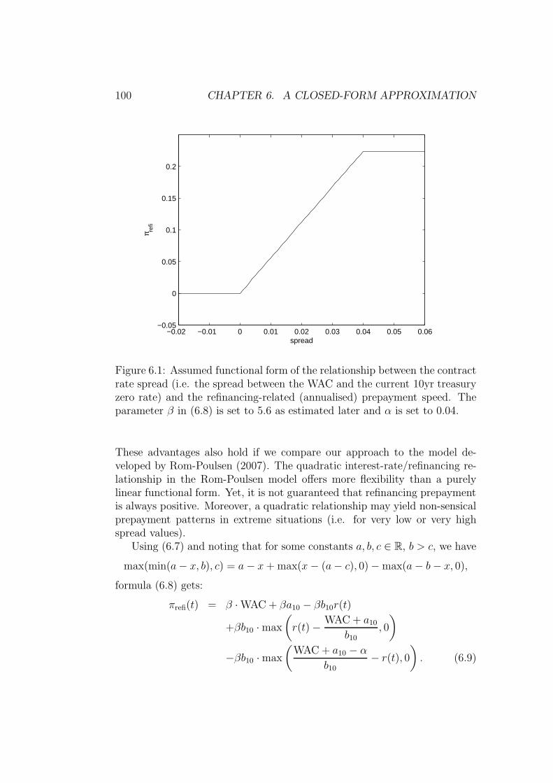
100 CHAPTER 6. A CLOSED-FORM APPROXIMATION
−0.02 −0.01 0 0.01 0.02 0.03 0.04 0.05 0.06−0.05
0
0.05
0.1
0.15
0.2
spread
π refi
Figure 6.1: Assumed functional form of the relationship between the contractrate spread (i.e. the spread between the WAC and the current 10yr treasuryzero rate) and the refinancing-related (annualised) prepayment speed. Theparameter β in (6.8) is set to 5.6 as estimated later and α is set to 0.04.
These advantages also hold if we compare our approach to the model de-veloped by Rom-Poulsen (2007). The quadratic interest-rate/refinancing re-lationship in the Rom-Poulsen model offers more flexibility than a purelylinear functional form. Yet, it is not guaranteed that refinancing prepaymentis always positive. Moreover, a quadratic relationship may yield non-sensicalprepayment patterns in extreme situations (i.e. for very low or very highspread values).
Using (6.7) and noting that for some constants a, b, c ∈ R, b > c, we have
max(min(a − x, b), c) = a − x + max(x − (a − c), 0) − max(a − b − x, 0),
formula (6.8) gets:
πrefi(t) = β · WAC + βa10 − βb10r(t)
+βb10 · max
(r(t) − WAC + a10
b10
, 0
)
−βb10 · max
(WAC + a10 − α
b10− r(t), 0
). (6.9)

6.1. THE MODEL SET-UP 101
Now, consider the term E eQ
[e−
R tk0 (r(s)+πrefi(s))ds
]. Defining
r(t) := r(1−βb10)(t) = (1 − βb10) · r(t)
we get by using (6.9):
E eQ
[e−
R tk0 (r(s)+πrefi(s))ds
]= E eQ
[e−
R tk0 β·WAC+βa10+er(s)ds·
e−
R tk0 βb10·max
“r(s)−WAC+a10
b10,0
”ds ·
eR tk0 βb10·max
“WAC+a10−α
b10−r(s),0
”ds
].
(6.10)
The following theorem shows how we can calculate this quantity, up to anerror term which will be discussed in more detail in the appendix.
Theorem 6.2. Defining
C(tk) := e−tk ·(β·WAC+βa10),
the expression
P refi(0, tk) := E eQ
[e−
R tk0 (r(s)+πrefi(s))ds
]
in the previously introduced model setting can be written in the following way:
P refi(0, tk) = C(tk) · P (0, tk) − C(tk) · βb10 · Cap(r, 0, tk, rCap, ∆t)
+C(tk) · βb10 · Floor(r, 0, tk, rF loor, ∆t)
+C(tk) · E eQ
[R(∆t, v2
k, w2k, zk · vk, zk · wk, vk · wk
)],
(6.11)

102 CHAPTER 6. A CLOSED-FORM APPROXIMATION
where, corresponding to Lemma 6.1,
P (0, tk) = P (1−βb10)(0, tk)
rCap :=WAC + a10
b10
rF loor :=WAC + a10 − α
b10
Cap(r, 0, T, rX, ∆t) :=
T/∆t∑
k=1
∆t ·[q + 1 + uk
ck− uk
ck· χ2(2ckrX , 2q + 6, 2uk)
−q + 1
ck
· χ2(2ckrx, 2q + 4, 2uk) − rX + rX · χ2(2ckrX , 2q + 2, 2uk)
]
Floor(r, 0, T, rX, ∆t) :=
T/∆t∑
k=1
∆t ·[rX · χ2(2ckrX , 2q + 2, 2uk)
−uk
ck
· χ2(2ckrX , 2q + 6, 2uk) −q + 1
ck
· χ2(2ckrX , 2q + 4, 2uk)
]
ck :=2ar
σ2r · (1 − e−ar ·k·∆t)
uk := ck · r(0) · e−ar ·k·∆t
q :=2θr
σ2r
− 1,
and χ2(·; a, b) denotes the cdf of the non-central Chi-square distribution withdegrees of freedom parameter a and non-centrality parameter b.R (∆t, v2
k, w2k, zk · vk, zk · wk, vk · wk) is a term containing residual terms of
the order O(∆t, v2k, w
2k, zk · vk, zk · wk, vk · wk). vk, wk, zk are defined as:
vk := −∫ tk
0
βb10 · max(r(s) − rCap, 0) ds
wk :=
∫ tk
0
βb10 · max(rF loor − r(s), 0) ds
zk :=
∫ tk
0
r(s) ds
Proof. After factoring out C(tk) in (6.10) we apply the approximation
ezk+vk+wk = ezk + vk + wk + R, (6.12)
6.1. THE MODEL SET-UP 103
where the term R contains residual terms of the order O(v2k, w
2k, zk · vk, zk ·
wk, vk · wk). If we then approximate the integrals by sums, we obtain:
E eQ
[e−
R tk0 (r(s)+πrefi(s))ds
]= C(tk) · P (0, tk)
−βb10 · C(tk) · ∆t ·⌈ tk∆t
⌉∑
k=1
E eQ
[max
(r(k · ∆t) − WAC + a10
b10, 0
)]
+βb10 · C(tk) · ∆t ·⌈ tk
∆t⌉∑
k=1
E eQ
[max
(WAC + a10 − α
b10− r(k · ∆t), 0
)]
+C(tk) · E eQ
[R(∆t, v2
k, w2k, zk · vk, zk · wk, vk · wk)
]
= C(tk) · P (0, tk)
−βb10 · C(tk) · ∆t ·⌈ tk∆t
⌉∑
k=1
∫ ∞
rCap
(r(k · ∆t) − rCap) f(r(k · ∆t))dr(k · ∆t)
+βb10 · C(tk) · ∆t ·⌈ tk
∆t⌉∑
k=1
∫ rF loor
0
(rF loor − r(k · ∆t)) f(r(k · ∆t))dr(k · ∆t)
+C(tk) · E eQ
[R(∆t, v2
k, w2k, zk · vk, zk · wk, vk · wk)
](6.13)
where f(·) denotes the pdf of the short rate and where the residual term Ralso contains the error terms of order O(∆t) resulting from the approximationof integrals by sums (see Appendix for a general discussion). Since we workwith a CIR model here, we know from Cox et al. (1985) that the distributionof 2 · ck · r(k · ∆t) is the non-central χ2-distribution with parameters 2q + 2and 2uk, with ck, uk and q as previously defined (see also Chapter 3.2.3).From the recurrence relation (see Johnson et al. (1995), p. 442)
λ · χ2(x; µ + 4, λ) = (λ − µ) · χ2(x; µ + 2, λ)
+(x + µ) · χ2(x; µ, λ) − x · χ2(x; µ − 2, λ)
(6.14)
(for µ > 2) and from the relation (see Johnson et al. (1995), p. 443)
∂χ2(x; µ, λ)
∂x= f(x; µ, λ) =
1
2(χ2(x; µ − 2, λ) − χ2(x; µ, λ)) (6.15)
it follows with some easy calculations that∫ b
0
xf(x; µ, λ)dx = µ · χ2(b; µ + 2, λ) + λ · χ2(b; µ + 4, λ). (6.16)

104 CHAPTER 6. A CLOSED-FORM APPROXIMATION
Applying (6.16) to the first integral in (6.13), we obtain:
∫ ∞
rCap
(r(k · ∆t) − rCap) f(r(k · ∆t))dr(k · ∆t) =1
2ck
[E eQ[2ckr(k · ∆t)] −
−(2q + 2) · χ2(2ckrCap; 2q + 4, 2uk) − 2uk · χ2(2ckrCap; 2q + 6, 2uk)
]
−rCap · (1 − χ2(2ckrCap; 2q + 2, 2uk)).
Similarly,∫ rF loor
0
(rF loor − r(k · ∆t)) f(r(k · ∆t))dr(k · ∆t) =
rF loor · χ2(2ckrF loor; 2q + 2, 2uk) −1
2ck
[(2q + 2)
·χ2(2ckrF loor; 2q + 4, 2uk) + 2uk · χ2(2ckrF loor; 2q + 6, 2uk)
].
Noting thatE eQ[2ckr(k · ∆t)] = 2q + 2 + 2uk,
formula (6.11) follows directly after rearranging of terms.
Note that the error term in Theorem 6.2 can be expected to be reasonablysmall, in particular for small values of tk. The error term will be discussedin more detail in the appendix. Note also that the notation ’Cap’ has notbeen chosen without motive. If one equates the linear interest rate at time tfor the period from t to t + ∆t with the short rate r(t), the expression
max
(r(k · ∆t) − (WAC + a10)
b10, 0
)· ∆t
in (6.10) is simply the payoff of a standard caplet from k ·∆t to (k + 1) ·∆twith cap rate rCap := (WAC + a10)/b10. A similar consideration applies for
the notation ’Floor’. We typically have ∆tk = 1/12 (i.e. 1 month) for allk = 1, ..., K. Hence, ∆t = 1/12 is a natural choice for the interval length ofthe discretisation in (6.11).
The baseline prepayment
We model the baseline or turnover component of prepayment within a two-factor Gaussian process framework where both factors follow Vasicek pro-cesses, similar to the specification of the baseline prepayment process in
6.1. THE MODEL SET-UP 105
Chapter 5. The second factor is fit to the GDP growth in the US, accountingfor the dependence between general economic conditions and turnover pre-payment. Of course, any other observable factor, e.g. a suitable house priceindex, could be used instead of or in addition to the GDP growth factor.While our empirical results have turned out to be satisfactory with the GDPgrowth as second factor in the baseline prepayment model, house prices havebeen used for example by Kariya et al. (2002), Sharp et al. (2006) or Down-ing et al. (2005). Our baseline prepayment processes are thus again given
by their Q-dynamics
dπ0(t) = (θp + bpww(t) − apπ0(t))dt + σpdWp(t), (6.17)
dw(t) = (θw − aww(t))dt + σwdWw(t),
where Wp, Ww are independent Q-Wiener processes (independent of the pre-
viously defined Wr) and ai := ai + λiσ2i , i = p, w, for the two prepayment-
risk-adjustment parameters λp, λw.In order to be able to calculate (6.1) we have to evaluate the expression
P d(t, T ) := E eQ[e−R Tt
(er(s)+π0(s))ds|Ft]
= E eQ[e−R Tt
er(s)ds|Ft] · E eQ[e−R Tt
π0(s)ds|Ft]
=: P (t, T ) · P base(t, T ),
where r(t) := r(1−βb10)(t), P (t, T ) := P (1−βb10)(t, T ). The letter d in the
superscript of P d(t, T ) is used in analogy to the reduced-form credit riskliterature.
Theorem 6.3. In the model set-up as previously introduced it holds that
P base(t, T ) = eAd(t,T )−Cd(t,T )π0(t)−Dd(t,T )w(t)
with
Cd(t, T ) =1
ap
(1 − e−ap(T−t)
),
Dd(t, T ) =bpw
ap
(1 − e−aw(T−t)
aw
+e−aw(T−t) − e−ap(T−t)
aw − ap
),
Ad(t, T ) =
∫ T
t
1
2
(σ2
pCd(l, T )2 + σ2
wDd(l, T )2)
−θpCd(l, T ) − θwDd(l, T )dl.
106 CHAPTER 6. A CLOSED-FORM APPROXIMATION
Proof. From the Feynman-Kac representation of the Cauchy-Problem (see(3.5)) we know that P base(t, T ) must satisfy:
P baset + (θw − aww)P base
w + (θp + bpw · w − apπ0)Pbaseπ0
+1
2· (σ2
p · P baseπ0π0
+ σ2w · P base
ww ) = π0 · P base
Calculating the derivatives of P base it follows that
Adt (t, T ) − π0(1 − apC
d(t, T ) + Cdt (t, T ))
−w(Ddt (t, T ) − awDd(t, T ) + bpwCd(t, T ))
+12· (σ2
pCd(t, T )2 + σ2
wDd(t, T )2) − θpCd(t, T ) − θwDd(t, T ) = 0.
Thus, we obtain the system of linear differential equations
1 − apCd(t, T ) + Cd
t (t, T ) = 0
bpwCd(t, T ) − awDd(t, T ) + Ddt (t, T ) = 0
Adt (t, T ) +
1
2· (σ2
pCd(s, T )2 + σ2
wDd(s, T )2)
−θpCd(s, T ) − θwDd(s, T ) = 0
with Ad(T, T ) = 0, Cd(T, T ) = Dd(T, T ) = 0. With some easy calculationsit is straightforward to verify that the formulas as stated in Theorem 6.3 arethe solutions of the linear differential equations above.
Note, that we have associated the prepayment speed π(t) with the intensityof prepayment. In our model specification in this chapter, however, π(t)can have negative values, albeit, in general, with only small probabilities.Prepayments for ordinary fixed-rate MBS can, of course, never be negative.Furthermore the association of the process π(t) with the prepayment intensity(and likewise the association of the baseline prepayment process π0(t) withthe corresponding default intensity process in the credit risk literature) is notunproblematic from a technical point of view for the same reason: intensitiescan never be negative. We thus consider the processes π(t) and π0(t) asproxies for the respective intensity processes. The fact that both π(t) andπ0(t) are negative only with small probabilities justifies this approach. Withthe parameter values as estimated in the following section (see Table 6.1),the probability that after one year the baseline prepayment is negative isjust 2%, if we set the GDP growth constant and equal to its mean-reversionlevel and the initial baseline prepayment level to its mean-reversion level ofapprox. 17% (see also Schonbucher (2003), p. 167, for a further discussionof this topic in the context of credit risk modelling).

6.1. THE MODEL SET-UP 107
The closed-form approximation
With the ingredients developed in the previous subsections the expressions
• E eQ
[M(tk) · e−
R t10
r(s)ds]
= M(tk) · P (0, t1)
• E eQ
[M(tk) · e−
R tk0 (r(s)+π(s))ds
]= M(tk) · P refi(0, tk) · P base(0, tk)
in (6.1) can readily be evaluated for all k, if the error term R is neglected.This is not yet the case for the terms involving π(tk) as a factor.
Lemma 6.4. It holds that in the previously introduced model set-up
E eQ
[π0(tk) · e−
R tk0
(r(s)+π(s))ds]
= C(tk) · P d(0, tk) · fd(0, tk)
−C(tk) · βb10 · P base(0, tk) · fd(0, tk) · Cap(r, 0, tk, rCap, ∆tk)
+C(tk) · βb10 · P base(0, tk) · fd(0, tk) · Floor(r, 0, tk, rF loor, ∆tk)
+C(tk) · βb10 · P base(0, tk) · fd(0, tk)
·E eQ
[R(∆t, v2
k, w2k, zk · vk, zk · wk, vk · wk)
]
where fd(0, tk) is the ”baseline spread forward rate”, i.e.
fd(0, tk) = − ∂
∂tkln P base(0, tk)
and all other quantities are as previously defined.
Proof. As a first step, recall the well-known result (see, e.g., Schmid (2004),p. 243) saying that
E eQ
[e−
R T
0r(l)dlr(T )|F0
]= −E eQ
[e−
R T
0r(l)dl|F0
]· ∂
∂TlnP (0, T ). (6.18)
Now, if we use the independence between (r(t), πrefi(t)) and π0(t), apply (6.18)to
E eQ
[π0(tk) · e−
R tk0
(r(s)+π(s))ds]
= E eQ
[e−
R tk0
(r(s)+πrefi(s))ds]·
E eQ
[π0(tk) · e−
R tk0 π0(s)ds
],
the lemma follows directly if we recall (6.11).
This leaves us with the term E eQ
[πrefi(tk) · e−
R tk0
(r(s)+π(s))ds].
108 CHAPTER 6. A CLOSED-FORM APPROXIMATION
Lemma 6.5. Within the previously introduced model set-up it holds that:
E eQ
[πrefi(tk) · e−
R tk0 (r(s)+π(s))ds
]= −P base(0, tk) · P refi(0, tk)
· ∂
∂tkln
[P refi(0, tk)
P (0, tk)
]. (6.19)
Proof. If we define the tk-forward measure Qtk in the usual way via its Radon-Nikodym derivative L(T ) with respect to Q by
L(t) =dQtk
dQ
∣∣∣∣Ft =P (t, tk)
P (0, tk) · eR tk0 r(s)ds
for t ∈ [0, tk] and use (6.18) we obtain:
E eQ
[πrefi(tk) · e−
R tk0
(r(s)+π(s))ds]
= E eQ
[πrefi(tk) · e−
R tk0
(r(s)+πrefi(s))ds]·
P base(0, tk)
= P (0, tk) · EQtk
[πrefi(tk) · e−
R tk0
πrefi(s)ds]· P base(0, tk)
= −P (0, tk) · EQtk
[e−
R tk0 πrefi(s)ds
]·
∂
∂tkln EQtk
[e−
R tk0
πrefi(s)ds]· P base(0, tk)
= −P refi(0, tk) ·∂
∂tkln
[P refi(0, tk)
P (0, tk)
]· P base(0, tk)
Note that by using Theorem 6.3 and Theorem 6.2, it is straightforward toevaluate the terms in (6.19), if the error term R is neglected.
We can finally summarise our results in the following theorem, where weuse Vapp as the value of a mortgage-backed security, if the error term R aspreviously defined is neglected.
Theorem 6.6. For a fixed-rate mortgage-backed security with K outstandingpayment dates at time 0 within the model specification as previously intro-duced it holds that:
Vapp(0) = S1 + S2 + S3 − ∆1 + ∆2 (6.20)

6.1. THE MODEL SET-UP 109
with
S1 =K∑
k=1
M(tk) · ∆tk · C(tk) · P d(0, tk)
S2 =
K∑
k=1
C(tk) · P d(0, tk) · A(tk) · ∆tk · fd(0, tk)
S3 = −K∑
k=1
C(tk) · P d(0, tk) · A(tk) · ∆tk ·
∂
∂tkln
[P refi(0, tk)
P (0, tk)
]
and
∆1 =K∑
k=1
Cap(r, 0, tk, rCap, ∆tk) · C(tk) · P base(0, tk) ·
βb10 ·[M(tk) · ∆tk + A(tk) · ∆tk · fd(0, tk) − A(tk) · ∆tk ·
∂
∂tkln
[P refi(0, tk)
P (0, tk)
] ]
∆2 =
K∑
k=1
Floor(r, 0, tk, rF loor, ∆tk) · C(tk) · P base(0, tk) ·
βb10 ·[M(tk) · ∆tk + A(tk) · ∆tk · fd(0, tk) − A(tk) · ∆tk ·
∂
∂tkln
[P refi(0, tk)
P (0, tk)
] ].
Formula (6.20) can readily be evaluated once the model parameters have beenestimated and calibrated. From Theorem 6.6 it is also easy to see how themost common mortgage derivatives, i.e. Interest-Only (IO) and Principal-Only (PO) securities, can be priced within our modelling framework. If wesplit up the mortgage payment M(tk) into the interest payment M I(tk) andregular principal repayment MP (tk), so that M(tk)=M I(tk) + MP (tk), and
110 CHAPTER 6. A CLOSED-FORM APPROXIMATION
denote
SI1 := M I(tk) · ∆t1 · P (0, t1) +
K∑
k=2
M I(tk) · ∆tk · C(tk) · P d(0, tk)
∆I1 :=
K∑
k=1
Cap(r, 0, tk, rCap, ∆tk) · C(tk) · P base(0, tk) · βb10 · M I · ∆tk
∆I2 :=
K∑
k=1
Floor(r, 0, tk, rF loor, ∆tk) · C(tk) · P base(0, tk) · βb10 · M I · ∆tk
SP1 := S1 − SI
1
∆P1 := ∆1 − ∆I
1
∆P2 := ∆2 − ∆I
2
we obtain the following two corollaries, where the notation V IOapp(0) and
V POapp (0) is again used for the calculation of values neglecting the error term
R. The two corollaries conclude this section.
Corollary 6.7. The value V IOapp(0) of an Interest-Only security with K out-
standing payment dates at time 0 is given by:
V IOapp(0) = SI
1 − ∆I1 + ∆I
2
Corollary 6.8. The value V POapp (0) of a Principal-Only security with K out-
standing payment dates at time 0 is given by:
V POapp (0) = SP
1 + S2 + S3 − ∆P1 + ∆P
2
6.2 Application to market data
6.2.1 Parameter estimation and model calibration
For the empirical evaluation of our closed-form approximation approach weuse again the monthly historical prepayment data of the 30yr fixed-ratemortgage-backed securities of the GNMA I and GNMA II program whichwe have already used for parameter estimation in our model presented inChapter 5. In addition to this we now use monthly historical prices of genericGNMA 30yr pass-through MBS with different coupons as traded on a to-be-announced (TBA) basis from 1996 to 2006 in order to assess the performanceof our model. All data were obtained from Bloomberg.
6.2. APPLICATION TO MARKET DATA 111
Weekly US treasury strip zero rates, obtained from the par rates by stan-dard bootstrapping, from 1993 to 2005 are used for the estimation of theparameters of the CIR interest-rate model. We estimate the CIR interest-model parameters with a state-space approach which integrates time-seriesinformation of different maturities, similar to the approach described in Geyerand Pichler (1999). Estimation of the unobservable state variables (i.e. ofthe short rate) is done with an approximative Kalman filter where the tran-sition densities are supposed to be normal. For the maximisation of the log-likelihood we use again the combined Downhill Simplex/Simulated Annealingalgorithm as described in Press et al. (1992). The parameters θp, ap, σp, bpw
can again be estimated by Kalman filtering techniques, similar in spirit tothe approach in Chapter 5. The measurement equation of the prepaymentstate space model is given by (6.2) with the historically observed annualised(continuous) prepayment rates π(tk) and πrefi as specified in (6.8). We obtain:
π1(tk)...
πN (tk)
=
π1,refi(tk)...
πN,refi(tk)
+
1...1
· π0(tk) + ǫk, (6.21)
where we assume that ǫk ∼ NN
(0, h2
p · IN
). Since in 2002-2004 prepayment
speeds were very high, we only use the data until 2004 for parameter esti-mation in the prepayment model in order to avoid noise in our observationscaused by small pool sizes after 2004. The transition equation for the (un-observable) baseline prepayment process is again given by
π0(tk+1) = e−ap∆tk+1 · π0(tk) +θp + bpww(tk)
ap· (1 − e−ap∆tk+1) + ηk+1
with
ηk+1 ∼ N1
(0,
σ2p
2ap
(1 − e−2ap∆tk+1)
).
The estimates of the interest-rate model parameters and of the (real-world)prepayment model parameters for our closed-form approximation model aregiven in Table 6.1. The standard errors are again estimates obtained from amoving block bootstrap procedure.
In order to illustrate the parameter estimates in our closed-form approx-imation prepayment model, we plot again the historical prepayment rates(as SMM) in Figure 6.2, similar to the presentation in Figure 5.1 for our fullMonte-Carlo valuation model. We also show the estimated single monthlymortalities according to our closed-form approximation model when the base-line prepayment process is set equal to its mean-reversion level. Note that
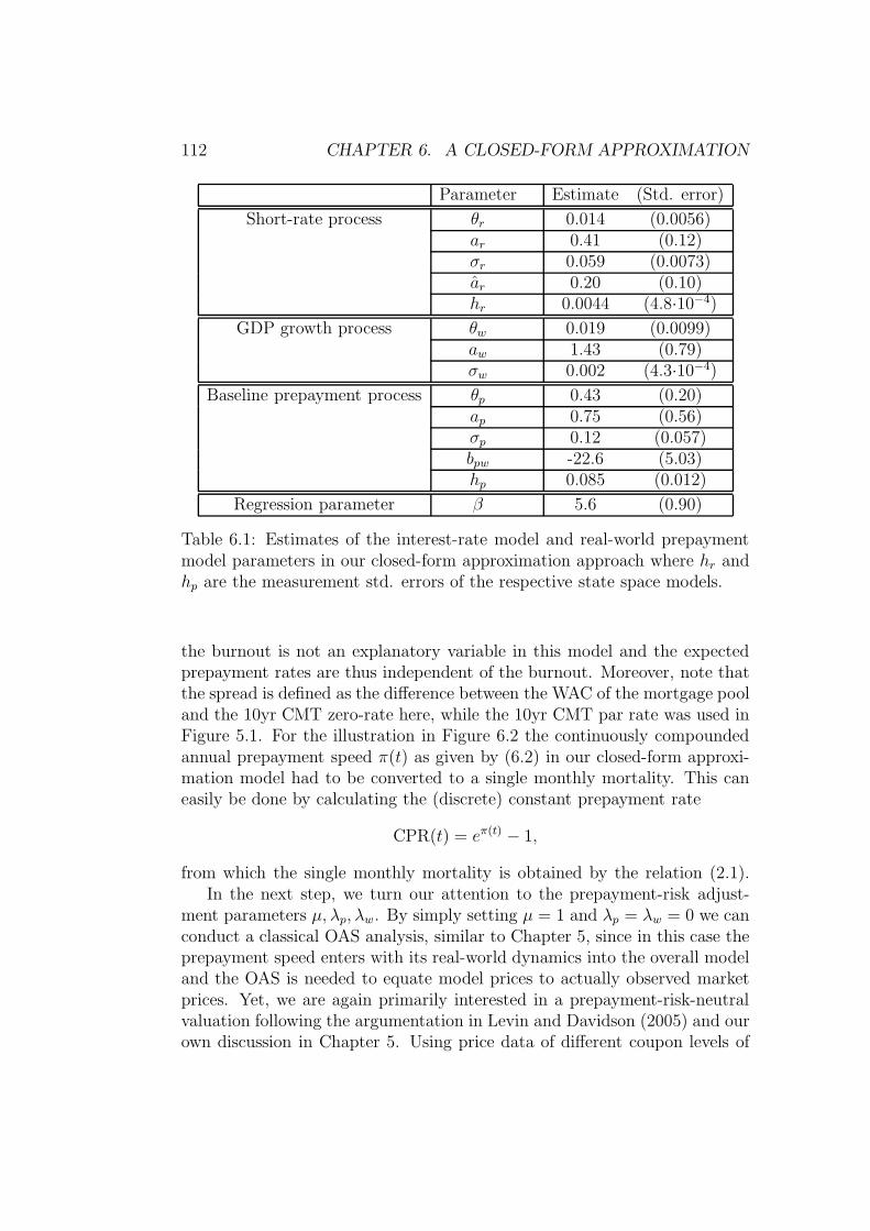
112 CHAPTER 6. A CLOSED-FORM APPROXIMATION
Parameter Estimate (Std. error)
Short-rate process θr 0.014 (0.0056)ar 0.41 (0.12)σr 0.059 (0.0073)ar 0.20 (0.10)hr 0.0044 (4.8·10−4)
GDP growth process θw 0.019 (0.0099)aw 1.43 (0.79)σw 0.002 (4.3·10−4)
Baseline prepayment process θp 0.43 (0.20)ap 0.75 (0.56)σp 0.12 (0.057)bpw -22.6 (5.03)hp 0.085 (0.012)
Regression parameter β 5.6 (0.90)
Table 6.1: Estimates of the interest-rate model and real-world prepaymentmodel parameters in our closed-form approximation approach where hr andhp are the measurement std. errors of the respective state space models.
the burnout is not an explanatory variable in this model and the expectedprepayment rates are thus independent of the burnout. Moreover, note thatthe spread is defined as the difference between the WAC of the mortgage pooland the 10yr CMT zero-rate here, while the 10yr CMT par rate was used inFigure 5.1. For the illustration in Figure 6.2 the continuously compoundedannual prepayment speed π(t) as given by (6.2) in our closed-form approxi-mation model had to be converted to a single monthly mortality. This caneasily be done by calculating the (discrete) constant prepayment rate
CPR(t) = eπ(t) − 1,
from which the single monthly mortality is obtained by the relation (2.1).In the next step, we turn our attention to the prepayment-risk adjust-
ment parameters µ, λp, λw. By simply setting µ = 1 and λp = λw = 0 we canconduct a classical OAS analysis, similar to Chapter 5, since in this case theprepayment speed enters with its real-world dynamics into the overall modeland the OAS is needed to equate model prices to actually observed marketprices. Yet, we are again primarily interested in a prepayment-risk-neutralvaluation following the argumentation in Levin and Davidson (2005) and ourown discussion in Chapter 5. Using price data of different coupon levels of
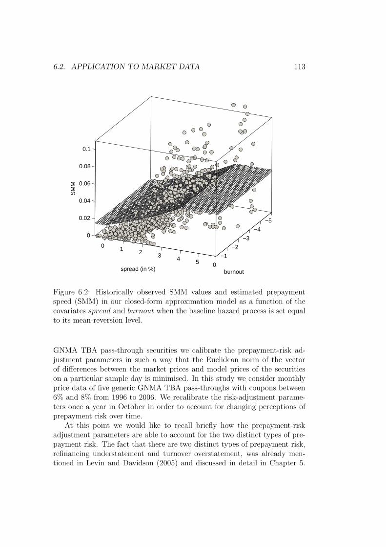
6.2. APPLICATION TO MARKET DATA 113
−5
−4
−3
−2
−1
0
0 1 2 3 4 5
0
0.02
0.04
0.06
0.08
0.1
burnoutspread (in %)
SM
M
Figure 6.2: Historically observed SMM values and estimated prepaymentspeed (SMM) in our closed-form approximation model as a function of thecovariates spread and burnout when the baseline hazard process is set equalto its mean-reversion level.
GNMA TBA pass-through securities we calibrate the prepayment-risk ad-justment parameters in such a way that the Euclidean norm of the vectorof differences between the market prices and model prices of the securitieson a particular sample day is minimised. In this study we consider monthlyprice data of five generic GNMA TBA pass-throughs with coupons between6% and 8% from 1996 to 2006. We recalibrate the risk-adjustment parame-ters once a year in October in order to account for changing perceptions ofprepayment risk over time.
At this point we would like to recall briefly how the prepayment-riskadjustment parameters are able to account for the two distinct types of pre-payment risk. The fact that there are two distinct types of prepayment risk,refinancing understatement and turnover overstatement, was already men-tioned in Levin and Davidson (2005) and discussed in detail in Chapter 5.
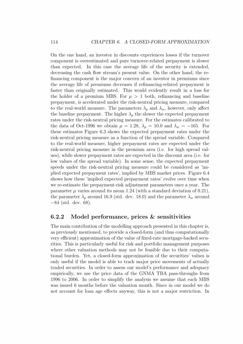
114 CHAPTER 6. A CLOSED-FORM APPROXIMATION
On the one hand, an investor in discounts experiences losses if the turnovercomponent is overestimated and pure turnover-related prepayment is slowerthan expected. In this case the average life of the security is extended,decreasing the cash flow stream’s present value. On the other hand, the re-financing component is the major concern of an investor in premiums sincethe average life of premiums decreases if refinancing-related prepayment isfaster than originally estimated. This would evidently result in a loss forthe holder of a premium MBS. For µ > 1 both, refinancing and baselineprepayment, is accelerated under the risk-neutral pricing measure, comparedto the real-world measure. The parameters λp and λw, however, only affectthe baseline prepayment. The higher λp the slower the expected prepaymentrates under the risk-neutral pricing measure. For the estimates calibrated tothe data of Oct-1996 we obtain µ = 1.28, λp = 10.0 and λw = −165. Forthese estimates Figure 6.3 shows the expected prepayment rates under therisk-neutral pricing measure as a function of the spread variable. Comparedto the real-world measure, higher prepayment rates are expected under therisk-neutral pricing measure in the premium area (i.e. for high spread val-ues), while slower prepayment rates are expected in the discount area (i.e. forlow values of the spread variable). In some sense, the expected prepaymentspeeds under the risk-neutral pricing measure could be considered as ’im-plied expected prepayment rates’, implied by MBS market prices. Figure 6.4shows how these ’implied expected prepayment rates’ evolve over time whenwe re-estimate the prepayment-risk adjustment parameters once a year. Theparameter µ varies around its mean 1.24 (with a standard deviation of 0.21),the parameter λp around 16.9 (std. dev. 18.0) and the parameter λw around−84 (std. dev. 68).
6.2.2 Model performance, prices & sensitivities
The main contribution of the modelling approach presented in this chapter is,as previously mentioned, to provide a closed-form (and thus computationallyvery efficient) approximation of the value of fixed-rate mortgage-backed secu-rities. This is particularly useful for risk and portfolio management purposeswhere other valuation methods may not be feasible due to their computa-tional burden. Yet, a closed-form approximation of the securities’ values isonly useful if the model is able to track major price movements of actuallytraded securities. In order to assess our model’s performance and adequacyempirically, we use the price data of the GNMA TBA pass-throughs from1996 to 2006. In order to simplify the analysis we assume that each MBSwas issued 6 months before the valuation month. Since in our model we donot account for loan age effects anyway, this is not a major restriction. In
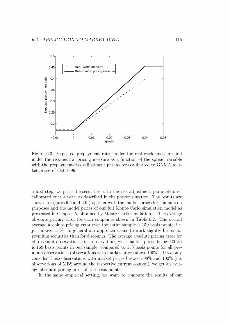
6.2. APPLICATION TO MARKET DATA 115
−0.01 0 0.01 0.02 0.03 0.04 0.05
0.2
0.25
0.3
0.35
0.4
0.45
0.5
spread
Exp
ecte
d pr
epay
men
t rat
e
Real−world measureRisk−neutral pricing measure
Figure 6.3: Expected prepayment rates under the real-world measure andunder the risk-neutral pricing measure as a function of the spread variablewith the prepayment-risk adjustment parameters calibrated to GNMA mar-ket prices of Oct-1996.
a first step, we price the securities with the risk-adjustment parameters re-calibrated once a year, as described in the previous section. The results areshown in Figures 6.5 and 6.6 (together with the market prices for comparisonpurposes and the model prices of our full Monte-Carlo simulation model aspresented in Chapter 5, obtained by Monte-Carlo simulation). The averageabsolute pricing error for each coupon is shown in Table 6.2. The overallaverage absolute pricing error over the entire sample is 159 basis points, i.e.just above 1.5%. In general our approach seems to work slightly better forpremium securities than for discounts. The average absolute pricing error forall discount observations (i.e. observations with market prices below 100%)is 169 basis points in our sample, compared to 153 basis points for all pre-mium observations (observations with market prices above 100%). If we onlyconsider those observations with market prices between 98% and 102% (i.e.observations of MBS around the respective current coupon), we get an aver-age absolute pricing error of 153 basis points.
In the same empirical setting, we want to compare the results of our
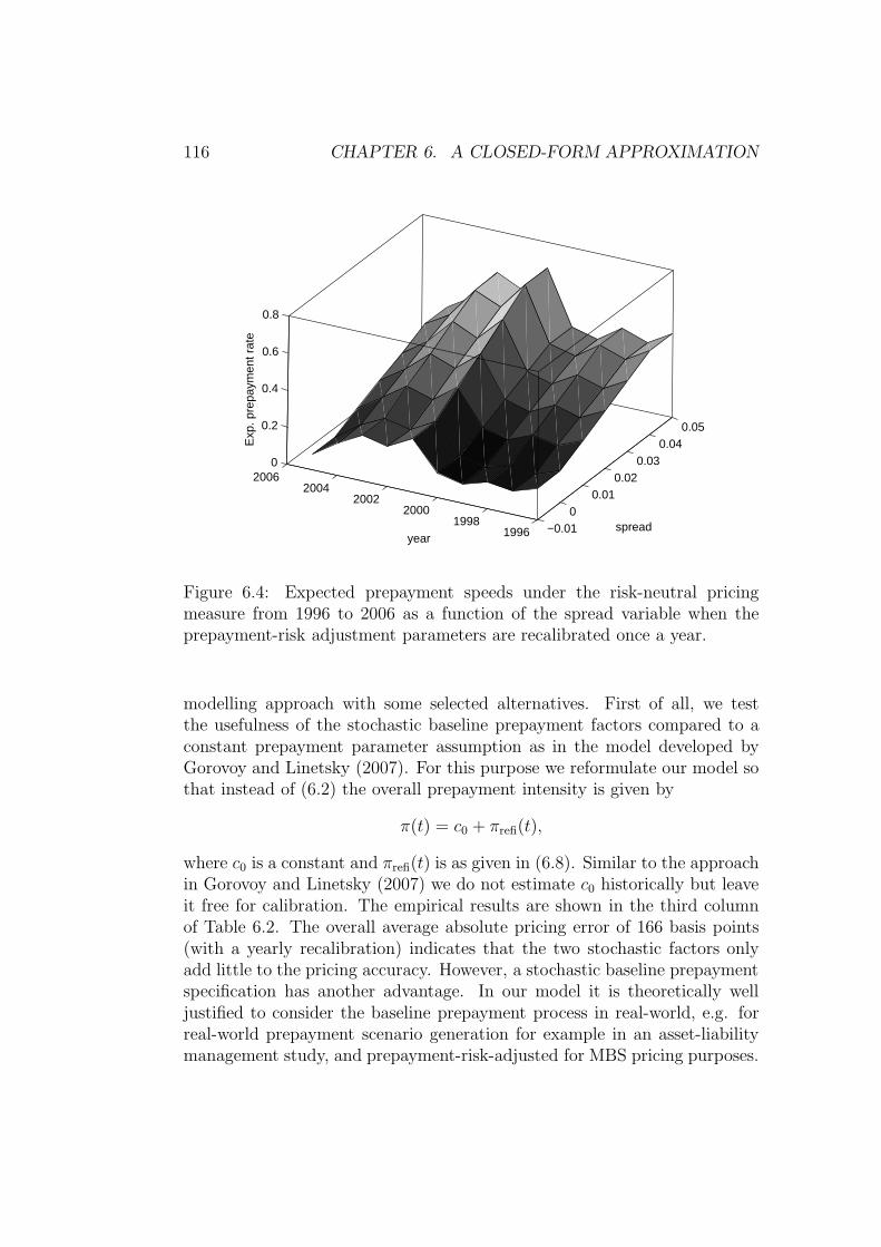
116 CHAPTER 6. A CLOSED-FORM APPROXIMATION
−0.010
0.010.02
0.030.04
0.05
19961998
20002002
20042006
0
0.2
0.4
0.6
0.8
spreadyear
Exp
. pre
paym
ent r
ate
Figure 6.4: Expected prepayment speeds under the risk-neutral pricingmeasure from 1996 to 2006 as a function of the spread variable when theprepayment-risk adjustment parameters are recalibrated once a year.
modelling approach with some selected alternatives. First of all, we testthe usefulness of the stochastic baseline prepayment factors compared to aconstant prepayment parameter assumption as in the model developed byGorovoy and Linetsky (2007). For this purpose we reformulate our model sothat instead of (6.2) the overall prepayment intensity is given by
π(t) = c0 + πrefi(t),
where c0 is a constant and πrefi(t) is as given in (6.8). Similar to the approachin Gorovoy and Linetsky (2007) we do not estimate c0 historically but leaveit free for calibration. The empirical results are shown in the third columnof Table 6.2. The overall average absolute pricing error of 166 basis points(with a yearly recalibration) indicates that the two stochastic factors onlyadd little to the pricing accuracy. However, a stochastic baseline prepaymentspecification has another advantage. In our model it is theoretically welljustified to consider the baseline prepayment process in real-world, e.g. forreal-world prepayment scenario generation for example in an asset-liabilitymanagement study, and prepayment-risk-adjusted for MBS pricing purposes.
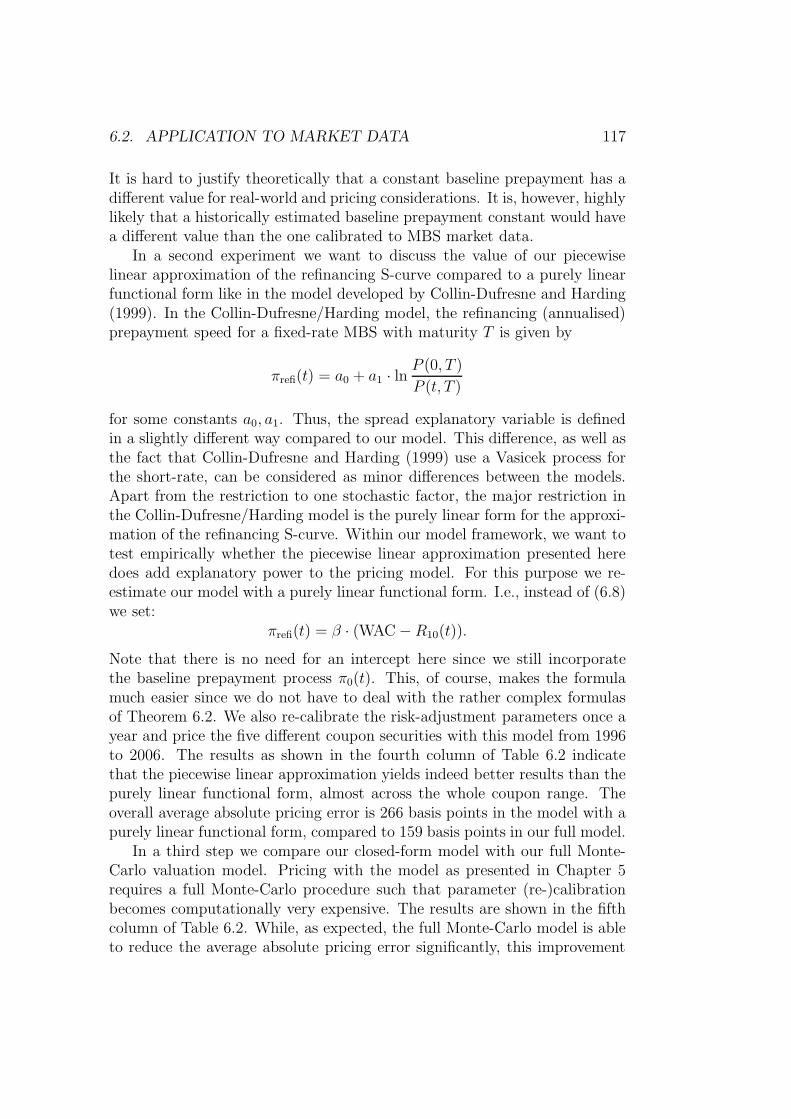
6.2. APPLICATION TO MARKET DATA 117
It is hard to justify theoretically that a constant baseline prepayment has adifferent value for real-world and pricing considerations. It is, however, highlylikely that a historically estimated baseline prepayment constant would havea different value than the one calibrated to MBS market data.
In a second experiment we want to discuss the value of our piecewiselinear approximation of the refinancing S-curve compared to a purely linearfunctional form like in the model developed by Collin-Dufresne and Harding(1999). In the Collin-Dufresne/Harding model, the refinancing (annualised)prepayment speed for a fixed-rate MBS with maturity T is given by
πrefi(t) = a0 + a1 · lnP (0, T )
P (t, T )
for some constants a0, a1. Thus, the spread explanatory variable is definedin a slightly different way compared to our model. This difference, as well asthe fact that Collin-Dufresne and Harding (1999) use a Vasicek process forthe short-rate, can be considered as minor differences between the models.Apart from the restriction to one stochastic factor, the major restriction inthe Collin-Dufresne/Harding model is the purely linear form for the approxi-mation of the refinancing S-curve. Within our model framework, we want totest empirically whether the piecewise linear approximation presented heredoes add explanatory power to the pricing model. For this purpose we re-estimate our model with a purely linear functional form. I.e., instead of (6.8)we set:
πrefi(t) = β · (WAC − R10(t)).
Note that there is no need for an intercept here since we still incorporatethe baseline prepayment process π0(t). This, of course, makes the formulamuch easier since we do not have to deal with the rather complex formulasof Theorem 6.2. We also re-calibrate the risk-adjustment parameters once ayear and price the five different coupon securities with this model from 1996to 2006. The results as shown in the fourth column of Table 6.2 indicatethat the piecewise linear approximation yields indeed better results than thepurely linear functional form, almost across the whole coupon range. Theoverall average absolute pricing error is 266 basis points in the model with apurely linear functional form, compared to 159 basis points in our full model.
In a third step we compare our closed-form model with our full Monte-Carlo valuation model. Pricing with the model as presented in Chapter 5requires a full Monte-Carlo procedure such that parameter (re-)calibrationbecomes computationally very expensive. The results are shown in the fifthcolumn of Table 6.2. While, as expected, the full Monte-Carlo model is ableto reduce the average absolute pricing error significantly, this improvement
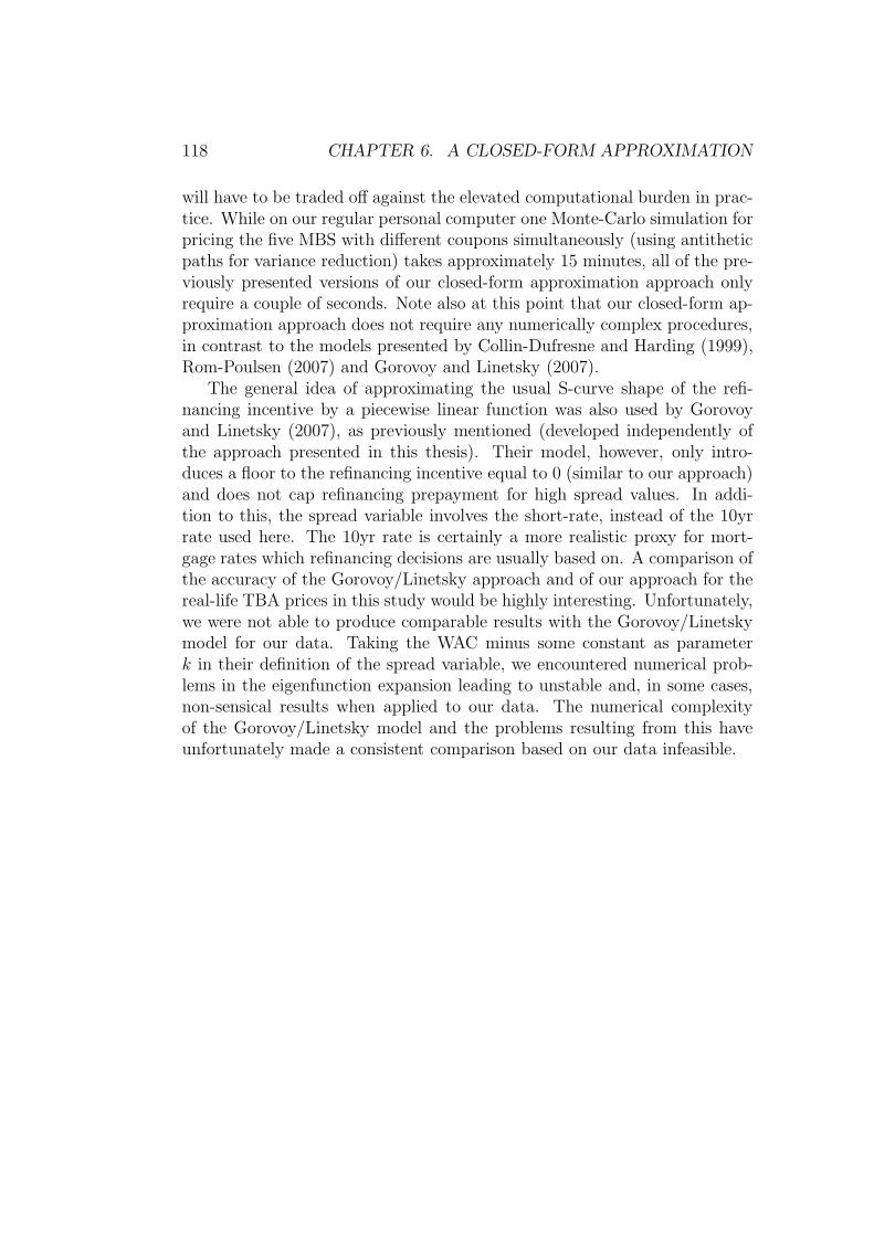
118 CHAPTER 6. A CLOSED-FORM APPROXIMATION
will have to be traded off against the elevated computational burden in prac-tice. While on our regular personal computer one Monte-Carlo simulation forpricing the five MBS with different coupons simultaneously (using antitheticpaths for variance reduction) takes approximately 15 minutes, all of the pre-viously presented versions of our closed-form approximation approach onlyrequire a couple of seconds. Note also at this point that our closed-form ap-proximation approach does not require any numerically complex procedures,in contrast to the models presented by Collin-Dufresne and Harding (1999),Rom-Poulsen (2007) and Gorovoy and Linetsky (2007).
The general idea of approximating the usual S-curve shape of the refi-nancing incentive by a piecewise linear function was also used by Gorovoyand Linetsky (2007), as previously mentioned (developed independently ofthe approach presented in this thesis). Their model, however, only intro-duces a floor to the refinancing incentive equal to 0 (similar to our approach)and does not cap refinancing prepayment for high spread values. In addi-tion to this, the spread variable involves the short-rate, instead of the 10yrrate used here. The 10yr rate is certainly a more realistic proxy for mort-gage rates which refinancing decisions are usually based on. A comparison ofthe accuracy of the Gorovoy/Linetsky approach and of our approach for thereal-life TBA prices in this study would be highly interesting. Unfortunately,we were not able to produce comparable results with the Gorovoy/Linetskymodel for our data. Taking the WAC minus some constant as parameterk in their definition of the spread variable, we encountered numerical prob-lems in the eigenfunction expansion leading to unstable and, in some cases,non-sensical results when applied to our data. The numerical complexityof the Gorovoy/Linetsky model and the problems resulting from this haveunfortunately made a consistent comparison based on our data infeasible.

6.2. APPLICATION TO MARKET DATA 119
Average absolute pricing errorCoupon Closed-form Constant Linear refi- Full MC val.
approx. model baseline incentive model
6% 226 223 380 1126.5% 187 167 142 1157% 141 150 165 104
7.5% 116 126 230 988% 121 139 402 97
Overall 159 166 266 105
Table 6.2: Average absolute pricing errors of our closed-form approximationmodel, of reduced versions of our closed-form approximation model and ofour full Monte-Carlo valuation model for a series of generic GNMA TBApass-throughs (Bloomberg ticker GNSF) with different coupons from 1996to 2006 when the prepayment-risk adjustment parameters are recalibratedonce a year.
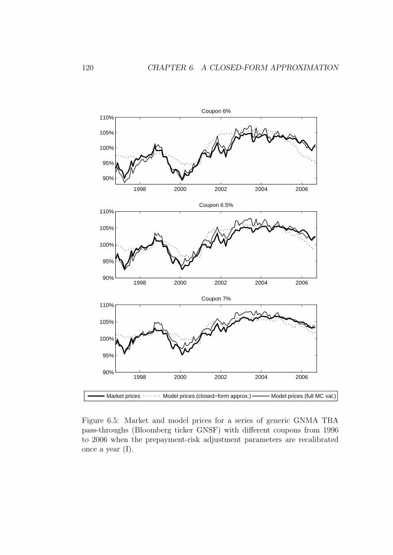
120 CHAPTER 6. A CLOSED-FORM APPROXIMATION
1998 2000 2002 2004 2006
90%
95%
100%
105%
110%Coupon 6%
1998 2000 2002 2004 200690%
95%
100%
105%
110%Coupon 6.5%
1998 2000 2002 2004 200690%
95%
100%
105%
110%Coupon 7%
Market prices Model prices (closed−form approx.) Model prices (full MC val.)
Figure 6.5: Market and model prices for a series of generic GNMA TBApass-throughs (Bloomberg ticker GNSF) with different coupons from 1996to 2006 when the prepayment-risk adjustment parameters are recalibratedonce a year (I).
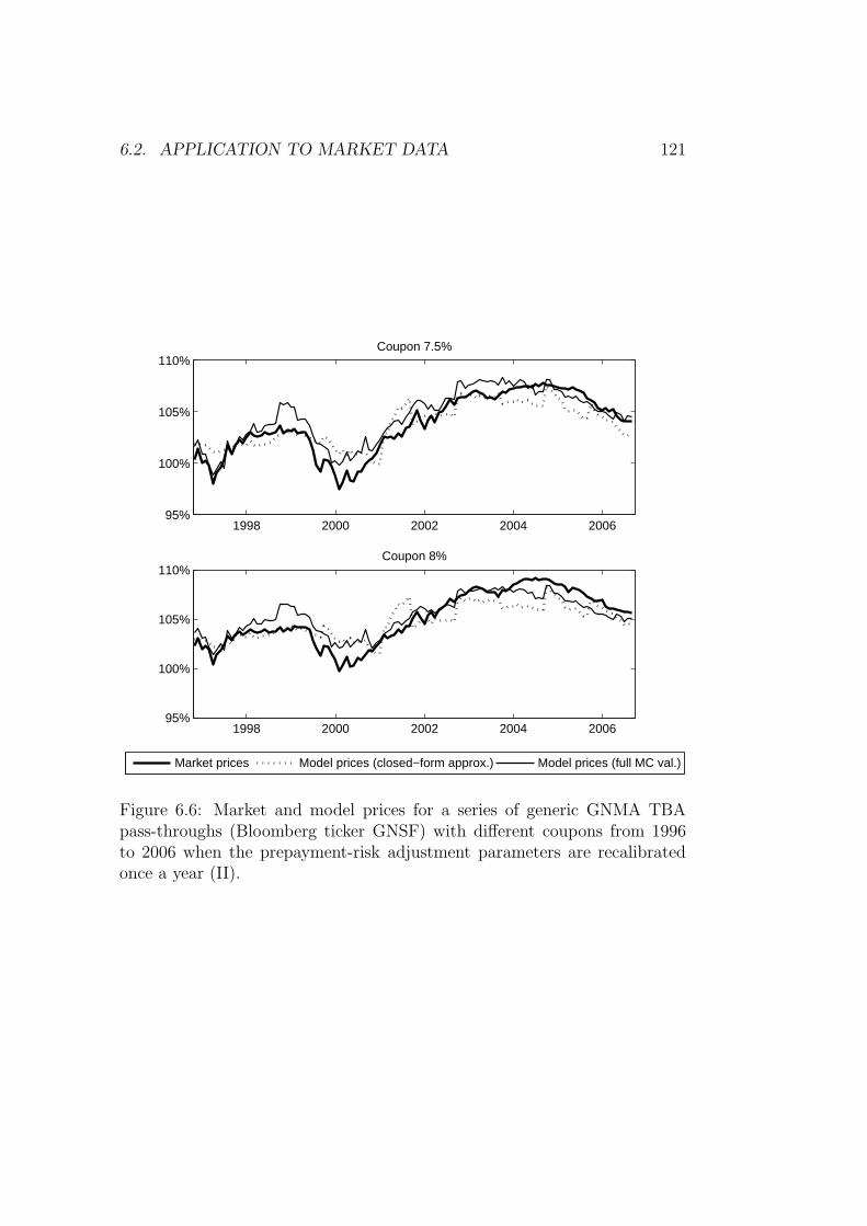
6.2. APPLICATION TO MARKET DATA 121
1998 2000 2002 2004 200695%
100%
105%
110%Coupon 7.5%
1998 2000 2002 2004 200695%
100%
105%
110%Coupon 8%
Market prices Model prices (closed−form approx.) Model prices (full MC val.)
Figure 6.6: Market and model prices for a series of generic GNMA TBApass-throughs (Bloomberg ticker GNSF) with different coupons from 1996to 2006 when the prepayment-risk adjustment parameters are recalibratedonce a year (II).
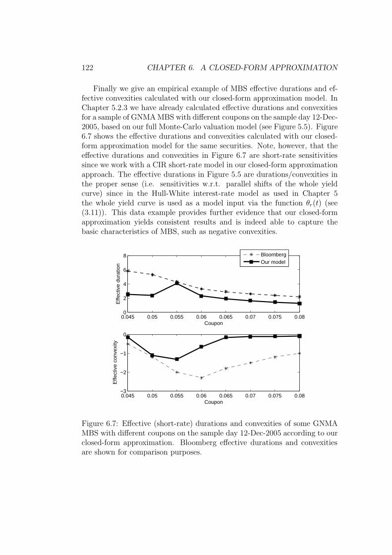
122 CHAPTER 6. A CLOSED-FORM APPROXIMATION
Finally we give an empirical example of MBS effective durations and ef-fective convexities calculated with our closed-form approximation model. InChapter 5.2.3 we have already calculated effective durations and convexitiesfor a sample of GNMA MBS with different coupons on the sample day 12-Dec-2005, based on our full Monte-Carlo valuation model (see Figure 5.5). Figure6.7 shows the effective durations and convexities calculated with our closed-form approximation model for the same securities. Note, however, that theeffective durations and convexities in Figure 6.7 are short-rate sensitivitiessince we work with a CIR short-rate model in our closed-form approximationapproach. The effective durations in Figure 5.5 are durations/convexities inthe proper sense (i.e. sensitivities w.r.t. parallel shifts of the whole yieldcurve) since in the Hull-White interest-rate model as used in Chapter 5the whole yield curve is used as a model input via the function θr(t) (see(3.11)). This data example provides further evidence that our closed-formapproximation yields consistent results and is indeed able to capture thebasic characteristics of MBS, such as negative convexities.
0.045 0.05 0.055 0.06 0.065 0.07 0.075 0.080
2
4
6
8
Coupon
Effe
ctiv
e du
ratio
n
0.045 0.05 0.055 0.06 0.065 0.07 0.075 0.08−3
−2
−1
0
Coupon
Effe
ctiv
e co
nvex
ity
BloombergOur model
Figure 6.7: Effective (short-rate) durations and convexities of some GNMAMBS with different coupons on the sample day 12-Dec-2005 according to ourclosed-form approximation. Bloomberg effective durations and convexitiesare shown for comparison purposes.
Chapter 7
The contribution of our MBSpricing models
’All models are wrong, but some are useful.’ (Box (1979))
In Chapter 4 we have motivated the need for further research concerning MBSvaluation. In this chapter we will briefly summarise what has been achievedin this thesis. In particular, we will comparatively assess the contribution ofour MBS pricing models and discuss the implications for their use in practice.
7.1 A comparative assessment
In the previous two chapters we have presented pricing models for agencyMBS within an intensity-based modelling framework. In particular, we haveextended the general model framework presented by Kau et al. (2004) forindividual mortgage contracts to the pricing of MBS. Moreover, our modelexplicitly accounts for the general economic environment by the incorpora-tion of a factor into the baseline hazard process which is fitted to the GDPgrowth rate. We have called our model ’prepayment-risk-neutral’ since we areable to directly target market prices and thus do not need the theoreticallydubious OAS in the pricing procedure. This is achieved by the introductionof prepayment-risk adjustment parameters which stem from the change ofmeasure from the real-world measure to a risk-neutral pricing measure. Wehave shown that these prepayment-risk adjustment parameters can be cal-ibrated to MBS market prices to obtain ’implied’ prepayment patterns, inthe sense of Levin and Davidson (2005). Our model therefore has the desir-able features of the Levin/Davidson model combined with the mathematicalrigour of the intensity-based modelling framework.
123
124 CHAPTER 7. CONTRIBUTION OF OUR MODELS
Furthermore, we have derived a closed-form approximation formula forthe pricing of fixed-rate agency MBS with a slightly adjusted model speci-fication. Our closed-form approximation is computationally highly efficientand reduces the computational burden of MBS valuation drastically. Ourapproach may thus be particularly useful for risk and portfolio manage-ment purposes where portfolios of MBS have to be revaluated frequently(see also the application in Chapter 8). Our approach offers a couple of ad-vantages compared to previous models concerned with closed-form valuationof MBS. Compared to the closed-form formula for MBS by Collin-Dufresneand Harding (1999), our model offers two major extensions. First, we arenot restricted to a single stochastic factor. In addition to our 1-factor CIRinterest-rate model we introduce two additional stochastic factors to modelthe baseline prepayment. Moreover, we do not approximate the usual S-like relation between coupon spread and refinancing-related prepayment by apurely linear functional form but introduce a piecewise linear approximation.Our results indicate that this contributes to a significant improvement of themodel performance. While these two issues are also explicitly addressed ina recent extension of the Collin-Dufresne/Harding model by Rom-Poulsen(2007), we do not encounter the (theoretical) weaknesses of the quadraticinterest-rate/refinancing relation in the Rom-Poulsen model for certain sce-narios. Moreover, both the Collin-Dufresne/Harding and the Rom-Poulsenmodel require numerical techniques to solve systems of partial differentialequations. These models can thus only be considered as semi-analytic. Nu-merical complexity is also a problem in the recently developed model byGorovoy and Linetsky (2007), as previously mentioned. While their approachoffers an ’exact’ solution within a quite similar model set-up compared to ourapproximation, the computation of this formula involves highly complex nu-merical evaluations related to eigenfunction expansion techniques.
Applied to historical price data of 30yr GNMA pass-throughs traded ona TBA basis, our closed-form approximation formula proved to be able totrack market price movements for a wide range of coupons with an overallaverage absolute pricing error of 159 basis points (with a yearly recalibra-tion of prepayment-risk adjustment parameters as described in the previouschapter). We consider this a highly satisfactory accuracy, in particular forrisk and portfolio management purposes.
A direct quantitative comparison of the performance of different MBSpricing models across the different model classes is a hardly feasible task.Such a comparison would require a well-defined criterion how model perfor-mance can be measured. A natural choice for such a criterion would of coursebe the models’ ability to explain market prices in the spirit of our empiri-cal evaluation in Chapter 6.2.2. Yet, the traditional econometric models do
7.1. A COMPARATIVE ASSESSMENT 125
not target market prices directly, but calculate the OAS as a model output.As previously mentioned, OAS levels derived from different prepayment andinterest-rate model assumptions may differ substantially and it is impossibleto say what the ’correct’ OAS is. Econometric models, however, aim to pre-dict real-life prepayment behaviour. Different traditional econometric mod-els, such as the models developed by Schwartz and Torous (1989) or Richardand Roll (1989) could thus be quantitatively compared by some purely sta-tistical goodness-of-fit criterion applied to historically observed and fittedprepayment rates. However, prepayment-risk-neutral models like the modeldeveloped by Levin and Davidson (2005) or like our modelling approach, arenot primarily meant to predict prepayment in real-life. They are in line withcommon derivative pricing principles, where implied parameter patterns (andthus implied prepayment patterns in our case) are obtained after calibratingthe model to market data. This fact is also discussed in Levin and Davidson(2005). A pure look at the ability of a model to explain market prices (possi-bly in-sample and out-of-sample) may equally be too single-minded, since itwould not take into account another issue which is of critical importance inpractice: computational burden. The computational burden is, however, initself not an easily comparable criterion. As previously discussed, MBS val-uation models, except the ones concerned with closed-form approximations,usually rely on either Monte-Carlo simulation or on backward induction tech-niques on multidimensional grids. The CPU time required for a Monte-Carlosimulation depends heavily on the concrete implementation, e.g. on the vari-ance reduction technique(s) used in the Monte-Carlo algorithm. And viceversa, the success of one particular variance reduction method will heavilydepend on the model specification. While, generally speaking, backwardinduction methods are usually faster than Monte-Carlo simulations, a well-implemented Monte-Carlo simulation can of course be faster than a poorlyimplemented backward induction scheme. This also depends substantiallyon the number of stochastic factors in the model.
Due to the lack of comparison criteria and consistent comparison stan-dards, a quantitative model comparison is hardly feasible. Yet, in the re-mainder of this section, we want to assess our modelling approach quali-tatively with respect to certain criteria compared to some selected modelsfrom each of the three model classes. Of course, this assessment can onlybe general in nature and has to be based on subjective perceptions to a cer-tain extent. Within the econometric model class we choose the Schwartzand Torous (1989) model. We furthermore include the Stanton (1995) modelas a representative example of the option-theoretic model class and the re-cently developed Gorovoy and Linetsky (2007) model from the intensity-based model class into this qualitative assessment. We finally include the
126 CHAPTER 7. CONTRIBUTION OF OUR MODELS
Levin and Davidson (2005) and Collin-Dufresne and Harding (1999) modelssince we have frequently cited them in the previous chapters. The results ofour qualitative assessment, based on the author’s best and honest judgementaccording to the discussions in the Chapters 4-7, are presented in Table 7.1.As comparison criteria we consider the mathematical rigour of the pricingroutine, the numerical complexity, the computational burden for the pricingof MBS pass-throughs, the flexibility of the models to include further ex-planatory factors or variables into the prepayment specification and finally,the flexibility with respect to extensions of the model to non-standard struc-tures such as adjustable-rate securities and CMOs. The mathematical rigourof the Schwartz and Torous (1989) model is arguable since this model im-plicitly needs the assumption that a prepayment function estimated underthe real-world measure can be used for pricing purposes. This is a highlyproblematic assumption as our empirical results in Chapter 5 indicate. TheCollin-Dufresne and Harding (1999) model has the undesirable feature thatrefinancing prepayment can become negative in a high interest-rate envi-ronment. While we consider our closed-form approximation mathematicallysound, it is still an approximation and can thus not be preferred to ’exact’approaches if mathematical rigour is the only selection criterion. We havealready discussed the issue of numerical complexity extensively. Apart fromthe closed-form pricing approaches, all other models are rather straightfor-ward to implement so that numerical complexity should not be an issue. Theremaining three criteria are particularly important for potential uses in prac-tice. While the closed-form approaches are of course particularly appealingwith respect to computational burden of pass-through pricing, they can noteasily be extended to include new factors or explanatory variables which aparticular user of the model may want to include. Nor can they be usedstraightforwardly for the pricing of non-standard MBS structures. The sameholds in general for option-theoretic models which work with pricing routines
on grids. The only group of models where these extensions are ratherstraightforward is the one based on Monte-Carlo simulation routines, suchas our full Monte-Carlo valuation model presented in Chapter 5.

7.1.A
CO
MPA
RA
TIV
EA
SSE
SSM
EN
T127
Other models in the literature Our models
Sch
war
tz/T
orou
s(1
989)
Sta
nton
(199
5)
Gor
ovoy
/Lin
etsk
y(2
007)
Lev
in/D
avid
son
(200
5)
Col
lin-D
ufres
ne/
Har
din
g(1
999)
Full
MC
-sim
ula
tion
Clo
sed-for
map
pro
xim
atio
n
Mathematical rigour −− ++ ++ 0 + ++ +of pricing logic
Numerical ++ ++ −− ++ − ++ ++complexity
Comput. burden of −− − ++ − ++ −− ++pass-through pricing
Flexibility w.r.t.new factors/variables ++ − 0 ++ − ++ 0in prepayment model
Flexibility w.r.t. pricingof adjustable-rate MBS & ++ − −− ++ −− ++ −−
pay-through structures (CMOs)
Table 7.1: Qualitative assessment of different agency MBS pricing models with respect to some desirable modelfeatures. Grades range from ++ (very good), 0 (some good, some problematic aspects) to −− (highly problematic).
128 CHAPTER 7. CONTRIBUTION OF OUR MODELS
7.2 Implications for the use in practice
After the analysis in the previous chapters, the question of which model isthe ’best’, in particular with a view towards the use in practice, still remainsopen. In the previous section we have already highlighted that the questionis, in its general sense, highly problematic. This is due to the lack of a con-sistent optimality criterion which is needed to be able to select the ’best’among all MBS pricing models.
From the previous discussion we can conclude that the choice of a pric-ing model in practice should be based on the purpose, i.e. the applicationthe MBS model is used for. With our closed-form approximation formula aspresented in Chapter 6 we have developed a computationally very efficientand thus very useful tool for applications in risk and portfolio managementof fixed-rate agency MBS in practice. An example of how our model canbe applied to portfolio management with MBS will be given in Chapter 8.However, the closed-form formula can not be extended straightforwardly tothe pricing of complex pay-through structures, i.e. of CMOs. For these se-curities, a computational more expensive valuation method, such as Monte-Carlo simulation based on, e.g., our model presented in Chapter 5, can notbe avoided. Also, if time is not a critical factor and the valuation should beas accurate as possible, we recommend to use our full Monte-Carlo valuationmodel, which may be enhanced and statistically fine-tuned with additionalexplanatory variables, if desired.
Both, our prepayment-risk neutral valuation model as presented in Chap-ter 5 and the closed-form approximation in Chapter 6 offer the possibility totarget market prices directly. This is a desirable feature in risk managementsince it eliminates the discussion of whether the OAS must be treated asa risk factor. Many risk measures commonly used in the MBS market areusually calculated with a constant OAS assumption (e.g., the calculation ofthe effective duration and effective convexity of a MBS with a traditionaleconometric valuation model). Yet, the question whether the OAS shouldbe considered as a constant or not is of course equivalent to the questionof parameter stability (in particular, w.r.t. the prepayment-risk adjustmentparameters) in our modelling approach.
Finally, it should be pointed out that MBS where the mortgagors canbe assumed to prepay optimally should definitely be valued with an option-theoretic model based on pricing routines for callable bonds. Optimal pre-payment can, however, only be expected in the institutional market, e.g.,when the mortgages are not residential but commercial. The treatment ofcommercial MBS is beyond the scope of this thesis.
Chapter 8
Optimal portfolios with MBS
As already mentioned in the first chapters of this thesis, mortgage-backedsecurities constitute a large and important segment of the US fixed-incomemarket. The total outstanding volume of MBS in the US has surpassed byfar the outstanding volume of US treasuries. MBS are thus an importantasset class and are in fact very popular among institutional investors. Whileagency MBS feature nearly the same credit quality as US treasuries - in par-ticular, GNMA securities have the full faith and credit of the US government-they often offer higher yields. Hence their popularity with investors.
Going back to the seminal work of Markowitz (1952), the question of howto build an optimal portfolio from a given set of different assets, consideringdifferent constraints and optimality criteria, is a well-studied problem (see,e.g., Meucci (2005) for a textbook covering a wide range of aspects of modernportfolio optimisation). In the majority of studies, however, the asset classesconsidered were stocks and regular bonds. More recent publications havealso included alternative assets such as hedge funds or real estate investmenttrusts (REITs) (see, e.g., Krokhmal et al. (2002) or Hocht et al. (2007)).Yet, an inclusion of MBS into portfolio optimisation problems remains rare.One exception is the work based on Zenios (1993), Zenios and Kang (1993)and McKendall et al. (1993) who consider portfolio optimisation with MBS,mainly in an asset-liability management context. The major reason whyMBS are usually not considered in portfolio optimisation problems is thecomputational burden associated with MBS valuation. Since most modernportfolio optimisation problems are also computationally expensive and re-quire frequent evaluation of the assets under different scenarios, the inclusionof MBS into portfolio optimisation problems has often been infeasible. McK-endall et al. (1993) use a recombining tree to create interest-rate scenarios,so that for a buy-and-hold static optimisation problem, the number of re-quired MBS valuations is limited due to the limited number of nodes in the
129
130 CHAPTER 8. OPTIMAL PORTFOLIOS WITH MBS
tree. However, when considering other correlated asset classes, such as equi-ties, the nodes in the tree grow exponentially and the optimisation problemmay again become computationally infeasible. This is particularly true if onewants to consider the possibility of asset reallocation during the investmenthorizon.
Our closed-form approximation approach as presented in Chapter 6 nowoffers a possibility to overcome the computational burden associated withportfolio optimisation with MBS. It is the main objective in this chapterto consider some selected portfolio optimisation approaches based on sim-ulated scenarios and to extend their usual application by including fixed-rate agency-MBS with different coupons. We thereby hope to close a gapin the applied portfolio optimisation literature where MBS have long beenneglected. Within a consistent simulation framework, we show how the inclu-sion of MBS into a classical stock/bond portfolio can enhance total returns.For this purpose we also apply our approach to real historical market datain an empirical case study. We show how optimal portfolios according to anexpected utility criterion and to a conditional value-at-risk (CVaR) criteriondevelop and perform over time, respectively, based on a static multi-periodasset allocation strategy with a rolling one year investment horizon.
In the following section we present the available assets for our study andgive details of the scenario simulation procedure used for portfolio optimisa-tion. We then consider the expected utility optimisation approach and theportfolio optimisation with CVaR constraints and apply these concepts tohistorical data in an empirical study.
8.1 The set-up: assets and scenarios
Of course, there are countless ways of combining possible assets and portfoliooptimisation settings. Concerning the assets, we therefore concentrate on aspecific set of assets which we believe to be quite representative. We assumethat the investor has the choice between a total of six assets. The S&P 500index represents the equity class, non-defaultable zero-coupon bonds with 3and 10 years to maturity constitute the available bonds. In addition to theseinstruments we allow the investor to invest in three different 30yr fixed-rateGNMA pass-through MBS with coupons of 6%, 7% and 8%, respectively.While we will consider different optimisation problems in the following sec-tion, we always restrict the investment horizon to one year. We do notconsider transaction costs, which is not a too unrealistic assumption sincewe only deal with very liquid instruments for which transaction costs for in-stitutional investors may indeed be negligible.
8.1. ASSETS AND SCENARIOS 131
Since we work with optimisation approaches based on simulated scenar-ios, we have to specify the distributional assumptions for the processes un-derlying the assets. We model the evolution of the equity index S(t) witha geometric Brownian motion in the usual way, correlated to interest rates.For the interest-rate dynamics we use a one-factor CIR model as in Chapter6 where the short-rate r(t) has the dynamics (under the real-world measureQ)
dr(t) = (θr − arr(t))dt + σr
√r(t)dW (t) (8.1)
for some positive constants θ, ar, σr with 2θ > σ2r . The (real-world) equity
index dynamics are given by
dS(t) = µS(t)dt + σSS(t)dZ(t) (8.2)
for some positive constants µ, σS and we assume that the Wiener processesW (t) and Z(t) are correlated such that
Cov[dW (t), dZ(t)] = ρdt.
By Cholesky decomposition (see, e.g., Brigo and Mercurio (2006), p. 886),we can rewrite (8.1) and (8.2) in the following way:
dr(t) = (θr − arr(t))dt + σr
√r(t)dW (t)
dS(t) = µS(t)dt + σSρS(t)dW (t) + σSS(t)√
1 − ρ2dZ(t) (8.3)
for two uncorrelated Wiener processes W (t), Z(t). For the estimation ofthe parameters in (8.3) we use historical weekly return data of the S&P 500index from 1996 to 2005 and weekly US treasury strip rates, obtained frompar rates by standard bootstrapping, of the same time period. We use a two-stage procedure for parameter estimation, similar in spirit to the approachtaken in Zagst (2002b). In the first stage we determine the parameters of theinterest-rate process and of the stock index process. For the parameters ofthe CIR interest-rate model we use the values as already reported in Table6.1. For the estimation of the parameters of the stock index process, notethat it follows from the Ito-formula that a discretised version of the dynamicsof the log-returns of the stock index is given by:
lnS(t + ∆t)
S(t)= (µ − 1
2σ2
S) · ∆t + σSρ√
∆t · N1 + σS
√1 − ρ2
√∆t · N2,
where N1, N2 are two independent standard-normal random variables. Thus,the log-returns of the stock index are normally distributed with
E
[ln
S(t + ∆t)
S(t)
]= (µ − 1
2σ2
S) · ∆t (8.4)
V ar
[ln
S(t + ∆t)
S(t)
]= σ2
Sρ2 · ∆t + σ2S(√
1 − ρ2)2 · ∆t = σ2S · ∆t. (8.5)
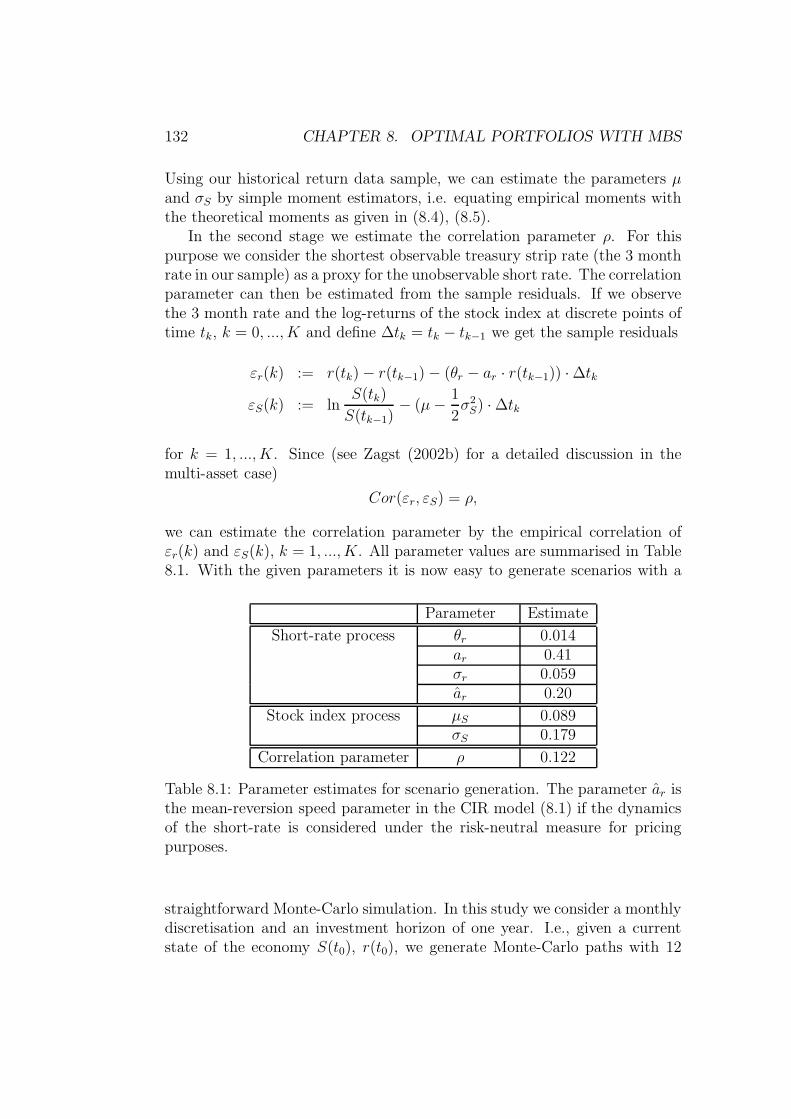
132 CHAPTER 8. OPTIMAL PORTFOLIOS WITH MBS
Using our historical return data sample, we can estimate the parameters µand σS by simple moment estimators, i.e. equating empirical moments withthe theoretical moments as given in (8.4), (8.5).
In the second stage we estimate the correlation parameter ρ. For thispurpose we consider the shortest observable treasury strip rate (the 3 monthrate in our sample) as a proxy for the unobservable short rate. The correlationparameter can then be estimated from the sample residuals. If we observethe 3 month rate and the log-returns of the stock index at discrete points oftime tk, k = 0, ..., K and define ∆tk = tk − tk−1 we get the sample residuals
εr(k) := r(tk) − r(tk−1) − (θr − ar · r(tk−1)) · ∆tk
εS(k) := lnS(tk)
S(tk−1)− (µ − 1
2σ2
S) · ∆tk
for k = 1, ..., K. Since (see Zagst (2002b) for a detailed discussion in themulti-asset case)
Cor(εr, εS) = ρ,
we can estimate the correlation parameter by the empirical correlation ofεr(k) and εS(k), k = 1, ..., K. All parameter values are summarised in Table8.1. With the given parameters it is now easy to generate scenarios with a
Parameter Estimate
Short-rate process θr 0.014ar 0.41σr 0.059ar 0.20
Stock index process µS 0.089σS 0.179
Correlation parameter ρ 0.122
Table 8.1: Parameter estimates for scenario generation. The parameter ar isthe mean-reversion speed parameter in the CIR model (8.1) if the dynamicsof the short-rate is considered under the risk-neutral measure for pricingpurposes.
straightforward Monte-Carlo simulation. In this study we consider a monthlydiscretisation and an investment horizon of one year. I.e., given a currentstate of the economy S(t0), r(t0), we generate Monte-Carlo paths with 12

8.1. ASSETS AND SCENARIOS 133
(monthly) grid points using the discretised version of (8.3)
r(tk) = r(tk−1) + (θ − arr(tk−1))∆tk + σr
√r(tk−1) ·
√∆tk · N1
S(tk) = S(tk−1) · e(µS− 12σ2
S)·∆tk+σS ·ρ·
√∆tk·N1+σS ·
√1−ρ2·√∆tk·N2 ,
for k = 1, ..., 12, where N1, N2 are again two independently drawn standard-normal random variables. Note that the discretisation method for r(t) usedhere is the simple Euler scheme as also used in, e.g., Zagst (2002b).
Given a state of the short rate r(t), the price
P (t, T ) := E eQ[e−R Tt
r(s)ds|Ft]
of a zero-coupon bond with maturity T at time t and notional 1 is givenin the CIR interest-rate model by (3.23). For the pricing of the mortgage-backed securities and for the generation of prepayment scenarios we use theclosed-form approximation approach developed in Chapter 6. Due to its com-putational efficiency, the closed-form pricing approach makes an integrationof MBS into a scenario-based portfolio optimisation feasible within a reason-able time frame. For the prepayment scenarios, we first have to generatescenarios for the (annualised, continuous) baseline prepayment process π0(t).We obtain from (6.17) after Euler discretisation:
π0(tk) = π0(tk−1) + (θp + bpww(tk) − apπ0(tk−1))∆tk + σp ·√
∆tk · N3,
w(tk) = w(tk−1) + (θw − aww(tk−1))∆tk + σw · N4,
where N3, N4 are two independently drawn standard-normal random vari-ables. In addition to the baseline prepayment, we obtain the (annualised,continuous) refinancing prepayment speed
πrefi(t) = 5.6 · max(min(WAC − R10(t), 0.04), 0),
where WAC is the security’s weighted average coupon and R10(t) is the 10-year treasury zero rate calculated according to the CIR interest-rate model.The overall prepayment speed
π(t) = πrefi(t) + π0(t)
has to be converted into the usual constant prepayment rate (CPR) by
CPR(t) = eπ(t) − 1
and we finally obtain the overall single monthly mortality by
SMM(t) = 1 − (1 − CPR(t))112 .
134 CHAPTER 8. OPTIMAL PORTFOLIOS WITH MBS
With the parameters as given in Table 6.1 the single monthly mortalities varyin the range between 1% and 6% for the three different MBS in 1000 simulatedinterest-rate and prepayment scenarios (if we take the short-rate level asof March 2001 and the mean-reversion level of the baseline prepayment asstarting values for the scenario generation). Recall that since the pricingapproach targets market prices directly, no OAS input is required for theMBS valuation. We calibrate the prepayment-risk-adjustment parameters ofour closed-form approximation model to market prices of GNMA securitieswith different coupons, traded on a to-be-announced (TBA) basis, on thestart date of the scenario generation.
8.2 Scenario-based portfolio optimisation
with MBS
For the empirical part of this study we focus on the time horizon from spring2001 to spring 2003, since this was an interesting time period in the US fixed-income market in general and in the MBS market in particular. Interestrates decreased sharply during this time period, the 1yr treasury zero-ratedropped from levels around 4.2% in March 2001 to about 1.1% in March2003. The 10yr rate slid from 5.3% to 4.1% during the same time period.This decrease in interest rates triggered a significant increase in prepayments(see also Figure 2.1). MBS which were traded in the discount area in spring2001 became premiums in the subsequent months. E.g., a 6% coupon GNMAsecurity was traded at 98.14% in March 2001 and at 103.94% in March 2003(see Figure 8.1). The development of the S&P 500 index and of the 3 monthtreasury strip rate during the same time period is shown in Figure 8.2. Byleaving the universe of available instruments for our portfolio optimisationprocedure unchanged, we can see the effects of these changes in the economicenvironment on the optimal portfolios. We select an optimal portfolio eachmonth, between March 2001 and February 2003 with an investment horizonof one year in any case. Our empirical case study is thus equivalent to anoptimal portfolio allocation strategy with monthly rebalancing, based on arolling one year investment horizon from March 2001 to March 2003.
The returns of the assets along each scenario path are calculated bytaking into account the prices, amortisation factors and cash flows of theinstruments. Similar to McKendall et al. (1993) we calculate the (scenario-dependent) total return of an investment of 1 in the j-th instrument over the
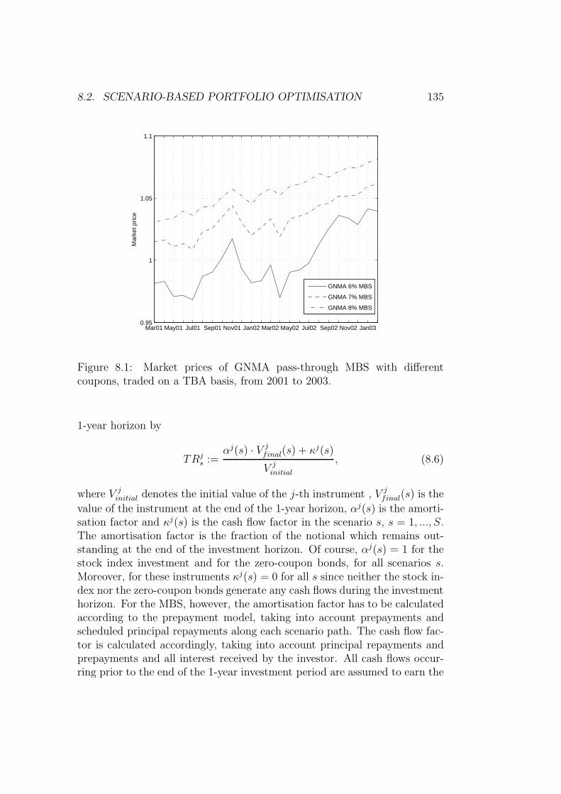
8.2. SCENARIO-BASED PORTFOLIO OPTIMISATION 135
Mar01 May01 Jul01 Sep01 Nov01 Jan02 Mar02 May02 Jul02 Sep02 Nov02 Jan030.95
1
1.05
1.1M
arke
t pric
e
GNMA 6% MBS
GNMA 7% MBS
GNMA 8% MBS
Figure 8.1: Market prices of GNMA pass-through MBS with differentcoupons, traded on a TBA basis, from 2001 to 2003.
1-year horizon by
TRjs :=
αj(s) · V jfinal(s) + κj(s)
V jinitial
, (8.6)
where V jinitial denotes the initial value of the j-th instrument , V j
final(s) is the
value of the instrument at the end of the 1-year horizon, αj(s) is the amorti-sation factor and κj(s) is the cash flow factor in the scenario s, s = 1, ..., S.The amortisation factor is the fraction of the notional which remains out-standing at the end of the investment horizon. Of course, αj(s) = 1 for thestock index investment and for the zero-coupon bonds, for all scenarios s.Moreover, for these instruments κj(s) = 0 for all s since neither the stock in-dex nor the zero-coupon bonds generate any cash flows during the investmenthorizon. For the MBS, however, the amortisation factor has to be calculatedaccording to the prepayment model, taking into account prepayments andscheduled principal repayments along each scenario path. The cash flow fac-tor is calculated accordingly, taking into account principal repayments andprepayments and all interest received by the investor. All cash flows occur-ring prior to the end of the 1-year investment period are assumed to earn the
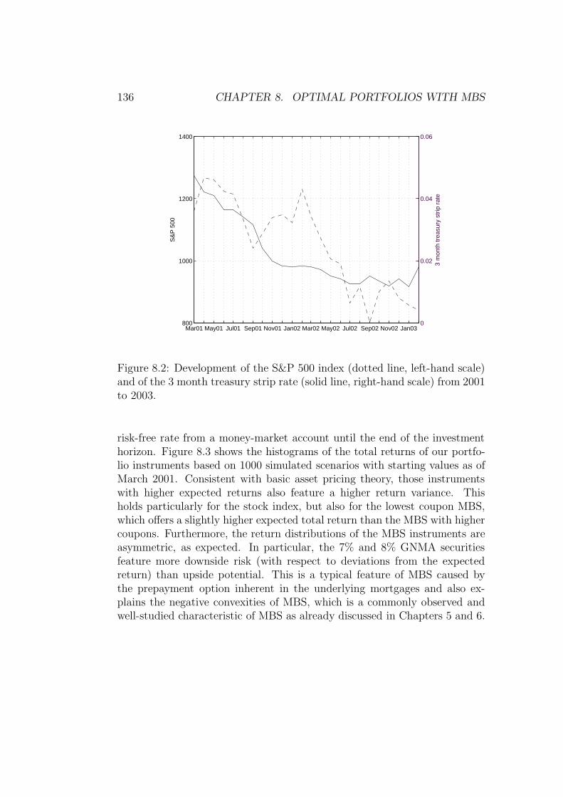
136 CHAPTER 8. OPTIMAL PORTFOLIOS WITH MBS
800
1000
1200
1400
S&
P 5
00
Mar01 May01 Jul01 Sep01 Nov01 Jan02 Mar02 May02 Jul02 Sep02 Nov02 Jan030
0.02
0.04
0.06
3 m
onth
trea
sury
str
ip r
ate
Figure 8.2: Development of the S&P 500 index (dotted line, left-hand scale)and of the 3 month treasury strip rate (solid line, right-hand scale) from 2001to 2003.
risk-free rate from a money-market account until the end of the investmenthorizon. Figure 8.3 shows the histograms of the total returns of our portfo-lio instruments based on 1000 simulated scenarios with starting values as ofMarch 2001. Consistent with basic asset pricing theory, those instrumentswith higher expected returns also feature a higher return variance. Thisholds particularly for the stock index, but also for the lowest coupon MBS,which offers a slightly higher expected total return than the MBS with highercoupons. Furthermore, the return distributions of the MBS instruments areasymmetric, as expected. In particular, the 7% and 8% GNMA securitiesfeature more downside risk (with respect to deviations from the expectedreturn) than upside potential. This is a typical feature of MBS caused bythe prepayment option inherent in the underlying mortgages and also ex-plains the negative convexities of MBS, which is a commonly observed andwell-studied characteristic of MBS as already discussed in Chapters 5 and 6.
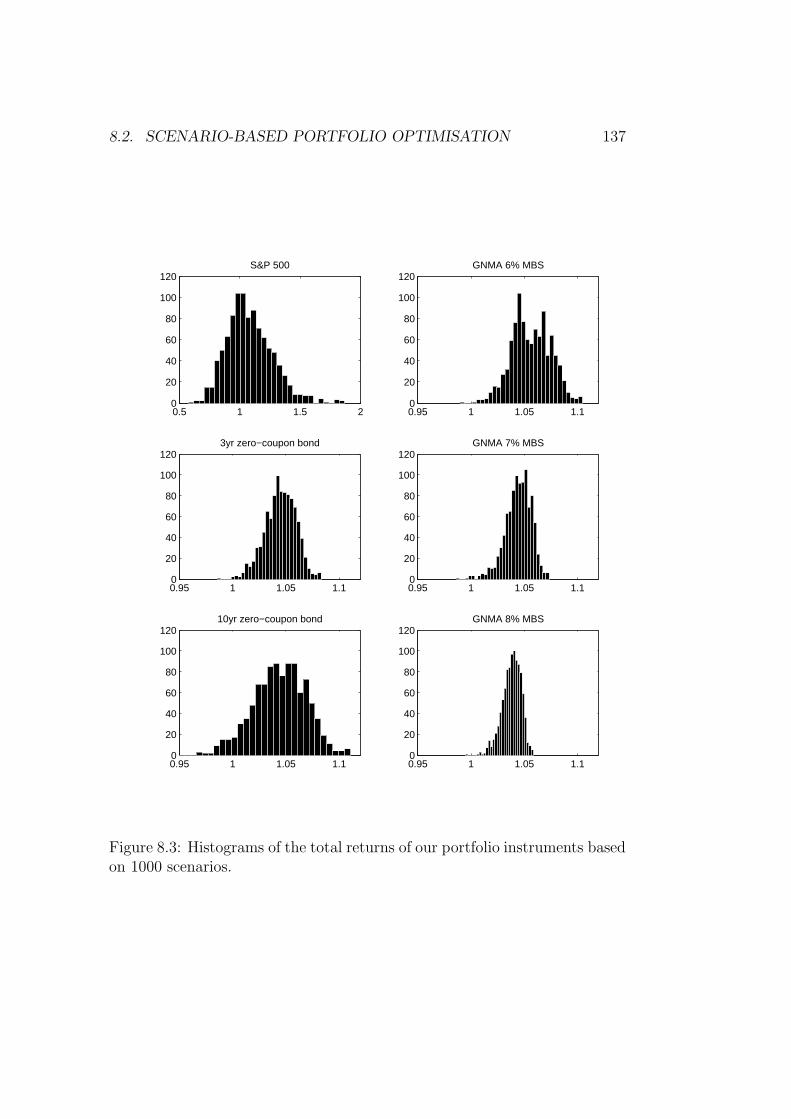
8.2. SCENARIO-BASED PORTFOLIO OPTIMISATION 137
0.5 1 1.5 20
20
40
60
80
100
120S&P 500
0.95 1 1.05 1.10
20
40
60
80
100
1203yr zero−coupon bond
0.95 1 1.05 1.10
20
40
60
80
100
12010yr zero−coupon bond
0.95 1 1.05 1.10
20
40
60
80
100
120GNMA 6% MBS
0.95 1 1.05 1.10
20
40
60
80
100
120GNMA 7% MBS
0.95 1 1.05 1.10
20
40
60
80
100
120GNMA 8% MBS
Figure 8.3: Histograms of the total returns of our portfolio instruments basedon 1000 scenarios.
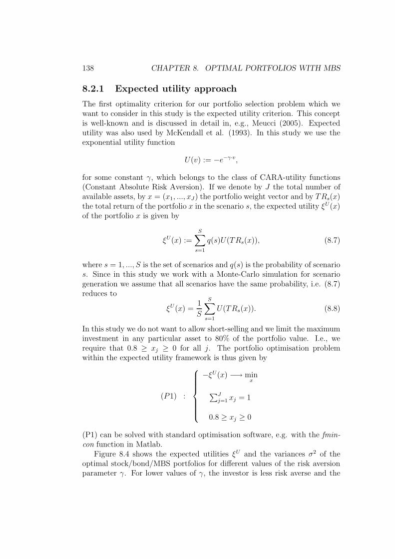
138 CHAPTER 8. OPTIMAL PORTFOLIOS WITH MBS
8.2.1 Expected utility approach
The first optimality criterion for our portfolio selection problem which wewant to consider in this study is the expected utility criterion. This conceptis well-known and is discussed in detail in, e.g., Meucci (2005). Expectedutility was also used by McKendall et al. (1993). In this study we use theexponential utility function
U(v) := −e−γ·v,
for some constant γ, which belongs to the class of CARA-utility functions(Constant Absolute Risk Aversion). If we denote by J the total number ofavailable assets, by x = (x1, ..., xJ) the portfolio weight vector and by TRs(x)the total return of the portfolio x in the scenario s, the expected utility ξU(x)of the portfolio x is given by
ξU(x) :=S∑
s=1
q(s)U(TRs(x)), (8.7)
where s = 1, ..., S is the set of scenarios and q(s) is the probability of scenarios. Since in this study we work with a Monte-Carlo simulation for scenariogeneration we assume that all scenarios have the same probability, i.e. (8.7)reduces to
ξU(x) =1
S
S∑
s=1
U(TRs(x)). (8.8)
In this study we do not want to allow short-selling and we limit the maximuminvestment in any particular asset to 80% of the portfolio value. I.e., werequire that 0.8 ≥ xj ≥ 0 for all j. The portfolio optimisation problemwithin the expected utility framework is thus given by
(P1) :
−ξU(x) −→ minx
∑Jj=1 xj = 1
0.8 ≥ xj ≥ 0
(P1) can be solved with standard optimisation software, e.g. with the fmin-con function in Matlab.
Figure 8.4 shows the expected utilities ξU and the variances σ2 of theoptimal stock/bond/MBS portfolios for different values of the risk aversionparameter γ. For lower values of γ, the investor is less risk averse and the
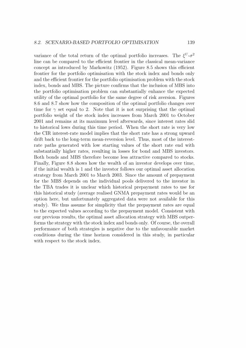
8.2. SCENARIO-BASED PORTFOLIO OPTIMISATION 139
variance of the total return of the optimal portfolio increases. The ξU -σ2
line can be compared to the efficient frontier in the classical mean-varianceconcept as introduced by Markowitz (1952). Figure 8.5 shows this efficientfrontier for the portfolio optimisation with the stock index and bonds onlyand the efficient frontier for the portfolio optimisation problem with the stockindex, bonds and MBS. The picture confirms that the inclusion of MBS intothe portfolio optimisation problem can substantially enhance the expectedutility of the optimal portfolio for the same degree of risk aversion. Figures8.6 and 8.7 show how the composition of the optimal portfolio changes overtime for γ set equal to 2. Note that it is not surprising that the optimalportfolio weight of the stock index increases from March 2001 to October2001 and remains at its maximum level afterwards, since interest rates slidto historical lows during this time period. When the short rate is very lowthe CIR interest-rate model implies that the short rate has a strong upwarddrift back to the long-term mean-reversion level. Thus, most of the interest-rate paths generated with low starting values of the short rate end withsubstantially higher rates, resulting in losses for bond and MBS investors.Both bonds and MBS therefore become less attractive compared to stocks.Finally, Figure 8.8 shows how the wealth of an investor develops over time,if the initial wealth is 1 and the investor follows our optimal asset allocationstrategy from March 2001 to March 2003. Since the amount of prepaymentfor the MBS depends on the individual pools delivered to the investor inthe TBA trades it is unclear which historical prepayment rates to use forthis historical study (average realised GNMA prepayment rates would be anoption here, but unfortunately aggregated data were not available for thisstudy). We thus assume for simplicity that the prepayment rates are equalto the expected values according to the prepayment model. Consistent withour previous results, the optimal asset allocation strategy with MBS outper-forms the strategy with the stock index and bonds only. Of course, the overallperformance of both strategies is negative due to the unfavourable marketconditions during the time horizon considered in this study, in particularwith respect to the stock index.
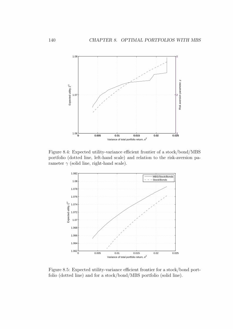
140 CHAPTER 8. OPTIMAL PORTFOLIOS WITH MBS
0 0.005 0.01 0.015 0.02 0.0251.06
1.07
1.08
Exp
ecte
d ut
ility
, ξU
Variance of total portfolio return, σ20 0.005 0.01 0.015 0.02 0.025
0
2
4
Ris
k av
ersi
on p
aram
eter
, γ
Figure 8.4: Expected utility-variance efficient frontier of a stock/bond/MBSportfolio (dotted line, left-hand scale) and relation to the risk-aversion pa-rameter γ (solid line, right-hand scale).
0 0.005 0.01 0.015 0.02 0.0251.062
1.064
1.066
1.068
1.07
1.072
1.074
1.076
1.078
1.08
1.082
Exp
ecte
d ut
ility
, ξU
Variance of total portfolio return, σ2
MBS/Stock/BondsStock/Bonds
Figure 8.5: Expected utility-variance efficient frontier for a stock/bond port-folio (dotted line) and for a stock/bond/MBS portfolio (solid line).
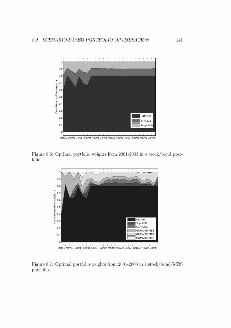
8.2. SCENARIO-BASED PORTFOLIO OPTIMISATION 141
Cum
ulat
ive
port
folio
wei
ght,
x
Mar01 May01 Jul01 Sep01 Nov01 Jan02 Mar02 May02 Jul02 Sep02 Nov02 Jan03
0
0.1
0.2
0.3
0.4
0.5
0.6
0.7
0.8
0.9
1
S&P 500
3−yr ZCB
10−yr ZCB
Figure 8.6: Optimal portfolio weights from 2001-2003 in a stock/bond port-folio.
Cum
ulat
ive
port
folio
wei
ght,
x
Mar01 May01 Jul01 Sep01 Nov01 Jan02 Mar02 May02 Jul02 Sep02 Nov02 Jan03
0
0.1
0.2
0.3
0.4
0.5
0.6
0.7
0.8
0.9
1
S&P 5003−yr ZCB
10−yr ZCB
GNMA 6% MBS
GNMA 7% MBSGNMA 8% MBS
Figure 8.7: Optimal portfolio weights from 2001-2003 in a stock/bond/MBSportfolio.
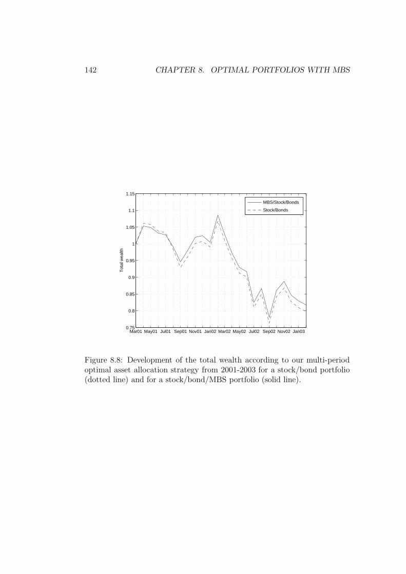
142 CHAPTER 8. OPTIMAL PORTFOLIOS WITH MBS
Mar01 May01 Jul01 Sep01 Nov01 Jan02 Mar02 May02 Jul02 Sep02 Nov02 Jan030.75
0.8
0.85
0.9
0.95
1
1.05
1.1
1.15
Tot
al w
ealth
MBS/Stock/Bonds
Stock/Bonds
Figure 8.8: Development of the total wealth according to our multi-periodoptimal asset allocation strategy from 2001-2003 for a stock/bond portfolio(dotted line) and for a stock/bond/MBS portfolio (solid line).
8.2. SCENARIO-BASED PORTFOLIO OPTIMISATION 143
8.2.2 Portfolio optimisation with CVaR constraints
The concept of portfolio optimisation with Conditional Value-at-Risk (CVaR,sometimes also called Tail Conditional Expectation or Expected Shortfall),was originally introduced by Krokhmal, Palmquist, and Uryasev (2002) andis summarised in, e.g., Krokhmal, Uryasev, and Zrazhevsky (2002). In ourset-up, let f(x, y) be the loss function defined by
f(x, ys) := 1 − TRs(x)
where the stochastic vector y with probability density function q(y) containsall uncertainty factors regarding the portfolio’s total return, and let Ψ(x, ζ)be the cumulative distribution function defined by
Ψ(x, ζ) := Q(f(x, y) ≤ ζ) =
∫
f(x,y)≤ζ
q(y) dy.
Similar to Krokhmal, Uryasev, and Zrazhevsky (2002), we define the value-at-risk V aR(α, x) with respect to the confidence level α by
V aR(α, x) := minζ ∈ R : Ψ(x, ζ) ≥ α
and the CVaR as the α-tail expectation of the loss function, i.e.
CV aR(α, x) :=1
1 − α·∫
f(x,y)≥V aR(α,x)
f(x, y) · q(y) dy.
Denoting by
ξ(x) :=1
S
S∑
s=1
TRs(x) (8.9)
the expected total return of the portfolio x and by ω some pre-specifiedCVaR limit (e.g. a certain fraction of the initial portfolio value), our generalportfolio optimisation problem can be written as
(P2) :
−ξ(x) −→ minx
CV aR(α, x) ≤ ω
∑Jj=1 xj = 1
0.8 ≥ xj ≥ 0
(8.10)

144 CHAPTER 8. OPTIMAL PORTFOLIOS WITH MBS
It is a major result of Krokhmal, Palmquist, and Uryasev (2002) that (8.10)is equivalent to a much easier-to-handle optimisation problem in which thefunction F (α, x, ζ) defined by
F (α, x, ζ) := ζ +1
1 − α·∫
max[f(x, y) − ζ, 0] · q(y) dy
on (0, 1) × X × R plays a crucial role. Its most important properties arecollected in the following theorem.
Theorem 8.1. As a function of ζ, F (α, x, ζ) is convex and continuouslydifferentiable. The Conditional Value-at-Risk with respect to the level α ofthe loss associated with any x ∈ X can be determined from the formula
CV aR(α, x) = min(x,ζ)∈X×R
F (α, x, ζ).
In this formula, the set consisting of the value of ζ for which the minimumis attained, namely
A(α, x) := argminζ∈R
F (α, x, ζ)
is a non-empty, closed, bounded interval (perhaps reducing to a single point),and the V aR(α, x) is given by
V aR(α, x) = left endpoint of A(α, x).
In particular, one always has
V aR(α, x) ∈ argminζ∈R
F (α, x, ζ)
and
CV aR(α, x) = F (α, x, V aR(α, x)).
Proof. The theorem is taken from Krokhmal, Palmquist, and Uryasev (2002).A proof can be found in Rockafellar and Uryasev (2000).
The following theorem gives the theoretical justification why one can usethe function F (α, x, ζ) instead of CV aR(α, x) for the purpose of determininga vector x that yields the minimum CV aR(α, x).
8.2. SCENARIO-BASED PORTFOLIO OPTIMISATION 145
Theorem 8.2. Minimising the Conditional Value-at-Risk with respect to thelevel α of the loss associated with x over all x ∈ X is equivalent to minimisingF (α, x, ζ) over all (x, ζ) ∈ X × R, in the sense that
minx∈X
CV aR(α, x) = min(x,ζ)∈X×R
F (α, x, ζ),
where moreover a pair (x∗, ζ∗) achieves the right hand side minimum if andonly if x∗ achieves the left hand side minimum and ζ∗ ∈ A(α, x∗). In par-ticular, therefore, in circumstances where the interval A(α, x∗) reduces to asingle point (as is typical), the minimisation of F (α, x, ζ) over (x, ζ) ∈ X×R
produces a pair (x∗, ζ∗), not necessarily unique, such that x∗ minimises theConditional Value-at-Risk and ζ∗ gives the corresponding α-Value-at-Risk.Furthermore, F (α, x, ζ) is convex with respect to (x, ζ) and CV aR(α, x) isconvex with respect to x when f(x, y) is convex with respect to x, in whichcase, if the constraints are such that X is a convex set, the joint minimisationis an instance of convex programming.
Proof. The theorem is also taken from Krokhmal, Palmquist, and Uryasev(2002) and proven in Rockafellar and Uryasev (2000).
We finally obtain the useful result:
Theorem 8.3. The minimisation problem (P2) as given in (8.10) is equiv-alent to the minimisation problem
(P3) :
−ξ(x) −→ minx,ζ
F (α, x, ζ) ≤ ω
∑Jj=1 xj = 1
0.8 ≥ xj ≥ 0
(8.11)
in the sense that their objectives achieve the same minimum values. More-over, a pair (x∗, ζ∗) achieves the minimum of (P3) if and only if x∗ achievesthe minimum of (P2) and ζ∗ ∈ A(α, x∗). In particular, when the intervalA(α, x∗) reduces to a single point, the minimisation of −ξ(x) produces a pair(x∗, ζ∗) such that x∗ maximises the expected return and ζ∗ gives the corre-sponding Value-at-Risk.
Proof. See Krokhmal, Palmquist, and Uryasev (2002).
146 CHAPTER 8. OPTIMAL PORTFOLIOS WITH MBS
If we use the Monte-Carlo approximation of the function F (α, x, ζ), de-fined by
F (α, x, ζ) := ζ +1
1 − α· 1
S
S∑
s=1
max[f(x, ys) − ζ, 0],
where ys denotes the realisation of the uncertainty vector y in scenario s wecan rewrite (P3) as
(P3′) :
−ξ(x) −→ minx,ζ
F (α, x, ζ) ≤ ω
∑Jj=1 xj = 1
0.8 ≥ xj ≥ 0
(8.12)
If we finally introduce the dummy-variables φs, s = 1, ..., S and replaceF (α, x, ζ) by the linear function
F (α, φ, ζ) := ζ +1
1 − α· 1
S
S∑
s=1
φs,
and the constraintsφs ≥ f(x, ys) − ζ, φs ≥ 0
for all s = 1, ..., S, we obtain the equivalent linear optimisation problem
(P4) :
−ξ(x) −→ minx,ζ
F (α, φ, ζ) ≤ ω
φs ≥ f(x, ys) − ζ, φs ≥ 0, s = 1, ..., S
∑Jj=1 xj = 1
0.8 ≥ xj ≥ 0, ζ ∈ R
(8.13)
which can be solved with standard software. E.g., with the linprog functionin Matlab.
In the empirical examples of our portfolio optimisation approach with
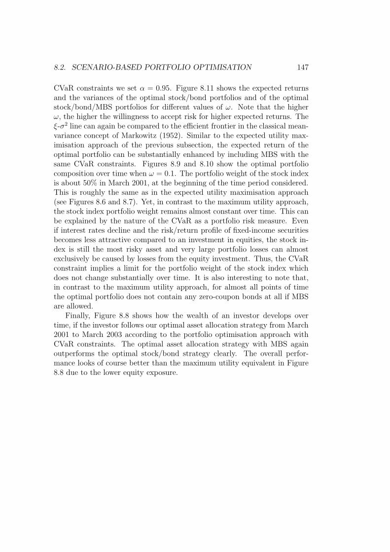
8.2. SCENARIO-BASED PORTFOLIO OPTIMISATION 147
CVaR constraints we set α = 0.95. Figure 8.11 shows the expected returnsand the variances of the optimal stock/bond portfolios and of the optimalstock/bond/MBS portfolios for different values of ω. Note that the higherω, the higher the willingness to accept risk for higher expected returns. Theξ-σ2 line can again be compared to the efficient frontier in the classical mean-variance concept of Markowitz (1952). Similar to the expected utility max-imisation approach of the previous subsection, the expected return of theoptimal portfolio can be substantially enhanced by including MBS with thesame CVaR constraints. Figures 8.9 and 8.10 show the optimal portfoliocomposition over time when ω = 0.1. The portfolio weight of the stock indexis about 50% in March 2001, at the beginning of the time period considered.This is roughly the same as in the expected utility maximisation approach(see Figures 8.6 and 8.7). Yet, in contrast to the maximum utility approach,the stock index portfolio weight remains almost constant over time. This canbe explained by the nature of the CVaR as a portfolio risk measure. Evenif interest rates decline and the risk/return profile of fixed-income securitiesbecomes less attractive compared to an investment in equities, the stock in-dex is still the most risky asset and very large portfolio losses can almostexclusively be caused by losses from the equity investment. Thus, the CVaRconstraint implies a limit for the portfolio weight of the stock index whichdoes not change substantially over time. It is also interesting to note that,in contrast to the maximum utility approach, for almost all points of timethe optimal portfolio does not contain any zero-coupon bonds at all if MBSare allowed.
Finally, Figure 8.8 shows how the wealth of an investor develops overtime, if the investor follows our optimal asset allocation strategy from March2001 to March 2003 according to the portfolio optimisation approach withCVaR constraints. The optimal asset allocation strategy with MBS againoutperforms the optimal stock/bond strategy clearly. The overall perfor-mance looks of course better than the maximum utility equivalent in Figure8.8 due to the lower equity exposure.
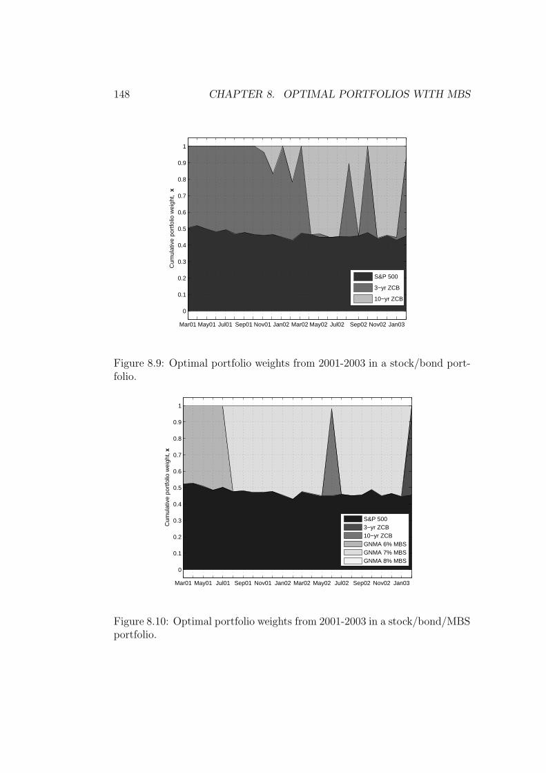
148 CHAPTER 8. OPTIMAL PORTFOLIOS WITH MBS
Cum
ulat
ive
port
folio
wei
ght,
x
Mar01 May01 Jul01 Sep01 Nov01 Jan02 Mar02 May02 Jul02 Sep02 Nov02 Jan03
0
0.1
0.2
0.3
0.4
0.5
0.6
0.7
0.8
0.9
1
S&P 500
3−yr ZCB
10−yr ZCB
Figure 8.9: Optimal portfolio weights from 2001-2003 in a stock/bond port-folio.
Cum
ulat
ive
port
folio
wei
ght,
x
Mar01 May01 Jul01 Sep01 Nov01 Jan02 Mar02 May02 Jul02 Sep02 Nov02 Jan03
0
0.1
0.2
0.3
0.4
0.5
0.6
0.7
0.8
0.9
1
S&P 5003−yr ZCB10−yr ZCBGNMA 6% MBSGNMA 7% MBSGNMA 8% MBS
Figure 8.10: Optimal portfolio weights from 2001-2003 in a stock/bond/MBSportfolio.
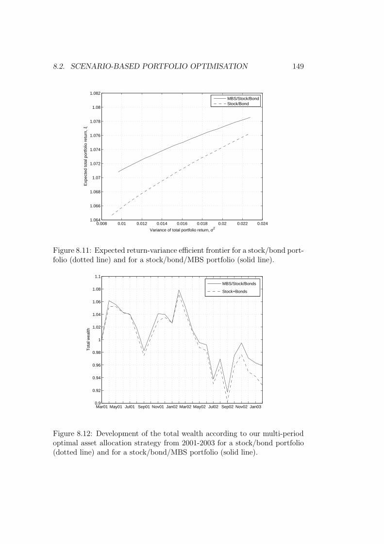
8.2. SCENARIO-BASED PORTFOLIO OPTIMISATION 149
0.008 0.01 0.012 0.014 0.016 0.018 0.02 0.022 0.0241.064
1.066
1.068
1.07
1.072
1.074
1.076
1.078
1.08
1.082
Exp
ecte
d to
tal p
ortfo
lio r
etur
n, ξ
Variance of total portfolio return, σ2
MBS/Stock/BondStock/Bond
Figure 8.11: Expected return-variance efficient frontier for a stock/bond port-folio (dotted line) and for a stock/bond/MBS portfolio (solid line).
Mar01 May01 Jul01 Sep01 Nov01 Jan02 Mar02 May02 Jul02 Sep02 Nov02 Jan030.9
0.92
0.94
0.96
0.98
1
1.02
1.04
1.06
1.08
1.1
Tot
al w
ealth
MBS/Stock/Bonds
Stock+Bonds
Figure 8.12: Development of the total wealth according to our multi-periodoptimal asset allocation strategy from 2001-2003 for a stock/bond portfolio(dotted line) and for a stock/bond/MBS portfolio (solid line).

150 CHAPTER 8. OPTIMAL PORTFOLIOS WITH MBS

Chapter 9
Valuation and Pricing ofReverse Mortgages
We have already introduced reverse mortgages in Chapter 2 and we have al-ready pointed out that the risk that the total amount of the loan may exceedthe house value at termination of the contract is crucial for the valuationand pricing of reverse mortgages. Yet, the question of how to take into ac-count this risk for a consistent valuation approach is not trivial. In a recentpaper, Wang et al. (2007) address this issue and consider survivor bondsand survivor swaps for reverse mortgages within an actuarial approach. Itis the main contribution of this chapter to develop a consistent frameworkfor the pricing of reverse mortgages with different characteristics under (lim-ited) default risk. Limited default risk means that, making reasonable modelassumptions, we calculate the maximum payment(s) to the mortgagor suchthat the mortgage lender does not experience any losses with a given proba-bility or that the losses of the mortgage lender do not exceed a given amountwith a certain probability. These considerations may justify the pricing ofa reverse mortgage contract with a particular interest-rate curve (e.g. theEURIBOR/Swap curve, which we use in the empirical examples).
Our mathematical model is again based on a stochastic intensity frame-work, which we have also used for the valuation of mortgage-backed securitiesin the previous chapters. In the following we adapt this modelling frameworkto reverse mortgages and develop, in a first step, formulas for the valuationof fixed-rate and adjustable-rate reverse mortgage contracts in a default-freesetting. By default-free valuation setting we mean that, for pricing pur-poses, we do not take into account the possibility that the total loan amountoutstanding at termination of the contract may exceed the house value. Sub-sequently, we extend these concepts for certain contract specifications andconsider the general case where the losses which a mortgage lender may suffer
151
152 CHAPTER 9. REVERSE MORTGAGES
are explicitly taken into account. We determine the maximum payment(s)to the mortgagor such that the total loan amount does not exceed the housevalue at termination of the reverse mortgage contract with a prespecifiedprobability. Alternatively, we propose a Credit-Value-at-Risk criterion in or-der to determine the maximum loan amounts. We finally illustrate our modelwith some examples directed towards the German market and investigate thesensitivity of the results with respect to some model parameters, e.g., withrespect to the drift parameter of the house price appreciation process.
9.1 The default-free modelling framework
For the sake of simplicity of the presentation, we will assume in the followingthat the reverse mortgage is associated with a single person and that there isa maximum age this person can attain. We explicitly consider two basic typesof reverse mortgages. The payment for the first type of reverse mortgage,denoted by upfront-payment reverse mortgage in the following, is made as alump sum at origination of the mortgage contract. The second type of reversemortgage we consider is a lifetime annuity, where the mortgagor receivesregular periodic payments until the contract is terminated. Of course, ourconcept can be readily applied to combinations of these two basic types andcan be easily extended to other forms of reverse mortgages, e.g. to lines ofcredit, which have become popular in the US. We do not consider any upfrontfees in the following. However, it is straightforward to incorporate upfrontfees into our modelling framework by simply considering them as an upfrontpayment which the mortgagor never receives. In any case, we assume thatthe reverse mortgage contract is only terminated when the mortgagor diesor sells the house and that all accrued interest is added to the outstandingloan amount. For both basic types of reverse mortgages we consider fixedinterest-rate agreements and adjustable-rate agreements, denoted by FRRMand ARRM respectively.
We assume that we have a probability space (Ω,G, Q) with the threefiltrations Gtt≥0, Ftt≥0, FN
tt≥0 as already introduced in Chapter 3.3.In this chapter we use again a Hull-White interest-rate model. I.e., the short-rate dynamics under the risk-neutral measure Q are given by
dr(t) = (θr(t) − arr(t))dt + σrdWr (9.1)
where Wr is a Q-Wiener process, ar := ar + λrσ2r with the market price
of risk parameter λr and ar, σr are some positive constants. The short-ratedynamics under the real-world measure Q are given by
dr(t) = (θr(t) − arr(t))dt + σrdWr. (9.2)
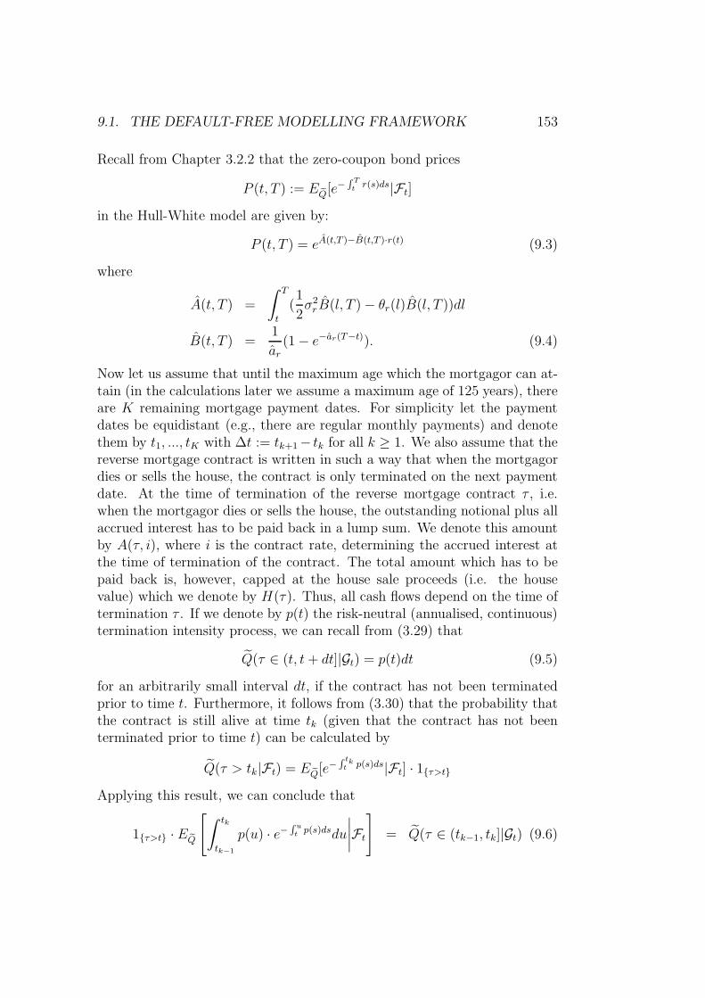
9.1. THE DEFAULT-FREE MODELLING FRAMEWORK 153
Recall from Chapter 3.2.2 that the zero-coupon bond prices
P (t, T ) := E eQ[e−R Tt
r(s)ds|Ft]
in the Hull-White model are given by:
P (t, T ) = eA(t,T )−B(t,T )·r(t) (9.3)
where
A(t, T ) =
∫ T
t
(1
2σ2
r B(l, T ) − θr(l)B(l, T ))dl
B(t, T ) =1
ar(1 − e−ar(T−t)). (9.4)
Now let us assume that until the maximum age which the mortgagor can at-tain (in the calculations later we assume a maximum age of 125 years), thereare K remaining mortgage payment dates. For simplicity let the paymentdates be equidistant (e.g., there are regular monthly payments) and denotethem by t1, ..., tK with ∆t := tk+1− tk for all k ≥ 1. We also assume that thereverse mortgage contract is written in such a way that when the mortgagordies or sells the house, the contract is only terminated on the next paymentdate. At the time of termination of the reverse mortgage contract τ , i.e.when the mortgagor dies or sells the house, the outstanding notional plus allaccrued interest has to be paid back in a lump sum. We denote this amountby A(τ, i), where i is the contract rate, determining the accrued interest atthe time of termination of the contract. The total amount which has to bepaid back is, however, capped at the house sale proceeds (i.e. the housevalue) which we denote by H(τ). Thus, all cash flows depend on the time oftermination τ . If we denote by p(t) the risk-neutral (annualised, continuous)termination intensity process, we can recall from (3.29) that
Q(τ ∈ (t, t + dt]|Gt) = p(t)dt (9.5)
for an arbitrarily small interval dt, if the contract has not been terminatedprior to time t. Furthermore, it follows from (3.30) that the probability thatthe contract is still alive at time tk (given that the contract has not beenterminated prior to time t) can be calculated by
Q(τ > tk|Ft) = E eQ[e−R tk
t p(s)ds|Ft] · 1τ>t
Applying this result, we can conclude that
1τ>t · E eQ
[∫ tk
tk−1
p(u) · e−R ut
p(s)dsdu
∣∣∣∣Ft
]= Q(τ ∈ (tk−1, tk]|Gt) (9.6)
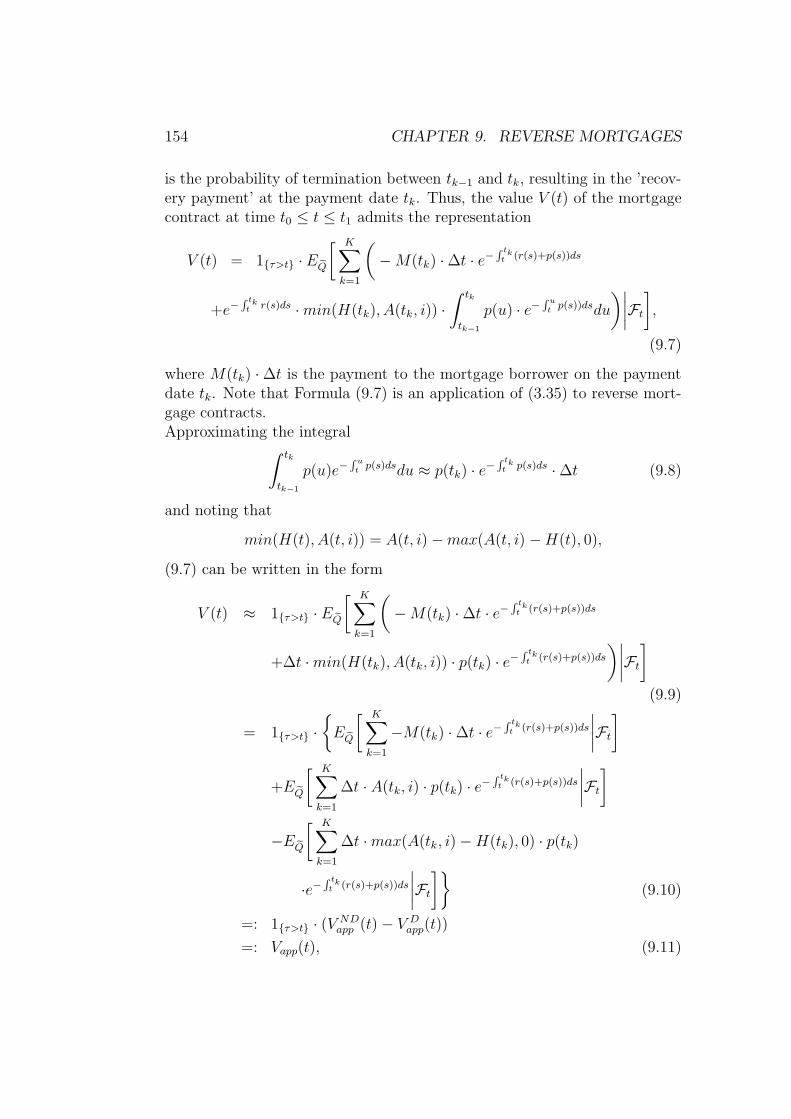
154 CHAPTER 9. REVERSE MORTGAGES
is the probability of termination between tk−1 and tk, resulting in the ’recov-ery payment’ at the payment date tk. Thus, the value V (t) of the mortgagecontract at time t0 ≤ t ≤ t1 admits the representation
V (t) = 1τ>t · E eQ
[ K∑
k=1
(− M(tk) · ∆t · e−
R tkt (r(s)+p(s))ds
+e−R tkt r(s)ds · min(H(tk), A(tk, i)) ·
∫ tk
tk−1
p(u) · e−R u
tp(s))dsdu
)∣∣∣∣Ft
],
(9.7)
where M(tk) · ∆t is the payment to the mortgage borrower on the paymentdate tk. Note that Formula (9.7) is an application of (3.35) to reverse mort-gage contracts.Approximating the integral
∫ tk
tk−1
p(u)e−R u
tp(s)dsdu ≈ p(tk) · e−
R tkt p(s)ds · ∆t (9.8)
and noting that
min(H(t), A(t, i)) = A(t, i) − max(A(t, i) − H(t), 0),
(9.7) can be written in the form
V (t) ≈ 1τ>t · E eQ
[ K∑
k=1
(− M(tk) · ∆t · e−
R tkt (r(s)+p(s))ds
+∆t · min(H(tk), A(tk, i)) · p(tk) · e−R tk
t (r(s)+p(s))ds
)∣∣∣∣Ft
]
(9.9)
= 1τ>t ·
E eQ
[ K∑
k=1
−M(tk) · ∆t · e−R tk
t (r(s)+p(s))ds
∣∣∣∣Ft
]
+E eQ
[ K∑
k=1
∆t · A(tk, i) · p(tk) · e−R tk
t (r(s)+p(s))ds
∣∣∣∣Ft
]
−E eQ
[ K∑
k=1
∆t · max(A(tk, i) − H(tk), 0) · p(tk)
·e−R tk
t (r(s)+p(s))ds
∣∣∣∣Ft
](9.10)
=: 1τ>t · (V NDapp (t) − V D
app(t))
=: Vapp(t), (9.11)
9.1. THE DEFAULT-FREE MODELLING FRAMEWORK 155
where V NDapp (t) is the value of a reverse mortgage contract without the pos-
sibility of loss for the mortgage lender and V Dapp(t) is the term capturing the
’value of the default risk’. The approximation error in (9.9) is again of thekind Rtk as already introduced in (3.36) and discussed in detail in the ap-pendix. We will concentrate on the reverse mortgage value Vapp(t) in thefollowing since the difference between (9.7) and (9.11) is negligible for rea-sonably small ∆t (e.g., for ∆t = 1/12, indicating monthly payments). In theremainder of this section we will assume that the last term in (9.10), i.e. the’value of the default risk’ V D
app(t), is small enough so that
V NDapp (t) = 1τ>t · E eQ
[ K∑
k=1
(− M(tk) · ∆t · e−
R tkt (r(s)+p(s))ds
+A(tk, i) · p(tk) · ∆t · e−R tkt (r(s)+p(s))ds
)∣∣∣∣Ft
](9.12)
is a good approximation of V (t). Evidently, this is only justified if the proba-bility that the house value is smaller than the total loan amount outstandingat termination of the contract is negligibly low. We will extensively discussthis topic and, in particular, the implications for the maximum paymentswhich can be made to the homeowner later in the subsequent section. Themore general case, where we have to evaluate (9.11) will also be discussed inthe subsequent section for the analytically tractable contract specifications.
We decompose the overall termination intensity p(t) into the two inde-pendent parts, pd(t) and ps(t) with
p(t) = pd(t) + ps(t),
where pd(t) denotes the ”death intensity process” and ps(t) denotes the homesale intensity. The separation of the overall contract termination intensityinto two independent parts was already used in Chapters 5 and 6 in thecontext of prepayment modelling for MBS. While pd can be extracted from lifeexpectancy tables (and is thus assumed to be deterministic in the following),we assume that the home sale intensity process follows a Vasicek process,with dynamics
dps(t) = (θp − apps(t))dt + σpdWp(t) (9.13)
under the risk-neutral pricing measure Q and by
dps(t) = (θp − apps(t))dt + σpdWp(t) (9.14)
under the real-world measure Q, where Wp (Wp) is a Q (Q)- Wiener pro-
cess (independent of the previously defined Wr (Wr)). With these modelspecifications we can explicitly calculate the expectations in (9.11).

156 CHAPTER 9. REVERSE MORTGAGES
Lemma 9.1. In the model set-up as previously introduced it holds that
P d(t, T ) := E eQ[e−R Tt
(r(s)+p(s))ds|Ft]
= P (t, T ) · e−R Tt
pd(s)ds · eAd(t,T )−Cd(t,T )·ps(t)
with
Ad(t, T ) =
∫ T
t
1
2σ2
pCd(l, T )2 − θpC
d(l, T )dl,
=
(θp
ap− σ2
2a2p
)[Cd(t, T ) − T + t] − σ2
4ap· Cd(t, T )2
Cd(t, T ) =1
ap
(1 − e−ap(T−t)
),
Proof. Since the short-rate process r(t) is independent of the terminationintensity p(t) and since pd(t) is deterministic, the lemma follows from thebond pricing formulas in the Vasicek model (see (3.12) and (3.13)).
Lemma 9.2. In the model set-up as previously introduced it holds that
E eQ[p(T ) · e−R T
t(r(s)+p(s))ds|F t] = P d(t, T ) · fd(t, T )
where
fd(t, T ) := − ∂
∂Tln
P d(t, T )
P (t, T )
is the ”termination spread forward rate”.
Proof. The lemma follows directly from the well-known result (see, e.g.,Schmid (2004), p. 243) saying that
E eQ
[e−
R Tt
r(l)dlr(T )|Ft
]= −E eQ
[e−
R Tt
r(l)dl|Ft
]· ∂
∂Tln P (t, T ),
which we have already used earlier in this thesis.
As a further ingredient of our pricing model we need to model the collateral,i.e. the house value, in order to be able to determine the maximum monthlypayment to the mortgagor so that the mortgage is adequately collateralisedand the pricing with the default-free valuation formula (9.12) is justified. Letus assume that the house price H(t) has the dynamics
dH(t) = µHH(t)dt + σHH(t)dWH(t) (9.15)
9.1. THE DEFAULT-FREE MODELLING FRAMEWORK 157
where µH and σH are some positive constants, WH(t) is a Wiener process(w.r.t. the real-world measure Q), independent of the previously definedWr, Wp, and H(0) = H0 is the value of the house at origination of the reversemortgage contract. Thus, the house price H(t) follows a geometric Brownianmotion and it follows that the distribution of H(t)/H0 is lognormal withparameters (µH − 1
2σ2
H) · t and σ2H · t, i.e.
H(t) ∼ H0 · LN((µH − 1
2σ2
H) · t, σ2H · t),
where LN(·, a, b) denotes the cdf of the lognormal distribution with param-eters a and b.
9.1.1 Fixed-rate reverse mortgages
If the interest-rate agreement of the reverse mortgage contract is a fixed-rate agreement with interest rate i (expressed as annual rate with discretecompounding), we obtain:
Theorem 9.3. The value at time t0 ≤ t ≤ t1 of a ”default-free” upfront-payment FRRM with initial payment M0 and fixed interest rate i is givenby:
V UPFRRM(t, i) = 1τ>t ·
(− M0 · P d(t, t1)
+M0 ·K∑
k=1
(1 + i · ∆t)k−1 · ∆t · P d(t, tk) · fd(t, tk)
).
Proof. Noting that
A(tk, i) = M0 · (1 + i · ∆t)k−1
for k = 1, ..., K, the theorem follows directly from (9.12).
Theorem 9.4. The value at time t0 ≤ t ≤ t1 of a ”default-free” lifetimeannuity FRRM with a periodic payment of M ·∆t and fixed interest rate i isgiven by:
V LAFRRM(t; i) = 1τ>t · M · ∆t ·
K∑
k=1
(− P d(t, tk)
+(1 + i · ∆t)k − 1
i· P d(t, tk) · fd(t, tk)
).
158 CHAPTER 9. REVERSE MORTGAGES
Proof. Noting that
A(tk, i) = M · ∆t ·k−1∑
j=0
(1 + i · ∆t)j
= M · ∆t · (1 + i · ∆t)k − 1
i · ∆t, (9.16)
the theorem follows again directly from (9.12).
9.1.2 Adjustable-rate reverse mortgages
In an adjustable-rate contract, the interest rate is not constant, but is ad-justed at given fixing dates, so that it reflects prevailing market conditionsduring the whole lifetime of the product. For simplicity, we assume in thefollowing that the fixing dates coincide with the payment dates and that onthe payment date tk the interest rate is fixed for the subsequent interest-rateperiod from tk to tk+1. Usually, for adjustable-rate contracts the referenceindex rate is a LIBOR (or EURIBOR) rate. LIBOR rates are simple money-market interest rates and can be considered as short-term riskless rates. Wedenote by L(tk) := L(tk, tk+1) the LIBOR rate for the time period from tkto tk+1, by sL some spread on the LIBOR rate. In the following, we use theapproximation
(1 + (L(tk) + sL) · ∆t) ≈ e(r(tk)+sL)·∆t. (9.17)
Theorem 9.5. The value at time t0 ≤ t ≤ t1 of a ’default-free’ adjustable-rate reverse mortgage with initial payment M0, i.e. A(t1) = M0, and fixedspread sL on the (simple) reference index rate is given by
V UPARRM (t, ∆t, sL) ≈ 1τ>t ·
(− M0 · P d(t, t1) + M0 · ∆t · P (t, t1)
·K∑
k=1
fd(t, tk) ·P d(t, tk)
P (t, tk)· esL·(tk−t1)
).
Proof. Note that using (9.17) we get
A(tk, sL) = M0 ·
k−1∏
j=1
(1 + (L(tj) + sL) · ∆t)
≈ M0 · ePk−1
j=1(r(tj )+sL)·∆t)
≈ M0 · eR tkt1
r(s)ds · esL·(tk−t1).
9.1. THE DEFAULT-FREE MODELLING FRAMEWORK 159
Then, it follows from (9.12) that
V UPARRM (t, ∆t, sL) = 1τ>t ·
(− M0 · P d(t, t1) + E eQ
[ K∑
k=1
M0
·(
k−1∏
j=1
(1 + (L(tj) + sL) · ∆t)
)· p(tk) · ∆t · e−
R tkt (r(s)+p(s))ds
∣∣∣∣Ft
])
≈ 1τ>t ·(− M0 · P d(t, t1) + E eQ
[ K∑
k=1
M0 · ∆t
·eR tkt1
r(s)ds · esL·(tk−t1) · p(tk) · e−R tkt (r(s)+p(s))ds
∣∣∣∣Ft
]),
which further simplifies to
V UPARRM (t, ∆t, sL) ≈ 1τ>t ·
(− M0 · P d(t, t1)
+M0 · ∆t ·K∑
k=1
esL·(tk−t1) · E eQ
[e
R t1t r(s)ds|Ft
]
·E eQ
[p(tk) · e−
R tkt p(s)ds|Ft
])
= 1τ>t ·(− M0 · P d(t, t1) + M0 · ∆t · P (t, t1)
·K∑
k=1
fd(t, tk) ·P d(t, tk)
P (t, tk)· esL·(tk−t1)
).
Theorem 9.6. The value at time t0 ≤ t ≤ t1 of a ’default-free’ adjustable-rate reverse mortgage with a periodic payment of M · ∆t and a fixed spreadsL on the (simple) reference index rate is given by
V LAARRM (t, ∆t, sL) = 1τ>t ·
K∑
k=1
(− M · ∆t · P d(t, tk) + P (t, tk) · M · ∆t
·K∑
m=k
∆t · esL·(tm−tk) · fd(t, tm) · P d(t, tm)
P (t, tm)
).

160 CHAPTER 9. REVERSE MORTGAGES
Proof. For notational convenience, we define
V (t) := V LAARRM(t, ∆t, sL).
Then, according to (9.12)
V (t) = 1τ>t ·K∑
k=1
− M · ∆t · P d(t, tk)
+E eQ
[( k−1∑
l=0
M · ∆t
k−1∏
j=k−l
(1 + (L(tj) + sL) · ∆t)
)
·∆t · p(tk) · e−R tk
t (r(s)+p(s))ds
∣∣∣∣Ft
]
≈ 1τ>t ·K∑
k=1
− M · ∆t · P d(t, tk) + M · ∆t
·k−1∑
l=0
P (t, tk−l) · esL·(tk−tk−l) · E eQ
[∆t · p(tk) · e−
R tkt p(s)ds|Ft
].
By applying Lemma 9.2 we get
V (t) = 1τ>t ·K∑
k=1
(− M · ∆t · P d(t, tk) + M · ∆t
·k−1∑
l=0
P (t, tk−l) · esL·(tk−tk−l) · fd(t, tk) ·P d(t, tk)
P (t, tk)· ∆t
).
Noting thatK∑
k=1
k−1∑
l=0
ak−l,k =
K∑
k=1
K∑
m=k
ak,m
finally yields
V (t) = 1τ>t ·K∑
k=1
(− M · ∆t · P d(t, tk) + M · ∆t
K∑
m=k
P (t, tk) · esL·(tm−tk) · ∆t · fd(t, tm) · P d(t, tm)
P (t, tm)
).
9.1. THE DEFAULT-FREE MODELLING FRAMEWORK 161
Note that it follows directly from Theorem 9.5 and Theorem 9.6 that ifsL = 0, i.e. if there is no spread on the index rate, the value of the reversemortgage contract is equal to the outstanding loan amount on any (next)payment and fixing date t1 (up to a very small discretisation error resultingfrom the discretisation in (9.11)). In order to see this, note that with t = t1the term
K∑
k=1
P (t, t1) · fd(t, tk) ·P d(t, tk)
P (t, tk)· ∆t · esL·(tk−t1)
reduces to
K∑
k=1
fd(t1, tk) ·P d(t1, tk)
P (t1, tk)· ∆t ≈
K∑
k=1
Q(τ = tk|Ft1) = 1,
given that τ > t0. Furthermore, note that with sL = 0 and t = t1 for thelifetime annuity ARRM, the term
K∑
k=1
P (t, tk) · M · ∆t ·K∑
m=k
∆t · esL·(tm−tk) · fd(t, tm) · P d(t, tm)
P (t, tm)
reduces toK∑
k=1
P (t1, tk) · M · ∆t ·K∑
m=k
Q(τ = tm|Ft1)
=K∑
k=1
P (t1, tk) · M · ∆t · Q(τ ≥ tk|Ft1)
=
K∑
k=1
P d(t1, tk) · M · ∆t,
given that τ > t1. I.e., the net present value of the sum of all future paymentsis equal to 0 and it follows that
V LAARRM (tj, ∆t, 0) = 0
The fact that the present value of an ARRM with sL = 0 is equal to the out-standing loan amount on any fixing date is perfectly consistent with the valu-ation principles of ordinary floating rate notes. The value of any floating-ratenote (independent of the maturity) must always be equal to the outstandingnotional on any fixing date, as long as the total notional is fully recovered attermination, i.e. as long as the floating-rate note is default-free.
162 CHAPTER 9. REVERSE MORTGAGES
9.2 Introducing default risk
In the first part of this section we address the question of how much a mort-gagor can borrow, so that the ”default-free” considerations are justified. Re-call that this is only the case if the probability that the total outstandingloan amount exceeds the house value at termination of the contract is negli-gibly low. Let us assume that the house value exceeds the total loan amountoutstanding at termination of the contract with a probability of at leastq ∈ (0, 1). Given such a probability q, at the time of origination of thecontract t0, the mortgage lender has to limit the initial payment M0 (foran upfront-payment FRRM) or the periodic payment M · ∆t (for a lifetimeannuity FRRM) in such a way that
Q(H(τ) < A(τ, i)) =K∑
k=1
Q(H(τ) < A(τ, i)|τ = tk) · Q(τ = tk) ≤ 1 − q
(9.18)
holds (we will call this criterion ’q-criterion’ in the following). Since
Q(H(τ) < A(τ, i)|τ = tk) = LN(A(tk, i)
H0; (µH − 1
2σ2
H) · tk, σ2H · tk),
it follows that (9.18) is equivalent to
K∑
k=1
LN(A(tk, i)
H0
; (µH − 1
2σ2
H) · tk, σ2H · tk) · Q(τ = tk) ≤ 1 − q.
(9.19)
We can calculate Q(τ = tk) using the following theorem.
Theorem 9.7. In the model set-up as previously introduced it holds that
Q(τ = tk) ≈(
∆t · pd(tk) · e−R tkt pd(s)ds · P s(t, tk)
−∆t · e−R tkt pd(s)ds · P s(t, tk) ·
∂
∂tkln P s(t, tk)
)· 1τ>t,
whereP s(t, tk) := EQ[e−
R tkt ps(u)du] = eAd(t,T )−Cd(t,T )·ps(t)
with
Ad(t, T ) =
(θp
ap− σ2
2a2p
)[Cd(t, T ) − T + t] − σ2
4ap· Cd(t, T )2
Cd(t, T ) =1
ap
(1 − e−ap(T−t)
)
9.2. INTRODUCING DEFAULT RISK 163
Proof. First, recall (9.6) and the approximation (9.8). Noting that pd(t) is
deterministic we have to calculate EQ[e−R tk
t ps(u)du], where the expectationis taken under the real-world measure Q. This expectation can directly becalculated using solely the distribution of the home sale intensity implied byits real-world dynamics as given in (9.14). Since the distribution of ps(t)is normal, it can be shown that the distribution of
∫ tkt
ps(u)du is also nor-
mal. Thus, the distribution of e−R tkt ps(u)du is lognormal and its expectation
follows from the expectation and variance of∫ tk
tps(u)du, which yields the
formulas as stated above (for a detailed derivation see, e.g., Mamon (2004)).
Furthermore, if we assume as usual that EQ[e−R tkt ps(u)du] < ∞ and note that
e−R tkt ps(u) is continuously differentiable w.r.t. tk (for almost all ω ∈ Ω, it
holds that
∂
∂tklnP s(t, tk) =
1
P s(t, tk)· EQ
[∂
∂tke−
R tkt ps(u)du
]
= − 1
P s(t, tk)· EQ[ps(tk) · e−
R tkt ps(u)du].
I.e., we obtain
EQ[ps(tk) · e−R tkt ps(u)du] = −P s(t, tk) ·
∂
∂tkln P s(t, tk).
Note that we have already used a similar result earlier for the short-rateprocess under the risk-neutral martingale measure. This completes the proof.
Since the left-hand side of (9.19) is a strictly increasing function in M0
and M for an upfront-payment FRRM and a lifetime annuity FRRM respec-tively, we get the maximum initial payment M∗
0 and the maximum periodicpayment M∗ if we replace ”≤” with ”=” in (9.19) and solve the equation forM0 and M respectively. This can be done by standard methods, e.g. withthe fzero function in Matlab.
The question of how much a mortgagor can borrow so that (9.19) holdsfor a certain probability q, is much more difficult for ARRM contracts thanfor FRRM contracts since in a contract with a floating interest rate the quan-tity A(tk) is stochastic. Within our Hull-White interest-rate model frame-work, the quantity A(tk) in a lifetime annuity ARRM is basically a sum ofcorrelated lognormal random variables. We would thus have to compare asum of correlated lognormal random variables with the house value, whichis also lognormally distributed. It is a well known fact, e.g. from the pric-ing of arithmetic average Asian options that the sum of lognormal random
164 CHAPTER 9. REVERSE MORTGAGES
variables is not lognormally distributed. While some closed-form approxima-tions have been suggested in the literature (see, e.g., Milevsky and Posner(1998)), these can not be used for our problem since we would finally haveto find a distribution for the difference between the lognormally distributedhouse value and the approximate distribution of A(tk), which is infeasible.Thus, for a lifetime annuity ARRM, the only way to determine the maxi-mum periodic payment M∗ is by simulation. The situation looks better for anupfront-payment ARRM. For an upfront-payment ARRM we can reasonablyapproximate the outstanding loan amount at time tk by
A(tk) ≈ M0 · eR tk0 r(s)ds · esL·tk .
We already know from Lemma 3.4 that the distribution of∫ tk0
r(s)ds is nor-mal in the Hull-White model and we obtain:
∫ tk
0
r(s)ds ∼ N(ak; V (0, tk)), (9.20)
where
ak := − ln P (0, tk) +σ2
r
2a2r
· [tk − 2 · B(0, tk)
+1
2ar(1 − e−2ar ·tk)]
V (0, tk) :=σ2
r
a2r
(tk +
2
ar
e−artk − 1
2ar
e−2artk − 3
2ar
)(9.21)
and B(0, tk) is as given in (3.17).Now, note that (9.18) is equivalent to
K∑
k=1
Q
(log
H(τ)
H0
− logA(τ)
M0
< log M0 − log H0
∣∣∣∣ τ = tk
)
·Q(τ = tk) ≤ 1 − q.
Thus, in order to get the maximum initial payment M∗0 we have to solve the
equation
K∑
k=1
Φ
(log M0 − log H0 − ((µH − 1
2σ2
H) · tk − ak − sL · (tk − t1))√σ2
H · tk + V (0, tk)
)
·Q(τ = tk) = 1 − q,
9.2. INTRODUCING DEFAULT RISK 165
where Φ(·) denotes the cdf of the standard normal distribution and Q(τ = tk)can be calculated as stated in Theorem 9.7.
All calculations so far have been based on ”default-free” considerations.This, as previously explained, is only justified if the maximum paymentsto the homeowner are sufficiently low. This, however, may make a reversemortgage unattractive to some homeowners. When taking into account thepotential losses the mortgage lender faces if the total loan amount exceedsthe house value at termination of the contract, we have to work with theexact (up to the very small discretisation error) valuation formula (9.11).The following considerations are, however, only analytically well tractablefor fixed-rate contracts. We will thus focus on these contracts and point outthat for adjustable-rate contracts formula (9.11) can, of course, always beevaluated by simulation7.
If we assume that the house price dynamics under the risk-neutral pricingmeasure are given by
dH(t) = r(t)dt + σHdWH(t) (9.22)
we obtain the following versions of Theorems 9.3 and 9.4:
Theorem 9.8. The value at time t0 ≤ t ≤ t1 of an upfront-payment FRRMwith initial payment M0, fixed interest rate i and recovery capped at the housevalue is given by:
V UPdFRRM (t, i) = 1τ>t ·
(− M0 · P d(t, t1) +
K∑
k=1
M0 · (1 + i · ∆t)k−1
·∆t · P d(t, tk) · fd(t, tk)
−∆t · P d(t, tk)
P (t, tk)· fd(t, tk) · PUT (t, tk, A(tk, i))
),
7An alternative to simulation is the use of another approximation. The term
E eQ[max(A(tk) − H(tk), 0) · p(tk) · eR t
k
t(r(s)+p(s))ds|Ft]
can be written as
E eQ[max(A(tk) − H(tk), 0) · eR t
k
tr(s)ds|Ft] · E eQ[p(tk) · e
R tk
tp(s)ds|Ft],
where the first expectation can be calculated using Margrabe’s exchange option formula,if one assumes that the interest rates for discounting are independent of those used fordetermining the outstanding loan amount A(tk) (see Margrabe (1978)) and the secondexpectation can be calculated using previously developed results.
166 CHAPTER 9. REVERSE MORTGAGES
where
PUT (t, tk, A(tk, i)) := A(tk, i) · P (t, tk)
·Φ(−
ln H(t)A(tk ,i)·P (t,tk)
− 12v2(t, tk)
v(t, tk)
)
−H(t) · Φ(−
ln H(t)A(tk ,i)·P (t,tk)
+ 12v2(t, tk)
v(t, tk)
),
v(t, tk) := V (t, tk) + σ2H(tk − t)
and V (t, tk) is similar to V (t, tk) as defined in (9.21) if ar is replaced withar.
Proof. Recalling Lemma 9.2 and Theorem 9.3 it remains to show that
E eQ[max(A(tk, i) − H(tk), 0) · e−R tk
t r(s)ds] = PUT (t, tk, A(tk, i))
with PUT (t, tk, A(tk, i)) as defined above. The expression max(A(tk, i) −H(tk), 0) is, however, simply the payoff of a European put option w.r.t. theunderlying H(t), strike price A(tk, i) and maturity tk. We can thus apply theput option formula in the Black-Scholes framework with stochastic interestrates (see, e.g., Brigo and Mercurio (2006), p. 888, for the case when interestrates follow the Hull-White 1-factor model, as we assume in our model).
Theorem 9.9. The value at time t0 ≤ t ≤ t1 of a lifetime annuity FRRMwith a periodic payment of M · ∆t, fixed interest-rate i and recovery cappedat the house value is given by:
V LAdFRRM (t; i) = 1τ>t ·
K∑
k=1
− M · ∆t · P d(t, tk)
+M · ∆t · (1 + i · ∆t)k − 1
i· P d(t, tk) · fd(t, tk)
−∆t · P d(t, tk)
P (t, tk)· fd(t, tk) · PUT (t, tk, A(tk, i))
,
where PUT (t, tk, A(tk, i)) is defined as in Theorem 9.8.
Proof. The Theorem follows directly from Theorems 9.4 and 9.8.
If we explicitly take into account the losses the mortgage lender possiblysuffers, it seems appropriate to limit the maximum payments to the home-owner in such a way that the lender’s losses do not exceed a certain amount
9.3. RESULTS AND IMPLICATIONS 167
with a given probability. In some sense, this is equivalent to setting a CreditValue-at-Risk (CreditVaR) limit.
The CreditVaR of a reverse mortgage contract could, e.g., simply be afraction of the initial house value. If we set this fraction to, say, 0.1 andthe CreditVaR-probability level to α we have to limit the payments to thehomeowner in such a way that
Q(A(τ, i) − H(τ) > 0.1 · H0) =K∑
k=1
Q(A(τ, i) − H(τ) > 0.1 · H0|τ = tk) · Q(τ = tk) ≤ 1 − α.
I.e. we have to solve
K∑
k=1
LN(max(0, A(tk, i) − 0.1 · H0)
H0
; (µH − 1
2σ2
H) · tk, σ2H · tk)
·Q(τ = tk) = 1 − α
to obtain the maximum initial payment M∗0,d or the maximum periodic pay-
ment M∗d .
In the last part of this section we briefly investigate the difference betweenthe valuation formulas in the ”default-free” setting of Chapter 9.1 and theformulas in this section where we explicitly take into account the possibilityof losses for the mortgage lender. This difference is, of course, the quantity
V Dapp(t) =
K∑
k=1
∆t · P d(t, tk)
P (t, tk)· fd(t, tk) · PUT (t, tk, A(tk, i))
which we have labelled ”value of the default risk”. Note that, assuminga complete market where the dynamics of the house price process underthe risk-neutral pricing measure are given by (9.22), the value of the PUToptions does not depend on the parameter µH . However, it does dependon the volatility of the house price process, i.e. on σH . If the volatility σH
increases, as in the current housing turmoil in the US, the value of the defaultrisk increases. We will exemplarily illustrate this in the following section.
9.3 Results and implications
In this section we discuss the available data and shortly comment on thetechniques which we need to estimate the model parameters. With the ob-tained parameter estimates (and assumptions where there is no reliable data
168 CHAPTER 9. REVERSE MORTGAGES
in order to estimate the parameters statistically) we then illustrate the pre-viously introduced modelling approach.
Let us start with the ”default-free” model set-up as discussed in Chapter9.1 and with the probability q. Recall that q has to be chosen close to 1 inorder to justify the ”default-free” considerations. As risk-free interest-ratecurve we use the LIBOR/Swap curve in this paper. In practice loans are of-ten priced with the LIBOR/Swap curve since this is the common benchmarkcurve for a bank’s or mortgage lender’s liabilities. The Global Average One-Year Rating Transition Rates for global corporates as of 2006 (with data from1981-2005; Source: Standard & Poor’s CreditPro 7.02) yield that a 25-yearloan of a AAA-rated company defaults with a probability of approximately4%. Thus, we can conclude for our purposes that by setting q = 96.5% areverse mortgage loan can be considered as virtually default-free and thatthe use of the LIBOR/Swap or the EURIBOR/Swap curve as risk free curveis adequate. We have historical EURO EURIBOR/Swap rates from 1999to 2007 for maturities from 6 months to 30 years for the estimation of theparameters in the Hull-White interest-rate model. We estimate the param-eters with Kalman filter techniques as described in Chapter 5. By usingthe Kalman filter with historical data we can estimate the dynamics of theshort-rate under the real-world measure Q and under the risk-neutral pricingmeasure Q simultaneously. The results are reported in Table 9.1.
The mortality rates which we need to determine the (deterministic) mor-
Parameter Estimatear 0.0518ar 0.0177σr 0.0065hr 0.0003
Table 9.1: Estimates of the interest-rate model parameters where hr is themeasurement std. error.
tality intensity process can easily be extracted from life expectancy tables.In this paper we use the 2004 R mortality rates of the first order publishedby the Deutsche Aktuarsvereinigung [association for actuaries in Germany]which are the current standard for pension insurance calculations in Ger-many. We thus obtain a piecewise constant mortality intensity pd(l) fromyear l to l + 1 given by
pd(l) = log(1 − Q(τd ∈ (l, l + 1]|τd > l)), (9.23)
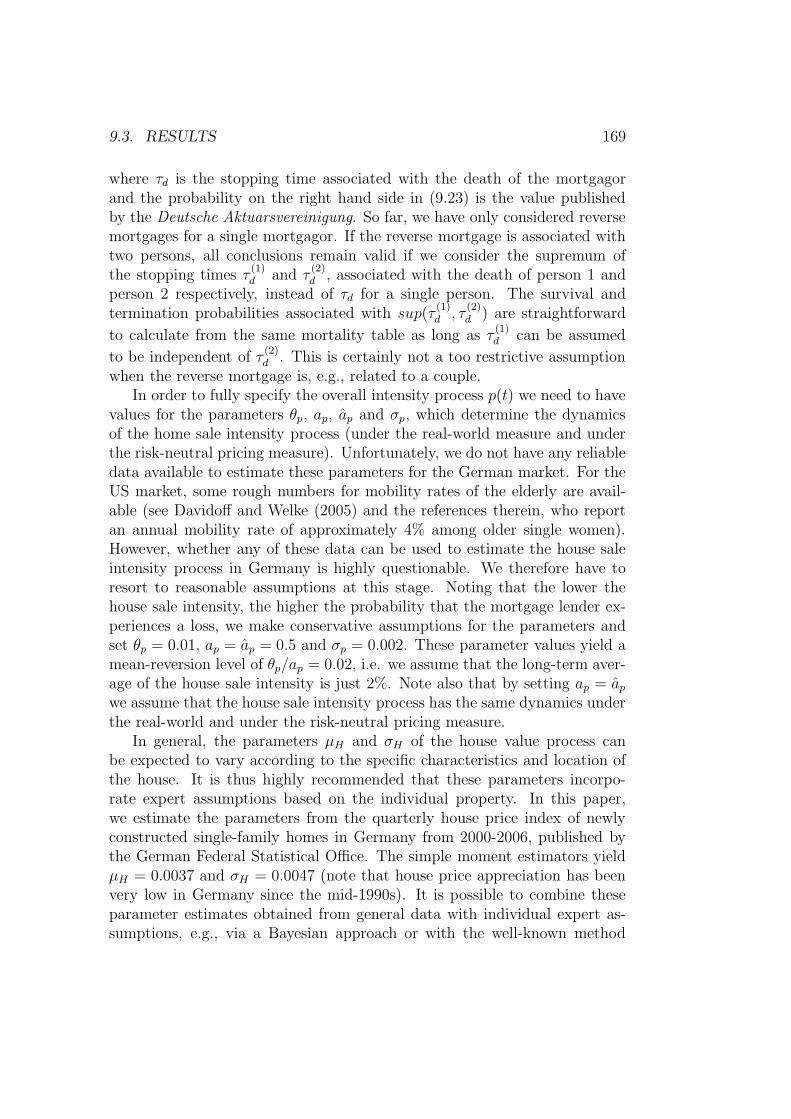
9.3. RESULTS 169
where τd is the stopping time associated with the death of the mortgagorand the probability on the right hand side in (9.23) is the value publishedby the Deutsche Aktuarsvereinigung. So far, we have only considered reversemortgages for a single mortgagor. If the reverse mortgage is associated withtwo persons, all conclusions remain valid if we consider the supremum ofthe stopping times τ
(1)d and τ
(2)d , associated with the death of person 1 and
person 2 respectively, instead of τd for a single person. The survival andtermination probabilities associated with sup(τ
(1)d , τ
(2)d ) are straightforward
to calculate from the same mortality table as long as τ(1)d can be assumed
to be independent of τ(2)d . This is certainly not a too restrictive assumption
when the reverse mortgage is, e.g., related to a couple.In order to fully specify the overall intensity process p(t) we need to have
values for the parameters θp, ap, ap and σp, which determine the dynamicsof the home sale intensity process (under the real-world measure and underthe risk-neutral pricing measure). Unfortunately, we do not have any reliabledata available to estimate these parameters for the German market. For theUS market, some rough numbers for mobility rates of the elderly are avail-able (see Davidoff and Welke (2005) and the references therein, who reportan annual mobility rate of approximately 4% among older single women).However, whether any of these data can be used to estimate the house saleintensity process in Germany is highly questionable. We therefore have toresort to reasonable assumptions at this stage. Noting that the lower thehouse sale intensity, the higher the probability that the mortgage lender ex-periences a loss, we make conservative assumptions for the parameters andset θp = 0.01, ap = ap = 0.5 and σp = 0.002. These parameter values yield amean-reversion level of θp/ap = 0.02, i.e. we assume that the long-term aver-age of the house sale intensity is just 2%. Note also that by setting ap = ap
we assume that the house sale intensity process has the same dynamics underthe real-world and under the risk-neutral pricing measure.
In general, the parameters µH and σH of the house value process canbe expected to vary according to the specific characteristics and location ofthe house. It is thus highly recommended that these parameters incorpo-rate expert assumptions based on the individual property. In this paper,we estimate the parameters from the quarterly house price index of newlyconstructed single-family homes in Germany from 2000-2006, published bythe German Federal Statistical Office. The simple moment estimators yieldµH = 0.0037 and σH = 0.0047 (note that house price appreciation has beenvery low in Germany since the mid-1990s). It is possible to combine theseparameter estimates obtained from general data with individual expert as-sumptions, e.g., via a Bayesian approach or with the well-known method
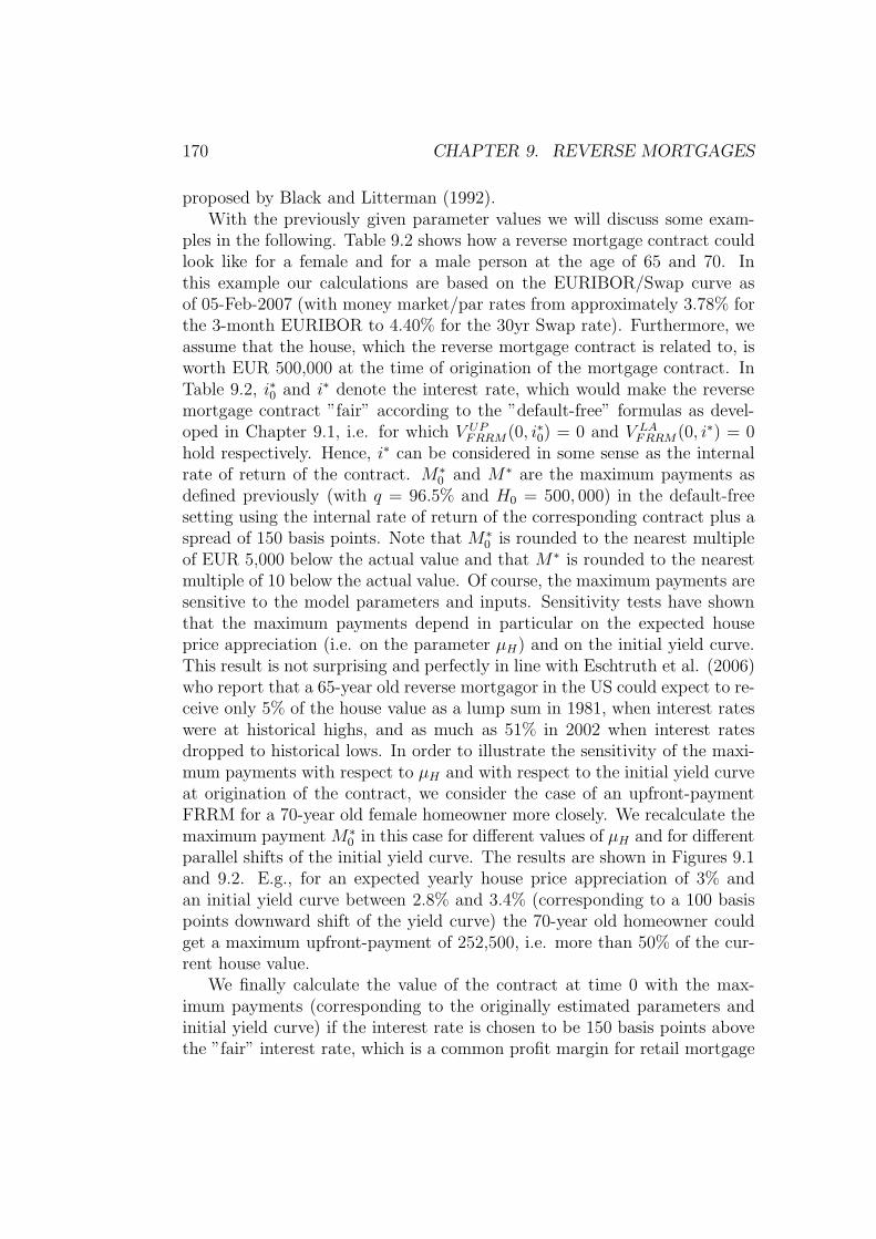
170 CHAPTER 9. REVERSE MORTGAGES
proposed by Black and Litterman (1992).With the previously given parameter values we will discuss some exam-
ples in the following. Table 9.2 shows how a reverse mortgage contract couldlook like for a female and for a male person at the age of 65 and 70. Inthis example our calculations are based on the EURIBOR/Swap curve asof 05-Feb-2007 (with money market/par rates from approximately 3.78% forthe 3-month EURIBOR to 4.40% for the 30yr Swap rate). Furthermore, weassume that the house, which the reverse mortgage contract is related to, isworth EUR 500,000 at the time of origination of the mortgage contract. InTable 9.2, i∗0 and i∗ denote the interest rate, which would make the reversemortgage contract ”fair” according to the ”default-free” formulas as devel-oped in Chapter 9.1, i.e. for which V UP
FRRM(0, i∗0) = 0 and V LAFRRM(0, i∗) = 0
hold respectively. Hence, i∗ can be considered in some sense as the internalrate of return of the contract. M∗
0 and M∗ are the maximum payments asdefined previously (with q = 96.5% and H0 = 500, 000) in the default-freesetting using the internal rate of return of the corresponding contract plus aspread of 150 basis points. Note that M∗
0 is rounded to the nearest multipleof EUR 5,000 below the actual value and that M∗ is rounded to the nearestmultiple of 10 below the actual value. Of course, the maximum payments aresensitive to the model parameters and inputs. Sensitivity tests have shownthat the maximum payments depend in particular on the expected houseprice appreciation (i.e. on the parameter µH) and on the initial yield curve.This result is not surprising and perfectly in line with Eschtruth et al. (2006)who report that a 65-year old reverse mortgagor in the US could expect to re-ceive only 5% of the house value as a lump sum in 1981, when interest rateswere at historical highs, and as much as 51% in 2002 when interest ratesdropped to historical lows. In order to illustrate the sensitivity of the maxi-mum payments with respect to µH and with respect to the initial yield curveat origination of the contract, we consider the case of an upfront-paymentFRRM for a 70-year old female homeowner more closely. We recalculate themaximum payment M∗
0 in this case for different values of µH and for differentparallel shifts of the initial yield curve. The results are shown in Figures 9.1and 9.2. E.g., for an expected yearly house price appreciation of 3% andan initial yield curve between 2.8% and 3.4% (corresponding to a 100 basispoints downward shift of the yield curve) the 70-year old homeowner couldget a maximum upfront-payment of 252,500, i.e. more than 50% of the cur-rent house value.
We finally calculate the value of the contract at time 0 with the max-imum payments (corresponding to the originally estimated parameters andinitial yield curve) if the interest rate is chosen to be 150 basis points abovethe ”fair” interest rate, which is a common profit margin for retail mortgage
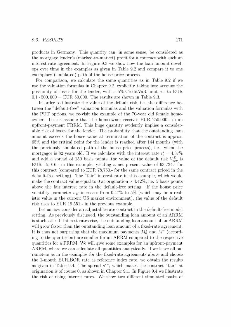
9.3. RESULTS 171
products in Germany. This quantity can, in some sense, be considered asthe mortgage lender’s (marked-to-market) profit for a contract with such aninterest-rate agreement. In Figure 9.3 we show how the loan amount devel-ops over time in the examples as given in Table 9.2 and compare it to oneexemplary (simulated) path of the house price process.
For comparison, we calculate the same quantities as in Table 9.2 if weuse the valuation formulas in Chapter 9.2, explicitly taking into account thepossibility of losses for the lender, with a 5%-CreditVaR limit set to EUR0.1 · 500, 000 = EUR 50,000. The results are shown in Table 9.3.
In order to illustrate the value of the default risk, i.e. the difference be-tween the ”default-free” valuation formulas and the valuation formulas withthe PUT options, we re-visit the example of the 70-year old female home-owner. Let us assume that the homeowner receives EUR 250,000.- in anupfront-payment FRRM. This huge quantity evidently implies a consider-able risk of losses for the lender. The probability that the outstanding loanamount exceeds the house value at termination of the contract is approx.65% and the critical point for the lender is reached after 144 months (withthe previously simulated path of the house price process), i.e. when themortgagor is 82 years old. If we calculate with the interest rate i∗0 = 4.37%and add a spread of 150 basis points, the value of the default risk V D
app isEUR 15,016.- in this example, yielding a net present value of 63,734.- forthis contract (compared to EUR 78,750.- for the same contract priced in thedefault-free setting). The ”fair” interest rate in this example, which wouldmake the contract value equal to 0 at origination is 4.42%, i.e. 5 basis pointsabove the fair interest rate in the default-free setting. If the house pricevolatility parameter σH increases from 0.47% to 5% (which may be a real-istic value in the current US market environment), the value of the defaultrisk rises to EUR 19,551.- in the previous example.
Let us now consider an adjustable-rate contract in the default-free modelsetting. As previously discussed, the outstanding loan amount of an ARRMis stochastic. If interest rates rise, the outstanding loan amount of an ARRMwill grow faster than the outstanding loan amount of a fixed-rate agreement.It is thus not surprising that the maximum payments M∗
0 and M∗ (accord-ing to the q-criterion) are smaller for an ARRM compared to the respectivequantities for a FRRM. We will give some examples for an upfront-paymentARRM, where we can calculate all quantities analytically. If we leave all pa-rameters as in the examples for the fixed-rate agreements above and choosethe 1-month EURIBOR rate as reference index rate, we obtain the resultsas given in Table 9.4. The spread sL∗, which makes the contract ”fair” atorigination is of course 0, as shown in Chapter 9.1. In Figure 9.4 we illustratethe risk of rising interest rates. We show two different simulated paths of
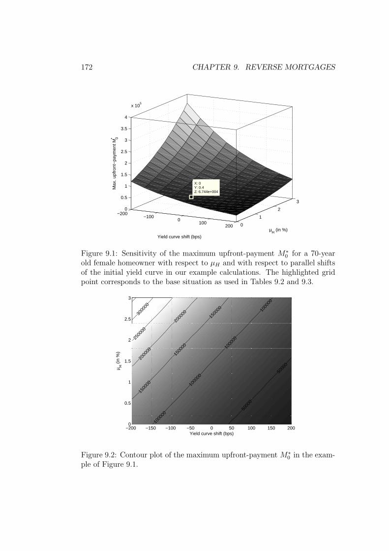
172 CHAPTER 9. REVERSE MORTGAGES
−200−100
0100
200 0
1
2
3
0
0.5
1
1.5
2
2.5
3
3.5
4
x 105
µH
(in %)
Yield curve shift (bps)
X: 0Y: 0.4Z: 6.744e+004
Max
. upf
ront
−pa
ymen
t M0*
Figure 9.1: Sensitivity of the maximum upfront-payment M∗0 for a 70-year
old female homeowner with respect to µH and with respect to parallel shiftsof the initial yield curve in our example calculations. The highlighted gridpoint corresponds to the base situation as used in Tables 9.2 and 9.3.
−200 −150 −100 −50 0 50 100 150 2000
0.5
1
1.5
2
2.5
3
5000
0
5000
0
1000
00
1000
00
1000
00
1000
00
1500
00
1500
00
1500
00
2000
00
2000
00
2500
00
3000
00
Yield curve shift (bps)
µ H (
in %
)
Figure 9.2: Contour plot of the maximum upfront-payment M∗0 in the exam-
ple of Figure 9.1.

9.3. RESULTS 173
Male FemaleAge i∗0 = 4.37% i∗0 = 4.39%65 i∗ = 4.36% i∗ = 4.36%
M∗0 = 60, 000 M∗
0 = 50, 000M∗ = 330 M∗ = 260
V UPFRRM(0, i∗0 + 0.015) = 19, 918 V UP
FRRM (0, i∗0 + 0.015) = 19, 001V LA
FRRM(0, i∗ + 0.015) = 10, 973 V LAFRRM (0, i∗ + 0.015) = 10, 412
Age i∗0 = 4.35% i∗0 = 4.37%70 i∗ = 4.35% i∗ = 4.35%
M∗0 = 80, 000 M∗
0 = 65, 000M∗ = 450 M∗ = 370
V UPFRRM(0, i∗0 + 0.015) = 21, 754 V UP
FRRM (0, i∗0 + 0.015) = 20, 475V LA
FRRM(0, i∗ + 0.015) = 10, 923 V LAFRRM (0, i∗ + 0.015) = 11, 119
Table 9.2: Examples of possible fixed-rate reverse mortgage contracts in the’default-free’ model setting with q = 0.965 and H0 = 500, 000.
Male FemaleAge i∗0,d = 4.37% i∗0,d = 4.39%65 i∗d = 4.36% i∗d = 4.36%
M∗0,d = 70, 000 M∗
0,d = 55, 000M∗
d = 400 M∗d = 320
V UPdFRRM(0, i∗0,d + 0.015) = 23, 153 V UP
dFRRM (0, i∗0,d + 0.015) = 20, 797V LA
dFRRM (0, i∗d + 0.015) = 12, 487 V LAdFRRM(0, i∗d + 0.015) = 11, 923
Age i∗0,d = 4.35% i∗0,d = 4.37%70 i∗d = 4.35% i∗d = 4.35%
M∗0,d = 95, 000 M∗
0,d = 80, 000M∗
d = 550 M∗d = 440
V UPdFRRM(0, i∗0,d + 0.015) = 25, 784 V UP
dFRRM (0, i∗0,d + 0.015) = 25, 127V LA
dFRRM (0, i∗d + 0.015) = 12, 757 V LAdFRRM(0, i∗d + 0.015) = 12, 482
Table 9.3: Examples of possible fixed-rate reverse mortgage contracts inthe model setting of Section 3 with a 5%-CreditVaR limit of 50,000 andH0 = 500, 000.
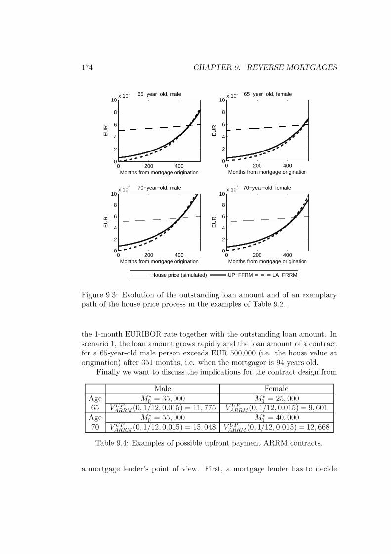
174 CHAPTER 9. REVERSE MORTGAGES
0 200 4000
2
4
6
8
10x 10
5
Months from mortgage origination
EU
R
65−year−old, male
0 200 4000
2
4
6
8
10x 10
5
Months from mortgage origination
EU
R
65−year−old, female
0 200 4000
2
4
6
8
10x 10
5
Months from mortgage origination
EU
R
70−year−old, male
0 200 4000
2
4
6
8
10x 10
5
Months from mortgage origination
EU
R
70−year−old, female
House price (simulated) UP−FFRM LA−FRRM
Figure 9.3: Evolution of the outstanding loan amount and of an exemplarypath of the house price process in the examples of Table 9.2.
the 1-month EURIBOR rate together with the outstanding loan amount. Inscenario 1, the loan amount grows rapidly and the loan amount of a contractfor a 65-year-old male person exceeds EUR 500,000 (i.e. the house value atorigination) after 351 months, i.e. when the mortgagor is 94 years old.
Finally we want to discuss the implications for the contract design from
Male FemaleAge M∗
0 = 35, 000 M∗0 = 25, 000
65 V UPARRM (0, 1/12, 0.015) = 11, 775 V UP
ARRM (0, 1/12, 0.015) = 9, 601Age M∗
0 = 55, 000 M∗0 = 40, 000
70 V UPARRM (0, 1/12, 0.015) = 15, 048 V UP
ARRM (0, 1/12, 0.015) = 12, 668
Table 9.4: Examples of possible upfront payment ARRM contracts.
a mortgage lender’s point of view. First, a mortgage lender has to decide
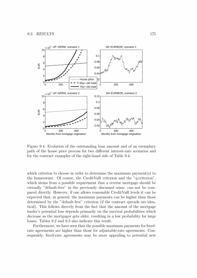
9.3. RESULTS 175
0 200 4000
2
4
6
8
10x 10
5 UP−ARRM, scenario 1
EU
R
0 200 400
0.02
0.04
0.06
0.08
0.1
1M−EURIBOR, scenario 1
0 200 4000
2
4
6
8
10x 10
5
Months from mortgage origination
EU
R
UP−ARRM, scenario 2
0 200 400
0.02
0.04
0.06
0.08
0.1
0.12
Months from mortgage origination
1M−EURIBOR, scenario 2
House price65yr−old male70yr−old male
Figure 9.4: Evolution of the outstanding loan amount and of an exemplarypath of the house price process for two different interest-rate scenarios andfor the contract examples of the right-hand side of Table 9.4.
which criterion to choose in order to determine the maximum payment(s) tothe homeowner. Of course, the CreditVaR criterion and the ”q-criterion”,which stems from a possible requirement that a reverse mortgage should bevirtually ”default-free” in the previously discussed sense, can not be com-pared directly. However, if one allows reasonable CreditVaR levels it can beexpected that, in general, the maximum payments can be higher than thosedetermined by the ”default-free” criterion (if the contract spreads are iden-tical). This follows directly from the fact that the amount of the mortgagelender’s potential loss depends primarily on the survival probabilities whichdecrease as the mortgagor gets older, resulting in a low probability for largelosses. Tables 9.2 and 9.3 also indicate this result.
Furthermore, we have seen that the possible maximum payments for fixed-rate agreements are higher than those for adjustable-rate agreements. Con-sequently, fixed-rate agreements may be more appealing to potential new
176 CHAPTER 9. REVERSE MORTGAGES
mortgagors. This is particularly true when long-term interest rates are low.Moreover, due to the higher maximum payments, the mortgage lender’s profitopportunities are larger (compare the examples in Tables 9.2 and 9.4). How-ever, these advantages of fixed-rate contracts do have a price: interest-raterisk. A mortgage lender issuing potentially long-term fixed-rate loans is obvi-ously exposed to considerable interest-rate risk when marking-to-market themortgage contracts. The hedging of this interest-rate risk is not straightfor-ward since the time of termination of the contracts is not known. A hedgingstrategy based on duration may constitute an easy first approach. Since adetailed discussion of this topic is beyond the scope of this thesis, we just addat this point that from a mortgage lender’s point of view, the interest-raterisk associated with fixed-rate contracts must be monitored carefully.
So far, we have excluded the possibility of systematic prepayment. Wehave already explained why this is not a restriction, particularly in the Ger-man market. Yet, we would like to mention at this point that if an explicitprepayment option is a desired contract feature, the valuation of the reversemortgage contract is still feasible, yet much more complex. The prepaymentintensity would, in this case, depend on the refinancing rates and a rela-tionship between (long-term) interest rates and prepayment would have tobe established. The valuation of reverse mortgage contracts would then fol-low the same lines as the intensity-based valuation of regular mortgages andmortgage-backed securities (see Chapters 5 and 6). Depending on the as-sumed relation between interest rates and prepayment, the modelling frame-work would, however, lose a considerable part of its analytical tractability.
Chapter 10
Summary and conclusion
In this thesis we have first developed new valuation techniques for mortgage-backed securities. MBS constitute a tremendously important segment of theUS fixed-income market and are widely accepted as an interesting asset classamong institutional investors, although their valuation and risk managementis in general a challenging and computationally expensive task.
In Chapter 5 we have presented a new valuation model based on a stochas-tic prepayment-intensity specification, which extends the more traditionaleconometric MBS models based on proportional hazard techniques. Ourmodel explicitly accounts for the general economic environment by the in-corporation of a factor which is fitted to the GDP growth rate. Applied toa series of GNMA MBS with different coupons we were able to successfullyexplain market prices across different coupons. While recognizing that a 1-factor model for the baseline prepayment process in the spirit of Kau et al.(2004) also produces good empirical results, we have found that the GDPfactor adds explanatory power to our model when applied to market prices.Both the risk of refinancing understatement (for premiums) and the risk ofturnover overstatement (for discounts) are accounted for in our prepayment-risk-neutral setting by three prepayment-risk adjustment parameters whichcan be calibrated to market data. The intensity-based modelling frameworkoffers the necessary mathematical rigour to target MBS market prices di-rectly, without the need of any OAS input. The OAS has become subjectto criticism in the academic literature lately due to its lack of a theoreticalfoundation. Yet, it remains perfectly possible to conduct a classical OASanalysis within our modelling framework by simply setting the prepayment-risk adjustment parameters to those values for which the prepayment inten-sity dynamics are identical under the real-world and under the risk-neutralpricing measure. This may be a particularly appealing characteristic of ourmodel with respect to its use in practice where the OAS is still a widely
177
178 CHAPTER 10. SUMMARY AND CONCLUSION
accepted quantity. It is also important to note that our model is of courseflexible enough to allow for further statistical fine-tuning by incorporatingadditional exogenously given covariates in a straightforward way. This maybe an interesting path to follow for further research, particularly with a viewtowards applications in practice. Furthermore, we have shown that our mod-elling approach can be easily adapted for the valuation of adjustable-rateMBS and CMOs. The valuation of more complex CMO structures, possiblyincorporating both prepayment and default risk (e.g., CMOs without agencyguarantees) may also be a fruitful field for further research.
We have then presented a closed-form formula which approximates thevalue of fixed-rate MBS in Chapter 6. While the model set-up is slightly dif-ferent for our closed-form approximation model in order to achieve a betteranalytical tractability, the approach is based on the same stochastic prepay-ment intensity techniques as the model presented in Chapter 5. Tacklingsome of the inconveniences of previous approaches to calculate MBS pricesin closed or semi-analytic form, our model proves to be able to explain ma-jor market price movements successfully for a wide range of coupons. Theoverall average absolute pricing error is 159 basis points in our sample (witha yearly recalibration of prepayment-risk adjustment parameters). The timeperiods where deviations between model and market prices were rather largewere in some cases characterised by unusually flat or even inverse shapesof the yield curve. A way to further improve the empirical performance ofour closed-form approximation may thus be the incorporation of a secondinterest-rate factor, representing long-term rates, into the CIR model. Withan overall of four stochastic factors in this case, however, one would have tocarefully analyse and weigh up the potential improvement in the empiricalfit against the danger of model overfitting. Obviously, an overparameterisedmodel may cause problems in the model calibration procedure and produceless reliable out-of-sample results. We leave this point for further research.
The closed-form formula is computationally highly efficient and reducesthe computational burden of MBS valuation drastically. It may thus be par-ticularly useful in risk and portfolio management. In Chapter 8 we haveconsidered selected scenario-based portfolio optimisation problems and ex-tended their usual application by including prepayment-sensitive fixed-rateagency MBS into the universe of available assets. In a case study with his-torical data from an interesting time period in the US fixed-income marketsfrom 2001 to 2003, when rates dropped to 40-year lows, we have empiricallytested our optimal asset allocation strategies. Our results indicate that aportfolio with MBS is indeed able to outperform a classical stock/bond port-folio significantly. We have therefore provided further empirical evidence forthe attractiveness of MBS from a quantitatively-oriented investor’s point of
179
view.Finally, we have presented a consistent framework for the valuation of
reverse mortgages in Chapter 9. Within our modelling framework we havealso calculated explicitly the probability that, at termination of the contract,the outstanding loan amount exceeds the house value. This probability canbe considered as ’default probability’ for the mortgage lender and by deter-mining the maximum payment(s) to the homeowner in such a way that thisdefault probability is very low, the pricing of the contract with a default-freemodel set-up and a riskless benchmark curve can be justified. We have shownthat for all fixed-rate reverse mortgages and for upfront-payment adjustable-rate reverse mortgages the ’default probabilities’ in a default-free setting canbe calculated analytically. In the case of a fixed-rate contract this is alsopossible if the valuation framework is extended to account for default andloss given default. In this extended set-up the maximum payment(s) to thehomeowner can be determined by a CreditVaR criterion. Applied to datafrom the German market, we have provided a couple of examples of howreverse mortgage contracts could look like in practice. While, due to thelimited availability of data, some assumptions are necessary, we have alsopointed out that it is possible to combine individual expert assumptionswith available data. By comparing different types of reverse mortgages andinterest-rate agreements we have also discussed implications for the designof reverse mortgage contracts from a lender’s perspective.
In a nutshell, the overall contribution of this thesis and its relation to therecent academic literature may be regarded as threefold: First, we have fur-ther developed and justified the intensity-based approach in the modellingof prepayment and in the valuation of MBS (introduced recently by, e.g.,Kau et al. (2006), Goncharov (2005)), taking into account the particulari-ties of a simultaneous consideration of discount and premium securities. Inthe spirit of an earlier model presented by Levin and Davidson (2005), wehave targeted prices directly by the introduction of prepayment-risk adjust-ment parameters. Second, we have presented a new concept to approximatethe value of fixed-rate MBS in closed-form. This has become an active fieldof research recently with some notable contributions by, e.g., Rom-Poulsen(2007) (extending a concept developed earlier by Collin-Dufresne and Hard-ing (1999)) and Gorovoy and Linetsky (2007). Our approach offers a com-putationally easy-to-handle alternative to these approaches which rely onnumerically complex techniques to evaluate semi-analytic pricing formulas.We have applied this approach in some selected asset allocation case studies,which would not have been feasible with more traditional, computationallyexpensive pricing routines. Third, this thesis aims to make a contribution to abetter understanding of valuation, pricing and risk issues associated with re-

180 CHAPTER 10. SUMMARY AND CONCLUSION
verse mortgages. Despite some publications and discussions in the economicand practitioner-oriented literature, a mathematically rigorous treatment ofreverse mortgages has so far remained scarce (with the possible exceptionof the recent contribution by Wang et al. (2007)). We thus hope that thisthesis may help to spread the popularity of reverse mortgages. Despite theobvious economic benefits of reverse mortgages, they are not yet available inmany European countries such as Germany.
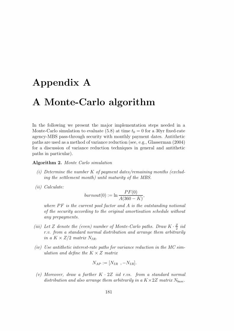
Appendix A
A Monte-Carlo algorithm
In the following we present the major implementation steps needed in aMonte-Carlo simulation to evaluate (5.8) at time t0 = 0 for a 30yr fixed-rateagency-MBS pass-through security with monthly payment dates. Antitheticpaths are used as a method of variance reduction (see, e.g., Glasserman (2004)for a discussion of variance reduction techniques in general and antitheticpaths in particular).
Algorithm 2. Monte Carlo simulation
(i) Determine the number K of payment dates/remaining months (exclud-ing the settlement month) until maturity of the MBS.
(ii) Calculate:
burnout(0) := lnPF (0)
A(360 − K),
where PF is the current pool factor and A is the outstanding notionalof the security according to the original amortisation schedule withoutany prepayments.
(iii) Let Z denote the (even) number of Monte-Carlo paths. Draw K · Z2
iidr.v. from a standard normal distribution and arrange them arbitrarilyin a K × Z/2 matrix NIR.
(iv) Use antithetic interest-rate paths for variance reduction in the MC sim-ulation and define the K × Z matrix
NAP := [NIR ,−NIR].
(v) Moreover, draw a further K · 2Z iid r.vs. from a standard normaldistribution and also arrange them arbitrarily in a K×2Z matrix Nbase.
181

182 APPENDIX A. A MONTE-CARLO ALGORITHM
(vi) Get r(0), Rpar(0, 10) from current yield curve, set w(0) equal to quar-terly GDP growth rate 6 months ago. Calculate
spread(0) := WAC − Rpar(0, 10),
p0(0) =θp + bpw · w(0)
ap
and p(0) according to (5.2). Also, calculate the discount rates R(0, tsettle)and R(0, t1) from the current yield curve, where tsettle and t1 correspondto the settlement date and the first payment date respectively.
(vii) Set the option-adjusted spread to the value OAS to be used in the val-uation routine.
(viii) Calculate the discount factors
DF (i) = e−(R(0,ti)+OAS)·ti i = settle, 1
(ix) Start MC simulation:for z=1:Zfor k=1:K
• Get f(0, tk), fτ (0, τ)|τ=tk from current yield curve, calculate θr(tk)according to (3.11).
• With ∆tk := tk − tk−1, calculate
r(tk) = e−ar ·∆tk · r(tk−1) +θr(tk)
ar· (1 − e−ar ·∆tk)
+
√σ2
r
2ar
· (1 − e−2·ar ·∆tk) · NAP (k, z)
• Calculate R(tk, tk + τ) for τ = 0.5, 1, 1.5, ..., 10 and the 10yr par-yield Rpar(tk, tk + 10) from R(tk, tk + τ) as given in, e.g., Hull(2003), p. 96.
• From r(tk), calculate the discount rate R(tk, tk + ∆tk) and thediscount factor from tk+1 to 0:
DF (tk+1) = e−(R(tk ,tk+∆tk)+OAS)·∆tk · DF (tk)
• Calculate
spread(tk) = WAC − Rpar(tk, tk + 10)

183
• Calculate PF (tk) given PF (tk−1) and p(tk−1) according to the for-mulas as stated in Chapter 2.2.3 and calculate
burnout(tk) = lnPF (tk)
A(360 − K + k).
• Calculate
w(tk) = e−aw ·∆tk · w(tk−1) +θw
aw· (1 − e−aw·∆tk)
+
√σ2
w
2aw· (1 − e−2·aw·∆tk) · Nbase(k, z)
• Calculate
p0(tk) = e−ap·∆tk · p0(tk−1) +θp0
+ bpw · w(tk)
aw· (1 − e−ap·∆tk)
+
√σ2
p
2ap· (1 − e−2·ap·∆tk) · Nbase(k, Z + z)
• Calculate p(tk) according to (5.2) and (5.9)end (loop over k)
• With prepayment vector p = (p(1), ..., p(tK−1))′ calculate MBS
cash flows (e.g., with mbscfamounts - function in Matlab), in-cluding accrued interest, for a face amount of 1.
• Discount cash flows occurring at dates tsettle, t1, ..., tK with the re-spective discount factors and calculate the sum of the discountedcash flows to obtain the value Vz(0) of the MBS.end (loop over z)
(x) Average over MC paths to obtain the value of the MBS
V (0) =1
Z·
Z∑
z=1
Vz(0)

184 APPENDIX A. A MONTE-CARLO ALGORITHM
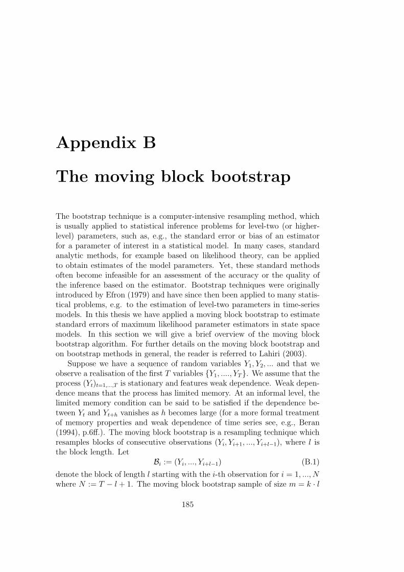
Appendix B
The moving block bootstrap
The bootstrap technique is a computer-intensive resampling method, whichis usually applied to statistical inference problems for level-two (or higher-level) parameters, such as, e.g., the standard error or bias of an estimatorfor a parameter of interest in a statistical model. In many cases, standardanalytic methods, for example based on likelihood theory, can be appliedto obtain estimates of the model parameters. Yet, these standard methodsoften become infeasible for an assessment of the accuracy or the quality ofthe inference based on the estimator. Bootstrap techniques were originallyintroduced by Efron (1979) and have since then been applied to many statis-tical problems, e.g. to the estimation of level-two parameters in time-seriesmodels. In this thesis we have applied a moving block bootstrap to estimatestandard errors of maximum likelihood parameter estimators in state spacemodels. In this section we will give a brief overview of the moving blockbootstrap algorithm. For further details on the moving block bootstrap andon bootstrap methods in general, the reader is referred to Lahiri (2003).
Suppose we have a sequence of random variables Y1, Y2, ... and that weobserve a realisation of the first T variables Y1, ...., YT. We assume that theprocess (Yt)t=1,...,T is stationary and features weak dependence. Weak depen-dence means that the process has limited memory. At an informal level, thelimited memory condition can be said to be satisfied if the dependence be-tween Yt and Yt+h vanishes as h becomes large (for a more formal treatmentof memory properties and weak dependence of time series see, e.g., Beran(1994), p.6ff.). The moving block bootstrap is a resampling technique whichresamples blocks of consecutive observations (Yi, Yi+1, ..., Yi+l−1), where l isthe block length. Let
Bi := (Yi, ..., Yi+l−1) (B.1)
denote the block of length l starting with the i-th observation for i = 1, ..., Nwhere N := T − l + 1. The moving block bootstrap sample of size m = k · l
185
186 APPENDIX B. THE MOVING BLOCK BOOTSTRAP
is then obtained by concatenating the blocks B∗1, ...,B∗
k which are drawn withreplacement from the collection B1, ...,BN. Usually, the sample size m ischosen to be of the same order as the original sample size T , i.e. m ≈ T(see Lahiri (2003), p. 26). The resampled sequence of random variables isdenoted by Y ∗
1 , ...., Y ∗m. Now, let
θ∗l,m := t(Y ∗1 , ..., Y ∗
m) (B.2)
denote one bootstrap realisation of the estimator of the parameter of interestθ, where t(·) is some function/statistic of the data used as an estimator forθ. Repeating the resampling procedure B times, let
θ∗,(j)l,m := t(Y
∗,(j)1 , ..., Y ∗,(j)
m ), (B.3)
j = 1, ..., B, denote the bootstrap replicates of θ∗l,m. Applying the Monte-
Carlo principle, an estimate θ of the quantity of interest θ is finally obtainedby averaging over the bootstrap replicates:
θT =1
B
B∑
j=1
θ∗,(j)l,m . (B.4)
The moving block bootstrapping procedure can be summarised in the follow-ing algorithm:
Algorithm 3. (Moving block bootstrap)
(i) Given a data sample YT := (Y1, ..., YT ) of size T , choose the blocklength l and the number of blocks k to be concatenated in the resamplingprocedure such that m = k · l ≈ T .
(ii) Randomly draw k blocks from the collection B1, ...,BN (with replace-ment) with Bi as defined in (B.1) to obtain a bootstrap sampleB∗
1, ...,B∗k. Calculate θ∗l,m as given in (B.2).
(iii) Repeat (ii) B times to obtain bootstrap replicates θ∗,(j)l,m , j = 1, ..., B, of
the quantity of interest.
(iv) Average over the bootstrap replicates to obtain the estimate of the quan-tity of interest as given in (B.4).
For a theoretical justification of the moving block bootstrap, the reader isreferred to Lahiri (2003). Yet, it has to be mentioned that the moving block

187
bootstrap principle is partly based on heuristic arguments only. In addi-tion to this, the theoretical foundation holds only asymptotically (i.e. asthe number of observations T → ∞) and it is hard to assess the quality ofthe approximation for finite samples. The choice of the block length, whichpotentially optimises the bootstrap procedure, is also a non-trivial problem.Lahiri (2003) discusses all these topics and further challenges concerningbootstrap techniques in detail. Since we have only used the bootstrap prin-ciple in order to obtain estimates for level-two parameters (which is not ourmain concern in this thesis), we rely on the results generated by this methodwhile keeping in mind that they should only be considered as rough estimates.

188 APPENDIX B. THE MOVING BLOCK BOOTSTRAP

Appendix C
Discussion of approximationerrors
The error term Rtk
In (3.36) we have introduced the error terms Rtk , k = 1, ..., K resulting fromthe approximation of an integral by sums. From (3.35) and (3.36) it followsthat for k = 1, ..., K:
|Rtk | =
∣∣∣∣∣
∫ tk
tk−1
γ(u)e−R ut
γ(s)dsdu − γ(tk) · e−R tkt γ(s)ds · ∆tk
∣∣∣∣∣
=∣∣∣e−
R tk−1t γ(s)ds − (1 + γ(tk) · ∆tk) · e−
R tkt γ(s)ds
∣∣∣
= e−R tkt γ(s)ds ·
∣∣∣∣eR tktk−1
γ(s)ds − (1 + γ(tk) · ∆tk)
∣∣∣∣
= e−R tkt γ(s)ds ·
∣∣∣∣∣∣
∫ tk
tk−1
γ(s)ds − γ(tk) · ∆tk + O
(∫ tk
tk−1
γ(s)ds
)2∣∣∣∣∣∣
≤ e−R tkt γ(s)ds · R∆tk
k ,
where
R∆tkk := max
ξ∈[tk−1,tk]|γ(ξ) − γ(tk)| · ∆tk + O
(∫ tk
tk−1
γ(s)ds
)2 .
Note that R∆tkk → 0 and consequently |Rtk | → 0 as ∆tk → 0.
189
190 APPENDIX C. DISCUSSION OF APPROXIMATION ERRORS
The error terms R, R
In Theorem 6.2 we have first introduced the error terms
R(∆t, v2k, w
2k, zk · vk, zk · wk, vk · wk), k = 1, ..., K.
These terms contain residual terms of the order O(∆t) resulting from theapproximation of integrals by sums, similar to the error term Rtk as discussedin the previous section, with
R(∆t, v2k, w
2k, zk · vk, zk · wk, vk · wk) → R(v2
k, w2k, zk · vk, zk · wk, vk · wk)
for ∆t → 0. R(v2k, w
2k, zk · vk, zk · wk, vk · wk) contains the residual terms
from the series expansion of the exponential function in (6.12). The size ofthis error term primarily depends on vk and wk. Following the definition ofthese quantities in Theorem 6.2, vk can be expected to be small for premiumsand wk can be expected to be small for discounts. The empirical results asdiscussed in Chapter 6 indicate that our closed-form approximation modelperforms slightly better for premiums than for discounts.
References
Acharya, V. and J. Carpenter (2002). Corporate Bond Valuation andHedging with Stochastic Interest Rates and Endogenous Bankruptcy.Review of Financial Studies 15, 1355–1383.
Ambrose, B. and M. LaCour-Little (2001). Prepayment Risk in AdjustableRate Mortgages Subject to Initial Year Discounts: Some New Evi-dence. Real Estate Economics 29, 305–327.
Artzner, P. and F. Delbaen (1992). Credit Risk and Prepayment Option.Astin Bulletin 22, 81–96.
Asay, M., F. Guillaume, and R. Mattu (1987). Duration and Convex-ity of Mortgage-Backed Securities: Some Hedging Implications from aSimple Prepayment-Linked Present-Value Model. In F. Fabozzi (Ed.),Mortgage-Backed Securities: New Strategies, Applications and Re-search. Chicago: Probus.
Beran, J. (1994). Statistics for long memory processes. New York: Chap-man & Hall.
Bielecki, T. and M. Rutkowski (2002). Credit Risk: Modeling, Valuationand Hedging. Berlin: Springer.
Bingham, N. and R. Kiesel (2004). Risk-Neutral Valuation (2nd ed.). Lon-don: Springer.
Black, F. and R. Litterman (1992). Global Portfolio Otimization. FinancialAnalysts Journal 48, 28–43.
Box, G. (1979). Robustness in the strategy of scientific model building.In R. Launer and G. Wilkinson (Eds.), Robustness in Statistics. NewYork: Academic Press.
Bremaud, P. (1981). Point Processes and Queues. New York: Springer.
Brennan, M. and E. Schwartz (1979). A continuous time approach to thepricing of bonds. Journal of Banking and Finance 3, 133–155.
191
192 REFERENCES
Brigo, D. and F. Mercurio (2001). On deterministic-shift extensions ofshort-rate models. Finance and Stochastics 5 (3).
Brigo, D. and F. Mercurio (2006). Interest-Rate Models: Theory and Prac-tice (2nd ed.). Berlin: Springer.
Collin-Dufresne, P. and J. Harding (1999). A Closed Form Formulafor Valuing Mortgages. Journal of Real Estate Finance and Eco-nomics 19 (2), 133–146.
Cox, J., J. Ingersoll, and S. Ross (1985). A Theory of the Term Structureof Interest Rates. Econometrica 53 (2), 385–408.
Davidoff, T. and G. Welke (2005). Selection and Moral Hazard in theReverse Mortgage Market. Working paper .
Davis, S. (2004). An ARMs Prepayment Model: A Parsimonious Ap-proach. Journal of Fixed Income March 2004, 73–79.
Downing, C., R. Stanton, and N. Wallace (2005). An Empirical Test of aTwo-Factor Mortgage Valuation Model: How Much Do House PricesMatter? Real Estate Economics 33, 681–710.
Duffie, D. (1998). First-to-default valuation. Working paper, Stanford Uni-versity .
Dunn, K. and J. McConnell (1981). Valuation of GNMA Mortgage-BackedSecurities. Journal of Finance 36, 599–616.
Efron, B. (1979). Bootstrap methods: Another look at the jackknife. TheAnnals of Statistics 7, 1–26.
Engle, R. (1982). Autoregressive Conditional Heteroscedasticity with Es-timates of the Variance of UK Inflation. Econometrica 50, 987–1008.
Eschtruth, A., W. Sun, and A. Webb (2006). Will Reverse MortgagesRescue the Baby Boomers? An issue in brief - Center for RetirementResearch at Boston College 54.
Fabozzi, F. (Ed.) (1998). Advances in the Valuation and Management ofMortgage-Backed Securities. New Hope: Frank J. Fabozzi Associates.
Fabozzi, F. (2006). The Handbook of Mortgage-Backed Securities (6th ed.).McGraw-Hill.
Francois, P. (2003). Measuring Prepayment Risk Exposure on DefaultableCallable Debt. Working Paper, HEC Montreal .
Geyer, A. and S. Pichler (1999). A state-space approach to estimate andtest multifactor Cox-Ingersoll-Ross models of the term structure. Jour-nal of Financial Research 22 (1), 107–130.
REFERENCES 193
Glasserman, P. (2004). Monte Carlo methods in financial engineering. NewYork: Springer.
Goncharov, Y. (2005). An Intensity-Based Approach to Valuation of Mort-gage Contracts and Computation of the Endogenous Mortgage Rate.International Journal of Theoretical and Applied Finance 9 (6), 889–914.
Goncharov, Y. (2007). Computing the Endogenous Mortgage Rate withoutIterations. Working paper .
Goncharov, Y., G. Okten, and M. Shah (2006). Computation of the En-dogenous Mortgage Rates with Randomized Quasi-Monte Carlo Simu-lations. Mathematical and Computer Modelling, forthcoming .
Gorovoy, V. and V. Linetsky (2007). Intensity-Based Valuation of Res-idential Mortgages: An Analytically Tractable Model. MathematicalFinance 17 (4), 541–573.
Harvey, A. (1989). Forecasting, Structural Time Series Models and theKalman Filter. Cambridge: Cambridge University Press.
Hocht, S., K. Ng, J. Wolf, and R. Zagst (2007). Optimal portfolio allocationwith Asian hedge funds and Asian REITs. International Journal ofServices Sciences, forthcoming .
Hu, J. (1997). Basics of Mortgage-Backed Securities. New Hope: Frank J.Fabozzi Associates.
Hull, J. and A. White (1990). Pricing Interest-Rate Derivative Securities.Review of Financial Studies 3 (4), 573–592.
Hull, J. C. (2003). Options, Futures and other derivatives (5th ed.). NewJersey: Prentice Hall.
Jacod, J. and A. Shiryaev (1987). Limit Theorems for Stochastic Processes.Berlin: Springer Verlag.
Johnson, L., S. Kotz, and N. Balakrishnan (1995). Continuous UnivariateDistributions, Vol. 2 (2nd ed.). New York: John Wiley & Sons.
Kagraoka, Y. (2002). The OAS Approach and the Martingale Measure forMortgage Prepayment. 2nd World Congress of the Bachelier FinanceSociety .
Kalman, R. (1960). A New Approach to Linear Filtering and Predic-tion Problems. Transaction of the ASME - Journal of Basic Engineer-ing (March 1960), 35–45.
194 REFERENCES
Kalotay, A., D. Yang, and F. Fabozzi (2004). An Option-Theoretic Pre-payment Model for Mortgages and Mortgage-Backed Securities. Inter-national Journal of Theoretical and Applied Finance 7, 949–978.
Karatzas, I. and S. Shreve (1991). Brownian Motion and Stochastic Cal-culus. Berlin: Springer.
Kariya, T., F. Ushiyama, and S. Pliska (2002). A 3-factor Valuation Modelfor Mortgage-Backed Securities. Working Paper .
Kau, J., D. Keenan, and A. Smurov (2004). Reduced-Form Mortgage Val-uation. Working Paper .
Kau, J., D. Keenan, and A. Smurov (2006). Reduced Form MortgagePricing as an Alterntive to Option-Pricing Models. Journal of RealEstate Finance and Economics 33, 183–196.
Kau, J. and V. Slawson (2002). Frictions, Heterogeneity and Optimal-ity in Mortgage Modeling. Journal of Real Estate Finance and Eco-nomics 24 (3), 239–260.
Koopman, S., N. Shephard, and J. Doornik (1999). Statistical algorithmsfor models in state space using Ssfpack 2.2. Econometrics Journal 2,113–166.
Korn, R. and E. Korn (1999). Optionsbewertung und Portfolio-Optimierung. Vieweg.
Krokhmal, P., J. Palmquist, and S. Uryasev (2002). Portfolio Optimiza-tion with Conditional Value-at-Risk Objective and Constraints. TheJournal of Risk 4 (2), 11–27.
Krokhmal, P., S. Uryasev, and G. Zrazhevsky (2002). Risk Managment forHedge Fund Portfolios: A Comparative Analysis of Linear RebalancingStrategies. Journal of Alternative Investments 5 (1), 10–29.
Kupiec, P. and A. Kah (1999). On the Origin and Interpretation of OAS.The Journal of Fixed Income 9 (3), 82–92.
Lahiri, S. (2003). Resampling Methods for Dependent Data. New York:Springer.
Levin, A. (2001). Active-Passive Decomposition in Burnout Modeling. TheJournal of Fixed Income 10 (4), 27–40.
Levin, A. and D. Daras (1998). Non-Traded Factors in MBS PortfolioManagement. In F. Fabozzi (Ed.), Advances in the Valuation and Man-agement of Mortgage-Backed Securities. New Hope: Frank J. FabozziAssociates.
REFERENCES 195
Levin, A. and A. Davidson (2005). Prepayment Risk- and Option-AdjustedValuation of MBS - Opportunities for Arbitrage. The Journal of Port-folio Management 31 (4).
Lilliefors, H. (1967). On the Kolmogorov-Smirnov test for normality withmean and variance unknown. Journal of the American Statistical As-sociation 62, 399–402.
Liptser, R. and A. Shiryaev (2001). Statistics of Random Processes, II.(2nd ed.). Berlin: Springer.
Ljung, G. and G. Box (1978). On a Measure of Lack of Fit in Time SeriesModels. Biometrika 65 (2), 297–303.
Mamon, R. (2004). Three Ways to Solve for Bond Prices in the VasicekModel. Journal of Applied Mathematics and Decision Sciences 8 (1).
Margrabe, W. (1978). The value of an option to exchange one asset foranother. Journal of Finance 33, 177–186.
Markowitz, H. (1952). Portfolio selection. Journal of Finance 7, 77–91.
Maxam, C. and M. LaCour-Little (2001). Applied Non-ParametricRegression Techniques: Estimating Prepayments on Fixed RateMortgage-Backed Securities. Journal of Real Estate Finance and Eco-nomics 23 (2), 139–161.
McKendall, R., S. Zenios, and M. Holmer (1993). Stochastic ProgrammingModels for Portfolio Optimization. Research Guide.
Meucci, A. (2005). Risk and Asset Allocation (2nd ed.). Berlin: Springer.
Milevsky, M. and S. Posner (1998). Asian Options, the Sum of Lognor-mals, and the Reciprocal Gamma Distribution. Journal of Financialand Quantitative Analysis 33, 409–421.
Nakagawa, H. and T. Shouda (2005). Analyses of Mortgage-Backed Se-curities Based on Unobservable Prepayment Cost Processes. WorkingPaper .
Popova, E., I. Popova, and E. George (2007). Bayesian forecasting of pre-payment rates for individual pools of mortgages. Working paper .
Press, W., S. Teukolsky, W. Vetterling, and B. Flamery (1992). NumericalRecipes in C, The Art of Scientific Computing (2nd ed.). Cambridge:Cambridge University Press.
Rebonato, R. (1998). Interest-Rate Option Models (2nd ed.). Chichester:John Wiley & Sons.
196 REFERENCES
Richard, S. and R. Roll (1989). Prepayments on Fixed-Rate Mortgage-Backed Securities. Journal of Portfolio Management 15, 73–82.
Rockafellar, R. and S. Uryasev (2000). Optimization of Conditional Value-at-Risk. Journal of Risk 2, 21–41.
Rom-Poulsen, N. (2007). Semi-analytical MBS Pricing. Journal of RealEstate Finance and Economics 34 (4), 463–498.
Schmid, B. (2002). Pricing Credit Linked Financial Instruments - Theoryand Empirical Evidence. Berlin: Springer.
Schmid, B. (2004). Credit Risk Pricing Models: Theory and Practice (2nded.). Berlin: Springer Finance.
Schonbucher, P. (2003). Credit derivatives pricing models. Chichester:John Wiley & Sons.
Schwartz, E. and W. Torous (1989). Prepayment and the Valuation ofMortgage-Backed Securities. The Journal of Finance 44, 375–392.
Sharp, N., D. Newton, and P. Duck (2006). An Improved Fixed-Rate Mort-gage Valuation Methodology With Interacting Prepayment and DefaultOptions. Journal of Real Estate Finance and Economics, forthcoming .
Shiller, R. and A. Weiss (2000). Moral Hazard in Home Equity Conversion.Real Estate Economics 28, 1–31.
Spahr, R. and M. Sunderman (1992). The Effect of Prepayment Model-ing in Pricing of Mortgage-Backed Securities. Journal of Housing Re-search 3 (2), 381–400.
Stanton, R. (1995). Rational Prepayment and the Valuation of Mortgage-Backed Securities. Review of Financial Studies 8, 677–708.
Vasicek, O. (1977). An Equilibrium Characterization of the Term Struc-ture. Journal of Financial Economics 5, 177–188.
Wang, L., E. Valdez, and J. Piggott (2007). Securitization of longevity riskin reverse mortgages. Working paper .
Young, R., L. Hayre, and S. Chaudhary (1999). The Mechanics of Investingin Mortgage- and Asset-Backed Securities. Salomon Smith Barney, USFixed Income Research Report .
Zagst, R. (2002a). Interest Rate Management. Berlin: Springer Finance.
Zagst, R. (2002b). Using scenario analysis for risk management. Allge-meines Statistisches Archiv 86, 97–117.
Zenios, S. (1993). A model for portfolio management with mortgage-backedsecurities. Annals of Operations Research 43 (6), 337–356.

REFERENCES 197
Zenios, S. and P. Kang (1993). Mean-absolute deviation portfolio op-timization for mortgage-backed securities. Annals of Operations Re-search 45 (1), 433–450.

198 REFERENCES
List of Figures
2.1 10yr treasury par yield and prepayment speeds . . . . . . . . . 12
2.2 Standard PSA curves . . . . . . . . . . . . . . . . . . . . . . . 13
5.1 Observed and estimated SMM values . . . . . . . . . . . . . . 70
5.2 Expected prepayment speed in real-world and under the risk-neutral pricing measure . . . . . . . . . . . . . . . . . . . . . . 73
5.3 OAS according to our model and to Bloomberg . . . . . . . . 74
5.4 Market and model prices on different sample dates . . . . . . . 77
5.5 Effective durations and convexities . . . . . . . . . . . . . . . 79
5.6 Sensitivities w.r.t. changes in model parameters (I) . . . . . . 82
5.7 Sensitivities w.r.t. changes in model parameters (II) . . . . . . 82
5.8 Sensitivities w.r.t. changes in model parameters (III) . . . . . 83
5.9 ARM prepayment speeds vs. pool age . . . . . . . . . . . . . . 85
5.10 Observed and expected GNMA ARM prepayment speeds . . . 86
5.11 Sequential-pay CMO tranche price sensitivities w.r.t. interest-rate volatility . . . . . . . . . . . . . . . . . . . . . . . . . . . 91
5.12 Sequential-pay CMO cash flow structure . . . . . . . . . . . . 92
6.1 Assumed functional form of the relationship between the con-tract rate spread and the refinancing-related prepayment speed 100
6.2 Observed and estimated prepayment speeds . . . . . . . . . . 113
6.3 Expected prepayment rates under the real-world measure andunder the risk-neutral pricing measure . . . . . . . . . . . . . 115
6.4 Expected prepayment speeds under the risk-neutral pricingmeasure from 1996 to 2006 . . . . . . . . . . . . . . . . . . . . 116
6.5 Market and model prices for a series of generic GNMA TBApass-throughs (I) . . . . . . . . . . . . . . . . . . . . . . . . . 120
6.6 Market and model prices for a series of generic GNMA TBApass-throughs (II) . . . . . . . . . . . . . . . . . . . . . . . . . 121
6.7 Effective (short-rate) durations and convexities . . . . . . . . . 122
199
200 LIST OF FIGURES
8.1 Market prices of GNMA pass-through MBS . . . . . . . . . . 1358.2 S&P 500 index and 3 month treasury strip rate from 2001 to
2003 . . . . . . . . . . . . . . . . . . . . . . . . . . . . . . . . 1368.3 Histograms of total returns of portfolio instruments . . . . . . 1378.4 Expected utility-variance efficient frontier, relation to risk-
aversion parameter . . . . . . . . . . . . . . . . . . . . . . . . 1408.5 Expected utility-variance efficient frontier for different instru-
ments . . . . . . . . . . . . . . . . . . . . . . . . . . . . . . . 1408.6 Optimal portfolio weights from 2001-2003 in a stock/bond
portfolio. . . . . . . . . . . . . . . . . . . . . . . . . . . . . . . 1418.7 Optimal portfolio weights from 2001-2003 in a stock/bond/MBS
portfolio. . . . . . . . . . . . . . . . . . . . . . . . . . . . . . . 1418.8 Total wealth according to our multi-period optimal asset allo-
cation strategy from 2001-2003 . . . . . . . . . . . . . . . . . 1428.9 Optimal portfolio weights from 2001-2003 in a stock/bond
portfolio. . . . . . . . . . . . . . . . . . . . . . . . . . . . . . . 1488.10 Optimal portfolio weights from 2001-2003 in a stock/bond/MBS
portfolio. . . . . . . . . . . . . . . . . . . . . . . . . . . . . . . 1488.11 Expected return-variance efficient frontier for different instru-
ments . . . . . . . . . . . . . . . . . . . . . . . . . . . . . . . 1498.12 Total wealth according to our multi-period optimal asset allo-
cation strategy from 2001-2003 . . . . . . . . . . . . . . . . . 149
9.1 Sensitivity of the maximum upfront-payment M∗0 w.r.t. µH
and to parallel shifts of the initial yield curve . . . . . . . . . 1729.2 Contour plot of the maximum upfront-payment M∗
0 . . . . . . 1729.3 Evolution of the outstanding loan amount . . . . . . . . . . . 1749.4 Exemplary evolution of the outstanding loan amount in an
ARRM contract . . . . . . . . . . . . . . . . . . . . . . . . . . 175