Industrial management I Production, procurement, and inventory · Production Order Quantity (POQ)...
37
Lehrstuhl für Industrie, Energie und Umwelt Universität Wien Fakultät für Wirtschaftswissenschaften Lehrstuhl für Industrie, Energie und Umwelt Brünner Straße 72, 1210 Wien Industrial management I Production, procurement, and inventory | Prof. Franz Wirl | Office hour: Thursday 9 – 10 Email: [email protected] Homepage:http://bwl.univie.ac.at/ieu
Transcript of Industrial management I Production, procurement, and inventory · Production Order Quantity (POQ)...
Lehrstuhl für Industrie, Energie und Umwelt
Universität Wien Fakultät für Wirtschaftswissenschaften Lehrstuhl für Industrie, Energie und Umwelt Brünner Straße 72, 1210 Wien
Industrial management I Production, procurement, and
inventory | Prof. Franz Wirl |
Office hour: Thursday 9 – 10
Email: [email protected]
Homepage:http://bwl.univie.ac.at/ieu
Industriebetriebslehre I Lehrstuhl f. Industrie, Energie und Umwelt
| Prof. Wirl WS 2012/13 Seite 2
Inventory Management |1
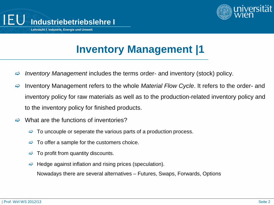
Inventory Management includes the terms order- and inventory (stock) policy.
Inventory Management refers to the whole Material Flow Cycle. It refers to the order- and
inventory policy for raw materials as well as to the production-related inventory policy and
to the inventory policy for finished products.
What are the functions of inventories?
To uncouple or seperate the various parts of a production process.
To offer a sample for the customers choice.
To profit from quantity discounts.
Hedge against inflation and rising prices (speculation).
Nowadays there are several alternatives – Futures, Swaps, Forwards, Options
Industriebetriebslehre I Lehrstuhl f. Industrie, Energie und Umwelt
| Prof. Wirl WS 2012/13 Seite 3
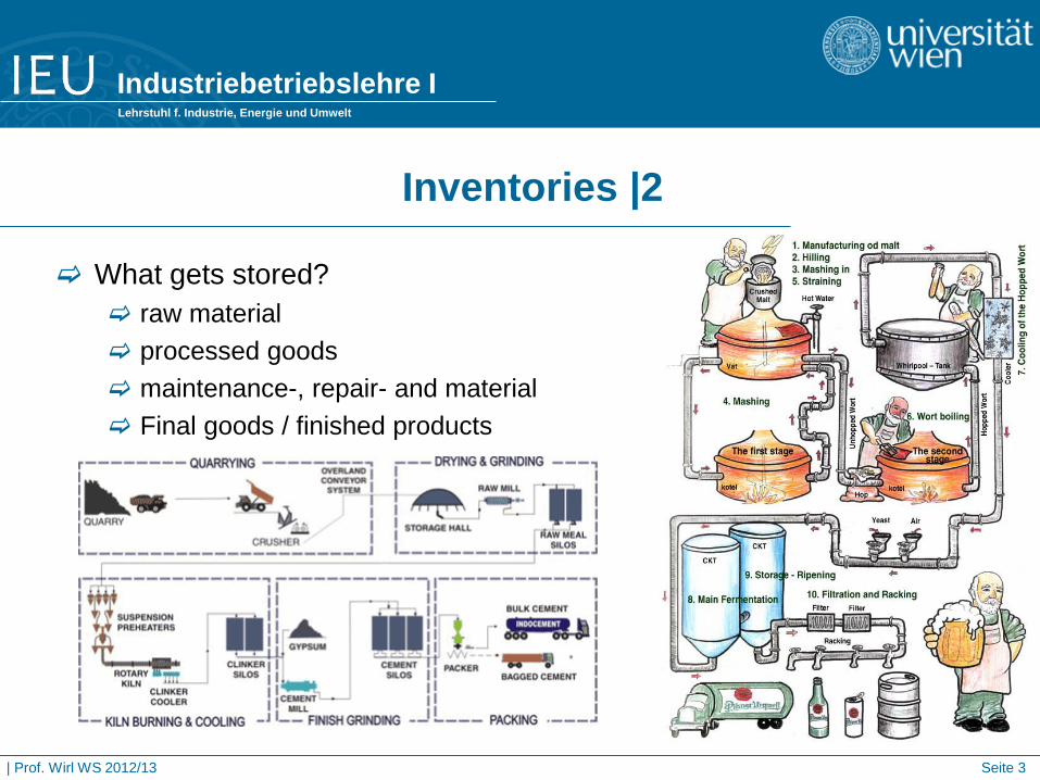
Inventories |2
What gets stored? raw material processed goods maintenance-, repair- and material Final goods / finished products
Industriebetriebslehre I Lehrstuhl f. Industrie, Energie und Umwelt
| Prof. Wirl WS 2012/13 Seite 4
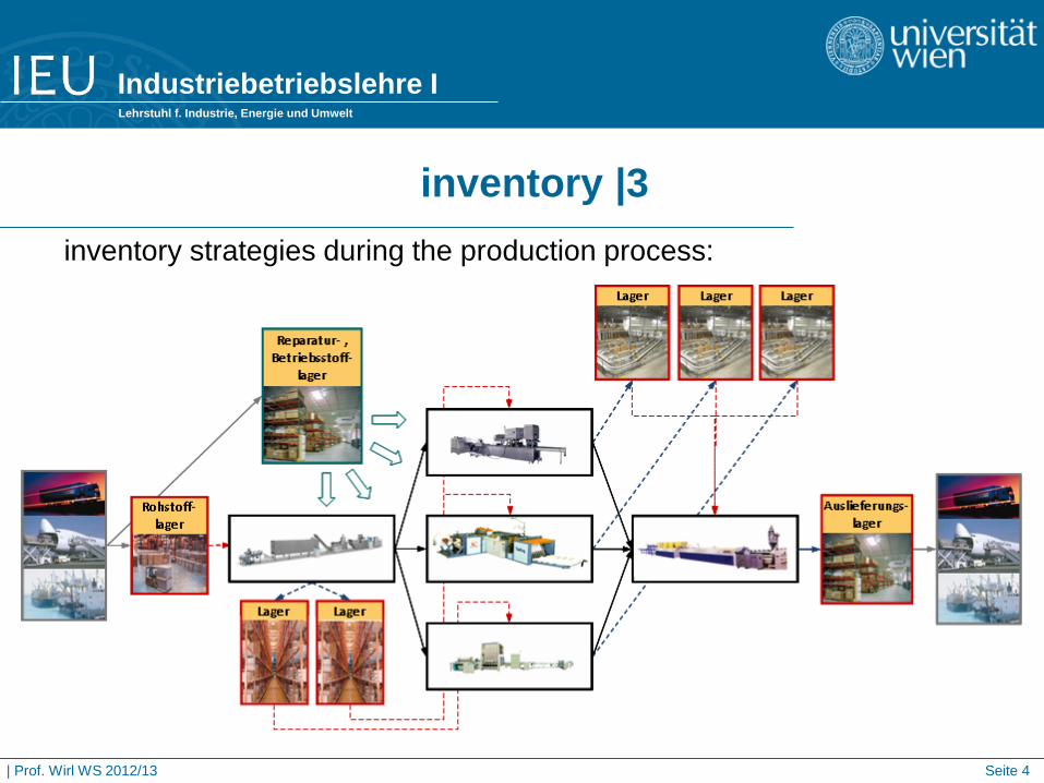
inventory |3 inventory strategies during the production process:
Industriebetriebslehre I Lehrstuhl f. Industrie, Energie und Umwelt
| Prof. Wirl WS 2012/13 Seite 5
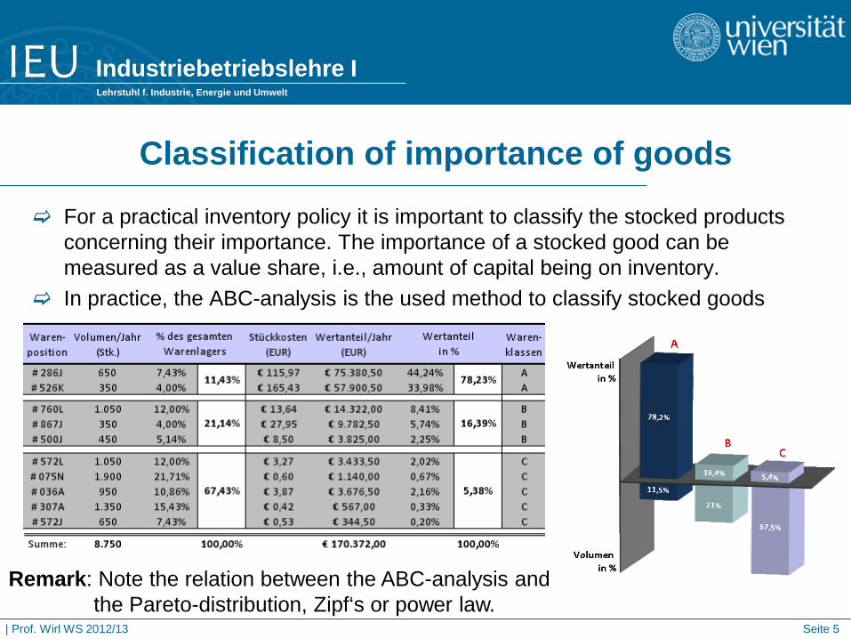
Classification of importance of goods
For a practical inventory policy it is important to classify the stocked products concerning their importance. The importance of a stocked good can be measured as a value share, i.e., amount of capital being on inventory.
In practice, the ABC-analysis is the used method to classify stocked goods
Remark: Note the relation between the ABC-analysis and the Pareto-distribution, Zipf‘s or power law.
Industriebetriebslehre I Lehrstuhl f. Industrie, Energie und Umwelt
| Prof. Wirl WS 2012/13 Seite 6
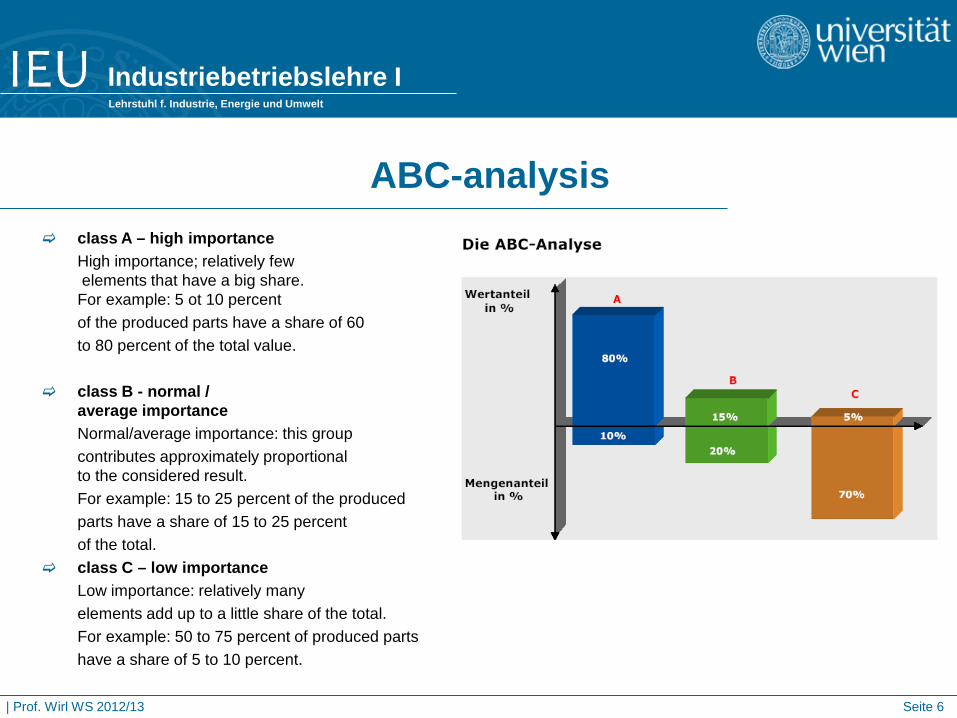
ABC-analysis
class A – high importance High importance; relatively few
elements that have a big share. For example: 5 ot 10 percent
of the produced parts have a share of 60 to 80 percent of the total value. class B - normal /
average importance Normal/average importance: this group contributes approximately proportional
to the considered result. For example: 15 to 25 percent of the produced parts have a share of 15 to 25 percent of the total. class C – low importance Low importance: relatively many elements add up to a little share of the total. For example: 50 to 75 percent of produced parts have a share of 5 to 10 percent.
Industriebetriebslehre I Lehrstuhl f. Industrie, Energie und Umwelt
| Prof. Wirl WS 2012/13 Seite 7
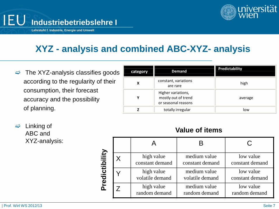
XYZ - analysis and combined ABC-XYZ- analysis
The XYZ-analysis classifies goods according to the regularity of their consumption, their forecast accuracy and the possibility of planning.
Linking of
ABC and XYZ-analysis:
category Demand Predictability
X constant, variations are rare
high
Y Higher variations, mostly out of trend or seasonal reasons
average
Z totally irregular low
A B C
X high value constant demand
medium value constant demand
low value constant demand
Y high value volatile demand
medium value volatile demand
low value constant demand
Z high value random demand
medium value random demand
low value random demand
Value of items
Pred
ictib
ility
Industriebetriebslehre I Lehrstuhl f. Industrie, Energie und Umwelt
| Prof. Wirl WS 2012/13 Seite 8
inventory | costs |1
In many companies the inventory represents one of the most costly assets and sometimes up to 50% of the investeted capital (e.g., Amazon.com).
The aim is to balance order versus inventory costs. The trade-off is between:
Little inventories but many orders Large inventories thus few orders
The optimal strategy dependends on the magnitudes of holding costs and order costs. The instrument of the optimization is quantity ordered (sometimes called lot size).
Industriebetriebslehre I Lehrstuhl f. Industrie, Energie und Umwelt
| Prof. Wirl WS 2012/13 Seite 9
inventory | costs |2
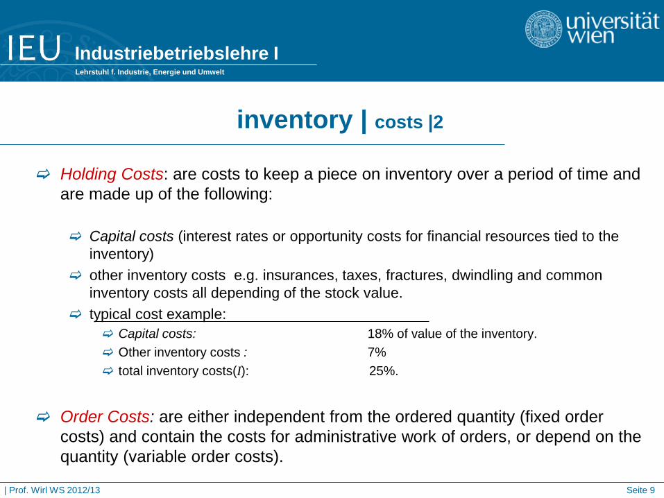
Holding Costs: are costs to keep a piece on inventory over a period of time and are made up of the following: Capital costs (interest rates or opportunity costs for financial resources tied to the
inventory) other inventory costs e.g. insurances, taxes, fractures, dwindling and common
inventory costs all depending of the stock value. typical cost example:
Capital costs: 18% of value of the inventory. Other inventory costs : 7% total inventory costs(I): 25%.
Order Costs: are either independent from the ordered quantity (fixed order
costs) and contain the costs for administrative work of orders, or depend on the quantity (variable order costs).
Industriebetriebslehre I Lehrstuhl f. Industrie, Energie und Umwelt
| Prof. Wirl WS 2012/13 Seite 10
inventory | Optimal order quantity |1
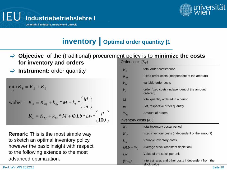
Objective of the (traditional) procurement policy is to minimize the costs for inventory and orders
Instrument: order quantity
/++=
++=
+=
100**O*
**:wobei
min
pLwLbMkKK
mMkMkKK
KKK
LvLfL
bEvEfE
LEBm
Order costs (KE)
KE total order costs/period
KEf Fixed order costs (independent of the amount)
kEv variable order costs
kb order fixed costs (independent of the amount ordered)
M total quantity ordered in a period
m Lot, respective order quantity
M/m Amount of orders
inventory costs (KL)
KL total inventory costs/ period
KLf fixed inventory costs (independent of the amount)
kLv Variable inventory costs
ØLb = m/2 Average stock (constant depletion)
Lw Value of the stock per unit
(p/100) Interest rates and other costs independent from the stock value
Remark: This is the most simple way to sketch an optimal inventory policy, however the basic insight with respect to the following extends to the most advanced optimization.
Industriebetriebslehre I Lehrstuhl f. Industrie, Energie und Umwelt
| Prof. Wirl WS 2012/13 Seite 11
inventory | Optimal Order quantity (lot size) |2
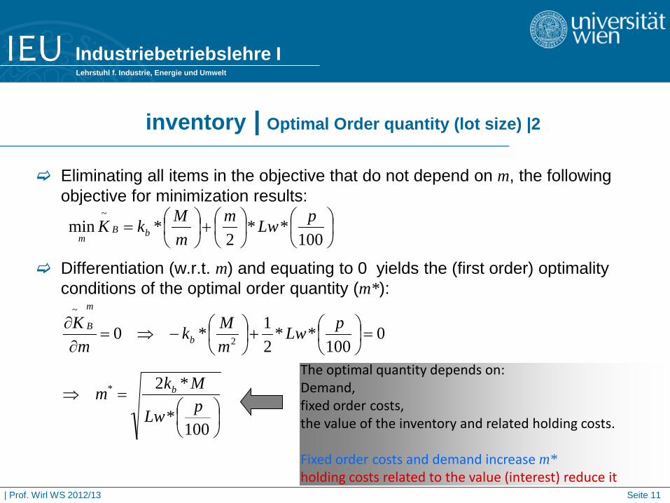
Eliminating all items in the objective that do not depend on m, the following objective for minimization results:
Differentiation (w.r.t. m) and equating to 0 yields the (first order) optimality conditions of the optimal order quantity (m*):
+
=
100**
2*min
~ pLwmmMkK bB
m
=⇒
=
+
−⇒=
∂∂
100*
*2
0100
**21*0
*
2
~
pLw
Mkm
pLwmMk
mK
b
b
m
B
The optimal quantity depends on: Demand, fixed order costs, the value of the inventory and related holding costs. Fixed order costs and demand increase m* holding costs related to the value (interest) reduce it
Industriebetriebslehre I Lehrstuhl f. Industrie, Energie und Umwelt
| Prof. Wirl WS 2012/13 Seite 12
Inventory Management | Optimal quantity ordered |3
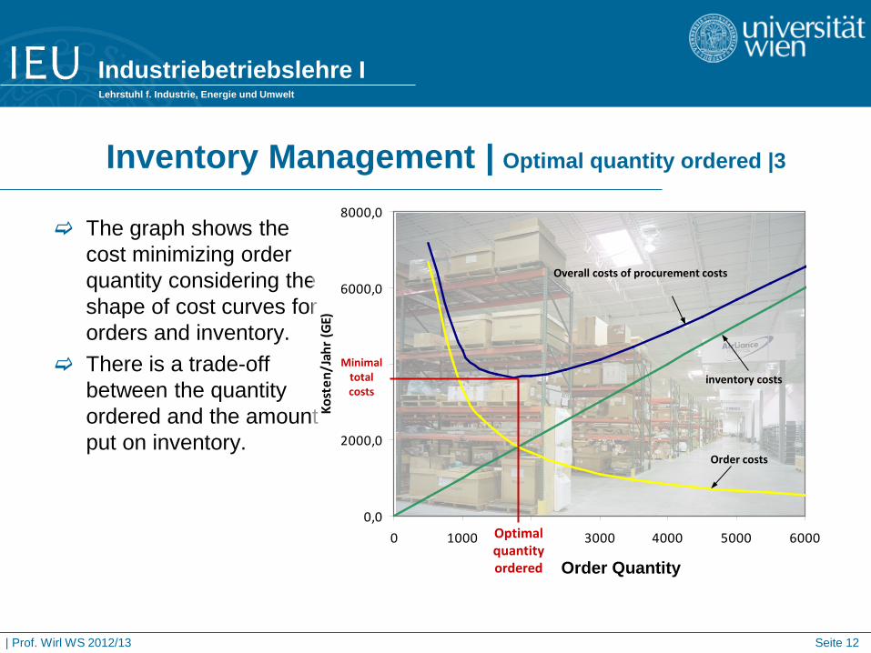
The graph shows the cost minimizing order quantity considering the shape of cost curves for orders and inventory.
There is a trade-off between the quantity ordered and the amount put on inventory.
0,0
2000,0
4000,0
6000,0
8000,0
0 1000 2000 3000 4000 5000 6000
Bestellmenge (ME)
Kost
en/J
ahr (
GE)
Overall costs of procurement costs
inventory costs
Order costs
Optimal quantity ordered
Minimal total costs
Order Quantity
Industriebetriebslehre I Lehrstuhl f. Industrie, Energie und Umwelt
| Prof. Wirl WS 2012/13 Seite 13
Heuristic Order policies |1
The aim of the order policy is to choose the time (when?) and the quantity to order (how much?) to ensure that the inventory meets the existing demand until the next date of placing another order.
Differentiation between:
rhythm (or cyclic order method)
Level
The rhythm method requires a frequency of order that ensures a positive inventory until the time of replenishment and thus must account for the lead times of orders.
The level method makes the timing of any order contingent on the remaining inventory level.
Industriebetriebslehre I Lehrstuhl f. Industrie, Energie und Umwelt
| Prof. Wirl WS 2012/13 Seite 14
Heuristic order policies |2
Objective is not only to satisfy demand but also to minimize costs.
Therefore it is necessary to balance the trade-off between order volumes and their corresponding order costs and the inventory costs.
Procurement costs consist of the order costs on the one hand and the inventory costs on the other hand.
Objective of an efficient procurement/order policy is to minimize the total costs subject to the constraint of satisfying demand.
The following schemes are heuristic even if the corresponding instruments/parameters are optimized because the true dynamic and stochastic optmization is reduced to an optimization with few parameters.
First presentation of the schemes and then ways to optimize within the scheme.
Industriebetriebslehre I Lehrstuhl f. Industrie, Energie und Umwelt
| Prof. Wirl WS 2012/13 Seite 15
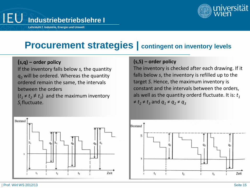
Procurement strategies | contingent on inventory levels
(s,q) – order policy If the inventory falls below s, the quantity q0 will be ordered. Whereas the quantity ordered remain the same, the intervals between the orders (t1 ≠ t2 ≠ t3) and the maximum inventory Si fluctuate.
(s,S) – order policy The inventory is checked after each drawing. If it falls below s, the inventory is refilled up to the target S. Hence, the maximum inventory is constant and the intervals between the orders, als well as the quantity orderd fluctuate. It is: t1 ≠ t2 ≠ t3 and q1 ≠ q2 ≠ q3
Industriebetriebslehre I Lehrstuhl f. Industrie, Energie und Umwelt
| Prof. Wirl WS 2012/13 Seite 16
Procurement strategies | cyclic orders |1
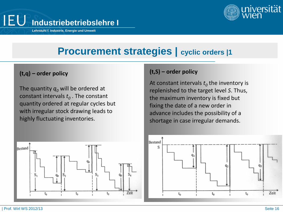
(t,q) – order policy The quantity q0 will be ordered at constant intervals t0 . The constant quantity ordered at regular cycles but with irregular stock drawing leads to highly fluctuating inventories.
(t,S) – order policy
At constant intervals t0 the inventory is replenished to the target level S. Thus, the maximum inventory is fixed but fixing the date of a new order in advance includes the possibility of a shortage in case irregular demands.
Industriebetriebslehre I Lehrstuhl f. Industrie, Energie und Umwelt
| Prof. Wirl WS 2012/13 Seite 17
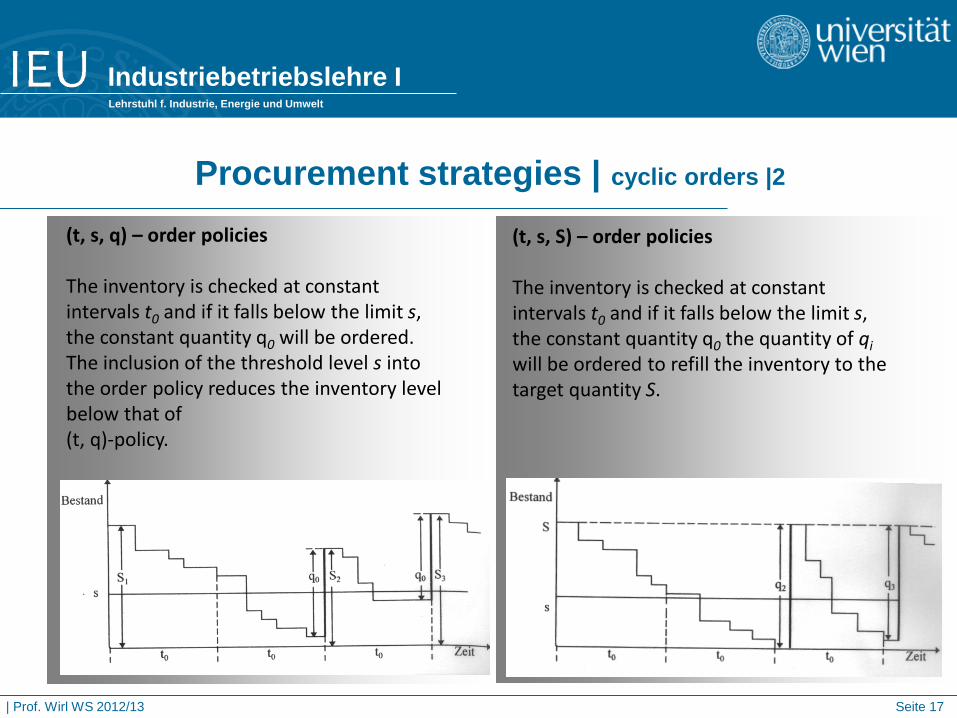
Procurement strategies | cyclic orders |2
(t, s, q) – order policies The inventory is checked at constant intervals t0 and if it falls below the limit s, the constant quantity q0 will be ordered. The inclusion of the threshold level s into the order policy reduces the inventory level below that of (t, q)-policy.
(t, s, S) – order policies The inventory is checked at constant intervals t0 and if it falls below the limit s, the constant quantity q0 the quantity of qi will be ordered to refill the inventory to the target quantity S.
Industriebetriebslehre I Lehrstuhl f. Industrie, Energie und Umwelt
| Prof. Wirl WS 2012/13 Seite 18
Perpetual Inventory Systems (compare order point procedure)
Economic Order Quantity (EOQ) Production Order Quantity (POQ) Quantity Discount (QD)
Fixed period (P) systems (cyclic order procedure)
Probability theoretical models
Models for procurement- and inventory policies
Industriebetriebslehre I Lehrstuhl f. Industrie, Energie und Umwelt
| Prof. Wirl WS 2012/13 Seite 19
Q-Systems | Economic Order Quantity |1
Economic Order Quantity models belong to the oldest and most spread stock control models.
EOQ-models are relatively simple models based on the following assumptions: The demand is known, constant and independent. The Lead Time (time between order and supply) is known and also constant. Supplies are immediately and bundled. Quantity discounts are not possible. The only variable costs are variable inventory and order costs. Shortages/stock outs can be avoided if orders are made at the right time.
Industriebetriebslehre I Lehrstuhl f. Industrie, Energie und Umwelt
| Prof. Wirl WS 2012/13 Seite 20
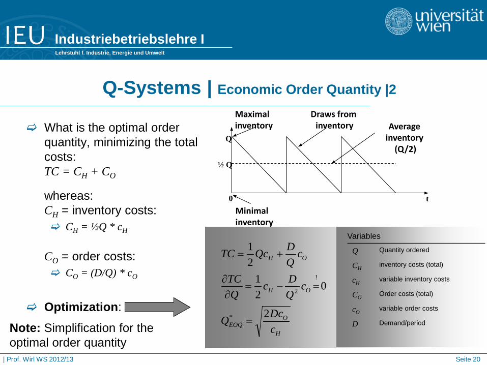
Q-Systems | Economic Order Quantity |2
What is the optimal order quantity, minimizing the total costs: TC = CH + CO whereas: CH = inventory costs: CH = ½Q * cH
CO = order costs:
CO = (D/Q) * cO
Optimization:
Q
½ Q
0 t
Maximal inventory
Minimal inventory
Average inventory
(Q/2)
Draws from inventory
H
OEOQ
OH
OH
cDcQ
cQDc
QTC
cQDQcTC
2
021
21
*
!
2
=
=−=∂∂
+=
Variables
Q Quantity ordered
CH inventory costs (total)
cH variable inventory costs
CO Order costs (total)
cO variable order costs
D Demand/period Note: Simplification for the optimal order quantity
Industriebetriebslehre I Lehrstuhl f. Industrie, Energie und Umwelt
| Prof. Wirl WS 2012/13 Seite 21
Q-Systems | Economic Order Quantity |3
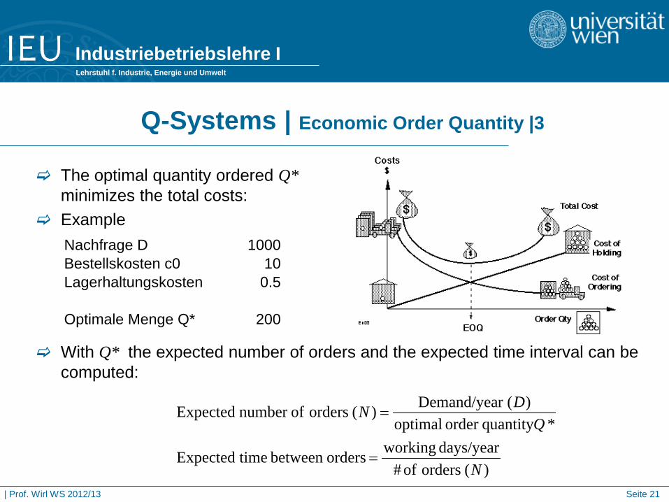
The optimal quantity ordered Q* minimizes the total costs:
Example
With Q* the expected number of orders and the expected time interval can be computed:
)(orders of#days/year working orders between timeExpected
*quantityorder optimal)(rDemand/yea)(orders ofnumber Expected
N
QDN
=
=
Nachfrage D 1000Bestellskosten c0 10Lagerhaltungskosten 0.5
Optimale Menge Q* 200
Industriebetriebslehre I Lehrstuhl f. Industrie, Energie und Umwelt
| Prof. Wirl WS 2012/13 Seite 22
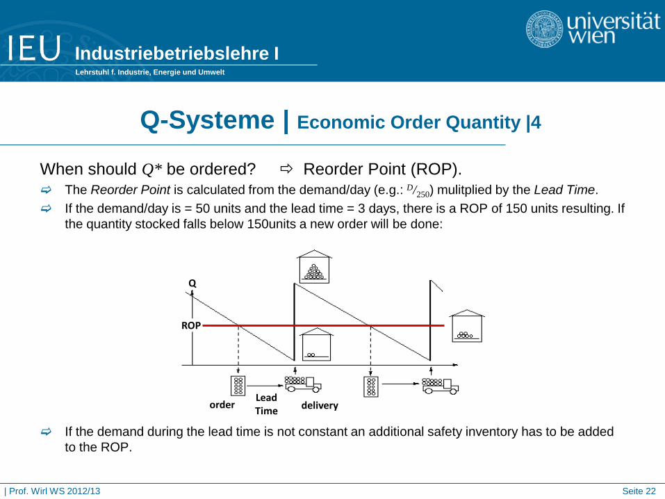
When should Q* be ordered? Reorder Point (ROP). The Reorder Point is calculated from the demand/day (e.g.: D/250) mulitplied by the Lead Time. If the demand/day is = 50 units and the lead time = 3 days, there is a ROP of 150 units resulting. If
the quantity stocked falls below 150units a new order will be done:
If the demand during the lead time is not constant an additional safety inventory has to be added to the ROP.
Q-Systeme | Economic Order Quantity |4
ROP
Q
order Lead Time delivery
Industriebetriebslehre I Lehrstuhl f. Industrie, Energie und Umwelt
| Prof. Wirl WS 2012/13 Seite 23
Q-Systems | Economic Order Quantity |5
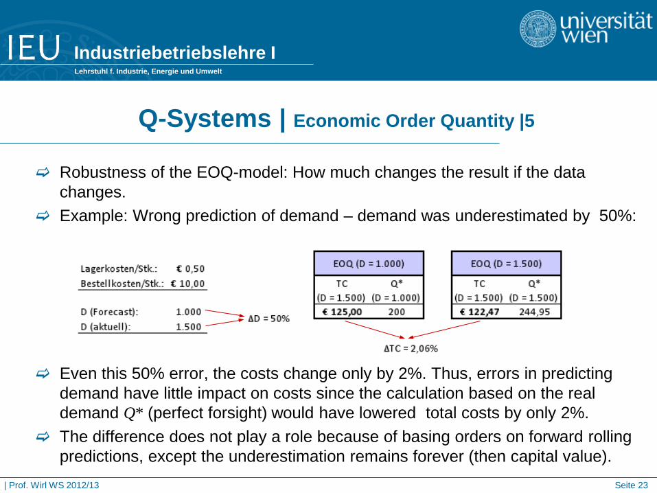
Robustness of the EOQ-model: How much changes the result if the data changes.
Example: Wrong prediction of demand – demand was underestimated by 50%:
Even this 50% error, the costs change only by 2%. Thus, errors in predicting demand have little impact on costs since the calculation based on the real demand Q* (perfect forsight) would have lowered total costs by only 2%.
The difference does not play a role because of basing orders on forward rolling predictions, except the underestimation remains forever (then capital value).
Industriebetriebslehre I Lehrstuhl f. Industrie, Energie und Umwelt
| Prof. Wirl WS 2012/13 Seite 24
Q-System | Production Order Quantity |1
The EOQ-model assumes that an order is bundled and completely delivered. If this is not the case, the inventory gets filled step by step and a differenciated approach is needed (the assumption of EOQ is violated)
The Production Order Quantity model has 2 conditions: The quantity stocked gets filled by continous inflows after an order has been done, or
Products get produced and sold at the same time.
Under these circumtances daily production- or inventory flow rates and daily demand rates are taken into account,
More general than discussed in the following, this leads to production smoothing at seasonal demand.
Industriebetriebslehre I Lehrstuhl f. Industrie, Energie und Umwelt
| Prof. Wirl WS 2012/13 Seite 25
Q-System | Production Order Quantity |2
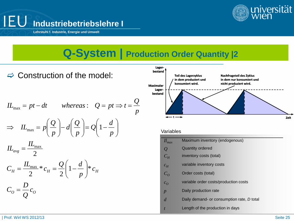
Construction of the model:
OO
HHH
avg
cQDC
cpdQcILC
ILIL
pdQ
pQd
pQpIL
pQtptQwhereasdtptIL
=
−==
=
−=
−
=⇒
=⇒=−=
*12
*2
2
1
:
max
max
max
max
Variables
Ilmax Q
Maximum inventory (endogenous) Quantity ordered
CH inventory costs (total)
cH variable inventory costs
CO Order costs (total)
cO variable order costs/production costs
p Daily production rate
d Daily demand- or consumption rate, D total
t Length of the production in days
Zeit
Lager-bestand
MaximalerLager-
bestand
Teil des Lagerzyklus in dem produziert und konsumiert wird.
Nachfrageteil des Zyklus in dem nur konsumiert und nicht produziert wird.
t Zeit
Lager-bestand
MaximalerLager-
bestand
Teil des Lagerzyklus in dem produziert und konsumiert wird.
Nachfrageteil des Zyklus in dem nur konsumiert und nicht produziert wird.
t

Industriebetriebslehre I Lehrstuhl f. Industrie, Energie und Umwelt
| Prof. Wirl WS 2012/13 Seite 26
Optimal quantity ordered:
The optimal quantity ordered at the POQ-model is normally higher than the quantity of the EOQ-model that can be explained by the lower inventory costs (compare Q*P and Q*EOQ)
Q-System | Production Order Quantity |2
H
OP
OH
OH
cpd
DcQQ
TC
cQDc
pdQTC
CCTC
−
=⇒=∂∂
+
−=
+=
1
20
12
*!
Zeit
Lager-bestand
MaximalerLager-
bestand
Teil des Lagerzyklus in dem produziert und konsumiert wird.
Nachfrageteil des Zyklus in dem nur konsumiert und nicht produziert wird.
t Zeit
Lager-bestand
MaximalerLager-
bestand
Teil des Lagerzyklus in dem produziert und konsumiert wird.
Nachfrageteil des Zyklus in dem nur konsumiert und nicht produziert wird.
t
Industriebetriebslehre I Lehrstuhl f. Industrie, Energie und Umwelt
| Prof. Wirl WS 2012/13 Seite 27
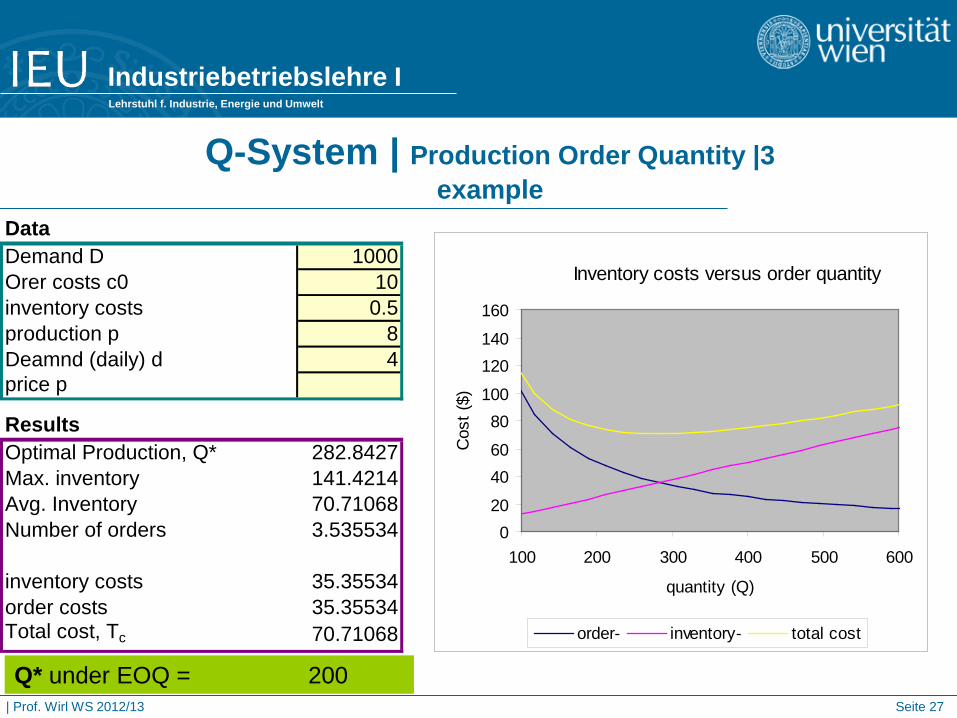
Q-System | Production Order Quantity |3 example
Inventory costs versus order quantity
020
4060
80100
120140
160
100 200 300 400 500 600
quantity (Q)
Cos
t ($)
order- inventory- total cost
Q* under EOQ = 200
DataDemand D 1000Orer costs c0 10inventory costs 0.5production p 8Deamnd (daily) d 4price p
ResultsOptimal Production, Q* 282.8427Max. inventory 141.4214Avg. Inventory 70.71068Number of orders 3.535534
inventory costs 35.35534order costs 35.35534Total cost, Tc 70.71068
Industriebetriebslehre I Lehrstuhl f. Industrie, Energie und Umwelt
| Prof. Wirl WS 2012/13 Seite 28
Q-System | quantity discount |1
In practice, Quantity Discounts are common (compare Nonlinear Pricing in the follow up course). Therefore, the following approach accounts for such quantity discounts.
A trade-off between reducing the unit product costs via larger orders leads to an increase of the inventory costs. Of course, it is stupid just to maximize the discount by ordering large quantities.
Objective is to calculate the optimal order quantity accounting in addition for discounts that depend on the ordered quantity.
Typically, discounts are available for exceeding certain thresholds that leads to discontinuities in the procurement costs.
Industriebetriebslehre I Lehrstuhl f. Industrie, Energie und Umwelt
| Prof. Wirl WS 2012/13 Seite 29
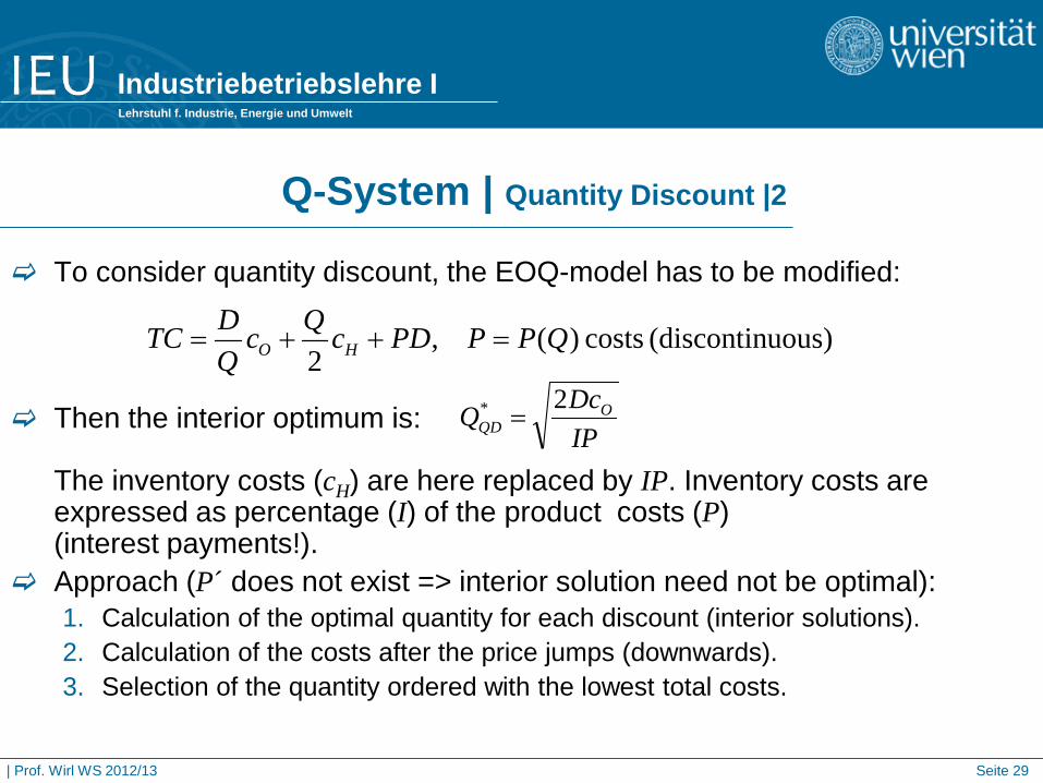
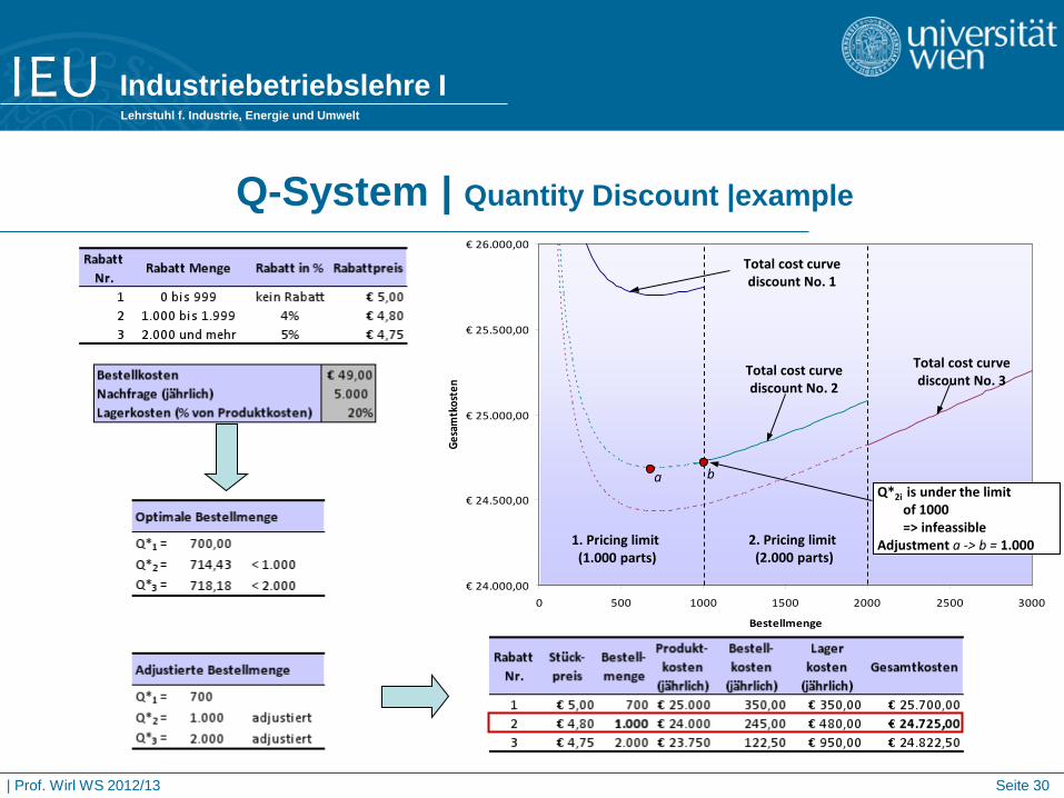
Q-System | Quantity Discount |2
To consider quantity discount, the EOQ-model has to be modified:
Then the interior optimum is: The inventory costs (cH) are here replaced by IP. Inventory costs are expressed as percentage (I) of the product costs (P) (interest payments!).
Approach (P´ does not exist => interior solution need not be optimal): 1. Calculation of the optimal quantity for each discount (interior solutions). 2. Calculation of the costs after the price jumps (downwards). 3. Selection of the quantity ordered with the lowest total costs.
uous)(discontin costs )(,2
QPPPDcQcQDTC HO =++=
IPDcQ O
QD2* =
Industriebetriebslehre I Lehrstuhl f. Industrie, Energie und Umwelt
| Prof. Wirl WS 2012/13 Seite 30
Q-System | Quantity Discount |example
€ 24.000,00
€ 24.500,00
€ 25.000,00
€ 25.500,00
€ 26.000,00
0 500 1000 1500 2000 2500 3000
Bestellmenge
Gesa
mtk
oste
n
1. Pricing limit (1.000 parts)
2. Pricing limit (2.000 parts)
Total cost curve discount No. 1
Total cost curve discount No. 2
Total cost curve discount No. 3
Q*2i is under the limit of 1000 => infeassible
Adjustment a -> b = 1.000
a b
Industriebetriebslehre I Lehrstuhl f. Industrie, Energie und Umwelt
| Prof. Wirl WS 2012/13 Seite 31
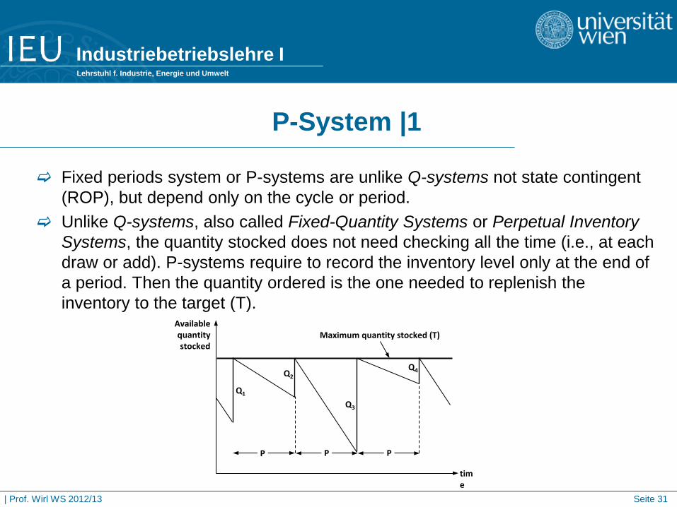
P-System |1
Fixed periods system or P-systems are unlike Q-systems not state contingent (ROP), but depend only on the cycle or period.
Unlike Q-systems, also called Fixed-Quantity Systems or Perpetual Inventory Systems, the quantity stocked does not need checking all the time (i.e., at each draw or add). P-systems require to record the inventory level only at the end of a period. Then the quantity ordered is the one needed to replenish the inventory to the target (T).
P P P
Q1
Q2
Q3
Q4
time
Available quantity stocked
Maximum quantity stocked (T)
Industriebetriebslehre I Lehrstuhl f. Industrie, Energie und Umwelt
| Prof. Wirl WS 2012/13 Seite 32
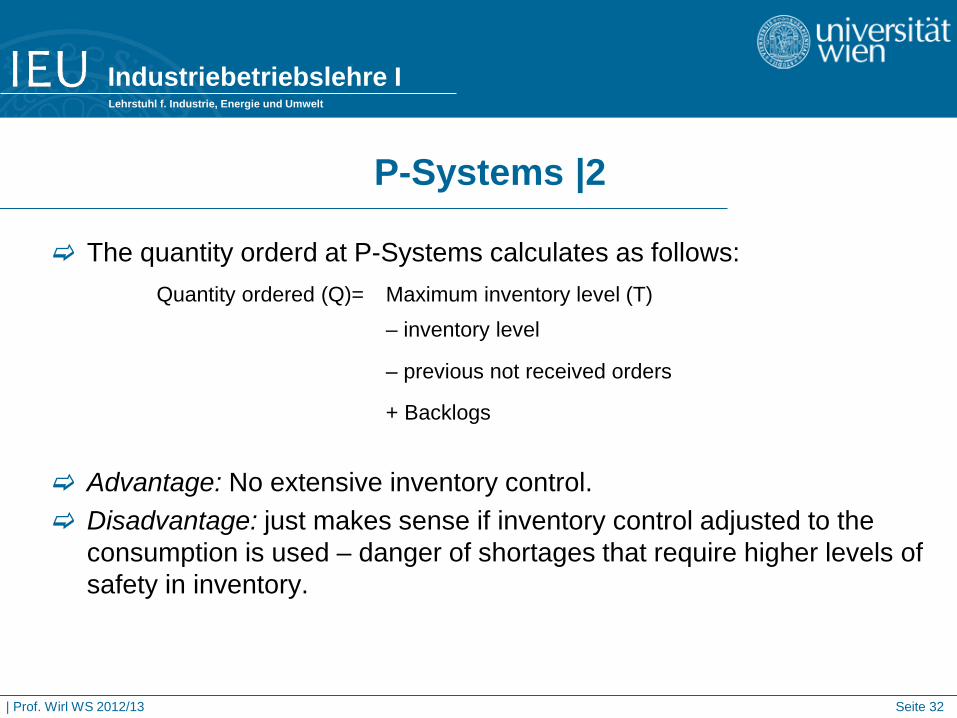
P-Systems |2
The quantity orderd at P-Systems calculates as follows:
Advantage: No extensive inventory control. Disadvantage: just makes sense if inventory control adjusted to the
consumption is used – danger of shortages that require higher levels of safety in inventory.
Quantity ordered (Q)= Maximum inventory level (T) – inventory level
– previous not received orders
+ Backlogs
Industriebetriebslehre I Lehrstuhl f. Industrie, Energie und Umwelt
| Prof. Wirl WS 2012/13 Seite 33
Theoretical models of probability
Until now it was assumed, that the demand is constant and known. This assumption has to be relaxed in many practical cases, which requires different kinds of models.
Theoretical models of probability are used when the assumption of a constant and known demand is wrong. However, most models make the assumption of a constant Lead Time.
The objective of these models is to determine an order policy such that the probablility for a shortage is low (compare Basel II, value at risk) in order to gurantee a high service level (= complement to the probability of a shortage).
There is again a trade-off between a high service level (requiring high inventory levels) and low inventory costs (= low service levels).
Industriebetriebslehre I Lehrstuhl f. Industrie, Energie und Umwelt
| Prof. Wirl WS 2012/13 Seite 34
Theoretical models of probability | example |1
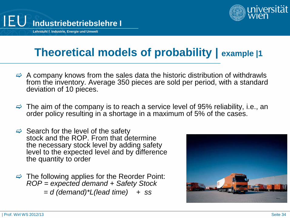
A company knows from the sales data the historic distribution of withdrawls from the inventory. Average 350 pieces are sold per period, with a standard deviation of 10 pieces.
The aim of the company is to reach a service level of 95% reliability, i.e., an
order policy resulting in a shortage in a maximum of 5% of the cases.
Search for the level of the safety stock and the ROP. From that determine the necessary stock level by adding safety level to the expected level and by difference the quantity to order
The following applies for the Reorder Point: ROP = expected demand + Safety Stock
= d (demand)*L(lead time) + ss
Industriebetriebslehre I Lehrstuhl f. Industrie, Energie und Umwelt
| Prof. Wirl WS 2012/13 Seite 35
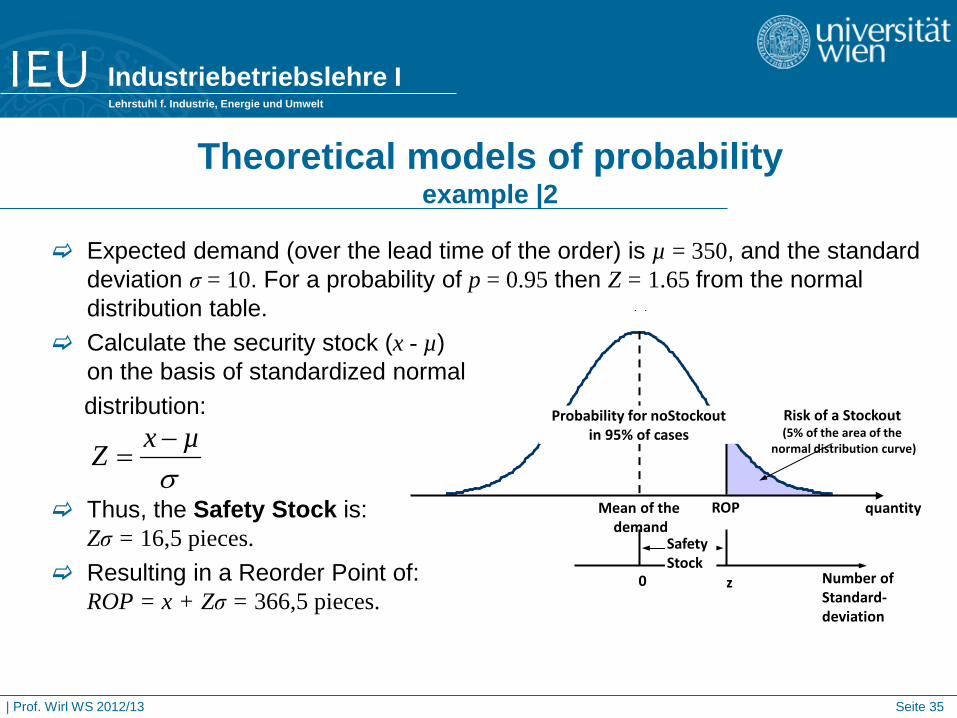
Expected demand (over the lead time of the order) is µ = 350, and the standard deviation σ = 10. For a probability of p = 0.95 then Z = 1.65 from the normal distribution table.
Calculate the security stock (x - µ) on the basis of standardized normal
distribution:
Thus, the Safety Stock is: Zσ = 16,5 pieces.
Resulting in a Reorder Point of: ROP = x + Zσ = 366,5 pieces.
Theoretical models of probability example |2
( )
0 z
ROP quantity
Risk of a Stockout (5% of the area of the
normal distribution curve)
Safety Stock
Mean of the demand
Probability for noStockout in 95% of cases
Number of Standard- deviation
σµxZ −
=
Industriebetriebslehre I Lehrstuhl f. Industrie, Energie und Umwelt
| Prof. Wirl WS 2012/13 Seite 36
Theoretical models of probability | example |3
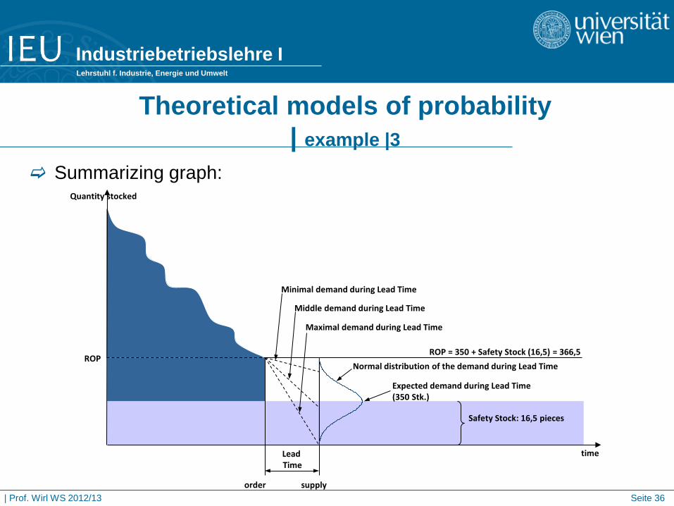
Summarizing graph:
Minimal demand during Lead Time
time
()
Middle demand during Lead Time
Maximal demand during Lead Time
ROP = 350 + Safety Stock (16,5) = 366,5
Expected demand during Lead Time (350 Stk.)
Normal distribution of the demand during Lead Time
Safety Stock: 16,5 pieces
Lead Time
order supply
Quantity stocked
ROP
Industriebetriebslehre I Lehrstuhl f. Industrie, Energie und Umwelt
| Prof. Wirl WS 2012/13 Seite 37
Additional literature
Heizer, J., Render, B., Operations Management Anderson, D.R., Sweeney, D.J., Williams, T.A.; Management Science –
Quantitative Approaches to Decision Making, 9th ed., South-West. Mendenhall, W., Reinmuth, J.E., Beaver, R., Statistics for Management and
Economics, 6th ed., PWS-Kent Publishing Company. Krajewski, L.J., Ritzman, L.P., Operations Management – Strategy and
Analysis, 6th ed., Prentice Hall.