
Intertemporal Allocation with Incomplete Markets · Intertemporal Allocation with Incomplete...
120
Intertemporal Allocation with Incomplete Markets Inaugural Dissertation zur Erlangung des akademischen Grades eines Doktors der Wirtschaftswissenschaften der Universit¨ at Mannheim vorgelegt von Wolfgang Kuhle April 2010
Transcript of Intertemporal Allocation with Incomplete Markets · Intertemporal Allocation with Incomplete...

Intertemporal Allocation
with
Incomplete Markets
Inaugural Dissertation zur Erlangung des akademischen
Grades eines Doktors der Wirtschaftswissenschaften der
Universitat Mannheim
vorgelegt von
Wolfgang Kuhle
April 2010

Dekan: Prof. Tom Krebs Ph.D.
Referent: Prof. Dr. Alexander Ludwig
Korreferent: Prof. Axel Borsch-Supan Ph.D.
Korreferent: Prof. David de la Croix Ph.D.
Tag der mundlichen Prufung: 03.08.2010

TO
Nataliya

Acknowledgements
This doctoral thesis was written during my time at the Mannheim Research Institute
for the Economics of Aging (MEA). I would like to thank Klaus Jaeger, Martin Salm,
Edgar Vogel, and Matthias Weiss for helpful discussions and comments on various
chapters of this thesis. Regarding my studies at the mathematics department of the
Universitat Mannheim I have to thank Martin Schmidt for his eye-opening lectures
on differential equations and dynamical systems. Viktor Bindewald, Sebastian Klein,
Markus Knopf, and Marianne Nowak made the time in the A5 worth while.
My parents provided indispensable support and advice. Nataliya Demchenko
contributed to this thesis with her patience and unreserved support. She also trans-
formed my drawings into the subsequent figures.
I am particularly indebted to my advisors Axel Borsch-Supan, David de la Croix
and Alexander Ludwig for their support, advice and helpful comments on earlier
drafts of this thesis − they helped me to adopt a more contemporary approach to
economics.
Contents
1 Introduction and Summary 1
1.1 Organization . . . . . . . . . . . . . . . . . . . . . . . . . . . . . . . 2
1.2 Results . . . . . . . . . . . . . . . . . . . . . . . . . . . . . . . . . . . 3
2 The Optimum Growth Rate for Population Reconsidered 11
2.1 Introduction . . . . . . . . . . . . . . . . . . . . . . . . . . . . . . . . 11
2.1.1 Organization . . . . . . . . . . . . . . . . . . . . . . . . . . . 12
2.2 The Optimum Growth Rate for Population without Debt . . . . . . . 13
2.2.1 The Planning Problem . . . . . . . . . . . . . . . . . . . . . . 13
2.2.2 The Serendipity Theorem . . . . . . . . . . . . . . . . . . . . 15
2.2.3 The Optimum Growth Rate for Population in a Laissez Faire
Economy . . . . . . . . . . . . . . . . . . . . . . . . . . . . . . 15
2.3 The Optimum Growth Rate for Population in an Economy with Gov-
ernment Debt . . . . . . . . . . . . . . . . . . . . . . . . . . . . . . . 20
2.3.1 The Model . . . . . . . . . . . . . . . . . . . . . . . . . . . . . 21
2.3.2 The Serendipity Theorem with Debt . . . . . . . . . . . . . . 21
2.3.3 The Optimum Growth Rate for Population in a Laissez Faire
Economy with Debt . . . . . . . . . . . . . . . . . . . . . . . 22
2.4 Concluding Remarks . . . . . . . . . . . . . . . . . . . . . . . . . . . 27
2.5 Appendix . . . . . . . . . . . . . . . . . . . . . . . . . . . . . . . . . 29
2.5.1 Construction of Diagram 1 . . . . . . . . . . . . . . . . . . . . 29
2.5.2 Proof of Proposition 1 . . . . . . . . . . . . . . . . . . . . . . 30
2.5.3 Oscillatory Stability . . . . . . . . . . . . . . . . . . . . . . . 31
2.5.4 Formal aspects to Diagram 4 . . . . . . . . . . . . . . . . . . . 32
2.5.5 Appendix: Pay-as-you-go Social Security and optimal popu-
lation . . . . . . . . . . . . . . . . . . . . . . . . . . . . . . . 32
3 Dynamic Efficiency and the Two-Part Golden Rule with Heteroge-
neous Agents 35
3.1 Introduction . . . . . . . . . . . . . . . . . . . . . . . . . . . . . . . . 35
3.1.1 Consumption Maximizing Growth . . . . . . . . . . . . . . . . 37
3.1.2 Utility Maximizing Growth . . . . . . . . . . . . . . . . . . . 38
3.1.3 Competitive Incomplete Markets . . . . . . . . . . . . . . . . 39
3.2 Competitive Markets with Heterogeneous Agents . . . . . . . . . . . 43
3.2.1 Heterogeneous Labor Endowment with Debt . . . . . . . . . . 44
3.2.2 Heterogeneous Labor Endowment without Debt . . . . . . . . 47
3.2.3 Heterogeneous Preferences . . . . . . . . . . . . . . . . . . . . 48
3.2.4 Hicks Neutral Technological Change . . . . . . . . . . . . . . . 50
3.3 Conclusion . . . . . . . . . . . . . . . . . . . . . . . . . . . . . . . . . 51
3.4 Appendix . . . . . . . . . . . . . . . . . . . . . . . . . . . . . . . . . 53
3.4.1 Construction of Diagram 6 . . . . . . . . . . . . . . . . . . . . 53
3.4.2 Comparative Statics . . . . . . . . . . . . . . . . . . . . . . . 54
3.4.3 Proof of Proposition 6 . . . . . . . . . . . . . . . . . . . . . . 56
4 The Optimum Structure for Government Debt 57
4.1 Introduction . . . . . . . . . . . . . . . . . . . . . . . . . . . . . . . . 57
4.2 The Model . . . . . . . . . . . . . . . . . . . . . . . . . . . . . . . . . 61
4.2.1 Population and factor-prices . . . . . . . . . . . . . . . . . . . 61
4.2.2 Implicit and Explicit Government Debt . . . . . . . . . . . . . 62
4.2.3 The Structure of Government Debt . . . . . . . . . . . . . . . 63
4.2.4 The Optimum Structure for Government Debt . . . . . . . . . 64
4.2.5 Efficiency . . . . . . . . . . . . . . . . . . . . . . . . . . . . . 67
4.3 Extensions . . . . . . . . . . . . . . . . . . . . . . . . . . . . . . . . . 73
4.3.1 Time-Varying Safe Returns . . . . . . . . . . . . . . . . . . . 73
4.3.2 Defined Benefits . . . . . . . . . . . . . . . . . . . . . . . . . . 74
4.3.3 A Working Class . . . . . . . . . . . . . . . . . . . . . . . . . 74
4.4 Conclusion . . . . . . . . . . . . . . . . . . . . . . . . . . . . . . . . . 76
4.5 Appendix . . . . . . . . . . . . . . . . . . . . . . . . . . . . . . . . . 77
4.5.1 The Envelope Conditions . . . . . . . . . . . . . . . . . . . . . 77
4.5.2 Characteristics of the Long-run Optimum . . . . . . . . . . . 78
4.5.3 Lagrangian . . . . . . . . . . . . . . . . . . . . . . . . . . . . 80
4.5.4 The Covariance Risk . . . . . . . . . . . . . . . . . . . . . . . 81
5 Intertemporal Compensation with Incomplete Markets 83
5.1 Conclusion . . . . . . . . . . . . . . . . . . . . . . . . . . . . . . . . . 88
6 Demographic Change and the Rates of Return to Risky Capital
and Safe Debt 89

6.1 Introduction . . . . . . . . . . . . . . . . . . . . . . . . . . . . . . . . 89
6.2 The Model . . . . . . . . . . . . . . . . . . . . . . . . . . . . . . . . . 90
6.2.1 Technology and factor-prices . . . . . . . . . . . . . . . . . . . 90
6.2.2 Government Debt . . . . . . . . . . . . . . . . . . . . . . . . . 91
6.2.3 Households . . . . . . . . . . . . . . . . . . . . . . . . . . . . 91
6.2.4 Equilibrium . . . . . . . . . . . . . . . . . . . . . . . . . . . . 93
6.2.5 Baby-Boom and Equity-Premium . . . . . . . . . . . . . . . . 94
6.3 Extensions . . . . . . . . . . . . . . . . . . . . . . . . . . . . . . . . . 94
6.3.1 The Effect of Human Capital . . . . . . . . . . . . . . . . . . 95
6.3.2 The Portfolio Decision . . . . . . . . . . . . . . . . . . . . . . 97
6.3.3 Discussion . . . . . . . . . . . . . . . . . . . . . . . . . . . . . 99
6.4 Conclusion . . . . . . . . . . . . . . . . . . . . . . . . . . . . . . . . . 101
References 102
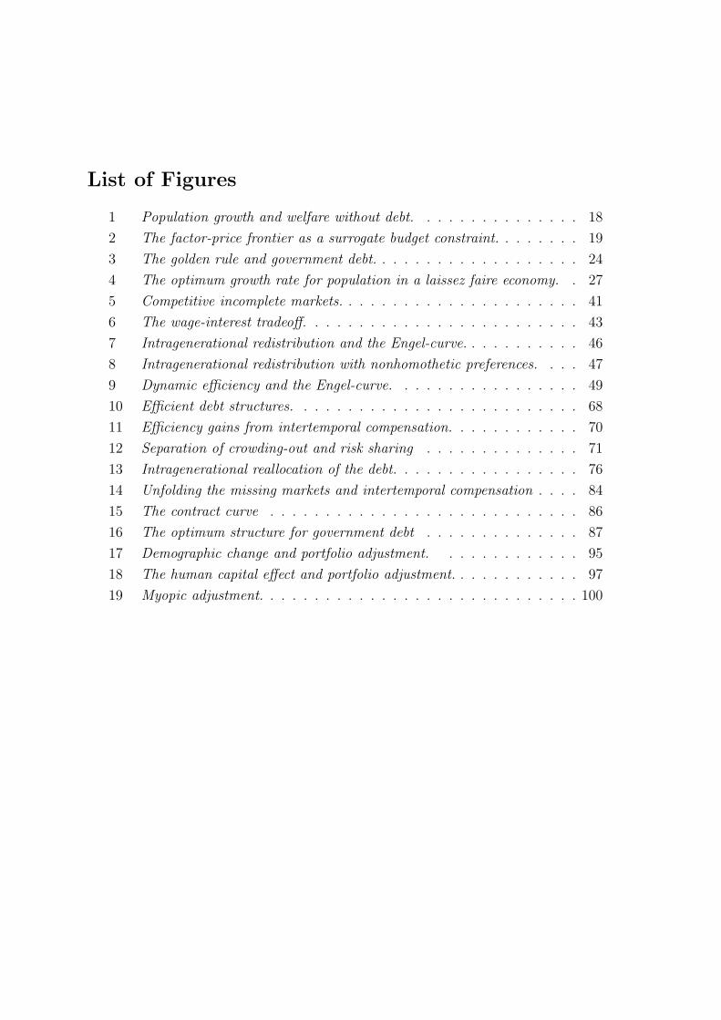
List of Figures
1 Population growth and welfare without debt. . . . . . . . . . . . . . . 18
2 The factor-price frontier as a surrogate budget constraint. . . . . . . . 19
3 The golden rule and government debt. . . . . . . . . . . . . . . . . . . 24
4 The optimum growth rate for population in a laissez faire economy. . 27
5 Competitive incomplete markets. . . . . . . . . . . . . . . . . . . . . . 41
6 The wage-interest tradeoff. . . . . . . . . . . . . . . . . . . . . . . . . 43
7 Intragenerational redistribution and the Engel-curve. . . . . . . . . . . 46
8 Intragenerational redistribution with nonhomothetic preferences. . . . 47
9 Dynamic efficiency and the Engel-curve. . . . . . . . . . . . . . . . . 49
10 Efficient debt structures. . . . . . . . . . . . . . . . . . . . . . . . . . 68
11 Efficiency gains from intertemporal compensation. . . . . . . . . . . . 70
12 Separation of crowding-out and risk sharing . . . . . . . . . . . . . . 71
13 Intragenerational reallocation of the debt. . . . . . . . . . . . . . . . . 76
14 Unfolding the missing markets and intertemporal compensation . . . . 84
15 The contract curve . . . . . . . . . . . . . . . . . . . . . . . . . . . . 86
16 The optimum structure for government debt . . . . . . . . . . . . . . 87
17 Demographic change and portfolio adjustment. . . . . . . . . . . . . 95
18 The human capital effect and portfolio adjustment. . . . . . . . . . . . 97
19 Myopic adjustment. . . . . . . . . . . . . . . . . . . . . . . . . . . . . 100
1 Introduction and Summary
Falling birth rates accompanied by increasing levels of public debt have been a
common trend among OECD countries over the last five decades. In this context,
the theories of optimal population and government debt, with their longstanding
tradition in social sciences, are of renewed interest. The current thesis presents
five neoclassical parables which emphasize particular aspects of the demographic
transition and the associated role of government debt. The natural framework for
such an analysis is provided by the non-ricardian overlapping generations model.
The first part of this thesis is dedicated to the deterministic overlapping generations
model with its consumption loan market failure and the pivotal two-part golden
rule relation. The second part is concerned with stochastic OLG models where
the consumption loan market failure is complemented by the missing markets for
factor-price risks.
Regarding methodology, this thesis intends to favor clarity over complexity. The
demographic transition and the theory of public debt are therefore treated in an
eclectic manner. While the analysis throughout is conducted in general equilibrium,
each chapter contains a setting which is adapted to the particular question at hand.
To obtain prominent results, the number of assumptions will be kept to the bare
minimum necessary to describe the respective objects of interest. The assumptions
chosen tend to be neoclassical. Apart from striking results, this rudimentary ap-
proach also allows to see their limitations. In particular, results are so transparent
that they can immediately be related to the assumptions upon which they rest. In
turn these assumptions can, in principle, be evaluated to whether or not they are
appropriate in the respective context.
This thesis studies the scope for government intervention which is associated with
the characteristic market failure in overlapping generations economies. This market
failure and the related concept of “dynamic (Pareto-) efficiency” will be approached
from different angels. Our results from the deterministic OLG models of chapters 2
and 3 suggest that the scope for Pareto-improving government interventions is rather
2 Intertemporal Allocation with Incomplete Markets
narrow. In particular, we find that in models with intracohort heterogeneity the
concept of dynamic efficiency regarding the size of the public debt is less restrictive.
Except for special cases it is no-longer possible to judge whether an economy is
dynamically efficient by the classical golden rule criterion. That is, competitive
growth pathes where the rate of return permanently falls short of the growth rate
of the aggregate economy can no longer be characterized as inefficient. This picture
changes in Chapter 4 where aggregate risks are introduced into the model. In this
case there are two missing markets. Those for consumption loans and those for
factor-price risks. This double incompleteness of competitive markets increases the
scope for government intervention. Namely, it allows to make a restructuring of the
public debt Pareto-improving. This suggests that the restructuring of the public
debt may be a field where the government can take an active role without the
adoption of a strong welfare criterion.
1.1 Organization
This thesis can be divided into two parts. The first one deals with the consumption
loan market failure in the deterministic overlapping generations model.1 In this
setting, the two-part golden rule is of pivotal importance as it serves as the watershed
between steady states that are efficient and those which are inefficient. In Chapter
2, we study the role of the golden rule in the context of the problem of optimal
population growth. Interestingly, it turns out that the growth rate for population
which leads the economy to a golden rule path may minimize utility. Moreover, the
growth rate for population associated with a golden rule path is never optimal in
an economy with government debt. Equipped with these doubts on the golden rule
relation, we introduce intracohort heterogeneity in Chapter 3. In this setting we find
that, except for one special case, the golden rule ceases to serve as a demarcation
line between Pareto-efficient and inefficient steady states.
In the second part of the thesis we introduce aggregate risks into our framework.
This gives rise to a second type of market failure. Households can trade neither
consumption loans nor factor-price risks. In this setting we analyze whether or
not the analytical equivalence of government bonds and pension debt known from
the deterministic Diamond (1965) model carries over. While the breakdown of this
1The deterministic OLG model is due to Allais (1947), Malinvaud (1953), Samuelson (1958)and Diamond (1965).
Introduction 3
strong equivalence/irrelevance result is hardly surprising, the analysis gives rise to an
interesting relevance result. Evaluated from an ex-ante expected utility perspective,
we show that there exists an optimal composition for the public debt. The fact that
this structure can be reached in a Pareto-improving manner makes it attractive.
Finally, in the last chapter we revisit the demographic transition in a stochastic
overlapping generations model. In this chapter we ask a positive question. Namely,
whether the risk free rate on government bonds will react more sensitive to the
demographic transition than the rate of profit to risky capital.
1.2 Results
In the first chapter we analyze the role of the two-part golden rule by varying the
growth rate for population as in Samuelson (1975a). However, unlike Samuelson
(1975a), we discuss a competitive economy rather than a pure planning framework.
Via the Serendipity Theorem, we approach the two-part golden rule relation from
the side of a competitive economy.2 The intention with the current approach is to
obtain a better understanding for the paradoxical interior minima that were found
by Deardorff (1976) and Michel and Pestieau (1993). The results can be summarized
as:
1. The growth rate for population under which the competitive economy with-
out government debt obtains a golden rule steady state may either maximize
steady state utility or minimize it. Moreover, the growth rate for population
which yields a golden rule allocation in an economy with debt is never optimal
and differs from the one obtained in the planned economy. Consequently, the
Serendipity Theorem does not hold in a model with debt.
2. If the growth rate for population, that yields a competitive golden rule steady
state, maximizes utility when compared to the other steady state equilibria, it
also maximizes the utility of all planned golden rule steady states and vicev-
ersa. That is, the necessary and sufficient conditions for an interior optimum
2The Serendipity theorem of Samuelson (1975a) can be stated as follows: provided that thereexists only one stable steady state equilibrium, the competitive economy will automatically evolveinto the most golden golden rule steady state once the optimum growth rate n∗ is imposed. It waslater shown that this n∗ may also be a minimum. A prominent example for an interior minimumis the case where production and utility are of the Cobb-Douglas type.

4 Intertemporal Allocation with Incomplete Markets
are identical.
3. The optimum growth rate for population in 2. exists if and only if high (low)
growth rates for population yield efficient (inefficient) steady states.
4. A lower growth rate for population increases (decreases) steady state utility if
and only if the original steady state was efficient (inefficient).
5. Finally we show that the growth rate for population that maximizes steady
state utility in an economy with debt implies a capital intensity that falls short
of the golden rule level.
The results 1 − 5 are of interest in the following sense. The pure planning frame-
work discussed by Samuelson (1975a, 1976), Deardorff (1976), Arthur and McNicoll
(1977, 1978), Michel and Pestieau (1993) and Bommier and Lee (2003) indicates
that the existence of an interior optimum hinges on unobservable parameters. The
current approach relates the existence of an interior optimum growth rate for pop-
ulation to observable variables instead. Namely, the growth rate for population
and the marginal product of capital. Moreover, we find that simulations based on
Cobb-Douglas production functions tend to yield watershed results. For elasticities
of capital-labor-substitution smaller (larger) than one, an increase in population
growth by one percent will increase the interest rate by more (less) than one percent
in the long-run.
In the second chapter, we approach the two-part golden rule relation from an-
other angle by introducing intracohort heterogeneity. In such a setting, it becomes
apparent that the two-part golden rule differs substantially from the golden rule of
accumulation. The golden rule of accumulation originates purely from the Solow
(1956), Swan (1956) models of capital and growth and maximizes per capita con-
sumption only. The two-part golden rule, on the contrary, is a composition of the
golden rule of accumulation and the Samuelson (1958) golden rule for consumption
loan interest. This composite character becomes visible once households differ re-
garding their preferences or their labor endowment. More specifically, we obtain the
following results:
1. If agents differ with regard to their labor endowment only, the two-part golden

Introduction 5
rule continues to maximize steady state utility if preferences are homothetic.3
In all other cases, however, the two-part golden rule relation ceases to separate
efficient from inefficient steady states. There will always exist households
whose steady state utility is maximized at a capital intensity exceeding the
golden rule level and vice versa. Hence, these steady states are no longer
inefficient in a competitive economy.
Taking the perspective of Abel et al. (1989), an increment in capital acts as
a source (sink) to society as a whole, i.e. increases aggregate consumption
in each period, if r > n (r < n). If society consisted of a representative
agent, r = n would therefore describe the steady state optimum. However,
in a society which is fragmented into different groups this conclusion does not
apply. Even if capital is already a sink to society as a whole, it may still act
as a source to some groups of that society.
2. If heterogeneity is introduced on the preference side, the two-part golden rule
ceases to serve as a demarcation line between efficient and inefficient steady
states in general. The classic result of Stein (1969) is therefore not warranted.
3. The two-part golden rule, however, continues to serve as a watershed in the
following sense: it separates agents whose present value of savings exceeds
(falls short of) the amount of capital absorbed by their labor supply. Those
agents with a relatively large (small) supply of savings prefer interest rates
exceeding (falling short of) the golden rule level. One may therefore interpret
the utility loss of thrifty households which occurs once the economy moves
towards the golden rule steady state as a case of the Bhagwati (1958) result
on “immiserizing growth”. While societies consumption rises, falling profits
and rising wages worsen the “terms of trade” for thrifty agents.
Put differently, agents would unanimously subscribe to the golden rule optimum if
they where “representative”. In this case, preferences and production are separable.
The Phelps (1961) golden rule maximizes consumption and the Samuelson (1958)
golden rule ensures efficient consumption patterns. Taken together, they maximize
utility. In a competitive economy with heterogeneous agents, the same golden rule
3This condition is equivalent to the requirement that all agents have linear Engel-curves withidentical slopes. That is, the propensity to save must be constant and identical for all households.
6 Intertemporal Allocation with Incomplete Markets
allocation is still available. However, this time it is dominated by other non-golden
rule allocations. Despite their lower level of aggregate consumption. That is, the
competitive mechanism brings-about intragenerational transfers which are so strong
that they allow some members of society to reach a higher utility than they would
reach at the golden rule.
Regarding policy, these transfers force us to think about intragenerational trade-
offs. That is, changes in the size of a Bismarckian pension scheme with “intragen-
erational fairness” induce intragenerational transfers through their effect on factor-
prices. In particular, if the propensity to save increases with income, the Bismarck
pension scheme reallocates resources from the poor to the wealthy. In the case of a
Beveridge scheme, these indirect transfers will thwart some of the direct redistribu-
tion. Put differently, this result complements earlier studies, e.g. Borsch-Supan and
Reil-Held (2001), on the intragenerational redistribution brought about by Pay-Go
pension systems. If one thinks of the propensity to safe as an observable variable the
conditions which we derive from our theoretical model are accessible to empirical
evaluation.
In the fourth chapter, aggregate factor-price risks are introduced into the over-
lapping generations model. Now there are two types of market failure as households
can neither trade consumption loans nor factor-price risks privately. It is well known,
that this second type of market failure introduces a second role for the government to
improve upon market allocations.4 In particular Green (1977), Kruger and Kubler
(2006) and Gottardi and Kubler (2008) have compared the risk sharing benefits
associated with government debt to the long-run utility losses that stem from the
associated crowding-out of capital. Starting from a situation without debt, they show
that even the introduction of a small social security scheme is not Pareto-improving,
i.e. the crowding-out effect dominates the risk sharing benefits.
In Chapter 4 of this thesis we argue that these previous papers have dealt with
a specific question where the consumption loan problem is mixed up with the risk
sharing properties of government debt. Rather than starting from a situation with-
out debt, we discuss an initial value problem where the government can either issue
safe bonds or claims to wage indexed social security to service a given initial liability.
In this setting we can separate the crowding-out effect from the risk sharing benefits
4See e.g. Diamond (1977), Merton (1983), Gordon and Varian (1988), Shiller (1999) and Balland Mankiw (2007).

Introduction 7
of fiscal policy. In a different interpretation we ask whether or not it is possible to
change the composition of the public debt in a Pareto-improving manner. Tracing
out this question yields four results.
1. If the government can service a given initial debt by issuing new bonds or by
introducing a social security system with a linear contribution rate, there is a
set of efficient debt schemes and another set of inefficient debt schemes. This
set is characterized by the conflicting interests of the current young agents and
the yet unborn generations regarding the allocation of factor-price risks.
2. Unlike deterministic economies, however, intertemporal compensation is possi-
ble. By varying the size and the composition of the governments debt scheme,
it is possible to shift risks and resources simultaneously and independently
between different generations. Consequently, the government can intermedi-
ate between the generations until only one optimal structure for the public
debt is left.5 This structure for government debt is optimal in the following
sense: maintaining any other debt structure permanently, is (ex-ante) Pareto-
inefficient.6
3. If society is fragmented into agents who undertake risky investments and others
who do not, both of these groups require different debt schemes. If the amount
of debt rolled over on the shoulders of those agents who do not undertake risky
investment, is too small to transport a sufficient amount of wage income risk
into the retirement period, it is Pareto-improving to inject some of the debt
from the “capitalists” debt scheme into the pension schemes of “workers”.
The results 1− 3 are of particular interest with regard to the current discussion
concerning the reform of unfunded social security schemes. While there are many
numerical studies available that quantify the effects stemming from “a transition”
to a “funded” pension scheme, these studies do not start from an optimization
5More precisely, the government can use its two instruments, i.e. the size and the compositionof the debt, to steer the economy towards a point on the contract curve.
6Note that this concept of Pareto-efficiency is also implicit in the golden rule result. Capital-intensities exceeding the golden rule are only inefficient if the excess capital is maintained perma-nently. That is, the excessive capital may never be consumed.
8 Intertemporal Allocation with Incomplete Markets
problem.7 It is unclear whether or not the proposed allocations are actually efficient.
Regarding this open problem, the current analysis suggests that the prospects of a
Pareto-improving reshuffling of the debt are rather good. Consequently, the set of
efficient rollover schemes tends to be small. Put differently, our results reconfirm
that a change in the size of the debt alone requires a welfare criterion if r > n.
There is a continuum of efficient debt sizes. However, if the government can change
both, the size and composition of the debt Pareto-improvements are possible. In
the current case, we obtain the strong result that there is only one Pareto-efficient
composition of the public debt. While we certainly cannot take this result literally,
it still indicates that the restructuring of the public debt may be a field where the
government can take an active role without a strong welfare criterion.
Chapter 5 generalizes the results of Chapter 4. It analyzes how the scope of gov-
ernment intervention increases with the number of missing markets: if there are N
missing markets and the government commands M different intertemporal budget
constraints intertemporal compensation is possible iff N,M = 2. If this condition is
satisfied, the government can use its budget constraints to open “surrogate markets”
for the respective goods, i.e. shift capital, consumption, natural resources and vari-
ous risks between the generations. Moreover, the efficiency gains associated with the
opening of markets can be recovered in a Pareto-improving manner. The resulting
new efficiency conditions differ qualitatively from those obtained in a setting where
N = M = 1 as in the classic Diamond (1965) model.
The last chapter considers whether or not there is a link between the growth rate
for population and the equity premium in a stochastic version of the Diamond (1965)
model. Put differently, we ask whether the demographic transition will affect the
risky or the risk-free rate more severely. We develop a tractable model, that intends
to complement previous studies which were based exclusively on numerical examples
and yielded conflicting evidence. The present setting emphasizes the portfolio choice
behavior of risk avers agents with von Neumann-Morgenstern preferences. We find
that:
1. A lower birth rate lowers the overall level of interest. Both, the risky return
7See Campbell and Feldstein (1999) for a collection of papers with such reform proposals. SeeMerton (1983) for a theoretical approach that suffers from a similar difficulty. Merton (1983) doesnot consider wether a transition towards the steady state “optimum” is Pareto-improving. More-over, Merton (1983) implements an incomplete markets allocation which may even be inefficient.

Introduction 9
to capital and the safe rate earned on government bonds fall. This lower level
of interest rates will be associated with a lower equity premium. That is, the
risky rate will react more sensitive to changes in the growth rate of population.
2. The falling equity premium originates from an asymmetry in the portfolio
adjustment behavior of the households. The portfolio share invested in the
risky asset reacts more sensitive to a one percent change in the risk free rate
than to a one percent change in the risky rate.
3. In a model where households hold unrealized wage-income, the level effect on
the equity premium described in 1 and 2 is thwarted by a “human capital
effect”. While both rates of return will still fall during the demographic tran-
sition, the resulting change in the equity premium depends on the size of the
implicit human capital holdings.

10

The Optimum Growth Rate for Population Reconsidered 11
2 The Optimum Growth Rate for Population Re-
considered
In this chapter8, we derive sharp conditions for the existence of an interior optimum
growth rate for population in the neoclassical two-generations-overlapping model.
In an economy where high (low) growth rates of population lead to a growth path
which is efficient (inefficient) there always exists an interior optimum growth rate
for population. In all other cases there exists no interior optimum. The Serendipity
Theorem, however, does in general not hold in an economy with government debt.
Moreover, the growth rate for population which leads an economy with debt to a
golden rule allocation can never be optimal.
2.1 Introduction
It was Phelps (1966a) who brought up the idea that there might exist a “golden
rule of procreation” in the neoclassical overlapping generations framework. In a
subsequent article on “the optimum growth rate for population” Samuelson (1975a)
proved − within the basic Diamond (1965) model without government debt − the
so-called Serendipity Theorem: provided that there exists only one stable steady
state equilibrium, the competitive economy will automatically evolve into the most
golden golden rule steady state once the optimum growth rate for population n∗ is
imposed.
However, Deardorff (1976) pointed out that the optimum growth rate for popu-
lation n∗ of Samuelson (1975a) is not optimal in general. In the special case where
both the utility and the production function are of the Cobb-Douglas type utility
takes on a global minimum at the n∗ of Samuelson.9 Deardorff also proved that,
in an economy with depreciation δ, there always exists an optimal corner solution
where n∗ = −δ as long as the elasticity of substitution between capital and labor
remains bound above unity. This discussion has been supplemented by Michel and
Pestieau (1993), who study the special case of a CES/CIES framework.
8This chapter is a revised version of the paper Jaeger and Kuhle (2009).9Recently Abio et al. (2004) considered the problem of Samuelson (1975a) and Samuelson
(1975b) in an endogenous fertility setting. They derive general sufficient conditions for the existenceof an interior optimum and show that, in such a framework, there may exist an interior optimumgrowth rate for population even within a double Cobb-Douglas economy.
12 Intertemporal Allocation with Incomplete Markets
After all, the debate can be summarized as follows: granted that the respective
elasticities of substitution (in consumption and more importantly production) are
not “too large” there does exist an interior optimum growth rate for population
n∗ > −δ in the planned economy. The greatest deficiency in this discussion appears
to be the fact that it was necessary to resort to a multitude of special cases in order
to examine the significance of the Serendipity Theorem. Especially since Samuelson
(1976) points out, that the respective elasticities of substitution are hard to estimate
and are prone to change once the growth rate for population is altered.
With the exception of Abio et al. (2004), who discuss the Samuelson (1975a)
and Samuelson (1975b) problem in a certain endogenous fertility setting, the recent
literature, e.g. Golosov et al. (2007), has not taken up the Samuelson approach to
the problem of optimal population. Thus the fundamental question for the exact
general structure of the problem of optimal population in the basic Diamond (1965)
model where population is exogenous remains, as Cigno and Luporini (2006) note,
still unresolved.
The intention with this chapter is twofold: In Section 2.2, we use, contrary to
the foregoing essays, a laissez faire framework to derive exact general sufficient
conditions for the existence of an interior optimum growth rate for population in
the Diamond (1965) model without government debt. In this framework it is our
primary intention to understand why some of the solutions to the Samuelson (1975a)
problem are optima while others constitute pessima. Using the concept of dynamic
efficiency we will develop a typology which allows to subsume and interpret all
special cases which have been discussed so far. In Section 2.3 we reconsider the
validity of the results of Samuelson (1975a) in the general Diamond (1965) model
with government debt.
2.1.1 Organization
In Section 2.2 we proceed along the following lines: our theoretical starting point
is the planning problem of Samuelson (1975a) where an imaginary authority can
set all quantities to their respective optimal level. In a second step we discuss a
laissez faire framework where the imaginary authority can only vary the growth rate
for population. In this competitive framework we utilize the stability condition to
derive a relation between the rate of profit r and the growth rate for population n.
This crucial r-n relation will then allow to draw the following conclusions:

The Optimum Growth Rate for Population Reconsidered 13
1. The necessary and sufficient conditions for the existence of an interior optimum
growth rate for population in a planned economy and in a laissez faire economy
are identical.
2. The existence of an interior optimum growth rate for population hinges solely
on the change in efficiency, which occurs in the laissez faire economy once
the growth rate for population is changed (increased or decreased) from the
optimal/worst level, where n = n∗ = r. Along these lines we find that it is
necessary to distinguish four cases in order to give a complete assessment of
the problem of optimal population. Only one of these four cases has been
analyzed by Samuelson (1975a).
3. The exact sufficient condition for the existence of an optimum growth rate for
population is given by drdn |n=n∗
> 1.
As previously mentioned, we will then generalize the foregoing discussion in
Section 2.3 by introducing government debt into the framework of analysis. In such
a framework we find that:
1. The Serendipity Theorem does not hold in an economy with government debt.
2. In an economy with debt there typically still exists a growth rate n ≷ n∗ for
population which leads the laissez faire economy to a golden rule allocation.
However, this growth rate will never be optimal. Instead, the optimum growth
rate for population n∗∗ in a laissez faire economy with government debt will
lead to an allocation where r > n.
2.2 The Optimum Growth Rate for Population without Debt
2.2.1 The Planning Problem
The planning problem in the conventional Diamond (1965) model for given growth
rates of population, can be stated as:10
maxc1,c2,k
U(c1, c2) s.t. f(k)− nk = c1 +c2
(1 + n); f ′(k) > 0, f ′′(k) < 0. (1)
10People live for two periods, one period of work is followed by one period of retirement. Ordinalwellbeing is described by a quasi-concave utility criterion U(c1, c2), where c1 and c2 are per capitaconsumption in the first and second period respectively. Population grows according to: Nt = (1+n)Nt−1 and each young individual supplies one unit of labor inelastically. Capital and labor inputs,K and N , produce aggregate net output F (K, N). Where F (K, N) is concave and first-degree-
14 Intertemporal Allocation with Incomplete Markets
With the familiar first order conditions:Uc1
Uc2= 1 + n, (2)
f ′(k) = n, (3)
f(k)− nk = c1 +c2
(1 + n). (4)
Condition (2) describes the optimal distribution of income between the generations.
Condition (3) describes the optimal accumulation pattern. Taken together condi-
tions (2) and (3) constitute the two-part golden rule. Condition (4) is the social
availability/budget constraint. These three conditions define (truly) optimal values
c1n, c2n and kn for every given growth rate of population.
By varying the growth rate for population, as in Samuelson (1975a), it is now
possible to choose the best among all golden rule paths, i.e. the optimum optimorum:
maxn
U(n) = U(f(kn)− nkn −
c2n(1 + n)
, c2n
), (5)
where U(n) is the indirect utility function for the planned economy. The first order
condition to this problem is:
− kn +c2n
(1 + n)2= 0. (6)
The corresponding sufficient condition for a maximum is given by:
d2U
dn2 |n=n∗= Uc1
(− dkn
dn+
(1 + n)2 dc2n
dn− 2(1 + n)c2n
(1 + n)4
)< 0. (7)
Condition (6) describes the tradeoff between the negative capital widening (−kn)and the positive intergenerational transfer effect ( c2n
(1+n)2), and implicitly defines the
optimum growth rate for population.
Together conditions (2)-(4) and (6) implicitly define optimal values c1∗, c2∗, k∗, n∗
which characterize the social optimum optimorum.11 However, as previously noted,
the first order condition (6) might locate the growth rate for population where the
indirect utility function U(n) takes on a global minimum rather than a maximum,
i.e. we might actually have d2Udn2 |n=n∗
> 0.
homogenous. Per capita output is thus f(k) := F (K,N)N with k := K
N . The real wage w payed for oneunit of labor is defined as w := f(k)−f ′(k)k. The rental rate r for one unit of capital is defined asr := f ′(k). Output can either be consumed by the young generation, the old generation or invested;the resource constraint for the economy is thus given by: F (Kt, Nt)+Kt = Kt+1 + c1
t Nt + c2t Nt−1.
In the following we compare different steady state equilibria only; hence, the time index will beomitted where no misunderstanding is expected.
11Deardorff (1976), Samuelson (1976) and especially Michel and Pestieau (1993) show that unique
The Optimum Growth Rate for Population Reconsidered 15
2.2.2 The Serendipity Theorem
The representative individual is driven by the following maximization problem:
maxc1,c2
U(c1, c2) s.t. w = c1 +c2
(1 + r); w = f(k)− f ′(k)k, r = f ′(k). (8)
With the corresponding first order conditions:
Uc1
Uc2= 1 + r, (9)
f(k)− rk = c1 +c2
(1 + r). (10)
Once we set k = k∗ and n = n∗ so that conditions (3) and (6) hold, we find that
the individual behavior, which is described by conditions (9) and (10), is compatible
with the remaining conditions (2) and (4) for the social optimum. Since condition
(6), with r = n∗, is identical with the steady state life-cycle savings condition,
we find that the values c1∗, c2∗, k∗, n∗ describe a feasible laissez faire steady state
equilibrium. This is the Serendipity Theorem of Samuelson (1975a): provided that
there exists only one stable steady state equilibrium, the competitive economy will
automatically evolve into the most golden golden rule steady state once the optimum
growth rate n∗ is imposed.
2.2.3 The Optimum Growth Rate for Population in a Laissez Faire Econ-omy
In order to analyze the welfare implications of changes in the growth rate for pop-
ulation in the laissez faire economy, we assume that consumption in each period is
a normal good, and use the life-cycle savings condition which is given by:
(1 + n)kt+1 = s(wt, rt+1); 0 < sw < 1. (11)
interior solutions to the first order conditions (2)-(4) and (6) exist for a wide range of parameters(Michel and Pestieau (1993) report only one special instance of multiple solutions). From now onwe will assume that there exists one unique interior solution in order to focus on the importantquestion why some of these solutions constitute minima rather than maxima. In other words weare trying to find the unifying economic characteristics of those cases for which we have a plannedminimum (maximum). We will also show (Proposition 1) that the results on the existence ofinterior solutions for the planning framework of Michel and Pestieau (1993) remain fully valid fora laissez faire economy.

16 Intertemporal Allocation with Incomplete Markets
Furthermore, we assume the existence of one unique and stable steady state equi-
librium with a capital intensity k = k > 0:12
0 <dkt+1
dkt=
−swkf ′′(k)(1 + n)− srf ′′(k)
< 1. (12)
Differentiation of (11) allows, by virtue of (12), to derive that an increase in the
growth rate for population decreases the steady state capital intensity:
dk
dn=
−k(1 + n)− srf ′′(k) + swkf ′′(k)
< 0. (13)
From the life-cycle savings condition (11), the respective factor-prices, and the in-
dividual budget constraint, one obtains the following maximization problem for the
laissez faire economy:
maxn
U(n) = U(f(k)− f ′(k)k − (1 + n)k, (1 + f ′(k))(1 + n)k
); k = k(n). (14)
Condition (9), which is always satisfied in a laissez faire economy, allows to rewrite
the first order condition for the optimum growth rate for population so that we have:
dU
dn= Uc1
[n− f ′(k)
1 + f ′(k)f ′′(k)k
]dkdn
= 0. (15)
According to the Serendipity Theorem, condition (15) holds only for n = n∗. The
sufficient condition for an optimum at n∗ is given by:
d2U
dn2 |n=n∗= Uc1
[(1− f ′′(k) dkdn
)
(1 + f ′(k))f ′′(k)k
]dkdn
< 0. (16)
Condition (16) reveals that the existence of an optimum or a minimum or an inflec-
tion point at n∗ hinges solely on:
dr
dn |n=n∗= f ′′(k)
dk
dn=
−k1f ′′
(1 + n) + swk − srT 1. (17)
However, a priori we can only say that drdn
> 0, if the steady state equilibrium is
stable. Hence it is necessary to distinguish four cases:
12As in Diamond (1965), we relegate the case of oscillatory stability to Appendix 2.5.3, wherewe show that for −1 < dkt+1
dkt< 0, we have dk
dn > 0. In such an economy, we have d2Udn2 < 0, i.e. the
sufficient condition for an optimum is always satisfied.

The Optimum Growth Rate for Population Reconsidered 17
1. The economy is growing on a dynamically inefficient (efficient) steady state
path where r < n (r > n) for low (high) growth rates of population n < n∗
(n > n∗). In this case we have drdn |n=n∗
> 1, and the sufficient condition for an
interior maximum is satisfied.
2. The economy is growing on an efficient (inefficient) steady state path for low
(high) growth rates n < n∗ (n > n∗). In this case we have drdn |n=n∗
< 1, that
is, an interior minimum.
3. The economy is growing on an inefficient path for all n 6= n∗. In this case we
have drdn |n=n∗
= 1 and population should grow as fast as possible. There is an
inflection point in the U(n) curve at n = n∗.
4. All steady states are efficient and the lowest possible growth rate for population
is best. We have, once again, an inflection point in the U(n) curve at n = n∗
and drdn |n=n∗
= 1. Similar to Case 3 this is a second special case.
With respect to Case 3 and Case 4 we can note that these cases have not been
explored so far. However, as the condition drdn |n=n∗
= 1 indicates and Quadrant II in
Diagram 1 illustrates, they seem to be rather special, and in our opinion they are
most likely of no relevance.
After these preparations it is now possible to give a complete diagrammatic
representation of the problem of optimal population in Diagram 1 (the formal aspects
to Diagram 1 are given in Appendix 2.5.1):
At this point we can note that the factor-prices which are associated with the two-
part golden rule allocation − for all given growth rates n 6= n∗ − allow in general to
reach a higher indifference curve in Quadrant III than the set of factor-prices which
is generated in the laissez faire framework.
More interesting, however, is a related point which can be found in Quadrant III
of Diagram 1: the conditions for the existence of an interior optimum growth rate
n∗ in a planned economy, where the central authority forces r = n as in Samuelson
(1975b) are identical with those in a laissez faire economy: in both cases it is nec-
essary that the indifference curve in the w, r plane is a tangent to the factor-price
frontier, i.e. dwdr |dU=0
= φ′(r), and it is sufficient that the curvature of the indiffer-
ence curve is algebraically larger than the curvature of the factor-price frontier, i.e.d2wdr2 |dU=0
> φ′′(r).
18 Intertemporal Allocation with Incomplete Markets
n
U(n)
n∗
U∗
r = n
U(n)
r∗
r
w∗
w
2
2
1
1
1 1
2 2
U1
U1
U2
U2
1 1
2 2
φ(r)
I
IIIII
IV
w∗
V
(1 + n∗)w∗
c1
c2
C1∗ w′′
(
1 + f ′(k))
w′
C2∗ = (1 + n∗)2k∗
U1
U1
1
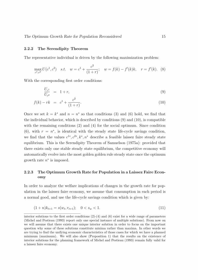
Diagram 1: Population growth and welfare without debt.Quadrant I is the familiar U, n diagram which contains the respective utility con-tours for the laissez faire economy. Quadrant II is the decisive n, r diagram whereall planned equilibria are located along the 45 line. The locus of the laissez fairesteady state curve with dr
dn= f ′′(k) dk
dn> 0 is ambiguous and four cases have to be
distinguished: Case 1: 1-1, Case 2: 2-2, Case 3: 1-2, Case 4: 2-1. Quadrant IIIis a w, r diagram which contains the convex factor-price frontier φ and the respec-tive indifference curves indicating an optimum (pessimum). Quadrant IV gives thewage utility relation. Quadrant V illustrates the respective individual consumptionpatterns for different growth rates (Case 1 only).
The Optimum Growth Rate for Population Reconsidered 19
r
w
r = n
φ(r)
U1
n∗
n
b
1
1
r
w
U2
r = n
φ(r)
n∗
n
b
2
2
1
Diagram 2: The factor-price frontier as a surrogate budget constraint.
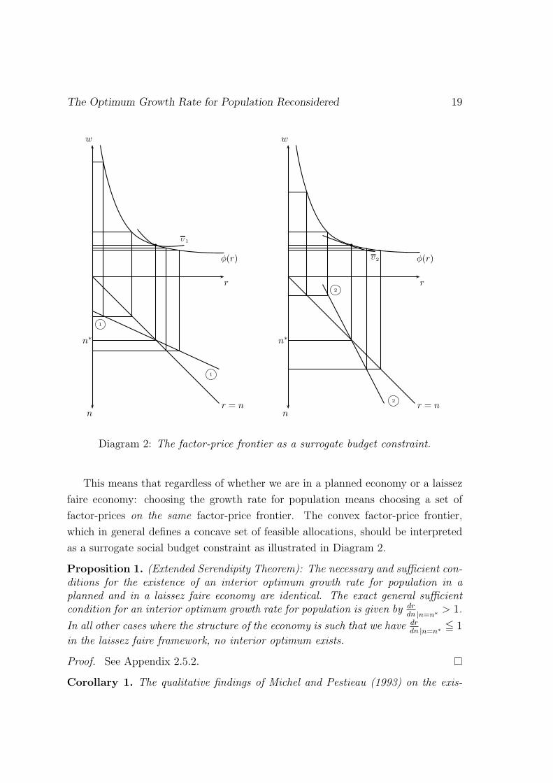
This means that regardless of whether we are in a planned economy or a laissez
faire economy: choosing the growth rate for population means choosing a set of
factor-prices on the same factor-price frontier. The convex factor-price frontier,
which in general defines a concave set of feasible allocations, should be interpreted
as a surrogate social budget constraint as illustrated in Diagram 2.
Proposition 1. (Extended Serendipity Theorem): The necessary and sufficient con-ditions for the existence of an interior optimum growth rate for population in aplanned and in a laissez faire economy are identical. The exact general sufficientcondition for an interior optimum growth rate for population is given by dr
dn |n=n∗> 1.
In all other cases where the structure of the economy is such that we have drdn |n=n∗
5 1
in the laissez faire framework, no interior optimum exists.
Proof. See Appendix 2.5.2.
Corollary 1. The qualitative findings of Michel and Pestieau (1993) on the exis-

20 Intertemporal Allocation with Incomplete Markets
tence of an interior optimum growth rate for population in the CES/CIES planningframework remain fully valid for a laissez faire economy.
Hence, all specifications, most notably the Cobb-Douglas case, where there is
an interior planned minimum are consistent with Case 2 and the counterintuitive
change in efficiency at n = n∗. In our opinion it is this counterintuitive behavior of
economies with high elasticities of substitution that should be criticized and not the
behavior in the two “corners” where k →∞ or n→∞ as in Samuelson (1976).13
We can now conclude that the reasoning of Samuelson (1975a) and Samuelson
(1975b) only remains valid as long as the economy behaves according to Case 1.
However, the assertion of Samuelson (1975a), (p. 535) and Samuelson (1975b), (p.
542) that all economies behave according to Case 1 − which was never questioned
by Deardorff (1976) or Michel and Pestieau (1993) − is wrong.
However, Case 1 is obviously the most plausible scenario. Using the data in Mar-
quetti (2004) for the years 1963-2000, Kuhle (2007) shows that real world economies
tend to behave according to Case 1. Estimates of the r-n relation for Japan, the
USA and a group of 17 mostly developed countries allow to refute the null hypothesisdrdn< 1 with a probability of error (t-test) of less than 2.5 percent.
2.3 The Optimum Growth Rate for Population in an Econ-omy with Government Debt
We will now proceed along the following lines: in a first step the Diamond (1965)
model with internal government debt and the corresponding government budget
constraint will be restated. In a second step we will show that the Serendipity
Theorem is in general not valid in an economy with government debt. The third
step is to derive the welfare implications which stem from a change in the growth
rate of population in a laissez faire economy where the government runs a constant
per capita debt policy.
13At this point we shall note that Phelps (1968) shows for a laissez faire economy that the Cobb-Douglas case is consistent with what we have called Case 2, i.e. an interior minimum at n = n∗.Hence, in the light of the Serendipity Theorem, it should have been no surprise to Deardorff (1976)and Samuelson (1975a) that the “most golden golden rule steady state” must be a minimum inthat case.
The Optimum Growth Rate for Population Reconsidered 21
2.3.1 The Model
The Diamond (1965) model with debt differs from the one which was discussed in
the foregoing section only with respect to the government budget constraint and
the steady state life-cycle savings condition. Government debt has a one-period
maturity and yields the same interest as real capital and there is no risk of default.
In each period the government has to service the matured debt Bt−1 and it has to
pay interest amounting to f ′(kt)Bt−1. The government can use two tools to meet
these obligations: it can raise a lump-sum tax Ntτ1t from the young generation, or
it can issue new debt Bt. Hence we have:
Bt +Ntτ1t = (1 + f ′(kt))Bt−1. (18)
In the following the government will simply pursue a constant per capita debt policy
defined by:14
Bt−1
Nt
= b ∀t. (19)
Thus (18) simplifies to:
τ 1 =[(1 + f ′(kt))− (1 + n)
]b = (f ′(kt)− n)b = τ 1(kt). (20)
Equation (20) reveals that taxes can be either positive or negative depending on
b ≷ 0 and the sign of (f ′(k) − n), i.e. on whether the economy is growing on an
efficient or inefficient path.
2.3.2 The Serendipity Theorem with Debt
From the perspective of the social planner the problem remains unaltered: the
relevant tradeoff is still between capital widening and the intergenerational transfer
effect, and conditions (2)-(4) and (6) still describe the social optimum.
The Competitive Economy with Government Debt The individual utility
maximization problem is given by:
maxc1,c2
U(c1t , c2t+1) s.t. w(kt)− τ 1
t (kt) = c1t + st; c2t+1 = (1 + f ′(kt+1))st. (21)
14Persson and Tabellini (2000) argue why an elected government might rather run such a debtpolicy than use its budget constraint to steer the economy towards the long run optimum asdiscussed in De La Croix and Michel (2002).
22 Intertemporal Allocation with Incomplete Markets
Thus the representative individual behaves according to:
Uc1
Uc2= 1 + f ′(kt+1), (22)
st = w(kt)− τ 1t (kt)− c1t , (23)
c2t+1 = (1 + f ′(kt+1))st. (24)
Attainability of the Social Optimum In a steady state equilibrium the life-
cycle savings condition is given by:
s(w(k), f ′(k)) = (1 + n)(b+ k); s > 0; w(k) := w(k)− τ 1(k), (25)
where s > 0 is an obvious restriction since negative savings would lead to negative old
age consumption. We will now examine whether the social optimum (c1∗, c2∗, n∗, k∗),
which is characterized by (2)-(4) and (6), is a feasible laissez faire steady state
equilibrium: once we set k = k∗ and n = n∗, conditions (3) and (6) hold. According
to (20) we have τ 1(k∗) = 0 and the individual budget constraint becomes the same
as the availability constraint. In this case the individual will voluntarily choose c1∗
and c2∗. Finally we have to check the steady state life-cycle savings condition:
s∗ = (1 + n∗)k∗ =c2∗
(1 + n∗)6= (1 + n∗)(k∗ + b); ∀b 6= 0. (26)
This means that since internal debt leads to the substitution of capital with debt
(paper) in the portfolio of the representative individual, the Serendipity Theorem
does not hold. Thus the only way to decentralize the social optimum is to reduce
per capita debt to zero.
2.3.3 The Optimum Growth Rate for Population in a Laissez Faire Econ-omy with Debt
Comparison of the social optimum and the individual behavior revealed that the
Serendipity Theorem does not hold in the Diamond model with internally held debt.
We will now assess the question of optimal population in a competitive economy.
Two related points will be discussed:
1. A change in the constant debt policy for a given growth rate for population.
2. A change in the growth rate for population for a given debt policy.
The Optimum Growth Rate for Population Reconsidered 23
Temporary Equilibrium As De La Croix and Michel (2002) point out, there are
several conditions which have to be met in each period to allow for a meaningful
temporary equilibrium:
st−1 > 0, (27)
w(kt, b) = w(kt)− τ 1(kt) = w(kt)− b(f ′(kt)− n) > 0, (28)
s(w(kt, b), f′(kt+1)) = (1 + n)(kt+1 + b) > (1 + n)b. (29)
While (27) ensures positive consumption of the old generation, w in (28) describes
that the income after taxes of the current young individuals must be positive. Con-
dition (29) must hold to allow for a positive capital intensity.
Steady State Equilibrium In order to carry out the following comparative static
(in per capita terms) analysis, it is necessary to determine the signs of dkdn
and dkdb
.
As in Diamond (1965), we will assume that there exists a unique stable steady state
at k = k:
0 <dkt+1
dkt=−sw(k + b)f ′′(k)
(1 + n)− srf ′′(k)< 1; 0 < sw < 1; k > 0. (30)
Total differentiation of the life-cycle savings condition (25) with db = 0 leads to:
dk
dn |db=0=
k + (1− sw)b
srf ′′ − (1 + n)− sw(k + b)f ′′< 0. (31)
The sign in the denominator of the expression (31) is negative by virtue of the
stability condition (30). The assumption of normality (0 < sw < 1) and conditions
(27) and (29) reveal that the sign of the numerator is positive. Total differentiation
of (25) with dn = 0 yields:
dk
db |dn=0=
(1 + n) + sw(f ′ − n)
srf ′′ − (1 + n)− swf ′′(k + b)< 0. (32)
With 0 < sw < 1, the sign in the numerator of (32) must be positive. The sign of
the denominator is negative according to (30).
Once the signs of dkdn
and dkdb
are known to be negative, the key elements to our
question can be displayed in Diagram 3.
24 Intertemporal Allocation with Incomplete Markets
n
k
k∗
n n∗
n
(a)
1
1
1’
1’
2
2
2’
2’
kn
n
k
kn
n∗
nn
(b)
4
4
4’
4’
3’
3’
3
3
k∗
1
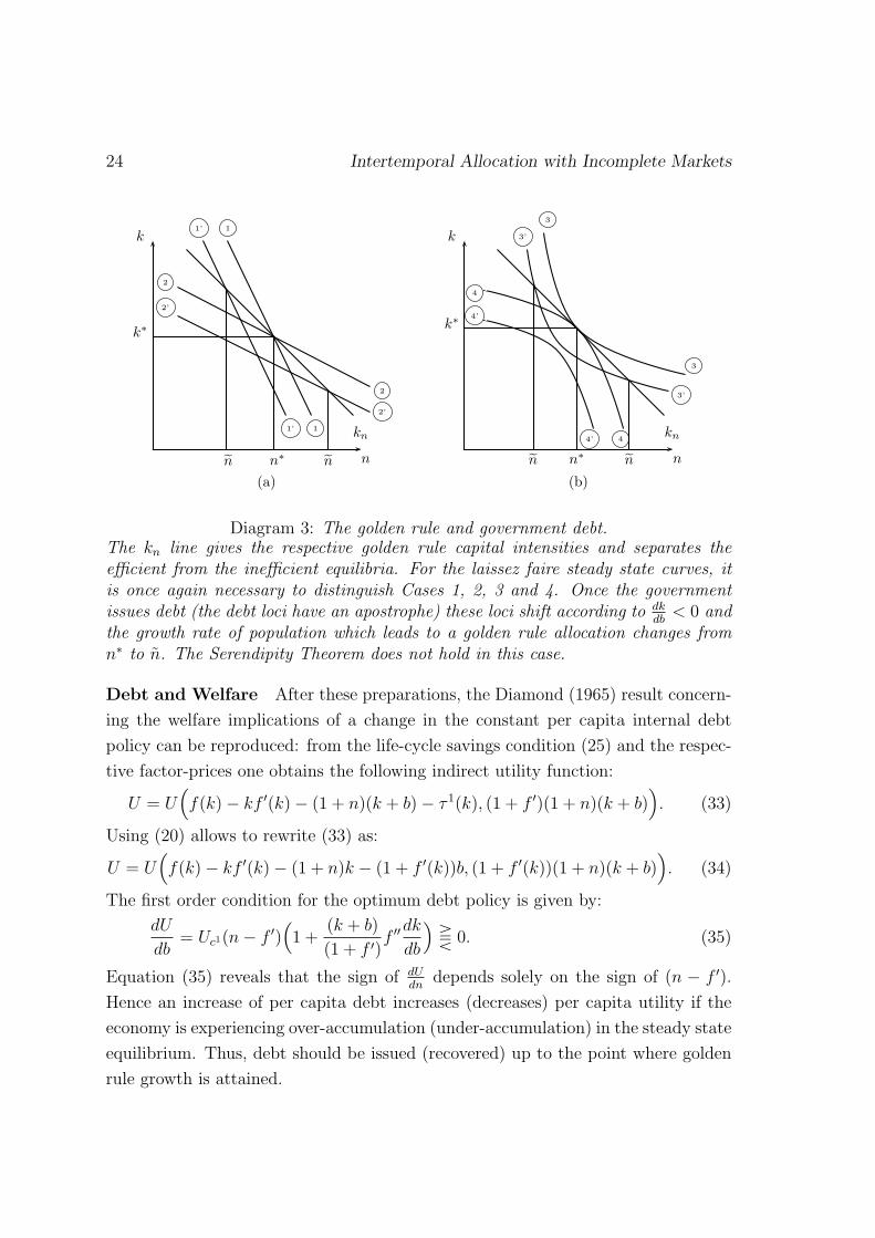
Diagram 3: The golden rule and government debt.The kn line gives the respective golden rule capital intensities and separates theefficient from the inefficient equilibria. For the laissez faire steady state curves, itis once again necessary to distinguish Cases 1, 2, 3 and 4. Once the governmentissues debt (the debt loci have an apostrophe) these loci shift according to dk
db< 0 and
the growth rate of population which leads to a golden rule allocation changes fromn∗ to n. The Serendipity Theorem does not hold in this case.
Debt and Welfare After these preparations, the Diamond (1965) result concern-
ing the welfare implications of a change in the constant per capita internal debt
policy can be reproduced: from the life-cycle savings condition (25) and the respec-
tive factor-prices one obtains the following indirect utility function:
U = U(f(k)− kf ′(k)− (1 + n)(k + b)− τ 1(k), (1 + f ′)(1 + n)(k + b)
). (33)
Using (20) allows to rewrite (33) as:
U = U(f(k)− kf ′(k)− (1 + n)k − (1 + f ′(k))b, (1 + f ′(k))(1 + n)(k + b)
). (34)
The first order condition for the optimum debt policy is given by:
dU
db= Uc1(n− f ′)
(1 +
(k + b)
(1 + f ′)f ′′dk
db
)T 0. (35)
Equation (35) reveals that the sign of dUdn
depends solely on the sign of (n − f ′).
Hence an increase of per capita debt increases (decreases) per capita utility if the
economy is experiencing over-accumulation (under-accumulation) in the steady state
equilibrium. Thus, debt should be issued (recovered) up to the point where golden
rule growth is attained.
The Optimum Growth Rate for Population Reconsidered 25
Population Growth and Welfare The same indirect utility function (34) can
now be used to derive the welfare implications which originate from changes in the
growth rate for population. Hence, the first derivative with respect to the growth
rate of population is:
dU
dn= −Uc1
([(k + b)f ′′ + (1 + n)]
dk
dn+ k
)+ Uc2
([(1 + n)(1 + f ′) + f ′′(1 + n)(b+ k)]
dk
dn+ (1 + f ′)(k + b)
). (36)
Using (22), we obtain:
dU
dn= Uc1b+ Uc1
(n− f ′)(k + b)
1 + f ′f ′′dk
dnT 0;
dk
dn< 0. (37)
The first order derivative (37) contains two elements: the first element Uc1b > 0 (for
b > 0) is the biological interest rate effect, which suggests that population should
grow as fast as possible. The reason for the appearance of the biological interest
argument is the following: each young individual buys government debt amounting
to (1 + n)b and pays taxes (f ′(k) − n)b. Hence the young individual hands over
a total amount of (1 + f ′(k))b to the government. In the retirement period the
government serves its obligations and pays (1 + f ′(k))(1 + n)b.
Thus the individual receives the biological rate of interest (1 + n) on its total
payments. This also reveals that the total amount of resources which is transferred
into the retirement period, at the biological rate of interest, depends on the rate
of interest (1 + f ′(k)) and hence, via the capital intensity, on the growth rate of
population.
The second element Uc1(n−f ′)(k+b)
1+f ′f ′′ dk
dndescribes the factor-price effects which
originate from a change in the growth rate of population. An increase in n leads to
a fall in k, which increases the interest rate payed on capital and debt, and decreases
wages.
In the special case b = 0, (37) degenerates into (15) where dUdn
= 0 for n = n∗,
and at n∗ the pair of factor-prices w(k(n∗)), r(k(n∗)) ensure maximum (minimum)
lifetime utility. The tradeoff is solely between wages and interest.
In the case b 6= 0 the situation differs fundamentally: as (37) indicates, the
tradeoff is now between what we will call the aggregate factor-price effects and the
biological interest rate. The growth rate which maximizes (minimizes) laissez faire
utility in an economy with government debt will be referred to as n∗∗. We can note
26 Intertemporal Allocation with Incomplete Markets
that n∗∗ is larger (for Case 1, b > 0) than the growth rate n which causes a golden
rule allocation, and it may or may not be larger than n∗. The conditions which
have to be met to allow for a laissez faire optimum at n∗∗ remain, compared to the
case without debt, basically unaltered with drdn> 1; the only additional condition is
that the difference (n − f ′(k(n))) must increase sufficiently to allow for an interior
optimum at n∗∗.
Optimal Population vs. Optimal Debt Conditions (35), and (37) indicate
that there is no symmetry in the respective optimal debt and population policies with
respect to the golden rule allocation. This gives rise to the following Proposition:
Proposition 2. In a laissez faire economy with constant per capita government debt,the growth rate of population, which leads to a golden rule allocation, can never beoptimal.
Corollary 2. If the government pursues an optimal debt policy according to condi-tion (35), the growth rate for population cannot be optimal simultaneously.
Corollary 3. : If the government imposes an optimum growth rate for populationaccording to (37), the debt policy cannot be optimal simultaneously.
Only by setting the per capita level of debt to zero and the growth rate for
population to n∗, the two optimality conditions (35) and (37) can be satisfied simul-
taneously:
Proposition 3. If the social planner can choose both: the optimum growth rate forpopulation and the optimal amount of debt, the only optimal debt policy is zero debt.
Illustration Using Case 1 with b > 0 as an example (the reader can experiment
with (35) and (37), which allow to evaluate the remaining three cases; Cases 2 and
3 may contain multiple solutions), the foregoing discussion concerning the optimum
growth rate of population in an economy with government debt can be summarized
in Diagram 4.15
Diagram 4 illustrates that the optimum growth rate for population n∗∗ is larger
than n. Compared to the case without debt, the preference ordering in the w, r
quadrant is changed since the interest rate is not only determining the relative price
15In Appendix 2.5.4 we develop the corresponding slope of the households indifference curvesdisplayed in Diagram 4. In Appendix 2.5.5, we show that the quality of our results remainsunaltered in a model with pay-go social security.
The Optimum Growth Rate for Population Reconsidered 27
n
U
n n∗∗ n∗
U∗∗
U
r = n
U(n)
r
r∗∗
r∗
r
w∗w∗∗w
w 1’
1’
1
1
U1
U1
U1,b=0
φ(r)
1
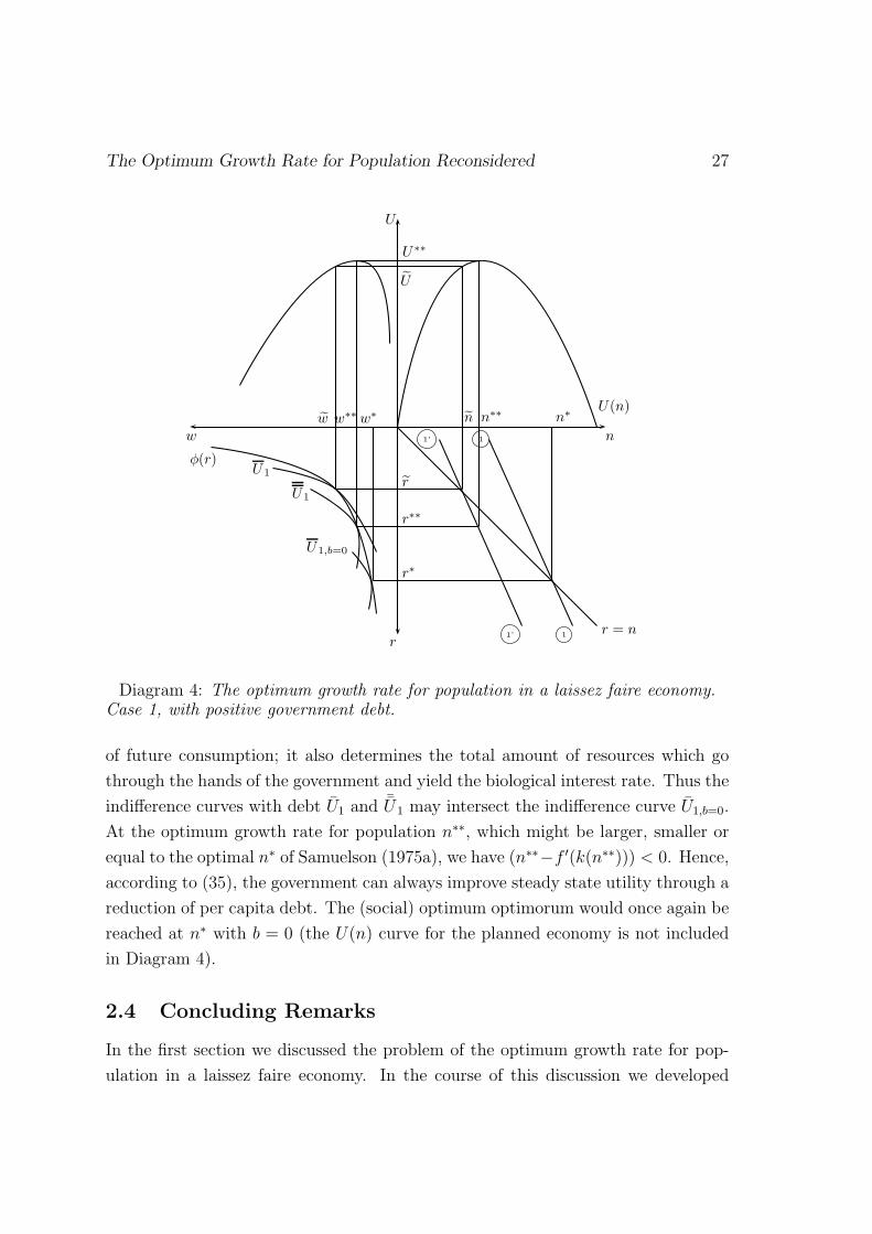
Diagram 4: The optimum growth rate for population in a laissez faire economy.Case 1, with positive government debt.
of future consumption; it also determines the total amount of resources which go
through the hands of the government and yield the biological interest rate. Thus the
indifference curves with debt U1 and ¯U1 may intersect the indifference curve U1,b=0.
At the optimum growth rate for population n∗∗, which might be larger, smaller or
equal to the optimal n∗ of Samuelson (1975a), we have (n∗∗−f ′(k(n∗∗))) < 0. Hence,
according to (35), the government can always improve steady state utility through a
reduction of per capita debt. The (social) optimum optimorum would once again be
reached at n∗ with b = 0 (the U(n) curve for the planned economy is not included
in Diagram 4).
2.4 Concluding Remarks
In the first section we discussed the problem of the optimum growth rate for pop-
ulation in a laissez faire economy. In the course of this discussion we developed
28 Intertemporal Allocation with Incomplete Markets
a general typology for the problem of optimal population in the Diamond (1965)
model without government debt. This led to the conclusion that:
1. The qualitative necessary and sufficient conditions for the existence of an in-
terior optimum growth rate for population in a planned and in a laissez faire
economy are identical. In both cases it is the convex factor-price frontier which
can be interpreted as the social budget constraint. Hence we have shown that
the findings of Michel and Pestieau (1993) for the planned economy remain
also valid in the more realistic case of a laissez faire framework.
2. There always exists an interior optimum in an economy where low (high)
growth rates for population lead to over-accumulation (under-accumulation).
The general sufficient condition for an interior optimum in a laissez faire as
well as in a planned economy is hence given by drdn |n=n∗
> 1. All cases where
there exists an interior minimum, like the Cobb-Douglas case, are consistent
with an economy, in which rapid population growth leads to over-accumulation
and low or negative growth rates for population lead to under-accumulation.
3. An increase in the growth rate for population increases (decreases) steady state
welfare only if the economy is growing on an inefficient (efficient) steady state
path.
In a second step we generalized the discussion by introducing government debt. In
such a framework we find that:
1. Due to the substitution between debt and capital in the portfolios of the
representative individuals, the Serendipity Theorem does not hold anymore.
However, except for the case of permanent efficiency there still exists at least
one growth rate for population n, which leads the laissez faire economy to
(two-part) golden rule growth.
2. In a laissez faire economy with constant per capita debt, the growth rate for
population n, which leads to a golden rule allocation, cannot be optimal since
it only balances the wage-interest tradeoff. The optimum growth rate for
population balances the tradeoff between factor-prices and the internal rate
of return of the pension/debt scheme. Such an optimum growth rate leads
the competitive economy to an allocation where the marginal productivity of
capital exceeds the optimum growth rate for population.

The Optimum Growth Rate for Population Reconsidered 29
2.5 Appendix
2.5.1 Construction of Diagram 1
In this appendix we substantiate our claim that the qualitative conditions for an
interior optimum are properly represented in Quadrant III of Diagram 1. Hence
we have to show that the necessary condition for an optimum at n∗ requires that
the indifference curve in the w, r plane is a tangent to the factor-price frontier, i.e.dwdr |dU=0
= φ′(r). Analogous we show that the sufficient condition is satisfied only if
the curvature of the indifference curve is larger than the curvature of the factor-price
frontier, i.e. d2wdr2 |dU=0
> φ′′(r). The factor-price frontier is given by:
w = φ(r);dw
dr= φ′(r) = −k; d2w
dr2= φ′′(r) =
−1
f ′′.
The indifference curve of the representative individual in the w, r plane is:
U = U(w, r);dw
dr |dU=0=−s(w, r)(1 + r)
;d2w
dr2 |dU=0=sws(w, r)− sr(1 + r) + s(w, r)
(1 + r)2.
Using the Serendipity Theorem we can show that the first order condition for a
laissez faire/planned optimum at an interior n∗ is satisfied if φ′(r) = dwdr |dU=0
at n∗:
− k∗ +c2∗
(1 + n∗)2= 0 ⇔ −k∗ =
−s∗
(1 + f ′(k(n∗))); f ′(k(n∗)) = n∗; c2∗ = (1 + n∗)s∗.
Now we will show that the sufficient condition d2wdr2 |dU=0
> φ′′(r) can be trans-
formed into f ′′(k) dkdn> 1, which was our sufficient condition (compare with (16) and
(17)) for a laissez faire optimum at n∗:
sws(w, r)− sr(1 + r) + s(w, r)
(1 + r)2>−1
f ′′;
at the stationary point we have s = (1 + n)k and n = n∗ = r, and hence:
sw(1 + n)k − sr(1 + n) + (1 + n)k
(1 + n)>
−1
f ′′(1 + n),
this can be rearranged such that:
− k <1
f ′′(1 + n) + swk − sr,
with 1f ′′
(1 + n) + swk − sr < 0 by virtue of the stability condition (12). Thus we
obtain:−k
1f ′′
(1 + n) + swk − sr> 1 ⇔ f ′′(k)
dk
dn> 1.
30 Intertemporal Allocation with Incomplete Markets
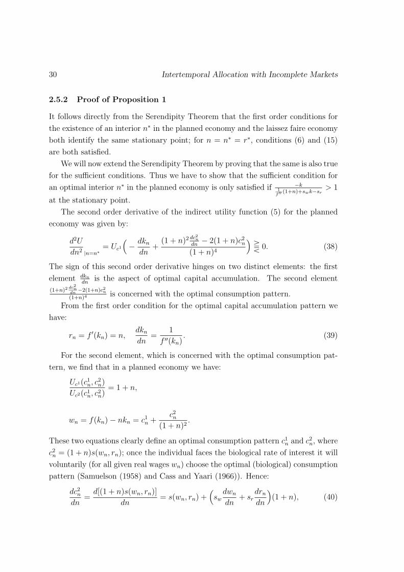
2.5.2 Proof of Proposition 1
It follows directly from the Serendipity Theorem that the first order conditions for
the existence of an interior n∗ in the planned economy and the laissez faire economy
both identify the same stationary point; for n = n∗ = r∗, conditions (6) and (15)
are both satisfied.
We will now extend the Serendipity Theorem by proving that the same is also true
for the sufficient conditions. Thus we have to show that the sufficient condition for
an optimal interior n∗ in the planned economy is only satisfied if −k1
f ′′ (1+n)+swk−sr> 1
at the stationary point.
The second order derivative of the indirect utility function (5) for the planned
economy was given by:
d2U
dn2 |n=n∗= Uc1
(− dkn
dn+
(1 + n)2 dc2n
dn− 2(1 + n)c2n
(1 + n)4
)T 0. (38)
The sign of this second order derivative hinges on two distinct elements: the first
element dkn
dnis the aspect of optimal capital accumulation. The second element
(1+n)2dc2ndn
−2(1+n)c2n(1+n)4
is concerned with the optimal consumption pattern.
From the first order condition for the optimal capital accumulation pattern we
have:
rn = f ′(kn) = n,dkndn
=1
f ′′(kn). (39)
For the second element, which is concerned with the optimal consumption pat-
tern, we find that in a planned economy we have:
Uc1(c1n, c
2n)
Uc2(c1n, c2n)
= 1 + n,
wn = f(kn)− nkn = c1n +c2n
(1 + n)2.
These two equations clearly define an optimal consumption pattern c1n and c2n, where
c2n = (1 + n)s(wn, rn); once the individual faces the biological rate of interest it will
voluntarily (for all given real wages wn) choose the optimal (biological) consumption
pattern (Samuelson (1958) and Cass and Yaari (1966)). Hence:
dc2ndn
=d[(1 + n)s(wn, rn)]
dn= s(wn, rn) +
(swdwndn
+ srdrndn
)(1 + n), (40)

The Optimum Growth Rate for Population Reconsidered 31
with:
drndn
= 1;dwndn
= f ′(kn)dkndn
− kn − ndkndn
= −kn.
We can now substitute the expressions in (39) and (40) into (38) to evaluate the sign
of d2Udn2 at the stationary point, where we have c2∗n = (1 + n∗)s(w∗, r∗) = (1 + n∗)2k∗:
d2U
dn2 |n=n∗= Uc1
(− 1
f ′′(k∗)+
(1 + n∗)3k∗ + (−swk∗ + sr)(1 + n∗)3
(1 + n∗)4− 2(1 + n∗)3k∗
(1 + n∗)4
).
Hence d2Udn2 |n=n∗
is negative if:
− k∗ < (1 + n∗)1
f ′′(k∗)+ swk
∗ − sr. (41)
According to the stability condition (12) we have (1 +n∗) 1f ′′(k∗)
+ swk∗− sr < 0 and
we find that d2Udn2 |n=n∗
< 0 if and only if:
−k∗
(1 + n∗) 1f ′′(k∗)
+ swk∗ − sr> 1. (42)
This sufficient condition for a social optimum (42) is identical with the sufficient
condition (17) for a laissez faire optimum at n∗.
2.5.3 Oscillatory Stability
In this appendix we will discuss the case of one unique oscillatory steady state
equilibrium. The corresponding stability condition is:
− 1 <dkt+1
dkt=
−swf ′′k(1 + n)− srf ′′
< 0; sw > 0. (43)
Since the numerator is positive sr must be algebraically large and negative, which
is only possible for σ < 1. From the life cycle savings condition (11) we obtain once
again:
dk
dn=
−kswf ′′k + (1 + n)− srf ′′
. (44)
Utilizing (43) reveals that dkdn> 0 and hence we have dr
dn< 0. It is now easy to show
that the sufficient condition for an interior optimum growth rate for population is
always satisfied:
d2U
dn2 |n=n∗= Uc1
(1− drdn
)
(1 + r)kdr
dn< 0. (45)

32 Intertemporal Allocation with Incomplete Markets
Hence we find that an interior minimum is only possible for
0 < drdn |n=n∗
< 1, in all other instances we have an interior optimum. However,
the oscillatory case with dkdn
> 0 appears to be rather unrealistic. In addition we
note that the claim, that the ”stability condition” together with the assumption of
normality allows to derive the sign of dkdn
, is not accurate. Instead, it is necessary to
distinguish two cases, in the same manner as in Diamond (1965).
2.5.4 Formal aspects to Diagram 4
Individual utility is given by:
U = U(w(n)− s(w(n), r(n))− (r(n)− n)b, (1 + r(n))s(w(n), r(n))
),
by varying the growth rate for population only, we obtain the following slope for the
indifference curve:
dw
dr |dU=0,U
c1U
c2=1+r,dn6=0
= b− s
1 + r− dn
drb.
We can now reproduce the first order condition (37) by settingdwdr |dU=0,
Uc1
Uc2
=(1+r)= φ′(r) = −k:
b− s
(1 + r)− dn
drb = −k ⇔ n− r
1 + r(k + b)
dr
dn+ b = 0.
For n = n = r we have:
dw
dr= b− s
(1 + r)− b
dn
dr< −k,
since,
− bdn
dr< 0.
Hence at n the slope of the indifference curve is algebraically larger than that of the
factor-price frontier.
2.5.5 Appendix: Pay-as-you-go Social Security and optimal population
In this appendix we will briefly substantiate the claim that the qualitative condi-
tions for an interior optimum in an economy with debt are similar to those for an
economy with a pay-as-you-go social security system. Once we denote the per capita
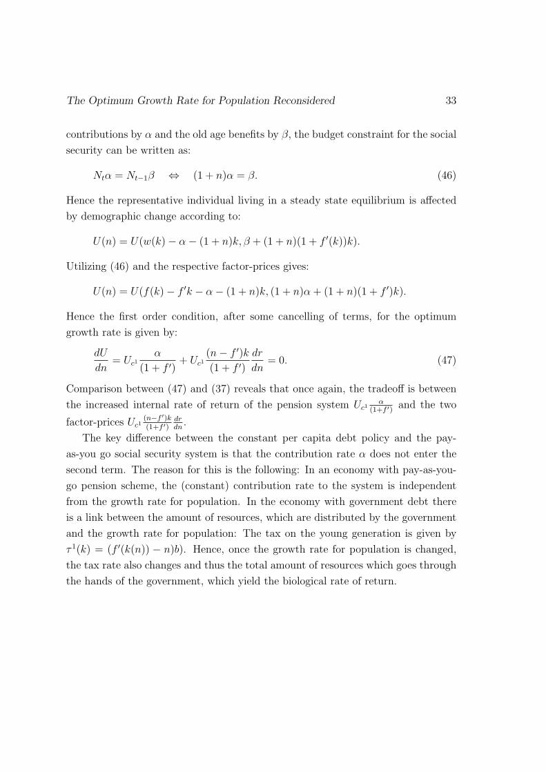
The Optimum Growth Rate for Population Reconsidered 33
contributions by α and the old age benefits by β, the budget constraint for the social
security can be written as:
Ntα = Nt−1β ⇔ (1 + n)α = β. (46)
Hence the representative individual living in a steady state equilibrium is affected
by demographic change according to:
U(n) = U(w(k)− α− (1 + n)k, β + (1 + n)(1 + f ′(k))k).
Utilizing (46) and the respective factor-prices gives:
U(n) = U(f(k)− f ′k − α− (1 + n)k, (1 + n)α+ (1 + n)(1 + f ′)k).
Hence the first order condition, after some cancelling of terms, for the optimum
growth rate is given by:
dU
dn= Uc1
α
(1 + f ′)+ Uc1
(n− f ′)k
(1 + f ′)
dr
dn= 0. (47)
Comparison between (47) and (37) reveals that once again, the tradeoff is between
the increased internal rate of return of the pension system Uc1α
(1+f ′)and the two
factor-prices Uc1(n−f ′)k(1+f ′)
drdn
.
The key difference between the constant per capita debt policy and the pay-
as-you go social security system is that the contribution rate α does not enter the
second term. The reason for this is the following: In an economy with pay-as-you-
go pension scheme, the (constant) contribution rate to the system is independent
from the growth rate for population. In the economy with government debt there
is a link between the amount of resources, which are distributed by the government
and the growth rate for population: The tax on the young generation is given by
τ 1(k) = (f ′(k(n)) − n)b). Hence, once the growth rate for population is changed,
the tax rate also changes and thus the total amount of resources which goes through
the hands of the government, which yield the biological rate of return.

34
Dynamic Efficiency and the Two-Part Golden Rule with Heterogeneous Agents 35
3 Dynamic Efficiency and the Two-Part Golden
Rule with Heterogeneous Agents
This chapter is concerned with the role of the two-part golden rule as the watershed
between equilibria which are dynamically efficient and those, which are inefficient.
In an economy where agents differ regarding their labor endowment, the golden
rule allocation ceases to serve as such a demarcation line. Except for the special
case where all agents possess a linear Engel-curve with identical slope, some agents’
maximum steady state utility will always be associated with a capital intensity
exceeding (falling short of) the golden rule level. This result stems from the fact
that the competitive markets entail an intra-generational redistribution of resources
once the capital intensity is altered. If heterogeneity is introduced on the preference
side, we find that the golden rule is never optimal for all agents. Consequently,
earlier results in the literature (e.g. Stein (1969)) on the two-part golden rule with
heterogeneous agents are not warranted.
3.1 Introduction
Having less of something useful may improve welfare. This is one of the key results
obtained from the normative evaluation of the Solow (1956), Swan (1956) models
of capital and growth: maintaining a capital intensity that permanently exceeds
the golden rule level is known to be inefficient.16 At the same time we know from
the pure consumption loan economy of the Samuelson (1958) type that a given
endowment should be distributed between adjacent cohorts such that the rate of
return on consumption loans is equated to the growth rate of population. Taken
together, these two optimality conditions constitute the two-part golden rule which
maximizes steady state utility in the Diamond (1965) model. The golden rule of
accumulation ensures maximum consumption in each period. In turn, the golden
rule of interest on consumption loans ensures efficient intergenerational distribution
of the consumption available.
In more recent studies, this two-part golden rule result was shown to be robust
with regard to several changes in the underlying assumptions. In particular, Abel
et al. (1989) and Zilcha (1990) show that the golden rule criterion carries over to a
16See Phelps (1961, 1966b), von Weizsacker (1962), Cass (1972). See Burmeister and Dobell(1970) and Jones (1975) for more references.
36 Intertemporal Allocation with Incomplete Markets
setting with aggregate and idiosyncratic risk. Angel and Garcia (2008) extend the
result to a model with endogenous labor supply.
Against this background, the present chapter is concerned with the role of the
two-part golden rule in a Diamond (1965) economy with heterogeneous agents. To
illustrate our results, two forms of heterogeneity which are widely employed in the
overlapping generations literature will be discussed: (i) heterogeneous labor endow-
ments, with homogeneous preferences and (ii) homogeneous labor endowments with
heterogeneous preferences. In these settings, the Phelps (1961) golden rule continues
to maximize society’s consumption opportunities, and the Samuelson (1958) golden
rule ensures efficient intergenerational consumption patterns. The two-part golden
rule, however, no longer describes the demarcation line between competitive equilib-
ria which are efficient and those which are inefficient. That is, even if the two-part
golden rule equilibrium could be reached at no (transition) cost, there will always be
individuals who prefer a lower and others who prefer a higher steady state capital
intensity. This result originates from an intra-generational reallocation of resources,
which operates through the competitive markets and occurs once the capital inten-
sity is altered. Compared to the golden rule level, this transfer effect will allow
agents whose present value of savings s1+r
exceeds (falls short of) the capital stock
lk, which is absorbed by their labor supply l, to reach higher steady state utility
once the capital intensity is reduced (increased). If heterogeneity is introduced on
the preference side, the corresponding condition is given by si
1+rT k, where thrifty
agents ( si
1+r> k) will once again prefer steady states with interest rates exceeding
the golden rule level.
Despite its simplicity, this result differs from what appears to be the consensus in
the literature. In particular, the often cited17 paper by Stein (1969) p. 144 analyzes
a competitive Diamond (1965) model where agents differ with regard to their rate
of time preference. As we show in Section 3.2.3, his conclusion that the golden rule
allocation is optimal for all members of such a society is not warranted.
17See Gale (1973), Ihori (1978), Krohn (1981) and Crettez et al. (2002). See De La Croixand Michel (2002) for a recent textbook. De La Croix and Michel (2002) p. 81 criticize Stein(1969) by pointing out that he fails to notice the double infinity aspects emphasized by Shell(1971). However, they do not point out that the golden rule no-longer serves as the watershedbetween efficient and inefficient steady states under the assumptions made by Stein (1969), wherehouseholds are heterogeneous. In Section 3.2.3 we complement their criticism and point out thatthe golden rule does not separate efficient from inefficient steady states in a competitive economywith heterogeneous preferences.
Dynamic Efficiency and the Two-Part Golden Rule with Heterogeneous Agents 37
Given the pivotal role played by the golden rule, our results may also provide use-
ful inference with regard to the social security literature (e.g. Persson and Tabellini
(2000) and in particular Pestieau et al. (2006)), where it is often argued that Bev-
eridge schemes are redistributive while Bismarck schemes are not.18 In the current
case, we find that both schemes redistribute resources through their induced factor-
price changes. In particular, if the propensity to save increases with income, the
crowding-out of capital brought about by both social security schemes favors the
rich at the expense of the poor. In the case of a Beveridge pension scheme, some of
the direct intra-generational redistribution is therefore thwarted by the associated
factor-price changes.
The rest of the chapter is organized as follows: In Sections 3.1.1 and 3.1.2,
we recall the two golden rule relations for the representative agent economy. In
Section 3.1.3 we present a dissection of the overlapping generations structure of
incomplete markets. With these elements in place, we isolate the main result in a
partial equilibrium setting. In Section 3.2, we prove the result in general equilibrium.
Section 3.3 offers concluding remarks.
3.1.1 Consumption Maximizing Growth
In the standard one-sector growth models of Solow (1956) and Swan (1956), where
production is homogeneous of degree one, output can be consumed or saved. With
flexible factor-prices, savings always equal investment and at each point in time we
have:
F (Kt, Lt) = Kt+1 −Kt + Ct = Ltf(kt); kt =Kt
Lt, f ′() > 0, f ′′() < 0.(48)
With population growing at a constant proportional rate n, per capita steady state
consumption c := CL
is then:
c = f(k)− nk. (49)
18Pestieau et al. (2006), p. 591 discuss an open economy with general non-homothetic prefer-ences with heterogeneous labor endowment. However, they conclude their analysis by remarking“If instead the pension system were purely contributive (Bismarckian), there would be no redis-tribution across individuals, and thus no tax competition per se. Then capital mobility would nothave any effect on the choice of the payroll tax, and each country would use it to achieve dynamicefficiency just as in autarky” (p. 595). The current analysis shows that the usual notion of dynamicefficiency, i.e. the golden rule result does not apply to the framework analyzed by Pestieau et al.(2006). That is, Bismarckian schemes are not only contributive but also redistributive.
38 Intertemporal Allocation with Incomplete Markets
As shown by Phelps (1961), von Weizsacker (1962) and others, consumption is
maximized if the rate of return on capital investment is equal to the economy’s
growth rate:
maxkc(k) = max
k
(f(k)− nk
)= f(kn)− nkn, f ′(kn) = n, (50)
where kn denotes the golden rule capital intensity. Once reached, this consumption
maximizing steady state can be sustained by investing profits, snf(kn) = nkn =
f ′(kn)kn, and the consumption of wages, c(kn) = f(kn)− nkn = wn.
3.1.2 Utility Maximizing Growth
In the Diamond (1965) life-cycle model, steady state utility is at its long-run op-
timum once the two-part golden rule is implemented. In each period t, aggregate
consumption Ct can now be allocated between the old and the young cohort, i.e.
Ct = C1t + C2
t . Recalling the resource constraint (48), the social planner chooses
the consumption maximizing capital intensity kn defined in (50). In turn, consump-
tion is allocated to the old and young according to the second biological interest
rate relation of Samuelson (1958). With utility concave in first and second period
consumption, we have the two-part golden rule optimum:
maxk,c2
U(c1, c2) s.t. f(k)− nk = c1 +c2
1 + n; (51)
f ′(kn) = n, (52)
Uc1(c1n, c
2n)
Uc2(c1n, c2n)
= 1 + n, (53)
where (52) maximizes consumption and (53) ensures efficient intergenerational dis-
tribution. As Diamond (1965), Samuelson (1975b) and Ihori (1978) show, this util-
ity maximizing allocation can be decentralized by an appropriate intergenerational
transfer that forces k = kn such that (52) is satisfied. In turn, consumers will volun-
tarily choose consumption according to (53). A striking property of (52) and (53)
is their asymmetry. A change in the utility function affects the consumption profile
c1n, c2n but does not affect the optimal capital intensity kn. However, a change in
the production function affects all three quantities kn, c1n, c
2n. If preferences are not
homothetic, it also affects the ratio c1nc2n
.
Dynamic Efficiency and the Two-Part Golden Rule with Heterogeneous Agents 39
3.1.3 Competitive Incomplete Markets
In this section, we dissect the competitive apparatus of maximizing behavior and
market clearing, which restricts the set of feasible steady state allocations. This
dissection will provide the background to interpret our results in Section 3.2. In a
first step we summarize the OLG market structure in the c1, c2 plane. In a second
step, we approach the same question in the w, r plane to emphasize the role of the
factor-price frontier as a resource constraint. The key insight in this section is that
the golden rule result vanishes for the representative agent economy once one of the
equations which describe the competitive equilibrium is not taken into account. In
Section 3.2, where we introduce heterogeneity, it will turn out that some equations,
most notably the life-cycle savings condition, are less restrictive: in a model with
heterogeneous agents, average savings rather than each agent’s savings have to be
sufficient to support the steady state capital stock. That is, in what follows we show
that dropping one of the equations of the representative agent model will make the
golden rule allocation suboptimal. In turn, we show in Section 3.2 that heterogeneity
will have an effect which is similar to the dropping of one equation: the life-cycle
savings condition will only require that average savings support the steady state. It
is therefore less restrictive and the golden rule result vanishes in the same manner
as it does in the representative agent economy where the life-cycle savings condition
is not taken into account.
The Golden Rule Consumption Profile The equations describing the com-
petitive Diamond (1965) model, where taxes are raised in each period to keep the
debt to labor ratio bt = Bt
Ltconstant over time, may be summarized as follows:
Lt+1 = (1 + n)Lt, (54)
st = (1 + n)(kt+1 + b), (55)
st = wt − c1t − (rt − n)b, (56)
c1t +c2t+1
(1 + rt+1)= wt − (rt − n)b, (57)
wt = f(kt)− f ′(kt)kt, (58)
rt = f ′(kt), (59)
f(kt) = (1 + n)kt+1 − kt + c1t +c2t
1 + n. (60)
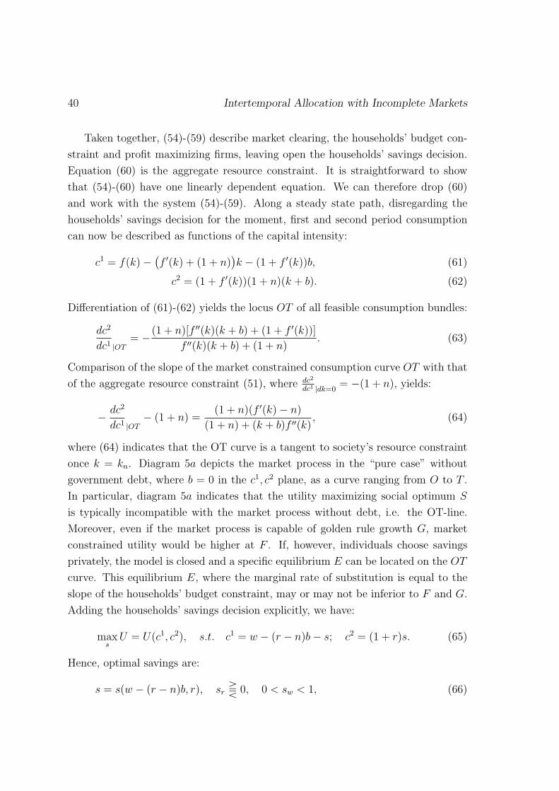
40 Intertemporal Allocation with Incomplete Markets
Taken together, (54)-(59) describe market clearing, the households’ budget con-
straint and profit maximizing firms, leaving open the households’ savings decision.
Equation (60) is the aggregate resource constraint. It is straightforward to show
that (54)-(60) have one linearly dependent equation. We can therefore drop (60)
and work with the system (54)-(59). Along a steady state path, disregarding the
households’ savings decision for the moment, first and second period consumption
can now be described as functions of the capital intensity:
c1 = f(k)−(f ′(k) + (1 + n)
)k − (1 + f ′(k))b, (61)
c2 = (1 + f ′(k))(1 + n)(k + b). (62)
Differentiation of (61)-(62) yields the locus OT of all feasible consumption bundles:
dc2
dc1 |OT= −(1 + n)[f ′′(k)(k + b) + (1 + f ′(k))]
f ′′(k)(k + b) + (1 + n). (63)
Comparison of the slope of the market constrained consumption curve OT with that
of the aggregate resource constraint (51), where dc2
dc1 |dk=0= −(1 + n), yields:
− dc2
dc1 |OT− (1 + n) =
(1 + n)(f ′(k)− n)
(1 + n) + (k + b)f ′′(k), (64)
where (64) indicates that the OT curve is a tangent to society’s resource constraint
once k = kn. Diagram 5a depicts the market process in the “pure case” without
government debt, where b = 0 in the c1, c2 plane, as a curve ranging from O to T .
In particular, diagram 5a indicates that the utility maximizing social optimum S
is typically incompatible with the market process without debt, i.e. the OT-line.
Moreover, even if the market process is capable of golden rule growth G, market
constrained utility would be higher at F . If, however, individuals choose savings
privately, the model is closed and a specific equilibrium E can be located on the OT
curve. This equilibrium E, where the marginal rate of substitution is equal to the
slope of the households’ budget constraint, may or may not be inferior to F and G.
Adding the households’ savings decision explicitly, we have:
maxsU = U(c1, c2), s.t. c1 = w − (r − n)b− s; c2 = (1 + r)s. (65)
Hence, optimal savings are:
s = s(w − (r − n)b, r), sr T 0, 0 < sw < 1, (66)
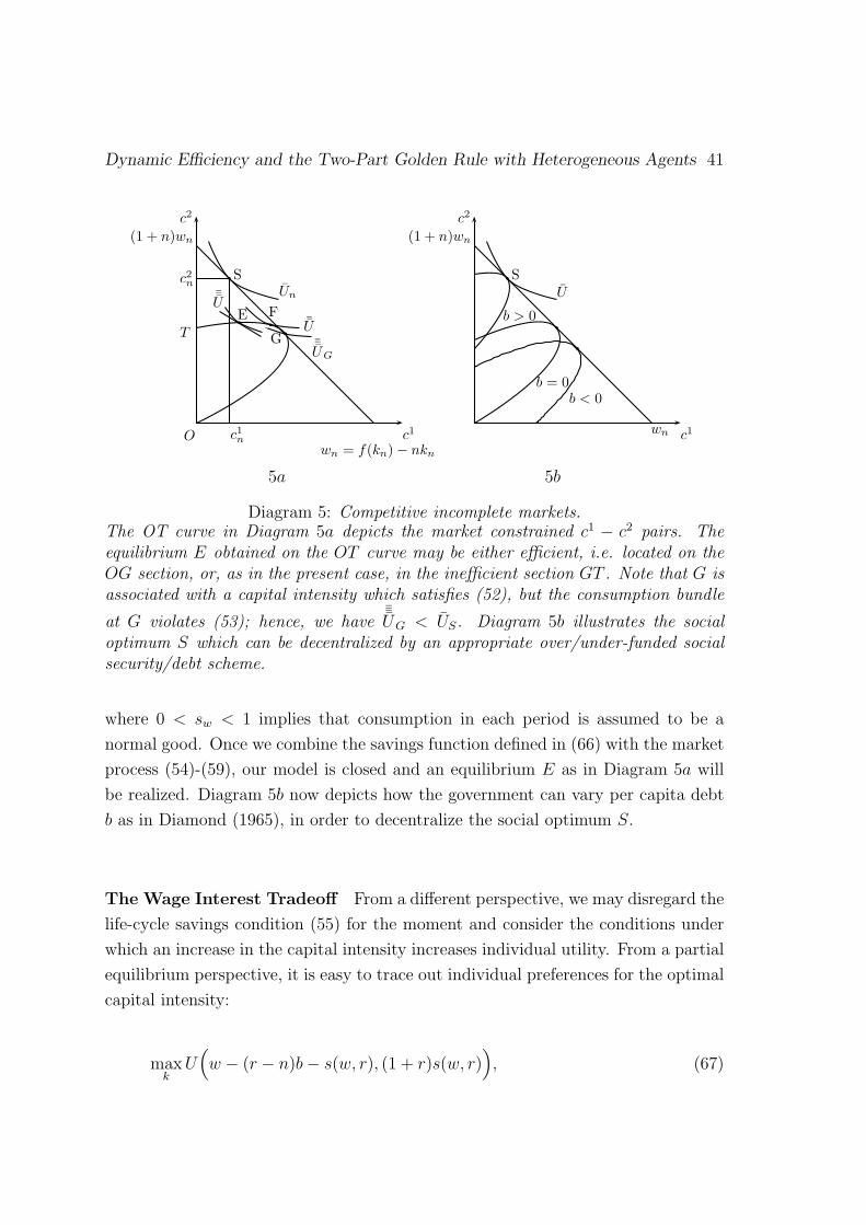
Dynamic Efficiency and the Two-Part Golden Rule with Heterogeneous Agents 41
c1c1
n
wn = f(kn)− nkn
c2
(1 + n)wn
c2
n
T
O
Un
¯U
¯U
¯UG
G
F
S
Eb
b
bb
c1
c2
(1 + n)wn
U
S
b > 0
b = 0b < 0
b
b
b
wn
1
5a 5b
Diagram 5: Competitive incomplete markets.The OT curve in Diagram 5a depicts the market constrained c1 − c2 pairs. Theequilibrium E obtained on the OT curve may be either efficient, i.e. located on theOG section, or, as in the present case, in the inefficient section GT . Note that G isassociated with a capital intensity which satisfies (52), but the consumption bundle
at G violates (53); hence, we have¯UG < US. Diagram 5b illustrates the social
optimum S which can be decentralized by an appropriate over/under-funded socialsecurity/debt scheme.
where 0 < sw < 1 implies that consumption in each period is assumed to be a
normal good. Once we combine the savings function defined in (66) with the market
process (54)-(59), our model is closed and an equilibrium E as in Diagram 5a will
be realized. Diagram 5b now depicts how the government can vary per capita debt
b as in Diamond (1965), in order to decentralize the social optimum S.
The Wage Interest Tradeoff From a different perspective, we may disregard the
life-cycle savings condition (55) for the moment and consider the conditions under
which an increase in the capital intensity increases individual utility. From a partial
equilibrium perspective, it is easy to trace out individual preferences for the optimal
capital intensity:
maxkU
(w − (r − n)b− s(w, r), (1 + r)s(w, r)
), (67)
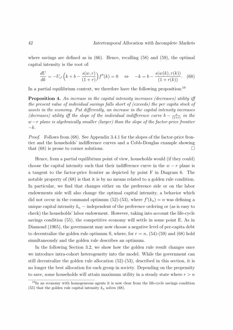
42 Intertemporal Allocation with Incomplete Markets
where savings are defined as in (66). Hence, recalling (58) and (59), the optimal
capital intensity is the root of:
dU
dk= −Uc1
(k + b− s(w, r)
(1 + r)
)f ′′(k) = 0 ⇔ −k = b− s(w(k), r(k))
(1 + r(k)). (68)
In a partial equilibrium context, we therefore have the following proposition:19
Proposition 4. An increase in the capital intensity increases (decreases) utility iffthe present value of individual savings falls short of (exceeds) the per capita stock ofassets in the economy. Put differently, an increase in the capital intensity increases(decreases) utility iff the slope of the individual indifference curve b − s
(1+r)in the
w−r plane is algebraically smaller (larger) than the slope of the factor-price frontier−k.
Proof. Follows from (68). See Appendix 3.4.1 for the slopes of the factor-price fron-tier and the households’ indifference curves and a Cobb-Douglas example showingthat (68) is prone to corner solutions.
Hence, from a partial equilibrium point of view, households would (if they could)
choose the capital intensity such that their indifference curve in the w − r plane is
a tangent to the factor-price frontier as depicted by point F in Diagram 6. The
notable property of (68) is that it is by no means related to a golden rule condition.
In particular, we find that changes either on the preference side or on the labor
endowments side will also change the optimal capital intensity, a behavior which
did not occur in the command optimum (52)-(53), where f ′(kn) = n was defining a
unique capital intensity kn − independent of the preference ordering or (as is easy to
check) the households’ labor endowment. However, taking into account the life-cycle
savings condition (55), the competitive economy will settle in some point E. As in
Diamond (1965), the government may now choose a negative level of per-capita debt
to decentralize the golden rule optimum S, where, for r = n, (54)-(59) and (68) hold
simultaneously and the golden rule describes an optimum.
In the following Section 3.2, we show how the golden rule result changes once
we introduce intra-cohort heterogeneity into the model. While the government can
still decentralize the golden rule allocation (52)-(53), described in this section, it is
no longer the best allocation for each group in society. Depending on the propensity
to save, some households will attain maximum utility in a steady state where r > n
19In an economy with homogeneous agents it is now clear from the life-cycle savings condition(55) that the golden rule capital intensity kn solves (68).
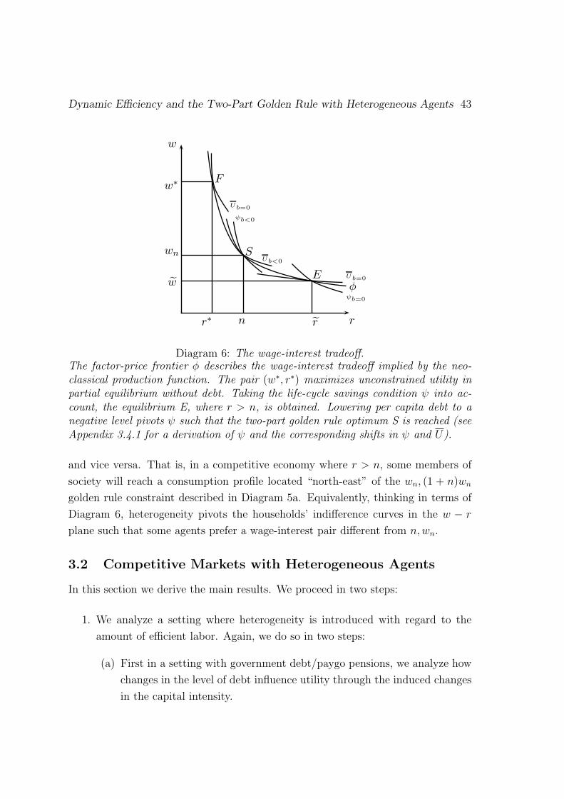
Dynamic Efficiency and the Two-Part Golden Rule with Heterogeneous Agents 43
rnr∗
wn
w∗
w
w
r
φ
Ub=0
S
E
F
Ub=0
Ub<0
ψb=0
ψb<0
1
Diagram 6: The wage-interest tradeoff.The factor-price frontier φ describes the wage-interest tradeoff implied by the neo-classical production function. The pair (w∗, r∗) maximizes unconstrained utility inpartial equilibrium without debt. Taking the life-cycle savings condition ψ into ac-count, the equilibrium E, where r > n, is obtained. Lowering per capita debt to anegative level pivots ψ such that the two-part golden rule optimum S is reached (seeAppendix 3.4.1 for a derivation of ψ and the corresponding shifts in ψ and U).
and vice versa. That is, in a competitive economy where r > n, some members of
society will reach a consumption profile located “north-east” of the wn, (1 + n)wn
golden rule constraint described in Diagram 5a. Equivalently, thinking in terms of
Diagram 6, heterogeneity pivots the households’ indifference curves in the w − r
plane such that some agents prefer a wage-interest pair different from n,wn.
3.2 Competitive Markets with Heterogeneous Agents
In this section we derive the main results. We proceed in two steps:
1. We analyze a setting where heterogeneity is introduced with regard to the
amount of efficient labor. Again, we do so in two steps:
(a) First in a setting with government debt/paygo pensions, we analyze how
changes in the level of debt influence utility through the induced changes
in the capital intensity.
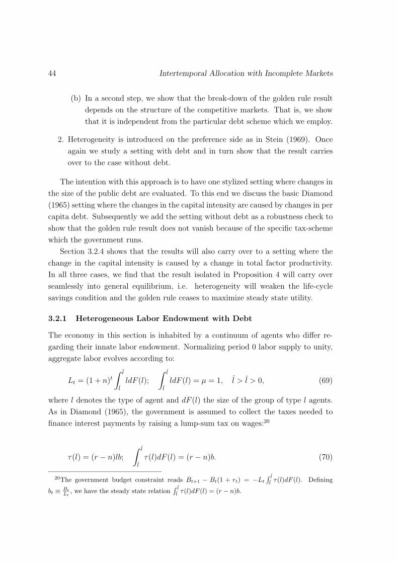
44 Intertemporal Allocation with Incomplete Markets
(b) In a second step, we show that the break-down of the golden rule result
depends on the structure of the competitive markets. That is, we show
that it is independent from the particular debt scheme which we employ.
2. Heterogeneity is introduced on the preference side as in Stein (1969). Once
again we study a setting with debt and in turn show that the result carries
over to the case without debt.
The intention with this approach is to have one stylized setting where changes in
the size of the public debt are evaluated. To this end we discuss the basic Diamond
(1965) setting where the changes in the capital intensity are caused by changes in per
capita debt. Subsequently we add the setting without debt as a robustness check to
show that the golden rule result does not vanish because of the specific tax-scheme
which the government runs.
Section 3.2.4 shows that the results will also carry over to a setting where the
change in the capital intensity is caused by a change in total factor productivity.
In all three cases, we find that the result isolated in Proposition 4 will carry over
seamlessly into general equilibrium, i.e. heterogeneity will weaken the life-cycle
savings condition and the golden rule ceases to maximize steady state utility.
3.2.1 Heterogeneous Labor Endowment with Debt
The economy in this section is inhabited by a continuum of agents who differ re-
garding their innate labor endowment. Normalizing period 0 labor supply to unity,
aggregate labor evolves according to:
Lt = (1 + n)t∫ l
l
ldF (l);
∫ l
l
ldF (l) = µ = 1, l > l > 0, (69)
where l denotes the type of agent and dF (l) the size of the group of type l agents.
As in Diamond (1965), the government is assumed to collect the taxes needed to
finance interest payments by raising a lump-sum tax on wages:20
τ(l) = (r − n)lb;
∫ l
l
τ(l)dF (l) = (r − n)b. (70)
20The government budget constraint reads Bt+1 − Bt(1 + rt) = −Lt
∫ l
lτ(l)dF (l). Defining
bt ≡ Bt
Lt, we have the steady state relation
∫ l
lτ(l)dF (l) = (r − n)b.
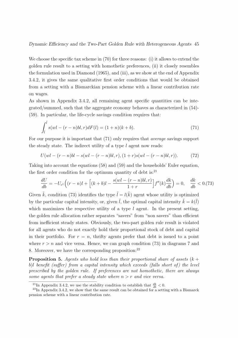
Dynamic Efficiency and the Two-Part Golden Rule with Heterogeneous Agents 45
We choose the specific tax scheme in (70) for three reasons: (i) it allows to extend the
golden rule result to a setting with homothetic preferences, (ii) it closely resembles
the formulation used in Diamond (1965), and (iii), as we show at the end of Appendix
3.4.2, it gives the same qualitative first order conditions that would be obtained
from a setting with a Bismarckian pension scheme with a linear contribution rate
on wages.
As shown in Appendix 3.4.2, all remaining agent specific quantities can be inte-
grated/summed, such that the aggregate economy behaves as characterized in (54)-
(59). In particular, the life-cycle savings condition requires that:∫ l
l
s(wl − (r − n)bl, r)dF (l) = (1 + n)(k + b). (71)
For our purpose it is important that (71) only requires that average savings support
the steady state. The indirect utility of a type l agent now reads:
U(wl − (r − n)bl − s(wl − (r − n)bl, r), (1 + r)s(wl − (r − n)bl, r)). (72)
Taking into account the equations (58) and (59) and the households’ Euler equation,
the first order condition for the optimum quantity of debt is:21
dU
db= −Uc1
((r − n)l +
[(k + b)l − s(wl − (r − n)bl, r)
1 + r
]f ′′(k)
dk
db
)= 0,
dk
db< 0.(73)
Given k, condition (73) identifies the type l = l(k) agent whose utility is optimized
by the particular capital intensity, or, given l, the optimal capital intensity k = k(l)
which maximizes the respective utility of a type l agent. In the present setting,
the golden rule allocation rather separates “savers” from “non savers” than efficient
from inefficient steady states. Obviously, the two-part golden rule result is violated
for all agents who do not exactly hold their proportional stock of debt and capital
in their portfolio. For r = n, thrifty agents prefer that debt is issued to a point
where r > n and vice versa. Hence, we can graph condition (73) in diagrams 7 and
8. Moreover, we have the corresponding proposition:22
Proposition 5. Agents who hold less than their proportional share of assets (k +b)l benefit (suffer) from a capital intensity which exceeds (falls short of) the levelprescribed by the golden rule. If preferences are not homothetic, there are alwayssome agents that prefer a steady state where n > r and vice versa.
21In Appendix 3.4.2, we use the stability condition to establish that dkdb < 0.
22In Appendix 3.4.2, we show that the same result can be obtained for a setting with a Bismarckpension scheme with a linear contribution rate.
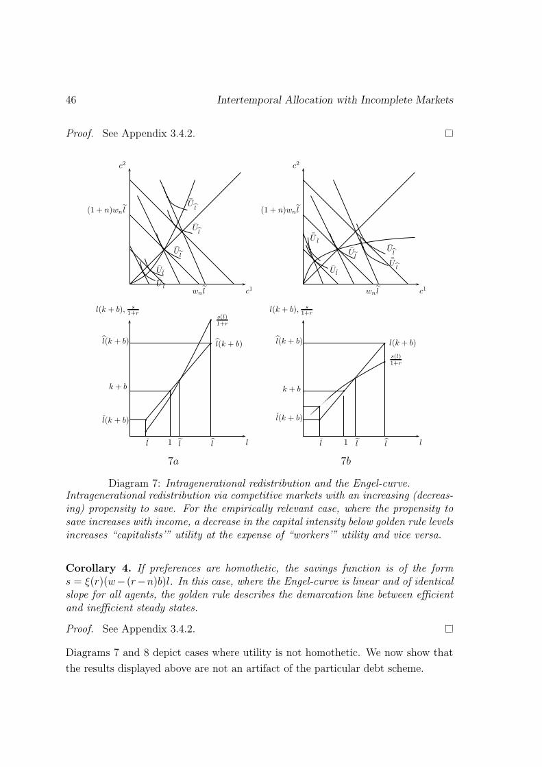
46 Intertemporal Allocation with Incomplete Markets
Proof. See Appendix 3.4.2.
c1
c2
(1 + n)wn l
wn l
¯Ul
Ul
Ul
Ul
¯Ul
b
b
b
b
b
b
c1
c2
(1 + n)wn l
wn l
¯Ul
UlU
l
Ul
¯Ul b
b
b
b
b
b
l
l(k + b), s
1+r
l(k + b)
k + b
l(k + b)
s(l)1+r
l(k + b)
b
b
b
b
b
b
l 1 l l l
l(k + b), s
1+r
l(k + b)
k + b
l(k + b)
s(l)1+r
l(k + b)
b
b
b
b
b
b
l l1 l
1
7a 7b
Diagram 7: Intragenerational redistribution and the Engel-curve.Intragenerational redistribution via competitive markets with an increasing (decreas-ing) propensity to save. For the empirically relevant case, where the propensity tosave increases with income, a decrease in the capital intensity below golden rule levelsincreases “capitalists’” utility at the expense of “workers’” utility and vice versa.
Corollary 4. If preferences are homothetic, the savings function is of the forms = ξ(r)(w− (r−n)b)l. In this case, where the Engel-curve is linear and of identicalslope for all agents, the golden rule describes the demarcation line between efficientand inefficient steady states.
Proof. See Appendix 3.4.2.
Diagrams 7 and 8 depict cases where utility is not homothetic. We now show that
the results displayed above are not an artifact of the particular debt scheme.
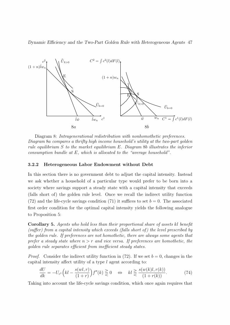
Dynamic Efficiency and the Two-Part Golden Rule with Heterogeneous Agents 47
c1lw lwn
c2
(1 + n)lwn
¯U b>0
Ub=0
S
E
b
b
C1 =∫
c1(l)dF (l)wn
C2 =∫
c2(l)dF (l)
(1 + n)wn
Ub=0
¯U b>0
SE b
b
b
w
1
8a 8b
Diagram 8: Intragenerational redistribution with nonhomothetic preferences.Diagram 8a compares a thrifty high income household’s utility at the two-part goldenrule equilibrium S to the market equilibrium E. Diagram 8b illustrates the inferiorconsumption bundle at E, which is allocated to the “average household”.
3.2.2 Heterogeneous Labor Endowment without Debt
In this section there is no government debt to adjust the capital intensity. Instead
we ask whether a household of a particular type would prefer to be born into a
society where savings support a steady state with a capital intensity that exceeds
(falls short of) the golden rule level. Once we recall the indirect utility function
(72) and the life-cycle savings condition (71) it suffices to set b = 0. The associated
first order condition for the optimal capital intensity yields the following analogue
to Proposition 5:
Corollary 5. Agents who hold less than their proportional share of assets kl benefit(suffer) from a capital intensity which exceeds (falls short of) the level prescribed bythe golden rule. If preferences are not homothetic, there are always some agents thatprefer a steady state where n > r and vice versa. If preferences are homothetic, thegolden rule separates efficient from inefficient steady states.
Proof. Consider the indirect utility function in (72). If we set b = 0, changes in thecapital intensity affect utility of a type l agent according to:
dU
dk= −Uc1
(kl − s(wl, r)
(1 + r)
)f ′′(k) T 0 ⇔ kl T
s(w(k)l, r(k))
(1 + r(k)). (74)
Taking into account the life-cycle savings condition, which once again requires that

48 Intertemporal Allocation with Incomplete Markets
average savings are sufficient to support the steady state, we have:∫ l
l
s(wl, r)dF (l) = (1 + n)k. (75)
If the economy grows on a golden rule path where we have r = n, conditions (75)and (74) yield for a steady state:
kl =
∫ l
ls(wl, n)dF (l)
1 + nl T
s(wl, n)
(1 + n). (76)
Hence, depending on the propensity to save out of income, a household of type l willprefer a capital intensity that exceeds (falls short of) the golden rule level. Finally,if preferences are homothetic, savings are known to be a positive fraction ξ(r) of theavailable income. That is, s(wl, r) = ξ(r)wl. Plugging this savings function into(76), we find that it holds with equality at the golden rule capital intensity. Thegolden rule therefore maximizes steady state utility if U() is homothetic.
3.2.3 Heterogeneous Preferences
Now let us change the perspective slightly and consider an economy inhabited by
agents with uniform labor endowment. As in Stein (1969), heterogeneity will now
be introduced on the preference side only. Society now consists of a continuum of
agents, where each group i has its own preference ordering Ui(c1, c2); i ∈ [0, 1]. Thus,
according to (65), each agent chooses a unique optimal si(w, r). Integration over
the index set in turn yields the aggregates in the same manner as in the previous
section. If agents are taxed equally, as in Diamond (1965), we have the following
first order condition with regard to the optimal capital intensity for a type i agent:23
dUidb
= −Ui,c1((r − n) +
[(k + b)− si
(1 + r)
]drdb
)= 0;
dr
db= f ′′(k)
dk
db> 0.(77)
Condition (77) indicates and Diagram 9 illustrates that thrifty agents benefit from
capital-intensities below the golden rule level. Impatient agents prefer capital-
intensities exceeding golden rule levels. This is in fact the opposite of the result
derived by Stein (1969) p. 141, who considers a competitive economy with het-
erogeneous time preferences just like ours and concludes his analysis:24 “No inter-
personal comparisons of utility are involved in this concept of an optimum since (7)
23Once again, we obtain dkdb < 0 from the stability condition.
24See also footnote 2 in Stein (1969), p.142, where he assumes “For simplicity we assumedthat βi = β....”. The subsequent optimality conditions would therefore not hold without thisassumption.
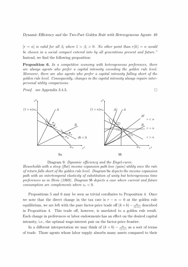
Dynamic Efficiency and the Two-Part Golden Rule with Heterogeneous Agents 49
[r = n] is valid for all βi where 1 > βi > 0. No other point than r(k) = n would
be chosen in a social compact entered into by all generations present and future.”
Instead, we find the following proposition:
Proposition 6. In a competitive economy with heterogeneous preferences, thereare always agents who prefer a capital intensity exceeding the golden rule level.Moreover, there are also agents who prefer a capital intensity falling short of thegolden rule level. Consequently, changes in the capital intensity always require inter-personal utility comparisons.
Proof. see Appendix 3.4.3.
c1wn
c2
(1 + n)wn
B
A
UA
UA
UB
UB
db < 0
b
b
b
b
c1wn
c2
(1 + n)wn
r > n
r = n
r < n
B
B′
AA′
GR0
GR0
GR0
b
b
b
bb
b
1
9a 9b
Diagram 9: Dynamic efficiency and the Engel-curve.Households with a steep (flat) income expansion path lose (gain) utility once the rateof return falls short of the golden rule level. Diagram 9a depicts the income expansionpath with an intertemporal elasticity of substitution of unity but heterogeneous timepreferences as in Stein (1969). Diagram 9b depicts a case where current and futureconsumption are complements where sr < 0.
Propositions 5 and 6 may be seen as trivial corollaries to Proposition 4. Once
we note that the direct change in the tax rate is r − n = 0 at the golden rule
equilibrium, we are left with the pure factor-price trade off (k+ b)− si
(1+r)described
in Proposition 4. This trade off, however, is unrelated to a golden rule result.
Each change in preferences or labor endowments has an effect on the desired capital
intensity, i.e., the optimal wage-interest pair on the factor-price frontier.
In a different interpretation we may think of (k + b) − si
(1+r)as a sort of terms
of trade. Those agents whose labor supply absorbs many assets compared to their

50 Intertemporal Allocation with Incomplete Markets
own saving, prefer a capital intensity exceeding the golden rule level and vice versa.
Consequently, the decrease in utility incurred by some agents once the capital inten-
sity moves towards the golden rule can be seen as a case of “immiserizing growth”.
Similar to the result on foreign trade derived by Bhagwati (1958), we find that an
increase in the capital intensity towards the golden rule increases per capita con-
sumption in each period. However, it also worsens the terms of trade of the thrifty
households.
Taking the current view it is also intuitive that the golden rule result holds in the
setting of section 3.2.1, where the labor supply was the sole source of heterogeneity,
if preferences are homothetic and homogeneous. In this case, each agent supplies
precisely the amount of savings necessary to absorb his proportional share of assets
in the economy. Consequently, in our trade interpretation, each group of agents lives
in “autarky”. In this case, the golden rule result carries over.
Finally, we note that the golden rule once again also ceases to serve as a watershed
in an economy without debt. Setting b = 0, the first order condition for the optimal
steady state capital intensity is given by:
dUidk
= −Ui,c1(k − si
(1 + r)
)= 0. (78)
Once again it is now easy to show that a household of type i will prefer to be born
into an economy where r T n, depending on whether his propensity to save is above
(below) the economy’s average propensity to save.
3.2.4 Hicks Neutral Technological Change
To further illustrate how Proposition 4 carries over to different settings, we will now
briefly reconsider the results which were derived regarding the adoption of a superior
“Hicks neutral” technology. While Matsuyama (1991) and Galor (1988) have shown
that such a technological innovation may only decrease utility if the economy is
dynamically inefficient, we will now show that this result once again does not carry
over to our heterogeneous agent setting.
Augmenting the production function with a technology level α, we define y ≡αf(k), r ≡ αf ′(k) and w ≡ α[f(k) − f ′(k)k]. Changes in α now affect utility
Dynamic Efficiency and the Two-Part Golden Rule with Heterogeneous Agents 51
according to:25
dU
dα= Uc1
1
α
[w +
r
1 + rs]
+ Uc1[s(wl, r)
1 + r− kl
]αf ′′(k)
dk
dα= 0. (79)
The first term in (79) indicates that utility increases due to the outward shift of
the factor-price-frontier. At a given capital intensity, wages and returns to capital
rise. The second term represents the movement along the factor-price frontier, re-
sulting from the changed capital intensity. This change may or may not increase the
respective agent’s utility obtained from his particular factor supplies (l, s(wl, r)).
Disregarding the heterogeneity in the labor endowment, condition (79) is identical
with that derived by Galor (1988). In the current case, however, the second term
will always be negative for some agents even if r > n. Hence, the results of Galor
(1988) and Matsuyama (1991), who show that technological progress may only de-
crease utility of some agents in an economy which is dynamically inefficient, do not
carry over.26
If we think of our households as small open economies, the second term in (79)
may once again be interpreted as a worsening of the “terms of trade” for thrifty
households. In a similar fashion it would now be straightforward to show that the
two-part golden rule ceases to serve its watershed role in similar problems, like for
example the optimum growth rate for population analyzed in Samuelson (1975a),
Michel and Pestieau (1993) and Jaeger and Kuhle (2009).27 Rather than separating
efficient equilibria from inefficient ones, the golden rule separates savers from non-
savers as in Propositions 4, 5 and 6 respectively.
3.3 Conclusion
The two-part golden rule balances the wage interest tradeoff faced by the represen-
tative agent in the competitive Diamond (1965) model. Competitive paths with a
25Note that dkdα = sw(f(k)−kf ′(k))+srf ′(k)
(1+n)+swαf ′′(k)k−srαf ′′(k) T 0. Assuming asymptotic (cyclical) stability, wecan show that the denominator is positive (negative). The numerator is positive if sr > 0, butambiguous if sr is sufficiently negative.
26The notable exception is of course the case with identical homothetic preferences.27The first order condition for the optimum growth rate for population for a type l agent is given
by:
dU
dn= −Uc1
(kl − s(lw, r)
1 + r
)f ′′(k)
dk
dn= 0, (80)
and has the same structure as the foregoing ones.
52 Intertemporal Allocation with Incomplete Markets
capital intensity exceeding the golden rule level are therefore dynamically inefficient.
This result carries over to economies where the present value of each agent’s savings
is equal to his proportional share of assets in the economy. This condition is sat-
isfied in economies where all agents have linear Engel-curves with identical slopes,
i.e. preferences which are homogenous and homothetic.
In all other cases, it turns out that the golden rule ceases to serve as a demar-
cation line between efficient and inefficient steady states. There are always some
members in society who prefer a capital intensity exceeding the golden rule level.
Hence, these steady states can no longer be viewed as inefficient.28 Taking the per-
spective of Abel et al. (1989), we find that an increment in capital acts as a source
(sink) to society as a whole, i.e. increases aggregate consumption in each period, if
r > n (r < n). If society consisted of a representative agent, r = n would therefore
describe the steady state optimum. However, in the current case society is frag-
mented into different groups. That is, while capital may already be a sink to society
as a whole, it may still act as a source to some groups of that society.29
Given the growing interest in models with heterogeneous agents, the current
result may provide useful inference in two directions: The simple comparison of
interest rate and aggregate growth rate is feasible for economies with heterogeneous
agents as long as consumption expansion paths are linear and identical, e.g. CES
specifications with homogeneous time discount rates. In another interpretation, the
above analysis may be a case against the reliance on CES specifications to the extent
that empirical evidence suggests that the savings propensity increases (or at least
varies) with income. Consequently, the intra-generational redistribution, which is a
byproduct of changes in the capital intensity, is not captured.
28Steady states with a capital intensity falling short of the golden rule level are now efficient fora second reason. Even if a golden rule allocation could be reached at no cost, this new path wouldalways bring about long-run utility losses for some agents.
29Naturally, this result carries over to competitive OLG models where risk avers agents faceideosyncratic risks.

Dynamic Efficiency and the Two-Part Golden Rule with Heterogeneous Agents 53
3.4 Appendix
3.4.1 Construction of Diagram 6
In this appendix we develop the properties of the Diamond (1965) model in the w−rspace:
Factor-price frontier The firm’s first order conditions are given by r = f ′(k),
w = f(k)− f ′(k)k. For k ∈ R+, f ′(k) is bijective and defines k = k(r). Differentia-
tion now yields:30
φ(r) = w(k(r)),dw
dr= φ′(r) = −k, d2w
dr2= φ′′(r) = − 1
f ′′(k). (81)
Indifference curves Regarding preferences, we recall (65) and (66), which implyUc1
Uc2= 1 + r, to obtain:
dw
dr |dU=0= b− s
1 + r,
d2w
dr2 |dU=0=sws− sr(1 + r) + s
(1 + r)2. (82)
Stability and life-cycle savings Throughout this chapter we assume that the
equilibrium is asymptotically stable. Using the life-cycle condition (1+n)(kt+1+b) =
s(wt − (rt − n)b, rt+1), the local stability condition around the steady state, where
k = kt = kt+1, reads:
0 <dkt+1
dkt=−swf ′′(k)(k + b)
(1 + n)− srf ′′(k)< 1. (83)
For a stable economy, the locus ψ of w−r pairs, where life-cycle savings support
a steady state, i.e. (1 + n)(k(r) + b) = s(w − (r − n)b, r), is now given by:
dw
dr |ψ=
(1 + n)− srf′′(k)
swf ′′(k)+ b <|(83) −(k + b) + b = −k. (84)
Hence, the savings locus ψ in the w−r space is steeper than the factor-price frontier
φ. Moreover, for r > n, ψ is also steeper than the indifference curve, i.e., dwdr |ψ <
−k = φ′(r) = b − s1+n
<|r>n b − s1+r
= dwdr |dU=0
. Varying per capita debt will now
30See Samuelson (1962) for an exposition of the factor-price frontier.

54 Intertemporal Allocation with Incomplete Markets
allow the planner to move both the savings locus and the households’ indifference
curve to a point where life-cycle savings support a golden rule steady state:
dw
db |dr=0,ψ=
1 + n+ (r − n)swsw
> 0, (85)
dr
db |dw=0,ψ=
−(1 + n+ swr)
(1 + n+ swbf ′′(k)− srf ′′(k))1
f ′′(k)
> 0. (86)
Hence, increasing debt shifts the savings locus ψ to the right. The households’
indifference curves rotate around the point wn, n according to:
dw
db |dU=0= r − n T 0;
dr
db |dU=0=
r − n
b− s1+r
T 0. (87)
Example Finally we may note an example which shows that condition (68), with
b = 0, is prone to corner solutions. Assuming a Cobb-Douglas production function,
full depreciation and logarithmic utility, with a propensity to save out of wage-
income of 0 < ξ < 1, we have y = kα, w = (1− α)kα, 1 + r = αkα−1, and thus (68)
reads:dU
dk= − 1
c1
(1− ξ
(1− α)
α
)k T 0;
α
1− αT ξ. (88)
3.4.2 Comparative Statics
In this section we briefly show how the market clearing apparatus (54)-(59) carries
over to an economy with heterogeneous agents. Moreover, we show that the stability
condition implies that an increase in per capita debt decreases the capital intensity.
Integrating the per capita quantities yields the respective aggregates:
Lt+1 =
∫ l
l
(1 + n)tldF (l) = (1 + n)Lt, (89)∫ l
l
ls(wtl − (rt − n)bl)dF (l) = (1 + n)(kt+1 + b), (90)∫ l
l
st(l)dF (l) =
∫ l
l
(wtl − c1t (l) + (rt − n)bl)dF (l), (91)∫ l
l
(c1t (l) +c2t+1(l)
1 + rt+1
)dF (l) =
∫ l
l
(wtl − (rt − n)bl)dF (l), (92)
wt = f(kt)− f ′(kt)kt, (93)
rt = f ′(kt). (94)
Dynamic Efficiency and the Two-Part Golden Rule with Heterogeneous Agents 55
Defining C1t ≡
∫ l
lc1t (l)dF (l), C2
t+1 ≡∫ l
lc2t+1(l)dF (l), Wt ≡
∫ l
lwtldF (l) and S ≡∫ l
lst(l)dF (l), we obtain the same set of equations as in (54)-(59). The geometric
exposition in Diagram 5a, 5b can now be constructed as before. However, C1, C2
now depict average consumption rather than the consumption of the representative
consumer.
Lemma 1: An increase in per capita debt decreases the steady state capital inten-
sity if the equilibrium exhibits Walrasian stability.
Proof: In per capita terms the life-cycle savings condition (90) reads∫ l
ls(w(kt)l−
(r(kt)−n)bl, r(kt+1))dF (l) = (1+n)(kt+1+b). Differentiation now yields the follow-
ing (Walrasian) stability condition: 0 < dkt+1
dkt=
−(k+b)f ′′(k)R l
l sw(wl−(r−n)bl,r)ldF (l)
(1+n)−f ′′(k)R l
l sr(wl−(r−n)bl,r)dF (l)< 1.
Government debt will therefore change the steady state capital intensity according
to: dkdb
=(1+n)+
R ll sw(f ′(k)−n)ldF (l)
f ′′(k)R l
l srdF (l)−(1+n)−(k+b)f ′′(k)R l
l swldF (l)< 0, where the numerator is positive
since 0 < sw < 1. By utilizing the stability condition, it is straightforward to show
that the denominator is negative.
Proof of Proposition 5 With general non-homothetic preferences, we have ∂s(wl,r)∂l
≷∂s(wl,r)
∂lfor some l, l ∈ [l, l]. Consequently, the life-cycle savings condition
∫ l
ls(wl, r)dF (l) =∫ l
l(1+n)(k+b)ldF (l) is only satisfied if the savings of some agents exceed (1+n)(k+
b)l and other agents’ savings fall short of what they absorb. Assuming the contrary,
s(wl, r) > (1 + n)(k + b)l, for all l ∈ [l, l] yields∫ l
ls(wl, r)dF (l) > (1 + n)(k + b),
which contradicts the steady state condition∫ l
ls(wl, r)dF (l) = (1+n)(k+b). Thus,
according to (73) there will always be two groups of agents. One group preferring
a capital intensity exceeding the golden rule and another preferring a lower capital
intensity where r > n. Those preferring the golden rule are of course a measure zero
set.
Proof of Corollary 4 For homothetic preferences savings are known to be a
positive fraction ξ of wealth, i.e. s = ξ(r)(w−(r−n)b)l.31 Consequently, the golden
rule steady state life-cycle savings condition in (71) reads ξ(n)w(kn) = (1+n)(kn+b).
Hence, we have s(l)1+r
= s(l)1+n
= (kn + b)l. Consequently condition (73) is satisfied for
31See Mas-Colell et al. (1995) p. 50 or De La Croix and Michel (2002) p. 53-54 for a proof.
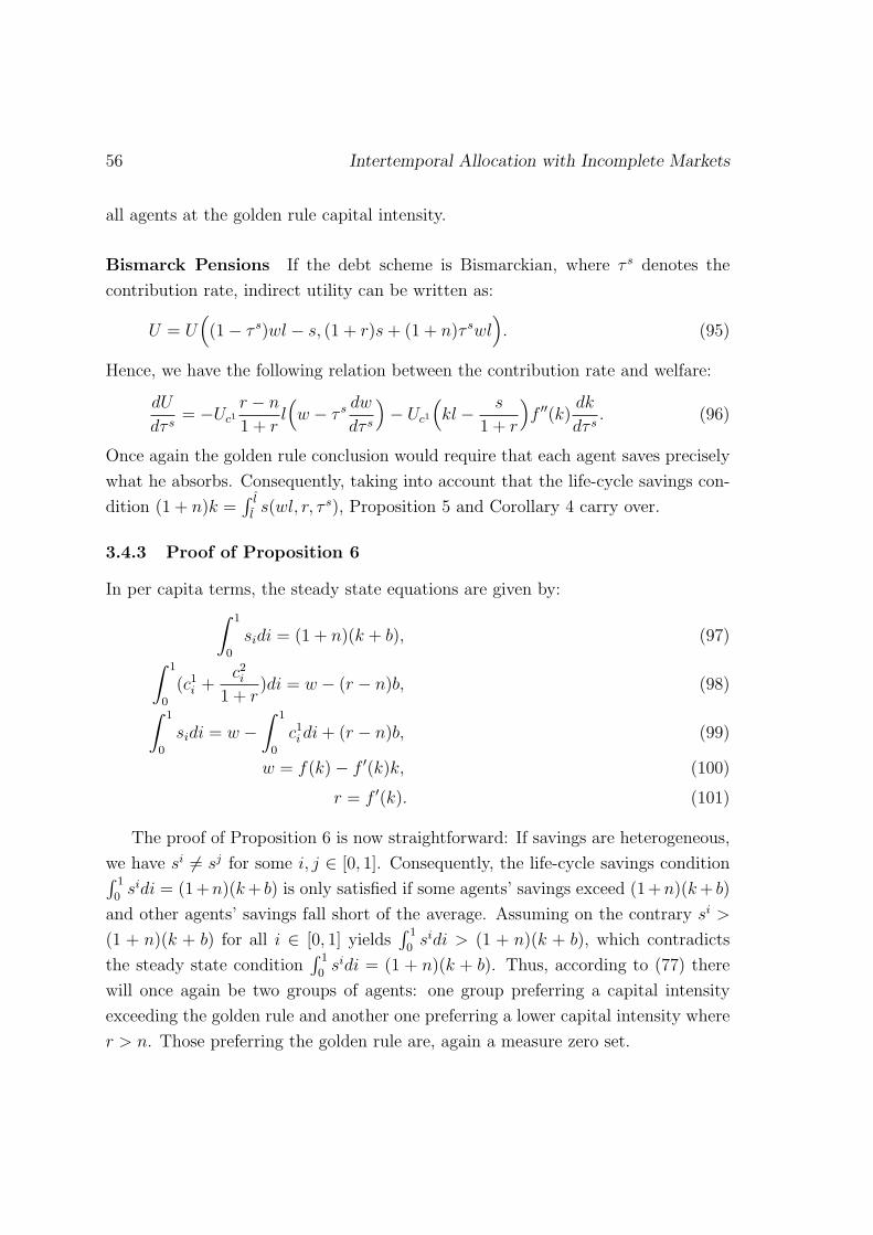
56 Intertemporal Allocation with Incomplete Markets
all agents at the golden rule capital intensity.
Bismarck Pensions If the debt scheme is Bismarckian, where τ s denotes the
contribution rate, indirect utility can be written as:
U = U((1− τ s)wl − s, (1 + r)s+ (1 + n)τ swl
). (95)
Hence, we have the following relation between the contribution rate and welfare:
dU
dτ s= −Uc1
r − n
1 + rl(w − τ s
dw
dτ s
)− Uc1
(kl − s
1 + r
)f ′′(k)
dk
dτ s. (96)
Once again the golden rule conclusion would require that each agent saves precisely
what he absorbs. Consequently, taking into account that the life-cycle savings con-
dition (1 + n)k =∫ l
ls(wl, r, τ s), Proposition 5 and Corollary 4 carry over.
3.4.3 Proof of Proposition 6
In per capita terms, the steady state equations are given by:∫ 1
0
sidi = (1 + n)(k + b), (97)∫ 1
0
(c1i +c2i
1 + r)di = w − (r − n)b, (98)∫ 1
0
sidi = w −∫ 1
0
c1i di+ (r − n)b, (99)
w = f(k)− f ′(k)k, (100)
r = f ′(k). (101)
The proof of Proposition 6 is now straightforward: If savings are heterogeneous,
we have si 6= sj for some i, j ∈ [0, 1]. Consequently, the life-cycle savings condition∫ 1
0sidi = (1+n)(k+ b) is only satisfied if some agents’ savings exceed (1+n)(k+ b)
and other agents’ savings fall short of the average. Assuming on the contrary si >
(1 + n)(k + b) for all i ∈ [0, 1] yields∫ 1
0sidi > (1 + n)(k + b), which contradicts
the steady state condition∫ 1
0sidi = (1 + n)(k + b). Thus, according to (77) there
will once again be two groups of agents: one group preferring a capital intensity
exceeding the golden rule and another one preferring a lower capital intensity where
r > n. Those preferring the golden rule are, again a measure zero set.
57
4 The Optimum Structure for Government Debt
This chapter studies the structural differences between implicit and explicit govern-
ment debt in a two-generations-overlapping model with stochastic factor-prices. If
a government can issue safe bonds and new claims to wage-indexed social security
to service a given initial obligation, there exists a set of Pareto-efficient ways to do
so. This set is characterized by the conflicting interests of the current young and
the yet unborn generations regarding the allocation of factor-price risks.
However, it is shown that there will always exist a simple intertemporal compensa-
tion mechanism which allows to reconcile these conflicting interests. This compen-
sation mechanism narrows the set of Pareto-efficient debt structures until only one
remains. This result hinges on the double-incomplete markets structure of stochastic
OLG models where households can neither trade consumption loans nor factor-price
risks privately.
4.1 Introduction
Privatizing social security has often been described as a pure “shell game”, where
an implicit liability is replaced by an explicit liability of equal size.32 From a dif-
ferent perspective, this equivalence between implicit and explicit government debt,
may also be seen as a counterpart to the Modigliani-Miller Theorem in corporate
finance. The underlying argument for this irrelevance result has its roots in the
consumption loan nature of both debt instruments. A pure reallocation of resources
between two adjacent cohorts can at most yield the biological interest rate.33 For
a deterministic economy, which is dynamically efficient in the sense of Diamond
(1965), bonds are issued with a rate of return that is, at first sight, superior to
the biological return earned on social security contributions. However, to prevent
an eventual default, the government has to collect a tax that exactly offsets this
return advantage. Taking these taxes into account, both instruments yield identical
32See e.g. Breyer (1989), Fenge (1995), Belan and Pestieau (1999), Friedman (1999). See Sinn(2000) for a survey. Samuelson (1975b) proves the related result that fully funded social securityis also neutral. More recently, Ludwig and Reiter (2009) have extended the result to a stochasticsetting with state dependent taxes.
33Samuelson (1958, 1959), Lerner (1959), Aaron (1966) and Cass and Yaari (1966). In the sequel,we abstract from technological progress as it does not change the basic tradeoffs.
58 Intertemporal Allocation with Incomplete Markets
allocations.34 In particular, they reduce long-run utility by crowding-out capital.
In stochastic overlapping generations models Enders and Lapan (1982), Merton
(1983), Gordon and Varian (1988), Gale (1990), Kruger and Kubler (2006) and
Gottardi and Kubler (2008) have shown that intergenerational transfers via PAYGO
pension schemes and safe government debt may serve a second role. They allow
to facilitate intergenerational risk sharing.35 In-turn, these beneficial aspects of
government debt have been compared to the negative long-run losses which stem
from the crowding-out of capital. In particular Green (1977), Kruger and Kubler
(2006) and Gottardi and Kubler (2008) examine this trade-off between risk sharing
and worsening factor-prices. Their analysis indicates that even the introduction of
a very small social security system tends to decrease long-run utility. That is, the
positive risk sharing effect is dominated by the negative crowding-out effect.36
The current analysis complements this literature by taking a different perspec-
34Both schemes pay the same returns, cause (in absence of intragenerational redistribution)the same excess burdens in the labor market, reallocate the same amount of resources betweengenerations, displace an equal amount of private savings and lower long-run utility.
35In particular, Fischer (1983) and Gale (1990), discuss the desirability of safe debt and itsmaturity structure in an OLG context with rate-of-return risk. Enders and Lapan (1982) examine amature pay-go scheme in an economy where fiat money is the only alternative store of value. Merton(1983) derives closed-form solutions for a three period OLG model with simultaneous demographic,TFP and income share risks. He shows that a tax and transfer system may replicate an (incompletemarkets) equilibrium where agents can trade human capital freely. In the Merton (1983) settingsuch an intervention is always warranted as young agents would starve under “total market failure”.Bohn (1998, 2003) shows that a constant debt to GDP ratio leads to pro-cyclical debt issues, thatamplify aggregate risks. Starting from a situation without government debt, Kruger and Kubler(2006) give numerical evidence that the introduction of unfunded social security is unlikely Pareto-improving − despite its risk sharing capacities − due to the crowding-out of capital. Gottardiand Kubler (2008) discuss the prospects of an ex-ante Pareto-improving introduction of unfundedsocial security in an economy with land. See Diamond (1977, 2000) for a broader assessment ofintergenerational and intragenerational insurance aspects of social security, and Shiller (1999) formore references on the sharing of aggregate risks. See Abel (2001a), Diamond and Geanakoplos(2003), and Ball and Mankiw (2007) for different approaches to utilize trust-fund assets − aquestion somewhat related to the present one. To focus firmly on the unfunded component ofsocial security we will not introduce a trust-fund. Moreover, we leave-out idiosyncratic risks. AsBester (1984) and Abel (1989) show these can be insured within each cohort, i.e. are not essentialin the current context.
36Intuitively this result is plausible if we think of it in terms of the Finetti (1952), Pratt (1964),Arrow (1970) approximation: E[U(c0 + ε)] ≈ U(c0) + U ′(c0)µε + 1
2U ′′(c0)σ2ε . The crowding-
out of capital induces first order welfare losses by lowering expected consumption µε. The risksharing benefits, however, are only of second order. For the above approximation we have usedthe approximation σ2
ε = E[ε2]− E[ε]2 ≈ E[ε2], which is accurate if E[ε] is small. For E[ε] = 0 wehave E[U(c0 + ε)] ≈ U(c0) + 1
2U ′′(c0)σ2ε . In this case, the lower consumption would be associated
with a reduction in c0.
The Optimum Structure for Government Debt 59
tive. We ask whether it is possible to restructure the vast debt which is already
present in most countries in a Pareto-improving manner. Following this question,
we show that it is possible to separate the crowding-out effect from the risk sharing
problem. Changes in the composition of the public debt leave expected intergen-
erational transfers constant over time but alter the allocation of factor-price risks
between different cohorts. Changes in the size of the debt change intergenerational
transfers but tend to leave the allocation of factor-price risks unaltered. This separa-
tion of crowding-out and intergenerational risk sharing associated with public debt
will in general allow the government to make a restructuring of the debt Pareto-
improving. To derive this result, we set up an initial value problem. Each member
of an initial old generation holds claims from past pension promises and debt issues
amounting to g0. The government can now raise a share λ of the revenue needed
to service these claims through the introduction of a linear social security tax on
the current young generations wage income. The remainder share 1 − λ has to be
financed by selling safe debt. Finally, there is the group of yet unborn generations
who have to service future pension claims issued to the current young generation.
There are two corollaries to the separation result sketched earlier: (i) if the
government can only change the composition of the existing debt, there will be a
set of efficient debt structures and another set of inefficient ones. The efficient set
is characterized by the conflicting interests of those agents who are currently young
and those who are yet unborn. The unborn generations benefit from the ex-ante
diversification of their wage risk if a large share λ of the initial debt is injected into
social security. The current young, who have already observed their wage income,
on the contrary prefer safe debt, i.e. safe retirement benefits. (ii) if the government
can also issue/recover additional bonds, i.e. change the size of the expected future
intergenerational transfers, the set described in (i) can be narrowed to only one
Pareto-optimal debt structure, which maximizes societies (ex-ante) “Marshallian
surplus” from intergenerational risk sharing. Put differently, the government can
use its two instruments, i.e. the size and the composition of the debt, to steer the
economy towards a point on the contract curve.
This second result appears to be of particular interest, when compared to the
problem of optimal capital accumulation in a deterministic Diamond (1965) model.
In analogy to our result (i), there always exists a set of efficient capital intensities.
This means that every change in the capital intensity requires a welfare criterion as
60 Intertemporal Allocation with Incomplete Markets
we can either shift resources into the future or redirect resources from the future
towards current generations.37 In the present stochastic setting, however, we show
that it is possible to compensate intertemporally. We can shift resources and risks
between the current young and the yet unborn members of society simultaneously
and independently. As a consequence, the government can compensate intertempo-
rally and narrow the set of efficient debt structures (without compensation) to the
set of points on the contract curve (with compensation).
Regarding our assumptions, a notable aspect of our analysis is that we rule-out
state-contingent lump-sum transfers. Following Merton (1983), Gordon and Varian
(1988), Bohn (1998, 2003), Kruger and Kubler (2006) and Gottardi and Kubler
(2008) we try to capture the basic features of most real-world pension and debt
schemes by limiting the government debt instruments to safe bonds and a linear
social security contribution rate on wages. We do so for two reasons: (i) while
state-contingent lump-sum transfers may allow to reach better allocations than our
simplistic debt instruments, they are not observed in actual policy. (ii) The optimal
allocations which are derived for such state-contingent tax and transfer systems
usually imply that the public debt follows a random walk as described in Gordon and
Varian (1988) and Ball and Mankiw (2001, 2007).38 Hence, if the government would
actually implement these policies, it would default in finite time with probability
one. One may therefore argue that such a risk sharing policy amplifies rather than
dampens the small risks faced by each generation as they create a tremendous default
risk.
Subsequently, in Section 4.2 we begin by laying out our model. The represen-
tative households, are assumed to maximize expected utility. Moreover, first and
second period consumption are assumed to be normal goods. Savings can be in-
vested in a risky and a safe production technology. Wages are determined according
to a third risky technology. As in Diamond and Geanakoplos (2003), it is assumed
that aggregate investment does not affect marginal returns. This tri-linear setting
37The lack of such a compensation mechanism led to the turnpike literature, see, e.g., Samuelson(1968) or Blanchard and Fischer (1989). The absence of such an intertemporal compensationmechanism is of course also the reason for the intertemporal efficiency of pay-go schemes that wehave been referring to in Footnote 32.
38Gordon and Varian (1988), p. 192, and Ball and Mankiw (2001, 2007) (Proposition 2), pointout that their debt schemes that reallocate risks “optimally” imply that per capita debt will follow arandom walk. Hence per-capita debt will hit any boundary in finite time. Consequently, as Gordonand Varian (1988), p. 192 point out, the economies total assets will eventually be negative, forcingthe government to default at some point.
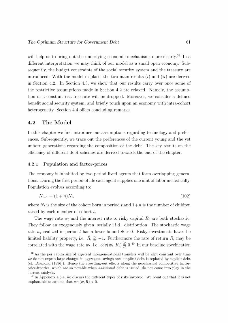
The Optimum Structure for Government Debt 61
will help us to bring out the underlying economic mechanisms more clearly.39 In a
different interpretation we may think of our model as a small open economy. Sub-
sequently, the budget constraints of the social security system and the treasury are
introduced. With the model in place, the two main results (i) and (ii) are derived
in Section 4.2. In Section 4.3, we show that our results carry over once some of
the restrictive assumptions made in Section 4.2 are relaxed. Namely, the assump-
tion of a constant risk-free rate will be dropped. Moreover, we consider a defined
benefit social security system, and briefly touch upon an economy with intra-cohort
heterogeneity. Section 4.4 offers concluding remarks.
4.2 The Model
In this chapter we first introduce our assumptions regarding technology and prefer-
ences. Subsequently, we trace out the preferences of the current young and the yet
unborn generations regarding the composition of the debt. The key results on the
efficiency of different debt schemes are derived towards the end of the chapter.
4.2.1 Population and factor-prices
The economy is inhabited by two-period-lived agents that form overlapping genera-
tions. During the first period of life each agent supplies one unit of labor inelastically.
Population evolves according to:
Nt+1 = (1 + n)Nt, (102)
where Nt is the size of the cohort born in period t and 1+n is the number of children
raised by each member of cohort t.
The wage rate wt and the interest rate to risky capital Rt are both stochastic.
They follow an exogenously given, serially i.i.d., distribution. The stochastic wage
rate wt realized in period t has a lower bound w > 0. Risky investments have the
limited liability property, i.e. Rt = −1. Furthermore the rate of return Rt may be
correlated with the wage rate wt, i.e. cov(wt, Rt) T 0.40 In our baseline specification
39As the per capita size of expected intergenerational transfers will be kept constant over timewe do not expect large changes in aggregate savings once implicit debt is replaced by explicit debt(cf. Diamond (1996)). Hence the crowding-out effects along the neoclassical competitive factor-price-frontier, which are so notable when additional debt is issued, do not come into play in thecurrent analysis.
40In Appendix 4.5.4, we discuss the different types of risks involved. We point out that it is notimplausible to assume that cov(w,R) < 0.

62 Intertemporal Allocation with Incomplete Markets
we assume that the safe rate r is exogenously given; respectively defined by a safe
linear technology. In the sequel we also assume that R < r < E[R], such that both
risky and riskfree assets may be held by risk-avers investors. In Section 4.3, we relax
the assumption of a constant riskfree rate.
4.2.2 Implicit and Explicit Government Debt
The government can interact with the competitive economy both via an unfunded
pay-as-you-go social security system and through the intertemporal budget con-
straint of the treasury. While both of these schemes may be used to roll over debt,
they differ with respect to the way that wage-income is taxed.
An unfunded social security system with a contribution rate τ s and per capita
benefits p is characterized by its budget constraint:
τ st wtNt = ptNt−1. (103)
Using the biological interest rate relation (102), constraint (103) can be rewritten,
such that per capita pension benefits are given by:
pt = (1 + n)τ st wt. (104)
Equation (104) indicates that an agent born in period t will contribute an amount
τ swt to the pension system in exchange for uncertain future benefits (1 + n)τ st wt+1.
In terms of expectations, the consumption loan scheme will grow at rate n if the
contribution rate is fixed. In this case, it remains constant in per capita terms:
Ewt+1 [pt+1] = (1 + n)τ sEwt+1 [wt+1]. (105)
The second channel through which the government can roll over debt is the treasury’s
budget constraint. Denoting the total amount of outstanding debt byBt, the amount
of claims that are due in period t+ 1 by Bt+1 and the treasury’s tax rate by τ tt , the
treasury’s intertemporal budget constraint for period t is:
Bt+1 = (1 + rt+1)(Bt −Ntτttwt). (106)
Defining debt per worker by bt ≡ Bt
Ntand substituting (102) into (106) yields:
(1 + n)bt+1 = (1 + rt+1)(bt − τ ttwt). (107)
If no taxes were levied, per capita debt would grow at a proportional rate of rt+1−n(1+n)
,
from period t to period t+ 1. To ensure that in per capita terms no additional debt
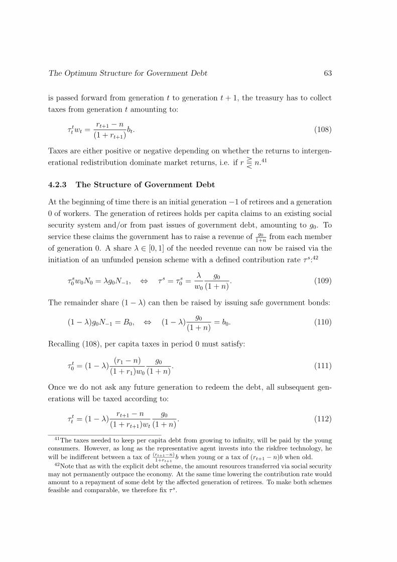
The Optimum Structure for Government Debt 63
is passed forward from generation t to generation t + 1, the treasury has to collect
taxes from generation t amounting to:
τ ttwt =rt+1 − n
(1 + rt+1)bt. (108)
Taxes are either positive or negative depending on whether the returns to intergen-
erational redistribution dominate market returns, i.e. if r T n.41
4.2.3 The Structure of Government Debt
At the beginning of time there is an initial generation −1 of retirees and a generation
0 of workers. The generation of retirees holds per capita claims to an existing social
security system and/or from past issues of government debt, amounting to g0. To
service these claims the government has to raise a revenue of g01+n
from each member
of generation 0. A share λ ∈ [0, 1] of the needed revenue can now be raised via the
initiation of an unfunded pension scheme with a defined contribution rate τ s:42
τ s0w0N0 = λg0N−1, ⇔ τ s = τ s0 =λ
w0
g0
(1 + n). (109)
The remainder share (1− λ) can then be raised by issuing safe government bonds:
(1− λ)g0N−1 = B0, ⇔ (1− λ)g0
(1 + n)= b0. (110)
Recalling (108), per capita taxes in period 0 must satisfy:
τ t0 = (1− λ)(r1 − n)
(1 + r1)w0
g0
(1 + n). (111)
Once we do not ask any future generation to redeem the debt, all subsequent gen-
erations will be taxed according to:
τ tt = (1− λ)rt+1 − n
(1 + rt+1)wt
g0
(1 + n). (112)
41The taxes needed to keep per capita debt from growing to infinity, will be paid by the youngconsumers. However, as long as the representative agent invests into the riskfree technology, hewill be indifferent between a tax of (rt+1−n)
1+rt+1b when young or a tax of (rt+1 − n)b when old.
42Note that as with the explicit debt scheme, the amount resources transferred via social securitymay not permanently outpace the economy. At the same time lowering the contribution rate wouldamount to a repayment of some debt by the affected generation of retirees. To make both schemesfeasible and comparable, we therefore fix τ s.
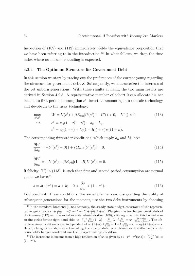
64 Intertemporal Allocation with Incomplete Markets
Inspection of (109) and (112) immediately yields the equivalence proposition that
we have been referring to in the introduction.43 In what follows, we drop the time
index where no misunderstanding is expected.
4.2.4 The Optimum Structure for Government Debt
In this section we start by tracing out the preferences of the current young regarding
the structure for government debt λ. Subsequently, we characterize the interests of
the yet unborn generations. With these results at hand, the two main results are
derived in Section 4.2.5. A representative member of cohort 0 can allocate his net
income to first period consumption c1, invest an amount a0 into the safe technology
and devote h0 to the risky technology:
maxc1,c2
W = U(c1) + βEwR[U(c2)]; U ′() > 0, U ′′() < 0, (113)
s.t. c1 = w0(1− τ t0 − τ s0 )− a0 − h0,
c2 = a0(1 + r) + h0(1 +R1) + τ s0w1(1 + n).
The corresponding first order conditions, which imply a∗0 and h∗0, are:
∂W
∂a0
= −U ′(c1) + β(1 + r)EwR[U ′(c2)] = 0, (114)
∂W
∂h0
= −U ′(c1) + βEwR[(1 +R)U ′(c2)] = 0. (115)
If felicity, U() in (113), is such that first and second period consumption are normal
goods we have:44
s = s(w; τ s) = a+ h; 0 <∂s
∂w< (1− τ s). (116)
Equipped with these conditions, the social planner can, disregarding the utility of
subsequent generations for the moment, use the two debt instruments by choosing
43In the standard Diamond (1965) economy, the steady state budget constraint of the represen-tative agent reads c1 + c2
1+r = w(1− τ s− τ t) + τsw1+r (1 + n). Plugging the two budget constraints of
the treasury (112) and the social security administration (109), with w0 = w, into this budget con-straint yields for the right-hand-side: w− r−n
1+rg0
1+n (1−λ)− g0(1+n)λ+λ g0
1+r = w− (r−n)g0(1+r)(1+n) . The life-
cycle savings condition is also independent of λ: (1+n)(λ g01+n +(1−λ) g0
1+n +k) = g0+(1+n)k = s.Hence, changing the debt structure along the steady state, is irrelevant as it neither affects thehousehold’s budget constraint nor the life-cycle savings condition.
44The increment in income from a high realization of wt is given by (1−τ s−τ t(wt))+∂τt(wt)
∂wtwt =
(1− τ s).
The Optimum Structure for Government Debt 65
λ such that the indirect utility of generation 0 is maximized. Taking into account
the budget constraints (109) and (111) yields the planning problem:45
maxλ
V0 = U(w0(1− τ s0 − τ t0)− a0 − h0) (117)
+βEwR[U(a0(1 + r) + h0(1 +R) + τ s0w(1 + n))],
s.t. (109), (111).
Utilizing the envelope condition (114) and the covariance rule, λ∗ is implicitly defined
by:
dV0
dλ=U ′(c1)g0
1 + r
(E[w]− w0
w0
+covwR(U ′(c2), w1)
w0EwR[U ′(c2)]
)= 0. (118)
Condition (118), which is reminiscent of the C-CAPM, indicates that members of
generation 0 will benefit from a high fraction of debt that is injected into the social
security system as long as the expected excess rate-of-return on this fraction of debt,
compared to the after-tax-return on safe bonds, is positive, i.e. Ew−w0
w0> 0. The
other relevant component is the covariance between second period marginal utility
and the pension benefit. Depending on cov(R1, w1) T 0, we have cov(U ′(c2), w1)|λ=0 S
0, i.e. the wage-indexed social security claims may or may not be a welcome oppor-
tunity to diversify stock market risks.
Subsequent Generations The social planner’s perspective on the welfare of sub-
sequent generations, which is obviously connected to the current choice of λ, will
be an ex-ante perspective. While the social planner knows the distribution over R
and w, the realizations are yet unknown. The agents, however, will start to make
their consumption savings decisions in period t after wt has been realized. The con-
sumer’s behavior is therefore still characterized by conditions (114) and (115) which
imply the wage dependent investment decisions at = at(wt;λ) and ht = ht(wt;λ).
Put differently, the social planner, who optimizes ex-ante utility, has to take note of
the agent’s investment decisions conditional on the realization of wt. Moreover, the
budget constraints (109) and (112) have to be satisfied in each period. From the
45Note that there is no life-cycle savings condition for bonds and capital in a small open economy,i.e. we only take note of the taxes that are needed to keep per capita debt from growing. In a closedeconomy with a tri-linear technology, we can also neglect the market clearing condition as longas agents demand safe investments in excess of the debt offered. In the following we assume thatagents are equating at the margin, i.e. we omit the prospect of Kuhn-Tucker-type ramifications.
66 Intertemporal Allocation with Incomplete Markets
perspective of period 0, the planning problem is therefore given by:
maxλ
Vt = Ewt
[U(wt(1− λ
g0
w0(1 + n))− r − n
(1 + r)
(1− λ)g0
(1 + n)− at − ht)
](119)
+βEwtwt+1Rt+1
[U(at(1 + r) + ht(1 +R) + λ
g0
w0
wt+1)].
The first order condition for an optimum debt structure, taking the envelope con-
ditions (114) and (115) into account (see Appendix 4.5.1), is then given by:46
dVtdλ
=g0
(1 + n)
(n− r
1 + r
E[w]− w0
w0
Ewt [U′(c1)] (120)
−covwt(U′(c1),
wtw0
) + β(1 + n)covwtwt+1R(U ′(c2),wt+1
w0
))
= 0.
Equation (120) characterizes the debt structure λ∗∗ which maximizes long-run ex-
pected utility. Inspection of (120) indicates that agents who are not yet born will
suffer a loss from excessive intergenerational redistribution if the safe returns ex-
ceed the biological returns on consumption loans. That is, the expected excess
amount of resources − when compared to bonds which are not wage-indexed − that
is redistributed via social security is given by Ew−w0
w0.47 The second element is the
intergenerational diversification of wage-income risk. With λ > 0 we have a positive
social security tax rate τ s, which transfers some of the risk associated with the real-
ization of wt into period t+1, where wt+1, i.e. the pension benefits are realized. The
sufficient condition for an interior optimum requires that dVdλ
is downward-sloping
in λ. A first inspection of (120) suggests dcov(U ′(c1),wt)dλ
> 0, dcov(U ′(c2),wt+1)dλ
< 0, and
therefore d2Vdλ2 < 0. Hence, as we shift wage-income risk from the first into the second
period, we expect the wage related covariance risk to move in the same direction
(see Appendix 4.5.2 for the associated conditions). However, as the set of admis-
sible debt structures is closed and bounded, there will always exist a “best” debt
structure λ∗∗ ∈ [0, 1].
The efficiency of the size of the debt scheme can be assessed once we ask whether
the unborn generations benefit from a larger initial debt. Taking the first derivative
46Taking advantage of our assumption that the stochastic wage rate wt is serially uncorrelatedwe may rewrite covwtwt+1R(U ′(c2), wt+1
w0) = covwt+1R(Ewt
U ′(c2), wt+1w0
). If such a serial correlationexisted, it would affect the location of λ∗∗. If a and h are normal, we have da
dwt> 0 and dh
dwt> 0;
thus we would have a smaller λ∗∗ if cov(wt, wt+1) > 0, and vice versa.47The expected intergenerational transfer through social security is E[τ sw] = g0
(1+n)w0Ew. Re-
garding bonds, the transfer is g0(1+n) . The difference in the expected size of the transfers, which
yield the inferior biological return, is therefore given by g0(1+n)
(Ew−w0)w0
.
The Optimum Structure for Government Debt 67
of Vt with respect to g0 yields:
dVtdg0 |dλ=0
=n− r
(1 + r)(1 + n)
(w0 + λ(E[w]− w0)
w0
)E[U ′(c1)] (121)
+λ1
(1 + n)
((1 + n)βcov(Ewt [U
′(c2)],wt+1
w0
)− cov(U ′(c1),wtw0
))
T 0.
The first element in (121) is the familiar return condition; larger intergenerational
reallocation of resources is desirable as long as consumption loans dominate market
returns. The second element reflects the benefits from intergenerational risk sharing
through the share λ of debt that is injected into the pension system. To see this
more clearly, we recall (120) and rearrange (121) such that:
dVtdg0 |dλ=0
=n− r
(1 + r)(1 + n)E[U ′(c1)] +
λ
g0
dVtdλ
T 0. (122)
If λ is zero or at its long-run optimum λ∗∗, the second risk sharing related term
vanishes and (122) exhibits the pure interest condition.
Furthermore, (122) indicates that safe debt does not reallocate risks, while social
security does. This is the opposite of the Bohn (1998, 2003) conclusion, where
debt was issued pro-cyclical such that it shifted risks towards future generations.
Equation (122) also shows that if the national debt is small, then this debt should
be injected entirely into the pension scheme if dVt
dλ, dV0
dλ> 0, such that the benefits
from risk sharing are maximized with λ = 1. In a different interpretation, the sign
of (122) is the subject studied by Green (1977), Kruger and Kubler (2006) and
Gottardi and Kubler (2008).
4.2.5 Efficiency
Inspection of our above analysis indicates that generation 0 will prefer a debt struc-
ture λ∗, that is a solution to (118), rather than λ∗∗, which solves (120).48 If the
government can control the composition of the public debt only, all debt structures
located between λ∗ and λ∗∗ are Pareto-efficient. Raising λ beyond λ∗ will increase
expected utility of all unborn generations at the expense of generation 0. Start-
ing with λ∗∗, the same applies when λ is lowered. Hence, we have the following
proposition:
48For appropriate (Ew − w0, r − n, cov(w,R)), λ∗ may actually coincide with λ∗∗. In this caseboth generations prefer − though for different reasons − the same debt structure, and, exceptfor choosing this structure, no additional government intervention is necessary. The same applieswhen corner solutions coincide.

68 Intertemporal Allocation with Incomplete Markets
Proposition 7. If the government can only implement the debt structure that is usedto roll over the initial debt, there exists a set [λ∗, λ∗∗] ⊆ [0, 1] of efficient financingmethods. This set is characterized by the conflicting interests of the current youngand the yet unborn generations.
Diagrams 10a and 10b illustrate this trade-off. We now trace out the set of Pareto-
1
b
λ
MB, MC
λ∗ λ∗∗
MC = −
dV0
dλ
MB =dVt
dλ
1
b
λ
MB, MC
λ∗∗ λ∗
MC = −
dV0
dλ
MB =dVt
dλ
1
10a 10b
Diagram 10: Efficient debt structures.Diagrams 10a and 10b illustrate the gains and losses of generation 0 and one rep-resentative member of the yet unborn generations. All debt structures located inthe dashed area are inefficient. Diagram 10b depicts a situation that may occur ifE[w] w0 and r n.
improving transitions from one debt scheme to another, which are available once
the government can change both, the composition and the structure of the public
debt. As we have stressed earlier, with these two instruments, it will be possible for
the government to separate the risk sharing properties of the public debt from the
crowding-out effect.
Efficiency with Government Intermediation Suppose now that the initial
conditions are such that λ = λ∗ < λ∗∗. In this case each member of the yet unborn
generations is willing to accept a (slightly) higher level of public debt in exchange for
a more favorable composition λ > λ∗ of the debt. At the same time members of the
current young generation are willing to accept additional pension claims and safe
The Optimum Structure for Government Debt 69
bonds in exchange for the less favorable allocation of factor-price risks associated
with λ. The government can now offer generation 0 to increase the per-capita (in
terms of generation −1) size of the public debt by π. The new debt scheme has a
per-capita (of generation 0) size of g1+n
≡ g0+π1+n
. The associated Lagrangian, which
allows to trace-out the set of Pareto-improving pension reforms, is then given by:
maxπ,λ,µ
L = V0(λ, π) + µ(Vt(λ, g)− V ); Vt(λ, g) = V ≡ Vt(λ∗, g0), g ≡ g0 + π.(123)
Where the Lagrangian (123) consists of the indirect utility functions of the current
young and the yet unborn generations which where discussed earlier in Section 4.2.4.
The additional argument π in V0 reflects that members of generation 0 receive ad-
ditional safe consumption (after taxes) amounting to (1 − λ) 11+r
π and additional
pension claims λ πw0w1 once the debt scheme is increased in size. The partial deriva-
tive ∂V0
∂πis therefore positive. Regarding future generations, we focus on the inter-
esting case where resources are scarce and an increase per-capita debt alone is not
Pareto-improving. That is, the partial derivative ∂Vt
∂g, described in (122), is assumed
to be negative. Finally, as per-capita debt does not grow over time it is sufficient to
represent future generations using only one lagrangian multiplier µ. Regarding the
first order conditions associated with (123) we have:
∂L∂π
=∂V0
∂π+ µ
∂Vt∂g
= 0, (124)
∂L∂λ
=∂V0
∂λ+ µ
∂Vt∂λ
= 0. (125)
Combining (124) and (125) we can drop the Lagrangian multiplier µ. The first order
condition for the optimum structure for government debt λ∗∗∗ is then:
∂V0
∂λ∂V0
∂π
=∂Vt
∂λ∂Vt
∂g
. (126)
Condition (126) indicates that the optimum structure for government debt is as-
sociated with a point on the contract curve. It equalizes the marginal rates of
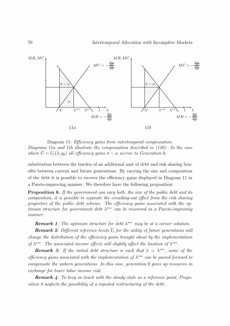
70 Intertemporal Allocation with Incomplete Markets
1
b
λ
MB, MC
λ∗ λ∗∗λ∗∗∗
MC = −
∂V0
∂λ∂V0
∂Π
MB = −
∂Vt∂λ∂Vt∂g
π − α
α
1
b
λ
MB, MC
λ∗ λ∗∗λ∗∗∗
MC = −
∂V0
∂λ∂V0
∂Π
MB = −
∂Vt∂λ∂Vt∂g
π − α
1
11a 11b
Diagram 11: Efficiency gains from intertemporal compensation.Diagrams 11a and 11b illustrate the compensation described in (126). In the casewhere U = Ut(λ, g0) all efficiency gains π − α accrue to Generation 0.
substitution between the burden of an additional unit of debt and risk sharing ben-
efits between current and future generations. By varying the size and composition
of the debt it is possible to recover the efficiency gains displayed in Diagram 11 in
a Pareto-improving manner. We therefore have the following proposition:
Proposition 8. If the government can vary both, the size of the public debt and itscomposition, it is possible to separate the crowding-out effect from the risk sharingproperties of the public debt scheme. The efficiency gains associated with the op-timum structure for government debt λ∗∗∗ can be recovered in a Pareto-improvingmanner.
Remark 1: The optimum structure for debt λ∗∗∗ may be at a corner solution.
Remark 2: Different reference levels Vt for the utility of future generations will
change the distribution of the efficiency gains brought about by the implementation
of λ∗∗∗. The associated income effects will slightly affect the location of λ∗∗∗.
Remark 3: If the initial debt structure is such that λ > λ∗∗∗, some of the
efficiency gains associated with the implementation of λ∗∗∗ can be passed forward to
compensate the unborn generations. In this case, generation 0 gives up resources in
exchange for lower labor income risk.
Remark 4: To keep in touch with the steady state as a reference point, Propo-
sition 8 neglects the possibility of a repeated restructuring of the debt.
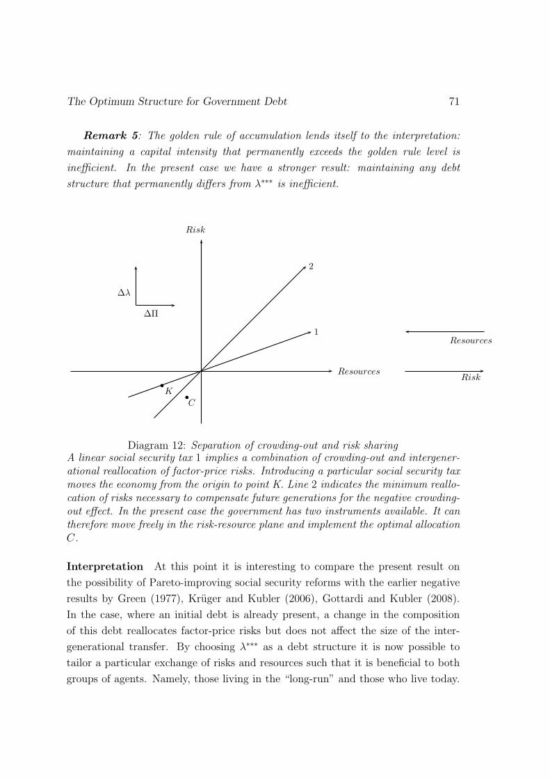
The Optimum Structure for Government Debt 71
Remark 5: The golden rule of accumulation lends itself to the interpretation:
maintaining a capital intensity that permanently exceeds the golden rule level is
inefficient. In the present case we have a stronger result: maintaining any debt
structure that permanently differs from λ∗∗∗ is inefficient.
Risk
Resources
b
b
C
K
∆Π
∆λ
2
1
Resources
Risk
1
Diagram 12: Separation of crowding-out and risk sharingA linear social security tax 1 implies a combination of crowding-out and intergener-ational reallocation of factor-price risks. Introducing a particular social security taxmoves the economy from the origin to point K. Line 2 indicates the minimum reallo-cation of risks necessary to compensate future generations for the negative crowding-out effect. In the present case the government has two instruments available. It cantherefore move freely in the risk-resource plane and implement the optimal allocationC.
Interpretation At this point it is interesting to compare the present result on
the possibility of Pareto-improving social security reforms with the earlier negative
results by Green (1977), Kruger and Kubler (2006), Gottardi and Kubler (2008).
In the case, where an initial debt is already present, a change in the composition
of this debt reallocates factor-price risks but does not affect the size of the inter-
generational transfer. By choosing λ∗∗∗ as a debt structure it is now possible to
tailor a particular exchange of risks and resources such that it is beneficial to both
groups of agents. Namely, those living in the “long-run” and those who live today.
72 Intertemporal Allocation with Incomplete Markets
Diagram 12 illustrates this. Curve 1 represents the long-run consequences of a linear
social security tax. As this tax increases, the economy moves from the origin to a
certain point e.g. K. Curve 2, which is steeper than 1, shows the threshold where
future generations are indifferent between the crowding-out of capital and the risk
sharing benefits. Finally, point C is an allocation that can be reached in the manner
described above: a change in the composition of the debt reallocates many risks via
the linear social security tax. The change in the allocation of resources is mainly
due to the change in the size of the debt π. Put differently, by introducing a linear
social security tax alone the government can only move along arrow 1. If there is
already an initial debt present it has two linearly independent instruments. In this
case it can move in the entire plane, where point C is associated with an optimal
pair λ∗∗∗, π∗∗∗.
Another Interpretation In a different interpretation (126) may be seen as an
intertemporal version of the Samuelson (1954) condition for the efficient provision
of a public good. Recalling equation (122) we can rewrite (126) such that:49
∂V0
∂λ∂V0
∂π
=∂Vt
∂λ
−Ewt [U′(c1)] r−n
(1+r)(1+n)+ λ
g∂Vt
∂λ
(127)
=∞∑t=1
(1 + n
1 + r
)t ∂Vt
∂λ
−Ewt [U′(c1)] 1
1+r+ λ
g∂Vt
∂λ1+nr−n
.
Condition (127) indicates that all future generations benefit from the public good
“risk sharing” which is embodied in the debt scheme. The cost with the provision of
this public good has to be incurred only once by generation 0, which bears additional
wage-related risk. Depending on its position on the time axis, the present value of
tax payments differs from cohort to cohort. The first element −E[U ′(c1)] 11+r
in the
numerator of the marginal rate of substitution of future generations indicates the
negative crowding-out effect. The second element λg∂Vt
∂λis positive. As a share λ
49For r > n, we have∑∞
t=1
(1+n1+r
)t
= 1+nr−n . Note that the RHS of condition (126) is the marginal
rate of substitution between an increase in λ and and increase of the debt level of one unit. The newformulation in (127) is the sum of the marginal rates of substitution between a marginal increaseof λ and a marginal increase in the tax level. In Appendix 4.5.3 we develop the more intuitive casewhere only safe debt is used as a means of compensation. That is, the debt is not injected into theoptimal debt scheme.
The Optimum Structure for Government Debt 73
of the new debt π is injected into social security. This increases the willingness of
future generations to accept a higher level of public debt.
The analogy to the problem of public good provision also extends to the aspect
of income effects. Changing levels of Vt will require different compensation schemes.
Hence, the exact location of λ∗∗∗ depends on the particular compensation scheme
as the associated income effects may slightly change preferences for λ, i.e. shift the
marginal cost and benefit curves displayed in Diagram 11.
4.3 Extensions
So far attention was confined to an economy where the safe rate-of-return is constant
over time. The prospects of a third debt instrument, namely a defined benefit social
security system, have also been neglected. In a first step, we now show that a time-
varying, safe rate-of-return does not alter the quality of the foregoing conclusions
and that defined benefits are equivalent to safe bonds. Finally a second group of
representative agents who do not invest in the stock market (risky technology) is
introduced into our model. In this setting we show that both groups require different
social security contribution rates, i.e. debt structures. If either is at a corner solution
there is additional scope for an intragenerational reallocation of the public debt.
4.3.1 Time-Varying Safe Returns
To work out the pivotal elements, the safe rate of return was assumed to remain
constant over time. However, the main results of our previous analysis carry over
to an economy where r is now an i.i.d. random variable. Regarding generation 0,
nothing is changed, i.e. the agents and the social planner start maximizing after r1
is known. Except for the additional expectations regarding r the long-run planning
problem (120) is also little changed:
maxλ
Vt = Ewt,rt+1
[U(wt(1− λ
g0
w0(1 + n))− rt+1 − n
(1 + rt+1)
(1− λ)g0
(1 + n)− at − ht)
]+βEwtwt+1Rt+1rt+1
[U(at(1 + rt+1) + ht(1 +R) + λ
g0
w0
wt+1)].
Employing the envelope conditions (114) and (115), yields:
dVtdλ
=g0
(1 + n)
(Ewr
[rt+1 − n
1 + rt+1
U ′(c1)]w0 − E[w]
w0
(128)
−covwtrt+1(U′(c1),
wtw0
) + β(1 + n)covrt+1wtwt+1R(U ′(c2),wt+1
w0
)])
= 0.

74 Intertemporal Allocation with Incomplete Markets
Due to the nature of the treasury’s tax schedule (112), the initial interest rate r1 does
not, unlike the wage rate w0, enter into the long-run first order condition. While
there are now additional expectations regarding the safe rate-of-return, the principal
structure of the first order condition is preserved. Regarding our Pareto-improving
interventions that were discussed in Section 4.2.5, we note that the government
can still reallocate gains and losses along its budget constraint. However, each
compensation scheme will now require some sort of risk-taking.
4.3.2 Defined Benefits
We will now briefly show that a defined benefit system is equivalent to an explicit
debt scheme. The budget constraint of a defined benefit system, which is used to
roll over a fraction γ of the public debt, is given by:
τDBt wt =γg0
(1 + n), pDBt = γg0. (129)
Once we recall that the young agent can consume c1, invest an amount a into safe
assets and an amount h into risky assets, the present value budget constraint is
given by:
c1t + at + ht = wt(1− τDBt − τ tt ) +pDBt+1
(1 + rt+1). (130)
Utilizing (129) and (112) where (1 − λ) is replaced by (1 − γ), the right-hand side
of (130) can now be rewritten such that:
c1t + at + ht = wt −g0(rt+1 − n)
(1 + n)(1 + rt+1). (131)
Hence the structure of debt γ is irrelevant, i.e. a defined benefit system is equivalent
to a bond-financed debt scheme.
4.3.3 A Working Class
This final paragraph considers a society that is partitioned into a group of capitalists
who are endowed with a large amount of efficient labor and a group of workers with
a low labor endowment. While capitalists participate in the stock-market, workers
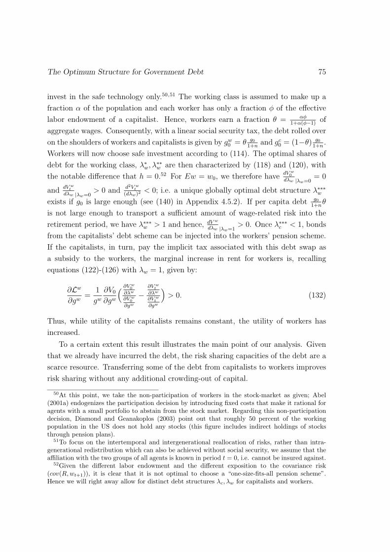
The Optimum Structure for Government Debt 75
invest in the safe technology only.50,51 The working class is assumed to make up a
fraction α of the population and each worker has only a fraction φ of the effective
labor endowment of a capitalist. Hence, workers earn a fraction θ = αφ1+α(φ−1)
of
aggregate wages. Consequently, with a linear social security tax, the debt rolled over
on the shoulders of workers and capitalists is given by gw0 = θ g01+n
and gc0 = (1−θ) g01+n
.
Workers will now choose safe investment according to (114). The optimal shares of
debt for the working class, λ∗w, λ∗∗w are then characterized by (118) and (120), with
the notable difference that h = 0.52 For Ew = w0, we therefore havedV w
0
dλw |λw=0= 0
anddV w
t
dλw |λw=0> 0 and
d2V wt
(dλw)2< 0; i.e. a unique globally optimal debt structure λ∗∗∗w
exists if g0 is large enough (see (140) in Appendix 4.5.2). If per capita debt g01+n
θ
is not large enough to transport a sufficient amount of wage-related risk into the
retirement period, we have λ∗∗∗w > 1 and hence, dV w
dλw |λw=1> 0. Once λ∗∗∗c < 1, bonds
from the capitalists’ debt scheme can be injected into the workers’ pension scheme.
If the capitalists, in turn, pay the implicit tax associated with this debt swap as
a subsidy to the workers, the marginal increase in rent for workers is, recalling
equations (122)-(126) with λw = 1, given by:
∂Lw
∂gw=
1
gw∂V0
∂gw
( ∂V w0
∂λw
∂V w0
∂gw
−∂V w
t
∂λw
∂V wt
∂gw
)> 0. (132)
Thus, while utility of the capitalists remains constant, the utility of workers has
increased.
To a certain extent this result illustrates the main point of our analysis. Given
that we already have incurred the debt, the risk sharing capacities of the debt are a
scarce resource. Transferring some of the debt from capitalists to workers improves
risk sharing without any additional crowding-out of capital.
50At this point, we take the non-participation of workers in the stock-market as given; Abel(2001a) endogenizes the participation decision by introducing fixed costs that make it rational foragents with a small portfolio to abstain from the stock market. Regarding this non-participationdecision, Diamond and Geanakoplos (2003) point out that roughly 50 percent of the workingpopulation in the US does not hold any stocks (this figure includes indirect holdings of stocksthrough pension plans).
51To focus on the intertemporal and intergenerational reallocation of risks, rather than intra-generational redistribution which can also be achieved without social security, we assume that theaffiliation with the two groups of all agents is known in period t = 0, i.e. cannot be insured against.
52Given the different labor endowment and the different exposition to the covariance risk(cov(R,wt+1)), it is clear that it is not optimal to choose a “one-size-fits-all pension scheme”.Hence we will right away allow for distinct debt structures λc, λw for capitalists and workers.
76 Intertemporal Allocation with Incomplete Markets
λ∗∗∗
wλ∗∗
wλw
MB, MC
MC′
w
MB′
w
MBw
MCw0
1
b
λ∗
w
1
Diagram 13: Intragenerational reallocation of the debt.
The shaded area to the right of λ = 1 is the welfare gain associated with an intra-generational debt swap.
4.4 Conclusion
If a government can issue safe bonds and claims to an unfunded social security
system to service a given obligation, there exists a set of Pareto-efficient financing
policies. This set is characterized by the conflicting interests of agents who are
currently alive and those who are yet unborn. The current young, who have already
observed their wage income, will prefer safe debt, i.e. safe retirement benefits. The
unborn generations on the contrary benefit from the ex-ante diversification of their
wage risk if a large portion of the initial debt is injected into social security.
The government may now act as a representative of the unborn members of
society. Through its budget constraint, it can offer generation 0 a compensation
that reflects the willingness to pay of all unborn agents. Such an intermediation
allows to collect the benefits, which are associated with the optimum structure for
government debt λ∗∗∗ in a Pareto-improving manner. If the initial conditions are
such that λ∗∗∗ > 0, an unfunded social security system is therefore always warranted.
Unlike the deterministic economy, where all debt policies are equally desirable,
the current analysis shows that the structure of government debt has distinct impli-
cations for individual welfare. If we compare our analysis to the problem of optimal
capital accumulation, the following analogy is notable: While the golden rule capital
intensity maximizes long-run utility, it comes at the cost of lower consumption along
The Optimum Structure for Government Debt 77
the transition path. All capital intensities below the golden rule level are efficient
and there is no compensation mechanism available.53 All government interventions
are either neutral or require a welfare criterion. Compared to the reallocation of
aggregate risks, the situation without compensation is similar; there exists a whole
set of efficient debt structures. In the present case, however, the government budget
constraint can be used to reconcile the conflicting interests of the current young and
those who live in the long run in a Pareto-improving manner. As a result, subject
to our assumptions, the set of efficient debt structures can be narrowed.
4.5 Appendix
4.5.1 The Envelope Conditions
Derivation of condition (120): Equations (114) and (115) imply an investment behav-
ior for each realization of the wage-income wt, namely at = at(wt, λ), ht = ht(wt, λ).
Hence, agents smooth consumption state by state with regard to first period wage
income. At the same time, they smooth consumption in expectations when it comes
to second period consumption. Taking expectations Ewt of (114) and (115) yields:
Ewt [U′(c1)] = β(1 + r1)Ewt
[Ewt+1R[U ′(c2)]
], (133)
Ewt [U′(c1)] = βEwt
[Ewt+1R[(1 +R)U ′(c2)]
]. (134)
Writing out the first order condition for λ∗∗, we obtain:
dVtdλ
=(Ewt
[− U ′(c1)wt + (1 + n)βEwt+1R[wt+1U
′(c2)]] g0
w0
(135)
+r − n
(1 + r)g0Ewt
[U ′(c1)
]) 1
1 + n
− Ewt [U′(c1)(
da
dλ+dh
dλ)− βEwt+1R[U ′(c2)((1 + r)
da
dλ+ (1 +R)
dh
dλ)]] = 0.
To rearrange the first line in (135), equation (133) can be utilized asEwt [U
′(c1)]
1+r=
βEwt [U′(c2)]. Applying the covariance rule (E[xy] = cov(x, y) + E[x]E[y]) to the
53The lack of such a compensation mechanism led to the turnpike literature; see e.g. Samuelson(1968) or Blanchard and Fischer (1989). The absence of such an intertemporal compensationmechanism is of course also the reason for the intertemporal efficiency of pay-go schemes that wehave been referring to in Footnote 32.

78 Intertemporal Allocation with Incomplete Markets
resulting expressions, we obtain (120). Noting that the derivatives dadλ
and dhdλ
are
functions of wt, the second line can be rearranged using the covariance rule such
that:
−Ewt [U′(c1)]Ewt [
da
dλ] + (1 + r)βEwtwt+1R[U ′(c2)]Ewt [
da
dλ]
−Ewt [U′(c1)]Ewt [
dh
dλ] + βEwtwt+1R[(1 +R)U ′(c2)]Ewt [
da
dλ]
+covwt(−U ′(c1) + (1 + r)βEwt+1R[U ′(c2)],da
dλ)
+covwt(−U ′(c1) + βEwt+1R[(1 +R)U ′(c2)],dh
dλ) = 0.
That is, recalling (114), (115), (133), and (134), the expressions related to changes
in the investment behavior vanish by the envelope theorem.
4.5.2 Characteristics of the Long-run Optimum
This appendix examines the properties of condition (120). In a first step we note
that (120) characterizes a “best” debt structure, which may or may not be interior.
In a next step it is shown that interior solutions will exist for appropriate parameters.
Finally the conditions, which ensure that dVt(λ)dλ |λ=0
> 0 and that d2Vt(λ)dλ2 < 0, are
outlined.
Existence Since short sales of bonds or social security claims were ruled out, the
set of feasible debt structures [0, 1] is a compact subset of R. If Vt(λ) is continuous
and real-valued, it will therefore attain its bounds on this choice set according to
the Weierstrass theorem.
Interior Solutions If dcov(U ′(c1),wt)dτs
dτs
dλand dcov(U ′(c2),wt+1)
dτsdτs
dλare continuous and
dhdτs < 0, it is obvious that for sufficiently large g0, sufficiently small cov(R,wt+1),
and Ew[w] = w0 or r = n, we have:
dVtdλ |λ=0
> 0,dVtdλ |λ=1
< 0. (136)
In this case, there exists one interior global optimum λ∗∗ and there may exist several
local optima.

The Optimum Structure for Government Debt 79
Unique Optimum To interpret condition (120) in more detail, we will first show
that cov(U ′(c1), wt) < 0 and give a condition for cov(U ′(c2), wt+1) T 0:
cov(c1, wt) = cov((1− τ s)wt −r − n
1 + r
g0
1 + n(1− λ)− s(wt, τ
s), wt) (137)
= cov((1− τ s)wt − s(wt, τs), wt) > 0,
where the sign cov(c1, wt) > 0 is due to the normality of c1; i.e. ∂((1−τs)wt−s(wt,τs))∂wt
>
0. Hence, since U ′′() < 0, cov(U ′(c1), wt) < 0. For cov(U ′(c2), wt+1) we have:
cov(c2, wt+1) = cov((1 + r)a+ (1 +R)h+ τ s(1 + n)wt+1, wt+1) (138)
= hcov(R,wt+1) + τ s(1 + n)σ2w T 0; τ s = λ
g0
(1 + n)w0
.
Hence, depending on the amount of risky assets h, cov(w,R) T 0 and the amount
of debt that is injected in the pension system, we may have cov(U ′(c2), wt+1) T 0.
Together with the ambiguous sign of (n−r)(Ew−w0)w0(1+r)
, we may or may not have dVt
dλ |λ=0>
0.
Sufficient Condition To allow for a global optimum, it is a sufficient condition,
that dVt
dλis downward-sloping in λ:
d2Vt(dλ)2
=g0
1 + n
(n− r
1 + r
E[w]− w0
w0
dE[U ′(c1)]
dλ(139)
−dcovwt(U
′(c1), wt
w0)
dλ+ β(1 + n)
dcovwt+1R(U ′(c2), wt+1
w0)
dλ
)< 0.
A first inspection of (139) indicates that for Ew = w0 and/or r = n, we ex-
pect dcov(U ′(c1),wt)dλ
> 0, dcov(U ′(c2),wt+1)dλ
< 0 and thus d2Vt
dλ2 < 0.54 With respect todcov(U ′(c1),wt)
dλwe have:
dcovwt(U′(c1), wt)
dλ= covwt(U
′′(c1)(−wdτs
dλ− ds
dλ), w) (140)
≈ Ewt [U′′(c1)]covwt(−w
dτ s
dλ− ds
dλ, w) T 0,
54Regarding the first element, which is inherently ambiguous, we note that for U ′′′(c1) > 0,dE[U(c1)]
dλ is most likely negative, as the variance of first period consumption is decreasing in λ.However, at the same time an increase in λ may increase second period variance and if U ′′′() > 0,precautionary savings (see Green (1977) and Kimball (1990) for the coefficient of prudence) willincrease E[U ′(c1)].
80 Intertemporal Allocation with Incomplete Markets
where (140) holds with strict equality if U ′′′(c1) = 0. Condition (140) indicates thatdcovwt (U
′(c1),wt)
dλ> 0 as long as covwt(
dsdλ, wt) is not large and negative. Finally, by the
same approximation as in (140) we have:
dcov(U ′(c2), wt+1)
dλ≈ EwR[U ′′(c2)]
(dhdλcov(R,wt+1) + (1 + n)σ2
w
)dτ sdλ
T 0, (141)
where (141) is negative if dhdλcov(R,wt+1) + (1 + n)σ2
w > 0. If cov(R,wt+1) is large
and positive and the share of savings invested in the risky technology is also very
large, the crowding-out effect (with regard to risky investment) of additional pen-
sion claims may in principle overcompensate the direct effect of the exposition to
additional wage-related risks once λ is increased.
4.5.3 Lagrangian
In this appendix, we discuss the Lagrangian associated with the set of efficient debt
structures and compensation schemes. However, in the current case, the premium
πt payed by members of generation t, is not injected into the general debt scheme.
Instead πt is issued in period 0 and redeemed (principal and interest) by generation
t in period t. In this case, the analogy to the problem of the efficient provision of a
public good is easier to conceive:
maxπtt=∞
t=1 ,λL = V0(λ, π0) +
∞∑t=1
µt
(Vt(λ, πt)− V (λ∗, 0)
)(142)
+γ( ∞∑t=1
(1 + n
1 + r
)tπt − π0
)Taking the first derivatives and eliminating γ yields:
∂L∂πt
=(1 + n
1 + r
)t∂V0
∂π0
+ µt∂Vt∂πt
= 0, ∀t = 1, 2, .....∞, (143)
∂L∂λ
=∂V0
∂λ+
∞∑t=1
µt∂Vt∂λ
= 0. (144)
Substitution allows to drop µ, and we have
∂V0
∂λ∂V0
∂π0
−∞∑t=1
(1 + n
1 + r
)t ∂Vt
∂λ∂Vt
∂πt
= 0 (145)
The Optimum Structure for Government Debt 81
In the particular case where each agent pays the same premium, πt = π, this sim-
plifies to:
∂V0
∂λ∂V0
∂π0
− 1 + n
r − n
∂Vt
∂λ∂Vt
∂π
= 0. (146)
If ∂Vt
∂λ, ∂V0
∂λ> 0 and ∂2V0
∂λ2 ,∂2Vt
∂λ2 < 0, as discussed in Appendix 4.5.2, the expression in
(146) changes signs and an interior maximum exists.
4.5.4 The Covariance Risk
Technology and Covariance This appendix reflects on the sign of cov(wt, Rt).
Taking the perspective of a small open economy, we examine the correlation of factor-
prices received from the global economy. If global production uses capital and labor
inputs, K and L, to produce aggregate net output zF (K,L), where zF (K,L) is
concave and first-degree-homogenous, factor-prices are given by
wt =∂ztF (Kt, Lt)
∂Lt= ztFLt(Kt, Lt), (147)
Rt =∂ztF (Kt, Lt)
∂Kt
= ztFKt(Kt, Lt).
If the global supply Lt of (efficient) labor fluctuates over time, we have cov(wt, Rt) <
0 since (by the Euler Theorem) FKtLt > 0 and FLtLt < 0. Examples for a stochastic
global labor supply may be the entrance of the labor force from Eastern Europe
into the EU labor market, or the rise of China. If total factor productivity zt is
stochastic, wages and profits are perfectly correlated and we have cov(wt, Rt) =
σ2ztFLtFKt > 0.55 If depreciation is stochastic, we have cov(wt, Rt) = 0. Finally,
unpredicted changes in global savings are associated with cov(wt, Rt) < 0. Hence,
depending on the relative magnitude of the respective effects, the sign the covariance
between wages and profits is ambiguous.
55See Bohn (1998) and Smetters (2006) for the strong results that originate from perfect corre-lation.

82
Intertemporal Compensation with Incomplete Markets 83
5 Intertemporal Compensation with Incomplete
Markets
This chapter briefly puts the results derived in chapters 2, 3, and 4 into a broader
perspective. In previous chapters we have shown that the scope for government
intervention increases with the number of missing markets in the economy. In this
chapter we sketch the more general underlying structure of the problem. In par-
ticular, we show that the potential use of the government budget constraint as an
intertemporal collusion device changes in nature once there are at least two goods
and two government budget constraints available. That is, an increase in the num-
ber of goods and budget constraints from one to two changes the quality of the
efficiency results obtained for OLG economies. Diagrams 14 and 15 illustrate this
point. Further increases in the number of budget constraints beyond two, however,
do not change the quality of the results.
For a simple exposition we discuss a stylized economy with the following prop-
erties:
Assumption 1: Households live for two periods. Each generation i has a smooth
and (jointly) concave utility criterion Ui = Ui(x1i , x
2i ) : Rn
+ ×Rn+ 7→ R. Where x1
i , x2i
are vectors containing n different consumption goods. In the first period of life, each
household is endowed with xi ∈ Rn+ units of consumption goods.
Assumption 2: Each consumption good can be stored/invested. The rate of return
rl > 0 for each good l = 1, 2, ...., n is independent of the aggregate level of investment.
Assumption 3: Technological progress and population growth are zero.
Assumption 4: The government can transfer goods of type l from generation i to
generation j. These transfers are denoted by τi,j ∈ Rn, i, j = 0, 1, 2...∞. Where τi,j,l,
l = 1, 2, ..., n, are the components of τi,j. These transfers are financed by appropriate
borrowing and lending at the technologically determined interest rates.
With these assumptions in place it is useful to define the following indirect utility
function for an agent born at node i:
Vi := argmaxsi
Ui
(xi − si −
i−1∑j=0
(1 + r)i−jτi,j −∞∑
j=i+1
1τi,j, (1 + r)si
), (148)
where si is a n×1 vector and (1+r) and 1 are diagonal matrixes of dimension n×nwith diagonal entries (1 + rl) and 1 respectively.

84 Intertemporal Allocation with Incomplete Markets
−1
0
1
1
Diagram 14a Diagram 14b
Diagram 14: Unfolding the missing markets and intertemporal compensation
In Diagram 14a there is only one government budget constraint along which goodscan be transferred. Every increase in consumption for generation i lowers consump-tion for members of some generation j. If r > 0 and marginal utility is positive, eachallocation (transfer scheme) is Pareto-efficient. In Diagram 14b on the contrary,there is a vector of taxes available in each period and intertemporal compensationis possible. Depending on the respective preferences, there exists a large set of inef-ficient allocations (transfer schemes). Using these taxes, the government can makeup for missing markets. However, private savings must be large enough to supportthe government borrowing along the diagonal of the diagram.
We now proceed as in the previous chapters. To find the set of Pareto-improving
intertemporal reallocations we write the associated Lagrangian:
maxτi,j ,µi,j ,λi,γi∞i,j=0
L = U0(x0 −∞∑i=1
τ0,i) (149)
+∞∑i=1
λi
(Vi(xi −
i−1∑j=0
(1 + r)i−jτi,j −∞∑
j=i+1
1τi,j)− Vi(xi))
+∞∑j=0
∞∑i=j+1
µi,j(τi,j + τj,i)
+∞∑i=0
γi
( i∑k=0
∞∑j=i+1
τk,j(1 + r)i−k + si(xi −i−1∑j=0
(1 + r)i−jτi,j −∞∑
j=i+1
1τi,j)).
Where the Lagrangian multipliers µi,j ensure that a transfer from agent i to agent
j increases consumption for agent j and lowers it for agent i and viceversa. The
Intertemporal Compensation with Incomplete Markets 85
second restriction associated with γi is of the Kuhn-Tucker type. It requires that the
government debt in the respective goods may not exceed households savings. That
is, if the government borrows in good l to implement trades between the generations
i and j, the generations in between must have sufficient savings to absorb the debt
which is rolled over from period i to period j. Put differently, if this condition
binds as in Diagram 15, households savings are a bottleneck to intergenerational
transfers.56 The savings decision would be associated with an externality. If the
reallocation scheme is sufficiently small the savings condition γi is not binding, i.e.
γi = 0, and the first order conditions for τi,j are:
−∇V0 + µi,0 = 0 ∀i = 1, 2, ...∞, (150)
−λi(1 + r)i−j∇Vi + µj,i = 0 ∀i > j, i = 1, 2, ...∞, j = 0, 1, 2, ...∞, (151)
−λi∇Vi + µi,j = 0 ∀i < j, i = 1, 2, ...∞, j = 0, 1, 2, ...∞, (152)
τi,j + τj,i = 0 ∀i, j = 0, 1, 2, ...∞, (153)
Vi = Vi ∀i = 1, 2, ...∞, (154)i∑
k=0
∞∑j=i+1
(1 + r)i−kτk,j (155)
+si(xi −i−1∑j=0
(1 + r)i−jτi,j −∞∑
j=i+1
1τi,j) = 0, ∀i = 1, 2, ...∞.
Where λi is a scalar and γi, µi,j, si, τi,j are appropriate n×1 vectors. Finally (1+r)i−j
is a diagonal matrix of dimension n× n with diagonal entries (1 + rl)i−j. Rewriting
these conditions yields the first order condition for the respective tax rates τi,j,l:
∂Vj∂xl∂Vj
∂xl+1
∂Vi∂xl∂Vi
∂xl+1
=( 1 + rl
1 + rl+1
)i−j, ∀ i, j = 0, 1, 2, ...∞, l = 1, 2, ...n− 1, (156)
56If one cohort i has a very low endowment (when compared to the surrounding generations)it will save little and therefore, it can absorb only little amounts of public debt. In this case thissavings constraint is likely to bind, i.e. γi 6= 0. In a different interpretation the condition associatedwith γi requires that aggregate assets of the different types cannot be negative at any point i.

86 Intertemporal Allocation with Incomplete Markets
where (156) indicates that taxes should be chosen such that a point on the contract
curve is reached.57 Moreover, if we have only m < n tax rates available per agent,
n − m optimality conditions are lost. Regarding the prospects of intertemporal
compensation we therefore have the following proposition:
Oi
Oj
τi,j
b
b
b
z
y
x
x1
x2
x1
x2
1
Diagram 15: The contract curve
The two origins represent members of generation i and j, respectively. Starting fromthe market allocation at x the government can raise a tax such that a point z on thecontract curve is obtained. If γi is binding at some point, we can only move towardsy where savings are no longer sufficient to support further transfers. The dashedlines surrounding the contract curve represent the “savings constraint”.
Proposition 9. If there are n > 1 goods and the government has m > 1 intertem-poral budget constraints it can reallocate resources such that a point on the contractcurve is reached in a Pareto-improving manner. Moreover, only those tax and trans-fer schemes that steer the economy towards a point on the contract curve are efficient.If the government can only reallocate resources of one type (one budget constraint)a Pareto-improving change in the tax scheme is not possible. Each initial allocationis constrained efficient.
Proof. The first part is obvious. For the second part we note that an increase inperiod 0 consumption, i.e. τ0,i < 0, requires higher taxes τi,0 > 0 at some point i. If
57This first order condition is of particular interest with regard to the problem of natural re-sources. If the first generation is the only one in possession of a particular good/resource, condition(156) defines how these resources can be exhausted optimally. That is, future households would bewilling to live with a higher debt in a different consumption good in exchange for more (natural)resources. Similar to the change in the validity of the golden rule there will be correspondingchanges to results like, e.g., the “green golden rule”.

Intertemporal Compensation with Incomplete Markets 87
preferences are locally non satiated this violates the condition Vi(xi− τi,0(1 + r)i) 5Vi(xi).
Oo
Ot
O
V 0
V 0 V t
V t
λg
λ
g∗∗∗ = g0 + Π∗∗∗ g∗∗∗ = g0 + Π∗∗∗
g0
λ∗ λ∗∗∗ λ∗∗
λ∗∗∗g
1
Diagram 16: The optimum structure for government debt
Compared to our problem of the optimum structure for government debt two
differences are notable: (i) we have changed the debt structure once for all to keep
in touch with the literature and the steady state as a reference point. (ii) The
current setting is linear regarding the resources transferred. In the setting with
the optimum structure for government debt we have the aspect of non-linearity.
This is reflected in the fact that there are points of satiation, namely λ∗ and λ∗∗.
If we would introduce non-linearity into the current model, there would also be
the possibility of satiation as with the optimal capital intensity in the Diamond
(1965) model. Moreover, there would be more externalities of a similar type as the
current savings externality (associated with the γi constraint). Diagram 16 gives
an illustration of the effects of nonlinearity of the derivatives of the indirect utility
functions associated with the FOC (126) in Chapter 4, for the optimum structure
for government debt.
The interesting point with Diagram 16 is the fact that the set of efficient alloca-
tions now depends on both, the curvature of the utility function and the technology.
In the case with only one good, this is different: positive marginal utility and the
interest rate condition are the only data required to know that all transfer schemes
are efficient as long as rl > 0 for all goods l = 1, 2, ...n.
88 Intertemporal Allocation with Incomplete Markets
5.1 Conclusion
The concept of dynamic efficiency in the basic Diamond (1965) model has a remark-
able property: the set of efficient capital intensities does not depend on preferences.
It is defined by the curvature of f(·) and the growth rate of the aggregate economy.
The mere comparison of the marginal product of capital and the aggregate growth
rate suffices to decide whether or not the economy grows on an efficient or inefficient
path. The results derived in Chapter 3 showed that this result was sensitive once
preferences are heterogeneous. In Chapter 4, where two goods were available, this
conclusion was also altered for a representative agent economy for the case with two
budget constraints and two missing markets. The present chapter shows that the
efficiency properties of the economy in general change once there are more than two
markets missing and there are at least two intertemporal budget constraints avail-
able. In the current model, the government can steer the economy to a certain point
on the contract curve. In this case the set of inefficient policies is quite large. The
notable difference compared to the Arrow-Debreu setting is the fact that the par-
ticular location on the contract curve is not an outcome of a market process. It has
to be chosen by the planner rather than the households. Moreover, if the economy
is closed, the life-cycle savings condition still limits intergenerational trades.
Taken together, chapters 3, 4 and the current one suggest that the role of pref-
erences tends to increase when the economy becomes more complex. Along-side the
scope for Pareto-improving government intervention also increases. On the contrary,
the importance of technology diminishes. The set of efficient capital intensities can
no-longer be determined by the shape of f(·) and the aggregate growth rate n alone.
89
6 Demographic Change and the Rates of Return
to Risky Capital and Safe Debt
This chapter studies how the upcoming demographic transition will affect the re-
turns to risky capital and safe government debt. In a neoclassical two-generations-
overlapping model we show that the entrance of smaller cohorts into the labor market
will lower both interest rates. The risky rate, however, will react more sensitive than
the risk free rate. Consequently, the risk premium deteriorates during the transition.
6.1 Introduction
Neoclassical models of the Solow (1956), Swan (1956) type predict a positive relation
between the growth rate for population and the rate of return to capital. In more
refined models, involving uncertainty and more than one asset, several authors have
recently examined the consequences of the demographic transition with regard to the
rates of return to risky capital and safe debt.58 However, while these studies tend to
agree that the overall level of interest will fall when the baby boom generation retires,
it remains an open question whether the demographic transition will affect both
rates of return in the same manner. In particular, Brooks (2002) and Geanakoplos
et al. (2004) project that the risky rate will deteriorate more severely than the
return to safe government bonds. That is, the equity premium would fall during the
demographic transition. At the same time, Brooks (2004) and Borsch-Supan et al.
(2007) project an increase in the equity premium for that period.
The purpose of the current note is to complement these previous studies, which
were based exclusively on simulations, by developing a modified version of the Di-
amond (1965) model which allows to analyze the relation between the growth rate
for population and the two key interest rates.
This chapter is organized as follows: In Section 6.2 we discuss a baseline setting
where households work in the first period only, aggregate shocks are log-normal, and
utility is of the Epstein and Zin (1989) type. In this setting we show that (i) both
rates of return increase with the growth rate for population, (ii) the risky rate to
capital reacts more sensitive than the risk free rate, i.e. the equity premium increases
with the growth rate of population. In Section 6.3 we show that the results from
Section 6.2 carry over to a setting with a general concave utility function and shocks
58See Poterba (2001) and Poterba et al. (2005) for surveys.
90 Intertemporal Allocation with Incomplete Markets
which are no longer log-normal. Finally, we discuss a model where households work
in both periods of life. In this setting it turns out that there is a “human capital
effect” to our portfolio choice problem which thwarts the positive relation between
the growth rate for population and the equity premium. While both rates fall, the
safe return will be affected more severely if the human capital effect is sufficiently
large.
6.2 The Model
6.2.1 Technology and factor-prices
The economy is inhabited by overlapping generations who live for two periods; one
period of work is followed by one period of retirement. During the first period of
life, each individual supplies one unit of labor inelastically and population evolves
according to:
Nt+1 = (1 + nt+1)Nt, (157)
where Nt is the size of the cohort born at time t and 1 + nt+1 is the number of
children raised by each member of cohort t.
Production is characterized by a continuous, concave, constant returns to scale,
aggregate production function F (Kt, Nt) ≡ F (Kt, Lt) + (1− δ)Kt. This production
process is subject to an aggregate technology shock zt, which follows a log-normal
distribution. For simplicity we assume that this shock is on average neutral. Per
capita output yt is therefore given by:
yt = ztf(kt); f ′() > 0, f ′′() < 0, E[zt] = 1, ∀t. (158)
Once the respective realization of the shock zt is known, each firm will rent capital
and hire labor up to the point where the respective marginal products are equal to
the market prices:
Rt = zt∂F (Kt, Nt)
∂Kt
= ztf′(kt), (159)
wt = zt∂F (Kt, Nt)
∂Nt
= zt(f(kt)− f ′(kt)kt). (160)
Demographic Change and the Rates of Return to Risky Capital and Safe Debt 91
6.2.2 Government Debt
Contrary to the approach, where safe debt/consumption loans are issued by the
households (zero net supply), we will take note of the fact that the government is
the only entity that can supply safe debt. The budget constraint of the government
is given by:
Bt +Ntτt = rtBt−1, (161)
where Bt−1 is the amount of outstanding and Bt the amount of newly issued debt
in period t. Lump-sum taxes are denoted by τt. The rate of (gross) interest on
government debt which was issued at time t−1 is denoted by rt. This rate of interest
earned on government debt is deterministic, i.e. at time t the government issues debt
with a guaranteed rate of return rt+1. Risk averse individuals will therefore be willing
to hold safe debt even if its rate of return is below the expected risky rate. As in
Bohn (1998) and Smetters (2006) we assume that the government holds the debt
to GDP ratio constant over time. This assumption is indeed consistent with the
Maastricht criterion on government debt for countries in the Euro-zone. If policy is
characterized by such a constant debt output ratio ρ, we have:59
Bt
Yt= ρ ∀t. (162)
Solving (161) for per capita taxes τ , using (162) and (157), yields:
τt =( 1
(1 + nt)rtyt−1 − yt
)ρ. (163)
6.2.3 Households
The representative household lives for two periods and supplies labor inelastically
in the first period only. Towards the end of the first period the household faces
a consumption/saving and a portfolio allocation decision. Preferences over current
and future consumption, ct,1 and ct+1,2, are described by a simplified Epstein and
Zin (1989) utility function:
Ut = ln(ct,1) +β
1− φln(Et[(ct+1,2)
1−φ]); 0 < φ, 0 < β < 1. (164)
59There are obviously many different debt policies perceivable. However, the following resultswill be valid for all perceivable debt policies provided that taxes τt and the amount of debt Bt
which is issued at time t do not depend on variables that are not yet realized in period t, e.g., thefuture capital intensity kt+1.

92 Intertemporal Allocation with Incomplete Markets
The utility function in (164) exhibits an elasticity of intertemporal substitution of
unity. Hence, the individual savings/consumption decision is independent of the
interest rate, since income and substitution effects cancel and precautionary savings
neither dampen nor amplify private thrift. This assumption is reasonable as long
as the (ambiguous) influence of changes in the rate of interest on savings is not too
large. The advantage of this specification can be seen in the coefficient of relative
risk aversion φ with respect to second period consumption, which allows to study
the entire scope of the portfolio choice problem.
Recalling the taxes levied by the government τt, the value of wealth owned by
the consumer when young can be written as:60
Ωt ≡ wt − τt. (165)
For given values of lifetime wealth Ω, the individual chooses to hold assets amounting
to:
at ≡ bt + ht, (166)
where bt and ht are the amounts of riskless bonds and risky capital respectively.
Denoting the portfolio share of risky assets by γt ≡ ht
atand the share of riskfree
assets by (1− γt) ≡ btat
yields, according to (164) and (165), the following household
problem:
maxa,γ
Ut = ln(Ωt − at) + β ln(at) +β
1− φln
(Et
[(γtRt+1 + (1− γt)rt+1)
1−φ]), (167)
with the corresponding first order condition for the optimal portfolio size:
at =β
1 + βΩt, (168)
where the propensity to save out of wealth is β1+β
. The portfolio choice is character-
ized by the familiar implicit condition for γt:
Et
([γtRt+1 + (1− γt)rt+1]
−φ(Rt+1 − rt+1))
= 0. (169)
Using a second order Taylor series approximation, Campbell and Viceira (2002)
show that the corresponding optimal portfolio share can be approximated as:
γt(Rt+1, rt+1;φ) =Et[ln(Rt+1)]− ln(rt+1) + 1
2σ2t
φσ2t
= ln(Et[Rt+1]
rt+1
) 1
φσ2t
, (170)
60The individual receives his wage wt after the realization of zt is known. Note also that taxesare known once zt is known.

Demographic Change and the Rates of Return to Risky Capital and Safe Debt 93
where σ2t = V ar[ln(Rt+1)] = V ar[ln(zt+1)] and ln(Et[Rt+1]) = Et[ln(Rt+1)] + 1
2σ2t .
61
Once the investment opportunities are changing, the individual will adjust his port-
folio according to:
γr ≡∂γt∂rt+1
= − 1
rt+1
1
φσ2t
< 0, γf ′ ≡∂γt
∂(f ′(kt+1))=
1
Et[Rt+1]
1
φσ2t
> 0. (171)
The decisive property of the portfolio adjustment behavior in (171) is:
d(f ′(kt+1))
drt+1 |dγt=0
= − γrγf ′
=f ′(kt+1)
rt+1
> 1, (172)
where (172) indicates that, for positive expected equity premia, the share devoted to
the risky asset reacts more sensitive with respect to the riskfree rate than the risky
rate. That is, an increase in both rates of return, which leaves the equity premium
unchanged, will result in a lower portfolio share in the risky asset.
6.2.4 Equilibrium
Having completed the partial analysis of the firm, the government and the household,
we can now turn towards the equilibrium conditions for the bond and equity markets.
Capital market clearing requires:
(1 + nt+1)kt+1 = γtβ
1 + βΩt. (173)
The bond market equilibrium condition reads:
ytρ = (1− γt)β
1 + βΩt. (174)
Taken together, equations (173), (174), (170) and (159) define the time path of the
capital intensity k, the safe rate of return r, the optimal portfolio share γ and the
risky rate R. Finally, the resulting expected equity premium Et[Πt+1] is given by:
Et[Πt+1] = Et[Rt+1]− rt+1 = f ′(kt+1)− rt+1. (175)
61 The rate of return Rt+1 = zt+1f′(kt+1) inherits its log-normal distribution from the technology
shock zt+1. Thus, ln(Rt+1) follows a normal distribution.
94 Intertemporal Allocation with Incomplete Markets
6.2.5 Baby-Boom and Equity-Premium
We can now consider the consequences of the entrance of a large/small cohort into
the labor market. Taking the current state of the economy (kt−1, kt, zt−1, zt) as
given, we differentiate (173) and (174) with respect to dnt+1, dγt, dkt+1. Hence,
after recalling (159) and (170), we have:
dkt+1
dnt+1
= − kt+1
(1 + nt+1)< 0, ∴
d(f ′(kt+1))
dnt+1
= f ′′(kt+1)dkt+1
dnt+1
> 0 (176)
and
dγtdnt+1
= 0, ∴ γf ′d(f ′(kt+1))
dnt+1
+ γrdrt+1
dnt+1
= 0. (177)
The expressions in (176) indicate that a change in the growth rate of population
does not change government taxes (163). Hence the value of life-cycle income Ωt out
of which individuals save a constant fraction remains unchanged. Thus, an increase
in the relative size of the next cohort lowers the capital intensity and increases the
expected future return on risky investments. The expressions in (177) follow from
the bond market equilibrium condition. They indicate that, for d(f ′(kt+1))dnt+1
> 0, the
government has to offer a higher riskless rate drt+1
dnt+1> 0 to sell a given amount of
debt. With respect to the expected equity premium (175), we can now use the
individual portfolio adjustment behavior described in (172) to show that:
d(Et[Πt+1])
dnt+1
=(d(f ′(kt+1))
drt+1
− 1) drt+1
dnt+1
=(Et[Πt+1]
rt+1
) drt+1
dnt+1
> 0. (178)
Equation (178) indicates that, due to the higher sensitivity of the portfolio shares
with respect to the riskfree rate, the government does not need to raise its riskfree
rate one for one with the expected risky rate to sell its debt. Diagram 17 illustrates
this link. The demographic transition affects the returns to physical capital through
the capital widening effect. In turn, households demand a higher safe rate. Due to
the asymmetric portfolio adjustment effect, the equity premium rises.
6.3 Extensions
In this section, we will briefly discuss the robustness of our foregoing results. In
particular we analyze the role of a potential human capital effect. Moreover, we
consider a more general portfolio choice setting, which is no longer based on CRRA
preferences and log-normal shocks.
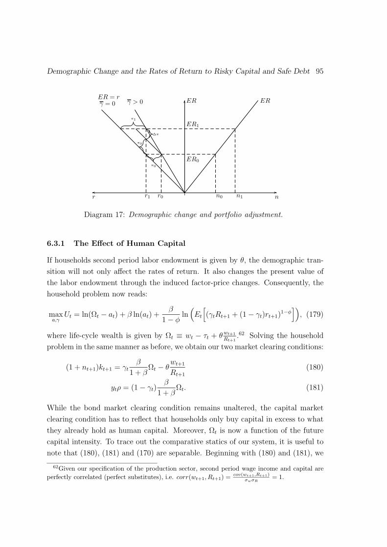
Demographic Change and the Rates of Return to Risky Capital and Safe Debt 95
nr n0 n1r0r1
ER ER
ER0
ER1
γ > 0ER = rγ = 0
π1
π0
π0
∆π
1
Diagram 17: Demographic change and portfolio adjustment.
6.3.1 The Effect of Human Capital
If households second period labor endowment is given by θ, the demographic tran-
sition will not only affect the rates of return. It also changes the present value of
the labor endowment through the induced factor-price changes. Consequently, the
household problem now reads:
maxa,γ
Ut = ln(Ωt − at) + β ln(at) +β
1− φln
(Et
[(γtRt+1 + (1− γt)rt+1)
1−φ]), (179)
where life-cycle wealth is given by Ωt ≡ wt − τt + θwt+1
Rt+1.62 Solving the household
problem in the same manner as before, we obtain our two market clearing conditions:
(1 + nt+1)kt+1 = γtβ
1 + βΩt − θ
wt+1
Rt+1
(180)
ytρ = (1− γt)β
1 + βΩt. (181)
While the bond market clearing condition remains unaltered, the capital market
clearing condition has to reflect that households only buy capital in excess to what
they already hold as human capital. Moreover, Ωt is now a function of the future
capital intensity. To trace out the comparative statics of our system, it is useful to
note that (180), (181) and (170) are separable. Beginning with (180) and (181), we
62Given our specification of the production sector, second period wage income and capital areperfectly correlated (perfect substitutes), i.e. corr(wt+1, Rt+1) = cov(wt+1,Rt+1)
σwσR= 1.
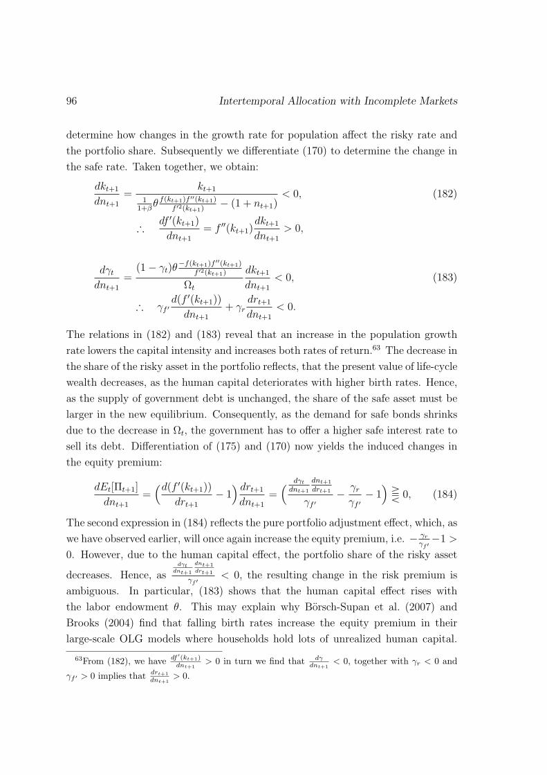
96 Intertemporal Allocation with Incomplete Markets
determine how changes in the growth rate for population affect the risky rate and
the portfolio share. Subsequently we differentiate (170) to determine the change in
the safe rate. Taken together, we obtain:
dkt+1
dnt+1
=kt+1
11+β
θ f(kt+1)f ′′(kt+1)f ′2(kt+1)
− (1 + nt+1)< 0, (182)
∴df ′(kt+1)
dnt+1
= f ′′(kt+1)dkt+1
dnt+1
> 0,
dγtdnt+1
=(1− γt)θ
−f(kt+1)f ′′(kt+1)f ′2(kt+1)
Ωt
dkt+1
dnt+1
< 0, (183)
∴ γf ′d(f ′(kt+1))
dnt+1
+ γrdrt+1
dnt+1
< 0.
The relations in (182) and (183) reveal that an increase in the population growth
rate lowers the capital intensity and increases both rates of return.63 The decrease in
the share of the risky asset in the portfolio reflects, that the present value of life-cycle
wealth decreases, as the human capital deteriorates with higher birth rates. Hence,
as the supply of government debt is unchanged, the share of the safe asset must be
larger in the new equilibrium. Consequently, as the demand for safe bonds shrinks
due to the decrease in Ωt, the government has to offer a higher safe interest rate to
sell its debt. Differentiation of (175) and (170) now yields the induced changes in
the equity premium:
dEt[Πt+1]
dnt+1
=(d(f ′(kt+1))
drt+1
− 1) drt+1
dnt+1
=( dγt
dnt+1
dnt+1
drt+1
γf ′− γrγf ′
− 1)
T 0, (184)
The second expression in (184) reflects the pure portfolio adjustment effect, which, as
we have observed earlier, will once again increase the equity premium, i.e. − γr
γf ′−1 >
0. However, due to the human capital effect, the portfolio share of the risky asset
decreases. Hence, asdγt
dnt+1
dnt+1drt+1
γf ′< 0, the resulting change in the risk premium is
ambiguous. In particular, (183) shows that the human capital effect rises with
the labor endowment θ. This may explain why Borsch-Supan et al. (2007) and
Brooks (2004) find that falling birth rates increase the equity premium in their
large-scale OLG models where households hold lots of unrealized human capital.
63From (182), we have df ′(kt+1)dnt+1
> 0 in turn we find that dγdnt+1
< 0, together with γr < 0 and
γf ′ > 0 implies that drt+1dnt+1
> 0.
Demographic Change and the Rates of Return to Risky Capital and Safe Debt 97
Accordingly, the simulations of Brooks (2002) and Geanakoplos et al. (2004) yield the
opposite result for smaller three- and four-generation-overlapping models. Diagram
18 illustrates the human capital effect to the portfolio adjustment problem.
rr0 r1
ER
ER0
ER1
γ0
γ1 γ = 0
π1
π0
∆πh
rr0 r1
ER
ER0
ER1
γ0
γ1 γ = 0
π1
π0
∆πh
1
Diagram 18: The human capital effect and portfolio adjustment.If the human capital effect is large (small), the equity premium is destined to fall(rise) if a large cohort enters the labor market.
6.3.2 The Portfolio Decision
In the previous section attention was confined to an economy where the TFP shock
was log-normal and utility of the CRRA variety. In this section we show, that the
asymmetry in the portfolio adjustment, which was driving our earlier results, carries
over to a more general setting where utility is only assumed to be concave. Moreover,
TFP shocks are no longer assumed to be log-normal. In this case, the two-period
98 Intertemporal Allocation with Incomplete Markets
two-asset problem is given by:64
maxγt
U(Ωt − st) + βEt[U((rt+1 + γt(Rt+1 − rt+1))st)], (186)
performing a second order Taylor-series expansion of the objective function at the
point where γ = 0 yields the portfolio problem:
maxγt,st
U(strt+1) + U ′(strt+1)Et[γtst(Rt+1 − rt+1)] (187)
+1
2U ′′(strt+1)Et[(γtst(Rt+1 − rt+1))
2],
where we have dropped the constant β in (187). The corresponding optimal portfolio
share is thus given by:
γ∗t = −U′(strt+1)
U ′′(strt+1)
E[Rt+1 − rt+1]
st(σ2R + Et[(Rt+1 − rt+1)]2)
(188)
=|CRRA,r≈11
φ
E[Rt+1 − rt+1]
σ2R + Et[(Rt+1 − rt+1)]2
.
64Note that there are two ways to think about the savings decision:
maxγt,st
U(Ωt − st) + βEt[U((rt+1 + γt(Rt+1 − rt+1))st)].
expanding (186) at the point γ = 0 and s = s, we have:
U(Ωt − st) + βU(strt+1) (185)
+βU ′(strt+1)E[Rt+1 − rt+1]stγt +12βU ′′(strt+1)
(E[Rt+1 − rt+1]stγt
)2
+(− U ′(Ωt − st) + βU ′(strt+1)rt+1
)(st − st)
+12
(U ′′(Ω− st) + βU ′′(strt+1)r2
t+1
)(st − st)2
+γtE[Rt+1 − rt+1]βU ′(strt+1)(U ′′(strt+1)
U ′(strt+1)rt+1st + 1
)(st − st).
The last term in (185) indicates the interaction between the size and the composition of the portfolio(cross derivative). There are now two ways to think of our approximation in the main text: (i)The household chooses savings according to the usual Euler equation and chooses the portfolioshares according to the Taylor approximation (187). Put differently, the household chooses savingsaccording to a precise rule. The portfolio shares, however, rely on an approximation. (ii) Thehousehold chooses both s and γ according to (185). In this (less appealing) case there would bean additional component in the FOC for γ of ambiguous sign.
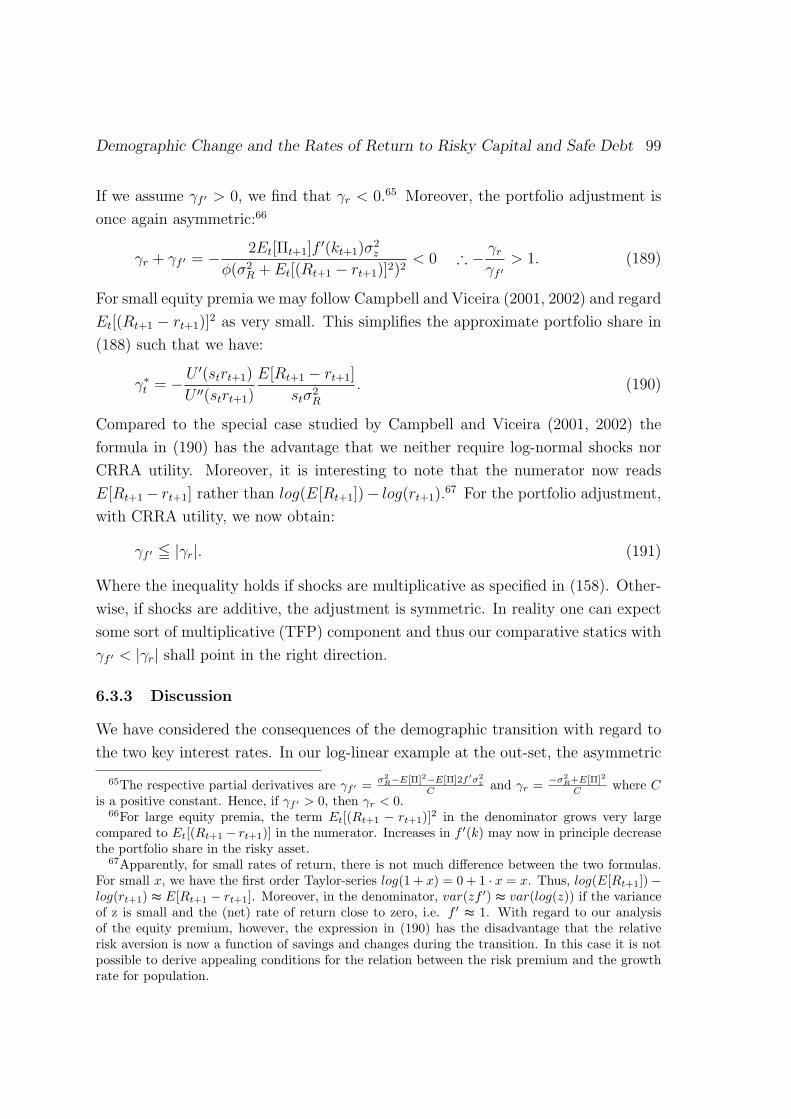
Demographic Change and the Rates of Return to Risky Capital and Safe Debt 99
If we assume γf ′ > 0, we find that γr < 0.65 Moreover, the portfolio adjustment is
once again asymmetric:66
γr + γf ′ = − 2Et[Πt+1]f′(kt+1)σ
2z
φ(σ2R + Et[(Rt+1 − rt+1)]2)2
< 0 ∴ − γrγf ′
> 1. (189)
For small equity premia we may follow Campbell and Viceira (2001, 2002) and regard
Et[(Rt+1 − rt+1)]2 as very small. This simplifies the approximate portfolio share in
(188) such that we have:
γ∗t = −U′(strt+1)
U ′′(strt+1)
E[Rt+1 − rt+1]
stσ2R
. (190)
Compared to the special case studied by Campbell and Viceira (2001, 2002) the
formula in (190) has the advantage that we neither require log-normal shocks nor
CRRA utility. Moreover, it is interesting to note that the numerator now reads
E[Rt+1− rt+1] rather than log(E[Rt+1])− log(rt+1).67 For the portfolio adjustment,
with CRRA utility, we now obtain:
γf ′ 5 |γr|. (191)
Where the inequality holds if shocks are multiplicative as specified in (158). Other-
wise, if shocks are additive, the adjustment is symmetric. In reality one can expect
some sort of multiplicative (TFP) component and thus our comparative statics with
γf ′ < |γr| shall point in the right direction.
6.3.3 Discussion
We have considered the consequences of the demographic transition with regard to
the two key interest rates. In our log-linear example at the out-set, the asymmetric
65The respective partial derivatives are γf ′ = σ2R−E[Π]2−E[Π]2f ′σ2
z
C and γr = −σ2R+E[Π]2
C where Cis a positive constant. Hence, if γf ′ > 0, then γr < 0.
66For large equity premia, the term Et[(Rt+1 − rt+1)]2 in the denominator grows very largecompared to Et[(Rt+1 − rt+1)] in the numerator. Increases in f ′(k) may now in principle decreasethe portfolio share in the risky asset.
67Apparently, for small rates of return, there is not much difference between the two formulas.For small x, we have the first order Taylor-series log(1 + x) = 0 + 1 · x = x. Thus, log(E[Rt+1])−log(rt+1) ≈ E[Rt+1 − rt+1]. Moreover, in the denominator, var(zf ′) ≈ var(log(z)) if the varianceof z is small and the (net) rate of return close to zero, i.e. f ′ ≈ 1. With regard to our analysisof the equity premium, however, the expression in (190) has the disadvantage that the relativerisk aversion is now a function of savings and changes during the transition. In this case it is notpossible to derive appealing conditions for the relation between the risk premium and the growthrate for population.
100 Intertemporal Allocation with Incomplete Markets
portfolio adjustment behavior was relating the equity-premium positively to the
growth rate of population. A higher level of interest was associated with a higher
risk-premium and viceversa.
In a more general setting with a human-capital effect this result was dampened.
An increase in the growth rate for population lowers the present value of second
period human-capital and increases savings in the risky asset. Moreover, the present
value of life cycle wealth falls. This effect lowers the demand for safe second-period
consumption and forces the government to increase the safe rate to sell its debt.
If this effect is sufficiently large, the initial conclusion may be reversed. Finally,
we relaxed our assumptions on the stochastic processes and the utility function to
conclude that the asymmetry in the portfolio adjustment is robust.
nr n0 n1r0,1
ER
ER0
ER1A1
γγ = 0
b
A0b
∆π = ∆R
1
Diagram 19: Myopic adjustment.If the demographic transition is unanticipated or the link between the rate of returnto capital not understood, the demographic transition will lower the expected riskpremium one for one.
Against this background it may be interesting to note that the relation between
the demographic structure and the risk-free rate is a fragile one. If households do
not understand that faster population growth dilutes the capital stock and raises
the risky rate, they do not demand a higher safe return to by safe bonds. In this
case, the equity premium increases one for one with the risky rate as Diagram 19
indicates. Apparently, the same effect is at work when fertility is stochastic, i.e.,
when each change in the growth rate for population is unanticipated as in the models
of Abel (2001b, 2003).

Demographic Change and the Rates of Return to Risky Capital and Safe Debt 101
6.4 Conclusion
Motivated by the conflicting results of previous simulation-based studies, we have
discussed the link between the entrance of smaller cohorts into the labor market
and the equity premium in a simple two-generations-overlapping economy. In this
framework it was shown that the entrance of a large (small) cohort into the labor
market will lead to a higher (lower) expected equity premium. While both rates of
return rise (fall), the risky rate will rise (fall) by more than the riskless rate.
In this setting, the positive link between the growth rate for population and
the equity premium is indirect. It operates through the capital widening effect
which increases the expected risky rate and forces the government to offer a higher
riskless rate to sell its debt. The increase in the equity premium is solely due to the
asymmetric portfolio adjustment behavior, i.e. γf ′ < |γr|.Myopia on the side of the households will amplify these effects. In the special
case of fully myopic households, there is a one for one relation between the risky
rate and the equity premium. However, in the case where households also antici-
pate changes in their implicit human capital holdings, our conclusions are no-longer
unambiguous. Increasing population growth lowers the present value of human cap-
ital. This reduces the demand for safe assets. Consequently, the government needs
to raise its riskfree rate more than in the case without human capital. That is, the
current model predicts that the rates of return to safe and risky assets will fall dur-
ing the demographic transition. The consequences for the equity premium, however,
are ambiguous.
102 References
References
Aaron, H. (1966). The social insurance paradox. Canadian Journal of Economics
and Political Science, 32(3):371–374.
Abel, A. B. (1989). The implications of insurance for the efficacy of fiscal policy.
The Journal of Risk and Insurance, 55(9):339–378.
Abel, A. B. (2001a). The effects of investing social security funds in the stock
market when fixed costs prevent some households from holding stocks. American
Economic Review, 91(1):128–148.
Abel, A. B. (2001b). Will bequests attenuate the predicted meltdown in stock prices
when baby boomers retire. Rewiew of Economics and Statistics, 83(4):589–595.
Abel, A. B. (2003). The effects of a baby boom on stock prices and capital accumu-
lation in the presence of social security. Econometrica, 71(2):551–578.
Abel, A. B., Mankiw, N. G., Summers, L. H., and Zeckhauser, R. J. (1989). Assessing
dynamic efficiency: Theory and evidence. Review of Economic Studies, 56(1):1–
19.
Abio, G., Mahieu, C., and Paxtot, C. (2004). On the optimality of payg pension
systems in an endogenous fertility setting. Journal of Pension Economics and
Finance, 3(1):35–62.
Allais, M. (1947). Economie et interet. Imprimerie Nationale.
Angel, M. and Garcia, L. (2008). On the role of public debt in an OLG model with
endogeneous labor supply. Journal of Macroeconomics, 30:1323–1328.
Arrow, K. J. (1970). Essays in the Theory of Risk Bearing. Amsterdam: North-
Holland Publishing.
Arthur, W. B. and McNicoll, G. (1977). Optimal time paths with age-dependency:
A theory of population policy. Review of Economic Studies, 44(1):111–123.
Arthur, W. B. and McNicoll, G. (1978). Samuelson, population and intergenera-
tional transfers. International Economic Review, 19(1):241–246.
References 103
Ball, L. and Mankiw, G. (2001). Intergenerational risk sharing in the spirit of Arrow,
Debreu, and Rawls, with applications to social security design. NBER Working
Paper, (8270):1–40.
Ball, L. and Mankiw, G. (2007). Intergenerational risk sharing in the spirit of arrow,
debreu, and rawls, with applications to social security design. Journal of Political
Economy, 115(4):523–547.
Belan, P. and Pestieau, P. (1999). Privatizing social security: A critical assessment.
The Geneva Papers on Risk and Insurance, 24(1):114–130.
Bester, H. (1984). Increasing risk and equilibrium under uncertainty. Journal of
Economic Theory, 33:378–386.
Bhagwati, J. (1958). Immiserizing growth: A geometrical note. Review of Economic
Studies, 25(3):201–205.
Blanchard, O. J. and Fischer, S. (1989). Lectures on Macroeconomics. Cambridge,
MA: MIT Press.
Bohn, H. (1998). Risk sharing in a stochastic overlapping generations economy.
Economics Working Paper Series, (1076):1–44.
Bohn, H. (2003). Intergenerational risk sharing and fiscal policy. Working paper,
University of California at Santa Barbara, pages 1–35.
Bommier, A. and Lee, R. D. (2003). Overlapping generations models with realistic
demography. Journal of Population Economics, (16):135–160.
Breyer, F. (1989). On the intergenerational pareto efficiency of pay-as-you-go fi-
nanced pension systems. Journal of Institutional and Theoretical Economics,
(145):643–658.
Brooks, R. (2002). Asset-market effects of the baby boom and social-security reform.
American Economic Review, 92(2):402–406.
Brooks, R. (2004). The equity premium and the baby boom. Econometric Society
Wintermeeting 2004, (155):1–25.
104 References
Borsch-Supan, A., Ludwig, A., and Sommer, M. (2007). Aging and asset prices.
MEA Discussion Paper, (129):1–75.
Borsch-Supan, A., Ludwig, A., and Winter, J. (2006). Aging, pension reform, and
capital flows: A multi-country simulation model. Economica, (73):625–658.
Borsch-Supan, A. and Reil-Held, A. (2001). How much is transfer and how much is
insurance in a pay-as-you-go system? The german case. Scandinavian Journal of
Economics, 103(3):505–524.
Burmeister, E. and Dobell, A. R. (1970). Mathematical Theories of Economic
Growth. MacMillan, New York.
Campbell, J. Y. and Feldstein, M. (1999). Risk Aspects of Investment-Based Social
Security Reform. University of Chicago Press, Chicago.
Campbell, J. Y. and Viceira, L. M. (2001). Appendix to Strategic Asset Allocation.
http://kuznets.fas.harvard.edu/ campbell/papers.html.
Campbell, J. Y. and Viceira, L. M. (2002). Strategic Asset Allocation. Oxford
University Press, Oxford.
Cass, D. (1972). On capital overaccumulation in the aggregative neoclassical model
of economic growth: A complete chracterization. Journal of Economic Theory,
4:200–223.
Cass, D. and Yaari, M. E. (1966). A re-examination of the pure consumption loans
model. Journal of Political Economy, 74(4):353–367.
Cass, D. and Yaari, M. E. (1967). Individual saving, aggregate capital accumulation,
and efficient growth. In Essays on the Theory of Optimal Economic Growth, pages
233–268. ed. Karl Shell, MIT Press.
Cigno, A. and Luporini, A. (2006). Optimal policy towards families with different
amounts of social capital, in the presence of asymmetric information and stochas-
tic fertility. CESifo Working Paper, (1664):1–28.
Crettez, B., Michel, P., and Wigniolle, B. (2002). Debt neutrality and the infinite-
lived representative consumer. Journal of Public Economic Theory, 4(4):499–521.
References 105
De La Croix, D. and Michel, P. (2002). A Theory of Economic Growth. Cambridge:
Cambridge Univ. Press.
Deardorff, A. V. (1976). The optimum growth rate for population: Comment.
International Economic Review, 17(2):510–515.
Diamond, P. A. (1965). National debt in a neoclassical growth model. American
Economic Review, 55(5):1126–1150.
Diamond, P. A. (1977). A framework for social security analysis. Journal of Public
Economics, 8(3):275–298.
Diamond, P. A. (1996). Proposals to restructure social security. The Journal of
Economic Perspectives, 10(3):67–88.
Diamond, P. A. (2000). Towards an optimal social security design. CeRP Working
Paper, (4):4–17.
Diamond, P. A. and Geanakoplos, J. (2003). Social security investment in equities.
American Economic Review, 93(4):1047–1074.
Enders, W. and Lapan, H. E. (1982). Social security taxation and intergenerational
risk sharing. International Economic Review, 23(3):647–658.
Epstein, L. G. and Zin, S. E. (1989). Substitution, risk aversion, and the temporal
behavior of consumption and asset returns: A theoretical framework. Economet-
rica, 57(4):937–969.
Fenge, R. (1995). Pareto-efficiency of the pay-as-you-go pension system with intra-
generational fairness. Finanzarchiv, 52(3):357–363.
Finetti, B. D. (1952). Sulla preferibilita. Annali di Economica, (11):685–709.
Fischer, S. (1983). Welfare aspects of government issue of indexed bonds. In Infla-
tion, Debt and Indexation, pages 223–246. ed. R. Dornbusch and M. Simonsen,
MIT Press.
Friedman, M. (1999). Speaking the truth about social security reform. Cato Institute
Briefing Papers, (46):1–3.
106 References
Gale, D. (1973). Pure exchange equilibrium of dynamic economic models. Journal
of Economic Theory, 6:12–36.
Gale, D. (1990). The efficient design of public debt. In Public debt management:
theory and history, pages 14–41. ed. R. Dornbusch and M. Draghi, Camebridge
University Press.
Galor, O. (1988). The long-run implications of a Hicks-neutral technical progress.
International Economic Review, 29(1):177–183.
Geanakoplos, J., Magill, M., and Quinzii, M. (2004). Demography and the long-
run predictability of the stock market. Cowels Foundation Discussion Paper,
(1380R):1–53.
Gollier, C. (2001). The Economics of Risk and Time. MIT Press.
Golosov, M., Jones, L., and Tertilt, M. (2007). Efficiency with endogenous popula-
tion growth. Econometrica, 75(4):1039–1072.
Gordon, R. H. and Varian, H. R. (1988). Intergenerational risk sharing. Journal of
Public Economics, 37(1):185–202.
Gottardi, P. and Kubler, F. (2008). Social security and risk sharing. Working Paper,
pages 1–40.
Green, J. R. (1977). Mitigating demographic risk through social insurance. NBER
Working Paper, (215):1–32.
Homburg, S. (1987). Theorie der Alterssicherung. Springer Verlag.
Ihori, T. (1978). The golden rule and the role of government in a life cycle growth
model. American Economic Review, 68(3):389–396.
Jaeger, K. (1989). The serendipity theorem reconsidered: The three-generations
case without inheritance. In Economic theory of optimal population, pages 75–87.
ed. K. F. Zimmermann, Springer.
Jaeger, K. and Kuhle, W. (2009). The optimum growth rate for population recon-
sidered. Journal of Population Economics, 22(1):23–41.
References 107
Jones, H. G. (1975). An Introduction to Modern Theories of Economic Growth.
London: Nelson.
Kimball, M. S. (1990). Precautionary savings in the small and in the large. Econo-
metrica, 58(1):53–73.
Kruger, D. and Kubler, F. (2006). Pareto improving social security reform when
financial markets are incomplete. American Economic Review, 96(3):737–755.
Kruger, D. and Ludwig, A. (2007). On the consequences of demographic change for
rates of return to capital, and the distribution of wealth and welfare. Journal of
Monetary Economics, (54):49–87.
Krohn, L. D. (1981). The generational optimum economy: Extracting monopoly
gains from posterity through taxation of capital. American Economic Review,
71(3):411–420.
Kuhle, W. (2007). The Optimum Growth Rate for Population in the Neoclassical
Overlapping Generations Model. Peter Lang, Frankfurt et al.
Kuhle, W. (2009a). Dynamic efficiency and the two-part golden rule. Universitat
Mannheim mimeographed, pages 1–23.
Kuhle, W. (2009b). The optimum structure for government debt. MEA Discussion
Paper, pages 1–28.
Lerner, A. P. (1959). Consumption-loan interest and money. Journal of Political
Economy, 67(5):512–518.
Ludwig, A. and Reiter, M. (2009). Sharing demographic risk - who is afraid of the
baby bust. Working Paper Koln University, pages 1–47.
Malinvaud, E. (1953). Capital accumulation and efficient allocation of resources.
Econometrica, 21(2):233–268.
Marquetti, A. A. (2004). Extended penn world tables 2.1. http://homepage.
newschool.edu/~foleyd/epwt[12.10.2006].
Mas-Colell, A., Whinston, M. D., and Green, J. R. (1995). Microeconomic Theory.
Oxford University Press.

108 References
Matsuyama, K. (1991). Immiserizing growth in Diamonds overlapping generations
model: A geometrical exposition. International Economic Review, 32(1):251–262.
Merton, R. (1983). On the role of social security as a means for efficient risk sharing
in an economy where human capital is not tradable. In Financial Aspects of
the United States Pension System, pages 259–290. ed. Z. Bodie and J. Shoven,
University of Chicago Press, Chicago.
Michel and Pestieau (1993). Population growth and optimality: When does serendip-
ity hold. Journal of Population Economics, 6(4):353–362.
Persson and Tabellini (2000). Political Economics. MIT Press.
Pestieau, P., Paiser, G., and Sato, M. (2006). PAYG pension systems with capital
mobility. International Tax and Public Finance, 13:587–599.
Phelps, E. (1961). The golden rule of accumulation: A fable for growthmen. Amer-
ican Economic Review, 51(4):638–643.
Phelps, E. (1966a). The golden rule of procreation. In Golden Rules of Economic
Growth, pages 176–183. ed. Edmund Phelps, North Holland Publishing Company,
Amsterdam.
Phelps, E. (1966b). Golden Rules of Economic Growth. North Holland Publishing
Company, Amsterdam.
Phelps, E. (1968). Population increase. Canadian Journal of Economics, 1(3):497–
518.
Poterba, J. M. (2001). Demographic structure and asset returns. Review of Eco-
nomics and Statistics, 83(4):565–584.
Poterba, J. M., Venti, S., and Wise, D. A. (2005). Demographic change, retirement
saving, and financial market returns: Part 1. Working Paper, pages 1–33.
Pratt, J. W. (1964). Risk aversion in the small and in the large. Econometrica,
32(1):122–136.
Samuelson, P. A. (1947). Foundations of Economic Analysis. Cambridge Ma.:
Harvard University Press.
References 109
Samuelson, P. A. (1954). The pure theory of public expenditure. Review of Eco-
nomics and Statistics, 36(4):386–389.
Samuelson, P. A. (1958). An exact consumption-loan model of interest with or
without the social contrivance of money. Journal of Political Economy, 66(6):467–
482.
Samuelson, P. A. (1959). Consumption-loan interest and money: Reply. Journal of
Political Economy, 67(5):518–522.
Samuelson, P. A. (1962). Parable and realism in capital theory: The surrogate
production function. Review of Economic Studies, (29):193–206.
Samuelson, P. A. (1968). The two-part golden rule deduced as the asymptotic
turnpike of catenary motions. Western Economic Journal, (VI , March, 1968):85–
89.
Samuelson, P. A. (1969). Lifetime portfolio selection by dynamic stochastic pro-
gramming. Review of Economics and Statistics, 51(3):239–246.
Samuelson, P. A. (1975a). The optimum growth rate for population. International
Economic Review, 16(3):531–538.
Samuelson, P. A. (1975b). Optimum social security in a life-cycle growth model.
International Economic Review, 16(3):539–544.
Samuelson, P. A. (1976). The optimum growth rate for population: Agreement and
evaluations. International Economic Review, 17(2):516–525.
Shell, K. (1971). Notes on the economics of infinity. Journal of Political Economy,
79(5):1002–1011.
Shiller, R. (1999). Social security and institutions for intergenerational, intragener-
ational and international risk sharing. Carnegie-Rochester Conference Series on
Public Policy, 50:165–204.
Sinn, H. W. (1989). Economic Decisions Under Uncertainty. Physica-Verlag: Hei-
delberg, 2. edition.
110 References
Sinn, H. W. (2000). Why a funded pension system is useful and why it is not useful.
International Tax and Public Finance, 7(4-5):389–410.
Smetters, K. (2006). Risk sharing across generations without publicly owned equi-
ties. Journal of Monetary Economics, 53(7):1493–1508.
Solow, R. M. (1956). A contribution to the theory of economic growth. Quarterly
Journal of Economics, 70(1):65–94.
Stein, J. L. (1969). A minimal role of government in achieving optimal growth.
Economica, 36(142):139–150.
Swan, T. W. (1956). Economic growth and capital accumulation. The Economic
Record, 32(November):334–361.
von Weizsacker, C. C. (1962). Wachstum , Zins und Optimale Investitionsquote.
Kyklos, Basel.
Zilcha, I. (1990). Dynamic efficiency in overlapping generations models with stochas-
tic production. Journal of Economic Theory, 52:364–379.

Eidesstattliche Erklarung
Hiermit erklare ich, dass ich diese Dissertation selbstandig angefertigt und mich
anderer als der in ihr angegebenen Hilfsmittel nicht bedient habe, insbesondere,
dass aus anderen Schriften Entlehnungen, soweit sie in dieser Dissertation nicht
ausdrucklich als solche gekennzeichnet und mit Quellenangaben versehen sind, nicht
stattgefunden haben.
Mannheim, 25.4.2010 Wolfgang Kuhle

Lebenslauf
Wolfgang Kuhle
Geburtsort: Gottingen
Staatsangehorigkeit: deutsch
Familienstand: ledig
Ausbildung:
• (2001) Theodor-Heuss-Gymnasium Gottingen: Abitur in den Fachern Physik,
Geschichte, Chemie und Deutsch
• (2006) Freie Universitat Berlin: Diplom in Volkswirtschaftslehre
• (2007)-(2010) Promotionsstudium in den Fachern VWL und Mathematik an
der Universitat Mannheim
Berufserfahrung:
• (2001-2002) Wehrdienst: Jagertruppe in Hammelburg
• (2005-2007) Studentischer Mitarbeiter am Lehrstuhl fur Wirtschaftstheorie
Freie Universitat Berlin
• (2007-2010) Wissenschaftlicher Mitarbeiter am MEA Universitat Mannheim