Karina Doorley - core.ac.uk · Citation of such a paper should account for its provisional...

econstor www.econstor.eu

Der Open-Access-Publikationsserver der ZBW – Leibniz-Informationszentrum WirtschaftThe Open Access Publication Server of the ZBW – Leibniz Information Centre for Economics

Standard-Nutzungsbedingungen:

Die Dokumente auf EconStor dürfen zu eigenen wissenschaftlichenZwecken und zum Privatgebrauch gespeichert und kopiert werden.

Sie dürfen die Dokumente nicht für öffentliche oder kommerzielleZwecke vervielfältigen, öffentlich ausstellen, öffentlich zugänglichmachen, vertreiben oder anderweitig nutzen.

Sofern die Verfasser die Dokumente unter Open-Content-Lizenzen(insbesondere CC-Lizenzen) zur Verfügung gestellt haben sollten,gelten abweichend von diesen Nutzungsbedingungen die in der dortgenannten Lizenz gewährten Nutzungsrechte.

Terms of use:

Documents in EconStor may be saved and copied for yourpersonal and scholarly purposes.

You are not to copy documents for public or commercialpurposes, to exhibit the documents publicly, to make thempublicly available on the internet, or to distribute or otherwiseuse the documents in public.

If the documents have been made available under an OpenContent Licence (especially Creative Commons Licences), youmay exercise further usage rights as specified in the indicatedlicence.

zbw Leibniz-Informationszentrum WirtschaftLeibniz Information Centre for Economics

Sierminska, Eva; Doorley, Karina

Working Paper

To Own or Not to Own? Household Portfolios,Demographics and Institutions in a Cross-NationalPerspective

IZA Discussion Paper, No. 7734

Provided in Cooperation with:Institute for the Study of Labor (IZA)

Suggested Citation: Sierminska, Eva; Doorley, Karina (2013) : To Own or Not to Own?Household Portfolios, Demographics and Institutions in a Cross-National Perspective, IZADiscussion Paper, No. 7734

This Version is available at:http://hdl.handle.net/10419/90083

DI

SC

US

SI

ON

P

AP

ER

S

ER

IE

S

Forschungsinstitut zur Zukunft der ArbeitInstitute for the Study of Labor

To Own or Not to Own?Household Portfolios, Demographics and Institutions in a Cross-National Perspective

IZA DP No. 7734

November 2013

Eva SierminskaKarina Doorley

To Own or Not to Own?

Household Portfolios, Demographics and Institutions in a Cross-National Perspective

Eva Sierminska CEPS/INSTEAD, DIW Berlin and IZA

Karina Doorley

IZA and CEPS/INSTEAD

Discussion Paper No. 7734 November 2013

IZA

P.O. Box 7240 53072 Bonn

Germany

Phone: +49-228-3894-0 Fax: +49-228-3894-180

E-mail: [email protected]

Any opinions expressed here are those of the author(s) and not those of IZA. Research published in this series may include views on policy, but the institute itself takes no institutional policy positions. The IZA research network is committed to the IZA Guiding Principles of Research Integrity. The Institute for the Study of Labor (IZA) in Bonn is a local and virtual international research center and a place of communication between science, politics and business. IZA is an independent nonprofit organization supported by Deutsche Post Foundation. The center is associated with the University of Bonn and offers a stimulating research environment through its international network, workshops and conferences, data service, project support, research visits and doctoral program. IZA engages in (i) original and internationally competitive research in all fields of labor economics, (ii) development of policy concepts, and (iii) dissemination of research results and concepts to the interested public. IZA Discussion Papers often represent preliminary work and are circulated to encourage discussion. Citation of such a paper should account for its provisional character. A revised version may be available directly from the author.

mailto:[email protected]

IZA Discussion Paper No. 7734 November 2013

ABSTRACT

To Own or Not to Own? Household Portfolios, Demographics and Institutions in a Cross-National Perspective*

Using harmonized wealth data and a novel decomposition approach, we show that cohort effects exist in the income profiles of asset and debt portfolios for a sample of European countries, the U.S. and Canada. We find that younger households’ participation decisions in assets are more responsive to income than older households. Family structure plays a significant role in explaining cross-country differences for both cohorts. Examining institutional differences, we find that in more financially developed and economically open countries, households are less likely to own housing but more likely to be in debt. Typical mortgage characteristics and mathematical literacy are also correlated with debt participation across countries. These findings have important implications for policy setting during times of financial unease for the young, as well as for the future in helping secure adequate income for the elderly. Our results show that there is scope for policies which promote asset participation for young households and debt participation, where there is a need for consumpation smoothing, for older households. JEL Classification: G11, G21, J10 Keywords: wealth portfolios, decomposition, institutions, demographics Corresponding author: Karina Doorley IZA P.O. Box 7240 53072 Bonn Germany E-mail: [email protected]

* We would like to thank seminar participants at IZA, CEPS/INSTEAD, Bank of France, INED, University of Graz and ECINEQ conference participants for helpful suggestions and comments. This research is part of the WealthPort project (Household Wealth Portfolios in a Comparative Perspective) supported by the Luxembourg ‘Fonds National de la Recherche’ (contract CORE C09/LM/04) and by core funding for CEPS/INSTEAD by the Ministry of Higher Education and Research of Luxembourg. An earlier version of this paper is entitled: Decomposing household wealth portfolios across countries: An age-old question?

mailto:[email protected]

1 Introduction

There has been growing interest in studying household wealth portfolios for several rea-sons. On the one hand, population aging has raised questions about the long-term sustain-ability of pension systems and the need to assess the adequacy of saving for retirementthrough the study of the level and composition of assets with which households retire(e.g. Chiuri and Jappelli (2010), Gornick et al. (2009)). On the other hand, the lastingeffects of the crisis and the resulting meltdown and subsequent appreciation of assets hashad different repercussions across various demographic groups. In addition, the growingcomplexities of wealth portfolios and the growing efforts to create a more unified marketfor consumers has sparked a literature on comparing the diversity of wealth portfolios.

Researchers have found that, despite greater integration of asset and labor market policiesin Europe, differences in market conditions among European countries are much morepronounced than within the US and that large differences in investment patterns still existin European countries, even after controlling for other household characteristics. This hasbeen found to be the case for mature households (Christelis et al. (2012)), for debt (Crookand Hochguertel (2007)) and for stockholding (Guiso et al. (2003)).

Nevertheless, despite several attempts, the literature on international portfolios is notabundant. Single or two-country studies are more common than cross-country compar-isons due to data availability and difficulties in performing cross-national comparisons.The few sources of cross-country wealth data that do exist are, generally, not directlycomparable due to differences in data collection techniques, which are shaped by theinstitutional environment and, indirectly, by the available wealth instruments. Conse-quently, a better understanding of what is captured by wealth survey data requires someknowledge of institutions. For example, a high take-up of individual loans in the US isdriven by less severe credit restraints than in other countries.

Comparable cross-country data is not easily available. For example, the Survey of Health,Aging and Retirement in Europe (SHARE) captures individuals 50 and over. The House-hold Finance and Consumption Survey (HFCS) is available for euro-zone countries onlyand some very recent studies (e.g., Bover et al. (2013)) use this to analyse wealth portfo-lios across countries during the crisis period. Another option for researchers is to rely ondata in the Luxembourg Wealth Study, which has thoroughly examined and harmonizedcomparable and non-comparable components of wealth and has made a detailed study of

country wealth components and institutions. This approach facilitates an insightful analy-sis of wealth portfolios across countries and allows comparisons across European, as wellas non-European countries.

In this paper we follow this approach and use the conceptual framework developed bythe Luxembourg Wealth Study, but apply it to independent data. We use two datasetsthat are used in the Household Finance and Consumption Survey (Italy and Spain) (butfor the pre-HFCS years) and are publicly available. In addition, we use data for Canada,Germany, Luxembourg and the United States, thus providing a unique pre-crisis view ofhousehold wealth portfolios in a cross-national perspective.

Our paper is novel in several ways. Apart from using data for a unique set of coun-tries with differential institutional backgrounds, we identify differences in asset portfoliosacross countries, focusing on differences between older and younger cohorts.1 Third, weextend the approach of Christelis et al. (2012) by disaggregating the effect of covariates inthe participation decision to discover which household characteristics contribute the mostto differences in wealth holdings across countries. 2 Our focus remains on the main assetsand liabilities held by households; financial assets, main residence, investment real estate;mortgages and non-housing debt.3

Past research suggests a large role for institutions in explaining cross-national differencesin portfolios for the older population. We show that the role of characteristics is more im-portant than previously thought. Based on surveys for the whole population, we confirmthat characteristics play a relatively minor role in the decision to participate in financialassets or principal residence investment for the over-50 population, but they do play a rolefor the younger cohort, particularly when it comes to asset participation. Financial assetsare, for example, very sensitive to income for the young. Differences in family structureat certain ages also explains a non-negligible share of cross-country differences. Youngerhouseholds’ participation decisions in assets also respond more to the institutional settingthan mature households while mature households debt decisions respond more to the in-stitutional setting than younger households. This result has implications for policy settingduring times of financial unease and for retirement planning. Measures to consider arethe promotion of savings and investment behaviour for the young, in anticipation of their

1In our reported analysis in this paper, we ultimately focus on the younger cohort and a comparison withmore mature households, as our previous work pointed to significant differences among the two.

2Sierminska et al. (2010) for example, show that labor market differences between men and womenexplain the majority of wealth differences and work in the opposite direction to demographic factors.

3Although we do not take into account other factors such as different risks and returns for financialassets it has been shown that the majority of households have only a few types of assets. Less than 35%of households in the U.S. hold risky assets in the form of stocks or mutual funds and this number is muchlower for the other countries.

2

retirement and the encouragment of debt holding, e.g., reverse mortgages, for the oldercohort in order to smooth their consumption during retirement.

In Section 2 we describe the data. Section 3 overviews the decomposition method forparticipation and discusses basic characteristics of wealth portfolios in our sample ofcountries. The results are in Section 4 and Section 5 concludes.

2 Data

In our sample, we use data for two North American countries: Canada and the US, andseveral European countries with varying institutional and welfare regimes: Germany,Italy, Luxembourg and Spain. At the time of data collection, all of these countries werein a pre-crisis stage with low unemployment and positive GDP growth (Table 1) 4. Thedata for Canada come from the 2005 Survey of Financial Security, for Germany the 2007wealth module of the Socio-Economic Panel (SOEP), for Italy the 2008 Survey of House-hold Income and Wealth (SHIW), for Luxembourg from the 2007 wealth module of thePSELL-3/EU-SILC, for Spain from the 2008 EFF and the data for the United States comefrom the 2007 Survey of Consumer Finances (SCF).

The data contain detailed information on multiple income sources and financial and non-financial assets and debts. On the basis of this detailed information, we use the conceptualframework developed by the Luxembourg Wealth Study (described in Sierminska et al.(2006)) for creating harmonized variables of net worth (total assets: financial assets, prin-cipal residence, investment real estate and business equity minus liabilities: mortgagesand non-housing debt) and income.5 The data are collected at the household level andindividual level variables that are reported (such as age, gender, education) refer to therespondent/household head. In most cases, this person is the person most knowledgeableabout household finances.

Wealth (or net worth) is defined as assets less liabilities, where assets are composed offinancial and non-financial assets. The components of wealth that we pay particular at-tention to in this study are total financial assets (which comprise deposit account, bonds,stocks, mutual funds, etc); principal residence, which equates to owner-occupied hous-ing; investment real estate, which is composed of all residential and corporate real estate

4One exception is Italy which registers a small decrease in GDP per capita in 2008, the year of datacollection.

5In the descriptive results (Table 3), each of the wealth variables have been bottom and top coded attheir 1% and 99% levels to stop outliers from over-influencing our results. Our monetary variables havebeen converted to 2007 USD using PPP and price indices.

3

besides the principal residence and, on the liabilities side, mortgage debt which can relateto the principal residence or to investment real estate and, finally, non-housing debt.

As in all cross-country studies, we face the issue of data comparability and, while our con-ceptual framework carefully alignes the most comparable components across countries,some differences among the surveys remain. Table A.1 gives an idea of the measurementdifferences that could arise due to varying collection methods. For example, financialassets are created for the most part by aggregating the individual components (depositaccounts, risky assets). In Germany and Luxembourg this is not the case. Only the totalbalance is collected 6. We consider these differences when interpreting our results.

In addition, we compare participation rates in the main assets and liabilities to two otherdata sources. Firstly, we compare the European countries in our harmonized database tothe first wave of the Household Finance and Consumption Survey (HFCS). The HFCSdata is collected in 2009-2010 which is slightly later than the data we use and the crisismay have had an impact on wealth portfolios in the meantime. However, we find that forthe comparable instruments, principle residence, investment real estate, mortgage hold-ings and non-housing debt, participation rates in these four instruments are within 5pptpoints of each other in both datasets (HFCN (2013)). Reported Financial Assets showgreater differences with Germany, Italy and Luxembourg holding much lower levels ofFinancial Assets in our harmonised datasets than in the HFCS. In part this is due to thecollection method, as shown in Table A.1, for Germany and Luxembourg and due to thefact that the HFCS data is multiply imputed for Italy while we rely on the simple im-putation performed for the public use data by the Bank of Italy. For this reason, in ouranalysis we report total financial assets, but take account of these differences in the inter-pretation of our results and focus on a subgroup of financial assets, risky assets (stocks,bonds and mutual funds), which does not suffer from these survey-related measurementerrors. Our second benchmark for checking the reliability of reported wealth holdings inour harmonized data is to compare our results for households in which the head is over50 years of age with households in the Health and Retirement Study (HRS) in the US andthe Survey of Health, Ageing and Retirement (SHARE) in Europe. Comparing our over-50 participation rates in comparable instruments (Principle Residence and Mortgage) tothose reported in (Christelis et al. (2012)), who use the HRS and SHARE datasets, wefind discrepancies of less than 4ppt. We, therefore, feel confident that our harmonizeddataset is broadly representative of wealth participation rates in the countries examined.In this paper, we ultimately focus on the younger cohort and draw comparisons with moremature household.

6In Germany, deposit accounts are not included in the aggregate, while in Luxembourg information iscollected in brackets and then imputed

4

3 Methodology

The participation decision is the decision to hold or not to hold a particular asset or li-ability. The participation rates for each asset/liability are shown in Table 2, while meanasset levels are in Table 3. There is quite a bit of cross-country variation in the decisionto hold assets, as well as liabilities. Among financial assets, risky assets (which includestocks, bonds, and mutual funds) are particularly different. In the US, the share of peopleinvesting in this type of asset is the highest, followed by Canada. Large differences arealso observed for debt. Italy has the lowest participation in debt followed by Germany,Luxembourg, Spain, Canada and the US.

The sample in both tables is further partitioned by age to highlight cohort differences inportfolio composition. The largest age differences are seen for homeownership, housingand non-housing debt. Younger households are less likely to own their home and are morelikely to have debt compared to more mature households (shown in the bottom panel ofTable 2). In a comparison across countries, we find smaller differences in participationrates among the young than among the elderly. In fact, the portfolio participation ratesin the United States and Canada are almost the same for the younger cohort, apart fromsome minor differences in business ownership and risky asset take up.

There is a strong relationship between income and participation in both assets and liabili-ties. Past research shows a variation in holdings of particular assets across the distributionwith higher income households holding a large share of risky assets (e.g. Carroll (2002)).We can also confirm that there is cross country variation in these trends. As we plot par-ticipation rates by income percentiles (Figure 1), we find that ownership rates of assetsand liabilities rise as we move up the income distribution, but there are also noticeablecross country differences. For example, there is large cross-country variation at the topof the distribution in risky asset ownership, with the US having the highest participationin our sample of countries. For debt there seem to be 2 groups: the higher debt coun-tries (Canada, Luxembourg and the US) and lower debt holdings (Germany, Italy, Spain).Spain has higher real estate ownership than every other country, particularly at the bottomof the income distribution while Germany is a low homeownership country.

Since substantial differences in asset participation by income level exist across countries,as a next step, we investigate whether there are other significant drivers of these ownershipdifferences. These differences could be driven by differences in population characteristicsbetween countries (such as household structure, education, the labor market) or could bea result of differences between countries that are more difficult to measure and capturein a regression, including institutional and cultural differences, for example. A suitable

5

way to examine these differences is to make use of an extension of the Blinder-Oaxacanonlinear decomposition for binary variables, elaborated by Fairlie (1999, 2005)

We estimate a logit model for participation in a particular wealth component w:

pj(w) = F (Xβ) (1)

and examine the differences between country j and our reference country, in this case theU.S. (j = us):

p̂us(w)− p̂j(w) =(p̂us(w)− p̂usj (w)

)+(p̂usj (w)− p̂j(w)

)(2)

where p̂usj (w) is the counterfactual participation rate of households in country j if facedwith U.S. institutional features and other unobservables, given the distribution of char-acteristics X in country j. The first expression on the right hand side of equation 2represents differences in participation due to characteristics, i.e., to differences in the dis-tribution of X between the U.S. and country j. The second term represents differencesdue to differences in the group processes determining the decision to own or not to own aparticular asset. This unexplained effect can be attributed to different cross-country riskpreferences, cultural differences, institutional differences and other unobservables acrosscountries. For simplicity, we refer to it as the unexplained or institutional effect.

The characteristic gap is the estimation of the total contribution of the whole set of ob-served characteristics to the country gap in participation. We would like to know thecontribution of each specific characteristic since it is likely that they have varying and,sometimes, opposing effects. Thus, in order to identify the contribution of specific fac-tors, we break X down into sets of characteristics: XL (labor market characteristics),XE (education characteristics), XD (demographic characteristics), XM (marital status),XI (income) and XW (the level of other wealth). Taking a simple example, assume thatX = XL +XD. We can express the independent contribution of XL to the gap as:

1

N

N∑i=1

[F (Xus

LiβusL +Xus

DiβusD )− F (Xj

LiβusL +Xus

DiβusD )]

(3)

For example, imagine that stock ownership is encouraged via employer company incen-tive plans. In this case, different employment levels between the US and country j mayexplain a portion of the difference in stock market participation between these two coun-tries. This effect will be captured in the overall characteristic effect but can also be isolated

6

from the effect of other characteristics using equation 3. Now, imagine that company in-centive plans differ across countries. This will be an institutional difference that will bepart of the unexplained difference in cross-country stock market participation levels.7

4 Results

4.1 Country differences in asset participation

In order to identify the determinants of holding a particular asset we estimate several logitspecifications for each country. We present the results for the one with the best fit. Thecoefficient estimates are used to determine whether there are country differences in thedecision to hold particular assets and to calculate the contribution of country differencesin household characteristics to the country differences in asset participation.

The dependent variable is equal to one if the household holds the asset in question andis equal to zero otherwise. We include a number of variables, which have been shownto affect participation in wealth. These include a set of demographic variables: age, thepresence of children under 18 and a set of marital status variables which consist of in-dicator variables for married and divorced. Out of these we create family types: singles,single-parents, couple without kids and couples with kids. We also include gender, educa-tion variables which have been harmonized across countries 8 and labor market variables,which include indicators for employment, self-employment and retirement for the olderpopulation. Finally, we include income and wealth levels not pertaining to the asset inquestion, transformed using the inverse hyperbolic sine.9

In a comprehensive study of household portfolios, Guiso et al. (2003) estimate the partic-ipation decision for selected assets on a common set of explanatory variables. The resultsfor the US indicate that the ownership of almost all types of assets and liabilities riseswith other wealth (except credit card balances and non-housing debt). And as wealthrises, the share of total assets held in homes and other non-financial assets declines, whilethe share in risky assets and investment real estate rises. This is also true for each of thecountries that we study as we observe a positive effect of other wealth on the participationdecision of each of the assets examined (see Table A.3 and A.4). However, we find no

7Isolating its contribution to the unexplained effect is beyond the scope of this study.8Low education indicates less than high school, medium education represents completed high school

and high education indicates completed university9We experiment with various specification of the monetary variables including levels and log transfor-

mation, but find the inverse hyperbolic sine transformation to yield the best fit.

7

conclusive evidence that the effect is larger for risky assets and investment real estate thanfor principal residence and financial assets in our sample countries.

Given that risk preference vary with age, we typically expect higher ownership of riskyassets among older cohorts. Younger people face more background risk, which affectstheir preference for risky assets. As their uncertainty about lifetime income declines andthey enter their prime-age years they may be willing to take on more risk. Older people,on the other hand, exhibit less labor supply flexibility compared to younger people. Thelatter can work more or retire later if they have low returns to their investments, the elderlyare left to rely on the retirement income. We find some evidence, looking at the marginaleffects of the 50+ households (not shown), that participation in risky assets increases withage.

Education is generally positively correlated with income and, hence, with asset holdings.Education may also be correlated with financial literacy (van Rooij et al. (2011)), with themore educated being more financially savy. We find that education increases participationin financial assets, risky assets and investment real estate for each country in our sample.We also find that it increases mortgage participaton, except in Canada and Luxembourg.

Another important explanatory characteristic can be household composition. For exam-ple, Bover (2010) find this to be important in explaining a lot of the observed differencesin the wealth distribution between the US and Spain. Other research indicates that mar-ried couples are generally better off and differences by family type are stronger than bygender (Bover (2010); Sedo and Kossoudji (2004) for housing; Yamokoski and Keister(2006) for wealth levels). We find that family types have higher explanatory power thanmarital status. In addition, since there exist strong age effects in portfolio composition,we interact household types with age. We find the the age-family-type effects can some-times be of opposite sign so that separating them by age cohort gives us more information.In Table A.3, we find that family types matter for the homeownership decision. Coupleswith children are more likely to own their home than singles or couples without chil-dren, particularly in the US, Canada and Germany. Single parents are also less likely tohold financial assets. This can be caused by two things. First, children generally lead ahousehold to incur higher expenses. Second, there is a higher probability of owning non-financial assets in households with children. In terms of debt, we find that as householdsage, they are more likely to have a mortgage, regardless of family type.

Figure 1 shows that the correlation between income and participation varies across coun-tries. From Tables A.3 and A.4, we see that the marginal effect of income is generallypositive and significant for homeownership and risky assets. For investment real estate itonly matters in the US while for financial assets, it is not significant in Italy and Spain,

8

where family gifts or bequests may play a greater role.

4.2 Decomposition of the Participation Decision

In our decomposition we focus on the assets and liabilities which constitute the main partof the portfolio: homeownership, investment real estate ownership and mortgage hold-ing. For a subset of countries we are also able to compare the effects for financial assets,risky assets and non-housing debt. We group the possible explanatory factors that can af-fect asset ownership. Demographics include family types (single, single parents, coupleswithout children and couples with children) interacted with 3 age groups (under 30, 30-39and 40-49). Education is composed of indicator variables for low and high education. Thelabor market group includes indicator variables for employed, self-employed and retired.We also include income and wealth seperately. The results for the decompositions canbe found in Tables 4 and 5 for principal residence, investment real estate, debt and finan-cial assets. We use the specification from the estimation shown in Tables A.3 to A.4 forhouseholds whose head is under 50 years of age.

Overall, we find that country differences in variables such as education, demographics andincome provide significant contributions to the wealth participation gap. The unexplainedpart of the gap varies across countries and asset types. These differences may be partlycaused by differences in institutions, but also by important unmeasurable factors such as,for example, risk preferences.

In each of the panels in tables 4 and 5, the top section reports estimates of the contributionof country differences in specific observable groups of variables to the explained portionof the participation gap. In the second panel, the probability of holding the asset in thebase country (the U.S.) P (x = 0) and the reference country P (x = 1) is reported. Next,Diff indicates the raw participation gap, Exp refers to the explained gap (due to charac-teristics) and Unexp the unexplained gap (due to institutions or culture). In the adjacentcolumn, for each country we show the percentage each set of characteristics contributesto the explained gap and, below this, we report the ratio of the explained and unexplainedgaps to the base participation in the U.S.

For example, looking at let top left panel of Table 4, we see that 62.6% of U.S. house-holds and 59.6% of Canadian households own their principal residence. 29% less Cana-dian households own their own home than U.S. households for explained reasons (thiscorresponds to a 18ppt counterfactual gap in homeownership if the institutional setting inCanada was identical to that in the U.S.). This explained gap is largely due to differences

9

in income between Canadian and U.S. households (as evidenced by the 71% contribu-tion of this variable to the explained gap). The unexplained gap is -24% meaning that,if Canadian households were like U.S. households in their characteristics - in this case,that would mainly require a convergence of their income levels to U.S. levels - 24% moreCanadian households would own their own home than U.S. households. This gap can beattributed to different institutional or cultural features of the two countries. So, to sum-marize, this decomposition tells us that, while U.S. households own their own home moreoften than Canadian households, this gap would be even larger were it not for institutionalor other differences between the two countries which encourage Canadian households tobuy their own home.

Principal residence First, we examine real estate. U.S. households are more likelyto own their main residence than those in Canada, Germany and Italy while the oppositeis true in Luxembourg and Spain. Raw participation gaps are small except in Germany(31 ppt), which has traditionally had very low homeownership rates and Spain (-14 ppt)which has quite high homeownership rates. However, in the case of Canada, Spain andItaly, the small raw participation gaps mask larger explained and unexplained gaps whichwork in opposite directions. In each of the countries except Luxembourg, the character-istics of U.S. households, mainly income and household composition, lead them to havehigher homeownership rates. In terms of household composition, the contribution of thetwo older household categories (30-39 and 40-49 years old) is higher than that of theyoungest category (20-29 years old). This indicates that it is cross-country differences inthe composition of this group of households, (the 30-49 year olds) that explain most ofthe explained demographic participation gap. In Canada, Italy and Spain, the unexplainedgaps are negative, indicating that these countries would have higher homeownership ratesif their households’ characteristics were the same as those in the U.S. Only in Germanyis there a large positive unexplained gap which reflects this country’s traditionally lowhomeownership rates for reasons unrelated to household characteristics.

Investment real estate The U.S. has a higher participation in investment real estatethan Canada and Germany while Italian, Luxembourgish and Spanish households havehigher investment real estate ownership than the U.S. However, for each country there isa large positive explained gap in participation rates, meaning that U.S. households havecharacteristics which lead them to hold more investment real estate than each of the othercountries. Again, most of the explained differences are due to income although virtuallyall of the other variable groups except other wealth also play a role. The unexplainedgap is large and negative in each country and is largest in Spain. If the European and

10

Canadian households were the same as those in the U.S. in terms of characteristics, theirparticipation in investment real estate would be around 50% higher due to the institutionaland cultural setting. So, while investment real estate ownership is higher in the U.S.than in Canada and Germany, this is explained by U.S. household characteristics. Theinstitutional effect works in the opposite direction, deterring similar U.S. households fromholding investment real estate compared to Canada or the European countries.

Debt In terms of debt, large differences can be observed across countries. The U.S. hashigher participation in debt than any of the other countries examined (both for mortgagesand non-housing debt). This difference is particularly large in the European countrieswhere the unexplained and explained gaps are generally both positive (Germany, Italyand Spain), indicating that European countries participate less in debt than the U.S. bothfor reasons related to household characteristics and for institutional reasons. For exam-ple, the largest differences in the take-up rate of mortgage is between the U.S. and Italy(32.7ppt), Germany (30.5ppt) and then Spain (10.1ppt). The gap between US mortgageparticipation and Luxembourg mortgage participation is very small. The large explainedgaps in mortgage participation between the U.S. and Europe are explained in large partby cross-country income differences although unexplained gaps are also large. There is asimilar patter for non-housing debt but, here, the role of explanatory variables is smallerthan in the case of mortgage. The majority of the gap in non-housing debt participationbetween the U.S. and the European countries is unexplained while the gap between theU.S. and Canada is very small.

Financial Assets As discussed in Section 2, our conclusions regarding financial as-sets relate to the sub-sample of countries for which the data are most reliable, i.e. the US,Canada and Spain. The U.S. has higher participation in financial assets than both of thesecountries. However, the participation gaps are small and partly explained by income, de-mographics and education such that the unexplained component is negligible. In eachcountry except Spain, the unexplained gap is positive indicating that households in thesecountries hold less financial assets due to institutional features.

For some countries, where data availability allows, we are also able to examine riskyassets. The US has the highest participation rate in this instrument. The smallest par-ticipation gap is observed for Canada (7.7ppt), followed by Italy (16.1ppt) and Spain(30.1ppt). In Canada, the gap is mostly explained by monetary factors: differences inincome and wealth. However, in Europe, education plays at least as important a roleas income. Education differences (noted in Table A.5) are responsible for much of the

11

explained difference in participation in risky assets between the US and Europe.

Cohort effects The findings presented above have been estimated for the populationunder 50. However, portfolio choice is affected by age and cohort effects. In fact, oneof the limitations of cohort specific data is the lack of insight into age differences in thedrivers of wealth portfolio choices. Meanwhile, there are reasons to believe that the roleof household characteristics will have a varying effect on their willingness to purchaseassets and take up loans over their life-span. For example, a new graduate with a full-time job could potentially have a much easier time purchasing a home in a country witheasier credit regulations (for example, where a lower down payment is required). For anolder individual, with an established credit history, these regulations may not be as muchof an issue and the portfolio decision could depend on other factors, for example, theirfamily structure. As a result, we perform the same analysis for households headed by aperson above 50 years old.10 In terms of explained participation gaps, income is the maindriver for the younger cohort while a range of variables and, education in particular, drivethe explained participation gaps for the older cohort. Liquidity constraints may be morebinding for the younger cohort who lack an earnings history and/or collateral so this isunsurprising and is true across countries.

We find that, for principal residence and investment real estate, the younger cohort haslarger unexplained participation gaps with the U.S., compared to the older cohort. This isshown in Table 6. This indicates that institutions may have more effect on the asset par-ticipation decisions of younger households than older households. The inverse is true fordebt. Cross-country institutional differences influence the debt participation of the oldercohort more than that of the younger cohort, for whom characteristics drive more of thecross-country debt participation gaps. One prominent example that comes to mind hereis opportunities for older cohorts to smooth their consumption via borrowing in order tosupplement their retirement income or due to educational expenditures for their children.The explained and unexplained gaps between US and European/Canadian participation infinancial and risky asssets are largely the same across cohorts.

Thus, a focus on the over-50 population, present in previous studies, may lead to an un-derestimation of the role of demographic differences, particularly income, in explainingmany portfolio component differences across countries. Institutional differences (inves-tigated below) appear to be more important for the younger cohort’s asset and the oldercohort’s debt participation decision. This is an important finding as the younger cohort’sasset participation decision and the older cohort’s debt participation decision may be more

10The results can be found in tables A.6 and A.7.

12

responsive to policy instruments while the younger cohort may react more to changes intheir own personal circumstances (for example, loss of income or job during the financialcrisis).

4.3 The role of institutions

In this section, we take a more in-depth look at institutional differences in the countriesin our sample and try to draw a link between the sign and magnitude of the unexplained(institutional) gaps in wealth participation across countries and the institutional setting.This is by no means and easy task given that we have a small sample of countries, butwe are able to find some consistent patterns. We run bivariate linear regressions of theunexplained participation gap for each component of wealth on institutional features ofeach country. We would like to perform a more sophisticated analysis of the link betweeninstitutions and the unexplained wealth participation gap but, for this, more data pointswould be needed.

In our analysis, we use eight indices summarized in Table 7. Their possible effect oninvestment decisions is discussed below. Four of these directly relate to the economy. Thefirst, the Financial Development Index, is a score for the breadth, depth and efficiency ofeach country’s financial system and capital markets (Bilodeau (2008)). Next, the Index ofEconomic Freedom, measures the economic freedom in each country, with higher scoresindicating lower government interference in the economy (Kane (2007)). The bankingregulation index measures the degree of banking regulation in each country, includingenforcement power (Andrews et al. (2011)). Lastly, the marginal tax rate measures thetax due on an extra dollar of income.

We also use three features of mortgages in each country (see Andrews et al. (2011)):the maximum loan-to-value (LTV) ratio, the prevalence of fixed rate mortgages and thetypical maturity rate of mortgages in each country. Lastly, we use a measure of mathemat-ical literacy from the PISA project as a proxy for the education system. We expect thatthese institutional and country specific indicators will help to shed some light on differentcross-country investment patterns that cannot be explained by household characteristics.

The results of these simple regressions are depicted in Table 8 and Figures A.1 to A.4 forfour components of the wealth portfolio. We exclude Financial Assets from this analysis,as it is difficult to interpret the relationship between financial assets held in different typesof account and these institutions. In addition, as explained in Section 2, the unexplainedgap in financial asset participation for some countries may capture differences in data

13

collection methods. This is not the case for the other components of the wealth portfolio.We also exclude Risky Assets from this analysis as we do not have information on thiswealth component in either Germany or Luxembourg and we consider four data points tobe too few for this analysis.

The dependent variable is the unexplained patricipation gap in each component of thewealth portfolio in turn. These gaps are summarised in Table 6 and measure the percent-age difference between each countries participation rate and the US participation rate,which is not explained by household characteristics:

p̂usj (w)− p̂j(w) (4)

For the purpose of this exercise and to facilitate interpretation, we multiply this gap by−1. That is, we define:

ˆgap = p̂j(w)− p̂usj (w) (5)

and use this definition of the unexplained gap, ˆgap as our dependent variable. Our simplemodel becomes:

ˆgap = α + βI (6)

where I takes the value of each of the institutional indices in turn. We represent the gapsin this way in this section so that the U.S. always has a 0 unexplained gap and a positiveunexplained gap for the other countries means that similar households in that country havehigher participation rates that those in the U.S. Hence, a positive slope in figures FiguresA.1 to A.4 implies a positive correlation between the unexplained gap and the institutionalindex and, therefore, a positive correlation between participation in that particular wealthcomponent and the institutional index in that country. Likewise, a positive coefficientin Table 8 indicates a positive correlation between participation in that particular wealthcomponent and the institutional index. We summarise the results by index below.

Financial Development This index measures the breadth, depth and efficiency ofeach country’s financial system across a range of factors including the institutional envi-ronment, financial stability, banking and non-banking financial services, financial marketsand financial access. As such, we expect more financially developed countries to providehigher access to credit through a more stable, accessible and efficient financial system.This is indeed what we observe in Table 8 and Figures A.1 to A.4. Regressing the un-explained participation gap in mortgages and in non-housing debt on this index yieldspositive coefficients both for households under 50 years of age and over. We also observea negative coefficient on this index when the dependent variable is either form of hous-

14

ing. It is possible that countries with more developed and stable financial systems substitereal estate investment for investment in more liquid financial assets. Financial develop-ment, therefore, seems to be negatively associated with homeownsership and positivelyassociated with holding debt.

Economic Freedom We observe similar patterns with the index of Economic Free-dom. Economic Freedom measures the degree of government interference in each econ-omy and captures business freedom, trade freedom, fiscal freedom, freedom from gov-ernment, monetary freedom, investment freedom, financial freedom, property rights free-dom, freedom from corurption and labor freedom. The higher this index is, the less thegovernment interferes in the economy. As such, we might expect more economically freecountries to provide less subsidies for housing and to regulate bank lending less. Ourresults confirm these theories with economic freedom associated with less investment inhousing and higher debt holding, especially non-housing debt.

Bank Regulation Banking regulation measures the degree of banking regulation, in-cluding enforcement power, in each country. We expect that countries with higher levelsof bank regulation will have stricter lending policies but, also, more banking stability.This may lead to higher trust in institutions. We observe that the degree of regulation isposivitely correlated with the propensity to hold debt (except for mortgage debt among theunder-50 population) which is in line with the idea that more regulation promotes lendingthrough its effect on stability rather than hindering it through its effect on regulatory cap-ital adequacy ratios and loan to value measures. We also observe a negative correlationbetween holding investment real estate and the degree of banking regulation which couldindicate that lending for this purpose is curtailed in more regulated banking systems orthat higher trust in institutions encourages households to invest in financial products morethan in real estate.

Marginal Tax Rate The marginal tax rate measures the tax due on an extra dollar ofincome for a one earner household with two children where the principal earner earnsthe average wage. Higher marginal tax rates indicate less disposable income and lessincentive to earn investment income as more of it will have to be paid over in tax. Intu-itively, we find a negative association between the marginal tax rate and homeownership,particularly investment real estate.

15

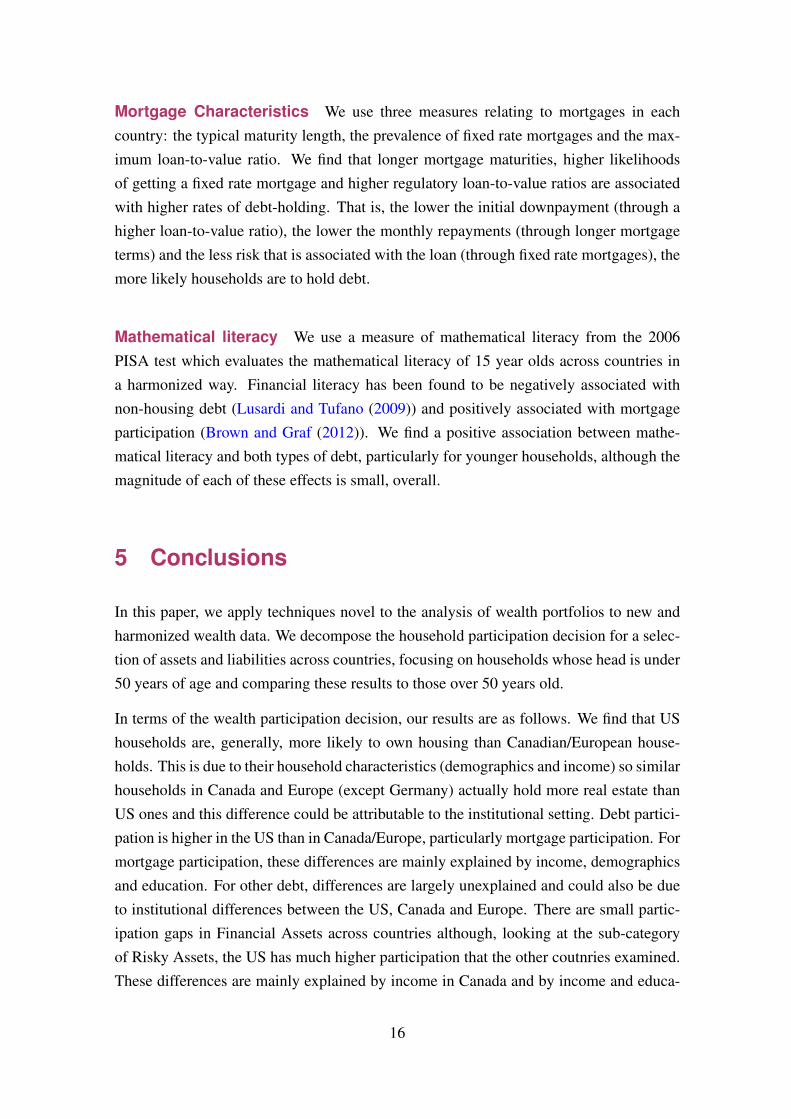
Mortgage Characteristics We use three measures relating to mortgages in eachcountry: the typical maturity length, the prevalence of fixed rate mortgages and the max-imum loan-to-value ratio. We find that longer mortgage maturities, higher likelihoodsof getting a fixed rate mortgage and higher regulatory loan-to-value ratios are associatedwith higher rates of debt-holding. That is, the lower the initial downpayment (through ahigher loan-to-value ratio), the lower the monthly repayments (through longer mortgageterms) and the less risk that is associated with the loan (through fixed rate mortgages), themore likely households are to hold debt.

Mathematical literacy We use a measure of mathematical literacy from the 2006PISA test which evaluates the mathematical literacy of 15 year olds across countries ina harmonized way. Financial literacy has been found to be negatively associated withnon-housing debt (Lusardi and Tufano (2009)) and positively associated with mortgageparticipation (Brown and Graf (2012)). We find a positive association between mathe-matical literacy and both types of debt, particularly for younger households, although themagnitude of each of these effects is small, overall.

5 Conclusions

In this paper, we apply techniques novel to the analysis of wealth portfolios to new andharmonized wealth data. We decompose the household participation decision for a selec-tion of assets and liabilities across countries, focusing on households whose head is under50 years of age and comparing these results to those over 50 years old.

In terms of the wealth participation decision, our results are as follows. We find that UShouseholds are, generally, more likely to own housing than Canadian/European house-holds. This is due to their household characteristics (demographics and income) so similarhouseholds in Canada and Europe (except Germany) actually hold more real estate thanUS ones and this difference could be attributable to the institutional setting. Debt partici-pation is higher in the US than in Canada/Europe, particularly mortgage participation. Formortgage participation, these differences are mainly explained by income, demographicsand education. For other debt, differences are largely unexplained and could also be dueto institutional differences between the US, Canada and Europe. There are small partic-ipation gaps in Financial Assets across countries although, looking at the sub-categoryof Risky Assets, the US has much higher participation that the other coutnries examined.These differences are mainly explained by income in Canada and by income and educa-

16

tion in Europe. There is a large unexplained gap only in Spain.

Where we find significant explained participation gaps, they are mainly explained byincome and household composition differences for young households. Education andhousehold composition drive the explained gaps for older households. For the young, as-set participation differences are more "unexplained" and likely to be influenced by insti-tutions while for the older households, debt participation differences across countries aremore "unexplained" and susceptible to be influenced by institutions. These are importantfindings as they indicate that the younger cohort’s wealth participation is more vulnerableto income shocks (such as those suffered during the great recession) and is more suscep-tible to be influenced by policies encouraging investment in assets. For the older cohort,which may have more trouble smoothing consumption through retirement, there is scopefor policies that encourage debt holding using assets as collateral e.g. reverse mortgages.

Experimenting with a selection of institutional indicators to attempt to discover why iden-tical households in different countries invest differently, we find institutions to affect de-cisions in the way we would expect. In more financially developed and economicallyopen countries, households are less likely to own housing but more likely to be in debt.Higher marginal tax rates are associated with lower investment in housing. Typical mort-gage characteristics and mathematical literacy are also found to be linked to the level ofdebt holding. There is a bigger link between debt and institutions for the old, confirmingthat the large unexplained debt participation gaps for this cohort are likely to be at leastpartly linked to institutions. We find a similar link between assets and institutions for theyoung and the old. Overall, the institutional features we study seem to encourage Euro-pean households, particularly mature ones, to participate in real estate while discouragingthem from mortgage use. Looking into the future, this has potentially negative conse-quences for the elderly population as they may find it difficult to cash-out equity fromtheir home to help finance their retirement

This paper has focused on the participation decision in wealth, without reference to thelevel of investment, given participation. This, obviously, is another important aspect ofwealth portfolios and deserves attention in future literature. With the development ofadditional data sources, which contain adequately detailed information, future researchcould also try to control for observable institutional factors using instrumental variables orother techniques to tease out the causal link between institutions and wealth participationacross countries.

17

References

Andrews, D., Sánchez, A. C., and Åsa Johansson (2011). Housing markets and structuralpolicies in oecd countries. OECD Economics Department Working Papers 836, OECDPublishing. 13

Bilodeau, J., editor (2008). The Financial Development Report 2008. World EconomicForum,. 13

Bover, O. (2010). Wealth Inequality and Household Structure: U.S. vs. Spain. Review of

Income and Wealth, 56(2):259–290. 8

Bover, O., Casado, J. M., Costa, S., Caju, P. D., McCarthy, Y., Sierminska, E.,Tzamourani, P., Villanueva, E., and Zavadil, T. (2013). The distribution of debt acrosseuro area countries. Working Paper. 1

Brown, M. and Graf, R. (2012). Financial literacy, household investment and householddebt: Evidence from switzerland. Working Papers on Finance 1301, University of St.Gallen, School of Finance. 16

Carroll, C. (2002). Household Portfolios, chapter Portfolios of the RIch. The MIT Press.5

Chiuri, M. and Jappelli, T. (2010). Do the elderly reduce housing equity? an internationalcomparison. Journal of Population Economics, 23(2):643–663. 1

Christelis, D., Georgarakos, D., and Haliassos, M. (2012). Differences in portfolios acrosscountries: Economic environment or household characteristics? The Review of Eco-

nomics and Statistics, (forthcoming). 1, 2, 4

Crook, J. and Hochguertel, S. (2007). US and European Household Debt and CreditConstraints. Discussion Paper 2007-087/3, TInbergen Institute. 1

Fairlie, R. W. (1999). The Absence of the African-American Owned Business: An Analy-sis of the Dynamics of Self-Employment. Journal of Labor Economics, 17(1):80–108.6

Fairlie, R. W. (2005). An Extension of the Blinder-Oaxaca Decomposition Technique toLogit and Probit Models. Journal of Economic and Social Measurement, 30(4):305–316. 6

Gornick, J. C., Sierminska, E., and Smeeding, T. M. (2009). The income and wealthpackages of older women in cross-national perspective. The Journals of Gerontology:

Social Sciences, Volume 64B, Number 3, May 2009:402–414. 1

18

Guiso, L., Haliassos, M., and Jappelli, T. (2003). Household stockholding in Europe:where do we stand and where do we go? Economic Policy, 18(36):123–170. 1, 7

HFCN, E. (2013). The eurosystem household finance and consumption survey. resultsfrom the first wave. Technical report, European Central Bank. 4

Kane, T. (2007). 2007 Index of Economic Freedom. Washington, D.C. and New York:Heritage oundation and the Wall street Journal. 13

Lusardi, A. and Tufano, P. (2009). Debt literacy, financial experiences, and overindebt-edness. NBER Working Papers 14808, National Bureau of Economic Research, Inc.16

Sedo, S. A. and Kossoudji, S. A. (2004). Rooms of One’s Own: Gender, Race and HomeOwnership as Wealth Accumulation in the United States. IZA Discussion Papers 1397,Institute for the Study of Labor (IZA). 8

Sierminska, E., Brandolini, A., and Smeeding, T. (2006). The Luxembourg Wealth Study:A cross-country comparable database for household wealth research. Journal of Eco-

nomic Inequality, 4(3):375–383. 3

Sierminska, E. M., Frick, J. R., and Grabka, M. M. (2010). Examining the gender wealthgap. Oxford Economic Papers, 62(4):669–690. 2

van Rooij, M., Lusardi, A., and Alessie, R. (2011). Financial literacy and stock marketparticipation. Journal of Financial Economics, 101(2):449 – 472. 8

Yamokoski, A. and Keister, L. (2006). The wealth of single women: Marital status andparenthood in the asset accumulation of young baby boomers in the united states. Fem-

inist Economics, 12(1-2):167–194. 8

19

6 Tables and Figures

Table 1: Country sample macroeconomic conditions.A. Real GDP growth

2002 2003 2004 2005 2006 2007 2008 2009Canada 2.9 1.9 3.1 3.0 2.9 2.5 0.4 -2.7Germany 0.0 -0.2 0.7 0.9 3.4 2.6 1.0 -4.9Italy 0.5 0.1 1.4 0.8 2.1 1.4 -1.3 -5.1Luxembourg 4.1 1.5 4.4 5.4 5.6 6.5 0.0 -3.4Spain 2.7 3.1 3.3 3.6 4.0 3.6 0.9 -3.6United States 1.8 2.5 3.6 3.1 2.7 2.1 0.4 -2.4

B. Harmonised unemployment rates

2002 2003 2004 2005 2006 2007 2008 2009Canada 7.7 7.6 7.2 6.8 6.3 6.0 6.1 8.3Germany 8.4 9.3 9.8 10.6 9.8 8.4 7.3 7.5Italy 8.6 8.5 8.0 7.7 6.8 6.2 6.8 7.7Luxembourg 2.6 3.8 5.0 4.6 4.6 4.2 4.9 5.4Spain 11.1 11.1 10.6 9.2 8.5 8.3 11.4 18.0United States 5.8 6.0 5.5 5.1 4.6 4.6 5.8 9.3

Source: OECD (2010), Annex Tables 1 and 14

20

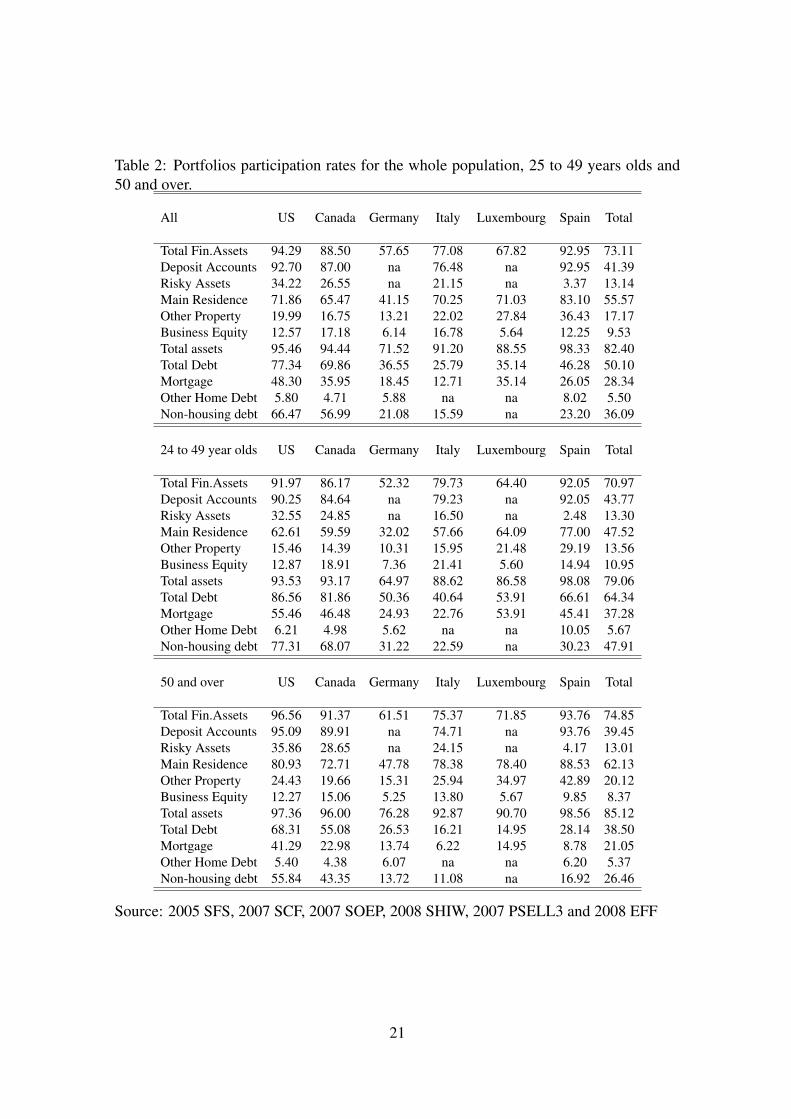
Table 2: Portfolios participation rates for the whole population, 25 to 49 years olds and50 and over.

All US Canada Germany Italy Luxembourg Spain Total

Total Fin.Assets 94.29 88.50 57.65 77.08 67.82 92.95 73.11Deposit Accounts 92.70 87.00 na 76.48 na 92.95 41.39Risky Assets 34.22 26.55 na 21.15 na 3.37 13.14Main Residence 71.86 65.47 41.15 70.25 71.03 83.10 55.57Other Property 19.99 16.75 13.21 22.02 27.84 36.43 17.17Business Equity 12.57 17.18 6.14 16.78 5.64 12.25 9.53Total assets 95.46 94.44 71.52 91.20 88.55 98.33 82.40Total Debt 77.34 69.86 36.55 25.79 35.14 46.28 50.10Mortgage 48.30 35.95 18.45 12.71 35.14 26.05 28.34Other Home Debt 5.80 4.71 5.88 na na 8.02 5.50Non-housing debt 66.47 56.99 21.08 15.59 na 23.20 36.09

24 to 49 year olds US Canada Germany Italy Luxembourg Spain Total


50 and over US Canada Germany Italy Luxembourg Spain Total


Source: 2005 SFS, 2007 SCF, 2007 SOEP, 2008 SHIW, 2007 PSELL3 and 2008 EFF

21

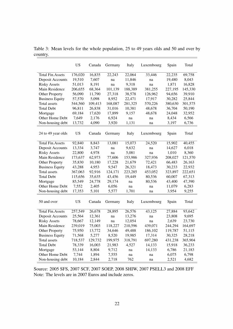
Table 3: Mean levels for the whole population, 25 to 49 years olds and 50 and over bycountry.

US Canada Germany Italy Luxembourg Spain Total

Total Fin.Assets 176,020 16,835 22,243 22,064 33,446 22,235 69,758Deposit Accounts 19,510 7,607 na 11,846 na 19,480 8,043Risky Assets 51,013 8,191 na 9,318 na 1,871 16,828Main Residence 206,655 68,364 101,139 188,389 381,255 227,195 145,330Other Property 56,090 11,790 27,318 38,578 126,962 94,656 39,910Business Equity 57,570 5,098 8,952 22,471 17,917 30,282 25,844Total assets 544,560 109,413 168,087 281,325 570,226 380,630 301,575Total Debt 96,811 26,838 31,016 10,381 48,678 36,704 50,190Mortgage 69,184 17,620 17,899 9,157 48,678 24,048 32,952Other Home Debt 7,649 2,176 6,924 na na 8,434 6,566Non-housing debt 13,732 4,090 3,920 1,131 na 3,197 6,736


Total Fin.Assets 92,840 8,843 13,081 15,073 24,520 15,902 40,455Deposit Accounts 13,334 3,747 na 9,632 na 14,627 6,018Risky Assets 22,800 4,978 na 5,081 na 1,010 8,360Main Residence 173,637 62,973 77,606 153,986 327,936 208,027 121,570Other Property 35,830 10,180 17,228 21,679 72,421 66,483 26,163Business Equity 43,288 4,953 9,547 26,321 18,473 30,233 22,932Total assets 367,063 92,916 124,171 223,285 453,052 323,897 222,651Total Debt 115,656 35,635 43,456 19,449 80,536 60,007 67,313Mortgage 85,549 24,778 29,174 na 80,536 43,400 47,390Other Home Debt 7,552 2,405 6,056 na na 11,079 6,283Non-housing debt 17,353 5,101 5,577 1,701 na 3,954 9,255


Total Fin.Assets 257,549 26,678 28,895 26,576 43,125 27,884 93,642Deposit Accounts 25,564 12,361 na 13,276 na 23,808 9,695Risky Assets 78,667 12,149 na 12,054 na 2,639 23,730Main Residence 239,019 75,003 118,227 210,596 439,071 244,294 164,697Other Property 75,950 13,772 34,646 49,488 186,102 119,787 51,115Business Equity 71,568 5,277 8,520 19,985 17,314 30,325 28,218Total assets 718,537 129,732 199,975 318,791 697,280 431,238 365,904Total Debt 78,339 16,003 21,983 4,527 14,133 15,918 36,233Mortgage 53,144 8,804 9,712 na 14,133 6,786 21,183Other Home Debt 7,744 1,894 7,555 na na 6,075 6,798Non-housing debt 10,184 2,844 2,718 762 na 2,521 4,682

Source: 2005 SFS, 2007 SCF, 2007 SOEP, 2008 SHIW, 2007 PSELL3 and 2008 EFFNote: The levels are in 2007 Euros and include zeros.

22

Table 4: Decomposition of portfolio participation decision for 25 to 49 year olds (Home,Investment Real Estate, and Debt.

Canada Germany Italy Luxembourg Spain(1) % (2) % (3) % (4) % (5) %

Principal Residencesex 0.004* 2 0.007* 6 0.003* 2 0.009* -25 0.008* 6demog1 -0.006* -3 0.002 2 0.021*** 17 0.007*** -19 0.011*** 8demog2 0.061*** 34 0.063*** 52 0.047*** 39 0.041*** -113 0.023*** 17demog3 -0.024*** -13 -0.049*** -40 -0.090*** -74 -0.063*** 174 -0.058*** -44educ -0.002*** -1 -0.006*** -5 0.055*** 45 0.026*** -72 0.039*** 30LM 0.004** 2 0.013*** 11 -0.000 0 0.007*** -19 0.018*** 14asini 0.128*** 71 0.088*** 72 0.097*** 80 -0.044*** 121 0.102*** 77asinwp 0.015*** 8 0.003*** 2 -0.012*** -10 -0.019*** 52 -0.011*** -8

100 99 100 99 100P(x=0) 0.626 0.626 0.626 0.626 0.626P(x=1) 0.596 0.320 0.577 0.641 0.770Diff 0.030 0.306 0.050 -0.015 -0.144Exp 0.180 29 0.122 19 0.121 19 -0.036 -6 0.132 21Unexp -0.150 -24 0.184 29 -0.071 -11 0.022 3 -0.276 -44Investment Real Estatesex 0.006*** 8 0.015*** 23 0.004*** 7 0.023*** 54 0.019*** 24demog1 -0.002 -3 0.000 0 0.001 2 -0.001 -2 0.000 0demog2 -0.005 -6 -0.004 -6 -0.006 -10 -0.007 -17 -0.013* -16demog3 0.016** 21 0.006 9 0.004 7 0.010 24 0.012 15educ 0.002** 3 0.003* 5 0.020*** 34 0.006*** 14 0.012*** 15LM 0.006*** 8 0.004*** 6 -0.013*** -22 0.007*** 17 0.001 1asini 0.053*** 69 0.039*** 59 0.049*** 84 0.006*** 14 0.048*** 61asinwi 0.001 1 0.002* 3 -0.001* -2 -0.002* -5 -0.001 -1

100 99 99 99 99P(x=0) 0.155 0.155 0.155 0.155 0.155P(x=1) 0.144 0.103 0.160 0.215 0.292Diff 0.011 0.052 -0.005 -0.060 -0.137Exp 0.077 50 0.066 42 0.059 38 0.042 27 0.079 51Unexp -0.067 -43 -0.014 -9 -0.064 -41 -0.103 -66 -0.216 -139Mortgagesex -0.003 -2 -0.005 -4 -0.002 0 -0.007 25 -0.006 -4demog1 -0.008* -4 0.002 2 0.019*** 11 0.006*** -21 0.010*** 6demog2 0.052*** 29 0.057*** 45 0.038*** 21 0.035*** -124 0.016*** 10demog3 -0.022*** -12 -0.043*** -34 -0.078*** -44 -0.058*** 206 -0.049*** -29educ 0.000 0 -0.003*** -2 0.077*** 43 0.034*** -121 0.053*** 32LM 0.003*** 2 0.013*** 10 0.000 0 0.008*** -28 0.017*** 10asini 0.156*** 87 0.106*** 83 0.123*** 69 -0.047*** 167 0.126*** 75

99 100 100 103 99P(x=0) 0.555 0.555 0.555 0.555 0.555P(x=1) 0.465 0.249 0.228 0.539 0.454Diff 0.0898 0.305 0.327 0.0156 0.101Exp 0.179 32 0.127 23 0.179 32 -0.0282 -5 0.168 30Unexp -0.089 -16 0.178 32 0.148 27 0.044 8 -0.067 -12Non-housing debtsex 0.000 0 0.000 0 0.000 0 0.000 0demog1 0.006** 28 0.010*** 27 0.016*** 18 0.013*** 20demog2 0.011*** 52 0.014*** 37 0.012*** 13 -0.002* -3demog3 -0.001 -5 -0.002 -5 -0.016** -18 -0.016*** -24educ -0.007*** -33 -0.014*** -37 0.054*** 61 0.038*** 57LM -0.003*** -14 0.006*** 16 0.007*** 8 0.016*** 24asini 0.015*** 70 0.023*** 61 0.015*** 17 0.016*** 24

99 99 99 98P(x=0) 0.773 0.773 0.773 0.773P(x=1) 0.681 0.312 0.226 0.302Diff 0.092 0.461 0.547 0.471Exp 0.021 3 0.037 5 0.089 12 0.067 9Unexp 0.071 9 0.424 55 0.458 59 0.405 52

Source: 2005 SFS, 2007 SCF, 2007 SOEP, 2008 SHIW, 2007 PSELL3 and 2008 EFFNote: Details of variable groupings (demog1, educ, etc) found in Table A.2

23

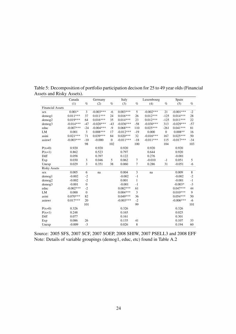
Table 5: Decomposition of portfolio participation decison for 25 to 49 year olds (FinancialAssets and Risky Assets).


Financial Assetssex 0.001* 3 -0.003*** -6 0.003*** 5 -0.002*** 21 -0.001*** -2demog1 0.011*** 37 0.011*** 24 0.016*** 26 0.012*** -125 0.014*** 28demog2 0.019*** 64 0.016*** 35 0.014*** 23 0.012*** -125 0.011*** 22demog3 -0.014*** -47 -0.020*** -43 -0.036*** -58 -0.030*** 313 -0.029*** -57educ -0.007*** -24 -0.004*** -9 0.068*** 110 0.025*** -261 0.041*** 81LM 0.001 3 0.008*** 17 -0.012*** -19 0.000 0 0.008** 16asini 0.021*** 71 0.039*** 84 0.020*** 32 -0.016*** 167 0.025*** 50asinwf -0.003*** -10 -0.000 0 -0.011*** -18 -0.011*** 115 -0.017*** -34

98 102 100 104 103P(x=0) 0.920 0.920 0.920 0.920 0.920P(x=1) 0.862 0.523 0.797 0.644 0.920Diff 0.058 0.397 0.122 0.276 -0.001Exp 0.030 3 0.046 5 0.062 7 -0.010 -1 0.051 5Unexp 0.029 3 0.351 38 0.060 7 0.286 31 -0.051 -6Risky Assetssex 0.005 6 na 0.004 3 na 0.009 8demog1 -0.002 -2 -0.002 -1 -0.002 -2demog2 -0.002 -2 0.001 1 -0.001 -1demog3 -0.001 0 -0.001 -1 -0.003* -3educ -0.002*** -2 0.082*** 61 0.047*** 44LM 0.000 0 0.004*** 3 0.010*** 9asini 0.070*** 82 0.049*** 36 0.054*** 50asinwr 0.017*** 20 -0.003*** -2 -0.006*** -6

101 99 101P(x=0) 0.326 0.326 0.326P(x=1) 0.248 0.165 0.025Diff 0.077 0.161 0.301Exp 0.086 26 0.135 41 0.107 33Unexp -0.009 -3 0.026 8 0.194 60


24

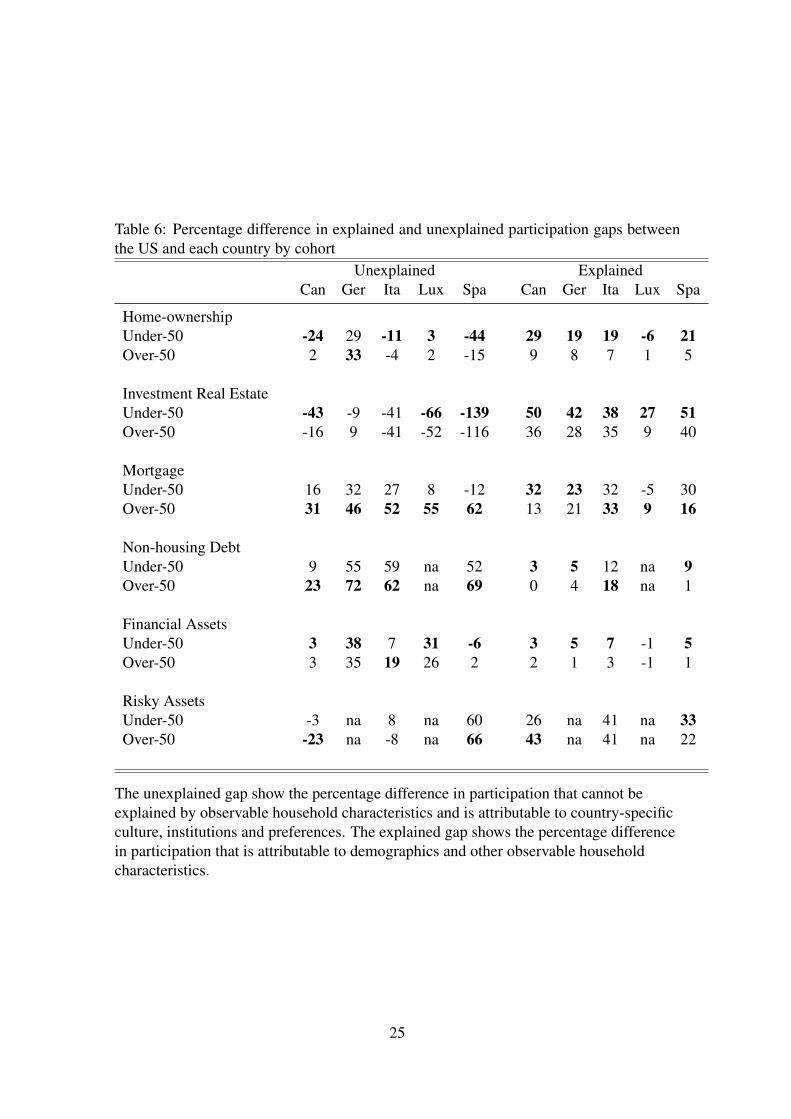
Table 6: Percentage difference in explained and unexplained participation gaps betweenthe US and each country by cohort

Unexplained ExplainedCan Ger Ita Lux Spa Can Ger Ita Lux Spa

Home-ownershipUnder-50 -24 29 -11 3 -44 29 19 19 -6 21Over-50 2 33 -4 2 -15 9 8 7 1 5

Investment Real EstateUnder-50 -43 -9 -41 -66 -139 50 42 38 27 51Over-50 -16 9 -41 -52 -116 36 28 35 9 40

MortgageUnder-50 16 32 27 8 -12 32 23 32 -5 30Over-50 31 46 52 55 62 13 21 33 9 16

Non-housing DebtUnder-50 9 55 59 na 52 3 5 12 na 9Over-50 23 72 62 na 69 0 4 18 na 1

Financial AssetsUnder-50 3 38 7 31 -6 3 5 7 -1 5Over-50 3 35 19 26 2 2 1 3 -1 1

Risky AssetsUnder-50 -3 na 8 na 60 26 na 41 na 33Over-50 -23 na -8 na 66 43 na 41 na 22

The unexplained gap show the percentage difference in participation that cannot beexplained by observable household characteristics and is attributable to country-specificculture, institutions and preferences. The explained gap shows the percentage differencein participation that is attributable to demographics and other observable householdcharacteristics.

25

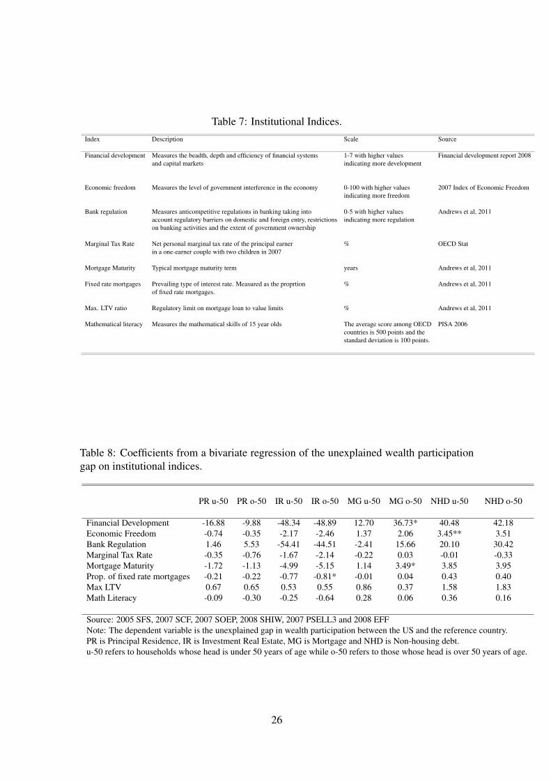
Table 7: Institutional Indices.Index Description Scale Source

Financial development Measures the beadth, depth and efficiency of financial systems 1-7 with higher values Financial development report 2008and capital markets indicating more development

Economic freedom Measures the level of government interference in the economy 0-100 with higher values 2007 Index of Economic Freedomindicating more freedom

Bank regulation Measures anticompetitive regulations in banking taking into 0-5 with higher values Andrews et al, 2011account regulatory barriers on domestic and foreign entry, restrictions indicating more regulationon banking activities and the extent of government ownership

Marginal Tax Rate Net personal marginal tax rate of the principal earner % OECD Statin a one-earner couple with two children in 2007

Mortgage Maturity Typical mortgage maturity term years Andrews et al, 2011

Fixed rate mortgages Prevailing type of interest rate. Measured as the proprtion % Andrews et al, 2011of fixed rate mortgages.

Max. LTV ratio Regulatory limit on mortgage loan to value limits % Andrews et al, 2011

Mathematical literacy Measures the mathematical skills of 15 year olds The average score among OECD PISA 2006countries is 500 points and thestandard deviation is 100 points.

Table 8: Coefficients from a bivariate regression of the unexplained wealth participationgap on institutional indices.

PR u-50 PR o-50 IR u-50 IR o-50 MG u-50 MG o-50 NHD u-50 NHD o-50

Financial Development -16.88 -9.88 -48.34 -48.89 12.70 36.73* 40.48 42.18Economic Freedom -0.74 -0.35 -2.17 -2.46 1.37 2.06 3.45** 3.51Bank Regulation 1.46 5.53 -54.41 -44.51 -2.41 15.66 20.10 30.42Marginal Tax Rate -0.35 -0.76 -1.67 -2.14 -0.22 0.03 -0.01 -0.33Mortgage Maturity -1.72 -1.13 -4.99 -5.15 1.14 3.49* 3.85 3.95Prop. of fixed rate mortgages -0.21 -0.22 -0.77 -0.81* -0.01 0.04 0.43 0.40Max LTV 0.67 0.65 0.53 0.55 0.86 0.37 1.58 1.83Math Literacy -0.09 -0.30 -0.25 -0.64 0.28 0.06 0.36 0.16

Source: 2005 SFS, 2007 SCF, 2007 SOEP, 2008 SHIW, 2007 PSELL3 and 2008 EFFNote: The dependent variable is the unexplained gap in wealth participation between the US and the reference country.PR is Principal Residence, IR is Investment Real Estate, MG is Mortgage and NHD is Non-housing debt.u-50 refers to households whose head is under 50 years of age while o-50 refers to those whose head is over 50 years of age.

26

Figure 1 Participation across the income distribution for 25 to 49 population (top) and 50and over (bottom).

Participation across the income distribution for 50 and over (below)

Source: 2005 SFS, 2007 SCF, 2007 SOEP, 2008 SHIW, 2007 PSELL3 and 2008 EFFNote: Weighted statistics. Lowess curve applied for smoothing purposes.

27

7 Appendix

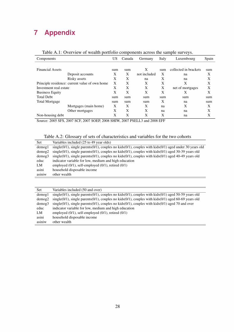
Table A.1: Overview of wealth portfolio components across the sample surveys.Components US Canada Germany Italy Luxembourg Spain

Financial Assets sum sum X sum collected in brackets sumDeposit accounts X X not included X na XRisky assets X X na X na X

Principle residence: current value of own home X X X X X XInvestment real estate X X X X net of mortgages XBusiness Equity X X X X X XTotal Debt sum sum sum sum sum sumTotal Mortgage sum sum sum X na sum

Mortgages (main home) X X X na X XOther mortgages X X X na na X

Non-housing debt X X X X na XSource: 2005 SFS, 2007 SCF, 2007 SOEP, 2008 SHIW, 2007 PSELL3 and 2008 EFF

Table A.2: Glossary of sets of characteristics and variables for the two cohortsSet Variables included (25 to 49 year olds)demog1 single(0/1), single parents(0/1), couples no kids(0/1), couples with kids(0/1) aged under 30 years olddemog2 single(0/1), single parents(0/1), couples no kids(0/1), couples with kids(0/1) aged 30-39 years olddemog3 single(0/1), single parents(0/1), couples no kids(0/1), couples with kids(0/1) aged 40-49 years oldeduc indicator variable for low, medium and high educationLM employed (0/1), self-employed (0/1), retired (0/1)asini household disposable incomeasiniw other wealth

Set Variables included (50 and over)demog1 single(0/1), single parents(0/1), couples no kids(0/1), couples with kids(0/1) aged 50-59 years olddemog2 single(0/1), single parents(0/1), couples no kids(0/1), couples with kids(0/1) aged 60-69 years olddemog3 single(0/1), single parents(0/1), couples no kids(0/1), couples with kids(0/1) aged 70 and overeduc indicator variable for low, medium and high educationLM employed (0/1), self-employed (0/1), retired (0/1)asini household disposable incomeasiniw other wealth

28

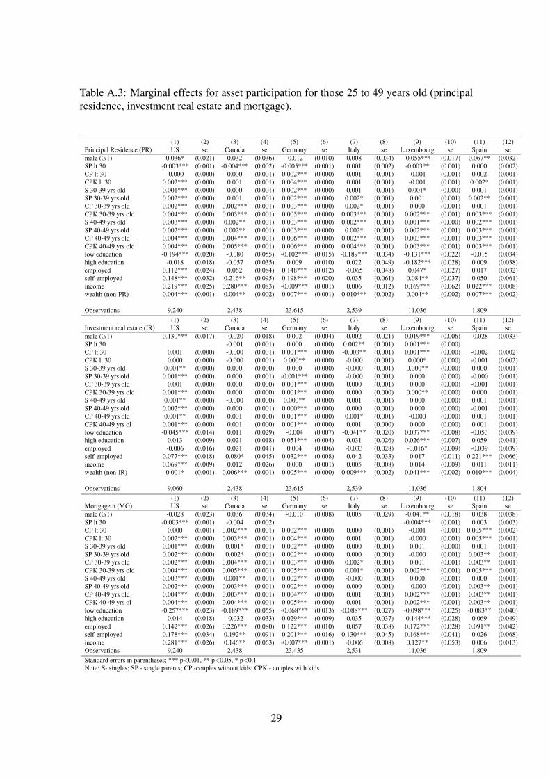
Table A.3: Marginal effects for asset participation for those 25 to 49 years old (principalresidence, investment real estate and mortgage).

(1) (2) (3) (4) (5) (6) (7) (8) (9) (10) (11) (12)Principal Residence (PR) US se Canada se Germany se Italy se Luxembourg se Spain semale (0/1) 0.036* (0.021) 0.032 (0.036) -0.012 (0.010) 0.008 (0.034) -0.055*** (0.017) 0.067** (0.032)SP lt 30 -0.003*** (0.001) -0.004*** (0.002) -0.005*** (0.001) 0.001 (0.002) -0.003** (0.001) 0.000 (0.002)CP lt 30 -0.000 (0.000) 0.000 (0.001) 0.002*** (0.000) 0.001 (0.001) -0.001 (0.001) 0.002 (0.001)CPK lt 30 0.002*** (0.000) 0.001 (0.001) 0.004*** (0.000) 0.001 (0.001) -0.001 (0.001) 0.002* (0.001)S 30-39 yrs old 0.001*** (0.000) 0.000 (0.001) 0.002*** (0.000) 0.001 (0.001) 0.001* (0.000) 0.001 (0.001)SP 30-39 yrs old 0.002*** (0.000) 0.001 (0.001) 0.002*** (0.000) 0.002* (0.001) 0.001 (0.001) 0.002** (0.001)CP 30-39 yrs old 0.002*** (0.000) 0.002*** (0.001) 0.003*** (0.000) 0.002* (0.001) 0.000 (0.001) 0.001 (0.001)CPK 30-39 yrs old 0.004*** (0.000) 0.003*** (0.001) 0.005*** (0.000) 0.003*** (0.001) 0.002*** (0.001) 0.003*** (0.001)S 40-49 yrs old 0.003*** (0.000) 0.002** (0.001) 0.003*** (0.000) 0.002*** (0.001) 0.001*** (0.000) 0.002*** (0.001)SP 40-49 yrs old 0.002*** (0.000) 0.002** (0.001) 0.003*** (0.000) 0.002* (0.001) 0.002*** (0.001) 0.003*** (0.001)CP 40-49 yrs old 0.004*** (0.000) 0.004*** (0.001) 0.006*** (0.000) 0.002*** (0.001) 0.003*** (0.001) 0.003*** (0.001)CPK 40-49 yrs old 0.004*** (0.000) 0.005*** (0.001) 0.006*** (0.000) 0.004*** (0.001) 0.003*** (0.001) 0.003*** (0.001)low education -0.194*** (0.020) -0.080 (0.055) -0.102*** (0.015) -0.189*** (0.034) -0.131*** (0.022) -0.015 (0.034)high education -0.018 (0.018) -0.057 (0.035) 0.009 (0.010) 0.022 (0.049) -0.182*** (0.028) 0.009 (0.038)employed 0.112*** (0.024) 0.062 (0.084) 0.148*** (0.012) -0.065 (0.048) 0.047* (0.027) 0.017 (0.032)self-employed 0.148*** (0.032) 0.216** (0.095) 0.198*** (0.020) 0.035 (0.061) 0.084** (0.037) 0.050 (0.061)income 0.219*** (0.025) 0.280*** (0.083) -0.009*** (0.001) 0.006 (0.012) 0.169*** (0.062) 0.022*** (0.008)wealth (non-PR) 0.004*** (0.001) 0.004** (0.002) 0.007*** (0.001) 0.010*** (0.002) 0.004** (0.002) 0.007*** (0.002)

Observations 9,240 2,438 23,615 2,539 11,036 1,809(1) (2) (3) (4) (5) (6) (7) (8) (9) (10) (11) (12)

Investment real estate (IR) US se Canada se Germany se Italy se Luxembourg se Spain semale (0/1) 0.130*** (0.017) -0.020 (0.018) 0.002 (0.004) 0.002 (0.021) 0.019*** (0.006) -0.028 (0.033)SP lt 30 -0.001 (0.001) 0.000 (0.000) 0.002** (0.001) 0.001*** (0.000)CP lt 30 0.001 (0.000) -0.000 (0.001) 0.001*** (0.000) -0.003** (0.001) 0.001*** (0.000) -0.002 (0.002)CPK lt 30 0.000 (0.000) -0.000 (0.001) 0.000** (0.000) -0.000 (0.001) 0.000* (0.000) -0.001 (0.002)S 30-39 yrs old 0.001** (0.000) 0.000 (0.000) 0.000 (0.000) -0.000 (0.001) 0.000** (0.000) 0.000 (0.001)SP 30-39 yrs old 0.001*** (0.000) 0.000 (0.001) -0.001*** (0.000) -0.000 (0.001) 0.000 (0.000) -0.000 (0.001)CP 30-39 yrs old 0.001 (0.000) 0.000 (0.000) 0.001*** (0.000) 0.000 (0.001) 0.000 (0.000) -0.001 (0.001)CPK 30-39 yrs old 0.001*** (0.000) 0.000 (0.000) 0.001*** (0.000) 0.000 (0.000) 0.000** (0.000) 0.000 (0.001)S 40-49 yrs old 0.001** (0.000) -0.000 (0.000) 0.000** (0.000) 0.001 (0.001) 0.000 (0.000) 0.001 (0.001)SP 40-49 yrs old 0.002*** (0.000) 0.000 (0.001) 0.000*** (0.000) 0.000 (0.001) 0.000 (0.000) -0.001 (0.001)CP 40-49 yrs old 0.001** (0.000) 0.001 (0.000) 0.001*** (0.000) 0.001* (0.001) -0.000 (0.000) 0.001 (0.001)CPK 40-49 yrs ol 0.001*** (0.000) 0.001 (0.000) 0.001*** (0.000) 0.001 (0.000) 0.000 (0.000) 0.001 (0.001)low education -0.045*** (0.014) 0.011 (0.029) -0.004 (0.007) -0.041** (0.020) 0.037*** (0.008) -0.053 (0.039)high education 0.013 (0.009) 0.021 (0.018) 0.051*** (0.004) 0.031 (0.026) 0.026*** (0.007) 0.059 (0.041)employed -0.006 (0.016) 0.021 (0.041) 0.004 (0.006) -0.033 (0.028) -0.016* (0.009) -0.039 (0.039)self-employed 0.077*** (0.018) 0.080* (0.045) 0.032*** (0.008) 0.042 (0.033) 0.017 (0.011) 0.221*** (0.066)income 0.069*** (0.009) 0.012 (0.026) 0.000 (0.001) 0.005 (0.008) 0.014 (0.009) 0.011 (0.011)wealth (non-IR) 0.001* (0.001) 0.006*** (0.001) 0.005*** (0.000) 0.009*** (0.002) 0.041*** (0.002) 0.010*** (0.004)

Observations 9,060 2,438 23,615 2,539 11,036 1,804(1) (2) (3) (4) (5) (6) (7) (8) (9) (10) (11) (12)

Mortgage n (MG) US se Canada se Germany se Italy se Luxembourg se Spain semale (0/1) -0.028 (0.023) 0.036 (0.034) -0.010 (0.008) 0.005 (0.029) -0.041** (0.018) 0.038 (0.038)SP lt 30 -0.003*** (0.001) -0.004 (0.002) -0.004*** (0.001) 0.003 (0.003)CP lt 30 0.000 (0.001) 0.002*** (0.001) 0.002*** (0.000) 0.000 (0.001) -0.001 (0.001) 0.005*** (0.002)CPK lt 30 0.002*** (0.000) 0.003*** (0.001) 0.004*** (0.000) 0.001 (0.001) -0.000 (0.001) 0.005*** (0.001)S 30-39 yrs old 0.001*** (0.000) 0.001* (0.001) 0.002*** (0.000) 0.000 (0.001) 0.001 (0.000) 0.001 (0.001)SP 30-39 yrs old 0.002*** (0.000) 0.002* (0.001) 0.002*** (0.000) 0.000 (0.001) -0.000 (0.001) 0.003** (0.001)CP 30-39 yrs old 0.002*** (0.000) 0.004*** (0.001) 0.003*** (0.000) 0.002* (0.001) 0.001 (0.001) 0.003** (0.001)CPK 30-39 yrs old 0.004*** (0.000) 0.005*** (0.001) 0.005*** (0.000) 0.001* (0.001) 0.002*** (0.001) 0.005*** (0.001)S 40-49 yrs old 0.003*** (0.000) 0.001** (0.001) 0.002*** (0.000) -0.000 (0.001) 0.000 (0.001) 0.000 (0.001)SP 40-49 yrs old 0.002*** (0.000) 0.003*** (0.001) 0.002*** (0.000) 0.000 (0.001) -0.000 (0.001) 0.003** (0.001)CP 40-49 yrs old 0.004*** (0.000) 0.003*** (0.001) 0.004*** (0.000) 0.001 (0.001) 0.002*** (0.001) 0.003** (0.001)CPK 40-49 yrs ol 0.004*** (0.000) 0.004*** (0.001) 0.005*** (0.000) 0.001 (0.001) 0.002*** (0.001) 0.003** (0.001)low education -0.257*** (0.023) -0.189*** (0.055) -0.068*** (0.013) -0.088*** (0.027) -0.098*** (0.025) -0.083** (0.040)high education 0.014 (0.018) -0.032 (0.033) 0.029*** (0.009) 0.035 (0.037) -0.144*** (0.028) 0.069 (0.049)employed 0.142*** (0.026) 0.226*** (0.080) 0.122*** (0.010) 0.057 (0.038) 0.172*** (0.028) 0.091** (0.042)self-employed 0.178*** (0.034) 0.192** (0.091) 0.201*** (0.016) 0.130*** (0.045) 0.168*** (0.041) 0.026 (0.068)income 0.281*** (0.026) 0.146** (0.063) -0.007*** (0.001) -0.006 (0.008) 0.127** (0.053) 0.006 (0.013)Observations 9,240 2,438 23,435 2,531 11,036 1,809Standard errors in parentheses; *** p<0.01, ** p<0.05, * p<0.1Note: S- singles; SP - single parents; CP -couples without kids; CPK - couples with kids.

29

Table A.4: Marginal effects for asset participation for those 25 to 49 year olds (financialassets, non-housing debt and risky assets).

(1) (2) (3) (4) (5) (6) (7) (8) (9) (10) (11) (12)Financial Assets (FA) US se Canada se Germany se Italy se Luxembourg se Spain semale (0/1) -0.013*** (0.004) -0.017 (0.018) -0.050*** (0.011) -0.042 (0.026) -0.025 (0.018) 0.003 (0.010)SP lt 30 -0.000*** (0.000) -0.000 (0.001) -0.006*** (0.001) -0.001 (0.001) -0.004*** (0.001) -0.005*** (0.001)CP lt 30 0.000** (0.000) 0.001 (0.000) 0.001*** (0.000) 0.001 (0.001) -0.001 (0.001)CPK lt 30 0.000** (0.000) 0.000 (0.000) 0.001*** (0.000) 0.001 (0.001) -0.002*** (0.001) -0.005*** (0.001)S 30-39 yrs old -0.000 (0.000) -0.000 (0.000) -0.000** (0.000) 0.000 (0.001) 0.000 (0.000) -0.005*** (0.001)SP 30-39 yrs old -0.000** (0.000) -0.000 (0.000) -0.002*** (0.000) -0.000 (0.001) -0.000 (0.001) -0.005*** (0.001)CP 30-39 yrs old 0.000** (0.000) -0.000 (0.000) 0.002*** (0.000) 0.001 (0.001) -0.001 (0.001) -0.005*** (0.001)CPK 30-39 yrs old 0.000*** (0.000) 0.000 (0.000) 0.001*** (0.000) 0.000 (0.001) -0.001** (0.001) -0.005*** (0.001)S 40-49 yrs old 0.000 (0.000) -0.001*** (0.000) -0.000 (0.000) 0.001 (0.001) -0.001 (0.000) -0.005*** (0.001)SP 40-49 yrs old -0.000 (0.000) 0.000 (0.000) -0.002*** (0.000) -0.000 (0.001) -0.002*** (0.001) -0.005*** (0.001)CP 40-49 yrs old 0.000*** (0.000) -0.000 (0.000) -0.000 (0.000) 0.000 (0.001) -0.002*** (0.001) -0.005*** (0.001)CPK 40-49 yrs ol 0.000** (0.000) 0.000 (0.000) 0.000 (0.000) 0.000 (0.001) -0.001 (0.001) -0.005*** (0.001)low education -0.037*** (0.005) -0.067*** (0.022) -0.195*** (0.017) -0.110*** (0.024) -0.198*** (0.022) -0.040*** (0.010)high education 0.055*** (0.005) 0.053** (0.021) 0.203*** (0.013) 0.031 (0.050) 0.034 (0.027) 0.010 (0.018)employed 0.010*** (0.003) 0.095*** (0.023) 0.145*** (0.013) 0.064** (0.032) 0.113*** (0.028) 0.009 (0.008)self-employed 0.053*** (0.011) 0.126*** (0.039) -0.036* (0.022) 0.134*** (0.048) 0.097** (0.044) -0.010 (0.020)income 0.011*** (0.002) 0.014* (0.007) 0.007*** (0.002) 0.044 (0.031) 0.096* (0.049) 0.003 (0.002)wealth (non-FA) 0.000*** (0.000) 0.002** (0.001) 0.016*** (0.001) 0.005*** (0.001) 0.011*** (0.002) 0.002*** (0.001)

Observations 9,240 2,438 23,615 2,539 11,036 1,790Non-housing debt (NHD) US se Canada se Germany se Italy se Luxembourg se Spain semale (0/1) 0.001 (0.016) -0.034 (0.029) 0.024*** (0.009) -0.051* (0.027) -0.013 (0.034)SP lt 30 -0.002*** (0.000) 0.002 (0.001) 0.001** (0.000) 0.001 (0.002)CP lt 30 -0.000 (0.000) 0.002*** (0.001) 0.002*** (0.000) 0.002* (0.001) -0.000 (0.002)CPK lt 30 0.000 (0.000) 0.000 (0.001) 0.003*** (0.000) 0.002** (0.001) 0.000 (0.001)S 30-39 yrs old -0.001*** (0.000) -0.000 (0.001) 0.000** (0.000) -0.000 (0.001) -0.002* (0.001)SP 30-39 yrs old -0.001* (0.000) 0.002*** (0.001) 0.002*** (0.000) 0.000 (0.001) 0.001 (0.001)CP 30-39 yrs old -0.001** (0.000) 0.000 (0.001) 0.002*** (0.000) -0.000 (0.001) 0.000 (0.001)CPK 30-39 yrs old 0.000 (0.000) 0.000 (0.001) 0.002*** (0.000) 0.001 (0.001) 0.000 (0.001)S 40-49 yrs old -0.002*** (0.000) -0.001 (0.001) 0.001*** (0.000) 0.000 (0.001) -0.001 (0.001)SP 40-49 yrs old -0.000 (0.000) 0.000 (0.001) 0.002*** (0.000) 0.001 (0.001) -0.001 (0.001)CP 40-49 yrs old -0.001** (0.000) 0.000 (0.001) 0.002*** (0.000) 0.001 (0.001) -0.001 (0.001)CPK 40-49 yrs ol -0.000 (0.000) -0.000 (0.001) 0.002*** (0.000) 0.001 (0.001) 0.000 (0.001)low education -0.164*** (0.013) -0.014 (0.047) -0.011 (0.014) 0.021 (0.024) 0.032 (0.034)high education -0.053*** (0.011) -0.084*** (0.029) -0.125*** (0.011) -0.102*** (0.039) -0.006 (0.044)employed 0.101*** (0.015) 0.184*** (0.054) -0.021* (0.011) 0.081** (0.037) -0.016 (0.038)self-employed 0.030 (0.019) 0.177*** (0.065) 0.014 (0.019) -0.001 (0.045) -0.003 (0.061)income 0.019*** (0.005) 0.042 (0.028) 0.013*** (0.001) 0.001 (0.008) -0.002 (0.010)

Observations 9,240 2,438 23,615 2,531 1,809Risky Assets (RA) US se Canada se Germany se Italy se Luxembourg se Spain semale (0/1) 0.032 (0.020) -0.037* (0.022) 0.020 (0.015) 0.002 (0.001)SP lt 30 -0.001 (0.001) -0.001 (0.001)CP lt 30 -0.001*** (0.000) 0.000 (0.001) -0.001 (0.001)CPK lt 30 -0.001* (0.000) 0.001 (0.001)S 30-39 yrs old -0.001*** (0.000) 0.000 (0.001) -0.000 (0.000) 0.000 (0.000)SP 30-39 yrs old -0.002*** (0.000) 0.000 (0.001) 0.000 (0.001) 0.000 (0.000)CP 30-39 yrs old -0.002*** (0.000) -0.001 (0.001) -0.000 (0.000) -0.000 (0.000)CPK 30-39 yrs old -0.000 (0.000) -0.000 (0.000) -0.001* (0.000) 0.000 (0.000)S 40-49 yrs old -0.001 (0.000) 0.000 (0.001) -0.000 (0.000) 0.000 (0.000)SP 40-49 yrs old -0.001*** (0.000) 0.000 (0.001) -0.001** (0.001) 0.000 (0.000)CP 40-49 yrs old -0.001*** (0.000) 0.000 (0.000) -0.001 (0.000) 0.000 (0.000)CPK 40-49 yrs ol -0.001 (0.000) -0.000 (0.000) -0.001 (0.000) 0.000 (0.000)low education -0.240*** (0.027) -0.085** (0.041) -0.068*** (0.018) -0.002 (0.002)high education 0.156*** (0.016) 0.032 (0.022) -0.012 (0.017) 0.001 (0.001)employed 0.110*** (0.029) 0.051 (0.057) 0.064** (0.027) 0.002 (0.001)self-employed 0.087** (0.035) 0.030 (0.069) 0.077** (0.033) -0.000 (0.001)income 0.098*** (0.024) 0.160*** (0.020) 0.098*** (0.014) 0.000 (0.001)wealth (non-RA) 0.008*** (0.001) 0.004*** (0.002) 0.007** (0.003) 0.001** (0.001)

Observations 9,240 2,438 2,492 1,749Standard errors in parenthese;*** p<0.01, ** p<0.05, * p<0.1sNote: S- singles; SP - single parents; CP -couples without kids; CPK - couples with kids.

30

Table A.5: Descriptive statistics (means) by country and age groups.


age 38.04 37.37 38.70 39.63 38.75 38.74 38.48male (0/1) 0.78 0.61 0.52 0.66 0.45 0.50 0.62no. of children lt 18 1.34 0.42 0.79 0.94 1.00 0.93 0.98s * 100 20.59 33.42 36.51 27.50 24.08 19.21 29.41sp * 100 15.18 7.92 11.02 6.47 6.52 9.59 11.96cp * 100 15.74 22.11 16.53 16.26 15.06 11.32 16.15cpk * 100 48.49 36.55 35.94 49.78 54.34 59.88 42.28married 0.53 0.56 0.42 0.66 0.58 0.71 0.49divorced 0.22 0.08 0.20 0.12 0.13 0.10 0.19low education 0.14 0.13 0.11 0.50 0.30 0.38 0.16high education 0.32 0.31 0.22 0.13 0.34 0.22 0.26employed 0.78 0.81 0.71 0.67 0.80 0.63 0.73self-employed 0.11 0.07 0.07 0.21 0.05 0.11 0.09retired 0.00 0.00 0.00 0.01 0.00 0.01 0.00income 11.32 10.47 10.25 10.59 11.52 10.53 10.66wealth (non-PR) 3.61 -0.25 2.66 6.81 7.86 6.86 3.35


age 64.89 63.94 67.28 67.12 64.69 65.54 66.41male (0/1) 0.67 0.60 0.58 0.62 0.51 0.52 0.61no. of children lt 18 0.36 0.04 0.08 0.12 0.19 0.05 0.16s * 100 35.60 40.41 48.17 40.56 35.82 29.67 42.84sp * 100 8.84 0.67 0.90 1.10 4.58 12.37 3.70cp * 100 39.12 54.91 45.78 50.32 36.62 28.61 43.54cpk * 100 16.44 3.64 4.02 8.01 22.98 29.35 9.67married 0.52 0.53 0.48 0.58 0.58 0.58 0.51divorced 0.41 0.01 0.43 0.33 0.34 0.34 0.40low education 0.17 0.32 0.19 0.74 0.46 0.70 0.25high education 0.30 0.20 0.20 0.08 0.22 0.14 0.22employed 0.40 0.37 0.24 0.16 0.24 0.19 0.28self-employed 0.11 0.06 0.05 0.10 0.03 0.07 0.07retired 0.47 0.48 0.50 0.68 0.43 0.39 0.50income 11.21 10.37 10.58 10.71 11.44 10.40 10.76wealth (non-PR) 8.53 4.97 5.88 8.13 9.46 8.99 6.93Note: S- singles; SP - single parents; CP -couples without kids; CPK - couples with kids.

31

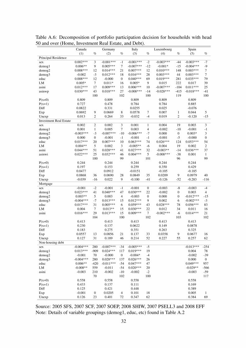
Table A.6: Decomposition of portfolio participation decision for households with head50 and over (Home, Investment Real Estate, and Debt).


Principal Residencesex 0.002*** 3 -0.001*** -1 -0.001*** -2 -0.003*** -44 -0.003*** -7demog1 0.006** 9 0.005*** 7 -0.007*** -12 -0.001* -15 -0.004*** -9demog2 0.008*** 12 0.014*** 21 0.007*** 12 0.010*** 148 0.003*** 7demog3 -0.002 -3 0.012*** 18 0.016*** 28 0.003*** 44 0.003*** 7educ 0.008*** 12 -0.000 0 0.040*** 69 0.019*** 281 0.035*** 79LM 0.005* 7 0.011* 16 0.005* 9 0.015 222 0.017 39asini 0.012*** 17 0.009*** 13 0.006*** 10 -0.007*** -104 0.011*** 25asinwp 0.030*** 43 0.018*** 27 -0.008*** -14 -0.028*** -415 -0.018*** -41

100 102 100 119 100P(x=0) 0.809 0.809 0.809 0.809 0.809P(x=1) 0.727 0.478 0.784 0.784 0.885Diff 0.0822 0.331 0.0255 0.025 -0.076Exp 0.0692 9 0.0669 8 0.0578 7 0.007 1 0.044 5Unexp 0.013 2 0.264 33 -0.032 -4 0.019 2 -0.120 -15Investment Real Estatesex 0.002 2 0.002 3 0.001 1 0.004 19 0.003 3demog1 0.001 1 0.005 7 0.003 4 -0.002 -10 -0.001 -1demog2 -0.003*** -3 -0.007*** -10 -0.006*** -7 0.000 0 0.003* 3demog3 0.000 0 -0.001 -1 -0.001 -1 -0.001 -5 -0.000 0educ 0.017*** 20 0.007*** 10 0.063*** 74 0.026*** 124 0.053*** 54LM 0.004** 5 0.002 3 -0.005** -6 0.004 19 0.002 2asini 0.044*** 51 0.028*** 41 0.027*** 32 -0.003** -14 0.036*** 37asinwi 0.022*** 25 0.032*** 46 0.004*** 5 -0.008*** -38 0.001 1

100 99 101 96 99P(x=0) 0.244 0.244 0.244 0.244 0.244P(x=1) 0.197 0.153 0.259 0.350 0.429Diff 0.0477 0.0912 -0.0151 -0.105 -0.185Exp 0.0868 36 0.0690 28 0.0849 35 0.0209 9 0.0979 40Unexp -0.039 -16 0.022 9 -0.100 -41 -0.126 -52 -0.283 -116Mortgagesex -0.001 -2 -0.001 -1 -0.001 0 -0.003 -8 -0.003 -4demog1 0.023*** 41 0.040*** 47 0.030*** 22 -0.002 0 0.003 4demog2 0.003** 5 0.003 4 -0.003 0 0.000 0 -0.012*** -15demog3 -0.004*** -7 0.013*** 15 0.012*** 9 0.002 6 -0.002*** -3educ 0.017*** 31 0.005*** 6 0.059*** 43 0.028*** 78 0.056*** 83LM 0.004 7 0.013** 15 0.030*** 22 0.012 34 0.011 16asini 0.016*** 29 0.013*** 15 0.009*** 7 -0.002*** -6 0.014*** 21

104 100 102 103 102P(x=0) 0.413 0.413 0.413 0.413 0.413P(x=1) 0.230 0.137 0.0622 0.149 0.0878Diff 0.183 0.275 0.351 0.263 0.325Exp 0.0557 13 0.0856 21 0.137 33 0.0358 9 0.0677 16Unexp 0.127 31 0.189 46 0.214 52 0.227 55 0.257 62Non-housing debtsex -0.004*** 280 -0.007*** -34 -0.005*** -5 -0.013*** -254demog1 0.013*** -909 0.024*** 117 0.019*** 19 0.004 78demog2 -0.001 70 -0.000 0 -0.004* -4 -0.002 -39demog3 -0.004*** 280 0.028*** 137 0.026*** 26 0.000 0educ 0.006** -420 -0.011*** -54 0.047*** 47 0.049*** 957LM -0.008** 559 -0.011 -54 0.020*** 20 -0.029** -566asini -0.003 210 -0.002 -10 -0.002 -2 -0.003 -59

70 102 100 117P(x=0) 0.558 0.558 0.558 0.558P(x=1) 0.433 0.137 0.111 0.169Diff 0.125 0.421 0.448 0.389Exp -0.001 0 0.0205 4 0.101 18 0.005 1Unexp 0.126 23 0.401 72 0.347 62 0.384 69


32

Table A.7: Decomposition of portfolio participation decision for households with headover 50 (Financial Assets and Risky Assets).


Financial Assetssex 0.004*** 21 0.001* 11 0.003*** 12 0.003*** -41 0.004*** 30demog1 0.003* 16 0.004* 45 0.000 0 0.000 0 0.000 0demog2 -0.002** -11 -0.001 -11 -0.001 -4 -0.001** 14 0.005*** 38demog3 0.002 11 0.002* 22 0.001 4 0.001 -14 0.002 15educ 0.016*** 86 0.003** 33 0.040*** 161 0.026*** -351 0.041*** 308LM -0.002 -11 -0.003 -33 0.003* 12 -0.003 41 -0.006 -45asini 0.007*** 37 0.008*** 89 0.004*** 16 -0.006*** 81 0.009*** 68asinwf -0.010*** -53 -0.005*** -56 -0.026*** -104 -0.027*** 365 -0.042*** -316

96 100 96 95 98P(x=0) 0.966 0.966 0.966 0.966 0.966P(x=1) 0.914 0.615 0.754 0.719 0.938Diff 0.0519 0.350 0.212 0.247 0.0280Exp 0.0187 2 0.00898 1 0.0249 3 -0.00740 -1 0.0133 1Unexp 0.033 3 0.341 35 0.187 19 0.254 26 0.015 2Risky Assetssex 0.000 0 na 0.000 0 na 0.001 1demog1 0.006*** 4 0.008** 5 -0.001 -1demog2 0.005*** 3 0.001 1 -0.004* -5demog3 0.002 1 -0.008*** -5 0.001 1educ 0.031*** 20 0.113*** 77 0.099*** 125LM -0.013*** -8 -0.013*** -7 -0.069*** -87asini 0.064*** 42 0.036*** 24 0.058*** 74asinwr 0.059*** 39 0.010*** 7 -0.006*** -8

101 102 100P(x=0) 0.359 0.359 0.359P(x=1) 0.286 0.241 0.0417Diff 0.0721 0.117 0.317Exp 0.153 43 0.147 41 0.0789 22Unexp -0.081 -23 -0.030 -8 0.238 66


33

Figure A.1 Linear regressions between the unexplained participation gap in PrincipalResidence and the institutional setting.


34

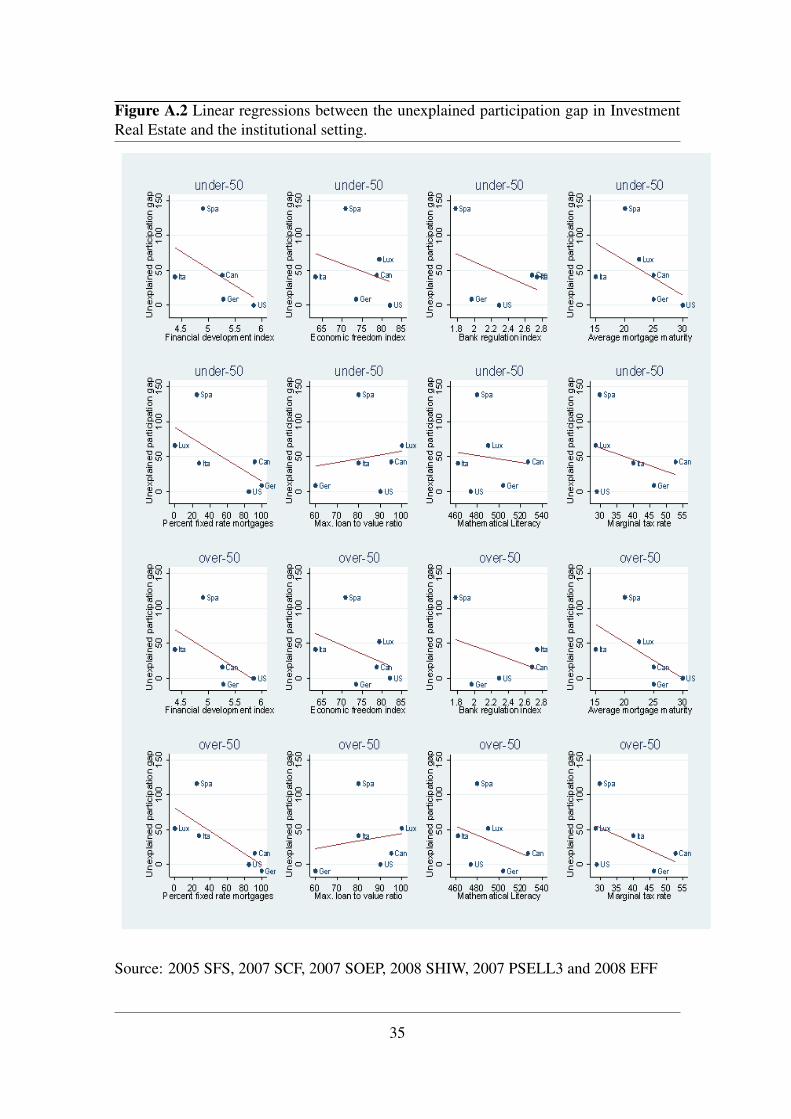
Figure A.2 Linear regressions between the unexplained participation gap in InvestmentReal Estate and the institutional setting.


35

Figure A.3 Linear regressions between the unexplained participation gap in Mortgagesand the institutional setting.


36

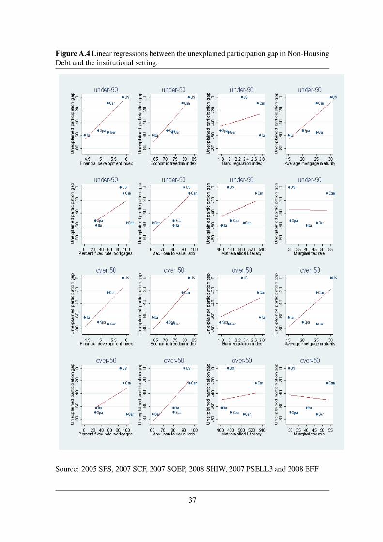
Figure A.4 Linear regressions between the unexplained participation gap in Non-HousingDebt and the institutional setting.


37

Karina Doorley - core.ac.uk · Citation of such a paper should account for its provisional...

Documents

Transcript of Karina Doorley - core.ac.uk · Citation of such a paper should account for its provisional...