Lehrstuhl fur¨ Steuerungs- und Regelungstechnik Technische ... · r y u d e n K G ¢ G Figure 1.1:...
153
Lehrstuhl f¨ ur Steuerungs- und Regelungstechnik Technische Universit¨ at M¨ unchen Ordinarius: Univ.-Prof. Dr.-Ing./Univ. Tokio Martin Buss Generation of low order LFT Representations for Robust Control Applications Simon Hecker Vollst¨ andiger Abdruck der von der Fakult¨ at f¨ ur Elektrotechnik und Infor- mationstechnik der Technischen Universit¨ at M¨ unchen zur Erlangung des akademischen Grades eines Doktor-Ingenieurs (Dr.-Ing.) genehmigten Dissertation. Vorsitzender: Univ.-Prof. Dr.-Ing. Klaus Diepold Pr¨ ufer der Dissertation: 1. Univ.-Prof. Dr.-Ing./Univ. Tokio Martin Buss 2. Univ.-Prof. Dr.-Ing. habil. Boris Lohmann Die Dissertation wurde am 04.07.2006 bei der Technischen Universit¨ at M¨ unchen eingereicht und durch die Fakult¨ at f¨ ur Elektrotechnik und Infor- mationstechnik am 16.10.2006 angenommen.
Transcript of Lehrstuhl fur¨ Steuerungs- und Regelungstechnik Technische ... · r y u d e n K G ¢ G Figure 1.1:...
Lehrstuhl fur Steuerungs- und RegelungstechnikTechnische Universitat Munchen
Ordinarius: Univ.-Prof. Dr.-Ing./Univ. Tokio Martin Buss
Generation of low order LFT Representations for
Robust Control Applications
Simon Hecker
Vollstandiger Abdruck der von der Fakultat fur Elektrotechnik und Infor-mationstechnik der Technischen Universitat Munchen zur Erlangung desakademischen Grades eines
Doktor-Ingenieurs (Dr.-Ing.)
genehmigten Dissertation.
Vorsitzender: Univ.-Prof. Dr.-Ing. Klaus Diepold
Prufer der Dissertation:1. Univ.-Prof. Dr.-Ing./Univ. Tokio Martin Buss2. Univ.-Prof. Dr.-Ing. habil. Boris Lohmann
Die Dissertation wurde am 04.07.2006 bei der Technischen UniversitatMunchen eingereicht und durch die Fakultat fur Elektrotechnik und Infor-mationstechnik am 16.10.2006 angenommen.
Veroffentlicht im VDI-Verlag:
Hecker, S.: Generation of low order LFT Representations for RobustControl Applications. Fortschritt-Berichte VDI Reihe 8 Nr.1114
Dusseldorf: VDI-Verlag 2006, ISBN 978-3-18-511408-3
Vorwort
Die vorliegende Arbeit entstand am Institut fur Robotik und Mechatronik des DeutschenZentrums fur Luft- und Raumfahrt e.V. (DLR) in Oberpfaffenhofen. Herrn Dr.-Ing.Johann Bals danke ich nicht nur fur die Moglichkeit, die Arbeit in seiner Abteilungdurchzufuhren, sondern auch fur die Freiheit in der Bearbeitung der mir gestellten wis-senschaftlichen Aufgabe, sowie fur das Vertrauen, das er mir nicht nur auf diesem Gebietentgegenbrachte.Herrn Prof. Dr.-Ing./Univ. Tokio Martin Buss danke ich fur die Ubernahme des Erst-gutachtens, sowie fur die hilfreichen Vorschlage und Anmerkungen zu meiner Arbeit.Herrn Prof. Dr.-Ing. Boris Lohmann danke ich fur die Ubernahme des Zweitgutachtensund Herrn Prof. Dr.-Ing. Klaus Diepold danke ich fur die Ubernahme des Vorsitzes derPrufung.Mein Dank gilt allen Kolleginnen und Kollegen fur das sehr gute Arbeitsklima in derAbteilung fur Entwurfsorientierte Regelung. Insbesondere danke ich Herrn Dr. AndrasVarga, der durch seine Ideen und Arbeiten mein Interesse an dem Forschungsthemageweckt hat. Viele der Ergebnisse und Erkenntnisse resultieren aus den zahlreichen Dis-kussionen mit ihm. Ich danke ihm auch fur die detaillierte Durchsicht meiner Arbeit.Besonderer Dank gilt auch Herrn Gertjan Looye, der durch seine vielen Anregungen undseine Unterstutzung beim RCAM Anwendungsbeispiel wesentlich zum Gelingen der Pro-motion beigetragen hat.Meinen Eltern danke fur die Unterstutzung, durch die sie mir die Arbeit uberhaupterst ermoglichten. Die Moglichkeit meines Studiums und ihr Ruckhalt haben mir dieVoraussetzungen fur die vorliegende Arbeit gegeben.Bei meiner Frau Birgit mochte ich mich in ganz besonderer Weise fur ihre liebevolleUnterstutzung bedanken. Ihr und der vielen Freude mit unserem Sohn Leon verdanke ichdie Motivation zur Durchfuhrung meiner Promotion.
Munchen, 2006 Simon Hecker
iii

Fur Birgit und Leon
iv
Contents
1 Introduction 11.1 Historical Remarks . . . . . . . . . . . . . . . . . . . . . . . . . . . . . . 11.2 Linear Fractional Transformations (LFTs) in robust control . . . . . . . . 31.3 Motivation and Thesis Structure . . . . . . . . . . . . . . . . . . . . . . . 4
2 Generalized Linear Fractional Representation (LFR) for parametric uncertainsystems 72.1 From nonlinear to linear parametric models . . . . . . . . . . . . . . . . 7
2.1.1 Jacobian-based linearization . . . . . . . . . . . . . . . . . . . . . 82.1.2 Quasi-LPV models . . . . . . . . . . . . . . . . . . . . . . . . . . 9
2.2 Standard LFT . . . . . . . . . . . . . . . . . . . . . . . . . . . . . . . . . 102.3 Generalized LFT . . . . . . . . . . . . . . . . . . . . . . . . . . . . . . . 13
2.3.1 Definition . . . . . . . . . . . . . . . . . . . . . . . . . . . . . . . 132.3.2 Algebraic Properties . . . . . . . . . . . . . . . . . . . . . . . . . 142.3.3 Object-oriented LFR realization procedure for rational parametric
matrices . . . . . . . . . . . . . . . . . . . . . . . . . . . . . . . . 202.3.4 Normalization . . . . . . . . . . . . . . . . . . . . . . . . . . . . . 222.3.5 Special form of generalized LFT . . . . . . . . . . . . . . . . . . . 242.3.6 Relation to Behavioral Representations . . . . . . . . . . . . . . . 26
2.4 LFR realization for parametric descriptor system . . . . . . . . . . . . . 292.4.1 E(δ) general . . . . . . . . . . . . . . . . . . . . . . . . . . . . . . 292.4.2 E(δ) invertible . . . . . . . . . . . . . . . . . . . . . . . . . . . . 30
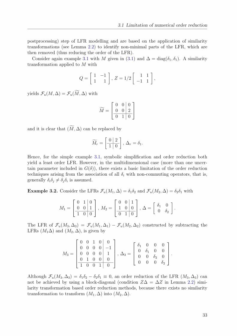
3 Symbolic techniques for low order LFR modelling 323.1 Limitation of numerical order reduction . . . . . . . . . . . . . . . . . . . 323.2 Definitions . . . . . . . . . . . . . . . . . . . . . . . . . . . . . . . . . . . 343.3 Single element conversions . . . . . . . . . . . . . . . . . . . . . . . . . . 35
3.3.1 Horner form . . . . . . . . . . . . . . . . . . . . . . . . . . . . . . 353.3.2 Partial fraction decomposition . . . . . . . . . . . . . . . . . . . . 373.3.3 Continued-fraction form . . . . . . . . . . . . . . . . . . . . . . . 37
3.4 Matrix conversions . . . . . . . . . . . . . . . . . . . . . . . . . . . . . . 383.4.1 Morton’s method . . . . . . . . . . . . . . . . . . . . . . . . . . . 383.4.2 Enhanced tree decomposition . . . . . . . . . . . . . . . . . . . . 39
3.5 Variable splitting factorization . . . . . . . . . . . . . . . . . . . . . . . . 433.5.1 Scalar case . . . . . . . . . . . . . . . . . . . . . . . . . . . . . . . 43
v
Contents
3.5.2 Vector case . . . . . . . . . . . . . . . . . . . . . . . . . . . . . . 453.5.3 Matrix case . . . . . . . . . . . . . . . . . . . . . . . . . . . . . . 46
3.6 Lower-bound for LFR order . . . . . . . . . . . . . . . . . . . . . . . . . 47
4 Enhanced LFR-toolbox for Matlab 494.1 Object definition . . . . . . . . . . . . . . . . . . . . . . . . . . . . . . . 504.2 Symbolic preprocessing . . . . . . . . . . . . . . . . . . . . . . . . . . . . 514.3 Numerical order reduction . . . . . . . . . . . . . . . . . . . . . . . . . . 52
5 Robust stability analysis for the RCAM 545.1 LFR model realization for the element a29 . . . . . . . . . . . . . . . . . 57
5.1.1 Enhanced numerical order reduction . . . . . . . . . . . . . . . . 585.1.2 Comparison of low order LFR realization techniques . . . . . . . . 58
5.2 LFR realization for the full RCAM . . . . . . . . . . . . . . . . . . . . . 605.3 Accuracy of low order LFRs . . . . . . . . . . . . . . . . . . . . . . . . . 615.4 Improved robust stability analysis using µ . . . . . . . . . . . . . . . . . 62
6 Robust vehicle steering control design 686.1 Single-Track model and steering actuator . . . . . . . . . . . . . . . . . . 696.2 LFR realization for roll-augmented single track model . . . . . . . . . . . 706.3 LFR realization for single track model without roll augmentation . . . . 726.4 Problem specification . . . . . . . . . . . . . . . . . . . . . . . . . . . . . 74
6.4.1 Controller Structure . . . . . . . . . . . . . . . . . . . . . . . . . 756.4.2 Mixed sensitivity specifications and synthesis structure . . . . . . 756.4.3 Closed-loop eigenvalue specification . . . . . . . . . . . . . . . . . 78
6.5 µ-Synthesis . . . . . . . . . . . . . . . . . . . . . . . . . . . . . . . . . . 806.5.1 Synthesis procedure . . . . . . . . . . . . . . . . . . . . . . . . . . 806.5.2 Frequency-weighted controller reduction . . . . . . . . . . . . . . 826.5.3 Frequency domain results . . . . . . . . . . . . . . . . . . . . . . 85
6.6 LPV-control design . . . . . . . . . . . . . . . . . . . . . . . . . . . . . . 926.6.1 Synthesis structure . . . . . . . . . . . . . . . . . . . . . . . . . . 926.6.2 Linear point designs . . . . . . . . . . . . . . . . . . . . . . . . . 936.6.3 LPV design . . . . . . . . . . . . . . . . . . . . . . . . . . . . . . 946.6.4 Frequency weighted controller reduction . . . . . . . . . . . . . . 956.6.5 Frequency domain results . . . . . . . . . . . . . . . . . . . . . . 96
6.7 Simulation results . . . . . . . . . . . . . . . . . . . . . . . . . . . . . . . 1016.8 Summary . . . . . . . . . . . . . . . . . . . . . . . . . . . . . . . . . . . 112
7 Summary and Future Directions 114
A Structured Singular Value (µ) Framework 117A.1 Definitions . . . . . . . . . . . . . . . . . . . . . . . . . . . . . . . . . . . 118A.2 Small Gain robust stability test . . . . . . . . . . . . . . . . . . . . . . . 119A.3 µ-Analysis . . . . . . . . . . . . . . . . . . . . . . . . . . . . . . . . . . . 120
A.3.1 Definition of µ . . . . . . . . . . . . . . . . . . . . . . . . . . . . . 120
vi
A.3.2 Bounds on µ . . . . . . . . . . . . . . . . . . . . . . . . . . . . . . 121A.3.3 Robust stability . . . . . . . . . . . . . . . . . . . . . . . . . . . . 122A.3.4 Robust performance . . . . . . . . . . . . . . . . . . . . . . . . . 123
A.4 µ-Synthesis . . . . . . . . . . . . . . . . . . . . . . . . . . . . . . . . . . 124
B Background on LPV control design 127B.1 Stability and performance of LPV systems . . . . . . . . . . . . . . . . . 127B.2 Robust LPV control design . . . . . . . . . . . . . . . . . . . . . . . . . . 128
C LFR-toolbox 130
D RCAM linear parametric system matrices 133
Bibliography 137
vii
Acronyms
BTA Balanced Truncation ApproximationDAE Differential and Algebraic EquationsETD Enhanced Tree DecopositionIQC Integral Quadratic ConstraintLFR Linear Fractional RepresentationLFT Linear Fractional TransformationLMI Linear Matrix InequalityLPV Linear Parameter VaryingLQG Linear Quadratic GaussianLTI Linear Time InvariantMIMO Multiple Input Multiple OutputOL Open-LoopONR Output Nulling RepresentationPS Parameter SpacePUM Parametric Uncertainty ModellingQFT Quantitative Feedback TheoryRCAM Research Civil Aircraft ModelSISO Single Input Single OutputSLICOT Subroutine Library in Systems and Control TheorySPA Singular Perturbation ApproximationTD Tree DecompositionVS Variable Splitting
viii
Notations
K controller matrixG plant modelGa actuator modelGd reference modelS sensitivity functionT complementary sensitivity functionR controller sensitivity functionδ parameter vector∆ uncertainty matrixΠ uncertain parameter setFu(·, ·) upper LFTFl(·, ·) lower LFTIn n-dimensional identity matrix0n n× n zero matrixR set of real numbersRn×m set of n by m matrices with elements in RR[δ] set of real multivariate polynomial functionsR[δ, δ−1] set of real multivariate Laurent polynomial functionsR(δ) set of real multivariate rational functionsC set of complex numbersCn×m set of n by m matrices with elements in CZ set of integersRH∞ set of real rational proper stable matricesXT transpose of matrix XX−1 inverse of matrix Xker[X] null space of matrix XX > Y X, Y hermitian, X − Y positive definiteX ≥ Y X, Y hermitian, X − Y positive semidefinite1-d one-dimensionaln-d n-dimensional (multi-dimensional)σ largest singular valueµ structured singular value
ix
Abstract
The Linear Fractional Transformation (LFT) is a general, flexible and powerful frameworkto represent uncertain systems. Linear Fractional Representations (LFRs) are the basisfor the application of many modern robust control techniques (e.g., robust H∞ controldesign, µ-synthesis/analysis). For several classes of uncertain systems, it is in principlestraightforward to generate equivalent LFRs. However, the resulting LFRs are generallynot unique, a theory for the generation of LFRs with minimal complexity does not existand the pure application of existing ad-hoc realization methods generally yields LFRsof high complexity. LFR-based modern robust control methods are numerically highlydemanding and of high computational complexity, e.g., many methods require to solvea large system of Linear Matrix Inequalities (LMIs). Therefore the application of thesemethods is restricted to LFRs of reasonable complexity, otherwise the computation timewill be unacceptable or the methods may even fail.
To realize LFRs of low complexity, a three step procedure is employed in this thesisconsisting of (i) symbolic preprocessing of uncertain system models using improved andnewly developed decomposition techniques, (ii) object-oriented LFR realization based ona newly developed generalized/descriptor LFT, (iii) numerical multidimensional orderreduction based on newly implemented numerical reliable and efficient routines.
All the techniques are implemented in version 2 of the LFR-toolbox for Matlab andallow to realize an LFR of almost minimal complexity for one of the most complexparametric aircraft models available in the literature. Using this LFR, a reliable LFR-based robust stability analysis covering the whole flight envelope has been performed,which was not possible with earlier generated LFRs of high complexity.
An LFR of minimal complexity is generated for a parametric vehicle model. Based onthis LFR, a µ-synthesis controller and a gain-scheduled Linear Parameter Varying (LPV)controller are synthesized. Both controllers show better performance and are robust withrespect to a considerably larger parametric uncertainty domain than recently developedcontrollers using the Parameter Space (PS) method.
x
1 Introduction
1.1 Historical Remarks
Model uncertainty and robustness have always been a central theme in the field of auto-matic control and the main motivation for using feedback control is to reduce the effectsof uncertainty, which may appear in various forms as disturbances or as imperfections inthe models used to design control laws [8].
r y u
d
e
n
K G
∆G
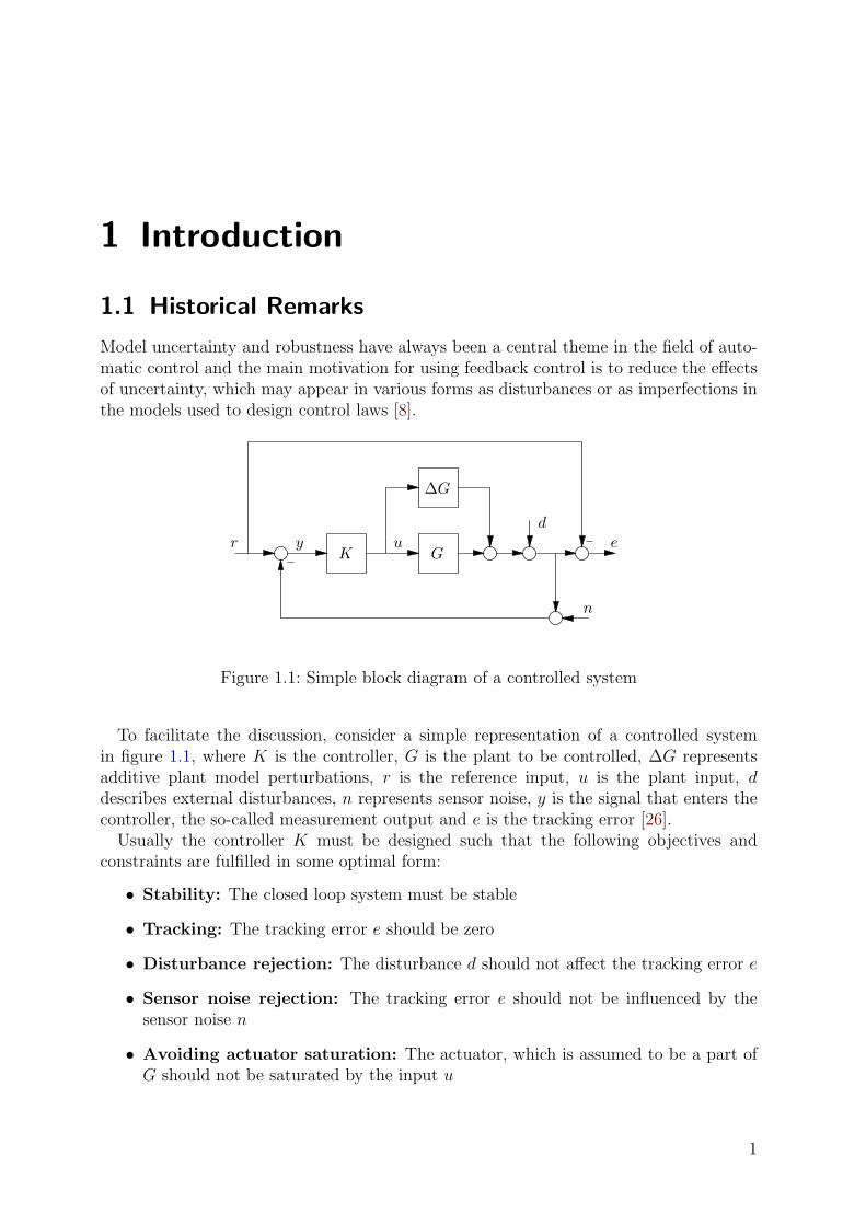
Figure 1.1: Simple block diagram of a controlled system
To facilitate the discussion, consider a simple representation of a controlled systemin figure 1.1, where K is the controller, G is the plant to be controlled, ∆G representsadditive plant model perturbations, r is the reference input, u is the plant input, ddescribes external disturbances, n represents sensor noise, y is the signal that enters thecontroller, the so-called measurement output and e is the tracking error [26].
Usually the controller K must be designed such that the following objectives andconstraints are fulfilled in some optimal form:
• Stability: The closed loop system must be stable
• Tracking: The tracking error e should be zero
• Disturbance rejection: The disturbance d should not affect the tracking error e
• Sensor noise rejection: The tracking error e should not be influenced by thesensor noise n
• Avoiding actuator saturation: The actuator, which is assumed to be a part ofG should not be saturated by the input u
1
1 Introduction
• Robustness: All aforementioned objectives and constraints - or at least the sta-bility requirement - should be fulfilled to an acceptable level, even if the real plantmay differ from the plant model G by an amount ∆G.
It is clear that all these requirements can only be fulfilled to some extent. Usuallydifferent requirements pose different demands on the control action and the final controllerK will be a compromise solution. Therefore it is important to quantify all the objectivesand to weigh them in a suitable way. The robustness requirement generally reducesthe achievable closed-loop performance as the controller can not be tuned only for onespecific nominal plant model G, but the objectives must be satisfactorily fulfilled forthe real plant, which may lie in a set of plant models given as G + ∆G. In general,model perturbations and uncertainties described by ∆G can never be avoided due to thefollowing facts:
• Unmodelled dynamics: Usually control design requires model descriptions ofreasonable size and complexity. In many cases linear, time-invariant models G ofreduced order are used for control design. High frequency dynamics or nonlinearitiesare usually approximated leading to imperfections in the model.
• Time variance: Plant dynamics undergo changes during operation. Varying envi-ronmental conditions (e.g., temperature changes or variation in the earth magneticfield during one orbit of a satellite) or the wear caused by aging influence the plantdynamics.
• Varying loads: Plant dynamics change depending on their load conditions. Forexample the inertia and the position of center of gravity of an aircraft changedepending on the distribution of passengers, cargo and fuel.
• Manufacturing variance: If we consider a series of plants the control designis usually performed for one or several prototypes of them. However, in a seriesproduction there will always be manufacturing variances between the individualplants and the controller must cope with these.
• Identification errors: Even if the model structure includes all dynamics of thereal process, there will always be errors in the identification of the model parametersdue to limitations of the identification hardware and methods.
Considering robustness of SISO systems to gain variations, a first systematic controldesign approach was developed by Bode [16, 17]. At this time linear systems were de-scribed using transfer functions or frequency responses and it was straightforward todescribe model uncertainties as deviations from some nominal frequency response. TheBode diagram has proven to be very useful to graphically design controllers and measuresas gain and phase margins were introduced. A generalization of Bode’s work, consideringrobustness to arbitrary plant variations, was developed by Horowitz [48], which foundedthe Quantitative Feedback Design Theory (QFT) [49].
In the 1960s, the state-space theory became more popular. Systems were then describedby differential equations allowing new insights [52] and initiating the development of
2
1.2 Linear Fractional Transformations (LFTs) in robust control
many new control design techniques. The LQG method [51] is probably the best-knowndevelopment of this time. The control design problem for a linear system with Gaussiandisturbances is formulated as an optimization problem with quadratic constraints andit admits an analytical solution. The controller structure consists of a Kalman filterand a linear state feedback. In the case that all state variables can be measured, theLQG design offers very strong robustness properties with at least 60 of phase marginand infinite gain margin as shown in [70]. Unfortunately, this does not hold for theoutput feedback case, where a Kalman filter is used to estimate the system states [33].An obvious idea to achieve robustness was to modify the Kalman filter in some way torecover the loop transfer of the case where all states are measured [69]. However, themodified Kalman filter may be completely nonoptimal as far as disturbance rejection isconcerned. Conclusively, the classical approach of LQG controller design as described in[51] is not the proper way to incorporate performance requirements, disturbance rejectionand robustness.
A paradigm shift in robust control was represented by the paper [89]. It was a startingpoint of the so called H∞ theory, which has become very popular in control theory. Itallows to incorporate performance specifications, disturbance rejection and robustnessrequirements into one optimization problem and allows to generalize the successful clas-sical design techniques in the frequency domain from SISO to MIMO systems. Solutionsof the H∞ problem in state-space were presented in [35] marking a cornerstone in therobust control theory.
1.2 Linear Fractional Transformations (LFTs) in robustcontrol
To perform robust H∞ controller synthesis it is essential to quantify the uncertainties inthe process model, to define a precise mathematical formulation and to describe how theseuncertainties enter into the system interconnection. In general two types of uncertaintiesare considered:
• Model imperfections due to neglected nonlinearities or unmodelled dynamics areusually represented as additive or multiplicative norm-bounded frequency domainerrors with arbitrary phase, which are related to process components or the wholeprocess. These are called unstructured uncertainties.
• Uncertainties in model parameters can be described more precisely. The processmodel usually contains structural information of how the uncertain parametersaffect the process dynamics. This often allows to achieve better closed-loop perfor-mance than in the unstructured uncertainty case. If the structural information isignored one may obtain a conservative approximation of the true error. Thereforeparametric uncertainties can be handled more systematically and they are denotedas structured uncertainties.
In literature the terminology structured uncertainty is usually equivalent to parametricuncertainty. However, considering a system consisting of at least two coupled components
3
1 Introduction
and each component admits an unstructured uncertainty description, then it is importantto note that at system level the overall uncertainty description also becomes structured,although not parametric, uncertainty. Hence, in such cases one also may reduce con-servativeness by considering this structure during robust stability/performance analysisor robust controller synthesis and the terminology structured uncertainty does not onlystand for parametric uncertainty.
Mathematical models of uncertainties must be explicitly included in the process model.In general the resulting overall model must be transformed/rearranged into a specialstructure that admits the application of robust H∞ methods. Linear Fractional Trans-formations (LFTs) are a general, flexible and powerful way to represent uncertainty insystems. The idea of using LFT-based uncertainty descriptions (denoted as Linear Frac-tional Representations (LFRs)) is to keep separated what is known from what is unknownby expressing the process model as a feedback connection of a nominal plant and the un-certainty description. An LFR defines a set of process models and the real process isassumed to lie inside this model set. LFRs are suitable for the application of robust H∞design methods.
LFT-based robust control was extensively studied during the last years (see [7, 29, 28,13, 24, 77, 65, 72, 74, 92] and references therein). Successful applications can be foundin various areas, as aeronautics [58], missile control [67], control of flexible structures [9],control of CD-players [31], high-precision positioning in IC-manufacturing [78] and manyothers.
1.3 Motivation and Thesis Structure
In principle, it is straightforward to transform a linear plant model including unstructuredand structured uncertainties into an LFR. However, this transformation is not uniqueand the blindfold application of ad-hoc methods [77] generally leads to LFRs of highcomplexity. LFT-based robust control methods are numerically highly demanding and ofhigh computational complexity, e.g., many methods are based on solving a large systemof Linear Matrix Inequalities (LMIs) [19, 73]. Therefore the application of these methodsis restricted to LFRs of reasonable complexity, otherwise the computation time will beunacceptable, the numerical errors will increase or the methods may even fail.
It is the aim of the present thesis to develop new techniques and to improve existingmethods for the realization of LFRs with reduced complexity for parametric plant mod-els. A plant model may include many uncertain parameters and these generally enter themodel equations in a highly structured way. The same parameter may appear in manyparts of the model and parametric expressions can be very complicated (e.g., resultingfrom rational parametric approximations of multidimensional tables in an aircraft model[84]). Therefore it is crucial to employ systematic and structure exploiting techniquesto reduce the LFR complexity resulting from parametric uncertainty. Concerning un-structured uncertainties, these are usually employed to describe general imperfections ofprocess components or the whole process and occur only once in a model description.Hence, the transformation of models including unstructured uncertainties to an LFR cangenerally be done by inspection and there is low potential to reduce the LFR complexity
4
1.3 Motivation and Thesis Structure
resulting from unstructured uncertainty. To simplify the presentation, the low order LFRrealization techniques developed in this thesis are presented exclusively for systems withstructured/parametric uncertainties.
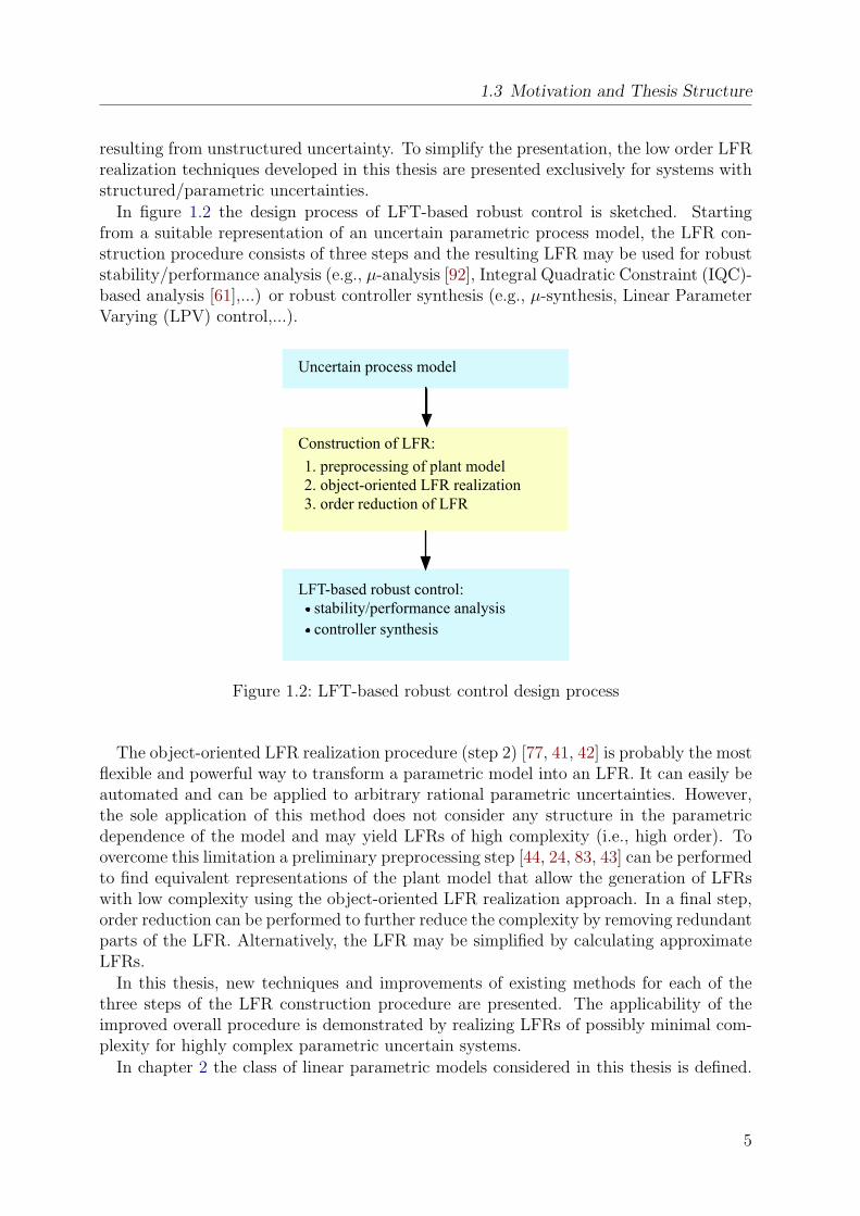
In figure 1.2 the design process of LFT-based robust control is sketched. Startingfrom a suitable representation of an uncertain parametric process model, the LFR con-struction procedure consists of three steps and the resulting LFR may be used for robuststability/performance analysis (e.g., µ-analysis [92], Integral Quadratic Constraint (IQC)-based analysis [61],...) or robust controller synthesis (e.g., µ-synthesis, Linear ParameterVarying (LPV) control,...).
Uncertain process model
Construction of LFR:
LFT-based robust control: stability/performance analysis controller synthesis
1. preprocessing of plant model2. object-oriented LFR realization3. order reduction of LFR
Figure 1.2: LFT-based robust control design process
The object-oriented LFR realization procedure (step 2) [77, 41, 42] is probably the mostflexible and powerful way to transform a parametric model into an LFR. It can easily beautomated and can be applied to arbitrary rational parametric uncertainties. However,the sole application of this method does not consider any structure in the parametricdependence of the model and may yield LFRs of high complexity (i.e., high order). Toovercome this limitation a preliminary preprocessing step [44, 24, 83, 43] can be performedto find equivalent representations of the plant model that allow the generation of LFRswith low complexity using the object-oriented LFR realization approach. In a final step,order reduction can be performed to further reduce the complexity by removing redundantparts of the LFR. Alternatively, the LFR may be simplified by calculating approximateLFRs.
In this thesis, new techniques and improvements of existing methods for each of thethree steps of the LFR construction procedure are presented. The applicability of theimproved overall procedure is demonstrated by realizing LFRs of possibly minimal com-plexity for highly complex parametric uncertain systems.
In chapter 2 the class of linear parametric models considered in this thesis is defined.
5
1 Introduction
Two ways how to derive such models from more general nonlinear parametric models arepresented. A new representation called generalized LFR is introduced to overcome a basiclimitation of the standard LFR to represent arbitrary rational parametric expressions.Formulas for the related object-oriented LFR realization technique are developed. Finally,procedures are presented for the realization of LFRs for generalized parametric state-spacesystems.
Chapter 3 presents an overview of symbolic decomposition methods suitable as pre-processing tools. New techniques are proposed and several enhancements of existingsymbolic preprocessing methods are shown. All these symbolic methods, together withthe generalized LFR and enhanced numerical order reduction techniques for LFRs aresupported by the newly developed version 2 of the LFR-toolbox for Matlab, which isbriefly described in chapter 4.
Chapter 5 describes the application of the developed low order LFR realization tech-niques to the RCAM (Research Civil Aircraft Model), which is one of the most compli-cated parametric models available in literature. The order of the generated LFR wasreduced by about 60% compared to former realizations reported in literature. This loworder LFR allows to apply µ-analysis techniques for the whole flight envelope, which wasnot possible before with the high-order models. Closed-loop robust stability was analyzedfor 12 different controllers and some of them were indicated to not achieve closed-loopstability for the uncertain plant model. This could be confirmed by a complementaryoptimization-based worst-case search, where worst-case plant models leading to unstableclosed-loop systems were identified, for these cases.
In chapter 6 an LFR of minimal complexity is realized for an uncertain parametricmodel describing the lateral dynamics of a vehicle. This LFR is employed for the re-alization of two a robust vehicle steering controllers. One controller is generated usingthe µ-synthesis technique and the second controller is an automatically generated gain-scheduled controller based on robust Linear Parameter Varying (LPV) control designtechniques. Both controllers provide better robust performance properties than recentlydeveloped controllers for this vehicle model.
6
2 Generalized Linear FractionalRepresentation (LFR) for parametricuncertain systems
2.1 From nonlinear to linear parametric models
Many physical dynamical systems can be described by a continuous-time, nonlinear,parametric plant of implicit form
0 = f(x, x, u, δ)
y = g(x, u, δ)(2.1)
where f ∈ Rn and g ∈ Rp are vector functions, x ∈ Rn is the state vector with xas its time derivative, u ∈ Rm is the input vector and δ ∈ Rk is a vector of physicalparameters. The parameter values are bounded by their minimum and maximum valuesand the admissible parameter value set is defined as
Π = δ : δi ∈ [δi,min, δi,max], i = 1, . . . , k (2.2)
Each parameter δi may be described in different units and the ranges of admissible val-ues may differ by orders of magnitudes. For the application of LFT-based techniques forrobust stability analysis and robust controller synthesis (e.g. µ-analysis and µ-synthesis)it is generally required that the uncertain parameters are normalized to lie in an k-dimensional cube centered at the origin.
To perform the normalization of parameters, δi can be replaced by a rational parametricfunction ni(δi) such that δi = ni(δi) with |δi| ≤ 1. The function ni(δi) is chosen such that,δi,min = ni(−1), δi,max = ni(1), δi,nom = ni(0), where δi,nom ∈ [δi,min, δi,max] represents thenominal value of the parameter δi. Hence the nominal system
0 = f(x, x, u, δ)|δ=δnom
y = g(x, u, δ)|δ=δnom
can be represented as
0 = f(x, x, u, n(δ))|δ=0
y = g(x, u, n(δ))|δ=0.
This is convenient because the nominal system corresponds now to a normalized systemwhere all parameters are zero, i.e., δ = 0.
7
2 Generalized Linear Fractional Representation (LFR) for parametric uncertain systems
In robust control applications, non-linear parametric models of the form (2.1) are usefulto perform parameter sensitivity studies (e.g., via simulations). However, the applicationof LFT-based robust control synthesis and analysis techniques requires a linear descrip-tion or approximation of the nonlinear plant (2.1). Such a description can be obtainedby applying Jacobian-based linearization or by reformulating the nonlinear plant in aquasi-Linear Parameter Varying (LPV) form. Both methods are briefly described in thefollowing. For a comprehensive treatment see [68, 55, 59].
2.1.1 Jacobian-based linearization
Recall that a trim point xt, xtrim, utrim, ytrim, δtrim of the plant model (2.1) satisfies 0 =f(xtrim, xtrim, utrim, δtrim), ytrim = g(xtrim, utrim, δtrim) and if xtrim = 0 it may be an equi-librium point of (2.1).
Definition 2.1. The functions xtrim(δ), xtrim(δ) and utrim(δ) define a family of trim pointsfor (2.1) on the set Π if
0 = f(xtrim(δ), xtrim(δ), utrim(δ), δ), δ ∈ Π
ytrim = g(xtrim(δ), utrim(δ), δ).(2.3)
The n + p nonlinear equations (2.1) must be solved (trimming) to determine n + p freecomponents of these vectors selected from a total of 2n + m + p components. Note, thatthe values of the remaining n + m components are set to values defining specific trimconditions.
A corresponding family of linearized parametric descriptor systems is defined by
E(δ)xδ = A(δ)xδ + B(δ)uδ
yδ = C(δ)xδ + D(δ)uδ
(2.4)
where
E(δ) = −∂f
∂x(xtrim(δ), xtrim(δ), utrim(δ), δ)
A(δ) =∂f
∂x(xtrim(δ), xtrim(δ), utrim(δ), δ)
B(δ) =∂f
∂u(xtrim(δ), xtrim(δ), utrim(δ), δ)
C(δ) =∂g
∂x(xtrim(δ), xtrim(δ), utrim(δ), δ)
D(δ) =∂g
∂u(xtrim(δ), xtrim(δ), utrim(δ), δ)
(2.5)
and where
xδ = x− xtrim(δ), xδ = x− xtrim(δ), uδ = u− utrim(δ) and yδ = y − ytrim(δ). (2.6)
For each fixed value of δ ∈ Π the linearization (2.4) describes to local behavior of thenonlinear plant (2.1) about the corresponding trim point.
8
2.1 From nonlinear to linear parametric models
If the inverse of E(δ) exists it is possible to obtain an explicit parametric state-spacesystem of the form
xδ = A(δ)xδ + B(δ)uδ
yδ = C(δ)xδ + D(δ)uδ
(2.7)
where A(δ) = E(δ)−1A(δ) and B(δ) = E(δ)−1B(δ).The main limitation of the Jacobian-based linearization is that in general there exists
no analytical solution for the functions xtrim(δ), xtrim(δ), utrim(δ), ytrim(δ). A commonpractice is to simply substitute these functions with their numerical values at the cor-responding trim point, computed for the nominal value of δ. The resulting Jacobianmatrices in (2.5) (obtained for example using symbolic differentiation) depend explicitlyon the parameters in δ. However, in this case all the information about the paramet-ric dependence of xtrim(δ), xtrim(δ), utrim(δ), ytrim(δ) is lost and the validity of the linearapproximation (2.4) is strongly limited. To increase the validity of the linear model repre-sentation, a more sophisticated way is to calculate polynomial or rational approximationsof these functions [84] based on physical knowledge of the parametric dependence in theentries of the matrices in (2.4).
2.1.2 Quasi-LPV models
For gain-scheduling control design a linear plant description may be obtained by rewritingthe nonlinear model (2.1) in quasi-LPV form, if possible. The idea is to hide nonlinearterms, that may also depend on state variables, in newly defined parameters that can bemeasured and are employed as scheduling variables. This means that in various partsof the model, state variables must be relabelled, while they remain dynamical variableselsewhere. Consider for example the nonlinear system
x = A(x, δ)x + B(x, δ)u
y = C(x, δ)x + D(x, δ)u,(2.8)
with x(t) confined to some operating region X ⊂ Rn. It is clear, that the solutions of(2.8) are a subset of the solutions of the system
x = A(δ)x + B(δ)u
y = C(δ)x + D(δ)u,(2.9)
with δ ∈ Π × X. Hence, it is possible to over-bound the nonlinear system (2.8) with aquasi-LPV system (2.9). This may introduce some conservativeness as no a priori knowl-edge of the arbitrarily varying parameters in δ is assumed and the explicit dependenceon the state variables is not exploited.
Both methods, the Jacobian-based linearization and the quasi-LPV approach achievelinearity in the plant description, however this is done in quite different ways.
In general, for the realization of LFRs, only rational parametric dependence is allowedin the entries of the linear plant descriptions and therefore finally all remaining nonlin-earities in these matrices must be approximated by rational functions.
9
2 Generalized Linear Fractional Representation (LFR) for parametric uncertain systems
2.2 Standard LFT
This section introduces a new matrix function: the linear fractional transformation(LFT).
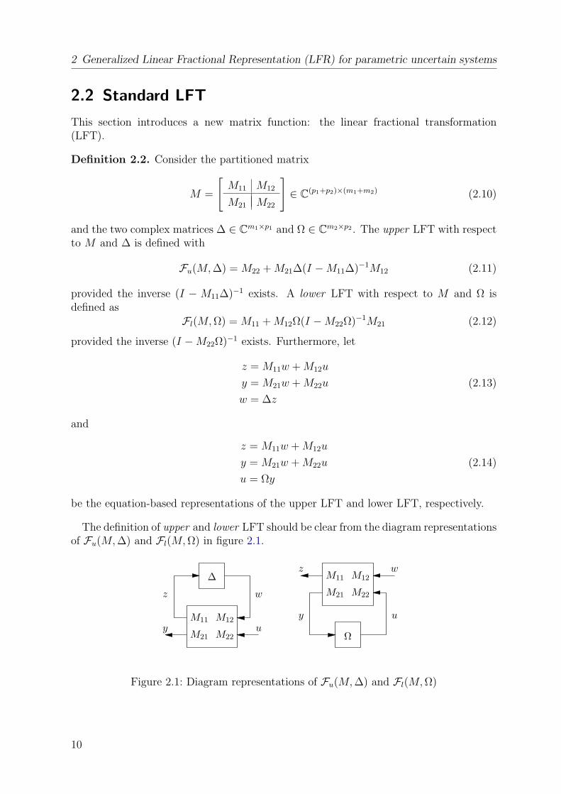
Definition 2.2. Consider the partitioned matrix
M =
[M11 M12
M21 M22
]∈ C(p1+p2)×(m1+m2) (2.10)
and the two complex matrices ∆ ∈ Cm1×p1 and Ω ∈ Cm2×p2 . The upper LFT with respectto M and ∆ is defined with
Fu(M, ∆) = M22 + M21∆(I −M11∆)−1M12 (2.11)
provided the inverse (I − M11∆)−1 exists. A lower LFT with respect to M and Ω isdefined as
Fl(M, Ω) = M11 + M12Ω(I −M22Ω)−1M21 (2.12)
provided the inverse (I −M22Ω)−1 exists. Furthermore, let
z = M11w + M12u
y = M21w + M22u
w = ∆z
(2.13)
and
z = M11w + M12u
y = M21w + M22u
u = Ωy
(2.14)
be the equation-based representations of the upper LFT and lower LFT, respectively.
The definition of upper and lower LFT should be clear from the diagram representationsof Fu(M, ∆) and Fl(M, Ω) in figure 2.1.
M11 M12
M22M21
M21
M11 M12
M22
∆
z
y
w
uΩ
y
z
u
w
Figure 2.1: Diagram representations of Fu(M, ∆) and Fl(M, Ω)
10
2.2 Standard LFT
The upper LFT describes the relation between y and u after closing the upper loop, i.e.w = ∆z and y = Fu(M, ∆)u. Similarly, the lower LFT describes the relation between zand w after closing the lower loop, i.e. u = Ωy and z = Fl(M, Ω)w. In the literature,usually the upper LFT is used to represent uncertainty in plant models and thereforethis representation will be employed in the following. Furthermore, the short term LFR(Linear Fractional Representation) will be used to denote the upper LFT representationof an uncertain parametric model.
In an LFR, M22 typically stands for the nominal model (i.e., corresponds to ∆ = 0),while M11, M12 and M21 describe the structure of how the uncertainty affects the nominalmodel. Hence the LFR can be employed to represent an uncertain model as a feedbackinterconnection of the model uncertainties described by ∆ and a nominal plant model.
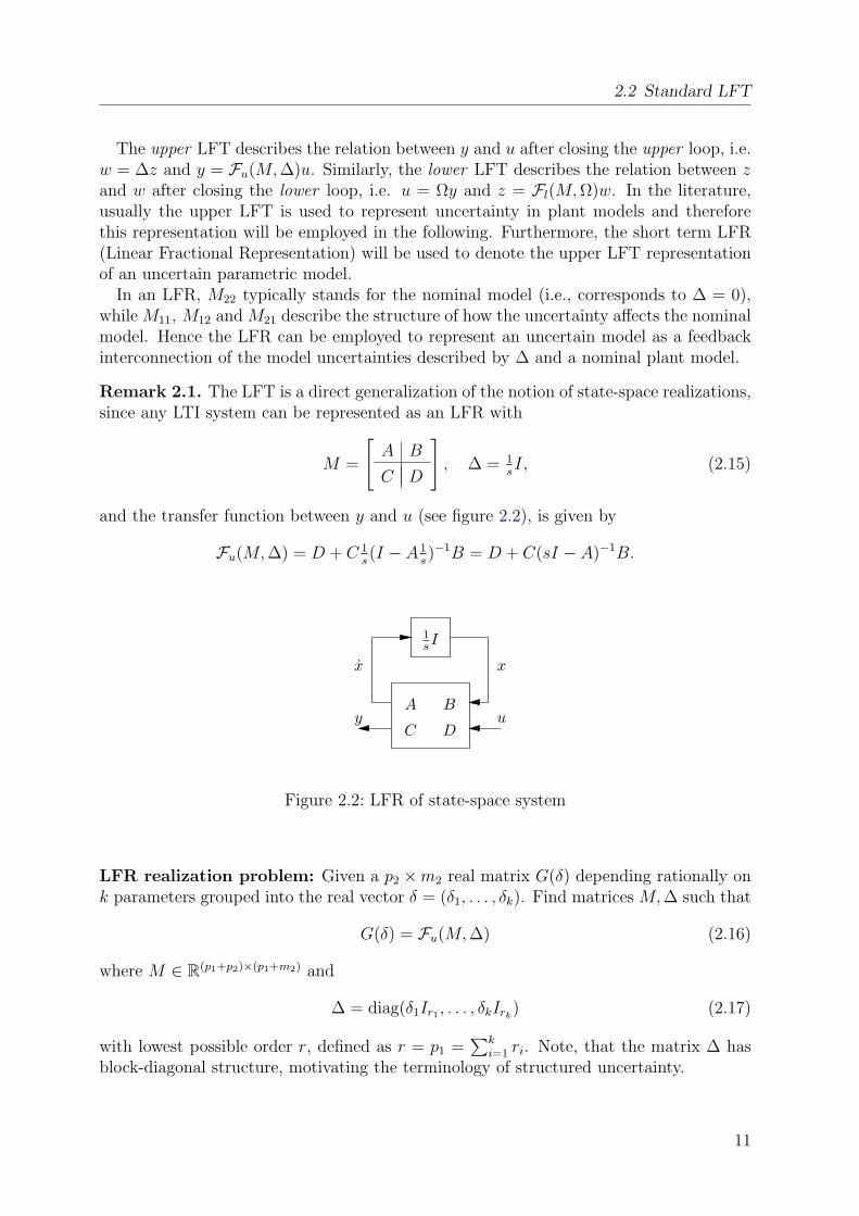
Remark 2.1. The LFT is a direct generalization of the notion of state-space realizations,since any LTI system can be represented as an LFR with
M =
[A B
C D
], ∆ = 1
sI, (2.15)
and the transfer function between y and u (see figure 2.2), is given by
Fu(M, ∆) = D + C 1s(I − A1
s)−1B = D + C(sI − A)−1B.
1
sI
x x
uBA
C Dy
Figure 2.2: LFR of state-space system
LFR realization problem: Given a p2 ×m2 real matrix G(δ) depending rationally onk parameters grouped into the real vector δ = (δ1, . . . , δk). Find matrices M, ∆ such that
G(δ) = Fu(M, ∆) (2.16)
where M ∈ R(p1+p2)×(p1+m2) and
∆ = diag(δ1Ir1 , . . . , δkIrk) (2.17)
with lowest possible order r, defined as r = p1 =∑k
i=1 ri. Note, that the matrix ∆ hasblock-diagonal structure, motivating the terminology of structured uncertainty.
11
2 Generalized Linear Fractional Representation (LFR) for parametric uncertain systems
Hence the ultimate goal is to find LFRs of minimal order. However, representing aparameter dependent matrix as an LFR is basically equivalent to a multidimensional real-ization problem [18], where a minimal realization theory is still lacking. For 1-dimensionalsystems as (2.15) (or equivalently, systems with only one diagonal block in ∆) a minimalrealization can always be obtained by eliminating unobservable and uncontrollable partsfrom the state-space representation (2.15). Unfortunately for multidimensional systemssimilar techniques cannot be employed (see [18] and section 3.1 for a brief description).
Example 2.1. Consider the simple scalar parametric expression G(δ) = δi, which canbe directly realized as
δi = Fu(M, ∆) = Fu
([0 1
1 0
], δi
)(2.18)
and will be denoted as elementary LFR. Starting from elementary LFRs for uncertainparameters, an object-oriented approach [77] can be employed to realize an LFR for arational parametric matrix G(δ). However, there is a basic limitation for the realization ofarbitrary rational matrices via standard LFRs. As an example, the expression G(δ) = 1/δi
cannot be represented as an LFR with ∆ of the form (2.17). This is equivalent to the casethat it is not possible to represent non-proper transfer functions as for example G(s) = sin standard state-space form (2.15). One way to represent G(δ) = 1/δi as an LFR is touse in (2.18) ∆ = 1/δi. However, G(δ) = δi + 1/δi does not have an LFR as both δi and1/δi enter the expression.
In practice, to overcome the above difficulties, a normalization of uncertainties is per-formed. Assuming, for example that δi ∈ [δi,min, δi,max] and δi,nom := (δi,max+δi,min)/2 6= 0,then with δi,sl := (δi,max− δi,min)/2 one obtains δi = δi,nom + δi,slδi, with δi ∈ [−1, 1]. Withthis normalization, G(δ) := 1/(δi,nom + δi,slδi) = 1/δi can be represented as
G(δ) = Fu
([−δi,slδ
−1i,nom −δi,slδ
−1i,nom
δ−1i,nom δ−1
i,nom
], δi
).
A negative aspect of this approach is that the normalization must be performed asa preliminary symbolic operation before the LFR realization and this often leads to anincrease of the overall order of the LFR (see [24] and next example).
Example 2.2. Consider G(δ) = δ2i and its normalized and expanded form G(δ) = δ2
i,nom+
2δi,nomδi,slδi +δ2i,slδ
2
i . The object-oriented LFR realization procedure of [77] yields an LFR
of minimal order 2 for G(δ), whereas an LFR of order 3 is obtained for G(δ), where this
procedure generates an LFR by interconnecting a second order LFR for δ2i,slδ
2
i with a first
order LFR for 2δi,nomδi,slδi and the constant term δ2i,nom. The result is a third order LFR.
This simple example clearly illustrates that it is desirable to perform the normalizationas the last step in any LFR generation. This is particularly important when employingsymbolic preprocessing techniques as described in section 3 or in [24], as these techniquesmay start with an expansion of the symbolic expressions in G(δ). Expanding normalizedsymbolic functions usually yields large expressions, which may result in LFRs of highorder, as this artificially introduced complexity cannot be fully recovered by the symbolicfactorization and decomposition techniques.
12
2.3 Generalized LFT
2.3 Generalized LFT
In this section the generalized LFT is introduced, which is a natural extension of thestandard LFT. It may also be called descriptor LFT in analogy to the generalized statespace realizations via descriptor systems [25].
2.3.1 Definition
The generalized upper LFT is defined with the partitioned matrix
M =
[M10 M11 M12
0 M21 M22
](2.19)
as
Fu(M, ∆) = M22 + M21∆(M10 −M11∆)−1M12, (2.20)
where the square submatrix M10 is allowed to be generally singular but the inverse (M10−M11∆)−1 must exist. For ∆ we assume the more general structure
∆ = diag(δ0Ir0 , δ1Ir1 , . . . , δkIrk), (2.21)
where δ0 is a nonzero constant, which is set to 1 in the following. The equation-baseddefinition of the generalized upper LFT is given as
M10z = M11w + M12u
y = M21w + M22u
w = ∆z,
(2.22)
and the order of a generalized LFR (M, ∆) is defined as r =∑k
i=1 ri. Note that thestandard LFR (2.11) corresponds to M10 = I and r0 = 0.
With the generalized LFR we can represent G(δ) = 1/δ as
1
δ= Fu
0 0 0 1 10 1 1 0 0
0 0 −1 0 0
,
[1 00 δ
] . (2.23)
There is a clear analogy to generalized state-space systems, where for example thedifferentiator G(s) = s is described in descriptor form as[
0 00 1
] [x1
x2
]=
[0 11 0
] [x1
x2
]+
[10
]u
y =[−1 0
]x,
(2.24)
consisting of a combination of differential (x2 = x1) and algebraic (x2 = u) equations(DAE system).
13
2 Generalized Linear Fractional Representation (LFR) for parametric uncertain systems
Remark 2.2. In the generalized LFR the algebraic equations are formally described as anadditional dimension - the block Ir0 in ∆ - in a multidimensional system representation.The generalized LFR may seem to be more complex as the standard LFR, as for example a2-dimensional system representation (2.23) (two diagonal blocks in ∆) is used to representG(δ) = 1/δ. However, it will be shown that the object-oriented LFR realization procedurebased on generalized LFRs is actually simpler than for standard LFRs, as explicit matrixinversions can be avoided. Furthermore, it will be shown that the artificially introducedadditional dimension (Ir0 in ∆) will usually vanish after a normalization of the generalizedLFR and finally a standard LFR is obtained. It is important to emphasize that thegeneralized LFR allows to perform the normalization step as the last step in the LFRrealization procedure and this generally leads to LFRs of lower order as a preliminarysymbolic normalization is avoided.
2.3.2 Algebraic Properties
Since LFRs are similar to transfer-function matrix representations of linear state-spacesystems, the basic matrix operations like addition/subtraction, multiplication, transpo-sition, inversion as well as column/row concatenation correspond to similar operationsperformed on the transfer-function matrices of linear systems. These are operations un-derlying the methods used to generate LFRs of parametric matrices [77, 41, 42]. Thefollowing results for generalized LFRs generalize similar results for standard LFRs. Tosimplify notation, in the following lemmas, the partitioned matrix M is written as
M =
[E A B
0 C D
],
where E = M10, A = M11, B = M12, C = M21 and D = M22.
Lemma 2.1. (without proofs) Let M1, M2 and M be partitioned matrices
M =
[E A B
0 C D
], M1 =
[E1 A1 B1
0 C1 D1
], M2 =
[E2 A2 B2
0 C2 D2
]and let ∆, ∆1, ∆2 be the corresponding uncertainty matrices.
(i) Parallel connection:
Fu(M, ∆) := Fu(M1, ∆1)±Fu(M2, ∆2),
with
M =
E1 0 A1 0 B1
0 E2 0 A2 ±B2
0 0 C1 C2 D1 ±D2
, ∆ =
[∆1 00 ∆2
].
(ii) Series/Cascade connection:
Fu(M, ∆) := Fu(M1, ∆1)Fu(M2, ∆2),
14
2.3 Generalized LFT
with
M =
E1 0 A1 B1C2 B1D2
0 E2 0 A2 B2
0 0 C1 D1C2 D1D2
, ∆ =
[∆1 00 ∆2
].
(iii) Column concatenation:
Fu(M, ∆) :=[Fu(M1, ∆1) Fu(M2, ∆2)
],
with
M =
E1 0 A1 0 B1 00 E2 0 A2 0 B2
0 0 C1 C2 D1 D2
, ∆ =
[∆1 00 ∆2
].
(iv) Row concatenation:
Fu(M, ∆) :=
[Fu(M1, ∆1)Fu(M2, ∆2)
],
with
M =
E1 0 A1 0 B1
0 E2 0 A2 B2
0 0 C1 0 D1
0 0 0 C2 D2
, ∆ =
[∆1 00 ∆2
].
(v) Transposition:
Fu(Mtr, ∆tr) := Fu(M, ∆)T ,
with
Mtr =
[ET AT CT
0 BT DT
], ∆tr = ∆T .
(vi) Consider [A(δ) B(δ)C(δ) D(δ)
]= Fu
E A B1 B2
0 C1 D11 D12
0 C2 D21 D22
, ∆
.
Then
Fu(M, ∆) := Fu
([E A(δ) B(δ)
0 C(δ) D(δ)
], ∆
),
with
M =
E 0 A B1 B2
0 E C1 D11 D12
0 0 C2 D21 D22
, ∆ =
[∆ 00 ∆
].
15
2 Generalized Linear Fractional Representation (LFR) for parametric uncertain systems
Lemma 2.2. Similarity transformations: Let Q and Z be invertible matrices such thatZ∆ = ∆Z. Then
Fu(M, ∆) = Fu(M, ∆)
where
M =
[QEZ QAZ QB
0 CZ D
], ∆ = ∆
Proof.Fu(M, ∆) = D + CZ∆(QEZ −QAZ∆)−1QB
with commutativity of Z and ∆ we obtain
Fu(M, ∆) = D + C∆Z(QEZ −QA∆Z)−1QB,
and moving Z and Q into the parenthesis finally yields
Fu(M, ∆) = D + C∆(Q−1QEZZ−1 −Q−1QA∆ZZ−1)−1B = Fu(M, ∆).
In the next lemma a more general class of transformations including similarity transfor-mations are considered. To define this transformation the equation based representationon a generalized LFR (2.22) is formally rewritten as[
0y
]=
[A∆− E B
C∆ D
] [zu
],
where w is substituted by w = ∆z.
Lemma 2.3. Let Q and Z be invertible matrices such that Z∆ = ∆Z. FurthermoreQk and Zk are matrices such that QkE = 0 and EZk = 0, i.e., im(QT
k ) ⊂ ker(ET ) andim(Zk) ⊂ ker(E). Then[
0y
]=
[A∆− E B
C∆ D
] [wu
]=
[Q 0Qk I
] [A∆− E B
C∆ D
] [Z Zk
0 I
] [wu
].
(2.25)
Proof. The matrices Q and Z define a similarity transformation which was shown inLemma 2.2. Therefore in the proof only the trivial case Q = I and Z = I is considered.
First, the transformation related to Qk is proven and without loss of generality it isassumed that Zk = 0. By definition QkEz = 0 and therefore Qk(A∆z + Bu) = 0. Thetransformation in (2.25) simply describes an addition of Qk(A∆z+Bu) = 0 to the outputequation, i.e., [
0y
]=
[I 0
Qk I
] [A∆− E B
C∆ D
] [zu
]=
[A∆− E B
QkA∆ + C∆ QkB + D
] [zu
].
16
2.3 Generalized LFT
and y = (QkA∆ + C∆)z + (QkB + D)u = C∆z + Du + Qk(A∆z + Bu) = C∆z + Du.The dual result for a transformation with Zk, assuming that Qk = 0, follows by con-
sidering the transposed system[0y
]=
[∆T AT − ET ∆T CT
ZTk ∆T AT − ZT
k ET + BT DT + ZTk ∆T CT
] [zu
],
where by definition ZTk ET z = 0 and therefore ZT
k (∆T AT z + ∆T CT u) = 0.
Lemma 2.4. Permutation: Let T be an orthogonal matrix, i.e. TT T = I. Furthermoreeach row of T consists only of zeros except one element, which is 1. Then for a diagonalmatrix ∆
Fu(M, ∆) = Fu(M, ∆),
with
M =
[T T ET T T AT T T B
0 CT D
], ∆ = T T ∆T,
and ∆ is a diagonal matrix with the same entries as in ∆, but the order of the entries ispermuted.
Proof. The permutation property of the transformation should be clear and it is alsoobvious that
Fu(M, ∆) = D + CTT T ∆T (T T ET + T T ATT T ∆T )−1T T B = Fu(M, ∆).
Lemma 2.5. Inversion: Suppose Fu(M, ∆) is a p× p invertible matrix with
M =
[E A B
0 C D
]then
Fu(Minv, ∆inv) := Fu(M, ∆)−1,
with
Minv =
0 0 D C Ip
0 E B A 0
0 0 −Ip 0 0
, ∆inv =
[Ip 00 ∆
]. (2.26)
Proof. To show that (2.26) represents a generalized LFR for the inverse system, theproduct Fu(MI , ∆I) = Fu(M, ∆)Fu(Minv, ∆inv) is calculated using (ii) of Lemma 2.1with
MI =
0 0 0 D C C D0 E 0 B A 0 00 0 E 0 0 A B
0 0 0 −Ip 0 0 0
, ∆I =
Ip 0 00 ∆ 00 0 ∆
. (2.27)
17
2 Generalized Linear Fractional Representation (LFR) for parametric uncertain systems
Applying the transformation defined in Lemma 2.3 with
Q =
Ip 0 00 I I0 0 I
, Qk =[
0p 0 0], Z =
Ip 0 00 I −I0 0 I
, Zk =
−Ip
00
,
to (2.27) yields Fu(MI , ∆I) = Fu(MI , ∆I) with
MI =
0 0 0 D C 0 00 E 0 B A 0 00 0 E 0 0 A B
0 0 0 −Ip 0 0 Ip
, ∆I = ∆I . (2.28)
From a direct evaluation of Fu(MI , ∆I) it follows Fu(MI , ∆I) = Ip.
Note, that by using a generalized LFR, its inverse (see (2.26)) can be determined as ageneralized LFR in terms of the original matrices, without any explicit matrix inversion.
Corollary 2.1. If D is invertible, an alternative expression for Minv and ∆inv, involvinginversion of D may be obtained. Therefore one may write the explicit relation defined byMinv, ∆inv as [
0 00 E
] [z1
z2
]=
[D CB A
] [w1
w2
]+
[Ip
0
]u,
y = −Ipw1,[z1
z2
]=
[I 00 ∆
] [w1
w2
].
(2.29)
From (2.29) it can be seen that z1 = w1 and one can solve for w1 as w1 = −D−1Cw2 −D−1u. Substituting w1 in (2.29) finally yields Minv and ∆inv as
Minv =
[E A−BD−1C −BD−1
0 D−1C D−1
], ∆inv = ∆.
It is well known that for any rational parametric matrix G(δ), it is possible to finda left (right) polynomial fractional representation, with G(δ) = D−1(δ)N(δ) (G(δ) =
N(δ)D−1(δ)), where N(δ), D(δ) (N(δ), D(δ)) are multivariate polynomial matrices. Itis possible to express such fractional representations in terms of the underlying LFRs ofthe factors. The following results are particularly useful when realizing LFRs for rationalparametric matrices in terms of polynomial factorizations.
Lemma 2.6. Let Fu(M, ∆) =[
N(δ) D(δ)]
be defined with
M =
[E A BN BD
0 C DN DD
]
18
2.3 Generalized LFT
and assume that D(δ) is a p× p invertible matrix. Then
Fu(Mlf, ∆lf) = D−1(δ)N(δ),
with
Mlf =
0 0 DD C DN
0 E BD A BN
0 0 −Ip 0 0
, ∆lf =
[Ip 00 ∆
]. (2.30)
If DD is invertible, alternative representations of Mlf and ∆lf are
Mlf =
[E A−BDD−1
D C BN −BDD−1D DN
0 D−1D C D−1
D DN
], ∆lf = ∆.
Proof. Using Lemma 2.5 and (ii) of Lemma 2.1, one obtains
Fu(MM , ∆M) = D−1(δ)N(δ),
where
MM =
[EM AM BM
0 CM DM
]=
0 0 0 DD C C DN
0 E 0 BD A 0 00 0 E 0 0 A BN
0 0 0 −Ip 0 0 0
,
∆M =
Ip 0 00 ∆ 00 0 ∆
.
Now, a similarity transformation is applied to MM , yielding a transformed matrix MM .Consider the transformation matrices Q and Z given by
Q =
Ip 0 00 I I0 0 I
, Z =
Ip 0 00 I −I0 0 I
,
with the identity matrix I of the same size as ∆. It is easy to see that Z∆M = ∆MZ,thus applying Lemma 2.2 yields
MM =
[QEMZ QAMZ QBM
0 CMZ DM
]=
0 0 0 DD C 0 DN
0 E 0 BD A 0 BN
0 0 E 0 0 A BN
0 0 0 −Ip 0 0 0
.
By evaluating Fu(MM , ∆M) directly, the expression reduces to Fu(Mlf, ∆lf).The result for invertible DD can easily be derived from (2.30) or it can be proven
similarly as done in [14].The following lemma (given without proof) is the dual result for a right fractional
representation.
19
2 Generalized Linear Fractional Representation (LFR) for parametric uncertain systems
Lemma 2.7. Let Fu(M, ∆) =
[N(δ)D(δ)
]be defined with
M =
E A B0 CN DN
0 CD DD
,
and assume that D(δ) is a p× p invertible matrix. Then
Fu(Mrf, ∆rf) = N(δ)D−1(δ)
with
Mrf =
0 0 DD CD −Ip
0 E B A 00 0 DN CN 0
, ∆rf =
[Ip 00 ∆
].
If DD is invertible, alternative representation of Mrf and ∆rf are
Mrf =
[E A−BD−1
D CD BD−1D
0 CN −DND−1D CD DND−1
D
], ∆rf = ∆.
2.3.3 Object-oriented LFR realization procedure for rationalparametric matrices
Using the results of section 2.3.2, one can readily build an LFR for an arbitrary rationalparametric matrix G(δ) along the lines of the following object-oriented procedure, wherethe realization problem is decomposed into the elementary steps:
1. Build elementary LFRs of the form (2.18) for all distinct parameters δi, i = 1, . . . , k.
2. Generate an LFR of each rational matrix element gij(δ) from the LFRs of its nu-merator and denominator polynomials by applying Lemma 2.6. The polynomialrealizations are constructed using object-oriented realization techniques based onmultiplication and addition/subtraction of LFRs (see Lemma 2.1) relying on effi-cient multivariate polynomial evaluation schemes.
3. Use row and column concatenations for LFRs (see Lemma 2.1) to obtain an LFRof G(δ) from the LFRs of the individual entries gij(δ).
4. employ Lemma 2.4 to reorder (M, ∆), such that ∆ is of the form as in (2.21).
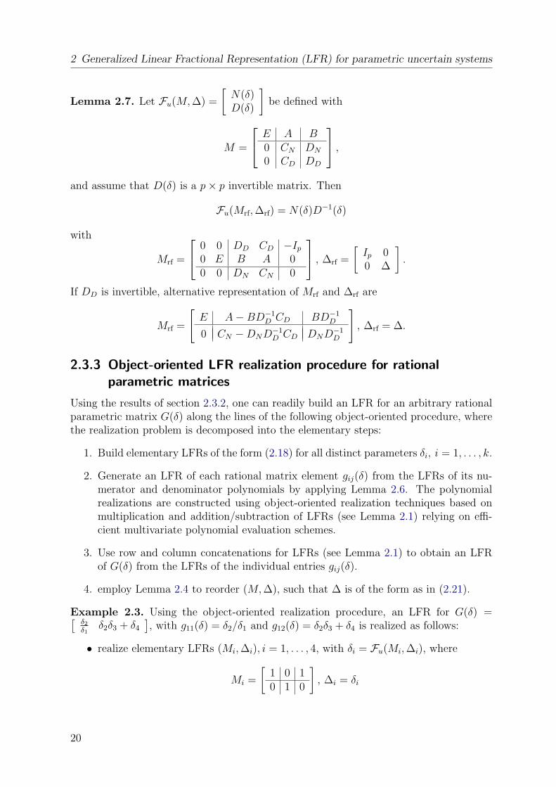
Example 2.3. Using the object-oriented realization procedure, an LFR for G(δ) =[δ2δ1
δ2δ3 + δ4
], with g11(δ) = δ2/δ1 and g12(δ) = δ2δ3 + δ4 is realized as follows:
• realize elementary LFRs (Mi, ∆i), i = 1, . . . , 4, with δi = Fu(Mi, ∆i), where
Mi =
[1 0 10 1 0
], ∆i = δi
20
2.3 Generalized LFT
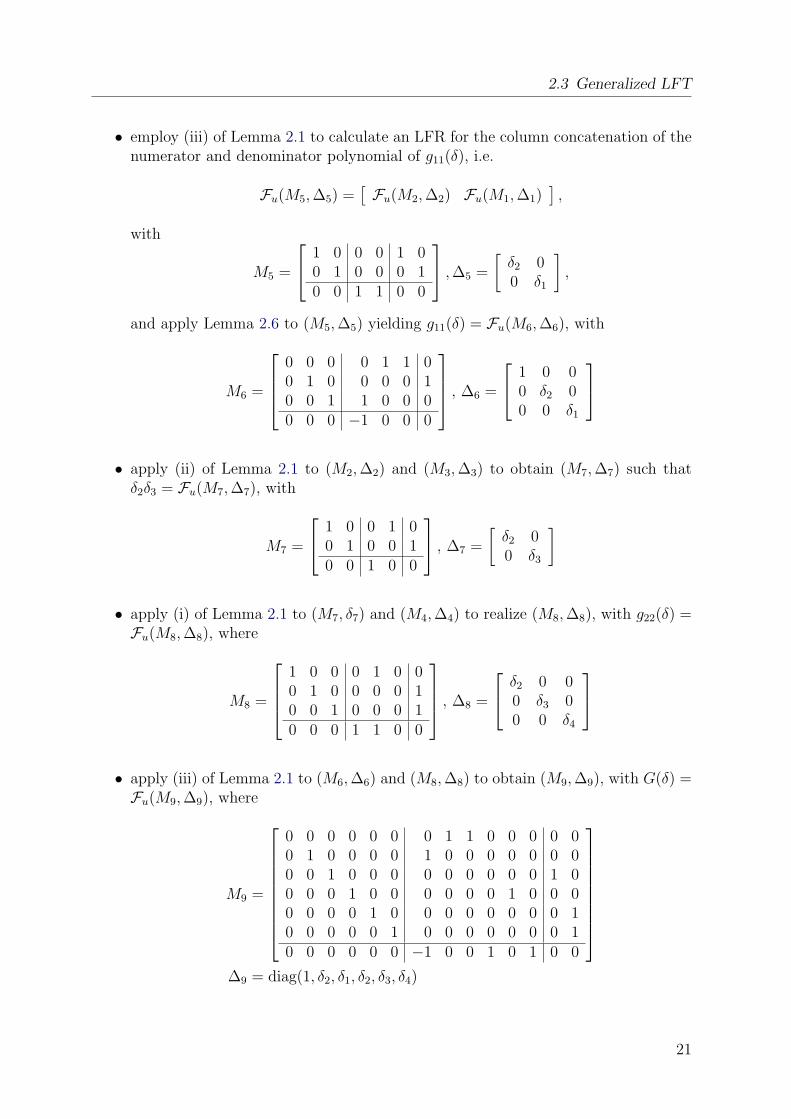
• employ (iii) of Lemma 2.1 to calculate an LFR for the column concatenation of thenumerator and denominator polynomial of g11(δ), i.e.
Fu(M5, ∆5) =[Fu(M2, ∆2) Fu(M1, ∆1)
],
with
M5 =
1 0 0 0 1 00 1 0 0 0 10 0 1 1 0 0
, ∆5 =
[δ2 00 δ1
],
and apply Lemma 2.6 to (M5, ∆5) yielding g11(δ) = Fu(M6, ∆6), with
M6 =
0 0 0 0 1 1 00 1 0 0 0 0 10 0 1 1 0 0 00 0 0 −1 0 0 0
, ∆6 =
1 0 00 δ2 00 0 δ1
• apply (ii) of Lemma 2.1 to (M2, ∆2) and (M3, ∆3) to obtain (M7, ∆7) such thatδ2δ3 = Fu(M7, ∆7), with
M7 =
1 0 0 1 00 1 0 0 10 0 1 0 0
, ∆7 =
[δ2 00 δ3
]
• apply (i) of Lemma 2.1 to (M7, δ7) and (M4, ∆4) to realize (M8, ∆8), with g22(δ) =Fu(M8, ∆8), where
M8 =
1 0 0 0 1 0 00 1 0 0 0 0 10 0 1 0 0 0 10 0 0 1 1 0 0
, ∆8 =
δ2 0 00 δ3 00 0 δ4
• apply (iii) of Lemma 2.1 to (M6, ∆6) and (M8, ∆8) to obtain (M9, ∆9), with G(δ) =Fu(M9, ∆9), where
M9 =
0 0 0 0 0 0 0 1 1 0 0 0 0 00 1 0 0 0 0 1 0 0 0 0 0 0 00 0 1 0 0 0 0 0 0 0 0 0 1 00 0 0 1 0 0 0 0 0 0 1 0 0 00 0 0 0 1 0 0 0 0 0 0 0 0 10 0 0 0 0 1 0 0 0 0 0 0 0 10 0 0 0 0 0 −1 0 0 1 0 1 0 0
∆9 = diag(1, δ2, δ1, δ2, δ3, δ4)
21
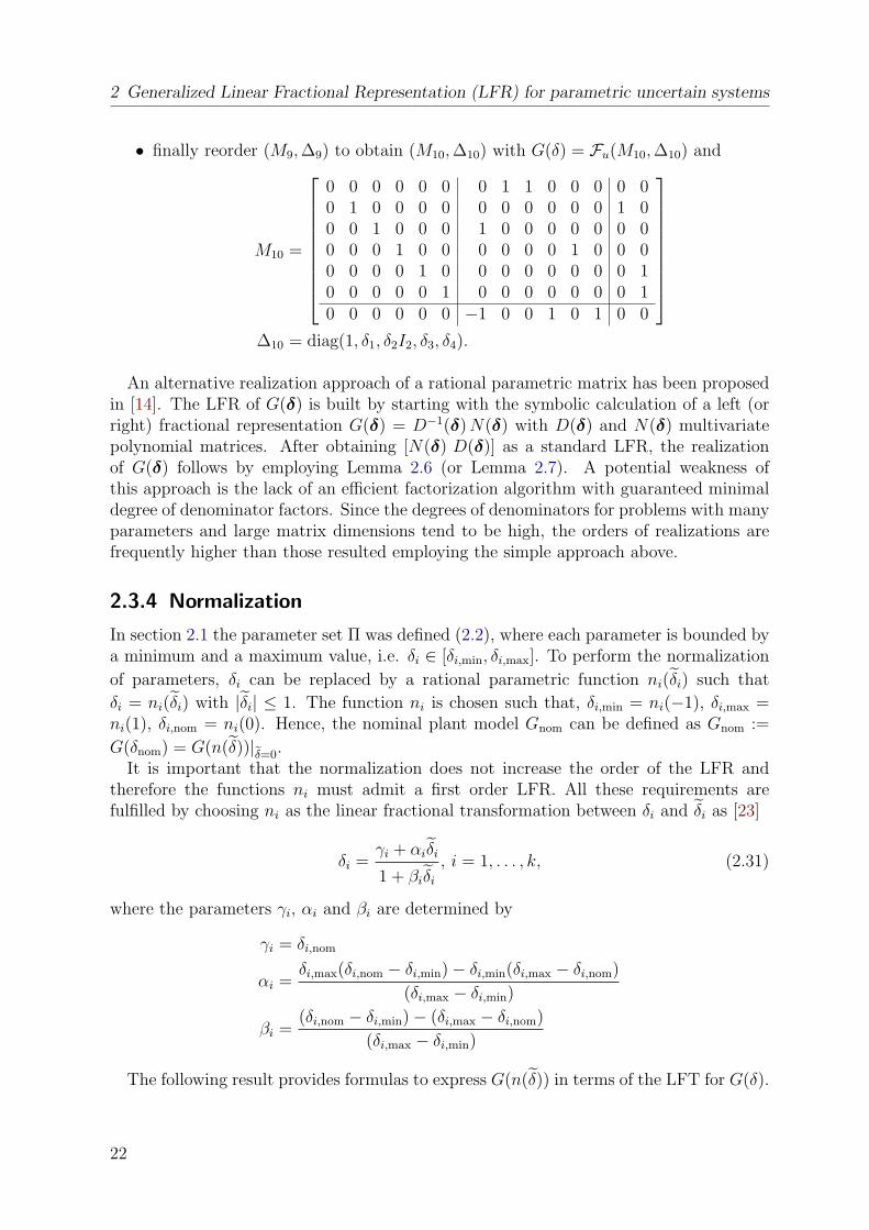
2 Generalized Linear Fractional Representation (LFR) for parametric uncertain systems
• finally reorder (M9, ∆9) to obtain (M10, ∆10) with G(δ) = Fu(M10, ∆10) and
M10 =
0 0 0 0 0 0 0 1 1 0 0 0 0 00 1 0 0 0 0 0 0 0 0 0 0 1 00 0 1 0 0 0 1 0 0 0 0 0 0 00 0 0 1 0 0 0 0 0 0 1 0 0 00 0 0 0 1 0 0 0 0 0 0 0 0 10 0 0 0 0 1 0 0 0 0 0 0 0 10 0 0 0 0 0 −1 0 0 1 0 1 0 0
∆10 = diag(1, δ1, δ2I2, δ3, δ4).
An alternative realization approach of a rational parametric matrix has been proposedin [14]. The LFR of G(δ) is built by starting with the symbolic calculation of a left (orright) fractional representation G(δ) = D−1(δ) N(δ) with D(δ) and N(δ) multivariatepolynomial matrices. After obtaining [N(δ) D(δ)] as a standard LFR, the realizationof G(δ) follows by employing Lemma 2.6 (or Lemma 2.7). A potential weakness ofthis approach is the lack of an efficient factorization algorithm with guaranteed minimaldegree of denominator factors. Since the degrees of denominators for problems with manyparameters and large matrix dimensions tend to be high, the orders of realizations arefrequently higher than those resulted employing the simple approach above.
2.3.4 Normalization
In section 2.1 the parameter set Π was defined (2.2), where each parameter is bounded bya minimum and a maximum value, i.e. δi ∈ [δi,min, δi,max]. To perform the normalization
of parameters, δi can be replaced by a rational parametric function ni(δi) such that
δi = ni(δi) with |δi| ≤ 1. The function ni is chosen such that, δi,min = ni(−1), δi,max =ni(1), δi,nom = ni(0). Hence, the nominal plant model Gnom can be defined as Gnom :=
G(δnom) = G(n(δ))|δ=0.It is important that the normalization does not increase the order of the LFR and
therefore the functions ni must admit a first order LFR. All these requirements arefulfilled by choosing ni as the linear fractional transformation between δi and δi as [23]
δi =γi + αiδi
1 + βiδi
, i = 1, . . . , k, (2.31)
where the parameters γi, αi and βi are determined by
γi = δi,nom
αi =δi,max(δi,nom − δi,min)− δi,min(δi,max − δi,nom)
(δi,max − δi,min)
βi =(δi,nom − δi,min)− (δi,max − δi,nom)
(δi,max − δi,min)
The following result provides formulas to express G(n(δ)) in terms of the LFT for G(δ).
22
2.3 Generalized LFT
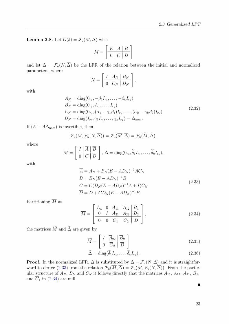
Lemma 2.8. Let G(δ) = Fu(M, ∆) with
M =
[E A B
0 C D
]and let ∆ = Fu(N, ∆) be the LFR of the relation between the initial and normalizedparameters, where
N =
[I AN BN
0 CN DN
],
with
AN = diag(0r0 ,−β1Ir1 , . . . ,−βkIrk)
BN = diag(0r0 , Ir1 , . . . , Irk)
CN = diag(0r0 , (α1 − γ1β1)Ir1 , . . . , (αk − γkβk)Irk)
DN = diag(Ir0 , γ1Ir1 , . . . , γkIrk) = ∆nom.
(2.32)
If (E − A∆nom) is invertible, then
Fu(M,Fu(N, ∆)) = Fu(M, ∆) = Fu(M, ∆),
where
M =
[I A B
0 C D
], ∆ = diag(0r0 , δ1Ir1 , . . . , δkIrk
),
with
A = AN + BN(E − ADN)−1ACN
B = BN(E − ADN)−1B
C = C(DN(E − ADN)−1A + I)CN
D = D + CDN(E − ADN)−1B.
(2.33)
Partitioning M as
M =
Ir0 0 A11 A12 B1
0 I A21 A22 B2
0 0 C1 C2 D
, (2.34)
the matrices M and ∆ are given by
M =
[I A22 B2
0 C2 D
](2.35)
∆ = diag(δ1Ir1 , . . . , δkIrk). (2.36)
Proof. In the normalized LFR, ∆ is substituted by ∆ = Fu(N, ∆) and it is straightfor-ward to derive (2.33) from the relation Fu(M, ∆) = Fu(M,Fu(N, ∆)). From the partic-ular structure of AN , BN and CN it follows directly that the matrices A11, A12, A21, B1,and C1 in (2.34) are null.
23
2 Generalized Linear Fractional Representation (LFR) for parametric uncertain systems
Remark 2.3. A necessary condition for the normalization of a generalized LFR isthat (E − A∆nom) is invertible. This simply means that the nominal model Gnom =Fu(M, ∆nom) = D + C∆nom(E − A∆nom)−1B is well-defined, and this condition mustalways be fulfilled. It is essential to note, that when applying the normalization to ageneralized LFR, the arbitrarily introduced additional block Ir0 in ∆ can be removedand the resulting LFR (2.35), (2.36) can be represented as a standard LFR. Thereforethe generalized LFR can be seen as a convenient means to avoid the preliminary symbolicnormalization of the parametric matrix G(δ). The normalization can be applied as thelast step in the LFR realization procedure and the final LFR will be a standard LFR.Of course this only holds for an LFR of a rational parametric matrix G(δ). In the caseof general multidimensional dynamical systems, operators like the integration operator1/s or the shift operator 1/z may be included in several dimensions (e.g., in the x and ydirection in 2-dimensional image processing applications) and for these operators a nor-malization does not make sense. If the model is non-proper in these dimensions, it is notpossible to represent the system as a standard LFR.
Remark 2.4. In literature, the most common normalization with δi,nom = (δi,max +δi,min)/2, i = 1, . . . , k is generally used. This implies that the nominal values are at thecenter of the uncertainty intervals, which is generally not true. In this case one maysimply choose βi = 0, γi = δi,nom = (δi,max + δi,min)/2 and αi = (δi,max− δi,min)/2 in (2.32).
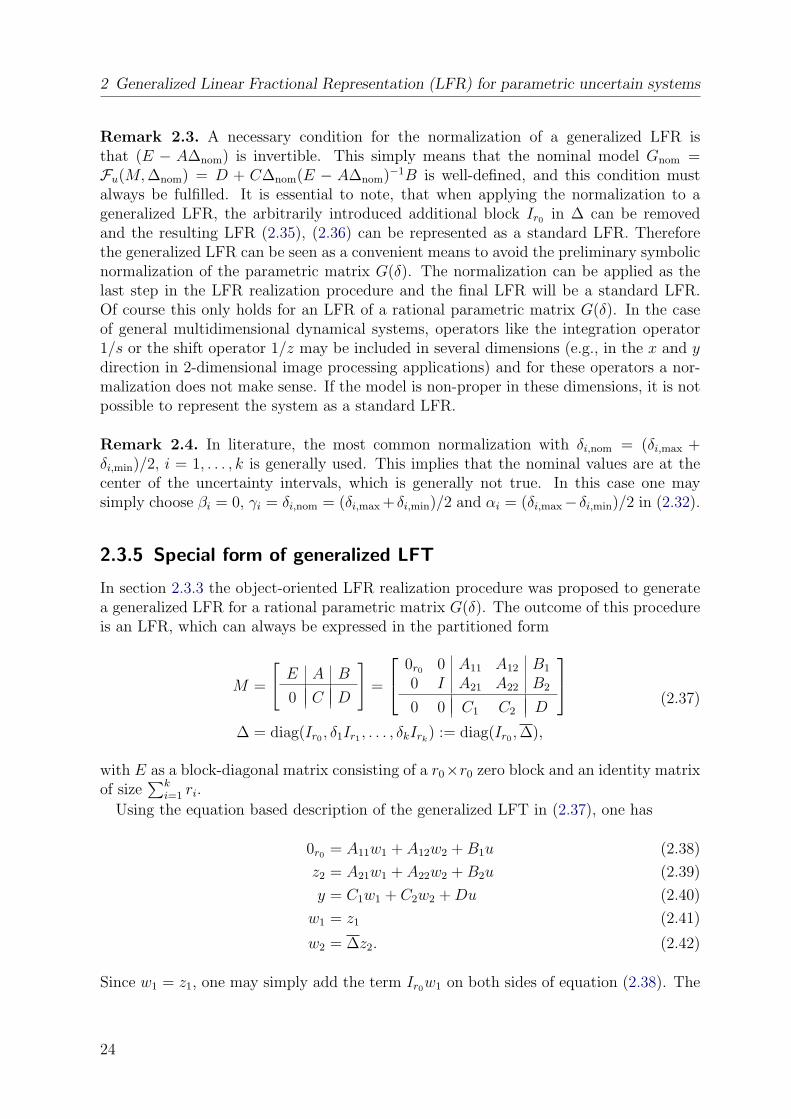
2.3.5 Special form of generalized LFT
In section 2.3.3 the object-oriented LFR realization procedure was proposed to generatea generalized LFR for a rational parametric matrix G(δ). The outcome of this procedureis an LFR, which can always be expressed in the partitioned form
M =
[E A B
0 C D
]=
0r0 0 A11 A12 B1
0 I A21 A22 B2
0 0 C1 C2 D
∆ = diag(Ir0 , δ1Ir1 , . . . , δkIrk
) := diag(Ir0 , ∆),
(2.37)
with E as a block-diagonal matrix consisting of a r0×r0 zero block and an identity matrixof size
∑ki=1 ri.
Using the equation based description of the generalized LFT in (2.37), one has
0r0 = A11w1 + A12w2 + B1u (2.38)
z2 = A21w1 + A22w2 + B2u (2.39)
y = C1w1 + C2w2 + Du (2.40)
w1 = z1 (2.41)
w2 = ∆z2. (2.42)
Since w1 = z1, one may simply add the term Ir0w1 on both sides of equation (2.38). The
24
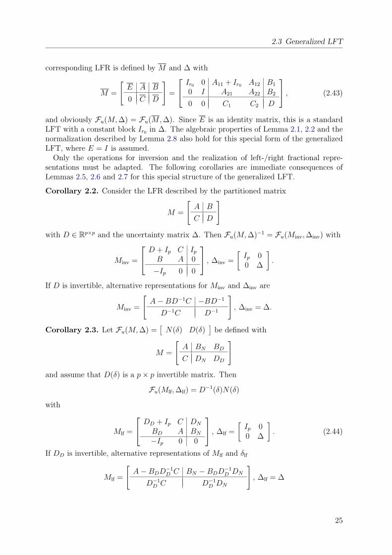
2.3 Generalized LFT
corresponding LFR is defined by M and ∆ with
M =
[E A B
0 C D
]=
Ir0 0 A11 + Ir0 A12 B1
0 I A21 A22 B2
0 0 C1 C2 D
, (2.43)
and obviously Fu(M, ∆) = Fu(M, ∆). Since E is an identity matrix, this is a standardLFT with a constant block Ir0 in ∆. The algebraic properties of Lemma 2.1, 2.2 and thenormalization described by Lemma 2.8 also hold for this special form of the generalizedLFT, where E = I is assumed.
Only the operations for inversion and the realization of left-/right fractional repre-sentations must be adapted. The following corollaries are immediate consequences ofLemmas 2.5, 2.6 and 2.7 for this special structure of the generalized LFT.
Corollary 2.2. Consider the LFR described by the partitioned matrix
M =
[A B
C D
]with D ∈ Rp×p and the uncertainty matrix ∆. Then Fu(M, ∆)−1 = Fu(Minv, ∆inv) with
Minv =
D + Ip C Ip
B A 0
−Ip 0 0
, ∆inv =
[Ip 00 ∆
].
If D is invertible, alternative representations for Minv and ∆inv are
Minv =
[A−BD−1C −BD−1
D−1C D−1
], ∆inv = ∆.
Corollary 2.3. Let Fu(M, ∆) =[
N(δ) D(δ)]
be defined with
M =
[A BN BD
C DN DD
]and assume that D(δ) is a p× p invertible matrix. Then
Fu(Mlf, ∆lf) = D−1(δ)N(δ)
with
Mlf =
DD + Ip C DN
BD A BN
−Ip 0 0
, ∆lf =
[Ip 00 ∆
]. (2.44)
If DD is invertible, alternative representations of Mlf and δlf
Mlf =
[A−BDD−1
D C BN −BDD−1D DN
D−1D C D−1
D DN
], ∆lf = ∆
25
2 Generalized Linear Fractional Representation (LFR) for parametric uncertain systems
Corollary 2.4. Let Fu(M, ∆) =
[N(δ)D(δ)
]be defined with
M =
A B
CN DN
CD DD
,
and assume that D(δ) is a p× p invertible matrix. Then
Fu(Mrf, ∆rf) = N(δ)D−1(δ)
with
Mrf =
DD + Ip CD −Ip
B A 0
DN CN 0
, ∆rf =
[Ip 00 ∆
].
If DD is invertible, alternative representations of Mrf and ∆rf are
Mrf =
[A−BD−1
D CD BD−1D
CN −DND−1D CD DND−1
D
], ∆rf = ∆.
2.3.6 Relation to Behavioral Representations
A behavioral representation for systems with structured uncertainty has been introducedin [30], having the form
z = A∆z + Bw
0 = C∆z + Dw(2.45)
This description will be referred to as output nulling representation (ONR). In this repre-sentation, the vector z is the state and w includes all system variables like inputs, outputsor some so-called latent variables. When manipulating such models there is no need for ana priori choice of input and output variables. In contrast, the explicit generalized LFRsare input-output type representations. Since conversions between the two representationsare straightforward (see below), both representations are suitable to represent arbitraryexpressions with rational dependency on uncertain parameters. However, as we will seelater, the capabilities of these representations to obtain low order LFRs (e.g., suitable forLFT-based robust stability analysis) are quite different.
For the realization of the input-output dependence y = G(δ)u, consider the followingONR
z = A∆z + B1y + B2u
0 = C∆z + D1y + D2u
which corresponds to (2.45) with B = [ B1 B2 ], D = [ D1 D2 ] and w = [yT uT ]T . Assum-ing that D1 ∈ Rp×p, an explicit generalized LFR of G(δ) is the following one
y = Fu
D1 + Ip C D2
B1 A B2
−Ip 0 0
,
[Ip 00 ∆
]u (2.46)
26
2.3 Generalized LFT
If D1 is invertible, a standard LFR is given by
y = Fu
([A−B1D
−11 C B2 −B1D
−11 D2
−D−11 C −D−1
1 D2
], ∆
)u (2.47)
Conversely, assume that we have for G(δ) an explicit generalized LFR of the form
y = Fu
A11 + Ip A12 B1
A21 A22 B2
C1 C2 D
,
[Ip 00 ∆
]u (2.48)
An ONR is given by
z =
[A11 + Ip A12
A21 A22
] [Ip 00 ∆
]z +
[0 B1
0 B2
] [yu
]0 =
[C1 C2
] [ Ip 00 ∆
]z +
[−Ip D
] [ yu
] (2.49)
From the above relations it follows that the generalized LFR and the ONR are mathe-matically equivalent formalisms to represent rational parametric matrices.
The basic aspect of generating LFRs is the efficient representation of interconnectedsystems. When interconnecting two ONRs, a basic requirement is (see [86]), that thetwo representations have the same signal space. To ensure this condition, the resultinginterconnected system typically contains latent variables and it may be necessary tointroduce additional variables to describe the interconnection constraints. The presence ofa large number of latent variables (very common for complex ONRs) makes the behavioralapproach less suitable for an efficient LFT-based model building. In contrast, object-oriented approaches like that described in section 2.3.3 or in [77], produce explicit LFRswith a ”minimal” amount of data. The following simple example will make this aspectclear.
Example 2.4. For the input-output dependence y = (δ1 + δ2)u we build an ONR toobtain via (2.47) an LFR suitable for µ-analysis. ONRs to represent yi = δiui for i = 1, 2are given by
zi = ui
0 = δizi − yi
To represent y = (δ1 + δ2)u the interconnection constraints
u1 = u2(= u)
y = y1 + y2
must be fulfilled. To obtain the final ONR, we collect all states in z = [ z1 z2 ]T and allvariables in w = [ y y1 u1 y2 u ]T and write down the above equations in the standard
27
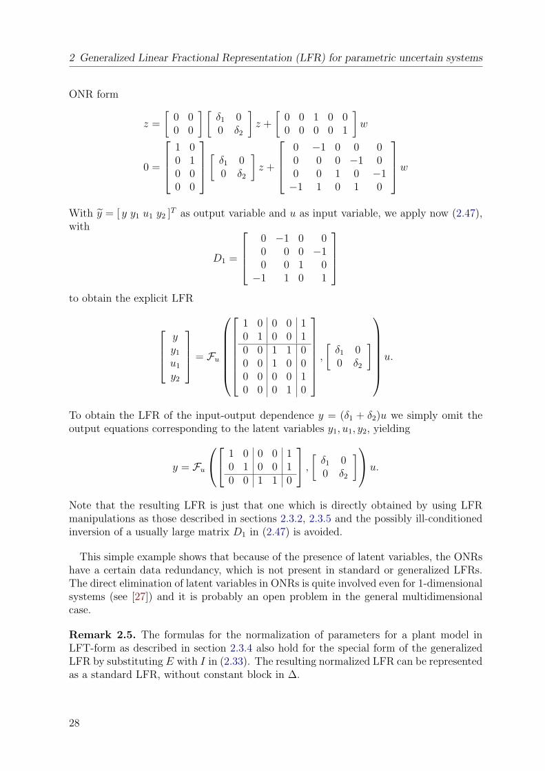
2 Generalized Linear Fractional Representation (LFR) for parametric uncertain systems
ONR form
z =
[0 00 0
] [δ1 00 δ2
]z +
[0 0 1 0 00 0 0 0 1
]w
0 =
1 00 10 00 0
[ δ1 00 δ2
]z +
0 −1 0 0 00 0 0 −1 00 0 1 0 −1−1 1 0 1 0
w
With y = [ y y1 u1 y2 ]T as output variable and u as input variable, we apply now (2.47),with
D1 =
0 −1 0 00 0 0 −10 0 1 0−1 1 0 1
to obtain the explicit LFR
yy1
u1
y2
= Fu
1 0 0 0 10 1 0 0 10 0 1 1 00 0 1 0 00 0 0 0 10 0 0 1 0
,
[δ1 00 δ2
]u.
To obtain the LFR of the input-output dependence y = (δ1 + δ2)u we simply omit theoutput equations corresponding to the latent variables y1, u1, y2, yielding
y = Fu
1 0 0 0 10 1 0 0 10 0 1 1 0
,
[δ1 00 δ2
]u.
Note that the resulting LFR is just that one which is directly obtained by using LFRmanipulations as those described in sections 2.3.2, 2.3.5 and the possibly ill-conditionedinversion of a usually large matrix D1 in (2.47) is avoided.
This simple example shows that because of the presence of latent variables, the ONRshave a certain data redundancy, which is not present in standard or generalized LFRs.The direct elimination of latent variables in ONRs is quite involved even for 1-dimensionalsystems (see [27]) and it is probably an open problem in the general multidimensionalcase.
Remark 2.5. The formulas for the normalization of parameters for a plant model inLFT-form as described in section 2.3.4 also hold for the special form of the generalizedLFR by substituting E with I in (2.33). The resulting normalized LFR can be representedas a standard LFR, without constant block in ∆.
28
2.4 LFR realization for parametric descriptor system
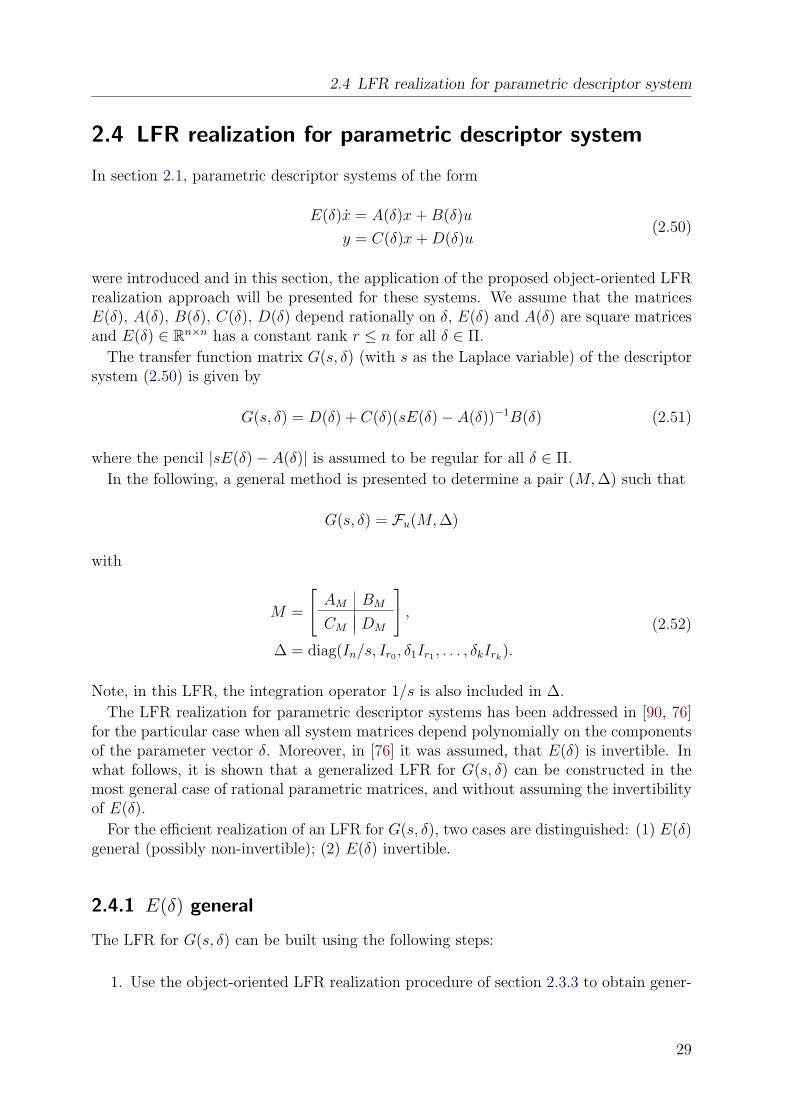
2.4 LFR realization for parametric descriptor system
In section 2.1, parametric descriptor systems of the form
E(δ)x = A(δ)x + B(δ)u
y = C(δ)x + D(δ)u(2.50)
were introduced and in this section, the application of the proposed object-oriented LFRrealization approach will be presented for these systems. We assume that the matricesE(δ), A(δ), B(δ), C(δ), D(δ) depend rationally on δ, E(δ) and A(δ) are square matricesand E(δ) ∈ Rn×n has a constant rank r ≤ n for all δ ∈ Π.
The transfer function matrix G(s, δ) (with s as the Laplace variable) of the descriptorsystem (2.50) is given by
G(s, δ) = D(δ) + C(δ)(sE(δ)− A(δ))−1B(δ) (2.51)
where the pencil |sE(δ)− A(δ)| is assumed to be regular for all δ ∈ Π.
In the following, a general method is presented to determine a pair (M, ∆) such that
G(s, δ) = Fu(M, ∆)
with
M =
[AM BM
CM DM
],
∆ = diag(In/s, Ir0 , δ1Ir1 , . . . , δkIrk).
(2.52)
Note, in this LFR, the integration operator 1/s is also included in ∆.
The LFR realization for parametric descriptor systems has been addressed in [90, 76]for the particular case when all system matrices depend polynomially on the componentsof the parameter vector δ. Moreover, in [76] it was assumed, that E(δ) is invertible. Inwhat follows, it is shown that a generalized LFR for G(s, δ) can be constructed in themost general case of rational parametric matrices, and without assuming the invertibilityof E(δ).
For the efficient realization of an LFR for G(s, δ), two cases are distinguished: (1) E(δ)general (possibly non-invertible); (2) E(δ) invertible.
2.4.1 E(δ) general
The LFR for G(s, δ) can be built using the following steps:
1. Use the object-oriented LFR realization procedure of section 2.3.3 to obtain gener-
29
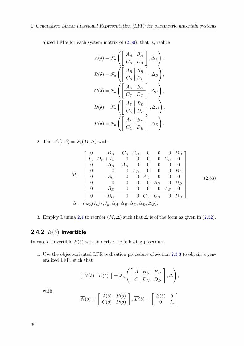
2 Generalized Linear Fractional Representation (LFR) for parametric uncertain systems
alized LFRs for each system matrix of (2.50), that is, realize
A(δ) = Fu
([AA BA
CA DA
], ∆A
),
B(δ) = Fu
([AB BB
CB DB
], ∆B
),
C(δ) = Fu
([AC BC
CC DC
], ∆C
),
D(δ) = Fu
([AD BD
CD DD
], ∆D
),
E(δ) = Fu
([AE BE
CE DE
], ∆E
).
2. Then G(s, δ) = Fu(M, ∆) with
M =
0 −DA −CA CB 0 0 0 DB
In DE + In 0 0 0 0 CE 00 BA AA 0 0 0 0 00 0 0 AB 0 0 0 BB
0 −BC 0 0 AC 0 0 00 0 0 0 0 AD 0 BD
0 BE 0 0 0 0 AE 0
0 −DC 0 0 CC CD 0 DD
∆ = diag(In/s, In, ∆A, ∆B, ∆C , ∆D, ∆E).
(2.53)
3. Employ Lemma 2.4 to reorder (M, ∆) such that ∆ is of the form as given in (2.52).
2.4.2 E(δ) invertible
In case of invertible E(δ) we can derive the following procedure:
1. Use the object-oriented LFR realization procedure of section 2.3.3 to obtain a gen-eralized LFR, such that
[N(δ) D(δ)
]= Fu
([A BN BD
C DN DD
], ∆
),
with
N(δ) =
[A(δ) B(δ)C(δ) D(δ)
], D(δ) =
[E(δ) 0
0 Ip
]
30
2.4 LFR realization for parametric descriptor system
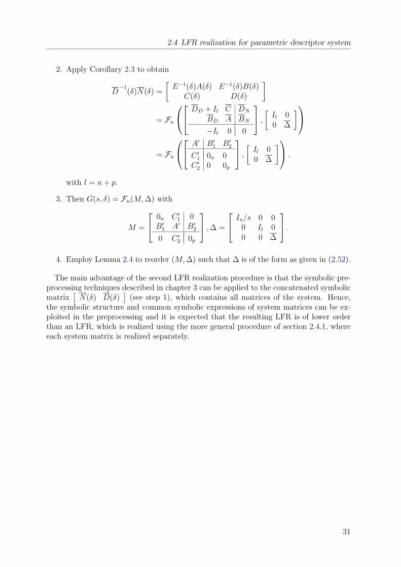
2. Apply Corollary 2.3 to obtain
D−1
(δ)N(δ) =
[E−1(δ)A(δ) E−1(δ)B(δ)
C(δ) D(δ)
]
= Fu
DD + Il C DN
BD A BN
−Il 0 0
,
[Il 00 ∆
]= Fu
A′ B′1 B′
2
C ′1 0n 0
C ′2 0 0p
,
[Il 00 ∆
] .
with l = n + p.
3. Then G(s, δ) = Fu(M, ∆) with
M =
0n C ′1 0
B′1 A′ B′
2
0 C ′2 0p
, ∆ =
In/s 0 00 Il 00 0 ∆
.
4. Employ Lemma 2.4 to reorder (M, ∆) such that ∆ is of the form as given in (2.52).
The main advantage of the second LFR realization procedure is that the symbolic pre-processing techniques described in chapter 3 can be applied to the concatenated symbolicmatrix
[N(δ) D(δ)
](see step 1), which contains all matrices of the system. Hence,
the symbolic structure and common symbolic expressions of system matrices can be ex-ploited in the preprocessing and it is expected that the resulting LFR is of lower orderthan an LFR, which is realized using the more general procedure of section 2.4.1, whereeach system matrix is realized separately.
31
3 Symbolic techniques for low orderLFR modelling
As already mentioned in chapter 1, for the application of LFT-based robust control tech-niques it is of paramount importance to obtain LFRs of least possible orders. Obviouslythis aim is not a trivial task and the introduction of the generalized LFR in chapter 2is one means to reduce the LFR order. In this chapter it will be shown, that symbolicpreprocessing is a powerful complementary tool to achieve low orders of the LFRs. Fora given parametric matrix G(δ), the symbolic processing allows to find equivalent repre-sentations of this matrix, which automatically lead to lower order LFRs, when employedin conjunction with the object-oriented LFR realization approach described in chapter2. The object-oriented LFR realization is very flexible and can easily be automated.However, a blindfold application of this procedure may yield LFRs of larger order thanthe least possible one.
Example 3.1. Consider the standard LFR Fu(M, ∆) for the sum G(δ) = δ1 + δ2, whichis obtained using (i) of Lemma 2.1 as
M =
0 0 10 0 11 1 0
, ∆ =
[δ1 00 δ2
]. (3.1)
This LFR has a least order of two. However, applying the above construction to theexpression G(δ) = δ1 + δ1, one may realize it as an LFR of order two with M given in(3.1) and ∆ = diag(δ1, δ1). Obviously, a first order LFR for G(δ) = δ1 + δ1 is possiblestarting from an equivalent expression
G(δ) = 2δ1 = Fu
([0 21 0
], δ1
).
From this very simple example it can be seen that the trivial symbolic simplificationof G(δ) = δ1 + δ1 to G(δ) = 2δ1 allows to reduce the LFR order by one, when theobject-oriented LFR realization technique is directly applied. Therefore it is clear thatthe resulting order of the generated LFR depends crucially on the way the expressionsunderlying the LFR realization are evaluated and the role of symbolic preprocessing is tofind simpler evaluation schemes of rational expressions and matrices which finally lead toLFRs of lower order.
3.1 Limitation of numerical order reduction
In chapter 1 special order reduction techniques [29, 83] have been mentioned as an ad-ditional means to reduce the order of an LFR. These are typically applied as a final (or
32
3.1 Limitation of numerical order reduction
postprocessing) step of LFR modelling and are based on the application of similaritytransformations (see Lemma 2.2) to identify non-minimal parts of the LFR, which arethen removed (thus reducing the order of the LFR).
Consider again example 3.1 with M given in (3.1) and ∆ = diag(δ1, δ1). A similaritytransformation applied to M with
Q =
[1 −11 1
], Z = 1/2
[1 1−1 1
],
yields Fu(M, ∆) = Fu(M, ∆) with
M =
0 0 00 0 20 1 0
and it is clear that (M, ∆) can be replaced by
Mr =
[0 21 0
], ∆r = δ1.
Hence, for the simple example 3.1, symbolic simplification and order reduction bothyield a least order LFR. However, in the multidimensional case (more than one uncer-tain parameter included in G(δ)), there exists a basic limitation of the order reductiontechniques arising from the association of all δi with non-commuting operators, that is,generally δiδj 6= δjδi is assumed.
Example 3.2. Consider the LFRs Fu(M1, ∆) = δ1δ2 and Fu(M2, ∆) = δ2δ1 with
M1 =
0 1 00 0 11 0 0
, M2 =
0 0 11 0 00 1 0
, ∆ =
[δ1 00 δ2
].
The LFR of Fu(M3, ∆3) = Fu(M1, ∆1) − Fu(M2, ∆2) constructed by subtracting theLFRs (M1∆) and (M2, ∆), is given by
M3 =
0 0 1 0 00 0 0 0 −10 0 0 0 10 1 0 0 01 0 0 1 0
, ∆3 =
δ1 0 0 00 δ1 0 00 0 δ2 00 0 0 δ2
.
Although Fu(M3, ∆3) = δ1δ2 − δ2δ1 ≡ 0, an order reduction of the LFR (M3, ∆3) cannot be achieved by using a block-diagonal (condition Z∆ = ∆Z in Lemma 2.2) simi-larity transformation based order reduction methods, because there exists no similaritytransformation to transform (M1, ∆) into (M2, ∆).
33
3 Symbolic techniques for low order LFR modelling
Remark 3.1. In general, symbolic preprocessing and order reduction can be seen ascomplementary tools, as the symbolic techniques described in the following are verypowerful but not perfect, i.e. in general they do not allow to obtain LFRs of minimalorder. Therefore in most applications (see for example chapter 5) it is usually possible tofurther reduce the order of an LFR by a certain amount using order reduction techniquesin a postprocessing step.
Remark 3.2. Order reduction techniques for standard LFRs as described in [77, 29], canbe directly applied to the special form of the generalized LFR (see section 2.3.5), wherethe constant block Ir0 in ∆ is simply considered as an additional system dimension.
3.2 Definitions
For the very simple examples above minimal order LFRs trivially result using elementarysymbolic simplifications. For more complicated parametric expressions or in the caseof parametric matrices, several ad-hoc or systematic symbolic pre-processing techniques[64, 24, 83, 43, 44] ranging from simple polynomial factorizations to more complex ma-trix decomposition algorithms are available. In several practical examples the symbolicpreprocessing appears to be the most effective step in generating low order LFRs.
Let δ = (δ1, . . . , δk) be the already defined parameter vector and denote by δ−1 =(δ−1
1 , . . . , δ−1k ) the vector of reciprocal variables. Three classes of matrices depending on
δ are considered, for which symbolic transformation techniques are discussed: R[δ]m×n -the set of m×n matrices with multivariate polynomial entries; R(δ)m×n - the set of m×nmatrices with multivariate rational entries; and R[δ, δ−1]m×n - the set of m× n matriceswith multivariate Laurent polynomial entries. This last case is explicitly considered sincemany aircraft and automotive related parametric models are described in terms of suchmatrices (see chapters 5 and 6).
A multivariate Laurent polynomial g(δ) has the expanded form
g(δ) =l∑
r=1
crδnr,1
1 δnr,2
2 . . . δnr,k
k , (3.2)
where cr are real coefficients and nr,1, . . . , nr,k ∈ Z for r = 1, . . . , l are integer exponents.We can associate to this polynomial the order of the LFR which results when applying theobject-oriented LFR realization approach as described in section 2.3.3 to the polynomialin the above expanded form. This order is given by
ord(g(δ)) =l∑
r=1
k∑s=1
|nr,s|
where we assumed that negative and positive powers of indeterminates contribute inthe same way to the order. This assumption is valid when employing the generalizedinversion formula of Corollary 2.2 to realize the reciprocal variables. If g(δ) is a generalmultivariate rational function of the form
g(δ) =a(δ)
b(δ)
34
3.3 Single element conversions
where a(δ) and b(δ) are polynomials in expanded forms, the associated order is given by
ord(g(δ)) = ord(a(δ)) + ord(b(δ))
We can also associate to an m× n rational matrix G(δ) with elements gij(δ) the totalorder
ord(G(δ)) =m∑
i=1
n∑j=1
ord(gij(δ)) (3.3)
which corresponds to realize G(δ) element-wise using row and column concatenations viathe object-oriented LFR realization approach.
The role of symbolic pre-processing in building low order LFRs of a given rationalmatrix G(δ) is to find equivalent representations of individual matrix elements, entirerows/columns or even the whole matrix which lead to LFRs of lower order than givenby (3.3). In the following several transformation techniques, which can be used for thispurpose are presented.
3.3 Single element conversions
Several conversions can be performed on single rational functions which can be usefulto obtain equivalent representations which lead automatically to reduced order LFRsvia an object oriented realization. These conversions can be performed either iterativelywith respect to selected single variables or can be performed simultaneously for severalvariables in a specified order. Using such conversions, it may be possible to determine ineach case a least achievable order of the corresponding LFRs over all permutations of thevariables. However, performing such exhaustive searches leads generally to combinatorialproblems with exponential complexity. Therefore, unless the number of variables is small(say below 10), exhaustive searches are impracticable. In what follows some of possibleconversions are illustrated by examples.
3.3.1 Horner form
The conversion of a multivariate polynomial to a nested Horner form is useful for anefficient numerical evaluation of polynomials [53]. For a given polynomial the Hornerform may be employed for the following operations with minimal computational cost:
• evaluation of polynomials
• division by a linear factor (e.g., (δ1 − 1))
• calculation of derivatives
• reordering of powers of a linear factor
The basic idea in all these computations is to avoid the time consuming calculation ofpowers of variables by appropriate factorizations. In addition to the reduced computationtime, rounding errors are reduced and large intermediate results are avoided [62].
35
3 Symbolic techniques for low order LFR modelling
Example 3.3. Let g(δ) be a given polynomial in one variable as
g(δ) = a0 + a1δ1 + . . . + anδn1 , (3.4)
with ai ∈ R. The Horner form of g(δ) is given by
g(δ) = (. . . (anδ1 + an−1)δ1 + . . . + a1)δ1 + a0. (3.5)
Assuming that ai 6= 0, the computational effort for the evaluation of g(δ) is reduced from2n − 1 multiplications and n additions for evaluating (3.4) to n multiplications and nadditions for evaluating (3.5).
In addition to the numerical benefits, the Horner form is also very useful to generate loworder LFRs by applying it to the numerator and denominator polynomials of a rationalfunction as proposed in [83]. For the polynomial given in (3.4) the resulting order of theLFR will be ord(g(δ)) = n(n + 1)/2 (see (3.3)), whereas the order of the LFR for theHorner form (3.5) will be n, which is minimal. Hence, for a one-dimensional (univariate)polynomial, the Horner form applied as symbolic preprocessing step allows to obtain aminimal order LFR by applying the object-oriented LFR realization approach.
For multivariate polynomials with k parameters there exists no unique conversion tonested Horner form and an exhaustive search for the least order of the correspondingLFTs involves k! conversions. This approach is effective especially when a few variableshave significantly larger powers than the rest of variables. Thus, in the case of manyvariables, exhaustive searches are meaningful only for the few variables with the highestpowers. The conversion to Horner form can be easily extended to multivariate Laurentpolynomials as well as can be generalized to multivariate polynomial matrices [60].
Example 3.4. Consider the polynomial
g(δ) = δ31 + δ2
1 + δ21δ2 + δ1 + δ2.
A realization of this polynomial without any preprocessing would lead to an LFR oforder 10. As the polynomial depends on two parameters the nested Horner form isdetermined recursively with respect to each parameter. Depending on the ordering of thetwo parameters, two different nested Horner forms are obtained:
g(δ) = (1 + (1 + δ1)δ1)δ1 + (δ21 + 1)δ2 (3.6)
g(δ) = δ2 + (1 + (δ2 + 1 + δ1)δ1)δ1 (3.7)
The form in (3.6) is obtained by starting with a Horner factorization for δ1 and theresulting LFR will have order 6, whereas (3.7) is obtained for the opposite ordering andthe resulting LFR will have order 5.
The above example shows that in principle all possible Horner forms must be calculatedto obtain the LFR with the lowest order. However, already in the case of this simplemultidimensional polynomial the nested Horner form does not allow to find the leastorder LFR, which is of order 4. Therefore more sophisticated factorization techniques asdescribed in section 3.5 may be applied.
36
3.3 Single element conversions
3.3.2 Partial fraction decomposition
This conversion allows to represent a rational function in an additively decomposed partialfraction form, where the individual terms have usually much simpler forms.
Consider the univariate rational function g(δ1) = n(δ1)/d(δ1). The partial fractionform is obtained as follows [62]:
1. Factorize d(δ1) asd(δ1) = (δ1 − a1)
p1 . . . (δ1 − am)pmc,
where c ∈ R is a real constant, ai ∈ C are zeros of d(δ1) with multiplicities pi.
2. Then g(δ1) can be represented as
g(δ1) = p(δ1) +m∑
i=1
pi∑j=1
Aij
(δ1 − ai)j,
with p(δ1) as a polynomial in δ1. The Aij are determined by comparison of coeffi-cients.
For multivariate rational functions an iterative realization procedure can be in principledevised by performing the above procedure with respect to a selected order of variables.In each step, the basic procedure is performed on all partial fractions computed at aprevious step. For a multivariate rational function with k parameters an exhaustivesearch for the least order of corresponding LFRs involves k! conversions. The maindifficulty of employing this conversion is the need to symbolically compute the roots ofmultivariate polynomials.
Example 3.5. Consider the rational function
g(δ) =2δ2
1 − 7δ1 − 3δ2 + δ2δ21 + δ2
2δ1 − δ22 + 3
δ31 + δ2δ2
1 − 4δ21 − 4δ1δ2 + 3δ1 + 3δ2
(3.8)
The partial fraction decomposition leading to the least order LFR is given by
g(δ) =1
δ1 − 1+
δ2
δ1 − 3+
1
δ1 + δ2
This decomposition results for both orderings of variables and the resulting LFR hasorder 5 instead of the expected order of 24 for a direct LFR realization of (3.8). Usingnested Horner forms of the numerator and denominator polynomials leads to an LFRwith order 11.
3.3.3 Continued-fraction form
The conversion to continued-fraction form is useful for an efficient numerical evaluationof rational expressions [53] and can also be applied as symbolic preprocessing for rationalexpressions.
37
3 Symbolic techniques for low order LFR modelling
For a univariate rational expression g(δ1) the continued fraction form has the followingstructure
g(δ1) = p(δ1) +1
c1δ1 + d1 +1
c2δ1 + d2 + . . .
,
with p(δ1) as polynomial expressions in δ1 and cj, dj ∈ R.For a multivariate rational function g(δ), this conversion is usually performed for a se-
lected parameter δi and the resulting coefficients cj, dj depend generally on the rest of theparameters. Although nested representations involving the representation of coefficientsin continued-fraction form are in principle possible to be computed, this computationis however not straightforward and can be frequently replaced by conversions to Hornerform. The main advantage of this conversion is that it can be performed for arbitraryrational functions. In particular, for any univariate rational function, this conversionallows to obtain the least order LFR.
Example 3.6. The continued-fraction form of
g(δ) =8δ2
1 − 8δ1 + 2δ3 + 2δ1δ2 − δ2 + 2
4δ21 − 4δ1 + δ3 + 1
(3.9)
with respect to δ1 is given by
g(δ) = 2 +δ2
2
δ1 −1
2+
δ3
4
(δ1 −
1
2
)
,
and allows to obtain an LFR of least order 4 instead of expected order 11. Note, that theconversion of (3.9) to partial fraction form allows to obtain an LFR of order 6 and usingthe nested Horner form for the numerator and denominator polynomial in (3.9) yields anLFR of order 8.
3.4 Matrix conversions
3.4.1 Morton’s method
Any affine parameter dependent matrix G(δ) can be expressed as an affine combination
G(δ) = G0 +k∑
i=1
δiGi, (3.10)
where Gi ∈ Rp×m, i = 0, . . . , k are constant matrices. Following (3.3) the resulting LFRorder for each term δiGi would be equal to the number of nonzero elements in Gi.
38
3.4 Matrix conversions
Let Gi = LiRi be full rank factorizations of Gi, where Li ∈ Rp×ri and Ri ∈ Rri×m. Themethod proposed in [64] rewrites G(δ) as
G(δ) = G0 +k∑
i=1
LiδiIriRi (3.11)
and the resulting LFR can be directly realized as
M =
0 . . . 0 Ri...
. . ....
...0 . . . 0 Rk
L1 . . . Lk G0
, ∆ = diag(δ1Ir1 , . . . , δkIrk).
The main advantage of this method in obtaining low order LFRs is that it exploits thefact that frequently the constant matrices Gi have non-full ranks ri. Moreover, insteadof a maximum multiplicity of pm for δi in ∆ (if there are pm non-zero elements), only amultiplicity of ri ≤ max(p, m) results. Note that for affine parameter dependent matrices,an object-oriented LFR realization of G(δ) in the form (3.11) yields a minimal order LFT,which is generally not the case for a direct object-oriented LFR realization of (3.10).
A straightforward extension of this method is considered in [21], where G(δ) ∈ R(δ)p×m
is a rational matrix and the coefficients in (3.11) are not the δi but rational expressionsci(δ). Note, that in this case the resulting LFR is generally not of minimal order, ascommon factors or dependencies between the different ci(δ) are not considered.
Example 3.7. Consider
G(δ) =
[δ1 δ1
2δ1 2δ1
]. (3.12)
A direct object-oriented LFR realization of (3.12) yields an LFR with order 4, whereas afirst order LFR is obtained for G(δ) in the following form
G(δ) =
[12
]δ1
[1 1
].
3.4.2 Enhanced tree decomposition
An efficient technique applicable to multivariate polynomial matrices is the tree-decom-position (TD) based approach proposed in [24]. This method exploits the structure ofa polynomial matrix to break it down into sums and products of ”simple” terms andfactors for which low order LFRs can be easily constructed. The TD approach involvesthe following elementary operations:
Direct sum decomposition: Recall that (s1, . . . , sl) is a partition of the finite sets = (1, . . . , k) ⊂ N, if
⋃li=1 si = s and si ∩ sj = ∅,∀i 6= j, 1 ≤ i, j ≤ l. δs denotes a
parameter vector including all parameters δi with index i ∈ s. G(δ) has a direct-sumdecomposition, if a nontrivial partition (s1, . . . , sl) of the parameter index set s existssuch that
G(δ) = G(0) + G1(δs1) + . . . + Gl(δsl). (3.13)
39
3 Symbolic techniques for low order LFR modelling
Note that the direct sum decomposition reduces the original k-dimensional problem intol independent problems of dimension less than or equal to k.
Affine factorization: Let δm be a common factor of the ith row (respectively column)of G(δ). Then G(δ) admits the factorized representation
G(δ) = Qi(δm)R(δ)(= R(δ)Qi(δm)),
where Qi(δm) (respectively Qi(δm)) is an identity matrix with its ith diagonal elementsubstituted by δm. The LFR order of Qi is one and this factorization allows to reduce theoverall LFR order of G(δ) by at least y − 1, where y is the number of nonzero elementsin the ith row (column) of G(δ).
Weighted sum decomposition: If none of the above operations can be applied toG(δ), the TD approach splits G(δ) as G(δ) = G1(δ) + G2(δ), where G1(δ) contains allentries depending on one specific parameter δi and G2(δ) does not depend on δi. Thepurpose of this operation is to prepare in the next step an affine factorization with respectto δi of the term G1(δ), which may potentially lead to order reduction. In particular, onewants to find the parameter δi for which the sum decomposition G(δ) = G1(δ) + G2(δ)maximizes the order reduction obtained by the affine factorization of G1(δ). This sumdecomposition is called weighted-sum decomposition.
Algorithm 1 TD(G)
1: T = 02: G← Direct-Sum(G)3: for S ∈ G do4: if S not simple then5: if S has affine row/column factor then6: [Q,R]← Affine-Factor(S)7: T = T+Realize-LFR(TD(Q)*TD(R))8: else9: [S1, S2]← Weighted-Sum(S)
10: [Q,R]← Affine-Factor(S1)11: T = T+Realize-LFR(TD(Q)*TD(R)+TD(S2))12: end if13: else14: T = T+Realize-LFR(S)15: end if16: end for17: Output= T
Algorithm 1 shows a pseudo-code for the TD algorithm, where G denotes the set ofmatrices including the additive terms obtained by a direct-sum decomposition (3.13),Realize-LFR(G) describes the application of the object-oriented LFR realization proce-dure to the parametric matrix G and ”simple” in line 4 of the algorithm means that theobject-oriented LFR realization procedure will yield a minimal order LFR for S.
40
3.4 Matrix conversions
The TD approach can be employed to construct LFRs of general rational matricesrepresented in polynomial fractional forms. It is well-known that any rational matrixG(δ) ∈ R(δ)p×m can be expressed as a right or left factorization G(δ) = N(δ)D−1(δ)
or G(δ) = D−1(δ)N(δ), respectively, where N(δ), D(δ), N(δ), D(δ) are polynomial ma-trices. Then, from the LFRs of the compound polynomial matrices [ NT (δ) DT (δ) ]T or
[ N(δ) D(δ) ] one can easily determine the LFRs of G(δ) by direct formulas (see Lemmas2.6 and 2.7).
The enhanced tree decomposition (ETD) method is an extension of the TD method tothe more general case of multivariate Laurent polynomial matrices G(δ, δ−1) ∈ R[δ, δ−1].The enhanced method formally substitutes each reciprocal variable δ−1
i in the Laurent
polynomial matrix G(δ, δ−1) by a new variable, say δi, and applies the standard TD
method to the resulting polynomial matrix G(δ, δ). Furthermore, Morton’s technique(see section 3.4.1) is integral part of the ETD and is applied in all cases where affine com-binations of the form
∑ci(δ)Gi arise as intermediate results during the decomposition.
In practical examples (see chapters 5 and 6) it could be observed that this occurs veryoften especially after the direct-sum decomposition steps. In addition to the resultinglower orders of LFRs, the integration of Morton’s approach leads usually to significanttime savings. In the case of the RCAM example presented in chapter 5, a reduction ofabout 20% of the LFR realization time has been achieved.
The TD approach as proposed in [24] requires an initial expansion of products intosums of monomials for the multivariate polynomial entries gij(δ, δ
−1) of G(δ, δ−1). How-ever, expanding a polynomial of the form (δ1 + δ2)
5(δ3 + δ4)5 may yield an LFR of order
up to 360 instead of an LFR with minimal order 20, which can be obtained by a directLFR realization of the polynomial in factorized form. The implementation of the ETDin [47] tries to avoid such expansions by performing direct sum decompositions and fac-torizations first on the level of whole expressions and not only on the level of monomialsof a polynomial in expanded form as proposed in [24]. An example of a highly complexparametric model of a fighter aircraft can be found in [32], where it is shown that ig-noring the existing structure of polynomial expressions and expanding the multivariatemodel equations increases substantially the order of the resulting LFR. Algorithm 2 showsa pseudo-code for the ETD algorithm, where Sub-Reciproc(G) and Resub-Reciproc(G)denote the substitution and re-substitution of reciprocal variables δ−1, respectively andSVD(S) denotes the singular value decomposition of a numeric matrix S.
Example 3.8. To illustrate the importance of the integration of Morton’s method intothe TD approach, consider again G(δ) of example 3.7, with
G(δ) =
[δ1 δ1
2δ1 2δ1
].
After two affine factorizations the TD approach will yield
G(δ) =
[δ1 00 1
] [1 00 δ1
] [1 12 2
],
with a resulting LFR order of two, whereas in example 3.7 an LFR with order one wasobtained.
41
3 Symbolic techniques for low order LFR modelling
Algorithm 2 ETD(G(δ, δ−1))
1: T = 02: G(δ, δ)← Sub-Reciproc(G(δ, δ−1))
3: G← Direct-Sum(G(δ, δ))
4: for S(δ, δ) ∈ G do
5: if S(δ, δ) not simple then
6: if S(δ, δ) = c(δ, δ)S then
7: [L, Ir, R]← SVD(S)
8: T = T+Realize-LFR(L*ETD(c(δ, δ))∗Ir ∗R)9: else
10: if S has affine factor then11: [Q(δ, δ), R(δ, δ)]← Affine-Factor(S(δ, δ))
12: T = T+Realize-LFR(ETD(Q(δ, δ))*ETD(R(δ, δ)))13: else14: [S1(δ, δ), S2(δ, δ)]← Weighted-Sum(S(δ, δ))
15: [Q(δ, δ), R(δ, δ)]← Affine-Factor(S1(δ, δ))
16: T = T+Realize-LFR(ETD(Q(δ, δ))*ETD(R(δ, δ))+ETD(S2(δ, δ)))17: end if18: end if19: else20: T = T+Realize-LFR(S(δ, δ))21: end if22: end for23: Output ← Resub-Reciproc(T )
42
3.5 Variable splitting factorization
3.5 Variable splitting factorization
3.5.1 Scalar case
For multivariate Laurent polynomials g(δ, δ−1), a variable splitting (VS) technique canbe employed to express such a polynomial in a factored form, where the factors containdisjoint subsets of δ and δ−1, respectively. It is easy to show that any Laurent polynomialcan be expressed as a product
g(δ, δ−1) = v(δs1 , δ−1s2
)T u(δs3 , δ−1s4
) (3.14)
where v(δs1 , δ−1s2
) and u(δs3 , δ−1s4
) are vectors depending on the parameter vectors δs1 , δs2
and δs3 , δs4 , respectively. The parameter index sets s, s1, . . . , s4 are chosen such thats = (1, . . . , k), s = s1 ∪ s3 = s2 ∪ s4, s1 ∩ s3 = s2 ∩ s4 = ∅ and δs denotes a parametervector including all parameters δi with i ∈ s.
Typically, one chooses one of the factors, say v(δs1 , δ−1s2
), to have only entries expressedby multivariate Laurent monomials. The VS factorization allows to transform the initialrealization problem into two realization problems, but each with fewer variables. Thistechnique is beneficial for cases, where scalar techniques as transformation to Horner formdo not allow a splitting of variables.
Example 3.9. Considerg(δ) = δ1 + δ1δ2 + δ2
Using transformations to Horner form one obtains either g(δ) = δ1(1 + δ2) + δ2 or g(δ) =δ1 + (δ1 + 1)δ2. Both representations allow to reduce the resulting LFR order from 4 to3.
By choosing δs1 = δ1 and δs3 = δ2, we obtain the VS factorization as
g(δ) =[
δ1 1] [ 1 + δ2
δ2
]which allows an additional decomposition such that
g(δ) =[
δ1 1]([ 1
1
]δ2 +
[10
])yielding an LFR of minimal order 2.
The nice result of example 3.9 can be generalized in the following lemma.
Lemma 3.1. Consider the Laurent polynomial g(δ, δ−1) depending on two variables δ1, δ2,that is, δ = (δ1, δ2). A VS factorization of the form
g(δ, δ−1) = v(δ1, δ−11 )T u(δ2, δ
−12 )
allows to realize minimal order LFRs (Mv, ∆v), (Mu, ∆u) with Fu(Mv, ∆v) = v(δ1, δ−11 ),
Fu(Mu, ∆u) = u(δ2, δ−12 ) and the LFR (Mg, ∆g) obtained using (ii) of Lemma 2.1 is a
minimal order LFR for g(δ, δ−1).
43
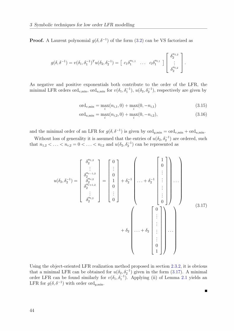
3 Symbolic techniques for low order LFR modelling
Proof. A Laurent polynomial g(δ, δ−1) of the form (3.2) can be VS factorized as
g(δ, δ−1) = v(δ1, δ−11 )T u(δ2, δ
−12 ) =
[c1δ
n1,1
1 . . . clδnl,1
1
] δn1,2
2...
δnl,2
2
.
As negative and positive exponentials both contribute to the order of the LFR, theminimal LFR orders ordv,min, ordu,min for v(δ1, δ
−11 ), u(δ2, δ
−12 ), respectively are given by
ordv,min = maxi
(ni,1, 0) + maxi
(0,−ni,1) (3.15)
ordu,min = maxi
(ni,2, 0) + maxi
(0,−ni,2), (3.16)
and the minimal order of an LFR for g(δ, δ−1) is given by ordg,min = ordv,min + ordu,min.
Without loss of generality it is assumed that the entries of u(δ2, δ−12 ) are ordered, such
that n1,2 < . . . < nr,2 = 0 < . . . < nl,2 and u(δ2, δ−12 ) can be represented as
u(δ2, δ−12 ) =
δn1,2
2...
δnr−1,2
2
δnr,2
2
δnr+1,2
2...
δnl,2
2
=
0...010...0
+ δ−1
2
. . . + δ−1
2
10............0
. . .
+ δ2
. . . + δ2
0............01
. . .
(3.17)
Using the object-oriented LFR realization method proposed in section 2.3.2, it is obviousthat a minimal LFR can be obtained for u(δ2, δ
−12 ) given in the form (3.17). A minimal
order LFR can be found similarly for v(δ1, δ−11 ). Applying (ii) of Lemma 2.1 yields an
LFR for g(δ, δ−1) with order ordg,min.
44
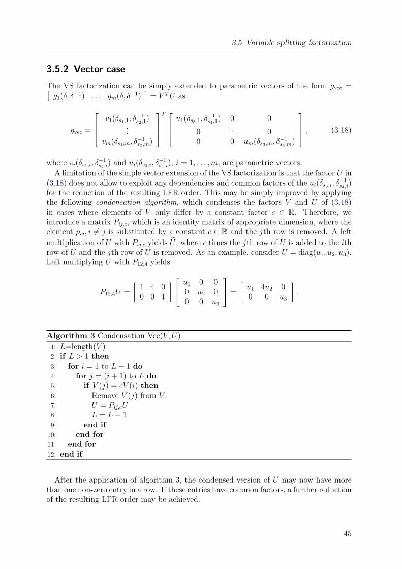
3.5 Variable splitting factorization
3.5.2 Vector case
The VS factorization can be simply extended to parametric vectors of the form gvec =[g1(δ, δ
−1) . . . gm(δ, δ−1)]
= V T U as
gvec =
v1(δs1,1, δ−1s2,1)
...vm(δs1,m, δ−1
s2,m)
T u1(δs3,1, δ
−1s4,1) 0 0
0. . . 0
0 0 um(δs3,m, δ−1s4,m)
, (3.18)
where vi(δs1,i, δ−1s2,i) and ui(δs3,i, δ
−1s4,i), i = 1, . . . ,m, are parametric vectors.
A limitation of the simple vector extension of the VS factorization is that the factor U in(3.18) does not allow to exploit any dependencies and common factors of the ui(δs3,i, δ
−1s4,i)
for the reduction of the resulting LFR order. This may be simply improved by applyingthe following condensation algorithm, which condenses the factors V and U of (3.18)in cases where elements of V only differ by a constant factor c ∈ R. Therefore, weintroduce a matrix Pij,c, which is an identity matrix of appropriate dimension, where theelement pij, i 6= j is substituted by a constant c ∈ R and the jth row is removed. A left
multiplication of U with Pij,c yields U , where c times the jth row of U is added to the ithrow of U and the jth row of U is removed. As an example, consider U = diag(u1, u2, u3).Left multiplying U with P12,4 yields
P12,4U =
[1 4 00 0 1
] u1 0 00 u2 00 0 u3
=
[u1 4u2 00 0 u3
].
Algorithm 3 Condensation Vec(V, U)
1: L=length(V )2: if L > 1 then3: for i = 1 to L− 1 do4: for j = (i + 1) to L do5: if V (j) = cV (i) then6: Remove V (j) from V7: U = Pij,cU8: L = L− 19: end if
10: end for11: end for12: end if
After the application of algorithm 3, the condensed version of U may now have morethan one non-zero entry in a row. If these entries have common factors, a further reductionof the resulting LFR order may be achieved.
45
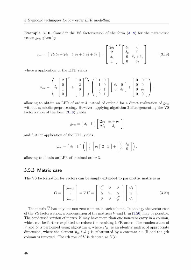
3 Symbolic techniques for low order LFR modelling
Example 3.10. Consider the VS factorization of the form (3.18) for the parametricvector gvec given by
gvec =[
2δ1δ2 + 2δ2 δ1δ2 + δ1δ3 + δ2
]=
2δ1
2δ1
1
T
δ2 0δ2 00 δ2 + δ3
0 δ2
(3.19)
where a application of the ETD yields
gvec =
δ1
2010
T
+
0201
T
1 01 00 10 1
[ δ2 00 δ2
]+
0 00 00 δ3
0 0
,
allowing to obtain an LFR of order 4 instead of order 8 for a direct realization of gvec
without symbolic preprocessing. However, applying algorithm 3 after generating the VSfactorization of the form (3.18) yields
gvec =[
δ1 1] [ 2δ2 δ2 + δ3
2δ2 δ2
]and further application of the ETD yields
gvec =[
δ1 1]([ 1
1
]δ2
[2 1
]+
[0 δ3
0 0
]),
allowing to obtain an LFR of minimal order 3.
3.5.3 Matrix case
The VS factorization for vectors can be simply extended to parametric matrices as
G =
gvec,1...
gvec,p
= V U =
V T1 0 0
0. . . 0
0 0 V Tp
U1
...Up
. (3.20)
The matrix V has only one non-zero element in each column. In analogy the vector caseof the VS factorization, a condensation of the matrices V and U in (3.20) may be possible.The condensed version of matrix V may have more than one non-zero entry in a column,which can be further exploited to reduce the resulting LFR order. The condensation ofV and U is performed using algorithm 4, where P ji,c is an identity matrix of appropriatedimension, where the element pji, i 6= j is substituted by a constant c ∈ R and the jth
column is removed. The ith row of U is denoted as U(i).
46
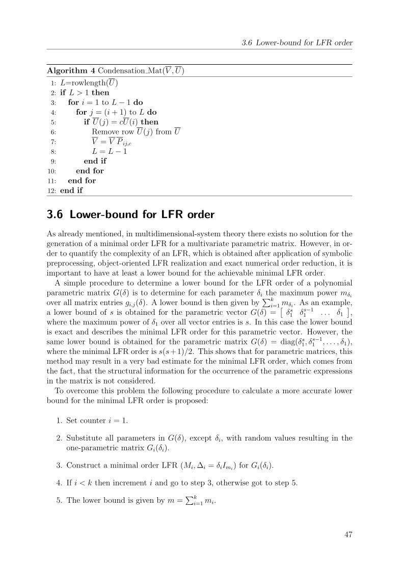
3.6 Lower-bound for LFR order
Algorithm 4 Condensation Mat(V , U)
1: L=rowlength(U)2: if L > 1 then3: for i = 1 to L− 1 do4: for j = (i + 1) to L do5: if U(j) = cU(i) then6: Remove row U(j) from U7: V = V P ij,c
8: L = L− 19: end if
10: end for11: end for12: end if
3.6 Lower-bound for LFR order
As already mentioned, in multidimensional-system theory there exists no solution for thegeneration of a minimal order LFR for a multivariate parametric matrix. However, in or-der to quantify the complexity of an LFR, which is obtained after application of symbolicpreprocessing, object-oriented LFR realization and exact numerical order reduction, it isimportant to have at least a lower bound for the achievable minimal LFR order.
A simple procedure to determine a lower bound for the LFR order of a polynomialparametric matrix G(δ) is to determine for each parameter δi the maximum power mδi
over all matrix entries gi,j(δ). A lower bound is then given by∑k
i=1 mδi. As an example,
a lower bound of s is obtained for the parametric vector G(δ) =[
δs1 δs−1
1 . . . δ1
],
where the maximum power of δ1 over all vector entries is s. In this case the lower boundis exact and describes the minimal LFR order for this parametric vector. However, thesame lower bound is obtained for the parametric matrix G(δ) = diag(δs
1, δs−11 , . . . , δ1),
where the minimal LFR order is s(s+1)/2. This shows that for parametric matrices, thismethod may result in a very bad estimate for the minimal LFR order, which comes fromthe fact, that the structural information for the occurrence of the parametric expressionsin the matrix is not considered.
To overcome this problem the following procedure to calculate a more accurate lowerbound for the minimal LFR order is proposed:
1. Set counter i = 1.
2. Substitute all parameters in G(δ), except δi, with random values resulting in theone-parametric matrix Gi(δi).
3. Construct a minimal order LFR (Mi, ∆i = δiImi) for Gi(δi).
4. If i < k then increment i and go to step 3, otherwise got to step 5.
5. The lower bound is given by m =∑k
i=1 mi.
47
3 Symbolic techniques for low order LFR modelling
The proposed procedure can be easily implemented and for practical examples it yieldsquite good estimates (see chapters 5 and 6). For the above mentioned matrix G(δ) =diag(δs
1, δs−11 , . . . , δ1), the lower bound will now be exactly the minimal LFR order. The
following example shows, that in some cases a gap between the lower bound calculatedwith proposed procedure and the exact minimal LFR order can not be avoided and to thebest of the authors knowledge there exists no method to exactly calculate the minimalLFR order.
Example 3.11. Consider the parametric vector G(δ) =[
δ1δ2 δ1 + δ2
]. In this case
the procedure yields a lower bound of m = 2. However, there will exists no LFR of orderless than 3.
48
4 Enhanced LFR-toolbox for Matlab
The LFR-toolbox is a Matlab toolbox for the realization of LFRs for uncertain systemmodels. With this toolbox, LFRs can be directly obtained from symbolic expressions orvia object-oriented manipulation of LFR objects.
The version 1 of the LFR-toolbox has been implemented by the author of [57] andgenerates standard LFRs for systems with structured (parametric) or unstructured un-certainties of real or complex type. The generation of low order LFRs is supported invarious ways. Special functions for symbolic preprocessing techniques as Mortons method[64] for affine uncertainty representations and the tree decomposition [24] for polynomialmatrices are provided. Furthermore numerical multidimensional order reduction and ap-proximation methods [29, 77] for LFRs are available. These algorithms rely on standardminimal realization tools available in the Control Toolbox of Matlab.
The present version 2 of the LFR-toolbox [46, 45, 47] includes major enhancements,which are mainly focused to improve the capabilities for low order LFR modelling. Withthe support of the generalized LFR [42], described in section 2.3.5 it is now possible torealize arbitrary rational expressions as LFRs. Furthermore, the new LFR object defi-nition is more transparent, user friendly and supports additional types of uncertaintiesto be directly compatible to other Matlab toolboxes like the µ-Analysis and Synthesistoolbox [12], the LMI toolbox [37] and the Robust Control toolbox [11]. Significant en-hancements of the computational efficiency and of numerical accuracy have been achievedby employing efficient and numerically robust Fortran implementations of order reductiontools via mex -function interfaces. The new enhancements in conjunction with improvedsymbolical preprocessing lead generally to a faster generation of LFRs with significantlylower orders.
Figure 4.1 shows the contributions of DLR (Deutsches Zentrum fur Luft-und Raum-fahrt) and ONERA (Office nationale d’Etudes et de Recherches Aerospatiales) to version2 of the LFR-toolbox, which was developed within the common research project HA-FUN (Handling of Flight Uncertainties). The contributions of the author including anew implementation of the underlying Matlab LFR object, the related object-orientedmanipulation functions, symbolic preprocessing routines and numerical order reductionroutines are briefly described in the following sections. From ONERA side, interfacesfor graphical robust stability/performance analysis and interfaces to use LFR objectswithin Simulink are provided. In addition, functions for the synthesis of automaticallygain-scheduled controllers based on eigenstructure assignment were developed.
For a list of all functions see appendix C.
49
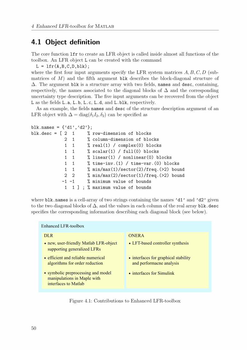
4 Enhanced LFR-toolbox for Matlab
4.1 Object definition
The core function lfr to create an LFR object is called inside almost all functions of thetoolbox. An LFR object L can be created with the commandL = lfr(A,B,C,D,blk);
where the first four input arguments specify the LFR system matrices A, B, C,D (sub-matrices of M) and the fifth argument blk describes the block-diagonal structure of∆. The argument blk is a structure array with two fields, names and desc, containing,respectively, the names associated to the diagonal blocks of ∆ and the correspondinguncertainty type description. The five input arguments can be recovered from the objectL as the fields L.a, L.b, L.c, L.d, and L.blk, respectively.
As an example, the fields names and desc of the structure description argument of anLFR object with ∆ = diag(δ1I2, δ2) can be specified as
blk.names = ’d1’,’d2’;
blk.desc = [ 2 1 % row-dimension of blocks
2 1 % column-dimension of blocks
1 1 % real(1) / complex(0) blocks
1 1 % scalar(1) / full(0) blocks
1 1 % linear(1) / nonlinear(0) blocks
1 1 % time-inv.(1) / time-var.(0) blocks
1 1 % min/max(1)/sector(2)/freq.(>2) bound
2 2 % min/max(2)/sector(1)/freq.(>2) bound
-1 -1 % minimum value of bounds
1 1 ] ; % maximum value of bounds
where blk.names is a cell-array of two strings containing the names ’d1’ and ’d2’ givento the two diagonal blocks of ∆, and the values in each column of the real array blk.desc
specifies the corresponding information describing each diagonal block (see below).
ONERALFT-based controller synthesis
interfaces for graphical stability and performacne analysis
interfaces for Simulink
new, user-friendly Matlab LFR-objectsupporting generalized LFRs
efficient and reliable numerical algorithms for order reduction
symbolic preprocessing and model manipulations in Maple with interfaces to Matlab
DLR
Enhanced LFR-toolbox
Figure 4.1: Contributions to Enhanced LFR-toolbox
50
4.2 Symbolic preprocessing
Each block in ∆ is uniquely identified by its name, which makes the manipulationof LFR objects flexible and transparent. For example, additional uncertainties can beeasily added to an LFR object and the already defined block names can be modified(e.g., by using the function set). The special names ’1/s’ and ’1/z’ are reserved forthe integrator block I/s (continuous-time systems) and the delay block I/z (discrete-timesystems), respectively. These blocks can be included in ∆ to represent standard lineartime-invariant systems (continuous- or discrete-time) as LFR objects. Furthermore thespecial name ’1’ is reserved for a constant identity matrix block I in ∆. This blockplays a major role in representing arbitrary rational parametric expressions as LFRs. Aninternal LFR object reordering (function reorderlfr) is performed after each LFR objectmanipulation where the constant block (if exists) is placed in the first block diagonalposition of ∆, the integrator/delay block (if exists) is placed in the second block diagonalposition followed by all the uncertainty blocks in a lexicographic order.
For each name in the field names there exists a corresponding column in the fielddesc, which describes the row/column dimensions and properties of this block. The LFRobject supports real or complex structured uncertainty (or dynamic) blocks and realor complex full unstructured uncertainty blocks. These blocks can have the propertieslinear/nonlinear and time-invariant/time-varying (in the case of nonlinear uncertaintiesthe property time-invariant means memoryless). Furthermore, the field desc includesbound information for each uncertainty block, which can be described by min/max-values,a sector bound (for nonlinear uncertainties) or a SISO frequency dependent bound.
For Matlab versions 6.1/6.5, conversions to LFR objects from LTI-objects of theControl Toolbox, PCK-system representations of the µ-Synthesis Toolbox as well as con-stant matrices, are automatically performed via the core function lfr. For Matlabversions 7.0/7.1, conversions from umat, ureal, ucomplex and uss-objects of the RobustControl Toolbox to LFR objects are supported. Furthermore, one may use the functionslfr2mu, lfr2mubnd, lfr2mussv, lfr2mustab and lfr2lmip to generate the requireddata structures for robust stability/performance analysis and controller synthesis usingthe µ-Analysis and Synthesis toolbox or the LMI-toolbox under Matlab 6.1/6.5 or thefunction lfr2rob for conversions to the objects supported by the Robust Control toolboxunder Matlab versions 7.0/7.1.
4.2 Symbolic preprocessing
All the methods for decomposition of multivariate rational functions and matrices de-scribed in chapter 3 are supported by the function sym2lfr of the toolbox. The functionis called with several options.
Besides the Horner form, partial fraction form, continued fraction form and the ETDthe function also allows to choose code generation techniques for optimized evaluationof polynomial/rational functions as symbolic preprocessing [83]. Therefore the Maplefunction optimize from the codegen package is employed. A tryhard option can bechosen to check all possible permutations for the Horner, partial fraction and continuedfraction forms and the LFR with the lowest resulting order is provided as output.
For the VS factorization the user can choose between a separate factorization of each
51
4 Enhanced LFR-toolbox for Matlab
matrix element or a column/row wise application as described in section 3.5.3 (for row-wise factorization). The resulting two factors (see (3.20)) are then further processedwith the ETD. The condensation of the factors as described in sections 3.5.2 and 3.5.3is automatically performed. The sets δs,i for the definition of the VS factorization canbe determined automatically, manually or one may choose a tryhard option, where allpossible combinations are calculated and the LFR with the lowest resulting order isprovided as output.
When the ETD is chosen, a standard feature of the function sym2lfr is to split arational matrix G(δ) into a pure rational part G1(δ) and a Laurent polynomial partG2(δ, δ
−1), such that G(δ) = G1(δ) + G2(δ, δ−1). The matrix G2(δ, δ
−1) can be di-rectly processed, whereas for G1(δ), a left (or right) fractional representation of the form
G1(δ) = D−1(δ)N(δ) (or G1(δ) = N(δ)D−1
(δ)) is calculated and the ETD is applied to
the concatenated polynomial matrix[
N(δ) D(δ)]
(or[
N(δ)T D(δ)T]T
). Finally,Lemma 2.6 (or Lemma 2.7) are used to obtain an LFR for G1(δ). It is possible to avoidthe splitting of G(δ) and to calculate a left (or right) fractional representation for thewhole matrix. However, the calculation of common denominators, which is necessary toobtain the fractional representation, may result in more complex symbolic expressionsand this may increase the resulting LFR order.
To increase the efficiency of the symbolic calculations, many of the core functions aredirectly implemented as Maple functions and executed within the efficient Maple kernelvia the Extended Symbolic Toolbox of Matlab.
4.3 Numerical order reduction
Efficient and numerically reliable tools for order reduction of LFRs are of primary im-portance to ease the usability of such models. To achieve efficiency of computation,numerical robustness and a high accuracy of results, the toolbox relies on Fortran basedrobust implementations of algorithms for basic computations related to order reduction.A language like Fortran allows to easily exploit all structural features of a computationalproblem with low additional computational effort and minimum memory usage. Fortranroutines can be easily executed within the user friendly environment Matlab via externalfunctions, the so called mex -functions. Several mex -functions based on powerful Fortranroutines from the LAPACK-based [5] public domain control library SLICOT [15, 81] formthe order reduction computational kernel of the LFR-toolbox.
The LFR-toolbox provides several order reduction tools for exact or approximativereduction of order. The exact 1-d order reduction technique [77] can be performed usingthe function minlfr1 which is based on the efficient (O(n3) complexity, with n as theorder of a state-space system) SLICOT-based mex -function ssminr1 for the calculationof minimal realizations. Note that a pure Matlab-based implementation using theMatlab Control Toolbox function minreal would have a O(n4) worst-case complexity.For a comparison of computation times see chapter 5.
The approximative 1-d order reduction [83] can be performed using redlfr1, which is
1The functions balsys, ssminr, sysred, sscof and partly minlfr have been implemented by A. Varga
52
4.3 Numerical order reduction
based on the collection of model reduction tools available in SLICOT [81], covering thebalanced truncation, singular perturbation approximation and Hankel-norm approxima-tion approaches. All these methods are implemented in a single mex -function sysred1
which is called by redlfr1 to cyclically reduce 1-d systems (assimilated to discrete-time).With an appropriate scaling of the A matrix of the LFRs (necessary to ensure stability indiscrete-time sense), this function can be also employed to perform exact order reduction.
The function minlfr can be used for n-d order reduction [29]. In version 2 of the LFRToolbox this function has been completely re-implemented to improve efficiency. Thecalculation of the n-d controllability/observability staircase forms relies on the O(n3)complexity SLICOT-based mex -function sscof1 to compute controllability/observabilitystaircase forms using orthogonal transformations. Note that a pure Matlab-based im-plementation using the Matlab Control Toolbox function ctrbf would have a O(n4)worst-case complexity. For a comparison of computation times see chapter 5.
The SLICOT-based mex -function balsys is systematically called in all order reductionfunctions to perform a system scaling of the LFRs as a preliminary operation within theorder reduction routines. As the LFRs resulting from the object-oriented realizationapproach can have matrices with a wide range of values, this operation is essential beforecomputing numerically sensitive controllability staircase forms.
The order reduction functions can be applied manually at any stage of the LFR realiza-tion or can be executed automatically after each object-oriented LFR manipulation (e.g.,multiplication, addition, etc.). To set global options (e.g., to perform or not automaticorder reduction), the function lfropt can be used. This function basically defines a setof global variables to control the order reduction and to set the associated tolerances.
53
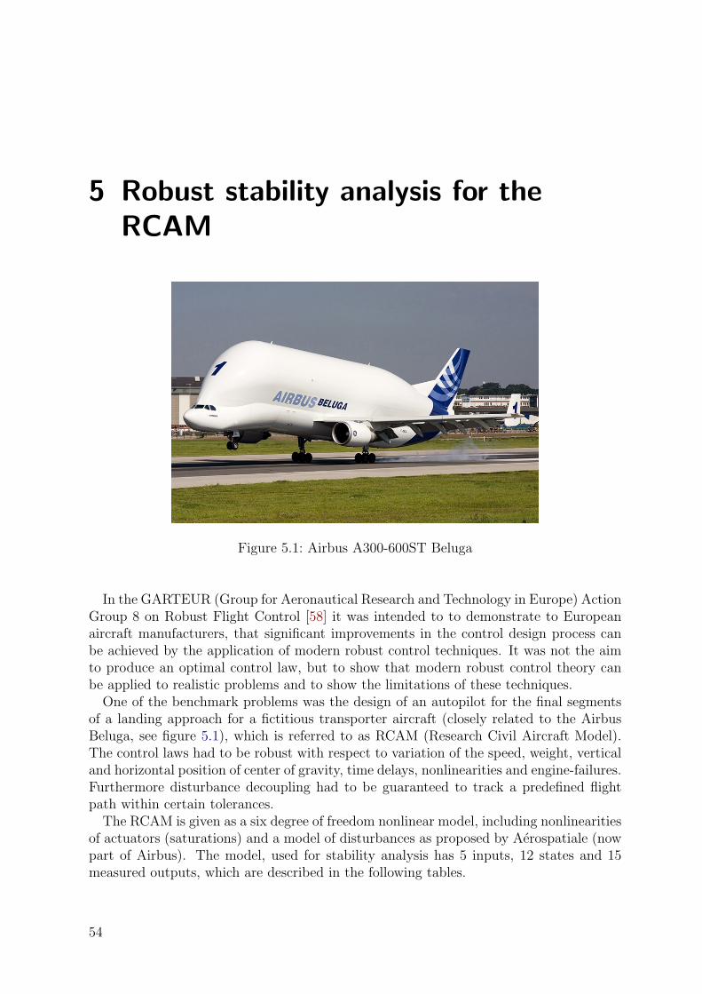
5 Robust stability analysis for theRCAM
Figure 5.1: Airbus A300-600ST Beluga
In the GARTEUR (Group for Aeronautical Research and Technology in Europe) ActionGroup 8 on Robust Flight Control [58] it was intended to to demonstrate to Europeanaircraft manufacturers, that significant improvements in the control design process canbe achieved by the application of modern robust control techniques. It was not the aimto produce an optimal control law, but to show that modern robust control theory canbe applied to realistic problems and to show the limitations of these techniques.
One of the benchmark problems was the design of an autopilot for the final segmentsof a landing approach for a fictitious transporter aircraft (closely related to the AirbusBeluga, see figure 5.1), which is referred to as RCAM (Research Civil Aircraft Model).The control laws had to be robust with respect to variation of the speed, weight, verticaland horizontal position of center of gravity, time delays, nonlinearities and engine-failures.Furthermore disturbance decoupling had to be guaranteed to track a predefined flightpath within certain tolerances.
The RCAM is given as a six degree of freedom nonlinear model, including nonlinearitiesof actuators (saturations) and a model of disturbances as proposed by Aerospatiale (nowpart of Airbus). The model, used for stability analysis has 5 inputs, 12 states and 15measured outputs, which are described in the following tables.
54
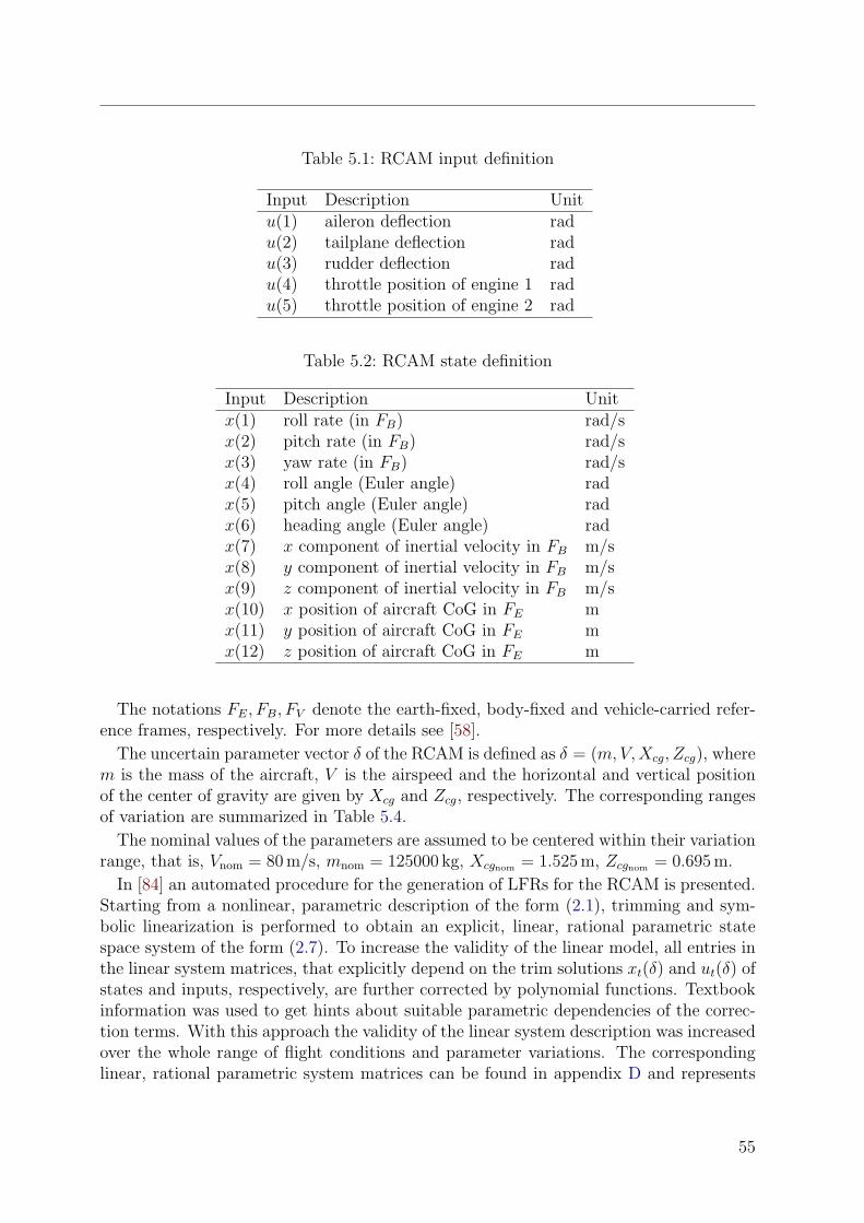
Table 5.1: RCAM input definition
Input Description Unitu(1) aileron deflection radu(2) tailplane deflection radu(3) rudder deflection radu(4) throttle position of engine 1 radu(5) throttle position of engine 2 rad
Table 5.2: RCAM state definition
Input Description Unitx(1) roll rate (in FB) rad/sx(2) pitch rate (in FB) rad/sx(3) yaw rate (in FB) rad/sx(4) roll angle (Euler angle) radx(5) pitch angle (Euler angle) radx(6) heading angle (Euler angle) radx(7) x component of inertial velocity in FB m/sx(8) y component of inertial velocity in FB m/sx(9) z component of inertial velocity in FB m/sx(10) x position of aircraft CoG in FE mx(11) y position of aircraft CoG in FE mx(12) z position of aircraft CoG in FE m
The notations FE, FB, FV denote the earth-fixed, body-fixed and vehicle-carried refer-ence frames, respectively. For more details see [58].
The uncertain parameter vector δ of the RCAM is defined as δ = (m, V, Xcg, Zcg), wherem is the mass of the aircraft, V is the airspeed and the horizontal and vertical positionof the center of gravity are given by Xcg and Zcg, respectively. The corresponding rangesof variation are summarized in Table 5.4.
The nominal values of the parameters are assumed to be centered within their variationrange, that is, Vnom = 80 m/s, mnom = 125000 kg, Xcgnom = 1.525 m, Zcgnom = 0.695 m.
In [84] an automated procedure for the generation of LFRs for the RCAM is presented.Starting from a nonlinear, parametric description of the form (2.1), trimming and sym-bolic linearization is performed to obtain an explicit, linear, rational parametric statespace system of the form (2.7). To increase the validity of the linear model, all entries inthe linear system matrices, that explicitly depend on the trim solutions xt(δ) and ut(δ) ofstates and inputs, respectively, are further corrected by polynomial functions. Textbookinformation was used to get hints about suitable parametric dependencies of the correc-tion terms. With this approach the validity of the linear system description was increasedover the whole range of flight conditions and parameter variations. The correspondinglinear, rational parametric system matrices can be found in appendix D and represents
55
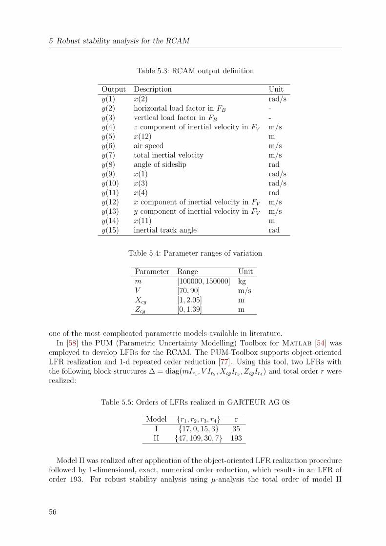
5 Robust stability analysis for the RCAM
Table 5.3: RCAM output definition
Output Description Unity(1) x(2) rad/sy(2) horizontal load factor in FB -y(3) vertical load factor in FB -y(4) z component of inertial velocity in FV m/sy(5) x(12) my(6) air speed m/sy(7) total inertial velocity m/sy(8) angle of sideslip rady(9) x(1) rad/sy(10) x(3) rad/sy(11) x(4) rady(12) x component of inertial velocity in FV m/sy(13) y component of inertial velocity in FV m/sy(14) x(11) my(15) inertial track angle rad
Table 5.4: Parameter ranges of variation
Parameter Range Unitm [100000, 150000] kgV [70, 90] m/sXcg [1, 2.05] mZcg [0, 1.39] m
one of the most complicated parametric models available in literature.In [58] the PUM (Parametric Uncertainty Modelling) Toolbox for Matlab [54] was
employed to develop LFRs for the RCAM. The PUM-Toolbox supports object-orientedLFR realization and 1-d repeated order reduction [77]. Using this tool, two LFRs withthe following block structures ∆ = diag(mIr1 , V Ir2 , XcgIr3 , ZcgIr4) and total order r wererealized:
Table 5.5: Orders of LFRs realized in GARTEUR AG 08
Model r1, r2, r3, r4 rI 17, 0, 15, 3 35II 47, 109, 30, 7 193
Model II was realized after application of the object-oriented LFR realization procedurefollowed by 1-dimensional, exact, numerical order reduction, which results in an LFR oforder 193. For robust stability analysis using µ-analysis the total order of model II
56
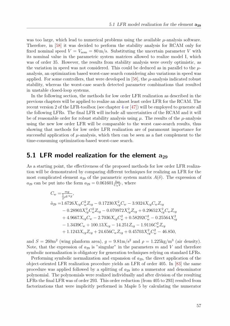
5.1 LFR model realization for the element a29
was too large, which lead to numerical problems using the available µ-analysis software.Therefore, in [58] it was decided to perform the stability analysis for RCAM only forfixed nominal speed V = Vnom = 80 m/s. Substituting the uncertain parameter V withits nominal value in the parametric system matrices allowed to realize model I, whichwas of order 35. However, the results from stability analysis were overly optimistic, asthe variation in speed was not considered. This could be deduced as in parallel to the µ-analysis, an optimization based worst-case search considering also variations in speed wasapplied. For some controllers, that were developed in [58], the µ-analysis indicated robuststability, whereas the worst-case search detected parameter combinations that resultedin unstable closed-loop systems.
In the following section, the methods for low order LFR realization as described in theprevious chapters will be applied to realize an almost least order LFR for the RCAM. Therecent version 2 of the LFR-toolbox (see chapter 4 or [47]) will be employed to generate allthe following LFRs. The final LFR will include all uncertainties of the RCAM and it willbe of reasonable order for robust stability analysis using µ. The results of the µ-analysisusing the new low order LFR will be comparable to the worst case-search results, thusshowing that methods for low order LFR realization are of paramount importance forsuccessful application of µ-analysis, which then can be seen as a fast complement to thetime-consuming optimization-based worst-case search.
5.1 LFR model realization for the element a29
As a starting point, the effectiveness of the proposed methods for low order LFR realiza-tion will be demonstrated by comparing different techniques for realizing an LFR for themost complicated element a29 of the parametric system matrix A(δ). The expression ofa29 can be put into the form a29 = 0.061601 a29
CwV, where
Cw = mg12
ρV 2S,
a29 =1.6726XcgC2wZcg − 0.17230X2
cgCw − 3.9324XcgCwZcg
− 0.28903X2cgC
2wZcg − 0.070972X2
cgZcg + 0.29652X2cgCwZcg
+ 4.9667XcgCw − 2.7036XcgC2w + 0.58292C2
w − 0.25564X2cg
− 1.3439Cw + 100.13Xcg − 14.251Zcg − 1.9116C2wZcg
+ 1.1243XcgZcg + 24.656CwZcg + 0.45703X2cgC
2w − 46.850,
and S = 260m2 (wing planform area), g = 9.81m/s2 and ρ = 1.225kg/m3 (air density).Note, that the expression of a29 is ”singular” in the parameters m and V and thereforesymbolic normalization is obligatory for generation techniques relying on standard LFRs.
Performing symbolic normalization and expansion of a29, the direct application of theobject-oriented LFR realization procedure yields an LFR of order 405. In [83] the sameprocedure was applied followed by a splitting of a29 into a numerator and denominatorpolynomial. The polynomials were realized individually and after division of the resultingLFRs the final LFR was of order 293. This order reduction (from 405 to 293) resulted fromfactorizations that were implicitly performed in Maple 5 by calculating the numerator
57
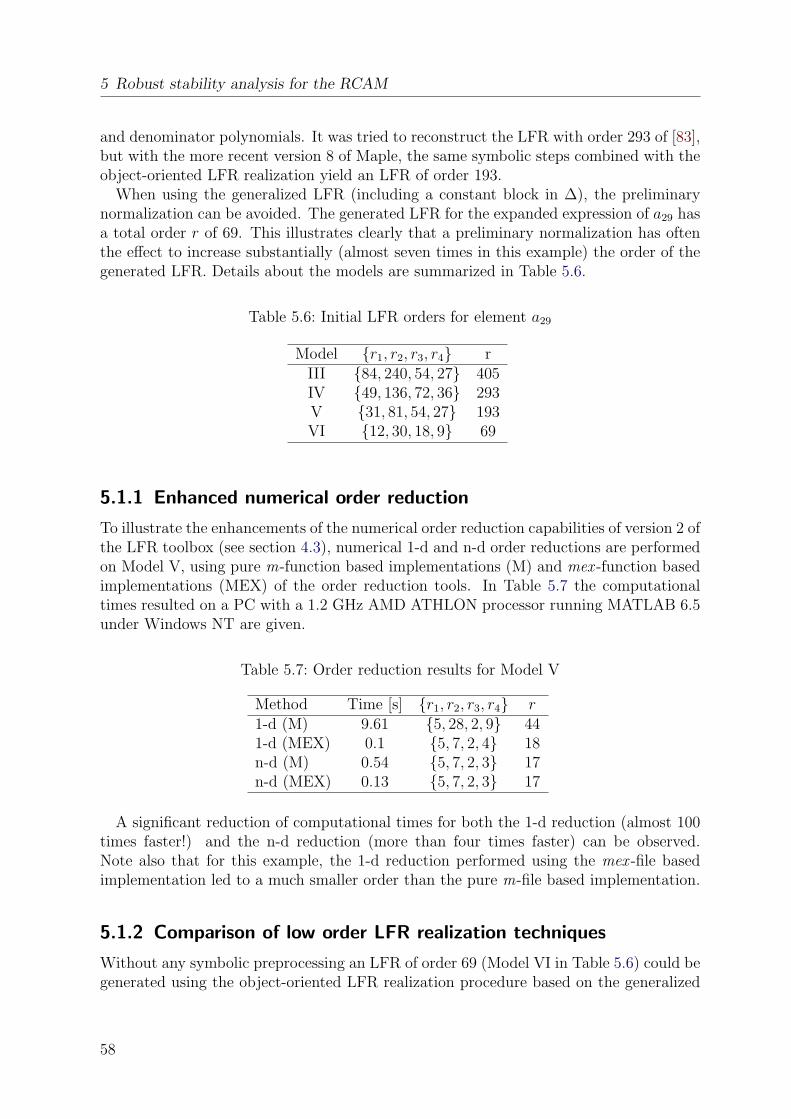
5 Robust stability analysis for the RCAM
and denominator polynomials. It was tried to reconstruct the LFR with order 293 of [83],but with the more recent version 8 of Maple, the same symbolic steps combined with theobject-oriented LFR realization yield an LFR of order 193.
When using the generalized LFR (including a constant block in ∆), the preliminarynormalization can be avoided. The generated LFR for the expanded expression of a29 hasa total order r of 69. This illustrates clearly that a preliminary normalization has oftenthe effect to increase substantially (almost seven times in this example) the order of thegenerated LFR. Details about the models are summarized in Table 5.6.
Table 5.6: Initial LFR orders for element a29
Model r1, r2, r3, r4 rIII 84, 240, 54, 27 405IV 49, 136, 72, 36 293V 31, 81, 54, 27 193VI 12, 30, 18, 9 69
5.1.1 Enhanced numerical order reduction
To illustrate the enhancements of the numerical order reduction capabilities of version 2 ofthe LFR toolbox (see section 4.3), numerical 1-d and n-d order reductions are performedon Model V, using pure m-function based implementations (M) and mex -function basedimplementations (MEX) of the order reduction tools. In Table 5.7 the computationaltimes resulted on a PC with a 1.2 GHz AMD ATHLON processor running MATLAB 6.5under Windows NT are given.
Table 5.7: Order reduction results for Model V
Method Time [s] r1, r2, r3, r4 r1-d (M) 9.61 5, 28, 2, 9 441-d (MEX) 0.1 5, 7, 2, 4 18n-d (M) 0.54 5, 7, 2, 3 17n-d (MEX) 0.13 5, 7, 2, 3 17
A significant reduction of computational times for both the 1-d reduction (almost 100times faster!) and the n-d reduction (more than four times faster) can be observed.Note also that for this example, the 1-d reduction performed using the mex -file basedimplementation led to a much smaller order than the pure m-file based implementation.
5.1.2 Comparison of low order LFR realization techniques
Without any symbolic preprocessing an LFR of order 69 (Model VI in Table 5.6) could begenerated using the object-oriented LFR realization procedure based on the generalized
58
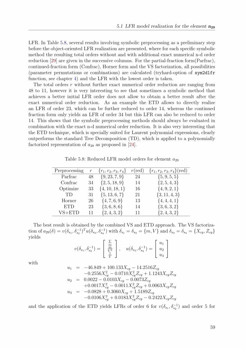
5.1 LFR model realization for the element a29
LFR. In Table 5.8, several results involving symbolic preprocessing as a preliminary stepbefore the object-oriented LFR realization are presented, where for each specific symbolicmethod the resulting total orders without and with additional exact numerical n-d orderreduction [29] are given in the successive columns. For the partial-fraction form(Parfrac),continued-fraction form (Confrac), Horner form and the VS factorization, all possibilities(parameter permutations or combinations) are calculated (tryhard-option of sym2dlfr
function, see chapter 4) and the LFR with the lowest order is taken.The total orders r without further exact numerical order reduction are ranging from
48 to 11, however it is very interesting to see that sometimes a symbolic method thatachieves a better initial LFR order does not allow to obtain a better result after theexact numerical order reduction. As an example the ETD allows to directly realizean LFR of order 23, which can be further reduced to order 14, whereas the continuedfraction form only yields an LFR of order 34 but this LFR can also be reduced to order14. This shows that the symbolic preprocessing methods should always be evaluated incombination with the exact n-d numerical order reduction. It is also very interesting thatthe ETD technique, which is specially suited for Laurent polynomial expressions, clearlyoutperforms the standard Tree Decomposition (TD), which is applied to a polynomiallyfactorized representation of a29 as proposed in [24].
Table 5.8: Reduced LFR model orders for element a29
Preprocessing r r1, r2, r3, r4 r(red) r1, r2, r3, r4(red)Parfrac 48 9, 23, 7, 9 24 5, 9, 5, 5Confrac 34 2, 5, 18, 9 14 2, 5, 4, 3Optimize 33 4, 10, 18, 1 16 4, 9, 2, 1
TD 31 5, 13, 6, 7 21 3, 11, 4, 3Horner 26 4, 7, 6, 9 13 4, 4, 4, 1ETD 23 3, 6, 8, 6 14 3, 6, 3, 2
VS+ETD 11 2, 4, 3, 2 11 2, 4, 3, 2
The best result is obtained by the combined VS and ETD approach. The VS factoriza-tion of a29(δ) = v(δs1 , δ
−1s2
)T u(δs3 , δ−1s4
) with δs1 = δs2 = m, V and δs3 = δs4 = Xcg, Zcgyields
v(δs1 , δ−1s2
) =
VmmV 3
1V
, u(δs3 , δ−1s4
) =
u1
u2
u3
with
u1 = −46.849 + 100.133Xcg − 14.2516Zcg
−0.2556X2cg − 0.0710X2
cgZcg + 1.1243XcgZcg
u2 = 0.0022− 0.0103Xcg − 0.0073Zcg
+0.0017X2cg − 0.0011X2
cgZcg + 0.0063XcgZcg
u3 = −0.0828 + 0.3060Xcg + 1.5189Zcg
−0.0106X2cg + 0.0183X2
cgZcg − 0.2422XcgZcg
and the application of the ETD yields LFRs of order 6 for v(δs1 , δ−1s2
) and order 5 for
59
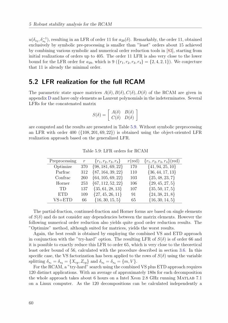
5 Robust stability analysis for the RCAM
u(δs3 , δ−1s4
), resulting in an LFR of order 11 for a29(δ). Remarkably, the order 11, obtainedexclusively by symbolic pre-processing is smaller than ”least” orders about 15 achievedby combining various symbolic and numerical order reduction tools in [83], starting frominitial realizations of orders up to 405. The order 11 LFR is also very close to the lowerbound for the LFR order for a29, which is 9 (r1, r2, r3, r4 = 2, 4, 2, 1). We conjecturethat 11 is already the minimal order.
5.2 LFR realization for the full RCAM
The parametric state space matrices A(δ), B(δ), C(δ), D(δ) of the RCAM are given inappendix D and have only elements as Laurent polynomials in the indeterminates. SeveralLFRs for the concatenated matrix
S(δ) =
[A(δ) B(δ)C(δ) D(δ)
]are computed and the results are presented in Table 5.9. Without symbolic preprocessingan LFR with order 400 (108, 201, 69, 22) is obtained using the object-oriented LFRrealization approach based on the generalized LFR.
Table 5.9: LFR orders for RCAM
Preprocessing r r1, r2, r3, r4 r(red) r1, r2, r3, r4(red)Optimize 370 98, 181, 69, 22 170 41, 94, 25, 10Parfrac 312 87, 164, 39, 22 110 36, 44, 17, 13Confrac 260 64, 105, 69, 22 103 25, 48, 23, 7Horner 253 67, 112, 52, 22 106 29, 45, 27, 5
TD 137 35, 61, 28, 13 107 35, 50, 17, 5ETD 109 27, 45, 26, 11 91 24, 38, 21, 8
VS+ETD 66 16, 30, 15, 5 65 16, 30, 14, 5
The partial-fraction, continued-fraction and Horner forms are based on single elementsof S(δ) and do not consider any dependencies between the matrix elements. However thefollowing numerical order reduction also yields quite good order reduction results. The”Optimize” method, although suited for matrices, yields the worst results.
Again, the best result is obtained by employing the combined VS and ETD approachin conjunction with the ”try-hard” option. The resulting LFR of S(δ) is of order 66 andit is possible to exactly reduce this LFR to order 65, which is very close to the theoreticalleast order bound of 56, calculated with the procedure described in section 3.6. In thisspecific case, the VS factorization has been applied to the rows of S(δ) using the variablesplitting δs1 = δs2 = Xcg, Zcg and δs3 = δs4 = m, V .
For the RCAM, a ”try-hard” search using the combined VS plus ETD approach requires120 distinct applications. With an average of approximately 180s for each decompositionthe whole approach takes about 6 hours on a Intel Xeon 2.8 GHz running Matlab 7.1on a Linux computer. As the 120 decompositions can be calculated independently a
60
5.3 Accuracy of low order LFRs
parallelization of the procedure is straightforward. At the DLR Institute of Robotics andMechatronics a Linux-Cluster with 30 PCs is available, which allowed to perform thewhole calculation within less than 15 minutes.
5.3 Accuracy of low order LFRs
For the very complex parametric model given by the RCAM, the combined VS and ETDapproach allows to obtain an LFR, where a further exact numerical order reduction isalmost unnecessary as the order of 66 can only be reduced to 65. For the a29 element, noadditional numerical reduction is possible. These are remarkable results as the symbolicpreprocessing can be applied without any loss of accuracy (floating-point numbers arerepresented exactly in rational form), whereas numerical order reduction is always basedon tolerance dependent rank decisions. Therefore it is always beneficial for the accuracyof the resulting LFR, if no numerical order reduction must be applied. To illustrate this,the accuracies of the low order LFRs obtained with the combined VS and ETD approachare compared with the accuracies of numerically reduced LFRs obtained with the RobustControl Toolbox 3.0.1 of Matlab. This toolbox offers two kinds of numerical reductioncalled ”basic” and ”full”. The ”basic” method is based on the 1-d order reduction methodof [77] and the Matlab function sminreal is repeatedly called to detect structurally 1-dunobservable/uncontrollable parts. The ”full” method is also based on the 1-d orderreduction principle, but performs 1-d balancing and truncation, where all system partswith Hankel singular values less than 1e-16 are truncated.
Table 5.10 presents the accuracies of the different LFRs. The accuracy is derivedas follows: substitute the symbolic vector δ in the symbolic matrix S(δ) with randomnumerical values δrand and subtract the numerical matrix S(δ)|δ=δrand
from the relatednumerical upper-LFT S ′(δ)|δ=δrand
= Fu(M, ∆)|δ=δrandfor 200 random parameterizations
δrand and the maximum of the 2-norms of the 200 samples is taken as accuracy, i.e.
e = maxi
(‖S(δ)|δ=δrand,i
− S ′(δ)|δ=δrand,i‖2), i = 1, . . . , 200.
The notation ”n-d” (”Appr”) in Table 5.10 means exact n-d (approximate 1-d) orderreduction and using the functions minlfr (redlfr1) of the LFR Toolbox.
The numerical reduction method ”Basic” has almost no effect on the order of theLFRs. The method ”Full”, which is applied after every step during the object-orientedLFR realization yields a large loss of accuracy with an error e of more than 3 percent.On the other hand, the LFRs obtained after symbolic preprocessing are almost of fullaccuracy, e =7e-18 for a29 and e =6e-14 for S(δ), which is very important to have reliableLFRs for the application of robust controller synthesis and stability/performance analysis.
It is interesting to see that if one may be confident with the low accuracy obtainedby the ”Full” method, almost the same accuracy can be obtained by applying numericalapproximation to the LFRs obtained after symbolic preprocessing. However, in this caseit is possible to further reduce the order to 7 and 48 for a29 and S(δ), respectively.
61
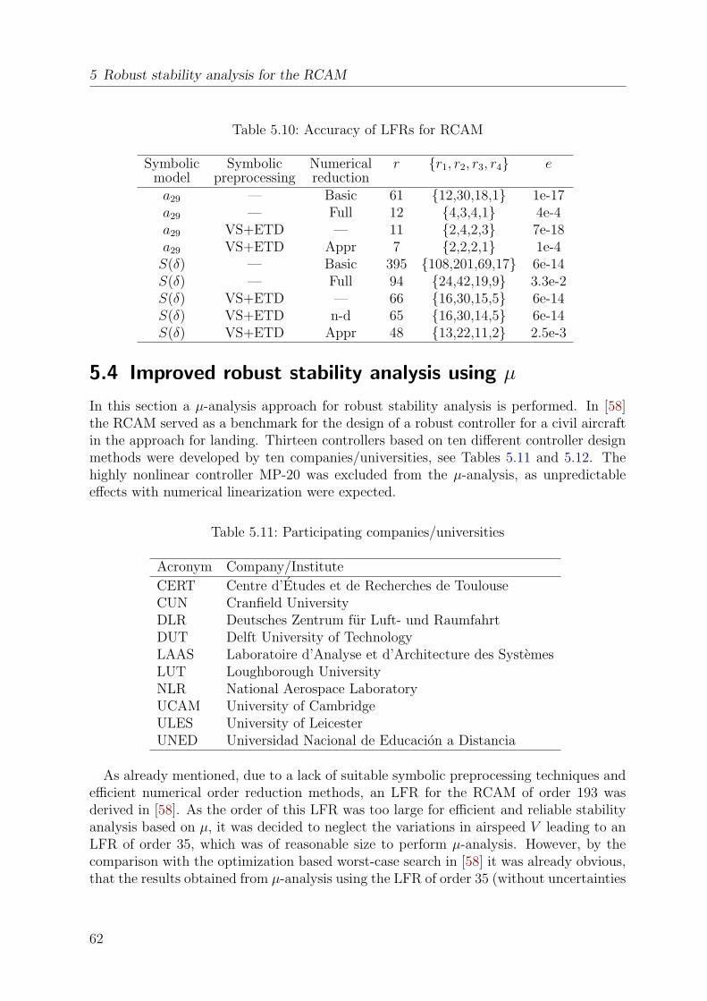
5 Robust stability analysis for the RCAM
Table 5.10: Accuracy of LFRs for RCAM
Symbolic Symbolic Numerical r r1, r2, r3, r4 emodel preprocessing reductiona29 — Basic 61 12,30,18,1 1e-17a29 — Full 12 4,3,4,1 4e-4a29 VS+ETD — 11 2,4,2,3 7e-18a29 VS+ETD Appr 7 2,2,2,1 1e-4S(δ) — Basic 395 108,201,69,17 6e-14S(δ) — Full 94 24,42,19,9 3.3e-2S(δ) VS+ETD — 66 16,30,15,5 6e-14S(δ) VS+ETD n-d 65 16,30,14,5 6e-14S(δ) VS+ETD Appr 48 13,22,11,2 2.5e-3
5.4 Improved robust stability analysis using µ
In this section a µ-analysis approach for robust stability analysis is performed. In [58]the RCAM served as a benchmark for the design of a robust controller for a civil aircraftin the approach for landing. Thirteen controllers based on ten different controller designmethods were developed by ten companies/universities, see Tables 5.11 and 5.12. Thehighly nonlinear controller MP-20 was excluded from the µ-analysis, as unpredictableeffects with numerical linearization were expected.
Table 5.11: Participating companies/universities
Acronym Company/Institute
CERT Centre d’Etudes et de Recherches de ToulouseCUN Cranfield UniversityDLR Deutsches Zentrum fur Luft- und RaumfahrtDUT Delft University of TechnologyLAAS Laboratoire d’Analyse et d’Architecture des SystemesLUT Loughborough UniversityNLR National Aerospace LaboratoryUCAM University of CambridgeULES University of LeicesterUNED Universidad Nacional de Educacion a Distancia
As already mentioned, due to a lack of suitable symbolic preprocessing techniques andefficient numerical order reduction methods, an LFR for the RCAM of order 193 wasderived in [58]. As the order of this LFR was too large for efficient and reliable stabilityanalysis based on µ, it was decided to neglect the variations in airspeed V leading to anLFR of order 35, which was of reasonable size to perform µ-analysis. However, by thecomparison with the optimization based worst-case search in [58] it was already obvious,that the results obtained from µ-analysis using the LFR of order 35 (without uncertainties
62
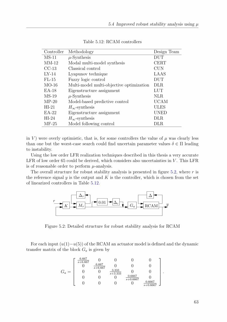
5.4 Improved robust stability analysis using µ
Table 5.12: RCAM controllers
Controller Methodology Design TeamMS-11 µ-Synthesis DUTMM-12 Modal multi-model synthesis CERTCC-13 Classical control CUNLY-14 Lyapunov technique LAASFL-15 Fuzzy logic control DUTMO-16 Multi-model multi-objective optimization DLREA-18 Eigenstructure assignment LUTMS-19 µ-Synthesis NLRMP-20 Model-based predictive control UCAMHI-21 H∞-synthesis ULESEA-22 Eigenstructure assignment UNEDHI-24 H∞-synthesis DLRMF-25 Model following control DLR
in V ) were overly optimistic, that is, for some controllers the value of µ was clearly lessthan one but the worst-case search could find uncertain parameter values δ ∈ Π leadingto instability.
Using the low order LFR realization techniques described in this thesis a very accurateLFR of low order 65 could be derived, which considers also uncertainties in V . This LFRis of reasonable order to perform µ-analysis.
The overall structure for robust stability analysis is presented in figure 5.2, where r isthe reference signal y is the output and K is the controller, which is chosen from the setof linearized controllers in Table 5.12.
r
K0.01 ∆c
∆
yRCAM
∆τ
Mτ Ga
Figure 5.2: Detailed structure for robust stability analysis for RCAM
For each input (u(1)−u(5)) of the RCAM an actuator model is defined and the dynamictransfer matrix of the block Ga is given by
Ga =
6.667
s+6.6670 0 0 0
0 6.667s+6.667
0 0 0
0 0 3.333s+3.333
0 0
0 0 0 0.6667s+0.6667
0
0 0 0 0 0.6667s+0.6667
.
63
5 Robust stability analysis for the RCAM
Furthermore an uncertain time delay τ ∈ [0.05, 0.1]s is assumed at each actuator input.The delay is approximated with a first order Pade-filter as
e−τs ≈ 2− τs
2 + τs
and is reasonably accurate up to a frequency of ±10rad/s. Since τ is identical for eachactuator input, the uncertainty matrix ∆τ of the LFR (Mτ , ∆τ ) is given by ∆τ = τI5. Inaddition a small extra complex perturbation is added. As it is assumed that ‖∆c‖∞ =‖diag(δc1 , δc2 , δc3 , δc4 , δc5)‖∞ ≤ 1, the perturbation 0.01∆c is only 1% and may for exam-ple account for unmodelled dynamics or gain and phase variations at the input of theactuators. However, the main motivation for the introduction of these small complexuncertainties is that the computation of the lower µ-bounds becomes tractable [11]. Thefinal interconnection structure for analysis is shown in figure 5.3, where
∆T = diag(mI16, V I30, XcgI14, ZcgI5, τI5, δc1 , δc2 , δc3 , δc4 , δc5),
with m, V, Xcg, Zcg, τ ∈ R and δc1 , δc2 , δc3 , δc4 , δc5 ∈ C.
∆T
z
y
P
K
u
w
Figure 5.3: Compact structure for robust stability analysis for RCAM
The results of the µ-analysis for controlled RCAM, using the very accurate, low orderLFR, are summarized in Table 5.13. In figures 5.4 and 5.5 the upper and lower µ-boundsfor the interesting frequency range from 10−1 rad/s to 101.5 rad/s are presented. In thisinterval, 100 equidistant grid points are chosen over a logarithmic frequency scale. TheRobust Control Toolbox of Matlab [11] is used to perform the µ-analysis.
For comparison the µ-analysis and the optimization-based worst-case search resultsfrom [58] are also included. The worst-case search repeatedly calculates the eigenvalues ofthe linearized closed-loop system within an optimization based parameter search directedto determine the minimum damping ζworst over all admissible parameter values. Eachcalculation of the least damping involves the trimming of the nonlinear open-loop systemand the linearization of the closed-loop system.
In every case the µ-analysis from [58] led to lower values for the maximum of theµ-upper-bound. These more optimistic results come from the fact, that the variationin airspeed V was not considered. Even more important is that the µ-analysis resultsfrom [58] indicate robust closed-loop stability for the controllers MS-11, EA-18, HI-24,
64
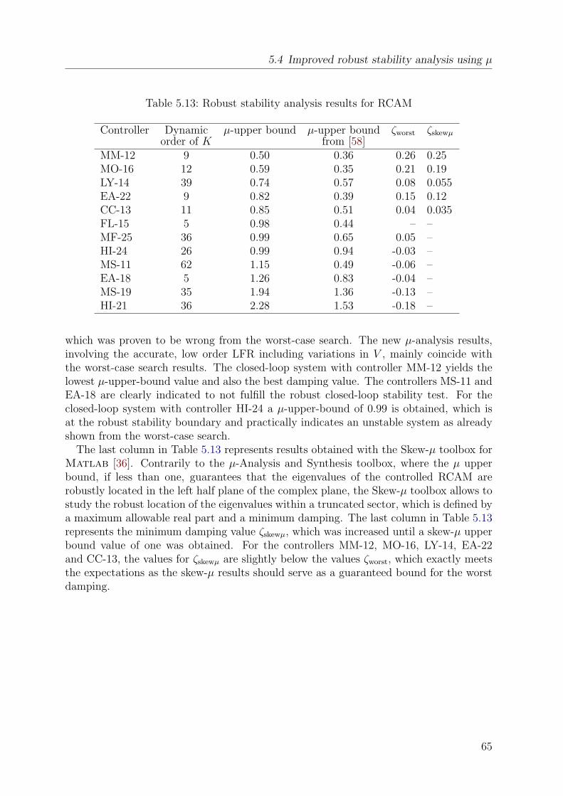
5.4 Improved robust stability analysis using µ
Table 5.13: Robust stability analysis results for RCAM
Controller Dynamic µ-upper bound µ-upper bound ζworst ζskewµ
order of K from [58]MM-12 9 0.50 0.36 0.26 0.25MO-16 12 0.59 0.35 0.21 0.19LY-14 39 0.74 0.57 0.08 0.055EA-22 9 0.82 0.39 0.15 0.12CC-13 11 0.85 0.51 0.04 0.035FL-15 5 0.98 0.44 – –MF-25 36 0.99 0.65 0.05 –HI-24 26 0.99 0.94 -0.03 –MS-11 62 1.15 0.49 -0.06 –EA-18 5 1.26 0.83 -0.04 –MS-19 35 1.94 1.36 -0.13 –HI-21 36 2.28 1.53 -0.18 –
which was proven to be wrong from the worst-case search. The new µ-analysis results,involving the accurate, low order LFR including variations in V , mainly coincide withthe worst-case search results. The closed-loop system with controller MM-12 yields thelowest µ-upper-bound value and also the best damping value. The controllers MS-11 andEA-18 are clearly indicated to not fulfill the robust closed-loop stability test. For theclosed-loop system with controller HI-24 a µ-upper-bound of 0.99 is obtained, which isat the robust stability boundary and practically indicates an unstable system as alreadyshown from the worst-case search.
The last column in Table 5.13 represents results obtained with the Skew-µ toolbox forMatlab [36]. Contrarily to the µ-Analysis and Synthesis toolbox, where the µ upperbound, if less than one, guarantees that the eigenvalues of the controlled RCAM arerobustly located in the left half plane of the complex plane, the Skew-µ toolbox allows tostudy the robust location of the eigenvalues within a truncated sector, which is defined bya maximum allowable real part and a minimum damping. The last column in Table 5.13represents the minimum damping value ζskewµ, which was increased until a skew-µ upperbound value of one was obtained. For the controllers MM-12, MO-16, LY-14, EA-22and CC-13, the values for ζskewµ are slightly below the values ζworst, which exactly meetsthe expectations as the skew-µ results should serve as a guaranteed bound for the worstdamping.
65
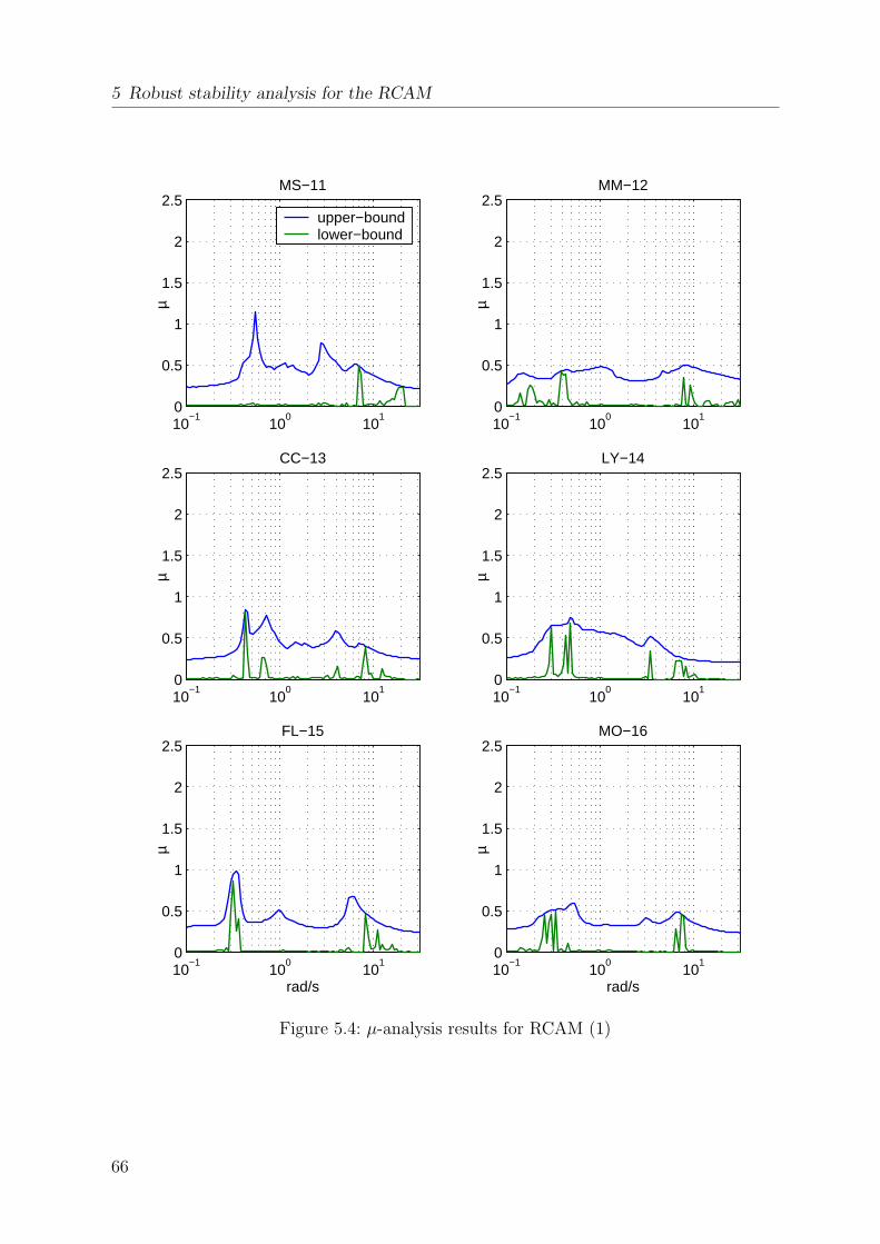
5 Robust stability analysis for the RCAM
10−1
100
101
0
0.5
1
1.5
2
2.5
µ
MS−11
10−1
100
101
0
0.5
1
1.5
2
2.5
µ
MM−12
10−1
100
101
0
0.5
1
1.5
2
2.5
µ
CC−13
10−1
100
101
0
0.5
1
1.5
2
2.5µ
LY−14
10−1
100
101
0
0.5
1
1.5
2
2.5
rad/s
µ
FL−15
10−1
100
101
0
0.5
1
1.5
2
2.5
rad/s
µ
MO−16
upper−boundlower−bound
Figure 5.4: µ-analysis results for RCAM (1)
66
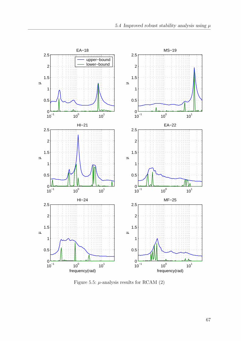
5.4 Improved robust stability analysis using µ
10−1
100
101
0
0.5
1
1.5
2
2.5
µ
EA−18
10−1
100
101
0
0.5
1
1.5
2
2.5
µ
MS−19
10−1
100
101
0
0.5
1
1.5
2
2.5
µ
HI−21
10−1
100
101
0
0.5
1
1.5
2
2.5µ
EA−22
10−1
100
101
0
0.5
1
1.5
2
2.5
frequency(rad)
µ
HI−24
10−1
100
101
0
0.5
1
1.5
2
2.5
frequency(rad)
µ
MF−25
upper−boundlower−bound
Figure 5.5: µ-analysis results for RCAM (2)
67
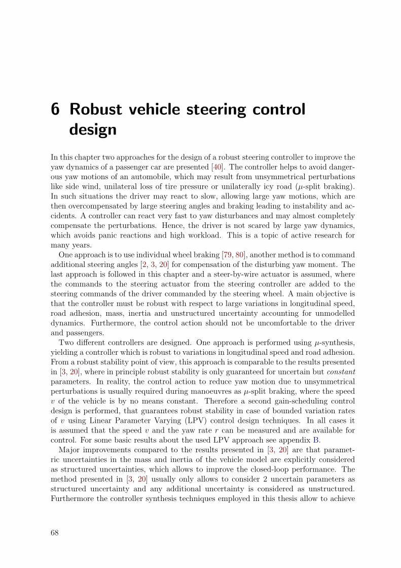
6 Robust vehicle steering controldesign
In this chapter two approaches for the design of a robust steering controller to improve theyaw dynamics of a passenger car are presented [40]. The controller helps to avoid danger-ous yaw motions of an automobile, which may result from unsymmetrical perturbationslike side wind, unilateral loss of tire pressure or unilaterally icy road (µ-split braking).In such situations the driver may react to slow, allowing large yaw motions, which arethen overcompensated by large steering angles and braking leading to instability and ac-cidents. A controller can react very fast to yaw disturbances and may almost completelycompensate the perturbations. Hence, the driver is not scared by large yaw dynamics,which avoids panic reactions and high workload. This is a topic of active research formany years.
One approach is to use individual wheel braking [79, 80], another method is to commandadditional steering angles [2, 3, 20] for compensation of the disturbing yaw moment. Thelast approach is followed in this chapter and a steer-by-wire actuator is assumed, wherethe commands to the steering actuator from the steering controller are added to thesteering commands of the driver commanded by the steering wheel. A main objective isthat the controller must be robust with respect to large variations in longitudinal speed,road adhesion, mass, inertia and unstructured uncertainty accounting for unmodelleddynamics. Furthermore, the control action should not be uncomfortable to the driverand passengers.
Two different controllers are designed. One approach is performed using µ-synthesis,yielding a controller which is robust to variations in longitudinal speed and road adhesion.From a robust stability point of view, this approach is comparable to the results presentedin [3, 20], where in principle robust stability is only guaranteed for uncertain but constantparameters. In reality, the control action to reduce yaw motion due to unsymmetricalperturbations is usually required during manoeuvres as µ-split braking, where the speedv of the vehicle is by no means constant. Therefore a second gain-scheduling controldesign is performed, that guarantees robust stability in case of bounded variation ratesof v using Linear Parameter Varying (LPV) control design techniques. In all cases itis assumed that the speed v and the yaw rate r can be measured and are available forcontrol. For some basic results about the used LPV approach see appendix B.
Major improvements compared to the results presented in [3, 20] are that paramet-ric uncertainties in the mass and inertia of the vehicle model are explicitly consideredas structured uncertainties, which allows to improve the closed-loop performance. Themethod presented in [3, 20] usually only allows to consider 2 uncertain parameters asstructured uncertainty and any additional uncertainty is considered as unstructured.Furthermore the controller synthesis techniques employed in this thesis allow to achieve
68
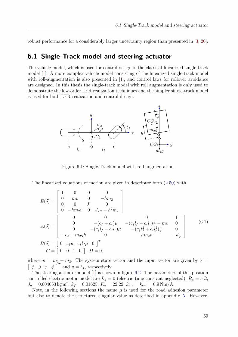
6.1 Single-Track model and steering actuator
robust performance for a considerably larger uncertainty region than presented in [3, 20].
6.1 Single-Track model and steering actuator
The vehicle model, which is used for control design is the classical linearized single-trackmodel [1]. A more complex vehicle model consisting of the linearized single-track modelwith roll-augmentation is also presented in [1], and control laws for rollover avoidanceare designed. In this thesis the single-track model with roll augmentation is only used todemonstrate the low-order LFR realization techniques and the simpler single-track modelis used for both LFR realization and control design.
y
r
lr
CG1
β
v
lf
δf
x
z
φCG2
m2gh
CG1 y
m1g
Figure 6.1: Single-Track model with roll augmentation
The linearized equations of motion are given in descriptor form (2.50) with
E(δ) =
1 0 0 00 mv 0 −hm2
0 0 Jz 00 −hm2v 0 Jx,2 + h2m2
A(δ) =
0 0 0 10 −(cf + cr)µ −(cf lf − crlr)
µv−mv 0
0 −(cf lf − crlr)µ −(cf l2f + crl
2r)
µv
0−cφ + m2gh 0 hm2v −dφ
B(δ) =
[0 cfµ cf lfµ 0
]TC =
[0 0 1 0
], D = 0,
(6.1)
where m = m1 + m2. The system state vector and the input vector are given by x =[φ β r φ
]Tand u = δf , respectively.
The steering actuator model [1] is shown in figure 6.2. The parameters of this positioncontrolled electric motor model are La = 0 (electric time constant neglected), Ra = 5 Ω,Ja = 0.004053 kg m2, kf = 0.01625, Ka = 22.22, kme = kem = 0.9 Nm/A.
Note, in the following sections the name µ is used for the road adhesion parameterbut also to denote the structured singular value as described in appendix A. However,
69
6 Robust vehicle steering control design
Table 6.1: Vehicle Data
Parameter Unit Description(or Variable)cf [kN/rad] front cornering stiffnesscr [kN/rad] rear cornering stiffnesscφ [kN m/rad] roll stiffness of passive suspensiondφ [kN m s/rad] roll damping of passive suspension
g [m/s2] acceleration due to gravityh [m] nominal height of CG2 over roll axisJx,2 [kg m2] roll moment of inertia, sprung massJz [kg m2] overall yaw moment of inertialf [m] distance of front axle to CG1
lr [m] distance of rear axle to CG1
m1 [kg] mass of chassism2 [kg] sprung massµ road adhesionv [m/s] magnitude of velocity vectorr [rad/s] yaw rateβ [rad] chassis side-slip angle at CG1
δf [rad] front wheel steering angleφ [rad] roll angle of sprung mass
for each occurrence of µ the meaning should be clear from the context. Furthermore,SI-units are assumed for all model parameters and for simplicity, the units are omitted.
6.2 LFR realization for roll-augmented single track model
For the single-track model with roll augmentation the parameters m1, m2, h, v, µ, Jx,2
and Jz are considered as uncertain.The vehicle model (6.1) is given in descriptor form as,[
1 00 M(δ)
]x =
[0 1
−K(δ) −D(δ)
]x +
[0
S(δ)
]u
y = Cx
which is the direct representation in state space for a second order physical system modeldescribed as
M(δ)x + D(δ)x + K(δ)x = S(δ)u.
A standard state-space description may be derived as
x =
[0 1
−M−1(δ)K(δ) −M−1(δ)D(δ)
]x +
[0
M−1(δ)S(δ)
]u
y = Cx,
(6.2)
70
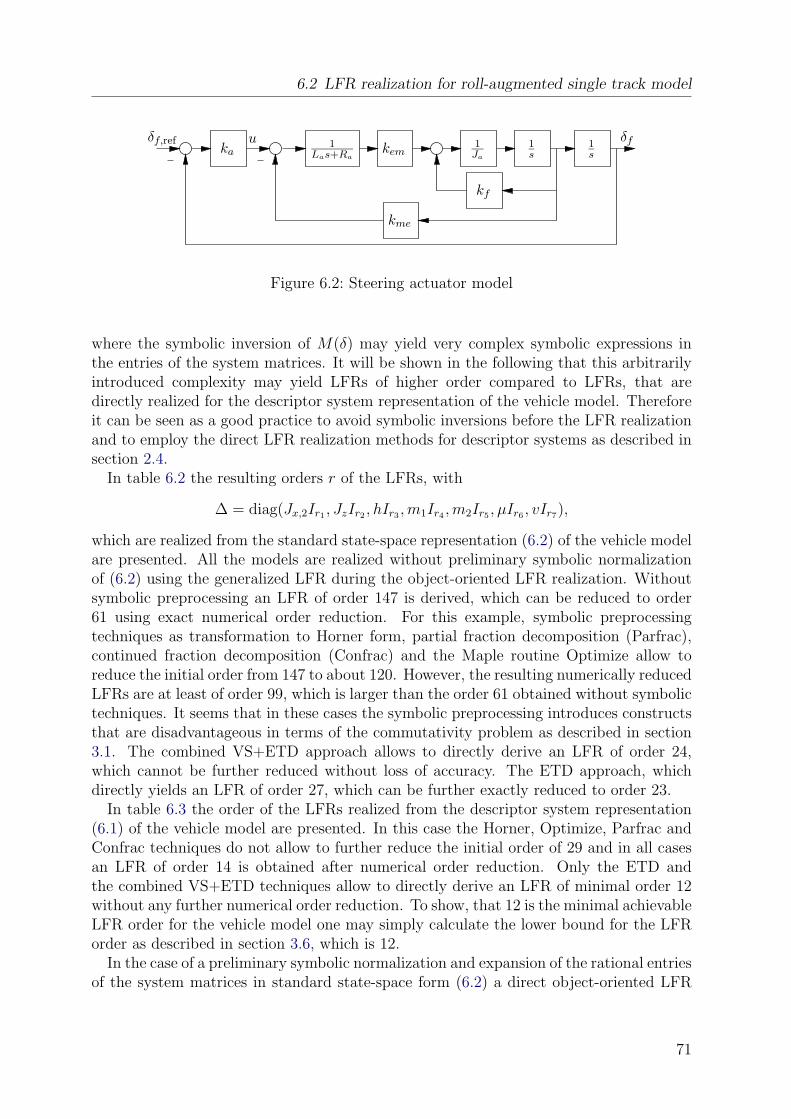
6.2 LFR realization for roll-augmented single track model
δf,ref ukem
kme
1
Las+Ra
kf
1
s1
s
δfka
1
Ja
Figure 6.2: Steering actuator model
where the symbolic inversion of M(δ) may yield very complex symbolic expressions inthe entries of the system matrices. It will be shown in the following that this arbitrarilyintroduced complexity may yield LFRs of higher order compared to LFRs, that aredirectly realized for the descriptor system representation of the vehicle model. Thereforeit can be seen as a good practice to avoid symbolic inversions before the LFR realizationand to employ the direct LFR realization methods for descriptor systems as described insection 2.4.
In table 6.2 the resulting orders r of the LFRs, with
∆ = diag(Jx,2Ir1 , JzIr2 , hIr3 , m1Ir4 , m2Ir5 , µIr6 , vIr7),
which are realized from the standard state-space representation (6.2) of the vehicle modelare presented. All the models are realized without preliminary symbolic normalizationof (6.2) using the generalized LFR during the object-oriented LFR realization. Withoutsymbolic preprocessing an LFR of order 147 is derived, which can be reduced to order61 using exact numerical order reduction. For this example, symbolic preprocessingtechniques as transformation to Horner form, partial fraction decomposition (Parfrac),continued fraction decomposition (Confrac) and the Maple routine Optimize allow toreduce the initial order from 147 to about 120. However, the resulting numerically reducedLFRs are at least of order 99, which is larger than the order 61 obtained without symbolictechniques. It seems that in these cases the symbolic preprocessing introduces constructsthat are disadvantageous in terms of the commutativity problem as described in section3.1. The combined VS+ETD approach allows to directly derive an LFR of order 24,which cannot be further reduced without loss of accuracy. The ETD approach, whichdirectly yields an LFR of order 27, which can be further exactly reduced to order 23.
In table 6.3 the order of the LFRs realized from the descriptor system representation(6.1) of the vehicle model are presented. In this case the Horner, Optimize, Parfrac andConfrac techniques do not allow to further reduce the initial order of 29 and in all casesan LFR of order 14 is obtained after numerical order reduction. Only the ETD andthe combined VS+ETD techniques allow to directly derive an LFR of minimal order 12without any further numerical order reduction. To show, that 12 is the minimal achievableLFR order for the vehicle model one may simply calculate the lower bound for the LFRorder as described in section 3.6, which is 12.
In the case of a preliminary symbolic normalization and expansion of the rational entriesof the system matrices in standard state-space form (6.2) a direct object-oriented LFR
71
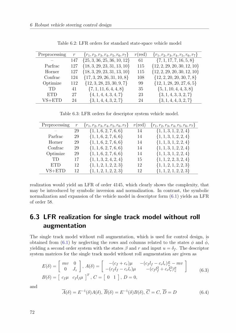
6 Robust vehicle steering control design
Table 6.2: LFR orders for standard state-space vehicle model
Preprocessing r r1, r2, r3, r4, r5, r6, r7 r(red) r1, r2, r3, r4, r5, r6, r7– 147 25, 3, 36, 25, 36, 10, 12 61 7, 1, 17, 7, 16, 5, 8
Parfrac 127 18, 3, 29, 23, 31, 13, 10 115 12, 2, 29, 20, 30, 12, 10Horner 127 18, 3, 29, 23, 31, 13, 10 115 12, 2, 29, 20, 30, 12, 10Confrac 124 17, 3, 29, 26, 31, 10, 8 108 12, 2, 20, 20, 30, 7, 8Optimize 112 12, 3, 28, 23, 30, 9, 7 99 12, 1, 28, 20, 27, 6, 5
TD 41 7, 1, 11, 6, 4, 4, 8 35 5, 1, 10, 4, 4, 3, 8ETD 27 4, 1, 4, 4, 3, 4, 7 23 3, 1, 4, 3, 3, 2, 7
VS+ETD 24 3, 1, 4, 4, 3, 2, 7 24 3, 1, 4, 4, 3, 2, 7
Table 6.3: LFR orders for descriptor system vehicle model.
Preprocessing r r1, r2, r3, r4, r5, r6, r7 r(red) r1, r2, r3, r4, r5, r6, r7– 29 1, 1, 6, 2, 7, 6, 6 14 1, 1, 3, 1, 2, 2, 4
Parfrac 29 1, 1, 6, 2, 7, 6, 6 14 1, 1, 3, 1, 2, 2, 4Horner 29 1, 1, 6, 2, 7, 6, 6 14 1, 1, 3, 1, 2, 2, 4Confrac 29 1, 1, 6, 2, 7, 6, 6 14 1, 1, 3, 1, 2, 2, 4Optimize 29 1, 1, 6, 2, 7, 6, 6 14 1, 1, 3, 1, 2, 2, 4
TD 17 1, 1, 3, 2, 4, 2, 4 15 1, 1, 2, 2, 3, 2, 4ETD 12 1, 1, 2, 1, 2, 2, 3 12 1, 1, 2, 1, 2, 2, 3
VS+ETD 12 1, 1, 2, 1, 2, 2, 3 12 1, 1, 2, 1, 2, 2, 3
realization would yield an LFR of order 4145, which clearly shows the complexity, thatmay be introduced by symbolic inversion and normalization. In contrast, the symbolicnormalization and expansion of the vehicle model in descriptor form (6.1) yields an LFRof order 58.
6.3 LFR realization for single track model without rollaugmentation
The single track model without roll augmentation, which is used for control design, isobtained from (6.1) by neglecting the rows and columns related to the states φ and φ,yielding a second order system with the states β and r and input u = δf . The descriptorsystem matrices for the single track model without roll augmentation are given as
E(δ) =
[mv 00 Jz
], A(δ) =
[−(cf + cr)µ −(cf lf − crlr)
µv−mv
−(cf lf − crlr)µ −(cf l2f + crl
2r)
µv
]B(δ) =
[cfµ cf lfµ
]T, C =
[0 1
], D = 0,
(6.3)
andA(δ) = E−1(δ)A(δ), B(δ) = E−1(δ)B(δ), C = C, D = D (6.4)
72
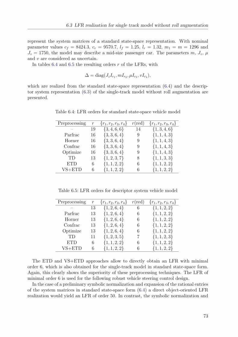
6.3 LFR realization for single track model without roll augmentation
represent the system matrices of a standard state-space representation. With nominalparameter values cf = 8424.3, cr = 9570.7, lf = 1.25, lr = 1.32, m1 = m = 1296 andJz = 1750, the model may describe a mid-size passenger car. The parameters m, Jz, µand v are considered as uncertain.
In tables 6.4 and 6.5 the resulting orders r of the LFRs, with
∆ = diag(JzIr1 , mIr2 , µIr3 , vIr4),
which are realized from the standard state-space representation (6.4) and the descrip-tor system representation (6.3) of the single-track model without roll augmentation arepresented.
Table 6.4: LFR orders for standard state-space vehicle model
Preprocessing r r1, r2, r3, r4 r(red) r1, r2, r3, r4– 19 3, 4, 6, 6 14 1, 3, 4, 6
Parfrac 16 3, 3, 6, 4 9 1, 1, 4, 3Horner 16 3, 3, 6, 4 9 1, 1, 4, 3Confrac 16 3, 3, 6, 4 9 1, 1, 4, 3Optimize 16 3, 3, 6, 4 9 1, 1, 4, 3
TD 13 1, 2, 3, 7 8 1, 1, 3, 3ETD 6 1, 1, 2, 2 6 1, 1, 2, 2
VS+ETD 6 1, 1, 2, 2 6 1, 1, 2, 2
Table 6.5: LFR orders for descriptor system vehicle model
Preprocessing r r1, r2, r3, r4 r(red) r1, r2, r3, r4– 13 1, 2, 6, 4 6 1, 1, 2, 2
Parfrac 13 1, 2, 6, 4 6 1, 1, 2, 2Horner 13 1, 2, 6, 4 6 1, 1, 2, 2Confrac 13 1, 2, 6, 4 6 1, 1, 2, 2Optimize 13 1, 2, 6, 4 6 1, 1, 2, 2
TD 11 1, 2, 3, 5 7 1, 1, 2, 3ETD 6 1, 1, 2, 2 6 1, 1, 2, 2
VS+ETD 6 1, 1, 2, 2 6 1, 1, 2, 2
The ETD and VS+ETD approaches allow to directly obtain an LFR with minimalorder 6, which is also obtained for the single-track model in standard state-space form.Again, this clearly shows the superiority of these preprocessing techniques. The LFR ofminimal order 6 is used for the following robust vehicle steering control design.
In the case of a preliminary symbolic normalization and expansion of the rational entriesof the system matrices in standard state-space form (6.4) a direct object-oriented LFRrealization would yield an LFR of order 50. In contrast, the symbolic normalization and
73
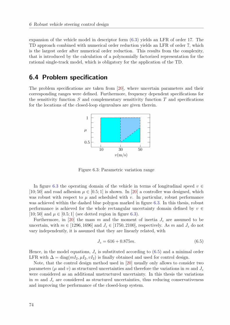
6 Robust vehicle steering control design
expansion of the vehicle model in descriptor form (6.3) yields an LFR of order 17. TheTD approach combined with numerical order reduction yields an LFR of order 7, whichis the largest order after numerical order reduction. This results from the complexity,that is introduced by the calculation of a polynomially factorized representation for therational single-track model, which is obligatory for the application of the TD.
6.4 Problem specification
The problem specifications are taken from [20], where uncertain parameters and theircorresponding ranges were defined. Furthermore, frequency dependent specifications forthe sensitivity function S and complementary sensitivity function T and specificationsfor the locations of the closed-loop eigenvalues are given therein.
0.5
1
µ
10 30
v(m/s)
50
Figure 6.3: Parametric variation range
In figure 6.3 the operating domain of the vehicle in terms of longitudinal speed v ∈[10; 50] and road adhesion µ ∈ [0.5; 1] is shown. In [20] a controller was designed, whichwas robust with respect to µ and scheduled with v. In particular, robust performancewas achieved within the dashed blue polygon marked in figure 6.3. In this thesis, robustperformance is achieved for the whole rectangular uncertainty domain defined by v ∈[10; 50] and µ ∈ [0.5; 1] (see dotted region in figure 6.3).
Furthermore, in [20] the mass m and the moment of inertia Jz are assumed to beuncertain, with m ∈ [1296, 1696] and Jz ∈ [1750, 2100], respectively. As m and Jz do notvary independently, it is assumed that they are linearly related, with
Jz = 616 + 0.875m. (6.5)
Hence, in the model equations, Jz is substituted according to (6.5) and a minimal orderLFR with ∆ = diag(mI2, µI2, vI2) is finally obtained and used for control design.
Note, that the control design method used in [20] usually only allows to consider twoparameters (µ and v) as structured uncertainties and therefore the variations in m and Jz
were considered as an additional unstructured uncertainty. In this thesis the variationsin m and Jz are considered as structured uncertainties, thus reducing conservativenessand improving the performance of the closed-loop system.
74
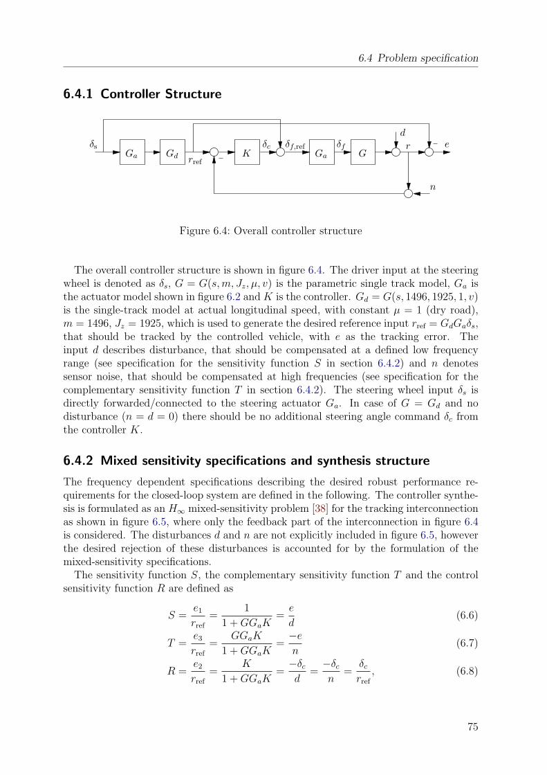
6.4 Problem specification
6.4.1 Controller Structure
δs
Ga Gdrref
K
δf,refδcGa
δfG
d
r e
n
Figure 6.4: Overall controller structure
The overall controller structure is shown in figure 6.4. The driver input at the steeringwheel is denoted as δs, G = G(s, m, Jz, µ, v) is the parametric single track model, Ga isthe actuator model shown in figure 6.2 and K is the controller. Gd = G(s, 1496, 1925, 1, v)is the single-track model at actual longitudinal speed, with constant µ = 1 (dry road),m = 1496, Jz = 1925, which is used to generate the desired reference input rref = GdGaδs,that should be tracked by the controlled vehicle, with e as the tracking error. Theinput d describes disturbance, that should be compensated at a defined low frequencyrange (see specification for the sensitivity function S in section 6.4.2) and n denotessensor noise, that should be compensated at high frequencies (see specification for thecomplementary sensitivity function T in section 6.4.2). The steering wheel input δs isdirectly forwarded/connected to the steering actuator Ga. In case of G = Gd and nodisturbance (n = d = 0) there should be no additional steering angle command δc fromthe controller K.
6.4.2 Mixed sensitivity specifications and synthesis structure
The frequency dependent specifications describing the desired robust performance re-quirements for the closed-loop system are defined in the following. The controller synthe-sis is formulated as an H∞ mixed-sensitivity problem [38] for the tracking interconnectionas shown in figure 6.5, where only the feedback part of the interconnection in figure 6.4is considered. The disturbances d and n are not explicitly included in figure 6.5, howeverthe desired rejection of these disturbances is accounted for by the formulation of themixed-sensitivity specifications.
The sensitivity function S, the complementary sensitivity function T and the controlsensitivity function R are defined as
S =e1
rref
=1
1 + GGaK=
e
d(6.6)
T =e3
rref
=GGaK
1 + GGaK=−e
n(6.7)
R =e2
rref
=K
1 + GGaK=−δc
d=−δc
n=
δc
rref
, (6.8)
75
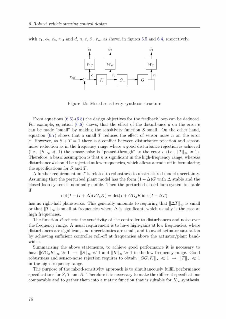
6 Robust vehicle steering control design
with e1, e2, e3, rref and d, n, e, δc, rref as shown in figures 6.5 and 6.4, respectively.
e1 e2
WR
e1
K
e2
Ga
rref
G
WT
e3
e3
WS
Figure 6.5: Mixed-sensitivity synthesis structure
From equations (6.6)-(6.8) the design objectives for the feedback loop can be deduced.For example, equation (6.6) shows, that the effect of the disturbance d on the error ecan be made ”small” by making the sensitivity function S small. On the other hand,equation (6.7) shows that a small T reduces the effect of sensor noise n on the errore. However, as S + T = 1 there is a conflict between disturbance rejection and sensor-noise reduction as in the frequency range where a good disturbance rejection is achieved(i.e., ‖S‖∞ 1) the sensor-noise is ”passed-through” to the error e (i.e., ‖T‖∞ ≈ 1).Therefore, a basic assumption is that n is significant in the high-frequency range, whereasdisturbance d should be rejected at low frequencies, which allows a trade-off in formulatingthe specifications for S and T .
A further requirement on T is related to robustness to unstructured model uncertainty.Assuming that the perturbed plant model has the form (1 + ∆)G with ∆ stable and theclosed-loop system is nominally stable. Then the perturbed closed-loop system is stableif
det(I + (I + ∆)GGaK) = det(I + GGaK)det(I + ∆T )
has no right-half plane zeros. This generally amounts to requiring that ‖∆T‖∞ is smallor that ‖T‖∞ is small at frequencies where ∆ is significant, which usually is the case athigh frequencies.
The function R reflects the sensitivity of the controller to disturbances and noise overthe frequency range. A usual requirement is to have high-gains at low frequencies, wheredisturbances are significant and uncertainties are small, and to avoid actuator saturationby achieving sufficient controller roll-off at frequencies above the actuator/plant band-width.
Summarizing the above statements, to achieve good performance it is necessary tohave ‖GGaK‖∞ 1 → ‖S‖∞ 1 and ‖K‖∞ 1 in the low frequency range. Goodrobustness and sensor-noise rejection requires to obtain ‖GGaK‖∞ 1 → ‖T‖∞ 1in the high-frequency range.
The purpose of the mixed-sensitivity approach is to simultaneously fulfill performancespecifications for S, T and R. Therefore it is necessary to make the different specificationscomparable and to gather them into a matrix function that is suitable for H∞ synthesis.
76
6.4 Problem specification
A very convenient way to reflect the different specifications is to employ appropriatefrequency dependent weighting functions WS, WT , WR, which are chosen such that thespecifications on S, T and R are fulfilled if the following inequalities hold:
‖WSS‖∞ ≤ 1, ∀ω (6.9)
‖WT T‖∞ ≤ 1, ∀ω (6.10)
‖WRR‖∞ ≤ 1, ∀ω. (6.11)
For example, the specification for the sensitivity function S can be translated into in-equality (6.9) by choosing WS such that WS 1 at low frequencies and WS is sufficientlysmall at high frequencies.
Gathering the weighted sensitivity functions into one vector E, with
E =
e1
rref
e2
rref
e3
rref
=
WSSWRRWT T
allows to formulate the mixed-sensitivity optimization problem as
minK‖E‖∞,
where ‖E‖∞ ≤ 1 means that all specifications for S, T and R are fulfilled.The specifications for S and T are taken from [20], where WS was chosen as WS =
(s+12.6)/(1.8s+1.26), which requires ‖S‖∞ ≤ 0.1 at low frequencies. In [20] a controllerstructure was chosen, which inherently offers infinite controller gain at s = 0 and thereforethe specification for S at low frequency will always be fulfilled. Choosing the same WS forthe controller structure as shown in figure 6.4, may yield a controller that allows an errore, where only 90% of a constant disturbance d are rejected. This may not be consideredsatisfactory. To improve performance, the weighting WS was chosen more demanding as
WS =s + 11
1.8s + 0.11,
thus requiring ‖e‖2 ≤ 0.01‖d‖2 at low frequencies. Due to Bode’s sensitivity integralrelation [91], the required small norm of S at low frequencies unavoidably results in anorm larger than one at high frequencies, which shall be bounded with ‖S‖∞ ≤ 1.8. Infigure 6.6 the frequency dependent magnitude of the upper bound W−1
S for S is shown.Robustness with respect to multiplicative unstructured uncertainty is formulated in
terms of a performance specifications for the complementary sensitivity function T . Thecontroller must be robust to 10% magnitude uncertainty at low frequencies, where themodel of the vehicle and actuator is reasonably accurate, and 500% uncertainty at highfrequencies, where unmodelled dynamics come into play. A transition frequency of 6 Hzbetween low and high frequency uncertainty was chosen based on the knowledge of themodel’s accuracy. This specification is formulated as
WT = 5s + 3.77
s + 188.5.
77
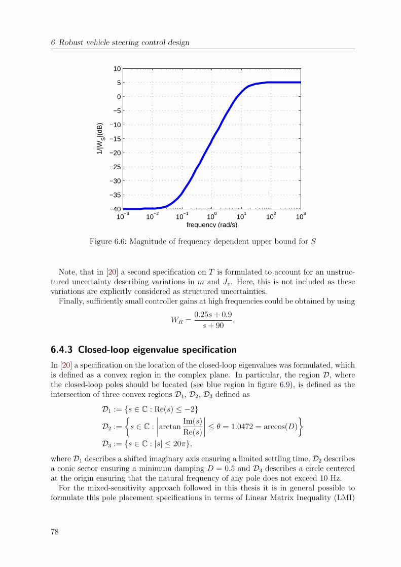
6 Robust vehicle steering control design
10−3
10−2
10−1
100
101
102
103
−40
−35
−30
−25
−20
−15
−10
−5
0
5
10
frequency (rad/s)
1/|W
S|(
dB)
Figure 6.6: Magnitude of frequency dependent upper bound for S
Note, that in [20] a second specification on T is formulated to account for an unstruc-tured uncertainty describing variations in m and Jz. Here, this is not included as thesevariations are explicitly considered as structured uncertainties.
Finally, sufficiently small controller gains at high frequencies could be obtained by using
WR =0.25s + 0.9
s + 90.
6.4.3 Closed-loop eigenvalue specification
In [20] a specification on the location of the closed-loop eigenvalues was formulated, whichis defined as a convex region in the complex plane. In particular, the region D, wherethe closed-loop poles should be located (see blue region in figure 6.9), is defined as theintersection of three convex regions D1, D2, D3 defined as
D1 := s ∈ C : Re(s) ≤ −2
D2 :=
s ∈ C :
∣∣∣∣arctanIm(s)
Re(s)
∣∣∣∣ ≤ θ = 1.0472 = arccos(D)
D3 := s ∈ C : |s| ≤ 20π,
where D1 describes a shifted imaginary axis ensuring a limited settling time, D2 describesa conic sector ensuring a minimum damping D = 0.5 and D3 describes a circle centeredat the origin ensuring that the natural frequency of any pole does not exceed 10 Hz.
For the mixed-sensitivity approach followed in this thesis it is in general possible toformulate this pole placement specifications in terms of Linear Matrix Inequality (LMI)
78
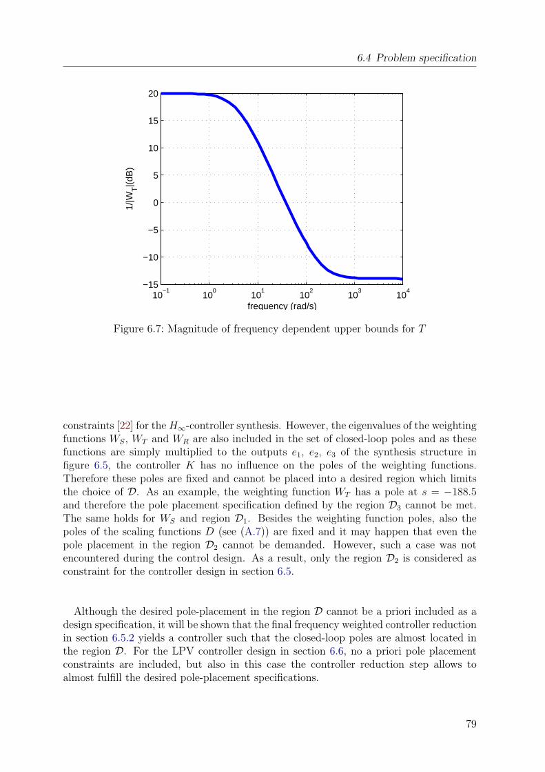
6.4 Problem specification
10−1
100
101
102
103
104
−15
−10
−5
0
5
10
15
20
frequency (rad/s)
1/|W
T|(
dB)
Figure 6.7: Magnitude of frequency dependent upper bounds for T
constraints [22] for the H∞-controller synthesis. However, the eigenvalues of the weightingfunctions WS, WT and WR are also included in the set of closed-loop poles and as thesefunctions are simply multiplied to the outputs e1, e2, e3 of the synthesis structure infigure 6.5, the controller K has no influence on the poles of the weighting functions.Therefore these poles are fixed and cannot be placed into a desired region which limitsthe choice of D. As an example, the weighting function WT has a pole at s = −188.5and therefore the pole placement specification defined by the region D3 cannot be met.The same holds for WS and region D1. Besides the weighting function poles, also thepoles of the scaling functions D (see (A.7)) are fixed and it may happen that even thepole placement in the region D2 cannot be demanded. However, such a case was notencountered during the control design. As a result, only the region D2 is considered asconstraint for the controller design in section 6.5.
Although the desired pole-placement in the region D cannot be a priori included as adesign specification, it will be shown that the final frequency weighted controller reductionin section 6.5.2 yields a controller such that the closed-loop poles are almost located inthe region D. For the LPV controller design in section 6.6, no a priori pole placementconstraints are included, but also in this case the controller reduction step allows toalmost fulfill the desired pole-placement specifications.
79
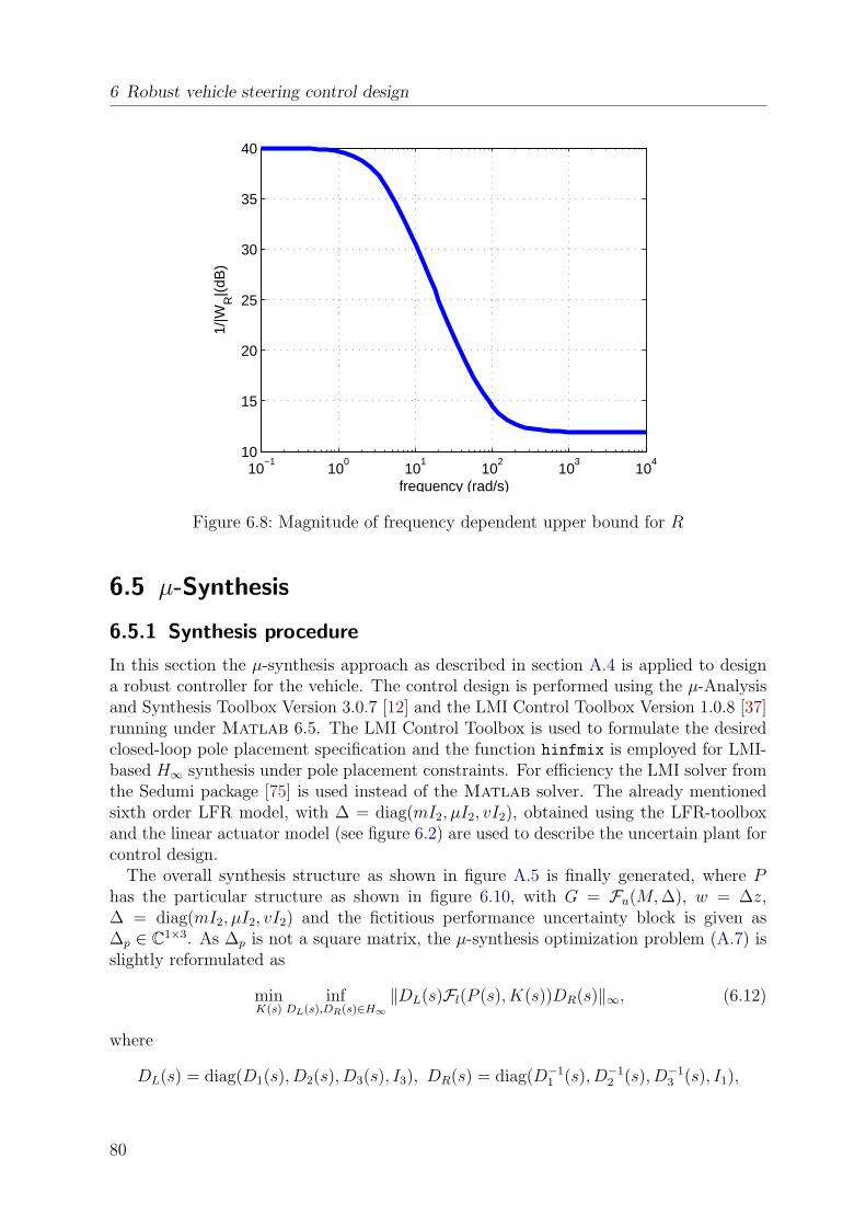
6 Robust vehicle steering control design
10−1
100
101
102
103
104
10
15
20
25
30
35
40
frequency (rad/s)
1/|W
R|(
dB)
Figure 6.8: Magnitude of frequency dependent upper bound for R
6.5 µ-Synthesis
6.5.1 Synthesis procedure
In this section the µ-synthesis approach as described in section A.4 is applied to designa robust controller for the vehicle. The control design is performed using the µ-Analysisand Synthesis Toolbox Version 3.0.7 [12] and the LMI Control Toolbox Version 1.0.8 [37]running under Matlab 6.5. The LMI Control Toolbox is used to formulate the desiredclosed-loop pole placement specification and the function hinfmix is employed for LMI-based H∞ synthesis under pole placement constraints. For efficiency the LMI solver fromthe Sedumi package [75] is used instead of the Matlab solver. The already mentionedsixth order LFR model, with ∆ = diag(mI2, µI2, vI2), obtained using the LFR-toolboxand the linear actuator model (see figure 6.2) are used to describe the uncertain plant forcontrol design.
The overall synthesis structure as shown in figure A.5 is finally generated, where Phas the particular structure as shown in figure 6.10, with G = Fu(M, ∆), w = ∆z,∆ = diag(mI2, µI2, vI2) and the fictitious performance uncertainty block is given as∆p ∈ C1×3. As ∆p is not a square matrix, the µ-synthesis optimization problem (A.7) isslightly reformulated as
minK(s)
infDL(s),DR(s)∈H∞
‖DL(s)Fl(P (s), K(s))DR(s)‖∞, (6.12)
where
DL(s) = diag(D1(s), D2(s), D3(s), I3), DR(s) = diag(D−11 (s), D−1
2 (s), D−13 (s), I1),
80
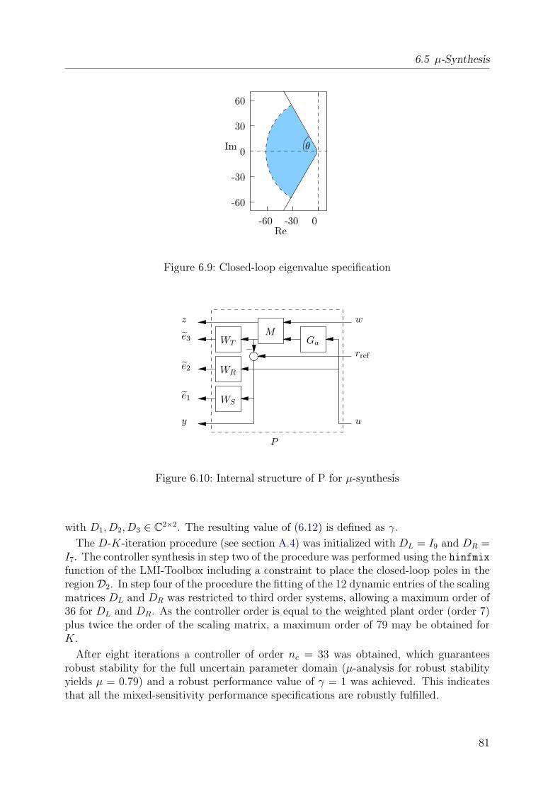
6.5 µ-Synthesis
0
-30
-60
60
30
Im θ
-60 -30 0
Re
Figure 6.9: Closed-loop eigenvalue specification
z
e3
y
e2
e1
w
rref
u
WS
WR
WT
MGa
P
Figure 6.10: Internal structure of P for µ-synthesis
with D1, D2, D3 ∈ C2×2. The resulting value of (6.12) is defined as γ.
The D-K-iteration procedure (see section A.4) was initialized with DL = I9 and DR =I7. The controller synthesis in step two of the procedure was performed using the hinfmixfunction of the LMI-Toolbox including a constraint to place the closed-loop poles in theregion D2. In step four of the procedure the fitting of the 12 dynamic entries of the scalingmatrices DL and DR was restricted to third order systems, allowing a maximum order of36 for DL and DR. As the controller order is equal to the weighted plant order (order 7)plus twice the order of the scaling matrix, a maximum order of 79 may be obtained forK.
After eight iterations a controller of order nc = 33 was obtained, which guaranteesrobust stability for the full uncertain parameter domain (µ-analysis for robust stabilityyields µ = 0.79) and a robust performance value of γ = 1 was achieved. This indicatesthat all the mixed-sensitivity performance specifications are robustly fulfilled.
81
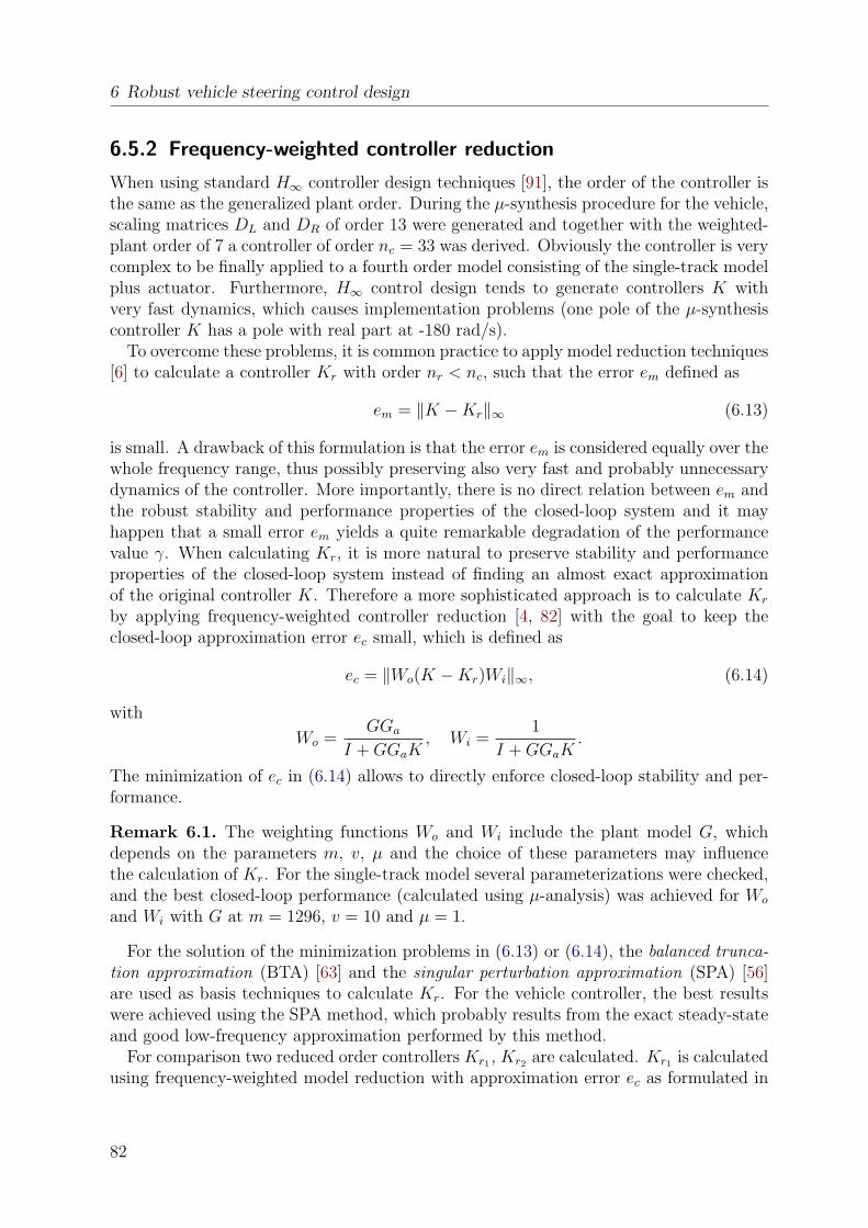
6 Robust vehicle steering control design
6.5.2 Frequency-weighted controller reduction
When using standard H∞ controller design techniques [91], the order of the controller isthe same as the generalized plant order. During the µ-synthesis procedure for the vehicle,scaling matrices DL and DR of order 13 were generated and together with the weighted-plant order of 7 a controller of order nc = 33 was derived. Obviously the controller is verycomplex to be finally applied to a fourth order model consisting of the single-track modelplus actuator. Furthermore, H∞ control design tends to generate controllers K withvery fast dynamics, which causes implementation problems (one pole of the µ-synthesiscontroller K has a pole with real part at -180 rad/s).
To overcome these problems, it is common practice to apply model reduction techniques[6] to calculate a controller Kr with order nr < nc, such that the error em defined as
em = ‖K −Kr‖∞ (6.13)
is small. A drawback of this formulation is that the error em is considered equally over thewhole frequency range, thus possibly preserving also very fast and probably unnecessarydynamics of the controller. More importantly, there is no direct relation between em andthe robust stability and performance properties of the closed-loop system and it mayhappen that a small error em yields a quite remarkable degradation of the performancevalue γ. When calculating Kr, it is more natural to preserve stability and performanceproperties of the closed-loop system instead of finding an almost exact approximationof the original controller K. Therefore a more sophisticated approach is to calculate Kr
by applying frequency-weighted controller reduction [4, 82] with the goal to keep theclosed-loop approximation error ec small, which is defined as
ec = ‖Wo(K −Kr)Wi‖∞, (6.14)
with
Wo =GGa
I + GGaK, Wi =
1
I + GGaK.
The minimization of ec in (6.14) allows to directly enforce closed-loop stability and per-formance.
Remark 6.1. The weighting functions Wo and Wi include the plant model G, whichdepends on the parameters m, v, µ and the choice of these parameters may influencethe calculation of Kr. For the single-track model several parameterizations were checked,and the best closed-loop performance (calculated using µ-analysis) was achieved for Wo
and Wi with G at m = 1296, v = 10 and µ = 1.
For the solution of the minimization problems in (6.13) or (6.14), the balanced trunca-tion approximation (BTA) [63] and the singular perturbation approximation (SPA) [56]are used as basis techniques to calculate Kr. For the vehicle controller, the best resultswere achieved using the SPA method, which probably results from the exact steady-stateand good low-frequency approximation performed by this method.
For comparison two reduced order controllers Kr1 , Kr2 are calculated. Kr1 is calculatedusing frequency-weighted model reduction with approximation error ec as formulated in
82
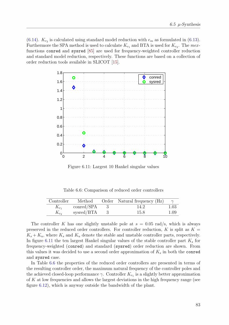
6.5 µ-Synthesis
(6.14). Kr2 is calculated using standard model reduction with em as formulated in (6.13).Furthermore the SPA method is used to calculate Kr1 and BTA is used for Kr2 . The mex -functions conred and sysred [85] are used for frequency-weighted controller reductionand standard model reduction, respectively. These functions are based on a collection oforder reduction tools available in SLICOT [15].
0 2 4 6 8 100
0.2
0.4
0.6
0.8
1
1.2
1.4
1.6
1.8conredsysred
Figure 6.11: Largest 10 Hankel singular values
Table 6.6: Comparison of reduced order controllers
Controller Method Order Natural frequency (Hz) γKr1 conred/SPA 3 14.2 1.03Kr2 sysred/BTA 3 15.8 1.09
The controller K has one slightly unstable pole at s = 0.05 rad/s, which is alwayspreserved in the reduced order controllers. For controller reduction, K is split as K =Ks + Ku, where Ks and Ku denote the stable and unstable controller parts, respectively.In figure 6.11 the ten largest Hankel singular values of the stable controller part Ks forfrequency-weighted (conred) and standard (sysred) order reduction are shown. Fromthis values it was decided to use a second order approximation of Ks in both the conred
and sysred case.In Table 6.6 the properties of the reduced order controllers are presented in terms of
the resulting controller order, the maximum natural frequency of the controller poles andthe achieved closed-loop performance γ. Controller Kr1 is a slightly better approximationof K at low frequencies and allows the largest deviations in the high frequency range (seefigure 6.12), which is anyway outside the bandwidth of the plant.
83
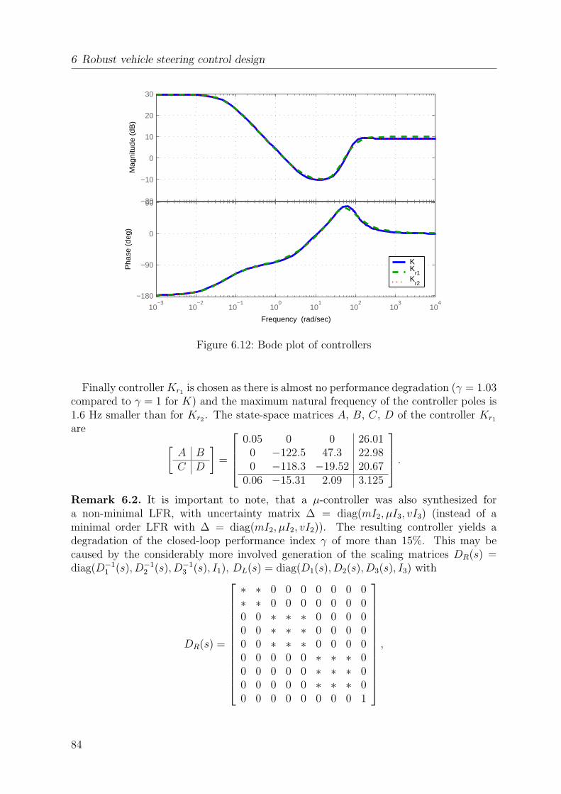
6 Robust vehicle steering control design
−20
−10
0
10
20
30
Mag
nitu
de (
dB)
10−3
10−2
10−1
100
101
102
103
104
−180
−90
0
90
Pha
se (
deg)
KK
r1K
r2
Bode Diagram
Frequency (rad/sec)
Figure 6.12: Bode plot of controllers
Finally controller Kr1 is chosen as there is almost no performance degradation (γ = 1.03compared to γ = 1 for K) and the maximum natural frequency of the controller poles is1.6 Hz smaller than for Kr2 . The state-space matrices A, B, C, D of the controller Kr1
are [A BC D
]=
0.05 0 0 26.010 −122.5 47.3 22.980 −118.3 −19.52 20.67
0.06 −15.31 2.09 3.125
.
Remark 6.2. It is important to note, that a µ-controller was also synthesized fora non-minimal LFR, with uncertainty matrix ∆ = diag(mI2, µI3, vI3) (instead of aminimal order LFR with ∆ = diag(mI2, µI2, vI2)). The resulting controller yields adegradation of the closed-loop performance index γ of more than 15%. This may becaused by the considerably more involved generation of the scaling matrices DR(s) =diag(D−1
1 (s), D−12 (s), D−1
3 (s), I1), DL(s) = diag(D1(s), D2(s), D3(s), I3) with
DR(s) =
∗ ∗ 0 0 0 0 0 0 0∗ ∗ 0 0 0 0 0 0 00 0 ∗ ∗ ∗ 0 0 0 00 0 ∗ ∗ ∗ 0 0 0 00 0 ∗ ∗ ∗ 0 0 0 00 0 0 0 0 ∗ ∗ ∗ 00 0 0 0 0 ∗ ∗ ∗ 00 0 0 0 0 ∗ ∗ ∗ 00 0 0 0 0 0 0 0 1
,
84
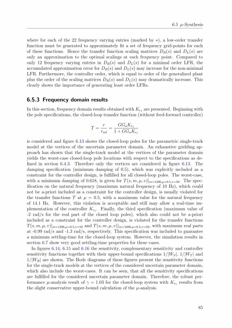
6.5 µ-Synthesis
where for each of the 22 frequency varying entries (marked by ∗), a low-order transferfunction must be generated to approximately fit a set of frequency grid-points for eachof these functions. Hence the transfer function scaling matrices DR(s) and DL(s) areonly an approximation to the optimal scalings at each frequency point. Compared toonly 12 frequency varying entries in DR(s) and DL(s) for a minimal order LFR, theaccumulated approximation error for DR(s) and DL(s) may increase for the non-minimalLFR. Furthermore, the controller order, which is equal to order of the generalized plantplus the order of the scaling matrices DR(s) and DL(s) may dramatically increase. Thisclearly shows the importance of generating least order LFRs.
6.5.3 Frequency domain results
In this section, frequency domain results obtained with Kr1 are presented. Beginning withthe pole specifications, the closed-loop transfer function (without feed-forward controller)
T =r
rref
=GGaKr1
1 + GGaKr1
is considered and figure 6.13 shows the closed-loop poles for the parametric single-trackmodel at the vertices of the uncertain parameter domain. An exhaustive gridding ap-proach has shown that the single-track model at the vertices of the parameter domainyields the worst-case closed-loop pole locations with respect to the specifications as de-fined in section 6.4.3. Therefore only the vertices are considered in figure 6.13. Thedamping specification (minimum damping of 0.5), which was explicitly included as aconstraint for the controller design, is fulfilled for all closed-loop poles. The worst-case,with a minimum damping of 0.618, is given for T (s, m, µ, v)|m=1296,µ=0.5,v=50. The spec-ification on the natural frequency (maximum natural frequency of 10 Hz), which couldnot be a-priori included as a constraint for the controller design, is usually violated forthe transfer functions T at µ = 0.5, with a maximum value for the natural frequencyof 14.1 Hz. However, this violation is acceptable and still may allow a real-time im-plementation of the controller Kr1 . Finally, the third specification (maximum value of-2 rad/s for the real part of the closed loop poles), which also could not be a-prioriincluded as a constraint for the controller design, is violated for the transfer functionsT (s, m, µ, v)|m=1296,µ=0.5,v=50 and T (s, m, µ, v)|m=1696,µ=0.5,v=50, with maximum real partsat -0.99 rad/s and -1.3 rad/s, respectively. This specification was included to guaranteea minimum settling-time for the closed-loop system. However, the simulation results insection 6.7 show very good settling-time properties for these cases.
In figures 6.14, 6.15 and 6.16 the sensitivity, complementary sensitivity and controllersensitivity functions together with their upper-bound specifications 1/|WS|, 1/|WT | and1/|WR| are shown. The Bode diagrams of these figures present the sensitivity functionsfor the single-track models at the vertices of the considered uncertain parameter domain,which also include the worst-cases. It can be seen, that all the sensitivity specificationsare fulfilled for the considered uncertain parameter domain. Therefore, the robust per-formance µ-analysis result of γ = 1.03 for the closed-loop system with Kr1 results fromthe slight conservative upper-bound calculation of the µ-analysis.
85

6 Robust vehicle steering control design
Considering robust stability only, the µ-analysis results shown in figure 6.17 yield amaximum upper-bound of 0.79 for the structured singular value µ, which indicates enoughstability margin for the uncertain parameter domain under consideration.
86
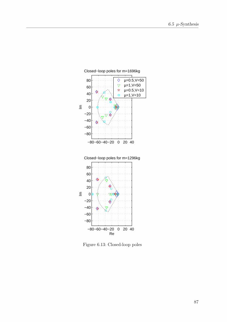
6.5 µ-Synthesis
−80−60−40−20 0 20 40
−80
−60
−40
−20
0
20
40
60
80Im
Closed−loop poles for m=1696kg
µ=0.5,V=50µ=1,V=50µ=0.5,V=10µ=1,V=10
−80−60−40−20 0 20 40
−80
−60
−40
−20
0
20
40
60
80
Re
Im
Closed−loop poles for m=1296kg
Figure 6.13: Closed-loop poles
87
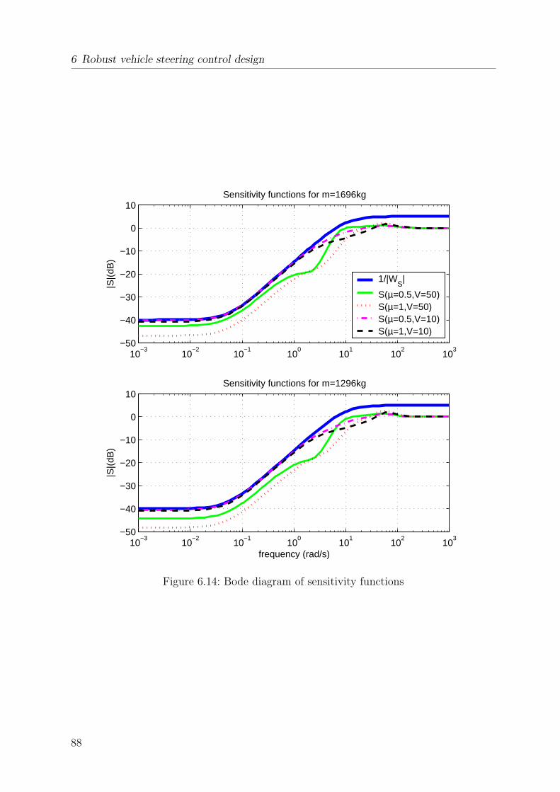
6 Robust vehicle steering control design
10−3
10−2
10−1
100
101
102
103
−50
−40
−30
−20
−10
0
10
|S|(
dB)
Sensitivity functions for m=1696kg
1/|WS|
S(µ=0.5,V=50)S(µ=1,V=50)S(µ=0.5,V=10)S(µ=1,V=10)
10−3
10−2
10−1
100
101
102
103
−50
−40
−30
−20
−10
0
10
frequency (rad/s)
|S|(
dB)
Sensitivity functions for m=1296kg
Figure 6.14: Bode diagram of sensitivity functions
88
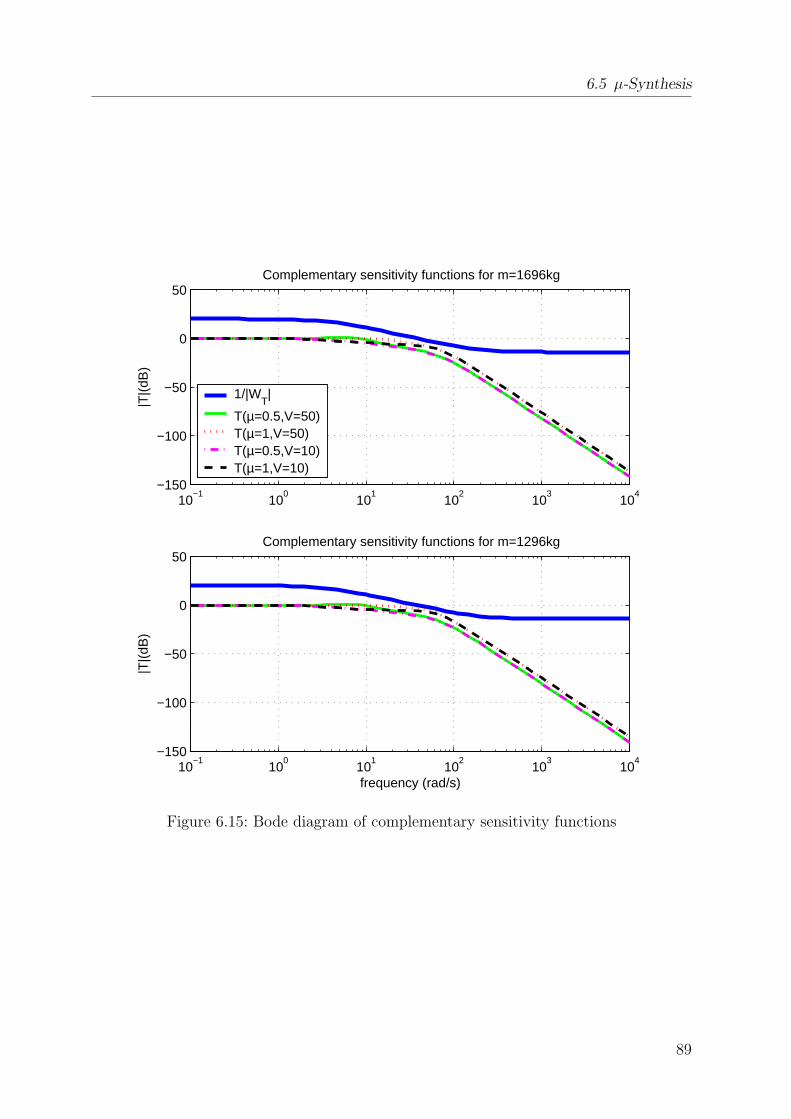
6.5 µ-Synthesis
10−1
100
101
102
103
104
−150
−100
−50
0
50
|T|(
dB)
Complementary sensitivity functions for m=1696kg
1/|WT|
T(µ=0.5,V=50)T(µ=1,V=50)T(µ=0.5,V=10)T(µ=1,V=10)
10−1
100
101
102
103
104
−150
−100
−50
0
50
frequency (rad/s)
|T|(
dB)
Complementary sensitivity functions for m=1296kg
Figure 6.15: Bode diagram of complementary sensitivity functions
89
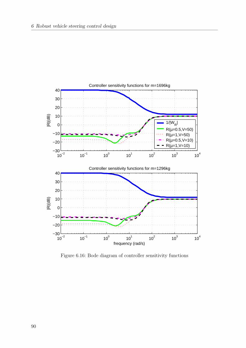
6 Robust vehicle steering control design
10−2
10−1
100
101
102
103
104
−30
−20
−10
0
10
20
30
40
|R|(
dB)
Controller sensitivity functions for m=1696kg
1/|WR
|
R(µ=0.5,V=50)R(µ=1,V=50)R(µ=0.5,V=10)R(µ=1,V=10)
10−2
10−1
100
101
102
103
104
−30
−20
−10
0
10
20
30
40
frequency (rad/s)
|R|(
dB)
Controller sensitivity functions for m=1296kg
Figure 6.16: Bode diagram of controller sensitivity functions
90
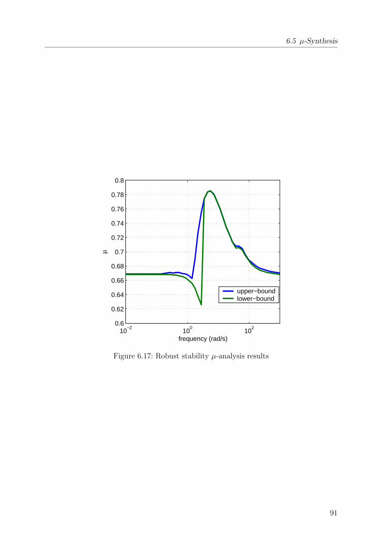
6.5 µ-Synthesis
10−2
100
102
0.6
0.62
0.64
0.66
0.68
0.7
0.72
0.74
0.76
0.78
0.8
µ
frequency (rad/s)
upper−boundlower−bound
Figure 6.17: Robust stability µ-analysis results
91
6 Robust vehicle steering control design
6.6 LPV-control design
In this section Linear Parameter Varying (LPV) control design methods as proposed in[88, 87] are applied to the uncertain single-track model. In contrast to the method in[20] and the µ-synthesis approach of the previous section, where robust stability andperformance is only guaranteed for model parameters that are uncertain but constant,the LPV approach allows bounded variation rates of parameters that are measurable andon-line available for control. For the single-track model, the uncertain parameters v, µ,m and Jz are explicitly considered. However, as it may be hard to measure the roadadhesion µ, mass m and moment of inertia Jz on-line, only the longitudinal vehicle speedv is assumed to be online measurable for control, whereas µ, m and Jz are considered tobe uncertain but constant. Providing robust stability and performance despite variationsin v is a very important property of the controller, as dangerous yaw disturbances arecaused for example by µ-split braking, where high variation rates of v may occur.
In principle, one may derive an LPV controller with no restrictions on the variation rateof v. However, guaranteeing robust performance for arbitrary parameter trajectories v(t)may be overly conservative (or even not possible) and may lead to poor performance ofthe closed-loop system [10]. To improve performance, the LPV control design techniqueproposed in [88, 87] is employed, where the variation rate of v is assumed to be bounded.This corresponds to the real physics, where the longitudinal speed v does not changearbitrarily fast. A drawback of this method is that the control design requires to solve aninfinite-dimensional convex feasibility problem, which can only be solved approximatelyby searching for feasibility over a finite dimensional subspace. Therefore a finite griddingof the single-track model with respect to v is performed and only this finite set of modelsis considered for control design, which if successful, yields a controller with guaranteedproperties.
The resulting controller also consists of a finite set of grid-point controllers and thestate-space matrices of the grid-point controllers are linearly interpolated based on thenearest grid-point plant model. This is in contrast to traditional gain-scheduling designprocesses, where several equilibrium point controller designs are performed, followed bythe design of a scheduling procedure to interpolate between the point designs. For somebackground on the employed LPV control design procedure see appendix B.
6.6.1 Synthesis structure
For the LPV controller synthesis, only the longitudinal speed v is assumed to be measur-able and on-line available for control, whereas µ, m and Jz are supposed to be uncertain.Hence, the resulting controller is scheduled with v and must be robust to uncertaintiesin µ, m and Jz.
The LPV control design approach requires a gridding of G(s, v, m, Jz, µ) over themeasurable, varying parameter space v ∈ [10, 50]. Some trials have shown, that arather coarse, equally-spaced 3-point gridding, with v = vi ∈ 10, 30, 50 is sufficientfor the LPV controller synthesis. Therefore three models Gi(s, m, Jz, µ), i = 1, . . . , 3,with Gi(s, m, Jz, µ) = G(s, v, m, Jz, µ)|v=vi
are calculated, where v is substituted withthe corresponding numerical grid-point value vi. For each Gi(s, m, Jz, µ), Jz is substi-
92
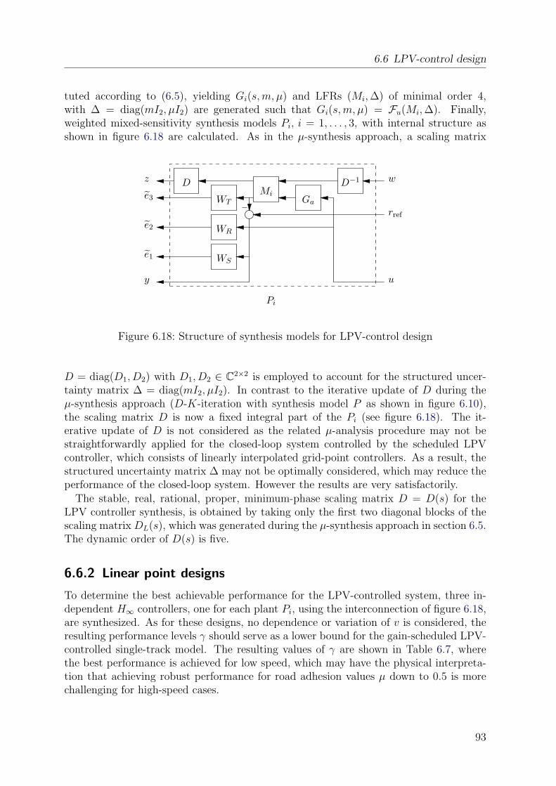
6.6 LPV-control design
tuted according to (6.5), yielding Gi(s, m, µ) and LFRs (Mi, ∆) of minimal order 4,with ∆ = diag(mI2, µI2) are generated such that Gi(s, m, µ) = Fu(Mi, ∆). Finally,weighted mixed-sensitivity synthesis models Pi, i = 1, . . . , 3, with internal structure asshown in figure 6.18 are calculated. As in the µ-synthesis approach, a scaling matrix
e2
e3
z
e1
y
w
rref
u
Pi
WS
WR
WT
DMi
Ga
D−1
Figure 6.18: Structure of synthesis models for LPV-control design
D = diag(D1, D2) with D1, D2 ∈ C2×2 is employed to account for the structured uncer-tainty matrix ∆ = diag(mI2, µI2). In contrast to the iterative update of D during theµ-synthesis approach (D-K-iteration with synthesis model P as shown in figure 6.10),the scaling matrix D is now a fixed integral part of the Pi (see figure 6.18). The it-erative update of D is not considered as the related µ-analysis procedure may not bestraightforwardly applied for the closed-loop system controlled by the scheduled LPVcontroller, which consists of linearly interpolated grid-point controllers. As a result, thestructured uncertainty matrix ∆ may not be optimally considered, which may reduce theperformance of the closed-loop system. However the results are very satisfactorily.
The stable, real, rational, proper, minimum-phase scaling matrix D = D(s) for theLPV controller synthesis, is obtained by taking only the first two diagonal blocks of thescaling matrix DL(s), which was generated during the µ-synthesis approach in section 6.5.The dynamic order of D(s) is five.
6.6.2 Linear point designs
To determine the best achievable performance for the LPV-controlled system, three in-dependent H∞ controllers, one for each plant Pi, using the interconnection of figure 6.18,are synthesized. As for these designs, no dependence or variation of v is considered, theresulting performance levels γ should serve as a lower bound for the gain-scheduled LPV-controlled single-track model. The resulting values of γ are shown in Table 6.7, wherethe best performance is achieved for low speed, which may have the physical interpreta-tion that achieving robust performance for road adhesion values µ down to 0.5 is morechallenging for high-speed cases.
93
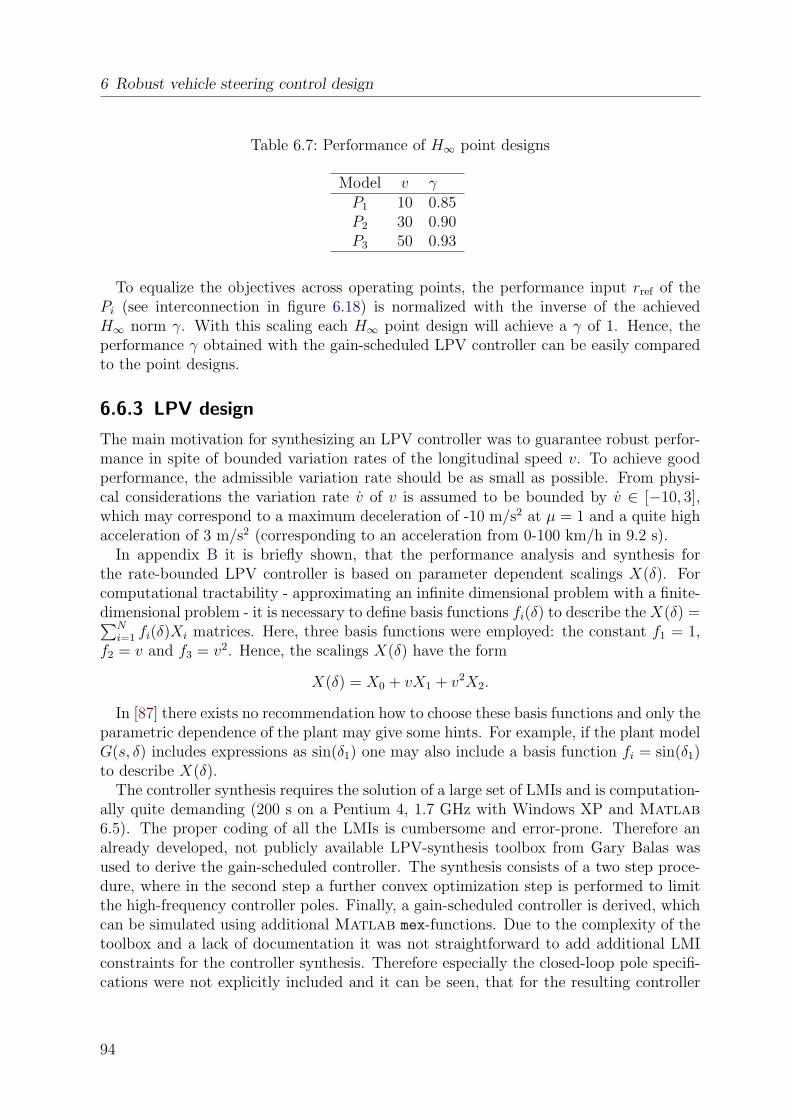
6 Robust vehicle steering control design
Table 6.7: Performance of H∞ point designs
Model v γP1 10 0.85P2 30 0.90P3 50 0.93
To equalize the objectives across operating points, the performance input rref of thePi (see interconnection in figure 6.18) is normalized with the inverse of the achievedH∞ norm γ. With this scaling each H∞ point design will achieve a γ of 1. Hence, theperformance γ obtained with the gain-scheduled LPV controller can be easily comparedto the point designs.
6.6.3 LPV design
The main motivation for synthesizing an LPV controller was to guarantee robust perfor-mance in spite of bounded variation rates of the longitudinal speed v. To achieve goodperformance, the admissible variation rate should be as small as possible. From physi-cal considerations the variation rate v of v is assumed to be bounded by v ∈ [−10, 3],which may correspond to a maximum deceleration of -10 m/s2 at µ = 1 and a quite highacceleration of 3 m/s2 (corresponding to an acceleration from 0-100 km/h in 9.2 s).
In appendix B it is briefly shown, that the performance analysis and synthesis forthe rate-bounded LPV controller is based on parameter dependent scalings X(δ). Forcomputational tractability - approximating an infinite dimensional problem with a finite-dimensional problem - it is necessary to define basis functions fi(δ) to describe the X(δ) =∑N
i=1 fi(δ)Xi matrices. Here, three basis functions were employed: the constant f1 = 1,f2 = v and f3 = v2. Hence, the scalings X(δ) have the form
X(δ) = X0 + vX1 + v2X2.
In [87] there exists no recommendation how to choose these basis functions and only theparametric dependence of the plant may give some hints. For example, if the plant modelG(s, δ) includes expressions as sin(δ1) one may also include a basis function fi = sin(δ1)to describe X(δ).
The controller synthesis requires the solution of a large set of LMIs and is computation-ally quite demanding (200 s on a Pentium 4, 1.7 GHz with Windows XP and Matlab6.5). The proper coding of all the LMIs is cumbersome and error-prone. Therefore analready developed, not publicly available LPV-synthesis toolbox from Gary Balas wasused to derive the gain-scheduled controller. The synthesis consists of a two step proce-dure, where in the second step a further convex optimization step is performed to limitthe high-frequency controller poles. Finally, a gain-scheduled controller is derived, whichcan be simulated using additional Matlab mex-functions. Due to the complexity of thetoolbox and a lack of documentation it was not straightforward to add additional LMIconstraints for the controller synthesis. Therefore especially the closed-loop pole specifi-cations were not explicitly included and it can be seen, that for the resulting controller
94
6.6 LPV-control design
the minimum damping requirement is slightly violated. However, in the time simulations(see section 6.7) there is no evidence of undamped behavior.
Finally, a controller consisting of three grid-point controllers, each of them of order 17,is synthesized. Consider the concatenated matrices
Si =
[Ai Bi
Ci Di
], i = 1, . . . , 3,
with Ai ∈ R17×17, Bi ∈ R17×1, Ci ∈ R1×17, Di ∈ R as the state-space matrices of thethree grid-point controllers for vi ∈ 10, 30, 50. The state-space matrices A(v), B(v),C(v), D(v) of the gain-scheduled controller are given as
[A(v) B(v)C(v) D(v)
]=
(
30− v
20
)S1 +
(v − 10
20
)S2, ∀ v ∈ [10, 30]
(50− v
20
)S2 +
(v − 30
20
)S3, ∀ v ∈ [30, 50]
It is remarkable, that the resulting H∞ performance γ for the gain-scheduled LPVcontroller is 1.02, which indicates that the rate-bounded LPV controller almost exactlyrecovers the performance of the H∞ point designs. Hence, by using the gain-scheduledLPV controller, the variations in v do not have any adverse effect on the achievableperformance.
6.6.4 Frequency weighted controller reduction
Frequency weighted controller reduction techniques are applied to each of the three grid-point controllers. All three controllers can be reduced to order 4 without loss of robustperformance. The maximum natural frequency of the controller poles is 15.6 Hz andthe minimum damping is 0.48. As in section 6.5.2, the same stability and performanceenforcing weighting functions Wo and Wi were employed to describe the reduction errorec and the SPA-method was used to calculate the reduced order controllers. To allowlinear interpolation of the reduced order controllers, the state-space matrices of the re-duced order controllers are transformed to block-diagonal form using well-conditionednon-orthogonal similarity transformations. The concatenated representations S1,r, S2,r,
95
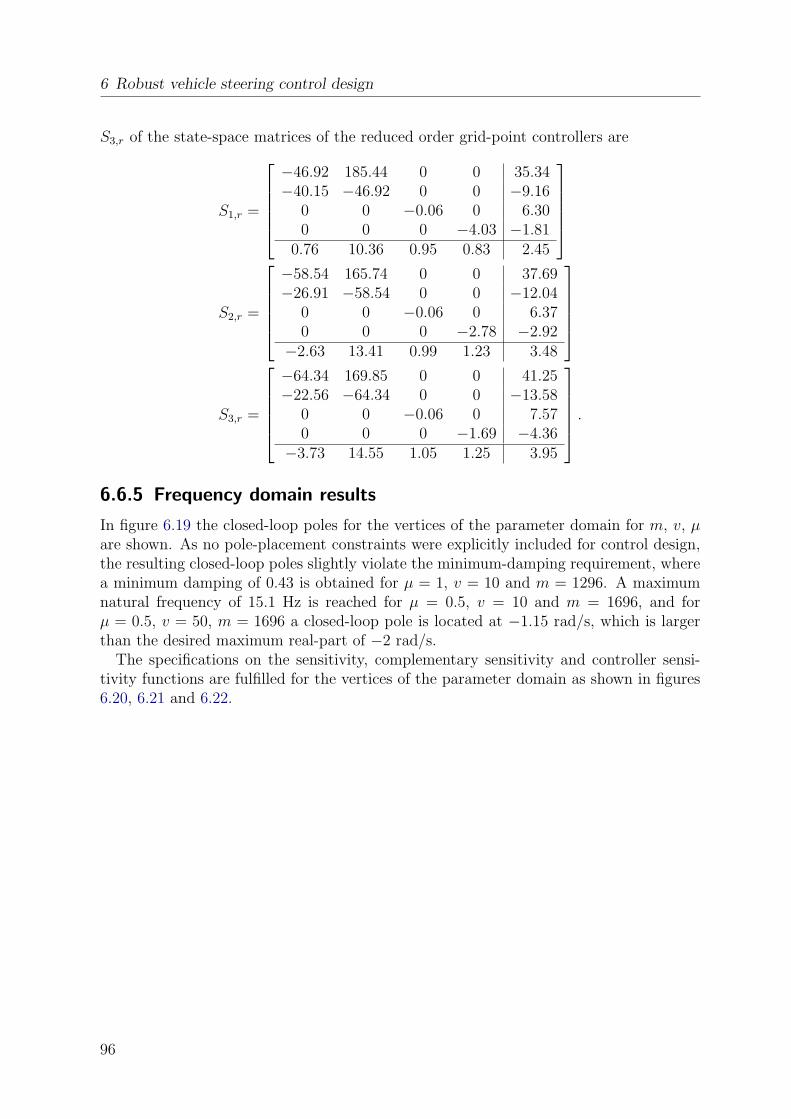
6 Robust vehicle steering control design
S3,r of the state-space matrices of the reduced order grid-point controllers are
S1,r =
−46.92 185.44 0 0 35.34−40.15 −46.92 0 0 −9.16
0 0 −0.06 0 6.300 0 0 −4.03 −1.81
0.76 10.36 0.95 0.83 2.45
S2,r =
−58.54 165.74 0 0 37.69−26.91 −58.54 0 0 −12.04
0 0 −0.06 0 6.370 0 0 −2.78 −2.92
−2.63 13.41 0.99 1.23 3.48
S3,r =
−64.34 169.85 0 0 41.25−22.56 −64.34 0 0 −13.58
0 0 −0.06 0 7.570 0 0 −1.69 −4.36
−3.73 14.55 1.05 1.25 3.95
.
6.6.5 Frequency domain results
In figure 6.19 the closed-loop poles for the vertices of the parameter domain for m, v, µare shown. As no pole-placement constraints were explicitly included for control design,the resulting closed-loop poles slightly violate the minimum-damping requirement, wherea minimum damping of 0.43 is obtained for µ = 1, v = 10 and m = 1296. A maximumnatural frequency of 15.1 Hz is reached for µ = 0.5, v = 10 and m = 1696, and forµ = 0.5, v = 50, m = 1696 a closed-loop pole is located at −1.15 rad/s, which is largerthan the desired maximum real-part of −2 rad/s.
The specifications on the sensitivity, complementary sensitivity and controller sensi-tivity functions are fulfilled for the vertices of the parameter domain as shown in figures6.20, 6.21 and 6.22.
96
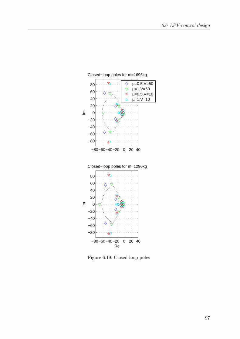
6.6 LPV-control design
−80−60−40−20 0 20 40
−80
−60
−40
−20
0
20
40
60
80Im
Closed−loop poles for m=1696kg
µ=0.5,V=50µ=1,V=50µ=0.5,V=10µ=1,V=10
−80−60−40−20 0 20 40
−80
−60
−40
−20
0
20
40
60
80
Re
Im
Closed−loop poles for m=1296kg
Figure 6.19: Closed-loop poles
97
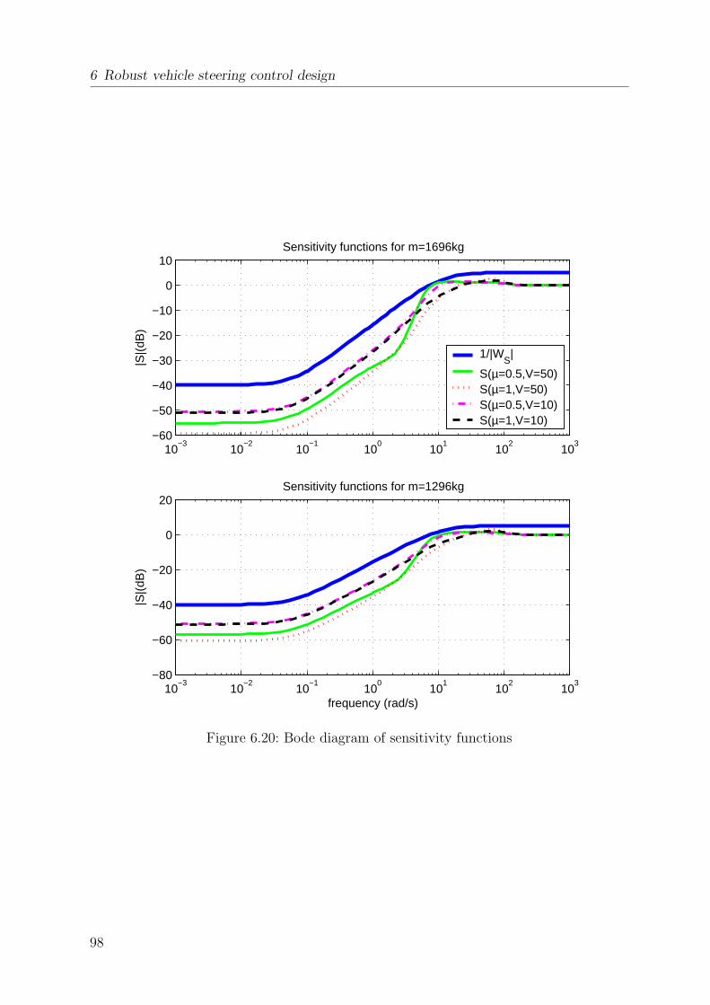
6 Robust vehicle steering control design
10−3
10−2
10−1
100
101
102
103
−60
−50
−40
−30
−20
−10
0
10
|S|(
dB)
Sensitivity functions for m=1696kg
1/|WS|
S(µ=0.5,V=50)S(µ=1,V=50)S(µ=0.5,V=10)S(µ=1,V=10)
10−3
10−2
10−1
100
101
102
103
−80
−60
−40
−20
0
20
frequency (rad/s)
|S|(
dB)
Sensitivity functions for m=1296kg
Figure 6.20: Bode diagram of sensitivity functions
98
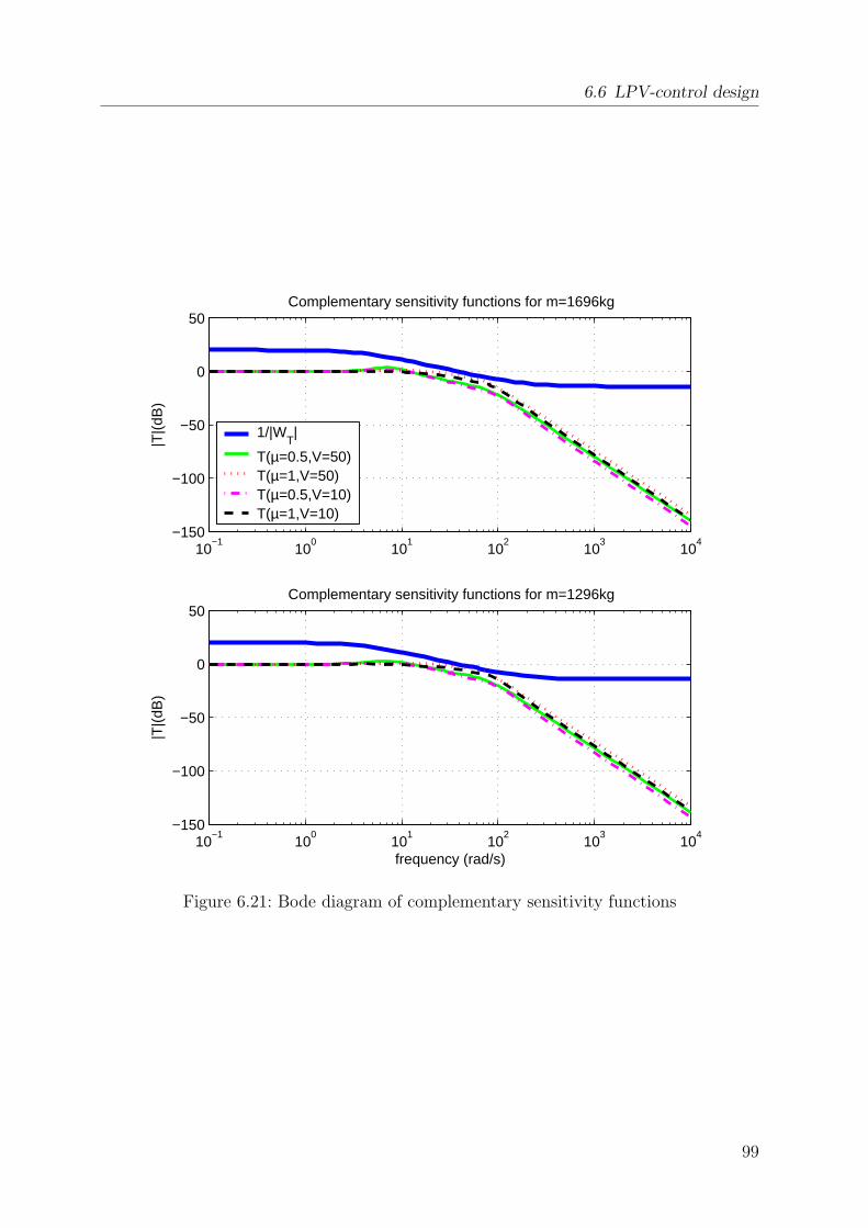
6.6 LPV-control design
10−1
100
101
102
103
104
−150
−100
−50
0
50
|T|(
dB)
Complementary sensitivity functions for m=1696kg
1/|WT|
T(µ=0.5,V=50)T(µ=1,V=50)T(µ=0.5,V=10)T(µ=1,V=10)
10−1
100
101
102
103
104
−150
−100
−50
0
50
frequency (rad/s)
|T|(
dB)
Complementary sensitivity functions for m=1296kg
Figure 6.21: Bode diagram of complementary sensitivity functions
99
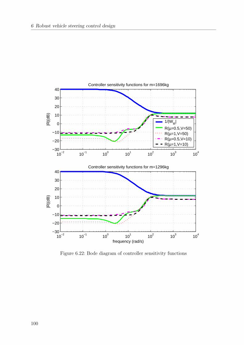
6 Robust vehicle steering control design
10−2
10−1
100
101
102
103
104
−30
−20
−10
0
10
20
30
40
|R|(
dB)
Controller sensitivity functions for m=1696kg
1/|WR
|
R(µ=0.5,V=50)R(µ=1,V=50)R(µ=0.5,V=10)R(µ=1,V=10)
10−2
10−1
100
101
102
103
104
−30
−20
−10
0
10
20
30
40
frequency (rad/s)
|R|(
dB)
Controller sensitivity functions for m=1296kg
Figure 6.22: Bode diagram of controller sensitivity functions
100
6.7 Simulation results
6.7 Simulation results
In this section, the simulation results for the closed-loop system as shown in figure 6.4are presented, where K = K(s) for the µ-synthesis controller and K = K(s, v) for theLPV- controller. The linear single-track model is taken as plant model G and Ga isgiven by the actuator model as shown in figure 6.2. As variations in the mass m haveno qualitative effect on the simulation results, all simulations are performed for nominalmass m = 1496.
Figures 6.23-6.29 represent the reaction of the controlled vehicle to a yaw disturbancetorque Mz step input, which may qualitatively describe a µ-split braking manoeuvre.For simulation, the matrices B(δ) and D of the single-track model as given in (6.1) aresubstituted by
B =
0 0
cfµ 0cf lfµ Jz
0 0
, D =[
0 0]
and the new input vector is given by u =[
δf Mz
]T. For comparison the results
obtained in [20] are also included in the plots and denoted as PS (Parameter-Spacedesign). The uncontrolled vehicle is denoted as OL (Open-Loop).
Figures 6.30-6.33 describe the tracking behavior of the closed-loop system, where asteering wheel step response is shown. It is shown how the reference rref (see figure 6.4)can be tracked for µ = 0.5. No comparison with [20] is given for these results as a differentreference model was used therein.
In detail, figures 6.23 and 6.24 show the low velocity (v = 10) simulations results for astep input of a yaw disturbance torque at µ = 0.5 and µ = 1, respectively. For µ = 0.5the best result is achieved using the LPV controller, where the maximum yaw rate r is11% smaller than for the µ-controller. After 0.3 s the LPV controller achieves zero yawrate and the following negative yaw rate may further help to correct the vehicle motion.For µ = 1 the maximum r is almost the same for all controllers. The LPV controllershows the best convergence properties and the PS controller shows undamped behavior,which may be uncomfortable to the driver.
For the high velocity cases shown in figures 6.25 and 6.26 the LPV controller andthe µ-controller clearly outperform the PS controller. For µ = 0.5, the PS controllerallows a maximum r, which is 19% and 33% larger compared to the µ-controller andLPV controller, respectively. This case is probably the most demanding, as it describesa manoeuvre at high speed on wet road. For µ = 1, the PS-controller allows a maxi-mum r, which is 24% and 30% larger compared to the µ-controller and LPV controller,respectively.
As during manoeuvres like µ-split braking a yaw disturbance torque is usually combinedwith a variation of the velocity v, a maybe more realistic scenario is presented in figures6.27, 6.28, 6.29, where a repeated yaw disturbance step torque Mz is combined with anacceleration of v = 3 or a full-braking with v = −10. In all cases, the LPV controller,which is explicitly designed to guarantee robust performance despite bounded variationrates of v, clearly provides the best disturbance rejection. For yaw disturbance torques
101
6 Robust vehicle steering control design
at velocities v > 15, the µ-controller generally achieves better disturbance rejection thanthe PS controller.
The tracking results for the µ-synthesis and LPV controller are shown in figures 6.30-6.33, where rref denotes the yaw rate of the reference model and OL denotes the yaw rateof the vehicle without control. Both controllers show very good tracking performance.In general the maximum tracking error e is about 10% smaller for the LPV controlledvehicle, however the µ-controller achieves a better damping of the error, which resultsfrom the larger damping value of the closed-loop poles (see figure 6.13 and 6.19).
0 0.2 0.4 0.6 0.8 1
0
0.02
0.04
0.06
0.08
0.1
0.12
0.14
t (s)
r (r
ad/s
) LPVµPSOL
Figure 6.23: Yaw disturbance torque at v = 10, µ = 0.5
102
6.7 Simulation results
0 0.2 0.4 0.6 0.8 1−0.05
0
0.05
0.1
0.15
0.2
t (s)
r (r
ad/s
) LPVµPSOL
Figure 6.24: Yaw disturbance torque at v = 10, µ = 1
0 0.5 1 1.5−0.1
0
0.1
0.2
0.3
0.4
t (s)
r (r
ad/s
) LPVµPSOL
Figure 6.25: Yaw disturbance torque at v = 50, µ = 0.5
103
6 Robust vehicle steering control design
0 0.1 0.2 0.3 0.4 0.5 0.6 0.7−0.1
0
0.1
0.2
0.3
0.4
0.5
0.6
t (s)
r (r
ad/s
) LPVµPSOL
Figure 6.26: Yaw disturbance torque at v = 50, µ = 1
104
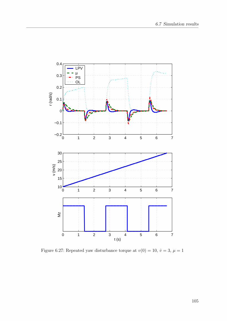
6.7 Simulation results
0 1 2 3 4 5 6 7−0.2
−0.1
0
0.1
0.2
0.3
0.4
r (r
ad/s
)
LPVµPSOL
0 1 2 3 4 5 6 710
15
20
25
30
v (m
/s)
0 1 2 3 4 5 6 7
Mz
t (s)
Figure 6.27: Repeated yaw disturbance torque at v(0) = 10, v = 3, µ = 1
105
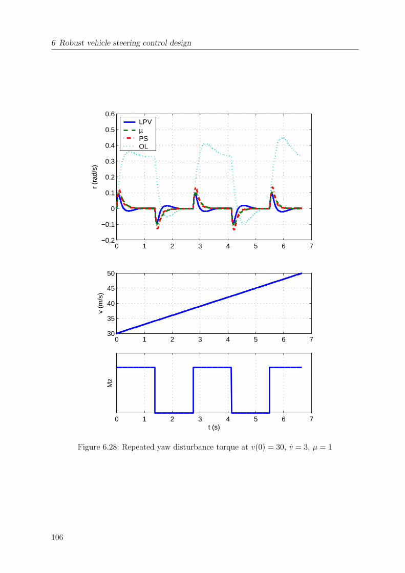
6 Robust vehicle steering control design
0 1 2 3 4 5 6 7−0.2
−0.1
0
0.1
0.2
0.3
0.4
0.5
0.6
r (r
ad/s
)
LPVµPSOL
0 1 2 3 4 5 6 730
35
40
45
50
v (m
/s)
0 1 2 3 4 5 6 7
Mz
t (s)
Figure 6.28: Repeated yaw disturbance torque at v(0) = 30, v = 3, µ = 1
106
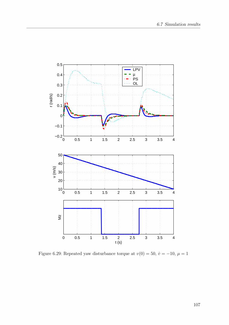
6.7 Simulation results
0 0.5 1 1.5 2 2.5 3 3.5 4−0.2
−0.1
0
0.1
0.2
0.3
0.4
0.5
r (r
ad/s
)
LPVµPSOL
0 0.5 1 1.5 2 2.5 3 3.5 410
20
30
40
50
v (m
/s)
0 0.5 1 1.5 2 2.5 3 3.5 4
Mz
t (s)
Figure 6.29: Repeated yaw disturbance torque at v(0) = 50, v = −10, µ = 1
107
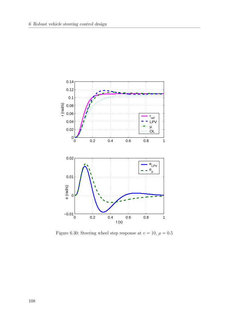
6 Robust vehicle steering control design
0 0.2 0.4 0.6 0.8 10
0.02
0.04
0.06
0.08
0.1
0.12
0.14
r (r
ad/s
)
rref
LPVµOL
0 0.2 0.4 0.6 0.8 1−0.01
0
0.01
0.02
t (s)
e (r
ad/s
)
eLPV
eµ
Figure 6.30: Steering wheel step response at v = 10, µ = 0.5
108
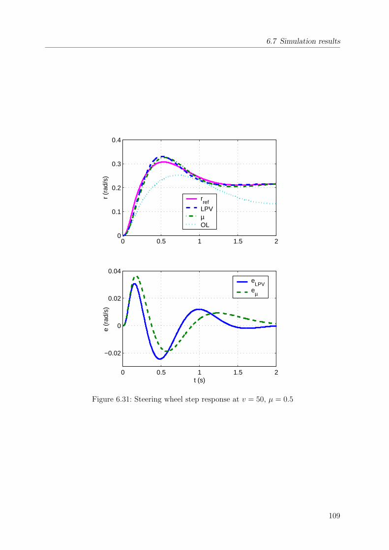
6.7 Simulation results
0 0.5 1 1.5 20
0.1
0.2
0.3
0.4
r (r
ad/s
)
rref
LPVµOL
0 0.5 1 1.5 2
−0.02
0
0.02
0.04
t (s)
e (r
ad/s
)
eLPV
eµ
Figure 6.31: Steering wheel step response at v = 50, µ = 0.5
109
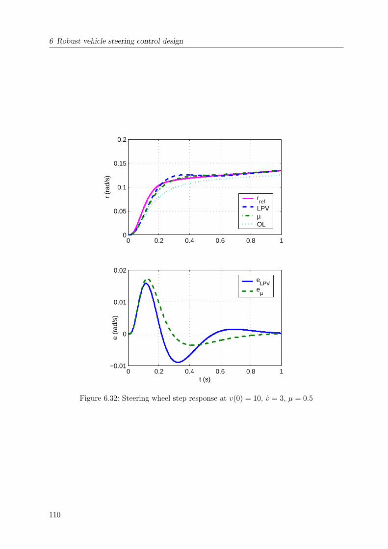
6 Robust vehicle steering control design
0 0.2 0.4 0.6 0.8 10
0.05
0.1
0.15
0.2
r (r
ad/s
)
rref
LPVµOL
0 0.2 0.4 0.6 0.8 1−0.01
0
0.01
0.02
t (s)
e (r
ad/s
)
eLPV
eµ
Figure 6.32: Steering wheel step response at v(0) = 10, v = 3, µ = 0.5
110
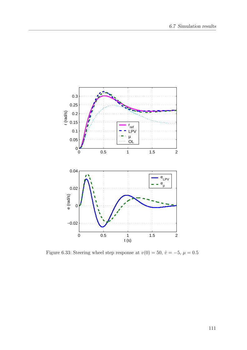
6.7 Simulation results
0 0.5 1 1.5 20
0.05
0.1
0.15
0.2
0.25
0.3
r (r
ad/s
)
rref
LPVµOL
0 0.5 1 1.5 2
−0.02
0
0.02
0.04
t (s)
e (r
ad/s
)
eLPV
eµ
Figure 6.33: Steering wheel step response at v(0) = 50, v = −5, µ = 0.5
111
6 Robust vehicle steering control design
6.8 Summary
Enhanced symbolic preprocessing techniques and object-oriented LFR realization basedon the newly developed generalized LFR were employed to obtain a minimal order LFR forthe parametric single-track model, where parametric uncertainties with respect to massm, moment of inertia Jz, road adhesion µ and longitudinal velocity v were assumed. Basedon this LFR, two controllers, a µ-synthesis controller and a gain-scheduled LPV controllerwere designed. The mixed sensitivity specifications for the control design were taken from[20], where a controller was synthesized based on the Parameter Space (PS) method. ThePS method is usually restricted to handle only up to two parameters (in our case µ andv) as structured uncertainties. Therefore in [20], additional uncertainties with respectto m and Jz were conservatively approximated as an unstructured uncertainty. For thecontrollers developed in this thesis, all parametric uncertainties are explicitly consideredas structured uncertainties, which resulted in a better closed-loop performance.
The developed controllers are synthesized based on H∞ control design methods. A gen-eral criticism about these methods is the high complexity/dynamic order of the resultingcontrollers, which is equal to the order of the weighted plant. For the considered vehicle,the orders of the µ-synthesis controller and the LPV controller were 33 and 17, respec-tively. Furthermore, the employed Matlab implementations for H∞ control design tendto generate controllers with very fast dynamics. However, at least for the vehicle controldesign, all these problems could be simply alleviated by applying frequency-weighted con-troller reduction techniques, reducing the order of the controllers to 3 for the µ-synthesiscontroller and 4 for the LPV controller (compared to 3 for the PS controller). The maxi-mum natural frequency of the closed-loop poles was limited to about 15 Hz, which clearlyallows real-time implementation of the controllers. All this could be achieved withoutany degradation of closed-loop stability and performance.
The µ-controller and the LPV controller fulfill the mixed-sensitivity specifications for aconsiderably larger uncertainty region than the PS controller. From the time simulations,the LPV controller shows the best performance for all road, mass and velocity conditions.At low speed, the time-responses with the PS controller show better performance than theresponses with the µ-controller, but at velocities larger than about 15 m/s the µ-controllershows better performance than the PS controller. Especially for the most demandingcase, which is a manoeuvre at high velocity (v=50 m/s) on wet road (µ = 0.5), the LPVcontroller and the µ-controller clearly outperform the PS controller.
The gain-scheduled LPV controller guarantees robust performance also for boundedvariation rates of v, which also results in better performance for such cases. All controllersare designed to reject yaw disturbances, which in real-life situations (e.g., µ-split braking)are usually combined with bounded variations rates of v. This motivates the usage ofthe LPV controller, as at least from theory, the µ-controller and the PS controller donot guarantee robust stability for non-constant parametric uncertainties. The stability-guaranteeing scheduling policy for the LPV controller is directly obtained from the controldesign and no heuristic switching strategy must be designed, which may affect robuststability.
It is important to note, that the LPV controller and the PS controller need a mea-surement of the longitudinal vehicle velocity v for the inner control loop. This is not the
112

6.8 Summary
case for the µ-controller, which therefore needs less sensor information and allows a morefault-tolerant/robust integration into the vehicle.
113

7 Summary and Future Directions
This thesis deals with new methods and tools for the realization of low order LinearFractional Transformation (LFT) based representations, which are a standard form torepresent uncertainties, nonlinearities and varying parameters in modern robust controltheory [92]. The transformation of a parametric system into a Linear Fractional Repre-sentation (LFR) is not unique and is equivalent to a multidimensional system realization[18], for which a theory for the generation of representations with minimal order doesnot exist. The pure application of simple ad-hoc methods [77] for LFR realization tendsto generate LFRs with large orders, which may limit/forbid the application of numeri-cally demanding modern robust control techniques. To realize LFRs of almost minimalcomplexity, a three step procedure is employed in this thesis consisting of (i) symbolicpreprocessing of parametric systems using improved and newly developed decompositiontechniques, (ii) object-oriented LFR realization based on a newly developed generalizedLFR, (iii) numerical multidimensional order reduction based on newly implemented nu-merically reliable and efficient routines.
Symbolic preprocessing has the role to exploit structural information in the parametricdependence of the system model and to find equivalent representations of the systemmodel, which are specially suited to generate low order LFRs in conjunction with theobject-oriented LFR realization step. Furthermore, symbolic methods perform withoutany loss of accuracy, which is not the case for tolerance dependent numerical order re-duction techniques. In this thesis newly developed methods as the Variable Splitting(VS) factorization or the Enhanced Tree Decomposition (ETD) [44, 43] are presentedand an overview about existing techniques is given. All techniques are compared by real-izing LFRs for a vehicle model (chapter 6) and one of the most complicated parametricaircraft models (chapter 5) available in literature. A combination of the VS and ETDtechniques allows to directly realize a minimal order LFR (order 6) for the vehicle modeland a nearly minimal order LFR (order 66) for the aircraft model. Especially for the air-craft model, the new methods clearly outperform existing techniques, which directly yieldLFRs with orders of at least 137. The impressive order reduction results obtained forrather complex uncertain models show that symbolic preprocessing is the most importantstep in obtaining low-order LFRs.
The object-oriented LFR realization [77] is the most flexible and efficient way to trans-form a rational parametric system model into an LFR. However, employing standardLFRs during this step generally requires to perform a preliminary symbolic normaliza-tion of the system parameters, which may increase the order of the resulting LFR. A newlydeveloped generalized LFR [42, 41] is presented in this thesis, which allows to directlyrealize LFRs for rational parametric system models and to perform the normalizationof parameters after the object-oriented LFR realization step. Therefore any unnecessaryincrease of the LFR order is avoided.
114
Numerical multidimensional order reduction [77, 29] is applied as the last step of theLFR realization procedure and may allow to remove non-minimal system parts, result-ing from the preceding steps. For the very complicated aircraft example in chapter 5,numerical order reduction allowed a further marginal reduction of the order from 66 to65. This shows that the newly developed symbolic preprocessing methods almost tapthe full potential in terms of achievable order reduction, while keeping the full accuracyof the original system model. However, for other examples, numerical order reductiontechniques may considerably reduce the order and therefore these methods are employedas a complementary third step in the overall low order LFR realization procedure. Inaddition, numerical order reduction may be used to further reduce the order of an LFRby calculating sufficiently accurate numerical approximations.
The newly developed Enhanced LFR-toolbox for Matlab [47] (chapter 4) fully sup-ports all symbolic preprocessing methods as described in chapter 3. Most of the functionsare directly implemented in Maple and efficiently executed via the Maple kernel of theExtended Symbolic Toolbox of Matlab. The toolbox also employs the generalized LFRduring the object-oriented LFR realization and provides numerically reliable and efficientimplementations for multidimensional numerical order reduction. The underlying sys-tem manipulations are performed by calling efficient Fortran routines via mex-functioninterfaces, allowing to reduce the computation times up to a factor of 100 compared tostandard Matlab tools. Hence, the LFR-toolbox provides a professional tool to fully au-tomate the proposed three-step low-order LFR realization procedure. The LFR-toolboxfully supports conversions between LFR-objects and objects from the Robust Controltoolbox, which also allows to employ the efficient order reduction routines from the LFR-toolbox as a complementary tool to the standard Matlab order reduction routines.
The capabilities of the toolbox are demonstrated by realizing an almost minimal orderLFR for the complex parametric aircraft model called RCAM (chapter 5). This LFRallows the application of µ-analysis to analyze robust stability for the whole flight en-velope, which was not possible with earlier generated LFRs of higher complexity. Theµ-analysis results fully agree with results obtained via an optimization-based worst-casesearch. Hence, µ-analysis based on low order and accurate LFRs represents a fast com-plementary tool to asses robust stability.
A minimal order LFR could be realized for a uncertain parametric model representingthe lateral dynamics of a vehicle. Parametric uncertainties/parameter variations areconsidered for the road adhesion, the longitudinal velocity, mass and moment of inertia ofthe vehicle. Based on this LFR, two robust vehicle steering controllers were synthesizedto improve the yaw dynamics of the vehicle and to increase safety during dangeroussituations as µ-split braking. The controller specifications were taken from [20]. Bothdesigns robustly fulfill the specifications on the sensitivity, complementary sensitivityand controller sensitivity functions for a considerably larger uncertainty region than theParameter Space (PS) controller synthesized in [20]. Without loss in robust stability andperformance, the high initial orders of the controllers could be remarkably reduced toat least an order of 4 by using frequency weighted controller reduction techniques. Onedesign was performed using µ-synthesis, guaranteeing robust stability and performancefor constant uncertain parameters. As realistic dangerous driving situations as µ-splitbraking are always combined with relatively high variations rates of the longitudinal
115
7 Summary and Future Directions
vehicle velocity, the second controller design is based on Linear Parameter Varying (LPV)techniques, guaranteeing robust stability and performance also for bounded variationrates of the vehicle velocity. The resulting LPV controller is scheduled with the vehiclevelocity, which therefore requires an online measurement of the vehicle velocity. In thetime-simulations, the LPV controller shows the best closed-loop performance results forall mass, road and velocity conditions and in most cases the µ-controller outperformsthe PS controller from [20]. A reason for this is that the two LFR-based control designsperformed in this thesis allow to non-conservatively consider all parametric uncertaintiesas structured uncertainties, which is usually limited to 2 parameters for the PS method.Compared to the PS controller and the LPV controller, the µ-synthesis controller doesnot require a measurement of the vehicle velocity for the inner control loop and thereforeallows a more robust/fault-tolerant integration into the vehicle.
Future directions of this research may be concentrated on the improvements of symbolicpreprocessing techniques. Actually, to achieve the best results in terms of low order LFRrealization, most of the symbolic preprocessing methods provide a ”try-hard” option tocheck all possible combinations/permutations of parameters. This may be very time-consuming for complex models with many parameters (e.g., more than 10 parameters)and therefore it will be important to develop a theory or guidelines, which allow to directlyfind the best parameter combination/permutation.
For the symbolic decomposition of vectors and matrices, the VS factorization algorithmincludes heuristic ”condensation” algorithms that increase the order reduction capabili-ties. Further improvements may be obtained by developing more sophisticated techniques.
116
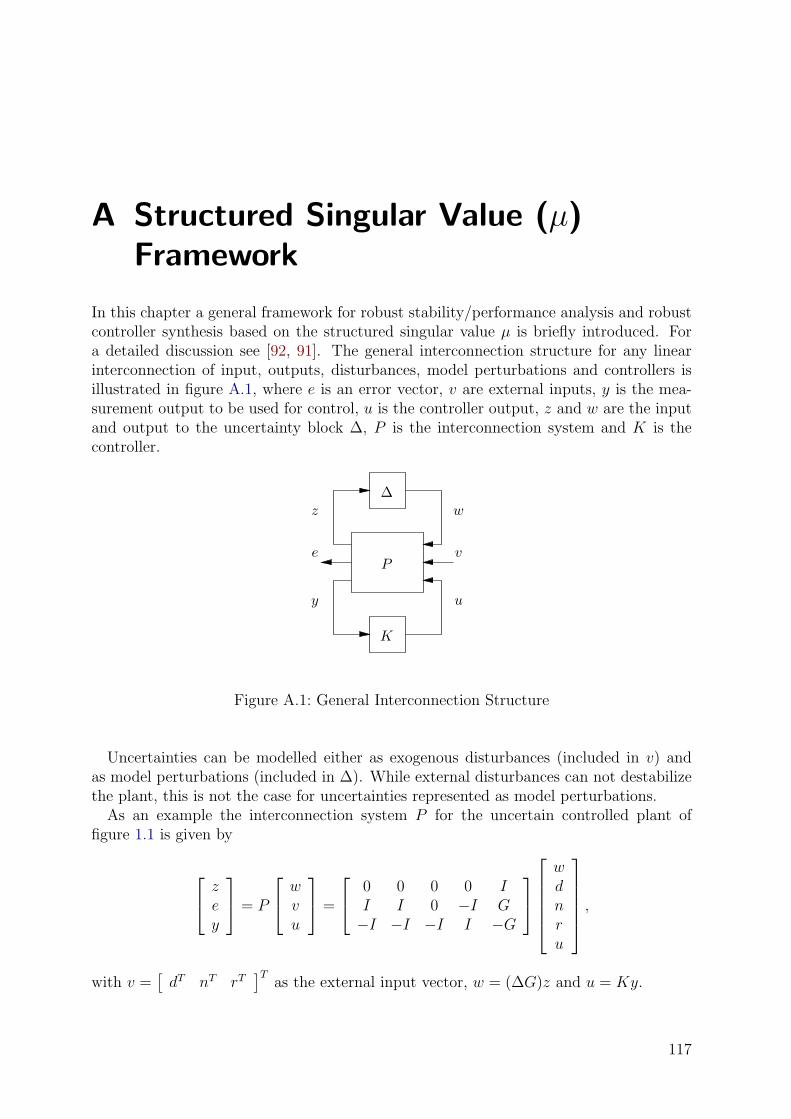
A Structured Singular Value (µ)Framework
In this chapter a general framework for robust stability/performance analysis and robustcontroller synthesis based on the structured singular value µ is briefly introduced. Fora detailed discussion see [92, 91]. The general interconnection structure for any linearinterconnection of input, outputs, disturbances, model perturbations and controllers isillustrated in figure A.1, where e is an error vector, v are external inputs, y is the mea-surement output to be used for control, u is the controller output, z and w are the inputand output to the uncertainty block ∆, P is the interconnection system and K is thecontroller.
∆
z
e
y
P
K
u
v
w
Figure A.1: General Interconnection Structure
Uncertainties can be modelled either as exogenous disturbances (included in v) andas model perturbations (included in ∆). While external disturbances can not destabilizethe plant, this is not the case for uncertainties represented as model perturbations.
As an example the interconnection system P for the uncertain controlled plant offigure 1.1 is given by
zey
= P
wvu
=
0 0 0 0 II I 0 −I G−I −I −I I −G
wdnru
,
with v =[
dT nT rT]T
as the external input vector, w = (∆G)z and u = Ky.
117
A Structured Singular Value (µ) Framework
The interconnection system P is assumed to be a finite dimensional LTI (linear timeinvariant) system of the form
P (s) =
P11(s) P12(s) P13(s)P21(s) P22(s) P23(s)P31(s) P32(s) P33(s)
. (A.1)
Closing the feedback loops for K and ∆ yields
e = Fu(Fl(P, K), ∆)v = Fl(Fu(P, ∆), K)v.
A.1 Definitions
The following notations and terminologies will be used in the following:
Definition A.1. Consider the general interconnection structure in figure A.1, where thenominal closed loop system is given for ∆ = 0. Then, the closed-loop system is said tohave
• Nominal Stability (NS): if the nominal closed-loop system is stable
• Robust Stability (RS): if the closed-loop system is stable for all possible closed-loop systems described by the uncertainty structure
• Nominal Performance (NP): if the performance requirements are met for thenominal closed-loop system
• Robust Performance (RP): if the performance requirements are met for allpossible closed-loop systems described by the uncertainty structure
Definition A.2. Analytic functions: Let S ⊂ C be an open set, and let f(s) be acomplex-valued function defined on S, that is, f(s) : S → C. Then, f(s) is said to beanalytic at a point z0 ∈ S if it is differentiable at z0 and also at each point in someneighborhood of z0.
Definition A.3. H∞ Space: The Hardy space H∞ describes all complex-valued func-tions with complex argument that are analytic and bounded in the open right-half plane.The H∞ norm is defined as
‖F‖∞ := supRe(s)>0
σ[F (s)] = supw∈R
σ[F (jω)],
where σ denotes the maximum singular value. The real rational subspace of H∞ isdenoted by RH∞, which describes all proper and real rational stable transfer functions.
Definition A.4. Well-posed: A feedback system is said to be well-posed if all closed-loop transfer matrices are well-defined and proper. Well-defined means that the inversein the expression of the transfer matrix exists (i.e., (I −M11∆)−1 in (2.11) must exist forall ∆ is a defined set).
118
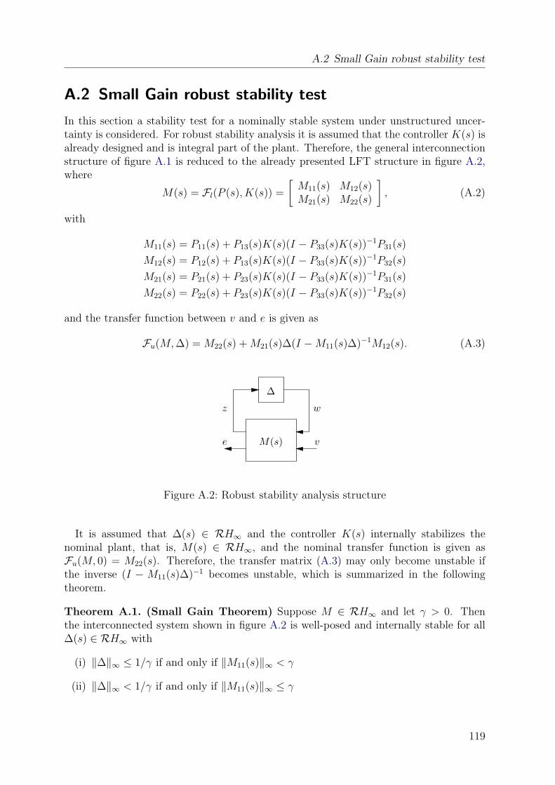
A.2 Small Gain robust stability test
A.2 Small Gain robust stability test
In this section a stability test for a nominally stable system under unstructured uncer-tainty is considered. For robust stability analysis it is assumed that the controller K(s) isalready designed and is integral part of the plant. Therefore, the general interconnectionstructure of figure A.1 is reduced to the already presented LFT structure in figure A.2,where
M(s) = Fl(P (s), K(s)) =
[M11(s) M12(s)M21(s) M22(s)
], (A.2)
with
M11(s) = P11(s) + P13(s)K(s)(I − P33(s)K(s))−1P31(s)
M12(s) = P12(s) + P13(s)K(s)(I − P33(s)K(s))−1P32(s)
M21(s) = P21(s) + P23(s)K(s)(I − P33(s)K(s))−1P31(s)
M22(s) = P22(s) + P23(s)K(s)(I − P33(s)K(s))−1P32(s)
and the transfer function between v and e is given as
Fu(M, ∆) = M22(s) + M21(s)∆(I −M11(s)∆)−1M12(s). (A.3)
∆
z
e M(s) v
w
Figure A.2: Robust stability analysis structure
It is assumed that ∆(s) ∈ RH∞ and the controller K(s) internally stabilizes thenominal plant, that is, M(s) ∈ RH∞, and the nominal transfer function is given asFu(M, 0) = M22(s). Therefore, the transfer matrix (A.3) may only become unstable ifthe inverse (I − M11(s)∆)−1 becomes unstable, which is summarized in the followingtheorem.
Theorem A.1. (Small Gain Theorem) Suppose M ∈ RH∞ and let γ > 0. Thenthe interconnected system shown in figure A.2 is well-posed and internally stable for all∆(s) ∈ RH∞ with
(i) ‖∆‖∞ ≤ 1/γ if and only if ‖M11(s)‖∞ < γ
(ii) ‖∆‖∞ < 1/γ if and only if ‖M11(s)‖∞ ≤ γ
119
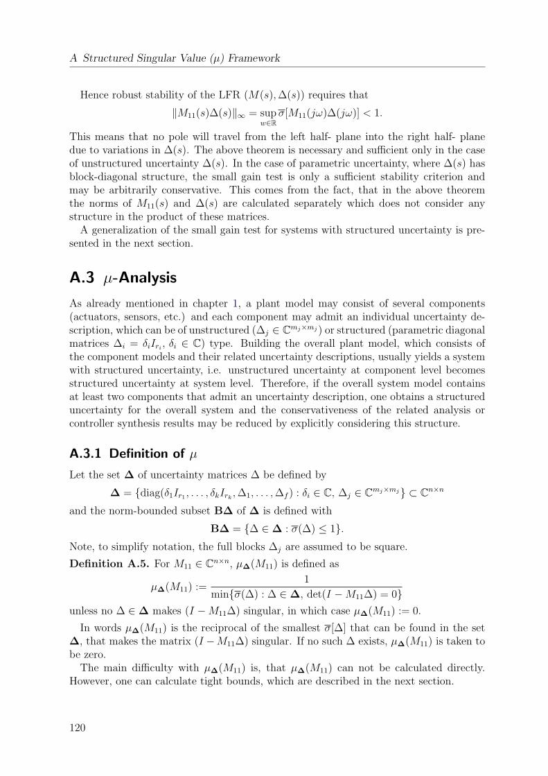
A Structured Singular Value (µ) Framework
Hence robust stability of the LFR (M(s), ∆(s)) requires that
‖M11(s)∆(s)‖∞ = supw∈R
σ[M11(jω)∆(jω)] < 1.
This means that no pole will travel from the left half- plane into the right half- planedue to variations in ∆(s). The above theorem is necessary and sufficient only in the caseof unstructured uncertainty ∆(s). In the case of parametric uncertainty, where ∆(s) hasblock-diagonal structure, the small gain test is only a sufficient stability criterion andmay be arbitrarily conservative. This comes from the fact, that in the above theoremthe norms of M11(s) and ∆(s) are calculated separately which does not consider anystructure in the product of these matrices.
A generalization of the small gain test for systems with structured uncertainty is pre-sented in the next section.
A.3 µ-Analysis
As already mentioned in chapter 1, a plant model may consist of several components(actuators, sensors, etc.) and each component may admit an individual uncertainty de-scription, which can be of unstructured (∆j ∈ Cmj×mj) or structured (parametric diagonalmatrices ∆i = δiIri
, δi ∈ C) type. Building the overall plant model, which consists ofthe component models and their related uncertainty descriptions, usually yields a systemwith structured uncertainty, i.e. unstructured uncertainty at component level becomesstructured uncertainty at system level. Therefore, if the overall system model containsat least two components that admit an uncertainty description, one obtains a structureduncertainty for the overall system and the conservativeness of the related analysis orcontroller synthesis results may be reduced by explicitly considering this structure.
A.3.1 Definition of µ
Let the set ∆ of uncertainty matrices ∆ be defined by
∆ = diag(δ1Ir1 , . . . , δkIrk, ∆1, . . . , ∆f ) : δi ∈ C, ∆j ∈ Cmj×mj ⊂ Cn×n
and the norm-bounded subset B∆ of ∆ is defined with
B∆ = ∆ ∈∆ : σ(∆) ≤ 1.Note, to simplify notation, the full blocks ∆j are assumed to be square.
Definition A.5. For M11 ∈ Cn×n, µ∆(M11) is defined as
µ∆(M11) :=1
minσ(∆) : ∆ ∈∆, det(I −M11∆) = 0unless no ∆ ∈∆ makes (I −M11∆) singular, in which case µ∆(M11) := 0.
In words µ∆(M11) is the reciprocal of the smallest σ[∆] that can be found in the set∆, that makes the matrix (I −M11∆) singular. If no such ∆ exists, µ∆(M11) is taken tobe zero.
The main difficulty with µ∆(M11) is, that µ∆(M11) can not be calculated directly.However, one can calculate tight bounds, which are described in the next section.
120
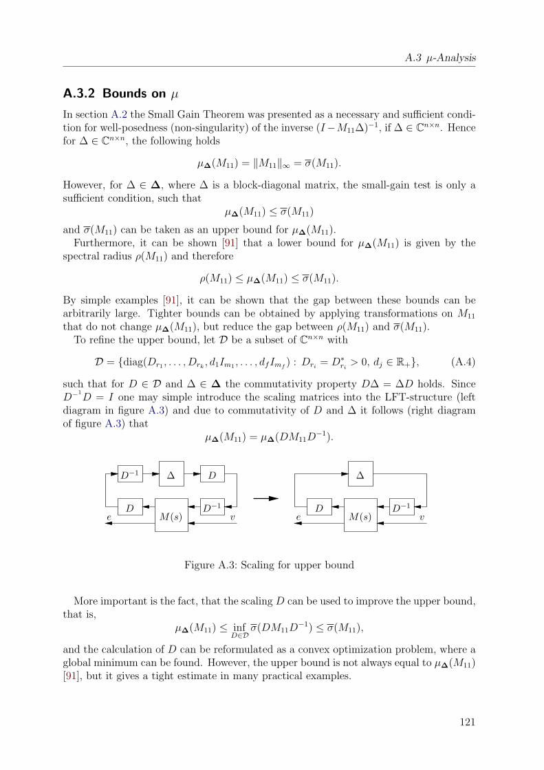
A.3 µ-Analysis
A.3.2 Bounds on µ
In section A.2 the Small Gain Theorem was presented as a necessary and sufficient condi-tion for well-posedness (non-singularity) of the inverse (I−M11∆)−1, if ∆ ∈ Cn×n. Hencefor ∆ ∈ Cn×n, the following holds
µ∆(M11) = ‖M11‖∞ = σ(M11).
However, for ∆ ∈ ∆, where ∆ is a block-diagonal matrix, the small-gain test is only asufficient condition, such that
µ∆(M11) ≤ σ(M11)
and σ(M11) can be taken as an upper bound for µ∆(M11).Furthermore, it can be shown [91] that a lower bound for µ∆(M11) is given by the
spectral radius ρ(M11) and therefore
ρ(M11) ≤ µ∆(M11) ≤ σ(M11).
By simple examples [91], it can be shown that the gap between these bounds can bearbitrarily large. Tighter bounds can be obtained by applying transformations on M11
that do not change µ∆(M11), but reduce the gap between ρ(M11) and σ(M11).To refine the upper bound, let D be a subset of Cn×n with
D = diag(Dr1 , . . . , Drk, d1Im1 , . . . , dfImf
) : Dri= D∗
ri> 0, dj ∈ R+, (A.4)
such that for D ∈ D and ∆ ∈ ∆ the commutativity property D∆ = ∆D holds. SinceD−1
D = I one may simple introduce the scaling matrices into the LFT-structure (leftdiagram in figure A.3) and due to commutativity of D and ∆ it follows (right diagramof figure A.3) that
µ∆(M11) = µ∆(DM11D−1).
D−1
De
∆
M(s)D−1
D
v eD
∆
M(s)D−1
v
Figure A.3: Scaling for upper bound
More important is the fact, that the scaling D can be used to improve the upper bound,that is,
µ∆(M11) ≤ infD∈D
σ(DM11D−1) ≤ σ(M11),
and the calculation of D can be reformulated as a convex optimization problem, where aglobal minimum can be found. However, the upper bound is not always equal to µ∆(M11)[91], but it gives a tight estimate in many practical examples.
121
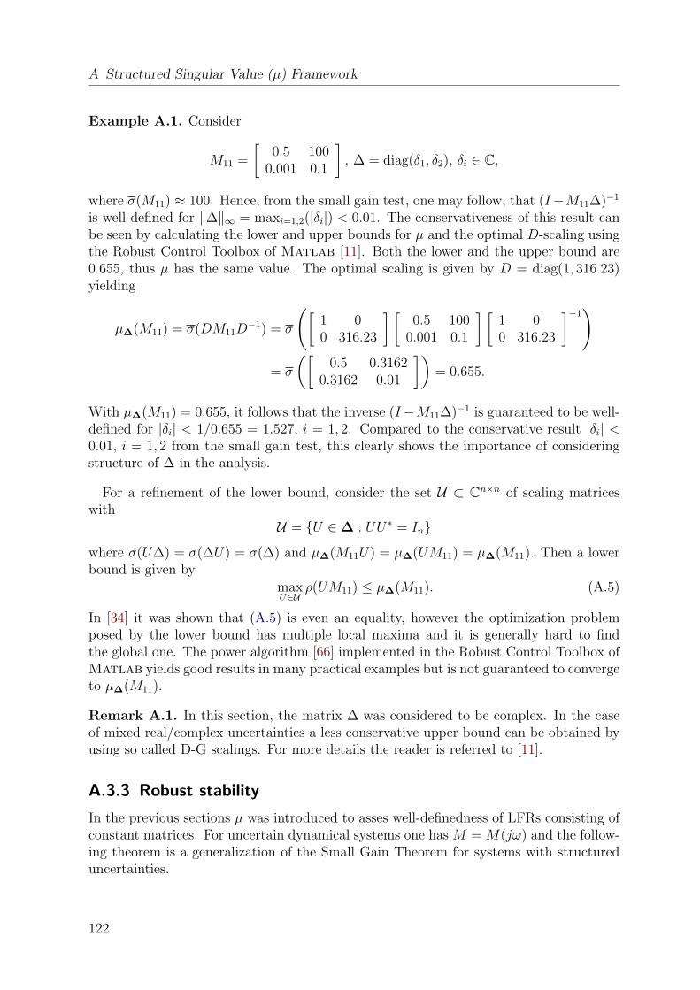
A Structured Singular Value (µ) Framework
Example A.1. Consider
M11 =
[0.5 100
0.001 0.1
], ∆ = diag(δ1, δ2), δi ∈ C,
where σ(M11) ≈ 100. Hence, from the small gain test, one may follow, that (I−M11∆)−1
is well-defined for ‖∆‖∞ = maxi=1,2(|δi|) < 0.01. The conservativeness of this result canbe seen by calculating the lower and upper bounds for µ and the optimal D-scaling usingthe Robust Control Toolbox of Matlab [11]. Both the lower and the upper bound are0.655, thus µ has the same value. The optimal scaling is given by D = diag(1, 316.23)yielding
µ∆(M11) = σ(DM11D−1) = σ
([1 00 316.23
] [0.5 100
0.001 0.1
] [1 00 316.23
]−1)
= σ
([0.5 0.3162
0.3162 0.01
])= 0.655.
With µ∆(M11) = 0.655, it follows that the inverse (I−M11∆)−1 is guaranteed to be well-defined for |δi| < 1/0.655 = 1.527, i = 1, 2. Compared to the conservative result |δi| <0.01, i = 1, 2 from the small gain test, this clearly shows the importance of consideringstructure of ∆ in the analysis.
For a refinement of the lower bound, consider the set U ⊂ Cn×n of scaling matriceswith
U = U ∈∆ : UU∗ = In
where σ(U∆) = σ(∆U) = σ(∆) and µ∆(M11U) = µ∆(UM11) = µ∆(M11). Then a lowerbound is given by
maxU∈U
ρ(UM11) ≤ µ∆(M11). (A.5)
In [34] it was shown that (A.5) is even an equality, however the optimization problemposed by the lower bound has multiple local maxima and it is generally hard to findthe global one. The power algorithm [66] implemented in the Robust Control Toolbox ofMatlab yields good results in many practical examples but is not guaranteed to convergeto µ∆(M11).
Remark A.1. In this section, the matrix ∆ was considered to be complex. In the caseof mixed real/complex uncertainties a less conservative upper bound can be obtained byusing so called D-G scalings. For more details the reader is referred to [11].
A.3.3 Robust stability
In the previous sections µ was introduced to asses well-definedness of LFRs consisting ofconstant matrices. For uncertain dynamical systems one has M = M(jω) and the follow-ing theorem is a generalization of the Small Gain Theorem for systems with structureduncertainties.
122
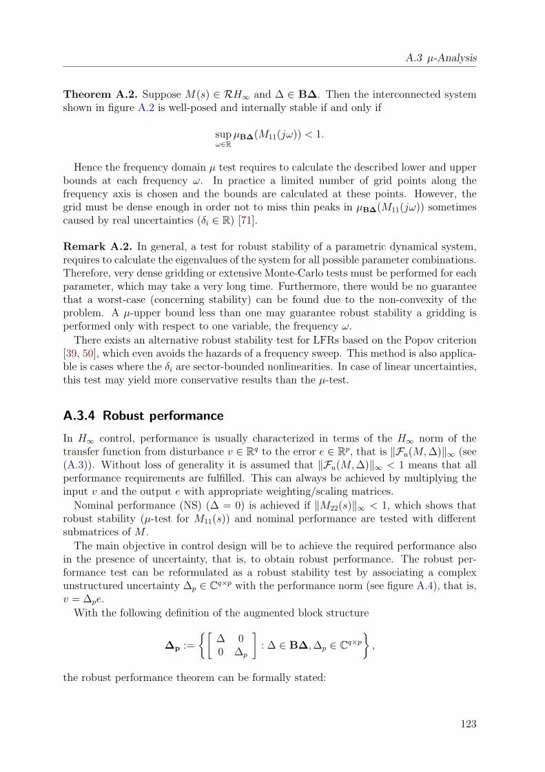
A.3 µ-Analysis
Theorem A.2. Suppose M(s) ∈ RH∞ and ∆ ∈ B∆. Then the interconnected systemshown in figure A.2 is well-posed and internally stable if and only if
supω∈R
µB∆(M11(jω)) < 1.
Hence the frequency domain µ test requires to calculate the described lower and upperbounds at each frequency ω. In practice a limited number of grid points along thefrequency axis is chosen and the bounds are calculated at these points. However, thegrid must be dense enough in order not to miss thin peaks in µB∆(M11(jω)) sometimescaused by real uncertainties (δi ∈ R) [71].
Remark A.2. In general, a test for robust stability of a parametric dynamical system,requires to calculate the eigenvalues of the system for all possible parameter combinations.Therefore, very dense gridding or extensive Monte-Carlo tests must be performed for eachparameter, which may take a very long time. Furthermore, there would be no guaranteethat a worst-case (concerning stability) can be found due to the non-convexity of theproblem. A µ-upper bound less than one may guarantee robust stability a gridding isperformed only with respect to one variable, the frequency ω.
There exists an alternative robust stability test for LFRs based on the Popov criterion[39, 50], which even avoids the hazards of a frequency sweep. This method is also applica-ble is cases where the δi are sector-bounded nonlinearities. In case of linear uncertainties,this test may yield more conservative results than the µ-test.
A.3.4 Robust performance
In H∞ control, performance is usually characterized in terms of the H∞ norm of thetransfer function from disturbance v ∈ Rq to the error e ∈ Rp, that is ‖Fu(M, ∆)‖∞ (see(A.3)). Without loss of generality it is assumed that ‖Fu(M, ∆)‖∞ < 1 means that allperformance requirements are fulfilled. This can always be achieved by multiplying theinput v and the output e with appropriate weighting/scaling matrices.
Nominal performance (NS) (∆ = 0) is achieved if ‖M22(s)‖∞ < 1, which shows thatrobust stability (µ-test for M11(s)) and nominal performance are tested with differentsubmatrices of M .
The main objective in control design will be to achieve the required performance alsoin the presence of uncertainty, that is, to obtain robust performance. The robust per-formance test can be reformulated as a robust stability test by associating a complexunstructured uncertainty ∆p ∈ Cq×p with the performance norm (see figure A.4), that is,v = ∆pe.
With the following definition of the augmented block structure
∆p :=
[∆ 00 ∆p
]: ∆ ∈ B∆, ∆p ∈ Cq×p
,
the robust performance theorem can be formally stated:
123
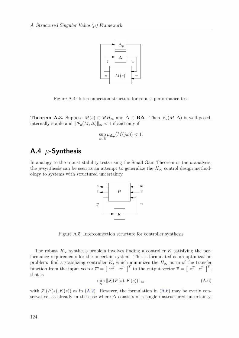
A Structured Singular Value (µ) Framework
∆z w
vM(s)e
∆p
Figure A.4: Interconnection structure for robust performance test
Theorem A.3. Suppose M(s) ∈ RH∞ and ∆ ∈ B∆. Then Fu(M, ∆) is well-posed,internally stable and ‖Fu(M, ∆)‖∞ < 1 if and only if
supω∈R
µ∆p(M(jω)) < 1.
A.4 µ-Synthesis
In analogy to the robust stability tests using the Small Gain Theorem or the µ-analysis,the µ-synthesis can be seen as an attempt to generalize the H∞ control design method-ology to systems with structured uncertainty.
u
v
wz
e
y
K
P
Figure A.5: Interconnection structure for controller synthesis
The robust H∞ synthesis problem involves finding a controller K satisfying the per-formance requirements for the uncertain system. This is formulated as an optimizationproblem: find a stabilizing controller K, which minimizes the H∞ norm of the transfer
function from the input vector w =[
wT vT]T
to the output vector z =[
zT eT]T
,that is
minK‖Fl(P (s), K(s))‖∞, (A.6)
with Fl(P (s), K(s)) as in (A.2). However, the formulation in (A.6) may be overly con-servative, as already in the case where ∆ consists of a single unstructured uncertainty,
124
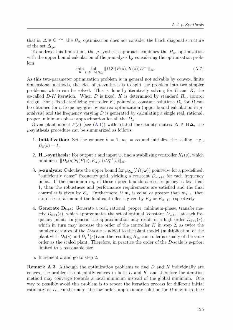
A.4 µ-Synthesis
that is, ∆ ∈ Cn×n, the H∞ optimization does not consider the block diagonal structureof the set ∆p.
To address this limitation, the µ-synthesis approach combines the H∞ optimizationwith the upper bound calculation of the µ-analysis by considering the optimization prob-lem
minK
infD,D−1∈H∞
‖DFl(P (s), K(s))D−1‖∞. (A.7)
As this two-parameter optimization problem is in general not solvable by convex, finitedimensional methods, the idea of µ-synthesis is to split the problem into two simplerproblems, which can be solved. This is done by iteratively solving for D and K, theso-called D-K iteration. When D is fixed, K is determined by standard H∞ controldesign. For a fixed stabilizing controller K, pointwise, constant solutions Dω for D canbe obtained for a frequency grid by convex optimization (upper bound calculation in µ-analysis) and the frequency varying D is generated by calculating a single real, rational,proper, minimum phase approximation for all the Dω.
Given plant model P (s) (see (A.1)) with related uncertainty matrix ∆ ∈ B∆, theµ-synthesis procedure can be summarized as follows:
1. Initialization: Set the counter k = 1, m0 = ∞ and initialize the scaling, e.g.,Dk(s) = I.
2. H∞-synthesis: For output z and input w, find a stabilizing controller Kk(s), whichminimizes ‖Dk(s)Fl(P (s), Kk(s))D
−1k (s)‖∞.
3. µ-analysis: Calculate the upper bound for µ∆p(M(jω)) pointwise for a predefined,”sufficiently dense” frequency grid, yielding a constant Dω,k+1 for each frequencypoint. If the maximum mk of these upper bounds across frequency is less than1, than the robustness and performance requirements are satisfied and the finalcontroller is given by Kk. Furthermore, if mk is equal or greater than mk−1, thenstop the iteration and the final controller is given by Kk or Kk−1, respectively.
4. Generate Dk+1: Generate a real, rational, proper, minimum-phase, transfer ma-trix Dk+1(s), which approximates the set of optimal, constant Dω,k+1 at each fre-quency point. In general the approximation may result in a high order Dk+1(s),which in turn may increase the order of the controller K in step 2, as twice thenumber of states of the D-scale is added to the plant model (multiplication of theplant with Dk(s) and D−1
k (s)) and the resulting H∞-controller is usually of the sameorder as the scaled plant. Therefore, in practice the order of the D-scale is a-priorilimited to a reasonable size.
5. Increment k and go to step 2.
Remark A.3. Although the optimization problems to find D and K individually areconvex, the problem is not jointly convex in both D and K, and therefore the iterationmethod may converge towards a local minimum instead of the global minimum. Oneway to possibly avoid this problem is to repeat the iteration process for different initialestimates of D. Furthermore, the low order, approximate solution for D may introduce
125
A Structured Singular Value (µ) Framework
some errors and the results are restricted to the frequency range under consideration.However, in many practical examples the µ-synthesis was applied with great success, andthe resulting controller may be close to the global optimum. For structured uncertainty,the µ-synthesis allows to reduce conservativeness compared to the standard H∞ synthesis,which may be interpreted as an upper bound for the µ-synthesis.
126
B Background on LPV control design
In this appendix some basic results for a quadratic Lyapunov approach to guaranteeclosed-loop stability and performance for parameter dependent systems are briefly sum-marized, which may help to understand the idea of the LPV control design procedureused in Chapter 6. For a detailed discussion see [87].
B.1 Stability and performance of LPV systems
Consider the linear time-invariant system
x = Ax + Bu
y = Cx.(B.1)
Theorem B.1. [19](Exponential stability) System (B.1) is exponentially stable if andonly if there exists a matrix X = XT > 0 such that
AT X + XA < 0.
Theorem B.2. [19](Bounded Real Lemma) System (B.1) is exponentially stable and
‖C(sI − A)−1B‖∞ < 1
if and only if there exists a matrix X = XT > 0 such that
AT X + XA + XBBT X + CT C < 0. (B.2)
Using the Schur complement formula [19], the inequality (B.2) can also be written as AT X + XA XB CT
BT X −I 0C 0 −I
< 0,
which is denoted as a linear matrix inequality (LMI) in the variable X and representsa convex constraint on X. The feasibility of this LMI and a solution for X can bedetermined by solving a convex optimization problem. The same results can be appliedfor parameter-dependent systems.
Lemma B.1. [87] Consider parameter dependent state-space matrices A(δ), B(δ), C(δ)and suppose there exists a matrix X = XT such that AT (δ)X + XA(δ) XB(δ) CT (δ)
BT (δ)X −I 0C(δ) 0 −I
< 0,
for all δ ∈ Π. Then for every parameter trajectory δ(t) ∈ Π, the system is exponentiallystable and ‖C(δ)(sI − A(δ))−1B(δ)‖∞ < 1.
127
B Background on LPV control design
The preceding lemma may be used for analysis of closed-loop parameter dependentsystems and it is also a starting point for the synthesis of parameter dependent controllersfor systems without rate bounded parametric variations. For the single-track modelconsidered in chapter 6, the parameter v does not change arbitrarily fast and therefore acontroller derived assuming a plant without rate bounded parametric variations may beoverly conservative. In [87] a generalization of the preceding lemma is presented, whichallows to exploit a priori known bounds on the parameter variation rate:
Lemma B.2. [87] Suppose that υ > 0. If there exists a continuously differentiablefunction X(δ) with X(δ) > 0 and the two inequalities υ
dX(δ)
dδ+ AT (δ)X(δ) + X(δ)A(δ) X(δ)B(δ) CT (δ)
BT (δ)X(δ) −I 0C(δ) 0 −I
< 0 (B.3)
−υdX(δ)
dδ+ AT (δ)X(δ) + X(δ)A(δ) X(δ)B(δ) CT (δ)
BT (δ)X(δ) −I 0C(δ) 0 −I
< 0 (B.4)
are fulfilled for all δ ∈ Π, then the system is exponentially stable for any trajectoryδ(t) ∈ Π, |δ(t)| ≤ υ and ‖C(δ)(sI − A(δ))−1B(δ)‖∞ < 1.
Note, that now X is itself a matrix function of δ, i.e. an unknown element of a functionspace, so that the inequalities (B.3) and (B.4) are infinite-dimensional LMIs. One way toapproximately solve this convex optimization problem is to grid the plant model over thevarying parameter space (see [88]). Furthermore, the structure of X(δ) must be fixed.This can be done by choosing suitable continuously differentiable basis functions fi(δ),such that X(δ) =
∑Ni=1 fi(δ)Xi, where the fi(δ) may be chosen based on the parameter
dependence of the plant itself.
B.2 Robust LPV control design
Based on Lemma B.2 a procedure is proposed in [87] how to derive a parameter dependentgain-scheduled controller K(s, δ). This requires that all parameters δ can be measuredand used for control. In general the parameter vector δ may be represented as δ =(δm, δu), where δm is a vector of measurable parameters and δu is a vector of uncertainparameters. Hence, only the parameters included in δm can be used for gain-scheduling,i.e., K = K(s, δm). To achieve robustness with respect to the uncertain parameter vectorδu, a D-K iteration can be performed, which is sketched in the following procedure for agiven plant model G(s, δ) ∈ Cp×m.
1. Generate an LFR (M(δm), ∆(s, δu)) such that G(s, δ) = Fu(M(δm), ∆(s, δu)), with
∆(s, δu) =
[In/s 0
0 ∆u(δu)
], ∆u(δu) ∈ Rr×r,
and initialize the scaling matrix, e.g. D(s) = Ir.
128
B.2 Robust LPV control design
2. Partition M(δm) as
M(δm) =
[M11(δm) M12(δm)
M21(δm) M22(δm)
]=
A(δm) B1(δm) B2(δm)C1(δm) D11(δm) D12(δm)
C2(δm) D21(δm) D22(δm)
,
such that the equation based representation of the LFR (M(δm), ∆(s, δu)) is givenas
x = A(δm)x + B1(δm)w + B2(δm)u
z = C1(δm)x + D11(δm)w + D12(δm)u
y = C2(δm)x + D21(δm)w + D22(δm)u
x = In/sx
w = ∆uz.
3. Apply the methods proposed in [87] to synthesize a gain-scheduled controllerK(s, δm) ∈ Ck×l, which solves the optimization problem
minK(s,δm)
∥∥∥∥[ D(s) 00 Ip−l
]Fl
(G(s, δm), K(s, δm)
) [ D−1(s) 00 Im−k
]∥∥∥∥∞
,
with
G(s, δm) = Fu
([A(δm) B(δm)
C(δm) D(δm)
], In/s
),
B(δm) =[
B1(δm) B2(δm)],
C(δm) =
[C1(δm)C2(δm)
], D(δm) =
[D11(δm) D12(δm)D21(δm) D22(δm)
].
4. Generate a stable, real, rational, proper, minimum-phase transfer matrix D(s) ∈Cr×r, with D(s)∆u = ∆uD(s), which solves the optimization problem
γ = infD(s)
∥∥∥∥[ D(s) 00 Ip−l
]Fl
(G(s, δm), K(s, δm)
) [ D−1(s) 00 Im−k
]∥∥∥∥∞
.
Stop the procedure if γ < 1, otherwise go to step 3.
129
C LFR-toolbox
In this appendix a list of the basic functions of the LFR-toolbox version 2 are presented.Additional modules for Simulink interfaces, gain-scheduling design and interfaces to anONERA-toolbox for skew-µ analysis are not yet finished and listed.
Overloaded functions for LFR objects:
display - show contents of lfr-objectssize - show size information of lfr-objectsisempty - check if lfr-object is emptyget - get fields of an lfr-objectset - change block-names, block-bounds or object-fieldsplus - addition of lfr-objectsminus - subtraction of lfr-objectsuminus - sign change of lfr-objectmtimes - product of lfr-objectsmpower - repeated product of lfr-objectsmrdivide - division of lfr-objectsinv - inversion of lfr-objectshorzcat - horizontal (column) concatenation of lfr-objectsvertcat - vertical (row) concatenation of lfr-objectsappend - block-diagonal concatenationblkdiag - block-diagonal concatenationtransp - transposition of lfr-objectssubsref - subscripted reference for lfr-objectssubsasgn - subscripted assignment for lfr-objectsfeedback - feedback interconnection of lfr-objectsdcgain - steady-state gaineval - evaluation from values in workspacediff - differentiation of lfr-objectseig - nominal eigenvalues of dynamic lfr-objectnull - null-space of lfr-objectreal - real part of lfr-objectimag - imaginary part of lfr-object
130
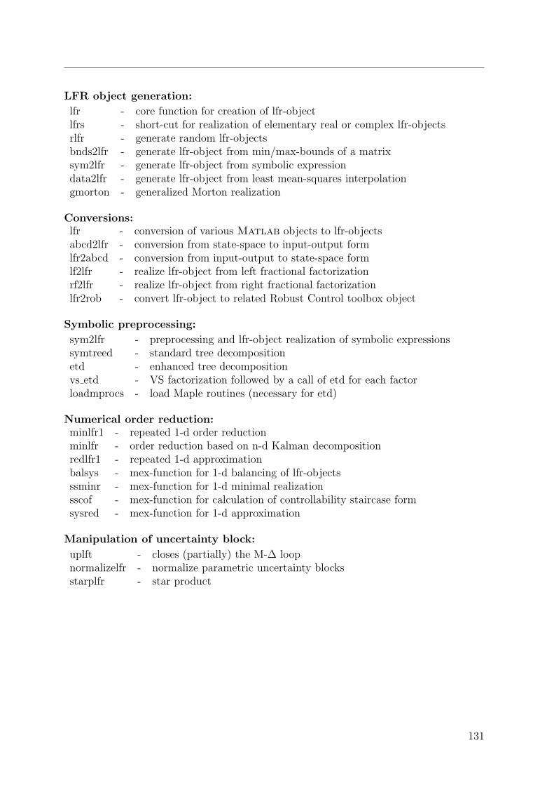
LFR object generation:
lfr - core function for creation of lfr-objectlfrs - short-cut for realization of elementary real or complex lfr-objectsrlfr - generate random lfr-objectsbnds2lfr - generate lfr-object from min/max-bounds of a matrixsym2lfr - generate lfr-object from symbolic expressiondata2lfr - generate lfr-object from least mean-squares interpolationgmorton - generalized Morton realization
Conversions:lfr - conversion of various Matlab objects to lfr-objectsabcd2lfr - conversion from state-space to input-output formlfr2abcd - conversion from input-output to state-space formlf2lfr - realize lfr-object from left fractional factorizationrf2lfr - realize lfr-object from right fractional factorizationlfr2rob - convert lfr-object to related Robust Control toolbox object
Symbolic preprocessing:
sym2lfr - preprocessing and lfr-object realization of symbolic expressionssymtreed - standard tree decompositionetd - enhanced tree decompositionvs etd - VS factorization followed by a call of etd for each factorloadmprocs - load Maple routines (necessary for etd)
Numerical order reduction:minlfr1 - repeated 1-d order reductionminlfr - order reduction based on n-d Kalman decompositionredlfr1 - repeated 1-d approximationbalsys - mex-function for 1-d balancing of lfr-objectsssminr - mex-function for 1-d minimal realizationsscof - mex-function for calculation of controllability staircase formsysred - mex-function for 1-d approximation
Manipulation of uncertainty block:
uplft - closes (partially) the M-∆ loopnormalizelfr - normalize parametric uncertainty blocksstarplfr - star product
131
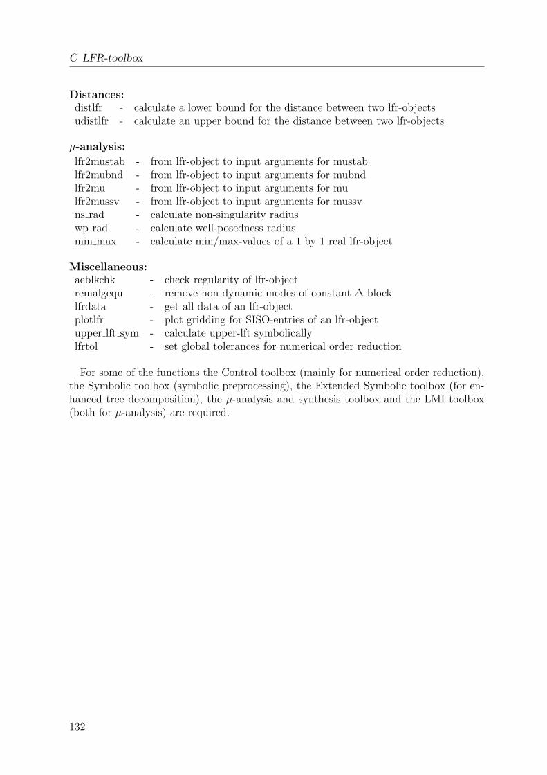
C LFR-toolbox
Distances:distlfr - calculate a lower bound for the distance between two lfr-objectsudistlfr - calculate an upper bound for the distance between two lfr-objects
µ-analysis:
lfr2mustab - from lfr-object to input arguments for mustablfr2mubnd - from lfr-object to input arguments for mubndlfr2mu - from lfr-object to input arguments for mulfr2mussv - from lfr-object to input arguments for mussvns rad - calculate non-singularity radiuswp rad - calculate well-posedness radiusmin max - calculate min/max-values of a 1 by 1 real lfr-object
Miscellaneous:aeblkchk - check regularity of lfr-objectremalgequ - remove non-dynamic modes of constant ∆-blocklfrdata - get all data of an lfr-objectplotlfr - plot gridding for SISO-entries of an lfr-objectupper lft sym - calculate upper-lft symbolicallylfrtol - set global tolerances for numerical order reduction
For some of the functions the Control toolbox (mainly for numerical order reduction),the Symbolic toolbox (symbolic preprocessing), the Extended Symbolic toolbox (for en-hanced tree decomposition), the µ-analysis and synthesis toolbox and the LMI toolbox(both for µ-analysis) are required.
132

D RCAM linear parametric systemmatrices
A(δ) =
−117.05 1Cw VA
0 50.807 1Cw VA
0 0 0
0 0.70528Zcg−96.507+24.879Xcg
Cw VA0 0 0 0
4.8192 1Cw VA
0 −48.116 1Cw VA
0 0 0
1.0 0 α 0 0 0
0 1.0 0 0 0 0
0 0 1.0004 0 0 0
0 −1.9860 b72−1.0VA2α Cw
Cw VA0 0 −9.8061 0
VA α 0 −VA 9.8061 0 0
0 −241.25+0.0040000Cw VA+VA2Cw
Cw VA0 0 −9.8100 α 0
0 0 0 0 0.000043244 0
0 0 0 −VA α 0 VA
0 0 0 0 −VA 0
0 −2.2278−0.054189Xcg+2.5880Zcg
Cw VA0 0 0 0
0.061601 a27
Cw VA0 0.061601 a29
Cw VA0 0 0
0 0.061601 a38
Cw VA0 0 0 0
0 0 0 0 0 0
0 0 0 0 0 0
0 0 0 0 0 0
−0.061601 a77
Cw VA0 −0.061601 a79
Cw VA0 0 0
0 −15.697 1Cw VA
0 0 0 0
−0.061601 a97
Cw VA0 −0.061601 a99
Cw VA0 0 0
1 0 α 0 0 0
0 1 0 0 0 0
−α 0 1 0 0 0
133
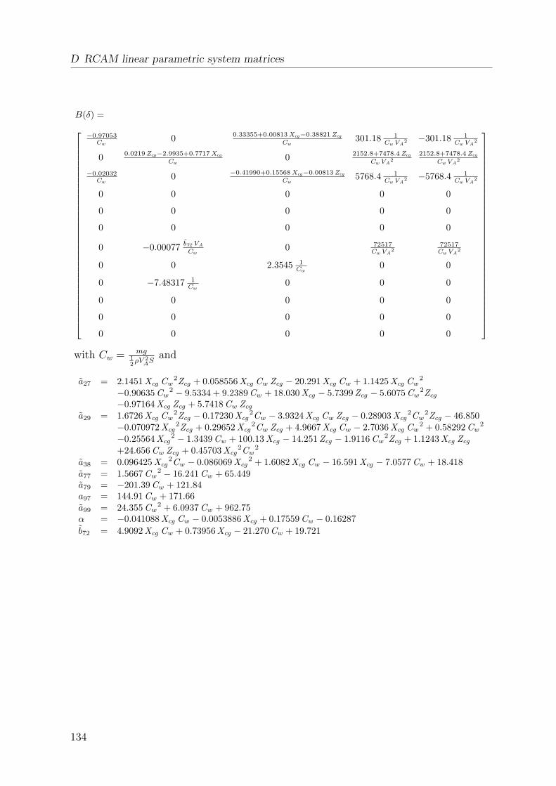
D RCAM linear parametric system matrices
B(δ) =
−0.97053Cw
0 0.33355+0.00813Xcg−0.38821Zcg
Cw301.18 1
CwVA2 −301.18 1
CwVA2
0 0.0219Zcg−2.9935+0.7717Xcg
Cw0 2152.8+7478.4Zcg
CwVA2
2152.8+7478.4Zcg
CwVA2
−0.02032Cw
0 −0.41990+0.15568Xcg−0.00813Zcg
Cw5768.4 1
CwVA2 −5768.4 1
CwVA2
0 0 0 0 0
0 0 0 0 0
0 0 0 0 0
0 −0.00077 b72VA
Cw0 72517
CwVA2
72517CwVA
2
0 0 2.3545 1Cw
0 0
0 −7.48317 1Cw
0 0 0
0 0 0 0 0
0 0 0 0 0
0 0 0 0 0
with Cw = mg
12ρV 2
ASand
a27 = 2.1451Xcg Cw2Zcg + 0.058556Xcg Cw Zcg − 20.291Xcg Cw + 1.1425Xcg Cw
2
−0.90635Cw2 − 9.5334 + 9.2389Cw + 18.030Xcg − 5.7399Zcg − 5.6075Cw
2Zcg
−0.97164Xcg Zcg + 5.7418Cw Zcg
a29 = 1.6726Xcg Cw2Zcg − 0.17230Xcg
2Cw − 3.9324Xcg Cw Zcg − 0.28903Xcg2Cw
2Zcg − 46.850−0.070972Xcg
2Zcg + 0.29652Xcg2Cw Zcg + 4.9667Xcg Cw − 2.7036Xcg Cw
2 + 0.58292Cw2
−0.25564Xcg2 − 1.3439Cw + 100.13Xcg − 14.251Zcg − 1.9116Cw
2Zcg + 1.1243Xcg Zcg
+24.656Cw Zcg + 0.45703Xcg2Cw
2
a38 = 0.096425Xcg2Cw − 0.086069Xcg
2 + 1.6082Xcg Cw − 16.591Xcg − 7.0577Cw + 18.418a77 = 1.5667Cw
2 − 16.241Cw + 65.449a79 = −201.39Cw + 121.84a97 = 144.91Cw + 171.66a99 = 24.355Cw
2 + 6.0937Cw + 962.75α = −0.041088Xcg Cw − 0.0053886Xcg + 0.17559Cw − 0.16287b72 = 4.9092Xcg Cw + 0.73956Xcg − 21.270Cw + 19.721
134
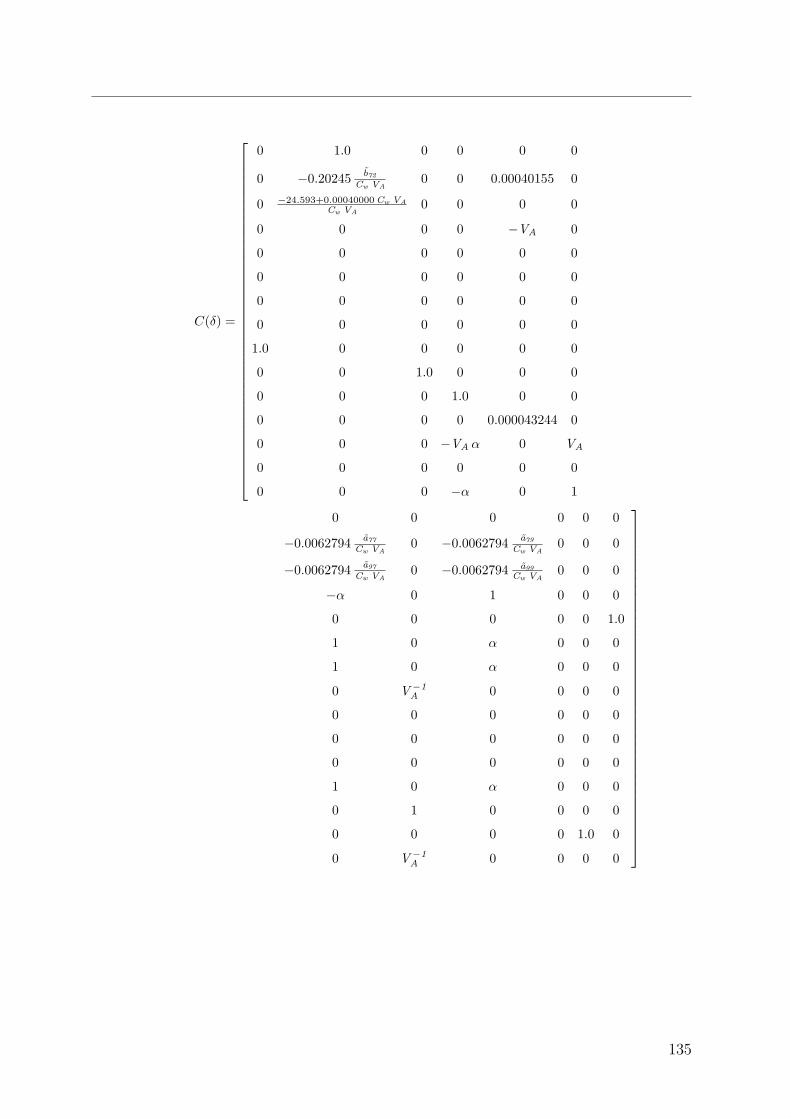
C(δ) =
0 1.0 0 0 0 0
0 −0.20245 b72
Cw VA0 0 0.00040155 0
0 −24.593+0.00040000Cw VA
Cw VA0 0 0 0
0 0 0 0 −VA 0
0 0 0 0 0 0
0 0 0 0 0 0
0 0 0 0 0 0
0 0 0 0 0 0
1.0 0 0 0 0 0
0 0 1.0 0 0 0
0 0 0 1.0 0 0
0 0 0 0 0.000043244 0
0 0 0 −VA α 0 VA
0 0 0 0 0 0
0 0 0 −α 0 1
0 0 0 0 0 0
−0.0062794 a77
Cw VA0 −0.0062794 a79
Cw VA0 0 0
−0.0062794 a97
Cw VA0 −0.0062794 a99
Cw VA0 0 0
−α 0 1 0 0 0
0 0 0 0 0 1.0
1 0 α 0 0 0
1 0 α 0 0 0
0 V−1A 0 0 0 0
0 0 0 0 0 0
0 0 0 0 0 0
0 0 0 0 0 0
1 0 α 0 0 0
0 1 0 0 0 0
0 0 0 0 1.0 0
0 V−1A 0 0 0 0
135
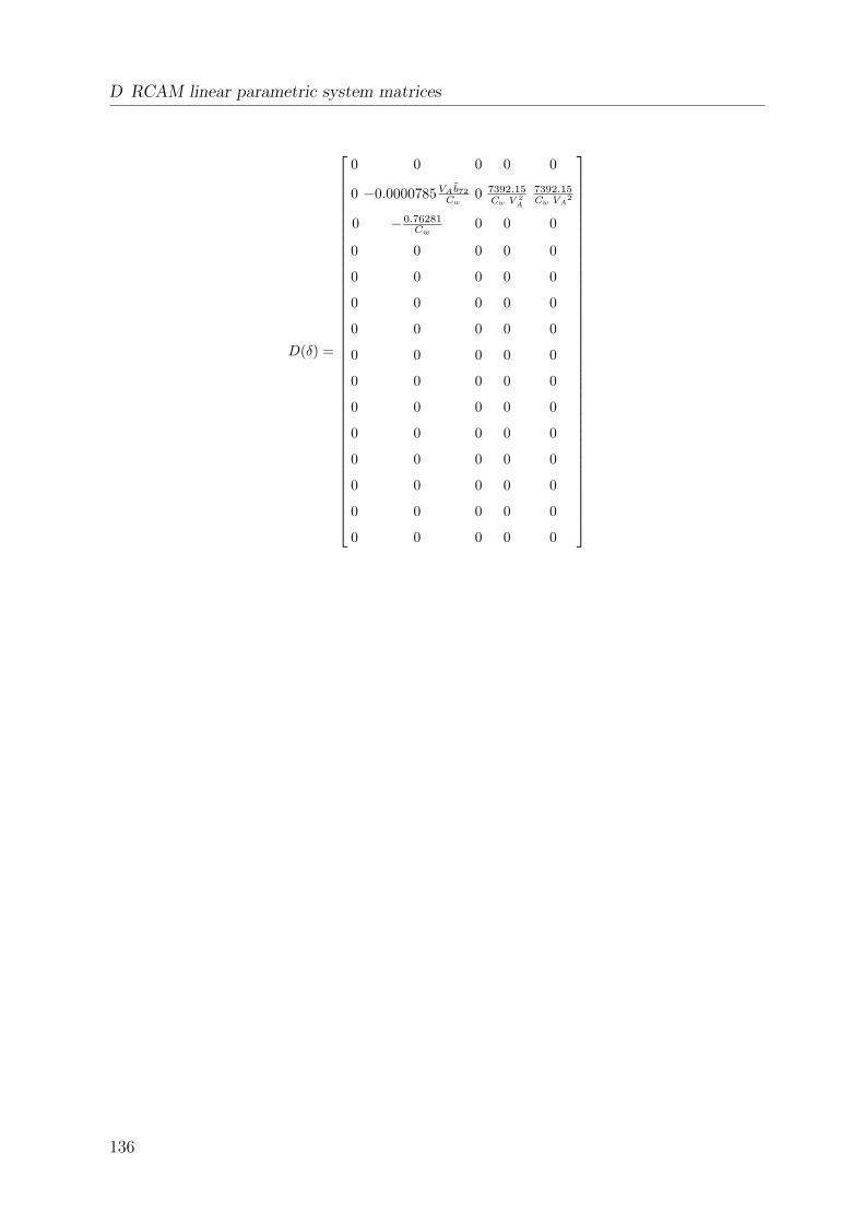
D RCAM linear parametric system matrices
D(δ) =
0 0 0 0 0
0 −0.0000785VAb72Cw
0 7392.15Cw V 2
A
7392.15Cw VA
2
0 − 0.76281Cw
0 0 0
0 0 0 0 0
0 0 0 0 0
0 0 0 0 0
0 0 0 0 0
0 0 0 0 0
0 0 0 0 0
0 0 0 0 0
0 0 0 0 0
0 0 0 0 0
0 0 0 0 0
0 0 0 0 0
0 0 0 0 0
136
Bibliography
[1] J. Ackermann, P. Blue, T. Bunte, L. Guvenc, D. Kaesbauer, M. Kordt, M. Muhler,and D. Odenthal, Robust Control. The Parameter Space Approach, 2nd ed., ser.Communications and Control Engineering. Springer, October 2002.
[2] J. Ackermann, T. Bunte, W. Sienel, H. Jeebe, and K. Naab, “Driving safety by ro-bust steering control,” in Proc. of the International Symposium on Advanced VehicleControl and Safety, Aachen, Germany, 1996.
[3] B. Aksun-Guvenc, T. Bunte, D. Odenthal, and L. Guvenc, “Robust two degree-of-freedom vehicle steering controller design,” IEEE Tranactions on Control SystemsTechnology, vol. 12, no. 4, pp. 627–636, 2004.
[4] B. Anderson and Y. Liu, “Controller reduction: Concepts and approaches,” IEEETrans. Automat. Contr., vol. 34, pp. 802–812, 1989.
[5] E. Anderson, Z. Bai, J. Bishop, J. Demmel, J. D. Croz, A. Greenbaum, S. Hammar-ling, A. McKenney, S. Ostrouchov, and D. Sorensen, LAPACK User’s Guide, SecondEdition, SIAM, Philadelphia, France, 1995.
[6] A. C. Antoulas, Approximation of Large-Scale Dynamical Systems, ser. Advanced inDesign and Control, R. C. Smith, Ed. SIAM, 2005.
[7] P. Apkarian and P. Gahinet, “A convex characterization of gain-scheduled H∞ con-trollers,” IEEE Trans. Automat. Contr., vol. 40, pp. 853–864, 1995.
[8] K. Astrom, P. Albertos, M. Blanke, A. Isidori, W. Schaufelberger, and R. Sanz,Control of Complex Systems. London: Springer, 2001.
[9] G. Balas, “Robust control of flexible structures: Theory and experiments,” Ph.D.dissertation, California Institute of Technology, 1990.
[10] G. Balas, “Linear, parameter-varying control and its application to a turbofan en-gine,” Int. Journal of Robust and Nonlinear Control, vol. 12, no. 9, pp. 763–796,2002.
[11] G. Balas, R. Chiang, A. Packard, and M. Safonov, Robust Control Toolbox 3.0.1,The MathWorks, Natick, MA, USA, March 2005.
[12] G. Balas, J. Doyle, K. Glover, A. Packard, and R. Smith, µ-Analysis and SynthesisToolbox, The MathWorks, Natick, MA, USA.
137
Bibliography
[13] C. Belcastro, “Parametric uncertainty modelling: an overview,” in Proc. AmericanControl Conference, Philadelphia, PA, 1998.
[14] C. M. Belcastro, “Uncertainty modeling of real parameter variations for robust con-trol applications,” Ph.D. dissertation, University of Drexel, US, December 1994.
[15] P. Benner, V. Mehrmann, V. Sima, S. V. Huffel, and A. Varga, SLICOT - A Sub-routine Library in Systems and Control Theory, ser. In B. N. Datta, Ed., Appliedand Computational Control, Signals and Circuits. Birkhauser, 1998.
[16] H. W. Bode, “Relations between attenuation and phase in feedback amplifier design,”Bell System Technical Journal, vol. 19, pp. 421–454, 1940.
[17] H. W. Bode, Network Analysis and Feedback Amplifier Design. New York: VanNostrand, 1945.
[18] N. K. Bose, Applied Multidimensional Systems Theory. Van Nostrand ReinholdCompany, 1982.
[19] S. Boyd, L. E. Ghaoui, E. Feron, and V. Balakrishnan, Linear Matrix Inequalitiesin System and Control Theory. Siam, 1994.
[20] T. Bunte, D. Odenthal, B. Aksun-Guvenc, and L. Guvenc, “Robust vehicle steeringcontrol design based on the disturbance observer,” IFAC Annual Reviews in Control,vol. 26, pp. 139–149, 2002.
[21] Y. Cheng and B. De Moor, “A multidimensional realization algorithm for parametricuncertainty modeling problems and multiparameter margin problems,” InternationalJournal of Control, vol. 60, pp. 3022–3023, 1994.
[22] M. Chilali and P. Gahinet, “H∞ design with pole placement constraints: an LMIapproach,” in Proc. of Conference on Decision and Control, 1994, pp. 553–558.
[23] J. Cockburn, “Discussion on: ”generalized lft-based representation of parametricuncertain models”,” European Journal of Control, vol. 10, no. 4, pp. 338–340, 2004.
[24] J. Cockburn and B. Morton, “Linear fractional representation of uncertain systems,”Automatica, vol. 33, no. 7, pp. 1263–1271, 1997.
[25] L. Dai, Singular Control Systems, ser. Lecture Notes in Control and InformationSciences. Heidelberg: Springer-Verlag, Berlin, 1989, no. 118.
[26] A. Damen and S. Weiland, “Lecture notes: Robust control,” Measurement andControl Group, Eindhoven University of Technology, The Netherlands, 2002.
[27] R. D’Andrea, “H∞ optimal interconnections,” Systems and Control Letters, vol. 32,pp. 313–322, 1997.
[28] R. D’Andrea and G. E. Dullerud, “Distributed control design for spatially intercon-nected systems,” IEEE Trans. Automat. Contr., vol. 48, no. 9, 2003.
138
Bibliography
[29] R. D’Andrea and S. Khatri, “Kalman decomposition of linear fractional transforma-tion representations and minimality,” in Proc. of the American Control Conference,Albuquerque, New Mexico, 1997, pp. 3557–3561.
[30] R. D’Andrea and F. Paganini, “Interconnection of uncertain behavioral systemsfor robust control,” in Proc. of the 32nd Conference on Decision and Control, SanAntonio, Texas, 1993, pp. 3642–3647.
[31] M. Dettori and C. W. Scherer, “Control design for a compact disc player with mul-tiple norm specifications,” Control Systems Technology, vol. 10, pp. 635–645, 2002.
[32] C. Doll and A. Knauf, “Comparison in terms of size of several LFT models for thelateral motion of a generic fighter aircraft,” in Proc. AIAA Guidance Navigation andControl Conference, 2005.
[33] J. C. Doyle, “Guaranteed margins for LQG regulators,” IEEE Trans. Automat.Contr., vol. 23, pp. 756–757, 1978.
[34] J. C. Doyle, “Analysis of feedback systems with structured uncertainties,” IEE-D,vol. 129, pp. 242–250, 1982.
[35] J. C. Doyle, K. Glover, P. Kkhargonekar, and B. Francis, “State-space solutions tostandard H2 and H∞ control problems,” IEEE Trans. Automat. Contr., vol. 34, pp.831–847, 1989.
[36] G. Ferreres and J. Biannic, “A skew mu toolbox (SMT) for robustness analy-sis,” in Proc. International Symposium on Computer Aided Control Systems Design(CACSD), Taipei, Taiwan, 2004.
[37] P. Gahinet, A. Nemirovski, A. Laub, and M. Chilali, LMI Control Toolbox, TheMathWorks, Natick, MA, USA.
[38] M. Green and D. Limebeer, Linear Robust Control, ser. Information and SystemSciences, T. Kailath, Ed. Englewood Cliffs, New Jersey: Prentice Hall, 1995.
[39] W. Haddad and D. Berstein, “Parameter-dependent lyapunov functions, constantreal parameter uncertainty, and the Popov citerion in robust analysis and synthesis,”in Proc. Conference on Decision and Control, 1991, pp. 2274–2279 and 2632–2633.
[40] S. Hecker, “Robust H∞ based vehicle steering control design,” in Proc. Conferenceon Control Applications, Munich, Germany, 2006.
[41] S. Hecker and A. Varga, “Generalized LFT-based representation of parametric un-certain models,” in Proc. European Control Conference ECC, Cambridge, UK, 2003.
[42] S. Hecker and A. Varga, “Generalized LFT-based representation of parametric un-certain models,” European Journal of Control, vol. 10, no. 4, pp. 326–337, 2004.
[43] S. Hecker and A. Varga, “Symbolic techniques for low order LFT-modelling,” inIFAC World Congress, Prag, Czech Republic, 2005.
139
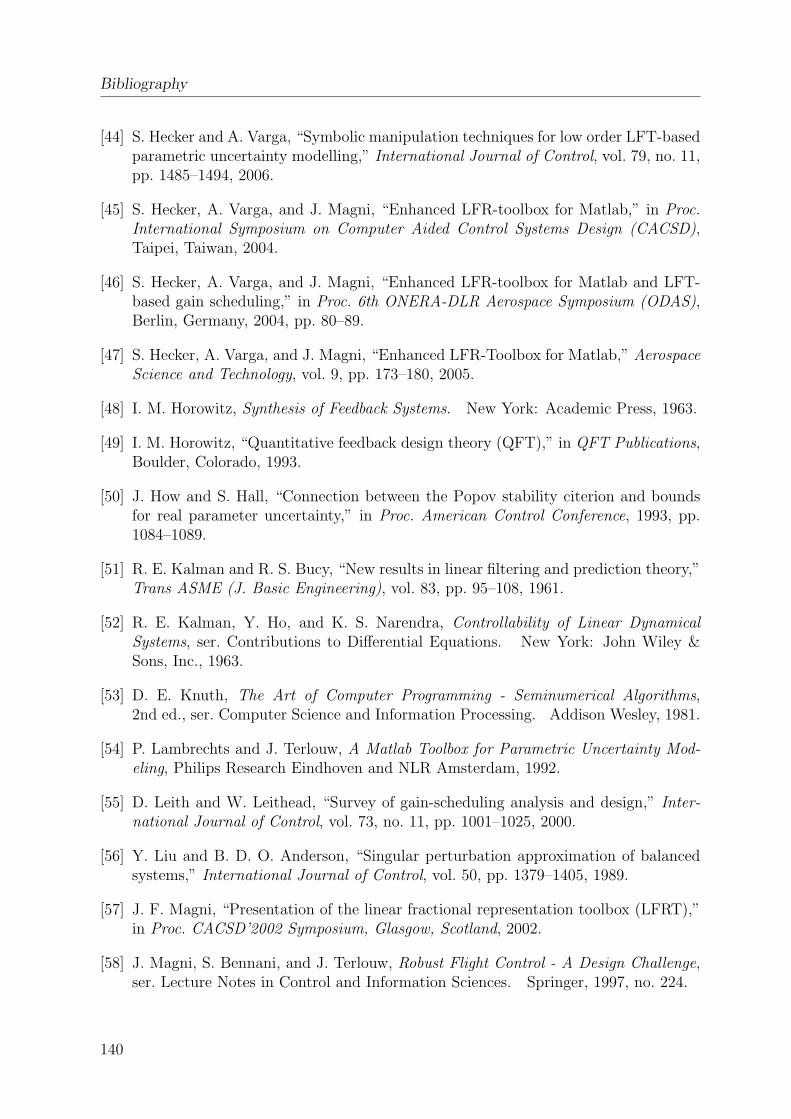
Bibliography
[44] S. Hecker and A. Varga, “Symbolic manipulation techniques for low order LFT-basedparametric uncertainty modelling,” International Journal of Control, vol. 79, no. 11,pp. 1485–1494, 2006.
[45] S. Hecker, A. Varga, and J. Magni, “Enhanced LFR-toolbox for Matlab,” in Proc.International Symposium on Computer Aided Control Systems Design (CACSD),Taipei, Taiwan, 2004.
[46] S. Hecker, A. Varga, and J. Magni, “Enhanced LFR-toolbox for Matlab and LFT-based gain scheduling,” in Proc. 6th ONERA-DLR Aerospace Symposium (ODAS),Berlin, Germany, 2004, pp. 80–89.
[47] S. Hecker, A. Varga, and J. Magni, “Enhanced LFR-Toolbox for Matlab,” AerospaceScience and Technology, vol. 9, pp. 173–180, 2005.
[48] I. M. Horowitz, Synthesis of Feedback Systems. New York: Academic Press, 1963.
[49] I. M. Horowitz, “Quantitative feedback design theory (QFT),” in QFT Publications,Boulder, Colorado, 1993.
[50] J. How and S. Hall, “Connection between the Popov stability citerion and boundsfor real parameter uncertainty,” in Proc. American Control Conference, 1993, pp.1084–1089.
[51] R. E. Kalman and R. S. Bucy, “New results in linear filtering and prediction theory,”Trans ASME (J. Basic Engineering), vol. 83, pp. 95–108, 1961.
[52] R. E. Kalman, Y. Ho, and K. S. Narendra, Controllability of Linear DynamicalSystems, ser. Contributions to Differential Equations. New York: John Wiley &Sons, Inc., 1963.
[53] D. E. Knuth, The Art of Computer Programming - Seminumerical Algorithms,2nd ed., ser. Computer Science and Information Processing. Addison Wesley, 1981.
[54] P. Lambrechts and J. Terlouw, A Matlab Toolbox for Parametric Uncertainty Mod-eling, Philips Research Eindhoven and NLR Amsterdam, 1992.
[55] D. Leith and W. Leithead, “Survey of gain-scheduling analysis and design,” Inter-national Journal of Control, vol. 73, no. 11, pp. 1001–1025, 2000.
[56] Y. Liu and B. D. O. Anderson, “Singular perturbation approximation of balancedsystems,” International Journal of Control, vol. 50, pp. 1379–1405, 1989.
[57] J. F. Magni, “Presentation of the linear fractional representation toolbox (LFRT),”in Proc. CACSD’2002 Symposium, Glasgow, Scotland, 2002.
[58] J. Magni, S. Bennani, and J. Terlouw, Robust Flight Control - A Design Challenge,ser. Lecture Notes in Control and Information Sciences. Springer, 1997, no. 224.
140
Bibliography
[59] A. Marcos and G. Balas, “Development of linear-parameter-varying models for air-craft,” Journal of Guidance, Control and Dynamics, vol. 27, no. 3, 2004.
[60] A. Marcos, D. Bates, and I. Postlethwaite, “A multivariate polynomial matrix order-reduction algorithm for linear fractional transformation modelling,” in Proc. IFACWorld Congress, Prague, Czech Republic, 2005.
[61] A. Megretski and A. Rantzer, “System analysis via integral quadratic constraints,”IEEE Trans. Automat. Contr., vol. 42, no. 6, pp. 819–830, 1997.
[62] K. Meyberg and P. Vachenauer, Hohere Mathematik 1, 6th ed. Berlin, Heidelberg:Springer, 2003.
[63] B. C. Moore, “Principal component analysis in linear system: Controllability, ob-servability and model reduction,” IEEE Trans. Automat. Contr., vol. 26, pp. 17–32,1981.
[64] B. Morton, “New applications of µ to real parameter variation problems,” in Proc.Conference on Decision and Control, Fort Lauderdale, Florida, 1985, pp. 233–238.
[65] A. Packard, “Gain scheduling via linear fractional transformations,” System andControl Letters, vol. 22, pp. 79–92, 1994.
[66] A. Packard, M. K. H. Fan, and J. C. Doyle, “A power method for the structuredsingular value,” in Proc. Conference on Decision and Control, 1988.
[67] P. Pellanda, P. Apkarian, and H. D. Tuan, “Missile autopilot design via multi-channelLFT/LPV control method,” Int. Journal of Robust and Nonlinear Control, vol. 12,pp. 1–20, 2002.
[68] W. Rugh and F. Shamma, “Research on gain scheduling,” Automatica, vol. 36, pp.1401–1425, 2000.
[69] A. Saberi, B. M. Chen, and P. Sannuti, Loop Transfer Recovery: Analysis and De-sign. Springer, London, 1993.
[70] M. G. Safonov and M. Athans, “Gain and phase margins for for multiloop LQGregulators,” IEEE Trans. Automat. Contr., vol. 22, pp. 173–179, 1977.
[71] C. W. Scherer, “Lecture notes for course on theory of robust control,” Dutch Instituteof Systems and Control, Delft, The Netherlands, 2001.
[72] C. W. Scherer, “LPV control and full block multipliers,” Automatica, vol. 37, pp.361–375, 2001.
[73] C. W. Scherer and S. Weiland, “Lecture notes DISC course on linear matrix inequal-ities in control,” Dutch Institute of Systems and Control, Delft, The Netherlands,1999.
141
Bibliography
[74] G. Scorletti and L. E. Ghaoui, “Improved LMI conditions for gain scheduling andrelated control problems,” Internatinal Journal of Robust and Nonlinear Control,vol. 8, pp. 845–877, 1998.
[75] J. Sturm, Sedumi 1.05R5 a Matlab Toolbox for Optimization over Symmetric Cones,Department of Econometrics, Tilburg University, The Netherlands, 1998-2003.
[76] T. Sugie and M. Kawanishi, “µ-analysis/synthesis based on exact expression of phys-ical parameter variations,” in Proc. European Control Conference, Rome, Italy, 1995,pp. 159–164.
[77] J. Terlouw, P. Lambrechts, S. Bennani, and M. Steinbuch, “Parametric uncertaintymodeling using LFTs,” in Proc. American Control Conference, San Francisco, CA,1993, pp. 267–272.
[78] M. van de Wal, G. van Baars, F. Sperling, and O. Bosgra, “Multivariable H∞/µfeedback control design for high-precision wafer stage motion,” Control EngineeringPractice, vol. 10, pp. 739–755, 2002.
[79] A. T. van Zanten, “Bosch ESP systems: 5 years of experience,” 2000, SAE Paperno. 2000-01-1633.
[80] A. T. van Zanten, R. Erhardt, and G. Pfaff, “VDC, the vehicle dynamics controlsystem of Bosch,” 1995, SAE Paper no. 950-759.
[81] A. Varga, “Model reduction software in the SLICOT library,” in Applied and Com-putational Control, Signals and Circuits, ser. The Kluwer International Series inEngineering and Computer Science, B. N. Datta, Ed. Kluwer Academic Publishers,Boston, 2001, vol. 629, pp. 239–282.
[82] A. Varga and B. D. O. Anderson, “Accuracy-enhancing methods for balancing-related frequency-weighted model and controller reduction,” Automatica, vol. 39,pp. 919–927, 2003.
[83] A. Varga and G. Looye, “Symbolic and numerical software tools for LFT-based loworder uncertainty modeling,” in Proc. CACSD’99 Symposium, Kohala Coast, Hawaii,1999.
[84] A. Varga, G. Looye, D. Moormann, and G. Grubel, “Automated generation of LFT-based parametric uncertainty descriptions from generic aircraft models,” Mathemat-ical and Computer Modelling of Dynamical Systems, vol. 4, pp. 249–274, 1998.
[85] A. Varga, Controller reduction using accuracy-enhancing methods. Springer Verlag,07 2005, vol. 45, pp. 225 – 260.
[86] J. C. Willems, “Paradigms and puzzles in the theory of dynamical systems,” IEEETrans. Automat. Contr., vol. 36, no. 3, pp. 259–294, 1991.
142
Bibliography
[87] F. Wu, “Control of linear parameter varying systems,” Ph.D. dissertation, Universityof California, Berkley, 1995.
[88] F. Wu, X. Yang, A. Packard, and G. Becker, “Induced L2-norm control for LPVsystem with bounded parameter variation rates,” in Proc. American Control Con-ference, 1995.
[89] G. Zames, “Feedback and optimal sensitivity: Model reference transformations, mul-tiplicative seminorms, and approximate inverse,” IEEE Trans. Automat. Contr.,vol. 26, no. 2, pp. 301–320, 1981.
[90] E. Zerz, “Linear fractional representations of polynomially parametrized descriptorsystems,” in Proc. 3rd Portuguese Conference on Automatic Control (Controlo 98),1998.
[91] K. Zhou and J. C. Doyle, Essentials of Robust Control. Prentice Hall, 1998.
[92] K. Zhou, J. C. Doyle, and K. Glover, Robust and Optimal Control. Prentice Hall,1996.
143