
Mario Zacharias - Universität zu Köln · Auf Grund von langreichweitigen Scherkr aften im...
172
Mott Transition and Quantum Critical Metamagnetism on Compressible Lattices Inaugural-Dissertation zur Erlangung des Doktorgrades der Mathematisch-Naturwissenschaftlichen Fakult¨ at der Universit¨ atzuK¨oln vorgelegt von Mario Zacharias aus Bochum 2013
Transcript of Mario Zacharias - Universität zu Köln · Auf Grund von langreichweitigen Scherkr aften im...
Mott Transition and
Quantum Critical Metamagnetism
on
Compressible Lattices
Inaugural-Dissertation
zur
Erlangung des Doktorgrades
der Mathematisch-Naturwissenschaftlichen Fakultat
der Universitat zu Koln
vorgelegt von
Mario Zacharias
aus Bochum
2013
Berichterstatter: Priv.-Doz. Dr. Markus Garst
Prof. Dr. Achim Rosch
Tag der mundlichen Prufung: 02.07.2013
Abstract
Solid state phase transitions, which are amenable to pressure, generically, have an
intrinsic coupling of the order parameter to the elastic degrees of freedom. The
applied pressure primarily affects the lattice by varying the lattice spacing which, in
turn, modifies the coupling constants of the critical degrees of freedom. Therefore, a
coupling of the strain to the order parameter can strongly affect the phase transition.
In this Thesis we investigate this influence on the finite temperature critical point
of the Mott metal-insulator transition and the zero temperature quantum critical
metamagnetic endpoint.
The universality class of the Mott endpoint is a topic which is still under debate.
In this Thesis, we show that the nature of the Mott transition is drastically changed
when interacting with a compressible lattice. The expected Ising criticality of the
electronic system is preempted by an isostructural instability. Due to long ranged
shear forces, in the vicinity of the critical endpoint an elastic Landau regime emerges,
where the system shows mean-field behavior. The smoking gun criterion to detect
the elastic Landau regime is the breakdown of Hooke’s law, i.e., a non-linear stress-
strain relation. Furthermore, the specific heat coefficient exhibits a finite mean
field jump at the transition. For the family of organic salts κ-(BEDT-TTF)2X, we
determine the extent of the elastic Landau regime as ∆T ? ≈ 2.5 K and ∆p? ≈ 50
bar based on thermal expansion experiments [1, 2].
In the second part, we investigate the quantum critical endpoint of itinerant
metamagnets. Recently, it was suggested that quantum critical metamagnetism is
a generic feature in itinerant ferromagnets [3] such as UCoAl [4] and UGe2 [5, 6].
Within the framework of spin fluctuation theory, we determine the free energy and its
temperature dependence, obtained by fluctuation renormalizations, and deduce the
critical thermodynamics. Importantly, the compressibility shows the same behavior
as the susceptibility which, by definition, diverges at a metamagnetic transition.
Therefore, the metamagnetic quantum critical endpoint is intrinsically unstable to-
wards an isostructural transition.
This isostructural transition preempts the metamagnetic quantum critical end-
point and the elastic degrees of freedom crucially alter the critical thermodynamics.
Most importantly, at the critical field we obtain for lowest but finite temperatures a
i
regime of critical elasticity which is characterized by unusual power laws of the ther-
modynamic quantities. Whereas the thermal expansion has a much stronger tem-
perature divergence for fields close to the critical field, the specific heat divergence
is cut off upon entering this regime. As a consequence, the Gruneisen parameter
diverges with an unusual high power of temperature.
ii
Kurzzusammenfassung
Druckabhangige Phasenubergange in Festkorpern sind stets an die elastischen Frei-
heitsgrade des Gitters gekoppelt. Der angelegte Druck wirkt auf das Gitter, indem
der Gitterabstand verandert wird, was wiederum die Wechselwirkung der kritischen
Freiheitsgrade beeinflusst. Daher kann eine Kopplung zwischen Gitterspannung und
Ordnungsparameter den Phasenubergang stark beeinflussen. In dieser Arbeit be-
trachten wir die Auswirkung einer solchen Kopplung auf den Mott Metall-Isolator
Ubergang, der bei endlichen Temperaturen stattfindet, sowie den quantenkritischen
metamagnetischen Endpunkt bei T = 0.
Die Frage nach der Universalitatsklasse des kritischen Endpunktes des Mott-
Ubergangs ist noch immer nicht abschließend geklart. In dieser Arbeit zeigen wir,
dass der Charakter des Mott-Ubergangs sich drastisch andert, wenn man Wech-
selwirkungen mit einem kompressiblen Gitter in Betracht zieht. Dem erwarteten
Ising-kritischen Verhalten des elektronischen Systems kommt ein isostruktureller
Phasenubergang zuvor. Auf Grund von langreichweitigen Scherkraften im Kristall
bildet sich in der unmittelbaren Nahe des kritischen Punktes ein elastisches Landau-
Regime, in dem das System Mean-Field Verhalten zeigt. Dieses elastische Landau-
Regime kann eindeutig durch die Verletzung des Hooke’schen Gesetzes identifiziert
werden, das eine linearen Zusammenhang zwischen der mechanischen Spannung
und der resultierenden Ausdehnung voraussagt. Des Weiteren springt die spezifische
Warme Mean-Field-artig am Ubergang. Basierend auf Messungen der thermischen
Ausdehnung [1, 2], konnen wir fur die Familie organischer Salze κ-(BEDT-TTF)2X
die Ausmaße des elastischen Landau-Regimes abschatzen und erhalten ∆T ? ≈ 2.5
K und ∆p? ≈ 50 bar.
Im zweiten Teil der Arbeit untersuchen wir den quantenkritischen Endpunkt von
itineranten Metamagneten. Kurzlich wurde darauf hingewiesen [3], dass dieser ganz
allgemein in itineranten Ferromagneten wie UCoAl [4] und UGe2 [5, 6] auftritt. Im
Rahmen der Spin-Fluktuationstheorie bestimmen wir die Temperaturabhangigkeit
der freien Energie und folgern die kritischen thermodynamischen Eigenschaften. Be-
merkenswerterweise ist die Kompressibilitat proportional zur Suszeptibilitat, welche
am metamagnetischen Ubergang divergiert. Daher der metamagnetische quanten-
kritische Endpunkt intrinsisch instabil gegenuber einem isostrukturellen Ubergang.
iii
Dieser isostrukturelle Phasenubergang kommt dem metamagnetischen quanten-
kritischen Endpunkt zuvor und die elastischen Freiheitsgrade verandern entschei-
dend die Thermodynamik. Insbesondere finden wir am kritische Magnetfeld bei
tiefsten aber endlichen Temperaturen einen Regime der kritischen Elastizitat das
durch ungewohnliche Potenzgesetze der kritischen thermodynamischen Großen cha-
rakterisiert ist. Wahrend die thermische Ausdehnung nahe des quantenkritischen
Endpunktes starker als ublich mit fallender Temperatur divergiert, wird die Diver-
genz der spezifischen Warme abgeschnitten. Daraus resultiert eine erstaunlich hohe
Divergenz des Gruneisenparameters als Funktion der Temperatur.
iv
Contents
1 Introduction 1
2 Elasticity 3
2.1 Continuous Elasticity Theory . . . . . . . . . . . . . . . . . . . . . . 4
2.1.1 Displacement and the Strain Tensor . . . . . . . . . . . . . . 4
2.1.2 The Stress Tensor . . . . . . . . . . . . . . . . . . . . . . . . 5
2.1.3 The Free Energy . . . . . . . . . . . . . . . . . . . . . . . . . 7
2.1.4 The Elastic Modulus Tensor . . . . . . . . . . . . . . . . . . . 8
2.2 Crystal Elasticity . . . . . . . . . . . . . . . . . . . . . . . . . . . . . 10
2.2.1 Crystal Structure . . . . . . . . . . . . . . . . . . . . . . . . . 11
2.2.2 Effective Potential of Displacements . . . . . . . . . . . . . . 12
2.2.3 Phonons . . . . . . . . . . . . . . . . . . . . . . . . . . . . . . 14
2.2.4 Continuum Limit . . . . . . . . . . . . . . . . . . . . . . . . . 15
2.3 Phonon Field Integral . . . . . . . . . . . . . . . . . . . . . . . . . . 21
3 Elasticity in Critical Systems 25
3.1 Landau Theory and Elasticity . . . . . . . . . . . . . . . . . . . . . . 26
3.1.1 Symmetry and Strain . . . . . . . . . . . . . . . . . . . . . . 26
3.1.2 Coupling to the Order Parameter . . . . . . . . . . . . . . . . 28
3.2 Ising Theory . . . . . . . . . . . . . . . . . . . . . . . . . . . . . . . 29
3.2.1 Quadratic Coupling . . . . . . . . . . . . . . . . . . . . . . . 29
3.2.2 Microscopics of the Quadratic Coupling . . . . . . . . . . . . 31
3.2.3 Bilinear Coupling . . . . . . . . . . . . . . . . . . . . . . . . . 37
3.3 Classification by Cowley . . . . . . . . . . . . . . . . . . . . . . . . . 39
4 Mott-Transition on Compressible Lattices 43
4.1 Mott Metal-Insulator Transition . . . . . . . . . . . . . . . . . . . . 44
4.1.1 Basic Concepts . . . . . . . . . . . . . . . . . . . . . . . . . . 45
4.1.2 Universality Class . . . . . . . . . . . . . . . . . . . . . . . . 48
4.1.3 The Ising Field Theory . . . . . . . . . . . . . . . . . . . . . 50
4.2 Coupling to the Lattice . . . . . . . . . . . . . . . . . . . . . . . . . 53
v
CONTENTS
4.3 Free Energy . . . . . . . . . . . . . . . . . . . . . . . . . . . . . . . . 54
4.3.1 Perturbative Solution . . . . . . . . . . . . . . . . . . . . . . 55
4.3.2 Non-Perturbative Solution . . . . . . . . . . . . . . . . . . . . 57
4.3.3 Behavior Around the Former Endpoint . . . . . . . . . . . . . 59
4.4 Thermodynamics . . . . . . . . . . . . . . . . . . . . . . . . . . . . . 60
4.4.1 Specific Heat Coefficient . . . . . . . . . . . . . . . . . . . . . 61
4.4.2 Thermal expansion . . . . . . . . . . . . . . . . . . . . . . . . 63
4.4.3 Compressibility . . . . . . . . . . . . . . . . . . . . . . . . . . 64
4.5 Experimental Relevance . . . . . . . . . . . . . . . . . . . . . . . . . 65
4.5.1 The κ-(BEDT-TTF)2X Family . . . . . . . . . . . . . . . . . 66
4.5.2 Vanadium Sesquioxide V2O3 . . . . . . . . . . . . . . . . . . 72
4.6 Summary and Discussion . . . . . . . . . . . . . . . . . . . . . . . . 73
5 Quantum Critical Metamagnets 77
5.1 Metamagnetism . . . . . . . . . . . . . . . . . . . . . . . . . . . . . . 78
5.1.1 Mean-Field Theory . . . . . . . . . . . . . . . . . . . . . . . . 78
5.1.2 Experiments . . . . . . . . . . . . . . . . . . . . . . . . . . . 80
5.2 Spin-Fluctuation Theory . . . . . . . . . . . . . . . . . . . . . . . . . 82
5.2.1 Wegner-Houghton Equation . . . . . . . . . . . . . . . . . . . 84
5.2.2 Effective Metamagnetic Potential . . . . . . . . . . . . . . . . 85
5.3 Free Energy . . . . . . . . . . . . . . . . . . . . . . . . . . . . . . . . 87
5.3.1 Linear Regime . . . . . . . . . . . . . . . . . . . . . . . . . . 87
5.3.2 Non-Linear Regime . . . . . . . . . . . . . . . . . . . . . . . . 90
5.3.3 Free Energy Density . . . . . . . . . . . . . . . . . . . . . . . 91
5.4 Thermodynamics . . . . . . . . . . . . . . . . . . . . . . . . . . . . . 93
5.4.1 Susceptibility, Magnetostriction and Compressibility . . . . . 94
5.4.2 Thermal Expansion, Temperature Derivative of the Magneti-
zation . . . . . . . . . . . . . . . . . . . . . . . . . . . . . . . 96
5.4.3 Specific Heat Coefficient . . . . . . . . . . . . . . . . . . . . . 98
5.4.4 Gruneisen Parameters . . . . . . . . . . . . . . . . . . . . . . 100
5.5 Summary . . . . . . . . . . . . . . . . . . . . . . . . . . . . . . . . . 101
6 Compressible Quantum Critical Metamagnetism 103
6.1 Elastic Coupling . . . . . . . . . . . . . . . . . . . . . . . . . . . . . 104
6.2 Phonons . . . . . . . . . . . . . . . . . . . . . . . . . . . . . . . . . . 105
6.2.1 Neutron Scattering Intensity . . . . . . . . . . . . . . . . . . 106
6.2.2 Parameter Renormalization Due To Phonons . . . . . . . . . 108
6.3 Free Energy . . . . . . . . . . . . . . . . . . . . . . . . . . . . . . . . 111
6.3.1 First Order Transition . . . . . . . . . . . . . . . . . . . . . . 112
6.3.2 Quantum Endpoint . . . . . . . . . . . . . . . . . . . . . . . . 117
vi
6.4 Thermodynamics . . . . . . . . . . . . . . . . . . . . . . . . . . . . . 119
6.4.1 Susceptibility, Compressibility and Magnetostriction . . . . . 119
6.4.2 Thermal Expansion, Temperature Derivative of the Magneti-
zation . . . . . . . . . . . . . . . . . . . . . . . . . . . . . . . 122
6.4.3 Specific Heat Coefficient . . . . . . . . . . . . . . . . . . . . . 124
6.4.4 Gruneisen Parameters . . . . . . . . . . . . . . . . . . . . . . 126
6.5 Estimate for Sr3Ru2O7 . . . . . . . . . . . . . . . . . . . . . . . . . 126
6.6 Summary . . . . . . . . . . . . . . . . . . . . . . . . . . . . . . . . . 128
7 Summary 131
A Symmetry Classes of the Elastic Constant Matrix 133
A.1 Triclinic System . . . . . . . . . . . . . . . . . . . . . . . . . . . . . . 133
A.2 Monoclinic System . . . . . . . . . . . . . . . . . . . . . . . . . . . . 134
A.3 Orthorhombic System . . . . . . . . . . . . . . . . . . . . . . . . . . 134
A.4 Trigonal System . . . . . . . . . . . . . . . . . . . . . . . . . . . . . 135
A.5 Tetragonal System . . . . . . . . . . . . . . . . . . . . . . . . . . . . 136
A.6 Hexagonal System . . . . . . . . . . . . . . . . . . . . . . . . . . . . 136
A.7 Cubic System . . . . . . . . . . . . . . . . . . . . . . . . . . . . . . . 137
B Irreducible Representations of the Strain Tensor 139
C Effective Action due to Phonons 141
Bibliography 151
Acknowledgments 158
Erklarung 161
Teilpublikationen 161
Lebenslauf 162
vii

Chapter 1
Introduction
Phase transitions, where a system drastically changes its properties, are one of
the most interesting phenomena in nature. Melting and solidification, magnetic
or metal-insulator transitions are not only of interest for physicists in their ambi-
tion to understand and explain nature and its phenomena, but also yield amazing
innovations in technical respects.
In recent years, physicists became interested in phase transitions happening at
absolute zero temperature, where the ground state of a system changes as function
of a non-thermal parameter. As thermal fluctuations are completely frozen out, such
a quantum phase transition is solely driven by quantum fluctuations. Although the
transition itself is not observable due to the inaccessibility of zero temperatures, its
existence is far from being a pure academic curiosity. Thermal fluctuations, acting
on the peculiar ground state of the transition point, yield an unusual behavior of
thermodynamic quantities up to relatively high temperatures.
In solid state theory, phase transitions of, for instance, electronic degrees of
freedom do not take place in the vacuum but on top of an underlying lattice of
atoms. In many cases, this lattice is considered to be completely rigid. However,
this is, of course, only a simplification. Instead, the lattice can be deformed and,
thus, has elastic degrees of freedom which are, generically, coupled to the critical
degrees of freedom. The influence of elastic couplings on the nature of a phase
transition is the subject of this thesis.
Although, the theory of elastic deformations is a long studied issue dating back
to the 17th century, nowadays this topic is no longer part of the common curricu-
lum of physics. Therefore, the first two chapters are devoted to an introduction
to this subject and an overview of preceding work considering critical systems on
compressible lattices.
In particular, Chap. 2 is intended to introduce the reader to the concepts and
nomenclature of elasticity, where we distinguish between elasticity in continuous
systems and in crystals. Classical, i.e., finite temperature phase transitions on com-
1
Chapter 1. Introduction
pressible lattices were the subject of intensive studies already in the 60’s and 70’s of
the 20th century, which we discuss in Chap. 3.
After these introductory chapters, we consider a particular finite temperature
phase transition, namely the Mott metal-insulator transition which is an electronic
transition due to strong correlation effects. We will see in Chap. 4 how the coupling
to the elastic degrees of freedom changes the nature of this phase transition. In
particular, it may help to solve the long standing discussion about the universality
class of the Mott transition. To be specific, we will consider two different materi-
als, the organic transfer salt κ-(BEDT-TTF)2X and chromium doped V2O3, both
being subject of current investigations, and we connect our theoretical results to
experimental findings. In particular, for κ-(BEDT-TTF)2X we are able to estimate
the temperature and pressure range on which the effects of the elastic coupling are
observable, and find them to be well withing experimental accessibility.
Having discussed the influence on classical finite temperature phase transitions,
we turn to the topic of a quantum phase transition. In particular, we will focus on
the special situation of a second-order critical endpoint which is driven to zero tem-
perature by some non-thermal parameter. Metamagnetism, i.e., a sudden increase
of the magnetization at some finite applied magnetic field, provides a way to such a
quantum critical point without any symmetry breaking.
In Chap. 5, we will first discuss the quantum critical metamagnetism in absence
of an elastic coupling. By means of functional renormalization group techniques,
we obtain the fluctuation-induced temperature-dependence of the free energy and
deduce the critical thermodynamics of the bare metamagnetic system. Due to a
coupling to the lattice, the diverging susceptibility induces a crystal softening and
yields an isostructural phase transition.
This elastic effects are considered in Chap. 6, where we investigate the influence
of the phonons and the macroscopic strain on the quantum critical metamagnetism.
We will show that, on the one hand, the intensity pattern of neutron scattering
experiments, measuring the magnetic structure, is changed by the phonons. On
the other hand, apart from a parameter renormalization their effect on the critical
behavior is only due to sub-leading terms. This is because of the different energy
scales of the ballistic phonons and the metamagnetic quasi-particles, i.e., the meta-
magnons, which are subject to Landau damping.
The macroscopic strain will, however, give rise to a qualitative change of the
critical free energy. In, particular, we find a regime with Fermi-liquid-like features
at the critical field, hc, below a finite temperature scale TFl > 0. This leads in the
vicinity of the quantum critical point to strong deviations from the bare metamag-
netic critical properties. The specific heat coefficient, for instance, which diverges
upon approaching the quantum critical point, approaches a constant in presence of
a magnetoelastic coupling.
2
Chapter 2
Elasticity
The theory of elastic deformations of solids is a subject dating back to the very
beginning of the investigation of mechanical systems. Since elastic stability is a
crucial aspect of any kind of construction work, people were very early interested in
this field of mechanics.
The first publication concerning elastic systems was Robert Hooke’s De Potentia
Restituiva in 1678, nine years before Newton’s Principia. In this work, Hooke found
the law named after him stating that the force restoring equilibrium is proportional
to the deviation from the equilibrium position. This law is the foundation of general
elasticity theory. In the following, many famous physicists and mathematicians
worked on this field, including Leibniz, Bernoulli, Euler and Cauchy.
The focus of these scientists was on homogeneous bodies, as those were used in
constructions. With the appearance of the modern solid state theory at the end
of the 19th century, people started to think also about crystal elasticity. Since in
crystals translational invariance is broken down to a subset of discrete lattice vectors,
a continuum description is not adequate to explain all effects. For instance, the
existence of optical phonon branches is completely determined by the microscopic
crystal structure.
In this chapter, we first give the basic notions of continuous elasticity theory in
Sec. 2.1. Thereafter, in Sec. 2.2, we discuss the basics of crystal elasticity, i.e., the
consequences and effects of the crystal structure. We will also make a connection to
the continuous description and its limits of applicability.
Since we will investigate the elastic properties of systems close to a phase transi-
tion, we are especially interested in the fluctuation modes of elastic systems, i.e., the
phonons. Therefore, these lattice waves are considered in some detail. In particular,
we will give a brief deduction of the field theoretical description of the elastic degrees
of freedom in Sec. 2.3.
For further details on elasticity the reader may be referred to Refs. [7–10] or
Refs. [11, 12], approaching the subject in terms of ultrasonic measurements.
3
Chapter 2. Elasticity
2.1 Continuous Elasticity Theory
In this section we will first consider homogeneous bodies, which can be described in a
continuum theory. This is the limit in which elasticity theory was first investigated,
as experiments were done on springs or wooden beams. In the following, the basic
concepts are introduced, along the lines of Ref. [7].
2.1.1 Displacement and the Strain Tensor
Applying forces to a solid yields deformations of the structure, which means that
a volume element centered at r = (x1, x2, x3) in some arbitrary chosen coordinate
system is shifted to the position r′. The local displacement is the difference between
initial and final position, u = r′ − r, and the distortions of all volume elements of
the body define the vector field of displacement, which is given as
u(r) = r′(r)− r. (2.1)
Since the counteracting force restoring equilibrium depends on the mutual distance
of the constituents, we have to consider the transformation of small length scales
dl2 = (r1−r2)2 upon deformations. With the abbreviation dr = r1−r2, the distorted
distance is given by dl′2 = (dr + u(r1) − u(r2))2. Assuming that the displacement
field is smooth, we may linearize
u(r1)− u(r2) ≈ ∂u(r1)
∂xi(r1 − r2)i. (2.2)
Here and in the following we applied the Einstein summation convention where over
every index is summed which appears more than once in a term. In the linearized
approximation, the deformed distance reads as
dl′2 = dxi dxi + 2∂ui(r1)
∂xkdxi dxk +
∂ui(r1)
∂xk
∂ui(r1)
∂xldxl dxk
= dxi dxi +
(∂ui(r1)
∂xk+∂uk(r1)
∂xi+
1
2
∂ul(r1)
∂xi
∂ul(r1)
∂xk
)dxi dxk, (2.3)
where we relabeled the summation indices in the second line. The last line may for
notational convenience be written as dl′2 = dl2 + 2uik(r1)dxi dxk. The tensor uik is
called the strain tensor and follows from Eq. (2.3) as
uik =1
2
(∂ui∂xk
+∂uk∂xi
+∂ul∂xi
∂ul∂xk
). (2.4)
Apparently, the strain tensor is symmetric, uik = uki, which implies that it can be
diagonalized at any given point. Such a diagonalization defines a local orthonormal
system, given by the principal axes of uik(r).
4
2.1. Continuous Elasticity Theory
Transforming to this local coordinate system, r→ r, the distance is given as
dl′2 = (1 + 2uii)dx2i . (2.5)
Thus, at any point, we can decompose the strain tensor such that the change of a
length element is given as a dilation or compression along three mutually perpen-
dicular directions. The length change along a principal axis is dx′i =√
1 + uiidxi.
Importantly, one has to keep in mind, that the diagonalization of the strain tensor
can only be done locally, i.e., the principal axes at one point, r1, are in generally
different from the ones at another point, r2.
In rigid bodies the change in distances due to the deformation is, in general, small
compared to the distance in the undeformed body, |dx′i − dxi| /dxi 1. Since the
strain tensor describes the relative changes in lengths, all its components are small
quantities, uij 1. Additionally, we assume the displacement vector, u(r), to be
also a small quantity. As we will see later, due to long range shear forces this is not
a strong restriction, as small strains do imply small displacements. Exceptions are,
of course, first order structural transitions of a crystal.
Given that the displacement is small, we can neglect the last term in Eq. (2.4)
and the strain tensor for small deformations is given by
uik =1
2
(∂ui∂xk
+∂uk∂xi
). (2.6)
The change in distances implies, of course, also a change of the infinitesimal
volume element, dV ′. In the local coordinate system defined by the principal axes,
it reads as dV ′ =∏di=1 dx′i ≈ dV (1 + uii), where we neglected higher order terms
of the strain. As the trace is invariant under orthogonal transformations, we may
write
dV ′ − dV
dV= uii(r), (2.7)
i.e., the relative change of the volume element centered at r is given by the trace of
the strain tensor.
2.1.2 The Stress Tensor
In absence of any external force, the constituents of the body under consideration
are fixed to a position determined by the thermal equilibrium condition. Deforming
it by applying a force, drives the constituents out of their equilibrium position and
an internal counteracting force builds up which is called the internal stress. We will
in the following assume that the molecular forces are very short ranged which is
valid in many cases. It does not apply to ionic crystals where deformations lead to
5
Chapter 2. Elasticity
the formation of macroscopic electric fields as, for instance, in piezoelectric crystals.
However, we will not consider this case.
The total force on an arbitrary volume of the deformed body, V ′, can be calcu-
lated by integrating over all forces, F, per unit volume: Ftot =∫
FdV ′. Considering
the smallness of the deformations, we may substitute the deformed coordinate sys-
tem by the original one, as the difference is of sub-leading order.
Since all internal forces of this volume have to add up to zero, the total force on
the volume is determined by the forces applied to the surface of the volume, and,
thus, we can rewrite the volume integral as a surface integral. For every component of
the force, Gauss’s theorem implies then the existence of a rank 2 tensor determining
the force components by
Fi =∂σik∂xk
. (2.8)
This tensor, σ, is called the stress tensor with which one can rewrite the volume
integral as a surface integral∫
VFi dV =
∫
V
∂σik∂xk
dV =
∫
∂Vσik dfk, (2.9)
where df denotes the surface vector pointing outwards of the volume.
The components of the stress tensor, σik, give the total force component Fi on
the surface perpendicular to the xk-axes. Thus, for instance, the normal force on
the xy-plane is given by σzz, whereas σzx and σzy, account for tangential forces on
this plane. These off-diagonal components are called shear stress and move surfaces
relative to each other. The surface integral in Eq. (2.9) describes the force exerted on
the volume under consideration and due to Newton the same force with an opposite
sign is exerted by the volume element on the surrounding.
Of particular interest is hydrostatic pressure, i.e., uniform compression from all
sides, as it is easy to apply it in pressure cells. In this case, the pressure p yields
a force on every surface element, dfi, given by Fi = −pdfi, pointing inside the
volumes. Comparison with Eq. (2.9), yields σik = −pδki, thus, no shear forces arise.
Let us consider, the moments, Mik =∫Fixk − FkxidV , of the applied force.
Substituting Eq. (2.8) and partial integration yields
Mik =
∫
∂V(σilxk − σklxi) dfl −
∫
V(σik − σki) dV. (2.10)
Due to the equilibrium condition the moments have to be a surface integral only,
thus, the second term has to vanish. This gives rise to the important symmetry
relation
σik = σki. (2.11)
6
2.1. Continuous Elasticity Theory
In equilibrium, all external forces are balanced by the internal stress. In particular,
if external forces are absent, we have Fi = 0, i.e.,
∂σik/∂xk = 0. (2.12)
which is the equilibrium condition.
2.1.3 The Free Energy
In the following, we will consider only elastic deformations, i.e., deformations which
disappear if the acing forces are removed. Additionally, we will assume that the
deformation is adiabatic such that the deformed body is in equilibrium at any time
and the processes are thermodynamically reversible.
The change in the internal energy, E , relative to a unit volume due to an in-
finitesimal deformation is given by the acquired heat, TdS and the work, dW , due
to the internal stresses
dE = TdS − dW. (2.13)
Considering a small displacement, δu, of an already deformed body, the work is
given by the volume integral of the force multiplied by the displacement
W =
∫
VFiδuidV. (2.14)
Replacing the force by the definition of the strain tensor, Eq. (2.9), and integrating
by parts, we obtain
W =
∫
∂Vσikδuidfk −
∫
Vσik
∂δui∂xk
dV. (2.15)
If we consider the thermodynamic limit, V → ∞, we may assume that the body is
not deformed at the surface. Then, the stress vanishes at the surface, i.e., σik = 0
in the first integral. Thus, we are only left with the second term which due to the
symmetry of the stress tensor can be rewritten as
W = −∫
Vσik
1
2
(∂δui∂xk
+∂δuk∂xi
)dV = −
∫
VσikδuikdV, (2.16)
Therefore, the work per unit volume can be read off as
dW = −σikduik. (2.17)
In particular, for hydrostatic pressure, σik = −p δik, the work per unit volume is
given by dW = p duii. As mentioned above, the trace of the strain tensor determines
7
Chapter 2. Elasticity
the relative volume change, Eq. (2.7). Therefore, as we consider the unit volume,
we obtain the familiar form dW = p dV .
The independent variables of the energy density, E , are the strains, uik, and the
entropy S. The stress is determined by differentiation with respect to the strains
σik = ∂E/∂uik. (2.18)
Since it is more convenient to take the temperature rather than the entropy as an
independent variable, we switch to a grand canonical ensemble. The thermodynamic
potential, the free energy, F , is defined as F = E − T S, thus, an infinitesimal
deformation changes the free energy as
dF = −S dT + σikduik. (2.19)
The stress is still determined analogous to Eq. (2.18), i.e., by a derivative with
respect to the strain tensor.
2.1.4 The Elastic Modulus Tensor
As the deformations are small, we may expand the free energy in the strain. In ab-
sence of external forces the body is undeformed, uik = 0, and due to the equilibrium
condition the stress vanishes also, σik = 0. From Eq. (2.18) follows that the free
energy has no term linear in the strain. Therefore, the free energy density reads to
lowest order as
F = F0 +1
2Cijkl uij ukl. (2.20)
The temperature dependent constant F0 will be neglected in the following.
To obtain a scalar quantity from two strain tensors, we had to introduce the
rank 4 tensor Cijkl, which is called the elastic modulus tensor. It has 81 components
which, however, are not completely independent of each other due to the symmetries
of the theory. Since the free energy has to be invariant under the exchange of the
index pairs (ij) and (kl), the same has to be true for the elastic modulus tensor.
Furthermore, the strain tensor is symmetric with respect to exchange of its indices,
i.e., (i ↔ j) and (k ↔ l), thus, the elastic modulus tensor has to have the same
symmetry. Taken together, we have the general symmetry properties
Cijkl = Cjikl = Cijlk = Cklij , (2.21)
and we are left with a total number of 21 independent components.
As the elastic stress tensor is the thermodynamically conjugated quantity to the
strain tensor, see Eq. (2.18), it follows immediately that it is determined by
8
2.1. Continuous Elasticity Theory
σij = Cijkl ukl. (2.22)
This linear stress-strain relation is the generalization of Hooke’s law that the force
restoring equilibrium is proportional to the deviation from the equilibrium position.
Inversion of this relation, uij = Dijkl σkl, defines the compliance tensor Dijkl. From
Eq. (2.18) we also deduce that if we consider external stress applied to the body, we
have to add a source term to the free energy yielding
F =1
2Cijkl uij ukl + uijσij . (2.23)
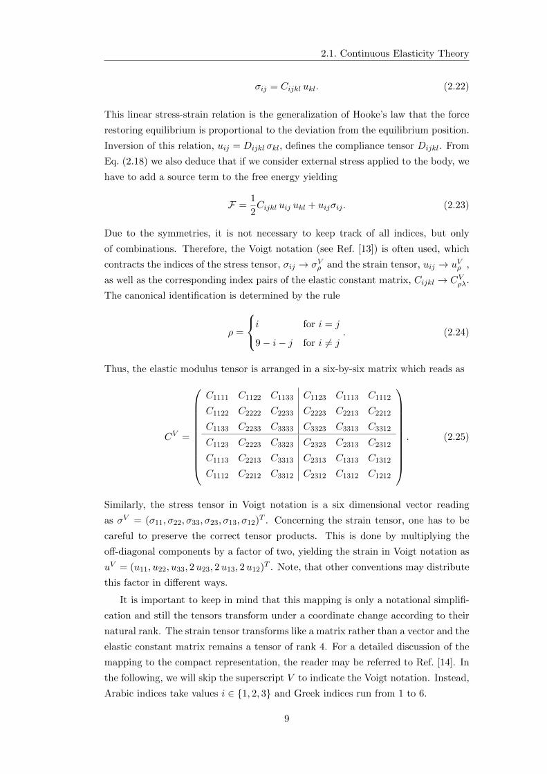
Due to the symmetries, it is not necessary to keep track of all indices, but only
of combinations. Therefore, the Voigt notation (see Ref. [13]) is often used, which
contracts the indices of the stress tensor, σij → σVρ and the strain tensor, uij → uVρ ,
as well as the corresponding index pairs of the elastic constant matrix, Cijkl → CVρλ.
The canonical identification is determined by the rule
ρ =
i for i = j
9− i− j for i 6= j. (2.24)
Thus, the elastic modulus tensor is arranged in a six-by-six matrix which reads as
CV =
C1111 C1122 C1133 C1123 C1113 C1112
C1122 C2222 C2233 C2223 C2213 C2212
C1133 C2233 C3333 C3323 C3313 C3312
C1123 C2223 C3323 C2323 C2313 C2312
C1113 C2213 C3313 C2313 C1313 C1312
C1112 C2212 C3312 C2312 C1312 C1212
. (2.25)
Similarly, the stress tensor in Voigt notation is a six dimensional vector reading
as σV = (σ11, σ22, σ33, σ23, σ13, σ12)T . Concerning the strain tensor, one has to be
careful to preserve the correct tensor products. This is done by multiplying the
off-diagonal components by a factor of two, yielding the strain in Voigt notation as
uV = (u11, u22, u33, 2u23, 2u13, 2u12)T . Note, that other conventions may distribute
this factor in different ways.
It is important to keep in mind that this mapping is only a notational simplifi-
cation and still the tensors transform under a coordinate change according to their
natural rank. The strain tensor transforms like a matrix rather than a vector and the
elastic constant matrix remains a tensor of rank 4. For a detailed discussion of the
mapping to the compact representation, the reader may be referred to Ref. [14]. In
the following, we will skip the superscript V to indicate the Voigt notation. Instead,
Arabic indices take values i ∈ 1, 2, 3 and Greek indices run from 1 to 6.
9
Chapter 2. Elasticity
In absence of external strains the free energy, Eq. (2.23), reads as
F =1
2Cρλ uρ uλ, (2.26)
and it is, thus, a quadratic form in a six-dimensional vector space. For the system
to be stable under elastic fluctuations, the matrix Cρλ has to be positive definite.
As known from linear algebra, this is true if and only if all principal minors, are
positive, i.e.,
C11 > 0,
∣∣∣∣∣C11 C12
C12 C22
∣∣∣∣∣ > 0, · · · , detC > 0, (2.27)
which are the conditions of stability.
Isotropic bodies are of particular simplicity. The free energy is then given by the
only two quadratic invariants the strain tensor can form, namely its squared trace
and the trace of its square
F =1
2λu2
ii + µuijuji. (2.28)
The constants λ = C12 and µ = C44 are called the Lame coefficients.
In Eq. (2.7), we have seen that the trace of the strain tensor yields the volume
change. We therefore may separate the trace of the strain tensor
uij = ukk + uij = ukk +
(uij −
1
3δij ukk
)(2.29)
which yields the free energy
F =1
2K u2
ii + µu2ij , (2.30)
The first term describes the free energy due to a pure hydrostatic compression, i.e.,
a volume change where the shape of the body is preserved. Therefore the constant
K = λ + 23µ is called the bulk modulus. The second term on the other hand,
only accounts for deformations which alter the shape of the body and preserves the
volume. This is called a pure shear strain, and µ is, correspondingly, called the shear
modulus. Stability under elastic fluctuations requires both constants to be positive.
2.2 Crystal Elasticity
The previous considerations were valid for elastic deformations of rigid bodies which
can be described in a continuum theory. However, solid state theory mainly focuses
on crystal systems where the constituents of the body, i.e., the atoms, are arranged
on a periodic lattice. The distance between the atomic positions is usually much
10
2.2. Crystal Elasticity
larger than the typical deformations, thus, a continuous description is oversimpli-
fied. In particular, we have an invariance under a discrete set of translations and,
depending on the crystal symmetry, may have also other discrete symmetries such
as rotations by certain angles. These microscopic details of the solid will show their
signatures also in macroscopic quantities, as they must have the same symmetries.
2.2.1 Crystal Structure
A perfect crystal is characterized by a Bravais lattice, which is a periodic structure
build up from three lattice vectors, ai. Every site of the Bravais lattice can be
reached from any other site by a vector
Rn = niai, (2.31)
where n = (n1, n2, n3) is a three tuple of integer numbers.
On every lattice site a primitive lattice cell is centered, the so-called Wigner-Seitz
cell, which is given by
VW =
x ∈ R3
∣∣∣∣ |x| ≤ |x−Rn| ∀n 6= (0, 0, 0)
, (2.32)
where the origin is placed at the Bravais lattice point. Therefore, the periodic array
of primitive cells fills the whole space.
For simple lattices, every cell is occupied by one atom of the same sort positioned
in the center of the cell. For more complex materials, a number of N atoms are
arranged in the cell forming the basis of the crystal. The position of the m-th atom
with respect to the cell center is given by some constant vector, xm, which has to
be within the Wigner-Seitz cell. Therefore, adapting the notation of Ref. [15], the
position of every atom of a crystal can be written as
r[nm] = Rn + xm with xm ∈ VW . (2.33)
From the basis vectors, aj , one obtains another set of vectors, bi, by the condition
bi · aj = 2π δij . These vectors are called the reciprocal vectors and have the form
bi =π εijk
det(a1,a2,a3)(aj × ak) , (2.34)
where εijk denotes the Levi-Civita symbol. Similar to the lattice vectors, the recip-
rocal vectors span a lattice, where every point is connected to any other point by a
vector
Gh = hibi with hi ∈ Z. (2.35)
11
Chapter 2. Elasticity
This lattice is called the reciprocal Bravais lattice, and the corresponding Wigner-
Seitz cell in reciprocal space is called the first Brillouin zone.
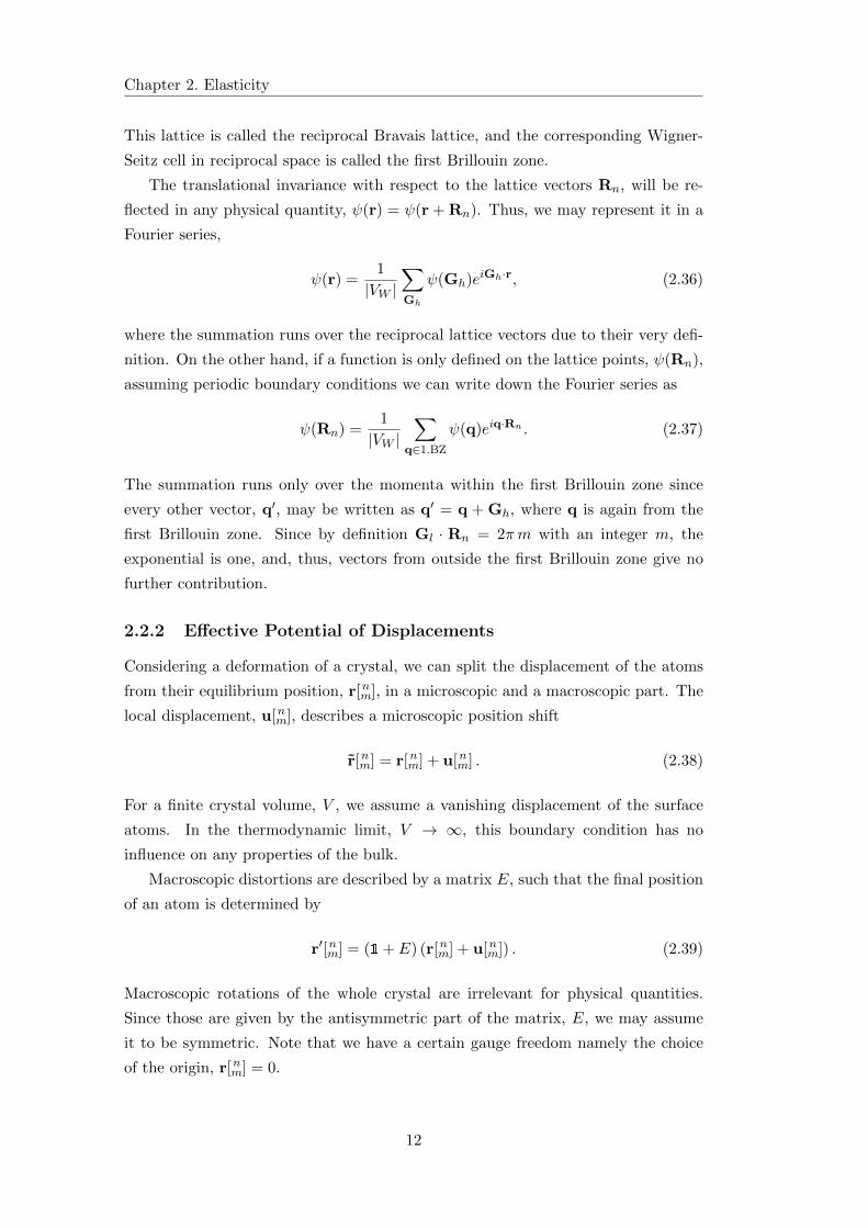
The translational invariance with respect to the lattice vectors Rn, will be re-
flected in any physical quantity, ψ(r) = ψ(r + Rn). Thus, we may represent it in a
Fourier series,
ψ(r) =1
|VW |∑
Gh
ψ(Gh)eiGh·r, (2.36)
where the summation runs over the reciprocal lattice vectors due to their very defi-
nition. On the other hand, if a function is only defined on the lattice points, ψ(Rn),
assuming periodic boundary conditions we can write down the Fourier series as
ψ(Rn) =1
|VW |∑
q∈1.BZ
ψ(q)eiq·Rn . (2.37)
The summation runs only over the momenta within the first Brillouin zone since
every other vector, q′, may be written as q′ = q + Gh, where q is again from the
first Brillouin zone. Since by definition Gl · Rn = 2πm with an integer m, the
exponential is one, and, thus, vectors from outside the first Brillouin zone give no
further contribution.
2.2.2 Effective Potential of Displacements
Considering a deformation of a crystal, we can split the displacement of the atoms
from their equilibrium position, r[nm], in a microscopic and a macroscopic part. The
local displacement, u[nm], describes a microscopic position shift
r[nm] = r[nm] + u[nm] . (2.38)
For a finite crystal volume, V , we assume a vanishing displacement of the surface
atoms. In the thermodynamic limit, V → ∞, this boundary condition has no
influence on any properties of the bulk.
Macroscopic distortions are described by a matrix E, such that the final position
of an atom is determined by
r′[nm] = (1+ E) (r[nm] + u[nm]) . (2.39)
Macroscopic rotations of the whole crystal are irrelevant for physical quantities.
Since those are given by the antisymmetric part of the matrix, E, we may assume
it to be symmetric. Note that we have a certain gauge freedom namely the choice
of the origin, r[nm] = 0.
12
2.2. Crystal Elasticity
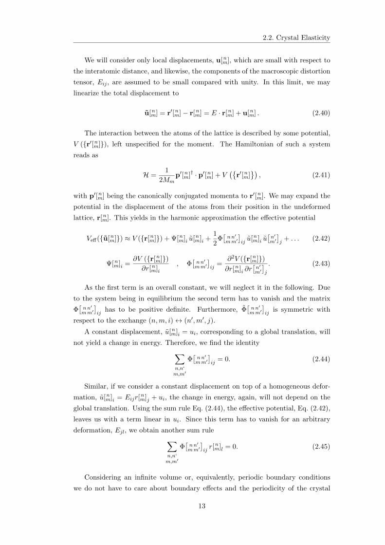
We will consider only local displacements, u[nm], which are small with respect to
the interatomic distance, and likewise, the components of the macroscopic distortion
tensor, Eij , are assumed to be small compared with unity. In this limit, we may
linearize the total displacement to
u[nm] = r′[nm]− r[nm] = E · r[nm] + u[nm] . (2.40)
The interaction between the atoms of the lattice is described by some potential,
V (r′[nm]), left unspecified for the moment. The Hamiltonian of such a system
reads as
H =1
2Mmp′[nm]† · p′[nm] + V
(r′[nm]
), (2.41)
with p′[nm] being the canonically conjugated momenta to r′[nm]. We may expand the
potential in the displacement of the atoms from their position in the undeformed
lattice, r[nm]. This yields in the harmonic approximation the effective potential
Veff(u[nm]) ≈ V (r[nm]) + Ψ[nm]i u[nm]i +1
2Φ[nn′mm′
]iju[nm]i u
[n′m′]j
+ . . . (2.42)
Ψ[nm]i =∂V (r[nm])∂r[nm]i
, Φ[nn′mm′
]ij
=∂2V (r[nm])∂r[nm]i ∂r
[n′m′]j
. (2.43)
As the first term is an overall constant, we will neglect it in the following. Due
to the system being in equilibrium the second term has to vanish and the matrix
Φ[nn′mm′
]ij
has to be positive definite. Furthermore, Φ[nn′mm′
]ij
is symmetric with
respect to the exchange (n,m, i)↔ (n′,m′, j).
A constant displacement, u[nm]i = ui, corresponding to a global translation, will
not yield a change in energy. Therefore, we find the identity
∑
n,n‘m,m′
Φ[nn′mm′
]ij
= 0. (2.44)
Similar, if we consider a constant displacement on top of a homogeneous defor-
mation, u[nm]i = Eijr[nm]j + ui, the change in energy, again, will not depend on the
global translation. Using the sum rule Eq. (2.44), the effective potential, Eq. (2.42),
leaves us with a term linear in ui. Since this term has to vanish for an arbitrary
deformation, Ejl, we obtain another sum rule
∑
n,n‘m,m′
Φ[nn′mm′
]ijr[nm]l = 0. (2.45)
Considering an infinite volume or, equivalently, periodic boundary conditions
we do not have to care about boundary effects and the periodicity of the crystal
13
Chapter 2. Elasticity
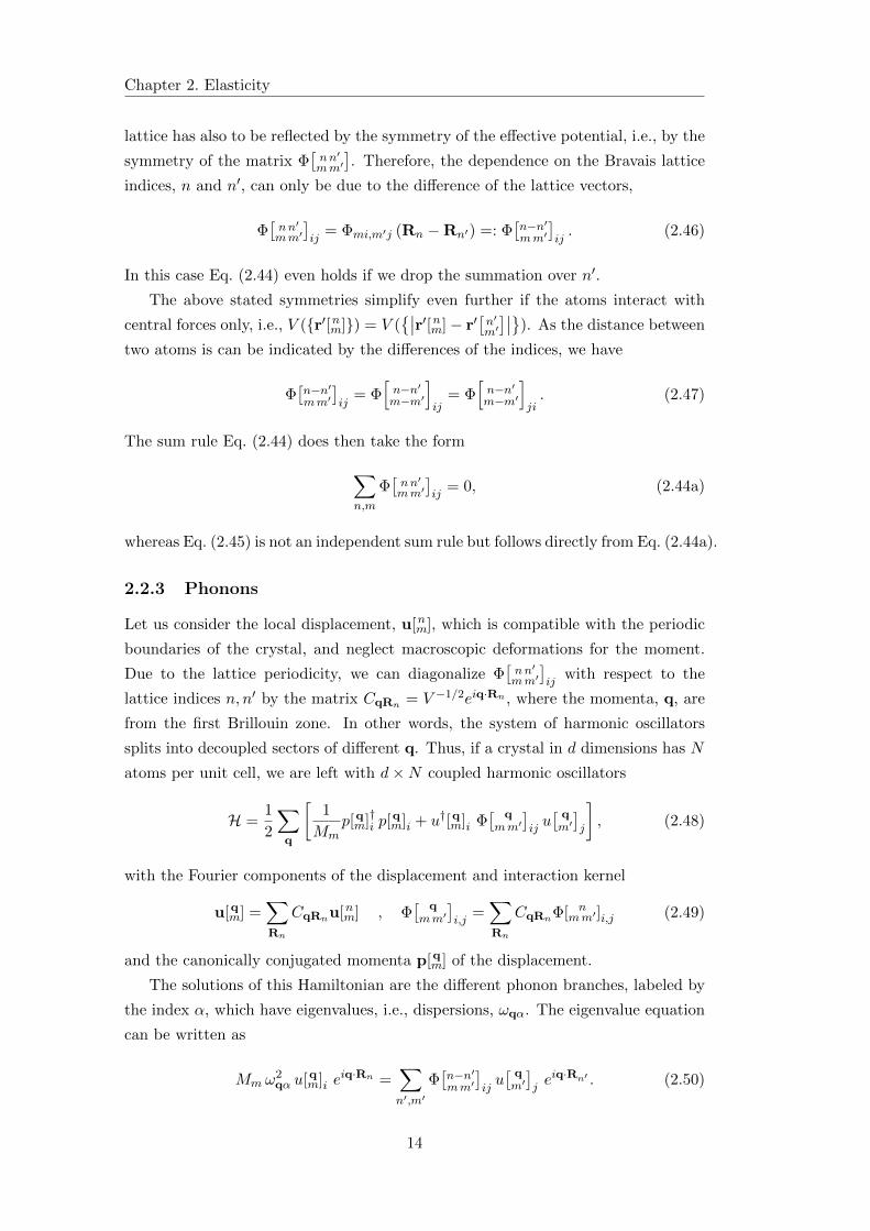
lattice has also to be reflected by the symmetry of the effective potential, i.e., by the
symmetry of the matrix Φ[nn′mm′
]. Therefore, the dependence on the Bravais lattice
indices, n and n′, can only be due to the difference of the lattice vectors,
Φ[nn′mm′
]ij
= Φmi,m′j (Rn −Rn′) =: Φ[n−n′mm′
]ij. (2.46)
In this case Eq. (2.44) even holds if we drop the summation over n′.
The above stated symmetries simplify even further if the atoms interact with
central forces only, i.e., V (r′[nm]) = V (∣∣r′[nm]− r′
[n′m′]∣∣). As the distance between
two atoms is can be indicated by the differences of the indices, we have
Φ[n−n′mm′
]ij
= Φ[n−n′m−m′
]ij
= Φ[n−n′m−m′
]ji. (2.47)
The sum rule Eq. (2.44) does then take the form
∑
n,m
Φ[nn′mm′
]ij
= 0, (2.44a)
whereas Eq. (2.45) is not an independent sum rule but follows directly from Eq. (2.44a).
2.2.3 Phonons
Let us consider the local displacement, u[nm], which is compatible with the periodic
boundaries of the crystal, and neglect macroscopic deformations for the moment.
Due to the lattice periodicity, we can diagonalize Φ[nn′mm′
]ij
with respect to the
lattice indices n, n′ by the matrix CqRn = V −1/2eiq·Rn , where the momenta, q, are
from the first Brillouin zone. In other words, the system of harmonic oscillators
splits into decoupled sectors of different q. Thus, if a crystal in d dimensions has N
atoms per unit cell, we are left with d×N coupled harmonic oscillators
H =1
2
∑
q
[1
Mmp[qm]†i p[
qm]i + u†[qm]i Φ
[ qmm′
]iju[ qm′]j
], (2.48)
with the Fourier components of the displacement and interaction kernel
u[qm] =∑
Rn
CqRnu[nm] , Φ[ qmm′
]i,j
=∑
Rn
CqRnΦ[ nmm′]i,j (2.49)
and the canonically conjugated momenta p[qm] of the displacement.
The solutions of this Hamiltonian are the different phonon branches, labeled by
the index α, which have eigenvalues, i.e., dispersions, ωqα. The eigenvalue equation
can be written as
Mm ω2qα u[qm]i e
iq·Rn =∑
n′,m′
Φ[n−n′mm′
]iju[ qm′]jeiq·Rn′ . (2.50)
14
2.2. Crystal Elasticity
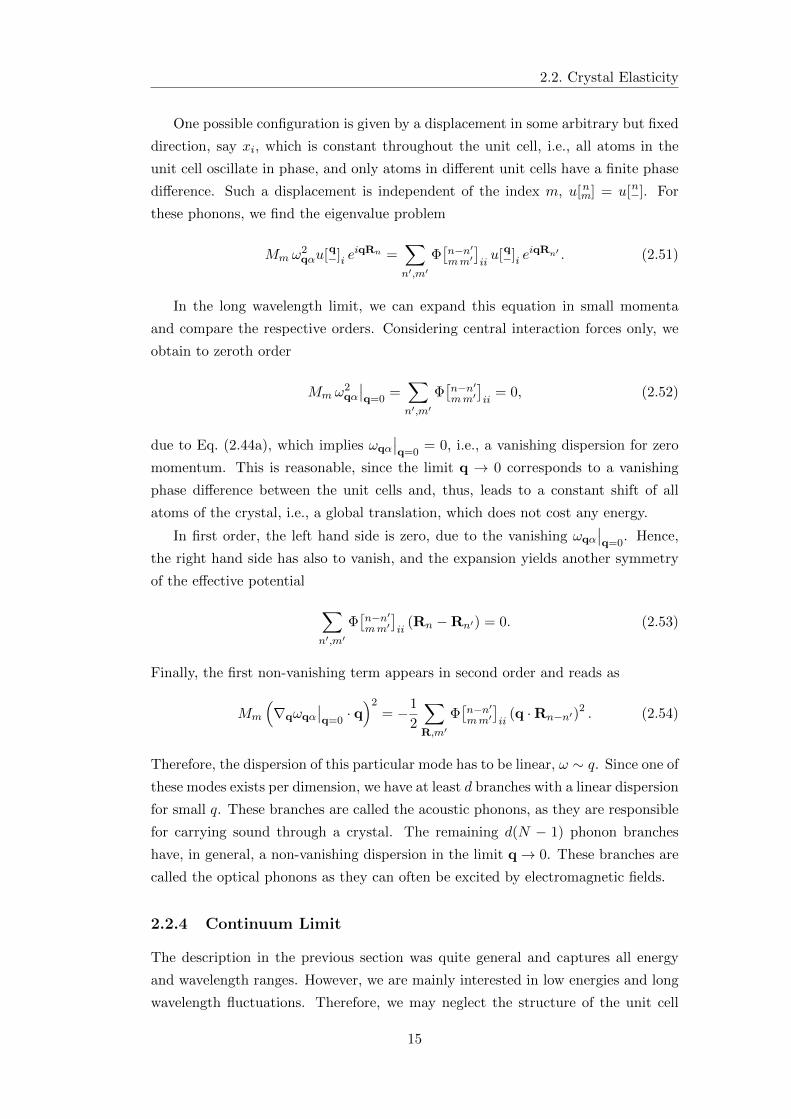
One possible configuration is given by a displacement in some arbitrary but fixed
direction, say xi, which is constant throughout the unit cell, i.e., all atoms in the
unit cell oscillate in phase, and only atoms in different unit cells have a finite phase
difference. Such a displacement is independent of the index m, u[nm] = u[n−]. For
these phonons, we find the eigenvalue problem
Mm ω2qαu[q−]i e
iqRn =∑
n′,m′
Φ[n−n′mm′
]iiu[q−]i e
iqRn′ . (2.51)
In the long wavelength limit, we can expand this equation in small momenta
and compare the respective orders. Considering central interaction forces only, we
obtain to zeroth order
Mm ω2qα
∣∣q=0
=∑
n′,m′
Φ[n−n′mm′
]ii
= 0, (2.52)
due to Eq. (2.44a), which implies ωqα
∣∣q=0
= 0, i.e., a vanishing dispersion for zero
momentum. This is reasonable, since the limit q → 0 corresponds to a vanishing
phase difference between the unit cells and, thus, leads to a constant shift of all
atoms of the crystal, i.e., a global translation, which does not cost any energy.
In first order, the left hand side is zero, due to the vanishing ωqα
∣∣q=0
. Hence,
the right hand side has also to vanish, and the expansion yields another symmetry
of the effective potential
∑
n′,m′
Φ[n−n′mm′
]ii
(Rn −Rn′) = 0. (2.53)
Finally, the first non-vanishing term appears in second order and reads as
Mm
(∇qωqα
∣∣q=0· q)2
= −1
2
∑
R,m′
Φ[n−n′mm′
]ii
(q ·Rn−n′)2 . (2.54)
Therefore, the dispersion of this particular mode has to be linear, ω ∼ q. Since one of
these modes exists per dimension, we have at least d branches with a linear dispersion
for small q. These branches are called the acoustic phonons, as they are responsible
for carrying sound through a crystal. The remaining d(N − 1) phonon branches
have, in general, a non-vanishing dispersion in the limit q→ 0. These branches are
called the optical phonons as they can often be excited by electromagnetic fields.
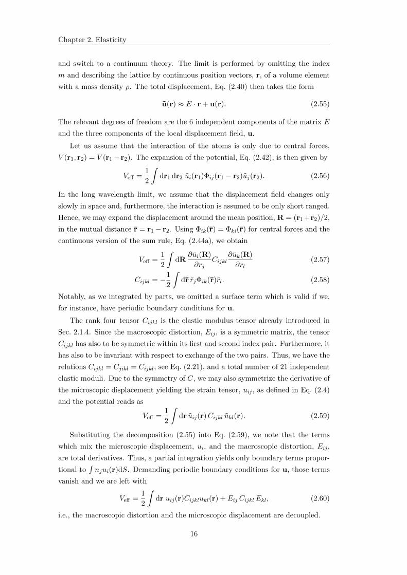
2.2.4 Continuum Limit
The description in the previous section was quite general and captures all energy
and wavelength ranges. However, we are mainly interested in low energies and long
wavelength fluctuations. Therefore, we may neglect the structure of the unit cell
15
Chapter 2. Elasticity
and switch to a continuum theory. The limit is performed by omitting the index
m and describing the lattice by continuous position vectors, r, of a volume element
with a mass density ρ. The total displacement, Eq. (2.40) then takes the form
u(r) ≈ E · r + u(r). (2.55)
The relevant degrees of freedom are the 6 independent components of the matrix E
and the three components of the local displacement field, u.
Let us assume that the interaction of the atoms is only due to central forces,
V (r1, r2) = V (r1− r2). The expansion of the potential, Eq. (2.42), is then given by
Veff =1
2
∫dr1 dr2 ui(r1)Φij(r1 − r2)uj(r2). (2.56)
In the long wavelength limit, we assume that the displacement field changes only
slowly in space and, furthermore, the interaction is assumed to be only short ranged.
Hence, we may expand the displacement around the mean position, R = (r1 +r2)/2,
in the mutual distance r = r1− r2. Using Φik(r) = Φki(r) for central forces and the
continuous version of the sum rule, Eq. (2.44a), we obtain
Veff =1
2
∫dR
∂ui(R)
∂rjCijkl
∂uk(R)
∂rl(2.57)
Cijkl = −1
2
∫dr rjΦik(r)rl. (2.58)
Notably, as we integrated by parts, we omitted a surface term which is valid if we,
for instance, have periodic boundary conditions for u.
The rank four tensor Cijkl is the elastic modulus tensor already introduced in
Sec. 2.1.4. Since the macroscopic distortion, Eij , is a symmetric matrix, the tensor
Cijkl has also to be symmetric within its first and second index pair. Furthermore, it
has also to be invariant with respect to exchange of the two pairs. Thus, we have the
relations Cijkl = Cjikl = Cijkl, see Eq. (2.21), and a total number of 21 independent
elastic moduli. Due to the symmetry of C, we may also symmetrize the derivative of
the microscopic displacement yielding the strain tensor, uij , as defined in Eq. (2.4)
and the potential reads as
Veff =1
2
∫dr uij(r)Cijkl ukl(r). (2.59)
Substituting the decomposition (2.55) into Eq. (2.59), we note that the terms
which mix the microscopic displacement, ui, and the macroscopic distortion, Eij ,
are total derivatives. Thus, a partial integration yields only boundary terms propor-
tional to∫njui(r)dS. Demanding periodic boundary conditions for u, those terms
vanish and we are left with
Veff =1
2
∫dr uij(r)Cijklukl(r) + Eij CijklEkl, (2.60)
i.e., the macroscopic distortion and the microscopic displacement are decoupled.
16
2.2. Crystal Elasticity
Concerning the elastic modulus tensor, Eq. (2.58) implies also invariance under
exchanging i↔ k and j ↔ l, respectively, such that the tensor is fully symmetric in
all its indices. In Voigt notation, these additional symmetries yield
C23 = C44, C13 = C55, C12 = C66,
C14 = C56, C25 = C46, C36 = C45,
which are called the Cauchy relations and reduce the number of independent elastic
moduli to a total number of 15.
These relations are, however, in physical systems not fulfilled in general. They
originate from the assumption that the atoms interact with central forces only which
is in general not valid. For instance, in covalent crystals the interaction between
the atoms is mediated by the valence electrons which are in general in anisotropic
orbitals. In ionic crystals, on the other hand, a deformation of the ions yields a
polarization giving rise to a surface charge, which has a macroscopic electric field.
The shape of the field depends on the geometry of the probe itself and, thus, has
no unique thermodynamic limit. The Cauchy relations are, however, approximately
fulfilled, if every atom is a center of inversion symmetry, since then no macroscopic
field will arise.
As we consider crystals having a lattice structure with certain symmetries, these
must also be reflected by the elastic modulus tensor. This yields additional restric-
tions reducing the number of independent components. As it turns out, the 32
crystallographic point groups give rise to 9 different symmetry classes of the elastic
modulus tensor which are discussed in App. A.
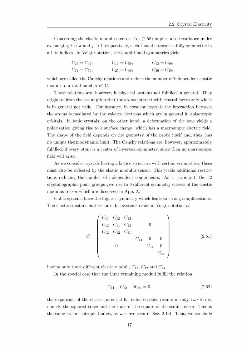
Cubic systems have the highest symmetry which leads to strong simplifications.
The elastic constant matrix for cubic systems reads in Voigt notation as
C =
C11 C12 C12
C12 C11 C12 0
C12 C12 C11
C44 0 0
0 C44 0
C44
, (2.61)
having only three different elastic moduli, C11, C12 and C44.
In the special case that the three remaining moduli fulfill the relation
C11 − C12 − 2C44 = 0, (2.62)
the expansion of the elastic potential for cubic crystals results in only two terms,
namely the squared trace and the trace of the square of the strain tensor. This is
the same as for isotropic bodies, as we have seen in Sec. 2.1.4. Thus, we conclude
17
Chapter 2. Elasticity
that a cubic crystal with the above relation of its elastic constants, Eq. (2.62), can
be considered as being completely isotropic with respect to the elastic degrees of
freedom. The bulk modulus reads as K = C11− 43C44 = C11− 2
3(C11−C12), whereas
the shear modulus is given by µ = C44.
Let us consider the dynamics of the lattice which follows from the equations of
motion for the strain, E, and the phonons, u. Of course, in the long wavelength
limit, we will only deal with the acoustic phonons. However, due to the dispersion
relation those are the low energy excitations and, thus, of particular interest.
Adding a time dependence of the displacement field, we have also to integrate
over the time to obtain the energy. The total kinetic energy due to the atomic
motion of a crystal of volume V is, thus, given by
Tel =
∫
Vdt dr
ρ
2˙ui(r, t) ˙ui(r, t), (2.63)
whereas the potential energy is given by Eq. (2.60) with an additional time depen-
dence of the field. Since the integral over the microscopic strain vanishes we may
rewrite it conveniently to
Vel =
∫
Vdt dr uij(r, t)Cijklukl(r, t). (2.64)
To obtain the equations of motion for the macroscopic distortion and the micro-
scopic strain we have to vary the atomic displacement as, δui = δui + δEijrj . The
resulting change of the action is to linear order given by
δS =
∫
Vdtdr ρ
[(∂tδui(r, t)) ˙ui(r, t) + (∂tδEij(t)) rj ˙ui(r, t)
]
−∫
Vdtdr [(∂j δui(r))Cijklukl(r) + δEij Cijklukl(r)] . (2.65)
After a partial integration and sorting by the variations, δui and δEij , we obtain
δS = −∫
dt
∫
Vdr ∂j [δui(r, t) Cijklukl(r, t)] (2.66)
−∫
dt
∫
Vdr δui(r, t)
[ρ¨ui(r, t)− ∂j (Cijklukl(r, t))
]
−∫
dt δEij(t)
∫
Vdr[rj ¨ui(r, t) + Cijklukl(r, t)
]
The first term is a boundary term which can be rewritten by substituting the
strain tensor, σij = Cijklukl, as
∫dt
∫
∂VdS njσij(r, t) δui(r, t), (2.67)
where n is the vector normal to the surface. As the energy change has to vanish
irrespectively of the particular variation the integrands have to be zero. Therefore,
the first and second line of Eq. (2.66) leaves us with two sets of equations, namely
18
2.2. Crystal Elasticity
njσij(r, t)
∣∣∣∣∂V
= 0 (2.68)
ρ(ui(r, t) + Eik(t)rk
)= ∂jσij(r, t). (2.69)
We may multiply Eq. (2.69) by rs and integrate the resulting equation over the
volume. Integrating the right hand side by parts and using the boundary condition,
Eq. (2.68), we obtain by relabeling the summation indices
ρ
∫
Vdr(rj ui(r, t) + rjEik(t)rk
)= −
∫
Vdrσij(r, t) (2.70)
which is exactly the equation of motion following from the third line of Eq. (2.66).
Thus, we obtain six independent equations of motion for the six independent
strain components, uij . Since a decomposition of the total strain is always a matter of
choice, we cannot expect more than these. However, for the particular decomposition
into the macroscopic and the microscopic part, we also require the local displacement
to have a vanishing zero-momentum component which yields an additional set of
three equations. Altogether we obtain the nine equations
ρ(ui(r, t) + Eik(t)rk
)= Cijkl∂j∂kul(r, t) (2.71a)
njCijkl∂kul(r, t)
∣∣∣∣∂V
= −CijklnjEkl (2.71b)
∫
Vdrui(r, t) = 0 (2.71c)
of which the first three, Eqs. (2.71a), are local equations, and the remaining six,
Eqs. (2.71b) and (2.71c), are global. This corresponds to the three local degrees of
freedom, ui(r, t) and the six global degrees of freedom, Eij(t).
Apparently, the macroscopic and microscopic strain are not independent from
each other. Furthermore, especially the Eqs. (2.71b) are defined only on the surface
of the crystal including the surface normals, n. Therefore, the solution of the equa-
tion of motions depends on the actual shape of the crystal and can not be obtained
in general. However, Eqs. (2.71a-c) define the crystal motion for a given geometry.
Let us consider for simplicity the situation of a static macroscopic deformation,
Eij = 0. Then, Eq. (2.71a) depends only on the microscopic displacement as
ρui(r, t) = Cijkl ∂j∂kul(r, t). (2.72)
The macroscopic deformation does however still enter through the boundary condi-
tions, Eqs. (2.71b). A Fourier transformation of Eq. (2.72) in space and time yields
the eigenvalue equation
ρω2ui(q, ω) = Dil(q)ul(q, ω), (2.73)
Dil(q) = Cijkl qj qk (2.74)
19
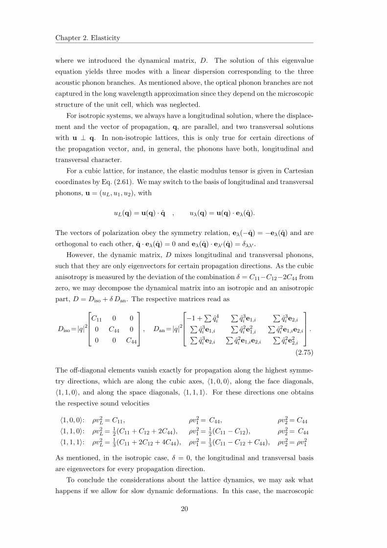
Chapter 2. Elasticity
where we introduced the dynamical matrix, D. The solution of this eigenvalue
equation yields three modes with a linear dispersion corresponding to the three
acoustic phonon branches. As mentioned above, the optical phonon branches are not
captured in the long wavelength approximation since they depend on the microscopic
structure of the unit cell, which was neglected.
For isotropic systems, we always have a longitudinal solution, where the displace-
ment and the vector of propagation, q, are parallel, and two transversal solutions
with u ⊥ q. In non-isotropic lattices, this is only true for certain directions of
the propagation vector, and, in general, the phonons have both, longitudinal and
transversal character.
For a cubic lattice, for instance, the elastic modulus tensor is given in Cartesian
coordinates by Eq. (2.61). We may switch to the basis of longitudinal and transversal
phonons, u = (uL, u1, u2), with
uL(q) = u(q) · q , uλ(q) = u(q) · eλ(q).
The vectors of polarization obey the symmetry relation, eλ(−q) = −eλ(q) and are
orthogonal to each other, q · eλ(q) = 0 and eλ(q) · eλ′(q) = δλλ′ .
However, the dynamic matrix, D mixes longitudinal and transversal phonons,
such that they are only eigenvectors for certain propagation directions. As the cubic
anisotropy is measured by the deviation of the combination δ = C11−C12−2C44 from
zero, we may decompose the dynamical matrix into an isotropic and an anisotropic
part, D = Diso + δ Dan. The respective matrices read as
Diso = |q|2
C11 0 0
0 C44 0
0 0 C44
, Dan = |q|2
−1 +
∑q4i
∑q3i e1,i
∑q3i e2,i∑
q3i e1,i
∑q2i e
21,i
∑q2i e1,ie2,i∑
q3i e2,i
∑q2i e1,ie2,i
∑q2i e
22,i
.
(2.75)
The off-diagonal elements vanish exactly for propagation along the highest symme-
try directions, which are along the cubic axes, 〈1, 0, 0〉, along the face diagonals,
〈1, 1, 0〉, and along the space diagonals, 〈1, 1, 1〉. For these directions one obtains
the respective sound velocities
〈1, 0, 0〉: ρv2L = C11, ρv2
1 = C44, ρv22 = C44
〈1, 1, 0〉: ρv2L = 1
2(C11 + C12 + 2C44), ρv21 = 1
2(C11 − C12), ρv22 = C44
〈1, 1, 1〉: ρv2L = 1
3(C11 + 2C12 + 4C44), ρv21 = 1
3(C11 − C12 + C44), ρv22 = ρv2
1
As mentioned, in the isotropic case, δ = 0, the longitudinal and transversal basis
are eigenvectors for every propagation direction.
To conclude the considerations about the lattice dynamics, we may ask what
happens if we allow for slow dynamic deformations. In this case, the macroscopic
20
2.3. Phonon Field Integral
strain tensor acts as a perturbation of the phonon solution derived above. As men-
tioned above, for a given crystal shape we may still solve the equation of motions,
for instance by a Green’s function approach, at least numerical.
However, since phonons describe coherent harmonic oscillations of the lattice
atoms with periodic boundary conditions, we can not expect a phonon-like solution
for a non-static boundary. Due to the dynamic macroscopic distortion the crystal
changes its shape with time and, thus, simple phonon modes are destroyed.
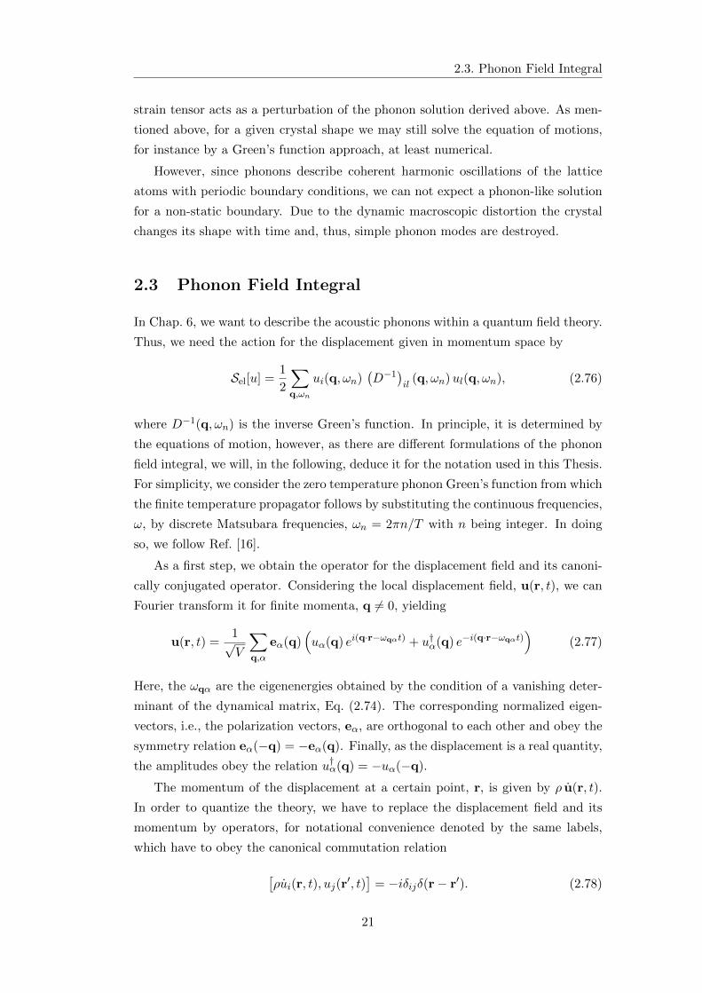
2.3 Phonon Field Integral
In Chap. 6, we want to describe the acoustic phonons within a quantum field theory.
Thus, we need the action for the displacement given in momentum space by
Sel[u] =1
2
∑
q,ωn
ui(q, ωn)(D−1
)il
(q, ωn)ul(q, ωn), (2.76)
where D−1(q, ωn) is the inverse Green’s function. In principle, it is determined by
the equations of motion, however, as there are different formulations of the phonon
field integral, we will, in the following, deduce it for the notation used in this Thesis.
For simplicity, we consider the zero temperature phonon Green’s function from which
the finite temperature propagator follows by substituting the continuous frequencies,
ω, by discrete Matsubara frequencies, ωn = 2πn/T with n being integer. In doing
so, we follow Ref. [16].
As a first step, we obtain the operator for the displacement field and its canoni-
cally conjugated operator. Considering the local displacement field, u(r, t), we can
Fourier transform it for finite momenta, q 6= 0, yielding
u(r, t) =1√V
∑
q,α
eα(q)(uα(q) ei(q·r−ωqαt) + u†α(q) e−i(q·r−ωqαt)
)(2.77)
Here, the ωqα are the eigenenergies obtained by the condition of a vanishing deter-
minant of the dynamical matrix, Eq. (2.74). The corresponding normalized eigen-
vectors, i.e., the polarization vectors, eα, are orthogonal to each other and obey the
symmetry relation eα(−q) = −eα(q). Finally, as the displacement is a real quantity,
the amplitudes obey the relation u†α(q) = −uα(−q).
The momentum of the displacement at a certain point, r, is given by ρ u(r, t).
In order to quantize the theory, we have to replace the displacement field and its
momentum by operators, for notational convenience denoted by the same labels,
which have to obey the canonical commutation relation
[ρui(r, t), uj(r
′, t)]
= −iδijδ(r− r′). (2.78)
21
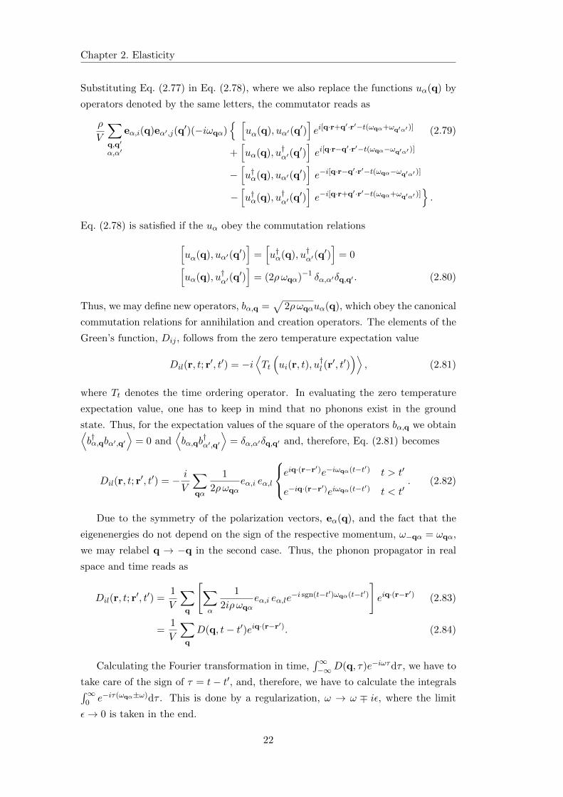
Chapter 2. Elasticity
Substituting Eq. (2.77) in Eq. (2.78), where we also replace the functions uα(q) by
operators denoted by the same letters, the commutator reads as
ρ
V
∑
q,q′
α,α′
eα,i(q)eα′,j(q′)(−iωqα)
[uα(q), uα′(q
′)]ei[q·r+q′·r′−t(ωqα+ωq′α′ )] (2.79)
+[uα(q), u†α′(q
′)]ei[q·r−q
′·r′−t(ωqα−ωq′α′ )]
−[u†α(q), uα′(q
′)]e−i[q·r−q
′·r′−t(ωqα−ωq′α′ )]
−[u†α(q), u†α′(q
′)]e−i[q·r+q′·r′−t(ωqα+ωq′α′ )]
.
Eq. (2.78) is satisfied if the uα obey the commutation relations
[uα(q), uα′(q
′)]
=[u†α(q), u†α′(q
′)]
= 0[uα(q), u†α′(q
′)]
= (2ρωqα)−1 δα,α′δq,q′ . (2.80)
Thus, we may define new operators, bα,q =√
2ρωqαuα(q), which obey the canonical
commutation relations for annihilation and creation operators. The elements of the
Green’s function, Dij , follows from the zero temperature expectation value
Dil(r, t; r′, t′) = −i
⟨Tt
(ui(r, t), u
†l (r′, t′)
)⟩, (2.81)
where Tt denotes the time ordering operator. In evaluating the zero temperature
expectation value, one has to keep in mind that no phonons exist in the ground
state. Thus, for the expectation values of the square of the operators bα,q we obtain⟨b†α,qbα′,q′
⟩= 0 and
⟨bα,qb
†α′,q′
⟩= δα,α′δq,q′ and, therefore, Eq. (2.81) becomes
Dil(r, t; r′, t′) = − i
V
∑
qα
1
2ρωqαeα,i eα,l
eiq·(r−r
′)e−iωqα(t−t′) t > t′
e−iq·(r−r′)eiωqα(t−t′) t < t′
. (2.82)
Due to the symmetry of the polarization vectors, eα(q), and the fact that the
eigenenergies do not depend on the sign of the respective momentum, ω−qα = ωqα,
we may relabel q → −q in the second case. Thus, the phonon propagator in real
space and time reads as
Dil(r, t; r′, t′) =
1
V
∑
q
[∑
α
1
2iρ ωqαeα,i eα,le
−i sgn(t−t′)ωqα(t−t′)
]eiq·(r−r
′) (2.83)
=1
V
∑
q
D(q, t− t′)eiq·(r−r′). (2.84)
Calculating the Fourier transformation in time,∫∞−∞D(q, τ)e−iωτdτ , we have to
take care of the sign of τ = t− t′, and, therefore, we have to calculate the integrals∫∞0 e−iτ(ωqα±ω)dτ . This is done by a regularization, ω → ω ∓ iε, where the limit
ε→ 0 is taken in the end.
22
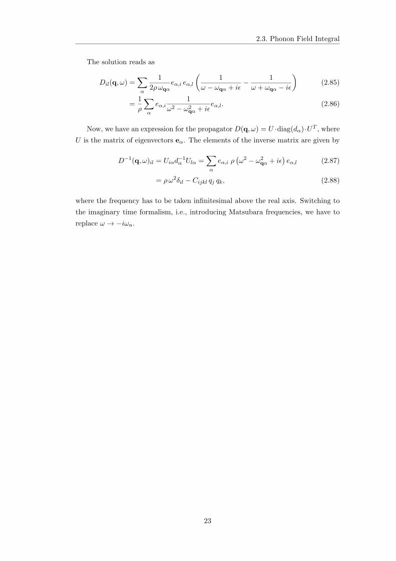
2.3. Phonon Field Integral
The solution reads as
Dil(q, ω) =∑
α
1
2ρωqαeα,i eα,l
(1
ω − ωqα + iε− 1
ω + ωqα − iε
)(2.85)
=1
ρ
∑
α
eα,i1
ω2 − ω2qα + iε
eα,l. (2.86)
Now, we have an expression for the propagator D(q, ω) = U ·diag(dα)·UT , where
U is the matrix of eigenvectors eα. The elements of the inverse matrix are given by
D−1(q, ω)il = Uiαd−1α Ulα =
∑
α
eα,i ρ(ω2 − ω2
qα + iε)eα,l (2.87)
= ρω2δil − Cijkl qj qk, (2.88)
where the frequency has to be taken infinitesimal above the real axis. Switching to
the imaginary time formalism, i.e., introducing Matsubara frequencies, we have to
replace ω → −iωn.
23

Chapter 3
Elasticity in Critical Systems
The influence of a compressible lattice on phase transitions is a widely studied
field, nevertheless, the elastic degrees of freedom still yield interesting and surprising
physics. In particular, as discussed in the following, at a structural phase transition
the speed of sound does generally not vanish but stays finite due to long-ranged
interactions. This result, although long known, is yet surprising when translated in
the language of critical theories. It implies that such a structural phase transition
is a symmetry breaking transition without soft modes. Consequently, second order
structural transitions show mean field behavior.
In this chapter, we will review the studies of classical critical systems on com-
pressible lattices, i.e., the coupling of critical degrees of freedom to the strain and its
fluctuations. We will focus on couplings which are non-perturbative in the sense that
they alter the critical behavior drastically. In particular, second order transitions
may be driven to first order or inherit the elastic mean field behavior.
In Sec. 3.1, we will discuss the Landau theory for elastically coupled phase tran-
sitions in general, focusing on the possible couplings between the critical and the
elastic degrees of freedom. As we will see, the symmetry of the crystal yields re-
straints in that respect. For a more detailed presentation of strain-order parameter
coupling at, in particular, structural phase transitions, the reader may be referred
to Refs. [17, 18].
Thereafter, in Sec. 3.2, we focus on a specific model, namely the classical Ising
model, which is by far the best studied critical theory. In particular, we discuss the
effect of the quadratic and the bilinear coupling of the order parameter to the strain
field. The calculations presented there follow Refs. [19, 20].
Finally, in Sec. 3.3, we review the most complete study on structural phase
transitions, done by Cowley [21]. He studied the strain tensor for all types of crystal
symmetry classes, and characterized the resulting phase transition. For other kinds
of phase transitions in crystals, where a bilinear elastic coupling between order
parameter and the strain is allowed, this discussion carries over.
25
Chapter 3. Elasticity in Critical Systems
3.1 Landau Theory and Elasticity
At a second order phase transition, the symmetry of the system changes sponta-
neously from a high symmetry state to a low symmetry state. In order to describe
such phase transitions, Landau introduced the concept of a macroscopic order pa-
rameter, φ, which is zero in the high symmetry phase and has a finite value in the
other phase [22].
Although this description is valid only for second order transitions, it is still
applicable for nearly continuous first order transitions. In particular, this implies
that Landau theory may be used to describe the behavior in the vicinity of a second
order critical endpoint.
In its original form, Landau theory is a mean field theory, neglecting fluctua-
tions, which is for second order transitions only correct in dimensions above the
so-called upper critical dimension, d+. This dimension depends on the character of
the fluctuations, and, thus, on the universality class of the transition. For the incom-
pressible Ising model, for instance, this upper critical dimension is d+ = 4. Below
this dimension, fluctuations of the order parameter become important and lead to
deviations from mean field behavior, thus, being responsible for the characteristics
of thermodynamic quantities.
Solid state phase transitions, which are amenable to pressure, have, generically,
an intrinsic coupling of the order parameter to the elastic degrees of freedom. The
applied pressure primarily affects the lattice by varying the lattice spacing. This, in
turn, modifies the coupling constants of the critical degrees of freedom, and, thus, a
finite strain also influences the critical behavior. In order to study the extent of this
influence, we first have to ask, how the order parameter and the strain can couple,
an issue which is intimately related to the symmetries of the crystal.
3.1.1 Symmetry and Strain
The interactions between some order parameter and the crystal lattice, of course,
obey the symmetries of this lattice which are characterized by a number of trans-
formations under which the lattice is invariant. These symmetry operations form
a group, namely one of the 32 crystallographic point groups, and, as such, can be
analyzed in the context of group theory. For an introduction to group theory and
its application in physics, the reader may be referred to Ref. [23].
According to group theory, every point group consists of several irreducible repre-
sentations, such that every group element can be written as a sum of the irreducible
representations. Since elasticity deals with a tensor of rank two, the strain tensor,
not all of the irreducible representations are important for our concerns. For in-
stance, a full inversion, mapping every coordinate on its negative, does not affect
the strain tensor as E−α,−β = Eα,β, due to the transformation rules for tensors.
26
3.1. Landau Theory and Elasticity
As a simple example, let us consider a cubic crystal, for which the strain tensor
splits into three irreducible representations, namely a singlet, A, a doublet, E, and
a triplet, T2. The basis vectors of the irreducible representations are given as
A: ε1 = 1√3
(Exx + Eyy + Ezz) ,
E: ε2 = 1√2
(Exx − Eyy),ε3 = 1√
6(2Ezz − Exx − Eyy)
T2: ε4 = Eyz, ε5 = Exz, ε6 = Exy.
The singlet corresponds to an isostructural volume change since it is the trace
of the strain tensor. The doublet is an expansion along one of the cubic axis and a
compression of the other axes such that the total volume is preserved, whereas the
triplet describes pure shear. The elastic constant tensor, given in Eq. (2.61) in Voigt
notation, is in this basis diagonal, reading
C =
C11 + 2C12 0 0
0 C11 − C12 0 0
0 0 C11 − C12
C44 0 0
0 C44 0
C44
. (3.1)
A full classification of the irreducible representations of the strain tensor for each of
the point groups, taken from Ref. [21], can be found in App. B.
In general, a Landau theory is an analytic expansion, which for the strain tensor
can be formulated in terms of the irreducible representations. In every order of the
expansion, we sum over all possible invariants which can be formed from combina-
tions of the irreducible representations. In second order, denoting the basis vectors
of an irreducible representation Γ by εΓ,i, we simply have
Vε =1
2
∑
Γ,i
CΓε2Γ,i
(3.2)
where the CΓ are the corresponding eigenvalues of the elastic constant matrix.
However, in higher order, the expansion is more complicated, as the symmetry of
a representation may not allow invariants of a certain order. In Sec. 3.3 the question
of the existence of a third order invariant of a given irreducible representations will
become particularly important.
On the other hand, in higher orders, more than one invariant may exist. In fourth
order, for instance, a doublet, εE = (εE ,1, εE ,2), has two invariants, namely (ε2E ,1
+
ε2E ,2
)2 and ε4E ,1
+ε4E ,2
. Finally, combinations of invariants are, of course, also invariant
under transformations, and, therefore, in fourth order, all strain components are
27
Chapter 3. Elasticity in Critical Systems
coupled to each other. Neglecting such couplings, the Landau theory, e.g., for a
singlet, εA , is given by
Vε =1
2CAε
2A− U (3)
Aε3A
+ U (4)Aε4A
+ . . . . (3.3)
and symmetry now dictates which of the prefactors, U (n), can be different from zero.
3.1.2 Coupling to the Order Parameter
As mentioned before, phase transitions are described by an order parameter, φ,
which can also be classified in terms of the irreducible representations of the sym-
metry group. The order parameter may be a scalar, e.g., the magnetization in
systems with an easy axis anisotropy, a vector as, for instance, the polarization
vector in ferroelectrics or some higher order tensor.
A coupling term between order parameter and strain has to be an invariant as
well, thus, the possible coupling terms are restricted. In the cubic case, for instance,
the singlet, A, transforms as a scalar and, hence, can only couple to another scalar
quantity, thus, if the order parameter is a vector, it has to enter the coupling term
quadratically. In return, if the order parameter is a scalar, only a singlet, A, can
couple bilinear to it, whereas couplings to doublets or triplets only appear in second
order in the strain and are, thus, much weaker affected by the ordering.
To lowest order, only one of the irreducible representations of the strain, say εA ,
will be strongly affected by the order parameter. For a scalar order parameter, φ,
expansion of the interaction potential to lowest order then yields
Vc = −γ1εAφ− γ2εAφ2. (3.4)
In the following, we restrict ourselves to the discussion of these two terms. In
principle, it would be sufficient to consider the bilinear coupling, i.e., the first term
in Eq. 3.4, as it the most relevant term. However, due to the symmetries of the high
temperature phase, the coupling may have to be invariant under the transformation,
φ → −φ, i.e., an Ising symmetry. In this case a bilinear coupling to the strain is
not allowed and the next order term hast to be considered, namely the quadratic
coupling.
Finally, the part of the Landau theory describing the ordering itself is organized
in ascending orders of invariants of the order parameter. Similar as for the strain,
there may be more than one nth-order invariant which, in principle, have different
coefficients and over which is summed. Also, not all invariants necessarily exist. For
scalar order parameters, the expansion reads as
Vφ = −hφ+r
2φ2 +
v
3!φ3 +
u
4!φ4 + . . . . (3.5)
28
3.2. Ising Theory
In case of a negative forth order coefficient, one has to take higher orders into
account. The cubic term can, for scalar order parameters, always be absorbed by a
shift, φ→ φ− vu .
The coefficients of the expansion are supposed to be only weakly temperature
dependent and are, in fact, treated as constants, apart from the quadratic coefficient,
r, which vanishes at the critical temperature. In the vicinity of the critical point, we
may expand it to first order, obtaining r = a(T − Tc), where Tc denotes the critical
temperature.
3.2 Ising Theory
The theory outlined above is quite general. To be more specific, we will consider in
the following the critical Ising system as it is, one the one hand, one of the most
important and, at the same time, one of the simplest models. It is characterized
by a scalar order parameter, φ, which, in the original formulation of critical spin
systems, denotes the magnetization. Therefore, in absence of a magnetic field, h, i.e.,
if the system is symmetric under time reversal, it is Ising symmetric. The Landau
functional, Eq. (3.5), is, thus, organized in even powers of φ and reads up to fourth
order as
VIsing = −h0 φ+r0
2φ2 +
u0
4!φ4. (3.6)
The magnetic field, h0, breaks the time inversion symmetry, therefore, the linear
coupling to the field is allowed and acts as a source term.
Due to the Ising symmetry at zero field, only a quadratic coupling to the strain is
allowed. However, we may also consider a line of first order phase transitions termi-
nating in a second order critical point. As mentioned above, close to the endpoint,
such a system has only a weak first order transition and can, thus, be described
within a Landau theory. The Ising symmetry is then an emergent symmetry as it
strictly exists only at the critical endpoint, therefore also a bilinear coupling to the
lattice degrees of freedom is allowed. In the following, we will discuss both couplings
in more detail.
3.2.1 Quadratic Coupling
The first considerations of the Ising model on compressible lattices dates back to
Rice [24] in 1954. Based on thermodynamic arguments, he pointed out that the
compressibility becomes negative close to the transition point whenever the specific
heat at constant pressure diverges. Since this is a physically unstable situation, the
system exhibits a first order transition before the critical temperature is reached.
29
Chapter 3. Elasticity in Critical Systems
Only shortly after, Domb [25] gave a very short argument for a first order tran-
sition of the compressible Ising model. He assumed a volume dependence of the
spin-spin interaction, J(v). Since the volume change is, for cubic systems, given by
the strain singlet, A, we indeed identify this coupling to be a quadratic coupling
effect. Writing the free energy as
F = TΨ
(J(v)
T
), (3.7)
the specific heat at constant volume follows as
Cv = T∂2F
∂T 2=
(J(v)
T
)2
Ψ′′(J(v)
T
). (3.8)
A divergence of the specific heat, thus, implies a divergence of Ψ′′ at the critical
temperature. The inverse compressibility can be obtained by differentiating the free
energy twice with respect to the volume, and thus reads as
∂P
∂v= −∂
2F
∂v2= J ′′(v)Ψ′
(J(v)
T
)+J ′(v)2
TΨ′′(J(v)
T
). (3.9)
The first term is finite since J(v) is assumed to be a smooth function and the
first derivative of Ψ describes the pressure, which does not diverge at the transition.
Therefore, the second term of the inverse compressibility becomes dominant before
the Curie point is reached. Since this would imply that a smaller volume yields
a lower pressure, the system becomes unstable. As in the van der Waals gas, a
Maxwell construction yields a first order transition before the Curie point is reached.
Although this argument is based only on a volume dependence of J , further work
by Mattis and Schultz [26] came to the same result
In terms of the Ising critical exponents, a diverging specific heat translates to
a positive critical exponent α. According to the scaling relations the specific heat
exponent is connected to the dimensionality as α = 2−νd, where ν is the correlation
length exponent. Therefore, this kind of elastic coupling yields a preemptive first
order transition and is, thus, non-perturbative for dimensions νd < 2. For a quantum
phase transition the same criterion applies, with the dimension replaced by the
effective dimension of the quantum theory, deff = d + z, where z is the dynamical
exponent, see Ref. [27].
These results were obtained for constant pressures, whereas for a constant vol-
ume Ising criticality is still obtained. However, Fisher [28] assumed that the “real”
underlying phase transition happens at constant pressures and, starting from that
assumption, studied how the system behaves for a constant volume. By means of
an RG analysis, he found a second order phase transition with so-called Fisher-
renormalized critical exponents, for instance αF = α/(1− α).
30
3.2. Ising Theory
The first to consider the microscopics of the quadratic coupling were Larkin and
Pikin [19], see also [20, 29] for a more comprehensive presentation. They considered
an isotropic crystal at constant pressure and, importantly, took spatial fluctuations
of the order parameter as well as of the elastic degrees of freedom into account.
Similar considerations were made by Sak [30], and subsequent publications [31, 32].
Bergman and Halperin [33] considered for the first time not only elastically
isotropic systems but also cubic lattices. By means of an RG analysis for the order
parameter and the elastic field, they found also a first order transition at constant
pressures. At constant volume, a second order transition with Fisher-renormalized
exponents was found for isotropic crystals, however, only if the surface atoms were
fixed. For the cubic symmetry, a microscopic instability preempted this transition
independent of the boundary conditions.
3.2.2 Microscopics of the Quadratic Coupling
In the following, the microscopic analysis of Larkin and Pikin [19] is reviewed along
the lines of the very pedagogical review of Dunweg [20].
According to Eq. (2.55), the total displacement is split into a macroscopic de-
formation and a microscopic displacement vector, ui(r) = Eijrj + ui(r), from which
the strain tensor in Fourier expansion follows as
uij(r) = Eij +i
2
∑
α,q 6=0
uα(q) [qjeα,i(q) + qieα,j(q)] eiq·r, (3.10)
where we chose for convenience the longitudinal-transversal basis, eα, with e0 = q.
We want to determine the free energy, i.e., the logarithm of the partition function,
of the elastically coupled Ising system in the framework of a classical field theory.
The partition function is given by the functional integral over all degrees of freedom
of the weights, exp [−βH], where H is the Hamiltonian of the system.
The potential per unit volume of the elastic system in terms of the strain tensor
is given by Eq. (2.30), yielding the elastic Hamiltonian per volume
1
VHel =
1
V
∫dr
K
2(uii(r) + Eii)
2 + µ(uij(r) + Eij
)2 − σijEij (3.11)
=K
2E2 + µEijEij − pE − (σij − pδij)Eij (3.12)
+1
2
(K +
4
3µ
)∑
q 6=0
q2 |uL(q)|2 +µ
2
2∑
α=1
∑
q6=0
q2 |uα(q)|2 .
In the second line, we used the orthogonality relations for the polarization vectors,
eα, and the Fourier basis, eiq·r. The quantities u and E, again, denote the respective
trace-free parts and the hydrostatic pressure p = −σii/3 was introduced.
31
Chapter 3. Elasticity in Critical Systems
Importantly, Larkin and Pikin [19] noticed that there is an apparent difference
between the modes with k = 0 and the ones with a finite momentum, as they are
governed by different moduli. In particular, for a finite shear modulus, µ > 0, the
macroscopic volume change E has the smaller modulus.
The Ising Hamiltonian for the spatially varying order parameter, φ(r), follows
from the potential, Eq. (3.6), as
H0 =
∫dr
[r0
2φ(r)2 +
1
2(∇φ(r))2 +
u0
4!φ(r)4 − hφ(r)
], (3.13)
by adding a gradient term and integration over the sample. The quadratic coupling
of the Ising to the elastic degrees of freedom reads as
Hc = λ
∫drφ(r)2 (Eii + uii(r)) = λ
∫dr
E + i
∑
q 6=0
q uL(q)eiq·r
φ(r)2. (3.14)
The free energy is, thus, obtained by functional integration over the microscopic
displacement and the order parameter field, Duα(q) and Dφ(r), and simple integra-
tions over the macroscopic strain,
F = −T ln
∫dEij Duα(q)Dφ(r) exp [−β (H0 +Hel +Hc)] . (3.15)
Holding the volume constant yields the constraint E = Eii = 0, whereas for constant
pressures the integration is unrestricted.
We can perform the functional integration over the transversal phonons since
they are not coupled to the order parameter, φ, but enter only quadratic in the
Hamiltonian. Similar, the macroscopic pure shear, Eij , is decoupled and upon com-
pleting the square in Hel we can also integrate out these degrees of freedom yielding
only a non-critical contribution, F0(p, T ), which will be neglected in the following.
Integration over the longitudinal phonons, also requires to complete the square
V
2
(K +
4
3µ
)∑
q 6=0
[q2 |uL(q)|2 − 2iλ
V(K + 4
3µ)q uL(q)
∫dr eiq·rφ(r)2
]
=V
2
(K +
4
3µ
)∑
q 6=0
[q uL(q)− iλ
V(K + 4
3µ)∫
drφ(r)2eiq·r
]2
+λ2
2V(K + 4
3µ)∑
q 6=0
∫dr dr′ φ(r)2φ(r′)2eiq·(r+r′). (3.16)
The term in the last line resembles the fourth order Ising term if we add the zero
momentum mode, therefore, we obtain
1
V
∑
q 6=0
∫dr dr′ φ(r)2φ(r′)2eiq·(r+r′) =
∫drφ(r)4 − 1
V
[∫drφ(r)2
]2
. (3.17)
32
3.2. Ising Theory
Finally, considering the macroscopic mode, E, we have to decide whether we
describe the system at a constant volume or at constant pressure. In the former
case the macroscopic volume change is zero, E = 0, and we, thus, end up with the
Hamiltonian
H =
∫dr
[r0
2φ(r)2 +
1
2(∇φ(r))2 +
u
4!φ(r)4 − h0 φ(r)
]− Jv
2V
[∫drφ(r)2
]2
,
(3.18)
with a repulsive infinitely long-ranged interaction, Jv, and a renormalized quartic
interaction, u, which read as
u = u0 −4!
2λ2
(K +
4
3µ
)−1
and Jv = − λ2
K + 43µ. (3.19)
On the other hand, if we allow for volume fluctuations, i.e., if we consider con-
stant pressures, we have to integrate over E. Thus, upon completing the square,
V
(K
2E2 − pE
)+ λE
∫drφ(r)2 = V
K
2
[E − p
K+
λ
V K
∫drφ(r)2
]2
(3.20)
− p2
2K+λ p
K
∫drφ(r)2 − λ2
2K
1
V
[∫drφ(r)2
]2
,
integration over E corresponds to dropping of the first term.
Concerning the second line, the first term can be absorbed into the non-critical
contribution of the free energy, F0(p, T ), whereas the second term leads to a renor-
malization of the quadratic coefficient, r0. The last term can be absorbed into a
renormalization of the long-ranged interaction constant in Eq. (3.18), yielding Jp.
Thus, the Hamiltonian takes the same form as in the case of volume having the
renormalized constants
r = r0 −λ p
K, u = u0 − 4!
λ2
2(K + 4
3µ) and Jp = λ2
(1
K− 1
K + 43µ
).
(3.21)
The renormalization of the quadratic coefficient, r, renders the critical temperature
to be pressure dependent, thus, turning the phase transition amenable to pressure
tuning. Importantly, the long-ranged interaction Jp, is now positive, supporting the
ordering, due to the difference of the elastic moduli or the volume fluctuations and
the finite momentum fluctuations. Thus, the cases of constant volume and constant
pressure are distinguished by the sign of the long-ranged interaction.
Furthermore, the quartic interaction gets a negative renormalization which may
drive it to negative values. Thus, we have to distinguish between a strong elastic
coupling, where u < 0 and a weak elastic coupling, u > 0.
33
Chapter 3. Elasticity in Critical Systems
Weak Coupling
If the coupling is not large enough to drive the quartic interaction term negative,
Eq. (3.18) is the usual Ising Hamiltonian, with an additional infinitely long-ranged
interaction, Jp/v. To treat this last term, for constant pressures, Jp > 0, a Gaussian
integration yields
exp
β Jp2V
[∫drφ(r)2
]2
=
√2πβJpV
∫dz exp
− V
2βJpz2 − z
∫drφ(r)2
.
The second term of the exponent yields another renormalization of the quadratic
coupling constant. Denoting the free energy density of the bare Ising model by f0(r),
the functional integration over the order parameter field, φ, yields the critical part
of the free energy,
Fcrit = −T log
∫dz exp
−β V f0
(r + z
2
β
)− V z2
2βJp
. (3.22)
Since the exponent is proportional to the volume, V , we may obtain the full free
energy by a saddle point approximation,
∂z
(βf0
(r + z
2
β
)+
z2
2βJp
)!
= 0, (3.23)
which becomes exact in the thermodynamic limit. Furthermore, the Ising free energy
is given in terms of the specific heat exponent, α, as f0(x) = −A |x|2−α, with the
critical amplitude A > 0. Therefore, we obtain the equation
g(x) := 8JpA(2− α) |x|1−α sgnx!
= x− r. (3.24)
The qualitative solution can be obtained by the intersection of the graphs of both
sides, as depicted in Fig. 3.1.
The right hand side of Eq, (3.24) is just a straight line which due to the tempera-
ture dependence of r ∼ T −T0 gets shifted upwards for decreasing temperatures and
vice versa. The behavior of the function g(x) depends on the specific heat exponent.
For the Ising model, it is α ≥ 0 in any dimension, therefore, it is a convex function
for negative x and concave for positive x. However, as the above analysis carries
over to other theories as, for instance, the Heisenberg model, we may also consider
the case α < 0, in which case the behavior of g(x) is the other way round.
Since there is in general more than one solution to this equation, we have to
consider the respective stability, which is determined by the second derivative of the
exponent in Eq, (3.22) to be negative, i.e.,
8JpA(2− α)(1− α) |x|−α > 1, (3.25)
34
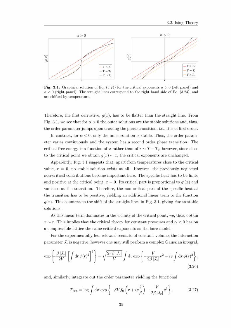
3.2. Ising Theory
.
Fig. 3.1: Graphical solution of Eq. (3.24) for the critical exponents α > 0 (left panel) andα < 0 (right panel). The straight lines correspond to the right hand side of Eq. (3.24), andare shifted by temperature.
Therefore, the first derivative, g(x), has to be flatter than the straight line. From
Fig. 3.1, we see that for α > 0 the outer solutions are the stable solutions and, thus,
the order parameter jumps upon crossing the phase transition, i.e., it is of first order.
In contrast, for α < 0, only the inner solution is stable. Thus, the order param-
eter varies continuously and the system has a second order phase transition. The
critical free energy is a function of x rather than of r ∼ T − Tc, however, since close
to the critical point we obtain g(x) ∼ x, the critical exponents are unchanged.
Apparently, Fig. 3.1 suggests that, apart from temperatures close to the critical
value, r = 0, no stable solution exists at all. However, the previously neglected
non-critical contributions become important here. The specific heat has to be finite
and positive at the critical point, x = 0. Its critical part is proportional to g′(x) and
vanishes at the transition. Therefore, the non-critical part of the specific heat at
the transition has to be positive, yielding an additional linear term to the function
g(x). This counteracts the shift of the straight lines in Fig. 3.1, giving rise to stable
solutions.
As this linear term dominates in the vicinity of the critical point, we, thus, obtain
x ∼ r. This implies that the critical theory for constant pressures and α < 0 has on
a compressible lattice the same critical exponents as the bare model.
For the experimentally less relevant scenario of constant volume, the interaction
parameter Jv is negative, however one may still perform a complex Gaussian integral,
exp
−β |Jv|
2V
[∫drφ(r)2
]2
=
√2πβ |Jv|
V
∫dv exp
− V
2β |Jv|v2 − iv
∫drφ(r)2
,
(3.26)
and, similarly, integrate out the order parameter yielding the functional
Fcrit = log
∫dv exp
−βV f0
(r + iv
2
β
)− V
2β |Jv|v2
. (3.27)
35
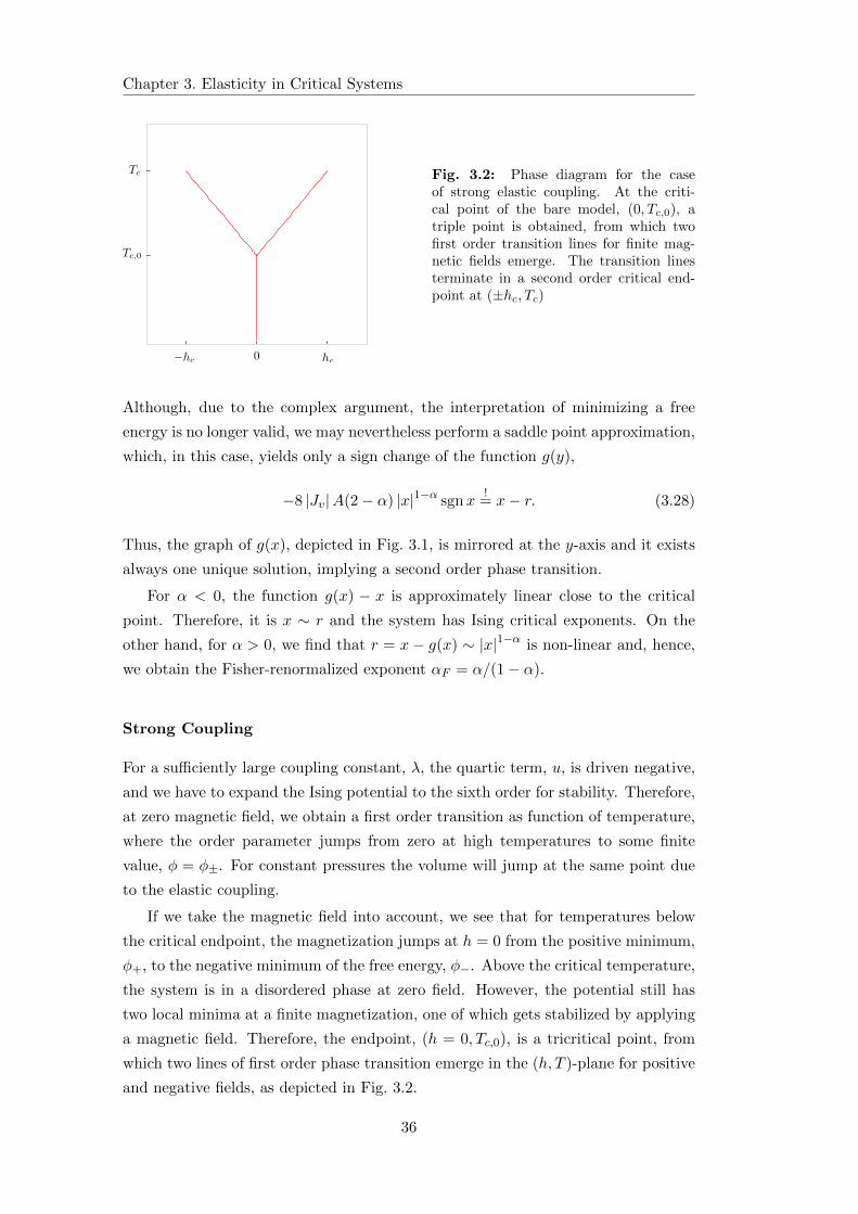
Chapter 3. Elasticity in Critical Systems
.
Fig. 3.2: Phase diagram for the caseof strong elastic coupling. At the criti-cal point of the bare model, (0, Tc,0), atriple point is obtained, from which twofirst order transition lines for finite mag-netic fields emerge. The transition linesterminate in a second order critical end-point at (±hc, Tc)
Although, due to the complex argument, the interpretation of minimizing a free
energy is no longer valid, we may nevertheless perform a saddle point approximation,
which, in this case, yields only a sign change of the function g(y),
−8 |Jv|A(2− α) |x|1−α sgnx!
= x− r. (3.28)
Thus, the graph of g(x), depicted in Fig. 3.1, is mirrored at the y-axis and it exists
always one unique solution, implying a second order phase transition.
For α < 0, the function g(x) − x is approximately linear close to the critical
point. Therefore, it is x ∼ r and the system has Ising critical exponents. On the
other hand, for α > 0, we find that r = x− g(x) ∼ |x|1−α is non-linear and, hence,
we obtain the Fisher-renormalized exponent αF = α/(1− α).
Strong Coupling
For a sufficiently large coupling constant, λ, the quartic term, u, is driven negative,
and we have to expand the Ising potential to the sixth order for stability. Therefore,
at zero magnetic field, we obtain a first order transition as function of temperature,
where the order parameter jumps from zero at high temperatures to some finite
value, φ = φ±. For constant pressures the volume will jump at the same point due
to the elastic coupling.
If we take the magnetic field into account, we see that for temperatures below
the critical endpoint, the magnetization jumps at h = 0 from the positive minimum,
φ+, to the negative minimum of the free energy, φ−. Above the critical temperature,
the system is in a disordered phase at zero field. However, the potential still has
two local minima at a finite magnetization, one of which gets stabilized by applying
a magnetic field. Therefore, the endpoint, (h = 0, Tc,0), is a tricritical point, from
which two lines of first order phase transition emerge in the (h, T )-plane for positive
and negative fields, as depicted in Fig. 3.2.
36
3.2. Ising Theory
On the other hand, for high temperatures, the influence of the quartic term
gets washed out, such that the first order phase transition at finite fields becomes
a crossover. Therefore, these transition lines have to terminate in a second order
critical endpoint, (±hc, Tc). At the critical endpoint, we can, again, set up a Landau
theory, however, due to the finite field and magnetization, the Ising symmetry is only
an emergent theory at the endpoint. Thus, odd terms in the order parameter are
allowed, yielding a bilinear strain coupling which is discussed in the next section.
3.2.3 Bilinear Coupling
If away from the critical point the Ising symmetry is broken, odd powers of the order
parameter are in general allowed. Shifting the order parameter such that the cubic
term vanishes and neglecting terms beyond fourth order, we have the same Ising
Hamiltonian as before. However, a bilinear coupling of the order parameter to the
strain does now exist which reads as
Hc = λ
∫drφ(r)uii(r), (3.29)
and will dominate the thermodynamics at the transition.
The first to consider the implications of such a linear coupling were Levanyuk and
Sobyanin [34]. They investigated the phase transition of ferroelectrics where a linear
coupling to the strain is allowed if the paraphase above the ferroelectric transition
is already piezoelectric. For simplifications, they neglected crystal anisotropies for
the elastic Hamiltonian, but considered a non-isotropic coupling to the ferroelectric
order parameter. With this approximation, they obtained a preemptive mean field
transition with a finite jump in the specific heat, a result which was also obtained
by Villain [35]. Similar, Wagner and Horner [36] considered the liquid-gas transition
of hydrogen dissolved in metals. They also found mean field behavior arising from
a long-ranged interaction due to the elastic coupling and, furthermore, an isotropic
volume change at the transition.
Let us consider the bilinear elastic coupling of a classical Ising transition on
the same theoretical grounds as the quadratic coupling in the previous section.
The free energy is, again, given by the field integral Eq. (3.15). After a Fourier
transformation, the coupling term reads as
Hc = λφ0E + iλ∑
q 6=0
|q|φ(q)?uL(q), (3.30)
Thus, the macroscopic strain couples to the zero momentum mode only, whereas the
finite momentum modes couple to the longitudinal phonons. As in the quadratic
case, we may, again, integrate out the transversal phonons and the pure shear strains,
which yields only a non-critical additive term to the free energy.
37
Chapter 3. Elasticity in Critical Systems
Completing the squares for the macroscopic volume change, E, and the longitu-
dinal phonons we end up with
H =V K
2
(E +
λφ0 − pK
)2
+V
2
(K +
4
3µ
)∑
q 6=0
∣∣∣∣q uL(q)− iλ
K + 4µ/3φ(q)
∣∣∣∣2
+
∫dr
[−hφ(r) +
r
2φ(r)2 +
1
2(∇φ(r))2 +
u0
4!φ(r)4
]− Jp V
2φ2
0. (3.31)
The longitudinal phonons can be integrated out and the second line, again, denotes
a renormalized Ising model, which captures all fluctuation effects, with a infinitely
long range “interaction” on top. The renormalized parameters and the interaction
constant, Jp, are given by
h = h0 −λ p
K, r = r0 −
λ2
K + 4µ/3and Jp = λ2
(1
K− 1
K + 43µ
). (3.32)
Note that for the bilinear coupling the critical magnetic field, Hc = H −h, becomes
pressure dependent and is to lowest order linear in p. The renormalization of the
quadratic coefficient is negative and, hence, corresponds to a shift of the critical
temperature to higher values, thus, the bare Ising transition gets preempted.
The distinction between the ensemble at constant pressure and the one with
a constant volume is again given by the sign of the long-ranged interaction. For
constant pressure, we again integrate out the macroscopic volume change, i.e., we
may skip the first term of Eq. (3.31). Instead, for constant volume, it is E = 0,
and the first term in Eq. (3.31) drives, again, the long-ranged interaction repulsive,
yielding Jv = − λ2
K+ 43µ
. Integrating out the finite momentum components of the
order parameter we obtain
F = −T ln
∫dφ0Dφq6=0 exp −βH
= −T ln
∫dφ0 exp
−βV
(f0(T, φ0)−
Jp/v
2φ2
0
), (3.33)
where the second line serves as a definition of the function f0.
For temperatures above the critical temperature of the bare Ising model, the
free energy and, thus, also f0 are analytic, hence, we may write down a Landau
expansion
f0(T, φ0) = −H(h, T )φ0 +a(h, T )
2φ2
0 +b(h, T )
4!φ2
0. (3.34)
Therefore, for a constant pressure, Jp > 0, we obtain a mean field like critical point,
at a critical temperature given by
a(h, Tc) = Jp. (3.35)
38
3.3. Classification by Cowley
Considering the experimentally less relevant scenario of a fixed volume, the long
range interaction constant, Jv, is negative and, therefore, suppresses order, φ0 6= 0.
Consequently, Eq. (3.35) has no solution in its range of applicability, thus, the critical
temperature of the bare Ising model can be reached. However, since the long range
interactions favors the zero magnetization state, φ0 = 0, critical fluctuations become
suppressed yielding mean field behavior. On a technical level, this can be shown by
finite size scaling arguments, see Ref. [20].
3.3 Classification by Cowley
The bilinear coupling is always non-perturbative because the strain directly follows
the order parameter and vice versa. On the basis of a pure mean field theory for an
arbitrary symmetry, minimization of the general potential with respect to the strain
multiplet yields
−λφ = CΓ εΓ , (3.36)
and both quantities are in a sense equivalent, Thus, the critical theory can be an-
alyzed in terms of the strain field, independent of the underlying type of phase
transition. For such systems, a detailed analysis for all crystal symmetry classes was
performed by Cowley [21], which will be discussed in the following.
As discussed in Sec. 2.2.4, a structural instability arises if one of the eigenvalues
of the elastic constant matrix CΓ vanishes. In this case, the crystal distorts to
another structure whose symmetry is determined by the corresponding irreducible
representation of the strain.
In contrast to other phase transitions, the corresponding fluctuations, i.e., the
elastic waves, are not governed by the same interaction kernel than the macroscopic
order parameter, as we already saw in the isotropic case. Rather than by the elastic
constant matrix, they are obtained by the dynamical matrix, Dik = Cijkl qj qj , see
Eq. (2.73). The eigenvalues of D, and therefore the dispersions of the phonons,
depend on the direction of propagation. We obtain three eigenvalues, and three
eigenvectors, i.e., phonon polarizations, u, for each propagation direction, u. In
general, these eigenvalues are, of course, different from the eigenvalues of the elastic
constant matrix.
From these considerations follows that at a structural instability the speed of
sound may stay finite, which is a well known fact. It is, nevertheless, surprising
when thinking about it in the framework of critical theories, where this statement
implies that it is a symmetry breaking phase transition without any soft modes.
This peculiarity stems from the fact that the order parameter is related to the
macroscopic strain tensor which has 6 independent degrees of freedom. The long
39
Chapter 3. Elasticity in Critical Systems
wave length fluctuations, however, are the acoustic waves of the crystal which have
only three components. Thus, in some sense, they have to be linear combinations of
the strain components and so are their eigenvalues, i.e., their mass.
Considering for instance a cubic crystal, the strain tensor E splits into the three
irreducible representations A, E and T2, as discussed in Sec. 3.1.1. The dynamical
matrix for the fluctuations, on the other hand, can be written as
Dik =
(1
3(CA − CE) + CT
)qiqk +
(CT |q|2 + (CE − 2CT ) q2
i
)δik (3.37)
For the propagation along the (100) direction, one eigenvector of the dynamical
matrix is the longitudinal phonon, uL, having an eigenvalue C11 = 13CA + 2
3CE .
Thus, it is a linear combination of the singlet and doublet strains,
uL∼=√
1
3A1 +
√2
3E (3.38)
The transversal phonons, on the other hand, have the eigenvalue C44 = CT, i.e., of
the triplet, T.
At a phase transition, one has, thus, to determine whether or not elastic waves
with frequencies solely given by the vanishing eigenvalue of the elastic constant ma-
trix exist. For elastically non-isotropic systems there are in principle three different
possibilities which Cowley termed type 0, I and II and are discussed in following.
First of all, instabilities of type 0 have no critical phonons, as, for instance, an
instability of the singlet, A in the cubic case. The singlet has the full cubic symmetry,
whereas any wave vector, q, necessarily breaks some of the symmetries. Thus, at a
phase transition, the fluctuations are always gapped and will only appear on length
scales comparable to the sample size. In the thermodynamic limit, V → ∞, the
transition, hence, becomes mean field like.
If, on the other hand, the eigenvalue of the doublet, E, vanishes, it exists a
one-dimensional subspace of phonon modes which become soft. Such a situation is
denoted as behavior of type I. These soft phonons with an eigenvalue CE propagate
on a face diagonal, e.g., in the direction [110]. Their polarization vector lies on the
same face but perpendicular to the propagation vector, i.e., [110].
Finally at instabilities of type II, there is a whole plane of soft propagation
directions, q. In cubic crystals this happens if CT becomes small, i.e., for a triplet
instability. We then find that transverse waves polarized along one of the cubic axis
of the crystal all have the eigenvalue C44 = CT .
In isotropic crystals, the soft phonons cannot break this isotropy, which leaves
two possibilities. Either, there are no soft acoustic waves close to the instability at
all, which is the case for the single eigenvalue C11, corresponding to an isotropic
volume change. The other case is a melting process, where soft phonons for every
40
3.3. Classification by Cowley
direction. Obviously the isotropy is preserved and the soft propagation vectors span
the whole three dimensional momentum space. Consequently, Cowley denotes these
instabilities with respect to the eigenvalue C44 as type III. The classification of the
behavior of the elastic fluctuations for all 32 crystallographic point groups, as done
by Cowley [21], is summarized in App. B.
To analyze the nature of the respective phase transition, Cowley [21], further on,
investigated for which symmetries a cubic invariant of the irreducible representations
of the strain exists. In presence of a third order invariant, Landau theory yields a
first order transition, at least for doublet and triplet representations. Notably, in
case of a very small cubic term, fluctuations may still become large, though not
divergent.
For singlets, a proper rescaling of the order parameter cancels the cubic term.
Upon fine-tuning one can also drive the linear and the quadratic term to zero and,p
thus, obtains a critical point in phase space where the transition may be still of
second order. However, as it turns out, all singlet instabilities, where symmetry
allows a cubic term, are of type 0, and, therefore, this classical critical endpoint
shows always mean field behavior.
If there is no cubic invariant of the strain tensor, the respective phase transition
is, in case of a positive quartic term, of second order. This happens for the strain
singlets of orthogonal crystals and some of the singlets as well as the doublet of
tetragonal crystals. For these cases, the influence of the elastic fluctuations, i.e.,
acoustic waves of type I or type II, have to be taken into account which was done
by means of renormalization group techniques.
As a result, the singlets of orthorhombic and the tetragonal crystals show, again,
mean field behavior. The flow equations concerning the doublet of tetragonal crystals
were intractable, however, Cowley argues that they, most likely, yield a first order
transition.
In conclusion, all structural transitions are either of first order or a classical,
i.e., mean field like, second order transition. If an order parameter of some other
symmetry breaking phase transition and the strain are coupled bilinear, the two
order parameters directly follow each other. Thus, the latter phase transition will
also become a first order transition or mean field like.
41

Chapter 4
Mott-Transition on
Compressible Lattices
As it was summarized in Chap. 3, the nature of a phase transition may be dramati-
cally changed by the influence of the elastic degrees of freedom. Pressure couples to
the lattice degrees of freedom, by changing the distance between neighboring sites.
This in turn affects the electronic interactions as the overlap between wave functions
depends on their distance. In combination with the non-linear tensorial structure
of crystal elasticity this may lead to non-perturbative effects changing the whole
nature of an electronic phase transition.
In this chapter we will investigate the influence of the elastic lattice on a particu-
lar phase transition at finite temperatures, namely the pressure driven Mott metal-
insulator transition. The Mott transition is a well studied electronic phase transition
and a paradigm for strongly correlated systems in condensed matter physics. For sys-
tems with exactly one electrons per site, i.e., at half filling, the ratio of the strength
of the Coulomb repulsion to the kinetic energy of the single electrons determines
their mobility. As the Coulomb repulsion grows the electrons avoid each other and
at half filling, eventually, freeze out, such that the conductivity vanishes. A brief
recapitulation of the basic concepts of the electronic Mott metal-insulator transition
is given in Sec. 4.1.1
In particular, the nature of the critical endpoint of the first order Mott transition
is subject of a long-standing discussion. As we will review in Sec. 4.1.2, theoreti-
cal work suggests that the Mott transition belongs to the Ising universality class,
however, experimental observations seem to contradict this statement.
In this chapter, we will argue, that these observations may be explained by
the coupling to the elastic degrees of freedom. Assuming that the bare electronic
Mott transition indeed belongs to the Ising universality class, we find that the Mott
transition on compressible lattices, i.e., in every solid state realization, does not
show Ising critical, but rather mean field behavior in the vicinity of the endpoint.
43
Chapter 4. Mott-Transition on Compressible Lattices
The mean field behavior is a result of a non-perturbative bilinear coupling between
the electronic and the elastic degrees of freedom which is specified in Sec. 4.2. In the
following Sec. 4.3, we will derive an expression for the free energy of the elastically
coupled Mott transition and discuss the resulting features of the thermodynamic
quantities (Sec. 4.4).
This work is mainly motivated by Refs. [1, 2], where the thermodynamics of an
organic salt of the series κ-(BEDT-TTF)2X were investigated. The Mott transition
in these compounds can be tuned by pressure and the members of this series are
at ambient pressures located at different points of the phase diagram. Thus, they
have different pressure distances to the critical endpoint and are good candidates to
investigate the elastic influence on the critical behavior of the phase transition. In
Sec. 4.5, we, therefore, address the quantitative implications of the elastic coupling
on these compounds. In particular, we estimate the range of the so-called non-
perturbative regime in the phase diagram, where the coupling to the lattice changes
the nature of the critical point. Furthermore, based on fits obtained by Bartosch
et al. [2], we show how the thermodynamics quantitatively change.
Additionally, we consider another well studied example for pressure driven Mott
transitions, namely the chromium doped V2O3, which shows in experiments hardly
any indications of Ising critical behavior. We will show, that this observation can
be explained by critical elasticity and propose further experiments to substantiate
this explanation
Large parts of this chapter we have published in Ref. [37].
4.1 Mott Metal-Insulator Transition
With the concept of Bloch’s band theory of electrons in solids [38], the distinction
between metals and insulators was made according to the band filling. In metals at
least one band is only partially filled i.e., the Fermi energy lies within an electron
band, whereas insulators have no states at the Fermi energy, having only completely
filled or empty bands. The band theory relies on the assumption that the electron-
electron interactions are very weak, which due to the screening of the Coulomb
interaction is often the case.
However, with the discovery of the insulating behavior of many transition metal
oxides with partially filled d-bands [39], this classification became questionable, as
they should be good metals according to the band picture. Following suggestions by
Peirels, Mott argued that strong electron interactions might be the reason for the
insulating behavior [40]. This metal-insulator transition, subsequently named Mott
transition, became one of the outstanding examples of strongly correlated electron
systems, a field which since then developed into one of the most exciting branches
in condensed matter theory. In the following, we will introduce the basic concepts
44
4.1. Mott Metal-Insulator Transition
of the Mott transition. For further studies, the reader may be referred to the very
detailed review of Imada et al. [41].
4.1.1 Basic Concepts
The basic idea of the mechanism at play in a Mott insulator can be understood
from a seemingly simple model, namely the Hubbard model [42]. For details of its
derivation see for instance Rev. [43]. The Hubbard model is a simplified lattice
fermion model where the Hamiltonian is given by
H = −∑
ij,σ
tij
(c†i,σcj,σ + h.c.
)+ U
∑
i
ni,↑ni,↓. (4.1)
The first term accounts for hopping of electrons with spin σ from one site, j, to
another site, i, which yields a gain in kinetic energy of tij . The hopping amplitude
is determined as the expectation value of the kinetic energy when hopping from an
atomic Wannier orbitals centered at site i, φi,σ(r), to another one centered at site j,
tij =
∫drφ∗i,σ(r)
[∇2
2m−∑
l
Vlat(Rl − r)
]φj,σ(r). (4.2)
where Vlat(Rl − r) accounts for the lattice potential due to the ion at site Rl.
As, for instance, the d-electrons are strongly localized at the positions of the ions,
the overlap between Wannier orbitals centered at distant sites is very small such
that it is sufficient to taken only hopping between nearest neighbors into account.
Additionally, depending on the lattice structure, the hopping amplitude often only
weakly depends on the site indices and is, therefore, simplified to tij = t for nearest
neighbors and tij = 0 otherwise.
The second term accounts for the Coulomb repulsion which is simplified to a
local on-site interaction; a doubly occupied site costs an energy U , which is given as
U =
∫dr dr′ φ∗i,σ(r)φi,σ(r)
e2
|r− r′|φ∗i,σ(r′)φi,σ(r′). (4.3)
This model is clearly oversimplified as it, for example, takes only one localized
electron orbital per ion into account, whereas especially in the transition metals
the d-electrons have an orbital degeneracy. Despite the simplifications, the Hubbard
model describes very well the low-energy properties of many systems. This is because
often only few or even just one band cross the Fermi level and are, thus, relevant for
low-energy excitations. However, multiband-effects strongly renormalize the actual
value for the parameters t and U .
The behavior of the system depends on the relative strength of both terms and
on the filling. For small on-site repulsion t U the electrons move freely through
45
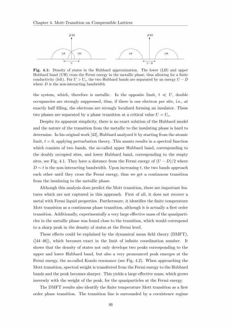
Chapter 4. Mott-Transition on Compressible Lattices
U
ρ (ε) ρ (ε)
LH UH
U − D
UHLH
Fig. 4.1: Density of states in the Hubbard approximation. The lower (LH) and upperHubbard band (UH) cross the Fermi energy in the metallic phase, thus allowing for a finiteconductivity (left). For U > Uc, the two Hubbard bands are separated by an energy U −Dwhere D is the non-interacting bandwidth.
the system, which, therefore is metallic. In the opposite limit, t U , double
occupancies are strongly suppressed, thus, if there is one electron per site, i.e., at
exactly half filling, the electrons are strongly localized forming an insulator. These
two phases are separated by a phase transition at a critical value U = Uc.
Despite its apparent simplicity, there is no exact solution of the Hubbard model
and the nature of the transition from the metallic to the insulating phase is hard to
determine. In his original work [42], Hubbard analyzed it by starting from the atomic
limit, t = 0, applying perturbation theory. This ansatz results in a spectral function
which consists of two bands, the so-called upper Hubbard band, corresponding to
the doubly occupied sites, and lower Hubbard band, corresponding to the empty
sites, see Fig. 4.1. They have a distance from the Fermi energy of (U −D)/2 where
D ∼ t is the non-interacting bandwidth. Upon increasing t, the two bands approach
each other until they cross the Fermi energy, thus we get a continuous transition
from the insulating to the metallic phase.
Although this analysis does predict the Mott transition, there are important fea-
tures which are not captured in this approach. First of all, it does not recover a
metal with Fermi liquid properties. Furthermore, it identifies the finite temperature
Mott transition as a continuous phase transition, although it is actually a first order
transition. Additionally, experimentally a very large effective mass of the quasiparti-
cles in the metallic phase was found close to the transition, which would correspond
to a sharp peak in the density of states at the Fermi level.
These effects could be explained by the dynamical mean field theory (DMFT),
([44–46]), which becomes exact in the limit of infinite coordination number. It
shows that the density of states not only develops two peaks corresponding to the
upper and lower Hubbard band, but also a very pronounced peak emerges at the
Fermi energy, the so-called Kondo resonance (see Fig. 4.2). When approaching the
Mott transition, spectral weight is transferred from the Fermi energy to the Hubbard
bands and the peak becomes sharper. This yields a large effective mass, which grows
inversely with the weight of the peak, for the quasiparticles at the Fermi energy.
The DMFT results also identify the finite temperature Mott transition as a first
order phase transition. The transition line is surrounded by a coexistence regime
46
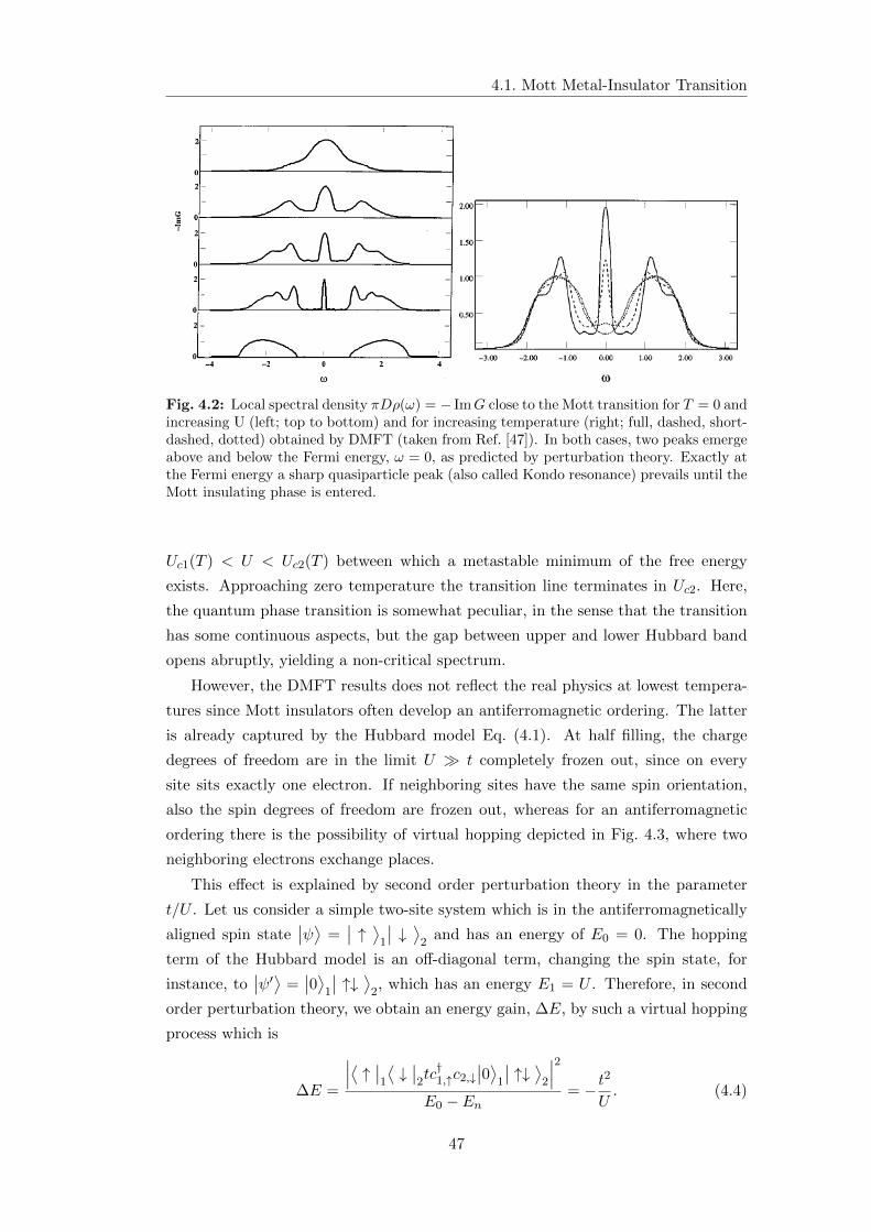
4.1. Mott Metal-Insulator Transition
Fig. 4.2: Local spectral density πDρ(ω) = − ImG close to the Mott transition for T = 0 andincreasing U (left; top to bottom) and for increasing temperature (right; full, dashed, short-dashed, dotted) obtained by DMFT (taken from Ref. [47]). In both cases, two peaks emergeabove and below the Fermi energy, ω = 0, as predicted by perturbation theory. Exactly atthe Fermi energy a sharp quasiparticle peak (also called Kondo resonance) prevails until theMott insulating phase is entered.
Uc1(T ) < U < Uc2(T ) between which a metastable minimum of the free energy
exists. Approaching zero temperature the transition line terminates in Uc2. Here,
the quantum phase transition is somewhat peculiar, in the sense that the transition
has some continuous aspects, but the gap between upper and lower Hubbard band
opens abruptly, yielding a non-critical spectrum.
However, the DMFT results does not reflect the real physics at lowest tempera-
tures since Mott insulators often develop an antiferromagnetic ordering. The latter
is already captured by the Hubbard model Eq. (4.1). At half filling, the charge
degrees of freedom are in the limit U t completely frozen out, since on every
site sits exactly one electron. If neighboring sites have the same spin orientation,
also the spin degrees of freedom are frozen out, whereas for an antiferromagnetic
ordering there is the possibility of virtual hopping depicted in Fig. 4.3, where two
neighboring electrons exchange places.
This effect is explained by second order perturbation theory in the parameter
t/U . Let us consider a simple two-site system which is in the antiferromagnetically
aligned spin state∣∣ψ⟩
=∣∣ ↑
⟩1
∣∣ ↓⟩
2and has an energy of E0 = 0. The hopping
term of the Hubbard model is an off-diagonal term, changing the spin state, for
instance, to∣∣ψ′⟩
=∣∣0⟩
1
∣∣ ↑↓⟩
2, which has an energy E1 = U . Therefore, in second
order perturbation theory, we obtain an energy gain, ∆E, by such a virtual hopping
process which is
∆E =
∣∣∣⟨↑∣∣1
⟨↓∣∣2tc†1,↑c2,↓
∣∣0⟩
1
∣∣ ↑↓⟩
2
∣∣∣2
E0 − En= − t
2
U. (4.4)
47
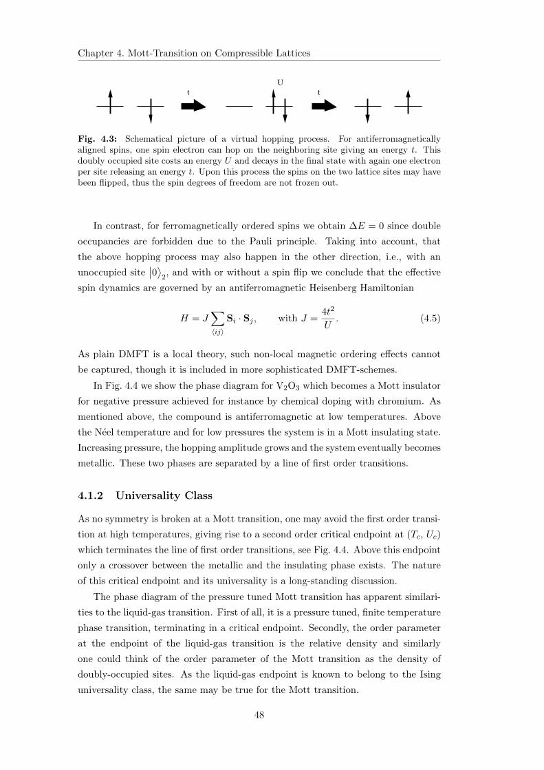
Chapter 4. Mott-Transition on Compressible Lattices
tt
U
Fig. 4.3: Schematical picture of a virtual hopping process. For antiferromagneticallyaligned spins, one spin electron can hop on the neighboring site giving an energy t. Thisdoubly occupied site costs an energy U and decays in the final state with again one electronper site releasing an energy t. Upon this process the spins on the two lattice sites may havebeen flipped, thus the spin degrees of freedom are not frozen out.
In contrast, for ferromagnetically ordered spins we obtain ∆E = 0 since double
occupancies are forbidden due to the Pauli principle. Taking into account, that
the above hopping process may also happen in the other direction, i.e., with an
unoccupied site∣∣0⟩
2, and with or without a spin flip we conclude that the effective
spin dynamics are governed by an antiferromagnetic Heisenberg Hamiltonian
H = J∑
〈ij〉
Si · Sj , with J =4t2
U. (4.5)
As plain DMFT is a local theory, such non-local magnetic ordering effects cannot
be captured, though it is included in more sophisticated DMFT-schemes.
In Fig. 4.4 we show the phase diagram for V2O3 which becomes a Mott insulator
for negative pressure achieved for instance by chemical doping with chromium. As
mentioned above, the compound is antiferromagnetic at low temperatures. Above
the Neel temperature and for low pressures the system is in a Mott insulating state.
Increasing pressure, the hopping amplitude grows and the system eventually becomes
metallic. These two phases are separated by a line of first order transitions.
4.1.2 Universality Class
As no symmetry is broken at a Mott transition, one may avoid the first order transi-
tion at high temperatures, giving rise to a second order critical endpoint at (Tc, Uc)
which terminates the line of first order transitions, see Fig. 4.4. Above this endpoint
only a crossover between the metallic and the insulating phase exists. The nature
of this critical endpoint and its universality is a long-standing discussion.
The phase diagram of the pressure tuned Mott transition has apparent similari-
ties to the liquid-gas transition. First of all, it is a pressure tuned, finite temperature
phase transition, terminating in a critical endpoint. Secondly, the order parameter
at the endpoint of the liquid-gas transition is the relative density and similarly
one could think of the order parameter of the Mott transition as the density of
doubly-occupied sites. As the liquid-gas endpoint is known to belong to the Ising
universality class, the same may be true for the Mott transition.
48
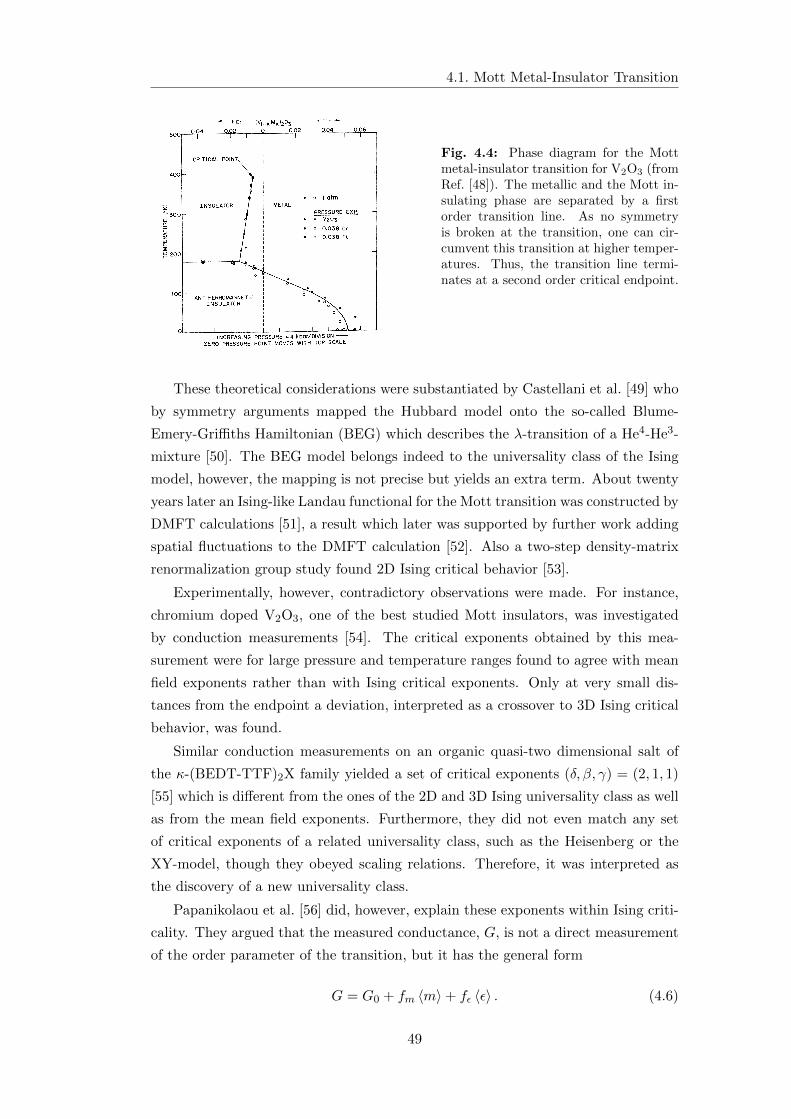
4.1. Mott Metal-Insulator Transition
Fig. 4.4: Phase diagram for the Mottmetal-insulator transition for V2O3 (fromRef. [48]). The metallic and the Mott in-sulating phase are separated by a firstorder transition line. As no symmetryis broken at the transition, one can cir-cumvent this transition at higher temper-atures. Thus, the transition line termi-nates at a second order critical endpoint.
These theoretical considerations were substantiated by Castellani et al. [49] who
by symmetry arguments mapped the Hubbard model onto the so-called Blume-
Emery-Griffiths Hamiltonian (BEG) which describes the λ-transition of a He4-He3-
mixture [50]. The BEG model belongs indeed to the universality class of the Ising
model, however, the mapping is not precise but yields an extra term. About twenty
years later an Ising-like Landau functional for the Mott transition was constructed by
DMFT calculations [51], a result which later was supported by further work adding
spatial fluctuations to the DMFT calculation [52]. Also a two-step density-matrix
renormalization group study found 2D Ising critical behavior [53].
Experimentally, however, contradictory observations were made. For instance,
chromium doped V2O3, one of the best studied Mott insulators, was investigated
by conduction measurements [54]. The critical exponents obtained by this mea-
surement were for large pressure and temperature ranges found to agree with mean
field exponents rather than with Ising critical exponents. Only at very small dis-
tances from the endpoint a deviation, interpreted as a crossover to 3D Ising critical
behavior, was found.
Similar conduction measurements on an organic quasi-two dimensional salt of
the κ-(BEDT-TTF)2X family yielded a set of critical exponents (δ, β, γ) = (2, 1, 1)
[55] which is different from the ones of the 2D and 3D Ising universality class as well
as from the mean field exponents. Furthermore, they did not even match any set
of critical exponents of a related universality class, such as the Heisenberg or the
XY-model, though they obeyed scaling relations. Therefore, it was interpreted as
the discovery of a new universality class.
Papanikolaou et al. [56] did, however, explain these exponents within Ising criti-
cality. They argued that the measured conductance, G, is not a direct measurement
of the order parameter of the transition, but it has the general form
G = G0 + fm 〈m〉+ fε 〈ε〉 . (4.6)
49
Chapter 4. Mott-Transition on Compressible Lattices
The second term is proportional to the order parameter, m, whereas the third term
is given by the energy density, ε. The relative magnitude of fε and fm determines
a crossover from an energy dominated regime to an order parameter dominated
regime. For fε fm indeed the order parameter determines the conductivity at
long length scales, G−G0 ∼ 〈m〉, but at short length scales we have G−G0 ∼ 〈ε〉.In terms of the critical exponents of the order parameter, 〈m〉 ∼ |T − T c|β , and
the specific heat, C ∼ ∂T ε ∼ |T − T c|−α, this implies
G−G0 ∼ 〈m〉−(α−1)/β . (4.7)
The following conversion of the measured conductivity exponents indeed recovered
the critical exponents of the 2D Ising universality class. Later dilatometric data on
the same compound [1] could also be fitted to the 2D Ising free energy [2].
In summary, there are indications that the Mott transition belongs to the Ising
universality class. However, there are also contradictory experimental results, there-
fore the question of the nature of the critical endpoint is not yet conclusively an-
swered.
4.1.3 The Ising Field Theory
To describe the finite temperature Mott transition close to the critical endpoint,
we would like to write down a Landau functional. As discussed in Sec. 4.1.2, the
theoretical considerations as well as some experimental results suggest that the Mott
transition belongs to the Ising universality class. Therefore, we will start from the
assumption, that the bare Mott transition is indeed described by an Ising theory.
The contradictory behavior seen in experiments on V2O3 Ref. [54] will be addressed
in Sec. 4.5.
The order parameter, φ, in which the Landau functional is formulated may, as
explained, be viewed as the density of the doubly occupied sites. More precise, it
is associated with the amplitude of the quasiparticle peak, as discussed in Ref. [51].
There are two relevant perturbations in the Ising model, namely the reduced tem-
perature, ∆T = (T − Tc)/Tc, where Tc denotes the critical temperature, and the
magnetic field H. Close to the critical point where the magnetization is small and
only long wavelength fluctuations are important, the effective field theory for the
Ising model is given as
S[φ] =
∫ddr
1
2(∂φ)2 +
r
2φ2 − hφ+
u
4!φ4
. (4.8)
The parameters r and h are the deviations from the critical point
r = Cr∆T(1 +O
(∆T,H2
))and h = CHH
(1 +O
(∆T,H2
)), (4.9)
where the positive constants Cr and CH are non-universal and depend on the mi-
croscopic model. The quartic interaction, u, is also a non-universal constant and
higher order interactions are neglected as they are irrelevant in the RG-sense.
50
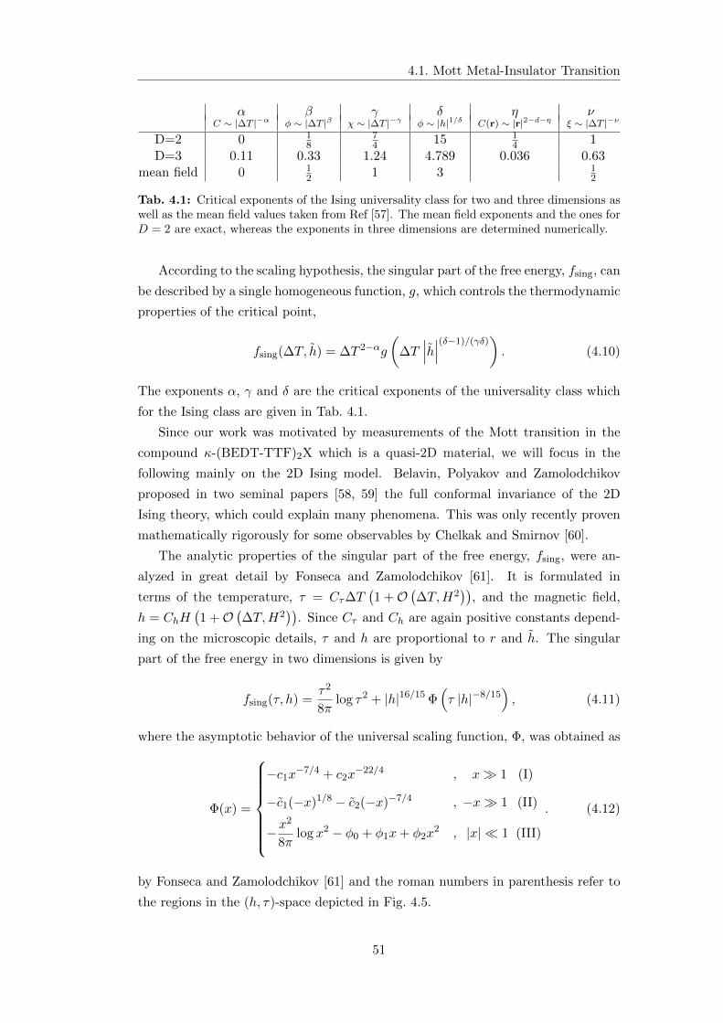
4.1. Mott Metal-Insulator Transition
α β γ δ η νC ∼ |∆T |−α φ ∼ |∆T |β χ ∼ |∆T |−γ φ ∼ |h|1/δ C(r) ∼ |r|2−d−η ξ ∼ |∆T |−ν
D=2 0 18
74 15 1
4 1D=3 0.11 0.33 1.24 4.789 0.036 0.63
mean field 0 12 1 3 1
2
Tab. 4.1: Critical exponents of the Ising universality class for two and three dimensions aswell as the mean field values taken from Ref [57]. The mean field exponents and the ones forD = 2 are exact, whereas the exponents in three dimensions are determined numerically.
According to the scaling hypothesis, the singular part of the free energy, fsing, can
be described by a single homogeneous function, g, which controls the thermodynamic
properties of the critical point,
fsing(∆T, h) = ∆T 2−αg
(∆T
∣∣∣h∣∣∣(δ−1)/(γδ)
). (4.10)
The exponents α, γ and δ are the critical exponents of the universality class which
for the Ising class are given in Tab. 4.1.
Since our work was motivated by measurements of the Mott transition in the
compound κ-(BEDT-TTF)2X which is a quasi-2D material, we will focus in the
following mainly on the 2D Ising model. Belavin, Polyakov and Zamolodchikov
proposed in two seminal papers [58, 59] the full conformal invariance of the 2D
Ising theory, which could explain many phenomena. This was only recently proven
mathematically rigorously for some observables by Chelkak and Smirnov [60].
The analytic properties of the singular part of the free energy, fsing, were an-
alyzed in great detail by Fonseca and Zamolodchikov [61]. It is formulated in
terms of the temperature, τ = Cτ∆T(1 +O
(∆T,H2
)), and the magnetic field,
h = ChH(1 +O
(∆T,H2
)). Since Cτ and Ch are again positive constants depend-
ing on the microscopic details, τ and h are proportional to r and h. The singular
part of the free energy in two dimensions is given by
fsing(τ, h) =τ2
8πlog τ2 + |h|16/15 Φ
(τ |h|−8/15
), (4.11)
where the asymptotic behavior of the universal scaling function, Φ, was obtained as
Φ(x) =
−c1x−7/4 + c2x
−22/4 , x 1 (I)
−c1(−x)1/8 − c2(−x)−7/4 , −x 1 (II)
−x2
8πlog x2 − φ0 + φ1x+ φ2x
2 , |x| 1 (III)
. (4.12)
by Fonseca and Zamolodchikov [61] and the roman numbers in parenthesis refer to
the regions in the (h, τ)-space depicted in Fig. 4.5.
51
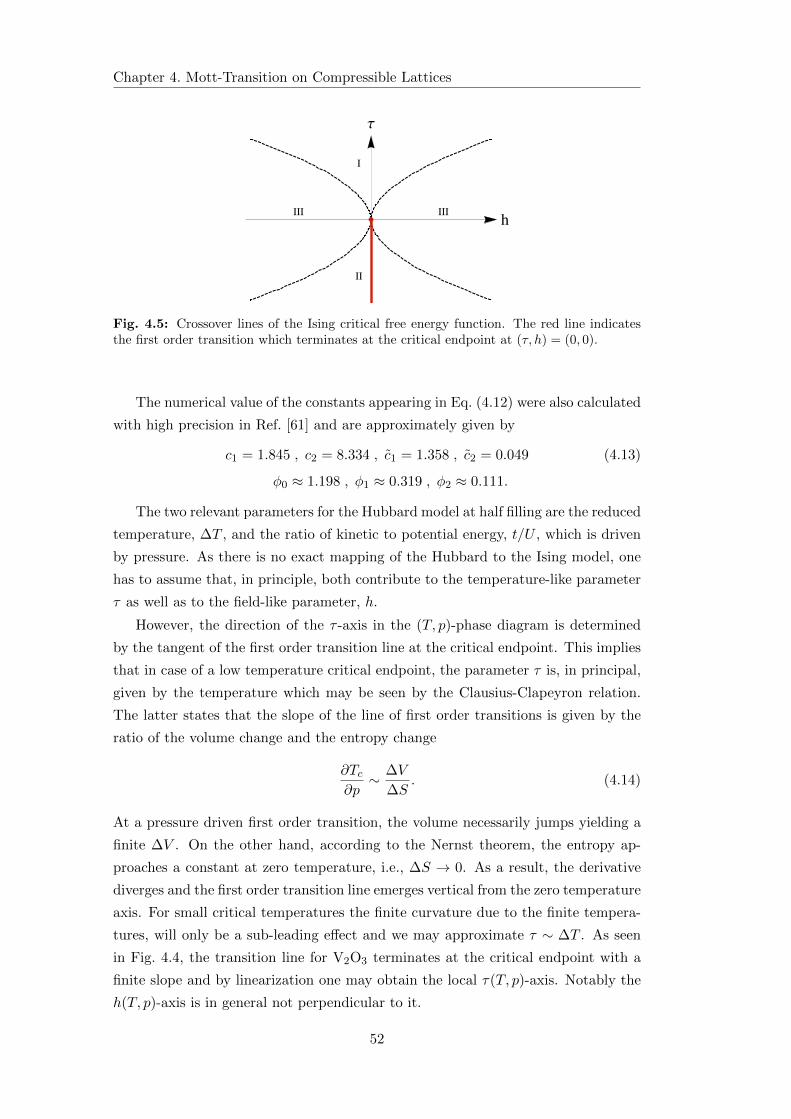
Chapter 4. Mott-Transition on Compressible Lattices
I
II
III IIIh
Τ
Fig. 4.5: Crossover lines of the Ising critical free energy function. The red line indicatesthe first order transition which terminates at the critical endpoint at (τ, h) = (0, 0).
The numerical value of the constants appearing in Eq. (4.12) were also calculated
with high precision in Ref. [61] and are approximately given by
c1 = 1.845 , c2 = 8.334 , c1 = 1.358 , c2 = 0.049 (4.13)
φ0 ≈ 1.198 , φ1 ≈ 0.319 , φ2 ≈ 0.111.
The two relevant parameters for the Hubbard model at half filling are the reduced
temperature, ∆T , and the ratio of kinetic to potential energy, t/U , which is driven
by pressure. As there is no exact mapping of the Hubbard to the Ising model, one
has to assume that, in principle, both contribute to the temperature-like parameter
τ as well as to the field-like parameter, h.
However, the direction of the τ -axis in the (T, p)-phase diagram is determined
by the tangent of the first order transition line at the critical endpoint. This implies
that in case of a low temperature critical endpoint, the parameter τ is, in principal,
given by the temperature which may be seen by the Clausius-Clapeyron relation.
The latter states that the slope of the line of first order transitions is given by the
ratio of the volume change and the entropy change
∂Tc∂p∼ ∆V
∆S. (4.14)
At a pressure driven first order transition, the volume necessarily jumps yielding a
finite ∆V . On the other hand, according to the Nernst theorem, the entropy ap-
proaches a constant at zero temperature, i.e., ∆S → 0. As a result, the derivative
diverges and the first order transition line emerges vertical from the zero temperature
axis. For small critical temperatures the finite curvature due to the finite tempera-
tures, will only be a sub-leading effect and we may approximate τ ∼ ∆T . As seen
in Fig. 4.4, the transition line for V2O3 terminates at the critical endpoint with a
finite slope and by linearization one may obtain the local τ(T, p)-axis. Notably the
h(T, p)-axis is in general not perpendicular to it.
52
4.2. Coupling to the Lattice
4.2 Coupling to the Lattice
Pressure tuning of the Mott transition necessarily implies a coupling of the electronic
degrees of freedom to the underlying lattice. As one applies pressure to the crystal,
the lattice sites get closer together, which in turn allows for a larger overlap of
the electronic wave functions, resulting in a larger hopping amplitude t. Thus, to
understand the pressure driven Mott transition, it is important to investigate the
coupling between the electronic and the elastic degrees of freedom.
As discussed in Chap. 2, the potential of the elastic system is given in terms of
the strain tensor uij(r) by
Vel = uij(r)Cijkl ukl(r) + uij(r)σij(r), (4.15)
where σij accounts for the external macroscopic stress and Cijkl is the elastic con-
stant matrix.
In lowest order the coupling to the electronic degrees of freedom will be linear
in the strain tensor. The order parameter field, φ, can couple both, linearly and
quadratically to the strain, since the Ising symmetry is only an emergent symmetry
at the critical endpoint. Thus, the interaction is given by
Lint [φ, uij ] = −γ1,ij uij φ+1
2γ2,ij uij φ
2, (4.16)
with a certain set of coupling constants γ1,ij and γ2,ij . The respective relevance
of these two terms can be obtained by comparing them to the terms of the Ising
theory, Eq. (4.8). We identify the bilinear term as the most important coupling since
the elastic degrees of freedom act as an additional magnetic field, δh, in the Ising
theory which is the most relevant parameter. The quadratic coupling, on the other
hand, yields a shift in r ∼ T − Tc and, thus, gives a renormalization of the critical
temperature. Additionally, it induces non-local interactions of the order parameter,
r(q) ∼ ui,j(q), which are not considered in the following.
We may also take the different point of view and consider the effect of the
electronic degrees of freedom on the elastic system. In second order perturbation
theory, the bilinear term yields a renormalization of the elastic tensor proportional
to δCijkl ∼ 〈φφ〉 ∼ χ. Since, this renormalization corresponds to the susceptibility,
χ, which close to the critical endpoint inevitably diverges, at least one of the elastic
moduli is driven to zero at some finite ∆T > 0. This, as explained in Chap. 3,
leads to a crystal softening which induces a structural transition preempting the
Mott transition. In turn the structural transition will trigger the metal-insulator
transition. This shift of the transition temperature was also pointed out in Ref. [62].
The acoustic modes, on the other hand, are not governed by the elastic moduli
itself but rather by the dynamical matrix Mil =∑
jk Cijklqjqk depending on the
53
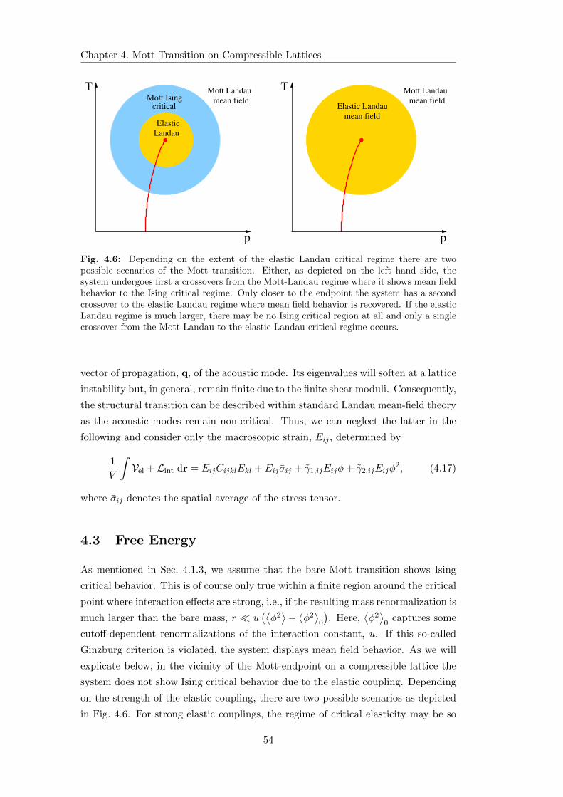
Chapter 4. Mott-Transition on Compressible Lattices
T
p
Mott Landau
Elastic Landaumean field
mean field
T
p
Mott Landau
Landau
Elastic
criticalMott Ising mean field
Fig. 4.6: Depending on the extent of the elastic Landau critical regime there are twopossible scenarios of the Mott transition. Either, as depicted on the left hand side, thesystem undergoes first a crossovers from the Mott-Landau regime where it shows mean fieldbehavior to the Ising critical regime. Only closer to the endpoint the system has a secondcrossover to the elastic Landau regime where mean field behavior is recovered. If the elasticLandau regime is much larger, there may be no Ising critical region at all and only a singlecrossover from the Mott-Landau to the elastic Landau critical regime occurs.
vector of propagation, q, of the acoustic mode. Its eigenvalues will soften at a lattice
instability but, in general, remain finite due to the finite shear moduli. Consequently,
the structural transition can be described within standard Landau mean-field theory
as the acoustic modes remain non-critical. Thus, we can neglect the latter in the
following and consider only the macroscopic strain, Eij , determined by
1
V
∫Vel + Lint dr = EijCijklEkl + Eij σij + γ1,ijEijφ+ γ2,ijEijφ
2, (4.17)
where σij denotes the spatial average of the stress tensor.
4.3 Free Energy
As mentioned in Sec. 4.1.3, we assume that the bare Mott transition shows Ising
critical behavior. This is of course only true within a finite region around the critical
point where interaction effects are strong, i.e., if the resulting mass renormalization is
much larger than the bare mass, r u(⟨φ2⟩−⟨φ2⟩
0
). Here,
⟨φ2⟩
0captures some
cutoff-dependent renormalizations of the interaction constant, u. If this so-called
Ginzburg criterion is violated, the system displays mean field behavior. As we will
explicate below, in the vicinity of the Mott-endpoint on a compressible lattice the
system does not show Ising critical behavior due to the elastic coupling. Depending
on the strength of the elastic coupling, there are two possible scenarios as depicted
in Fig. 4.6. For strong elastic couplings, the regime of critical elasticity may be so
54
4.3. Free Energy
large, that Ising critical behavior will not develop at all. For weak elastic couplings,
Ising criticality can be observed around the endpoint and the elastic coupling will
affect the system only at much smaller distances from the endpoint. In the following
analysis, we assume the latter scenario.
The singular part of the free energy of the bare electronic system is then given
by Eq. (4.11) depending on the two parameters τ = r Cτ/Cr and h = h Ch/CH .
On the other hand, we have seen that the interaction with the elastic degrees of
freedom yields a renormalization of the electronic parameters, δh = γ1,ijEij and
δr = γ2,ijEij . Thus, denoting γ2,ij = γ2,ijCτ/Cr and γ1,ij = γ1,ijCh/CH we may
substitute parameters of the bare Mott transition, τ and h0, in the argument of the
electronic free energy by the elastically renormalized values and obtain the effective
elastic potential
V (Eij) = EijCijklEkl + Eij σij + fsing(τ + γ2,ijEij , h0 + γ1,ijEij), (4.18)
To obtain the free energy density of the coupled system, we have to minimize
Eq. (4.18) with respect to the macroscopic strain fields.
Due to the bilinear coupling, only singlets of the irreducible representation of
the crystal group couple to the Mott degrees of freedom as discussed in Sec. 3.1. In
the following, we will, for simplicity, only consider the strongest coupled singlet, E
which becomes critical first. The corresponding potential Eq. (4.18) reads as
V (E) =K0
2E2 − pE + f0fsing(τ + γ2E, h0 + γ1E), (4.19)
with K0 being the bare eigenvalue of the elastic constant matrix which corresponds
to the strain E. Furthermore, we consider hydrostatic pressure σij = −p δij and
assume that it has a finite overlap with E. As fsing is a dimensionless quantity, we
have to take a non-universal scale factor f0 into account to get the right units. For
simplicity, it is set to one in the following, which corresponds to measuring the bulk
modulus, K0, and the pressure, p, on a scale set by f0.
4.3.1 Perturbative Solution
To obtain the macroscopic strain field E we have to minimize the potential Eq. (4.19).
Sufficiently far from the Mott endpoint, the fluctuations originating from the Ising
theory are weak. Thus, we can minimize the potential Eq. (4.19), perturbatively in
the elastic couplings, γ1 and γ2, by expanding the singular part of the free energy.
To lowest order the solution is simply given by E = p/K0 and, hence, the free energy
density of the system is obtained as
Fpert = − p2
2K0+ fsing(τ + γ2
p
K0, h0 + γ1
p
K0). (4.20)
55
Chapter 4. Mott-Transition on Compressible Lattices
Hence, the elastic coupling leads to a pressure dependence of the arguments of the
singular part of the Ising free energy. Thereby, the elastic coupling, Eq. (4.16), makes
the Mott transition amenable to pressure tuning, i.e., we can control the distance
to the critical endpoint with p. In particular, the dependence of the arguments on
the pressure is linear which is the assumption made in Ref. [2].
The critical point is identified by the condition that the arguments of the function
fsing have to vanish which leads to pc,0 = −h0K0/γ1 and τc,0 = γ2 h0/γ1. Defining
the quantities t0 = τ − τc,0 and p = γ1 (p− pc,0)/K0, Eq. (4.20) takes the form
Fpert = −K0
2γ21
(p− h0)2 + fsing(t0 +γ2
γ1p, p) (4.21)
Therefore, we see, that as a consequence of the finite quadratic coupling, the two
arguments of the Ising free energy are not independent of each other, i.e., in the
(p, T )-phase diagram they do not draw a 90 angle. However, one has also to keep
in mind that in principle h0 is temperature dependent and thus also pc,0 is not a
constant.
As argued above, the elastic coupling to the field-like argument of the Ising free
energy is more important than to the temperature one. Thus, we may for simplicity
consider the limit γ2 → 0. The free energy follows from Eqs. (4.11) and (4.12) as
Fpert = −K0
2γ21
(p− h0)2 +
1
8πt20 log t20 − c1p
2t− 7
40 + c2p
4t− 11
20 , (I)
1
8πt20 log t20 − c1 |p| |t0|
18 − c2p
2 |t0|−74 , (II)
1
8πt20 log |p| 16
15 − φ0 |p|1615 + φ1 |p|
815 t0, (III)
. (4.22)
The roman numbers again refer to Fig. 4.5 identifying the h-axis with p and τ with
t0, and denote the high temperature (I), low temperature (II) and the large pressure
regime (III).
Upon approaching the critical endpoint, the fluctuations become stronger and,
thus, such a perturbative treatment is no longer valid. This becomes most obvious
when setting γ2 = 0 and approaching the critical point from high temperatures.
There, the Ising free energy adds a term δV = −c1 (h0 + γ1E)2 t−7/40 to the elastic
potential. Importantly, this contribution diverges as t0 is driven to zero, and, hence,
causes a sign change of the quadratic term of the potential at some finite value of
τ , i.e., above the critical point identified by the perturbative approach. Thus, as
already mentioned, the critical point is preempted by an isostructural transition,
which in turn will trigger the Mott transition and determines the critical endpoint
of the Mott transition on a compressible lattice. Notably, this does not depend on
the sign of the elastic interaction, γ1.
56
4.3. Free Energy
4.3.2 Non-Perturbative Solution
Close to the critical endpoint of the elastic Mott transition, the diverging singular
part of the Ising free energy density cannot be treat as a small perturbation of
the elastic potential. Since, the argument of the function fsing are small but finite,
(τ + γ2E, h0 + γ1E) 6= (0, 0), we may expand the potential Eq. (4.19) in a Taylor
series up to fourth order. For convenience, we expand in ε = E − E(τ, h0) where
E(τ, h0) is chosen such that the third order term of the expansion vanishes. With
the shifted variables t = τ + γ2E and h = h0 + γ1E the resulting potential in the
non-perturbative regime reads up to constant terms as
Vnon = fsing(t, h)− (p− pc) ε+K(t)
2ε2 +
u(t)
4!ε4. (4.23)
The quartic interaction, u(t), is a superposition of all fourth-order derivatives of
fsing(t, h), and the critical pressure takes the form pc = K0E + γ1 ∂h fsing(t, h) +
γ2 ∂t fsing(t, h). Most important is, however, the renormalization of the effective
bulk modulus, K(t) due to the second order derivatives of fsing(t, h)
K(t) = K0 − γ21χhh − 2γ1 γ2 χht − γ2
2 χtt, (4.24)
where we introduced the generalized susceptibilities χαβ = −∂α ∂βfsing(t, h). When
the critical endpoint of the uncoupled system is approached, χhh necessarily diverges.
At some finite value (tc, hc) 6= (0, 0), where the Taylor expansion is well defined, the
effective bulk modulus is driven to zero. Thus, we see that the Mott-Ising endpoint
is preempted by an isostructural transition at (tc, pc). Importantly, the critical
endpoint of the compressible system is mean-field like since the Ising singularities
at (t, h) = (0, 0) are avoided. Also note that this happens for any finite value of γ1,
independent of its magnitude.
To minimize Eq. (4.23) one may first rescale the strain as ε = ε p/ |K(t)| where
we set p = p− pc. The conditional equation for ε reads then as
−1 + ε
(sgnK(t) +
1
3!
|p|2 u(t)
|K(t)|3ε2
)= 0. (4.25)
The magnitude of the ratio |p|2 u(t)/ |K(t)|3 and the sign of the effective bulk mod-
ulus, K(t), discriminate the three different regimes, depicted in Fig. 4.7:
For large pressures, |p|2 u(t) |K(t)|3 the solution is independent of the sign of
K(t) and reads as
εc = sign(p)
[(6|p|u(t)
)1/3
−K(t)
(4
3|p|u(t)2
)1/3], (4.26)
In particular, at the critical value K(t) = 0 we obtain ε ∼ |p|1/δ with the Lan-
dau mean field exponent δ = 3 for the stress-strain relation. Importantly, this
57
Chapter 4. Mott-Transition on Compressible Lattices
non-perturbative relation is a clear violation of Hooke’s law which states a linear
dependence of ε on the pressure. This power law is the smoking gun criterion for
the identification of critical elasticity.
In the opposite limit of small pressures, |p|2 u(t) |K(t)|3, it is important
whether the temperature is above or below tc. If the bulk modulus, K(t), is positive,
the solution is simply
εa =p
K(t), (4.27)
resembling the perturbative regime for large temperatures, as K(t) converges to K0
with increasing temperatures. Below the endpoint, however, we have to keep the
cubic term in Eq. (4.25) to obtain the global minimum of the potential given by
εb = sgn(p)
[√−6K(t)
u(t)+
|p|2 |K(t)|
]. (4.28)
Thus, tuning through p = 0 the volume jumps about 2√−6K(t)/u(t) into the
coexisting but previously metastable local minimum of the potential, characteristic
for a first order isostructural transition. At the crossover to the large pressure
regime, (c), this metastable minimum ceases to exist.
An important question is, on what scales this elastic Ising mean field regime
arises in the phase diagram. The pressure range can be estimated by comparing the
perturbative and the non-perturbative volume change, i.e., at which pressure the
deviation from Hooks law arises. In the rescaled variables the perturbative solution
is given as εpert = (p+pc−K0E)/K0 ≈ p/K0 where the last approximation holds in
zeroth order of the elastic couplings. Now, comparing this with Eq. (4.26) we obtain
for the extent of the non-perturbative region
p∗ =
(6K3
0
u
)1/2
. (4.29)
The temperature scale of the non-perturbative regime may be defined by the differ-
ence between the critical temperature, tc, and the perturbatively calculated one.
For simplicity, we set γ2 = 0 for the remainder of the analysis. Since it is t > 0
around the endpoint, the Ising free energy is evaluated in regime I of Fig. 4.5, having
the form
fsing(t, h+ γ1ε) =t2
8πlog t2 − c1t
−7/4 |h+ γ1ε|2 + c2t−22/4 |h+ γ1ε|4 . (4.30)
Thus, the condition of a vanishing third order term translates to h = 0 implying
E = −h0/γ1. The critical pressure follows as pc = K0h0/γ1 and the fourth order
interaction is given as u(t) = 4! γ41 c2 t
−22/4. The renormalized bulk modulus is
K(t) = K0 − 2γ21 c1 t
−7/4, (4.31)
58
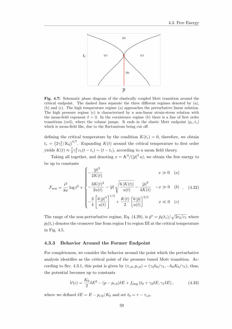
4.3. Free Energy
HaL
HcLHcL
HbL
p
tc
Fig. 4.7: Schematic phase diagram of the elastically coupled Mott transition around thecritical endpoint. The dashed lines separate the three different regimes denoted by (a),(b) and (c). The high temperature regime (a) approaches the perturbative linear solution.The high pressure regime (c) is characterized by a non-linear strain-stress relation withthe mean-field exponent δ = 3. In the coexistence regime (b) there is a line of first ordertransitions (red), where the volume jumps. It ends in the elastic Mott endpoint (pc, tc)which is mean-field like, due to the fluctuations being cut off.
defining the critical temperature by the condition K(tc) = 0, therefore, we obtain
tc =(2γ2
1/K0
)4/7. Expanding K(t) around the critical temperature to first order
yields K(t) ≈ 72γ
21 c1(t− tc) ∼ (t− tc), according to a mean field theory.
Taking all together, and denoting x = K3/(|p|2 u), we obtain the free energy to
be up to constants
Fnon =t2
8πlog t2 +
− |p|2
2K(t)x 0 (a)
−3K(t)2
2u(t)− |p|
√6 |K(t)|u(t)
− |p|24K(t)
−x 0 (b)
−3
4
[6 |p|4u(t)
]1/3
+K(t)
2
[6 |p|u(t)
]2/3
x 0 (c)
. (4.32)
The range of the non-perturbative regime, Eq. (4.29), is p∗ = pI(tc)/√
2c2/c1 where
pI(tc) denotes the crossover line from region I to region III at the critical temperature
in Fig. 4.5.
4.3.3 Behavior Around the Former Endpoint
For completeness, we consider the behavior around the point which the perturbative
analysis identifies as the critical point of the pressure tuned Mott transition. Ac-
cording to Sec. 4.3.1, this point is given by (τc,0, pc,0) = (γ2h0/γ1,−h0K0/γ1), thus,
the potential becomes up to constants
V(ε) =K0
2δE2 − (p− pc,0)δE + fsing (t0 + γ2δE, γ1δE) , (4.33)
where we defined δE = E − pc,0/K0 and set t0 = τ − τc,0.
59
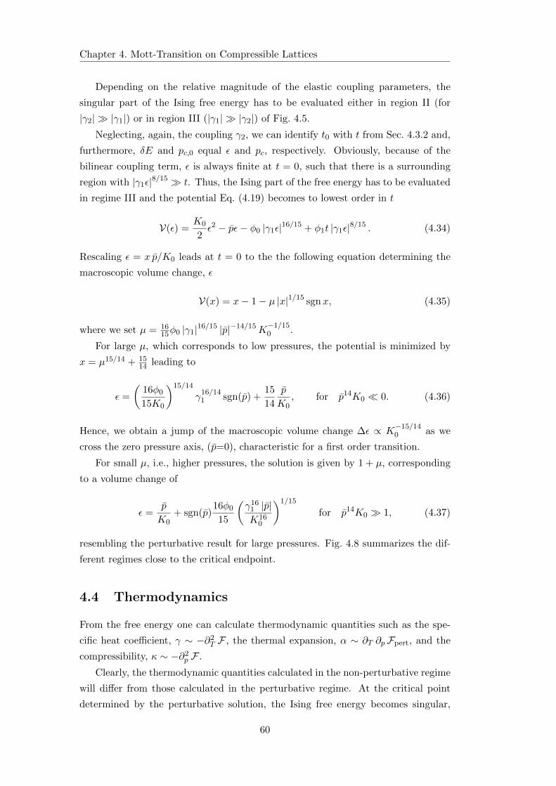
Chapter 4. Mott-Transition on Compressible Lattices
Depending on the relative magnitude of the elastic coupling parameters, the
singular part of the Ising free energy has to be evaluated either in region II (for
|γ2| |γ1|) or in region III (|γ1| |γ2|) of Fig. 4.5.
Neglecting, again, the coupling γ2, we can identify t0 with t from Sec. 4.3.2 and,
furthermore, δE and pc,0 equal ε and pc, respectively. Obviously, because of the
bilinear coupling term, ε is always finite at t = 0, such that there is a surrounding
region with |γ1ε|8/15 t. Thus, the Ising part of the free energy has to be evaluated
in regime III and the potential Eq. (4.19) becomes to lowest order in t
V(ε) =K0
2ε2 − pε− φ0 |γ1ε|16/15 + φ1t |γ1ε|8/15 . (4.34)
Rescaling ε = x p/K0 leads at t = 0 to the the following equation determining the
macroscopic volume change, ε
V(x) = x− 1− µ |x|1/15 sgnx, (4.35)
where we set µ = 1615φ0 |γ1|16/15 |p|−14/15K
−1/150 .
For large µ, which corresponds to low pressures, the potential is minimized by
x = µ15/14 + 1514 leading to
ε =
(16φ0
15K0
)15/14
γ16/141 sgn(p) +
15
14
p
K0, for p14K0 0. (4.36)
Hence, we obtain a jump of the macroscopic volume change ∆ε ∝ K−15/140 as we
cross the zero pressure axis, (p=0), characteristic for a first order transition.
For small µ, i.e., higher pressures, the solution is given by 1 + µ, corresponding
to a volume change of
ε =p
K0+ sgn(p)
16φ0
15
(γ16
1 |p|K16
0
)1/15
for p14K0 1, (4.37)
resembling the perturbative result for large pressures. Fig. 4.8 summarizes the dif-
ferent regimes close to the critical endpoint.
4.4 Thermodynamics
From the free energy one can calculate thermodynamic quantities such as the spe-
cific heat coefficient, γ ∼ −∂2T F , the thermal expansion, α ∼ ∂T ∂pFpert, and the
compressibility, κ ∼ −∂2p F .
Clearly, the thermodynamic quantities calculated in the non-perturbative regime
will differ from those calculated in the perturbative regime. At the critical point
determined by the perturbative solution, the Ising free energy becomes singular,
60
4.4. Thermodynamics
pc
Tc
Tc,0
T
p
Elastic Ising
criticalMott Ising
mean field
Fig. 4.8: Different regimes of the Mottendpoint on compressible lattices. Closeto the endpoint at Tc, elastic criticality isobtained (yellow), whereas further awaythe Ising critical behavior of the Motttransition is recovered (blue). Aroundthe perturbatively estimated endpoint,Tc,0(brown), the behavior is neither Ising crit-ical nor mean field. Far away from theendpoint, the fluctuations become weakand one obtains Mott mean field behaviorwhich is not shown here.
thus, yielding divergences in thermodynamics. In the non-perturbative regime, in
contrast, the Ising free energy is non-singular, therefore, we expect that at least
some divergences are cut-off at the elastic Mott transition.
In order to focus on the important effects, we will again consider the limit of a
vanishing quadratic coupling, γ2 = 0, in the following. As mentioned in Sec. 4.3.3,
in this case we can identify t = t0 and pc = pc,0. Furthermore, to lowest order, we
can assume t to be linear in temperature, t = (T − Tc,0)/T0, where Tc,0 denotes the
perturbatively calculated critical temperature and T0 is some non-universal tem-
perature scale. As a further simplification, we will assume h0 to be temperature
independent since for small critical temperatures it only weakly depends on T . This
is due to the Clausius Clapeyron relation as explained in Sec. 4.1.3.
In the perturbative regime, the free energy is given in terms of the parameter
p = γ1(p− pc,0)/K0. Thus, we deduce
∂T Fpert(t, p) =1
T0
∂Fpert(t, p)
∂t
∣∣p=pγ1/K0
, ∂T Fnon(t, p) =1
T0
∂Fnon(t, p)
∂t
∂pFpert(t, p) =γ1
K0
∂ Fpert(t, p)
∂p
∣∣p=pγ1/K0
, ∂pFnon(t, p) =1
T0
∂Fnon(t, p)
∂t.
Additionally, we reintroduce the free energy scale f0, which enters linear in K(t)−K0
and u(t). In the following, one has to keep in mind, that while the perturbatively
calculated critical point lies at (t, p) = (0, 0), the (actual) non-perturbative endpoint
is at a finite temperature, tc.
4.4.1 Specific Heat Coefficient
The specific heat coefficient in the perturbative regime is given by
γpert = − f0
T 20
∂2fsing(t, h)
∂t2
∣∣∣∣h=γ1 p/K0
. (4.38)
61
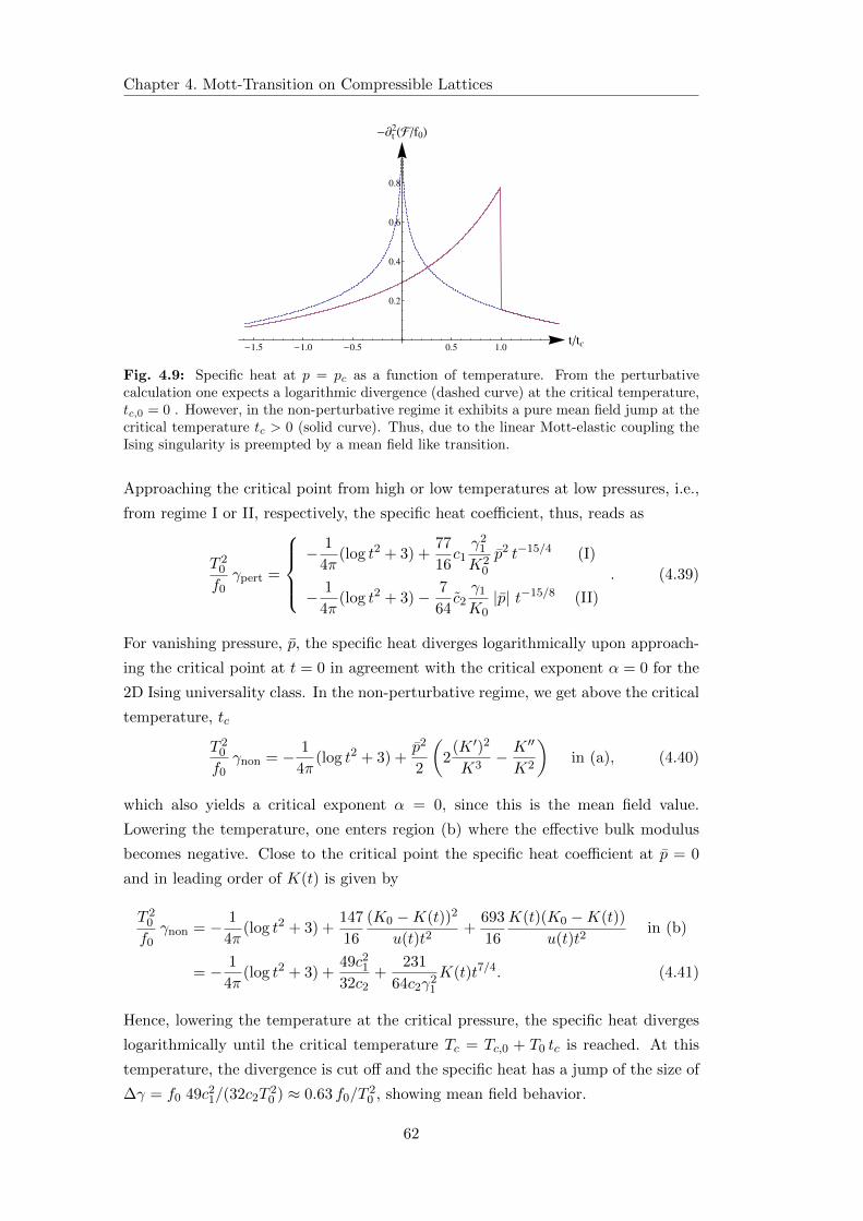
Chapter 4. Mott-Transition on Compressible Lattices
-1.5 -1.0 -0.5 0.5 1.0ttc
0.2
0.4
0.6
0.8
-¶t2HF f0L
Fig. 4.9: Specific heat at p = pc as a function of temperature. From the perturbativecalculation one expects a logarithmic divergence (dashed curve) at the critical temperature,tc,0 = 0 . However, in the non-perturbative regime it exhibits a pure mean field jump at thecritical temperature tc > 0 (solid curve). Thus, due to the linear Mott-elastic coupling theIsing singularity is preempted by a mean field like transition.
Approaching the critical point from high or low temperatures at low pressures, i.e.,
from regime I or II, respectively, the specific heat coefficient, thus, reads as
T 20
f0γpert =
− 1
4π(log t2 + 3) +
77
16c1γ2
1
K20
p2 t−15/4 (I)
− 1
4π(log t2 + 3)− 7
64c2γ1
K0|p| t−15/8 (II)
. (4.39)
For vanishing pressure, p, the specific heat diverges logarithmically upon approach-
ing the critical point at t = 0 in agreement with the critical exponent α = 0 for the
2D Ising universality class. In the non-perturbative regime, we get above the critical
temperature, tc
T 20
f0γnon = − 1
4π(log t2 + 3) +
p2
2
(2
(K ′)2
K3− K ′′
K2
)in (a), (4.40)
which also yields a critical exponent α = 0, since this is the mean field value.
Lowering the temperature, one enters region (b) where the effective bulk modulus
becomes negative. Close to the critical point the specific heat coefficient at p = 0
and in leading order of K(t) is given by
T 20
f0γnon = − 1
4π(log t2 + 3) +
147
16
(K0 −K(t))2
u(t)t2+
693
16
K(t)(K0 −K(t))
u(t)t2in (b)
= − 1
4π(log t2 + 3) +
49c21
32c2+
231
64c2γ21
K(t)t7/4. (4.41)
Hence, lowering the temperature at the critical pressure, the specific heat diverges
logarithmically until the critical temperature Tc = Tc,0 + T0 tc is reached. At this
temperature, the divergence is cut off and the specific heat has a jump of the size of
∆γ = f0 49c21/(32c2T
20 ) ≈ 0.63 f0/T
20 , showing mean field behavior.
62
4.4. Thermodynamics
Notably, this jump is universal, in the sense, that it does not depend on the
magnitude of the elastic coupling constant, γ1 or the critical temperature. Of course,
this is no longer true if anharmonic effects, ∼ u0ε4, are included in the bare elastic
potential. Similarly, switching on the quadratic interaction γ2 or taking temperature
effects of the field, h0, into account would lead to a finite slope of γ as function of
T . Instead, the jump would occur along some curved trace in the (T, p)-diagram,
however, the logarithmic divergence would still be cut off.
Below Tc, the specific heat coefficient decreases and asymptotically resembles
the perturbative result. In Fig. 4.9 the specific heat at the critical temperature,
calculated numerically with the exact function fsing, is shown. The blue, dashed
curve is calculated perturbatively by setting F = V(E = p/K0), while the red
curve gives the exact non-perturbative result, which was obtained by numerical
minimization of the full potential Eq. (4.19).
For temperatures close to the critical temperature and large pressures, i.e., in
regime III, the perturbative calculation gives for the specific heat coefficient
T 20
f0γpert = − 1
4πlog
∣∣∣∣γ1p
K0
∣∣∣∣16/15
− 2φ2 (III), (4.42)
i.e., also a logarithmic divergence as function of pressure. When entering the non-
perturbative regime, the logarithmic divergence has to be cut off since one has no
longer to evaluate the function fsing in region III but rather in region I. Close to
t = tc in lowest order of the effective bulk modulus and pressure, we obtain
T 20
f0γnon = − 1
4π(log t2 + 3)− 147
8
(K0 −K(t))2
t2u(t)
(1 +
5
9K(t)
(6
p2u(t)
)1/3)
(4.43)
= − 1
4π(log t2 + 3)− 49 c2
1
16 c2
(1 +
5
9K(t)
(1
4 γ41 c2 p2
)1/3
t11/6
)in (c).
Hence, the specific heat saturates at a value 14π (log t2c + 3)− (49 c2
1)/(16 c2).
4.4.2 Thermal expansion
The thermal expansion is given by the mixed derivative with respect to t and p,
αpert =f0 γ1
T0K0
∂2fsing(t, h)
∂t ∂h
∣∣∣∣h=γ1 p/K0
. (4.44)
As the potential is an even function of the pressure, the thermal expansion is an odd
function of p. For the perturbative solution, we obtain for smallest pressures
T0
f0αpert =
7
2
γ21
K20
c1t−11/4p (I), (4.45)
T0
f0αpert =
1
8
γ1
K0c1 |t|−7/8 sgn p (II). (4.46)
63
Chapter 4. Mott-Transition on Compressible Lattices
As argued above, the sgn(p) yields the right symmetry concerning the pressure
axis. For vanishing pressure, the thermal expansion is zero above the transition,
whereas it has a finite value below the critical point. Being the mixed derivative
with respect to pressure and temperature, one can identify the thermal expansion as
the derivative of the elastic order parameter, ε = ∂pF , with respect to temperature.
The order parameter scales as ε ∼ |t|β, from which we deduce α ∼ |t|β−1. Hence, we
can identify the critical exponent β = 1/8, which agrees with the critical exponent
of the Ising class.
In the non-perturbative regime, on the other hand, approaching the critical point
from high temperatures we have
T0
f0αnon = p
K ′(t)
K(t)2in (a), (4.47)
again recovering asymptotically the perturbative result for K(t) ≈ K0, i.e., far from
the critical point. Below the critical point, we obtain
T0
f0αnon = −1
2
√6 |K(t)|u(t)
(K ′(t)
|K(t)| −u′(t)
u(t)
)sgn p in (b), (4.48)
diverging as αnon ∝ |K(t)|−1/2 ∝ |t− tc|−1/2, hence, we can identify the critical
exponent β = 1/2 in agreement with mean field behavior.
Lowering the pressure at K(t) = 0, the perturbative result states a divergence
according toT0
f0αpert = |γ1p|−7/15
[8φ1
15+
4
15π
t
|γ1p|8/15
]sgn p (III), (4.49)
whereas the non-perturbative calculation yields a crossover to
T0
f0αnon = K ′(t)
(4
3 p u(t)2
)1/3
sgn p in (c). (4.50)
4.4.3 Compressibility
The compressibility in the perturbative regime consists of two contributions, namely
κ =1
K0− f0
(γ1
K0
)2 ∂2fcr(t, h)
∂h2
∣∣∣∣h=γ1 p/K0
. (4.51)
The first term is the constant lattice contribution which is also present in the bare
elastic system and will be not considered in the following. Concerning the critical
part, κpert,c = κpert − 1/K0, it follows as
1
f0κpert,c = 2c1
γ21
K20
t−7/4 (I), (4.52)
1
f0κpert,c = 2c2
γ21
K20
t−7/4 (II), (4.53)
64
4.5. Experimental Relevance
and diverges, apart from the different coefficients, symmetrically as |t|−7/4 above
and below the critical point.
In the non-perturbative regime above (a) and below (b) the critical point, we
obtain the compressibility to be
1
f0κnon =
1
K(t)in (a), (4.54)
1
f0κnon =
1
2K(t)in (b). (4.55)
Thus, a perturbative expansion for large temperatures resembles the previous result
of the perturbative solution 1f0κnon ≈ 1
K0+ 2γ2
1c1t−7/4/K2
0 . Close to the elastic
Mott transition, however, the compressibility diverges with the inverse power of
the renormalized bulk modulus χ ∼ K(t)−1 ∼ (T − Tc)−1. When tuning through
the critical point, the compressibility obeys the mean field ratio κanon/κ
bnon = 2.
Asymptotically, it does not exactly reproduce the perturbative result, Eq. (4.53),
which is, however, not surprising. It is due to the finite range of validity of the
Taylor expansion of fsing close to the critical point, which necessarily breaks down
when this function changes its behavior, i.e., ultimately when t < 0.
Considering the compressibility at the critical temperature for finite pressures,
we see that the perturbative calculation yields
1
f0κpert,c =
16φ0
225
∣∣∣∣γ1
K0
∣∣∣∣16/15
|p|−14/15 (III). (4.56)
Since the compressibility is the second derivative of the free energy with respect to
pressure, it is also the pressure derivative of the elastic order parameter, ε = ∂pF .
Close to the endpoint, the order parameter scales as ε ∼ p1/δ, from which the
scaling of the compressibility follows as κ ∼ p(1−δ)/δ. Thus, we can identify the
critical exponent δ = 15 in agreement with the Ising universality class.
In contrast, the non-perturbative calculation determines the compressibility at
the critical temperature as
K20
f0γ21
κnon =
(2
9p2u(t)
)1/3
+K(t)
3
(4
3p4u(t)2
)1/3
in (c). (4.57)
This implies a mean field exponent δ = 3 as it was already shown in Sec. 4.3.2.
4.5 Experimental Relevance
So far, we discussed the elastically coupled Mott transition on theoretical and quite
general grounds. In this section, we will now turn to specific experimental conse-
quences and want to connect the theory to actual physical situations. Of particular
importance is the extent of the elastic Landau critical region in the phase diagram,
i.e., over which pressure and temperature range the elastic coupling induces mean
field behavior for the Mott transition.
65
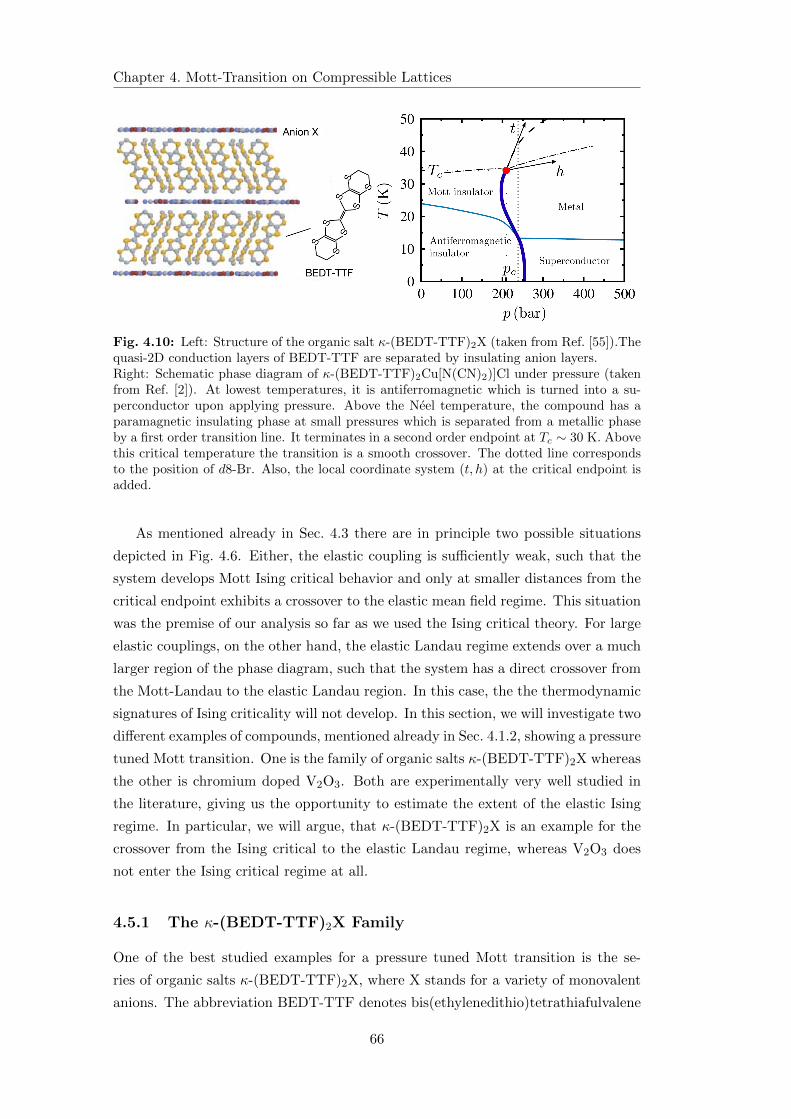
Chapter 4. Mott-Transition on Compressible Lattices
Fig. 4.10: Left: Structure of the organic salt κ-(BEDT-TTF)2X (taken from Ref. [55]).Thequasi-2D conduction layers of BEDT-TTF are separated by insulating anion layers.Right: Schematic phase diagram of κ-(BEDT-TTF)2Cu[N(CN)2)]Cl under pressure (takenfrom Ref. [2]). At lowest temperatures, it is antiferromagnetic which is turned into a su-perconductor upon applying pressure. Above the Neel temperature, the compound has aparamagnetic insulating phase at small pressures which is separated from a metallic phaseby a first order transition line. It terminates in a second order endpoint at Tc ∼ 30 K. Abovethis critical temperature the transition is a smooth crossover. The dotted line correspondsto the position of d8-Br. Also, the local coordinate system (t, h) at the critical endpoint isadded.
As mentioned already in Sec. 4.3 there are in principle two possible situations
depicted in Fig. 4.6. Either, the elastic coupling is sufficiently weak, such that the
system develops Mott Ising critical behavior and only at smaller distances from the
critical endpoint exhibits a crossover to the elastic mean field regime. This situation
was the premise of our analysis so far as we used the Ising critical theory. For large
elastic couplings, on the other hand, the elastic Landau regime extends over a much
larger region of the phase diagram, such that the system has a direct crossover from
the Mott-Landau to the elastic Landau region. In this case, the the thermodynamic
signatures of Ising criticality will not develop. In this section, we will investigate two
different examples of compounds, mentioned already in Sec. 4.1.2, showing a pressure
tuned Mott transition. One is the family of organic salts κ-(BEDT-TTF)2X whereas
the other is chromium doped V2O3. Both are experimentally very well studied in
the literature, giving us the opportunity to estimate the extent of the elastic Ising
regime. In particular, we will argue, that κ-(BEDT-TTF)2X is an example for the
crossover from the Ising critical to the elastic Landau regime, whereas V2O3 does
not enter the Ising critical regime at all.
4.5.1 The κ-(BEDT-TTF)2X Family
One of the best studied examples for a pressure tuned Mott transition is the se-
ries of organic salts κ-(BEDT-TTF)2X, where X stands for a variety of monovalent
anions. The abbreviation BEDT-TTF denotes bis(ethylenedithio)tetrathiafulvalene
66
4.5. Experimental Relevance
and is often further abbreviated to ET. A variation where the protons of the termi-
nal ethylene groups are replaced by deuterium is called d8-ET and accordingly there
also exists a hydrogenated variant called h8-ET. The salts have a layered structure,
as depicted on the right hand side of Fig. 4.10, and are, thus, quasi-two dimen-
sional. On the right hand side of Fig. 4.10, the phase diagram of κ-(d8-ET)2X with
X=Cu[N(CN)2)]Cl is depicted which is the prototypical compound as it shows all
phases of the family. Other members of the family are subject to chemical pressure
meaning that, depending on the kind of anion and whether it is the pure, deuterated
or hydrogenated variant of ET, ambient pressures for them corresponds to a finite
pressure to the prototypical compound. For example, the fully deuterated salt with
X=Cu[N(CN)2)]Br, also called d8-Br, is at ambient pressure located at p ≈ 240 bar
(dotted line) in this phase diagram.
Ultrasonic measurements of longitudinal waves propagating perpendicular to the
layers revealed a huge dip in the relative velocity (about 20 %, Ref. [63]) close to the
critical endpoint corresponding to a very pronounced softening of the elastic mode
C22. A further lattice anomaly was found by de de Souza et al. [1], by measuring the
thermal expansion in d8-Br. This compound is at ambient pressure slightly above
the critical pressure, p − pc ≈ 50 bar and could be fitted by a critical Ising theory
[2], i.e., assuming a perturbative coupling to the elastic degrees of freedom.
Also, the conductivity measurements of Kagawa et al. [55] together with their
later interpretation in Ref. [56] showed strong indications that the pressure tuned
Mott transition of this compound belongs to the Ising universality class. These
results give reason to assume that the Ising critical regime is realized in these com-
pounds, i.e., the scenario on the the left hand side of Fig. 4.6 is realized.
However, we have to estimate the extend of this regime in order to identify
whether the κ-(BEDT-TTF)2X family is a good candidate to experimentally find
elastic Landau criticality. This would, for instance, not be the case if the pressure
scale is too small to be experimentally accessible. Also, the difference between the
Ising critical and the Ising mean field properties may be so small that they are not
resolvable, convicting the discussion above to an interesting, yet academic problem
for this series. The aforementioned analysis of the thermal expansion data [1] by
Bartosch et al. [2] gives us the opportunity of having an estimate of the physical
parameters of this compound.
First of all, we have to identify the theoretical parameters with the physical
ones. The parameter t is the tangent of the line of first order transitions on the
right of Fig. 4.10 at the critical endpoint. Thus, the temperature-like variable has a
small linear pressure admixture, and, similar, the pressure-like variable has a small
temperature admixture
t =T − Tc,0 − ζ(p− pc)
Tc,0, h =
p− pc − λ(T − Tc,0)
p0. (4.58)
67
Chapter 4. Mott-Transition on Compressible Lattices
Here, we used the freedom of scaling to measure t in units of Tc,0 ≈ 30 K which
is the critical temperature deduced in the perturbative regime. The parameters ζ
and λ govern the admixtures which lead to the slopes of the h- and t- axis in the
(p, T )-diagram on the right hand side of Fig. 4.10 and are assumed to be small. Up
to order λ0 and ζ0, the thermal expansion as derived from the perturbative analysis
reads as
α(T, p) ≈ f0
p0Tc,0∂t ∂h fsing(t, h) (4.59)
=f0
p0Tc,0sgn(h)h−7/15Ψα
(t
h8/15
), (4.60)
where we introduced the function Ψα(x) = 815(Φ′(x)−xΦ′′(x)). In Ref. [2], the data
was fitted by the function
α(T, p) = A sgnh |p0 h|−7/15 Ψα
(BTc,0
p8/150
t
|h|8/15
)+ C +DTc,0 t, (4.61)
leading to the identification B = p8/150 /Tc,0 and A = f0/(T
2c,0B). The coefficients C
and D account for a non-singular background contribution and, as such, will be of
no importance for our following considerations. The best fit for the parameter set
to the experimental data was obtained by Bartosch et al. [2] as
(p− pc)/λ = 26.7K , Tc,0 + ζ(p− pc) = 27.5K
Bλ−8/15 = 3.88K−7/15 , Aλ−7/15 = 874 · 10−6K−8/15.
Now, we have to translate these numbers into the notation used in the previous
sections, especially the values for the coupling constants γ1 and γ2. From the fitting
parameters we can directly obtain f0 = 5.7 bar. For the other parameters, we have
to compare the definitions of t and h given in Eq. (4.58) with the arguments of
the Ising part of the free energy in Eq. (4.20). In the perturbative regime, where
E = p/K0, these were
t = τ + pcγ2
K0+γ2
K0(p− pc), (4.62)
h = h0 + pcγ1
K0+γ1
K0(p− pc), (4.63)
which we have to compare to the definitions given in Eq. (4.58).
τ + pcγ2
K0+γ2
K0(p− pc) =
T − Tc,0Tc,0
− ζ(p− pc)Tc,0
(4.64)
h0 + pcγ1
K0+γ1
K0(p− pc) =
p− pcp0
− λT − Tc,0p0
. (4.65)
Following Ref. [64], we estimate the bulk modulus as K0 = 122 000 bar and infer
τ + γ2 pc/K0 = (T −Tc,0)/Tc,0 as well as h0 + pcγ1/K0 = −0.004(T −Tc,0)/Tc,0. For
the elastic coupling constants, γ1 and γ2, we obtain γ1/K0 = 1/p0 = 7 · 10−5 and
γ2/K0 = −ζ/Tc,0 = −1.7 · 10−3 bar−1. However, as the exact critical temperature is
68
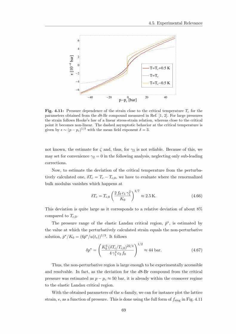
4.5. Experimental Relevance
-40 -20 0 20 40
-6
-4
-2
0
2
4
6
p-pc
@barD
Ε@10
-4
bar
D
T=Tc-0.5 K
T=Tc
T=Tc+0.5 K
Fig. 4.11: Pressure dependence of the strain close to the critical temperature Tc for theparameters obtained from the d8-Br compound measured in Ref. [1, 2]. For large pressuresthe strain follows Hooke’s law of a linear stress-strain relation, whereas close to the criticalpoint it becomes non-linear. The dashed asymptotic behavior at the critical temperature isgiven by ε ∼ (p− pc)1/δ with the mean field exponent δ = 3.
not known, the estimate for ζ and, thus, for γ2 is not reliable. Because of this, we
may set for convenience γ2 = 0 in the following analysis, neglecting only sub-leading
corrections.
Now, to estimate the deviation of the critical temperature from the perturba-
tively calculated one, δTc = Tc − Tc,0, we have to evaluate where the renormalized
bulk modulus vanishes which happens at
δTc = Tc,0
(2 f0 c1 γ
21
K0
)4/7
≈ 2.5 K. (4.66)
This deviation is quite large as it corresponds to a relative deviation of about 8%
compared to Tc,0.
The pressure range of the elastic Landau critical region, p∗, is estimated by
the value at which the perturbatively calculated strain equals the non-perturbative
solution, p∗/K0 = (6p∗/u(tc))1/3. It follows
δp∗ =
(K3
0 (δTc/Tc,0)22/4
4 γ41 c2 f0
)1/2
≈ 44 bar. (4.67)
Thus, the non-perturbative region is large enough to be experimentally accessible
and resolvable. In fact, as the deviation for the d8-Br compound from the critical
pressure was estimated as p− pc ≈ 50 bar, it is already within the crossover regime
to the elastic Landau critical region.
With the obtained parameters of the κ-family, we can for instance plot the lattice
strain, ε, as a function of pressure. This is done using the full form of fsing in Fig. 4.11
69
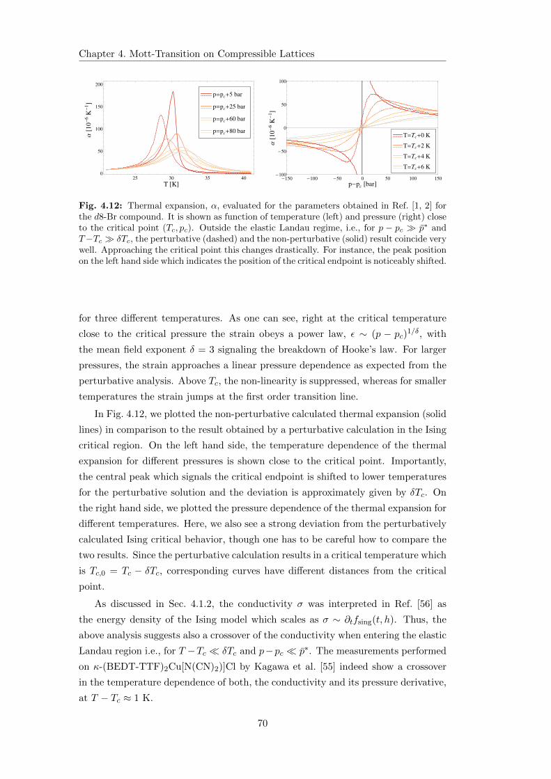
Chapter 4. Mott-Transition on Compressible Lattices
25 30 35 400
50
100
150
200
T @KD
Α@10
-6
K-
1D
p=pc+80 bar
p=pc+60 bar
p=pc+25 bar
p=pc+5 bar
-150 -100 -50 0 50 100 150-100
-50
0
50
100
p-pc @barD
Α@10
-6
K-
1D
T=Tc+6 K
T=Tc+4 K
T=Tc+2 K
T=Tc+0 K
Fig. 4.12: Thermal expansion, α, evaluated for the parameters obtained in Ref. [1, 2] forthe d8-Br compound. It is shown as function of temperature (left) and pressure (right) closeto the critical point (Tc, pc). Outside the elastic Landau regime, i.e., for p − pc p∗ andT−Tc δTc, the perturbative (dashed) and the non-perturbative (solid) result coincide verywell. Approaching the critical point this changes drastically. For instance, the peak positionon the left hand side which indicates the position of the critical endpoint is noticeably shifted.
for three different temperatures. As one can see, right at the critical temperature
close to the critical pressure the strain obeys a power law, ε ∼ (p − pc)1/δ, with
the mean field exponent δ = 3 signaling the breakdown of Hooke’s law. For larger
pressures, the strain approaches a linear pressure dependence as expected from the
perturbative analysis. Above Tc, the non-linearity is suppressed, whereas for smaller
temperatures the strain jumps at the first order transition line.
In Fig. 4.12, we plotted the non-perturbative calculated thermal expansion (solid
lines) in comparison to the result obtained by a perturbative calculation in the Ising
critical region. On the left hand side, the temperature dependence of the thermal
expansion for different pressures is shown close to the critical point. Importantly,
the central peak which signals the critical endpoint is shifted to lower temperatures
for the perturbative solution and the deviation is approximately given by δTc. On
the right hand side, we plotted the pressure dependence of the thermal expansion for
different temperatures. Here, we also see a strong deviation from the perturbatively
calculated Ising critical behavior, though one has to be careful how to compare the
two results. Since the perturbative calculation results in a critical temperature which
is Tc,0 = Tc − δTc, corresponding curves have different distances from the critical
point.
As discussed in Sec. 4.1.2, the conductivity σ was interpreted in Ref. [56] as
the energy density of the Ising model which scales as σ ∼ ∂tfsing(t, h). Thus, the
above analysis suggests also a crossover of the conductivity when entering the elastic
Landau region i.e., for T −Tc δTc and p−pc p∗. The measurements performed
on κ-(BEDT-TTF)2Cu[N(CN)2)]Cl by Kagawa et al. [55] indeed show a crossover
in the temperature dependence of both, the conductivity and its pressure derivative,
at T − Tc ≈ 1 K.
70
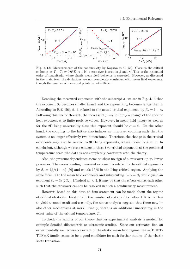
4.5. Experimental Relevance
Fig. 4.13: Measurements of the conductivity by Kagawa et al. [55]. Close to the criticalendpoint at T − Tc ≈ 0.03Tc ≈ 1 K, a crossover is seen in β and γ. This is the estimatedorder of magnitude, where elastic mean field behavior is expected. However, as discussedin the main text, the deviations are not completely consistent with mean field exponents,though the number of measured points is not sufficient.
Denoting the measured exponents with the subscript σ, we see in Fig. 4.13 that
the exponent βσ becomes smaller than 1 and the exponent γσ becomes larger than 1.
According to Ref. [56], βσ is related to the actual critical exponents by βσ = 1− α.
Following this line of thought, the increase of β would imply a change of the specific
heat exponent α to finite positive values. However, in mean field theory as well as
for the 2D Ising universality class this exponent should be α = 0. On the other
hand, the coupling to the lattice also induces an interlayer coupling such that the
system is no longer effectively two-dimensional. Therefore, the change in the critical
exponents may also be related to 3D Ising exponents, where indeed α ≈ 0.11. In
conclusion, although we see a change in these two critical exponents at the predicted
temperature scale, the data is not completely consistent with the theory.
Also, the pressure dependence seems to show no sign of a crossover up to lowest
pressures. The corresponding measured exponent is related to the critical exponents
by δσ = δβ/(1 − α) [56] and equals 15/8 in the Ising critical region. Applying the
same formula to the mean field exponents and substituting 1−α = βσ would yield an
exponent δσ = 3/(2βσ). If indeed βσ < 1, it may be that the effects cancel each other
such that the crossover cannot be resolved in such a conductivity measurement.
However, based on this data no firm statement can be made about the regime
of critical elasticity. First of all, the number of data points below 1 K is too few
to yield a sound result and secondly, the above analysis suggests that there may be
also other mechanisms at work. Finally, there is an additional uncertainty in the
exact value of the critical temperature, Tc.
To check the validity of our theory, further experimental analysis is needed, for
example detailed dilatometric or ultrasonic studies. Since our estimates find an
experimentally well accessible extent of the elastic mean field regime, the κ-(BEDT-
TTF)2X family seems to be a good candidate for such further studies of the elastic
Mott transition.
71
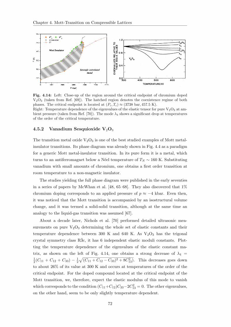
Chapter 4. Mott-Transition on Compressible Lattices
Fig. 4.14: Left: Close-up of the region around the critical endpoint of chromium dopedV2O3 (taken from Ref. [69]). The hatched region denotes the coexistence regime of bothphases. The critical endpoint is located at (Pc, Tc) ≈ (3738 bar, 457.5 K).Right: Temperature dependence of the eigenvalues of the elastic tensor for pure V2O3 at am-bient pressure (taken from Ref. [70]). The mode λ4 shows a significant drop at temperaturesof the order of the critical temperature.
4.5.2 Vanadium Sesquioxide V2O3
The transition metal oxide V2O3 is one of the best studied examples of Mott metal-
insulator transitions. Its phase diagram was already shown in Fig. 4.4 as a paradigm
for a generic Mott metal-insulator transition. In its pure form it is a metal, which
turns to an antiferromagnet below a Neel temperature of TN ∼ 160 K. Substituting
vanadium with small amounts of chromium, one obtains a first order transition at
room temperature to a non-magnetic insulator.
The studies yielding the full phase diagram were published in the early seventies
in a series of papers by McWhan et al. [48, 65–68]. They also discovered that 1%
chromium doping corresponds to an applied pressure of p ≈ −4 kbar. Even then,
it was noticed that the Mott transition is accompanied by an isostructural volume
change, and it was termed a solid-solid transition, although at the same time an
analogy to the liquid-gas transition was assumed [67].
About a decade later, Nichols et al. [70] performed detailed ultrasonic mea-
surements on pure V2O3 determining the whole set of elastic constants and their
temperature dependence between 300 K and 640 K. As V2O3 has the trigonal
crystal symmetry class R3c, it has 6 independent elastic moduli constants. Plot-
ting the temperature dependence of the eigenvalues of the elastic constant ma-
trix, as shown on the left of Fig. 4.14, one obtains a strong decrease of λ4 =12(C11 + C12 + C33) − 1
2
√(C11 + C12 − C33)2 + 8C2
13). This decreases goes down
to about 26% of its value at 300 K and occurs at temperatures of the order of the
critical endpoint. For the doped compound located at the critical endpoint of the
Mott transition, we, therefore, expect the elastic modulus of this mode to vanish
which corresponds to the condition (C11+C12)C33−2C213 = 0. The other eigenvalues,
on the other hand, seem to be only slightly temperature dependent.
72
4.6. Summary and Discussion
The corresponding strain is a superposition of longitudinal strains in the basal
plane (e1 + e2) and along the c-axis (e3). The ratio of the two contributions is given
by (e1 + e2)/e3 = −2C13/(λ4 − C33) which also goes through a minimum. Notably,
this mode is not associated with a breaking of the crystal symmetry as e1 + e2
and e3 are invariant under all 3m crystal symmetry operations. This agrees with
our prediction of an isostructural instability close to the Mott transition. Also, the
pronounced softening of only a single mode fits to our assumption, that the most
important coupling should be bilinear as explained in Sec. 3.1.
In Fig. 4.15, we show the conductivity data obtained by Limelette et al. [54].
They found mean field behavior over at least two decades in temperature and pres-
sure. Only for pressures of the order of p − pc ∼ 10−3 pc ≈ 4 bar, i.e., in the
immediate vicinity of the critical endpoint, deviations were seen. Comparison with
the pressure range of p−pc ≈ 4000 bar, on which the crystal softening is already very
pronounced, this should be deep within the regime of elastic criticality. Therefore,
we conclude that the elastic Landau regime is larger than the Ising critical regime
and, thus, there is only a crossover from the Mott Landau regime to the elastic
Landau regime.
Recently, also ultrasonic measurements of transversal and longitudinal waves
propagating along the c-axis of (V1−xCrx)2O3 with x = 0.11 were performed [71].
The velocity changes of these two acoustic waves give access to the pressure depen-
dence of the two elastic moduli C33 and C44, respectively. The first one shows a
pronounced softening, whereas the latter shows no sign of critical behavior which
coincides with the measurements of the pure compound [70]. Unfortunately, the
constants C11 and C12 were not accessible, which showed a much stronger decrease
in the pure compound.
In future experiments, it would be instructive to obtain the pressure dependence
of the elastic constant λ4 close to the critical point. Most interesting would be a
direct measurement of the order parameter of the transition, which is the corre-
sponding strain, E = e1 + e2 + ae3. The coefficient a close to the endpoint can be
estimated from Ref. [70] as a = 2C13/C33 ≈ 0.8. Such a measurement of the lattice
constants can be achieved by Lamor diffraction experiments as, for instance, done
for MnSi in Ref. [72].
4.6 Summary and Discussion
In this chapter, the influence of the elastic lattice on the Mott metal-insulator tran-
sition was investigated as an example for an electronic finite temperature phase
transition. It turned out that the non-perturbative bilinear coupling has a strong
influence on the transition and even changes the universality class of its critical end-
73
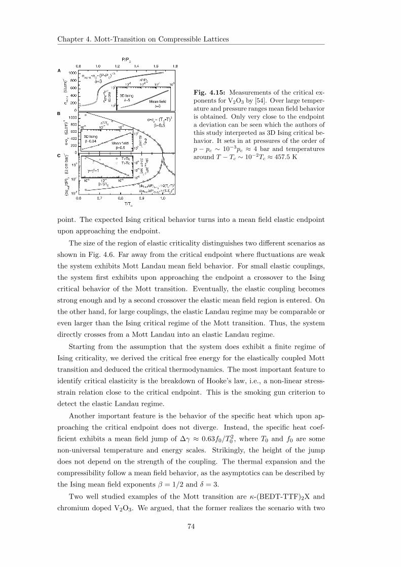
Chapter 4. Mott-Transition on Compressible Lattices
Fig. 4.15: Measurements of the critical ex-ponents for V2O3 by [54]. Over large temper-ature and pressure ranges mean field behavioris obtained. Only very close to the endpointa deviation can be seen which the authors ofthis study interpreted as 3D Ising critical be-havior. It sets in at pressures of the order ofp − pc ∼ 10−3pc ≈ 4 bar and temperaturesaround T − Tc ∼ 10−2Tc ≈ 457.5 K
point. The expected Ising critical behavior turns into a mean field elastic endpoint
upon approaching the endpoint.
The size of the region of elastic criticality distinguishes two different scenarios as
shown in Fig. 4.6. Far away from the critical endpoint where fluctuations are weak
the system exhibits Mott Landau mean field behavior. For small elastic couplings,
the system first exhibits upon approaching the endpoint a crossover to the Ising
critical behavior of the Mott transition. Eventually, the elastic coupling becomes
strong enough and by a second crossover the elastic mean field region is entered. On
the other hand, for large couplings, the elastic Landau regime may be comparable or
even larger than the Ising critical regime of the Mott transition. Thus, the system
directly crosses from a Mott Landau into an elastic Landau regime.
Starting from the assumption that the system does exhibit a finite regime of
Ising criticality, we derived the critical free energy for the elastically coupled Mott
transition and deduced the critical thermodynamics. The most important feature to
identify critical elasticity is the breakdown of Hooke’s law, i.e., a non-linear stress-
strain relation close to the critical endpoint. This is the smoking gun criterion to
detect the elastic Landau regime.
Another important feature is the behavior of the specific heat which upon ap-
proaching the critical endpoint does not diverge. Instead, the specific heat coef-
ficient exhibits a mean field jump of ∆γ ≈ 0.63f0/T20 , where T0 and f0 are some
non-universal temperature and energy scales. Strikingly, the height of the jump
does not depend on the strength of the coupling. The thermal expansion and the
compressibility follow a mean field behavior, as the asymptotics can be described by
the Ising mean field exponents β = 1/2 and δ = 3.
Two well studied examples of the Mott transition are κ-(BEDT-TTF)2X and
chromium doped V2O3. We argued, that the former realizes the scenario with two
74
4.6. Summary and Discussion
crossovers, exhibiting an Ising critical regime. Based on thermal expansion data
[1, 2], we estimated the extent of the elastic Landau regime as ∆T ? ≈ 2.5 K and
∆p? ≈ 50 bar. The conductivity measurements by Kagawa et al. [55] indicate indeed
a crossover at a temperature scale of the order of ∆T ?. However, the available
data does not conclusively support a crossover to mean field exponents and further
experimental investigations are needed. Since the compound of Ref. [1] is at ambient
pressures already above or at the crossover to the Ising critical regime, it would be,
in particular, instructive to investigate a member of the κ-(BEDT-TTF)2X family
with a lower chemical pressure.
In V2O3, we argued that the crossover to the Ising critical regime is preempted
by the elastic Landau regime and, thus, Ising critical behavior is not obtained. A
comparison of elastic measurements in the pure material with conductivity measure-
ments in the chromium doped compound close to the endpoint, suggests that one of
the elastic constants gets critical long before a deviation from mean field behavior
is observed. Since the elastic mode which gets soft at the transition could be iden-
tified, it would be interesting to obtain its actual pressure dependence close to the
endpoint. Thereby, the regime of critical elasticity could be detected directly by the
breakdown of Hooke’s law.
75

Chapter 5
Quantum Critical Metamagnets
In the last chapter, we discussed the effects of an elastic coupling to a finite tem-
perature phase transition. Here, we consider the situation of a transition at zero
temperature, a quantum phase transition (QPT), which arises when the ground
state of a system changes in response to a non-thermal control parameter. This
field of condensed matter theory was pioneered by Hertz [73] in 1976 and since then
attracted much attention. For reviews see, e.g., Refs. [74–76].
Although there is, in principle, a large variety of non-thermal control parameters,
many of them have conceptual or experimental disadvantages. Applying chemical
pressure by doping introduces crystal defects, disorder and, in particular, cannot
be varied continuously. Therefore, sweeps through the quantum critical point are
not possible. Applying physical pressure, on the other hand, although continuously
variable, causes difficulties in measuring some thermodynamic quantities due to the
experimental setup in a pressure cell. Using a magnetic field as a tuning parameter
inherently breaks the spatial symmetry of the system. Thus, many phase transi-
tions induced by a finite magnetic field are first-order transitions which do not yield
diverging susceptibilities.
However, there are different examples where a field-driven transition is of second
order as, for instance, the Bose-Einstein condensation of magnons, see Ref. [77, 78].
In other materials, a phase transition between a low-magnetization state to a high-
magnetization state occurs at a finite applied magnetic field Hc > 0. Such so-
called metamagnetic systems provide another way to magnetic field driven quantum
critical points. The possibility of metamagnetic quantum criticality was introduced
by Grigera et al. [79] when analyzing the layered perovskite Sr3Ru2O7. They found
that the endpoint of the first-order metamagnetic transition could be driven to lower
temperatures and eventually to zero. Thus, they concluded that the system exhibits
a so-called quantum critical endpoint (QCEP) which differs from usual quantum
critical points by the absence of a spontaneous symmetry breaking. Recently, it was
suggested that a metamagnetic QCEP might even be a generic feature for materials
77
Chapter 5. Quantum Critical Metamagnets
with an itinerant ferromagnetic phase when applying pressure [3] which increased
the interest in quantum critical metamagnetism even further.
In this chapter, we focus on the bare metamagnetic QCEP and follow essen-
tially our work as described in Ref. [80], whereas the discussion of elastic effects is
postponed to the next chapter. In the following, we review the mean-field theory of
metamagnetism and the experimental findings concerning metamagnetic criticality
in Sec. 5.1. Thereafter, we introduce the spin-fluctuation theory of metamagnetism
(Sec. 5.2) from which we obtain the effective potential of the theory. In Sec. 5.3,
we derive the magnetization and the free energy from which the thermodynamics
follow as function of applied field and temperature discussed in Sec. 5.4.
5.1 Metamagnetism
Metamagnetism is a phenomenological term for a super-linear rise of the magnetiza-
tion at a finite magnetic field, H. In some systems it may even jump at a first-order
transition. Since no symmetry is broken at a metamagnetic transition, the line of
first-order transitions in a (H,T ) diagram terminates in a critical endpoint, (H∗, T ∗),
where the transition is of second order and above which the magnetization increases
rapidly but smoothly. If by tuning of a third control parameter this endpoint can be
driven to zero temperature, one obtains a QCEP. In the following, we briefly discuss
the theoretical background of metamagnetism and subsequently give an overview of
experimental evidence of a QCEP.
5.1.1 Mean-Field Theory
To introduce the basic principle behind metamagnetism, we follow Ref. [81] and con-
sider the simplest model of the magnetization, M, in a magnetic field, H. Since the
field breaks rotational invariance, we can focus on the component of the magnetiza-
tion parallel to the field, M = M · H, and expand the free energy in it. In absence
of a magnetic field the system has an Ising symmetry, therefore, this expansion can
only contain even powers of the magnetization and reads as
F (M) = −gµBHM +a
2M2 +
u
4M4 +
v
6M6. (5.1)
This approach of course neglects the effects of thermal and quantum fluctuations,
but it will suffice to get an understanding of the metamagnetic transition. To obtain
a second minimum of the free energy, we need a > 0, u < 0 and of course v > 0 to
stabilize the potential. Upon rescaling M = m√|u| /v and gµBH = H
√|u|5 /v3,
Eq. (5.1) takes the form
F (M) =|u|3v2
(−Hm+
α
2m2 − 1
4m4 +
1
6m6
), (5.2)
where α = av/u2 is the only free coefficient of the system.
78
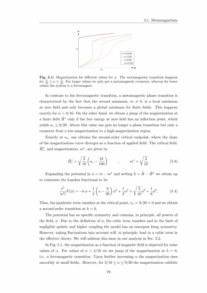
5.1. Metamagnetism
H~ *
c
H~
m*
m
Α=1120
Α=920
Α=720
Α=316
Fig. 5.1: Magnetization for different values for α. The metamagnetic transition happensfor 3
16 ≤ α ≤ 920 . For larger values we only get a metamagnetic crossover, whereas for lower
values the system is a ferromagnet.
In contrast to the ferromagnetic transition, a metamagnetic phase transition is
characterized by the fact that the second minimum, m 6= 0, is a local minimum
at zero field and only becomes a global minimum for finite fields. This happens
exactly for α = 3/16. On the other hand, we obtain a jump of the magnetization at
a finite field H∗ only if the free energy at zero field has an inflection point, which
yields αc ≤ 9/20. Above this value one gets no longer a phase transition but only a
crossover from a low-magnetization to a high-magnetization region.
Exactly at αc, one obtains the second-order critical endpoint, where the slope
of the magnetization curve diverges as a function of applied field. The critical field,
H∗c , and magnetization, m∗, are given by
H∗c =
√3
10
(αc −
21
100
), m∗ =
√3
10. (5.3)
Expanding the potential in φ = m −m∗ and setting h = H − H∗ we obtain up
to constants the Landau functional to be
v2
|u3|F (φ) = −hφ+1
2
(α− 9
20
)φ2 +
1
2φ4 +
√3
10φ5 +
1
6φ6, (5.4)
Thus, the quadratic term vanishes at the critical point, αc = 9/20 = 0 and we obtain
a second-order transition at h = 0.
The potential has no specific symmetry and contains, in principle, all powers of
the field, φ. Due to the definition of φ, the cubic term vanishes and in the limit of
negligible quintic and higher coupling the model has an emergent Ising symmetry.
However, taking fluctuations into account will, in principle, lead to a cubic term in
the effective theory. We will address this issue in our analysis in Sec. 5.2.
In Fig. 5.1, the magnetization as a function of magnetic field is depicted for some
values of α. For values of α < 3/16 we see jump of the magnetization at h = 0,
i.e., a ferromagnetic transition. Upon further increasing α the magnetization rises
smoothly at small fields,. However, for 3/16 ≤ α ≤ 9/20 the magnetization exhibits
79
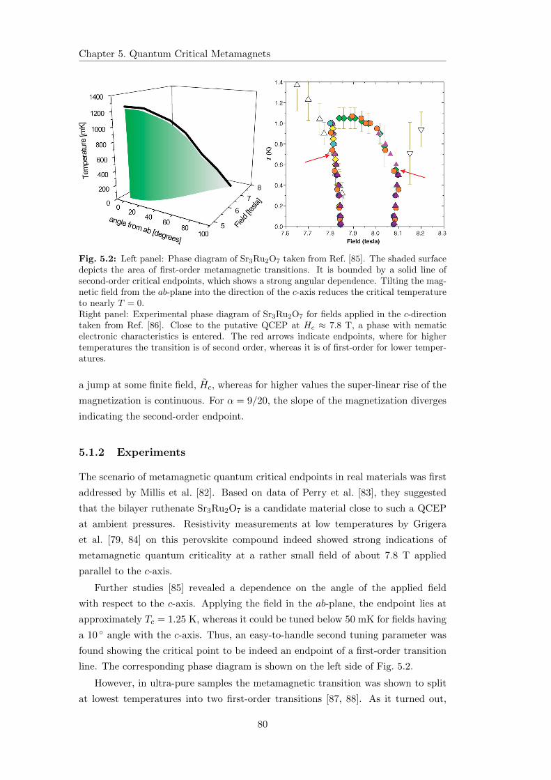
Chapter 5. Quantum Critical Metamagnets
Fig. 5.2: Left panel: Phase diagram of Sr3Ru2O7 taken from Ref. [85]. The shaded surfacedepicts the area of first-order metamagnetic transitions. It is bounded by a solid line ofsecond-order critical endpoints, which shows a strong angular dependence. Tilting the mag-netic field from the ab-plane into the direction of the c-axis reduces the critical temperatureto nearly T = 0.Right panel: Experimental phase diagram of Sr3Ru2O7 for fields applied in the c-directiontaken from Ref. [86]. Close to the putative QCEP at Hc ≈ 7.8 T, a phase with nematicelectronic characteristics is entered. The red arrows indicate endpoints, where for highertemperatures the transition is of second order, whereas it is of first-order for lower temper-atures.
a jump at some finite field, Hc, whereas for higher values the super-linear rise of the
magnetization is continuous. For α = 9/20, the slope of the magnetization diverges
indicating the second-order endpoint.
5.1.2 Experiments
The scenario of metamagnetic quantum critical endpoints in real materials was first
addressed by Millis et al. [82]. Based on data of Perry et al. [83], they suggested
that the bilayer ruthenate Sr3Ru2O7 is a candidate material close to such a QCEP
at ambient pressures. Resistivity measurements at low temperatures by Grigera
et al. [79, 84] on this perovskite compound indeed showed strong indications of
metamagnetic quantum criticality at a rather small field of about 7.8 T applied
parallel to the c-axis.
Further studies [85] revealed a dependence on the angle of the applied field
with respect to the c-axis. Applying the field in the ab-plane, the endpoint lies at
approximately Tc = 1.25 K, whereas it could be tuned below 50 mK for fields having
a 10 angle with the c-axis. Thus, an easy-to-handle second tuning parameter was
found showing the critical point to be indeed an endpoint of a first-order transition
line. The corresponding phase diagram is shown on the left side of Fig. 5.2.
However, in ultra-pure samples the metamagnetic transition was shown to split
at lowest temperatures into two first-order transitions [87, 88]. As it turned out,
80
5.1. Metamagnetism
the quantum critical endpoint was preempted by the formation of a novel phase
which has electronic nematic features [86]. Resistivity measurements showed that
the fourfold symmetry of the RuO2 planes was reduced to a twofold symmetry
giving rise to the idea of a d-wave Pomeranchuk instability of the Fermi surface.
Electron-lattice coupling also induces an crystal anisotropy which was confirmed by
thermal expansion measurements [89]. However, it is not clear yet what is actually
the driving force of the formation of the nematic phase. A current review of the
nematic phase in Sr3Ru2O7 can be found in Ref. [90].
Applying hydrostatic pressure also decreases the critical temperature, as shown
in Ref. [91], where the magnetic field was applied in the ab-plane. The QCEP was
determined to be at pc ≈ 13.6 kbar and, importantly, no evidence of a nematic phase
masking the QCEP was found. However, pressure tuning yields experimental diffi-
culties for some measurements due to the required pressure cell and also increases
the transition field from H? ≈ 5 T to H? ≈ 9 T. To further investigate the metam-
agnetic quantum critical point also the magnetoelastic coupling in the related single
layer ruthenate SrRuO4 doped with calcium was investigated [92].
Metamagnetism was also investigated in antiferromagnetic heavy-fermion com-
pounds, some of which may also have a metamagnetic QCEP. More than twenty
years ago, a metamagnetic transition in CeRu2Si2 at lowest temperatures was found
[93–96]. It turned out that the putative metamagnetic quantum endpoint is located
at negative pressures in the phase diagram of CeRu2Si2. Such negative pressures
can be achieved by doping with lanthanum [97] which yields a volume expansion.
Also CeRh2Si2 [98], UPt3 [99] as well as MnSi [100] show metamagnetic behavior.
However, up to now a metamagnetic QCEP is found in none of those compounds
yet.
Recently, Belitz et al. [3] suggested that a metamagnetic quantum endpoint
might even be a generic feature of itinerant ferromagnets. When applying pressure
to ferromagnets, neighboring sites get closer together, and the overlap of the wave-
function increases yielding a larger spin-spin coupling constant and a decreasing
Curie temperature. Non-analytic corrections in Fermi liquid theory yield a non-
analytic long-range interaction of the order parameter. This interaction leads to
the termination of the second-order transition line in a tricritical point, where the
ferromagnetic transition becomes first-order. From the tricritical point wings of first-
order metamagnetic transition surfaces emerge in the (T,H, p) space, see Fig. 5.3.
The boundary of these wings is a line of second-order critical endpoints which may
also be tuned to zero by further increasing the pressure.
This scenario could explain previously found metamagnetic features in ZrZn2
[101] and UGe2 [102] close to the critical pressure, where the Curie temperature
goes to zero. Further measurements on the boundary of the metamagnetic first-
order transition in UGe2 [5, 6] estimated (Hc, pc) = (17-19 T, 3.5-3.6 GPa) for the
81
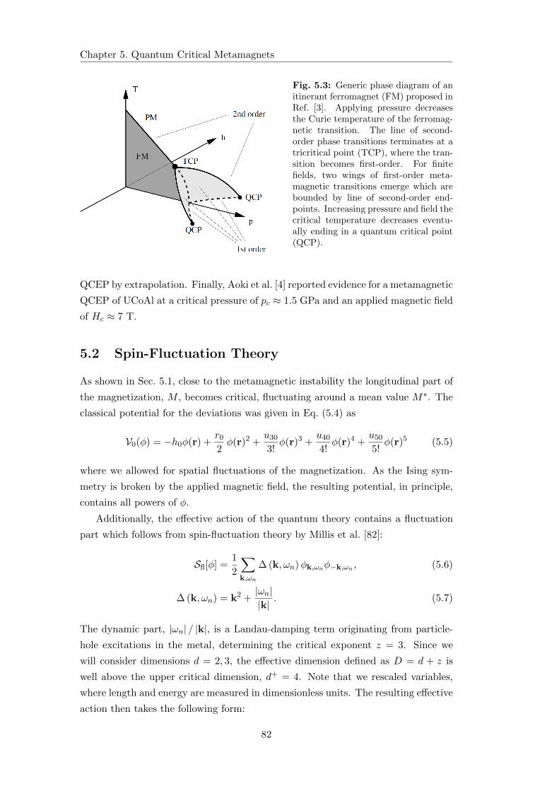
Chapter 5. Quantum Critical Metamagnets
Fig. 5.3: Generic phase diagram of anitinerant ferromagnet (FM) proposed inRef. [3]. Applying pressure decreasesthe Curie temperature of the ferromag-netic transition. The line of second-order phase transitions terminates at atricritical point (TCP), where the tran-sition becomes first-order. For finitefields, two wings of first-order meta-magnetic transitions emerge which arebounded by line of second-order end-points. Increasing pressure and field thecritical temperature decreases eventu-ally ending in a quantum critical point(QCP).
QCEP by extrapolation. Finally, Aoki et al. [4] reported evidence for a metamagnetic
QCEP of UCoAl at a critical pressure of pc ≈ 1.5 GPa and an applied magnetic field
of Hc ≈ 7 T.
5.2 Spin-Fluctuation Theory
As shown in Sec. 5.1, close to the metamagnetic instability the longitudinal part of
the magnetization, M , becomes critical, fluctuating around a mean value M∗. The
classical potential for the deviations was given in Eq. (5.4) as
V0(φ) = −h0φ(r) +r0
2φ(r)2 +
u30
3!φ(r)3 +
u40
4!φ(r)4 +
u50
5!φ(r)5 (5.5)
where we allowed for spatial fluctuations of the magnetization. As the Ising sym-
metry is broken by the applied magnetic field, the resulting potential, in principle,
contains all powers of φ.
Additionally, the effective action of the quantum theory contains a fluctuation
part which follows from spin-fluctuation theory by Millis et al. [82]:
Sfl[φ] =1
2
∑
k,ωn
∆ (k, ωn)φk,ωnφ−k,ωn , (5.6)
∆ (k, ωn) = k2 +|ωn||k| . (5.7)
The dynamic part, |ωn| / |k|, is a Landau-damping term originating from particle-
hole excitations in the metal, determining the critical exponent z = 3. Since we
will consider dimensions d = 2, 3, the effective dimension defined as D = d + z is
well above the upper critical dimension, d+ = 4. Note that we rescaled variables,
where length and energy are measured in dimensionless units. The resulting effective
action then takes the following form:
82

5.2. Spin-Fluctuation Theory
S[φ] =1
2
∑
k,ωn
φk,ωn∆ (k, ωn)φ−k,ωn +
∫dτ
∫drV0(φ(r, τ)), (5.8)
with V0(φ) given in Eq. (5.5). Here, h0 and r0 measure the distance to the critical
point and are assumed to be small.
Concerning the validity of the spin-fluctuation theory there are two general as-
sumptions. First, the Taylor expansion of the bare potential, Eq. (5.5), has to exist,
and, second, the static susceptibility has to be an analytic function of momenta
such that indeed ∆(k, 0) = k2. As the coefficients depend on the derivatives of the
density of states, it has to be sufficiently smooth at the Fermi energy. Van-Hove
singularities at the Fermi energy, for example, would spoil the possibility of this
expansion.
Also non-analytic corrections to the correlation functions in Fermi liquid theory
can be induced by interaction effects. As already mentioned, in particular for fer-
romagnetic quantum phase transitions interactions between fermions and the long-
wavelength bosonic modes induce non-analyticities in the static spin susceptibility
as well as in the Landau potential, see Refs. [103–105]. Long-range interactions of
the order parameter fluctuations mediated by virtual particle-hole pairs may even
render the ferromagnetic transition first-order [3].
However, for a metamagnetic instability the Pauli susceptibility and the mag-
netic field have already a finite value. Thus, spin-flip processes are frozen out,
and the Ising order parameter couples to the relative density fluctuations of the
spin-majority and spin-minority Fermi surfaces. This leads then to the fact that in
contrast to the SU(2) case the non-analytic contributions cancel out, and the static
spin susceptibility is indeed analytic, χ−1 ∼ k2 as shown in Ref. [104]. Therefore,
the model given in Eq. (5.8) is applicable to the metamagnetic transition provided
that there is no van-Hove singularity at the Fermi level.
In principle, all parameters of the action are functions of applied magnetic field,
pressure and temperature and can be obtained from microscopic calculations, see
Ref. [106]. However, in the following this dependence is assumed to be small. In
particular, the couplings ui and the mass r0 are treated as constant with respect
to temperature whereas for the field h0 we assume that it has an implicit Fermi
liquid-like temperature dependence proportional to T 2,
h0(H, p, T ) ≈ h0(H, p) + hTT2 (5.9)
r0(H, p, T ) ≈ r0(H, p). (5.10)
Although hT is irrelevant in the RG sense, it yields important corrections to ther-
modynamics, and its effects will be discussed in Sec. 5.4 below.
83
Chapter 5. Quantum Critical Metamagnets
5.2.1 Wegner-Houghton Equation
Rather than treating the fluctuations close to the metamagnetic endpoint perturba-
tively, we will in the following consider their effects in a systematic self-consistent
way. This is done by means of the renormalization group (RG) in the spirit of Weg-
ner and Houghton (see Ref. [107] for details). They derived the so-called Wegner-
Houghton equation which is a formally exact functional differential equation describ-
ing the flow of the effective action upon infinitesimally decreasing the cutoff Λ. This
captures all momentum-dependent interactions in a infinite hierarchy of functional
RG equations.
Integrating out an infinitesimal high-energy/high-momentum shell, [Λ e−l,Λ]
with l 1, of the Gaussian part of the action adds the re-exponentiated propa-
gator to the potential, V(φ) = V(φ) + f(T, r0), where the function f is given by
f(T, r0) =1
2
∂
∂ ln Λln detG(r0,k, ωn)
=1
2Λ∂
∂Λ
∫ Λ
0
ddk
(2π)d1
β
∑
ωn
lnG(r0,k, ωn). (5.11)
Here, in the second line we assumed a scalar propagator, G, and the summation over
Matsubara frequencies has to be understood as regularized by the cutoff Λz. In the
usual spirit of the RG approach, we rescale the residual action to the original cutoff
Λ, yielding a renormalization of the bare parameters according to their engineering
dimensions, i.e., r0 → r0e2l and T → Tezl. The full mass term of the renormalized
action is now given by the second derivative of the potential V with respect to the
field φ instead of the bare mass, r0. Iterating this procedure corresponds to an
integration along a trajectory of the RG flow and the effective potential at an RG
scale λ is given by
Vλ(φ) = V0(φ) +
∫ λ
0dl e−Dlf(Tezl,V ′′l (φ)e2l). (5.12)
Thus, in the limit λ→∞ we get a self-consistent equation for the effective potential,
V(φ), for the macroscopic magnetization summing up the effects of the fluctuation
in the additional integral to infinite order.
Having a closer look at the function f(T,R), we see that we can split it in two
parts f(T,R) = f0(R) + f∞(T,R) which are of different nature. The first one is
given by an analytic expansion of f(0, R) to second order in the mass,
f0(R) = f(0, 0) + f (0,1)(0, 0)R+1
2f (0,2)(0, 0)R2. (5.13)
Its contribution to the RG flow, Eq. (5.12) is exponentially suppressed by at least a
factor of e−(d−4)l and thus yields a significant correction only at the beginning of the
flow. Because of this, we can conveniently absorb its effect into a renormalization of
84
5.2. Spin-Fluctuation Theory
the bare parameters of the potential given in Eq. (5.5), as the new starting values
of the remaining RG flow,
Vren(φ) = V0(φ) +
∫ ∞
0dl e−Dlf0(V ′′0 (φ)e2l)
≡ −hφ+r
2!φ2 +
u
4!φ4 +
u5
5!φ5 + · · · . (5.14)
In the last line we skipped an unimportant constant and, furthermore, used the
freedom to shift the field φ to eliminate the cubic term. For a negligible quintic term
the potential gains an emergent Ising symmetry, however, note that the quintic term
will lead to renormalizations as specified below.
The remaining contribution, f∞(T,R), is most important at the final stage of
the RG flow and captures the universal fluctuation corrections. Substituting in the
integral l = µ+ ln(ΛT−1/z) we obtain the fluctuation function
TD/zAd(RT−2/z) = TD/z∞∫
− ln ΛT−1/z
dµ e−DµΛ−Df∞(Λzezµ,Λ2RT−2/ze2µ), (5.15)
where the subscript d accounts for the spatial dimensionality. Thus, the effective
potential for the macroscopic magnetization is given by
V(φ) = Vren(φ) + TD/zAd(V ′′(φ)T−2/z), (5.16)
which is a self-consistent differential equation and usually hard to solve. However,
it turns out that it can be solved perturbatively for small temperatures and the
asymptotic behavior can be determined.
5.2.2 Effective Metamagnetic Potential
For the metamagnetic action, Eq. (5.8), replacing the Matsubara summation by an
integral along the branch cut singularity and employing a hard cutoff regularization,
the integration kernel, f , is given by
f(T,R) =Kd
2Λ∂
∂Λ
∫ Λ
0dk kd−1
∫ Λz
−Λz
dω
2πicoth
ω
2Tln(r + k2 − i ω|k|)
= KdΛ∂
∂Λ
∫ Λ
0dk kd−1
∫ Λz
0
dω
2πcoth
ω
2TImln(R+ k2 − iω
k)
= −Kd
2πΛ∂
∂Λ
∫ Λ
0dk kd−1
∫ Λz
0dω coth
ω
2Tarctan
ω
k(R+ k2), (5.17)
where the d-dimensional angular integration yields the factor Kd =[2d−1π
d2 Γ(d2)
]−1.
The derivative with respect to the cutoff gives, in principle, two terms corresponding
to the two integrals. However, as the derivative with respect to the energy integration
85
Chapter 5. Quantum Critical Metamagnets
only leads to sub-leading contributions, we will omit it. With this simplification and
substituting ε = ω/(2T ), the function Ad(x) reads
Ad(x) = Ad,0(x)− Kd
2π
∫ Λz
0dε (coth ε− 1)
∞∫
− ln ΛT−1/z
dµ e−dµ 2 arctan2ezµε
xe2µ + 1, (5.18)
where the term Ad,0(x) accounts for the zero-temperature part of the function
f∞(T,R). It can be evaluated exactly, whereas for the rest we can calculate the
asymptotic behavior for small and large arguments. This asymptotics are given in
d = 3 dimensions to leading order by
A3(x) =
−b1 logΛ3
T− b0 + b2x− b3x
32 , x 1
b1x3 log
Λ3
Tx3/2+ b0x
3 − b2 logΛ3
Tx3/2+ b3 x
−3 log x ,Λ2
T 2/3 x 1,
(5.19)
which has a remaining dependence on the non-universal cutoff Λ. The coefficients b0
and b0 can be absorbed in the non-universal logarithmic dependence of the leading
behavior, and both are omitted in the following. The other coefficients are
b1=1
36π, b2=
1
6√
3π2Γ(4/3)ζ(4/3) , b3=
1
12π,
b1=1
72π3, b2=
1
36π, b3=
π
60.
(5.20)
For d = 2 dimensions we obtain
A2(x) =
−c1 + c3x log1
x, x 1
c1 x52 − c2 x
− 12 + c3x
−2 , x 1
, (5.21)
which is universal in the limit Λ/T 1/3 →∞, i.e., independent of the cutoff, Λ. The
coefficients are given as
c1 =1
4πΓ(5/3)ζ(5/3), c3 =
1
8π, c1 =
1
30π, c2 =
π
24, c3 =
1
4πζ(3). (5.22)
The limiting behaviors for d = 2, 3 can be summarized as
Ad(x) =
−a1 + a2x− a3x
d2 , x 1
xD2
(a1 − a2 x
−z + a3 x− z(d−z+4)
2
), x 1
, (5.23)
where the coefficients are positive up to logarithms.
The term proportional to a1 stems from the zero-temperature part, Ad,0(x) ,
whereas the non-analytic term with coefficient a3 originates from the zero Matsubara
mode. The term with the coefficient a3 will give rise to non-analytic Fermi liquid
corrections.
86
5.3. Free Energy
In the following, we will only consider situations, where all coupling constants
in Eq. (5.14) are positive. This includes, in particular, r > 0, implying that we
will approach the critical endpoint, r = 0, from above, and we will not discuss the
first-order transition occurring for negative r.
5.3 Free Energy
The effective dimension is well above the upper critical dimension, D > d+ = 4, and,
hence, the quartic and quintic coupling as well as even higher terms are irrelevant
in the RG sense. However, the fourth-order term is needed to stabilize the potential
and therefore we have to keep it. The influence of the quintic term, u5, will be
addressed only when it is necessary.
Omitting the quintic term, the potential obtains an emergent Ising symmetry,
i.e., it is invariant under the transformation (h, φ) → (−h,−φ). Hence, we can
immediately conclude that for lowest temperatures the critical free energy density,
Fcr, has to be an even function of the field h. As in Chap. 4, we obtain the free
energy by minimizing the effective potential, Eq. (5.16).
Just as for the Mott-transition in Chap. 4, the most relevant operator is h, which
is proportional to the deviation from the metamagnetic field, h ∼ H −H∗. Due to
the linear coupling to the magnetization, φ, it acts as a force driving it out of its zero-
field equilibrium value φ = 0. The finite-field equilibrium configuration is reached
when the potential built by the quadratic and quartic term cancel this force. The
magnitude of the magnetization depends, thus, on the stiffness of the potential. In
the following, we distinguish a linear regime with a stiff potential and a non-linear
regime, where the potential is soft.
5.3.1 Linear Regime
In the linear regime, the minimizing configuration, φ, is close to zero, and we may
simply expand the effective potential, Eq. (5.16), in φ. Thereby, the parameters of
the effective theory become temperature-dependent and are defined by the value of
the respective derivative of the effective potential at φ = 0. The potential stiffness,
R(T ) = V(2)(0), is to leading order in the temperature given as
R(T ) = r + uT (D−2)/zA′d(RT−2/z
). (5.24)
Furthermore, we obtain also a renormalization of the magnetic field due to existence
of the quintic term
H(T ) = h− U3T(D−2)/zA′d
(RT−2/z
)(5.25)
U3(T ) = u5T(D−2)/zA′d
(RT−2/z
)(5.26)
87
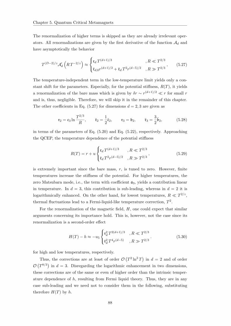
Chapter 5. Quantum Critical Metamagnets
The renormalization of higher terms is skipped as they are already irrelevant oper-
ators. All renormalizations are given by the first derivative of the function Ad and
have asymptotically the behavior
T (D−2)/zA′d(RT−2/z
)≈
rd T
(d+1)/3 , R T 2/3
rd,0r(d+1)/2 + rd T
2r(d−5)/2 , R T 2/3, (5.27)
The temperature-independent term in the low-temperature limit yields only a con-
stant shift for the parameters. Especially, for the potential stiffness, R(T ), it yields
a renormalization of the bare mass which is given by δr ∼ r(d+1)/2 r for small r
and is, thus, negligible. Therefore, we will skip it in the remainder of this chapter.
The other coefficients in Eq. (5.27) for dimensions d = 2, 3 are given as
r2 = c3 lnT 2/3
R, r2 =
1
2c2, r3 = b2, r3 =
3
2b2, (5.28)
in terms of the parameters of Eq. (5.20) and Eq. (5.22), respectively. Approaching
the QCEP, the temperature dependence of the potential stiffness
R(T ) = r + u
rd T
(d+1)/3 , R T 2/3
rd T2r(d−5)/2 , R T 2/3
, (5.29)
is extremely important since the bare mass, r, is tuned to zero. However, finite
temperatures increase the stiffness of the potential. For higher temperatures, the
zero Matsubara mode, i.e., the term with coefficient a3, yields a contribution linear
in temperature. In d = 3, this contribution is sub-leading, whereas in d = 2 it is
logarithmically enhanced. On the other hand, for lowest temperatures, R T 2/z,
thermal fluctuations lead to a Fermi-liquid-like temperature correction, T 2.
For the renormalization of the magnetic field, H, one could expect that similar
arguments concerning its importance hold. This is, however, not the case since its
renormalization is a second-order effect
H(T )− h ≈ −u5
r2d T
2(d+1)/3 , R T 2/3
r2d T4r(d−5) , R T 2/3
. (5.30)
for high and low temperatures, respectively.
Thus, the corrections are at least of order O(T 2 ln2 T
)in d = 2 and of order
O(T 8/3
)in d = 3. Disregarding the logarithmic enhancement in two dimensions,
these corrections are of the same or even of higher order than the intrinsic temper-
ature dependence of h, resulting from Fermi liquid theory. Thus, they are in any
case sub-leading and we need not to consider them in the following, substituting
therefore H(T ) by h.
88
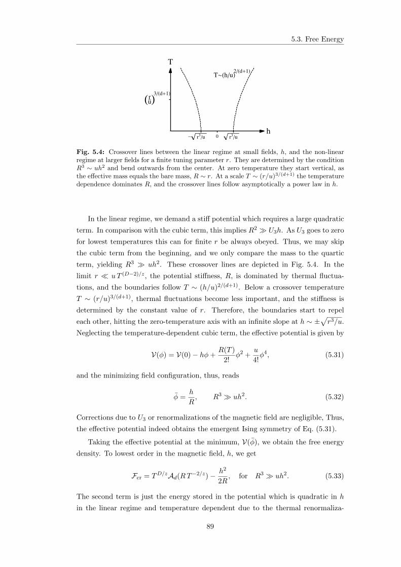
5.3. Free Energy
T~HhuL2Hd+1L
0h
T
ru_H L3Hd+1L
r3ur3u-
Fig. 5.4: Crossover lines between the linear regime at small fields, h, and the non-linearregime at larger fields for a finite tuning parameter r. They are determined by the conditionR3 ∼ uh2 and bend outwards from the center. At zero temperature they start vertical, asthe effective mass equals the bare mass, R ∼ r. At a scale T ∼ (r/u)3/(d+1) the temperaturedependence dominates R, and the crossover lines follow asymptotically a power law in h.
In the linear regime, we demand a stiff potential which requires a large quadratic
term. In comparison with the cubic term, this implies R2 U3h. As U3 goes to zero
for lowest temperatures this can for finite r be always obeyed. Thus, we may skip
the cubic term from the beginning, and we only compare the mass to the quartic
term, yielding R3 uh2. These crossover lines are depicted in Fig. 5.4. In the
limit r uT (D−2)/z, the potential stiffness, R, is dominated by thermal fluctua-
tions, and the boundaries follow T ∼ (h/u)2/(d+1). Below a crossover temperature
T ∼ (r/u)3/(d+1), thermal fluctuations become less important, and the stiffness is
determined by the constant value of r. Therefore, the boundaries start to repel
each other, hitting the zero-temperature axis with an infinite slope at h ∼ ±√r3/u.
Neglecting the temperature-dependent cubic term, the effective potential is given by
V(φ) = V(0)− hφ+R(T )
2!φ2 +
u
4!φ4, (5.31)
and the minimizing field configuration, thus, reads
φ =h
R, R3 uh2. (5.32)
Corrections due to U3 or renormalizations of the magnetic field are negligible, Thus,
the effective potential indeed obtains the emergent Ising symmetry of Eq. (5.31).
Taking the effective potential at the minimum, V(φ), we obtain the free energy
density. To lowest order in the magnetic field, h, we get
Fcr = TD/zAd(RT−2/z)− h2
2R, for R3 uh2. (5.33)
The second term is just the energy stored in the potential which is quadratic in h
in the linear regime and temperature dependent due to the thermal renormaliza-
89

Chapter 5. Quantum Critical Metamagnets
tion of the stiffness. The first term accounts for the energy arising from Gaussian
fluctuations around the minimizing field configuration.
5.3.2 Non-Linear Regime
In the non-linear regime, the potential stiffness is small, R3 uh2, and the second
derivative is dominated by V ′′ ≈ uφ2/2, i.e., the field itself. Thus, we have to
minimize the potential
V(φ) ≈ −hφ+u
4!φ4 + TD/zAd
(u2φ2T−2/z
). (5.34)
Here, we neglected the quintic term which is only valid for fields smaller than a
certain threshold field |h| < h5. By rescaling φ→ (h/u)1/3φ in Eq. (5.14) we obtain
this threshold to be h5 = u4/u35, above which the emergent Ising symmetry is lost.
At zero temperature, the force applied by the magnetic field has to be balanced
by the quartic term. This gives the classical field configuration
φ = sgnh
(6 |h|u
)1/3
, R3 h2u (5.35)
The exponent of the magnetization equals the mean field exponent δ = 3 as we
are above the upper critical dimension. Now, turning on the temperature, we may
expand the field configuration around this mean field result φ = φ + δφ, where δφ
is assumed to be a small temperature correction. Expanding the potential in this
deviation and keeping only the leading-order temperature dependencies, we obtain
V(φ) ≈ V(φ) + φ[r + uT (D−2)/zA′d
(u2φ2T−2/z
)]δφ+
u
4φ2δφ2 (5.36)
Minimization simply yields δφ = 2f/(uφ), where we identified the temperature-
dependent force as
f = −[r + uT (D−2)/zA′d
(u2φ2T−2/z
)]. (5.37)
The temperature dependence of the solution can be obtained from Eq. (5.27),
where in the low-temperature regime one has to substitute r by uφ2/2. In particular,
the effect of the correction of the magnetization on the critical free energy is an extra
term proportional to the square the force, f2. Its temperature dependence is the
same as the temperature dependence of the renormalization of the magnetic field in
the linear regime, Eq. (5.30). Therefore this correction exceeds the current level of
accuracy and is, thus, sub-leading. Neglecting this correction, the critical part of
the free energy is given by
Fcr = TD/zAd[(
9uh2
2T 2
)1/3]− 3
4
(6h4
u
)1/3
. (5.38)
90
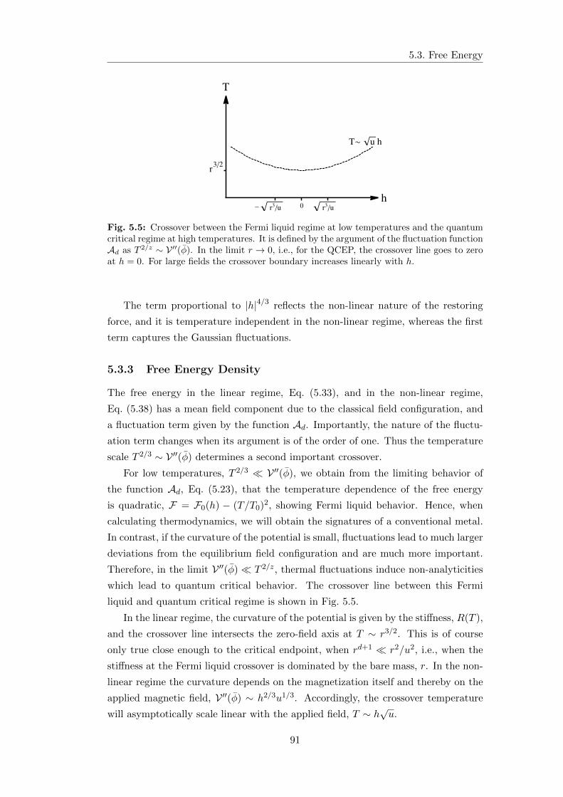
5.3. Free Energy
T~ u h
0h
T
r32
r3ur3u-
Fig. 5.5: Crossover between the Fermi liquid regime at low temperatures and the quantumcritical regime at high temperatures. It is defined by the argument of the fluctuation functionAd as T 2/z ∼ V ′′(φ). In the limit r → 0, i.e., for the QCEP, the crossover line goes to zeroat h = 0. For large fields the crossover boundary increases linearly with h.
The term proportional to |h|4/3 reflects the non-linear nature of the restoring
force, and it is temperature independent in the non-linear regime, whereas the first
term captures the Gaussian fluctuations.
5.3.3 Free Energy Density
The free energy in the linear regime, Eq. (5.33), and in the non-linear regime,
Eq. (5.38) has a mean field component due to the classical field configuration, and
a fluctuation term given by the function Ad. Importantly, the nature of the fluctu-
ation term changes when its argument is of the order of one. Thus the temperature
scale T 2/3 ∼ V ′′(φ) determines a second important crossover.
For low temperatures, T 2/3 V ′′(φ), we obtain from the limiting behavior of
the function Ad, Eq. (5.23), that the temperature dependence of the free energy
is quadratic, F = F0(h) − (T/T0)2, showing Fermi liquid behavior. Hence, when
calculating thermodynamics, we will obtain the signatures of a conventional metal.
In contrast, if the curvature of the potential is small, fluctuations lead to much larger
deviations from the equilibrium field configuration and are much more important.
Therefore, in the limit V ′′(φ) T 2/z, thermal fluctuations induce non-analyticities
which lead to quantum critical behavior. The crossover line between this Fermi
liquid and quantum critical regime is shown in Fig. 5.5.
In the linear regime, the curvature of the potential is given by the stiffness, R(T ),
and the crossover line intersects the zero-field axis at T ∼ r3/2. This is of course
only true close enough to the critical endpoint, when rd+1 r2/u2, i.e., when the
stiffness at the Fermi liquid crossover is dominated by the bare mass, r. In the non-
linear regime the curvature depends on the magnetization itself and thereby on the
applied magnetic field, V ′′(φ) ∼ h2/3u1/3. Accordingly, the crossover temperature
will asymptotically scale linear with the applied field, T ∼ h√u.
91
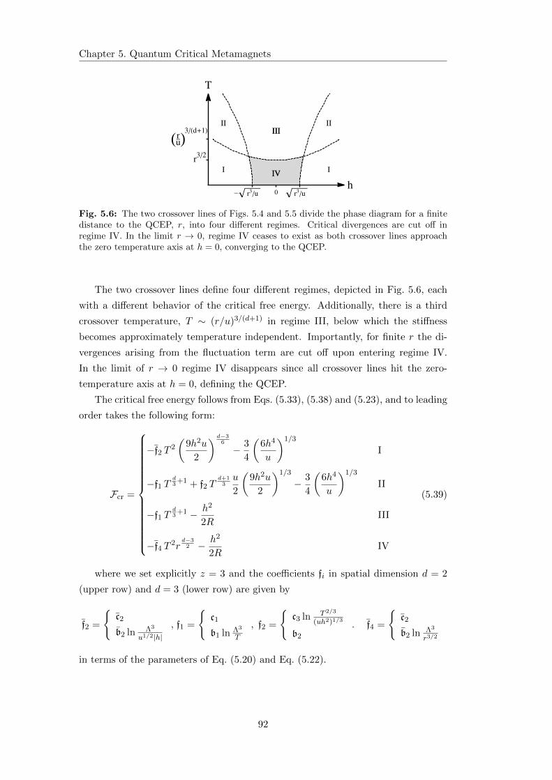
Chapter 5. Quantum Critical Metamagnets
I I
II IIIII
IV
III
IV
0h
T
r32
ru_H L3Hd+1L
r3ur3u-
Fig. 5.6: The two crossover lines of Figs. 5.4 and 5.5 divide the phase diagram for a finitedistance to the QCEP, r, into four different regimes. Critical divergences are cut off inregime IV. In the limit r → 0, regime IV ceases to exist as both crossover lines approachthe zero temperature axis at h = 0, converging to the QCEP.
The two crossover lines define four different regimes, depicted in Fig. 5.6, each
with a different behavior of the critical free energy. Additionally, there is a third
crossover temperature, T ∼ (r/u)3/(d+1) in regime III, below which the stiffness
becomes approximately temperature independent. Importantly, for finite r the di-
vergences arising from the fluctuation term are cut off upon entering regime IV.
In the limit of r → 0 regime IV disappears since all crossover lines hit the zero-
temperature axis at h = 0, defining the QCEP.
The critical free energy follows from Eqs. (5.33), (5.38) and (5.23), and to leading
order takes the following form:
Fcr =
−f2 T 2
(9h2u
2
) d−36
− 3
4
(6h4
u
)1/3
I
−f1 Td3
+1 + f2 Td+1
3u
2
(9h2u
2
)1/3
− 3
4
(6h4
u
)1/3
II
−f1 Td3
+1 − h2
2RIII
−f4 T 2rd−3
2 − h2
2RIV
(5.39)
where we set explicitly z = 3 and the coefficients fi in spatial dimension d = 2
(upper row) and d = 3 (lower row) are given by
f2 =
c2
b2 ln Λ3
u1/2|h|, f1 =
c1
b1 ln Λ3
T
, f2 =
c3 ln T 2/3
(uh2)1/3
b2
. f4 =
c2
b2 ln Λ3
r3/2
in terms of the parameters of Eq. (5.20) and Eq. (5.22).
92
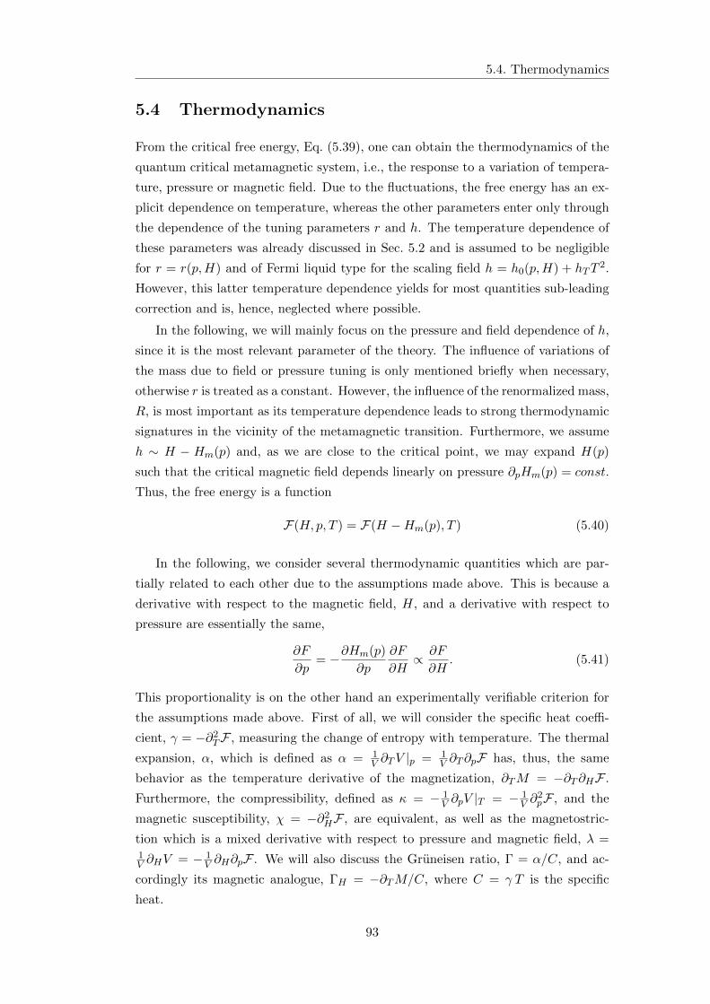
5.4. Thermodynamics
5.4 Thermodynamics
From the critical free energy, Eq. (5.39), one can obtain the thermodynamics of the
quantum critical metamagnetic system, i.e., the response to a variation of tempera-
ture, pressure or magnetic field. Due to the fluctuations, the free energy has an ex-
plicit dependence on temperature, whereas the other parameters enter only through
the dependence of the tuning parameters r and h. The temperature dependence of
these parameters was already discussed in Sec. 5.2 and is assumed to be negligible
for r = r(p,H) and of Fermi liquid type for the scaling field h = h0(p,H) + hTT2.
However, this latter temperature dependence yields for most quantities sub-leading
correction and is, hence, neglected where possible.
In the following, we will mainly focus on the pressure and field dependence of h,
since it is the most relevant parameter of the theory. The influence of variations of
the mass due to field or pressure tuning is only mentioned briefly when necessary,
otherwise r is treated as a constant. However, the influence of the renormalized mass,
R, is most important as its temperature dependence leads to strong thermodynamic
signatures in the vicinity of the metamagnetic transition. Furthermore, we assume
h ∼ H − Hm(p) and, as we are close to the critical point, we may expand H(p)
such that the critical magnetic field depends linearly on pressure ∂pHm(p) = const.
Thus, the free energy is a function
F(H, p, T ) = F(H −Hm(p), T ) (5.40)
In the following, we consider several thermodynamic quantities which are par-
tially related to each other due to the assumptions made above. This is because a
derivative with respect to the magnetic field, H, and a derivative with respect to
pressure are essentially the same,
∂F
∂p= −∂Hm(p)
∂p
∂F
∂H∝ ∂F
∂H. (5.41)
This proportionality is on the other hand an experimentally verifiable criterion for
the assumptions made above. First of all, we will consider the specific heat coeffi-
cient, γ = −∂2TF , measuring the change of entropy with temperature. The thermal
expansion, α, which is defined as α = 1V ∂TV |p = 1
V ∂T∂pF has, thus, the same
behavior as the temperature derivative of the magnetization, ∂TM = −∂T∂HF .
Furthermore, the compressibility, defined as κ = − 1V ∂pV |T = − 1
V ∂2pF , and the
magnetic susceptibility, χ = −∂2HF , are equivalent, as well as the magnetostric-
tion which is a mixed derivative with respect to pressure and magnetic field, λ =1V ∂HV = − 1
V ∂H∂pF . We will also discuss the Gruneisen ratio, Γ = α/C, and ac-
cordingly its magnetic analogue, ΓH = −∂TM/C, where C = γ T is the specific
heat.
93
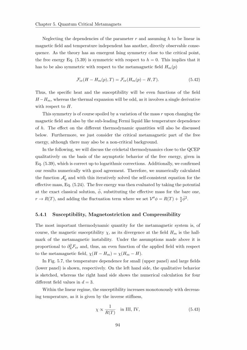
Chapter 5. Quantum Critical Metamagnets
Neglecting the dependencies of the parameter r and assuming h to be linear in
magnetic field and temperature independent has another, directly observable conse-
quence. As the theory has an emergent Ising symmetry close to the critical point,
the free energy Eq. (5.39) is symmetric with respect to h = 0. This implies that it
has to be also symmetric with respect to the metamagnetic field Hm(p)
Fcr(H −Hm(p), T ) = Fcr(Hm(p)−H,T ). (5.42)
Thus, the specific heat and the susceptibility will be even functions of the field
H−Hm, whereas the thermal expansion will be odd, as it involves a single derivative
with respect to H.
This symmetry is of course spoiled by a variation of the mass r upon changing the
magnetic field and also by the sub-leading Fermi liquid like temperature dependence
of h. The effect on the different thermodynamic quantities will also be discussed
below. Furthermore, we just consider the critical metamagnetic part of the free
energy, although there may also be a non-critical background.
In the following, we will discuss the cricketal thermodynamics close to the QCEP
qualitatively on the basis of the asymptotic behavior of the free energy, given in
Eq. (5.39), which is correct up to logarithmic corrections. Additionally, we confirmed
our results numerically with good agreement. Therefore, we numerically calculated
the function A′d and with this iteratively solved the self-consistent equation for the
effective mass, Eq. (5.24). The free energy was then evaluated by taking the potential
at the exact classical solution, φ, substituting the effective mass for the bare one,
r → R(T ), and adding the fluctuation term where we set V ′′φ = R(T ) + u2 φ
2.
5.4.1 Susceptibility, Magnetostriction and Compressibility
The most important thermodynamic quantity for the metamagnetic system is, of
course, the magnetic susceptibility χ, as its divergence at the field Hm is the hall-
mark of the metamagnetic instability. Under the assumptions made above it is
proportional to ∂2hFcr and, thus, an even function of the applied field with respect
to the metamagnetic field, χ(H −Hm) = χ(Hm −H).
In Fig. 5.7, the temperature dependence for small (upper panel) and large fields
(lower panel) is shown, respectively. On the left hand side, the qualitative behavior
is sketched, whereas the right hand side shows the numerical calculation for four
different field values in d = 3.
Within the linear regime, the susceptibility increases monotonously with decreas-
ing temperature, as it is given by the inverse stiffness,
χ ∝ 1
R(T )in III, IV, (5.43)
94
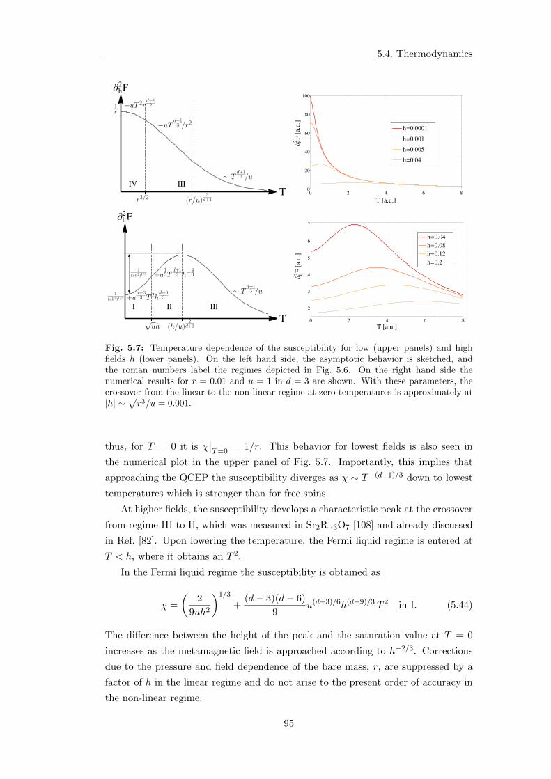
5.4. Thermodynamics
1
IV IIIT
¶h2F
1r
−uT 2rd−92
−uTd+13 /r2
∼ Td+13 /u
r3/2 (r/u)3
d+1
0 2 4 6 80
20
40
60
80
100
T @a.u.D
¶ h2F
@a.u.D
h=0.04
h=0.005
h=0.001
h=0.0001
1
I II III
T
¶h2F
1(uh2)1/3
1(uh2)1/3
+ud−33 T 2h
d−93
+u13T
d+13 h−
43
∼ Td+13 /u
√uh (h/u)
2d+1
0 2 4 6 8
2
3
4
5
6
7
T @a.u.D
¶ h2F
@a.u.D
h=0.2
h=0.12
h=0.08
h=0.04
Fig. 5.7: Temperature dependence of the susceptibility for low (upper panels) and highfields h (lower panels). On the left hand side, the asymptotic behavior is sketched, andthe roman numbers label the regimes depicted in Fig. 5.6. On the right hand side thenumerical results for r = 0.01 and u = 1 in d = 3 are shown. With these parameters, thecrossover from the linear to the non-linear regime at zero temperatures is approximately at|h| ∼
√r3/u = 0.001.
thus, for T = 0 it is χ∣∣T=0
= 1/r. This behavior for lowest fields is also seen in
the numerical plot in the upper panel of Fig. 5.7. Importantly, this implies that
approaching the QCEP the susceptibility diverges as χ ∼ T−(d+1)/3 down to lowest
temperatures which is stronger than for free spins.
At higher fields, the susceptibility develops a characteristic peak at the crossover
from regime III to II, which was measured in Sr2Ru3O7 [108] and already discussed
in Ref. [82]. Upon lowering the temperature, the Fermi liquid regime is entered at
T < h, where it obtains an T 2.
In the Fermi liquid regime the susceptibility is obtained as
χ =
(2
9uh2
)1/3
+(d− 3)(d− 6)
9u(d−3)/6h(d−9)/3 T 2 in I. (5.44)
The difference between the height of the peak and the saturation value at T = 0
increases as the metamagnetic field is approached according to h−2/3. Corrections
due to the pressure and field dependence of the bare mass, r, are suppressed by a
factor of h in the linear regime and do not arise to the present order of accuracy in
the non-linear regime.
95
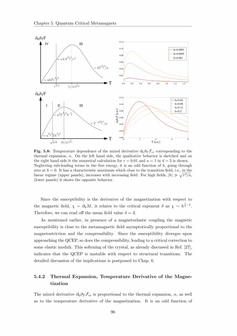
Chapter 5. Quantum Critical Metamagnets
1
IV III
T
¶h¶TF
∼ uhTrd−92
∼ uhTd−23 /r2
∼ hTd+43 /u
r3/2 (r/u)3
d+1
0.0 0.2 0.4 0.6 0.8 1.0 1.2 1.4
0.02
0.04
0.06
0.08
0.10
0.12
h=0.001
h=0.0005
h=0.0001
1
I II III
T
¶h¶TF
∼ ud−33 Th
d−63
∼ u13T
d−23 h−
13
∼ T−hd+43 /u
√uh (h/u)
2d+1
0 2 4 6 80.00
0.02
0.04
0.06
0.08
0.10
0.12
T @a.u.D
¶ h¶ T
.Dh=0.2
h=0.12
h=0.08
h=0.04
Fig. 5.8: Temperature dependence of the mixed derivative ∂h∂TFcr corresponding to thethermal expansion, α. On the left hand side, the qualitative behavior is sketched and onthe right hand side it the numerical calculation for r = 0.01 and u = 1 in d = 3 is shown.Neglecting sub-leading terms in the free energy, it is an odd function of h, going throughzero at h = 0. It has a characteristic maximum which close to the transition field, i.e., in thelinear regime (upper panels), increases with increasing field. For high fields, |h|
√r3/u,
(lower panels) it shows the opposite behavior.
Since the susceptibility is the derivative of the magnetization with respect to
the magnetic field, χ ∼ ∂hM , it relates to the critical exponent δ as χ ∼ h1δ−1.
Therefore, we can read off the mean field value δ = 3.
As mentioned earlier, in presence of a magnetoelastic coupling the magnetic
susceptibility is close to the metamagnetic field asymptotically proportional to the
magnetostriction and the compressibility. Since the susceptibility diverges upon
approaching the QCEP, so does the compressibility, leading to a critical correction to
some elastic moduli. This softening of the crystal, as already discussed in Ref. [27],
indicates that the QCEP is unstable with respect to structural transitions. The
detailed discussion of the implications is postponed to Chap. 6.
5.4.2 Thermal Expansion, Temperature Derivative of the Magne-
tization
The mixed derivative ∂h∂TFcr is proportional to the thermal expansion, α, as well
as to the temperature derivative of the magnetization. It is an odd function of
96
5.4. Thermodynamics
the field h and, thus, has a sign change, which is a generic behavior at quantum
critical points, as discussed in Ref. [109]. For field-tuned quantum critical points,
for instance, the temperature derivative of the magnetization is the derivative of the
entropy, S = ∂TFcr, with respect to the magnetic field. Exactly at the QCP, the
entropy will have a maximum since the system has two different ground states which
leads to frustration. Therefore, the derivative of the entropy has a sign change at
the critical field.
Fig. 5.8 shows the thermal expansion as function of temperature, for high and
low fields. Close to the metamagnetic field it is given by
α ∝ hR′(T )
R(T )2in III, IV. (5.45)
proportional to the field h. At high temperatures it decreases with increasing T
as α ∼ T−(d+4)/3. At the scale, where the temperature dependence of the mass
ceases to dominate, the thermal expansion has a maximum and goes linear to zero.
The position and the height of the maximum is defined by the saturation of R(T ).
Hence, for the QCEP the thermal expansion will at a finite field diverge as function
of temperature. This divergence is cut off when the Fermi liquid regime at lowest
temperatures is reached.
Upon entering the non-linear regime, |h| >√r3/u, the thermal expansion has
qualitatively the same features, but the maximum is defined by the crossover tem-
perature between regime III and II. Hence, it is shifted to higher temperatures as
the field increases. The asymptotic behavior in the non-linear regime is given by
α ∝ T (d−2)/3u1/3h−1/3 in II (5.46)
α ∝ Tu(d−3)/6h(d−6)/3 in I. (5.47)
Thus, the maximum decreases with increasing magnetic field, in contrast to the
behavior in the linear regime.
The behavior of the thermal expansion was already discussed in Ref. [110] with
respect to measurements on Sr3Ru2O7 and in Ref. [111] in the context of CeRu2Si2.
Both measurements showed an asymmetry of the thermal expansion with respect to
h. However, it is the emergent Ising symmetry of the theory which constrains the sign
change to happen at the metamagentic field, H = Hm. As already mentioned, the
Ising symmetry is broken by the temperature-dependent part, hT , of the scaling field
and also by the pressure and field dependence of the bare mass r(p,H). Both effects
yield, in principle, only sub-leading corrections. However, whenever the leading-
order contribution vanishes, these corrections become important. Asymmetries in
the thermal expansion are, thus, a measure of the strength of sub-leading corrections.
97
Chapter 5. Quantum Critical Metamagnets
To discuss the most important contributions, we can limit ourselves to the
regimes III and IV in the phase diagram, Fig. 5.6, as the shift in the thermal ex-
pansion will be small. The critical free energy is given by Fcr = −h2/(2R) and the
thermal expansion follows as
∂F∂p∂T
=∂F∂h∂T
∂ph0 +∂F∂r∂T
∂pr + 2hT T
(∂F∂h∂h
∂ph0 +∂F∂r∂h
∂pr
). (5.48)
On the right hand side, the temperature derivative acts on the explicit tem-
perature dependence of F and on R(T ) only. The first term yields the thermal
expansion calculated above, whereas the other terms are corrections to the leading
order behavior. Most important is the twofold derivative with respect to the field, h,
since it is the only term independent of h and, thus, accountable for a finite thermal
expansion at h = 0. It yields
δα∣∣h=0
= 2ThT∂F∂h∂h
=2hTT
R(T )= 2hT
1rduT−(d−2)/3 T
(ru
)2/(d+1)
1rT T
(ru
)2/(d+1)(5.49)
and close to the QCEP, r = 0, the upper limit is realized. Therefore, the residual
thermal expansion increases with decreasing temperatures.
On the other hand, we can calculate the field at which the thermal expansion
vanishes, or equivalently, where the maxima of the entropy are located in the (H,T )
diagram. For a nearly pressure independent mass, r we find the field correction
(H −Hm)∣∣α=0
= 2hTTR
R′(T )− hTT 2 ≈ 5− d
d+ 1hT T
2 (5.50)
where the approximations holds for T (r/u)3/(d+1), i.e., close to the QCEP.
For experiments, this implies that subtracting this contribution from the data, one
should recover the Ising symmetry, provided h(p) and r(p) vary sufficiently weak.
5.4.3 Specific Heat Coefficient
Like the susceptibility, the specific heat is in the Ising symmetric limit an even
function of magnetic field h. In Fig. 5.9 the field dependence of the specific heat co-
efficient is plotted. For lowest temperatures in the Fermi liquid regime I, it increases
upon lowering the field as
γ = 2 f2
(9
2uh2
)(d−3)/6
in I, (5.51)
which becomes logarithmic in three dimensions. Upon entering the regime IV, the
specific heat coefficient saturates to a value of
γ = 2 f4 r(d−3)/2 in IV. (5.52)
98
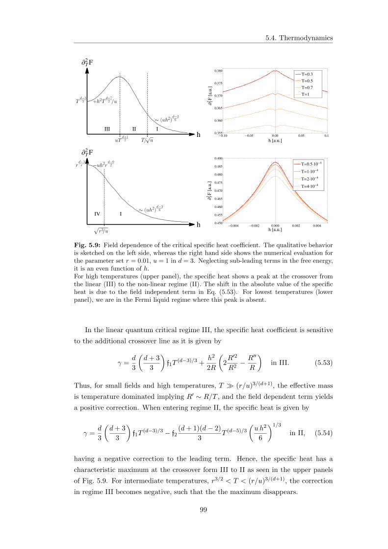
5.4. Thermodynamics
1
III II Ih
¶T
2 F
Td−33 +h2T
d+73 /u
∼ (uh2)d−36
uTd+12 T/
√u
-0.10 -0.05 0.00 0.05 0.100.355
0.360
0.365
0.370
0.375
0.380
h @a.u.D
¶ T2F
@a.u.D
T=1
T=0.7
T=0.5
T=0.3
1
IV I
h
¶T
2 F
rd−3r −uh2r
d−92
∼ (uh2)d−36
√r3/u
-0.004 -0.002 0.000 0.002 0.0040.450
0.455
0.460
0.465
0.470
0.475
0.480
0.485
0.490
h @a.u.D
¶ T2F
@a.u.D
T=4×10⁻⁴
T=2×10⁻⁴
T=1×10⁻⁴
T=0.5×10⁻⁴
Fig. 5.9: Field dependence of the critical specific heat coefficient. The qualitative behavioris sketched on the left side, whereas the right hand side shows the numerical evaluation forthe parameter set r = 0.01, u = 1 in d = 3. Neglecting sub-leading terms in the free energy,it is an even function of h.For high temperatures (upper panel), the specific heat shows a peak at the crossover fromthe linear (III) to the non-linear regime (II). The shift in the absolute value of the specificheat is due to the field independent term in Eq. (5.53). For lowest temperatures (lowerpanel), we are in the Fermi liquid regime where this peak is absent.
In the linear quantum critical regime III, the specific heat coefficient is sensitive
to the additional crossover line as it is given by
γ =d
3
(d+ 3
3
)f1T
(d−3)/3 +h2
2R
(2R′2
R2− R′′
R
)in III. (5.53)
Thus, for small fields and high temperatures, T (r/u)3/(d+1), the effective mass
is temperature dominated implying R′ ∼ R/T , and the field dependent term yields
a positive correction. When entering regime II, the specific heat is given by
γ =d
3
(d+ 3
3
)f1T
(d−3)/3 − f2(d+ 1)(d− 2)
3T (d−5)/3
(uh2
6
)1/3
in II, (5.54)
having a negative correction to the leading term. Hence, the specific heat has a
characteristic maximum at the crossover form III to II as seen in the upper panels
of Fig. 5.9. For intermediate temperatures, r3/2 < T < (r/u)3/(d+1), the correction
in regime III becomes negative, such that the the maximum disappears.
99
Chapter 5. Quantum Critical Metamagnets
The characteristic double-peak structure close to the critical field was also seen
in CeRu2Si2 [112]. In Ref. [111] it was shown to be a generic feature whenever the
susceptibility has a positive curvature with respect to temperature. The reason is
that the curvature of the specific heat with respect to the magnetic field, h, and the
curvature of the susceptibility with respect to the temperature are basically the same
close to the metamagnetic field, ∂2hγ ∼ ∂2
h∂2TF ∼ ∂2
Tχ. Thus, a positive curvature
of the susceptibility at lowest fields together with the symmetry and the asymptotic
decrease implies two maxima around H = Hm of the specific heat.
Taking into account the Fermi liquid temperature correction of the scaling field
h, we see that the specific heat gets three additional contributions
γ =− ∂2TF − 2hT∂hF − 4hT T∂T∂hF − 2hT∂
2hF
=γ0 + 2hTM − 4hT T α0 + 2hTT2χ0 (5.55)
where the index indicates that the respective quantity at hT = 0 is meant.
In the Fermi liquid regime (I and IV) all these corrections are sub-leading and,
thus, negligible. In the linear quantum critical regime (III), terms linear in the field
h are added by the magnetization and by the thermal expansion which, however, are
both sub-leading due to the inverse stiffness. For large fields h and temperatures,
i.e., in regime II, all contributions are sub-leading, though the magnetization yields
an additional contribution, important at intermediate scales.
5.4.4 Gruneisen Parameters
For pressure-tuned quantum critical points the Gruneisen ratio, Γ = α/Cp, is an
interesting quantity to look at. As discussed in Ref. [113], the critical Gruneisen
ratio, Γcr = αcr/(Tγcr) necessarily diverges near a QCP, in contrast to a classi-
cal critical point, where it is in general constant. As long as scaling applies, the
exponents of the divergence and even the prefactor are fully determined by the
critical exponents of the universality class of the transition. The analogous con-
sideration holds in case of magnetic field driven quantum critical points for the
magnetic Gruneisen ratio, ΓH = −∂TM/CH . Within our approximation, the volu-
metric Gruneisen parameter and the magnetic Gruneisen ratio are proportional to
each other, Γ ∝ ΓH ∝ ∂h∂TFcr/(T∂2TFcr).
Due to the Ising symmetry, the thermal expansion vanishes at H = Hm and this
feature is passed on to the Gruneisen parameter. For small but finite fields (regime
III) and high temperatures, T (r/u), the Gruneisen ratio is
ΓH =3(d+ 1)
d(d+ 3)f1rd
h
uT−2(d+2)
3 in III for T ( ru
) 3d+1
. (5.56)
100
5.5. Summary
Upon lowering the temperatures, the temperature dependence of the effective mass,
R(T ), is negligible and the Gruneisen parameter becomes
ΓH =3(d+ 1)
d(d+ 3)
rdf1
hu
r2T−2/3 in III for T
( ru
) 3d+1
. (5.57)
Taking into account the logarithmic correction hidden in the factor r2, one obtains
ΓH ∼ hT−2/z ln 1/T , whereas in d = 3 the factor f1 depends logarithmically on tem-
perature yielding ΓH ∼ h(T 2/z ln 1/T )−1. This is the same temperature dependence
as deduced in Ref. [113]. However, the additional factor h yields a suppression of
the Gruneisen parameter.
In regime I, the Gruneisen parameter is in two dimensions simply proportional
to the inverse of the tuning parameter,
ΓH =3− d
3
1
H −Hmin I (d = 2) (5.58)
which also agrees to the general scaling arguments presented in [113]. In d = 3, due
to the logarithmic dependence of the free energy on h, we obtain also a logarithmic
correction to the Gruneisen parameter
ΓH =1
(H −Hm) log Λ3√u|h|
in I (d = 3). (5.59)
Notably, the prefactor differs in both dimensions from the scaling predictions. This
is on the one hand side due to the fact that the system is above the upper critical
dimension. On the other hand, a strict scaling form can only be obtained for 2
relevant parameters. However, in the situation at hand we have three relevant
parameters namely T , r and h, thus the Gruneisen parameter has to be less universal.
5.5 Summary
In this chapter, we discussed the critical thermodynamics of an itinerant metam-
agnetic quantum critical endpoint. This metamagnetic endpoint is defined by the
divergence of the differential susceptibility at a finite field H?. Close to the endpoint
the theory develops an emergent Ising symmetry. We studied the metamagnetism
in the framework of spin-fluctuation theory as proposed by Millis et al. [82] based
on works by Moriya [114] and Yamada [115]. The dynamics of the spin fluctuations
are dominated by Landau-damping yielding a critical dynamical exponent z = 3.
We applied functional renormalization group techniques which yields a self-
consistent equation, Eq. (5.16), for the effective potential. This equation was the
starting point of our analysis and yielded the asymptotic temperature dependence
of the effective potential.
101
Chapter 5. Quantum Critical Metamagnets
The phase diagram for the metamagnet close to a quantum critical endpoint
consists of two crossover lines. First, there is a crossover line from a linear field
dependence of the magnetization for small deviations from the metamagnetic field,
h ∼ H −H?, to a non-linear regime for higher fields. Second, we obtain a crossover
from a quantum critical regime at high temperatures to a Fermi-liquid like regime.
These lines both terminate in the quantum critical endpoint giving rise to three
different regimes. For systems which are not yet critical, but exhibit only a meta-
magnetic crossover, a fourth regime is obtained which has a linear magnetization,
but is Fermi-liquid like otherwise.
We obtained the critical free energy as a function of temperature and magnetic
field in these different regimes, from which we could derive the critical thermody-
namics of the metamagnetic instability. Assuming a linear pressure dependence of
the metamagnetic transition field, Hm(p), we obtained the susceptibility, the thermal
expansion, the specific heat coefficient and the Gruneisen parameter.
The thermal expansion exhibits a sign change at the transition field, Hm(p),
which corresponds to a maximum of the entropy. To leading order, the thermal
expansion is odd in the field h due to the emergent Ising symmetry. However,
sub-leading temperature dependent contributions of h spoil the Ising symmetry and
result in a shift of the region of entropy accumulation from H = Hm which is
quadratic in temperature.
The specific heat as function of the applied magnetic field shows a characteristic
double peak structure resulting in a minimum at the critical field. Right at the
critical field, h = 0, it diverges as T (d−3)/3, a behavior which is cut off away from
the critical point, i.e., for finite r. The (magnetic) Gruneisen parameter also diverges
for finite fields, but as it is linear in the field it vanishes in the zero-field limit.
These results are especially important for the scenario of itinerant ferromag-
nets with a zero-field tricritical point. Here, wings of metamagnetic transitions,
emerging from the tricritical point, terminate in a QCEP which should show the
thermodynamic signatures obtained above. The systems UCoAl [4] and UGe2 [5, 6]
are promising candidates for a quantitative test of spin-fluctuation theory for critical
metamagnetism based on the results obtained above.
Importantly, susceptibility, magnetostriction, and compressibility should show
similar behavior which implies a divergence of the compressibility upon approaching
the metamagnetic instability. Therefore, the elastic moduli get renormalized and one
expects a pronounced crystal softening. As for the finite temperature Mott transition
(Chap. 4) we, thus, find the metamagnetic QCEP to be unstable in presence of
a magnetoelastic coupling, since the spin fluctuations will destabilize the crystal
lattice. Since no symmetry is broken at the metamagnetic transition, one expects
a isostructural transition preempting the quantum critical endpoint, which is the
subject of the next chapter.
102
Chapter 6
Compressible Quantum Critical
Metamagnetism
As discussed in the previous chapter, the metamagnetic fluctuations yield a diverg-
ing compressibility. Thus, the quantum critical endpoint is inherently unstable with
respect to elastic deformations of the crystal, and the critical endpoint will be pre-
empted by an isostructural transition.
In the following, we will investigate the elastic coupling of a quantum critical
metamagnetic system. After having specified, how the elastic degrees of freedom are
coupled to the metamagnetic fluctuations (Sec. 6.1), we investigate, in particular,
the influence of the phonons in Sec. 6.2. We will show, that, for instance, the
neutron scattering intensity pattern, by which the magnetic structure is investigated,
crucially changes.
On the other hand, the influence of the phonons on the critical thermodynamics
is shown to be negligible. Due to the finite shear moduli, the phonons remain
non-critical in the event of a vanishing eigenvalue of the elastic constant matrix.
Therefore, they will only yield a renormalization of the physical parameters. The
analysis is carried out along the same lines as in Chap. 5, i.e., obtaining a self-
consistent equation for the effective potential by means of functional RG.
We deduce the free energy and the crossover lines in the phase diagram for the
finite temperature endpoint of the first order transition in Sec. 6.3.1 and, especially,
focus on the fine-tuned situation of a quantum endpoint in Sec. 6.3.2.
From the free energy, we derive the critical thermodynamics, i.e., the specific
heat coefficient, thermal expansion and the compressibility as well as the Gruneisen
parameter (Sec. 6.4). We show that the elastic coupling yields a suppression of some
of the critical divergences, for instance of the specific heat, at lowest temperatures.
On the other hand, the Gruneisen parameter diverges with an unusual high power
law. Furthermore, we estimate a temperature scale on which the elastic effects
should be observable on the example of Sr3Ru2O7 in Sec. 6.5.
103
Chapter 6. Compressible Quantum Critical Metamagnetism
6.1 Elastic Coupling
Analogous to Sec. 5.2, we describe the metamagnetic system within spin-fluctuation
theory for the longitudinal fluctuations of the Pauli magnetization, φ, around its
mean value. Within this theory, the action of the metamagnons is given by Eq. (5.8).
For later convenience, we introduce the magnon propagator, g−10 (q, ωn), and rewrite
this action as
S0mm[φ] =
1
2
∑
q,ωn
φq,n g−10 (q, ωn)φq,n +
∫ (v30
3!φ3 +
v40
4!φ4 +
v50
5!φ5 − h0φ
)dx dτ.
Here we introduced for later convenience the propagator
g−10 (q, ωn) = r0 + q2 + γm
|ωn|q. (6.1)
The dynamics of the metamagnetic action is governed by Landau damping due to
particle-hole excitations, giving rise to a dynamical exponent z> = 3. The damping
term is only active if the energy-momentum ratio is small, ωn/q 1, since otherwise
there is no phase space to scatter into. Anticipating the different scaling of the
phonons and the energy rescaling within the RG-procedure, we also introduce the
constant γm.
Concerning the lattice degrees of freedom, we describe them in the continuum
limit as we are interested in low energy physics. Splitting the strain tensor, u, into
the local displacement, u, and the macroscopic volume change, E, as discussed in
Sec. 2.2.4, the action for the elastic system in the harmonic approximation is given
according to Sec. 2.3 by
Sel,p[u] =1
2
∑
q 6=0,ωn
ui(q, ωn)Dim(q, ωn)um(q, ωn), (6.2)
Sel,E[E] =1
2Eij Cijlm Elm. (6.3)
The phonon propagator, D is in terms of the elastic constant matrix, Cijlm, given
by
Dim(q, ωn) = δimρω2n + Cijlmqjql, (6.4)
where, ρ is the mass density. The acoustic phonons are ballistic modes, having a
dynamical exponent z< = 1, therefore, as already mentioned, we have a system
with two different dynamical exponents. The dynamics of the macroscopic modes,
Eij , are not considered since they yield only a non-extensive contribution to the
free energy, i.e., the number of modes does not increase with the volume. Thus,
concerning the thermodynamics of the system, they can be neglected.
104
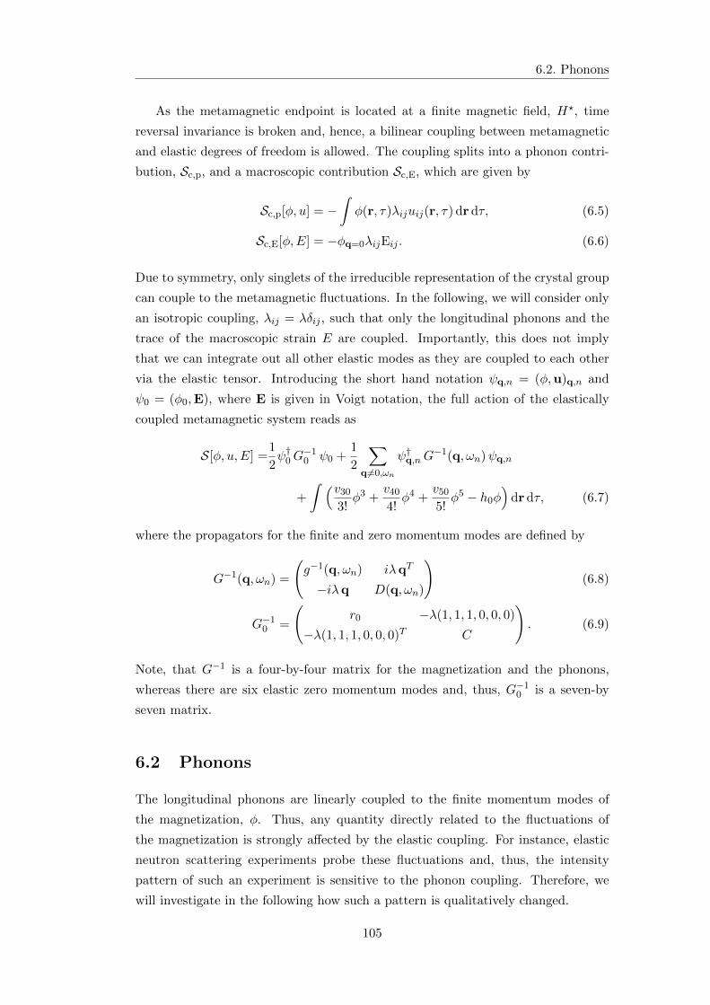
6.2. Phonons
As the metamagnetic endpoint is located at a finite magnetic field, H?, time
reversal invariance is broken and, hence, a bilinear coupling between metamagnetic
and elastic degrees of freedom is allowed. The coupling splits into a phonon contri-
bution, Sc,p, and a macroscopic contribution Sc,E, which are given by
Sc,p[φ, u] = −∫φ(r, τ)λijuij(r, τ) dr dτ, (6.5)
Sc,E[φ,E] = −φq=0λijEij . (6.6)
Due to symmetry, only singlets of the irreducible representation of the crystal group
can couple to the metamagnetic fluctuations. In the following, we will consider only
an isotropic coupling, λij = λδij , such that only the longitudinal phonons and the
trace of the macroscopic strain E are coupled. Importantly, this does not imply
that we can integrate out all other elastic modes as they are coupled to each other
via the elastic tensor. Introducing the short hand notation ψq,n = (φ,u)q,n and
ψ0 = (φ0,E), where E is given in Voigt notation, the full action of the elastically
coupled metamagnetic system reads as
S[φ, u,E] =1
2ψ†0G
−10 ψ0 +
1
2
∑
q 6=0,ωn
ψ†q,nG−1(q, ωn)ψq,n
+
∫ (v30
3!φ3 +
v40
4!φ4 +
v50
5!φ5 − h0φ
)dr dτ, (6.7)
where the propagators for the finite and zero momentum modes are defined by
G−1(q, ωn) =
(g−1(q, ωn) iλqT
−iλq D(q, ωn)
)(6.8)
G−10 =
(r0 −λ(1, 1, 1, 0, 0, 0)
−λ(1, 1, 1, 0, 0, 0)T C
). (6.9)
Note, that G−1 is a four-by-four matrix for the magnetization and the phonons,
whereas there are six elastic zero momentum modes and, thus, G−10 is a seven-by
seven matrix.
6.2 Phonons
The longitudinal phonons are linearly coupled to the finite momentum modes of
the magnetization, φ. Thus, any quantity directly related to the fluctuations of
the magnetization is strongly affected by the elastic coupling. For instance, elastic
neutron scattering experiments probe these fluctuations and, thus, the intensity
pattern of such an experiment is sensitive to the phonon coupling. Therefore, we
will investigate in the following how such a pattern is qualitatively changed.
105
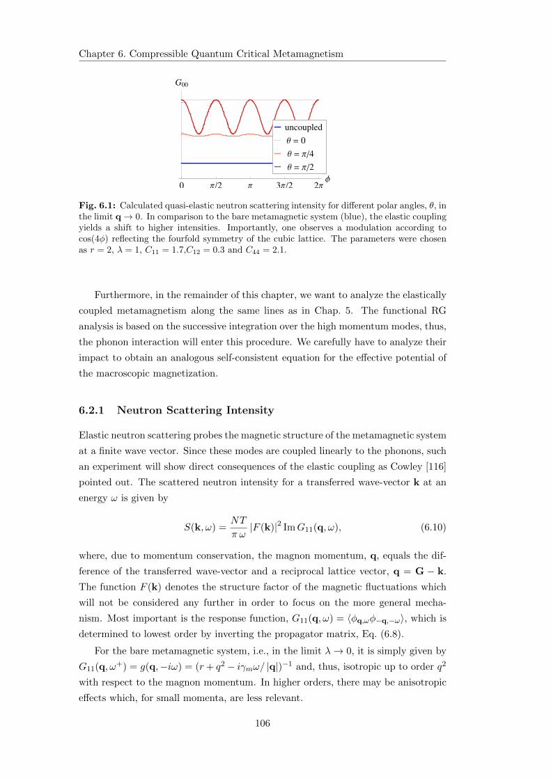
Chapter 6. Compressible Quantum Critical Metamagnetism
0 Π2 Π 3Π2 2ΠΦ
G00
Θ = Π2
Θ = Π4
Θ = 0
uncoupled
Fig. 6.1: Calculated quasi-elastic neutron scattering intensity for different polar angles, θ, inthe limit q→ 0. In comparison to the bare metamagnetic system (blue), the elastic couplingyields a shift to higher intensities. Importantly, one observes a modulation according tocos(4φ) reflecting the fourfold symmetry of the cubic lattice. The parameters were chosenas r = 2, λ = 1, C11 = 1.7,C12 = 0.3 and C44 = 2.1.
Furthermore, in the remainder of this chapter, we want to analyze the elastically
coupled metamagnetism along the same lines as in Chap. 5. The functional RG
analysis is based on the successive integration over the high momentum modes, thus,
the phonon interaction will enter this procedure. We carefully have to analyze their
impact to obtain an analogous self-consistent equation for the effective potential of
the macroscopic magnetization.
6.2.1 Neutron Scattering Intensity
Elastic neutron scattering probes the magnetic structure of the metamagnetic system
at a finite wave vector. Since these modes are coupled linearly to the phonons, such
an experiment will show direct consequences of the elastic coupling as Cowley [116]
pointed out. The scattered neutron intensity for a transferred wave-vector k at an
energy ω is given by
S(k, ω) =NT
π ω|F (k)|2 ImG11(q, ω), (6.10)
where, due to momentum conservation, the magnon momentum, q, equals the dif-
ference of the transferred wave-vector and a reciprocal lattice vector, q = G − k.
The function F (k) denotes the structure factor of the magnetic fluctuations which
will not be considered any further in order to focus on the more general mecha-
nism. Most important is the response function, G11(q, ω) = 〈φq,ωφ−q,−ω〉, which is
determined to lowest order by inverting the propagator matrix, Eq. (6.8).
For the bare metamagnetic system, i.e., in the limit λ→ 0, it is simply given by
G11(q, ω+) = g(q,−iω) = (r+ q2 − iγmω/ |q|)−1 and, thus, isotropic up to order q2
with respect to the magnon momentum. In higher orders, there may be anisotropic
effects which, for small momenta, are less relevant.
106
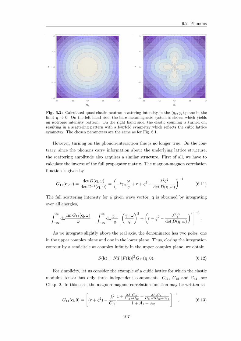
6.2. Phonons
- 1.0 - 0.5 0.0 0.5 1.0
- 1.0
- 0.5
0.0
0.5
1.0
qx
q y
- 1.0 - 0.5 0.0 0.5 1.0
- 1.0
- 0.5
0.0
0.5
1.0
qx
q y
Fig. 6.2: Calculated quasi-elastic neutron scattering intensity in the (qx, qy)-plane in thelimit q → 0. On the left hand side, the bare metamagnetic system is shown which yieldsan isotropic intensity pattern. On the right hand side, the elastic coupling is turned on,resulting in a scattering pattern with a fourfold symmetry which reflects the cubic latticesymmetry. The chosen parameters are the same as for Fig. 6.1.
However, turning on the phonon-interaction this is no longer true. On the con-
trary, since the phonons carry information about the underlying lattice structure,
the scattering amplitude also acquires a similar structure. First of all, we have to
calculate the inverse of the full propagator matrix. The magnon-magnon correlation
function is given by
G11(q, ω) =detD(q, ω)
detG−1(q, ω)=
(−iγm
ω
q+ r + q2 − λ2q2
detD(q, ω)
)−1
. (6.11)
The full scattering intensity for a given wave vector, q is obtained by integrating
over all energies,
∫ ∞
−∞dω
ImG11(q, ω)
ω=
∫ ∞
−∞dω
γmq
[(γmω
q
)2
+
(r + q2 − λ2q2
detD(q, ω)
)2]−1
.
As we integrate slightly above the real axis, the denominator has two poles, one
in the upper complex plane and one in the lower plane. Thus, closing the integration
contour by a semicircle at complex infinity in the upper complex plane, we obtain
S(k) = NT |F (k)|2G11(q, 0). (6.12)
For simplicity, let us consider the example of a cubic lattice for which the elastic
modulus tensor has only three independent components, C11, C12 and C44, see
Chap. 2. In this case, the magnon-magnon correlation function may be written as
G11(q, 0) =
[(r + q2)− λ2
C11
1 + 2A1C11C11+C12
+ 3A2C11C11+2C12+C44
1 +A1 +A2
]−1
, (6.13)
107
Chapter 6. Compressible Quantum Critical Metamagnetism
where A1 and A2 are functions of the polar (θ) and azimuthal (φ) angle of the
momentum q and read as
A1 =(C11 − C12 − 2C44)(C11 + C12)
8C11C44
[2 sin2(2θ) + (1− cos 4φ) sin4 θ
],
A2 =(C11 − C12 − 2C44)2(C11 + 2C12 + C44)
32C11C244
(1− cos 4φ) sin2(2θ) sin2 θ.
Hence, we find a cos(4φ)-modulation, which is depicted in Fig. 6.1, reflecting the
fourfold symmetry of the cubic lattice. Additionally to this modulation, the am-
plitude of the oscillation as well as the mean value of the intensity depend on the
polar angle, θ. Importantly, the anisotropy is independent of the modulus of q, i.e.,
the zero momentum limit depends on the direction, q, from which it is approached.
Note that in the fine-tuned isotropic limit, C11 −C12 = 2C44, the angle dependence
of the scattering amplitude vanishes and the coupling results in a constant shift of
the scattering amplitude, Giso11 = (r + q2 − λ2/C11)−1.
In Fig. 6.2, we show a density plot of the correlation function in the (qx, qy)-plane
for the uncoupled and the coupled system, respectively. Again, we see that the
formerly isotropic scattering pattern obtains a modulation reflecting the symmetry
of the lattice structure. For larger momenta, this modulation is washed out, as the
isotropic part in Eq. (6.13) dominates over the angle dependence originating from
the elastic coupling.
6.2.2 Parameter Renormalization Due To Phonons
Let us again consider, the full action given in Eq. (6.7). In order to obtain the focus
on the important mechanisms at work, we will make a couple of simplifications. If
we again consider a cubic lattice, with its three different elastic constants, C11, C12
and C44, in particular, the macroscopic shear modes, Eij for i 6= j, are decoupled
from the diagonal strain elements and can be integrated out. Therefore, the action
for a cubic lattice reads as
S[φ,u,E] =1
2
∑
q 6=0,ωn
(φ
u
)†
q,n
(g−1(q, ωn) iλqT
−iλq D(q, ωn)
)(φ
u
)
q,n
+1
2
(φ0
E
)†(r0 −λ(1, 1, 1)
−λ(1, 1, 1)T C
)(φ0
E
)
+
∫ (v30
3!φ3 +
v40
4!φ4 +
v50
5!φ5 − h0φ
)dr dτ, (6.14)
where the components of the vector E are given by the diagonal elements of the
tensor of macroscopic distortions (Ei = Eii) and the matrix C is given by Cij = Ciijj .
Notably, Landau damping is absent for the zero momentum magnetic mode, due to
the lack of phase space, as discussed above, and higher order terms in ω are neglected.
108
6.2. Phonons
Since only the longitudinal phonons couple to the order parameter, we switch
to a longitudinal-transversal basis,u = (uL, u1, u2), in which the dynamic matrix
splits into an isotropic and an anisotropic part, D = Diso + δ Dan. The anisotropy
parameter, δ = C11 − C12 − 2C44, vanishes for elastically isotropic crystals. The
isotropic part is given by Diso = ω21 + |q|2 diag (C11, C44, C44), whereas Dan has
momentum dependent off-diagonal elements and is given in Eq. (2.75).
E = Exx + Eyy + Ezz, E1 = Exx − Ezz and, E2 = Exx − 2Eyy + Ezz.
in which the interaction tensor, C, of the macroscopic modes is diagonal,
C =
C11 − 4
3C44 − 23δ 0 0
0 C44 − δ2 0
0 0 C44 − δ2
. (6.15)
As E1 and E2 appear only quadratic in the action they can be integrated out.
Importantly, the criteria for stability under elastic fluctuations demand C11 > 0
and C211 > C2
12 which implies C11 > C12. Substituting δ in Eq. (6.15), the modulus
governing the macroscopic volume change, E, reads as K = C11− 23(C11−C12) and
is, thus, always smaller than C11 which governs the longitudinal phonons. There-
fore, when the magneto-elastic coupling drives the macroscopic modes critical, the
phonons will still be non-critical. In the following, we will, for simplicity, analyze the
system in the isotropic limit, i.e., for δ = 0, in which case the longitudinal and the
transversal phonons are decoupled. Therefore, we can also integrate out the latter
reducing the action to
S[φ, uL, E] =1
2
∑
q 6=0,ωn
(φ
uL
)†
q,n
(g−1(q, ωn) i λ q
−i λ q ρω2n + q2C11
)(φ
uL
)
q,n
+
∫ (v30
3!φ3 +
v40
4!φ4 +
v50
5!φ5 − h0 φ
)dr dτ (6.16)
+1
2
(φ0
E
)†(r0 −λ−λ K
)(φ0
E
)(6.17)
The corrections due to anisotropy could then, in principle, be treated in a pertur-
bative approach. However, concerning thermodynamics a small anisotropy will only
yield subleading corrections. To simplify notations, we will drop the subscript, L,
further on, denoting the longitudinal phonons with u. This is our starting point for
the analysis of the quantum endpoint of compressible metamagnetic systems.
The self-consistent functional RG equation, Eq. (5.12), defines the effective
macroscopic potential of the coupled magneto-elastic system by the evolution of
109
Chapter 6. Compressible Quantum Critical Metamagnetism
the microscopic potential along a RG trajectory. In the coupled theory, we have
not only to consider the second derivative of the action, S[φ, u], with respect to the
metamagnons, φ, but also the second derivative with respect to the longitudinal
phonons, u, and the mixed derivative. Thus, the effective macroscopic potential is
obtained by
V = V0 +
∫ µ
0dµ′e−(d+z)µ′fµ′
(δ2Sµ′δφ2
,δ2Sµ′δφδu
,δ2Sµ′δu2
). (6.18)
The subscript µ′ denotes that the parameters are rescaled according to their respec-
tive engineering dimensions. Importantly, phonons and metamagnons are governed
by different dynamics. The phonons have a dynamical exponent z< = 1, whereas we
obtain z> = 3 for the metamagnons. In the rescaling step of the RG procedure, we,
therefore, leave the general frequency exponent, z, unspecified and rescale the mass
density of the atoms, ρ, and the previously introduced parameter γm accordingly,
as done in Ref. [117]:
r → re2µ, γm → γme−(z−z>)µ, λ→ λeµ,
ρ→ ρe−2(z−z<)µ, T → Tezµ, C11 → C11.(6.19)
The function f is again the re-exponentiated contribution of a high energy shell
integration of the Gaussian part of the action,
f = −Λ∂
∂Λ
1
2
∫ Λ
0
dq
(2π)d1
β
∑
ωn
log[detG−1
], (6.20)
where the matrix G−1 is given by the Hessian of the action
G−1 =
(Sφ,φ Su,φ†Su,φ Su,u
). (6.21)
Here, we introduced the shorthand notation for the functional derivatives of the
action Sα,β = δ2S/(δα δβ).
Because of the bilinear coupling and the lack of anharmonic phonon terms, only
Sφ,φ depends self-consistently on the potential, R = V ′′(φ), and we obtain
detG−1 =
(R+ q2 + γm
|ωn|q
)(ρω2
n + C11q2
)− λ2q2. (6.22)
As it turns out, the function f splits into two terms. One describes phonons
with a renormalized energy, ω1 < vΛ and a damping term-, and the other describes
a metamagnetic system, with a renormalized mass, Rph < R, which is given by
Rph = R − λ2/C11. As we will see in the following, the preemptive structural
transition occurs at R = λ2/K. Importantly, the bulk modulus, K, is smaller than
110
6.3. Free Energy
C11 and, therefore, the phonon-renormalized mass is always larger than zero above
the transition, implying non-critical fluctuations.
The integration over the RG-flow yields, first of all, a renormalization of the
bare parameters, due to zero temperature contributions which only act at the initial
stage of the RG flow. Apart from that, we obtain two fluctuation terms, Ad and Bd,for the metamagnetic and the phonon fluctuations, respectively, and the effective
potential reads as
V(E, φ) =K
2E2 − pE − λφE − hφ+
r
2!φ2 +
u
4!φ4 (6.23)
+ TD>z> Ad
(V ′′ph(φ)T
− 2z>
)+ T
D<z< Bd
(V ′′ph(φ)T
− 2z< ,V ′′(φ)T
− 2z<
).
The function Ad(x) is the same as in Chap. 5 since it stems from the renormalized
metamagnetic theory. However, its argument is not the bare metamagnetic potential
stiffness but the renormalized one V ′′ph(φ) = V ′′(φ)− λ2/C11.
Concerning the phonon part, Bd(x, y), it is V ′′(φ) T 2 as well as V ′′ph(φ) T 2
close to the quantum endpoint. In this limit and for Λ T , the asymptotic behavior
is given by
TD</z<Bd(V ′′ph(φ)T
− 2z< ,V ′′(φ)T
− 2z<
)= T d+1bd
(v2V ′′ph(φ)
V ′′(φ)
)d/2. (6.24)
Comparison with TD>/z>Ad(V ′′ph(φ)T
− 2z>
)shows that this contribution is always
sub-leading at low temperatures, i.e., in the vicinity of the quantum critical endpoint.
Therefore, we may neglect the phonon contribution in the following.
This splitting is of course not at all obvious and is related to the different dy-
namics of the phonons and the magnons. For the details of the tedious and technical
derivation of this equation and the exact form of the two fluctuation function, Bd,the reader may be referred to App. C.
6.3 Free Energy
The elastic part of the effective potential, Eq. (6.23) reads as
Vel(E) =K
2E2 − pE − λφE (6.25)
where we added the second term to account for an applied pressure, p. The strain,
E, is obtained by minimizing Vel(E) yielding E = (p + λφ)/K. Thus, the strain
follows directly the behavior of the magnetization. Substituting this in Eq. (6.23)
leads to the following effective metamagnetic potential
V(φ) =− p2
2K− (h+
λ p
K)φ+
r − λ2/K
2!φ2 +
u
4!φ4 + TD>/z>Ad
(V ′′ph(φ)T−2/z>
).
(6.26)
111
Chapter 6. Compressible Quantum Critical Metamagnetism
The constant first term is irrelevant with respect to minimization of the potential,
therefore, we will skip it in the following. However, it will give rise to an extra
contribution 1/K to the compressibility of the system, which we discuss in Sec. 6.4.
Apart from the fluctuation function, Eq. (6.26) resembles the metamagnetic
potential discussed in Chap. 5 with a shifted magnetic field, hel = h+ λp/K, and a
renormalized bare mass, rel = r − λ2/K. Therefore, large parts of the discussion of
the bare theory also apply to this case. In particular, the negligence of terms higher
than fourth order in the magnetization, φ, is equally well justified. It, again, leads
to an emergent Ising symmetry, though, in this case with respect to hc = −λp/Krather than to hc = 0.
The main difference to the bare system is that the quadratic term of the potential
may become negative. Therefore, we obtain a first order phase transition at hel = 0
terminating in a second order endpoint, which is determined by V ′′(0)− λ2/K = 0.
Importantly, the argument of the fluctuation term, Ad, depends on the phonon-
renormalized potential, V ′′(0) − λ2/C11. As K > C11 the argument is positive at
the endpoint and, therefore, the system exhibits no critical fluctuations.
Since we analyze the system along the same lines as in Chap. 5, we will not be
as explicit in the following as before. To begin with, we will consider the first order
transition with a finite temperature endpoint at Tc and, thereafter, investigate the
fine-tuned limit Tc → 0, i.e., the quantum endpoint.
6.3.1 First Order Transition
If the mass becomes negative, r < λ2/K, the elastically coupled metamagnetic
system exhibits a first order isostructural transition at low temperatures. At a finite
temperature, Tc, the line of these first order transitions terminates in a second order
endpoint. The behavior around the endpoint is similar to the finite temperature
endpoint of the Mott transition on compressible lattices as both have an emergent
Ising symmetry. However, since we start the analysis here from the magnetic sector,
rather than from the effective elastic potential as done in Chap. 4, it is still instructive
to look at this case again. Starting from the more general phase diagram of this
situation, we investigate then the emergence of the quantum critical endpoint.
As before, we can distinguish two different regimes by the strength of the fluc-
tuations. In the so-called linear regime, the potential experienced by the fluctu-
ations, Vph(φ), is rather stiff and we can simply expand the fluctuation function,
Ad(V ′′ph(φ)T−2/z>
), in the magnetization, φ. In contrast, the fluctuations become
very strong, if the phonon-renormalized potential becomes very soft. In this case,
the curvature of the potential is given by the magnetization itself, V ′′(φ) ≈ u2φ
2. The
two regimes are separated by a crossover line determined by the mean magnetization,
φ, as u2 φ
2 ∼ V ′′ph(0).
112
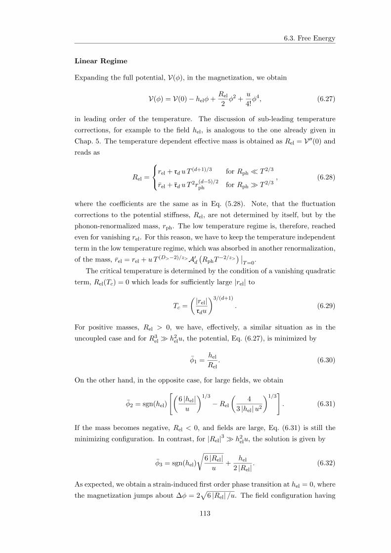
6.3. Free Energy
Linear Regime
Expanding the full potential, V(φ), in the magnetization, we obtain
V(φ) = V(0)− helφ+Rel
2φ2 +
u
4!φ4, (6.27)
in leading order of the temperature. The discussion of sub-leading temperature
corrections, for example to the field hel, is analogous to the one already given in
Chap. 5. The temperature dependent effective mass is obtained as Rel = V ′′(0) and
reads as
Rel =
rel + rd uT
(d+1)/3 for Rph T 2/3
rel + rd uT2r
(d−5)/2ph for Rph T 2/3
, (6.28)
where the coefficients are the same as in Eq. (5.28). Note, that the fluctuation
corrections to the potential stiffness, Rel, are not determined by itself, but by the
phonon-renormalized mass, rph. The low temperature regime is, therefore, reached
even for vanishing rel. For this reason, we have to keep the temperature independent
term in the low temperature regime, which was absorbed in another renormalization,
of the mass, rel = rel + uT (D>−2)/z>A′d(RphT
−2/z>) ∣∣T=0
.
The critical temperature is determined by the condition of a vanishing quadratic
term, Rel(Tc) = 0 which leads for sufficiently large |rel| to
Tc =
( |rel|rdu
)3/(d+1)
. (6.29)
For positive masses, Rel > 0, we have, effectively, a similar situation as in the
uncoupled case and for R3el h2
elu, the potential, Eq. (6.27), is minimized by
φ1 =hel
Rel. (6.30)
On the other hand, in the opposite case, for large fields, we obtain
φ2 = sgn(hel)
[(6 |hel|u
)1/3
−Rel
(4
3 |hel|u2
)1/3]. (6.31)
If the mass becomes negative, Rel < 0, and fields are large, Eq. (6.31) is still the
minimizing configuration. In contrast, for |Rel|3 h2elu, the solution is given by
φ3 = sgn(hel)
√6 |Rel|u
+hel
2 |Rel|. (6.32)
As expected, we obtain a strain-induced first order phase transition at hel = 0, where
the magnetization jumps about ∆φ = 2√
6 |Rel| /u. The field configuration having
113
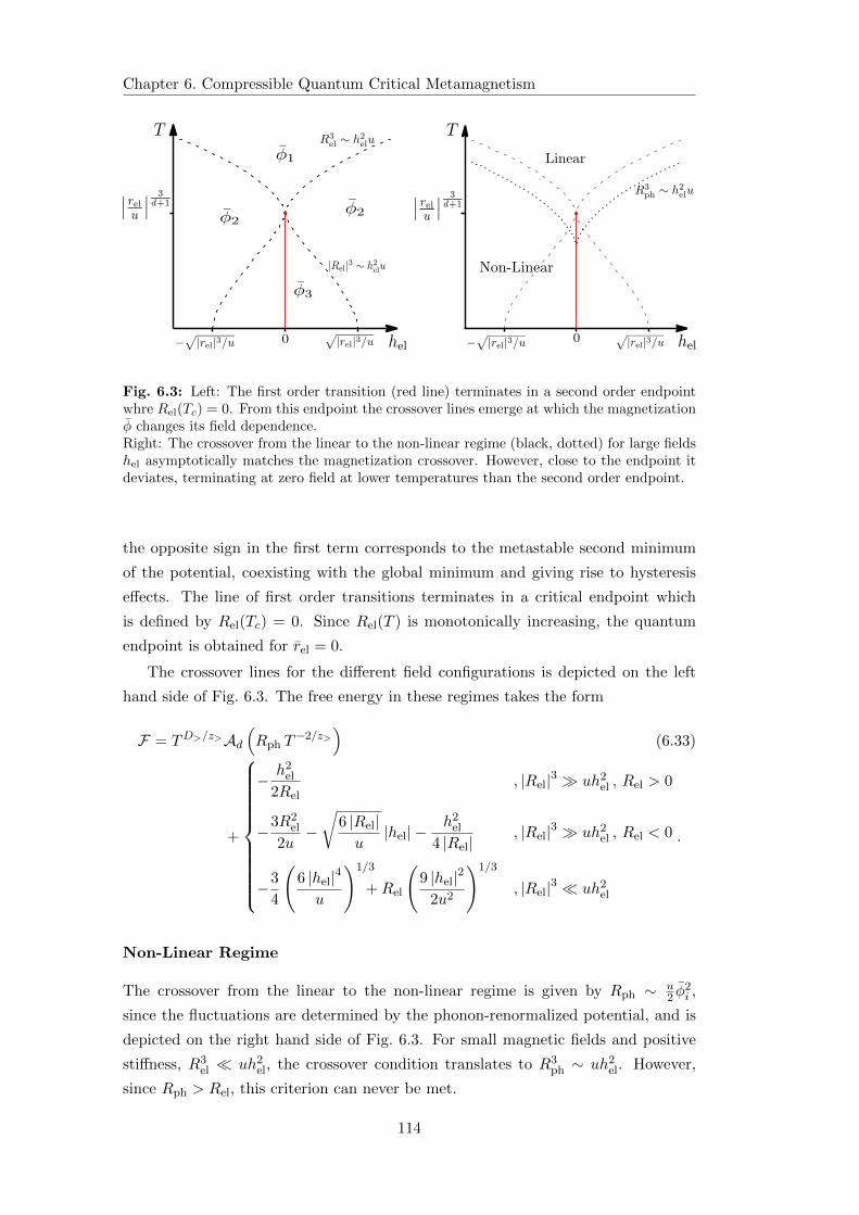
Chapter 6. Compressible Quantum Critical Metamagnetism
0 0
Fig. 6.3: Left: The first order transition (red line) terminates in a second order endpointwhre Rel(Tc) = 0. From this endpoint the crossover lines emerge at which the magnetizationφ changes its field dependence.Right: The crossover from the linear to the non-linear regime (black, dotted) for large fieldshel asymptotically matches the magnetization crossover. However, close to the endpoint itdeviates, terminating at zero field at lower temperatures than the second order endpoint.
the opposite sign in the first term corresponds to the metastable second minimum
of the potential, coexisting with the global minimum and giving rise to hysteresis
effects. The line of first order transitions terminates in a critical endpoint which
is defined by Rel(Tc) = 0. Since Rel(T ) is monotonically increasing, the quantum
endpoint is obtained for rel = 0.
The crossover lines for the different field configurations is depicted on the left
hand side of Fig. 6.3. The free energy in these regimes takes the form
F = TD>/z>Ad(Rph T
−2/z>)
(6.33)
+
− h2el
2Rel, |Rel|3 uh2
el , Rel > 0
−3R2el
2u−√
6 |Rel|u|hel| −
h2el
4 |Rel|, |Rel|3 uh2
el , Rel < 0
−3
4
(6 |hel|4u
)1/3
+Rel
(9 |hel|2
2u2
)1/3
, |Rel|3 uh2el
.
Non-Linear Regime
The crossover from the linear to the non-linear regime is given by Rph ∼ u2 φ
2i ,
since the fluctuations are determined by the phonon-renormalized potential, and is
depicted on the right hand side of Fig. 6.3. For small magnetic fields and positive
stiffness, R3el uh2
el, the crossover condition translates to R3ph ∼ uh2
el. However,
since Rph > Rel, this criterion can never be met.
114
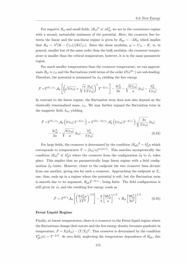
6.3. Free Energy
For negative Rel and small fields, |Rel|3 uh2el, we are in the coexistence regime
with a second, metastable minimum of the potential. Here, the crossover line be-
tween the linear and the non-linear regime is given by Rph ∼ −3Rel which implies
that Rel ∼ λ2(K − C11)/(KC11). Since the shear modulus, µ ∼ C11 − K, is, in
general, smaller but of the same order than the bulk modulus, the crossover temper-
ature is smaller than the critical temperature, however, it is in the same parametric
region.
For much smaller temperatures than the crossover temperature, we can approxi-
mate Rel ≈ rel and the fluctuations yield terms of the order O(φD>) are sub-leading.
Therefore, the potential is minimized by φ3 yielding the free energy
F =TD>/z>Ad[(√
3 |rel|+√u
2
|hel|2 |rel|
)2
T−2/z>
]− 3r2
el
2u−√
6 |rel|u|hel| −
h2el
4 |rel|.
In contrast to the linear regime, the fluctuation term does now also depend on the
elastically renormalized mass, rel. We may further expand the fluctuation term in
the magnetic field, hel, yielding
F =TD>/z>Ad(
3 |rel|T−2/z>)
+ T (D>−2)/z>A′d(
3 |rel|T−2/z>)√ 3u
2 |rel||hel|
− 3r2el
2u−√
6 |rel|u|hel| −
h2el
4 |rel|. (6.34)
For large fields, the crossover is determined by the condition |Rph|3 ∼ h2elu which
corresponds to temperatures T ∼ (hel/u)2/(d+1). This matches asymptotically the
condition |Rel|3 h2elu where the crossover from the configuration φ2 to φ1 takes
place. This implies that no parametrically large linear regime with a field config-
uration φ2 exists. However, closer to the endpoint the two crossover lines deviate
from one another, giving rise for such a crossover. Approaching the endpoint at Tc,
one, thus, ends up in a regime where the potential is soft, but the fluctuation term
is smooth due to its argument, RphT−2/z> , being finite. The field configuration is
still given by φ1 and the resulting free energy reads as
F = TD/zAd[(
9h2elu
2T 2
)1/3]− 3
4
[6h4
el
u
]1/3
+Rel
[9h2
el
2u2
]1/3
. (6.35)
Fermi Liquid Regime
Finally, at lowest temperatures, there is a crossover to the Fermi liquid regime where
the fluctuations change their nature and the free energy density becomes quadratic in
temperature, F = F0(hel)− (T/T0)2. This crossover is determined by the condition
V ′′ph(φ) ∼ T−2/3. At zero field, neglecting the temperature dependence of Rph, this
115
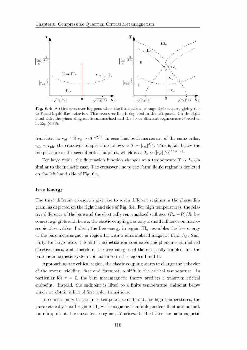
Chapter 6. Compressible Quantum Critical Metamagnetism
0 0
Fig. 6.4: A third crossover happens when the fluctuations change their nature, giving riseto Fermi-liquid like behavior. This crossover line is depicted in the left panel. On the righthand side, the phase diagram is summarized and the seven different regimes are labeled asin Eq. (6.36).
translates to rph + 3 |rel| ∼ T−2/3. In case that both masses are of the same order,
rph ∼ rph, the crossover temperature follows as T ∼ |rel|3/2. This is fair below the
temperature of the second order endpoint, which is at Tc ∼ (|rel| /u)3/(d+1)
For large fields, the fluctuation function changes at a temperature T ∼ hel√u
similar to the inelastic case. The crossover line to the Fermi liquid regime is depicted
on the left hand side of Fig. 6.4.
Free Energy
The three different crossovers give rise to seven different regimes in the phase dia-
gram, as depicted on the right hand side of Fig. 6.4. For high temperatures, the rela-
tive difference of the bare and the elastically renormalized stiffness, (Rel−R)/R, be-
comes negligible and, hence, the elastic coupling has only a small influence on macro-
scopic observables. Indeed, the free energy in region IIIa resembles the free energy
of the bare metamagnet in region III with a renormalized magnetic field, hel. Sim-
ilarly, for large fields, the finite magnetization dominates the phonon-renormalized
effective mass, and, therefore, the free energies of the elastically coupled and the
bare metamagnetic system coincide also in the regions I and II.
Approaching the critical region, the elastic coupling starts to change the behavior
of the system yielding, first and foremost, a shift in the critical temperature. In
particular for r = 0, the bare metamagnetic theory predicts a quantum critical
endpoint. Instead, the endpoint is lifted to a finite temperature endpoint below
which we obtain a line of first order transitions.
In connection with the finite temperature endpoint, for high temperatures, the
parametrically small regime IIIb with magnetization-independent fluctuations and,
more important, the coexistence regime, IV arises. In the latter the metamagnetic
116
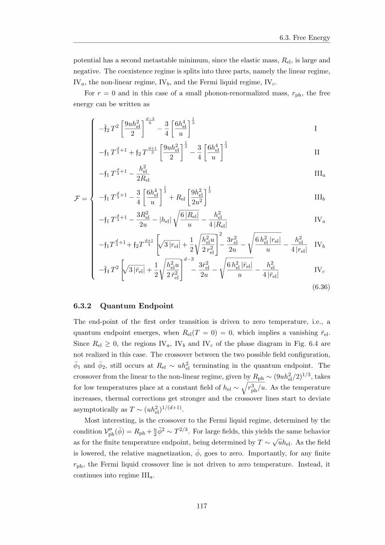
6.3. Free Energy
potential has a second metastable minimum, since the elastic mass, Rel, is large and
negative. The coexistence regime is splits into three parts, namely the linear regime,
IVa, the non-linear regime, IVb, and the Fermi liquid regime, IVc.
For r = 0 and in this case of a small phonon-renormalized mass, rph, the free
energy can be written as
F =
−f2 T 2
[9uh2
el
2
] d−36
− 3
4
[6h4
el
u
] 13
I
−f1 Td3
+1 + f2 Td+1
3
[9uh2
el
2
] 13
− 3
4
[6h4
el
u
] 13
II
−f1 Td3
+1 − h2el
2RelIIIa
−f1 Td3
+1 − 3
4
[6h4
el
u
] 13
+Rel
[9h2
el
2u2
] 13
IIIb
−f1 Td3
+1 − 3R2el
2u− |hel|
√6 |Rel|u− h2
el
4 |Rel|IVa
−f1Td3
+1+ f2Td+1
3
[√
3 |rel|+1
2
√h2
elu
2 r2el
]2
− 3r2el
2u−
√6h2
el |rel|u
− h2el
4 |rel|IVb
−f4 T 2
[√
3 |rel|+1
2
√h2
elu
2 r2el
]d−3
− 3r2el
2u−
√6h2
el |rel|u
− h2el
4 |rel|IVc
(6.36)
6.3.2 Quantum Endpoint
The end-point of the first order transition is driven to zero temperature, i.e., a
quantum endpoint emerges, when Rel(T = 0) = 0, which implies a vanishing rel.
Since Rel ≥ 0, the regions IVa, IVb and IVc of the phase diagram in Fig. 6.4 are
not realized in this case. The crossover between the two possible field configuration,
φ1 and φ2, still occurs at Rel ∼ uh2el terminating in the quantum endpoint. The
crossover from the linear to the non-linear regime, given by Rph ∼ (9uh2el/2)1/3, takes
for low temperatures place at a constant field of hel ∼√r3
ph/u. As the temperature
increases, thermal corrections get stronger and the crossover lines start to deviate
asymptotically as T ∼ (uh2el)
1/(d+1).
Most interesting, is the crossover to the Fermi liquid regime, determined by the
condition V ′′ph(φ) = Rph + u2 φ
2 ∼ T 2/3. For large fields, this yields the same behavior
as for the finite temperature endpoint, being determined by T ∼ √uhel. As the field
is lowered, the relative magnetization, φ, goes to zero. Importantly, for any finite
rph, the Fermi liquid crossover line is not driven to zero temperature. Instead, it
continues into regime IIIa.
117
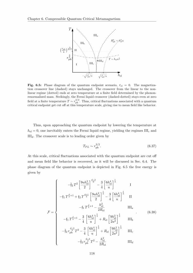
Chapter 6. Compressible Quantum Critical Metamagnetism
Fig. 6.5: Phase diagram of the quantum endpoint scenario, rel = 0. The magnetiza-tion crossover line (dashed) stays unchanged. The crossover from the linear to the non-linear regime (dotted) ends at zero temperature at a finite field determined by the phonon-renormalized mass. Strikingly, the Fermi liquid crossover (dashed-dotted) stays even at zero
field at a finite temperature T ∼ r3/2ph . Thus, critical fluctuations associated with a quantumcritical endpoint get cut off at this temperature scale, giving rise to mean field like behavior.
Thus, upon approaching the quantum endpoint by lowering the temperature at
hel = 0, one inevitably enters the Fermi liquid regime, yielding the regimes IIIc and
IIId. The crossover scale is to leading order given by
TFL ∼ r3/2ph . (6.37)
At this scale, critical fluctuations associated with the quantum endpoint are cut off
and mean field like behavior is recovered, as it will be discussed in Sec. 6.4. The
phase diagram of the quantum endpoint is depicted in Fig. 6.5 the free energy is
given by
F =
−f2 T 2
[9uh2
el
2
] d−36
− 3
4
[6h4
el
u
] 13
I
−f1 Td3
+1 + f2 Td+1
3
[9uh2
el
2
] 13
− 3
4
[6h4
el
u
] 13
II
−f1 Td3
+1 − h2el
2RelIIIa
−f1 Td3
+1 − 3
4
[6h4
el
u
] 13
+Rel
[9h2
el
2u2
] 13
IIIb
−f2 rd−3
2ph T 2 − 3
4
[6h4
el
u
] 13
+Rel
[9h2
el
2u2
] 13
IIIc
−f2 rd−3
2ph T 2 − h2
el
2RelIIId
. (6.38)
118
6.4. Thermodynamics
Notably, the potential stiffness, Rel(T ), has no term independent of temperature as
it is fine-tuned to zero to obtain the quantum endpoint. For high temperatures, it
scales as Rel ∼ Td+1
3 , whereas for lowest temperatures it goes as Rel ∼ T 2. According
to Eq. (6.28), the crossover is determined by the condition Rph ≈ rph ∼ T 2/3 which
is the Fermi liquid crossover temperature.
6.4 Thermodynamics
From the asymptotic analytic expressions for the free energy density, Eq. (6.38) and
Eq. (6.36), we can, similar to Sec. 5.4, derive the response of the elastically coupled
metamagnetic system to changes of temperature, magnetic field or pressure. Since
the pressure only shift the magnetic field linearly, derivatives with respect to field
and pressure are proportional to each other,
∂F
∂p=
λ
K
∂F
∂h∝ ∂F
∂H. (6.39)
Therefore, as already emphasized in Sec. 5.4, many thermodynamic quantities
show the same critical behavior. For instance, the thermal expansion, α = 1V ∂T∂pF ,
is equivalent to the temperature derivative of the magnetization, ∂TM = ∂T∂HF .
Likewise, the magnetostriction, λ = − 1V ∂H∂pF , and the differential magnetic sus-
ceptibility, χ = −∂2HF , have the same critical behavior. In principle, the compress-
ibility, χ = − 1V ∂
2pF , also follows the same behavior, however, as already mentioned
in Sec. 6.3, due to the quadratic pressure term in the potential, Eq. (6.26), it has an
additional non-critical contribution, δκ = 1/K.
Furthermore, we will also consider the specific heat coefficient, γ = −∂2TF , as
well as the Gruneisen parameter, Γ = α/(Tγ), which coincides with its magnetic
analogue, ΓH = −∂TM/(Tγ).
As already seen, far away from the endpoint in the regimes I, II and IIIa, the
influence of the elastic coupling is small, and the thermodynamic quantities are the
same as for the bare metamagnetic system. However, close to the endpoint, the
elastic coupling will be responsible for deviations from the critical behavior. In the
following, we derive the analytic expressions from Eq. (6.38) and Eq. (6.36), and,
additionally, show numerical plots, which were calculated within the same scheme
as in Chap. 5.
6.4.1 Susceptibility, Compressibility and Magnetostriction
Susceptibility, χ, and magnetostriction, λ, are proportional to each other, as well
as the critical part, κcrit, of the compressibility, κ = K−1 + κcrit. Since the metam-
agnetic transition is associated with an isostructural transition, the compressibility
has to diverge upon approaching the endpoint.
119
Chapter 6. Compressible Quantum Critical Metamagnetism
Finite Temperature Endpoint
Sweeping the magnetic field through the endpoint at Tc, the susceptibility will di-
verge as
χ =
(2
9u
) 13
|hel|−23 sgnhel in II and IIIb, (6.40)
thus, it is not sensitive to the crossover from II to IIIb. Similarly, upon lowering the
temperature at the metamagnetic field, hel = 0, we find for temperatures T > Tc
χ =1
Rel=
1
rel + rduTd+1
3
in IIIa. (6.41)
The divergence is proportional to χ ∼ (T − Tc)−γ , from which we deduce by lin-
earization of Rel ∼ T − Tc the critical exponent, γ = 1. This equals the mean
field value which was also obtained for the finite temperature endpoint of the Mott
transition. Below the critical endpoint, this behavior is qualitatively continued
χ =1
2 |Rel|in IVa, (6.42)
and the relative prefactor of χIIIa/χIVa = 2 is also an indication for Ising mean field
behavior. Upon lowering the temperature further, we end up in regime IVb, where
the susceptibility is given by
χ =1
2 |rel|− 1
2f2uT
d+13
(1
r2el
)in IVb, (6.43)
which is the low temperature expansion of χ in IVa.
Quantum Endpoint
In case of a quantum endpoint, the behavior does not change much. For lowest
temperatures the field dependence is also given by
χ = sgnhel
[(2
9u
) 13
|hel|−23 +Rel
(2
9u
) 23
|hel|−43
]in I and IIIc (6.44)
and, thus, diverges exactly as in the elastically uncoupled case. This divergence is
cut off when entering IIId, where the susceptibility will saturate. In terms of critical
exponents, it is χ ∼ h−1+1/δel , hence, we obtain the mean field value δ = 3.
For zero field, hel = 0, the susceptibility has the general form χ = R−1el . How-
ever, the behavior of the elastically renormalized mass depends on the phonon-
renormalized mass, Rph. Therefore, it changes its behavior at the same temperature
scale where the crossover temperature to the Fermi liquid regime is reached to a
120
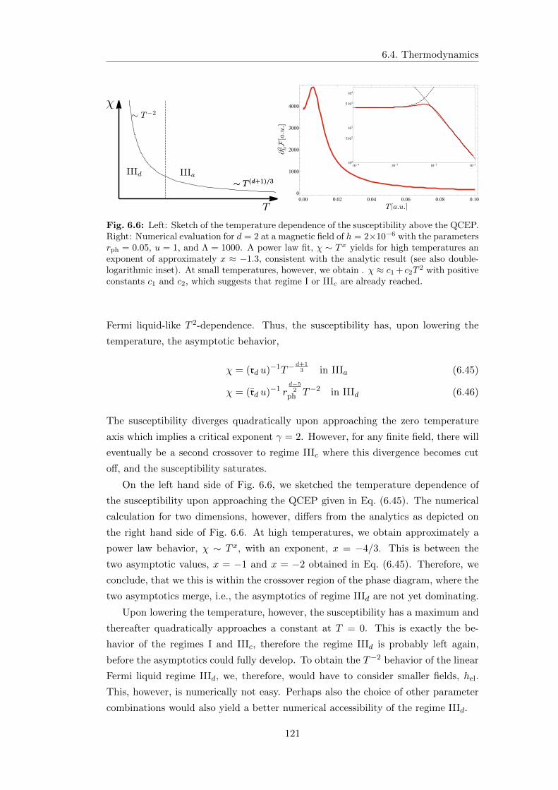
6.4. Thermodynamics
0.00 0.02 0.04 0.06 0.08 0.100
1000
2000
3000
4000
10 4 10 3 10 2 10 1102
102
103
5103
104
5
4
Fig. 6.6: Left: Sketch of the temperature dependence of the susceptibility above the QCEP.Right: Numerical evaluation for d = 2 at a magnetic field of h = 2×10⁻⁶ with the parametersrph = 0.05, u = 1, and Λ = 1000. A power law fit, χ ∼ T x yields for high temperatures anexponent of approximately x ≈ −1.3, consistent with the analytic result (see also double-logarithmic inset). At small temperatures, however, we obtain . χ ≈ c1 + c2T
2 with positiveconstants c1 and c2, which suggests that regime I or IIIc are already reached.
Fermi liquid-like T 2-dependence. Thus, the susceptibility has, upon lowering the
temperature, the asymptotic behavior,
χ = (rd u)−1T−d+1
3 in IIIa (6.45)
χ = (rd u)−1 rd−5
2ph T−2 in IIId (6.46)
The susceptibility diverges quadratically upon approaching the zero temperature
axis which implies a critical exponent γ = 2. However, for any finite field, there will
eventually be a second crossover to regime IIIc where this divergence becomes cut
off, and the susceptibility saturates.
On the left hand side of Fig. 6.6, we sketched the temperature dependence of
the susceptibility upon approaching the QCEP given in Eq. (6.45). The numerical
calculation for two dimensions, however, differs from the analytics as depicted on
the right hand side of Fig. 6.6. At high temperatures, we obtain approximately a
power law behavior, χ ∼ T x, with an exponent, x = −4/3. This is between the
two asymptotic values, x = −1 and x = −2 obtained in Eq. (6.45). Therefore, we
conclude, that we this is within the crossover region of the phase diagram, where the
two asymptotics merge, i.e., the asymptotics of regime IIId are not yet dominating.
Upon lowering the temperature, however, the susceptibility has a maximum and
thereafter quadratically approaches a constant at T = 0. This is exactly the be-
havior of the regimes I and IIIc, therefore the regime IIId is probably left again,
before the asymptotics could fully develop. To obtain the T−2 behavior of the linear
Fermi liquid regime IIId, we, therefore, would have to consider smaller fields, hel.
This, however, is numerically not easy. Perhaps also the choice of other parameter
combinations would also yield a better numerical accessibility of the regime IIId.
121
Chapter 6. Compressible Quantum Critical Metamagnetism
6.4.2 Thermal Expansion, Temperature Derivative of the Magne-
tization
As mentioned before, the thermal expansion has the same behavior as the temper-
ature derivative of the magnetization. Neglecting the inherent quadratic tempera-
ture dependence of h, both are odd functions of the field hel due to the emergent
Ising symmetry at the endpoint. Deviations from this symmetry were discussed in
Chap. 5, and carry over to the elastically coupled system, thus, we will not discuss
them here.
Finite Temperature Endpoint
Approaching the critical endpoint by varying the magnetic field, we obtain the ther-
mal expansion to be
α =2(d+ 1)
9f2uT
d−23
(9
2u2
) 13
|hel|−13 sgnhel in II. (6.47)
Upon the crossover to regime IIIc, the thermal expansion does not change qualita-
tively and will diverge further as
α =2(d+ 1)
9rduT
d−23
(9
2u2
) 13
|hel|−13 sgnhel in IIIb. (6.48)
More interesting, however, is the behavior upon temperature tuning through the
critical endpoint. For high temperatures and zero field hel, the thermal expansion
has to vanish exactly, due to the Ising symmetry. However, for small but finite
magnetic fields, it is
α =hel
R2el
R′el in IIIa. (6.49)
Below the critical temperature, in the coexistence regime, the thermal expansion is
even at zero field finite and reads as
α =
√3
2u
R′el√Rel
+hel
R2el
R′el in IVa (6.50)
Since the thermal expansion is proportional to the temperature derivative of the
order parameter of the structural transition, α ∼ ∂T (∂pF), it is related to the
critical exponent β as α ∼ |T − Tc|β−1. Therefore, with |Rel(T )| ∼ |T − Tc|, we
find the mean field exponent β = 1/2. Lowering the temperature further, we enter
regime IVb, where the thermal expansion takes the form
α =2(d+ 1)
3f2uT
d−23
√u
2 r2el
in IVb, (6.51)
which, as for the susceptibility, equals the low temperature expansion of the thermal
expansion in regime IVa.
122
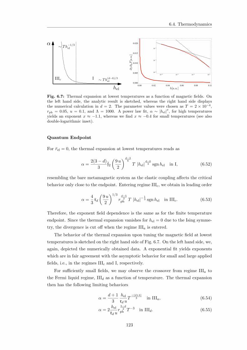
6.4. Thermodynamics
0.00 0.02 0.04 0.06 0.08 0.100.000
0.005
0.010
0.015
0.020
10 4 10 3 10 2 10 1
10 4
10 3
10 2
Fig. 6.7: Thermal expansion at lowest temperatures as a function of magnetic fields. Onthe left hand side, the analytic result is sketched, whereas the right hand side displaysthe numerical calculation in d = 2. The parameter values were chosen as T = 2 × 10⁻⁴,rph = 0.05, u = 0.1, and Λ = 1000. A power law fit, α ∼ |hel|x, for high temperaturesyields an exponent x ≈ −1.1, whereas we find x ≈ −0.4 for small temperatures (see alsodouble-logarithmic inset).
Quantum Endpoint
For rel = 0, the thermal expansion at lowest temperatures reads as
α =2(3− d)
3f2
(9u
2
) d−36
T |hel|d−6
3 sgnhel in I, (6.52)
resembling the bare metamagnetic system as the elastic coupling affects the critical
behavior only close to the endpoint. Entering regime IIIc, we obtain in leading order
α =4
3rd
(9u
2
)1/3
rd−5
2ph T |hel|−
13 sgnhel in IIIc. (6.53)
Therefore, the exponent field dependence is the same as for the finite temperature
endpoint. Since the thermal expansion vanishes for hel = 0 due to the Ising symme-
try, the divergence is cut off when the regime IIIa is entered.
The behavior of the thermal expansion upon tuning the magnetic field at lowest
temperatures is sketched on the right hand side of Fig. 6.7. On the left hand side, we,
again, depicted the numerically obtained data. A exponential fit yields exponents
which are in fair agreement with the asymptotic behavior for small and large applied
fields, i.e., in the regimes IIIc and I, respectively.
For sufficiently small fields, we may observe the crossover from regime IIIa to
the Fermi liquid regime, IIId as a function of temperature. The thermal expansion
then has the following limiting behaviors
α =d+ 1
3
hel
rd uT−(d+4)
3 in IIIa, (6.54)
α = 2hel
rd ur
5−d2
ph T−3 in IIId. (6.55)
123
Chapter 6. Compressible Quantum Critical Metamagnetism
Although the thermal expansion is suppressed by a factor of hel, it diverges with a
very high power of temperature when approaching the quantum endpoint. However,
for any finite field, there will, eventually, be a second crossover to the regime IIIc
where this divergence is cut off, and, finally, the thermal expansion will scale linearly
to zero.
6.4.3 Specific Heat Coefficient
The specific heat coefficient shows the strongest influence of the elastic coupling,
since it stems from the fluctuation term only. Thus, it is very sensitive to the
absence of critical fluctuations in the elastically coupled case.
Finite Temperature Endpoint
As already seen in Chap. 4 for the finite temperature endpoint of the Mott transition,
the specific heat coefficient does not show any divergence upon sweeping through
the endpoint with the magnetic field. Instead, we obtain
γ =d(d+ 3)
9f1T
d3−1 −R′′el
(9h2
el
2u2
)1/3
for II and IIIb. (6.56)
If we lower the temperature at zero field, the specific heat coefficient increases ac-
cording to
γ =d(d+ 3)
9f1T
d3−1 for IIIa. (6.57)
However, since the endpoint is at a temperature Tc > 0, it does not diverge, and
below the crossover the specific heat coefficient is given as
γ =d(d+ 3)
9f1T
d3−1 +
3R′2el
u+
3RelR′′el
2ufor IVa. (6.58)
As in Chap. 4 , we obtain a mean field jump of the specific heat which is of the order
of ∆γ ∼ T 2(d−2)/3c /u.
Quantum Endpoint
For the quantum endpoint, varying the magnetic field at lowest temperatures the
specific heat will first resemble the behavior of the bare metamagnetic system
γ = 2 f2
(9uh2
el
2
) d−36
in I. (6.59)
124
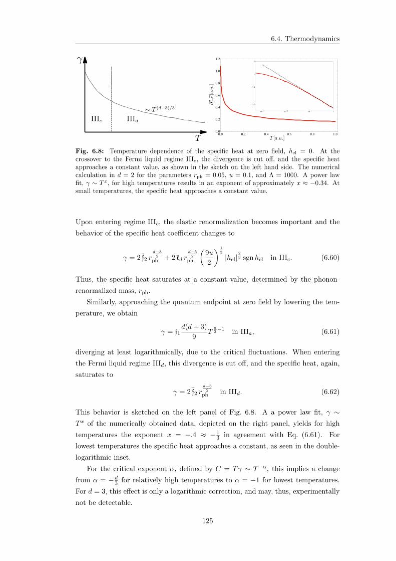
6.4. Thermodynamics
0.0 0.2 0.4 0.6 0.8 1.00.0
0.2
0.4
0.6
0.8
1.0
1.2
10 3 10 2 10 1 1
0.2
0.5
1
2
Fig. 6.8: Temperature dependence of the specific heat at zero field, hel = 0. At thecrossover to the Fermi liquid regime IIIc, the divergence is cut off, and the specific heatapproaches a constant value, as shown in the sketch on the left hand side. The numericalcalculation in d = 2 for the parameters rph = 0.05, u = 0.1, and Λ = 1000. A power lawfit, γ ∼ T x, for high temperatures results in an exponent of approximately x ≈ −0.34. Atsmall temperatures, the specific heat approaches a constant value.
Upon entering regime IIIc, the elastic renormalization becomes important and the
behavior of the specific heat coefficient changes to
γ = 2 f2 rd−3
2ph + 2 rd r
d−52
ph
(9u
2
) 13
|hel|23 sgnhel in IIIc. (6.60)
Thus, the specific heat saturates at a constant value, determined by the phonon-
renormalized mass, rph.
Similarly, approaching the quantum endpoint at zero field by lowering the tem-
perature, we obtain
γ = f1d(d+ 3)
9Td3−1 in IIIa, (6.61)
diverging at least logarithmically, due to the critical fluctuations. When entering
the Fermi liquid regime IIId, this divergence is cut off, and the specific heat, again,
saturates to
γ = 2 f2 rd−3
2ph in IIId. (6.62)
This behavior is sketched on the left panel of Fig. 6.8. A a power law fit, γ ∼T x of the numerically obtained data, depicted on the right panel, yields for high
temperatures the exponent x = −.4 ≈ −13 in agreement with Eq. (6.61). For
lowest temperatures the specific heat approaches a constant, as seen in the double-
logarithmic inset.
For the critical exponent α, defined by C = Tγ ∼ T−α, this implies a change
from α = −d3 for relatively high temperatures to α = −1 for lowest temperatures.
For d = 3, this effect is only a logarithmic correction, and may, thus, experimentally
not be detectable.
125
Chapter 6. Compressible Quantum Critical Metamagnetism
6.4.4 Gruneisen Parameters
The Gruneisen parameter, defined as the ratio between the thermal expansion and
the specific heat, Γ = α/(T γ), is an particularly interesting quantity at a quantum
critical point. In contrast to a finite temperature critical point, where it remains
constant, the Gruneisen ratio diverges at a quantum critical point. If scaling ap-
plies, the divergence is determined by the critical exponents as shown in Ref. [113].
However, as we have seen above, the metamagnetic system on a compressible lattice
does not have a real quantum critical endpoint, but rather a quantum mean field
endpoint, hence, we also expect unusual exponents for the Gruneisen parameter.
Far from the QCEP, at large fields, the Gruneisen parameter diverges as
Γ =3− d
3h−1
el in I, (6.63)
which is, except for prefactors, in agreement with general scaling arguments, as
discussed in Sec. 5.4.4. However, when entering regime IIIc, it becomes
Γ =2
3
rdf2
(9u
2
) 13
r−1ph |hel|−
13 sgnhel in IIIc, (6.64)
diverging with the unusual weak power law of |hel|−1/3. Approaching the quantum
endpoint by lowering the temperature at small but finite magnetic fields, we obtain
Γ =3(d+ 1)
3d(d+ 3)
hel
f1 rd uT−
2(d+2)3 in IIIa, (6.65)
like in the bare metamagnetic system. The crossover to the Fermi liquid regime
yields a change in the behavior of the Gruneisen parameter
Γ =hel
f2 rd ur4−d
ph T−4 in IIId, (6.66)
Thus, in contrast, to the field dependence, it shows a very high divergence with tem-
perature and differs from the usual quantum critical behavior discussed in Ref. [113].
However, one has to take into account that the Gruneisen parameter is suppressed
by a factor of hel, therefore, at some finite temperature it will reach the crossover to
regime IIIc where it saturates to a constant.
6.5 Estimate for Sr3Ru2O7
In this section, we want to estimate the temperature scale on which effects of the
elastic coupling may be observed in real systems. This is achieved with help of
thermal expansion measurements performed by Gegenwart et al. [110] for Sr3Ru2O7.
126
6.5. Estimate for Sr3Ru2O7
As discussed in Sec. 5.1.2, Sr3Ru2O7 is a quasi-2 dimensional system which
develops towards a metamagnetic quantum endpoint at a magnetic field of 7.8 T
applied parallel to the c-axis. Although the quantum endpoint in this system is
preempted by the formation of an electronic nematic phase, the compound may,
nevertheless, serve us as an exemplary system of a metamagnetic quantum endpoint.
In the following, we calculate the temperature shift of the second order endpoint
for r = 0, i.e., in the scenario, where the bare system would exhibit a quantum
critical point. Although this is not an experimental accessible quantity, it will serve
us as an estimate of the temperature scale on which elasticity affects the critical
properties.
In terms of the microscopic parameters, the critical temperature is given in
Eq. (6.29) as Tc = (|rel| /(rdu))3/(d+1). For r = 0, the shift of the quantum critical
endpoint to finite temperatures in the quasi-2 dimensional Sr3Ru2O7 follows as
Tc =λ2/K
r2u. (6.67)
From magnetoresistance measurements under pressure, Ref. [118], we can deter-
mine the pressure dependence of the critical magnetic field as
∂µ0Hc
∂p=∂hel
∂p=
λ
K≈ 5.6
T
GPa. (6.68)
Furthermore, in the linear regime, IIIa, the free energy can be written, up to
field-independent terms, as F = −12χ |µ0(H −Hc)|2, where the susceptibility at
r = 0 is given by χ = (r2uT − λ2/K)−1 ≈ (r2uT )−1. The thermal expansion follows
from this form of the free energy density as
α =∂2F
∂(µ0Hc) ∂T
∂µ0Hc
∂p=∂χ
∂T
∂µ0Hc
∂p(µ0(H −Hc))
=1
r2u
λ
K
µ0(H −Hc)
T 2,
⇒ λ2/K
r2u= K
∂µ0Hc
∂p
αT 2
µ0(H −Hc). (6.69)
The previously mentioned thermal expansion measurements of Gegenwart et al.
[110], are depicted in form of a scaling plot in Fig. 6.9 and show a linear behavior
in the scaling region for H < Hc (left) as well as for H > Hc (right). Unfortunately,
the measurements in theses two regimes due not collapse onto one curve as the Ising
symmetry would predict. As discussed in Sec. 5.4.2, the temperature dependence
of h yields deviations from the Ising-symmetric results, thus, our analysis will yield
two different critical temperatures. However, as this temperature is itself not a
measurable quantity it anyhow serves as a benchmark for the temperature regime
in which the elastic effects occur.
127
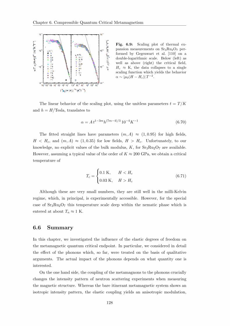
Chapter 6. Compressible Quantum Critical Metamagnetism
Fig. 6.9: Scaling plot of thermal ex-pansion measurements on Sr3Ru2O7 per-formed by Gegenwart et al. [110] on adouble-logarithmic scale. Below (left) aswell as above (right) the critical field,Hc ≈ K, the data collapses to a singlescaling function which yields the behaviorα ∼ |µ0(H −Hc)|T−2.
The linear behavior of the scaling plot, using the unitless parameters t = T/K
and h = H/Tesla, translates to
α = A t1−3mh(7m−4)/3 10−4K−1 (6.70)
The fitted straight lines have parameters (m,A) ≈ (1, 0.95) for high fields,
H < Hc, and (m,A) ≈ (1, 0.35) for low fields, H > Hc. Unfortunately, to our
knowledge, no explicit values of the bulk modulus, K, for Sr3Ru2O7 are available.
However, assuming a typical value of the order of K ≈ 200 GPa, we obtain a critical
temperature of
Tc =
0.1 K, H < Hc
0.03 K, H > Hc
(6.71)
Although these are very small numbers, they are still well in the milli-Kelvin
regime, which, in principal, is experimentally accessible. However, for the special
case of Sr3Ru2O7 this temperature scale deep within the nematic phase which is
entered at about Tn ≈ 1 K.
6.6 Summary
In this chapter, we investigated the influence of the elastic degrees of freedom on
the metamagnetic quantum critical endpoint. In particular, we considered in detail
the effect of the phonons which, so far, were treated on the basis of qualitative
arguments. The actual impact of the phonons depends on what quantity one is
interested.
On the one hand side, the coupling of the metamagnons to the phonons crucially
changes the intensity pattern of neutron scattering experiments when measuring
the magnetic structure. Whereas the bare itinerant metamagnetic system shows an
isotropic intensity pattern, the elastic coupling yields an anisotropic modulation,
128
6.6. Summary
reflecting the symmetry of the underlying lattice. For the special case of a cubic
lattice, we obtained an intensity modulation according to I(φ) ∼ cos(4φ).
On the other hand, phonons play only a minor role for the critical thermodynam-
ics of the quantum endpoint due to the different dynamics of the phonons and the
metamagnons. Whereas the phonons have a dynamical critical exponent of z< = 1,
the metamagnons are governed by an exponent z> = 3. Because of these different
energy scales, the system basically splits into a phonon and a magnon system, with
renormalized parameters such as the phonon velocity, vm < v, and a renormalized
magnon mass, Rph < R.
However, the macroscopic modes are strongly affecting the metamagnetic system.
The quantum critical endpoint is preempted by an isostructural first order transition,
similar to the finite temperature Mott endpoint, discussed in Chap. 4. This first
order transition terminates in an endpoint which, again, shows elastic Landau mean
field behavior. The bilinear elastic coupling also yields a linear pressure dependence
of the critical metamagnetic field, Hc(p) = Hc,0 + p/K, which was assumed in
Chap. 5.
However, fine tuning the parameters of the theory by an additional control pa-
rameter, e.g., the angle between the magnetic field an the ab-plane in Sr3Ru2O7,
one can still drive the critical temperature of the endpoint to zero and, thus, obtain
a quantum endpoint. Importantly, approaching this quantum endpoint exactly at
the critical field, the system still exhibits a crossover to the Fermi liquid regime at
a finite temperature, TFL > 0.
The thermodynamics in this regime are quite peculiar, as, for instance, the ther-
mal expansion shows at small but finite fields a strong divergence according to
α ∼ hel T−3. On the other hand, the divergence of the specific heat coefficient at
zero field is cut off upon entering the Fermi liquid regime. Both effects conspire in
the behavior of the (magnetic) Gruneisen parameter which diverges with an unusual
high power of temperature according to Γ ∼ helT−4 at small but finite fields.
Finally, we considered the layered compound Sr3Ru2O7 as an exemplary system
close to a metamagnetic quantum endpoint. As a benchmark of the strength of the
elastic coupling, we estimated the temperature of the endpoint for the case that the
system develops a quantum critical point in the uncoupled case. This temperature
is of the order of 100 mK and, thus, very small, however, it may be still in the
experimentally accessible regime. Also, for other compounds, the parameters may
be more convenient such that the temperature range on which the elastic coupling
manifests itself is larger.
129

Chapter 7
Summary
In this Thesis, we studied the coupling of the critical degrees of freedom at a solid
state phase transition to the underlying lattice. In particular, we considered the
finite temperature phase transition from a Mott insulator to a metal and the meta-
magnetic quantum endpoint.
After a general introduction to the theory of crystal elasticity we reviewed the
preceding work on classical phase transitions on compressible lattices. Due to the
peculiar difference between the macroscopic strain and its spatial fluctuations, i.e.,
the elastic waves, a long ranged interaction is induced which may change the na-
ture of the phase transition. In particular, due to the absence of soft modes at
the critical point, the system becomes mean field like and critical behavior of the
thermodynamics is suppressed.
In the following, this mechanism was studied for the Mott metal-insulator tran-
sition. The nature of this phase transition and its universality class was discussed
for over thirty years [49] and is still under debate . Starting from the theoretically
expected Ising critical behavior, we showed that the interplay with elastic degrees
of freedom will render the behavior mean field like, in the vicinity of the endpoint.
The smoking gun criterion to detect the elastic mean field regime is the breakdown
of Hooke’s law, i.e., a non-linear stress-strain relation close to the critical endpoint.
Also the specific heat coefficient exhibits a finite mean field jump instead of a diver-
gence.
Depending on the relative magnitude of the elastic coupling, Ising critical be-
havior may either still be preserved at a finite distance from the critical point, or it
is completely suppressed. We argued, that the organic salt κ-(BEDT-TTF)2X is an
example for the former scenario and could, based on thermal expansion data [1, 2],
estimate the elastic Landau regime as ∆T ? ≈ 2.5 K and ∆p? ≈ 50 bar. On the other
hand, we argue that Ising critical behavior is absent in the chromium doped V2O3,
since one of the elastic constants becomes critical long before a deviation from mean
field behavior is observed.
131
Chapter 7. Summary
The following chapters, were devoted to the zero temperature critical endpoint in
itinerant metamagnets and its critical thermodynamics. Such a metamagnetic quan-
tum phase transition was recently suggested of being a generic feature for itinerant
ferromagnets [3] and was found in UCoAl [4] and UGe2 [5, 6].
Starting from spin-fluctuation theory, we derived an effective potential for the
macroscopic magnetization by means of functional renormalization group techniques,
which takes fluctuations self-consistently into account. This potential enabled us, to
derive the asymptotic appearance of the free energy and, subsequently, of thermo-
dynamic quantities such as, specific heat, thermal expansion and susceptibility. The
obtained characteristics compare qualitatively well to existing experimental mea-
surements.
Importantly, the compressibility shows the same behavior as the susceptibility
which necessarily diverges at the transition. Thus, we expect a crystal softening
which results in an isostructural transition preempting the metamagnetic QCEP.
We investigated this mechanism by including elastic degrees of freedom, i.e., the
macroscopic strain and the phonons, in the functional RG approach used for the bare
metamagnetic system. For simplicity, we restricted ourselves to isotropic crystals.
The influence of the phonons on the system is, as shown, crucial for quantities
sensitive to finite momentum metamagnons. It changes, for instance, the neutron
scattering intensity pattern when measuring the magnetic structure which inherits
the symmetry of the underlying lattice. However, concerning the critical thermo-
dynamics, the phonons yield only sub-leading contributions. Due to the different
dynamics of the metamagnons and the phonons, the system can be described as two
renormalized but decoupled sub-systems.
However, the macroscopic elastic modes yield, as expected, an isostructural first
order transition, similar to the finite temperature Mott transition, preempting the
quantum critical endpoint. The resulting finite temperature second order endpoint,
again, shows elastic Landau mean field behavior.
When tuning this endpoint to zero temperature, we obtain a quantum endpoint
which, however, shows a very interesting behavior. Most important, upon lowering
the temperature at the critical field, the system will, inevitably, enter a Fermi liquid
regime at a finite temperature, TFL > 0. This results in unusual power laws of the
critical thermodynamics. Whereas the thermal expansion diverges strongly with
temperature above the quantum critical endpoint, the usual specific heat divergence
is cut off. As a consequence, the (magnetic) Gruneisen parameter diverges with an
unusual high power of temperature, Γ ∼ helT−4.
As a benchmark of the strength of the elastic coupling in metamagnetic systems,
we estimated the temperature shift of the quantum critical endpoint for Sr3Ru2O7.
It was found to be of the order of 100 mK, which is still within an experimentally
accessible regime though it is within the nematic phase in this specific material.
132
Appendix A
Symmetry Classes of the Elastic
Constant Matrix
The elastic constant matrix, C, has in general 21 independent components. However,
if the lattice has certain symmetries, all quantities describing it have to be also
symmetric in that respect. Thus, the symmetries of the lattice reduce the number of
independent components as they yield further constraints. Here, following Ref. [7],
we determine the elastic constant matrix for all of the 32 crystallographic point
groups. As it turns out, there are 9 different symmetry groups of the elastic constant
matrix, one for each lattice system and two more for trigonal and tetragonal systems
with higher symmetries.
A.1 Triclinic System
In the two triclinic systems, 1, 1, all 21 components of the elastic constant matrix
are independent. If every atom is a center of inversion symmetry, Cauchy’s relation
applies Cijkl = Cikjl and only 15 of the elastic constants are independent. The
resulting elastic constant matrix reads as
C =
C11 C12 C13 C14 C15 C16
C12 C22 C23 C24 C25 C26
C13 C23 C33 C34 C35 C36
C14 C24 C34 C23 C16 C25
C15 C25 C35 C16 C13 C14
C16 C26 C36 C25 C14 C12
. (A.1)
Since we have to choose a coordinate system which depends on three angles relative
to the body, it can be chosen such that it imposes three additional conditions. Such
the triclinic system has in general 18 independent elastic moduli and 12 if Cauchy’s
relations apply.
133
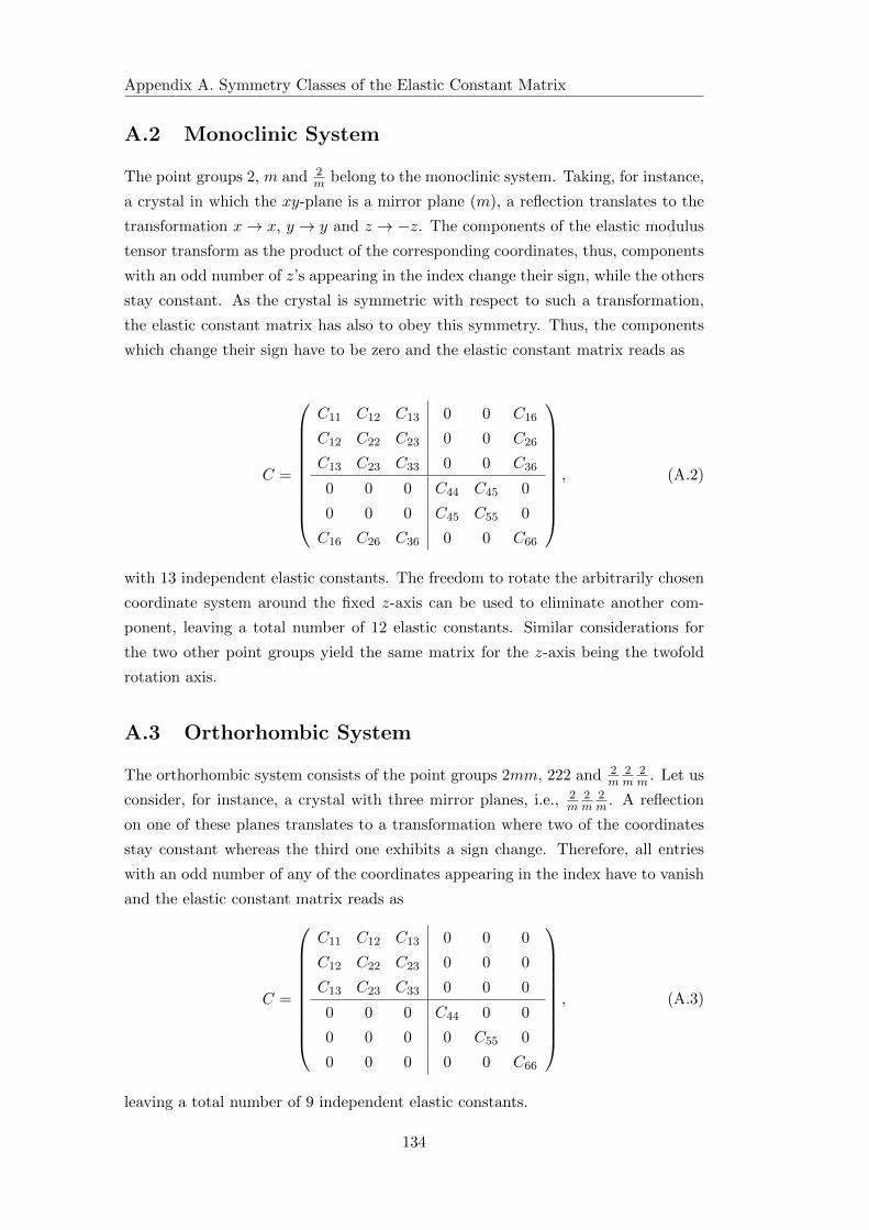
Appendix A. Symmetry Classes of the Elastic Constant Matrix
A.2 Monoclinic System
The point groups 2, m and 2m belong to the monoclinic system. Taking, for instance,
a crystal in which the xy-plane is a mirror plane (m), a reflection translates to the
transformation x→ x, y → y and z → −z. The components of the elastic modulus
tensor transform as the product of the corresponding coordinates, thus, components
with an odd number of z’s appearing in the index change their sign, while the others
stay constant. As the crystal is symmetric with respect to such a transformation,
the elastic constant matrix has also to obey this symmetry. Thus, the components
which change their sign have to be zero and the elastic constant matrix reads as
C =
C11 C12 C13 0 0 C16
C12 C22 C23 0 0 C26
C13 C23 C33 0 0 C36
0 0 0 C44 C45 0
0 0 0 C45 C55 0
C16 C26 C36 0 0 C66
, (A.2)
with 13 independent elastic constants. The freedom to rotate the arbitrarily chosen
coordinate system around the fixed z-axis can be used to eliminate another com-
ponent, leaving a total number of 12 elastic constants. Similar considerations for
the two other point groups yield the same matrix for the z-axis being the twofold
rotation axis.
A.3 Orthorhombic System
The orthorhombic system consists of the point groups 2mm, 222 and 2m
2m
2m . Let us
consider, for instance, a crystal with three mirror planes, i.e., 2m
2m
2m . A reflection
on one of these planes translates to a transformation where two of the coordinates
stay constant whereas the third one exhibits a sign change. Therefore, all entries
with an odd number of any of the coordinates appearing in the index have to vanish
and the elastic constant matrix reads as
C =
C11 C12 C13 0 0 0
C12 C22 C23 0 0 0
C13 C23 C33 0 0 0
0 0 0 C44 0 0
0 0 0 0 C55 0
0 0 0 0 0 C66
, (A.3)
leaving a total number of 9 independent elastic constants.
134
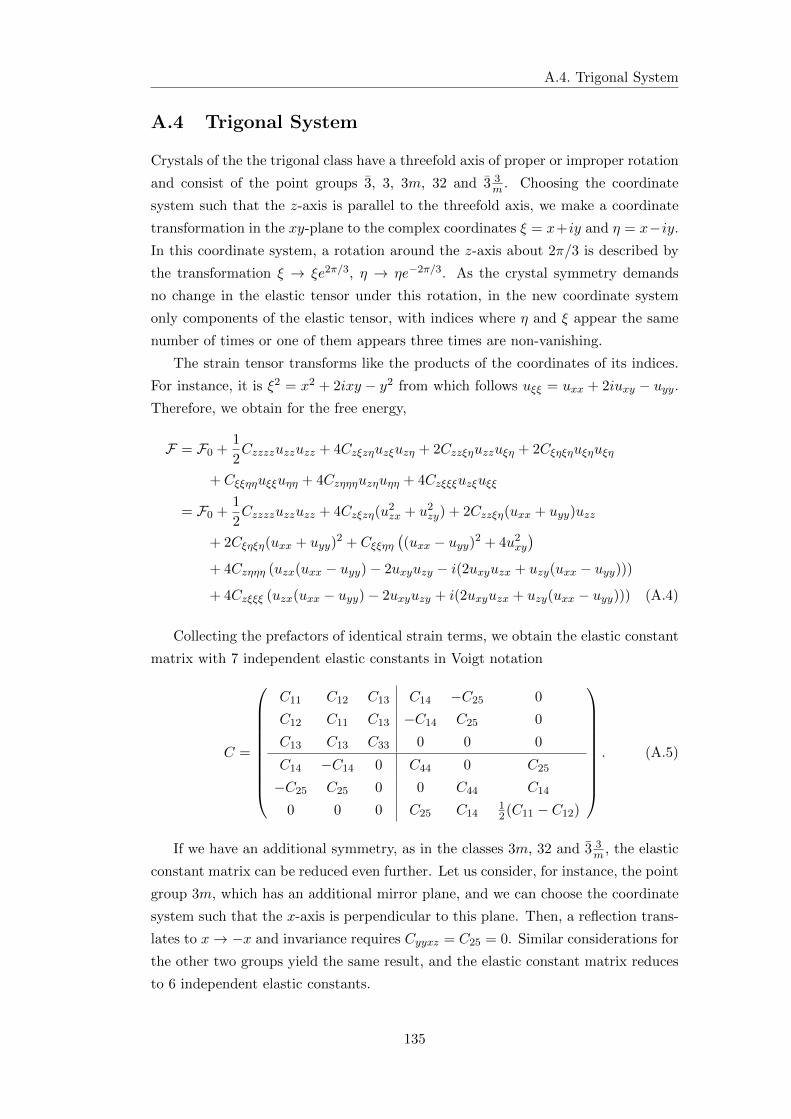
A.4. Trigonal System
A.4 Trigonal System
Crystals of the the trigonal class have a threefold axis of proper or improper rotation
and consist of the point groups 3, 3, 3m, 32 and 3 3m . Choosing the coordinate
system such that the z-axis is parallel to the threefold axis, we make a coordinate
transformation in the xy-plane to the complex coordinates ξ = x+iy and η = x−iy.
In this coordinate system, a rotation around the z-axis about 2π/3 is described by
the transformation ξ → ξe2π/3, η → ηe−2π/3. As the crystal symmetry demands
no change in the elastic tensor under this rotation, in the new coordinate system
only components of the elastic tensor, with indices where η and ξ appear the same
number of times or one of them appears three times are non-vanishing.
The strain tensor transforms like the products of the coordinates of its indices.
For instance, it is ξ2 = x2 + 2ixy − y2 from which follows uξξ = uxx + 2iuxy − uyy.Therefore, we obtain for the free energy,
F = F0 +1
2Czzzzuzzuzz + 4Czξzηuzξuzη + 2Czzξηuzzuξη + 2Cξηξηuξηuξη
+ Cξξηηuξξuηη + 4Czηηηuzηuηη + 4Czξξξuzξuξξ
= F0 +1
2Czzzzuzzuzz + 4Czξzη(u
2zx + u2
zy) + 2Czzξη(uxx + uyy)uzz
+ 2Cξηξη(uxx + uyy)2 + Cξξηη
((uxx − uyy)2 + 4u2
xy
)
+ 4Czηηη (uzx(uxx − uyy)− 2uxyuzy − i(2uxyuzx + uzy(uxx − uyy)))+ 4Czξξξ (uzx(uxx − uyy)− 2uxyuzy + i(2uxyuzx + uzy(uxx − uyy))) (A.4)
Collecting the prefactors of identical strain terms, we obtain the elastic constant
matrix with 7 independent elastic constants in Voigt notation
C =
C11 C12 C13 C14 −C25 0
C12 C11 C13 −C14 C25 0
C13 C13 C33 0 0 0
C14 −C14 0 C44 0 C25
−C25 C25 0 0 C44 C14
0 0 0 C25 C1412(C11 − C12)
. (A.5)
If we have an additional symmetry, as in the classes 3m, 32 and 3 3m , the elastic
constant matrix can be reduced even further. Let us consider, for instance, the point
group 3m, which has an additional mirror plane, and we can choose the coordinate
system such that the x-axis is perpendicular to this plane. Then, a reflection trans-
lates to x→ −x and invariance requires Cyyxz = C25 = 0. Similar considerations for
the other two groups yield the same result, and the elastic constant matrix reduces
to 6 independent elastic constants.
135
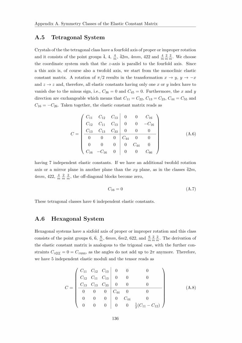
Appendix A. Symmetry Classes of the Elastic Constant Matrix
A.5 Tetragonal System
Crystals of the the tetragonal class have a fourfold axis of proper or improper rotation
and it consists of the point groups 4, 4, 4m , 42m, 4mm, 422 and 4
m2m
2m . We choose
the coordinate system such that the z-axis is parallel to the fourfold axis. Since
a this axis is, of course also a twofold axis, we start from the monoclinic elastic
constant matrix. A rotation of π/2 results in the transformation x → y, y → −xand z → z and, therefore, all elastic constants having only one x or y index have to
vanish due to the minus sign, i.e., C36 = 0 and C45 = 0. Furthermore, the x and y
direction are exchangeable which means that C11 = C22, C13 = C23, C44 = C55 and
C16 = −C26. Taken together, the elastic constant matrix reads as
C =
C11 C12 C13 0 0 C16
C12 C11 C13 0 0 −C16
C13 C13 C33 0 0 0
0 0 0 C44 0 0
0 0 0 0 C44 0
C16 −C16 0 0 0 C66
(A.6)
having 7 independent elastic constants. If we have an additional twofold rotation
axis or a mirror plane in another plane than the xy plane, as in the classes 42m,
4mm, 422, 4m
2m
2m , the off-diagonal blocks become zero,
C16 = 0 (A.7)
These tetragonal classes have 6 independent elastic constants.
A.6 Hexagonal System
Hexagonal systems have a sixfold axis of proper or improper rotation and this class
consists of the point groups 6, 6, 6m , 6mm, 6m2, 622, and 6
m2m
2m . The derivation of
the elastic constant matrix is analogous to the trigonal case, with the further con-
straints Czξξξ = 0 = Czηηη, as the angles do not add up to 2π anymore. Therefore,
we have 5 independent elastic moduli and the tensor reads as
C =
C11 C12 C13 0 0 0
C12 C11 C13 0 0 0
C13 C13 C33 0 0 0
0 0 0 C44 0 0
0 0 0 0 C44 0
0 0 0 0 0 12(C11 − C12)
(A.8)
136
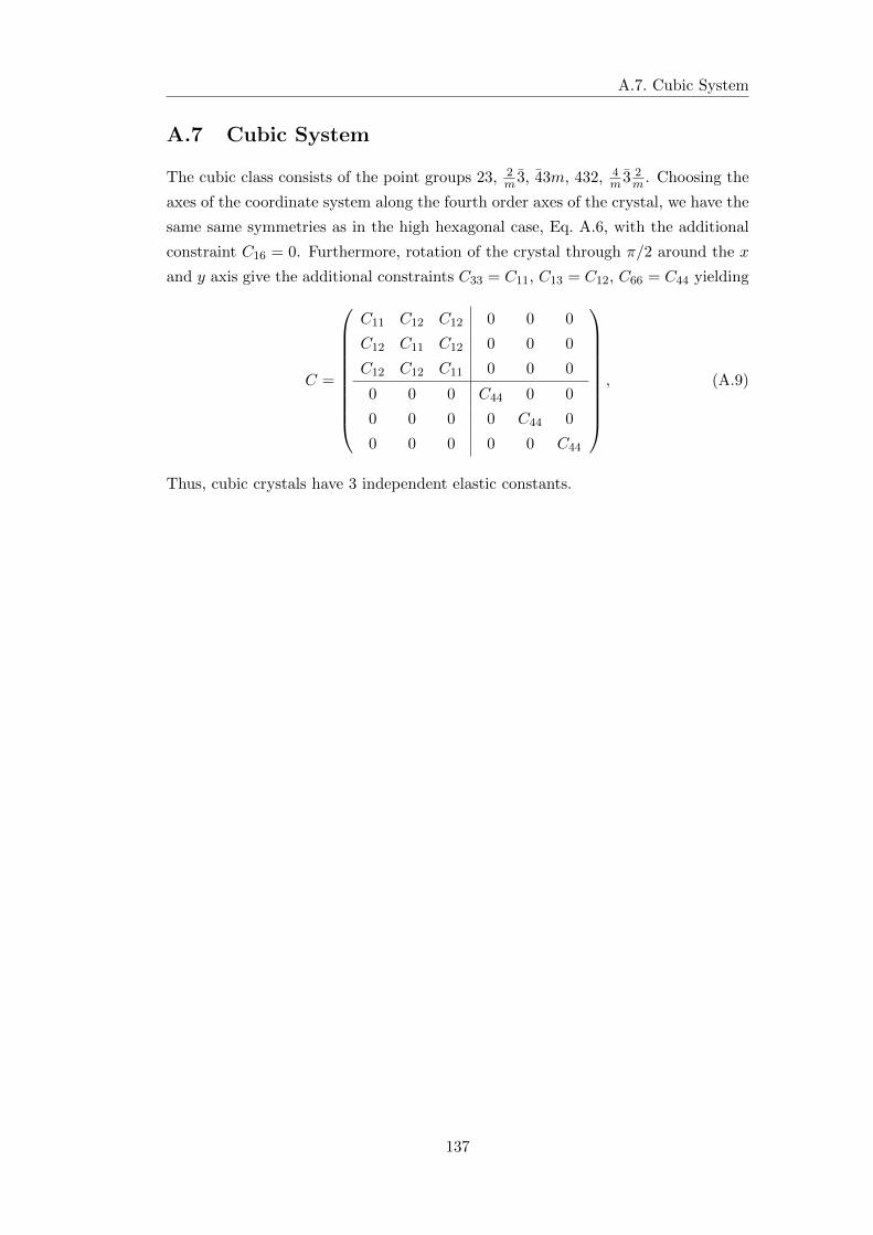
A.7. Cubic System
A.7 Cubic System
The cubic class consists of the point groups 23, 2m 3, 43m, 432, 4
m 3 2m . Choosing the
axes of the coordinate system along the fourth order axes of the crystal, we have the
same same symmetries as in the high hexagonal case, Eq. A.6, with the additional
constraint C16 = 0. Furthermore, rotation of the crystal through π/2 around the x
and y axis give the additional constraints C33 = C11, C13 = C12, C66 = C44 yielding
C =
C11 C12 C12 0 0 0
C12 C11 C12 0 0 0
C12 C12 C11 0 0 0
0 0 0 C44 0 0
0 0 0 0 C44 0
0 0 0 0 0 C44
, (A.9)
Thus, cubic crystals have 3 independent elastic constants.
137

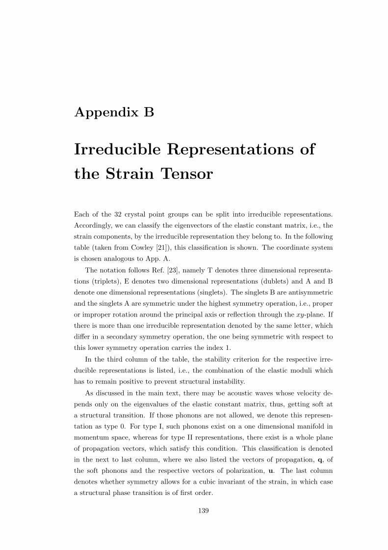
Appendix B
Irreducible Representations of
the Strain Tensor
Each of the 32 crystal point groups can be split into irreducible representations.
Accordingly, we can classify the eigenvectors of the elastic constant matrix, i.e., the
strain components, by the irreducible representation they belong to. In the following
table (taken from Cowley [21]), this classification is shown. The coordinate system
is chosen analogous to App. A.
The notation follows Ref. [23], namely T denotes three dimensional representa-
tions (triplets), E denotes two dimensional representations (dublets) and A and B
denote one dimensional representations (singlets). The singlets B are antisymmetric
and the singlets A are symmetric under the highest symmetry operation, i.e., proper
or improper rotation around the principal axis or reflection through the xy-plane. If
there is more than one irreducible representation denoted by the same letter, which
differ in a secondary symmetry operation, the one being symmetric with respect to
this lower symmetry operation carries the index 1.
In the third column of the table, the stability criterion for the respective irre-
ducible representations is listed, i.e., the combination of the elastic moduli which
has to remain positive to prevent structural instability.
As discussed in the main text, there may be acoustic waves whose velocity de-
pends only on the eigenvalues of the elastic constant matrix, thus, getting soft at
a structural transition. If those phonons are not allowed, we denote this represen-
tation as type 0. For type I, such phonons exist on a one dimensional manifold in
momentum space, whereas for type II representations, there exist is a whole plane
of propagation vectors, which satisfy this condition. This classification is denoted
in the next to last column, where we also listed the vectors of propagation, q, of
the soft phonons and the respective vectors of polarization, u. The last column
denotes whether symmetry allows for a cubic invariant of the strain, in which case
a structural phase transition is of first order.
139
Appendix B. Irreducible Representations of the Strain Tensor
CubicRep. Strain Stability Phonons Inv.
Triclinic classes
6 A uxx; uyy ; uzz ; uxy ; uxz ; uyz detCij 0 no
Monoclinic classes
4 A uxx; uyy ; uzz ; uxy detCij , i, j ∈ 1, 2, 3, 6 0 yes
2 B uxz ; uyz C44C55 − C245 0 no
Orthorhombic classes
3 A1 uxx; uyy ; uzz detCij , i, j ≤ 3 0 yes
B1 uxy C66 I q ‖ [010], [100] no
u ‖ [100], [010]
B2 uxz C55 I q ‖ [100], [001] no
u ‖ [001], [100]
B3 uyz C44 I q ‖ [001], [010] no
u ‖ [010], [001]
Trigonal classes 3, 3
2 A uxx + uyy ; uzz (C11 + C12)C33 − 2C213 0 yes
2 E uxx − uyy , uxy ; uxz , uyz (C11 − C12)C44 − 2C214 − 2C2
25 0 yes
Trigonal classes 32, 3m, 3m
2 A1 uxx + uyy ; uzz (C11 + C12)C33 − 2C213 0 yes
2E uxx − uyy , uxy ; uxz , uyz (C11 − C12)C44 − 2C214 0 yes
Tetragonal classes 4, 4, 4m
2 A uxx + uyy ; uzz (C11 + C12)C33 − 2C213 0 yes
2 B uxx − uyy ; uxy (C11 + C12)C66 − 2C216 0 no
E uxz , uyz C44 II q ⊥ [001], [001] no
u ‖ [001]
Tetragonal classes 4mm, 42m, 422 4m
2m
2m
2 A1 uxx + uyy ; uzz (C11 + C12)C33 − 2C213 0 yes
B1 uxx − uyy C11 − C12 I q ‖ [110] no
u ‖ [110]
B2 uxy C66 I q ‖ [100] no
u ‖ [010]
E uxz , uyz C44 II q ⊥ [001] no
u ‖ [001]
Hexagonal classes
2 A1 uxx + uyy ; uzz (C11 + C12)C33 − 2C213 0 yes
E1 uxx − uyy , uxy C11 − C12 II q ⊥ [001] yes
u ⊥ [001] and q
E2 uxz , uyz C44 II q ⊥ [001] yes
u ‖ [001]
Cubic classes
A1 uxx + uyy + uzz C11 + 2C12 0 yes
E uxx − uyy , 2uzz − uxx − uyy C11 − C12 I q ‖ [110] yes
u ‖ [110]
T2 uxy , uxz , uyz C44 II q ⊥ [100] yes
u ‖ [100]
Isotropic classes
L=0 uxx + uyy + uzz 3C12 + 2C44 0 yes
L=2 uxx − uyy , 2uzz − uxx − uyy C44 II u ⊥ q yes
uxy , uxz , uyz
140
Appendix C
Effective Action due to Phonons
The Wegner-Houghton equation for the evolution of the microscopic potential along
a RG trajectory reads as
V = V0 +
∫ µ
0dµ′e−(d+z)µ′fµ′
(δ2Sµ′δφ2
,δ2Sµ′δφδu
,δ2Sµ′δu2
, Tµ′
). (C.1)
The subscript µ′ denotes that all parameters are rescaled according to their engi-
neering dimensions
r → re2µ, γm → γme−(z−z>)µ, λ→ λeµ,
ρ→ ρe−2(z−z<)µ, T → Tezµ, C11 → C11.(C.2)
The dynamical exponent, z, is left unspecified, whereas z< = 1 and z> = 3 are
the dynamical exponents of the bare phonon and magnon system, respectively. The
function f is the re-exponentiated contribution of a high energy shell integration of
the Gaussian part of the action (6.16), which is given by
f = −Λ∂
∂Λ
1
2
∫ Λ
0
dk
(2π)d1
β
∑
ωn
log[detG−1
], (C.3)
Denoting Sλ,µ = δ2S/(δλ δµ), the matrix G−1 is given by
G−1 =
(Sφ,φ Su,φ†Su,φ Su,u
). (C.4)
Due to the linear coupling and the lack of anharmonic phonon terms, only Sφ,φdepends on the field φ. Denoting R = Vφ,φ
∣∣φmin
the determinant yields
detG−1(ωn)=ρ
(R+ k2 + γm
|ωn|k
)(ω2n + v2k2
)− λ2k2. (C.5)
Here, we introduced the phonon velocity v2 = C11/ρ.
141
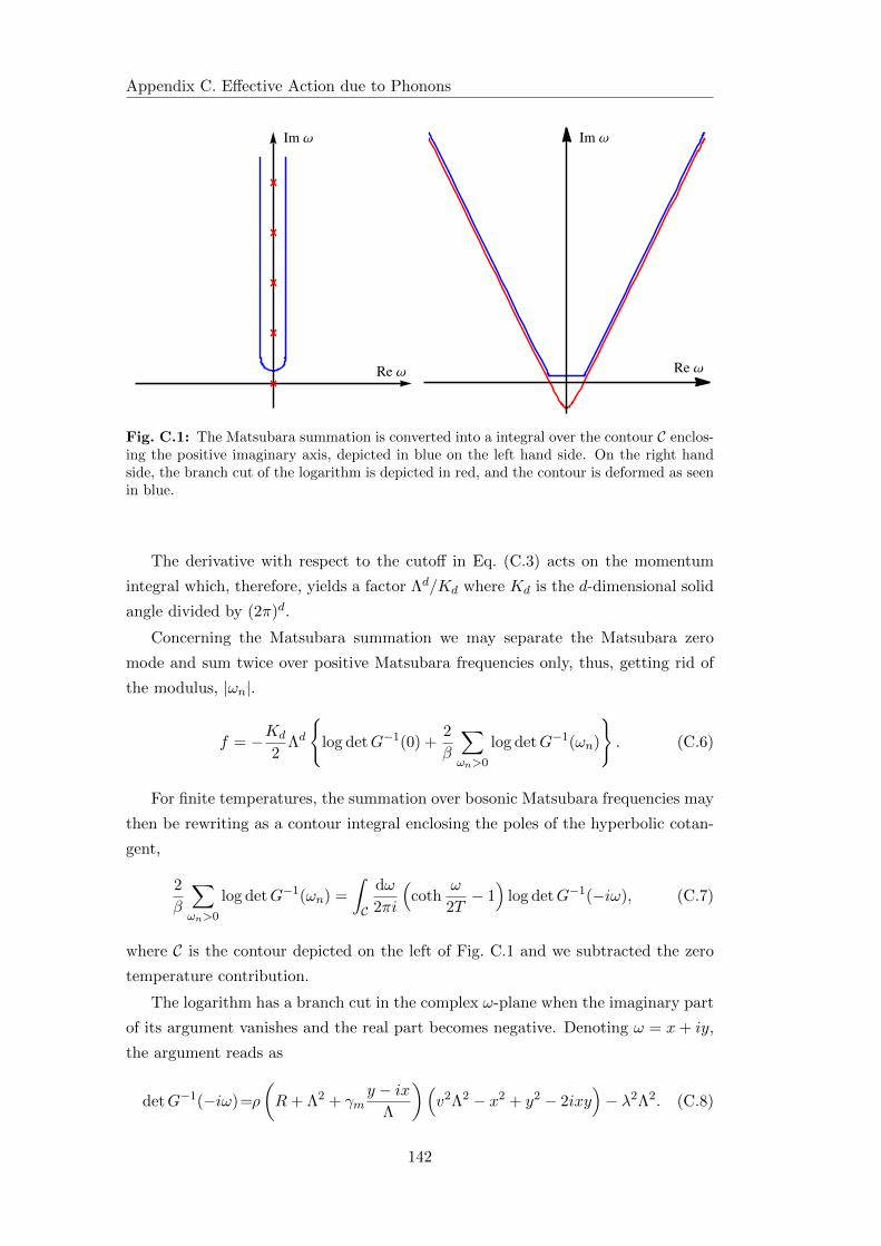
Appendix C. Effective Action due to Phonons
Re Ω
Im Ω
Re Ω
Im Ω
Fig. C.1: The Matsubara summation is converted into a integral over the contour C enclos-ing the positive imaginary axis, depicted in blue on the left hand side. On the right handside, the branch cut of the logarithm is depicted in red, and the contour is deformed as seenin blue.
The derivative with respect to the cutoff in Eq. (C.3) acts on the momentum
integral which, therefore, yields a factor Λd/Kd where Kd is the d-dimensional solid
angle divided by (2π)d.
Concerning the Matsubara summation we may separate the Matsubara zero
mode and sum twice over positive Matsubara frequencies only, thus, getting rid of
the modulus, |ωn|.
f = −Kd
2Λd
log detG−1(0) +
2
β
∑
ωn>0
log detG−1(ωn)
. (C.6)
For finite temperatures, the summation over bosonic Matsubara frequencies may
then be rewriting as a contour integral enclosing the poles of the hyperbolic cotan-
gent,
2
β
∑
ωn>0
log detG−1(ωn) =
∫
C
dω
2πi
(coth
ω
2T− 1)
log detG−1(−iω), (C.7)
where C is the contour depicted on the left of Fig. C.1 and we subtracted the zero
temperature contribution.
The logarithm has a branch cut in the complex ω-plane when the imaginary part
of its argument vanishes and the real part becomes negative. Denoting ω = x+ iy,
the argument reads as
detG−1(−iω)=ρ
(R+ Λ2 + γm
y − ixΛ
)(v2Λ2 − x2 + y2 − 2ixy
)− λ2Λ2. (C.8)
142
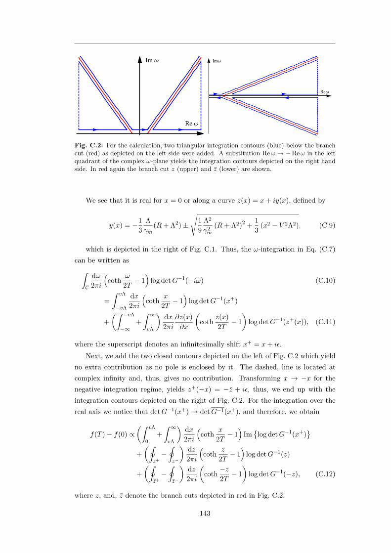
Re Ω
Im Ω
ReΩ
ImΩ
Fig. C.2: For the calculation, two triangular integration contours (blue) below the branchcut (red) as depicted on the left side were added. A substitution Reω → −Reω in the leftquadrant of the complex ω-plane yields the integration contours depicted on the right handside. In red again the branch cut z (upper) and z (lower) are shown.
We see that it is real for x = 0 or along a curve z(x) = x+ iy(x), defined by
y(x) = −1
3
Λ
γm(R+ Λ2)±
√1
9
Λ2
γ2m
(R+ Λ2)2 +1
3(x2 − V 2Λ2). (C.9)
which is depicted in the right of Fig. C.1. Thus, the ω-integration in Eq. (C.7)
can be written as
∫
C
dω
2πi
(coth
ω
2T− 1)
log detG−1(−iω) (C.10)
=
∫ vΛ
−vΛ
dx
2πi
(coth
x
2T− 1)
log detG−1(x+)
+
(∫ −vΛ
−∞+
∫ ∞
vΛ
)dx
2πi
∂z(x)
∂x
(coth
z(x)
2T− 1
)log detG−1(z+(x)), (C.11)
where the superscript denotes an infinitesimally shift x+ = x+ iε.
Next, we add the two closed contours depicted on the left of Fig. C.2 which yield
no extra contribution as no pole is enclosed by it. The dashed, line is located at
complex infinity and, thus, gives no contribution. Transforming x → −x for the
negative integration regime, yields z+(−x) = −z + iε, thus, we end up with the
integration contours depicted on the right of Fig. C.2. For the integration over the
real axis we notice that detG−1(x+)→ detG−1(x+), and therefore, we obtain
f(T )− f(0) ∝(∫ vΛ
0+
∫ ∞
vΛ
)dx
2πi
(coth
x
2T− 1)
Im
log detG−1(x+)
+
(∮
z+
−∮
z−
)dz
2πi
(coth
z
2T− 1)
log detG−1(z)
+
(∮
z+
−∮
z−
)dz
2πi
(coth
−z2T− 1
)log detG−1(−z), (C.12)
where z, and, z denote the branch cuts depicted in red in Fig. C.2.
143
Appendix C. Effective Action due to Phonons
Across the branch cuts, the imaginary part of detG−1(z) and detG−1(−z) has
a sign change. Thus, the integration infinitesimally above and below the branch cut
just yields the imaginary part of the integrand which can be simplified to
f(T )− f(0) ∝(∫ vΛ
0+
∫ ∞
vΛ
)dx
π
(coth
x
2T− 1)
Im
log detG−1(x+)
+
∮
z
dz
π
(coth
z
2T− 1)
Im
log detG−1(z+)
+
∮
z
dz
π
(coth
−z2T− 1
)Im
log detG−1(−z−). (C.13)
Concerning the integrals along the real axis, we have to evaluate the imagi-
nary part of log detG−1(ω+). In the first integral we have Re detG−1 < 0 and
Im detG−1 > 0. In the integration regime of the second integral the imaginary
part is always negative Im detG−1 < 0, whereas the real part changes its sign at a
renormalized phonon energy ω1 = v1Λ with the renormalized phonon velocity
v1 = v
√1− λ2/C11
R+ Λ2= v
√Rph + Λ2
R+ Λ2, (C.14)
Rph = R− λ2
C11. (C.15)
The velocity, v1, is well defined, since the renormalized mass, Rph, is positive above
the transition temperature. Thus, the imaginary part of the logarithm yields
arctan
[Im detG−1(ω+)
Re detG−1(ω+)
]+
0 , ω < ω1
−π , ω1 < ω < vΛ
π , ω > vΛ.
.
Note that this function is discontinuous only at the bare phonon pole but continuous
at the renormalized phonon energy, ω1. A partial integration finally yields.
−P∫ Γ
02T(
log[sinh
ω
2T
]− ω
2T
) ∂
∂ωarctan
[Im detG−1(ω)
Re detG−1(ω)
]dω
π
− 4T
(log
[sinh
vΛ
2T
]− vΛ
2T
)+ T
(log
[sinh
Γ
2T
]− Γ
2T
), (C.16)
where the principal value is taken at the bare phonon pole, ω = vΛ.
For the integration along the branch cuts the imaginary part of the determinant
is Im detG−1(z+(x)) = −ε, therefore, we find for the logarithm
Im[log detG−1(z+(x))
]= arctan
( −εRe detG−1(x)
)− π.
144
A partial integration yields a derivative with respect to x of the arc tangent,
which for vanishing ε becomes the delta function, πδ(Re detG−1(x)
). As the real
part of the determinant is strictly smaller zero we are left with the boundary terms
only. Thus, the integration over the branch cut yields
4T
(log sinh
vΛ
2T− vΛ
2T
)− 4T
(Re
[log sinh
z(Γ)
2T
]+z(Γ)
2T
). (C.17)
Gathering the contributions of the integration along the real axes, Eq. (C.16), and
along the branch cut, Eq. (C.17), and taking the limit Γ→∞, we end up with
f(T )− f(0) = −Kd
2πΛd
P∫ ∞
0
dω
π2T(
log[2 sinh
ω
2T
]− ω
2T
)Q(ω)
. (C.18)
The function Q(ω) denotes the derivative of the arctan in Eq. (C.16) and separates
into two parts which can be written as
Q(ω) = −γmΛ
R(ω) + Λ2
(R(ω) + Λ2)2 +(γm
Λ ω)2 −A(ω)
σ(ω)
(ω − ω1)2 + σ(ω)2. (C.19)
The first term resembles the bare metamagnetic contribution with an energy
dependent mass which is given by
R(ω) = Rph −λ2
C11
ω2/(vΛ)2
1− ω2/(vΛ)2. (C.20)
Since the magnons scale according to z> = 3, whereas the phonons scale ac-
cording to z< = 1, we have to consider both scalings to analyze the renormalization
effect. In the former case we have ω ∼ Λ3 and, the mass correction scales as
ω2/(vΛ)2
1− ω2/(vΛ)2∼ Λ4
1− Λ4. (C.21)
On the RG-trajectory, the cutoff decreases exponentially and, thus, the correction is
irrelevant in the final RG-flow. The integrand has to be analyzed for Rph Λ2 1,
thus, the first term in Eq. (C.19) scales with z> = 3 asymptotically as
−γmΛ
R(ω) + Λ2
(R(ω) + Λ2)2 +(γm
Λ ω)2 ∼ −
γmΛ
Λ2
Λ4, (C.22)
and is thus divergent up to at a scale Λ ∼√Rph.
If, on the other, hand we apply z< = 1 scaling, we obtain that Rph scales to the
bare mass R, however, the integrand scales as
−γmΛ
R(ω) + Λ2
(R(ω) + Λ2)2 +(γm
Λ ω)2 ∼ −
γmΛ
Λ2
γm, (C.23)
145
Appendix C. Effective Action due to Phonons
and, thus, does not contribute to the asymptotic RG-flow. The divergence of R(ω)
at the bare phonon pole, ω = vΛ, is, on the one hand, excluded due to the principal
value and, on the other hand, the integrand decreases close to the divergence as
−γmΛ
R(ω) + Λ2
(R(ω) + Λ2)2 +(γm
Λ ω)2 ∼ −
γmΛ
1
R(ω). (C.24)
From this analysis, we conclude that we can set R(ω) = Rph recovering the bare
magnon contribution with a renormalized mass.
The second term of the function Q(ω), Eq. (C.19), resembles the phonon part of
the theory. Bare phonons would yield just a single delta peak at the phonon energy
ω = vΛ. Here, we have written the second term to resemble a Lorentzian with an
energy dependent width, σ(ω), and weight, A(ω). The peak position is given by
the renormalized phonon energy, ω1 = v1Λ, and the scale dependent parameters are
given as
A(ω) = π2ω(v2Λ2 − ω2
1
)
(ω + ω1) (v2Λ2 − ω2), (C.25)
σ(ω) =γ
Λ
ω(v2Λ2 − ω2
)
(ω + ω1) (R+ Λ2). (C.26)
Again we analyze the behavior of this term upon scaling according to the two
different dynamical exponents, z< = 1 and z> = 3. In the former case, we can
set ω = ω1, and, keeping in mind that the bare mas, R, is finite, we find the two
parameters scale as
A(ω1) = π and σ(ω1) =γ
Λ
v2Λ2λ2/C11
2 (R+ Λ2)2 ∼ Λ. (C.27)
Upon the asymptotic RG flow, the width becomes exponentially small, i.e., the
Lorentzian peak gets sharper. Since the prefactor equals the normalization factor
π, we, indeed, obtain a Dirac delta function which is peaked at the renormalized
phonon energy.
In contrast, if we scale according to >z = 3 we obtain
A(ω) ∼ ω v2Λ2
ω1 v2Λ2∼ Λ2 and σ(ω) ∼ 1
Λ
ω v2Λ2
ω1R∼ Λ3. (C.28)
Still the width is decreasing, however, likewise the weight vanishes. Taking a look
at the scaling of the second part of Eq. (C.19), we see that
A(ω)σ(ω)
(ω − ω1)2 + σ(ω)2∼ Λ2 Λ3
ω21 + Λ6
∼ Λ3 (C.29)
and, hence, it vanishes for the asymptotic RG-flow.
146
In conclusion, the second part of the function Q(ω), Eq. (C.19), resembles the
single delta peak of phonons with a renormalized phonon energy ω1. Taking all
together, we can approximation Eq. (C.18) as
f(T )− f(0) =Kd
2πΛd
2Tπ log[2 sinh
ω1
2T
]− πω1 (C.30)
+2T P∫ Γ
0dω(
log[sinh
ω
2T
]− ω
2T
) Rph + Λ2
(γmΛ ω)2
+ (Rph + Λ2)2
.
where the first line is the phonon contribution of energy ω1, whereas the second line
is the metamagnetic contribution having a mass Rph. Thus, the coupled system re-
sembles the two bare systems with renormalized parameters. As seen in the analysis
above, this is due to the fact that the dynamics and, in particular, the dynamical
exponents for phonons and magnons are different. Thus, the characteristic energies
at a given momentum, Λ, differ strongly so that energy and momentum conservation
prohibit most decay processes.
For zero temperatures, the Matsubara frequencies become continuous and the
summation in Eq. (C.6) goes over in an integral T∑
n →∫
dω2π with some cutoff Γ.
By partial integration, we obtain apart from a cutoff dependent boundary term
f(T = 0) =Kd
2πΛd∫ ∞
0dω ω
(γmΛ
1
R(ω) + Λ2 + γmΛ ω
+2ω
ω2 + v(ω)2Λ2
), (C.31)
which, again, separates into two contributions. The first term in parentheses resem-
bles the zero temperature contribution of bare phonons with a frequency-dependent
velocity v(ω). Similarly, the second part resembles the bare metamagnetic theory
with a frequency-dependent effective mass R(ω). These effective parameters are
R(ω) = Rph +λ2
C11
ω2/(vΛ)2
1 + ω2/(vΛ)2, (C.32)
v(ω) = v
(1− λ2
C11
1
R+ Λ2 + γmω/Λ
)1/2
. (C.33)
A similar scaling analysis as in the finite temperature case shows that the en-
ergy dependence can be replaced by the static renormalization of the mass and the
velocity and, again, the system splits into the two subsystems. Integrating out the
phonon part, we end up with
f(T = 0) =Kd
2πΛd
Γ[log(ρ(Γ2 + Λ2v2
)]− 2)
+ πω1 (C.34)
+Γ log
R− λ2
C11
(Γ2Λ2
v2 + 1) + Λ2 +
γmΓ
Λ
−
∫ ∞
0dω
γmΛ ω
Rph + Λ2 + γmΛ ω
.
147
Appendix C. Effective Action due to Phonons
Since the zero temperature as well as the finite temperature contributions can
be decomposed into a magnon and a phonon part, we can split the function f into
these two contributions, f(T ) = m(T ) + p(T ).
An expansion to second order in Rph, of the zero temperature magnon contribu-
tion yields
m0(Rph) = m(0, 0) +m(0,1)(0, 0)Rph +1
2m(0,2)(0, 0)R2
ph. (C.35)
All terms are exponentially suppressed upon the final RG-flow, hence, we can absorb
them in a renormalization of the bare parameters of the potential.
Considering the phonons, the zero temperature contribution apart from cutoff
dependent terms given by v1Λ/2 where the renormalized phonon velocity was defined
in Eq. (C.14). On the RG-trajectory, the velocity flows as v → vµ = ve−(z<−z)µ,
and Eq. (C.1) yields for the zero temperature phonon contribution
KdΛd
∫ ∞
0dµ′e−dµ
′
ve−µΛ
2
√Rphe2µ + Λ2
Re2µ + Λ2+
Γ
π
[1
2log(ρ(e−2zΓ2 + Λ2v2
)]− 1
) .
which also vanishes also for the asymptotic RG-flow. Therefore, we we can also
absorb it in a renormalization of the bare parameters. Taking both renormalizations
together we define
Vren = V0 +
∫ ∞
0dµ e−(d+z)µ′
m0,µ
(V ′′ph,0e
2µ)
+ p0,µ
(ve−(z<−z)µ,V ′′mm,0e
2µ)
= −hφ0 +r
2!φ2
0 +u
4!φ4
0 − λφ0E +K
2E2 (C.36)
where we set Vph,0(φ) = V0(φ)−λ2/C11 and used the freedom of shifting φ0, to elimi-
nate the cubic term. Also, we neglected a unimportant constant. The remaining RG-
integration for the magnetic contribution is analogous to the bare metamagnetic sys-
tem, covered in Chap. 5, yielding the fluctuation term TD>/z>Ad(V ′′ph(φ)T−2/z>
).
Using log(2 sinhx)− x = log(1− e2x), the integration of the phonon part reads as
TD</z<Bd =
∞∫
0
dµ e−DµKdΛdTezµ log
1− exp
ve
(z−z<)µΛ
Tezµ
√Rphe2µ + Λ2
Re2µ + Λ2
= TD</z<Kd
∞∫
− log ΛT−1/z<
dµ e−dµ log
1− exp
ve−µ
√T−1/z<Rph + e−2µ
T−1/z<R+ e−2µ
where in the second line we shifted the integration variable µ→ µ+ log ΛT−1/z< .
148
Close to the quantum endpoint, both, the bare and the renormalized mass are
large compared to the temperature, Rph, R T 2, such that we can replace the
square root by the constant√Rph/R. In this limit, defining the magnetically renor-
malized velocity vm = v√Rph/R, the function Bd has the asymptotic behavior
TD</z<Bd = TD</z<Kdv−dm
∞∫
− log vmΛT−1/z<
dµ e−dµ log[1− exp(e−µ)
](C.37)
= bd Td+1
(v2Rph
R
)d/2(C.38)
where in the last line we assumed the limit vmΛ T .
149

Bibliography
[1] M. de Souza, A. Bruhl, C. Strack, B. Wolf, D. Schweitzer, and M. Lang, Phys.
Rev. Lett. 99, 037003 (2007).
[2] L. Bartosch, M. de Souza, and M. Lang, Phys. Rev. Lett. 104, 245701 (2010).
[3] D. Belitz, T. R. Kirkpatrick, and J. Rollbuhler, Phys. Rev. Lett. 94, 247205
(2005).
[4] D. Aoki, T. Combier, V. Taufour, T. D. Matsuda, G. Knebel, H. Kotegawa,
and J. Flouquet, Journal of the Physical Society of Japan 80, 094711 (2011).
[5] V. Taufour, D. Aoki, G. Knebel, and J. Flouquet, Phys. Rev. Lett. 105, 217201
(2010).
[6] H. Kotegawa, V. Taufour, D. Aoki, G. Knebel, and J. Flouquet, Journal of
the Physical Society of Japan 80, 083703 (2011).
[7] L. D. Landau and E. M. Lifshitz, Theory of Elasticity (Pergamon Press, 1959),
ISBN 9780750626330.
[8] H. B. Huntington, The Elastic Constants of Crystals, no. Bd. 7 in Solid State
Reprints (Academic Press, 1958), ISBN 9780521004541.
[9] H. Kleinert, Gauge Fields in Condensed Matter: Stresses and defects, Bd. 2
(World Scientific, 1989), ISBN 9789971502102.
[10] J. Solyom, Fundamentals of the Physics of Solids, Vol. 1 (Springer, 2007),
ISBN 9783540725992.
[11] R. Truell, C. Elbaum, and B. Chick, Ultrasonic Methods in Solid State Physics
(Acad. Press, 1969).
[12] B. Luthi, Physical Acoustics in the Solid State, no. Bd. 15 in Springer Series
in Solid-State Sciences (Springer, 2007), ISBN 9783540721932.
[13] W. Voigt, Lehrbuch der Kristallphysik: (mit Ausschluss der Kristalloptik),
B.G. Teubners Sammlung von Lehrbuchern auf dem Gebiete der mathematis-
chen Wissenschaften mit Einschluss ihrer Anwendungen (B.G. Teubner, 1910).
151
BIBLIOGRAPHY
[14] P. Helnwein, Computer Methods in Applied Mechanics and Engineering 190,
2753 (2001), ISSN 0045-7825.
[15] M. Born and K. Huang, Dynamical theory of crystal lattices, International
Series of Monographs on Physics (Clarendon Press, 1962), ISBN 0198512481.
[16] A. Abrikosov, L. Gor’kov, and I. Dzyaloshinskii, Quantum Field Theoretical
Methods in Statistical Physics, International series of monographs in natural
philosophy (Pergamon Press, 1965).
[17] W. Rehwald, Advances in Physics 22, 721 (1973).
[18] R. Cowley, Advances in Physics 29, 1 (1980).
[19] A. I. Larkin and S. A. Pikin, Sov. Phys. JETP 29, 891 (1969).
[20] B. Dunweg, Habilitation (2000).
[21] R. A. Cowley, Phys. Rev. B 13, 4877 (1976).
[22] L. Landau, Phys. Z. Sowjet 11, 26 (1937).
[23] V. Heine, Group Theory in Quantum Mechanics: An Introduction to Present
Usage, vol. 9 of International Series of Monographs in Pure and Applied Math-
ematics (Pergamon Press, 1960).
[24] O. K. Rice, J. Chem. Phys. 22, 1535 (1954).
[25] C. Domb, J. Chem. Phys. 25, 783 (1956).
[26] D. C. Mattis and T. D. Schultz, Phys. Rev. 129, 175 (1963).
[27] F. Anfuso, M. Garst, A. Rosch, O. Heyer, T. Lorenz, C. Ruegg, and K. Kramer,
Phys. Rev. B 77, 235113 (2008).
[28] M. E. Fisher, Phys. Rev. 176, 257 (1968).
[29] S. Pikin, Physica A: Statistical Mechanics and its Applications 194, 352
(1993).
[30] J. Sak, Phys. Rev. B 10, 3957 (1974).
[31] J. Bruno and J. Sak, Phys. Rev. B 22, 3302 (1980).
[32] J. Bruno and J. Sak, Phys. Rev. B 22, 3319 (1980).
[33] D. J. Bergman and B. I. Halperin, Phys. Rev. B 13, 2145 (1976).
[34] A. P. Levanyuk and A. A. Sobyanin, ZhETF Pis. Red. 11, 540 (1970).
152
BIBLIOGRAPHY
[35] J. Villain, Solid State Communications 8, 295 (1970).
[36] H. Wagner and H. Horner, Advances in Physics 23, 587 (1974).
[37] M. Zacharias, L. Bartosch, and M. Garst, Phys. Rev. Lett. 109, 176401 (2012).
[38] F. Bloch, Zeitschrift fur Physik 57, 545 (1929), ISSN 0044-3328.
[39] J. H. de Boer and E. J. W. Verwey, Proceedings of the Physical Society 49,
59 (1937).
[40] N. F. Mott, Proc. R. Soc. Lond. A 62, 416 (1949).
[41] M. Imada, A. Fujimori, and Y. Tokura, Rev. Mod. Phys. 70, 1039 (1998).
[42] J. Hubbard, Proc. R. Soc. Lond. A 276, 238 (1963).
[43] A. Altland and B. Simons, Condensed Matter Field Theory (Cambridge Univ.
Press, Cambridge, 2010).
[44] M. J. Rozenberg, X. Y. Zhang, and G. Kotliar, Phys. Rev. Lett. 69, 1236
(1992).
[45] A. Georges and W. Krauth, Phys. Rev. Lett. 69, 1240 (1992).
[46] A. Georges and W. Krauth, Phys. Rev. B 48, 7167 (1993).
[47] A. Georges, G. Kotliar, W. Krauth, and M. J. Rozenberg, Rev. Mod. Phys.
68, 13 (1996).
[48] D. B. McWhan, A. M. andj. P. Remeika, W. F. Brinckman, and T. M. Rice,
Phys Rev. B 7, 1920 (1973).
[49] C. Castellani, C. D. Castro, D. Feinberg, and J. Ranninger, Phys. Rev. Lett.
43, 1957 (1979).
[50] M. Blume, V. J. Emery, and R. B. Griffiths, Phys. Rev. A 4, 1071 (1971).
[51] G. Kotliar, E. Lange, and M. J. Rozenberg, Phys. Rev. Lett. 84, 5180 (2000).
[52] S. Onoda and M. Imada, Phys. Rev. B 67, 161102 (2003).
[53] S. Moukouri and E. Eidelstein, Phys. Rev. B 86, 155112 (2012).
[54] P. Limelette, A. Georges, D. Jerome, P. Wzietek, P. Metcalf, and J. M. Honig,
Science 302, 89 (2003).
[55] F. Kagawa, K. Miyagawa, and K. Kanoda, Nature 436, 534 (2005).
153
BIBLIOGRAPHY
[56] S. Papanikolaou, R. M. Fernandes, E. Fradkin, P. W. Phillips, J. Schmalian,
and R. Sknepnek, Phys. Rev. Lett. 100, 026408 (2008).
[57] A. Pelissetto and E. Vicari, Physics Reports 368, 549 (2002).
[58] A. A. Belavin, A. M. Polyakov, and A. Zamolodchikov, Nucl. Phys. B 241,
333 (1984).
[59] A. A. Belavin, A. M. Polyakov, and A. Zamolodchikov, J. Stat. Phys 34, 763
(1984).
[60] D. Chelkak and S. Smirnov, Invent. math. 189, 515 (2012).
[61] P. Fonseca and A. Zamolodchikov, J. Stat. Phys. 110 (2003).
[62] P. Majumdar and H. R. Krishnamurthy, Phys. Rev. Lett. 73, 1525 (1994).
[63] D. Fournier, M. Poirier, M. Castonguay, and K. D. Truong, Phys Rev. Lett.
90, 127002 (2003).
[64] S. R. Hassan, A. Georges, and H. R. Krishnamurthy, Phys. Rev. Lett. 94,
036402 (2005).
[65] D. B. McWhan, T. M. Rice, and J. P. Remeika, Phys. Rev. Lett. 23, 1384
(1969).
[66] D. B. McWhan and J. P. Remeika, Phys. Rev. B 2, 3734 (1970).
[67] A. Jayaraman, D. B. McWhan, J. P. Remeika, and P. D. Dernier, Phys. Rev.
B 2, 3751 (1970).
[68] D. B. McWhan, J. P. Remeika, T. M. Rice, W. F. Brinkman, J. P. Maita, and
A. Menth, Phys. Rev. Lett. 27, 941 (1971).
[69] P. Limelette, Ph.D. thesis, l’universite Paris Sud (Paris XI) (2003).
[70] D. N. Nichols, R. J. Sladek, and H. R. Harrison, Phys. Rev. B 24, 3025 (1981).
[71] S. Populoh, P. Wzietek, R. Gohier, and P. Metcalf, Phys. Rev. B 84, 075158
(2011).
[72] C. Pfleiderer, P. Boni, T. Keller, U. K. Roßler, and A. Rosch, Science 316,
1871 (2007).
[73] J. A. Hertz, Phys. Rev. B 14, 1165 (1976).
[74] S. Sachdev, Quantum Phase Transitions (University Press, 2001), ISBN
9780521004541.
154
BIBLIOGRAPHY
[75] T. Vojta, Annalen der Physik 9 (2000), ISSN 1521-3889.
[76] M. Vojta, Reports on Progress in Physics 66, 2069 (2003).
[77] T. Nikuni, M. Oshikawa, A. Oosawa, and H. Tanaka, Phys. Rev. Lett. 84,
5868 (2000).
[78] T. Radu, H. Wilhelm, V. Yushankhai, D. Kovrizhin, R. Coldea, Z. Tylczynski,
T. Luhmann, and F. Steglich, Phys. Rev. Lett. 95, 127202 (2005).
[79] S. A. Grigera, R. S. Perry, A. J. Schofield, M. Chiao, S. R. Julian, G. G.
Lonzarich, S. I. Ikeda, Y. Maeno, A. J. Millis, and A. P. Mackenzie, Science
294, 329 (2001).
[80] M. Zacharias and M. Garst, Phys. Rev. B 87, 075119 (2013).
[81] A. Schofield, A. Millis, S. Grigera, and G. Lonzarich, in Ruthenate and
Rutheno-Cuprate Materials, edited by C. Noce, A. Vecchione, M. Cuoco, and
A. Romano (2002), vol. 603 of Lecture Notes in Physics, pp. 271–289, ISBN
978-3-540-44275-2.
[82] A. J. Millis, A. J. Schofield, G. G. Lonzarich, and S. A. Grigera, Phys. Rev.
Lett. 88, 217204 (2002).
[83] R. S. Perry, L. M. Galvin, S. A. Grigera, L. Capogna, A. J. Schofield, A. P.
Mackenzie, M. Chiao, S. R. Julian, S. I. Ikeda, S. Nakatsuji, et al., Phys. Rev.
Lett. 86, 2661 (2001).
[84] S. Grigera, A. Mackenzie, A. Schofield, S. Julian, and G. Lonzarich, Int. J.
Mod. Phys. B 16, 3258 (2002).
[85] S. A. Grigera, R. A. Borzi, A. P. Mackenzie, S. R. Julian, R. S. Perry, and
Y. Maeno, Phys. Rev. B 67, 214427 (2003).
[86] S. A. Grigera, P. Gegenwart, R. A. Borzi, F. Weickert, A. J. Schofield, R. S.
Perry, T. Tayama, T. Sakakibara, Y. Maeno, A. G. Green, et al., Science 306,
1154 (2004).
[87] R. S. Perry, K. Kitagawa, S. A. Grigera, R. A. Borzi, A. P. Mackenzie,
K. Ishida, and Y. Maeno, Phys. Rev. Lett. 92, 166602 (2004).
[88] A. G. Green, S. A. Grigera, R. A. Borzi, A. P. Mackenzie, R. S. Perry, and
B. D. Simons, Phys. Rev. Lett. 95, 086402 (2005).
[89] C. Stingl, R. S. Perry, Y. Maeno, and P. Gegenwart, Phys. Rev. Lett. 107,
026404 (2011).
155
BIBLIOGRAPHY
[90] A. Mackenzie, J. Bruin, R. Borzi, and A. R. S. Grigera (2013).
[91] W. Wu, A. McCollam, S. A. Grigera, R. S. Perry, A. P. Mackenzie, and S. R.
Julian, Phys. Rev. B 83, 045106 (2011).
[92] J. Baier, P. Steffens, O. Schumann, M. Kriener, S. Stark, H. Hartmann,
O. Friedt, A. Revcolevschi, P. Radaelli, S. Nakatsuji, et al., Journal of Low
Temperature Physics 147, 405 (2007).
[93] P. Haen, J. Flouquet, F. Lapierre, P. Lejay, and G. Remenyi, Journal of Low
Temperature Physics 67, 391 (1987), ISSN 0022-2291.
[94] C. Paulsen, A. Lacerda, L. Puech, P. Haen, P. Lejay, J. Tholence, J. Flouquet,
and A. Visser, Journal of Low Temperature Physics 81, 317 (1990).
[95] H. Aoki, S. Uji, A. K. Albessard, and Y. Onuki, Phys. Rev. Lett. 71, 2110
(1993).
[96] J. Flouquet, S. Kambe, L. Regnault, P. Haen, J. Brison, F. Lapierre, and
P. Lejay, Physica B: Condensed Matter 215, 77 (1995), ISSN 0921-4526.
[97] D. Aoki, C. Paulsen, T. D. Matsuda, L. Malone, G. Knebel, P. Haen, P. Lejay,
R. Settai, Y. Onuki, and J. Flouquet, Journal of the Physical Society of Japan
80, 053702 (2011).
[98] T. Hamamoto, K. Kindo, T. Kobayashi, Y. Uwatoko, S. Araki, R. Settai, and
Y. Onuki, Physica B: Condensed Matter 281-282, 64 (2000), ISSN 0921-4526.
[99] M. B. Suvasini, G. Y. Guo, W. M. Temmerman, and G. A. Gehring, Phys.
Rev. Lett. 71, 2983 (1993).
[100] C. Thessieu, C. Pfleiderer, A. N. Stepanov, and J. Flouquet, Journal of
Physics: Condensed Matter 9, 6677 (1997).
[101] M. Uhlarz, C. Pfleiderer, and S. M. Hayden, Phys. Rev. Lett. 93, 256404
(2004).
[102] A. Huxley, I. Sheikin, and D. Braithwaite, Physica B: Condensed Matter 284-
288, Part 2, 1277 1278 (2000), ISSN 0921-4526.
[103] D. Belitz, T. R. Kirkpatrick, and T. Vojta, Phys. Rev. B 55, 9452 (1997).
[104] J. Rech, C. Pepin, and A. V. Chubukov, Phys. Rev. B 74, 195126 (2006).
[105] D. L. Maslov and A. V. Chubukov, Phys. Rev. B 79, 075112 (2009).
[106] B. Binz and M. Sigrist, EPL (Europhysics Letters) 65, 816 (2004).
156
BIBLIOGRAPHY
[107] F. J. Wegner and A. Houghton, Phys. Rev. A 8, 401 (1973).
[108] S.-I. Ikeda, Y. Maeno, S. Nakatsuji, M. Kosaka, and Y. Uwatoko, Phys. Rev.
B 62, R6089 (2000).
[109] M. Garst and A. Rosch, Phys. Rev. B 72, 205129 (2005).
[110] P. Gegenwart, F. Weickert, M. Garst, R. S. Perry, and Y. Maeno, Phys. Rev.
Lett. 96, 136402 (2006).
[111] F. Weickert, M. Brando, F. Steglich, P. Gegenwart, and M. Garst, Phys. Rev.
B 81, 134438 (2010).
[112] Y. Aoki, T. Matsuda, H. Sugawara, H. Sato, H. Ohkuni, R. Settai, Y. O¯nuki,
E. Yamamoto, Y. Haga, A. Andreev, et al., Journal of Magnetism and Mag-
netic Materials 177-181, Part 1, 271 (1998).
[113] L. Zhu, M. Garst, A. Rosch, and Q. Si, Phys. Rev. Lett. 91, 066404 (2003).
[114] T. Moriya, Journal of the Physical Society of Japan 55, 357 (1986).
[115] H. Yamada, Phys. Rev. B 47, 11211 (1993).
[116] R. A. Cowley, Phys. Rev. Lett. 36, 744 (1976).
[117] M. Zacharias, P. Wolfle, and M. Garst, Phys. Rev. B 80, 165116 (2009).
[118] M. Chiao, C. Pfleiderer, S. Julian, G. Lonzarich, R. Perry, A. Mackenzie, and
Y. Maeno, Physica B: Condensed Matter 312-313, 698 (2002).
157

Acknowledgments
Zu allererst mochte ich mich bei Dr. Markus Garst fur seine Betreuung wahrend mei-
ner Doktorarbeit bedanken. Seine Anleitung und Unterstutzung haben diese Arbeit
durch unschatzbare Diskussionen, Erklarungen und, wenn es sein musste, Geduld
erst ermoglicht. Nicht minder dankbar bin ich Prof. Dr. Achim Rosch, dessen Ideen
und lebendige Faszination fur die Physik mich immer wieder fesselte. Zudem hat er
eine Gruppenatmosphare geschaffen, die gleichermaßen anregend wie freundschaft-
lich ist. Naturlich gilt ihm mein Dank auch nicht zuletzt dafur, dass er mir die
Moglichkeit gab, diese Arbeit zu schreiben. Bezuglich des letzten Punktes mochte
ich mich auch bei der Bonn-Cologne Graduate School of Physics and Astronomy
(BCGS) bedanken; zum einen fur ihre finanzielle Unterstutzung aber auch dafur,
dass sie mir die Moglichkeit gab außerst interessante Seminare und Workshops zu
besuchen.
Es war ein Vergnugen, hier in Koln in dieser Gruppe zu arbeiten, und nicht
geringen Anteil habe daran naturlich auch meine heutigen und ehemaligen Kollegen.
Die oben erwahnte, offene Atmosphare wurde naturlich sehr von ihnen befordert. Ob
bei fachlichen Fragen unkompliziert und engagiert weitergeholfen wurde, oder beim
Feierabendbier zusammengesessen wurde, stets hatte man einen freundschaftlichen
Umgang miteinander. Viele von ihnen sind in der Tat langst keine Kollegen mehr,
sondern Freunde geworden, mit denen ich schon so manchen schonen Abend (gerne
auch langer) verbracht habe.
Zunachst mochte ich mich bei meinen Burokollegen bedanken, die mir mit Rat
und Tat zur Seite standen, meine dummsten Fragen beantworteten und meine ei-
genen Arten und Marotten ertrugen (keine Angst, die Kasten kommen irgendwann
weg). Daher einen großen Dank an Fabrizio Anfuso, Akos Rapp, Benjamin Buld-
man, Jonathan Lux, Michael Becker, Tobias Meng und Matthias Sitte. Letzterem
zusammen mit Karin Everschor-Sitte mochte ich noch insbesondere fur ihre Hilfe
beim redigieren und ihre moralische Unterstutzung wahrend der letzten Zeit dan-
ken. Alles Gute euch dreien in den US’n’A.
Fur eine schone Zeit in den letzten Jahre zeichnen sich neben den oben genannten
verantwortlich Lucas Hollender, Stephan Mandt, Alex Wollny, Etienne Gartner, Ca-
rolin Kuppersbusch, Heidi Weber, Johannes Waizner, Lars Fritz, David Rasch, Ste-
159
fan Burhand, Christoph Schutte, Maximilian Genske, Robert Bamler, Pascal Kraut-
scheidt, Eran Sela, Karen Rodriguez, Ralf Bulla, Adel Benlagra, Ricardo Doretto,
Andrew Mitchell, Simon Trebst, Mascha Baedorf, Stefan Bittihn, Peter Brocker,
Max Gerlach, Johannes Helmes, Maria Hermanns und Matthias Vojta.
Zum Abschluss dieser Aufzahlung mussen noch unbedingt die hochwohlgebore-
nen Mitglieder des geheimen und verschwiegenen Ordens erwahnt werden, der hier
nicht genannt werden soll. Sie haben mit Witz und Poesie, Feuer und Flamme und
allerlei Unseriositaten diese Zeit zu einer unvergesslichen gemacht. Carpe Noctem,
Bruder, Schwestern und Ladyboys.
Aber auch außerhalb unseres Institutes mochte ich mich bedanken, und bleibe
zunachst einmal bei der Physik. Es war immer wieder schon und erfrischend mit
unseren netten Kollegen der experimentellen Festkorperphysik zusammen zu sein.
Auch dank des Doktorandenseminars des SFB 608 durfte ich sie als hilfsbereite Men-
schen kennenlernen, die man im Falle von “Experimentalo”-Problemen immer um
Rat fragen konnte. Auch die netten (feucht)-frohlichen Abende, die wir miteinander
hatte, werden mir stets in guter Erinnerung bleiben.
Des weiteren bedanke ich bei allen meinen Freunden. Fur die schonen, die tollen
und die langen Tage. Fur die, die nie wiederkommen, und fur die Erinnerungen, die
guten wie die schlechten.
Oder eben auch nicht, denn steter Tropfen hohlt den Kopf. Dahingehend sei
vor allem noch Tobias Stangier erwahnt, der mich quasi an den Toren Kolns will-
kommen geheißen hat. Ich dank dir fur die schone Zeit beim Spabieren, bei unserer
Lesereise und bei allen anderen Gelegenheiten. Und ich dank dir fur die Aufnahme
des Dusseldorfers, der ich zwar immer noch voller Stolz bin, der aber Koln auch
deinetwegen sehr missen wurde. Du bist ein echter Freund...Dein Wort halt Wort,
lass alle Schatten fort.
Zu guter Letzt geht mein Dank an meine Freundin, Andrea Schafer, die es
trotz großtmoglicher lokalpatriotisch-moralischer Skrupel und meiner manchmal an-
strengenden Art mit mir aushalt. Vor allem die letzten Wochen hielten schwerste
korperlichen und geistige Entbehrungen bereit, die sie (fast) ohne zu klagen erdul-
dete. Ich werde versuchen, das in nachster Zukunft wieder gut zu machen. Ich danke
dir fur deine Unterstutzung, deine Motivation, deinen Witz, naturlich auch fur deine
Hartnackigkeit und deine Liebe. Ich freue mich auf unsere gemeinsame Zukunft. Ich
liebe dich.
Erklarung
Ich versichere, dass ich die von mir vorgelegte Dissertation selbstandig angefertigt,
die benutzten Quellen und Hilfsmittel vollstandig angegeben und die Stellen der
Arbeit - einschließlich Tabellen, Karten und Abbildungen-, die anderen Werken im
Wortlaut oder dem Sinn nach entnommen sind, in jedem Einzelfall als Entlehnung
kenntlich gemacht habe; dass diese Dissertation noch keiner anderen Fakultat oder
Universitat zur Prufung vorgelegen hat; dass sie - abgesehen von unten angegebenen
Teilpublikationen - noch nicht veroffentlicht worden ist sowie, dass ich eine solche
Veroffentlichung vor Abschluss des Promotionsverfahrens nicht vornehmen werde.
Die Bestimmungen der Promotions- ordnung sind mir bekannt. Die von mir vorge-
legte Dissertation ist von Prof. Dr. Achim Rosch betreut worden.
Koln, 04. Mai 2013
Mario Zacharias
Teilpublikationen
• Mario Zacharias, Lorenz Bartosch and Markus Garst, Mott Metal-Insulator
Transition On Compressible Lattices, Phys. Rev. Lett. 109, 176401 (2012)
• Mario Zacharias and Markus Garst, Quantum Criticality In Itinerant Meta-
magnets, Phys. Rev. B 87, 075119 (2013)
161
LebenslaufDipl.-Phys.
Mario Zacharias 12. Marz 2014
Personliche Daten:
Anschrift: Severinstr. 149
50678 Koln
Telefon: 0221 / 7162694
E-mail: M [email protected]
Geburtsdatum und -ort: 15.05.1983 in Bochum
Staatsangehorigkeit: deutsch
Familienstand: ledig
Studium:
02/2009 - 07/2013 Promotion an der Universitat zu Koln
Doktorvater: Prof. Dr. Achim Rosch
10/2003 - 02/2009 Universitat zu Koln
Studienfach Theoretische Festkorperphysik
Diplomarbeit bei Prof. Dr. Achim Rosch (1,1):
The Quadrupolar Pomeranchuk Instability:
Interplay of Multiple Critical Modes with Different Dynamics
Wehrdienst:
06/2002 - 08/2003 Grundwehrdienst
Tatigkeit als Fernmeldesoldat in Drabenderhohe
Schulische Ausbildung:
08/1993 - 06/2002 Gymnasium Hochdahl in Erkrath
Abschluss: Abitur (1,4)
02/1991 - 06/1993 Grundschule Unterfeldhaus in Erkrath
08/1989 - 02/1991 Grundschule Bad Driburg
Auszeichnungen/Stipendien:
10/2009 - 07/2013 Stipendiat der Bonn-Cologne Graduate School
Publikationen:
Multiscale Quantum Criticality: Pomeranchuk Instability In Isotropic Metals
Mario Zacharias, Peter Wolfle and Markus Garst, Phys. Rev. B 80, 165116 (2009),
ausgewahlt als Editor’s Suggestion
Mott Metal-Insulator Transition On Compressible Lattices
Mario Zacharias, Lorenz Bartosch and Markus Garst, Phys. Rev. Lett. 109, 176401 (2012)
Quantum Criticality In Itinerant Metamagnets
Mario Zacharias and Markus Garst, Phys. Rev. B 87, 075119 (2013)


![Der thermodynamische Casimir-Effekt mit ... · dies ist ein Phasen¨ubergang zweiter Ordnung. In [7, 8] wurde in der N ¨ahe eines sol-chen Phasen¨ubergangs die Casimir-Kraft zwischen](https://static.fdokument.com/doc/165x107/5e1edb803567c52a160cb6b0/der-thermodynamische-casimir-effekt-mit-dies-ist-ein-phasenubergang-zweiter.jpg)