MARKET AND COUNTERPARTY CREDIT RISK: SELECTED COMPUTATIONAL AND

MANAGERIAL ASPECTS

Von der Mercator School of Management,

Fakultät für Betriebswirtschaftslehre,

der Universität Duisburg-Essen

zur Erlangung des akademischen Grades

eines Doktors der Wirtschaftswissenschaften (Dr. rer. oec.)

genehmigte Dissertation

von

Daniel Schwake

aus

Tiberias

Referentin: Prof. Dr. Antje Mahayni

Korreferent: Prof. Dr. Martin Thomas Hibbeln

Tag der mündlichen Prüfung: 15.07.2016

“No book can ever be finished. While working on it we learn just enough to find it immature the moment we turn away from it”

The Open Society and its Enemies Karl R. Popper

ii

TABLE OF CONTENTS

List of Tables ................................................................................................................ vi

List of Figures ............................................................................................................. viii

Abbreviations ................................................................................................................. x

Acknowledgements ..................................................................................................... xiv

Chapter 1: Introduction and Summary of Contribution ............................................... 1

1.1. Introductory Remarks .............................................................................................. 1

1.2. Thesis Summary ....................................................................................................... 6

Part I: Interest Rate Risk Management .......................................................... 11

Chapter 2: Interest Rate Risk Management for Pension Funds – An Application

of the Cairns Model ................................................................................................ 12

2.1. Introduction ........................................................................................................................ 12

2.2. Overview on Asset Liability Management ...................................................................... 15

2.2.1. Definitions and Literature Overview ................................................................... 15

2.2.2. PV01 as a Measure for Interest Rate Sensitivity ................................................. 18

2.2.3. Hedging with Interest Rate Swaps: Basic Mechanisms ..................................... 19

2.3. Modeling Interest Rate Dynamics ................................................................................... 24

2.3.1. Remarks and Literature Overview ........................................................................ 24

2.3.2. The Cairns Approach: Model Framework .......................................................... 26

iii

2.3.3. Model Implementation ........................................................................................... 31

2.3.4. Measuring Interest Rate Sensitivity ...................................................................... 35

2.4. Procedure for Structuring an Optimal Swap-Overlay .................................................. 37

2.5. Case Study ........................................................................................................................... 41

2.5.1. Remarks .................................................................................................................... 41

2.5.2. Preparations – Model Calibration ......................................................................... 41

2.5.3. Structuring an Optimal Swap-Overlay ................................................................. 43

2.5.4. Hedge Effectiveness – Backtest Approach ......................................................... 46

2.5.5. Hedge Effectiveness – Monte Carlo Simulation Approach ............................. 48

2.6. Concluding Remarks .......................................................................................................... 51

Part II: Counterparty Credit Risk Management ......................................... 54

Chapter 3: Pricing and Managing Counterparty Credit Risk in Theory and

Practice ................................................................................................................... 55

3.1. Introduction ........................................................................................................................ 55

3.2. Preliminaries, Definitions and Literature Overview ..................................................... 59

3.3. Computing Credit Valuation Adjustment ...................................................................... 66

3.3.1. General Pricing Framework for CVA ............................................................................. 66

3.3.2. Practical Pricing Framework for CVA ............................................................................ 70

3.3.3. Estimating Expected Exposure ............................................................................ 73

3.3.4. Estimating Default Probabilities and Recovery Rates ....................................... 81

3.4. Accounting and Regulatory Background of Counterparty Credit Risk...................... 86

3.4.1. Remarks .................................................................................................................... 86

3.4.2. Accounting Background ........................................................................................ 87

iv

3.4.3. Regulatory Background .......................................................................................... 97

3.4.4. Evaluation Summary ............................................................................................ 108

3.5. Managing and Mitigating Credit Valuation Adjustment ............................................. 114

3.5.1. Managing and Pricing CVA ................................................................................. 114

3.5.2. Mitigating CVA – Collateral Agreements .......................................................... 121

3.5.3. Mitigating CVA – Hedging Strategies ................................................................ 126

3.5.4. Evaluation Summary ............................................................................................ 135

Chapter 4: Pricing Credit Default Swaps with Wrong Way Risk – Model

Implementation and Computational Tune Up .................................................... 137

4.1. Introduction and Literature Overview .......................................................................... 137

4.2. Preliminaries and Definitions ......................................................................................... 143

4.2.1. Credit Default Swaps ............................................................................................ 143

4.2.2. Modeling Credit Risk – Structural vs. Reduced Form Models ....................... 146

4.2.3. Copula Functions – Modeling Multiname Defaults ........................................ 151

4.3. The Framework of the Model ........................................................................................ 155

4.3.1. First-to-Default Credit Valuation Adjustment for Credit Default Swaps .... 155

4.3.2. An Overview of the Algorithm ........................................................................... 159

4.3.3. Modeling Interdependent Defaults .................................................................... 160

4.3.4. Modeling the Conditional Expected Exposure ................................................ 164

4.3.5. Computational Tune up and Numerical Examples ......................................... 172

4.4. Case Study ......................................................................................................................... 178

4.5. Critical Evaluation ............................................................................................................ 185

4.6. Concluding Remarks ........................................................................................................ 189

v

Chapter 5: Overall Conclusion .................................................................................... 191

Appendix A: The Framework of Flesaker and Hughston ......................................... 194

Appendix B: Risk-Neutral Valuation Paradigm of Harrison and Pliska .................. 199

Appendix C: Revisiting the Proof for the Conditional Survival Function ................. 201

Appendix D: First-to-Default CVA for CDS – Implementation in R ....................... 204

Bibliography ............................................................................................................... 209

vi

LIST OF TABLES

Table 1: Example for Computing a Vector of PV01 Metrics for a Single Liability ................. 19

Table 2: Example for Computing a Vector of PV01 Metrics for a Forward Receiver

Swap ................................................................................................................................. 22

Table 3: Results for Testing the Capability of the Kalman Filter Approach in Calibrating

the Cairns Model ............................................................................................................ 34

Table 4: Calibration Results of the Cairns Model using Historical Interest Rate Curves ........ 42

Table 5: Predefined Bucket Structure .............................................................................................. 44

Table 6: Swap Overlay Structure Using the Cairns Model ........................................................... 45

Table 7: Distribution Parameters of the Simulated Funding Status in Comparison ................ 49

Table 8: Default-Dependent Losses in OTC Derivatives Transactions .................................... 60

Table 9: Gross Credit Exposure after Netting ............................................................................... 79

Table 10: Stripping Default Probabilities from Quoted CDS Spreads ...................................... 84

Table 11: Addon Factors Used within the CEM Approach ...................................................... 104

Table 12: Weights Used in the Standard Approach for Calculating CVA Capital Charge .... 106

Table 13: Percentage of Active Bilateral Derivative Collateral Agreements by

Counterparty Type ....................................................................................................... 122

Table 14: Bilateral Derivative Collateral Transactions by Product Type ................................. 123

Table 15: Comparison of the Model Results Using the Analytical Approximation and

FRFT (Part I) ................................................................................................................ 175

Table 16: Comparison of the Model Results Using the Analytical Approximation and

FRFT (Part II) .............................................................................................................. 176

vii

Table 17: Comparison of Analytical Approximation with FRFT and Capponi (2009)

(Part III) ........................................................................................................................ 177

Table 18: CDS Spreads of Five Leading Banks and One Monoline Insurer ........................... 180

Table 19: Calibrated CIR Parameters for the Three Entities ..................................................... 181

Table 20: First-to-default CVA Results ......................................................................................... 182

viii

LIST OF FIGURES

Figure 1: Outstanding Notional Amounts of Over the Counter (OTC) Derivatives ................ 4

Figure 2: Historical Evolution of Swap Rates Term Structures .................................................. 25

Figure 3: Simulation Results using the Cairns Model ................................................................... 30

Figure 4: Sensitivity Measures of Bond Prices Using the Cairns Model as a Function of

Time to Maturity ............................................................................................................ 36

Figure 5: Volatility of the Measuring Error Used in the Calibration of the Cairns Model...... 43

Figure 6: The Course of Interest Rate Sensitivity of an Exemplary Pension Fund (I) ............ 44

Figure 7: The Course of Interest Rate Sensitivity of an Exemplary Pension Fund (II) .......... 46

Figure 8: Backtesting Results for a Swap-Overlay Structure ....................................................... 47

Figure 9: Monte Carlo Simulation Results for a Swap-Overlay ................................................... 50

Figure 10: Perfect Hedge Position to Illustrate the Effects of Replacement Risk ................... 61

Figure 11: Framework for Exposure Simulation ........................................................................... 74

Figure 12: Expected Exposure Profile of an Interest Rate Swap ................................................ 81

Figure 13: Illustration of the Role of a CVA Desk in Hedging and Pricing ........................... 119

Figure 14: Practical Hedging Strategies for CVA Credit Sensitivity ......................................... 134

Figure 15: Visual Illustration of a Single Name CDS Contract ................................................. 144

Figure 16: Illustration of the Algorithm for Computing FTDCVA for CDS ......................... 158

Figure 17: Results of the Fractional Fast Fourier Transformation ........................................... 171

Figure 18: Lognormal Distribution vs. FRFT Approach ........................................................... 171

Figure 19: Market Implied Probabilities of Default for an Exemplary Bank .......................... 182

ix

Figure 20: Market Implied Survival Probabilities vs. Model Implied Survival Probabilities . 183

Figure 21: R Code for the Generation of CIR processes and Default Scenarios ................... 204

Figure 22: R Code for the Main Function of the Algorithm ..................................................... 205

Figure 23: R Code for Computing Probabilities at Default ....................................................... 206

Figure 24: R Code for Computing the Copula Terms Needed ................................................. 207

Figure 25: The Code for Computing the Fractional Fourier Transform ................................. 208

x

ABBREVIATIONS

ABS Asset backed securities

AFME Association for Financial Markets in Europe

ALM Asset liability management

ASC Accounting standards codification

ASRF Asymptotic single risk factor

ASW Asset swap

BCBS Basel Committee on Banking Supervision

BCVA Bilateral credit valuation adjustment

BIS Bank of international settlement

Bps. Basis points

C-CDS Contingent credit default swap

CCR Counterparty credit risk

CDF Cumulative distribution function

CDO Collateralized debt obligations

CDS Credit default swap

CE Current exposure

CEM Current exposure method

CFT Continuous Fourier transformation

CIR Cox Ingersoll Ross

Corp. Corporation

CRD Capital Requirement Directive

CRR Capital requirement regulation

CS01 Credit spread one basis point

CSA Credit support annex

CVA Credit valuation adjustment

xi

DB Defined benefit

DC Defined contribution

DFT Discrete Fourier transformation

Distrib. Distribution

DJS Direct jump to simulation

DV01 Dollar value [change through] one basis point [shift]

EAD Exposure at default

EBA European Banking Authority

ECB European Central Bank

EE Expected exposure

EffEE Effective expected exposure

EffEPE Effective expected positive exposure

EMIR European Market Infrastructure Regulatory

EPE Expected positive exposure

EU European Union

EUR Euro

FBA Funding benefit adjustment

FCA Funding cost adjustment

FFT Fast Fourier transformation

FRFT Fractional Fourier transformation

FTDCVA First-to-default credit valuation adjustment

FVA Funding valuation adjustment

FX Foreign exchange

GMV Gross market value

HGB Handelsgesetzbuch (“German Gaap”)

IDW RS HFA IDW RS Hauptfachausschuss der Wirtschaftsprüfer

IDW RS IDW Stellungnahmen zu Rechnungslegung

xii

IDW Institut der Wirtschaftsprüfer

IFRS International Financial Reporting Standards

IMM Internal model method

IR Interest rates

IRB Internal rating based approach

IRR Interest rate risk

IRS Interest rate swap

ISDA International Swaps and Derivatives Association

ITM In-the-money

KPI Key performance indicator

LDI Liability driven investment

LGD Loss given default

LS Least square

M Month(s)

Mm Million

MTA Minimum transfer amount

MtM Mark-to-market

NEE Negative expected exposure

NPV Net present value

OTC Over the counter

OTM Out-of-the-money

P&L Profit and loss [statement]

PD Probability of default

PDS Price-dependent simulation

PnL Profit and loss [statement]

PV01 Present value [change through] one basis point [shift]

RC Regulatory capital

xiii

RMBS Residential mortgage-backed securities

RR Recovery rate

RW Risk weight

RWA Risk weighted asset

RWR Right way risk

SA-CCR Standard approach for measuring counterparty credit risk

SDE Stochastic differential equation

SM Standardized method

SPV Special purpose vehicle

SSRD Shifted square root diffusion

SSRJD Shifted squared root (jump) diffusion

transform. Transformation

UCVA Unilateral credit valuation adjustment

UDVA Unilateral debt valuation adjustment

USD United States Dollar

US-GAAP United States Generally Accepted Principles

VaR Value at risk

WWA Wrong way risk

WYSIATI What you see is all there is

Y Year(s)

ZCB Zero coupon bond

xiv

ACKNOWLEDGEMENTS

The most satisfying part of writing this thesis was to witness the willingness of so many

people – including absolute strangers – to give unconditionally. In the course of the last years

I have been given so much materials, advises, ideas, encouragements and (most costly of all)

time by so many people that it overwhelms me.

I owe my greatest gratitude to Prof. Antje Mahayni who was not only willing to support and

advise but also to encourage me to pursue my goal. It was a great honor to be part of her

team, and to have worked with her personally. She was able to create a unique atmosphere

of both high-class professional research and an uncompetitive and enjoyable working place

in her chair at the University of Duisburg-Essen. In that sense I would also like to thank the

whole team; Stefan Kaltepoth, Susanne Lucassen, Judith Schneider, Nikolaus Schweizer,

Cathleen Sende, Daniel Steuten and Daniel Zieling. A special thanks goes to Sven Balder

with whom I had the pleasure to write the research paper on interest rate risk management

(which is the basis for Chapter 2). Over the years Sven proved to be a very supportive

colleague and a patient teacher. At this stage I would also like to thank Prof. Nicole Branger

from the University of Münster for supporting me at the early stages and for establishing the

link to Prof. Mahayni.

My work on interest rate risk management would not have been possible if I did not have

had the opportunity to discuss challenges with Martin Thiesen. I am also very thankful to

Victor Bemmann and Matthias Lutz, whose research laid the foundations for mine and who

did not hesitate to share their unpublished theses with me – in the case of Mathias Lutz that

meant sharing with an absolute stranger.

A unique person to whom I owe much with respect to this thesis is Thomas Siwik. Thomas

was among many other things the mastermind behind the research paper on pricing CDS

xv

with wrong-way risk (which is the basis for Chapter 4), a paper I wrote with Dmitri

Grominski and Tobias Sudmann, whose brains and experience made this work possible.

Much of my analyses and insights around pricing and managing counterparty credit risk are a

fruit of my consulting work, an experience I owe also to Dirk Stemmer. During my

consulting work I have had countless discussions and encounters that formed and inspired

my thinking. In this sense I would like to specifically thank Klaus Böcker, Stephan Blanke,

Stephen Nurse and Rainer Overbeck for the engaged discussions and the sharing of ideas. I

am also very grateful to Nick Cooper, Dominik Langenscheidt, Alexander Lipton, Ben

Reeve and Stephan Simon for sharing valuable materials and information.

In addition, I would like to thank the numerous persons that have reviewed my results,

especially Roman Bedau, Rainer Glaser and Gero Mayr-Gollwitzer. I am especially grateful

to Tom Wulf for taking his time to read some chapters of the manuscript. All remaining

mistakes are of course mine.

Most importantly I would like to thank my family for backing me up and supporting me

along the way. My absolute gratitude goes to my wife for being there all the time, from

writing my first Matlab code to putting down these very lines. Thank you!

CHAPTER 1:

INTRODUCTION AND SUMMARY OF CONTRIBUTION

1.1. INTRODUCTORY REMARKS

While interest rates determine the costs for borrowing and lending money credit spreads denote

the additional charge reflecting the fact that debtors are default-prone. Hence, both interest

rates and credit spreads drive the costs and returns of everyday life items such as mortgages

and saving plans. Both factors are of considerable significance for financial and non-financial

institutions as well as for the general public as a whole. In the following thesis we study the

modeling of interest rates and credit spreads. We also analyze the use of so-called financial

derivatives to price and manage interest rate risk as well as credit risk, especially discussing the

counterparty credit risk that derivatives themselves might exhibit.

Financial derivatives are assets whose value is derived from the value of another (underlying)

asset. Take for example a call option on the stock of a company. Such an option gives the

right to buy the stock in the future for a pre-defined price. The value of such an option is

thus derived from the value of the company’s equity.1 Most prominent example of interest

rate derivatives are interest rate swaps, contracts in which two parties agree on swapping

future interest payments, e.g. floating rate against a fixed rate relating to a predefined

notional amount. Financial derivatives take many forms and are “limited only by the imagination

of man” (Berkshire Hathaway, 2002, p. 13). Standardized derivatives such as equity options

are exchange-traded. The lion’s share of financial derivatives is, however, less standardized

and is traded bilaterally, i.e. over the counter (OTC). Following the financial crisis and the

1 Notice that in turn the value of the company’s equity can be interpreted as a call option on its assets and is thus derived from the value of the latter (see Merton, 1974).

2

resulting regulatory changes an increasing portion of financial derivatives is being traded

through central counterparties (see ISDA, 2015).

The discourse around financial derivatives – especially the ones traded OTC – has been

controversial at best. On the one hand, they are celebrated as financial innovations, allowing

risk to be borne by those best positioned to do so. After all, derivatives such as interest rate

swaps enable not only banks but also corporates and pension funds to offset unwanted risks,

guaranteeing a certain level of financial performance.2 On the other hand, derivatives have

been associated with “excessive and opaque risk-taking” (BCBS, 2013) and even “market

manipulation” (Stulz, 2010). They have drawn criticism of financial market “gurus” like

Warren Buffer and George Soros, describing them as “time bombs”, “financial weapons of mass

destruction” and “toxic instruments”.3 While facilitating a more liquid transfer of risk derivatives

introduce counterparty credit risk, because derivative traders can default on their claims. This

is why the “web of linkages” (Stulz, 2010) derivatives build across financial institutions has

made financial markets more fragile, considerably attributing to the financial crisis that began

in 2007.

The role of derivatives in the financial crisis indeed led to fundamental adjustments in

regulation of banks in particular and financial markets in general.4 Still, since Warren Buffer

made his scathing statements about OTC derivatives in 2002 they seem to have only gained

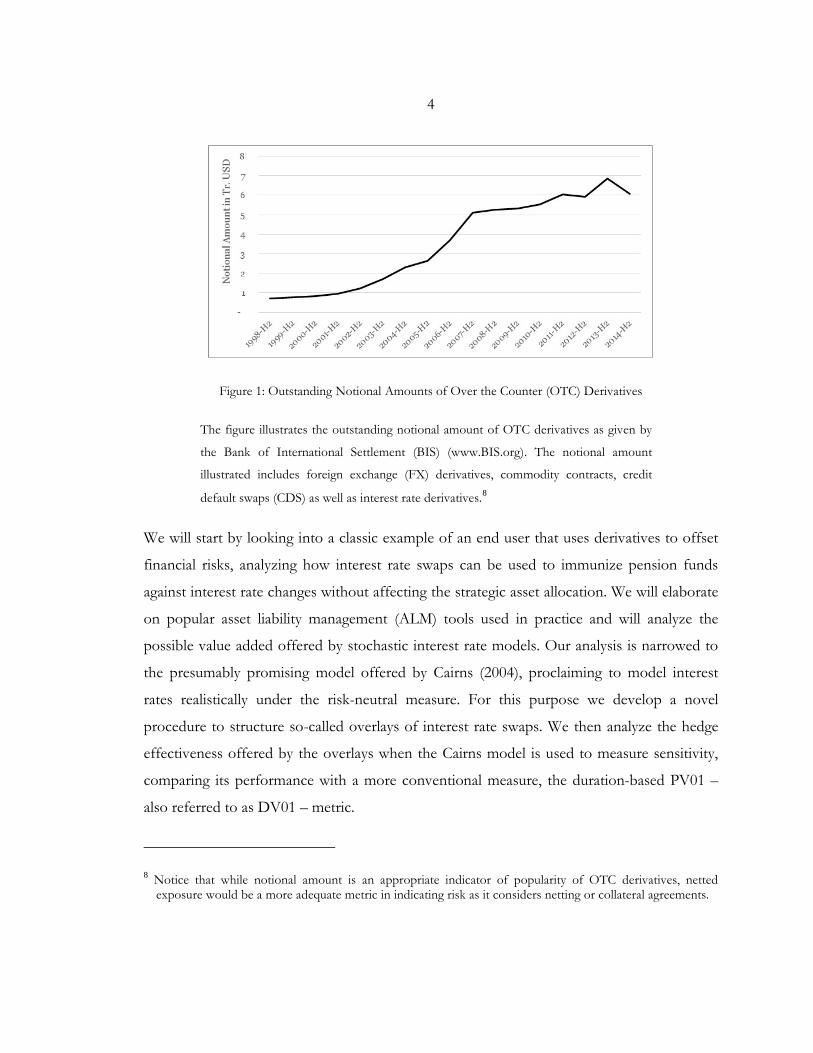
in popularity at least until the financial crisis. Figure 1 illustrates how outstanding notional

amounts of financial derivatives skyrocketed since the late 90s. This evolution mirrors an

increased interest in reducing (hedging) financial risk (especially arising from interest rate

changes) combined with an enhanced capability in speculation activities. This evolution has

2 See for example the analysis around credit default swaps (CDS) by Stulz (2010) or the publication of ISDA (2014b) on end user activity in the OTC market.

3 The quotes are taken from the financial report of Berkshire Hathaway (2002) in which Charlie Munger and Warren Buffer explain their exit from the derivatives business, and from an article written by Soros (2009) in which he pleads for banning “naked” credit default swap (CDS).

4 See the margin requirements for non-centrally cleared derivatives by BCBS (2013).

3

been accompanied by a new “science”, trying to price derivatives and capture the dynamics

of the underlying financial risk factors in mathematical terms. Computational finance has

also been subject to a very controversial discourse. Financial models such as the Black-

Scholes model for pricing options have helped researchers receive the “Nobel Prize”5 in

economic sciences, being praised for “[paving] the way for economic valuations in many areas and

[facilitating] more efficient risk management in society”.6 On the other hand, others have deprived

this research branch of any scientific notion, accusing it of “charlatanism” and in increasing

system blindness, also referred to as “model dope”.7

While thoroughly deep-diving into a range of different technical and managerial aspects

especially around interest rates and credit spreads we aim on maintaining a bird’s view with

regards to the overall discourse. We especially intend to contribute to the discussion on

derivatives between the poles of being “innovations” and “time bombs” on the one hand,

and the discussion around the scientific notions and the value added offered by financial

models on the other.

5 Officially referred to as Bank of Sweden Prize in Economic Sciences in Memory of Alfred Nobel. 6 See the press release of the Royal Swedish Academy of Science (1997) for awarding the prize to Robert

Merton and Myron Scholes. Comments in brackets [.] have been added by the author. 7 See MacKenzie and Spears (2014) for a discussion on the role of copula models in pricing Credit Debt

Obligations (CDO), analyzing the existence of “model dope”. Mikosch (2005) discuss the use of copula functions. Haug and Taleb (2011) analyze the non-use of the Black-Scholed formula for equity options. See Taleb (1997) for a more general critic of derivative pricing.

4

Figure 1: Outstanding Notional Amounts of Over the Counter (OTC) Derivatives

The figure illustrates the outstanding notional amount of OTC derivatives as given by

the Bank of International Settlement (BIS) (www.BIS.org). The notional amount

illustrated includes foreign exchange (FX) derivatives, commodity contracts, credit

default swaps (CDS) as well as interest rate derivatives.8

We will start by looking into a classic example of an end user that uses derivatives to offset

financial risks, analyzing how interest rate swaps can be used to immunize pension funds

against interest rate changes without affecting the strategic asset allocation. We will elaborate

on popular asset liability management (ALM) tools used in practice and will analyze the

possible value added offered by stochastic interest rate models. Our analysis is narrowed to

the presumably promising model offered by Cairns (2004), proclaiming to model interest

rates realistically under the risk-neutral measure. For this purpose we develop a novel

procedure to structure so-called overlays of interest rate swaps. We then analyze the hedge

effectiveness offered by the overlays when the Cairns model is used to measure sensitivity,

comparing its performance with a more conventional measure, the duration-based PV01 –

also referred to as DV01 – metric.

8 Notice that while notional amount is an appropriate indicator of popularity of OTC derivatives, netted exposure would be a more adequate metric in indicating risk as it considers netting or collateral agreements.

5

We will then turn to the counterparty credit risk exhibited by financial derivatives, giving a

compact overview in modeling and managing credit valuation adjustment (CVA), a metric

that has emerged as a standard method for pricing counterparty credit risk. We also discuss

the regulatory and accounting landscape behind counterparty credit risk and CVA which also

flows into a critical analysis of the prevailing discourse. Besides thoroughly discussing key

technical and managerial aspects around counterparty credit risk and CVA we aim to achieve

a novel overall evaluation of regulatory efforts on the one hand, and lobbying activities on

the other. We also synthesize the implications for derivative traders, discussing the

challenges around pricing CVA and the corresponding limits of risk-neutral valuation,

especially when it comes to constructing adequate hedges.

Finally, we discuss the specific case of credit default swaps (CDS), financial instruments in

which the splits between being an “innovation” and a “time bomb” is most evident. In this

context we revisit the key characteristics of CDS contracts, and discuss approaches for

modeling credit risk in general and credit spreads in particular. We show that while CDS can

be used to mitigate (counterparty) credit risk they are not excluded from exhibiting such risk

themselves. This is mostly evident if the credit quality of the protection seller and the

reference entity are interdependent, i.e. if wrong way risk is present. For this purpose we

revisit an approach offered by Brigo and Capponi (2010) to capture this feature. Besides

decomposing the approach into its bits and pieces, and elaborating on aspects Brigo and

Capponi (2010) left relatively open, we also offer a respective computational tune up for the

model. Subsequently we run a critical evaluation of the Brigo and Capponi (2010) approach

in particular, and CVA modeling in general. We analyze both the capability of such models

in delivering an arbitrage-free framework as well as in its use for inter- and intra-

organizational communication. Besides revealing key challenges, risks and limitations, we

also aim on shedding light on possible benefits and insights offered by such approaches.

6

1.2. THESIS SUMMARY

The thesis is structured in two main parts. Part 1 is dedicated to a specific issue around

interest rate risk management, while Part 2 deals with topics around counterparty credit risk

management. In the following we give an abstract for each chapter.

Part 1 covers interest rate risk management, consisting of one chapter:

‒ Chapter 2: Managing Interest Rate Risks of Pension Funds – An Application of the Cairns

Model:9 Long-term portfolios consisting of asset and liabilities such as pension funds

often exhibit significant sensitivities to changes in interest rates. Due to the

separation of responsibilities and the otherwise unwanted complication, interest rate

risk management of these portfolios is often done with a so-called derivative overlay

(as part of asset liability management, ALM). The interest rate sensitivity is

immunized by adding corresponding derivatives – mostly interest rate swaps –

without affecting the strategic asset allocation.

The use of stochastic models in this process is particular and ALM in general is

limited. One of the main reasons behind this is the lack of respective approaches that

combine arbitrage-free valuation with realistic modeling of short- and long-term

interest rate dynamics, a gap the interest rate model of Cairns (2004) proclaims to

address. We have therefore chosen to apply the Cairns model to the practical

challenge of immunizing a pension fund against interest rate risk.

We start by giving an overview on ALM in general and interest rate risk management

in particular, revisiting the duration-based PV01 metric for measuring interest rate

9 Chapter 2 is an adaptation of previous work of the author published in Balder and Schwake (2011). This means that some elaborations, especially in the computational part, are identical. Chapter 2 also uses materials already published by the author in Mahayni and Schwake (2013), especially regarding some of the exemplary calculations.

7

sensitivity. We describe the key mechanisms of interest rate swaps, elaborating on

their use in ALM strategies.

After revisiting the two-factor version of the Cairns model and its main features, we

derive respective model-based sensitivity measures. We subsequently discuss the use

of the extended Kalman filter approach in calibrating the parameters of the model.

This is followed by a comparison of the hedge effectiveness offered by the Cairns

model with the one given by the PV01 metric. For this purpose we introduce a novel

rule-based and model-independent algorithm that immunizes pension fund-like

portfolios against interest rate risk by structuring an overlay of appropriate swaps.

The hedge effectiveness offered by both overlays is analyzed in a backtesting

environment and in a Monte Carlo simulation scheme. While we do identify slight

advantages offered by the Cairns model we are not able to justify its use through

hedge effectiveness solely, especially if we bear the sophistication of its application in

mind (compared with the PV01 approach). We, however, conclude that the Cairns

model can offer an appropriate framework for analyzing investment strategies and

facilitating respective discussions, especially because it can combine risk-neutrality

with realistic modeling.

Part 2 covers counterparty credit risk management, consisting of the two following chapters:

‒ Chapter 3: Pricing and Managing Counterparty Credit Risk in Theory and Practice. It is at

the latest since the financial crisis in general and the collapse of Lehman Brothers in

particular that the “default-free scheme” has been finally falsified. It has become

clear that derivative traders are default-prone and that the risk of them defaulting

impacts derivative prices. The increased significance of counterparty credit risk has

also drawn the attention of regulators, standard setters and auditors. Those have in

turn further stressed the significance of the subject matter through more punitive

rules and regulations. This pressure seems to have pushed derivative traders –

especially financial institutions – to step up their procedures around pricing,

8

managing and mitigating counterparty credit risk. Credit valuation adjustment (CVA)

has emerged as a standard method for pricing counterparty credit risk. CVA can be

interpreted as the cost of hedging the counterparty credit risk of the respective

position. This introduces a new derivative instrument, usually referred to as

contingent credit default swap (C-CDS) that, in return to a premium, insures the

(stochastic) exposure at default. The pricing of a C-CDS (i.e. CVA valuation) usually

turns out to be a much more elaborate task than pricing the default-free derivative

itself.

Chapter 3 intends to give a compact overview in modeling and managing CVA,

accompanied by a critical analysis of the prevailing discourse. This analysis is the

heart of the chapter, which aims at exploring the challenges around CVA from

different angles rather than offering a comprehensive description of all relevant

aspects. It aims on achieving an overall evaluation of regulatory efforts on the one

hand, and lobbying activities on the other.

After giving an overview on counterparty credit risk and CVA literature we study the

quantification of CVA from a theoretically consistent perspective as well as based on

a more practical approach. We then turn to the accounting and regulatory landscape,

revisiting key requirements around counterparty credit risk and CVA risk.

Subsequently, we give an overview on charging CVA and discuss its allocation across

an organization in order to allow for adequate incentives. We also discuss the

possibility to reduce counterparty credit risk, especially through collateralization and

hedging activities.

Our analysis enables us to show how financial institutions are heavily driven by

regulatory requirements that originally aimed to actually mirror how they “do

business”. We elaborate on how banks not only measure and manage CVA

according to detailed requirements, but also on how such regulations considerably

affect the way banks price their products.

9

We also show the limits of arbitrage-free valuation, especially when it comes to

practical implementation of CVA pricing models or constructing adequate hedges.

We conclude that clinging to use market implied parameters or elaborate models that

need overcomplicated calibration without reflecting on their economic sense might

not only imply mere model and valuation risks, but also significant financial risks at

the latest when it comes to hedge CVA.

‒ Chapter 4: Pricing Credit Default Swaps with Wrong Way Risk – Model Implementation and

Computational Tune Up.10 One possibility for investors to mitigate counterparty credit

risk is to buy protection in form of a credit default swap (CDS). If the credit quality

of both protection seller and reference entity are positively interdependent, such a

“protection” becomes questionable if not worthless. Brigo and Capponi (2010) were

among the first to propose an arbitrage-free framework to price CDS considering

this wrong way risk in conjunction with symmetric pricing.

We start by describing the key mechanisms of CDS contracts, and giving an

overview on the “competing” approaches for modeling credit risk in general and

credit spreads in particular. We place the promising approach of Brigo and

Capponi (2010) within the category of reduced form credit risk models that use

copula functions to model default dependency. The approach is subsequently

decomposed into its bits and pieces, allowing a discussion around its benefits and

pitfalls. We also provide a step-by-step implementation guide, going into detail on

aspects that Brigo and Capponi (2010) left open, especially the computation of the

conditional survival probability of the reference entity. We illustrate how the

fractional Fourier transformation (FRFT) can be used for this purpose, and propose

a respective computational tune-up through a heuristic approximation. We then use a

10 Chapter 4 is an adaptation of previous work of the author published in Grominski et al. (2012), ). This means also that some elaborations, especially the computational part, are identical.

10

case study with real market data to demonstrate the use of the model and the insights

it delivers.

Finally, we run a critical evaluation of the Brigo and Capponi (2010) approach in

particular, and CVA modeling in general. We analyze both the capability of the

model in delivering an arbitrage-free framework as well as in its use for inter- and

intra-organizational communication. We show how the model can be used to

facilitate discussions around the specific case of CVA for CDS contracts with

considerable wrong way risk. We argue, however, that less elaborate models might

display more appropriate solutions, avoiding over-complication and higher model

risks, especially if wrong way risk is assumed to be less significant. After all, while

Brigo and Capponi (2010) do offer a coherent and risk-neutral framework, they do not

specify the needed duplication strategy. The lack of instruments to calibrate a risk-

neutral correlation matrix and of a possibility to hedge own credit risk puts a

question mark on the practicability of the model.

PART I:

INTEREST RATE RISK MANAGEMENT

……………………………………………….

INTEREST RATE RISK MANAGEMENT

……………………………………………….

12

CHAPTER 2:

INTEREST RATE RISK MANAGEMENT FOR PENSION FUNDS – AN

APPLICATION OF THE CAIRNS MODEL

2.1. INTRODUCTION

Funded retirement arrangements like pension funds and life insurance products have

extreme long-term claims, exceeding 50 or even 60 years. These liabilities are mostly

financed by bonds with maturities way shorter on the asset side. Besides the duration gap

produced by the lack of liquid long-term bonds, the providers and asset managers of such

products have to deal with the risk of interest rates maturing in decades. Due to the

separation of responsibilities and the otherwise unwanted complication, interest rate risk

management of these portfolios is often done with a so-called derivative overlay (as part of

asset liability management, ALM). The interest rate sensitivity is immunized by adding

corresponding derivatives – mostly interest rate swaps – without affecting the strategic asset

allocation.

A common practice in measuring interest rate sensitivity is using the PV01-approach. This

duration-based metric measures interest rate risk as the change in value due to a shift of the

interest rate curve. Based on a vector of PV01 metrics an interest rate swap overlay is usually

introduced in order to (statically) hedge interest rate risks. Although this method might seem

suspiciously easy for the academic world, it is quite wide spread under practitioners.

A key motive behind the limited use of theoretically more elaborate models (e.g. stochastic

interest rate models) is the lack of respective approaches that combine arbitrage-free

valuation with realistic modeling of short- and long-term interest rate dynamics. While

celebrated interest rate models such as the ones introduced by Cox et al. (1985), Heath et

al. (1992) or Miltersen et al. (1997) offer arbitrage-free valuation of derivatives, they are

presumably less capable in modeling realistic dynamics, especially when it comes to long

time horizons. On the other hand, actuarial models such the approaches of Wilkie (1995) or

13

Yakoubov et al. (1999) put more emphasis on modeling realistic dynamics but abandon the

arbitrage-free framework.

In the meanwhile the risk-neutral model-family for interest rates introduced by Cairns (2004)

simultaneously models short- and long-term interest rates. Adequately calibrated, the Cairns

model proclaims to deliver realistic simulation of the whole term structure, making it

especially promising for the case of pension funds. We have therefore chosen to put the

model to the test by applying it to structuring swap overlays, and comparing it with the

popular PV01-approach.

For this purpose we introduce interest rate sensitivity measures based on the two-factor

version of the Cairns model. For the construction of the swap overlays we introduce a novel

algorithm that is rule-based and model independent. Given an interest rate model, the

algorithm decomposes the interest rate sensitivity of portfolios containing assets and

liabilities. It then adds swaps to the portfolio in order to immunize it against interest rate

risks. A subsequent linear optimization defines the optimal notional amounts needed to

ensure interest rate risk is fully hedged. Using a realistic pension fund portfolio structure we

compare the hedge effectiveness delivered by the Cairns model with the one offered by the

PV01-approach. The comparison is done both in a backtest environment and using a Monte

Carlo simulation scheme.

The remaining parts of Chapter 2 are structured as follows. Section 2.2 gives an overview of

interest rate risk management as part of asset liability management (ALM), starting with

respective definitions and a literature summary given in Subchapter 2.2.1. Being a key and

popular measure of interest rate risk used in ALM strategies we dedicate Subchapter 2.2.2 to

the PV01 metric. The basis mechanisms behind the use of interest rate swaps are revisited in

Subchapter 2.2.3. Section 2.3 then moves to stochastic interest rate models, starting with a

respective literature summary, given in Subchapter 2.3.1. Subchapter 2.3.2 then describes the

main features of the chosen Cairns model for interest rates, while Subchapter 2.3.3 revisits

the methodology chosen for estimating the model parameters (extended Kalman filter). In

14

Subchapter 2.3.4 we derive the sensitivity measures (“Cairns deltas”) that will be used to

quantify and manage interest rate risk. Section 2.4 introduces a novel procedure for

structuring an interest rate swap overlay. In Section 2.5 we use a realistic use case to illustrate

the application of the Cairns approach for modeling and managing interest rate risk within

pension funds, comparing its performance with the one offered by the PV01 approach.

After giving an overview on implementing and calibrating the model (given in

Subchapters 2.5.1 and 2.5.2), we illustrate the structuring of an interest rate swap overlay in

Subchapter 2.5.3. We test its performance using a backtest approach as well as a Monte

Carlo simulation scheme, in Subchapter 2.5.4 and Subchapter 2.5.5., respectively. We

conclude the analysis in Section 2.6.

Notice that this Chapter is an adaptation of previous work of the author published in Balder

and Schwake (2011), and that some elaborations, especially the computational part, are

identical. 11 This Chapter also uses materials already published by the author in Mahayni and

Schwake (2013), especially some of the exemplary calculations. In order to avoid redundancy

we will refrain from continuously referring to both papers.

11 Balder (2014) also published an adopted version of Balder and Schwake (2011).

15

2.2. OVERVIEW ON ASSET LIABILITY MANAGEMENT

2.2.1. DEFINITIONS AND LITERATURE OVERVIEW

Asset liability management (ALM) refers to the simultaneous coordination of assets and

liabilities, aiming on capturing the overarching risk profile. This rather broad term is usually

reserved to the management of financial assets and liabilities, mostly relevant for financial

institutions, insurance companies and pension schemes.12 We will focus on the latter and will

narrow our analysis to interest rate risk management. We acknowledge that ALM within

pension funds might also cover further risk factors such as inflation, credit spreads and

longevity risk.13 Still, interest rate risk is presumed as most relevant, leading even to possible

analogy between the terms ALM and interest rate risk management (IRR) in practice jargon

(see for example Brick, 2014).

In the case of pension funds liabilities consist of pension payments to retired plan members

or ones that will retire in the future.14 These liabilities behave similarly to long-term bonds,

exhibiting a (relatively high) sensitivity to interest rates. Assets held by pension funds are

predominantly “fixed income” securities with additional investments in “riskier” markets

12 The definition is inspired amongst others by Sodhi (2005) and Fabbozi et al. (2005). For pension funds one also uses the term liability driven investment, LDI (see Ryan, 2013).

13 This short list of risk factors is not exhaustive. For credit spread modeling we refer the reader to Chapter 3 of this thesis. For modelling longevity risk see for example Mahayni and Steuten (2013).

14 Pension payments are paid out according to a predefined procedure. One speaks of “defined contribution” (DC) plans, when the pension plan sponsor (e.g. a company) is only obliged to pay pre-determined contributions into the fund (e.g. periodically). All remaining investment risk is borne by the pension members (e.g. employees). Defined benefit (DB) plans refer, on the other hand, to pension schemes that contain (partially) guaranteed payments. Thus, strictly speaking our analysis is limited to DB pension funds. The definition of DC plans follows the one used in International Financial Reporting Standards (IFRS) given in IAS 19.7, while the definition of DB plans is derived by negation.

16

such as equities and real estate.15 Still, one usually focuses on fixed income securities when it

comes to interest rate risk, because of their relatively high portfolio portion and the

ambiguous interest rate sensitivity of other asset classes.

In a broader sense ALM strategies offer the foundation for the optimal asset allocation of

the core portfolio (see also Ryan, 2013). Such optimization schemes will need to consider the

dynamics of both the liabilities and the assets in an integrated manner, providing answers

with regards to future contributions and changes in the asset allocation (see Fabozzi et al.,

2005). Prominent examples for such “full-fledged” solutions are given by Mulvey et

al. (2000) as well as Gondzio and Kouwenberg (2001). The former proposes a stochastic

planning model, aiming on maximizing the expected wealth while minimizing the risk of the

pension fund collapsing. They make the case that borrowing (e.g. from the fund sponsor)

can be optimal at certain situations. Gondzio and Kouwenberg (2001) analyze Dutch

pension plans, offering a so-called decomposition-based algorithm that is implemented on a

particular parallel computer.

A review of stochastic ALM models is given for example in Sodhi (2005), who covers

models for banks, insurance companies as well as pension funds. He also notes that such

approaches face methodological and computational challenges. First, they struggle with

offering a methodologically sound framework to model all the different aspects (e.g. interest

rates, mortality rates, salary variances etc.), ensuring consistency within the model as well as

with financial theory. Second, considering a large number of different factors and scenarios

implies substantial difficulty in solving the optimization problem. Gondzio and

Kouwenberg (2001) for example report on modeling “4,826,809 scenarios, 12,469,250

constraints and 24,938,502 variables” stating that it “is the largest stochastic linear program ever solved.”

There is one further considerable challenge which surrounds the role of models in decision

15 The asset allocation differs significantly from region to region. According to Towers Watson (2015) Australian pension schemes invest more than 50% in equity, while the respective figure at Swiss plans is less than 30%.

17

making. As put by a fund manager quoted in Fabozzi et al. (2005), the complexity of such

models makes them appear as a “black box to the investment committee”.

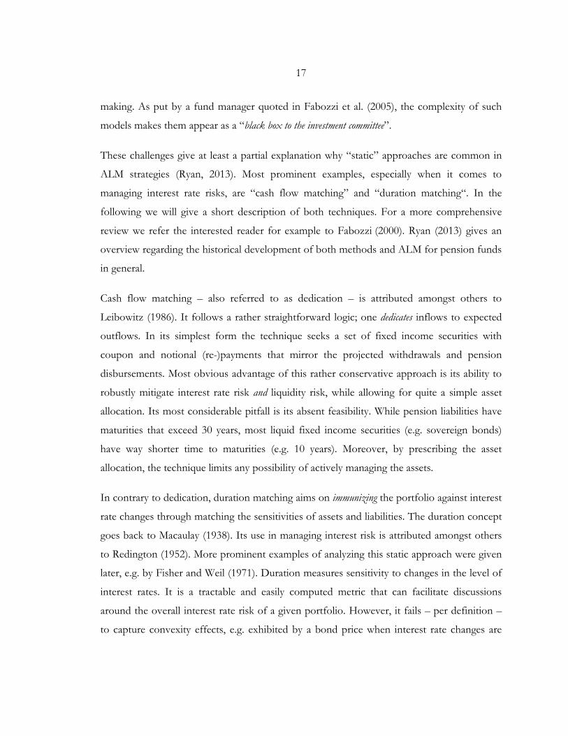
These challenges give at least a partial explanation why “static” approaches are common in

ALM strategies (Ryan, 2013). Most prominent examples, especially when it comes to

managing interest rate risks, are “cash flow matching” and “duration matching“. In the

following we will give a short description of both techniques. For a more comprehensive

review we refer the interested reader for example to Fabozzi (2000). Ryan (2013) gives an

overview regarding the historical development of both methods and ALM for pension funds

in general.

Cash flow matching – also referred to as dedication – is attributed amongst others to

Leibowitz (1986). It follows a rather straightforward logic; one dedicates inflows to expected

outflows. In its simplest form the technique seeks a set of fixed income securities with

coupon and notional (re-)payments that mirror the projected withdrawals and pension

disbursements. Most obvious advantage of this rather conservative approach is its ability to

robustly mitigate interest rate risk and liquidity risk, while allowing for quite a simple asset

allocation. Its most considerable pitfall is its absent feasibility. While pension liabilities have

maturities that exceed 30 years, most liquid fixed income securities (e.g. sovereign bonds)

have way shorter time to maturities (e.g. 10 years). Moreover, by prescribing the asset

allocation, the technique limits any possibility of actively managing the assets.

In contrary to dedication, duration matching aims on immunizing the portfolio against interest

rate changes through matching the sensitivities of assets and liabilities. The duration concept

goes back to Macaulay (1938). Its use in managing interest risk is attributed amongst others

to Redington (1952). More prominent examples of analyzing this static approach were given

later, e.g. by Fisher and Weil (1971). Duration measures sensitivity to changes in the level of

interest rates. It is a tractable and easily computed metric that can facilitate discussions

around the overall interest rate risk of a given portfolio. However, it fails – per definition –

to capture convexity effects, e.g. exhibited by a bond price when interest rate changes are

18

more material. For this purpose, second order approximations, e.g. dollar convexity

measures (see Fabbozi, 2000, pp. 68-77), have been proposed. More importantly duration-

based approaches have a significant theoretical shortfall. Not considering possible non-

parallel shifts (i.e. changes in the shape) of the term structure implies inconsistency with

arbitrage-free valuation, meaning that duration delivers a misleading measurement of risk

(see Ingersoll et al., 1978).16 A possible solution was introduced by Chambers and

Carlton (1988) and Ho (1992), proposing the use of duration vectors – also referred to as

key durations, measuring the sensitivity to yields with differing maturities.

2.2.2. PV01 AS A MEASURE FOR INTEREST RATE SENSITIVITY

A particular key duration-based measure is PV01 – also referred to as DV01 (dollar value) –

which measures sensitivity as the change of the present value (PV) due to a shift of the

interest rate curve by 1 basis point (01). Sensitivity is thus measured as the valuation change

– here of a zero bond – due to a parallel shift of the interest rate curve of 1 basis point. A

zero bond with the notional amount �̈�𝑁 has the following sensitivity to changes in the interest

rate 𝑟𝑟

𝑃𝑃𝑃𝑃01 =

110.000

∙ 𝜕𝜕𝑃𝑃(𝑡𝑡,𝑇𝑇)𝜕𝜕𝑟𝑟(𝑡𝑡,𝑇𝑇)

=1

10.000∙ 𝜕𝜕��̈�𝑁𝑒𝑒−𝑟𝑟(𝑡𝑡,𝑇𝑇)(𝑇𝑇−𝑡𝑡)�

𝜕𝜕𝑟𝑟(𝑡𝑡,𝑇𝑇)

= −104 ∙ (𝑇𝑇 − 𝑡𝑡) ∙ �̈�𝑁 ∙ 𝑃𝑃(𝑡𝑡,𝑇𝑇)

(2.1)

where 𝑃𝑃(𝑡𝑡,𝑇𝑇) stands for the value at time 𝑡𝑡 of the zero bond that matures in 𝑇𝑇. Notice that by

decomposing the portfolio into a stream of cash flows one can estimate a vector of PV01

metrics. For this purpose the cash flow positions are decomposed into a series of zero

16 This is due to the fact that one can construct “duplication portfolios”, generating structurally superior payoff profiles.

19

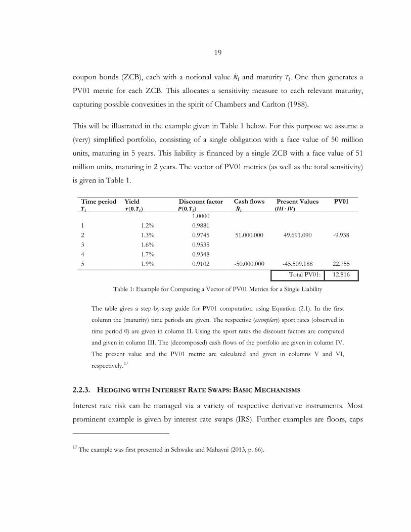
coupon bonds (ZCB), each with a notional value �̈�𝑁𝑖𝑖 and maturity 𝑇𝑇𝑖𝑖 . One then generates a

PV01 metric for each ZCB. This allocates a sensitivity measure to each relevant maturity,

capturing possible convexities in the spirit of Chambers and Carlton (1988).

This will be illustrated in the example given in Table 1 below. For this purpose we assume a

(very) simplified portfolio, consisting of a single obligation with a face value of 50 million

units, maturing in 5 years. This liability is financed by a single ZCB with a face value of 51

million units, maturing in 2 years. The vector of PV01 metrics (as well as the total sensitivity)

is given in Table 1.

Time period 𝑻𝑻𝒊𝒊

Yield 𝒓𝒓(𝟎𝟎,𝑻𝑻𝒊𝒊)

Discount factor 𝑷𝑷(𝟎𝟎,𝑻𝑻𝒊𝒊)

Cash flows �̈�𝑵𝒊𝒊

Present Values (𝑰𝑰𝑰𝑰𝑰𝑰 ∙ 𝑰𝑰𝑰𝑰)

PV01

1.0000 1 1.2% 0.9881 2 1.3% 0.9745 51.000.000 49.691.090 -9.938 3 1.6% 0.9535 4 1.7% 0.9348 5 1.9% 0.9102 -50.000.000 -45.509.188 22.755

Total PV01: 12.816

Table 1: Example for Computing a Vector of PV01 Metrics for a Single Liability

The table gives a step-by-step guide for PV01 computation using Equation (2.1). In the first

column the (maturity) time periods are given. The respective (exemplary) sport rates (observed in

time period 0) are given in column II. Using the sport rates the discount factors are computed

and given in column III. The (decomposed) cash flows of the portfolio are given in column IV.

The present value and the PV01 metric are calculated and given in columns V and VI,

respectively.17

2.2.3. HEDGING WITH INTEREST RATE SWAPS: BASIC MECHANISMS

Interest rate risk can be managed via a variety of respective derivative instruments. Most

prominent example is given by interest rate swaps (IRS). Further examples are floors, caps

17 The example was first presented in Schwake and Mahayni (2013, p. 66).

20

and swaptions (see for example Brigo and Mercurio, 2006). One speaks of overlay

management if derivatives are being used “on top”, i.e. without affecting the (active) asset

allocation. In the following we will illustrate how interest rate swaps can be used in hedging

interest rate risks of portfolios containing assets and liabilities. The objective of the overlay

strategy is to seek swaps that allow the sensitivity of the asset side to be equal to the

sensitivity of the liability side, i.e. to immunize the overall portfolio.

Interest rate swaps (IRS) refer to contracts in which counterparties agree to exchange

interest payments in a predefined frequency (e.g. monthly) for an agreed upon time period.

For example while one counterparty pays a fixed rate (in relation to a predefined notional

amount) the other party pays in return a floating rate (e.g. based on 3 months-Euribor).18

The compatibility of IRS in hedging is easily seen by duplicating the interest rate derivatives.

The value at time 𝑡𝑡 of a swap settling in 𝑡𝑡0, maturing in 𝑡𝑡𝑛𝑛 while paying a fixed rate 𝑐𝑐 can be

written as:

𝑃𝑃𝑠𝑠𝑠𝑠𝑠𝑠𝑠𝑠(𝑡𝑡) = 𝑃𝑃(𝑡𝑡, 𝑡𝑡0) −∑ 𝑐𝑐𝑃𝑃(𝑡𝑡, 𝑡𝑡𝑖𝑖) − 𝑃𝑃(𝑡𝑡, 𝑡𝑡𝑛𝑛), 𝑡𝑡 ∈ [0, 𝑡𝑡𝑛𝑛]𝑛𝑛𝑖𝑖=0 . (2.2)

The swap can thus be duplicated in the following manner. The fixed leg is seen as a portfolio

of zero coupon bonds with 𝑐𝑐 as their face values. The floating leg is duplicated using a

position in a bond maturing with the swap in 𝑡𝑡𝑛𝑛, and a contrariwise bond maturing at the

end of the forward period in 𝑡𝑡0. In a payer (receiver) swap a short (long) position is built up

in 𝑡𝑡0 and a long (short) position is built up in 𝑡𝑡𝑛𝑛.

The values of both separate legs can thus be written as

18 Interest rate swaps could be constructed to allow for swapping fixed against fixed payments or floating against floating payments. Other examples on interest rate swaps (including illustrations) are given in Section 3.2.

21

𝑃𝑃𝑓𝑓𝑓𝑓𝑓𝑓𝑠𝑠𝑡𝑡𝑖𝑖𝑛𝑛𝑓𝑓(𝑡𝑡) = 𝑃𝑃(𝑡𝑡, 𝑡𝑡0) − 𝑃𝑃(𝑡𝑡, 𝑡𝑡𝑛𝑛), 𝑡𝑡 ∈ [0, 𝑡𝑡𝑛𝑛]

𝑃𝑃𝑓𝑓𝑖𝑖𝑓𝑓(𝑡𝑡) = �𝑐𝑐𝑃𝑃(𝑡𝑡, 𝑡𝑡𝑖𝑖), 𝑡𝑡 ∈ [0, 𝑡𝑡𝑛𝑛]𝑛𝑛

𝑖𝑖=0

.

(2.3)

This means that the fixed leg will have sensitivities towards interest rate changes on every

payment date of the swap. Yet the more significant sensitivities (for a given time period) will

arise from the floating leg. A (spot) swap will demonstrate such sensitivity at its maturity,

while forward swaps will have significant sensitivities at maturity as well as at their first fixing

date.

These mechanisms will be illustrated in the following example which builds on the simplified

framework we used in Subchapter 2.2.2 above. For this purpose we assume a (very)

simplified portfolio, consisting of a single forward receiver swap. The first fixing date will be

in 2 years, and the settlement date will take place in 3 years-times, maturing in 5 years from

now. Table 2 summarizes the decomposed cash flow positions of the swap, using the

duplication strategy discussed above (see Equation (2.3)).

22

Time period 𝑻𝑻𝒊𝒊

Yield 𝒓𝒓(𝟎𝟎,𝑻𝑻𝒊𝒊)

Discount factor 𝑷𝑷(𝟎𝟎,𝑻𝑻𝒊𝒊)

Cash flows 𝑵𝑵𝒊𝒊̈

Present Values (𝑰𝑰𝑰𝑰𝑰𝑰 ∙ 𝑰𝑰𝑰𝑰)

PV01

1.0000 1 1.2% 0.9881 2 1.3% 0.9745 -50,000,000 -48,716,754 9,743 3 1.6% 0.9535 1,149,101 1,095,247 -329 4 1.7% 0.9348 1,149,101 1,073,560 -429 5 1.9% 0.9102 51,149,101 46,513,608 -23,257

Total PV01: -14,271

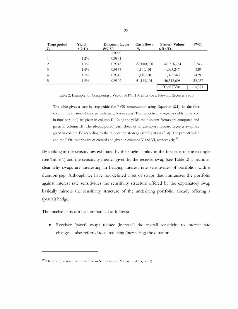
Table 2: Example for Computing a Vector of PV01 Metrics for a Forward Receiver Swap

The table gives a step-by-step guide for PV01 computation using Equation (2.1). In the first

column the (maturity) time periods are given in years. The respective (exemplary) yields (observed

in time period 0) are given in column II. Using the yields the discount factors are computed and

given in column III. The (decomposed) cash flows of an exemplary forward receiver swap are

given in column IV according to the duplication strategy (see Equation (2.3)). The present value

and the PV01 metrics are calculated and given in columns V and VI, respectively.19

By looking at the sensitivities exhibited by the single liability in the first part of the example

(see Table 1) and the sensitivity metrics given by the receiver swap (see Table 2) it becomes

clear why swaps are interesting in hedging interest rate sensitivities of portfolios with a

duration gap. Although we have not defined a set of swaps that immunizes the portfolio

against interest rate sensitivities the sensitivity structure offered by the explanatory swap

basically mirrors the sensitivity structure of the underlying portfolio, already offering a

(partial) hedge.

The mechanisms can be summarized as follows:

• Receiver (payer) swaps reduce (increase) the overall sensitivity to interest rate

changes – also referred to as reducing (increasing) the duration.

19 The example was first presented in Schwake and Mahayni (2013, p. 67).

23

• Forward receiver (payer) swaps increase (decrease) the sensitivity at the first

settlement date (end of the forward period) while decreasing (increasing) the

sensitivity towards the maturity time period of the swap

24

2.3. MODELING INTEREST RATE DYNAMICS

2.3.1. REMARKS AND LITERATURE OVERVIEW

Due to the challenging characteristics of interest rate instruments numerous models have

been developed in order to mathematically capture the dynamics of term structures (i.e. yield

curves), following these key objectives:

a. Arbitrage-free and risk-neutral valuation of interest rate derivatives

b. Realistic modeling of interest rate changes (motivated by Figure 2 below), e.g.:

i. Dynamics should fit observed historical data

ii. Interest rates should be non-negative, yet possibly getting close to zero

iii. Interest rates should be a mean reverting

iv. Term structures should exhibit a variety of shapes (incl. non-parallel movements)

v. Long periods with both relatively high and low interest rates should be possible

At the latest since the work of Black (1976) have option theory and the increasing need for

derivatives pricing given this research branch a considerable push. Most of the celebrated

models in this context focus on the valuation of short- and middle-term contingent claims,

i.e. fulfilling objective (a) rather than objective (b). In the following we will give a short recap

on prominent examples of stochastic models for interest rates. This summary is largely

inspired by Brigo and Mercurio (2006) who offer a comprehensive and detailed description

and analysis of all models, and to whom we refer the interested reader. For the use of

interest rate models for pricing application see also Hull (2006), and Björk (2009). Andresen

and Piterbarg (2010 a, b, c) present a more up-to-date and recent analysis of arbitrage-free

models in three comprehensive volumes. For stochastic basis spread modeling refer to

Mercurio and Xie (2012). For multi curve modeling and OIS discounting see Hull and

White (2012b).

25

Prominent examples of so-called short rate models were given by Vasicek (1977),

Rendleman and Bartter (1980), and Cox, Ingersoll and Ross (Cox et al., 1985). These

approaches are motivated by the fact that the prices of zero coupon bonds are completely

driven by the probabilistic dynamics of the instantaneous short rate.20 Modeling the short

rate in a risk-neutral manner will thus enable us to model the whole term structure. The most

significant pitfall of the models mentioned is that the endogenous term structure delivered

by the model is not confirmed by (exogenous) market implied ones. A solution has been

proposed through arbitrage-free short rate models, offered for example by Hull and

White (1990), Black et al. (1990) as well as Black and Karasinski (1991). Brigo and

Mercurio (2006) also analyze the shifted CIR model (CIR++), offering an analytically

tractable approach that fits to current market information.

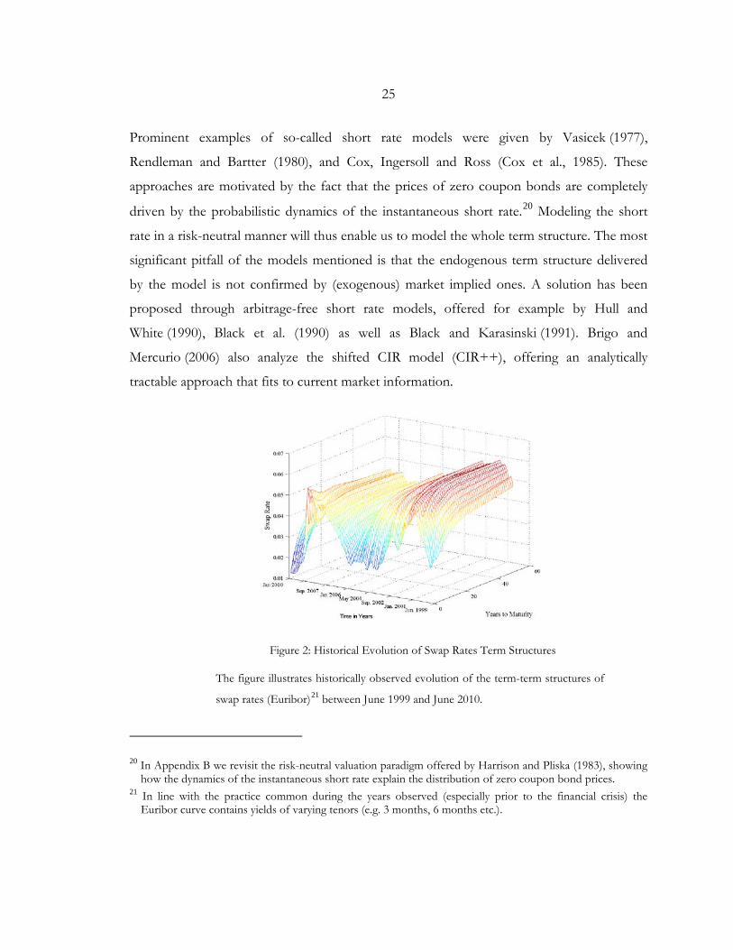
Figure 2: Historical Evolution of Swap Rates Term Structures

The figure illustrates historically observed evolution of the term-term structures of

swap rates (Euribor)21 between June 1999 and June 2010.

20 In Appendix B we revisit the risk-neutral valuation paradigm offered by Harrison and Pliska (1983), showing how the dynamics of the instantaneous short rate explain the distribution of zero coupon bond prices.

21 In line with the practice common during the years observed (especially prior to the financial crisis) the Euribor curve contains yields of varying tenors (e.g. 3 months, 6 months etc.).

26

Heath et al. (1992) proposed an arbitrage-free approach to model instantaneous forward

rates. In contrast to short rate models, the approach is more general and aims to describe the

dynamics of the whole yield curve directly. The model offers an adequate framework for

studying the properties of arbitrage freedom, and has gained substantial interest in academic

literature. The models of Brace et al. (1997) and Miltersen et al. (1997) focused on modeling

observed (not theoretical) interest rates (e.g. Libor rate). Adding stochastic features to the

volatility term as in Wu and Zhang (2002) or the introduction of a stochastic basis between

tenor dependent term structures as in Mercurio (2010) are some of the main adaptations

done in order to deliver more accurate risk-neutral pricing.

Although the above mentioned models partially satisfy some of the requirements around

realistic modelling (e.g. mean reverting), their primary focus remains in achieving arbitrage-

free valuation, offering pricing frameworks for derivatives. In a parallel stream, approaches

of Wilkie (1995) and Yakoubov et al. (1999) have put more emphasis on the actuarial (risk

oriented) interest of realistic modeling, i.e. focusing on objective (b) rather than objective (a).

These time-discrete approaches are not designed for the valuation of interest rate

instruments and their short-term risk management.

Cairns (2004) introduced a family of models that aims on satisfying both objectives, i.e.

allowing for arbitrage-free valuation and realistic modeling of interest rates with diverse

maturities. This makes the Cairn models promising with regards to managing interest rate

risk in long-term pension funds. We have, therefore, decided to narrow our analysis to this

approach, especially studying its ability in delivering a consistent framework for ALM as well

as any value add it offers if compared to popular static approaches (i.e. duration-based

PV01).

2.3.2. THE CAIRNS APPROACH: MODEL FRAMEWORK

Based on the framework of Flesaker and Hughston (1996), Cairns (2004) introduces a family

of models that aim to satisfy both the arbitrage-free evaluation and the realistic modeling of

interest rates with diverse maturities. In the following we will shortly revisit the approach

27

and its main characteristics. For previous work on the family models offered by Cairns see

also Lutz (2006) and Pfeiffer et al. (2010).

Cairns (2004) denotes the price at time 𝑡𝑡 of the zero coupon bond 𝑃𝑃(𝑡𝑡,𝑇𝑇), maturing in 𝑇𝑇 as

follows:

𝑃𝑃(𝑡𝑡,𝑇𝑇) =

∫ 𝐻𝐻�𝑢𝑢,𝑋𝑋(𝑡𝑡)�𝑑𝑑𝑢𝑢∞𝑇𝑇−𝑡𝑡

∫ 𝐻𝐻�𝑢𝑢,𝑋𝑋(𝑡𝑡)�𝑑𝑑𝑢𝑢∞0

. (2.4)

These bond prices are a function of the specified martingale family

𝐻𝐻(𝑢𝑢, 𝑥𝑥) = exp �−𝛽𝛽𝑢𝑢 + �𝜎𝜎𝑖𝑖𝑋𝑋𝑖𝑖𝑒𝑒−𝛼𝛼𝑖𝑖𝑢𝑢

𝑛𝑛

𝑖𝑖=1

−12�

𝜌𝜌𝑖𝑖𝑖𝑖𝜎𝜎𝑖𝑖𝜎𝜎𝑖𝑖𝛼𝛼𝑖𝑖 + 𝛼𝛼𝑖𝑖

𝑒𝑒−�𝛼𝛼𝑖𝑖+𝛼𝛼𝑗𝑗�𝑢𝑢𝑛𝑛

𝑖𝑖,𝑖𝑖=1

� (2.5)

for some parameters 𝛽𝛽, 𝛼𝛼𝑖𝑖 , … ,𝛼𝛼𝑛𝑛,𝜎𝜎𝑖𝑖 , … ,𝜎𝜎𝑛𝑛 and 𝑛𝑛 correlated 𝑋𝑋𝑖𝑖 factors with 𝜌𝜌𝑖𝑖𝑖𝑖 standing for the

respective correlation coefficient. The 𝑛𝑛 factors are a function of an Ornstein-Uhlenbeck

process, driven by the same number of independent Brownian motions 𝑍𝑍𝚥𝚥�

𝑑𝑑𝑋𝑋𝑖𝑖(𝑡𝑡) = 𝛼𝛼𝑖𝑖�𝜇𝜇𝑖𝑖 − 𝑋𝑋(𝑡𝑡)�𝑑𝑑𝑡𝑡 + �𝑐𝑐𝑖𝑖𝑖𝑖𝑑𝑑𝑍𝑍𝚥𝚥� (𝑡𝑡)

𝑛𝑛

𝑖𝑖=1

(2.6)

with 𝜇𝜇 standing for an additional constant parameter per factor. The matrix 𝐶𝐶 = (𝑐𝑐𝑖𝑖𝑖𝑖)𝑖𝑖;𝑖𝑖=1𝑛𝑛 is

defined in such a manner that 𝐶𝐶𝐶𝐶’ represents the correlation matrix for the processes,

𝑋𝑋1(𝑡𝑡), … ,𝑋𝑋𝑛𝑛(𝑡𝑡), 𝐶𝐶𝐶𝐶’ = (𝜌𝜌𝑖𝑖𝑖𝑖)𝑖𝑖;𝑖𝑖=1𝑛𝑛 . The solution of the stochastic differential equation equals

𝑋𝑋𝑖𝑖(𝑡𝑡) = 𝑒𝑒−𝛼𝛼𝑖𝑖𝑡𝑡𝑋𝑋𝑖𝑖(0) + 𝜇𝜇𝑖𝑖(1 − 𝑒𝑒−𝛼𝛼𝑖𝑖𝑡𝑡) + �𝑐𝑐𝑖𝑖𝑖𝑖 � 𝑒𝑒−𝛼𝛼𝑖𝑖(𝑡𝑡−𝑠𝑠)

𝑡𝑡

𝑓𝑓𝑑𝑑𝑍𝑍𝚥𝚥� (𝑠𝑠)

𝑛𝑛

𝑖𝑖=1

(2.7)

Given suitably parametrized values for the constants, 𝛽𝛽, 𝛼𝛼, 𝜎𝜎,𝜌𝜌, 𝜇𝜇 and an appropriate number

of factors, Cairns (2004) shows that the model satisfies the following:

a) All interest rates are positive

b) All interest rates can get close to zero

28

c) The model is mean reverting

d) Long periods with both relatively high and low interest rates are possible

e) Par yields for long-term bonds should have realistic probabilities of reaching both

high and low values

f) The model is preferably time homogeneous

g) The constant parameters in the model need no regular recalibration

While most of these characteristics have already been targeted by other models, points (d)

and (e) are the unique ones that distinguish the Cairns-model at most. For the derivation of

these characteristics the 𝛼𝛼-parameters are vital. These are the parameters that drive the

mean-reverting Ornstein-Uhlenbeck processes. Given at least one rather low 𝛼𝛼-term will lead

to one factor 𝑋𝑋 being subject to long-term cycles, feeding through to long-term cycles in

interest rates. Furthermore, such a parameter would allow par yields on long-term bonds to

vary over a wide range. Meanwhile, Cairns (2004) shows that the 𝛽𝛽-term can be interpreted

as a long-term forward interest rate.

In the following we will narrow the analysis to the two-factor version of the model, i.e.

having 𝑋𝑋1 and 𝑋𝑋2 factors. As noted by Cairns (2004) two factors already enable the

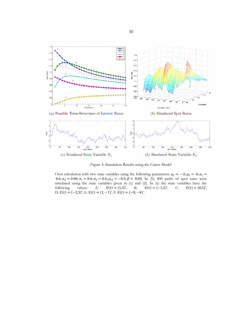
demonstration of key features of the multi-factor version.22 Figure 1 illustrates the dynamics

of the term structure under the use of the two-factor version. While Subfigure (a)

demonstrates the ability of generating various changes with respect to the curvature of the

term structure, Subfigure (b) illustrates the overall dynamics, incl. the ability of modeling

relatively low as well as relatively high yield curves without re-calibrating the model.

22 Jamshidian and Zhu (1997) for example show that three factors explain 93% to 94% of interest rate dynamics. They also show that two factors already explain up to 91% of variations in the yield curve, while one factor will exhibit an explanatory power of 68% to 76%. Interestingly, Rebonato (1998) indicates that one factor models can already explain up to 92% of the dynamics, while two factors might capture 99.1% of the variations.

29

As discussed in Cairns (2004) the measure under which the term shown in Equation (2.4) is

a martingale can either be interpreted as a real-world measure ℙ or a risk-neutral measure ℚ.

Using the risk-neutral measure ℚ will allow endogenously generated prices to fit market

prices, standing in line with no arbitrage theory. Theoretically speaking we should opt to use

the risk-neutral measure ℚ as we are seeking to hedge interest rate risk, i.e. use exogenous

price information. Our focus is however not limited to “pricing”. We are interested in

shedding light on the value added offered by the model in managing interest rate risk of

long-term portfolios, emphasizing the need in generating realistic dynamics of interest rates.

For this purpose we choose a historical calibration method (i.e. under the real-world measure

ℙ) as will be discussed in Subchapter 2.3.3.

30

Figure 3: Simulation Results using the Cairns Model

Own calculation with two state variables using the following parameters: 𝜇𝜇1 = −2;𝜇𝜇2 = 6;𝛼𝛼1 = 0.6;𝛼𝛼2 = 0.06;𝜎𝜎1 = 0.6;𝜎𝜎2 = 0.4;𝜌𝜌12 = −0.5;𝛽𝛽 = 0.04. In (b) 400 paths of spot rates were simulated using the state variables given in (c) and (d). In (a) the state variables have the following values: A: 𝑋𝑋(𝑡𝑡) = (1,3)’, B: 𝑋𝑋(𝑡𝑡) = (−1,5)’, C: 𝑋𝑋(𝑡𝑡) = (0,3)’, D: 𝑋𝑋(𝑡𝑡) = (−2,3)′, E: 𝑋𝑋(𝑡𝑡) = (1,−1)’, F: 𝑋𝑋(𝑡𝑡) = (−8,−4)’.

31

2.3.3. MODEL IMPLEMENTATION

In the following we show how the parameters of the two-factor version of the Cairns model

can be estimated. We subsequently display the robustness of the approach chosen.

We base the estimation of the parameters of the Cairns model on the so-called extended

Kalman filter approach. For this purpose we adopt the algorithm described by Lutz (2006).

The approach has also been analyzed for example by Babbs and Nowman (1999) to calibrate

generalized Vasicek term structure models. Duan and Simonato (1999) have applied it to

affine term structure models, and Chen and Scott (2003) have narrowed the analyses to Cox-

Ingersoll-Ross models. In the following we will briefly revisit the main steps of the

calibration algorithm. For a more comprehensive elaboration we refer the reader to

Lutz (2006).

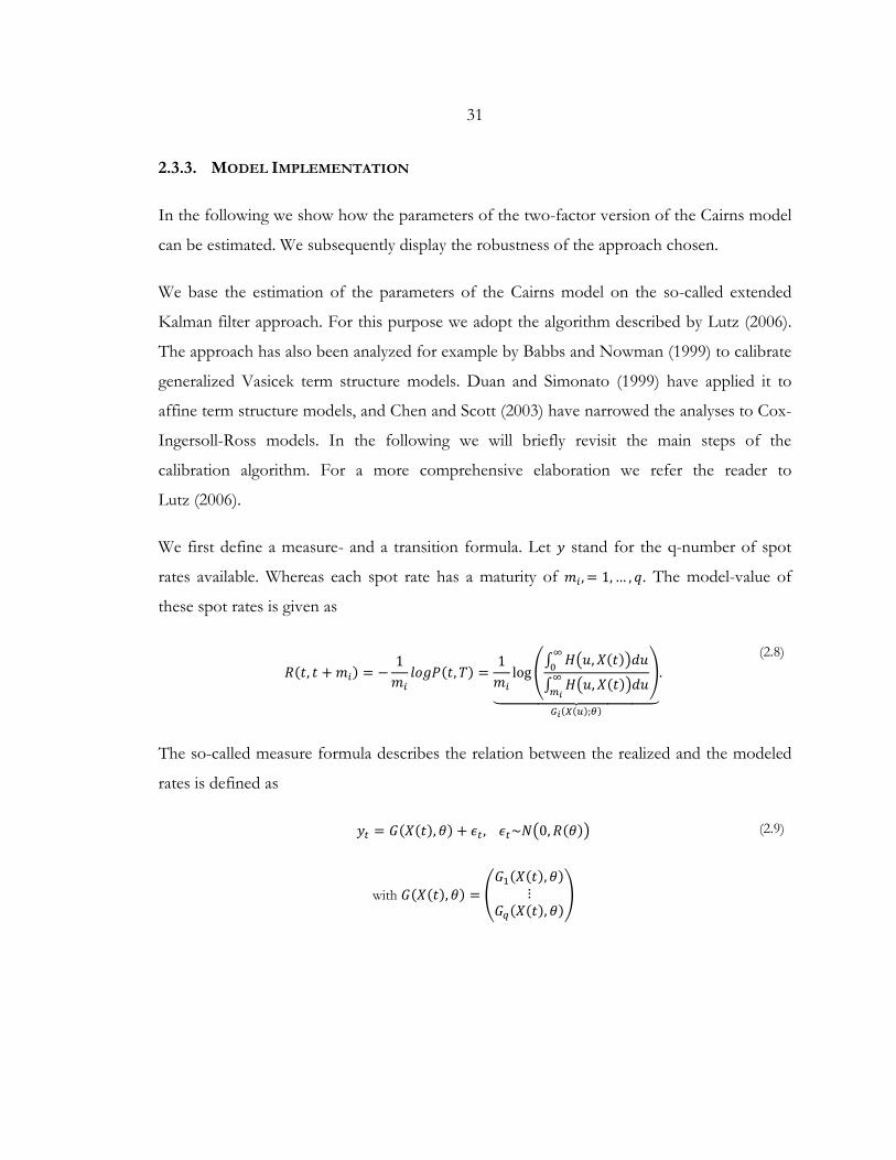
We first define a measure- and a transition formula. Let 𝑦𝑦 stand for the q-number of spot

rates available. Whereas each spot rate has a maturity of 𝑚𝑚𝑖𝑖 , = 1, … , 𝑞𝑞. The model-value of

these spot rates is given as

𝑅𝑅(𝑡𝑡, 𝑡𝑡 + 𝑚𝑚𝑖𝑖) = −

1𝑚𝑚𝑖𝑖

𝑙𝑙𝑙𝑙𝑙𝑙𝑃𝑃(𝑡𝑡,𝑇𝑇) =1𝑚𝑚𝑖𝑖

log�∫ 𝐻𝐻�𝑢𝑢,𝑋𝑋(𝑡𝑡)�𝑑𝑑𝑢𝑢∞0

∫ 𝐻𝐻�𝑢𝑢,𝑋𝑋(𝑡𝑡)�𝑑𝑑𝑢𝑢∞𝑚𝑚𝑖𝑖

��������������������

𝐺𝐺𝑖𝑖(𝑋𝑋(𝑢𝑢);𝜃𝜃)

. (2.8)

The so-called measure formula describes the relation between the realized and the modeled

rates is defined as

𝑦𝑦𝑡𝑡 = 𝐺𝐺(𝑋𝑋(𝑡𝑡),𝜃𝜃) + 𝜖𝜖𝑡𝑡 , 𝜖𝜖𝑡𝑡~𝑁𝑁�0,𝑅𝑅(𝜃𝜃)�

with 𝐺𝐺(𝑋𝑋(𝑡𝑡),𝜃𝜃) = �𝐺𝐺1(𝑋𝑋(𝑡𝑡),𝜃𝜃)

⋮𝐺𝐺𝑞𝑞(𝑋𝑋(𝑡𝑡),𝜃𝜃)

�

(2.9)

32

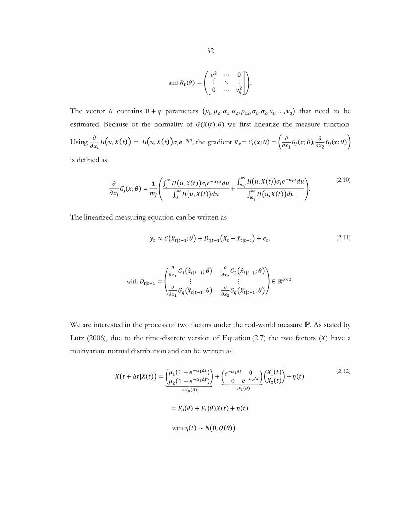
and 𝑅𝑅𝑡𝑡(𝜃𝜃) = ��𝜈𝜈12 ⋯ 0⋮ ⋱ ⋮0 ⋯ 𝜈𝜈𝑞𝑞2

��.

The vector 𝜃𝜃 contains 8 + 𝑞𝑞 parameters �𝜇𝜇1, 𝜇𝜇2,𝛼𝛼1,𝛼𝛼2,𝜌𝜌12,𝜎𝜎1,𝜎𝜎2, 𝜈𝜈1, … , 𝜈𝜈𝑞𝑞� that need to be

estimated. Because of the normality of 𝐺𝐺(𝑋𝑋(𝑡𝑡),𝜃𝜃) we first linearize the measure function.

Using 𝜕𝜕𝜕𝜕𝑓𝑓𝑖𝑖

𝐻𝐻�𝑢𝑢,𝑋𝑋(𝑡𝑡)� = 𝐻𝐻�𝑢𝑢,𝑋𝑋(𝑡𝑡)�𝜎𝜎𝑖𝑖𝑒𝑒−𝛼𝛼𝑖𝑖𝑢𝑢, the gradient ∇𝑓𝑓= 𝐺𝐺𝑖𝑖(𝑥𝑥; 𝜃𝜃) = � 𝜕𝜕𝜕𝜕𝑥𝑥1

𝐺𝐺𝑖𝑖(𝑥𝑥; 𝜃𝜃), 𝜕𝜕𝜕𝜕𝑥𝑥2

𝐺𝐺𝑖𝑖(𝑥𝑥; 𝜃𝜃)�

is defined as

𝜕𝜕𝜕𝜕𝑥𝑥𝑖𝑖

𝐺𝐺𝑖𝑖(𝑥𝑥; 𝜃𝜃) =1𝑚𝑚𝑖𝑖

�∫ 𝐻𝐻�𝑢𝑢,𝑋𝑋(𝑡𝑡)�𝜎𝜎𝑖𝑖𝑒𝑒−𝛼𝛼𝑖𝑖𝑢𝑢𝑑𝑑𝑢𝑢∞0

∫ 𝐻𝐻�𝑢𝑢,𝑋𝑋(𝑡𝑡)�𝑑𝑑𝑢𝑢∞0

+∫ 𝐻𝐻�𝑢𝑢,𝑋𝑋(𝑡𝑡)�𝜎𝜎𝑖𝑖𝑒𝑒−𝛼𝛼𝑖𝑖𝑢𝑢𝑑𝑑𝑢𝑢∞𝑚𝑚𝑗𝑗

∫ 𝐻𝐻�𝑢𝑢,𝑋𝑋(𝑡𝑡)�𝑑𝑑𝑢𝑢∞𝑚𝑚𝑗𝑗

�. (2.10)

The linearized measuring equation can be written as

𝑦𝑦𝑡𝑡 ≈ 𝐺𝐺�𝑥𝑥�𝑡𝑡|𝑡𝑡−1; 𝜃𝜃� + 𝐷𝐷𝑡𝑡|𝑡𝑡−1�𝑋𝑋𝑡𝑡 − 𝑥𝑥�𝑡𝑡|𝑡𝑡−1� + 𝜖𝜖𝑡𝑡 ,

with 𝐷𝐷𝑡𝑡|𝑡𝑡−1 = �

𝜕𝜕𝜕𝜕𝑓𝑓1

𝐺𝐺1�𝑥𝑥�𝑡𝑡|𝑡𝑡−1;𝜃𝜃�⋮

𝜕𝜕𝜕𝜕𝑓𝑓1

𝐺𝐺𝑞𝑞�𝑥𝑥�𝑡𝑡|𝑡𝑡−1; 𝜃𝜃�

𝜕𝜕𝜕𝜕𝑓𝑓2

𝐺𝐺2�𝑥𝑥�𝑡𝑡|𝑡𝑡−1; 𝜃𝜃�⋮

𝜕𝜕𝜕𝜕𝑓𝑓2

𝐺𝐺𝑞𝑞�𝑥𝑥�𝑡𝑡|𝑡𝑡−1; 𝜃𝜃�� ∈ ℝ𝑞𝑞×2.

(2.11)

We are interested in the process of two factors under the real-world measure ℙ. As stated by

Lutz (2006), due to the time-discrete version of Equation (2.7) the two factors (𝑋𝑋) have a

multivariate normal distribution and can be written as

𝑋𝑋�𝑡𝑡 + ∆𝑡𝑡|𝑋𝑋(𝑡𝑡)� = �𝜇𝜇1

(1 − 𝑒𝑒−𝛼𝛼1∆𝑡𝑡)𝜇𝜇2(1 − 𝑒𝑒−𝛼𝛼2∆𝑡𝑡)

������������

=:𝐹𝐹0(𝜃𝜃)

+ �𝑒𝑒−𝛼𝛼1∆𝑡𝑡

00

𝑒𝑒−𝛼𝛼2∆𝑡𝑡������������=:𝐹𝐹1(𝜃𝜃)

�𝑋𝑋1(𝑡𝑡)

𝑋𝑋2(𝑡𝑡)� + 𝜂𝜂(𝑡𝑡)

= 𝐹𝐹0(𝜃𝜃) + 𝐹𝐹1(𝜃𝜃)𝑋𝑋(𝑡𝑡) + 𝜂𝜂(𝑡𝑡)

with 𝜂𝜂(𝑡𝑡) ∼ 𝑁𝑁�0,𝑄𝑄(𝜃𝜃)�

(2.12)

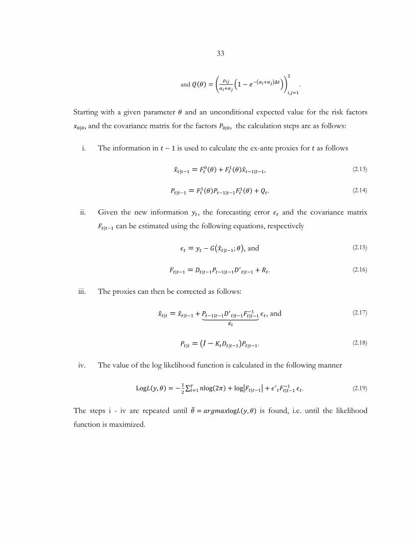
33

and 𝑄𝑄(𝜃𝜃) = �𝜌𝜌𝑖𝑖𝑗𝑗

𝛼𝛼𝑖𝑖+𝛼𝛼𝑗𝑗�1 − 𝑒𝑒−�𝛼𝛼𝑖𝑖+𝛼𝛼𝑗𝑗�Δ𝑡𝑡��

𝑖𝑖,𝑖𝑖=1

2

.

Starting with a given parameter 𝜃𝜃 and an unconditional expected value for the risk factors

𝑥𝑥0|0, and the covariance matrix for the factors 𝑃𝑃0|0, the calculation steps are as follows:

i. The information in 𝑡𝑡 − 1 is used to calculate the ex-ante proxies for 𝑡𝑡 as follows

𝑥𝑥�𝑡𝑡|𝑡𝑡−1 = 𝐹𝐹𝑡𝑡0(𝜃𝜃) + 𝐹𝐹𝑡𝑡1(𝜃𝜃)𝑥𝑥�𝑡𝑡−1|𝑡𝑡−1, (2.13)

𝑃𝑃𝑡𝑡|𝑡𝑡−1 = 𝐹𝐹𝑡𝑡1(𝜃𝜃)𝑃𝑃𝑡𝑡−1|𝑡𝑡−1𝐹𝐹𝑡𝑡1(𝜃𝜃) + 𝑄𝑄𝑡𝑡 . (2.14)

ii. Given the new information 𝑦𝑦𝑡𝑡, the forecasting error 𝜖𝜖𝑡𝑡 and the covariance matrix

𝐹𝐹𝑡𝑡|𝑡𝑡−1 can be estimated using the following equations, respectively

𝜖𝜖𝑡𝑡 = 𝑦𝑦𝑡𝑡 − 𝐺𝐺�𝑥𝑥�𝑡𝑡|𝑡𝑡−1; 𝜃𝜃�, and (2.15)

𝐹𝐹𝑡𝑡|𝑡𝑡−1 = 𝐷𝐷𝑡𝑡|𝑡𝑡−1𝑃𝑃𝑡𝑡−1|𝑡𝑡−1𝐷𝐷′𝑡𝑡|𝑡𝑡−1 + 𝑅𝑅𝑡𝑡. (2.16)

iii. The proxies can then be corrected as follows:

𝑥𝑥�𝑡𝑡|𝑡𝑡 = 𝑥𝑥�𝑡𝑡|𝑡𝑡−1 + 𝑃𝑃𝑡𝑡−1|𝑡𝑡−1𝐷𝐷′𝑡𝑡|𝑡𝑡−1𝐹𝐹𝑡𝑡|𝑡𝑡−1

−1�������������

𝐾𝐾𝑡𝑡

𝜖𝜖𝑡𝑡, and (2.17)

𝑃𝑃𝑡𝑡|𝑡𝑡 = �𝐼𝐼 − 𝐾𝐾𝑡𝑡𝐷𝐷𝑡𝑡|𝑡𝑡−1�𝑃𝑃𝑡𝑡|𝑡𝑡−1. (2.18)

iv. The value of the log likelihood function is calculated in the following manner

Log𝐿𝐿(𝑦𝑦,𝜃𝜃) = −12∑ 𝑛𝑛log(2𝜋𝜋) + log�𝐹𝐹𝑡𝑡|𝑡𝑡−1� + 𝜖𝜖′𝑡𝑡𝐹𝐹𝑡𝑡|𝑡𝑡−1

−1𝑇𝑇𝑡𝑡=1 𝜖𝜖𝑡𝑡. (2.19)

The steps i - iv are repeated until 𝜃𝜃� = 𝑎𝑎𝑟𝑟𝑙𝑙𝑚𝑚𝑎𝑎𝑥𝑥log𝐿𝐿(𝑦𝑦,𝜃𝜃) is found, i.e. until the likelihood

function is maximized.

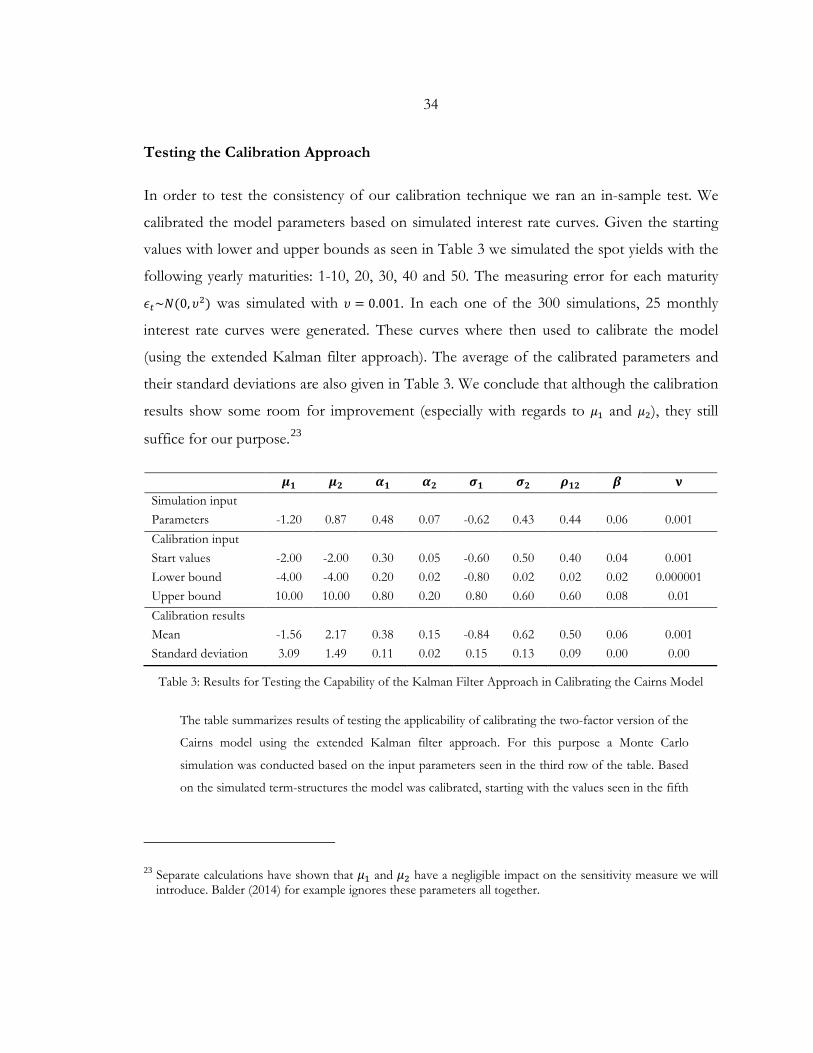
34

Testing the Calibration Approach

In order to test the consistency of our calibration technique we ran an in-sample test. We

calibrated the model parameters based on simulated interest rate curves. Given the starting

values with lower and upper bounds as seen in Table 3 we simulated the spot yields with the

following yearly maturities: 1-10, 20, 30, 40 and 50. The measuring error for each maturity

𝜖𝜖𝑡𝑡~𝑁𝑁(0, 𝜐𝜐2) was simulated with 𝜐𝜐 = 0.001. In each one of the 300 simulations, 25 monthly

interest rate curves were generated. These curves where then used to calibrate the model

(using the extended Kalman filter approach). The average of the calibrated parameters and

their standard deviations are also given in Table 3. We conclude that although the calibration

results show some room for improvement (especially with regards to 𝜇𝜇1 and 𝜇𝜇2), they still

suffice for our purpose.23

𝝁𝝁𝟏𝟏 𝝁𝝁𝟐𝟐 𝜶𝜶𝟏𝟏 𝜶𝜶𝟐𝟐 𝝈𝝈𝟏𝟏 𝝈𝝈𝟐𝟐 𝝆𝝆𝟏𝟏𝟐𝟐 𝜷𝜷 𝛎𝛎 Simulation input Parameters -1.20 0.87 0.48 0.07 -0.62 0.43 0.44 0.06 0.001 Calibration input Start values -2.00 -2.00 0.30 0.05 -0.60 0.50 0.40 0.04 0.001 Lower bound -4.00 -4.00 0.20 0.02 -0.80 0.02 0.02 0.02 0.000001 Upper bound 10.00 10.00 0.80 0.20 0.80 0.60 0.60 0.08 0.01 Calibration results Mean -1.56 2.17 0.38 0.15 -0.84 0.62 0.50 0.06 0.001 Standard deviation 3.09 1.49 0.11 0.02 0.15 0.13 0.09 0.00 0.00

Table 3: Results for Testing the Capability of the Kalman Filter Approach in Calibrating the Cairns Model

The table summarizes results of testing the applicability of calibrating the two-factor version of the

Cairns model using the extended Kalman filter approach. For this purpose a Monte Carlo

simulation was conducted based on the input parameters seen in the third row of the table. Based

on the simulated term-structures the model was calibrated, starting with the values seen in the fifth

23 Separate calculations have shown that 𝜇𝜇1 and 𝜇𝜇2 have a negligible impact on the sensitivity measure we will introduce. Balder (2014) for example ignores these parameters all together.

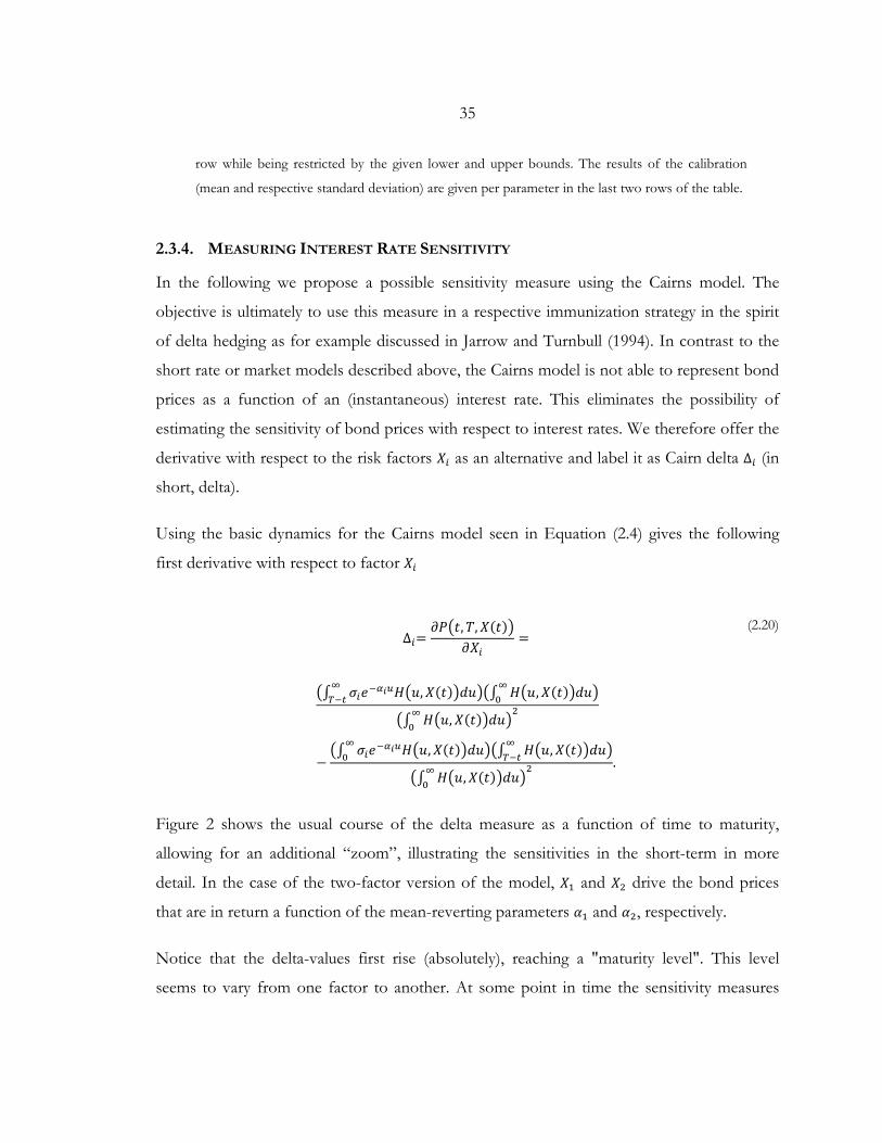
35

row while being restricted by the given lower and upper bounds. The results of the calibration

(mean and respective standard deviation) are given per parameter in the last two rows of the table.

2.3.4. MEASURING INTEREST RATE SENSITIVITY

In the following we propose a possible sensitivity measure using the Cairns model. The

objective is ultimately to use this measure in a respective immunization strategy in the spirit

of delta hedging as for example discussed in Jarrow and Turnbull (1994). In contrast to the

short rate or market models described above, the Cairns model is not able to represent bond

prices as a function of an (instantaneous) interest rate. This eliminates the possibility of

estimating the sensitivity of bond prices with respect to interest rates. We therefore offer the

derivative with respect to the risk factors 𝑋𝑋𝑖𝑖 as an alternative and label it as Cairn delta ∆𝑖𝑖 (in

short, delta).

Using the basic dynamics for the Cairns model seen in Equation (2.4) gives the following

first derivative with respect to factor 𝑋𝑋𝑖𝑖

∆𝑖𝑖=

𝜕𝜕𝑃𝑃�𝑡𝑡,𝑇𝑇,𝑋𝑋(𝑡𝑡)�𝜕𝜕𝑋𝑋𝑖𝑖

=

�∫ 𝜎𝜎𝑖𝑖𝑒𝑒−𝛼𝛼𝑖𝑖𝑢𝑢𝐻𝐻�𝑢𝑢,𝑋𝑋(𝑡𝑡)�𝑑𝑑𝑢𝑢∞𝑇𝑇−𝑡𝑡 ��∫ 𝐻𝐻�𝑢𝑢,𝑋𝑋(𝑡𝑡)�𝑑𝑑𝑢𝑢∞

0 �

�∫ 𝐻𝐻�𝑢𝑢,𝑋𝑋(𝑡𝑡)�𝑑𝑑𝑢𝑢∞0 �

2

−�∫ 𝜎𝜎𝑖𝑖𝑒𝑒−𝛼𝛼𝑖𝑖𝑢𝑢𝐻𝐻�𝑢𝑢,𝑋𝑋(𝑡𝑡)�𝑑𝑑𝑢𝑢∞0 ��∫ 𝐻𝐻�𝑢𝑢,𝑋𝑋(𝑡𝑡)�𝑑𝑑𝑢𝑢∞

𝑇𝑇−𝑡𝑡 �

�∫ 𝐻𝐻�𝑢𝑢,𝑋𝑋(𝑡𝑡)�𝑑𝑑𝑢𝑢∞0 �

2 .

(2.20)

Figure 2 shows the usual course of the delta measure as a function of time to maturity,

allowing for an additional “zoom”, illustrating the sensitivities in the short-term in more

detail. In the case of the two-factor version of the model, 𝑋𝑋1 and 𝑋𝑋2 drive the bond prices

that are in return a function of the mean-reverting parameters 𝛼𝛼1 and 𝛼𝛼2, respectively.

Notice that the delta-values first rise (absolutely), reaching a "maturity level". This level

seems to vary from one factor to another. At some point in time the sensitivity measures

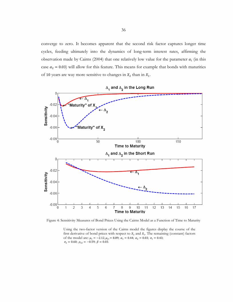
36

converge to zero. It becomes apparent that the second risk factor captures longer time

cycles, feeding ultimately into the dynamics of long-term interest rates, affirming the

observation made by Cairns (2004) that one relatively low value for the parameter 𝛼𝛼𝑖𝑖 (in this

case 𝛼𝛼2 = 0.03) will allow for this feature. This means for example that bonds with maturities

of 10 years are way more sensitive to changes in 𝑋𝑋2 than in 𝑋𝑋1.

Figure 4: Sensitivity Measures of Bond Prices Using the Cairns Model as a Function of Time to Maturity

Using the two-factor version of the Cairns model the figures display the course of the first derivative of bond prices with respect to 𝑋𝑋2 and 𝑋𝑋1. The remaining (constant) factors of the model are: 𝜇𝜇1 = −2.12,𝜇𝜇2, = 8.89; 𝛼𝛼1 = 0.44; 𝛼𝛼2 = 0.03; 𝜎𝜎1 = 0.43; 𝜎𝜎2 = 0.60; 𝜌𝜌12 = −0.59; 𝛽𝛽 = 0.03.

37

2.4. PROCEDURE FOR STRUCTURING AN OPTIMAL SWAP-OVERLAY

In the following we will illustrate how a set of interest rate swaps is defined in order to

immunize a pension-fund-like portfolio, i.e. how to structure a swap overlay that minimizes

the volatility of the “funding-status” (present value of the assets / present value of the

liabilities). We assume that the pension fund is closed, meaning that no additional

contributions are expected, i.e. inflows stem only from held assets.

We start by decomposing the portfolio into its netted cash flows. These cash flow positions

can be seen as a set of zero coupon bonds (ZCB) that need to be hedged individually, e.g. if

we have 50 yearly cash flows we will need 50 hedge instruments to achieve an optimal hedge.

For each ZCB we derive the interest rate sensitivity ∆𝑖𝑖,𝑚𝑚𝑠𝑠 as follows

∆𝑖𝑖,𝑚𝑚𝑠𝑠 = ∆𝑖𝑖,𝑚𝑚 ∙ 𝐶𝐶𝐹𝐹𝑚𝑚, 𝑚𝑚 ∈ [1, … ,𝑀𝑀] (2.21)

whereas 𝑀𝑀 is the time of maturity of the portfolio and 𝐶𝐶𝐹𝐹𝑚𝑚 stands for the netted cash flow at

time period 𝑚𝑚. In our example ∆𝑖𝑖,𝑚𝑚 is calculated using Equation (2.20), where 𝑖𝑖 stands for the

risk factor considered (i.e. either 1 or 2 as we are applying the two-factor version of the

Cairns model). One can of course replace ∆𝑖𝑖,𝑚𝑚𝑠𝑠 through the PV01 measure given in

Equation (2.1).

In line with common practice we aggregate the cash flow sensitivities into buckets, i.e. we

reduce the number of ZCB and thus the number of hedge instruments needed. The

theoretical rationale behind buckets would be that interest rate sensitivities of neighboring

time periods (especially with long-term maturities) exhibit a relatively high correlation, e.g.

yields with time to maturity between 10 and 15 years will be subject to similar dynamics. The

practical rationale would be that liquid interest rate swaps are available for a set of maturities,

predefining the bucket structure.

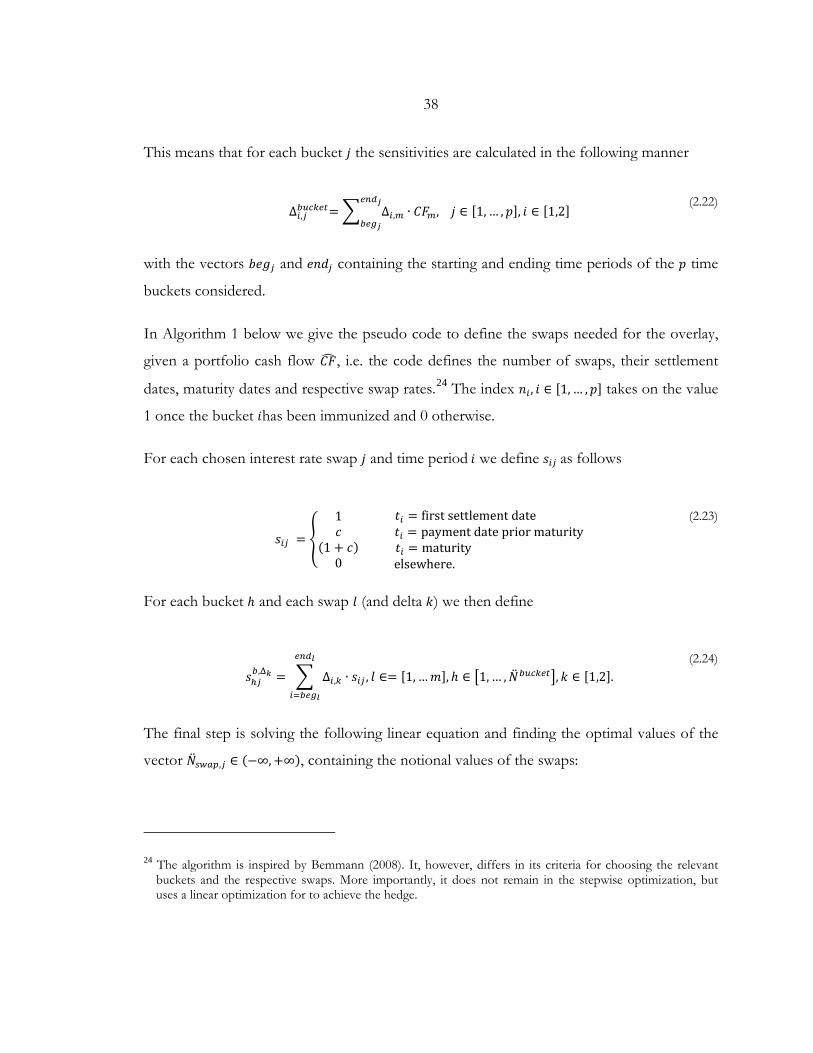
38

This means that for each bucket 𝑗𝑗 the sensitivities are calculated in the following manner

∆𝑖𝑖,𝑖𝑖𝑏𝑏𝑢𝑢𝑏𝑏𝑏𝑏𝑏𝑏𝑡𝑡= � ∆𝑖𝑖,𝑚𝑚

𝑏𝑏𝑛𝑛𝑒𝑒𝑗𝑗

𝑏𝑏𝑏𝑏𝑓𝑓𝑗𝑗∙ 𝐶𝐶𝐹𝐹𝑚𝑚, 𝑗𝑗 ∈ [1, … , 𝑝𝑝], 𝑖𝑖 ∈ [1,2]

(2.22)

with the vectors 𝑏𝑏𝑒𝑒𝑙𝑙𝑖𝑖 and 𝑒𝑒𝑛𝑛𝑑𝑑𝑖𝑖 containing the starting and ending time periods of the 𝑝𝑝 time

buckets considered.

In Algorithm 1 below we give the pseudo code to define the swaps needed for the overlay,

given a portfolio cash flow 𝐶𝐶𝐹𝐹� , i.e. the code defines the number of swaps, their settlement

dates, maturity dates and respective swap rates.24 The index 𝑛𝑛𝑖𝑖 , 𝑖𝑖 ∈ [1, … , 𝑝𝑝] takes on the value

1 once the bucket 𝑖𝑖has been immunized and 0 otherwise.

For each chosen interest rate swap 𝑗𝑗 and time period 𝑖𝑖 we define 𝑠𝑠𝑖𝑖𝑖𝑖 as follows

𝑠𝑠𝑖𝑖𝑖𝑖 = �

1𝑐𝑐

(1 + 𝑐𝑐)0

𝑡𝑡𝑖𝑖 = first settlement date 𝑡𝑡𝑖𝑖 = payment date prior maturity𝑡𝑡𝑖𝑖 = maturity elsewhere.

(2.23)

For each bucket ℎ and each swap 𝑙𝑙 (and delta 𝑘𝑘) we then define

𝑠𝑠ℎ𝑖𝑖𝑏𝑏,Δ𝑘𝑘 = � Δ𝑖𝑖,𝑏𝑏 ∙ 𝑠𝑠𝑖𝑖𝑖𝑖 , 𝑙𝑙 ∈= [1, …𝑚𝑚], ℎ ∈ �1, … , �̈�𝑁𝑏𝑏𝑢𝑢𝑏𝑏𝑏𝑏𝑏𝑏𝑡𝑡�, 𝑘𝑘 ∈ [1,2]

𝑏𝑏𝑛𝑛𝑒𝑒𝑙𝑙

𝑖𝑖=𝑏𝑏𝑏𝑏𝑓𝑓𝑙𝑙

. (2.24)

The final step is solving the following linear equation and finding the optimal values of the

vector �̈�𝑁𝑠𝑠𝑠𝑠𝑠𝑠𝑠𝑠,𝑖𝑖 ∈ (−∞, +∞), containing the notional values of the swaps:

24 The algorithm is inspired by Bemmann (2008). It, however, differs in its criteria for choosing the relevant buckets and the respective swaps. More importantly, it does not remain in the stepwise optimization, but uses a linear optimization for to achieve the hedge.

39

⎝

⎜⎜⎜⎜⎜⎜⎛𝑠𝑠11𝑏𝑏,∆1 𝑠𝑠12

𝑏𝑏,∆1 ⋯ 𝑠𝑠1𝑚𝑚𝑏𝑏,∆1

𝑠𝑠21𝑏𝑏,∆1 𝑠𝑠22

𝑏𝑏,∆1 ⋯ 𝑠𝑠2𝑚𝑚𝑏𝑏,∆1

⋮ ⋮ ⋱ ⋮𝑠𝑠𝑠𝑠1𝑏𝑏,∆1 𝑠𝑠𝑠𝑠2

𝑏𝑏,∆1 ⋯ 𝑠𝑠𝑠𝑠𝑚𝑚𝑏𝑏,∆1

𝑠𝑠11𝑏𝑏,∆2 𝑠𝑠12

𝑏𝑏,∆2 ⋯ 𝑠𝑠1𝑚𝑚𝑏𝑏,∆2

𝑠𝑠21𝑏𝑏,∆2 𝑠𝑠22

𝑏𝑏,∆2 ⋯ 𝑠𝑠2𝑚𝑚𝑏𝑏,∆2

⋮ ⋮ ⋱ ⋮𝑠𝑠𝑠𝑠1𝑏𝑏,∆2 𝑠𝑠𝑠𝑠2

𝑏𝑏,∆2 ⋯ 𝑠𝑠𝑠𝑠𝑚𝑚𝑏𝑏,∆2⎠

⎟⎟⎟⎟⎟⎟⎞

⎝

⎜⎛�̈�𝑁𝑠𝑠𝑠𝑠𝑠𝑠𝑠𝑠,1

�̈�𝑁𝑠𝑠𝑠𝑠𝑠𝑠𝑠𝑠,2⋮

�̈�𝑁𝑠𝑠𝑠𝑠𝑠𝑠𝑠𝑠,𝑚𝑚⎠

⎟⎞

=

⎝

⎜⎜⎜⎜⎜⎛

−∆1,1𝑏𝑏

−∆1,2𝑏𝑏

⋮−∆1,𝑠𝑠

𝑏𝑏

−∆2,1𝑏𝑏

−∆2,2𝑏𝑏

⋮−∆2,𝑠𝑠

𝑏𝑏 ⎠

⎟⎟⎟⎟⎟⎞

. (2.25)

Algorithm 1 : An algorithm for choosing 𝒑𝒑 swaps to net interest rate sensitivity Calculate ∆�𝟏𝟏 and ∆�𝟐𝟐 (e.g. as in Equation (2.20)) for 𝒊𝒊 = 𝟏𝟏 to 𝒑𝒑 do

for 𝒊𝒊 = 𝟏𝟏 to 𝒑𝒑 do if 𝒏𝒏𝒊𝒊 = 𝟎𝟎 then (with 𝒏𝒏𝒊𝒊, 𝒊𝒊 ∈ [𝟏𝟏, … ,𝒑𝒑] taking on the value 1 once bucket 𝒊𝒊 has been netted, 0 otherwise.)

Calculate the delta values for each bucket to be netted

∆�𝟏𝟏(𝒊𝒊) = ∆𝟏𝟏,𝒊𝒊𝒃𝒃𝒃𝒃𝒃𝒃𝒃𝒃𝒃𝒃𝒃𝒃= � ∆𝟏𝟏,𝒎𝒎

𝒑𝒑𝒑𝒑𝒓𝒓𝒃𝒃 ∙ 𝑪𝑪𝑪𝑪𝒎𝒎𝒃𝒃𝒏𝒏𝒆𝒆𝒊𝒊

𝒃𝒃𝒃𝒃𝒃𝒃𝒊𝒊

∆�𝟐𝟐(𝒊𝒊) = ∆𝟐𝟐,𝒊𝒊𝒃𝒃𝒃𝒃𝒃𝒃𝒃𝒃𝒃𝒃𝒃𝒃= � ∆𝟐𝟐,𝒎𝒎

𝒑𝒑𝒑𝒑𝒓𝒓𝒃𝒃 ∙ 𝑪𝑪𝑪𝑪𝒎𝒎𝒃𝒃𝒏𝒏𝒆𝒆𝒊𝒊

𝒃𝒃𝒃𝒃𝒃𝒃𝒊𝒊

end if end for

Calculate ∆𝒎𝒎𝒊𝒊𝒏𝒏𝒋𝒋 = min(∆�𝟏𝟏) and ∆𝒎𝒎𝒎𝒎𝒎𝒎𝒃𝒃 = max(∆�𝟏𝟏)

if ∆𝒎𝒎𝒊𝒊𝒏𝒏𝒋𝒋 < 𝟎𝟎 and ∆𝒎𝒎𝒎𝒎𝒎𝒎

𝒋𝒋 > 𝟎𝟎 then Construct an appropriate forward swap

set settlement date: 𝒃𝒃𝟎𝟎𝒊𝒊 = 𝒃𝒃𝒃𝒃𝒃𝒃𝒋𝒋 set maturity date: 𝒃𝒃𝒏𝒏𝒊𝒊 = 𝒃𝒃𝒃𝒃𝒃𝒃𝒃𝒃

set swap rate: 𝒃𝒃 =𝑷𝑷�𝒃𝒃,𝒃𝒃𝟎𝟎

𝒊𝒊 �−𝑷𝑷(𝒃𝒃,𝒃𝒃𝒏𝒏𝒊𝒊 )

∑ 𝑷𝑷(𝒃𝒃,𝒃𝒃𝒛𝒛)𝒏𝒏𝒛𝒛=𝟏𝟏

else ∆𝒏𝒏𝒃𝒃𝒃𝒃𝒍𝒍 = 𝒎𝒎𝒎𝒎𝒎𝒎��∆𝒎𝒎𝒊𝒊𝒏𝒏𝒊𝒊 �, �∆𝒎𝒎𝒎𝒎𝒎𝒎𝒊𝒊 �� Build an appropriate spot swap

set settlement date: 𝒃𝒃𝟎𝟎𝒊𝒊 = 𝟎𝟎 set maturity date: 𝒃𝒃𝒏𝒏𝒊𝒊 = 𝒃𝒃𝒃𝒃𝒃𝒃𝒍𝒍

set swap rate: 𝒃𝒃 = 𝟏𝟏−𝑷𝑷(𝒃𝒃,𝒃𝒃𝒏𝒏𝒊𝒊 )∑ 𝑷𝑷(𝒃𝒃,𝒃𝒃𝒛𝒛)𝒏𝒏𝒛𝒛=𝟏𝟏

end if end for

40

Given 𝑝𝑝 buckets - each containing one time period - the swap overlay of 𝑝𝑝 swaps would

basically mirror the cash flows of the portfolio, netting the payments and thus hedging all

interest rate risks. Using such an overlay the portfolio would be perfectly "immune" to

interest rate risks.

While in the example given above the procedure is constructed to hedge two sensitivity

parameters, the algorithm can be generalized to hedge 𝑙𝑙 factors. In particular this means that

we can apply the algorithm to (one) PV01 measure in order to define a respective optimal

overlay.

41

2.5. CASE STUDY

2.5.1. REMARKS

In the following we will illustrate the use of the algorithm proposed in the previous

Section 2.4 to structure an interest rate swap overlay for an exemplary (but realistic) pension

fund. The case study will allow the analysis of possible value added offered by using model-

based – instead of duration-based – sensitivities in hedging. Besides examining the hedge

effectiveness of both approaches, our analysis aims on shedding light on further challenges

and advantaged offered by applying the two-factor version of the Cairn model in managing

interest rate risk.

We base our analysis on a realistic pension-fund structure, leaning on the portfolio illustrated

by Bemmann (2008). The pension fund has a typical liability structure that is assumed to be

given (e.g. using the base case scenario of previous actuarial modeling). The pension fund is

assumed to be fixed and observed in the year 2000. While the bulk of the liabilities will

mature in 2010 to 2030 years, a substantial portion of the liabilities exhibits a maturity

between 30 and 50 years. The net present value of liabilities as seen in the year 2000 is

€ 536.50 mm. The portfolio is funded by fixed income securities (bonds) that exhibit a net

present value of € 464.69 mm in year 2000. We assume that the majority of the assets will

mature in the next 10 years, leading to a significant duration gap. We further assume that the

pension fund does not accept any additional contributions, i.e. inflows stem only from held

assets. Finally, we introduce a cash account with € 71.82 mm, initializing the funding status

at 1.

2.5.2. PREPARATIONS – MODEL CALIBRATION

We start by calibrating the parameters of the Cairns model. Again, we acknowledge the need

to calibrate the model to fit market implied information (i.e. under the risk-neutral measure

ℚ), especially when it comes to pricing and hedging. We have, however, deliberately decided

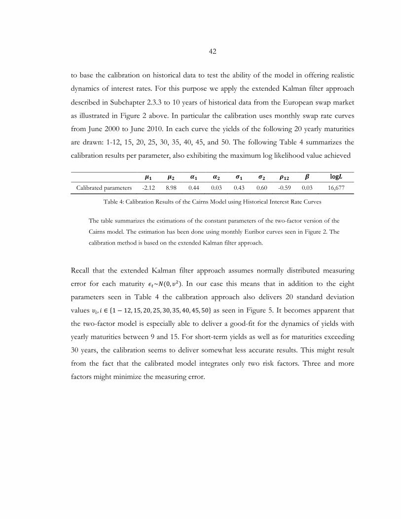
42

to base the calibration on historical data to test the ability of the model in offering realistic

dynamics of interest rates. For this purpose we apply the extended Kalman filter approach

described in Subchapter 2.3.3 to 10 years of historical data from the European swap market

as illustrated in Figure 2 above. In particular the calibration uses monthly swap rate curves

from June 2000 to June 2010. In each curve the yields of the following 20 yearly maturities

are drawn: 1-12, 15, 20, 25, 30, 35, 40, 45, and 50. The following Table 4 summarizes the

calibration results per parameter, also exhibiting the maximum log likelihood value achieved

𝝁𝝁𝟏𝟏 𝝁𝝁𝟐𝟐 𝜶𝜶𝟏𝟏 𝜶𝜶𝟐𝟐 𝝈𝝈𝟏𝟏 𝝈𝝈𝟐𝟐 𝝆𝝆𝟏𝟏𝟐𝟐 𝜷𝜷 log𝑳𝑳

Calibrated parameters -2.12 8.98 0.44 0.03 0.43 0.60 -0.59 0.03 16,677

Table 4: Calibration Results of the Cairns Model using Historical Interest Rate Curves

The table summarizes the estimations of the constant parameters of the two-factor version of the

Cairns model. The estimation has been done using monthly Euribor curves seen in Figure 2. The

calibration method is based on the extended Kalman filter approach.

Recall that the extended Kalman filter approach assumes normally distributed measuring

error for each maturity 𝜖𝜖𝑡𝑡~𝑁𝑁(0, 𝜐𝜐2). In our case this means that in addition to the eight

parameters seen in Table 4 the calibration approach also delivers 20 standard deviation

values 𝜐𝜐𝑖𝑖 , 𝑖𝑖 ∈ {1 − 12, 15, 20, 25, 30, 35, 40, 45, 50} as seen in Figure 5. It becomes apparent that

the two-factor model is especially able to deliver a good-fit for the dynamics of yields with

yearly maturities between 9 and 15. For short-term yields as well as for maturities exceeding

30 years, the calibration seems to deliver somewhat less accurate results. This might result

from the fact that the calibrated model integrates only two risk factors. Three and more

factors might minimize the measuring error.

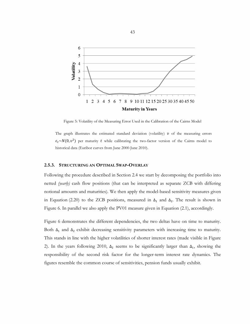
43

Figure 5: Volatility of the Measuring Error Used in the Calibration of the Cairns Model

The graph illustrates the estimated standard deviation (volatility) 𝜐𝜐 of the measuring errors

𝜖𝜖𝑡𝑡~𝑁𝑁(0, 𝜐𝜐2) per maturity 𝑡𝑡 while calibrating the two-factor version of the Cairns model to

historical data (Euribor curves from June 2000-June 2010).

2.5.3. STRUCTURING AN OPTIMAL SWAP-OVERLAY

Following the procedure described in Section 2.4 we start by decomposing the portfolio into

netted (yearly) cash flow positions (that can be interpreted as separate ZCB with differing

notional amounts and maturities). We then apply the model-based sensitivity measures given

in Equation (2.20) to the ZCB positions, measured in ∆1 and ∆2. The result is shown in

Figure 6. In parallel we also apply the PV01 measure given in Equation (2.1), accordingly.

Figure 6 demonstrates the different dependencies, the two deltas have on time to maturity.

Both ∆1 and ∆2 exhibit decreasing sensitivity parameters with increasing time to maturity.

This stands in line with the higher volatilities of shorter interest rates (made visible in Figure

2). In the years following 2010, ∆2 seems to be significantly larger than ∆1, showing the

responsibility of the second risk factor for the longer-term interest rate dynamics. The

figures resemble the common course of sensitivities, pension funds usually exhibit.

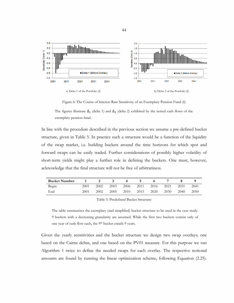
44

a) Delta 1 of the Portfolio (I)

b) Delta 2 of the Portfolio (I)

Figure 6: The Course of Interest Rate Sensitivity of an Exemplary Pension Fund (I)

The figures illustrate ∆1 (delta 1) and ∆2 (delta 2) exhibited by the netted cash flows of the

exemplary pension fund.

In line with the procedure described in the previous section we assume a pre-defined bucket

structure, given in Table 5. In practice such a structure would be a function of the liquidity

of the swap market, i.e. building buckets around the time horizons for which spot and

forward swaps can be easily traded. Further considerations of possibly higher volatility of

short-term yields might play a further role in defining the buckets. One must, however,

acknowledge that the final structure will not be free of arbitrariness.

Bucket Number 1 2 3 4 5 6 7 8 9 Begin 2001 2002 2003 2006 2011 2016 2021 2031 2041 End 2001 2002 2005 2010 2015 2020 2030 2040 2050

Table 5: Predefined Bucket Structure

The table summarizes the exemplary (and simplified) bucket structure to be used in the case study.

9 buckets with a decreasing granularity are assumed. While the first two buckets consist only of

one year of cash flow each, the 9th bucket entails 9 years.

Given the yearly sensitivities and the bucket structure we design two swap overlays; one

based on the Cairns deltas, and one based on the PV01 measure. For this purpose we run

Algorithm 1 twice to define the needed swaps for each overlay. The respective notional

amounts are found by running the linear optimization scheme, following Equation (2.25).

45

Table 6 summarizes the chosen swaps if the model-based deltas are used. As expected the

number of swaps equals the predefined number of buckets. The total notional amount of the

swap overlay is € 440.38 mm. In comparison, using the PV01 measure would deliver a

notional amount of € 419.35 mm. The smaller notional amount is due to the fact that the

PV01-approach hedges only one sensitivity measure (not two risk factors).25

Swap Life time Receiver/Payer Notional (€ mm) Swap Rate Swap I 2003-2021 Receiver 142.24 6.31% Swap II 2006-2031 Receiver 149.20 6.36% Swap III 2021-2041 Receiver 20.99 6.02% Swap IV 2000-2011 Payer 24.67 5.92% Swap V 2000-2031 Payer 42.88 6.12% Swap VI 2000-2041 Receiver 33.62 6.10% Swap VII 2000-2002 Payer 8.52 5.34% Swap VIII 2000-2001 Receiver 0.07 5.04% Swap IX 2000-2016 Receiver 18.20 6.05%

Table 6: Swap Overlay Structure Using the Cairns Model

The table summarizes the swaps chosen to immunize the pension fund against interest rate risks.

Their settlement date, maturity date (life time) and swap rate are defined by Algorithm 1. The

notional amounts are an output of the linear optimization given in Equation (2.25) which also

defines the feature “receiver” or “payer” according to the sign (-/+) of the amount chosen.

The plotted gray bars in the Figure 7(a) and Figure 7(b) show the sensitivities remaining after

the introduction of the overlay. These figures show the extreme sensitivities that are built up

on the level of the payment dates. After all, the algorithm treats sensitivity on bucket level.

25 In order to match the cash flows the portfolio, an overlay of 50 swaps would be needed. Using the algorithm described in the previous chapter such an overlay would have a total notional amount of € 589.67 mm.

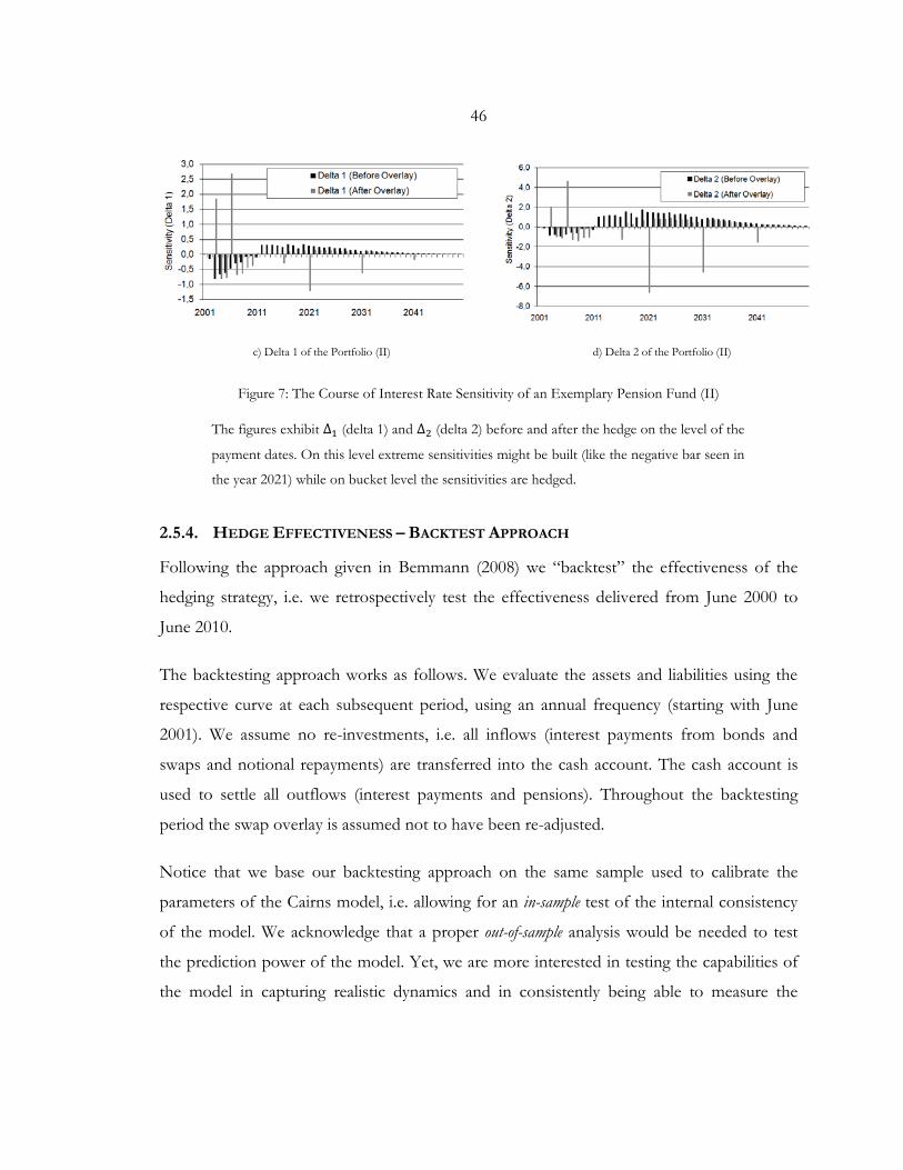
46

c) Delta 1 of the Portfolio (II)

d) Delta 2 of the Portfolio (II)

Figure 7: The Course of Interest Rate Sensitivity of an Exemplary Pension Fund (II)

The figures exhibit ∆1 (delta 1) and ∆2 (delta 2) before and after the hedge on the level of the

payment dates. On this level extreme sensitivities might be built (like the negative bar seen in

the year 2021) while on bucket level the sensitivities are hedged.

2.5.4. HEDGE EFFECTIVENESS – BACKTEST APPROACH

Following the approach given in Bemmann (2008) we “backtest” the effectiveness of the

hedging strategy, i.e. we retrospectively test the effectiveness delivered from June 2000 to

June 2010.

The backtesting approach works as follows. We evaluate the assets and liabilities using the

respective curve at each subsequent period, using an annual frequency (starting with June

2001). We assume no re-investments, i.e. all inflows (interest payments from bonds and

swaps and notional repayments) are transferred into the cash account. The cash account is

used to settle all outflows (interest payments and pensions). Throughout the backtesting

period the swap overlay is assumed not to have been re-adjusted.

Notice that we base our backtesting approach on the same sample used to calibrate the

parameters of the Cairns model, i.e. allowing for an in-sample test of the internal consistency

of the model. We acknowledge that a proper out-of-sample analysis would be needed to test

the prediction power of the model. Yet, we are more interested in testing the capabilities of

the model in capturing realistic dynamics and in consistently being able to measure the

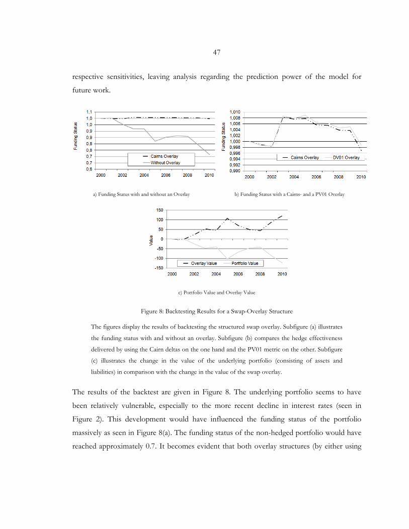
47

respective sensitivities, leaving analysis regarding the prediction power of the model for

future work.

a) Funding Status with and without an Overlay

b) Funding Status with a Cairns- and a PV01 Overlay

c) Portfolio Value and Overlay Value

Figure 8: Backtesting Results for a Swap-Overlay Structure

The figures display the results of backtesting the structured swap overlay. Subfigure (a) illustrates

the funding status with and without an overlay. Subfigure (b) compares the hedge effectiveness

delivered by using the Cairn deltas on the one hand and the PV01 metric on the other. Subfigure

(c) illustrates the change in the value of the underlying portfolio (consisting of assets and

liabilities) in comparison with the change in the value of the swap overlay.

The results of the backtest are given in Figure 8. The underlying portfolio seems to have

been relatively vulnerable, especially to the more recent decline in interest rates (seen in

Figure 2). This development would have influenced the funding status of the portfolio

massively as seen in Figure 8(a). The funding status of the non-hedged portfolio would have

reached approximately 0.7. It becomes evident that both overlay structures (by either using

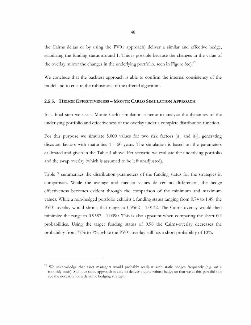
48

the Cairns deltas or by using the PV01 approach) deliver a similar and effective hedge,

stabilizing the funding status around 1. This is possible because the changes in the value of

the overlay mirror the changes in the underlying portfolio, seen in Figure 8(c).26

We conclude that the backtest approach is able to confirm the internal consistency of the

model and to ensure the robustness of the offered algorithm.

2.5.5. HEDGE EFFECTIVENESS – MONTE CARLO SIMULATION APPROACH

In a final step we use a Monte Carlo simulation scheme to analyze the dynamics of the

underlying portfolio and effectiveness of the overlay under a complete distribution function.

For this purpose we simulate 5.000 values for two risk factors (𝑋𝑋1 and 𝑋𝑋2), generating

discount factors with maturities 1 - 50 years. The simulation is based on the parameters

calibrated and given in the Table 4 above. Per scenario we evaluate the underlying portfolio

and the swap overlay (which is assumed to be left unadjusted).

Table 7 summarizes the distribution parameters of the funding status for the strategies in

comparison. While the average and median values deliver no differences, the hedge

effectiveness becomes evident through the comparison of the minimum and maximum

values. While a non-hedged portfolio exhibits a funding status ranging from 0.74 to 1.49, the

PV01-overlay would shrink that range to 0.9562 - 1.0132. The Cairns-overlay would then

minimize the range to 0.9587 - 1.0090. This is also apparent when comparing the short fall

probabilities. Using the target funding status of 0.98 the Cairns-overlay decreases the

probability from 77% to 7%, while the PV01-overlay still has a short probability of 10%.

26 We acknowledge that asset managers would probably readjust such static hedges frequently (e.g. on a monthly basis). Still, our static approach is able to deliver a quite robust hedge so that we at this part did not see the necessity for a dynamic hedging strategy.

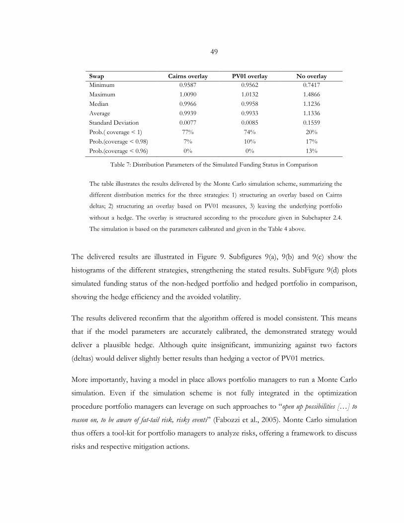
49

Swap Cairns overlay PV01 overlay No overlay Minimum 0.9587 0.9562 0.7417 Maximum 1.0090 1.0132 1.4866 Median 0.9966 0.9958 1.1236 Average 0.9939 0.9933 1.1336 Standard Deviation 0.0077 0.0085 0.1559 Prob.( coverage < 1) 77% 74% 20% Prob.(coverage < 0.98) 7% 10% 17% Prob.(coverage < 0.96) 0% 0% 13%

Table 7: Distribution Parameters of the Simulated Funding Status in Comparison

The table illustrates the results delivered by the Monte Carlo simulation scheme, summarizing the

different distribution metrics for the three strategies: 1) structuring an overlay based on Cairns

deltas; 2) structuring an overlay based on PV01 measures, 3) leaving the underlying portfolio

without a hedge. The overlay is structured according to the procedure given in Subchapter 2.4.

The simulation is based on the parameters calibrated and given in the Table 4 above.

The delivered results are illustrated in Figure 9. Subfigures 9(a), 9(b) and 9(c) show the

histograms of the different strategies, strengthening the stated results. SubFigure 9(d) plots

simulated funding status of the non-hedged portfolio and hedged portfolio in comparison,

showing the hedge efficiency and the avoided volatility.

The results delivered reconfirm that the algorithm offered is model consistent. This means

that if the model parameters are accurately calibrated, the demonstrated strategy would

deliver a plausible hedge. Although quite insignificant, immunizing against two factors

(deltas) would deliver slightly better results than hedging a vector of PV01 metrics.

More importantly, having a model in place allows portfolio managers to run a Monte Carlo

simulation. Even if the simulation scheme is not fully integrated in the optimization

procedure portfolio managers can leverage on such approaches to “open up possibilities […] to

reason on, to be aware of fat-tail risk, risky events” (Fabozzi et al., 2005). Monte Carlo simulation

thus offers a tool-kit for portfolio managers to analyze risks, offering a framework to discuss

risks and respective mitigation actions.

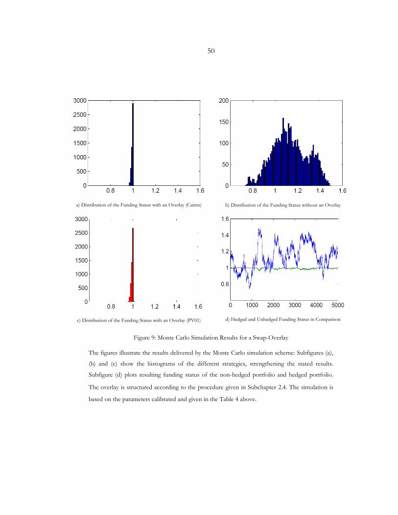
50

a) Distribution of the Funding Status with an Overlay (Cairns)

b) Distribution of the Funding Status without an Overlay

c) Distribution of the Funding Status with an Overlay (PV01)

d) Hedged and Unhedged Funding Status in Comparison

Figure 9: Monte Carlo Simulation Results for a Swap-Overlay

The figures illustrate the results delivered by the Monte Carlo simulation scheme: Subfigures (a),

(b) and (c) show the histograms of the different strategies, strengthening the stated results.

Subfigure (d) plots resulting funding status of the non-hedged portfolio and hedged portfolio.

The overlay is structured according to the procedure given in Subchapter 2.4. The simulation is

based on the parameters calibrated and given in the Table 4 above.

51

2.6. CONCLUDING REMARKS

We have started by going through the spectrum of ALM strategies in general and interest

rate risk management of pension funds in particular, concluding that the practical use of

stochastic models is limited. Static approaches such as the duration-based PV01 measure

seem to be structurally preferred by asset managers despite their theoretical pitfalls. A key

motive behind the limited use of stochastic models is the lack of respective approaches that

combine arbitrage-free valuation with realistic modeling of short- and long-term interest rate

dynamics, a gap Cairns (2004) proclaims to address. We have therefore chosen to apply the

Cairns model to the practical challenge of immunizing a pension fund against interest rate

risk, analyzing its ability in actually closing that gap.

After revisiting the two-factor version of the Cairns model and its main features, we derived

respective sensitivity measures (deltas). We then discussed the use of the extended Kalman

filter approach in calibrating the parameters of the model. By going through these steps we

hoped to shed light on the relevant complexities and implementation challenges.

At the heart of our analysis was the comparison of the hedge effectiveness offered by the

Cairns model with the one given by the popular PV01 metric. For this purpose we

introduced a rule-based and model-independent algorithm that immunizes pension fund-like

portfolios against interest rate risk by structuring an overlay of appropriate swaps. Using a

realistic example of a pension fund we subsequently ran the algorithm twice, structuring two

possible overlays, one using model-based sensitivities (Cairns overlay) and one using the

PV01 measures (PV01 overlay).

First, the hedge effectiveness offered by both overlays was analyzed in a backtesting

environment in which both overlays exhibited similarly satisfying results. Second, a Monte

Carlo simulation was applied. By observing a wider range of respective scenarios the

simulation scheme was able to identify the slight advantage offered by the Cairns model. The

52

use of the model can thus not be motivated by higher hedge effectiveness, especially if we

bear the sophistication of its application in mind (compared with the PV01 approach).

As made apparent by the Monte Carlo simulation using a model-based approach offers

further advantages as summarized in the following statement cited in Fabozzi et al. (2005):

“[I]t allows one to simulate dynamic investment strategies. It gives you the distributions, the

confidence levels.

By reducing uncertainty, modeling allows better decision making. Using powerful modeling

tools, management can analyze scenarios and observe, through computer simulations, the

future consequences of decisions.”

Having that said, the Cairns model offers a possible framework for such analysis, facilitating

discussions around investment and especially because it can combine risk-neutrality with

realistic modeling.

53

PART II:

COUNTERPARTY CREDIT RISK

MANAGEMENT

……………………………………………….

COUNTERPARTY CREDIT RISK MANAGEMENT

……………………………………………….

55

CHAPTER 3:

PRICING AND MANAGING COUNTERPARTY CREDIT RISK IN THEORY

AND PRACTICE

3.1. INTRODUCTION

In the previous chapter we looked into modeling and pricing interest rate derivatives,

implicitly assuming that no further risk factors are material. We have in particular assumed,

either that the counterparties dealing with such OTC derivatives are default-free or that their

default will have no considerable effect on the derivative’s value. Our assumption seems to be

aligned with the prevailing view, at least prior to the financial crisis. This becomes apparent

when looking at prominent textbooks in financial risk modeling and derivatives pricing such

as Hull (2006), Björk (2009), Rebonato (2002) or vastly cited publications such as Miltersen

et al. (1997) or Brace et al. (1997) – just to name a few – in which counterparty credit risk is

either mentioned as by-the-way-issue or is missing completely.

Although from a risk management and a regulatory perspective there seems to have been –

at least to a certain degree – an awareness for the inherent credit risk in OTC derivatives, e.g.

the regulatory framework Basel II required financial institutions to capitalize the default risk

inherent in their OTC portfolios, the incorporation of this element in pricing theory has

been sporadic at best.

It is at the latest since the financial crisis in general and the collapse of Lehman Brothers in

particular that the “default-free scheme” has been finally falsified. It has become clear that

derivative traders – also AAA-rated investment banks – are default-prone and that their

default considerably impacts prices. Major financial institutions claim to have started pricing

56

and managing counterparty credit risk on a systematic basis before the crisis.27 Still, it was

the credit deterioration and the overall spread volatility during the financial crisis that finally

inaugurated counterparty credit risk as a significant risk factor that must be incorporated in

pricing.28 This has been empirically confirmed for example by Arora et al. (2012) and

becomes apparent if we look at the increasing number of publications that are dedicated to

modeling, pricing and managing counterparty credit risk such as Brigo and Pallavicini (2008),

Gregory (2009), Brigo and Capponi (2010) or Lipton and Sepp (2009) and textbooks such

Cesari et al. (2009), Canabarro (2010), Gregory (2012), or Brigo et al. (2013a). This list is non

exhaustive and can be extended if necessary.

The significance of counterparty credit risk has also drawn the attention of the regulators,

standard setters and auditors, who in return further stressed the significance of the subject

matter. Being material, counterparty credit risk has to be incorporated in fair value

measurement, directly affecting profit and loss (P&L) statements and their volatility.

According to the more recent regulatory framework Basel III, financial institutions are

henceforth required to capitalize this additional volatility, significantly increasing the minimal

regulatory capital needed.

The standard method for pricing counterparty credit risk is through a separate so-called

credit valuation adjustment (CVA). CVA can be interpreted as the cost of hedging the

counterparty credit risk of the respective position. This introduces a new derivative

instrument, usually referred to as contingent credit default swap (C-CDS) that, in return to a

premium, insures the (stochastic) exposure at default. The pricing of a C-CDS (i.e. CVA

valuation) usually turns out to be a much more elaborate task than pricing the default-free

derivative itself. After all, CVA depends not only on expected exposure – which is by itself

sufficiently complex – but also on credit risk and the on the interconnection between both.

27 Cesari et al. (2009) who worked for a major European Investment Bank claim for example to have started with a systematic modeling of counterparty credit risk in 2005.

28 See similar arguments for instance in Gregory (2009) or Brigo and Capponi (2010).

57

This means that closed-form solutions for CVA remain an exception. In addition, portfolios

containing different classes of derivatives (e.g. interest rate and equity derivatives) underline

the fact that C-CDS is probably one of the most complicated derivatives to price, especially

if further aspects such as netting and collateral are considered. Bear in mind that derivative

traders are not only interested in valuing CVA, but also in hedging and managing it.

The higher awareness and the regulatory pressure seem to have pushed derivatives traders to

step up the mitigation of counterparty credit risk. Being the most efficient way of reducing

counterparty credit risk, collateral agreements, seem to have become more popular.29

Counterparties are not only entering new collateral agreements, they are also amending

existing ones by reducing thresholds and adjusting the types of eligible collateral. By

amending such agreements the inherent counterparty credit risk – and thus CVA (as well as

further exposure-dependent adjustments) changes, adjusting in return the overall value of

the respective OTC derivatives portfolio.30 This underlines the necessity of models to

compute the effects of such amendments in order to reach mutual agreements and fair

compensations.

The following Chapter 3 intends to give a compact overview in modeling and managing

CVA, always accompanied by a critical analysis of the prevailing discourse. This analysis is

the heart of the chapter, which aims on exploring the challenges around CVA from different

angles rather than offering a comprehensive description of all relevant aspects. For a more

29 See the margin surveys conducted annually by the International Swap and Derivatives Association (ISDA), for example ISDA (2014a), especially pp. 6-7.

30 Notice that further factors, especially funding issues have to be considered as main drivers in such an analysis as well. Due to the fact that uncollateralized exposure has to be funded (e.g. due to the fact that the hedge portfolio, i.e. the duplication strategy of the default-free derivative, is fully collateralized) and the fact that funding costs of financial institutions have significantly increased, there is a similar on-going discussion on incorporating funding effects through a separate metric, funding valuation adjustment (FVA). Due to the complexity of the issue we will continue our analysis by focusing on counterparty credit risk and will touch on FVA only if necessary. For further reading on funding of OTC derivatives and FVA see for example Morini and Prampolini (2011), Hull and White (2012a) or Burgard and Kjaer (2013) as well as Pallavicini et al. (2011).

58

comprehensive description on all aspects around CVA we refer the reader to

Gregory (2012). For a more technical focus on modelling counterparty credit risk we refer

the reader to Cesari et al. (2009) or Brigo et al. (2013a), all of which have inspired the

elaborations and analysis throughout the chapter.

Section 3.2 starts with an overview of key terms and definitions, linking these to relevant

previous research and literature. Section 3.3 then lays the foundations for quantifying CVA,

starting with the general pricing framework in Subchapter 3.3.1, and then moving to a more

practical approach in Subchapter 3.3.2. Subchapter 3.3.3 takes us through a step-by-step

approach to estimate the expected exposure profile, and Subchapter 3.3.4 elaborates on the

techniques of estimating the probabilities of default. Section 3.4 describes and analyzes the

regulatory and accounting requirements behind the CVA discourse, starting with describing

the regulatory landscape in Subchapter 3.4.1. A critical analysis of relevant accounting

standards is then given in Subchapter 3.4.2 whilst Subchapter 3.4.3 focuses on relevant

regulatory requirements. A conclusion of the analysis regarding counterparty credit risk and

CVA regulation is given in Subchapter 3.4.4. Section 3.5 moves to discuss and analyze key

aspects in managing CVA risk. Subchapter 3.5.1 starts with looking into pricing CVA and

analyzes the role and effectiveness of central units that manage CVA, also referred to as

CVA desks. Key aspects around mitigating CVA risk through collateralization and hedging

are discussed critically in Subchapter 3.5.2 and Subchapter 3.5.3, respectively.

Subchapter 3.5.4 gives a concluding statement with regards to managing and mitigating CVA

risk.

59

3.2. PRELIMINARIES, DEFINITIONS AND LITERATURE OVERVIEW

Counterparty Credit Risk

Given two debt securities (bonds) from two issuers that have differing credit quality – and all

other things held equal – it is apparent that an investor will pay less for the bond of the

riskier issuer. This difference is associated with a (higher) risk premium the investor

demands. After all, there is a higher probability that the investor will face (credit) losses.

Consentingly the credit insurance – and thus the hedge strategy – will also be more

expensive. In an analogous manner it is obvious that an investor will pay less (or offer worse

conditions) for a derivative that is traded over the counter (OTC) if the counterparty has a

higher risk of defaulting. Notice that counterparty credit risk refers only to OTC derivatives,

and does not apply to exchange-traded derivatives.

Despite the obvious similarities, counterparty credit risk differs from credit risk mainly in

that the value that can potentially be lost is stochastic due to underlying market risk factors

driving the derivative value, and in it being bilateral. This means that both counterparties are

default prone and that the value of many derivatives (e.g. interest rate swaps) can be either

positive or negative. In the following we will describe the motivation behind it.

We will assume an investor and a counterparty trading an OTC derivative. The following

Table 8 summarizes the effects due to a default of either the investor or the counterparty. A

default of the counterparty will affect the investor only if the net present value (NPV) from

the investor’s perspective is positive. If the NPV from the investor’s perspective is negative

and the counterparty defaults there will be no effect as the former will still be able to meet

the obligations to the latter. Analogously if the investor defaults before the counterparty

while the NPV from the latter’s perspective is positive, the latter will incur a loss. The

bilateral aspect comes into play by interpreting the losses the counterparty incurs as gains of

the investor and vice versa.

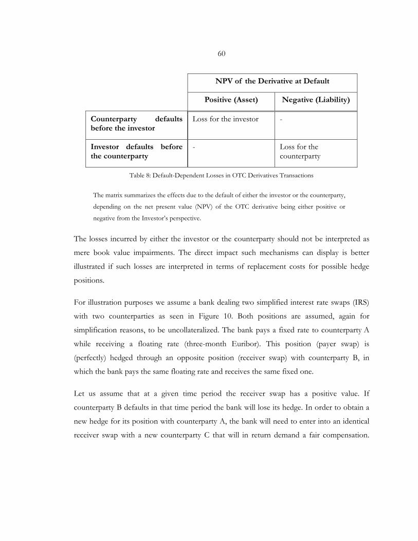
60

NPV of the Derivative at Default

Positive (Asset) Negative (Liability)

Counterparty defaults before the investor

Loss for the investor -

Investor defaults before the counterparty

- Loss for the counterparty

Table 8: Default-Dependent Losses in OTC Derivatives Transactions

The matrix summarizes the effects due to the default of either the investor or the counterparty,

depending on the net present value (NPV) of the OTC derivative being either positive or

negative from the Investor’s perspective.

The losses incurred by either the investor or the counterparty should not be interpreted as

mere book value impairments. The direct impact such mechanisms can display is better

illustrated if such losses are interpreted in terms of replacement costs for possible hedge

positions.

For illustration purposes we assume a bank dealing two simplified interest rate swaps (IRS)

with two counterparties as seen in Figure 10. Both positions are assumed, again for

simplification reasons, to be uncollateralized. The bank pays a fixed rate to counterparty A

while receiving a floating rate (three-month Euribor). This position (payer swap) is

(perfectly) hedged through an opposite position (receiver swap) with counterparty B, in

which the bank pays the same floating rate and receives the same fixed one.

Let us assume that at a given time period the receiver swap has a positive value. If

counterparty B defaults in that time period the bank will lose its hedge. In order to obtain a

new hedge for its position with counterparty A, the bank will need to enter into an identical

receiver swap with a new counterparty C that will in return demand a fair compensation.

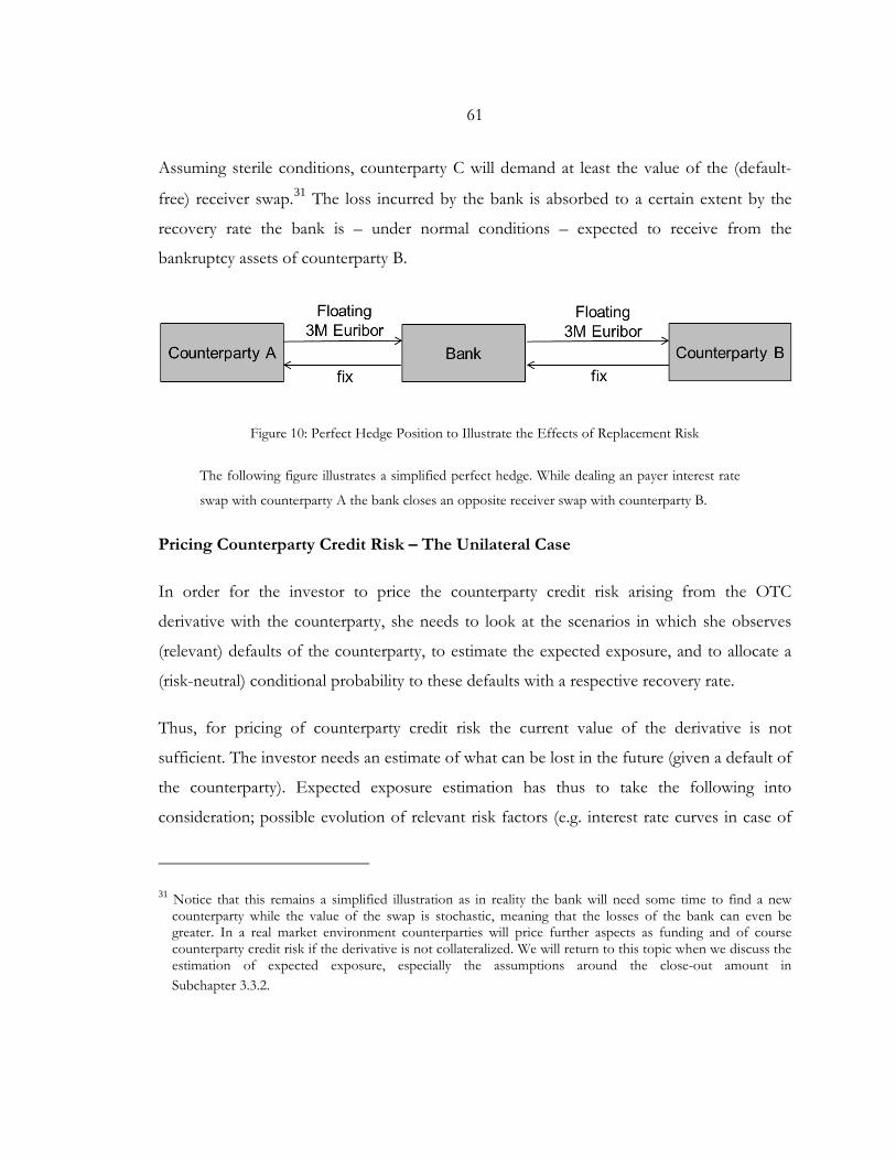
61

Assuming sterile conditions, counterparty C will demand at least the value of the (default-

free) receiver swap.31 The loss incurred by the bank is absorbed to a certain extent by the

recovery rate the bank is – under normal conditions – expected to receive from the

bankruptcy assets of counterparty B.

Figure 10: Perfect Hedge Position to Illustrate the Effects of Replacement Risk

The following figure illustrates a simplified perfect hedge. While dealing an payer interest rate

swap with counterparty A the bank closes an opposite receiver swap with counterparty B.

Pricing Counterparty Credit Risk – The Unilateral Case

In order for the investor to price the counterparty credit risk arising from the OTC

derivative with the counterparty, she needs to look at the scenarios in which she observes

(relevant) defaults of the counterparty, to estimate the expected exposure, and to allocate a

(risk-neutral) conditional probability to these defaults with a respective recovery rate.

Thus, for pricing of counterparty credit risk the current value of the derivative is not

sufficient. The investor needs an estimate of what can be lost in the future (given a default of

the counterparty). Expected exposure estimation has thus to take the following into

consideration; possible evolution of relevant risk factors (e.g. interest rate curves in case of

31 Notice that this remains a simplified illustration as in reality the bank will need some time to find a new counterparty while the value of the swap is stochastic, meaning that the losses of the bank can even be greater. In a real market environment counterparties will price further aspects as funding and of course counterparty credit risk if the derivative is not collateralized. We will return to this topic when we discuss the estimation of expected exposure, especially the assumptions around the close-out amount in Subchapter 3.3.2.

62

IRS), the specific terms of the deal (e.g. amortization structure of the IRS) as well as possible

interconnection between the underlying market risk factors and the probability of the

counterparty defaulting.

CVA is usually referred to as unilateral when the own credit risk is being ignored, i.e. when

the counterparty doing the computation is assumed to be default-free. For the investor to

compute a unilateral CVA (UCVA) means to observe only the scenarios in which the

counterparty might default while the NPV is positive from her perspective.

Sorensen and Bollier (1994) were among the first to explore pricing UCVA as also discussed

by Cherubini (2005), Brigo and Mercurio (2006) as well as Arvanitis and Gregory (2001).

These works focused mainly on counterparty credit risk for one IRS, while netting aspects

were subsequently introduced for example by Brigo and Masetti (2005). The main results

being that the expected exposure can be approximated using swaptions with different

maturities.

Taking possible interdependencies between credit risk and interest rates, Brigo and

Pallavicini (2008) modelled UCVA using Monte Carlo simulation methods. A main product

of this work is the consideration of wrong way risk (WWR), i.e. the possibility to be

negatively affected from counterparty credit risk and market risk simultaneously.

In order to better understand wrong way risk we will assume interest rates (e.g. three-month

Euribor) and credit spreads of the counterparty to be positively correlated. If the investor

has a long interest rates position with the counterparty (e.g. a payer swap), she will be “hit

twice” if credit spreads and exposure rise simultaneously. Put in other words, the risk of the

counterparty defaulting is highest when the investor needs her most. A further example,

commonly used in illustrating wrong way risk is for the investor to buy a put option (over

the counter) on the stock of the counterparty from the counterparty. The positive

interdependence between the put price (i.e. exposure) and the default risk of the

63

counterparty are most evident. Consistently one speaks of right way risk (RWR) if exposure

and credit spreads are conversely interdependent.

Brigo and Bakkar (2009) discussed pricing counterparty credit unilaterally for energy-

commodities. Brigo and Chourdakis (2009) explored pricing it for energy-commodities, and

Brigo et al. (2011b) delivered a framework for equity products.

DVA and Bilateral CVA

As already elaborated in the previous chapter, assuming a counterparty to be default-free – in

our case that being the investor – is definitely nontrivial. In order for the (counterparty

credit-) risk adjusted price to be symmetric, both counterparties have to consider their own

credit risk while computing CVA. Looking at Table 8, we see that if the investor defaults

while owing the counterparty, the former will reap a profit. This might seem counterintuitive

in terms of making a profit through one’s own default. But from a shareholders’ perspective

not having to repay an obligation of one’s own firm (in the course of filed bankruptcy) is

indeed beneficial. Still, it remains in dispute whether an institution should price a profit it will

be making only by defaulting, especially because that implies a gain from possible own-credit

deterioration.

Accounting standard setters seem to advocate the consideration of own credit risk as

required by IFRS 13 in combination with IFRS 9 as well as ASC 820 (previous FAS 157).

From a regulatory (prudent) perspective (under Basel II and Basel III), financial institutions

are however required to neglect own credit risk for regulatory capital computation

purposes.32

The metric for taking one’s own counterparty credit risk is usually referred to as Debt

Valuation Adjustment (DVA). Laterally reverse to UCVA we thus get a unilateral DVA

32 We refer the interest reader to Subchapter 3.4.2 and Subchapter 3.4.3 of this work for more elaborate discussion around DVA and relative accounting and regulatory requirements.

64

(UDVA). A DVA from the investor’s perspective is hence UCVA from the counterparty’s

perspective. For example in their UCVA model (also incorporating wrong way risk and right

way risk) Hull and White (2011) discuss the analogous adaptation for DVA purses.

Adjusting the UCVA by a DVA (both from one counterparty’s perspective) gathers up to a

so-called bilateral CVA (BCVA), defined as follows33

BCVA = UCVA – UDVA. (3.1)

Notice that BCVA can display either a positive or a negative adjustment, depending on

exposure expectations and on whose credit riskiness is higher, the investor or the

counterparty.

First-to-Default CVA

The main fallback of the bilateral CVA is that possible interdependencies between the credit

risk of the investor and the counterparty is not accounted for. Already implicitly explored by

Duffie and Huang (1996) an explicit modeling of what we will refer to as first-to-default CVA

was introduced by Brigo and Capponi (2010).34 Pricing CVA for credit default swaps (CDS),

Brigo and Capponi (2010) took possible correlations between the credit risk of the involved

counterparties into consideration. This approach has subsequently been extended to

consider netting and collateral by Brigo et al. (2013b).35 First-to-default CVA has also been

underlined by Gregory (2009) or Brigo and Morini (2011).36

33 See for instance Gregory (2009) or Albanese et al. (2013). 34 In his PhD thesis Capponi (2009) elaborates on some of the main results that were later published in Brigo

and Capponi (2010). 35 Chapter 4 of this thesis is dedicated to modeling the framework of Brigo and Capponi (2010), offering a

step-by-step modeling approach and a computational tune-up. 36 What we refer to as first-to-default CVA is referred to Brigo and Capponi (2010) or Gregory (2009) as

bilateral CVA. The term first-to-default CVA stems from Albanese et al. (2013).

65

Analogously to BCVA the first-to-default CVA – also abbreviated as FTDCVA – can either

be positive or negative. Besides exposure expectations and the credit riskiness the latter

depends on the interdependence (i.e. correlation or contingency) between the probabilities

of default of both counterparties.

As mentioned by Albanese et al. (2013) first-to-default CVA has some theoretical pitfalls.

The metric decreases if the credit of the computing counterparty deteriorates, almost

vanishing at default. Compared to unilateral CVA a more significant shortcoming of the

first-to-default CVA is its unhedgebility. After all, hedging a first-to-default CVA involves

hedging DVA, an almost impossible task, dependent on selling one’s own credit risk.37

The main fallback is however a practical one. Modeling a unilateral CVA is by itself a

sophisticated task. Adding possible interdependencies between the credit risks of both

counterparties that have to be modelled (and calibrated) will make things even more

complicated (if not unfeasible).

As mentioned, from a regulatory perspective financial institutions are required to base their

equity computations on a UCVA while accounting standards specifically require the

consideration of DVA. The bilateral CVA framework seems in this respect to offer a

practical compromise in which DVA can be “switched off and on”, depending on the

respective computation purpose.

37 For a more elaborate discussion around pricing DVA see Subchapter 3.4.2.

66

3.3. COMPUTING CREDIT VALUATION ADJUSTMENT

3.3.1. GENERAL PRICING FRAMEWORK FOR CVA

Before moving to the more practical (unilateral) CVA and DVA we will in the following start

with the more general pricing framework based on the so-called first-to-default CVA as for

example introduced in Brigo and Capponi (2010).38

For this purpose we will return to the two defined parties, dealing an OTC derivative; the

investor (name “0”), and a counterparty (name “2”).39 The computations are always done

from the investor’s perspective. We define 𝔼𝔼𝑡𝑡ℚ{𝜋𝜋(𝑡𝑡,𝑇𝑇)} as the counterparty credit risk-free

value at time 𝑡𝑡 of an OTC derivative maturing at time 𝑇𝑇 (under the risk-neutral measure ℚ).

The aim is to define a separate metric that adjusts this term for (bilateral) counterparty credit

risk.

We are interested in observing the scenarios in which the default of the counterparty implies

a loss to the investor and vice versa. Each party will bear a loss due to the default of the

other side only if the value of the derivative is positive from its perspective, i.e. if the

derivative is in the money (ITM). Put in other words, the default of a counterparty is relevant

if the derivative is a liability held by the counterparty.

Let 𝜏𝜏0 and 𝜏𝜏2 stand for the default time periods of the investor and the counterparty,

respectively. For the sake of academic completeness we will define the probability space and

the different relevant variables as used by Brigo and Capponi (2009). The computations are

assumed to be conducted in the probability space (Ω,𝒢𝒢,𝒢𝒢𝑡𝑡 ,ℚ). Again, ℚ is the risk-neutral

measure, and 𝒢𝒢𝑡𝑡 is a filtration driving the whole market. ℱ𝑡𝑡 is a further subfilteration

38 As mentioned, Grominski et al. (2012) have already published main results presented in this thesis. 39 Notice that name 1 is reserved for a possible reference entity, e.g. relevant in a credit default swap (CDS).

67

standing for all observable market quantities exept for default events, hence ℱ𝑡𝑡 ⊆ 𝒢𝒢𝑡𝑡 ≔

ℱ𝑡𝑡 ∨ℋ𝑡𝑡 .40 ℋ𝑡𝑡 stands for the subfilteration standing only for all default events. The stopping

time is defined by the time period of the first default, i.e.

𝜏𝜏 = {𝜏𝜏0, 𝜏𝜏2}. (3.2)

Given a default event, i.e. 𝜏𝜏 is a stopping time of ℱ𝑡𝑡, then the stopped filtration is given by

ℱ𝜏𝜏 = 𝜎𝜎(ℱ𝑡𝑡 ∪ {𝑡𝑡 < 𝜏𝜏}, 𝑡𝑡 ≥ 0). (3.3)

If 𝜏𝜏 is a stopping time of 𝒢𝒢𝑡𝑡 , then the stopped filteration is given by

𝒢𝒢𝜏𝜏 = 𝜎𝜎(𝒢𝒢𝑡𝑡 ∪ {𝑡𝑡 < 𝜏𝜏}, 𝑡𝑡 ≥ 0). (3.4)

Following Brigo and Capponi (2009) we define the following mutually exclusive and

collectively exhaustive scenarios

A = {𝜏𝜏0 ≤ 𝜏𝜏2 ≤ T} B = {𝜏𝜏0 ≤ T ≤ 𝜏𝜏2}

C = {𝜏𝜏2 ≤ 𝜏𝜏0 ≤ T} D = {𝜏𝜏2 ≤ 𝑇𝑇 ≤ 𝜏𝜏0}

E = {T ≤ 𝜏𝜏0 ≤ 𝜏𝜏2} F = {T ≤ 𝜏𝜏2 ≤ 𝜏𝜏0}.

(3.5)

𝐴𝐴 stands for the scenarios in which the investor defaults before the counterparty which

defaults before the maturity of the derivative. 𝐶𝐶 stands for similar scenarios in which the

counterparty defaults first. 𝐷𝐷 (𝐵𝐵) stands for the scenarios in which the counterparty

(investor) defaults before maturity, while the investor (counterparty) outlives the derivative.

In 𝐸𝐸 and 𝐹𝐹 both counterparties outlive the derivative. Notice that a simultaneous default is

excluded, i.e. it is assumed that the investor and the counterparty will not default at the same

time, technically formulated as

40 Brigo and Capponi (2009) define ℋ𝑡𝑡 = 𝜎𝜎({𝜏𝜏0 ≤ 𝑢𝑢} ∨ {𝜏𝜏1 ≤ 𝑢𝑢} ∨ {𝜏𝜏2 ≤ 𝑢𝑢}: 𝑢𝑢 ≤ 𝑡𝑡), thus capturing the default events of the counterparties and the reference portfolio. For further elaboration on their specific models see also Chapter 4 of this thesis.

68

ℚ(𝜏𝜏0 = 𝜏𝜏2) = 0. (3.6)

Brigo et al. (2013a, p. 281) argue that this assumption is verified by most models, referring

the reader to one prominent exception, the multivariate exponential distribution used by

Marshall and Olkin (1967). For the introduction of simultaneous defaults in CVA pricing see

also Gregory (2009).

We define 𝐿𝐿𝐺𝐺𝐷𝐷0 and 𝐿𝐿𝐺𝐺𝐷𝐷2 as the loss given default ratios for the investor and the

counterparty, respectively. Notice that 𝐿𝐿𝐺𝐺𝐷𝐷 = 1 − 𝑅𝑅𝑅𝑅 where 𝑅𝑅𝑅𝑅 stands for the recovery rate.

Let 𝑁𝑁𝑃𝑃𝑃𝑃(𝑡𝑡) be the net present value (NPV) of the derivative at time period 𝑡𝑡 and 𝐶𝐶(𝑡𝑡) the

respective collateral amount received, we define the net exposure 𝐸𝐸 at time 𝑡𝑡 as follows

𝐸𝐸(𝑡𝑡) = 𝑚𝑚𝑎𝑎𝑥𝑥{𝑁𝑁𝑃𝑃𝑃𝑃(𝑡𝑡) − 𝐶𝐶(𝑡𝑡),0}. (3.7)

Analogously we define negative exposure 𝑁𝑁𝐸𝐸 as follows

𝑁𝑁𝐸𝐸(𝑡𝑡) = 𝑚𝑚𝑖𝑖𝑛𝑛{𝑁𝑁𝑃𝑃𝑃𝑃(𝑡𝑡) − 𝐶𝐶(𝑡𝑡), 0}. (3.8)

Let 𝑃𝑃(𝑡𝑡,𝑇𝑇) stand for the discounting factor for time period 𝑇𝑇 at time 𝑡𝑡. Brigo and

Capponi (2009) deliver a proof that the counterparty credit risk-adjusted value of the

derivative can be defined as follows

𝔼𝔼𝑡𝑡ℚ{𝜋𝜋�(𝑡𝑡,𝑇𝑇)} = 𝔼𝔼𝑡𝑡

ℚ{𝜋𝜋(𝑡𝑡,𝑇𝑇)}

− 𝔼𝔼𝑡𝑡ℚ{𝐿𝐿𝐺𝐺𝐷𝐷21𝐶𝐶∪𝐷𝐷𝑃𝑃(𝑡𝑡, 𝜏𝜏2)𝐸𝐸(𝜏𝜏2)}

+ 𝔼𝔼𝑡𝑡ℚ{𝐿𝐿𝐺𝐺𝐷𝐷01𝐴𝐴∪𝐵𝐵𝑃𝑃(𝑡𝑡, 𝜏𝜏0)𝑁𝑁𝐸𝐸(𝜏𝜏0)}.

(S.1)

(S.2)

(S.3)

(3.9)

Bearing in mind that all quantities are given from the investor’s perspective Equation (3.9)

clarifies that the counterparty credit risk-adjusted derivative value is a function of three

complementing terms.

69

As mentioned above (S.1) stands for the risk-neutral contract value when no

relevant defaults occur. In that case the risk-neutral value is driven by the discounted

contractual cash flows.

(S.2) stands for the correction term, taking relevant defaults of the counterparty into

consideration, i.e. standing for the CVA term. The term can also be explained as the

risk-neutral expectation for losses, put in terms of discounted and LGD-adjusted

positive exposure if the counterparty defaults.

Analogously (S.3) stands for the correction term, taking relevant defaults of the

investor into consideration, i.e. standing for the DVA term. Notice that while S.2

incorporates scenarios in which the exposure is positive from the investor’s

perspective, S.3 takes only scenarios into consideration in which the exposure is

positive from the counterparty’s perspective.

The first-to-default CVA can be written as follows41

𝐹𝐹𝑇𝑇𝐷𝐷𝐶𝐶𝑃𝑃𝐴𝐴 = 𝔼𝔼𝑡𝑡ℚ{𝐿𝐿𝐺𝐺𝐷𝐷21𝐶𝐶∪𝐷𝐷𝑃𝑃(𝑡𝑡, 𝜏𝜏2)𝐸𝐸(𝜏𝜏2)}

−𝔼𝔼𝑡𝑡ℚ{𝐿𝐿𝐺𝐺𝐷𝐷01𝐴𝐴∪𝐵𝐵𝑃𝑃(𝑡𝑡, 𝜏𝜏0)𝑁𝑁𝐸𝐸(𝜏𝜏0)}.

(3.10)

As stated by Brigo and Capponi (2010) it becomes apparent that the valuation of CVA

involves the valuation of a short position in a call option (the DVA term) and of a long

position in a put option (the CVA term). Both options refer to the remaining exposure and

have a strike of zero.

Equation (3.10) is the value of a hedge portfolio, offering a perfect protection against

counterparty credit risk arising from both the counterparty and the investor. Notice that for

the investor such a strategy would imply not only buying a protection on the exposure but

41 Notice that Brigo and Capponi (2009) refer to the term as the general bilateral credit valuation adjustment. We on the other hand stay with the term first-to-default CVA, standing in line the elaborations given in Subchapter 3.2.

70

also selling protection on her own credit risk, quite a complicated task if not an impossible

one. We will analyze the implication of DVA in general and its hedging in particular in

Subchapter 3.4.2.

Using the same notation for FTDCVA we will in the following define the unilateral CVA.

For this purpose we assume the investor to be credit risk free. We are thus only interested in

the scenarios in which 𝜏𝜏2 ≤ 𝑇𝑇. The unilateral CVA can thus be written as follows:

𝑈𝑈𝐶𝐶𝑃𝑃𝐴𝐴 = 𝔼𝔼𝑡𝑡ℚ�𝐿𝐿𝐺𝐺𝐷𝐷21𝜏𝜏2≤𝑇𝑇𝑃𝑃(𝑡𝑡, 𝜏𝜏2)𝐸𝐸(𝜏𝜏2)�. (3.11)

The price process of UCVA can also be given through the following risk the risk-neutral

expectation of the credit losses given in Equation (3.11).42

𝑈𝑈𝐶𝐶𝑃𝑃𝐴𝐴(𝑡𝑡) = LGD2 �𝔼𝔼𝑢𝑢

ℚ{𝑃𝑃(𝑡𝑡,𝑢𝑢))𝐸𝐸(𝑢𝑢)|𝜏𝜏2 = 𝑢𝑢 }𝑑𝑑ℚ(𝜏𝜏2 ≤ 𝑢𝑢).𝑇𝑇

𝑡𝑡

(3.12)

where ℚ(𝜏𝜏2 ≤ 𝑡𝑡) stands for the risk-neutral default probability of the counterparty. As for

instance noted by Cesari et al. (2009, p. 217) Equation (3.12) represents the price process of

a C-CDS.43 The value of such a C-CDS is the function of the risk-neutral probability of

default and the respective recovery as well as the exposure.

3.3.2. PRACTICAL PRICING FRAMEWORK FOR CVA

Looking at Equation (3.12) it becomes apparent that the exposure is conditional on the

default event and the survival of the counterparty, i.e. exposure and credit risk are

interdependent. As stated above interdependence between exposure and credit risk is

42 Pykhtin and Zhu (2007) were among the first to use similar notation (in their case of unilateral CVA). 43 They note that the value of the C-CDS at time 𝜏𝜏2 equals the exposure 𝐸𝐸(𝜏𝜏2). One could however argue that

the value has to take the recovery into consideration, i.e. equaling LGD2𝐸𝐸(𝜏𝜏2).

71

relevant, because of possible right-way/wrong-way risk. Modeling interdependence between

credit and exposure as well as between the credit risks of the counterparties involves

however elaborate Monte Carlo simulation schemes.44 It also presumes the possibility to

estimate the (risk-neutral) parameters of such interdependency using market information. It

is worth stating that assuming no right-way/wrong-way risk at least for interest rates and

foreign exchange derivatives seems to be an acceptable assumption as noted for example by

Pykhtin and Zhu (2007).45 One can of course think of a variety of examples where right-

way/wrong-way risk would play a significant role also for interest rate and foreign exchange

derivatives, especially ones referring to exotic currencies.46 Still, the majority of derivatives

traders today either lack the capabilities to do so or they find the implied complexity to be

unjustified. The financial institutions that do model right-way/wrong-way risk seem to be

doing it in form of an additional analysis at best.47

In order to examine the widespread methodology for pricing CVA we will therefore

introduce the assumption of no right-way/wrong-way risk as for instance done by Pykhtin

and Zhu (2007) or Gregory (2012). Doing so allows us to define UCVA as follows:

𝑈𝑈𝐶𝐶𝑃𝑃𝐴𝐴(𝑡𝑡) = LGD2 �𝔼𝔼𝑢𝑢

ℚ{𝑃𝑃(𝑡𝑡,𝑢𝑢)𝐸𝐸(𝑢𝑢)}𝑑𝑑ℚ(𝜏𝜏2 ≤ 𝑢𝑢)𝑇𝑇

𝑡𝑡

. (3.13)

Still, solving Equation (3.13) analytically is limited to a rather small number of simple

examples such as stand-alone European options. Computing exposure on the counterparty

44 See the example given in Chapter 4. See also Cesari et al. (2009), p. 224. 45 See also Gregory (2012), pp. 242-263. 46 Assume for example an American bank dealing a cross currency swap with the German state agency

(Finanzagentur) in which the former borrows an amount in USD in exchange for an amount in EUR. The bank will then pay 3M Libor and receive three-month Euribor. At maturity the counterparties will exchange the borrowed notionals. The bank might assume that deterioration of Germany’s credit quality will go along with a depreciation of the Euro. In our example this would mean that the riskier Germany is, the less it will have to pay, i.e. the exposure exhibits a right way risk as it decreases with increasing credit risk.

47 See for example the survey done by Deloitte and Solum (2013).

72

level, taking netting and collateral into consideration, will always require simulation

approaches. Assuming the simulation is done in the time steps {𝑡𝑡𝑏𝑏}𝑏𝑏=1𝑁𝑁 UCVA can be

defined using the following time-descrete manner

𝑈𝑈𝐶𝐶𝑃𝑃𝐴𝐴(𝑡𝑡) = LGD2�𝔼𝔼𝑢𝑢

ℚ{𝑃𝑃(𝑡𝑡, 𝑡𝑡𝑏𝑏)𝐸𝐸(𝑡𝑡𝑏𝑏)}𝑁𝑁

𝑖𝑖=1

ℚ(𝑡𝑡𝑏𝑏−1 < 𝜏𝜏2 ≤ 𝑡𝑡𝑏𝑏). (3.14)

Analogously DVA could be computed in the following manner

𝐷𝐷𝑃𝑃𝐴𝐴(𝑡𝑡) = LGD0�𝔼𝔼𝑡𝑡

ℚ{𝑃𝑃(𝑡𝑡, 𝑡𝑡𝑏𝑏)𝑁𝑁𝐸𝐸(𝑡𝑡𝑏𝑏)}𝑁𝑁

𝑖𝑖=1

ℚ(𝑡𝑡𝑏𝑏−1 < 𝜏𝜏0 ≤ 𝑡𝑡𝑏𝑏). (3.15)

In the same manner we are also able to define the (contingent) bilateral CVA, i.e.

𝐵𝐵𝐶𝐶𝑃𝑃𝐴𝐴(𝑡𝑡) = LGD2�𝔼𝔼𝑢𝑢

ℚ{𝑃𝑃(𝑡𝑡, 𝑡𝑡𝑏𝑏)𝐸𝐸(𝑡𝑡𝑏𝑏)}𝑁𝑁

𝑖𝑖=1

ℚ(𝑡𝑡𝑏𝑏−1 < 𝜏𝜏0, 𝑡𝑡𝑏𝑏−1 < 𝜏𝜏2 ≤ 𝑡𝑡𝑏𝑏)

− LGD0�𝔼𝔼𝑡𝑡ℚ{𝑃𝑃(𝑡𝑡, 𝑡𝑡𝑏𝑏)𝑁𝑁𝐸𝐸(𝑡𝑡𝑏𝑏)}

𝑁𝑁

𝑖𝑖=1

ℚ(𝑡𝑡𝑏𝑏−1 < 𝜏𝜏2, 𝑡𝑡𝑏𝑏−1 < 𝜏𝜏0 ≤ 𝑡𝑡𝑏𝑏).

(3.16)

Notice that the CVA term of Equation (3.16) takes the survival probability of the investor

into consideration while the DVA term depends on the survival probability of the

counterparty. After all, the investor will suffer a loss from the default of the counterparty if

she will not default until then, and vice versa.

The discrete manner of computing CVA with no right-way/wrong-way risk as given in

Equation (3.14) offers a variety of very convenient aspects, especially the ability of modeling

the necessary factors, i.e. expected exposure and credit, in two separate blocks. In the

following we will elaborate on the steps needed to model the expected exposure

(Subchapter 3.3.3) and estimating the credit risk (Subchapter 3.3.4), i.e. the probability of

default and the respective recovery.

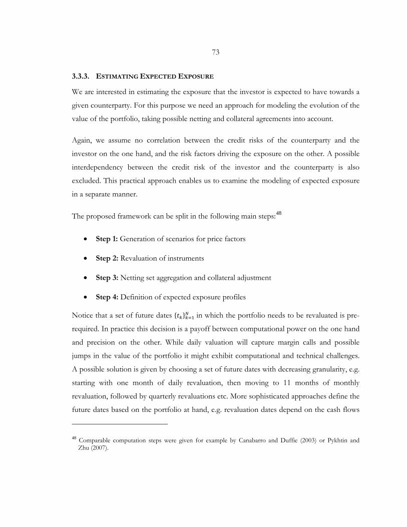
73

3.3.3. ESTIMATING EXPECTED EXPOSURE

We are interested in estimating the exposure that the investor is expected to have towards a

given counterparty. For this purpose we need an approach for modeling the evolution of the

value of the portfolio, taking possible netting and collateral agreements into account.

Again, we assume no correlation between the credit risks of the counterparty and the

investor on the one hand, and the risk factors driving the exposure on the other. A possible

interdependency between the credit risk of the investor and the counterparty is also

excluded. This practical approach enables us to examine the modeling of expected exposure

in a separate manner.

The proposed framework can be split in the following main steps:48

• Step 1: Generation of scenarios for price factors

• Step 2: Revaluation of instruments

• Step 3: Netting set aggregation and collateral adjustment

• Step 4: Definition of expected exposure profiles

Notice that a set of future dates {𝑡𝑡𝑏𝑏}𝑏𝑏=1𝑁𝑁 in which the portfolio needs to be revaluated is pre-

required. In practice this decision is a payoff between computational power on the one hand

and precision on the other. While daily valuation will capture margin calls and possible

jumps in the value of the portfolio it might exhibit computational and technical challenges.

A possible solution is given by choosing a set of future dates with decreasing granularity, e.g.

starting with one month of daily revaluation, then moving to 11 months of monthly

revaluation, followed by quarterly revaluations etc. More sophisticated approaches define the

future dates based on the portfolio at hand, e.g. revaluation dates depend on the cash flows

48 Comparable computation steps were given for example by Canabarro and Duffie (2003) or Pykhtin and Zhu (2007).

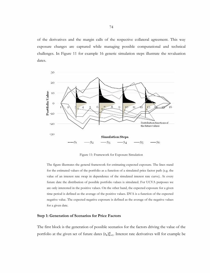
74

of the derivatives and the margin calls of the respective collateral agreement. This way

exposure changes are captured while managing possible computational and technical

challenges. In Figure 11 for example 16 generic simulation steps illustrate the revaluation

dates.

Figure 11: Framework for Exposure Simulation

The figure illustrates the general framework for estimating expected exposure. The lines stand

for the estimated values of the portfolio as a function of a simulated price factor path (e.g. the

value of an interest rate swap in dependence of the simulated interest rate curve). At every

future date the distribution of possible portfolio values is simulated. For UCVA purposes we

are only interested in the positive values. On the other hand, the expected exposure for a given

time period is defined as the average of the positive values. DVA is a function of the expected

negative value. The expected negative exposure is defined as the average of the negative values

for a given date.

Step 1: Generation of Scenarios for Price Factors

The first block is the generation of possible scenarios for the factors driving the value of the

portfolio at the given set of future dates {𝑡𝑡𝑏𝑏}𝑏𝑏=1𝑁𝑁 . Interest rate derivatives will for example be

75

driven by reference rates such as Eonia, three-month Euribor or 12-month Libor. Other

examples of price factors are foreign exchange rates, stock prices, commodity prices or

inflation indexes.

Pykhtin and Zhu (2007) distinguish between two general methods for generating price factor

scenarios. They refer to the first method as Price-Dependent Simulation (PDS) and to the

second as Direct Jump to Simulation Date (DJS). Within the PDS method the price factors

simulated for a future date 𝑡𝑡𝑖𝑖 would depend on the simulated results in the previous future

date 𝑡𝑡𝑖𝑖−1. In the DJS method they are only dependent on the results given for the simulation

date, i.e. 𝑡𝑡0. Although both methods should bring identical price factor distributions for a

given future date the valuation of path-dependent products such as American or Bermudian

options might however imply path-dependent simulation of price factors, implying that for

CVA purposes PDS approaches are more adequate.

In line with derivative pricing CVA computation is based on risk-neutral valuation. This

means for example that for the generation of exposure of interest rate derivatives (e.g.

interest rate swap) arbitrage-free interest rate models are needed.49 A prominent example

used for this purposes is the Hull White interest rate model. We will apply the one factor

version of this model in an example below. This model describes the dynamics of the short

term interest rate using the following stochastic differential equation (SDE):

𝑑𝑑𝑟𝑟𝑡𝑡 = (𝜃𝜃(𝑡𝑡) − 𝑎𝑎𝑟𝑟𝑡𝑡)𝑑𝑑𝑡𝑡 + 𝜎𝜎𝑑𝑑𝑊𝑊𝑡𝑡 (3.17)

where 𝑟𝑟𝑡𝑡 stands for the short rate at time period t. 𝜅𝜅, 𝜃𝜃, 𝑎𝑎, 𝜎𝜎,𝑢𝑢 are the model parameters, 𝑊𝑊𝑡𝑡 is

a standard Brownian motion. This means that for each future date a set of short-term

interest rates (e.g. 10.000) needs to be simulated in order to generate the same number of

49 For an overview on risk-neutral models for interest rate risk see Subchapter 2.3.1.

76

respective interest rate curves. In Figure 11 for example six different sets of path-dependent

risk factors are given at each future date.

A further complication is the simulation of correlated market risk factors, e.g. generation of

interdependent interest rates and foreign exchange rates. While interdependency can be

modelled through simplified approaches, the market lacks sufficient instruments to allow for

its risk-neutral calibration. Interdependence can for example be modelled through

introducing respective correlation coefficients driving the diffusion process. Due to the lack

of instruments to calibrate the needed correlation matrix some practitioners refer to

historical values for approximations.50

Step 2: Revaluation of Instruments

Given the sets of generated risk factors for each future date the instruments are subsequently

revaluated, producing respective distribution of derivative values. For interest rate swaps for

example a pricing model is needed that re-estimates the remaining cash flows and the

respective value of the instrument at each time step and scenario. In the example illustrated

in Figure 11 the instrument needs to be revaluated in each one of the 16 time steps and for

each one of the 6 scenarios, i.e. 6 × 16 = 96. In a more realistic example of a portfolio

consisting of 50 positions then need to be revaluated 50 times, given 10.000 scenarios it

would imply 25.000.000 revaluations. This makes it clear that in large portfolios of financial

institutions with numerous counterparties and instruments this number can easily explode,

and needs to be managed carefully.

Having adequate pricing models for each instrument in the portfolio can be a very

challenging task, especially if the portfolio contains exotic derivatives that require Monte

Carlo pricing techniques (e.g. Bermudian swaptions etc.). After all, this requires a draw of

realizations for the relevant risk factors (outer step) and further (inner steps) to re-valuate the

50 See for example the survey on counterparty credit risk conducted by Deloitte & Solum (2013), esp. p. 25.

77

instrument, conditional on the drawn risk factor distribution. Gordy and Juneja (2008) or

more recent work of Broadie et al. (2011) demonstrate possible solutions for nested Monte

Carlo simulations. American Monte Carlo methods as described in Longstaff and

Schwartz (2001) or Glasserman and Yu (2002) provide a further possible solution if closed-

form pricing solutions are not available. These methods exploit future simulations in

approximating the (expected) exposure at a given revaluation time period, avoiding the inner

step simulation.

In practice exotic derivatives tend to be part of a bigger portfolio that is mainly driven by

plain vanilla instruments (e.g. interest rate swaps). In such cases approximations tend to

suffice, e.g. Bermudian swaptions can be proxied through European swaptions as proposed

by Gregory (2012, p. 164) or even through more crude add-on-based estimates.

In addition, the value of an instrument might depend on past events (i.e. on the simulation

path prior to the revaluation date) as for barrier options or callable swaps for example. This

underlines the importance of using path-dependent simulation approaches as proposed by

Pykhtin and Zhu (2007).51

Step 3: Netting Set Aggregation and Collateral Adjustment

If the instruments are part of a netting set their values at each time step and scenario need to

be summed up, producing an aggregated distribution of the value of the portfolio at each

time step. Let 𝑁𝑁𝑃𝑃𝑃𝑃(𝑖𝑖, 𝑠𝑠, 𝑡𝑡) stand for the net present value of instrument 𝑖𝑖, in scenrio 𝑠𝑠 at time

period 𝑡𝑡. Assuming that the instruments 𝑖𝑖 = 1, … , 𝐼𝐼 are all part of the same netting set the

aggregated value for a given combination of a scenario and a time period is defined as

follows

51 Pykhtin and Zhu (2007), p. 19 also refer to Lomibau and Zhu (2005) for possible solutions also relevant for Direct Jump to Simulation Date (DJS) approaches.

78

𝑁𝑁𝑃𝑃𝑃𝑃𝑃𝑃(𝑠𝑠, 𝑡𝑡) = �𝑁𝑁𝑃𝑃𝑃𝑃(𝑖𝑖, 𝑠𝑠, 𝑡𝑡)

𝐼𝐼

𝑖𝑖=1

. (3.18)

In addition, a possible collateral agreement needs to be considered. Let 𝐶𝐶(𝑠𝑠, 𝑡𝑡) stand for the

value of the collateral posted or received at a given scenario and time period, the exposure of

the netting set if defined as follows

𝐸𝐸(𝑠𝑠, 𝑡𝑡) = 𝑚𝑚𝑎𝑎𝑥𝑥{𝑁𝑁𝑃𝑃𝑃𝑃𝑃𝑃(𝑠𝑠, 𝑡𝑡) − 𝐶𝐶(𝑠𝑠, 𝑡𝑡), 0}. (3.19)

This means that if the NPV is negative and the investor posts a collateral amount to the

counterparty that exceeds the absolute value of the NPV, the investor will have a positive

exposure (due to overcollateralization).

This pre-requires the modelling of the collateral for each time step, or at least the most

significant properties of the collateral agreement at hand. Such agreements are usually

specified in an annex to the master service agreement used. A Credit Support Annex (CSA)

is for example part of the most commonly used ISDA master agreement as published by the

International Swaps and Derivatives Association. Main properties of a CSA that are usually

modelled are the following: 52

a. Type of eligible collateral, e.g. cash, sovereign bonds, equity etc.

b. Threshold amount, i.e. the amount which the portfolio value needs to exceed

before an exchange of collateral takes place

c. Minimum transfer amount (MTA), i.e. the amount which the collateral to be

exchanged needs to exceed before an exchange takes place

d. Margin periods, i.e. the frequency of collateral exchanges (e.g. daily, weekly

etc.)

52 Further properties are the rounding method of the exchanged amount or the interest rate paid on the collateral posted (e.g. Eonia).

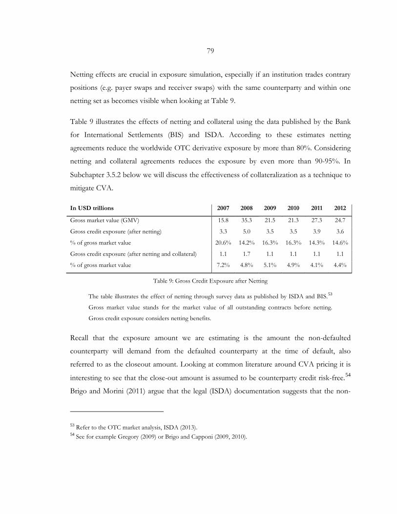
79

Netting effects are crucial in exposure simulation, especially if an institution trades contrary

positions (e.g. payer swaps and receiver swaps) with the same counterparty and within one

netting set as becomes visible when looking at Table 9.

Table 9 illustrates the effects of netting and collateral using the data published by the Bank

for International Settlements (BIS) and ISDA. According to these estimates netting

agreements reduce the worldwide OTC derivative exposure by more than 80%. Considering

netting and collateral agreements reduces the exposure by even more than 90-95%. In

Subchapter 3.5.2 below we will discuss the effectiveness of collateralization as a technique to

mitigate CVA.

In USD trillions 2007 2008 2009 2010 2011 2012

Gross market value (GMV) 15.8 35.3 21.5 21.3 27.3 24.7

Gross credit exposure (after netting) 3.3 5.0 3.5 3.5 3.9 3.6

% of gross market value 20.6% 14.2% 16.3% 16.3% 14.3% 14.6%

Gross credit exposure (after netting and collateral) 1.1 1.7 1.1 1.1 1.1 1.1

% of gross market value 7.2% 4.8% 5.1% 4.9% 4.1% 4.4%

Table 9: Gross Credit Exposure after Netting

The table illustrates the effect of netting through survey data as published by ISDA and BIS.53

Gross market value stands for the market value of all outstanding contracts before netting.

Gross credit exposure considers netting benefits.

Recall that the exposure amount we are estimating is the amount the non-defaulted

counterparty will demand from the defaulted counterparty at the time of default, also

referred to as the closeout amount. Looking at common literature around CVA pricing it is

interesting to see that the close-out amount is assumed to be counterparty credit risk-free.54

Brigo and Morini (2011) argue that the legal (ISDA) documentation suggests that the non-

53 Refer to the OTC market analysis, ISDA (2013). 54 See for example Gregory (2009) or Brigo and Capponi (2009, 2010).

80

defaulted counterparty should actually price its own-counterparty credit risk, i.e. DVA.55

This introduces a recursive problem. The expected exposure amount is dependent on future

DVA amounts, which in return depend on the expected exposure amount. Iterative

approaches to solve the problem are discussed also in Gregory and German (2012).

Acknowledging the need for such approaches (to ensure a more realistic illustration) we will

in the following retain the assumption of risk-free closeout amount for simplicity reasons, in

line with common literature and practice.

Step 4: Definition of Expected Exposure Profiles

For CVA purposes we are interested in the (risk-neutral) expectation of what the investor

can lose given a default of the counterparty. In mathematical terms we need to define the

following expected exposure (𝐸𝐸𝐸𝐸) for each re-valuation time period

𝐸𝐸𝐸𝐸(𝑡𝑡) = 𝔼𝔼𝑡𝑡ℚ[𝐸𝐸(𝑠𝑠, 𝑡𝑡)] (3.20)

where 𝐸𝐸(𝑠𝑠, 𝑡𝑡) is the net exposure at time 𝑡𝑡 for a given scenario s, given in Equation (3.19). 𝔼𝔼𝑡𝑡ℚ

stands for risk neutral expectation at time 𝑡𝑡. Looking at Figure 11 this means that we need to

define the average of the positive values of the distribution at each one of the 16 time steps.

Notice that for DVA purposes the mirroring exposure profile needs to be estimated. The

negative expected exposure (NEE) stands for the risk-neutral expectation of what the

counterparty can lose if the investor defaults, i.e. the average of the negative values of the

distribution.

Figure 12 exhibits a typical expected exposure profile for an interest rate swap and is given

for illustration purposes only. The typical profile increase is a function of the drift captured

55 Brigo and Morini (2010) and Brigo and Morini (2011) do not limit the aspect to be a modeling question, and discuss the unwanted implications on creditors if the closeout amount is credit risk-free.

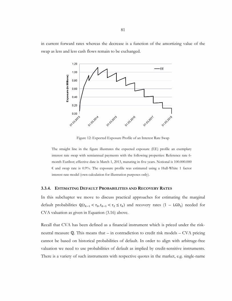
81

in current forward rates whereas the decrease is a function of the amortizing value of the

swap as less and less cash flows remain to be exchanged.

Figure 12: Expected Exposure Profile of an Interest Rate Swap

The straight line in the figure illustrates the expected exposure (EE) profile an exemplary

interest rate swap with semiannual payments with the following properties: Reference rate 6-

month Euribor; effective date is March 1, 2013, maturing in five years. Notional is 100.000.000

€ and swap rate is 0.9%. The exposure profile was estimated using a Hull-White 1 factor

interest rate model (own calculation for illustration purposes only).

3.3.4. ESTIMATING DEFAULT PROBABILITIES AND RECOVERY RATES

In this subchapter we move to discuss practical approaches for estimating the marginal

default probabilities ℚ(𝑡𝑡𝑏𝑏−1 < 𝜏𝜏0, 𝑡𝑡𝑏𝑏−1 < 𝜏𝜏2 ≤ 𝑡𝑡𝑏𝑏) and recovery rates (1 – LGD2) needed for

CVA valuation as given in Equation (3.16) above.

Recall that CVA has been defined as a financial instrument which is priced under the risk-

neutral measure ℚ. This means that – in contradiction to credit risk models – CVA pricing

cannot be based on historical probabilities of default. In order to align with arbitrage-free

valuation we need to use probabilities of default as implied by credit-sensitive instruments.

There is a variety of such instruments with respective quotes in the market, e.g. single-name

82

credit default swaps (CDS), index CDS, asset swaps (ASW) or bonds. Whereas credit default

swaps (CDS) can be considered as the most straightforward ones.56 Also from a theoretical

perspective CDS spreads have the cleanest isolation of credit risk, enabling the estimation of

default risk and the respective implied risk premium.

It is worth mentioning that also yields of default-able bonds are a standard source for

measuring implied default probability. Notice, however, that besides credit risk, bond

spreads may incorporate a significant portion of further aspects such as liquidity. For

empirical analysis on bonds spreads and credit risk see for example Longstaff et al. (2005).

For the relationship between bond spreads and CDS spreads see for example Hull et

al. (2004). Credit linked notes and Asset swaps are further quite popular instruments that are

worth being mentioned.57

Notice that historical and market implied probabilities differ systematically. The former

represent an actual assessment under the real world-measure of an entity defaulting while

market implied probabilities reflect current market quotes and associated hedge costs.58

Following the notations given by Brigo et al. (2013a, esp. pp. 66-70) we will in the following

discuss how CDS can be used to estimate risk-neutral probabilities of survival (and of

default) in a model-independent manner.59 A more elaborate discussion on key CDS

characteristics is given in Subchapter 4.2.1 of this thesis.

For this purpose we assume a standard CDS contract with inception time 𝑇𝑇𝑠𝑠, and maturity

time 𝑇𝑇𝑏𝑏 . The protection buyer pays a premium 𝑅𝑅, e.g. regular payments of a (credit) spread

56 As for example also noted by Schönbucher (2005), p. 15. 57 For an overview and description of a variety of credit dependent derivatives see for example

Schönbucher (2005), especially pp. 8-50. 58 For studies on the differences between risk-neutral and real-world probabilities of default see for example

Altman (1989), Hull et al. (2005) and Giesecke et al. (2010). 59 For a proof of the discussed we refer the reader to Brigo at al. (2013a), pp. 66-70.

83

times a given protection amount. If the reference entity defaults within the lifetime of the

contract the protection seller will compensate the buyer with a respective settlement

payment (i.e. loss given default (𝐿𝐿𝐺𝐺𝐷𝐷) times the protected amount). Notice that the valuation

of such a contract might seem mathematically rather straightforward. After all, we only need

to estimate the expected cash flows for each leg. The complication comes through the fact

that the cash flows are credit-sensitive per se. The premiums need to be paid only if the

entity has survived until that time period while the protection amount needs to be paid only

if the entity defaults within the time period. The cash flows need thus to be weighted with

probabilities of survival and default, respectively.

The mid-market premium seen at inception time 𝑅𝑅𝑠𝑠.𝑏𝑏𝑀𝑀𝐼𝐼𝐷𝐷(0) ensures a fair valuation of the

contract, i.e. that the premium leg value equals the protection leg value. This means that the

CDS contract has a value of zero, i.e. 𝐶𝐶𝐷𝐷𝐶𝐶𝑠𝑠,𝑏𝑏(0,𝑅𝑅𝑠𝑠.𝑏𝑏𝑀𝑀𝐼𝐼𝐷𝐷(0), 𝐿𝐿𝐺𝐺𝐷𝐷) = 0.

Given the market premiums 𝑅𝑅𝑠𝑠.𝑏𝑏𝑀𝑀𝐼𝐼𝐷𝐷(0) for a set of different maturities, e.g. 𝑇𝑇𝑏𝑏 = 1𝑦𝑦, 2y, … 5y

and 𝑇𝑇𝑠𝑠 = 0, an assumption for the LGD underlying the quotes as well as the current (risk-

free) discount function 𝑃𝑃(0,∙) and the given survival probabilities ℚ(𝜏𝜏 >∙) – with ∙ standing for

the maturities of the used instruments – can be stripped by solving the following equation:

𝑃𝑃𝑟𝑟𝑙𝑙𝑡𝑡𝑒𝑒𝑐𝑐𝐿𝐿𝑒𝑒𝑙𝑙0,𝑏𝑏(𝐿𝐿𝐺𝐺𝐷𝐷,𝑃𝑃(0,∙),ℚ(𝜏𝜏 >∙)) = 𝑃𝑃𝑟𝑟𝑒𝑒𝑚𝑚𝑖𝑖𝑢𝑢𝑚𝑚𝐿𝐿𝑒𝑒𝑙𝑙0,𝑏𝑏�𝑅𝑅;𝑃𝑃(0,∙),ℚ(𝜏𝜏 >∙)� (3.21)

whereas the protection leg and the premium leg are valued as follows:60

𝑃𝑃𝑟𝑟𝑙𝑙𝑡𝑡𝑒𝑒𝑐𝑐𝐿𝐿𝑒𝑒𝑙𝑙𝑠𝑠,𝑏𝑏�𝐿𝐿𝐺𝐺𝐷𝐷;𝑃𝑃(0,∙),ℚ(𝜏𝜏 >∙)� ≔ −𝐿𝐿𝐺𝐺𝐷𝐷� 𝑃𝑃(0, 𝑡𝑡)𝑑𝑑𝑡𝑡 ℚ(𝜏𝜏 ≥ 𝑡𝑡)𝑇𝑇𝑐𝑐

𝑇𝑇𝑎𝑎,

(3.22)

𝑃𝑃𝑟𝑟𝑒𝑒𝑚𝑚𝑖𝑖𝑢𝑢𝑚𝑚𝐿𝐿𝑒𝑒𝑙𝑙0,𝑏𝑏�𝑅𝑅;𝑃𝑃(0,∙),ℚ(𝜏𝜏 >∙)� ≔ (3.23)

60 As also noted by Brigo et al. (2013a), p. 68, given a discretization time step that is small enough the given integrals can be approximated numerically through by summations of Riemann-Stieltjes sums.

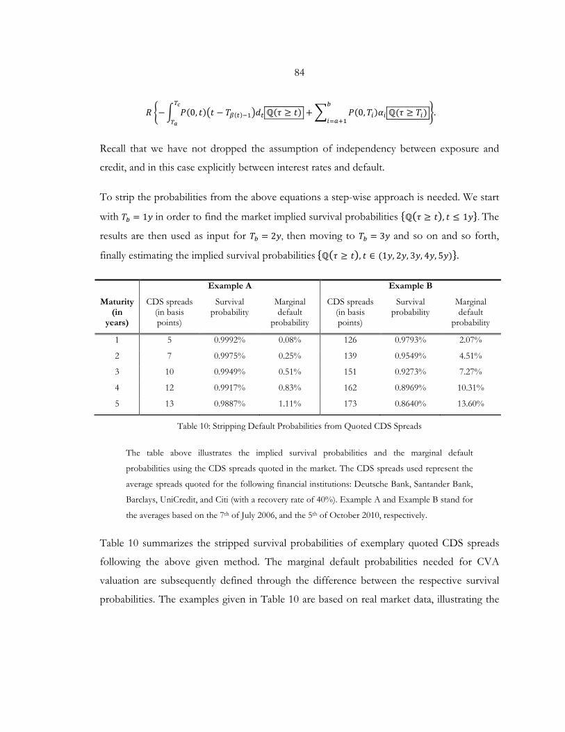
84

𝑅𝑅 �−� 𝑃𝑃(0, 𝑡𝑡)�𝑡𝑡 − 𝑇𝑇𝛽𝛽(𝑡𝑡)−1�𝑑𝑑𝑡𝑡 ℚ(𝜏𝜏 ≥ 𝑡𝑡)𝑇𝑇𝑐𝑐

𝑇𝑇𝑎𝑎+ � 𝑃𝑃(0,𝑇𝑇𝑖𝑖)𝛼𝛼𝑖𝑖 ℚ(𝜏𝜏 ≥ 𝑇𝑇𝑖𝑖)

𝑏𝑏

𝑖𝑖=𝑠𝑠+1�.

Recall that we have not dropped the assumption of independency between exposure and

credit, and in this case explicitly between interest rates and default.

To strip the probabilities from the above equations a step-wise approach is needed. We start

with 𝑇𝑇𝑏𝑏 = 1𝑦𝑦 in order to find the market implied survival probabilities {ℚ(𝜏𝜏 ≥ 𝑡𝑡), 𝑡𝑡 ≤ 1𝑦𝑦}. The

results are then used as input for 𝑇𝑇𝑏𝑏 = 2𝑦𝑦, then moving to 𝑇𝑇𝑏𝑏 = 3𝑦𝑦 and so on and so forth,

finally estimating the implied survival probabilities {ℚ(𝜏𝜏 ≥ 𝑡𝑡), 𝑡𝑡 ∈ (1𝑦𝑦, 2𝑦𝑦, 3𝑦𝑦, 4𝑦𝑦, 5𝑦𝑦)}.

Example A Example B

Maturity (in

years)

CDS spreads (in basis points)

Survival probability

Marginal default

probability

CDS spreads (in basis points)

Survival probability

Marginal default

probability

1 5 0.9992% 0.08% 126 0.9793% 2.07%

2 7 0.9975% 0.25% 139 0.9549% 4.51%

3 10 0.9949% 0.51% 151 0.9273% 7.27%

4 12 0.9917% 0.83% 162 0.8969% 10.31%

5 13 0.9887% 1.11% 173 0.8640% 13.60%

Table 10: Stripping Default Probabilities from Quoted CDS Spreads

The table above illustrates the implied survival probabilities and the marginal default

probabilities using the CDS spreads quoted in the market. The CDS spreads used represent the

average spreads quoted for the following financial institutions: Deutsche Bank, Santander Bank,

Barclays, UniCredit, and Citi (with a recovery rate of 40%). Example A and Example B stand for

the averages based on the 7th of July 2006, and the 5th of October 2010, respectively.

Table 10 summarizes the stripped survival probabilities of exemplary quoted CDS spreads

following the above given method. The marginal default probabilities needed for CVA

valuation are subsequently defined through the difference between the respective survival

probabilities. The examples given in Table 10 are based on real market data, illustrating the

85

increase in market implied default probabilities in particular, and in the significance and level

of CVA in general following the financial crisis.

After having discussed practical approaches to estimate expected exposure and default

probabilities we turn to recovery rates (or loss given default, LGD) which are needed

twofold to price CVA: (1) indirectly in order to strip probabilities of default; and (b) directly

as seen in Equation (3.16). The recovery rate stands for the percentage of par value that

investors will receive after a default event of the reference entity.

Evidence suggests that collateral and thus recovery rates are stochastic, and jointly

distributed with probabilities of default, especially in times of distress. This means that

adequate credit risk modelling should rely on stochastic models for recovery rates as for

example discussed in Altman (2006), Bilal and Singh (2012) as well as Li (2009) for the

specific case of CVA pricing. Market convention, however, seems to rely on a more practical

approach, assuming a constant recovery rate. The CDS data quotes given for example by the

data provider Markit assume a constant recovery rate of 40%, i.e. LGD of 60%.61 The use of

a constant recovery rate is not limited to practice and is also wide-spread in academic and

research work as seen in Brigo and Chourdakis (2009) or Lipton and Sepp (2009).

In any case, it indeed seems consistent to use the same assumption for recovery rate twice,

i.e. for stripping default probabilities and directly for CVA valuation. This would in fact also

limit the effect of LGD on CVA due to a cancellation effect, as referred to by

Gregory (2012, p. 252). On the one hand, the higher (lower) the LGD assumed the lower

(higher) the default probabilities stripped and the CVA computed. On the other hand, CVA

is a direct function of LGD, i.e. a higher LGD increases CVA and vice versa.

61 See for example Brigo et al. (2013a), pp. 185-186 or Bilal and Singh (2012).

86

3.4. ACCOUNTING AND REGULATORY BACKGROUND OF

COUNTERPARTY CREDIT RISK

3.4.1. REMARKS

Counterparty credit risk in general and CVA in particular seem to be highly driven by

regulatory and accounting standards.62 From a regulatory perspective financial institutions

are faced with requirements with respect to measuring and capitalizing counterparty credit

and (unilateral) CVA volatility. In addition, international accounting standards require the

consideration of (bilateral) CVA in fair value measurement, affecting not only financial

institutions but all OTC derivative traders such as corporates that use such derivatives for

example to hedge their interest rate and foreign exchange positions. In fact such non-

financial institutions seem to be concerned with possibly being impaired twice. On the one

hand accounting standards require them to compute CVA and DVA, facing them with

methodological and technical challenges. In addition, banks will try and rollout their higher

requirements through higher margins. Watt (2011) cites the Head of Finance at Lufthansa,

one of the major German non-financials, saying the following:

“We think the new [CVA capital] charge will have a big impact on our business. Long-

term derivatives will be a problem. For some of these trades, we understand the cost will be so

high that we will have to accept the risk of sharp movements in whatever we are hedging

against, like floating interest rates or oil prices. That means our profit and loss figures will be

more volatile”

As will be displayed, the accounting and regulatory requirements can be seen as quite

straightforward from a theoretical perspective. Still, as seen from the above given quote

there seems to be a controversial discussion around their diverse practical implications. An

62 This view is shared for example by Albanese et al. (2013).

87

overview on counterparty credit risk cannot leave out an elaboration on these requirements

because they seem to influence the discourse on risk management and CVA pricing.

In the following two subchapters we will give an overview of the main accounting and

regulatory requirements, focusing on international accounting standards (IFRS and US-

GAAP) and the Basel III framework.63 In Subchapter 3.4.4 we summarize our analysis of

the regulatory efforts, commenting on whether the fear of the cited Lufthansa manager is

justified.

3.4.2. ACCOUNTING BACKGROUND

CVA as Part of an Exit Price

Derivatives have to be measured and disclosed according to the fair value measurement both

under the international financial accounting standards (IFRS) and under US-GAAP as

specified in IFRS 13 and ASC 815. Both standards refer to fair value as an “exit price” and

require the use of a “fair value hierarchy”. In the following we will give a recap for both

terms.

According to IFRS 13.9 or ASC 820-10-20 exit price is defined as the price that would be

received for an asset or the price that would be paid to transfer a liability. As specified in

IFRS 13.72 and ASC 820-10-35 exit prices have to be estimated according to a fair value

hierarchy which categorizes pricing parameters along three levels. If possible one must use

quoted prices for identical assets and liabilities in active markets, these categorized as level 1

parameters. For example the liquid stock price should be used to evaluate a respective stock

position. If such quotes are not available one must refer to level 2 parameters, i.e. direct or

indirect input parameters and standard pricing methods. The value of interest rate swaps is

63 For a further reading on the regulatory framework around CVA and counterparty credit risk see for example Schwake et al. (2011) who also give an overview of the specific requirements under the German GAAP (Handelsgesetzbuch, HGB).

88

for instance not directly quoted. Bootstrapping of interest rate curves (such as three-month

Euribor or Eonia) from market information is needed and the valuation is subsequently

done using a discounting cashflow method. Lastly level 3 parameters consist of unobservable

parameters that need to be estimated, e.g. for the valuation of an asset backed security (ABS)

one needs to estimate a default probability and severity of the respective pool of loans. Such

parameters are usually not quoted and have to be estimated using historical statistics, peer

group comparisons or expert estimations.

Taking counterparty credit risk into consideration in the fair value of an OTC derivative can

in general be motivated twofold. For one, being a significant risk factor counterparty credit

risk will be priced in by third parties, making CVA part of an exit price. In addition, both

US-GAAP and IFRS have specific requirements to take non-performance risk into

consideration as specified for example in ASC 80-10 and IFRS 13.42. Notice that this

implies the consideration of own credit risk in derivative pricing as specifically required by

IFRS 13.42:

“The fair value of a liability reflects the effect of non-performance risk. Non-performance risk

includes, but may not be limited to an entity’s own credit risk (as defined in IFRS 7:

Financial Instruments: Disclosures).”

It goes without saying that there are circumstances in which CVA or DVA for a given entity

or for parts of its OTC derivatives portfolio are concluded as not material. The

consideration of CVA or DVA would then not be obligatory.64 This might for example be

the case if collateral agreements with daily posting are in place and the counterparties

involved exhibit high credit quality. This could also be the case for corporates with relatively

64 See also Schwake et al. (2011), pp. 293-294.

89

small derivatives portfolio.65 In any case materiality is entity-specific and has usually to be

validated and agreed upon with the auditor.

Estimation of Credit Risk

As mentioned in previous subchapters – especially Subchapter 3.3.3 – one of the drivers of

CVA is the credit risk of the counterparty, i.e. the risk of default and changes in the credit

quality.66 According to the “fair value hierarchy” this has to be estimated using as much

market data as possible. If such data is not available, approximations and indirect data can be

used. Historical and statistical estimation or expert opinions can only be used if all other

alternatives are not available.

Following the “fair value hierarchy” one should thus use credit spreads that are directly

traceable to the respective counterparty. This means that – if available – single name CDS

spreads should be used. This aligns with what we have discussed in Subchapter 3.3.3

above.67 If such spreads are not available entities should map these to other tradable CDS

spreads (e.g. categorized by rating, geography or industry). According to this logic internally

estimated spreads should hence only be used if mapping procedures are either impossible or

economically meaningless. In order to deliver market implied valuation (i.e. staying in line

with duplicating strategy or hedge strategy valuation) but also in order to stay aligned with

the “fair value hierarchy” this spread has to contain – besides default risk – an estimate for a

market risk premium.

Despite the fact that these requirements are quite straightforward from an academic and

theoretical point of view they seem to imply significant challenges for many entities. After

65 It is worth mentioning that both IFRS 13 and ASC 820 explicitly allow the computation of CVA on counterparty level (in order to take netting and collateral aspects into consideration).

66 An overview on credit risk modeling is given in Subchapter 4.2.2. 67 In its comment on fair value measurement, the Institute of Public Auditors in Germany, names CDS spreads

as sole example for market source of credit risk estimation (see IDW RS HFA 47, paragraph 102).

90

all, for a large part of entities there are no liquid CDS spreads, and the use of mapping

procedures seems arbitrary, lacking economic reason.68 Credit risk of small and medium

sized corporations (e.g. a local German corporation with 30 employees in the construction

business) can hardly be mapped to index CDS, containing large and international

corporations. A further reason why corporations might not want to use market implied

information is their apparent higher volatility, a reason that cannot, however, be cleansed

from balance sheet manipulation. It can furthermore be argued that if hedging of

counterparty credit risk is impossible then market implied valuation is not needed (also

referred to as warehouse book valuation). In that case CVA is interpreted as a metric for

expected credit loss. Still, risk-neutral valuation is based on duplication strategies, irrespective

of whether hedging strategies are truly in place. In addition, from an accounting point of

view, market implied valuation can be motivated not only by being market standard but

because of its limited manipulability if compared with entity specific information. Moreover,

it facilitates a better comparability of financial statements of differing entities.

In a recent comprehensive assessment the European Central Bank (ECB) challenged

valuation and provisioning methodologies of European banks. The assessment revealed a

gab of € 3.1 billion to CVA calculation., resulting in a 27% increase in the respective metric

for the banks that were part of the assessment. Most of this adjustment was driven by an

incorrect use of historical – instead of market implied – probabilities of default.69

It is worth mentioning that the standardization of risk-neutral CVA valuation, especially in

the market of counterparties with no liquid CDS spreads which largely intersects with the

non-financial market in which no collateral is daily posted is very difficult, because arbitrage

68 For empirical findings on the use of internal spreads see for example Schwake et al. (2011) or Deloitte and Solum (2013), p. 26. For an attempt to use internal data with market implied information see for example Knoth and Schulz (2010).

69 See ECB (2014), pp. 98-100.

91

opportunities are rather excluded and the counterparties do not have to agree on the value

of the portfolio on daily basis.

It can be concluded that marked implied default probabilities seem to have become more

popular.70 This trend cannot however be regarded independently from the specifications of

IFRS 13 and subsequent higher focus of audit firms and supervisors on the subject matter.

Accounting for Debt Valuation Adjustment (DVA)

A further topic that has quite controversially been discussed is DVA. The accounting

standard requirements are actually rather clear with regard to this topic. Entities have to

consider their own credit risk, i.e. CVA has to be computed on a bilateral basis. Still, studies

show that the consideration of DVA for accounting purposes but also in front-office pricing

is not as straightforward as the standard setters might have had in mind.71 DVA seems to be

presumed as unintuitive, implying a variety of unwanted challenges. In the following we will

go through the main issues around DVA, extending and commenting the discussion given

by Gregory (2009).

First, by taking DVA into account, the evaluating entity assumes a gain from its own default.

This is indeed questionable from the entity’s perspective because such gains are irrelevant

and unrealizable. From a valuation perspective, a bilateral CVA might allocate a higher value

to a derivatives portfolio than its “default-free” value (also referred to as marked-to-market

value, MtM). On the other hand, for the shareholders not having to redeem obligations (in

that case derivative obligations) does exhibit a profit when one’s company is at default. Taking

DVA into account would thus make sense if the shareholders are viewed as the main

stakeholders of financial reporting. Even if some counterparties claim not to price a DVA

70 See for example Schwake et al. (2011), pp. 295-298 or the more recent analysis done by EBA (2015). 71 For the consideration of DVA in pricing and accounting purposes see the study done by Deloitte and

Solum (2013), especially p. 29. Schwake et al. (2011) have collected information from publicly available information on DVA, focusing on its consideration for accounting purposes. For DVA in pricing see 3.5.1.

92

component the fact that they are pricing a CVA component plainly means that someone else

is symmetrically (willingly or not, knowingly or not) pricing DVA. Arora et al. (2012) find

evidence that the higher the credit risk of a dealer, the lower is the price he can charge for

selling a CDS. This implies that these dealers are (willingly or not, knowingly or not) taking

their own credit into consideration.

Gregory (2009) does argue that from an entity’s perspective realizing DVA is possible if the

entity is near default, and brings in some examples from the insurance business. In such

cases the counterparties would readily unwound the portfolios and pay-out the entity a

respective compensation. We argue that the realization of DVA is not limited to such

extreme cases. Counterparties can for example also agree on raising the collateralization, e.g.

through a two way collateral agreement with minimal thresholds or through central clearing.

These amendments would trigger a change in the value of the bilateral CVA. The

counterparty that benefits more from the amendment (through a relief in its CVA position)

would thereby compensate the other party, allowing it to (at least partially) realize DVA.

Second, accounting for DVA implies that the financial results are subject for changes in

one’s own credit risk, hence making a profit from own credit deterioration. The following

newspaper quotes on the financial reports of leading investment banks expose how

unintuitive this effect is:

“Citigroup benefited from a paper gain of nearly $ 2 billion, reflecting a sharp increase in the

perceived riskiness of its debt […]. That contributed about one-third of its pre-tax operating

profit […]”72

“Debit valuation adjustments […] helped Citigroup Inc. post a $ 3.77 billion profit Monday

even as its revenue fell. And J.P. Morgan Chase & Co. included a $1.9 billion pre-tax

benefit from debt valuation adjustments in its investment bank when it posted third-quarter

72 See Dash (2011).

93

earnings last Thursday. And this morning, Bank of America Corp. reported booking a $ 1.7

billion gain due to the accounting rule.”73

On the other hand one can argue that these effects are transparent, and can thus be correctly

interpreted by analysts and investors. Furthermore, one could also argue that if the

derivatives portfolios are unwound or better collateralized at the time period of the financial

reports the entity will indeed receive higher compensations.

We conclude that the unintended effect of “making money” with one’s own default is rather

a critical issue for management accounting, less so for financial accounting. This is especially

relevant for derivatives traders with relatively large OTC portfolios. In these cases trading

departments should not be able to make profits (and hence pay higher bonuses to their

employees) due to a higher DVA. This can be reached for example either by not considering

DVA in management accounting or by designating DVA to a special unit (e.g. CVA desk) or

by taking DVA into account only on a bank-wide level.

Third, from a risk management perspective accounting for DVA contradicts the principle of

prudency, especially if the bilateral CVA metric is either zero or negative, implying no or

negative counterparty credit risk.74 The regulator is however aware of these effects. Financial

institutions are required therefore to use unilateral CVA for determining regulatory capital.

Also the capital charge for CVA risk, i.e. CVA volatility accounts only for the volatility

driven by the unilateral CVA.

Fourth, as noted by Albanese et al. (2013) or Gregory (2009), a main problem of bilateral

CVA is it being unhedgeable. For one, the unilateral CVA part has to be hedged only as long

73 See Burne (2011). 74 This might be the case if the DVA component is larger than the UCVA component, delivering a negative

BCVA. Notice that this is not only a function of credit risk. If both counterparties have similar credit risk but the expected negative exposure is significantly larger than the expected positive exposure the DVA component would be larger, delivering a total negative adjustment.

94

as the entity doing the computation is solvent. More complex is the fact that DVA hedging

implies selling a protection on one’s own default, quite an impossible task. Gregory (2009)

mentions beta hedging as a possible approach. The company might sell protection on

comparable counterparties (e.g. from one’s peer-group). However, this strategy will deliver a

proxy-hedge for credit spread volatility at best. In a worst case scenario it might also imply

dramatic losses if the credit risk of such comparable counterparties deteriorates or if they

even default on their obligations while the own entity is still solvent.

There is actually a further – and less discussed alternative – for hedging one’s own credit

risk. This possibility is however limited to a handful of entities, whose single name CDS is

part of a liquid CDS index.75 If for example a single name CDS referenced to an entity (e.g.

Deutsche Bank) is part of a CDS index (e.g. iTraxx Europe Senior Financials) that company

would theoretically be able to sell its own credit risk. The company could sell the index and

buy protection on all the remaining counterparties in the index. It has however to be stressed

that this hedge strategy would still be very (and probably prohibitively) expensive, especially

if re-hedge costs are considered.

Fifth, and probably the most controversial and sophisticated aspect both from a theoretical

as well as from a practical perspective is the overlap between DVA and expected funding

benefits. In the following we will synthesize the key takeaways that are relevant for our

analysis of the overall discourse on DVA, but will refrain from giving a comprehensive

overview, especially with regards to a possible misalignment between pricing funding and

financial theory. For this purpose we refer the interested reader to Morini and Prampolini

(2011), Pallavacini et al. (2011), Hull and White (2012a) or Burgard and Kjaer (2013).76

75 The author thanks R. O. for this intuitive idea, raised in a discussion on CVA and DVA. 76 On the controversy around funding of derivatives while also touching the overlap between DVA and

funding see for example Cameron (2014). For a high level overview on FVA see also Fries et al. (2013).

95

Funding costs (benefits) are associated with uncollateralized positive (negative) exposure.

While positive exposure needs to be funded, negative exposure is interpreted as a liability, i.e.

a funding source. This can be illustrated through the following example. Assume a bank is

trading an uncollateralized interest rate swap with a client. The bank hedges the interest rate

risk arising from this swap through a mirroring position, traded with a bank. The only

difference between the two swaps is that while the client derivative is not collateralized the

hedge position is. Now if the client position is positive (negative) the hedge position will be

negative (positive). In the first case the bank will need to post collateral to the hedging

counterparty while not receiving any from the client. The bank will thus need to fund an

amount equal to the positive exposure. In the second case the bank will receive collateral

from the hedge counterparty and will not need to post any to the client. The bank will thus

receive a funding amount equal to the negative exposure.77

A funding cost adjustment (FCA) considers expected funding costs arising from expected

positive exposure, i.e. depending on the same exposure profile like UCVA and the assumed

funding spread. On the other hand, funding benefit adjustment (FBA) considers expected

funding benefits arising from expected negative exposure, i.e. depending on the same

exposure profile as DVA and an assumed funding spread. It becomes clear that an

institution that prices FBA and DVA might be double counting, especially if the funding

spread and the credit spread (used for DVA valuation) contain similar information. Morini

and Prampolini (2011) point out that funding benefit should be based only on the CDS-

bond-basis, excluding possible double counting per definition. In practice one also sees

traders that price FBA while being reluctant in pricing DVA. In a survey done by Deloitte

and Solum (2013, p. 39) we find the following conclusion: “[…] banks are increasingly seeing

77 One can argue that the above given motivation is flowed because the value of a derivative cannot be driven by the funding structure of the trading institution. Recall, however, that arbitrage-free valuation is based on the possibility to structure a duplication portfolio. In practice the hedge of an uncollateralized trade is collateralized. This implies additional funding considerations to achieve a duplication. See also Burgard and Kjaer (2013).

96

DVA as a funding benefit and not as a benefit in the event they default. We note that whilst a bank may

consider CVA + symmetric funding [FCA + FBA] to be relevant, they may refer to the funding benefit as

DVA.”

We conclude that although DVA has a variety of pitfalls and challenges that have to be taken

into account its consideration is not a mere theoretical and accounting aspect. If some

market participants are pricing CVA then other market participants must (willingly or not,

knowingly or not) be taking their own credit risk into consideration, i.e. pricing (at least to a

certain extent) DVA.

97

3.4.3. REGULATORY BACKGROUND

Remarks

In December 2010 the Basel Committee on Banking Supervision (BCBS) published a

document containing its revised standards under the title “Basel III: A Global Regulatory

Framework for more Resilient Banks and Banking Systems”. Through the new basis for

international lawmaking, the BCBS intended to deliver a (quick) response to the financial

crisis, taking lessons-learned from recent events into consideration. Basel III offers major

amendments to the previous Basel II78 accord in general and with respect to counterparty

credit risk and CVA in particular.

The regulatory requirements for capitalizing counterparty credit risk, in terms of default risk,

have been amended on the one hand to be more prudent (e.g. stressed exposure etc.). On

the other hand Basel III offers financial institutions an incentive to clear their OTC

derivatives through a central counterparty (CCP), assigning significantly lower risk weights

for such exposures. This is aligned with further regulatory efforts to shift the OTC market

towards central clearing as codified in the US-American Dodd-Frank Act and in the

European Regulation EMIR.79

Basel III has in particular introduced a new capital charge for CVA risk, i.e. CVA volatility. It

has been correctly anticipated that this new charge will increase the capital requirement for

counterparty credit risk considerably. Since the publication of the first draft of Basel III in

December 2009, CVA capital charge seems to have been dominating the discourse on

counterparty credit risk and CVA pricing, raising the attention of the top management not

only of financial institutions but also of non-financial corporations, followed by vehement

78 Basel II is the common reference to the document of the BCBS “International Convergence of Capital Measurement and Capital Standards”, published in 2006.

79 Dodd-Frank Act stands for the Dodd-Frank Wall Street Reform and Consumer Protection Act signed into federal law on July 21, 2010. EMIR stands for European Market Infrastructure Regulatory interred into force on August 16, 2012.

98

critique and organized lobbyism.80 At least in Europe, this opposition seems to have been

effective. The latest package of the Capital Requirement Directive (CRD IV) which

transposed Basel III into EU law, introduces exemptions from the CVA capital charge for

non-financial counterparties, a clear advantage to European institutions, when compared to

north American banks for instance.81

In the following we will display the very main regulatory requirements around counterparty

credit risk and CVA risk (the emphasis is on very main). The following elaboration is in no

means an exhaustive description of all the respective requirements.82 We will especially not

elaborate on country specific amendments (e.g. through an endorsement process of the

framework). The aim of the following elaboration is rather to pinpoint the relevant issues in

order to demonstrate the interplay between the regulatory requirements, accounting issues

and the discourse around counterparty credit risk and CVA, trying in particular to

understand whether the fear of the cited Lufthansa manager is justified.

Measuring and Capitalizing (Counterparty) Credit Risk

As noted, banks have already under Basel II been required to capitalize and measure the

default risk inherent in their derivatives portfolios, i.e. (counterparty) credit risk. For this

purpose, the supervisor prescribes a loan-equivalent technique, requiring the capitalization of

the risk-weighted exposure at default, computed on a netting-set level. Banks must thus hold

sufficient capital against their risk weighted assets (RWA), defined as follows:

RWA = RW ∙ EAD. (3.24)

80 The first draft for the Basel III accord was published by the BCBS in December 2009 in a document titled "Strengthening the Resilience of the Banking Sector". For the discussion on the CVA capital charge within the first Basel III draft see for example Pengelly (2010). For the CVA capital charge in its last version see for example Rebonato et al. (2010).

81 CRD IV entered into force on July 17, 2013. 82 For a more extensive description see for example Gregory (2012), pp. 371-402.

99

RW stands for the risk-weight of the position, depending in general on the credit risk of the

counterparty and the maturity of the portfolio at hand. EAD is the exposure at default to a

specific counterparty with a one year horizon, depending in general on the market risk

inherent in the derivatives portfolio, taking possible collateralization effects into

consideration.

The Basel framework offers three main approaches for assessing the risk-weight of a

position; (1) the standardized approach, (2) the internal rating-based approach (IRBA) and

(3) the advanced IRBA. Under the first approach banks are offered rating-based grids of

risk-weights for each class of counterparties (e.g. sovereigns, financial institutions etc.).

IRBA, on the other hand, prescribes the use of a model-based formula to define the risk

weight. Following BCBS (2005) the risk weight RW can be defined as

RW = LGD ∙ �𝑁𝑁 �

𝑁𝑁−1(𝑃𝑃𝐷𝐷) − �𝜌𝜌𝑁𝑁−1(0.999)

�1 − 𝜌𝜌� − 𝑃𝑃𝐷𝐷� ∙ 𝑀𝑀𝐹𝐹(𝑀𝑀,𝑃𝑃𝐷𝐷) ∙ 12.5 (3.25)

with 𝐿𝐿𝐺𝐺𝐷𝐷 standing for the loss given default, i.e. the proportion of the exposure that will not

be recovered. 𝑁𝑁(∙) is the standard normal cumulative distribution function. 𝑃𝑃𝐷𝐷 is the

probability of default (in one year) and 𝜌𝜌 is the correlation factor between the obligor and

the market factor. 𝑀𝑀𝐹𝐹 is a so-called maturity factor, a function of the maturity 𝑀𝑀 for several

values of 𝑃𝑃𝐷𝐷.

Under IRBA banks will be allowed to estimate the default probability, subject to meeting

predefined conditions and explicit supervisory approval. Banks operating under advanced

IRBA will be allowed to estimate LGD and exposure at default (EAD) as will be explained

below in more detail.

Assuming a minimum capital ratio of 8% – as required under Basel II – the minimum

regulatory capital requirement RC is given as follows

100

RC = LGD ∙ �𝑁𝑁 �

𝑁𝑁−1(𝑃𝑃𝐷𝐷) − �𝜌𝜌𝑁𝑁−1(0.999)

�1 − 𝜌𝜌� − 𝑃𝑃𝐷𝐷� ∙ 𝑀𝑀𝐹𝐹(𝑀𝑀,𝑃𝑃𝐷𝐷) ∙ 𝐸𝐸𝐴𝐴𝐷𝐷. (3.26)

Equations (3.25) and (3.26) find their theoretical foundation in the Asymptotic Single Risk

Factor (ASRF) model of portfolio credit risk, developed amongst others by Gordy (2003).83

In the following, we will not elaborate extensively on this model and will refer the interested

reader to the cited works and to the explanatory note given in BCBS (2005). Relevant for our

analysis on counterparty credit risk and CVA is the main objective of the formula: Assuming

a large homogenous and granular pool of obligors with a normal distributed default rate, the

formula aims on approximating the (expected and unexpected) credit loss that will be

exceeded with a small probability of 0.1%. The maturity adjustment is expected to capture

the higher risk given by longer maturities for example due to a higher probability of credit

deterioration, i.e. migration.

Hence, the above given formula delivers a value at risk (VaR) measure for credit risk with a

confidence level of 99.9% and a time horizon of one year. This stands in line with the

proclaimed objective behind the Basel framework to capitalize a peek loss, a balance

between prudency and solvency on the one hand and economic efficiency on the other.

The Basel Committee argues that by fixing the confidence level to 99.9% “an institution is

expected to suffer losses that exceed its level of tier 1 and tier 2 capital on average once in a thousand years”,

adding that “[t]his confidence level might seem rather high.” The Committee advocates this high level

as “[protecting] against estimation errors, that might inevitably occur from banks’ internal […] estimations,

as well as other model uncertainties.”84 The financial crisis offers a hindsight in which these

elaborations appear rather inadequate, if not even naive. Basel III has addressed this issue by

83 See also Merton (1974), Schönbucher (2005) and Vasicek (2002). For an overview on credit risk modeling see Subchapter 4.2.2.

84 See BCBS (2005), especially p. 11.

101

prescribing an evolution for the minimum capital requirement, raising it up to 14.5% by

2018.85 Future will tell whether this increase suffices.

Estimating Regulatory Exposure (EAD)

A challenging task within the exercise of capitalizing counterparty credit risk is estimating the

amount at stake, i.e. the exposure at default (EAD) from Equation (3.24). We have described

the challenges involved in estimating expected exposure in Subchapter 3.3.3. In the

following we will focus on unique aspects relevant for regulatory purposes while revisiting

some notations in order to allow for a more fluent elaboration.

The supervisor prescribes three possible alternatives for this purpose: (1) the current

exposure method (CEM), (2) the standardized method (SM) and (3) the internal model

method (IMM).86 The use of SM seems however to be rather rare so that we will in the

following solely focus on the significantly more popular approaches, CEM and IMM.87

The Internal Model Method (IMM)

The IMM approach is based on the use of Monte Carlo schemes to estimate the (future)

value of the derivatives portfolio, i.e. through the simulation of possible evolutions of the

relevant risk factors in a forward looking manner.88 The exposure 𝐸𝐸 inherent in a portfolio

of OTC derivatives at a given time period 𝑡𝑡 is defined as follows

85 We refer the reader to critical analysis of the VaR measure found for example in Beder (1995) or Taleb (1997), pp. 445-453.

86 Notice that at the time of writing these lines BCBS has introduced a new standardized approach for measuring counterparty credit risk exposures (SA-CCR). The SA-CCR is supposed to be more risk sensitive, taking collateral and netting effects better into consideration. Because banks are still not required to adopt the approach we will keep it uncommented and refer the interested reader to BCBS (2014).

87 According to an international survey on counterparty credit risk only one participating institution stated to use SM whilst no participant planned to use SM in the future, see Deloitte and Solum (2013), p. 8.

88 For a more detailed description of exposure simulation we refer the reader to Subchapter 3.3.3.

102

𝐸𝐸(𝑡𝑡) = 𝑚𝑚𝑎𝑎𝑥𝑥{𝑁𝑁𝑃𝑃𝑃𝑃(𝑡𝑡) − 𝐶𝐶(𝑡𝑡),0} (3.27)

where 𝑁𝑁𝑃𝑃𝑃𝑃 stands for the net present value of a given netting set, i.e. the (default-free) value

or the marked-to-market (MtM) metric of the respective derivatives. 𝐶𝐶 is the value of the

collateral posted or received. This means that if the NPV is negative and the bank posts a

collateral amount to the counterparty that exceeds the absolute value of the NPV, the bank

will have a positive exposure (due to overcollateralization). Notice that the IMM approach

enables the full consideration of netting and collateral effects.

After producing possible exposure profiles for a given time period set {𝑡𝑡𝑏𝑏} the expected

exposure 𝐸𝐸𝐸𝐸 at time period 𝑡𝑡𝑏𝑏 is given as follows

𝐸𝐸𝐸𝐸(𝑡𝑡𝑏𝑏) = 𝔼𝔼ℙ[𝐸𝐸(𝑡𝑡𝑏𝑏)] (3.28)

Where 𝐸𝐸 is the net exposure at time t given in Equation (3.27) and 𝔼𝔼ℙ denoting the

expectation under the probability (real-world) measure ℙ. It is worth mentioning that the

exposure models used for regulatory purposes are supposed under Basel III to be calibrated

to historical stress periods, allowing for more prudent exposure estimation (also deviating

from the risk-neutral measure ℚ used in CVA valuation). In order to assign yet more

prudency to the computation the regulator introduces a further exposure metric, the

effective expected exposure 𝐸𝐸𝐸𝐸𝐸𝐸𝐸𝐸𝐸𝐸, defined as the maximum expected exposure until the

date of calculation, given as follows

𝐸𝐸𝐸𝐸𝐸𝐸𝐸𝐸𝐸𝐸(𝑡𝑡𝑏𝑏) = max𝑡𝑡𝑖𝑖∈[0,𝑡𝑡𝑘𝑘]{𝐸𝐸𝐸𝐸(𝑡𝑡𝑖𝑖)}, (3.29)

Focusing on a time horizon of one year (𝐻𝐻), the effective expected positive exposure 𝐸𝐸𝐸𝐸𝐸𝐸𝐸𝐸𝑃𝑃𝐸𝐸

is defined as the average of the 𝐸𝐸𝐸𝐸𝐸𝐸𝐸𝐸𝑃𝑃𝐸𝐸 given in the following equation

𝐸𝐸𝐸𝐸𝐸𝐸𝐸𝐸𝑃𝑃𝐸𝐸 =

1𝐻𝐻�𝐸𝐸𝐸𝐸𝐸𝐸𝐸𝐸𝐸𝐸(𝑡𝑡𝑖𝑖)𝛥𝛥𝑡𝑡𝑖𝑖𝑡𝑡<𝐻𝐻

(3.30)

103

where ∆𝑡𝑡𝑖𝑖 ≡ 𝑡𝑡𝑖𝑖 − 𝑡𝑡𝑖𝑖−1. The regulatory exposure at default EAD is finally computed as a

product of the effective expected positive exposure and a multiplier alpha 𝛼𝛼, i.e.

𝐸𝐸𝐴𝐴𝐷𝐷 = 𝛼𝛼 𝐸𝐸𝐸𝐸𝐸𝐸𝐸𝐸𝑃𝑃𝐸𝐸. (3.31)

The aim of the 𝛼𝛼 factor is to consider the fact that the portfolios are not granular and that

the interdependencies between the exposure profiles and credit risk of the counterparties can

be disadvantageous. The 𝛼𝛼 factor can thus be seen as a surcharge for concentration risk and

general wrong way risk. The regulator sets the default value of the 𝛼𝛼 factor at 1.4 while

allowing institutions to calibrate their own values.89

The Current Exposure Method (CEM)

The CEM offers an alternative proxy approach for institutions that do not have (or do not

want) the ability to use Monte Carlo schemes to estimate their exposures. The regulatory

exposure at default EAD is defined as the sum of the current exposure (CE) of a given

netting set, taking collateral into consideration, i.e. the exposure 𝐸𝐸 at time period 0 from

Equation (3.27), and a prescribed addon factor. EAD is given by:

EAD = CE + Addon (3.32)

where Addon is an adjustment, given as a percentage of the notional amount, depending on

the underlying asset class and the maturity of the derivatives portfolio as given in Table 11

below. In contrast to the internal model approach CEM allows only for a limited

consideration of netting effects, using 60% of the current netting benefit. Notice in addition

that while IMM might assign a zero exposure to a netting set, CEM, being significantly more

prudent, will usually deliver higher exposure metrics. If for example the current value of the

89 The regulator sets a floor of 1.2 if own calibration methods are used. The own calibration of alpha seems to be quite rare, see Deloitte and Solum (2013). For measuring and analyzing the alpha factor see for example Cespedes et al. (2010).

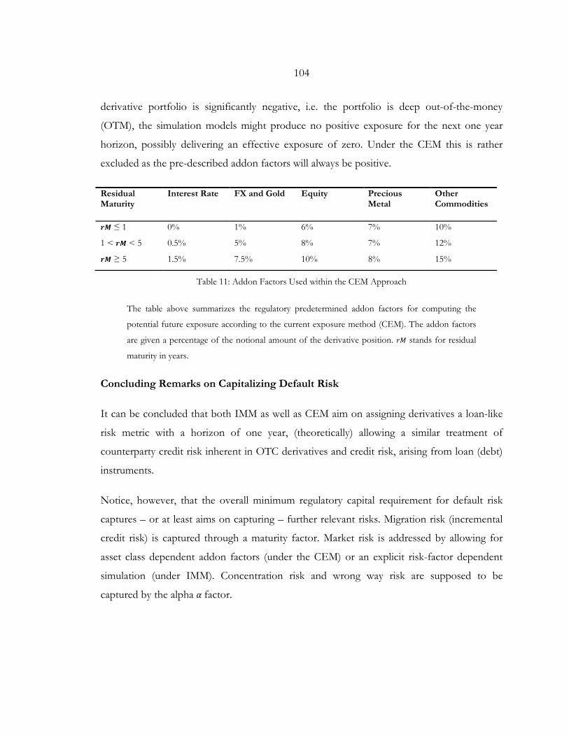
104

derivative portfolio is significantly negative, i.e. the portfolio is deep out-of-the-money

(OTM), the simulation models might produce no positive exposure for the next one year

horizon, possibly delivering an effective exposure of zero. Under the CEM this is rather

excluded as the pre-described addon factors will always be positive.

Residual Maturity

Interest Rate FX and Gold Equity Precious Metal

Other Commodities

𝒓𝒓𝒓𝒓 ≤ 1 0% 1% 6% 7% 10%

1 < 𝒓𝒓𝒓𝒓 < 5 0.5% 5% 8% 7% 12%

𝒓𝒓𝒓𝒓 ≥ 5 1.5% 7.5% 10% 8% 15%

Table 11: Addon Factors Used within the CEM Approach

The table above summarizes the regulatory predetermined addon factors for computing the

potential future exposure according to the current exposure method (CEM). The addon factors

are given a percentage of the notional amount of the derivative position. 𝑟𝑟𝑀𝑀 stands for residual

maturity in years.

Concluding Remarks on Capitalizing Default Risk

It can be concluded that both IMM as well as CEM aim on assigning derivatives a loan-like

risk metric with a horizon of one year, (theoretically) allowing a similar treatment of

counterparty credit risk inherent in OTC derivatives and credit risk, arising from loan (debt)

instruments.

Notice, however, that the overall minimum regulatory capital requirement for default risk

captures – or at least aims on capturing – further relevant risks. Migration risk (incremental

credit risk) is captured through a maturity factor. Market risk is addressed by allowing for

asset class dependent addon factors (under the CEM) or an explicit risk-factor dependent

simulation (under IMM). Concentration risk and wrong way risk are supposed to be

captured by the alpha 𝛼𝛼 factor.

105

The capital requirement measure is on no account a pricing metric as it is not based on

arbitrage-free or risk-neutral aspects, solely quantifying the risk inherent in the next year. It

can rather be qualified as a risk metric, based on historically estimated parameters that are

supposed to be prudent, not necessarily economically plausible.

CVA Capital Charge – Remarks

Adding a price adjustment to incorporate counterparty credit risk, e.g. in form of a CVA

metric, introduces additional price sensitivities. CVA depends on the credit quality of the

counterparty, usually quantified in terms of credit spread sensitivity (e.g. CS01). If for

instance the credit quality deteriorates and spreads widen, CVA will increase, leading to value

losses. Being exposure dependent, CVA exhibits also market risk sensitivity (e.g. DV01).

Decreasing interest rates will for instance boost the value of receiver swaps as well as their

expected exposure, subsequently enhancing CVA. In addition, CVA would also exhibit a

sensitivity to the correlation between credit spreads and the relevant risk factors.

The Basel Committee reports that during the financial crises two-third of the credit losses

incurred by financial institutions were driven by the overall deteriorating credit quality and

the increase of credit spreads (see BCBS, 2011). Losses incurred through counterparties

actually defaulting and filing bankruptcy accounted only for one-third of the credit losses

reported. This drove the Basel Committee to require for an additional capital charge. The

CVA capital charge aims on capitalizing CVA volatility arising from credit spread sensitivity.

Notice that the regulator (uncommented-wise) left further sensitivities of CVA, i.e. DV01

and gamma, not accounted for.

Basel III offers two alternatives for measuring CVA risk, a standard and an advanced

method. In the following we will give a brief account of both approaches.

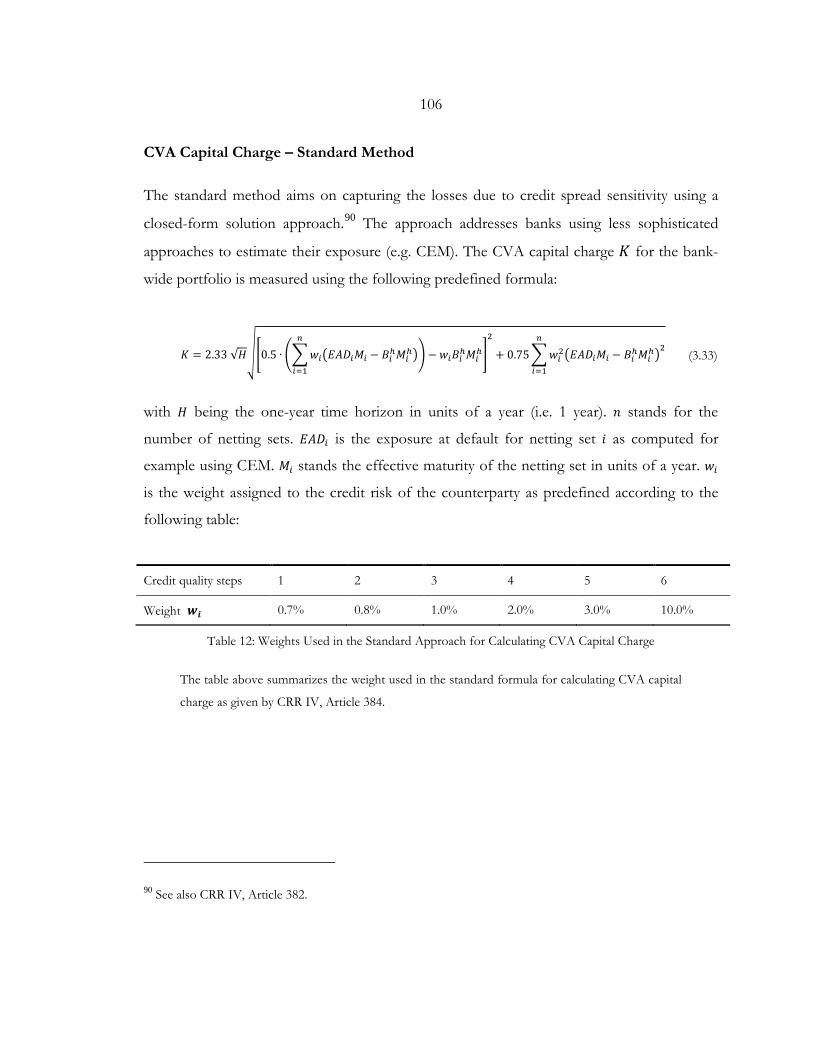
106

CVA Capital Charge – Standard Method

The standard method aims on capturing the losses due to credit spread sensitivity using a

closed-form solution approach.90 The approach addresses banks using less sophisticated

approaches to estimate their exposure (e.g. CEM). The CVA capital charge 𝐾𝐾 for the bank-

wide portfolio is measured using the following predefined formula:

𝐾𝐾 = 2.33 √𝐻𝐻��0.5 ∙ ��𝑤𝑤𝑖𝑖�𝐸𝐸𝐴𝐴𝐷𝐷𝑖𝑖𝑀𝑀𝑖𝑖 − 𝐵𝐵𝑖𝑖ℎ𝑀𝑀𝑖𝑖ℎ�

𝑛𝑛

𝑖𝑖=1

� − 𝑤𝑤𝑖𝑖𝐵𝐵𝑖𝑖ℎ𝑀𝑀𝑖𝑖ℎ�

2

+ 0.75�𝑤𝑤𝑖𝑖2�𝐸𝐸𝐴𝐴𝐷𝐷𝑖𝑖𝑀𝑀𝑖𝑖 − 𝐵𝐵𝑖𝑖ℎ𝑀𝑀𝑖𝑖ℎ�2

𝑛𝑛

𝑖𝑖=1

(3.33)

with 𝐻𝐻 being the one-year time horizon in units of a year (i.e. 1 year). 𝑛𝑛 stands for the

number of netting sets. 𝐸𝐸𝐴𝐴𝐷𝐷𝑖𝑖 is the exposure at default for netting set 𝑖𝑖 as computed for

example using CEM. 𝑀𝑀𝑖𝑖 stands the effective maturity of the netting set in units of a year. 𝑤𝑤𝑖𝑖

is the weight assigned to the credit risk of the counterparty as predefined according to the

following table:

Credit quality steps 1 2 3 4 5 6

Weight 𝒘𝒘𝒊𝒊 0.7% 0.8% 1.0% 2.0% 3.0% 10.0%

Table 12: Weights Used in the Standard Approach for Calculating CVA Capital Charge

The table above summarizes the weight used in the standard formula for calculating CVA capital

charge as given by CRR IV, Article 384.

90 See also CRR IV, Article 382.

107

Notice that the regulator explicitly allows the recognition of credit hedges. 𝐵𝐵𝑖𝑖 in the formula

above stands for the notional of a credit derivative, e.g. single name or index CDS,

protecting from the default of counterparty 𝑖𝑖.91

Pykhtin (2012) shows that the Basel III equation for CVA capital charge is the closed-form

solution of the value at risk based on a one-factor credit spread model with conservative

assumptions. Instead of using market implied volatilities for credit spreads the equation

relies on (conservative) constant risk weights.

CVA Capital Charge – Advanced Method

Under the advanced method the CVA capital charge is measured using a Monte Carlo

scheme in which the credit spreads for each counterparty are simulated and the CVA VaR is

subsequently computed, based on the following prescribed formula:92

𝐶𝐶𝑃𝑃𝐴𝐴 = 𝐿𝐿𝐺𝐺𝐷𝐷𝑀𝑀𝐾𝐾𝑇𝑇�𝑀𝑀𝑎𝑎𝑥𝑥 �0; 𝑒𝑒𝑥𝑥𝑝𝑝 �−𝑠𝑠𝑖𝑖−1𝑡𝑡𝑖𝑖−1𝐿𝐿𝐺𝐺𝐷𝐷𝑀𝑀𝐾𝐾𝑇𝑇

� − 𝑒𝑒𝑥𝑥𝑝𝑝 �−𝑠𝑠𝑖𝑖𝑡𝑡𝑖𝑖

𝐿𝐿𝐺𝐺𝐷𝐷𝑀𝑀𝐾𝐾𝑇𝑇��

𝑇𝑇

𝑖𝑖=1

∙ �𝐸𝐸𝐸𝐸𝑖𝑖−1𝑃𝑃𝑖𝑖−1 + 𝐸𝐸𝐸𝐸𝑖𝑖𝑃𝑃𝑖𝑖

2 � (3.34)

with 𝐿𝐿𝐺𝐺𝐷𝐷𝑀𝑀𝐾𝐾𝑇𝑇 standing for the loss given default ratio, based on market implied information.

𝑇𝑇 is the maturity of the netting set and 𝑡𝑡𝑖𝑖 stands for the respective future time period. 𝑃𝑃𝑖𝑖 is

the discount factor at time period 𝑖𝑖. 𝐸𝐸𝐸𝐸𝑖𝑖 is the expected exposure, considering possible

collateral and netting agreements, and based on the stressed calibration method as elaborated

above for EPE purposes. 𝑠𝑠𝑖𝑖 is the simulated credit spread at future time period 𝑖𝑖. Basel III

explicitly requires the use of market implied data to estimate the credit spreads, prescribing a

hierarchy of sources and a respective mapping approach. If possible banks should rely on

CDS spreads referencing to the counterparty. If such spreads are not available they are

91 Eligible hedges according to CRD IV, Article 386 are (a) single-name CDS or other equivalent hedging instruments referencing the counterparty directly; (b) index CDS.

92 See CRD IV, Article 383.

108

expected to develop a mapping procedure based on rating, industry and region of

counterparties.93

CVA is thus being modeled as a function of the same components as given in the practical

Equation (3.16) for CVA pricing: (1) LGD is clearly visible and is based on market implied

information, (2) the first part of the summation is the derived default probability, and (3)

stands for the discounted expected exposure as average between each two future time steps.

The VaR measure is computed using a 99% confidence level and 10-day horizon (in addition

to a predefined multiplier of three).

Banks are allowed to incorporate possible hedge positions that reduce credit sensitivity (e.g.

CS01). This means that credit hedges such as single name CDS can be modeled to reduce

the expected exposure profile, and thus the CVA VaR computed. Hedges aiming to reduce

other sensitivities, e.g. interest rate sensitivities, are on the other hand not considered as

eligible.

3.4.4. EVALUATION SUMMARY

As with other regulatory capital requirements the approaches described above exhibit certain

shortcomings and inconsistencies. After all, regulatory capital requirements can be seen as

following contradicting objectives. On the one hand they are supposed to display theoretical

soundness that is presumably aligned with the way “banks do business”. On the other hand

they are supposedly prudent, ensuring banks are sufficiently capitalized for extreme cases. In

the following we give a very short summary of the criticism against CVA capital charge, and

93 “Whenever the credit default swap spread of the counterparty is available, this must be used. Whenever such a credit default swap spread is not available, the bank must use a proxy spread that is appropriate based on the rating, industry and region of the counterparty.” CRD IV, Article 383, Paragraph 1.

109

will subsequently conclude with an own assessment of the requirements and their

consequences.94

Banks have criticized the misalignment of the approaches with how they calculate CVA, i.e.

with how “they do business”

Aiming to be theoretically sound the advanced approach (in line with accounting

requirements for fair value measurement) prescribes the use of market implied

parameters to estimate LGD and default probabilities (CDS spreads). Recall that

many banks have relied their valuation on historical and rating-based parameters.

Agnostic of the reasons – which have already been discussed in Subchapter 3.4.2 –

banks seem to advocate the use of theoretically inconsistent approaches, especially

contradicting the risk-neutral valuation scheme.

CVA capital charge has also been criticized for its prudency:

The advanced approach prescribes the use of stressed expected exposure measures,

i.e. the use of data from historical periods of distress to calibrate the exposure

models. This clearly deviates from risk-neutral valuation, which is behind the use of

market implied data. In the meanwhile the standard method prescribes the use of

EAD which is per se a conservative measure, standing for a different metric than the

exposure measures used for CVA calculation.95

In contrary to accounting standards the regulatory capital approaches focus only on

the unilateral CVA. Excluding DVA means that a “natural hedge” for the bilateral

CVA is not considered. After all, the credit spreads of the bank and its counterparty

might display a similar dependency to a common market factor. If CVA increases

94 For a more comprehensive overview of the industry’s criticism against the CVA capital charge methods we refer the reader to Gregory (2012), pp. 393-396.

95 The conservative assumptions used in the standardized approach have also been discussed, especially regarding the use of risk weights instead of market implied CDS volatilities.

110

due to a general market deterioration DVA will also increase, absorbing – at least to

some extent – some of the CVA volatility.

Both the standard and advanced approaches consider credit-sensitive hedges as

eligible. Holding a single name CDS referencing to the counterparty will for example

reduce the exposure and thus the CVA capital charge. Other hedges, e.g. interest rate

or FX hedges aiming to reduce the volatility of the CVA due to exposure changes

are, however, excluded.

Given CVA is a volatile number with significant impact on the P&L of a bank it is

straightforward that regulators are now requiring its capitalization. The more interesting

aspect about CVA capital charge and the associated discourse is that it gives an almost

school-book-like example of how regulatory-driven financial institutions actually are. It also

shows the tautology behind many of the discussions around regulatory requirements.

Yes, it can be argued that CVA is a volatile number that needs to be capitalized. Yet, it seems

that most banks started accounting for CVA in their financial statements after the

introduction of the regulatory requirements described above. Recent studies do show that

banks “have progressively converged in reflecting the cost of the credit risk of their counterparties in the fair

value of derivatives using market implied data based on CDS spreads and proxy spreads in the vast majority

of cases.”96 But as also acknowledged by the regulators “[t]his convergence is the result of industry

practice, as well as a consequence of the implementation […]of IFRS 13 and the Basel CVA framework.”

One could argue that the supply with regulatory capital requirements has produced its own

demand through insisting on using (volatile) marked implied data that increased the volatility

of banks' P&L statements. After all, it is only fair to note that risk-neutral and arbitrage-free

valuation presume traded hedging instruments that allow for a “duplication strategy”. As

discussed above this is hardly the case for CVA, especially when it is material at most.

Clinging to use market implied parameters without reflecting on their economic sense and

96 EBA (2015), p. 8.

111

most importantly on their consequences risks financial statements to aspire for something

they cannot deliver per se.97

If we, however, agree that financial statements should give a “true and fair view” then – as it

applies for all other plain-vanilla and exotic derivatives – considering CVA and measuring it

according to the fair value hierarchy is straightforward. Bearing in mind that the disclosed

CVA measures are a proxy at best, their bare existence increases the value of the financial

statements as it points to a significant risk, reducing at least some of the opaqueness

surrounding counterparty credit risk. After all, stakeholders that haven’t been aware of CVA

might make decisions without considering all relevant risks.98

Evidence indeed shows that banks have started to charge significantly more for

uncollateralized derivatives as a reaction to the new regulatory paradigm. A comparative

study coordinated by the Association for Financial Markets in Europe (AFME) and cited by

EBA (2015) claims for example that the costs associated with regulatory capital for

counterparties with a rating of BB have doubled. This indeed reveals that the lobby-like

pressure coming from the industry was not justified, and that the concerns articulated by the

Lufthansa manager quoted above hit the spot. A CVA capital charge would increase hedging

costs, possibly making them too punitive for counterparties with no access to liquid

collateral.

This also explains why the EU lawmakers have reacted to the pressure by allowing to exempt

transactions with non-financial counterparties such as Lufthansa.99 Interestingly, however –

97 The increased use of CDS spreads for CVA valuation has indeed increased the demand for CDS in the market which in return increased the level of CVA as shown for example by Bilal and Singh (2012).

98 Psychologists refer to the fact that humans tend to jump to conclusions based on limited evidence as WYSIATI, which stands for what you see is all there is, see Kahneman (2011), especially pp. 85-88.

99 The CRR exempts the following: (I) Transaction with non-financial counterparties below the EMIR clearing threshold, as codified in CRR Article 382(4)(a); (II) Transactions between clearing members and clients in the context of indirect clearing when the clearing member is acting as an intermediary between the client and a qualifying central counterparty - CRR Article 382(3); (III) Intragroup transactions - CRR Article 382(4)(b);

112

as EBA (2015) seemingly acknowledges – “accounting CVA is usually [already] reflected in the price

of derivative contracts”. The increased charges are thus only a function of the bank’s decision “to

also pass on the capital costs associated with the regulatory CVA risk charge to their counterparties”. In the

following we will take a second glance at this rather daring hypothesis that seems to pass

through without sufficient scrutiny.

Indeed, the CVA capital charge formulas are not equal to the formula used to price CVA

and supposedly also used to measure it for accounting purposes, as illustrated by Equation

(3.16). Still, both formulas are definitely not miles away from each other (especially under the

advanced approach). A bank that incorporates the (accounting) CVA will be double-

counting for a series of factors if it then fully incorporates the CVA capital charge on top.

Think of the (accounting) CVA as the hedge cost for counterparty credit risk. If we charge

these costs to the client then we should theoretically be able to hedge the exposure-

sensitivity as well as the credit-sensitivity of CVA. Hedging the latter is crucial as it will

minimize the regulatory capital requirement both under the standard and the advanced

methods. The remaining requirements will result from the prudency of the regulatory

requirements, especially the use of stressed exposure measures etc.

CVA capital charge will thus indeed lead to an increase in hedge costs. It is, however,

questionable whether that increase will be as significant as the evidence shows. It can rather

be concluded that the evidence discovers that banks have not been pricing for CVA

adequately in the past. This might be driven by the competitive market, cross-selling aspects

or the fact that people selling these product plainly did not think systematically about

counterparty credit risk, because no metric pointed to it.

The exemption rule will thus only help the industry if banks systematically misprice their

products, i.e. charging less for them than the hedge costs they imply. Interestingly banks also

(IV) Transactions with pension funds - CRR Article 382(4)(c) and CRR Article 482; and (V) Transactions with sovereign counterparties - CRR Article 382(4)(d)

113

pledged for these exemptions which might speak for a strong belief in cross-selling aspects

and the increased opaqueness they bring along. It might also speak for the fact that the risk-

neutral and arbitrage-free perspective – for right or for wrong – did not yet penetrate the

executive management levels of financial institutions.

If the above analysis can be synthesized into one key takeaway it is that financial institutions

are heavily driven by regulatory requirements. They do not only measure and manage their

risks according to detailed requirements they also trade and price according to such

requirements that originally aimed to actually mirror how banks “do business”. Bearing in

mind that regulatory requirements should set minimum standards for all financial institutions

it remains questionable if the detailed level of such requirements is beneficial. Especially

when it comes to topics like CVA where there is a lack of theoretical soundness and practical

experience it would be more beneficial to let a larger number of entities experiment than

having one entity prescribing everything in detail to the rest.

114

3.5. MANAGING AND MITIGATING CREDIT VALUATION ADJUSTMENT

3.5.1. MANAGING AND PRICING CVA

The previous subsections revealed the technical challenges around modeling CVA. They also

shed light on the evolving regulatory and accounting landscape. Agnostic of whether the

regulatory requirements increased the awareness of CVA or whether they are only a reaction

of its increased importance, derivative traders - especially banks - are faced with the

challenges of systematically incorporating counterparty credit risk into pricing. This implies

techniques for charging CVA to the client but also to allocate it across the organization in

order to allow for adequate incentives. In this subchapter we will give an overview of such

techniques, evaluating their effectiveness from the perspective of the management of a

financial institution as well as their counterparties.

The technical challenges around CVA, especially the discussions around estimating default

probabilities, revealed how shaky (if not even unscientific) CVA modeling can be. Lacking

theoretically sound valuation schemes at all times, traders - as they probably always do -

cannot base their pricing solely on mathematical considerations. Not incorporating CVA

into pricing can indeed lead to adverse selection in Akerlof’s (1970) sense as the bank will

not only face a problem of not covering costs through default, it will also draw a higher

proportion of counterparties with relatively high credit risk. Still, it may remain a well-taken

management decision to invest in order for example to increase market shares in a specific

segment or in order to reap cross-selling benefits from other products. In the following we

will discuss key issues around incorporating CVA into pricing. We will show that even when

it seems highly technical, the need for strategic and tactical considerations will prevail as all

decisions will be taken under a significant proportion of uncertainty.

115

Incremental CVA

As already discussed in previous subchapters exposure and thus CVA are calculated on

netting set level. If the instruments within a netting set do not exhibit offsetting effects, e.g.

if the derivatives are identical, then CVA on a netting set level will equal the sum of the

individual CVA metrics. If, however, the instruments do exhibit offsetting effects, e.g. a

netting set with payer and receiver swaps, the overall unilateral CVA will be smaller than the

sum of the individual instruments.100

In case of the unilateral CVA the relation can be formalized as follows:

𝐶𝐶𝑃𝑃𝐴𝐴𝑃𝑃 ≤�𝐶𝐶𝑃𝑃𝐴𝐴𝑖𝑖

𝑛𝑛

𝑖𝑖=1

(3.35)

with 𝐶𝐶𝑃𝑃𝐴𝐴𝑃𝑃 standing for CVA on a netting-set (portfolio) level. 𝑛𝑛 is the number of instruments

within the netting set, and 𝐶𝐶𝑃𝑃𝐴𝐴𝑖𝑖 is the CVA of the instrument 𝑖𝑖. This means that pricing

unilateral CVA on a standalone basis could be punitive if a netting set is in place. Pricing a

so-called incremental CVA allows the consideration of such offsetting effects. Estimating

the incremental CVA of a new trade includes the quantification of CVA on a netting-set

level before and after the trade has been introduced. The following equation formalizes this

relation

𝐶𝐶𝑃𝑃𝐴𝐴𝑖𝑖𝑖𝑖𝑛𝑛𝑏𝑏𝑟𝑟𝑏𝑏𝑚𝑚𝑏𝑏𝑛𝑛𝑡𝑡𝑠𝑠𝑓𝑓 = 𝐶𝐶𝑃𝑃𝐴𝐴𝑃𝑃+𝑖𝑖 − 𝐶𝐶𝑃𝑃𝐴𝐴𝑃𝑃 (3.36)

where 𝐶𝐶𝑃𝑃𝐴𝐴𝑖𝑖𝑖𝑖𝑛𝑛𝑏𝑏𝑟𝑟𝑏𝑏𝑚𝑚𝑏𝑏𝑛𝑛𝑡𝑡𝑠𝑠𝑓𝑓 stands for the incremental CVA of instrument 𝑖𝑖. 𝐶𝐶𝑃𝑃𝐴𝐴𝑃𝑃+𝑖𝑖 stands for CVA

of the netting set if instrument 𝑖𝑖 included, and 𝐶𝐶𝑃𝑃𝐴𝐴𝑃𝑃 stands for the CVA on netting set if

instrument 𝑖𝑖 is not included.

100 Notice that the effect on the bilateral CVA is not that intuitive, because the final metric is not only a function of the expected positive exposure but also of the expected negative exposure, and thus DVA. See also Gregory (2012), pp. 177-178.

116

From a pricing perspective charging for the incremental CVA seems the theoretically right

thing to do. A transaction gets charged with the CVA amount it contributes. This does,

however, imply certain challenges that will be discussed in the following.

First, incremental CVA is not additive, i.e. it is not possibly to allocate the portfolio CVA

metric to the different trades.101 This implies possible inconsistencies when simultaneously

trading a number of derivatives with the same counterparty while being interested in having

an incremental CVA metric for each trade. This pitfall seems more relevant for CVA

allocation, i.e. post pricing.

In addition, pricing incremental CVA implies that the unilateral CVA of a new trade does

not have to be positive. If a trade exhibits extreme offsetting effects, reducing the expected

exposure of a netting set, its incremental CVA would be negative.102 Assuming both

counterparties are equally informed and sophisticated a negative CVA would be an obvious

contractual prerequisite. OTC derivatives are, however, not always traded between equally

informed and sophisticated counterparties. One can question the willingness of a trader to

share a negative CVA with an uninformed counterparty, e.g. a buy-side (client) without the

technical capabilities. Also from a management perspective one can argue that flooring CVA,

e.g. by zero, would avoid too progressive a pricing, especially relevant for non-collateralized

client portfolios.

A further aspect of incremental CVA is its dependency on the order in which transactions

are traded. Think for example of a netting set with numerous derivatives, e.g. receiver and

payer swaps. The counterparties now plan to trade two mirroring instruments. The first

instrument (trade A) is a receiver swap (e.g. semi-annual payments of three-month Euribor,

101 See also Pykhtin and Rosen (2010). 102 As discussed above bilateral CVA does not have to be positive per definition, e.g. if the counterparty doing

the calculation has the worse credit quality or if the expected negative exposure is larger than the expected positive exposure.

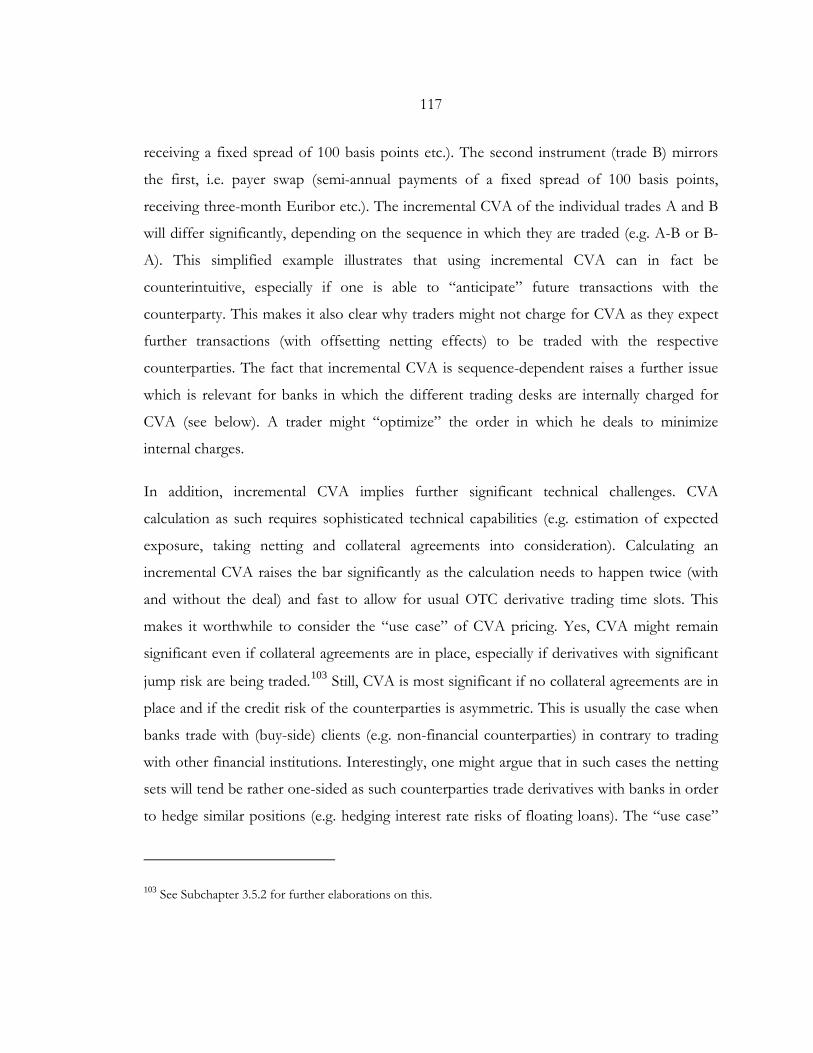
117

receiving a fixed spread of 100 basis points etc.). The second instrument (trade B) mirrors

the first, i.e. payer swap (semi-annual payments of a fixed spread of 100 basis points,

receiving three-month Euribor etc.). The incremental CVA of the individual trades A and B

will differ significantly, depending on the sequence in which they are traded (e.g. A-B or B-

A). This simplified example illustrates that using incremental CVA can in fact be

counterintuitive, especially if one is able to “anticipate” future transactions with the

counterparty. This makes it also clear why traders might not charge for CVA as they expect

further transactions (with offsetting netting effects) to be traded with the respective

counterparties. The fact that incremental CVA is sequence-dependent raises a further issue

which is relevant for banks in which the different trading desks are internally charged for

CVA (see below). A trader might “optimize” the order in which he deals to minimize

internal charges.

In addition, incremental CVA implies further significant technical challenges. CVA

calculation as such requires sophisticated technical capabilities (e.g. estimation of expected

exposure, taking netting and collateral agreements into consideration). Calculating an

incremental CVA raises the bar significantly as the calculation needs to happen twice (with

and without the deal) and fast to allow for usual OTC derivative trading time slots. This

makes it worthwhile to consider the “use case” of CVA pricing. Yes, CVA might remain

significant even if collateral agreements are in place, especially if derivatives with significant

jump risk are being traded.103 Still, CVA is most significant if no collateral agreements are in

place and if the credit risk of the counterparties is asymmetric. This is usually the case when

banks trade with (buy-side) clients (e.g. non-financial counterparties) in contrary to trading

with other financial institutions. Interestingly, one might argue that in such cases the netting

sets will tend be rather one-sided as such counterparties trade derivatives with banks in order

to hedge similar positions (e.g. hedging interest rate risks of floating loans). The “use case”

103 See Subchapter 3.5.2 for further elaborations on this.

118

of CVA pricing does not argue against incremental CVA. It does, however, put it into

proportion, facilitating a more adequate discussion around the importance and urgency of

implementing the respective technical capabilities. This explains why derivative traders rely

also on approximations for CVA pricing such as lookup tables with grids of predefined CVA

values, e.g. depending on the maturity and credit quality.104

Pricing DVA

As noted in Subchapter 3.4.2 above, if CVA is priced then some counterparties are (willingly

or not, knowingly or not) pricing DVA. This indeed sheds a different light on the discussion

around how counterintuitive it presumably is to price DVA. After all, the unilateral CVA,

calculated by one counterparty is the DVA of the other counterparty, independently of

whether one can monetize DVA or not. Still, it seems hard to detach the discussion around

pricing CVA and DVA from the pricer at hand, especially if the counterparties can be

classified as price setters or price takers, e.g. as is the case when financial institutions trade

with clients from industries other than financial services. While two banks trading would

accept and expect CVA and DVA to be priced in order to allow for fair contractual terms

and symmetrical pricing, a bank trading with a client (e.g. non-financial services corporation)

might be reluctant to price in its own counterparty credit risk, because of a variety of

reasons. (a) The trader might argue that his bank’s credit risk is negligible if compared with

the credit risk of the client. This can indeed be the case in many situations, making DVA

seem like theoretical (over-) complication with no real practical use; (b) The trader might see

himself as a service provider (and not as a counterparty on equal terms); (c) A reputational

issue might arise by “admitting” that the bank is default-prone in front of a client; (d) Lastly

DVA simply reduces the profit margin, leaving no incentive for the trader to price it in the

first place. The latter argument (d) might seem banal, but it is an important indication that

104 See also Gregory (2012), p. 411.

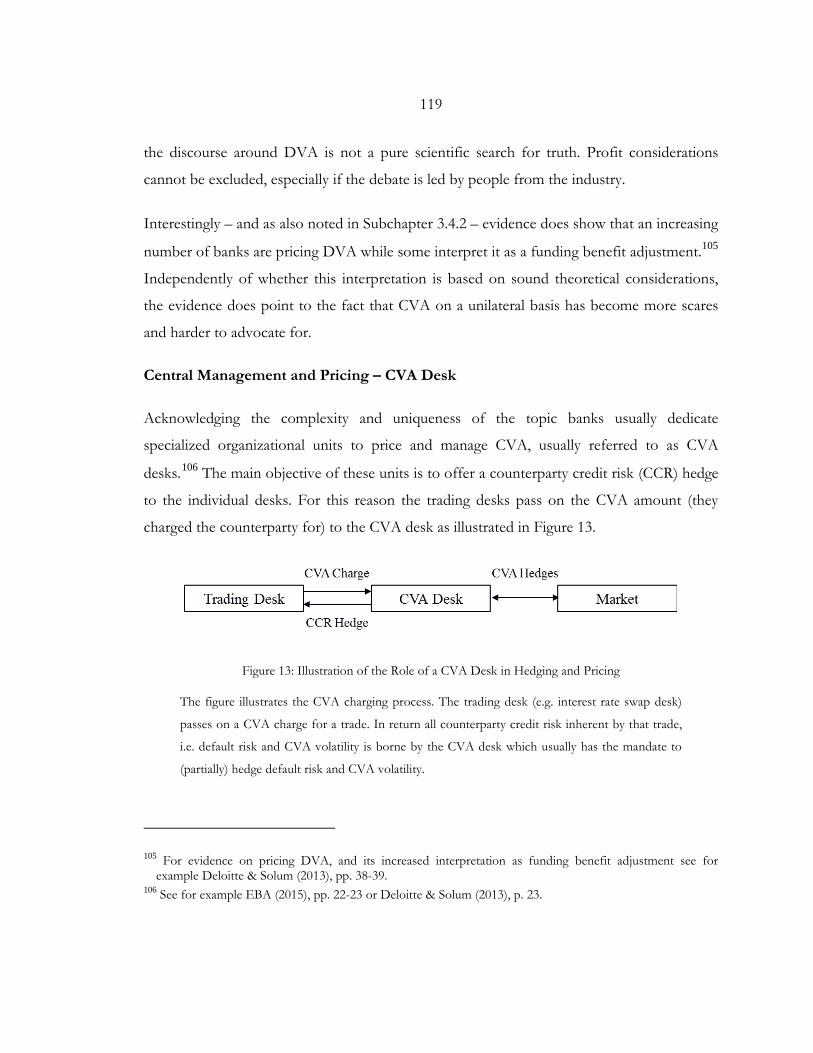
119

the discourse around DVA is not a pure scientific search for truth. Profit considerations

cannot be excluded, especially if the debate is led by people from the industry.

Interestingly – and as also noted in Subchapter 3.4.2 – evidence does show that an increasing

number of banks are pricing DVA while some interpret it as a funding benefit adjustment.105

Independently of whether this interpretation is based on sound theoretical considerations,

the evidence does point to the fact that CVA on a unilateral basis has become more scares

and harder to advocate for.

Central Management and Pricing – CVA Desk

Acknowledging the complexity and uniqueness of the topic banks usually dedicate

specialized organizational units to price and manage CVA, usually referred to as CVA

desks.106 The main objective of these units is to offer a counterparty credit risk (CCR) hedge

to the individual desks. For this reason the trading desks pass on the CVA amount (they

charged the counterparty for) to the CVA desk as illustrated in Figure 13.

Figure 13: Illustration of the Role of a CVA Desk in Hedging and Pricing

The figure illustrates the CVA charging process. The trading desk (e.g. interest rate swap desk)

passes on a CVA charge for a trade. In return all counterparty credit risk inherent by that trade,

i.e. default risk and CVA volatility is borne by the CVA desk which usually has the mandate to

(partially) hedge default risk and CVA volatility.

105 For evidence on pricing DVA, and its increased interpretation as funding benefit adjustment see for example Deloitte & Solum (2013), pp. 38-39.

106 See for example EBA (2015), pp. 22-23 or Deloitte & Solum (2013), p. 23.

120

The CCR hedge between the different desks and the CVA desk can take the form of an

internal contingent CDS (C-CDS) contract (discussed in Section 3.1 above). A perfect CCR

hedge means that the individual desks suffer no losses if the counterparty defaults nor do

they need to deal with additional volatility as a function of CVA changes. If the hedge is

based on a bilateral CVA it would also imply that individual trading desks do not profit (nor

do they lose) from deterioration (improvement) in the credit quality of their banks, avoiding

non-plausible P&L effects on trading desk level.

In addition, these units are supposed to ensure the following: (a) Complex decisions around

pricing and mitigating CVA (as well as DVA) are taken by employees with adequate training

and professional knowhow; (b) Possible diversification (netting) effects are considered. This

becomes especially relevant when considering effects within a multi-asset netting set; and

(c) Expertise to develop and run adequate modeling capabilities for the different CVA

components, e.g. expected exposure, collateral agreements, probabilities of default, wrong-

way-risk etc.

An essential question that needs to be discussed is whether CVA desks should operate as

profit generating units or as a cost center. After all, it seems intuitive for a trading

department to want to “make money” from CVA, and to incentivize the CVA desk to

operate accordingly. Doing that, the banks might, however, run the risk of incentivizing the

CVA desk to generate profits at the expense of the other trading desks or to increase the risk

positions, in misalignment with the overall trading strategy, e.g. through hedging CVA risk of

other banks or other proprietary (prop) trading positions. It might therefore seem more

promising to define the CVA desk as a so-called utility function. Gregory (2012, pp. 409-

410) uses the term to indicate that “the mandate of the CVA desk is to have a flat PnL”, while

commenting that “a zero PnL mandate on annual basis is still not ideal” as it might give rise to

wrong incentives. In addition he points to several measures that can reduce CVA without

automatically increasing the risk.

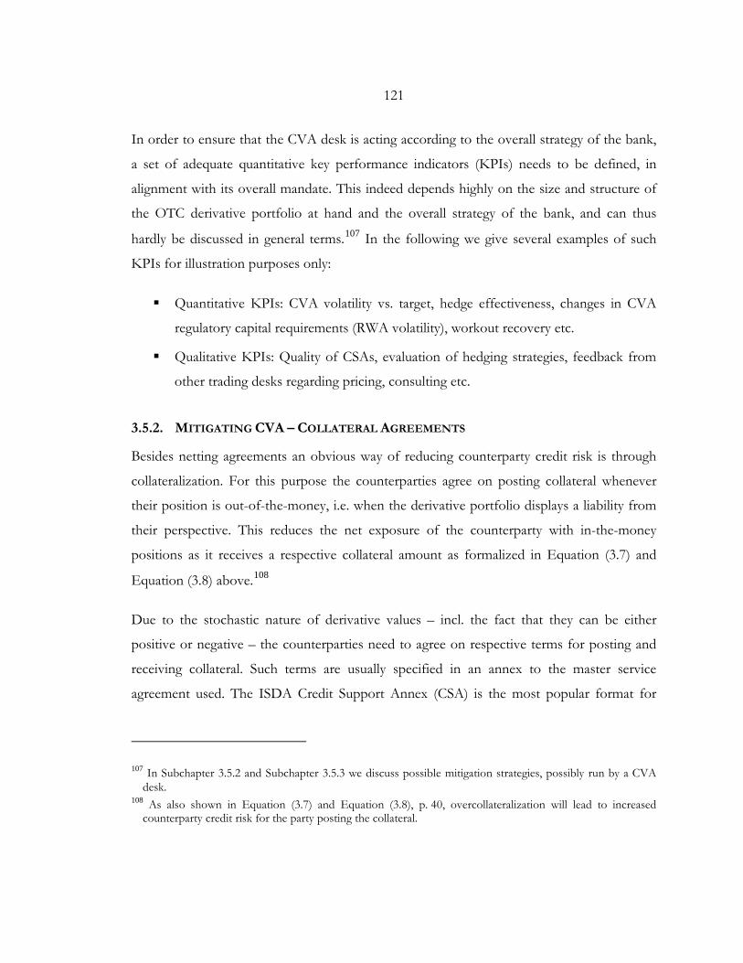
121

In order to ensure that the CVA desk is acting according to the overall strategy of the bank,

a set of adequate quantitative key performance indicators (KPIs) needs to be defined, in

alignment with its overall mandate. This indeed depends highly on the size and structure of

the OTC derivative portfolio at hand and the overall strategy of the bank, and can thus

hardly be discussed in general terms.107 In the following we give several examples of such

KPIs for illustration purposes only:

Quantitative KPIs: CVA volatility vs. target, hedge effectiveness, changes in CVA

regulatory capital requirements (RWA volatility), workout recovery etc.

Qualitative KPIs: Quality of CSAs, evaluation of hedging strategies, feedback from

other trading desks regarding pricing, consulting etc.

3.5.2. MITIGATING CVA – COLLATERAL AGREEMENTS

Besides netting agreements an obvious way of reducing counterparty credit risk is through

collateralization. For this purpose the counterparties agree on posting collateral whenever

their position is out-of-the-money, i.e. when the derivative portfolio displays a liability from

their perspective. This reduces the net exposure of the counterparty with in-the-money

positions as it receives a respective collateral amount as formalized in Equation (3.7) and

Equation (3.8) above.108

Due to the stochastic nature of derivative values – incl. the fact that they can be either

positive or negative – the counterparties need to agree on respective terms for posting and

receiving collateral. Such terms are usually specified in an annex to the master service

agreement used. The ISDA Credit Support Annex (CSA) is the most popular format for

107 In Subchapter 3.5.2 and Subchapter 3.5.3 we discuss possible mitigation strategies, possibly run by a CVA desk.

108 As also shown in Equation (3.7) and Equation (3.8), p. 40, overcollateralization will lead to increased counterparty credit risk for the party posting the collateral.

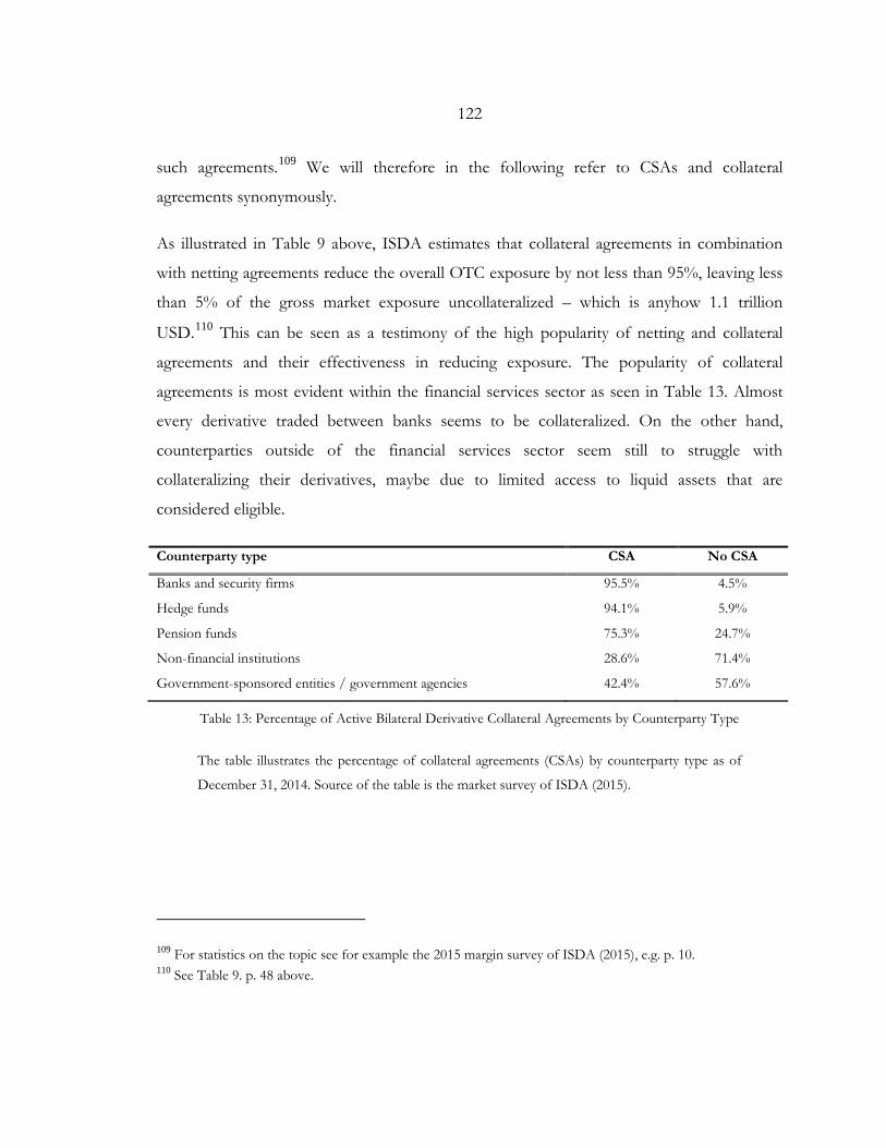
122

such agreements.109 We will therefore in the following refer to CSAs and collateral

agreements synonymously.

As illustrated in Table 9 above, ISDA estimates that collateral agreements in combination

with netting agreements reduce the overall OTC exposure by not less than 95%, leaving less

than 5% of the gross market exposure uncollateralized – which is anyhow 1.1 trillion

USD.110 This can be seen as a testimony of the high popularity of netting and collateral

agreements and their effectiveness in reducing exposure. The popularity of collateral

agreements is most evident within the financial services sector as seen in Table 13. Almost

every derivative traded between banks seems to be collateralized. On the other hand,

counterparties outside of the financial services sector seem still to struggle with

collateralizing their derivatives, maybe due to limited access to liquid assets that are

considered eligible.

Counterparty type CSA No CSA

Banks and security firms 95.5% 4.5%

Hedge funds 94.1% 5.9%

Pension funds 75.3% 24.7%

Non-financial institutions 28.6% 71.4%

Government-sponsored entities / government agencies 42.4% 57.6%

Table 13: Percentage of Active Bilateral Derivative Collateral Agreements by Counterparty Type

The table illustrates the percentage of collateral agreements (CSAs) by counterparty type as of

December 31, 2014. Source of the table is the market survey of ISDA (2015).

109 For statistics on the topic see for example the 2015 margin survey of ISDA (2015), e.g. p. 10. 110 See Table 9. p. 48 above.

123

Product type CSA No CSA

Commodity derivatives 59.1% 40.9%

Credit derivatives 97.0% 3.0%

Equity derivatives 91.3% 8.7%

Fixed-income derivatives 88.9% 11.1%

Foreign exchange derivatives 73.0% 27.0%

Table 14: Bilateral Derivative Collateral Transactions by Product Type

The table illustrates the percentage of collateral agreements (CSAs) by product type as of

December 31, 2014. Source of the table is the market survey of ISDA (2015).

As for example shown by Brigo et al. (2013b) or Lipton and Shelton (2012) collateral

agreements can reduce the expected exposure, and can thus have a mitigating effect on

counterparty credit risk and CVA. Still, a differentiated analysis is needed in order to

understand which risks remain despite having a CSA in place, and which new challenges

collateral agreements introduce. For this purpose we revisit and analyze the key

characteristics of CSAs (introduced shortly in Subchapter 3.3.3):111

i. Collateral type: The CSA defines the eligible type of collateral each counterparty needs

to post, e.g. cash, government bonds, corporate bonds etc. Cash can be seen as the

least risky collateral type.112 Still, an FX risk may arise if the currency of the collateral

differs from the currency of the derivatives. If, in addition, the CSA allows for cash

to be posted in more than one currency, e.g. EUR and USD a cheapest to deliver

option is introduced. Such an option might exhibit a considerable value which needs

to be taken into account as for example shown by Fujii and Takahashi (2011).

111 See also Cesari et al. (2009), pp. 190-191. 112 According to ISDA (2015) cash (especially USD and EUR) makes out around 75% of the collateral received

and delivered worldwide. The second most popular type are government securities (especially of the United States and member states of the European Union) who make ~18% of the collateral delivered.

124

Collateral becomes riskier if we turn to securities such as bonds (especially with

rather risky issuers) or even equities. To account for such risks counterparties might

agree on so-called haircuts.113 Posting securities such as bonds might imply

additional wrong-way risk that needs to be analyzed and considered. This is

especially relevant if the credit risk of the counterparty (e.g. state-owned bank),

posting the collateral, is highly correlated with the credit risk of the issuer (e.g.

government bond).

ii. Threshold: A threshold stands for the level underneath which collateral will not be

called. If the portfolio value exceeds the threshold collateral will be exchanged to

cover the surplus exposure. The threshold amount will remain uncollateralized.

Counterparties might agree on thresholds to reduce operational costs, but from a

CVA perspective they can be significant and need to be considered.114 Thresholds

can also be defined asymmetrically, i.e. the counterparties will have differing

amounts. This is especially relevant if one counterparty has an “unlimited” threshold

as this implies that it will never post collateral. In that case one can also refer to the

CSA as being one-sided.

From a modelling perspective thresholds can be relatively challenging if they can

change, e.g. if a rating downgrade triggers a lower threshold.115

iii. Minimum transfer amount (MTA): MTA is the amount which the collateral to be

exchanged needs to exceed before an exchange takes place. Because collateral can

only be exchanged in blocks that exceed the MTA it also resembles an

uncollateralized amount.

113 See also Gregory (2012), pp. 68-69. 114 See for example Cesari et al. (2009), especially pp. 190-194 or Gregory (2012), pp. 261-262. 115 According to ISDA (2015), especially p. 22, the most popular threshold methodology is based on credit

ratings.

125

iv. Margining frequency: The CSA also defines the frequency in which collateral is

exchanged (e.g. daily, weekly etc.). The bigger the time difference between each

collateral call the bigger the risk of the exposure changing, i.e. the bigger the risk of

having undercollateralized exposure.

This risk is of course also a function of the type of derivatives traded. Derivatives

with jump-like changes will have a higher probability of causing significant under

collateralization as shown by Brigo et al. (2011a) for CDS, especially with high

wrong-way risk. This can be seen as one factor driving the relatively high collateral

coverage of credit derivatives (97% CSA) as seen in Table 14.116

Daily margining – which can be considered as the least risky frequency – is especially

common among institutions with large OTC portfolios. This seems to remain a

challenge for institutions with smaller OTC portfolios that lack the operational

capabilities.117

Besides the contractual margining frequency one has to assess the risk that arises

when the counterparty defaults due to the time it takes to liquidate the portfolio, i.e.

close-out risk which as noted for example by Cesari et al. (2009, p. 195) need to be

taken into account when estimating CVA. For this purpose one assumes that default

can happen at any time, and adjusts the frequency in which collateral is called by a

so-called margin period of risk, i.e. the expected time it takes to complete the close-

out procedures after the counterparty has defaulted.118

Estimating the margin period of risk is not trivial and involves a number of

operational and legal aspects. Among others one has to estimate the time it takes to

re-valuate the positions, to receive the collateral (incl. disputes and settlement risk),

116 One might argue in addition that a further factor is the type of counterparty trading the different derivative types, i.e. credit derivatives are mostly traded by financial institutions etc.

117 ISDA (2015), p. 26, reports that especially among large portfolios (greater than 5,000 trades) daily reconciliation is the norm (87.1%) and expects this to be further driven by Dodd-Frank and EMIR regulations.

118 See for example Brigo et al. (2013a), p. 313.

126

and to liquidate the positions and structure new hedges.119 Institutions can also rely

on historical figures or regulatory requirements.120

v. Re-hypothecation: A further aspect that needs to be considered is whether the collateral

taker has an unrestricted right to lend and sell the collateral under a “repo” or re-

hypothecate it. Re-hypothecation is especially relevant for non-cash collateral

agreements, introducing a new credit risk for the counterparty that is posting the

collateral. After all, the collateral giver is now exposed to the risk of an additional

party (e.g. buyer of collateral) defaulting. Brigo et al. (2013a, p. 335) show that re-

hypothecation can have ludicrous consequences, making collateral agreements riskier

than having no collateral at all.

It can be concluded that collateral agreements can be an efficient tool to mitigate

counterparty credit risk. Having a collateral agreement in place does not, however,

automatically imply full-collateralization. CVA pricing and counterparty credit risk

management need to consider the above mentioned CSA characteristics in order to

adequately estimate future exposure. Even if the CSA is structured to enable full-

collateralization (i.e. cash collateral, zero MTA, zero (bilateral) thresholds with daily

frequency) the remaining close-out risk implies that the counterparty credit risk is not

eliminated. While on a trade level such risk might indeed be negligible this conclusion might

differ on a portfolio level, especially given a large OTC portfolio with risky counterparties.

3.5.3. MITIGATING CVA – HEDGING STRATEGIES

An institution can also decide to hedge its positions to mitigate counterpart credit risk and

reduce the CVA volatilities inherent in its books. In the following we will touch upon the

119 See for example Gregory (2012), pp. 146-148. 120 According to Gregory (2012), p. 147 (footnote 23), it took market participants around 5-10 business days to

complete close-out after Lehman Brothers defaulted. Basel III defines margin period of risk up to 20 days. See for example CRV IV, Article 285.

127

key issues around CVA hedging, analyzing the challenges in light of the regulatory

framework as well as the consequences it can have on the market as a whole.

A perfect hedge for CVA can be achieved through a single-name contingent credit default

swap (C-CDS), i.e. a CDS in which the protected amount equals the (stochastic) exposure at

default of a predefined counterparty. After all, CVA can be defined as the funds required to

duplicate a C-CDS, i.e. CVA is the value of such a contract.121 For this reason – as shortly

discussed in Subchapter 3.5.1 – internal deals between a possible CVA desk and the different

trading desks usually take the form of a C-CDS. Accordingly, a single-name C-CDS is

considered an eligible credit hedge that would reduce the regulatory CVA capital charge.122

Still, the use of C-CDS to hedge CVA externally is rather limited.123 Gregory (2012, pp. 347-

387) points out two obvious risks that C-CDS contracts might exhibit, possibly explaining

their relative low popularity:

a. Legal risk. C-CDS contracts need to reference to all the relevant trade economics of

all deals within the protected netting set (e.g. day-count-conventions, reference rates,

maturity dates etc.). Otherwise the protection seller and buyer will possibly run into

disputes with regards to the exposure amount at default. Notice that the legal

challenges increase if the netting set is adjusted regularly, e.g. through new trades and

novation of older ones. Such legal disputes might be indeed more manageable within

an institution which explains the feasibility to use C-CDS internally.

b. Joint default risk. The protection buyer runs a possible wrong way risk if the credit risk

of the protection seller and the reference entity are correlated. The quality of the

credit of the protection seller needs not only to be better than the reference entity,

121 As shown in Subchapters 3.1 and 3.3.1. 122 See also Subchapter 3.4.3 for CVA capital charge and eligible hedges. 123 In the survey conducted by EBA (2015) only one bank stated that it is uses C-CDS hedging. See also

Deloitte and Solum (2013), p. 33.

128

but also to display a rather low interdependency with it. Otherwise the protection

seller might default exactly when the protection buyer needs him most. This type of

wrong way risk is, however, not limited to C-CDS contracts and might be also

inherent in standard CDS contracts as well. We will dedicate a separate Chapter 4 to

discuss wrong way risk within CDS.

In addition to the above, C-CDS contracts display an enormous practical challenge for

protection sellers, because – as already noted by Cesari et al. (2009, p. 220) – a duplicating

strategy might be prohibitively expensive, and the hedging instruments could be illiquid, if

not inexistent. The statement might seem tautological, but it does mirror the challenges of

every institution seeking to hedge its CVA risk. After all, CVA exhibits sensitivities to a very

large number of factors that might also exhibit interdependencies between themselves. Using

a standard taxonomy of CVA sensitivities we will discuss key aspects around respective

hedging strategies:124

a. Credit sensitivities. CVA is sensitive to changes in the credit quality of a counterparty.

This includes CVA sensitivity to CDS spreads (delta), delta sensitivity to CDS spreads

(gamma), and CVA sensitivity to changes in the volatility of CDS spreads (vega).

A standard instrument to hedge these risks is a single name CDS. A perfect static

hedge using single name CDS would replicate the expected exposure profile, offering

a protection at each time point equaling the expected amount to be lost given a

default of the counterparty. As the exposure profile might change over time such a

static hedge would need rebalancing, implying respective additional costs.

Alternatively one might chose to keep the approximation of the exposure profile

rather gross or even decide to hedge only the average expected exposure (also

referred to as expected positive exposure, EPE), leaving parts of the exposure

(willingly) unhedged. Such a hedge would still reduce the P&L volatility, also offering

124 For more comprehensive elaborations on CVA hedging we refer the reader to Gregory (2012), pp. 339-369.

129

a partial hedge if the counterparty defaults. As illustrated in the example given in

Figure 14 below there is a payoff between an adequate credit protection and hedging

costs.125

If a single name CDS is not available or illiquid an institution might chose to hedge

the credit component using index CDS (e.g. iTraxx Europe Senior Financials). Such

a proxy will however not offer protection against the idiosyncratic credit risk of the

counterparty. It will offer a sensitivity hedge if the credit risk of the counterparty and

the index at hand display a high correlation. It does not, however, offer any

protection if the counterparty does default (if the index does not include a CDS

referencing to the specific counterparty).

From a regulatory perspective both single name CDS and index CDS are considered

eligible hedges. Having an eligible hedge in place reduces the exposure, subsequently

decreasing the CVA capital charge both under the standard and advanced methods

as seen in Equations (3.33) and (3.34), respectively. Notice, however, that both the

advanced and the standard method use rather prudent exposure methods as has been

discussed in Subchapter 3.4.4 above. This leads to a structural misalignment between

the regulatory CVA capital charge on one hand and with how CVA is computed for

financial accounting on the other. From a hedging perspective this implies a further

payoff that needs to be considered as both metrics demand differing hedging

strategies. For example – as has been described above – the standard approach is

based on a prudent exposure measure, exposure at default (EAD) which demands an

economic over-hedge in order to eliminate the CVA capital charge completely.

Evidence indicates that hedging CVA risk with CDS might lead to unintended

negative consequences.126 An increased use of CDS – especially in times of crises –

might cause a widening of CDS spreads. From the perspective of the institutions

125 For other possibilities to determine an optimal static hedge refer also to Cesari et al. (2009), pp. 220-221. 126 See also Carver (2011), Carver (2013) or Gregory (2012), pp. 360-361.

130

seeking to hedge their risk a widening of CDS spreads actually increases the level of

CVA, possibly triggering a loop of higher demands to hedge CVA and higher

hedging costs. From the perspective of debtors, widening credit spreads imply higher

debt issuance costs that in time of crisis might even be prohibitively high.127

Avoiding the negative consequences of such pro-cyclicality might have been one of

the reasons the European implementation of Basel III (CRD IV) exempts

transactions with sovereign counterparties from the CVA capital charge.

In addition, buying CDS to hedge counterparty credit will lead to an increase of

“naked” CDS positions in the market, i.e. situations in which the protection buyer

does not hold the original risk in form of debt securities (e.g. bonds) in his portfolio.

“Naked” positions are associated with pure speculation, and claims to ban them

found resonance in respective legislations, e.g. in Germany and in the EU.128 This

means that an investor interested in hedging the counterparty credit risk inherent in a

contract with an Italian sovereign will need to have an Italian government bond in

his portfolio. While the ban does seem to follow intended market regulation it does

contradict the Basel III accord which incentives the use of CDS for hedging

derivative (not only bond) exposure.

b. Exposure sensitivities. CVA is sensitive to the same factors that underlie the

counterparty credit risk-free value of the derivative. Given changes in the underlying

market factors the exposure profile will change, triggering a change in the CVA

metric as well. For example for the CVA metric of a standard interest rate swap the

respective sensitivities would include one to interest rate changes (delta) and a delta

sensitivity to interest rate changes (gamma) as well as sensitivity to changes in the

127 Bilal and Singh (2012) look at the link between CVA hedging and sovereign debt issuance in the European “periphery” (e.g. Greece, Italy etc.).

128 See for example Augustin (2014).

131

volatility of interest rates (vega).129 In that case the expected exposure profile can be

duplicated by a series of swaptions as shown by Sorensen and Bollier (1994).

A netting set would, however, usually include differing swaps (with differing

reference rates) as well as other derivative products (e.g. FX options, FX swaps etc.).

This sheds light on the complexity of deriving all relevant CVA sensitivities,

including the cross-gamma sensitivities between the different market factors (e.g.

correlation between three-month Euribor and USD/EUR exchange rate). Let alone

finding liquid hedging instruments. Theoretically such hedges can also increase the

overall CVA risk, depending on the quality of the counterparty with which they are

traded, especially if no collateral agreements are in place.

Whilst hedging against exposure sensitivity might reduce the CVA volatility, banks

are disincentivized to do so from a regulatory perspective. Hedges aiming to reduce

the exposure sensitivity are not considered as eligible, neither under the standard nor

under the advanced CVA capital charge approach. As seen in Equations (3.33) and

(3.34) none of the approaches is able to capture such hedges as mitigants.

Interestingly larger banks report that they do hedge for exposure sensitivity130,

aiming on reducing the P&L volatility, accepting the regulatory disadvantages.

c. Cross gammas. CVA displays a sensitivity to the interdependency between the

exposure and the credit quality of the counterparty, also referred to as cross gamma.

This brings us back to the concept of wrong way risk (and right way risk). As will be

discussed in the next Chapter 4 quantifying wrong way risk is rather complicated. Let

alone finding appropriate instruments to hedge it. As noted by Gregory (2012, p.

129 For delta hedging of interest rate risk see also Chapter 2 of this thesis. 130 See for example EBA (2015), pp. 88-91.

132

360) in most cases hedging wrong way risk will only be partial at best. In specific

cases strategies can be constructed.131

Cesari et al. (2009, p. 223) argue that the difficulties around hedging wrong way risk

are mitigated somewhat by the fact that the cross gamma is rarely the key risk driver.

On the other hand Brigo and Capponi (2010) or Hull and White (2011) discuss cases

in which wrong way risk is a key driver behind CVA risk.132

d. Own credit. Bilateral CVA exhibits a sensitivity to changes in the credit quality of the

institution, i.e. DVA. We have discussed the risks and challenges around hedging

DVA in Subchapter 3.4.2 above.

It can be concluded that while hedging can significantly help in mitigating CVA risk, an

institution cannot rely on it solely due to a variety of significant challenges. CVA of a given

netting set might exhibit sensitivities to a very large number of factors, incl. cross-gammas.

This implies technical challenges in measuring sensitivities that are accompanied with

significant model risks (e.g. measuring right way risk). Even if the sensitivities are measured

adequate hedging instruments with sufficient liquidity need to be available (e.g. single name

CDS). Hedging CVA has thus also to rely on proxies and alternative approaches. An

adequately manned CVA desk becomes crucial in finding such solutions. Consider for

example a bank that is interested in reducing its (net) exposure to a peer and is not able to

find adequate hedging instruments. CVA managers will need to “think out-of-the-box” in

order to find alternative solutions, e.g. borrowing money (e.g. through a loan) from the other

bank as it functions similarly to collateral etc.

131 Gregory (2012), p. 360 gives the example of an institution trading a cross currency swap with a sovereign. While the institution pays USD the sovereign pays in the local currency of the institution. By buying a local currency CDS and selling a USD CDS the institution ensures that the FX rate at default will be hedged.

132 See also Gregory (2012), pp. 358-359.

133

In addition, banks need to consider the structural misalignment between regulatory CVA

capital charge on the one hand and accounting standards on the other. The challenges will

differ from one institution to the other, highly depending on the OTC portfolio at hand as

well as the overall trading strategy of the bank.

For some institutions CVA hedging might indeed be unfeasible. Consider for example a

locally active tier 2 bank, offering OTC derivatives to its clients (mostly mid-sized local

companies with no liquid single name CDS). Most of the client OTC book is left

uncollateralized so that the counterparty credit risk is not insignificant. The bank hedges its

market risk positions (e.g. interest rate risk) through respective transactions with other banks

(usually a handful of tier 1 banks with bigger portfolios). These transactions are adequately

collateralized (with daily margining, no threshold etc.) so that the counterparty credit risk is

rather limited, and no hedging is needed. Still, the bank can be interested in hedging the

CVA risk inherent in its client book. With respect to credit sensitivity the bank can only

hedge some generic or sector risk, based on index CDS (as no single name CDSs are

available). There is, however, a good possibility that none of its counterparties can be

economically mapped to a respective index. This leaves the bank only with the possibility of

hedging the market risk component of CVA. Such a strategy might seem expensive if it only

reduces the CVA volatility, having no mitigating effect on the regulatory capital

requirements.

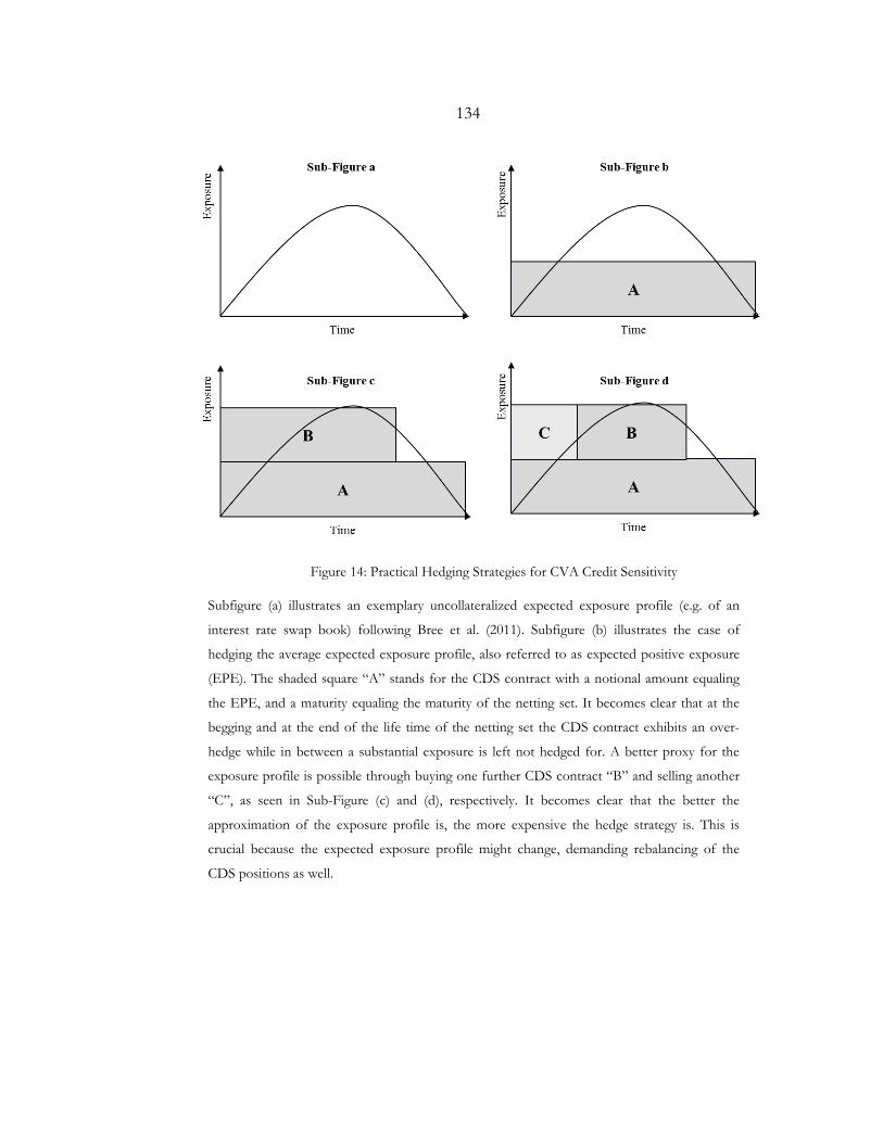
134

Figure 14: Practical Hedging Strategies for CVA Credit Sensitivity

Subfigure (a) illustrates an exemplary uncollateralized expected exposure profile (e.g. of an

interest rate swap book) following Bree et al. (2011). Subfigure (b) illustrates the case of

hedging the average expected exposure profile, also referred to as expected positive exposure

(EPE). The shaded square “A” stands for the CDS contract with a notional amount equaling

the EPE, and a maturity equaling the maturity of the netting set. It becomes clear that at the

begging and at the end of the life time of the netting set the CDS contract exhibits an over-

hedge while in between a substantial exposure is left not hedged for. A better proxy for the

exposure profile is possible through buying one further CDS contract “B” and selling another

“C”, as seen in Sub-Figure (c) and (d), respectively. It becomes clear that the better the

approximation of the exposure profile is, the more expensive the hedge strategy is. This is

crucial because the expected exposure profile might change, demanding rebalancing of the

CDS positions as well.

135

3.5.4. EVALUATION SUMMARY

The level of sophistication but also the mere feasibility of managing counterparty credit risk

and CVA depends highly on the institution at hand, especially the OTC derivatives strategy it

follows and the respective financial and technical capabilities it aspires. The bigger and more

complicated the OTC portfolio, the higher the inherent counterparty credit risk possibly is.

This means also that it becomes more worthwhile to invest in technical and management

infrastructures (e.g. CVA computation engine, CVA desk etc.) on the one hand. On the

other hand it also implies a widening of the spectrum of possible mitigation strategies, e.g.

introducing the possibility of hedging credit risk sensitivity due to a higher probability of

having counterparties with liquid CDS.

Still, counterparty credit risk and CVA aspects, incl. pricing and management issues are

relevant for every institution trading OTC derivatives, independent of its portfolio size and

complexity. This becomes apparent if regulatory requirements and accounting standards are

considered, especially the ones affecting financial institutions. As the below given example

of Bayer indicates, having elaborated capabilities to measure and manage counterpart credit

risk and CVA is not limited to banks. Head of corporate financial controlling at Bayer is

cited by a press release of a company offering IT solutions for counterparty credit risk and

CVA, saying:

“To help mitigate risks, Bayer decided to utilize the same risk management methodologies used

by some of the largest and most advanced global banks. [The IT solutions] enable Bayer to

determine, monitor and steer our counterparty risk accurately and consistently across our

counterparties. With the automated […] solution in particular, we are now able to calculate

136

Monte Carlo-based CVA and DVA and attribute the results accurately to the trade level,

even within netting sets, helping us to comply with regulations such as IFRS 13.133

Beyond complying with rules and regulations every institution trading OTC derivatives

should be aware of counterparty credit risk and CVA simply because if it does not, it might

get “punished” by the market. After all, many of the topics we have discussed in the

previous subchapters indicate much opaqueness around pricing CVA. This usually benefits

the more sophisticated and capable counterparties. By having minimal capabilities to price

and manage – or just to comprehend – CVA issues the less sophisticated and capable

counterparties limit their vulnerability. If for example a larger institution (e.g. tier 1

investment bank) approaches a (buy-side) client (e.g. health care company), and offers to

amend existing collateral agreements, e.g. lowering the thresholds. The client is well advised

to investigate the effects such an amendment would have on the expected exposure profile,

and thus CVA (and DVA), before agreeing.

A key takeaway from our discussion around CVA is that it reveals the limits of risk-neutral

valuation, especially when it comes to practical implementation of pricing models or

constructing adequate hedges. Clinging to use market implied parameters or elaborate

models that need overcomplicated calibration (e.g. first-to-default CVA models) without

reflecting on their economic sense might not only imply mere model and valuation risks, but

also significant financial risks at the latest when it comes to hedging CVA. While elaborate

and theory-based modeling is crucial to allow for intersubjective discussions around factors

driving CVA and subsequent consequences, every CVA manager will need to tailor his

management tools to his portfolio, focusing mainly on not being “arbitraged”.

133 See Sungard (2013). In the press release Bayer is defined as “[…] a global enterprise with core competencies in the fields of health care, agriculture and high-tech materials.”

137

CHAPTER 4:

PRICING CREDIT DEFAULT SWAPS WITH WRONG WAY RISK – MODEL

IMPLEMENTATION AND COMPUTATIONAL TUNE UP

4.1. INTRODUCTION AND LITERATURE OVERVIEW

One possibility for investors to mitigate counterparty credit risk is to buy protection in form

of a credit default swap (CDS) as discussed in the previous Chapter 3, esp. Subchapter 3.5.3.

In return for a premium, investors buying CDS contracts, receive protection for a certain

notional amount of debt of a predefined reference entity. CDS contracts can thus be used to

hedge the risk of the counterparty defaulting or its credit quality deteriorating.

We have, however, also extensively discussed the fact that all over-the-counter (OTC)

derivatives exhibit counterparty credit risk, and there is no reason why CDS contracts should

be an exception.134 After all, protection buyers now have an exposure to a new counterparty

with non-zero probability of default. Protection buyers can still benefit if the credit quality of

the protection seller is superior to that of the reference entity, especially if both

counterparties agree on posting collateral. If, however, the credit quality of both protection

seller and reference entity are positively interdependent, such a “protection” becomes

questionable if not worthless, since the protection seller might default exactly when needed

most.

This inherent wrong-way risk and the systemic risk accompanied by it are key reasons why

CDS contracts have been identified by some as contributors to the financial crisis, analyzed

for example by Mirochnik (2010) or Stulz (2010).135 In his article “Buffet’s ‘time bomb’ goes

134 For the definition of counterparty credit risk see for example Section 3.2 above. 135 Note that both cited papers do not use the term wrong way risk, which originates from counterparty credit

risk literature, e.g. Cesari et al. (2009).

138

off on Wall Street” Kelleher (2008) cites an interviewee, explaining the reasons behind the

crisis as follows:

"This was supposedly a way to hedge risk," […] "I'm sure their predictive models

[financial institutions] were right as far as the risk of the things they were insuring

against. But what they didn't factor in was the risk that the sellers of this protection wouldn't

pay... That's what we're seeing now."

Although the opinion of the interviewee around the predictive power of financial modeling

seems inappropriately flattering, the comment around the lack of consideration of possible

wrong way risk does hit the spot, especially when it comes to the fad of buying credit

protection against structured securities as collateralized debt obligations (CDOs) from

monoline insurers, i.e. insurance companies that traditionally provide coverage for one

insurance line.136

Monoline insurers were common underwriters of such CDSs in the years leading to the

subprime and financial crisis.137 According to ISDA (2011) by 2008 monoline insurers wrote

protections “on tens of billions of dollars” on CDOs on residential mortgage-backed securities

(RMBS), primarily referencing to subprime loans. This made them extremely sensitive to a

deterioration in the mortgage market. Still, monoline insurers had top ratings (mostly AAA),

granting guaranteed structured notes an almost credit-risk-free status even though monoline

insurers successfully resisted collateralization.138

136 Much of the information given in this Subchapter is backed by evidence from ISDA (2011). See also Brunnermeier (2009) for a qualitative analysis of the situation that led to the financial crisis also elaborating on the role of monoline insurance companies. Notice that as discussed in Jaffee (2006) monoline insurers focus on one product line due to legal restrictions. This means, paradoxically, that the significant concentration risk borne by monoliners can be attributed to regulation.

137 For more on the subprime crises and asset-backed securities see for example Longstaff (2010). 138 See ISDA (2011) according to which some monoliners did agree on posting collateral if downgraded.

139

Amid the plummeting of market prices for CDOs on RMBS in 2007 the investment

community seemed to have finally found the catch. Rating agencies started downgrading

monoline insurers while others had to file for bankruptcy. Market prices started accounting

for significant credit valuation adjustments (CVA) due to the deteriorating of the credit

quality of both reference entity and the protection seller. The significant CVA figures that

went through the profit and loss statements of the banks increased the demand for modeling

approaches that incorporate wrong way risk.139 Banks, hedge funds, monoline insurers, asset

managers, auditors, regulators – to name a few – were in the need for such models to

compute CVA consistently with the new prevailing view. In the following we will go through

some of the most prominent examples that tried to deliver appropriate solutions, motivating

our focus on Brigo and Capponi (2010).

In the spirits of Merton’s structural approach Blanchet-Scalliet and Patras (2008) derive

closed-form solutions for counterparty credit on a CDS. Yet, due to the focus on analytically

solvable dynamics their model cannot be fit to CDS spread quotes. Lipton and Sepp (2009)

present a multi-dimensional jump-diffusion structural model that can be calibrated to current

market information. The model demonstrates the significance of default correlation and

credit spread volatility while pricing CVA on CDS.

Leung and Kwok (2005) examine bilateral counterparty credit risk using a reduced form

framework with deterministic functions and contagious defaults. Based on the shifted

squared root (jump) diffusion (SSRJD) – previously introduced in Brigo and Alfonsi (2005)

– Brigo and Chourdakis (2009) introduce a unilateral CVA model with stochastic credit

spreads. They adopt stochastic intensity models for the default events, connected via a

Gaussian copula function. Brigo and Capponi (2010) generalize this approach. Assuming all

three entities are subject to interdependent default risk, they explicitly model what we have

139 In its survey of 12 international investment banks ISDA (2011) attributed CVA charges of more than $ 50 billion to monoline exposure.

140

referred to as first-to-default CVA (FTDCVA).140 This means that the model can be used to

analyze wrong-way risk as well as the presumable inconsistencies around pricing own credit

risk, i.e. DVA. We have therefore chosen to revisit this model and analyze it in detail.

Further model extensions were offered for example by Assefa et al. (2009) who introduce

netting and collateral agreements. Using a Markov chain copula Crepey et al. (2010) model

wrong way risk with possible simultaneous defaults. Li (2009) examine the effect of

stochastic recovery on CVA of CDS.

As mentioned, the following Chapter 4 is dedicated to analyze the approach offered by Brigo

and Capponi (2010). When appropriate we will also refer to the more comprehensive

elaborations and calculations given in Brigo and Capponi (2009) or Capponi (2009). We

introduce a step-by-step implementation guide and offer a computation tune up for the most

elaborate part of the computation, i.e. generation of the default probability structure of the

reference entity, conditional on the default of either the investor or the counterparty. For

this purpose Brigo and Capponi (2010) suggest the use of the Fractional Fourier

Transformation (FRFT) technique. The heuristic approach we suggest is based on an easy-to-

implement lognormal approximation. Throughout a variety of examples we show that this

approximation delivers rather robust and satisfying results, while requiring less

computational power and less excessive implementation. A case study based on real market

data demonstrates the use of the model and the insights it delivers. In addition, the codes

(written in R) used for the main functions of the algorithm are given in Appendix D.

The descriptive part is followed by a comprehensive critical evaluation of the Brigo and

Capponi (2010) approach in particular, and CVA modeling in general. We analyze both the

capability of the model in delivering an arbitrage-free framework as well as in its use for

inter- and intra-organizational communication. A specific feature of interest in this respect is

140 See also Subchapter 3.2 above.

141

the use of a copula function to model interdependency, a formula accused of “killing Wall

Street”.141 Besides revealing key challenges, risks and limitations of the model, the analysis

will also point to possible benefits and insights offered by such approaches.

The remaining of Chapter 4 is structured as follows. In Subchapter 4.2 we start with a short

introduction to CDS contracts, followed by an overview on structural and reduced form

credit modeling, explicitly elaborating on their use also for CVA modeling, given in

Subchapter 4.2.2. Subchapter 4.2.3 is dedicated to the use of (Gaussian) copula functions to

model default dependency. A detailed description of the model is given in Section 4.3. While

Subchapter 4.3.1 revisits the first-to-default CVA for CDS, Subchapter 4.3.2 gives an

overview of the algorithm. Subchapter 4.3.3. discusses the approach used to model

interdependent defaults, e.g. stochastic intensity approach in conjunction with a Gaussian

copula. In Subchapter 4.3.4 we revisit the computation of the conditional value of the CDS

given a default. We give a detailed guide for estimating the needed partial derivatives of the

Gaussian copula as well as the cumulative distribution function (CDF) using the method

suggested by Brigo and Capponi (2010), i.e. fractional Fourier transformation (FRFT)

technique. In the subsequent Subchapter 4.3.5 we offer a heuristic approach based on a log-

normal approximation of the CDF, reducing the complicity of the implementation and

speeding up the computation. Numerical examples are delivered both for understanding the

mechanism of the model in general and to back our heuristic approach in particular. The

case study given in Section 4.4 returns to our introductory example of monoline insurers

selling protection on structured notes. An evaluation of the approach is discussed in

Section 4.5. We conclude the chapter in Section 4.6.

Notice that the Chapter is an adaptation of previous work of the author published in

Grominski et al. (2012), and that some elaborations, especially in the computational part, are

141 See for example MacKenzie and Spears (2014).

142

identical. In order to avoid redundancy we will, however, refrain from continuously referring

to Grominski et al. (2012).

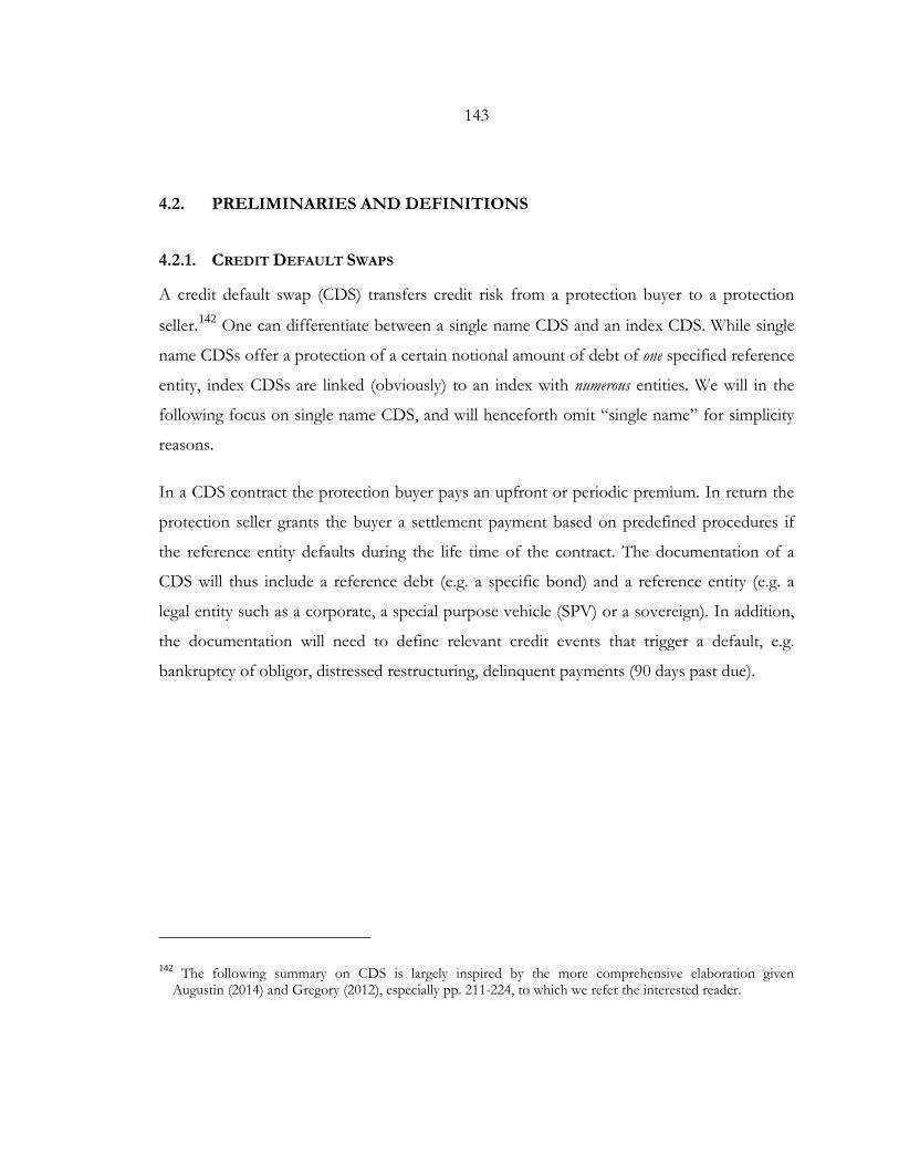
143

4.2. PRELIMINARIES AND DEFINITIONS

4.2.1. CREDIT DEFAULT SWAPS

A credit default swap (CDS) transfers credit risk from a protection buyer to a protection

seller.142 One can differentiate between a single name CDS and an index CDS. While single

name CDSs offer a protection of a certain notional amount of debt of one specified reference

entity, index CDSs are linked (obviously) to an index with numerous entities. We will in the

following focus on single name CDS, and will henceforth omit “single name” for simplicity

reasons.

In a CDS contract the protection buyer pays an upfront or periodic premium. In return the

protection seller grants the buyer a settlement payment based on predefined procedures if

the reference entity defaults during the life time of the contract. The documentation of a

CDS will thus include a reference debt (e.g. a specific bond) and a reference entity (e.g. a

legal entity such as a corporate, a special purpose vehicle (SPV) or a sovereign). In addition,

the documentation will need to define relevant credit events that trigger a default, e.g.

bankruptcy of obligor, distressed restructuring, delinquent payments (90 days past due).

142 The following summary on CDS is largely inspired by the more comprehensive elaboration given Augustin (2014) and Gregory (2012), especially pp. 211-224, to which we refer the interested reader.

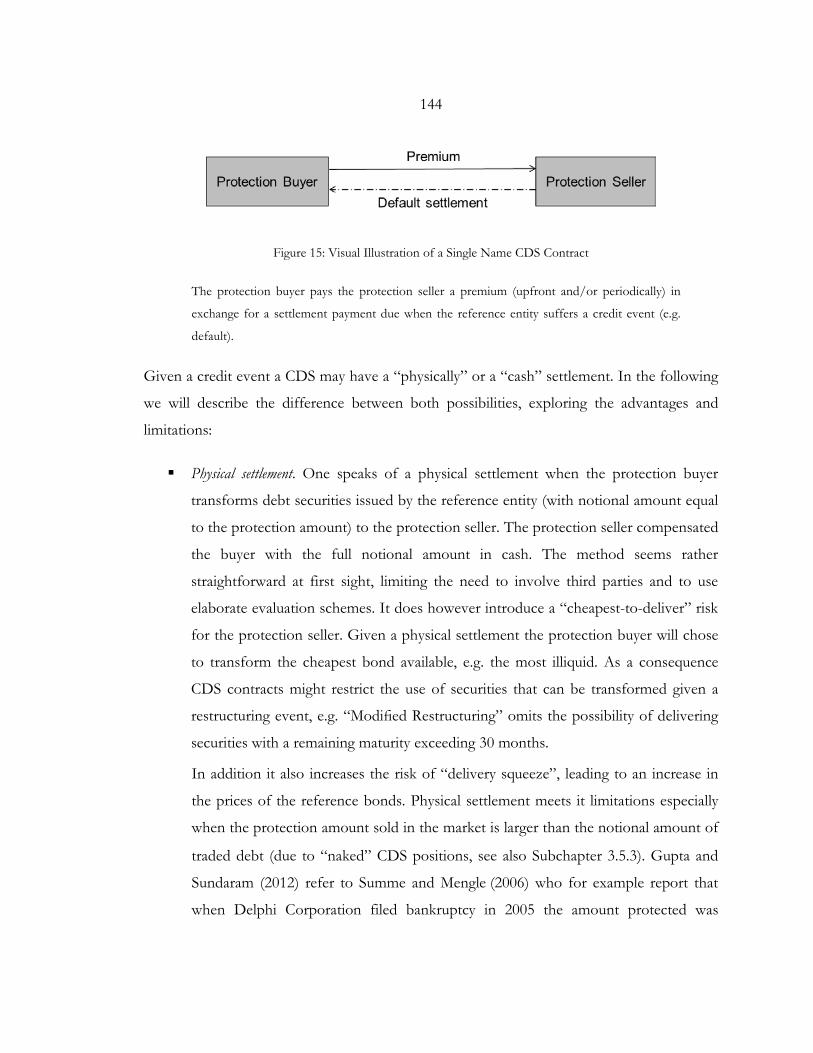
144

Figure 15: Visual Illustration of a Single Name CDS Contract

The protection buyer pays the protection seller a premium (upfront and/or periodically) in

exchange for a settlement payment due when the reference entity suffers a credit event (e.g.

default).

Given a credit event a CDS may have a “physically” or a “cash” settlement. In the following

we will describe the difference between both possibilities, exploring the advantages and

limitations:

Physical settlement. One speaks of a physical settlement when the protection buyer

transforms debt securities issued by the reference entity (with notional amount equal

to the protection amount) to the protection seller. The protection seller compensated

the buyer with the full notional amount in cash. The method seems rather

straightforward at first sight, limiting the need to involve third parties and to use

elaborate evaluation schemes. It does however introduce a “cheapest-to-deliver” risk

for the protection seller. Given a physical settlement the protection buyer will chose

to transform the cheapest bond available, e.g. the most illiquid. As a consequence

CDS contracts might restrict the use of securities that can be transformed given a

restructuring event, e.g. “Modified Restructuring” omits the possibility of delivering

securities with a remaining maturity exceeding 30 months.

In addition it also increases the risk of “delivery squeeze”, leading to an increase in

the prices of the reference bonds. Physical settlement meets it limitations especially

when the protection amount sold in the market is larger than the notional amount of

traded debt (due to “naked” CDS positions, see also Subchapter 3.5.3). Gupta and

Sundaram (2012) refer to Summe and Mengle (2006) who for example report that

when Delphi Corporation filed bankruptcy in 2005 the amount protected was

145

estimated to be around $28 billion while the notional amount in deliverable bonds

was merely $2 billion.

Cash settlement. As no securities are delivered under a cash settlement the protection

seller will only need to compensate the protection buyer for the incurred loss, i.e. the

difference between the par value and the recovery value. While introducing a

possible solution for the delivery squeeze, cash settlement imply a process for

determining the recovery value such as auctions.143

The use of credit default swap (CDS) is controversial at best, as analyzed for example by

Stulz (2010). While praised as innovative solutions that transform risk to those best suitable

to bear it, they have also been associated with the financial crisis, e.g. due to “naked” CDS

positions taken for pure speculation. Prominent figures such as the investor Warren Buffer

have referred to them as “time bombs” and others such as hedge fund manager George

Soros pleaded to ban them completely.144 In order to limit the effect of speculation on CDS

and the associated cost of issuing debt, the EU banned the use of “naked” CDS for

respective sovereign reference entities (see also Subsection 3.5.3). In the meanwhile the

regulatory framework Basel III recognizes CDS as eligible collateral. Basel III as well as

international accounting standards demand the use CDS spreads for counterparty credit risk

and CVA measurement (see also Section 3.4).

One might be aware of the possible limitations and market distortions, CDS contracts cause,

and still be interested in using the information they imply. Especially from a no-arbitrage

theory perspective CDS (spreads) are crucial as they determine respective prices and

conditions under which one excludes being arbitraged, agnostic of whether the market turns

out to be “mispriced”. In the subsequent Subchapter we will revisit two approaches for

143 Gupta and Sundaram (2012) analyze the CDS auctions and possible informative biases. They also describe in detail the auction process designed by ISDA and auction administrators CreditEx and Markit.

144 See Berkshire Hathaway (2002) and Soros (2009).

146

modelling credit, elaborating on the use CDS spreads to generate risk-neutral probabilities of

default.

4.2.2. MODELING CREDIT RISK – STRUCTURAL VS. REDUCED FORM MODELS

Two broad approaches have emerged in literature to model credit risk: structural (or firm-

value) models, based on the work of Black and Scholes (1973) and Merton (1974), and

reduced form – also referred to as intensity or hazard rate models given a suitable context –

models that go back to Jarrow and Turnbull (1992) and Duffie and Singleton (1999). In the

following we will give a short overview of the “two competing methodologies” (Bielecki and

Rutkowski 2001, p. 26), linking both to CVA literature and the explored model approach

introduced by Brigo and Capponi (2010). The description given below is inspired by Bielecki

and Rutkowski (2001), Brigo et al. (2013a, esp. pp. 48-86) and Jarrow et al. (2003) to which

we refer the interested reader for more comprehensive elaborations.

Structural models

Structural models relate default to an economic variable (e.g. firm value). A default is

triggered when the economic variable crosses a pre-defined threshold (or barrier). This

methodology goes back to the model introduced by Merton (1974) in which firm assets

follow a lognormal distribution and the firm is assumed to be financed both by equity and

debt (in form of a finite zero coupon bond). The model postulates that the firm defaults if

the notional amount of its debt exceeds the value of its assets (only) at the time of maturity.

The equity value can thus be viewed as a European call option on all assets of the firm. The

option matures with the zero bond and the strike price equals its face value. The Merton

approach shows two kern elements of this category of models: a) Key issue within this

methodology are modelling assumptions around the evolution of the firm’s value and the

firm’s capital structure. For this reason they are referred to as “structural” or “firm value”

models, and b) Structural models usually base these assertions on option pricing models,

using these also to calibrate probabilities of default.

147

Black and Cox (1976) offered a notable extension to the Merton approach by introducing

continuous default barrier, i.e. relaxing the assumption that default can happen only at debt

maturity. Many extensions and generalizations have been offered. Prominent examples that

introduced stochastic interest rates were Shimko et al. (1993), Nielsen et al. (1993) and

Longstaff and Schwartz (1995). More complex debt structures were modelled for example by

Leland (1998) and Tauren (1999).

The implied default probability of these models for a company with a high credit quality in

the short-term is close to zero, especially contrasting high near term CDS spreads. For this

purpose further extensions were introduced for example by Hull and White (2001),

incorporating curvilinear barrier. Jumps in a firm’s value were introduced for example by

Lipton (2002) and Sepp (2004, 2006).

Structural models are seen as elegant, because they are motivated with economic reason,

allowing investors’ expectations of firm’s future performance to be considered. Moreover,

structural models can be seen as forward looking with evidence of explanatory power as for

example discussed in Arora et al. (2005). In addition, they imply an arbitrage relationship

between equity and debt which can be informative when it comes to analyze relative pricing

of respective financial instruments. Indeed structural models have found their way into the

center of “mainstream” risk management. As discussed in Jarrow and Turnbull (2000) they lay

the foundations for prominent risk management services such as Moody’s KMV and

CreditMetrics. More importantly – through the asymptotic single risk factor (ASRF)

approach discussed in Subchapter 3.4.3 – they display the backbone of the Basel regulation

framework, clearly influencing measurement and capitalization of credit risk.

As noted above a variety of CVA structural models, considering wrong-way risk have been

introduced, e.g. Blanchet-Scalliet and Patras (2008), Lipton and Sepp (2009) and Lipton and

Savenscu (2013).

148

As shown by Jarrow and Protter (2004) structural approaches have a restrictive assumption,

implying that modelers have “continuous and detailed information about all of the firm’s assets and

liabilities.” More importantly they show that the modelers and firm’s managers (and

regulators in the case of commercial banks) would all have to hold the complete information

about default time and expected recovery, meaning also that the default time is always

predictable. Moreover, from a pricing perspective structural models are still regarded as

limited, because they generally provide a poor fit of market information, particularly

underpricing short term securities as for example discussed in Jarrow et al. (2003) or

Capponi (2009). Moreover, as shown for example by Brigo et al. (2013a, p. 65 or p. 80)

structural models can be challenging when it comes to practical calibration, especially when

the credit risk of more than three entities is involved.

Reduced form models

In contrary to structural models reduced form models do not proclaim any economic

rationale behind default which is not triggered by observable variables but is given through

an exogenously driven jump process, i.e. a Poisson process with stochastic or deterministic

intensity. Modelling default through an exogenous process frees reduced form approaches

also from assumptions around firm’s assets and its capital structure. It also implies that

default becomes unpredictable.

Main motivation behind intensity models is their suitability to model credit spreads and the

easiness in which they can be calibrated to CDS quotes. Prominent examples of reduced

form models were given by Jarrow and Turnbull (1992), Madan and Unal (1998), Duffie and

Singleton (1999), Hull and White (2001) as well as Brigo and Alfonsi (2005). This list is not

exhaustive and can be easily extended.

Following the notations given by Brigo et al. (2013a, esp. pp. 66-77) we will reintroduce the

main assumptions and features behind reduced form models. For this purpose we assume

149

that default time 𝜏𝜏 is the first jump of Poisson process. Given no default has occurred yet,

the (risk-neutral) probability ℚ of defaulting in the next 𝑑𝑑𝑡𝑡 is

ℚ(𝜏𝜏 ∈ [𝑡𝑡, 𝑡𝑡 + 𝑑𝑑𝑡𝑡]|𝜏𝜏 > 𝑡𝑡, market info up to 𝑡𝑡) = 𝜆𝜆(𝑡𝑡)𝑑𝑑𝑡𝑡. (4.1)

with 𝜆𝜆(𝑡𝑡)𝑑𝑑𝑡𝑡 standing for intensity or hazard rate which – for simplicity reasons - is assumed

to be strictly positive. It can be seen as an ad-hoc combination of market and financial

variables. The intensity function can be fit to market data (e.g. CDS spreads), and is the

exogenous force related to the dynamics of the firm at hand. The cumulative intensity

function Λ is given as

Λ(𝑡𝑡): = ∫ 𝜆𝜆𝑡𝑡0 (𝑢𝑢)𝑑𝑑𝑢𝑢. (4.2)

Recall that the transformation of the jump time 𝜏𝜏 of a Poisson process according to its own

cumulated intensity Λ gives an exponential random variable, i.e.

Λ(𝜏𝜏) = : 𝜉𝜉 ∽ standard exponential random variable with mean 1 (4.3)

with 𝜉𝜉 being independent of all other variables, e.g. interest rates, equities, and other

(stochastic) intensities etc. Notice that exactly this independence and stochasticity of 𝜉𝜉 are

what allow reduced form models to assume incomplete markets, produce unpredictable

defaults and allow for instantaneous credit spreads to be different from zero.

Inverting the Equation (4.3) leads to

𝜏𝜏 = : Λ−1(𝜉𝜉) (4.4)

which illustrates why 𝜉𝜉 are also referred to as default triggers. The survival probability at time

period 𝑡𝑡 is given as follows

ℚ{𝜏𝜏 > 𝑡𝑡} = ℚ{Λ(𝜏𝜏) > Λ(𝑡𝑡)} = ℚ{𝜉𝜉 > Λ(𝑡𝑡)} = 𝔼𝔼ℚ �𝑒𝑒−∫ 𝜆𝜆(𝑢𝑢)𝑒𝑒𝑢𝑢𝑡𝑡0 � (4.5)

because the cumulative distribution function (CDF) of a standard exponential random

variable is given by ℚ{𝜉𝜉 ≥ x} = 𝑒𝑒−𝑓𝑓.

150

Looking at Equation (4.5) it becomes clear that the survival probability is just the price of a

zero coupon bond while the stochastic intensity process replaces the stochastic interest rate

process, usually noted with 𝑟𝑟. This allows us to interpret intensities as instantaneous credit

spreads. Now assuming that the intensity 𝜆𝜆 is constant then pricing formula for a bond is

simplified to

𝑃𝑃(𝑡𝑡,𝑇𝑇) = 𝑒𝑒−(𝑟𝑟+𝜆𝜆)(𝑇𝑇−𝑡𝑡), (4.6)

displaying the similarity between the intensity (or hazard rate) and the credit spread more

clearly. Analogously practitioners make an intensive use of the following formula

𝜆𝜆 = 𝑅𝑅0.𝑏𝑏𝑀𝑀𝐼𝐼𝐷𝐷(0) 𝐿𝐿𝐺𝐺𝐷𝐷

(4.7)

with 𝑅𝑅0.𝑏𝑏𝑀𝑀𝐼𝐼𝐷𝐷(0) standing for the mid-market spread of a CDS, running from time period 0 to b.

Despite the fact that this formula is an approximation at best it is popular among

practitioners, especially for quick plausibility checks. After all, it is very simple as it does not

require any extensive calculation or assumptions, e.g. regarding interest rates dynamics.

Moreover, it intuitively relates CDS spreads to probabilities of default.145

It is of course more realistic to assume credit spreads – and thus intensities – to be volatile.

As noted survival probabilities can be interpreted as zero coupon bond prices. This implies

that stochastic interest rate models can be used to model intensity. Recall that the intensity

process is strictly positive, excluding some interest rate models (e.g. Gaussian models).

Flexibility and analytical tractability makes Cox Ingersoll Ross (CIR) processes especially

appealing in this case. Their suitability is studied for example by Brigo and Alfonsi (2005),

Brigo and Cousot (2006) or Brigo and El-Bachir (2008). Also Brigo and Capponi (2009,

2010) model intensity using a shifted CIR process (i.e. with a drift term to ensure an exact fit

of the term structure) as will be elaborated in more detail below. In principle, the CIR

145 For the proof of this equation we refer the interest reader to Brigo et al. (2013a), pp. 70-71.

151

process they use incorporates an additional jump term that Brigo and Capponi (2010),

however, omit in the implementation part of their paper.

The fact that intensity models lack an economic rationale can be seen as a weakness.

Moreover, Arora et al. (2005) argue that the flexibility of intensity models to fit observable

data makes them more prone to focus on in-sample fitting properties while displaying poor

out-of-sample predictive ability. While this argument might be worth analyzing from a credit

risk management or rating perspective, it is rather irrelevant for arbitrage-free pricing. In

contrary, the intuitiveness and tractability in which reduced form approaches presumably

depict market implied information makes it worthwhile to analyze their application to

pricing, incl. arbitrage free CVA modeling.

4.2.3. COPULA FUNCTIONS – MODELING MULTINAME DEFAULTS

Modeling default dependency is central when it comes to bilateral CVA, especially in the

case of CDS with wrong way risk. For this purpose reduced form approaches are usually

enriched with copula functions.146 A prominent examples is given by Schönbucher and

Schubert (2000).147 Copulas introduce a very general manner to model dependence of

random variables. Theoretically there is an infinite number of possible copula functions. Due

to the scarcity of data on default interdependence Schönbucher (2005), however, advices to

use more convenient low-parametric families of copula functions. One such function is the

Gaussian copula used in the approach of Brigo and Capponi (2010). Other examples include

the t-copula and the Archimedean copulae.148

146 See also Brigo et al. (2013a), especially pp. 78-86, that have inspired the elaboration on Copula functions. For alternative approaches to model correlated defaults (e.g. correlated intensity functions) see also Duffie and Singleton (2003), especially pp. 229-249.

147 The use of copulas to model dependency in general is attributed to Li (2000) as well as Frey and McNeil (2003).

148 See also McNeil et al. (2005), especially pp. 184-237.

152

In the following, we provide a definition for copula functions in general and the Gaussian

copula in particular. In addition, we provide the procedure for generating triggers of default

on the basis of a Gaussian copula.

Following Schönbucher (2005), a copula function can be defined as follows

Definition 1 A function 𝐶𝐶 ∶ [0, 1]𝐼𝐼 → [0, 1] is a copula if there are uniform random variables

𝑈𝑈1, … ,𝑈𝑈𝐼𝐼 with values in [0,1] while 𝐶𝐶 is their joint distribution function. 𝐶𝐶 has uniform marginal

distributions, meaning for all 𝑖𝑖 ≤ 𝐼𝐼; 𝑢𝑢𝑖𝑖 ∈ [0,1] there is

𝐶𝐶(1, … ,1,𝑢𝑢𝑖𝑖 , 1, … ,1) = 𝑢𝑢𝑖𝑖. (4.8)

According to Sklar's Theorem as given below, any multivariate distribution function 𝐹𝐹 can

defined as a copula.

Theorem 1 (Sklar) 𝑋𝑋1, …𝑋𝑋𝐼𝐼 are random variables with the following marginal distribution functions

𝐹𝐹1,𝐹𝐹2, … ,𝐹𝐹𝐼𝐼. If their joint distribution function is 𝐹𝐹, then there exists a copula (𝐼𝐼-dimensional) 𝐶𝐶 such that

for all (𝑥𝑥1, … , 𝑥𝑥𝐼𝐼) ∈ ℝ:

𝐹𝐹(𝑥𝑥1, … , 𝑥𝑥𝐼𝐼) = 𝐶𝐶�𝐹𝐹1(𝑥𝑥1),𝐹𝐹2(𝑥𝑥2), … ,𝐹𝐹𝐼𝐼(𝑥𝑥𝐼𝐼)�. (4.9)

This implies that 𝐶𝐶 is the distribution function of �𝐹𝐹1(𝑥𝑥1),𝐹𝐹2(𝑥𝑥2), … ,𝐹𝐹𝐼𝐼(𝑥𝑥𝐼𝐼)�. Whenever 𝐹𝐹1,𝐹𝐹2, … ,𝐹𝐹𝐼𝐼 are

continuous 𝐶𝐶 will be unique. If not, 𝐶𝐶 will be uniquely determined on 𝑅𝑅𝑎𝑎𝑛𝑛𝐹𝐹1 × ⋯× 𝑅𝑅𝑎𝑎𝑛𝑛𝐹𝐹𝐼𝐼. Whereas 𝑅𝑅𝑎𝑎𝑛𝑛𝐹𝐹𝑖𝑖

stands for the range of 𝐹𝐹𝐼𝐼(𝑖𝑖 = 1, … , 𝐼𝐼).149

Definition 2 (Gaussian copula) Let 𝑋𝑋1, …𝑋𝑋𝐼𝐼 be random normal distributed variables with the means

𝜇𝜇1, … 𝜇𝜇𝐼𝐼, the standard deviations 𝜎𝜎1, …𝜎𝜎𝐼𝐼 and the correlation matrix R. By definition the distribution

function 𝐶𝐶𝑅𝑅(𝑢𝑢0,𝑢𝑢1,𝑢𝑢2) of the standard normal distributed variables 𝑈𝑈𝑖𝑖 is a so-called Gaussian copula.

Whereas 𝑈𝑈𝑖𝑖 are

149 See Schönbucher (2005), pp. 326-333.

153

𝑈𝑈𝑖𝑖 = Φ�𝑋𝑋1 − 𝜇𝜇1𝜎𝜎𝐼𝐼

� , 𝑖𝑖 ≤ 𝐼𝐼 (4.10)

and

𝐶𝐶𝑅𝑅(𝑢𝑢0,𝑢𝑢1,𝑢𝑢2) = Q(𝑈𝑈0 ≤ 𝑢𝑢0,𝑈𝑈1 ≤ 𝑢𝑢1,𝑈𝑈2 ≤ 𝑢𝑢2) (4.11)

where 𝛷𝛷(∙) stands for the cumulative univariate standard normal distribution function.

In the following we give a procedure for generating triggers of default for three parties on

the basis of a Gaussian copula:

1. Generate a matrix 𝑍𝑍𝑚𝑚 , containing of three vectors each with 𝑛𝑛 independent standard

normal distributed variables 𝑍𝑍1𝑣𝑣 = (𝑧𝑧11, … , 𝑧𝑧𝑛𝑛1),𝑍𝑍2𝑣𝑣 = (𝑧𝑧12, … , 𝑧𝑧𝑛𝑛2) and 𝑍𝑍3𝑣𝑣 = (𝑧𝑧13, … , 𝑧𝑧𝑛𝑛3)

2. Define a matrix 𝐴𝐴𝑚𝑚 = 𝐶𝐶ℎ𝑙𝑙𝑙𝑙(𝑅𝑅)−1 ∙ 𝑍𝑍𝑚𝑚, with 𝐶𝐶ℎ𝑙𝑙𝑙𝑙(𝑅𝑅)−1 standing for the Cholesky

decomposition of the correlation matrix between the independent uniforms 𝑅𝑅

3. Define 𝑈𝑈𝑚𝑚 = 𝛷𝛷(𝐴𝐴𝑚𝑚) (item-wise)

4. Use 𝑈𝑈𝑚𝑚 to define the default triggers 𝜉𝜉𝑚𝑚 = −log(1 − 𝑈𝑈𝑚𝑚) (item-wise)

Despite their popularity copula models are seen as controversial, even being blamed for

causing the financial crisis150 Their main disadvantage is the lack of a robust methodology to

estimate the copula function, especially being short of feasible and logical (market implied or

historical) data to calibrate the correlation matrix. Indeed one can argue that “the rationale for

their applications is murky” (Mikosch, 2005).

They are considered to be superior to linear correlation that is not fit to model dependence

between variables that are not jointly instantaneous Gaussian shocks. More importantly,

both advocates and opponents underline the mathematical convenience copula functions

offer. They allow separate modeling of the individual (marginal) credit risk on the one hand,

150 See MacKenzie and Spears (2014).

154

and the modeling of the interdependence (joint) structure on the other. Moreover, especially

the Gaussian copula function is popular because of its easiness in simulating correlated

normal distributed variables through the Cholesky decomposition.

155

4.3. THE FRAMEWORK OF THE MODEL

4.3.1. FIRST-TO-DEFAULT CREDIT VALUATION ADJUSTMENT FOR CREDIT DEFAULT

SWAPS

Based on the general pricing framework for CVA introduced in Subchapter 3.3.1 we will in

the following specify the relevant pricing framework for the case of CDS contracts. For the

sake of completion we will recall key elements of the general framework. For a more

comprehensive description we refer the reader to the respective Subchapter 3.3.1 above.

Analogous to the general framework we define an investor (name “0”) and a counterparty

(name “2”), dealing a CDS. Note that these definitions are agnostic of which party is selling

and which party is the buying protection. In addition, we introduce a reference entity

(name “1”) to whose default the CDS contract is linked. Notice that if the reference entity is

assumed to be default-free name “1” can be removed.

Let 𝜏𝜏0, 𝜏𝜏1 and 𝜏𝜏2 stand for the default time periods of the investor, the reference entity and

the counterparty, respectively. Analogous to the general framework the computations are

assumed to be conducted in the probability space (Ω,𝒢𝒢,𝒢𝒢𝑡𝑡 ,ℚ).151 In line with the elaborations

given in Subchapter 3.3.1 we define the counterparty credit risk-free CDS value at inception

time period as follows

CDS𝑠𝑠,𝑏𝑏(0, S1, LGD1) = 𝔼𝔼𝑡𝑡ℚ{𝜋𝜋(0,𝑇𝑇)} (4.12)

with 𝐿𝐿𝐺𝐺𝐷𝐷1 standing for the assumed (constant) loss given default. We assume a periodic

premium 𝐶𝐶1 is paid in the time interval [𝑇𝑇𝑠𝑠;𝑇𝑇𝑏𝑏]. We also assume deterministic interest rates

151As stated in Subchapter 3.3.1 ℚ stands for the risk-neutral measure, and 𝒢𝒢𝑡𝑡 is a filtration driving the whole market. ℱ𝑡𝑡 is a further subfilteration standing for all observable market quantities except for default events, hence ℱ𝑡𝑡 ⊆ 𝒢𝒢𝑡𝑡 ≔ ℱ𝑡𝑡 ∨ ℋ𝑡𝑡 . ℋ𝑡𝑡 stands for the subfilteration standing only for all default events.

156

which lead to independence between default events and interest rates. Ignoring the default

probability of the seller and the buyer for the time being, the model-independent value of

the CDS from the perspective of the receiver (protection seller) at inception is given as

follows

CDS𝑠𝑠,𝑏𝑏(0, S1, LGD1) = 𝐶𝐶1 �−� 𝑃𝑃(0, 𝑡𝑡)�𝑡𝑡 − 𝑇𝑇𝛾𝛾(𝑡𝑡)−1�𝑇𝑇𝑏𝑏

𝑇𝑇𝑎𝑎𝑑𝑑 ℚ(𝜏𝜏1 > 𝑡𝑡)

+ � 𝛼𝛼𝑖𝑖𝑃𝑃(0,𝑇𝑇) ℚ(𝜏𝜏𝑖𝑖 > 𝑇𝑇𝑖𝑖)𝑏𝑏

𝑖𝑖=𝑠𝑠+1

� + 𝐿𝐿𝐺𝐺𝐷𝐷1 �� 𝑃𝑃(0, 𝑡𝑡)𝑑𝑑 ℚ(𝜏𝜏1 > 𝑡𝑡)𝑇𝑇𝑏𝑏

𝑇𝑇𝑎𝑎�

(4.13)

whereas 𝛼𝛼𝑖𝑖 represents the time elapsing between payment period 𝑡𝑡𝑖𝑖−1 and 𝑡𝑡𝑖𝑖, measured in

years. 𝛾𝛾(𝑡𝑡) is the next payment time period after 𝑡𝑡. 𝑃𝑃(𝑡𝑡; 𝑥𝑥) is the (deterministic) discount

factor. ℚ(𝜏𝜏1 > 𝑡𝑡) stands for the survival probability of the reference entity, i.e. the probability

that the reference entity defaults only after time period 𝑡𝑡. The term in the first pair of

brackets represents the expected amount (of premiums) the receiver will collect in case the

reference entity defaults during the life time of the CDS and in case it does not. The term in

the second pair of brackets is the expected value (LGD weighted), the receiver will have to

pay, if the reference entity defaults. Notice that the first and last highlighted terms stand for

the partial derivatives of the default (not the survival) probability. In order to make this more

intuitive let 𝐹𝐹(𝑡𝑡) = ℚ(𝜏𝜏1 > 𝑡𝑡) ⟺ 1 − 𝐹𝐹(𝑡𝑡) = ℚ(𝜏𝜏1 ≤ 𝑡𝑡), the partial derivative of both functions

is thus 𝜕𝜕𝐹𝐹(𝑡𝑡)𝜕𝜕𝑡𝑡

= 𝐸𝐸(𝑡𝑡) ⟺ 𝜕𝜕�1 − 𝐹𝐹(𝑡𝑡)�/𝜕𝜕𝑡𝑡 = −𝐸𝐸(𝑡𝑡), respectively.

Now let 𝑁𝑁𝑃𝑃𝑃𝑃(𝑡𝑡) be the net present value (NPV) of the CDS at time period T𝑖𝑖 , with

T𝑠𝑠 < T𝑖𝑖 < 𝑇𝑇𝑏𝑏, denoted as follows

𝑁𝑁𝑃𝑃𝑃𝑃�T𝑖𝑖 , T𝑏𝑏� ) = CDS𝑠𝑠,𝑏𝑏(T𝑖𝑖 , S1, LGD1). (4.14)

We combine Equation (4.13) with Equation (4.14), leading to

157

CDS𝑠𝑠,𝑏𝑏�T𝑖𝑖 , S1, LGD1� = 1𝜏𝜏1>𝑇𝑇𝑗𝑗𝐶𝐶𝐷𝐷𝐶𝐶������𝑠𝑠,𝑏𝑏�T𝑖𝑖 , S1, LGD1� (4.15)

≔ 1𝜏𝜏1>𝑇𝑇𝑗𝑗 �𝐶𝐶1 �−� 𝑃𝑃�𝑇𝑇𝑖𝑖 , 𝑡𝑡��𝑡𝑡 − 𝑇𝑇𝛾𝛾(𝑡𝑡)−1�𝑑𝑑ℚ �𝜏𝜏1 > 𝑡𝑡|𝒢𝒢T𝑗𝑗 �𝑇𝑇𝑏𝑏

max�𝑇𝑇𝑎𝑎,𝑇𝑇𝑗𝑗�

+ � 𝛼𝛼𝑖𝑖𝑃𝑃�𝑇𝑇𝑖𝑖 ,𝑇𝑇𝑖𝑖�ℚ �𝜏𝜏1 > 𝑇𝑇𝑖𝑖|𝒢𝒢𝑇𝑇𝑗𝑗 �𝑏𝑏

𝑖𝑖=max(𝑠𝑠,𝑖𝑖)+1

�

+ 𝐿𝐿𝐺𝐺𝐷𝐷1 �� 𝑃𝑃�𝑇𝑇𝑖𝑖 , 𝑡𝑡�𝑑𝑑ℚ �𝜏𝜏1 > 𝑡𝑡|𝒢𝒢T𝑗𝑗 �𝑇𝑇𝑏𝑏

max (𝑇𝑇𝑎𝑎,𝑇𝑇𝑗𝑗)��

which stands for the residual value of the CDS contract at time T𝑖𝑖, conditional on the

available information at T𝑖𝑖 , especially with regards to credit information, incl. default events

of the three entities. Note that 1𝜏𝜏1>𝑇𝑇𝑗𝑗 ensures the reference entity has not defaulted yet.

Plugging Equation (4.15) with Equation (3.10) we receive the first-to-default CVA for

specific case of CDS contracts152

𝐹𝐹𝑇𝑇𝐷𝐷𝐶𝐶𝑃𝑃𝐴𝐴 − CDS𝑠𝑠,𝑏𝑏(t, 𝐶𝐶1, LGD1) = 𝐿𝐿𝐺𝐺𝐷𝐷2 𝔼𝔼𝑡𝑡 �1𝐶𝐶∪𝐷𝐷𝑃𝑃(𝑡𝑡, 𝜏𝜏2)�1𝜏𝜏1>𝜏𝜏2𝐶𝐶𝐷𝐷𝐶𝐶������𝑠𝑠,𝑏𝑏(𝜏𝜏2, 𝐶𝐶1, 𝐿𝐿𝐺𝐺𝐷𝐷1)�+�

− 𝐿𝐿𝐺𝐺𝐷𝐷0𝔼𝔼𝑡𝑡 �1𝐴𝐴∪𝐵𝐵𝑃𝑃(𝑡𝑡, 𝜏𝜏0)�−1𝜏𝜏1>𝜏𝜏0𝐶𝐶𝐷𝐷𝐶𝐶������𝑠𝑠,𝑏𝑏(𝜏𝜏0, 𝐶𝐶1, 𝐿𝐿𝐺𝐺𝐷𝐷1)�+�

(4.16)

with A = {𝜏𝜏0 ≤ 𝜏𝜏2 ≤ T}, B = {𝜏𝜏0 ≤ T ≤ 𝜏𝜏2}, C = {𝜏𝜏2 ≤ 𝜏𝜏0 ≤ T}, and D = {𝜏𝜏2 ≤ 𝑇𝑇 ≤ 𝜏𝜏0}.

In the first right term an adjustment for the default probability of the counterparty is

undertaken. The events (C and D) – in which the counterparty defaults before the other two

parties – are considered. The condition term 𝜏𝜏1 > 𝜏𝜏2 makes sure that only such default events

are considered, in which the reference entity outlives the counterparty. The sign (+) implies

that the CDS value at 𝜏𝜏2 is positive from the perspective of the investor, meaning that the

CDS contract is a liability of the counterparty. In the second term on the right hand a second

adjustment is taken to consider the counterparty credit risk of the investor, i.e. the events (A

152 For a proof see Capponi (2009), p. 67.

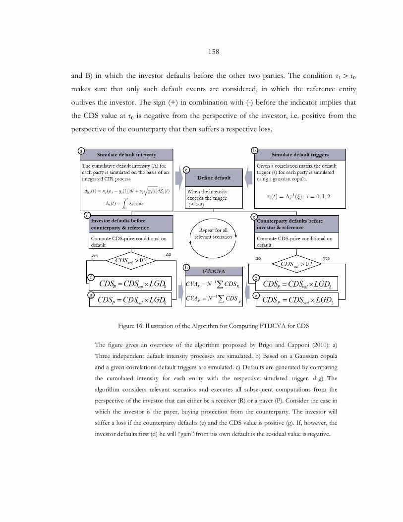
158

and B) in which the investor defaults before the other two parties. The condition 𝜏𝜏1 > 𝜏𝜏0

makes sure that only such default events are considered, in which the reference entity

outlives the investor. The sign (+) in combination with (-) before the indicator implies that

the CDS value at 𝜏𝜏0 is negative from the perspective of the investor, i.e. positive from the

perspective of the counterparty that then suffers a respective loss.

Figure 16: Illustration of the Algorithm for Computing FTDCVA for CDS

The figure gives an overview of the algorithm proposed by Brigo and Capponi (2010): a)

Three independent default intensity processes are simulated. b) Based on a Gaussian copula

and a given correlations default triggers are simulated. c) Defaults are generated by comparing

the cumulated intensity for each entity with the respective simulated trigger. d-g) The

algorithm considers relevant scenarios and executes all subsequent computations from the

perspective of the investor that can either be a receiver (R) or a payer (P). Consider the case in

which the investor is the payer, buying protection from the counterparty. The investor will

suffer a loss if the counterparty defaults (e) and the CDS value is positive (g). If, however, the

investor defaults first (d) he will “gain” from his own default is the residual value is negative.

159

4.3.2. AN OVERVIEW OF THE ALGORITHM

The task of the algorithm proposed by Brigo and Capponi (2010) is to compute

Equation (4.16). It assumes the investor can be either the payer or the receiver of the CDS

contract, delivering two FTDCVA metrics, 𝐶𝐶𝑃𝑃𝐴𝐴𝑃𝑃 and 𝐶𝐶𝑃𝑃𝐴𝐴𝑅𝑅, respectively. In the following we

will give a high level description of the numerical approach, while more detail on the various

items will follow in subsequent sections. An illustrative overview is also given in Figure 16.

The risk-neutral probabilities of default as seen in Equation (4.16) are considered numerically

through a Monte Carlo scheme, simulating default time periods of the three entities. For this

purpose Brigo and Capponi (2010) rely on an intensity approach, simulating three

independent shifted CIR processes. In the meanwhile a Gaussian copula function models

the interdependencies between the defaults, simulating default triggers for each entity. A

default occurs when the integrated CIR process of one the parties exceeds the value of the

respective trigger.

The algorithm then considers only relevant defaults, i.e. defaults either of the investor or of

the counterparty, given that the reference entity survived. For these cases the value the

surviving entity loses given a default is computed, i.e. the 𝐿𝐿𝐺𝐺𝐷𝐷1-weighted conditional residual

value of CDS seen in Equation (4.15). Averaging these terms according to the logic given in

Figure 16 delivers the FTDCVA metrics.

For this purpose the conditional survival probabilities of the reference entity are needed, i.e.

conditional on the set of information given a default of the counterparty (𝜏𝜏0) or the investor

(𝜏𝜏2), defined as

1𝐶𝐶∪𝐷𝐷1𝜏𝜏1>𝜏𝜏2ℚ�𝜏𝜏1 > 𝑡𝑡|𝒢𝒢𝜏𝜏2 � (4.17)

and

1𝐴𝐴∪𝐵𝐵1𝜏𝜏1>𝜏𝜏0ℚ�𝜏𝜏1 > 𝑡𝑡|𝒢𝒢𝜏𝜏0 �, (4.18)

respectively.

160

As shown by Brigo and Capponi (2009) the probabilities given in Equations (4.17) and (4.18)

can be computed in a closed-form manner using a Fourier transformation as will be shown

in a subsequent subchapter. Technically speaking this is actually the most elaborate part of

the model, and we contribute a greater part of this paper to explain the needed steps in

detail. We will also introduce a heuristic tune up, based on a log-normal approximation.

4.3.3. MODELING INTERDEPENDENT DEFAULTS

In the following we will first take the reader through the steps needed to model defaults via

an intensity process. Subsequently we will elaborate on the use of Gaussian copulas in

modeling interdependencies between the respective processes.

Brigo and Capponi (2010) use a stochastic intensity model that mirrors the shifted interest

rate CIR model – also referred to as CIR++ – examined for example by Brigo and

Mercurio (2006). Instead of modelling the instantaneous short rate the reduced form

approach models the instantaneous intensity that can also be interpreted as the instantaneous

default probability. The model incorporates a shift term that allows for exact calibration of

CDS quotes. Although Brigo and Capponi (2010) introduce jumps in the intensity process

formally, they subsequently drop the term – possibly due to technical challenges – and refer

the reader to future work. We therefore, will also focus on intensities without jumps, i.e.

using the shifted squared root diffusion (SSRD), previously examined by Brigo and

Alfonsi (2005).

Within the SSRD approach the stochastic intensity for each party 𝑗𝑗 is given by

𝜆𝜆𝑖𝑖(𝑡𝑡) = 𝑦𝑦𝑖𝑖(𝑡𝑡) + 𝜓𝜓𝑖𝑖(𝑡𝑡,𝛽𝛽), 𝑡𝑡 ≥ 0, 𝑗𝑗 = 0,1,2 (4.19)

with 𝜓𝜓𝑖𝑖 standing for the shift term, i.e. a deterministic function guaranteeing that the

modeled survival probabilities equal the market implied terms. The dynamics of the

stochastic term 𝑦𝑦𝑖𝑖 are defined as follows

161

𝑑𝑑𝑦𝑦𝑖𝑖(𝑡𝑡) = 𝜅𝜅𝑖𝑖 �𝜇𝜇𝑖𝑖 − 𝑦𝑦𝑖𝑖(𝑡𝑡)� 𝑑𝑑𝑡𝑡 + 𝜈𝜈𝑖𝑖�𝑦𝑦𝑖𝑖(𝑡𝑡)𝑑𝑑𝑍𝑍𝑖𝑖(𝑡𝑡), 𝑗𝑗 = 0,1,2 (4.20)

whereas Zj is a Brownian motion process under the risk-neutral measure ℚ. The CIR process

of each entity is represented by the vector βj = �κj, µj, νj, y(0)�, consisting of positive

constants. The integrated processes are then given by

Λ𝑖𝑖(𝑡𝑡) = ∫ 𝜆𝜆𝑖𝑖(𝑠𝑠)𝑑𝑑𝑠𝑠𝑡𝑡0 , 𝑌𝑌𝑖𝑖(𝑡𝑡) = ∫ 𝑦𝑦𝑖𝑖(𝑠𝑠)𝑑𝑑𝑠𝑠𝑡𝑡

0 , Ψ𝑖𝑖(𝑡𝑡,𝛽𝛽𝑡𝑡) = ∫ 𝜓𝜓𝑖𝑖�𝑠𝑠,𝛽𝛽𝑖𝑖�𝑑𝑑𝑠𝑠𝑡𝑡0 . (4.21)

Model implied survival probabilities are defined as follows

ℚ(𝜏𝜏𝑖𝑖 > 𝑡𝑡) ≔ 𝔼𝔼ℚ�𝑒𝑒−𝑌𝑌𝑖𝑖(𝑡𝑡)�

:= 𝑃𝑃𝐶𝐶𝐼𝐼𝑅𝑅(0, 𝑡𝑡,𝛽𝛽𝑖𝑖). (4.22)

𝑃𝑃𝐶𝐶𝐼𝐼𝑅𝑅(0, 𝑡𝑡,𝛽𝛽𝑖𝑖) resembles the zero coupon price within the CIR approach, solved analytically by

the following equation

𝑃𝑃𝐶𝐶𝐼𝐼𝑅𝑅(0, 𝑡𝑡,𝛽𝛽𝑖𝑖) = 𝐴𝐴(𝑡𝑡,𝑇𝑇,𝛽𝛽𝑖𝑖) exp{−𝐵𝐵(𝑡𝑡,𝑇𝑇,𝛽𝛽𝑖𝑖)} (4.23)

where

ℎ = �𝜅𝜅 + 2𝜎𝜎2

𝐴𝐴(𝑡𝑡,𝑇𝑇,𝛽𝛽𝑖𝑖) = �2ℎ𝑒𝑒𝑥𝑥𝑝𝑝(𝜅𝜅 + ℎ)(𝑇𝑇 − 𝑡𝑡)/2

2ℎ + (𝜅𝜅 + ℎ)(exp(𝑇𝑇 − 𝑡𝑡)ℎ − 1)�2𝜅𝜅Θ𝜎𝜎2

𝐵𝐵(𝑡𝑡,𝑇𝑇,𝛽𝛽𝑖𝑖) =2(𝑒𝑒𝑥𝑥𝑝𝑝(𝑇𝑇 − 𝑡𝑡)ℎ − 1)

2ℎ + (𝜅𝜅 + ℎ)(exp(𝑇𝑇 − 𝑡𝑡)ℎ − 1).

(4.24)

Calibration of the parameters can be obtained by comparing the model implied survival

probabilities 𝑃𝑃𝐶𝐶𝐼𝐼𝑅𝑅(0, 𝑡𝑡,𝛽𝛽𝑖𝑖) and market implied probabilities 𝑄𝑄(𝜏𝜏𝑖𝑖 > 𝑡𝑡)𝑚𝑚𝑠𝑠𝑟𝑟𝑏𝑏𝑏𝑏𝑡𝑡 as will be shown in

the case study below. For stripping market implied survival probabilities from CDS spreads

please see also Subchapter 3.3.4 above.

162

Finally we turn to the shift (deterministic) term of the intensity process given

Equation (4.19). Its integrated process Ψ𝑖𝑖(𝑡𝑡,𝛽𝛽𝑡𝑡) already introduced in Equation (4.21) is

defined as follows

Ψ𝑖𝑖(𝑡𝑡,𝛽𝛽𝑡𝑡) = 𝑙𝑙𝑙𝑙𝑙𝑙 �𝑃𝑃𝐶𝐶𝐼𝐼𝑅𝑅(0, 𝑡𝑡,𝛽𝛽𝑖𝑖)

ℚ(𝜏𝜏𝑖𝑖 > 𝑡𝑡)𝑚𝑚𝑠𝑠𝑟𝑟𝑏𝑏𝑏𝑏𝑡𝑡�, (4.25)

taking the differences between model-implied and market implied survival probabilities into

consideration, ensuring that the model values are consistent with observed market data.

For the simulation of the intensity dynamics of each party, Brigo and Capponi (2009) offer

the following formula

y(𝑡𝑡) =𝜈𝜈2�1 − 𝑒𝑒−𝜅𝜅(𝑡𝑡−𝑢𝑢)�

4𝜅𝜅𝜒𝜒𝑒𝑒′ �

4𝜅𝜅𝑒𝑒−𝜅𝜅(𝑡𝑡−𝑢𝑢)

𝜈𝜈2(1 − 𝑒𝑒−𝜅𝜅(𝑡𝑡−𝑢𝑢))𝑦𝑦(𝑢𝑢)� (4.26)

with

𝑑𝑑 =4𝜅𝜅𝜇𝜇𝜈𝜈2

(4.27)

whereas 𝜒𝜒𝑒𝑒′ (o) stands for a non-central chi-square random variable with 𝑑𝑑 degrees of

freedom. 𝑙𝑙 is the non-centrality parameter. Using the trapezoidal rule, the integrated process

𝑌𝑌(𝑡𝑡) can then be defined through the following approximation

𝑌𝑌(𝑡𝑡) = � 𝑦𝑦(𝑠𝑠)𝑑𝑑𝑠𝑠 =1

2𝛿𝛿𝑡𝑡�𝑦𝑦(𝑧𝑧 − 1) + 𝑦𝑦(𝑧𝑧)𝑡𝑡

𝑧𝑧=1

𝑡𝑡

0 (4.28)

with 𝛿𝛿𝑡𝑡 is a predefined discretization parameter.

Let Λi(t) stand be the integrated stochastic process for the default intensity of party 𝑖𝑖. We

define 𝜉𝜉𝑖𝑖 as the default trigger of party 𝑖𝑖. The default time period of the same party can be

given as such

163

τ𝑖𝑖(t) = Λ𝑖𝑖−1(𝜉𝜉𝑖𝑖), i = 0,1,2. (4.29)

Again, the three CIR processes are independent. The introduction of interdependencies

between the default times of the three parties are generated on the basis of a Gaussian

copula that determines the correlated default triggers.

The default triggers are defined as exponential random variables with the following uniforms

U𝑖𝑖 = 1 − exp{−𝜉𝜉𝑖𝑖}. (4.30)

The uniforms from Equation (4.30) are correlated through a trivariate Gaussian copula

function

C𝑅𝑅(𝑢𝑢0,𝑢𝑢1,𝑢𝑢2) = ℚ(𝑈𝑈0 < 𝑢𝑢0,𝑈𝑈1 < 𝑢𝑢1,𝑈𝑈2 < 𝑢𝑢2). (4.31)

For the simulation of these default triggers we thus only need the following correlation

matrix as an input

R = �1 𝜌𝜌𝑖𝑖,ℎ 𝜌𝜌𝑖𝑖,𝑖𝑖𝜌𝜌𝑖𝑖,ℎ 1 𝜌𝜌𝑖𝑖,𝑖𝑖𝜌𝜌𝑖𝑖,𝑖𝑖 𝜌𝜌𝑖𝑖,𝑖𝑖 1

� (4.32)

whereas 𝜌𝜌𝑖𝑖,𝑖𝑖 stands for the correlation coefficient between the default triggers of the parties 𝑗𝑗

and 𝑖𝑖.

Remarks

The short elaboration given above illustrates the theoretical and practical advantages the

SSRD approach has. The dynamics of the process are well researched, with relatively

straightforward approaches to implement fast simulation procedures. Moreover, the CIR

framework offers analytical (closed-form) solutions for bonds that can be applied for

survival probabilities, facilitating easy calibration schemes.

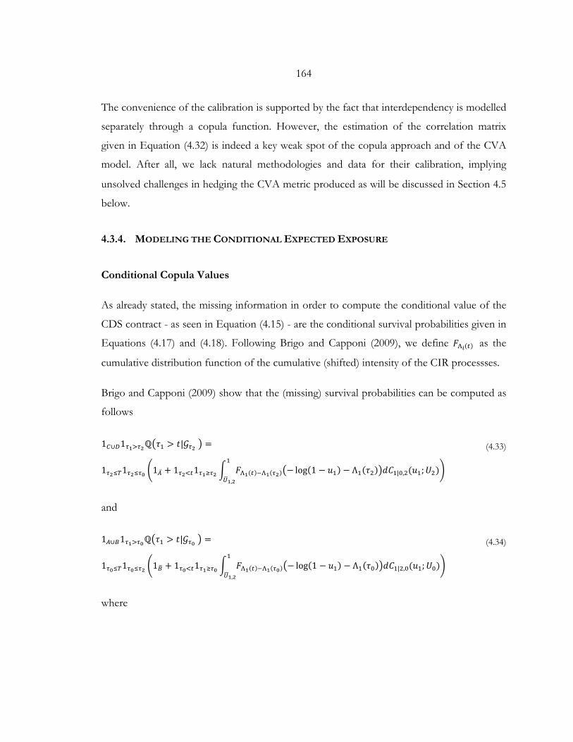
164

The convenience of the calibration is supported by the fact that interdependency is modelled

separately through a copula function. However, the estimation of the correlation matrix

given in Equation (4.32) is indeed a key weak spot of the copula approach and of the CVA

model. After all, we lack natural methodologies and data for their calibration, implying

unsolved challenges in hedging the CVA metric produced as will be discussed in Section 4.5

below.

4.3.4. MODELING THE CONDITIONAL EXPECTED EXPOSURE

Conditional Copula Values

As already stated, the missing information in order to compute the conditional value of the

CDS contract - as seen in Equation (4.15) - are the conditional survival probabilities given in

Equations (4.17) and (4.18). Following Brigo and Capponi (2009), we define 𝐹𝐹Λ𝑖𝑖(𝑡𝑡) as the

cumulative distribution function of the cumulative (shifted) intensity of the CIR processses.

Brigo and Capponi (2009) show that the (missing) survival probabilities can be computed as

follows

1𝐶𝐶∪𝐷𝐷1𝜏𝜏1>𝜏𝜏2ℚ�𝜏𝜏1 > 𝑡𝑡|𝒢𝒢𝜏𝜏2 � = (4.33)

1𝜏𝜏2≤𝑇𝑇1𝜏𝜏2≤𝜏𝜏0 �1�̅�𝐴 + 1𝜏𝜏2<𝑡𝑡1𝜏𝜏1≥𝜏𝜏2 � 𝐹𝐹Λ1(𝑡𝑡)−Λ1(𝜏𝜏2)�− log(1 − 𝑢𝑢1) − Λ1(𝜏𝜏2)�𝑑𝑑𝐶𝐶1|0,2(𝑢𝑢1;𝑈𝑈2)1

𝑈𝑈�1,2

�

and

1𝐴𝐴∪𝐵𝐵1𝜏𝜏1>𝜏𝜏0ℚ�𝜏𝜏1 > 𝑡𝑡|𝒢𝒢𝜏𝜏0 � = (4.34)

1𝜏𝜏0≤𝑇𝑇1𝜏𝜏0≤𝜏𝜏2 �1𝐵𝐵� + 1𝜏𝜏0<𝑡𝑡1𝜏𝜏1≥𝜏𝜏0 � 𝐹𝐹Λ1(𝑡𝑡)−Λ1(𝜏𝜏0)�− log(1 − 𝑢𝑢1) − Λ1(𝜏𝜏0)�𝑑𝑑𝐶𝐶1|2,0(𝑢𝑢1;𝑈𝑈0)1

𝑈𝑈�1,2

�

where

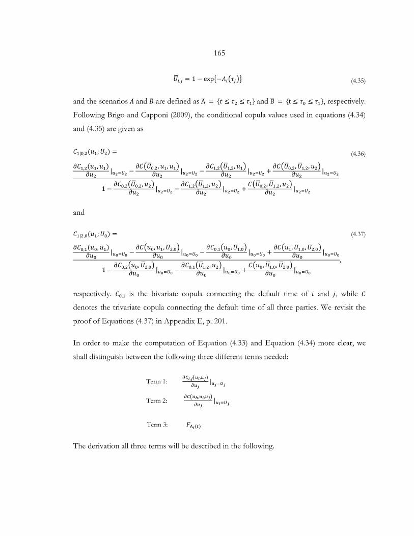
165

𝑈𝑈�𝑖𝑖,𝑖𝑖 = 1 − exp�−𝛬𝛬𝑖𝑖�𝜏𝜏𝑖𝑖�� (4.35)

and the scenarios �̅�𝐴 and 𝐵𝐵� are defined as A� = {𝑡𝑡 ≤ 𝜏𝜏2 ≤ 𝜏𝜏1} and B� = {t ≤ 𝜏𝜏0 ≤ 𝜏𝜏1}, respectively.

Following Brigo and Capponi (2009), the conditional copula values used in equations (4.34)

and (4.35) are given as

𝐶𝐶1|0,2(𝑢𝑢1;𝑈𝑈2) = (4.36)

𝜕𝜕𝐶𝐶1,2(𝑢𝑢1,𝑢𝑢1)𝜕𝜕𝑢𝑢2

|𝑢𝑢2=𝑈𝑈2 −𝜕𝜕𝐶𝐶�𝑈𝑈�0,2,𝑢𝑢1,𝑢𝑢1�

𝜕𝜕𝑢𝑢2|𝑢𝑢2=𝑈𝑈2 −

𝜕𝜕𝐶𝐶1,2�𝑈𝑈�1,2,𝑢𝑢1�𝜕𝜕𝑢𝑢2

|𝑢𝑢2=𝑈𝑈2 +𝜕𝜕𝐶𝐶�𝑈𝑈�0,2,𝑈𝑈�1,2,𝑢𝑢2�

𝜕𝜕𝑢𝑢2|𝑢𝑢2=𝑈𝑈2

1 −𝜕𝜕𝐶𝐶0,2�𝑈𝑈�0,2,𝑢𝑢2�

𝜕𝜕𝑢𝑢2|𝑢𝑢2=𝑈𝑈2 −

𝜕𝜕𝐶𝐶1,2�𝑈𝑈�1,2,𝑢𝑢2�𝜕𝜕𝑢𝑢2

|𝑢𝑢2=𝑈𝑈2 +𝐶𝐶�𝑈𝑈�0,2,𝑈𝑈�1,2,𝑢𝑢2�

𝜕𝜕𝑢𝑢2|𝑢𝑢2=𝑈𝑈2

and

𝐶𝐶1|2,0(𝑢𝑢1;𝑈𝑈0) = (4.37)

𝜕𝜕𝐶𝐶0,1(𝑢𝑢0,𝑢𝑢1)𝜕𝜕𝑢𝑢0

|𝑢𝑢0=𝑈𝑈0 −𝜕𝜕𝐶𝐶�𝑢𝑢0,𝑢𝑢1,𝑈𝑈�2,0�

𝜕𝜕𝑢𝑢0|𝑢𝑢0=𝑈𝑈0 −

𝜕𝜕𝐶𝐶0,1�𝑢𝑢0,𝑈𝑈�1,0�𝜕𝜕𝑢𝑢0

|𝑢𝑢0=𝑈𝑈0 +𝜕𝜕𝐶𝐶�𝑢𝑢1,𝑈𝑈�1,0,𝑈𝑈�2,0�

𝜕𝜕𝑢𝑢0|𝑢𝑢0=𝑈𝑈0

1 −𝜕𝜕𝐶𝐶0,2�𝑢𝑢0,𝑈𝑈�2,0�

𝜕𝜕𝑢𝑢0|𝑢𝑢0=𝑈𝑈0 −

𝜕𝜕𝐶𝐶0,1�𝑈𝑈�1,2,𝑢𝑢2�𝜕𝜕𝑢𝑢0

|𝑢𝑢0=𝑈𝑈0 +𝐶𝐶�𝑢𝑢0,𝑈𝑈�1,0,𝑈𝑈�2,0�

𝜕𝜕𝑢𝑢0|𝑢𝑢0=𝑈𝑈0

,

respectively. 𝐶𝐶0,1 is the bivariate copula connecting the default time of 𝑖𝑖 and 𝑗𝑗, while 𝐶𝐶

denotes the trivariate copula connecting the default time of all three parties. We revisit the

proof of Equations (4.37) in Appendix E, p. 201.

In order to make the computation of Equation (4.33) and Equation (4.34) more clear, we

shall distinguish between the following three different terms needed:

Term 1: 𝜕𝜕𝐶𝐶𝑖𝑖,𝑗𝑗�𝑢𝑢𝑖𝑖,𝑢𝑢𝑗𝑗�

𝜕𝜕𝑢𝑢𝑗𝑗|𝑢𝑢𝑗𝑗=𝑈𝑈𝑗𝑗

Term 2: 𝜕𝜕𝐶𝐶�𝑢𝑢ℎ,𝑢𝑢𝑖𝑖,𝑢𝑢𝑗𝑗�

𝜕𝜕𝑢𝑢𝑗𝑗|𝑢𝑢𝑖𝑖=𝑈𝑈𝑗𝑗

Term 3: 𝐹𝐹Λ𝑖𝑖(𝑡𝑡)

The derivation all three terms will be described in the following.

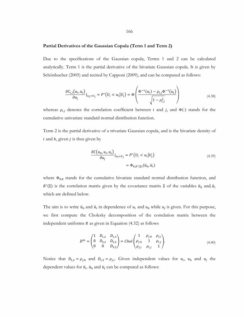
166

Partial Derivatives of the Gaussian Copula (Term 1 and Term 2)

Due to the specifications of the Gaussian copula, Terms 1 and 2 can be calculated

analytically. Term 1 is the partial derivative of the bivariate Gaussian copula. It is given by

Schönbucher (2005) and recited by Capponi (2009), and can be computed as follows:

𝜕𝜕𝐶𝐶𝑖𝑖,𝑖𝑖�𝑢𝑢𝑖𝑖 ,𝑢𝑢𝑖𝑖�𝜕𝜕𝑢𝑢𝑖𝑖

|𝑢𝑢𝑗𝑗=𝑈𝑈𝑗𝑗 = 𝑃𝑃∗�𝑈𝑈𝑖𝑖 < 𝑢𝑢𝑖𝑖�𝑈𝑈𝑖𝑖� = Φ

⎝

⎛Φ−1(𝑢𝑢𝑖𝑖) − 𝜌𝜌𝑖𝑖,𝑖𝑖Φ−1�𝑢𝑢𝑖𝑖�

�1 − 𝜌𝜌𝑖𝑖,𝑖𝑖2 ⎠

⎞ (4.38)

whereas 𝜌𝜌𝑖𝑖,𝑖𝑖 denotes the correlation coefficient between 𝑖𝑖 and 𝑗𝑗, and Φ(⋅) stands for the

cumulative univariate standard normal distribution function.

Term 2 is the partial derivative of a trivariate Gaussian copula, and is the bivariate density of

𝑖𝑖 and ℎ, given 𝑗𝑗 is thus given by

𝜕𝜕𝐶𝐶�𝑢𝑢ℎ,𝑢𝑢𝑖𝑖,𝑢𝑢𝑖𝑖�𝜕𝜕𝑢𝑢𝑖𝑖

|𝑢𝑢𝑖𝑖=𝑈𝑈𝑗𝑗 = 𝑃𝑃∗�𝑈𝑈𝑖𝑖 < 𝑢𝑢𝑖𝑖�𝑈𝑈𝑖𝑖� (4.39)

= Φ0,𝑅𝑅∗(Σ)(𝑢𝑢�ℎ,𝑢𝑢�𝑖𝑖)

where Φ0,𝑅𝑅 stands for the cumulative bivariate standard normal distribution function, and

𝑅𝑅∗(Σ) is the correlation matrix given by the covariance matrix Σ of the variables 𝑢𝑢�ℎ and,𝑢𝑢�𝑖𝑖

which are defined below.

The aim is to write 𝑢𝑢�ℎ and 𝑢𝑢�𝑖𝑖 in dependence of 𝑢𝑢𝑖𝑖 and 𝑢𝑢ℎ while 𝑢𝑢𝑖𝑖 is given. For this purpose,

we first compute the Cholesky decomposition of the correlation matrix between the

independent uniforms 𝑅𝑅 as given in Equation (4.32) as follows

𝐷𝐷𝑚𝑚 = �1 𝐷𝐷1,2 𝐷𝐷1,30 𝐷𝐷2,2 𝐷𝐷2,30 0 𝐷𝐷3,3

� = 𝐶𝐶ℎ𝑙𝑙𝑙𝑙 �1 𝜌𝜌𝑖𝑖,ℎ 𝜌𝜌𝑖𝑖,𝑖𝑖𝜌𝜌𝑖𝑖,ℎ 1 𝜌𝜌𝑖𝑖,𝑖𝑖𝜌𝜌𝑖𝑖,𝑖𝑖 𝜌𝜌𝑖𝑖,𝑖𝑖 1

�. (4.40)

Notice that 𝐷𝐷1,2 = 𝜌𝜌𝑖𝑖,ℎ and 𝐷𝐷1,3 = 𝜌𝜌𝑖𝑖,𝑖𝑖. Given independent values for 𝑢𝑢𝑖𝑖, 𝑢𝑢ℎ and 𝑢𝑢𝑖𝑖 the

dependent values for 𝑢𝑢�𝑖𝑖 , 𝑢𝑢�ℎ and 𝑢𝑢�𝑖𝑖 can be computed as follows:

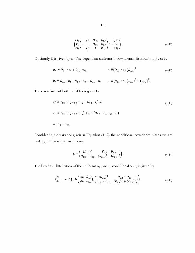
167

�𝑢𝑢�𝑖𝑖𝑢𝑢�ℎ𝑢𝑢�𝑖𝑖� = �

1 𝐷𝐷1,2 𝐷𝐷1,30 𝐷𝐷2,2 𝐷𝐷2,30 0 𝐷𝐷3,3

� 𝑇𝑇 ∙ �𝑢𝑢𝑖𝑖𝑢𝑢ℎ𝑢𝑢𝑖𝑖� . (4.41)

Obviously 𝑢𝑢�𝑖𝑖 is given by 𝑢𝑢𝑖𝑖. The dependent uniforms follow normal distributions given by

𝑢𝑢�ℎ = 𝐷𝐷1,2 ∙ 𝑢𝑢𝑖𝑖 + 𝐷𝐷1,2 ∙ 𝑢𝑢ℎ ~ 𝑁𝑁(𝐷𝐷1,2 ∙ 𝑢𝑢𝑖𝑖, �𝐷𝐷2,2�2 (4.42)

𝑢𝑢�𝑖𝑖 = 𝐷𝐷1,3 ∙ 𝑢𝑢𝑖𝑖 + 𝐷𝐷2,3 ∙ 𝑢𝑢ℎ + 𝐷𝐷3,3 ∙ 𝑢𝑢𝑖𝑖 ~ 𝑁𝑁(𝐷𝐷1,3 ∙ 𝑢𝑢𝑖𝑖 , �𝐷𝐷1,3�2 + �𝐷𝐷3,3�

2.

The covariance of both variables is given by

𝑐𝑐𝑙𝑙𝑐𝑐�𝐷𝐷2,2 ∙ 𝑢𝑢ℎ,𝐷𝐷2,3 ∙ 𝑢𝑢ℎ + 𝐷𝐷3,3 ∙ 𝑢𝑢𝑖𝑖� = (4.43)

𝑐𝑐𝑙𝑙𝑐𝑐�𝐷𝐷2,2 ∙ 𝑢𝑢ℎ,𝐷𝐷2,3 ∙ 𝑢𝑢ℎ� + 𝑐𝑐𝑙𝑙𝑐𝑐�𝐷𝐷2,2 ∙ 𝑢𝑢ℎ,𝐷𝐷3,3 ∙ 𝑢𝑢𝑖𝑖�

= 𝐷𝐷2,2 ∙ 𝐷𝐷2,3.

Considering the variance given in Equation (4.42) the conditional covariance matrix we are

seeking can be written as follows

Σ = �(𝐷𝐷2,2)2 𝐷𝐷2,2 ∙ 𝐷𝐷2,3

𝐷𝐷2,2 ∙ 𝐷𝐷2,3 (𝐷𝐷2,3)2 + (𝐷𝐷3,3)2� . (4.44)

The bivariate distribution of the uniforms 𝑢𝑢ℎ, and 𝑢𝑢𝑖𝑖 conditional on 𝑢𝑢𝑖𝑖 is given by

�𝑢𝑢𝑖𝑖𝑢𝑢𝑖𝑖|𝑢𝑢𝑖𝑖 = 𝑈𝑈𝑖𝑖�~N��

𝑢𝑢𝑖𝑖 ∙ 𝐷𝐷1,2𝑢𝑢𝑖𝑖 ∙ 𝐷𝐷1,3

� ,�(𝐷𝐷2,2)2 𝐷𝐷2,2 ∙ 𝐷𝐷2,3

𝐷𝐷2,2 ∙ 𝐷𝐷2,3 (𝐷𝐷2,3)2 + (𝐷𝐷3,3)2�� . (4.45)

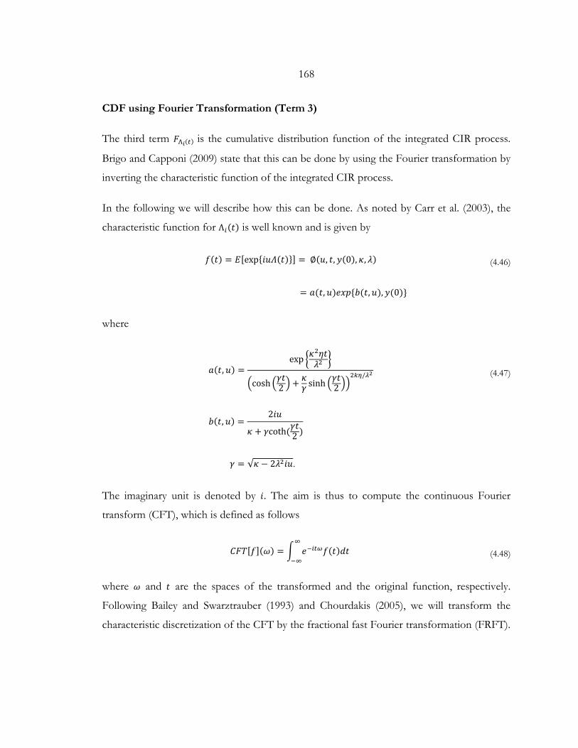
168

CDF using Fourier Transformation (Term 3)

The third term 𝐹𝐹Λ𝑖𝑖(𝑡𝑡) is the cumulative distribution function of the integrated CIR process.

Brigo and Capponi (2009) state that this can be done by using the Fourier transformation by

inverting the characteristic function of the integrated CIR process.

In the following we will describe how this can be done. As noted by Carr et al. (2003), the

characteristic function for Λ𝑖𝑖(𝑡𝑡) is well known and is given by

𝐸𝐸(𝑡𝑡) = 𝐸𝐸[exp{𝑖𝑖𝑢𝑢𝛬𝛬(𝑡𝑡)}] = ∅(𝑢𝑢, 𝑡𝑡, 𝑦𝑦(0), 𝜅𝜅, 𝜆𝜆) (4.46)

= 𝑎𝑎(𝑡𝑡,𝑢𝑢)𝑒𝑒𝑥𝑥𝑝𝑝{𝑏𝑏(𝑡𝑡,𝑢𝑢), 𝑦𝑦(0)}

where

𝑎𝑎(𝑡𝑡,𝑢𝑢) =exp �𝜅𝜅

2𝜂𝜂𝑡𝑡𝜆𝜆2 �

�cosh �𝛾𝛾𝑡𝑡2 � + 𝜅𝜅𝛾𝛾 sinh �𝛾𝛾𝑡𝑡2 ��

2𝑏𝑏𝑘𝑘/𝜆𝜆2 (4.47)

𝑏𝑏(𝑡𝑡,𝑢𝑢) =2𝑖𝑖𝑢𝑢

𝜅𝜅 + 𝛾𝛾coth (𝛾𝛾𝑡𝑡2 )

𝛾𝛾 = √𝜅𝜅 − 2𝜆𝜆2𝑖𝑖𝑢𝑢.

The imaginary unit is denoted by 𝑖𝑖. The aim is thus to compute the continuous Fourier

transform (CFT), which is defined as follows

𝐶𝐶𝐹𝐹𝑇𝑇[𝐸𝐸](𝜔𝜔) = � 𝑒𝑒−𝑖𝑖𝑡𝑡𝜔𝜔𝐸𝐸(𝑡𝑡)𝑑𝑑𝑡𝑡∞

−∞ (4.48)

where 𝜔𝜔 and 𝑡𝑡 are the spaces of the transformed and the original function, respectively.

Following Bailey and Swarztrauber (1993) and Chourdakis (2005), we will transform the

characteristic discretization of the CFT by the fractional fast Fourier transformation (FRFT).

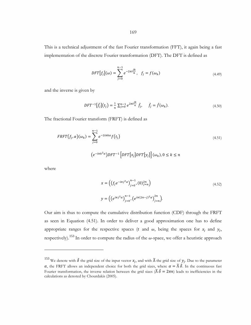
169

This is a technical adjustment of the fast Fourier transformation (FFT), it again being a fast

implementation of the discrete Fourier transformation (DFT). The DFT is defined as

𝐷𝐷𝐹𝐹𝑇𝑇�𝐸𝐸𝑖𝑖�(𝜔𝜔) = �𝑒𝑒−2𝜋𝜋𝑖𝑖𝑖𝑖𝑏𝑏𝑛𝑛

𝑛𝑛−1

𝑖𝑖=0

, 𝐸𝐸𝑖𝑖 = 𝐸𝐸(𝜔𝜔𝑏𝑏) (4.49)

and the inverse is given by

𝐷𝐷𝐹𝐹𝑇𝑇−1�𝐸𝐸𝑖𝑖��𝑡𝑡𝑖𝑖� = 1𝑛𝑛

∑ 𝑒𝑒2𝜋𝜋𝑖𝑖𝑗𝑗𝑘𝑘𝑛𝑛𝑛𝑛−1

𝑖𝑖=0 𝐸𝐸𝑖𝑖, 𝐸𝐸𝑖𝑖 = 𝐸𝐸(𝜔𝜔𝑏𝑏). (4.50)

The fractional Fourier transform (FRFT) is defined as

𝐹𝐹𝑅𝑅𝐹𝐹𝑇𝑇�𝐸𝐸𝑖𝑖 ,𝛼𝛼�(𝜔𝜔𝑏𝑏) = �𝑒𝑒−2𝑖𝑖𝜋𝜋𝑏𝑏𝛼𝛼𝐸𝐸�𝑡𝑡𝑖𝑖�𝑛𝑛−1

𝑖𝑖=0

(4.51)

�𝑒𝑒−𝑖𝑖𝜋𝜋𝑏𝑏2𝛼𝛼�𝐷𝐷𝐹𝐹𝑇𝑇−1 �𝐷𝐷𝐹𝐹𝑇𝑇�𝑥𝑥𝑖𝑖�𝐷𝐷𝐹𝐹𝑇𝑇�𝑦𝑦𝑖𝑖�� (𝜔𝜔𝑏𝑏), 0 ≤ 𝑘𝑘 ≤ 𝑛𝑛

where

𝑥𝑥 = ��𝐸𝐸𝑖𝑖𝑒𝑒−𝑖𝑖𝜋𝜋𝑖𝑖2𝛼𝛼�

𝑖𝑖=0

𝑛𝑛−1, (0)𝑖𝑖=𝑛𝑛2𝑛𝑛 � (4.52)

𝑦𝑦 = ��𝑒𝑒𝑖𝑖𝜋𝜋𝑖𝑖2𝛼𝛼�𝑖𝑖=0

𝑛𝑛−1, �𝑒𝑒𝑖𝑖𝜋𝜋(2𝑛𝑛−𝑖𝑖)2𝛼𝛼�

𝑖𝑖=𝑛𝑛

2𝑛𝑛�.

Our aim is thus to compute the cumulative distribution function (CDF) through the FRFT

as seen in Equation (4.51). In order to deliver a good approximation one has to define

appropriate ranges for the respective spaces (𝑡𝑡 and 𝜔𝜔, being the spaces for 𝑥𝑥𝑖𝑖 and 𝑦𝑦𝑖𝑖,

respectively).153 In order to compute the radius of the 𝜔𝜔-space, we offer a heuristic approach

153 We denote with 𝛿𝛿 the grid size of the input vector 𝑥𝑥𝑖𝑖 , and with Λ� the grid size of 𝑦𝑦𝑖𝑖 . Due to the parameter 𝛼𝛼, the FRFT allows an independent choice for both the grid sizes, where 𝛼𝛼 = Λ� 𝛿𝛿. In the continuous fast Fourier transformation, the inverse relation between the grid sizes (Λ� 𝛿𝛿 = 2𝜋𝜋𝑛𝑛) leads to inefficiencies in the calculations as denoted by Chourdakis (2005).

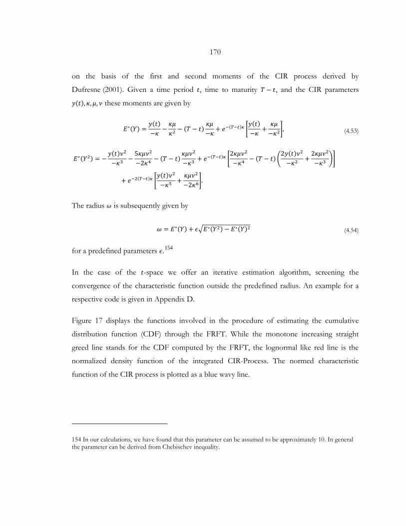
170

on the basis of the first and second moments of the CIR process derived by

Dufresne (2001). Given a time period 𝑡𝑡, time to maturity 𝑇𝑇 − 𝑡𝑡, and the CIR parameters

𝑦𝑦(𝑡𝑡), 𝜅𝜅, 𝜇𝜇, 𝜈𝜈 these moments are given by

𝐸𝐸∗(𝑌𝑌) =𝑦𝑦(𝑡𝑡)−𝜅𝜅

−𝜅𝜅𝜇𝜇𝜅𝜅2

− (𝑇𝑇 − 𝑡𝑡)𝜅𝜅𝜇𝜇−𝜅𝜅

+ 𝑒𝑒−(𝑇𝑇−𝑡𝑡)𝜅𝜅 �𝑦𝑦(𝑡𝑡)−𝜅𝜅

+𝜅𝜅𝜇𝜇−𝜅𝜅2

�, (4.53)

𝐸𝐸∗(𝑌𝑌2) = −𝑦𝑦(𝑡𝑡)𝜈𝜈2

−𝜅𝜅3−

5𝜅𝜅𝜇𝜇𝜈𝜈2

−2𝜅𝜅4− (𝑇𝑇 − 𝑡𝑡)

𝜅𝜅𝜇𝜇𝜈𝜈2

−𝜅𝜅3+ 𝑒𝑒−(𝑇𝑇−𝑡𝑡)𝜅𝜅 �

2𝜅𝜅𝜇𝜇𝜈𝜈2

−𝜅𝜅4− (𝑇𝑇 − 𝑡𝑡)�

2𝑦𝑦(𝑡𝑡)𝜈𝜈2

−𝜅𝜅2+

2𝜅𝜅𝜇𝜇𝜈𝜈2

−𝜅𝜅3��

+ 𝑒𝑒−2(𝑇𝑇−𝑡𝑡)𝜅𝜅 �𝑦𝑦(𝑡𝑡)𝜈𝜈2

−𝜅𝜅5+𝜅𝜅𝜇𝜇𝜈𝜈2

−2𝜅𝜅6�.

The radius 𝜔𝜔 is subsequently given by

𝜔𝜔 = 𝐸𝐸∗(𝑌𝑌) + 𝜖𝜖�𝐸𝐸∗(𝑌𝑌2) − 𝐸𝐸∗(𝑌𝑌)2 (4.54)

for a predefined parameters 𝜖𝜖.154

In the case of the 𝑡𝑡-space we offer an iterative estimation algorithm, screening the

convergence of the characteristic function outside the predefined radius. An example for a

respective code is given in Appendix D.

Figure 17 displays the functions involved in the procedure of estimating the cumulative

distribution function (CDF) through the FRFT. While the monotone increasing straight

greed line stands for the CDF computed by the FRFT, the lognormal like red line is the

normalized density function of the integrated CIR-Process. The normed characteristic

function of the CIR process is plotted as a blue wavy line.

154 In our calculations, we have found that this parameter can be assumed to be approximately 10. In general the parameter can be derived from Chebischev inequality.

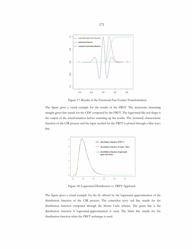
171

Figure 17: Results of the Fractional Fast Fourier Transformation

The figure gives a visual example for the results of the FRFT. The monotone increasing

straight green line stands for the CDF computed by the FRFT. The lognormal-like red shape is

the output of the transformation before summing up the results. The (normed) characteristic

function of the CIR process and the input needed for the FRFT is plotted through a blue wavy

line.

Figure 18: Lognormal Distribution vs. FRFT Approach

The figure gives a visual example for the fit offered by the lognormal approximation of the

distribution function of the CIR process. The somewhat wavy red line stands for the

distribution function computed through the Monte Carlo scheme. The green line is the

distribution function if lognormal-approximation is used. The black line stands for the

distribution function when the FRFT technique is used.

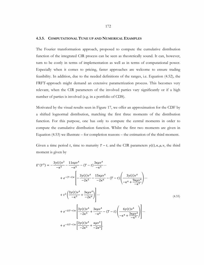
172

4.3.5. COMPUTATIONAL TUNE UP AND NUMERICAL EXAMPLES

The Fourier transformation approach, proposed to compute the cumulative distribution

function of the integrated CIR process can be seen as theoretically sound. It can, however,

turn to be costly in terms of implementation as well as in terms of computational power.

Especially when it comes to pricing, faster approaches are welcome to ensure trading

feasibility. In addition, due to the needed definitions of the ranges, i.e. Equation (4.52), the

FRFT-approach might demand an extensive parametrization process. This becomes very

relevant, when the CIR parameters of the involved parties vary significantly or if a high

number of parties is involved (e.g. in a portfolio of CDS).

Motivated by the visual results seen in Figure 17, we offer an approximation for the CDF by

a shifted lognormal distribution, matching the first three moments of the distribution

function. For this purpose, one has only to compute the central moments in order to

compute the cumulative distribution function. Whilst the first two moments are given in

Equation (4.53) we illustrate – for completion reasons – the estimation of the third moment.

Given a time period 𝑡𝑡, time to maturity 𝑇𝑇 − 𝑡𝑡, and the CIR parameters 𝑦𝑦(𝑡𝑡), 𝜅𝜅, 𝜇𝜇, 𝜈𝜈, the third

moment is given by

𝐸𝐸∗(𝑌𝑌3) = −3𝑦𝑦(𝑡𝑡)𝜈𝜈3

−𝜅𝜅5−

11𝜅𝜅𝜇𝜇𝜈𝜈4

−𝜅𝜅6− (𝑇𝑇 − 𝑡𝑡)

3𝜅𝜅𝜇𝜇𝜈𝜈4

−𝜅𝜅5⋯

+ 𝑒𝑒−(𝑇𝑇−𝑡𝑡)𝜅𝜅 �−3𝑦𝑦(𝑡𝑡)𝜈𝜈4

−2𝜅𝜅5−

15𝜅𝜅𝜇𝜇𝜈𝜈4

−2𝜅𝜅6− (𝑇𝑇 − 𝑡𝑡)�

3𝑦𝑦(𝑡𝑡)𝜈𝜈4

−𝜅𝜅4 + 9𝜅𝜅𝜇𝜇𝜈𝜈4−𝜅𝜅5

�⋯

+ 𝑡𝑡2 �3𝑦𝑦(𝑡𝑡)𝜈𝜈4

−𝜅𝜅5+

3𝜅𝜅𝜇𝜇𝜈𝜈4

−2𝜅𝜅6��⋯

+ 𝑒𝑒−2(𝑇𝑇−𝑡𝑡)𝜅𝜅 �3𝑦𝑦(𝑡𝑡)𝜈𝜈4

−2𝜅𝜅5+

3𝜅𝜅𝜇𝜇𝜈𝜈4

−𝜅𝜅6− (𝑇𝑇 − 𝑡𝑡)�

6𝑦𝑦(𝑡𝑡)𝜈𝜈4

−𝜅𝜅4 + 3𝜅𝜅𝜇𝜇𝜈𝜈4−𝜅𝜅5

��⋯

+ 𝑒𝑒−3(𝑇𝑇−𝑡𝑡)𝜅𝜅 �3𝑦𝑦(𝑡𝑡)𝜈𝜈4

−2𝜅𝜅5+𝜅𝜅𝜇𝜇𝜈𝜈4

−2𝜅𝜅6�.

(4.55)

173

In order to demonstrate the goodness of fit, offered by the heuristic approach we conducted

a series of exemplary numerical exercises, comparing the results produces using the Fourier

transformation with those produced using the log-normal approximation. In a second step

we compare further examples with the results given by Capponi (2009). We based the

parameterization of the CIR process on the ones given in Capponi (2009), pricing the first-

to-default CVA (FTDCVA) for a five-year CDS. The results are summarized in Table 15,

Table 16 and Table 17. The delivered CVA metrics are in basis points, given from the

perspective of the investor (either protection payer or protection seller).

Table 15 summarizes the results of the first-to-default CVA if the investor is the receiver

(protection seller) under a variety of correlation matrixes and volatility terms for the CIR

process of the reference entity 𝜈𝜈1. Table 16 summarizes the first-to-default CVA results if the

investor is the premium payer (protection buyer), following the structure of Table 15, i.e.

summarizing the results of the first-to-default CVA under a variety of correlation matrixes

and volatility terms for the CIR process of the reference entity 𝜈𝜈1. Table 17 tests further

possible combinations of the correlation coefficients, and compares our results with these

delivered by Capponi (2009).

Concerning the scenarios, in which the investor is the receiver (protection seller) the results

of both approaches seem to be quite stable (s. Table 15). The results resemble the ones

delivered by Capponi (2009, p. 73). Notice, however, that he uses a different volatility term

for the counterparty, explaining some of the deviations we have when the investor is the

payer (protection buyer). In that case our results display higher uncertainty as seen in Table

16 and Table 17, and made apparent by the standard error terms.155 This leads to some

deviations, especially in some more (numerically seen) challenging scenarios (e.g. when the

correlation coefficient is 0.99). Still, one can conclude that in total the deviations between the

155 In such cases it seems that the results are quite dependent on the discretization parameters of the cumulative distribution function (CDF).

174

three approaches seem to lie in an acceptable range, especially if the standard errors are

considered.

Beyond exhibiting the fitness of both the Fourier transformation technique implemented as

well as the log-normal approximation these numerical examples shed light on the intuitive

mechanisms of the algorithm as well as on its limits.

Table 15 shows that if the investor is the protection seller the FTDCVA metric decreases

with an increase in the correlation between the reference entity and the counterparty,

reaching near-zero terms. This can be explained by the pattern already discussed in

Schönbucher and Schubert (2000). If the counterparty defaults before the reference entity

while having a negative (positive) correlation the survival probability of the reference entity

will increase (decrease). Now if the survival probability of the reference entity increases

(decreases) the conditional value of the CDS – from the perspective of the protection seller

– will increase (decrease), implying higher (lower) adjustments.

A contrary pattern is observed when the investor buys protection as seen in Table 16. The

higher the correlation between the reference entity and the counterparty, the higher the

adjustment. Table 17 shows that there is one exception to this rule, i.e. the case in which the

reference entity and counterparty are almost perfectly correlated, i.e. 𝜌𝜌1,2 = 0.99, in which the

adjustment decreases significantly. Because of the high correlations the default triggers are

almost identical. If the counterparty defaults before the investor, the residual value of the

CDS will be relatively low, because of the high probability that the reference entity would

have had defaulted already. Brigo and Chourdakis (2009) classify the pattern as “somewhat

reasonable”, showing that it loses some of its significance if the reference entity becomes

riskier. It does, however, imply some inconsistency, especially when it comes to pricing

wrong-way risk. After all, wrong way risk – as seen in the monoline example – can also be

accompanied by presumably riskless references. In cases of extreme wrong way risk the

model will deliver rather low (if not negligible) CVA values.

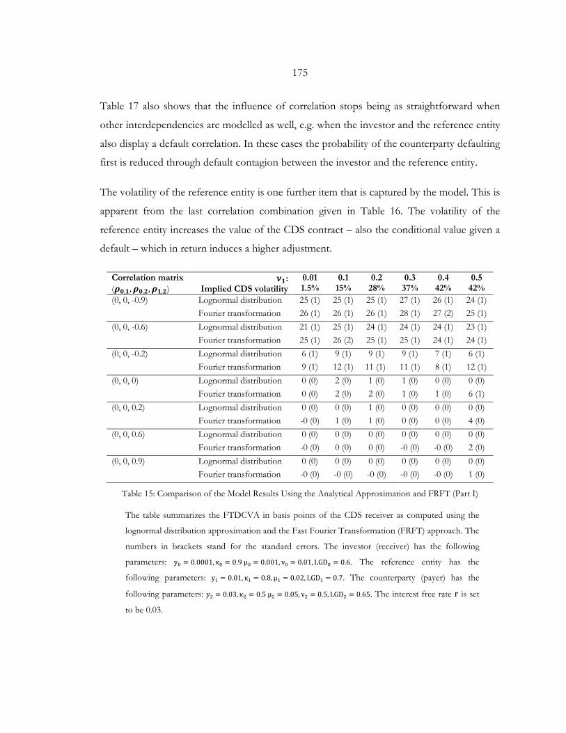
175

Table 17 also shows that the influence of correlation stops being as straightforward when

other interdependencies are modelled as well, e.g. when the investor and the reference entity

also display a default correlation. In these cases the probability of the counterparty defaulting

first is reduced through default contagion between the investor and the reference entity.

The volatility of the reference entity is one further item that is captured by the model. This is

apparent from the last correlation combination given in Table 16. The volatility of the

reference entity increases the value of the CDS contract – also the conditional value given a

default – which in return induces a higher adjustment.

Correlation matrix (𝝆𝝆𝟎𝟎,𝟏𝟏,𝝆𝝆𝟎𝟎,𝟐𝟐,𝝆𝝆𝟏𝟏,𝟐𝟐)

𝝂𝝂𝟏𝟏: Implied CDS volatility

0.01 1.5%

0.1 15%

0.2 28%

0.3 37%

0.4 42%

0.5 42%

(0, 0, -0.9) Lognormal distribution 25 (1) 25 (1) 25 (1) 27 (1) 26 (1) 24 (1) Fourier transformation 26 (1) 26 (1) 26 (1) 28 (1) 27 (2) 25 (1) (0, 0, -0.6) Lognormal distribution 21 (1) 25 (1) 24 (1) 24 (1) 24 (1) 23 (1) Fourier transformation 25 (1) 26 (2) 25 (1) 25 (1) 24 (1) 24 (1) (0, 0, -0.2) Lognormal distribution 6 (1) 9 (1) 9 (1) 9 (1) 7 (1) 6 (1) Fourier transformation 9 (1) 12 (1) 11 (1) 11 (1) 8 (1) 12 (1) (0, 0, 0) Lognormal distribution 0 (0) 2 (0) 1 (0) 1 (0) 0 (0) 0 (0) Fourier transformation 0 (0) 2 (0) 2 (0) 1 (0) 1 (0) 6 (1) (0, 0, 0.2) Lognormal distribution 0 (0) 0 (0) 1 (0) 0 (0) 0 (0) 0 (0) Fourier transformation -0 (0) 1 (0) 1 (0) 0 (0) 0 (0) 4 (0) (0, 0, 0.6) Lognormal distribution 0 (0) 0 (0) 0 (0) 0 (0) 0 (0) 0 (0) Fourier transformation -0 (0) 0 (0) 0 (0) -0 (0) -0 (0) 2 (0) (0, 0, 0.9) Lognormal distribution 0 (0) 0 (0) 0 (0) 0 (0) 0 (0) 0 (0) Fourier transformation -0 (0) -0 (0) -0 (0) -0 (0) -0 (0) 1 (0)

Table 15: Comparison of the Model Results Using the Analytical Approximation and FRFT (Part I)

The table summarizes the FTDCVA in basis points of the CDS receiver as computed using the

lognormal distribution approximation and the Fast Fourier Transformation (FRFT) approach. The

numbers in brackets stand for the standard errors. The investor (receiver) has the following

parameters: y0 = 0.0001,κ0 = 0.9 µ0 = 0.001, ν0 = 0.01, LGD0 = 0.6. The reference entity has the

following parameters: y1 = 0.01,κ1 = 0.8,µ1 = 0.02, LGD1 = 0.7. The counterparty (payer) has the

following parameters: y2 = 0.03,κ2 = 0.5 µ2 = 0.05, ν2 = 0.5, LGD2 = 0.65. The interest free rate r is set

to be 0.03.

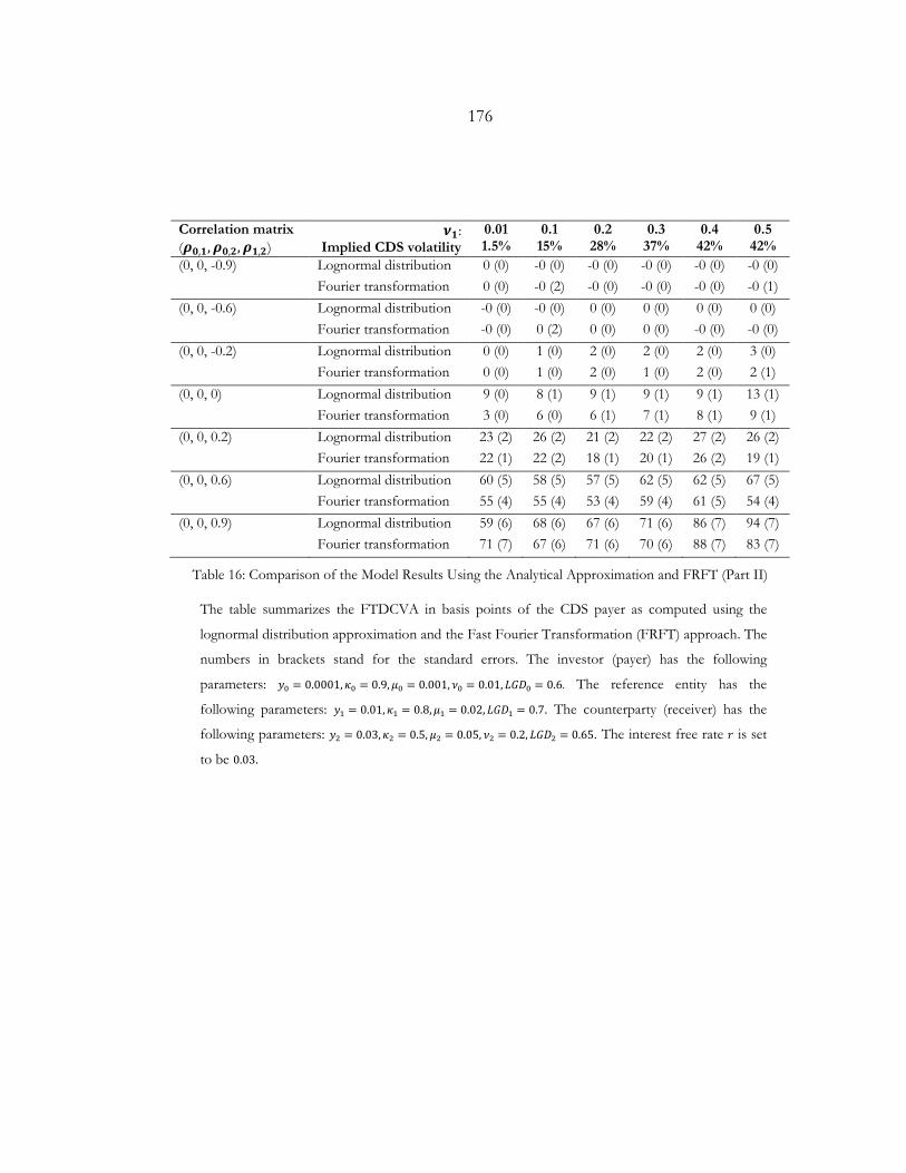
176

Correlation matrix (𝝆𝝆𝟎𝟎,𝟏𝟏,𝝆𝝆𝟎𝟎,𝟐𝟐,𝝆𝝆𝟏𝟏,𝟐𝟐)

𝝂𝝂𝟏𝟏: Implied CDS volatility

0.01 1.5%

0.1 15%

0.2 28%

0.3 37%

0.4 42%

0.5 42%

(0, 0, -0.9) Lognormal distribution 0 (0) -0 (0) -0 (0) -0 (0) -0 (0) -0 (0) Fourier transformation 0 (0) -0 (2) -0 (0) -0 (0) -0 (0) -0 (1) (0, 0, -0.6) Lognormal distribution -0 (0) -0 (0) 0 (0) 0 (0) 0 (0) 0 (0) Fourier transformation -0 (0) 0 (2) 0 (0) 0 (0) -0 (0) -0 (0) (0, 0, -0.2) Lognormal distribution 0 (0) 1 (0) 2 (0) 2 (0) 2 (0) 3 (0) Fourier transformation 0 (0) 1 (0) 2 (0) 1 (0) 2 (0) 2 (1) (0, 0, 0) Lognormal distribution 9 (0) 8 (1) 9 (1) 9 (1) 9 (1) 13 (1) Fourier transformation 3 (0) 6 (0) 6 (1) 7 (1) 8 (1) 9 (1) (0, 0, 0.2) Lognormal distribution 23 (2) 26 (2) 21 (2) 22 (2) 27 (2) 26 (2) Fourier transformation 22 (1) 22 (2) 18 (1) 20 (1) 26 (2) 19 (1) (0, 0, 0.6) Lognormal distribution 60 (5) 58 (5) 57 (5) 62 (5) 62 (5) 67 (5) Fourier transformation 55 (4) 55 (4) 53 (4) 59 (4) 61 (5) 54 (4) (0, 0, 0.9) Lognormal distribution 59 (6) 68 (6) 67 (6) 71 (6) 86 (7) 94 (7) Fourier transformation 71 (7) 67 (6) 71 (6) 70 (6) 88 (7) 83 (7)

Table 16: Comparison of the Model Results Using the Analytical Approximation and FRFT (Part II)

The table summarizes the FTDCVA in basis points of the CDS payer as computed using the

lognormal distribution approximation and the Fast Fourier Transformation (FRFT) approach. The

numbers in brackets stand for the standard errors. The investor (payer) has the following

parameters: 𝑦𝑦0 = 0.0001,𝜅𝜅0 = 0.9,𝜇𝜇0 = 0.001, 𝜈𝜈0 = 0.01,𝐿𝐿𝐺𝐺𝐷𝐷0 = 0.6. The reference entity has the

following parameters: 𝑦𝑦1 = 0.01,𝜅𝜅1 = 0.8,𝜇𝜇1 = 0.02,𝐿𝐿𝐺𝐺𝐷𝐷1 = 0.7. The counterparty (receiver) has the

following parameters: 𝑦𝑦2 = 0.03,𝜅𝜅2 = 0.5, 𝜇𝜇2 = 0.05, 𝜈𝜈2 = 0.2, 𝐿𝐿𝐺𝐺𝐷𝐷2 = 0.65. The interest free rate 𝑟𝑟 is set

to be 0.03.

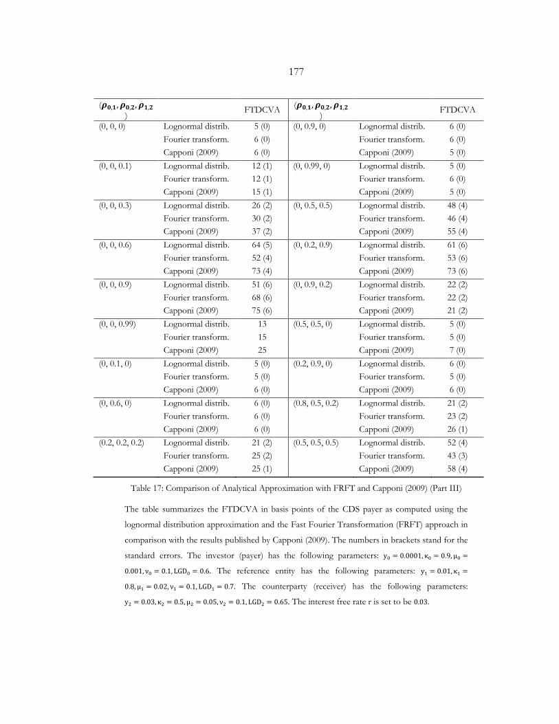
177

(𝝆𝝆𝟎𝟎,𝟏𝟏,𝝆𝝆𝟎𝟎,𝟐𝟐,𝝆𝝆𝟏𝟏,𝟐𝟐) FTDCVA (𝝆𝝆𝟎𝟎,𝟏𝟏,𝝆𝝆𝟎𝟎,𝟐𝟐,𝝆𝝆𝟏𝟏,𝟐𝟐

) FTDCVA

(0, 0, 0) Lognormal distrib. 5 (0) (0, 0.9, 0) Lognormal distrib. 6 (0) Fourier transform. 6 (0) Fourier transform. 6 (0) Capponi (2009) 6 (0) Capponi (2009) 5 (0) (0, 0, 0.1) Lognormal distrib. 12 (1) (0, 0.99, 0) Lognormal distrib. 5 (0) Fourier transform. 12 (1) Fourier transform. 6 (0) Capponi (2009) 15 (1) Capponi (2009) 5 (0) (0, 0, 0.3) Lognormal distrib. 26 (2) (0, 0.5, 0.5) Lognormal distrib. 48 (4) Fourier transform. 30 (2) Fourier transform. 46 (4) Capponi (2009) 37 (2) Capponi (2009) 55 (4) (0, 0, 0.6) Lognormal distrib. 64 (5) (0, 0.2, 0.9) Lognormal distrib. 61 (6) Fourier transform. 52 (4) Fourier transform. 53 (6) Capponi (2009) 73 (4) Capponi (2009) 73 (6) (0, 0, 0.9) Lognormal distrib. 51 (6) (0, 0.9, 0.2) Lognormal distrib. 22 (2) Fourier transform. 68 (6) Fourier transform. 22 (2) Capponi (2009) 75 (6) Capponi (2009) 21 (2) (0, 0, 0.99) Lognormal distrib. 13 (0.5, 0.5, 0) Lognormal distrib. 5 (0) Fourier transform. 15 Fourier transform. 5 (0) Capponi (2009) 25 Capponi (2009) 7 (0) (0, 0.1, 0) Lognormal distrib. 5 (0) (0.2, 0.9, 0) Lognormal distrib. 6 (0) Fourier transform. 5 (0) Fourier transform. 5 (0) Capponi (2009) 6 (0) Capponi (2009) 6 (0) (0, 0.6, 0) Lognormal distrib. 6 (0) (0.8, 0.5, 0.2) Lognormal distrib. 21 (2) Fourier transform. 6 (0) Fourier transform. 23 (2) Capponi (2009) 6 (0) Capponi (2009) 26 (1) (0.2, 0.2, 0.2) Lognormal distrib. 21 (2) (0.5, 0.5, 0.5) Lognormal distrib. 52 (4) Fourier transform. 25 (2) Fourier transform. 43 (3) Capponi (2009) 25 (1) Capponi (2009) 58 (4)

Table 17: Comparison of Analytical Approximation with FRFT and Capponi (2009) (Part III)

The table summarizes the FTDCVA in basis points of the CDS payer as computed using the

lognormal distribution approximation and the Fast Fourier Transformation (FRFT) approach in

comparison with the results published by Capponi (2009). The numbers in brackets stand for the

standard errors. The investor (payer) has the following parameters: y0 = 0.0001,κ0 = 0.9, µ0 =

0.001, ν0 = 0.1, LGD0 = 0.6. The reference entity has the following parameters: y1 = 0.01,κ1 =

0.8, µ1 = 0.02, ν1 = 0.1, LGD1 = 0.7. The counterparty (receiver) has the following parameters:

y2 = 0.03,κ2 = 0.5, µ2 = 0.05, ν2 = 0.1, LGD2 = 0.65. The interest free rate r is set to be 0.03.

178

4.4. CASE STUDY

In the following we would like to return to our introductory example in which a financial

institution buys protection in form of a CDS from a monoline insurance in order to hedge

the credit risk arising from (one unit) senior structured note (RMBS). We assume a 5 year

contract without a collateral agreement.

The case study will describe needed computational steps in more detail, especially with

respect to calibrating the models to market data. It will also explore the insights offered by

the model as well as its limits. In order to capture the dynamics caused by the financial crisis

we will compute the first-to-default CVA based on real market data from 2006 as well as

2010. We especially expect to gain insights regarding the increasing significance of CVA in

general and wrong way risk in particular.

The investor is defined as an average bank. For this purpose we estimated the average of the

CDS spreads of five leading banks as seen in Table 18.156 As an exemplary monoline insurer

we chose Assured Corp., displaying the CDS spreads seen in Table 18. For the RMBS note

we assume a constant CDS spread of 30 bps. and 400 bps. in the years 2006 and 2010,

respectively. The significant shift in the curve of CDS spreads underlines the deteriorating

credibility of all the parties involved due to the financial crisis.

Following the procedure described in Subchapter 3.3.4 we estimate the implied default

probabilities (PD) of all involved parties based on the assumed CDS spreads. We assume the

recovery rate to be 40% (i.e. LGD to be 60%), standing in line with market practice (see also

Subsection 3.3.4). In order to limit the effect of the LGD assumption we use the same LGD

in order to strip the market implied survival probabilities as well as within the CVA

calculation.

156 We used the same set of names in Subchapter 3.3.4 when we discussed calibration of default probabilities.

179

The CDS spreads imply the probabilities of defaults illustrated in Figure 19. The figure

shows the drastic increase of default probabilities the market attributed (even to large and

international) banks. While the market implied 5 year PD of an average bank was practically

negligible before the crises, it exceeded 10% in 2010 as seen in Subfigure (b). Subfigure (a)

shows how the market attributed almost credit risk-free status to monoline insurance

companies before the crises, standing in line with their top rating. This changed dramatically

in the course of the subprime crises. The situation in the monoline insurance market in

general and the idiosyncratic risk of Assured Corp. in particular seem to have considerably

increased the market implied probability of default across all maturities by 2010.

Using the closed-form solutions for survival probability given in Equation (4.23) and the

market implied survival probabilities we subsequently calibrate the CIR parameters using a

straight-forward least square (LS) method. The calibration results are listed in Table 19. The

increased risk of all parties is especially visible through the surge in the volatility term 𝜈𝜈.

Figure 20 displays a key advantage of stochastic intensity models in general and the SSRD

approach in particular. The model-based survival probabilities fit the market implied ones

across the whole term structure in a very satisfying manner.

We face the key shortfall of the CVA model however when estimating the correlation

structure. As noted above we lack natural appropriate methodologies. For this reason we

follow Cesari et al. (2009, p. 222) and study a range of possibilities instead of using one

particular correlation matrix. Some scenarios seem plausible (e.g. the first example given in

Table 20). Others are less plausible, but helpful to understand the mechanism of the model

(e.g. the last scenario given in Table 20).

We then run the algorithm illustrated in Figure 16, delivering first-to-default CVA metrics

for the years 2006 and 2010. The calculation of the conditional value of the CDS needed

within the algorithm is based on the proposed lognormal approximation (for the cumulative

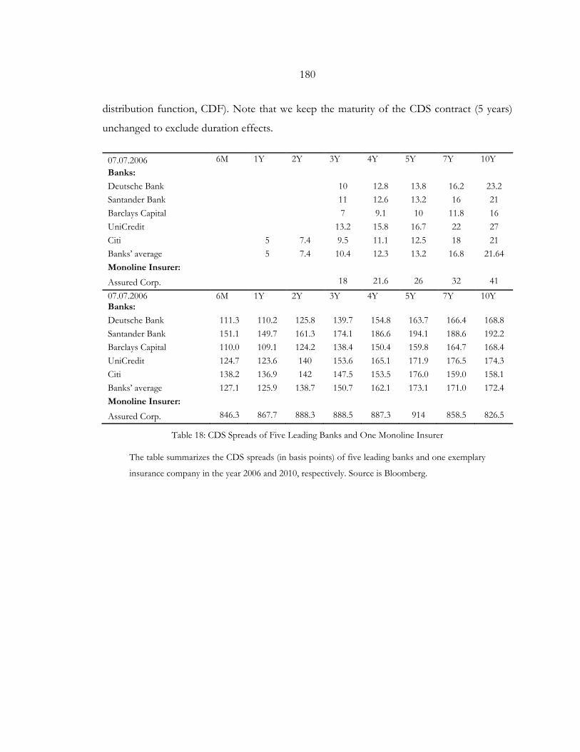
180

distribution function, CDF). Note that we keep the maturity of the CDS contract (5 years)

unchanged to exclude duration effects.

07.07.2006 6M 1Y 2Y 3Y 4Y 5Y 7Y 10Y Banks: Deutsche Bank 10 12.8 13.8 16.2 23.2 Santander Bank 11 12.6 13.2 16 21 Barclays Capital 7 9.1 10 11.8 16 UniCredit 13.2 15.8 16.7 22 27 Citi 5 7.4 9.5 11.1 12.5 18 21 Banks’ average 5 7.4 10.4 12.3 13.2 16.8 21.64 Monoline Insurer:

Assured Corp. 18 21.6 26 32 41

07.07.2006 6M 1Y 2Y 3Y 4Y 5Y 7Y 10Y Banks: Deutsche Bank 111.3 110.2 125.8 139.7 154.8 163.7 166.4 168.8 Santander Bank 151.1 149.7 161.3 174.1 186.6 194.1 188.6 192.2 Barclays Capital 110.0 109.1 124.2 138.4 150.4 159.8 164.7 168.4 UniCredit 124.7 123.6 140 153.6 165.1 171.9 176.5 174.3 Citi 138.2 136.9 142 147.5 153.5 176.0 159.0 158.1 Banks’ average 127.1 125.9 138.7 150.7 162.1 173.1 171.0 172.4 Monoline Insurer:

Assured Corp. 846.3 867.7 888.3 888.5 887.3 914 858.5 826.5

Table 18: CDS Spreads of Five Leading Banks and One Monoline Insurer

The table summarizes the CDS spreads (in basis points) of five leading banks and one exemplary

insurance company in the year 2006 and 2010, respectively. Source is Bloomberg.

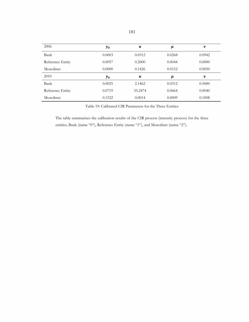
181

2006 𝒚𝒚𝟎𝟎 𝜿𝜿 𝝁𝝁 𝝂𝝂

Bank 0.0003 0.0312 0.0268 0.0942

Reference Entity 0.0057 0.2000 0.0044 0.0000

Monoliner 0.0000 0.1426 0.0152 0.0050

2010 𝒚𝒚𝟎𝟎 𝜿𝜿 𝝁𝝁 𝝂𝝂

Bank 0.0025 2.1462 0.0312 0.5000

Reference Entity 0.0719 35.2474 0.0664 0.0040

Monoliner 0.1522 0.0014 0.0009 0.1008

Table 19: Calibrated CIR Parameters for the Three Entities

The table summarizes the calibration results of the CIR process (intensity process) for the three

entities, Bank (name “0”), Reference Entity (name “1”), and Monoliner (name “2”).

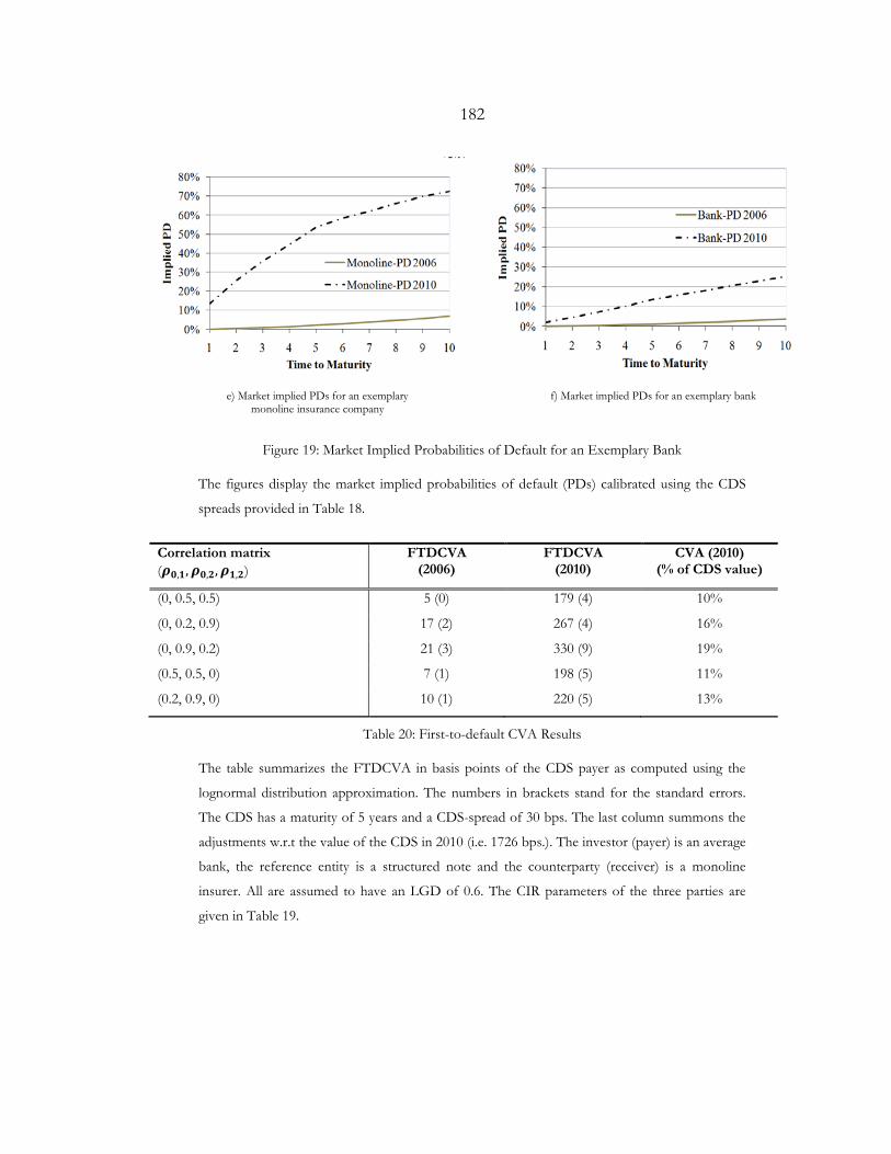
182

e) Market implied PDs for an exemplary monoline insurance company

f) Market implied PDs for an exemplary bank

Figure 19: Market Implied Probabilities of Default for an Exemplary Bank

The figures display the market implied probabilities of default (PDs) calibrated using the CDS

spreads provided in Table 18.

Correlation matrix (𝝆𝝆𝟎𝟎,𝟏𝟏,𝝆𝝆𝟎𝟎,𝟐𝟐,𝝆𝝆𝟏𝟏,𝟐𝟐)

FTDCVA (2006)

FTDCVA (2010)

CVA (2010) (% of CDS value)

(0, 0.5, 0.5) 5 (0) 179 (4) 10%

(0, 0.2, 0.9) 17 (2) 267 (4) 16%

(0, 0.9, 0.2) 21 (3) 330 (9) 19%

(0.5, 0.5, 0) 7 (1) 198 (5) 11%

(0.2, 0.9, 0) 10 (1) 220 (5) 13%

Table 20: First-to-default CVA Results

The table summarizes the FTDCVA in basis points of the CDS payer as computed using the

lognormal distribution approximation. The numbers in brackets stand for the standard errors.

The CDS has a maturity of 5 years and a CDS-spread of 30 bps. The last column summons the

adjustments w.r.t the value of the CDS in 2010 (i.e. 1726 bps.). The investor (payer) is an average

bank, the reference entity is a structured note and the counterparty (receiver) is a monoline

insurer. All are assumed to have an LGD of 0.6. The CIR parameters of the three parties are

given in Table 19.

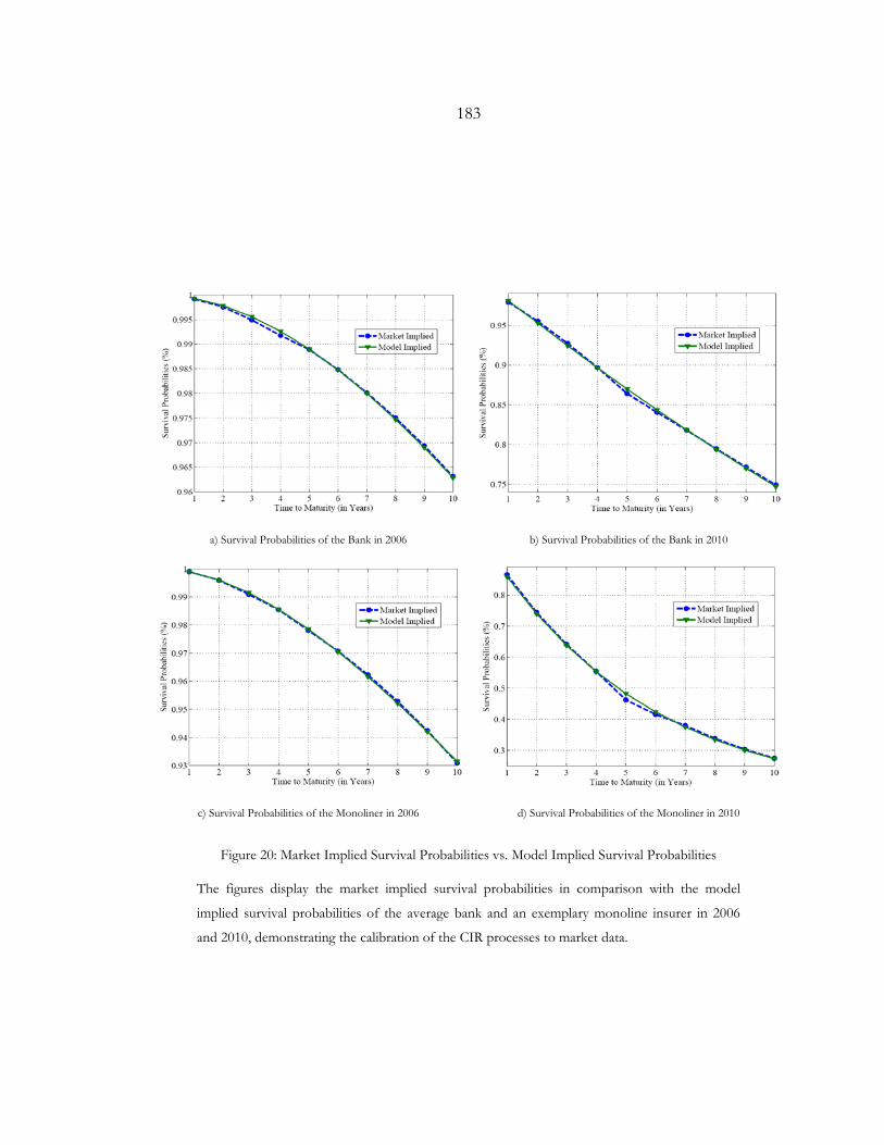
183

a) Survival Probabilities of the Bank in 2006

b) Survival Probabilities of the Bank in 2010

c) Survival Probabilities of the Monoliner in 2006

d) Survival Probabilities of the Monoliner in 2010

Figure 20: Market Implied Survival Probabilities vs. Model Implied Survival Probabilities

The figures display the market implied survival probabilities in comparison with the model

implied survival probabilities of the average bank and an exemplary monoline insurer in 2006

and 2010, demonstrating the calibration of the CIR processes to market data.

184

The results shown in Table 20 are to be interpreted as follows. If the bank had bought a

protection from a monoline insurer in 2006, it would have had to adjust the value of the

CDS by 5 to 21 basis points, depending on the correlation matrix assumed. Assuming a

correlation structure similar to the one in the first example might have already been

conservative, and the CVA metric delivered is still rather negligible. This is due to the low

CDS spreads observed (and the respective implied survival probabilities). Note that the

initial value of the CDS in 2006 is zero.

The picture changes significantly in 2010. In the meanwhile the counterparty credit risk-free

value of the CDS increased from 0 to 1726 bps. due to the increased risk of the reference

entity, this being a key driver behind the increase in the CVA metrics across the correlation

scenarios. A further driver is of course the increased risk of the counterparty. This becomes

evident if we look at the second correlation scenario which seems plausible for 2010. In this

case the bank would need to adjust the value of the CDS by approximately 16%. Notice that

for the monoline insurer the CVA increase (e.g. from 5 to 267 bps.) would imply a profit due

to the worsening of own credit risk.

185

4.5. CRITICAL EVALUATION

In the following we evaluate the model offered by Brigo and Capponi (2010), focusing on

the capabilities of the approach in delivering its proclaimed target, i.e. “arbitrage-free

framework” to price symmetric CVA for CDS. After discussing the theoretical and technical

strengths and pitfalls we turn to discuss the practical “use test” of the model. Whilst some

issues are only relevant for the specific approach at hand many arguments have a broader

scope, aiming on intensity models, the use of (Gaussian) copula functions and derivative

pricing models in general.

In principle the framework does capture default dependency, delivering a theoretically

coherent and symmetric first-to-default CVA, i.e. incorporating the credit risk of both the

investor and the counterparty. By modeling the default dependency through a copula

function the approach allows for separate modeling of credit spread dynamics on the one

hand and the default dependency on the other. This can be seen as an advantage from a

practicality perspective, less so if mathematical rigor is central. After all, the calibration of a

function with two or more parameters should not be done sequentially but simultaneously.

Credit spread dynamics are modelled through a standard stochastic intensity approach.

Incorporating jumps would have facilitated the calibration of higher (but possible) implied

volatilities as discussed in Brigo and El-Bachir (2008). Still, the chosen (and implemented)

SSRD approach is not only mathematically convenient, it also captures market implied

survival probabilities in a very satisfying manner.

Default is defined when the cumulative intensity process exceeds a respective default trigger.

A Gaussian copula captures the dependency of the default triggers of the investor, the

counterparty and the reference entity. Whereas the possibility of joint default is excluded.

This assumption does not, however, seem that unrealistic, especially if the discretization is

subsequently done in relatively small time steps (e.g. trading days). The Gaussian copula

introduces convenient analytical tractability to the model, e.g. with respect to computing

186

partial derivatives etc. The statistical rigor of using Gaussian copulas to model the

dependency of default triggers remains controversial (see Mikosch, 2005). In addition to

assuming constant default correlation, it fails to capture the “tails” of the distribution,

systematically underestimating the conditional probability of default, which is exactly the

proclaimed target of the “CVA with wrong-way risk” model. Moreover, as discussed above

in Subchapter 4.3.5 the model tends to underestimate CVA in extreme scenarios when

correlation between the reference entity and the counterparty is close to one, especially if the

reference entity is relatively less risky.

Besides default risk the approach assumes deterministic interest rates and constant recovery

rates. While the small role interest rates play in this case might support the negligence of

their stochasticity, this does not apply to recovery rates. Li (2009) shows that although not as

important as default correlation the volatility of recovery rates can drive CVA significantly.

Modeling stochastic recovery rates will, however, introduce a further layer of complication

and uncertainties, especially with regards to calibrating the recovery rate volatility.

A more relevant missing characteristic is collateralization. As seen in Table 14 credit

derivatives are almost always collateralized. It needs, however, to be noted that especially in

infamous examples of CDS contracts with wrong way risk (e.g. monoline insurers selling

CDS on RMBS) no collateral agreements were put in place. Moreover, the framework has

been extended by Brigo et al. (2013b) to model collateralization, allowing also for re-

hypothecation.

More importantly while Brigo and Capponi (2010) do offer a risk-neutral framework to

model CVA, they do not specify the needed duplication strategy. This can be pointed out as

the key pitfall of the model, questioning the applicability and practicability of the model.

First, we lack market quotes to calibrate a risk-neutral correlation matrix. Second, the

duplication strategy would imply hedging own credit risk. As discussed in Subchapter 3.4.2

hedging DVA is already an almost impossible task. Let alone hedging the sensitivity of a

187

first-to-default CVA to changes in own credit risk, which involves hedging sensitivities of

conditional exposure values given a default of a counterparty and possible contagion effects.

Thus, although theoretically coherent the model exhibits significant pitfalls that limit its

practical use, especially when it comes to pricing and hedging. Following the terminology of

Taleb and Martin (2012) a trader hedging his positions based on the model presented would

resemble a pilot flying according to the map of a different territory. Bearing in mind that

models will principally deviate from reality, the impossibility of structuring a duplicating

strategy calls the whole approach into question. It can be argued that using such “flawed”

models (“wrong maps”) might even increase the risk as it induces overconfidence – also

referred to as “model-dope” (MacKenzie and Spears, 2014) – and allows for “charlatanism”

(Taleb, 2012).157 This links into what Hayek (1942) calls “scientism”, i.e. the illusion of

science. In their analysis of the Gaussian copula and its role in the financial crisis MacKenzie

and Spears (2014) do confirm the risk of models being – “gamed” and exploited. They find,

however, evidence that questions the existence of blind confidence in models, concluding

that “model dope” notions should be treated as forms of “othering”.158 More importantly,

they point to the coordinating role financial models play, facilitating communication within

and between organizations, e.g. “providing a shared yardstick that enabled accountants and auditors to

determine whether a valuation was correct and risk managers to assess whether a position was properly hedged

[…]”.

Returning to the model at hand this means that while bearing the risks of using the model in

mind, we need to analyze its use as a communication tool. Because the model is based on a

standard modeling approach (e.g. reduced form approach in conjunction with Gaussian

copula) while preserving theoretical coherence it can provide a framework to discuss the

157 See also Taleb (2012), pp. 238-240, Taleb (2007), p. xxv or Taleb (1997), pp. 445-453. 158 MacKenzie and Spears (2014) cite amongst others the following research papers that question the notion of

model dope: Beunza and Stark (2010) and Svetlova (2012). Notice that also Haug and Taleb (2011) argue that traders are not “blind” to the pitfalls of the Black-Scholes formula.

188

dynamics of wrong-way risk but also of DVA pricing. Such a discussion is not only of

academic nature, but can contribute relevant insights to the regulatory and accounting

discourse, revealing the significance of wrong way risk (especially amid the financial crisis)

and shedding light on the controversies of accounting for DVA (see previous Section 4.4).

Yet, it is exactly this “theoretical coherence” that limits the use of the model for inter- and

intra-organizational communication. Simpler approaches (as the one discussed in

Subchapter 3.3.2) in which the different building blocks (esp. exposure profile) are derived

and presented in a more straightforward manner seem more appropriate for this purpose.

Still, the model at hand can facilitate discussions around the specific (and rare) case of CVA

for a netting set consisting only of one CDS contract (with not collateralization). It can for

example offer an inter-subjective framework for discussions between banks on the one

hand, and auditors and supervisors on the other, e.g. “providing a shared yardstick” to determine

whether they have correctly adjusted for the counterparty risk arising from the credit

protections they bought from monoline insurers, referencing to RMBS notes.

189

4.6. CONCLUDING REMARKS

We chose to focus on the implementation and analysis of the model proposed by Brigo and

Capponi (2010), because it was one of the first CVA models promising an arbitrage-free

framework for symmetric pricing in conjunction with dependency between probabilities of

default and exposure.

First, we laid the grounds for the analysis by revisiting the mechanisms behind CDS

contracts. We then placed the approach offered by Brigo and Capponi (2010) within the

category of reduced-form credit risk models that use (Gaussian) copula functions to model

default dependency. Subsequently, we decomposed the model which allowed a thorough

analysis of the benefits and pitfalls of the model. In addition, we provided a step-by-step

implementation guide, especially going into detail into the aspects that Brigo and

Capponi (2010) left relatively open – the computation of the survival probability of the

reference entity conditional on the default of either the counterparty or the investor. It has

been illustrated in detail how the fractional Fourier transform (FRFT) can be used for this

purpose. We also proposed a computational tune-up through a heuristic approximation,

which reduces the complexity of the elaborate implementation and speeds-up the

computation, while delivering satisfying pricing results.

We synthesize that while Brigo and Capponi (2010) do offer a coherent and risk-neutral

framework, they do not specify the needed duplication strategy. The lack of instruments to

calibrate a risk-neutral correlation matrix and possibility to hedge own credit risk puts the

arbitrage-freedom of the model into question. In addition, we note that the theoretical

coherence of the model actually limits its use for inter- and intra-organizational

communication, and suggest that simpler approaches are more appropriate as they facilitate

discussions around the different building blocks (e.g. exposure profile).

This does not deprive the model from the possibility of facilitating discussions around the

specific case of CVA for CDS contracts (with no collateralization). After all, the model is

190

able to explain the high adjustments needed for CDS on structured notes that were bought

from monoline insurance, i.e. meeting the demand following the financial crisis.

191

CHAPTER 5: OVERALL CONCLUSION

This thesis can be placed within the literature on market and counterparty credit risk,

contributing along the following three dimensions:

• Interest rate risk management. We gave an overview on asset liability management

(ALM) in general and interest rate risk management in particular. In that respect we

offered a novel procedure for structuring swap overlays for pensions funds, allowing

for optimal hedging of interest rate risk without affecting the strategic asset

allocation. We also extended the analysis of the Cairns (2004) stochastic interest rate

model. Besides deriving respective model-based sensitivity measures (Cairns deltas),

we applied the two-factor version of the model to the practical application of ALM

for pension funds, analyzing its strengths and weaknesses when it comes to long-

term contracts.

• Pricing and managing counterparty credit risk. We offered a compact overview on

counterparty credit risk and credit valuation adjustment (CVA), running unique

analyses around valuation, relevant accounting and regulatory requirements as well as

pricing and mitigation. We illustrated how the CVA capital charge shows the

tautology behind many of the discussions around regulatory requirements. It reveals

how financial institutions are heavily driven by regulatory requirements that originally

aimed to actually mirror the way banks “do business”. In addition, we showed that

the discourse around CVA and counterparty credit risk cannot be seen as a “pure

scientific search for truth” as it is dominated by lobby-like argumentations. We

agreed for example that the regulatory CVA capital charge will indeed lead to an

increase in hedge costs. We questioned, however, whether the increase will be as

significant as the evidence shows. We argued rather that banks have not been pricing

for CVA adequately in the past. This might be due to the fact that banks did not

think systematically about counterparty credit risk, because no metric pointed to it.

192

• CVA modeling and wrong way risk. We gave an overview on credit risk modeling in

general and credit spreads in particular, revisiting the CVA for CDS model

introduced by Brigo and Capponi (2010). We offered a step-by-step implementation

guide, elaborating on the parts Brigo and Capponi (2010) left open. We especially

offered a computational tune-up, and demonstrated its robustness across a variety of

scenarios. After illustrating the use of the model using a realistic case study, we ran a

novel analysis of the Brigo and Capponi (2010) model in particular and CVA

modeling in general.

With regards to the overall discourse around financial derivatives we were able to illustrate

the value added by using swaps to hedge interest rate risk of pension funds. We showed that

financial derivatives can offer considerable benefits, allowing risk to be borne by the ones

most fit to do so. By immunizing their portfolios against changes in interest rates, fund

managers pursue the noble objective of ensuring the funding of pension payments. The

discussion around counterparty credit risk, however, reveals a range of risks and challenges

derivatives imply. This means especially that while structuring a swap overlay fund managers

will need to consider counterparty credit risk, possibly pricing (bilateral) CVA. Most

importantly they will need to accommodate to the changing needs of their counterparties, i.e.

banks that are under regulatory pressure to collateralize their derivative exposure. For

pension fund managers full collateralization involves funding considerable amounts of liquid

assets, possibly affecting the strategic asset allocation and thus questioning the benefits

offered by derivatives in the first place.

A similarly ambivalent evaluation is evident if we consider the models to price financial

derivatives and to capture the dynamics of the underlying risk factors. In the case of the

Cairns model we found an approach that can exhibit benefits, especially in modeling short- as

well as long-term interest rates, facilitating founded discussions around investment

discussions. However, by focusing on “realistic” modeling in times of considerable (and

stochastic) basis spreads in combination with negative interest rates the model does also

seem superseded.

193

Also in the case of Brigo and Capponi (2010) we were able to show that the model can be

used for inter- and intra-organizational communication, albeit restricted to rather limited

application. We concluded that while Brigo and Capponi (2010) do offer a coherent and risk-

neutral framework, they do not specify the needed duplication strategy. The lack of

instruments to calibrate a risk-neutral correlation matrix and possibility to hedge own credit

risk puts a question mark on the applicability and practicability of the model. A similar tone

is echoed in our discussion around pricing and managing CVA in general as we reveal the

limits of arbitrage-free valuation, especially when it comes to the practical implementation of

pricing models or constructing adequate hedges. Clinging to use elaborate models that need

overcomplicated calibration without reflecting on their economic sense might not only imply

mere model and valuation risks, but also significant financial risks at the latest when it comes

to hedging.

We conclude that computational finance has been able to offer novel innovations,

accompanied by elaborate mathematics that facilitate respective inter- and intra-

organizational communication. Still, the unlimited complication of the real world in general

and financial markets in particular has continuously challenged these efforts fundamentally.

This reminds us of how new this field of research is, having yet a long journey ahead of it. In

the meantime a considerable amount of skepticism and humility will do both academics and

practitioners well. An attitude this thesis cannot and does not want to free itself from. After

all, as put by Popper (1945, p. 249):

“You may be right and I may be wrong, and by an effort, we may get nearer to the truth”

APPENDIX A: THE FRAMEWORK OF FLESAKER AND HUGHSTON

In the following we revisit the framework offered by Flesaker and Hughston (1996) for

pricing zero coupon bonds, and elaborate on some extensions given by Cairns (2004).

The general positive-interest rate framework of Flesaker and Hughston (1996) models bond

prices with

𝑃𝑃(𝑡𝑡,𝑇𝑇) = ∫ 𝐻𝐻�𝑢𝑢,𝑋𝑋(𝑡𝑡)�𝑑𝑑𝑢𝑢∞𝑇𝑇−𝑡𝑡

∫ 𝐻𝐻�𝑢𝑢,𝑋𝑋(𝑡𝑡)�𝑑𝑑𝑢𝑢∞0

(A.1)

for some function 𝐻𝐻(𝑢𝑢, 𝑥𝑥). In order to proof the above let 𝑃𝑃(𝑎𝑎, 𝑏𝑏) be the price at time 𝑎𝑎 of a

zero coupon bond that matures at time b (b > a). At maturity the bond price equals 1 unit.

This price function is further differentiable at time b. Set 𝑃𝑃(𝑎𝑎,𝑇𝑇) as the pricing measure

(numeraire) so that

𝑃𝑃(𝑎𝑎, 𝑏𝑏)𝑃𝑃(𝑎𝑎,𝑇𝑇) = 𝑁𝑁(𝑎𝑎, 𝑏𝑏). (A.2)

It can be shown that 𝑁𝑁(𝑎𝑎, 𝑏𝑏) is a martingale. Because 𝑃𝑃(𝑎𝑎, 𝑎𝑎) = 1 ⇒ 1𝑃𝑃(𝑠𝑠,𝑇𝑇)

= 𝑁𝑁(𝑎𝑎, 𝑎𝑎).

Equation (A.2) can be transformed to

𝑃𝑃(𝑎𝑎, 𝑏𝑏) = 𝑃𝑃(𝑎𝑎,𝑇𝑇)𝑁𝑁(𝑎𝑎, 𝑏𝑏) =1

𝑁𝑁(𝑎𝑎, 𝑎𝑎) = 𝑁𝑁(𝑎𝑎, 𝑏𝑏)𝑁𝑁(𝑎𝑎, 𝑎𝑎). (A.3)

The ratio of two bond prices is given as

𝑃𝑃(𝑎𝑎, 𝑐𝑐)𝑃𝑃(𝑎𝑎, 𝑏𝑏) =

𝑃𝑃(𝑎𝑎,𝑇𝑇)𝑁𝑁(𝑎𝑎, 𝑐𝑐)𝑃𝑃(𝑎𝑎, 𝑏𝑏) = 𝑁𝑁(𝑎𝑎, 𝑐𝑐)

1𝑁𝑁(𝑎𝑎, 𝑏𝑏)

=𝑁𝑁(𝑎𝑎, 𝑐𝑐)𝑁𝑁(𝑎𝑎, 𝑏𝑏)

. (A.4)

If for 𝑐𝑐 > 𝑏𝑏, 𝑃𝑃(𝑠𝑠,𝑏𝑏)𝑃𝑃(𝑠𝑠,𝑏𝑏)

< 1 then positive interest rates are obtained. This is reached if 𝑁𝑁(𝑎𝑎, 𝑐𝑐) <

𝑁𝑁(𝑎𝑎, 𝑏𝑏), meaning that the derivative of this martingale (which is a martingale in itself) is

subject to 𝜕𝜕𝑁𝑁(𝑠𝑠,𝑏𝑏)𝜕𝜕𝑏𝑏 < 0.

There exists a family of martingales 𝑀𝑀(𝑎𝑎, 𝑏𝑏) that for 0 ≤ 𝑎𝑎 ≤ 𝑏𝑏 ≤ 𝑠𝑠 has the following

characteristics:

1. 𝑀𝑀(𝑎𝑎, 𝑠𝑠) = 𝐸𝐸𝑠𝑠[𝑀𝑀(𝑏𝑏, 𝑠𝑠)]

2. 𝑀𝑀(𝑎𝑎, 𝑠𝑠) > 0

3. 𝑀𝑀(0, 𝑠𝑠) = 1

4. lim𝑠𝑠→∞𝑀𝑀(0, 𝑠𝑠) = 1

Using this family of martingales we define:

𝜕𝜕𝑁𝑁(𝑎𝑎, 𝑏𝑏)𝜕𝜕𝑏𝑏 =

𝜕𝜕𝑁𝑁(0, 𝑏𝑏)𝜕𝜕𝑏𝑏 𝑀𝑀(𝑎𝑎, 𝑏𝑏). (A.5)

𝑁𝑁(𝑎𝑎,𝑇𝑇) being 1 and 𝑁𝑁(0, 𝑏𝑏) = 𝑃𝑃(0,𝑏𝑏)𝑃𝑃(0,𝑇𝑇) then:

𝑁𝑁(𝑎𝑎, 𝑏𝑏) = 1 −1

𝑃𝑃(0, 𝑡𝑡)�

𝜕𝜕𝑃𝑃(0, 𝑠𝑠)𝜕𝜕𝑠𝑠 𝑀𝑀(𝑎𝑎, 𝑠𝑠)𝑑𝑑𝑠𝑠.

𝑇𝑇

𝑏𝑏 (A.6)

Then by Equation (A.3) we have:

𝑃𝑃(𝑎𝑎, 𝑏𝑏) =𝑃𝑃(0, 𝑡𝑡) − ∫ 𝜕𝜕𝑃𝑃(0, 𝑠𝑠)

𝜕𝜕𝑠𝑠 𝑀𝑀(𝑎𝑎, 𝑠𝑠)𝑑𝑑𝑠𝑠𝑇𝑇𝑏𝑏

𝑃𝑃(0, 𝑡𝑡) − ∫ 𝜕𝜕𝑃𝑃(0, 𝑠𝑠)𝜕𝜕𝑠𝑠 𝑀𝑀(𝑎𝑎, 𝑠𝑠)𝑑𝑑𝑠𝑠𝑇𝑇

𝑠𝑠

. (A.7)

By taking the maturity of the numeraire to infinity we obtain:

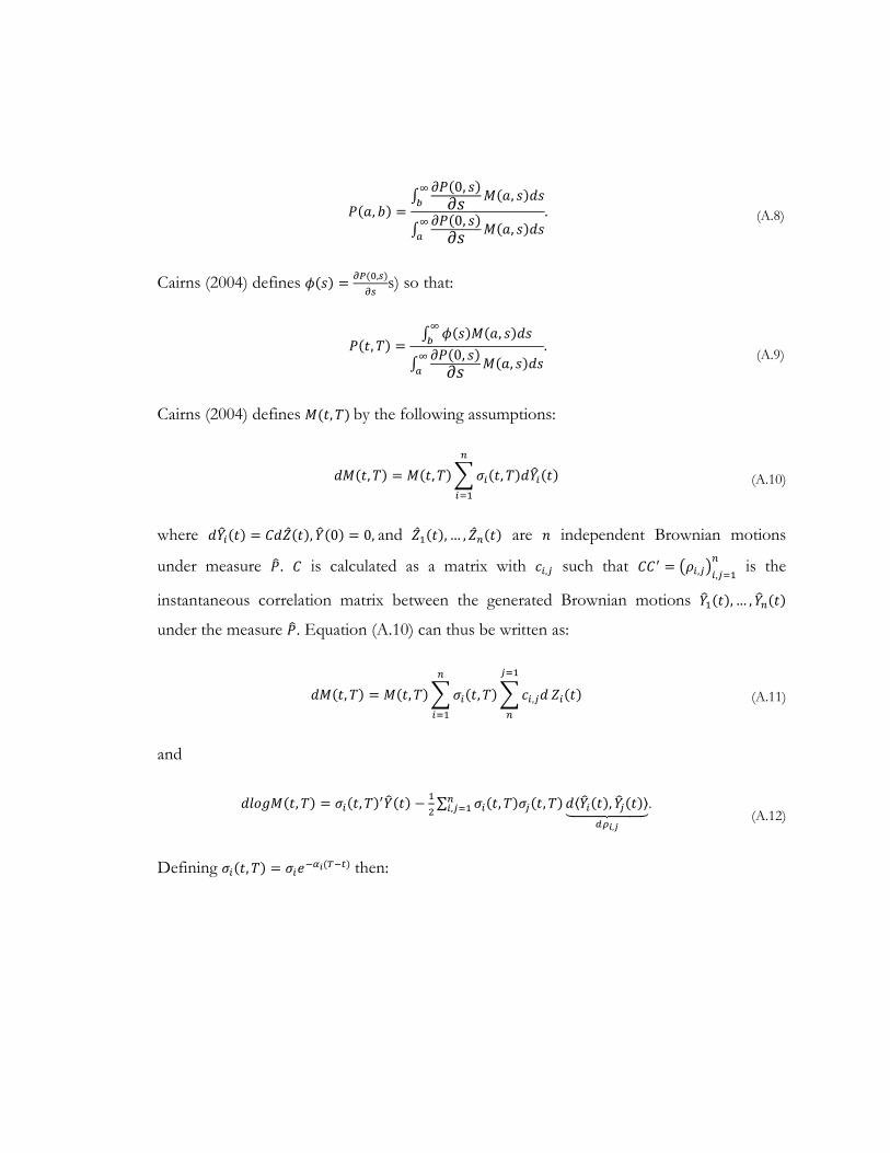
𝑃𝑃(𝑎𝑎, 𝑏𝑏) =∫ 𝜕𝜕𝑃𝑃(0, 𝑠𝑠)

𝜕𝜕𝑠𝑠 𝑀𝑀(𝑎𝑎, 𝑠𝑠)𝑑𝑑𝑠𝑠∞𝑏𝑏

∫ 𝜕𝜕𝑃𝑃(0, 𝑠𝑠)𝜕𝜕𝑠𝑠 𝑀𝑀(𝑎𝑎, 𝑠𝑠)𝑑𝑑𝑠𝑠∞

𝑠𝑠

. (A.8)

Cairns (2004) defines 𝜙𝜙(𝑠𝑠) = 𝜕𝜕𝑃𝑃(0,𝑠𝑠)𝜕𝜕𝑠𝑠

s) so that:

𝑃𝑃(𝑡𝑡,𝑇𝑇) =∫ 𝜙𝜙(𝑠𝑠)𝑀𝑀(𝑎𝑎, 𝑠𝑠)𝑑𝑑𝑠𝑠∞𝑏𝑏

∫ 𝜕𝜕𝑃𝑃(0, 𝑠𝑠)𝜕𝜕𝑠𝑠 𝑀𝑀(𝑎𝑎, 𝑠𝑠)𝑑𝑑𝑠𝑠∞

𝑠𝑠

. (A.9)

Cairns (2004) defines 𝑀𝑀(𝑡𝑡,𝑇𝑇) by the following assumptions:

𝑑𝑑𝑀𝑀(𝑡𝑡,𝑇𝑇) = 𝑀𝑀(𝑡𝑡,𝑇𝑇)�𝜎𝜎𝑖𝑖(𝑡𝑡,𝑇𝑇)𝑑𝑑𝑌𝑌�𝑖𝑖(𝑡𝑡)𝑛𝑛

𝑖𝑖=1

(A.10)

where 𝑑𝑑𝑌𝑌�𝑖𝑖(𝑡𝑡) = 𝐶𝐶𝑑𝑑�̂�𝑍(𝑡𝑡),𝑌𝑌�(0) = 0, and �̂�𝑍1(𝑡𝑡), … , �̂�𝑍𝑛𝑛(𝑡𝑡) are 𝑛𝑛 independent Brownian motions

under measure 𝑃𝑃�. 𝐶𝐶 is calculated as a matrix with 𝑐𝑐𝑖𝑖,𝑖𝑖 such that 𝐶𝐶𝐶𝐶′ = �𝜌𝜌𝑖𝑖,𝑖𝑖�𝑖𝑖,𝑖𝑖=1𝑛𝑛 is the

instantaneous correlation matrix between the generated Brownian motions 𝑌𝑌�1(𝑡𝑡), … ,𝑌𝑌�𝑛𝑛(𝑡𝑡)

under the measure 𝑃𝑃�. Equation (A.10) can thus be written as:

𝑑𝑑𝑀𝑀(𝑡𝑡,𝑇𝑇) = 𝑀𝑀(𝑡𝑡,𝑇𝑇)�𝜎𝜎𝑖𝑖(𝑡𝑡,𝑇𝑇)𝑛𝑛

𝑖𝑖=1

�𝑐𝑐𝑖𝑖,𝑖𝑖𝑑𝑑𝑖𝑖=1

𝑛𝑛

𝑍𝑍𝑖𝑖(𝑡𝑡) (A.11)

and

𝑑𝑑𝑙𝑙𝑙𝑙𝑙𝑙𝑀𝑀(𝑡𝑡,𝑇𝑇) = 𝜎𝜎𝑖𝑖(𝑡𝑡,𝑇𝑇)′𝑌𝑌�(𝑡𝑡) − 12∑ 𝜎𝜎𝑖𝑖(𝑡𝑡,𝑇𝑇)𝜎𝜎𝑖𝑖(𝑡𝑡,𝑇𝑇)𝑑𝑑⟨𝑌𝑌�𝑖𝑖(𝑡𝑡),𝑌𝑌�𝑖𝑖(𝑡𝑡)⟩���������

𝑒𝑒𝜌𝜌𝑖𝑖,𝑗𝑗

𝑛𝑛𝑖𝑖,𝑖𝑖=1 .

(A.12)

Defining 𝜎𝜎𝑖𝑖(𝑡𝑡,𝑇𝑇) = 𝜎𝜎𝑖𝑖𝑒𝑒−𝛼𝛼𝑖𝑖(𝑇𝑇−𝑡𝑡) then:

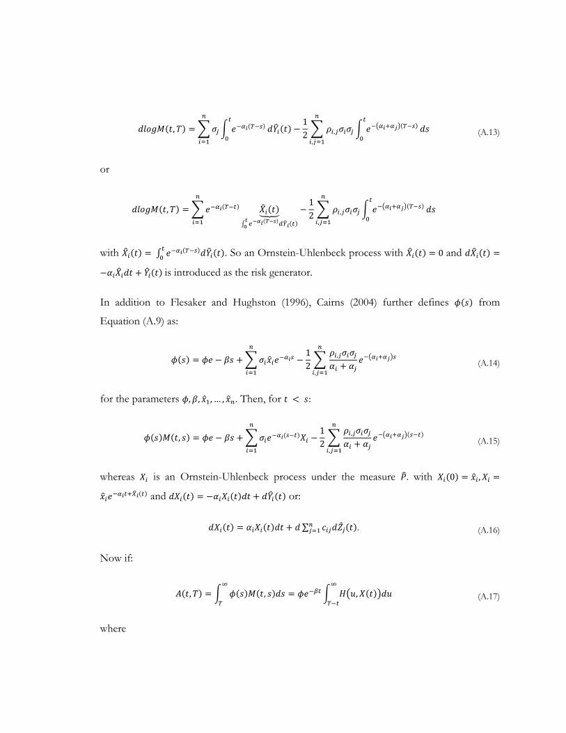
𝑑𝑑𝑙𝑙𝑙𝑙𝑙𝑙𝑀𝑀(𝑡𝑡,𝑇𝑇) = �𝜎𝜎𝑖𝑖 � 𝑒𝑒−𝛼𝛼𝑖𝑖(𝑇𝑇−𝑠𝑠)𝑡𝑡

0𝑑𝑑𝑌𝑌�𝑖𝑖(𝑡𝑡)

𝑛𝑛

𝑖𝑖=1

−12� 𝜌𝜌𝑖𝑖,𝑖𝑖𝜎𝜎𝑖𝑖𝜎𝜎𝑖𝑖 � 𝑒𝑒−�𝛼𝛼𝑖𝑖+𝛼𝛼𝑗𝑗�(𝑇𝑇−𝑠𝑠)

𝑡𝑡

0𝑑𝑑𝑠𝑠

𝑛𝑛

𝑖𝑖,𝑖𝑖=1

(A.13)

or

𝑑𝑑𝑙𝑙𝑙𝑙𝑙𝑙𝑀𝑀(𝑡𝑡,𝑇𝑇) = �𝑒𝑒−𝛼𝛼𝑖𝑖(𝑇𝑇−𝑡𝑡) 𝑋𝑋�𝑖𝑖(𝑡𝑡)���∫ 𝑏𝑏−𝛼𝛼𝑖𝑖(𝑇𝑇−𝑠𝑠)𝑒𝑒𝑌𝑌�𝑖𝑖(𝑡𝑡)𝑡𝑡0

𝑛𝑛

𝑖𝑖=1

−12� 𝜌𝜌𝑖𝑖,𝑖𝑖𝜎𝜎𝑖𝑖𝜎𝜎𝑖𝑖 � 𝑒𝑒−�𝛼𝛼𝑖𝑖+𝛼𝛼𝑗𝑗�(𝑇𝑇−𝑠𝑠)

𝑡𝑡

0𝑑𝑑𝑠𝑠

𝑛𝑛

𝑖𝑖,𝑖𝑖=1

with 𝑋𝑋�𝑖𝑖(𝑡𝑡) = ∫ 𝑒𝑒−𝛼𝛼𝑖𝑖(𝑇𝑇−𝑠𝑠)𝑑𝑑𝑌𝑌�𝑖𝑖(𝑡𝑡)𝑡𝑡0 . So an Ornstein-Uhlenbeck process with 𝑋𝑋�𝑖𝑖(𝑡𝑡) = 0 and 𝑑𝑑𝑋𝑋�𝑖𝑖(𝑡𝑡) =

−𝛼𝛼𝑖𝑖𝑋𝑋�𝑖𝑖𝑑𝑑𝑡𝑡 + 𝑌𝑌�𝑖𝑖(𝑡𝑡) is introduced as the risk generator.

In addition to Flesaker and Hughston (1996), Cairns (2004) further defines 𝜙𝜙(𝑠𝑠) from

Equation (A.9) as:

𝜙𝜙(𝑠𝑠) = 𝜙𝜙𝑒𝑒 − 𝛽𝛽𝑠𝑠 + �𝜎𝜎𝑖𝑖𝑥𝑥�𝑖𝑖𝑒𝑒−𝛼𝛼𝑖𝑖𝑠𝑠𝑛𝑛

𝑖𝑖=1

−12�

𝜌𝜌𝑖𝑖,𝑖𝑖𝜎𝜎𝑖𝑖𝜎𝜎𝑖𝑖𝛼𝛼𝑖𝑖 + 𝛼𝛼𝑖𝑖

𝑒𝑒−�𝛼𝛼𝑖𝑖+𝛼𝛼𝑗𝑗�𝑠𝑠𝑛𝑛

𝑖𝑖,𝑖𝑖=1

(A.14)

for the parameters 𝜙𝜙,𝛽𝛽, 𝑥𝑥�1, … , 𝑥𝑥�𝑛𝑛. Then, for 𝑡𝑡 < 𝑠𝑠:

𝜙𝜙(𝑠𝑠)𝑀𝑀(𝑡𝑡, 𝑠𝑠) = 𝜙𝜙𝑒𝑒 − 𝛽𝛽𝑠𝑠 + �𝜎𝜎𝑖𝑖𝑒𝑒−𝛼𝛼𝑖𝑖(𝑠𝑠−𝑡𝑡)𝑋𝑋𝑖𝑖

𝑛𝑛

𝑖𝑖=1

−12�

𝜌𝜌𝑖𝑖,𝑖𝑖𝜎𝜎𝑖𝑖𝜎𝜎𝑖𝑖𝛼𝛼𝑖𝑖 + 𝛼𝛼𝑖𝑖

𝑒𝑒−�𝛼𝛼𝑖𝑖+𝛼𝛼𝑗𝑗�(𝑠𝑠−𝑡𝑡)𝑛𝑛

𝑖𝑖,𝑖𝑖=1

(A.15)

whereas 𝑋𝑋𝑖𝑖 is an Ornstein-Uhlenbeck process under the measure 𝑃𝑃� . with 𝑋𝑋𝑖𝑖(0) = 𝑥𝑥�𝑖𝑖 ,𝑋𝑋𝑖𝑖 =

𝑥𝑥�𝑖𝑖𝑒𝑒−𝛼𝛼𝑖𝑖𝑡𝑡+𝑋𝑋�𝑖𝑖(𝑡𝑡) and 𝑑𝑑𝑋𝑋𝑖𝑖(𝑡𝑡) = −𝛼𝛼𝑖𝑖𝑋𝑋𝑖𝑖(𝑡𝑡)𝑑𝑑𝑡𝑡 + 𝑑𝑑𝑌𝑌�𝑖𝑖(𝑡𝑡) or:

𝑑𝑑𝑋𝑋𝑖𝑖(𝑡𝑡) = 𝛼𝛼𝑖𝑖𝑋𝑋𝑖𝑖(𝑡𝑡)𝑑𝑑𝑡𝑡 + 𝑑𝑑 ∑ 𝑐𝑐𝑖𝑖𝑖𝑖𝑑𝑑�̂�𝑍𝑖𝑖(𝑡𝑡)𝑛𝑛𝑖𝑖=1 . (A.16)

Now if:

𝐴𝐴(𝑡𝑡,𝑇𝑇) = � 𝜙𝜙(𝑠𝑠)𝑀𝑀(𝑡𝑡, 𝑠𝑠)𝑑𝑑𝑠𝑠 = 𝜙𝜙𝑒𝑒−𝛽𝛽𝑡𝑡 � 𝐻𝐻�𝑢𝑢,𝑋𝑋(𝑡𝑡)�𝑑𝑑𝑢𝑢∞

𝑇𝑇−𝑡𝑡

∞

𝑇𝑇 (A.17)

where

𝐻𝐻(𝑢𝑢, 𝑥𝑥) = 𝑒𝑒 − 𝛽𝛽𝑢𝑢 + �𝜎𝜎𝑖𝑖𝑥𝑥𝑖𝑖𝑒𝑒−𝛼𝛼𝑖𝑖𝑢𝑢𝑛𝑛

𝑖𝑖=1

−12�

𝜌𝜌𝑖𝑖,𝑖𝑖𝜎𝜎𝑖𝑖𝜎𝜎𝑖𝑖𝛼𝛼𝑖𝑖 + 𝛼𝛼𝑖𝑖

𝑒𝑒−�𝛼𝛼𝑖𝑖+𝛼𝛼𝑗𝑗�𝑢𝑢𝑛𝑛

𝑖𝑖,𝑖𝑖=1

(A.18)

which returns us back to Equation (A.1).

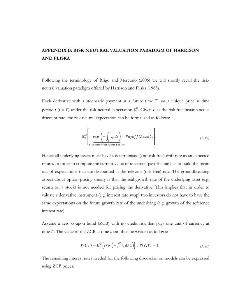
APPENDIX B: RISK-NEUTRAL VALUATION PARADIGM OF HARRISON

AND PLISKA

Following the terminology of Brigo and Mercurio (2006) we will shortly recall the risk-

neutral valuation paradigm offered by Harrison and Pliska (1983).

Each derivative with a stochastic payment at a future time 𝑇𝑇 has a unique price at time

period 𝑡𝑡 (𝑡𝑡 < 𝑇𝑇) under the risk-neutral expectation 𝔼𝔼𝑡𝑡ℚ. Given 𝑟𝑟 as the risk free instantaneous

discount rate, the risk-neutral expectation can be formalized as follows:

𝔼𝔼𝑡𝑡ℚ

⎣⎢⎢⎡

𝑒𝑒𝑥𝑥𝑝𝑝 �−� 𝑟𝑟𝑠𝑠𝑇𝑇

𝑡𝑡𝑑𝑑𝑠𝑠�

�����������𝑆𝑆𝑡𝑡𝑓𝑓𝑏𝑏ℎ𝑠𝑠𝑠𝑠𝑡𝑡𝑖𝑖𝑏𝑏 𝑒𝑒𝑖𝑖𝑠𝑠𝑏𝑏𝑓𝑓𝑢𝑢𝑛𝑛𝑡𝑡 𝑓𝑓𝑠𝑠𝑏𝑏𝑡𝑡𝑓𝑓𝑟𝑟

𝑃𝑃𝑎𝑎𝑦𝑦𝑙𝑙𝐸𝐸𝐸𝐸(𝐴𝐴𝑠𝑠𝑠𝑠𝑒𝑒𝑡𝑡)𝑇𝑇

⎦⎥⎥⎤. (A.19)

Hence all underlying assets must have a deterministic (and risk free) drift rate as an expected

return. In order to compute the current value of uncertain payoffs one has to build the mean

out of expectations that are discounted at the relevant (risk free) rate. The groundbreaking

aspect about option pricing theory is that the real growth rate of the underlying asset (e.g.

return on a stock) is not needed for pricing the derivative. This implies that in order to

valuate a derivative instrument (e.g. interest rate swap) two investors do not have to have the

same expectations on the future growth rate of the underlying (e.g. growth of the reference

interest rate).

Assume a zero coupon bond (ZCB) with no credit risk that pays one unit of currency at

time 𝑇𝑇. The value of the ZCB at time 𝑡𝑡 can thus be written as follows:

𝑃𝑃(𝑡𝑡,𝑇𝑇) = 𝔼𝔼𝑡𝑡ℚ �𝑒𝑒𝑥𝑥𝑝𝑝 �−∫ 𝑟𝑟𝑠𝑠

𝑇𝑇𝑡𝑡 𝑑𝑑𝑠𝑠 1�� , 𝑃𝑃(𝑇𝑇,𝑇𝑇) = 1. (A.20)

The remaining interest rates needed for the following discussion on models can be expressed

using ZCB prices.

The interbank reference spot Libor/Euribor rate with a maturity of 𝑇𝑇 at time 𝑡𝑡 can be

expressed as:159

𝐿𝐿(𝑡𝑡,𝑇𝑇) =1 − 𝑃𝑃(𝑡𝑡,𝑇𝑇)

(𝑇𝑇 − 𝑡𝑡)𝑃𝑃(𝑡𝑡,𝑇𝑇). (A.21)

The forward Libor rate at time 𝑡𝑡, expiry 𝑇𝑇𝑖𝑖−1 and maturity 𝑇𝑇𝑖𝑖 can be computed as follows:

𝐹𝐹𝑖𝑖(𝑡𝑡) =1

𝑇𝑇𝑖𝑖 − 𝑇𝑇𝑖𝑖−1�𝑃𝑃(𝑡𝑡,𝑇𝑇𝑖𝑖−1)𝑃𝑃(𝑡𝑡,𝑇𝑇𝑖𝑖)

− 1�. (A.22)

The periodic fixed swap rate of an interest rate swap referencing to the Libor rate with the

tenor structure 𝑇𝑇𝛼𝛼, 𝑇𝑇𝛼𝛼+1, …, 𝑇𝑇𝛽𝛽 is given by:

𝑠𝑠𝛼𝛼,𝛽𝛽(𝑡𝑡) ≔𝑃𝑃(𝑡𝑡,𝑇𝑇𝛼𝛼) − 𝑃𝑃�𝑡𝑡,𝑇𝑇𝛽𝛽�

∑ (𝑇𝑇𝑖𝑖 − 𝑇𝑇𝑖𝑖−1)𝑃𝑃(𝑡𝑡,𝑇𝑇𝑖𝑖)𝛽𝛽𝑖𝑖=𝛼𝛼+1

�𝑃𝑃(𝑡𝑡,𝑇𝑇𝑖𝑖−1)𝑃𝑃(𝑡𝑡,𝑇𝑇𝑖𝑖)

− 1�. (A.23)

Notice that swap rates are market rates with observable quotes in the market. While spot and

forward Libor rates as well as swap rates can be stripped from ZCB, the price of ZCB is a

function of the expected dynamics of the short rate.

159 Notice that we are working within the so-called “single curve” paradigm. We are assuming no default risk of the bond issuer. Within this paradigm the fixing frequency of a reference rate does not have an influence on the rate, implying for example that 12-month Euribor and 3-month Euribor must be equal (e.g. on a per annum basis). Since the financial crises begging in 2008 this assumption, however, has been greatly falsified.

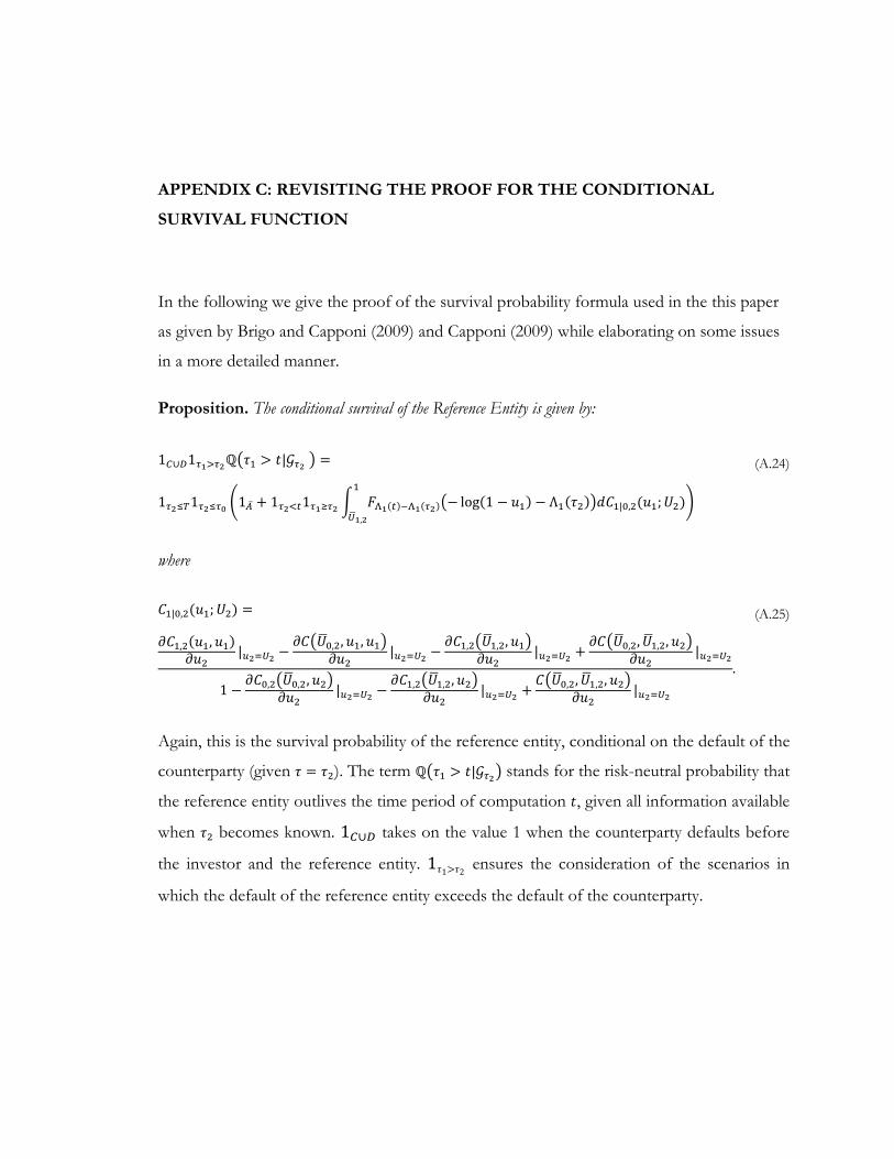
APPENDIX C: REVISITING THE PROOF FOR THE CONDITIONAL

SURVIVAL FUNCTION

In the following we give the proof of the survival probability formula used in the this paper

as given by Brigo and Capponi (2009) and Capponi (2009) while elaborating on some issues

in a more detailed manner.

Proposition. The conditional survival of the Reference Entity is given by:

1𝐶𝐶∪𝐷𝐷1𝜏𝜏1>𝜏𝜏2ℚ�𝜏𝜏1 > 𝑡𝑡|𝒢𝒢𝜏𝜏2 � = (A.24)

1𝜏𝜏2≤𝑇𝑇1𝜏𝜏2≤𝜏𝜏0 �1�̅�𝐴 + 1𝜏𝜏2<𝑡𝑡1𝜏𝜏1≥𝜏𝜏2 � 𝐹𝐹Λ1(𝑡𝑡)−Λ1(𝜏𝜏2)�− log(1 − 𝑢𝑢1) − Λ1(𝜏𝜏2)�𝑑𝑑𝐶𝐶1|0,2(𝑢𝑢1;𝑈𝑈2)1

𝑈𝑈�1,2

�

where

𝐶𝐶1|0,2(𝑢𝑢1;𝑈𝑈2) = (A.25)

𝜕𝜕𝐶𝐶1,2(𝑢𝑢1,𝑢𝑢1)𝜕𝜕𝑢𝑢2

|𝑢𝑢2=𝑈𝑈2 −𝜕𝜕𝐶𝐶�𝑈𝑈�0,2,𝑢𝑢1,𝑢𝑢1�

𝜕𝜕𝑢𝑢2|𝑢𝑢2=𝑈𝑈2 −

𝜕𝜕𝐶𝐶1,2�𝑈𝑈�1,2,𝑢𝑢1�𝜕𝜕𝑢𝑢2

|𝑢𝑢2=𝑈𝑈2 +𝜕𝜕𝐶𝐶�𝑈𝑈�0,2,𝑈𝑈�1,2,𝑢𝑢2�

𝜕𝜕𝑢𝑢2|𝑢𝑢2=𝑈𝑈2

1 −𝜕𝜕𝐶𝐶0,2�𝑈𝑈�0,2,𝑢𝑢2�

𝜕𝜕𝑢𝑢2|𝑢𝑢2=𝑈𝑈2 −

𝜕𝜕𝐶𝐶1,2�𝑈𝑈�1,2,𝑢𝑢2�𝜕𝜕𝑢𝑢2

|𝑢𝑢2=𝑈𝑈2 +𝐶𝐶�𝑈𝑈�0,2,𝑈𝑈�1,2,𝑢𝑢2�

𝜕𝜕𝑢𝑢2|𝑢𝑢2=𝑈𝑈2

.

Again, this is the survival probability of the reference entity, conditional on the default of the

counterparty (given 𝜏𝜏 = 𝜏𝜏2). The term ℚ�𝜏𝜏1 > 𝑡𝑡|𝒢𝒢𝜏𝜏2� stands for the risk-neutral probability that

the reference entity outlives the time period of computation 𝑡𝑡, given all information available

when 𝜏𝜏2 becomes known. 1𝐶𝐶∪𝐷𝐷 takes on the value 1 when the counterparty defaults before

the investor and the reference entity. 1𝜏𝜏1>𝜏𝜏2 ensures the consideration of the scenarios in

which the default of the reference entity exceeds the default of the counterparty.

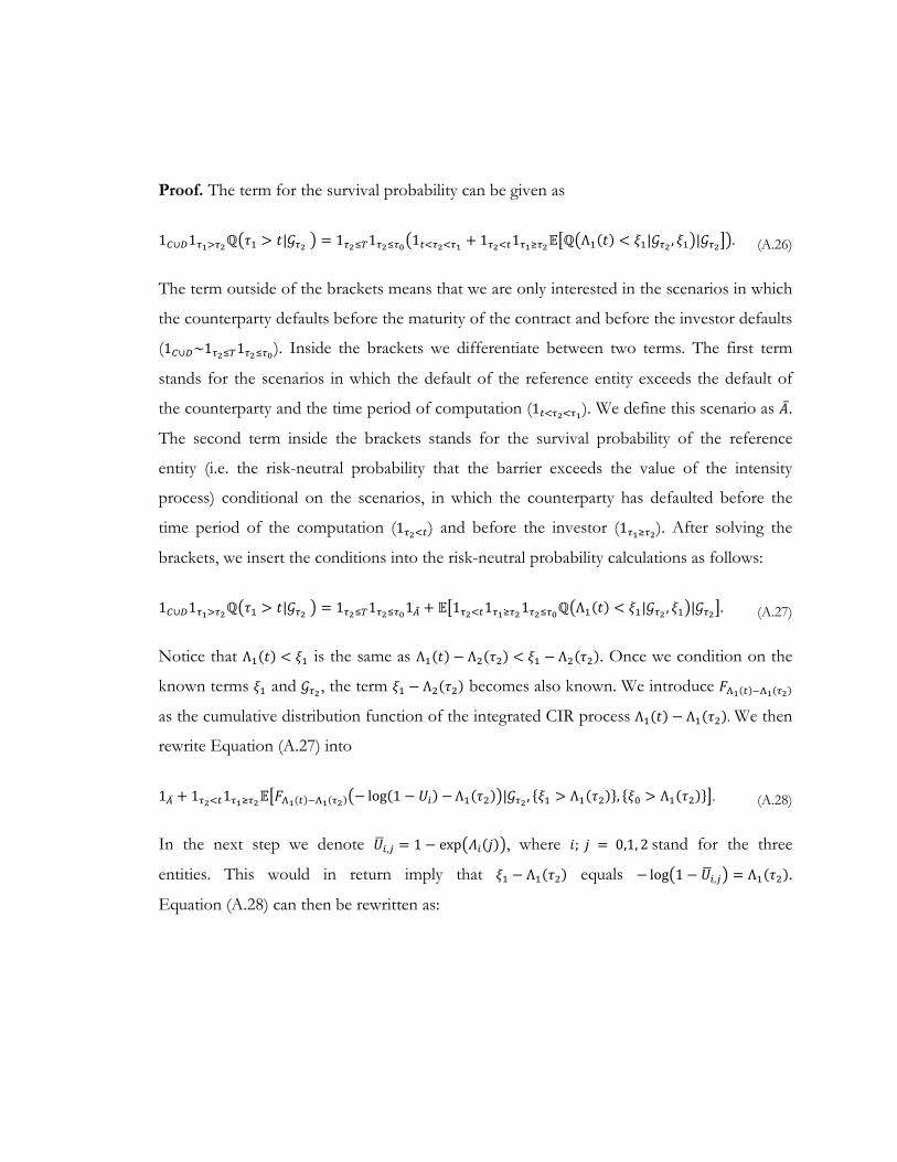
Proof. The term for the survival probability can be given as

1𝐶𝐶∪𝐷𝐷1𝜏𝜏1>𝜏𝜏2ℚ�𝜏𝜏1 > 𝑡𝑡|𝒢𝒢𝜏𝜏2 � = 1𝜏𝜏2≤𝑇𝑇1𝜏𝜏2≤𝜏𝜏0�1𝑡𝑡<𝜏𝜏2<𝜏𝜏1 + 1𝜏𝜏2<𝑡𝑡1𝜏𝜏1≥𝜏𝜏2𝔼𝔼�ℚ�Λ1(𝑡𝑡) < 𝜉𝜉1|𝒢𝒢𝜏𝜏2 , 𝜉𝜉1�|𝒢𝒢𝜏𝜏2��. (A.26)

The term outside of the brackets means that we are only interested in the scenarios in which

the counterparty defaults before the maturity of the contract and before the investor defaults

(1𝐶𝐶∪𝐷𝐷~1𝜏𝜏2≤𝑇𝑇1𝜏𝜏2≤𝜏𝜏0). Inside the brackets we differentiate between two terms. The first term

stands for the scenarios in which the default of the reference entity exceeds the default of

the counterparty and the time period of computation (1𝑡𝑡<𝜏𝜏2<𝜏𝜏1). We define this scenario as �̅�𝐴.

The second term inside the brackets stands for the survival probability of the reference

entity (i.e. the risk-neutral probability that the barrier exceeds the value of the intensity

process) conditional on the scenarios, in which the counterparty has defaulted before the

time period of the computation (1𝜏𝜏2<𝑡𝑡) and before the investor (1𝜏𝜏1≥𝜏𝜏2). After solving the

brackets, we insert the conditions into the risk-neutral probability calculations as follows:

1𝐶𝐶∪𝐷𝐷1𝜏𝜏1>𝜏𝜏2ℚ�𝜏𝜏1 > 𝑡𝑡|𝒢𝒢𝜏𝜏2 � = 1𝜏𝜏2≤𝑇𝑇1𝜏𝜏2≤𝜏𝜏01�̅�𝐴 + 𝔼𝔼�1𝜏𝜏2<𝑡𝑡1𝜏𝜏1≥𝜏𝜏21𝜏𝜏2≤𝜏𝜏0ℚ�Λ1(𝑡𝑡) < 𝜉𝜉1|𝒢𝒢𝜏𝜏2 , 𝜉𝜉1�|𝒢𝒢𝜏𝜏2�. (A.27)

Notice that Λ1(𝑡𝑡) < 𝜉𝜉1 is the same as Λ1(𝑡𝑡) − Λ2(𝜏𝜏2) < 𝜉𝜉1 − Λ2(𝜏𝜏2). Once we condition on the

known terms 𝜉𝜉1 and 𝒢𝒢𝜏𝜏2, the term 𝜉𝜉1 − Λ2(𝜏𝜏2) becomes also known. We introduce 𝐹𝐹Λ1(𝑡𝑡)−Λ1(𝜏𝜏2)

as the cumulative distribution function of the integrated CIR process Λ1(𝑡𝑡) − Λ1(𝜏𝜏2). We then

rewrite Equation (A.27) into

1�̅�𝐴 + 1𝜏𝜏2<𝑡𝑡1𝜏𝜏1≥𝜏𝜏2𝔼𝔼�𝐹𝐹Λ1(𝑡𝑡)−Λ1(𝜏𝜏2)�− log(1 − 𝑈𝑈𝑖𝑖) −Λ1(𝜏𝜏2)�|𝒢𝒢𝜏𝜏2 , {𝜉𝜉1 > Λ1(𝜏𝜏2)}, {𝜉𝜉0 > Λ1(𝜏𝜏2)}�. (A.28)

In the next step we denote 𝑈𝑈�𝑖𝑖,𝑖𝑖 = 1 − exp�𝛬𝛬𝑖𝑖(𝑗𝑗)�, where 𝑖𝑖; 𝑗𝑗 = 0,1, 2 stand for the three

entities. This would in return imply that 𝜉𝜉1 − Λ1(𝜏𝜏2) equals − log�1 − 𝑈𝑈�𝑖𝑖,𝑖𝑖� = Λ1(𝜏𝜏2).

Equation (A.28) can then be rewritten as:

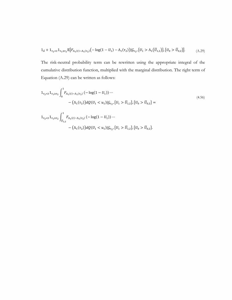
1�̅�𝐴 + 1𝜏𝜏2<𝑡𝑡1𝜏𝜏1≥𝜏𝜏2𝔼𝔼�𝐹𝐹Λ1(𝑡𝑡)−Λ1(𝜏𝜏2)�− log(1 − 𝑈𝑈1) −Λ1(𝜏𝜏2)�|𝒢𝒢𝜏𝜏2 , �𝑈𝑈1 > Λ1�𝑈𝑈�1,2��, �𝑈𝑈0 > 𝑈𝑈�0,2��. (A.29)

The risk-neutral probability term can be rewritten using the appropriate integral of the

cumulative distribution function, multiplied with the marginal distribution. The right term of

Equation (A.29) can be written as follows:

1𝜏𝜏2<𝑡𝑡1𝜏𝜏1≥𝜏𝜏2 � 𝐹𝐹Λ1(𝑡𝑡)−Λ1(𝜏𝜏2)

1

0(− log(1 − 𝑈𝑈1))⋯

− �Λ1(𝜏𝜏2)�𝑑𝑑𝑑𝑑(𝑈𝑈1 < 𝑢𝑢1)|𝒢𝒢𝜏𝜏2 , �𝑈𝑈1 > 𝑈𝑈�1,2�, �𝑈𝑈0 > 𝑈𝑈�0,2� = (4.56)

1𝜏𝜏2<𝑡𝑡1𝜏𝜏1≥𝜏𝜏2 � 𝐹𝐹Λ1(𝑡𝑡)−Λ1(𝜏𝜏2)

1

𝑈𝑈�1,2

(− log(1 − 𝑈𝑈1))⋯

− �Λ1(𝜏𝜏2)�𝑑𝑑𝑑𝑑(𝑈𝑈1 < 𝑢𝑢1)|𝒢𝒢𝜏𝜏2 , �𝑈𝑈1 > 𝑈𝑈�1,2�, �𝑈𝑈0 > 𝑈𝑈�0,2�.

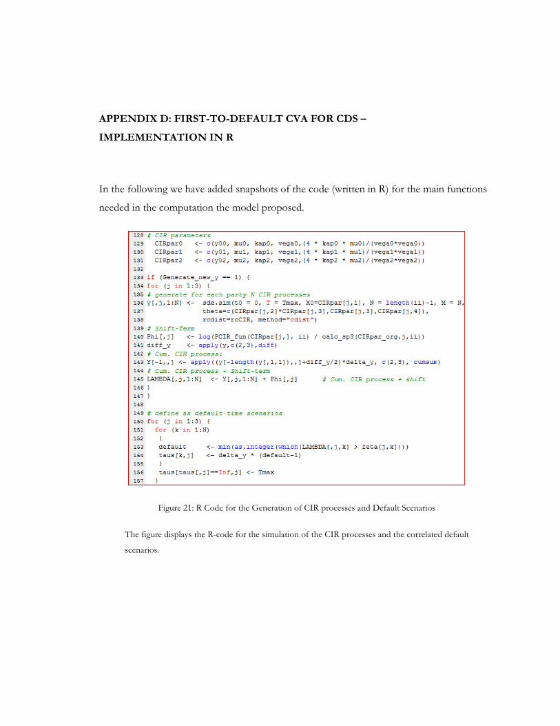
APPENDIX D: FIRST-TO-DEFAULT CVA FOR CDS –

IMPLEMENTATION IN R

In the following we have added snapshots of the code (written in R) for the main functions

needed in the computation the model proposed.

Figure 21: R Code for the Generation of CIR processes and Default Scenarios

The figure displays the R-code for the simulation of the CIR processes and the correlated default

scenarios.

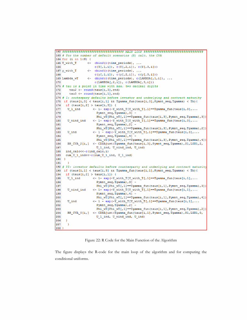
Figure 22: R Code for the Main Function of the Algorithm

The figure displays the R-code for the main loop of the algorithm and for computing the

conditional uniforms.

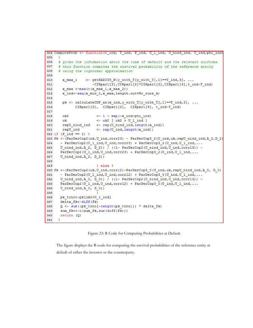
Figure 23: R Code for Computing Probabilities at Default

The figure displays the R-code for computing the survival probabilities of the reference entity at

default of either the investor or the counterparty.

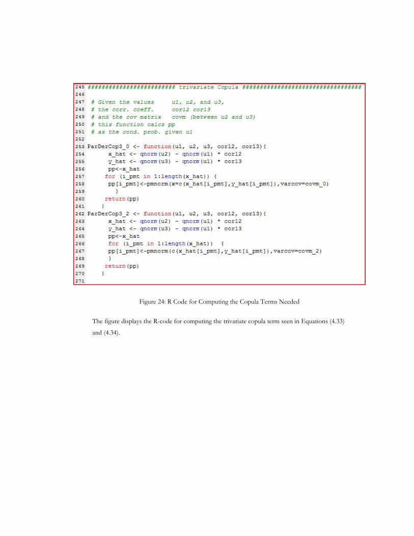
Figure 24: R Code for Computing the Copula Terms Needed

The figure displays the R-code for computing the trivariate copula term seen in Equations (4.33)

and (4.34).

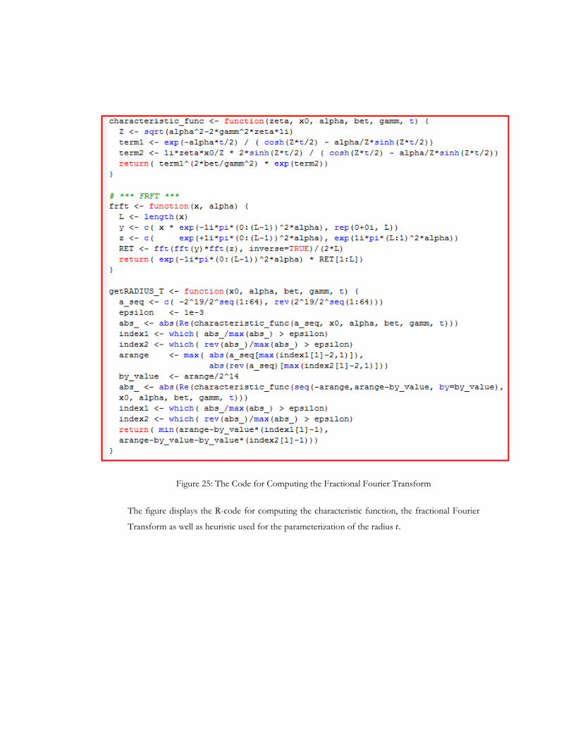
Figure 25: The Code for Computing the Fractional Fourier Transform

The figure displays the R-code for computing the characteristic function, the fractional Fourier

Transform as well as heuristic used for the parameterization of the radius 𝑡𝑡.

BIBLIOGRAPHY

Akerlof, G. (1970). The market for "lemons": Quality uncertainty and the market

mechanism, The Quarterly Journal of Economics, 84 (3), 488-500.

Albanese, C.; Brigo, D.; and F. Oertel (2013). Restructuring counterparty credit risk,

International Journal of Theoretical and Applied Finance, 16 (2).

Altman, E. (1989). Measuring corporate bond mortality and performance, Journal of Finance,

44 (4), 909-922.

Altman, E. (2006). Default recovery and LGD in credit risk modeling and practice, Working

Paper, Stern School of Business.

Andresen, L.; and V. Piterbarg (2010a). Interest rate modeling (volume 1): Foundations and

vanilla models, Atlantic Financial Press.

Andresen, L.; and V. Piterbarg (2010b). Interest rate modeling (volume 2): Term structure

models, Atlantic Financial Press.

Andresen, L.; and V. Piterbarg (2010c). Interest rate modeling (volume 3): Products and risk

management, Atlantic Financial Press.

Arora, N.; Bohn, J.; and F. Zhu (2005). Reduced form vs. structural models of credit risk: A

case study of three models, Moody’s KMV.

Arora, N.; Gandhi, P.; and F. A. Longstaff (2012). Counterparty credit risk and the credit

default swap market, Journal of Financial Economics, 103 (2), 280-293.

Arvanitis, A.; and J. Gregory (2001). Credit: The complete guide to pricing, hedging and risk

management, Risk Books.

Assefa, S.; Bielecki, T.; Crepey, S.; and M. Jeanblanc (2009). CVA computation for

counterparty risk assessment in credit portfolio, Credit Risk Frontiers: Subprime Crisis,

Pricing and Hedging, CVA, MBS, Ratings and Liquidity, Bielecki, T.; Brigo, D.; and F. Patras

(eds.), Wiley.

Augustin, P. (2014). Sovereign credit default swap premia, Journal of Investment Management,

12 (2), 65-102.

Babbs, S. H.; and K. B. Nowman (1999). Kalman filtering of generalized Vasicek term

structure models, Journal of Financial and Quantitative Analysis, 34 (1), 115-130.

Bailey, D.; and P. Swarztrauber (1993). A fast method for the numerical evaluation of

continuous Fourier and Laplace transforms, SIAM Journal of Scientific Computing, 15 (5),

1105-1110.

Balder, S. (2014). On the role of strategies in finance, Habilitation Thesis at the University of

Duisburg-Essen.

Balder, S.; and D. Schwake (2011). Hedging of interest rate risks in long-term contracts: An

application of the Cairns model, Working Paper of the University of Duisburg-Essen.

Basel Committee on Banking Supervision, BCBS (2005). An explanatory note on the Basel II

IRB risk weight functions, July 2005.

Basel Committee on Banking Supervision, BCBS (2011). Press release: Capital treatment for

bilateral counterparty credit risk finalised by the Basel Committee, June 2011.

Basel Committee on Banking Supervision, BCBS (2013). Margin requirements for non-

centrally cleared derivatives, September 2013.

Basel Committee on Banking Supervision, BCBS (2014). The standardised approach for

measuring counterparty credit risk exposure, April 2014.

Beder, T. S. (1995). VaR: Seductive but dangerous, Financial Analyst Journal,

September/October, 12-24.

Bemmann, V. (2008). Hedging interest rate exposure of pension funds by the use of a

DV01-matching swap overlay - an economic application of the Heath-Jarrow-Morton

methodology. Diplom Thesis - Dresden University of Technology.

Berkshire Hathaway (2002). Bershire Hathaway Inc. 2002 annual report, available online:

http://www.berkshirehathaway.com/2002ar/2002ar.pdf.

Beunza, D.; and D. Stark (2010). Tools of the trade: The socio-technology of arbitrage in a

wall street trading room, Industrial and Corporate Change, 13, 369-400.

Bielecki, T.; and M. Rutkowski (2001). Credit Risk: Modeling, Valuation and Hedging,

Springer Finance.

Bielecki, T.; Cialenco, I.; and I. Iyigunler (1993). Counterparty Risk and the Impact of

Collateralization in CDS Contracts, Working Paper of the Cornell University.

Bilal, M.; and M. Singh (2012). CDS spreads in European periphery ― some technical issues

to consider, IMF Working Paper.

Björk, T. (2009). Arbitrage theory in continuous time, Oxford Finance.

Black, F. (1976). The pricing of commodity contracts, Journal of Financial Economics, 3,

167-179.

Black, F.; and J. C. Cox (1976). Valuing corporate securities: Some effects of bond indenture

provisions, Journal of Finance, 31 (2), 351-367.

Black, F.; and M. Scholes (1973). The pricing of options and corporate liabilities, Journal of

Political Economy, 81, 637-654.

Black, F.; and P. Karasinski (1991). Bond and option pricing when short rates are lognormal,

Financial Analysts Journal, 47, 52–59.

Black, F.; Derman, E.; and W. Toy (1990). A one-factor model of interest rates and its

application to treasury bond prices, Financial Analyst Journal, 46, 33-39.

Blanchet-Scalliet, C.; and F. Patras (2008). Counterparty risk valuation for CDS, Credit Risk

Frontiers: Subprime crisis, Pricing and Hedging, CVA, MBS, Ratings and Liquidity, Bielecki, T.;

Brigo, D.; and F. Patras (eds.), Wiley.

Brace, A.; Gatarek, D.; and M. Musiela (1997). The market model of interest rate dynamics,

Mathematical Finance, 7, 127-147.

Branger, N.; and C. Schlag (2004). Zinsderivate – Modelle und Bewertung. Springer.

Bree, C.; Linder, A.; and Mario Schlener (2011). Einsatz von Derivativen zum Hedging,

Kontrahentenrisiko – Bewertung, Steuerung und Unterlegung nach Basel III und IFRS, Ludwig, S.;

Martin, M.; and C. Wehn (eds.), Schäffer-Poeschel.

Brick, J. R. (2014). Asset-liability management: Theory, practice, implementation, and role of

judgment, Report of Bricks & Associates, Inc.

Brigo D.; and M. Morini (2010). Dangers of bilateral counterparty credit risk: The

fundamental impact of closeout conventions, Working Paper.

Brigo D.; and M. Morini (2011). Close out convention tensions, Risk, December, 86-90.

Brigo D.; and N. El-Bachir (2008). An exact formula for default swaptions’ pricing in the

SSRJD stochastic intensity model, Mathematical Finance, 20, 365-382.

Brigo D.; Capponi, A.; and A. Pallavicini (2011a). Arbitrage-free bilateral counterparty risk

valuation under collateralization and application to credit default swaps, Mathematical

Finance, 24 (1), 125-146.

Brigo D.; Capponi, A.; Pallavicini, A.; and V. Papatheodorou (2013b). Pricing counterparty

risk including collateralization, netting rules, re-hypothecation and wrong-way risk,

International Journal of Theoretical and Applied Finance, 16 (2).

Brigo D.; Morini M.; and M. Tarenghi (2011b). Equity return swap valuation under

counterparty risk, Credit Risk Frontiers: Sub- prime crisis, Pricing and Hedging, CVA, MBS,

Ratings and Liquidity, Bielecki, D.; Brigo, D.; and F. Patras (eds.), John Wiley & Sons, Ltd.

Brigo D.; Morini, M.; and A. Pallavicini (2013a). Counterparty credit risk, collateral and

funding – with pricing cases for all asset classes. John Wiley & Sons.

Brigo, D.; and A. Alfonsi (2005). Credit default swap calibration and derivatives pricing with

the SSRD stochastic intensity model, Finance and Stochastic, 9, 29-42.

Brigo, D.; and A. Capponi (2009). Bilateral counterparty risk valuation with stochastic

dynamical models and application to credit default swaps. Working Paper.

Brigo, D.; and A. Capponi (2010). Bilateral counterparty risk with application to CDSs, Risk,

March, 85-90.

Brigo, D.; and A. Pallavicini (2008). Counterparty risk under correlation between default and

interest rates, Numerical Methods for Finance, Miller, J.; Edelman, D.; and J. Appleby (eds.),

Taylor & Francis Group.

Brigo, D.; and F. Mercurio (2006). Interest rate models: Theory and practice – with smile,

inflation and credit, 2nd edition, Springer Verlag.

Brigo, D.; and I. Bakkar (2009). Accurate counterparty risk valuation for energy-

commodities swaps, Energy Risk, March.

Brigo, D.; and L. Cousot (2006). A comparison between the SSRD model and the market

model for CDS option pricing, International Journal of Theoretical and Applied Finance, 9 (3).

Brigo, D.; and K. Chourdakis (2009). Counterparty risk for credit default swaps: Impact of

spread volatility and default correlation, International Journal of Theoretical and Applied

Finance, 12, 1007-1029.

Brigo, D.; and M. Masetti (2005). Risk-neutral pricing of counterparty risk, Counterparty Credit

Risk Model – Risk Management, Pricing and Regulation, Pykhtin, M. (ed.), Risk Books.

Broadie, M.; Du, Y.; and C. C. Moallemi (2011). Efficient risk estimation via nested

sequential simulation, Management Science, 57 (6), 1172-1194.

Brunnermeier, M. K. (2009). Deciphering the liquidity and credit crunch 2007-2008, Journal of

Economic Perspectives, 23 (1), 77-100.

Burgard, C.; and M. Kjaer (2013). Funding strategies, funding costs, Risk, December, 82-87.

Burne, K. (2011). How weakening credit strengthens banks’ results – and vice versa, The

Wall Street Journal, October 18, 2011.

Cairns, A. J. (2004). A family of term-structure models for long-term risk management and

derivative pricing, Mathematical Finance, 14 (3), 415-444.

Cameron, M. (2014). The black art of FVA, part II: Conditioning chaos, Risk, March.

Canabarro, E. (2010). Counterparty credit risk: Management, pricing and hedging,

Risk Books.

Canabarro, E.; and D. Duffie (2003). Chapter 9: Measuring and marking counterparty risk,

Asset/Liability Management of Financial Institutions: Maximizing Shareholder Value Through

Risk-Conscious Investing, Tilman, L. (ed.), Euromoney Books.

Capponi, A. (2009). Credit Risk and Nonlinear Filtering: Computational Aspects and

Empirical Evidence, PhD Thesis at California Institute of Technology (CIT).

Carr, P.; Geman, H.; Madan, D.; and M. Yor (2003). Stochastic volatility for levy processes,

Mathematical Finance, 13 (3), 345-382.

Carver, L. (2011). The CVA-CDS feedback loop, Risk, 14. December.

Carver, L. (2013). Cutting edge introduction: Pricing the CVA doom loop, Risk, October.

Cesari, G.; Aquilina, J.; Charpillon, N.; Filipovic, Z; Lee, G.; and I. Manda (2009). Modelling,

pricing and hedging counterparty credit exposure: A technical guide. Springer.

Cespedes, J. C. G.; Herrero, J. A. de J.; Rosen, D.; and D. Saunders (2010). Effective

modeling of wrong way risk, counterparty credit risk capital, and alpha in Basel II, Journal

of Risk Model Valuation, 4 (1), 71-98.

Chambers, D.; and W. Carleton (1988). A generalized approach to duration, Research in

Finance, 7, 163-181.

Chen, R. R.; and L. Scott (2003). Multi-factor Cox-Ingersoll-Ross models of the term

structure: Estimates and tests from a Kalman filter model, Journal of Real Estate Finance

and Economics, 27 (2), 143-172.

Cherubini, U. (2005). Counterparty risk in derivatives and collateral policies: The replicating

portfolio approach, Proceedings of the Counterparty Credit Risk 2005 CREDIT Conference, 22-

23.

Chourdakis, K. (2005). Option pricing using the fractional FFT, Journal of Computation Finance,

8, 1-18.

Cox, J., Ingersoll, J.; and S. Ross (1985). A theory of the term structure of interest rates,

Econometrica, 53, 385-407.

Crepey, S.; Jeanblanc, M.; and B. Zargari (2010). Counterparty risk on a CDS in a Markov

chain copula model with joint defaults, Recent Advances in Financial Engineering, Kijima, M.;

Hara, C.; Muromachi, Y.; and K. Tanaka (eds.), World Scientific Publishing Co. Pte.

Dash, E. (2011). Citigroup Earnings Rise 74%, to $3.8 Billion, New York Times, November 28,

2011.

Deloitte and Solum (2013). Counterparty Risk and CVA Survey – Current market practice

around counterparty risk regulation, CVA management and funding, February.

Duan, J.; and J. Simonato (1999). Estimating and testing exponential-affine term structure

models by Kalman filter, Review of Quantitative Finance and Accounting, 13.

Duffie, D.; and K. Singleton (1999). Modeling term structure of defaultable bonds, Review of

Financial Studies, 12 (4), 197-226.

Duffie, D.; and K. Singleton (2003). Credit risk: Pricing, measurement and management.

Princeton University Press.

Duffie, D.; and M. Huang (1996). Swap rates and credit quality, Journal of Finance, 51 (3), 921-

950.

Dufresne, D. (2001). The integrated square-root process, Working Paper, No. 90, Centre of

Actuarial Studies, University of Melbourne.

European Banking Association, EBA (2015). EBA report on credit valuation adjustment

(CVA) under Article 456(2) of Regulation (EU) No 575/2013 (capital requirements

regulation – CRR) and EBA review on the application of CVA charges to non-financial

counterparties established in a third country under Article 382(5) of regulation (EU) No

575/2013 (capital requirements regulation – CRR), 25 February 2015.

European Central Bank, ECB (2014). Aggregate report on the comprehensive assessment,

October.

Fabozzi, F. (2000). Bond markets, analysis and strategies, 4th edition, Prentice Hall.

Fabozzi, F.; Focardi, S.; and C. Jonas (2005). Market experience with modeling for defined

benefit pension funds: Evidence from four countries, Journal of Pension Economics and

Finance, 4 (3), 313-327.

Fischer, L.; and R. Weil (1971). Coping with the risk of interest-rate fluctuation: Returns to

bondholders from naïve and optimal strategies, Journal of Business, 44 (4), 408-431.

Flesaker, B.; and L. Hughston (1996). Positive interest, Risk, 9 (1), 46-49.

Frey, R.; and A. McNeil (2003). Dependent defaults in models of portfolio risk, Journal of

Risk, 6, 59-62.

Fries, C.; Schwake, D.; and T. Sudmann (2013). FVA – Berücksichtigung der Finanzierung in

der Derivatebewertung, Zeitschrift für das gesamte Kreditwesen, 11, 573-575.

Fujii, M.; and A. Takahashi (2011). Choice of collateral currency, Risk, January, 120-125.

Giesecke, K.; Longstaff, F. A.; Schaefer, S.; and I. Strebulaev (2010). Corporate bond default

risk – A 150-year perspective, NBER Working Paper No. 15848, March.

Glasserman, P.; and B. Yu (2002). Pricing American options by simulation: Regression now

or regression later?, Monte Carlo and Quasi-Monte Carlo Methods, Niederreiter, H. (ed.),

Springer.

Gondzio, J.; and R. Kouwenberg (2001). High-performance computing for asset-liability

management. Operations Research, 49 (6), 879–891.

Gordy, M.; and S. Juneja (2008). Nested simulation in portfolio risk management, Working

Paper.

Gordy, M. (2003). A risk-factor model foundation for ratings-based bank capital rules,

Journal of Financial Intermediation, 12, 199-232.

Gregory, J. (2009). Being two-faced over counterparty credit risk, Risk, 22 (2), 86-90.

Gregory, J. (2012). Counterparty credit risk and credit valuation adjustment. John Wiley and

Sons, Ltd.

Gregory, J.; and I. German (2012). Closing out DVA, Working Paper.

Grominski, D.; Schwake, D.; and T. Sudmann (2012). Valuation of credit default swaps with

wrong way risk: Model implementation and a computational tune-up, 13th Doctoral

Conference in Accounting and Finance, Prague.

Gupta, S.; and K. Sundaram (2012). CDS auctions and informative biases in CDS recovery

rates, Working Paper of the New York University.

Harrison, J. M.; and S. R. Pliska (1983). A stochastic calculus model of continuous trading:

complete markets, Stochastic Processes and their Applications, 15, 313-316.

Haug, E. G.; and N. N. Taleb (2011). Option traders use (very) sophisticated heuristics,

never the Black-Scholes-Merton formula, Journal of Economics & Organization, 77, 97-106.

Hayek, F. A. (1942). Scientism and the study of society, Part I., Economica, 9, 267-291.

Heath, D.; Jarrow R.; and A. Morton (1992). Bond pricing and the term structure of interest

rates: A new methodology for contingent claims valuation, Econometrica, 60 (1), 77-105.

Ho, T. S. Y. (1992). Key rate durations: Measure of interest rate risk, Journal of Fixed Income, 2

(2), 29-44.

Ho, T. S. Y.; and S. B. Lee (1986). Term structure movements and pricing interest rate

contingent claims, Journal of Finance, 41 (5), 1011-1029.

Hull, H.; Presdescu, M.; and A. White (2005). Bond prices, default probabilities and risk

premiums, Journal of Credit Risk, 1 (2 Spring), 53-60.

Hull, J. (2006). Options, futures and other derivatives, 6th edition, Person Education.

Hull, J.; and A. White (1990). Pricing interest-rate derivative securities, The Review of Financial

Studies, 3 (4), 573-592.

Hull, J.; and A. White (2001). Valuing credit default swaps II: Modeling default correlations,

Journal of Derivatives, 8 (3), 12-22.

Hull, J.; and A. White (2011). CVA and wrong way risk, Financial Analyst Journal, March 5.

Hull, J.; and A. White (2012a). The FVA debate, Risk, 25th anniversary edition, 83-85.

Hull, J.; and A. White (2012b). LIBOR vs. OIS: The derivatives discounting dilemma, Journal

of Investment Management, 11 (3), 14-27.

Hull, J.; Preduscu, M.; and A. White (2004). The relationship between credit default swap

spreads, bond yields, and credit rating announcements, Journal of Banking and Finance, 28

(11), 2789-2811.

Ingersoll, J. E.; Skelton, J., Jr.; and R. L. Weil (1978). Duration: Forty years later. Journal of

Financial and Quantitative Analysis, 13 (4), 627-650.

International Swaps and Derivatives Association, ISDA (2011). Counterparty credit risk

management in the US over-the-counter (OTC) derivatives markets, part II: A review of

monoline exposure.

International Swaps and Derivatives Association, ISDA (2013). OTC Derivatives Market

Analysis Year-End 2012.

International Swaps and Derivatives Association, ISDA (2014a). ISDA Margin Survey 2014.

International Swaps and Derivatives Association, ISDA (2014b). ISDA Research Study:

Dispelling Myths: End-user activity in OTC derivatives.

International Swaps and Derivatives Association, ISDA (2015). ISDA margin survey 2015.

Jaffee, D. (2006). Monoline restrictions, with applications to mortgage insurance and title

insurance, Review of Industrial Organization, 23, 83-108.

Jamshidian F.; and Y. Zhu (1997). Scenario simulation: Theory and methodology, Finance and

Stochastics, 1, 43-67.

Jarrow, R. A.; and M. S. Turnbull (1992). Credit risk: Drawing the analogy, Risk, 5 (9), 63-70.

Jarrow, R. A.; and M. S. Turnbull (1994). Delta, gamma and bucket hedging of interest rate

derivatives, Applied Mathematical Finance, 1, 21-48.

Jarrow, R. A.; and P. Protter (2004). Structural versus reduced form models: A new

information based perspective, Journal of Investment Management, 2 (2), 1-10.

Jarrow, R. A.; and S. M. Turnbull (2000). The intersection of market and credit risk, Journal of

Banking and Finance, 24, 271-299.

Jarrow, R.; van Deventer, D. R.; and X. Wang (2003). A robust test of Merton’s structural

model for credit risk, Journal of Risk, 6 (1), 39-58.

Kahneman, D. (2011). Thinking, fast and slow. Farrar, Straus and Giroux.

Kelleher, J. B. (2008). Buffet’s “time bomb” goes off on Wall Street, Reuters, September 18,

2008.

Knoth, H.; and M. Schulz (2010). Counterparty Default Adjustments nach IFRS auf Basis

markadjustierter Basel-II-Parameter, Zeitschrift für internationale und kapitalmarktorientierte

Rechnungslegung, 5, 247-253.

Leibowitz, M. L. (1986). The dedicated bond portfolio in pension funds - part I: Motivations

and basics, Financial Analysts Journal, 42 (1), 68-75.

Leland, H. E. (1998). Agency costs, risk management, and capital structure, Journal of Finance,

51, 987-1019.

Leung, S. Y.; and Y. K. Kwok (2005). Credit default swap valuation with counterparty risk,

The Kyoto Economic Review, 74 (1), 25-45.

Li, D. X. (2000). On default correlation: A Copula function approach, Journal of Fixed Income,

9, 43-54.

Li, H. (2009). Double impact on CVA for CDS: Wrong-way risk with stochastic recovery.

MPRA paper, No. 20365.

Lipton, A. (2002); Assets with jumps. Risk, September, 149-153.

Lipton, A.; and D. Shelton (2012). Pricing of credit derivatives with and without

counterparty and collateral adjustments, Stochastics: An International Journal of Probability and

Stochastic Processes, 84 (5-6), 603-624.

Lipton, A.; and S. Sepp (2009). Credit value adjustment for credit default swaps via the

structural default model, Journal of Credit Risk, 5, 123-146.

Lipton, A.; and I. Savenscu (2013). CDSs, CVA and DVA – a structural approach. Risk,

April, 56-61.

Litterman, R.; and J. Scheinkman (1991). Common Factors Affecting Bond Returns, Journal

of Fixed Income, 1, 54-61.

Lomibao, D.; and S. Zhu (2005). A conditional valuation approach for path-dependent

instruments, Counterparty Credit Risk Modeling, Pykhtin, M. (ed.), Risk Books.

Longstaff, F. A. (2010). The subrime credit crisis and contagion in financial markets, Journal

of Financial Economics, 97, 436-450.

Longstaff, F. A.; and E. Schwartz (1995). A simple approach to valuing risky fixed and

floating rate debt, Journal of Finance, 50 (3), 789-821.

Longstaff, F. A.; and S. E. Schwartz (2001). Valuing American options by simulation – A

simple least square approach, The Review of Financial Studies, 14 (1), 113-147.

Longstaff, F. A.; Mithal, S.; and E. Neis (2005). Corporate yield spreads: Default risk or

liquidity? New evidence from the credit default swaps market, Journal of Finance, 60 (5),

2213-2253.

Lutz, M. (2006). Die Cairns-Familie von Zinsstrukturmodellen: Kalibrierung, Analyse und

Anwendung im Risikomanagement. Diplom Thesis - University of Ulm.

Macaulay, F. R. (1938). Some theoretical problems suggested by the movement of interest

rates, bond yields and stock prices in the United States since 1856, National Bureau of

Economic Research.

MacKenzie, D.; and T. C. Spears (2014). 'The formula that killed Wall Street': The Gaussian

copula and modelling practices in investment banking, Social Studies of Science, 44, 393-417.

Madan, D.; and H. Unal (1998). Pricing the risks of default, Review of Derivatives Research, 2,

121-160.

Mahayni, A.; and D. Schwake (2013). Asset Liability Management, Handbuch zur Lektion im

Lehrgang Risikomanagement von Versicherungen, Euroforum.

Mahayni, A.; and D. Steuten (2013). Deferred life annuities: On the combined effects of

stochastic mortality and interest rates, Review of Managerial Science, 7 (1), 1-28.

Marshall, A.; and I. Olkin (1967). A multivariate exponential distribution, Journal of American

Statistical Association, 62 (317), 30-44.

McNeil, A. J.; Frey. R.; and P. Embrechts (2005). Quantitative risk management: Concepts,

techniques, and tools, Princeton University Press.

Mercurio, F. (2010). LIBOR market models with Stochastic Basis, Working Paper.

Mercurio, F.; and Z. Xie (2012). The basis goes stochastic, Risk, 25 (12), 783.

Merton, R. (1974). On the pricing of corporate debt: The risk structure of interest rates,

Journal of Finance, 29, 449-470.

Mikosch, T. (2005). Copulas: Tales and facts, Extremes, 9, 3-20.

Miltersen, K. R.; Sandmann, K.; and D. Sondermann (1997). Closed form solutions for term

structure derivatives with log-normal interest rates, Journal of Finance, 52 (1), 409-430.

Mirochnik, M. (2010). Credit default swaps and the financial crisis, Working Paper of Columbia

University Academic Commons.

Morini, M.; and A. Prampolini (2011). Risky funding with counterparty and liquidity charges,

Risk, March, 70-75.

Mulvey, J. M.; Gould, G.; and C. Morgan (2000). An asset liability management system for

Towers Perrin-Tillinghast, Interfaces, 30 (1), 96-114.

Nielsen, L. T.; Saá-Requejo, J.; and P. Santa-Clara (1993). Default risk and default risk: The

term structure of default spreads, Working Paper. INSEAD.

Niizeki, M. K. (1998). A Comparison of short-term interest rate models: Empirical tests of

interest rate volatility, Applied Financial Economics, 8, 505-512.

Pallavicini, A.; Perini, D.; and D. Brigo (2011). Funding valuation adjustment: A consistent

framework including CVA, DVA, collateral, netting rules and re-hypothecation, Working

Paper.

Pengelly, M. (2010). Charge changes, Risk, August, 27-29.

Pfeiffer, R.; Bierbaum, J.; Kunze, M.; Quapp, N.; and N. Bäuerle (2010). Zinsmodelle für

Versicherungen – Diskussionen der Anforderungen und Vergleich der Modelle von

Hull-White und Cairns, Blätter DGVM, 31, 261-290.

Popper, K. (1945). The open society and its enemies (volume 2): Hegel and Marx, Routledge

Classics (reprint), 2002.

Pykhtin, M. (2012). Mode foundations of the Basel III standardized CVA charge, Asia Risk,

August, 60-66.

Pykhtin, M.; and D. Rosen (2010). Pricing counterparty risk at the trade level and CVA

allocation, Journal of Credit Risk, 6, 3-38.

Pykhtin, M.; and S. Zhu (2007). A guide to modelling counterparty credit risk, GARP Risk

Review, July/August, 16-22.

Rebonato, R. (1998). Interest rate options models, 2nd edition, John Wiley and Sons, Ltd.

Rebonato, R. (2002). Modern pricing of interest-rate derivatives: The LIBOR market model

and beyond, Princeton University Press.

Rebonato, R.; Sherring, M.; and R. Barnes (2010). CVA and the equivalent bond, Risk,

September, 118-121.

Redington, F. M. (1952). Review of the principles of life-office valuations, Journal of the

Institute of Actuaries, 78, 286-340.

Reitano, R. R. (1990). A multivariate approach to immunization theory, Actuarial Research

Clearing House, 2, 261-312.

Rendleman, R.; and B. Bartter (1980). The pricing of options on debt securities, Journal of

Financial and Quantitative Analysis, 15 (March), 11-24.

Royal Swedish Academy of Science (1997). Press release: The Sveriges Riksbank prize in

economic sciences in memory of Alfred Nobel 1997, October 14, 1997.

Ryan, R. (2013). The evolution of asset/liability management, Research Foundation of CFA

Institute.

Schönbucher, A. (2005). Credit derivatives pricing models: Models, pricing and

implementation. Wiley Finance.

Schönbucher, P.; and D. Schubert (2000). Copula-dependent defaults in intensity models,

Working Paper.

Schwake, D.; Siwik, T.; and D. Stemmer (2011). Kontrahentenausfallrisiken in

Rechnungslegung und Aufsichtsrecht, Kontrahentenrisiko – Bewertung, Steuerung und

Unterlegung nach Basel III und IFRS, Ludwig, S.; Martin, M.; and C. Wehn (eds.), Schäffer-

Poeschel.

Sepp, A. (2004). Analytical pricing of double-barrier options under a double-exponential

jump diffusion process: Applications of Laplace transform, International Journal of

Theoretical and Applied Finance, 7 (2), 151-75.

Sepp, A. (2006). Extended creditgrades model with stochastic volatility and jumps, Wilmott

Magazine, September, 50-62.

Shimko, D.; Tejima, N.; and D. V. Deventer (1993). The pricing of risky debt when interest

rates are stochastic, Journal of Fixed Income, 3 (2), 58-65.

Sodhi, M. S. (2005). LP modeling for asset-liability management: A survey of choices and

simplifications, Operations Research, 52 (2), 181-196.

Sorensen, E. H.; and T. F. Bollier (1994). Pricing swap default risk, Financial Analyst Journal,

50, 23-33.

Soros, G. (2009). One way to stop bear raids: Credit default swaps need much stricter

regulation, The Wall Street Journal, March 24, 2009.

Stulz, R. M. (2010). Credit default swaps and the credit crisis, Journal of Economic Perspectives,

24 (1), 73-93.

Summe, K.; and D. Mengle (2006). Settlement of credit default swaps: Mechanics,

challenges, and solutions, Presentation made at the Credit Derivative Symposium, Fordham

Graduate School of Business, September 29, 2006.

Sungard (2013). Press release: Bayer goes live with SunGard’s Adaptiv Analytics to help

improve risk calculations and support regulatory compliance, May 6, 2013, Germany.

Svetlova, E. (2012). On the performative power of financial markets, Economy and Society, 41

(3), 418-434.

Taleb, N. N. (1997). Dynamic hedging: Managing vanilla and exotic options, John Wiley &

Sons, Ltd.

Taleb, N. N. (2007). The black swan: The impact of the highly improbable, Random House.

Taleb, N. N. (2012). Antifragile: Things that gain from disorder, Random House.

Taleb, N. N.; and G. A. Martin (2012). How to prevent other financial crisis, SAIS Review, 32

(1), 49-60.

Tauren, M. (1999). A comparison of bond pricing models in the pricing of credit risk,

Working paper of the Indiana University.

Towers Watson (2015). Global pension assets study 2015, February, available online:

www.towerswatson.com.

Vasicek, O. (1977). An equilibrium characterisation of the term structure, Financial Economics,

5, 177-188.

Vesicek, O. (2002). Loan portfolio value, Risk, December, 160-162.

Vrins, F.; and J. Gregory (2011). Getting CVA up and running, Risk, October.

Watt, M. (2011).Corporates fear CVA charge will make hedging too expensive, Risk,

October.

Wilkie, A. D. (1995). More on stochastic asset model for actuarial use, British Actuarial, 1 (5),

777-964.

Wu, L.; and F. Zhang (2002). LIBOR market model with stochastic volatility, Journal of

Industrial and Management Optimization, 2 (2), 199-227.

Yakoubov, Y.; Teeger, M.; and D. Duval (1999). A stochastic investment model for asset

and liability management, Proceedings of the 30th International ASTIN Colloquium and 9th

International AFIR Colloquium, 237-266.