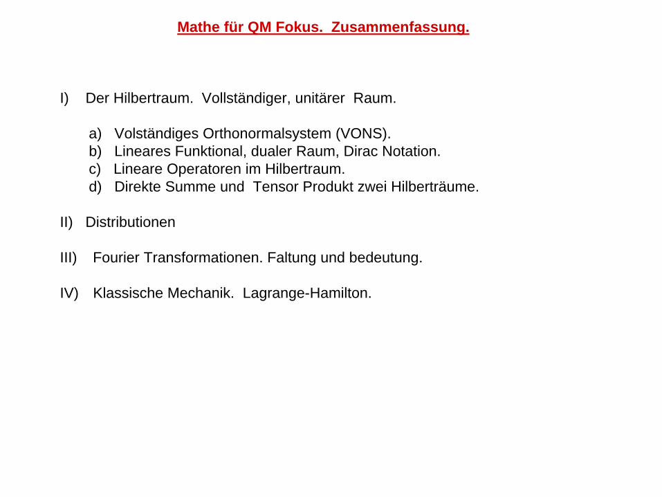
Mathe für QM Fokus. Zusammenfassung.

I) Der Hilbertraum. Vollständiger, unitärer Raum.

a) Volständiges Orthonormalsystem (VONS). b) Lineares Funktional, dualer Raum, Dirac Notation.c) Lineare Operatoren im Hilbertraum.d) Direkte Summe und Tensor Produkt zwei Hilberträume.

II) Distributionen

III) Fourier Transformationen. Faltung und bedeutung.

IV) Klassische Mechanik. Lagrange-Hamilton.

I. Definitionen.

Def: Körper K. Menge M mit zwei Operationen : und :K K K K K K+ × → • × →

, , gilt

K1) ,K2) ( ) ( ), ( ) ( )K3) ( )K4) 0, 1 mit 0 1 | 0 , 1K5) | 0,

| 1, 1/

x y z K

x y y x x y y xx y z x y z x y z x y z

x y z x y x zK x K x x x x

x K y K x y y xx K y K x y y x

∀ ∈

+ = + =+ + = + + =+ = +

∃ ∈ ≠ ∀ ∈ + = =∀ ∈ ∃ ∈ + = = −∀ ∈ ∃ ∈ = =

i ii i i i

i i ii

i

Kommutativität

Assoziativität

Distributivität

Beisp. ,

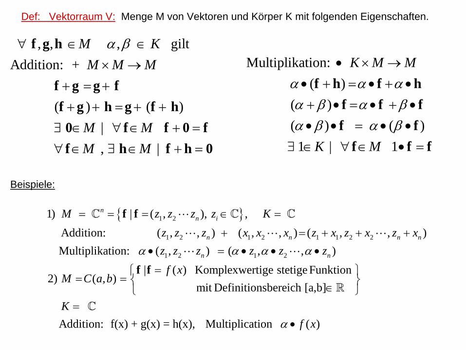
Def: Vektorraum V: Menge M von Vektoren und Körper K mit folgenden Eigenschaften.

, , , giltAddition: +

( ) ( )|, |

M KM M M

M MM M

α β∀ ∈ ∈× →

+ = ++ + = + +

∃ ∈ ∀ ∈ + =∀ ∈ ∃ ∈ + =

f g h

f g g ff g h g f h0 f f 0 ff h f h 0

Multiplikation:( )

( )( ) ( )

1 | 1

K M M

K M

α α αα β α βα β α β

• × →• + = • + •+ • = • + •• • = • •

∃ ∈ ∀ ∈ • =

f h f hf f ff f

f f f

Beispiele:

{ }1 2

1 2 1 2 1 1 2 2

1 2 1 2

1) | ( , ), ,Addition: ( , , ) ( , , ) ( , , )Multiplikation: ( , ) ( , , )

| ( ) Komplexwertige stetige Funktion2) ( , )

mit Definitionsbereich [

nn i

n n n n

n n

M z z z z Kz z z x x x z x z x z xz z z z z zf x

M C a b

α α α α

= = = ∈ =

+ = + + +• = • • •

== =

f f

f fa,b]

Addition: f(x) + g(x) = h(x), Multiplication ( )K

f xα

⎧ ⎫⎨ ⎬∈⎩ ⎭

=•

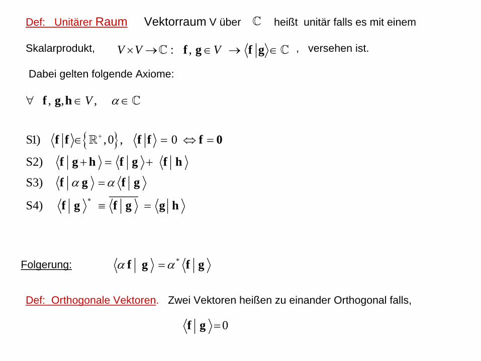
Def: Orthogonale Vektoren. Zwei Vektoren heißen zu einander Orthogonal falls,

Def: Unitärer Raum Vektorraum V über heißt unitär falls es mit einem

Skalarprodukt, , versehen ist.

Dabei gelten folgende Axiome:

: ,V V V× → ∈ → ∈f g f g

{ }

, , ,

S1) ,0 , 0

S2)

S3)

S4)

V α

α α

+

∗

∀ ∈ ∈

∈ = ⇔ =

+ = +

=

≡ =

f g h

f f f f f 0

f g h f g f h

f g f g

f g f g g h

Folgerung:

0=f g

*α α=f g f g

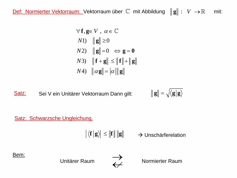
Def: Normierter Vektorraum: Vektorraum über mit Abbildung mit:: V →g

, ,1) 0

2) 0

3)

4)

VN

N

N

N

α

α α

∀ ∈ ∈

≥

= ⇔ =

+ ≤ +

=

f gg

g g 0

f g f g

g g

Satz: Sei V ein Unitärer Vektorraum Dann gilt: =g g g

Satz: Schwarzsche Ungleichung.

≤f g f g Unschärferelation

Bem:Unitärer Raum Normierter Raum→

←

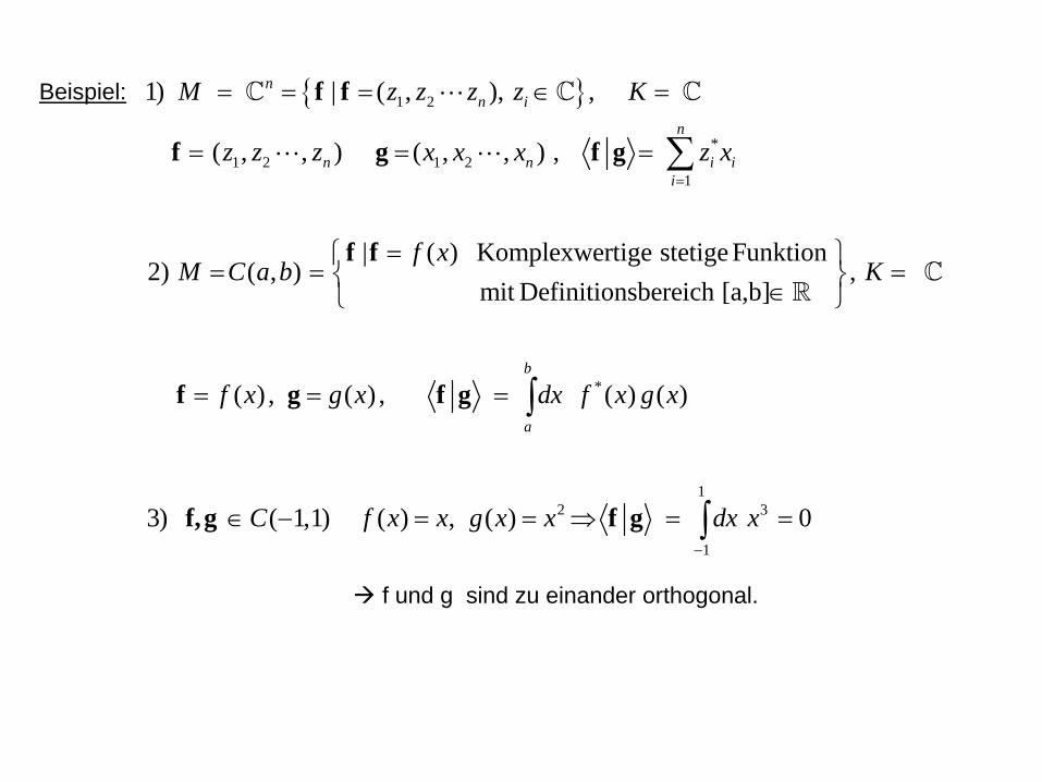
Beispiel: { }1 2

*1 2 1 2

1

*

1) | ( , ), ,

( , , ) ( , , ) ,

| ( ) Komplexwertige stetige Funktion2) ( , ) ,

mit Definitionsbereich [a,b]

( ) , ( ) , ( ) ( )

3) ( 1,1)

nn i

n

n n i ii

b

a

M z z z z K

z z z x x x z x

f xM C a b K

f x g x dx f x g x

C

=

= = = ∈ =

= = =

=⎧ ⎫= = =⎨ ⎬∈⎩ ⎭

= = =

∈ −

∑

∫

f f

f g f g

f f

f g f g

f,g1

2 3

1

( ) , ( ) 0f x x g x x dx x−

= = ⇒ = =∫f g

f und g sind zu einander orthogonal.

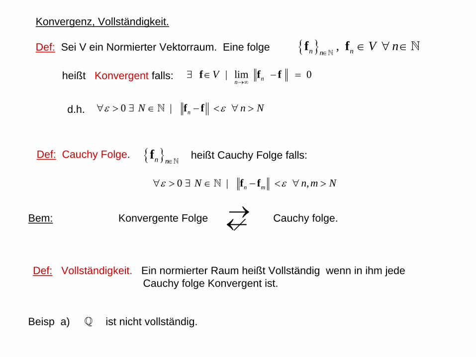
Konvergenz, Vollständigkeit.

Def: Sei V ein Normierter Vektorraum. Eine folge

| lim 0nnV

→∞∃ ∈ − =f f f

{ } ,n nnV n

∈∈ ∀ ∈f f

heißt Konvergent falls:

0 | nN n Nε ε∀ > ∃ ∈ − < ∀ >f fd.h.

Def: Cauchy Folge. { }n n∈f heißt Cauchy Folge falls:

0 | ,n mN n m Nε ε∀ > ∃ ∈ − < ∀ >f f

Bem: Konvergente Folge Cauchy folge. →←

Def: Vollständigkeit. Ein normierter Raum heißt Vollständig wenn in ihm jede Cauchy folge Konvergent ist.

Beisp a) ist nicht vollständig.

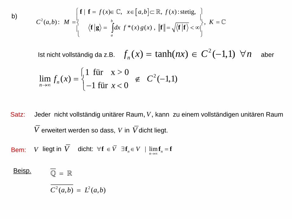
b) [ ]2

| ( ) , , , ( ) : stetig,( , ) : ,

*( ) ( ) ,b

a

f x x a b f xC a b M K

dx f x g x

⎧ ⎫= ∈ ∈ ⊂⎪ ⎪

= =⎨ ⎬= = < ∞⎪ ⎪

⎩ ⎭∫

f f

f g f f f

Ist nicht vollständig da z.B. aber2( ) tanh( ) ( 1,1)nf x nx C n= ∈ − ∀

21 für x > 0lim ( ) ( 1,1)

1 für 0nnf x C

x→∞

⎧= ∉ −⎨− <⎩

Satz: Jeder nicht vollständig unitärer Raum, , kann zu einem vollständigen unitären Raum

erweitert werden so dass, in dicht liegt.

V

V V V

Bem: VV liegt in dicht: | limn nnV V

→∞∀ ∈ ∃ ∈ =f f f f

Beisp.

2 2( , ) ( , )C a b L a b=

=

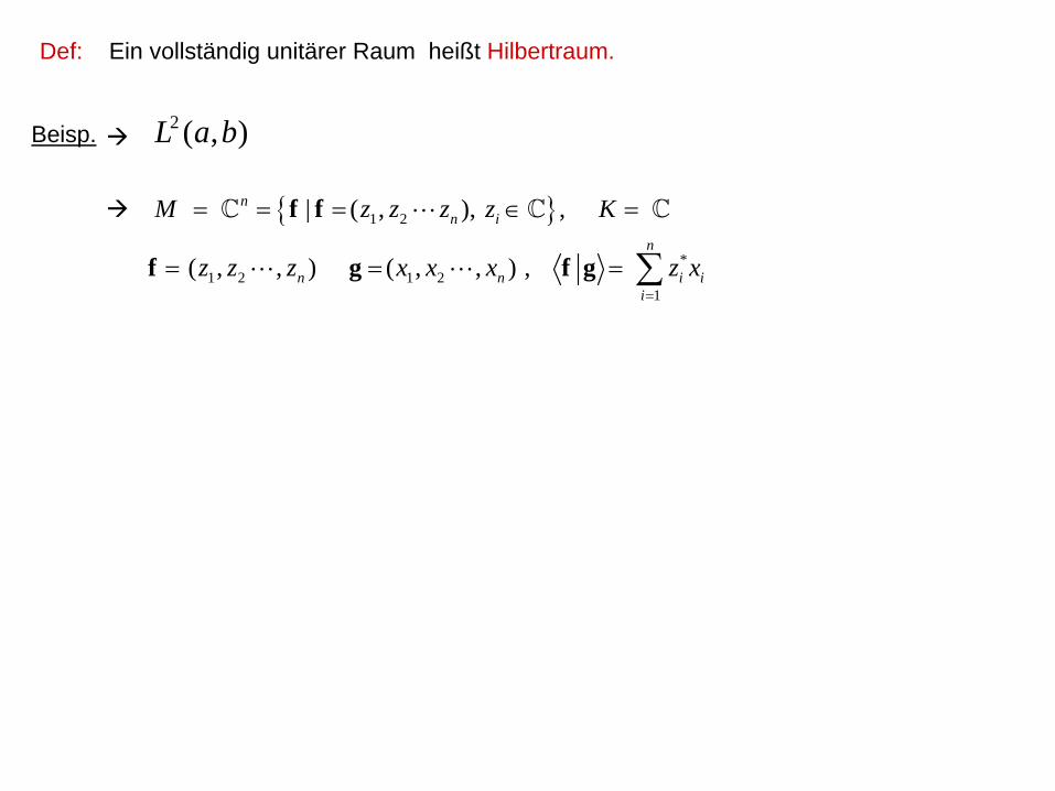
Def: Ein vollständig unitärer Raum heißt Hilbertraum.

Beisp. 2 ( , )L a b

{ }1 2

*1 2 1 2

1

| ( , ), ,

( , , ) ( , , ) ,

nn i

n

n n i ii

M z z z z K

z z z x x x z x=

= = = ∈ =

= = = ∑

f f

f g f g

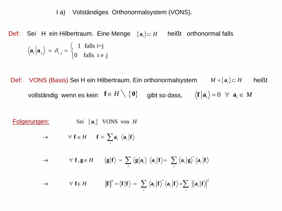
I a) Volständiges Orthonormalsystem (VONS).

Def: Sei H ein Hilbertraum. Eine Menge heißt orthonormal falls{ }i H⊂a

,

1 falls i=j0 falls i ji j i jδ⎧

= = ⎨ ≠⎩a a

Def: VONS (Basis) Sei H ein Hilbertraum. Ein orthonormalsystem heißt

vollständig wenn es kein gibt so dass,

{ }iM H= ⊂a

H∈f { }0 0i i M= ∀ ∈f a a

Folgerungen: { }Sei VONS voni Ha

*

22 *

,

i ii

i i i ii i

i i ii i

H

H

H

→ ∀ ∈ =

→ ∀ ∈ = =

→ ∀ ∈ = = =

∑

∑ ∑

∑ ∑

f f a a f

f g g f g a a f a g a f

f f f f a f a f a f

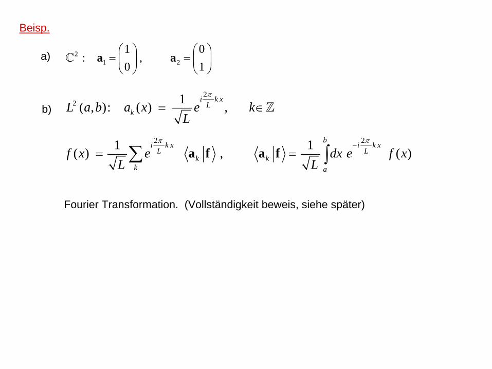
Beisp.

a) 21 2

1 0: ,

0 1⎛ ⎞ ⎛ ⎞

= =⎜ ⎟ ⎜ ⎟⎝ ⎠ ⎝ ⎠

a a

b)2

2 1( , ): ( ) ,i k x

LkL a b a x e k

L

π

= ∈

2 21 1( ) , ( )b

i k x i k xL L

k kk a

f x e dx e f xL L

π π−

= =∑ ∫a f a f

Fourier Transformation. (Vollständigkeit beweis, siehe später)

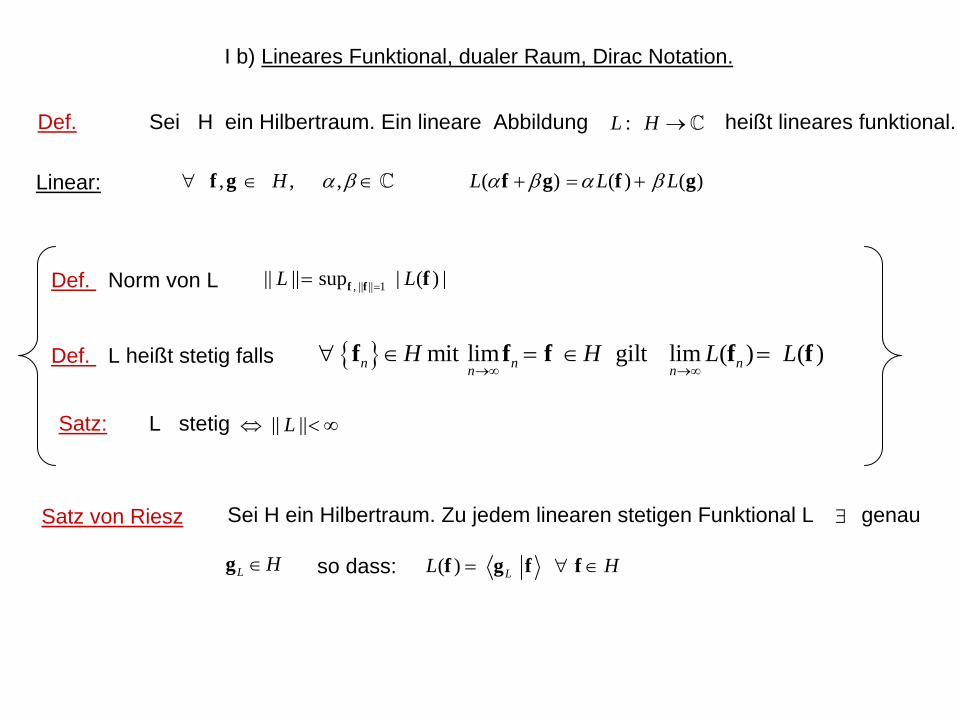
I b) Lineares Funktional, dualer Raum, Dirac Notation.

Def. Sei H ein Hilbertraum. Ein lineare Abbildung heißt lineares funktional.:L H →

Linear: , , , ( ) ( ) ( )H L L Lα β α β α β∀ ∈ ∈ + = +f g f g f g

Def. Norm von L , || || 1|| || sup | ( ) |L L== f f f

Def. L heißt stetig falls { } mit lim gilt lim ( ) ( )n n nn nH H L L

→∞ →∞∀ ∈ = ∈ =f f f f f

Satz: L stetig || ||L⇔ <∞

Satz von Riesz Sei H ein Hilbertraum. Zu jedem linearen stetigen Funktional L genau

so dass:

∃

L H∈g ( ) LL H= ∀ ∈f g f f

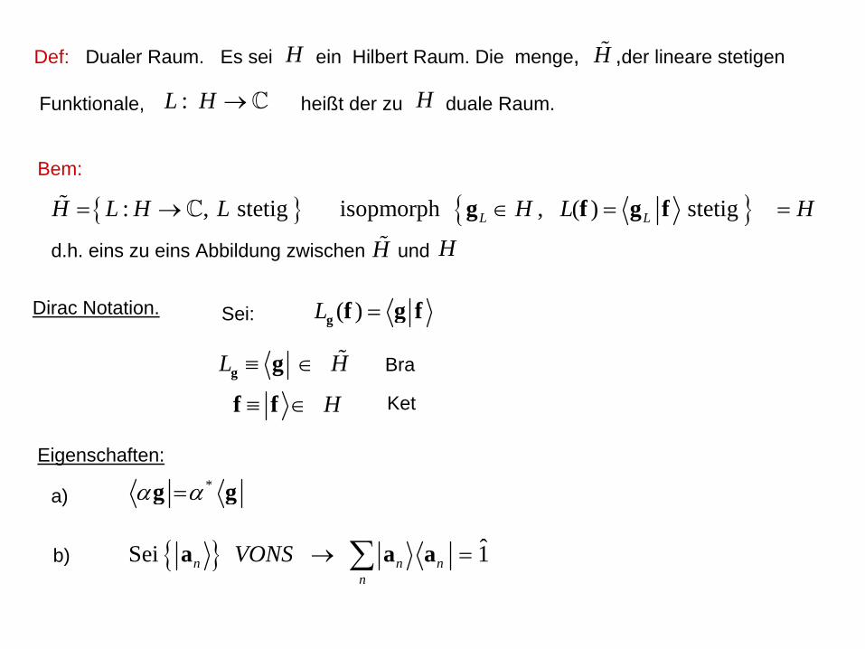
Def: Dualer Raum. Es sei ein Hilbert Raum. Die menge, ,der lineare stetigen

Funktionale, heißt der zu duale Raum.

H H

:L H → H

Bem:

{ } { }: , stetig isopmorph , ( ) stetigL LH L H L H L H= → ∈ = =g f g f

d.h. eins zu eins Abbildung zwischen und HH

Dirac Notation. ( )L =g f g fSei:

L H≡ ∈g g Bra

H≡ ∈f f Ket

Eigenschaften:

a) *α α=g g

{ } ˆSei 1n n nn

VONS → =∑a a ab)

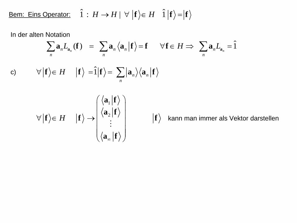
Bem: Eins Operator: ˆ ˆ1 : | 1H H H→ ∀ ∈ =f f f

ˆ( ) 1n nn n n n

n n n

L H L= = ∀ ∈ ⇒ =∑ ∑ ∑a aa f a a f f f aIn der alten Notation

c) 1 n nn

H∀ ∈ = = ∑f f f a a f

1

2H

∞

⎛ ⎞⎜ ⎟⎜ ⎟∀ ∈ → ⎜ ⎟⎜ ⎟⎜ ⎟⎝ ⎠

a fa f

f f

a f

f kann man immer als Vektor darstellen

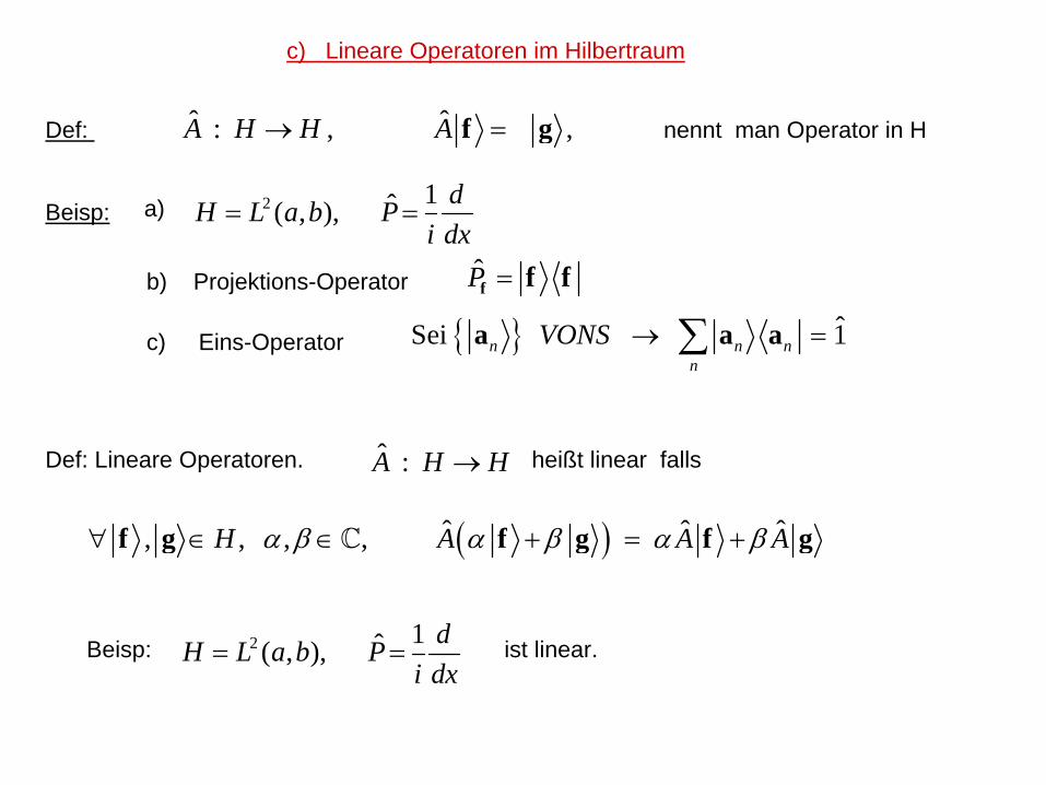
c) Lineare Operatoren im Hilbertraum

Def: nennt man Operator in Hˆ ˆ: , ,A H H A→ =f g

Beisp: 2 1ˆ( , ), dH L a b Pi dx

= =a)

P =f f fb) Projektions-Operator

c) Eins-Operator { } ˆSei 1n n nn

VONS → =∑a a a

Def: Lineare Operatoren. heißt linear falls

( )ˆ ˆ ˆ, , , ,H A A Aα β α β α β∀ ∈ ∈ + = +f g f g f g

ˆ :A H H→

2 1ˆ( , ), dH L a b Pi dx

= =Beisp: ist linear.

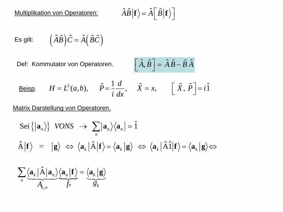
Multiplikation von Operatoren: ˆ ˆˆ ˆAB A B⎡ ⎤= ⎣ ⎦f f

Es gilt: ( ) ( )ˆ ˆ ˆ ˆˆ ˆAB C A BC=

Def: Kommutator von Operatoren. ˆ ˆ ˆˆ ˆ ˆ,A B A B B A⎡ ⎤ = −⎣ ⎦

2 1 ˆˆ ˆ ˆ ˆ( , ), , , , 1dH L a b P X x X P ii dx

⎡ ⎤= = = =⎣ ⎦Beisp.

Matrix Darstellung von Operatoren.

{ } ˆSei 1n n nn

VONS → =∑a a a

,

ˆ ˆ ˆ ˆA = A A1

A

k k k k

k n n kn

n kk ngfA

⇔ = ⇔ = ⇔

=∑

f g a f a g a f a g

a a a f a g

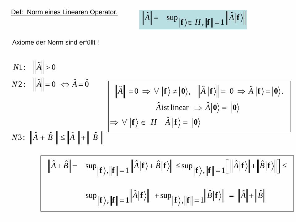
Def: Norm eines Linearen Operator. ˆ ˆsup , 1A AH= ∈ = ff f

Axiome der Norm sind erfüllt !

ˆ1: 0

ˆ ˆ ˆ2 : 0 0

ˆ ˆˆ ˆ3 :

N A

N A A

N A B A B

>

= ⇔ =

+ ≤ +

ˆ ˆ ˆ0 , 0 .

ˆ ˆist linearˆ

A A A

A A

H A

= ⇒ ∀ ≠ = ⇒ =

⇒ =

⇒ ∀ ∈ =

f 0 f f 0

0 0

f f 0

ˆ ˆ ˆˆ ˆ ˆsup sup, 1 , 1

ˆ ˆˆ ˆsup sup, 1 , 1

A B A B A B

A B A B

⎡ ⎤+ = + ≤ + ≤⎣ ⎦= =

+ = += =

f f f ff f f f

f ff f f f

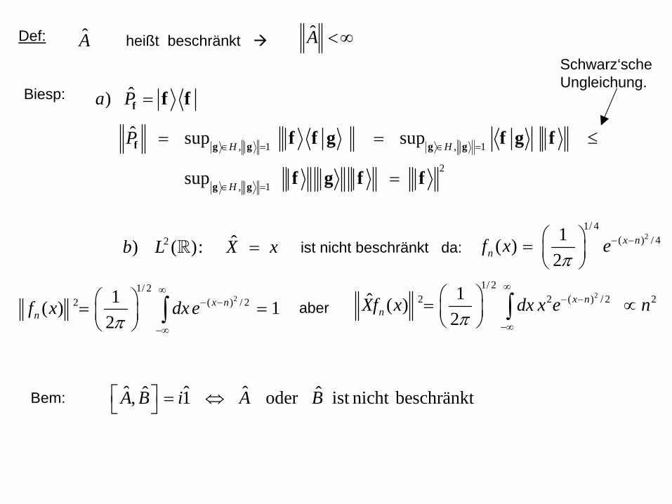
Def: A A <∞heißt beschränkt

Biesp: ˆ)a P =f f f

, 1 , 1

2

, 1

ˆ sup sup

sup

H H

H

P ∈ = ∈ =

∈ =

= = ≤

=

f g g g g

g g

f f g f g f

f g f f

Schwarz‘sche Ungleichung.

2 ˆ) ( ):b L X x= ist nicht beschränkt da:2

1/ 4( ) / 41( )

2x n

nf x eπ

− −⎛ ⎞= ⎜ ⎟⎝ ⎠

21/ 2

2 ( ) / 21( ) 12

x nnf x dx e

π

∞− −

−∞

⎛ ⎞= =⎜ ⎟⎝ ⎠ ∫

21/ 2

2 2 ( ) / 2 21ˆ ( )2

x nnXf x dx x e n

π

∞− −

−∞

⎛ ⎞= ∝⎜ ⎟⎝ ⎠ ∫aber

Bem: ˆ ˆ ˆˆ ˆ, 1 oder ist nicht beschränktA B i A B⎡ ⎤ = ⇔⎣ ⎦

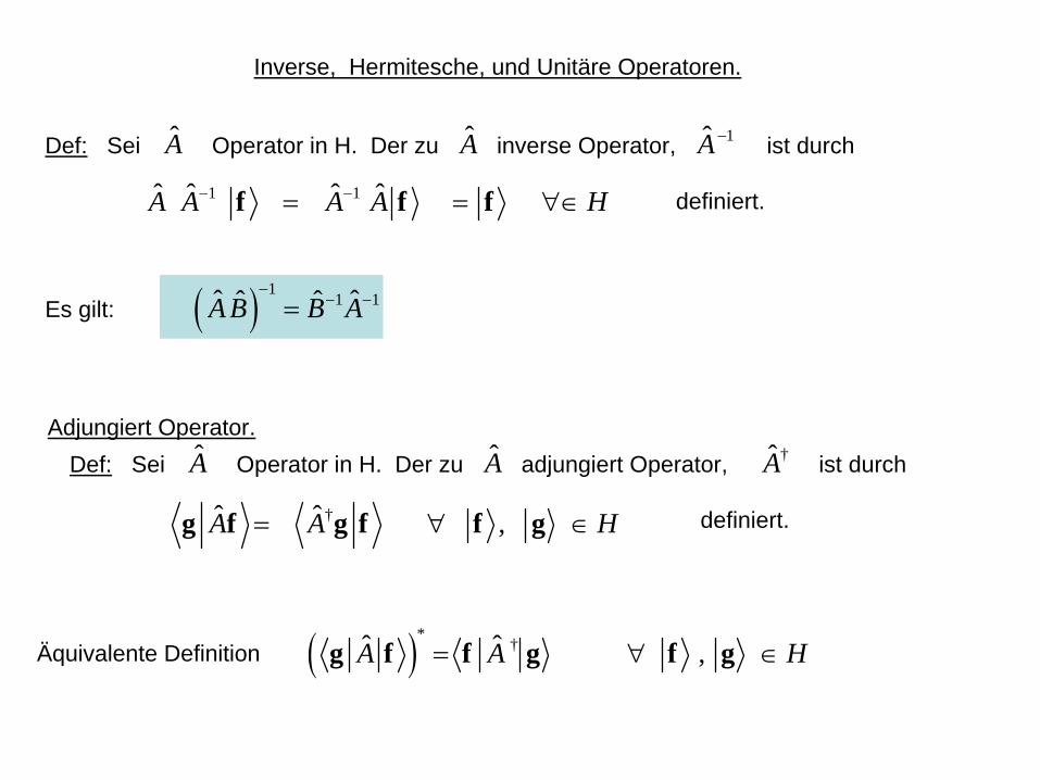
Inverse, Hermitesche, und Unitäre Operatoren.

Def: Sei Operator in H. Der zu inverse Operator, ist durch

definiert.

A A 1A −

1 1ˆ ˆ ˆ ˆA A A A H− −= = ∀∈f f f

Es gilt: ( ) 11 1ˆ ˆˆ ˆAB B A

−− −=

Adjungiert Operator.Def: Sei Operator in H. Der zu adjungiert Operator, ist durch

definiert.

A A †A

†ˆ ˆ ,A A H= ∀ ∈g f g f f g

( )* †ˆ ˆ ,A A H= ∀ ∈g f f g f gÄquivalente Definition

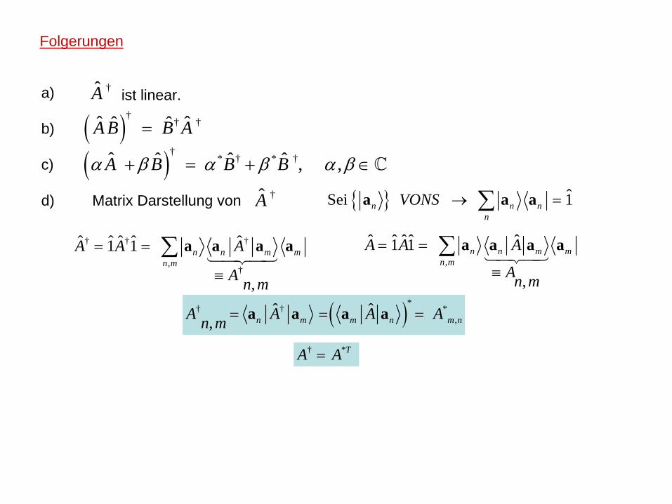
Folgerungen

a)

b)

c)

d) Matrix Darstellung von

†A ist linear.

( )†† †ˆ ˆˆ ˆA B B A=

( )†* † * †ˆ ˆ ˆ ˆ , ,A B B Bα β α β α β+ = + ∈

†A { } ˆSei 1n n nn

VONS → =∑a a a

† † †

,†

ˆ ˆ ˆ ˆ ˆ1 1

,

n n m mn m

A A A

A n m

= =

≡

∑ a a a a,

ˆ ˆ ˆ ˆ ˆ1 1

,

n n m mn m

A A A

An m

= =

≡∑ a a a a

( )*† † *,

ˆ ˆ, n m m n m nA A A An m = = =a a a a

† *TA A=

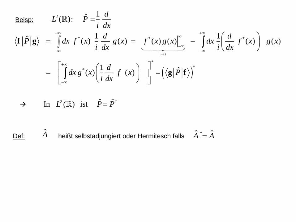
Beisp: 2 1ˆ( ): dL Pi dx

=

( )

* * *

0*

**

1 1ˆ ( ) ( ) ( ) ( ) ( ) ( )

1 ˆ( ) ( )

d dP dx f x g x f x g x dx f x g xi dx i dx

ddx g x f x Pi dx

+∞ +∞∞

−∞−∞ −∞

=

+∞

−∞

⎛ ⎞= = − ⎜ ⎟⎝ ⎠

⎡ ⎤⎛ ⎞= =⎢ ⎥⎜ ⎟⎝ ⎠⎣ ⎦

∫ ∫

∫

f g

g f

2 †ˆ ˆIn ( ) istL P P=

Def: heißt selbstadjungiert oder Hermitesch falls A †ˆ ˆA A=

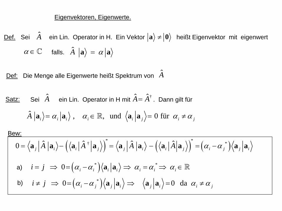
Eigenvektoren, Eigenwerte.

Def. Sei ein Lin. Operator in H. Ein Vektor heißt Eigenvektor mit eigenwert

falls.

A

A α=a a

≠a 0

α ∈

Def: Die Menge alle Eigenwerte heißt Spektrum von A

Satz: Sei ein Lin. Operator in H mit . Dann gilt für A †ˆ ˆA A=

ˆ , , und 0 füri i i i i j i jA α α α α= ∈ = ≠a a a a

Bew:

( ) ( ) ( )* *† *ˆ ˆ ˆ ˆ0 j i i j j i i j i j j iA A A A α α= − = − = −a a a a a a a a a a

a) ( )* *0 i i i i i i ii j α α α α α= ⇒ = − ⇒ = ⇒ ∈a a

b) ( )*0 0 dai j j i j i i ji j α α α α≠ ⇒ = − ⇒ = ≠a a a a

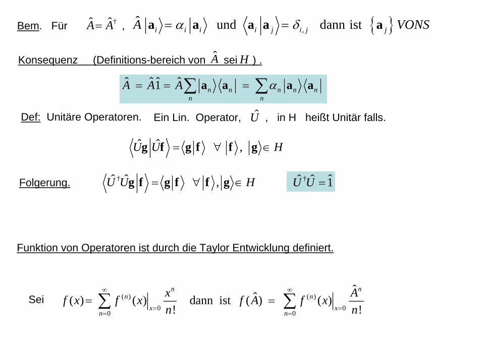
Bem. Für , †ˆ ˆA A= { },ˆ und dann isti i i i j i j jA VONSα δ= =a a a a a

Konsequenz (Definitions-bereich von sei ) .

ˆ ˆ ˆ ˆ1 n n n n nn n

A A A α= = =∑ ∑a a a a

Def: Unitäre Operatoren. Ein Lin. Operator, , in H heißt Unitär falls. U

ˆ ˆ ,U U H= ∀ ∈g f g f f g

Folgerung. †ˆ ˆ ,U U H= ∀ ∈g f g f f g † ˆˆ ˆ 1U U =

Funktion von Operatoren ist durch die Taylor Entwicklung definiert.

( ) ( )

0 00 0

ˆˆ( ) ( ) dann ist ( ) ( )! !

n nn n

x xn n

x Af x f x f A f xn n

∞ ∞

= == =

= =∑ ∑Sei

A H

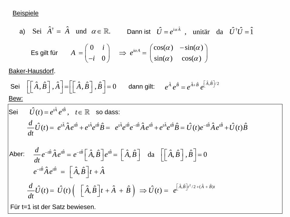
Beispiele

†ˆ ˆSei und .A A α= ∈ ˆ † ˆˆ ˆ ˆ, unitär da 1i AU e U Uα= =Dann ista)

Es gilt für 0 cos( ) sin( )

0 sin( ) cos( )i Ai

A ei

α α αα α

−⎛ ⎞ ⎛ ⎞= ⇒ =⎜ ⎟ ⎜ ⎟−⎝ ⎠ ⎝ ⎠

Baker-Hausdorf.

Sei dann gilt: ˆ ˆ ˆˆ ˆ ˆ, , , , 0A B A A B B⎡ ⎤ ⎡ ⎤⎡ ⎤ ⎡ ⎤= =⎣ ⎦ ⎣ ⎦⎣ ⎦ ⎣ ⎦ˆ ˆ, / 2ˆ ˆˆ ˆ A BA B A Be e e e

⎡ ⎤+ ⎣ ⎦=Bew:

Sei so dass: ˆ ˆ

ˆ ˆ ˆ ˆˆ ˆ ˆ ˆ ˆ ˆ ˆ ˆ

ˆ ( ) ,

ˆ ˆ ˆˆ ˆ ˆ ˆ ˆ ˆ( ) ( ) ( )

tA tB

tA tB tA tB tA tB tB tB tA tB tB tB

U t e e td U t e Ae e e B e e e Ae e e B U t e Ae U t Bdt

− −

= ∈

= + = + = +

ˆ ˆ ˆ ˆ

ˆ ˆ

ˆ ˆ ˆ ˆˆ ˆ ˆ ˆ, , da , , 0

ˆ ˆ ˆˆ,

tB tB tB tB

tB tB

d e Ae e A B e A B A B Bdte Ae A B t A

− −

−

⎡ ⎤⎡ ⎤ ⎡ ⎤ ⎡ ⎤= = =⎣ ⎦ ⎣ ⎦ ⎣ ⎦⎣ ⎦

⎡ ⎤= +⎣ ⎦

Aber:

( ) 2ˆ ˆˆ ˆ, / 2 ( )ˆ ˆˆ ˆ ˆ ˆ ˆ( ) ( ) , ( ) A B t A B td U t U t A B t A B U t edt

⎡ ⎤ + +⎣ ⎦⎡ ⎤= + + ⇒ =⎣ ⎦

Für t=1 ist der Satz bewiesen.

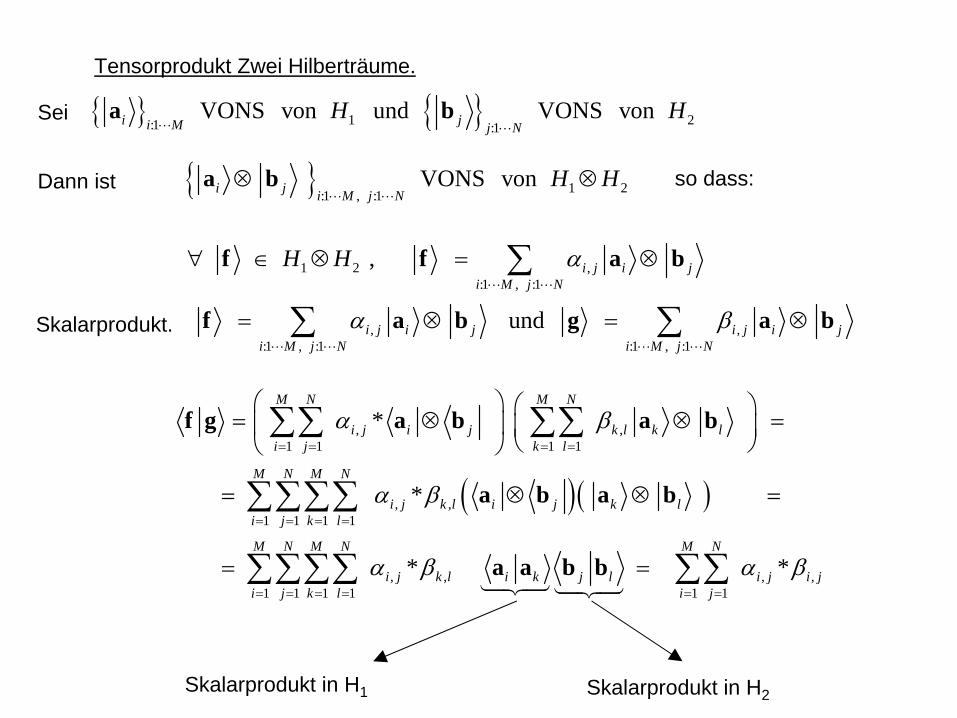
Tensorprodukt Zwei Hilberträume.

Sei { } { }1 2:1 :1VONS von und VONS voni ji M j N

H Ha b

Dann ist { } 1 2:1 , :1VONS voni j i M j N

H H⊗ ⊗a b so dass:

1 2 ,:1 , :1

, i j i ji M j N

H H α∀ ∈ ⊗ = ⊗∑f f a b

, ,:1 , :1 :1 , :1

undi j i j i j i ji M j N i M j N

α β= ⊗ = ⊗∑ ∑f a b g a bSkalarprodukt.

( )( )

, ,1 1 1 1

, ,1 1 1 1

, , , ,1 1 1 1 1 1

*

*

* *

M N M N

i j i j k l k li j k l

M N M N

i j k l i j k li j k l

M N M N M N

i j k l i k j l i j i ji j k l i j

α β

α β

α β α β

= = = =

= = = =

= = = = = =

⎛ ⎞ ⎛ ⎞= ⊗ ⊗ =⎜ ⎟ ⎜ ⎟

⎝ ⎠⎝ ⎠

= ⊗ ⊗ =

= =

∑∑ ∑∑

∑∑∑∑

∑∑∑∑ ∑∑

f g a b a b

a b a b

a a b b

Skalarprodukt in H1 Skalarprodukt in H2

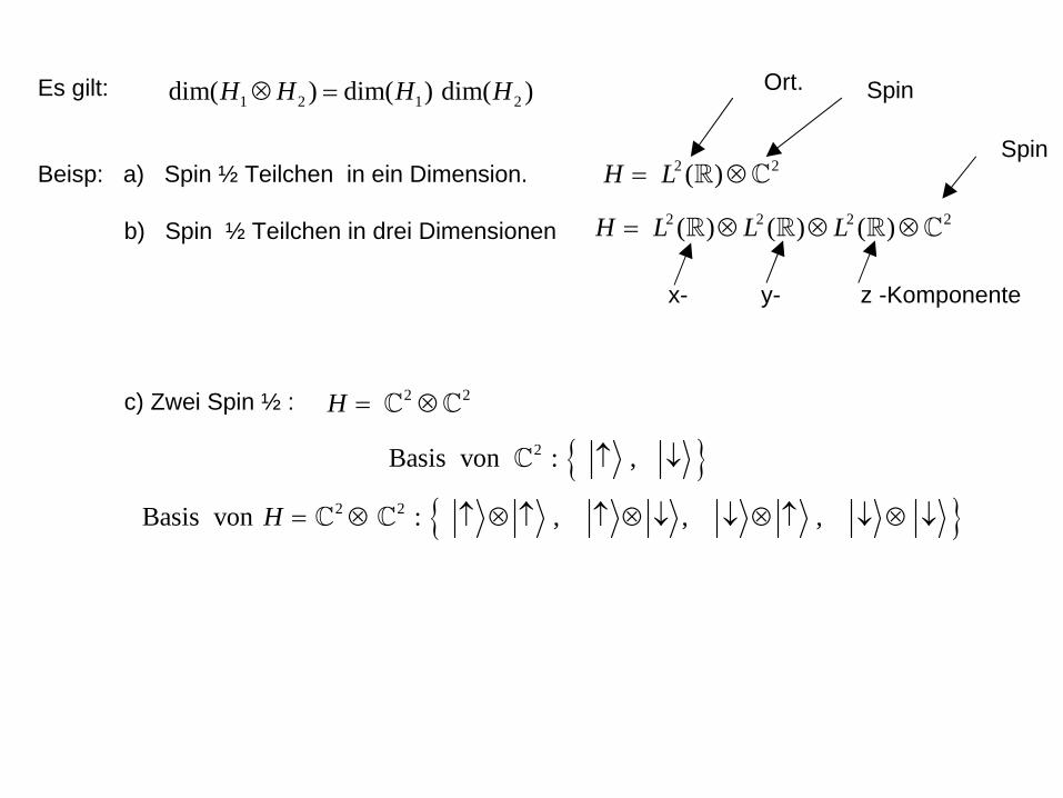
1 2 1 2dim( ) dim( ) dim( )H H H H⊗ =Es gilt:

Beisp: a) Spin ½ Teilchen in ein Dimension.

b) Spin ½ Teilchen in drei Dimensionen

c) Zwei Spin ½ :

2 2( )H L= ⊗

SpinOrt.

2 2 2 2( ) ( ) ( )H L L L= ⊗ ⊗ ⊗

x- y- z -Komponente

Spin

2 2H = ⊗

{ }2 2Basis von : , , ,H = ⊗ ↑ ⊗ ↑ ↑ ⊗ ↓ ↓ ⊗ ↑ ↓ ⊗ ↓

{ }2Basis von : ,↑ ↓

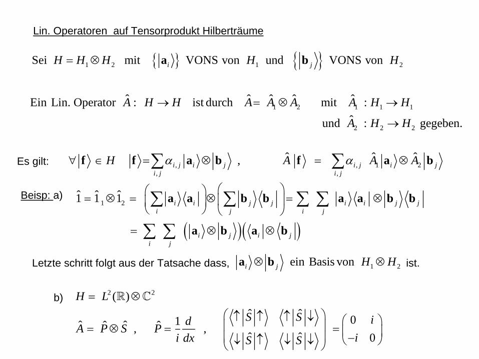
Lin. Operatoren auf Tensorprodukt Hilberträume

{ } { }1 2 1 2

1 2 1 1 1

2 2 2

Sei mit VONS von und VONS von

ˆ ˆ ˆ ˆ ˆEin Lin. Operator : ist durch mit :ˆund : gegeben.

i jH H H H H

A H H A A A A H H

A H H

= ⊗

→ = ⊗ →

→

a b

, , 1 2, ,

ˆ ˆ ˆ,i j i j i j i ji j i j

H A A Aα α∀ ∈ = ⊗ = ⊗∑ ∑f f a b f a bEs gilt:

Beisp: a)

b) 2 2( )H L= ⊗ˆ ˆ 01ˆ ˆˆ ˆ, ,ˆ ˆ 0

S S idA P S Pii dx S S

⎛ ⎞↑ ↑ ↑ ↓ ⎛ ⎞⎜ ⎟= ⊗ = = ⎜ ⎟⎜ ⎟ −↓ ↑ ↓ ↓ ⎝ ⎠⎝ ⎠

( )( )1 2

ˆ ˆ ˆ1 1 1 i i j j i i j ji j i j

i j i ji j

⎛ ⎞⎛ ⎞= ⊗ = ⊗ = ⊗⎜ ⎟⎜ ⎟

⎝ ⎠ ⎝ ⎠

= ⊗ ⊗

∑ ∑ ∑ ∑

∑ ∑

a a b b a a b b

a b a b

1 2ein Basis voni j H H⊗ ⊗a bLetzte schritt folgt aus der Tatsache dass, ist.

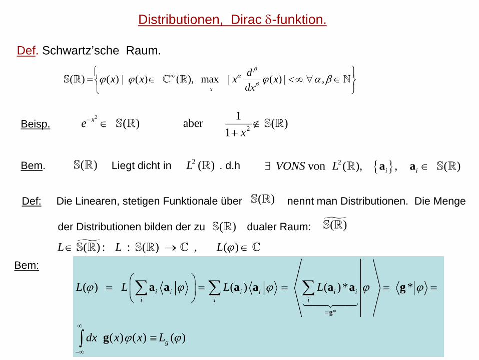
Def: Die Linearen, stetigen Funktionale über nennt man Distributionen. Die Menge

der Distributionen bilden der zu dualer Raum:

Distributionen, Dirac δ-funktion.

Def. Schwartz’sche Raum.

( ) ( ) | ( ) ( ), max | ( ) | ,x

dx x x xdx

βα

βϕ ϕ ϕ α β∞⎧ ⎫= ∈ <∞ ∀ ∈⎨ ⎬⎩ ⎭

S

Beisp. 2

2

1( ) aber ( )1

xex

− ∈ ∉+

S S

Bem. Liegt dicht in . d.h( )S 2 ( )L { }2von ( ), , ( )i iVONS L∃ ∈a a S

( )S

( )S ( )S

( ) : : ( ) , ( )L L L ϕ∈ → ∈S SBem:

*

( ) ( ) ( )* *

( ) ( ) ( )

i i i i i ii i i

g

L L L L

dx x x L

ϕ ϕ ϕ ϕ ϕ

ϕ ϕ

=

∞

−∞

⎛ ⎞= = = = =⎜ ⎟⎝ ⎠

≡

∑ ∑ ∑

∫

g

a a a a a a g

g

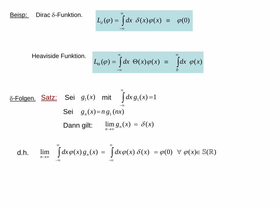
Beisp: Dirac δ-Funktion.( ) ( ) ( ) (0)L dx x xδ ϕ δ ϕ ϕ

∞

−∞

= ≡∫

Heaviside Funktion.

0

( ) ( ) ( ) ( )L dx x x dx xϕ ϕ ϕ∞ ∞

Θ−∞

= Θ ≡∫ ∫

δ-Folgen. Satz: Sei mit 1( ) 1dx g x∞

−∞

=∫1( )g x

Sei 1( ) ( )ng x n g nx=

Dann gilt: lim ( ) ( )nng x xδ

→∞=

d.h. lim ( ) ( ) ( ) ( ) (0) ( ) ( )nndx x g x dx x x xϕ ϕ δ ϕ ϕ

∞ ∞

→∞−∞ −∞

= = ∀ ∈∫ ∫ S

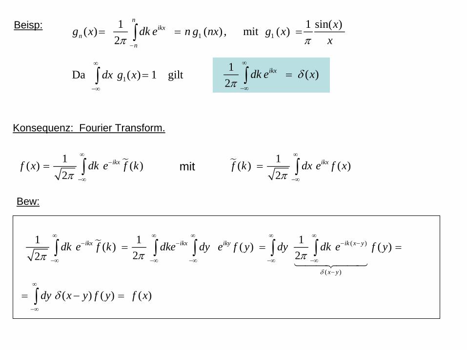
Beisp:1 1

1 1 sin( )( ) ( ) , mit ( )2

nikx

nn

xg x dk e n g nx g xxπ π−

= = =∫

1Da ( ) 1 giltdx g x∞

−∞

=∫1 ( )

2ikxdk e xδ

π

∞

−∞

=∫

Konsequenz: Fourier Transform.

1 1( ) ( ) ( ) ( )2 2

ikx ikxf x dk e f k f k dx e f xπ π

∞ ∞−

−∞ −∞

= =∫ ∫mit

( )

( )

1 1 1( ) ( ) ( )2 22

( ) ( ) ( )

ikx ikx iky ik x y

x y

dk e f k dke dy e f y dy dk e f y

dy x y f y f x

δ

π ππ

δ

∞ ∞ ∞ ∞ ∞− − − −

−∞ −∞ −∞ −∞ −∞

−

∞

−∞

= = =

= − =

∫ ∫ ∫ ∫ ∫

∫

Bew:

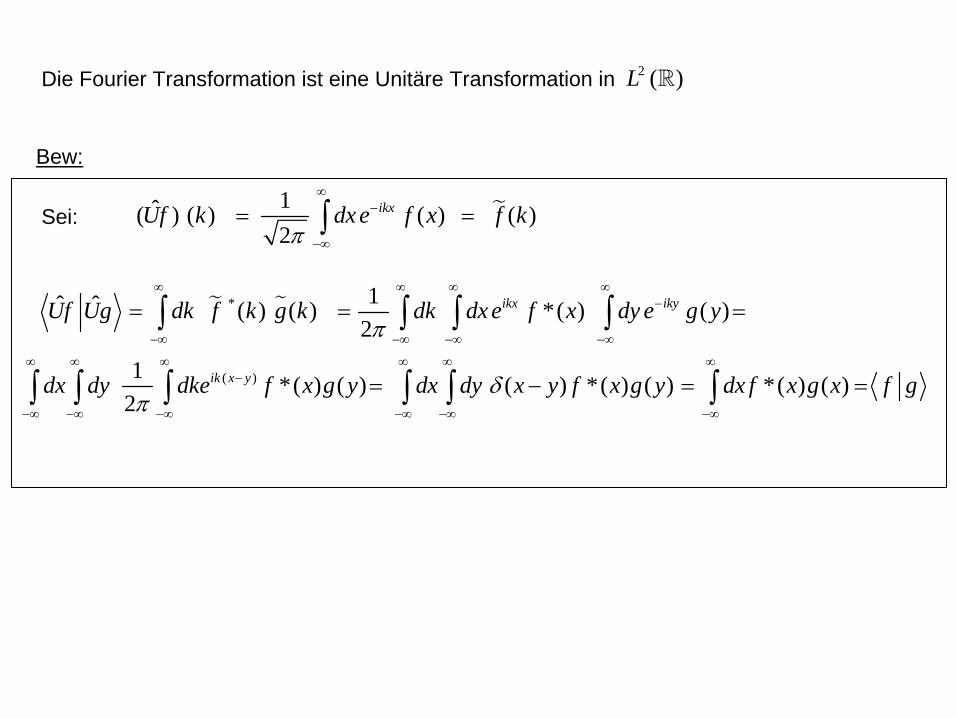
Die Fourier Transformation ist eine Unitäre Transformation in 2 ( )L

Bew:

1ˆ( ) ( ) ( ) ( )2

ikxUf k dxe f x f kπ

∞−

−∞

= =∫Sei:

*

( )

1ˆ ˆ ( ) ( ) *( ) ( )2

1 *( ) ( ) ( ) *( ) ( ) *( ) ( )2

ikx iky

ik x y

Uf Ug dk f k g k dk dxe f x dy e g y

dx dy dke f x g y dx dy x y f x g y dx f x g x f g

π

δπ

∞ ∞ ∞ ∞−

−∞ −∞ −∞ −∞

∞ ∞ ∞ ∞ ∞ ∞−

−∞ −∞ −∞ −∞ −∞ −∞

= = =

= − = =

∫ ∫ ∫ ∫

∫ ∫ ∫ ∫ ∫ ∫

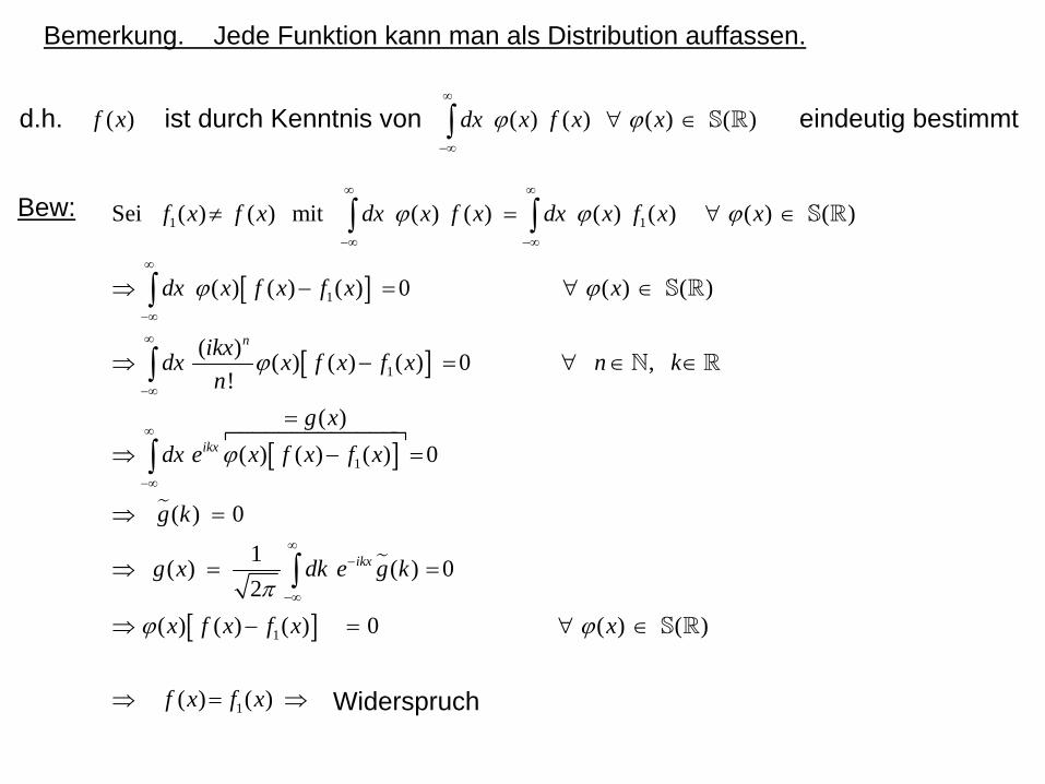
Bemerkung. Jede Funktion kann man als Distribution auffassen.

d.h. ist durch Kenntnis von eindeutig bestimmt( )f x ( ) ( ) ( ) ( )dx x f x xϕ ϕ∞

−∞

∀ ∈∫ S

[ ]

[ ]

[ ]

1 1

1

1

1

Sei ( ) ( ) mit ( ) ( ) ( ) ( ) ( ) ( )

( ) ( ) ( ) 0 ( ) ( )

( ) ( ) ( ) ( ) 0 ,!

( )( ) ( ) ( ) 0

( ) 0

1( ) (2

n

ikx

ikx

f x f x dx x f x dx x f x x

dx x f x f x x

ikxdx x f x f x n kn

g xdx e x f x f x

g k

g x dk e g k

ϕ ϕ ϕ

ϕ ϕ

ϕ

ϕ

π

∞ ∞

−∞ −∞

∞

−∞

∞

−∞

∞

−∞

−

≠ = ∀ ∈

⇒ − = ∀ ∈

⇒ − = ∀ ∈ ∈

=

⇒ − =

⇒ =

⇒ =

∫ ∫

∫

∫

∫

S

S

[ ]1

1

) 0

( ) ( ) ( ) 0 ( ) ( )

( ) ( )

x f x f x x

f x f x

ϕ ϕ

∞

−∞

=

⇒ − = ∀ ∈

⇒ = ⇒

∫S

Bew:

Widerspruch

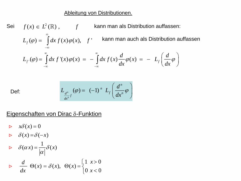
Eigenschaften von Dirac δ-Funktion

( ) 0( ) ( )

1( ) ( )

1 0( ) ( ), ( )

0 0

x xx x

x x

xd x x xxdx

δδ δ

δ α δα

δ

== −

=

>⎧Θ = Θ = ⎨ <⎩

Ableitung von Distributionen.

Sei kann man als Distribution auffassen: 2

'

( ) ( ) ,

( ) ( ) ( ), '

( ) '( ) ( ) ( ) ( )

f

f f

f x L f

L dx f x x f

d dL dx f x x dx f x x Ldx dx

ϕ ϕ

ϕ ϕ ϕ ϕ

∞

−∞

∞ ∞

−∞ −∞

∈

=

⎛ ⎞= = − = − ⎜ ⎟⎝ ⎠

∫

∫ ∫

kann man auch als Distribution auffassen

Def: ( ) ( 1)n

n

nn

f nd fdx

dL Ldx

ϕ ϕ⎛ ⎞

= − ⎜ ⎟⎝ ⎠