
Opticallyselectedgalaxyclusters asacosmologicalprobe · Opticallyselectedgalaxyclusters...
162
Optically selected galaxy clusters as a cosmological probe Annalisa Mana M¨ unchen, 2013
Transcript of Opticallyselectedgalaxyclusters asacosmologicalprobe · Opticallyselectedgalaxyclusters...
Optically selected galaxy clusters
as a cosmological probe
Annalisa Mana
Munchen, 2013


Optically selected galaxy clusters
as a cosmological probe
Annalisa Mana
Dissertation
an der Fakultat fur Physik
der Ludwig–Maximilians–Universitat
Munchen
vorgelegt von
Annalisa Mana
aus Fossano (CN), Italien
Munchen, den 2. September 2013

Erstgutachter: Prof. Dr. Jochen Weller
Zweitgutachter: PD Dr. Klaus Dolag
Tag der mundlichen Prufung: 9. Oktober 2013

Ai miei genitori


Contents
Zusammenfassung x
Summary xiii
1 Introduction 11.1 The homogeneous Universe . . . . . . . . . . . . . . . . . . . . . . . . 1
1.1.1 Cosmological principle . . . . . . . . . . . . . . . . . . . . . . 21.1.2 Friedmann-Lemaıtre-Robertson-Walker metric . . . . . . . . . 21.1.3 Einstein’s field equations . . . . . . . . . . . . . . . . . . . . . 31.1.4 Friedmann equations . . . . . . . . . . . . . . . . . . . . . . . 31.1.5 The critical density . . . . . . . . . . . . . . . . . . . . . . . . 51.1.6 Energy density components . . . . . . . . . . . . . . . . . . . 51.1.7 Hubble’s law . . . . . . . . . . . . . . . . . . . . . . . . . . . 81.1.8 Cosmological distances . . . . . . . . . . . . . . . . . . . . . . 10
1.2 The theory of structure formation . . . . . . . . . . . . . . . . . . . . 111.2.1 Cosmic inflation . . . . . . . . . . . . . . . . . . . . . . . . . . 111.2.2 Jeans gravitational instability . . . . . . . . . . . . . . . . . . 121.2.3 Evolution of inhomogeneities . . . . . . . . . . . . . . . . . . . 121.2.4 Linearised perturbation equations . . . . . . . . . . . . . . . . 141.2.5 Perturbation equations in an expanding Universe . . . . . . . 151.2.6 Power spectrum of density fluctuations . . . . . . . . . . . . . 17
1.3 Cosmological probes . . . . . . . . . . . . . . . . . . . . . . . . . . . 191.3.1 Supernovae Type Ia . . . . . . . . . . . . . . . . . . . . . . . . 191.3.2 Baryon Acoustic Oscillations . . . . . . . . . . . . . . . . . . . 201.3.3 The Cosmic Microwave Background Radiation . . . . . . . . . 21
1.4 Galaxy Clusters . . . . . . . . . . . . . . . . . . . . . . . . . . . . . . 251.4.1 History of galaxy clusters observations . . . . . . . . . . . . . 251.4.2 Main features, components and observables . . . . . . . . . . . 26

viii CONTENTS
1.4.3 Cluster mass proxies . . . . . . . . . . . . . . . . . . . . . . . 281.4.4 Formation of galaxy clusters . . . . . . . . . . . . . . . . . . . 291.4.5 Clusters as cosmological probes . . . . . . . . . . . . . . . . . 29
1.5 ΛCDM standard model . . . . . . . . . . . . . . . . . . . . . . . . . . 311.5.1 Cosmological constraints from observations . . . . . . . . . . . 33
2 Galaxy Clusters from theory side 372.1 Cluster masses . . . . . . . . . . . . . . . . . . . . . . . . . . . . . . 37
2.1.1 Definition . . . . . . . . . . . . . . . . . . . . . . . . . . . . . 382.1.2 Halo density distribution . . . . . . . . . . . . . . . . . . . . . 382.1.3 Weak Lensing signal . . . . . . . . . . . . . . . . . . . . . . . 39
2.2 Mass function . . . . . . . . . . . . . . . . . . . . . . . . . . . . . . . 432.2.1 Press-Schechter formalism . . . . . . . . . . . . . . . . . . . . 442.2.2 N-body simulations calibration . . . . . . . . . . . . . . . . . 462.2.3 Cosmology dependence of the mass function . . . . . . . . . . 48
2.3 Modelling cluster counts and total masses . . . . . . . . . . . . . . . 512.4 Clustering of clusters . . . . . . . . . . . . . . . . . . . . . . . . . . . 53
2.4.1 Halo bias . . . . . . . . . . . . . . . . . . . . . . . . . . . . . 532.4.2 Cluster power spectrum . . . . . . . . . . . . . . . . . . . . . 55
2.5 Primordial non-Gaussianity . . . . . . . . . . . . . . . . . . . . . . . 582.5.1 Definition of fNL parameter . . . . . . . . . . . . . . . . . . . 592.5.2 Modified mass function . . . . . . . . . . . . . . . . . . . . . . 602.5.3 Modified bias . . . . . . . . . . . . . . . . . . . . . . . . . . . 62
3 Observations, data and errors 653.1 Multi-wavelength surveys of galaxy clusters . . . . . . . . . . . . . . . 65
3.1.1 X-ray surveys . . . . . . . . . . . . . . . . . . . . . . . . . . . 663.1.2 SZ surveys . . . . . . . . . . . . . . . . . . . . . . . . . . . . . 663.1.3 WL surveys . . . . . . . . . . . . . . . . . . . . . . . . . . . . 673.1.4 Optical surveys . . . . . . . . . . . . . . . . . . . . . . . . . . 673.1.5 Future surveys . . . . . . . . . . . . . . . . . . . . . . . . . . 683.1.6 Cosmological constraints from cluster catalogues . . . . . . . . 68
3.2 The Sloan Digital Sky Survey . . . . . . . . . . . . . . . . . . . . . . 703.2.1 MaxBCG catalogue . . . . . . . . . . . . . . . . . . . . . . . . 70
3.3 MaxBCG cluster number counts . . . . . . . . . . . . . . . . . . . . . 723.3.1 Cluster abundances . . . . . . . . . . . . . . . . . . . . . . . . 723.3.2 Counts covariance matrix . . . . . . . . . . . . . . . . . . . . 73
3.4 MaxBCG cluster masses . . . . . . . . . . . . . . . . . . . . . . . . . 76

Table of contents ix
3.4.1 Mean cluster masses from weak lensing observations . . . . . . 763.4.2 Mass-richness scaling relation . . . . . . . . . . . . . . . . . . 783.4.3 Cluster total masses . . . . . . . . . . . . . . . . . . . . . . . 80
3.5 MaxBCG cluster power spectrum . . . . . . . . . . . . . . . . . . . . 813.5.1 Cluster power spectrum calculation . . . . . . . . . . . . . . . 813.5.2 Cluster power spectrum covariance matrix . . . . . . . . . . . 84
3.6 The counts-clustering off-diagonal covariance . . . . . . . . . . . . . . 85
4 Cosmological analysis 894.1 Parameter estimation . . . . . . . . . . . . . . . . . . . . . . . . . . . 89
4.1.1 Bayes theorem . . . . . . . . . . . . . . . . . . . . . . . . . . 904.1.2 Gaussian χ2 statistics . . . . . . . . . . . . . . . . . . . . . . . 904.1.3 C-statistics . . . . . . . . . . . . . . . . . . . . . . . . . . . . 924.1.4 Confidence regions and marginalisation . . . . . . . . . . . . . 92
4.2 Sampling methods . . . . . . . . . . . . . . . . . . . . . . . . . . . . 934.2.1 Markov chains . . . . . . . . . . . . . . . . . . . . . . . . . . . 944.2.2 Monte Carlo methods . . . . . . . . . . . . . . . . . . . . . . . 944.2.3 MCMC methods . . . . . . . . . . . . . . . . . . . . . . . . . 95
4.3 The Cosmological Monte-Carlo . . . . . . . . . . . . . . . . . . . . . 984.4 Combined maxBCG analysis . . . . . . . . . . . . . . . . . . . . . . . 1014.5 Results . . . . . . . . . . . . . . . . . . . . . . . . . . . . . . . . . . . 103
4.5.1 Ωm − σ8 contours . . . . . . . . . . . . . . . . . . . . . . . . . 1034.5.2 Scaling relation parameters contours . . . . . . . . . . . . . . 1064.5.3 log(1010As)− σ8 contours . . . . . . . . . . . . . . . . . . . . 1104.5.4 fNL − Ωm and fNL − σ8 contours . . . . . . . . . . . . . . . . . 110
5 Clusters-galaxies cross correlation 1155.1 Measurement by pixelization . . . . . . . . . . . . . . . . . . . . . . . 115
5.1.1 Pixelization method . . . . . . . . . . . . . . . . . . . . . . . 1165.1.2 The mask and the catalogues . . . . . . . . . . . . . . . . . . 117
5.2 Angular correlation function estimator . . . . . . . . . . . . . . . . . 1185.3 Theoretical prediction . . . . . . . . . . . . . . . . . . . . . . . . . . 1185.4 Error estimates . . . . . . . . . . . . . . . . . . . . . . . . . . . . . . 119
6 Conclusions 121
Acronyms 128
Danksagung 146

Zusammenfassung
Aktuell werden großraumige Himmelsdurchmusterungen bei vielen verschiedenenWellenlangen durchgefuhrt. Diese Beobachtungen dienen der Errichtung und Bestati-gung eines kosmologischen Standardmodells fur unser Universum. In den letztenJahren wurden große Fortschritte in Theorie und Beobachtungen gemacht, um Galax-ienhaufen als Testbett fur die Kosmologie zu nutzen. Galaxienhaufen sind die großtengravitativ gebunden Strukturen und ihre Verteilung folgt der Entwicklung der groß-skaligen Struktur im Universum. Die Anzahldichte der Galaxienhaufen ist zudemsensitiv auf das zu Grunde gelegte kosmologische Modell. Durch die Beobachtungvon Galaxienhaufen konnen die kosmologischen Parameter, zusatzlich zu anderenMessungen, eingeschrankt werden.
Diese Dissertation behandelt den wichtigen Beitrag von Galaxienhaufen zur Ver-ifizierung des kosmologischen Standardmodells in einem von dunkler Materie unddunkler Energie dominierten Universum. Insbesondere untersuchen wir das Clus-tering von optisch selektierten Galaxienhaufen als zusatzlichen Parameter zu denublichen kosmologischen Observablen. Das Clustering von Galaxienhaufen erganztdie traditionellen Methoden der Zahlung von Galaxienhaufen und der Vermessungvon Masse-Observablen Relationen, weil die Analyse des Clusterings von Galaxienin den High-Peak, High-Bias Bereich vorangetrieben wird. Diese Methode ist einmachtiges Werkzeug um bestehende Entartungen zu durchbrechen und genauere kos-mologische Parameter zu gewinnen.
Als Erstes legen wir die wichtigsten theoretischen Grundlagen und Beobachtun-gen fur das heutige Standardmodell der Kosmologie dar. Anschließend behandelnwir die grundlegenden Eigenschaften von Galaxienhaufen und insbesondere ihrenBeitrag als Testbett fur kosmologische Modelle.
Als nachstes entwickeln wir den theoretischen Rahmen fur die Zahlung von Galax-ienhaufen und die Bestimmung des Leistungsspektrums. Wir uberarbeiten die For-

xii Zusammenfassung
mulierung und Kalibirierung der Halomassenfunktion, welche im Bereich hoher Mas-sen von Galaxienhaufen bevolkert ist. Zusatzlich geben wir ein Rezept zur Model-lierung des Leistungsspektrums von Galaxienhaufen mit dem Ort und der Rotver-schiebung. Hierbei ist die Modellierung des schwach nicht-linearen Beitrags einge-schlossen und eine beliebige photometrische Glattung mit der Rotverschiebung ermo-glicht. Zuletzt zeigen wir welchen Beitrag Galaxienhaufen bei der Beschrankung derParameter fur nicht Gauß-verteilte primordiale Anfangsbedingungen liefern konnen.
Anschließend widmen wir ein Kapitel der Prasentation unserer Basisdaten, demSloan Digital Sky Survey maxBCG Katalog. Wir beschreiben die Ableitung un-serer Datensatze aus diesem Katalog von Galaxienhaufen und die entsprechendendazugehorigen Fehlerabschatzungen. Speziell verwenden wir, jeweils mit den ent-sprechenden Kovarianzmatrizen, die Haufigkeit von Galaxienhaufen in verschiedenenReichhaltigkeitsbereichen, Abschatzungen fur die schwachen Linsenmassen und dasLeistungsspektrum uber Ort und Rotverschiebung. Zusatzlich, durch eine empirischeSkalierungsrelation, setzen wir die Masse der Galaxienhaufen mit ihrer beobachtetenReichhaltigkeit in Verbindung und quantifizieren die Streuung der Daten.
Im nachsten Kapitel zeigen wir die Ergebnisse unserer Monte-Carlo-Markov-Ketten-Analyse und die daraus abgeleiteten Beschrankungen der kosmologischen Pa-rameter. Mit dem maxBCG Datenset konnen wir sowohl die kosmologischen Parame-ter einschranken, als auch gleichzeitig die Masse-Observable-Relation vermessen. Wirfinden, dass die Berucksichtigung des Leistungsspektrums eine ∼ 50% Verbesserungdes Fehlers in der Fluktuationsamplitude σ8 und der Materiedichte Ωm ergibt. Furdie anderen kosmologischen Parameter finden wir weniger signifikante Verbesserun-gen. Außerdem verwenden wir das mit WMAP7 gemessene Leistungsspektrum derkosmischen Hintergrundstrahlung, zusatzlich zu den Daten uber Galaxienhaufen,und erhalten eine weitere Beschrankung der Vertrauensregionen. Zuletzt wenden wirunsere Methode auf Modelle des fruhen Universums an, und bestimmen den Anteilder nicht Gauß-verteilten Fluktuationen des primordialen Dichtefelds (lokaler Typ).Unsere Ergebnisse sind konsistent mit den aktuellsten Beobachtungen.
Im letzten Kapitel prasentieren wir vorlaufige Rechnungen zur Kreuzkorrelationzwischen Galaxienhaufen und Galaxien. Diese Rechnungen sind in der Lage die kos-mologischen Modelle noch weiter einzuschranken.
Abschließend fassen wir unsere wichtigsten Ergebnisse zusammen und geben einenAusblick auf mogliche weiterfuhrende Forschungsprojekte.

Summary
Multi-wavelength large-scale surveys are currently exploring the Universe and es-tablishing the cosmological scenario with extraordinary accuracy. There has beenrecently a significant theoretical and observational progress in efforts to use clustersof galaxies as probes of cosmology and to test the physics of structure formation.Galaxy clusters are the most massive gravitationally bound systems in the Universe,which trace the evolution of the large-scale structure. Their number density and dis-tribution are highly sensitive to the underlying cosmological model. The constraintson cosmological parameters which result from observations of galaxy clusters arecomplementary with those from other probes.
This dissertation examines the crucial role of clusters of galaxies in confirming thestandard model of cosmology, with a Universe dominated by dark matter and darkenergy. In particular, we examine the clustering of optically selected galaxy clustersas a useful addition to the common set of cosmological observables, because it ex-tends galaxy clustering analysis to the high-peak, high-bias regime. The clustering ofgalaxy clusters complements the traditional cluster number counts and observable-mass relation analyses, significantly improving their constraining power by breakingexisting calibration degeneracies.
We begin by introducing the fundamental principles at the base of the concor-dance cosmological model and the main observational evidence that support it. Wethen describe the main properties of galaxy clusters and their contribution as cos-mological probes.
We then present the theoretical framework of galaxy clusters number counts andpower spectrum. We revise the formulation and calibration of the halo mass func-tion, whose high mass tail is populated by galaxy clusters. In addition to this, wegive a prescription for modelling the cluster redshift space power spectrum, includ-ing an effective modelling of the weakly non-linear contribution and allowing for an

xiv Summary
arbitrary photometric redshift smoothing. Some definitions concerning the studyof non-Gaussian initial conditions are presented, because clusters can provide con-straints on these models.
We dedicate a Chapter to the data we use in our analysis, namely the Sloan Dig-ital Sky Survey maxBCG optical catalogue. We describe the data sets we derivedfrom this large sample of clusters and the corresponding error estimates. Specifically,we employ the cluster abundances in richness bins, the weak-lensing mass estimatesand the redshift-space power spectrum, with their respective covariance matrices.We also relate the cluster masses to the observable quantity (richness) by means ofan empirical scaling relation and quantify its scatter.
In the next Chapter we present the results of our Monte Carlo Markov Chainanalysis and the cosmological constraints obtained. With the maxBCG sample,we simultaneously constrain cosmological parameters and cross-calibrate the mass-observable relation. We find that the inclusion of the power spectrum typicallybrings a ∼ 50% improvement in the errors on the fluctuation amplitude σ8 and thematter density Ωm. Constraints on other parameters are also improved, even if lesssignificantly. In addition to the cluster data, we also use the CMB power spectrafrom WMAP7, which further tighten the confidence regions. We also apply thismethod to constrain models of the early universe through the amount of primordialnon-Gaussianity of the initial density perturbations (local type) obtaining consistentresults with the latest constraints.
In the last Chapter, we introduce some preliminary calculations on the cross-correlation between clusters and galaxies, which can provide additional constrainingpower on cosmological models.
In conclusion, we summarise our main achievements and suggest possible futuredevelopments of research.

Chapter 1
Introduction
In this Chapter we introduce the theoretical and experimental research which hasbuilt the current concordance cosmological model. We first introduce the frameworkof a homogeneous Universe, based on Einstein equations for General relativity appliedto the Universe as a whole. Secondly, we describe the basics of the evolution ofprimordial perturbations, which have led to the formation of the structures we seetoday. We then present the main cosmological probes which enable us to estimatecosmological parameters: the Supernovae Type Ia, the Baryon Acoustic Oscillationsand the Cosmic Microwave Background. An entire Section is dedicated to the clustersof galaxies, their properties and their role in cosmology. Finally, we present the state-of-the-art of the constraints on ΛCDM parameters, obtained by combining galaxyclusters together with other cosmological probes.
1.1 The homogeneous Universe
In this Section, we introduce the mathematical background of modern cosmologybased on Einstein’s theory of gravity, in the assumption of a homogeneous andisotropic Universe. We describe how the Friedmann-Lemaıtre-Robertson-Walkermetric, together with Einstein’s field equations, leads to the Friedmann equations:the latter combine the description of the dynamics of the Universe, which dependson the energy density and pressure of the components, and the energy conservationof the components themselves.

2 1. Introduction
1.1.1 Cosmological principle
On sufficiently large scales (> 100Mpc), the Universe is isotropic, namely its prop-erties are independent of the direction from which it is observed. This feature,combined with the cosmological principle which states that there is no preferred po-sition in the Universe, implies that the Universe is also homogeneous on large scales.Among the four force interactions (electromagnetic, strong, weak, gravitational),only gravity plays a role on these scales.
1.1.2 Friedmann-Lemaıtre-Robertson-Walker metric
The effects of the gravitational force are described by the General Relativity (GR)framework (Einstein 1916). GR defines the space-time as a 4-dimensional manifoldwith a 4× 4 metric tensor gµν , ten components of which are independent (time-timecomponent g00, three space-time components g0i and six space-space componentsgij). According to standard notation, Greek indices run from 0 to 3, where the 0-component is time, and refer to 4-d quantities (space-time), while Latin indices runfrom 1 to 3 and are used for 3-d (spatial) quantities. Considering the line elementgiven by
ds2 = gµνdxµdxν , (1.1)
we can obtain the comoving spatial coordinates for fundamental observers by settingdxi = 0, which implies g00 = c2, where c is the speed of light. In addition to this,isotropy condition sets g0i = 0. Thus, Eq. (1.1) can be simplified in terms of a time-dependent dimensionless scale factor a(t) and a 3-dimensional line element dl for anisotropic and homogeneous space, as
ds2 = c2dt2 − a2(t)dl2 . (1.2)
Alternatively, the most common reformulation in comoving spatial polar coordinates(r, θ, φ) is
ds2 = c2 dt2 − a2(t)
[dr2
1−Kr2+ r2
(dθ2 + sin2θ dφ2
)], (1.3)
known as the Friedmann-Lemaıtre-Robertson-Walker metric (FLRW). Here r has alength dimension, while K has units of inverse squared length and represents thecurvature scale of the Universe: K can assume values of 0,+1,−1 respectively ina flat (Euclidean), spherical (closed) or hyperbolic (open) model of Universe. Notethat the curvature of space is equivalent to gravity: it is a measure of the energy
1.1 The homogeneous Universe 3
content in the Universe. The scale factor a(t) defines also the deceleration parameter
q = − a aa2
, (1.4)
where a < 0 (q > 0) represents a decelerating Universe, while a > 0 (q < 0) anaccelerating one.
1.1.3 Einstein’s field equations
A step further, leads us to Einstein’s field equations, which describe the dynamics ofEq. (1.3) by coupling the metric to the energy content of the Universe, as follows:
Gµν ≡ Rµν −1
2Rgµν =
8πG
c4Tµν , (1.5)
where Gµν is the Einstein tensor, G is the gravitational constant, Rµν the Ricci tensorand R the Ricci scalar. An additional term involving the so-called cosmologicalconstant Λ was originally introduced by Einstein to achieve a static Universe, butthen removed because of the evidence of an expanding Universe observed by Hubble(see 1.1.7). Tµν is the energy momentum tensor for the various component of theUniverse, given by
Tµν =
(P
c2+ ρ
)uµuν − Pgµν , (1.6)
with the 4-velocity uµ = (c, 0, 0, 0), where P is the pressure and ρ the mass density.From this definitions, it becomes clear how matter and space are related: mattertells space how to curve, while space tells matter how to move.
1.1.4 Friedmann equations
We assume hereafter that dots represent time derivatives, e.g. a = da/dt. FromEq. (1.3), Christoffel symbols, Ricci tensor and Ricci scalar can be computed andinserted into Eq. (1.5). By solving then the time-time component G00 and the space-space components Gij we obtain the so called Friedmann equations (FE), whichdescribe the expansion of the Universe and its evolution in time:
a2
a2+K c2
a2=
8πG
3ρ+
Λ c2
3, (1.7)
a
a= −4πG
3
(ρ+
3P
c2
)+
Λ c2
3. (1.8)
4 1. Introduction
Here Λ has been reintroduced to explain the observed accelerated expansion of theUniverse, being however still poorly motivated by particle physics (see 1.5). Thepressure P is related to the mass density ρ by means of the perfect fluid equation ofstate P = wρc2, where w is a constant dimensionless number and c is the speed oflight, typically set to unity: so we do hereafter.
By differentiating Eq. (1.7) and inserting it in Eq. (1.8), the FE can be recast intoa single equation, known as the continuity equation, which represents the mass-energyconservation:
ρ+ 3a
a(ρ+ P ) = 0 . (1.9)
It is convenient to introduce the Hubble parameter, defined as
H(t) ≡ a(t)
a(t), (1.10)
which represents the relative expansion rate of a homogeneous and isotropic FLRWUniverse. For convention, the scale factor a(t) today (t = t0) is set to unity, i.e.a(t0) = 1. With this definition, Eqs. (1.7) and (1.9) can be rearranged into thefollowing:
H2 +K
a2=
8πG
3
(∑
i
ρi + ρΛ
), (1.11)
∑
i
ρi + 3H∑
i
(ρi + Pi) = 0 . (1.12)
We have introduced an energy density associated to the cosmological constant as
ρΛ ≡ Λ
8πG, (1.13)
and we have replaced the density ρ with∑
i ρi+ ρΛ, where i refers to the various en-ergy components we are considering. In particular, i = m for non-relativistic matterdensity (dust, or more precisely baryons and cold dark matter), i = r for radiationdensity (relativistic matter), i = Λ for the cosmological constant (or vacuum energyor dark energy, DE). Note that, even if the conservation of the total mass-energyholds because our Universe is an isolated system, there could be exchange/decaybetween different species.

1.1 The homogeneous Universe 5
1.1.5 The critical density
By demanding that the Universe is flat (K = 0), Eq. (1.11) gives the definition ofthe critical density of the Universe:
ρc(t) =3H2(t)
8πG, (1.14)
and its value today is given by
ρc,0 = ρc(t0) =3H2
0
8πG= 1.86× 10⁻²⁹ h2 g cm−3 . (1.15)
This also shows that the gravitational potential of a sphere of radius a(t) filled withmatter at critical density is equivalent to its kinetic energy. The value of ρc todaycorresponds to approximately a galaxy mass per Mpc3. The shape of the Universeand its finiteness depends on the balance between its expansion rate and the counteraction of gravity, which is itself related to the matter density ρm:
i) If ρm > ρc, the Universe is closed with positive curvature (K > 0), like asphere surface; it will eventually stop expanding and start collapsing in onitself (so-called Big Crunch).
ii) If ρm < ρc, the Universe is open with negative curvature (K < 0), like a saddlesurface; it will expand forever.
iii) If ρm = ρc, the Universe is flat with zero curvature (K = 0), like a plane surface;it will expand forever, decreasing the rate of expansion. Recent measurementssuggest that our Universe is most likely flat (see Section 1.3.3).
1.1.6 Energy density components
The energy density contents of the Universe are expressed by dimensionless param-eters in units of the critical density ρc, i.e.
Ωi(t) ≡ρi(t)
ρc(t), Ωi,0 ≡
ρi,0ρc,0
, (1.16)
where the label ‘0’ refers always to the present value. By combining Eqs. (1.13) and(1.14), the DE dimensionless parameter turns out to be:
ΩΛ(t) ≡ρΛ(t)
ρc(t)=
Λ
3H2(t), ΩΛ,0 =
Λ
3H20
. (1.17)

6 1. Introduction
Table 1.1: Evolution of energy densities components of the Universe, classified by type,pressure, equation of state parameter and corresponding scale factor evolution.
Type Pressure w ρ(t) a(t)
non-relativistic matter 0 0 ∝ a−3(t) ∝ t2/3
radiation ρ/3 1/3 ∝ a−4(t) ∝ t1/2
curvature −ρ/3 −1/3 ∝ a−2(t) ∝ tvacuum energy −ρ −1 ∝ a0(t) ∝ exp(Ht)
Since Ω ≡ Ωtot =∑
iΩi = 1, the curvature parameter is defined as:
Ωk(t) = 1− Ωm(t)− Ωr(t)− ΩΛ(t) = − K c2
H2(t) a2(t), Ωk,0 = −K c2
H20
. (1.18)
With this notation, we can calculate explicitly solutions to FE for each densitycomponent of the Universe. Namely, if each component is separately conserved, thecontinuity equation (1.12) can be integrated (assuming K = 0) to give
ρi ∝ a−3(1+wi) , a(t) ∝ t2
3(1+wi) , (1.19)
where the latter is obtained by combining with Eq. (1.11) and represents the evolutionof the scale factor. Table 1.1 lists the behaviours of the various components of theUniverse. Fig. 1.1 shows the evolution of ρm, ρr, ρΛ with respect to the cosmic size.Fig. 1.2 instead is representing the evolution of the scale factor in time for differentmodels of the Universe: accelerating Universe, empty Universe, high/critical/lowdensity Universe. We can finally reformulate in compact form Eq. (1.11) as
H2(z) = H20 E
2(z) , (1.20)
E2(z) ≡ Ωm (1 + z)3 + ΩΛ (1 + z)3(1+w) + Ωk (1 + z)2 + Ωr (1 + z)4 .
The relevance of each energy component is evidently dependent on time: the Universehad a radiation-dominated epoch, up to the matter-radiation equality (ρr = ρm) ataeq, followed by a matter-dominated era. At late times (z ∼ 0), the DE componentρΛ starts to dominate, starting the DE-dominated epoch and driving the presentday accelerated expansion of the Universe. Note that if we have a Universe and wepopulate it with ordinary particles, it will contract under the effect of gravity. If weinstead populate this space with particles having a negative pressure (like DE), thespace will expand, while GR would be still valid: the negative pressure is the cause

1.1 The homogeneous Universe 7
of the accelerated expansion of the Universe. As an example, if we throw an applein a DE-dominated Universe, it will not fall, not because there is no gravity, butbecause while falling the space in between is expanding.
Figure 1.1: Log-log plot of energy density components of the Universe and their depen-dence on the scale factor a(t): radiation energy density (red) scales as ∝ a−4, matter energydensity (blue) as ∝ a−3 and dark energy (black dashed) is constant with respect to a(t).The scale factor is set to unity today (a0 = 1). The present value of the ratio ρ/ρc = Ω isunity (i.e. ρ0 = ρc, Ω0 = 1).
Figure 1.2: Scale factor as a function of time for different models of the Universe: ac-celerating Universe, empty Universe, high/critical/low density Universe. Credit: PearsonEducation, Inc. 2011, http://physics.uoregon.edu/
8 1. Introduction
1.1.7 Hubble’s law
The discovery that the Universe was not static but expanding, by the astronomerHubble (1929), can be considered as the dawn of observational cosmology. Thephenomenon of galaxies appearing to recede from us at a rate proportional to theirdistance from Earth, can be quantified in terms of redshift of a galaxy spectrum.In fact, the intrinsic wavelength of light is stretched linearly, due to the expansionof the Universe, i.e. λ(t) ∝ a(t). More precisely, we can define the cosmologicalredshift (or simply redshift) z for relatively nearby objects as
z ≡ λobsλem
− 1 =νemνobs
− 1 =a(tobs)
a(tem)− 1 , (1.21)
where λobs and λem are the observed and the emitted wavelengths, respectively, whileνobs and νem are the observed and the emitted frequencies, respectively. If we locatethe observer at today, as a0 = 1, we obtain the relation a = 1/(1 + z).
Hubble’s observations revealed that the light from galaxies which move awayfrom Earth is shifted toward the red, while the light from galaxies which move towardEarth is shifted to the blue. This implies that the more distant a galaxy is, the longer(redder) is the observed wavelength of its emitted light, the greater its redshift is, andthe faster it is moving away from Earth. The mathematical expression for Hubble’slaw is
v = H0D , (1.22)
where v is the galaxy radial recession velocity in km/s, D is the distance betweengalaxy and Earth in Mpc and H0 ≡ H(t0) is the value of the Hubble constantat present time in km s−1 Mpc−1. The Hubble constant is a scaling factor rep-resenting the today expansion rate of the Universe. It can be also written asH0 = 100 h km s−1Mpc−1, where h is a dimensionless number. In Fig. 1.3 we showthe original Hubble diagram, displaying the velocities of distant galaxies (in km/s)with respect to the distance (in parsec). Filled points, whose best fit is the solidline, are corrected for the motion of the Sun, while open points, whose best fit is thedashed line, are not corrected for this effect. The slope in the diagram is the Hub-ble constant itself. After Hubble’s discovery, it was thought that gravity acting onmatter was slowing the expansion of the Universe. In 1998, however, a campaign ofobservations of distant Supernovae Ia, carried out with the Hubble Space Telescope(HST) revealed that the expansion of the Universe was instead accelerating, givinghints on an unknown component of DE (Garnavich et al. 1998; Schmidt et al. 1998;Riess et al. 1998b,a; Perlmutter et al. 1999).

1.1 The homogeneous Universe 9
Figure 1.3: The original Hubble diagram (Hubble 1929). Velocities of distant galaxiesin km/s are plotted with respect to the distance in parsec. Solid line is the best fit to thefilled points, which are corrected for the motion of the Sun. Dashed line is the best fit tothe open points, which are not corrected for this effect. As velocity increases linearly withdistance, there is an evident slope, i.e. the Hubble constant. Credit: Hubble (1929).
Finally, the inverse of the Hubble constant defines the Hubble time, i.e. anestimate of the age of the Universe, which assumes the following value from thelatest Planck data (Planck Collaboration et al. 2013b):
tH =1
H0= 13.813± 0.058× 10⁹yr (68%c.l.) . (1.23)
The Hubble radius or length is instead the speed of light times the Hubble time:
rH =c
H0
= 3.01× 10³h−1Mpc = 9.30× 1025h−1m . (1.24)
10 1. Introduction
1.1.8 Cosmological distances
The expansion of space-time forces us to generalise the Euclidean concepts of dis-tances. In a flat Universe, photons travelling to us satisfy c dt = a(t) dr. Thus, thecomoving radial distance can be defined as
r = c
∫ t0
t
dt′
a(t′)= c
∫ z
0
dz′
a0H(z′), (1.25)
where H(z) is given by Eq. (1.20).
The angular diameter distance DA is given by the scale factor times the comovingradial distance
DA(z) = a(z) r =c
1 + z
∫ z
0
dz′
H(z′). (1.26)
This distance will be used in the Alcock-Paczynski effect for the cluster power spec-trum in our analysis (see Eq. 2.47).
The luminosity distance DL, instead, links the bolometric observable flux F ,namely the energy per unit time per unit area from the source to the observer, andbolometric intrinsic luminosity L of the source:
DL =
√L
4πF. (1.27)
This means that farther objects appear dimmer. By observing the apparent lumi-nosity of light sources, whose intrinsic luminosity is known (standard candles), wecan infer the luminosity distance. Moreover, in a FLRW metric and assuming thatlight travels on null geodesics, the following relation holds
DL(z) = a0 (1 + z) r = (1 + z)2DA(z) . (1.28)
This method has been applied to Supernovae Type Ia, which we will introduce inSection 1.3.1.

1.2 The theory of structure formation 11
1.2 The theory of structure formation
This Section is entirely dedicated to the process of cosmic structure formation. Wefirst introduce cosmic inflation and its importance in solving the horizon, flatness andmagnetic monopoles problems. Then, we describe the Jeans gravitational instabilitytheory, which is at the base of the structure formation scenario. We also present theevolution of density inhomogeneities of cold dark matter and baryons by means oflinearised perturbation equations and their generalisation to an expanding Universe.Finally, we introduce the power spectrum of density fluctuations as a fundamentaltool for the statistical description of the large-scale structures.
1.2.1 Cosmic inflation
Another key element of our current understanding of structure formation in the Uni-verse is cosmic inflation (Guth 1981; Sato 1981). The decelerated expansion of thestandard Big Bang scenario during the radiation-dominated and matter-dominatederas is not sufficient to solve few questions. One of these questions is known asthe horizon problem: it asks why the Universe had almost the same temperatureacross the whole sky at t = 300, 000 yrs (as seen from the last scattering surface),when regions could not have been in causal contact due to the finite speed of light.Another problem is related to the flatness of the Universe: even if Ω should shiftaway from unity in an expanding Universe, present observations suggest that Ω ∼ 1(i.e. the current density of the Universe is observed to be very close to this criticalvalue) and thus was most likely very close to unity in the past too. This implies anaccurate fine-tuning of initial conditions, otherwise the Universe would have alreadycollapsed or expanded too fast to form structures. Finally, the magnetic monopoles
problem refers to the observed absence of magnetic monopoles in the present Uni-verse: this contradicts the Grand Unified Theories, unifying electromagnetic, strongand weak forces, which predict magnetic monopoles of about the same abundanceas protons in the early Universe and thus expected to be present today. Therefore,a rapid epoch of accelerated, exponential expansion in the early Universe of a factor∼ 1026 in size (∼ 1078 in volume), from t = 10−33 to t = 10−30 s after the BigBang, driven probably by a negative-pressure vacuum energy, is theorised to addressthese questions. This means that all the observable Universe is originated in a smallcausally-connected region. As a consequences of inflation, the Universe grows upso quickly that there is no time for the homogeneity to be broken, justifying thesmooth temperature distribution of the last scattering surface. Furthermore, thequick enormous expansion can force Ωk down to zero, or around it, allowing for a

12 1. Introduction
tiny growth up to the currently observed value. Finally, despite the huge number ofmagnetic monopoles in the early Universe, the chances of observing even one are in-finitesimally small in such an extended Universe. After setting the initial conditionsof the Universe, cosmic inflation amplifies also the tiny quantum fluctuations alreadypresent before inflation, generating the seeds of cosmic structures which then havebeen evolving in time till today.
1.2.2 Jeans gravitational instability
Jeans gravitational instability studies are the starting point of our standardcosmic structure formation scenario. Jeans (1902) investigated the gravitational in-stability in clouds of gas to explain how stars and planets form. It was provedthat, in a static homogeneous and isotropic background fluid, small perturbations indensity and velocity can occur and evolve in time. In particular, if pressure is negli-gible, an overdense region tends to become denser because it attracts material fromthe surroundings, and eventually collapse into a gravitational bounded system. Thegravitational Jeans instability which causes the region to collapse can be quantifiedin terms of the Jeans length of a fluid
λJ = cs
(π
Gρ
)1/2
, (1.29)
which represents the length scale to exceed (i.e. λ > λJ) for the fluctuations to grow,where G is the gravitational constant, cs the speed of sound and ρ the backgroundfluid mean density. In the case of λ < λJ, instead, fluctuations oscillate as acousticwaves. This simple theory can be generalised to an expanding cosmological model,with the additional complications of a matter density which decreases with time(ρ ∼ G−1t−2) and a slower growing of perturbations, alternatively in accreting anddecaying modes.
1.2.3 Evolution of inhomogeneities
Before the decoupling of photons from baryons, radiation pressure and gravitationalcollapse of matter competed with each other, producing oscillations of the baryon-photon plasma, known as Baryon Acoustic Oscillations (BAO, see Section 1.3.2). Onthe other hand, cold dark matter (CDM) inhomogeneities, by means of gravitationalinteraction only, could start to condensate and grow: the gravitational Jeans insta-bility for dark matter (DM) particles allowed compact structures to form because itwas not constrained by any force, such as radiation pressure. After recombination,

1.2 The theory of structure formation 13
Figure 1.4: Evolution of density perturbations in cold dark matter δX, baryonic matterδm and radiation δr components, at mass scale M ∼ 1015M⊙, in a Universe with Ω = 1,h = 0.5. Credit: Coles & Lucchin (1995).
when baryons decoupled from radiation, the first local overdensities in the baryondensity field could form and accrete in amplitude, because no radiative pressurecould counteract the gravitational collapse anymore. The baryonic matter collapseddirectly into the potential wells already created by the DM, forming structures muchfaster than it would have done without the presence of DM itself. Without DM, infact, stars and galaxies formation would have occurred much later in the Universethan is observed. Even if, at this point, we can treat the evolution of perturba-tions in baryons and DM with the same physics description, the power spectrumof fluctuations in baryonic matter and DM are quite different. In particular, BAOdominate the baryon density power spectrum at early times, while their signature isalmost negligible in the DM distribution. We will describe mathematically the evo-lution of perturbation in Sections 1.2.4 and 1.2.5. Fig. 1.4 exhibits the evolution ofdensity perturbations in CDM δX, baryonic matter δm and radiation δr components,at a mass scale of M ∼ 1015M⊙, in a Universe with Ω = 1, h = 0.5. It is clearlyshown how the perturbation in the baryon-photon fluid oscillates before decoupling,and how it grows rapidly to match the dominant dark matter perturbation, afterdecoupling.

14 1. Introduction
1.2.4 Linearised perturbation equations
In order to describe quantitatively the evolution of the density perturbations, it isuseful to introduce the dimensionless density contrast as
δ(~x, t) =ρ(~x, t)− ρ(t)
ρ(t), (1.30)
where ρ(~x, t) is the matter density field as function of comoving coordinate ~x andtime t, while ρ(t) is the average density of the Universe as a function of time t. Themost common representation of this quantity is however in Fourier space:
δ(~x, t) =
∫d3k
(2π)3δ(~k, t) e−i
~k·~x , δ(~k, t) =
∫d3x
(2π)3δ(~x, t) ei
~k·~x . (1.31)
It is also useful to define the power spectrum P (k) and its dimensionless expression∆(k) as
P (k) ≡ 〈|δ(~k, t)|2〉 , ∆2(k) ≡ k3 P (k)
2π2. (1.32)
If δ(~x, t) is a Gaussian random field, then P (k) completely describes the statistics ofthe perturbations field. We will examine the properties of this useful statistical toolin Section 1.2.6.
If we assume that matter (DM + baryonic) is accreting only via gravitationalinteractions, we can use the ideal fluid approximation. The evolution of primordialfluctuations can be described in the linear regime, if perturbations are small, i.e.|δ(~x)| << 1. The set of linearised fluid equations is the following:
∂ρ
∂t+ ~∇ · (ρ~u) = 0 Continuity equation (conservation of mass)
∂~u
∂t+ (~u · ~∇)~u+
1
ρ~∇P + ~∇Φ = 0 Euler’s equation (conservation of momentum)
∇2Φ− 4 πGρ = 0 Poisson’s equation,
where ρ = ρ(~x, t) is the density, ~u(~x, t) is the flow velocity, ~∇ is the gradient of ascalar field or the divergence of a vector field with respect to the spatial component,∇2 is the Laplace operator (i.e. the divergence of the gradient), Φ is the gravitationalpotential. The static solution of this system of equations is ~u0 = 0, ρ0 constant. Thelatter can be perturbed as ρ = ρ0 + δρ, P = P0 + δP , ~u = ~u0 + δ~u, Φ = Φ0 + δΦ:then the system can be recast into a single second order differential equation in δρand solved.

1.2 The theory of structure formation 15
1.2.5 Perturbation equations in an expanding Universe
If we want to extend this framework to an expanding Universe, then the aboveequations expressed in δ (see Eq. 1.30) would be the following:
∂δ
∂t+
1
a~∇ · [(1 + δ) ~u] = 0
∂~u
∂t+a
a~u+
1
a(~u · ~∇)~u+
1
a~∇Φ = 0
∇2Φ− 4πGρ a2δ = 0 .
By assuming small perturbations and keeping only linear terms in δ, we obtain thefollowing linearised set of equations:
∂δ
∂t+
1
a~∇ · ~u = 0
∂~u
∂t+a
a~u+
1
a~∇Φ = 0
∇2Φ− 4πGρ a2δ = 0 .
The time evolution of linear matter density perturbations δ in an expanding back-ground fluid, neglecting radiation and DE contributions, can be finally reformulatedin a single equation as
δ + 2Hδ = 4πGρδ +c2s∇2δ
a. (1.33)
This represents a damped wave equation: on the left-hand side, the drag term in-cluding the Hubble parameter suppresses the growth of the perturbation; on theright-hand side, gravity and pressure act one against the other. Here cs =
√∂P/∂ρ
is the adiabatic sound speed. Solution to Eq. (1.33) are given as
δ(~k, t) = δ+(~k, t)D+(t) + δ−(~k, t)D−(t) , (1.34)
given that D+ and D− correspond to the fluctuations growing and decaying modes,respectively. In the case of a collisionless fluid in a flat Universe with Ωm < 1, thegrowing mode is given by:
D+(z) =5
2ΩmE(z)
∫ ∞
z
1 + u
E3(u)du , (1.35)
where E(z) is defined as in Eq. (1.20). This redshift dependent quantity is very sensi-tive to cosmology and complementary to other probes such as luminosity and angular
16 1. Introduction
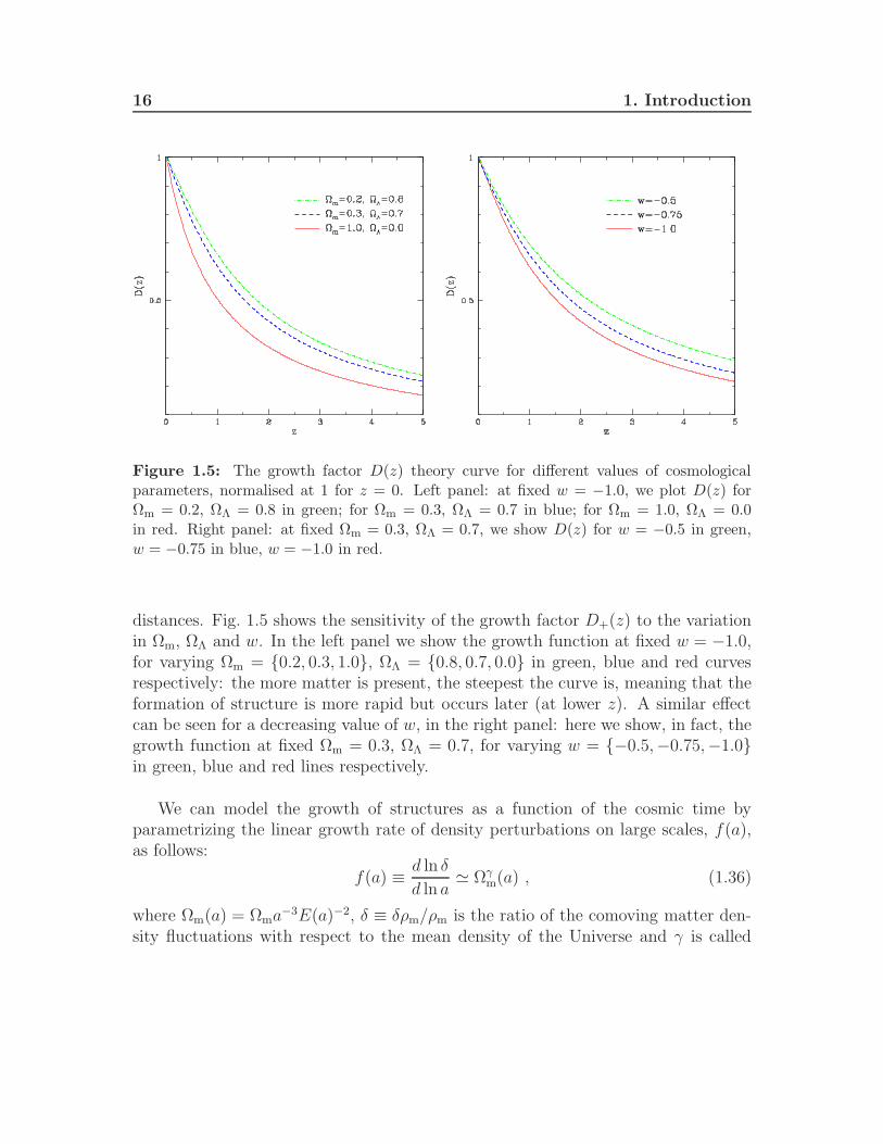
Figure 1.5: The growth factor D(z) theory curve for different values of cosmologicalparameters, normalised at 1 for z = 0. Left panel: at fixed w = −1.0, we plot D(z) forΩm = 0.2, ΩΛ = 0.8 in green; for Ωm = 0.3, ΩΛ = 0.7 in blue; for Ωm = 1.0, ΩΛ = 0.0in red. Right panel: at fixed Ωm = 0.3, ΩΛ = 0.7, we show D(z) for w = −0.5 in green,w = −0.75 in blue, w = −1.0 in red.
distances. Fig. 1.5 shows the sensitivity of the growth factor D+(z) to the variationin Ωm, ΩΛ and w. In the left panel we show the growth function at fixed w = −1.0,for varying Ωm = 0.2, 0.3, 1.0, ΩΛ = 0.8, 0.7, 0.0 in green, blue and red curvesrespectively: the more matter is present, the steepest the curve is, meaning that theformation of structure is more rapid but occurs later (at lower z). A similar effectcan be seen for a decreasing value of w, in the right panel: here we show, in fact, thegrowth function at fixed Ωm = 0.3, ΩΛ = 0.7, for varying w = −0.5,−0.75,−1.0in green, blue and red lines respectively.
We can model the growth of structures as a function of the cosmic time byparametrizing the linear growth rate of density perturbations on large scales, f(a),as follows:
f(a) ≡ d ln δ
d ln a≃ Ωγm(a) , (1.36)
where Ωm(a) = Ωma−3E(a)−2, δ ≡ δρm/ρm is the ratio of the comoving matter den-
sity fluctuations with respect to the mean density of the Universe and γ is called

1.2 The theory of structure formation 17
growth index (see Peebles 1980, 1993; Linder 2005). The growth index allows usto distinguish GR from modified gravity theories which can mimic the expansionhistory of the ΛCDM model. Several of these models predict a time and scale de-pendent growth index, i.e. γ(a, k). It was obtained γ = 6/11 ≃ 0.55 for ΛCDM(Wang & Steinhardt 1998), and, for example, γ = 11/16 in the Dvali et al. (2000)(DGP) braneworld modified gravity model (Linder & Cahn 2007).
Non linear interactions between baryonic matter, dark matter and dark energybecome important when perturbations are not small anymore, i.e. |δ(~x)| ∼ 1.The complex evolution of structure formation in this regime can be studied onlywith numerical simulations (Kuhlen et al. 2012), such as the Millennium Simulation(Springel et al. 2005), and Millennium XXL (Angulo et al. 2012, 2013). Note alsothat for perturbations on large scales, the simple Newtonian approach we introducedis not valid anymore and we should perturb FLRW metric as gµν = g0µν + hµν , where|hµν | << gµν .
1.2.6 Power spectrum of density fluctuations
The power spectrum of density fluctuations is an extremely useful tool for the sta-tistical description of the large-scale structures in general. A correlated quantity isσ2(M, z), namely the variance in mass of the density fluctuation field, within identi-cal volume elements corresponding to 1/k length scale, in a linear evolution regime.To obtain an expression of σ2(M, z), we need to define the filtered density contrastby convolving it with a window function WR as
δR(~x, t) = δM(~x, t) =
∫d3x′ δ(~x′)WR(|~x− ~x′|) , (1.37)
where R = R(M) = (3M/4πρm)1/3 is the characteristic length scale below which we
smooth out all the fluctuations, and WR(x) is usually the spherical top-hat windowfunction in real space
WR(|~x− ~x′|) =
1, if |~x− ~x′| < R,0, otherwise.
(1.38)
This leads to the definition of the variance of the density field:
σ2(M, z) ≡ σ2M(z) ≡ σ2
R(z) =1
2π2
∫ ∞
0
dk k2 P (k, z) |WR(k)|2 , (1.39)

18 1. Introduction
where WR(k) is the Fourier Transformation (FT) of the top-hat filter function of R,given by
WR(k) =3[sin(kR)− kR cos(kR)]
(kR)3. (1.40)
Here P (k, z) is the power spectrum of linear, independently evolving fluctuations,which can be expressed as
P (k, z) = Pin(k) T2(k)D2(z) , (1.41)
where Pin(k) is the primordial power spectrum, T (k) in known as the transfer function(Eisenstein & Hu 1998) and D(z) is the linear growing mode defined in Eq. (1.35).The power spectrum at primordial times is usually described by a power law asPin(k) = As k
ns. Here ns the primordial scalar spectral index, which is observed to beclose to unity (Spergel et al. 2007), in agreement with inflationary models predictions(Harrison 1970; Zeldovich 1972), and As is the amplitude of the primordial powerspectrum, which is by definition related to σ2. The transfer function is carryingall scale-imprinting effects that modified the linear form of the primordial powerspectrum during its evolution to the present day:
T (k) =δk(z = 0)
δk(z)D(z), (1.42)
z being here large enough for δk(z) to mimic the original power spectrum. The scalekeq = (2ΩmH
20 zeq)
1/2 in the CDM model, which corresponds to the transition be-tween the radiation-dominated phase and the matter-dominated epoch, breaks thetransfer function shape: perturbations on small scales (k > keq) are suppressed in am-plitude (Meszaros effect), while they can grow on larger scales (k < keq). Effectively,T (k) ∝ k−2 for k ≫ keq and T (k) ∼ 1 for k ≪ keq. As a consequence, for higherΩm perturbations are suppressed earlier and the peak of the matter power spectrumshifts to higher k. On small scales, dissipative processes from baryon-photon inter-actions leave their imprint (Silk damping, Silk 1968): the more baryons, the moredamped the transfer function is. Finally, BAO appear in the transfer function as well:the position and amplitude of the wiggles depend on the amount of baryons and DM.
If the features of the power spectrum can be theoretically inferred, the normal-isation has to be determined observationally. The latter is generally parametrisedby the quantity σ8, which is the variance defined in Eq. (1.39) having comoving ra-dius R = 8 h−1Mpc. This was motivated by Davis & Peebles (1983) results on earlygalaxy surveys, who found the variance of the galaxy number density on this scaleto be about unity.
1.3 Cosmological probes 19
1.3 Cosmological probes
In this Section we summarise the main cosmological probes which enable us to mea-sure cosmological parameters. Here we introduce the Supernovae Type Ia (SNIa),the Baryon Acoustic Oscillations (BAO) and the Cosmic Microwave Background(CMB), which respectively place constraints on ΩΛ, Ωb and Ωk. The constrainingpower of a single cosmological probe is generally too weak to constrain simultane-ously all cosmological parameters. However, by combining different probes, it ispossible to place tight constraints on the cosmological parameters, to break degen-eracies between them and reduce uncertainties. We will see the results obtained fromthe combination of these probes together with clusters of galaxies in Section 1.5.1.
1.3.1 Supernovae Type Ia
SNIa are thought to be the result of white dwarfs which accrete and explode uponreaching the Chandrasekhar mass limit. This process enable the Supernovae to havea characteristic intrinsic luminosity, which can be standardised empirically: thus,SNIa are potentially independent distance estimators, i.e. standard candles. Othertypes of Supernovae, instead, have more complex collapsing processes and differentintrinsic luminosities, being thus less standardisable. In Fig. 1.6 we show the SNIaobservations from the Supernova Cosmology Project and High-Z Supernova Search(high z) and from Calan/Tololo Supernova Survey (Hamuy et al. 1993, 1995) (lowz), on a logarithmic redshift scale. The apparent magnitude of SNIa is proportionalto the luminosity distance, which is associated to the redshift of the host galaxy.The measured luminosity distance can be compared to the theoretical prediction(see Eq. 1.27) to constrain Ωm, ΩΛ and discriminate between different cosmologicalscenarios. In fact, here the SNIa observations are compared to few cosmologicalmodel: data are strongly inconsistent with Λ = 0 models and favour models withΛ > 0 (Perlmutter 2003). While high-redshift SNIa reveal that the Universe isnow accelerating (Riess et al. 1998a; Perlmutter et al. 1999), nearby ones providethe most precise measurements of the present expansion rate, H0. The most precisemeasurement of H0 comes from the luminosity calibration of nearby SNe Ia throughHubble Space Telescope observations of Cepheids in their host galaxies, carried onby the SH0ES program. With this method, Riess et al. (2011) obtained a value ofthe Hubble constant of H0 = (73.8± 2.4) km s−1Mpc−1 (68% c.l.), including system-atics. The combination of this result alone with the WMAP DR7 (see Section 1.3.3)constraints yields w = 1.08± 0.10 (68% c.l.).

20 1. Introduction
Figure 1.6: Hubble diagram from SNIa, showing the apparent magnitude on a logarith-mic redshift scale for nearby (Calan/Tololo Supernova Survey) and distant (SupernovaCosmology Project, High-Z Supernova Search) Type Ia Supernovae. At redshifts beyondz = 0.1, the cosmological predictions start to diverge, depending on the assumed cosmicdensities. The red curves represent models with zero vacuum energy and mass densitiesfrom the critical density down to zero. The best fit (blue line) assumes a mass density ofabout ρc/3 plus a vacuum energy density of about 2ρc/3, implying an accelerating cosmicexpansion. Credit: Perlmutter (2003).
1.3.2 Baryon Acoustic Oscillations
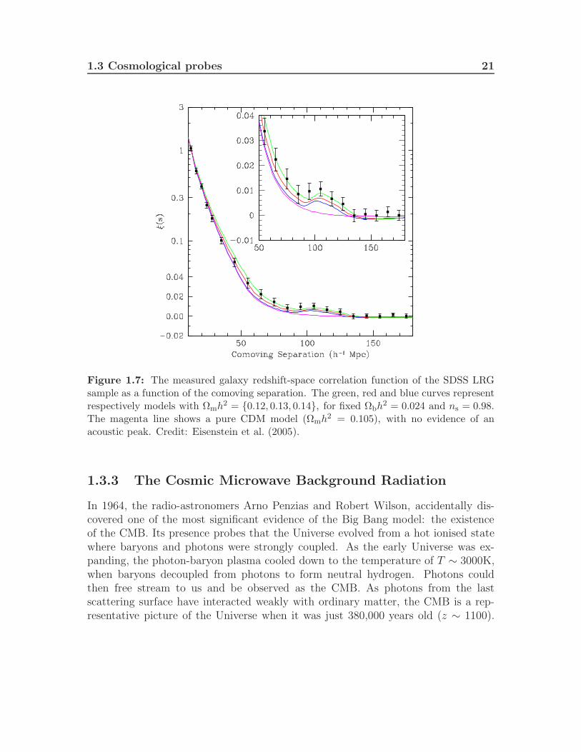
Prior to the decoupling phase of the Universe, when photons were scattered byelectrons through Thomson scattering, radiation pressure opposed the gravitationalcollapse of matter, generating pressure waves, known as BAO. These oscillations lefta signature in the distribution of matter on very large scales and in the featuresof CMB anisotropies (Hu & Dodelson 2002). This signature has been measured bygalaxy surveys as an overdensity of galaxies at a characteristic comoving scale of100h−1 Mpc. For example, Fig. 1.7 shows the statistically significant bump on thiscomoving scale, revealed only by models which include baryons. This was obtainedby Eisenstein et al. (2005), who measured the redshift-space correlation function ξ(s)of the Luminous Red Galaxies from the Sloan Digital Sky Survey (see Section 3.2),with median redshift z = 0.35, as a function of the comoving separation s.
1.3 Cosmological probes 21
Figure 1.7: The measured galaxy redshift-space correlation function of the SDSS LRGsample as a function of the comoving separation. The green, red and blue curves representrespectively models with Ωmh
2 = 0.12, 0.13, 0.14, for fixed Ωbh2 = 0.024 and ns = 0.98.
The magenta line shows a pure CDM model (Ωmh2 = 0.105), with no evidence of an
acoustic peak. Credit: Eisenstein et al. (2005).
1.3.3 The Cosmic Microwave Background Radiation
In 1964, the radio-astronomers Arno Penzias and Robert Wilson, accidentally dis-covered one of the most significant evidence of the Big Bang model: the existenceof the CMB. Its presence probes that the Universe evolved from a hot ionised statewhere baryons and photons were strongly coupled. As the early Universe was ex-panding, the photon-baryon plasma cooled down to the temperature of T ∼ 3000K,when baryons decoupled from photons to form neutral hydrogen. Photons couldthen free stream to us and be observed as the CMB. As photons from the lastscattering surface have interacted weakly with ordinary matter, the CMB is a rep-resentative picture of the Universe when it was just 380,000 years old (z ∼ 1100).

22 1. Introduction
The CMB appears to us as an isotropic radiation filling the whole Universe in alldirections, with a characteristic black body spectrum at the temperature of approx-imately TCMB = 2.73K. According to the cosmological principle, the Universe, andthus the CMB, is approximately isotropic and homogeneous on those large scales.More accurate investigations and more recent measurement, such as the ones by theCOBE (Boggess et al. 1992; Smoot et al. 1992), WMAP (Bennett et al. 2013) andPlanck (Planck Collaboration et al. 2013a) satellites show the presence of tiny tem-perature irregularities (see Fig. 1.8): these correspond to regions of slightly differentdensities, which represent the seeds of all structures we see today. More precisely,it has been observed that the distribution of the CMB is isotropic to the precisionof 10−3: the background (monopole, l = 0) appears completely uniform at a tem-perature of 2.73 K. Most of the residual anisotropy is due to the dipole anisotropy(l = 1, ∼mK), caused to the Doppler effect from the motion of the Sun with respectto the background radiation and the primordial anisotropy (l ≥ 2, ∼ µK), due to ascattering effect and a gravitational effect (Sachs-Wolfe effect, Sachs & Wolfe 1967).After subtracting all these contributions (including Milky Way emission visible inthe central part of the map), we are left with density fluctuations of
∆T
T=
∆ρmρm
≈ 10−5 . (1.43)
Note that the equality here between temperature and density fluctuations holds onlyif perturbations are adiabatic.
Statistical properties of the CMB are represented by the temperature power spec-trum as a function of angular wavenumber l (small l correspond to large angularscales). The CMB power spectrum is a measure of the anisotropy power on differentangular scales: the sky is divided up into polar coordinates and the observed temper-ature field is decomposed into spherical harmonics. The theoretical prediction of theCMB temperature power spectrum is related to the energy contents of the Universeand can be used to constrain cosmological parameters, by comparing with observeddata. The CMB gives us information about the early Universe (z ∼ 1100), beingless sensitive to the late Universe, as photons interact rarely with matter. The CMBanisotropies has been measured by COBE, WMAP, and more recently by Planck,South Pole Telescope and Atacama Cosmology Telescope up to l ∼ 3000. For thecosmological analysis presented in this work, we include the CMB spectra measuredby WMAP, for which we now provide some description.

1.3 Cosmological probes 23
Figure 1.8: The anisotropies of the CMB as observed by Planck satellite. Cold spots arein blue, while hot are in red. Copyright ESA and the Planck Collaboration.
Wilkinson Microwave Anisotropy Probe
TheWMAP1 is a NASA Explorer mission which collected a huge amount of data, nowfully analysed to obtain important cosmological achievements. Charles Bennett andthe WMAP team won the 2012 Gruber Cosmology Prize because of these publishedresults. The WMAP instrument is composed of cooled microwave radiometers, with1.4 × 1.6 meter diameter primary reflectors, in five frequency bands (22-90 GHz)to allow the separation of the foreground signals from the CMB. WMAP measuresthe temperature difference between two points in the sky to an accuracy of 10−6
degree: this means also that systematics have been carefully handled. The mainachievement of this project has been the first fine-resolution (0.2 deg) full-sky mapof the microwave sky. In addition to this, the inflationary model has been supported,as well as the Gaussian distribution of temperature fluctuations. Furthermore, thefollowing constraints on cosmological parameters have been placed : the age of theUniverse is 13.77 billion years old, within a 0.5%; the curvature of space is zerowithin 0.4%; the Universe contents are baryons (4.6%), dark matter (24.0%) anddark energy (71.4%). In our cosmological analysis, we include the CMB spectrafrom the WMAP Data Release 7, whose detailed cosmological results have beenpublished by Komatsu et al. (2011). Fig. 1.9 shows the CMB temperature power
1http://map.gsfc.nasa.gov/

24 1. Introduction
Figure 1.9: The 7-year temperature (TT) power spectrum from WMAP. The curve isthe CDM model best fit to the 7-year WMAP data: Ωbh
2 = 0.02270, Ωch2 = 0.1107,
ΩΛ = 0.738, ns = 0.969. The plotted errors include instrumental noise. The grey bandrepresents cosmic variance. Credit: Larson et al. (2011).
spectrum l(l+1)Cl/2π as a function of multipole l (l = π/θ) as measured by WMAPDR7 (Larson et al. 2011). The locations and shapes of the first (l ∼ 200) and secondpeak (l ∼ 500) has been detected with high precision, while the third peak (l ∼ 800)is less constrained. The first peak location corresponds to the size of the soundhorizon at the last scattering surface. As we can measure the distance to the lastscattering surface, knowing the redshift of the CMB, we can locate a point in theHubble diagram with very high accuracy, and probe the geometry of the Universe.This method measures the Universe to be spatially flat Ωk ∼ 1. The other peaksinstead represent combinations of Ωr, Ωb, Ωm. The cosmology results of WMAP DR9have recently been published (Hinshaw et al. 2013).

1.4 Galaxy Clusters 25
1.4 Galaxy Clusters
Clusters of galaxies are a particularly rich source of information about the underlyingcosmological model. They are the largest and most recent collapsed objects in theUniverse. Studies of their evolution and properties can place strong constraints onthe growth of structures and on the current cosmological paradigm. Here we brieflydescribe the history of galaxy clusters observations, their main constituents andobservables, their formation process and their role as cosmological probes.
1.4.1 History of galaxy clusters observations
Galaxy clusters were discovered quite early in the history of modern astronomyby Messier (1784) and Herschel (1785), independently. The extragalactic natureof these objects was only later confirmed and galaxy clusters were considered asproper physical objects. Their nature was not recognised until the 1930’s, when thedynamical analysis of Zwicky (1937) and Smith (1936) enable the first estimation oftheir mass. They showed the evidence for much more gravitational material thanindicated by the stellar content of the galaxies in the cluster alone, giving the first hintof DM in the Universe. This was later confirmed by measurements of cluster massesusing the velocity distribution of the galaxies by means of the Viral Theorem2 (Rood1974b,a). Then, the studies on galaxy clusters were extended to several aspects:origin and evolution, dynamical properties, distribution and characterization of thegalaxies inside a cluster. Large catalogues of clusters (Abell 1958; Zwicky et al.1968) based on eye estimates of the number of galaxies per unit solid angle weredeveloped. The first all sky X-ray survey with the Uhuru satellite (Giacconi et al.1972) confirmed that many clusters were spatially extended X-ray sources. Morerecently, the discovery of hot high-redshift clusters by Bahcall & Fan (1998) was thefirst suggestion of a DE component. Finally, last decades experienced the birth ofnumerous surveys in all wavelengths and an exponential increase of publications ongalaxy clusters. More details about these latest scientific results will be covered inChapter 3.
2The Virial Theorem states that, for a stable, self-gravitating, spherical distribution of objectsof same mass, it holds Ek = −1/2Ep, where Ek is the total kinetic energy of the objects and Ep isthe total gravitational potential energy.

26 1. Introduction
1.4.2 Main features, components and observables
Clusters typically have masses of 1013-1015M⊙, sizes of the order of few Mpc, velocitydispersions of 800-1000 km/s and X-ray luminosities of 1043-1045 erg/s. Clusters ofgalaxies are typically larger than groups and contain about 50 to 1000 members:this limits assign the denomination of rich and poor cluster, respectively. We canalso distinguish clusters between regular, which are spherical with a central regionof higher density, and irregular ones, which are instead not spherical and without aunique dense central region. Phenomenologically clusters are composed of:
- Galaxies (2-5%), which contain the condensed baryonic matter in the form ofstars and cold gas. The typical population is composed of old and passive (redand dead) galaxies, which ended their star formation at z > 2 and which siton a red-sequence locus in a colour-magnitude diagram.
- Intra-Cluster Medium (ICM) (11-15%), which mainly consists of hydrogenand helium, represents most of the baryonic matter in a highly ionised form andlow density (∼ 10−3atoms/cm3). As a matter of fact, the ICM reaches tem-perature of approximately 108K to balance the gravitational pull of the DMpotential well, and emits in the X-ray band. The main X-ray emission pro-cesses from ICM are collisional: thermal Bremsstrahlung (free-free emission),recombination (free-bound emission), line radiation (bound-bound emission).The emissivity of the Bremsstrahlung mechanism is stronger in the densestinnermost regions because is proportional to the squared number density ofparticles.
- Dark Matter Halo (80-87%): it follows a universal distribution known as theNavarro-Frenk-White (NFW) profile (Navarro et al. 1997), which depends onthe central density and scale radius (see Section 2.1.2).
- Intra-Cluster light: it is the optical light from stars which are gravitationallybounded to the cluster itself.
As a consequence, they are accessible by multiple signals, across the whole electro-magnetic spectrum. Fig. 1.10 shows the superposition of three views of the galaxycluster Abell 520. The optical view represents the galaxy population; the hot ICM iscaptured in red in the Chandra X-ray Observatory image; finally, the gravitationallensing image is instead highlighting the collisionless core of DM component in blue.In general, the galaxy population and the intra-cluster light are visible in opticaland near-infrared bands. The hot ICM is instead detected by the strong X-ray

1.4 Galaxy Clusters 27
Figure 1.10: Composite image of three views of the galaxy cluster Abell 520. The opticalview shows the galaxies bound together by gravitational force. Diffuse, hot gas in betweenthe galaxies emits X-rays: this is shown in red in the Chandra X-ray Observatory image.Gravitational lensing image is representing, instead, the collisionless core of dark mattercomponent in blue. Credit: X-ray: NASA/CXC/UVic./A.Mahdavi et al.; Optical/Lensing:CFHT/UVic./A.Mahdavi et al..
emission, while at radio frequencies, synchrotron emission from relativistic electronscan be detected and provide information on the intra-cluster gas. Furthermore, atmillimetre wavelengths, high-density regions within clusters cause distortions of theCMB spectrum by inverse Compton scattering, namely the Sunyaev-Zel’dovich (SZ)effect (Sunyaev & Zeldovich 1972): the low-energy CMB photons enhance their en-ergy because of the collision with the high energy ICM electrons, causing a localfrequency-dependent shift in the CMB spectrum observed through the cluster. This

28 1. Introduction
effect is used to detect clusters with no redshift limitation and is quantified by theCompton y-parameter, i.e. the electron pressure integrated along the line of sight l:
y =
∫kBTX(l)
c2mene(l)σTdl . (1.44)
Here kB is the Boltzmann constant, TX is the X-ray temperature, me and ne arethe electron mass and number density respectively, σT is the Thomson cross-section.More practically, the quantity which is usually measured is the projection on thecluster area dA, namely the integrated Compton parameter YSZ ∝
∫ydA. Finally,
strong features are also detected in the gravitational lensing shear field, which givesinformation about the DM halo (see Section 2.1.3).
1.4.3 Cluster mass proxies
One of the key issues in the study of galaxy clusters is the determination of theirtrue mass. Cluster total masses cannot be directly determined from observation, butinstead they have to be deduced from some observational properties, called massproxies, which correlate with the true mass via the so-called scaling relations.Various mass proxies in different wavelength and associated systematics have beenused so far to determine the mass of clusters from observations, via the respectivescaling relations and scatter around them. Here we only list the most common ones:
i) the optical richness, i.e. number of red galaxies within R200: N200 (Rozo et al.2010) - this is the observable throughout all our analysis;
ii) the line-of-sight velocity dispersion: σv, which is related to the total mass as(Longair 2008) M ∝ σ2
vRvir, where Rvir is the virialization radius;
iii) the X-ray temperature, bolometric luminosity, gas mass, gas total thermalenergy;
iv) the integrated SZ parameter at mm wavelength.
Note that another valid technique to measure cluster masses is gravitational lens-ing: it uses the distortions of background galaxies images caused by the space-timedeformation, which is induced by the cluster halo mass.

1.4 Galaxy Clusters 29
1.4.4 Formation of galaxy clusters
Formation and evolution of clusters of galaxies trace directly the hierarchical growthof structures in the Universe. The first objects which start to collapse and virialize,deviating from the Hubble flow, have sub-galactic sizes. Then, these structures mergeto originate the galaxies, which analogously can form galaxy clusters by merging.Fluctuations inside a region grow until they balance the local expansion: at thispoint, the expansion of the region is slowed down till it reaches a maximum radius.Having no more kinetic energy but only gravitational potential energy, the regioncollapses: baryons fall into the gravitational potential wells produced by the DM andpotential energy is converted into kinetic one. This brings the gas to thermalisation,thus producing the hot plasma. When the Virial Theorem condition is satisfied,the dynamical equilibrium is reached. The kinetic energy of the galaxies movingrandomly inside the cluster furnishes a pressure which counteracts the gravitationalattraction: this gives stability to the cluster.
1.4.5 Clusters as cosmological probes
As in GR the geometry of the Universe is fully described by the total energy content(see Eq. 1.5), one can study the structure of the Universe by testing the geometryby means of probes such as SNIa, BAO and CMB. Alternatively, it is possible totest both the geometry and the structure with different probes and then comparethe constraints. Clusters of galaxies are fundamental because they provide both anindependent measure of cosmological parameters with different systematics to theCMB, SNIa and BAO, and a probe of the growth of structures. In particular, galaxyclusters are used to test cosmology my measuring their mass function, namely thenumber density of clusters as a function of their mass and redshift. The precisedetermination of the mass function and its evolution can place constraints on theenergy components of the Universe. As an example, we show in Fig. 1.11 an earlyresult for the cluster mass function obtained by Bahcall & Cen (1992). The opticaldata are based on richness, velocities and luminosity function of clusters, while theX-ray data refer to the temperature distribution of clusters. Here the observationsof optical and X-ray galaxy clusters are compared with expectations from differentcosmologies using CDM large-scale (box size of 400h−1Mpc) simulations. The com-parison shows that the cluster mass function is a powerful discriminant among mod-els: the Ωm = 1 model cannot reproduce the observations for any bias parameter. Infact, when normalised to the COBE CMB fluctuations on large scales (Smoot et al.1992), this model predicts a much larger number of massive clusters then is ob-served. On the other hand, a low-density CDM model, with Ωm = 0.25, 0.35 and

30 1. Introduction
Figure 1.11: Cluster mass function observations of optical and X-ray data, comparedwith CDM simulations. A model with Ωm = 0.25, 0.35 (with or without a cosmolog-ical constant), appears to match the observations. The Ωm = 1 model, instead, fails inreproducing data. Credit: Bahcall & Cen (1992).
bias b = 1.0, 1.3, with or without a cosmological constant, appears to fit well theobservations. Precise observations of large numbers of clusters have later providedan important tool for understanding better their abundances. The full theoreticalderivation, numerical calibration and discussion on the cosmology dependence of themass function are provided in Section 2.2. In addition to a predicted mass functionand a well-determined relation between the true cluster mass and the observable, acluster experiment needs a large, clean, complete survey with a well-defined selectionfunction. We list the main X-ray, millimetre, weak lensing and optical cluster surveysin Section 3.1. Complementary to the abundances, the clustering of galaxy clusters,i.e. their spatial distribution at z = 0 and its evolution to higher redshifts, containsfundamental information on the underlying matter distribution as well. We give adetailed description of the cluster power spectrum and its cosmology dependence inSection 2.4.
Detailed theoretical modelling of clusters is a complicated astrophysics probleminvolving a variety of physical phenomena. Useful tools in this regards are numericalsimulations. While the pure gravitational interactions of DM particles can be treatedin a linear regime and their behaviour is well described, baryonic physics is far morecomplex, non-linear and involves hydrodynamical processes.

1.5 ΛCDM standard model 31
1.5 ΛCDM standard model
Several observations over the past decades confirmed that the Universe is experienc-ing a phase of cosmic acceleration, driven by a dark form of energy with negativevacuum pressure. Perlmutter et al. (1999) with SNIa, Allen et al. (2004, 2008) withclusters of galaxies, Eisenstein et al. (2005) with Large-Scale Structure (LSS) andKomatsu et al. (2011) with the CMB, independently confirm the accelerated expan-sion epoch which is currently ongoing. Therefore the concordance Lambda ColdDark Matter (ΛCDM) cosmological model has been formulated. It affirms thatthe Universe is composed of: ∼ 5% of ordinary baryonic matter Ωb, mainly made up by hydrogen atoms (∼
75%), Helium atoms (∼ 25%), while heavier elements are only a tiny fraction; ∼ 25% of unknown (dark) form of matter Ωcdm, made up by species of sub-atomic particles that interact almost only gravitationally (and not electromag-netically) with ordinary matter, being thus totally collisionless; ∼ 70% of unknown (dark) form of energy ΩΛ, responsible of the late timeaccelerating expansion; a radiation component Ωr, which is negligible today, as Ωr/Ωm ≃ 1/3250.
There are few probes of the existence of the DM component. One is relatedto the rotation curves of galaxies (see Fig. 1.12 and Freeman 1970) which do notreveal a Keplerian decline (namely the squared velocity is not proportional to theinverse radius), giving evidence of an undetected matter component. Furthermore,the gravitational lensing in galaxy clusters shows a mismatch between the amount ofnormal matter and the estimated total mass. In addition to this, the evidence of thecollisionless nature of dark matter has been observed in few objects (e.g. the ’bulletcluster’ in Markevitch et al. 2004; Clowe et al. 2004). A fundamental property ofDM is that it is non-relativistic (i.e. cold): this is necessary to explain the struc-ture formation model currently accepted. Possible candidates for a DM particle areprovided by theoretical particle physics, e.g. Weakly Interacting Massive Particles(WIMPSs), which are massive particles interacting through the weak nuclear forceand gravity.
The simplest way to define the DE dominant component is a positive value ofthe cosmological constant Λ introduced in Einstein field equations, with constantequation of state w = −1. However, few problems arise from this choice. First of all,

32 1. Introduction
Figure 1.12: Rotation curve of galaxy NGC 6503: the data points with error bars arethe observed velocities, the disk stars contribution is shown by the dashed line, while thecontribution of the gas is represented by the dotted line. As Freeman (1970) first noticedthat the expected Keplerian decline (i.e. v2 ∝ r−1) was not present in NGC 300 and M33galaxies, also here there is clear evidence of an undetected dark matter halo component,with density ρDM(r) ∝ r−2. Credit: Kamionkowski (1998).
the cosmological constant problem appears if we associate Λ to the vacuum energy,i.e. the background energy in absence of matter: the observed cosmological constantis smaller by a factor of ∼ 10120 than the value for the vacuum energy predicted byquantum field theories. In addition to this, the coincidence problem asks why welive at the special epoch where DE density is approximately equal to matter density.Numerous alternative theories try to explain the nature of this constituent (e.g.quintessence,...). For example, by assuming that the equation of state of DE evolvesin time, we obtain w(z) = w0+w
′z (Maor et al. 2001; Weller & Albrecht 2001, 2002),which diverges at high redshift, or w(z) = w0 + w1 z/(1 + z) (Chevallier & Polarski2001; Linder 2003). Alternatively, modification of gravity can be performed: they donot invoke a new form of energy, but instead introduce new physics which modifiesEinstein’s equations on large scales (e.g. Dvali et al. 2000).

1.5 ΛCDM standard model 33
1.5.1 Cosmological constraints from observations
For completeness, we now list the main cosmological parameters in the concordanceΛCDM model, which govern the global properties of the Universe and the spectrumof the initial density perturbations, together with their current constraints from thelatest Planck mission (Planck Collaboration et al. 2013b) (see Table 1.2).
Symbol Definition Constraint
ωb = Ωbh2 Baryon density 0.02214±0.00024
ωcdm = Ωch2 Cold Dark Matter density 0.1187±0.0017
Ωk Spatial curvature -0.0005+0.0065−0.0066
ΩΛ Dark Energy density 0.692±0.010ln(1010As) Primordial pert. amplitude 3.091±0.025
σ8 RMS matter fluctuations 0.826±0.012w Constant EoS of Dark Energy -1.13+0.23
−0.25
τ Reionization optical depth 0.092±0.013ns Primordial scalar spectral index 0.9608±0.0054∑mν Sum of the neutrino masses in eV <0.230
Neff Effective number of neutrino-like species 3.30+0.54−0.51
H0 Hubble constant 67.80±0.77t0 Age of the Universe (Gyr) 13.798±0.037zre Redshift of half-reionization 11.3±1.1
100θ∗ 100 × angular size of sound horizon 1.04162±0.00056
Table 1.2: List of the main cosmological parameters of ΛCDM model, together the con-straints from Planck+WMAP+highL+BAO (Planck Collaboration et al. 2013b) for thefollowing models: six parameter base ΛCDM model and derived parameters (blue, 68%limits) and extensions to the base ΛCDM model (green, 95% limits).
We conclude this Chapter by highlighting the constraining power on cosmolog-ical parameters of clusters of galaxies: in combination with other probes, such asSNIa, BAO and CMB, some parameters degeneracies can be broken and the errorstightened.
34 1. Introduction
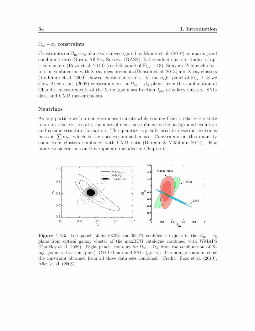
Ωm − σ8 constraints
Constraints on Ωm−σ8 plane were investigated by Mantz et al. (2010) comparing andcombining three Rosita All Sky Surveys (RASS). Independent clusters studies of op-tical clusters (Rozo et al. 2010) (see left panel of Fig. 1.13), Sunyaev-Zeldovich clus-ters in combination with X-ray measurements (Benson et al. 2013) and X-ray clusters(Vikhlinin et al. 2009) showed consistent results. In the right panel of Fig. 1.13 weshow Allen et al. (2008) constraints on the Ωm −ΩΛ plane, from the combination ofChandra measurements of the X-ray gas mass fraction fgas of galaxy clusters, SNIadata and CMB measurements.
Neutrinos
As any particle with a non-zero mass transits while cooling from a relativistic stateto a non-relativistic state, the mass of neutrinos influences the background evolutionand cosmic structure formation. The quantity typically used to describe neutrinosmass is
∑mν , which is the species-summed mass. Constraints on this quantity
come from clusters combined with CMB data (Burenin & Vikhlinin 2012). Fewmore considerations on this topic are included in Chapter 6.
Ωm
ΩΛ
0 0.2 0.4 0.6 0.8 10
0.2
0.4
0.6
0.8
1
1.2
1.4
1.6
SNIa
CMB
Cluster fgas
Figure 1.13: Left panel: Joint 68.3% and 95.4% confidence regions in the Ωm − σ8plane from optical galaxy cluster of the maxBCG catalogue combined with WMAP5(Dunkley et al. 2009). Right panel: contours for Ωm − ΩΛ from the combination of X-ray gas mass fraction (pink), CMB (blue) and SNIa (green). The orange contours showthe constraint obtained from all three data sets combined. Credit: Rozo et al. (2010);Allen et al. (2008).

1.5 ΛCDM standard model 35
DE equation of state
Allen et al. (2011) analysed the constraints on the DE equation of state togetherwith Ωm (see left panel of Fig. 1.14) or σ8. He combined the abundance andgrowth of RASS clusters (Mantz et al. 2010), fgas measurements (Allen et al. 2008),WMAP5 results (Dunkley et al. 2009), Supernovae Ia data (Kowalski et al. 2008)and BAO measurements (Percival et al. 2010, 2011). Constraints on DE equationof state from data were also performed by Rapetti et al. (2005) with X-ray clus-ters+SNIa+CMB, by Mantz et al. (2010); Benson et al. (2013) with X-ray clusters,while Vikhlinin et al. (2009) constrained w and ΩΛ.
Cosmic growth γ
Rapetti et al. (2013) tested the cosmic growth predicted by GR (γ = 0.55) withthree independent measurements: galaxy clusters abundances and fgas from RASSand Chandra, galaxy clustering from WiggleZ Dark Energy Survey, 6-degree FieldGalaxy Survey and CMASS BOSS, and CMB from WMAP. The cosmic growth ismodelled by the growth index γ defined in Eq. (1.36) and σ8. We show in the rightpanel of Fig. 1.14 the constraints obtained on these parameters.
σ8
γ
0.4 0.6 0.8 1 1.2 1.4 1.6
−0.5
0
0.5
1
1.5
2
2.5
CMB
cl
galcl+CMB+gal
Figure 1.14: Left panel: Joint 68.3% and 95.4% confidence regions for w−Ωm, from theabundance and growth of RASS clusters (violet), X-ray gas mass fraction (pink), WMAP5(blue), SNIa (green) and BAO (brown). Right panel: joint contours in the σ8 − γ plane,from galaxy growth (green), CMB (blue) and cluster growth (red). The gold contours showthe combination of the data sets. Credit: Allen et al. (2011); Rapetti et al. (2013).

36 1. Introduction

Chapter 2
Galaxy Clusters from theory side
In this Chapter the theoretical framework of galaxy clusters one-point (numbercounts) and two-points statistic (power spectrum) is introduced, in order to un-derstand why they are fundamental probes of the LSS of the Universe. For the studygalaxy clusters, in fact, one needs to have first an estimate of their masses, whichare not directly accessible. Here, we define the cluster masses and density profiles,with a particular emphasis to the weak lensing mass estimation, as this is the one weuse in our analysis. Secondly, to understand how the cluster number counts changewith the mass and with the cosmological model assumed, we revise the formulationand calibration of the cluster mass function and its sensitivity to cosmology. Inaddition to this, the spatial distribution of clusters can give additional informationon cosmology. We thus introduce the concept of the model bias and a prescriptionfor the clusters redshift space power spectrum. Finally, some definitions concerningthe study of non-Gaussian initial conditions are provided, as clusters can be a goodprobe in this context.
2.1 Cluster masses
As the mass of galaxy clusters is not directly measurable, we describe here how toget an estimate of it. Cosmologists usually define the cluster mass with respect tothe critical or the mean density of the Universe and assume a halo density profile.We then focus on the gravitational weak lensing technique to reconstruct the massdistribution, as it is part of the data sets we need for our combined cosmologicalanalysis.
38 2. Galaxy Clusters from theory side
2.1.1 Definition
A common way to define a cluster mass is with respect to the critical density of theUniverse, ρc(z) (see Eq. 1.14). One considers a spherical region of a virialized haloof radius R∆ and volume V∆ = 4 π/3R3
∆, with mean density of ρ(z) = ∆ ρc(z). Thetotal amount of matter contained in this region is defined to be the mass M∆ as
M∆ = V∆ ρ(z) =4 π
3R3
∆ ∆ ρc(z) . (2.1)
Typical values of ∆ are 200 (this work) or 500, because cluster properties are moreevident to observe in high density contrast regions. Alternatively, the mass canbe defined with respect to the background mean density of the Universe, ρm(z): themean density inside the virial radius is then ρ(z) = ∆ ρm(z) = ∆Ωm(z)ρc(z) (becauseof Eq. 1.16), and the value of Ωm(z) has to be assumed.
2.1.2 Halo density distribution
In order to estimate the mass of a cluster, we need to have a prescription for its densityprofile. Observation of galaxy clusters show that the velocity dispersion σv of galaxiesinside a cluster remains nearly constant with distance from the cluster centre: thisimplies an underlying mass-density distribution, ρ(R) ∝ R−2. Binney & Tremaine(1987) found that the Singular Isothermal Sphere (SIS) was the simplest analyticalmodel consistent with the observed mass distribution. Such a profile resembles thedensity structure of an isothermal self-gravitating system of particles, which encoun-tered a violent relaxation process (Lynden-Bell 1967) from a chaotic initial state toa quasi-equilibrium. This density distribution is characterised by a constant andisotropic velocity dispersion σv, and has the following form
ρSIS(R) =1
2πG
σ2v
R2. (2.2)
This approximation is, however, incomplete because the mass diverges with R lin-early. Later, cluster formation numerical simulations obtained a more accurate formof density profile:
ρ(R) ∝ R−p(R +Rs)p−q , (2.3)
where p and q describe the slopes of inner and outer regions, and Rs is the scaleradius where the profile steepens. Fits of Eq. (2.3) to simulated clusters give, forexample, the Moore et al. (1999) profile (p = 1.5, q = 3) and Rasia et al. (2004)

2.1 Cluster masses 39
profile (p = 1, q = 2.5). Navarro et al. (1997) best fit values were instead p = 1, q =3: more precisely they obtained the following expression (for ∆ = 200)
ρNFW(R) =ρc(z)λc
(R/Rs)(1 +R/Rs)2, (2.4)
where λc is the density contrast given by
λc =200
3
c3
ln(1 + c)− c/(1 + c), (2.5)
being c = R200/Rs the concentration of the halo, namely the ratio of the virial radiusR200 to the scale radius Rs. The concentration parameter is a function of halo massand redshift and depends on cosmological parameters: typically, the earlier the haloforms, the higher is the value of c. Eq. (2.4) is known as the Navarro-Frenk-White(NFW) profile and it is the most widely used fitting formula for haloes density: wewill assume this profile in this work.
Note that on large scales (clusters) CDM simulations have proven very successful,while on galaxy scales their predictions seem to be in conflict with some observations.Among these, the cusped central density profile given by the NFW profile, which isnot observed in dwarf galaxies. Burkert (1995) empirically modified the analyticform of the NFW profile, trying to find the best-fitting density law to the observedrotation curves of dwarf galaxies. The Burkert’s profile can be expressed as:
ρB(R) =ρ0R
3s
(R +Rs)(R2 +R2s ), (2.6)
where the central density ρ0 and the scale radius are free parameters. This densitylaw resembles an isothermal profile in the inner regions (R < Rs) and predict a finitecentral density ρ0, while in the outer regions it diverges logarithmically with radius,in agreement with the NFW profile.
2.1.3 Weak Lensing signal
According to GR, light rays propagate along null-geodesics of the space-time metrics.The presence of mass distribution perturbs the metrics, deflecting the light trajec-tories. This deflection distorts the shape of distant galaxies, allowing the study ofthe mass distribution of objects in the Universe. This distortion is called gravita-tional lensing effect. In 1804 Johann Soldner wrote the first paper on this topic,
40 2. Galaxy Clusters from theory side
predicting with Newtonian physics that a light ray passing close to the Sun is de-flected by an angle of ∼ 0.84 arcsec. In 1919, Einstein obtained the same valueα = 2GM⊙/c
2R⊙ ∼ 0.83 arcsec, by applying Huygens principle to a wave front pass-ing through a region in which the speed of the wave varies with position (the closerto the massive body, the smaller the speed is). After completing GR, he realised thecorrect equation for the deflection angle of a light ray passing at a distance R froman object with mass M was:
α =4GM
c2R, (2.7)
finding for the Sun the value of 1.74 arcsec. The additional factor of two is due tothe spatial curvature which is missing in the Newtonian approach. More precisely,the full theory takes into account not just the variation of the time-time componentof the metric, but also the variation of the spatial components.
By measuring the gravitational lensing distortions of background galaxies causedby clusters of foreground galaxies, it is possible to probe their matter distribution.It plays a critical role, because it can measure the total cluster mass regardless ofthe baryonic content, star formation history, or dynamical state. Thus, lensing iscrucial for calibrating the mass-observable relation, as we will detail in Chapter 3. Inorder to describe how gravitational lensing works, we need to introduce some basicnotation following Bartelmann & Schneider (2001). If the lens is thin compared tothe total length of the light path, the lens mass distribution can be projected on anorthogonal plane with respect to the line-of-sight, called lens plane. This mass sheetis characterised by its surface mass density
Σ(~ξ) =
∫ρ(~ξ, z) dz , (2.8)
where ρ is the density and ~ξ is a two-dimensional vector in the lens plane. Thedeflection angle at ~ξ is the sum of all mass elements deflections in the lens plane:
~α(~ξ) =4G
c2
∫(~ξ − ~ξ′)Σ(~ξ′)
|~ξ − ~ξ′|2d2ξ′ . (2.9)
The geometry of a typical gravitational lens system is shown in Fig. 2.1. A lightray from a source S, assumed to lie in the so-called source plane, is deflected by theangle ~α at the lens plane before reaching observer O. The angle between the opticalaxis and the image I is ~θ, while the one between the optical axis and the true sourceis ~β. The angular diameter distances observer-lens, lens-source, observer-source are
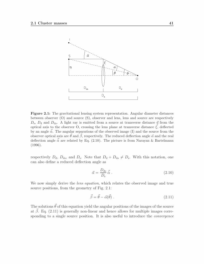
2.1 Cluster masses 41
Figure 2.1: The gravitational lensing system representation. Angular diameter distancesbetween observer (O) and source (S), observer and lens, lens and source are respectivelyDs, Dd and Dds. A light ray is emitted from a source at transverse distance ~η from theoptical axis to the observer O, crossing the lens plane at transverse distance ~ξ, deflectedby an angle ~α. The angular separations of the observed image (I) and the source from theobserver optical axis are ~θ and ~β, respectively. The reduced deflection angle ~α and the realdeflection angle ~α are related by Eq. (2.10). The picture is from Narayan & Bartelmann(1996).
respectively Dd, Dds, and Ds. Note that Dd + Dds 6= Ds. With this notation, onecan also define a reduced deflection angle as
~α =Dds
Ds
~α . (2.10)
We now simply derive the lens equation, which relates the observed image and truesource positions, from the geometry of Fig. 2.1:
~β = ~θ − ~α(~θ) . (2.11)
The solutions ~θ of this equation yield the angular positions of the images of the sourceat ~β. Eq. (2.11) is generally non-linear and hence allows for multiple images corre-sponding to a single source position. It is also useful to introduce the convergence

42 2. Galaxy Clusters from theory side
parameter, which is the dimensionless surface mass density, as
κ(~θ) =Σ(Dd
~θ)
Σcwith Σc =
c2
4πG
Ds
DdDds, (2.12)
where Σc is the critical surface mass density, and thus rewrite the reduced deflectionangle as
~α(~θ) =1
π
∫d2θ′
(~θ − ~θ′)κ(~θ′)
|~θ − ~θ′|2. (2.13)
The lens mapping can then be linearised locally: the Jacobian describing the distor-tion of images is given by
A =∂~β
∂~θ=
(1− κ− γ1 −γ2
−γ2 1− κ + γ1
). (2.14)
Here γ = γ1+ iγ2 = |γ|e2iψ = |γ|(cos 2ψ+ i sin 2ψ), ψ being the angle between ~α andthe x-axis, is the tangential shear which stretches the image around the lens, whilethe magnification of the image is described by the convergence κ. The weak lensingapproximation is valid for κ≪ 1 and |γ| ≪ 1.
In order to estimate the mass of galaxy cluster, we have to employ a model forits density distribution, e.g. the NFW of Eq. (2.4). For any value of the NFWprofile parameters (scale radius Rs and density contrast λc), the convergence and theshear can be analytically inferred. By introducing a dimensionless radial distancex = r/Rs = θ/θs (where θs = Rs/Dd), we can in fact reformulate the convergence as
κ(x) =
(2Rsλcρc)/[Σc(1− x2)][1− 2/√1− x2 atanh
√(1− x)/(1 + x)] x < 1,
(2Rsλcρc)/3 x = 1,
(2Rsλcρc)/[Σc(x2 − 1)[1− 2/
√x2 − 1 atan
√(x− 1)/(x+ 1)] x > 1.
The gravitational shear can instead be recast as
γ(x) =
(Rsλcρc)/Σcg<(x) x < 1,
(Rsλcρc)/Σc [10/3 + 4 ln(1/2)] x = 1,
(Rsλcρc)/Σcg>(x) x < 1,
where the functions g<(x) and g>(x) are given by
g<(x) =8 atanh
√(1− x)/(1 + x)
x2√1− x2
+4 ln(x/2)
x2− 2
(x2 − 1)+
4 atanh√(1− x)/(1 + x)
(x2 − 1)(1− x2)1/2,
g>(x) =8 atan
√(x− 1)/(1 + x)
x2√x2 − 1
+4 ln(x/2)
x2− 2
(x2 − 1)+
4 atan√
(x− 1)/(1 + x)
(x2 − 1)3/2.

2.2 Mass function 43
In the case of galaxy clusters, the observable is the reduced shear γ, which is obtainedby averaging over observed galaxies shapes, and is defined as
γ(θ) =γ(θ)
1− κ(θ). (2.15)
In order to estimate the mass of the cluster (lens), having assumed a density profile,we can compare the observed reduced shear with its theoretical prediction obtainedcombining the analytical expressions for κ and γ. We will use cluster mass estimatesdone with this technique in our cosmological combined analysis.
2.2 Mass function
Once the definition of the cluster mass is given, we can investigate the number densityof clusters as a function of it, namely the mass function. This represents the expectednumber density of virialized dark matter halos at redshift z, with mass in the range[M,M + dM ], and can be expressed as
dn(M, z)
d lnM= ρm
∣∣∣∣d ln σ−1
dM
∣∣∣∣ f(ν) . (2.16)
Here, ρm is the mean matter density of the Universe, ν ≡ δc/σ(M, z), δc being thecritical linear overdensity and σ2(M, z) is the variance of the density fluctuation fieldfiltered at scale M in the linear evolution regime (see Eq. 1.39).
To calculate the value for δc analytically, we assume a spherical top-hat col-lapsing model. A closed spherical region of radius R and overdensity δ (seeEq. 1.30), in a homogeneous expanding background field with mean density ρ, evolvesindependently of the environment influenced by local properties only (Birkhoff’s the-orem). This region expands up to a maximum radius Rmax at the turn-around timetturn and then decouples from Hubble expansion and recollapses to a bound systemof radius Rvir = Rmax/2 at the collapse time tcol = tvir = 2tturn, reaching the virialtheorem equilibrium condition. For an Einstein-de Sitter Universe (Ωm = 1, Ωk = 0),the overdensity reaches the value of ∆vir ∼ 178 at tvir. If one linearly extrapolatesthe density contrast at tvir, according to Eq. (1.35), then obtains δc ≡ δ(tvir) = 1.686.This value represents the threshold that a perturbation in the initial density fieldhas to exceed to be able to collapse and virialize.
44 2. Galaxy Clusters from theory side
The analytic function f(ν) was first derived theoretically by Press & Schechter(1974), then formalised by the excursion set approach (Bond et al. 1991) and gener-alised to non-spherical model by Sheth & Tormen (1999). More accurate estimationswere obtained by means of a full fitting to N -body simulation (e.g. Jenkins et al.2001; Tinker et al. 2008, 2010).
2.2.1 Press-Schechter formalism
Press and Schechter (Press & Schechter 1974, PS) combined the linear growth of den-sity fluctuation field and the spherical top-hat collapse model to analytically derivea prescription of the mass function. They assumed that the density perturbationscollapse and virialize when their linear density contrast exceeds a critical thresholdδc (as already seen, δc = 1.686 for spherical collapse). They also assigned a Gaussianprobability distribution to the smoothed density field δM (where position and timedependences are left understood),
p(δM) =1√
2πσMexp
(− δ2M2σ2
M
), (2.17)
whereM = 4πR3ρm/3 and σM is the square root of Eq. (1.39). Then, the probabilitythat a given point in space has an overdensity greater than the critical one, namelyδM > δc, is simply
pδM>δc(M) =
∫ ∞
δc
p(δM)dδM =1
2erfc
(δc√2σM
). (2.18)
Here erfc(x) = 1− erf(x) = 2/π∫∞
xexp(−t2)dt is the complementary error function.
The Press and Schechter argument takes the latter probability to be proportionalto the probability of a point being part of a collapsed object of mass greater thanM (or equivalently scale greater than R). This means that the fraction of spacein which δM > δc corresponds to the fraction of cosmic volume filled with haloesof mass greater than M . Considering the whole mass range and in the limit ofM → 0, one should be able to account for the whole mass in the Universe and ob-tain
∫∞
0pδM>δc(M) = 1. In reality, this formalism gives only
∫∞
0pδM>δc(M) = 1/2,
meaning that half of the mass is miscounted. The problem of this approach is theso-called cloud-in-cloud problem: a point with δM < δc at a certain mass scale M ,has zero probability of reaching later the condition of δM ′ > δc, at some larger scaleM ′ > M . In other words, a non-collapsed object at scale M has no chance of being

2.2 Mass function 45
later part of another collapsed object on some scale M ′ > M . This means that ata given epoch we are accounting only for the objects which have just collapsed, i.e.for which δM = δc. Press and Schechter solved the problem by adding by hand acorrective factor of 2, but later Bond et al. (1991) justified the missing factor of 2,with the theory of excursion sets.
By differentiating now Eq. (2.18) with respect to the mass M , we obtain
dn(M, z)
dM=
2
V
∂pδM>δc(M, z)
∂M= −
√2
π
ρmδcMσ2
M
dσMdM
exp
(− δ2c2σ2
M
), (2.19)
where we have divided by V = M/ρm to obtain a quantity with units per volume.The previous formula gives the comoving number density of collapsed objects of massM at redshift z, in terms of σM and δc: this is indeed the Press-Schechter massfunction. Following the notation of Eq. (2.16), we can write
fPS(ν) =
√2
πν exp
(−ν
2
2
). (2.20)
The shape of this mass function and its evolution is in reasonable agreement withwhat is measured in numerical simulations of hierarchical clustering from Gaussianinitial conditions (e.g. Lacey & Cole 1994), although it underpredicts the abundancesof low mass haloes and over-estimates the number of high mass ones. Sheth & Tormen(1999); Sheth et al. (2001); Sheth & Tormen (2002) (ST), following the method ofBond et al. (1991), incorporated into the PS mass function the effect of a non-spherical collapse approximation. In particular, they adopted an ellipsoidal model,where the collapse of a region depends not only on the initial overdensity, but alsoon the surrounding shear field. Since the mass of a region is related to its initialsize, in this model there is a relation between the density threshold value requiredfor collapse and the mass of the final object. However, they needed a fit to numericalsimulations in order to estimate the mass function parameters, as we will describein the next Section.
46 2. Galaxy Clusters from theory side
2.2.2 N-body simulations calibration
As we just mentioned, the ST semi-analytical mass function, which generalised thePS one, is a cosmology dependent fitting formula, which can be expressed as
fST(ν) = AST
√2αST
πν[1 + (ν2 αST)
βST]exp
(−ν
2 αST
2
), (2.21)
where the coefficients are obtained by a fit to GIF/Virgo Collaboration simulationsof clustering (Kauffmann et al. 1999a). These simulations were performed with 2563
particles, in two boxes of sizes L1 = 85Mpc/h and L2 = 141Mpc/h, for three cosmo-logical models. They used a spherical overdensity (SO) group finder (Tormen 1998)to measure the mass function in the simulations. The best-fitting values they ob-tained are αST = 0.707 and βST = 0.3, while AST = 0.3222 is derived assuming thatall mass is collapsed into haloes (i.e. the integral of the mass function to infinity isequal to unity). The PS case follows easily from αST = 1, βST = 0 and AST = 0.5. STimprove the analytical fit to N-body simulations results, but nevertheless remainingstill poor in the agreement for rare high redshift haloes (Reed et al. 2007).
By means of larger and more elaborated N-body simulations, it has been foundempirically that the mass function determined for a wide range of redshifts andcosmological models can be fitted accurately by a universal function (Jenkins et al.2001; Evrard et al. 2002; Warren et al. 2006; Tinker et al. 2008). Some expressions,based on fits to simulation data, have been calculated and they agree at the 10−30%,with the largest discrepancy on the high mass tail. Jenkins et al. (2001) showedthat the mass function of DM haloes from galaxies to clusters masses is quite welldescribed by the ST function up to redshift z = 5, with some suppression at highmasses. He analysed the results of the Hubble Volume simulation, a simulation ofDM clustering in a cubic volume of size L = 3Gpc/h, with 10243 DM particles.This yields a DM particle mass of 2.2 × 10¹²M⊙, implying that a galaxy clusterhalo typically contains 100-1000 particles. Despite the poor mass resolution, thevery large volume allowed to explore the mass function on a broad range of masses,including the very high mass end, where clusters reside. They identified DM halosusing the friends-of-friends algorithm (Davis et al. 1985). Jenkins proposed finallythe following alternative analytic fitting formula to the simulations:
fJ(σM) = AJ exp(−|lnσ−1
M + αJ|βJ), (2.22)
where AJ = 0.301, αJ = 0.64 and βJ = 3.82. Its accuracy is well tested by the Mil-
lennium simulation of Springel et al. (2005) and by the high precision mass function

2.2 Mass function 47
Figure 2.2: Left panel: Tinker’s f(σ) at z = 0 and for ∆ = 200, from all simulations.The solid line is the best fit function. The lower window shows the residuals with respectto the fitting function. Left panel: f(σ) at z = 1.25 and for ∆ = 200. The lower windowshows that the z = 1.25 mass function is offset by ∼ 20% with respect to the z = 0 one.Credit: Tinker et al. (2008)
at redshift zero measured by Warren et al. (2006). This last work was aimed to testthe mass function over a wider range of mass scales than the one obtained from asingle simulation. For this purpose, they simulated 16 boxes of different physical sizebut the same number of DM particles (10243), nested in such a way that they defineda composite halo mass function covering five orders of magnitude in mass scale.
The current state-of-the-art halo mass function has been estimated by Tinker et al.(2008, 2010), who achieved a fit at the 5% precision level, for a ΛCDM cosmology.The simulations used to obtain this result were based on variants of the flat ΛCDMmodel, where the parameters referred to the first-year or three-year WMAP results(Spergel et al. 2003, 2007). They used fifty realizations of a simulation on a cubic boxof L = 1280Mpc/h size, performed with the GADGET2 code (Springel 2005) andsix simulations using the adaptive refinement technique of Kravtsov et al. (1997).They employed the standard SO algorithm Lacey & Cole (1994), but relocating the

48 2. Galaxy Clusters from theory side
centres of haloes at their density peaks, instead that on the centre of mass of theparticles within the sphere. The results of all these simulations can be visualised inFig. 2.2, showing the mass function best fit (solid line) at z = 0, 1.25, for ∆ = 200.The model they obtained, valid over wide redshift and mass ranges, has the followingform:
fT (ν) = AT
[1 + (βTν)
−2φT]ν2ηT+1e−γTν
2/2 , (2.23)
where AT = 0.368 and the other parameters evolve in redshift as
βT = 0.589 (1 + z)0.20 ,
φT = −0.729 (1 + z)−0.08 ,
ηT = −0.243 (1 + z)0.27 ,
γT = 0.864 (1 + z)−0.01 . (2.24)
The above results are only valid for cluster mass at R200, with an overdensity of∆ = 200 in units of the mean mass density of the Universe, which is the case werestrict to.
In none of the above calibrated mass functions, the effects of baryon physics istaken into account. An interesting analysis on the effect on the halo mass functioncaused by the inclusion of baryons has been performed by Cui et al. (2012). Theyemployed two hydrodynamical simulations: one including radiative cooling, star for-mation and kinetic feedback from Supernovae, and a non-radiative simulation. Thesewere based on the TreePM/SPH GADGET-3 code (Springel 2005), having a cubicvolume of size L = 410Mpc/h, with 2 × 10243 DM particles and using a SO halofinder algorithm. They obtained that the inclusion of baryons increases the mass of1-2% at ∆ = 200 and of 4-5% at ∆ = 500.
2.2.3 Cosmology dependence of the mass function
Galaxy clusters reside in the tail of the halo mass function and thus their numbersare exponentially sensitive to variations in cosmology, as evident from all the expres-sions for the cluster mass function that we have just shown (see Eqs. 2.20, 2.21, 2.22,2.23). Thanks to this dependence, the mass function is a powerful probe of cosmo-logical models: the cosmological parameters enter in the mass function through σM,which depends on the power spectrum and on the linear perturbation growth factor.In Fig. 2.3 we show the sensitivity of the Tinker mass function to variation in Ωm
and σ8 parameters. For increasing values of Ωm, the number of clusters increasessimilarly on all mass scales. On the other hand, an increasing values of σ8 enhances

2.2 Mass function 49
Figure 2.3: Left panel: mass function cosmological dependence on Ωm. Here we showthe Tinker mass function at z = 0.2 for Ωm = 0.1, 0.2, 0.3, 0.4 respectively in dottedmagenta, dashed cyan, black dotted-dashed and green long-dashed curves and for fixedσ8 = 0.8, assuming a flat Universe. Right panel: mass function cosmological dependenceon σ8. Here we show the Tinker mass function at z = 0.2 for σ8 = 0.6, 0.7, 0.8, 0.9respectively in dotted magenta, dashed cyan, black dotted-dashed and green long-dashedcurves and for fixed Ωm = 0.25, assuming a flat Universe.
mainly the number of massive clusters. If considering the mass function evolution inredshift, for a fixed mass, the higher the amplitude of mass fluctuations is, the morerapidly structures form at early times. On the other hand, the lower the amplitudeof mass fluctuations is, the more slowly structures form at early times. Therefore,the normalisation of the power spectrum, has an evident influence on structure for-mation and evolution. Note that cluster counts and their redshift evolution are apowerful probe of cosmology, but nevertheless any systematics in the cluster massmeasurements are enhanced by the steepness of the function itself.
Recently, the discovery of high redshift, massive clusters have led to possibletension with the ΛCDM model, because the cluster mass function is particularlysensitive to the cosmological parameters at high masses and redshifts. In Fig. 2.4 weshow how high redshift clusters can help to discriminate between different cosmologi-cal models. Vikhlinin et al. (2009) presented the cosmological parameter constraintsobtained from Chandra observations of high and low redshift clusters, detected in

50 2. Galaxy Clusters from theory side
z =0.550.90
z =0.0250.25
1014 1015
109
108
107
106
105
M500, h1M⊙
N(>M),h
3Mpc
3
ΩM=0.25, ΩΛ =0.75, h =0.72
z =0.025−0.25
1014 1015
10−9
10−8
10−7
10−6
10−5
M500, h−1M⊙
N(>M),h−3Mpc−3
ΩM=0.25, ΩΛ =0, h =0.72
z =0.55−0.90
Figure 2.4: Left panel: the measured mass function and predicted models for a nearlyΛCDM cosmology. Right panel: the data and the models are computed for a cosmologywith ΩΛ = 0. The predicted number density of z > 0.55 clusters is in strong disagreementwith the data, and therefore the model with Ωm = 1 and ΩΛ = 0 has to be discarded.Credit: Vikhlinin et al. (2009)
X-ray by ROSAT survey. In particular, they used 37 clusters at < z >= 0.55 and 49clusters at < z >= 0.05. In the left panel, we show their measured mass function fora cosmology with Ωm = 0.25 and ΩΛ = 0.75, which is reproduced for both the high-zand low-z clusters. In the right panel, the cosmology adopted is with Ωm = 0.25and ΩΛ = 0 and the measured mass function is changed. The high-z cluster numberdensity is clearly in strong disagreement with the data, and therefore the model withΩm = 0.25, ΩΛ = 0.75 has to be preferred to the Ωm = 0.25, ΩΛ = 0 one.
In addition to this, the high mass tail of the mass function, which correspondsto rare events, is sensitive to primordial non-Gaussianities, as we will investigate inSection 2.5.

2.3 Modelling cluster counts and total masses 51
2.3 Modelling cluster counts and total masses
We now are interested in predicting the number of observed galaxy clusters as afunction of an observable Mobs, that we need to relate to the true mass M of theclusters via the scaling relation. In case of optical surveys, which is the case werestrict to, the observable is defined to be the richness Nobs
gal , i.e. the number of redgalaxies within the radius R200 from the cluster centre. As already defined, R200 isthe radius within which the average overdensity is ∆ = 200 times the mean densityof the Universe. We first consider the probability of observing Nobs
gal member galaxiesat R200 for a given true mass M of the cluster. We can write this as:
p(Nobsgal |M) =
∫p(Nobs
gal |Ngal) p(Ngal|M) dNgal , (2.25)
where the distribution p(Ngal|M) is a delta function, because the relation betweenMand Ngal is the empirical mass-observable relation, which we will detail in Chapter 3(see Eq. 3.11). We then assume p(Nobs
gal |Ngal) to follow a log-normal distribution assuggested by Lima & Hu (2005)
p(Nobsgal |Ngal) =
1√2πσ2
lnNobsgal |M
exp[−x2(Nobsgal )] , (2.26)
where
x(Nobsgal ) =
lnNobsgal − lnNgal(M)√2σ2
lnNobsgal |M
, (2.27)
and σlnNobsgal |M
≡ σlnNobsgal |Ngal
is the scatter around the meanNgal(M) given by Eq. (3.11)
(Lima & Hu 2005; Battye & Weller 2003): the equality between the two sigmas holdsbecause p(Ngal|M) is a delta function. The cluster average number density within arichness bin [Nobs
gal, i, Nobsgal, i+1] is then given by
ni =
∫ Nobsgal, i+1
Nobsgal, i
d lnNobsgal
∫d lnNgal
dn
d lnNgal
p(Nobsgal |Ngal) =
=
∫d lnNgal
dn
d lnNgal
1
2[erfc(xi)− erfc(xi+1)] , (2.28)
where p(Nobsgal |Ngal) is given by Eq. (2.26), xi ≡ x(Nobs
gal, i) from Eq. (2.27). Note that
dn
d lnNgal
=dn
d lnM
d lnM
d lnNgal
, (2.29)

52 2. Galaxy Clusters from theory side
and for the mass function dn/d lnM , defined in Eq. (2.16), we use the Tinker fitof Eq. (2.23). Hence, the total number of predicted galaxy clusters in the redshiftrange [zmin, zmax] and within the richness bin [Nobs
gal, i, Nobsgal, i+1] can be calculated as
∆Ni = ∆Ω
∫ zmax
zmin
dzd2V
dz dΩni , (2.30)
where ∆Ω is the survey sky coverage and d2V/dz/dΩ is the comoving volume ele-ment. In the above formula, cosmology enters through both the mass function andthe volume element. We will show the sensitivity to cosmology, in particular to Ωm
and σ8, of the number counts in the results of our analysis.
Similar to Eqs. (2.28) and (2.30), we can compute the total mass contained in theclusters. The average total mass contained in clusters within a bin can be obtainedby weighting the integrand of Eq. (2.28) by mi, i.e. the mean mass of clusters withinthe bin, estimated via the mass-observable relation:
(nm)i =
∫d lnNgal
dn
d lnNgal
1
2mi [erfc(xi)− erfc(xi+1)] . (2.31)
The total mass of clusters in the redshift range [zmin, zmax] and within the richnessbin [Nobs
gal, i, Nobsgal, i+1] is thus
(∆NM
)i= β ∆Ω
∫ zmax
zmin
dzd2V
dz dΩ(nm)i . (2.32)
The parameter β is a nuisance parameter introduced to account for possible mis-match with the WL mass estimates, as discussed in Rozo et al. (2010): we will makethis point more clear in Section 3.4.1.
To conclude, for our analysis we will need both Eqs. (2.30) and (2.32) and therespective binned data sets, in order to fit the richness-mass relation and constraincosmological parameters simultaneously.

2.4 Clustering of clusters 53
2.4 Clustering of clusters
Galaxy clusters are tracers of the LSS of the Universe (Mo et al. 1996), as theyselect the highest-density regions of the dark matter overdensity field, namely thedark matter haloes. The overdensity of the latter is related to the underlyingdark matter distribution by the halo bias parameter, whose derivation from themass function is provided here. We then give a prescription for the cluster two-points statistics (power spectrum) calculation. As the effect of baryons is negligiblefor the clustering properties of the clusters, in the following we use the naming’cluster’ and ’halo’ interchangeably. This simplification is an advantage with respectto the clustering of galaxies, where additional assumption on the halo occupationdistribution must be made to model correctly the galaxy clustering.
2.4.1 Halo bias
Fluctuations in the cluster number density on large scales are more pronouncedthan the fluctuations of the underlying matter density field (Bahcall & Soneira 1983;Klypin & Kopylov 1983): the ratio between the two is known as the bias parameter.Equivalently, the squared bias can be defined as the ratio between the halo powerspectrum and the linear matter power spectrum. The halo bias can be derivedfrom a theory of the mass function by using the peak-background split formalism(Cole & Kaiser 1989; Mo & White 1996), in which the density perturbations aresplit between long-wavelength δl and short-wavelength δs modes. This method givesa prediction for the halo bias in Lagrangian space bL(~q,M), that at linear order looksas
δLh(~q,M) = bL0 + bL(~q,M) δ(~q) . (2.33)
The Lagrangian coordinate ~q represents the position in space of the initial condi-tions, which will move to the position ~x after evolution. Assuming linear Gaussianperturbations, spherical collapse model and neglecting a large-scale velocity bias, theLagrangian bias can be related to the Eulerian one by (Mo & White 1996)
b = bE = 1 + bL , (2.34)
leaving out the known dependences. The bias parameter can be assumed to bescale-independent (except for the modifications in the presence of primordial non-Gaussianity), as long as only linear scales are considered.
Cluster bias can be seen also as a variation of δc parameter by long-wavelengthdensity modes (Kaiser 1984; White et al. 1987). According to the peak-background

54 2. Galaxy Clusters from theory side
split model, the long modes modulate the overall amplitude, so that the halo over-density is given by (Cole & Kaiser 1989; Mo & White 1996)
δLh (~q,M) =n[M, δl(q)]
n− 1 =
f[δc−δl(~q)σ(M)
]
f[
δcσ(M)
] − 1 , (2.35)
where the second equality follows from expressing the number of halos n and theirmean n using the mass function f(δc/σ) ≡ f(ν). The formula for the Lagrangianbias at any order then follows by expanding this equation in a Taylor series of δl. Forexample, at linear order, the Lagrangian bias as a function of mass M and redshiftz is simply
bL(M, z) = − f ′(ν)
f(ν) σ, (2.36)
where the derivative of the mass function is taken with respect to ν, and the massand redshift dependences of ν and σ are implicit. The linear Eulerian bias is thenobtained by simply adding unity. Note that small values of σ(M) (large values ofM) correspond to large values of b(M): this means that rare, high-mass objects aremore likely to be observed in regions where the underlying matter density is muchhigher than the average one.
Considering the PS mass function of Eq. (2.20), the Eulerian bias function takesthe form
bPS(ν) = 1 +ν2 − 1
δc= 1− 1
δc+δcσ2
. (2.37)
However, the PS bias does not match properly the simulations (Sheth & Tormen1999; Jing 1999), due to the already discussed discrepancy between the PS massfunction and simulated data. When using the ST mass function of Eq. (2.21), instead,we recover the following improved expression (Sheth et al. 2001):
bST(ν) = 1 +1√aδc
[√a(aν2) +
√ab(aν2)1−c − (aν2)c
(aν2)c + b(1− c)(1− c/2)
], (2.38)
where a = 0.707, b = 0.5 and c = 0.6. Finally, by plugging in the Tinker’s massfunction of Eq. (2.23) and keeping the leading order terms, the Eulerian bias is(Tinker et al. 2010):
bT(M, z) ≃ 1 +γν2 − (1 + 2η)
δc+
2φ/δc
1 + [βν]2φ, (2.39)
2.4 Clustering of clusters 55
where all parameters are defined in Eq. (2.24).
We can finally calculate the average cluster bias b over a certain mass range byweighting the bias function with the mass function (Lima & Hu 2005):
b(z) =1
∆N
∫ Mmax
Mmin
d lnMdn(M, z)
d lnMb(M, z) , (2.40)
where the normalisation factor ∆N is the full integral of the mass function in theobserved range and where we restrict to the Tinker’s case, namely b(M, z) = bTthrough all our analysis.
2.4.2 Cluster power spectrum
Clustering is analysed statistically by the two-point correlation function, which isdefined as the variance of the density field in two points separated by a distance ~r:
ξ(~x,~r) ≡ 〈δ(~x+ ~r)δ(~x)〉 . (2.41)
By assuming homogeneity and isotropy conditions, ξ depends only on the modulus ofthe distance between the two points, i.e. ξ(|~r|) ≡ ξ(r). The corresponding functionin Fourier space is the power spectrum. We also know that for a DM halo it holds
δh(~k,M) = b(~k,M) δ(~k) , (2.42)
thus in linear approximation the halo-halo power spectrum Phh can be related to thelinear matter power spectrum Plin as
Phh(k,M, z) = b2(M, z)Plin(k, z) = b2(M, z)D2(z)Plin(k, 0) , (2.43)
where D(z) is the linear growth function and Plin(k, 0) = Pin(k) T2(k), Pin(k) being
the primordial power spectrum and T (k) the transfer function (see Eq. 1.41). Inorder to integrate the mass dependence, we need to weight the bias as described inEq. (2.40) and compute all quantities at a fixed redshift (which in our case is themean redshift of the cluster sample, z ≃ 0.2). This is further justified by observingthat the growth of b(z) is compensated by a similar drop in D(z); we have checkedthat for our fiducial cosmology, in the observed range 0.1 ≤ z ≤ 0.3 the variation ofb(z)D(z) is at the percent level.
Furthermore, to be able to correctly fit models to the data, the following fiveeffects have to be taken into account (Hutsi 2010):

56 2. Galaxy Clusters from theory side the convolution with the survey window, which suppresses the power on scalescomparable (and larger) to the survey size; the photo-z errors, which are responsible for a damping of the spectrum onsmall scales; the weak non-linearities, which add power on small scales; the redshift-space distortions (RSD) contribution; the Alcock-Paczynski effect.
We first define the full power spectrum PNL to be
PNL(k) =(bobs)2
(1 + qNLk3/2) s(k) Plin(k)
[1 +
2
3βz +
1
5β2z
]. (2.44)
Here the bias is rescaled as bobs = b B, where we include a nuisance parameter B torepresent the uncertainty on the bias derived from the mass function. The secondterm in Eq. (2.44) models the effect of residual weak non-linearities with a simpleeffective fitting function with one free parameter qNL, considering the fact that inour analysis we only use data up to kmax = 0.15 h Mpc−1. This form is similar to theone of Cole et al. (2005), but the index 3/2 is found by Hutsi (2006c) to be a betterfit. We then model the photo-z smoothing with the corrective factor
s(k) =
( √π
2 σz k
)erf (σz k) , (2.45)
assuming that photo-z errors follow a Gaussian distribution with dispersion δz andcorresponding spatial smoothing scale σz = δz c/H0. The last term of Eq. (2.44) isthe linear correction due to redshift space distortions, for which we assume (Kaiser1987)
βz(z) ≃ Ω0.55m (z)/bobs(z) . (2.46)
These distortions arise because of the cluster galaxies peculiar velocities: the red-shift space power spectrum is modified with respect to the power spectrum in thereal space. We have checked that the RSD correction changes at most at the percentlevel if we calculate it at the limits of our redshift range.
We finally take into account the Alcock-Paczynski effect (Alcock & Paczynski1979): we rescale the full theoretical power spectrum with respect to the cosmology

2.4 Clustering of clusters 57
used to convert redshifts to distances in the measurements (denoted by the super-script ‘fid’), assuming a single isotropic dilation applies (Eisenstein et al. 2005; Hutsi2006c), i.e.
P obs(k) =1
c3isotrP obs
(k
cisotr
). (2.47)
Here cisotr =(c‖ c
2⊥
)1/3, c‖ = Hfid/H , c⊥ = DA/D
fidA , DA is the angular diameter
distance of Eq. (1.26). All quantities are calculated at the mean redshift z.
After including the convolution with the survey window, the total observed powerspectrum P obs is modelled as
P obs(k) =
∫d ln κ κ3 PNL(κ)K(κ, k) . (2.48)
Here the kernel K(κ, k), accounting for the effect of the finite survey area, can bedescribed by the analytic fit of Hutsi (2010, 2006a):
K(κ, k) = K(k, κ) =c
kκ[g(k + κ)− g(k − κ)] , (2.49)
where
g(y) = atan
(e4 + 2d2y2
e2√4d4 − e4
). (2.50)
By imposing the condition∫K(κ, k)κ2dκ = 1 one obtains the normalisation constant
c =1
πe√2− (e/d)2
. (2.51)
In the case of the maxBCG catalogue survey geometry, the best fitting parametersare d = 0.0044 and e = 0.0041.

58 2. Galaxy Clusters from theory side
2.5 Primordial non-Gaussianity
The simplest single-field, slow-roll model for inflation gives rise to nearly Gaus-sian distributed curvature perturbations (Maldacena 2003; Acquaviva et al. 2003).However, many generalizations, such as multi-field models, predict evidence forlarge primordial non-Gaussianities (PNG, Bartolo et al. 2004). In general, non-Gaussianity arises from any source of non-linearities. Free fields having no interac-tions have a precisely Gaussian wave function. In the case of a single scalar field Φ(inflaton field), the equation of motion is given by
Φ + 3HΦ + V ′(Φ) = 0 , (2.52)
where V ′(φ) = dV (Φ)/dΦ is linear and the potential V (Φ) can be expressed as
V (Φ) = V0 +1
2m2Φ2 , (2.53)
with a constant V0 and mass m. This leads to a linear system, with no trace ofnon-linearities, implying that if Φ is Gaussian, it cannot gain deviations from Gaus-sianity. Self-interactions of the field Φ are defined to be the higher orders terms inthe potential, i.e.
V (Φ) = V0 +1
2m2Φ2 +
µ
3Φ3 +
λ
4Φ4 + .... , (2.54)
which cause V ′ to be non-linear anymore and thus giving rise to non-linearities.However these self-interactions cannot be large for the inflation to happen: theyneed to satisfy the slow-roll condition
ǫ = − H
H2≃ 1
2
(V ′
V
)2
≪ 1 , (2.55)
which implies a severe limit on the flatness of the potential and for H(t) to varyslowly. The curvature perturbations are then related to the scalar field perturba-tions δΦ: even if δΦ is Gaussian, non-Gaussianities could be detected, because themetric perturbations are not linear in δΦ, even if they are always of the order of ǫ.To summarise, Gaussian quantum fluctuations by means of self-interactions generatenon-Gaussian fluctuations in the inflaton field. The latter produce non-Gaussian cur-vature perturbations, which then generate non-Gaussian signature in the large-scalestructures.

2.5 Primordial non-Gaussianity 59
PNG would have multiple observable consequences, of which we will here con-sider only two: the halo mass function changes as a function of the non-zero (posi-tive) skewness (LoVerde et al. 2008; Pillepich et al. 2010), and the halo bias becomesstrongly scale-dependent due to the coupling of long- and short-wavelength modes(Dalal et al. 2008; Matarrese & Verde 2008; Slosar et al. 2008; Afshordi & Tolley2008; Desjacques et al. 2009; Giannantonio & Porciani 2010; Desjacques & Seljak2010; Schmidt & Kamionkowski 2010; Desjacques et al. 2011). As a consequenceon the structure growth, we expect more massive collapsed structures at high red-shift, because of the change in the timing of structure formation, and shape andevolution of the mass function, and a scale dependence on the linear large-scale bias.Therefore, the effects of PNG are mainly visible at high redshifts, high masses ob-jects and on the large scale power spectrum.
Constraints on PNG can be investigated by measurements of abundances andclustering of galaxy clusters. This is the main motivation that leads us to extendour model to constrain primordial non-Gaussianity from both bias and abundancesof the maxBCG clusters sample.
2.5.1 Definition of fNL parameter
We first introduce some useful notation, following Giannantonio & Porciani (2010).The fNL parameter quantifies the amount of PNG in the simplest local, scale-independent case as
Φ(~x, z∗) = ϕ(~x, z∗) + fNL ∗[ϕ2(~x, z∗)− 〈ϕ2〉(z∗)
], (2.56)
where Φ is the Bardeen’s potential at redshift z∗ and position ~x, ϕ is an auxiliaryGaussian potential with same dependences, and ∗ represents convolution (whichreduces to multiplication in case of constant fNL). Throughout this work, we definefNL at early times (z∗ ≈ 1100), according to the CMB convention (opposite to theLSS one, which refers instead to z = 0). We then assume the local shape for thebispectrum
Bϕ(~k1, ~k2, ~k3) = 2 fNLB2s (k
n′
1 kn′
2 + kn′
1 kn′
3 + kn′
2 kn′
3 ) , (2.57)
where Bs is the amplitude of Pϕ(~k) and n′ = ns − 4, ns being the index of theprimordial density fluctuation spectrum P (k) = As k
ns . The relation between thespectral amplitudes As and Bs is given by
Bs
As
=9
4H4
0Ω2m .

60 2. Galaxy Clusters from theory side
At leading order in fNL and neglecting trispectrum corrections, the potential powerspectrum can be approximated by its Gaussian part:
PΦ(k) ≃ Pϕ(k) . (2.58)
The matter perturbations are related to the primordial potential by the Poissonequation:
δ(~k, z) = α(~k, z) Φ(~k, z∗) , (2.59)
where
α(k, z) =2
3
c2k2T (k)D(z)
ΩmH20
g(0)
g(z∗). (2.60)
Here T (k) is the transfer function, D(z) the linear growth function, c = 300000 [km/s]is the speed of light and g(z) ∝ (1+z)D(z). We can then write for the matter powerspectrum P as follows
P (k, z) = α2(k, z)PΦ(k, z∗) ≃ α2(k, z)Pϕ(k, z∗) (2.61)
and, as we consider linear theory only, we assume throughout P = Plin.
2.5.2 Modified mass function
The halo mass function is modified in the presence of PNG as it gains a dependenceon the skewness. We use the LoVerde et al. (2008) mass function (LV), which isgiven by
fLV(ν) =
√2
πe−
ν2
2
[ν + S3
σ
6(ν4 − 2ν2 − 1) +
dS3
d lnσ
σ
6(ν2 − 1)
], (2.62)
where ν = δc/σ and σ is defined in Eq. (1.39). S3 is the normalised skewness of thematter density field (the mass dependence is implicit), defined as
S3 =µ3
σ4=
〈δ3M〉〈δ2M〉2
, (2.63)
in terms of the third-order momentum µ3 of the smoothed density field.
µ3 ≡ 〈δ3M〉 =∫
d3k1(2π)3
d3k2(2π)3
d3k3(2π)3
〈δM(~k1)δM(~k2)δM(~k3)〉 , (2.64)
and dS3/d lnσ is its first derivative with respect of ln σ, defined as in Desjacques et al.(2009). To improve the agreement withN -body simulations, and for consistency with

2.5 Primordial non-Gaussianity 61
Figure 2.5: We show a comparison between various mass functions, computed for ourfiducial cosmology at z = 0. Press-Schechter (magenta dotted), Sheth-Tormen (green long-dashed), Jenkins (blue dashed), Tinker (black solid) and LoVerde (red dotted-dashed) forfNL = 200.
the rest of our analysis, we replace the Gaussian limit of the mass function from thePress-Schechter form to the Tinker one, so that we will use the rescaled form definedas:
fLV(ν) ≡fT(ν)
fPS(ν)fLV(ν) , (2.65)
where fPS and fT are respectively given by Eqs. (2.20) and (2.23). In Fig. 2.5 weshow a comparison between all the mass functions introduced so far, computed atz = 0 for the fiducial cosmology of our analysis: PS (magenta dotted), ST (greenlong-dashed), Jenkins (blue dashed), Tinker (black solid) and LV (red dotted-dashed)mass function for fNL = 200.
62 2. Galaxy Clusters from theory side
2.5.3 Modified bias
By applying the peak-background split formalism, we analytically derive the La-grangian linear halo bias associated to the LV mass function of Eq. (2.62), usingEq. (2.36):
bLLV(ν) =δcσ2
− 1
σ
6 + S3 σ (4ν3 − 4ν) + 2 dS3
d lnσσ ν
6ν + S3 σ (ν4 − 2ν2 − 1) + dS3
d lnσσ (ν2 − 1)
. (2.66)
It follows that the Lagrangian bias associated to the rescaled mass function ofEq. (2.65) is hence
bLLV(ν) = −1
σ
∂fLV (ν)
∂ν= bLLV(ν) + bLT(ν)− bLPS(ν) , (2.67)
where bLLV is given in Eq. (2.66), while bLT and bLPS are derived from the Eulerianbiases of Eqs. (2.39) and (2.37) by subtracting unity.
In the presence of PNG, the halo density perturbations depend not only on thedark matter perturbations δ, but also on the potential ϕ. The latter can then berelated back to the density in Fourier space by using the Poisson equation, so thatthe effective Eulerian bias can be written at a fixed redshift z as
bobseff (M, k, fNL) = b(M, fNL) + ∆b(M, k, fNL) , (2.68)
where the bias contains implicitly the following two corrections:
(i) a scale-independent correction with respect to the Gaussian case, followingfrom the difference in the mass function, given by
δb(fNL) ≡ b(M, fNL)− b(M, 0) ; (2.69)
(ii) a scale-dependent correction, given by
∆b(M, k, fNL) ≡2 fNL δc b
L(M, fNL)
α(k, z). (2.70)
Fig. 2.6 shows the linear Tinker halo bias bT(M) as a function of halo mass M atz = 0.2, compared with the PS case, and with the scale-independent part of the biasin the presence of primordial non-Gaussianity described in Eq. (2.68): the cosmologyis fixed to the best-fit model for our analysis. As in the Gaussian case, we will then

2.5 Primordial non-Gaussianity 63
Figure 2.6: Mass dependence of the linear halo bias at z = 0.2 for three mass functions:Press-Schechter (cyan dotted), Tinker (black solid) and modified LoVerde mass functionin the presence of primordial non-Gaussianity (magenta dot-dashed), with fNL = 400. Thecosmological model is fixed at the fiducial model in our analysis.
.
average the bias over the masses in our catalogue, following Eq. (2.40). To includethe uncertainty on the assumption of a mass function, we introduce a nuisance pa-rameter B, which rescales the bias as bobs = b B.
The scale-independent correction δb(fNL) is small, easily confused with othernormalisation effects, and relies on the assumed form of the mass function and thepeak-background split method. For these reasons, it is worth ensuring that the re-sults do not depend on this contribution. We make sure this happens in our casebecause any constant rescaling of the bias can be equally explained by either a changein the nuisance parameter B or a change in fNL. But since a model with fNL 6= 0also predicts the scale-dependent bias, it will be favoured only in case such a featureis indeed observed in the data, otherwise the B 6= 1 model will be assigned a betterlikelihood. In practice, we impose a Gaussian prior centred on B = 1 (details inChapter 4), but we have checked that the results on fNL do not depend significantlyon this choice.
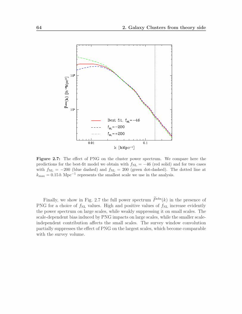
64 2. Galaxy Clusters from theory side
Figure 2.7: The effect of PNG on the cluster power spectrum. We compare here thepredictions for the best-fit model we obtain with fNL = −46 (red solid) and for two caseswith fNL = −200 (blue dashed) and fNL = 200 (green dot-dashed). The dotted line atkmax = 0.15h Mpc−1 represents the smallest scale we use in the analysis.
Finally, we show in Fig. 2.7 the full power spectrum P obs(k) in the presence ofPNG for a choice of fNL values. High and positive values of fNL increase evidentlythe power spectrum on large scales, while weakly suppressing it on small scales. Thescale-dependent bias induced by PNG impacts on large scales, while the smaller scale-independent contribution affects the small scales. The survey window convolutionpartially suppresses the effect of PNG on the largest scales, which become comparablewith the survey volume.

Chapter 3
Observations, data and errors
This Chapter is dedicated to the description of the data sets and error estimates weuse in our combined cosmological analysis. First, we describe briefly galaxy clusterobservations through the whole electromagnetic spectrum. We list the most impor-tant X-ray, millimetre (SZ), weak lensing and optical surveys of past, present andfuture times, as well as the cosmological constraints obtained from previous workswith cluster catalogue. A particular focus is given to the Sloan Digital Sky Sur-vey maxBCG optical catalogue, which is used in this work, and to the data sets wederived from it. We first describe the cluster counts and their covariance matrix. Sec-ondly, we concentrate on the weak lensing mass estimates, the richness-mass scalingrelation and the cluster total masses. Finally, the description of the redshift spacecluster power spectrum is provided, together with its covariance error matrix. Weend with some considerations on the cross-covariance matrix between counts andpower spectrum.
3.1 Multi-wavelength surveys of galaxy clusters
Clusters have been detected across multiple wavelengths with varying degrees of suc-cess. To date, a few hundreds have been observed in the millimetre, few thousandsin the X-ray, many tens of thousands in the optical. The efficiency of a survey is dueto the combination of the technical properties of the detection instrument (e.g. fluxsensitivity and angular resolution) and the physical features of the observed objects(e.g. intrinsic luminosity and redshift). Surveys are thus characterised by complete-ness (namely amount of objects that should have been detected), and purity (i.e.contamination due to spurious detected objects). This section includes a description

66 3. Observations, data and errors
of the the various detection methods as well as the main galaxy cluster surveys andthe derived catalogues.
3.1.1 X-ray surveys
The peculiar X-ray extended emission from the hot intra-cluster medium in galaxyclusters is relatively simple to identify. However, X-ray surveys are limited in surfacebrightness: too diffuse or too faint sources are missed. The deep knowledge of theX-ray emission from galaxy clusters enables to predict exactly the completeness andthe purity of the survey, by means of extensive numerical simulations. The first X-ray cluster catalogues (Edge et al. 1990; Gioia et al. 1990) were derived from ArielV1 and HEAO-12 all-sky surveys and made use of the Einstein Observatory andEXOSAT3 (Lahav et al. 1989). Later, the ROSAT satellite All-Sky Survey (RASS4,Voges et al. 1999) provided data used to create few catalogues: e.g. the ROSAT-ESOFlux Limited X-ray (REFLEX) galaxy clusters survey (Bohringer et al. 2004); theHIFLUGCS (Reiprich & Bohringer 2002) and the Massive Cluster Survey (MACS,Ebeling et al. 2010). Another catalogue of serendipitously observed clusters at highz is the ROSAT Deep Cluster Survey (RDCS, Rosati et al. 1998). Later NASA’sChandra X-ray Observatory5 and ESA X-ray Multi-Mirror Mission Newton (XMM-Newton6) represented a breakthrough in X-ray observations, thanks to the improvedangular resolution (θ ∼ 0.5′′), and the high sensitivity due to the large collectingarea, respectively.
3.1.2 SZ surveys
Galaxy clusters can distort the spectrum of the CMB by the SZ effect, which is ob-served at millimetre wavelengths. SZ surveys are able to detect high-redshift, massiveclusters, due to the redshift-independent SZ signature on the CMB: they can poten-tially observe the most distant clusters in the Universe, being only limited in the in-trinsic SZ signal (related to the mass) and not in flux. However, the current mm tele-scopes have a poor spatial resolution (θ ∼ 60′′), being unable to resolve substructuresor possible contaminating sources. The current operating SZ surveys are the Atacama
1http://heasarc.gsfc.nasa.gov/docs/ariel5/ariel5.html2http://heasarc.gsfc.nasa.gov/docs/heao1/heao1.html3https://heasarc.gsfc.nasa.gov/docs/exosat/exosat.html4http://www.xray.mpe.mpg.de/cgi-bin/rosat/rosat-survey5http://chandra.harvard.edu/6http://xmm.esac.esa.int/

3.1 Multi-wavelength surveys of galaxy clusters 67
Cosmology Telescope (ACT7, Kosowsky 2006; Marriage et al. 2011; Menanteau et al.2013), the South Pole Telescope (SPT8, Vanderlinde et al. 2010; Carlstrom et al.2011; Reichardt et al. 2013) and Planck9 satellite (Planck Collaboration et al. 2011).
3.1.3 WL surveys
Clusters have also been detected as peaks in the shear field of deep weak gravita-tional lensing surveys (Wittman et al. 2001, 2003; Dahle et al. 2003). This methoddirectly detects the projected surface mass density of the clusters, but introducingrelevant noise in the mass estimation for individual systems (White & Kochanek2002; de Putter & White 2005). In order to detect a cluster via its gravitationallensing signal, numerous images of many background faint galaxies need to be taken,thus this is a quite expensive technique. Despite the fact that WL is probably notan optimal method for cluster detection, it is a valid tool in cluster mass calibration(Sheldon et al. 2001; Johnston et al. 2007a) for clusters detected with other methods:more details will come in Section 3.4.1.
3.1.4 Optical surveys
Optical selection is based on overdensity of galaxies on the sky. This method wasused first in 1784 by Charles Messier in the discovery of the Virgo Cluster. Ityielded to the first statistically complete sample of galaxy clusters built by GeorgeAbell (Abell 1958) using the Palomar Observatory Sky Survey, then extended toinclude more than 4000 objects (ACO, Abell et al. 1989), and to the catalogue byZwicky et al. (1968). These catalogues are biased towards identification of massiveobjects, with centrally peaked galaxy distribution, and nearby systems. Anotheridentification technique is based on the overdensity of red galaxies which typicallypopulate the well-evolved galaxy clusters and results into a tight red-sequence in acolour-magnitude diagram. This method has been used by the Red-Sequence Clus-ter Survey (RCS, Gladders & Yee 2005) using the Canada-France-Hawai’i Telescopeand Cerro Tololo Inter-American Observatory, leading to the first cosmological con-straints in optical surveys (Gladders et al. 2007). The large amount of data fromthe Sloan Digital Sky Survey (SDSS10) with its multi-band imaging and hundredsof thousands spectroscopic targets (Ahn et al. 2012) has been used to select several
7http://www.princeton.edu/act/8http://pole.uchicago.edu/9http://www.esa.int/Our Activities/Space Science/Planck
10http://www.sdss.org/

68 3. Observations, data and errors
samples, such as the maxBCG cluster catalogue (Koester et al. 2007b) discussed inSection 3.2.1. This has later been extended to the GMBCG catalogue by Hao et al.(2010). Other larger SDSS cluster samples include the work of Wen et al. (2009)and Szabo et al. (2011). Although the large number of detected clusters, the mainissue with optical clusters is the difficult choice of a low-scatter mass proxy, as theseare affected by selection effects. Another problem is that, while in the local Uni-verse most galaxies members of a clusters are known to be red, this may not bevalid anymore at high redshift, where galaxies seem to have star formation processes(Fassbender et al. 2011), causing then the lack of red-sequence feature.
3.1.5 Future surveys
The optical and near-infrared current and upcoming generation of galaxy clustersurveys will include the Panoramic Survey Telescope and Rapid Response System(PanSTARRS11), the Dark Energy Survey (DES12), the KIlo-Degree Survey (KIDS13)and VISTA Kilo-degree INfrared Galaxy Survey (VIKING14), the Large SynopticSurvey Telescope (LSST15), and the Euclid mission16. X-ray observations will be im-proved by the eROSITA all-sky survey, while for the SZ signal the future data releasesof Planck, ACT, SPT, and the Cerro Chajanantor Atacama Telescope (CCAT17) willplay a key role. Great improvements in the mm-band observations are expected tocome from the Atacama Large Millimetre Array (ALMA18 Testi et al. 2010), reachingθ ∼ 0.01′′.
3.1.6 Cosmological constraints from cluster catalogues
The cluster number counts from some of the catalogues listed above have been usedto constrain cosmology via the mass function. Efforts on this front have been led byRozo et al. (2010); Zu et al. (2012) who derived cosmological constraints from themaxBCG cluster sample. The tightest scaling relation between observable and clus-ter mass comes from fgas measurements of X-ray data (< 10% scatter, Allen et al.
11http://pan-starrs.ifa.hawaii.edu/public/12http://www.darkenergysurvey.org/13http://kids.strw.leidenuniv.nl/14http://www.eso.org/public/teles-instr/surveytelescopes/vista/surveys.html15http://www.lsst.org/lsst/16http://sci.esa.int/euclid17http://www.ccatobservatory.org/18http://www.almaobservatory.org/
3.1 Multi-wavelength surveys of galaxy clusters 69
2008). Constraints on dark energy with ∼ 20% uncertainty were obtained from X-ray cluster samples studied by Mantz et al. (2008, 2010) and Vikhlinin et al. (2009).Preliminary results for SZ surveys show agreement with the concordance WMAPCMB results (Komatsu et al. 2011).
Data on the cluster masses obtained from weak-lensing analyses of backgroundgalaxies have been combined with the number counts to improve the constrainingpower (Johnston et al. 2007b; Sheldon et al. 2009; Mahdavi et al. 2007).
The statistics of rare events in the high-peak, high-mass limit has been used toconstrain cosmology by Hotchkiss (2011); Hoyle et al. (2012).
The uncertainty in the scaling relation is one of the biggest obstacles in usinggalaxy clusters as cosmological probes (e.g. Haiman et al. 2001; Battye & Weller2003). Majumdar & Mohr (2003) suggested to use the clustering of clusters as acomplementary probe. So far, only limited efforts have been dedicated to the mea-surement of the clustering properties of galaxy clusters: Hutsi (2010) measured thepower spectrum of maxBCG clusters resulting in weak detection of baryon acous-tic oscillations, Estrada et al. (2009) measured the correlation function for the samecatalogue, and Hong et al. (2012) measured the correlation function of the clustercatalogue by Wen et al. (2009). Collins et al. (2000) measured the spatial correlationfunction of the REFLEX X-ray cluster catalogue, while Balaguera-Antolınez et al.(2011) measured its power spectrum. From the same survey, Schuecker et al. (2003)derived cosmological constraints from cluster abundances and large-scale clustering.
Finally, the constraining power of these data on measurements of the amount ofprimordial non-Gaussianity in the initial density perturbations field, which can po-tentially rule out entire classes of inflationary models (Bartolo et al. 2004), has beeninvestigated by several authors. Bounds from the LSS using multiple galaxy cata-logues have been studied by Afshordi & Tolley (2008); Slosar et al. (2008); Xia et al.(2010a,b, 2011); Sefusatti et al. (2012); Giannantonio et al. (2013); Ross et al. (2013).In particular Slosar et al. (2008) found −29 < fNL < 70 at 95% c.l., while Xia et al.(2011) reported hints of detection at 8 < fNL < 88 (95% c.l.) for the local model.Other constraints come from the CMB bispectrum analyses: from WMAP datait was obtained −3 < fNL < 77 at 95% c.l. (Hinshaw et al. 2013; Bennett et al.2013), Shandera et al. (2013) found fNL = −3+78
−91 at 68% c.l. from X-ray clusterdata combined with the WMAP7 data, while latest constraints on fNL local pa-rameter from Planck are 2.7 < fNL < 5.8 at 68% c.l. (Planck Collaboration et al.

70 3. Observations, data and errors
2013c). Future galaxy surveys such as Euclid are expected to reach an accuracyof ∆fNL ∼ 3 (Giannantonio et al. 2012). Oguri (2009) suggested that measur-ing the variance of cluster counts can yield significant constraints on PNG, whileSartoris et al. (2010) showed in principle how such constraints can be improved byusing the cluster power spectrum. Forecasts for cosmology and PNG have been alsoinvestigated by Pillepich et al. (2012), with the future eROSITA X-ray cluster survey.
3.2 The Sloan Digital Sky Survey
The SDSS is an imaging (5 bands (u, g, r, i, z), spanning from ultraviolet to in-frared) and spectroscopic survey in the North Galactic Cap and a small region inthe South, encompassing 10,000 deg2. It contains more than 930,000 galaxies and120,000 quasars. SDSS-I operated between 2000 and 2005, while SDSS-II between2005 and 2008. The final public data release from SDSS-II in 2008 was the DataRelease 7 (DR7, Abazajian et al. 2009). Meanwhile, SDSS-III will operate till 2014and already produced Data Release 8 (DR8, Aihara et al. 2011) in 2011 and DataRelease 9 (DR9, Ahn et al. 2012), which contains the first results of the Baryon Os-cillation Spectroscopic Survey (BOSS19). The survey employs a 2.5-meter telescopeat Apache Point Observatory in New Mexico, equipped with a 120-mega-pixel cam-era and a pair of spectrographs. In 2009 the Nobel Prize in Physics was awardedfor the optical fibres and the digital imaging detectors (CCDs) technologies used inSDSS. The great quality and quantity of these data were crucial to the developmentof significant research in astrophysics and cosmology, including structure and stellarpopulations of the Milky Way, properties of galaxies, LSS, DM and DE.
3.2.1 MaxBCG catalogue
The maxBCG catalogue 20 (Koester et al. 2007a) is a sample of 13,823 galaxy clus-ters compiled from SDSS DR5 photometric data. The clusters are chosen in anapproximately volume-limited way from a 500 Mpc3 region, covering ∼7,500 deg2 ofsky with a photometric redshift (photo-z) range of 0.1 ≤ z ≤ 0.3. The photo-z errorsare small and of the order of ∆z = 0.01. Each of these clusters contains 10 to 190E/S0 ridgeline galaxies, which are brighter than 0.4 L∗, within the scale radius R200.Two catalogues derived from SDSS data are used to construct the maxBCG sample:
19http://www.sdss3.org/surveys/boss.php20http://umsdss.physics.lsa.umich.edu/catalogs/maxbcg public catalog.dat
3.2 The Sloan Digital Sky Survey 71
a photometric catalogue, used for the cluster detection, and a spectroscopic one,useful to test the validity of the photo-z estimates. The maxBCG sample is assem-bled by selecting the brightest cluster galaxies and applying a red-sequence method
to identify cluster members in its neighbourhood. This relies on two key features ofgalaxy clusters: there is an almost ubiquitous population of galaxies which occupiesa tight-scattered region in a colour-magnitude diagram (the E/S0 ridgeline), andthe brightest cluster galaxies (BCG), typically located in the centre of the clusters,have similar colours and luminosities. The maxBCG algorithm considers two spatialdimensions (RA,DEC), two colour dimensions (g-r, r-i), one brightness dimension (i)and the redshift, and calculates the membership likelihood of each galaxy.
The pipeline calculates two likelihoods for each galaxy: the likelihood to be partof the E/S0 ridgeline and the likelihood to check the similarity to a BCG at redshiftz. These likelihoods are computed over a grid of redshifts in the range 0.1 ≤ z ≤ 0.3.The redshift corresponding to the maximum likelihood gives a first estimate of theredshift of the object. Subsequently, the algorithm assigns the status of BCG to thegalaxy which maximises the product of these likelihoods. Then, it calculates thenumber of galaxies Ng within 1h−1Mpc from the BCG, with luminosity greater than0.4 L∗ (where L∗ is the SDSS typical galaxy luminosity) and smaller than the BCGluminosity. This quantity is converted by Hansen et al. (2005) empirical relation toR200, which is the radius at which the overdensity of galaxies with an absolute rband magnitude of −24 ≤Mr ≤ −16 is 200 times that of the average galaxy density.The galaxies within R200, with similar colours (±2σ) and magnitude of the BCGand within a ∆z = 0.02 are then promoted as members of a cluster. This selectionprocess starts from the richest cluster, and removes the BCG and cluster membersfrom the galaxy catalogue before identifying the next highest likelihood, and thusthe next BCG and associated cluster. In this way, previously flagged BCG and cor-responding cluster members can be absorbed by richer clusters. The procedure isiterated until all galaxies are either BCGs or cluster members. Finally a cut on thenumber of cluster members is imposed, i.e. Ng > 10.
An analysis of N-body mock galaxy catalogues shows that the maxBCG algorithmresults in more than 90% purity and more than 85% completeness, for clusters withmasses M ≥ 1014M⊙ (Wechsler et al. 2006; Koester et al. 2007a). These simulationsensure that each cluster has a BCG by locating the brightest galaxy within thehalo at the bottom of the dark matter potential well. Then, two quantities arecomputed for each mock cluster detected by the maxBCG algorithm: the fraction fcof cluster galaxies within the richest DM halo, and the fraction fh of galaxy halos

72 3. Observations, data and errors
within the cluster halo. The first quantity represents the purity of the cluster findingalgorithm: for each cluster, the halo with the maximum fraction of cluster membersis identified. The second measurement, instead, estimates the completeness: for eachhalo, the cluster with the largest fraction of members is selected. A low value of fcdenotes a false positive detection of cluster, due to the fact that galaxies cannot beclearly associated to a single DM halo. If fh falls below a threshold, the cluster isnot detectable, because the number of identified galaxy halos within the cluster istoo low. They obtained that for fc = 0.3 the purity is > 90% for cluster Ng > 10and 95− 100% pure for clusters with Ng > 20. On the other hand, for fh = 0.3, thecompleteness of the sample is > 90% above a mass of ∼ 2× 10¹⁴M⊙ and 95− 100%complete above a mass of ∼ 3× 10¹⁴M⊙ .
3.3 MaxBCG cluster number counts
This Section introduces the first data set we need for the combined cosmologicalanalysis presented here, namely the maxBCG cluster abundances. We also describein detail the counts covariance error matrix which is composed of Poisson errors,sample variance and observational uncertainties.
3.3.1 Cluster abundances
As already introduced in Section 2.3, the richness Ngal of a galaxy cluster is definedas the number of red galaxies within the radius R200 from the cluster centre. Thecluster abundances we use in our analysis (see Table3.1) are divided into nine richnessbins in the range
11 ≤ Ngal ≤ 120 ,
which approximately corresponds to (Rozo et al. 2010)
7× 10¹³h−1M⊙ ≤M ≤ 1.2× 10¹⁵h−1M⊙ .
The relatively low mass limit of this sample evolves weakly with redshift, resulting ina sample that is significantly large. The sample also includes five additional clusterswith richness Ngal > 120, that we decide not to consider because of their negligibleimpact on the cosmological analysis. We extend the counts data used by Rozo et al.(2010) by including an additional bin at 9 ≤ Ngal ≤ 11 (Eduardo Rozo, privatecommunication). However, we checked the results are not affected by this choice.
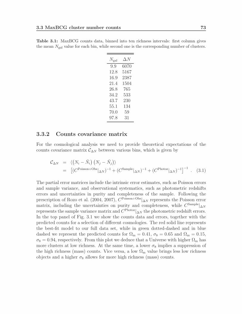
3.3 MaxBCG cluster number counts 73
Table 3.1: MaxBCG counts data, binned into ten richness intervals: first column givesthe mean Ngal value for each bin, while second one is the corresponding number of clusters.
Ngal ∆N
9.9 607012.8 516716.9 238721.4 150426.8 76534.2 53343.7 23055.1 13470.0 5997.8 31
3.3.2 Counts covariance matrix
For the cosmological analysis we need to provide theoretical expectations of thecounts covariance matrix C∆N between various bins, which is given by
C∆N = 〈(Ni − Ni
) (Nj − Nj
)〉
=[(CPoisson+Obs|∆N)−1 + (CSample|∆N)−1 + (CPhotoz|∆N)−1
]−1. (3.1)
The partial error matrices include the intrinsic error estimates, such as Poisson errorsand sample variance, and observational systematics, such as photometric redshiftserrors and uncertainties in purity and completeness of the sample. Following theprescription of Rozo et al. (2004, 2007), CPoisson+Obs|∆N represents the Poisson errormatrix, including the uncertainties on purity and completeness, while CSample|∆Nrepresents the sample variance matrix and CPhotoz|∆N the photometric redshift errors.In the top panel of Fig. 3.1 we show the counts data and errors, together with thepredicted counts for a selection of different cosmologies. The red solid line representsthe best-fit model to our full data set, while in green dotted-dashed and in bluedashed we represent the predicted counts for Ωm = 0.41, σ8 = 0.65 and Ωm = 0.15,σ8 = 0.94, respectively. From this plot we deduce that a Universe with higher Ωm hasmore clusters at low richness. At the same time, a lower σ8 implies a suppression ofthe high richness (mass) counts. Vice versa, a low Ωm value brings less low richnessobjects and a higher σ8 allows for more high richness (mass) counts.
74 3. Observations, data and errors
Poisson errors
When counting a discrete number of events in cells, the first associated uncertaintyis the Poisson error. Therefore, if we count clusters in bins, the probability ofobserving ∆N clusters in a bin of given redshift and richness, is determined by thefollowing Poissonian distribution:
P (∆N |N) =N∆N
∆N !e−N , (3.2)
where N = 〈∆N〉 = Var[∆N ] is positive. This distribution is uni-modal, centredroughly on the mean and exhibits positive skew which decreases as the mean in-creases. Let us assume now that the mean N fluctuates in different bins as
Ni =
∫d3xWi(~x)n(~x, zi) , (3.3)
where n(~x, zi) is the spatial number density and Wi(~x) is the usual top-hat windowfunction. The sample averaged number counts is
Ni = ni Vi , (3.4)
where Vi =∫d3xWi(~x) and ni is the averaged cluster density given by Eq. (2.28).
Thus, the Poisson error contribution to the covariance matrix is
CPoissonij |∆N = 〈
(Ni − Ni
) (Nj − Nj
)〉 Poisson = δij Ni , (3.5)
where Var[Ni] = Ni.
Purity and completeness
For a correct analysis, we need to take into account for purity and completenessissues. For the cosmological analysis presented here, we assume 100% purity andcompleteness, adding a 5% uncertainty in quadrature (Rozo et al. 2010). This meansadding a parameter λ = λ±σλ = 1.00±0.05 which transforms Ni to λNi. Accordingto error propagation formulae, the variance of λNi is given by:
Var[λNi] =
(∂λNi
∂λ
)2
σ2λ +
(∂λNi
∂Ni
)2
σ2Ni
= N2i σ
2λ + λ2Ni . (3.6)
Thus the Poisson error matrix diagonal elements change as:
CPoisson+Obsij |∆N = 〈
(Ni − Ni
) (Nj − Nj
)〉 Poisson+Obs = δij
(N2i σ
2λ + Ni
). (3.7)

3.3 MaxBCG cluster number counts 75
Sample variance
Another important source of uncertainty is the cell-to-cell variance due to large-scalestructure (Hu & Kravtsov 2003; Lima & Hu 2004), usually called sample variance(or cosmic variance). In fact, observational estimates of number densities of a clus-tered population in finite volumes are subject to uncertainties which exceed thePoisson noise, arising from the underlying large-scale density fluctuations. If thetypical clustering scale of the observed objects is much smaller than the sample vol-ume, then cosmic variance is negligible. On the contrary, if the observed volumes aresmaller than the clustering scale, one might count more or less objects with respectto the average number: in this case, cosmic variance becomes dominant and shouldbe taken into account. For example, cosmic variance is relevant for deep galaxiessurveys, because galaxies at high redshifts are more strongly clustered than darkmatter compared to the local Universe (Kauffmann et al. 1999b). To check if a sur-vey is independent of cosmic variance and accurately samples the Universe, one cancompare the variation between the number counts for samples of different angularsizes which mimic different survey fields. In the case of strong cosmic variance, thenumber counts depend on where the samples are located in the sky and differ signif-icantly for each region. If instead the counts agree while approaching the total sizeof the survey, the cosmic variance can be neglected. For clusters, we can recast thecounts of Eq. (3.3) as
Ni =
∫d3 xWi(~x) (ni + δni) =
∫d3 xWi(~x) [ni (1 + bi δi)] , (3.8)
where δi ≡ δ(~x, zi) is the underlying linear density field and bi is the average biasgiven by Eq. (2.40). Note that the index i identifies unique cells in redshift, angleand observable mass. The covariance matrix between cluster counts found in eachbin due to sample variance is given by
CSampleij |∆N = 〈
(Ni − Ni
) (Nj − Nj
)〉 Sample =
= bi bj ni nj
∫d3x
∫d3xWi(~x)Wj(~x)〈δi δj〉 =
= bi bj ni nj
∫d3k
(2π)3Wi(~k)Wj(~k)P (k) , (3.9)
where P (k) is the linear power spectrum and Wj(~k) is the Fourier transform ofWj(~k).In our cosmological analysis, however, the survey volume is big enough (∼7,500 deg2)to have a negligible sample variance contribution.

76 3. Observations, data and errors
Photometric redshift errors
The observational uncertainties associated to the photometric redshifts estimates aredescribed by the probability distribution p(zc|zh)dzc, where zc is the photo-z estimateand zh is the true halo redshift. This probability depends on the richness measurebecause the number of galaxies contributing to the photometric estimate increaseswith Ngal. However, systematics can reduce the sensitivity to cluster richness. Wehave found that the photo-z errors have a negligible impact on the number countsanalysis presented here, so we neglect their contribution CPhotoz|∆N in the numbercounts covariance matrix.
3.4 MaxBCG cluster masses
This Section describes the estimation of the mean cluster masses and errors fromthe maxBCG catalogue by the WL technique. We also specify the nature of themass-richness relation and constraints on its scatter from previous works. Finally,we introduce the second data set we need for our analysis, namely the total clustermasses together with their covariance error matrix.
3.4.1 Mean cluster masses from weak lensing observations
Sheldon et al. (2009) first measured the weak lensing effect from maxBCG galaxyclusters. By stacking the clusters in narrow richness bins, the signal-to-noise wasimproved considerably compared to the measurement of the profile of an individ-ual cluster. In this way, they could measure the cluster average weak lensing shearprofile. These profiles were then converted to surface mass density contrast profiles(see Eq. 2.8) for different luminosity and richness bins, by means of the photomet-ric redshift distribution of the background galaxies, estimated with the methods ofLima et al. (2008) and Oyaizu et al. (2008). Johnston et al. (2007b) fit the resultingprofiles and reconstructed the mean 3D cluster density and mass profiles: this allowsone to estimate the mass and the concentration of clusters in a given redshift bin.For this reconstruction a Navarro-Frenk-White profile (Navarro et al. 1997) for thecluster density was assumed (see Eq. 2.4). They found for the whole sample, thefollowing mean mass-richness relation:
M200(Ngal) ≃ 8.8× 10¹³h−1M⊙ (Ngal/20)1.28 , (3.10)

3.4 MaxBCG cluster masses 77
whereM200 is the mass contained within the radius R200. Mandelbaum et al. (2008b)used a different method for estimating the redshift of the background sources, whichcorrected the biased mass estimates of Sheldon et al. (2009) upwards by a factor of1.18, as described also in Rozo et al. (2009). Mandelbaum et al. (2008a) performeda similar but independent weak lensing analysis of the maxBCG clusters, but us-ing a slightly different overdensity threshold for the mass definition (180 insteadof 200), which added only a 2% correction. Applying this correction, the slopesof Johnston et al. (2007b) and Mandelbaum et al. (2008a) agreed almost perfectly,but the latter found a mean mass difference of approximately 6% with respect toJohnston et al. (2007b). Rozo et al. (2010) included this discrepancy by introducingan offset factor β with a suitable chosen prior, as we will described in Chapter 4.
For the cosmological analysis presented here we follow Rozo et al. (2010) and fitfor the mass-richness relation using the Johnston et al. (2007b) data and their errors(see Table 3.2). We use five richness bins for this, in the range 12 ≤ Ngal ≤ 300, plusanother extra bin at 9 ≤ Ngal ≤ 12 (Eduardo Rozo, private communication). Thebottom panel of Fig. 3.1 shows the mean weak lensing mass estimates with errors,together with the theoretical expectations for a selection of different cosmologies.The red solid line represents the best-fit model to our full data set (counts, totalmasses and power spectrum). The green dotted-dashed (blue dashed) curve repre-sent the theoretical predictions for Ωm = 0.41, σ8 = 0.65 (Ωm = 0.15, σ8 = 0.94).From this plot we can deduce that in a Universe with low Ωm, structures form early,thus being more numerous at high z. In addition to this, they have more time toaccrete, implying the reach higher masses. On the contrary, if Ωm is high, structuresform late, resulting in less structures at high z. Furthermore, they have less time toaccrete and thus they will end up with lower mean masses.
Note that in general the estimated WL mass of a galaxy cluster depends on theunderlying cosmological model. For the analysis presented here, this dependency isthrough the angular diameter distance, which is modified by the total matter densityΩm. In order to estimate the size of this cosmology dependence, we placed a galaxycluster with mass M = 1.1 × 10¹⁵h−1M⊙ at redshift z = 0.2 and produced a mockcatalogue of sheared background galaxies. From this catalogue we estimated themass of the cluster by fitting to a NFW profile. We found that, if we allow Ωm tochange within the 1-σ level of our best fit cosmology, the mass varies within 5%.However, we allow for an uncertainty in the mass estimation with the offset factorβ with a prior width of 6%. Hence any change due to a different Ωm is completelydegenerate with the β parameter, which we assume does not depend on cosmology.
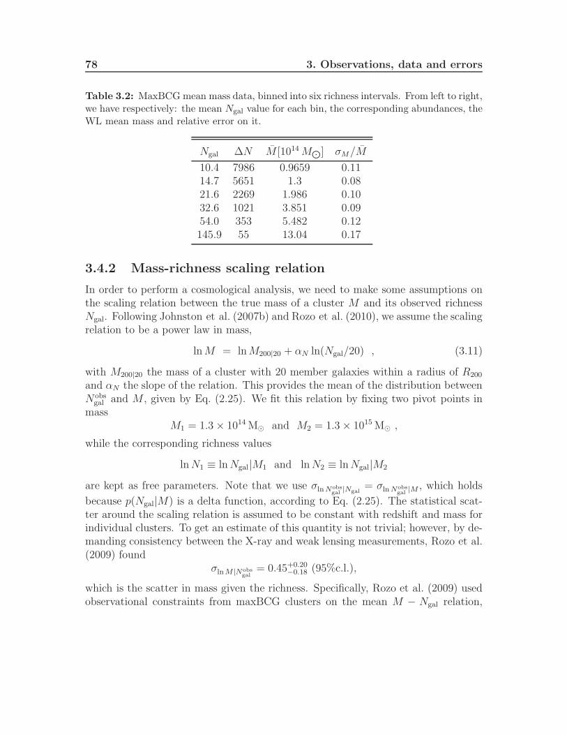
78 3. Observations, data and errors
Table 3.2: MaxBCG mean mass data, binned into six richness intervals. From left to right,we have respectively: the mean Ngal value for each bin, the corresponding abundances, theWL mean mass and relative error on it.
Ngal ∆N M [1014M⊙] σM/M
10.4 7986 0.9659 0.1114.7 5651 1.3 0.0821.6 2269 1.986 0.1032.6 1021 3.851 0.0954.0 353 5.482 0.12145.9 55 13.04 0.17
3.4.2 Mass-richness scaling relation
In order to perform a cosmological analysis, we need to make some assumptions onthe scaling relation between the true mass of a cluster M and its observed richnessNgal. Following Johnston et al. (2007b) and Rozo et al. (2010), we assume the scalingrelation to be a power law in mass,
lnM = lnM200|20 + αN ln(Ngal/20) , (3.11)
with M200|20 the mass of a cluster with 20 member galaxies within a radius of R200
and αN the slope of the relation. This provides the mean of the distribution betweenNobs
gal and M , given by Eq. (2.25). We fit this relation by fixing two pivot points inmass
M1 = 1.3× 10¹⁴M⊙ and M2 = 1.3× 10¹⁵M⊙ ,
while the corresponding richness values
lnN1 ≡ lnNgal|M1 and lnN2 ≡ lnNgal|M2
are kept as free parameters. Note that we use σlnNobsgal |Ngal
= σlnNobsgal |M
, which holds
because p(Ngal|M) is a delta function, according to Eq. (2.25). The statistical scat-ter around the scaling relation is assumed to be constant with redshift and mass forindividual clusters. To get an estimate of this quantity is not trivial; however, by de-manding consistency between the X-ray and weak lensing measurements, Rozo et al.(2009) found
σlnM |Nobsgal
= 0.45+0.20−0.18 (95%c.l.),
which is the scatter in mass given the richness. Specifically, Rozo et al. (2009) usedobservational constraints from maxBCG clusters on the mean M − Ngal relation,
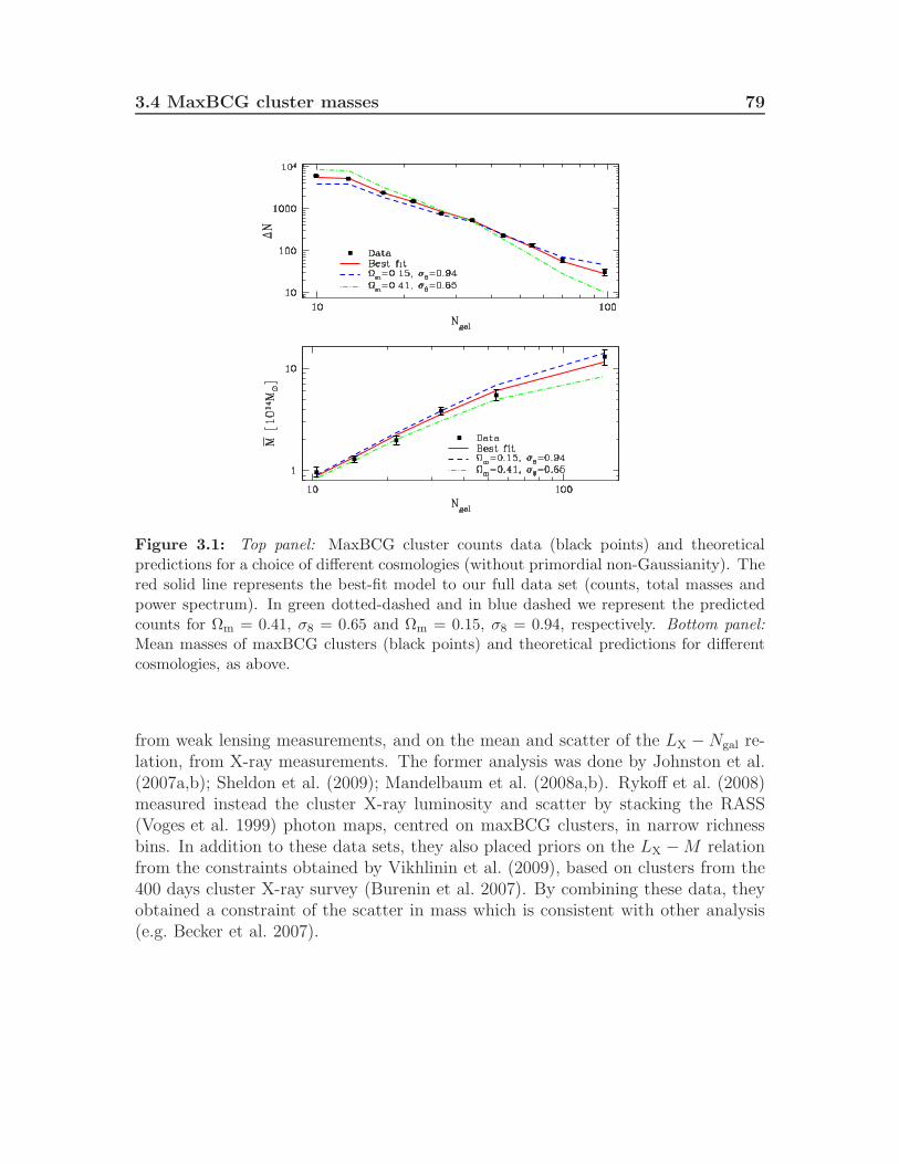
3.4 MaxBCG cluster masses 79
Figure 3.1: Top panel: MaxBCG cluster counts data (black points) and theoreticalpredictions for a choice of different cosmologies (without primordial non-Gaussianity). Thered solid line represents the best-fit model to our full data set (counts, total masses andpower spectrum). In green dotted-dashed and in blue dashed we represent the predictedcounts for Ωm = 0.41, σ8 = 0.65 and Ωm = 0.15, σ8 = 0.94, respectively. Bottom panel:
Mean masses of maxBCG clusters (black points) and theoretical predictions for differentcosmologies, as above.
from weak lensing measurements, and on the mean and scatter of the LX −Ngal re-lation, from X-ray measurements. The former analysis was done by Johnston et al.(2007a,b); Sheldon et al. (2009); Mandelbaum et al. (2008a,b). Rykoff et al. (2008)measured instead the cluster X-ray luminosity and scatter by stacking the RASS(Voges et al. 1999) photon maps, centred on maxBCG clusters, in narrow richnessbins. In addition to these data sets, they also placed priors on the LX −M relationfrom the constraints obtained by Vikhlinin et al. (2009), based on clusters from the400 days cluster X-ray survey (Burenin et al. 2007). By combining these data, theyobtained a constraint of the scatter in mass which is consistent with other analysis(e.g. Becker et al. 2007).

80 3. Observations, data and errors
For our cosmological analysis we need to place a prior on the converse scatter,σlnNobs
gal |M. The scatter and the converse scatter can be readily related to each other
by invoking the relation of Eq. (3.11), which results in
σlnM |Nobsgal
= αN σlnNobsgal |M
.
3.4.3 Cluster total masses
In our combined analysis, we do not use the WL cluster mean masses as an additionaldata set to the cluster abundances. Instead, we use the cluster total masses ∆NM ,i.e. the product of counts and mean mass in the corresponding richness bins. Thecovariance matrix of the total masses is calculated in an analogous way as done forcounts (see Eq. 3.1):
C∆NM = 〈(NiM − NiM
) (NjM − NjM
)〉 . (3.12)
Note that when introducing the uncertainty λ = λ± σλ = 1.00± 0.05 on purity andcompleteness, as described for counts already (see also (Rozo et al. 2010)), the totalmasses change from NiM to λNiM . According to error propagation formulae, thevariance of λNiM is thus given by:
Var[λNiM ] =
(∂λNiM
∂λ
)2
σ2λ +
(∂λNiM
∂Ni
)2
σ2Ni
+
(∂λNiM
∂M
)2
σ2M =
= (NiM)2σ2λ + λ2M2Ni + N2
i σ2M . (3.13)
The Poisson error matrix diagonal elements then become:
CPoisson+Obsij |∆NM = δij
[(NiM)2σ2
λ + M2Ni + N2i σ
2M
]. (3.14)
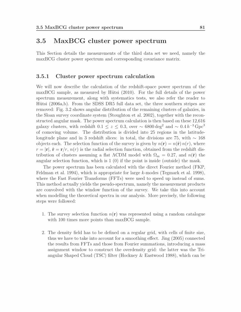
3.5 MaxBCG cluster power spectrum 81
3.5 MaxBCG cluster power spectrum
This Section details the measurements of the third data set we need, namely themaxBCG cluster power spectrum and corresponding covariance matrix.
3.5.1 Cluster power spectrum calculation
We will now describe the calculation of the redshift-space power spectrum of themaxBCG sample, as measured by Hutsi (2010). For the full details of the powerspectrum measurement, along with systematics tests, we also refer the reader toHutsi (2006a,b). From the SDSS DR5 full data set, the three southern stripes areremoved: Fig. 3.2 shows angular distribution of the remaining clusters of galaxies, inthe Sloan survey coordinate system (Stoughton et al. 2002), together with the recon-structed angular mask. The power spectrum calculation is then based on these 12,616galaxy clusters, with redshift 0.1 ≤ z ≤ 0.3, over ∼ 6800 deg2 and ∼ 0.4 h−3Gpc3
of comoving volume. The distribution is divided into 25 regions in the latitude-longitude plane and in 3 redshift slices: in total, the divisions are 75, with ∼ 168objects each. The selection function of the survey is given by n(r) = n(r)n(r), wherer = |r|, r = r/r, n(r) is the radial selection function, obtained from the redshift dis-tribution of clusters assuming a flat ΛCDM model with Ωm = 0.27, and n(r) theangular selection function, which is 1 (0) if the point is inside (outside) the mask.
The power spectrum has been calculated with the direct Fourier method (FKP,Feldman et al. 1994), which is appropriate for large k-modes (Tegmark et al. 1998),where the Fast Fourier Transforms (FFTs) were used to speed up instead of sums.This method actually yields the pseudo-spectrum, namely the measurement productsare convolved with the window function of the survey. We take this into accountwhen modelling the theoretical spectra in our analysis. More precisely, the followingsteps were followed:
1. The survey selection function n(r) was represented using a random cataloguewith 100 times more points than maxBCG sample.
2. The density field has to be defined on a regular grid, with cells of finite size,thus we have to take into account for a smoothing effect. Jing (2005) connectedthe results from FFTs and those from Fourier summations, introducing a massassignment window to construct the overdensity grid: the latter was the Tri-angular Shaped Cloud (TSC) filter (Hockney & Eastwood 1988), which can be
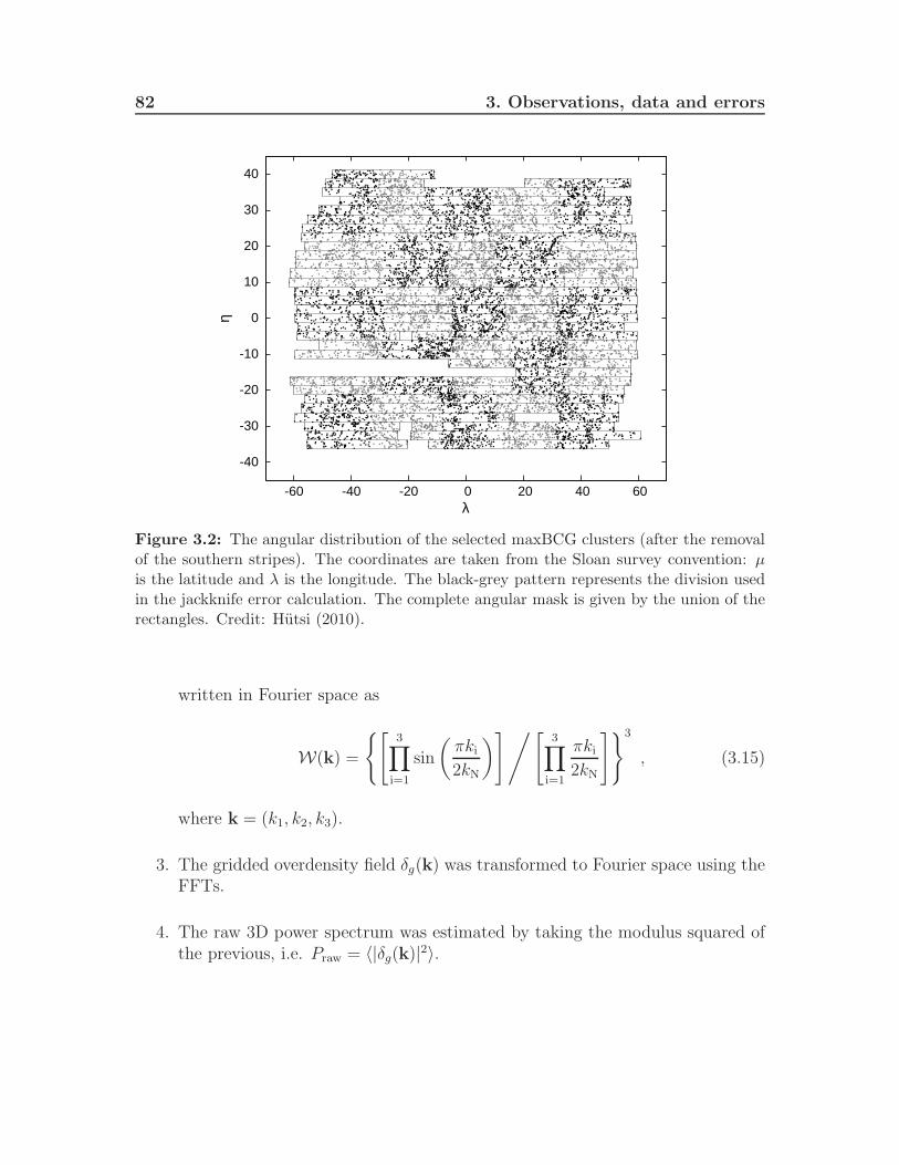
82 3. Observations, data and errors
-40
-30
-20
-10
0
10
20
30
40
-60 -40 -20 0 20 40 60
η
λ
Figure 3.2: The angular distribution of the selected maxBCG clusters (after the removalof the southern stripes). The coordinates are taken from the Sloan survey convention: µis the latitude and λ is the longitude. The black-grey pattern represents the division usedin the jackknife error calculation. The complete angular mask is given by the union of therectangles. Credit: Hutsi (2010).
written in Fourier space as
W(k) =
[3∏
i=1
sin
(πki2kN
)]/[3∏
i=1
πki2kN
]3
, (3.15)
where k = (k1, k2, k3).
3. The gridded overdensity field δg(k) was transformed to Fourier space using theFFTs.
4. The raw 3D power spectrum was estimated by taking the modulus squared ofthe previous, i.e. Praw = 〈|δg(k)|2〉.

3.5 MaxBCG cluster power spectrum 83
Figure 3.3: The redshift-space power spectrum of maxBCG cluster sample (black points)and errors. The dashed line corresponds to the linear matter power spectrum, dotted-dashed and solid magenta lines represent the final best fitting model in Hutsi (2010),without survey window convolution and with, respectively. Credit: Hutsi (2010).
5. When applying the TSC method, the shot noise term takes the form
Pshot =1
N
3∏
i=1
[1− sin2
(πki2kN
)+
2
15sin4
(πki2kN
)]. (3.16)
The latter was subtracted from the raw 3D power spectrum.
6. It was checked that the aliasing effects due to the finite grid size were negligiblefor the measurements, and were nonetheless corrected with the iterative methodby Jing (2005) to obtain finally the angle averaged pseudo-spectrum, i.e. withsmoothing effect of the TSC deconvolved.

84 3. Observations, data and errors
Figure 3.4: The different lines represents the theoretical models for best fit (red solid), forΩm = 0.15, σ8 = 0.94 (blue dashed) and for Ωm = 0.41, σ8 = 0.65 (green dotted dashed),while data are in black. The dotted line at k = 0.15 represents the data cut to linear scales.Top panel: linear matter power spectrum. Bottom panel: full non-linear observed powerspectrum.
3.5.2 Cluster power spectrum covariance matrix
The uncertainties on the power spectrum measurements have been estimated byHutsi (2010) with three different methods, shown to be comparable:
i) with the original FKP theoretical prescription, which assumes Gaussian errorsfrom cosmic variance and a shot noise, neglecting redshift space distortions;
ii) with a jackknife method (Lupton 1993), implemented by dividing the surveyinto the 75 regions with ∼168 clusters each;
iii) with a Monte Carlo method, based on the fiducial ΛCDM cosmology, in which1000 mock realisations of the maxBCG survey were generated, including redshift-space distortions and photo-z errors.
In our analysis we used only the Monte Carlo covariance matrix, so that we canwrite the covariance matrix CP for the cluster power spectrum as
CP = R · σ2P , (3.17)

3.6 The counts-clustering off-diagonal covariance 85
where R is the correlation matrix, namely the covariance with diagonal elementsequal to unity and off-diagonal ones showing the correlation between the errors, andσ2P is the variance of P (k).
The power spectrum measurements and errors are reported in Table 3.3 andshown in Fig. 3.3 (black points). The dashed line represents the linear powerspectrum. The dotted dashed curve is the theoretical model (see Eq. 2.44), in-cluding the photo-z smoothing and the non-linearities, without the survey windowconvolution. Finally, solid magenta line shows the best fitting model convolvedwith the survey window. Note that to take into account data in the quasi-linearregime only, we restrict ourselves to scales larger than (wavenumbers smaller than)kmax = 0.15 hMpc−1.
We show in Fig. 3.4 the linear matter power spectrum Plin(k) and the full halo
power spectrum P obs(k) from Eq. (2.48) respectively, as a function of k. The differentlines correspond to the theory curves for our combined best-fit cosmological model(red solid) and for two other models (Ωm = 0.15, σ8 = 0.94 for the blue dashed lineand Ωm = 0.41, σ8 = 0.65 for the green dotted dashed curve), chosen to be at the2σ limit of the marginalised Ωm − σ8 contour, compared with data and errors fromHutsi (2010) in black. We are assuming Gaussian initial condition and fixing all theother model parameters to our best-fit values.
3.6 The counts-clustering off-diagonal covariance
We estimate now the off-diagonal terms of the covariance matrix between the cluster-ing and the binned number distributions ∆N of the maxBCG clusters. For simplicity,instead of the power spectrum we use, as a clustering estimator here, the projectedtwo-point angular correlation function w(θ) of objects at a given angular distance θ(Peebles 1980). The angular separation θ is usually defined as
cos(θ) = n1 · n2 ,
where n1 and n2 are the unit vectors pointing to the objects locations. So theprojected correlation function can be written as
w(θ) ≡ 〈δh(n1) δh(n2)〉 , (3.18)
where δh(n) is the halo (cluster) projected overdensity in a direction n and the averageis carried over all pairs at an angular distance θ. We use the jackknife technique as

86 3. Observations, data and errors
follows: we split the maxBCG footprint into 100 equal-area jackknife regions usinghealpix21(Gorski et al. 2005) and populate the full footprint with 50 random pointsfor each maxBCG cluster, to reduce shot noise. A common approach for estimatingthe correlation function of objects is to count pairs and to compare the data withan approximately ten times bigger random (unclustered) sample with same redshiftdistribution and angular coverage. It is then possible to define some estimatorswhich combine data and random objects as number of data-data (DD), random-random (RR) and data-random (DR) pairs. We use the Landy-Szalay-estimator(Landy & Szalay 1993), given by:
wLS(θ) =DD − 2DR+RR
RR. (3.19)
We also bin the number of clusters within six equal-width bins in log10 space. Weiteratively remove and replace each jackknife region and calculate the number his-togram and correlation function at each iteration. In general, the covariance matrixCJK between measured statistics x = x(α) and y = y(β) can be estimated from Njackknifes using (see e.g. Efron 1982):
[CJK(xi, yj)
]α,β
=N − 1
N
N∑
k=1
(xk−i − xi)α (yk−j − yj)β , (3.20)
where x−i (y−j) is the statistic with jackknife region i (j) removed, and xi (yj) is theaverage value of all x−i (y−i). We note that typically, but not necessarily, x and yare the same statistic. We compare the square root of the diagonal elements of thew(θ) covariance matrix, i.e.
CJKw(θ) ≡ CJK
[w(θ), w(θ)
], (3.21)
with the error expected from Poisson counting statistics and find agreement withthe theoretical expectations (as described by e.g., Ross et al. 2009). Moreover, thediagonal elements of the counts covariance matrix, i.e.
CJK∆N ≡ CJK
(∆N,∆N
), (3.22)
are approximately Poissonian, independently of the number of jackknifes used, aswe would expect. Finally, the off-diagonal terms of the normalised counts-clusteringcovariance, i.e.
CJK∆N,w(θ) ≡ CJK
[∆N,w(θ)
], (3.23)
21http://healpix.jpl.nasa.gov/

3.6 The counts-clustering off-diagonal covariance 87
Figure 3.5: The off-diagonal elements of the normalised covariance matrix of the correla-tion function w(θ) and the histogram distribution of ∆N , as calculated using the jackknifetechnique.
are shown in Fig. 3.5. Note that the average value of the off-diagonal terms is−0.03 ± 0.10 (1σ), which is consistent with zero. We observe that as the numberof jackknifes increases, the mean of the average value of the off-diagonal terms ap-proaches zero.
We also compare the magnitude of the off-diagonal terms obtained from themaxBCG clusters with simulated clusters from the Millennium Simulation (see e.g.Springel et al. 2005; Lemson & Virgo Consortium 2006). Specifically, we join thelight-cone table of Henriques2012a.wmap1.BC03 AllSky 00 (Henriques et al. 2012;Guo et al. 2011) with the halo-tree table MPAHaloTrees..MHalo. We apply the sameredshift and survey footprint constraints to mimic the maxBCG sample and calculatethe correlation function and histogram distribution of ∆N . We find the data andsimulations agree closely: e.g., for 100 jackknifes the mean and 1σ error of the off-diagonal terms are 0.00 ± 0.10 from the simulations. From these tests we concludethat our choice of ignoring the off-diagonal covariance matrix between clustering andnumber counts is a reasonable approximation.
88 3. Observations, data and errors
Table 3.3: MaxBCG power spectrum data binned into k-intervals. From left to right:the mean k value for each bin, corresponding observed power spectrum value and standarddeviation on it. Note that we restrict to the quasi-linear regime only, thus we will usein our cosmological analysis only the first 18 k-bins, corresponding to data up to kmax =0.15 [hMpc−1].
k[hMpc−1] P obs[104 h−3Mpc3] σP [103]
0.0065 19.470 76.1800.0131 23.100 46.2700.0212 17.340 26.1400.0292 12.060 15.3200.0371 7.0390 9.45700.0452 5.1410 6.40900.0534 4.0760 4.46300.0616 3.3410 3.48200.0698 3.2410 2.81200.0779 2.2220 2.14700.0860 1.7980 1.80400.0942 1.7570 1.56100.1024 1.2610 1.31700.1105 1.1110 1.12600.1188 1.0820 1.01800.1270 0.9194 0.90480.1351 0.7111 0.81530.1433 0.6027 0.79000.1514 0.5924 0.67500.1596 0.4517 0.65170.1678 0.4524 0.61990.1760 0.4414 0.57350.1841 0.4318 0.53920.1923 0.4423 0.54940.2005 0.3285 0.50950.2087 0.2738 0.46830.2169 0.2354 0.47510.2251 0.2384 0.45520.2332 0.3122 0.42220.2414 0.2882 0.40190.2496 0.2127 0.41080.2578 0.1852 0.4121
Chapter 4
Cosmological analysis
This Chapter is entirely dedicated to the statistical analysis of data for cosmologicalparameters estimation. The standard approach for extracting cosmological parame-ters from observational data sets makes use of maximum likelihood methods, basedon the Bayes Theorem. If the dimensionality of the parameter space is very large,there are ways to study the likelihood surface efficiently, sampling the space moredensely where the likelihood is high: these are the Monte Carlo Markov Chain meth-ods (MCMC), a combination of Monte Carlo methods and the advantages of theMarkov chains. Our primary MCMC tool for cosmological analysis is the cosmomcsoftware, for which we provide here a description. In particular we focus on the resultsof Rozo et al. (2010) and Zu et al. (2012), who derived cosmological constraints fromthe maxBCG cluster sample, using cluster counts and weak lensing mass estimates.The goal of this project is to extend their analysis to fully include the clusteringinformation: we show that the inclusion of the cluster power spectrum significantlyimproves the cosmological constraints, and also reduces the degeneracies between thescaling relation nuisance parameters. We present the improved cosmological resultsobtained in this way from the maxBCG cluster counts, weak lensing masses andpower spectrum. As an interesting application, we present the constraining powerof these data on the amount of primordial non Gaussianity of the initial densityperturbations.
4.1 Parameter estimation
One of the main purposes in cosmology is to estimate the parameters describing amodel of the Universe and their confidence limits, on the basis of a set of observationaldata. This is a non-trivial task when more than few parameters are involved. In this

90 4. Cosmological analysis
Section, we first introduce the importance of Bayesian statistics, which is based onthe interpretation of probability as a conditional measure of uncertainty. We thenconsider the posterior calculation in case of Gaussian (χ2 statistics) and Poissonian(C-statistics) distributions. Finally we introduce some useful concepts in parametersestimation, such as confidence regions and marginalisation.
4.1.1 Bayes theorem
Suppose that D is some set of data, Θ = (θ1, ...θm) is the m-dimensional unknownparameter vector of a certain model, then the Bayes theorem states that
P (Θ|D) =P (D|Θ)P (Θ)
P (D)=
P (D|Θ)P (Θ)∫P (D|Θ)P (Θ) dΘ
, (4.1)
where P (Θ|D) is the multivariate posterior distribution, namely the inferred jointprobability distribution of the parameters, after considering the data. This is achievedby calculating the likelihood P (D|Θ) ≡ L(D|Θ), which is the conditional proba-bility of obtaining the observed data given a set of input parameter values, and bysetting a prior probability on the parameters themselves, P (Θ). The likelihood tellsus about the mismatch between data and theoretical predictions. The prior, instead,represents literally the a priori knowledge on the distribution of the expectationvalues of the parameters, before considering any measurement. The normalizationconstant P (D) plays a key role in the model selection and it is called evidence ormarginal likelihood: from Eq. (4.1) it can be seen that is equal to the integral over Θof the likelihood times the prior. Throughout our analysis, however, P (D) = 1. Thegeneral problem of posterior estimation is then to calculate an integral: compressingthe posterior distribution to a set of samples can save a vast amount of computationaltime, if compared to the integration over the m-dimensional parameter space. Thiscan be done efficiently by a Monte Carlo integration method. This sampling methodis very convenient when calculating quantities, like moments, which typically are theexpectation values of a function of the model parameters.
4.1.2 Gaussian χ2 statistics
When comparing a theoretical model to real data, one has to determine the best fitmodel to the data and the corresponding errors. The χ2 statistics is a measure ofhow good the fit of the model to the data is. The best fit condition is fulfilled by themodel which minimises the χ2. This is also equivalent to maximise the likelihood

4.1 Parameter estimation 91
that the observations were produced by the theory we fit, when the samples aredescribed by a Gaussian distribution. We assume then the following: Θ representsthe parameters of the model we need to estimate, xi and µi ≡ µi(Θ) are respectivelythe n observed data and corresponding theoretical predictions in some bin i, σi theerrors associated to the data. We also assume that the probability of observing agiven value xi is its Gaussian probability
Pi ∝ exp(xi − µi)
2
2σ2i
. (4.2)
If data are uncorrelated, then the probability of observing a set of samples is theproduct of the single probabilities over all the bins. The logarithm of the latter isthe χ2:
χ2 ≡ lnn∏
i=1
Pi =n∑
i=1
[xi − µi]2
σ2i
. (4.3)
Finally, the posterior probability, proportional to the likelihood assuming a flat prior,is then given by
P (Θ|D) ∝ L(Θ|D) ∝ exp
[−1
2χ2
], (4.4)
from which is clear that a maximum likelihood corresponds to the minimum valueof χ2. In the case of correlated data, the modified χ2 equation is
χ2 =
n∑
i=1
n∑
j=1
[xi − µi]T C−1ij [xj − µj] , (4.5)
whereCij = 〈(xi − µi) (xj − µj)〉 (4.6)
is the covariance error matrix, describing the covariance between the data. Thelatter can be also decomposed into the product of the correlation matrix Rij =Cij/
√CiiCjj, i.e. a normalised version of the covariance matrix, and the diagonal
elements Cii = Var(xi) = σ2i .
We can also define the degrees of freedom as ν = n−m, where n the numberof independent data points and m is the number of parameters. In addition to this,one can use the so-called reduced chi-square, which is given by χ2
red = χ2/ν. A usefulpractical rule is that a good fit is achieved for a reduced chi-square equal to unity,i.e. χ2 ∼ ν.
92 4. Cosmological analysis
The binned data sets we use in our analysis (see Table 3.1) show that each bincontains a sufficient number of observations to be approximated by the Gaussianlimit of the Poisson distribution. In the case of the cluster power spectrum, theGaussian approximation is standard. Thus we restrict to the Gaussian picture here-after. In addition to this, our data are correlated and we use the covariance matricesalready defined.
4.1.3 C-statistics
The probability distribution for bins with a small number of observations is Poisso-nian and the χ2 statistics is not appropriate anymore. In fact, if the counts in a binare less then ∼10, the Poisson distribution differs significantly from the Gaussianone. In this case one can use the C-statistics (Cash 1979):
Pi =µxii e
−µi
xi!, P =
n∏
i=1
Pi , (4.7)
where xi is the observation and µi the theoretical expectation in the bin i. Thequantity which needs to be minimised to obtain the best fit model is then:
χ2cash = −2 lnP = −2
N∑
i=1
(xi lnµi − µi − ln xi!) ≈ −2N∑
i=1
(xi lnµi − µi) . (4.8)
4.1.4 Confidence regions and marginalisation
Once the best fit parameters are obtained, the accuracy of estimates can be visu-alised by showing the confidence limits (or region) around them. This can be done byselecting a region in the m-dimensional parameter space, around the best fit value,which encloses a given percentage of the probability distribution. One should thusintegrate the likelihood surface and compute where a certain percentage of points lie.Typically this is obtained by considering compact regions of constant χ2 boundaries.However, in case the χ2 has more than one minimum, a non-connected confidenceregion is more appropriate. For multi-variate Gaussian distributions the regions ofconstant χ2 are ellipsoidal regions. The usually defined confidence levels are the68.3%, 95.4% and 99.5%, which correspond to the conventional 1, 2 and 3σ, in thecase of Gaussian distributions.

4.2 Sampling methods 93
Knowing the joint posterior probability distribution of m parameters, i.e.
P (Θ|D) ≡ P (θ1, ..., θm|D) ≡ P (θ1 = t1, ..., θm = tm|D) , (4.9)
one could be interested into the probability distribution of a single parameter, forexample θ1, regardless of the others, θ2, ..., θm. In this case, one can derive themarginal probability by integrating over all the parameters, except the one ofinterest. Mathematically, this translates into
P (θ1|D) =
∫dθ2 ...
∫dθm P (θ1, ..., θm|D) . (4.10)
This is the simplest 1D case, where the marginalised distribution of a parameter isgiven by the maximum (or the mean) of the distribution, together with confidencelimits. In cosmological analysis, however, the marginalisation is often used to obtain2D posterior distributions for various combination of parameter pairs θ1, θ2, whichcan show possible degeneracies. This translates simply into:
P (θ1, θ2|D) =
∫dθ3 ...
∫dθm P (θ1, θ2, ..., θm|D) . (4.11)
We include few 2D marginalised posterior probabilities contour plots of our results,together with their interpretation.
4.2 Sampling methods
Bayesian methods are often used to compare physical models to data. The parame-ters in different models are most easily constrained by sampling from the posteriordistribution. The sampling methods scale at best linearly with the dimension ofthe parameter space, compared to integration which is computationally more ex-pensive. The most common method for sampling from a general distribution inhigh-dimensions is the Markov Chain Monte Carlo (MCMC), based on the MonteCarlo approximation method and on the useful properties of the Markov Chains,which we both revise in this Section. MCMC generates a set of points in the param-eter space, which have the same distribution as the target posterior distribution, bycomputing the Bayesian likelihood at random points selected using the MetropolisHastings algorithm. Then, from the correlated samples of the posterior distributionit is possible to derive other significant statistical quantities.

94 4. Cosmological analysis
4.2.1 Markov chains
Let us assume that X is a random variable and Xt is its value at time t. We defineX as a Markov process if the probability distribution at the present status, Xt,depends only on the previous status, Xt−1, and not on the entire history:
P (Xt = xt|X0 = x0, ..., Xt−1 = xt−1) = P (Xt = xt|Xt−1 = xt−1) . (4.12)
A Markov chain Xt is a sequence of random variables X0, X1 , ... , Xt generatedby a Markov process. If the probability is regular, the chain will gradually forgetabout the initial state X0 and approach an invariant distribution after a sufficientnumber of steps. In fact, the main property of Markov chain is stationarity : thereexists a probability distribution φ(x) such that if Xt ∼ φ(x), then Xt+1 ∼ φ(x). InFig. 4.1 we show an example of a sequence which approaches an asymptotic stationarydistribution. If a chain starts in a random position of the parameter space, it willtake some time (few hundreds of steps) to equilibrate. The term burn-in period refersto those iterations at the beginning of the chain, which are still far from converging tothe invariant distribution: these chain steps are usually discarded, before computingthe chain analysis. It could happen that a Markov chain looks like it has reachedits invariant distribution when it has not: this is called pseudo-convergence. Thishappens when there are regions of the parameter space which are weakly connectedby the chain, so that the chain remains there for many iteration. In the oppositecase of a good mixing, the true convergence is reached after a sufficient number ofsteps.
4.2.2 Monte Carlo methods
The Ordinary Monte Carlo (OMC) is based on the idea of using independentand identically distributed (IID) simulations X1, ..., Xn of a random process X toapproximate the expectation
µ = 〈h(X)〉 =∫h(x)π(x) dx , (4.13)
where h is a real-valued function and π(x) is the common distribution of the variables.The OMC method works by selecting n samples Xi from π(x) and then approximat-ing Eq. (4.13) by the sample average of the h(Xi) = Yi, having 〈Yi〉 = µ and varianceVar[Yi] = σ2:
µn ≃ 〈h(X)〉 = 1
n
n∑
i=1
h(Xi) =1
n
n∑
i=1
Yi . (4.14)

4.2 Sampling methods 95
Figure 4.1: Four MCMC chains (blue, red, green, cyan) from our runs, which areapproaching a stationary distribution for the Ωm parameter. The horizontal line repre-sents the best fit value, Ωm = 0.22, while the marginalised mean value and 1σ error areΩm = 0.215 ± 0.02. Left panel: first 1000 steps (burn-in). Right panel: full chains. Notethat the number of parameters being varied in total here is nine, which justifies the quitesignificant spread of the chains.
The Central Limit Theorem (CLT) states that the mean of n independent randomvariables, with the same mean and variance, is well-approximated by a normallydistributed random variable, for a large enough n and regardless of the variablesdistribution. The mean of this normal distribution is equal to the mean of randomvariables. The variance is instead equal to the variance of the random variablesdivided by the sample size. According to the CLT then, µn ∼ N (µ, σ2/n) .
4.2.3 MCMC methods
MCMC methods are used to simulate non-standard, complex multivariate distribu-tions. The most important of these methods is the Metropolis-Hastings (M-H)algorithm, created by Metropolis & Ulam (1949); Metropolis et al. (1953) and im-proved by Hastings (1970). According to the previous definitions, a MCMC is anOMC where the IID simulations are replaced by a Markov Chain process with acertain equilibrium distribution. Following the notation in the previous sections, oneneeds to create a Markov chain which has π(x) as asymptotic invariant distribution.
96 4. Cosmological analysis
Assuming that we have m burn-in steps, we are then able to estimate 〈h(X)〉 as (seeEq. 4.14)
µ∗n =
1
n−m
n∑
i=m+1
h(Xi) . (4.15)
One of the advantages of the MCMC methods is that the number of iterations re-quired for convergence roughly scales linearly with the number of parameters. How-ever as the number of parameters in the models grows, the computational cost can bequite challenging. There is furthermore a dependence on the nature of the posteriordistribution itself: longer chains need to be constructed when the posterior departsfrom a Gaussian distribution. In this Section, we revise only the parts concerning theMCMC methods which are relevant for our work. For a more detailed description,we refer to: MacKay (2003); Gamerman & Lopes (2006); Neal (1993); Gilks (1999);Hobson et al. (2010); Geyer (2011).
Metropolis-Hastings algorithm
The most interesting aspect is to understand how the Metropolis-Hastings algorithmgenerates a sequence of correlated variables from a certain distribution. This can besummarised into the following steps.
i) Set any initial random value X0.
ii) Sample a candidate point X∗ from a conditional probability density given thecurrent state Xt, denoted ψ(·|Xt). The latter can have any form, but the finalstationary distribution of the chain will be π(x).
iii) Calculate the Hastings ratio defined as
r(X∗|Xt) =π(X∗)ψ(X|X∗)
π(X)ψ(X∗|X). (4.16)
iv) Sample a Uniform variable U in (0, 1).
v) Define the acceptance probability for the state X∗ as
a(X∗|Xt) = min [1, r(X∗|Xt)] = min
[1,π(X∗)
π(X)
]. (4.17)
The last equivalence comes from the fact that this algorithm typically considersonly symmetric proposals: ψ(X∗|X) = ψ(X|X∗). Then, if U ≤ a(X∗|Xt), the

4.2 Sampling methods 97
candidate point is accepted and the next state becomes Xt+1 = X∗. Otherwise,the candidate point is rejected and the chain does not move, i.e. Xt+1 = Xt.This step is usually called Metropolis rejection.
vi) Increment t and start again from step ii).
Note that in general, the choice of the proposal density ψ(·|Xt) is relevant for thealgorithm efficiency: for a quicker convergence, it is more appropriate to choose onewith a shape which is similar to the posterior. Similarly, the choice of its covariancematrix is important. A tight distribution will cause slow mixing and high acceptancerate, while a wide distribution will result in low acceptance and no movement of thechain, hence resulting in slow mixing as well.
Convergence
The next question to address is about how long do we need to run the chain to besure that it has converged. Having sampled sufficiently enough points in the param-eter space the MCMC chain equilibrates to the target distribution and it is said tohave reached convergence. In practice, convergence may be tested through one ofthe many convergence tests.
The simplest method to solve the convergence issue is by running multiple chainsin parallel, with over-dispersed initial values and compare the estimates µ∗
n. A fun-damental problem is that there will always be regions of the target distribution thathave not been covered by the finite chain. Over-dispersion can be obtained afterrunning a single chain and use the variance from the chain itself. Let us assume weare interested in a quantity φ from the chain, e.g. some parameters or any function ofthem. Let us further assume that we run m parallel sequences of length n and labelthe quantities (φij), j = 1, ..., n and i = 1, ..., m. We hence compute two quantities:the between-sequence variance V and the within-sequence variances W , i.e.
V =n
m− 1
m∑
i=1
(φi − φ
)2, W =
1
m
m∑
i=1
s2i , (4.18)
where
φi =1
n
n∑
j=1
φij , φ =1
m
m∑
i=1
φi , s2i =1
n− 1
n∑
j=1
(φij − φi
)2. (4.19)
W is the average variance of all the chains, while V measures the variance of the
averages of the chains. Note that the between-sequence variance V contains a factor
98 4. Cosmological analysis
n because it is based on the variance of the within-sequence means, φi, each of whichis an average of n values φij . An overestimate of the variance of φ in the targetdistribution is
Var∗(φ) =n− 1
nW +
1
nV . (4.20)
Further, W is an underestimate of the target variance Var(φ), because individualchains do not have time to cover the entire target distribution. However it holdsthat:
limn→∞
Var∗(φ) = limn→∞
W = Var(φ) . (4.21)
Convergence can now be established by monitoring
√R =
√Var∗(φ)
W, (4.22)
which approaches 1 at convergence, in the so-called (R-1) test. Note that thereare many other convergence criteria (see for example Cowles & Carlin 1996), whichhowever we do not consider in our work.
4.3 The Cosmological Monte-Carlo
The MCMC method in a cosmological context has been developed by the Cosmo-logical Monte-Carlo (cosmomc1) publicly available parameter estimation tool. Thissoftware has been developed by Lewis & Bridle (2002) and it is supported by thesoftware forum2. It includes two main Fortran 90 programs: a MCMC code forexploring cosmological parameter space (cosmomc*) and a code for analysing Monte-Carlo samples and importance sampling (getdist*). cosmomc is originally basedon the M-H sampler, but there are options for other sampling and methods for explor-ing fast/slow parameter space. It contains the Boltzmann code camb 3, i.e. the Codefor Anisotropies in the Microwave Background by Lewis et al. (2000) for calculatingtheoretical matter power spectrum and CMB anisotropies, based on cmbfast 4 bySeljak & Zaldarriaga (1996). Useful overviews can be found also in Lewis & Bridle(2006); Lewis (2011). The data sets available include WMAP7, SN-Ia, BAO andHST. The last version contains also Planck data via a specific Planck likelihoodcode.
1http://cosmologist.info/cosmomc/2http://cosmocoffee.info/3http://camb.info/4http://cmbfast.org
4.3 The Cosmological Monte-Carlo 99
How does it work?
The cosmomc* algorithm produces chain files, containing all the accepted set ofparameters: the first column gives the sample weight, the second the likelihoodand from third on all the parameters (primary and derived ones). The programtakes as inputs the central values, ranges and standard deviations of the parameters,from an input file called params.ini. The default primary parameters are: Ωbh
2,Ωch
2, Ωk, log(1010As), w, τ , ns, nt, θ, mν , nν , nrun and r = At/As. The derived
ones are instead: H0, t0 and ΩΛ. Priors on the fundamental parameters have to beassigned: the final results should not depend on this choice. This helps the programto estimate a proposal distribution: if one provides an input covariance matrix withthe parameters correlation, the estimation procedure can be significantly improved.It is also possible to get an estimated covariance matrix for the best fit model, aswell as to learn the proposal distribution from the covariance with the MPI option(run on different cluster nodes). The process will stop when convergence is reachedand the diagnostics for multiple chains is done by the (R-1) test (see Eq. 4.22), usingthe second half of each chain. Note that varying some parameters can be much morecomputationally expensive (the so-called slow parameters) than varying others (theso-called fast parameters).
Chains analysis
Once the convergence is reached and the burn-in steps removed, the getdist* anal-yses the chains and generates the following outputs:
i) .likestats, which contains the best fit sample model and likelihood, as wellas the limits from the extremal values of the posterior distribution;
ii) .margestat, which gives mean, standard deviation and marginalised limits forall the parameters;
iii) .covmat, which is a covariance proposal matrix for generating other chains;
iv) Matlab or Python files for generating marginalised plots (1D, 2D, 3D).
Generally, it is useful to consider both the likelihood and marginalised distributions.The likelihood function is used to estimate the best fit model parameters as thosewhich maximise the likelihood itself, or equivalently the logarithm of the likelihood.The marginalised distribution instead gives the projected shape of probability densityin one or two dimensions only. We show in Fig. 4.2 an example of 1D and 2Dmarginalised posteriors for the parameters Ωm and σ8, obtained from one of ourruns.

100 4. Cosmological analysis
Ωm
σ 8
0.18 0.2 0.22 0.24 0.26 0.28
0.75
0.8
0.85
0.9
0.95
Figure 4.2: 1D and 2D marginalised posterior probabilities for parameters Ωm and σ8,for same run used in Fig. 4.1. The best fit values of the parameters are Ωm = 0.22and σ8 = 0.83, while the marginalised mean and 1σ error are Ωm = 0.215 ± 0.02 andσ8 = 0.84 ± 0.04. Left panel: the solid lines show the fully marginalised posterior, thedotted lines show the mean likelihood of the samples. For Gaussian distributions theyshould be the same. However, for skewed distributions, or if chains are poorly converged,they will not be. Right panel: 2D marginalised posterior probability for the pair Ωm − σ8.The external contour corresponds to the 95% confidence level, while the internal contourcorresponds to the 68% c.l.
Importance sampling
This program also does post-processing on chains, like importance sampling: thisis a quick way to re-weight the results for different priors, new data sets or smalltheoretical corrections. More precisely, according to the previous notation, the ex-pectation value of a function h under the distribution π(x) (see Eq. 4.13) can beconverted into:
〈h(X)〉π =
∫h(x) π(x) dx =
∫h(x)
π(x)
π′(x)π′(x) dx = 〈h(x) π(x)
π′(x)〉π′ , (4.23)
where π′(x) is another distribution.

4.4 Combined maxBCG analysis 101
4.4 Combined maxBCG analysis
The purpose of our analysis is to constrain cosmology and fit for the richness-massrelation and scatter around it, simultaneously. To do this, we perform a Bayesianparameter estimation by running an MCMC, using M-H sampler with a modifiedversion of cosmomc. In this Section we describe the set up of the runs, namely thecode which produces the theory, the data sets we need and the parameters we vary.We also list the different runs, which are characterised by different combinations ofdata sets and free parameters.
The code
We work on a Fortran 90 code, which implements the standard cosmological frame-work and cluster statistics, first developed by Battye & Weller (2003). In particular,the code provides calculation of the mass function and cluster number counts, bylinking to camb and solving perturbation equation. The code has been adapted tothe data sets we want to use, by applying some crucial modifications. In particular,we need first to introduce the mass-observable relation and convert functions of thetrue mass into functions of the real observable (optical richness). Secondly, we haveto implement the bias and the observed power spectrum theoretical expectation. Fi-nally, the coding of primordial non-Gaussianity routines is necessary to introducefNL parameter in the analysis. We then need to link properly the modified code tocosmomc in order to compare theory and real data for the parameter estimation,by means of the χ2 statistic.
The data sets
As already introduced, we use the following data sets from the maxBCG sample,integrated over all the redshift range:
(i) cluster number counts ∆N , divided into 10 richness bins;
(ii) total mass of clusters ∆NM , divided into 6 richness bins;
(iii) cluster power spectrum P obs, divided into 18 k-bins.
We also include the corresponding covariance matrices. In addition to the clusterdata, we also use the CMB power spectra from WMAP7 (Larson et al. 2011), in thecases specified below.

102 4. Cosmological analysis
The parameters
We assume a flat ΛCDM cosmological model. In Table 4.1 we list all the parametersof the analysis, including their flat or Gaussian priors. The main parameters weconsider in our analysis are:
i) standard cosmological parameters: CDM energy density Ωc, amplitude of pri-mordial perturbations log(1010As), primordial non-Gaussianity parameter fNL;
ii) scaling relation parameters: lnN1, lnN2 and the scatter σlnM |Nobsgal
;
iii) nuisance parameters: weak lensing mass bias β, power spectrum non-linearcorrection qNL, photo-z errors σz, scatter on bias B.
When using cluster data alone, we fix the Hubble parameter h = 0.7, primordialspectral index ns = 0.96 and baryon density Ωb = 0.044, as these parameters arenot easily constrained in this case. When adding the external CMB data instead,we relax the assumptions on h, ns, Ωb and we add the optical depth τ as well as theamplitude of CMB SZ template Asz. Note that for us the total matter energy densityΩm and the power spectrum normalization σ8 are always derived parameters.
The runs
In order to understand the constraining power of each data set, we estimate thehigh-dimensional posterior parameter distributions in the following cases:
1. counts only: 6 free parameters [Ωc, log(1010As), lnN1, lnN2, σlnM |Nobs
gal, β],
with counts and masses data sets;
2. counts with fNL: 7 free parameters [Ωc, log(1010As), lnN1, lnN2, σlnM |Nobs
gal,
β, fNL], with counts and masses data sets;
3. counts+P (k): 9 free parameters [Ωc, log(1010As), lnN1, lnN2, σlnM |Nobs
gal, β,
qNL, σz, B], with cluster counts, masses and cluster power spectrum;
4. counts+P (k) with fNL: 10 free parameters [Ωc, log(1010As), lnN1, lnN2,
σlnM |Nobsgal
, β, qNL, σz, B, fNL], with cluster counts, masses and cluster powerspectrum;
5. P (k) only: 9 free parameters [Ωc, log(1010As), lnN1, lnN2, σlnM |Nobs
gal, β, qNL,
σz, B], with cluster power spectrum only;
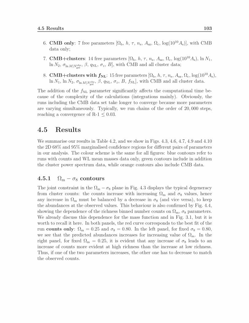
4.5 Results 103
6. CMB only: 7 free parameters [Ωb, h, τ , ns, Asz, Ωc, log(1010As)], with CMB
data only;
7. CMB+clusters: 14 free parameters [Ωb, h, τ , ns, Asz, Ωc, log(1010As), lnN1,
lnN2, σlnM |Nobsgal
, β, qNL, σz, B], with CMB and all cluster data;
8. CMB+clusters with fNL: 15 free parameters [Ωb, h, τ , ns, Asz, Ωc, log(1010As),
lnN1, lnN2, σlnM |Nobsgal
, β, qNL, σz, B, fNL], with CMB and all cluster data.
The addition of the fNL parameter significantly affects the computational time be-cause of the complexity of the calculations (integrations mainly). Obviously, theruns including the CMB data set take longer to converge because more parametersare varying simultaneously. Typically, we run chains of the order of 20, 000 steps,reaching a convergence of R-1 ≤ 0.03.
4.5 Results
We summarise our results in Table 4.2, and we show in Figs. 4.3, 4.6, 4.7, 4.9 and 4.10the 2D 68% and 95% marginalised confidence regions for different pairs of parametersin our analysis. The colour scheme is the same for all figures: blue contours refer toruns with counts and WL mean masses data only, green contours include in additionthe cluster power spectrum data, while orange contours also include CMB data.
4.5.1 Ωm − σ8 contours
The joint constraint in the Ωm − σ8 plane in Fig. 4.3 displays the typical degeneracyfrom cluster counts: the counts increase with increasing Ωm and σ8 values, henceany increase in Ωm must be balanced by a decrease in σ8 (and vice versa), to keepthe abundances at the observed values. This behaviour is also confirmed by Fig. 4.4,showing the dependence of the richness binned number counts on Ωm, σ8 parameters.We already discuss this dependence for the mass function and in Fig. 3.1, but it isworth to recall it here. In both panels, the red curve corresponds to the best fit of therun counts only: Ωm = 0.25 and σ8 = 0.80. In the left panel, for fixed σ8 = 0.80,we see that the predicted abundances increases for increasing value of Ωm. In theright panel, for fixed Ωm = 0.25, it is evident that any increase of σ8 leads to anincrease of counts more evident at high richness than the increase at low richness.Thus, if one of the two parameters increases, the other one has to decrease to matchthe observed counts.
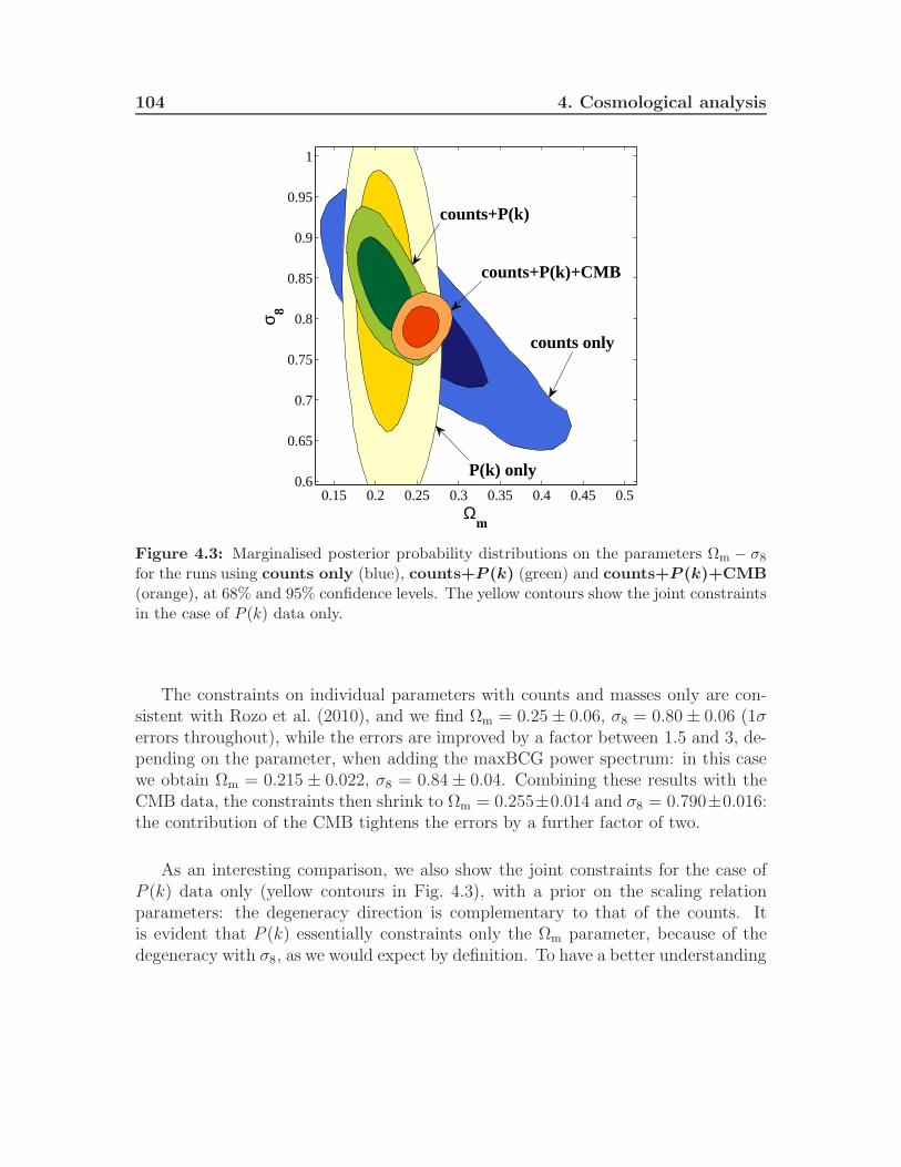
104 4. Cosmological analysis
Ωm
σ 8
0.15 0.2 0.25 0.3 0.35 0.4 0.45 0.50.6
0.65
0.7
0.75
0.8
0.85
0.9
0.95
1
counts only
P(k) only
counts+P(k)
counts+P(k)+CMB
Figure 4.3: Marginalised posterior probability distributions on the parameters Ωm − σ8for the runs using counts only (blue), counts+P (k) (green) and counts+P (k)+CMB(orange), at 68% and 95% confidence levels. The yellow contours show the joint constraintsin the case of P (k) data only.
The constraints on individual parameters with counts and masses only are con-sistent with Rozo et al. (2010), and we find Ωm = 0.25 ± 0.06, σ8 = 0.80± 0.06 (1σerrors throughout), while the errors are improved by a factor between 1.5 and 3, de-pending on the parameter, when adding the maxBCG power spectrum: in this casewe obtain Ωm = 0.215 ± 0.022, σ8 = 0.84 ± 0.04. Combining these results with theCMB data, the constraints then shrink to Ωm = 0.255±0.014 and σ8 = 0.790±0.016:the contribution of the CMB tightens the errors by a further factor of two.
As an interesting comparison, we also show the joint constraints for the case ofP (k) data only (yellow contours in Fig. 4.3), with a prior on the scaling relationparameters: the degeneracy direction is complementary to that of the counts. Itis evident that P (k) essentially constraints only the Ωm parameter, because of thedegeneracy with σ8, as we would expect by definition. To have a better understanding
4.5 Results 105
Figure 4.4: Cluster number counts for different values of Ωm (left panel) and σ8 (rightpanel). The red curve corresponds to the best fit of the run counts only: Ωm = 0.25 andσ8 = 0.80. In the left panel, we fix σ8 = 0.80 and give Ωm the values 0.2 (blue dashed),0.25 (red solid), 0.3 (green dotted-dashed). In the right panel, we fix Ωm = 0.25 and assignto σ8 the values 0.75 (blue dashed), 0.80 (red solid), 0.85 (green dotted-dashed).
Figure 4.5: Full observed power spectrum for different values of Ωm (left panel) and σ8(right panel). The red curve corresponds to the best fit of the run P (k) only: Ωm = 0.21and σ8 = 0.83. The other curves select values at approximately 1σ level of the marginalisedposterior distribution. In the right panel, we fix σ8 = 0.80 and give Ωm the values 0.17 (bluedashed), 0.21 (red solid), 0.25 (green dotted-dashed). In the right panel, we fix Ωm = 0.21and assign to σ8 the values 0.95 (blue dashed), 0.83 (red solid), 0.7 (green dotted-dashed).

106 4. Cosmological analysis
of the power spectrum dependence on these parameters, we show the full observedpower spectrum for different values of Ωm and σ8 in Fig. 4.5. In both panels, the redcurve corresponds to the best fit of the run P (k) only: Ωm = 0.21 and σ8 = 0.83.The left panel shows the power spectrum varying Ωm, at fixed σ8 = 0.83, while theright panel shows the power spectrum varying σ8, at fixed Ωm = 0.21. We notice thatif we increase (decrease) Ωm, the peak of the power spectrum decreases (increases)while also being shifted to higher (lower) values of k, while σ8 simply changes theoverall normalisation. In our case, the size of the posterior on σ8 depends on theassumptions made on the cluster bias: allowing for a completely free bias wouldcause a complete degeneracy with σ8. However here the degeneracy is partiallybroken because we are assuming that the bias is centred around the predicted valuesfrom the mass function, allowing only for deviations from this (parametrised by thescatter B), whose amplitude is limited by the prior on B.
4.5.2 Scaling relation parameters contours
In Fig. 4.6, left panel, we show the marginalised posterior probability contours of thescaling relation parameters lnN1 − lnN2. These two parameters correspond to thetwo pivot points in (log) mass lnM1, lnM2, which define a linear scaling relation inthe lnNgal − lnM plane, with slope αN , intercept lnM200|20 and scatter σlnM .
From Fig. 4.8 we can better understand the degeneracy between these two pa-rameters. The left panels show the mean masses estimates in richness bins, whilethe right panels show the counts in richness bins. In all plots the best fit is shownby a red solid curve, while any increase or decrease of scaling relation parameters orscatter is plotted in green dotted-dashed or blue dashed line, respectively. Note thatwe do not plot the linear relation across the two points (lnN1, lnM1), (lnN2, lnM2),but instead we connect the mass estimates in each richness bin. This can give us anintuition on the approximate scaling relation behaviour. If we fix the two pivot pointsin mass, as lnN1 increases, so does lnN2, to keep the slope of the linear relation atthe observed value: this is shown by the green dotted-dashed curve in the top leftpanel of Fig. 4.8. At the same time, the intercept lnM200|20 decreases, resulting ina parallel displacement of the linear scaling relation towards higher richness values.We also notice that for fixed lnNgal, the corresponding mass has now decreased. Onthe other hand, the blue dashed line displays the case of a decreasing lnN1, and thuslnN2, and an increasing intercept.

4.5 Results 107
ln N1
ln N
2
2.1 2.2 2.3 2.4 2.5 2.6 2.7
3.7
3.8
3.9
4
4.1
4.2
4.3
4.4
4.5
4.6
4.7
counts only
counts+P(k)
counts+P(k)+CMB
αN
ln M
200|
20
1.1 1.2 1.3 1.4 1.5 1.6 1.7
28
28.2
28.4
28.6
28.8
29
29.2
29.4
29.6
29.8
counts only
counts+P(k)
counts+P(k)+CMB
Figure 4.6: Left panel: constraints on the scaling relation parameters lnN1 − lnN2.Note that lnN1 ≡ lnNgal|M1 and lnN2 ≡ lnNgal|M2, where M1 = 1.3 × 10¹⁴M⊙ andM2 = 1.3 × 10¹⁵M⊙. Right panel: constraints on the slope αN and intercept lnM200|20 ofthe scaling relation. The runs used for this plot are: counts only (blue), counts+P (k)(green) and counts+P (k)+CMB (orange). The confidence levels are at 68% and 95%.
ln N1
σ ln M
2.1 2.2 2.3 2.4 2.5 2.6 2.70.15
0.2
0.25
0.3
0.35
0.4
0.45
0.5
0.55
counts only
counts+P(k)
counts+P(k)+CMB
ln N2
σ ln M
3.8 4 4.2 4.4 4.60.15
0.2
0.25
0.3
0.35
0.4
0.45
0.5
0.55
counts only
counts+P(k)
counts+P(k)+CMB
Figure 4.7: Left panel: constraints on the scaling relation parameters lnN1 − σlnM .Right panel: constraints on the scaling relation parameters lnN2 − σlnM . The runs usedfor this plot are: counts only (blue), counts+P (k) (green) and counts+P (k)+CMB(orange). The confidence levels are at 68% and 95%.

108 4. Cosmological analysis
Figure 4.8: Predictions for mean masses (left panels) and number counts (right pan-els) varying scaling relation parameters. First row: for fixed scatter σlnM = 0.36,lnN1 ≡ lnNgal|M1, with M1 = 1.3 × 10¹⁴M⊙, is equal to 2.38, 2.48, 2.58 andlnN2 ≡ lnNgal|M2 , with M2 = 1.3×10¹⁵M⊙, is equal to 4.02, 4.12, 4.22, which we bothplot in blue dashed, red (best fit) and green dotted-dashed respectively. Second row: forfixed lnN1 = 2.48, lnN2 = 4.12, σlnM is equal to 0.26, 0.36, 0.46, which we show in bluedashed, red (best fit) and green dotted-dashed respectively. The run used for these plotsis counts+P (k).

4.5 Results 109
In order to keep the scaling relation to the observed value, then, the scatter playsa key role: even if the slope is kept constant by the increasing of both lnN1 andlnN2, the decrease of the intercept is compensated by a decrease of σlnM . This isconfirmed by Fig. 4.7, showing the joint constraints lnN1 − σlnM and lnN2 − σlnM :any increase of lnN1 or lnN2 corresponds to a decrease of σlnM . The converse is ofcourse also true. Furthermore, the bottom left panel of Fig. 4.8 displays an analogousdisplacement of the predicted masses to higher Ngal values obtained by increasing thescatter (green dotted-dashed line) and to lower Ngal values obtained by decreasingthe scatter (blue dashed line). As a consequence, the mean masses corresponding tothe same richness result lower or higher, respectively.
Finally, from the right panels of Fig. 4.8 we can deduce another confirmation fromthe cluster number counts. If the scaling relation parameters or scatter increase, wewill count more objects in general, thus the counts increase in each richness bin. Thisis motivated by the fact that if we have lower mass estimates, we automatically havemore structures due to the shape of the mass function. The opposite arguments canalso be formulated for a decrease in lnN1, lnN2 and σlnM . As a consequence, again,any increase of lnN1 and lnN2 implies a decrease of σlnM , to keep the abundancesto the observed values.
Constraints on individual parameters using counts and masses are only compat-ible with Rozo et al. (2010) (lnN1 = 2.44 ± 0.11, lnN2 = 4.16 ± 0.15), while errorsare reduced when adding the power spectrum, even if less significantly (lnN1 =2.49 ± 0.09, lnN2 = 4.13± 0.13). Combining these results with the CMB data, theconstraints are almost identical, as the CMB is not sensitive to the clusters scalingrelation. Our constraints on the scaling relation scatter σlnM are in agreement withRozo et al. (2010), and they are not improved by the addition of power spectrumand CMB data.
We then calculated the likelihood contours on the derived parameters αN −lnM200|20: these are shown in the right panel of Fig. 4.6. By definition of slope and in-tercept, it is evident that any increase of αN implies a decrease of lnM200|20 (and viceversa), motivating the degeneracy line of these two parameters. The marginalisedmean values and 1σ errors on individual parameters, using counts and masses only,are αN = 1.35 ± 0.11, lnM200|20 = 28.85 ± 0.33. When adding the power spec-trum, the errors reduce to αN = 1.41 ± 0.06, lnM200|20 = 28.64 ± 0.17. Combiningthen with the CMB data, the constraints are further improved to αN = 1.32± 0.03,lnM200|20 = 28.93± 0.09.
110 4. Cosmological analysis
4.5.3 log(1010As)− σ8 contours
In Fig. 4.9, left panel, we show the degeneracy between the amplitude of primordialfluctuations log(1010As) and power spectrum normalization σ8, being respectively aprimary and a derived parameter of our analysis. The constraints on individual pa-rameters with counts and masses only are σ8 = 0.8±0.06, log(1010As) = 3.2±0.5, andadding the maxBCG power spectrum they become σ8 = 0.84 ± 0.04, log(1010As) =3.5 ± 0.25. Finally, the inclusion of the CMB data shrink the constraints to σ8 =0.079± 0.016 and log(1010As) = 3.06± 0.03.
4.5.4 fNL − Ωm and fNL − σ8 contours
In Fig. 4.10 we show the constraints on the amount of primordial non-Gaussianityand its degeneracies with Ωm and σ8. First, it is evident that when only counts andmasses are used, the constraints on fNL are weak as expected. In Fig. 4.9, rightpanel, we show how the relative counts with respect to the fNL = 0 vary for differentfNL values. For this theoretical expectations we use the run counts with fNL. It isclear that the difference between the curves is more relevant at large values of Ngal:higher fNL corresponds to higher skewness, which implies more rare (massive) objects.
The situation improves when adding the cluster power spectrum: in this case, theconstraints are tighter, and we observe a positive correlation between fNL and Ωm
and an anti-correlation with σ8. To understand this behaviour, we can refer again tothe power spectrum dependence on Ωm and σ8 parameters. Any increase of Ωm tiltsthe power spectrum, decreasing and shifting the peak to higher values of k, whileany increase of σ8 shifts up the whole shape. The converse of this is also true. Wehave also understood that an increase in fNL causes a boost in the power spectrumon large scales (small k), so that σ8 needs to decrease to compensate a higher fNL:this is exactly what is shown in the right panel of Fig. 4.10. In addition to this Ωm
should increase to compensate a higher fNL: this can be seen in the left panel.
We also see that the addition of the CMB power spectrum data improves theconstraints on Ωm and σ8 and only indirectly reduces the bounds on fNL, since PNGsimply affects the higher-order statistics of the CMB.
Our constraints on PNG are fNL = 12 ± 157 (1σ) (without CMB) and fNL =194 ± 128 (with CMB), which are statistically compatible with zero and with eachother. The shift in the mean between the two results is clear by looking at Fig. 4.10:the addition of the CMB favours lower values of σ8 (and higher values of Ωm), thus

4.5 Results 111
log (1010 As)
σ 8
2 2.5 3 3.5 4 4.50.6
0.65
0.7
0.75
0.8
0.85
0.9
0.95
1
counts only
counts+P(k)
counts+P(k)+CMB
Figure 4.9: Left panel: marginalised posterior probability distributions on log(1010As)−σ8 parameters. The runs used are: counts only (blue), counts+P (k) (green) andcounts+P (k)+CMB (orange), at 68% and 95% confidence levels. Right panel: countspredictions for fNL = 300, 100, 0,−100,−300, relative to the fNL = 0 case. The run usedin this plot is counts with fNL.
fNL
Ωm
−400 −200 0 200 400 600 800 1000 12000.05
0.1
0.15
0.2
0.25
0.3
0.35
0.4
0.45
0.5
counts only
counts+P(k) counts+P(k)+CMB
fNL
σ 8
−400 −200 0 200 400 600 800 1000
0.6
0.65
0.7
0.75
0.8
0.85
0.9
0.95
1counts only
counts+P(k)
counts+P(k)+CMB
Figure 4.10: Marginalised posterior probability distributions on the parameters fNL−Ωm
(left panel) and fNL − σ8 (right panel). The runs used for these plots are counts withfNL (blue), counts+P (k) with fNL (green) and CMB+clusters with fNL (orange),at 68% and 95% confidence levels.

112 4. Cosmological analysis
shifting the favoured fNL values in the process. While not competitive with resultsfrom the CMB bispectrum or from combined analyses of multiple galaxy surveys, itis interesting to find such constraints independently and for the first time with theclustering of optically selected galaxy clusters.
It is also worth mentioning the results on the B parameter, which was introducedto take into account the uncertainty in the bias expression derived from the massfunction. As this parameter allows an arbitrary constant rescaling of the bias, italso has the desirable property of cancelling the effect of the scale-independent biascorrection δb(fNL), as described in Section 2.5. To check that the Gaussian priorwe are imposing B = 1.0 ± 0.15 is large enough for both purposes, we made anadditional run replacing it with a flat prior, B ∈ [0.0001, 5]. In this way, we obtainnearly unchanged results on fNL. We also obtain no relevant degeneracies of B withany of the other parameters in the analysis.
Finally, since we restrict our analysis to near-linear scales by imposing the datacut at kmax = 0.15 h Mpc−1, we are not expecting strong constraints on qNL. Theconstraints we found are indeed broad and in agreement within the errors with theresults by Hutsi (2010), who found qNL = 14.2 ± 2.8 when marginalising over threeparameters only. We instead obtain qNL = 26± 10 (without CMB) and qNL = 14± 6(with CMB).

4.5
Resu
lts113
Table 4.1: Parameters used in the analysis and their assumed priors (with or without the CMB data). In the prior columnsa single number n stands for a fixed value, [a, b] stands for a flat prior, µ± σ means a Gaussian prior of mean µ and standarddeviation σ.
Type Symbol Definition Prior (no CMB) Prior (+CMB)
Cosmology h Dimensionless Hubble parameter 0.7 [0.4, 0.9]ns Scalar spectral index 0.96 [0.5, 1.5]Ωb Baryon energy density 0.04397 [0.01, 0.2]Ωc Cold dark matter energy density [0.1, 0.9] [0.1, 0.9]
log(1010As) Amplitude of primordial perturbations [0.1, 6.0] [0.1, 6.0]τ Optical depth 0.09 [0.01, 0.125]fNL Primordial non-Gaussianity [−900, 900] [−900, 900]
Scaling relation lnN1 ≡ lnNgal|M1 Richness at M1 = 1.3× 10¹⁴M⊙ [1.0, 4.0] [1.0, 4.0]lnN2 ≡ lnNgal|M2 Richness at M2 = 1.3× 10¹⁵M⊙ [1.0, 4.0] [1.0, 4.0]
σlnM |Nobsgal
Scatter 0.45± 0.1 0.45± 0.1
Nuisance β WL mass measurements bias 1.0± 0.06 1.0± 0.06B Scatter on bias 1.0± 0.15 1.0± 0.15qNL Non-linear P(k) correction [0.0, 50.0] [0.0, 50.0]σz Photo-z errors [0, 120] [0, 120]Asz Amplitude of CMB SZ template 1 [0, 2]
Derived Ωm Total matter energy density — —σ8 Power spectrum normalization — —

114
4.Cosm
ologicalanalysis
Table 4.2: Marginalised mean values and 1σ errors on the cosmological parameters, for the runs counts only, counts withfNL, counts+P (k), counts+P (k) with fNL, CMB+clusters and CMB+clusters with fNL. Note that Ωm and σ8 arederived parameters in our analysis.
Params counts only counts+P (k) clusters+CMB
no fNL +fNL no fNL +fNL no fNL +fNL
Ωm 0.25± 0.06 0.25± 0.06 0.215± 0.022 0.209± 0.022 0.255± 0.014 0.248± 0.013σ8 0.80± 0.06 0.77± 0.07 0.84± 0.04 0.85± 0.05 0.790± 0.016 0.780± 0.016
lnN1 2.44± 0.11 2.44± 0.11 2.49± 0.09 2.49± 0.08 2.44± 0.08 2.43± 0.08lnN2 4.16± 0.15 4.15± 0.15 4.13± 0.13 4.11± 0.12 4.19± 0.11 4.15± 0.11σlnM 0.38± 0.06 0.38± 0.06 0.36± 0.06 0.37± 0.06 0.378± 0.059 0.38± 0.06β 1.00± 0.06 1.01± 0.06 1.01± 0.06 1.01± 0.06 1.01± 0.06 1.00± 0.06qNL - - 26± 10 27± 10 14± 6 16± 7σz - - 46± 12 42± 8 43± 10 31± 5B - - 1.07± 0.13 1.01± 0.15 1.19± 0.11 1.00± 0.14fNL - 282± 317 - 12± 157 - 194± 128

Chapter 5
Clusters-galaxies cross correlation
The correlation function is one of the best statistical tools to measure quantitativelythe clustering of objects in a sample. Correlation statistic methods are an impor-tant tool for relating galaxies and clusters to the underlying mass distribution, beingclusters more strongly correlated in space than galaxies. Therefore, the two-point an-gular correlation function of galaxies and clusters efficiently quantifies the large-scalestructure of the Universe. In this Chapter, we describe the measuring of the clus-tering properties of clusters and galaxies by using the two-point angular correlationfunction w(θ). As we have been focusing on optical data so far, the measurementof the 2D angular projected correlation function is to prefer to the 3D correlationfunction, because of the uncertainty on the photometric redshift estimates and thesmoothing due to the relatively large radial distance errors. This part of the projectis still in a preliminary, incomplete status. Here we introduce the measurement bypixelization, the theoretical expectation and the error estimates, in the case of clusterauto-correlation function only. The goal is to fully complete the estimations for thegalaxies auto-correlation and for the clusters-galaxies cross-correlation, in order toinvestigate their constraining power on cosmological models.
5.1 Measurement by pixelization
Estimating the angular correlation function with pixelated analysis is similar to theapproach used to calculate the CMB temperature anisotropies. The angular resolu-tion of the particular instruments gives a natural limit for the maximum reasonableresolution used in the analysis. Here we describe the pixelization technique we em-ploy, based on the healpix software. We also present the mask calculation and thecatalogues of clusters and galaxies we choose.
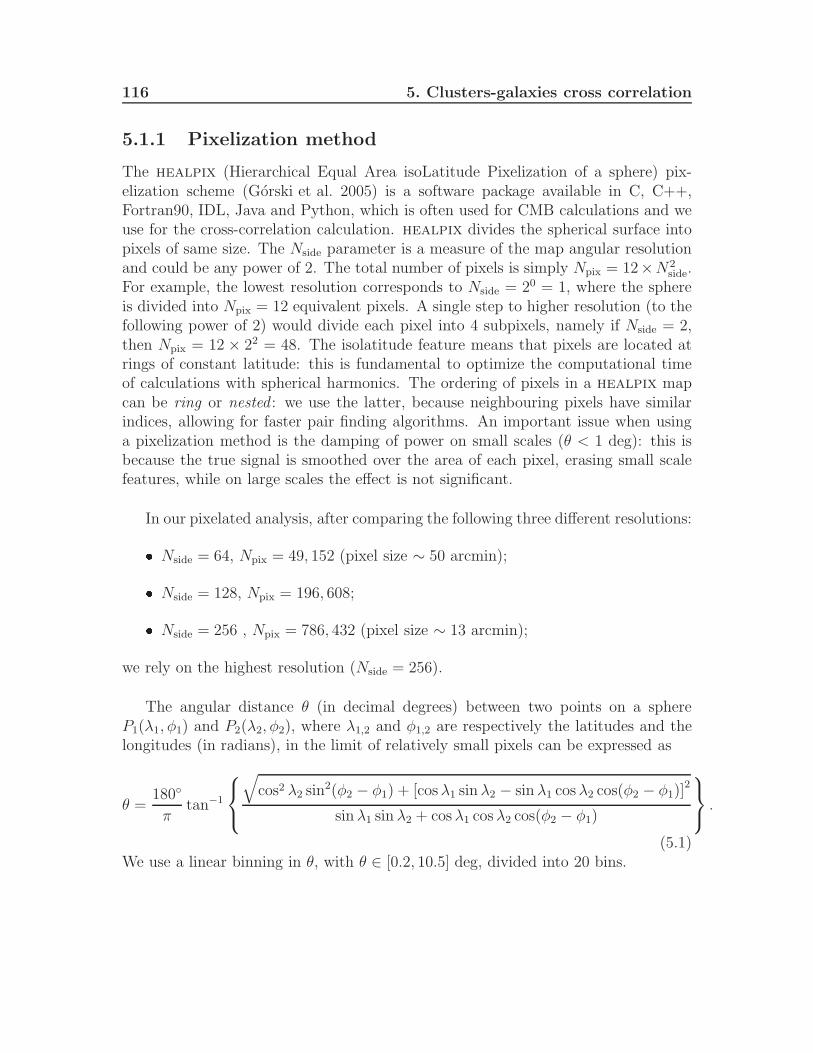
116 5. Clusters-galaxies cross correlation
5.1.1 Pixelization method
The healpix (Hierarchical Equal Area isoLatitude Pixelization of a sphere) pix-elization scheme (Gorski et al. 2005) is a software package available in C, C++,Fortran90, IDL, Java and Python, which is often used for CMB calculations and weuse for the cross-correlation calculation. healpix divides the spherical surface intopixels of same size. The Nside parameter is a measure of the map angular resolutionand could be any power of 2. The total number of pixels is simply Npix = 12×N2
side.For example, the lowest resolution corresponds to Nside = 20 = 1, where the sphereis divided into Npix = 12 equivalent pixels. A single step to higher resolution (to thefollowing power of 2) would divide each pixel into 4 subpixels, namely if Nside = 2,then Npix = 12 × 22 = 48. The isolatitude feature means that pixels are located atrings of constant latitude: this is fundamental to optimize the computational timeof calculations with spherical harmonics. The ordering of pixels in a healpix mapcan be ring or nested : we use the latter, because neighbouring pixels have similarindices, allowing for faster pair finding algorithms. An important issue when usinga pixelization method is the damping of power on small scales (θ < 1 deg): this isbecause the true signal is smoothed over the area of each pixel, erasing small scalefeatures, while on large scales the effect is not significant.
In our pixelated analysis, after comparing the following three different resolutions: Nside = 64, Npix = 49, 152 (pixel size ∼ 50 arcmin); Nside = 128, Npix = 196, 608; Nside = 256 , Npix = 786, 432 (pixel size ∼ 13 arcmin);
we rely on the highest resolution (Nside = 256).
The angular distance θ (in decimal degrees) between two points on a sphereP1(λ1, φ1) and P2(λ2, φ2), where λ1,2 and φ1,2 are respectively the latitudes and thelongitudes (in radians), in the limit of relatively small pixels can be expressed as
θ =180
πtan−1
√cos2 λ2 sin
2(φ2 − φ1) + [cosλ1 sinλ2 − sin λ1 cosλ2 cos(φ2 − φ1)]2
sinλ1 sin λ2 + cosλ1 cosλ2 cos(φ2 − φ1)
.
(5.1)We use a linear binning in θ, with θ ∈ [0.2, 10.5] deg, divided into 20 bins.

5.1 Measurement by pixelization 117
Figure 5.1: Mask used for the calculation of angular correlation function with pixelatedanalysis, in equatorial coordinates.
5.1.2 The mask and the catalogues
We adopt a mock catalogue provided by Will Percival (private communication),consisting of about 5.2 million objects corresponding to the SDSS DR7 spectroscopicfootprint, to create our mask (see Fig. 5.1). We use Nside = 256 to determine whichpixels are covered by the catalogue, downscale to Nside = 64 and remove all pixels inthe lower resolution that are not fully covered. The final mask is binary (mi = 1, 0).We then applied the mask to the following two catalogues: GMBCG (Gaussian Mixture Brightest Cluster Galaxy) largest publicly avail-
able cluster catalogue (Hao et al. 2010) from SDSS DR7 optical data, withzphoto < 0.55, 8 < Ngal < 140 over 8, 200 deg2 of comoving volume, with 55,431objects; A volume limited sample of galaxies from the SDSS-II DR7 (Ben Hoyle, pri-vate communication), with zphoto < 0.55, ∆zphoto < 0.1 and R-band absolutemagnitude smaller than −21.5, with 9,489,664 objects .

118 5. Clusters-galaxies cross correlation
5.2 Angular correlation function estimator
From Giannantonio et al. (2008) we employ the following estimator for the angularcorrelation function between clusters (c) and galaxies (g):
w(θ)cgpix =1
Nθ
∑
i,j
mi
(ci − c
c
)mj
(gj − g
g
), (5.2)
where Nθ =∑
i,jmimj is the weighted number of pixel pairs separated by θ, ci isthe number of clusters inside pixel i, gj is the galaxies number inside pixel j, mi,j isthe unique mask value for pixels i, j, c and g are respectively the average numbersof clusters and galaxies per pixel (i.e. the total number of objects divided by thenumber of the non-empty pixels). In the case of clusters auto-correlation, we havethen
w(θ)ccpix =1
Nθ
∑
i,j
mi
(ci − c
c
)mj
(cj − c
c
), (5.3)
while for the galaxies auto-correlation we have
w(θ)ggpix =1
Nθ
∑
i,j
mi
(gi − g
g
)mj
(gj − g
g
). (5.4)
5.3 Theoretical prediction
The numerical tool we use for calculating the theoretical correlation function is cambSources1(Lewis & Challinor 2007) a Fortran 90 code similar to camb, cmbfast
(Seljak & Zaldarriaga 1996), cmbeasy (Doran 2005), class (Lesgourgues 2011;Blas et al. 2011). It computes the angular power spectrum Cl of the CMB anisotropiesas well as matter perturbations at different redshifts. We will calculate the Cls ofthe matter density, given a certain redshift distribution d(z), for both clusters andgalaxies. The relation between the Cls and w(θ) is given by
w(θ)theory =∑
l≥0
(2l + 1
4π
)Pl(cos θ)Cl , (5.5)
where Pl are the Legendre polynomials of degree l. The observed signal is thenexpected to be w(θ) = b2eff w(θ)theory, for a bias factor bcleff ∼ 2 for clusters andbgeff ∼ 1 for galaxies. In Fig. 5.2 we show our preliminary results for the clusterauto-correlation function, together with theoretical predictions and errors estimates.
1http://camb.info/sources/

5.4 Error estimates 119
Figure 5.2: Cluster auto-correlation function, with estimated errors and theoretical pre-diction. The angle θ is given in degrees.
5.4 Error estimates
Having the theoretical Cl, we can use the following analytical prescription (Ross et al.2011) for the covariance matrix of the correlation function:
Cθθ′ =2
fsky
∑
l≥0
2l + 1
(4π)2Pl(cos θ)Pl(cos θ
′)
(b2effCl +
1
n
)2
, (5.6)
where fsky is the number of observed steradians, n is the number of object persteradian. Note that 1/n is the shot-noise contribution, while beff2Cl is the cosmicvariance term.

120 5. Clusters-galaxies cross correlation

Chapter 6
Conclusions
This dissertation was aimed to examine the contribution of clusters of galaxies in con-firming the concordance ΛCDM cosmological model. After introducing the currentcosmological framework and the main properties of galaxy clusters, we showed howthese massive gravitationally bound systems in the Universe provide a unique testof cosmology and structure formation. Their number density and distribution arehighly sensitive to cosmology and provide tight and robust constraints on cosmolog-ical parameters, complementing those which result from other observational probes.However, these constraints are critically dependent on our ability to estimate clustermasses. Our work highlighted in particular the power of optically selected clus-ter samples to produce precision constraints on cosmological parameters. This wasachieved by adding the clustering information of galaxy clusters to complement thecluster number counts and observable-mass relation analyses.
The first achievement was to reproduce the cosmological constraints obtained inthe analysis done by Rozo et al. (2010). In this analysis, they used cluster abun-dances in richness bins together with weak-lensing mass measurements of the SDSSmaxBCG cluster catalogue to constrain cosmology and the richness-mass relationof the clusters. They assumed a flat Universe and they used the Tinker halo massfunction for the computation. The richness-mass relation they adopted was a power-law in mass and they constrained the scatter around it by demanding consistencybetween X-ray and WL measurements. Their final cosmological results were fur-ther improved by a joint analysis with the WMAP DR5 data. We followed theirtheoretical modelling of cluster counts and cluster total masses, together with theircorresponding covariance matrices. By adopting a Bayesian approach for derivingcosmological constraints from the sample, we obtained consistent constraints on the
122 6. Conclusions
matter density Ωm, the fluctuation amplitude σ8, the scaling relation parameterslnN1, lnN2 and the scatter σlnM .
An interesting development of this joint cosmological analysis was to fully in-clude the redshift space power spectrum of the maxBCG clusters, calculated byHutsi (2010). We followed this prescription to model the cluster power spectrum, in-cluding the effect of weak non-linearities and redshift space distortions and allowingfor an arbitrary photometric redshift smoothing. We found that the inclusion of thepower spectrum typically brings a factor between 1.5 and 3, depending on the pa-rameter, improvement of the errors on σ8 and Ωm. Constraints on other parametersare also improved, even if less significantly. In addition to the cluster data, we alsoused the CMB power spectra from WMAP7, which further contributed to tightenthe confidence regions by an additional factor of 2, mainly on σ8 and Ωm parameters.
Another peculiar application of this analysis was concerning the study of non-Gaussian initial conditions to constrain models of the early universe. MaxBCGgalaxy clusters provided constraints on the amount of the local type primordial non-Gaussianity of the initial density perturbations which are statistically compatiblewith zero and consistent with the latest constraints. While these results are notcompetitive with those from combined analyses of multiple galaxy surveys of fromthe CMB bispectrum, we found such constraints independently and for the first timewith the clustering of optically selected galaxy clusters.
All our MCMC analysis was performed using the Cosmological Monte-Carlo(cosmomc) publicly available parameter estimation tool by Lewis & Bridle (2002).All the cosmological analysis implementation and results have been published inMana et al. (2013). We are currently updating our results to include the Plancklikelihood.
In the last Chapter of this thesis, we presented some preliminary calculations onthe clustering of clusters and galaxies, by means of the two-point angular correlationfunction, estimated by a pixelization technique and theoretical modelling. This sta-tistical quantity efficiently quantifies the large-scale structure of the Universe, thusproviding additional constraining power on cosmological models. Our work can beseen as a proof of concept towards a full joint analysis of the LSS, consistently includ-ing both galaxies and clusters as dark matter tracers, to achieve the full potentialof the upcoming galaxy surveys such as the Dark Energy Survey and the Euclidmission.

123
We conclude by suggesting two possible extensions to this work, which couldresult in promising results: the inclusion of massive neutrinos and the application tomodified gravity models.
Modified gravity
The accelerated expansion of the Universe can be explained by introducing modifica-tions to gravity, instead of a dark energy component. A possible modification is theaddition of a free function f(R) of the Ricci scalar R to the Einstein-Hilbert action.This leads to modified Einstein equations, containing terms with f(R) and differen-tials of this function with respect to R (i.e. fR, fRR). Valid f(R) model should closelymatch the ΛCDM expansion history and satisfy local gravity constraints. Strong con-straints on deviation from GR can be inferred from the large-scale structure: in fact,the increased growth of structure observed in f(R) gravity affects the large scalesof the CMB temperature power spectrum. However, the most stringent constraintson f(R) models are due to the abundance of low-redshift (z < 0.15) X-ray clusters(Schmidt et al. 2009). An interesting analysis was performed by Lombriser et al.(2012). They performed a MCMC study of f(R) gravity models which reproducethe ΛCDM expansion history using data from CMB (WMAP DR5), SNIa (SupernovaCosmology Project, SCP), BAO (SDSS DR7), H0 (SH0ES) and cluster abundancesfrom the likelihood code of Seljak et al. (2013). They parametrize their solutions interms of the Compton wavelength parameter, defined as
B =fRR
1 + fRR′ H
H ′, (6.1)
where prime denote derivative with respect to ln a: more precisely, they consideredthe value of B at ln a = 0, i.e. B0 ≡ B(ln a = 0). Standard gravity correspondsto B0 = 0. The constraint on the Compton wavelength parameter B0 is essentiallydriven by the cluster abundances alone: they obtained 100B0 < 0.333 (95% c.l.)from the cluster data alone and 100B0 < 0.11 (95% c.l.) from the combined datasets.
These interesting results involving low redshift galaxy clusters suggest us a possi-ble development direction of our research. It would be intriguing to test these f(R)gravity models with the maxBCG optical cluster sample.

124 6. Conclusions
Massive neutrinos
Neutrino oscillation experiments have provided evidence that neutrinos have non-zero masses. In the standard picture, there are three neutrino species with a lowerbound on the summed mass
∑mν at 0.06 eV coming from solar and atmospheric
oscillations observations. On the other hand, combined cosmological data, such asCMB, BAO, galaxy clustering and cluster mass function, provide an upper limit onthe summed mass in the range
∑mν < 0.3 − 0.8 eV (95% c.l.). Neutrinos, in fact,
produce visible effects on the background evolution and structure formation. Morespecifically, neutrinos decouple from the primordial plasma when they are still ultra-relativistic, becoming non-relativistic only after recombination, due to their smallmass. During this period, their energy density contributes as radiation and changesboth the expansion rate and the time of matter-radiation equality: a larger value of∑mν implies a larger value of the radiation density and therefore a postponed time
of equality. These modifications appear in the matter power spectrum as a shift ofthe peak to larger scales. Moreover, since density fluctuations grow more efficientlyon small scales after equality (i.e. in the matter-dominated era), the matter powerspectrum is suppressed on small scales with respect to large scales. As a consequence,a suppression effect is also visible in the halo mass function. Analogous features arecaused by non-relativistic neutrinos, which suppress density fluctuations on scalessmaller than their free-streaming length.
Costanzi Alunno Cerbolini et al. (2013) performed a forecast analysis for a largephotometric galaxy cluster survey (like Euclid survey) on neutrino properties con-straints: in particular, the total neutrino mass and effective number of neutrinospecies. They combined cluster number counts and cluster power spectrum and useda MCMC method. They found that combining cluster data with CMB from Planckimproves by more than an order of magnitude the constraint on neutrino masses,if compared to each probe used independently. On the other hand, galaxy clusterstogether with CMB and BAO can provide precise constraints on the sum of neutrinomasses but these constraints depend on the calibration of the mass-observable rela-tion (Rozo et al. 2013).
These studies motivate us to include the effect of massive neutrinos in our analy-sis, through the modifications on the cluster mass function and power spectrum. Wewill thus investigate the constraints on neutrinos properties in the near future.

List of Figures
1.1 Energy densities of the Universe. . . . . . . . . . . . . . . . . . . . . 7
1.2 Scale factor as a function of time. . . . . . . . . . . . . . . . . . . . . 7
1.3 The original Hubble diagram. . . . . . . . . . . . . . . . . . . . . . . 9
1.4 Evolution of density perturbations. . . . . . . . . . . . . . . . . . . . 13
1.5 Growth factor dependence on cosmological parameters . . . . . . . . 16
1.6 Hubble diagram from SNIa. . . . . . . . . . . . . . . . . . . . . . . . 20
1.7 SDSS LRGs galaxy cross correlation. . . . . . . . . . . . . . . . . . . 21
1.8 CMB map from Planck. . . . . . . . . . . . . . . . . . . . . . . . . . 23
1.9 Temperature power spectrum from WMAP DR7 . . . . . . . . . . . . 24
1.10 Composite image of galaxy cluster Abell 520. . . . . . . . . . . . . . . 27
1.11 Cluster mass function from Bahcall & Cen (1992). . . . . . . . . . . . 30
1.12 Rotation curve of galaxy NGC 6503. . . . . . . . . . . . . . . . . . . 32
1.13 Constraints on Ωm, σ8, ΩΛ . . . . . . . . . . . . . . . . . . . . . . . . 34
1.14 Constraints on Ωm, w and GR . . . . . . . . . . . . . . . . . . . . . . 35
2.1 The gravitational lensing system representation. . . . . . . . . . . . . 41
2.2 Tinker mass function . . . . . . . . . . . . . . . . . . . . . . . . . . . 47
2.3 Mass function cosmological dependence on Ωm and σ8. . . . . . . . . 49
2.4 High-z clusters sensitivity to cosmological models . . . . . . . . . . . 50
2.5 Mass functions comparison . . . . . . . . . . . . . . . . . . . . . . . . 61
2.6 Mass dependence of the linear halo bias. . . . . . . . . . . . . . . . . 63
2.7 The effect of PNG on the cluster power spectrum. . . . . . . . . . . . 64
3.1 MaxBCG counts and masses data and theoretical curves. . . . . . . . 79
3.2 The angular distribution of the selected maxBCG clusters. . . . . . . 82
3.3 The redshift-space power spectrum of maxBCG sample. . . . . . . . . 83
3.4 Linear and full power spectrum. . . . . . . . . . . . . . . . . . . . . . 84
3.5 The off-diagonal elements of w(θ)-∆N covariance matrix. . . . . . . . 87
126 List of figures
4.1 Example of MCMC chains. . . . . . . . . . . . . . . . . . . . . . . . . 954.2 Example of 1D, 2D marginalised posteriors. . . . . . . . . . . . . . . 1004.3 Marginalised posterior probability distribution on Ωm − σ8. . . . . . . 1044.4 Number counts with varying Ωm and σ8. . . . . . . . . . . . . . . . . 1054.5 Power spectrum with varying Ωm and σ8. . . . . . . . . . . . . . . . . 1054.6 Constraints on scaling relation parameters. . . . . . . . . . . . . . . . 1074.7 Constraints on the scaling relation scatter. . . . . . . . . . . . . . . . 1074.8 Masses and counts varying scaling relation parameters. . . . . . . . . 1084.9 Marginalised posteriors on log(1010As)− σ8 . . . . . . . . . . . . . . . 1114.10 Marginalised posteriors of fNL − Ωm, fNL − σ8. . . . . . . . . . . . . . 111
5.1 Mask for the angular correlation function with pixelated analysis. . . 1175.2 Cluster auto-correlation function with theoretical prediction. . . . . . 119

List of Tables
1.1 Evolution of energy densities components of the Universe. . . . . . . . 61.2 Cosmological parameters of ΛCDM model. . . . . . . . . . . . . . . . 33
3.1 MaxBCG counts data. . . . . . . . . . . . . . . . . . . . . . . . . . . 733.2 MaxBCG mean mass data. . . . . . . . . . . . . . . . . . . . . . . . . 783.3 MaxBCG power spectrum data. . . . . . . . . . . . . . . . . . . . . . 88
4.1 Parameters and priors used in the analysis. . . . . . . . . . . . . . . . 1134.2 Marginalised mean values and 1σ errors in the analysis. . . . . . . . . 114


Acronyms
ACT Atacama Cosmology TelescopeAP Alcock-PaczynskiBAO Baryons Acoustic OscillationsBCG Brightest Cluster GalaxyCAMB Code for Anisotropies in the Microwave BackgroundCDM Cold Dark MatterCLT Central Limit TheoremCMB Cosmic Microwave BackgroundCOSMOMC Cosmological Monte CarloDE Dark EnergyDGP Dvali, Gabadadze, Porrati modelDM Dark MatterDR Data ReleaseFE Friedmann EquationsFFTs Fast Fourier TransformsFKP Feldman-Kaiser-PeacockFLRW Friedmann-Lemaıtre-Robertson-WalkerFT Fourier TransformationGMBCG Gaussian Mixture Brightest Cluster GalaxyGR General RelativityHEALPIX Hierarchical Equal Area isoLatitude Pixelization of a sphereHST Hubble Space TelescopeICM Intracluster MediumIID Independent Identically distributedJK JackknifeΛCDM Lambda Cold Dark MatterLS Landy-SzalayLSS Large Scale StructureLV LoVerde
130 Acronyms
MCMC Monte Carlo Markov ChainM-H Metropolis-HastingsNFW Navarro-Frenk-White density profileOMC Ordinary Monte CarloPNG Primordial Non-GaussianityPS Press-SchechterRDS Redshift Space DistortionsSDSS Sloan Digital Sky SurveySIS Singular Isothermal SphereSNIa Type Ia SupernovaeSO Spherical OverdensitySPT South Pole TelescopeST Sheth-TormenSZ Sunyaev-Zel’dovichTSC Triangular Shaped CloudWL Weak gravitational LensingWMAP Wilkinson Microwave Anisotropy Probe

Bibliography
Abazajian K. N., Adelman-McCarthy J. K., Agueros M. A., et al., 2009, ApJS, 182,543
Abell G. O., 1958, ApJS, 3, 211
Abell G. O., Corwin Jr. H. G., Olowin R. P., 1989, ApJS, 70, 1
Acquaviva V., Bartolo N., Matarrese S., Riotto A., 2003, Nuclear Physics B, 667,119
Afshordi N., Tolley A. J., 2008, Phys. Rev. D, 78, 12, 123507
Ahn C. P., Alexandroff R., Allende Prieto C., et al., 2012, ApJS, 203, 21
Aihara H., Allende Prieto C., An D., et al., 2011, ApJS, 193, 29
Alcock C., Paczynski B., 1979, Nature, 281, 358
Allen S. W., Evrard A. E., Mantz A. B., 2011, ARA&A, 49, 409
Allen S. W., Rapetti D. A., Schmidt R. W., Ebeling H., Morris R. G., Fabian A. C.,2008, MNRAS, 383, 879
Allen S. W., Schmidt R. W., Ebeling H., Fabian A. C., van Speybroeck L., 2004,MNRAS, 353, 457
Angulo R. E., Hahn O., Abel T., 2013, MNRAS, 434, 1756
Angulo R. E., Springel V., White S. D. M., Jenkins A., Baugh C. M., Frenk C. S.,2012, MNRAS, 426, 2046
Bahcall N. A., Cen R., 1992, ApJ, 398, L81
Bahcall N. A., Fan X., 1998, ApJ, 504, 1

132 BIBLIOGRAPHY
Bahcall N. A., Soneira R. M., 1983, ApJ, 270, 20
Balaguera-Antolınez A., Sanchez A. G., Bohringer H., Collins C., Guzzo L., PhlepsS., 2011, MNRAS, 413, 386
Bartelmann M., Schneider P., 2001, Phys. Rep., 340, 291
Bartolo N., Komatsu E., Matarrese S., Riotto A., 2004, Phys. Rep., 402, 103
Battye R. A., Weller J., 2003, Phys. Rev. D, 68, 8, 083506
Becker M. R., McKay T. A., Koester B., et al., 2007, ApJ, 669, 905
Bennett C. L., Larson D., Weiland J. L., et al., 2013, ApJS, 208, 20
Benson B. A., de Haan T., Dudley J. P., et al., 2013, ApJ, 763, 147
Binney J., Tremaine S., 1987, Galactic dynamics
Blas D., Lesgourgues J., Tram T., 2011, J. Cosmology Astropart. Phys., 7, 34
Boggess N. W., Mather J. C., Weiss R., et al., 1992, ApJ, 397, 420
Bohringer H., Schuecker P., Guzzo L., et al., 2004, A&A, 425, 367
Bond J. R., Cole S., Efstathiou G., Kaiser N., 1991, ApJ, 379, 440
Burenin R. A., Vikhlinin A., Hornstrup A., Ebeling H., Quintana H., MescheryakovA., 2007, ApJS, 172, 561
Burenin R. A., Vikhlinin A. A., 2012, Astronomy Letters, 38, 347
Burkert A., 1995, ApJ, 447, L25
Carlstrom J. E., Ade P. A. R., Aird K. A., et al., 2011, PASP, 123, 568
Cash W., 1979, ApJ, 228, 939
Chevallier M., Polarski D., 2001, International Journal of Modern Physics D, 10, 213
Clowe D., Gonzalez A., Markevitch M., 2004, ApJ, 604, 596
Cole S., Kaiser N., 1989, MNRAS, 237, 1127
Cole S., Percival W. J., Peacock J. A., et al., 2005, MNRAS, 362, 505

BIBLIOGRAPHY 133
Coles P., Lucchin F., 1995, Cosmology. The origin and evolution of cosmic structure
Collins C. A., Guzzo L., Bhringer H., et al., 2000, Monthly Notices of the RoyalAstronomical Society, 319, 3, 939
Costanzi Alunno Cerbolini M., Sartoris B., Xia J.-Q., Biviano A., Borgani S., VielM., 2013, J. Cosmology Astropart. Phys., 6, 20
Cowles M. K., Carlin B. P., 1996, Journal of the American Statistical Association,91, 434, 883
Cui W., Borgani S., Dolag K., Murante G., Tornatore L., 2012, MNRAS, 423, 2279
Dahle H., Pedersen K., Lilje P. B., Maddox S. J., Kaiser N., 2003, ApJ, 591, 662
Dalal N., Dore O., Huterer D., Shirokov A., 2008, Phys. Rev. D, 77, 12, 123514
Davis M., Efstathiou G., Frenk C. S., White S. D. M., 1985, ApJ, 292, 371
Davis M., Peebles P. J. E., 1983, ApJ, 267, 465
de Putter R., White M., 2005, New A, 10, 676
Desjacques V., Jeong D., Schmidt F., 2011, Phys. Rev. D, 84, 6, 061301
Desjacques V., Seljak U., 2010, Advances in Astronomy, 2010
Desjacques V., Seljak U., Iliev I. T., 2009, MNRAS, 396, 85
Doran M., 2005, J. Cosmology Astropart. Phys., 10, 11
Dunkley J., Komatsu E., Nolta M. R., et al., 2009, ApJS, 180, 306
Dvali G., Gabadadze G., Porrati M., 2000, Physics Letters B, 485, 208
Ebeling H., Edge A. C., Mantz A., et al., 2010, MNRAS, 407, 83
Edge A. C., Stewart G. C., Fabian A. C., Arnaud K. A., 1990, MNRAS, 245, 559
Efron B., 1982, CBMS-NSF conference series in applied mathematics, Soc. Ind. andApp. Math., Philadelphia
Einstein A., 1916, Annalen der Physik, 354, 769
Eisenstein D. J., et al., 2005, ApJ, 633, 560

134 BIBLIOGRAPHY
Eisenstein D. J., Hu W., 1998, ApJ, 496, 605
Estrada J., Sefusatti E., Frieman J. A., 2009, ApJ, 692, 265
Evrard A. E., MacFarland T. J., Couchman H. M. P., et al., 2002, ApJ, 573, 7
Fassbender R., Nastasi A., Bohringer H., et al., 2011, A&A, 527, L10
Feldman H. A., Kaiser N., Peacock J. A., 1994, ApJ, 426, 23
Freeman K. C., 1970, ApJ, 160, 811
Gamerman D., Lopes H. F., 2006, Markov Chain Monte Carlo: Stochastic Simulationfor Bayesian Inference, Chapman and Hall/CRC
Garnavich P. M., Kirshner R. P., Challis P., et al., 1998, ApJ, 493, L53
Geyer C. J., 2011, Introduction to Markov chain Monte Carlo., 3–48, Boca Raton,FL: CRC Press
Giacconi R., Murray S., Gursky H., Kellogg E., Schreier E., Tananbaum H., 1972,ApJ, 178, 281
Giannantonio T., Porciani C., 2010, Phys. Rev. D, 81, 6, 063530
Giannantonio T., Porciani C., Carron J., Amara A., Pillepich A., 2012, MNRAS,422, 2854
Giannantonio T., Ross A. J., Percival W. J., et al., 2013, arXiv:1303.1349
Giannantonio T., Scranton R., Crittenden R. G., et al., 2008, Phys. Rev. D, 77, 12,123520
Gilks W. R., 1999, Markov Chain Monte Carlo In Practice, Chapman and Hall/CRC
Gioia I. M., Henry J. P., Maccacaro T., Morris S. L., Stocke J. T., Wolter A., 1990,ApJ, 356, L35
Gladders M. D., Yee H. K. C., 2005, ApJS, 157, 1
Gladders M. D., Yee H. K. C., Majumdar S., et al., 2007, ApJ, 655, 128
Gorski K. M., Hivon E., Banday A. J., et al., 2005, ApJ, 622, 759
Guo Q., White S., Boylan-Kolchin M., et al., 2011, MNRAS, 413, 101

BIBLIOGRAPHY 135
Guth A. H., 1981, Phys. Rev. D, 23, 347
Haiman Z., Mohr J. J., Holder G. P., 2001, ApJ, 553, 545
Hamuy M., Maza J., Phillips M. M., et al., 1993, AJ, 106, 2392
Hamuy M., Phillips M. M., Maza J., Suntzeff N. B., Schommer R. A., Aviles R.,1995, AJ, 109, 1
Hansen S. M., McKay T. A., Wechsler R. H., Annis J., Sheldon E. S., Kimball A.,2005, ApJ, 633, 122
Hao J., McKay T. A., Koester B. P., et al., 2010, ApJS, 191, 254
Harrison E. R., 1970, Phys. Rev. D, 1, 2726
Hastings W., 1970, Biometrika, 97–109
Henriques B. M. B., White S. D. M., Lemson G., et al., 2012, MNRAS, 421, 2904
Herschel F., 1785, Phil. Trans., 75, 213
Hinshaw G., Larson D., Komatsu E., et al., 2013, ApJS, 208, 19
Hobson M. P., Jaffe A. H., Liddle A. R., Mukherjee P., Parkinson D., 2010, Bayesianmethods in cosmology, Cambridge Univ. Press
Hockney R. W., Eastwood J. W., 1988, Bristol, Hilger, 1988
Hong T., Han J. L., Wen Z. L., Sun L., Zhan H., 2012, The Astrophysical Journal,749, 1, 81
Hotchkiss S., 2011, J. Cosmology Astropart. Phys., 7, 4
Hoyle B., Jimenez R., Verde L., Hotchkiss S., 2012, J. Cosmology Astropart. Phys.,2, 9
Hu W., Dodelson S., 2002, ARA&A, 40, 171
Hu W., Kravtsov A. V., 2003, ApJ, 584, 702
Hubble E., 1929, Contributions from the Mount Wilson Observatory, vol. 3, pp.23-28,3, 23
Hutsi G., 2006a, A&A, 449, 891

136 BIBLIOGRAPHY
Hutsi G., 2006b, A&A, 446, 43
Hutsi G., 2006c, A&A, 459, 375
Hutsi G., 2010, MNRAS, 401, 2477
Jeans J. H., 1902, Royal Society of London Philosophical Transactions Series A, 199,1
Jenkins A., Frenk C. S., White S. D. M., et al., 2001, MNRAS, 321, 372
Jing Y. P., 1999, ApJ, 515, L45
Jing Y. P., 2005, ApJ, 620, 559
Johnston D. E., Sheldon E. S., Tasitsiomi A., Frieman J. A., Wechsler R. H., McKayT. A., 2007a, ApJ, 656, 27
Johnston D. E., Sheldon E. S., Wechsler R. H., et al., 2007b, arXiv:0709.1159
Kaiser N., 1984, ApJ, 284, L9
Kaiser N., 1987, MNRAS, 227, 1
Kamionkowski M., 1998, arXiv:astro-ph/9809214
Kauffmann G., Colberg J. M., Diaferio A., White S. D. M., 1999a, MNRAS, 303,188
Kauffmann G., Colberg J. M., Diaferio A., White S. D. M., 1999b, MNRAS, 307,529
Klypin A. A., Kopylov A. I., 1983, Soviet Astronomy Letters, 9, 41
Koester B. P., McKay T. A., Annis J., et al., 2007a, ApJ, 660, 239
Koester B. P., McKay T. A., Annis J., et al., 2007b, ApJ, 660, 221
Komatsu E., Smith K. M., Dunkley J., et al., 2011, ApJS, 192, 18
Kosowsky A., 2006, New A Rev., 50, 969
Kowalski M., Rubin D., Aldering G., et al., 2008, ApJ, 686, 749
Kravtsov A. V., Klypin A. A., Khokhlov A. M., 1997, ApJS, 111, 73
BIBLIOGRAPHY 137
Kuhlen M., Vogelsberger M., Angulo R., 2012, Physics of the Dark Universe, 1, 50
Lacey C., Cole S., 1994, MNRAS, 271, 676
Lahav O., Fabian A. C., Edge A. C., Putney A., 1989, MNRAS, 238, 881
Landy S. D., Szalay A. S., 1993, ApJ, 412, 64
Larson D., et al., 2011, ApJS, 192, 16
Lemson G., Virgo Consortium t., 2006, arXiv:astro-ph/0608019
Lesgourgues J., 2011, arXiv:1104.2932
Lewis A., 2011, CAMB Notes, http://cosmologist.info/notes/CAMB.pdf
Lewis A., Bridle S., 2002, Phys. Rev. D, 66, 10, 103511
Lewis A., Bridle S., 2006, CosmoMC Notes,http://cosmologist.info/notes/CosmoMC.pdf
Lewis A., Challinor A., 2007, Phys. Rev. D, 76, 8, 083005
Lewis A., Challinor A., Lasenby A., 2000, Astrophys. J., 538, 473
Lima M., Cunha C. E., Oyaizu H., Frieman J., Lin H., Sheldon E. S., 2008, MNRAS,390, 118
Lima M., Hu W., 2004, Phys. Rev. D, 70, 4, 043504
Lima M., Hu W., 2005, Phys. Rev. D, 72, 4, 043006
Linder E. V., 2003, Physical Review Letters, 90, 9, 091301
Linder E. V., 2005, Phys. Rev. D, 72, 4, 043529
Linder E. V., Cahn R. N., 2007, Astroparticle Physics, 28, 481
Lombriser L., Slosar A., Seljak U., Hu W., 2012, Phys. Rev. D, 85, 12, 124038
Longair M. S., 2008, Galaxy Formation
LoVerde M., Miller A., Shandera S., Verde L., 2008, J. Cosmology Astropart. Phys.,4, 14

138 BIBLIOGRAPHY
Lupton R., 1993, Statistics in theory and practice
Lynden-Bell D., 1967, MNRAS, 136, 101
MacKay D. J. C., 2003, Information Theory, Inferenceand Learning Algorithms, Cambrdige University Press,http://www.inference.phy.cam.ac.uk/mackay/itprnn/book.html
Mahdavi A., Hoekstra H., Babul A., Sievers J., Myers S. T., Henry J. P., 2007, ApJ,664, 162
Majumdar S., Mohr J. J., 2003, ApJ, 585, 603
Maldacena J., 2003, Journal of High Energy Physics, 5, 13
Mana A., Giannantonio T., Weller J., Hoyle B., Hutsi G., Sartoris B., 2013, MNRAS,434, 684
Mandelbaum R., Seljak U., Hirata C. M., 2008a, J. Cosmology Astropart. Phys., 8,6
Mandelbaum R., Seljak U., Hirata C. M., et al., 2008b, MNRAS, 386, 781
Mantz A., Allen S. W., Ebeling H., Rapetti D., 2008, MNRAS, 387, 1179
Mantz A., Allen S. W., Rapetti D., Ebeling H., 2010, MNRAS, 406, 1759
Maor I., Brustein R., Steinhardt P. J., 2001, Physical Review Letters, 86, 6
Markevitch M., Gonzalez A. H., Clowe D., et al., 2004, ApJ, 606, 819
Marriage T. A., Acquaviva V., Ade P. A. R., et al., 2011, ApJ, 737, 61
Matarrese S., Verde L., 2008, ApJ, 677, L77
Menanteau F., Sifon C., Barrientos L. F., et al., 2013, ApJ, 765, 67
Messier C., 1784, Connaissance des Temps (Paris)
Metropolis, Ulam, 1949, Journal of the American statistical Association, 44, 247,335
Metropolis N., Rosenbluth A. W., Rosenbluth M. N., Teller A. H., Teller E., 1953,J. Chem. Phys., 21, 1087

BIBLIOGRAPHY 139
Mo H. J., Jing Y. P., White S. D. M., 1996, MNRAS, 282, 1096
Mo H. J., White S. D. M., 1996, MNRAS, 282, 347
Moore B., Quinn T., Governato F., Stadel J., Lake G., 1999, MNRAS, 310, 1147
Narayan R., Bartelmann M., 1996, arXiv:astro-ph/9606001
Navarro J. F., Frenk C. S., White S. D. M., 1997, ApJ, 490, 493
Neal R. M., 1993, Probabilistic Inference Using Markov Chain Monte Carlo Methods,http://cosmologist.info/Neal93
Oguri M., 2009, Physical Review Letters, 102, 21, 211301
Oyaizu H., Lima M., Cunha C. E., Lin H., Frieman J., Sheldon E. S., 2008, ApJ,674, 768
Peebles P. J. E., 1980, The large-scale structure of the universe
Peebles P. J. E., 1993, Principles of Physical Cosmology
Percival W. J., Reid B. A., Eisenstein D. J., et al., 2010, MNRAS, 401, 2148
Percival W. J., Reid B. A., Eisenstein D. J., et al., 2011, MNRAS, 417, 3101
Perlmutter S., 2003, Physics Today, 56, 4, 040000
Perlmutter S., Aldering G., Goldhaber G., et al., 1999, ApJ, 517, 565
Pillepich A., Porciani C., Hahn O., 2010, MNRAS, 402, 191
Pillepich A., Porciani C., Reiprich T. H., 2012, MNRAS, 422, 44
Planck Collaboration, Ade P. A. R., Aghanim N., et al., 2011, A&A, 536, A8
Planck Collaboration, Ade P. A. R., Aghanim N., et al., 2013a, arXiv:1303.5062
Planck Collaboration, Ade P. A. R., Aghanim N., et al., 2013b, arXiv:1303.5076
Planck Collaboration, Ade P. A. R., Aghanim N., et al., 2013c, arXiv:1303.5084
Press W. H., Schechter P., 1974, ApJ, 187, 425
Rapetti D., Allen S. W., Weller J., 2005, MNRAS, 360, 555

140 BIBLIOGRAPHY
Rapetti D., Blake C., Allen S. W., Mantz A., Parkinson D., Beutler F., 2013, MN-RAS, 432, 973
Rasia E., Tormen G., Moscardini L., 2004, MNRAS, 351, 237
Reed D. S., Bower R., Frenk C. S., Jenkins A., Theuns T., 2007, MNRAS, 374, 2
Reichardt C. L., Stalder B., Bleem L. E., et al., 2013, ApJ, 763, 127
Reiprich T. H., Bohringer H., 2002, ApJ, 567, 716
Riess A. G., Filippenko A. V., Challis P., et al., 1998a, AJ, 116, 1009
Riess A. G., Macri L., Casertano S., et al., 2011, ApJ, 730, 119
Riess A. G., Nugent P., Filippenko A. V., Kirshner R. P., Perlmutter S., 1998b, ApJ,504, 935
Rood H. J., 1974a, ApJ, 194, 27
Rood II H. J., 1974b, ApJ, 188, 451
Rosati P., della Ceca R., Norman C., Giacconi R., 1998, ApJ, 492, L21
Ross A. J., et al., 2013, MNRAS, 428, 1116
Ross A. J., Percival W. J., Crocce M., Cabre A., Gaztanaga E., 2011, MNRAS, 415,2193
Ross N. P., Shen Y., Strauss M. A., et al., 2009, ApJ, 697, 1634
Rozo E., Dodelson S., Frieman J. A., 2004, Phys. Rev. D, 70, 8, 083008
Rozo E., Rykoff E. S., Bartlett J. G., Evrard A. E., 2013, arXiv:1302.5086
Rozo E., Rykoff E. S., Evrard A., et al., 2009, ApJ, 699, 768
Rozo E., Wechsler R. H., Koester B. P., Evrard A. E., McKay T. A., 2007,arXiv:astro-ph/0703574
Rozo E., Wechsler R. H., Rykoff E. S., et al., 2010, ApJ, 708, 645
Rykoff E. S., McKay T. A., Becker M. R., et al., 2008, ApJ, 675, 1106
Sachs R. K., Wolfe A. M., 1967, ApJ, 147, 73

BIBLIOGRAPHY 141
Sartoris B., Borgani S., Fedeli C., et al., 2010, MNRAS, 407, 2339
Sato K., 1981, MNRAS, 195, 467
Schmidt B. P., Suntzeff N. B., Phillips M. M., et al., 1998, ApJ, 507, 46
Schmidt F., Kamionkowski M., 2010, Phys. Rev. D, 82, 10, 103002
Schmidt F., Vikhlinin A., Hu W., 2009, Phys. Rev. D, 80, 8, 083505
Schuecker P., Bohringer H., Collins C. A., Guzzo L., 2003, A&A, 398, 867
Sefusatti E., Crocce M., Desjacques V., 2012, MNRAS, 425, 2903
Seljak U., Slosar A., Mandelbaum R., 2013, In preparation
Seljak U., Zaldarriaga M., 1996, Astrophys. J., 469, 437
Shandera S., Mantz A., Rapetti D., Allen S. W., 2013, J. Cosmology Astropart.Phys., 8, 4
Sheldon E. S., Annis J., Bohringer H., et al., 2001, ApJ, 554, 881
Sheldon E. S., Johnston D. E., Scranton R., et al., 2009, ApJ, 703, 2217
Sheth R. K., Mo H. J., Tormen G., 2001, MNRAS, 323, 1
Sheth R. K., Tormen G., 1999, MNRAS, 308, 119
Sheth R. K., Tormen G., 2002, MNRAS, 329, 61
Silk J., 1968, ApJ, 151, 459
Slosar A., Hirata C., Seljak U., Ho S., Padmanabhan N., 2008, J. Cosmology As-tropart. Phys., 8, 31
Smith S., 1936, ApJ, 83, 23
Smoot G. F., Bennett C. L., Kogut A., et al., 1992, ApJ, 396, L1
Spergel D. N., Bean R., Dore O., et al., 2007, ApJS, 170, 377
Spergel D. N., Verde L., Peiris H. V., et al., 2003, ApJS, 148, 175
Springel V., 2005, MNRAS, 364, 1105

142 BIBLIOGRAPHY
Springel V., White S. D. M., Jenkins A., et al., 2005, Nature, 435, 629
Stoughton C., Lupton R. H., Bernardi M., et al., 2002, AJ, 123, 485
Sunyaev R. A., Zeldovich Y. B., 1972, Comments on Astrophysics and Space Physics,4, 173
Szabo T., Pierpaoli E., Dong F., Pipino A., Gunn J., 2011, ApJ, 736, 21
Tegmark M., Hamilton A. J. S., Strauss M. A., Vogeley M. S., Szalay A. S., 1998,ApJ, 499, 555
Testi L., Hills R., Laing R., Stanghellini S., Wild W., 2010, The Messenger, 142, 17
Tinker J., Kravtsov A. V., Klypin A., et al., 2008, ApJ, 688, 709
Tinker J. L., Robertson B. E., Kravtsov A. V., et al., 2010, ApJ, 724, 878
Tormen G., 1998, MNRAS, 297, 648
Vanderlinde K., Crawford T. M., de Haan T., et al., 2010, ApJ, 722, 1180
Vikhlinin A., Kravtsov A. V., Burenin R. A., et al., 2009, ApJ, 692, 1060
Voges W., Aschenbach B., Boller T., et al., 1999, A&A, 349, 389
Wang L., Steinhardt P. J., 1998, ApJ, 508, 483
Warren M. S., Abazajian K., Holz D. E., Teodoro L., 2006, ApJ, 646, 881
Wechsler R. H., Zentner A. R., Bullock J. S., Kravtsov A. V., Allgood B., 2006, ApJ,652, 71
Weller J., Albrecht A., 2001, Physical Review Letters, 86, 1939
Weller J., Albrecht A., 2002, Phys. Rev. D, 65, 10, 103512
Wen Z. L., Han J. L., Liu F. S., 2009, ApJS, 183, 197
White M., Kochanek C. S., 2002, ApJ, 574, 24
White S. D. M., Davis M., Efstathiou G., Frenk C. S., 1987, Nature, 330, 451
Wittman D., Margoniner V. E., Tyson J. A., Cohen J. G., Becker A. C., Dell’AntonioI. P., 2003, ApJ, 597, 218

BIBLIOGRAPHY 143
Wittman D., Tyson J. A., Margoniner V. E., Cohen J. G., Dell’Antonio I. P., 2001,ApJ, 557, L89
Xia J.-Q., Baccigalupi C., Matarrese S., Verde L., Viel M., 2011, J. CosmologyAstropart. Phys., 8, 33
Xia J.-Q., Bonaldi A., Baccigalupi C., et al., 2010a, J. Cosmology Astropart. Phys.,8, 13
Xia J.-Q., Viel M., Baccigalupi C., De Zotti G., Matarrese S., Verde L., 2010b, ApJ,717, L17
Zeldovich Y. B., 1972, MNRAS, 160, 1P
Zu Y., Weinberg D. H., Rozo E., Sheldon E. S., Tinker J. L., Becker M. R., 2012,arXiv:1207.3794
Zwicky F., 1937, ApJ, 86, 217
Zwicky F., Herzog E., Wild P., 1968, Catalogue of galaxies and of clusters of galaxies


Curriculum vitae
Personal
Date of birth 29 March 1985
Place of birth Fossano (Cuneo)
Nationality Italian
Education
2010 - present Ph.D. student at University Observatory (Munchen).Thesis topic: Cosmology with optically selected galaxy clusters.Supervisor: Prof. Dr. Jochen Weller
2009 Master degree in Mathematics at the University of Torino, Italy.Grade: 110/110.Thesis Topic: Singularities in Einstein’s equations solutions forpolytropic stars in Palatini f(R) theories.Supervisor: Prof. Dr. Lorenzo Fatibene
2007 Bachelor degree in Mathematics the University of Torino, Italy.Grade: 110/110.Thesis topic: Morphogenesis of fractal structures.Supervisor: Prof. Dr. Guido Magnano.
2004 High School Diploma.Grade: 100/100
Publications
Mana et al. (2013) Mana A., Giannantonio T., Weller J., Hoyle B., Hutsi G., SartorisB., 2013, MNRAS, 434, 684


Danksagung
I owe plenty of thanks to all the people who have been at my side during the pastthree years here in Munich.
First of all, I would like to thank my supervisor, Jochen Weller, for the constantsupport, fundamental advices and constructive discussions. You always motivatedme to achieve my scientific purposes, showing great enthusiasm for the subject andthe results we obtained. You were also able to well understand my personality andthe problems I encountered during my Ph.D. This really helped a lot to have a greatworking and human experience.
Secondly, I wish to warmly thank Tommaso and Ben for their great help andcollaboration, and all my past and present group members (Marco, Stephen, Martin,Michi, Katarina, Laura, Florian, Ixandra) for the fruitful discussions and good timespent together. Thanks also to all professors and post-docs I had the pleasure tomeet personally here or around the world, because I learned a lot from their lessons.
Very special thanks go far away, to my parents, without whom I would not behere now: no distance can ever keep us apart. Grazie mamma e papi: senza di
voi e ai vostri sacrifici, tutto questo non sarebbe stato possibile e ve ne saro eter-
namente grata. Vi porto con me, perche siete e sarete sempre la parte migliore di me.
Special thanks go to Alessandro: you light up my days. Grazie Ale per la tua
infinita pazienza e comprensione, per il tuo sostegno morale nei momenti di sconforto,
per la serenita che mi hai regalato in questi anni. Grazie soprattutto per avermi
insegnato ad avere piu fiducia in me stessa.

Thank you to the people who made me spend a really good time in Munich:Manos, Luca, Andi, Annina, Viola, Michele, Giancarlo, Anna, Alexandra, Alex B.,Alex K., Veronika, all the IMPRS students I had the chance to meet, all the USMpeople I have interacted with. Thanks also to Alex Saro and Fra for helping me withthe corrections.
I also wish to thank my far away friends (Marzia, Al, Andre, Umbe, Paul, Clod)because you never forgot about your crazy friend up there, and the rest of my fam-ily (Paolo, Alex, Fabri, nonna Piera, nonna Pina, Piery, Laura, Davide, Fede, Vale,Andre, Marina, Ale, Giulia e Lory) for the long distance support.
And finally, thanks to myself, to my stubbornness, my heart, my mind, my arms,my tears, my passion.