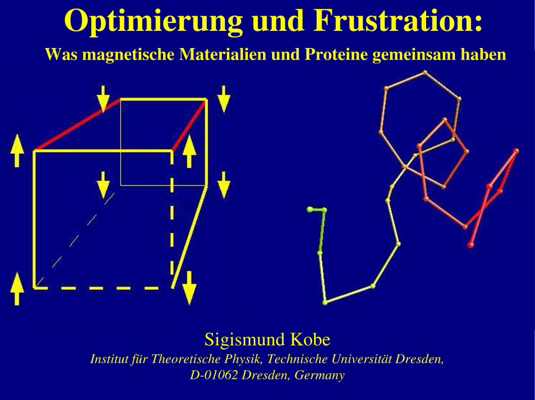
Optimierung und Frustration: Was magnetische Materialien und Proteine gemeinsam haben 

Sigismund KobeInstitut für Theoretische Physik, Technische Universität Dresden, 

D­01062 Dresden, Germany

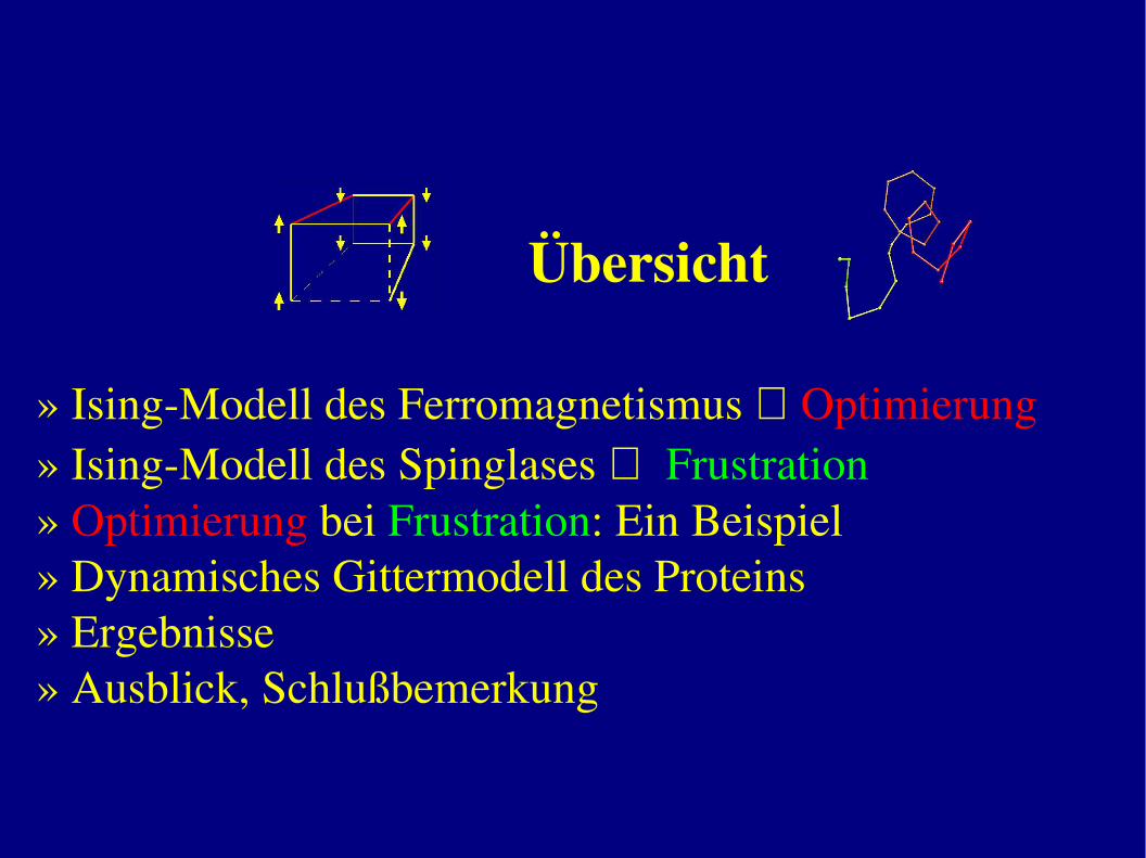
Übersicht

» Ising­Modell des Ferromagnetismus ⇒ Optimierung » Ising­Modell des Spinglases ⇒ Frustration» Optimierung bei Frustration: Ein Beispiel» Dynamisches Gittermodell des Proteins» Ergebnisse» Ausblick, Schlußbemerkung

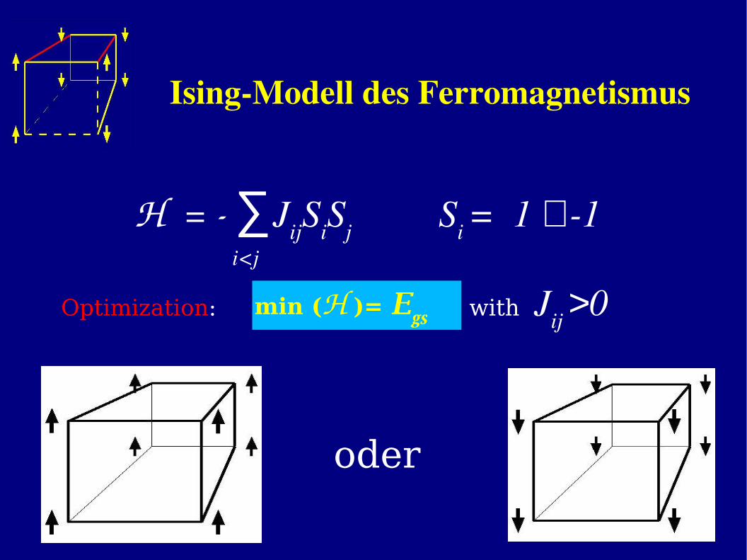
Ising­Modell des Ferromagnetismus

H  = ­ ∑JijSiSj                Si =  1 ∨ ­1                   i<j

Optimization: with Jij >0

oder

min (H )= Egs

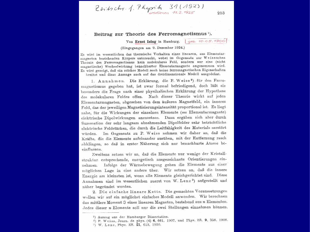
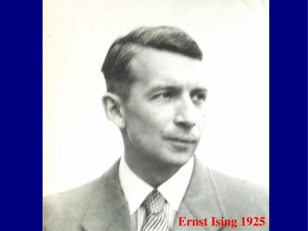
                                           Ernst Ising 1925

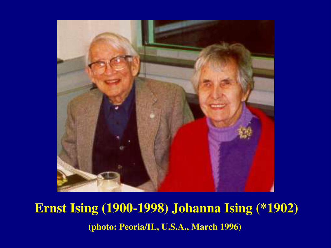
Ernst Ising (1900­1998) Johanna Ising (*1902)(photo: Peoria/IL, U.S.A., March 1996) 

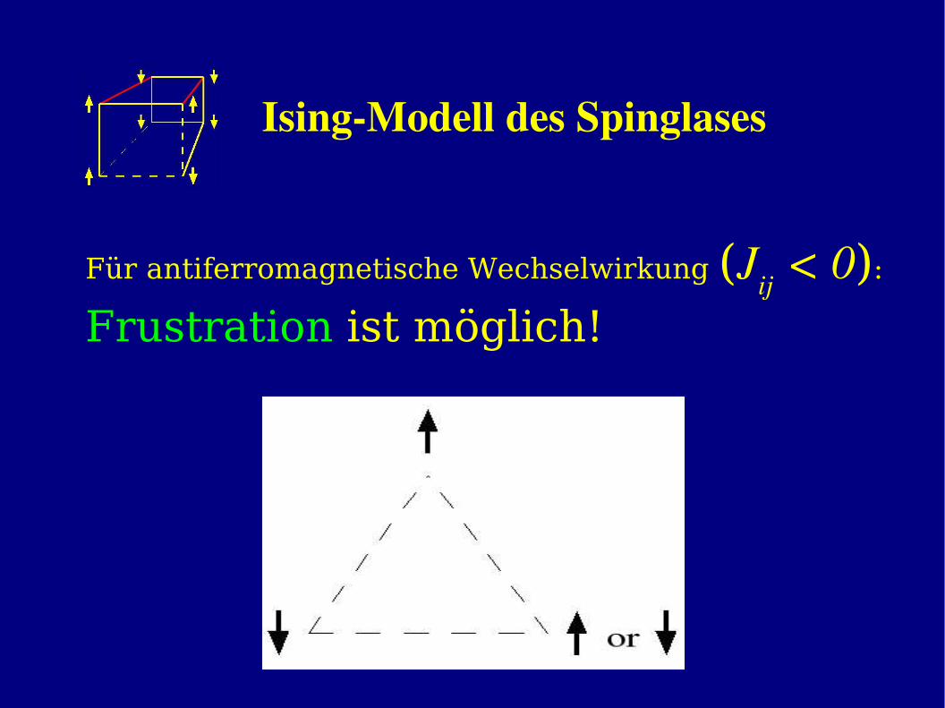
Ising­Modell des Spinglases

Für antiferromagnetische Wechselwirkung (Jij  < 0):

Frustration ist möglich!

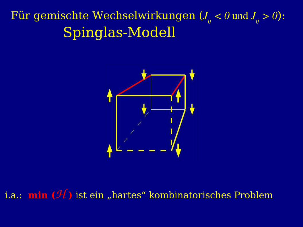
Für gemischte Wechselwirkungen (Jij  < 0 und Jij  > 0):

Spinglas-Modell

i.a.: min (H ) ist ein „hartes“ kombinatorisches Problem

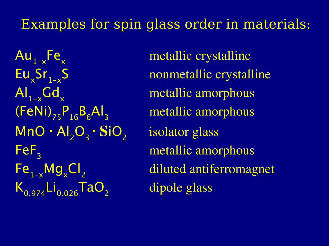
Examples for spin glass order in materials:

Au1-xFex metallic crystallineEuxSr1-xS nonmetallic crystallineAl1-xGdx metallic amorphous(FeNi)75P16B6Al3 metallic amorphous

MnO ∙ Al2O3 ∙ SiO2 isolator glassFeF3 metallic amorphousFe1-xMgxCl2 diluted antiferromagnetK0.974Li0.026TaO2 dipole glass

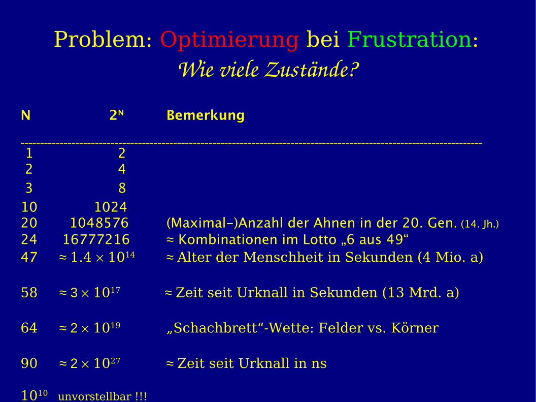
Problem: Optimierung bei Frustration:Wie viele Zustände?

N 2N Bemerkung

______________________________________________________________________________________________________________________

1 2 2 4 3 810 102420 1048576 (Maximal-)Anzahl der Ahnen in der 20. Gen. (14. Jh.)

24 16777216 ≈ Kombinationen im Lotto „6 aus 49“47 ≈ 1.4 1014 ≈ Alter der Menschheit in Sekunden (4 Mio. a)

58 ≈ 3 1017 ≈ Zeit seit Urknall in Sekunden (13 Mrd. a)

64 ≈ 2 1019 „Schachbrett“-Wette: Felder vs. Körner

90 ≈ 2 1027 ≈ Zeit seit Urknall in ns

1010 unvorstellbar !!!

.

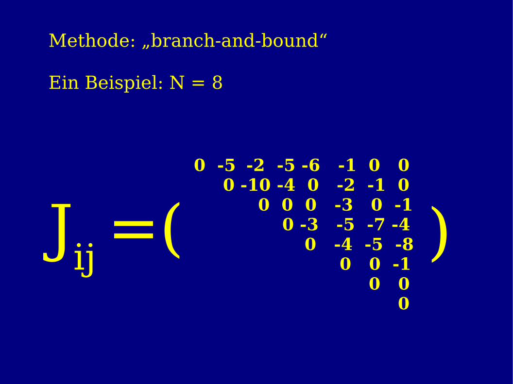
Methode: „branch-and-bound“

Ein Beispiel: N = 8

Jij =(

) )0 -5 -2 -5 -6 -1 0 0 0 -10 -4 0 -2 -1 0 0 0 0 -3 0 -1 0 -3 -5 -7 -4

0 -4 -5 -8 0 0 -1

0 0 0

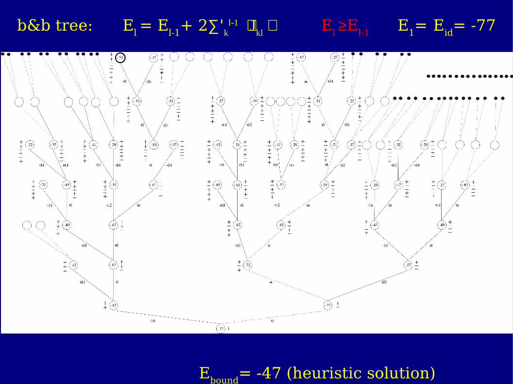
b&b tree: El = El-1+ 2∑ 'k

l-1 Jkl El ≥ El-1 E1= Eid= -77

Ebound= -47 (heuristic solution)

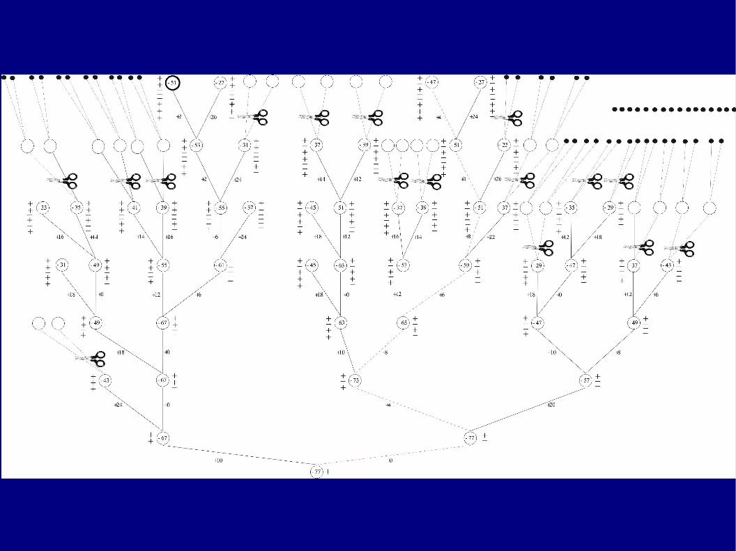
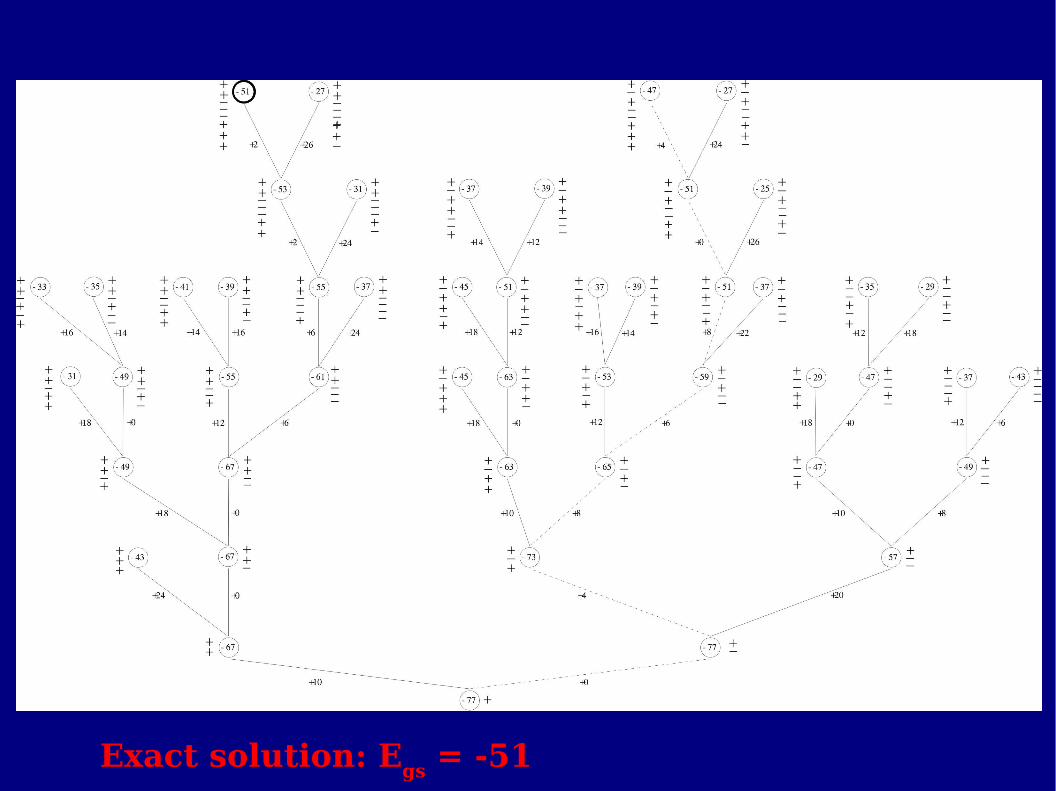
Exact solution: Egs = -51

Molecular modeling of biological structures

Optimization and Frustration in:

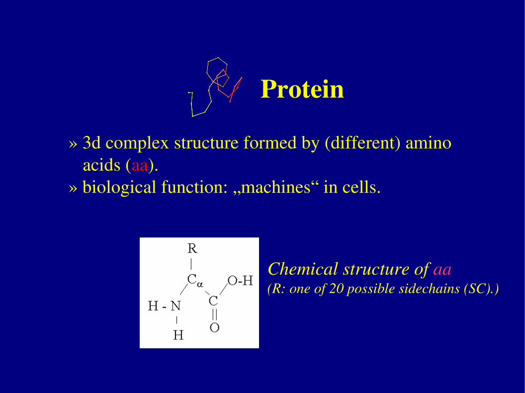
Protein

» 3d complex structure formed by (different) amino acids (aa).

» biological function: „machines“ in cells.

Chemical structure of aa (R: one of 20 possible sidechains (SC).)

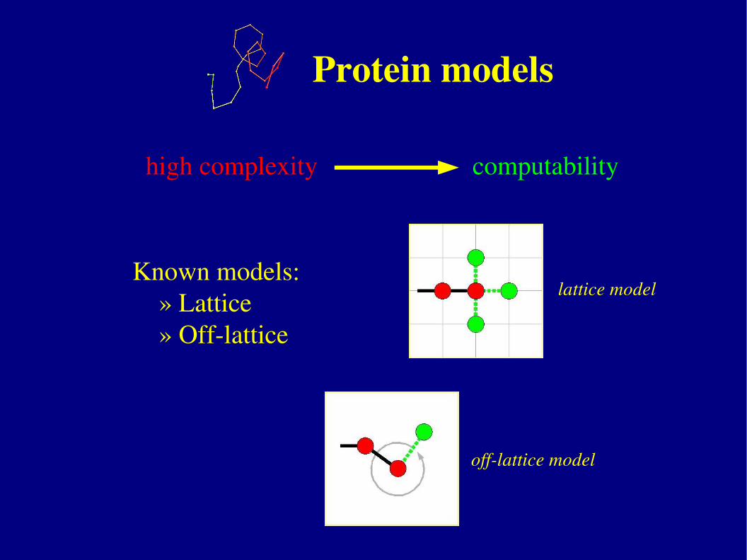
Protein models

Known models:» Lattice» Off­lattice

lattice model

off­lattice model

high complexity computability

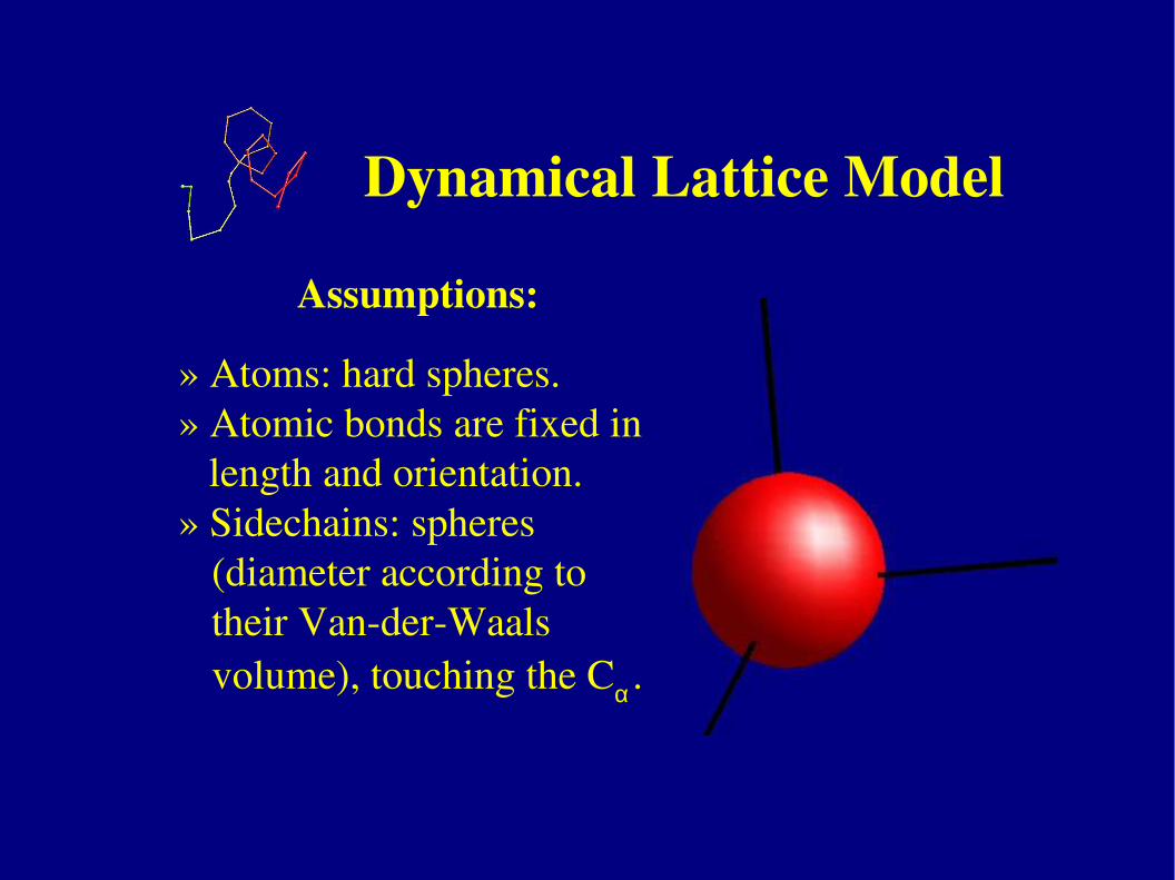
Dynamical Lattice Model

Assumptions:

» Atoms: hard spheres.» Atomic bonds are fixed in 

length and orientation.» Sidechains: spheres 

(diameter according to their Van­der­Waals volume), touching the Cα.

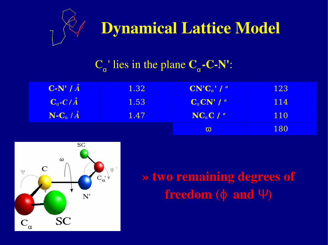
Dynamical Lattice Model

C-N' / Å 1.32 CN'Cα' / º 123

Cα­C / Å 1.53 CαCN' / º 114

N-Cα / Å 1.47 NCαC / º 110

ω 180

Cα ' lies in the plane Cα­C­N':

» two remaining degrees of freedom (ϕ  and Ψ)

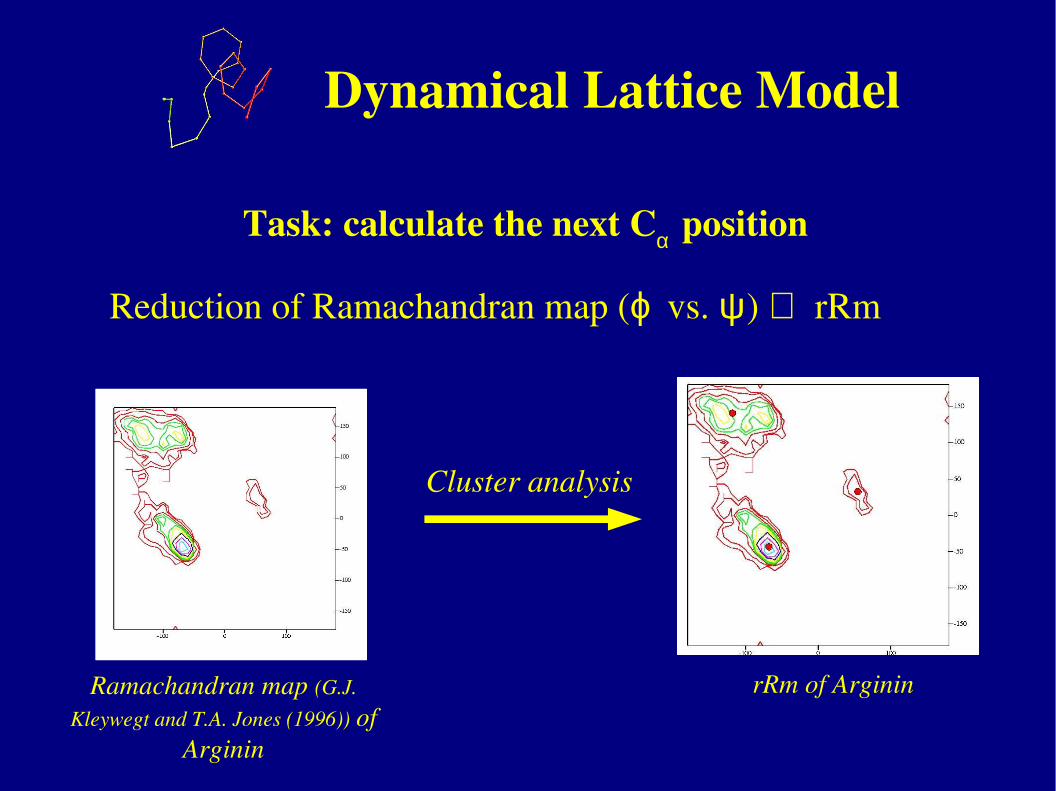
Dynamical Lattice Model

Reduction of Ramachandran map (ϕ   vs. ψ  ) ⇒  rRm

Cluster analysis

Ramachandran map (G.J. 

Kleywegt and T.A. Jones (1996)) of Arginin

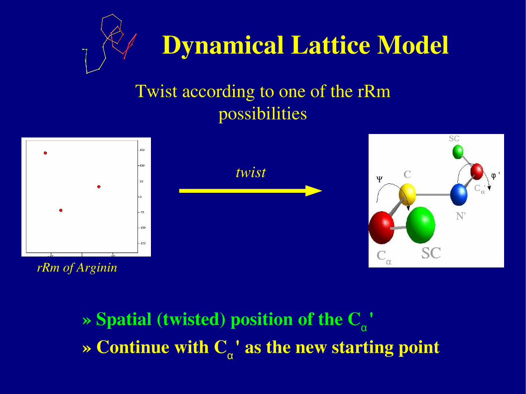
rRm of Arginin

Task: calculate the next Cα position

Dynamical Lattice Model

Twist according to one of the rRm possibilities

twist

» Spatial (twisted) position of the Cα'» Continue with Cα' as the new starting point

rRm of Arginin 

Dynamical Lattice Model

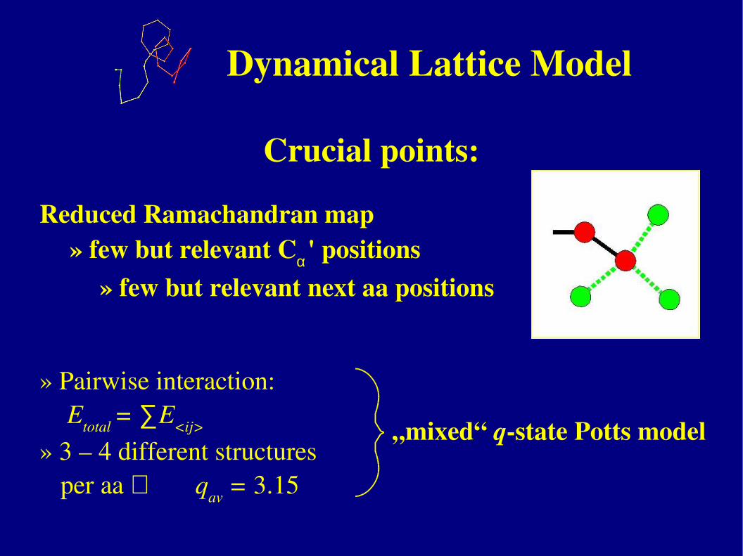
Reduced Ramachandran map» few but relevant Cα' positions

» few but relevant next aa positions

Crucial points:

» Pairwise interaction:Etotal = ∑E<ij>

» 3 – 4 different structures per aa ⇒ qav = 3.15

„mixed“ q­state Potts model

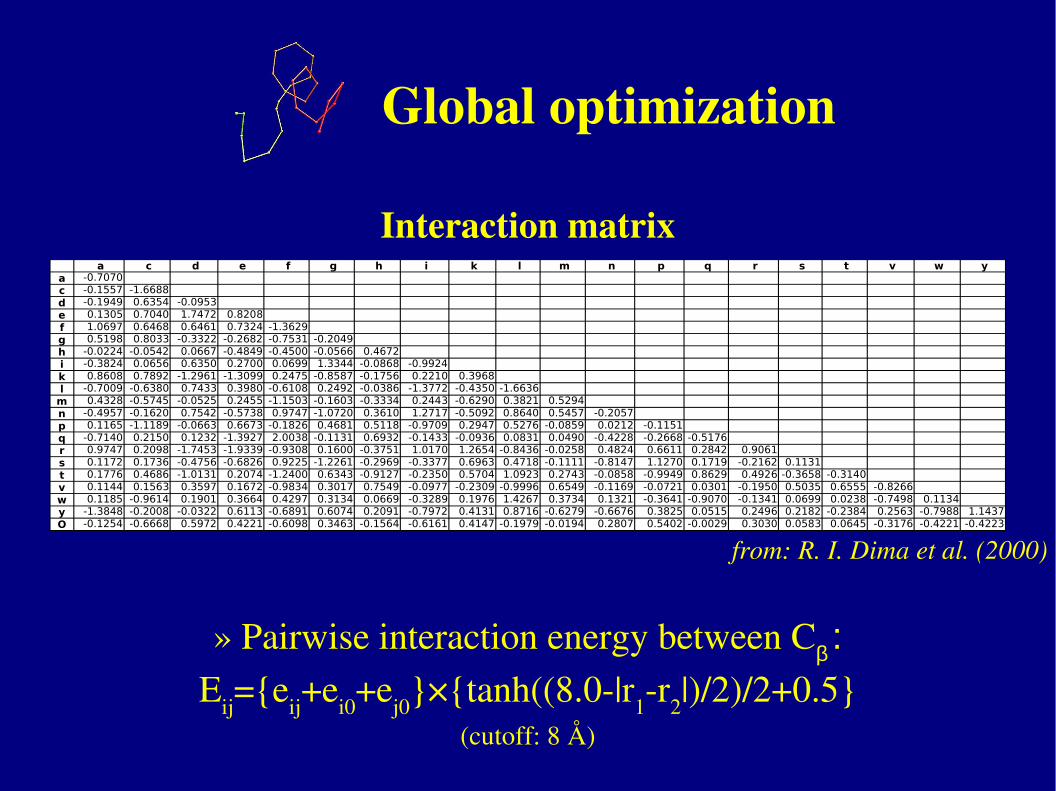
Global optimization

from: R. I. Dima et al. (2000)

Interaction matrix

» Pairwise interaction energy between Cβ : Eij={eij+ei0+ej0}×{tanh((8.0­|r1­r2|)/2)/2+0.5}

(cutoff: 8 Å)

a c d e f g h i k l m n p q r s t v w ya -0.7070c -0.1557 -1.6688d -0.1949 0.6354 -0.0953e 0.1305 0.7040 1.7472 0.8208f 1.0697 0.6468 0.6461 0.7324 -1.3629g 0.5198 0.8033 -0.3322 -0.2682 -0.7531 -0.2049h -0.0224 -0.0542 0.0667 -0.4849 -0.4500 -0.0566 0.4672i -0.3824 0.0656 0.6350 0.2700 0.0699 1.3344 -0.0868 -0.9924k 0.8608 0.7892 -1.2961 -1.3099 0.2475 -0.8587 -0.1756 0.2210 0.3968l -0.7009 -0.6380 0.7433 0.3980 -0.6108 0.2492 -0.0386 -1.3772 -0.4350 -1.6636

m 0.4328 -0.5745 -0.0525 0.2455 -1.1503 -0.1603 -0.3334 0.2443 -0.6290 0.3821 0.5294n -0.4957 -0.1620 0.7542 -0.5738 0.9747 -1.0720 0.3610 1.2717 -0.5092 0.8640 0.5457 -0.2057p 0.1165 -1.1189 -0.0663 0.6673 -0.1826 0.4681 0.5118 -0.9709 0.2947 0.5276 -0.0859 0.0212 -0.1151q -0.7140 0.2150 0.1232 -1.3927 2.0038 -0.1131 0.6932 -0.1433 -0.0936 0.0831 0.0490 -0.4228 -0.2668 -0.5176r 0.9747 0.2098 -1.7453 -1.9339 -0.9308 0.1600 -0.3751 1.0170 1.2654 -0.8436 -0.0258 0.4824 0.6611 0.2842 0.9061s 0.1172 0.1736 -0.4756 -0.6826 0.9225 -1.2261 -0.2969 -0.3377 0.6963 0.4718 -0.1111 -0.8147 1.1270 0.1719 -0.2162 0.1131t 0.1776 0.4686 -1.0131 0.2074 -1.2400 0.6343 -0.9127 -0.2350 0.5704 1.0923 0.2743 -0.0858 -0.9949 0.8629 0.4926 -0.3658 -0.3140v 0.1144 0.1563 0.3597 0.1672 -0.9834 0.3017 0.7549 -0.0977 -0.2309 -0.9996 0.6549 -0.1169 -0.0721 0.0301 -0.1950 0.5035 0.6555 -0.8266w 0.1185 -0.9614 0.1901 0.3664 0.4297 0.3134 0.0669 -0.3289 0.1976 1.4267 0.3734 0.1321 -0.3641 -0.9070 -0.1341 0.0699 0.0238 -0.7498 0.1134y -1.3848 -0.2008 -0.0322 0.6113 -0.6891 0.6074 0.2091 -0.7972 0.4131 0.8716 -0.6279 -0.6676 0.3825 0.0515 0.2496 0.2182 -0.2384 0.2563 -0.7988 1.1437O -0.1254 -0.6668 0.5972 0.4221 -0.6098 0.3463 -0.1564 -0.6161 0.4147 -0.1979 -0.0194 0.2807 0.5402 -0.0029 0.3030 0.0583 0.0645 -0.3176 -0.4221 -0.4223

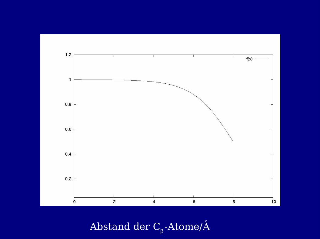
Abstand der Cβ -Atome/Å

Global optimization

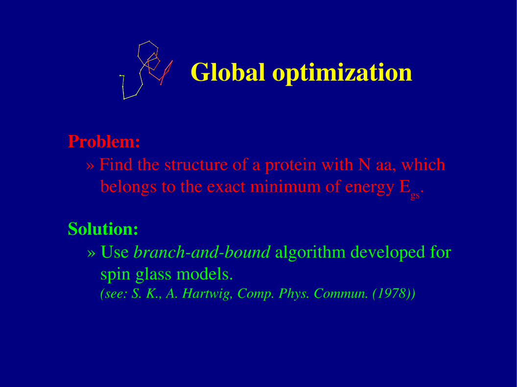
Problem:» Find the structure of a protein with N aa, which 

belongs to the exact minimum of energy Egs.

Solution:» Use branch­and­bound algorithm developed for 

spin glass models.(see: S. K., A. Hartwig, Comp. Phys. Commun. (1978))

Results

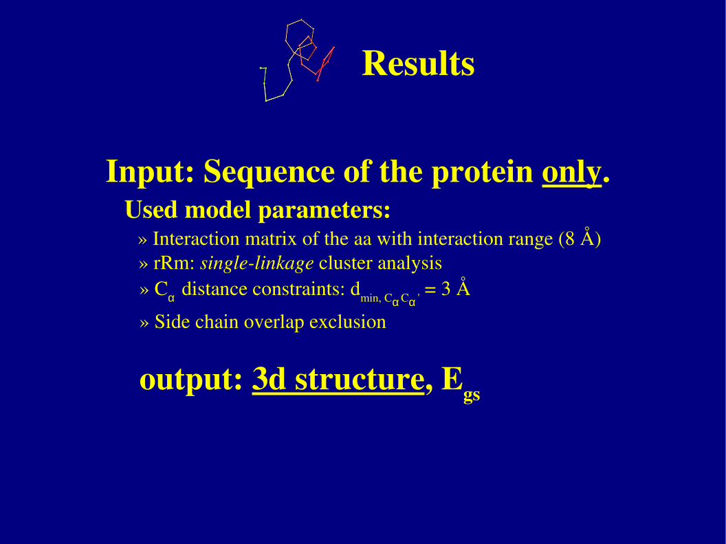
Input: Sequence of the protein only.Used model parameters:

» Interaction matrix of the aa with interaction range (8 Å)» rRm: single­linkage cluster analysis » Cα distance constraints: dmin, CαCα ' = 3 Å

» Side chain overlap exclusion

output: 3d structure, Egs

Results

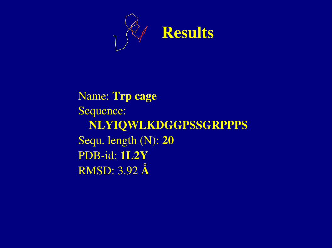
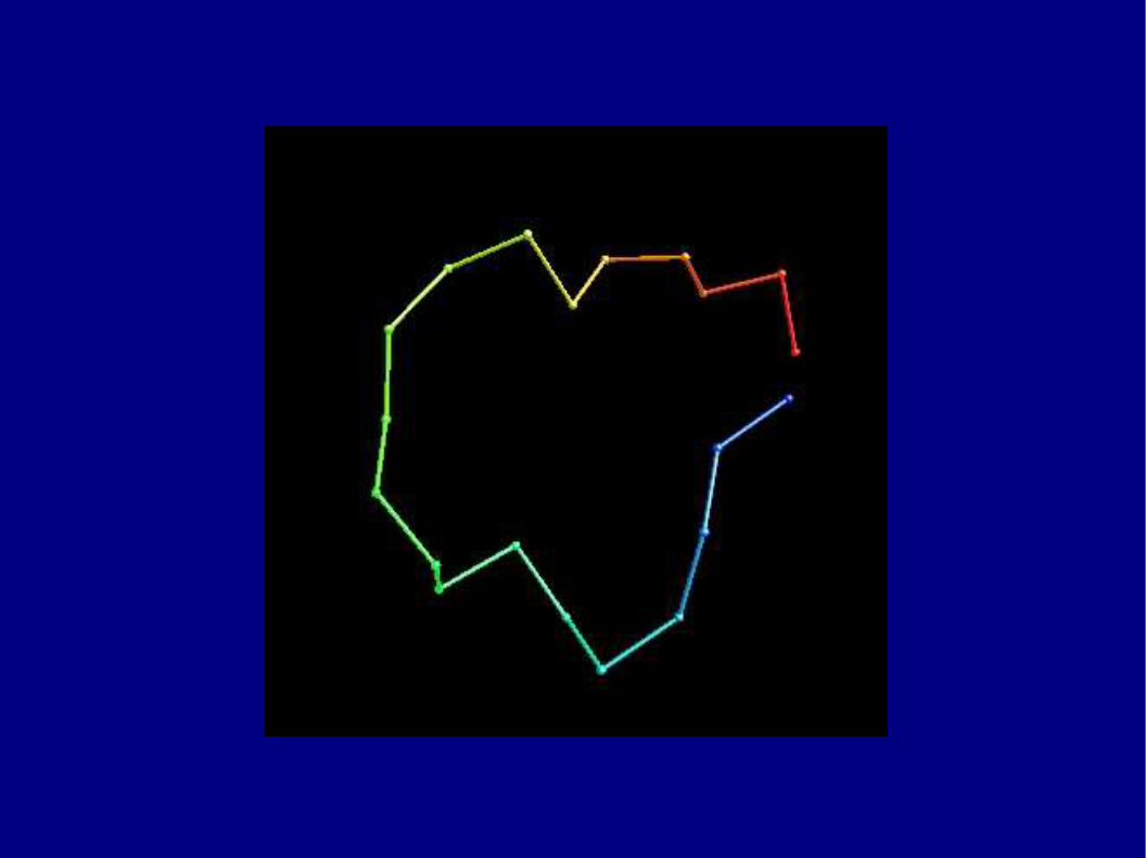
Name: Trp cageSequence:

NLYIQWLKDGGPSSGRPPPSSequ. length (N): 20PDB­id: 1L2YRMSD: 3.92 Å

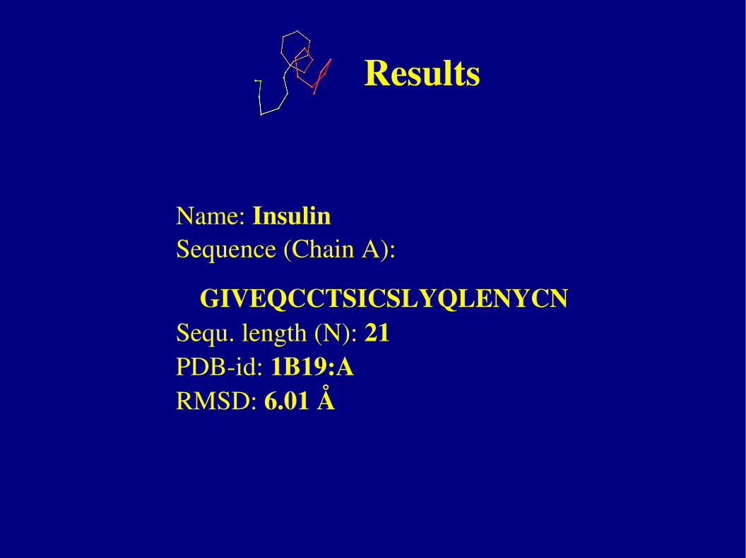
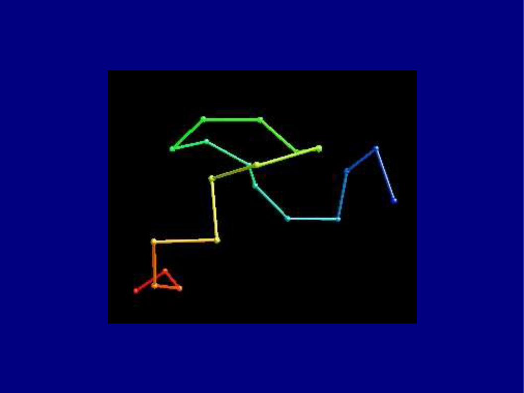
Results

Name: InsulinSequence (Chain A):

GIVEQCCTSICSLYQLENYCNSequ. length (N): 21PDB­id: 1B19:ARMSD: 6.01 Å

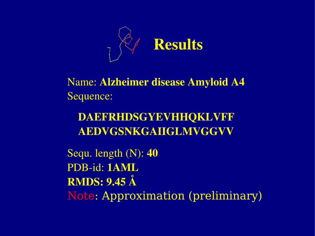
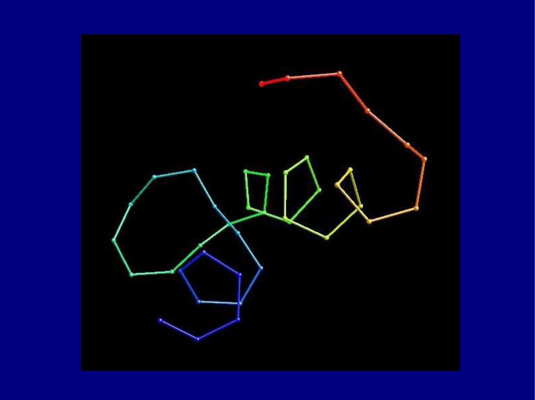
Results

Name: Alzheimer disease Amyloid A4Sequence:

DAEFRHDSGYEVHHQKLVFFAEDVGSNKGAIIGLMVGGVV

Sequ. length (N): 40PDB­id: 1AMLRMDS: 9.45 ÅNote: Approximation (preliminary)

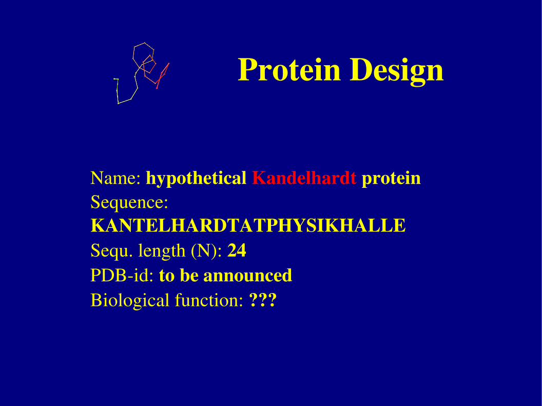
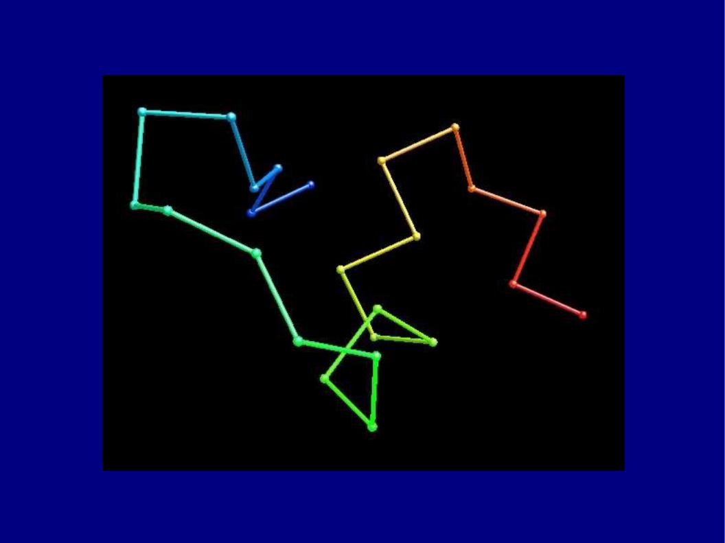
Name: hypothetical Kandelhardt proteinSequence: KANTELHARDTATPHYSIKHALLESequ. length (N): 24PDB­id: to be announcedBiological function: ???

Protein Design

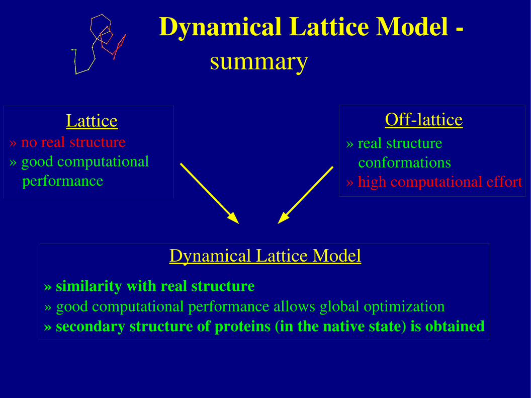
Dynamical Lattice Model

» similarity with real structure» good computational performance allows global optimization» secondary structure of proteins (in the native state) is obtained

Lattice» no real structure» good computational 

performance

Off­lattice» real structure 

conformations» high computational effort

Dynamical Lattice Model ­        summary

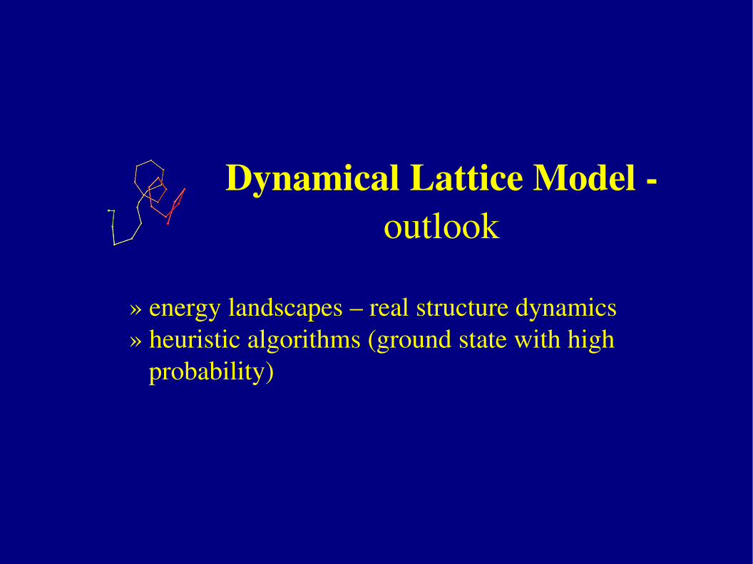
» energy landscapes – real structure dynamics» heuristic algorithms (ground state with high 

probability)

Dynamical Lattice Model ­ outlook

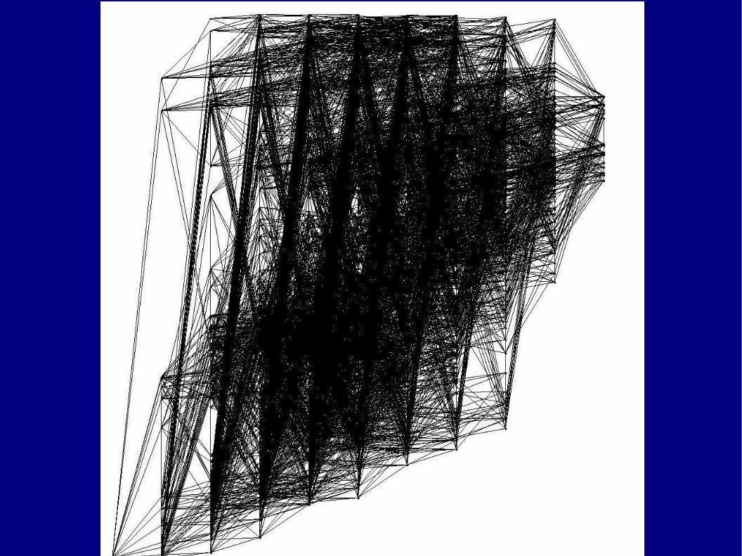
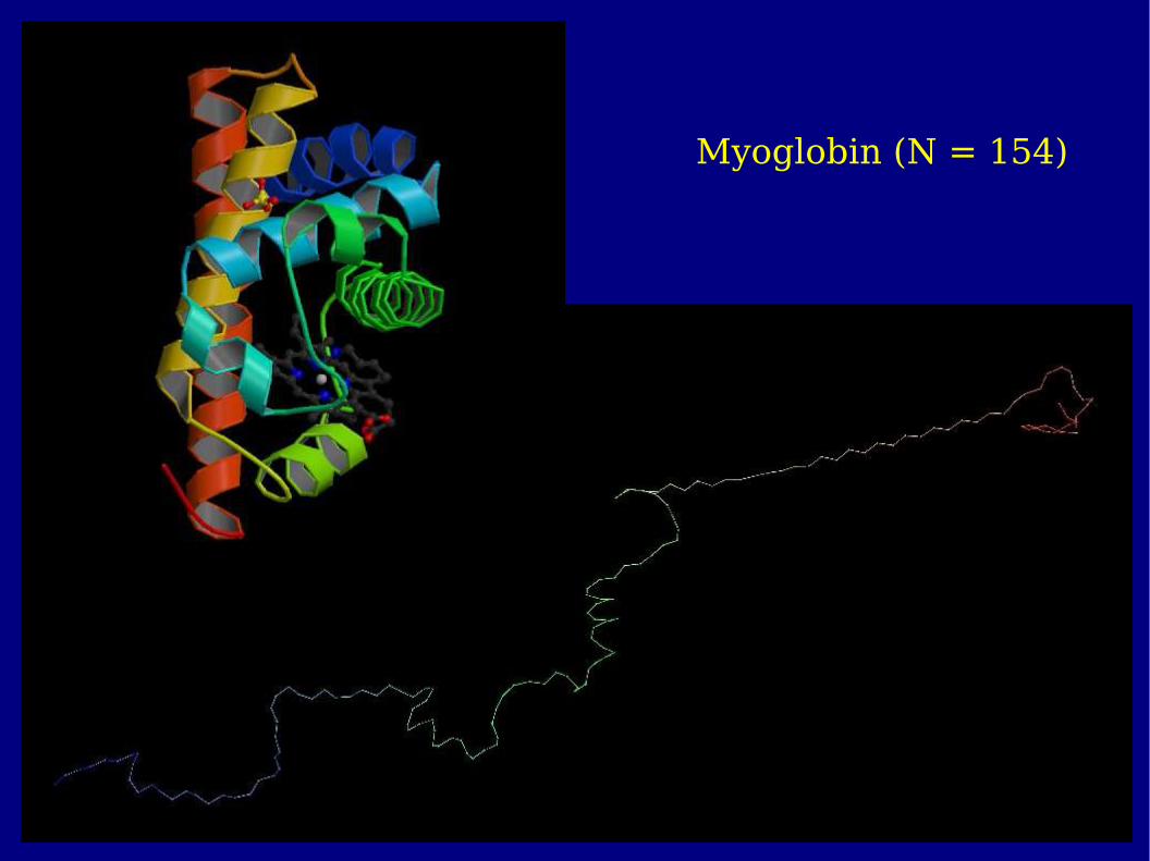
Myoglobin (N = 154)

Schlußbemerkung:

» Optimierung and Frustration    sind grundlegende Konzepte in der Natur» Beispiele (Modelle):­   Magnetische Ordnung in Materialien­   Räumliche Struktur von Proteinen

Acknowledgment: Frank Dressel, Andreas Hartwig