Thilo  StreckBiogeophysik

Ins4tut  für  Bodenkunde  und  StandortslehreUniversität  Hohenheim,  Stu@gart

Rückkopplungen  an  der  Landoberfläche

Typischer  Ablauf  in  der  Anpassungsforschung

Pflanzenwachs-­‐tumsmodell

ÖkonomischeBewertung

Handlungs-­‐opDonen

Böden,  Landnutzung

Management

ÖkonomischeRahmenbedingungen

Entwicklungs-­‐szenarien

Globale  KlimaprojekDon

Regionale  KlimaprojekDon

LandwirtschaHliche  Erträge  im  Jahr  2050

Herm

ans  e

t  al.  (2010)

1.  Wie  genau  sind  Klimamodelle?

Warrach-­‐Sagi  et  al.  (2012,  subm.)

Spa

tial p

df

modeledobserved

Precipitation, mm/monthSommerniederschläge  (JJA),  1990-­‐2008,  Vergleich  von  WRF331-­‐NOAH  (12  km  Auflösung)  mit  DWD  REGNIE-­‐Datensatz

2.  Wie  genau  sind  Pflanzenwachstumsmodelle?

Sommergerste,  7  Standorte  in  Nord-­‐  und  MiWeleuropa,44  Wachstumsperioden

R.P. Rötter et al. / Field Crops Research 133 (2012) 23–36 31

OBSERVEDWOFOST

STICSMONICAHERMESFASSET

DSSAT!CERESDAISY

CROPSYSTAPES!ACE

0 2000 4000 6000 8000

Grain yield [kg ha!1, dry matter]

a b

c d

WOFOST

STICS

MONICA

HERMES

FASSET

DSSAT!CERES

DAISY

APES!ACE

0 500 1500 2500 3500

Root biomass [kg ha!1, dry matter]

WOFOST

STICS

MONICA

HERMES

FASSET

DSSAT!CERES

DAISY

CROPSYST

APES!ACE

0 5000 10000 15000 20000

TAGB [kg ha!1, dry matter]

WOFOST

STICS

MONICA

HERMES

FASSET

DSSAT!CERES

DAISY

CROPSYST

APES!ACE

0.3 0.4 0.5 0.6 0.7

Harve st index

Fig. 5. Box-and-whisker plots of (a) grain yield estimates of models and observations, (b) root biomass estimates, (c) maximum above-ground biomass estimates, and (d)harvest indices of the models – among the simulated sites and years (N = 44). Boxes delimit the inter-quartile range (25–75 percentiles) and whiskers show the high and lowextreme values.

rank correlation coefficients of 0.552 and 0.49, respectively, wereperforming best for all seasons (N = 44), while for Verovany site(N = 14), models DSSAT-CERES, WOFOST and HERMES showedhighest rank correlation coefficients (0.539, 0.537 and 0.488,respectively).

4. Discussion

4.1. Uncertainty levels

Our results from this barley model comparison show that sim-ulated grain yields vary widely, ranging from 1700 to 8100 kg ha!1

for all sites and seasons, being similar to the observed range

(2400–8100 kg ha!1). However, there were considerable differ-ences in estimates for individual sites and years among the models(Figs. 3–5 and 7). Under conditions of limited data available for cal-ibration (as in this blind test), uncertainty ranges in yield estimatesfrom individual models are mostly not acceptable and beyond themeasurement error of about 10–15% found in field experiments(Joernsgaard and Halmoe, 2003). This result is similar to the winterwheat study by Palosuo et al. (2011) and confirms that the differ-ences in estimates of grain yield between models, and betweenthe models and field observations have not much decreased whencompared to earlier model comparisons for wheat, where yieldswere off by 20% and more (Goudriaan et al., 1994; Jamieson et al.,1998).

Ertrag in kg ha-1

RöPer  et  al.  (2012,  verändert)

R.P. Rötter et al. / Field Crops Research 133 (2012) 23–36 29

APES!ACE

020

0040

0060

0080

00 CROPSYST DAISY

DSSAT!CERES

020

0040

0060

0080

00 FASSET HERME S

MONICA

020

0040

0060

0080

00 STICS

0 2000 4000 6000 8000

WOFOST

0 2000 4000 6000 8000MEAN

0 2000 4000 6000 80000

2000

4000

6000

8000

LedniceVerovanyBratislavaFlakkebjergJyndeva dFoulumJokioinen

Obse

rved

grain

yield

[kg

ha!1

, dry

matt

er]

Simulated grain yield [kg ha!1, dry matter]

Fig. 3. Simulated and observed grain yield estimates [kg ha!1, dry matter] for 44 studied growing seasons. Simulation results are shown for nine individual models andmulti-model means. Different study sites are depicted with different symbols. The 1:1 line is shown, representing perfect agreement.

Exceptions include Bratislava in 1994, Flakkeberg in 2006 andJokioinen in 2005.

At the two Czech sites, the “best model” HERMES estimatesyields slightly better than the MMM (Fig. 7). Overall, however,the MMM is a slighly better predictor than HERMES as indicatedby RMSE and IA (Fig. 4). Two other models, DAISY and WOFOSTalmost perform as well as the “best model”. However, their “bestperformances” look quite different, as we found when plotting yieldestimates by the individual models vis a vis observed (not shown)

as in Fig. 7. Except for Bratislava site, DAISY tends to underesti-mate observed yields and remains below the MMM. This is mostpronounced for the Czech and Finnish sites. WOFOST, on the otherhand, in most cases overestimates observed yields, on average byabout 1000 kg ha!1.

For all growing seasons, and for Verovany site separately,we also calculated Spearman’s rank correlations (not shown) toexamine how well the models are in reproducing the order ofobserved yields. Models DAISY and WOFOST, with Spearman’s

Gem

esse

n (k

g ha

-1)

Simuliert (kg ha-1)

+  25%

-­‐  25%

MulU  Model  Mean  

Symbole = Standorte

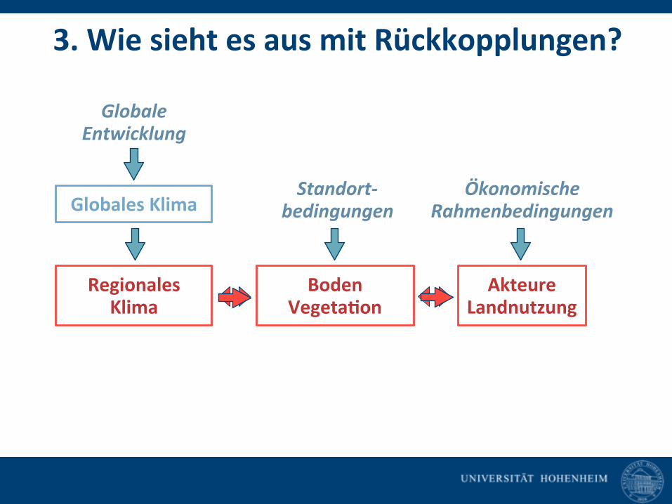
3.  Wie  sieht  es  aus  mit  Rückkopplungen?  

BodenVegetaDon

AkteureLandnutzung

Standort-­‐bedingungen

ÖkonomischeRahmenbedingungen

Globale  Entwicklung

Globales  Klima

Regionales  Klima

Prozesse  und  Rückkopplungen  im  Landsystem

Atmosphärische  Grenzschicht

WolkenbildungNiederschlag

Boden-­‐bearbeitung,Management

Bestandes-­‐entwicklungLAI,  Albedo

Bodenwasser-­‐haushalt

Energiebilanz

Landnutzungs-­‐entscheidungen

Einstrahlung

FOR  1695

Einfluss  der  Bodenfeuchte  auf  die  regionale  Niederschlagsverteilung

Niederschlag (m

m)

Avissar  und  Liu  (1996)

WeWer-­‐  und  Klimamodelle

MM5

NOAH

WRF

CLM

COSMO

Terra  ML

Atmosphärenmodelle

Landoberflächenmodelle

WRF

NOAH-­‐MP

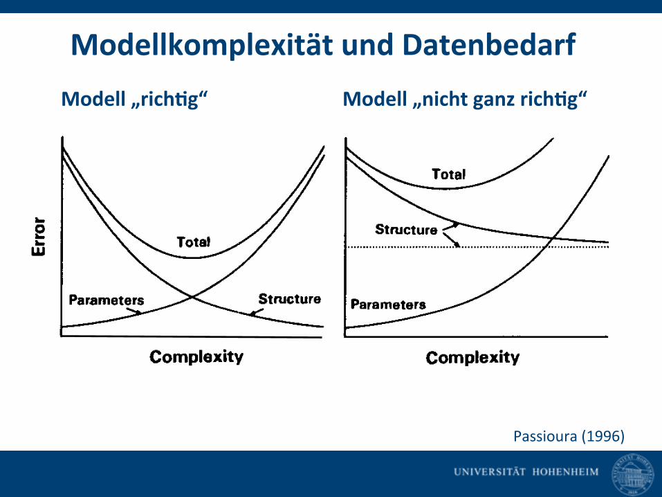
Modellkomplexität  und  DatenbedarfModell  „richDg“ Modell  „nicht  ganz  richDg“

692 AGRONOMY JOURNAL, VOL. 88, SEPTEMBER-OCTOBER 1996

ters, for example those defining hydraulic conductivity,with increasing spatial resolution. If the flow is occurringpreferentially, however, for example in continuous mac-ropores, or if there are perched water tables that resultin lateral flow in the soil, then the one-dimensional modelis inappropriate, and persisting with it while increasingthe level of spatial detail is futile.

It is in the realm of environmental physics, though,that we probably do know enough about the structureof the main processes for us to be reasonably confidentof our predictions, at least where they concern theaboveground microenvironment within crop canopies.A good example of success in this area is that of Berryet al. (1991), whose simulation of the environment closeto the Surface of transpiring corn (Zea mays L.) leavesgave good insights into the interactions between preyand predator mites.

Reynolds and Acock (1985), following R.V. O’Neill,have discussed sources of error in relation to the complex-ity of models. They dissected the notional total error intotwo components, one arising from errors in estimatingparameters, the other arising from systematic bias re-sulting from oversimplifying. They postulated that cumu-lative errors in the parameters grow with the number ofthe parameters as a model becomes more complex. Andthey postulated that this systematic bias (which is similarto what I have been calling erroneous structure) decreasesas complexity increases. Figure 3a, adapted from theirFig. 5 illustrates this argument. Their argument is con-vincing where we are sure of the fundamental structureof the system-for example, adding a wing mirror tothe simulated model of a car will improve our prospectsof predicting the overall aerodynamic drag. The aerody-namic principles are well understood. However, if thestructure is fundamentally wrong, as it could be in theexample of photosynthetically driven growth illustratedin Fig. 2, then no amount of complexity will improvethe structural error. There will be an irreducible mini-mum error, as illustrated by the dotted asymptote inFig. 3b.

Occasionally, though, the structure seems to be sowrong that no amount of adjusting of the parametersenables the model to fit the data. When that happens,we have moved beyond the realm of validation and arein a position to discover something new. A good example

a b

Complexity ComplexityFig. 3. Notional components or’prediction error in modeis of increasing

complexity: (a) when the structure of the system is well understood;(b) when the structure is wrong, with the irreducible structuralerror represented by the dotted asymptote (after Reynolds andAcock, 1985). Complexity and error increase away from the inter-eept.

is the problem that the CERES models met with theirroutine for the withdrawal of water from the subsoil (J.T.Ritchie, personal communication, 1983). This routinegreatly overestimated the rate of uptake by the roots,even when the measured root length density was used.The disagreement stimulated research into alternativestructures for the routine: for example, that the rootswere not uniformly distributed through the given layerof soil, but were clumped into preexisting pores or cracks(Passioura, 1991).

Another example comes from Loomis et al. (1976),whose sugar beet (Beta vulgaris L.) model failed whenthey changed plant density, owing to its having the wrongstructure for partitioning assimilate between root andshoot. This failure stimulated work on reciprocal graftsbetween beet (large root, small leaves) and chard (smallroot, large leaves) that showed that the voracious appetiteof a small fraction of the cells in the root of the beetlargely determined the size of the axis (Rapoport andLoomis, 1986).

Even if the structure is right, as it might be in someof the leaching models when they are applied to soilsin which the flow is essentially one-dimensional, themodels can rarely be applied with confidence to a field,because the parameters vary greatly in space. We haveto assume average values of, say, the hydraulic conduc-tivity to apply the Richards equation, and because thisequation is not linear, the averaging is an art rather thana well-defined procedure, and often works poorly.

EDUCATIONSo far, the part played by the large mechanistic simula-

tion models of crops, those that aspire to occupy thescientific end of the spectrum, seems to have been largelyone of self-education for the developer. Perhaps this isinevitable: these models are typically so complex thatnobody but the developer is likely to have the enthusiasmto dip inside them. Thus, they are not transmissible toothers in the sense that the research described in a typicalresearch paper is transmissible. We do not know enoughabout the structure of the soil-plant-atmosphere systemto expect such models to be accurate, except perhaps inthe domain of the aboveground microenvironment. Theyare too complex to be tested as entities, but talenteddevelopers enhance their understanding of the interac-tions that occur and that may be far from obvious. Theformidable understanding of the interacting processeswithin plants, or between plants and their environment,that is evident in the writings of, for example, R.S.Loomis or J.M. Norman, has undoubtedly been honedby their developing mechanistic simulation models (see,for example, Loomis and Connor, 1992; Norman, 1989).At best, comprehensive mechanistic models of cropsgive structural insights to their developers. At worst,they are merely time-wasting ceremony. There is littlepoint, for example, in trying to cope with the structuraldifficulty illustrated in Fig. 2 by creating a simulationmodel that combines both scenarios. Such a model wouldmerely be an elaborate shopping list of disposable param-eters having no predictive value.

Passioura  (1996)

Räumliche  Auflösung  und  Modellfehler

0 1 2 3 4 5 6 7 8 9 10

0

1

2

3

4

5

6

7

8

9

10

Räumliche Auflösung

Kum

ulat

iver

Feh

ler

Topographie

Gesamt

Boden-Vegetation

Fehler:  Abweichung  zwischen  SimulaUon  und  Messung

Höhe  über  NN  in  m

Topographie  Südwestdeutschlandsbei  unterschiedicher  Auflösung

Auflösung  7  km Auflösung  1  km

Bauer et al. (2007)

Niederschlag  in  SüdwestdeutschlandSommer  2005,  simuliert  mit  MM5-­‐NOAH

Auflösung  7  km Auflösung  1  km

Bauer et al. (2007)

mm/Tag

Räumliche  Auflösung  regionaler  KlimasimulaDonenSchär  et  al.  (2004)56  km  GiPer

THE FUTURE OF DRY AND WET SPELLS IN EUROPE

linear trend from the seasonal mean values of bothperiods (Raisanen, 2002). As a measure for interannualvariability, the mean of the squared deviations of theseasonal values from the linear fit (mean-squared error;MSE) is further used and the projected changes arecalculated as ratios between future and baseline MSE.The pooled residuals of the eight models are used toassess the statistical significance of the seasonal changesin interannual variability. The pooled residuals partlyshow severe deviations from normality and, therefore, theFligner–Killeen test is applied which proofed to be mostrobust against non-normally distributed data (Conoveret al., 1981).

Significance levels lower than 1, 1–5, 5–10 and greaterthan 10% are termed as highly significant, significant,weakly significant and insignificant, respectively.

Uncertainties of the projected changes are quantifiedby two different measures. First, the inter-model stan-dard deviation is calculated. With the information of themulti-model mean change, probabilities of the projectedchanges can be derived. According to the normal dis-tribution, about 68% of the climate change signals liewithin ±1 standard deviation, while already about 95%lie within ±2 standard deviations. Second, the percentageof models which coincide in the sign of change is calcu-lated as a nonparametric uncertainty measure. Applyingthe confidence terminology of the 4th Assessment Reportof the Intergovernmental Panel on Climate Change (IPCC4AR; Solomon et al., 2007), very high confidence, highconfidence, and medium confidence are reached if at least90% (in our study all 8 models), at least 80% (6 models),

and at least 50% (4 models) coincide in the sign ofchange, respectively.

4. Results and discussion

4.1. Changes in the mean, their significance,and uncertainty

For air temperature, Figure 5 displays maps of the errorcorrected seasonal multi-model mean change betweenbaseline (1961–1990) and future (2021–2050) periodover Europe. Air temperature changes are positive in allseasons, and the most responsive regions are the north-eastern parts of Europe in winter and southern Europein summer. The centred values in each box of Figure 9indicate the seasonal multi-model mean changes of thenine subregions. The magnitude of the change is lowestfor IL in summer with +1.04 K while the most sensi-tive regions (SC in winter and MD in summer) showa warming of +2.43 K. The brightness of the coloursof Figure 9 represents the level of significance of the t-test. It can be seen that highly significant shifts towardsincreasing air temperature are obtained for all seasons andsubregions. Concerning the uncertainty of the changes,all models agree in increasing air temperature (lower leftvalues in each box of Figure 9) and, therefore, very highconfidence can be attributed to the changes for all sea-sons and subregions. The inter-model standard deviation(lower right values in each box of Figure 9) is a factortwo to three (even more for some cases) smaller than themulti-model mean change, underpinning high confidenceof the projected changes.

–20 0 20

–20 0 20

5070

5070

(a)

–20 0 20

–20 0 20

5070

5070

(b)

–20 0 20

–20 0 20

5070

5070

(c)

–20 0 20

–20 0 2050

7050

70(d)

1.0

1.5

2.0

2.5

[K]

Figure 5. Multi-model mean change between 1961 and 1990, and 2021 and 2050 of the error-corrected RCMs for seasonal mean airtemperature for: (a) winter (DJF), (b) spring (MAM), (c) summer (JJA), and (d) autumn (SON). This figure is available in colour online at

wileyonlinelibrary.com/journal/joc

Copyright ! 2011 Royal Meteorological Society Int. J. Climatol. (2011)

Heinrich  &  Gobiet  (2011)ENSEMBLES-­‐KonsorUum25  km  GiPer

Kotlarski  (2011)CORDEX-­‐KonsorUum12  km  GiPer

FOR  1695  u.a.2  km  GiPer

•••

Böden  in  LandoberflächenmodellenBoden-

einheiten

BodenübersichtskarteBÜK 1000

72

Cosmo-DE (DWD) 7NOAH/NOAH-MP 13

Bodenarten  in  CLM

Bodenübersichtskarte  BÜK  1000

%T%S

Fernerkundung  mit  mulDtemporalen  RapidEye-­‐Daten

grassland corn winter crop rapeseed root crops other

Figure 4. CRFmulti-classification superimposed by GIS cropland

object borders (black borders) 6.5 Detailed results of CRFmulti

The association potential in CRFmulti is the context-free result of a separate Maximum-Likelihood-classification for each epoch (Equation 3). A section of the ML-classification result for the four individual epochs is displayed in Figure 5 a)-d). For most of the pixels the classification results for the epochs differ, sometimes three or even four different classes are assigned. Moreover the classification result within many fields is inhomogeneous. Overall the classification accuracy for the single epochs is 59.6%.

a) b)

c) d)

e) f)

grassland corn winter crop rapeseed root crops other

Figure 5 a)-d) Results of ML-classification for t=1...4; e) Result of CRFmulti-classification; f) Reference

By use of the temporal interaction potential (Equations 5-9) these results are set in temporal context and the overall accuracy is increased to 84.2%. Results of the CRFmulti-classification and the corresponding reference can be seen in Figure 5 e) and f).

7. CONCLUSION

In this work we presented two CRF-based approaches for multitemporal crop type analysis and tested them on RapidEye data of 4 epochs. Even with using just very few simple features, we achieved a classification accuracy of far over 80% for six crop type classes (grassland, corn, winter crop, rapeseed, root crops and other crops) with both approaches. Both of them performed better than a SVM-classification that served as a benchmark   with   the   “classic   approach”   CRFall being slightly better than CRFmulti. Nevertheless the CRFmulti approach generally has a higher potential for any kind of multitemporal analysis. Because of its flexibility in the definition of the temporal interaction potential, it is also applicable for tasks of change detection or multi-scale analysis..

ACKNOWLEDGEMENT

The implementation of the CRF-classification is based on “UGM:  A  Matlab  toolbox  for  probabilistic  undirected  graphical models”   by   Mark   Schmidt, http://people.cs.ubc.ca/~schmidtm/ Software/UGM.html. The research is funded by the Federal Ministry of Economics and Technology (BMWi) via the German Aerospace Center (DLR e.V.) under the funding number 50EE0914 and by the German Science Foundation (Deutsche Forschungs-gemeinschaft) under grant HE 1822/22-1.

REFERENCES

AdV, Arbeitsgemeindschaft der Vermessungsverwaltungen der Länder der Bundesrepublik Deutschland, 1997. ATKIS – Amtlich Topographisch-Kartographisches Informationssystem, Germany. http://www.atkis.de (accessed 2011-04-01).

Bishop, C. M., 2006. Pattern recognition and machine learning. 1st edition, Springer New York.

Burges, C. J. C., 1998. A Tutorial on Support Vector Machines for Pattern Recognition. Data Mining and Knowledge Discovery, 2, pp. 121–167.

Bruzzone, L., Cossu, R., Vernazza, G., 2004. Detection of land-cover transitions by combining multidate classifiers. Pattern Recognition Letters, 25(13), pp. 1491-1500.

Chang, C.C. and Lin, C.J., 2001 LIBSVM: a library for support vector machines. http://www.csie.ntu.edu.tw/~cjlin/libsvm/, accessed: 2011-04-01.

De  Wit,  A.  J.  W.  and  Clevers,  J.  G.  P.  W.,  2004.  Efficiency  and accuracy of per-field   classification   for   operational   crop  mapping. International Journal of Remote Sensing, 25(20), pp. 4091–4112.

Feitosa, R. Q., Costa, G. A. O. P., Mota, G. L. A., Pakzad, K., Costa, M. C. O., 2009. Cascade multitemporal classification

Müller  &  Hoberg  (2011)

Reference

SVM-classification

CRFall-classification

CRFmulti-classification

Legend: grassland corn winter crop rapeseed root crops other

Figure 3. Reference data and classification results in comparison 6.2 Description of manual reference

A manual reference is used that was made in the same year 2010 like the satellite images. It consists of 121 separate fields of an area of about 322ha and has been acquired by field walking. The portion of the individual crop types of the whole area is 12% grassland, 21% corn, 28% winter crop, 11% rapeseed, 11% root crops and 17% other crops. In the process an existing GIS was used to define the borders of single fields. The manual reference builds the training and evaluation sample for the test classifications. 6.3 CRF vs. SVM

For our tests we applied the cross-validation method by separation the learning sample into two equal parts. Tables 1-4 show the results for the two CRF-approaches and the SVM-classification. Overall 129001 pixels were classified. Both of the CRF-based approaches slightly outperform the SVM classification with CRFall being best. For all approaches the overall accuracy is far over 80%, only the class grassland is classified with lower accuracy in each case. The classification results for a section of 21 fields are displayed in Figure 3. In a next step, the majority of pixels belonging to a class in each reference fields was determined. This gives an idea of how good this approach is suited for classifying complete fields, ignoring classification errors at their borders. Applying CRFall 108 of the 121 reference fields were classified correctly (89.3%), with CRFmulti 102 fields were correct (84,3%). In general there are two main reasons for misclassifications: At first  some  fields  show  an  “untypical”  appearance  for  their  class,  e.g. most of the fields of one class are already harvested at one time of image acquisition but on some fields the crop is still present. Second some fields are very slender. So by using our feature extraction in an 11*11 window, their characteristics become blurred.

Cla Ref Gra Cor Win Rap Roo Oth

Gra 74.8 2.4 13.1 5.7 2.9 1.1 Cor 0.2 93.4 0 4.0 1.8 0.6 Win 1.0 3.3 88.7 2.7 1.9 2.3 Rap 0 4.5 0 95.5 0 0 Roo 0.8 2.3 0.5 0.1 95.2 1.0 Oth 2.7 6.8 4.0 0.4 9.4 76.7

Table 1. Confusion matrix for CRFall-classification

Cla Ref Gra Cor Win Rap Roo Oth

Gra 63.2 11.1 13.8 7.1 3.2 1.6 Cor 0.1 90.6 0.1 4.5 4.0 0.7 Win 2.1 0 94.9 0 0 2.9 Rap 0.8 17.7 0.2 81.2 0 0.2 Roo 0.3 13.5 0.1 0 83.5 2.7 Oth 1.5 7.4 3.4 0.3 7.1 80.4

Table 2. Confusion matrix for CRFmulti-classification

Cla Ref Gra Cor Win Rap Roo Oth

Gra 70.9 0.5 8.9 12.9 0.3 6.6 Cor 1.8 76.6 0.1 12.3 0.4 8.9 Win 3.2 0.2 87.7 0.6 0.1 8.1 Rap 4.3 6.5 0.5 88.6 0 0.1 Roo 1.1 3.7 1.6 0.5 83.4 8.9 Oth 2.4 0.6 6.3 0.5 5.3 84.9

Table 3. Confusion matrix for SVM-classification (Cla=classification, Ref=Reference, Gra=Grassland, Cor=Corn, Win=winter crop, Rap=rapeseed, Roo=root crops, Oth=other

crops.)

overall accuracy kappa CRFall 87.4 0.85

CRFmulti 84.2 0.81 SVM 82.7 0.79

Table 4. Overview on overall accuracy and kappa coefficient 6.4 Comparison to GIS data

To evaluate the results concerning geometric accuracy we superimposed them with a national GIS dataset more specifically the German Authoritative Topographic Cartographic Information System (ATKIS). Among other sources ATKIS data are collected using aerial photography with a resolution of 20cm or 40cm supported by ground truth data, and set to be used in scale between 1:10.000 and 1:25.000. Objects of interest are point, line and area based objects listed at (AdV, 1997) with a minimum mapping unit of 0.1 ha to 1 ha. The geometric accuracy is 3m. Figure 4 illustrates that the class borders of the CRF-based approaches fit to boundaries of the GIS-dataset quite well.

RapidEye

Confusion  matrix

Daten  der  StaDsDschen  Landesämter

28

Tabelle 2: Übersicht über die erhobenen Merkmalskomplexe Merkmalskomplex 1999 2000 2001 2002 2003 2004 2005 2006 2007 2008 Rechtsform, Nutzung Gesamtfläche Anbau Ackerland Stillgelegte Fl., Zwischenfrucht-anbau Ökologischer Landbau Rinder, Schweine, Schafe Pferde, Geflügel Arbeitskräfte Personengruppen Arbeitskräfte Einzelpersonen gepachtete Fläche, Jahrespacht Neupachten der letzten 2 Jahre, Flächen mit Pachtpreisänderung Haupt/Nebenerwerb Gewinnermittlung, Umsatzbesteuerung Außerbetriebliche. Erwerbs-/ Unterhaltsquellen Wirtschaftsdünger Außerldw. Einkommen Umweltleistungen Pfluglose Bearbeitung Maschinenaus-stattung Ausbildung Hofnachfolge

Total Repräsentativ

28

Tabelle 2: Übersicht über die erhobenen Merkmalskomplexe Merkmalskomplex 1999 2000 2001 2002 2003 2004 2005 2006 2007 2008 Rechtsform, Nutzung Gesamtfläche Anbau Ackerland Stillgelegte Fl., Zwischenfrucht-anbau Ökologischer Landbau Rinder, Schweine, Schafe Pferde, Geflügel Arbeitskräfte Personengruppen Arbeitskräfte Einzelpersonen gepachtete Fläche, Jahrespacht Neupachten der letzten 2 Jahre, Flächen mit Pachtpreisänderung Haupt/Nebenerwerb Gewinnermittlung, Umsatzbesteuerung Außerbetriebliche. Erwerbs-/ Unterhaltsquellen Wirtschaftsdünger Außerldw. Einkommen Umweltleistungen Pfluglose Bearbeitung Maschinenaus-stattung Ausbildung Hofnachfolge

Total Repräsentativ

• Forschungsdaten-­‐zentrum  seit  2002

• Zugriff  auf  anonymisierte  Einzeldaten,  z.B.  aus  der  Agrarstruktur-­‐erhebung,  seit  2009

17

Tabelle 1: Exemplarische Beispiele nationaler und internationaler Plattformen für die Langzeitbeobachtung terrestrischer Systeme

Plattform Kompartiment Landnutzung Skala Status Exp. Obs. Hyp RS Laufzeit* Org. Nationale Plattformen - Deutschland ICOS-D PE/BIO/AT W/A/G P/F G - + + - 2008-2031 BMBF Boden-Dauerbeobachtung PE/BIO/HY W/A/G P/F L - + - - Länder Landwirtschaftliche Dauerversuche

PE/BIO A/G P/F L + + - Länder

ICP-Forest Level PE/BIO/AT W P/F L - + - - Länder TERENO PE/BIO/AT/HY/GE W/A/G P/F/E/R L + + + + Start 2008 HGF GCEF PE/BIO A/G P/F G + - + - Start 2012 HGF COSYNA BIO/AT/HY Meer R L - + - + Start 2009 HGF DFG-Expl. PE/BIO W/A/G P/F/ L + + + - Start 2006 DFG Agrarmeteologisches Netzwerk

PE/BIO W/A/G P/F L - + - - DWD

LTER-D PE/BIO W/A/G P/F/ L - + + + LTER Nationale Plattformen – Andere Länder MISTRALS PE/BIO/AT/HY W/A/G P/F/R L + + + + 2007-2020 CNRS,

France NATIONAL CRITICAL ZONE OBSERVATORY PROGRAME

PE/BIO/AT/HY W/A/G P/F/E/R L + + + - Start 2007 USA

NEON PE/BIO/AT/HY W/A/G P/F/E/R/G L - + -/+ + USA Internationale Plattformen ANAEE PE/BIO W/A/G P/F/R G + + + + 2010 Start der

Vorbereitungsphase ESFRI

ICOS PE/BIO/AT/HY W/A/G P/F/R/G L - + + - Start 2014 ESFRI IAGOS AT/BIO - R L - + + - Start 2012 ESFRI NOHA PEBIO/AT/HY W/A/G P/F/E/R G + + + + ESFRI SOILTREC PE/HY W/A/G P L + + + - EU LTER-Europe PE/BIO/HY W/A/G P/F/E/R L - + - - LTER TERENO-MED PE/BIO/AT/HY W/A/G P/F/E G + + + + Start 2012 HGF DF

G,  AG  „Terrstrisc

he  Infrastruktur“

Plaformen• TERENO  (HGF)• Biodiversitätsexploratorien  (DFG)• ICOS-­‐D  (BMBF),  Bodendauerbeobachtung  (Länder)• MISTRALS  (F),  CriUcal  Zone  Obs.  (USA),  TERENO-­‐MED  (INT)

Großprojekte• TR  32  „PaPerns  in  Soil-­‐VegetaUon-­‐Atmosphere  Systems“  (DFG)• PAK  346/FOR  1695  „Regional  Climate  Change“  (DFG)• FOR  1598  „Catchments  As  Organised  Systems  (CAOS)“  (DFG)• REKLIM  „Regionale  Klimaänderungen“  (HGF)

Untersuchungsgebiete  der  Forschergruppe  1695„Regional  Climate  Change“

Kraichgau• Hügellandschao  mit  Lößböden,  intensiv  bewirtschaoet

• JahresmiPeltemperatur:  9  °C• Jahresniederschlag:  720-­‐830  mm• LNF/Ackerland:  53%/83%• Weizen,  Gerste,  Körnermais,  Zuckerrüben

MiWlere  Schwäbische  Alb• Karstlandschao  mit  überwiegend  flachgrün-­‐digen  Böden,  extensiv  bewirtschaoet

• JahresmiPeltemperatur:  6-­‐7  °C• Jahresniederschlag:  800-­‐1000  mm• LNF/Ackerland:  52%/47%• Sommergerste,  Wintergerste,  Winterweizen

EC 1 EC 2 EC 3

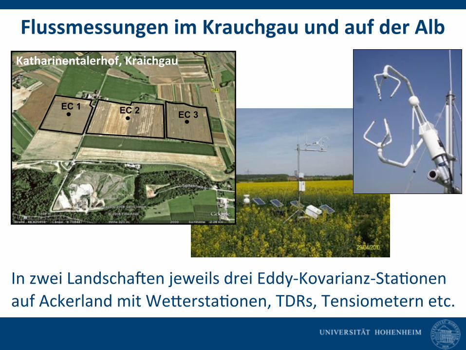
Katharinentalerhof,  Kraichgau

Flussmessungen  im  Krauchgau  und  auf  der  Alb

In  zwei  Landschaoen  jeweils  drei  Eddy-­‐Kovarianz-­‐StaUonen  auf  Ackerland  mit  WePerstaUonen,  TDRs,  Tensiometern  etc.

Energieflüsse  über  verschiedenen  Ackerfrüchten

120 150 180 210 240-20

0

20

40

60

80

100

120

120 150 180 210 240-20

0

20

40

60

80

100

120

120 150 180 210 240 270-20

0

20

40

60

80

100

120

120 150 180 210 240-50

0

50

100

150

200

250

120 150 180 210 240-50

0

50

100

150

200

250

120 150 180 210 240 270-50

0

50

100

150

200

250

120 150 180 210 240-0.5

0.0

0.5

1.0

1.5

2.0

2.5

3.0

120 150 180 210 240-0.5

0.0

0.5

1.0

1.5

2.0

2.5

3.0

120 150 180 210 240 270-0.5

0.0

0.5

1.0

1.5

2.0

2.5

3.0

Swabian Alb Kraichgau

a Winter Wheat 2009Q

H,

Wm

-2

dWinter Rape 2010

gMaize 2011

b

QE,

Wm

-2

e

h

c

Bow

en R

atio

Day of Year

f

Day of Year

i

Day of Year

LE  (W

 m-­‐2)

H  (W

 m-­‐2)

   H/LE      

Kraichgau

Alb

Wiz

eman

n, In

gwer

sen,

FOR

169

5, U

niv.

Hoh

enhe

im

Bowen-­‐

Verhältnis

~Verdu

nstung

Ernte

Energieflüsse  über  verschiedenen  Ackerfrüchten

Wiz

eman

n, F

OR

169

5, U

niv.

Hoh

enhe

im

120 150 180 210 240-20

0

20

40

60

80

100

120

120 150 180 210 240-20

0

20

40

60

80

100

120

120 150 180 210 240 270-20

0

20

40

60

80

100

120

120 150 180 210 240-50

0

50

100

150

200

250

120 150 180 210 240-50

0

50

100

150

200

250

120 150 180 210 240 270-50

0

50

100

150

200

250

120 150 180 210 240

0.0

0.5

1.0

1.5

2.0

2.5

3.0

120 150 180 210 240-0.5

0.0

0.5

1.0

1.5

2.0

2.5

3.0

120 150 180 210 240 270-0.5

0.0

0.5

1.0

1.5

2.0

2.5

3.0

a Winter Wheat 2009Winter Wheat 2011

QH,

Wm

-2

dWinter Rape 2010Winter Rape 2009

gMaize 2011Maize 2010

b

QE,

Wm

-2

e

h

c

Bow

en R

atio

Day of Year

f

Day of Year

i

Day of Year

LE  (W

 m-­‐2)

H  (W

 m-­‐2)

   H/LE      

Bowen-­‐

Verhältnis

~Verdu

nstung

Ernte

Schwäbische Alb

RN   JH    LE   H

Abreife Ernte

MonatsgemiWelte  Tagesverläufe  der  Energieflüsseüber  Winterweizen

Kraichgau  2009

Steffens  (2010)

constantRc,min

Ingwersen  et  al.  (2011)

time-variableRc,min

Verdunstungsfluss  über  Winterweizen  

EC flux measurement

NOAH land surface model

Rc,min    Minimaler  Stomatawiderstand

Das  Landoberflächenmodell  NOAH  kann  die  Entwicklungsdynamik  von  Ackerfrüchten  und  damit  die  EnergieauHeilung  an  der  Landoberfläche  nach  

Einsetzen  der  Abreife  nicht  richDg  darstellen

SimulaUon  mit  Landoberflächen-­‐modell  NOAH

Vergleich  von  Pflanzen-­‐  und  Landoberflächenmodellen

Gayler  et  al.  (2012,  subm.)

WochenmiWelwerteAlle  Modelle  anhand  von  Boden-­‐  und  Pflanzendatenkalibriert

week of the year14 16 18 20 22 24 26 28 30 32

LHF

(W m

-2)

0

25

50

75

100

125

150

175

200

Landoberflächen-­‐modell  (CLM  3.5)

EinfachesPflanzenmodell  (XN-­‐LeachN)

KomplexeresPflanzenmodell(XN-­‐SPASS)

Messungen

Late

nt h

eat f

lux

(W m

-2)

Kopplung  WRF-­‐NOAH-­‐GECROS

Ingwersen,  FOR  1695,  Univ.  Hohenheim

WRF

NOAH

Atmosphärenmodell

Landoberflächenmodell

PflanzenmodellGECROS

Kalibrierung  von  NOAH-­‐GECROS

Winterweizen

Ingw

ersen,  FOR  1695,  U

niv.  Hoh

enhe

im

0,0

0,4

0,8

1,2

1,6

2,0

2,4

0 30 60 90 120 150 180 2100

1

2

3

4

5

6

0,2

0,4

0,6

0,8

0 30 60 90 120 150 180 210

0

25

50

75

100

125

Messung Standard-Parametrisierung Nach Kalibrierung

E

ntw

ickl

ungs

stad

ium

Grüner LAI

Bla

ttflä

chen

inde

x

Tag des Jahres

Totaler LAI

Bes

tand

eshö

he (m

)

Kor

nert

rag

(dt/h

a)

Tag des Jahres

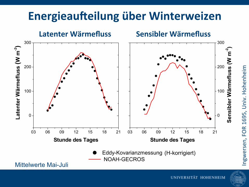
Latenter  Wärmefluss Sensibler  Wärmefluss

EnergieauHeilung  über  Winterweizen

03 06 09 12 15 18 21

0

100

200

300

03 06 09 12 15 18 21

0

100

200

300

Eddy-Kovarianzmessung NOAH-GECROS

Late

nter

Wär

mef

luss

(W m

-2)

Stunde des Tages

Sen

sibl

er W

ärm

eflu

ss (W

m-2)

Stunde des Tages

Ingw

ersen,  FOR  1695,  U

niv.  Hoh

enhe

im

(H-korrigiert)

Mittelwerte Mai-Juli

Entscheidungmodell

Wie  reagieren  die  landwirtschaHlichen  Betriebe?

Troo

st,  B

erger,  FO

R  1695,  U

niv.  Hoh

enhe

im

Erwartungsbildung  (Lernen)

Anpassung  der  ProdukDon

Klimawandel

Anpassung  der  BetriebsausstaWung

kurzfris4g

langfris4g

Zusammenfassung• Die  derzeiUge  Qualität  regionaler  KlimaprojekUonen  und  von  diesen  abgeleiteter  ErtragsprojekUonen  sollte  man,  gerade  in  der  Anpassungsforschung,  kriUsch  sehen.

• Die  regionalen  KlimaprojekUonen  werden  jedoch  konUnuierlich  besser,  vor  allem  durch  die  Erhöhung  der  räumlichen  Auflösung.  

• Die  Abbildung  von  Prozessen  und  Rückkopplungen  an  der  Landoberfläche  (Boden-­‐VegetaUon-­‐Atmosphäre)  in  regionalen  Klimamodellen  kann  und  muss  verbessert  werden,  indem    vorhandene  Daten  besser  genutzt  werden  und  mehr  Prozess-­‐wissen  in  die  Modelle  eingearbeitet  wird.

• Wechselwirkungen  zwischen  Klima  und  Landnutzung  sollten  in  KlimaprojekUonen  berücksichUgt  werden.  

Vielen  Dank  für  Ihre  Aufmerksamkeit!Vielen  Dank  auch  an:

Joachim  Ingwersen,  KrisUna  Imukova,  Maxim  PoltoradnevInsDtut  für  Bodenkunde  und  Standortslehre,  Biogeophysik,  UHOH

SebasUan  GaylerWater  &  Earth  System  Science  (WESS)  Competence  Cluster,  Tübingen

Volker  Wulfmeyer,  Hans-­‐Dieter  Wizemann,  Kirsten  Warrach-­‐Sagi,  Thomas  SchwitallaInsDtut  für  Physik  und  Meteorologie,  UHOH

Petra  Högy,  Andreas  FangmeierInsDtut  für  LandschaUs-­‐  und  Pflanzenökologie,  UHOH

ChrisUan  Troost,  Thomas  BergerInsDtut  für  Agrarökonomik  und  SozialwissenschaUenin  den  Tropen  und  Subtropen,  UHOH