Refined 3-d Transport and Horizontal Diffusion for the REM ...

Abschlußbericht zum Forschungs- und Entwicklungsvorhaben 298 41 252 auf dem Gebiet des Umweltschutzes „Modellierung und Prüfung von Strategien zur Verminderung der Belastung durch Ozon“

Refined 3-d Transport and Horizontal Diffusion for the REM/CALGRID Air Quality Model

Robert J. Yamartino

Februar 2003

Freie Universität Berlin Institut für Meteorologie Troposphärische Umweltforschung

Carl-Heinrich-Becker-Weg 6-10 12165 Berlin

Berichts-Kennblatt

BerichtsnummerUBA-FB 2.

3.

4. Titel des Berichts Refined 3-d Transport and Horizontal Diffusion for the REM/CALGRID Air Quality Model

5. Autor(en), Name(n), Vorname(n)

8. Abschlußdatum

Februar 2003 Yamartino, Robert

9. Veröffentlichungsdatum

6. Durchführende Institution (Name, Anschrift)

Integrals Unlimited 509 Chandler’s Wharf Portland, Maine USA 04101 Im Auftrag der Freie Universität Berlin Institut für Meteorologie Troposphärische Umweltforschung


10. UFOPLAN-Nr.

298 41 252

11. Seitenzahl

42 7. Fördernde Institution (Name, Anschrift)

12. Literaturangaben

Umweltbundesamt, Postfach 33 00 22, D-14191 Berlin 61

13. Tabellen und Diagramme

1

14. Abbildungen

5 15. Zusätzliche Angaben

16. Kurzfassung Der Bericht beschreibt die Entwicklung eines neuen Transportalgorithmus für das chemische Transportmodell REM/CALGRID. Der Algorithmus ist absolut massenerhaltend und minimiert die durch das „operator splitting“ verursachten Fehler auf die numerische Genauigkeit. Es wird ein Überblick gegeben über existierende Parametrisierungsansätze für die horizontale Diffusion. Ein dem Stand der Kenntnis entsprechender Ansatz wird für die Anwendung in REM/CALGRID entwickelt.

17. Schlagwörter REM/CALGRID Ausbreitungsmodell, Transport-Algorithmus, Massenerhaltung, laterale Diffusion, operator-splitting 18. Preis

19.

20.

Report Cover Sheet

Report No.UBA-FB 2.

3.

4. Report Title Refined 3-d Transport and Horizontal Diffusion for the REM/CALGRID Air Quality Model

5. Autor(s), Family Name(s), First Name(s) 8. Report Date

Yamartino, Robert

February 2003 6. Performing Organisation (Name, Address)

Integrals Unlimited 509 Chandler’s Wharf Portland, Maine USA 04101 for

Freie Universität Berlin Institut für Meteorologie Troposphärische Umweltforschung


10. UFOPLAN-Ref. No. 298 41 252 11. No of pages

42 7. Sponsoring Agency (Name, Address)

12. No. of Reference

Umweltbundesamt, Postfach 33 00 22, D-14191 Berlin

61

13. No. of Tables, Diagrams

1

14. No. of Figures 5

15. Supplementary Notes 16. Abstract A revised transport algorithm was developed for the chemical transport model REM/CALGRID. The algorithm removes all velocity-shear-induced, operator- splitting errors. The resulting, computationally-efficient transport scheme conserves mass, ensures the transport of correct mass fluxes, and maintains constant mixing ratios. Second, the magnitude and constituent components of lateral diffusion in the atmosphere were reviewed. The resulting REM/CALGRID model lateral diffusivity module also incorporates the results of this investigation and subsequent parameterization of numerical diffusion. 17. Keywords

REM/CALGRID dispersion model, operator splitting, numerical diffusion, advection scheme, lateral diffusion, mass conservation

18. Price 19.

20.

Forschungs- und Entwicklungsvorhaben 298 41 252

auf dem Gebiet des Umweltschutzes

„Modellierung und Prüfung von Strategien zur

Verminderung der Belastung durch Ozon“

Abschlussbericht:

Refined 3-d Transport and Horizontal Diffusion

for the REM/CALGRID Air Quality Model

Prepared for:

Umweltbundesamt

II 6.1 Postfach 33 00 22

14191 Berlin

Prepared by:

Dr. Robert J. Yamartino

Integrals Unlimited 509 Chandler’s Wharf

Portland, Maine USA 04101

as subcontractor of

Institute of Meteorology Free University of Berlin

Berlin, Germany

February 2003

UBA F&E Vorhaben298 41 252 REM/CALGRID Transport scheme 1

TABLE OF CONTENTS SECTION PAGE

ABSTRACT ....................................................................................................................................4

1. INTRODUCTION....................................................................................................................5

2. OPERATOR SPLITTING ERRORS .......................................................................................7

2.1 Errors Created by Shear Flows .............................................................................................7 2.2 Elimination of Shear-Flow Induced Operating Splitting Errors...........................................8 2.3 Code Steps and Necessary Conditions ...............................................................................10 2.4 Additional Limitations........................................................................................................11

3. HORIZONTAL DIFFUSION....................................................................................................12

3.1 Representation of Horizontal Diffusion in Grid Models ....................................................12 3.2 Determination of the Magnitude of the Horizontal Diffusion Coefficient .........................12 3.3 Evaluating the Role of Wind Shears...................................................................................15 3.4 Inclusion of Wind Shear Effects.........................................................................................18

4. ERRORS AND CORRECTIONS IN HORIZONTAL TRANSPORT..................................20

4.1 Advection Scheme Choices, Characteristics and Constraints ............................................20 4.2 Advection Scheme Performance and Numerical Diffusion................................................21 4.3 Local Wavelength Determination and Optimal Utilization................................................25 4.4 Correction for Artificial Diffusion....................................................................................28 4.5 Adjustment of the Horizontal Diffusion Coefficients in the REM/CALGRID Model ......29 4.6 Refined Measures of Advection Scheme Performance.....................................................29

5. SUMMARY AND CONCLUSIONS.....................................................................................32

6. REFERENCES.......................................................................................................................33

APPENDIX: FUNCTIONAL DESCRIPTION OF FORTRAN SUBROUTINES......................38


LIST OF FIGURES

Page

Figure 3-1. KSP generated total and relative diffusion estimates for 180 clusters of 10 released from a 100m non-buoyant source into a neutral, shear-free atmosphere....14 Figure 3-2. MM-5 explained variance normalized by the variance of the measured surface Winds as a function of time during the August 2-7, 1990 SJV AQS episode..........16 Figure 3-3. Ratio of the average absolute MM-5 non-dimensional shear measure.....................17 Figure 4-1. Non-dimensional diffusivities, kN, versus Courant number for the λ = 4⋅∆x wave. ..............................................................................................26 Figure 4-2. Non-dimensional diffusivities, kN, versus Courant number for the λ = 8·∆x wave. ..............................................................................................27

LIST OF TABLES

Table 4-1. Point Source Test Results for CFL=0.50..................................................................23


ACKNOWLEDGMENTS We thank Drs. Talat Odman and Chris Walcek for providing many insights into alternative advection solvers, Professor Mark Z. Jacobson for his comments on eliminating operator splitting from 3-d transport, and Professor Mike Moran for his assistance in understanding the complex subject of mesoscale horizontal diffusion. Dr. Walcek was also particularly helpful in providing various codes and a review of analysis methods and results. REM/CALGRID model development and its applications were funded by the Federal Republic of Germany’s Umweltbundesamt through Research and Development project 29841252, “Modellierung und Prüfung von Strategien zur Verminderung der Belastung durch Ozon", and partly through the R&D-project 29943246, „Entwicklung eines Modellsystems für das Zusammenspiel von Messung und Rechnung für die bundeseinheitliche Umsetzung der EU-Rahmenrichtlinie Luftqualität". We also thank Dipl.-Met. A. Graff of the Umweltbundesamt for his support.


ABSTRACT The REM/CALGRID model’s available advection schemes have numerical diffusivities that are sufficiently low that one must be concerned about: (a) adding back some horizontal diffusion appropriate to the atmospheric conditions being modeled; and, (b) operator-splitting and shear flow errors, heretofore buried by the numerical diffusion. The revised transport algorithm developed during this project removes all velocity-shear-induced, operator- splitting errors. The result is an efficient transport scheme that conserves mass, ensures the transport of correct mass fluxes, and maintains monotonicity of mixing ratios. For the range of grid resolutions (e.g., 2-40 km) where REM/CALGRID is applied, the goal is to have transport and diffusivity formulations that will yield net levels of pollutant dispersion that accurately mimic reality. Such formulations must account for the dominant atmospheric advective (e.g., wind shear) and turbulent transfer processes, compensate for smoothing or filtering present in the modeled wind fields, and correct for the unintended mixing processes accompanying present-day numerical advection schemes. This study also revealed that:

• prognostic and diagnostic modeled wind fields do cause some spatial smoothing of surface wind gradients, but retain 50-80% of the observed gradients, and are therefore quite useful for correcting the pollutant transport scheme for wind-/concentration-gradient effects, though such wind gradient-related transport terms generally yield small changes in surface pollutant concentrations;

• as modeled wind fields already include most wind directional shear with height, an

important mechanism in lateral dispersion, avoidance of “double-counting” of such shear influences demands that explicitly-modeled dispersion rates and diffusivities exclude such shear influences -- a fact which greatly reduces the usefulness of most tracer experiment results, as real-world experiments include all mechanisms;

• a numerical simulation using the synthetic turbulence model, KSP, suggested that an

appropriate lateral diffusivity for 10km wide plumes in an atmosphere free of directional shear is of order u*⋅σy, where u* is the friction velocity and σy is the plume's lateral standard deviation;

• extension of this concept throughout the PBL leads to a physical, non-dimensional

diffusivity of kH = 0.2⋅iy⋅ε , where iy is the local turbulent intensity, σv/U, and ε is the local Courant number, U⋅∆t /∆x; and

• long-wave numerical tests favor the Bott and ASD schemes, while short-wave tests favor

the Blackman-cubic and Walcek schemes. The Walcek scheme is computationally fastest and its rapid Courant number, ε, dependence of extracted diffusivities suggests possible room for additional improvements.


1. INTRODUCTION The starting point for the development of the REM/CALGRID model involved the merger of the urban-scale photochemical model CALGRID (Yamartino et al., 1992 and 1996) and the regional scale model REM (Stern, 1994; Hass et al., 1997). REM/CALGRID is a modern, high-resolution photochemical grid model, with the evolution of each of its multi-species, concentration fields is governed by the partial differential equation (PDE):

[ ] RP −∇•∇∂∂ = )(C/K - VC +

tC ρρ (1)

where V is the vector wind field; K is the diffusivity tensor of rank 2; ρ is the atmospheric density, which is included so the diffusion process is properly driven by the gradient in the dimensionless mixing ratio, C/ρ; and P and R represent all production and removal mechanisms, respectively, including non-linear chemical conversion, aerosol formation, and wet and dry deposition removal. Within the framework of a photochemical grid model, this PDE must be solved numerically, and unlike analytic solutions, this solution process involves the introduction of errors that can grow over time. Given that a primary purpose of REM/CALGRID’s development is to fulfill the requirements of the European Commission’s ambient air quality framework directive 96/62/EC (FWD), and that directive demands that the requisite model be capable of hourly predictions of O3, CO, SO2, NO2 and PM10 concentrations for periods of a year or more, minimization or elimination of modeling errors is a high priority. Thus, amongst the model's new features are: a new methodology to eliminate transport operator-splitting errors on a generalized-metric, fixed- or dynamic-layer grid; true mass conservation; and the preservation of constant mixing ratio fields. Further, the need to model long periods efficiently implies that any improvements to the transport methodology must not sacrifice speed or accuracy, and that the formulation be applicable to computationally-efficient, vertical level structures that may be dynamic in space and time. Such dynamic, vertical-layer approaches were used in early models, such as UAM, as they were faster and demanded less storage, but the approach went out of fashion about a decade ago because these early implementations displayed serious numerical problems in areas where the mixing height changed rapidly (e.g., at the coast). The significant role of non-linear processes within a photochemical model is responsible for the need for space discretization or gridding of the PDE solution, and, because the fields to be advected are known at only a finite number of points, some errors are unavoidable during the transport process; however, some errors are self-limiting or dissipative (e.g., numerical diffusion), while others can continue to evolve and are hence more sinister. Also, the fact that various model processes, such as advection and non-linear chemistry, are best handled by specialized numerical methods, coupled with the widespread desire and trend toward modularity, forces the factorization of the basic PDE into multiple, discrete operations. This process of "operator splitting" then demands genuine time discretization, and this time discretization is also accompanied by the introduction of errors. The fact that operator splitting (plus operator reversal) errors are second-order in time has generally led to these errors being ignored; however, the reduced numerical diffusion accompanying modern advection schemes can lead to the development and amplification of unphysical, mixing-ratio ripples, particularly in shear flows.


This report first describes a new methodology to eliminate transport operator-splitting errors on a generalized-metric (e.g., lat./long.), fixed-/dynamic-layer grid, and further ensures correct fluxes, complete mass conservation, and preservation of constant mixing ratio fields. Rather than simply involving an improved algorithm, this methodology involves a re-formulation and reorganization of the advection and diffusion transport operators. An Appendix explains the functions of the various subroutines included in REM/CALGRID code to achieve this goal. The report also describes progress in further increasing the fidelity and reducing the numerical diffusion of the model’s basic 1-d advection operator. Numerical diffusion incurred during application of the horizontal transport operator can be one of the leading sources of error in numerical grid modeling. Fortunately, the quality of advection schemes is now at the point where one has to be concerned about: (a) operator-splitting and shear flow errors, heretofore buried by the numerical diffusion; and, (b) adding back some horizontal diffusion appropriate to the atmospheric conditions being modeled. While the solution of problem (a) is now solved in general for any advection operator incorporating mass conservation and the blockage of unphysical extrema, appropriate treatment of horizontal diffusion (b) involves surmounting several obstacles including (i) the characterization of a horizontal advection scheme’s numerical diffusivity, (ii) accounting for the "artificial" diffusion arising from the instantaneous dilution of emissions and concentrations by the finite volume of the grid cells, and (iii) recognizing the crudeness with which horizontal atmospheric diffusion is currently understood and parameterized. Each of these issues is addressed in the subsequent chapters.


2. OPERATOR SPLITTING ERRORS Nearly all of the Eulerian oxidant and acid rain models in existence today employ operator-splitting (Yanenko, 1971) to solve the advection-diffusion partial differential equation (PDE) including linear and non-linear (i.e., 2nd order chemistry) source and sink terms. The primary motivation for using operator-splitting is that it enables the optimal numerical methods to be employed for specific elements of the overall time-development operator. McRae et al. (1982), Yamartino et al. (1992), and many other authors, have discussed the validity, limitations and ramifications of invoking the symmetric operator-splitting approximation, but the most important ramification from the point of view of choosing the horizontal advection scheme is that the truncation error of a model based on operator-splitting plus operator reversal is second-order in time (Marchuk, 1975) even for sub-operators having first-order in time truncation errors. Consequently, there has been little motivation to use time-marching schemes in the advection operator above first-order in time and similarly no need to store or manipulate more than one time level of species concentrations. Not all errors induced by operating splitting can be easily compensated for, but the particularly irksome problem of unphysical mixing ratio variations generated in shear flows can be eliminated, as described in the following subsections. 2.1 Errors Created by Shear Flows The second-order accuracy in time resulting from operator-splitting can create some genuine problems, particularly in shear flows. These problems can be seen when advecting a uniform mass density distribution in an incompressible flow field with net outflows ∆εx, ∆εy and ∆εz (i.e., expressed as the difference of cell-face Courant numbers, εx = uf·∆t/∆x in the x, y and z directions, respectively. Envisioning one grid cell as a solid block of material undergoing transport, the successive X, Y, and Z transport operations are not unlike successively slicing off (or adding when ε<0 ) 2-d layers of width ∆εx, ∆εy, and ∆εz from the block. After these three operators are applied, the fractional mass remaining in the cell is related to the remaining block volume and is given as: fm = (1 - ∆εx)·(1 - ∆εy)·(1 - ∆εz) , (2) an expression which when expanded-out involves terms of order (∆t)2 and (∆t)3. However, if one thinks in terms of the a single, linear 3-d operation, the resulting mass fraction would be simply fm = (1 - ∆εx - ∆εy - ∆εz) = 1 , (3) or unchanged, as the sum, ∆εx + ∆εy + ∆εz, is equivalent to the divergence relation ∇•V, and is constrained to be zero. This gulf between the results of Eq.(2) and Eq.(3) must be bridged, because it is efficient to work with 1-d operator-splitting; however, wind fields are known to satisfy the conservation equation ∇•V=0 or the more general, compressible form, ∇•(ρV)= -∂ρ/∂t. Flatoy (1993) proposed an iterative adjustment to the winds to ensure a constant mixing ratio; however, this iterative process was extremely time-consuming. Clappier (1998) proposed a comprehensive set of corrections to be made to advective fluxes (i.e., rather than the velocities) for 2-d and 3-d split-operator transport. His corrections completely eliminate the errors for the wind fields he has considered, but the process has to be re-solved for each species and, though it may deliver excellent results


even in very complex flow situations, his procedure is quite time consuming. Yamartino (1998) proposed an explicit method for correcting the transport velocities in two-dimensions; however, the resulting facial fluxes do not correspond to traditional results, and the 3-d solution was not presented. Unfortunately, it turns out that there are infinitely many ways to reconcile Eqs.(2) and (3), but fortunately only one unique method that will yield the "correct" fluid mass fluxes through each of the faces. Though the word "correct" has several interpretations sensitive to one's assumptions about the within-cell transport and mixing that occurs during the time step of length ∆t, our present definition of "correct" is consistent with an X-face, fluid mass flux, Fx = uf ·ρ0·∆y·∆z = εx·m0/∆t, where ρ0 is the cell density relevant for the specific face, and where the mass within the cell is just m0 = ρ0·∆x·∆y·∆z when the "donor cell" interpretation is added. These assumptions do not limit one to donor cell transport schemes, as the pollutant mass flux is defined as Fx = εx·m0·<cf>/∆t, and the pollutant mixing ratio, <cf>, relevant to the cell face may be determined by higher-order methods. Such higher-order methods can include Crowley (1968) integral-average formulations that are sensitive to pollutant and/or velocity gradients within the cell, but we note that we have chosen to explicitly exclude the effect of along-cell velocity gradients from the definition of the face Courant number, εx, (e.g., the "last molecule" correction of Yamartino (1998) appropriate for Lagrangian modeling) as such a definition leads to difficulty in the case of 2-d transport modeling of uniform velocity, 1-d pipe flow around a 90o bend. 2.2 Elimination of Shear-Flow Induced Operating Splitting Errors Given the above definition of a "correct" flux, if one now demands that the correct mass flux be transported across each cell face, then regardless of whether the operator is applied first or last, the solution to the operator-splitting problem becomes clear and unambiguous. In the simple case of the uniform, unit density field, the mass across the x, y, and z faces should be simply εx, εy, εz, respectively. This is achieved within the 1-d operator-split framework of Eq.(2) by defining corrected Courant numbers, ε′, as: ε′x = εx , (4a) ε′y = εy / (1 - ∆ε′x) , and (4b) ε′z = εz / [(1 - ∆ε′x) · (1 - ∆ε′y)] , (4c) assuming X, Y, and Z are the first, second, and third operators, respectively. Substituting these results into an Eq.(2) expressed in terms of the adjusted ε′ values, one finds fm = (1 - ∆ε′x)·(1 - ∆ε′y)·(1 - ∆ε′z) = 1 - (∆εx + ∆εy + ∆εz) = 1 , if and only if ∆εx + ∆εy + ∆εz = 0. Of course, in the case of space-time variable, air density field, ρ, one cannot anticipate the result of the first operator before it has actually been performed, so that Eq.(4b) must be defined after the X transport operation and Eq.(4c) must be defined after both the X and Y operations are completed. This is quite easy to do if one advects air density, ρ, in the new direction before any of the pollutant species mixing ratios (i.e., dimensionless concentrations in ppm, for example). Then, assuming the donor cell densities relevant for a specific face are ρ0 initially, ρx after the X


(i.e., first) operator, ρxy after the X and Y (i.e., 1st and 2nd) operators, Eq.(4) is generalized to: ε′x = εx , (5a) ε′y = εy · (ρ0 / ρx) , and (5b) ε′z = εz · (ρ0 / ρxy) . (5c) Such an approach was also implicit in Walcek and Aleksic's (1998) introduction of 1-d advection scheme that could maintain constant mixing ratio fields and has been attributed to Easter (1993). In principle, the final density field, ρxyz, following application of all three operators should exactly match the density field, ρn appropriate for the next time step; however, computational roundoff errors will often cause the density field to drift away from its expected future value, so Eq.(5c) is replaced with adjustments to the vertical velocities (i.e., starting at the ground face, k=1 where ε′z,1 = 0, and working up the model column) to ensure that modeled, advected densities truly match the known future densities. Given that the donor cell method is used for the transport of density, one can invert the donor method flux relation to replace Eq.(5c) with Eq.(5d) given as: ε′z,k = (ρxy - ρn) / ρxy,k + ε′z,k-1 · (ρxy,k-1 / ρxy,k) , (5d) where ρxy,k is the appropriate donor density defined as face k and ρxy, ρn are the densities in cell k before and after application of the Z operator. Such a condition (i.e., defined by Eq.(5d) rather than Eq.(5c)) is required if a uniform mixing ratio field is to remain truly uniform for all time. This methodology can be implemented with any 1-d advection solver and has been successfully tested in conjunction with the Blackman scheme (Yamartino, 1993); however, the highly-accurate, monotonic advection scheme developed by Walcek (2000) proved to be considerably faster than the original Blackman scheme or recent, more accurate and monotonic, variants of it. Thus, the decision was made to use the Walcek(2000) solver in the REM/CALGRID code; though, as will be considered later, some fine-tuning of this algorithm has been done. One possible criticism of this overall approach is that air density is being advected by the highly diffusive donor-cell method, whereas the pollutant species are being transported using a much less diffusive algorithm. While it is clear that the monotonicity constraint in the Walcek algorithm is appropriate for mixing ratios and not mass concentrations, one could "switch-off" that constraint for air density or use another, low diffusion algorithm, such as the Blackman cubic scheme. We have tried this strategy of advecting air density with a less diffusive scheme and find that it makes essentially no difference in practical problems. This is perhaps due to the fact that air density fields do not typically display large gradients in the horizontal, and, in the vertical, where the gradients are larger, the numerical diffusivity of the transport scheme is made irrelevant by Eq.(5d), which forces resulting densities to match known future values. Independently of this effort, Mark Jacobson (private communication) has also implemented Walcek’s approach into the GATOR code and, in addition, has adopted the same supplemental velocity corrections (i.e., Eq. 4d) that we perform in the vertical to ensure that the advected density ends up the same as the future 3-d density field input (or computed from pressure and temperature fields) from the meteorological model.


2.3 Code Steps and Necessary Conditions The equations of the previous section describe the theory; however, it is also useful to see how this translates into actual steps within the model. The approach and constraints involve the following steps: a) Winds are first made consistent with the full conservation equation, ∇•(ρV)= -∂ρ/∂t. We choose to satisfy this criteria on an Arakawa C-grid (i.e., cell-face-centered winds and grid-point scalars e.g., density and temperature) though other solutions are possible. b) Three-dimensional advection is then performed without any intervening diffusion operations. That is, if Xa, Ya, Za define 1-d advection operators and Xd, Yd, Zd define 1-d diffusion operators, the sequence (Xa•Ya•Za) • (Xd•Yd•Zd) is allowed, but the often-used sequence (Xa•Xd) • (Ya•Yd) • (Za•Zd) is not allowed. This is because the air conservation equation (a) does not involve diffusion. c) Operator-splitting errors are completely avoided by making sure that a 1-d operator yields the same material fluxes whether it is the first, or a subsequent, operator in the sequence. Suppose we begin with a uniform field of C(0)=1, but, because of wind shears, the first operator, Xa, yields some values of C(∆t) < 1. Now if a second operator, Ya, is applied, the resulting Y fluxes will be too low when the donating cell concentration is low (C < 1). Knowing what the Y fluxes “should have been” had Ya been the first operator, enables us to correct the fluxes by applying a multiplicative correction factor to the Y velocities. d) The final operator in the advection operator sequence (e.g., Za) must be further adjusted to ensure that final air densities match the final densities assumed in solving the air conservation equation (a). This is very nearly achieved with Eq.(5c) but is better-achieved using Eq.(5d). e) The flux formulation guarantees mass conservation, and Walcek's min/max. constraints preserve the constant mixing ratio; however these constraints can be met with a variety (i.e., an infinity) of solutions. The further requirement that the air mass fluxes through each cell face be correct (i.e., be what they would have been had each operator been performed first in the operator-splitting sequence) guarantees that. This still does not ensure that each pollutant species mass flux through each cell face is independent of operator splitting, as that would require species-by-species corrections dependent on local concentration gradients (e.g., see Clappier, 1989), and such corrections are presently considered too computationally intensive. f) The approach wipes out operator-splitting errors due to wind-shear effects, though we continue to alternate with XYZ and YXZ operations (N.B.: Z is always last for the fine tuning of the density via the W) to minimize possible species concentration field differences. However, most tests to date show that XY and YX alternation is no longer essential. g) Spatially-varying layer depths are accommodated by redistributing exchanged horizontal fluxes to the appropriate vertical levels. This step is effectively part of the Xa and Ya operators, and is as described for the CALGRID model except for the slight complexity introduced by having arbitrary horizontal metric factors. h) Dynamic vertical layers are accommodated after 3-d transport by remapping the concentration fields onto the new layers in a donor-cell-like manner that conserves mass.


2.4 Additional Limitations The previous sections describe the theory and code steps; however, testing of the algorithms, particularly on the urban scale (i.e., with ∆x of a few km), showed problems traceable to excessively high Courant numbers and excessive cell depletion during some 1-d advection operations. The1-d advection operator can, in principle, handle CFL values exceeding unity (i.e., |ε|>1) by simply sub-dividing the operation into multiple sub-time-steps, each having a maximum CFL less than unity. However, this 1-d, sub-time-stepping violates the basic rules of operator splitting and can lead to some unusual concentration patterns as well. For example, high CFL transport of emissions from a continuous point source can result in disconnected blobs of concentration on the grid. Thus, high CFL transport is not something one wishes to indulge in regularly. On the other hand, it is definitely wasteful of computer resources to slow the entire model down if |ε|>1 in only one or two cells on the grid. This is especially true if there are no significant concentrations gradients. If for example, C=1 everywhere, it makes no difference if we advect this field at CFL>1 or not at all. Thus, one must exercise more care in areas of significant concentration gradients, that is, in source rich regions. These considerations have led us to allow peak CFL as large as 2.1 in layers above the mixing height (i.e., provided that this height also exceeds a minimum of 750m), where only weak horizontal concentration gradients are anticipated. However, for layers below this limit, peak CFL are not allowed to exceed 1.1, as source related concentration gradients are anticipated and it is more critical that the predicted concentrations are correct. Aside from CFL magnitude concerns, one must also be concerned with the degree of cell depletion, that is, ∆CFL or ∆ε. If for example, the ∆ε′x of Eq. (4b) were unity, the cell would be 100% depleted of air mass during the operation, such that no finite correction of εy would be possible to obtain an ε′y. Hence, along with the check of CFL, one must also check that wind shears do not overly deplete a cell of air mass for the subsequent transport operators. While the 2-d constraint, ∆εx + ∆εy < ∆εmax, is probably adequate, we have added the subsidiary conditions that ∆εx < ∆εmax and ∆εy < ∆εmax as well, and have chosen a conservative value of ∆εmax = 0.5. Violation of either the CFL or ∆CFL conditions results in an increase in the number of overall sub-time-steps taken within that particular hour, such that all the limit criteria are satisfied.


3. HORIZONTAL DIFFUSION 3.1 Representation of Horizontal Diffusion in Grid Models The current REM/CALGRID model horizontal diffusion methodology is also explicit and forward-in-time, which is appropriate given the small size of the horizontal non-dimensional diffusivities, k (i.e., k ≡ K⋅∆t/(∆x)2 << 0.25) on spatial scales of a few km or more. The concentration gradients estimated for use in REM/CALGRID model's diffusion module are first-order accurate in space, as they simply involve the differences of grid-point concentrations -- a methodology that is both standard and adequate for the purpose. 3.2 Determination of the Magnitude of the Horizontal Diffusion Coefficient A major limitation of representing atmospheric diffusion with Eq.(1) is that use of a temporally-constant diffusivity, K, generally limits one to plume growths that are proportional to the square root of transport time, t, in direct contrast with the nearly linear growth rates that are observed in nature (Hanna, 1994). A major reason for the masking of the anticipated transition to t1/2 growth, for travel times longer than any reasonable estimate of a lateral turbulence Lagrangian time scale, is the combined effect of wind directional shear with height and vertical mixing. Moran's (1992) extensive dissertation on mesoscale atmospheric dispersion, including simulation of the long-range transport, Great Plains and CAPTEX tracer experiments using the prognostic wind field model RAMS (Pielke et al., 1992), concludes that "horizontal dispersion can be enhanced and even dominated by vertical wind shear through either the simultaneous of delayed interaction of horizontal differential advection and vertical mixing..." Knowing that the vertical wind shear (e.g., turning of the wind with height) is built into most wind field models, one must now ask:

a) How should the lateral turbulence in a directional-shear-free atmosphere be modeled; and b) How well does the chosen wind field driver emulate the shears in the atmosphere?

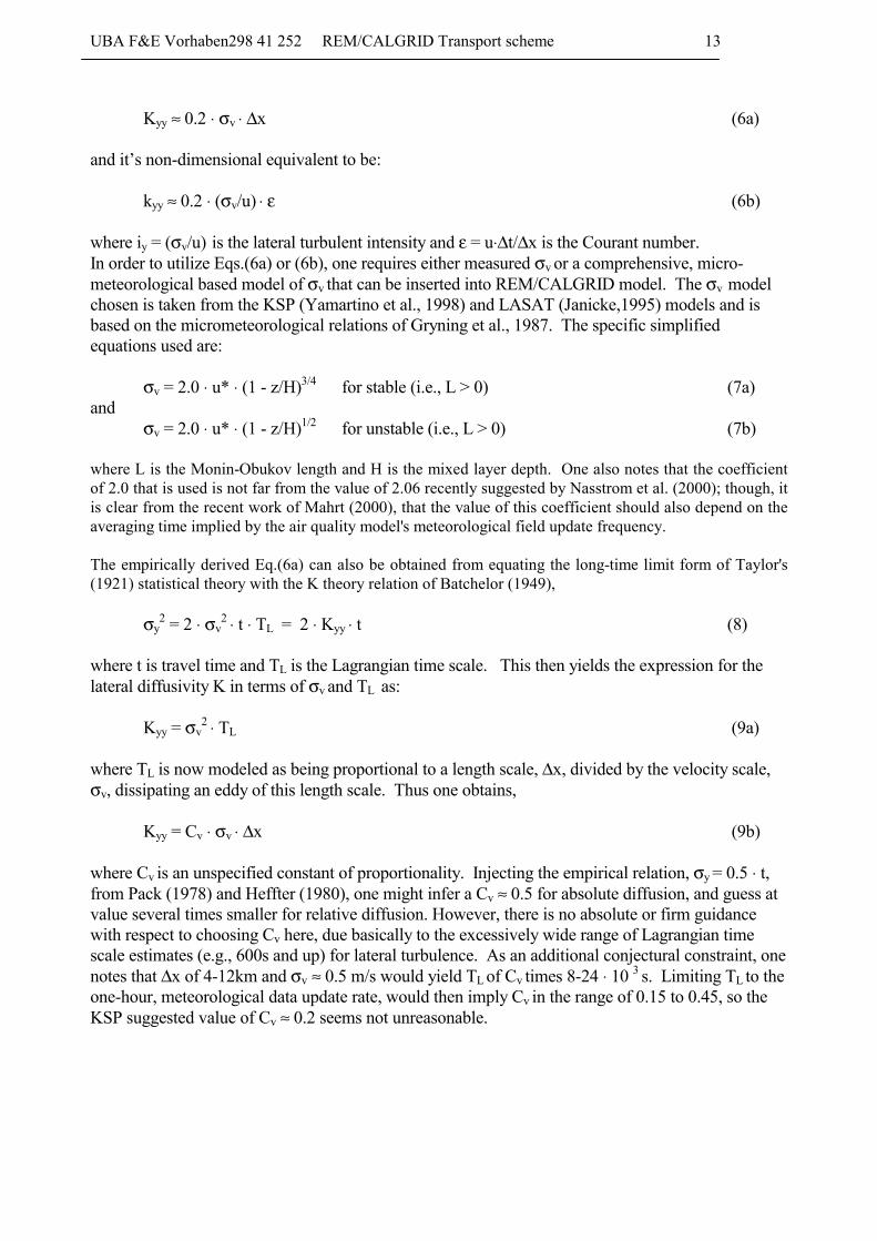
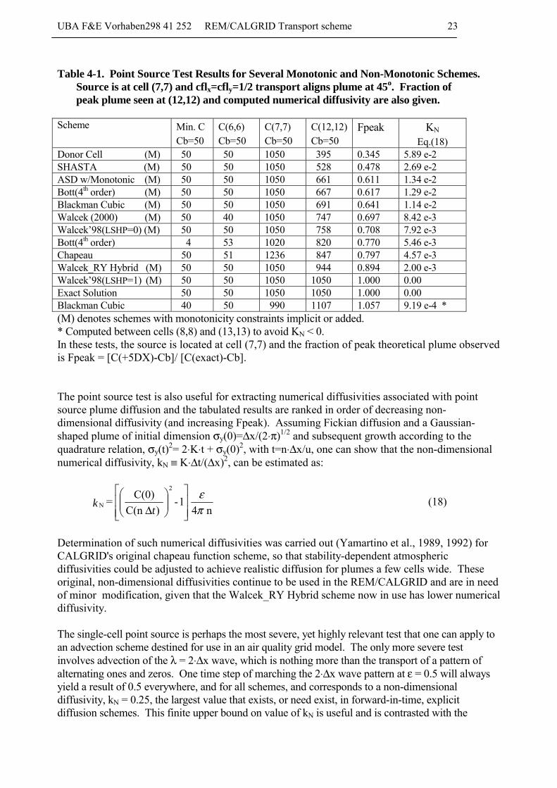
Assuming presently, that wind shear effects are accounted for by the FUB wind field models, one must ask where appropriate mesoscale diffusivities are to be found. Plume growth rates measured in tracer experiments can not, of course, directly isolate the diffusive and wind shear contributions of the atmosphere; although, model dependent analyses of such experiments could. An alternative approach might involve use of an LES model in a shear-free atmosphere. We have alternatively used the Kinematic Simulation Particle (KSP) model (Yamartino et al., 2000) to simulate plume growth rates in a shear-free flow. Though KSP uses simple micrometeorological formulae to specify the magnitude of temporally-evolving (i.e., via Langevin equations), turbulent velocity fields of varying wavelengths, the fact that center-of-mass movements and particle separations are tracked for individual n-particle clusters enables the relative diffusion component of total diffusion to be identified. Figure 3-1 shows total and relative diffusion plume sigmas for a 100m elevated, point source release. Particles were released in clusters of 10 every 20 seconds for one hour. These clusters then evolve in a steady, D stability atmosphere with u*≈0.5 m/s. For a plume having a standard deviation of order 10 km, lateral diffusivities of order Kyy ≈ u*⋅σy ≈ 5000 m2/s are extracted for the relative diffusion and may be appropriate for inclusion into the lateral diffusion module of the REM/CALGRID air quality model. Generalizing this result to a grid where σy = ∆x/(2⋅π)1/2 , and assuming σv ≈ 2⋅u*, one would estimate the lateral diffusivity to be:


Kyy ≈ 0.2 ⋅ σv ⋅ ∆x (6a) and it’s non-dimensional equivalent to be:

kyy ≈ 0.2 ⋅ (σv/u) ⋅ ε (6b)

where iy = (σv/u) is the lateral turbulent intensity and ε = u⋅∆t/∆x is the Courant number. In order to utilize Eqs.(6a) or (6b), one requires either measured σv or a comprehensive, micro-meteorological based model of σv that can be inserted into REM/CALGRID model. The σv model chosen is taken from the KSP (Yamartino et al., 1998) and LASAT (Janicke,1995) models and is based on the micrometeorological relations of Gryning et al., 1987. The specific simplified equations used are: σv = 2.0 ⋅ u* ⋅ (1 - z/H)3/4 for stable (i.e., L > 0) (7a) and σv = 2.0 ⋅ u* ⋅ (1 - z/H)1/2 for unstable (i.e., L > 0) (7b) where L is the Monin-Obukov length and H is the mixed layer depth. One also notes that the coefficient of 2.0 that is used is not far from the value of 2.06 recently suggested by Nasstrom et al. (2000); though, it is clear from the recent work of Mahrt (2000), that the value of this coefficient should also depend on the averaging time implied by the air quality model's meteorological field update frequency. The empirically derived Eq.(6a) can also be obtained from equating the long-time limit form of Taylor's (1921) statistical theory with the K theory relation of Batchelor (1949),

σy2 = 2 ⋅ σv

2 ⋅ t ⋅ TL = 2 ⋅ Kyy ⋅ t (8)

where t is travel time and TL is the Lagrangian time scale. This then yields the expression for the lateral diffusivity K in terms of σv and TL as:

Kyy = σv2 ⋅ TL (9a)

where TL is now modeled as being proportional to a length scale, ∆x, divided by the velocity scale, σv, dissipating an eddy of this length scale. Thus one obtains,

Kyy = Cv ⋅ σv ⋅ ∆x (9b) where Cv is an unspecified constant of proportionality. Injecting the empirical relation, σy = 0.5 ⋅ t, from Pack (1978) and Heffter (1980), one might infer a Cv ≈ 0.5 for absolute diffusion, and guess at value several times smaller for relative diffusion. However, there is no absolute or firm guidance with respect to choosing Cv here, due basically to the excessively wide range of Lagrangian time scale estimates (e.g., 600s and up) for lateral turbulence. As an additional conjectural constraint, one notes that ∆x of 4-12km and σv ≈ 0.5 m/s would yield TL of Cv times 8-24 ⋅ 10 3 s. Limiting TL to the one-hour, meteorological data update rate, would then imply Cv in the range of 0.15 to 0.45, so the KSP suggested value of Cv ≈ 0.2 seems not unreasonable.


Sigma Y vrs Travel Time for D Stability - 100m Release

1.0E+00

1.0E+01

1.0E+02

1.0E+03

1.0E+04

1.0E+05

1.0E+01 1.0E+02 1.0E+03 1.0E+04 1.0E+05

Travel Time (s)

Sigm

a Y

(m)

Rel. Dif.

Tot. Dif.

Figure 3-1. KSP generated total and relative diffusion estimates for 180 clusters of 10 particles released from a 100m non-buoyant source into a neutral, shear- free atmosphere. Accompanying lines indicate growth rates of t, t3/2, and t1/2 .


3.3 Evaluating the Role of Wind Shears Several mesoscale, photochemical models have long recognized the significance of wind shear in dispersing the pollutants and have attempted to include its effects through the use of the Smagorinsky (1963) stress tensor in the model's mesoscale diffusivity. For example, the original CALGRID model (Yamartino, et al., 1992) uses the Smagorinsky formulation. KS = αo

2 |D| (∆x)2 (10a) where αo ≈ 0.28 and |D| is the absolute value of the stress tensor, specified as,

��

�

�

��

�

�

��

�

�

∂∂

∂∂

��

�

�

∂∂

∂∂

yv -

xu +

yu +

xv = D

22 2/1

(10b)

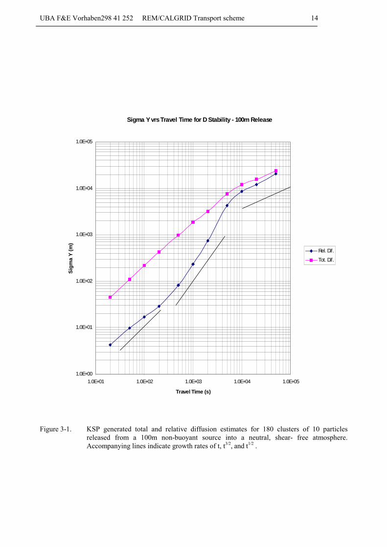
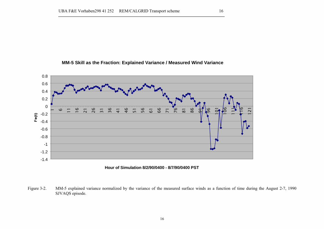
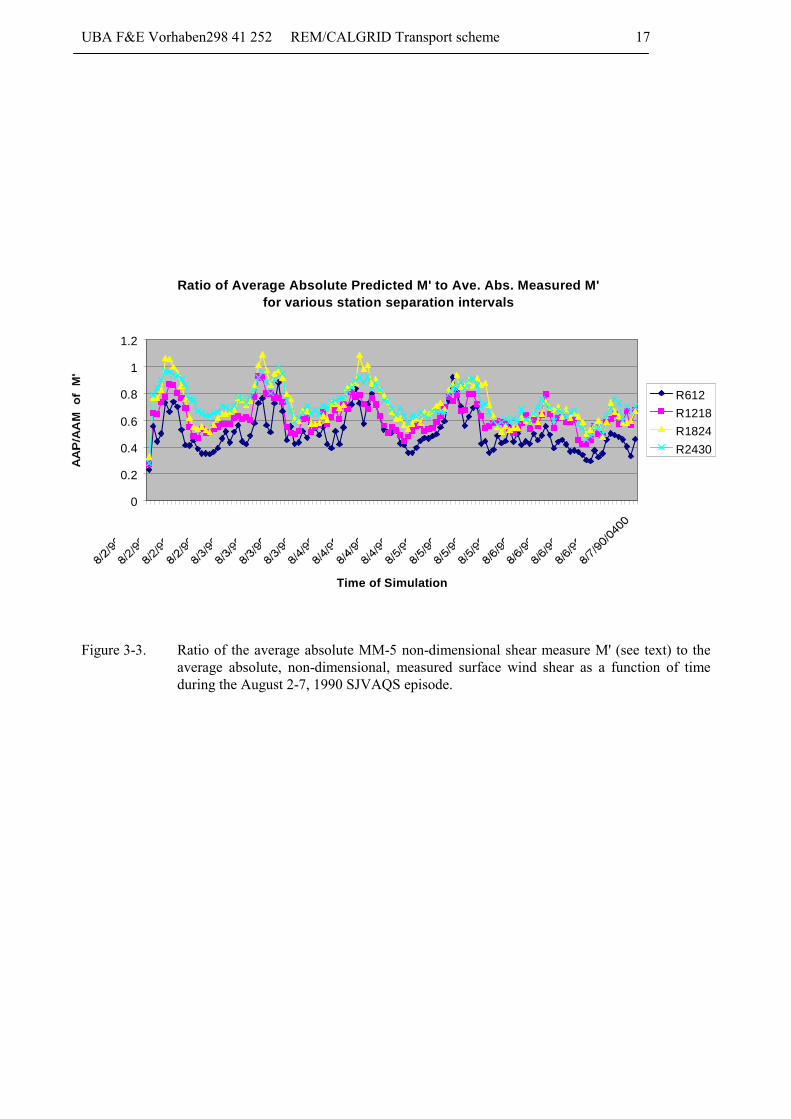
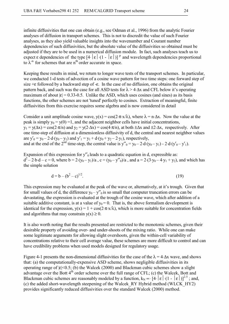
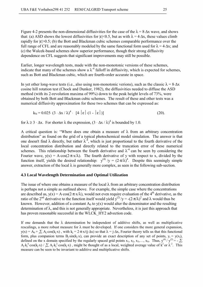
to characterize the impact of stress in the wind field. Of course, if there are no velocity gradients or the wind field generator is incapable of simulating or maintaining these gradients, the approach has greatly reduced value. While the shear related corrections to horizontal transport in the REM/CALGRID model will be advective rather than diffusive (as detailed in Section 4), the question of velocity gradient fidelity by the wind field generator remains a valid concern. Seaman (1998, private communications) has indicated that the gridded nature of the MM-5 prognostic model coupled with the properties of it's numerical algorithms can preserve only those spatial structures that exist over "several grid cells or more". Hence, any complete model of horizontal diffusivity should attempt to capture those strong, near-surface wind gradients lost by the driving prognostic or diagnostic wind field model. Figure 3-2 is taken from Yamartino et al. (2000) and it shows a plot of the fraction of the mean surface wind residual that is explained by MM-5 for a 5-day episode in the Central Valley of California. A value of 1.0 would indicate that the MM-5 field predicts the surface observations exactly, while a value of 0.0 could be achieved by having all MM-5 winds set to 0.0, so as to not influence the residual. A negative value indicates that the MM-5 predictions are worse than no prediction at all and could result from MM-5 predicting the wind flow in the opposite direction. Figure 3-2 shows that, after a short spin-up period, MM-5 predictions account for about half of the residual for the first three days, but that after this time the predictive power deteriorates rapidly. During the last two days, the MM-5 winds yield near-zero to negative skill fractions; suggesting that the model should have been re-initialized to obtain more realistic wind fields. Given the more immediate role of measured winds in diagnostic models, it is estimated that the diagnostic wind field models driving REM/CALGRID should account for in excess of 50% of the modeled-measurement residual for surface winds. Figure 3-3, also taken from Yamartino et al. (2000), shows the ability of the 4-km resolution MM-5 winds to reproduce observed non-dimensional wind shears, (i.e., effectively (dU/dX)*(∆X/U)), for four intervals of station separation: 6-12km, 12-18km, 18-24km and 24-30km. As expected, one sees better performance (i.e., an Average Predicted/Average Measured ratio of 1.0 is ideal), for increased station separations. This is because the model is unable to reproduce detail associated with waves shorter than ‘several’ ∆X. The peaks tend to occur in the morning, before significant daytime convective activity, and the minima occur in the early evening, just after the cessation of convective activity. This behavior is seen consistently, but is not fully understood.


MM-5 Skill as the Fraction: Explained Variance / Measured Wind Variance

-1.4

-1.2

-1

-0.8

-0.6

-0.4

-0.2

0

0.2

0.4

0.6

0.8

1 6 11 16 21 26 31 36 41 46 51 56 61 66 71 76 81 86 91 96 101

106

111

116

121

Hour of Simulation 8/2/90/0400 - 8/7/90/0400 PST

Figure 3-2. MM-5 explained variance normalized by the variance of the measured surface winds as a function of time during the August 2-7, 1990

SJVAQS episode.

16


Ratio of Average Absolute Predicted M' to Ave. Abs. Measured M' for various station separation intervals

0

0.2

0.4

0.6

0.8

1

1.2

Time of Simulation

R612R1218R1824R2430

Figure 3-3. Ratio of the average absolute MM-5 non-dimensional shear measure M' (see text) to the

average absolute, non-dimensional, measured surface wind shear as a function of time during the August 2-7, 1990 SJVAQS episode.


Nevertheless, the fact that a prognostic model can capture 60-80% of the shear, suggests that the shear corrections to transport based on modeled winds should have roughly the correct magnitude, and permits use of the shear formalism developed in the next subsection. 3.4 Inclusion of Wind Shear Effects In order to account for diffusion due to distortion or stress in the horizontal wind field, the CALGRID model used the moderately simple Smagorinsky (1963) formulation of Eq.(10) to characterize and simulate the stress in the wind field. The KS of Eq.(10) can be computed directly from the already existing u, v horizontal wind field components. In his review of horizontal diffusion processes and their representation, Hanna (1994) points out the problem that “horizontal diffusion follows a linear growth rate with time for travel times out to a day or more” whereas K-theory diffusion leads to t1/2 plume growth. This fact stresses the importance of capturing as much as possible of the wind field shear in the advective portion of the transport flux vector, F, given as ; (11) )(C/ K - VC = F ρρ∇ unfortunately, this cannot be done for the scales that are smaller than ∆x. For these smaller scales we first consider the problem of u (i.e., x) transport through the face of a single grid cell. One then may write the local flux as either an advective flux,

��

��

��

�

�

∂∂

��

�

�

∂∂

��

��

��

�

�

∂∂

��

�

�

∂∂ z

zC +y

yC + C z

zu +y

yu +u = Fa (12)

or as a diffusive flux,

��

��

��

�

�

∂∂

��

�

�

∂∂

��

�

�

∂∂

z)(C/ K +

y)(C/ K +

x)(C/ K - = F xzxyxxd

ρρρρ (13)

Integrating Eqs.(12 and 13) over the facial area ∆y⋅∆z of the cell, and noting that the u⋅C term is the purely advective term already handled by the advection scheme and the term containing Kxx is the traditional diffusion term, the matching of terms enables one to extract expressions for the K tensor elements, such as:

��

��

��

�

�

∂∂

��

�

�

∂∂

��

��

��

�

�

∂∂

��

�

�

∂∂∆

y C -

yC /

yC

yu

12)y ( - = K

2

xyρ

ρ (14a)

and

��

��

��

�

�

∂∂

��

�

�

∂∂

��

��

��

�

�

∂∂

��

�

�

∂∂∆

z C -

zC /

zC

zu

12)z ( - = K

2

xzρ

ρ (14b)

which in the case of negligible density variation become

yu

12)y ( - = K

2

xy ��

��

�

∂∂∆ (15a)

and


zu

12)z ( - = K

2

xz ��

��

�

∂∂∆ . (15b)

Extension to the y flux-related tensor components Kyx and Kyz is straightforward and the similarity between Eq.(15) and Eq.(10) becomes more striking when one realizes that αo

2 = (0.28)2 = 1/12.8 or αo

2 ≅ 1/12. Further, what this comparative analysis shows is that:

• rather than use the directionally blind KS for wind shear-related lateral “diffusion” in both directions x and y, one may now selectively employ the direction-specific tensor elements Kxy and Kxz for x exchange fluxes and Kyx and Kyz for y exchange fluxes, respectively, with the Kxz and Kyz terms dominating over the Kxy and Kyx ;

• unlike in the directionally blind KS, where only the diagonal diffusivities, such as Kxx, are

impacted and hence where x direction fluxes are purely diffusive and proportional only to (∂C/∂x), inclusion of these off-diagonal terms can result in x diffusive fluxes to be driven by gradients (∂C/∂y) and (∂C/∂z). While seemingly counterintuitive, one must recall that we are not modeling actual diffusion with these off-diagonal terms, but rather the influence of wind shears on mass transfer;

• unlike in the directionally blind KS, the divergence related terms, (∂u/∂x) and (∂v/∂y),

will not appear in the four K tensor elements. Rather, these terms can and should instead be included in the wind gradient correction to any Crowley integral-flux advection scheme. This correction (Yamartino, 1998) amounts to replacing the one-dimensional Courant number, ε, with the corrected ε′= ε⋅[1 - exp(-a)]/a, where a=(∂ε/∂x). Such a correction correctly pinpoints the “last molecule” destined to leave the grid cell during the advection step and is consistent with Emde's (1992) correction for Lagrangian back trajectories; and

• unlike the Smagorinsky KS, the lateral diffusivities will now include corrections for the

variation in winds u and v between vertical levels via terms Kxz and Kyz respectively. While the above outlined approach certainly appears more promising than the traditional Smagorinsky formulation, analyses of the REM/CALGRID model code indicated that it would be far more practical to implement shear using the advective representation (i.e., Eq.(12)) rather than as off-diagonal diffusion terms. In addition, consistent treatment of second-order terms called for expansion of Eq.(12) to: Fa = [ u + uy ⋅ y + uz⋅ z + (uyy ⋅ y2 + uzz⋅ z2) / 2 ] ⋅ [ C + Cy ⋅ y + Cz⋅ z + (Cyy ⋅ y2 + Czz⋅ z2) / 2 ] , (16) where subscripts denote differentiation here. Expanding Eq.(16) and integrating over the facial area ∆y⋅∆z of the cell, one obtains the integral average advective flux as: < Fa > = u⋅C + [uy ⋅ Cy + (uyy ⋅ C + u ⋅ Cyy ) / 2 ] ⋅ (∆y)2 / 12 + [uz ⋅ Cz + (uzz ⋅ C + u ⋅ Czz ) / 2 ] ⋅ (∆z)2 / 12 . (17) Studies with the prototype model indicated that inclusion of the [uy ⋅ Cy + uz ⋅ Cz] term made negligible differences (e.g., ± 1 ppb) to the ozone, and given the resulting increases in CPU time for REM/CALGRID model, the second derivative terms were not added in.


4. ERRORS AND CORRECTIONS IN HORIZONTAL TRANSPORT 4.1 Advection Scheme Choices, Characteristics and Constraints Numerous papers have been written describing the theoretical stability characteristics and actual performance of different advection schemes. Roache (1976) provides an extensive introduction to the subject. Published intercomparisons of advection schemes (e.g., Long and Pepper (1976, 1981), Pepper et al. (1979), Chock and Dunker (1982), Schere (1983), Yamartino and Scire (1984), Chock (1985, 1991), van Eykeren et al. (1987)) are far from unanimous in their conclusion of the best overall scheme, but some consensus is emerging with respect to several considerations:

• It is important to conduct numerous tests, such as short- and long-wavelength fidelity and moments conservation tests, grid transmission tests, and point source tests, in one and two dimensions. Schemes showing superb fidelity with one test can show disastrous properties in another test.

• The constraint exists that implementation into a model with non-linear operators (e.g.,

second-order chemistry) and via operator splitting makes it conceptually difficult, if not impossible, to implement a time marching scheme more sophisticated than the Euler method (i.e., first order)*.

• Progressively higher order spatial accuracy rapidly encounters a “diminishing returns”

plateau if one is limited to Euler time marching. The Odman et al. (1996) report, Horizontal Advection Solver Uncertainty in the Urban Airshed Model, identifies three solvers that are most appropriate for photochemical modeling. These solvers were considered as alternative solvers for use within the REM/CALGRID model: (1) Bott's (1989) area-preserving flux form (APF) algorithm. This fourth-order scheme

is based on generalizations of the Crowley (1968) approach by Tremback et al. (1987), followed by a flux renormalization to ensure positive definite concentrations. This method yielded some unacceptable concentration over/undershoots that were eliminated in a more stringent monotone flux limiter version (MAPF) (Bott, 1992, 1993); however, the newer schemes are somewhat more diffusive.

(2) Yamartino's (1993) spectrally-constrained, Blackman cubic scheme. This Crowley-type scheme uses a polynomial expansion of within-grid-cell concentrations coupled with formulations of the derivatives that involve a blend of local and global definitions. These polynomials are then further constrained by bounds extracted from spectral theory (Blackman and Tukey, 1958) to suppress dispersive, short-wavelength components. The approach also renormalizes within-cell concentrations to ensure correct within-cell mass and contains a minimally diffusive filter. This algorithm is currently in use in the European RTM-like model REM-3 and is implemented in recent releases of the CALGRID model (Yamartino et al., 1989, 1992).

* A high-order time marching scheme is possible in the absence of the operator splitting associated with the method of fractional steps. In such a case the whole system of equations would be marched at a rate acceptable to the chemical system and a high spatial-order scheme, such as pseudospectral, would then be very promising. Computing costs could, however, be very large.


(3) The Accurate Space Derivative (ASD) scheme (also referred to as the Advective

Spectral Density scheme) as recently improved by Chock (1991) and Dabdub and Seinfeld (1994). Built upon the earlier ASD techniques of Gazdag (1973), this method uses the spectral expansion of the concentration field (i.e., the highest-spatial-order expansion that a grid can support) as its engine. It then uses the Forester filter to reduce fast Fourier transform noise, dissipate high frequency ripples, and avoid negative concentrations, with a claimed minor performance degradation.

These three horizontal advection solvers are explicit, forward-in-time, high-spatial order (4th order accurate or better) methods. A fourth scheme considered is the Walcek (2000) scheme, which uses a low-spatial-order accuracy definition of within-cell concentrations, coupled with a “steepening” methodology and strong monotonicity constraints, to achieve surprizing transport accuracy. These modern schemes all exhibit the following features:

• creation of small numerical diffusion, • good transport fidelity in terms of phase speed, group velocity, and low shape distortion, • prohibition of negative concentrations, • ability to cope with space-time varying vertical level structures, • mass conservation, and • limitations on the creation of new maximum or minimum concentration values, and, in

the case of Walcek (2000), complete monotonicity of mixing ratios.

One additional feature, the ability to accommodate strong shear flows correctly, is generally not demanded of advection schemes, but can play an important role in the overall modeling process. Satisfying some of the above constraints can cause deterioration in other aspects of a scheme's performance. For example, the avoidance of negative concentrations is often achieved via clipping or some other form of short-wavelength filtering. This in turn increases the effective numerical diffusivity of the scheme, but is considered a necessary performance price to pay, as the presence of negative concentrations would, among other problems, cause most chemistry solvers to fail. Mass conservation is another feature that one would expect in a regulatory model, and it is easy to guarantee in most flux formulations of the advection equation; however, some regulatory models have encountered problems conserving both mass and the constancy of a uniform mixing ratio field. Finally, some authors (e.g., Hov et al., 1989; Odman and Russell, 1991) note that some minor limitations in the previously identified features can become more serious problems when the non-linear chemistry operator is included, as predicted concentrations are sensitive to bilinear species concentration products. Such problems are likely minimized by choosing or optimizing a scheme based on minimal residuals or chi-square considerations, rather than best peak value retention or some other non-optimal criterion. For example, adjustable coefficients within the Yamartino (1993) scheme can be changed to yield negligible numerical diffusion (or even anti-diffusion), but the ensuing loss in accuracy may render this a dubious achievement. 4.2 Advection Scheme Performance and Numerical Diffusion Numerical transport schemes are often tested using initial mass distributions that are dominated by the longer (e.g., λ > 6⋅∆x) wavelengths on the grid. Whereas such long wavelength propagation tests are essential, they tend to show an advection scheme at its minimally diffusive best.


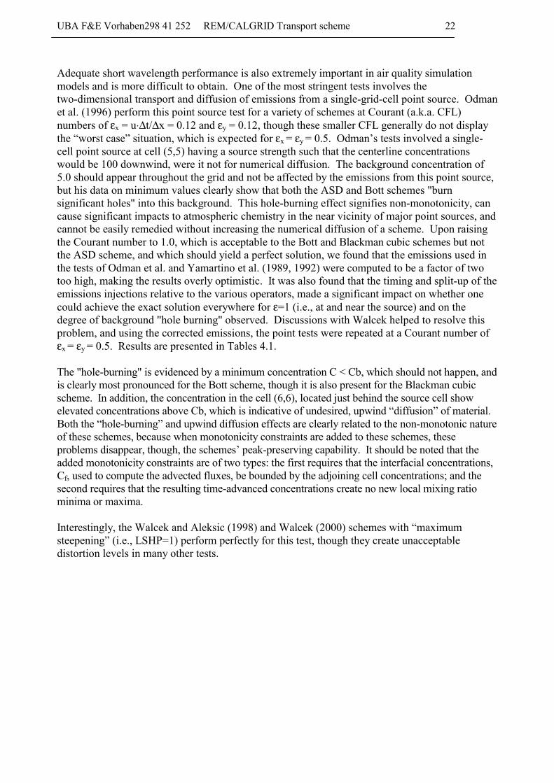
Adequate short wavelength performance is also extremely important in air quality simulation models and is more difficult to obtain. One of the most stringent tests involves the two-dimensional transport and diffusion of emissions from a single-grid-cell point source. Odman et al. (1996) perform this point source test for a variety of schemes at Courant (a.k.a. CFL) numbers of εx = u⋅∆t/∆x = 0.12 and εy = 0.12, though these smaller CFL generally do not display the “worst case” situation, which is expected for εx = εy = 0.5. Odman’s tests involved a single-cell point source at cell (5,5) having a source strength such that the centerline concentrations would be 100 downwind, were it not for numerical diffusion. The background concentration of 5.0 should appear throughout the grid and not be affected by the emissions from this point source, but his data on minimum values clearly show that both the ASD and Bott schemes "burn significant holes" into this background. This hole-burning effect signifies non-monotonicity, can cause significant impacts to atmospheric chemistry in the near vicinity of major point sources, and cannot be easily remedied without increasing the numerical diffusion of a scheme. Upon raising the Courant number to 1.0, which is acceptable to the Bott and Blackman cubic schemes but not the ASD scheme, and which should yield a perfect solution, we found that the emissions used in the tests of Odman et al. and Yamartino et al. (1989, 1992) were computed to be a factor of two too high, making the results overly optimistic. It was also found that the timing and split-up of the emissions injections relative to the various operators, made a significant impact on whether one could achieve the exact solution everywhere for ε=1 (i.e., at and near the source) and on the degree of background "hole burning" observed. Discussions with Walcek helped to resolve this problem, and using the corrected emissions, the point tests were repeated at a Courant number of εx = εy = 0.5. Results are presented in Tables 4.1. The "hole-burning" is evidenced by a minimum concentration C < Cb, which should not happen, and is clearly most pronounced for the Bott scheme, though it is also present for the Blackman cubic scheme. In addition, the concentration in the cell (6,6), located just behind the source cell show elevated concentrations above Cb, which is indicative of undesired, upwind “diffusion” of material. Both the “hole-burning” and upwind diffusion effects are clearly related to the non-monotonic nature of these schemes, because when monotonicity constraints are added to these schemes, these problems disappear, though, the schemes’ peak-preserving capability. It should be noted that the added monotonicity constraints are of two types: the first requires that the interfacial concentrations, Cf, used to compute the advected fluxes, be bounded by the adjoining cell concentrations; and the second requires that the resulting time-advanced concentrations create no new local mixing ratio minima or maxima. Interestingly, the Walcek and Aleksic (1998) and Walcek (2000) schemes with “maximum steepening” (i.e., LSHP=1) perform perfectly for this test, though they create unacceptable distortion levels in many other tests.


Table 4-1. Point Source Test Results for Several Monotonic and Non-Monotonic Schemes. Source is at cell (7,7) and cflx=cfly=1/2 transport aligns plume at 45o. Fraction of peak plume seen at (12,12) and computed numerical diffusivity are also given. Scheme Min. C

Cb=50 C(6,6) Cb=50

C(7,7) Cb=50

C(12,12) Cb=50

Fpeak KN

Eq.(18) Donor Cell (M) 50 50 1050 395 0.345 5.89 e-2 SHASTA (M) 50 50 1050 528 0.478 2.69 e-2 ASD w/Monotonic (M) 50 50 1050 661 0.611 1.34 e-2 Bott(4th order) (M) 50 50 1050 667 0.617 1.29 e-2 Blackman Cubic (M) 50 50 1050 691 0.641 1.14 e-2 Walcek (2000) (M) 50 40 1050 747 0.697 8.42 e-3 Walcek’98(LSHP=0) (M) 50 50 1050 758 0.708 7.92 e-3 Bott(4th order) 4 53 1020 820 0.770 5.46 e-3 Chapeau 50 51 1236 847 0.797 4.57 e-3 Walcek_RY Hybrid (M) 50 50 1050 944 0.894 2.00 e-3 Walcek’98(LSHP=1) (M) 50 50 1050 1050 1.000 0.00 Exact Solution 50 50 1050 1050 1.000 0.00 Blackman Cubic 40 50 990 1107 1.057 9.19 e-4 * (M) denotes schemes with monotonicity constraints implicit or added. * Computed between cells (8,8) and (13,13) to avoid KN < 0. In these tests, the source is located at cell (7,7) and the fraction of peak theoretical plume observed is Fpeak = [C(+5DX)-Cb]/ [C(exact)-Cb]. The point source test is also useful for extracting numerical diffusivities associated with point source plume diffusion and the tabulated results are ranked in order of decreasing non-dimensional diffusivity (and increasing Fpeak). Assuming Fickian diffusion and a Gaussian-shaped plume of initial dimension σy(0)=∆x/(2⋅π)1/2 and subsequent growth according to the quadrature relation, σy(t)2= 2⋅K⋅t + σy(0)2, with t=n⋅∆x/u, one can show that the non-dimensional numerical diffusivity, kN ≡ K⋅∆t/(∆x)2, can be estimated as:

n 4

1 - )C(n

C(0) = 2

N πε

��

�

�

��

�

�

��

�

�

∆tk (18)

Determination of such numerical diffusivities was carried out (Yamartino et al., 1989, 1992) for CALGRID's original chapeau function scheme, so that stability-dependent atmospheric diffusivities could be adjusted to achieve realistic diffusion for plumes a few cells wide. These original, non-dimensional diffusivities continue to be used in the REM/CALGRID and are in need of minor modification, given that the Walcek_RY Hybrid scheme now in use has lower numerical diffusivity. The single-cell point source is perhaps the most severe, yet highly relevant test that one can apply to an advection scheme destined for use in an air quality grid model. The only more severe test involves advection of the λ = 2⋅∆x wave, which is nothing more than the transport of a pattern of alternating ones and zeros. One time step of marching the 2⋅∆x wave pattern at ε = 0.5 will always yield a result of 0.5 everywhere, and for all schemes, and corresponds to a non-dimensional diffusivity, kN = 0.25, the largest value that exists, or need exist, in forward-in-time, explicit diffusion schemes. This finite upper bound on value of kN is useful and is contrasted with the


infinite diffusivities that one can obtain (e.g., see Odman et al., 1996) from the analytic Fourier analyses of diffusion in transport schemes. This is not to discredit the value of such Fourier analyses, as they also yield valuable insights into the wavenumber and Courant number dependencies of such diffusivities, but the absolute value of the diffusivities so obtained must be adjusted if they are to be used in a numerical diffusion module. In fact, such analyses teach us to expect ε dependencies of the type [4⋅⏐ε⏐⋅(1 - ⏐ε⏐)] p

and wavelength dependencies proportional to λ-n for schemes that are nth order accurate in space. Keeping these results in mind, we return to longer wave tests of the transport schemes. In particular, we conducted 1-d tests of advection of a cosine wave pattern for two time steps: one forward step of size +ε followed by a backward step of -ε. In the case of no diffusion, one obtains the original pattern back, and such was the case for all ASD tests for λ > 4⋅∆x and CFL below it’s operating maximum of about |ε| = 0.33-0.5. Unlike the ASD, which uses cosines (and sines) as its basis functions, the other schemes are not 'tuned' perfectly to cosines. Extraction of meaningful, finite diffusivities from this exercise requires some algebra and is now considered in detail Consider a unit amplitude cosine wave, y(x) = cos(2⋅π⋅x/λ), where λ = n⋅∆x. Now the value at the peak is simply y0 = y(0) =1, and the adjacent neighbor cells have initial concentrations, y1 = y(∆x) = cos(2⋅π/n) and y2 = y(2⋅∆x) = cos(4⋅π/n), at both ±∆x and ±2⋅∆x, respectively. After one time-step of diffusion at a dimensionless diffusivity of d, the central and nearest neighbor values are y′0 = y0 – 2⋅d⋅(y0 – y1) and y′1 = y1 + d⋅(y0 + y2 – 2⋅y1), respectively, and at the end of the 2nd time-step, the central value is y′′0 = y0 – 2⋅d⋅(y0 – y1) - 2⋅d⋅(y′0 – y′1). Expansion of this expression for y′′0 leads to a quadratic equation in d, expressible as: d2 – 2⋅b⋅d – c = 0, where b = 2⋅(y0 – y1)/a , c = (y0 – y′′0)/a , and a = 2⋅(3⋅y0 – 4⋅y1 + y2), and which has the simple solution

d = b – (b2 – c)1/2. (19) This expression may be evaluated at the peak of the wave or, alternatively, at it’s trough. Given that for small values of d, the difference y0 – y′′0 is so small that computer truncation errors can be devastating, the expression is evaluated at the trough of the cosine wave, which after addition of a suitable additive constant, is at a value of y0 = 0. That is, the above formalism development is identical for the expression, y(x) = 1 + cos(2⋅π⋅x/λ), which is more suitable for concentration fields and algorithms that may constrain y(x) ≥ 0. It is also worth noting that the results presented are restricted to the monotonic schemes, given their desirable property of avoiding over- and under-shoots of the mixing ratio. While one can make some legitimate arguments for allowing slight overshoots, given the within-cell variability of concentrations relative to their cell average value, these schemes are more difficult to control and can have credibility problems when used models designed for regulatory usage. Figure 4-1 presents the non-dimensional diffusivities for the case of the λ = 4⋅∆x wave, and shows that: (a) the computationally-expensive ASD scheme, shows negligible diffusivities in its operating range of |ε|<0.5; (b) the Walcek (2000) and Blackman cubic schemes show a slight advantage over the Bott 4th order scheme over the full range of CFL; (c) the Walcek, Bott and Blackman cubic schemes are reasonably modeled by a function, kN ∝⋅ [4⋅⏐ε⏐⋅(1 - ⏐ε⏐)]2.5 ; and, (c) the added short-wavelength steepening of the Walcek_RY Hybrid method (WLCK_HY2) provides significantly reduced diffusivities over the standard Walcek (2000) method.


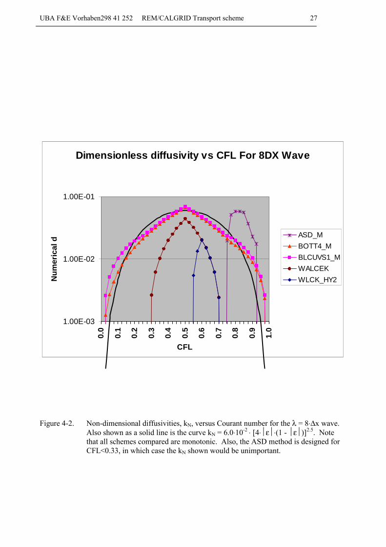
Figure 4-2 presents the non-dimensional diffusivities for the case of the λ = 8⋅∆x wave, and shows that: (a) ASD shows the lowest diffusivities for |ε|<0.5, but as with λ = 4⋅∆x, these values climb rapidly for |ε|>0.5; (b) the Bott and Blackman cubic schemes comparable performance over the full range of CFL and are reasonably modeled by the same functional form used for λ = 4⋅∆x; and (c) the Walcek-based schemes show superior performance, though their strong diffusivity dependence on CFL suggests that significant improvements may still be possible. Earlier, longer wavelength tests, made with the non-monotonic versions of these schemes, indicate that many of the schemes show a λ-4 falloff in diffusivity, which is expected for schemes, such as Bott and Blackman cubic, which are fourth-order accurate in space. In yet other long-wave tests (i.e., also using non-monotonic verions), such as the classic λ = 8⋅∆x cosine hill rotation test (Chock and Dunker, 1982), the diffusivities needed to diffuse the ASD method (with its 2-revolution maxima of 99%) down to the peak height levels of 73%, were obtained by both Bott and Blackman cubic schemes. The result of these and other tests was a numerical diffusivity approximation for these two schemes that can be expressed as:

kN = 0.025⋅ (3 ⋅ ∆x / λ)4 ⋅ [4⋅⏐ε⏐⋅(1 - ⏐ε⏐)] (20). for λ ≥ 3 ⋅ ∆x. For shorter λ the expression, (3 ⋅ ∆x / λ)4 is bounded by 1.0. A critical question is: “Where does one obtain a measure of λ from an arbitrary concentration distribution” as found on the grid of a typical photochemical model simulation. The answer is that one doesn't find λ directly, but rather λ-4, which is just proportional to the fourth derivative of the local concentration distribution and directly related to the truncation error of these numerical schemes. This relationship between the fourth derivative and λ-4 can be seen by considering the Fourier wave, y(x) = A⋅cos(2⋅π⋅x/λ). The fourth derivative of y with respect to x, divided by the function itself, yields the desired relationship: y(4) /y = (2⋅π/λ)4. Despite this seemingly simple answer, extraction of the local λ is generally more complex, as seen in the following sub-section. 4.3 Local Wavelength Determination and Optimal Utilization The issue of where one obtains a measure of the local λ from an arbitrary concentration distribution is perhaps not a simple as outlined above. For example, the simple case where the concentrations are described as, y(x) = A⋅cos(2⋅π⋅x/λ), would not even require evaluation of the 4th derivative, as the ratio of the 2nd derivative to the function itself would yield y(2) /y = -(2⋅π/λ)2 and λ would thus be known. However, addition of a constant A0 to y(x) would alter the denominator and the resulting determination of λ, and this is not generally appropriate. Nevertheless, it is just this approach that has proven reasonable successful in the WLCK_HY2 advection code. If one demands that the λ determination be independent of additive shifts, as well as multiplicative rescalings, a more robust measure for λ must be developed. If one considers the more general expansion, y(x) = A0 + j� Aj⋅cos(kj⋅x) , with kj = 2⋅π⋅x/(j⋅∆x) so that λ = j⋅∆x, Fourier theory tells us that this functional form, plus companion terms Bj⋅sin(kj⋅x), can provide an exact description of any set of points, yi = y(xi), defined on the x domain specified by the regularly spaced grid points x1, x2, x3,…, xN. Thus, y(4) / y(2) = - j� Aj⋅kj

4⋅cos(kj⋅x) / j� Aj⋅kj2⋅cos(kj⋅x) , might be thought of as a local, weighted average value of k2 or λ-2. This

measure can be seen to be invariant to additive and multiplicative shifts.


Figure 4-1. Non-dimensional diffusivities, kN, versus Courant number for the λ = 4⋅∆x wave.

Also shown as a solid line is the curve kN = 8.5⋅10-2 ⋅ [4⋅⏐ε⏐⋅(1 - ⏐ε⏐)]2.5. Note that all schemes compared are monotonic. Also, the ASD method is designed for CFL<0.5, in which case the kN shown would be unimportant.

Dimensionless diffusivity vs CFL For 4DX Wave

1.00E-03

1.00E-02

1.00E-01

0.0

0.1

0.2

0.3

0.4

0.5

0.6

0.7

0.8

0.9

1.0

CFL

Num

eric

al d

ASD_MBOTT4_MBLCUVS1_MWALCEKWLCK_HY2


Figure 4-2. Non-dimensional diffusivities, kN, versus Courant number for the λ = 8⋅∆x wave.

Also shown as a solid line is the curve kN = 6.0⋅10-2 ⋅ [4⋅⏐ε⏐⋅(1 - ⏐ε⏐)]2.5. Note that all schemes compared are monotonic. Also, the ASD method is designed for CFL<0.33, in which case the kN shown would be unimportant.

Dimensionless diffusivity vs CFL For 8DX Wave

1.00E-03

1.00E-02

1.00E-01

0.0

0.1

0.2

0.3

0.4

0.5

0.6

0.7

0.8

0.9

1.0

CFL

Num

eric

al d

ASD_MBOTT4_MBLCUVS1_MWALCEKWLCK_HY2


The question now is how to best obtain this local mean k2 numerically. Just as the lowest order approximation of the 2nd derivative is written as y(2)(x0)⋅(∆x)2 = y(x-1) + y(x+1) - 2⋅y(x0), so the 4th derivative can be expressed as the 2nd derivative of the 2nd derivative or: y(4)(x0)⋅(∆x)4 = y(x-2) + y(x+2) - 4⋅[y(x-1) + y(x+1)] + 6⋅y(x0). As this 5th order accurate characterization of the 4th derivative involves use of five grid point values, there seems little value in using fewer points to define the local 2nd derivative. A simple blending of two forms of the 2nd derivative then lead us to: y(2)(x0)⋅(∆x)2 = β⋅[y(x-2) + y(x+2)] + (1 - 4⋅β)⋅[y(x-1) + y(x+1)] + 2⋅(1 - 3⋅β)⋅y(x0). While choice of β= -1/12 = -0.08333 yields the 5th order accurate characterization of the 2nd derivative, there is no guarantee that it represents the best characterization of the reciprocal of the 2nd derivative, which is what is required. Evaluation of numerical derivatives of admixtures of cosine functions suggest that the most robust measure of local mean k2 is achieved by choosing β= -2/9 = -0.22222. Despite the success in quantifying the local mean k2, it is now unclear that this variable represents the best single variable with which to selectively tune an advection scheme. As a result, research work is continuing on this matter. 4.4 Correction for Artificial Diffusion “Artificial” diffusion refers to the instantaneous dilution of emissions and concentrations by the finite volume, δV = ∆x⋅∆y⋅∆z, of the grid cells. This instantaneous diffusion has traditionally either been ignored or, if the sources contributing to this cell of volume, δV, are deemed important enough, treated by:

a) a finer nested mesh to cover the sub-domain of interest, or b) a plume-in-grid (PiG) module to describe the early dispersion/chemistry evolution of

pollutants emitted by one or a few sources. If one does not wish to incur the computational expense, added complexity, and unresolved scientific issues (e.g., use of simplified chemistry in PiGs, 1-way vs. 2-way nested grids) surrounding either of these approaches, one must accept this initial dilution into the volume, δV. However, there are considerations one may take into account in deciding on the "actual" amount of horizontal diffusivity to be used in REM/CALGRID model. As indicated previously, the basic goal of this study is to determine all the processes in the atmosphere that lead to the “total” horizontal diffusion or smearing of material in nature, and then represent the REM/CALGRID model's “actual” horizontal diffusion coefficient as: actual = total - (numerical + artificial). If the sources within volume, δV, predominate over the material advected into this cell, this will show up as a "sharpening or peaking" of the concentration distribution, which in turn will be seen as a lowering of the effective local wavelength of the concentration distribution toward the minimum value of λ = 2⋅∆x (or ∆y or ∆z). For example, one could use the criteria, λ < 3⋅∆x, to decide that enough artificial diffusion has already occurred, so that the "actual" diffusion should be set to zero. This approach, while intellectually appealing, has not been tested due to the currently poor and unpredictable response of most of the present advection schemes (e.g., the Bott and ASD schemes) to transporting these short wavelengths. That is, the use of some "actual" diffusion can serve as a "preemptive strike" against the even worse numerical diffusion associated with short wavelength distributions. Consistent with these short wavelength transport problems, it may actually be beneficial to apply filtering (e.g., the Forester filter used in ASD) before transport step rather than after transport, as is currently done in nearly all transport algorithms.


4.5 Adjustment of the Horizontal Diffusion Coefficients in the REM/CALGRID Model In the original REM/CALGRID model, the lateral plume dispersion process was taken almost directly from the urban-scale CALGRID model. It is now clear that these diffusivities underestimate the diffusivities appropriate to scales of 20-50 km. Further examining the diffusivity values and the relative centerline concentrations of Table 4-1, we note that plume dispersion begins to “look significant” relative to daytime dispersion rates at dimensionless diffusivities of order 10-2. For the finer REM/CALGRID model grid (i.e., ∆x = 2 km and ∆t = 300 s), this would correspond to diffusivities of about 133 m2 /s, and 15,000 m2 /s for the coarser 30km grid; thus, it is important to include the larger diffusivities corresponding to lateral diffusion in the atmosphere as well as correct for the numerical diffusion in the horizontal transport scheme. Both of these effects, and the additional correction for wind shears, is presently being incorporated into a revised REM/CALGRID model modeling system. The modified and additional subroutines developed during this study can be brought into (or removed from) the operational REM/CALGRID model simply by changing the mix of subroutines available at code compilation time. In practice, this is accomplished by having different "Make" files for the original and modified versions, and no other changes to data structures, formats, or input files are needed. Thus, no changes to REM/CALGRID model's meteorological preprocessor or other REM/CALGRID model file structures were instituted. A complete list and description of these new and modified subroutines will be documented in an Appendix. 4.6 Refined Measures of Advection Scheme Performance Equation (19) developed in section 4.2 provides an important of the numerical diffusion caused by transport algorithms. However, one drawback of Eq(19) is that some algorithms (e.g., Walcek (2000) with “full steepening” will maintain the peak and trough values perfectly, but will slowly distort the cosine wave into something more like a square wave. In this case, Eq(19) will yield a diffusivity of zero, and thus “mask” the serious distortion issue. This leads one to search for a measure that will encompass classical diffusion, as well as the more subtle distortion and anti-diffusion mechanisms existing in modern transport algorithms. One usual comprehensive measure is the mean-square residual, expressible as Rs = i�(y′′i – yi)2

/N where the sum on i includes N points that span at least one full cycle of the cosine wave. The question then arises as to how we relate the summed measure of Rs to a diffusivity d. The answer can be found by considering the analytic solution to the diffusion equation. For the case of the initial functional form y(x,0) = cos(2⋅π⋅x/λ) = cos(k⋅x), where k = 2⋅π/λ, the solution over all time is just y(x,t) = cos(k⋅x) ⋅ exp(–k2⋅K⋅t), where K is the dimensional diffusivity, K = d⋅∆x2/∆t, and dt is the theoretical, non-dimensional diffusivity. Thus, the exponential term may be re-expressed as F(t) = exp(–k2⋅K⋅t) = exp[–(2⋅π/n)2⋅ dt ⋅ (t/∆t)], so that the theoretical residual, Rt, between the original field and the one existing after two time steps is simply xm

Rt = (1/xm) 0� dx ⋅ [1 – F2]2 ⋅ cos2(k⋅x) ,

where F = F(∆t) = exp[–(2⋅π/n)2⋅ dt] and xm should be large enough to average over a full wave. This is achieved by choosing xm = 2⋅π/k and yields the simple result Rt = (1/2)⋅[1 – F2]2. Now equating Rt and Rs enables one to solve for F, as F2 = 1 – (2⋅Rs)1/2 , and hence obtain dt as:

dt = – ½ ⋅ [n/(2⋅π)]2 log[1 – (2⋅Rs)1/2]. (21a)


For small values of Rs, this expression can be approximated as, dt ≈ ½ ⋅ [n/(2⋅π)]2 (2⋅Rs)1/2 (21b) which shows that dt is proportional to the r.m.s.residual and reassures us that dt now reflects the overall goodness-of-fit rather than just diffusion of the extrema. Now this does still not tell us how to relate this theoretical diffusivity dt to the numerically derived diffusivity, d, of Eq(19); however, this is easily done by matching the solution of both methodologies at the unit cosine’s peak after one time-step. This comparison tells us that y′0 = 1 – 2⋅d⋅[1 – cos(2⋅π/n)] = exp[–(2⋅π/n)2⋅ dt], and this may be rearranged to yield:

d = ½ ⋅ {1 – exp[–(2⋅π/n)2⋅ dt] } / [1 – cos(2⋅π/n)] (22) This unusual-looking relationship tells one, for example, that an infinite dt for the λ= 2⋅∆x cosine wave (i.e., n=2) is equivalent to d = ¼ in a grid model. In fact, this is just the needed diffusivity to diffuse the 2⋅∆x wave in a single time-step. Combining Eq(21a) and (22) now leads us to the quite simple relation between d and Rs as

d = ½ ⋅ {1 – [1 – (2⋅Rs)1/2] 1/2} / [1 – cos(2⋅π/n)] . (23) Small Rs allow this expression to be approximated as d ≈ ¼ ⋅ (2⋅Rs)1/2 / [1 – cos(2⋅π/n)] and for large n (i.e., long waves, well resolved on the grid) further approximated as d ≈ ½ ⋅ [n/(2⋅π)]2 ⋅ (2⋅Rs)1/2 , which not surprisingly is identical to Eq(21b). Thus, d ≈ dt in the limit of small diffusivities for waves well resolved on the grid (i.e., large n for long waves). Equation (23) also reminds one that this formulation requires Rs ≤ ½, which represents the limit of the fully-diffused, unit-amplitude, cosine wave. Hence, one must be careful to ensure that Rs is properly renormalized to the case of a unit-amplitude wave before extracting diffusivities. The only problem now is that the d one obtains from Eq(23) combines the influences of classical diffusion and various types of distortion. The reason for this is that the residual, Rs, Rs = i�(y′′i – yi)2

/N involves the difference between the two-time-step-diffused observed values and the original values, which incidentally are equal to the original theory values. Suppose instead that a residual were defined as the difference between the two-time-step-diffused observed values and the two-time-step-diffused theoretical values. That is, for the theoretical form, y(xi,t) = 1 + cos(k⋅xi), and its two-time-step-diffused form y′′(xi,t) = 1 + cos(k⋅xi)⋅exp[–2⋅(2⋅π/n)2⋅ dtn] , one forms the purely “distortional” residual Rd, defined as

Rd = i� [y′′i – y′′(xi,t)]2 /N = i� {y′′i – 1 – cos(k⋅xi)⋅exp[–2⋅(2⋅π/n)2⋅ dtn] }2

/N (24) This expression now incorporates an unknown, theoretical, numerical diffusivity, dtn , due to the transport algorithm, and isolates the distortional residual, Rd, accompanying those two transport steps. Finding this unknown value of dtn in Eq(24) is accomplished by evaluating the expression: ∂Rd/∂dtn = 0 to obtain that value dtn yielding a minimal value of Rr. This differentiation leads to,

exp[–2⋅(2⋅π/n)2⋅ dtn] = i� (y′′i – 1)⋅cos(k⋅xi) / i� cos2(k⋅xi)


which, after taking the log of both sides, yields the improved, “optimal” result for dtn as, dtn = –½ ⋅ [n/(2⋅π)]2 ⋅ log{ i� (y′′i – 1)⋅cos(k⋅xi) / i� cos2(k⋅xi) } . (25) Equation (22) may now be used to transform this purely diffusional dtn into its numerical grid model equivalent, dn, corresponding to a pure numerical diffusivity. Another advantage of this reformulation is that it allows for negative values of dtn and dn, and identification of these negative diffusivities is useful for identifying those schemes which may lead to unacceptable behaviors over many time steps. Substituting Rd for Rs in Eq(23) now enables us to define a purely distortionary “diffusivity”, Dd, as

Dd = ½ ⋅ {1 – [1 – (2⋅Rd)1/2] 1/2} / [1 – cos(2⋅π/n)] . (26) Whether Dd turns out to add any particular “value” over the more traditional measures of mean-square-residual, Rs and Rd, remains to be seen; however, it does offer the opportunity to form the comparative ratio dn/Dd, which may be useful in judging whether the diffusion and distortion created by a scheme are “in balance” with one another. Also, perhaps not surprisingly, the resulting set of diffusivities obey the quadrature addition rule,

d2 = dn2 + Dd

2 ; (27a)

however; this holds only for classical values of dn > 0, and not for those algotithms exhibiting “anti-diffusive” characteristics accompanying dn < 0. In these anti-diffusive cases, one finds that

d2 > dn2 + Dd

2 . (27b) What we have developed above represents refined measures of the pure numerical diffusion, dn, and the measure of all other distortions, Dd, induced by a numerical advection scheme. The advantage of this formulation, over the earlier Eq(19), is that it is based on analysis of the complete cosine wave rather than peak or trough values that can be manipulated by various extrema preservation techniques. Exploration of this new diagnostic methodology is continuing.


5. SUMMARY AND CONCLUSIONS A number of issues and phenomena were examined in detail as part of this study. First, a revised transport algorithm was developed that removes all velocity-shear-induced, operator- splitting errors. The resulting, computationally-efficient transport scheme conserves mass, ensures the transport of correct mass fluxes, and maintains constant mixing ratios. Second, the magnitude and constituent components of lateral diffusion in the atmosphere were reviewed. Given the very significant role of wind shear (e.g., shears at a particular horizontal level and turning of the wind direction with height) in the lateral diffusion process, a wind model's ability to capture wind shears was examined. The prognostic model MM-5 is seen to capture 50-80% of the shear measured over separations greater than three grid cells, and it is anticipated that the diagnostic wind models of the Free University should preserve an even greater fraction of that shear, provided the wind fields are not excessively smoothed. This suggests that the shear correction module developed for REM/CALGRID model during this study can reasonably utilize the available diagnostic winds and achieve the appropriate advective redistribution of pollutants; however, this finding should be confirmed with actual wind fields generated by these FUB diagnostic models. The vertical resolution of most wind field models also ensure their capturing the important vertical wind shears, which in turn demands that the diffusivities that one utilizes in a REM/CALGRID model lateral diffusivity module not "double count" this important effect. As a result, a more appropriate horizontal diffusion coefficient has been computed with the aid of a synthetic turbulence model, KSP, that can simulate lateral dispersion in an artificial atmosphere that is free of such vertical wind shear. KSP results indicated that an appropriate lateral diffusivity for 10km wide plumes in a neutral atmosphere, free of directional shear, is of order u*⋅σy, where u* is the friction velocity and σy is the plume's lateral standard deviation. Extension of this concept throughout the PBL then led to a physical, non-dimensional diffusivity of kH = 0.2⋅iy⋅ε , where iy is the local turbulent intensity, σv/U, and ε is the local Courant number, U⋅∆t /∆x. The resulting diffusivity module thus utilizes micrometeorologically-based estimates of the standard deviation of lateral velocity, σv, times a constant and the grid resolution, ∆x, of the modeling domain. The resulting REM/CALGRID model lateral diffusivity module also incorporates the results of our investigation and subsequent parameterization of numerical diffusion. This aspect of the study revealed that the long-wave numerical diffusivities of most high fidelity advection schemes can be characterized in terms of simple functions of the local Courant number, ε, and an estimate of the local wavelength, λ, of the concentration distribution. Numerical diffusion corrections for the Bott and Blackman-cubic advection schemes have been developed, and a comparable correction is being formulated for the more complex Walcek scheme. These parameterizations of numerical diffusion are then easily implemented into the existing module code. The completed set of lateral transport and diffusivity modules is then smoothly and seamlessly integrated into the REM/CALGRID model simply via substitution of a number of REM/CALGRID model's subroutines, and no changes to REM/CALGRID model's preprocessor, input data formats, or control files are required.


6. REFERENCES Batchelor, G.K., 1949. Diffusion in a field of homogeneous turbulence. Austral. J. Sci. Res. A2,

437-450. Blackman, R.B. and J.W. Tukey, 1958: The Measurement of Power Spectra, New York, Dover

Publications, 190 pp. Bott, A., 1993: The monotone area-preserving flux-form advection algorithm: Reducing the

time-splitting error in two dimensional flow fields. Mon. Wea. Rev., 121, 2637-2641. Bott, A., 1992: Monotone flux limitation in the area-preserving flux-form advection algorithm.

Mon. Wea. Rev., 120, 2592-2602. Bott, A., 1989: A positive definite advection scheme obtained by nonlinear renormalization of the

advection fluxes. Mon. Wea. Rev., 117, 1006-1015. Briggs, G.A., 1973: Diffusion estimates for small emissions (Draft). Air Resources Atmospheric

Turbulence and Diffusion Laboratory. ATDL No. 79. and also Internal memorandum as reported by F.A. Gifford, Jr., in Turbulent diffusion-typing schemes: a review. Nuclear Safety, 17, 68-86.

Chock, D.P., 1991: A comparison of numerical methods for solving the advection equation-III,

Atmos. Environ., 25A, 853-871. Chock, D.P., 1985: A comparison of numerical schemes for solving the advection equation--II.

Atmos. Environ., 19, 571-586. Chock, D.P. and A.M. Dunker, 1982: A comparison of numerical methods for solving the

advection equation, General Motors Report No. GMR-3603/ENV#100 and Atmos. Environ., 17, 11-24.

Clappier, A., 1989: A correction method for use in multidimensional time-splitting advection

algorithms: Applications to two- and three-dimensional transport. Mon. Wea. Rev., 126, 232-242.

Crowley, W.P., 1968: Numerical advection experiments, Mon. Wea. Rev., 96, 1-11. Dabdub, D. and J.H. Seinfeld, 1994: Numerical advective schemes used in air quality models --

Sequential and parallel implementation. Atmos. Environ., 28, 3369-3385. DaMassa J. et al. (1996) Performance evaluation of SAQM in Central California and attainment

demonstration for the August 3-6, 1990 ozone episode. Technical Report, California Air Resources Board, Sacramento, CA, 109 pp.

Dudhia, J., 1993: A non-hydrostatic version of the Penn State/NCAR Mesoscale Model:

Validation tests and simulation of an Atlantic cyclone and cold front, Mon. Wea. Rev., 121, 1493-1513.


Eckman M. (1994) Re-examination of empirically derived formulas for horizontal diffusion from surface sources. Atmos. Environ. 28, 265-272.

Emde, K.V.D., 1992: Solving conservation laws with parabolic and cubic splines. Mon. Wea.

Rev., 120, 482-492. Gazdag, J., 1973: Numerical convective schemes based on accurate computation of space

derivatives. J. Comp. Phys., 13, 100-113. Gifford, F.A. (1982) Horizontal diffusion in the atmosphere: A Lagrangian-dynamical theory.

Atmos. Environ. 16, 505-511. Grell, G., J. Dudhia, and D. Stauffer, 1994: A Description of the Fifth-Generation Penn

State/NCAR Mesoscale Model (MM5), NCAR/TN-398+STR, National Center for Atmospheric Research, Boulder, CO, 138pp.

Gryning S.E., Holtslag A.M., Irwin J.S. and Sivertsen B. (1987) Applied dispersion modelling

based on meteorological scaling parameters. Atmos. Environ. 21, 79-89. Hanna S.R. (1994) Random variability in mesoscale wind observations and implications for

diffusion models. Proceedings of the 8th Joint Conference on Applications of Air Pollution Meteorology with A&WNA, Nashville, TN, January 23-28.

Heffter J.L. (1980) Air Resources Laboratory atmospheric transport and dispersion model (ARL-

ATAD). NOAA Tech. Memo., ERL-AFL-81 Hov, O., Z. Zlatev, R. Berkowicz, A. Eliassen and L.P. Prahm, 1989: Comparison of numerical

techniques for use in air pollution models with non-linear chemical reactions. Atmos. Environ., 23, 967-983.

Irwin J.S. (1983) Estimating plume dispersion — a comparison of several sigma schemes. J. Clim.

appl. Met. 22, 92-114. Janicke, L., 1995: Ausbreitungsmodell LASAT: Referenzbuch zu Version 2.51, Primelweg 8,

D-88662 Überlingen, FRG. (In German) Long, P.E. and D.W. Pepper, 1981: An examination of some simple numerical schemes for

calculating scalar advection. J. appl. Meteor., 20, 146-156. Long, P.E. and D.W. Pepper, 1976: A comparison of six numerical schemes for calculating the

advection of atmospheric pollution. Third Symposium on Atmospheric Turbulence, Diffusion, and Air Quality, Raleigh, NC, 19-22 October, 1976.

Mahrt, L, 2000. Diffusion in the Stable Boundary Layer. Proceedings of the 11 th Joint

AMS/AWMA Conference on the Applications of Air Pollution Meteorology, Long Beach, CA, Jan. 9-14, pp 1-3.

Marchuk, G.I., 1975: Methods of Numerical Mathematics. New York, Springer-Verlag. 316 pp.


McRae, G.J., W.R. Goodin and J.H. Seinfeld, 1982: Numerical solution of the atmospheric diffusion equation for chemically reacting flows. J. Comp. Phys., 45, 1-42.

Moran, M.D., 1992. Numerical Modelling of Mesoscale Atmospheric Dispersion, Atmospheric

Science Paper No. 513, Colorado State University, Fort Collins, CO, 758 pp. Nasstrom, J.S., G Sugiyama, J.M. Leone, and D.E. Ermak, 2000. A Real-time Atmospheric

Dispersion Modeling System. Proceedings of the 11 th Joint AMS/AWMA Conference on the Applications of Air Pollution Meteorology, Long Beach, CA, January 9-14, pp84-89.

Odman M.T., Wilkinson J.G., McNair L.A., Russell A.G., Ingram C.L. and Houyoux M.R.

(1996), Horizontal advection solver uncertainty in the Urban Airshed Model. Final Report, Contract No. 93-722, California Air Resources Board, Sacramento, CA.

Odman, M.T., Xiu, A., and Byun, D.W. (1995) Evaluating advection schemes for use in the next

generation of air quality modeling systems. In Regional Photochemical Measurement and Modeling Studies (edited by A.J. Ranzieri and P.A. Solomon), Vol. III, 1386-1401, Air & Waste Management Association, Pittsburgh, PA.

Odman, M.T. and A.G. Russell, 1991: Multiscale modeling of pollutant transport and chemistry.

J. Geophys. Res., 96, 7363-7370. Pack, D.H., G.J. Ferber, J.L. Heffter, K. Telegadas, J.K. Angell, W.H. Hoecker, and L. Machta,

1978. Meteorology of long-range transport. . Atmos. Environ., 12, 425-444. Pepper, D.W., C.D. Kern and P.E. Long, 1979: Modeling the dispersion of atmospheric pollution

using cubic splines and chapeau functions. Atmos. Environ., 13, 223-237. Pielke, R.A., et al., 1992: A comprehensive meteorological modeling system - RAMS. Meteor.

Atmos. Phys., 49, 69-91. Prather M.J. (1986) Numerical advection by conservation of second-order moments. J. Geophys.

Res. 91, 6671-6681. Roache, P.J., 1976: Computational Fluid Dynamics (2nd edn.). Hermosa, Albuquerque, NM. Schere, K.L., 1983: An evaluation of several numerical advection schemes. Atmos. Environ., 17,

1897-1907. Seaman, N.L., D.R. Stauffer, and A.M. Lario-Gibbs, 1995: A multi-scale four-dimensional data

assimilation system applied in the San Joaquin Valley during SARMAP. Part I: Modeling design and basic performance characteristics, J. Appl. Meteorol., 34, 1739.

Smagorinsky, J., 1963: General circulation experiments with the primitive equations: 1. The basic

experiment. Mon. Weath. Rev., 91, 99-164. Stauffer, D.R. and N.L. Seaman, 1994: Multiscale four-dimensional data assimilation, Mon. Wea.

Rev., 33, 416-434.


Stern, R. and R.J. Yamartino, 2002. Development and first results of a new photochemical model for simulating ozone and PM-10 over extended periods. Proceedings of the 12th

AMS/AWMA Conf. on the Applications of Air Pollution Meteorology, Norfolk, Virginia, May 20-24, AMS, Boston, MA.

Stern, R., 1994: Development and application of a three-dimensional photochemical dispersion

model using different chemical mechanisms. Meteorologische Abhandlungen, Serie A Vol. 8, Dietrich Reimer, Berlin (in German).

Tanrikulu S. and Odman M.T. (1996) The effects of advection solvers on the performance of air

quality models. Presented at the 5th International Conference on Atmospheric Sciences and Applications to Air Quality, Seattle, Washington, June 18-20, 1996.

Tesche T.W. et al. (1990) Improvement of procedures for evaluating photochemical models.

Radian Corporation, Report to the California Air Resources Board Tremback, C.J., J. Powell, W.R. Cotton and R.A. Pielke, 1987: The forward-in-time upstream

advection scheme: Extension to high orders. Mon. Wea. Rev., 115, 540-555. U.S. EPA, 1987: Industrial Source Complex (ISC) dispersion model user's guide -- Second

edition (revised). EPA-450/4-88-002. van Eykeren, J., Th. van Stijn and N. Praagman, 1987: A comparative investigation of numerical

methods for advective processes. In Air Pollution Modeling and Its Application VI (edited by H. van Dop), pp. 641-652. Plenum Press, New York.

Walcek, C.J.; Minor flux adjustment near mixing ratio extremes for simplified yet highly accurate

monotonic calculation of tracer advection, J. Geophy. Res. , 105, D7 (2000), 9335-9348. Walcek, C.J. and N.M. Aleksic; A simple but accurate mass conservative, peak-preserving, mixing

ratio bounded advection algorithm with FORTRAN code, Atmos. Environ., 32 (1998), 3863-3880.

Yamartino, R .J., M. E. Fernau, and S. Machiraju, 2000. Determination of the Horizontal

Diffusion Coefficient for Use in the SARMAP Air Quality Model. Final Report, Contract 96-314, California Air Resources Board Research Division, 2020 L Street, Sacramento, CA 95812.

Yamartino, R.J., 2000. Refinement of Horizontal Diffusion in Photochemical Grid Models.

Proceedings of the 11 th Joint AMS/AWMA Conference on the Applications of Air Pollution Meteorology, Long Beach, CA, January 9-14, pp226-229.

Yamartino, R.J., 1998. Improvements to Horizontal Transport in Grid Models. Proceedings of

the 23rd NATO/CCMS ITM on Air Polluting Modeling and its Application, Varna, Bulgaria, Sept. 28 - Oct. 2.

Yamartino, R. and D. Strimaitis, 1998. Refinement and Evaluation of the Kinematic Simulation

Particle Model. EARTH TECH Final Report to the German Umweltbundesamt, Sept.


Yamartino, R.J., 1993: Nonnegative, conserved scalar transport using grid-cell-centered, spectrally constrained Blackman cubics for applications on a variable-thickness mesh. Mon. Wea. Rev., 121, 753-763.

Yamartino, R.J., J.S. Scire, G.R. Carmichael and Y.S. Chang, 1992: The CALGRID mesoscale

photochemical grid model--I. Model formulation. Atmos. Environ., 26A, 1493-1512. Yamartino, R.J., J.S. Scire, S.R. Hanna, G.R. Carmichael and Y.S. Chang, 1989: CALGRID: A

mesoscale photochemical grid model. Volume 1: Model formulation document, California ARB Report, Sacramento, CA.

Yamartino, R.J. and J.S. Scire, 1984: The transport and diffusion modules, Volume 3.

ADOM/TADAP Model Development Program, Ontario Ministry of the Environment, Rexdale, Ontario, Canada.

Yanenko, N.N., 1971: The Method of Fractional Steps. Springer, New York.

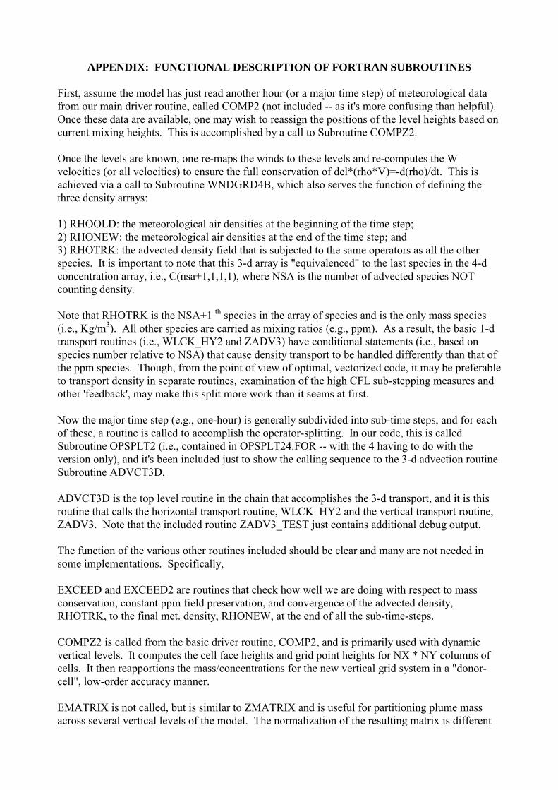
APPENDIX: FUNCTIONAL DESCRIPTION OF FORTRAN SUBROUTINES First, assume the model has just read another hour (or a major time step) of meteorological data from our main driver routine, called COMP2 (not included -- as it's more confusing than helpful). Once these data are available, one may wish to reassign the positions of the level heights based on current mixing heights. This is accomplished by a call to Subroutine COMPZ2. Once the levels are known, one re-maps the winds to these levels and re-computes the W velocities (or all velocities) to ensure the full conservation of del*(rho*V)=-d(rho)/dt. This is achieved via a call to Subroutine WNDGRD4B, which also serves the function of defining the three density arrays: 1) RHOOLD: the meteorological air densities at the beginning of the time step; 2) RHONEW: the meteorological air densities at the end of the time step; and 3) RHOTRK: the advected density field that is subjected to the same operators as all the other species. It is important to note that this 3-d array is "equivalenced" to the last species in the 4-d concentration array, i.e., C(nsa+1,1,1,1), where NSA is the number of advected species NOT counting density. Note that RHOTRK is the NSA+1 th species in the array of species and is the only mass species (i.e., Kg/m3). All other species are carried as mixing ratios (e.g., ppm). As a result, the basic 1-d transport routines (i.e., WLCK_HY2 and ZADV3) have conditional statements (i.e., based on species number relative to NSA) that cause density transport to be handled differently than that of the ppm species. Though, from the point of view of optimal, vectorized code, it may be preferable to transport density in separate routines, examination of the high CFL sub-stepping measures and other 'feedback', may make this split more work than it seems at first. Now the major time step (e.g., one-hour) is generally subdivided into sub-time steps, and for each of these, a routine is called to accomplish the operator-splitting. In our code, this is called Subroutine OPSPLT2 (i.e., contained in OPSPLT24.FOR -- with the 4 having to do with the version only), and it's been included just to show the calling sequence to the 3-d advection routine Subroutine ADVCT3D. ADVCT3D is the top level routine in the chain that accomplishes the 3-d transport, and it is this routine that calls the horizontal transport routine, WLCK_HY2 and the vertical transport routine, ZADV3. Note that the included routine ZADV3_TEST just contains additional debug output. The function of the various other routines included should be clear and many are not needed in some implementations. Specifically, EXCEED and EXCEED2 are routines that check how well we are doing with respect to mass conservation, constant ppm field preservation, and convergence of the advected density, RHOTRK, to the final met. density, RHONEW, at the end of all the sub-time-steps. COMPZ2 is called from the basic driver routine, COMP2, and is primarily used with dynamic vertical levels. It computes the cell face heights and grid point heights for NX * NY columns of cells. It then reapportions the mass/concentrations for the new vertical grid system in a "donor-cell", low-order accuracy manner. EMATRIX is not called, but is similar to ZMATRIX and is useful for partitioning plume mass across several vertical levels of the model. The normalization of the resulting matrix is different

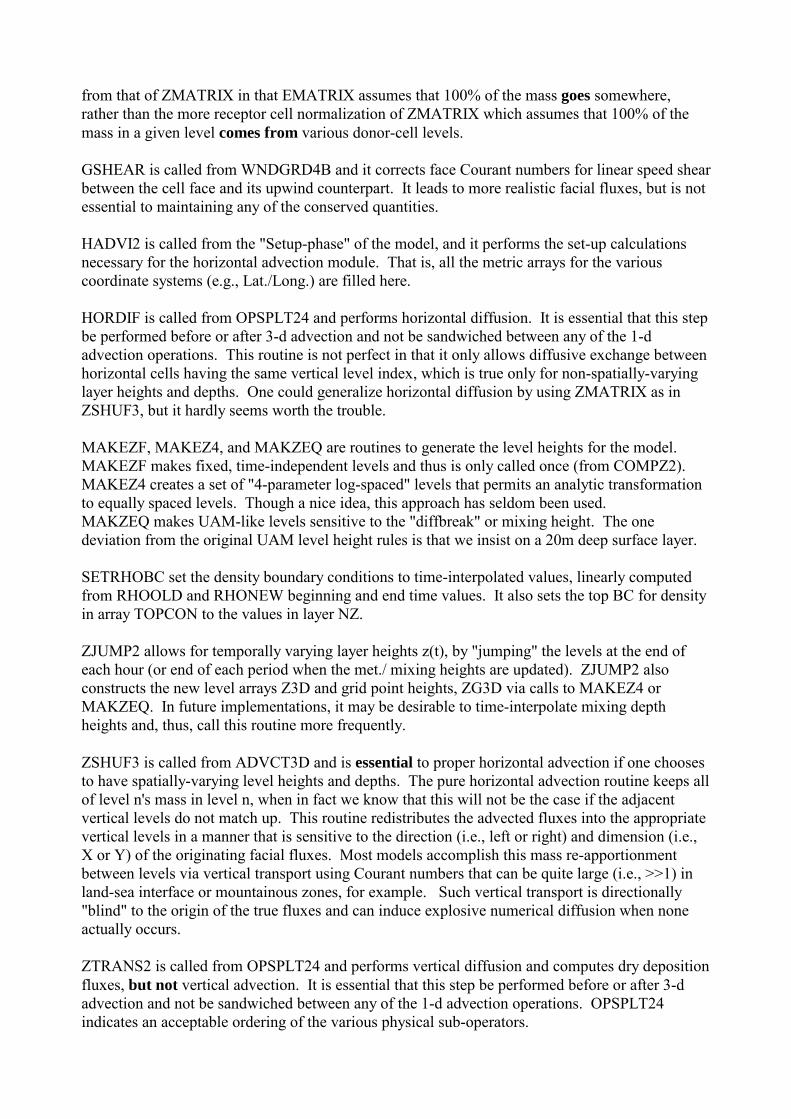
from that of ZMATRIX in that EMATRIX assumes that 100% of the mass goes somewhere, rather than the more receptor cell normalization of ZMATRIX which assumes that 100% of the mass in a given level comes from various donor-cell levels. GSHEAR is called from WNDGRD4B and it corrects face Courant numbers for linear speed shear between the cell face and its upwind counterpart. It leads to more realistic facial fluxes, but is not essential to maintaining any of the conserved quantities. HADVI2 is called from the "Setup-phase" of the model, and it performs the set-up calculations necessary for the horizontal advection module. That is, all the metric arrays for the various coordinate systems (e.g., Lat./Long.) are filled here. HORDIF is called from OPSPLT24 and performs horizontal diffusion. It is essential that this step be performed before or after 3-d advection and not be sandwiched between any of the 1-d advection operations. This routine is not perfect in that it only allows diffusive exchange between horizontal cells having the same vertical level index, which is true only for non-spatially-varying layer heights and depths. One could generalize horizontal diffusion by using ZMATRIX as in ZSHUF3, but it hardly seems worth the trouble. MAKEZF, MAKEZ4, and MAKZEQ are routines to generate the level heights for the model. MAKEZF makes fixed, time-independent levels and thus is only called once (from COMPZ2). MAKEZ4 creates a set of "4-parameter log-spaced" levels that permits an analytic transformation to equally spaced levels. Though a nice idea, this approach has seldom been used. MAKZEQ makes UAM-like levels sensitive to the "diffbreak" or mixing height. The one deviation from the original UAM level height rules is that we insist on a 20m deep surface layer. SETRHOBC set the density boundary conditions to time-interpolated values, linearly computed from RHOOLD and RHONEW beginning and end time values. It also sets the top BC for density in array TOPCON to the values in layer NZ. ZJUMP2 allows for temporally varying layer heights z(t), by "jumping" the levels at the end of each hour (or end of each period when the met./ mixing heights are updated). ZJUMP2 also constructs the new level arrays Z3D and grid point heights, ZG3D via calls to MAKEZ4 or MAKZEQ. In future implementations, it may be desirable to time-interpolate mixing depth heights and, thus, call this routine more frequently. ZSHUF3 is called from ADVCT3D and is essential to proper horizontal advection if one chooses to have spatially-varying level heights and depths. The pure horizontal advection routine keeps all of level n's mass in level n, when in fact we know that this will not be the case if the adjacent vertical levels do not match up. This routine redistributes the advected fluxes into the appropriate vertical levels in a manner that is sensitive to the direction (i.e., left or right) and dimension (i.e., X or Y) of the originating facial fluxes. Most models accomplish this mass re-apportionment between levels via vertical transport using Courant numbers that can be quite large (i.e., >>1) in land-sea interface or mountainous zones, for example. Such vertical transport is directionally "blind" to the origin of the true fluxes and can induce explosive numerical diffusion when none actually occurs. ZTRANS2 is called from OPSPLT24 and performs vertical diffusion and computes dry deposition fluxes, but not vertical advection. It is essential that this step be performed before or after 3-d advection and not be sandwiched between any of the 1-d advection operations. OPSPLT24 indicates an acceptable ordering of the various physical sub-operators.

Refined 3-d Transport and Horizontal Diffusion for the REM ...

Documents

Transcript of Refined 3-d Transport and Horizontal Diffusion for the REM ...