I

No./Nr. 08/2005

Investment Performance of Residual IncomeValuation Models on the German Stock Market

Gösta Jamin

Research Papersof the Institute for Business Management______________________________

Forschungsberichtedes Betriebswirtschaftlichen Instituts

Wirtschaftswissenschaftliche Fakultät derBayerischen Julius-Maximilians-Universität

Würzburg

II

Investment Performance of Residual IncomeValuation Models on the German Stock Market

Gösta Jamin1

Abstract

This paper analyses value-investing strategies based on the residual

income valuation approach which has become popular due to the

work of Ohlson (1995) and Feltham and Ohlson (1995) for the

German stock market. Plenty of empirical evidence shows that it is

possible to earn positive abnormal returns by investing in on the basis

of simple fundamental ratios such as PE ratio, PB ratio, or dividend

yield undervalued stocks. A price-value (PV) ratio calculated with the

residual income approach is theoretically better founded than the

simple ratios mentioned above as it captures all value-generating

aspects. Four model specifications are developed and their

performance when using them for value-investing strategies is

compared to the performance of the simple ratios for German

companies over a period of 1990 – 2002. It turns out that

fundamentally undervalued companies indeed earn higher returns but

the results are statistically weak and the theoretically superior models

do not perform significantly better than the simple ratios.

1 Diplom-Volkswirt Gösta Jamin, Chair of Accounting and Auditing, Bayerische Julius-

Maximilians-Universität Würzburg and McKinsey & Company, Inc., Prinzregentenstr. 22,D-80538 München. E-Mail: goesta_jamin@mckinsey.com. This paper is based on mydissertation. I would like to express my gratitude to Prof. Hansrudi Lenz from theBayerische Julius-Maximilians-Universität in Würzburg and Prof. Horst Entorf from TUDarmstadt for their guidance. I also appreciate grateful support from my employerMcKinsey & Company, Inc during my leave of absence. Furthermore I would like tothank workshop participants at Bayerische Julius-Maximilians-Universität in Würzburgand TU Darmstadt for helpful comments and suggestions.

III

Impressum:

Herausgeber:

Bayerische Julius-Maximilians-Universität WürzburgWirtschaftswissenschaftliche FakultätBetriebswirtschaftliches InstitutDer GeschäftsführerSanderring 297070 Würzburg

V.i.S.d.P.: Gösta Jamin

Redaktionsschluss: 7. Juni 2005Erscheinungsort: Würzburg

ISSN 1612-233X

1

Investment Performance of Residual Income ValuationModels on the German Stock Market

Contents

Table of abbreviations....................................................................................2

Table of symbols .............................................................................................3

Table of figures ...............................................................................................4

Table of tables .................................................................................................5

1 Introduction............................................................................................6

2 Residual Income Valuation Approach.................................................8

3 Value-Investing Strategies ..................................................................11

3.1 Fundamentals of Value-Investing...............................................11

3.2 Explanations for the Profitability of Value-Investing ..............13

4 Models ...................................................................................................16

4.1 Impact of Accounting Conservatism..........................................16

4.2 Model Development .....................................................................17

5 Data .......................................................................................................26

6 Results ...................................................................................................28

6.1 Descriptive Statistics....................................................................28

6.2 Parameter Estimates for Models 3 and 4...................................32

6.3 Forecasting Future Stock Returns .............................................36

7 Conclusion ............................................................................................44

References......................................................................................................45

Appendix........................................................................................................51

2

Table of abbreviations

CAPM Capital Asset Pricing ModelCDAX Composite Deutscher AktienindexCSR Clean Surplus RelationDAX Deutscher AktienindexDCF Discounted Cash FlowDDM Dividend Discount ModelFY1 Fiscal year 1FY2 Fiscal year 2HGB HandelsgesetzbuchIAS International Accounting StandardsI/B/E/S Institutional Brokers Estimates SystemIPO Initial public offeringLIM Linear information modellingMFEP Mean forecast error scaled by priceMAFEP Mean absolute forecast error scaled by priceMFEE Mean forecast error scaled by earningsMAFEE Mean absolute forecast error scaled by earningsNEMAX Neuer Markt IndexOLS Ordinary least squaresPB Price-BookPE Price-EarningsPV Price-ValueRIV Residual income valuationSUR Seemingly unrelated regressionsUS GAAP United States General Agreement on Accounting Principles

3

Table of symbols

1α Coefficient in valuation equation of the model of Ohlson (1995)for residual income

2α Coefficient in valuation equation of the model of Ohlson (1995)for "other information"

3α Coefficient in valuation equation for book value in model 4

tB Book value of equity in t

tD Dividend in t

[ ].tE Expected value in t

t,1ε Error term of autoregressive process of residual income

t,2ε Error term of autoregressive process of "other information"

t,3ε Error term of book value growth process in model 4

tf Analyst forecast in t on earnins per share in t+1a

tf Analyst forecast in t on residual income per share in t+1

G Growth factor

tGW Goodwill in t

R Discount factor for cost of capital

tV Intrinsic firm value in t

tv "Other information" in t

ϖ Persistence parameter for residual income

0ϖ Regression constant for parameter estimation

0~ϖ Empirically measured regression constant for parameter

estimation

1ϖ Persistence parameter for residual income

1~ϖ Empirically estimated value for persistence parameter for

residual income

tx Earnings per share in tatx Residual income per share in t

implatx , Implicit market expectation on residual income

γ Persistence parameter of "other information"

0γ Regression constant in second-stage regression of parameterestimation for models 3 and 4

4

Table of figures

Figure 1: Return CDAX and Sample.....................................................................30Figure 2: Cumulated hedge-return of the four model specifications .....................37Figure 3: Cumulated hedge-return of simple ratios ...............................................41

5

Table of tables

Table 1: Number of companies included in sample ..............................................28Table 2: Descriptive statistics on accounting and earnings forecast data..............29Table 3: Mean forecast error of analyst earnings forecasts over one year (FY1)

and two years (FY2) ......................................................................................31Table 4: Results of one-stage parameter estimates for model 3 ............................32Table 5: Results of one-stage parameter estimates for model 4 ............................33Table 6: One-stage estimation of persistence parameters without γ for models 3

and 4...............................................................................................................35Table 7: Hedge-return of model specifications under the assumption of a market

risk premium of 2% .......................................................................................38Table 8: Hedge-return of model specifications under the assumption of a market

risk premium of 5% .......................................................................................39Table 9: Hedge-return of simple ratios ..................................................................42Table 10: Average portfolio beta under the assumption of a market risk premium

of 2%..............................................................................................................43

6

1 Introduction

The past five years have been a rollercoaster on the German as well as oninternational stock markets. The DAX as the leading index of the German stockmarket rose from 4,500 in the second half of 1998 to 7,500 at the beginning of2000, and plummeted to 2,200 in March 2003. Until mid-2005 the recovery on theinternational stock markets led to an increase of the DAX to around 4,500 in June2005. The development at the so-called Neuer Markt, the segment for high-techstart-up firms, was even more remarkable. The 700 percent increase of theNEMAX All Share, an index comprising all stocks traded at the Neuer Markt,from 1,000 in 1997 to around 8,000 at the beginning of 2000 fuelled euphoriaamong investors about a never-ending boom at the stock markets. Those dreamswere shattered when the NEMAX All Share lost about 95% of its value in theaftermath of the collapse of the technology boom in the years following 2000.

Such an up and down in the value of companies can hardly be justified byeconomic hard facts.2 The economic environment in which German firms operate– the business cycle, the cost of capital, long-term growth prospects of theeconomy etc. – didn't change enough in order to justify such extreme movementsof stock prices.3 Thus, the natural question arises if fundamental factors can beidentified around which stocks gravitate. If this is possible then those factors can,at least to a certain degree, be used to forecast the development of stock prices asif there are significant deviations from fundamental or intrinsic value in the longrun stock prices must swing back. Two lines of research emanate from theseconsiderations: First, is it possible to forecast developments of the market as awhole based on fundamental factors? Second, is it possible to forecast the relativeperformance of single stocks?

The first question is addressed e.g. by Robert Shiller in his book "IrrationalExuberance" which was published at the height of the boom in technology stocksin 2000.4 He found a significant overvaluation of the American stock marketbased on the price-earnings (PE) ratio and predicted a sharp decline in stock priceswhich actually occurred. Another example of this line of thinking are Smithersand Wright (2001) who promote the q-factor or Tobin's q as the most importantfactor around which actual stock prices gravitate. They also predicted a sharpdecline of stock prices.

The second question is in the spirit of so-called value-investing strategies whichgo at least back to Benjamin Graham and his classic "Security Analysis" of which

2 See Shiller (1981) for a first discussion on the issue that volatility of stock prices is higher thanfundamentally justified.

3 Indeed, economic growth in Germany was lower in 2001 – 2003 with an average growth rate of0.3 percent than in 1998 – 2000 with an average growth rate of 2.3 percent (seewww.bundesbank.de). But nevertheless this is a normal development in the course of thebusiness cycle.

4 See Shiller (2000).

7

the first edition was published in 1934. Value-investors seek to identifyundervalued stocks with the help of simple fundamental numbers such as price-earnings (PE) ratio, price-book (PB) ratio, or the dividend yield. Indeed, empiricalresearch has revealed that it is generally possible to earn abnormal profits on thestock market by applying such strategies.5

This paper will focus on answering the second question by applying newtheoretical developments in accounting research.6 The models of Ohlson (1995)and Feltham and Ohlson (1995) have renewed interest in fundamental valuationusing accounting information. They rest on the residual income valuationapproach which explains the intrinsic value of a firm as the sum of its book valueof equity plus the discounted value of its residual income, i.e. its earningsexceeding its cost of capital.7 It can be shown that this approach is theoretically –and under certain assumptions also practically – equivalent to other valuationapproaches such as the dividend-discount model (DDM) and the discounted cash-flow model (DCF).8

In the empirical part of this paper intrinsic values will be computed for the samplefirms based on different specifications of the residual income valuation approach.By dividing the firms' share price by its intrinsic value a price-value (PV) ratiowill be derived. It will finally be tested if companies with a low PV ratio(undervaluation) earn higher yields than companies with a high PV ratio(overvaluation). Those returns will also be compared to returns from fundamentalstrategies based on simple fundamental factors such as PE, PB, and dividendyield. The hypothesis is that the residual income based strategy should performbetter as its intrinsic values rest on a stronger theoretical basis than the simplefactors.

The remainder of the paper is organized as follows: The residual income valuationapproach is described in chapter 2. Chapter 3 describes how value-investingstrategies can be implemented including a brief overview of the empiricalliterature and explanations from the behavioral finance literature for theprofitability of such strategies. In chapter 4 models are developed. Chapter 5describes the data used, followed by the results in chapter 6. Chapter 7 offers afew concluding remarks.

5 See e.g. Lakonishok, Shleifer, and Vishny (1994). A short survey of this literature can be foundin Jamin (2004).

6 Those new developments can actually also be applied in answering the first question; see Jamin(2004).

7 For a general discussion of the residual income valuation approach see Penman (2001a), chapter6.

8 See Lücke (1955) and Lundholm and O'Keefe (2001).

8

2 Residual Income Valuation Approach

In the valuation literature the dividend discount model is regarded as thebenchmark model for valuation9

(2-1) ∑∞

=

=1

0t

tt

R

DV .

Current firm value 0V is expected dividends tD over the entire life of the firm

discounted by firm-specific cost of capital R . In order to perform an actualvaluation one would have to forecast dividends until infinity which of course is adaunting task as very often dividend policies change over the life-time of the firmand therefore it is difficult to forecast future dividends from currently observabledividends.10 Thus, alternative approaches have been developed in the valuationliterature which simplify this task by incorporating currently observableinformation into the valuation.

One of those approaches is the residual income valuation approach.11 It rests uponthe clean surplus relation (CSR)

(2-2) tttt DxBB −+= −1 ,

which states that book value of equity tB is the sum of the book value of the

preceding period 1−tB plus current earnings tx minus dividends paid tD .12 Thus,

changes of owners' equity may occur only in the form of retained earnings or inthe form of capital transfers between the firm and its owners.13

9 See Damodaran (1996), p. 191, Soffer and Soffer (2003), p. 172, or Wagenhofer and Ewert(2003), p. 126.

10 Some successful firms do not pay any dividends at all. An example is Berkshire Hathaway, theholding company of Warren Buffet; see Soffer and Soffer (2003), p. 180.

11 The other is the discounted cash flow model which will not be dealt with in detail in this paper.It relies on the firm's cash flows for valuation. See e.g. Copeland, Koller, and Murrin (2002)who name their chapter 3 "Cash is King".

12 See Ohlson (1995), p. 666.13 The CSR is usually regarded as being a feature of a "good" accounting system. See e.g. the

discussion in Schildbach (1999) who shows that there are fewer violations of the CSR underGerman GAAP than under US GAAP or IAS. The claim for clean surplus accounting in theGerman business literature goes back to Schmalenbach (1926). Nevertheless there areviolations of the CSR in all accounting systems in the world. Ordelheide (1998) gives anoverview over violations of the CSR under German GAAP, US GAAP, and IAS.

9

Solving equation (2-2) for tD , inserting into equation (2-1), and rearranging terms

gives14

(2-3) ∑∞

=

−−−+=

1

100

)1(

tt

tt

R

BRxBV .

Equation (2-3) is the basic valuation equation for the residual income valuationapproach. It explains current firm value 0V as the sum of book value of equity 0B

plus the future residual income which is the difference between net income tx and

the required return on equity 1)1( −− tBR discounted by the firm's discount factor

R . For the sake of notation residual income atx is defined as

1)1( −−−= ttat BRxx .

The advantage of equation (2-3) over equation (2-1) in terms of performing anactual valuation is that the book value of equity is observable in the firm's balancesheet and the residual earnings to be forecasted have a much lower weight in thevaluation formula than the dividends to be forecasted in equation (2-1). Thereforethe residual income valuation has been suggested as a superior alternative toDDM and DCF.15

Another advantage is that equation (2-3) is in principle compatible with anyaccounting system that is based on the clean surplus relation. If e.g. the bookvalue of equity is determined according to conservative accounting rules and isthus "too low" it will be compensated by residual income which is "too high" as areduced cost of capital will be deducted from net income tx . This holds true for

infinite valuation horizons.16 As will be seen in the empirical part of this paper forfinite valuation horizons some knowledge of the degree of conservatism in theaccounting rules is necessary.

The basic valuation formula in equation (2-3) doesn't give any guidance in how toderive forecasts for future residual income. For this purpose Ohlson (1995) hascomplemented the basic valuation equation with a linear information dynamic

(2-4) 111 ++ ++= ttat

at vxx εϖ

(2-5) 121 ++ += ttt vv εγ .17

14 For details see Jamin (2004), p. 30.15 See in particular the discussion in Penman (1992) and Penman and Sougiannis (1998). The

residual income valuation approach is also theoretically equivalent to the DCF model, seeLücke (1955).

16 See Penman (2001b), p. 684.17 See Ohlson (1995), p. 668.

10

Residual income atx 1+ is explained by the preceding period's residual income a

tx

multiplied by the persistence parameter ϖ , the "other information" tv and an

error term 11 +tε with an expected value of zero. Thus, residual earnings follow a

first-order autoregressive process. The same holds true for the variable for "otherinformation" 1+tv which is also explained by the preceding period's "other

information" tv multiplied with the persistence parameter γ and an error term

12 +tε with an expected value of zero. The persistence parameters are restricted to

lie between zero and one. This restriction ensures that both autoregressiveprocesses converge, i.e. [ ] 00 →+

atxE τ and [ ] 00 →+τtvE for ∞→τ .

Ohlson (1995) shows that applying this linear information dynamic modifiesequation (2-3) to

(2-6) 020100 vxBV a αα ++= , where

(2-7) ϖ

ϖα−

=R1 , and

(2-8) ))((2 γϖ

α−−

=RR

R.18

The firm value 0V is a linear combination of book value 0B , current residual

income ax0 and current "other information" tv . The coefficients 1α and 2αdepend on the parameter values for ϖ and γ as well as on the firm's cost ofcapital R . Thus, the advantage of equation (2-6) over equation (2-3) is that thevaluation can be performed on the basis of currently observable information ifparameter values for ϖ and γ are known. Those parameter values can inprinciple be estimated on the basis of past time-series behaviour of residualincome and "other information".

In the empirical literature on using the residual income valuation approach forstock valuation two approaches have been used: The simple residual incomevaluation (RIV) approach on the basis of the basic valuation formula of equation(2-3) which uses simple ad-hoc forecasts for residual earnings19 and the linearinformation modelling (LIM) approach which implements the informationdynamic of Ohlson (1995) or modified variants of it.20 In the empirical section ofthis paper two variants of the RIV approach and two variants of the LIM approachwill be implemented empirically.

18 See Ohlson (1995), p. 682.19 See e.g. Frankel and Lee (1998).20 See e.g. Dechow, Hutton, and Sloan (1999) or Choi, O'Hanlon, and Pope (2003).

11

3 Value-Investing Strategies

3.1 Fundamentals of Value-Investing

The idea of value investing dates back at least to Benjamin Graham and his classic"Security Analysis" of which the first edition was published in 1934. The basicidea is to invest into fundamentally undervalued stocks that are expected toperform better than the stock market as a whole. Usually the market is sortedaccording to ratios that contain the stock price either in the nominator or in thedenominator. Typical examples are the price earnings (PE) ratio, the price book(PB) ratio, or the dividend yield.21 The value investor invests in stocks that areundervalued on the basis of the ratio chosen, e.g. in stocks with low PE or PBratio or a high dividend yield in comparison to the other stocks that are availablein the market.

Indeed, the empirical literature shows that those strategies offer higher returnsthan an investment in the market as a whole. Only a few studies are mentionedhere.22 Fama and French (1992) and Lakonishok, Shleifer, and Vishny (1994)find for the PE ratio yield spreads from 3.9 – 8.2% annually between undervaluedand overvalued stocks for the US stock market. Those results are confirmed forthe Japanese stock market by Chan, Hamao, and Lakonishok (1991), for theGerman stock market by Wallmeier (2000), and for several other Europeanmarkets by Brouwer, van der Put, and Veld (1996). Those studies find even higherspreads for the PB ratio which go up to 19.4% annually found by Fama andFrench (1992) for the US stock market. Similar results can be obtained for thedividend yield. Kotkamp and Otte (2001) analyze a strategy that invests in the fiveDAX companies with the highest dividend yield. With this strategy one achieves a4.4% better investment performance than with the DAX as a whole.

This outperformance is surprising insofar as it is achieved on the basis of ratiosthat lack sound theoretical foundation.23 The ratios used in the studies mentionedeach explain only part of the value generation in a company. E.g., the PE ratio iscalculated on the basis of current earnings regardless of the future increase ofearnings to be expected. Also the degree of how much a company earns more orless than its cost of capital is unaccounted for. The PB ratio accounts only for thebook value of equity of a company. Current and expected profitability of thecompany are not considered in the determination of relative over- orundervaluation of a company. The dividend yield from a theoretical point of viewshould have a low discriminatory power for detecting relative over- orundervaluation. First, the dividend irrelevance theorem of Modigliani-Miller

21 Other examples are the price sales ratio or the price cash flow ratio. See Sattler (1999).22 For similar results see Basu (1977), Reinganum (1981), Jaffe, Keim, and Westerfield (1989),

Chan, Hamao, and Lakonishok (1991), Fama and French (1992), Fama and French (1997), DeBondt and Thaler (1985), De Bondt and Thaler (1987), Oertmann (1999) and Stock (2001).

23 See, e.g., Hüfner (2000).

12

states that firm value should be independent of a company's dividend policy.Second, a large number of very successful firms with very low or even zerodividends can be found.24 Similar considerations apply to other ratios such as theprice sales ratio or the price cash flow ratio.

In contrast to the considerations concerning the simple ratios a price value (PV)ratio calculated on the basis of the residual income valuation approach does notsuffer from those shortcomings. The intrinsic company value allows for acomplete representation of firm value as all drivers of value – book value, thefirm's ability to earn more or less than its cost of capital, growth – can be takeninto account with the basic valuation formula in equation (2-3). Thus, the sortingof companies according to their PV ratios calculated on the basis of the residualincome valuation approach should have a higher predictive power for forecastingstock returns than the simple ratios.

The empirical literature shows that indeed companies with a low PV ratio earnhigher stock returns than those with a high PV ratio. One of the first studiesinvestigating this question is Frankel and Lee (1998). They examine differentspecifications of the residual income valuation approach without implementing alinear information dynamic according to Ohlson (1995) or Feltham and Ohlson(1995) for the US stock market. Over a period of 12 months the differencebetween the portfolio with the lowest and the highest PV ratio is 3.3%. Dechow,Hutton, and Sloan (1999) implement the linear information dynamic of Ohlson(1995) and find return spreads from 5.4% to 9.9% over a holding period of 12months between the undervalued and the overvalued portfolio depending on themodel specification chosen. This study's subject is also the US stock market. In aEuropean context McCrae and Nilsson (2001) find for the Swedish stock marketreturn spreads from 5.3% and 9.8%. Lee, Myers, and Swaminathan (1999) findthat the intrinsic company value calculated according to the residual incomevaluation approach is a better predictor for the return of the member companies ofthe Dow Jones Index than PE ratio, PB ratio, or dividend yield.

One question not yet directly addressed in the literature is the question whether aPV strategy based on the residual income valuation approach performs better thanthe simple ratios PE, PB, or dividend yield. Thus, one objective of this paper is tocompare the relative performance of value investing strategies based on theresidual income valuation approach with strategies based on simple ratios in thesame sample. If the theoretical considerations outlined above hold true thensorting the market according to a PV ratio should be more rewarding than usingthe PE, PB, or dividend yield.

24 Such as, e.g., Microsoft or Berkshire Hathaway, the holding company of Warren Buffet.

13

3.2 Explanations for the Profitability of Value-Investing

A few remarks have to be made concerning the aspect of market efficiency. Iffinancial markets are efficient in the spirit of Fama (1970) and Fama (1991), thenfundamental analysis using accounting information and analysts' earningsforecasts should be meaningless.25 The investor should follow a buy-and-hold-strategy, i.e. he should buy a diversified portfolio and liquidate it as soon as heneeds his money for consumption purposes. Fundamental analysis would beunnecessary. A prerequisite of market efficiency is rationality among investors. Ifall investors process information rationally, then only newly available informationcan have an impact on market prices whereas available information will beprocessed immediately when it gets known to the market.

The paradigm of market efficiency and of rationality among investors has comeunder scrutiny from two sides. As mentioned above, empirical evidence showsthat fundamental analysis using simple ratios such as PE, PB, or dividend yield orPV calculated on the basis of the residual income valuation approach can be usedto forecast stock returns.26 Furthermore, the behavioural finance literatureprovides explanations for investor behaviour that at first sight seems to beinconsistent with rationality.27 This literature derives insights concerning investorbehaviour from psychology. This paper does not attempt to give a completeoverview of the behavioural finance literature. The purpose of this section is togive some theoretical explanations for the predictability of stock returns usingaccounting fundamentals.

An important aspect lies in human limitations concerning the absorption andprocessing of information. Usually human beings have difficulty in a completeprocessing of all relevant information for a specific decision. In order to simplifythe decision-making process people use so-called heuristics that base a decisiononly on a few observables. One such heuristic is the representativenessheuristic.28 Individuals equate the probability of a future event with theprobability of the same event today. This implies in the context of financialmarkets that investors extrapolate current trends into the future. A positive recentperformance of a stock is expected to continue. The contrary holds true for a

25 In the literature on market efficiency three forms of market efficiency are distinguished: Strongefficiency implies that all information, also private, is already incorporated in the market price.In a semi-strong efficient market all publicly available information is incorporated in the price.Weak efficiency means that past price movements are incorporated in the market price. For adiscussion on market efficiency see, among others, Steiner and Bruns (1998) or Wagenhoferand Ewert (2003). The concept of strong efficiency usually is regarded as a theoretical concepteven by proponents of market efficiency in general as the empirical literature provides plentyof evidence on the profitablity of insider knowledge.

26 The literature discusses other so-called anomalies that are inconsistent with the paradigm ofmarket efficiency as well, e.g. the January effect, the firm-size effect, or momentum effects,see Steiner and Bruns (1998), pp. 44 et seq., Siegel (1998), pp. 91 et seq., or Sattler (1999), pp.44 et seq.

27 For an overview of the behavioral finance literature see Goldberg and Nitzsch (2000), Barberisand Thaler (2003), or Glaser, Nöth, and Weber (2004).

28 For psychological insights concerning the representativeness heuristic see Barberis, Shleifer,and Vishny (1998), pp. 315 et seq.

14

negative recent performance.29 This bias leads to an overvaluation of currentlywell-performing and to an undervaluation of currently bad-performing companies.

Experience shows that it is highly unlikely that either very positive or verynegative trends continue indefinitely. A very successful company that earns highabnormal earnings will attract competitors that will finally erode the firm'scompetitive advantage and thus the performance of the company will deteriorate.The contrary applies to a very unsuccessful company. The capital market will putpressure on the management to improve performance. If this does not happen thecompany might become a take-over target and the management be replaced.These forces lead to a tendency from a very positive or a very negativeperformance back to an average or mean performance. This effect is called meanreversion in the literature.

One might be inclined to assume that professional portfolio managers should notsuffer from those behavioural limitations as they should process informationregarding their investment choices more rationally than private individuals. Thereason why this is not the case lies in herd behaviour among institutionalinvestors.30 Herd behaviour might be caused by risk aversion of professionalinvestors. Their compensation often is determined according to the performanceof their funds relative to a benchmark such as a broad index. In this case themanager has an incentive to imitate the benchmark.31 When doing this themanager will never lose his job. If his portfolio performs badly, the benchmarkperforms badly as well. Even if the manager has superior knowledge aboutmispricing at the stock market he will not make use of it. On the one hand he hasa chance to beat the benchmark and to become a "star" if the mispricingdisappears. On the other hand he faces the risk that the mispricing does notdisappear and, thus, that he might lose his job.32 The manager's problem is theuncertainty of his superior knowledge and the time dimension as an identifiedmispricing might not disappear as quickly as forecasted.33

Another relevant aspect is investor underreaction concerning new information.34

Underreaction means that investors do not capture the whole impact of newinformation on stock prices immediately. Thus, the adjustment of stock prices tonew information might be delayed. One example is the work of Löffler (1999). Heshows that positive abnormal earnings can be earned with a strategy that invests instocks with positive forecast revisions. This implies that the positive revision is

29 Similar observations can be made in other areas of research as well. Shefrin (2000), p. 17, citesan experiment, where participants were supposed to make forecasts of final exam grades ofbad, mediocre, and good students. The bad students were expected to perform much worse andthe good students to perform much better than they actually did.

30 For a survey on herd behaviour see Bikhchandani and Sharma (2000).31 See Bikhchandani and Sharma (2000), p. 12.32 Keynes (1936) writes in his General Theory: "Worldly wisdom teaches that it is better for

reputation to fail conventionally than to succeed unconventionally"; see p. 158. For a surveyabout the literature on rational herd behaviour see Devenow and Welch (1996).

33 See also Shleifer (2000), chapter 2.34 See Shefrin (2000), p. 22.

15

not processed immediately in the stock price but only with a certain time lag.35

Therefore, the aspect of underreaction might also contribute to deviations of stockprices from intrinsic firm value.

At this point it should again be emphasized that this section does not attempt togive a comprehensive explanation for behavioural issues in the capital market.The purpose of this section is to highlight that there indeed exist psychologicalexplanations for the predictability of stock returns.

35 See also Brown (1993), Huijgen and Plantinga (1999), and Colas and Teiletche (2003).

16

4 Models

4.1 Impact of Accounting Conservatism

One important aspect for model development is accounting conservatism.36 Inreality companies do not publish perfect balance sheets. This would be the case ifbook value of equity equalled market value and, thus, the PB ratio was one.37

Nevertheless, in reality, the PB ratio usually exceeds one.38 Zhang (2000) showsthat this observation is equivalent to accounting conservatism as in terms ofequation (2-3) the market expects positive residual earnings on average. Incompetitive economies such as the US or Western European economies it seemsunlikely that, economically, companies should earn positive residual earnings onaverage. Therefore if the PB ratio on average exceeds one the book value ofequity must be undervalued relative to its "true" economic value.

In all accounting systems there are conservative accounting rules. In the followinga few examples from German GAAP (HGB) will be given without any claim forcompleteness. One example is the historical cost principle. This means that capitalassets are valued at their original cost minus depreciations depending on theuseful life. In some cases, e.g. in the case of real estate, this might lead to asignificant undervaluation of assets over time if the market value of capital assetshas risen. The imparity principle implies that in the case of value decreases ofcapital assets their book value will be adjusted while in the case of value increasesthis is not the case. The realisation principle means that revenues from selling aproduct can be entered in the books only when the service of the company iseffected, even if the payment of the customer is very likely already before that.Another example is that the value of self-provided intangibles cannot be bookedas an asset. All these rules lead to a too low valuation of the book value ofequity.39

This implies that earning the cost of capital on the company's book value of equityis not sufficient to economically earning the cost of capital. The equity investorwill demand an adequate return on the hidden reserves of the company as well.Therefore, relative to the book value of equity, the investor will demand a rate ofreturn higher than the company's cost of capital in order to earn the cost of capitalon the sum of book value of equity and hidden reserves.40 Therefore modelsaccounting for accounting conservatism have to allow for positive averageresidual income in the long run.

36 See Watts (2003b).37 See Penman (2001a), pp. 418 et seq.38 For the sample used in this study the PB ratio is 1.66 on the 31st of May, 2002. Also at all other

valuation dates the PB ratio is much larger than one.39 Conservative accounting rules can be found in all accounting systems all over the world. This

also applies to allegedly more equity investor oriented accounted systems such as US GAAP,see Watts (2003a). This author provides evidence that the degree of conservatism of US GAAPhas even increased in the past decades.

40 See the numerical example in Jamin (2004), pp. 134f.

17

4.2 Model Development

For the empirical analyses in this paper four models will be developed. The firsttwo models will be simple residual income specifications as e.g. used by Frankeland Lee (1998) that describe intrinsic firm value as the sum of book value ofequity and ad hoc forecasts of residual earnings.41 The other two models will beempirical implementations of the linear information dynamic of Ohlson (1995) orthe first time implemented in the literature by Dechow, Hutton, and Sloan(1999).42 One variant of the simple residual income specification and one of thelinear information dynamic specification will allow for accounting conservatismwhile the other will not. Finally, a brief description of the estimation procedurefor the model parameters for the linear information dynamic specifications will begiven.

Model 1

Model 1 is a very simple first specification according to equation

(4-1) ∑=

−−−+=

2

1

100

)1(

tt

tt

R

BRfBV .

Firm value 0V is the sum of book value 0B and the discounted value of the

forecast of residual income for the following two years, calculated as thedifference between the forecast of earnings tf and the return on the book value in

the preceding period 1)1( −− tBR . This specification therefore assumes that residual

income will be zero after two years. This assumption can be motivated with thesupposition that competitive forces in the market lead to a rate of return equal tothe company's cost of capital after a relatively short period of time. Of course, thisspecification does not allow for accounting conservatism as residual income isassumed to be zero after the second year.

Model 2

As described above the aspect of conservatism can have a significant impact onmodel development. The degree of conservatism expected by the stock market canbe represented by the goodwill, the difference between market and book value ofa company. Inserting market value 0P for intrinsic value 0V in equation (2-3) and

deducting book value 0B on both sides gives

41 See also Claus and Thomas (2001) and McCrae and Nilsson (2001).42 See also Hand and Landsman (1998), McCrae and Nilsson (2001) and Choi, O'Hanlon, and

Pope (2003).

18

(4-2) ∑∞

=

−−−=−=

1

1000

)1(

tt

tt

R

BRxBPGW .

Current goodwill 0GW therefore is the present value of expected future residual

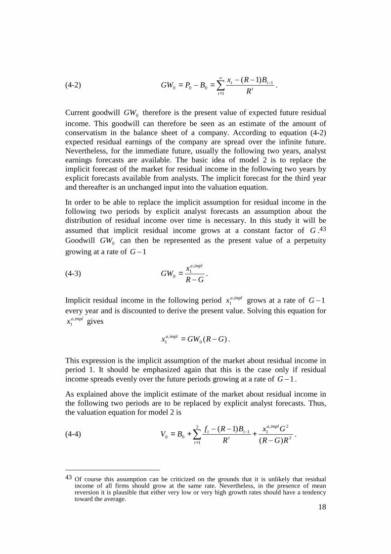
income. This goodwill can therefore be seen as an estimate of the amount ofconservatism in the balance sheet of a company. According to equation (4-2)expected residual earnings of the company are spread over the infinite future.Nevertheless, for the immediate future, usually the following two years, analystearnings forecasts are available. The basic idea of model 2 is to replace theimplicit forecast of the market for residual income in the following two years byexplicit forecasts available from analysts. The implicit forecast for the third yearand thereafter is an unchanged input into the valuation equation.

In order to be able to replace the implicit assumption for residual income in thefollowing two periods by explicit analyst forecasts an assumption about thedistribution of residual income over time is necessary. In this study it will beassumed that implicit residual income grows at a constant factor of G .43

Goodwill 0GW can then be represented as the present value of a perpetuity

growing at a rate of 1−G

(4-3) GR

xGW

impla

−=

,1

0 .

Implicit residual income in the following period implax ,1 grows at a rate of 1−G

every year and is discounted to derive the present value. Solving this equation forimplax ,

1 gives

)(0,

1 GRGWx impla −= .

This expression is the implicit assumption of the market about residual income inperiod 1. It should be emphasized again that this is the case only if residualincome spreads evenly over the future periods growing at a rate of 1−G .

As explained above the implicit estimate of the market about residual income inthe following two periods are to be replaced by explicit analyst forecasts. Thus,the valuation equation for model 2 is

(4-4) 2

2,1

2

1

100 )(

)1(

RGR

Gx

R

BRfBV

impla

tt

tt

−+

−−+= ∑

=

− .

43 Of course this assumption can be criticized on the grounds that it is unlikely that residualincome of all firms should grow at the same rate. Nevertheless, in the presence of meanreversion it is plausible that either very low or very high growth rates should have a tendencytoward the average.

19

The intrinsic value of the firm is the sum of book value of equity 0B , the present

value of explicit analyst forecasts of residual income 1)1( −−− tt BRf in the

following two periods 1)1( −−− tt BRf , and the present value of the implicit

estimate of the market of residual income thereafter. The implicit estimate ofresidual income in period 3 is residual income in period 1 implax ,

1 twice multipliedwith the growth factor G .

For the analyses of the predictability of relative performance of stock returns it isnecessary to compare the market value of a firm with the intrinsic value using thePV ratio. With model 2 this comparison is reduced to a comparison between theimplicit estimate of residual income in the following two periods with the explicitanalyst forecasts, i.e. the comparison

GR

xB

RGR

Gx

R

BRfB

implaimpla

tt

tt

−+<=>

−+

−−+∑

=

−,

102

2,1

2

1

10 )(

)1(or

2

,1

,1

2

1

1)1(

R

Gx

R

x

R

BRf implaimpla

tt

tt +<=>−−∑

=

− .

The left side of the upper expression is the value equation of model 2, whereas theright side is the market value of the firm expressed as the sum of book value ofequity and goodwill. In the lower expression book value and the implicit estimatesof residual income from period 3 onwards have been subtracted. The explicitanalyst forecast of residual income is compared with the implicit estimate derivedfrom the market valuation of the firm. The hypothesis is that companies whoseexplicit analyst forecasts of residual income are high relative to the implicitestimates are fundamentally undervalued as a higher share of goodwill can beearned in the immediate future. The contrary would hold true for companieswhose explicit analyst forecasts are low relative to the implicit estimates.

Concerning the sorting of companies according to their PV ratios to detectfundamental undervaluation another interpretation is possible. As can be seenfrom a comparison of intrinsic firm value according to model 2 with the marketvalue, the only component of the intrinsic value that is different from the marketvalue is the estimates for residual income in periods 1 and 2. Thus, the sortingaccording to the PV ratio corresponds to a sorting according to a "price-residualincome in t=1,2 ratio".44

Model 2 is to be seen as a first attempt to compare explicit residual incomeforecasts with implicit forecasts derived from market valuation. Presumably futurestudies will be able to develop more sophisticated approaches.

44 For this reason the exact size of the growth factor G is not important for this comparison. Achange of G does not change the sequence of the companies under examination.

20

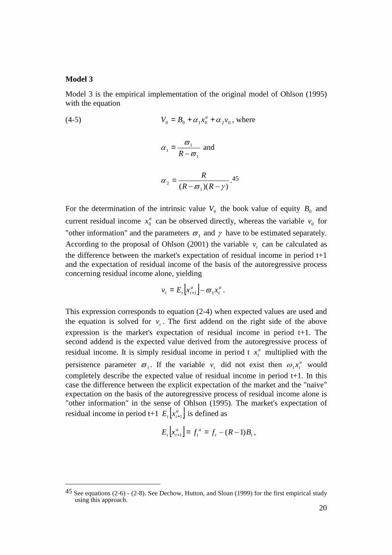
Model 3

Model 3 is the empirical implementation of the original model of Ohlson (1995)with the equation

(4-5) 020100 vxBV a αα ++= , where

1

11 ϖ

ϖα

−=

Rand

))(( 12 γϖ

α−−

=RR

R.45

For the determination of the intrinsic value 0V the book value of equity 0B and

current residual income ax0 can be observed directly, whereas the variable 0v for

"other information" and the parameters 1ϖ and γ have to be estimated separately.

According to the proposal of Ohlson (2001) the variable tv can be calculated as

the difference between the market's expectation of residual income in period t+1and the expectation of residual income of the basis of the autoregressive processconcerning residual income alone, yielding

[ ] at

attt xxEv 11 ϖ−= + .

This expression corresponds to equation (2-4) when expected values are used andthe equation is solved for tv . The first addend on the right side of the above

expression is the market's expectation of residual income in period t+1. Thesecond addend is the expected value derived from the autoregressive process ofresidual income. It is simply residual income in period t a

tx multiplied with the

persistence parameter 1ϖ . If the variable tv did not exist then atx1ω would

completely describe the expected value of residual income in period t+1. In thiscase the difference between the explicit expectation of the market and the "naive"expectation on the basis of the autoregressive process of residual income alone is"other information" in the sense of Ohlson (1995). The market's expectation ofresidual income in period t+1 [ ]a

tt xE 1+ is defined as

[ ] tta

tatt BRffxE )1(1 −−==+ ,

45 See equations (2-6) - (2-8). See Dechow, Hutton, and Sloan (1999) for the first empirical studyusing this approach.

21

where tf is the analyst forecast in period t on earnings in period t+1 and atf 1+ the

corresponding analyst forecast on residual income. Thus, the equation for thevariable for "other information" is

(4-6) at

att xfv 1ϖ−= .

A time series of the variable "other information" can thus be calculated. Theestimation procedure for the parameters 1ϖ and γ will be described at the end ofthe chapter.

Model 4

Model 3 assumes unbiased accounting as due to the parameter restrictions for 1ϖand γ residual income converges to zero in the long run. Empirical studies suchas Dechow, Hutton, and Sloan (1999) show that intrinsic values calculated usingthis approach are much lower than observable market values. This shows that theassumption of unbiased accounting and of zero residual income in the long runmight lead to an underestimation of firm value. In addition to that whenestimating the persistence parameters for the linear information dynamic severalauthors such as Dechow, Hutton, and Sloan (1999), McCrae and Nilsson (2001),and Prokop (2003) detect regression constants that are significantly different fromzero which is a violation of the assumptions of the original model of Ohlson(1995). The studies cited "solve" this issue by simply not using these results intheir further analyses.

Choi, O'Hanlon, and Pope (2003) propose a modification of the original model ofOhlson (1995) that incorporates conservatism by allowing for permanentlypositive residual income. Their value equation includes the regression constants ofthe autoregressive processes for residual income and "other information" toaccount for on average non-zero residual income or "other information". In thisstudy a modified variant of the proposal of Choi, O'Hanlon, and Pope (2003) willbe used as model 4.

The modified linear information dynamic is

(4-7) 1,1101

++ +++= t

t

t

t

at

t

at

B

v

B

x

B

xεϖϖ ,

(4-8) 1,21

++ += t

t

t

t

t

B

v

B

vεγ ,

(4-9) 1,3

1+

+ += tt

t GB

Bε ,

22

where G is the growth factor of the book value of the company.46 Thisinformation dynamic is different from the original information dynamic inequations (2-4) - (2-5) in two respects: First, the autoregressive process of residualincome in equation (4-7) is supplemented by the constant term 0ϖ to take account

of on average positive residual income. Second, equation (4-9) is added whichdescribes the development of book value over time. This is necessary, as theamount of constant residual income represented by 0ϖ depends on the size of 0B .

1,1 +tε , 1,2 +tε , and 1,3 +tε are error terms with an expected value of zero. All

equations are scaled with book value of equity.

Forming expected values of equations (4-7) - (4-9) results in

(4-10) [ ] tatt

att vxBxE ++=+ 101 ϖϖ ,

(4-11) [ ] ttt vvE γ=+1 ,

(4-12) [ ] ttt GBBE =+1 .

Analogous to the original model of Ohlson (1995) the valuation equation resultsin

(4-13) 0320100 BvxBV ta ααα +++= , where

(4-14)1

11 ϖ

ϖα

−=

R,

(4-15)))(( 11

2 γϖα

−−=

RR

Rand

(4-16)))(( 1

03 GRR

R

−−=

ϖϖ

α .47

The coefficients 1α and 2α are identical with those of the original model of

Ohlson (1995) and with those of model 3. The coefficient 3α takes account of the

modification that in model 4 residual income can be larger than zero in the longrun. The coefficient 3α is getting larger, the larger 0ϖ , 1ϖ , G , and the lower R

get. The model of Ohlson (1995) can be seen as a special case where

46 See Choi, O'Hanlon, and Pope (2003), p. 6.47 See Jamin (2004), Anhang 1.

23

00 30 =→= αϖ . This is the case when accounting is unbiased and residual

income is not different from zero in the long run, implying a value of 0ϖ of

zero.48

For an empirical implementation of model 4 the parameters 0ϖ , 1ϖ , and γ are

necessary, as well as the variable tv and the growth factor G . The procedure for

estimating the parameters will be explained in the next section. The variable tv

can be calculated in a similar way as for model 3, by solving equation (4-10) for

tv and inserting the analyst forecast atf for [ ]a

tt xE 1+ which results in

(4-17) )( 10att

att xBfv ϖϖ +−= .

The difference to equation (4-6) is that the average positive residual earnings

tB0ϖ also have to be deducted from the analyst forecast atf in order to derive

"other information" tv .

Parameter estimation for linear information dynamic

Finally, in order to calculate intrinsic firm values according to models 3 and 4 theparameters 0ϖ , 1ϖ , and γ have to be estimated. An important question that arises

in this context is for which group of companies this should be done. In principle itwould be possible to estimate the parameters for each company separately. Itcould be argued that the persistence behaviour of residual income and "otherinformation" as well as the degree of conservatism of a company's accountingmight be firm-specific. One problem with this is the fact that data are available fora maximum of 13 years – for many firms in the sample this time span is evenshorter. Thus, a firm-specific parameter estimation does not seem to beadequate.49 Nevertheless, the sample will be separated into two groups: "OldEconomy" firms and "New Economy" firms.50

48 See Jamin (2004), p. 153, for a numerical example for the impact of an inclusion of ω0 into thevaluation equation on intrinsic value.

49 Of course the estimation could be done sector-wise as one might argue that competitive forcesand thus the persistence behaviour of residual income and "other information" should besector-specific. The issue with this is that the sector classification available is such that the sizeof the sectors varies hugely, see chapter 6. Therefore a sector-wise estimation also seems to beunreliable. Other studies such as Dechow, Hutton, and Sloan (1999), Choi, O'Hanlon, and Pope(2003), or Prokop (2003) estimate the parameters for the whole sample.

50 "Old Economy" comprises the sectors Automobile, Basic Resources, Chemicals, Construction,Consumer-cyclical, Food & Beverages, Industrial, Machinery, Pharma & Health, Retail,Transport & Logistics, and Utilities. "New Economy" comprises the sectors Media, Software,Technology, and Telecommunications. For a detailed description about the data used seechapter 5.

24

In the literature51 a two-stage procedure is used to estimate the parameters. In thefirst stage a panel regression

(4-18) tiati

ati xx ,1,101, εϖϖ ++=+

is estimated to derive a value for 1ϖ . The estimated value for 1ϖ is then insertedinto equation (4-6) such that

ati

atiti xfv ,1,, ϖ−= .

In the second stage the panel regression

(4-19) tititi vv ,21,0, εγγ ++= −

is estimated to derive a parameter estimate for γ . To avoid heteroskedasticityDechow, Hutton, and Sloan (1999) scale with market value, Choi, O'Hanlon, andPope (2003) with book value, and Prokop (2003) with both.

This procedure is problematic insofar as it ignores the interdependency betweenthe parameters 1ϖ and γ . This can be seen by inserting the expected value ofequation (2-5) into the expected value of equation (2-4) resulting in

[ ] 111 −+ += tat

at vxxE γϖ

[ ] )( 11111at

at

at

at xfxxE −−+ −+= ϖγϖ .

Obviously the two parameters 1ϖ and γ cannot be estimated independently fromeach other as there is a multiplicative relationship between both which can be seenin the bracket in the above expression.52 Thus, in this study, the one-stageestimation

(4-20) titi

ati

ti

atti

ti

ati

ti

ati

B

x

B

f

B

x

B

x,

,

1,1

,

,

,

,10

,

1, )( εϖγϖϖ +−++= −−+

is estimated to estimate the parameters for model 3 taking account for thestructure of the theoretical model. Equation (4-20) is a panel regression and allvariables are scaled by book value tiB , .

Equivalently, the regression equation for model 4 is

51 See, e.g., Dechow, Hutton, and Sloan (1999) or Prokop (2003).52 See Jamin (2004), Anhang 2, for a discussion of differences between using the two approaches.

25

(4-21) titi

ati

ti

ti

ti

atti

ti

ati

ti

ati

B

x

B

B

B

f

B

x

B

x,

,

1,1

,

1,0

,

,

,

,10

,

1, )( εϖϖγϖϖ +−−++= −−−+ .

This takes account of the requirement to subtract the constant residual income

1,0 −tiBϖ in addition to atix 1,1 −ϖ from the analyst forecast a

tif 1, − to derive a value for

1, −tiv .53

It would be desirable to use seemingly unrelated regressions (SUR) to estimateequations (4-20) and (4-21). This method allows for a provision for correlation inthe error terms which is due to influencing factors affecting all firms in thesample.54 But to use SUR it is necessary that the number of time-seriesobservations exceeds the number of cross-section observations. This is not thecase, as the maximum number of years available is 13, and the minimum numberof cross-sections available is 55. Thus, the system is estimated using ordinaryleast squares (OLS).

53 See equation (4-17).54 See Srivastava and Giles (1987), p. 1.

26

5 Data

Basis for the sample under examination is the index CDAX on the 31st ofDecember, 2002. The CDAX is the broadest index available for the German stockmarket including all publicly traded companies.55 The CDAX is made up of 19sector sub-indices.56 The sectors Banks, Financial Services, and Insurance areexcluded from the following empirical investigations as they are subject toparticular accounting rules and, thus, not directly comparable. In order to avoid asurvivorship bias an additional selection in Thomson Financial Datastream wasconducted to identify companies that were delisted prior to December 2002.

The necessary accounting information book value of equity, number of shares,and earnings per share are taken from the financial information providerBloomberg. Dividend per share is from Thomson Financial Datastream. Asearnings forecasts the mean consensus forecasts from the I/B/E/S database areused. These are available for the next two fiscal years.57 The advantage of usingan average of individual forecasts is the better quality of aggregated forecasts thatare provided by different individuals and institutions and according to differentmethodologies.58

As German companies have been switching their accounting from traditionalGerman GAAP (HGB) accounting to international standards (IAS and US GAAP)since the mid-nineties the sample has to be separated into sub-groups that preparetheir books according to HGB, IAS, and US GAAP. The sorting of companiesaccording to their PV ratios is first done within this sub-samples, and then thesub-samples are aggregated again.59 Beginning with the fiscal year 1998 asufficiently large group of IAS-companies and beginning with the fiscal year 1999a sufficiently large group of US GAAP-companies is available.60

As valuation date the 31st of May is chosen in each year analysed. On that dateintrinsic firm value is calculated using accounting information for the precedingfiscal year61 and analyst forecasts per 31st of May for the current and the

55 For information regarding stock indices of Deutsche Börse see www.deutsche-boerse.com.56 These are Automobile, Banks, Basic Resources, Chemicals, Construction, Consumer-cyclical,

Financial Services, Food & Beverages, Industrial, Insurance, Machinery, Media, Pharma &Health, Retail, Software, Technology, Telecommunications, Transport & Logistics, andUtilities.

57 I/B/E/S also provides other measures of forecasts such as a median forecast which in principlecould also be used.

58 See Kacapyr (1996), pp. 141 et seq.59 E.g., the according to their PV ratio undervalued portfolios of HGB, IAS, and US GAAP are

merged to the undervalued portfolio for the whole sample.60 See Jamin (2004), section 6.3, for a detailed discussion concerning the problems arising from

the correct classification of companies.61 Only companies whose fiscal year ends on the 31st of December are included into the sample.

27

following fiscal year.62 One reason for this is that according to § 290 Abs. 1 HGBGerman companies have to produce their financial statements five months afterthe end of the fiscal year.63 Furthermore, the work of Stromann (2003) showsempirically that the correlation between intrinsic firm value according to themodel of Feltham and Ohlson (1995) and market value for German companies ishighest for the month of May.

Firm-specific cost of capital is calculated using the capital asset pricing model(CAPM) going back to Sharpe (1966), Lintner (1965), and Mossin (1966). Asinputs for determining cost of capital according to the CAPM a risk-free rate, themarket risk premium, and the company beta as the quotient of the stock'scovariance with the market return and the variance of the market portfolio.64 Asrisk-free rate the interest on government bonds with a maturity of one to two yearsis chosen, which is in accordance with the recommendation in Ross, Westerfield,and Jaffe (1996).65 Two different market risk premiums are chosen: 5% whichcorresponds to the historically ex post measured risk premium in the Germanstock market66, and 2% which corresponds to the results of newer approaches thattry to infer the risk premium from current market valuation and investoropinion.67 As beta the sector beta of the CDAX sector indices is used as for manycompanies the time series of available data is too short to carry out an estimationof firm-specific betas. The estimation of beta is done with monthly data over afive year period by regressing the return of the CDAX sector indices on theCDAX return itself.

To measure the performance of the undervalued and overvalued portfolios formedaccording to their PV ratios the return index from Thomson Financial Datastreamis used which is a total return index including value changes of the stocks anddividends.

62 E.g., on the 31st of May, 2000 book value of equity as per 31st of December, 1999 and analystearnings forecasts per 31st of May, 2000 for fiscal year 2000 and for fiscal year 2001 are usedto calcalate intrinsic firm value.

63 This does not necessarily include disclosure as well.64 See Weston and Copeland (1992), p. 403 and Damodaran (1996), p. 52.65 In the literature there is a considerable debate on choosing the right risk-free rate. The

Arbeitskreis "Finanzierung" der Schmalenbach-Gesellschaft (1996) as well as Kußmaul (2003)recommend a long-term rate. Rosenberg and Rudd (1998) recommend a short-term rate whichshould correspond with the expected investment horizon. Penman and Sougiannis (1998) use intheir study a maturity of three years, Myers (1999) uses one month.

66 See Bimberg (1993), Morawietz (1994), Arbeitskreis "Finanzierung" der Schmalenbach-Gesellschaft (1996), and Institut der Wirtschaftsprüfer in Deutschland (2002).

67 See, e.g., Claus and Thomas (2001) and Abou and Prat (2003). This area of research wasstimulated by the so-called equity premium puzzle initiated by Mehra and Prescott (1985)which suggests that the empirically observed risk premiums are too high to be justified byplausible utility functions of individuals. See also Ronge (2002) who shows that the totalperformance of equity investments on the German stock market over a longer period of timeincluding both world wars is much lower than over a period that includes only the time afterthe second world war. This result implies that the risk premium might be lower whenexamining not only good but also bad economic periods.

28

6 Results

6.1 Descriptive Statistics

Table 1 shows the number of firms that are included in the sample.68 The numberincreases significantly from 1990 to 2002 for mainly two reasons: First, thenumber of publicly traded companies has increased on the German capital market,mainly due to the boom in technology stocks at the end of 1990s. Second, thecoverage of firms by electronic databases such as Bloomberg and ThomsonFinancial Datastream as well as by professional analysts has increased.

No. of firmsThereofHGB

ThereofIAS

ThereofUSGAAP

1990 55 55

1991 56 56

1992 93 93

1993 115 115

1994 125 125

1995 114 114

1996 131 131

1997 132 132

1998 139 139

1999 160 128 32

2000 183 94 53 36

2001 288 74 119 95

2002 275 49 134 92

Total 1866 13055 338 223

Table 1: Number of companies included in sample

68 Of course it is impossible to use as many observations for an analysis of the German stockmarket as, e.g., for an analysis of the US stock market which has many more publicly tradedcompanies and which has longer time series of electronically available data. Nevertheless, thenumber of firm-years used in this study is similar to that of other studies. Stromann (2003) uses1,342 firm-years, McCrae and Nilsson (2001) 1,339.

29

Book Value perShare Share Price Earnings per Share

Earnings perShare Forecast t+1

Earnings per ShareForecast t+2 Dividend Ratio Price-Book-Ratio

Price-Earnings-Ratio Dividend Yield

Jahr Mean Median Mean Median Mean Median Mean Median Mean Median Mean Median Mean Median Mean Median Mean Median

1990 30.85 11.35 91.26 35.79 3.19 1.32 2.81 1.37 3.33 1.55 0.61 0.44 3.4 2.9 36 27 0.0186 0.0173

1991 34.01 11.14 89.06 19.53 2.98 0.94 2.95 1.19 3.44 1.29 0.47 0.43 2.9 2.6 29 25 0.0199 0.0177

1992 32.14 10.33 79.22 10.33 2.03 0.87 3.28 1.14 3.83 1.28 0.52 0.47 2.7 2.2 30 21 0.0215 0.0204

1993 44.22 13.47 96.64 26.70 4.17 1.07 4.18 1.24 4.68 1.43 0.49 0.45 2.3 1.8 29 21 0.0229 0.0235

1994 41.78 12.66 108.42 26.51 1.38 0.80 2.58 1.01 3.97 1.46 0.44 0.44 2.7 2.3 35 27 0.0177 0.0182

1995 38.82 11.47 85.34 23.58 2.74 0.95 3.33 1.05 4.31 1.66 0.48 0.45 2.4 1.9 20 20 0.0217 0.0193

1996 35.43 11.26 70.06 26.92 1.65 1.04 2.30 1.22 3.37 1.55 0.45 0.41 2.3 1.9 25 19 0.0226 0.0224

1997 27.10 10.90 64.37 27.75 0.70 0.94 1.99 1.24 2.99 1.53 0.36 0.38 2.9 2.3 26 24 0.0187 0.0185

1998 26.01 10.83 72.73 35.54 0.25 1.23 2.58 1.42 3.54 1.78 0.35 0.38 3.5 2.7 28 23 0.0196 0.0172

1999 20.70 9.86 49.30 21.20 1.56 1.21 2.50 1.54 3.17 1.99 0.41 0.40 3.5 2.2 27 19 0.0331 0.0236

2000 12.39 8.46 36.61 24.55 -1.11 0.62 0.87 1.00 2.05 1.32 0.34 0.27 5.5 2.5 40 17 0.0190 0.0123

2001 9.47 6.46 19.98 12.61 0.10 0.18 0.65 0.49 1.22 0.91 0.19 0.00 2.8 1.9 35 23 0.0010 0.0000

2002 9.22 5.96 13.79 5.15 -0.39 -0.05 0.11 0.15 0.79 0.38 0.17 0.00 1.7 1.1 29 20 0.0104 0.0000

Table 2: Descriptive statistics on accounting and earnings forecast data

Notes: Annual data per 31st of May of each year. * Price-book-ratios of more than 50 were eliminated, thus removing two observations. Negative price-book-ratios were also eliminated. ** Price-earnings-ratios of more than 200 were eliminated, thus removing 54 observations. Negative price-earnings-ratios were also eliminated.

30

Table 2 shows descriptive statistics about the accounting and earnings forecastdata used for the empirical analyses. A few distinctive features concerning thedata used have to be mentioned here. Earnings per share decrease sharply andeven become negative, on average, at the end of the period under examination.This reflects the fact that many of the companies that went public during thetechnology boom at the end of the 1990s were actually loss-making. Earningsforecasts on average are slightly higher than actual earnings per share reflectingthe plausible assumption that in an expanding economy earnings should growover time. The price-book-ratio and the price-earnings-ratio mirror the remarkabledevelopments at the stock market. Price-book mean reaches its highest value with5.5 in May 2000 followed by a decline to 1.7. Price-earnings behaves similarly.

Naturally the question arises whether the sample of firms used which does notcomprise all German stock market companies is representative of the Germancapital market as a whole. Thus, in Figure 1 the return of the sample is comparedto the return of the CDAX.

-0.5

-0.4

-0.3

-0.2

-0.1

0

0.1

0.2

0.3

0.4

0.5

0.6

1990 1991 1992 1993 1994 1995 1996 1997 1998 1999 2000 2001 2002

Return CDAX

Return Sample

Figure 1: Return CDAX and Sample

Notes: The return of a year is the return over 12 months following the 31st of Mayof the year. The sample return is the unweighted average of the returns of thecompanies on the basis of the return index of Thomson Financial Datastream. Thereturn of the CDAX is an average return of all CDAX companies weighted withmarket capitalization.

31

As can be seen in Figure 1 the behaviour of both time series is quite similar.Indeed, the correlation between the two is 0.88. Nevertheless the return of theCDAX during the years from 1994 to 2001 is always slightly higher than thesample return. One reason for this might be huge capital gains immediatelyfollowing an IPO.69 These returns are of course included in the computation ofthe return of the CDAX but very often they are not part of the sample return. Thereason for this is that a new stock does not enter the sample on the first tradingday but earliest on the 31st of May following the IPO. Much of the initialabnormal return probably was earned before that. There were plenty of IPOsduring the technology boom at the end of the 1990s that might contribute to thisfinding.

Also the quality of analyst earnings forecasts has to be assessed before proceedingwith the empirical analyses. This will be done using the forecast error scaled byshare price MFEP , the absolute forecast error scaled by share price MAFEP , theforecast error scaled by actual earnings MFEE , as well as by the absolute forecasterror scaled by actual earnings MAFEE .70

MFEP MAFEP MFEE MAFEE NPrognose FY1* 0.0165 0.0266 0.3332 0.9374 3813Prognose FY2** 0.0467 0.0769 0.5676 1.2548 2569

Table 3: Mean forecast error of analyst earnings forecasts over one year

(FY1) and two years (FY2)

Notes: * Average of arithmetic mean of FY1 forecasts for 1989 – 2002.** Average of arithmetic mean of FY2 forecasts for 1989 – 2001.

Table 3 exhibits the analyst optimism well-known from the literature on thequality of earnings forecasts.71 Also the absolute errors MAFEP and MAFEEare larger than MFEP and MFEE which shows that forecast errors for singlecompanies can go into two directions. Overall it can be noted that the quality ofearnings forecasts used in this study is far from perfect but can be compared toquality of forecasts used in other studies. Basu, Hwang, and Jan (1998) e.g. findfor the German stock market a value of MFEP 1.78%. According to this studythe forecast error for the German market is in a comparable order of magnitude asthe error for other important capital markets.

69 Gerke and Fleischer (2001) find an average abnormal return of 90.6% during the six monthsfollowing an IPO at the German Neuer Market, the technology segment of Deutsche Börse.

70 See Jamin (2004), section 7.1.6 for a more detailed discussion.71 See Lakonishok and Givoly (1984), O'Brien (1988), or Capstaff, Paudyal, and Rees (1995).

32

The time-series for the risk-free rate and the sector betas estimated which both areinputs necessary to calculate cost of capital can be found in Appendix 1 and inAppendix 2.

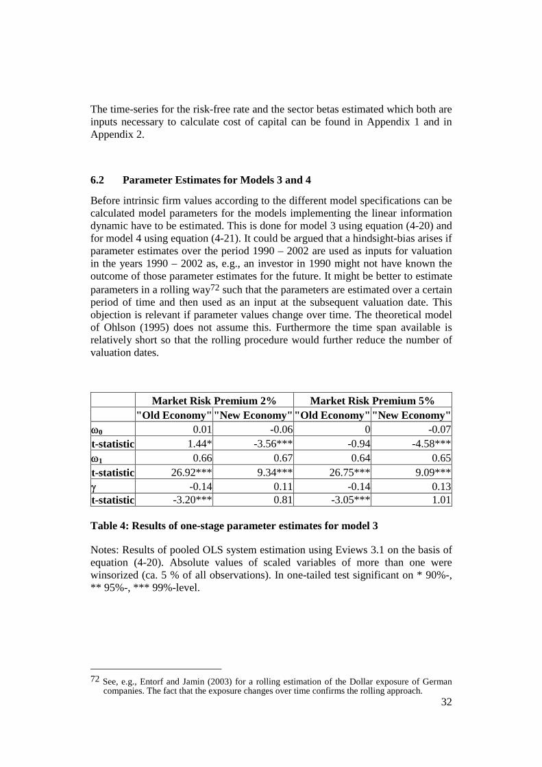
6.2 Parameter Estimates for Models 3 and 4

Before intrinsic firm values according to the different model specifications can becalculated model parameters for the models implementing the linear informationdynamic have to be estimated. This is done for model 3 using equation (4-20) andfor model 4 using equation (4-21). It could be argued that a hindsight-bias arises ifparameter estimates over the period 1990 – 2002 are used as inputs for valuationin the years 1990 – 2002 as, e.g., an investor in 1990 might not have known theoutcome of those parameter estimates for the future. It might be better to estimateparameters in a rolling way72 such that the parameters are estimated over a certainperiod of time and then used as an input at the subsequent valuation date. Thisobjection is relevant if parameter values change over time. The theoretical modelof Ohlson (1995) does not assume this. Furthermore the time span available isrelatively short so that the rolling procedure would further reduce the number ofvaluation dates.

Market Risk Premium 2% Market Risk Premium 5%"Old Economy" "New Economy""Old Economy" "New Economy"

ω0 0.01 -0.06 0 -0.07t-statistic 1.44* -3.56*** -0.94 -4.58***ω1 0.66 0.67 0.64 0.65t-statistic 26.92*** 9.34*** 26.75*** 9.09***γ -0.14 0.11 -0.14 0.13t-statistic -3.20*** 0.81 -3.05*** 1.01

Table 4: Results of one-stage parameter estimates for model 3

Notes: Results of pooled OLS system estimation using Eviews 3.1 on the basis ofequation (4-20). Absolute values of scaled variables of more than one werewinsorized (ca. 5 % of all observations). In one-tailed test significant on * 90%-,** 95%-, *** 99%-level.

72 See, e.g., Entorf and Jamin (2003) for a rolling estimation of the Dollar exposure of Germancompanies. The fact that the exposure changes over time confirms the rolling approach.

33

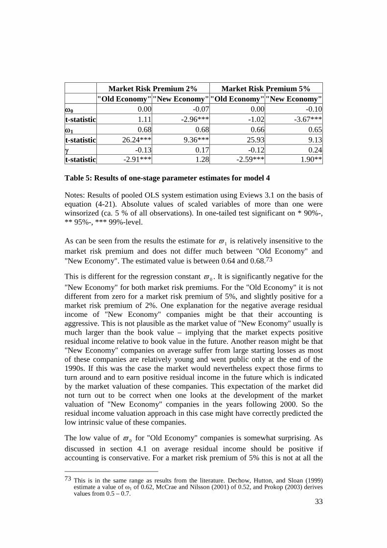
Market Risk Premium 2% Market Risk Premium 5%"Old Economy" "New Economy""Old Economy" "New Economy"

ω0 0.00 -0.07 0.00 -0.10t-statistic 1.11 -2.96*** -1.02 -3.67***ω1 0.68 0.68 0.66 0.65t-statistic 26.24*** 9.36*** 25.93 9.13γ -0.13 0.17 -0.12 0.24t-statistic -2.91*** 1.28 -2.59*** 1.90**

Table 5: Results of one-stage parameter estimates for model 4

Notes: Results of pooled OLS system estimation using Eviews 3.1 on the basis ofequation (4-21). Absolute values of scaled variables of more than one werewinsorized (ca. 5 % of all observations). In one-tailed test significant on * 90%-,** 95%-, *** 99%-level.

As can be seen from the results the estimate for 1ϖ is relatively insensitive to themarket risk premium and does not differ much between "Old Economy" and"New Economy". The estimated value is between 0.64 and 0.68.73

This is different for the regression constant 0ϖ . It is significantly negative for the

"New Economy" for both market risk premiums. For the "Old Economy" it is notdifferent from zero for a market risk premium of 5%, and slightly positive for amarket risk premium of 2%. One explanation for the negative average residualincome of "New Economy" companies might be that their accounting isaggressive. This is not plausible as the market value of "New Economy" usually ismuch larger than the book value – implying that the market expects positiveresidual income relative to book value in the future. Another reason might be that"New Economy" companies on average suffer from large starting losses as mostof these companies are relatively young and went public only at the end of the1990s. If this was the case the market would nevertheless expect those firms toturn around and to earn positive residual income in the future which is indicatedby the market valuation of these companies. This expectation of the market didnot turn out to be correct when one looks at the development of the marketvaluation of "New Economy" companies in the years following 2000. So theresidual income valuation approach in this case might have correctly predicted thelow intrinsic value of these companies.

The low value of 0ϖ for "Old Economy" companies is somewhat surprising. As

discussed in section 4.1 on average residual income should be positive ifaccounting is conservative. For a market risk premium of 5% this is not at all the

73 This is in the same range as results from the literature. Dechow, Hutton, and Sloan (1999)estimate a value of ω1 of 0.62, McCrae and Nilsson (2001) of 0.52, and Prokop (2003) derivesvalues from 0.5 – 0.7.

34

case, confirming the newer findings that the ex ante market risk premium is lowerthan historically measured.74 But even for the market risk premium of 2% it ispositive only at a very low significance level. Two potential explanations arise forthis finding: First, even a market risk premium of 2% might be too high. Second,it might be the case that companies on average economically do not earn their costof capital.

Interestingly, other empirical studies find negative values for 0ϖ as well.75

Dechow, Hutton, and Sloan (1999) who use a constant cost of capital of 12%estimate a value of -0.02. Also Myers (1999) who uses on average a cost ofcapital of 12.13% states that "…the negative median residual income is … due tothe fact that the discount rate is higher than ROE, on average".76 Those studies donot discuss possible explanations for the finding that thousands of US companiesover a period of several decades should not earn their cost of capital. A plausibleexplanation for this is that these studies use a too high cost of capital.Nevertheless, in this study further analyses will be conducted for both market riskpremiums in order to identify the sensitivity to different values of it.

The results for the persistence parameter of "other information" γ arecontradictory to the theoretical predictions of the linear information dynamic ofOhlson (1995). Parameter values should be between zero and one. In fact, for"Old Economy" companies they are significantly negative, whereas for "NewEconomy" companies they are not significantly different from zero. Apparentlythe "other information" does not have the persistence properties predicted by themodel. For this reason it will be assumed that the parameter value of γ is zeroand the whole system will again be estimated for both models 3 and 4 as a simplefirst-order autoregressive process of residual income with the regression equation

(6-1) titi

ati

ti

ati

B

x

B

x,

1,

1,10

1,

, εϖϖ ++=−

−

−

.

The results shown in Table 6 confirm the results for the persistence parameter 1ϖwhich does not change very much relative to the first estimation. Also theregression constant 0ϖ offers a similar picture. For "New Economy" companies it

is strongly negative for both market risk premiums. For "Old Economy"companies it is slightly positive for a market risk premium of 2% and slightlynegative for a market risk premium of 5%. Model 4 will for the further analysesconcerning the predictability of stock returns be used only for a market riskpremium of 2% as the negative value of 0ϖ seems to suggest that a market risk

premium of 5% is simply too high to be justified by expectations of the market.

74 See section 5.75 As they do not differentiate between "Old Economy" and "New Economy" this is an average

finding for the whole sample of those studies.76 See Myers (1999), p. 15. Also the study of Prokop (2003) finds a negative value for ω0.

35

Market Risk Premium 2% Market Risk Premium 5%"Old Economy" "New Economy""Old Economy" "New Economy"

ω0 0,01 -0,03 -0,01 -0,05t-statistic 1,53* -2,57*** -1,38* -4.11***ω1 0,57 0,66 0,55 0,64t-statistic 25,54*** 13,11*** 25,13*** 13,08***

Table 6: One-stage estimation of persistence parameters without γ for

models 3 and 4

Notes: Results of pooled OLS system estimation with Eviews 3.1 on the basis ofequation (6-1). Detailed regression output can be seen in Appendix 3. Absolutevalues of scaled variable of more than one were eliminated (ca. 5% of allobservations). In one-tailed test significant on * 90%-, ** 95%-, *** 99%-level.

The fact that the persistence parameter of "other information" is for the furtheranalyses assumed to be zero obviously has an effect on the valuation equations formodels 3 and 4. The valuation equation for model 3 equation (4-5) using theempirically estimated parameters 0

~ϖ and 1~ϖ becomes

)~(~1

~

~010

10

1

100 xf

Rx

RBV aa ϖ

ϖϖϖ

−−

+−

+=

afR

BV 01

00 ~1

ϖ−+= .

Analogously the valuation equation for model 4 equation (4-13) becomes

01

001000

10

1

100 ))(~(

~)~~(

)~(

1B

GRR

RxBf

Rx

RBV aaa

−−+−−

−+

−+=

ϖϖ

ϖϖωϖ

ϖ

01

0000

100 ))(~(

~)~(

)~(

1B

GRR

RBf

RBV a

−−+−

−+=

ϖϖ

ϖω

01

000

100 ))(~(

)(~~

)~(

1B

GRR

GRRf

RBV a

−−−−

+−

+=ϖϖϖ

ω.

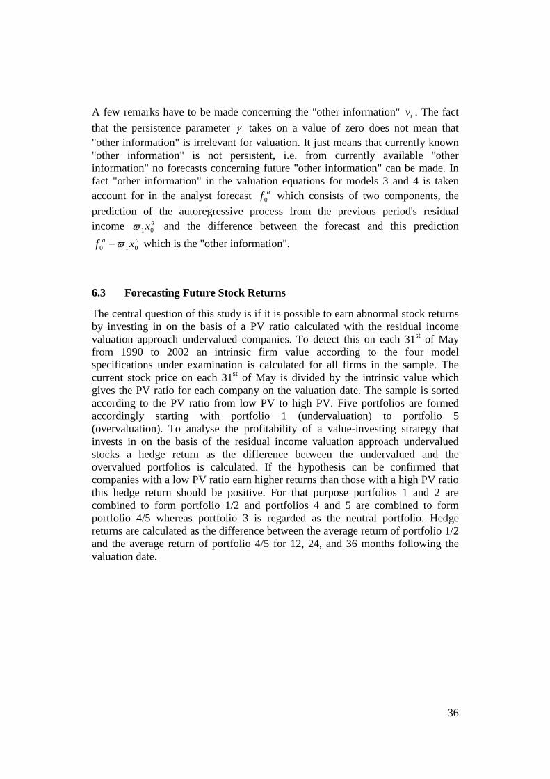
36

A few remarks have to be made concerning the "other information" tv . The fact

that the persistence parameter γ takes on a value of zero does not mean that"other information" is irrelevant for valuation. It just means that currently known"other information" is not persistent, i.e. from currently available "otherinformation" no forecasts concerning future "other information" can be made. Infact "other information" in the valuation equations for models 3 and 4 is takenaccount for in the analyst forecast af0 which consists of two components, the

prediction of the autoregressive process from the previous period's residualincome ax01ϖ and the difference between the forecast and this prediction

aa xf 010 ϖ− which is the "other information".

6.3 Forecasting Future Stock Returns

The central question of this study is if it is possible to earn abnormal stock returnsby investing in on the basis of a PV ratio calculated with the residual incomevaluation approach undervalued companies. To detect this on each 31st of Mayfrom 1990 to 2002 an intrinsic firm value according to the four modelspecifications under examination is calculated for all firms in the sample. Thecurrent stock price on each 31st of May is divided by the intrinsic value whichgives the PV ratio for each company on the valuation date. The sample is sortedaccording to the PV ratio from low PV to high PV. Five portfolios are formedaccordingly starting with portfolio 1 (undervaluation) to portfolio 5(overvaluation). To analyse the profitability of a value-investing strategy thatinvests in on the basis of the residual income valuation approach undervaluedstocks a hedge return as the difference between the undervalued and theovervalued portfolios is calculated. If the hypothesis can be confirmed thatcompanies with a low PV ratio earn higher returns than those with a high PV ratiothis hedge return should be positive. For that purpose portfolios 1 and 2 arecombined to form portfolio 1/2 and portfolios 4 and 5 are combined to formportfolio 4/5 whereas portfolio 3 is regarded as the neutral portfolio. Hedgereturns are calculated as the difference between the average return of portfolio 1/2and the average return of portfolio 4/5 for 12, 24, and 36 months following thevaluation date.

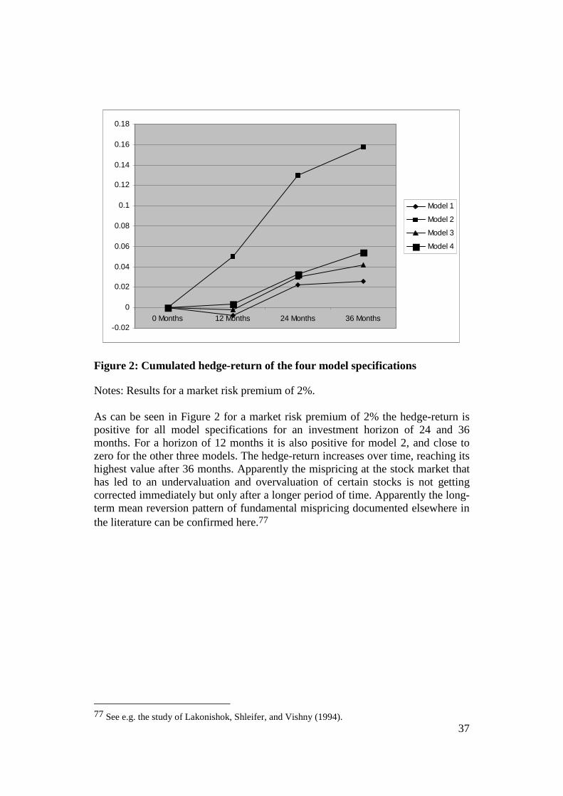
37

-0.02

0

0.02

0.04

0.06

0.08

0.1

0.12

0.14

0.16

0.18

0 Months 12 Months 24 Months 36 Months

Model 1

Model 2

Model 3

Model 4

Figure 2: Cumulated hedge-return of the four model specifications

Notes: Results for a market risk premium of 2%.

As can be seen in Figure 2 for a market risk premium of 2% the hedge-return ispositive for all model specifications for an investment horizon of 24 and 36months. For a horizon of 12 months it is also positive for model 2, and close tozero for the other three models. The hedge-return increases over time, reaching itshighest value after 36 months. Apparently the mispricing at the stock market thathas led to an undervaluation and overvaluation of certain stocks is not gettingcorrected immediately but only after a longer period of time. Apparently the long-term mean reversion pattern of fundamental mispricing documented elsewhere inthe literature can be confirmed here.77

77 See e.g. the study of Lakonishok, Shleifer, and Vishny (1994).

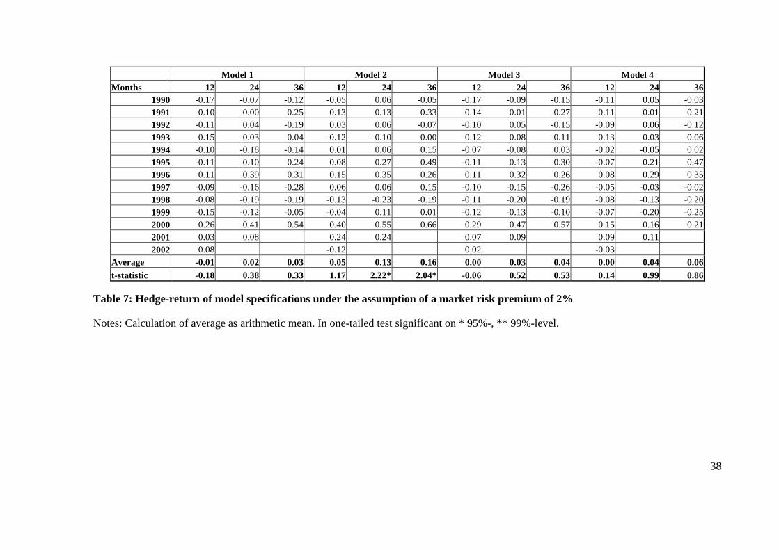
38

Model 1 Model 2 Model 3 Model 4Months 12 24 36 12 24 36 12 24 36 12 24 36

1990 -0.17 -0.07 -0.12 -0.05 0.06 -0.05 -0.17 -0.09 -0.15 -0.11 0.05 -0.031991 0.10 0.00 0.25 0.13 0.13 0.33 0.14 0.01 0.27 0.11 0.01 0.211992 -0.11 0.04 -0.19 0.03 0.06 -0.07 -0.10 0.05 -0.15 -0.09 0.06 -0.121993 0.15 -0.03 -0.04 -0.12 -0.10 0.00 0.12 -0.08 -0.11 0.13 0.03 0.061994 -0.10 -0.18 -0.14 0.01 0.06 0.15 -0.07 -0.08 0.03 -0.02 -0.05 0.021995 -0.11 0.10 0.24 0.08 0.27 0.49 -0.11 0.13 0.30 -0.07 0.21 0.471996 0.11 0.39 0.31 0.15 0.35 0.26 0.11 0.32 0.26 0.08 0.29 0.351997 -0.09 -0.16 -0.28 0.06 0.06 0.15 -0.10 -0.15 -0.26 -0.05 -0.03 -0.021998 -0.08 -0.19 -0.19 -0.13 -0.23 -0.19 -0.11 -0.20 -0.19 -0.08 -0.13 -0.201999 -0.15 -0.12 -0.05 -0.04 0.11 0.01 -0.12 -0.13 -0.10 -0.07 -0.20 -0.252000 0.26 0.41 0.54 0.40 0.55 0.66 0.29 0.47 0.57 0.15 0.16 0.212001 0.03 0.08 0.24 0.24 0.07 0.09 0.09 0.112002 0.08 -0.12 0.02 -0.03

Average -0.01 0.02 0.03 0.05 0.13 0.16 0.00 0.03 0.04 0.00 0.04 0.06t-statistic -0.18 0.38 0.33 1.17 2.22* 2.04* -0.06 0.52 0.53 0.14 0.99 0.86

Table 7: Hedge-return of model specifications under the assumption of a market risk premium of 2%

Notes: Calculation of average as arithmetic mean. In one-tailed test significant on * 95%-, ** 99%-level.

39

Model 1 Model 2 Model 3Months 12 24 36 12 24 36 12 24 36

1990 -0.18 -0.08 -0.12 -0.05 0.11 0.05 -0.10 -0.08 -0.131991 0.10 0.00 0.25 0.10 0.10 0.23 0.14 0.01 0.271992 -0.11 0.04 -0.19 0.05 0.09 -0.01 -0.10 0.05 -0.151993 0.14 -0.03 -0.03 -0.12 -0.07 0.10 0.12 -0.08 -0.111994 -0.07 -0.13 -0.08 0.07 0.16 0.29 -0.07 -0.13 -0.071995 -0.10 0.12 0.23 0.09 0.22 0.47 -0.10 0.13 0.271996 0.09 0.34 0.26 0.13 0.49 0.40 0.10 0.31 0.241997 -0.10 -0.17 -0.30 0.13 0.16 0.29 -0.09 -0.15 -0.261998 -0.09 -0.22 -0.21 -0.13 -0.20 -0.16 -0.10 -0.18 -0.171999 -0.15 -0.12 -0.06 -0.04 0.10 0.05 -0.13 -0.16 -0.102000 0.25 0.40 0.52 0.39 0.52 0.66 0.29 0.47 0.572001 0.03 0.08 0.28 0.28 0.04 0.082002 0.08 -0.09 0.03

Average -0.01 0.02 0.02 0.06 0.16 0.22 0.00 0.02 0.03t-statistic -0.23 0.35 0.30 1.45 2.79* 3.02* 0.09 0.41 0.40

Table 8: Hedge-return of model specifications under the assumption of a market risk premium of 5%

Notes: Calculation of average as arithmetic mean. In one-tailed test significant on * 95%-, ** 99%-level. No results for model 4, asregression constant 0ϖ negative for a market risk premium of 5%.

40

From Figure 2 it can be seen that models 2 und 4 yield the highest hedge-returns.These model specifications interestingly are those that take account ofconservative accounting by allowing for positive residual income in the long run.Apparently this feature of the model improves the discrimination betweenfundamentally undervalued and overvalued companies.

Despite the first impression that hedge-returns are positive for all modelspecifications Table 7 and Table 8 reveal that they are statistically significant onlyfor model 2. Only this specification reaches t-statistics of more than two, but onlyfor investment horizons of 24 and 36 months. All other three model specificationsyield insignificant hedge-returns – no matter which market risk premium isassumed. Model 2 is the model where implicit assumptions from the marketvaluation concerning residual income of the following two years are replaced byexplicit analyst forecasts.78 The sorting of firms according to their PV ratiocorresponds to a sorting according to a "price-residual income in t=1,2 ratio".Apparently this is a promising area of future efforts for model development.

It should also be noted that the models implementing the linear informationdynamic in the spirit of Ohlson (1995), models 3 and 4, do not perform better thanthe simple residual income specifications, models 1 and 2. Apparently therelatively complex information dynamic does not add significant value in terms ofpredicting future stock returns.79

A further task of this study is to compare the hedge-returns calculated on the basisof the residual income valuation approach with those calculated on the basis ofsimple ratios such as PE ratio, PB ratio, and dividend yield. The hypothesis is thatthe theoretically better founded models based on the residual income valuationapproach should provide the investor with a better performance as the simpleratios cover only partial aspects of value generation. Thus, the same analyses asfor the four model specifications were conducted for the PE ratio, PB ratio, anddividend yield.

78 See section 4.2.79 Possibly Lo and Lys (2000) are correct with their criticism that the model of Ohlson (1995)

does not provide any additional value in comparison to simpler residual income specifications;see p. 32.

41

0

0,02

0,04

0,06

0,08

0,1

0,12

0,14

0months

12months

24months

36months

PE ratio

PB ratio

Dividend yield

Figure 3: Cumulated hedge-return of simple ratios

In Figure 3 the cumulated hedge-return of value-investing strategies with simpleratios is displayed. It turns out that it is positive for all investment horizons andalso increasing over time, with the exception of the PE ratio where the cumulatedhedge return reaches its highest value after 24 months. Here again it can be shownthat it is possible to earn superior returns by investing in fundamentallyundervalued stocks.80 Nevertheless, it is somewhat surprising that the dividendyield apparently yields the highest hedge-return which is in contradiction totheoretical predictions such as the theorem of Miller and Modigliani (1961) thatthe dividend policy of a company should be irrelevant for its stock return. It isalso surprising that the hedge-return of the dividend yield with 13% after aninvestment horizon of 36 months is in the same order of magnitude as the hedge-return model 2 with 16% (market risk premium of 2%) and 22% (market riskpremium of 5%). Thus, the theoretically better founded model 2 obviously yieldsonly slightly better results than the simple ratio dividend yield. Whereas allhedge-returns are positive it can be seen in Table 9 that only the hedge-return ofthe dividend yield is statistically significant.

80 See the literature cited in section 3.

42

PE Ratio PB Ratio Dividend YieldMonths 12 24 36 12 24 36 12 24 36

1990 -0.10 0.06 -0.05 -0.16 -0.05 -0.09 0.02 0.12 0.031991 0.21 0.15 0.47 0.09 -0.02 0.19 0.09 0.00 0.231992 -0.02 0.06 0.01 -0.13 0.02 -0.16 0.04 0.12 -0.021993 0.15 0.15 0.22 0.34 0.19 0.24 0.05 0.00 0.091994 0.07 0.14 0.06 -0.06 -0.10 -0.05 0.03 0.09 0.031995 0.01 -0.01 -0.05 -0.08 0.13 0.29 0.09 0.10 0.151996 0.02 -0.14 -0.20 0.04 0.28 0.22 -0.03 0.01 0.061997 -0.16 -0.15 -0.37 -0.03 -0.05 -0.14 -0.05 -0.01 0.031998 -0.06 -0.12 0.03 -0.07 -0.14 -0.13 0.05 0.00 0.111999 -0.14 0.04 0.04 -0.10 -0.02 0.04 -0.07 0.22 0.162000 0.26 0.35 0.40 0.24 0.44 0.51 0.46 0.52 0.572001 0.29 0.31 -0.03 0.03 0.31 0.312002 -0.08 0.09 0.11

Durchschnitt 0.04 0.07 0.05 0.01 0.06 0.08 0.09 0.12 0.13t-Statistik 0.84 1.49 0.67 0.23 1.21 1.26 2.10* 2.64* 2.64*

Table 9: Hedge-return of simple ratios

Notes: Calculation of average as arithmetic mean. In one-tailed test significant on * 95%-, ** 99%-level.

43

In summary it can be noted that indeed it is possible to earn higher stock returnsby investing in fundamentally undervalued stocks on the basis of the residualincome valuation approach. The same is true for simple ratios. Nevertheless, theresults are statistically significant only for two specifications – model 2 and thedividend yield. Furthermore, the theoretical prediction that the fundamentallybetter founded specifications based on the residual income valuation approachshould perform better than the simple ratios can be confirmed only to a limiteddegree, as model 2 performs only slightly better than the dividend yield.

One objection of the proponents of the efficient market hypothesis against suchresults is that higher returns might occur because of a higher systematic risk. If thiswas the case, the higher return would just be the compensation that the investordemands for a higher level of risk. For this reason portfolio betas were calculcatedfor portfolios 1/2 and 4/5 in order to find out if the fundamentally undervaluedportfolio really has a higher systematic risk.

Model 1 Model 2 Model 3 Model 4 PE PB Div. YieldPortfolio 1/2 0.98 0.90 0.98 0.89 0.95 0.99 0.95

Portfolio 4/5 0.96 1.02 0.94 0.91 0.97 0.95 0.99

Table 10: Average portfolio beta under the assumption of a market risk

premium of 2%

Notes: Average of arithmetic mean of estimated beta values over a period of 1990– 2002. For models 1 – 4 only results for a market risk premium of 2% are given.

As can be seen in Table 10 the assumption that the systematic risk of theundervalued portfolios should be higher than that of the overvalued portfolios doesnot turn out to be correct. On the contrary, for the specifications yielding thehighest hedge-returns the average portfolio beta of portfolio 1/2 is even lower thanthat of portfolio 4/5. This implies that an increased return is associated with adecreased level of risk. This of course is in sharp contrast to the predictions ofportfolio theory. Apparently the behavioral limitations predicted by the behavioralfinance theory lead to the opportunity to earn higher returns with lower risk.81

81 See Jamin (2004), sections 7.3.3 and 7.3.4 for a further discussion of the anatomy of thesefindings.

44

7 Conclusion

The residual income valuation approach has become hugely popular since thework of Ohlson (1995) and Feltham and Ohlson (1995). It has added a linearinformation dynamic to the basic valuation formula of the residual incomevaluation approach which allows for a prediction of future residual earnings fromcurrent observables.

As in the literature lots of empirical evidence is documented which shows that it ispossible to earn abnormal stock returns with on the basis of simple fundamentalratios such as the PE ratio, the PB ratio, and the dividend yield undervalued stocksthe question arises if it is possible to improve the performance of such value-investing strategies with a valuation on the basis of the theoretically better foundedresidual income valuation approach. This should be possible since an intrinsicvalue computed with the residual income valuation approach represents acomplete value expression in contrast to the simple ratios. The behavioral financeliterature provides psychological explanations for the existence of mispricing atfinancial markets.

In this study four different model specifications of the residual income valuationapproach are implemented empirically. Two of them are simple specifications,whereas the two other implement a linear information dynamic in the spirit ofOhlson (1995). One of the simple specifications and one of the linear informationspecifications assumes unbiased accounting, whereas the other allows forconservative accounting.

For the linear information dynamic models persistence parameters for residualincome and "other information" have to be estimated. It turns out that theparameter for "other information" is not in accordance with the theoreticalpredictions of the model, thus casting doubt on the validity of the linearinformation dynamic of Ohlson (1995) for the German stock market.

When comparing the returns of undervalued and overvalued portfolios it can beshown that the return of the undervalued portfolio is higher for all modelspecifications, whereas it is significant only for model 2. The same holds true forthe simple ratios, where only the return difference for the dividend yield issignificant. In contrast to the theoretical prediction the performance of the residualincome valuation approach models is not much better than that of the simpleratios. The better performance of the undervalued portfolios is not due to a highersystematic risk of those stocks.

45

References

Abou, A. and Prat, G. (2003), Primes de risque ex-ante sur le N.Y.S.E.: analysedes opinions d'experts au niveau individuel, Working Paper, Universite Paris X.

Arbeitskreis "Finanzierung" der Schmalenbach-Gesellschaft (1996),Wertorientierte Unternehmenssteuerung mit differenzierten Kapitalkosten, zfbf,48, pp. 543 - 578.

Barberis, N., Shleifer, A., and Vishny, R. (1998), A model of investor sentiment,Journal of Financial Economics, 49, pp. 307 - 343.

Barberis, N. and Thaler, R. (2003), A Survey of Behavioral Finance, Handbook ofthe Economics of Finance, pp. 1053 - 1123.

Basu, S. (1977), Investment performance of common stocks in relation to theirprice earnings ratios: A test of the efficient market hypothesis, Journal of Finance,32, pp. 663 - 682.

Basu, S., Hwang, L., and Jan, C.-L. (1998), International variation in accountingmeasurement rules and analysts' earnings forecast errors, Journal of BusinessFinance & Accounting, 25, 9, pp. 1207 - 1247.

Bikhchandani, S. and Sharma, S. (2000), Herd Behavior in Financial Markets: AReview, IMF Working Papier, 00/48,

Bimberg, L. H. (1993), Langfristige Renditenberechnung zur Ermittlung vonRisikoprämien, 2nd edition, Frankfurt.

Brouwer, I., van der Put, J., and Veld, C. (1996), Contrarian Investment Strategiesin a European Context, Center for Economic Research Discussion Paper, No. 36,Tilburg University.

Brown, L. D. (1993), Earnings forecasting research: its implications for capitalmarkets research, International Journal of Forecasting, 9, pp. 295 - 320.

Capstaff, J., Paudyal, K., and Rees, W. (1995), The Accuracy and Rationality ofEarnings Forecasts by UK Analysts, Journal of Business Finance & Accounting,22, 1, pp. 67 - 120.

Chan, L., Hamao, Y., and Lakonishok, J. (1991), Fundamentals and stock returnsin Japan, Journal of Finance, 46, pp. 1739 - 1764.

Choi, Y.-S., O'Hanlon, J., and Pope, P. (2003), Conservative Accounting andLinear Information Valuation Models, Working Paper, Lancaster University.

46

Claus, J. and Thomas, J. (2001), Equity Premia a Low as Three Percent? Evidencefrom Analysts' Earnings Forecasts for Domestic and International Stock Markets,Journal of Finance, 56, 5, pp. 1629 - 1666.

Colas, H. and Teiletche, J. (2003), Anticipations de benefice et performances desactions: une analyse des actions europeennes, Working Paper, Universite Paris X.

Copeland, T., Koller, T., and Murrin, J. (2002), Unternehmenswert, Frankfurt amMain.

Damodaran, A. (1996), Investment Valuation, New York.

De Bondt, W. F. M. and Thaler, R. (1985), Does the stock market overreact?,Journal of Finance, 40, pp. 793 - 805.

De Bondt, W. F. M. and Thaler, R. (1987), Further evidence on investoroverreaction and stock market seasonality, Journal of Finance, 42, pp. 557 - 581.

Dechow, P. M., Hutton, A. P., and Sloan, R. G. (1999), An empirical asessment ofthe residual income valuation model, Journal of Accounting and Economics, 26,pp. 1 - 34.

Devenow, A. and Welch, I. (1996), Rational Herding in Financial Economics,European Economic Review, 40, pp. 603 - 616.

Entorf, H. and Jamin, G. (2003), German Exchange Rate Exposure at DAX andAggregate Level, International Trade, and the Role of Exchange Rate AdjustmentCosts, Discussion Paper, TU Darmstadt.

Fama, E. F. (1970), Efficient capital markets: A review of theory and empiricalwork, Journal of Finance, 25, pp. 383 - 417.

Fama, E. F. (1991), Efficient Capital Markets: II, Journal of Finance, 46, pp. 1575- 1617.

Fama, E. F. and French, K. R. (1992), The Cross-Section of Expected StockReturns, Journal of Finance, 47, 2, pp. 427 - 465.

Fama, E. F. and French, K. R. (1997), Value versus Growth: the InternationalEvidence, Journal of Finance, 53, 6, pp. 1975 - 1999.

Feltham, G. A. and Ohlson, J. A. (1995), Valuation and Clean Surplus Accountingfor Operating and Financial Activities, Contemporary Accounting Research, 11, 2,pp. 689 - 731.

Frankel, R. and Lee, C. M. C. (1998), Accounting valuation, market expectation,and cross-sectional stock returns, Journal of Accounting and Economics, 25, pp.283 - 319.

47

Gerke, W. and Fleischer, J. (2001), Die Performance der Börsengänge am NeuenMarkt, zfbf, 53, 8, pp. 827 - 839.

Glaser, M., Nöth, M., and Weber, M. (2004), Behavioral Finance, in: Koehler,Derek J.und Harvey, Nigel, Blackwell Handbook of Judgment and DecisionMaking, Kapitel 26, Oxford.

Goldberg, J. and Nitzsch, R. v. (2000), Behavioral Finance, 2nd edition, München.

Hand, J. R. M. and Landsman, W. R. (1998), Testing the Ohlson model: v or not v,that is the question, Working Paper, UNC Chapel Hill.

Huijgen, C. and Plantinga, A. (1999), Analysts' earnings forecasts andinternational asset allocation, Working Paper, University of Groningen.

Hüfner, B. (2000), Fundamentale Aktienbewertung und Rechnungslegung,Frankfurt am Main.

Institut der Wirtschaftsprüfer in Deutschland (2002), Wirtschaftsprüfer-Handbuch2002 - Handbuch für Rechnungslegung, Prüfung und Beratung Band II, 12.Auflage, Düsseldorf.

Jaffe, J., Keim, D. B., and Westerfield, R. (1989), Earnings yields, market values,and stock returns, Journal of Finance, 44, pp. 135 - 148.

Jamin, G. (2004), Der Residualgewinnansatz in der fundamentalenAktienbewertung - empirische Untersuchungen für den deutschen Aktienmarkt,Unpublished dissertation, Würzburg.

Kacapyr, E. (1996), Economic Forecasting, New York.

Keynes, J. M. (1936), The General Theory of Employment, Interest, and Money,London.

Kotkamp, S. and Otte, M. (2001), Die langfristige Performance von DAX-Dividendenstrategien, Kredit und Kapital, 3/2001, pp. 393 - 417.

Kußmaul, H. (2003), Darstellung der Discounted-Cash-Flow-Verfahren - auch imVergleich zur Ertragswertmethode nach dem IDW Standard ES 1 -, DerSteuerberater, 9, pp. 332 - 347.

Lakonishok, J. and Givoly, D. (1984), The Quality of Analysts' Forecasts ofEarnings, Financial Analysts Journal, September - October, pp. 40 - 47.

Lakonishok, J., Shleifer, A., and Vishny, R. W. (1994), Contrarian Investment,Extrapolation, and Risk, Journal of Finance, 5, pp. 1541 - 1578.

Lee, C. M. C., Myers, J., and Swaminathan, B. (1999), What is the Intrinsic Valueof the Dow?, Journal of Finance, 54, 4, pp. 1693 - 1742.

48

Lintner, J. (1965), The Valuation of Risk Assets and the Selection of RiskyInvestments in Stock Portfolios and Capital Budgets, Review of Economics andStatistics, 47, pp. 13 - 37.

Lo, K. and Lys, T. (2000), The Ohlson Model: Contribution to Valuation Theory,Limitations, and Empirical Applications, Journal of Accounting, Auditing andFinance, Summer 2000, pp. 1 - 47.

Löffler, G. (1999), Die Verarbeitung von Gewinnprognosen am deutschenAktienmarkt, zfbf, 51, pp. 128 - 147.

Lundholm, R. J. and O'Keefe, T. (2001), Reconciling Value Estimates from theDiscounted Cash Flow Model and the Residual Income Model, ContemporaryAccounting Research, 18, 2, pp. 311 - 335.

Lücke, W. (1955), Investitionsrechnungen auf der Grundlage von Ausgaben undKosten, Zeitschrift für betriebswirtschaftliche Forschung, 7, pp. 310 - 324.

McCrae, M. and Nilsson, H. (2001), The explanatory and predictive power ofdifferent specifications ot the Ohlson (1995) valuation models, EuropeanAccounting Review, 10, 2, pp. 315 - 341.

Mehra, R. and Prescott, E. C. (1985), The Equity Premium: A Puzzle, Journal ofMonetary Economics, 15, 2, pp. 145 - 161.

Miller, M. and Modigliani, F. (1961), Dividend Policy, Growth, and the Valuationof Shares, Journal of Business, October 1961, pp. 411 - 433.

Morawietz, M. (1994), Rentabilität und Risiko deutscher Aktien- undRentenanlagen seit 1970, Wiesbaden.

Mossin, J. (1966), Equilibrium in a Capital Asset Market, Econometrica, 35, pp.768 - 783.

Myers, J. N. (1999), Implementing Residual Income Valuation with LinearInformation Dynamics, Accounting Review, 74, 1, pp. 1 - 28.

O'Brien, P. C. (1988), Analysts' Forecasts as Earnings Expectations, Journal ofAccounting and Economics, 10, pp. 53 - 83.

Oertmann, P. (1999), Why do value stocks earn higher returns than growth stocks,and vice versa?, Working Paper, University of St. Gallen.

Ohlson, J. A. (1995), Earnings, Book Values, and Dividends in Equity Valutaion,Contemporary Accounting Research, 11, 2, pp. 661 - 687.

Ohlson, J. A. (2001), Earnings, Book Values, and Dividends in Equity Valuation:An Empirical Perspective, Contemporary Accounting Research, 18, 1, pp. 107 -120.

49

Ordelheide, D. (1998), Rechnungslegung und internationale Aktienanalyse,Möller, Hans-Peter und Schmidt, Franz, Rechnungswesen als Instrument fürFührungsentscheidungen, Stuttgart, pp. 505 - 524.

Penman, S. H. (1992), Return to Fundamentals, Journal of Accounting, Auditingand Finance, Fall 1992, pp. 465 - 484.

Penman, S. H. (2001a), Financial Statement Analysis & Security Valuation, NewYork.

Penman, S. H. (2001b), On Comparing Cash Flow and Accrual AccountingModels for Use in Equity Valuation: A Response to Lundholm and O'Keefe,Contemporary Accounting Research, 18, 4, pp. 681 - 692.

Penman, S. H. and Sougiannis, T. (1998), A Comparison of Dividend, Cash Flow,and Earnings Approaches to Equity Valuation, Contemporary AccountingResearch, 15, 3, pp. 343 - 383.

Prokop, J. (2003), Die Bewertung zukünftiger Unternehmenserfolge, Wiesbaden.

Reinganum, M. R. (1981), Misspecification of Capital Asset Pricing - EmpiricalAnomalies Based on Earnings' Yields and Market Values, Journal of FinancialEconomics, 9, pp. 19 - 46.

Ronge, U. (2002), Die langfristige Rendite deutscher Standardaktien, Frankfurt.

Rosenberg, B. and Rudd, A. (1998), The Corporate Uses of Beta, in: Stern, JoelM., Chew, Donald H.(Herausgeber), The Revolution in Corporate Finance,Malden 1998, Blackwell Publishers, 3.Auflage, pp. 58 - 68.

Ross, S., Westerfield, R., and Jaffe, J. (1996), Corporate Finance, 4th edition,Chicago.

Sattler, R. R. (1999), Aktienkursprognose, München.

Schildbach, T. (1999), Externe Rechnungslegung und Kongruenz - Ursache für dieUnterlegenheit deutscher verglichen mit angelsächsischer Bilanzierung?, DerBetrieb, Jg. 52, pp. 1813 - 1820.

Schmalenbach, E. (1926), Dynamische Bilanz, 4th edition, Leipzig.

Sharpe, W. F. (1966), Capital Asset Prices: A Theory of Market Equilibrium underConditions of Risk, Journal of Finance, 19, pp. 425 - 442.

Shefrin, H. (2000), Börsenerfolg mit Behavioral Finance, Stuttgart.

Shiller, R. (2000), Irrationaler Überschwang, Frankfurt.

50

Shiller, R. J. (1981), Do Stock Prices Move Too Much to be Justified bySubsequent Changes in Dividends?, American Economic Review, 71, 3, pp. 421 -436.

Shleifer, A. (2000), Inefficient Markets, Oxford.

Siegel, J. J. (1998), Stocks for the Long Run, 2nd edition, New York.

Smithers, A. and Wright, S. (2001), Die besten Strategien zur Aktienbewertung,Landsberg/Lech.

Soffer, L. and Soffer, R. (2003), Financial Statement Analysis - a ValuationApproach, Upper Saddle River.

Srivastava, V. K. and Giles, D. E. (1987), Seemingly Unrelated RegressionEquations Models, New York.

Steiner, M. and Bruns, C. (1998), Wertpapiermanagement, 6th edition, Stuttgart.

Stock, D. (2001), Zur Tauglichkeit des Kurs-Gewinn-Verhältnisses für diePrognose von Aktienkursveränderungen - eine Replik, ZfB, 3, pp. 321 - 344.

Stromann, H. (2003), Wertrelevanz deutscher und US-amerikanischerRechnungslegungsinformationen, Wiesbaden.

Wagenhofer, A. and Ewert, R. (2003), Externe Unternehmensrechnung, Berlin.

Wallmeier, M. (2000), Determinanten erwarteter Renditen am deutschenAktienmarkt - Eine empirische Untersuchung anhand ausgewählter Kennzahlen,zfbf, 52, pp. 27 - 57.

Watts, R. L. (2003a), Conservatism in Accounting - Part II: Evidence andResearch Opportunities, Working Paper, FR 03-25, University of Rochester.

Watts, R. L. (2003b), Conservatism in Accounting: Explanations and Implications,Working Paper, FR 02-21, University of Rochester.

Weston, J. F. and Copeland, T. E. (1992), Managerial Finance, 9. Auflage, FortWorth.

Zhang, X.-J. (2000), Conservative accounting and equity valuation, Journal ofAccounting and Economics, 29, pp. 125 - 149.

51

Appendix

Appendix 1: Risk-free rate

1990 1991 1992 1993 1994 1995 1996 1997 1998 1999 2000 2001 2002

8.8 8.8 9 6.4 5.3 5 3.7 3.5 4.1 2.7 4.9 4.5 4.1

Notes: Interest on government bonds with a maturity of one to two years as per31st of May of each year. Source: Deutsche Bundesbank.

52

Appendix 2: Sector betas for CDAX sector indices

1990 1991 1992 1993 1994 1995 1996 1997 1998 1999 2000 2001 2002

Automobile 1.36 1.24 1.22 1.18 1.21 1.24 1.35 1.41 1.35 1.37 1.19 1.12 1.19

Basic Resources 0.66 0.89 0.91 0.93 0.92 0.95 0.92 0.93 0.63 0.67 0.66 0.66 0.67

Chemicals 0.69 0.78 0.80 0.77 0.81 0.94 1.02 0.99 1.12 1.07 1.01 0.91 0.90

Construction 0.78 1.13 1.20 1.29 1.19 1.18 1.04 1.01 0.73 0.74 0.36 0.28 0.36

Consumer-cyclical 0.86 0.98 0.95 1.00 0.99 0.99 0.89 0.99 0.66 0.65 0.48 0.38 0.44

Food & Beverages 0.45 0.62 0.62 0.69 0.66 0.61 0.51 0.51 0.41 0.32 0.22 0.26 0.26

Industrial 0.95 0.95 0.97 1.07 1.12 1.11 1.32 1.18 1.15 1.05 0.98 0.93 1.03

Machinery 0.84 0.97 0.99 1.05 1.05 1.06 1.15 1.17 0.98 0.90 0.66 0.57 0.54

Media 0.71 0.65 0.69 0.67 0.55 0.44 0.30 0.36 0.37 0.60 0.75 1.14 1.23

Pharma & Health 0.81 0.85 0.85 0.85 0.84 0.84 0.81 0.83 0.73 0.72 0.53 0.45 0.39

Retail 1.23 1.00 0.99 0.91 0.90 0.88 0.92 1.00 0.97 0.77 0.63 0.57 0.52

Software 0.85 1.09 1.12 0.81 0.75 0.92 0.66 0.61 0.83 1.26 1.47 1.78 1.77

Technology 1.28 1.15 1.13 1.08 1.06 1.00 0.93 0.93 1.05 0.99 1.20 1.32 1.52

Telecommunications 0.91 0.87 0.71 0.70 0.59 0.53 0.19 0.49 0.72 0.68 0.88 1.13 1.14

Transp & Logistics 0.93 1.03 0.95 1.03 1.01 1.06 1.08 1.15 0.98 1.04 0.90 0.84 0.90

Utilities 0.67 0.78 0.77 0.81 0.84 0.80 0.76 0.79 0.70 0.62 0.49 0.39 0.34

Notes: Sector beta per 31st of May of respective year. Estimation over five yearsusing monthly data with OLS. As sector indices are available only from beginningof 1988 onwards betas until 1992 are estimated using an abbreviated period oftime.

53

Appendix 3: Regression output for estimation of persistence parametersaccording to equation (6-1) Market Risk Premium 2%

"Old Economy"Dependent Variable: OLDVOR?Method: Pooled Least SquaresDate: 05/24/04 Time: 11:20Sample(adjusted): 1990 2002Included observations: 13 after adjusting endpointsNumber of cross-sections used: 219Total panel (unbalanced) observations: 1850Cross sections without valid observations dropped

Variable Coefficient Std. Error t-Statistic Prob.

C 0.006103 0.004000 1.525639 0.1273OLDGL?(-1) 0.569239 0.022288 25.54021 0.0000

R-squared 0.260889 Mean dependent var 0.015565Adjusted R-squared 0.260489 S.D. dependent var 0.199219S.E. of regression 0.171318 Sum squared resid 54.23830F-statistic 652.3024 Durbin-Watson stat 1.714203Prob(F-statistic) 0.000000

"New Economy"Dependent Variable: NEWVOR?Method: Pooled Least SquaresDate: 05/24/04 Time: 16:05Sample(adjusted): 1990 2002Included observations: 13 after adjusting endpointsNumber of cross-sections used: 102Total panel (unbalanced) observations: 459

Variable Coefficient Std. Error t-Statistic Prob.

C -0.028452 0.011069 -2.570525 0.0105NEWGL?(-1) 0.661908 0.050507 13.10537 0.0000

R-squared 0.273162 Mean dependent var -0.036000Adjusted R-squared 0.271572 S.D. dependent var 0.277472S.E. of regression 0.236817 Sum squared resid 25.62953F-statistic 171.7508 Durbin-Watson stat 1.647955Prob(F-statistic) 0.000000

54

Market Risk Premium 5%

"Old Economy"Dependent Variable: OLDVOR?Method: Pooled Least SquaresDate: 05/25/04 Time: 10:30Sample(adjusted): 1990 2002Included observations: 13 after adjusting endpointsNumber of cross-sections used: 219Total panel (unbalanced) observations: 1849

Variable Coefficient Std. Error t-Statistic Prob.

C -0.005504 0.003999 -1.376236 0.1689OLDGL?(-1) 0.552139 0.021970 25.13104 0.0000

R-squared 0.254812 Mean dependent var -0.010393Adjusted R-squared 0.254409 S.D. dependent var 0.198933S.E. of regression 0.171774 Sum squared resid 54.49824F-statistic 631.5693 Durbin-Watson stat 1.689716Prob(F-statistic) 0.000000

"New Economy"

Dependent Variable: NEWVOR?Method: Pooled Least SquaresDate: 05/25/04 Time: 11:39Sample(adjusted): 1990 2002Included observations: 13 after adjusting endpointsNumber of cross-sections used: 102Total panel (unbalanced) observations: 459

Variable Coefficient Std. Error t-Statistic Prob.

C -0.046683 0.011369 -4.106319 0.0000NEWGL?(-1) 0.641202 0.049007 13.08378 0.0000

R-squared 0.272508 Mean dependent var -0.072364Adjusted R-squared 0.270916 S.D. dependent var 0.280968S.E. of regression 0.239908 Sum squared resid 26.30305F-statistic 171.1853 Durbin-Watson stat 1.615746Prob(F-statistic) 0.000000