
Robustness of O(5)/Spin(5) Quantum Numbers in the ...
125
Robustness of O(5)/Spin(5) Quantum Numbers in the Interacting Boson (Fermion) Model in Selected Molybdenum and Gold Isotopes Inaugural-Dissertation zur Erlangung des Doktorgrades der Mathematisch-Naturwissenschaftlichen Fakultät der Universität zu Köln vorgelegt von Tim Thomas aus Wetzlar Köln 2014
Transcript of Robustness of O(5)/Spin(5) Quantum Numbers in the ...

Robustness of O(5)/Spin(5)Quantum Numbers in the
Interacting Boson (Fermion) Modelin Selected Molybdenum and Gold
Isotopes
Inaugural-Dissertationzur
Erlangung des Doktorgradesder Mathematisch-Naturwissenschaftlichen Fakultät
der Universität zu Köln
vorgelegt von
Tim Thomasaus Wetzlar
Köln 2014

Berichterstatter: Prof. Dr. Jan JolieProf. Dr. Andreas Zilges
Tag der mündlichen Prüfung: 27.05.2014

Zusammenfassung
Die Beschreibung der Kernstruktur von mittelschweren bis schweren Atom-kernen stellt eine große Herausforderung an theoretische Modelle dar. Diegroße Anzahl und die Komplexität von Nukleon-Nukleon Wechselwirkungenmacht insbesondere die Beschreibung von Atomkernen fernab von Schalen-abschlüssen sehr schwierig. Um dennoch Aussagen über die Struktursolcher Kerne machen zu können spielen Symmetrieüberlegungen, die zuVerkleinerung des Modellraums führen, eine wichtige Rolle. Im Rahmendieser Arbeit wurden die gerade-gerade Molybdän Isotope 96Mo und 98Mo,sowie die ungerade-gerade Gold Isotope 193Au und 195Au in Hinblick auf dieErhaltung ihrer O(5) und Spin(5) Quantenzahlen untersucht. Insgesamt wur-den dafür vier Experimente an den Tandembeschleunigern der kernpysikalis-chen Institute in Köln und New Haven durchgefürt.Die Untersuchung von 96Mo und 98Mo zeigte Signaturen, die mit shapecoexistence in Verbindung gebracht werden. Basierend auf mikroskopis-chen Modellen wurden Berechnungen im Rahmen des Interacting BosonModel 2 durchgeführt, die eine starke Mischung einer vibrationell ähnlichenKonfiguration und einer γ-instabil ähnlichen Konfiguration ergaben. Dieswurde experimentell durch die Quadrupolmomente und β-Deformationen dertiefliegenden 2+ Zustände bestätigt. Aufgrund der guten Übereinstimmungwurde das verwendete IBM-2 Modell auf den Nachbarkern 96Mo angewen-det. Hierbei wurden sowohl Rechnungen mit einer Konfiguration, als auchmit Konfigurationsmischungen durchgeführt. Der Vergleich dieser Rechnun-gen könnte darauf hinweisen, dass zum Verständnis dieses Kerns shape co-existence notwendig ist. Desweiteren erlauben die Proton-Neutron Freiheits-grade das Phänomen der gemischt symmetrischen Zustände zu untersuchen.Wegen der strengen O(5) Auswahlregeln, die mit Übergängen dieser Zuständeverbunden sind, konnte die Erhaltung der O(5) Quantenzahlen überprüft wer-den.Die ungerade-gerade Gold Isotope 193Au und 195Au wurden auf Erhaltungder Spin(5) Quantenzahlen, hervorgerufen durch die Bose-Fermi Symmetrie,untersucht. Insgesamt zeigen die angeregten Zustände und Übergangsstärkeneinen gleichmäßigen Verlauf, in den sich die Ergebnisse der Experimente guteinfügen. Unter Verwendung der Eigenfunktion der Bose-Fermi Symmetrielässt sich der Verlauf durch lediglich vier Parameter darstellen.

4
Abstract
The nuclear structure of medium and heavy nuclei represent a huge challengefor theories dealing with nucleon-nucleon interactions. The large number andthe complexity of nucleon-nucleon interactions make the description of nu-clei far away from closed shells rather difficult. In order to understand thestructure of such nuclei, symmetry considerations leading to a reduction of themodel space play a major role.In this work the even-even molybdenum isotopes 96Mo and 98Mo and the odd-even gold isotopes 193Au and 195Au were investigated with special regard tothe goodness of the O(5) and Spin(5) quantum numbers. Therefore, four in-beam experiments have been performed at the tandem accelerator facilities inCologne (IKP) and in New Haven (WNSL).The investigation of 96Mo and 98Mo revealed that these nuclei exhibit complexnuclear structures associated with shape coexistence. Based on microscopicconsiderations the calculations of 98Mo in the framework of the InteractingBoson Model 2 showed a strong mixing of a U(5)-like normal configurationand an O(6)-like intruder configuration. This is experimentally confirmed byquadrupole moments, and the β deformation of the first excited 2+ states. Thesuccessful calculation of 98Mo was extended to 96Mo. The comparison of calcu-lations with single configuration and configuration mixing indicated that thenuclear structure of 96Mo can be understood in terms of shape coexistence.The neutron-proton degree of freedom of the IBFM-2 allowed to understandthe mixed symmetry states in the vicinity of configuration mixing and offereda crucial test for the goodness of the O(5) quantum number.In the framework of the Interacting Boson Fermion Model 193Au and 195Auwere investigated to test the goodness of the Spin(5) quantum numbers in-duced by the Bose-Fermi symmetry. The obtained data of the low spin states in193,195Au fits well to the overall smooth evolution of level energies and transi-tion strengths in the odd-even gold isotopes. This allows to use a simple four-parameter expression based on the eigenfunction of the Bose-Fermi symme-try to describe more than 54 states confirming the conservation of the Spin(5)quantum number.
Contents
1 Introduction 7
1.1 IBM . . . . . . . . . . . . . . . . . . . . . . . . . . . . . . . . . . . 10
1.2 O(5) group . . . . . . . . . . . . . . . . . . . . . . . . . . . . . . . 12
1.3 Spin(5) group . . . . . . . . . . . . . . . . . . . . . . . . . . . . . 13
1.4 F-spin . . . . . . . . . . . . . . . . . . . . . . . . . . . . . . . . . . 13
1.5 shape coexistence . . . . . . . . . . . . . . . . . . . . . . . . . . . 14
1.6 Structure of this thesis . . . . . . . . . . . . . . . . . . . . . . . . 16
2 Method 17
2.1 Case study 1 . . . . . . . . . . . . . . . . . . . . . . . . . . . . . . 17
2.2 Case study 2 . . . . . . . . . . . . . . . . . . . . . . . . . . . . . . 19
3 The gold isotopes 21
3.1 The structure of 193Au within the Interacting Boson Fermion Model 22
3.2 Bose-Fermi symmetry in the odd-even gold isotopes . . . . . . . 47
4 The molybdenum isotopes 63
4.1 Evidence for shape coexistence in 98Mo . . . . . . . . . . . . . . . 64
4.2 Nuclear structure of 96,98Mo . . . . . . . . . . . . . . . . . . . . . 70
4.2.1 Experimental results . . . . . . . . . . . . . . . . . . . . . 70
4.3 Shape coexistence in 96Mo . . . . . . . . . . . . . . . . . . . . . . 83
4.3.1 Shape coexistence within the IBM-1 . . . . . . . . . . . . 83
4.3.2 Shape coexistence within the microscopic IBM-2 . . . . . 85
4.4 Discussion . . . . . . . . . . . . . . . . . . . . . . . . . . . . . . . 89
4.4.1 Conservation of boson seniority . . . . . . . . . . . . . . 89
4.4.2 Conservation of F-spin and the one phonon mixed sym-metry state . . . . . . . . . . . . . . . . . . . . . . . . . . . 91
4.5 Brief summary . . . . . . . . . . . . . . . . . . . . . . . . . . . . . 96
5 Summary and conclusion 97
5

6 CONTENTS
A 101A.1 γγ angular correlation analysis . . . . . . . . . . . . . . . . . . . 101

Chapter 1
Introduction
”Since the beginning of physics, symmetry considerations haveprovided us with an extremely powerful and useful tool in our ef-fort to understand nature.”— Tsung-Dao Lee [1]
Since the fundamental work from Emmy Noether which is known as Noether’stheorem [2] we recognize the encompassing importance of symmetries and theconservation laws associated with symmetries. The Noether’s theorem formu-lates, that for every transformation which leaves a system unchanged, an ob-servable exist which is preserved. One conclusion is that in contained, isotropicphysical systems the energy, momentum and angular momentum is preserved.In classical mechanics, this is expressed by {f,H} + δf/δt = 0, so the Poissonbracket of an observable f and a Hamiltonian H together with the partial dif-ferentiation of the observable in time t equals to zero. In this case the observ-able f is conserved in terms of the constants of motion. In quantum mechan-ics, the Poisson bracket is replaced by the Commutator {f,H} −→ −i/~[f , H],where observables are now operators and the Ehrenfest Theorem must be ful-filled for the operator to be a constant of motions [3].In quantum mechanics, the concept of symmetries introducing invariants isof major importance. On the very basic level of particle physics, these symme-tries hint on fundamental laws in nature. In the following table 1.1, an exampleof conserved quantum numbers are given, together with the group associatedwith the invariant transformation [4]. One interesting aspect of some examplesgiven in table 1.1 is, that while the symmetry might be broken, the quantumnumbers are still preserved. A famous example for this is the isospin. Based onthe discovery of neutrons [5, 6] and the almost identical mass between protonsand neutrons, Werner Heisenberg [7] introduced the concept that protons and
7
8 CHAPTER 1. INTRODUCTION
conserved quantity invarianceconservation of charge C U(1)conservation of the number of baryons B SU(3)conservation of the number of leptons L U(1)conservation of color SU(3)cnoservation of isospin I SU(2)
Table 1.1: conservations of quantum numbers and the associated groups
-10
18
ener
gy (M
eV)
15
0 1 Tz
T
1
1
00
0
1
+
+
+
B C N12 12 12
β β+-γ
γ γ γ
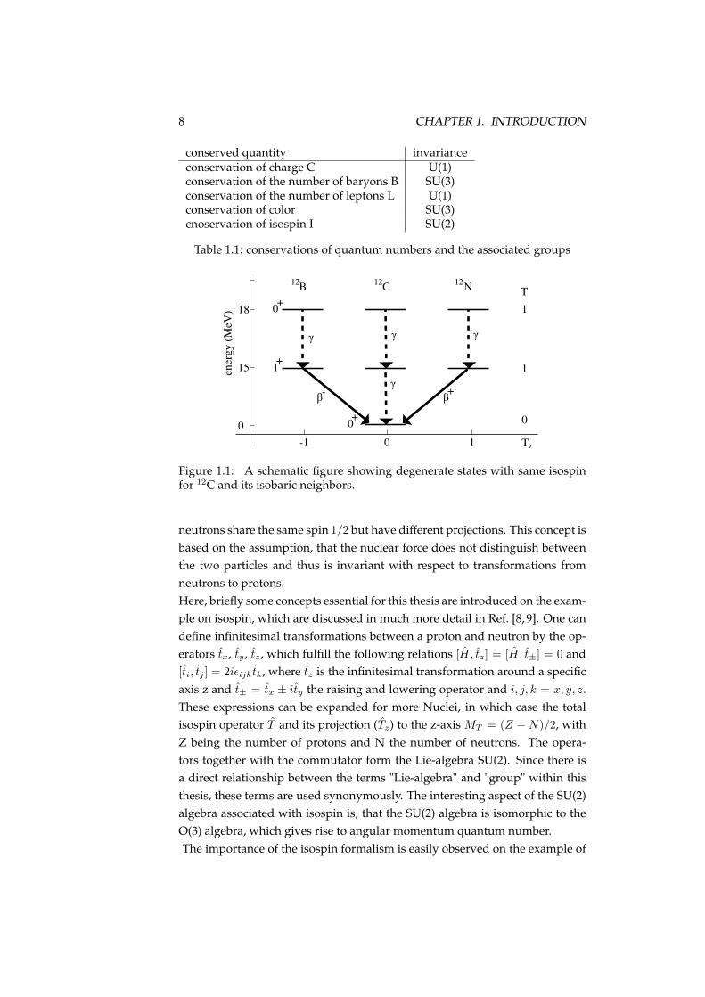
Figure 1.1: A schematic figure showing degenerate states with same isospinfor 12C and its isobaric neighbors.
neutrons share the same spin 1/2 but have different projections. This concept isbased on the assumption, that the nuclear force does not distinguish betweenthe two particles and thus is invariant with respect to transformations fromneutrons to protons.Here, briefly some concepts essential for this thesis are introduced on the exam-ple on isospin, which are discussed in much more detail in Ref. [8, 9]. One candefine infinitesimal transformations between a proton and neutron by the op-erators tx, ty , tz , which fulfill the following relations [H, tz] = [H, t±] = 0 and[ti, tj ] = 2iεijk tk, where tz is the infinitesimal transformation around a specificaxis z and t± = tx ± ity the raising and lowering operator and i, j, k = x, y, z.These expressions can be expanded for more Nuclei, in which case the totalisospin operator T and its projection (Tz) to the z-axis MT = (Z − N)/2, withZ being the number of protons and N the number of neutrons. The opera-tors together with the commutator form the Lie-algebra SU(2). Since there isa direct relationship between the terms "Lie-algebra" and "group" within thisthesis, these terms are used synonymously. The interesting aspect of the SU(2)algebra associated with isospin is, that the SU(2) algebra is isomorphic to theO(3) algebra, which gives rise to angular momentum quantum number.The importance of the isospin formalism is easily observed on the example of
9
126 C6 [10]. From the independent shell model perspective, the ground state of12C is formed by 4 protons and 4 neutrons in a p3/2 orbital ahich are coupledto spin 0. For convenience only a two nucleon system is considered . Together,they can form states associated with T =0, 1. As a antisymmetric T=0 state isenergetically favored, the ground state has T=0, while another state with spin0 and T=1 must exist at higher energies as well as T=1 states with higher spin.In the neighboring isobaric nuclei 12
7 N5 and 12N B7 the first excited state with
spin 0 is associated with isospin T=1. This is schematically shown in Fig. 1.1,where energy (excitation energy and binding energy) of the states are plottedrelative to the ground state in 12C. The degenerate energies of the T=1 tripletstates suggest, that the nuclear force can be assumed to be charge independentin the first order and the isospin a conserved quantity. This is confirmed by in-elastic scattering experiments with deuterons on 12C. A deuteron with isopinT=0 cannot excite the ground state T=0 to excited T=1 states without breakingisospin conservation, thus this reaction is isospin forbidden [11].As mentioned before, the electromagnetic interaction breaks the isospin sym-metry, so states with the same T quantum number in different nuclei are notdegenerate as shown schematically in Fig. 1.1. Using first order perturbationtheory to estimate the energy shift of a given state |ηTTz〉 (with η being anadditional label to distinguish states with same T, TZ), one can calculate thediagonal matrix elements and rewrite the Coulomb interaction to [8]
V u V ≡ κ0 + κ1Tz + κ2T2z , (1.1)
This way, even while the symmetry induced by the SU(2) algebra is broken, itsquantum number T is retained. Analogue to the expression in Eq. (1.1), thiscan also be written in terms of nested algebras:
SU(2) ⊃ SO(2).
[T ] [MT ]
(1.2)
with the eigenfunction
E(MT ) = κ0 + κ1MT + κ2M2T . (1.3)
The constructed algebraic chain given in Eq. (1.2) forms a dynamical symme-try, and MT follows the reduction rule MT = −T, ..., T . Equation (1.3) can nowbe applied to predict the binding energy (hence mass) of an isospin triplet, ifparameters κ0, κ1, κ2 are known. Thus, Eq. (1.3) is also called the isobaric-

10 CHAPTER 1. INTRODUCTION
Figure 1.2: A schematic figure showing the splitting of degenerate states withthe same isospin T=1 and T=3/2 in terms of binding energies. This figure isadopted from Ref. [8].
multiplet mass equation (IMME) and was first proposed by Wigner [12]. Fig-ure 1.2 shows an example for the splitting of the T=2 multiplet (on the lefthand side) and the T=3/2 multiplet (on the right hand side). Experimentaldata was taken from Refs. [13,14] and are reproduced within an error of 1 keV.So the isospin quantum number is still preserved, even though a breaking ofthe symmetry occurs. This is called "dynamical symmetry" breaking. Opera-tors, which produce such a symmetry breaking are called Casimir operators.
1.1 IBM
The concept of symmetry breaking is also applied in the Interacting BosonModel (IBM-1). A just brief introduction is given here. For detailed informa-tion, the interested reader is referred to Ref. [9, 15–18].The prediction of calculated states tend to become uncomputable for micro-scopic models (ie. shell model [19–21]) with increasing mass A and awayfrom the so-called magic numbers. Especially the Geometric Collective Model(GCM) [22, 23] and its simplifications turned out to be successful for nucleiexhibiting substantial deformation. The geometric model deals with the col-lective motion of nucleons in type of surface vibrations and rotations ratherthan with the individual nucleon. While this models describes rotational bandsof deformed nuclei with a large set of nucleons accurately, problems arise for

1.1. IBM 11
nuclei situated closer to shell closure. The IBM-1 is motivated to account forboth approaches. To avoid computational problems, the number of nucleonsare drastically reduced by considering only valence nucleons. Using a con-cept well known in solid state physics, the number of nucleons is still reducedby combining nucleon pairs to so-called Cooper pairs (BCS pairs) [24, 25] withangular momentum l = 0 (s bosons) and l = 2 (d bosons). In second quan-tization, the corresponding boson creation and annihilation operators can beused to construct the generators of a U(6) algebra. Note, the IBM-1 does notdistinguish between proton bosons and neutron bosons. The possibilities toform a chain of nested algebras is limited, since it is sensible to require that theangular momentum is conserved. Only three algebra chains can be formed:
U(6) ⊃ U(5) ⊃ O(5) ⊃ O(3)
U(5)− Symmetrie : ↓ ↓ ↓ ↓[N ] {nd} (ν) L
U(6) ⊃ SU(3) ⊃ O(3)
SU(3)− Symmetrie : ↓ ↓ ↓[N ] (λ, µ) L
U(6) ⊃ O(6) ⊃ O(5) ⊃ O(3)
O(6)− Symmetrie : ↓ ↓ ↓ ↓[N ] {Σ} (τ) L
These algebraic chains are also called dynamical limits. As already discussedfor the isospin, the symmetry of the embedding algebra can be broken by theCasimir operators of the nested algebra. However, the Casimir operators of thenested algebras commute with the embedding algebra, thus the quantum num-bers are preserved. The Hamiltonians of the dynamical limits can be writtenamongst others (multipole form) as linear combination of Casimir operators,allowing to use eigenfunctions to determine the energy for a given set of quan-tum numbers associated with that state.The nuclei discussed in this thesis don’t exhibit strong deformation of the nu-clear shape, so the SU(3) limit will be neglected. Instead, the focus of this workwill be whether the O(5) quantum numbers are preserved. In the following abrief introduction to the groups essential for this thesis is discussed.

12 CHAPTER 1. INTRODUCTION
0+
2+
2+ 4+
1
0
2 2
τ L
Figure 1.3: A schematic figure showing a level scheme using the dynamicalO(6) limit and the corresponding reduction rules (see text). All states share thesame σ = 2 quantum number. Labeling is given in the box. All the shownarrows are E2 transition.
1.2 O(5) group
The O(5) group is part of the algebraic chain of the U(5) limit and the O(6) limit.In the two limits, they are denoted with different quantum numbers, howeverin a purely bosonic system the simple relation is τ = ν. The eigenfunction ofthe second order Casimir operator C2[O(5)] is defined as [9]
E(O(5)) = τ(τ + 3). (1.4)
The τ quantum number induced by the O(5) group is also called seniority. Theseniority can be understood when applying the Casimir operator C2[O(5)] ona given state with good O(5) quantum number, which is directly related to thenumber of d bosons which do not belong to pairs coupled to zero. In Fig. 1.3an exemplary level scheme is given specifically for the O(6) limit. For clarity,only a system with two nucleon bosons N = 2 is considered. In that figure allstates belong to the highest σ = 2 multiplet.
The reduction rule for O(6)⊃O(5) is τ = 0, 1, ..., N = σ, whereN is the numberof valence bosons. The angular momentum L is obtained for O(5) ⊃ O(3) withthe reduction rule τ = 3n∆ + µ and L = µ, µ + 1, ..., 2µ − 2, 2µ. Using thereduction rules for the algebraic chain, all possible sets of quantum numbersare derived. For the ground state all d bosons are coupled to zero, thus seniorityτ = 0. To construct a L = 2+ state, one d boson pair must be coupled to2. In this way a level scheme can be constructed. An important experimentalobservable in order to verify τ quantum numbers are to observeE2 transitions.In the IBM-1, E2 transition operator is defined as
TE2µ = εb[s
† × d+ d† × s](2)µ + χ εb[d
† × d](2)µ , (1.5)
1.3. SPIN(5) GROUP 13
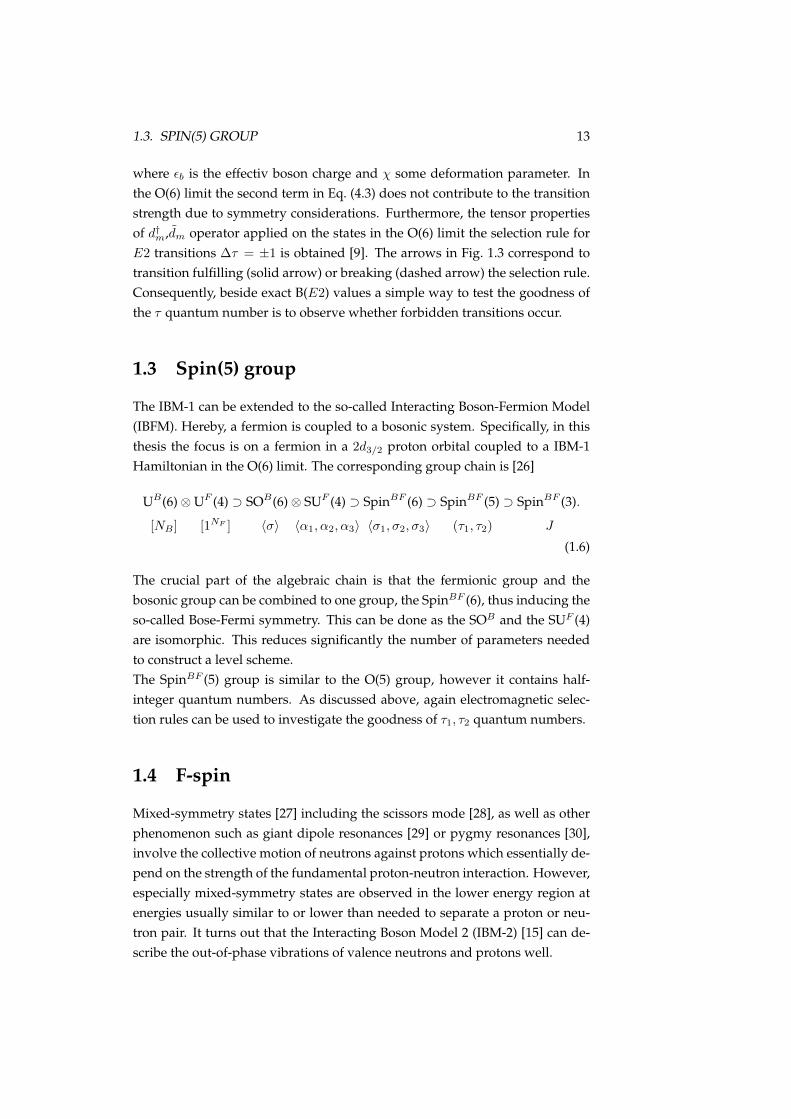
where εb is the effectiv boson charge and χ some deformation parameter. Inthe O(6) limit the second term in Eq. (4.3) does not contribute to the transitionstrength due to symmetry considerations. Furthermore, the tensor propertiesof d†m,dm operator applied on the states in the O(6) limit the selection rule forE2 transitions ∆τ = ±1 is obtained [9]. The arrows in Fig. 1.3 correspond totransition fulfilling (solid arrow) or breaking (dashed arrow) the selection rule.Consequently, beside exact B(E2) values a simple way to test the goodness ofthe τ quantum number is to observe whether forbidden transitions occur.
1.3 Spin(5) group
The IBM-1 can be extended to the so-called Interacting Boson-Fermion Model(IBFM). Hereby, a fermion is coupled to a bosonic system. Specifically, in thisthesis the focus is on a fermion in a 2d3/2 proton orbital coupled to a IBM-1Hamiltonian in the O(6) limit. The corresponding group chain is [26]
UB(6)⊗UF (4) ⊃ SOB(6)⊗ SUF (4) ⊃ SpinBF (6) ⊃ SpinBF (5) ⊃ SpinBF (3).
[NB ] [1NF ] 〈σ〉 〈α1, α2, α3〉 〈σ1, σ2, σ3〉 (τ1, τ2) J
(1.6)
The crucial part of the algebraic chain is that the fermionic group and thebosonic group can be combined to one group, the SpinBF (6), thus inducing theso-called Bose-Fermi symmetry. This can be done as the SOB and the SUF (4)are isomorphic. This reduces significantly the number of parameters neededto construct a level scheme.The SpinBF (5) group is similar to the O(5) group, however it contains half-integer quantum numbers. As discussed above, again electromagnetic selec-tion rules can be used to investigate the goodness of τ1, τ2 quantum numbers.
1.4 F-spin
Mixed-symmetry states [27] including the scissors mode [28], as well as otherphenomenon such as giant dipole resonances [29] or pygmy resonances [30],involve the collective motion of neutrons against protons which essentially de-pend on the strength of the fundamental proton-neutron interaction. However,especially mixed-symmetry states are observed in the lower energy region atenergies usually similar to or lower than needed to separate a proton or neu-tron pair. It turns out that the Interacting Boson Model 2 (IBM-2) [15] can de-scribe the out-of-phase vibrations of valence neutrons and protons well.
14 CHAPTER 1. INTRODUCTION
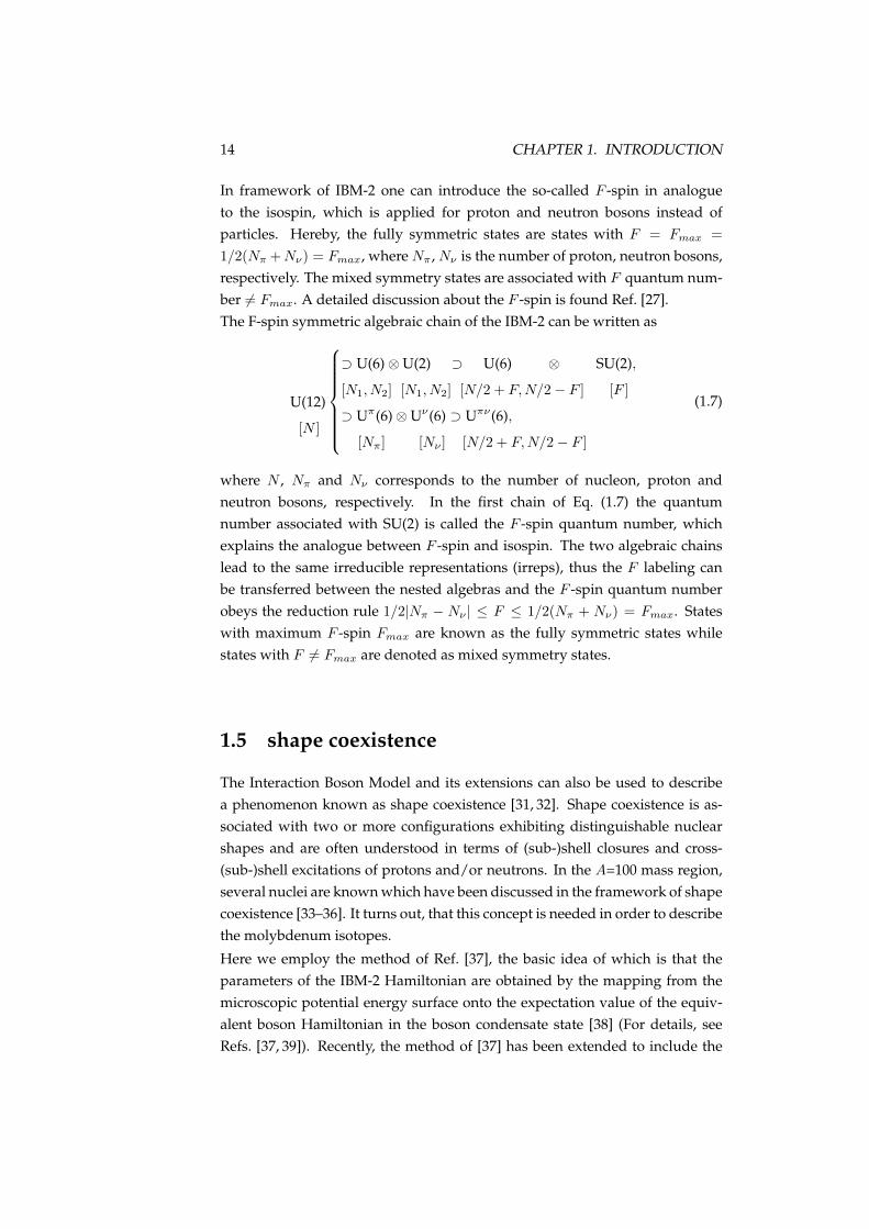
In framework of IBM-2 one can introduce the so-called F -spin in analogueto the isospin, which is applied for proton and neutron bosons instead ofparticles. Hereby, the fully symmetric states are states with F = Fmax =
1/2(Nπ +Nν) = Fmax, where Nπ , Nν is the number of proton, neutron bosons,respectively. The mixed symmetry states are associated with F quantum num-ber 6= Fmax. A detailed discussion about the F -spin is found Ref. [27].The F-spin symmetric algebraic chain of the IBM-2 can be written as
U(12)
[N ]
⊃ U(6)⊗U(2) ⊃ U(6) ⊗ SU(2),
[N1, N2] [N1, N2] [N/2 + F,N/2− F ] [F ]
⊃ Uπ(6)⊗Uν(6) ⊃ Uπν(6),
[Nπ] [Nν ] [N/2 + F,N/2− F ]
(1.7)
where N , Nπ and Nν corresponds to the number of nucleon, proton andneutron bosons, respectively. In the first chain of Eq. (1.7) the quantumnumber associated with SU(2) is called the F -spin quantum number, whichexplains the analogue between F -spin and isospin. The two algebraic chainslead to the same irreducible representations (irreps), thus the F labeling canbe transferred between the nested algebras and the F -spin quantum numberobeys the reduction rule 1/2|Nπ − Nν | ≤ F ≤ 1/2(Nπ + Nν) = Fmax. Stateswith maximum F -spin Fmax are known as the fully symmetric states whilestates with F 6= Fmax are denoted as mixed symmetry states.
1.5 shape coexistence
The Interaction Boson Model and its extensions can also be used to describea phenomenon known as shape coexistence [31, 32]. Shape coexistence is as-sociated with two or more configurations exhibiting distinguishable nuclearshapes and are often understood in terms of (sub-)shell closures and cross-(sub-)shell excitations of protons and/or neutrons. In the A=100 mass region,several nuclei are known which have been discussed in the framework of shapecoexistence [33–36]. It turns out, that this concept is needed in order to describethe molybdenum isotopes.
Here we employ the method of Ref. [37], the basic idea of which is that theparameters of the IBM-2 Hamiltonian are obtained by the mapping from themicroscopic potential energy surface onto the expectation value of the equiv-alent boson Hamiltonian in the boson condensate state [38] (For details, seeRefs. [37, 39]). Recently, the method of [37] has been extended to include the

1.5. SHAPE COEXISTENCE 15
mixing of the different configurations associated to the different shape intrinsicshapes. Hereby, we first perform a set of constrained Hartree-Fock-BCS calcu-lations using the Skyrme functional SLy6 [40] using the code ev8 [41] to obtainthe potential energy surface for a given nucleus. The constraint imposed hereis for mass quadrupole moments, associated to the deformation parametersβ and γ of the geometrical model [42]. The density-dependent pairing inter-action is used for the pairing correlation in the BCS approximation, with itsstrength being the fixed value of V0=1000 MeV, and Lipkin-Nogami prescrip-tion is taken for the treatment of the particle number. For the review on theself-consistent mean-field approach, the reader is referred to [43].
For the boson part, the following Hamiltonian is used for each configuration:
H = εν ndν + επndπ + κQν · Qπ + Mπν , (1.8)
where the first term
ndρ =∑
ρ,md†ρ,mdρ,m, ρ = π, ν (1.9)
stand for the d boson number operator. ερ is the single proton or neutron bosonenergy, and is assumed to be the same between protons and neutrons, εν =
επ ≡ ε. The second term in (1.8) is the quadrupole-quadrupole interactionbetween the proton and the neutron bosons, with the quadrupole operator Qρbeing
Qρ = d†ρsρ + s†ρdρ + χρ[d†ρ × dρ](2). (1.10)
In the above equation, κ and χρ stand for the strength parameter and the pa-rameter which determines whether the nucleus is prolate or oblate.
The fourth term in Eq. (1.8) represents the so-called Majorana term which ren-ders the symmetric states energetically favored:
Mπν = 12ξ2(d†πs
†ν − s†πd†ν) · (dπsν − sπdν) +
∑λ=1,3 ξλ(d†πd
†ν)(λ) · (d†πd†ν)(λ)(1.11)
ξ1,2,3 are the strength parameters, which are normally determined so that themixed symmetry states are higher enough in energy.
Since the Majorana terms do not influence the boson energy surface, providedthat the equal deformations between proton and neutron are assumed, the onlyparameters which are to be extracted by mapping from the microscopic poten-tial energy surface are ε, κ, χπ , and χν .
The full Hamiltonian is given as
H = PnorHnorPnor + Pintr(Hintr + ∆)Pintr + Hmix, (1.12)

16 CHAPTER 1. INTRODUCTION
where Hnor (Hintr) and Pnor (Pintr) represent the Hamiltonian of and the pro-jection operator onto the normal (intruder) configuration space, respectively,and ∆ specifies the energy shift between the configurations. The mixing ofconfigurations is defined as
Hmix = ω1(s†π · s†π + d†π · d†π) + ω2(sπ · sπ + dπ · dπ). (1.13)
For simplicity, the mixing strength is set to ω1 = ω2 ≡ ω.
1.6 Structure of this thesis
The primary aim of this work is to test how robust the O(5)/Spin(5) quantumnumber are within the evolution of nuclear shapes and with increasing num-ber of neutrons. The odd-even gold isotopes in the A=200 were selected toinvestigate the Spin(5) symmetry. This is motivated by the occurrence of thewell known supermultiplets around 194Pt and 196Pt, in which the Bose-fermisymmetry is embedded for the odd-A nuclei. The very gradual change appar-ent for the odd-even gold isotopes allows to test the preservation of the Spin(5)quantum number for a long chain of gold isotopes. Furthermore, the challengeis to test whether the switch of the ground state from spin 1/2 to 3/2 is repro-ducible for the Interacting Boson Fermion Model.The molybdenum isotopes in the A=100 mass region provides a even greaterchallenge, since the nuclear shape in that mass region tends to change ratherabruptly. Based on the concept of shape coexistence, the even-even molybde-num isotopes can be used to test the goodness seniority in the harsh conditionof configuration mixing. Especially the mixed symmetry states provide a strin-gent test whether the selections rules can be still applied for shape coexistencein these nuclei.First, some advances in the evaluation technique are presented, followed bypapers dealing with the Bose-Fermi symmetry in the odd-even gold nuclei.Then the results of experiments in the even-even molybdenum isotopes con-densed in two more publications are presented. Finally, the results are summa-rized and an outlook for further research is given.

Chapter 2
Method
In this thesis only data obtained from in-beam experiments were evaluated.The data of 96Mo, 193Au, and 195Au originate from in-beam experiments per-formed at the Cologne FN-Tandem accelerator by using the Osiris spectrometerfor 96Mo and the Horus spectrometer for 193,195Au. 98Mo was measured in thelast experimental campaign at the ESTU-Tandem accelerator at the Wright Nu-clear Structure Lab (WNSL) at Yale University before the permanent shutdownof the accelerator in June, 2011.In general, the advantage of in-beam experiments is that γγ coincidencesin relation to the angle of the detectors provide angular correlations to testspin hypotheses and multipole mixing ratios. The angular correlation anal-ysis together with the coincidence technique is extensively covered in theliterature [44–46] and will not be discussed any further in this thesis. Theangular correlation analysis was performed with the computer code COR-LEONE [47, 48].However, for the calculation of branching ratios the previous technique is im-proved to include the angular correlation analysis and is discussed in the fol-lowing section.
2.1 Case study 1
In Fig. 2.1 the exemplary decays A, B, C are shown. Transition A with the γenergy Eγ,A feeds a state, which is depopulated by the transition B and C. Inthis section the calculation of the relative γ intensity I(B,C) (or branchingratio) between the transitions B and C is explained by using a gate set on theenergy of transition A:
17

18 CHAPTER 2. METHOD
A
BC
Figure 2.1: Two exemplary (γγ) cascades (A,B) and (A,C) are show. The widthof arrows correspond to the relative γ intensity between transition B and C.The two parallel lines symbolize the gate set at the energy of transition A.
[h]
b1 = b · ω1 · ε1bi = b · ωi · εi
...bk = b · ωk · εk
(2.1)
with
k=number of correlation groupsi=denominates the correlation group (from 1,..k)bi=volume of transition B in coincidence with transition A in correlation groupiω(σ, δ, J)=angular correlation in correlation group iεi=efficiency of correlation group i
The volume b of transition B denotes the volume after the correction due toangular correlations and efficiency. Thus, the total volume btot (the sum of allγγ coincidences) of transition B in coincidence with transition A is:

2.2. CASE STUDY 2 19
btot =∑ki=1 bi =
∑ki=1 b · ωi · εi = b
∑k
i=1·ωi · εi︸ ︷︷ ︸
V (ω, ε)b
(2.2)
⇒ b =btot
V (ω, ε)b(2.3)
analogue for the γγ cascade (A,C):
c =ctot
V (ω, ε)c(2.4)
I(B,C) =b
c=btotctot· V (ω, ε)cV (ω, ε)b
(2.5)
The corresponding error ∆b (∆c) is derived from error propagation:
∆b = btot ·√(
∆btotbtot · V (ω, ε)b
)2
+∑
i
(ωi ·∆εiV (ω, ε)2
b
)2
+∑
i
(εi ·∆ωiV (ω, ε)2
b
)2
(2.6)
The errors in the correlation groups depends on the deviation from one spinhypothesis to another in the corresponding correlation group. However, incase of a 4π detector array the sum over the different angular correlations isthe same. Since not all angles are covered by detectors, the sum over differentspin hypothesis differ, which is denoted as ∆ω. This leads to the followingsimplification: ∑
i
(εi ·∆ωiV (ω, ε)2
b
)2
=
(εtot ·∆ωV (ω, ε)2
b
)2
(2.7)
The error propagation of Eq. (2.5) and formula (2.6) leads to
∆I(B,C) = I(B,C) ·√(
∆b
b
)2
+
(∆c
c
)2
(2.8)
2.2 Case study 2
In the prior section the coincidences of one feeding transition A were usedto investigate the relative γ intensity of the depopulating transitions B and C.Alternatively, instead of using a feeding transition one can use coincident de-populating transitions to calculate the relative γ intensity I(B,C). In Fig. 2.2a schematic level scheme is shown. The total volume btot (the sum of all γγcoincidences) of transition B is obtained by using coincidences with transitionD (gate on the energy of transition D). However, btot has to be corrected for the

20 CHAPTER 2. METHOD
BC
A
D E
Figure 2.2: Exemplary γγ cascades (B,A), (B,D) and (C,E) are show. The twoparallel lines symbolize the consecutive gates set at the energy of transition Dand E, respectively. See text for detail.
alternative (B,A) γγ cascade. Thus, b is defined as:
b =btot ·
(dd + a·(1+αA)
d
)V (ω, ε)b
, (2.9)
with a = atotV (ω,ε)a
, d = dtotV (ω,ε)d
and αA being the conversion coefficient of transi-tion A. For the total volume ctot, coincidences with transition E are used. Thus,for the calculation of errors additional terms with errors of the relative inten-sity for other depopulating transitions have to be included. The computer codeMAMMEL [49] employs Eqs. (2.5-2.9) and was used to calculate the relative γintensities.

Chapter 3
The gold isotopes
21

Available online at www.sciencedirect.com
ScienceDirect
Nuclear Physics A 922 (2014) 200–224
www.elsevier.com/locate/nuclphysa
The structure of 193Au within the InteractingBoson Fermion Model
T. Thomas a,b,∗, C. Bernards a,b, J.-M. Régis a, M. Albers a, C. Fransen a,J. Jolie a, S. Heinze a, D. Radeck a, N. Warr a, K.-O. Zell a
a Institute for Nuclear Physics, University of Cologne, Zülpicher Straße 77, D-50937 Köln, Germanyb WNSL, Yale University, P.O. Box 208120, New Haven, CT 06520-8120, USA
Received 7 November 2013; received in revised form 5 December 2013; accepted 7 December 2013
Available online 13 December 2013
Abstract
A γ γ angular correlation experiment investigating the nucleus 193Au is presented. In this work the level
scheme of 193Au is extended by new level information on spins, multipolarities and newly observed states.
The new results are compared with theoretical predictions from a general Interacting Boson Fermion Model
(IBFM) calculation for the positive-parity states. The experimental data is in good agreement with an IBFM
calculation using all proton orbitals between the shell closures at Z = 50 and Z = 126. As a dominant
contribution of the d3/2 orbital to the wave function of the lowest excited states is observed, a truncated
model of the IBFM using a Bose–Fermi symmetry is applied to the describe 193Au. Using the parameters
of a fit performed for 193Au, the level scheme of 192Pt, the supersymmetric partner of 193Au, is predicted
but shows a too small boson seniority splitting. We obtained a common fit by including states observed in192Pt. With the new parameters a supersymmetric description of both nuclei is established.
2013 Elsevier B.V. All rights reserved.
Keywords: NUCLEAR REACTIONS 194Pt(p,2n), E = 14 MeV; Measured Eγ , Iγ , γ γ -coin, γ (θ), using HORUS
spectrometer. 193Au; Deduced levels, J , π , branching and mixing ratios, B(M1), B(E2); Comparison with IBFM
calculations
1. Introduction
The low-lying levels of the odd–even Au isotopes were studied, in the early 1970s, to ad-
dress the question, whether theories coupling phonons to a proton are able to describe these
* Corresponding author.
E-mail address: [email protected] (T. Thomas).
0375-9474/$ – see front matter 2013 Elsevier B.V. All rights reserved.
http://dx.doi.org/10.1016/j.nuclphysa.2013.12.004
T. Thomas et al. / Nuclear Physics A 922 (2014) 200–224 201
nuclei [1–3]. The measurement of conversion electrons and γ rays following the β decay from193Hg enabled Fogelberg et al. [1] to obtain the M1 and E2 transition strengths of several γ tran-
sitions in 193Au. Half-life measurements were done via electron–electron coincidences. The aim
was to describe the nucleus either in terms of a pairing-plus-quadrupole force model or in terms
of a core-excitation model. Although both models described the energies of the low-lying states,
the known transition strengths of the three lowest levels were not reproduced satisfactorily.
In 1980, Iachello introduced dynamical supersymmetries to describe bosonic and fermionic
systems [4]. In the following year, the Interacting Boson Fermion Model (IBFM), an extension of
the Interacting Boson Model (IBM), was applied to the positive-parity states of the nucleus 193Au
by Wood [5]. Theoretical transition strengths were calculated and compared them to experimental
values, showing for the first time that the IBFM was able to describe this Au isotope.
In 1984, Van Isacker et al. [6] introduced the so-called extended supersymmetry by including
the proton-neutron degree of freedom and, thus, were able to describe sets of four neighboring
nuclei: even–even 196Pt, odd-neutron 197Pt, odd-proton 197Au, and odd–odd 198Au. Such a su-
permultiplet is also called magical quartet or magical square. Members of a supermultiplet are
all described by the same algebraic Hamiltonian and by the same total number Nρ = Nρ + Mρ
of particles with Nρ the number of bosons (or boson holes) and Mρ the number of fermions
(or fermion holes) with ρ = ν,π (ν = neutrons, π = protons). The total number of particles,
used for the description of the supermultiplet including 196,197Pt and 197,198Au, is Nν +Nπ = 6.
About 15 years later, experimental evidence was found for a new neighboring magical quartet
consisting of 194,195Pt and 195,196Au [7–9]. Recently, the supersymmetric description was used
to extend the magical quartets to quintets by including the nuclei 196Hg and 198Hg [10,11].
As these magical quartets consist of nuclei in the gold–platinum mass region, it is of interest
whether 193Au can be described by the Interacting Boson Fermion Model, and if a common
description of the isotones 193Au and 192Pt in the supersymmetric O(6) limit is feasible.
In the following section, the Interacting Boson Fermion Model is introduced. A truncation
of this model using only the dπ,3/2 orbital and in the O(6)-limit, the Bose–Fermi symmetry,
is described in Section 3. Section 4 describes the experiment, and the results are presented. In
Section 5, we discuss the implications of the new data to our understanding of the nucleus, as
well as compare the data to theoretical predictions of the IBFM. Finally, the parameters of the fit
are used to predict states in the neighboring 192Pt nucleus.
2. Interacting Boson Fermion Model
The IBM was introduced, in order to describe collective behavior of even–even nuclei within
an algebraic framework. This model was extended to the Interacting Boson Fermion Model 1
[12,13] (IBFM-1) by coupling one fermion to a bosonic system.
H = Hsd + HF + VBF, (1)
where Hsd represents the pure bosonic part of the Hamiltonian, while
HF =5
∑
k=1
PEN(k)nk (2)
is the Hamiltonian for the single nucleon degrees of freedom. The parameters PEN(k) denote the
quasi-particle energies and nk = −√
2jk + 1[a†k × ak](0)
0 with jk being the spin of the orbital k.
The boson-fermion Interaction strength VBF in its general [14] form can be reduced on basis of
microscopic arguments [15] to

202 T. Thomas et al. / Nuclear Physics A 922 (2014) 200–224
VBF =5
∑
k,k′=1,k�k′
BFQJ(Nkk′){(
Q(2) ·(
a†k × ak′
)(2)) + h.c.}
+5
∑
k,k′=1
∑
k′′Λk′′
kk′1
j ′′k
:[[
d† × ak
](jk′′ ) ×[
d × a†k′](jk′′ )](0)
0:
+5
∑
k=1
BFMJ(k)nd nk, (3)
where : : represents the normal ordering, nd =√
5[d† × d](0)0 , the fermion annihilation operator
defined as akm = (−1)jk−mak−m, and
Q(2) =(
s† × d + d† × s)(2) + χ
(
d† × d)(2)
, (4)
Λk′′kk′ = −
√5 BFE
{
(uk′vk′′ + vk′uk′′)Qk′k′′βkk′′ + (ukvk′′ + vkuk′′)Qkk′′βk′k′′}
, (5)
βkk′ ={
β ′kk′ , k � k′,
(−1)jk−jk′ β ′kk′ , k′ � k,
(6)
with vk =√
VSQ(k), uk =√
1 − VSQ(k), and VSQ(k) being the occupation probability of the
orbital k. The coefficients βkk′ can be related to the microscopic structure of the d-boson. Under
the assumption that the |D〉-state absorbs the full E2-strength, it can be shown that:
β ′kk′ = 1
PEN(k) + PEN(k′) − Ω(ukvk′ + uk′vk)Qkk′ , (7)
where Ω denotes the energy of the |D〉-state relative to the |S〉-state. Ω can be obtained from the
excitation energy of the 2+1 state in a semimagic nucleus.
The monopole and quadrupole force can be simplified assuming independence of the orbit
BFQJ(Nkk′) = BFQ(ukuk′ − vkvk′)Qkk′ , k � k′, (8)
BFMQJ(k) = BFM. (9)
Summarizing, the boson-fermion interaction given by Eqs. (3)–(9) is fully specified by the three
interaction strengths BFQ, BFE, BFM, the parameter in the quadrupole operator, χ , the occupa-
tion probabilities VSQ(k) of the different orbitals, and the quasi-particle energies PEN(k).
3. Bose–Fermi symmetry and supersymmetry
Since 193Au is located in the proximity of the supermultiplets, the Interacting Boson Fermion
Model 1 (IBFM), in the O(6) limit [16], seems to be an appropriate choice for the description of
this nucleus. Hereby, a fermion in the J π = 3/2+ orbital is coupled to a system of seven bosons
using the UB(6) ⊗ UF(4) algebra. Isomorphisms in the sub-algebra structure of UB(6) ⊗ UF(4)
can be found between the boson and fermion algebras. Such an isomorphism exists between
UB(6) ⊃ SOB(6) and UF(4) ⊃ SUF(4) ≃ SpinF(6) groups. The generators, gk , of these sub-
groups, SOB(6) and SOF(6) commute and a linear combination of these generators closes under
commutation, and thus, form a boson-fermion algebra SpinBF(6). This is the so-called Bose–
Fermi symmetry and is discussed in more detail in Refs. [17,18], while only equations essential
for this work are given here.

T. Thomas et al. / Nuclear Physics A 922 (2014) 200–224 203
The group chain of the Hamiltonian in the O(6) limit is:
UB(6) ⊗ UF(4) ⊃ SOB(6) ⊗ SUF(4) ⊃ SpinBF(6) ⊃ SpinBF(5) ⊃ SpinBF(3),
[NB][
1NF]
〈σ 〉 〈α1, α2, α3〉 〈σ1, σ2, σ3〉 (τ1, τ2) J
(10)
where we have indicated under each group the quantum number classifying the irreducible repre-
sentation. The number of fermions is NF = 1 in the case of the odd A nucleus and NB denotes the
number of bosons. Other quantum numbers of the nested algebras are determined by reduction
rules (see Ref. [16]). The Hamiltonian written in the form of a linear combination of Casimir
operators corresponding to the group chain, neglecting constant terms that only contribute to the
binding energy, is:
H = D · C2
[
SOB(6)]
+ A · C2
[
SpinBF(6)]
+ B · C2
[
SpinBF (5)]
+ C · C2
[
SpinBF(3)]
. (11)
Where C2[X] is the second order Casimir operator of the given algebra. The corresponding
energy eigenfunction of the Hamiltonian can be derived from the eigenfunction of the Casimir
operators of the subgroups:
E = Dσ(σ + 4) + A(
σ1(σ1 + 4) + σ2(σ2 + 2) + σ 23
)
+ B(
τ1(τ1 + 3) + τ2(τ2 + 1))
+ C(
J (J + 1))
. (12)
For this Hamiltonian, it is possible to find an embedding superalgebra to the Bose–Fermi sym-
metry [18]. The generators of this supersymmetry consist of mixed boson-fermion creation and
annihilation operators, and therefore, do not form a Lie algebra, but a superalgebra. While the
Bose–Fermi symmetry preserves the boson and fermion numbers separately, the supersymme-
try only preserves the total number of particles N = NB + NF. The embedding algebra of
UB(6) ⊗ UF (4) is:
U(6/4) ⊃ UB(6) ⊗ UF(4).
↓ ↓[N ] [NB,1NF ]
(13)
In the case that a fermion is annihilated and a boson created, the number of fermions is NF = 0
and the problem can be described within the Interacting Boson Model (IBM). The eigenvalues
of the IBM-1 in the O(6) limit are [18]
E = Aσ (σ + 4) + Bτ(τ + 3) + CJ(J + 1), (14)
with A = A + D. Note, that in this work the IBFM with a J = 3/2 particle in the O(6) limit is
referred to as the U(6/4) limit.
4. Experimental results
The experiment was performed at the Cologne tandem accelerator by impinging a 14 MeV
proton beam onto a 1.3 mg/cm2 194Pt target. In the primary reaction channel, 193Au was pro-
duced via a 194Pt(p, 2n) reaction. The expected cross section for this reaction is predicted around
700 mbarn, calculated with the computer code CASCADE [19]. The code also predicts a grazing
angular momentum transfer of about 3.5h. We have used the HORUS spectrometer [20], an array
equipped, during this experiment, with 12 high-purity germanium detectors on the edges and the

204 T. Thomas et al. / Nuclear Physics A 922 (2014) 200–224
Fig. 1. (Color online.) Comparison of theoretical angular correlation with different spin hypotheses (black solid and greendashed line) with relative intensities obtained from 16 correlation groups for the 539–614 keV γ γ coincidence.
Fig. 2. γ γ coincidence spectrum energy-gated on the 258.0 keV transition in 193Au from Jπ = 5/2+1 state to the ground
state. The energies of the strongest transitions in coincidence with the 258.0 keV transition are given.
faces of a cube, to detect γ transitions of excited states in 193Au. The setup of the spectrometerallows the analysis of γ γ angular correlations. We sorted the data in so-called correlation groupmatrices, which consist of detector pairs defined by specific angles. This way the experimentalangular correlation of two correlated γ transitions is determined. The method, using the HO-RUS spectrometer is described in more detail in the Refs. [10,20]. By fitting a spin hypothesis
J1EA,δA−−−−→ J2
EB,δB−−−−→ J3, described in Refs. [21,22], to the data, spins of the initial Einital andfinal state Efinal and multipole mixing ratios, δA,B , are obtained. The fit is performed with thecomputer code CORLEONE [23]. Fig. 1 shows an exemplary γ γ angular correlation analysisfor the spin hypotheses 11/2 614−−→ 7/2 539−−→ 3/2gs (black solid line) and 9/2 614−−→ 7/2 539−−→ 3/2gs
(green dashed line). The spin hypothesis 11/2 614−−→ 7/2 539−−→ 3/2gs fits the data best. Thus, thespin for the state at 1153 keV was determined to be 11/2. In Appendix A (see Figs. A.1–A.6),more angular correlation plots are shown.
Although 193Au has been measured in in-beam experiments [2,24–26] previously, this is thefirst time that an experiment with small momentum transfer was chosen, in order to observelow-energy positive-parity states. An example of a γ -ray coincidence spectrum, with a gate onthe 258.0 keV transition of the Jπ = 5/2+
1 state to the ground state, is shown in Fig. 2. Byanalyzing the γ γ coincidence matrices, we identified numerous new transitions and states. Thespins of all known low-lying positive-parity states were determined, except for a state at 38 keV.
T. Thomas et al. / Nuclear Physics A 922 (2014) 200–224 205
Our results are listed in Table 1. Unless stated otherwise, corrections of the level energies or
transition energies, given in Table 1, are due to the improved capability to detect γ rays. All those
values differing from the results of this work, are based on the observations of Ref. [3]. Three
Ge(Li) detectors were used to observe γ decays in Ref. [3], whereas in this work, an array of 12
high purity Ge detectors was applied, resulting in a superior absolute efficiency [20].
In the case that new states are observed with only one depopulating transition, coincidence
spectra with a gate on the depopulating transition as well as a gate on a coincident transition is
given (see Figs. A.7, A.8 in Appendix A). In Table A.1, additional coincident γ transitions are
listed.
In the following section, some states in 193Au are discussed in more detail, in order to clarify
experimental observation, especially if the experimental results of this work are in conflict with
literature:
38.2 keV, (1/2)+. The transition to the ground state is not observed, due to the low energy of
the γ ray. The experimental setup was optimized to detect γ energies between Eγ =180–1000 keV. The spin of this state was not determined in this experiment, but is
adopted from Ref. [3].
290.2 keV, 11/2−. This level is known as an isomeric state with τ = 5.6(4) s [27]. No γ
transitions are observed, since the 290.2 keV state decays dominantly via conversion
electrons. The spin of this state was not determined in this experiment, but is adopted
from Ref. [3].
381.6 keV,5/2+. The γ γ angular correlation analysis yields two possible multipole mixing
ratios, δ = −2.93+45−62 and δ = −0.07(5), for the 381.6 keV transition to the ground
state. In Ref. [3], a multipole mixing ratio of δ = 1.2+5−3 was determined by measuring
conversion electrons, for the 381.6 keV transition, with a magnetic Siebahn–Svartholm
π√
2 spectrometer. Since a strong E2 characteristic seems to be more likely from the
conversion electron measurement, the multipole mixing ratio closer to zero is ruled out,
and δ = −2.93+45−62 is given in Table 1 for this transition.
828.0 keV, 3/2+. Our data do not agree with the assignment of the transition at 289.0 keV,
from [3], to this level. This supports the statement in the NDS [28], that the placement
of this γ decay is not clear, suggesting it belongs to 193Hg. Furthermore, the strongest
transition at 789.21(20) keV in Ref. [3] turns out to be a doublet, and is corrected to
789.7(2) keV. The transition at 827.81(20) keV, in Ref. [3], is observed at 828.0(2) keV,
as this γ line turned out to be a triplet. Distinguishing these multiplets is possible with
the newly observed γ decays at 277.9, 488.9, 635.1 and 750.0 keV, feeding the state at
828.0 keV. Using these feeding transitions and the newly observed decay at 603.2 keV
depopulating this state, new branching ratios are established. The spin of this state could
be established, due to angular correlation of the (446, 381) keV cascade (see Fig. A.5).
1106.0 keV, 7/2+. The angular correlation analysis of transitions depopulating this newly ob-
served state show, that either spin J = 7/2 or 9/2 can be assigned to this state. However,
we observe a 277.9 keV transition, populating the 828 keV state with spin J = 3/2+,
so the spin hypothesis J = 9/2+ is discarded.
1119.0 keV, 3/2+. The angular correlation analysis of this state yields the spin J = 3/2 (cf.
A.6) for this state, with two possible multipole mixing ratios δ861 = 0.35(8) and
δ861 = 1.33(40). While the experimental K/L1,2 = 6.1(13) ratio [3] is reproduced by
the theoretical ratios K/L861,δ=0.35 = 6.2(3) and K/L861,δ=1.33 = 5.9(3) [47], the con-
version coefficient for the larger multipole mixing ratio (αK,δ=0.35 = 0.0161(6) and
206 T. Thomas et al. / Nuclear Physics A 922 (2014) 200–224
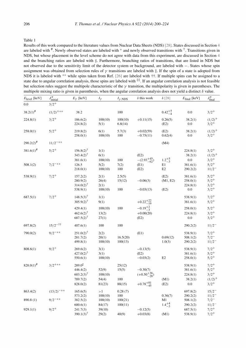
Table 1
Results of this work compared to the literature values from Nuclear Data Sheets (NDS) [28]. States discussed in Section 4
are labeled with #. Newly observed states are labeled with ❇ and newly observed transitions with †. Transitions given in
NDS, but whose placement in the level scheme do not agree with data from this experiment, are discussed in Section 4
and the branching ratios are labeled with ♯. Furthermore, branching ratios of transitions, that are listed in NDS but
not observed due to the sensitivity limit of the detector system or background, are labeled with −. States whose spin
assignment was obtained from selection rules of γ transitions are labeled with ‖. If the spin of a state is adopted from
NDS it is labeled with ❇❇ while spins taken from Ref. [26] are labeled with ††. If multiple spins can be assigned to a
state due to angular correlation analysis, those spins are labeled with ‡‡. If an angular correlation analysis is not feasible
but selection rules suggest the multipole characteristic of the γ transition, the multipolarity is given in parentheses. The
multipole mixing ratio is given in parenthesis, when the angular correlation analysis does not yield a distinct δ value.
Elevel [keV] Jπinitial Eγ [keV] Iγ Iγ,NDS δ this work δ [28] Efinal [keV] Jπ
final
0.0 3/2+
38.2(1)# (1/2)+❇❇ 38.2 100 0.42+5−4 0.0 3/2+
224.8(1) 3/2+ 186.6(2) 100(10) 100(10) +0.11(15) 0.26(5) 38.2(1) (1/2)+224.8(2) 5(1) 6.8(14) (E2) 0.0 3/2+
258.0(1) 5/2+ 219.8(2) 6(1) 5.7(3) +0.02(59) (E2) 38.2(1) (1/2)+258.0(1) 100(10) 100 −0.75(11) 0.62(4) 0.0 3/2+
290.2(2)# 11/2−❇❇ (M4)
381.6(1)# 5/2+ 156.8(2)† 1(1) 224.8(1) 3/2+
343.4(2)† 6(1) (E2) 38.2(1) (1/2)+
381.6(1) 100(10) 100 −(2.93+45−62) 1.2+5
−3 0.0 3/2+
508.1(2) 7/2−❇❇ 126.5 5(2) 7(2) (E1) E1 381.6(1) 5/2+218.0(1) 100(10) 100 (E2) E2 290.2(2) 11/2−
538.9(1) 7/2+ 157.2(2) 2(1) 2.5(5) (E2) 381.6(1) 5/2+280.9(2) 26(4) 15(12) −0.06(3) (M1, E2) 258.0(1) 5/2+
314.0(2)† 2(1) 224.8(1) 3/2+538.9(1) 100(10) 100 −0.03(13) (E2) 0.0 3/2+
687.5(1) 7/2+ 148.5(3)† 1(1) 538.9(1) 7/2+
305.9(2)† 9(1) +0.22+22−19 381.6(1) 5/2+
429.4(1) 100(10) 100 −0.19+2−3 258.0(1) 5/2+
462.6(2)† 13(2) +0.00(20) 224.8(1) 3/2+
687.5(2)† 27(1) (E2) 0.0 3/2+
697.8(2) 15/2−†† 407.6(1) 100 100 290.2(2) 11/2−
790.0(2) 9/2−❇❇ 251.0(2)† 2(2) (E1) 538.9(1) 7/2+281.7(2) 20(1) 16.5(20) 0.69(12) 508.1(2) 7/2−499.8(1) 100(10) 100(13) 1.0(3) 290.2(2) 11/2−
808.6(1) 9/2+ 269.6(2) 3(1) −0.13(5) 538.9(1) 7/2+
427.0(2)† 3(1) (E2) 381.6(1) 5/2+550.6(1) 100(10) −0.03(2) E2 258.0(1) 5/2+
828.0(1)# 3/2+❇❇ 289.0♯ 25(12) 538.9(1) 7/2+446.4(2) 52(9) 15(5) −0.30(7) 381.6(1) 5/2+
603.2(3)† 100(10) (+0.50+36−28) 224.8(1) 3/2+
789.7(2) 54(4) 100 (M1) 38.2(1) (1/2)+
828.0(2) 81(23) 88(15) +0.78+81−45 (E2) 0.0 3/2+
863.4(2) (13/2)−❇❇ 165.6(5) >1 0.28 (7) 697.8(2) 15/2−573.2(2) 100(10) 100 0.36(7) 290.2(2) 11/2−
890.8 (1) 9/2−❇❇ 382.5(2) 100(10) 100(21) M1 508.1(2) 7/2−
600.6(1) 84(17) 100(11) 1.4+4−3 290.2(2) 11/2−
929.1(1) 9/2+ 241.7(3) 39(10) −0.12(5) 687.5(1) 7/2+
390.1(3)† 29(2) 40(9) +0.03(8) (M1) 538.9(1) 7/2+

T. Thomas et al. / Nuclear Physics A 922 (2014) 200–224 207
Table 1 (continued)
Elevel [keV] Jπinitial Eγ [keV] Iγ Iγ,NDS δ this work δ [28] Efinal [keV] Jπ
final
547.5(1) 100(10) 100(26) −0.03(7) (E2) 381.6(1) 5/2+
638.9(2)† 14(5) (E1) 290.2(2) 11/2−
983.6(2)❇ 7/2+ 155.6(4)† 2(1) 828.0(1) 3/2+
444.6(4)† 100(10) 538.9(1) 7/2+
725.6(2)† 100(10) +2.54+30−25 258.0(1) 5/2+
758.8(2)† 56(4) 0.02(21) 224.8(1) 3/2+
1085.3❇(2) (7/2)+ 295.4(3)† 100 (10) (E1) 790.0(2) 9/2−
577.1(2)† 23(3) (E1) 508.1(2) 7/2−
703.7(2)† 37(4) (+0.36+21−19) 381.6(1) 5/2+
827.5(3)† 40(5) (+0.48(16)) 258.0(1) 5/2+
860.5(3)† 63(8) (E2) 224.8(1) 3/2+
1089.6(3) 581.4(2) 100 100 508.1(2) 7/2−
1106.0(2)❇,# 7/2+ 277.9(2)† 20 (4) (E2) 828.0(1) 3/2+
567.1(3)† 59(12) +0.32+22−19 538.9(1) 7/2+
724.3(2)† 100(10) +0.40(11) 381.6(1) 5/2+
847.8(3)† 35(7) +0.28(5) 258.0(1) 5/2+
1119.0(2)# 3/2+ 861.0(2) 100 100(17) +1.33(40) E2 258.0(1) 5/2+1080.7 – 29(4) 38.2(1) (1/2)+1118.8 – 64(9) (E2) 0.0 3/2+
1131.8(3) 7/2−,9/2−,11/2−❇❇ 341.8(3) 100 100 0.9(3) 790.0(2) 9/2−
1153.5(3) 11/2+ 344.9(3) 63(13) 91(39) −0.02(5) 808.6(1) 9/2+614.7(3) 100(10) 100(16) +0.03(9) (E2) 538.9(1) 7/2+
1194.3(3) (9/2−,11/2−,13/2−)❇❇ 404.3(3) 100 100 (E2) 790.0(2) 9/2−
1243.6(3)❇ (1/2 to 9/2+)‖ 962(3)† 19(6) 381.6(1) 5/2+
1085.7(2)† 100(10) 258.0(1) 5/2+
1284.8(3) 9/2,11/2−❇❇ 394.0(3) 100 100 0.59(23) 890.8(1) 9/2−776.6(2) 35(7) 26(10) 508.1(2) 7/2−994.9(2) 54(11) 61(7) 290.2(2) 11/2−
1297.6(3)❇ (3/2 to 11/2)‖ 207.7(3)† 19(4) 1089.6(3)
789.1(2)† 100(10) 508.1(2) 7/2−
1300.4(3)❇ (3/2 to 11/2+)‖ 215.1(3)† 100(10) 1085.3(2) 7/2+
612.9(3)† 13(5) 687.5(1) 7/2+
1330.9(2)❇ 9/2+ 347.3(3)† 100(10) −0.20(13) 983.6(2) 7/2+
401.8(3)† 95(19) 929.1(1) 9/2+
522.3(3)† 53(11) 808.6(1) 9/2+
643.5(3)† 89(18) 687.5(1) 7/2+
949.3(3)† 28(6) 381.6(1) 5/2+
1372.9(3) 15/2,17/2− 675.1(3) 100 100 1.5+11−5 697.8(2) 15/2−
1379.9(2)# 11/2+ 516.7(3)♯ 52(15) 863.4(2) (13/2)−
571.3(2)† 100(10) +0.05(7) 808.6(1) 9/2+692.5(3) 98(20) 97(30) −0.05(8) (E2) 687.5(1) 7/2+840.9(3) 77(15) 100(21) (E2) 538.9(1) 7/2+
1398.4(3) (13/2)−❇❇ 535.1(3) 100(10) 100(20) 1.4+12−5 863.4(2) (13/2)−
608.70(10) – 4.7(3) 790.0(2) 9/2−
700.8(3) 49(20) 15(3) 1.2+9−5 697.8(2) 15/2−
1400.4(3) 11/2−❇❇ 509.43(6) – 37(18) 890.8(1) 9/2−
537.0(3) 100 100(13) 0.8+5−4 863.4(2) (13/2)−
1109.80(17) – 32(5) 290.2(2) 11/2−(continued on next page)

208 T. Thomas et al. / Nuclear Physics A 922 (2014) 200–224
Table 1 (continued)
Elevel [keV] Jπinitial Eγ [keV] Iγ Iγ,NDS δ this work δ [28] Efinal [keV] Jπ
final
1418.0(3)❇ (5/2,7/2)+‖ 434.4(3)† 58(12) 983.6(2) 7/2+
488.9(3)† 64(13) 929.1(1) 9/2+
590.0(3)† 67(17) 828.0(1) 3/2+
609.3(3)† 32(6) 808.6(1) 9/2+
879.1(3)† 100(10) 538.9(1) 7/2+
1419.1(3) 19/2−†† 721.3(3) 100 100 +0.09 (12) E2 697.8(2) (15/2)−
1463.1(4)❇ (1/2 to 7/2+)‖ 572.3(3)† 100(10) (E1) 890.8(1) 9/2−
635.1(3)† 21(5) 828.0(1) 3/2+
1477.0(3)# 9/2+,11/2+,13/2+ 668.4(2) 100 808.6(1) 9/2+
1496.1(3) (9/2)−❇❇ 364.3(3) 100(10) 100(11) −0.53+10−11 1.3+5
−4 1131.8(3) 11/2−
706.2(3) 32(6) 39(18) (E2) 790.0(2) 9/2−957.42(25) – 13(3) (E1) 538.9(1) 7/2+
1205.3(6) – 1.3(5) 290.2(2) 11/2−
1526.7(4)❇ (9/2,7/2+)‡‡ 987.9(3)† 100 538.9(1) 7/2+
1571.8(3)❇ 274.4(3)† 100(10) 1297.6(3) (3/2+ to 11/2+)
482.1(3)† 17(3) 1089.6(3)
1575.7(3) 11/2−,13/2−❇❇ 290.8(3)† 30(6) 40(8) M1 1284.8(3) 9/2,11/2−444.0(4) – 3.5(10) 1131.8(3) 7/2−,9/2−,11/2−684.77(12) – 29(12) (E2) 890.8(1) 9/2−712.5(3) 10(3) 17(3) (E2) 863.4(2) (13/2)−877.9(3) 100(10) 100(13) E2 697.8(2) (15/2)−
1285.20(20) – 29(4) (E2) 290.2(2) 11/2−
1578.0(3)❇ (5/2,7/2)+‡‡ 472.1(2)† 100(10) 1106.0(2)❇ 7/2+
750.0(2)† 17(6) 828.0(1) 3/2+
1598.7(4)❇ 404.3(3)† 100 1194.3(3) (9/2−,11/2−,
13/2−)
1630.4(4) 11/2−,13/2−❇❇ 274.95(7) – 0.56(14) 1.2+9−4 1355.31(8) (11/2 to 15/2−)
345.46(4) – 8.6(9) 0.37+13−1 1284.8(3) 9/2,11/2−
739.47(17) – 1.3(8) 890.8(1) 9/2−766.97(20) – 3.1(6) 863.4(2) (13/2)−932.6(3) 100 100(10) (E2) 697.8(2) 15/2−
1655.4(4)❇ (3/2 to 11/2+)‖ 726.3(3)† 100 929.1(1) 9/2+
1658.5 (4) (1/2+ to 9/2+)‖ 1276.9(3) 100 (E2) 381.6(1) 5/2+
1678.8(3❇) (3/2+ to 11/2+)‖ 695.2(2)† 100(10) 983.6(2) 7/2+870.2(3) 68(18) 687.5(1) 7/2+
1733.3(3) (15/2)−❇❇ 360.5(4) 30 (8) 14 (4) 1.0+6−4 1372.9(3) (17/2)−
869.9(3) 100(10) 100(14) (E2) 863.4(2) (13/2)−1035.9(3) 60(12) 62(10) (E2) 697.8(2) 15/2−
1745.1(3)❇ 1236.8(3)† 100 508.1(2) 7/2−
αK,δ=1.33 = 0.0101(20)) fits better the observed value, αK,exp = 0.0061(16). Thus, in
Table 1, only the larger multipole mixing ratio is given. Note, that the angular corre-
lation analysis from this experiment does also support a spin hypothesis of J = 7/2
with δ861 = −2.28+49−75, but this spin, together with the positive-parity, does not fit to the
observed log(ft) value and thus is discarded.
1379.9 keV, 11/2+. Considering the branching ratios in [3], our data does not support the as-
signment of the transition with 516.7 keV to this level, as no transition with about 50%
intensity with respect to the 840.9 keV transition is observed in the γ γ coincidence

T. Thomas et al. / Nuclear Physics A 922 (2014) 200–224 209
Table 2
The first two rows compare single-particle energy (SPE) in MeV, given in Ref. [30] for A = 207, with SPEs adjusted for193Au for a orbital k. The next rows show the parameters PEN in MeV and VSQ in percentage of the orbitals derived
with the BCS formalism from the SPEs193Au. Note that the PENs and VSQs are calculated for proton-holes.
g7/2 d5/2 h11/2 d3/2 s1/2
SPE[30] (MeV) 0.0 0.80 2.10 2.60 2.95
SPE193Au (MeV) 0.0 0.80 2.10 2.60 3.05
PEN (MeV) 2.881 2.090 0.842 0.449 0.415
VSQ (%) 0.4 0.8 5.0 21.3 73.1
spectra. Our sensitivity allows the detection of peaks with intensities of at least 5% of
the 840.9 keV transition.
1477.0 keV, 9/2+,11/2+,13/2+. In Ref. [3], a 668.48 keV γ transition depopulating the state
at 1477.17(12) keV was reported. The analyses of conversion electrons suggest E1 char-
acteristics for this transition; thus the possible spins of this state are (7/2, 9/2, 11/2)−.
In Refs. [24,25], a state at 1478.4(3) keV with a depopulating 669.8(3) keV γ transition
was observed and the spin was assumed to be (13/2). Our γ γ coincidence spectra show
a 668.4(2) keV transition, without a broadened peak width, depopulating the state at
1477 keV. In Fig. A.1, different spin hypotheses for the (668, 550) γ cascade are shown.
The possible spins of this state can be limited to 9/2, 11/2 or 13/2. The corresponding
multipole mixing ratios are δ9/2 = +0.28(17), δ11/2 = +0.47(8) and δ13/2 = +0.02(9),
respectively. While the 13/2 668−−→ 9/21550−−→ 5/2 spin hypothesis reproduces the angu-
lar correlation best, other spin hypotheses for the 1477 keV state cannot be discarded.
The determination of the multipole mixing ratio excludes a pure E1 characteristic for
the 668.4 keV transition.
5. Interacting Boson Fermion Model calculation
The nucleus 193Au was first examined within the U(6/4) limit of the IBFM by Wood [5]. In
this publication, E2 transition strengths were calculated. Unfortunately, only the lifetimes of the
J π = 1/2+1 state at 38.2 keV, the J π = 5/2+
1 at 258.0 keV and an upper limit for the lifetime
of the J π = 3/2+2 state at 224.8 keV were known (see Ref. [1]). A theoretical level scheme was
established for states assigned with the quantum numbers up to (τ1, τ2) = (5/2,1/2) of the O(5)
symmetry.
Based on the new data (see Table 1), a more detailed discussion of the nucleus becomes feasi-
ble. The newly determined states with positive-parity allow an investigation of levels with spin up
to J π = 11/2+. In addition, newly assigned spins and new transitions allow an improved assign-
ment of theoretical eigenstates to experimental states. With the new data, we can test the basic
assumption used in Ref. [5], that primarily the d3/2 orbital contributes to the low-lying excited
states in 193Au. Therefore, we performed new calculations within the framework of the IBFM,
based on a quasi-particle populating the g7/2, d5/2, h9/2, d3/2, s1/2 orbitals (see Section 2). Thus,
the population of all possible orbitals, between the shell closures at Z = 50 and Z = 82 for the
unpaired proton, are taken into account. Using the BCS formalism [29], the quasi-particle ener-
gies PEN(k) and the occupation probabilities VSQ(k) are derived from single-particle energies
SPE(k) of the orbitals k. The single-particle energies are based on values for nuclei with mass
A = 207, given in Ref. [30], and only the energy of the s1/2 is slightly modified to accommodate
for 193Au (cf. Table 2). For the parametrization of the bosonic core, the IBM-2 calculation of
210 T. Thomas et al. / Nuclear Physics A 922 (2014) 200–224
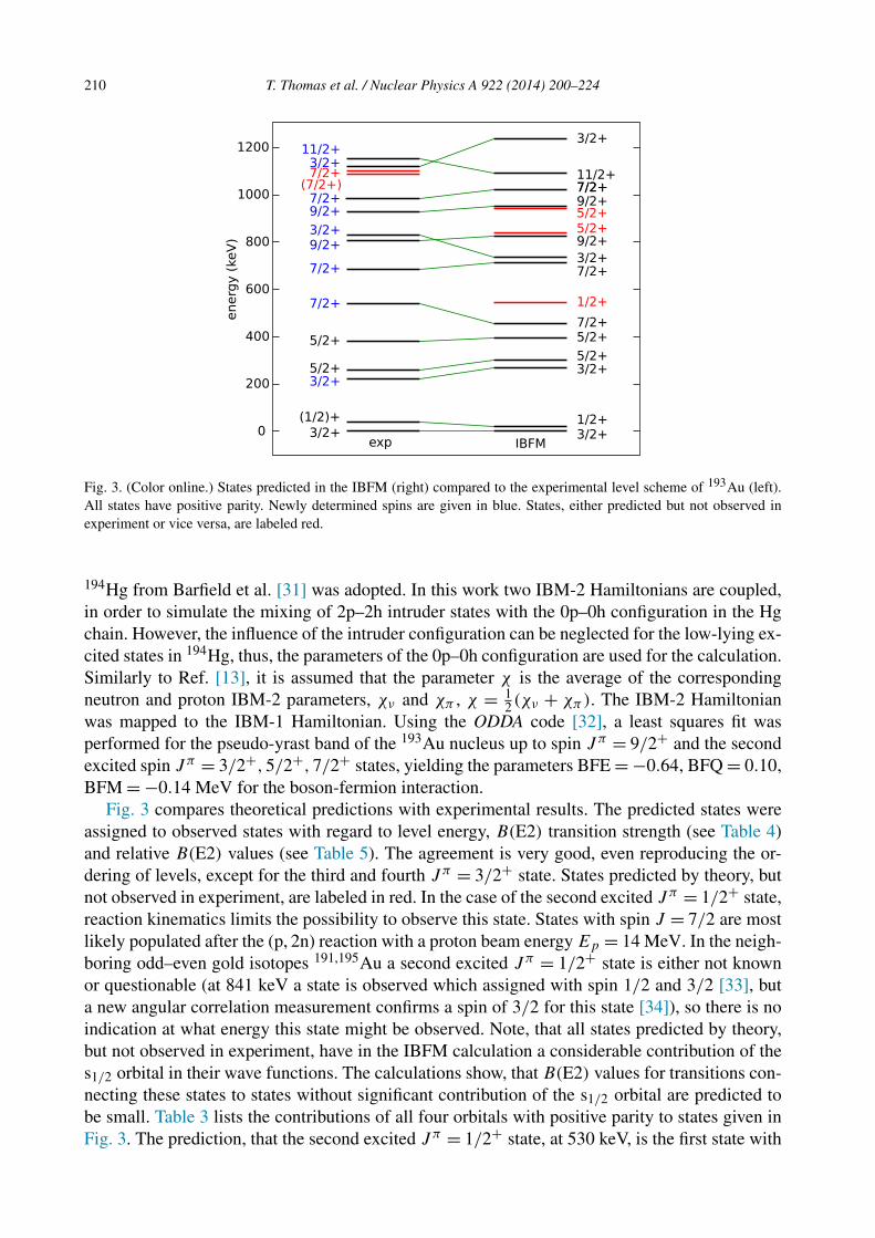
Fig. 3. (Color online.) States predicted in the IBFM (right) compared to the experimental level scheme of 193Au (left).All states have positive parity. Newly determined spins are given in blue. States, either predicted but not observed inexperiment or vice versa, are labeled red.
194Hg from Barfield et al. [31] was adopted. In this work two IBM-2 Hamiltonians are coupled,in order to simulate the mixing of 2p–2h intruder states with the 0p–0h configuration in the Hgchain. However, the influence of the intruder configuration can be neglected for the low-lying ex-cited states in 194Hg, thus, the parameters of the 0p–0h configuration are used for the calculation.Similarly to Ref. [13], it is assumed that the parameter χ is the average of the correspondingneutron and proton IBM-2 parameters, χν and χπ , χ = 1
2 (χν + χπ). The IBM-2 Hamiltonianwas mapped to the IBM-1 Hamiltonian. Using the ODDA code [32], a least squares fit wasperformed for the pseudo-yrast band of the 193Au nucleus up to spin Jπ = 9/2+ and the secondexcited spin Jπ = 3/2+,5/2+,7/2+ states, yielding the parameters BFE = −0.64, BFQ = 0.10,BFM = −0.14 MeV for the boson-fermion interaction.
Fig. 3 compares theoretical predictions with experimental results. The predicted states wereassigned to observed states with regard to level energy, B(E2) transition strength (see Table 4)and relative B(E2) values (see Table 5). The agreement is very good, even reproducing the or-dering of levels, except for the third and fourth Jπ = 3/2+ state. States predicted by theory, butnot observed in experiment, are labeled in red. In the case of the second excited Jπ = 1/2+ state,reaction kinematics limits the possibility to observe this state. States with spin J = 7/2 are mostlikely populated after the (p, 2n) reaction with a proton beam energy Ep = 14 MeV. In the neigh-boring odd–even gold isotopes 191,195Au a second excited Jπ = 1/2+ state is either not knownor questionable (at 841 keV a state is observed which assigned with spin 1/2 and 3/2 [33], buta new angular correlation measurement confirms a spin of 3/2 for this state [34]), so there is noindication at what energy this state might be observed. Note, that all states predicted by theory,but not observed in experiment, have in the IBFM calculation a considerable contribution of thes1/2 orbital in their wave functions. The calculations show, that B(E2) values for transitions con-necting these states to states without significant contribution of the s1/2 orbital are predicted tobe small. Table 3 lists the contributions of all four orbitals with positive parity to states given inFig. 3. The prediction, that the second excited Jπ = 1/2+ state, at 530 keV, is the first state with
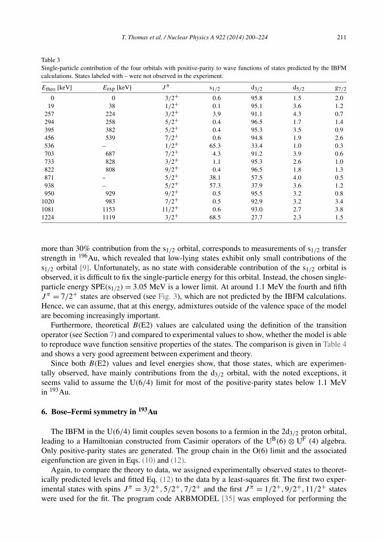
T. Thomas et al. / Nuclear Physics A 922 (2014) 200–224 211
Table 3
Single-particle contribution of the four orbitals with positive-parity to wave functions of states predicted by the IBFM
calculations. States labeled with – were not observed in the experiment.
Etheo [keV] Eexp [keV] Jπ s1/2 d3/2 d5/2 g7/2
0 0 3/2+ 0.6 95.8 1.5 2.0
19 38 1/2+ 0.1 95.1 3.6 1.2
257 224 3/2+ 3.9 91.1 4.3 0.7
294 258 5/2+ 0.4 96.5 1.7 1.4
395 382 5/2+ 0.4 95.3 3.5 0.9
456 539 7/2+ 0.6 94.8 1.9 2.6
536 – 1/2+ 65.3 33.4 1.0 0.3
703 687 7/2+ 4.3 91.2 3.9 0.6
733 828 3/2+ 1.1 95.3 2.6 1.0
822 808 9/2+ 0.4 96.5 1.8 1.3
871 – 5/2+ 38.1 57.5 4.0 0.5
938 – 5/2+ 57.3 37.9 3.6 1.2
950 929 9/2+ 0.5 95.5 3.2 0.8
1020 983 7/2+ 0.5 92.9 3.2 3.4
1081 1153 11/2+ 0.6 93.0 2.7 3.8
1224 1119 3/2+ 68.5 27.7 2.3 1.5
more than 30% contribution from the s1/2 orbital, corresponds to measurements of s1/2 transfer
strength in 196Au, which revealed that low-lying states exhibit only small contributions of the
s1/2 orbital [9]. Unfortunately, as no state with considerable contribution of the s1/2 orbital is
observed, it is difficult to fix the single-particle energy for this orbital. Instead, the chosen single-
particle energy SPE(s1/2) = 3.05 MeV is a lower limit. At around 1.1 MeV the fourth and fifth
J π = 7/2+ states are observed (see Fig. 3), which are not predicted by the IBFM calculations.
Hence, we can assume, that at this energy, admixtures outside of the valence space of the model
are becoming increasingly important.
Furthermore, theoretical B(E2) values are calculated using the definition of the transition
operator (see Section 7) and compared to experimental values to show, whether the model is able
to reproduce wave function sensitive properties of the states. The comparison is given in Table 4
and shows a very good agreement between experiment and theory.
Since both B(E2) values and level energies show, that those states, which are experimen-
tally observed, have mainly contributions from the d3/2 orbital, with the noted exceptions, it
seems valid to assume the U(6/4) limit for most of the positive-parity states below 1.1 MeV
in 193Au.
6. Bose–Fermi symmetry in 193Au
The IBFM in the U(6/4) limit couples seven bosons to a fermion in the 2d3/2 proton orbital,
leading to a Hamiltonian constructed from Casimir operators of the UB(6) ⊗ UF (4) algebra.
Only positive-parity states are generated. The group chain in the O(6) limit and the associated
eigenfunction are given in Eqs. (10) and (12).
Again, to compare the theory to data, we assigned experimentally observed states to theoret-
ically predicted levels and fitted Eq. (12) to the data by a least-squares fit. The first two exper-
imental states with spins J π = 3/2+,5/2+,7/2+ and the first J π = 1/2+,9/2+,11/2+ states
were used for the fit. The program code ARBMODEL [35] was employed for performing the
212 T. Thomas et al. / Nuclear Physics A 922 (2014) 200–224
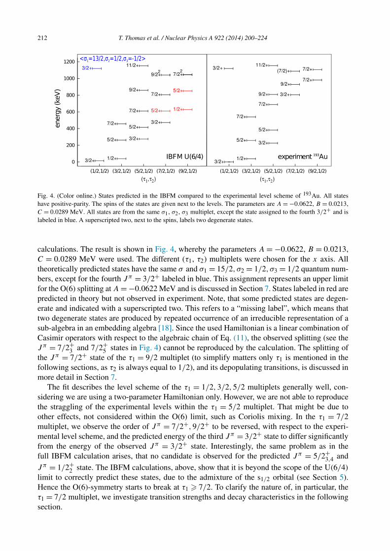
Fig. 4. (Color online.) States predicted in the IBFM compared to the experimental level scheme of 193Au. All stateshave positive-parity. The spins of the states are given next to the levels. The parameters are A = −0.0622, B = 0.0213,C = 0.0289 MeV. All states are from the same σ1, σ2, σ3 multiplet, except the state assigned to the fourth 3/2+ and islabeled in blue. A superscripted two, next to the spins, labels two degenerate states.
calculations. The result is shown in Fig. 4, whereby the parameters A = −0.0622, B = 0.0213,C = 0.0289 MeV were used. The different (τ1, τ2) multiplets were chosen for the x axis. Alltheoretically predicted states have the same σ and σ1 = 15/2, σ2 = 1/2, σ3 = 1/2 quantum num-bers, except for the fourth Jπ = 3/2+ labeled in blue. This assignment represents an upper limitfor the O(6) splitting at A = −0.0622 MeV and is discussed in Section 7. States labeled in red arepredicted in theory but not observed in experiment. Note, that some predicted states are degen-erate and indicated with a superscripted two. This refers to a “missing label”, which means thattwo degenerate states are produced by repeated occurrence of an irreducible representation of asub-algebra in an embedding algebra [18]. Since the used Hamiltonian is a linear combination ofCasimir operators with respect to the algebraic chain of Eq. (11), the observed splitting (see theJπ = 7/2+
3 and 7/2+5 states in Fig. 4) cannot be reproduced by the calculation. The splitting of
the Jπ = 7/2+ state of the τ1 = 9/2 multiplet (to simplify matters only τ1 is mentioned in thefollowing sections, as τ2 is always equal to 1/2), and its depopulating transitions, is discussed inmore detail in Section 7.
The fit describes the level scheme of the τ1 = 1/2,3/2,5/2 multiplets generally well, con-sidering we are using a two-parameter Hamiltonian only. However, we are not able to reproducethe straggling of the experimental levels within the τ1 = 5/2 multiplet. That might be due toother effects, not considered within the O(6) limit, such as Coriolis mixing. In the τ1 = 7/2multiplet, we observe the order of Jπ = 7/2+,9/2+ to be reversed, with respect to the experi-mental level scheme, and the predicted energy of the third Jπ = 3/2+ state to differ significantlyfrom the energy of the observed Jπ = 3/2+ state. Interestingly, the same problem as in thefull IBFM calculation arises, that no candidate is observed for the predicted Jπ = 5/2+
3,4 and
Jπ = 1/2+2 state. The IBFM calculations, above, show that it is beyond the scope of the U(6/4)
limit to correctly predict these states, due to the admixture of the s1/2 orbital (see Section 5).Hence the O(6)-symmetry starts to break at τ1 � 7/2. To clarify the nature of, in particular, theτ1 = 7/2 multiplet, we investigate transition strengths and decay characteristics in the followingsection.
T. Thomas et al. / Nuclear Physics A 922 (2014) 200–224 213
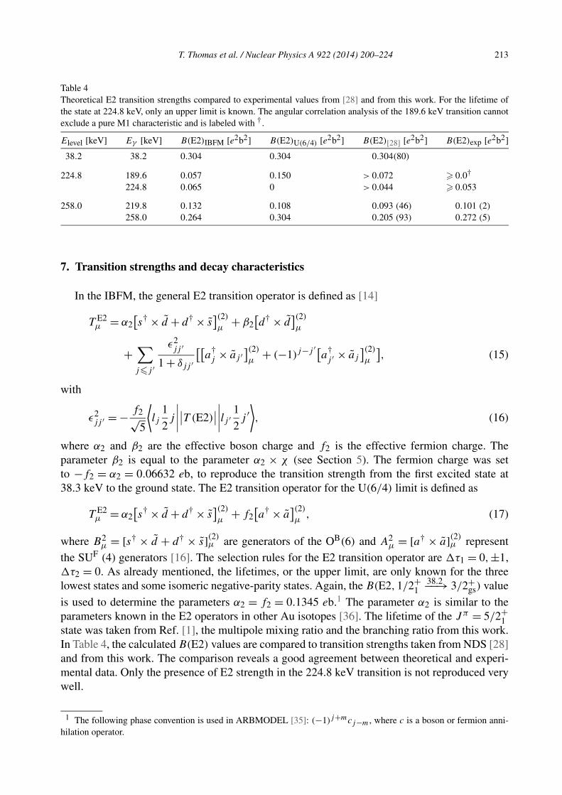
Table 4
Theoretical E2 transition strengths compared to experimental values from [28] and from this work. For the lifetime of
the state at 224.8 keV, only an upper limit is known. The angular correlation analysis of the 189.6 keV transition cannot
exclude a pure M1 characteristic and is labeled with †.
Elevel [keV] Eγ [keV] B(E2)IBFM [e2b2] B(E2)U(6/4) [e2b2] B(E2)[28] [e2b2] B(E2)exp [e2b2]38.2 38.2 0.304 0.304 0.304(80)
224.8 189.6 0.057 0.150 > 0.072 � 0.0†
224.8 0.065 0 > 0.044 � 0.053
258.0 219.8 0.132 0.108 0.093 (46) 0.101 (2)
258.0 0.264 0.304 0.205 (93) 0.272 (5)
7. Transition strengths and decay characteristics
In the IBFM, the general E2 transition operator is defined as [14]
T E2μ = α2
[
s† × d + d† × s](2)
μ+ β2
[
d† × d](2)
μ
+∑
j�j ′
ǫ2jj ′
1 + δjj ′
[[
a†j × aj ′
](2)
μ+ (−1)j−j ′[
a†j ′ × aj
](2)
μ
]
, (15)
with
ǫ2jj ′ = − f2√
5
⟨
lj1
2j
∣
∣
∣
∣
∣
∣T (E2)∣
∣
∣
∣
∣
∣
lj ′1
2j ′
⟩
, (16)
where α2 and β2 are the effective boson charge and f2 is the effective fermion charge. The
parameter β2 is equal to the parameter α2 × χ (see Section 5). The fermion charge was set
to −f2 = α2 = 0.06632 eb, to reproduce the transition strength from the first excited state at
38.3 keV to the ground state. The E2 transition operator for the U(6/4) limit is defined as
T E2μ = α2
[
s† × d + d† × s](2)
μ+ f2
[
a† × a](2)
μ, (17)
where B2μ = [s† × d + d† × s](2)
μ are generators of the OB(6) and A2μ = [a† × a](2)
μ represent
the SUF (4) generators [16]. The selection rules for the E2 transition operator are �τ1 = 0,±1,
�τ2 = 0. As already mentioned, the lifetimes, or the upper limit, are only known for the three
lowest states and some isomeric negative-parity states. Again, the B(E2,1/2+1
38.2−−→ 3/2+gs) value
is used to determine the parameters α2 = f2 = 0.1345 eb.1 The parameter α2 is similar to the
parameters known in the E2 operators in other Au isotopes [36]. The lifetime of the J π = 5/2+1
state was taken from Ref. [1], the multipole mixing ratio and the branching ratio from this work.
In Table 4, the calculated B(E2) values are compared to transition strengths taken from NDS [28]
and from this work. The comparison reveals a good agreement between theoretical and experi-
mental data. Only the presence of E2 strength in the 224.8 keV transition is not reproduced very
well.
1 The following phase convention is used in ARBMODEL [35]: (−1)j+mcj−m , where c is a boson or fermion anni-
hilation operator.
214 T. Thomas et al. / Nuclear Physics A 922 (2014) 200–224
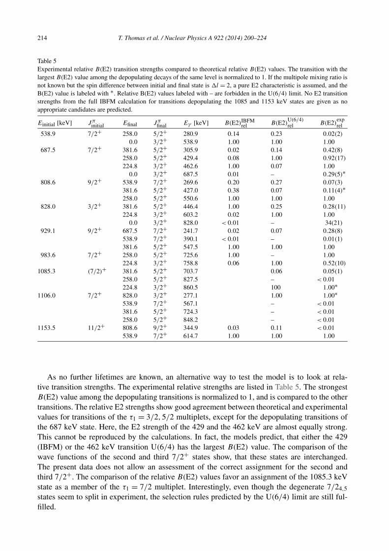
Table 5
Experimental relative B(E2) transition strengths compared to theoretical relative B(E2) values. The transition with the
largest B(E2) value among the depopulating decays of the same level is normalized to 1. If the multipole mixing ratio is
not known but the spin difference between initial and final state is �l = 2, a pure E2 characteristic is assumed, and the
B(E2) value is labeled with ∗. Relative B(E2) values labeled with – are forbidden in the U(6/4) limit. No E2 transition
strengths from the full IBFM calculation for transitions depopulating the 1085 and 1153 keV states are given as no
appropriate candidates are predicted.
Einitial [keV] Jπinitial Efinal Jπ
final Eγ [keV] B(E2)IBFMrel B(E2)
U(6/4)rel B(E2)
exprel
538.9 7/2+ 258.0 5/2+ 280.9 0.14 0.23 0.02(2)
0.0 3/2+ 538.9 1.00 1.00 1.00
687.5 7/2+ 381.6 5/2+ 305.9 0.02 0.14 0.42(8)
258.0 5/2+ 429.4 0.08 1.00 0.92(17)
224.8 3/2+ 462.6 1.00 0.07 1.00
0.0 3/2+ 687.5 0.01 – 0.29(5)∗
808.6 9/2+ 538.9 7/2+ 269.6 0.20 0.27 0.07(3)
381.6 5/2+ 427.0 0.38 0.07 0.11(4)∗
258.0 5/2+ 550.6 1.00 1.00 1.00
828.0 3/2+ 381.6 5/2+ 446.4 1.00 0.25 0.28(11)
224.8 3/2+ 603.2 0.02 1.00 1.00
0.0 3/2+ 828.0 < 0.01 – 34(21)
929.1 9/2+ 687.5 7/2+ 241.7 0.02 0.07 0.28(8)
538.9 7/2+ 390.1 < 0.01 – 0.01(1)
381.6 5/2+ 547.5 1.00 1.00 1.00
983.6 7/2+ 258.0 5/2+ 725.6 1.00 – 1.00
224.8 3/2+ 758.8 0.06 1.00 0.52(10)
1085.3 (7/2)+ 381.6 5/2+ 703.7 0.06 0.05(1)
258.0 5/2+ 827.5 – < 0.01
224.8 3/2+ 860.5 100 1.00∗
1106.0 7/2+ 828.0 3/2+ 277.1 1.00 1.00∗
538.9 7/2+ 567.1 – < 0.01
381.6 5/2+ 724.3 – < 0.01
258.0 5/2+ 848.2 – < 0.01
1153.5 11/2+ 808.6 9/2+ 344.9 0.03 0.11 < 0.01
538.9 7/2+ 614.7 1.00 1.00 1.00
As no further lifetimes are known, an alternative way to test the model is to look at rela-
tive transition strengths. The experimental relative strengths are listed in Table 5. The strongest
B(E2) value among the depopulating transitions is normalized to 1, and is compared to the other
transitions. The relative E2 strengths show good agreement between theoretical and experimental
values for transitions of the τ1 = 3/2,5/2 multiplets, except for the depopulating transitions of
the 687 keV state. Here, the E2 strength of the 429 and the 462 keV are almost equally strong.
This cannot be reproduced by the calculations. In fact, the models predict, that either the 429
(IBFM) or the 462 keV transition U(6/4) has the largest B(E2) value. The comparison of the
wave functions of the second and third 7/2+ states show, that these states are interchanged.
The present data does not allow an assessment of the correct assignment for the second and
third 7/2+. The comparison of the relative B(E2) values favor an assignment of the 1085.3 keV
state as a member of the τ1 = 7/2 multiplet. Interestingly, even though the degenerate 7/24,5
states seem to split in experiment, the selection rules predicted by the U(6/4) limit are still ful-
filled.

T. Thomas et al. / Nuclear Physics A 922 (2014) 200–224 215
Table 6
Comparison of measured multipole mixing ratios from this work with calculated values derived from the IBFM in U(6/4)
limit.
Elevel [keV] Eγ [keV] δtheo δexp
258.0 258.0 −0.80 −0.75 (11)
538.9 280.9 −0.22 −0.06 (3)
687.5 305.9 +0.35 +0.44+22−19
429.4 −1.28 −0.19+2−3
808.6 269.6 −0.44 −0.13 (7)
828.0 446.4 +0.15 −0.30 (7)
603.2 +0.47 +0.50+36−28
929.1 241.7 −2.74 −0.12 (5)
1153.5 344.9 −0.19 −0.02 (5)
B(M1) values can also be used to test the model. Again, as no experimental absolute values
are available, relative M1 transition strengths might be used. The definition of the M1 operator
is as follows [16]:
T M1μ = β1
[
d† × d](1)
μ+ t1√
2
[
a†32
× a 32
](1)
μ, (18)
where the parameters t1 = 0.09μN and β1 = 0.662μN were obtained by fitting Eq. (18) to the
magnetic moment of the ground state [37] (μ( 32
+) = 0.1396 (5)μN ) and the known M1 fraction
of the transition of the J π = 52
+1
state to the ground state (B(M1) = 0.021(16)μ2N , lifetime
adopted from [1]).2 Both parameters are similar to those given in IBFM calculations for nuclei
in this region [16]. Unfortunately, we did not observe sufficient depopulating M1 transitions of
the same state to compare among each other, so no conclusions can be drawn. Again, lifetimes
are needed to test the predicted M1 transition strengths of the IBFM.
However, with the definition of the M1 operator, the multipole mixing ratio δ can be tested
with the following equation [38]:
δ = 0.835 × Eγ (MeV)〈If ||T (E2)||Ii〉〈If ||T (M1)||Ii〉
. (19)
In Table 6, the theoretical multipole mixing ratios of allowed transitions are compared to our
data. Generally, the calculated multipole mixing ratios, and thus, the E2 strength, of a transition
are always predicted to be larger than observed in experiment. One major reason might be the
overestimation of the effective boson charge. It was chosen to reproduce the B(E2) value of the
transition 1/2+1
38.2−−→ 3/2+gs. The uncertainty for this B(E2) value allows a significantly lower
effective boson charge thereby allowing the multipole mixing ratios to decrease. Note, that a
different boson charge will not change the calculated relative B(E2) values in Table 5. Overall,
except for the 429 and 241 keV transitions, reasonably good agreement with the experimental
values is achieved.
2 The calculation of B(M1) values using the IBFM with all five orbitals is omitted, as the operator depends on effective
single-particle g-factors for all five orbitals. All together, this would lead to eleven parameters, which would have to be
adjusted.

216 T. Thomas et al. / Nuclear Physics A 922 (2014) 200–224
Fig. 5. (Color online.) States predicted by the IBFM with the parameters obtained from the fit to the data of 193Auand compared to the level scheme of 192Pt. Only with states of positive parity were considered. The parameters areA = −0.0432, B = 0.0213, C = 0.0289 MeV. All states are from the same σ multiplet, except the state assigned to thethird 0+ and is labeled in blue. States either predicted but not observed in experiment or vice versa are labeled red.
8. The supersymmetric partner 192Pt
We can now use the properties of the IBFM Hamiltonian in the U(6/4) limit to describe theneighboring 192Pt nucleus, that is eight bosons away from shell closures at N = 126 and Z = 82.According to the supersymmetry between bosons and fermions (see Eq. (13)), the fermion istransformed into a boson, but the system is still described by the same set of parameters. In fact,the Hamiltonian is the one of the O(6) limit [39] with the eigenfunction of Eq. (14). Only param-eter D of the SOB(6) group has to be fitted to the Pt data, since the parameter A is composedof A = D + A. In the previous fit to the nucleus 193Au, parameter D was chosen in such a waythat only levels with quantum number σ = 7 are relevant for the fit. For the assignment of the-oretical predicted states to the experimentally observed states, IBM calculations performed inRef. [39] on 196Pt were used. Consistent with Ref. [39], the third 0+ state in 192Pt was assignedto the σ = 6 (σ = Nmax − 2) multiplet, determining the parameter A = −0.0432 MeV. Fig. 5shows the comparison of the experimental and theoretical level scheme. Experimental data of192Pt was taken from Refs. [40–43]. Fig. 5 reveals that the observed states are not reproducedvery well; especially the Jπ = 0+
2 state predicted at 383 keV has not been observed. As thenucleus 192Pt was studied with (p,t) reactions [41,43] and no 0+ state was observed between500 and 1000 keV, it is questionable, whether the predicted state exists. Furthermore, no exper-imental state is assigned to the τ = 5 multiplets, as they do not agree with the expected decaycharacteristics.
To achieve a better fit, states of both nuclei, 192Pt and 193Au, were used. For the fit, in additionto the states in 193Au (see Section 6), the yrast band up to the 4+ and the 0+
2,3, 2+2 , 4+
2 states in192Pt were considered. The comparison of the theoretical level scheme using the new parame-ters A = −0.0432 MeV, B = 0.0403 MeV, C = 0.0173 MeV is presented in Fig. 6. The newparameters have values similar to the parameters in Refs. [36,39]. The 0+
2 state is now predictedat 725 keV and fits better to the observed second 0+ state. The remaining difference in energy
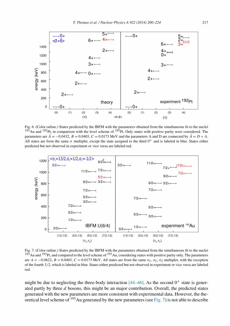
T. Thomas et al. / Nuclear Physics A 922 (2014) 200–224 217
Fig. 6. (Color online.) States predicted by the IBFM with the parameters obtained from the simultaneous fit to the nuclei193Au and 192Pt, in comparison with the level scheme of 192Pt. Only states with positive parity were considered. Theparameters are A = −0.0432, B = 0.0403, C = 0.0173 MeV and the parameters A and D are connected by A = D + A.All states are from the same σ multiplet, except the state assigned to the third 0+ and is labeled in blue. States eitherpredicted but not observed in experiment or vice versa are labeled red.
Fig. 7. (Color online.) States predicted by the IBFM with the parameters obtained from the simultaneous fit to the nuclei193Au and 192Pt, and compared to the level scheme of 193Au, considering states with positive parity only. The parametersare A = −0.0622, B = 0.0403, C = 0.0173 MeV. All states are from the same σ1, σ2, σ3 multiplet, with the exceptionof the fourth 3/2, which is labeled in blue. States either predicted but not observed in experiment or vice versa are labeledred.
might be due to neglecting the three-body interaction [44–46]. As the second 0+ state is gener-ated partly by three d bosons, this might be an major contribution. Overall, the predicted statesgenerated with the new parameters are more consistent with experimental data. However, the the-oretical level scheme of 193Au generated by the new parameters (see Fig. 7) is not able to describe
218 T. Thomas et al. / Nuclear Physics A 922 (2014) 200–224
the ordering of observed states in the τ1 = 3/2,5/2 multiplet as well as the old parameters, but
decay characteristics and transitions strength are still reproduced. Hence, a supersymmetric de-
scription of the transition strengths and decay probabilities of the low-lying excited states in 192Pt
and 193Au is possible. In contrast, the 3/2+ and 7/2+ state of the τ1 = 7/2 multiplet now show a
better agreement with experimental data. The difference between the two set of parameters seems
to result from varying strengths of the O(5) parameter, as this generates the τ splitting. In 193Au,
the first J π = 1/2+ of the τ1 = 3/2 multiplet is low in energy with respect to the ground state;
thus, the τ splitting is small in order to generate the first excited state, whereby one fermion has
to couple with one d boson by annihilating one s boson. In contrast to this, the first excited state
in 192Pt and especially the second 0+ state, which is a member of the τ = 3 multiplet, is predicted
too low. Thus, a larger τ splitting is needed in 192Pt. In order to incorporate this difference in
energy, a three-body interaction or a U(5) term has to be introduced, thereby breaking the O(6)
symmetry.
9. Conclusion
A wealth of new data is presented in this work. 49 states were investigated, 15 of them pre-
viously unknown. Using γ γ coincidence spectra, more than 120 γ transitions, assigned to the
nucleus 193Au, were investigated regarding their multipolarities and branching ratios. This en-
abled us to determine the spins of several states.
The comparison of a general IBFM calculation to the new data allows a better under-
standing of the limit of the Bose–Fermi symmetry. While states, which are member of the
τ = 1/2,3/2,5/2 multiplet, show good agreement with data, some states predicted by both
theories are not observed in experiment. The general IBFM calculation suggests a significant
admixture from the 3s1/2 orbital to the wave functions of these states; thus, it cannot be expected
to be reproduced by a simple IBFM calculation in the U(6/4) limit. Still, while the degeneracy
of the fourth and fifth J π = 7/2+ state, a member of the τ = 9/2 multiplet, is not valid anymore,
the decay characteristics seem to be preserved. The experimentally determined E2 transition
strengths of the depopulating transitions of the three lowest excited levels can be reproduced by
both calculations. Furthermore, relative E2 transition strengths were compared and show good
agreement for transitions between states in the lower energy region. Some transitions depopu-
lating higher excited states are forbidden in the U(6/4) limit, which should be reflected by low
absolute transition strengths. In order to test the accuracy of these predictions, lifetimes for higher
excited states are needed.
Within the framework of the supersymmetric U(6/4) limit, the level scheme of 192Pt was pre-
dicted, using parameters obtained from a fit to the nucleus 193Au. A poor agreement is reached
for most of the levels up to an excitation energy of 1600 keV. Therefore, a new set of parameters
was obtained using the level schemes of both nuclei. This way, even though the agreement of
separate IBFM fits to 193Au and 192Pt is not achieved, we successfully reproduce the experimen-
tal level scheme. We conclude, that we are able to establish a dynamical supersymmetry with
only three parameters for 193Au and 192Pt.
Acknowledgements
We thank our coworkers and the Tandem accelerator staff at the IKP Köln for their help during
the experiment. We thank F. Iachello, M. Elvers and V. Werner for fruitful discussions concerning
this work.

T. Thomas et al. / Nuclear Physics A 922 (2014) 200–224 219
Appendix A. γ γ coincidence spectra and angular correlation analysis
Fig. A.1. (Color online.) Different spin hypotheses are tested for the (550, 668) cascade. The corresponding multipolemixing ratios are δ9/2,668 = +0.282(167), δ11/2,668 = +0.465(76) and δ13/2,668 = +0.016(88). The spin of this statecould not be determined unambiguously.
Fig. A.2. (Color online.) The fits for the spin hypotheses 9/2 347−−→ 7/23725−−→ 5/21 and 7/2 347−−→ 7/23
725−−→ 5/21 arecompared. The correlation groups 11, 13, 16 were removed due to low statistics. Clearly, a spin of 9/2 is favored for thestate at 1379 keV. The corresponding multipole mixing ratio is δ347 = −0.445(238).
Fig. A.3. (Color online.) The fit for the spin hypothesis 9/2 347−−→ 7/23758−−→ 3/22 is shown. The correlation groups 13,
14, 16 were removed, due to low statistics. The corresponding multipole mixing ratio is δ758 = +0.02(21).

220 T. Thomas et al. / Nuclear Physics A 922 (2014) 200–224
Fig. A.4. (Color online.) From angular correlation analysis of the (692,462) cascade the multipole mixing ratio of the 462keV transition is determined to either exhibit a pure E2 characteristic, if the spin is J2 = 3/2, or if the spin is J2 = 5/2,the multipole mixing ratio is determined to be δ462 = +0.21(20) or δ462 = +12.0+8
−3. The fits for the spin hypotheses
7/22462−−→ 3/2 186−−→ 1/21 and 7/22
462−−→ 5/2 186−−→ 1/21 with the two possible δ186 are compared. Clearly, the spinJ2 = 3/2 is favored and the corresponding multipole mixing ratio of the depopulating transition is δ186 = +0.11(15).
Fig. A.5. (Color online.) The fits for the spin hypotheses 3/2 446−−→ 5/22381−−→ 3/21 and 1/2 446−−→ 5/22
381−−→ 3/21 arecompared. For the 381 keV transition, the already measured multipole mixing ratio δ462 = −2.93 from angular correla-tion analysis of the (547,381) cascade (see also the discussion in 4 was used. The corresponding multipole mixing ratiofor the 446 keV transition is δ186 = −0.30(7).
Fig. A.6. (Color online.) The spin hypotheses for 3/2 861−−→ 5/21258−−→ 3/21, 1/2 861−−→ 5/21
258−−→ 3/21 and 5/2 861−−→5/21
258−−→ 3/21 is shown. For the 258 keV transition, the multipole mixing ratio δ258 = −0.75(11) was used. The fitsshow that the spin 3/2 is clearly favored, but two multipole mixing ratios are possible (For the sake of clarity, only thespin hypothesis with δ861 = −1.33(40) is shown). In Section 4 the state at 1119 keV with the depopulating 861 keVtransition is discussed in more detail.

T. Thomas et al. / Nuclear Physics A 922 (2014) 200–224 221
Fig. A.7. The top figure shows (a) γ γ coincidence spectrum energy gated on the 547.5 keV transition from Jπ = 9/2+2
state at 929.1 keV to the Jπ = 5/2+2 state at 381.6 keV. Two new transitions with the energy 726.3 keV depopulating
the state at 1655.4 keV and the energy 746.2 keV depopulating the state at 1675.3 keV are observed in the spectrum.
The middle figure (b) shows a γ γ coincidence spectrum, energy gated on the newly observed 726.3 keV transition to the
Jπ = 9/2+2 state at 929.1 keV. Coincident transitions at 381.6, 429.4, 547.5 keV are observed. The 381.6 keV peak is
comparatively larger due to the coincidence with another transition at 724.3 keV. The 434.4 keV transition is observed
due to the coincidence with a 725.6 transition. The negative peaks in the spectrum yield from background subtraction.
A γ γ coincidence spectrum, energy gated on the new 746.2 keV transition to the Jπ = 9/2+2 state at 929.1 keV, is
shown in the bottom figure (c). Coincident transitions at 381.6, 429.4, 547.5 keV are observed. The 381.6 keV peak is
comparatively larger due to the coincidence with another transition at 724.3 keV. The 434.4 keV transition is observed
due to the coincidence with a 725.6 keV transition.
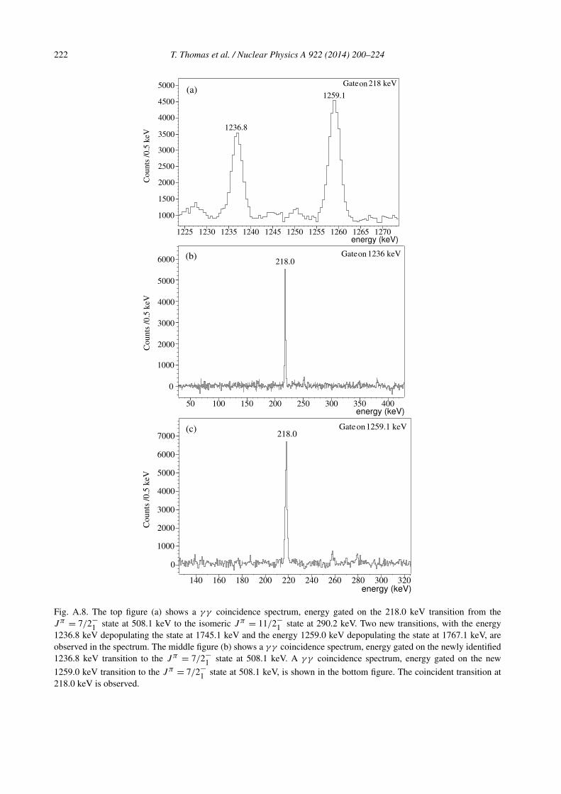
222 T. Thomas et al. / Nuclear Physics A 922 (2014) 200–224
Fig. A.8. The top figure (a) shows a γ γ coincidence spectrum, energy gated on the 218.0 keV transition from the
Jπ = 7/2−1 state at 508.1 keV to the isomeric Jπ = 11/2−
1 state at 290.2 keV. Two new transitions, with the energy
1236.8 keV depopulating the state at 1745.1 keV and the energy 1259.0 keV depopulating the state at 1767.1 keV, are
observed in the spectrum. The middle figure (b) shows a γ γ coincidence spectrum, energy gated on the newly identified
1236.8 keV transition to the Jπ = 7/2−1 state at 508.1 keV. A γ γ coincidence spectrum, energy gated on the new
1259.0 keV transition to the Jπ = 7/2−1 state at 508.1 keV, is shown in the bottom figure. The coincident transition at
218.0 keV is observed.

T. Thomas et al. / Nuclear Physics A 922 (2014) 200–224 223
Table A.1
Additional transitions Eγ observed in coincidence with a gated γ transition Egate,γ .
New transitions are labeled with ❇.
Egate,γ [keV] Eγ [keV] Egate,γ [keV] Eγ [keV]
407 1097.3(3) 429 1212.0(5)❇
1171.5(3) 499 1115.6(3)❇
1178.7(3) 573 913.1(3)
1232.4(4) 989.7(3)❇
1241.6(3) 1052.5(3)
1314.5(3) 1174.1(3)
1325.9(3) 1352.2(3)
1339.7(3) 581 809.4(3)❇
1365.4(3) 675 422.2(3)
1442.2(3) 545.1(3)
1460.0(3) 721 528.2(4)
1505.0(4)
1557.2(4)
References
[1] B. Fogelberg, A. Baecklin, V. Berg, S.G. Malmskog, Nucl. Phys. A 153 (1970) 301.
[2] Y. Gono, R.M. Lieder, M. Müller-Veggian, A. Neskas, C. Mayer-Böricke, Nucl. Phys. A 327 (1979) 269.
[3] C.L.M. Vieu, PhD thesis, CSNSM-T-74-01, Orsay, 1974, unpublished.
[4] F. Iachello, Phys. Rev. Lett. 44 (1980) 772.
[5] J.L. Wood, Phys. Rev. C 24 (1981) 1788.
[6] P. Van Isacker, J. Jolie, K. Heyde, A. Frank, Phys. Rev. Lett. 54 (1985) 653.
[7] A. Metz, J. Jolie, G. Graw, R. Hertenberger, J. Gröger, C. Günther, N. Warr, Y. Eisermann, Phys. Rev. Lett. 83
(1999) 1542.
[8] J. Gröger, et al., Phys. Rev. C 62 (2000) 064304.
[9] H.-F. Wirth, et al., Phys. Rev. C 70 (2004) 014610.
[10] C. Bernards, S. Heinze, J. Jolie, C. Fransen, A. Linnemann, D. Radeck, Phys. Rev. C 79 (2009) 054307.
[11] C. Bernards, S. Heinze, J. Jolie, M. Albers, C. Fransen, D. Radeck, Phys. Rev. C 81 (2010) 024312.
[12] F. Iachello, O. Scholten, Phys. Rev. Lett. 43 (1979) 679.
[13] R. Bijker, L.E.A. Dieperink, Nucl. Phys. A 379 (1982) 221.
[14] O. Scholten, PhD thesis, University of Groningen, 1980, https://www.kvi.nl/~scholten/other/OlafsPhD-Thesis.pdf.
[15] A. de Shalit, I. Talmi, Nuclear Shell Theory, Academic Press, New York, USA, 1963.
[16] F. Iachello, P. Van Isacker, The Interacting Boson Fermion Model, Cambridge University Press, Cambridge, Eng-
land, 1991.
[17] F. Iachello, S. Kuyucak, Ann. Phys. 136 (1981) 19.
[18] A. Frank, J. Jolie, P. Van Isacker, Symmetries in Atomic Nuclei – From Isospin to Supersymmetry, Springer, New
York, USA, 2009.
[19] F. Pühlhofer, Nucl. Phys. A 280 (1977) 267.
[20] A. Linnemann, Ph.D. thesis, University of Cologne, 2005, http://kups.ub.uni-koeln.de/1747/.
[21] K.S. Krane, R.M. Steffen, Phys. Rev. C 2 (1970) 724.
[22] K.S. Krane, R.M. Steffen, R.M. Wheeler, At. Data Nucl. Data Tables 11 (1973) 351.
[23] I. Wiedenhöver, code CORLEONE, University of Cologne, 1995, unpublished.
[24] V. Kölschbach, P. Schüler, K. Hardt, D. Rosendaal, C. Günther, K. Euler, R. Tölle, M. Marten-Tölle, P. Zeyen, Nucl.
Phys. A 439 (1985) 189–206.
[25] P.O. Tjom, M.R. Maier, D. Benson Jr, F.S. Stephens, R.M. Diamond, Nucl. Phys. A 231 (1974) 397–410.
[26] Y. Oktem, et al., Nucl. Phys. A 231 (1974) 397–410.
[27] V.K. Fischer, Phys. Rev. 99 (1955) 764.
[28] E. Achterberg, G.V. Marti, V.R. Vanin, et al., Nucl. Data Sheets 107 (2006) 1.
[29] J. Bardeen, N.L. Cooper, R.J. Schrieffer, Phys. Rev. C 108 (1957) 1175.
[30] L.S. Kisslinger, R.A. Sorensen, Rev. Mod. Phys. 35 (1963) 853.

224 T. Thomas et al. / Nuclear Physics A 922 (2014) 200–224
[31] F.A. Barfield, R.B. Barrett, A.K. Sage, D.P. Duval, Z. Phys. A 311 (1983) 205.
[32] O. Scholten, 252 Computer Code ODDA, K.V.I. Internal Report, University of Groningen, 1980.
[33] Zhou Chunmei, Nucl. Data Sheets 86 (1998) 645.
[34] T. Thomas, private communication.
[35] S. Heinze, Ph.D. thesis, University of Cologne, 2008, http://kups.ub.uni-koeln.de/2357/.
[36] A. Frank, P. Van Isacker, Algebraic Methods in Molecular and Nuclear Structure Physics, Wiley-Interscience, New
York, USA, 1994.
[37] G. Passler, J. Rikovska, E. Arnold, H.-J. Kluge, L. Monz, R. Neugart, H. Ravn, K. Wend, Nucl. Phys. A 580 (1994)
173–212.
[38] K.S. Krane, Phys. Rev. C 8 (1973) 1494.
[39] A. Arima, F. Iachello, The Interacting Boson Model, Cambridge University Press, Cambridge, England, 1987.
[40] C.M. Baglin, Nucl. Data Sheets 84 (1998) 717.
[41] P.T. Deason, C.H. King, T.L. Khoo, J.A. Nolen, F.M. Bernthal, Phys. Rev. C 20 (1979) 927.
[42] E.A. McCutchan, R.F. Casten, V. Werner, R. Winkler, R.B. Cakirli, G. Gürdal, X. Liang, E. Williams, Phys. Rev. C
78 (2008) 014320.
[43] G. Ilie, et al., Phys. Rev. C 82 (2010) 024303.
[44] Liao Ji-zhi, Wang Huang-sheng, Phys. Rev. C 49 (1994) 2465.
[45] K. Heyde, P. Van Isacker, M. Waroquier, J. Moreau, Phys. Rev. C 29 (1984) 1420.
[46] R.F. Casten, P. von Brentano, K. Heyde, J. Jolie, Nucl. Phys. A 439 (1985) 289.
[47] T. Kibedi, T.W. Burrows, M.B. Trzhaskovskaya, P.M. Davidson, C.W. Nestor, Nucl. Instrum. Methods Phys. Res.,
Sect. A, Accel. Spectrom. Detect. Assoc. Equip. 589 (2008) 202.
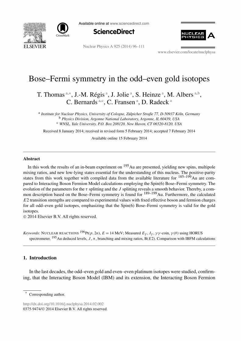
Available online at www.sciencedirect.com
ScienceDirect
Nuclear Physics A 925 (2014) 96–111
www.elsevier.com/locate/nuclphysa
Bose–Fermi symmetry in the odd–even gold isotopes
T. Thomas a,∗, J.-M. Régis a, J. Jolie a, S. Heinze a, M. Albers a,b,
C. Bernards a,c, C. Fransen a, D. Radeck a
a Institute for Nuclear Physics, University of Cologne, Zülpicher Straße 77, D-50937 Köln, Germanyb Physics Division, Argonne National Laboratory, Argonne, IL 60439, USA
c WNSL, Yale University, P.O. Box 208120, New Haven, CT 06520-8120, USA
Received 8 January 2014; received in revised form 5 February 2014; accepted 7 February 2014
Available online 15 February 2014
Abstract
In this work the results of an in-beam experiment on 195Au are presented, yielding new spins, multipole
mixing ratios, and new low-lying states essential for the understanding of this nucleus. The positive-parity
states from this work together with compiled data from the available literature for 185–199Au are com-
pared to Interacting Boson Fermion Model calculations employing the Spin(6) Bose–Fermi symmetry. The
evolution of the parameters for the τ splitting and the J splitting reveals a smooth behavior. Thereby, a com-
mon description based on the Bose–Fermi symmetry is found for 189–199Au. Furthermore, the calculated
E2 transition strengths are compared to experimental values with fixed effective boson and fermion charges
for all odd–even gold isotopes, emphasizing that the Spin(6) Bose–Fermi symmetry is valid for the gold
isotopes.
2014 Elsevier B.V. All rights reserved.
Keywords: NUCLEAR REACTIONS196Pt(p,2n), E = 14 MeV; Measured Eγ , Iγ , γ γ -coin, γ (θ) using HORUS
spectrometer. 195Au deduced levels, J , π , branching and mixing ratios, B(E2). Comparison with IBFM calculations
1. Introduction
In the last decades, the odd–even gold and even–even platinum isotopes were studied, confirm-
ing, that the Interacting Boson Model (IBM) and its extension, the Interacting Boson Fermion
* Corresponding author.
http://dx.doi.org/10.1016/j.nuclphysa.2014.02.002
0375-9474/ 2014 Elsevier B.V. All rights reserved.
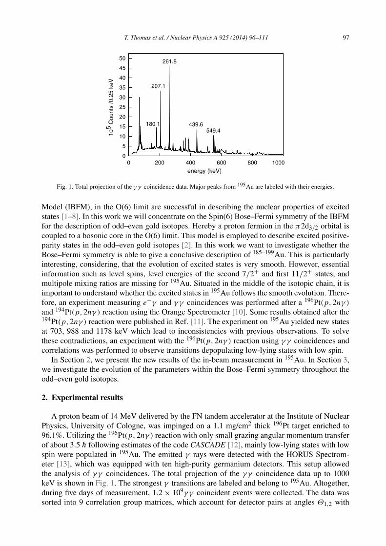
T. Thomas et al. / Nuclear Physics A 925 (2014) 96–111 97
Fig. 1. Total projection of the γ γ coincidence data. Major peaks from 195Au are labeled with their energies.
Model (IBFM), in the O(6) limit are successful in describing the nuclear properties of excited
states [1–8]. In this work we will concentrate on the Spin(6) Bose–Fermi symmetry of the IBFM
for the description of odd–even gold isotopes. Hereby a proton fermion in the π2d3/2 orbital is
coupled to a bosonic core in the O(6) limit. This model is employed to describe excited positive-
parity states in the odd–even gold isotopes [2]. In this work we want to investigate whether the
Bose–Fermi symmetry is able to give a conclusive description of 185–199Au. This is particularly
interesting, considering, that the evolution of excited states is very smooth. However, essential
information such as level spins, level energies of the second 7/2+ and first 11/2+ states, and
multipole mixing ratios are missing for 195Au. Situated in the middle of the isotopic chain, it is
important to understand whether the excited states in 195Au follows the smooth evolution. There-
fore, an experiment measuring e−γ and γ γ coincidences was performed after a 196Pt(p,2nγ )
and 194Pt(p,2nγ ) reaction using the Orange Spectrometer [10]. Some results obtained after the194Pt(p,2nγ ) reaction were published in Ref. [11]. The experiment on 195Au yielded new states
at 703, 988 and 1178 keV which lead to inconsistencies with previous observations. To solve
these contradictions, an experiment with the 196Pt(p,2nγ ) reaction using γ γ coincidences and
correlations was performed to observe transitions depopulating low-lying states with low spin.
In Section 2, we present the new results of the in-beam measurement in 195Au. In Section 3,
we investigate the evolution of the parameters within the Bose–Fermi symmetry throughout the
odd–even gold isotopes.
2. Experimental results
A proton beam of 14 MeV delivered by the FN tandem accelerator at the Institute of Nuclear
Physics, University of Cologne, was impinged on a 1.1 mg/cm2 thick 196Pt target enriched to
96.1%. Utilizing the 196Pt(p,2nγ ) reaction with only small grazing angular momentum transfer
of about 3.5 h following estimates of the code CASCADE [12], mainly low-lying states with low
spin were populated in 195Au. The emitted γ rays were detected with the HORUS Spectrom-
eter [13], which was equipped with ten high-purity germanium detectors. This setup allowed
the analysis of γ γ coincidences. The total projection of the γ γ coincidence data up to 1000
keV is shown in Fig. 1. The strongest γ transitions are labeled and belong to 195Au. Altogether,
during five days of measurement, 1.2 × 10⁹γ γ coincident events were collected. The data was
sorted into 9 correlation group matrices, which account for detector pairs at angles Θ1,2 with
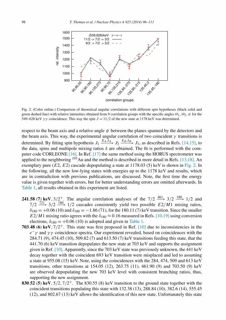
98 T. Thomas et al. / Nuclear Physics A 925 (2014) 96–111
Fig. 2. (Color online.) Comparison of theoretical angular correlations with different spin hypotheses (black solid andgreen dashed line) with relative intensities obtained from 9 correlation groups with the specific angles Θ1,Θ2,ψ for the549–628 keV γ γ coincidence. This way the spin J = 11/2 of the new state at 1178 keV was determined.
respect to the beam axis and a relative angle ψ between the planes spanned by the detectors andthe beam axis. This way, the experimental angular correlation of two coincident γ transitions is
determined. By fitting spin hypothesis J1EA,δA−−−−→ J2
EB,δB−−−−→ J3, as described in Refs. [14,15], tothe data, spins and multipole mixing ratios δ are obtained. The fit is performed with the com-puter code CORLEONE [16]. In Ref. [17] the same method using the HORUS spectrometer wasapplied to the neighboring 193Au and the method is described in more detail in Refs. [13,18]. Anexemplary pure (E2, E2) cascade depopulating a state at 1178.03 (5) keV is shown in Fig. 2. Inthe following, all the new low-lying states with energies up to the 1178 keV and results, whichare in contradiction with previous publications, are discussed. Note, the first time the energyvalue is given together with errors, but for better understanding errors are omitted afterwards. InTable 1, all results obtained in this experiment are listed.
241.58 (7) keV,3/2+. The angular correlation analyses of the 7/2 461−−→ 3/2 180−−→ 1/2 and7/2 721−−→ 3/2 180−−→ 1/2 cascades consistently yield two possible E2/M1 mixing ratios,δ180 = +0.06 (10) and δ180 = −1.86 (71), for the 180.11 (7) keV transition. Since the smallerE2/M1 mixing ratio agrees with the δ180 ≈ 0.16 measured in Refs. [10,19] using conversionelectrons, δ180 = +0.06 (10) is adopted and given in Table 1.
703.48 (6) keV,7/2+. This state was first proposed in Ref. [10] due to inconsistencies in thee−γ and γ γ coincidence spectra. Our experiment revealed, based on coincidences with the284.71 (9), 474.45 (10), 509.82 (7) and 613.50 (7) keV transitions feeding this state, that the441.70 (6) keV transition depopulates the new state at 703 keV and supports the assignmentgiven in Ref. [10]. Apparently, since the 703 keV state was previously unknown, the 441 keVdecay together with the coincident 693 keV transition were misplaced and led to assuminga state at 955.08 (15) keV. Note, using the coincidences with the 284, 474, 509 and 613 keVtransitions, other transitions at 154.05 (12), 263.75 (11), 461.90 (9) and 703.50 (9) keVare observed depopulating the new 703 keV level with consistent branching ratios, thus,supporting the new assignment.
830.52 (5) keV,5/2,7/2+. The 830.55 (8) keV transition to the ground state together with thecoincident transitions populating this state with 132.38 (13), 288.84 (10), 382.6 (14), 555.45(12), and 802.67 (13) keV allows the identification of this new state. Unfortunately this state

T. Thomas et al. / Nuclear Physics A 925 (2014) 96–111 99
Table 1
Results of this work on 195Au compared to the literature values from Nuclear Data Sheets (NDS) [23]. States discussed
in Section 2 are labeled with #. Newly observed states are labeled with ∗ and newly observed transitions with †. Further-
more, γ intensities Iγ of transitions that are listed in NDS but are not observed due to the sensitivity limit of the detector
system or background are labeled with −. If the spin or energy of a state is adopted from NDS it is labeled with ❇❇.
If a spin assignment of a state due to angular correlation analysis is not unique, those spins are labeled with ‡‡ . If an
angular correlation analysis is not feasible but selection rules suggest the multipole characteristic of the γ transition, the
multipolarity is given in parentheses.
Elevel (keV) Jπinitial
Eγ (keV) Iγ [23] Iγ,exp δ [23] δexp Efinal (keV) Jπfinal
0.0 3/2+
61.46 (5) 1/2+❇❇ 61.46 (5) 100 100 0.45 (1) 0 3/2+
241.58 (7)# 3/2+ 180.11 (7) 100 (5) 100 ≈0.16 +0.06 (10) 61.46 (5) 1/2+
241.60 (12) 3.6 (6) 3.8 (10) ≈2.2 0 3/2+
261.78 (5) 5/2+ 200.37 (12) 2.6 (3) 2.1 (5) E2 +0.01 (6) 61.46 (5) 1/2+
261.77 (5) 100 (5) 100 0.51 (1) −0.55 (14) 0 3/2+
318.58 (4)❇❇ 11/2−❇❇ 318.60 (10)❇❇ 100 (11) – M4 0 3/2+
56.80 (3)❇❇ 72 (3) – E3 261.77 (5) 5/2+
439.58 (5) 5/2+ 198.00 (11)† 6.2 (6) −0.29 (26) 241.58 (7) 3/2+
378.15 (14)† 6.0 (7) (E2) 61.46 (5) 1/2+
439.58 (6) 100 100 M1 −0.04 (4) 0 3/2+
525.69 (7) 7/2− 207.11 (6) 100 100 E2 +0.01 (10) 318.58 (4) 11/2−
549.46 (5) 7/2+ 287.67 (6) 21 (4) 21.7 (14) +0.04 (2) 261.78 (5) 5/2+
307.87 (13)† 1.6 (4) (+3.94+18.12−1.88
) 241.58 (7) 3/2+
549.47 (6) 100 (10) 100 (E2) +0.05 (10) 0 3/2+
703.48 (6)∗ 7/2+ 154.05 (12)† 3.3 (4) −0.13 (21) 549.47 (6) 7/2+
263.75 (11)† 7.7 (6) +0.15 (6) 439.58 (5) 5/2+
441.70 (6)† 100 −0.20 (2) 261.78 (5) 5/2+
461.90 (9)† 10.4 (7) +0.00 (12) 241.58 (7) 3/2+
703.50 (9)† 14.9 (11) −0.17 (18) 0 3/2+
706.52 (7) 15/2− 387.94 (6) 100 100 E2 −0.05 (6) 318.58 (4)❇❇ 11/2−
818.18 (7) 9/2+ 268.71 (12)† 5.4 (5) −0.34 (12) 549.46 (5) 7/2+
556.41 (6) 100 100 (E2) +0.01 (2) 261.78 (5) 5/2+
830.52 (5)∗# 5,7/2+∗‡‡ 390.87 (12)† 38.0 (38) 439.58 (5) 5/2+
588.94 (6)† 45.0 (50) 241.58 (7) 3/2+
830.55 (8)† 100 0 3/2+
841.31 (9) 3/2+ 401.74❇❇ 0.07 (2) – 439.58 (5) 5/2+
599.75 (8) 26.2 (9) 20 (8) 0.55 (2) +0.54 (23) 241.58 (7) 3/2+
779.79 (21) 100 100 61.46 (5) 1/2+
841.27❇❇ 4.0 (9) – M1, E2 0 3/2+
878.90 (7) 13/2−❇❇ 172.35 (15) 0.76 (11) 1.0 (3) M1 (M1) 706.52 (7) 15/2−
560.32 (6) 100 100 M1 +0.23 (4) 318.58 (4) 11/2−
894.14 (6) 9/2− 368.43 (6) 100 (4) 100 M1 +0.18 (6) 525.69 (7) 7/2−
575.58 (7) 65 (7) 57.0 (49) 0.65 (30) −0.60 (40) 318.58 (4) 11/2−
(continued on next page)
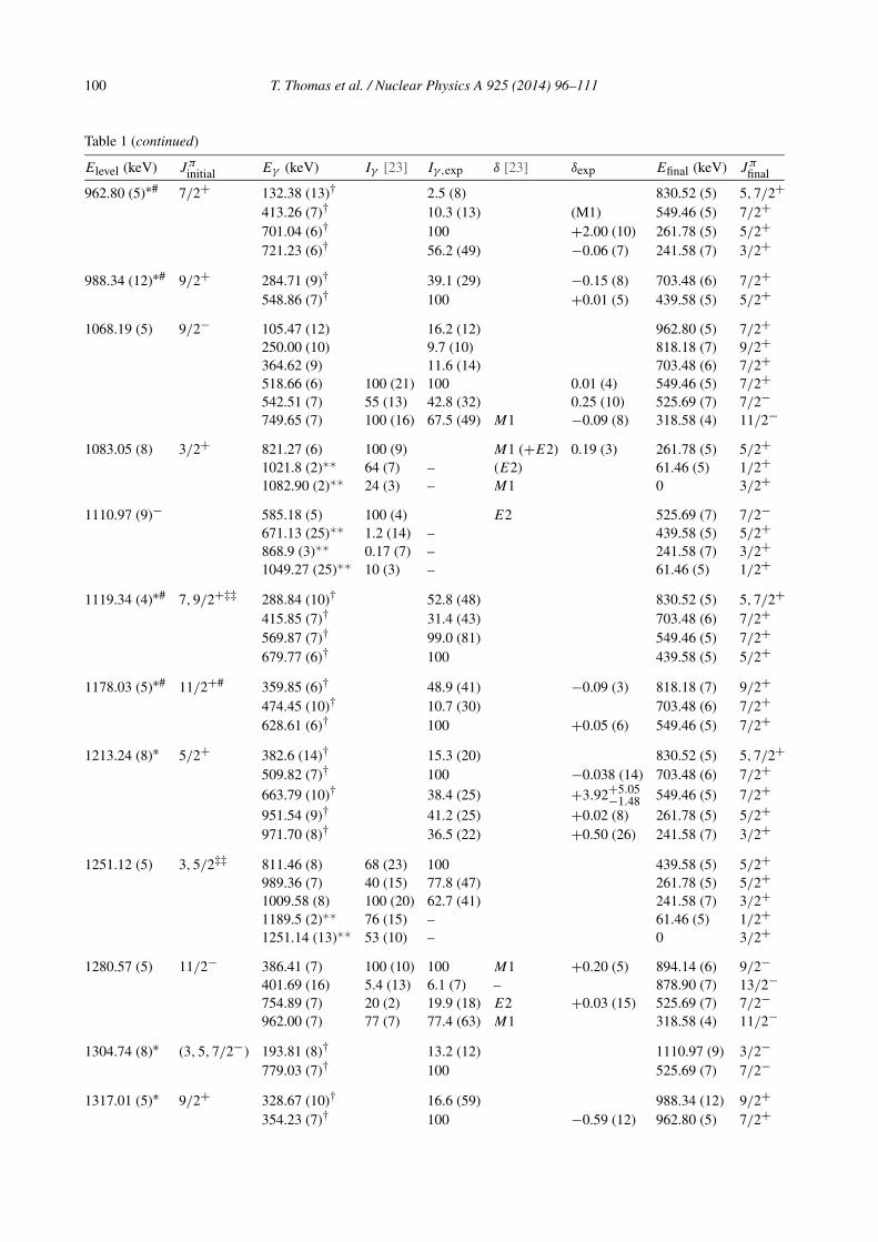
100 T. Thomas et al. / Nuclear Physics A 925 (2014) 96–111
Table 1 (continued)
Elevel (keV) Jπinitial
Eγ (keV) Iγ [23] Iγ,exp δ [23] δexp Efinal (keV) Jπfinal
962.80 (5)∗# 7/2+ 132.38 (13)† 2.5 (8) 830.52 (5) 5,7/2+
413.26 (7)† 10.3 (13) (M1) 549.46 (5) 7/2+
701.04 (6)† 100 +2.00 (10) 261.78 (5) 5/2+
721.23 (6)† 56.2 (49) −0.06 (7) 241.58 (7) 3/2+
988.34 (12)∗# 9/2+ 284.71 (9)† 39.1 (29) −0.15 (8) 703.48 (6) 7/2+
548.86 (7)† 100 +0.01 (5) 439.58 (5) 5/2+
1068.19 (5) 9/2− 105.47 (12) 16.2 (12) 962.80 (5) 7/2+
250.00 (10) 9.7 (10) 818.18 (7) 9/2+
364.62 (9) 11.6 (14) 703.48 (6) 7/2+
518.66 (6) 100 (21) 100 0.01 (4) 549.46 (5) 7/2+
542.51 (7) 55 (13) 42.8 (32) 0.25 (10) 525.69 (7) 7/2−
749.65 (7) 100 (16) 67.5 (49) M1 −0.09 (8) 318.58 (4) 11/2−
1083.05 (8) 3/2+ 821.27 (6) 100 (9) M1 (+E2) 0.19 (3) 261.78 (5) 5/2+
1021.8 (2)❇❇ 64 (7) – (E2) 61.46 (5) 1/2+
1082.90 (2)❇❇ 24 (3) – M1 0 3/2+
1110.97 (9)− 585.18 (5) 100 (4) E2 525.69 (7) 7/2−
671.13 (25)❇❇ 1.2 (14) – 439.58 (5) 5/2+
868.9 (3)❇❇ 0.17 (7) – 241.58 (7) 3/2+
1049.27 (25)❇❇ 10 (3) – 61.46 (5) 1/2+
1119.34 (4)∗# 7,9/2+‡‡ 288.84 (10)† 52.8 (48) 830.52 (5) 5,7/2+
415.85 (7)† 31.4 (43) 703.48 (6) 7/2+
569.87 (7)† 99.0 (81) 549.46 (5) 7/2+
679.77 (6)† 100 439.58 (5) 5/2+
1178.03 (5)∗# 11/2+# 359.85 (6)† 48.9 (41) −0.09 (3) 818.18 (7) 9/2+
474.45 (10)† 10.7 (30) 703.48 (6) 7/2+
628.61 (6)† 100 +0.05 (6) 549.46 (5) 7/2+
1213.24 (8)∗ 5/2+ 382.6 (14)† 15.3 (20) 830.52 (5) 5,7/2+
509.82 (7)† 100 −0.038 (14) 703.48 (6) 7/2+
663.79 (10)† 38.4 (25) +3.92+5.05−1.48
549.46 (5) 7/2+
951.54 (9)† 41.2 (25) +0.02 (8) 261.78 (5) 5/2+
971.70 (8)† 36.5 (22) +0.50 (26) 241.58 (7) 3/2+
1251.12 (5) 3,5/2‡‡ 811.46 (8) 68 (23) 100 439.58 (5) 5/2+
989.36 (7) 40 (15) 77.8 (47) 261.78 (5) 5/2+
1009.58 (8) 100 (20) 62.7 (41) 241.58 (7) 3/2+
1189.5 (2)❇❇ 76 (15) – 61.46 (5) 1/2+
1251.14 (13)❇❇ 53 (10) – 0 3/2+
1280.57 (5) 11/2− 386.41 (7) 100 (10) 100 M1 +0.20 (5) 894.14 (6) 9/2−
401.69 (16) 5.4 (13) 6.1 (7) – 878.90 (7) 13/2−
754.89 (7) 20 (2) 19.9 (18) E2 +0.03 (15) 525.69 (7) 7/2−
962.00 (7) 77 (7) 77.4 (63) M1 318.58 (4) 11/2−
1304.74 (8)∗ (3,5,7/2−) 193.81 (8)† 13.2 (12) 1110.97 (9) 3/2−
779.03 (7)† 100 525.69 (7) 7/2−
1317.01 (5)∗ 9/2+ 328.67 (10)† 16.6 (59) 988.34 (12) 9/2+
354.23 (7)† 100 −0.59 (12) 962.80 (5) 7/2+

T. Thomas et al. / Nuclear Physics A 925 (2014) 96–111 101
Table 1 (continued)
Elevel (keV) Jπinitial
Eγ (keV) Iγ [23] Iγ,exp δ [23] δexp Efinal (keV) Jπfinal
498.79 (7)† 32.8 (60) −2.04+0.71−1.61
818.18 (7) 9/2+
613.50 (7)† 73.0 (77) +4.11+1.94−1.03
703.48 (6) 7/2+
767.62 (13)† 38.9 (68) 549.46 (5) 7/2+
1346.22 (6) 11/2− 452.06 (6) 72 (5) 75.2 (43) M1 +0.16 (6) 894.14 (6) 9/2−
467.34 (6) 100 (6) 100 M1 +0.04 (5) 878.90 (7) 13/2−
1027.45 (11)❇❇ 40 (5) – M1 318.58 (4) 11/2−
1365.52 (9) 17/2− 659.00 (6) 100 100 +0.29 (3) 706.52 (7) 15/2−
1386.01 (5)∗ 9/2+ 397.75 (7)† 100 +0.43 (18) 988.34 (12) 9/2+
423.19 (7)† 87.5 (53) +0.17 (5) 962.80 (5) 7/2+
555.45 (12)† 39.2 (49) 830.52 (5) 5,7/2+
682.63 (13)† 15.9 (12) 703.48 (6) 7/2+
836.56 (9)† 89.9 (52) +0.58(17) 549.46 (5) 7/2+
1396.90 (5)# 11/2+ 578.67 (6) 100 (17) 79.5 (17) (M1) −0.19 (4) 818.18 (7) 9/2+
693.40 (6) 100 (E2) −0.02 (7) 703.48 (6) 7/2+
847.57 (10) 69 (17) 33.6 (12) 549.46 (5) 7/2+
1404.65 (7) 15/2− 525.68 (7) 100 (6) 100 M1 +0.22 (4) 878.90 (7) 13/2−
698.19 (7) 13.1 (13) 12.4 (12) M1 +0.09 (46) 706.52 (7) 15/2−
1086.2 (20)❇❇ 9.7 (14) – 318.58 (4) 11/2−
1406.09 (8) 11/2− 337.90 (6) 100 100 −1.02(15) 1068.19 (5) 9/2−
1424.73 (9) 19/2− 718.21 (5) 100 100 E2 −0.01 (5) 706.52 (7) 15/2−
1475.56 (6)∗ 581.42 (6)† 100 894.14 (6) 9/2−
949.86 (6)† 81.3 (84) 525.69 (7) 7/2−
1487.25 (9) 9,11/2−❇❇ 419.06 (7) 100 100 ≈2.4 1068.19 (5) 9/2−
1489.45 (10) 13/2+ 671.27 (7) 100 100 −0.01 (4) 818.18 (7) 9/2+
1527.10 (8)∗ 7/2+ 708.92 (7) 100 +0.24 (9) 818.18 (7) 9/2+
977.63 (11) 26.3 (29) −0.19+0.51−0.61
549.46 (5) 7/2+
1559.74 (6) 13/2−❇❇ 279.11 (10) 22 (6) 61.6 (62) M1 1280.57 (5) 11/2−
665.42 (12)❇❇ 8.7 (8) – 894.14 (6) 9/2−
680.88 (9) 35 (4) 69.3 (68) M1 878.90 (7) 13/2−
853.23 (9) 42 (5) 100 M1 706.52 (7) 15/2−
1241.17 (10)❇❇ 100 (1) – M1 318.58 (4) 11/2−
1567.89 (15)∗ 263.24 (8) 45.6 (28) 1304.74 (8) (3,5,7/2−)
673.94 (7) 100 894.14 (6) 9/2−
1041.9 (7) 53.6 (32) 525.69 (7) 7/2−
1605.55 (27) (11,13)/2− 324.50 (7) 16 (6) 32.9 (19) 1280.57 (5) 11/2−
711.01 (13)† 10.0 (12) 894.14 (6) 9/2−
727.37 (7) 100 (10) 61.6 (33) M1 878.90 (7) 13/2−
899.01 (1) 82 (15) 100 (E2) 706.52 (7) 15/2−
1286.4 (4)❇❇ 13 (3) – 318.58 (4) 11/2−
1633.01 (10)∗ 513.69 (9)† 100 1119.34 (4) 7,9/2+
802.67 (13)† 24.9 (27) 830.52 (5) 5,7/2+
814.62 (11)† 49.5 (34) 818.18 (7) 9/2+
(continued on next page)
102 T. Thomas et al. / Nuclear Physics A 925 (2014) 96–111
Table 1 (continued)
Elevel (keV) Jπinitial
Eγ (keV) Iγ [23] Iγ,exp δ [23] δexp Efinal (keV) Jπfinal
1656.42 (5)∗ 9,11/2+‡‡ 270.35 (8)† 28.7 (45) 1386.01 (5) 9/2+
478.38 (9)† 74.0 (47) 1178.03 (5) 11/2+
668.25 (5)† 100 988.34 (12) 9/2+
838.23 (9)† 57.2 (44) 818.18 (7) 9/2+
1691.84 (9)∗ (9,11/2−) 411.11 (8)† 24.9 (23) 1280.57 (5) 11/2−
797.86 (12)† 11.3 (11) 894.14 (6) 9/2−
812.78 (12)† 12.4 (11) 878.90 (7) 13/2−
1166.3 (6)† 100 525.69 (7) 7/2−
1711.8 (4)∗ 315.05 (6)† 62.3 (52) 1396.90 (5) 11/2+
723.72 (4)† 100 988.34 (12) 9/2+
1779.3 (5)∗ 372.94 (8)† 100 1406.09 (7) 11/2−
is not populated strongly enough in order to distinguish between the possible spins 5/2, 7/2
in the angular correlation analysis.
946.83 (16) keV. This state with the depopulating transition of 628.30 (20) keV reported by
Refs. [20,21] cannot be confirmed by our data. Instead the 628 keV transition is assigned to
a new state at 1178 keV (cf. discussion about the state at 1178 keV).
955.08 (15) keV, (9/2+). This state with the depopulating transition of 693.17 (25) keV re-
ported by Refs. [20–22] cannot be confirmed by our data. Instead the analysis of γ γ coin-
cidences reveals that the 693 keV transition is feeding a state at 703.48 (6) keV reported in
Ref. [10], thus, this transition is assigned to a state at 1396 keV (cf. discussion about the
state at 1396 keV). Due to the large error, the observation of a state at 960 (10) keV after a
(p, t) reaction [22] could also corresponds to a new state at 962.80 (5) keV observed in our
experiment.
962.80 (5) keV,7/2+. This state could be identified with the 105.47 (12), 354.23 (7) and
423.19 keV transitions feeding this state. The feeding transitions reveal consistent branching
ratios for the transitions depopulating the 962 keV state.
988.34 (5) keV,9/2+. This state was already proposed in Ref. [10] and the coincidence spectra
of the 328.67 (10), 397.75 (7) and 668.25 (5) keV transitions confirm this new state.
1119.34 (4) keV,7/2,9/2+. The γ γ coincidences show, that a 513.69 (9) keV transition feeds
a state at 1119 keV and that this state is depopulated by 288.84 (10), 415.85 (7), 569.87 (7)
and 679.77 (6) keV transitions.
1178.03 (5) keV,11/2+. A 478.38 (9) keV transition feeding the 1178 keV state and in coinci-
dence with the depopulating transitions at 359.58 (6), 474.45 (10) and 693.17 (25) keV con-
firms the existence of this new state. Fig. 2 shows a γ γ angular correlation analysis for the
spin hypotheses 11/2614−−→ 7/2
549−−→ 3/2gs (black solid line) and 9/2
614−−→ 7/2
549−−→ 3/2gs
(green dashed line). The spin hypothesis 11/2614−−→ 7/2
549−−→ 3/2gs fits the data best. The
angular correlation analysis of the (359,556 keV) cascade also favors a spin assignment of
11/2 to the 1178 keV state. Thus, the spin for the newly observed state at 1178 keV was
determined to be 11/2. The multipole mixing ratio of the transition to the 9/2+ state favors
the assignment of positive parity to the 1178 keV state.
1396.90 (5) keV,11/2+. A transition at 441.50 (20) keV was assigned to this state in Ref. [20].
This transition is now assigned to the new state at 703 keV (see the discussion about the
T. Thomas et al. / Nuclear Physics A 925 (2014) 96–111 103
703 keV state). The new assignment of transitions is supported by a new 315.05 (6) keV
transition feeding this state and by measurements using e−γ coincidences in Ref. [10].
3. IBFM calculation in the framework of the Spin(6) Bose–Fermi symmetry
In various publications [7,9,24–26], the nuclear properties of 195Au were described using the
Interacting Boson Fermion Model as well as the Interacting Boson Fermion Model-2, establish-
ing that both the positive-parity and negative-parity states can be understood in the framework
of these models. In the current work, we focus on the structure of the positive-parity states in195Au and in the neighboring odd–even gold isotopes. For this, we use the Spin(6) Bose–Fermi
symmetry and couple a proton in the π2d3/2 orbital to a bosonic core described by the IBM O(6)
limit [4,27]. The corresponding group chain of this Hamiltonian can be written as:
UB(6) ⊗ UF (4) ⊃ SOB(6) ⊗ SUF (4) ⊃ SpinBF(6) ⊃ SpinBF(5) ⊃ SpinBF(3)
[NB ][
1NF]
〈σ 〉 〈α1, α2, α3〉 〈σ1, σ2, σ3〉 (τ1, τ2) J (1)
with NF = 1 in the case of the odd-A nucleus. In the gold isotopes NB corresponds to the number
of boson holes with respect to the neutron shell closure at N = 126 and the proton shell closure at
Z = 82. Other quantum numbers (〈σ 〉, 〈α1, α2, α3〉 〈σ1, σ2, σ3〉, (τ1, τ2), J ) of the nested algebras
are determined by reduction rules (see Ref. [2]). The Hamiltonian written in form of a linear
combination of Casimir operators corresponding to the group chain, neglecting constant terms
that only contribute to the binding energy, is:
H = D · C2
[
SOB(6)]
+ A · C2
[
SpinBF(6)]
+ B · C2
[
SpinBF(5)]
+ C · C2
[
SpinBF(3)]
. (2)
Where C2[X] is the second order Casimir operator of the given algebra X. The corresponding
energy eigenfunction of the Hamiltonian can be derived from the eigenfunction of the Casimir
operators of the subgroups and yields [27]:
E = Dσ(σ + 4) + A(
σ1(σ1 + 4) + σ2(σ2 + 2) + σ 23
)
+ B(
τ1(τ1 + 3) + τ2(τ2 + 1))
+ C(
J (J + 1))
. (3)
Calculations using the Bose–Fermi symmetry were already successfully employed for the fol-
lowing gold isotopes: 191Au [28], 193Au [17,29], 195Au [5–7], 197Au [2,3,30–32] and 199Au [33].
In these references the Bose–Fermi symmetry was applied to individual nuclei or specific odd–
even and odd–odd neighboring gold isotopes. Here we present a systematic investigation for a
larger number of odd–even gold isotopes within the framework of the Spin(6) Bose–Fermi sym-
metry according to Eqs. (1)–(3).
Recently, an Interacting Boson Fermion Model calculation using all proton orbitals (π1g7/2,
π2d5/2, π1h9/2, π2d3/2, π3s1/2) between the Z = 50 and Z = 82 shell closures for 193Au [17]
was performed, showing that the main contribution to the wave functions of the low-lying
positive-parity states with (τ1, τ2) = (1/2,1/2) − (5/2,1/2) originates from the π2d3/2 orbital.
To simplify matters only τ1 is mentioned in the following sections, as τ2 is always equal to
1/2. However, according to the full IBFM calculation, the π3s1/2 contribution to the wave func-
tion increases considerably for the third 5/2+ states, thus this state cannot be described as a
member of the τ1 = 7/2 multiplet. Another difficulty is the determination of positive-parity
states associated to other multiplets than the 〈σ 〉 = 〈NB〉 and 〈σ1, σ2, σ3〉 = 〈NB +1/2,1/2,1/2〉

104 T. Thomas et al. / Nuclear Physics A 925 (2014) 96–111
multiplet. Furthermore, only a few low-spin states far off pseudo-yeast especially for the more
exotic gold isotopes are known. Thus, in this work we investigate only states associated with the
τ1 = 1/2,3/2,5/2 multiplets and with spins up to 11/2+ in each of the odd–even gold isotopes.
Hence, only the parameters B and C in the eigenfunction (3) are relevant for a fit of the excitation
energies.
Note, the level scheme of the Spin(6) Bose–Fermi symmetry looks similar to the Spin(5)
Bose–Fermi symmetry, where a nucleon in a j = 3/2 orbital is coupled to a bosonic core in the
U(5) limit [2], especially when solely the τ1, τ2 and J quantum numbers are considered. But two
crucial differences allows the distinction between these two Bose–Fermi symmetries in the gold
isotopes. Firstly, in the Spin(5) Bose–Fermi symmetry the second (τ1, τ2) = (1/2,1/2) and J =
3/2 state is associated with the same nd = 1 multiplet (the other states are J = 1/2,5/2,7/2).
Together with the J = 3/2 states associated with the nd = 0 and nd = 2 multiplets, more 3/2
states are predicted than observed in the gold isotopes between 0–800 keV. In the Spin(6) Bose–
Fermi symmetry this problem is avoided, since the second (τ1, τ2) = (1/2,1/2), J = 3/2 state
belongs to the next 〈σ1, σ2, σ3〉 = 〈NB − 1/2,1/2,1/2〉 multiplet and thus can be shifted to
higher energies without affecting other low-lying states. Secondly, in the Spin(5) Bose–Fermi
symmetry the B(E2) strength for transitions connecting the lowest J = 1/2 − 7/2 states to the
ground state depend purely on the effective boson charge α2 and the number of bosons NB . In
the Spin(6) Bose–Fermi symmetry, the fermion charge f2 and the τ1 quantum number influence
the B(E2) strength (see Eq. (4)). Furthermore, for transition between higher excited states in
the Spin(5) Bose–Fermi symmetry, β2, another effective boson charge, is crucial for the B(E2)
value. Due to algebraic considerations the effective boson charge β2 is omitted in the Spin(5)
Bose–Fermi symmetry. Hence, albeit only the highest 〈σ1〉 multiplet of the Spin(6) Bose–Fermi
symmetry is observed, a differentiation to the Spin(5) Bose–Fermi symmetry is possible.
The knowledge of the levels in the gold isotopes is primarily based on the compilation of
data in the Nuclear Data Sheets (NDS) [23,34–40]. For 193Au, additional information was taken
from Ref. [17] and for 195Au the results from this work were adopted. 183Au and 201Au are
not considered due to the scarce knowledge of states which can be associated to the τ1 = 5/2
multiplet.
In Fig. 3(a), levels associated with the τ1 = 1/2,3/2,5/2 multiplets in 185–199Au are shown. If
the spin of a state is not unambiguously known, that state is given in parenthesis. States in 195Au
are labeled in blue in case the state has been firstly observed in this experiment and labeled in
red, if the spin is determined for the first time. Note, the results obtained from this experiment
are important for the interpretation of the evolution of levels. The new second 7/2+ and first
11/2+ fits in with the overall smooth evolution of level energies. This indicates, that the differ-
ence in single-particle energies between the π2d3/2 and π3s1/2 orbitals and the population of the
d3/2 and s1/2 orbitals are constant for different odd–even gold isotopes. Calculations based on
the Nilsson Model show consistent results, predicting a constant difference between the single-
particle energies for the π2d3/2 and π3s1/2 orbitals despite increasing β-deformation [41]. With
regard to the evolution of the states shown in Fig. 3(a), just three changes of the ordering of levels
are observed, the most significant one is the switch of the ground state from 1/2+ to 3/2+ from189Au to 191Au.
In order to investigate the Bose–Fermi symmetry, a least-square fit was preformed for each
odd–even gold isotope separately and to all those levels given in Fig. 3(a). For the fit, the com-
puter code ArbModel [42] was used and the quantum numbers were derived from Eq. (3).
The parameters of the fits are listed in Table 2 and the theoretical levels are shown in Fig. 3(b).
Note, the parameters are similar to the parameters derived from calculations in other Refs. [3,17].

T. Thomas et al. / Nuclear Physics A 925 (2014) 96–111 105
Table 2The parameters derived from a least-square fit using Eq. (3) to the energy of the states of the gold nuclei. The correspond-ing root mean square error (RMS) is given in MeV.
Gold isotope C (MeV) B (MeV) RMS (MeV)
185 0.0210 0.0109 0.102187 0.0268 0.0148 0.065189 0.0296 0.0141 0.057191 0.0291 0.0180 0.049193 0.0289 0.0213 0.050195 0.0284 0.0240 0.051197 0.0284 0.0274 0.049199 0.0298 0.0302 0.025
Fig. 3. (Color online.) The evolution of low-lying states in the odd–even 185–199Au isotopes is shown top figure (a). Ifthe spin is not unambiguously known, the states are labeled with parentheses. States in 195Au are colored in red, in casethe spin could be exactly determined and blue, in case that state is observed of the first time. ∗ denotes, that in 185Authe ground state is 5/2− , thus, the excitation energies of positive-parity states are normalized with respect to the energyof the first excited 1/2+ state. The bottom figure (b) shows the evolution of the states derived from an IBFM calculationemploying the Bose–Fermi symmetry. The (τ1) and J quantum numbers are given next to the states.
On the left of the figure the quantum number (τ1) and the spin J of each state is given. As dis-cussed above, all states shown in the figure have the same 〈σ 〉 = 〈NB〉 and 〈σ1, σ2, σ3〉 quantumnumbers. Comparison between Fig. 3(a) and 3(b) reveals that the observed levels are in a good

106 T. Thomas et al. / Nuclear Physics A 925 (2014) 96–111
Fig. 4. (Color online.) A linear function f (NB) = aτ − bτ × NB is fitted to the strength of the τ splitting (parameter B)in 189–199Au with the boson holes NB = 4–9. The derived parameters are aτ = 0.0432 MeV and bτ = 0.0032 MeV.
agreement with the calculated states, also indicated by root mean square error (RMS) given inTable 2. In fact the change of ordering of levels observed experimentally can be reproduced inthe calculations. Especially the switch of the ground state from spin Jπ = 1/2+ in 187Au toJπ = 3/2+ in 191Au is described by the model. Overall, the evolution of levels along the goldisotopes is rather smooth. However, in 185Au the energies of especially the 9/2+ and 11/2+states are drastically reduced, which can be attributed to the influence of the bosonic core. In186Hg, the bosonic core for 185Au, shape coexistence of 0p–2h configuration and a configura-tion induced by two-particle excitations across the Z = 82 shell gap plays a major role [43,44].For 187Au the influence of shape coexistence diminishes considering that the intruder configu-ration in 188Hg is shifted up sharply to higher energies. Of greater significance to the low-lyingpositive-parity states could be the proximity of 187Au to 186Pt. Similar to the situation in the mer-cury isotopes, in the neutron-deficient even–even 178–188Pt coexisting strongly deformed prolateand weakly deformed oblate configurations are observed [45–47]. In fact, the ground state in178–186Pt nuclei are strongly deformed, while in 188Pt the first state associated with a prolate con-figuration is observed at 900 keV and the ground state exhibits oblate shape. Since the influenceof the strongly deformed configuration to the low-lying states in 188Pt should be greatly reduced,it seems appropriate to use the Bose–Fermi symmetry to describe 189Au.
The parameters B and C derived for τ and J splitting (see Table 2), respectively, are shownin Figs. 4 and 5. The x-axis denotes the number of boson holes needed to describe the nucleus.For the parameters obtained for 189–199Au, a graduate change is apparent and linear functionsf (NB) = aτ,J − bτ,J × NB were fitted to these values. 185Au and 187Au are omitted from thefits as the model space encompassing the Bose–Fermi symmetry cannot describe shape coex-istence. The solid lines represents the linear functions and show excellent agreement with thestrength of the τ and J splitting, respectively. While the slope of the linear fit to parameter C
is approximately constant (bJ = −0.0001 MeV and aJ = 0.0283 MeV), parameter B decreaseswith increasing number of bosons NB (bτ = 0.0032 MeV and aτ = 0.0432 MeV). In fact, thechange of τ splitting, induced by the SpinBF(5) algebra, in the IBFM reflects the collectivity.Phenomenologically, this can be understood using the bosonic core of the odd–even gold iso-topes. It is well known, that generally in even–even nuclei the energy of the first 2+ decreaseslinearly as collectivity increases along an isotopic chain and as the nuclei approach mid-shell.

T. Thomas et al. / Nuclear Physics A 925 (2014) 96–111 107
Fig. 5. (Color online.) A linear function f (NB) = aJ − bJ ×NB is fitted to the strength of the J splitting (parameter C)in 189–199Au with the boson holes NB = 4–9. The derived parameters are aJ = 0.0283 MeV and bJ = −0.0001 MeV.
Table 3The quadrupole moments of the ground state 3/2+ in 191–199Auare adopted from Ref. [48]. Using Eq. (5), the effective bosoncharge are calculated.
Gold isotope Q3/2+ (eb) α2 (eb)
191 +0.72 (2) 0.1085 (27)193 +0.66 (2) 0.1106 (29)195 +0.61 (2) 0.1130 (30)197 +0.547 (16) 0.1154 (31)
0.597 (10) 0.1259 (21)199 +0.37 (1) 0.0901 (24)
+0.510 (16) 0.1241 (39)0.55 (3) 0.1339 (73)0.64 (6) 0.1558 (146)
Assuming the IBM in the O(6) limit is valid for the bosonic core, the first excited 2+ state hasseniority τ = 1 and the ground state is assigned τ = 0. On the basis of a constant J splitting,the compression of excitation energy can only be expressed by a reduction of the τ splitting. Be-sides level energies, it is interesting to investigate whether other observables confirm the smoothevolution of collectivity along the odd–even gold isotopes. Particularly quadrupole moments areassociated with collectivity, with high values describing strong deformation due to collectivemotion of the valence nucleons. In the Spin(6) Bose–Fermi symmetry, the quadrupole transitionoperator and the quadrupole moment are defined as [2]:
T E2μ = α2
[s† × d + d† × s
](2)
μ+ f2
[a
†3/2 × a3/2
](2)
μ, (4)
QJ =√
16π
5
√J (2J − 1)
(2J + 1)(J + 1)(2J + 3)〈J |∣∣T(E2)
∣∣|J 〉. (5)
Here, α2 is the effective boson charge and f2 the effective fermion charge. We can use thesimplification α2 = f2 [1], as only the ground state quadrupole moments are known.
Table 3 lists the quadrupole moments of ground states adopted from Ref. [48]. In the caseof 197,199Au multiple quadrupole moments are known for the ground state and given in Table 3.
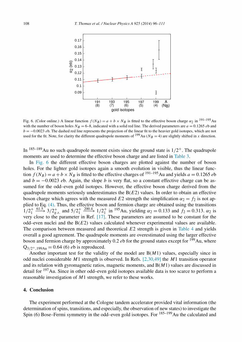
108 T. Thomas et al. / Nuclear Physics A 925 (2014) 96–111
Fig. 6. (Color online.) A linear function f (NB) = a + b × NB is fitted to the effective boson charge α2 in 191–195Auwith the number of boson holes NB = 6–8, indicated with a solid red line. The derived parameters are a = 0.1265 eb andb = −0.0023 eb. The dashed red line represents the projection of the linear fit to the heavier gold isotopes, which are notused for the fit. Note, for clarity the different quadrupole moments of 199Au (NB = 4) are slightly shifted in x direction.
In 185–189Au no such quadrupole moment exists since the ground state is 1/2+. The quadrupolemoments are used to determine the effective boson charge and are listed in Table 3.
In Fig. 6 the different effective boson charges are plotted against the number of bosonholes. For the lighter gold isotopes again a smooth evolution in visible, thus the linear func-tion f (NB) = a +b ×NB is fitted to the effective charges of 191–195Au and yields a = 0.1265 eband b = −0.0023 eb. Again, the slope b is very flat, so a constant effective charge can be as-sumed for the odd–even gold isotopes. However, the effective boson charge derived from thequadrupole moments seriously underestimates the B(E2) values. In order to obtain an effectiveboson charge which agrees with the measured E2 strength the simplification α2 = f2 is not ap-plied to Eq. (4). Thus, the effective boson and fermion charge are obtained using the transitions1/2+
161.5−−→ 3/2+
g.s. and 5/2+1
200.4−−−→ 1/2+1 in 195Au, yielding α2 = 0.133 and f2 = 0.313. α2 is
very close to the parameter in Ref. [17]. These parameters are assumed to be constant for theodd–even nuclei and the B(E2) values calculated whenever experimental values are available.The comparison between measured and theoretical E2 strength is given in Table 4 and yieldsoverall a good agreement. The quadrupole moments are overestimated using the larger effectiveboson and fermion charge by approximately 0.2 eb for the ground states except for 199Au, whereQ3/2+,199Au = 0.64 (6) eb is reproduced.
Another important test for the validity of the model are B(M1) values, especially since inodd nuclei considerable M1 strength is observed. In Refs. [2,30,49] the M1 transition operatorand its relation with gyromagnetic ratios, magnetic moments, and B(M1) values are discussed indetail for 197Au. Since in other odd–even gold isotopes available data is too scarce to perform areasonable investigation of M1 strength, we refer to these works.
4. Conclusion
The experiment performed at the Cologne tandem accelerator provided vital information (thedetermination of spins, transitions, and especially, the observation of new states) to investigate theSpin (6) Bose–Fermi symmetry in the odd–even gold isotopes. For 185–199Au the calculated and

T. Thomas et al. / Nuclear Physics A 925 (2014) 96–111 109
Table 4
Comparison of calculated E2 strength with measured B(E2) values from Refs. [38,23,39,40,17] and this work.
Einitial Jπinitial
Efinal Jπfinal
Eγ B(E2)theory B(E2)NDS
(keV) (keV) (keV) (e2b2) (e2b2)
193Au 38.2 1/2+ 0.0 3/2+ 38.2 0.343 0.304 (80)
224.8 3/2+ 38.2 1/2+ 189.6 0.160 �0.0
3/2+ 0.0 3/2+ 224.8 – �0.053
258.0 5/2+ 38.2 1/2+ 219.8 0.067 0.101 (20)
5/2+ 0.0 3/2+ 258.0 0.343 0.272 (5)
195Au 61.4 1/2+ 0.0 3/2+ 61.4 0.275 0.275 (27)
241.6 3/2+ 61.4 1/2+ 180.1 0.125 �0.022
241.6 3/2+ 0.0 3/2+ 241.6 – �0.007
261.8 5/2+ 61.4 1/2+ 200.4 0.058 0.058 (13)
5/2+ 0.0 3/2+ 261.8 0.275 0.121 (27)
197Au 77.4 1/2+ 0.0 3/2+ 77.4 0.213 0.238 (20)
268.8 3/2+ 77.4 1/2+ 191.4 0.094 0.123 (20)
3/2+ 0.0 3/2+ 268.9 – �0.126
279.0 5/2+ 77.4 1/2+ 201.6 0.050 0.098 (12)
5/2+ 0.0 3/2+ 279.0 0.213 0.177 (41)
502.5 5/2+ 77.4 1/2+ 425.0 0.108 0.052 (23)
5/2+ 0.0 3/2+ 502.6 – 0.047 (41)
547.5 7/2+ 279.0 5/2+ 268.5 0.073 0.012 (5)
7/2+ 268.8 3/2+ 278.7 0.015 0.046 (14)
7/2+ 0.0 3/2+ 547.5 0.213 0.224 (20)
736.7 7/2+ 279.0 5/2+ 457.7 0.137 0.143 (41)
7/2+ 268.8 3/2+ 468.1 0.020 0.041 (27)
855.5 9/2+ 547.5 7/2+ 308.0 0.057 0.068 (48)
9/2+ 279.0 5/2+ 576.5 0.210 0.279 (34)
199Au 77.2 1/2+ 0.0 3/2+ 77.2 0.158 0.166 (90)
317.1 5/2+ 77.2 1/2+ 239.9 0.043 �0.037
5/2+ 0.0 3/2+ 317.1 0.158 �0.049
323.7 3/2+ 77.2 1/2+ 246.5 0.066 �0.283
493.8 7/2+ 323.6 3/2+ 170.6 0.011 �0.041
7/2+ 0.0 3/2+ 493.8 0.158 �0.052
543.0 5/2+ 323.7 3/2+ 219.4 0.010 �0.016
5/2+ 317.1 5/2+ 225.9 0.029 �0.004
5/2+ 77.2 1/2+ 468.8 0.113 �0.004
experimental level schemes for the τ1 = 1/2,3/2,5/2 multiplets were compared, revealing, that
not only the agreement is very good, but also the switch of the ground state from 1/2+ to 3/2+
in 191Au is predicted correctly. The parameters derived from a least-squares fit reflect the smooth
evolution of levels in 189–199Au. Since the J splitting is almost constant, solely the τ splitting
indicates the increasing collectivity towards mid-shell. Indeed, it turns out that the evolution of
parameters B and C throughout 189–199Au can be predicted and the energy of states belonging to
the τ1 = 1/2,3/2,5/2 multiplet can be expressed by the simple equation (all numerical values
in MeV):
E(NB) = E0 + (0.0435 − NB × 0.0032)(
τ1(τ1 + 3) + τ2(τ2 + 1))
+ (0.0283 + NB × 0.0001)(
J (J + 1))
. (6)
110 T. Thomas et al. / Nuclear Physics A 925 (2014) 96–111
We can conclude from this equation, that the compression of level energies with the increasing
number of boson holes can mainly be attributed to collectivity. In fact, the linear dependency
of collectivity for the excited states is expected if other interactions are stable. The analysis
of the experimental levels for 185,187Au and the proximity to shape coexistence in the even–even
mercury isotopes [43] and platinum isotopes [47] suggest, that the Spin(6) Bose–Fermi symmetry
is not applicable to these nuclei.
The quadrupole moments available for the odd–even gold isotopes support the observation of
a very smooth change of nuclear properties in 189–199Au. This is stressed by the good agreement
between calculated and observed B(E2) values. The calculated B(E2) values are based on effec-
tive boson charge and effective fermion charge derived solely from B(E2) transitions in 195Au
and seem to be valid for the other odd–even gold isotopes. However, using the effective boson
charge and fermion charge, a simultaneous description of both, quadrupole moments and B(E2)
values, is not possible. The quadrupole moments are overestimated by approximately 0.2 eb,
although the evolution of the quadrupole moments to smaller values towards shell closure is
reproduced.
Overall, the Spin(6) Bose–Fermi symmetry quite successfully describes the properties of odd–
even gold isotopes, particularly considering the simplicity of the model employed by restricting
the fermion to the π2d3/2 orbital.
Acknowledgements
We thank our coworkers and the Tandem accelerator staff at the IKP Köln for their help during
the experiment. We thank R.V. Jolos for fruitful discussions concerning this work. Part of this
work was supported by DFG under grant JO391/2-1 and JO391/3-2.
References
[1] A. Arima, F. Iachello, The Interacting Boson Model, Cambridge University Press, Cambridge, England, 1987.
[2] F. Iachello, P. Van Isacker, The Interacting Boson Fermion Model, Cambridge University Press, Cambridge, Eng-
land, 1991.
[3] A. Frank, P. Van Isacker, Algebraic Methods in Molecular & Nuclear Structure Physics, Wiley–Interscience, New
York, USA, 1994.
[4] A. Frank, J. Jolie, P. Van Isacker, Symmetries in Atomic Nuclei – From Isospin to Supersymmetry, Springer, New
York, USA, 2009.
[5] A. Metz, J. Jolie, G. Graw, R. Hertenberger, J. Gröger, C. Günter, N. Warr, Y. Eisermann, Phys. Rev. Lett. 83 (1999)
1542.
[6] J. Gröger, et al., Phys. Rev. C 62 (2000) 064304.
[7] H.-F. Wirth, et al., Phys. Rev. C 70 (2004) 014610.
[8] P. Van Isacker, J. Jolie, K. Heyde, A. Frank, Phys. Rev. Lett. 54 (1985) 653.
[9] P. Navrátil, J. Dobes, Phys. Rev. C 37 (1988) 2126.
[10] J.-M. Régis, Diploma thesis, University of Cologne, 2007, unpublished.
[11] J.-M. Régis, T. Materna, G. Pascovici, S. Christen, A. Dewald, C. Fransen, J. Jolie, P. Petkov, K.O. Zell, Rev. Sci.
Instrum. 81 (2010) 113505.
[12] F. Pühlhofer, Nucl. Phys. A 280 (1977) 267.
[13] A. Linnemann, Ph.D. thesis, University of Cologne, 2005, http://kups.ub.uni-koeln.de/1747/.
[14] K.S. Krane, R.M. Steffen, Phys. Rev. C 2 (1970) 724.
[15] K.S. Krane, R.M. Steffen, R.M. Wheeler, At. Data Nucl. Data Tables 11 (1973) 351.
[16] I. Wiedenhöver, Code CORLEONE, University of Cologne, 1995, unpublished.
[17] T. Thomas, C. Bernards, J.-M. Régis, M. Albers, C. Fransen, J. Jolie, S. Heinze, D. Radeck, N. Warr, K.-O. Zell,
Nucl. Phys. A 922 (2014) 200.
[18] C. Bernards, S. Heinze, J. Jolie, C. Fransen, A. Linnemann, D. Radeck, Phys. Rev. C 81 (2009) 024312.

T. Thomas et al. / Nuclear Physics A 925 (2014) 96–111 111
[19] J. Frana, A. Spalek, M. Fiser, A. Kokes, Nucl. Phys. A 165 (1971) 625.
[20] K. Farzine, V.H. Buttlar, Z. Phys. C 270 (1974) 155.
[21] C. Vieu, A. Peghaire, J.S. Dionisio, Rev. Phys. Appl. 8 (1973) 231.
[22] L.H. Goldmann, B.L. Cohen, R.A. Moyer, R.C. Diehl, Phys. Rev. C 2 (1970) 561.
[23] Zhou Chunmei, Nucl. Data Sheets 86 (1998) 645.
[24] R. Bijker, A.E.L. Dieperink, Nucl. Phys. A 379 (1982) 221.
[25] J.M. Arias, C.E. Alonso, M. Lozano, Phys. Rev. C 33 (1986) 1482.
[26] P.B. Semmes, A.F. Barfield, B.R. Barrett, J.L. Wood, Phys. Rev. C 35 (1987) 844.
[27] F. Iachello, S. Kuyucak, Ann. Phys. 136 (1981) 19.
[28] C.D. Papanicolopulos, J. L, Wood, J.D. Cole, J.H. Hamilton, K.S. Krane, R.L. Mlekodaj, A.V. Ramayya, M. Huyse,
L. Vanneste, E.F. Zganjar, ORNL 6004 (1983) 180.
[29] J.L. Wood, Phys. Rev. C 24 (1981) 4.
[30] A.E. Stuchbery, L.D. Wood, H.H. Bolotin, C.E. Doran, I. Morrison, A.P. Byrne, G.J. Lampard, Nucl. Phys. A 486
(1988) 374.
[31] J. Vervier, Phys. Lett. B 100 (1981) 383.
[32] J. Vervier, R. Holzmann, R.V.F. Janssens, M. Loiselet, M.A. Van Hove, Phys. Lett. B 105 (1981) 343.
[33] U. Mayerhofer, T. von Egidy, J. Jolie, H.G. Borner, G. Colvin, S. Judge, B. Krusche, S.J. Robinson, K. Schrecken-
bach, S. Brant, V. Paar, Z. Phys. A 341 (1991) 1.
[34] M.S. Basunia, Nucl. Data Sheets 106 (2005) 619.
[35] M.S. Basunia, Nucl. Data Sheets 110 (2009) 999.
[36] S.-c. Wu, H. Niu, Nucl. Data Sheets 100 (2003) 1.
[37] V.R. Vanin, et al., Nucl. Data Sheets 108 (2007) 2393.
[38] E. Achterberg, G.V. Marti, V.R. Vanin, et al., Nucl. Data Sheets 107 (2006) 1.
[39] Huang Xiaolong, Zhou Chunmei, Nucl. Data Sheets 104 (2005) 283.
[40] Balraj Singh, Nucl. Data Sheets 108 (2007) 79.
[41] S.G. Nilsson, Dan. Mat. Fys. Medd. 29 (16) (1955).
[42] S. Heinze, Ph.D. thesis, University of Cologne, 2008, http://kups.ub.uni-koeln.de/2357/.
[43] M. Scheck, et al., Phys. Rev. C 83 (2011) 037303.
[44] K. Heyde, J.L. Wood, Rev. Mod. Phys. 83 (2011) 1467.
[45] A.E. Stuchbery, S.S. Anderssen, A.P. Byrne, P.M. Davidson, G.D. Dracoulis, G.J. Lane, Phys. Rev. Lett. 79 (1996)
13.
[46] M.K. Harder, K.T. Tang, P. Van Isacker, Phys. Lett. B 405 (1997) 25.
[47] I.O. Morales, A. Frank, C.E. Vargas, P. Van Isacker, Phys. Rev. 78 (2008) 024303.
[48] N.J. Stone, At. Data Nucl. Data Tables 90 (2005) 75.
[49] H.H. Bolotin, D.L. Kennedy, B.J. Linard, A.E. Stuchbery, S.H. Sien, I. Katayama, H. Sakai, Nucl. Phys. A 321
(1979) 231.

Chapter 4
The molybdenum isotopes
63
PHYSICAL REVIEW C 88, 044305 (2013)
Evidence for shape coexistence in 98Mo
T. Thomas,1,2,* K. Nomura,1,3 V. Werner,2 T. Ahn,2 N. Cooper,2 H. Duckwitz,1 M. Hinton,2,4 G. Ilie,2 J. Jolie,1
P. Petkov,1,5 and D. Radeck1
1Institut fur Kernphysik, Universitat zu Koln, Zulpicher Straße 77, D-50937 Koln, Germany2Wright Nuclear Structure Laboratory, Yale University, New Haven, Connecticut 06520, USA
3Grand Accelerateur National d’Ions Lourds, CEA/DSM-CNRS/IN2P3, Boulevard Henri Becquerel, F-14076 Caen Cedex 05, France4Department of Physics, University of Surrey, Guildford GU2 7XH, United Kingdom
5Bulgarian Academy of Science, Institute for Nuclear Research and Nuclear Energy, Tsarigradsko Chausse 72, 1784 Sofia, Bulgaria
(Received 6 June 2013; revised manuscript received 5 September 2013; published 7 October 2013)
A γ γ angular-correlation experiment has been performed to investigate the low-energy states of the nucleus98Mo. The new data, including spin assignments, multipole mixing ratios, and lifetimes reveal evidence for
shape coexistence and mixing in 98Mo, arising from a proton intruder configuration. This result is reproduced
by a theoretical calculation within the proton-neutron interacting boson model with configuration mixing, based
on microscopic energy density functional theory. The microscopic calculation indicates the importance of the
proton particle-hole excitation across the Z = 40 subshell closure and the subsequent mixing between spherical
vibrational and the γ -soft equilibrium shapes in 98Mo.
DOI: 10.1103/PhysRevC.88.044305 PACS number(s): 21.60.Jz, 21.60.Fw, 23.20.En, 25.55.−e
I. INTRODUCTION
For decades, clarifying the nature of shape coexistence has
been one of the major objectives in nuclear structure physics
[1,2]. The phenomenon has been observed in various regions
of the nuclear chart, from light [3] to heavy [4] systems. In186Pb, for example, three low-lying 0+ states bunch together in
energy within the range of 700 keV [4]. The emergence of the
extremely low-lying 0+ states is, in terms of the spherical shell
model, attributed to two- or four-proton excitations across the
Z = 82 shell closure. The residual interaction between protons
and neutrons leads to the lowering of the excited 0+ states
and the different corresponding shell-model configurations are
linked to relevant geometrical deformations in a mean-field
picture [5].
The A ∼ 100 mass region also presents a unique laboratory
for the evolution of nuclear shape and shape coexistence [6,7].
The interplay between single-particle and collective degrees
of freedom leads to shape phase transitions along isotopic and
isotonic chains [8]. The most dramatic examples for shape
coexistence and shape transition occur in the Zr isotopic
chain, as recently revealed for 94Zr [9]. Especially in the
N = 50–56 Zr isotopes the 0+1 state and the very low-lying
0+2 state are considered strongly mixed 0p-0h and 2p-2h
proton configurations, where protons are promoted from the
pf shell to the g9/2 orbital, as also found in shell-model
calculations [6,10]. The structure of the low-lying 0+2 state
in N � 58 Zr isotopes is somewhat more complicated due to
neutron contributions. In Mo isotopes, starting from N = 50,
the nuclear shape gradually evolves from a sphere and, driven
by the enhanced proton-neutron residual interaction, large
deformation sets in at N ≈ 60 [11]. Situated in between,9842Mo56 is pivotal for understanding shape transitions in this
mass region. In particular, the concept of shape coexistence
can apply to this nucleus, where proton cross-shell excitations
from the Z = 28–40 pf shell to the πg9/2 orbit may play an
important role [12]. In fact, experimentally, the first-excited
state of 98Mo has been shown to be an coexisting isomeric
0+ state of different shape [13,14]. The mixing between the
proton 2p-0h and 4p-2h configurations forms the first excited
0+ state and the ground state as revealed by the investigation
of γ transitions depopulating 1+ states with equal strengths to
both 0+ states [12], akin to the findings for 92Zr [6].
To address the important issue of the nature of low-lying
structure in 98Mo, we performed a γ γ angular-correlation
experiment. In this paper, the results of this experiment are
reported as well as the identification of shape coexistence
and the role of a proton intruder configuration in 98Mo.
The experimental results are supported by predictions of
the interacting boson model [15] with configuration mixing,
where the Hamiltonian is determined microscopically. The
microscopic calculation indicates the importance of the proton
intruder configuration and the substantial mixing between
spherical-vibrational and γ -unstable shapes in 98Mo.
II. EXPERIMENTAL PROCEDURE
In order to extend the 98Mo level scheme, we used the reac-
tion 96Zr(α, 2n)98Mo. A 16 MeV α beam was delivered by the
extended stretched transuranium (ESTU) tandem accelerator
at the Wright Nuclear Structure Laboratory, Yale University,
impinging on a 1.25 mg/cm2 thick 96Zr target enriched to
57.36%. The γ transitions were detected by 10 Compton-
suppressed high-purity Ge (HPGe) Clover detectors of the
YRAST Ball array [16]. During five days of measurement,
1.2 × 10⁹ events were collected using a γ γ coincidence
trigger.
Figure 1 shows the total projection of the γ γ coincidence
data. Due to impurities in the 96Zr target transitions from93–99Mo isotopes were observed. The most prominent peaks
are labeled with their associated nuclear origin. The data
044305-10556-2813/2013/88(4)/044305(6) ©2013 American Physical Society

T. THOMAS et al. PHYSICAL REVIEW C 88, 044305 (2013)6
0
2
4
6
8
10
12
200 400 600 800 1000 1200 1400energy (keV)
10 c
ount
s/1.
0 ke
V
FIG. 1. Total projection of the γ γ coincidence data. Major peaksfrom 98Mo and the main side reactions are marked.
were sorted into 11 correlation group matrices, which accountfor detector pairs at angles �1 and �2 with respect to thebeam axis and a relative angle ψ between the plains spannedby the detectors and the beam axis, in order to perform aγ γ angular-correlation analysis. Relative intensities in thecorrelation groups were then fit to angular-correlation func-tions to extract spins and multipole mixing ratios, as describedin Refs. [17,18], by using the computer code CORLEONE
[19,20]. The code takes into account the attenuation factors ofthe detectors [21,22]. An example of a γ γ angular-correlations
analysis is shown in Fig. 2 for the 2+4
1419−−→ 2+1
787−→ 0+gs
cascade, yielding the hitherto unknown multipole mixingratio δ1419 = 0.33 ± 0.11. In the literature [23], conflictingmultipole mixing ratios are given for γ transitions depopulat-ing low-lying states in 98Mo. The superior sensitivity of thepresent setup allowed us to resolve discrepancies. For moredetailed information about γ γ angular-correlations analysiswith the YRAST Ball array see Refs. [22,24]. In the same
way, the multipole mixing ratio of the 2+2
644−→ 2+1 transition
was measured to be +1.67 (25), which is in agreement withthe larger solution from an (n, n′γ ) experiment [25] and refutesthe most recent value from Coulomb excitation [14].
400
500
600
700
800
900
1000
90,9
0,13
5
rel.
inte
nsity
(ar
b. u
nits
)
(1419,787)keV2 -> 2 -> 0
correlation groups (Θ1 ,Θ2 ,φ)90,4
5,13
590
,90,
180
90,9
0,-9
090
,45,
090
,45,
9045
,90,
-135
45,9
0,0
45,9
0,-9
045
,45,
180
45,1
35,1
80
FIG. 2. (Color online) Comparison of a fitted theoretical angu-lar correlation (solid line) with relative intensities obtained from11 correlation groups for the 1419–787 keV γ γ coincidence.
0θ =45°
θ =45°
0
500
1000
1500
2000
2500
3000
1410 1420 1430
inte
nsity
energy (keV)
θ =135°
θ =135°
experimental data,experimental data,lineshape,lineshape,
FIG. 3. (Color online) Determination of the effective lifetime ofthe 1419 keV transition depopulating the 2+
4 state using a gate seton the 787 keV transition. Coincidence spectra with a gate set onthe 787 keV transition for two different angles are shown. The redsolid line represents the simulated lineshape at forward angle and theblue dashed line the backward angle. The effective average lifetimeis τ = 0.30 (7) ps.
Lifetimes of excited states were determined using theDoppler-shift attenuation method (DSAM) [26]. The datawas sorted into three matrices according to the three anglesθ = 45◦, 90◦, 135◦ of the detectors relative to the beamaxis. For the lineshape analysis, the stopping process of anexcited nucleus is simulated using nuclear [27] and electronicstopping powers [28]. In Fig. 3, a lineshape analysis for the1419 keV transition depopulating the 2+
4 state is shown. Theweighted mean value over the angles for the effective lifetimeis calculated to be τ = 0.30 (7) ps. The analysis procedure isoutlined in more detail in Ref. [29].
III. THEORETICAL PROCEDURE
To interpret the nature of the low-lying structure andthe relevant shape dynamics in 98Mo, we performed a self-consistent mean-field calculation using the Skyrme energydensity functional (EDF) (see Ref. [30] for review). Figure 4(a)shows the total energy surface of 98Mo in terms of the axialquadrupole deformation β and triaxiality γ [31] obtainedthrough the constrained Hartree-Fock-BCS (HF-BCS) methodwith the Skyrme functional SLy6 [32] using the code EV8 [33].Figure 4(a) displays two minima in the mean-field energysurface, with the deeper one being close to a spherical shape(β ≈ 0) and the other at β ≈ 0.21 and γ ≈ 20◦ with somedegree of softness. On the other hand, no coexisting minimaare visible in the microscopic energy surfaces of the adjacentnuclei 96Mo [Fig. 4(c)] and 100Mo [Fig. 4(d)]. 98Mo appears tobe transitional between near-spherical (96Mo) and deformed(100Mo) shapes.
To study quantitatively the spectroscopic observables asso-ciated with the intrinsic shape of interest, it is necessary to gobeyond the mean-field approximation. In this work we resort tothe proton-neutron interacting boson model (IBM-2) [15,34]to generate spectra and transition rates that are comparableto data. By mapping the microscopic energy surface onto the
044305-2

EVIDENCE FOR SHAPE COEXISTENCE IN 98Mo PHYSICAL REVIEW C 88, 044305 (2013)
0.1 0.2 0.3 0.4
10
20
30
40
50
0.1
0.2
0.3
0.4
(deg)SLy6
(MeV)98Mo
SLy6 SLy6
0.1 0.2 0.3 0.4
10
20
30
40
50
0.1
0.2
0.3
0.4
(deg)Mapped
(MeV)
0.0
0.5
1.0
1.5
(a)
0.1 0.2 0.3 0.4
10
20
30
40
50
0.1
0.2
0.3
0.4
(deg)
(d)
(MeV)100Mo
0.5
1.0
1.5
0.0
0.0
0.5
1.0
1.5
(b)
0.1 0.2 0.3 0.4
10
20
30
40
50
0.1
0.2
0.3
0.4
(deg)
(c)
(MeV)96Mo
0.0
0.5
1.0
1.5
FIG. 4. (Color online) Contour plots of the microscopic (a) andthe mapped (b) energy surfaces in (β, γ ) plane of 98Mo, and ofthe microscopic energy surfaces of the adjacent nuclei 96Mo (c) and100Mo (d). The color code ranges from 0 (mean-field minimum) to2 MeV, and the minima are identified by the solid white circles. TheSkyrme SLy6 functional is used.
equivalent IBM-2 Hamiltonian in the boson condensate [35],the Hamiltonian parameters are determined microscopically,thereby not invoking any adjustment to data (cf. Refs. [36,37]for details). The mapped Hamiltonian is to be diagonalizednumerically in the boson m-scheme basis to provide levelenergies and transition rates with good quantum numbers in thelaboratory frame. We note that the above-mentioned procedureis similar to that used in Ref. [38], where it was used to makea prediction on the structure of 96Kr, whereas in the presentwork we put this procedure to a more crucial test.
In order to describe the two mean-field minima, the modelspace of the IBM-2 needs to be extended by includingthe intruder configuration and by mixing the Hamiltoniansassociated with the two configurations [39]. From the observedsystematics of the two-neutron separation energies (see, e.g.,Ref. [40] for a review), the N = 56 neutron subshell gap is onlynotable for Z � 40, and the gap becomes rapidly quenched forhigher Z (�42). This indicates that proton intruder states aremore significant for heavier Mo isotopes than neutron shelleffects. Furthermore, the calculated single-particle energies asfunctions of the β deformation indicate the lowering of theproton g9/2 orbitals and the occupation of the last protons inthe orbitals at β ≈ 0.2 associated with the γ -soft minimum inFig. 4(a). These considerations lead us to take the IBM-2 modelspace including the two-proton excitation across the Z = 40shell. The 90Zr nucleus is then taken to be the inert core, andthe number of proton bosons is 1 and 3 for the normal and theintruder configurations, respectively, while the neutron bosonnumber is fixed at 3. Note that normal (intruder) configurationdenotes hereafter the proton 2p-0h (4p-2h) configuration. Thefull Hamiltonian of the system is then given as [38]
H = PnorHnorPnor + Pintr(Hintr + �)Pintr + Hmix, (1)
TABLE I. The intrinsic deformation parameter β2 for the lowest-three excited 2+ states. The theoretical values extracted from theintrinsic quadrupole moments obtained by the IBM-2 (K = 0 isassumed) β IBM
2 , and the equivalent values βMF2 associated with the
mean-field minima, and the experimental values βexpt2 from inelastic
scattering of deuterons [43,44] and Coulomb excitation [45] areshown.
Elevel (keV) J π βMF2 β IBM
2 |β (d,d ′)2 | |βCoulEx
2 |a
787.26 2+1 (+0.21) +0.132 0.167 (4)b 0.174 (5)
1432.29 2+2 (≈0.0) +0.060 0.046c 0.037 (2)
1758.32 2+3 − 0.121 0.029c 0.11 (5)
aTaken from Ref. [45].bTaken from Ref. [44].cTaken from Ref. [43].
where Hnor (Hintr) and Pnor (Pintr) represent the Hamiltonianof and the projection operator onto the normal (intruder)configuration space, respectively. � and Hmix = ω(s†πs†π +d†
πd†π ) + H.c. stand for the energy offset needed for the
proton cross-shell excitation and interaction that mixes twoconfigurations, respectively. The resulting mapped IBM-2energy surface is shown in Fig. 4(b). One can see in Fig. 4(b)two equivalent minima near β ≈ 0 and β ≈ 0.2, with the latterbeing γ soft similarly to the microscopic energy surface.1
IV. RESULTS AND DISCUSSION
The calculation predicts a spectroscopic quadrupole mo-ment for the 2+
1 state of Q(2+1 ) = −0.245eb, corresponding to
a weak prolate deformation. This is consistent with a previousexperimental value of Q(2+
1 ) = −0.25 (9)eb [42], but differsfrom the more recent one, Q(2+
1 ) = −0.05 (2)eb [14]. We notethat the latter result stems from a global fit to data taking knownmultipole mixing ratios and lifetimes into account. Some ofthese input data have been changed and complemented byour present measurement. In Table I, we give the intrinsicβ-deformation parameters for the lowest three 2+ states, takenfrom inelastic scattering [43,44] and Coulomb excitation [45]data. These data are compared to the value obtained from theminima in the mean-field energy surface [Fig. 4(a)], and thedeformation extracted from the intrinsic quadrupole momentin the IBM-2, assuming K = 0. The best agreement is foundwith Coulomb excitation values from Ref. [45].
Next we analyze the structure of the low-energy levelscheme of 98Mo. Figure 5 compares the data from the presentexperiment (left-hand side) and the calculated spectra after(center) and before the mixing, i.e., unperturbed configurations(right-hand side). Note that some experimental states, whichare close in energy and have the same spin, have been identified
1A minimum at γ = 20◦, however, is not obtained with the usedHamiltonian containing up to only two-body boson terms. It has beenshown [41] that a three-body boson term should be included in theIBM Hamiltonian to give rise to the triaxial minimum and to betterdescribe the detailed structure of the quasi-γ band. This is, however,not particularly of relevance for the present paper.
044305-3

T. THOMAS et al. PHYSICAL REVIEW C 88, 044305 (2013)
0+,
0+, 46.9
0+, 76.0
0+, 41.9
2+, 75.8
2+, 47.9
2+, 67.2
2+, 45.1
2+, 20.43+, 95.4
4+, 47.9
4+, 71.3
4+, 42.3
6+, 93.4
0+
2+0+
2+4+2+0+
0(+) 2+4+
2(+)4+
6+2
4+3+5+
22
4+
0+
expt.unassigned0
1
2
ener
gy (M
eV)
IBM-2: pert. configuration
intruder(%) normal
3+
intruder
55.30+
0+
2+
2+
0+
2+4+
3+ 2+4+
4+0+
6+2+
FIG. 5. (Color online) Low-energy level scheme of 98Mo. The experimental (left) and the calculated spectra with mixing (“IBM-2: pert.configuration,” center) and without mixing (right). New spin assignments are denoted in italic letters. The number indicated next to spin value(center) represents the fraction of the intruder configuration in the wave function of each state.
from the comparison to predicted B(E2) values (cf. Tables IIand III). Even though the energy levels are calculated withoutany fit to data; that is, the Hamiltonian parameters are derivedsolely from the microscopic EDF and the mapping procedure,the overall agreement between data and calculation in Fig. 5is remarkably good. While the experimental 0+
2 excitationenergy is well reproduced by the theory, the calculated 2+
1level energy seems rather low compared with the experimentalvalue. The reason is the strong level repulsion between theunperturbed low-spin states of the two configurations due toa rather large mixing strength. In the experiment an excessof states is observed above the 0+
4 state, which could not be
TABLE II. Theoretical E2 transition strengths (in W.u.) comparedto experimental values from Refs. [14,23] and from this work. Statesin bold are predicted to be of intruder nature in theory. For transitionswith mixed multipolarity the multipole mixing ratio δ measured inthe present experiment is given.
Elevel (keV) J πI Eγ (keV) J π
F B(E2)theor B(E2)expt δexpt
787.26a 2+1 787.26 0+
1 27 21.4 +11−10
52.6 0+2 256 280 (40)b
1432.29a 2+2 644.70 2+
1 22 47.8+132−100 +1.67 (25)
697.10 0+2 8 2.5+8
−6
1432.29 0+1 0.03 1.0+2
−1
1509.74a 4+1 722.48 2+
1 49 49.1+5.5−4.5
1758.32a 2+3 326.05 2+
2 13 4.7+189−23 − 0.17 (22)
971.03 2+1 6 3.2+134
−16 − 0.97 (14)
1023.61 0+2 7 7.8+286
−34
2206.74 2+4 1419.48 2+
1 1.3 1.7 (2) − 0.33 (11)
2333.03 2(+)5 900.85 2+
2 1 1.6+8−4 −0.15+0.19
−0.20
2343.26c 6+1 833.52 4+
1 56 10.1 (4)
aτ Adopted from Ref. [45].bB(E2) adopted from Ref. [23].cτ Adopted from Ref. [14].
assigned to predicted states. These might originate from a morecomplicated structure eventually associated with higher-ordereffects such as the four-proton cross-shell excitation and/or theexcitation of neutrons, which are outside of the model spaceof the present calculation.
Looking into the origin of each state in a more quantitativemanner, first we notice on the right-hand side of Fig. 5 that theunperturbed 0+
1 and 0+2 states of the normal and the intruder
configurations are very close in energy. After the mixing, the0+ ground states in each configuration repel each other by≈350 keV in energy (as illustrated by arrows). Here, thematrix element 〈Hmix〉, which mixes unperturbed 0+
1 statesof the normal and the intruder configurations, is calculatedto be 385 keV. This value is consistent with the result from aschematic two-level mixing calculation of 326 keV [12]. In theresulting 0+
1 and 0+2 states, normal and intruder configurations
TABLE III. Same as Table II, but normalized with respect to thelargest B(E2) value among the depopulating decays from a giveninitial state.
Elevel (keV) J πI Eγ (keV) J π
F B(E2)reltheor B(E2)rel
expt δexpt
1962.81 0+3 530.61 2+
2 1 1
1175.57 2+1 0.10 0.05 (1)
2104.66 3+1 594.65 4+
1 0.66 <0.40a
672.50 2+2 1 1 + 6.66+3.41
−1.71
1317.37 2+1 0.13 0.04 (3) +2.91+0.64
−0.46
2223.74 4+2 713.80 4+
1 1 1 + 1.13 (17)
791.58 2+2 1.60 0.88 (11)
1436.68 2+1 0.03 0.04 (1)
2419.48 4+4 661.16 2+
3 1 1
909.52 4+1 0.54 0.33 (3) − 0.64 (10)
1632.46 2+1 0.06 0.02 (1)
aBranching ratio adopted from Ref. [23], no multipole mixing ratioavailable, assumed to be a pure E2 transition.
044305-4

EVIDENCE FOR SHAPE COEXISTENCE IN 98Mo PHYSICAL REVIEW C 88, 044305 (2013)
are almost equally mixed with fraction of 55.3% and 46.9%,
respectively.
One should also notice that the unperturbed normal and the
intruder level schemes exhibit, to a certain extent, vibrational
and γ -soft characteristics, respectively. Within the unperturbed
intruder configuration, the R4/2 = E(4+1 )/E(2+
1 ) ratio of 2.67,
as well as the closely lying 4+1 , 2+
2 states, in which a two-
phonon 0+ state is absent, is typical for a γ -soft structure.
The unperturbed normal configuration, in contrast, displays
closely lying 4+1 , 2+
2 , and 0+2 states, more typical for a
spherical vibrator. Also the R4/2 = 2.32 of the unperturbed
normal configuration deviates strongly from deformed values
toward the spherical harmonic oscillator (R4/2 = 2.0). This
interpretation correlates with the microscopic energy surface
in Fig. 4(a) and is consistent with previous empirical IBM-2
fitting calculations [46].
Finally, in Tables II and III we compare experimental and
theoretical B(E2) values. Lifetimes are either adopted from
Ref. [14] or measured in the present experiment. If not stated
differently, all multipole mixing ratios and branching ratios
are from the present work. The conversion coefficient α was
obtained from calculations using the code BRICC [47]. Very
good agreement between experiment and theory is obtained,
confirming the strong mixing between both configurations. In
particular, the strong B(E2; 2+1 → 0+
2 ) and B(E2; 2+2 → 2+
1 )
transitions, relative to the 2+1 → 0+
1 transition (see Table II),
present a stringent test of configuration mixing. The measured
B(E2; 6+1 → 4+
1 ) is much smaller than predicted, perhaps due
to fragmentation.
In Table III we compare relative B(E2) values, normalized
with respect to the largest B(E2) value among the depopulating
decays from a given initial state, for the states without lifetime
information. Note that the three 4+2,3,4,expt states are observed
within 200 keV. From comparison of relative B(E2) values
the 4+2,expt state can be assigned to the predicted 4+
3,theor state
generated mainly by the intruder configuration, while the
4+4,expt state can be assigned to a strongly mixed 4+
2,theor state.
Table III shows the same extent of consistency as obtained in
Table II.
V. CONCLUSION
We have revealed robust experimental evidence for shape
coexistence and configuration mixing in the low-lying struc-
ture of 98Mo. Key data on multipole mixing ratios and lifetimes
have been obtained, allowing for a detailed comparison
with a new theoretical calculation within the IBM based on
the microscopic EDF. The EDF calculation predicted two
(near-spherical and γ -soft) mean-field minima in the energy
surface [Fig. 4(a)], which necessitates the extension of the
IBM to include a intruder configuration associated with the
proton excitation across the Z = 40 subshell closure. The two
intrinsic shapes are mixed strongly into low-spin states (cf.
Fig. 5). The excitation spectra and E2 properties are calculated
in a fully microscopic way and are in excellent agreement
with the wealth of new spectroscopic data and consistent with
a previous phenomenological IBM fit [46]. The theoretical
method used in this work is robust and capable of appropriately
modeling the coexistence of different shapes. Hence, it allows
for a universal description of nuclear shapes and will be applied
to other heavy exotic nuclei in the future.
ACKNOWLEDGMENTS
We thank the Tandem accelerator staff at the Wright Nuclear
Structure Laboratory, Yale University for their help during the
experiment. This work is supported by US DOE under Grant
No. DE-FG02-91ER-40609. K.N. acknowledges the support
through the JSPS postdoctoral program for research abroad.
P.P. is indebted to the Bulgarian Science Fund for the financial
support under contract DFNI-E 01/2.
[1] J. L. Wood, K. Heyde, W. Nazarewicz, M. Huyse, and P. van
Duppen, Phys. Rep. 215, 101 (1992).
[2] K. Heyde and J. L. Wood, Rev. Mod. Phys. 83, 1467 (2011).
[3] G. E. Brown and A. M. Green, Nucl. Phys. 85, 87 (1966).
[4] A. N. Andreyev et al., Nature (London) 405, 430 (2000).
[5] W. Nazarewicz, Phys. Lett. B 305, 195 (1993).
[6] V. Werner et al., Phys. Lett. B 550, 140 (2002).
[7] G. S. Simpson et al., Phys. Rev. C 74, 064308 (2006).
[8] P. Cejnar, J. Jolie, and R. F. Casten, Rev. Mod. Phys. 82, 2155
(2010).
[9] A. Chakraborty et al., Phys. Rev. Lett. 110, 022504 (2013).
[10] K. Sieja, F. Nowacki, K. Langanke, and G. Martinez-Pinedo,
Phys. Rev. C 79, 064310 (2009).
[11] P. Federman and S. Pittel, Phys. Rev. C 20, 820 (1979).
[12] G. Rusev et al., Phys. Rev. Lett. 95, 062501 (2005).
[13] D. Burch, P. Russo, H. Swanson, and G. E. Adelberger, Phys.
Lett. B 40, 357 (1972).
[14] M. Zielinska et al., Nucl. Phys. A 712, 3 (2002).
[15] F. Iachello and A. Arima, The Interacting Boson Model
(Cambridge University Press, Cambridge, 1987).
[16] C. W. Beausang et al., Nucl. Instrum. Methods Phys. Res., Sect.
A 452, 431 (2000).
[17] K. S. Krane and R. M. Steffen, Phys. Rev. C 2, 724 (1970).
[18] K. S. Krane, R. M. Steffen, and R. M. Wheeler, At. Data Nucl.
Data Tables 11, 351 (1973).
[19] I. Wiedenhover, code CORLEONE, University of Cologne, 1995
(unpublished).
[20] I. Wiedenhover et al., Phys Rev. C 58, 721 (1998).
[21] M. E. Rose, Phys Rev. 91, 610 (1953).
[22] R. J. Casperson, Ph.D. thesis, Yale University, 2009
(unpublished).
[23] B. Sing, Nucl. Data Sheets 98, 335 (2003).
[24] E. Williams et al., Phys. Rev. C 80, 054309 (2009).
[25] R. A. Meyer, J. Lin, G. Molnar, B. Fazekas, A. Veres, and
M. Sambataro, Phys. Rev. C 29, 1839 (1984).
[26] W. M. Currie and C. H. Johnson, Nucl. Instrum. Methods 63,
221 (1968).
[27] L. C. Northcliffe and R. F. Schilling, At. Data Nucl. Data Tables
7, 233 (1970).
[28] J. F. Ziegler, Helium Stopping Powers and Ranges in Elemental
Matter (Pergamon Press, New York, 1978).
[29] P. Petkov et al., Nucl. Phys. A 640, 293 (1998).
[30] M. Bender, P.-H. Heenen, and P.-G. Reinhard, Rev. Mod. Phys.
75, 121 (2003).
044305-5
T. THOMAS et al. PHYSICAL REVIEW C 88, 044305 (2013)
[31] A. Bohr and B. R. Mottelson, Nuclear Structure (Benjamin, New
York, 1975), Vol. II.
[32] E. Chabanat, P. Bonche, P. Haensel, J. Meyer, and R. Shaeffer,
Nucl. Phys. A 627, 710 (1997).
[33] P. Bonche, H. Flocard, and P.-H. Heenen, Comput. Phys.
Commun. 171, 49 (2005).
[34] T. Otsuka, A. Arima, and F. Iachello, Nucl. Phys. A 309, 1
(1979).
[35] J. N. Ginocchio and M. W. Kirson, Nucl. Phys. A 350, 31
(1980).
[36] K. Nomura, N. Shimizu, and T. Otsuka, Phys. Rev. Lett. 101,
142501 (2008).
[37] K. Nomura, R. Rodrıguez-Guzman, L. M. Robledo, and
N. Shimizu, Phys. Rev. C 86, 034322 (2012).
[38] M. Albers et al., Nucl. Phys. A 899, 1 (2013).
[39] P. D. Duval and B. R. Barrett, Phys. Lett. B 100, 223 (1981).
[40] A. Kankainen et al., J. Phys. G 39, 093101 (2012).
[41] K. Nomura, N. Shimizu, D. Vretenar, T. Niksic, and T. Otsuka,
Phys. Rev. Lett. 108, 132501 (2012).
[42] P. Paradis, R. Lecomte, S. Landsberger, and S. Monaro, Phys.
Rev. C 20, 1201 (1979).
[43] R. J. Peterson, R. A. Emigh, and R. E. Anderson, Nucl. Phys. A
290, 155 (1977).
[44] G. M. Ukita, T. Borello-Lewin, L. B. Horodynski-Matsushigue,
J. L. M. Duarte, and L. C. Gomes, Phys. Rev. C 64, 014316
(2001).
[45] J. Barrette, M. Barrette, A. Boutard, R. Haroutunian,
G. Lamoureux, and S. Monaro, Phys. Rev. C 6, 1339 (1972).
[46] M. Sambataro and G. Molnar, Nucl. Phys. A 376, 201 (1982).
[47] T. Kibedi, T. W. Burrows, M. B. Trzhaskovskaya, P. M.
Davidson, and C. W. Nestor, Nucl. Instrum. Methods Phys. Res.,
Sect. A 589, 202 (2008).
044305-6

70 CHAPTER 4. THE MOLYBDENUM ISOTOPES
4.2 Nuclear structure of 96,98Mo: shape coexistence,
robustness of boson seniority and mixed sym-
metry states
4.2.1 Experimental results
To excite low-lying states in 96Mo, an in-beam experiment was performedat the FN-Tandem accelerator of the Institute of Nuclear Physics, Universityof Cologne. A 3He beam was accelerated to 18 MeV and impinged on a8 mg/cm2 ≈96% enriched 96Zr target. The emitted γ rays were detectedwith the OSIRIS [50] cube coincidence spectrometer, equipped with nineHPGe-detectors in this experiment. Six of them were equipped with Comptonsuppression shields. During one week of measurement around 1.5 billioncoincident γγ events were collected. Figure 4.1 shows a total projection of the
0
2
4
6
8
10
12
0 500 1000 1500 2000
10 C
ounts
/0.5
4 k
eV
energy (keV)
6
21+ -> 01
+
41+ -> 21
+
42+ -> 21
+
Figure 4.1: Total projection of the γγ coincidence data (up to 2000 keV) of the96Mo experiment. The strongest γ lines are observed at around 800 keV andbelong to Yrast band transitions of 96Mo.
γγ coincidence data. States with spins J≥8 are weakly populated, and off-Yraststates are observed in this experiment.To extend the level scheme and verify multipole mixing ratios reported inprevious experiments in the neighboring even-even molybdenum isotopes,
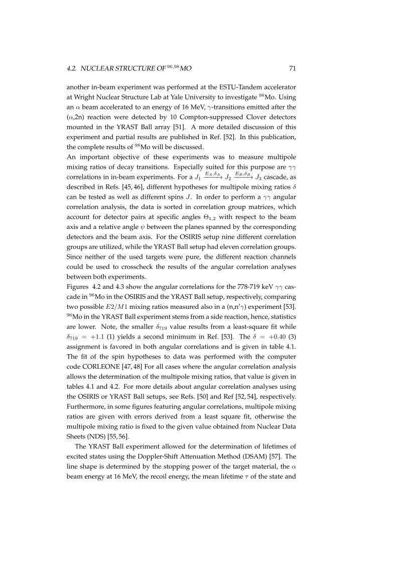
4.2. NUCLEAR STRUCTURE OF 96,98MO 71
another in-beam experiment was performed at the ESTU-Tandem acceleratorat Wright Nuclear Structure Lab at Yale University to investigate 98Mo. Usingan α beam accelerated to an energy of 16 MeV, γ-transitions emitted after the(α,2n) reaction were detected by 10 Compton-suppressed Clover detectorsmounted in the YRAST Ball array [51]. A more detailed discussion of thisexperiment and partial results are published in Ref. [52]. In this publication,the complete results of 98Mo will be discussed.An important objective of these experiments was to measure multipolemixing ratios of decay transitions. Especially suited for this purpose are γγcorrelations in in-beam experiments. For a J1
EA,δA−−−−→ J2EB ,δB−−−−→ J3 cascade, as
described in Refs. [45, 46], different hypotheses for multipole mixing ratios δcan be tested as well as different spins J . In order to perform a γγ angularcorrelation analysis, the data is sorted in correlation group matrices, whichaccount for detector pairs at specific angles Θ1,2 with respect to the beamaxis and a relative angle ψ between the planes spanned by the correspondingdetectors and the beam axis. For the OSIRIS setup nine different correlationgroups are utilized, while the YRAST Ball setup had eleven correlation groups.Since neither of the used targets were pure, the different reaction channelscould be used to crosscheck the results of the angular correlation analysesbetween both experiments.Figures 4.2 and 4.3 show the angular correlations for the 778-719 keV γγ cas-cade in 96Mo in the OSIRIS and the YRAST Ball setup, respectively, comparingtwo possible E2/M1 mixing ratios measured also in a (n,n′γ) experiment [53].96Mo in the YRAST Ball experiment stems from a side reaction, hence, statisticsare lower. Note, the smaller δ719 value results from a least-square fit whileδ719 = +1.1 (1) yields a second minimum in Ref. [53]. The δ = +0.40 (3)assignment is favored in both angular correlations and is given in table 4.1.The fit of the spin hypotheses to data was performed with the computercode CORLEONE [47, 48] For all cases where the angular correlation analysisallows the determination of the multipole mixing ratios, that value is given intables 4.1 and 4.2. For more details about angular correlation analyses usingthe OSIRIS or YRAST Ball setups, see Refs. [50] and Ref [52, 54], respectively.Furthermore, in some figures featuring angular correlations, multipole mixingratios are given with errors derived from a least square fit, otherwise themultipole mixing ratio is fixed to the given value obtained from Nuclear DataSheets (NDS) [55, 56].
The YRAST Ball experiment allowed for the determination of lifetimes ofexcited states using the Doppler-Shift Attenuation Method (DSAM) [57]. Theline shape is determined by the stopping power of the target material, the αbeam energy at 16 MeV, the recoil energy, the mean lifetime τ of the state and

72 CHAPTER 4. THE MOLYBDENUM ISOTOPES
6000650070007500800085009000
rel.
inte
nsity
correlation groups (Θ1 ,Θ2 ,φ)
45,9
0,90
90,4
5,90
45,9
0,18
045
,225
,045
,135
,045
,90,
3590
,45,
3545
,90,
5590
,90,
90
(719,778)keVδ
δ=+0.40 (3)
=+1.1
Figure 4.2: Comparison of two spin hypotheses 2719,δ719−−−−−→ 2
778,δ778=0−−−−−−−→ 0 withdifferent E2/M1 mixing ratios δ719 (black solid and green dashed line) withrelative intensities obtained from nine γγ angular correlation groups at theOSIRIS setup. The E2/M1 mixing ration δ = +0.40 (3) obtained from a least-square fit is favored over δ = +1.1 (1), one of two minima reported in Ref. [53].The smaller E2/M1 mixing ratio +0.34+0.90
−0.70 reported in Ref. [53] agrees withthe present values from both experiments (see also Fig. 4.3).
the angle of the detected γ ray with respect to the beam axis. Figure 4.4 showsthe application of line shape analysis. The determined mean lifetime τ =0.25(5) ps of the state at 2700.86 (36) keV is an effective lifetime, since delayed sidefeeding cannot be excluded in general in such DSAM experiments. In Ref. [52]another example of the DSAM technique is given and discussed in more detail.
In the following section the complete results obtained from the γγ analyzesof both in-beam experiments, 96Mo and 98Mo, are given. First, some statesconflicting with previous data in 96Mo and 98Mo are discussed, followed bytables 4.1 and 4.2 with all experimental results.
96Mo:
1497.96 (9) keV, 2+. In addition to the 2+2
1497−−−→ 0+1 and 2+
2719−−→ 2+
1 transitions,a 2+
2349−−→ 0+
2 would be expected at 349.9 keV. Due to multiple transitionswith energy close to 350 keV, it is not possible to confirm such a transition,thus a upper limit is given.
1625.92 (9) keV, 2+. For the 847.68 (12) keV transition conflictingE2/M1 mix-

4.2. NUCLEAR STRUCTURE OF 96,98MO 73
140
160180200220240
rel.i
nten
sity
(719,778)keVδ=+0.40 (10)
δ=+1.1
90,9
0,13
5
correlation groups (Θ1 ,Θ2 ,φ)
90,4
5,13
590
,90,
180
90,9
0,-9
090
,45,
090
,45,
9045
,90,
-135
45,9
0,0
45,9
0,-9
045
,45,
180
45,1
35,1
80
Figure 4.3: Comparison of theoretical angular correlations of the 2719,δ719−−−−−→
2778,δ778=0−−−−−−−→ 0 spin hypothesis with relative intensities obtained from eleven
correlation groups at the YRAST Ball setup for the 778-719 keV γγ coincidence.The E2/M1 mixing ratio δ = +0.40 (10) (black solid) obtained from a leastsquare fit is favored over δ = +1.1 (1) (green dashed line) reported in Ref. [53].For more information see Fig. 4.2.
ing ratios, δ(2+2
847−−→ 2+1 )=−1.05+9
−10,−0.6 (5),−6.9+12−21, were determined,
where the first value was measured in a (n,γ) [58] experiment and thelatter two originate from Ref. [53]. Evaluation of the angular correla-tion of the 847-778 γγ cascade reveals a rather strong M1 admixture withδ847 = −0.12 (5) (see Figure A.1), which agrees with the smaller E2/M1
mixing ratio given in Ref. [53]. In order to determine the E2/M1 mix-ing ratio, the two peaks at 847.68 (12) keV and 849.99 (9) (4+
1 −→ 2+1 ) keV
have to be discriminated, which is challenging for NaI(Tl) detectors em-ployed in Ref. [58] but possible in this experiment due to the superiorresolution of the HPGe detectors. To verify that the nearby 850 keV tra-nition did not influence our result, the total volume of the doublet at 847keV and 849 keV was integrated and compared with superposed spinhypotheses 2
847,δ847−−−−−→ 2778,δ778=0−−−−−−−→ 0 and 2
849,δ849=0−−−−−−−→ 2778,δ778=0−−−−−−−→ 0 (see
Figure A.2). Note, since the ratio of the volumes of the 847 keV and the849 keV peaks is not known in detail, the superposed spin hypotheseswere normalized to relative intensities in the correlation groups at theangles (45,90,90) and (45,90,55). The normalization reflects that the major

74 CHAPTER 4. THE MOLYBDENUM ISOTOPES
100200300400500600
(a)
(b)
inte
nsity
0100200300400500600
1890 1900 1910 1920 1930
inte
nsity
energy (keV)
exp. dataline shape, θ=135
exp. dataline shape, θ=45
Figure 4.4: Determination of the effective lifetime by analyzing the line shapeof the 1913 keV transition in 98Mo depopulating a (2+) state at 2700 keV usinga gate set on the 787 keV transition. Coincidence spectra with a gate set onthe 787 keV transition for two different angles are shown. The black solid linerepresents the simulated line shape at forward (a) and backward (b) angle. Thedetermined effective mean lifetime is τ = 0.25 (5) ps.
component of the superposed angular correlations stems from the 778-849 keV cascade. Nevertheless, only correlation groups with the angles(45,90,180) and (45,225,0) are sensitive to δ847 and yield a better fit forδ847 = −0.12 than δ847 = −1.05. Both figures, A.1 and A.2, togethershow, that δ847 = −0.12 (5) assignment is favored.
1978.43 (10) keV, 3+. The angular correlation analysis of the depopulatingtransition at 480.55 (9) keV shows that the E2/M1 mixing ratio δ480 =
−17.8+10.3−64.6 is favored (see Figure A.3) to the assignment of δ480 = −0.12
(4) reported in Ref. [53]. A rather pure E2 characteristic for the 480 keVtransition is also supported by the angular correlation of the 1498-480

4.2. NUCLEAR STRUCTURE OF 96,98MO 75
keV cascade. On the other hand, for the other depopulating transitionat 1200.39 (7) keV a stronger E2/M1 mixing with δ1200 = +0.34(4) wasdetermined (see Figure A.4) than in Ref. [53].
2219.46 (9) keV, 4+. The branching ratios from this work for the transitionsdepopulating this state mostly agree with values reported in Ref. [53].However the relative γ intensity of the 241.36 (20) keV transition seemsto be overestimated in Ref. [58], which might originate from a doubletwith a 241.33 keV transition depopulating a state at 1869.64 (6) keV andcannot be distinguished in the singles spectrum used in Ref. [58]. Thecoincidence technique employed in this work allows to determine thebranching ratio and avoids any contribution of the contaminating 241.33keV transition.
2594.39 (12) keV, 3+. The analysis of the branching ratios of the depopulatingtransitions yields different results than given in [53]. One reason mightbe that the coincidence technique together with the superior absolute ef-ficiency of the OSIRIS setup allows a better discrimination of the 966 keVand 968 keV peaks compared to the one detector used in Ref. [53].
2818.67 (35) keV, 4+. The angular correlation analysis of the 1190-849 keVγγ cascade suggests a spin for the state with either J2818 = 4, 5, 6, butthe spin assignment J2818 = 5, 6 can be ruled out due to the depopulat-ing 1320.9 (5) keV transition to the Jπ = 2+ state reported in Ref. [53],assuming only dipole and quadrupole transitions.
Table 4.1: Results of this work on 96Mo. States discussed in section 4.2.1 are labeled with asharp sign (#). Newly observed states are labeled with a asterisk (∗) and newly observed tran-sitions with dagger (†). Furthermore, γ intensities Iγ of transitions that are listed in NDS [55]but are not observed due to the sensitivity limit of the detector system or background are la-beled with a dash (−). If a value is adopted from NDS it is labeled with a double asterisk(∗∗). If a spin assignment of a state due to angular correlation analysis is not unique, thosespins are labeled with a double-dagger (‡‡). If an angular correlation analysis is not feasiblebut selection rules suggest the multipole characteristic of the γ transition, the multipolarity isgiven in parentheses.
Elevel (keV) Jπinitial τ (ps) Eγ (keV) Iγ,exp δexp Efinal(keV) Jπfinal
0.0 0+ stable778.23 (6) 2+ 5.29 (9)∗∗ 778.23 (6) 100 E2 0.0 0+
1147.96 (10) 0+ 88 (12)∗∗ 369.73 (8) 100 E2 778.23 (6) 2+
1497.88 (9)# 2+ 1.13 (10)∗∗ (349.9) <2.3 E2 1147.96 (10) 0+
719.55 (7) 100 +0.40 (4) 778.23 (6) 2+
1497.97 (9) 39.9 (8) E2 0.0 0+
1625.92 (9)# 2+ >1.30∗∗ 128.0 (4)∗∗ <0.9 1497.88 (9) 2+
477.61 (25)∗ 1.7 (4) E2 1147.96 (10) 0+
847.68 (12) 100 -0.12 (5) 778.23 (6) 2+
1626.00 (22) 6.4 (17) E2 0.0 0+
1628.22 (8) 4+ 1.73 (29)∗∗ 849.99 (6) 100 -0.01 (2) 778.23 (6) 2+
1869.64 (6) 4+ 9.23+40,∗∗−22 241.33 (7) 9.0 (5) +0.5+1.2
−0.6 1628.22 (8) 4+
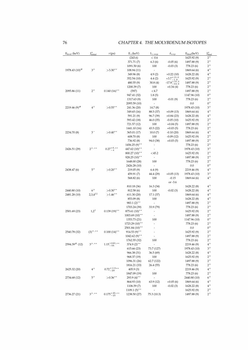
76 CHAPTER 4. THE MOLYBDENUM ISOTOPES
Elevel (keV) Jπinitial τ (ps) Eγ (keV) Iγ,exp δexp Efinal(keV) Jπfinal
(243.6) < 0.6 1625.92 (9) 2+
371.71 (7) 6.3 (6) -0.05 (6) 1497.88 (9) 2+
1091.50 (6) 100 -0.03 (3) 778.23 (6) 2+
1978.43 (10)# 3+ >3.30∗∗ 108.94 (11) - 1869.64 (6) 4+
349.96 (8) 4.9 (2) +0.22 (10) 1628.22 (8) 4+
352.54 (10) 4.4 (2) +3.7+15.0−1.8 1625.92 (9) 2+
480.55 (9) 30.8 (4) -17.8+10.3−64.6 1497.88 (9) 2+
1200.39 (7) 100 +0.34 (4) 778.23 (6) 2+
2095.86 (11) 2+ 0.140 (16)∗∗ (597) <4.7 1497.88 (9) 2+
947.41 (32) 1.8 (5) 1147.96 (10) 0+
1317.63 (9) 100 -0.01 (9) 778.23 (6) 2+
2095.59 (10) - 0.0 0+
2219.46 (9)# 4+ >0.55∗∗ 241.36 (20) 14.7 (8) 1978.43 (10) 3+
349.65 (16) 88.5 (37) +0.09 (13) 1869.64 (6) 4+
591.21 (9) 96.7 (39) +0.84 (23) 1628.22 (8) 4+
593.42 (18) 46.0 (35) -0.05 (10) 1625.92 (9) 2+
721.57 (12) 100 +0.04 (5) 1497.88 (9) 2+
1441.10 (16) 43.5 (22) +0.03 (5) 778.23 (6) 2+
2234.70 (8) 3− >0.40∗∗ 365.01 (17) 10.0 (7) -0.10 (20) 1869.64 (6) 4+
608.70 (8) 100 -0.09 (12) 1625.92 (9) 2+
736.92 (8) 94.0 (38) +0.03 (5) 1497.88 (9) 2+
1456.25 (9)∗∗ - 778.23 (6) 2+
2426.51 (29) 2+,∗∗ 0.27+6,∗∗−4 447.62 (10)∗∗ - 1978.43 (10) 3+
800.27 (10)∗∗ <45.2 1625.92 (9) 2+
928.25 (10)∗∗ - 1497.88 (9) 2+
1648.00 (28) 100 778.23 (6) 2+
2426.28 (10) - 0.0 0+
2438.47 (6) 5+ >0.20∗∗ 219.05 (9) 6.4 (9) 2219.46 (9) 4+
459.91 (7) 44.4 (29) +0.05 (13) 1978.43 (10) 3+
568.82 (6) 100 -0.15 1869.64 (6) 4+
or -3.6810.18 (36) 16.3 (34) 1628.22 (8) 4+
2440.80 (10) 6+ >0.30∗∗ 812.58 (6) 100 -0.02 (3) 1628.22 (8) 4+
2481.28 (10) 2,3,4‡‡ >1.46∗∗ 611.30 (20) 17.1 (37) 1869.64 (6) 4+
853.09 (8) 100 1628.22 (8) 4+
983.1 (2)∗∗ - 1497.88 (9) 2+
1703.24 (39) 33.9 (79) 778.23 (6) 2+
2501.69 (23) 1,2† 0.139 (19)∗∗ 875.61 (10)∗∗ - 1625.92 (9) 2+
1003.69 (10)∗∗ - 1497.88 (9) 2+
1353.73 (21) 100 1147.96 (10) 0+
1723.29 (10)∗∗ - 778.23 (6) 2+
2501.84 (10)∗∗ - 0.0 0+
2540.78 (32) (3)+,∗∗ 0.100 (14)∗∗ 914.53 (9)∗∗ - 1625.92 (9) 2+
1042.62 (9)∗∗ - 1497.88 (9) 2+
1762.55 (32) 100 778.23 (6) 2+
2594.39# (12) 3+,∗∗ 1.15+620,∗∗−58 374.9 (2)∗∗ - 2219.46 (9) 4+
615.66 (23) 73.7 (127) 1978.43 (10) 3+
966.38 (31) 36.5 (69) 1628.22 (8) 4+
968.37 (19) 100 1625.92 (9) 2+
1096.31 (26) 62.7 (122) 1497.88 (9) 2+
1816.21 (33) 26.4 (55) 778.23 (6) 2+
2625.32 (20) 4+ 0.72+115∗∗−29 405.9 (3) - 2219.46 (9) 4+
1847.09 (19) 100 778.23 (6) 2+
2734.68 (12) 5+ >0.36∗∗ 293.9 (4)∗∗ - 2440.80 (10) 6+
864.93 (10) 63.9 (12) +0.05 (6) 1869.64 (6) 4+
1106.59 (7) 100 -0.02 (3) 1628.22 (8) 4+
1109.1 (5)∗∗ - 1625.92 (9) 2+
2736.27 (21) 3+,∗∗ 0.175+26,∗∗−25 1238.50 (27) 75.3 (10.3) 1497.88 (9) 2+
4.2. NUCLEAR STRUCTURE OF 96,98MO 77
Elevel (keV) Jπinitial τ (ps) Eγ (keV) Iγ,exp δexp Efinal(keV) Jπfinal
1957.89 (32) 100 +0.14 (25) 778.23 (6) 2+
2755.31 (33) 6+,∗∗ >0.280∗∗ 314.17 (9) 20.1 (8) +0.19 (14) 2440.80 (10) 6+
316.52 (19) 14.0 (7) 2438.47 (6) 5+
535.78 (8)∗∗ - 2438.47 (6) 5+
885.4 (2)∗∗ - 1869.64 (6) 4+
1127.09 (7) 100 -0.03 (5) 1628.22 (8) 4+
2806.42 (24) (1)∗∗ 0.164+30,∗∗−26 1180.42 (10)∗∗ - 1625.92 (9) 2+
1308.39 (10)∗∗ - 1497.88 (9) 2+
1658.46 (22) 100 1147.96 (10) 0+
2818.67 (35) 4+ 0.085+23,∗∗−17 1190.45 (34) 100 -0.08 (15) 1628.22 (8) 4+
1320.9 (5)∗∗ - 1497.88 (9) 2+
2875.35 (12) 6, 7+ 120.34 (18) 2.9 (6) 2755.31 (33) 6+,∗∗
434.55 (7) 100 +0.12 (7) 2440.80 (10) 6+
or +1.8 (2)2975.70 (14) 5+ 434.6 (2)∗∗ - 2540.78 (32) (3)+,∗∗
740.78 (12) 46.0 (57) 2234.70 (8) 3−
755.6 (2)∗∗ - 2219.46 (9) 4+
997.15 (22) 53.1 (72) (E2) 1978.43 (10) 3+
1347.54 (15) 100 +1.5+4.1−0.9 1628.22 (8) 4+
2978.51 (11) 8+ 223.31 (9) 2.1 (4) 2755.31 (33) 6+,∗∗
537.70 (7) 100 2440.80 (10) 6+
3014.43 (20) 5(+),∗ 279.53 (9)∗ 77.7 (35) 2734.68 (12) 5+
1386.39 (11)∗ 100 +0.02 (7) 1628.22 (8) 4+
3030.83 (12)∗ 592.43 (10)∗ 100 2438.47 (6) 5+
3143.32 (34)∗ 388.01 (10)∗ 100 2755.31 (33) 6+,∗∗
3370.29 (12) 8+ 391.59 (13) 6.1 (2) -0.04 (38) 2978.51 (11) 8+
929.49 (7) 100 -0.01 (3) 2440.80 (10) 6+
3445.96 (12) 6+ 1007.49 (10) 100 +0.35 (8) 2438.47 (6) 5+
3473.14 (10) 7+ 738.39 (7) 78.6 (19) +0.04 (5) 2734.68 (12) 5+
1032.42 (12) 100 -0.02 (4) 2440.80 (10) 6+
3597.08 (16) 862.40 (10)∗ 100 2734.68 (12) 5+
3710.73 (16)∗ 732.22 (11) 100 2978.51 (11) 8+
3787.26 (13) 10+ 808.75 (7) 100 2978.51 (11) 8+
3804.55 (39)∗ 434.26 (37)∗ 100 3370.29 (12) 8+
3916.20 (15) 7+, 9‡‡ 545.91 (9) 100 3370.29 (12) 8+
4533.33 (17) 9+, 11‡‡ 746.07 (11) 100 3787.26 (13) 10+
4795.38 (26) 11∗∗ 879.18 (21) 100 3916.20 (15) 7+, 9‡‡
Table 4.2: Results of this work on 98Mo. States discussed in section 4.2.1 are labeled with asharp sign (#). Newly observed states are labeled with a asterisk (∗) and newly observed tran-sitions with dagger (†). Furthermore, γ intensities Iγ of transitions that are listed in NDS [56]but are not observed due to the sensitivity limit of the detector system or background are la-beled with a dash (−). If a value is adopted from NDS it is labeled with a double asterisk(∗∗). If a spin assignment of a state due to angular correlation analysis is not unique, thosespins are labeled with a double-dagger (‡‡). If an angular correlation analysis is not feasiblebut selection rules suggest the multipole characteristic of the γ transition, the multipolarity isgiven in parentheses.
Elevel (keV) Jπinitial τ (ps) Eγ (keV) Iγ,exp δexp Efinal(keV) Jπfinal
98Mo734.75 (4) 0+ 31.45 (130)∗∗
787.26 (15) 2+ 5.08 (9)∗∗ (52.6) − 734.75 (4) 0+
787.26 (15) 100 +0.0 0.0 0+
1432.18 (12)# 2+ 2.21 (23)∗∗ 644.70 (15) 100 +1.67 (25) 787.26 (15) 2+
697.10 (46) 5.8 (7) (E2) 734.75 (4) 0+
1432.29 (20) 81.5 (16) +0.0 0.0 0+
1509.74 (21) 4+ 3.65 (7)∗∗ (78.0) − 1509.74 (21) 4+

78 CHAPTER 4. THE MOLYBDENUM ISOTOPES
Elevel (keV) Jπinitial τ (ps) Eγ (keV) Iγ,exp δexp Efinal(keV) Jπfinal
722.48 (15) 100 +0.02 (3) 787.26 (15) 2+
1758.32 (12) 2+ 2.05 (8)∗∗ 248.5 − 1432.18 (12) 2+
326.05 (25) 7.0 (3) -0.17 (22) 1432.18 (12) 2+
971.03 (16) 65.9 (10) -0.97 (14) 787.26 (15) 2+
1023.61 (16) 100 +0.0 734.75 (4) 0+
1758.64 (14) − 0.0 0+
1962.81 (20) 0+ 530.61 (30) 39.1 (29) (E2) 1432.18 (12) 2+
1175.57 (20) 100 +0.0 787.26 (15) 2+
2017.36 (16) 3− 93.8 (101)∗∗ 258.96 (26) 22.0 (19) +0.01 (6) 1758.32 (12) 2+
507.8 (2) − 1509.74 (21) 4+
1230.04 (15) 100 -0.04 (7) 787.26 (15) 2+
2018.01 (53) 16.2 (17) (E3) 0.0 0+
2037.26 (14) 0(+) 1250.00 (19) 100 +0.0 787.26 (15) 2+
2104.66 (15) 3+ 594.65 (12) − 1509.74 (21) 4+
672.50 (17) 78.9 (28) +6.7+3.4−1.7 1432.18 (12) 2+
1317.37 (17) 100 +2.9+0.6−0.5 787.26 (15) 2+
2206.74 (26) 2+ 0.30 (2) 448.2 (2) − 1758.32 (12) 2+
1419.48 (22) 100 -0.33 (11) 787.26 (15) 2+
2223.74 (14) 4+ 206.3 (5) − 2017.36 (16) 3−
465.5 (2) − 1758.32 (12) 2+
713.80 (16) 100 +1.13 (17) 1509.74 (21) 4+
791.58 (17) 82.9 (36) +0.07 (8) 1432.18 (12) 2+
1436.68 (25) 23.4 (19) -0.03 (7) 787.26 (15) 2+
2333.03 (24)# 2(+) 0.50 (17) 900.85 (21) 100 -0.15+0.19−0.20 1432.18 (12) 2+
2333.32 (17)# 4+ 109.48 (44) 10.9 (44) 2223.74 (14) 4+
575.06 (10) − 1758.32 (12) 2+
823.33 (16) 77.4 (47) -0.388 (7) 1509.74 (21) 4+
1546.30 (22) 100 -0.04 (4) 787.26 (15) 2+
2343.26 (26) 6+ 7.50 (29)∗∗ 833.52 (15) 100 -0.01 (7) 1509.74 (21) 4+
2418.52 (29)# 2(+) 986.34 (27) 100 +0.01 (7) 1432.18 (12) 2+
1631.26 (50) 96.5 (59) 787.26 (15) 2+
2419.48 (18)# 4+ 195.66 (10) − 2223.74 (14) 4+
314.9 (2) − 2104.66 (15) 3+
402.33 (39) 10.0 (14) (E1) 2017.36 (16) 3−
661.16 (40) 17.8 (13) +0.09 (10) 1758.32 (12) 2+
909.52 (17) 100 -0.64 (10) 1509.74 (21) 4+
987.48 (10) − 1432.81 (12) 2+
1632.46 (33) 40.5 (16) (E2) 787.26 (15) 2+
2485.47 (21) 3+ 151.9 (2) − 2333.32 (17) 4+
380.05 (43) 21.8 (17) 2104.66 (15) 3+
467.0 (9) − 2104.66 (15) 3+
726.83 < 4.6 1758.32 (12) 2+
975.25 (32) 35.9 (17) -0.89+0.62−1.60 1509.74 (21) 4+
1053.04 (26) 55.2 (27) -0.97+0.27−0.36 1432.18 (12) 2+
1698.49 (26) 100 -0.52 (13) 787.26 (15) 2+
2506.10 (16)# 5+ 86.51 (32) 8.2 (44) 2419.48 (18) 4+
162.53 (15) − 2343.26 (26) 6+
172.89 (16) 73.6 (32) +0.05 (11) 2333.32 (17) 4+
282.52 (10) − 2223.72 (14) 4+
299.6 (2) − 2206.74 (26) 2+
996.33 (16) 100 -0.96 (10) 1509.74 (21) 4+
2525.50 (29) 2∗∗ 0.47 (6) 1093.32 (26) 100 +0.01 (17) 1432.18 (12) 2+
2562.41 (23) 2 544.52 (39) 7.4 (9) 2017.36 (16) 3−
803.6 (5) − 1758.32 (12) 2+
1775.37 (23) 100 +0.05 (7) 787.26 (15) 2+
2572.83 (17) 3 239.2 (2) − 2333.32 (17) 4+
555.07 (35) 47.0 (66) 2017.36 (16) 3−
814.46 (26) 49.6 (27) +0.10 (10) 1758.32 (12) 2+
1140.83 (47) 29.1 (34) 1432.18 (12) 2+

4.2. NUCLEAR STRUCTURE OF 96,98MO 79
Elevel (keV) Jπinitial τ (ps) Eγ (keV) Iγ,exp δexp Efinal(keV) Jπfinal
1785.90 (24) 100 +0.01 (6) 787.26 (15) 2+
2574.35 (16) 4+ 350.81 (18) 100 -0.13 (24) 2223.74 (14) 4+
557.08 (39) 19.9 (56) (E1) 2017.36 (16) 3−
1064.27 (18) 90.9 (40) -2.69+0.75−1.47 1509.74 (21) 4+
2612.21 (46) 0(+) 1824.95 (44) 100 +0.0 787.26 (15) 2+
2619.99 (28) 3+ 1187.50 (43) 9.7 (7) +0.95+0.98−0.50 1432.18 (12) 2+
1832.93 (33) 100 -0.54 (13) 787.26 (15) 2+
1886.3 (7) − 734.75 (4) 0+
2620.56 (17) 5− 603.25 (17) 63.3 (12) -0.08 (11) 2017.36 (16) 3−
1110 .75 (16) 100 -0.05 (10) 1509.74 (21) 4+
2678.49 (20) 6+ 172.47 (26) 3.6 (5) 2506.10 (16) 5+
335.15 (16) 52.8 (8) -0.01 (10) 2343.26 (26) 6+
345.258 (20) − 2333.32 (17) 4+
445.04 (10) − 2223.74 (14) 4+
1168.81 (16) 100 +0.01 (4) 1509.74 (21) 4+
2700.86 (36)# (2+)∗∗ 0.25 (5) 493.4 (6) − 2206.74 (26) 2+
1913.60 (33) 100 -0.14 (14) 787.26 (15) 2+
2733.27 (36)# (2+)∗∗ 1946.01 (33) 100 -0.09 (15) 787.26 (15) 2+
2768.46 (35) 4+ 1981.20 (32) 100 +0.01 (11) 787.26 (15) 2+
2795.37 (18) 4− 778.01 (20)† 37.7 (31) -0.37 (15) 2017.36 (16) 3−
1285.63 (16) 100 -0.02 (3) 1509.74 (21) 4+
2812.72 (42)# 1+,2+,3+,‡‡ 2025.46 (39)† 100 -4.4+2.2−56.7 787.26 (15) 2+
2836.33 (16) 6+ 157.87 (16) 100 2678.49 (20) 6+
330.18 (23) 23.3 (56) -0.24 (6) 2506.10 (16) 5+
493.09 (20) 23.0 (56) -0.29 (15) 2343.26 (26) 6+
1326.7 − 1509.74 (21) 4+
2853.71 (31) 8+,7+,6+,5+,‡‡ 510.45 (16) 100 2343.26 (26) 6+
2871.00 (43) 2+,3 2083.74 (40)† 100 +0.06(10) 787.26 (15) 2+
or -3.7+1.5−5.8
2896.58 (21) 5+ 791.83 (28)† 100 (E2) 2104.66 (15) 3+
1386.84 (19)† 96.0 (35) +3.2+0.8−0.5 1509.74 (21) 4+
2905.07 (74) (4+)∗∗ 0.22 (2) 2117.81 (72))† 100 787.26 (15) 2+
2916.29 (47) (2+) 0.11+9−6 2129.03 (45) 100 -0.71+0.37
−0.57 787.26 (15) 2+
2962.58 (45) (2+,3,4+) 944.39 (44) 18.5 (47) 2017.36 (16) 3−
1452.69 (42) 100 1509.74 (21) 4+
2176.41 (47)† 82.5 (141) 787.26 (15) 2+
2976.70 (32) (4+,‡‡) 557.1 (4) − 1419.48 (18) 4+
753.19 (14) − 2223.74 (14) 4+
0.64 (33) 1466.96 (24) 100 +0.05 (17) 1509.74 (21) 4+
2189.4 (5) 787.26 (15) 2+
3019.73 (18) 5− 399.43 (18) 100 +0.06 (15) 2620.56 (17) 5−
676.66(26) 33.5 (24) -0.01 (10) 2343.26 (26) 6+
1002.85 (31) 24.4 (10) +0.03 (5) 2017.36 (16) 3−
1510.4 − 1509.74 (21) 4+
3021.39 (40) (5−,∗∗) 688.23 (10) − 2333.03 (24) 2+
797.88 (10) − 2223.74 (14) 4+
815.5 (3) − 2206.74 (26) 2+
917.05 (13) − 2104.66 (15) 3+
1004.31 (10) − 2017.36 (16) 3−
1263.36 (11) − 1758.32 (12) 2+
1511.65 (34) 100 1509.74 (21) 4+
1589.62 (10) − 1432.18 (12) 2+
2234.31 (10) − 787.26 (15) 2+
3025.93 (33) 5+ 1516.19 (25)† 100 +0.27 (6) 1509.74 (21) 4+
3050.21 (35) (4+,3+)‡‡ 544.5 (4) − 2506.10 (16) 5+
631.4 (2) − 2419.48 (18) 4+
717.5 (3) − 2333.03 (24) 2(+)
0.18 (3) 1540.47 (52) 100 -0.20 (27) 1509.74 (21) 4+

80 CHAPTER 4. THE MOLYBDENUM ISOTOPES
Elevel (keV) Jπinitial τ (ps) Eγ (keV) Iγ,exp δexp Efinal(keV) Jπfinal
1618.75 (11) − 1432.18 (12) 2+
2263.0 (2) − 787.26 (15) 2+
3067.34 (24) 4−,5 446.78 (17) 100 2620.56 (17) 5−
3095.74 (19) 7− 475.23 (17) 100 +0.01 (3) 2620.56 (17) 5−
752.41 (16) 81.2 (16) -0.01 (4) 2343.26 (26) 6+
3108.99 (21) (2+,4)‡‡ 1091.52 (20) 100 +0.05 (7) 2017.36 (16) 3−
1599.50 (33) 24.2 (37) 1509.74 (21) 4+
3210.45 (34) (4+)∗∗ 1193.09 (30) 100 2017.36 (16) 3−
3228.71 (29) (5+,6+)‡‡ 0.22 (3) 885.48 (21) 100 +0.67 (12) 2343.26 (26) 6+
or +0.07 (16)1718.80 (55) <23.8 1509.74 (21) 4+
3271.24 (31) (8+,7+,6+)‡‡ 927.95 (17) 100 2343.26 (26) 6+
3323.12 (21) 7(−) 227.37 (18)† 100 -0.08 (10) 3095.74 (19) 7−
979.87 (23)† 99.9 (66) (E1) 2343.26 (26) 6+
3556.67 (46) 0.24 (7) 1213.41 (38)† 2343.26 (26) 6+
98Mo:
1432.18 (10) keV, 2+. For the depopulating 644 keV transition conflicting mul-tipole mixing ratios are reported. A (n,n’γ) experiment [59] measuredtwo competing values, +1.70 (16) and +0.13 (4) (less likely according tothe publication). The Coulomb excitation experiment by M.Zielinska etal. [60], however, resulted in a multipole mixing ratio delta of +0.27 (2),and a (n,γ) experiment [61] determined a value of 0.58 (5). The differ-ent multipole mixing ratios are tested in the angular correlation analysisshown in figure A.5. A multipole mixing ratio of δ644 = 1.67 (25) is fa-vored and is in good agreement with one of the multipole mixing ratiosfrom the previous (n,n’γ) experiments. Note, that in a neutron captureexperiment the angular correlation function for a sequence of γ cascadesdepends only on the angle between the γ rays. In a Coulomb excitationexperiment, firstly, the second 2+ state is much less excited than the first2+ state (see figure 1 in M. Zielinska et al. [60]), and secondly, knownE2/M1 mixing ratios have been used as input (to the GOSIA code), inorder to obtain matrix elements in a global fit. The present in-beam exper-iment avoids all of the above-mentioned problems. The (α, 2n) reactionsufficiently populates non-Yrast 2+ states of 98Mo. The multi-detectorsetup and the given beam quantization axis allow to use 11 correlationgroups for the angular correlation analysis. Furthermore, a δ644 = 1.67
(25) is supported by the angular correlation analysis using the OSIRISsetup (δOsiris,644 = 3.2+4.6
−1.4).
2333.03 (24) and 2333.32 (17) keV, 2(+) and 4+. Using γγ coincidences ofthe 172.89 (16) transition which feeds the state at 2333.32 keV, a γ line at900.85 keV cannot be detected. This agrees with data from a β decay ex-periment [59], where a depopulating transition at 900.85 keV was not ob-

4.2. NUCLEAR STRUCTURE OF 96,98MO 81
served with the relative γ intensity reported in Ref. [56]. The 900.85 keVtransition also exhibit a Doppler shift in detectors positioned in forwardand backward direction which is not observed for the other transitionsgiven in NDS, thus establishing that in the level scheme at 2333 keV infact two states can be placed as proposed in proton and deuteron inelasticscattering experiments [62]. Summarizing, the 2333.03 and 2333.32 statecan be confirmed by independent gates.
2418.52 (29) keV, 2. The two states at 2418.52 (29) keV and 2419.48 (18) keVare difficult to disentangle. But the coincidence spectrum of the observed86.51 (32) keV transition depopulating the 2506.10 (16) keV state (see dis-cussion of this state) allows to solely observe γ decays from the state at2419.48 keV, since a transition with an E3 multipole characteristic is un-likely to be observed. From the coincidence spectrum of the 86 keV wecan assume that a hypothetical contributions of a 987.48 keV transitiondepopulating the state at 2419.48 keV to the 986.34 keV transition depop-ulating the state at 2418.52 keV is negligible.
2419.48 (18) keV, 4+. In previous (p, t) and β decay experiments [59,63] a spinof 3− was assigned to the 2419 keV state while in a (pol t,p) reaction [64]the spin 2 was determined for this state. Figure A.6 shows the compar-ison of the three possible spin hypothesis with data and a spin of 4+ isfavored. The new spin assignment is confirmed by the angular correla-tion analysis of the γγ cascade 661-1023. Note, the (pol t, p) experimentmight have observed the state at 2418 keV instead, (see discussion to the2418 keV state) which revealed a spin of 2.
2485.47 (21) keV, 3+. The relative intensity of the 726.83 (11) keV transitionobserved in Ref. [59] cannot be confirmed, as no γ line is observed in γγcoincidence spectrum with the 1023 keV transition. At this energy thesensitivity is such that peaks with a relative γ intensity greater than 4.6%with respect to the other depopulating 1698.49 keV transition would beobserved.
2506.10 (16) keV, 5+. The angular correlation analysis of the 722-996 keV γγ
cascade (see Figure A.7) favors the spin assignment 5+ for the 2506 keVstate and the multipole mixing ratio is δ996 =-0.96 (10).
2700.86 (36) keV, (2+). The angular correlation analysis favors a spin assign-ment of 2+ for this state, a spin assignment of 1+ or 3+ cannot be fullyrejected. The δ1913 value given in Table 4.2 is for a presumed spin 2+
adopted from literature [56]. The E2/M1 mixing ratio for other spin hy-potheses are δ1+−→2+
1= −0.45 (10) and δ3+−→2+
1= +0.34 (9).
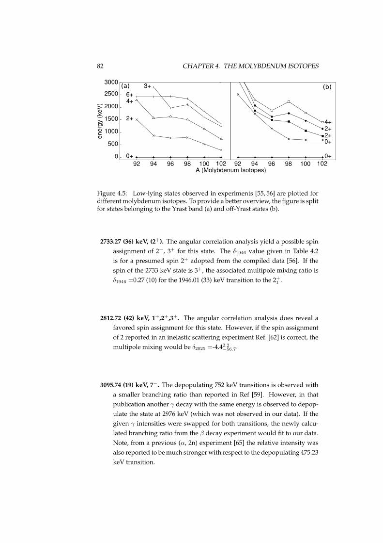
82 CHAPTER 4. THE MOLYBDENUM ISOTOPES
0
500
1000
1500
2000
2500
3000
92 94 96 98 100
ener
gy (k
eV)
A (Molybdenum Isotopes)102 92 94 96 98 100 102
0+
2+
4+
3+(a) (b)6+
0+
0+2+2+4+
Figure 4.5: Low-lying states observed in experiments [55, 56] are plotted fordifferent molybdenum isotopes. To provide a better overview, the figure is splitfor states belonging to the Yrast band (a) and off-Yrast states (b).
2733.27 (36) keV, (2+). The angular correlation analysis yield a possible spinassignment of 2+, 3+ for this state. The δ1946 value given in Table 4.2is for a presumed spin 2+ adopted from the compiled data [56]. If thespin of the 2733 keV state is 3+, the associated multipole mixing ratio isδ1946 =0.27 (10) for the 1946.01 (33) keV transition to the 2+
1 .
2812.72 (42) keV, 1+,2+,3+. The angular correlation analysis does reveal afavored spin assignment for this state. However, if the spin assignmentof 2 reported in an inelastic scattering experiment Ref. [62] is correct, themultipole mixing would be δ2025 =-4.42.2
−56.7.
3095.74 (19) keV, 7−. The depopulating 752 keV transitions is observed witha smaller branching ratio than reported in Ref [59]. However, in thatpublication another γ decay with the same energy is observed to depop-ulate the state at 2976 keV (which was not observed in our data). If thegiven γ intensities were swapped for both transitions, the newly calcu-lated branching ratio from the β decay experiment would fit to our data.Note, from a previous (α, 2n) experiment [65] the relative intensity wasalso reported to be much stronger with respect to the depopulating 475.23keV transition.
4.3. SHAPE COEXISTENCE IN 96MO 83
4.3 Shape coexistence in 96Mo
4.3.1 Shape coexistence within the IBM-1
Already Sambataro et al [66] suggested that configuration mixing is neces-sary in order to describe excited states in 96Mo. Several observables stronglypoint towards shape coexistence. The evolution of low-lying states is givenin Fig. 4.5. It is striking, that while the excitation energy of the second 0+ statedrops steeply from 94Mo to 98Mo, the states belonging to the Yrast band remainapproximately constant. On the other hand, the states shown in Fig. 4.5(b) de-crease in energy for 96Mo and show a local maximum for 98Mo. These featurestogether with other observables such as γ transitions depopulating 1+ stateswith equal strengths to both 0+ states [67] in 98Mo are well described by shapecoexistence [52,66] associated with the two minima in Fig. 4.7. To test whetherexplicit inclusion of shape coexistence can improve the description of 96Mo,IBM-1 calculations were performed using a 2p-2h intruder configuration dueto proton excitations across the Z=40 sub-shell [68]. For 98Mo, in Fig. 5 inRef. [52] the mixed and unmixed configurations are given and can be associ-ated with a rather vibrational and a γ-soft nuclear shape. As a simple test forthe potential influence of configuration mixing, IBM-1 Hamiltonians [15] of theU(5) limit and the O(6) limit was fitted to the corresponding unmixed configu-rations of 98Mo, as derived in Ref. [52]. The Casimir notation was used for theeigenfunction of two configurations:
E = αI nd + βI (τ(τ + 3)) + γI (J(J + 1)) (4.1)
E = αII σ(σ + 4) + βII (τ(τ + 3)) + γII (J(J + 1)) (4.2)
where (I) denotes the U(5) limit representing the normal 0p-0h configuration,and (II) is the O(6) limit representing the intruder 2p-2h configuration. TheU(6) Casimir operators are neglected as they only contribute to binding energy.Consistent with Ref. [52], 90Zr was used as the core, thus the number of bosonsare N = 3 and N = 5 for the normal and intruder configuration, respectively.The parameters obtained from the fit of Eq.s 4.1,4.2 to the unmixed configura-tions are given in table 4.3. The full Hamiltonian for the configuration mixingis similar to the one given in Eqs. 1.12 and 1.13. The parameters ∆, ω inducethe mixing of the configurations and are determined from a fit to the low-lyingstates in 96Mo. In Fig. 4.6 the calculated level scheme is compared to data ob-tained in this work. For clarity, not all states between 2000 keV and 2500 keVare shown in the figure, notably the 2+ state at 2095 keV identified as the onephonon mixed symmetry state in Ref. [53], which cannot be discussed in the

84 CHAPTER 4. THE MOLYBDENUM ISOTOPES
Table 4.3: Parameters of the IBM-1 Hamiltonians in Eqs. 4.1, 4.2 and thoseresponsible for configuration mixing in 96Mo. Furthermore, ω = 0.1 and ∆ =0.8 MeV for the mixing of the configuration.
nucleus configuration αI,II (MeV) βI,II (MeV) γI,II (MeV)96Mo normal 1.096 0.025 -0.023
intruder -0.10 0.11 -0.02
framework of IBM-1. The mixing of the configurations (on the right hand sideof Fig. 4.6) will be discussed in more detail below. The configuration mixingresults in a good description of the low-lying 0+
2 state, while still conservingthe R4/2 ratio of approximately 2. The assumption, that the O(6) like intruderconfiguration is located at higher energies, i.e. shifted up by ∆, is essential,otherwise the 2+
1 would be predicted too low. This agrees with an evolutionof the nuclear shapes from deformed (N=60) to spherical (N=52), where 94Moshows vibrational character (see Fig. 4.7). However, with the used parametersit is not possible to describe the large energy gap between the 0+
2 and 0+3 states
of about 1500 MeV. To accommodate for this, the configurations would needto be adjusted to 96Mo. Nevertheless, the overall agreement between the per-turbed configuration and the experimental levels is reasonably good (left handside of Fig. 4.6) and shows the importance of configuration mixing for 96Mo.Beside level energies, transition strengths are important observables to obtaininformation on the wave function of states. In the IBM-1, the E2 operator isdefined as
TE2µ,i = εi,b[s
† × d+ d† × s](2)µ + χ εi,b[d
† × d](2)µ , (4.3)
where i denotes the different (normal, intruder) configurations and εi,b the ef-fective boson charge of the configuration i. The total E2 transition operator forthe perturbed configuration is defined as
TE2µ = TE2
µ,normal + TE2µ,intruder. (4.4)
The effective boson charge εnormal,b =εintruder,b=0.115 eb was chosen such that theB(E2) strength of the 2+
1719−−→ 0+
1 is reproduced. The comparison between cal-culated and observed B(E2) values are shown in table 4.5 and reveal, that con-figuration mixing is needed to describe 96Mo. Of major importance is herebythe 0+
2369−−→ 2+
1 transition, as it connects the ground state of the intruder config-uration with the first excited 2+ state. To reproduce the B(E2) value of 51 (7),which is not possible in a single configuration in the U(5) limit, the two config-urations have to mix strongly. As the value is still smaller than the observedvalue, the mixing strength ω might have to be increased. But overall, the tran-
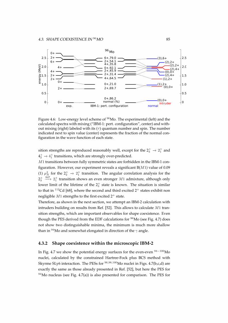
4.3. SHAPE COEXISTENCE IN 96MO 85
0
0.5
1.0
1.5
2.0
2.5
0+
0+
0+
2+
2+2+
2+
4+4+
6+
0
0.5
1.0
1.5
2.0
2.5
energ
y (
MeV
)
0+,86.2(0),0+
0+,21.0(0),0+
0+,92.1(0),0+
2+,69.7(1),2+
2+,31.4
(1),2+
2+,45.9
(2),2+2+,54.1 (2),2+
4+,64.5(2),4+
4+,35.8
(2),4+
6+,79.0 (3),6+
normal (%)IBM-1: pert. configurationexp. normal
intruder
Mo96
Figure 4.6: Low-energy level scheme of 96Mo. The experimental (left) and thecalculated spectra with mixing (“IBM-1: pert. configuration”, center) and with-out mixing (right) labeled with its (τ ) quantum number and spin. The numberindicated next to spin value (center) represents the fraction of the normal con-figuration in the wave function of each state.
sition strengths are reproduced reasonably well, except for the 2+3 −→ 2+
1 and4+
2 −→ 4+1 transitions, which are strongly over-predicted.
M1 transitions between fully symmetric states are forbidden in the IBM-1 con-figuration. However, our experiment reveals a significant B(M1) value of 0.09(1) µ2
N for the 2+2 −→ 2+
1 transition. The angular correlation analysis for the2+
3847−−→ 2+
1 transition shows an even stronger M1 admixture, although onlylower limit of the lifetime of the 2+
3 state is known. The situation is similarto that in 112Cd [68], where the second and third excited 2+ states exhibit nonnegligible M1 strengths to the first excited 2+ state.Therefore, as shown in the next section, we attempt an IBM-2 calculation withintruders building on results from Ref. [52]. This allows to calculate M1 tran-sition strengths, which are important observables for shape coexistence. Eventhough the PES derived from the EDF calculations for 96Mo (see Fig. 4.7) doesnot show two distinguishable minima, the minimum is much more shallowthan in 94Mo and somewhat elongated in direction of the γ angle.
4.3.2 Shape coexistence within the microscopic IBM-2
In Fig. 4.7 we show the potential energy surfaces for the even-even 94−100Monuclei, calculated by the constrained Hartree-Fock plus BCS method withSkyrme SLy6 interaction. The PESs for 96,98,100Mo nuclei in Figs. 4.7(b,c,d) areexactly the same as those already presented in Ref. [52], but here the PES for94Mo nucleus (see Fig. 4.7(a)) is also presented for comparison. The PES for

86 CHAPTER 4. THE MOLYBDENUM ISOTOPES
98 Mo 100Mo
0.05 0.15 0.25
0.05
0.10
0.15
0.20
0.25
0.0
0.4
0.8
1.2
1.6
2.094Mo
β s
inγ
2
96Mo
(MeV)
a) b)
c) d)
0.05
0.10
0.15
0.20
0.25
β s
inγ
20.05
0.10
0.15
0.20
0.25
β s
inγ
2
0.05
0.10
0.15
0.20
0.25
β s
inγ
2
0.0
0.4
0.8
1.2
1.6
2.0
0.0
0.4
0.8
1.2
1.6
2.0
0.0
0.4
0.8
1.2
1.6
2.0
(MeV)
(MeV) (MeV)β cosγ2
0.05 0.15 0.25β cosγ2
0.05 0.15 0.25β cosγ2
0.05 0.15 0.25β cosγ2
Figure 4.7: Contour plots of the microscopic energy surfaces in (β, γ) plane of94−98Mo (a-d). The color code ranges from 0 (mean-field minimum) to 2 MeV,and the minima are identified by the solid white circles. The Skyrme SLy6functional is used.
94Mo nucleus exhibits almost pure spherical shape, while the topology of thePES for 96Mo is flatter in β direction and is rather elongated in the γ direction.The second minimum is not visible in both nuclei. As discussed in [52], one cansee two distinct minima for 98Mo (c), one at spherical and the other at prolateregion. Much pronounced deformation characterized by the deep minimum isfound for 100Mo (d).
When one tries to describe both shape coexistence and the mixed symmetrystates at the same time in the framework of [69], there are two major problems.First, the ξ1,2,3 parameters for the Majorana interaction are not determined bysimply referring to the PES. One should then consider looking at some otherquantities than the PES, which is beyond the scope of the present work. Thesecond problem is that only one minimum is seen in the PES for 96Mo, whichmakes it difficult to fix the Hamiltonian for the intruder configuration. Forthese reasons, we end up with taking an empirical way as follows: We take,for the parametrization of the Majorana interactions, the values used in theSambataro-Molnár’s phenomenological IBM-2 calculation, ξ1 = ξ3 = −0.07
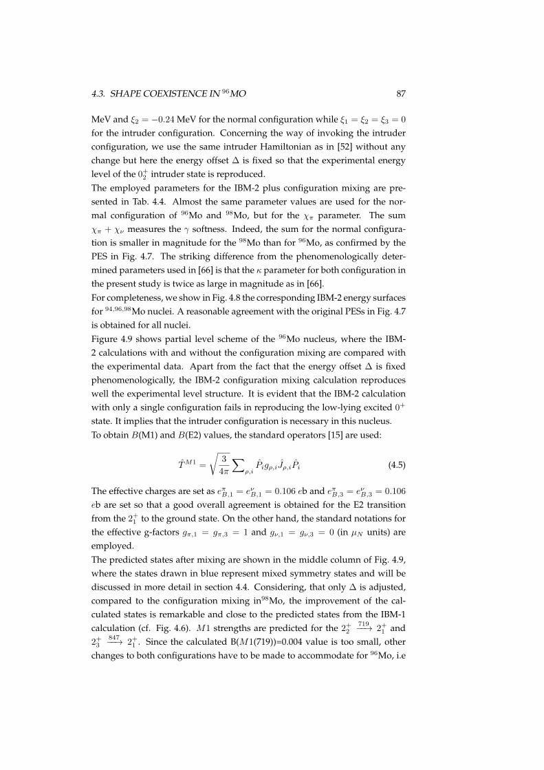
4.3. SHAPE COEXISTENCE IN 96MO 87
MeV and ξ2 = −0.24 MeV for the normal configuration while ξ1 = ξ2 = ξ3 = 0
for the intruder configuration. Concerning the way of invoking the intruderconfiguration, we use the same intruder Hamiltonian as in [52] without anychange but here the energy offset ∆ is fixed so that the experimental energylevel of the 0+
2 intruder state is reproduced.The employed parameters for the IBM-2 plus configuration mixing are pre-sented in Tab. 4.4. Almost the same parameter values are used for the nor-mal configuration of 96Mo and 98Mo, but for the χπ parameter. The sumχπ + χν measures the γ softness. Indeed, the sum for the normal configura-tion is smaller in magnitude for the 98Mo than for 96Mo, as confirmed by thePES in Fig. 4.7. The striking difference from the phenomenologically deter-mined parameters used in [66] is that the κ parameter for both configuration inthe present study is twice as large in magnitude as in [66].For completeness, we show in Fig. 4.8 the corresponding IBM-2 energy surfacesfor 94,96,98Mo nuclei. A reasonable agreement with the original PESs in Fig. 4.7is obtained for all nuclei.Figure 4.9 shows partial level scheme of the 96Mo nucleus, where the IBM-2 calculations with and without the configuration mixing are compared withthe experimental data. Apart from the fact that the energy offset ∆ is fixedphenomenologically, the IBM-2 configuration mixing calculation reproduceswell the experimental level structure. It is evident that the IBM-2 calculationwith only a single configuration fails in reproducing the low-lying excited 0+
state. It implies that the intruder configuration is necessary in this nucleus.To obtain B(M1) and B(E2) values, the standard operators [15] are used:
TM1 =
√3
4π
∑ρ,iPigρ,iJρ,iPi (4.5)
The effective charges are set as eπB,1 = eνB,1 = 0.106 eb and eπB,3 = eνB,3 = 0.106
eb are set so that a good overall agreement is obtained for the E2 transitionfrom the 2+
1 to the ground state. On the other hand, the standard notations forthe effective g-factors gπ,1 = gπ,3 = 1 and gν,1 = gν,3 = 0 (in µN units) areemployed.The predicted states after mixing are shown in the middle column of Fig. 4.9,where the states drawn in blue represent mixed symmetry states and will bediscussed in more detail in section 4.4. Considering, that only ∆ is adjusted,compared to the configuration mixing in98Mo, the improvement of the cal-culated states is remarkable and close to the predicted states from the IBM-1calculation (cf. Fig. 4.6). M1 strengths are predicted for the 2+
2719−−→ 2+
1 and2+
3847−−→ 2+
1 . Since the calculated B(M1(719))=0.004 value is too small, otherchanges to both configurations have to be made to accommodate for 96Mo, i.e
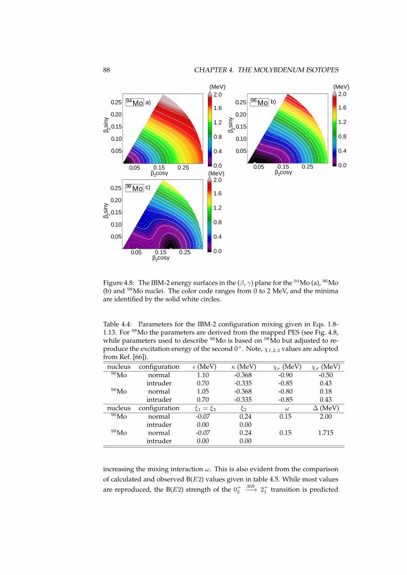
88 CHAPTER 4. THE MOLYBDENUM ISOTOPES
98 Mo
0.05 0.15 0.25
0.05
0.10
0.15
0.20
0.25
0.0
0.4
0.8
1.2
1.6
2.094Mo
β s
inγ
2
96Mo
(MeV)
a) b)
c)
0.05
0.10
0.15
0.20
0.25
β s
inγ
20.05
0.10
0.15
0.20
0.25
β s
inγ
2
0.0
0.4
0.8
1.2
1.6
2.0
0.0
0.4
0.8
1.2
1.6
2.0(MeV)
(MeV)β cosγ2
0.05 0.15 0.25β cosγ2
0.05 0.15 0.25β cosγ2
Figure 4.8: The IBM-2 energy surfaces in the (β, γ) plane for the 94Mo (a), 96Mo(b) and 98Mo nuclei. The color code ranges from 0 to 2 MeV, and the minimaare identified by the solid white circles.
Table 4.4: Parameters for the IBM-2 configuration mixing given in Eqs. 1.8-1.13. For 98Mo the parameters are derived from the mapped PES (see Fig. 4.8,while parameters used to describe 96Mo is based on 98Mo but adjusted to re-produce the excitation energy of the second 0+. Note, χ1,2,3 values are adoptedfrom Ref. [66]).
nucleus configuration ε (MeV) κ (MeV) χν (MeV) χπ (MeV)96Mo normal 1.10 -0.368 -0.90 -0.50
intruder 0.70 -0.335 -0.85 0.4398Mo normal 1.05 -0.368 -0.80 0.18
intruder 0.70 -0.335 -0.85 0.43nucleus configuration ξ1 = ξ3 ξ2 ω ∆ (MeV)
96Mo normal -0.07 0.24 0.15 2.00intruder 0.00 0.00
98Mo normal -0.07 0.24 0.15 1.715intruder 0.00 0.00
increasing the mixing interaction ω. This is also evident from the comparisonof calculated and observed B(E2) values given in table 4.5. While most valuesare reproduced, the B(E2) strength of the 0+
2369−−→ 2+
1 transition is predicted
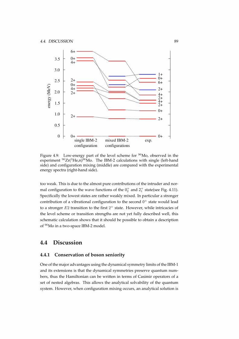
4.4. DISCUSSION 89
0+
2+
0+2+4+2+4+2+
0+
0+
2+
2+4+0+2+
4+0+
0
0.5
1.0
1.5
2.0
2.5
3.0
3.5
ener
gy (M
eV) 6+
1+
6+
single IBM-2configuration
mixed IBM-2configurations
exp.
Figure 4.9: Low-energy part of the level scheme for 96Mo, observed in theexperiment 96Zr(3He,n)96Mo. The IBM-2 calculations with single (left-handside) and configuration mixing (middle) are compared with the experimentalenergy spectra (right-hand side).
too weak. This is due to the almost pure contributions of the intruder and nor-mal configuration to the wave functions of the 0+
2 and 2+1 state(see Fig. 4.11).
Specifically the lowest states are rather weakly mixed. In particular a strongercontribution of a vibrational configuration to the second 0+ state would leadto a stronger E2 transition to the first 2+ state. However, while intricacies ofthe level scheme or transition strengths are not yet fully described well, thisschematic calculation shows that it should be possible to obtain a descriptionof 96Mo in a two-space IBM-2 model.
4.4 Discussion
4.4.1 Conservation of boson seniority
One of the major advantages using the dynamical symmetry limits of the IBM-1and its extensions is that the dynamical symmetries preserve quantum num-bers, thus the Hamiltonian can be written in terms of Casimir operators of aset of nested algebras. This allows the analytical solvability of the quantumsystem. However, when configuration mixing occurs, an analytical solution is

90 CHAPTER 4. THE MOLYBDENUM ISOTOPES
Table 4.5: Theoretical E2 transition strengths (in W.u.) compared to exper-imental values given in table 4.1. Transition given in parentages are upperlimits for relative intensities and not yet observed. States in bold are predictedto be of intruder nature in theory. The IBM-1 and IBM-2 values are discussedin section 4.3.1 and section 4.3.2, respectively.Elevel (keV) JπI Eγ (keV) JπF B(E2)IBM-2 B(E2)IBM-1 B(E2)exp
778.23 2+1 778.23 0+
1 20 20 20.7 (4)1147.96 0+
2 369.73 2+1 6 34 51 (7)
1497.88 2+2 (349) 0+
2 32 30 <93.2719.55 2+
1 0 4 13.9 (28)1497.97 0+
1 0.1 0.5 1.0+0.2−0.1
1625.92 2+3 128.01 2+
2 11 9 <46100477.61 0+
2 0.1 0 <18.7847.68 2+
1 8 32 <1.41626.00 0+
1 0.5 0 <0.41628.22 4+
1 849.99 2+1 25 31 41 (7)
1869.64 4+2 241.33 4+
1 0.4 20 0.2 (1)(243.6) 2+
3 1 5 <32371.71 2+
2 37 36 26 (11)1091.50 2+
1 0.4 1 2 (1)
not possible as symmetries are broken. It turns out that in specific cases sym-metries are partially preserved. For 96Mo and 98Mo the mixing configurationsare associated with a vibrational U(5) like structure and a γ-soft O(6) like struc-ture, so algebraic chains have the same irreps for the nested SO(5) and SO(3)algebras. The algebraic chain for the two limits are defined as
Uπν(6) ⊃{
Uπν(5)SOπν(6)
}⊃ SOπν(5) ⊃ SOπν(3), (4.6)
Since the mixing term is an O(5) scalar, the boson seniority associated to theO(5) group is preserved. This leads to interesting effects, as states with samespin and close in energy do not mix, if the seniority τ of these states differ [70].In Fig. 4.6 (on the right hand side) both, the effect of level mixing and thepreservation of the τ quantum number is observed. This is best illustratedfor the unmixed 2+ states with τ = 1, 2 between 1.4 and 2.1 MeV. The τ = 2,2+ states are in close proximity of 50 keV to each other, thus strongly repelling,leading to an energy gap of 700 keV in the perturbed configuration. If theO(5) quantum number is broken the repelling effect for the intruder 2+ statewould be cushioned by the lower-lying 2+ state. Since the τ quantum num-bers differ, such moderation of the repulsion is not observed. The best way totest the goodness of quantum numbers are transition strengths. As discussed

4.4. DISCUSSION 91
previously the 2+ intruder and normal states with τ = 2 heavily contributeto the wave function of the third 2+ state in the perturbed configuration. Theselection rule for E2 transitions states that ∆τ > 1 are forbidden if the O(5)symmetry is not broken. This is observed for the B(E2,2+
3 −→ 0+1 ) values and
predicted for the 2+3 −→ 0+
2 transition.
The used IBM-2 Hamiltonian does not fully conserve Uπν(6) symmetry or theOπν(5) symmetry. However, since the symmetries are not strongly broken onecan still approximately extract the τ and F -spin quantum numbers associatedwith a given state. This corresponds to the similarities between the calculatedB(E2) values (cf. table 4.5) in the U(6) symmetry conserving IBM-1 formalismand the symmetry breaking IBM-2 Hamiltonian. Therefore, the IBM-2 Hamil-tonian is treated as approximately O(5) symmetry conserving.
4.4.2 Conservation of F-spin and the one phonon mixed sym-metry state
The O(6) like and U(5) like configurations assumed for the unmixed config-urations for the IBM-2 calculations not only break the O(5) symmetry ratherweakly, but the F -spin quantum number is nearly preserved as well. This canbe tested by projecting the wave function of a state onto F = Fmax. Whilelow-lying states associated with fully symmetric states have more than 90% ofFmax, mixed symmetry states are below 50% of Fmax (see table 4.6). Similarto unmixed IBM-2 configurations in the O(6) and U(5) limit, the mixed IBM-2calculation shows a strongM1 transition (> 0.1 µ2
N ) to the first excited 2+ state.
The occurrence of mixed symmetry in 94Mo has been well established [71].Also in 96Mo one and two mixed symmetry phonon states are observed [53].In Fig. 4.10 the M1 strengths of 2+ states to first excited 2+ are plotted againstthe level energies of the depopulating transition for 94−98Mo. In all three cases,a state with a depopulating transition carrying the largest portion of this M1
strength is located at about 2100 keV. However, the absoluteM1 strengths varystrongly. This can be analyzed in terms of configurations mixing. In 96Mo themixed symmetry states associated to the normal configuration is predicted at2335 keV, well below the mixed symmetry state associated with the intruderconfiguration at 3236 keV. This energy gap between the mixed symmetry statesis roughly half of the value of the shift ∆ between the configurations. Due tothe large energy gap the mixed symmetry state is almost unmixed with 86.7%contribution of the normal configuration to the wave function (see the statedrawn in blue in Fig. 4.11). The calculated B(E2) and B(M1) values agree withthe experimental values and confirm the near preservation of F -spin in 96Mo.
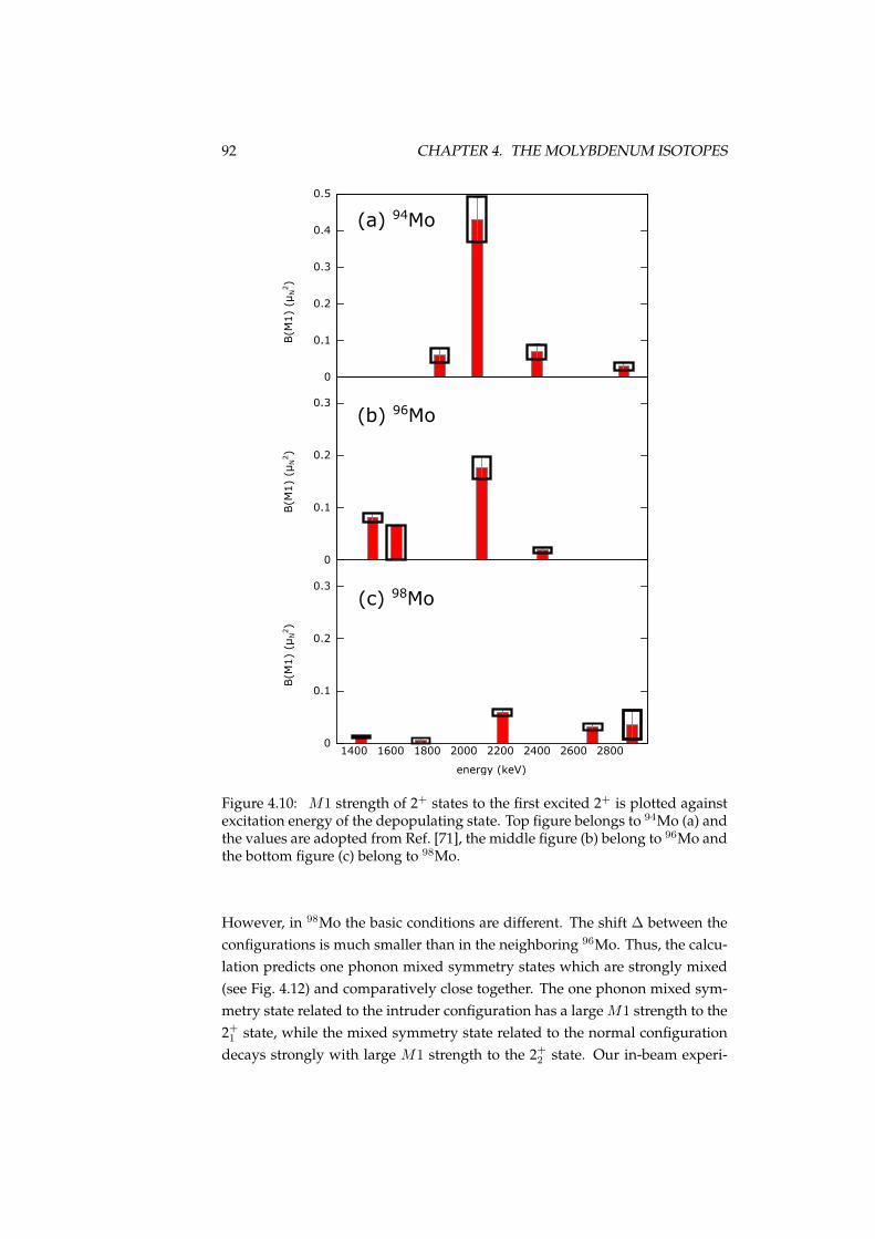
92 CHAPTER 4. THE MOLYBDENUM ISOTOPES
0
0.1
0.2
0.3
0.4(a) 94Mo
(b) 96Mo
(c) 98Mo
0.5
B(M
1)
(μN
2)
0
0.1
0.2
0.3
0
0.1
0.2
1400 1600 1800 2000 2200 2400 2600 2800
energy (keV)
0.3
B(M
1)
(μN
2)
B(M
1)
(μN
2)
Figure 4.10: M1 strength of 2+ states to the first excited 2+ is plotted againstexcitation energy of the depopulating state. Top figure belongs to 94Mo (a) andthe values are adopted from Ref. [71], the middle figure (b) belong to 96Mo andthe bottom figure (c) belong to 98Mo.
However, in 98Mo the basic conditions are different. The shift ∆ between theconfigurations is much smaller than in the neighboring 96Mo. Thus, the calcu-lation predicts one phonon mixed symmetry states which are strongly mixed(see Fig. 4.12) and comparatively close together. The one phonon mixed sym-metry state related to the intruder configuration has a large M1 strength to the2+
1 state, while the mixed symmetry state related to the normal configurationdecays strongly with large M1 strength to the 2+
2 state. Our in-beam experi-

4.4. DISCUSSION 93
normal (%) intruder (%)
(0),0+
(1),2+
(2),4+
(2),2+(0),0+
(1),2+(2),1+
(0),0+
(1),2+
(2),2+(2),4+
(3),6+
85.9
79.8
64.5
87.3
86.7
87.3
81.9
58.2
69.9
87.9
83.6
51.9
0
1
2
3
ener
gy (M
eV)
Figure 4.11: Theoretical level scheme for 96Mo is shown with the normal(blue)and intruder (red) configuration. In the parentages the O(5) quantum numberτ (seniority) is given. Above or below unmixed state the contribution of a con-figuration to the wave function of the mixed state is given. Some states in themiddle are colored blue, representing mixed symmetry states. Furthermore,next to the quantum numbers of unmixed states associated with the mixedsymmetry states, are placed black dots.
ment revealed two candidates for the one phonon mixed symmetry states ofeither configuration. The candidates are shown in table 4.7, which comparescalculated and experimental values. Note, that in some cases the parity couldnot be determined, as small M1/E2 mixing ratios could also indicate E1 tran-sitions. It is assumed that these states are of positive parity, however, as the de-populating transitions only feed positive parity states. In table 4.7, especiallythe B(M1, 2+
ms −→ 2+2 ) value is not reproduced. Therefore, either one phonon
mixed symmetry state related to the intruder configuration is not populated inthe in-beam experiment or it fragments strongly. Still, one can observe frag-ments of the M1 strength to the first excited 2+ roughly at the expected energyof 2100 keV in 98Mo. The M1 strength of the transitions depopulating the onephonon mixed symmetry state related to the normal configuration is repro-duced by the sum of the M1 strengths of the 900 keV transition and the 1093keV transition. This suggests, that the mixed symmetry state of the normalconfiguration fragments into two states at 2333 keV and 2525 keV.
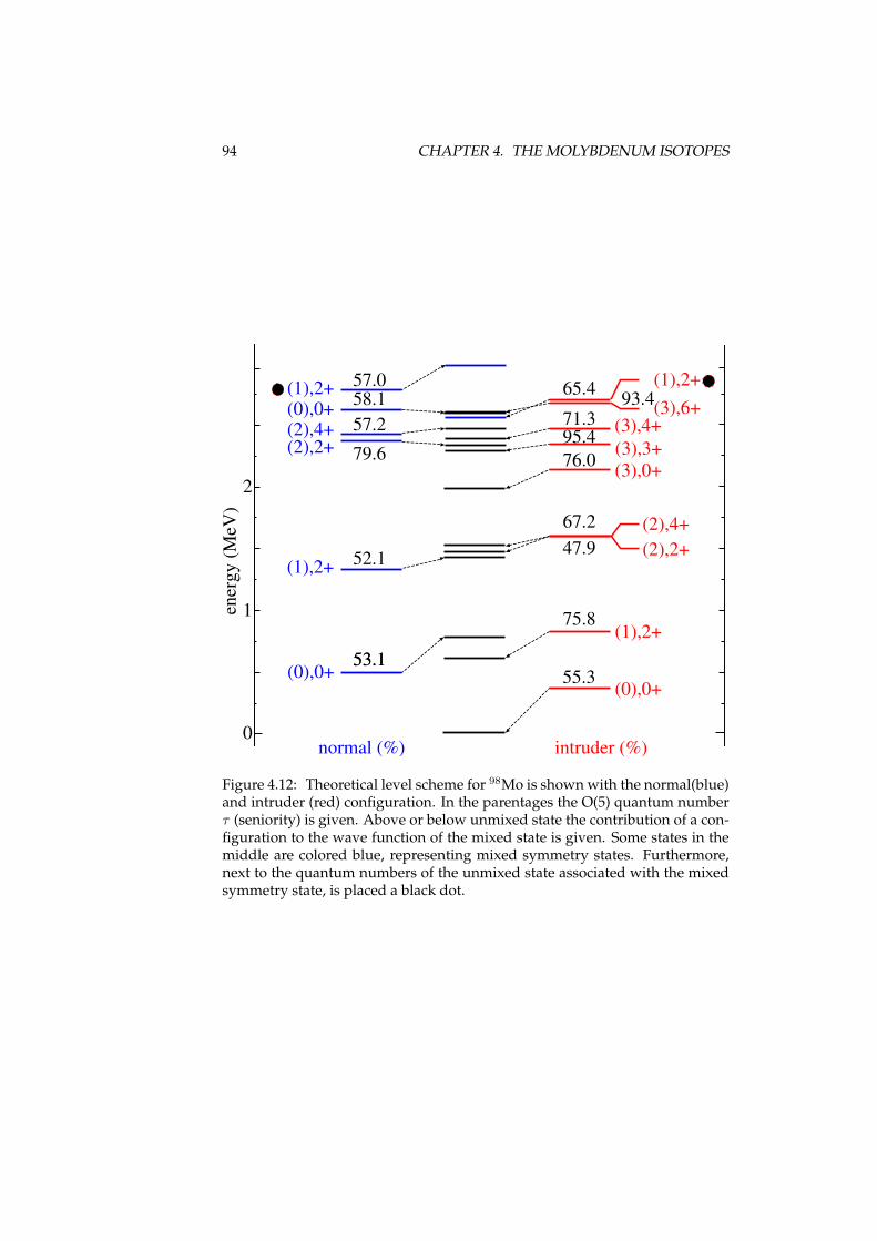
94 CHAPTER 4. THE MOLYBDENUM ISOTOPES
0
1
2
ener
gy (M
eV)
normal (%) intruder (%)
(0),0+(0),0+
(1),2+
(1),2+
(3),0+
(2),2+(2),4+
(3),3+(2),2+(2),4+ (3),4+(0),0+ (3),6+
55.3
75.8
53.1
47.967.2
76.095.471.3
93.4
52.1
79.6
57.258.1
53.1
65.4 (1),2+57.0(1),2+
Figure 4.12: Theoretical level scheme for 98Mo is shown with the normal(blue)and intruder (red) configuration. In the parentages the O(5) quantum numberτ (seniority) is given. Above or below unmixed state the contribution of a con-figuration to the wave function of the mixed state is given. Some states in themiddle are colored blue, representing mixed symmetry states. Furthermore,next to the quantum numbers of the unmixed state associated with the mixedsymmetry state, is placed a black dot.
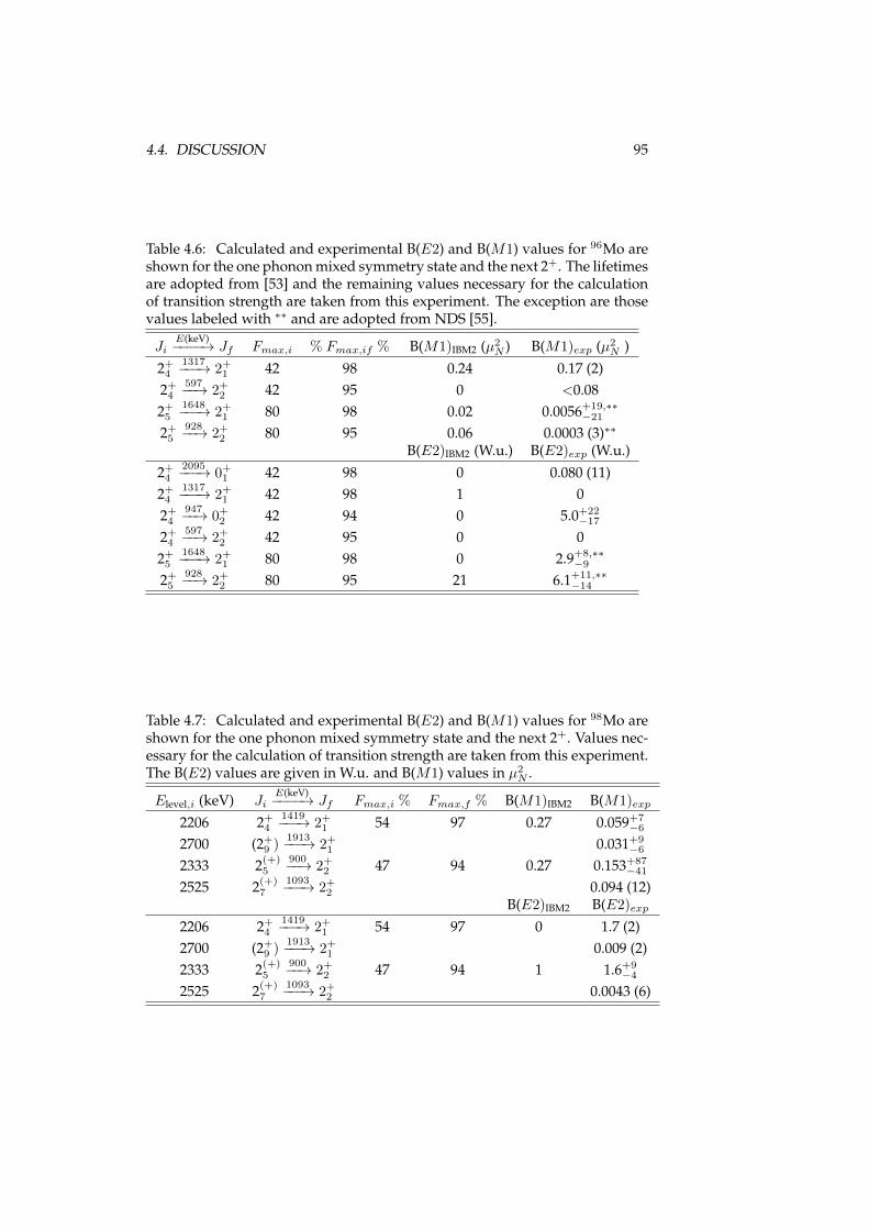
4.4. DISCUSSION 95
Table 4.6: Calculated and experimental B(E2) and B(M1) values for 96Mo areshown for the one phonon mixed symmetry state and the next 2+. The lifetimesare adopted from [53] and the remaining values necessary for the calculationof transition strength are taken from this experiment. The exception are thosevalues labeled with ∗∗ and are adopted from NDS [55].
JiE(keV)−−−−→ Jf Fmax,i % Fmax,if % B(M1)IBM2 (µ2
N ) B(M1)exp (µ2N )
2+4
1317−−−→ 2+1 42 98 0.24 0.17 (2)
2+4
597−−→ 2+2 42 95 0 <0.08
2+5
1648−−−→ 2+1 80 98 0.02 0.0056+19,∗∗
−21
2+5
928−−→ 2+2 80 95 0.06 0.0003 (3)∗∗
B(E2)IBM2 (W.u.) B(E2)exp (W.u.)2+
42095−−−→ 0+
1 42 98 0 0.080 (11)2+
41317−−−→ 2+
1 42 98 1 02+
4947−−→ 0+
2 42 94 0 5.0+22−17
2+4
597−−→ 2+2 42 95 0 0
2+5
1648−−−→ 2+1 80 98 0 2.9+8,∗∗
−9
2+5
928−−→ 2+2 80 95 21 6.1+11,∗∗
−14
Table 4.7: Calculated and experimental B(E2) and B(M1) values for 98Mo areshown for the one phonon mixed symmetry state and the next 2+. Values nec-essary for the calculation of transition strength are taken from this experiment.The B(E2) values are given in W.u. and B(M1) values in µ2
N .
Elevel,i (keV) JiE(keV)−−−−→ Jf Fmax,i % Fmax,f % B(M1)IBM2 B(M1)exp
2206 2+4
1419−−−→ 2+1 54 97 0.27 0.059+7
−6
2700 (2+9 )
1913−−−→ 2+1 0.031+9
−6
2333 2(+)5
900−−→ 2+2 47 94 0.27 0.153+87
−41
2525 2(+)7
1093−−−→ 2+2 0.094 (12)
B(E2)IBM2 B(E2)exp
2206 2+4
1419−−−→ 2+1 54 97 0 1.7 (2)
2700 (2+9 )
1913−−−→ 2+1 0.009 (2)
2333 2(+)5
900−−→ 2+2 47 94 1 1.6+9
−4
2525 2(+)7
1093−−−→ 2+2 0.0043 (6)

96 CHAPTER 4. THE MOLYBDENUM ISOTOPES
4.5 Brief summary
The data obtained from the 96Mo experiment and the performed IBM-1/IBM-2calculations are discussed and summarized in more detail in the next chapter 5together with the results from the previous experiments. Thus, in this sectionthe results are only briefly summed up.The full results obtained from two in-beam experiments on 96Mo and 98Mo arereported in the table 4.1 and 4.2. The angular correlation analyses allowed todetermine spins and multipole mixing ratios, in particular the E2/M1 mixingratio of the 2+
3847−−→ 2+
1 transition. This and the M1 strength of the 2+2
719−−→ 2+1
transition together with the drop of the 0+2 state indicates, that configuration
mixing might have to be considered. This is emphasized by single configura-tion IBM-2 calculations which only poorly agree with the observed level en-ergies and are shown in Fig 4.9. IBM-1 configuration mixing calculations (seeFig. 4.11) and IBM-2 configuration mixing were performed as well and show amuch better agreement with the obtained data.The IBM-1 calculation also allowed to investigate whether the O(5) quantumnumber is conserved. Furthermore, in the framework of IBM-2 using configu-ration mixing, the one phonon mixed symmetry state was investigated. Whilethe used IBM-2 Hamiltonian with configuration mixing does not fully conservethe F -spin quantum number and seniority, both quantum numbers are onlyslightly broken. The comparison ofM1 strength of the transition depopulatingthe one phonon mixed symmetry state to the first 2+ state shows (see table 4.6),that the predicted M1 strength is only marginally stronger than the observedvalue. For 98Mo, two one phonon mixed symmetry states for either config-uration are predicted (see Fig. 4.12), one exhibiting a strong M1 transition tothe first excited 2+ state and another exhibiting a strong M1 transition to thesecond excited 2+ state. Especially the strength of the latter transition is repro-duced by two fragments in the experimental data (see table 4.7).
Chapter 5
Summary and conclusion
In this thesis the even-even molybdenum isotopes in the A=100 mass regionand the odd-even gold isotopes in the A=200 mass region were investigated.The aim of this thesis was to test whether the Spin(5)/O(5) quantum numbersare conserved.For 193Au Interacting Boson Fermion Model calculations were performed in-cluding all possible proton orbitals between the Z=50 and Z=82 shell closure.The calculation shows that the dominant contribution to the wave function ofthe lowest states stems from the dπ,3/2 orbital. At higher excitation energies,contribution from the sπ,1/2 orbital has to be considered. On that basis, IBFMcalculations were performed employing the Spin(5) Bose-Fermi symmetrywhich specifically accounts only for a proton in the dπ,3/2 orbital. Using thenewly obtained data from an in-beam experiment, a detailed comparisonbetween the two IBFM calculations and experiment is done. Both IBFMcalculations agreed reasonably well with the relative transition strengthsobserved in the experiment. Considering that in the framework of the Spin(5)Bose-Fermi symmetry only two parameters were used to describe the levelenergies in 193Au, it was established that the τ1 quantum number for statesbelonging to the first three multiplets (τ1 = 1/2, 3/2, 5/2) is conserved.Based on the results of Ref. [72], the Interacting Boson Fermion Model usingthe Spin(5) Bose-Fermi symmetry is extended to other neighboring odd-evengold nuclei. It turns out, that the low-lying states in the odd-even gold nucleiexhibit a rather gradual evolution of levels. This agrees with the predictionof the Nilsson Model (see Fig. 5.1) of a rather smooth behavior of the twomost dominant orbitals for the odd-even gold nuclei, the dπ,3/2 and the sπ,1/2orbitals.
Using the eigenfunction derived from the Bose Fermi symmetry and thesimple expression given in Eq. (6) in sect. 3 [74], the smooth evolution of the
97

98 CHAPTER 5. SUMMARY AND CONCLUSION
Figure 5.1: (Color online) The energy of the proton Nilsson orbits are plottedagainst deformation parameter ε (similar to β). The evolution of dπ,3/2 or-bital (blue curve) and the sπ,1/2 orbital (red curve) with growing deformationis shown. The figure is adopted from Ref. [73].
level energies throughout the odd-even gold isotopes is described well. Forthis evolution the switch of the ground state from 1/2+ to 3/2+ from 189Auto 191Au is of major importance and is reproduced in the framework of theBose-Fermi symmetry. This indicates that it is sufficient to change the orderingof the τ1 = 1/2 and the τ1 = 3/2 multiplet, rather than rearrange the orderingof the dπ,3/2 and sπ,1/2 orbitals which are not described by the Nilsson Model.Beside the level energies, other important observables are transition strengths.The agreement between the absolute E2 transition strengths and data (seetable 4 in sect. 3) throughout the odd-even gold isotopes is rather good,considering that the same effective boson and effective fermion charge wasapplied for all the investigated nuclei. The notable exception is the strength ofthe 3/2+
2 −→ 3/2+1 E2 transition. In the Bose-Fermi symmetry this E2 transition
is forbidden, however, the full IBFM calculation (with the all five protonorbitals) show comparatively more contribution from the dπ,5/2 and sπ,1/2

99
orbitals to the wave function of the 3/2+2 state than for other members of the
τ1 ≤ 5/2 multiplets. Altogether, the good agreement between the predictionsof the Spin(5) Bose-Fermi symmetry and available data suggests, that theSpin(5) quantum number is conserved for 189−199Au.
In contrast to the odd-even gold isotopes, the evolution of the nuclear struc-ture in the even-even molybdenum isotopes is much more complicated. Insect. 4, the different signatures for shape coexistence in 98Mo are discussed,the most obvious one being that the first excited state is a 0+ state whichis rarely observed in even-even nuclei. The description of nuclei exhibitingconfiguration mixing is particularly challenging as such models require to fixa lot of parameters. Thus, the mapping technique described in sect. 4 [52] isof major importance. This way, one avoids to use the level scheme to adjustparameters, instead the parameters are extracted from a potential energysurface calculated by a microscopic model. The PES of 98Mo calculated usingconstrained Hartree-Fock plus BCS method with Skyrme SLy6 interactionshows two distinct minima, where one minimum can be associated with arather vibrational configuration and the second minimum can be associatedwith a rather γ-soft configuration. Indeed, the mixing of these two configura-tions reproduces many features observed in the 98Mo. Most importantly, thequadrupole moments and the β deformation of the lowest excited 2+ statesare in good agreement with experimental values. The successful application ofthe mapping technique motivated to extend this procedure to the neighboring96Mo, where the microscopic PES shows one distinct minimum (see Fig. 4 insect. 4 and Ref. [52]).In sect. 4.2 the result of a single configuration IBM-2 calculation mappedonto the microscopic PES (exhibiting a rather vibrational nuclear shape)is compared with data obtained from an in-beam experiment on 96Mo (cf.Fig. 4.9). The agreement between calculated and observed level energies ispoor. Indeed, the obtained data again show characteristics associated withshape coexistence. The angular correlation analyses of the 2+
2719−−→ 2+
1 and2+
3847−−→ 2+
1 transitions show small E2/M1 multipole mixing ratios, whichcannot be described in a purely vibrational model. Here, transitions exhibitingM1 characteristics are forbidden. Such transitions between the low-lying 2+
states are found in the 112Cd as well, where shape coexistence was observed.Another indication of configuration mixing is the drop of the level energy ofthe second 0+ from 94Mo to 96Mo (see Fig. 4.5).Thus, based on the unmixed configurations of the calculations for 98Mo,two IBM-1 configurations, one in the U(5) limit and one in the O(6) limit,were derived. These configurations were mixed such, that the level ener-

100 CHAPTER 5. SUMMARY AND CONCLUSION
gies in 96Mo were reproduced. The schematic calculations show a muchenhanced agreement with the data. Particularly, the calculations show thatthe E2 strength of the 0+
2947−−→ 2+
1 transition depends on the strength ofthe configuration mixing. Since the IBM-1 calculations were specificallycarried out for a vibrational and a γ-soft configuration, the O(5) quantumnumbers are preserved and discussed for selected transitions obeying E2
selection rules associated with τ quantum numbers. Another schematiccalculation of configuration mixing was carried out for 96Mo, this time usingthe IBM-2 formalism. The same parameters as those used for the calculationsin 98Mo [52] were adopted. Only the parameter ∆, which controls the shiftbetween the two configurations was varied such that the second 0+ in 96Mo isreproduced. While this is not sufficient to fully reproduce transition strengths,the concept of configuration mixing seems to be required to describe thelow-lying states in 96Mo. For example, due to configuration mixing, M1
strengths are predicted between the lowest 2+ states and correspond toexperimental observations. Also, the PES of the IBM-2 calculation showsremarkable agreement with the microscopic PES. Furthermore, the agreementof the M1 strength from the mixed symmetry state to the first excited 2+ statesuggests that F-spin and O(5) quantum numbers are approximately conserved.

Appendix A
A.1 γγ angular correlation analysis
6000700080009000
100001100012000
rel.
inte
nsity
(778,847)keV
correlation groups (Θ1 ,Θ2 ,φ)
45,9
0,90
90,4
5,90
45,9
0,18
045
,225
,045
,135
,045
,90,
3590
,45,
3545
,90,
5590
,90,
90
δ=-0.12 (5)δ
=-1.05=-6.90δ
Figure A.1: Comparison of theoretical angular correlations with different spinhypotheses (black solid, green dashed line and blue dashed line) with relativeintensities obtained from eleven correlation groups at the OSIRIS setup for the778-847 keV γγ coincidence. The multipole mixing ration δ = −0.12(5) is fa-vored. See text in sect. 4.2 for more detail.
101

102 APPENDIX A.
0.8
0.9
1.0
1.1
1.2
1.3data
δ=-0.12 (5)δ
δ=-1.05=-6.90
correlation groups (Θ1 ,Θ2 ,φ)
45,9
0,90
90,4
5,90
45,9
0,18
045
,225
,045
,135
,045
,90,
3590
,45,
3545
,90,
5590
,90,
90
rel. inte
nsi
ty
Figure A.2: The integrated volumes of the 847 and 849 keV γ lines in coin-cidence with the 778 keV transition in the correlation groups are compared tosuperposed theoretical spin hypotheses (see discussion of the state at 1625 keVin the text 4.2.1 for details).
900100011001200130014001500160017001800
rel.
inte
nsity
correlation groups (Θ1 ,Θ2 ,φ)
45,9
0,90
90,4
5,90
45,9
0,18
045
,225
,045
,135
,045
,90,
3590
,45,
3545
,90,
5590
,90,
90(480,719)keV δ =-17.8
δ=+0.12
+10.3-64.6
Figure A.3: The spin hypothesis 3480,δ480−−−−−→ 2
719,δ719=−0.12−−−−−−−−−−→ 2 is comparedto relative intensities obtained from nine correlation groups at the OSIRISsetup for the 719-480 keV γγ coincidences. The multipole mixing ratio δ480 =−17.8+10.3
−64.6 (black solid) obtained from a least-square fit is favored to δ480 =−0.12 (4) (green dashed line) reported in Ref. [53].

A.1. γγ ANGULAR CORRELATION ANALYSIS 103
5000550060006500700075008000850090009500
rel.
inte
nsity
correlation groups (Θ1 ,Θ2 ,φ)
45,9
0,90
90,4
5,90
45,9
0,18
045
,225
,045
,135
,045
,90,
3590
,45,
3545
,90,
5590
,90,
90
(1200,778)keV δ=+0.34 (4)δ =+0.89
Figure A.4: Comparison of theoretical angular correlations 31200,δ1200−−−−−−→ 2
778,δ778=+0.0−−−−−−−−−→ 2 with relative intensities obtained from nine correlation groupsat the OSIRIS setup. The multipole mixing ratio δ1200 = 0.34 (4) (black solidline) is favored to the E2/M1 mixing ratio δ1200 = 0.89 (10) reported inRef. [53].

104 APPENDIX A.
2500
3000
3500
4000
4500
5000
rel.
inte
nsity
(644, 787)keV
δ644δ644=+0.27δ644=+0.58
90,90,13
5
correlation groups (Θ1 ,Θ2 ,φ)
90,45,13
590
,90,18
090
,90,-9
090
,45,0
90,45,90
45,90,-1
3545
,90,0
45,90,-9
045
,45,18
045
,135
,180
=+1.67 (25)
Figure A.5: The spin hypothesis 2644,δ644−−−−−→ 2
787,δ787=+0.0−−−−−−−−−→ 0 is compared torelative intensities obtained from eleven correlation groups at the YRAST Ballsetup. The multipole mixing ratio δ644 = +1.67 (25) (black solid) obtained froma least-square fit is favored to δ644 = +0.27 (2) (blue dashed line) reported inRef. [60] and δ644 = +0.58 (5) (green dashed line) reported in Ref. [61].
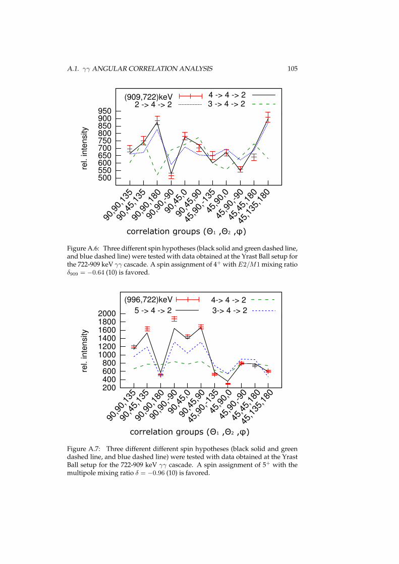
A.1. γγ ANGULAR CORRELATION ANALYSIS 105
500550600650700750800850900950
rel.
inte
nsity
90,9
0,13
5
correlation groups (Θ1 ,Θ2 ,φ)
90,4
5,13
590
,90,
180
90,9
0,-9
090
,45,
090
,45,
9045
,90,
-135
45,9
0,0
45,9
0,-9
045
,45,
180
45,1
35,1
80
(909,722)keV 4 -> 4 -> 23 -> 4 -> 22 -> 4 -> 2
Figure A.6: Three different spin hypotheses (black solid and green dashed line,and blue dashed line) were tested with data obtained at the Yrast Ball setup forthe 722-909 keV γγ cascade. A spin assignment of 4+ withE2/M1 mixing ratioδ909 = −0.64 (10) is favored.
200400600800
100012001400160018002000
rel.
inte
nsity
(996,722)keV5 -> 4 -> 2
4-> 4 -> 23-> 4 -> 2
90,9
0,13
5
correlation groups (Θ1 ,Θ2 ,φ)
90,4
5,13
590
,90,
180
90,9
0,-9
090
,45,
090
,45,
9045
,90,
-135
45,9
0,0
45,9
0,-9
045
,45,
180
45,1
35,1
80
Figure A.7: Three different different spin hypotheses (black solid and greendashed line, and blue dashed line) were tested with data obtained at the YrastBall setup for the 722-909 keV γγ cascade. A spin assignment of 5+ with themultipole mixing ratio δ = −0.96 (10) is favored.

106 APPENDIX A.

List of Figures
1.1 A schematic figure showing degenerate states with same isospinfor 12C and its isobaric neighbors. . . . . . . . . . . . . . . . . . . 8
1.2 A schematic figure showing the splitting of degenerate stateswith the same isospin T=1 and T=3/2 in terms of binding en-ergies. This figure is adopted from Ref. [8]. . . . . . . . . . . . . 10
1.3 A schematic figure showing a level scheme using the dynamicalO(6) limit and the corresponding reduction rules (see text). Allstates share the same σ = 2 quantum number. Labeling is givenin the box. All the shown arrows are E2 transition. . . . . . . . . 12
2.1 Two exemplary (γγ) cascades (A,B) and (A,C) are show. Thewidth of arrows correspond to the relative γ intensity betweentransition B and C. The two parallel lines symbolize the gate setat the energy of transition A. . . . . . . . . . . . . . . . . . . . . . 18
2.2 Exemplary γγ cascades (B,A), (B,D) and (C,E) are show. The twoparallel lines symbolize the consecutive gates set at the energyof transition D and E, respectively. See text for detail. . . . . . . 20
4.1 Total projection of the γγ coincidence data (up to 2000 keV)of the 96Mo experiment. The strongest γ lines are observed ataround 800 keV and belong to Yrast band transitions of 96Mo. . 70
4.2 Comparison of two spin hypotheses 2719,δ719−−−−−→ 2
778,δ778=0−−−−−−−→ 0
with different E2/M1 mixing ratios δ719 (black solid and greendashed line) with relative intensities obtained from nine γγ an-gular correlation groups at the OSIRIS setup. The E2/M1 mix-ing ration δ = +0.40 (3) obtained from a least-square fit is fa-vored over δ = +1.1 (1), one of two minima reported in Ref. [53].The smaller E2/M1 mixing ratio +0.34+0.90
−0.70 reported in Ref. [53]agrees with the present values from both experiments (see alsoFig. 4.3). . . . . . . . . . . . . . . . . . . . . . . . . . . . . . . . . 72
107
108 LIST OF FIGURES
4.3 Comparison of theoretical angular correlations of the 2719,δ719−−−−−→
2778,δ778=0−−−−−−−→ 0 spin hypothesis with relative intensities obtained
from eleven correlation groups at the YRAST Ball setup for the778-719 keV γγ coincidence. The E2/M1 mixing ratio δ = +0.40
(10) (black solid) obtained from a least square fit is favored overδ = +1.1 (1) (green dashed line) reported in Ref. [53]. For moreinformation see Fig. 4.2. . . . . . . . . . . . . . . . . . . . . . . . 73
4.4 Determination of the effective lifetime by analyzing the lineshape of the 1913 keV transition in 98Mo depopulating a (2+)state at 2700 keV using a gate set on the 787 keV transition. Co-incidence spectra with a gate set on the 787 keV transition fortwo different angles are shown. The black solid line representsthe simulated line shape at forward (a) and backward (b) angle.The determined effective mean lifetime is τ = 0.25 (5) ps. . . . . 74
4.5 Low-lying states observed in experiments [55,56] are plotted fordifferent molybdenum isotopes. To provide a better overview,the figure is split for states belonging to the Yrast band (a) andoff-Yrast states (b). . . . . . . . . . . . . . . . . . . . . . . . . . . 82
4.6 Low-energy level scheme of 96Mo. The experimental (left) andthe calculated spectra with mixing (“IBM-1: pert. configura-tion”, center) and without mixing (right) labeled with its (τ )quantum number and spin. The number indicated next to spinvalue (center) represents the fraction of the normal configurationin the wave function of each state. . . . . . . . . . . . . . . . . . 85
4.7 Contour plots of the microscopic energy surfaces in (β, γ) planeof 94−98Mo (a-d). The color code ranges from 0 (mean-field mini-mum) to 2 MeV, and the minima are identified by the solid whitecircles. The Skyrme SLy6 functional is used. . . . . . . . . . . . . 86
4.8 The IBM-2 energy surfaces in the (β, γ) plane for the 94Mo (a),96Mo (b) and 98Mo nuclei. The color code ranges from 0 to 2MeV, and the minima are identified by the solid white circles. . 88
4.9 Low-energy part of the level scheme for 96Mo, observed in theexperiment 96Zr(3He,n)96Mo. The IBM-2 calculations with sin-gle (left-hand side) and configuration mixing (middle) are com-pared with the experimental energy spectra (right-hand side). . 89
4.10 M1 strength of 2+ states to the first excited 2+ is plotted againstexcitation energy of the depopulating state. Top figure belongsto 94Mo (a) and the values are adopted from Ref. [71], the middlefigure (b) belong to 96Mo and the bottom figure (c) belong to 98Mo. 92

LIST OF FIGURES 109
4.11 Theoretical level scheme for 96Mo is shown with the nor-mal(blue) and intruder (red) configuration. In the parentagesthe O(5) quantum number τ (seniority) is given. Above or belowunmixed state the contribution of a configuration to the wavefunction of the mixed state is given. Some states in the middleare colored blue, representing mixed symmetry states. Further-more, next to the quantum numbers of unmixed states associ-ated with the mixed symmetry states, are placed black dots. . . 93
4.12 Theoretical level scheme for 98Mo is shown with the nor-mal(blue) and intruder (red) configuration. In the parentagesthe O(5) quantum number τ (seniority) is given. Above or belowunmixed state the contribution of a configuration to the wavefunction of the mixed state is given. Some states in the middleare colored blue, representing mixed symmetry states. Further-more, next to the quantum numbers of the unmixed state asso-ciated with the mixed symmetry state, is placed a black dot. . . 94
5.1 (Color online) The energy of the proton Nilsson orbits are plot-ted against deformation parameter ε (similar to β). The evo-lution of dπ,3/2 orbital (blue curve) and the sπ,1/2 orbital (redcurve) with growing deformation is shown. The figure isadopted from Ref. [73]. . . . . . . . . . . . . . . . . . . . . . . . . 98
A.1 Comparison of theoretical angular correlations with differentspin hypotheses (black solid, green dashed line and blue dashedline) with relative intensities obtained from eleven correla-tion groups at the OSIRIS setup for the 778-847 keV γγ coinci-dence. The multipole mixing ration δ = −0.12(5) is favored. Seetext in sect. 4.2 for more detail. . . . . . . . . . . . . . . . . . . . 101
A.2 The integrated volumes of the 847 and 849 keV γ lines in coin-cidence with the 778 keV transition in the correlation groups arecompared to superposed theoretical spin hypotheses (see dis-cussion of the state at 1625 keV in the text 4.2.1 for details). . . . 102
A.3 The spin hypothesis 3480,δ480−−−−−→ 2
719,δ719=−0.12−−−−−−−−−−→ 2 is compared torelative intensities obtained from nine correlation groups at theOSIRIS setup for the 719-480 keV γγ coincidences. The multi-pole mixing ratio δ480 = −17.8+10.3
−64.6 (black solid) obtained froma least-square fit is favored to δ480 = −0.12 (4) (green dashedline) reported in Ref. [53]. . . . . . . . . . . . . . . . . . . . . . . 102

110 LIST OF FIGURES
A.4 Comparison of theoretical angular correlations 31200,δ1200−−−−−−→ 2
778,δ778=+0.0−−−−−−−−−→ 2 with relative intensities obtained from nine cor-relation groups at the OSIRIS setup. The multipole mixing ratioδ1200 = 0.34 (4) (black solid line) is favored to theE2/M1 mixingratio δ1200 = 0.89 (10) reported in Ref. [53]. . . . . . . . . . . . . 103
A.5 The spin hypothesis 2644,δ644−−−−−→ 2
787,δ787=+0.0−−−−−−−−−→ 0 is compared torelative intensities obtained from eleven correlation groups atthe YRAST Ball setup. The multipole mixing ratio δ644 = +1.67
(25) (black solid) obtained from a least-square fit is favored toδ644 = +0.27 (2) (blue dashed line) reported in Ref. [60] andδ644 = +0.58 (5) (green dashed line) reported in Ref. [61]. . . . . 104
A.6 Three different spin hypotheses (black solid and green dashedline, and blue dashed line) were tested with data obtained at theYrast Ball setup for the 722-909 keV γγ cascade. A spin assign-ment of 4+ with E2/M1 mixing ratio δ909 = −0.64 (10) is favored. 105
A.7 Three different different spin hypotheses (black solid and greendashed line, and blue dashed line) were tested with data ob-tained at the Yrast Ball setup for the 722-909 keV γγ cascade. Aspin assignment of 5+ with the multipole mixing ratio δ = −0.96
(10) is favored. . . . . . . . . . . . . . . . . . . . . . . . . . . . . . 105

List of Tables
1.1 conservations of quantum numbers and the associated groups . 8
4.1 Results of this work on 96Mo. States discussed in section 4.2.1are labeled with a sharp sign (#). Newly observed states arelabeled with a asterisk (∗) and newly observed transitions withdagger (†). Furthermore, γ intensities Iγ of transitions that arelisted in NDS [55] but are not observed due to the sensitivitylimit of the detector system or background are labeled with adash (−). If a value is adopted from NDS it is labeled with adouble asterisk (∗∗). If a spin assignment of a state due to an-gular correlation analysis is not unique, those spins are labeledwith a double-dagger (‡‡). If an angular correlation analysis isnot feasible but selection rules suggest the multipole character-istic of the γ transition, the multipolarity is given in parentheses. 75
4.2 Results of this work on 98Mo. States discussed in section 4.2.1are labeled with a sharp sign (#). Newly observed states arelabeled with a asterisk (∗) and newly observed transitions withdagger (†). Furthermore, γ intensities Iγ of transitions that arelisted in NDS [56] but are not observed due to the sensitivitylimit of the detector system or background are labeled with adash (−). If a value is adopted from NDS it is labeled with adouble asterisk (∗∗). If a spin assignment of a state due to an-gular correlation analysis is not unique, those spins are labeledwith a double-dagger (‡‡). If an angular correlation analysis isnot feasible but selection rules suggest the multipole character-istic of the γ transition, the multipolarity is given in parentheses. 77
4.3 Parameters of the IBM-1 Hamiltonians in Eqs. 4.1, 4.2 and thoseresponsible for configuration mixing in 96Mo. Furthermore, ω =
0.1 and ∆ = 0.8 MeV for the mixing of the configuration. . . . . 84
111
112 LIST OF TABLES
4.4 Parameters for the IBM-2 configuration mixing given in Eqs. 1.8-1.13. For 98Mo the parameters are derived from the mapped PES(see Fig. 4.8, while parameters used to describe 96Mo is basedon 98Mo but adjusted to reproduce the excitation energy of thesecond 0+. Note, χ1,2,3 values are adopted from Ref. [66]). . . . 88
4.5 Theoretical E2 transition strengths (in W.u.) compared to exper-imental values given in table 4.1. Transition given in parentagesare upper limits for relative intensities and not yet observed.States in bold are predicted to be of intruder nature in theory.The IBM-1 and IBM-2 values are discussed in section 4.3.1 andsection 4.3.2, respectively. . . . . . . . . . . . . . . . . . . . . . . 90
4.6 Calculated and experimental B(E2) and B(M1) values for 96Moare shown for the one phonon mixed symmetry state and thenext 2+. The lifetimes are adopted from [53] and the remain-ing values necessary for the calculation of transition strength aretaken from this experiment. The exception are those values la-beled with ∗∗ and are adopted from NDS [55]. . . . . . . . . . . 95
4.7 Calculated and experimental B(E2) and B(M1) values for 98Moare shown for the one phonon mixed symmetry state and thenext 2+. Values necessary for the calculation of transitionstrength are taken from this experiment. The B(E2) values aregiven in W.u. and B(M1) values in µ2
N . . . . . . . . . . . . . . . . 95
Bibliography
[1] T. Lee, Particle Physics and Introduction to Field Theory. Chur, Switzerland:Harwood Acadamic Publishers GmbH, 1981.
[2] E. Noether, “Invariante Variationsprobleme,” Nachr. D. König. Gesellsch. D.Wiss. Zu Göttingen, pp. 235–257, 1918.
[3] P. Ehrenfest, “Bemerkung über die angenäherte Gültigkeit der klassischenMechanik innerhalb der Quantenmechanik,” Zeitschrift für Physik, vol. 45,no. 7-8, pp. 455–457, 1927.
[4] G. Sterman, An Introduction to Quantum Field Theory. Cambridge, UK:Cambridge University Press, 1993.
[5] I. Joliot-Curie and F. Joliot, “The Emission of High energy Photons fromHydrogenous Substances Irradiated with Very Penetrating Alpha Rays,”Comptes Rendus, vol. 194, p. 273, 1932.
[6] J. Chadwick, “Possible Existence of a Neutron,” Nature, vol. 129, p. 312,1932.
[7] W. Heisenberg, “Über den Bau der Atomkern,” Zeitschrift für Physik,vol. 77, no. 1-2, pp. 1–11, 1932.
[8] A. Frank, J. Jolie, and P. V. Isacker, Symmetries in Atomic Nuclei. Springer,2009.
[9] A. Frank and P. V. Isacker, Algebraic Methods in Molelcular & Nuclear Struc-ture Physics. John Wiley & Sons, 1994.
[10] D.Dubbers and H.-J. Stöckmann, Quantum Physics: The Bottom-Up Ap-proach. Springer, 1993.
[11] F. Ajzenberg-Selove, “Energy levels of light nuclei A = 11–12 ,” NuclearPhysics A, vol. 433, no. 1, pp. 1 – 157, 1985.
113
114 BIBLIOGRAPHY
[12] E.P.Wigner, “Proceedings of the Robert A Welch Foundation Conferenceson Chemical Research. I The Structure of the Nucleus,” 1957.
[13] K.Baum et al., “Masses of 32Ar and 33Ar for Fundamental Tests,” Phys.Rev. Lett., vol. 91, p. 260801, 2003.
[14] K.Baum, “High-accuracy mass spectrometry with stored ions,” Phys. Re-ports, vol. 425, p. 1, 2006.
[15] F. Iachello and A. Arima, The Interacting Boson Model. Cambridge Univer-sity Press, Cambridge, 1987.
[16] A. Arima and F. Iachello, “Interacting Boson Model of Collective NuclearStates I. The Vibrational Limit,” Ann. Phys, vol. 99, pp. 253–317, 1976.
[17] A. Arima and F. Iachello, “Interacting Boson Model of Collective NuclearStates II. The Rotational Limit,” Ann. Phys, vol. 111, pp. 201–238, 1978.
[18] A. Arima and F. Iachello, “Interacting Boson Model of Collective NuclearStates IV. The O(6) Limit,” Ann. Phys, vol. 123, pp. 468–492, 1979.
[19] M.Göppert-Mayer, “Nuclear configurations in the spin-orbit couplingmodel. I. Empirical Evidence,” Phys. Rev., vol. 78, p. 16, 1950.
[20] M.Göppert-Mayer, “Nuclear configurations in the spin-orbit couplingmodel. II. Theoretical Considerations,” Phys. Rev., vol. 78, p. 22, 1950.
[21] O.Haxel, H.E.Suess, and J.H.D.Jensen, “Zur Interpretation der ausgeze-ichneten Nukleonenzahlen im Bau des Atomkerns,” Phys. Rev., vol. 75,p. 1766, 1949.
[22] A.Bohr and B.R.Mottelson, Nuclear Structure Volume II. W.A Benjamin Inc.Massachusetts, 1975.
[23] G. Gneuss and W. Greiner, “Collective potential energy surfaces and nu-clear structure ,” Nuclear Physics A, vol. 171, no. 3, pp. 449 – 479, 1971.
[24] L. Cooper, “Bound Electron Pairs in a Degenerate Fermi Gas,” Phys. Rev.,vol. 104, p. 1189, 1956.
[25] L. Cooper, “Microscopic Theory of Superconductivity,” Phys. Rev.,vol. 106, p. 162, 1957.
[26] F. Iachello and P. V. Isacker, The Interacting Boson-Fermion Model. Cam-bridge University Press, Cambridge, 1991.
BIBLIOGRAPHY 115
[27] N. Pietralla, P. von Brentano, and A. F. Lisetskiy, “Experiments on mul-tiphonon states with proton neutron mixed symmetry in vibrational nu-clei,” Prog. Part. Nucl. Phys., vol. 60, p. 225, 2013.
[28] A. Richter, “Probing the nuclear magnetic dipole response with electrons,photons and hadrons ,” Progress in Particle and Nuclear Physics, vol. 34,no. 0, pp. 261 – 284, 1995. Electromagnetic Probes and the StructureHadrons and Nuclei.
[29] R. Mohan, M. Danos, and L. C. Biedenharn, “Three-Fluid Hydrodynami-cal Model of Nuclei,” Phys. Rev. C, vol. 3, pp. 1740–1749, May 1971.
[30] D. Savran, T. Aumann, and A. Zilges, “Experimental studies of the PygmyDipole Resonance ,” Progress in Particle and Nuclear Physics, vol. 70, no. 0,pp. 210 – 245, 2013.
[31] J. Wood, K. Heyde, W. Nazarewicz, M. Huyse, and P. van Duppen, “Co-existence in even-mass nuclei ,” Physics Reports, vol. 215, no. 3–4, pp. 101– 201, 1992.
[32] K. Heyde and J. L. Wood, “Shape coexistence in atomic nuclei,” Rev. Mod.Phys., vol. 83, pp. 1467–1521, Nov 2011.
[33] V. Werner, D. Belic, P. von Brentano, C. Fransen, A. Gade, H. von Garrel,J. Jolie, U. Kneissl, C. Kohstall, A. Linnemann, A. Lisetskiy, N. Pietralla,H. Pitz, M. Scheck, K.-H. Speidel, F. Stedile, and S. Yates, “Proton–neutronstructure of the N=52 nucleus 92Zr ,” Physics Letters B, vol. 550, no. 3–4,pp. 140 – 146, 2002.
[34] G. S. Simpson, J. A. Pinston, D. Balabanski, J. Genevey, G. Georgiev, J. Jolie,D. S. Judson, R. Orlandi, A. Scherillo, I. Tsekhanovich, W. Urban, andN. Warr, “High-spin mus isomer in 98Zr,” Phys. Rev. C, vol. 74, p. 064308,Dec 2006.
[35] A. Chakraborty, E. E. Peters, B. P. Crider, C. Andreoiu, P. C. Bender, D. S.Cross, G. A. Demand, A. B. Garnsworthy, P. E. Garrett, G. Hackman,B. Hadinia, S. Ketelhut, A. Kumar, K. G. Leach, M. T. McEllistrem, J. Pore,F. M. Prados-Estévez, E. T. Rand, B. Singh, E. R. Tardiff, Z.-M. Wang, J. L.Wood, and S. W. Yates, “Collective Structure in 94Zr and Subshell Effectsin Shape Coexistence,” Phys. Rev. Lett., vol. 110, p. 022504, Jan 2013.
[36] W. Urban, M. Jentschel, R. F. Casten, J. Jolie, C. Bernards, B. Maerkisch,T. Materna, P. Mutti, L. Prochniak, T. Rzkaca-Urban, G. S. Simpson,
116 BIBLIOGRAPHY
V. Werner, and S. Ahmed, “0+2 band in 102Ru and the evolution of nu-clear deformation in Ru isotopes,” Phys. Rev. C, vol. 87, p. 031304, Mar2013.
[37] K. Nomura, N. Shimizu, and T. Otsuka, “Mean-Field Derivation of theInteracting Boson Model Hamiltonian and Exotic Nuclei ,” Phys. Rev. Lett.,vol. 101, p. 142501, Sep 2008.
[38] J. Ginocchio and M. Kirson, “An intrinsic state for the interacting bosonmodel and its relationship to the Bohr-Mottelson model ,” Nuclear PhysicsA, vol. 350, no. 1–2, pp. 31 – 60, 1980.
[39] K. Nomura, N. Shimizu, and T. Otsuka, “Formulating the interacting bo-son model by mean-field methods ,” Phys. Rev. C, vol. 81, p. 044307, Apr2010.
[40] E. Chabanat, P. Bonche, P. Haensel, J. Meyer, and R. Schaeffer, “A Skyrmeparametrization from subnuclear to neutron star densities Part II. Nucleifar from stabilities ,” Nuclear Physics A, vol. 635, no. 1–2, pp. 231 – 256,1998.
[41] P. Bonche, H. Flocard, and P. Heenen, “Solution of the Skyrme HF andBCS equation on a 3D mesh ,” Computer Physics Communications, vol. 171,no. 1, pp. 49 – 62, 2005.
[42] A. Bohr and B. R. Mottelson, Nuclear Structure Vol. II . Benjamin, NewYork, 1975.
[43] M. Bender, P.-H. Heenen, and P.-G. Reinhard, “Self-consistent mean-fieldmodels for nuclear structure ,” Rev. Mod. Phys., vol. 75, pp. 121–180, Jan2003.
[44] A. Linnemann, Das HORUS-Würfelspektrometer und Multiphononenanre-gungen in 106Cd. PhD thesis, Universität zu Köln, 2005.
[45] K. Krane and R. Steffen, “Determination of the E2/M1 Multipole MixingRatios of the Gamma Transitions in 110Cd,” Phys. Rev. C, vol. 2, pp. 724–734, 1970.
[46] K. Krane, R. Steffen, and R. Wheeler, “Directional Correlations of GammaRadiations Emitted from Nuclear States Orientated by Nuclear Reactionsor Cryogenic Methods,” Nucl. Data Tab., vol. 11, pp. 351–406, 1973.
[47] I. Wiedenhöver, “Programm CORLEONE,” 1995. Universität zu Köln.
BIBLIOGRAPHY 117
[48] I. Wiedenhöver, O. Vogel, H. Klein, A. Dewald, P. von Brentano,J. Gableske, R. Krücken, N. Nicolay, A. Gelberg, P. Petkov, A. Gizon, J. Gi-zon, D. Bazzacco, C. Rossi Alvarez, G. de Angelis, S. Lunardi, P. Pavan,D. R. Napoli, S. Frauendorf, F. Donau, R. V. F. Janssens, and M. P. Carpen-ter, “Detailed angular correlation analysis with 4pi spectrometers: Spindeterminations and multipolarity mixing measurements in 128Ba,” Phys.Rev. C, vol. 58, pp. 721–728, Aug 1998.
[49] H. Duckwitz, “Programm Mammel ,” 2013. Universität zu Köln.
[50] R. Wirowski, M. Schimmer, L. Eßer, S. Albers, K. Zell, and P. von Brentano,“gamma-spectroscopy of 114Sn with the OSIRIS-cube-spectrometer ,” Nu-clear Physics A, vol. 586, no. 3, pp. 427 – 444, 1995.
[51] C. Beausang, C. Barton, M. Caprio, R. Casten, J. Cooper, R. Krücken,B. Liu, J. Novak, Z. Wang, M. Wilhelm, A. Wilson, N. Zamfir, andA. Zilges, “The YRAST Ball array ,” Nuclear Instruments and Methods inPhysics Research Section A: Accelerators, Spectrometers, Detectors and Associ-ated Equipment, vol. 452, no. 3, pp. 431 – 439, 2000.
[52] T. Thomas, K. Nomura, V. Werner, T. Ahn, N. Cooper, H. Duckwitz,M. Hinton, G. Ilie, J. Jolie, P. Petkov, and D. Radeck, “Evidence for shapecoexistence in 98Mo,” Phys. Rev. C, vol. 88, p. 044305, Oct 2013.
[53] S. R. Lesher, C. J. McKay, M. Mynk, D. Bandyopadhyay, N. Boukharouba,C. Fransen, J. N. Orce, M. T. McEllistrem, and S. W. Yates, “Low-spin struc-ture of 96Mo studied with the (n,n’gamma) reaction ,” Phys. Rev. C, vol. 75,p. 034318, Mar 2007.
[54] E. Williams, R. J. Casperson, V. Werner, H. Ai, P. Boutachkov, M. Cham-berlain, G. Gurdal, A. Heinz, E. A. McCutchan, J. Qian, and R. Winkler,“Candidates for low-lying mixed-symmetry states in 140Nd ,” Phys. Rev.C, vol. 80, p. 054309, Nov 2009.
[55] D. Abriola and A. A. Sonzogni, “Nuclear Data Sheets A=96,” Nuclear DataSheets, vol. 109, p. 2501, 2008.
[56] B. Sing, “Nuclear Data Sheets A=98,” Nuclear Data Sheets, vol. 98, p. 335,2003.
[57] P. Petkov, J. Gableske, O. Vogel, A. Dewald, P. von Brentano, R. Krücken,R. Peusquens, N. Nicolay, A. Gizon, J. Gizon, D. Bazzacco, C. Rossi-Alvarez, S. Lunardi, P. Pavan, D. Napoli, W. Andrejtscheff, and R. Jolos,“In-band {M1} and {E2} transition rates and collective structures in 128Ba,” Nuclear Physics A, vol. 640, no. 3–4, pp. 293 – 321, 1998.
118 BIBLIOGRAPHY
[58] D. Heck, N. Ahmed, U. Fanger, W. Michaelis, H. Ottmar, and H. Schmidt,“Untersuchung Der Anregungszustande Des 96Mo Kernes über Die Reak-tion 95Mo(n, gamma)96Mo ,” Nuclear Physics A, vol. 159, no. 2, pp. 49 – 80,1970.
[59] R. A. Meyer, J. Lin, G. Molnár, B. Fazekas, A. Veres, and M. Sambataro,“Influence of cross subshell excitations on the collective states of 98Moobserved by beta decay and (n,n’gamma) reaction spectroscopy ,” Phys.Rev. C, vol. 29, pp. 1839–1858, May 1984.
[60] M. Zielinska, T. Czosnyka, J. Choinski, J. Iwanicki, P. Napiorkowski, J. Sre-brny, Y. Toh, M. Oshima, A. Osa, Y. Utsuno, Y. Hatsukawa, J. Katakura,M. Koizumi, M. Matsuda, T. Shizuma, M. Sugawara, T. Morikawa,H. Kusakari, A. Efimov, and V. Mikhajlov, “Electromagnetic structure of98Mo ,” Nuclear Physics A, vol. 712, no. 1–2, pp. 3 – 13, 2002.
[61] D. Heck, U. Fanger, W. Michaelis, H. Ottmar, and H. Schmidt, “Energylevels of 98Mo excited in the (n, gamma) reaction ,” Nuclear Physics A,vol. 165, no. 2, pp. 327 – 352, 1971.
[62] M. Pignanelli, N. Blasi, S. Micheletti, R. D. Leo, L. LaGamba, R. Perrino,J. Bordewijk, M. Hofstee, J. Schippers, S. van der Werf, J. Wesseling, andM. Harakeh, “Hexadecapole strength distributions of vibrational nuclei inthe A = 100 mass region ,” Nuclear Physics A, vol. 540, no. 1–2, pp. 27 – 56,1992.
[63] H. L. Sharma, R. Seltz, and N. M. Hintz, “Search for an Excited RotationalBand in 98Mo with the (p,t) Reaction ,” Phys. Rev. C, vol. 7, pp. 2567–2574,Jun 1973.
[64] E. R. Flynn, F. Ajzenberg-Selove, R. E. Brown, J. A. Cizewski, and J. W.Sunier, “92,94,97,98Mo(t,p) reactions at Et=17MeV ,” Phys. Rev. C, vol. 24,pp. 2475–2498, Dec 1981.
[65] C. Lederer, J. Jaklevic, and J. Hollander, “In-beam gamma-ray spec-troscopy of even Mo and Ru isotopes ,” Nuclear Physics A, vol. 169, no. 3,pp. 449 – 488, 1971.
[66] M. Sambataro and G. Molnar, “Configuration mixing in Mo isotopes ,”Nuclear Physics A, vol. 376, no. 2, pp. 201 – 212, 1982.
[67] G. Rusev, R. Schwengner, F. Donau, S. Frauendorf, L. Kaubler, L. K. Kos-tov, S. Mallion, K. D. Schilling, A. Wagner, E. Grosse, H. von Garrel,U. Kneissl, C. Kohstall, M. Kreutz, H. H. Pitz, M. Scheck, F. Stedile, P. von

Brentano, J. Jolie, A. Linnemann, N. Pietralla, and V. Werner, “Decay ofStates 1+ as a New Probe of the Structure of 0+ Shape Isomers ,” Phys.Rev. Lett., vol. 95, p. 062501, Aug 2005.
[68] C. D. Coster, K. Heyde, B. Decroix, P. V. Isacker, J. Jolie, H. Lehmann,and J. Wood, “Particle-hole excitations in the interacting boson model (I)General structure and symmetries ,” Nuclear Physics A, vol. 600, no. 2,pp. 251 – 271, 1996.
[69] K. Nomura, R. Rodriguez-Guzman, L. M. Robledo, and N. Shimizu,“Shape coexistence in lead isotopes in the interacting boson model witha Gogny energy density functional ,” Phys. Rev. C, vol. 86, p. 034322, Sep2012.
[70] J. Jolie and H. Lehmann, “On the influence of the O(5) symmetry on shapecoexistence in atomic nuclei ,” Physics Letters B, vol. 342, no. 1–4, pp. 1 – 5,1995.
[71] C. Fransen, N. Pietralla, Z. Ammar, D. Bandyopadhyay, N. Boukharouba,P. von Brentano, A. Dewald, J. Gableske, A. Gade, J. Jolie, U. Kneissl, S. R.Lesher, A. F. Lisetskiy, M. T. McEllistrem, M. Merrick, H. H. Pitz, N. Warr,V. Werner, and S. W. Yates, “Comprehensive studies of low-spin collectiveexcitations in 94Mo ,” Phys. Rev. C, vol. 67, p. 024307, Feb 2003.
[72] T. Thomas, C. Bernards, J.-M. Régis, M. Albers, C. Fransen, J. Jolie,S. Heinze, D. Radeck, N. Warr, and K.-O. Zell, “The structure of 193Auwithin the Interacting Boson Fermion Model ,” Nuclear Physics A, vol. 922,pp. 200 – 224, 2014.
[73] R. Casten, Nuclear Structure from a Simple Perspective. Oxford UniversityPress Inc., New York, 1990.
[74] T. Thomas, J.-M. Régis, J. Jolie, S. Heinze, M. Albers, C. Bernards,C. Fransen, and D. Radeck, “Bose–Fermi symmetry in the odd–even goldisotopes ,” Nuclear Physics A, vol. 925, pp. 96 – 111, 2014.

Acknowledgments - Danksagung
An dieser Stelle möchte ich mich an die vielen Menschen wenden, denen ichdie Vervollständigung dieser Arbeit verdanke.Ich möchte Herrn Prof. Dr. J.Jolie danken für die sehr gute Zusammenarbeit,die intensive Betreuung und die Freiheit, die mir während meiner Zeit amInstitut für Kernphysik gewährt wurde.Bei Prof. Dr. A.Zilges bedanke ich mich für das Erstellen des Zweitgutachtens.Weiterhin möchte ich mich bei Prof. Dr. V.Werner für die Gelegenheitbedanken, als Forscher über drei Monate an der Yale University arbeiten zudürfen. Nicht nur den vielen Diskussionen habe ich viel für die Doktorarbeitzu verdanken, auch empfand ich die Zeit in New Haven als persönlich sehrbereichernd.Ein herzliches Danke an Dr. Ch.Bernards, der mich so fürsorglich durch dieDiplomarbeitszeit geführt hat. Die Summer School in Prag werde ich nievergessen.Ein besonderer Dank gilt Dr. St.Heinze für die vielen interessanten Diskus-sionen, der gemeinsamen Arbeit an den Publikationen und für arbmodel. Isincerely thank K.Nomura for his great help to calculate the molybdenumisotopes and for working together on the publications.Bei Dr. J.-M.Régis und Dr. Ch.Fransen bedanke ich mich für die Hilfe und denAufbau der verschiedenen Experimente in Köln und auswärts.Bei Dr. N.Warr bedanke ich mich für die Einführung in die verschiedenenProgramme und die vielen hilfreichen Ratschläge.Für das Korrekturlesen der Doktorarbeit möchte ich mich bei Dr. Ch.Fransen,Dr. St.Heinze, D.Wilmsen und M.Dewald bedanken.Ein großer Dank geht an meine jetzigen und ehemaligen Bürokollegen Dr.Cl.Scholl, Dr. G.Ilie, Dr. Ch.Bernards, Dr. D.Radeck, H.Duckwitz, Dr.G.Friessner für die produktiven Diskussionen und Anregungen.Bei Prof. Dr. P. von Brentano möchte ich mich sowohl für die interessantenDiskussionen als auch für das Heranführen an die Kernstrukturphysik be-danken.Ich danke den jetzigen und ehemaligen Mitarbeitern der Arbeitsgruppefür die tolle Atmosphäre und die gemeinsame Zeit am Institut für Kern-physik, speziell Dr. M.Hackstein, Cl.Feuerstein, Cl.Müller-Gattermann,J.Litzinger, K.Moschner, P.Thöle, D.Wilhmsen, Dr. M.Rudigier, Dr. H.Hess, Dr.B.Birkenbach, B.Siebeck, Dr. M.Pfeiffer, M.Dannhoff, M.Dewald, A.Hennig,V.Derya und Dr. A.Blazhev.I also thank T.Ahn, M.Hinton, N.Cooper, G.Ilie for the great time in NewHaven.
Großer Dank gebührt Manfred und Hildegard Wilke für die Anteilnahme ander Doktorarbeit und die Betreung meiner Tochter in der nicht immer ganzeinfachen Zeit.Bei meinen Eltern und meiner Schwester möchte ich mich für die große Unter-stützung während meiner Studienzeit und in der Endphase der Doktorarbeitbedanken.Und bedanken möchte ich mich insbesondere bei meiner Verlobten KatharinaWilke für die gemeinsame Zeit, unsere gemeinsame Tochter und die liebevolleUnterstützung.
List of publications
"Bose-Fermi Symmetry in the Odd-even Gold Isotopes, T. Thomas, J.-M. Régis,J. Jolie, S. Heinze, C. Bernards, M. Albers, C. Fransen, D. Radeck, Nucl. Phys. A,in press,DOI: 10.1016/j.nuclphysa.2014.02.002.
“Nuclear Structure of 193Au within the IBFM”, T. Thomas, C. Bernards,J.-M. Régis, M. Albers, C. Fransen, J. Jolie, S. Heinze, D. Radeck, N. Warr,K.-O. Zell, Nucl. Phys. A922, 200 (2014).
“Evidence for shape coexistence in 98Mo”, T. Thomas, K. Nomura, V. Werner,T. Ahn, N. Cooper, H. Duckwitz, M. Hinton, G. Ilie, J. Jolie, P. Petkov,D. Radeck, Phys. Rev. C88, 044305 (2013).
"Delayed gamma-ray and conversion-electron spectroscopy of A=97 fissionfragments", M. Rudigier et al., Phys. Rev. C87, 064317 (2013).
"Study of vibrational signatures in Ru-102", H. Duckwitz, M. Pfeiffer, M. Al-bers, C. Bernards, C. Fransen, J. Jolie, P. Petkov, D. Radeck, T. Thomas, K. Zell,Nucl. Phys. A903, 18 (2013).
"Shape dynamics in neutron-rich Kr isotopes: Coulomb excitation of Kr-92,Kr-94 and Kr-96", M. Albers et al., Nucl. Phys. A899, 1 (2013).
"β-delayed γ-ray spectroscopy of 196Hg", C. Bernards, M. Elvers, D. Radeck,J. Jolie, T. Thomas, K. O. Zell, T. Ahn, A. Heinz, G. Illie, D. Savran, V. Werner,T. Ahmed, C. Deng, E. Jiang, R. Lee, N. Shenkov, American Physical Society,2012 Fall Meeting of the APS Division of Nuclear Physics, 2012.
"Evidence for a Smooth Onset of Deformation in the Neutron-Rich Kr Iso-topes", M. Albers et al., Phys. Rev. Lett. 108, 062701 (2012).
"Recent advances in the application of dynamical supersymmetry to describeatomic nuclei", J. Jolie, Ch. Bernards, S. Heinze, J. Regis, T. Thomas, Journal ofPhysics Conference Series 366, 012023 (2012).
"Gamma gamma angular-correlation analysis of Hg-200 after cold-neutroncapture", C. Bernards, W. Urban, M. Jentschel, B. Maerkisch, J. Jolie, C. Fransen,U. Koester, T. Materna, G. Simpson, T. Thomas, Phys. Rev. C84, 047304 (2011).

Contribution to publications essential for this thesis
Evidence for shape coexistence in 98Mo:
• T.Thomas and V.Werner conceived the experiment
• T.Thomas, carried out the experiment together with T.Ahn N.Cooper,M.Hinton, and G.Ilie
• T.Thomas carried out the data analysis with V.Werner, H.Duckwitz,P.Petkov, and D.Radeck
• K.Nomura performed the model calculations
• T.Thomas wrote the paper, K.Nomura, J.Jolie, and V.Werner cowrote thepaper
Nuclear Structure of 193Au within the IBFM:
• J.M.Regis conceived the experiment
• J.M.Regis carried out the experiment together with M.Albers,C.Bernards, C.Fransen, D.Radeck
• T.Thomas, C.Bernards, and J.M.Regis carried out the data analysis
• T.Thomas performed the model calculations together with J.Jolie,S.Heinze, and N.Warr
• T.Thomas wrote the paper
Bose-Fermi Symmetry in the Odd-even Gold Isotopes:
• J.M.Regis conceived the experiment
• J.M.Regis carried out the experiment together with M.Albers,C.Bernards, C.Fransen, D.Radeck
• T.Thomas,J.M.Regis carried out the data analysis
• T.Thomas performed the model calculations together with J.Jolie andS.Heinze
• T.Thomas wrote the paper


Erklärung
Ich versichere, dass ich die von mir vorgelegte Dissertation selbständig ange-fertigt, die benutzten Quellen und Hilfsmittel vollständig angegeben und dieStellen der Arbeit - einschließlich Tabellen, Karten und Abbildungen -, die an-deren Werken im Wortlaut oder dem Sinn nach entnommen sind, in jedemEinzelfall als Entlehnung kenntlich gemacht habe; dass diese Dissertation nochkeiner anderen Fakultät oder Universität zur Prüfung vorgelegen hat; dasssie - abgesehen von unten angegebenen Teilpublikationen - noch nicht veröf-fentlicht worden ist, sowie, dass ich eine solche Veröffentlichung vor Abschlussdes Promotionsverfahrens nicht vornehmen werde. Die Bestimmungen derPromotionsordnung sind mir bekannt. Die von mir vorgelegte Dissertation istvon Herrn Prof. Dr. Jan Jolie betreut worden.
Teilpublikationen
“Bose-Fermi Symmetry in the Odd-even Gold Isotopes”, T. Thomas et al.,Nucl. Phys. A925, 96 (2014).
“Nuclear Structure of 193Au within the IBFM”, T. Thomas et al.,Nucl. Phys. A922, 200 (2014).
“Evidence for shape coexistence in 98Mo”, T. Thomas et al., Phys. Rev. C88,044305 (2013).
"Recent advances in the application of dynamical supersymmetry to describeatomic nuclei", J. Jolie, Ch. Bernards, S. Heinze, J. Regis, T. Thomas, Journal ofPhysics Conference Series 366, 012023 (2012).
125


![Berechnung von Konfidenzintervallen für Impact Numbers aus ... · Epidemiologische Effektmaße: PAR, AF e Neu: Impact Numbers: CIN, ECIN (Vorschlag von Heller et al. [5]) ÆABER:](https://static.fdokument.com/doc/165x107/5f07f4d37e708231d41f9af5/berechnung-von-konfidenzintervallen-fr-impact-numbers-aus-epidemiologische.jpg)