DIPLOMARBE IT

Sequence Reconstruction

in Nanopore Sequencing

Ausgeführt am Institut für

Analysis und Scienti�c Computing

der Technischen Universität Wien

unter der Anleitung von

Prof. Dr. Clemens Heitzinger

durch

Clemens Etl

Grohgasse 5-7/1/7, 1050 Wien

Wien, 14.02.2019Unterschrift Verfasser Unterschrift Betreuer

Acknowledgements

First of all, I would like to thank my supervisor Prof. Clemens Heitzingerfor giving me the opportunity to be a part of this fascinating project and forsupporting me with his advice.

Furthermore, I express my gratitude to my colleagues, on whom I couldalways rely on and with whom I could cooperate well. They were very help-ful and motivating.

Also I want to thank my friends for giving me the backing I needed dur-ing my whole study time.

Finally, I want to thank my family, especially my parents Hubert and Maria,for their trust, their support and their patience.

1

Danksagung

Zuerst möchte ich mich bei meinem Betreuer Prof. Clemens Heitzinger be-danken, der mir die Möglichkeit gab, an diesem faszinierenden Projekt mit-zuwirken und mich stets mit seinen Ratschlägen unterstützte.

Des Weiteren bedanke ich mich bei meinen Studienkollegen, die sehr hilfsbe-reit waren, auf die ich mich immer verlassen konnte und mit denen ich gutzusammenarbeiten konnte.

Ein groÿer Dank gilt auch meinen Freunden, die mir den nötigen Rückhaltwährend meiner Studienzeit gaben.

Zu guter letzt möchte ich mich herzlich bei meiner Familie bedanken, speziellbei meinen Eltern Maria and Hubert, für ihr Vertrauen, ihre Unterstützungund ihre Geduld.

2

Abstract

This master thesis is about nanopore sequencing. In this method, a single-stranded DNA oligomer is pulled through a tiny pore. Electric current �owsthrough the pore and is modulated to di�erent degrees by the di�erent basescontained therein. By measuring the current one can draw conclusions onthe DNA sequence. This process is called basecalling.

The goal of this thesis is to develop, implement and evaluate algorithmsfor basecalling. Currently this value is about 80% for a single read. Bysequencing the same section multiple times an accuracy of over 99% canbe reached. In order to develop a basecaller bidirectional recurrent neuralnetworks are used in this thesis. In addition to their implementation, theoptimal hyperparameters, e.g. the size and number of layers, the optimizer,the loss function, etc. are determined.

To train the RNN a training dataset must be created �rst. For each read,the corresponding section in the reference sequence must be determined inorder to assign the actual bases to the read. Since the bases translate thepore at di�erent speeds, it is necessary to �rst determine from the raw datawhen a base reaches the pore. Therefore a break point detection is applied.This method detects when the current changes signi�cantly. The methodused for this work is a window-based break point detection algorithm, whichis characterized by its high speed.

The evaluations of the test data obtained have shown that the precisionof the developed basecaller does not exceed the precision of the basecallerMetrichor, supplied by Oxford Nanopore. An improvement could be achievedby using a di�erent break point detection algorithm.

3

Zusammenfassung

In dieser Diplomarbeit geht es um Nanopore-Sequenzierung. Bei dieserMethode wird ein einsträngiges DNA-Oligomer durch eine winzige Pore gezo-gen. Elektrischer Strom �ieÿt anschlieÿend durch diese Pore und wird durchdie darin be�ndlichen Basen unterschiedlich stark moduliert. Wird dieserStrom gemessen, so kann man anhand der Messwerte auf die DNA-Sequenzzurückrechnen. Dieser Vorgang wird Basecalling genannt.

Das Ziel dieser Diplomarbeit ist es, Algorithmen für das Basecalling miteiner möglichst hohen Genauigkeit zu entwickeln, zu implementieren undauszuwerten. Derzeit liegt diese bei ungefähr 80% für einen einzelnen Read.Durch mehrfaches Sequenzieren desselben Abschnittes können Genauigkeitenvon über 99% erreicht werden. Um den Basecaller zu entwickeln, werden indieser Arbeit bidirektionale rekurrente neurale Netze (kurz RNN) verwen-det. Neben deren Implementierung müssen zusätzlich die optimalen Hyper-parameter, wie z.B. die Gröÿe und Anzahl der Schichten, der Optimierer,die Verlustfunktion etc. bestimmt werden.

Um das RNN trainieren zu können, muss zuvor ein Trainings-Datensatzerstellt werden. Dafür muss für jeden Read der zugehörige Abschnitt in derReferenzsequenz ermittelt werden, um die tatsächlichen Basen dem Readzuordnen zu können. Da die Basen mit unterschiedlichen Geschwindigkeitendurch die Pore wandern, muss man zuvor anhand der Rohdaten feststellen,wann eine Base die Pore erreicht. Dazu wird eine Break Point Detection

durchgeführt. Diese erkennt, wenn sich ein Signal signi�kant ändert. AlsMethode wurde für diese Arbeit ein Window-based Break Point Detection-Algorithmus verwendet, der sich durch seine hohe Geschwindigkeit auszeich-net.

Die Auswertungen der erhaltenen Testdaten haben gezeigt, dass die Präzi-sion des erstellten Basecallers die des von Oxford Nanopore mitgeliefertenBasecallers Metrichor nicht übersteigt. Durch die Verwendung eines anderenBreak Point Detection-Algorithmus könnte eine Verbesserung erzielt werden.

4

Contents

1 Introduction 71.1 The History of Nanopore Sequencing . . . . . . . . . . . . . . 71.2 Recurrent Neural Networks . . . . . . . . . . . . . . . . . . . 8

2 Methods 102.1 Break Point Detection . . . . . . . . . . . . . . . . . . . . . . 10

2.1.1 Raw Signal . . . . . . . . . . . . . . . . . . . . . . . . 102.1.2 Finding the Sequencing Start . . . . . . . . . . . . . . 102.1.3 Overview of Break Point Detection Algorithms . . . . 122.1.4 Window-based Break Point Detection . . . . . . . . . 162.1.5 Window Lengths and Thresholds . . . . . . . . . . . . 17

2.2 Recurrent Neural Networks . . . . . . . . . . . . . . . . . . . 202.3 Preparation of Training Data . . . . . . . . . . . . . . . . . . 21

2.3.1 Finding the Initial Event . . . . . . . . . . . . . . . . . 222.3.2 Allocating the Corresponding Bases to the Events . . 23

2.4 Training . . . . . . . . . . . . . . . . . . . . . . . . . . . . . . 262.4.1 Optimizer . . . . . . . . . . . . . . . . . . . . . . . . . 262.4.2 Loss Function . . . . . . . . . . . . . . . . . . . . . . . 282.4.3 Hyperparameters . . . . . . . . . . . . . . . . . . . . . 282.4.4 Building the Model . . . . . . . . . . . . . . . . . . . . 282.4.5 Training the Model . . . . . . . . . . . . . . . . . . . . 29

2.5 Sequencing . . . . . . . . . . . . . . . . . . . . . . . . . . . . 31

3 Numerical Results 323.1 Recurrent Neural Network . . . . . . . . . . . . . . . . . . . . 32

3.1.1 Loss Function . . . . . . . . . . . . . . . . . . . . . . . 323.1.2 Optimizer . . . . . . . . . . . . . . . . . . . . . . . . . 333.1.3 Size of the Layers . . . . . . . . . . . . . . . . . . . . . 353.1.4 Number of Layers . . . . . . . . . . . . . . . . . . . . . 363.1.5 Learning Rate Decay . . . . . . . . . . . . . . . . . . . 373.1.6 Class Weight . . . . . . . . . . . . . . . . . . . . . . . 403.1.7 Regularizer . . . . . . . . . . . . . . . . . . . . . . . . 423.1.8 Training vs. Validation . . . . . . . . . . . . . . . . . . 43

5

3.2 Break Point Detection . . . . . . . . . . . . . . . . . . . . . . 443.2.1 Window Lengths and Thresholds . . . . . . . . . . . . 45

3.3 Comparison of the results . . . . . . . . . . . . . . . . . . . . 45

4 Conclusions 48

6

Chapter 1

Introduction

1.1 The History of Nanopore Sequencing

In the late 80's David Deamer, a biophysicist, had the idea to sequenceDNA by pulling it through a tiny pore and measuring the electric currentthat �ows through the pore, see Figure 1.1. This is the principle of a Coultercounter. Deamer's expectation was that the bases block the pore di�erently,depending on their shapes and sizes. He believed that when ions pass throughthe pore at the same time, the ionic is modulated. By measuring the ioniccurrent, one can draw conclusions on the DNA that passes through. Intoday's nanopores at least �ve bases in�uence the measurements at a time.Since DNA consists of four di�erent bases � cytosine, guanine, adenine andthymine � there are 1024 possible arrangements, called pentamers, whichrequire a high precision of the measurements.

The pores were made of a protein isolated from the bacterium Staphylo-coccus aureus called α-hemolysin. Seven units are arranged in a circle witha hole in the middle. Several thousands of these pores are placed on a mem-brane, which increases the speed of sequencing. An enzyme, which bindsto the end of the single-stranded DNA, is used to control the speed of thestrand that passes through. When it is attached to the pore, the DNA issplit into two strands and is fed to the pore.

This idea took Deamer and the Harvard University cell biologist DanielBranton decades of research to develop the �rst prototype for nanopore se-quencing [7, 18, 12]. The di�culty was to �nd a pore with an appropriatesize and charging state to control the speed of the DNA while it passesthrough and to measure the electric current accurately. Years later the ideawas patented by Deamer, Branton and others.

Almost 30 years later this technology was licensed by the company Ox-ford Nanopore Technologies. They developed a device called MinION, whichis able to read DNA, RNA and protein samples and has the size of a mod-ern mobile phone. There are also larger models, such as PromethION and

7

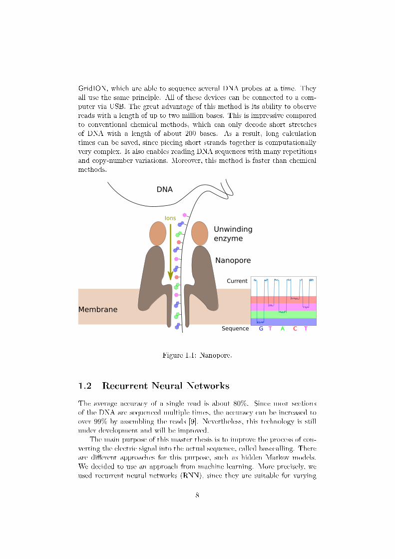
GridION, which are able to sequence several DNA probes at a time. Theyall use the same principle. All of these devices can be connected to a com-puter via USB. The great advantage of this method is its ability to observereads with a length of up to two million bases. This is impressive comparedto conventional chemical methods, which can only decode short stretchesof DNA with a length of about 200 bases. As a result, long calculationtimes can be saved, since piecing short strands together is computationallyvery complex. It also enables reading DNA sequences with many repetitionsand copy-number variations. Moreover, this method is faster than chemicalmethods.

DNA

Nanopore

Unwindingenzyme

G T A C T

Current

Sequence

Membrane

Ions

Figure 1.1: Nanopore.

1.2 Recurrent Neural Networks

The average accuracy of a single read is about 80%. Since most sectionsof the DNA are sequenced multiple times, the accuracy can be increased toover 99% by assembling the reads [9]. Nevertheless, this technology is stillunder development and will be improved.

The main purpose of this master thesis is to improve the process of con-verting the electric signal into the actual sequence, called basecalling. Thereare di�erent approaches for this purpose, such as hidden Markov models.We decided to use an approach from machine learning. More precisely, weused recurrent neural networks (RNN), since they are suitable for varying

8

input lengths. An RNN consists of several neurons, which are connected toeach other. During the learning process some of these connections becomestronger. The more the RNN is trained, the more accurate it becomes. Inorder to develop a functioning network, an appropriate training set has tobe created. This leads us inter alia to break point detection algorithms.

This thesis is structured as follows:

• Chapter 2 delivers the theoretical background to create a basecaller.First, break point detection algorithms are presented. They are used todetermine when a new base has reached the pore. Depending on thesoftware used, the break point detection is already performed duringthe sequencing. If this is not the case, one has to perform it oneself.In this case the window-based break point detection algorithm, whichis known for its speed, is used. It is also explained how to create anRNN and the needed training datasets. Finally, the training processand the basecalling are discussed.

• In Chapter 3 the numerical results are presented. The e�ects of thevarious parameter settings are compared in several charts and tables.Also, both the accuracy of the RNN and the functionality of the breakpoint detection were tested.

• Chapter 4 includes conclusions about the results and provides ap-proaches for further improvement.

9

Chapter 2

Methods

This chapter presents the theoretical background that is necessary to developa basecaller.

2.1 Break Point Detection

The electric current in the pore is represented by a raw signal at every pointin time during the whole read. The number of measurements per second isde�ned by the sampling rate. The duration a base is located in the poreis variable, but can be detected since the current changes immediately witheach base. For this purpose break point detection algorithms are required.These algorithms search through the raw data for signi�cant changes.

2.1.1 Raw Signal

The raw signal is digitized and therefore needs to be converted to the actualvalue of the measured current. For this we need the o�set, range and digiti-zation, which are stored in the meta data. All these parameters are storedin HDF5 �les, together with the raw signal and the break point detection.The digitization represents the number of possible output values. The rangeis the di�erence between the smallest and greatest values. By adding theo�set to the raw signal, we calculate the actual current as

rawreal = (rawdigitized + o�set) · range

digitization. (2.1)

Since there are many reads, where the �rst base reaches the pore sometime after the start of the recording, it is necessary to evaluate the momentwhen the actual sequencing starts.

2.1.2 Finding the Sequencing Start

As evident from Figure 2.1, the measured current peaks at the very beginningof the read. This occurs due to the fact that no base has yet reached the

10

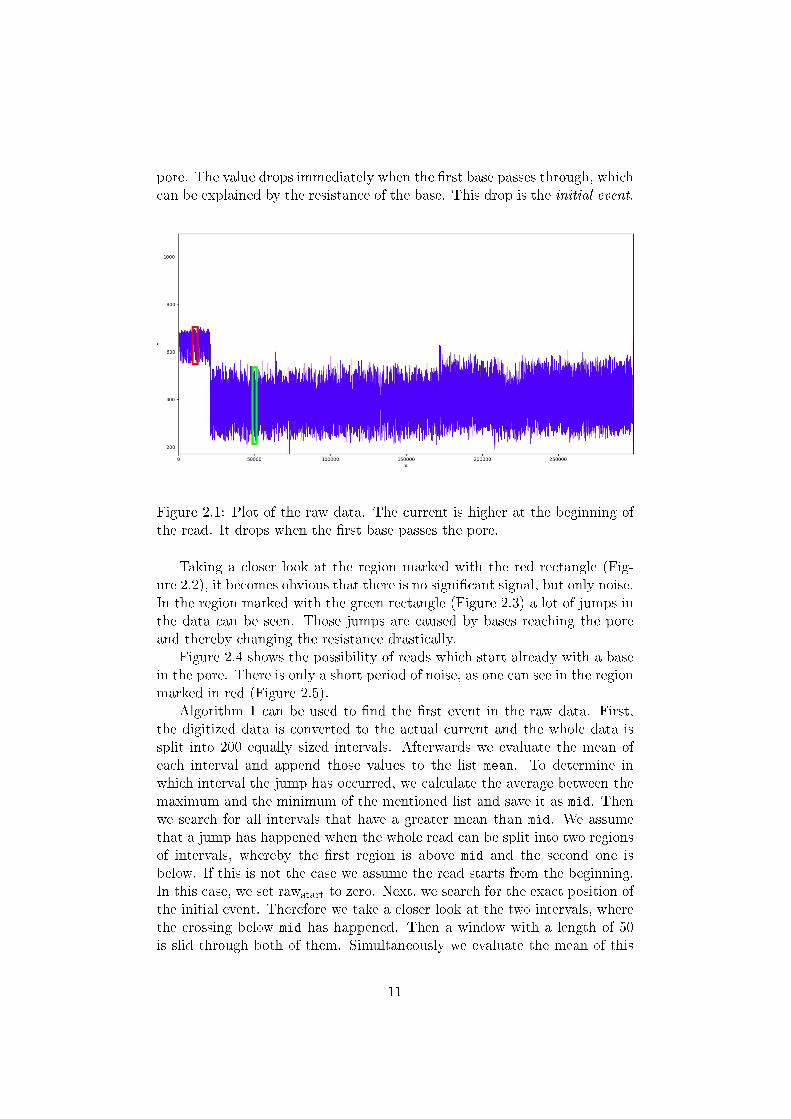
pore. The value drops immediately when the �rst base passes through, whichcan be explained by the resistance of the base. This drop is the initial event.

Figure 2.1: Plot of the raw data. The current is higher at the beginning ofthe read. It drops when the �rst base passes the pore.

Taking a closer look at the region marked with the red rectangle (Fig-ure 2.2), it becomes obvious that there is no signi�cant signal, but only noise.In the region marked with the green rectangle (Figure 2.3) a lot of jumps inthe data can be seen. Those jumps are caused by bases reaching the poreand thereby changing the resistance drastically.

Figure 2.4 shows the possibility of reads which start already with a basein the pore. There is only a short period of noise, as one can see in the regionmarked in red (Figure 2.5).

Algorithm 1 can be used to �nd the �rst event in the raw data. First,the digitized data is converted to the actual current and the whole data issplit into 200 equally sized intervals. Afterwards we evaluate the mean ofeach interval and append those values to the list mean. To determine inwhich interval the jump has occurred, we calculate the average between themaximum and the minimum of the mentioned list and save it as mid. Thenwe search for all intervals that have a greater mean than mid. We assumethat a jump has happened when the whole read can be split into two regionsof intervals, whereby the �rst region is above mid and the second one isbelow. If this is not the case we assume the read starts from the beginning.In this case, we set rawstart to zero. Next, we search for the exact position ofthe initial event. Therefore we take a closer look at the two intervals, wherethe crossing below mid has happened. Then a window with a length of 50is slid through both of them. Simultaneously we evaluate the mean of this

11

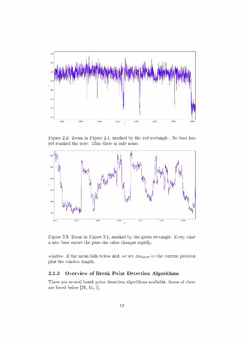
Figure 2.2: Zoom in Figure 2.1, marked by the red rectangle. No base hasyet reached the pore. Thus there is only noise.

Figure 2.3: Zoom in Figure 2.1, marked by the green rectangle. Every timea new base enters the pore the value changes rapidly.

window. If the mean falls below mid, we set rawstart to the current positionplus the window length.

2.1.3 Overview of Break Point Detection Algorithms

There are several break point detection algorithms available. Some of themare listed below [21, 15, 5].

12

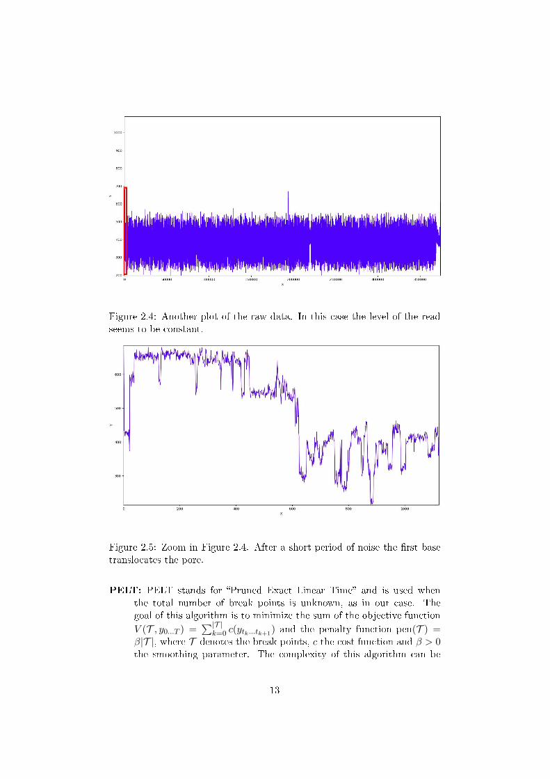
Figure 2.4: Another plot of the raw data. In this case the level of the readseems to be constant.

Figure 2.5: Zoom in Figure 2.4. After a short period of noise the �rst basetranslocates the pore.

PELT: PELT stands for �Pruned Exact Linear Time� and is used whenthe total number of break points is unknown, as in our case. Thegoal of this algorithm is to minimize the sum of the objective function

V (T , y0...T ) =∑|T |

k=0 c(ytk...tk+1) and the penalty function pen(T ) =

β|T |, where T denotes the break points, c the cost function and β > 0the smoothing parameter. The complexity of this algorithm can be

13

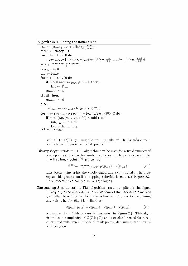
Algorithm 1 Finding the initial event

raw← (rawdigitized + o�set) rangedigitization

mean ← empty listfor n ← 1 to 200 do

mean append mean of(raw(length(raw) n200 , . . . , length(raw)n+1

200 ))

mid ← max(mean)+min(mean)2

rawstart ← 0fail ← Falsefor n ← 1 to 200 do

if n > 0 and rawstart 6= n− 1 then:fail ← True

rawstart ← n

if fail then:rawstart ← 0

else:rawstart ← rawstart · length(raw)/200

for n← rawstart to rawstart + length(raw)/200 · 2 doif mean(raw(n, . . . , n+ 50) < mid then

rawstart ← n+ 50Leave the for loop

return rawstart

reduced to O(T ) by using the pruning rule, which discards certainpoints from the potential break points.

Binary Segmentation: This algorithm can be used for a �xed number ofbreak points and when the number is unknown. The principle is simple:The �rst break point t(1) is given by

t(1) := argmin1≤t<T−1c(y0...t) + c(yt...T ). (2.2)

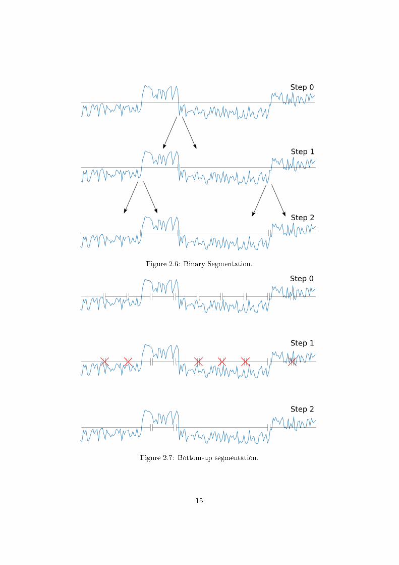
This break point splits the whole signal into two intervals, where werepeat this process until a stopping criterion is met, see Figure 2.6.This process has a complexity of O(T log T ).

Bottom-up Segmentation This algorithm starts by splitting the signalinto equally sized intervals. Afterwards some of the intervals are mergedgradually, depending on the distance function d(., .) of two adjoiningintervals, whereby d(., .) is de�ned as

d(ya...t, yt...b) = c(ya...b)− c(ya...t)− c(yt...b). (2.3)

A visualization of this process is illustrated in Figure 2.7. This algo-rithm has a complexity of O(T log T ) and can also be used for both,known and unknown numbers of break points, depending on the stop-ping criterion.

14

Step 0

Step 1

Step 2

Figure 2.6: Binary Segmentation.

Step 0

Step 1

Step 2

Figure 2.7: Bottom-up segmentation.

15

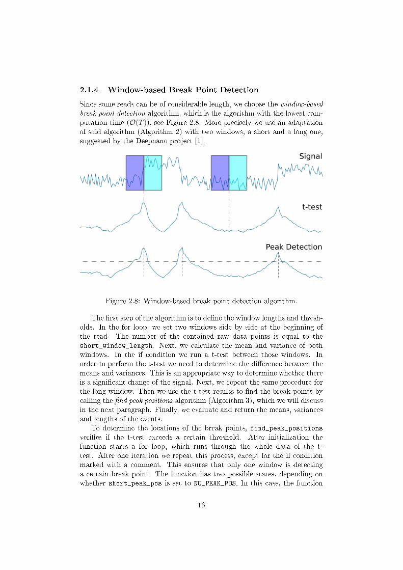
2.1.4 Window-based Break Point Detection

Since some reads can be of considerable length, we choose the window-basedbreak point detection algorithm, which is the algorithm with the lowest com-putation time (O(T )), see Figure 2.8. More precisely we use an adaptationof said algorithm (Algorithm 2) with two windows, a short and a long one,suggested by the Deepnano project [1].

Signal

t-test

Peak Detection

Figure 2.8: Window-based break point detection algorithm.

The �rst step of the algorithm is to de�ne the window lengths and thresh-olds. In the for loop, we set two windows side by side at the beginning ofthe read. The number of the contained raw data points is equal to theshort_window_length. Next, we calculate the mean and variance of bothwindows. In the if condition we run a t-test between those windows. Inorder to perform the t-test we need to determine the di�erence between themeans and variances. This is an appropriate way to determine whether thereis a signi�cant change of the signal. Next, we repeat the same procedure forthe long window. Then we use the t-test results to �nd the break points bycalling the �nd peak positions algorithm (Algorithm 3), which we will discussin the next paragraph. Finally, we evaluate and return the means, variancesand lengths of the events.

To determine the locations of the break points, find_peak_positionsveri�es if the t-test exceeds a certain threshold. After initialization thefunction starts a for loop, which runs through the whole data of the t-test. After one iteration we repeat this process, except for the if conditionmarked with a comment. This ensures that only one window is detectinga certain break point. The function has two possible states, depending onwhether short_peak_pos is set to NO_PEAK_POS. In this case, the function

16

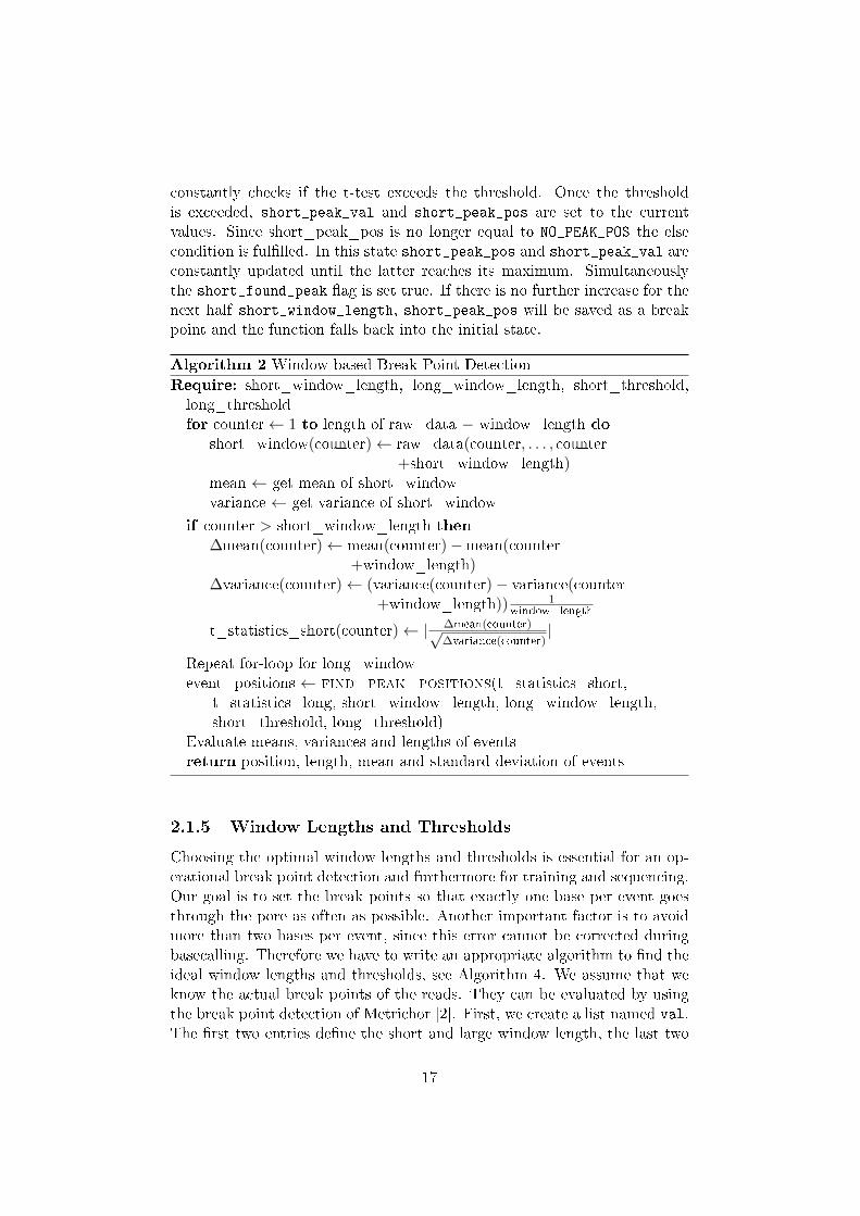
constantly checks if the t-test exceeds the threshold. Once the thresholdis exceeded, short_peak_val and short_peak_pos are set to the currentvalues. Since short_peak_pos is no longer equal to NO_PEAK_POS the elsecondition is ful�lled. In this state short_peak_pos and short_peak_val areconstantly updated until the latter reaches its maximum. Simultaneouslythe short_found_peak �ag is set true. If there is no further increase for thenext half short_window_length, short_peak_pos will be saved as a breakpoint and the function falls back into the initial state.

Algorithm 2 Window-based Break Point Detection

Require: short_window_length, long_window_length, short_threshold,long_thresholdfor counter← 1 to length of raw_data − window_length do

short_window(counter)← raw_data(counter, . . . , counter+short_window_length)

mean ← get mean of short_windowvariance ← get variance of short_window

if counter > short_window_length then∆mean(counter)← mean(counter)−mean(counter

+window_length)∆variance(counter)← (variance(counter)− variance(counter

+window_length)) 1window_length

t_statistics_short(counter)← | ∆mean(counter)√∆variance(counter)

|

Repeat for-loop for long_windowevent_positions ← find_peak_positions(t_statistics_short,

t_statistics_long, short_window_length, long_window_length,short_threshold, long_threshold)

Evaluate means, variances and lengths of eventsreturn position, length, mean and standard deviation of events

2.1.5 Window Lengths and Thresholds

Choosing the optimal window lengths and thresholds is essential for an op-erational break point detection and furthermore for training and sequencing.Our goal is to set the break points so that exactly one base per event goesthrough the pore as often as possible. Another important factor is to avoidmore than two bases per event, since this error cannot be corrected duringbasecalling. Therefore we have to write an appropriate algorithm to �nd theideal window lengths and thresholds, see Algorithm 4. We assume that weknow the actual break points of the reads. They can be evaluated by usingthe break point detection of Metrichor [2]. First, we create a list named val.The �rst two entries de�ne the short and large window length, the last two

17

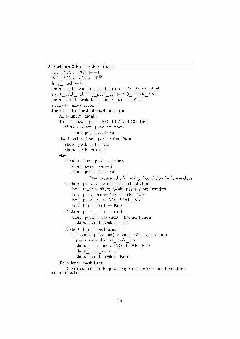
Algorithm 3 Find peak positions

NO_PEAK_POS ← −1NO_PEAK_VAL ← 10100

long_mask ← 0short_peak_pos, long_peak_pos ← NO_PEAK_POSshort_peak_val, long_peak_val ← NO_PEAK_VALshort_found_peak, long_found_peak ← Falsepeaks ← empty vectorfor i← 1 to length of short_data do

val ← short_data[i]if short_peak_pos = NO_PEAK_POS then

if val < short_peak_val thenshort_peak_val ← val

else if val > short_peak_value thenshort_peak_val ← valshort_peak_pos ← i

elseif val > short_peak_val then

short_peak_pos ← ishort_peak_val ← val

. Don't repeat the following if condition for long-valuesif short_peak_val > short_threshold then

long_mask ← short_peak_pos + short_windowlong_peak_pos ← NO_PEAK_POSlong_peak_val ← NO_PEAK_VALlong_found_peak ← False

if short_peak_val > val andshort_peak_val > short_threshold thenshort_found_peak ← True

if short_found_peak and(i − short_peak_pos) > short_window / 2 thenpeaks append short_peak_posshort_peak_pos ← NO_PEAK_POSshort_peak_val ← valshort_found_peak ← False

if i > long_mask thenRepeat code of For-loop for long-values, except one If-condition

return peaks

18

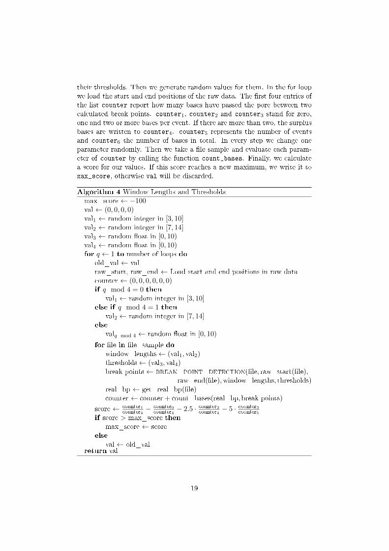
their thresholds. Then we generate random values for them. In the for loopwe load the start and end positions of the raw data. The �rst four entries ofthe list counter report how many bases have passed the pore between twocalculated break points. counter1, counter2 and counter3 stand for zero,one and two or more bases per event. If there are more than two, the surplusbases are written to counter4. counter5 represents the number of eventsand counter6 the number of bases in total. In every step we change oneparameter randomly. Then we take a �le sample and evaluate each param-eter of counter by calling the function count_bases. Finally, we calculatea score for our values. If this score reaches a new maximum, we write it tomax_score, otherwise val will be discarded.

Algorithm 4 Window Lengths and Thresholdsmax_score ← −100val ← (0, 0, 0, 0)val1 ← random integer in [3, 10]val2 ← random integer in [7, 14]val3 ← random �oat in [0, 10)val4 ← random �oat in [0, 10)for q ← 1 to number of loops do

old_val ← valraw_start, raw_end ← Load start and end positions in raw datacounter ← (0, 0, 0, 0, 0, 0)if q mod 4 = 0 then

val1 ← random integer in [3, 10]else if q mod 4 = 1 then

val2 ← random integer in [7, 14]else

valq mod 4 ← random �oat in [0, 10)

for �le in �le_sample dowindow_lengths← (val1, val2)thresholds← (val3, val4)break points ← break_point_detection(�le, raw_start(�le),

raw_end(�le),window_lengths, thresholds)real_bp ← get_real_bp(�le)counter ← counter + count_bases(real_bp, break points)

score ← counter1counter4

− counter0counter4

− 2.5 · counter2counter4− 5 · counter3counter5

if score > max_score thenmax_score ← score

elseval ← old_val

return val

19

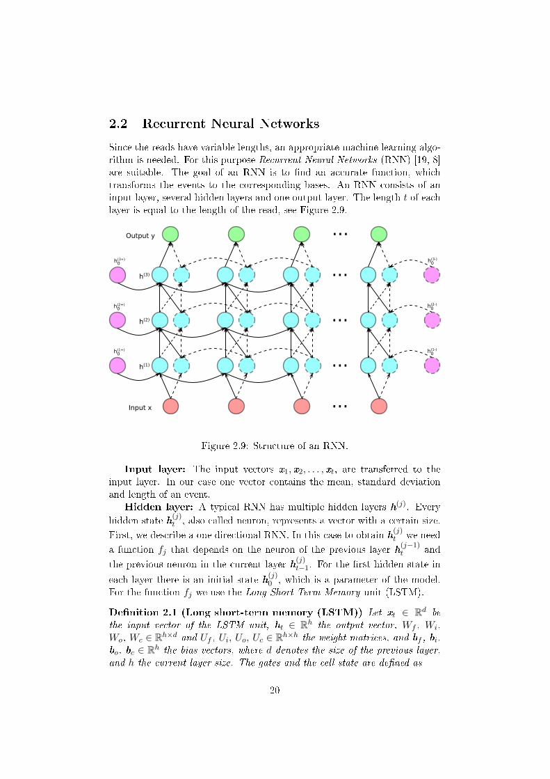
2.2 Recurrent Neural Networks

Since the reads have variable lengths, an appropriate machine learning algo-rithm is needed. For this purpose Recurrent Neural Networks (RNN) [19, 8]are suitable. The goal of an RNN is to �nd an accurate function, whichtransforms the events to the corresponding bases. An RNN consists of aninput layer, several hidden layers and one output layer. The length t of eachlayer is equal to the length of the read, see Figure 2.9.

...

...

...

...

...

h(3+)0

h(2+)0

h(1+)0

h(3-)0

h(2-)0

h(1-)0

h(3)

h(2)

h(1)

Output y

Input x

Figure 2.9: Structure of an RNN.

Input layer: The input vectors x1, x2, . . . , xt, are transferred to theinput layer. In our case one vector contains the mean, standard deviationand length of an event.

Hidden layer: A typical RNN has multiple hidden layers h(j). Every

hidden state h(j)t , also called neuron, represents a vector with a certain size.

First, we describe a one directional RNN. In this case to obtain h(j)t we need

a function fj that depends on the neuron of the previous layer h(j−1)t and

the previous neuron in the current layer h(j)t−1. For the �rst hidden state in

each layer there is an initial state h(j)0 , which is a parameter of the model.

For the function fj we use the Long Short-Term Memory unit (LSTM).

De�nition 2.1 (Long short-term memory (LSTM)) Let xt ∈ Rd be

the input vector of the LSTM unit, ht ∈ Rh the output vector, Wf , Wi,

Wo, Wc ∈ Rh×d and Uf , Ui, Uo, Uc ∈ Rh×h the weight matrices, and bf , bi,

bo, bc ∈ Rh the bias vectors, where d denotes the size of the previous layer,

and h the current layer size. The gates and the cell state are de�ned as

20

• forget gate ft = σ(Wfxt + Ufht−1 + bf ),

• input gate it = σ(Wixt + Uiht−1 + bi),

• output gate ot = σ(Woxt + Uoht−1 + bo),

• cell state ct = ft ◦ ct−1 + it ◦ tanh(Woxt + Uoht−1 + bo),

where ◦ denotes the element-wise product and σ the sigmoid function. Fi-

nally, the output vector ht is given by

ht = ot ◦ tanh(ct).

The weight matrices U and W , the bias vectors b and the initial state h0 arealso parameters of our network and will be trained.

Since the output vector is also in�uenced by the following outputs, weneed a bidirectional RNN. Therefore two output vectors will be calculated,one in forward and one in backward direction. The concatenation of thoseyields the input vector of the next layer.

Output layer: Ideally, each input event leads to exactly one base, butin some cases more than one base passes through the pore during one event.Thus we need at least two outputs. It is also possible, that there are threeor more bases, but this happens very rarely and for this reason was leftunattended. For every output there are �ve possibilities: A, C, G and Tdenote the four bases and N denotes no base. In case of one base per event,the base in question is allocated to the second output. The probabilities forthe four bases, respectively blank, are calculated by the softmax function

P (out(k)i = q) =

exp(Wi ◦ h(n)i + bi)∑5

i=1 exp(Wi ◦ h(n)i + bi)

, (2.4)

where h(n)i is the output vector of the last hidden layer, k ∈ {1, 2},W ∈ Rd×5

and b ∈ R5. W and b are also trainable parameters.The RNN returns two 5-dimensional vectors for each event, where every

element stands for the probability of one base, or a blank.

2.3 Preparation of Training Data

To train our model a set of training data is necessary. The reads of thosedata sets are usually stored in HDF5 �les, containing the raw data, breakpoint detection and output of the Oxford Nanopore Technologies' basecallerMetrichor. We use this output to determine the region of the referencesequence to which the read belongs to. For that, we use the aligner Minialign[3] (Algorithm 5).

The output at the beginning and ending of the read is often inaccurate,which is why it cannot be aligned. Therefore Minialign returns the start and

21

Algorithm 5 Prepare dataset

for all reads do(read_start_pos, read_end_pos, ref_start_pos,ref_end_pos, cigar_string)←Minialign(read, reference sequence)

scale events of read to normal distribution N (0, 1)Data append load_data(read, read_start_pos, read_end_pos,

ref_start_pos, ref_end_pos, cigar_string)

split Data into trainData, validationData and testDatareturn events with the corresponding bases

end position in the read and in the reference, as well as the accuracy and thecigar string. The cigar string describes how the read aligns with the refer-ence. It consists of a series of sets, containing a number followed by one letter,whereby the letter denotes an operator and the number stands for the quan-tity of those. Here a short example: 49S3M1D3M1D8M1I23M1D4M1D9M1D6M...

The meaning of the operators are shown in Table 2.1.

Operator Description

D Deletion: the nucleotide is present in the reference, but not inthe read.

H Hard clipping: the clipped nucleotides are not present in theread.

I Insertion: the nucleotide is present in the read, but not in thereference.

M Match: can be either an alignment match or mismatch. Thenucleotide is present in the reference.

S Soft clipping: the clipped nucleotides are present in the read.

Table 2.1: Meaning of the cigar string operators.

2.3.1 Finding the Initial Event

In the next step, we will use this string to allocate each event to the corre-sponding bases of the reference. Since the basecaller of Metrichor sometimesreturns two or no bases, the start and end position of the output is not thesame as the one of the events. Thus, �rst we have to �nd the starting event(Algorithm 6).

Along with the mean, standard deviation and length, there are also afew more bits of information about every single event. They are stored in anarray of the HDF5 �les. Most of them a�ect the hidden Markov model thatMetrichor works with and are thereby irrelevant for our problem. However,

22

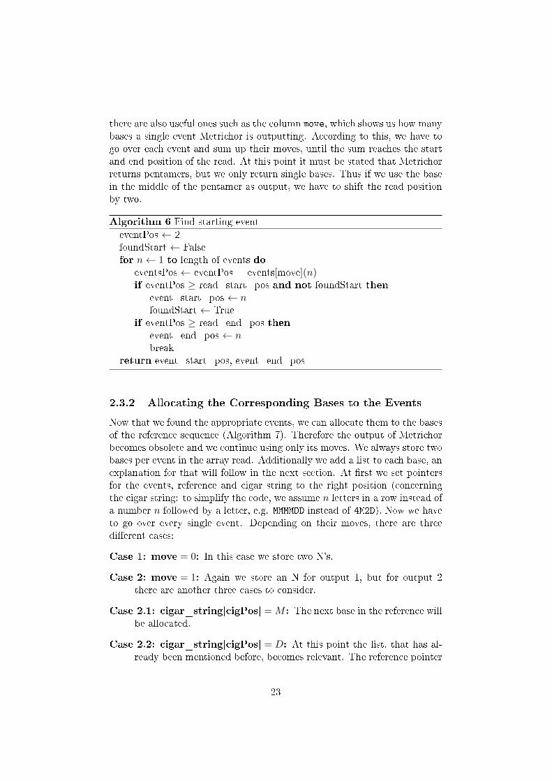
there are also useful ones such as the column move, which shows us how manybases a single event Metrichor is outputting. According to this, we have togo over each event and sum up their moves, until the sum reaches the startand end position of the read. At this point it must be stated that Metrichorreturns pentamers, but we only return single bases. Thus if we use the basein the middle of the pentamer as output, we have to shift the read positionby two.

Algorithm 6 Find starting event

eventPos ← 2foundStart ← Falsefor n← 1 to length of events do

eventsPos ← eventPos + events[move](n)if eventPos ≥ read_start_pos and not foundStart then

event_start_pos ← nfoundStart ← True

if eventPos ≥ read_end_pos thenevent_end_pos ← nbreak

return event_start_pos, event_end_pos

2.3.2 Allocating the Corresponding Bases to the Events

Now that we found the appropriate events, we can allocate them to the basesof the reference sequence (Algorithm 7). Therefore the output of Metrichorbecomes obsolete and we continue using only its moves. We always store twobases per event in the array read. Additionally we add a list to each base, anexplanation for that will follow in the next section. At �rst we set pointersfor the events, reference and cigar string to the right position (concerningthe cigar string: to simplify the code, we assume n letters in a row instead ofa number n followed by a letter, e.g. MMMMDD instead of 4M2D). Now we haveto go over every single event. Depending on their moves, there are threedi�erent cases:

Case 1: move = 0: In this case we store two N's.

Case 2: move = 1: Again we store an N for output 1, but for output 2there are another three cases to consider.

Case 2.1: cigar_string[cigPos] = M : The next base in the reference willbe allocated.

Case 2.2: cigar_string[cigPos] = D: At this point the list, that has al-ready been mentioned before, becomes relevant. The reference pointer

23

Algorithm 7 Allocating the Corresponding Bases to the Eventsevent_pos ← event_start_posref_pos ← ref_start_poscig_pos ← 0if move(n) = 0 then

read append [N, []]read append [N, []]

else if move(n) = 1 thenread append [N, []]if cigar_string[cigPos] = M then

read append reference[refPos]refPos ← refPos + 1

else if cigar_string[cigPos] = D thennoDels ← number of D's until next M in cigar_stringdels ← reference[refPos, refPos + noDels]refPos ← refPos + noDelscigPos ← cigPos + noDelsread append [reference[refPos], dels]refPos ← refPos + 1

else if cigar_string[cigPos] = I thenread append [N, []]

cigPos ← cigPos + 1else

for n← 1 to 2 doif cigar_string[cigPos] = M then

read append reference[refPos]refPos ← refPos + 1

else if cigar_string[cigPos] = D thennoDels ← number of D's until next M in cigar_stringdels ← reference[refPos, refPos + noDels]refPos ← refPos + noDelscigPos ← cigPos + noDelsread append [reference[refPos], dels]refPos ← refPos + 1

else if cigar_string[cigPos] = I thenread append [N, []]

cigPos ← cigPos + 1return read

24

jumps to the next base that has a match. The skipped bases are addedto the list and if possible, they can later be inserted to the output.

Case 2.3: cigar_string[cigPos] = I: No base will be allocated. Finally,the pointer has to be set to the correct positions.

Case 3: move = 2: Similar to case 2, but this time we make the distinctionfor output 2 as well.

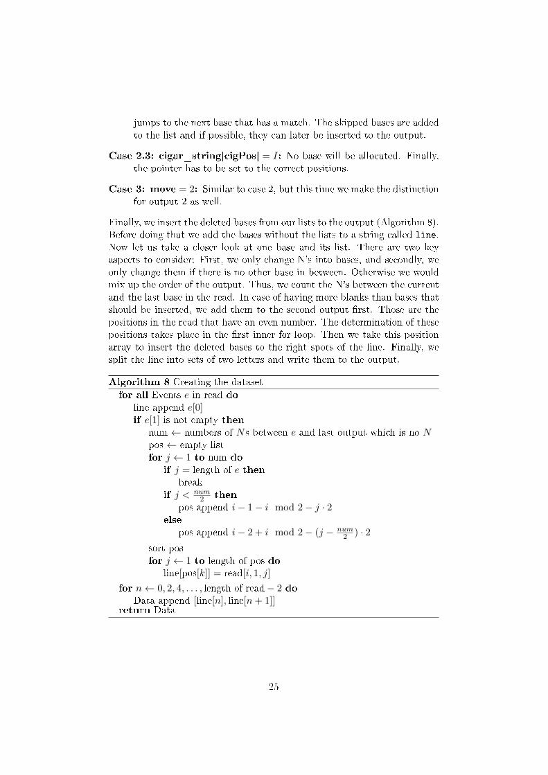
Finally, we insert the deleted bases from our lists to the output (Algorithm 8).Before doing that we add the bases without the lists to a string called line.Now let us take a closer look at one base and its list. There are two keyaspects to consider: First, we only change N's into bases, and secondly, weonly change them if there is no other base in between. Otherwise we wouldmix up the order of the output. Thus, we count the N's between the currentand the last base in the read. In case of having more blanks than bases thatshould be inserted, we add them to the second output �rst. Those are thepositions in the read that have an even number. The determination of thesepositions takes place in the �rst inner for loop. Then we take this positionarray to insert the deleted bases to the right spots of the line. Finally, wesplit the line into sets of two letters and write them to the output.

Algorithm 8 Creating the dataset

for all Events e in read doline append e[0]if e[1] is not empty then

num ← numbers of Ns between e and last output which is no Npos ← empty listfor j ← 1 to num do

if j = length of e thenbreak

if j < num2 then

pos append i− 1− i mod 2− j · 2else

pos append i− 2 + i mod 2− (j − num2 ) · 2

sort posfor j ← 1 to length of pos do

line[pos[k]] = read[i, 1, j]

for n← 0, 2, 4, . . . , length of read− 2 doData append [line[n], line[n+ 1]]

return Data

25

2.4 Training

2.4.1 Optimizer

After having prepared our dataset, we can �nally train our network. Inorder to do that we use Python and the Keras library with the Tensor�owbackend. First, we have to determine the hyperparameters, such as thelearning rate, decay, size and number of hidden layers etc. Furthermore weneed an appropriate loss function and optimizer. An overview of the mostcommonly used optimizers is given below.

Stochastic Gradient Descent: In order to optimize the RNN stochasticgradient descent (SGD) [6] uses the gradient of the loss function f . Ineach training step, the parameters x are updated by

xt+1 := xt − η∇f(xt), (2.5)

where η denotes the learning rate. If η is small enough the loss getssmaller with each step.

Momentum: Momentum [20] adds another term to the equation which usesthe previous update to prevent the learning process from oscillations.

xt+1 := xt − η∇f(xt) + α(xt − xt−1), (2.6)

where α denotes the coe�cient of momentum. This extra term enlargesthe step size when the direction of the gradient stays the same andreduces it when the direction changes. It is called momentum due toits analogy to the momentum in physics.

Nesterov Accelerated Gradient Descent: Nesterov accelerated gradientdescent (NAG) [17, 16] changes the second term of (2.6) to γ∇f(xt +α(xt − xt−1)). By using the momentum for the gradient, Nesterov ap-proximates the next position of the parameters. This method improvedthe convergence rate from O(1/t) to O(1/t2).

Adagrad: Unlike SGD, Adagrad [11] uses di�erent learning rates for everyparameter xt,i. These learning rates are updated at every time step τby using the outer product matrix

Gt :=t∑

τ=1

gτgTτ , (2.7)

where gτ = ∇f(xτ ). The update of xt is given by

xt+1,i := xt,i −η√

Gt,ii + εgt,i. (2.8)

26

The ε is added to avoid division by zero. Adagrad's weakness is that thelearning rate decreases with every time step and eventually becomesin�nitesimally small.

Adadelta: Adadelta [24] �xes Adagrad's problem by restricting the numberof past gradients used to some �xed size w. Therefore, the factor Giiis replaced by the running average E[g2]t, which is de�ned by

E[g2]t+1 = γE[g2]t + (1− γ)g2t+1. (2.9)

Since√E[g2]t + ε is equal to the root mean squared (RMS) error cri-

terion of the gradient, the update of x can be written as

xt+1,i := xt,i −η

RMS[g]tgt,i. (2.10)

Adam: In addition to evaluating the RMS of the gradient vt like Adadelta,Adaptive Moment Estimation (Adam) [13] also calculates the exponen-tially decaying average of the gradient mt. vt and mt are recursivelyde�ned by

mt+1 := β1mt + (1− β1)gt+1, (2.11)

vt+1 := β2vt + (1− β2)g2t+1. (2.12)

Since vt and mt are initialized as vectors of zeros their values are toosmall at the beginning and therefore have to be corrected by

mt :=mt

1− βt1, (2.13)

vt :=vt

1− βt2. (2.14)

mt and vt are then used for updating x by

xt+1,i := xt,i −η√vi + ε

mt+1,i. (2.15)

Adamax: Adamax replaces vt from the Adam optimizer by a vector ut,which is de�ned as

ut+1 := max(β2 · ut, |gt+1|). (2.16)

Since ut is not biased to zeros, a bias correction is not necessary.

Nadam: Nesterov-accelerated Adaptive Moment Estimation (Nadam) [10]extends the Adam optimizer by using NAG. For this purpose gt isreplaced by γ∇f(x+ α∆x). The update of x is then given by

xt+1,i := xt,i −η√

vt+1,i + ε(β1mt+1,i +

(1− β1)gt+1,i

1− βt+11

). (2.17)

27

2.4.2 Loss Function

During training, binary cross entropy turned out to be by far the best lossfunction. The only di�erence to the categorical cross entropy is the fact thatit can only categorize two classes. The binary cross entropy function f isde�ned as

f(y, y) = − 1

N

N∑n=1

yn log(yn) + (1− yn) log(1− yn), (2.18)

where y denotes the predicted and y the actual output.

2.4.3 Hyperparameters

The layer size and the number of hidden layers have a major impact on theaccuracy. If the size is too small the network cannot cover the complexityof the problem. On the other hand, too large a size leads to over�ttingand longer computation time. Thus we have to try out several sizes tooptimize the accuracy and computation time. Changing the learning rate,β1 and β2, as well as using learning rate decay have no positive in�uenceon the precision. Due to the huge amount of training data over�tting is noproblem. This is the reason why regularizers are not only unnecessary, butalso slow down the learning process.

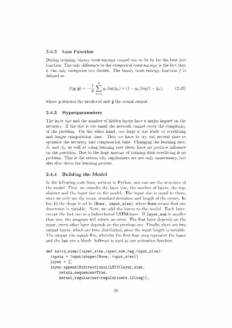
2.4.4 Building the Model

In the following code lines, written in Python, one can see the structure ofthe model. First, we transfer the layer size, the number of layers, the reg-ularizer and the input size to the model. The input size is equal to three,since we only use the mean, standard deviation and length of the events. Inline 15 the shape is set to (None, input_size), where None means that onedimension is variable. Next, we add the layers to the model. Each layer,except the last one is a bidirectional LSTM-layer. If layer_num is smallerthan one, the program will return an error. The �rst layer depends on theinput, every other layer depends on the previous one. Finally, there are twooutput layers, which are time distributed, since the input length is variable.The output size equals �ve, whereby the �rst four ones represent the basesand the last one a blank. Softmax is used as our activation function.

def build_model(layer_size,layer_num,reg,input_size):

inputs = Input(shape=(None, input_size))

layer = []

layer.append(Bidirectional(LSTM(layer_size,

return_sequences=True,

kernel_regularizer=regularizers.l2(reg)),

28

input_shape=(None,input_size))(inputs))

for n in range(layer_num-1):

layer.append(Bidirectional(LSTM(layer_size,

return_sequences=True,

kernel_regularizer=regularizers.l2(reg)))(layer[-1]))

out_layer1 = TimeDistributed(Dense(5, activation="softmax",

kernel_regularizer=regularizers.l2(reg)),

name="out_layer1")(layer[-1])

out_layer2 = TimeDistributed(Dense(5, activation="softmax",

kernel_regularizer=regularizers.l2(reg)),

name="out_layer2")(Concatenate()([layer[-1], out_layer1]))

return Model(inputs=inputs, outputs=[out_layer1, out_layer2])

2.4.5 Training the Model

To simplify the code, we use a generator for the training and validation. Thegenerator is constructed by calling

training_generator = DataGenerator(args.subseq_size,

trainPackage,32)

and de�ned as

class DataGenerator():

def __init__(self,subseq_size,data_package,batch_size):

self.subseq_size = subseq_size

self.data_package = data_package

self.batch_size = batch_size.

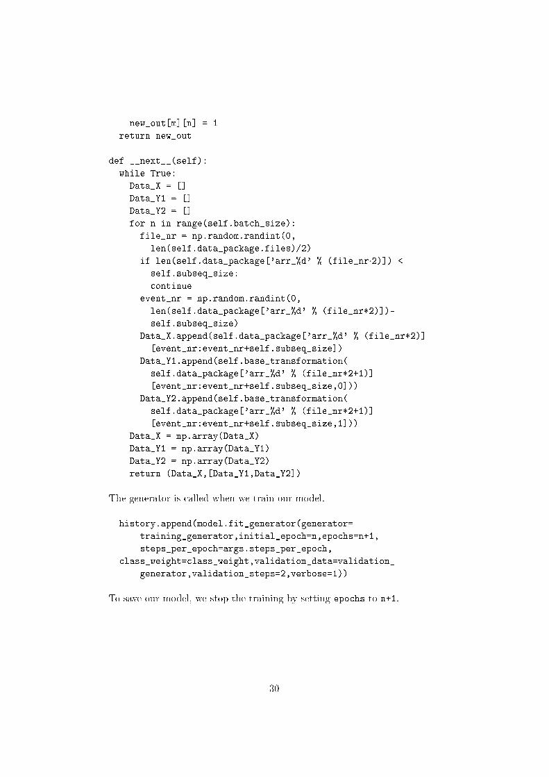
subseq_size de�nes how many events are used per training step. Thisnumber is essential for the speed, as well as the batch_size. If it is too low,the gradient may point in the wrong direction. If it is too high, each step willtake longer. When the generator is called, three empty lists will be created.Data_X contains the input, whereas Data_Y1 as well as Data_Y2 contain thecorresponding outputs one and two. The number of sequences added is equalto the batch size. In the for loop we choose a random sub-sequence froma random read. Next, we add the events and bases from the sub-sequenceto the corresponding lists. After transferring the lists to numpy-arrays wereturn them.

def base_transformation(self,out):

new_out = [[0,0,0,0,0] for i in range(len(out))]

for m,n in enumerate(out):

29

new_out[m][n] = 1

return new_out

def __next__(self):

while True:

Data_X = []

Data_Y1 = []

Data_Y2 = []

for n in range(self.batch_size):

file_nr = np.random.randint(0,

len(self.data_package.files)/2)

if len(self.data_package['arr_%d' % (file_nr·2)]) <

self.subseq_size:

continue

event_nr = np.random.randint(0,

len(self.data_package['arr_%d' % (file_nr*2)])-

self.subseq_size)

Data_X.append(self.data_package['arr_%d' % (file_nr*2)]

[event_nr:event_nr+self.subseq_size])

Data_Y1.append(self.base_transformation(

self.data_package['arr_%d' % (file_nr*2+1)]

[event_nr:event_nr+self.subseq_size,0]))

Data_Y2.append(self.base_transformation(

self.data_package['arr_%d' % (file_nr*2+1)]

[event_nr:event_nr+self.subseq_size,1]))

Data_X = np.array(Data_X)

Data_Y1 = np.array(Data_Y1)

Data_Y2 = np.array(Data_Y2)

return (Data_X,[Data_Y1,Data_Y2])

The generator is called when we train our model.

history.append(model.fit_generator(generator=

training_generator,initial_epoch=n,epochs=n+1,

steps_per_epoch=args.steps_per_epoch,

class_weight=class_weight,validation_data=validation_

generator,validation_steps=2,verbose=1))

To save our model, we stop the training by setting epochs to n+1.

30

2.5 Sequencing

For the last step, the sequencing, we load the model we trained before. Forusing our own detection we have to use a di�erent model than the detectionof Metrichor as its break point detection is di�erent from ours. In this casewe have to apply the break point detection to the raw data �rst. At thispoint it is important to use the same window lengths and thresholds weused during the training. As a next step, we use the prediction functionfrom Keras to apply our model to the events. Then we have to translatethe output to the sequence. Thereby we evaluate the maximum of output 1and 2 of every event, convert it to the corresponding bases and remove theblanks. Finally, we write the �lenames and sequences to a FASTA �le.

31

Chapter 3

Numerical Results

In order to develop the basecaller with the highest possible accuracy weneed to evaluate the optimal hyperparameters. In this chapter we thereforecompare the obtained results for each of them. Moreover, we will go intodetail on the outputs of the break point detection algorithms.

3.1 Recurrent Neural Network

To train the RNN, the E. coli data set [4] was used. This data set containsover 50,000 reads, hence it provides enough data to work with. Moreover theE. coli bacteria has almost no mutations and is therefore perfectly suited fortraining. In order to reach accurate results several options had to be tested,such as di�erent loss functions, optimizers, layer size, etc.

In the following sections those options are compared by using the lossand the accuracy of the validation data for the outputs 1 and 2.

3.1.1 Loss Function

Choosing an appropriate loss function had the biggest impact on the results.Figure 3.1 and Figure 3.2 show the accuracies of the available loss functionsof Keras. Binary cross entropy had by far the highest accuracy, whereashinge, mean absolute error and mean absolute percentage error de-livered the lowest precision.

32

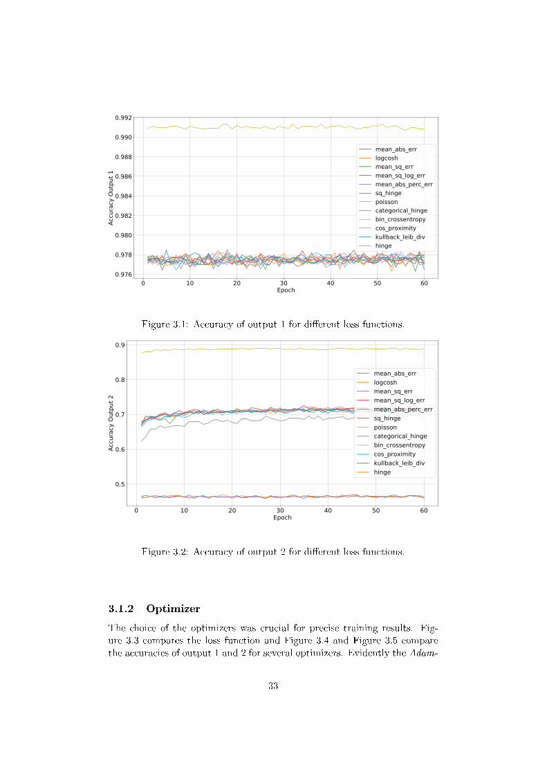
Figure 3.1: Accuracy of output 1 for di�erent loss functions.

Figure 3.2: Accuracy of output 2 for di�erent loss functions.

3.1.2 Optimizer

The choice of the optimizers was crucial for precise training results. Fig-ure 3.3 compares the loss function and Figure 3.4 and Figure 3.5 comparethe accuracies of output 1 and 2 for several optimizers. Evidently the Adam-

33

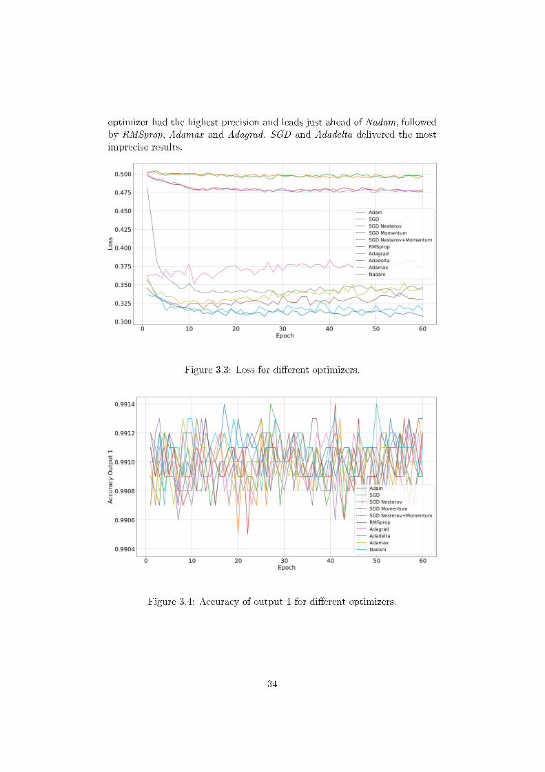
optimizer had the highest precision and leads just ahead of Nadam, followedby RMSprop, Adamax and Adagrad. SGD and Adadelta delivered the mostimprecise results.

Figure 3.3: Loss for di�erent optimizers.

Figure 3.4: Accuracy of output 1 for di�erent optimizers.

34

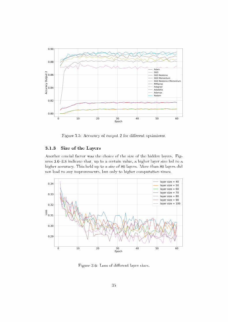
Figure 3.5: Accuracy of output 2 for di�erent optimizers.

3.1.3 Size of the Layers

Another crucial factor was the choice of the size of the hidden layers. Fig-ures 3.6�3.8 indicate that, up to a certain value, a higher layer size led to ahigher accuracy. This held up to a size of 80 layers. More than 80 layers didnot lead to any improvements, but only to higher computation times.

Figure 3.6: Loss of di�erent layer sizes.

35

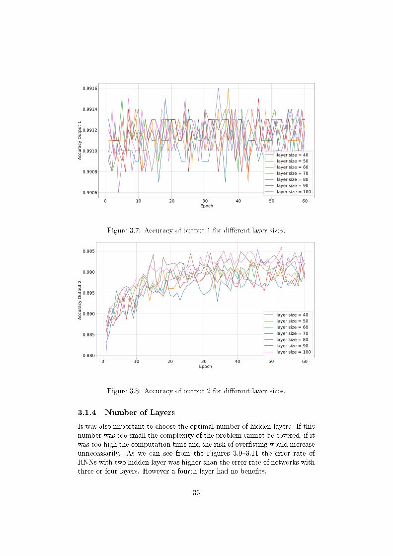
Figure 3.7: Accuracy of output 1 for di�erent layer sizes.

Figure 3.8: Accuracy of output 2 for di�erent layer sizes.

3.1.4 Number of Layers

It was also important to choose the optimal number of hidden layers. If thisnumber was too small the complexity of the problem cannot be covered, if itwas too high the computation time and the risk of over�tting would increaseunnecessarily. As we can see from the Figures 3.9�3.11 the error rate ofRNNs with two hidden layer was higher than the error rate of networks withthree or four layers. However a fourth layer had no bene�ts.

36

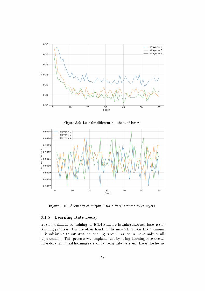
Figure 3.9: Loss for di�erent numbers of layers.

Figure 3.10: Accuracy of output 1 for di�erent numbers of layers.

3.1.5 Learning Rate Decay

At the beginning of training an RNN a higher learning rate accelerates thelearning progress. On the other hand, if the network is near the optimumit is advisable to use smaller learning rates in order to make only smalladjustments. This process was implemented by using learning rate decay.Therefore, an initial learning rate and a decay rate were set. Later the learn-

37

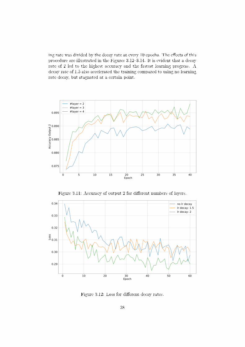
ing rate was divided by the decay rate at every 10 epochs. The e�ects of thisprocedure are illustrated in the Figures 3.12�3.14. It is evident that a decayrate of 2 led to the highest accuracy and the fastest learning progress. Adecay rate of 1.5 also accelerated the training compared to using no learningrate decay, but stagnated at a certain point.

Figure 3.11: Accuracy of output 2 for di�erent numbers of layers.

Figure 3.12: Loss for di�erent decay rates.

38

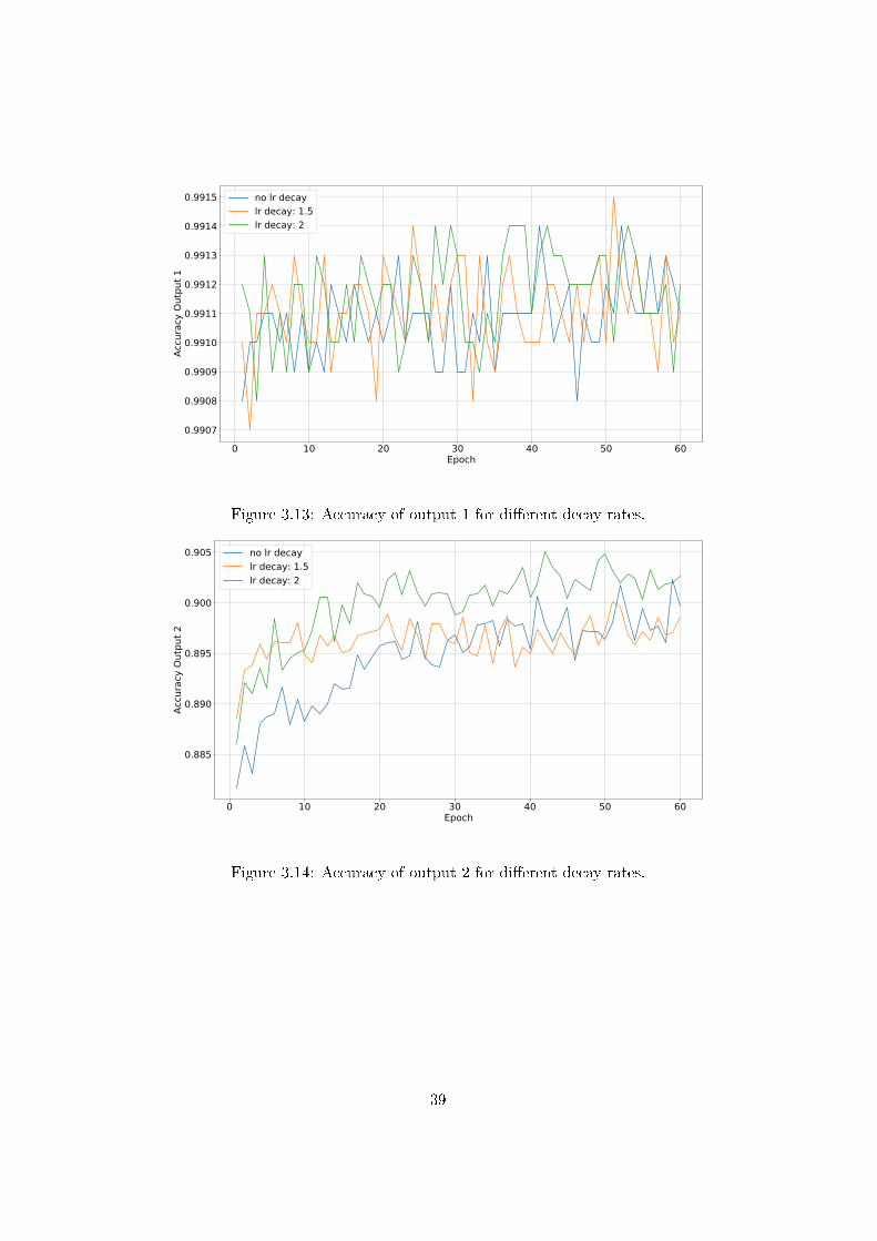
Figure 3.13: Accuracy of output 1 for di�erent decay rates.

Figure 3.14: Accuracy of output 2 for di�erent decay rates.

39

3.1.6 Class Weight

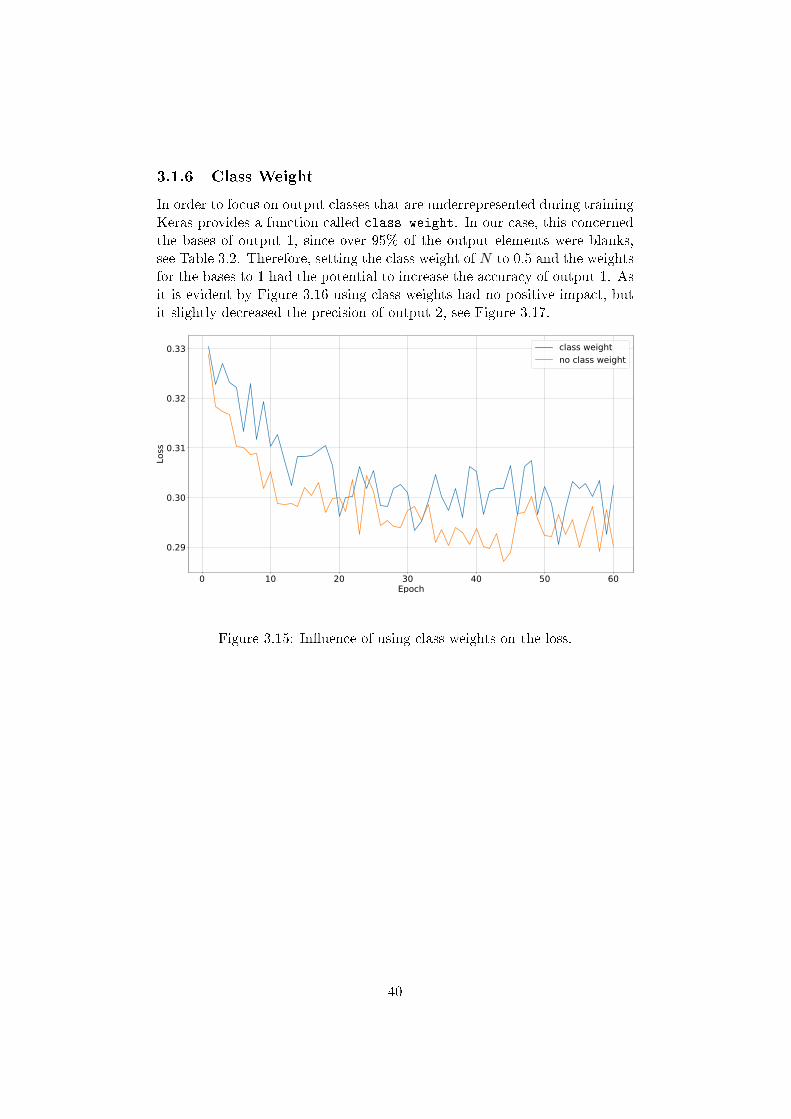
In order to focus on output classes that are underrepresented during trainingKeras provides a function called class weight. In our case, this concernedthe bases of output 1, since over 95% of the output elements were blanks,see Table 3.2. Therefore, setting the class weight of N to 0.5 and the weightsfor the bases to 1 had the potential to increase the accuracy of output 1. Asit is evident by Figure 3.16 using class weights had no positive impact, butit slightly decreased the precision of output 2, see Figure 3.17.

Figure 3.15: In�uence of using class weights on the loss.

40

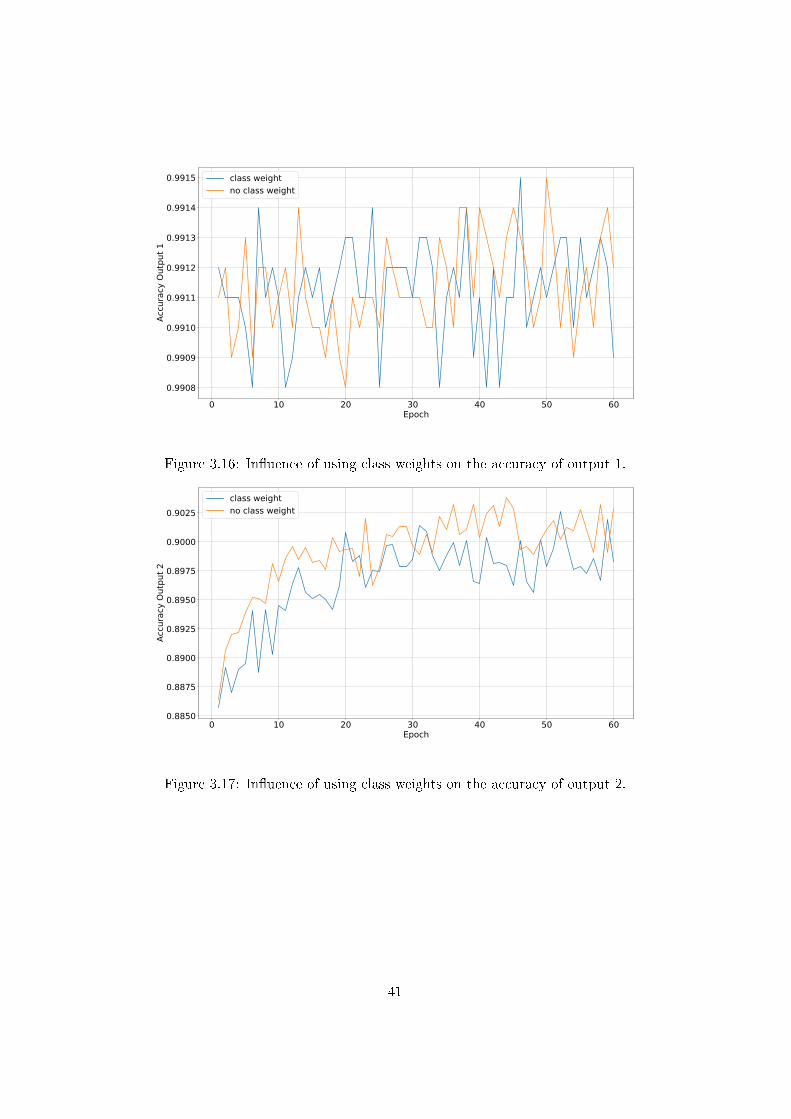
Figure 3.16: In�uence of using class weights on the accuracy of output 1.

Figure 3.17: In�uence of using class weights on the accuracy of output 2.

41

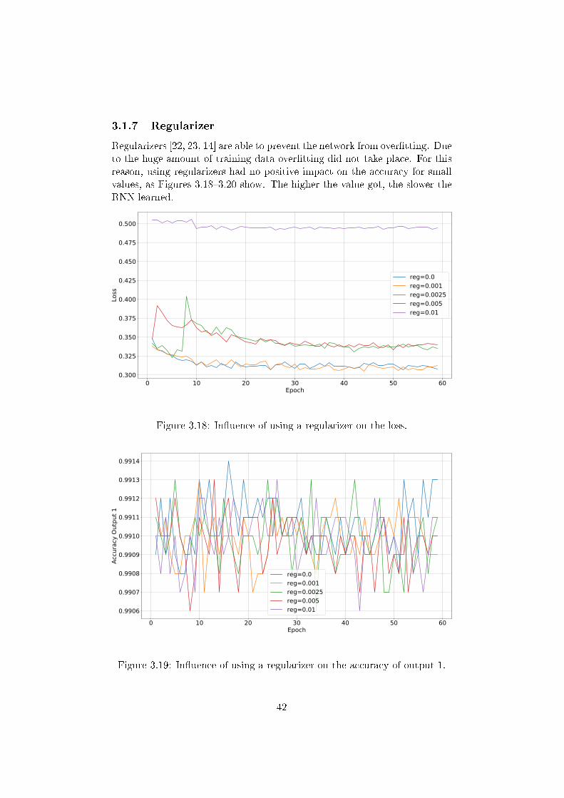
3.1.7 Regularizer

Regularizers [22, 23, 14] are able to prevent the network from over�tting. Dueto the huge amount of training data over�tting did not take place. For thisreason, using regularizers had no positive impact on the accuracy for smallvalues, as Figures 3.18�3.20 show. The higher the value got, the slower theRNN learned.

Figure 3.18: In�uence of using a regularizer on the loss.

Figure 3.19: In�uence of using a regularizer on the accuracy of output 1.

42

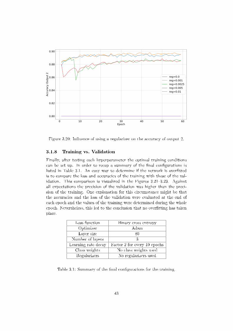
Figure 3.20: In�uence of using a regularizer on the accuracy of output 2.

3.1.8 Training vs. Validation

Finally, after testing each hyperparameter the optimal training conditionscan be set up. In order to recap a summary of the �nal con�gurations islisted in Table 3.1. An easy way to determine if the network is over�ttedis to compare the loss and accuracies of the training with those of the val-idation. This comparison is visualized in the Figures 3.21�3.23. Againstall expectations the precision of the validation was higher than the preci-sion of the training. One explanation for this circumstance might be thatthe accuracies and the loss of the validation were evaluated at the end ofeach epoch and the values of the training were determined during the wholeepoch. Nevertheless, this led to the conclusion that no over�tting has takenplace.

Loss function Binary cross entropy

Optimizer Adam

Layer size 80

Number of layers 3

Learning rate decay Factor 2 for every 10 epochs

Class weights No class weights used

Regularizers No regularizers used

Table 3.1: Summary of the �nal con�gurations for the training.

43

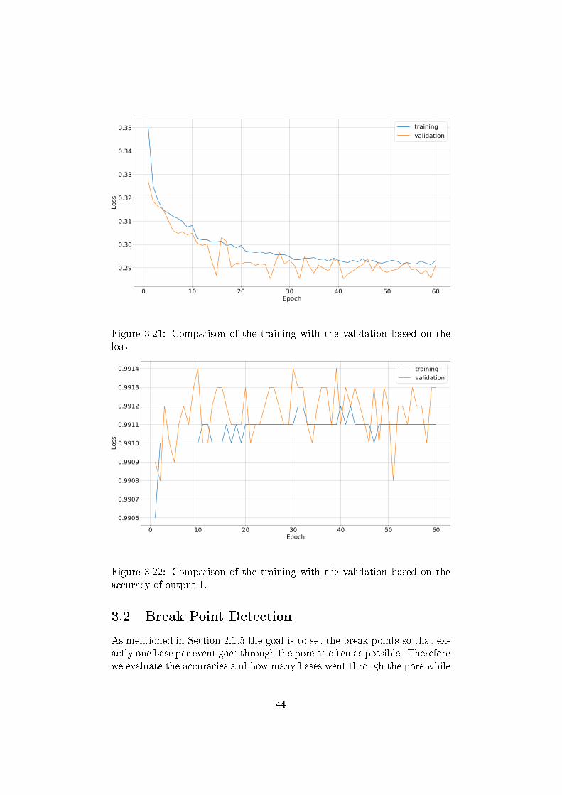
Figure 3.21: Comparison of the training with the validation based on theloss.

Figure 3.22: Comparison of the training with the validation based on theaccuracy of output 1.

3.2 Break Point Detection

As mentioned in Section 2.1.5 the goal is to set the break points so that ex-actly one base per event goes through the pore as often as possible. Thereforewe evaluate the accuracies and how many bases went through the pore while

44

using the window-based and Metrichor's break point detection. In this sec-tion we compare both.

3.2.1 Window Lengths and Thresholds

Applying Algorithm 4 of Section 2.1.5 to the raw reads yielded certain val-ues for the window lengths and thresholds: short window length = 6, longwindow length = 10, threshold for the short window = 1.4 and threshold forthe long window = 2.2. Table 3.2 shows the amount of events where zero,one and two or more bases went through the pore and how many bases wereskipped due to too long events for the window-based break point detectionand the break point detection of Metrichor. The ideal case was maximizingthe amount of events with exactly one base, while simultaneously minimizingthe deleted bases. On the one hand the window-based break point detectionhad more events with one base, on the other hand it had more deleted bases.

3.3 Comparison of the results

In order to compare the results of the di�erent basecallers they were appliedto test �les. Afterwards, Minialign was applied on the outputs to determinethe accuracies. Table 3.3 and Figure 3.24 compare the accuracies usingthe basecaller of Metrichor and the RNN with and without break pointdetection. Apparently, Metrichor had the highest accuracy, but also the

Figure 3.23: Comparison of the training with the validation based on theaccuracy of output 2.

45

Window-based break Metrichor breakpoint detection point detection

0 bases/event 41.1% 46.5%

1 base/event 53.5% 51.3%

≥2 bases/event 5.43% 2.22%

Deleted bases 3.07% 1.71%

Table 3.2: Amount of events, with 0, 1 and 2 or more bases passing the poreand the amount of deleted bases for the window-based and Metrichor's breakpoint detection.

highest standard deviation. The average precision of the RNN was slightlylower, especially when using the window-based break point detection. Thisindicates that using another break point detection algorithm may have thepotential for improvements.

Average of Standard deviationthe accuracy of the accuracy

Metrichor 79.0% 7.42%

RNN with Metichor bp detection 76.4% 6.18%

RNN with window-based bp detecion 73.7% 4.51%

Table 3.3: Accuracies of the di�erent basecallers.

46

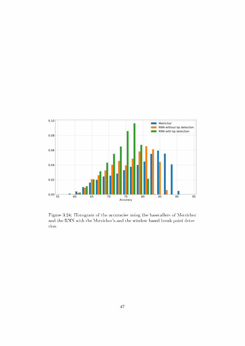
Figure 3.24: Histogram of the accuracies using the basecallers of Metrichorand the RNN with the Metrichor's and the window-based break point detec-tion.

47

Chapter 4

Conclusions

The purpose of this master thesis was to develop and to evaluate a basecallerfor nanopore sequencing with a high accuracy. The basecaller from Metrichorwas used, which has an accuracy of 79%, served as a comparison. Inspiredby other projects that used machine learning for basecalling, we decided touse RNNs. In order to maximize the precision many adjustments of thehyperparameters had to be made. The only method to �gure out whichoptions worked best was to test and compare each of them. During ourresearch it became clear that using an appropriate loss function was the mostin�uential factor. Binary cross entropy turned out to be the only useful lossfunction, as the outputs of other loss functions had such low accuracies thatnot even a single read could be aligned to the reference. Changing the otherhyperparameters in�uenced the precision by just a few percent as Section 3.1shows.

Although we optimized several hyperparameters, the accuracy of theRNN, when using the break point detection of Metrichor, was 76.4% andthus lower than the precision of Metrichor's basecaller. This suggests thatRNNs work, but they are less suitable for basecalling than hidden Markovmodels.

It was necessary to implement a break point detection since some versionsof Metrichor did not use events for basecalling. There were many algorithmsto choose from. Because many of them were time consuming, the choicefell on the window-based break point detection algorithm. This algorithmachieved a higher amount of events with exactly one base passing through.However, there were also more deleted bases. Unfortunately, Metrichor'sbreak point detection is unknown, thus no conclusions can be drawn as towhy it works better. Nevertheless, the comparison of the results of theRNNs with Metrichor's break point detection on the one hand and with thewindow-based break point detection on the other hand, allow conclusions inregards to possible improvements. Apparently the number of deleted baseshad a greater impact on the accuracy than the amount of events with exactlyone base.

48

Bibliography

[1] https://github.com/jeammimi/deepnano.

[2] https://metrichor.com/.

[3] https://github.com/ocxtal/minialign.

[4] http://s3.climb.ac.uk/nanopore/R9_Ecoli_K12_MG1655_lambda_MinKNOW_0.51.1.62.tar.

[5] E. Ahmed, A. Clark, and G. Mohay. A novel sliding window basedchange detection algorithm for asymmetric tra�c. In IFIP International

Conference on Network and Parallel Computing, pages 168�175. IEEE,2008.

[6] L. Bottou. Large-scale machine learning with stochastic gradient de-scent. In Proceedings of COMPSTAT 2010, pages 177�186. Springer,2010.

[7] D. Branton and D. Deamer. Nanopore Sequencing: An Introduction.World Scienti�c, 2019.

[8] J. Chung, C. Gulcehre, K. Cho, and Y. Bengio. Empirical evaluation ofgated recurrent neural networks on sequence modeling. arXiv preprint

arXiv:1412.3555, 2014.

[9] D. Deamer, M. Akeson, and D. Branton. Three decades of nanoporesequencing. Nature Biotechnology, 34(5):518, 2016.

[10] T. Dozat. Incorporating Nesterov momentum into ADAM. CaribeHilton, San Juan, Puerto Rico, 2016.

[11] J. Duchi, E. Hazan, and Y. Singer. Adaptive subgradient methodsfor online learning and stochastic optimization. Journal of Machine

Learning Research, 12(Jul):2121�2159, 2011.

[12] Y. Feng, Y. Zhang, C. Ying, D. Wang, and C. Du. Nanopore-basedfourth-generation DNA sequencing technology. Genomics, Proteomics

& Bioinformatics, 13(1):4�16, 2015.

49

[13] D. P. Kingma and J. Ba. Adam: A method for stochastic optimization.International Conference on Learning Representations, 2014.

[14] C.-S. Leung, A.-C. Tsoi, and L. W. Chan. Two regularizers for recursiveleast squared algorithms in feedforward multilayered neural networks.IEEE Transactions on Neural Networks, 12(6):1314�1332, 2001.

[15] S. Liu, M. Yamada, N. Collier, and M. Sugiyama. Change-point de-tection in time-series data by relative density-ratio estimation. NeuralNetworks, 43:72�83, 2013.

[16] Y. Nesterov. A method for solving the convex programming problemwith convergence rate O(1/k2). In Doklady AN USSR, volume 269,pages 543�547, 1983.

[17] Y. Nesterov. Lectures on Convex Optimization, volume 137. Springer,2018.

[18] E. Pennisi. Search for pore-fection. Science, 336(6081):534�537, 2012.

[19] M. Schuster and K. K. Paliwal. Bidirectional recurrent neural networks.IEEE Transactions on Signal Processing, 45(11):2673�2681, 1997.

[20] R. Sutton. Two problems with back propagation and other steepestdescent learning procedures for networks. In Proceedings of the Eighth

Annual Conference of the Cognitive Science Society, 1986, pages 823�832, 1986.

[21] C. Truong, L. Oudre, and N. Vayatis. Ruptures: change point detectionin Python. arXiv preprint arXiv:1801.00826, 2018.

[22] L. Wan, M. Zeiler, S. Zhang, Y. L. Cun, and R. Fergus. Regularization ofneural networks using dropconnect. In S. Dasgupta and D. McAllester,editors, Proceedings of the 30th International Conference on Machine

Learning, volume 28 of Proceedings of Machine Learning Research, pages1058�1066, Atlanta, Georgia, USA, 17�19 Jun 2013. PMLR.

[23] L. Wu and J. Moody. A smoothing regularizer for feedforward andrecurrent neural networks. Neural Computation, 8(3):461�489, 1996.

[24] M. D. Zeiler. ADADELTA: an adaptive learning rate method. arXiv

preprint arXiv:1212.5701, 2012.

50