Spatial analysis of crop rotation practice in

North-western Germany

Dissertation

zur Erlangung des Doktorgrades (Dr. sc. agr.)

der Fakultät für Agrarwissenschaften

der Georg-August-Universität Göttingen

vorgelegt von

Dipl.-Geogr. Susanne Stein

geboren in Weimar

Göttingen, im September 2020

1. Gutachter: Prof. Dr. Johannes Isselstein

2. Gutachter: Dr. Horst-Henning Steinmann

Tag der mündlichen Prüfung: 14.07.2020

Meinem geliebten Mann Carsten gewidmet,

der hierfür unzählige Stunden im Zug und einsame Abende in Kauf genommen hat.

Content

Introduction ........................................................................................................................... 5

References ........................................................................................................................ 8

Linking arable crop occurrence with site conditions by the use of highly resolved spatial data .............................................................................................................................................10

Abstract ............................................................................................................................11

Introduction .......................................................................................................................11

Materials and Methods ......................................................................................................12

Results..............................................................................................................................19

Discussion ........................................................................................................................22

Conclusion ........................................................................................................................25

References .......................................................................................................................25

Identifying crop rotation practice by the typification of crop sequence patterns for arable farming systems – A case study from Central Europe .......................................................................31

Abstract ............................................................................................................................32

Introduction .......................................................................................................................32

Materials and methods ......................................................................................................35

Results..............................................................................................................................43

Discussion ........................................................................................................................48

Conclusion ........................................................................................................................51

References .......................................................................................................................52

Annual crop census data does not proper represent actual crop rotation practice ................57

Abstract ............................................................................................................................58

Introduction .......................................................................................................................58

Materials and Methods ......................................................................................................59

Results..............................................................................................................................62

Discussion ........................................................................................................................64

Conclusion ........................................................................................................................66

References .......................................................................................................................66

General Discussion ..............................................................................................................69

References .......................................................................................................................72

Summary ..............................................................................................................................75

Zusammenfassung ...............................................................................................................77

List of Publications ............................................................................................................. 800

Acknowledgements ............................................................................................................ 811

Introduction

__________________________________________________________________________

Introduction

Crop rotation means the systematic cultivation of different crops on the same land in a recurring

sequence (Liebman and Dyck, 1993). This involves growing crops in a useful order considering

crop-to-crop compatibilities and management processes. The principles of crop rotation are as

old as arable land use itself and have already been scientifically described in the 19th century

(e.g. Daubeny, 1845). A well-adapted crop rotation has positive effects on the soil fertility and

all factors of the field ecosystem services like the water and nutrient cycle, humus content, and

the diversity and density of yield supporting or reducing micro- and macro-organisms (Karlen

et al., 1994). Variety of the weed flora and related species like invertebrates is strongly

determined by the kind of crop and its order in a sequence and improves, therefore,

phytosanitary conditions (Blackshaw et al., 2007; Smith et al., 2008; Melander et al., 2013).

Changing the main crop and, consequently, the soil tillage and the residue regime has positive

effects on the soil, such as diversified microorganism community, improvement of the soil

aggregates stability, bulk density, and hydraulic properties (Blanco-Canqui and Lal, 2009;

Tiemann et al., 2015). Short rotations may result in degradation of soil structure and fertility as

well as force soil erosion (Bullock, 1992).

Even if crop rotation is a fundamental agricultural instrument for each farmer, the green

revolution (1950-1970) with synthetic fertilizers and pesticides, high yielding crop varieties, and

modern machinery seemed to replace the rules of crop rotation/effect (Bullock, 1992). The

impact of these developments was enforced in the following decades by an enormous grew in

the world agricultural trade and increased importance of economic drivers apart from the

regional scale. The rotations became simplified and short. Today it is political consensus again

that crop rotation serves as an instrument to reduce chemical inputs and grants sustain soil

fertility (European Commission, 2010). Negative side effects of intensive agriculture, like soil

degradation and resistant weeds, force the need to reintroduce crop rotation (Kay, 1990).

This dissertation was developed in the light of a significant increase of the Lower

Saxonian maize acreage in a comparably short period of time, from about 355.000 ha in 2005

to about 610.000 ha in 2011, whereby one-third of the latter was maize for biogas production

(NMELV, 2013). One reason for this development was the amendment of the Renewable

Energy Act (EEG) in 2004, which included bonuses for energy plant production. The change

of the crop rotation practice started a long time before, for the reasons mentioned above. The

intensive livestock farms, which are located mainly in the North-western part of Lower Saxony,

namely the Weser-Ems region, had high maize acreage of more than 30% already before the

biogas plant developments. The historical as well as recent developments, lead to the

question, whether there are still patterns of crop rotation detectible or not. What are the present

crop rotation patterns in Lower Saxony? Since I am a geographer by training, including the

spatial dimension in my analysis seemed natural. Are there regional patterns of crop rotation

in Lower Saxony? And what are the driving forces for the formation of these patterns? The first

Introduction

step for answering these questions was to analyze the spatial crop distribution in one year. To

use the crop statistic of one year is the most common way to derive crop rotation, usually

quantified by the Shannon Index (e.g. Monteleone et al., 2018).

The first chapter of this thesis presents an alternative approach, the formation of

regional crop clusters. This allows for comparing the spatial congruency of the crop clusters

with clusters of site conditions, e.g. soil texture, arable farming potential, precipitation, and

livestock density. The results of that one-year-analysis build the fundament for the detection

of regional crop rotation patterns in a seven-year-analysis and enlightened the driving forces

for these patterns, as explained in the second chapter. To answer this central question of my

study was possible due to the lucky coincidence of having access to an enormous set of data.

It included information on the main arable crop at field scale in Lower Saxony for the years

2005 to 2011 for which the farmers received direct payments from the European Union. The

source of the data is the Integrated Administration and Control System (IACS), which helps

farmers and authorities with the area-based administration of the yearly agricultural subsidies

within the frame of the Common Agricultural Policy (CAP) (European Council Regulation

1593/2000 – European Commission, 2000). The agricultural reference parcels are registered

in the Land Parcel Identification System (LPIS). IACS and LPIS were conceptualized in 1992

(European Council Regulation 3508/92 and Commission Regulation 3887/92 – European

Commission, 1992) and further developed into a Geographic Information System that replaced

the cadastre in 2005. LPIS with its high spatial and temporal resolution offers a valuable data

source for land-use change and cropland dynamic studies, (e.g. Leteinturier et al., 2006;

Schönhart et al., 2011, Levavasseur et al., 2016; Lüker-Jahns et al., 2016; Zimmermanns et

al., 2016; Barbottin et al., 2018) and evaluation and monitoring approaches (Reiter &

Roggendorf, 2007; Lomba et al., 2017). A first analysis of the LPIS data for Lower Saxony by

Steinmann and Dobers (2013) identified a great variety of crop sequences. It concluded that

most of the farmers tend to change their crop order highly dynamic. This goes in line with the

conclusion for the European crop rotation practice that farmers seem to choose crops mainly

depending on the preceding crop and not following any crop rotation pattern (European

Commission, 2010).

The second chapter of this thesis presents a method to uncover crop rotation patterns

by defining crop sequence types based on structural properties, like the number of crops and

their transition rate in a sequence, and based on physical properties of the crops. These

physical properties determine the functional role of a crop in an appropriate crop rotation.

The third chapter of this thesis uses this typification approach for a methodological

excurse and relates the crop sequence types in the temporal dimension of crop rotation

practice with the spatial dimension of crop pattern based on one-year crop data.

Introduction

References

Barbottin, A., Bouty, C., Martin, P., 2018. Using the French LPIS database to highlight farm area dynamics: The case study of the Niort Plain. Land Use Policy 73, 281-289. DOI: 10.1016/j.landusepol.2018.02.012

Blackshaw, R. E., Andersson, R.L., Lemerle, D., 2007. Chapter 3: Cultural weed management. In: Upadyaya, M.K. and Blackshaw, R.E.: Non-Chemical weed management: Principles, concepts and technology. CAB International, Wallingford, UK, 35-48.

Blanco-Canqui, H., Lal, R., 2009. Crop residue removal impacts on soil productivity and environmental quality. Crit. Rev. Plant Sci. 28, 139-163.

Bullock, D.G., 1992. Crop rotation. Crit. Rev. Plant Sci. 11, 309-326.

Daubeny, C., 1845. Memoir on the rotation of crops, and on the quantity of inorganicmatters abstracted from the soil by various plants under different circumstances. Philos. Trans. R. Soc. Lond. 135, 179–252.

European Commission, 2010. Environmental Impacts of Different Crop Rotation in the European Union (Final Report 6 Sept. 2010).

Karlen, D.L., Varvel, G.E., Bullock, D.G., Cruse, R.M., 1994. Crop Rotations for the 21st Century. Advances in Agronomy 53, 1-45.

Kay, B. D. 1990. Rates of change of soil structure under different cropping systems. In: Stewart, B.E. (Ed.): Advances in Soil Science, Volume 12, Springer Verlag New York, 1-52. DOI: 10.1007/978-1-4612-3316-9

Leteinturier, B., Herman, J. L., de Longueville, F., Quintin, L., Oger, R., 2006. Adaptation of a crop sequence indicator based on a land parcel management system. Agric. Ecosyst. Environ. 112, 324-334.

Levavasseur, F., Martin, P., Bouty, C, Barbottin, A., Bretagnolle, V., Thérond, O., Scheurer, O., 2016. RPG Explorer: A new toll to ease the analysis of agricultural landscape dynamics with the Land Parcel Identification System. Comput. Electron. Agr. 127, 541-552.

Liebman, M., Dyck, E., 1993. Crop rotation and intercropping strategies for weed management. Ecol. Appl. 3, 92-122.

Lomba, A., Strohbach, M., Jerrentrup, J. S., Dauber, J., Klimek, S., McCracken, D. I., 2017. Making the best of both worlds: Can high-resolution agricultural administrative data support the assessment of High Nature Value farmlands across Europe?. Ecological Indicators 72, 118-130.

Lüker-Jahns, N., Simmering, D., Otte, A., 2016. Analysing data of the Integrated Administration and Control System (IACS) to detect patterns of agricultural land-use change at municipality level. Landscape Online 48, 1-24. DOI: 10.3097/LO.201648

Melander, B., Munier-Jolain, N., Charles, R., Wirth, J., Schwarz, J., van der Weide, R., Bonin, L., Jensen, P. K., Kudsk, P., 2013. European perspectives on the adoption of nonchemical weed management in reduced-Tillage systems for arable crops. Weed Technol. 27, 231-240.

Monteleone, M., Cammerino, A.R.B., Libutti, A., 2018. Agricultural “greening” and cropland diversification trends: Potential contribution of agroenergy crops in Capitanata (South Italy). Land Use Policy 70, 591-600. DOI: 10.1016/j.landusepol.2017.10.038

NMELV, 2013. Ergänzungen zur Broschüre: Die niedersächsische Landwirtschaft in Zahlen 2011 (Stand: November 2013). Niedersächsisches Ministerium für Ernährung, Landwirtschaft und Verbraucherschutz, Hannover.

Reiter, K., Roggendorf, W., 2007. Nutzbarkeit vorhandener Datenbestände für Monitoring und Evaluierung – am Beispiel des InVeKoS. In: Begemann, F., Schröder, S., Wenkel, K.-O., Weigel, H.-J. (Eds.): Monitoring und Indikatoren der Agrobiodiversität. Agrobiodiversität 27, 274-287.

Schönhart, M., Schmidt, E., Schneider, U. A., 2011. CropRota – A crop rotation model to support integrated land use assessments. Europ. J. Agron. 34, 263-277.

Smith, V., Bohan, D. A., Clark, S. J., Haughton, A. J., Bell, J. R., Heard, M. S., 2008. Weed and invertebrate community compositions in arable farmland. Arthropod-Plant Interactions 2, 21-30. DOI: 10.1007/s11829-007-9027-y

Introduction

Steinmann, H.-H., Dobers, S., 2013. Spatio-temporal analysis of crop rotations and crop sequence patterns in Northern Germany: potential implications on plant health and crop protection. J. Plant Dis. Protect. 120 (2), 85–94.

Tiemann, L.K., Grandy, A.S., Atkinson E.E., Marin-Spiotta, E., McDaniel, M.D., 2015. Crop rotational diversity enhances belowground communities and functions in an agroecosystem. Ecol. Letters 18, 761-771.

Zimmermann, J.; González, A.; Jones, M. B.; O’Brien, P.; Stout, J. C.; Green, S. (2016): Assessing land-use history for reporting on cropland dynamics – A comparison between the Land-Parcel Identification System and traditional inter-annual approaches. Land Use Policy 52, 30-40.

__________________________________________________________________________

Chapter 1

Linking arable crop occurrence with site conditions

by the use of highly resolved spatial data

__________________________________________________________________________

Chapter 1

11

Abstract

Agricultural land use is influenced in different ways by local factors such as soil conditions,

water supply and socioeconomic structure. We investigated at the regional and the field scale

how strong the relationship of arable crop pattern and specific local site conditions is. At field

scale a logistic regression analysis for the main crops and selected site variables detected for

each of the analyzed crops its own specific character of crop-site relationship. Some crops

have diverging site relations such as maize and wheat, while other crops show similar

probabilities under comparable site conditions e.g. oilseed rape and winter barley. At the

regional scale the spatial comparison of clustered variables and clustered crop pattern showed

a slightly stronger relationship of crop combination and specific combinations of site variables

compared to the view on the single crop-site relationship.

Introduction

In the last decades, European arable farming was characterized by modifications of cropping

patterns and crop choice driven by an enormous progress in plant breeding, plant protection,

fertilization and drainage techniques (Tilman et al., 2002; van Zanten et al., 2014). Also, market

prices, farm subsidies and political incentives such as support of bioenergy crops influenced

crop choice [Dury et al., 2013; Aouadi et al., 2015; Troost et al., 2015). Recent studies have

shown that a few cash crops are preferentially grown both in time and space while other crops

are neglected (Baaker et al., 2011; Steinmann and Dobers, 2013). In Northern Germany maize

and winter wheat are cropped on more than 50 % of the arable area and in many regions only

one to three relevant crops are grown (Steinmann and Dobers, 2013). On the other hand, a

decreasing importance of regional site conditions such as soil conditions, water supply and

climate for choosing a crop for a given site can be observed (Antrop, 2005; Baaker et al., 2013).

Thus, the relationship between site conditions and farmers crop choice (hereafter referred to

as crop-site relationship) seems to become weaker in modern farming.

One initial objective of the Common Agricultural Policy (CAP) is to increase productivity.

This policy, therefore, has been a major driver of land use change for many decades (Viaggi

et al., 2013). The reform of 2003 introduced new rules of payments to farmers. Payments were

decoupled from production to Single Farm Payment. At the same time, intervention prices for

specific crops were maintained. National schemes on the promotion of renewable energy crops

supported the intensive cultivation of crops for biomass production (EEG, 2004). All this

resulted in a continuation of intensive arable production in many historically intensively

managed regions (OECD, 2004; Tzanopoulos et al., 2012; Trubins, 2013). The latest reform

of the CAP in 2013 implemented political instruments that are commonly named with the term

“greening” (European Parliament, Reg. No 1307/2013) like crop diversification. However, there

Chapter 1

12

is lack of knowledge to which extend farmers do have enough options to diversify crop

rotations. In a recent approach, it was shown on the basis of spatial data that some crop

rotation patterns refer to site conditions, whereas others do explicitly not (Stein and Steinmann,

2018). To our knowledge, there is no spatial explicit information to which extent crop-site

relationship still exist in recent landscapes. We present here a method to detect the relationship

of crop cultivation and site conditions to improve the understanding and assessment of

ecosystem services in the agricultural system.

With the presented methods, a binary logistic regression and a k-means clustering, we

analysed crop patterns in the landscape to understand to what extent crop choice still depends

on site conditions. We had chosen the two methods to explore, first, how intensive the

individual relationship between the single crop and the single site variable is. Second, we

localized regions of relationship between the clustered sets of site variables and the clustered

crop patterns. Our study combines site variables and crop data of the year 2011 for the German

federal state Niedersachsen (Lower Saxony) which includes an exceptional variety of

agricultural systems. These characteristics make the region a good example for other arable

regions and for the estimation of future trends in agricultural land use.

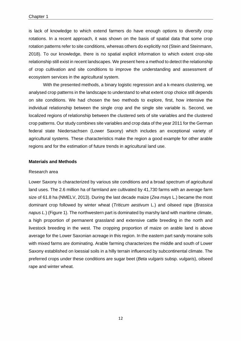
Materials and Methods

Research area

Lower Saxony is characterized by various site conditions and a broad spectrum of agricultural

land uses. The 2.6 million ha of farmland are cultivated by 41,730 farms with an average farm

size of 61.8 ha (NMELV, 2013). During the last decade maize (Zea mays L.) became the most

dominant crop followed by winter wheat (Triticum aestivum L.) and oilseed rape (Brassica

napus L.) (Figure 1). The northwestern part is dominated by marshy land with maritime climate,

a high proportion of permanent grassland and extensive cattle breeding in the north and

livestock breeding in the west. The cropping proportion of maize on arable land is above

average for the Lower Saxonian acreage in this region. In the eastern part sandy moraine soils

with mixed farms are dominating. Arable farming characterizes the middle and south of Lower

Saxony established on loessial soils in a hilly terrain influenced by subcontinental climate. The

preferred crops under these conditions are sugar beet (Beta vulgaris subsp. vulgaris), oilseed

rape and winter wheat.

Chapter 1

13

Figure 1. Natural area classification of the German federal state of Niedersachsen (Lower Saxony NUTS 1 region

DE9 (European Nomenclature of Territorial Units for Statistics)) and the acreage of the ten main crops or crop

groups in 2011, forage includes.

Data characteristics and processing

Our analysis followed two complementary approaches to detect the characteristics and spatial

distribution of specific crop-site relationship. In a first step a logistic regression analysis was

processed that combines crop information at the field scale for the ten most commonly used

crops in Lower Saxony with site variables such as soil, precipitation or livestock density to

characterize the relationship between these and the crops at the field scale. This result is

compared with the result from a k-means clustering process to localize spatial overlays of

clustered crops and clustered site variables at the regional scale.

For the crop data at the field scale the Land Parcel Identification System (LPIS) was

used, a yearly updated database which supports the administration of direct payments for

European farmers as part of the Integrated and Control System (IACS). It was established in

all member states of the European Union in 1992 and developed concurrently with political

reform measures (European Parliament, Reg. No 1782/2003). In Germany the data are

managed by the German Federal States’ institutions. The access is limited due to privacy

protection reasons and special permission is required for scientific use. For this study

Chapter 1

14

information about the main agricultural land use type in 2011, the field size and individual field

identification numbers were provided for the state Lower Saxony. The dataset was attributed

to a GIS-geometry which comprises the boundaries for all agricultural parcels (about 990,000

records in total) (SLA, 2011). Due to a small amount of imprecise field identification, e.g. the

assignment of one ID to more than one field, the IACS dataset had to be debugged for

uncertainties. For the analysis only arable fields were included. Hence, with a loss of 15% due

to imprecise field identification and intersection loss, the basic dataset of the analysis consists

of 444,009 agricultural parcels.

To analyse the crop-site relationship it was necessary to find spatial variables which

represent the site conditions of the investigated area in a suitable resolution and area-wide

consistent availability. Official data from well-established public sources satisfied these

requirements (Table 1). The variables were selected with the aim to represent the

environmental site conditions in Lower Saxony. This North-western part of Germany is

characterized by locally high densities of livestock husbandry and grassland farming (NMELV,

2011, Figure 2). Therefore, variables on animal production were included.

The data for cattle density, pig and poultry density, and the average farm size were

extracted from agricultural census data at LAU-2 (Local Administrative Unit) scale (Figure 2).

The relative biotope index was developed by the Julius Kühn-Institute, the German Federal

Research Centre for Cultivated Plants, to estimate the biotope features in agricultural

landscapes. The value for the relative biotope density was calculated using the locally

observed density of linear biotope habitats (field margins and hedgerows) and patch biotopes

(small woods and grassland patches) per estimated minimum biotope density at LAU-2 scale.

The latter was extrapolated from the intensity of plant protection in the corresponding

landscape type – the higher the intensity of plant protection applications, the higher is the need

for biotopes (Gutsche and Enzian, 2002). The proportion of grassland refers to the area of

grassland per arable area in a 1 x 1 km cell of a raster. The multi-annual precipitation sum

(1981-2010, DWD, 2014) is available in 0.96 x 0.96 km raster format. The temperature was

not regarded due to the low variation of the thermal regime in the study region. For the soil

texture and slope information, the data of the European Soil Database were used which are

available in so called Soil Typological Units (ESDAC, 2004). The arable farming potential was

derived by the Lower Saxonian State Office for Mining, Energy and Geology (LBEG) based on

soil and climate parameters (e.g. soil texture, bulk density, humus content, soil structure, water

logging level) (Richter and Eckelmann, 1993). The higher the value of the arable farming

potential is, the higher is the natural locally potential for biomass production of the soil. For the

regression analysis all metric variables were transformed from metric values into interval

values to facilitate the comparison of the variables’ potential (Table 1). The classification of the

Chapter 1

15

intervals was implemented by a geometrical interval algorithm which minimizes the sum of

squares of the number of elements per class to ensure approximately the same number of

values in each range (ESRI, 2007).

Table 1. Site variables with their classes, units and source scale. Classification of the metric variables was implemented corresponding to the geometrical intervals.

Predictor variable Classes Unit Source

Arable farming potential 1-7 Classes: ‘extremely low’ to

‘extremely high’

(LBEG, 1996)

1: 50 000

Soil texture (Dominant

surface textural class of

the Soil)

1 Peat soil

2 Coarse (> 65% sand)

3 Medium (< 65% sand)

4 Medium fine (< 15 % sand)

5 Fine (>35% clay)

(ESDAC, 2004)

1: 1 000 000

Slope (Dominant slope

class)

1 Level (< 8 %)

2 Sloping (8 - 15 %)

3 Moderately steep (>15 %)

(ESDAC, 2004)

1: 1 000 000

multi-annual precipitation

sum (1981-2010)

1 560-676

2 677-746

3 747-806

4 807-878

5 879-1202

mm*y-1

(DWD, 2014)

0.96 x 0.96 km

Relative biotope density Observed Density/

Potential Density

(JKI, 2004)

LAU 2

Grassland proportion 1 0.00-0.02

2 0.03-0.06

3 0.07-0.17

4 0.18-0.44

5 0.45-1.00

ha/ ha agric. area

Based on IACS-

data 2011

1x1 km

Cattle density 1 0.00-0.10

2 0.11-0.29

3 0.30-0.65

4 0.66-1.32

5 1.33-2.93

Livestock unit/ha

(agricultural area)

(LSKN, 2012)

LAU 2

Pig/poultry density 1 0.00-0.02

2 0.03-0.09

3 0.10-0.30

4 0.31-0.99

5 1.00-3.21

Livestock unit/ha

(agricultural area)

(LSKN, 2012)

LAU 2

Average farm size 1 0-40

2 41-64

3 65-104

4 105-172

5 172-311

ha

(agricultural area)

(LSKN, 2012)

LAU 2

Due to the differences in format and spatial scales of the used datasets they were processed

in relation to a reference scale. For the logistic regression the reference scale was the field

scale. For the cluster process the information content of the variable polygons was attributed

to a 1 x 1 km grid according to their spatial location and proportion. Grid cells with less than

10% of arable area within the grid cell area, i.e. less than 10 ha of arable area, were not

Chapter 1

16

included in the analysis. The merging of the attributed information was performed with the

Spatial Join tool in ArcGIS®. For the small patched polygons of the arable farming potential the

mean of all soil classes per quadrant was attributed. Furthermore, the grid surface permits the

calculation of the crop area proportion (crop area per arable area in a 1 x 1 km grid cell) as

metric variables. The crop area per grid cell is a sum of all fields which had their centroid within

one grid cell.

Figure 2. Exemplary mapping of the spatial distribution of two crops and two variables: a) Acreage of maize 2011; b) Acreage of winter wheat 2011; c) Cattle density per LAU-2 unit; d) Soil texture distribution.

Binary logistic regression (field scale)

Logistic regression is used instead of linear regression when the observed or measured

response of interest is not continuous but binary to predict the likelihood of an event over the

likelihood of non-occurrence (Tarpey, 2012). The cultivation of a crop on a specific field is such

a binary event. Its likelihood under the occurrence of a specific site variable indicates the

strength of its relationships to the cultivation site. If the site variable, e.g. cattle density,

changes by one unit while all other variables stay stable, the likelihood of crop occurrence, e.g.

Chapter 1

17

maize, is increased or decreased by the resulted value of the regression equation. This

resulting value is larger or smaller than zero and can be larger than one. The two variables,

arable farming potential and soil texture, have an ordinal scale and not a metric scale like all

the other variables. Due to this, all characteristics of these two variables were analysed

separately (Table 3). The first characteristic, peat soil for soil texture and very low arable

farming potential, had the role of the reference value, the same role that zero had for the other

variables.

The nine main crops of Lower Saxony were chosen for analysis plus one group containing all

spring cereals. For each of the ten crop categories a binomial regression equation with a binary

response variable, y ϵ {0, 1}, was defined to determine the probability of occurrence for each

crop separately (Menard, 1995; Hosmer and Lemeshow, 2000). The regression analysis was

performed by using the software CRAN-R version 3.1.0 (R Core Team, 2013). It uses a

logarithmic function calculating the logit (𝜋𝑖) for the ratio of the probability (Pij) that a field (i) is

cultivated with a specific crop (j) or not (1 - Pij). Written in a logit equation as suggested by

Fahrmeir et al. (2013):

𝜋𝑖 = 𝑃(𝑦𝑖 = 1) =exp(𝜂𝑖)

1+exp(𝜂𝑖) ,

containing the linear predictor

𝜂𝑖 = 𝛽0 + 𝛽1𝑥𝑖1+. . . +𝛽𝑘𝑥𝑖𝑘 .

The predictor (𝜋𝑖) represents the logarithmic odds (log odds), while the coefficient (𝛽𝑘) for this

variable (𝑥𝑖𝑘) is the expected change in these log odds. While holding the corresponding

predictor variables constant, a one unit increase of the predictor variable causes the change

of the probability corresponding to the coefficient value for having the subject crop (ESRI, 2007;

Fahrmeir et al., 2013).

The likelihood ratio test with a null model for each crop resulted in a rejection of the null

hypothesis for all crops. That means that the observed crop occurrence is more likely under

the presented model than under the null model.

In contrast to the other variables, arable farming potential and soil texture are handled as factor

variables. The coefficient of the first category acts as reference category with a value of zero.

We inspected the correlation effects between the site variables to identify the rate of correlation

between the variables, e.g. cattle density and biotope density or soil texture and arable farming

potential (Table 2). These effects are immanent for variables which characterize ecological

and spatial phenomena (Kleinn et al., 1999). A high correlation of the variables is an expected

effect and is therefore not considered in the equation. This decision is forced by the objective

Chapter 1

18

of the regression analysis which is not used as a predicting model but as a method to

characterize the relationship between the crops and the site conditions.

Table 2. Correlation matrix of the site variables used in the logistic regression model.

A. F. Pot.1 Soil texture Slope Precipit. Biotope I2 Farm Size CattleD3 PigPoulD4 GrassL5

A. F. Pot. 1

Soil texture 0.617 1

Slope 0.145 0.267 1

Precipit. -0.125 -0.093 0.117 1

Biotope I -0.503 -0.548 -0.227 0.350 1

Farm Size 0.162 0.161 0.084 -0.421 -0.367 1

CattleD -0.439 -0.437 -0.190 0.501 0.665 -0.435 1

PigPoulD -0.207 -0.248 -0.161 0.248 0.227 -0.358 0.221 1

GrassL -0.242 -0.144 0.006 0.235 0.332 -0.154 0.388 -0.132 1

1 Arable Farming Potential, 2 Biotope Index, 3 Cattle Density, 4 Pig/ Poultry Density, 5 Grassland proportion

Cluster analysis (regional scale)

A non-hierarchical k-means clustering with the Hartigan & Wong algorithm (Hartigan and

Wong, 1979) was used to detect regional patterns of similarities for the site variables and for

crops (Hartigan, 1975; Draper and Smith, 1998). This was realized with the software CRAN-R

version 3.1.0 (R Core Team, 2013; R Documentation, 2015). The k-means clustering is a

common method for identifying spatial units at the landscape scale (Schmidt et al., 2010;

Caravalho et al., 2016; Ivadi et al., 2017). It was used in this paper to identify spatial units with

consistent properties. The crop clusters and the site clusters were than compared in their

spatial concordance.

The optimal number of classes, k, was found by comparing results of multiple runs with

different number of classes and visualizing the grade of clustering in a map (Morissette and

Chartier, 2013). The uncertainty of the initial random partition was adjusted by choosing the

most frequent version of partition in ten runs. In a previous step a z-transformation of all

variable values standardized the very different scales to improve the comparability of the

results. The cluster analysis generated five site clusters (S1, S2, S3, S4, S5) and five crop

clusters (C1, C2, C3, C4, C5).

Chapter 1

19

Results

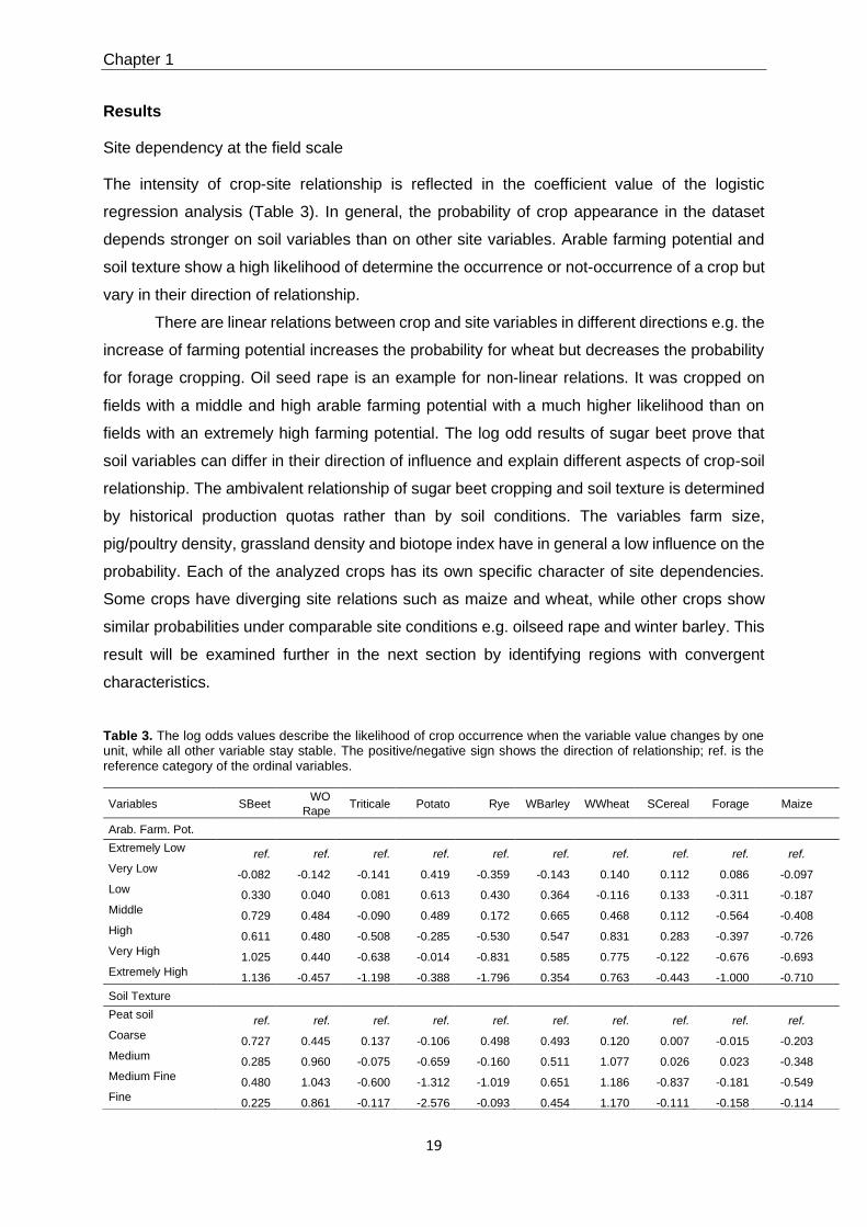
Site dependency at the field scale

The intensity of crop-site relationship is reflected in the coefficient value of the logistic

regression analysis (Table 3). In general, the probability of crop appearance in the dataset

depends stronger on soil variables than on other site variables. Arable farming potential and

soil texture show a high likelihood of determine the occurrence or not-occurrence of a crop but

vary in their direction of relationship.

There are linear relations between crop and site variables in different directions e.g. the

increase of farming potential increases the probability for wheat but decreases the probability

for forage cropping. Oil seed rape is an example for non-linear relations. It was cropped on

fields with a middle and high arable farming potential with a much higher likelihood than on

fields with an extremely high farming potential. The log odd results of sugar beet prove that

soil variables can differ in their direction of influence and explain different aspects of crop-soil

relationship. The ambivalent relationship of sugar beet cropping and soil texture is determined

by historical production quotas rather than by soil conditions. The variables farm size,

pig/poultry density, grassland density and biotope index have in general a low influence on the

probability. Each of the analyzed crops has its own specific character of site dependencies.

Some crops have diverging site relations such as maize and wheat, while other crops show

similar probabilities under comparable site conditions e.g. oilseed rape and winter barley. This

result will be examined further in the next section by identifying regions with convergent

characteristics.

Table 3. The log odds values describe the likelihood of crop occurrence when the variable value changes by one unit, while all other variable stay stable. The positive/negative sign shows the direction of relationship; ref. is the reference category of the ordinal variables.

Variables SBeet WO

Rape Triticale Potato Rye WBarley WWheat SCereal Forage Maize

Arab. Farm. Pot.

Extremely Low ref. ref. ref. ref. ref. ref. ref. ref. ref. ref.

Very Low -0.082 -0.142 -0.141 0.419 -0.359 -0.143 0.140 0.112 0.086 -0.097

Low 0.330 0.040 0.081 0.613 0.430 0.364 -0.116 0.133 -0.311 -0.187

Middle 0.729 0.484 -0.090 0.489 0.172 0.665 0.468 0.112 -0.564 -0.408

High 0.611 0.480 -0.508 -0.285 -0.530 0.547 0.831 0.283 -0.397 -0.726

Very High 1.025 0.440 -0.638 -0.014 -0.831 0.585 0.775 -0.122 -0.676 -0.693

Extremely High 1.136 -0.457 -1.198 -0.388 -1.796 0.354 0.763 -0.443 -1.000 -0.710

Soil Texture

Peat soil ref. ref. ref. ref. ref. ref. ref. ref. ref. ref.

Coarse 0.727 0.445 0.137 -0.106 0.498 0.493 0.120 0.007 -0.015 -0.203

Medium 0.285 0.960 -0.075 -0.659 -0.160 0.511 1.077 0.026 0.023 -0.348

Medium Fine 0.480 1.043 -0.600 -1.312 -1.019 0.651 1.186 -0.837 -0.181 -0.549

Fine 0.225 0.861 -0.117 -2.576 -0.093 0.454 1.170 -0.111 -0.158 -0.114

Chapter 1

20

Slope -0.040 0.230 -0.146 -0.513 -0.269 0.254 0.159 -0.330 0.130 -0.493

Precipitation -0.198 0.019 -0.213 -0.113 -0.285 0.018 0.021 0.092 0.078 0.093

Biotope Index -0.278 -0.165 0.036 -0.003 0.205 -0.047 -0.240 -0.067 -0.037 0.173

Farm size 0.067 -0.026 -0.213 0.094 0.141 -0.304 -0.055 -0.060 -0.031 0.043

Cattle Density -0.498 -0.323 -0.201 -0.145 0.391 -0.176 -0.034 -0.145 0.091 -0.176

Pig/ Poultry Density -0.215 0.125 -0.033 -0.209 0.141 0.167 0.202 -0.209 -0.008 0.167

Grassland/ a. area -0.192 -0.230 0.056 0.084 0.058 -0.008 0.002 0.084 0.221 -0.008

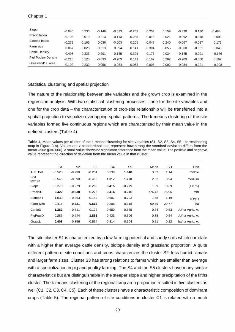
Statistical clustering and spatial projection

The nature of the relationship between site variables and the grown crop is examined in the

regression analysis. With two statistical clustering processes – one for the site variables and

one for the crop data – the characterization of crop-site relationship will be transferred into a

spatial projection to visualize overlapping spatial patterns. The k-means clustering of the site

variables formed five continuous regions which are characterized by their mean value in the

defined clusters (Table 4).

Table 4. Mean values per cluster of the k-means clustering for site variables (S1, S2, S3, S4, S5 - corresponding map in Figure 3 a). Values are z-standardized and represent how strong the standard deviation differs from the mean value (μ=0.000). A small value shows no significant difference from the mean value. The positive and negative value represent the direction of deviation from the mean value in that cluster.

S1 S2 S3 S4 S5 Mean SD Unit

A. F. Pot. -0.520 -0.290 -0.254 0.530 1.648

3.63 1.14 middle

Soil

texture -0.545 -0.390 -0.453 1.017 1.298

2.52 0.94 medium

Slope -0.278 -0.279 -0.269 3.415 -0.279

1.09 0.39 (< 8 %)

Precipit. 0.422 -0.638 0.276 0.414 -0.246

774.42 75.96 mm

Biotope I 1.030 -0.363 -0.159 -0.607 -0.703

1.68 1.19 oD/pD

Farm Size -0.415 0.321 -0.612 0.205 0.318

69.59 29.77 ha

CattleD 1.362 -0.511 0.122 -0.680 -0.665

0.64 0.53 LU/ha Agric. A.

PigPoulD -0.285 -0.244 1.861 -0.423 -0.306

0.38 0.54 LU/ha Agric. A.

GrassL 0.408 -0.356 -0.564 -0.314 -0.504 0.21 0.22 ha/ha Agric. A.

The site cluster S1 is characterized by a low farming potential and sandy soils which correlate

with a higher than average cattle density, biotope density and grassland proportion. A quite

different pattern of site conditions and crops characterizes the cluster S2: less humid climate

and larger farm sizes. Cluster S3 has strong relations to farms which are smaller than average

with a specialization in pig and poultry farming. The S4 and the S5 clusters have many similar

characteristics but are distinguishable in the steeper slope and higher precipitation of the fifths

cluster. The k-means clustering of the regional crop area proportion resulted in five clusters as

well (C1, C2, C3, C4, C5). Each of these clusters have a characteristic composition of dominant

crops (Table 5): The regional pattern of site conditions in cluster C1 is related with a much

Chapter 1

21

higher than average maize proportion of the crop clustering process. Cluster C2 is the only

cluster which is not dominated by maize or wheat but by a mixture of other crops, mainly rye

and potato. The C3 cluster is characterized by a mixture of maize, triticale and forage cropping.

A composition of oilseed rape, winter wheat and winter barley is the distinct feature of the forth

cluster C4. The most obvious characteristic of cluster C5 is a winter wheat proportion which is

three times higher than the mean in Lower Saxony.

The transfer in a spatial projection of the clustering results reveals relationships

between the site variables and the crop clustering on the one hand and distinctive differences

on the other (Figure 3). Significant congruencies can be proved for the second site cluster S2

and the potato-rye-cluster C2. The second and third highest proportions of quadrants with

spatial congruence were observed for the S5 with C5 and for the S1 with C1. The other two

crop clusters have less than 50% spatial congruence with the site clusters.

Table 5. Mean values of the k-means clustering of crop data (corresponding map in Figure 3 b). The values represent mean ratios of the crop area per arable area of the related quadrant. Values in bold are significantly higher than the mean value of the certain crop and are considered as characteristic crops for the cluster type.

C1 C2 C3 C4 C5 Mean SD Unit

SBeet 0.002 0.052 0.013 0.098 0.090

0.05 0.11 ha/ha Arab. A.

Potato 0.015 0.184 0.060 0.026 0.015

0.06 0.13 ha/ha Arab. A.

WO Rape 0.005 0.034 0.028 0.222 0.064

0.06 0.13 ha/ha Arab. A.

SCereal 0.018 0.094 0.040 0.030 0.021

0.04 0.10 ha/ha Arab. A.

Maize 0.816 0.120 0.463 0.092 0.070

0.34 0.31 ha/ha Arab. A.

Triticale 0.018 0.066 0.062 0.032 0.008

0.04 0.09 ha/ha Arab. A.

Rye 0.033 0.218 0.073 0.026 0.009

0.07 0.14 ha/ha Arab. A.

Forage 0.042 0.062 0.090 0.034 0.024

0.05 0.11 ha/ha Arab. A.

WWheat 0.021 0.044 0.074 0.228 0.621

0.21 0.25 ha/ha Arab. A.

WBarley 0.020 0.055 0.072 0.177 0.054

0.07 0.12 ha/ha Arab. A.

All others 0.008 0.071 0.025 0.035 0.022 0.03 0.08 ha/ha Arab. A.

Chapter 1

22

Figure 3. Spatial projection of the statistical k-means clustering results and the proportion of congruent areas in percent: a) Site clustering (S1-S5) and description, b) Crop clustering (C1-C5). Only quadrants ≥ 10 ha of arable area are included.

Discussion

General Discussion

Agricultural crops do not grow randomly at a specific site. Their spatial occurrence reflects the

sum of farmers’ decisions as a product of site conditions and the political and economic

framework. In the last decades many farmers, breeders and the plant protection industry

focused on a few profitable crops. This was also a result of the market price development and

the European agricultural policy and culture of yield-based subsidies. However, sustainable

cropping systems rely on diverse cropping systems, among other factors (Smith et al., 2005;

Storkey et al., 2019). In our study, we detect the strongest relationship of site variables, namely

soil texture and arable farming potential, with crops at the most productive areas and the least

productive areas. Crops like sugar beet, oil seed rape and winter wheat are characterized by

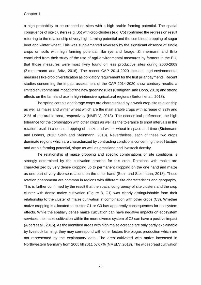
Chapter 1

23

a high probability to be cropped on sites with a high arable farming potential. The spatial

congruence of site clusters (e.g. S5) with crop clusters (e.g. C5) confirmed the regression result

referring to the relationship of very high farming potential and the combined cropping of sugar

beet and winter wheat. This was supplemented reversely by the significant absence of single

crops on soils with high farming potential, like rye and forage. Zimmermann and Britz

concluded from their study of the use of agri-environmental measures by farmers in the EU,

that those measures were most likely found on less productive sites during 2000-2009

(Zimmermann and Britz, 2016). The recent CAP 2014-2020 includes agri-environmental

measures like crop diversification as obligatory requirement for the first pillar payments. Recent

studies concerning the impact assessment of the CAP 2014-2020 show contrary results: a

limited environmental impact of the new greening rules (Cortignani and Dono, 2019) and strong

effects on the farmland use in high-intensive agricultural regions (Bertoni et al., 2018).

The spring cereals and forage crops are characterized by a weak crop-site relationship

as well as maize and winter wheat which are the main arable crops with acreage of 32% and

21% of the arable area, respectively (NMELV, 2013). The economical preference, the high

tolerance for the combination with other crops as well as the tolerance to short intervals in the

rotation result in a dense cropping of maize and winter wheat in space and time (Steinmann

and Dobers, 2013; Stein and Steinmann, 2018). Nevertheless, each of these two crops

dominate regions which are characterized by contrasting conditions concerning the soil texture

and arable farming potential, slope as well as grassland and livestock density.

The relationship of maize cropping and specific combinations of site conditions is

strongly determined by the cultivation practice for this crop. Rotations with maize are

characterized by very dense cropping up to permanent cropping on the one hand and maize

as one part of very diverse rotations on the other hand (Stein and Steinmann, 2018). These

rotation phenomena are common in regions with different site characteristics and geography.

This is further confirmed by the result that the spatial congruency of site clusters and the crop

cluster with dense maize cultivation (Figure 3, C1) was clearly distinguishable from their

relationship to the cluster of maize cultivation in combination with other crops (C3). Whether

maize cropping is allocated to cluster C1 or C3 has apparently consequences for ecosystem

effects. While the spatially dense maize cultivation can have negative impacts on ecosystem

services, the maize cultivation within the more diverse system of C3 can have a positive impact

(Albert et al., 2016). As the identified areas with high maize acreage are only partly explainable

by livestock farming, they may correspond with other factors like biogas production which are

not represented by the explanatory data. The area cultivated with maize increased in

Northwestern Germany from 2005 till 2011 by 67% (NMELV, 2013). The widespread cultivation

Chapter 1

24

of maize is an effect of the expansion of biogas production after the implementation of the

national renewable energy law (EEG, 2004; LSKN, 2012).

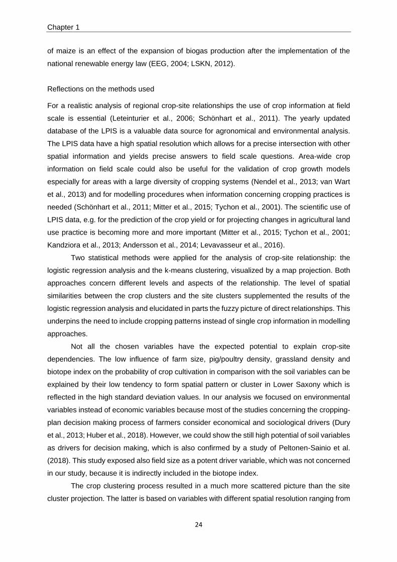
Reflections on the methods used

For a realistic analysis of regional crop-site relationships the use of crop information at field

scale is essential (Leteinturier et al., 2006; Schönhart et al., 2011). The yearly updated

database of the LPIS is a valuable data source for agronomical and environmental analysis.

The LPIS data have a high spatial resolution which allows for a precise intersection with other

spatial information and yields precise answers to field scale questions. Area-wide crop

information on field scale could also be useful for the validation of crop growth models

especially for areas with a large diversity of cropping systems (Nendel et al., 2013; van Wart

et al., 2013) and for modelling procedures when information concerning cropping practices is

needed (Schönhart et al., 2011; Mitter et al., 2015; Tychon et al., 2001). The scientific use of

LPIS data, e.g. for the prediction of the crop yield or for projecting changes in agricultural land

use practice is becoming more and more important (Mitter et al., 2015; Tychon et al., 2001;

Kandziora et al., 2013; Andersson et al., 2014; Levavasseur et al., 2016).

Two statistical methods were applied for the analysis of crop-site relationship: the

logistic regression analysis and the k-means clustering, visualized by a map projection. Both

approaches concern different levels and aspects of the relationship. The level of spatial

similarities between the crop clusters and the site clusters supplemented the results of the

logistic regression analysis and elucidated in parts the fuzzy picture of direct relationships. This

underpins the need to include cropping patterns instead of single crop information in modelling

approaches.

Not all the chosen variables have the expected potential to explain crop-site

dependencies. The low influence of farm size, pig/poultry density, grassland density and

biotope index on the probability of crop cultivation in comparison with the soil variables can be

explained by their low tendency to form spatial pattern or cluster in Lower Saxony which is

reflected in the high standard deviation values. In our analysis we focused on environmental

variables instead of economic variables because most of the studies concerning the cropping-

plan decision making process of farmers consider economical and sociological drivers (Dury

et al., 2013; Huber et al., 2018). However, we could show the still high potential of soil variables

as drivers for decision making, which is also confirmed by a study of Peltonen-Sainio et al.

(2018). This study exposed also field size as a potent driver variable, which was not concerned

in our study, because it is indirectly included in the biotope index.

The crop clustering process resulted in a much more scattered picture than the site

cluster projection. The latter is based on variables with different spatial resolution ranging from

Chapter 1

25

the smaller scaled LAU 2 data to 1 km² resolved raster data that gave different degree of

precision. However, the reason for the different degree of spatial clustering is not only caused

by the spatial resolution of the data sources. While the site clusters are a product of natural

conditions, the crop clusters are a result of both, site conditions and socio-economic factors,

e.g. market prices and subsidies. That supports flexibility of the farmers in the crop choice and

therefore the fragmentation of crop clusters especially in the center of Lower Saxony (# 3, 5, 6

referring to Figure 1) with medium arable farming potential, sandy soils and a higher variation

of farm types in this area than in other regions.

Conclusion

The relationship of site conditions and crop cultivation at the field scale is generally weak but

detectible for some crops. One reason is that modern cropping practice enables the farmer to

override the relationship of crop and site to a large extent. However, this does not apply to all

crop-site relationships. In arable regions with productive soils the crop-site relationship is

stronger. This comes along with specialization of the farming systems to a few cash crops,

mainly the most profitable crops like sugar beet and winter wheat. On the other hand, a

stronger relationship of crop and site at the regional scale was also detected for clusters with

less productive soils and the crop cluster with dominant maize cultivation. Economic reasons

and policy-based incentives, such as support for bioenergy crops may have enforced this

allocation. Farming practice and agricultural policy must face the chances but also the risks of

this development.

In regions with less fertile soils and mixed farming structure, the farmers cultivation

practice is much more diverse. The site clusters are not dominated by one crop cluster but by

a side-by-side of crop clusters with up to four dominating crops. The chance for crop rotation

diversification is higher in these multiform regions but in the rather monotonous regions

diversification efforts would be much more crucial.

References

Albert, Ch., Hermes, J., Neuendorf, F., von Haaren, Chr., Rode, M., 2016. Assessing and

Governing Ecosystem Services Trade-Offs in Agrarian Landscapes: The Case of

Biogas. Land, 5 (1), 1. DOI : 10.3390/land5010001

Andersson, G. K. S., Ekroos, J., Stjernman, M., Rundlöf, M., Smith, H. G., 2014. Effects of

farming intensity, crop rotation and landscape heterogeneity on field bean pollination.

Agr. Ecosyst. Environ. 184, 145-148.

Chapter 1

26

Antrop, M., 2005. Why landscapes of the past are important for the future. Landscape and

Urban Planning 70 (1/2), 21-34.

Aouadi, N., Aubertot, J.N., Caneill, J., Munier-Jolain, N., 2015. Analyzing the impact of the

farming context and environmental factors on cropping systems: A regional case

study in Burgundy. Eur. J. Agron. 66, 21-29.

Bakker, M. M., Hatna, E., Kuhlman, T., Mücher, C. A., 2011. Changing environmental

characteristics of European cropland. Agr. Syst. 104 (7), 522-532.

Bakker, M. M., Sonneveld, M. P. W., Brookhuis, B., Kuhlman, T., 2013. Trends in soil–land-

use relationships in the Netherlands between 1900 and 1990. Agr. Ecosyst. Environ.

181, 134-143.

Bertoni, D., Aletti, G., Ferrandi, G., Micheletti, A., Cavicchioli, D., 2018. Farmland use

transition after the CAP greening: A preliminary analysis using Markov chains

approach. Land Use Policy 79, 789-800.

Caravalho, M.J., Melo-Goncalves, P., Teixeira, J.C., Rocha, A., 2016. Regionalization of

Europe based on a K-Means Cluster Analysis of the climate change of temperatures

and precipitation. Physics and Chemistry of the Earth Parts A/B/C 94, 22-28.

Cortignani, R., Dono, G., 2019. CAP’s environmental policy and land use in arable farms: An

impacts assessment of greening practices changes in Taly. Sc. of the Total

Environment 647, 516-524. DOI: 10.1016/j.scitotenv.2018.07.443

Draper, N. R., Smith, H., 1998. Applied regression analysis. 3rd Ed. Wiley, New York.

Dury, J., Garcia, F., Reynaud, A., Bergez, J.-E., 2013. Cropping-plan decision-making on

irrigated crop farms: A spatio-temporal analysis. Eur. J. Agron. 50, 1-10.

DWD (Deutscher Wetterdienst), 2014. Multi-annual precipitation sum (1981-2010). Online

download via WebWerdis (accessed 06-03-2014).

EEG, 2004. Erneuerbare-Energien-Gesetz (Renewable Energies Act) of 21 July 2004

(Federal Law Gazette I p. 1918), last amended by Art. 1 Act of 7 November 2006

(Federal Law Gazette I p. 2550).

ESRI, 2007. ArcGIS 9.2 Desktop Help: Geometrical Interval.

http://webhelp.esri.com/arcgisdesktop/9.2/index.cfm?topicname=geometrical_interval

(accessed 22-03-2015).

European Parliament and Council, 2003. Regulation (EC) No 1782/2003 establishing

common rules for direct support schemes under the common agricultural policy and

establishing certain support schemes for farmers. Official Journal of the European

Union (L 270/1-69), ELI: http://data.europa.eu/eli/reg/2003/1782/oj.

European Parliament and Council, 2013. Regulation (EU) No 1307/2013 establishing rules

for direct payments to farmers under support schemes within the framework of the

Chapter 1

27

common agricultural policy and repealing Council Regulation (EC) No 637/2008 and

Council Regulation (EC) No 73/2009. Official Journal of the European Union (L 347/

608-669), ELI: http://data.europa.eu/eli/reg/2013/1307/oj

ESDAC (European Soil Data Centre), 2004. The European Soil Database distribution version

2.0, European Commission and the European Soil Bureau Network, CD-ROM, EUR

19945 EN.

Fahrmeir, L., Kneib, T., Lang, S., Marx, B., 2013. Regression: Models, Methods and

Applications. Springer, Berlin.

Gutsche, V., Enzian, S., 2002. Quantifizierung der Ausstattung einer Landschaft mit

naturbetonten terrestrischen Biotopen auf der Basis digitaler topographischer Daten.

Nachrichtenbl. Deut. Pflanzenschutzd. 54 (4), 92-101.

Hartigan, J. A., 1975. Clustering algorithms. John Wiley & Sons (Wiley series in probability

and mathematical statistics).

Hartigan, J. A., Wong, M. A., 1979. Algorithm AS 136: A K-Means Clustering Algorithm. J. R.

Stat. Soc. Series C 28/1, 100-108.

Hastie, T., Tibshirani, R., Friedmann, J., 2001. The Elements of Statistical Learning: Data

Mining, Inference and Prediction, second ed. Springer.

Hosmer, D. W., Lemeshow, S., 2000. Applied Logistic Regression, second ed. Wiley, New

York.

Huber, R., Bakker, M., Balmann, A., Berger, T., Bithell, M., Brown, C., Gret-Regamey, A.,

Xiong, H. et al., 2018. Representation of decision-making in European agricultural

agent-based models. Agricultural Systems 167, 143-160. DOI:

10.1016/j.agsy.2018.09.007

Javadi, S., Hashemy, S.M., Mohammadi, K., Howard, K.W.F., Neshat, A., 2017.

Classification of aquifer vulnerability using K-means cluster analysis. Journal of

Hydrology 549, 27-37.

JKI (Julius Kühn-Institut) (Eds.), 2004. Verzeichnis der regionalen Kleinstrukturen des

Landes Niedersachsen auf Gemeindebasis. Kleinmachnow.

Kandziora, M., Burkhard, B., Müller, F., 2013. Mapping provisioning ecosystem services at

the local scale using data of varying spatial and temporal resolution. Ecosystem

Services 4, 47-59.

Kleinn, Ch., Jovel, J., Hilje, L., 1999. A model for assessing the effect of distance on disease

spread in crop fields. Crop Prot. 18 (9), 609-617.

Leteinturier, B., Herman, J. L., de Longueville, F., Quintin, L., Oger, R., 2006. Adaptation of a

crop sequence indicator based on a land parcel management system. Agr. Ecosyst.

Environ. 112 (4), 324-334.

Chapter 1

28

Levavasseur, F., Martin, P., Bouty, C, Barbottin, A., Bretagnolle, V., Thérond, O., Scheurer,

O., 2016. RPG Explorer: A new toll to ease the analysis of agricultural landscape

dynamics with the Land Parcel Identification System. Computers and Electronics in

Agriculture 127, 541-552.

LBEG (Landesamt für Bergbau, Energie und Geologie), 1996. Bodenübersichtskarte 1:50

000 (BÜK 50) von Niedersachsen. Standortbezogenes natürliches ackerbauliches

Ertragspotenzial. Hannover.

LSKN (Landesbetrieb für Statistik und Kommunikationstechnologie Niedersachsen), 2012.

Statistische Berichte Niedersachsen. Landwirtschaftszählung 2010, Brochure 1/A

(Landuse) and 4 (Livestock). Hannover.

Menard, S., 1995. Applied Logistic Regression Analysis, second ed. Sage University Paper.

Mitter, H., Heumesser, Ch., Schmid, E., 2015. Spatial modeling of robust crop production

portfolios to assess agricultural vulnerability and adaptation to climate change. Land

Use Policy 46, 75-90.

Morissette, L., Chartier, S., 2013. The k-means clustering technique: General considerations

and implementation in Mathematica. The Quantitative Methods for Psychology 9 (1),

15–24.

Nendel, C., Wieland, R., Mirschel, W., Specka, X., Guddat, C., Kersebaum, K. C., 2013.

Simulating regional winter wheat yields using input data of different spatial resolution.

Field Crops Res. 145, 67-77.

NLWKN (Niedersächsischer Landesbetrieb für Wasserwirtschaft, Küsten-und Naturschutz),

2010. Naturräumliche Regionen in Niedersachsen. Extract from the Geobasisdata,

map basis: TK1000/ Niedersächsische Vermessungs- und Katasterverwaltung (Eds.).

NMELV (Niedersächsisches Ministerium für Ernährung, Landwirtschaft und

Verbraucherschutz) (Eds.), 2013. Ergänzungen zur Broschüre: Die Niedersächsische

Landwirtschaft in Zahlen 2011 (Stand: November 2013). Hannover. Available online:

http://www.ml.niedersachsen.de/download/83668/Die_niedersaechsische_Landwirtsc

haft_in_Zahlen_2011_-_Ergaenzung_11-2013.pdf (accessed on 04-05-2016).

OECD, 2004. Analysis of the 2003 CAP Reform. Paris. Available online:

https://www.oecd.org/tad/32039793.pdf (accessed 20-03-2019).

Peltonen-Sainio, P., Jauhiainen, L., Sorvali, J., Laurila, H., Rajala, A., 2018. Field

characteristics driving fram-scale decision-making on land allocation to primary crops

in high latitude conditions. Land Use Policy 71, 49-59. DOI:

10.1016/j.landusepol.2017.11.040

Chapter 1

29

R Core Team, 2013. R: A Language and Environment for Statistical Computing. R

Foundation for Statistical Computing, Vienna, Austria (online access: http://www.R-

project.org).

R Documentation, 2015. K-Means Clustering. Package ‘stats’ version 3.3.0. R Foundation for

Statistical Computing, Vienna, Austria (2015). https://stat.ethz.ch/R-manual/R-

devel/library/stats/html/kmeans.html (accessed 12-02-2015).

Richter, U., Eckelmann, W., 1993. Das Ertragspotential ackerbaulich genutzter Standorte in

Niedersachsen - Beispiel einer Auswertungsmethode im Niedersächsischen

Bodeninformationssystem NIBIS. Geol. Jb. F 27, 197-205.

Schönhart, M., Schmid, E., Schneider, U. A., 2011. CropRota – A crop rotation model to

support integrated land use assessments. Europ. J. Agron., 34 (4), 263-277.

SLA (Niedersächsisches Servicezentrum für Landentwicklung und Agrarförderung), 2011.

Digitale Feldblockkarte Niedersachsens (DFN). Digital map.

Smith, R.G., Gross, K.L., Robertson, G.P., 2008. Effects of Cropping Diversity on

Agroecosystem Function: Crop Yield Response. Ecosystems 11, 355-366. DOI:

10.1007/s10021-008-9124-5

Stein, S., Steinmann, H.-H., 2018. Identifying crop rotation practice by the typification of crop

sequence patterns for arable farming systems – A case study from Central Europe.

Europ. J. Agron., 92, 30-40, DOI: https://doi.org/10.1016/j.eja.2017.09.010.

Steinmann, H.-H., Dobers, S., 2013. Spatio-temporal analysis of crop rotations and crop

sequence patterns in Northern Germany: potential implications on plant health and

crop protection. J. Plant Dis. Protect. 120 (2), 85–94.

Storkey, J., Bruce, T.J.A., McMillan, V.E., Neve, P., 2019. Chapter 12 – The future of

sustainable crop protection relies on increased diversity of cropping systems and

landscapes. Agroecosystem Diversity. Academic Press, 199-209. DOI:

10.1016/B978-12-811050-8.00012-1

Tarpey, T., 2012. Generalized Linear Models.

http://www.wright.edu/~thaddeus.tarpey/ES714glm.pdf (last update at: 28-05-2012)

(accessed 10-06-2015).

Tilman, D., Cassman, K. G., Matson, P. A., Naylor, R., Polasky, S., 2002. Agricultural

sustainability and intensive production practices. Nature 418 (6898), 671-677.

Troost, Ch., Walter, T., Berger, T., 2015. Climate, energy and environmental policies in

agriculture: Simulating likely farmer responses in Southwest Germany. Land Use

Policy 46, 50-64.

Trubins, R., 2013. Land-use change in southern Sweden: Before and after decoupling. Land

Use Policy 33, 161-169.

Chapter 1

30

Tychon, B., Buffet, D., Dehem, D., Eerens, H., Oger, R., 2001. The Belgium crop growth

monitoring system. 2nd International Symposium: Modelling Cropping Systems.

Florence, Italy (16-07-2001).

Tzanopoulos, J., Jones, P.J., Mortimer, S.R., 2013. The implications of the 2003 Common

Agricultural Policy reforms for land use and landscape quality in England. Landscape

and Urban Planning 108, 39-48.

van Wart, J., Kersebaum, K. C., Peng, S., Milner, M., Cassman, K. G., 2013. A protocol for

estimating crop yield potential at regional to national scales. Field Crops Res. 143,

34-43.

van Zanten, B.T., Verburg, P.H., Espinosa, M., Gomez-y-Paloma, S., Galimberti, G.,

Kantelhardt, J., Kapfer, M., Lefebvre, M., Manrique, R., Piorr, A., Raggi, M., Schaller,

L., Targetti, S., Zasada, I., Viaggi, D., 2014. European agricultural landscapes,

common agricultural policy and ecosystem services: a review. Agron. Sustain. Dev.

34, 309-325.

Viaggi, D., Gomez y Paloma,S., Mishra, A., Raggi, M., 2013. The role of the EU Common

Agricultural Policy: Assessing multiple effects in alternative policy scenarios. Land

Use Policy 31, 99-101. DOI: 10.1016/j.landusepol.2012.04.019

Zimmermann, A., Britz, W., 2016. European farm’s participation in agri-environmental

measures. Land Use Policy 50, 214-218. DOI: 10.106/j.landusepol.2015.09.019

Xiao, Y., Mignolet, C., Mari, J.-F., Benoît, M., 2014. Modeling the spatial distribution of crop

sequences at a large regional scale using land-cover survey data: A case from France.

Comput. Electron. Agr. 102, 51-63.

31

__________________________________________________________________________

Chapter 2

Identifying crop rotation practice by the typification

of crop sequence patterns for arable farming

systems – A case study from Central Europe

__________________________________________________________________________

Chapter 2

32

Abstract

During the last decades crop rotation practice in conventional farming systems was subjected

to fundamental changes. This process was forced by agronomical innovations, market

preferences and specialist food processing chains and resulted in the dominance of a few cash

crops and short-term management plans. Classical crop rotation patterns became uncommon

while short rotations and flexible sequence cropping characterize the standard crop rotation

practice. The great variety and flexibility in cropping management as a reaction to economic

demands and climatic challenges complicate the systematization of crop rotation practice and

make historical systematization approaches less suitable. We present a generic typology

approach for the analysis of crop rotation practice in a defined region based on administrative

time series data. The typology forgoes the detection of fixed defined crop rotations but has its

focus on crop sequence properties and a consideration of the main characteristics of crop

rotation practice: i) the transition frequency of different crops and ii) the appropriate

combination of crops with different physical properties (e.g. root system, nutritional needs) and

growing seasons. The presented approach combines these characteristics and offers a

diversity-related typology approach for the differentiation and localization of crop sequence

patterns. The typology was successfully applied and examined with a data set of annual arable

crop information available in the form of seven-year sequences for Lower Saxony in the north-

western part of Germany. About 60% of the investigated area was cropped with the ten largest

crop sequence types, which represent the full range of crop pattern diversity from continuous

cropping to extreme diversified crop sequences. Maize played an ambivalent role as driver for

simplified rotation practice in permanent cropping on the one hand and as element of

diversified sequences on the other hand. It could be verified that the less diverse crop

sequence types were more strongly related to explicit environmental and socio-economic

factors than the widespread diverse sequence types.

Introduction

Crop rotation has always been a cornerstone in annual cropping systems. However, farmers

operate between different and often contrary objectives and demands for planning their crop

cultivation. Market preferences, specialist food processing chains as well as political objectives

forced the dense rotation of cash crops and short-term management plans in conventional

farming systems (Fraser, 2006; Bennett et al., 2011; Bowman and Zilberman, 2013; van

Zanten et al., 2014). This was supported by enormous progress in plant protection and plant

breeding as well as technological advances during the last decades. In many parts of Europe

these developments resulted in the dominance of a few crops and a reduction in crop diversity.

Chapter 2

33

Fixed cyclical crop rotations are increasingly being replaced by short sequences of two or three

years (Leteinturier et al., 2006; Glemnitz et al., 2011). Hence, decreasing crop diversity is one

characteristic of agricultural intensification which affects the biodiversity of agricultural

landscapes and related ecosystem services in a negative way (Tscharntke et al., 2005). The

repeated cultivation of the same crop with the same management practices has negative

effects on the soil quality and increases the risk for an accumulation of harmful organisms like

weeds, pests and diseases, which can result in yield decline (Karlen et al., 1994; Berzsenyi et

al., 2000; Ball et al., 2005; Bennett et al., 2011).

Political measures to address these challenges are already implemented. Recently, the

European Commission targeted the connection between intensive agricultural production and

ecosystem services decline in its Biodiversity Strategy 2020 and in the Common Agricultural

Policy (CAP) reform in 2014 (European Commission, 2011; Science for Environment Policy,

2015). The latter rewards the preservation of environmental public goods such as crop

diversification in the direct payments (European Parliament, 2013). Another recent example of

increasing political attention on crop rotation diversification is the EU members’ efforts

regarding the efficient use of plant protecting measures in accordance with the aim of

integrated pest management and sustainable agriculture (Boller et al., 1997; European

Commission, 2007a; European Parliament, 2009). The increase of functional diversity over a

crop rotation course has been argued to reduce resource-competing crop–weed relations and

is therefore an important measure of non-chemical weed management and integrated farming

(El Titi et al., 1993; Blackshaw et al., 2007; Smith et al., 2009; Melander et al., 2013). Crop

sequences with a high grade of structural and functional diversity have positive effects on the

function of the agroecosystem and its capacity to generate ecosystem services (Altieri, 1999;

Zhang et al., 2007). Further, the diversification of agricultural systems is considered as an

adaptation for changing thermal and hydrological conditions in the future (IAASTD, 2009; Lin,

2011). However, a crop rotation classification focusing on both diversity properties - functional

and structural diversity - is missing so far. We present a new crop sequence typology approach

to close this gap. A crop sequence typology facilitates the detection and localization of crop

rotation patterns which can help to estimate trends and locate risks in agricultural land use and

to assess the vulnerability or resilience of an agricultural system (Abson et al., 2013). Together

with the crop management system crop rotation is the key element to investigate land use

intensity and describe cropping systems (Leenhardt et al., 2010; Glemnitz et al., 2011;

Steinmann and Dobers, 2013). We demonstrate the potential of the presented typology to

describe cropping systems by qualifying the diversity aspect of crop sequences in a study area

and examine the linkage of the generated crop sequence types with landscape factors.

Chapter 2

34

The typification of crop sequences by their diversity aspects depends strongly on the

availability of crop data. Improvements in the collection and storage of spatially explicit and

high-resolution crop data have made a comprehensive detection of crop rotation practice much

easier. A recent example is the Integrated Administration and Control System (IACS) of the

EU and its land parcel information system, which stores area-based annual crop information

for administrative purposes. Beside this, the data offers a vast amount of information on current

agricultural land use (Levavasseur et al., 2016). However, the crop rotation analysis from those

data sets requires the development of methods for structuring large crop data sets in spatial

and temporal dimensions. Administrative data usually store time series information on the

presence of annual crops on a given parcel. A series of crop presence data represent sections

or segments of rotations with a possible rotation start in the middle or at the end of the series.

A further challenge is the trace of one rotation over time if the parcel boundaries within a field

block change from one year to another. Hence, the analysis of these sequences for crop

rotation questions requires appropriate treatment.

A well-known problem of recent studies which analyzed the crop rotation practice in a

defined region from time series is the high number of different crop combinations and the

relatively low occurrence of each combination type. Previous studies solve this by analyzing

short individual sequences of two or three years (Leteinturier et al., 2006; Long et al., 2014).

Although this method provides information on the relation of crop and previous crop, the real

rotation pattern remains concealed.

Tools for crop rotation modelling and prediction based on agronomical rules or farm-

scale decision-making processes are well established for integrated and organic farming

systems at the regional and landscape scale (Rounsevell et al., 2003; Stöckle et al., 2003;

Klein Haneveld and Stegeman, 2005; Bachinger and Zander, 2007; Schönhart et al., 2011).

Although these studies are very important and the tools are also useful for the evaluation of

crop rotation practices, they are only partly suitable for sequence typology. An important

approach for the characterization of crop rotation practice in a defined region based on internal

structure and cyclical pattern was presented by Castellazzi et al. (2008). The scientists studied

crop sequences with a straight mathematical approach which describes rotations as

probabilities of crop succession from the pre-crop to the main crop by using transition matrices

of a Markov chain. This so-called first-order Markov model was also applied by other research

groups for modelling spatial aspects of cropping systems (Salmon-Monviola et al., 2012;

Aurbacher and Dabbert, 2011). A continued development of this approach was the

implementation of second-order hidden Markov models, which allows modelling based on the

pre-crop and the pre-pre-crop of the main crop (Le Ber et al., 2006; Mari and Le Ber, 2006;

Xiao et al., 2014). The filtering of big data sets by this method requires though a fixed definition

Chapter 2

35

of the searched crop sequence concerning length, crop order and the frequency of crop

occurrence (Xiao et al., 2014). These are limiting requirements for the mining of unstructured

sequence data.

A historical example of a crop rotation typology in a classical sense was presented by

Brinkmann (1950) for the seasonal arable cropping systems in Germany. For Brinkmann the

main criterion to distinguish regional crop rotation types was the ratio of cereal crops and leaf

crops within a rotation. Leaf crops were here defined as dicotyledonous crops with a high

proportion of leaf surface like potato, legumes or sugar beet. The crops have positive impact

on soil structure, soil fertility and serve as a break crop for cereals. However, this typology

approach does not comply with recent crop rotation practice due to the increased role of

comparably new crops in European cropping systems like maize. Maize is a symbol crop for

the disregard of crop rotation rules and the practice of permanent cropping on the one hand a

profitable spring crop with the potential to improve the pure winter crop rotations on the other

hand. So, the presented typology approach complement the leaf crop-cereal crop distinction

by the distinction of spring crops and winter crops to consider the special role of maize in the

rotation practice and to complete the qualitative aspects in the typification. Typology

approaches of the more recent past operate mainly with the quantitative and structural

characteristics of crop rotations like the number of different crops or the minimal return time of

a crop (Leteinturier et al., 2006). This is a methodological reaction to the fact that farmers today

face a complex decision-making process to draw up their cropping plan and react more often

with the adaptation of crop sequence parts from one season to the next and the abandonment

of planned crop rotations with a length of more than three years (Bennett et al., 2011; Dury et

al., 2013). Our presented typology approach builds a bridge between the qualitative focus of

historical crop rotation systematization and the quantitative perspective of most recent

systematization approaches.

Materials and methods

Research area

Lower Saxony is a federal state in north-western Germany in Central Europe (DE9 in the

European Nomenclature of Territorial Units for Statistics NUTS 1). The study area is

characterized by a great variety of landscape types, with a marshy coastal area in the north

and moraine deposits in the east and west, dissected by river plains which also formed the

hilly uplands in the south. Fertile lowland with loessial soils stretches in the transition area from

the moraine landscapes to the uplands. These regions are dominated by arable farming with

cash crops such as sugar beet (Beta vulgaris subsp. vulgaris), oilseed rape (Brassica napus)

and winter wheat (Triticum aestivum L.). The cultivation of maize (Zea mays L.) has increased

Chapter 2

36

in all parts of Lower Saxony during the last ten years but plays the biggest role in the western

and northern parts, where it is linked with traditional structures of livestock farming and new

structures of biogas production (Figure 4). These four crops are considered highly important

for arable land use and crop sequence composition due to their proportion of the cropped area

(maize, wheat; see Table 6) and their specific economic importance as cash crops (sugar beet,

oilseed rape).

The observed area is located in a temperate climate zone with maritime influence in

the northwestern part and a stronger continental character to the east. Annual precipitation

ranges from 560 mm*yr-1 to 1200 mm*yr-1 with a mean of 750 mm*yr-1 (DWD, 2014).

Figure 4. Selected maps of characteristic distribution pattern in Lower Saxony: a) Share of maize acreage per arable area (IACS, 2011); b) Share of winter wheat acreage per arable area (IACS, 2011); c) Cattle density per grid cell (LSKN, 2012); d) Soil texture c class distribution (European Soil Portal, 2014).

Data and data processing

The Integrated Administration and Control System (IACS) was implemented by each member

state of the EU since the subsidies are based on the farming area to verify the correct sharing

of the European Agricultural Guarantee Fund (European Commission, 2007b). It records and

stores high-resolution land use data using a Land Parcel Identification System (LPIS), a GIS-

Chapter 2

37

supported identification system which replaced the cadastral system with the reform in 2005

and facilitated the spatially explicit land use data analysis. However, an analysis of individual

areas over a series of years needs to consider specific peculiarities. The identification of the

individual land use unit is realized by an individual code which does not allow any conclusion

on the corresponding farm due to privacy issues. An individual ID ensures the explicit

localization of each land use unit, aside from small inconsistencies in the data frame each year

like duplicates (1.5% in 2011 for the observed region). It has to be mentioned that the definition

of the smallest spatial land use unit is not uniform in the EU member states (Kay and Milenov,

2008). In Germany, as well as in some other European countries (e.g. France, Czech

Republic), the physical field block or farmer block framed by stable physical landscape

elements is the reference scale which can be identified by a fixed individual IACS code (so-

called field block identifier). Each block contains one or several so-called parcels of agricultural

land use, defined as a unit of one main crop for one cropping period and numbered

consecutively each year. The challenge for sequence analysis is the potential change of the

parcels’ shape and number in each growing season and the related change of the parcels ID

number in that block. So, the longer the observed time series is, the greater is the loss of clear

identifiable parcels due to changing parcel sizes.

Table 6. Share of cultivation area on arable area per year of the investigated fields and the average deviation

[ z̅ =1

n∑ zini=1 whenzi = (xi) − (yi)] of the sequence crop area proportion [xi] from the actual crop area proportion

[yi] in Lower Saxony (n= 122,956 records with 371,711 ha in total).

Crop Acronym Quality 2005 2006 2007 2008 2009 2010 2011 z̅

Maize MA C / S 22.9% 23.5% 24.3% 26.7% 26.5% 29.4% 32.1% 1.9%

Winter Wheat WW C / W 26.5% 25.9% 24.5% 26.1% 26.2% 26.3% 24.7% 3.3%

Winter Barley BA C / W 11.6% 13.8% 12.5% 11.6% 11.9% 10.5% 9.5% -0.4%

Oilseed Rape OR L / W 5.4% 6.3% 7.4% 7.5% 8.1% 8.6% 7.8% 1.1%

Rye RY C / W 5.8% 6.1% 7.3% 7.3% 7.7% 6.5% 6.3% 1.9%

Sugar Beet SB L / W 6.0% 4.7% 5.6% 5.6% 5.3% 5.4% 5.6% 0.1%

Triticale TR C / W 5.5% 4.7% 4.3% 4.4% 4.6% 4.6% 4.0% -0.8%

Spring Cereals SC C / S 4.5% 3.9% 3.4% 4.2% 3.2% 2.5% 3.4% 0.4%

Potato PO L / S 3.5% 3.2% 3.2% 3.2% 3.2% 2.9% 2.9% -0.6%

Arable Grassa) GR C / W 2.4% 2.6% 2.5% 2.7% 2.7% 2.6% 2.8% -0.5%

Legumes LE C / S 0.5% 0.6% 0.5% 0.5% 0.5% 0.5% 0.5% -0.8%

Vegetables VE C / S 0.2% 0.2% 0.2% 0.2% 0.2% 0.2% 0.3% -0.2%

a) Arable Grass = annual or multi-annual (max. 5 yr.) cultivation of fodder grass on arable fields C = Cereal crop

L* = Leaf crop S = Spring sown crop W = Winter sown crop

Chapter 2

38

The Lower Saxon LPIS stores crop and land use information for about 900,000 parcels per

year; half of these records represent arable parcels (about 1.6 million hectares of arable area

in total), whereas the rest comprises grassland, vegetables and other agricultural uses. For

the year 2011 we used an administrative digital map of the parcels location which facilitates a

spatially explicit traceability for a sufficient number of parcels. So, for the seven-year time

series (2005–2011) 34% of all parcels were located precisely by the consistent identification

code due to stable parcel size and proportion within the field block. For crop sequence analysis

only complete seven-year sequences of arable cropping were involved. This was the case for

24% of the arable parcels (122,956 records). These parcels were considered as a

representative sample for probing spatial distribution since they resemble the complete area.

Nevertheless, some crops were slightly overrepresented while others are less represented in

the sample sequences per year in comparison with the total acreage per year (Table 6)

depending on the parcels’ shape stability.

Crop Sequence Typology

The temporal distance of replanting the same crop or crops of similar physical and

physiological properties as well as the appropriate combination of crop growing seasons are

the main characteristics of crop rotation practice (Karlen et al., 1994). Our approach combines

these characteristics and differentiates the crop sequences by their pattern of these properties.

The result is a typology of crop sequences according to their grade of diversity, which enables

an analysis and interpretation of land use structures. The analysis of crop sequences instead

of crop rotations was owed to the fact that the data set represented a time frame showing

incomplete rotation cycles. The concept of ‘crop sequences’ implies the order of crops,

distances and frequencies of appearance in a fixed time period (Leteinturier et al., 2006). This

concept is related to the definition of crop rotations as the practice of “sequentially growing a

sequence of plant species on the same land” (Karlen et al., 1994). This principle of ‘crop

sequences’ is used in the following. We analyzed a period of seven years, from 2005 till 2011,

to ensure the inclusion of four-year sequences, which are typical for many regions. All

sequences with more than two years of fallow or temporary grass were defined as crop

livestock systems, instead of cropping systems, and were not included in the typology. This

follows the classic differentiation approach of crop rotations in crop-livestock systems and

cropping systems (Andreae, 1952; Brinkmann, 1950), based on the amount of temporary

extensive farming in rotation with arable crop farming. The approach was applied for the seven-

year period but could be adjusted to longer time series.

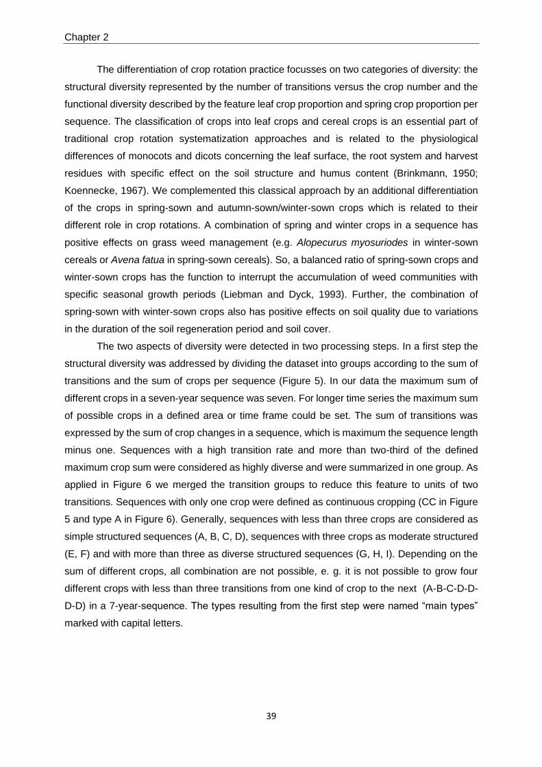
Chapter 2

39

The differentiation of crop rotation practice focusses on two categories of diversity: the

structural diversity represented by the number of transitions versus the crop number and the

functional diversity described by the feature leaf crop proportion and spring crop proportion per

sequence. The classification of crops into leaf crops and cereal crops is an essential part of

traditional crop rotation systematization approaches and is related to the physiological

differences of monocots and dicots concerning the leaf surface, the root system and harvest

residues with specific effect on the soil structure and humus content (Brinkmann, 1950;

Koennecke, 1967). We complemented this classical approach by an additional differentiation

of the crops in spring-sown and autumn-sown/winter-sown crops which is related to their

different role in crop rotations. A combination of spring and winter crops in a sequence has

positive effects on grass weed management (e.g. Alopecurus myosuriodes in winter-sown

cereals or Avena fatua in spring-sown cereals). So, a balanced ratio of spring-sown crops and

winter-sown crops has the function to interrupt the accumulation of weed communities with

specific seasonal growth periods (Liebman and Dyck, 1993). Further, the combination of

spring-sown with winter-sown crops also has positive effects on soil quality due to variations

in the duration of the soil regeneration period and soil cover.

The two aspects of diversity were detected in two processing steps. In a first step the

structural diversity was addressed by dividing the dataset into groups according to the sum of

transitions and the sum of crops per sequence (Figure 5). In our data the maximum sum of

different crops in a seven-year sequence was seven. For longer time series the maximum sum

of possible crops in a defined area or time frame could be set. The sum of transitions was

expressed by the sum of crop changes in a sequence, which is maximum the sequence length

minus one. Sequences with a high transition rate and more than two-third of the defined

maximum crop sum were considered as highly diverse and were summarized in one group. As

applied in Figure 6 we merged the transition groups to reduce this feature to units of two

transitions. Sequences with only one crop were defined as continuous cropping (CC in Figure

5 and type A in Figure 6). Generally, sequences with less than three crops are considered as

simple structured sequences (A, B, C, D), sequences with three crops as moderate structured

(E, F) and with more than three as diverse structured sequences (G, H, I). Depending on the

sum of different crops, all combination are not possible, e. g. it is not possible to grow four

different crops with less than three transitions from one kind of crop to the next (A-B-C-D-D-

D-D) in a 7-year-sequence. The types resulting from the first step were named “main types”

marked with capital letters.

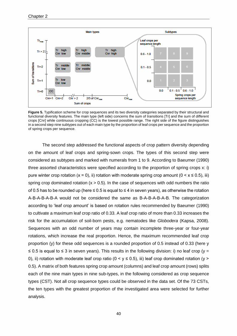
Chapter 2

40

Figure 5. Typification scheme for crop sequences and its two diversity categories separated by their structural and functional diversity features. The main type (left side) concerns the sum of transitions [Tr] and the sum of different crops [Cnr] while continuous cropping (CC) is the lowest possible range. The right side of the figure distinguishes in a second step nine subtypes out of each main type by the proportion of leaf crops per sequence and the proportion of spring crops per sequence.

The second step addressed the functional aspects of crop pattern diversity depending

on the amount of leaf crops and spring-sown crops. The types of this second step were

considered as subtypes and marked with numerals from 1 to 9. According to Baeumer (1990)

three assorted characteristics were specified according to the proportion of spring crops x: i)

pure winter crop rotation (x = 0), ii) rotation with moderate spring crop amount (0 < x ≤ 0.5), iii)

spring crop dominated rotation (x > 0.5). In the case of sequences with odd numbers the ratio

of 0.5 has to be rounded up (here ≤ 0.5 is equal to ≤ 4 in seven years), as otherwise the rotation

A-B-A-B-A-B-A would not be considered the same as B-A-B-A-B-A-B. The categorization

according to ‘leaf crop amount’ is based on rotation rules recommended by Baeumer (1990)

to cultivate a maximum leaf crop ratio of 0.33. A leaf crop ratio of more than 0.33 increases the

risk for the accumulation of soil-born pests, e.g. nematodes like Globodera (Kapsa, 2008).

Sequences with an odd number of years may contain incomplete three-year or four-year

rotations, which increase the real proportion. Hence, the maximum recommended leaf crop

proportion (y) for these odd sequences is a rounded proportion of 0.5 instead of 0.33 (here y

≤ 0.5 is equal to ≤ 3 in seven years). This results in the following division: i) no leaf crop (y =

0), ii) rotation with moderate leaf crop ratio (0 < y ≤ 0.5), iii) leaf crop dominated rotation (y >

0.5). A matrix of both features spring crop amount (columns) and leaf crop amount (rows) splits

each of the nine main types in nine sub-types, in the following considered as crop sequence

types (CST). Not all crop sequence types could be observed in the data set. Of the 73 CSTs,

the ten types with the greatest proportion of the investigated area were selected for further

analysis.

Chapter 2

41

Figure 6. Application of the typification scheme for seven-year crop sequences. The left side of the figure presents the sum of transitions per sequence (Tr) on the y-axis and on the x-axis the sum of crops per sequence (Cnr) resulting in nine main types A - I. The right side of the figure concerns the amount of leaf crops on the y-axis and

spring crops on the x-axis which form the nine subtypes 1–9.

The schema of the main types reflects the grade of diversity in a linear way in proportion to

sum of transition and sum of crops per sequence while in schema of the subtypes the diversity

decreases circular from the center to the edge. In the following we denote simple crop

sequences as sequences with a low structural diversity and unbalanced amounts of winter

sown crops in proportion to spring sown crops or cereal crops in proportion to leaf crops, e.g.

pure maize sequences (A3) or sequences with a very high share of winter wheat (C5). The

second example shows that a low structural diversity outweighs a high functional diversity.

These types of sequences entailed a higher risk for pests and diseases and are therefore

stronger dependent on plant protection products.

Landscape variables

To determine the role of location factors of the defined crop sequence types we studied the

linkage of CSTs and specific site conditions. We selected spatial variables which represent the

environmental and agro-economic attributes of the investigated area in a suitable resolution

and area-wide consistent availability. Official data from public sources were obtained to meet

these criteria (Table 7). The environmental conditions were characterized by the variables soil

texture, slope and average annual precipitation. The average annual temperature was not

considered due to the low variation of the thermal regime in the study region. The agro-

economic characteristics were represented by the spatial density of livestock farming (livestock

unit/ ha agricultural area), which was extracted from agricultural census data on LAU-2 (Local

Administrative Unit) scale. With regard to the different land use patterns connected with cattle

Chapter 2

42

farming and pig and poultry farming, the livestock data were separated into two variables.

These two variables – cattle density and pig/poultry density – were subdivided into five classes

according to the quartiles of the frequency distribution and one class for no occurrence of

livestock farming per LAU-2 area.

Table 7. Selected variables characterizing the arable landscape, their units, scales and data sources.

Predictor variable Unit Scale Source

Soil texture (Dominant surface textural class of the soil)

1 peat soil

2 coarse (> 65% sand)

3 medium (< 65% sand)

4 medium fine (< 15% sand)

5 fine (>35% clay)

1: 1 000 000 European Soil Portal,

2004

Slope (Dominant slope class)

1 level (< 8%)

2 sloping (8–15%)

3 moderately steep (>15%)

1: 1 000 000 European Soil Portal,

2004

Average annual precipitation (1981–2010)

mm*y-1 0.96 x 0.96 km DWD, 2014

Cattle density

Livestock unit/ha (agricultural area) LAU 2 LSKN, 2012

Pig/poultry density Livestock unit/ha (agricultural area)

LAU 2 LSKN, 2012

The information of these landscape data was assigned to the parcels according to the parcel’s

centroid position in space and merged by the ArcGIS® tool Spatial Join. The relationship

between the chosen variables and the crop sequence types was analyzed by a coefficient of

variation which is closely related to the Chi-squared test without squaring and summation. The

result is a value which represents the deviation from the overall mean per variable class. It is

calculated as the deviation of the observed frequencies (obs = observed) from the expected

frequencies (rand = random), computed as 100*(obs-rand)/rand.

Table 8. Correlation Matrix of the landscape variables used.

Soil texture Slope Precipit. CattleD PigPoulD

Soil texture 1

Slope 0.267 1

Precipit. -0.093 0.117 1

CattleD -0.437 -0.190 0.501 1

PigPoulD -0.248 -0.161 0.248 0.221 1

Chapter 2

43

The correlations among the landscape variables show relations of various intensities (Table

8). High positive correlations, e.g. between cattle density and precipitation or negative

correlation between cattle density and soil texture were validated by the results of the analyzed

CST-landscape-relationship.

Results

Application of crop sequence types

The crop sequence types approach was applied for the crop sequence data of Lower Saxony

in north-west Germany. We found that the nearly all forms of structural diversity, represented

by the main types of the typification, where cropped in significant extent (Table 9). Both very

simple sequence types and very diverse types occurred on large proportions of arable land.

The sequences with only one or two crops (A, B, C, D) were detectable on 31.4% of the arable

area. The main type F, which includes three crops that are combined in a very diverse way,

represents the biggest share of land use (24% of the arable area).

Table 9. The share in arable area in percent of the nine crop sequence types (CST) in letters A–I of the main types and the 9 CSTs of the sub types in numerals from 1–9. Some combinations were not cropped in the observed period ( - ).

CST Subtype

1 2 3 4 5 6 7 8 9 ∑

Main type

A 0.6 - 8.1 - - - - - <0.1 8.7

B 0.4 0.7 5.2 0.8 0.6 0.5 <0.1 <0.1 0.1 8.2

C 0.3 0.8 2.6 2.2 4.6 0.3 <0.1 <0.1 0.1 10.7

D 0.3 1.1 1.6 0.2 0.3 0.1 <0.1 <0.1 0.2 3.8

E 0.3 1.6 2.8 3.7 5.2 1.1 <0.1 <0.1 0.1 14.9

F 0.4 5.1 1.8 7.8 6.2 1.7 <0.1 0.3 0.7 24.0

G <0.1 0.7 0.6 0.7 1.8 0.6 <0.1 <0.1 <0.1 4.4

H 0.1 2.7 0.8 2.1 9.6 2.0 <0.1 0.3 0.9 18.4

I <0.1 0.6 0.1 0.2 4.1 1.1 - 0.3 0.4 6.8

∑ 2.3 13.4 23.6 17.6 32.4 7.5 <0.1 0.9 2.4 100.0

However, this high structural diversity is no guarantee for the functional diversity of a sequence.

The main type F contained three subtypes of the ten most frequently cropped sequence types

(Table 10) showing a great heterogeneity regarding the functional diversity aspects: F4 without

any spring-sown crop, F2 without any leaf crop and F5, characterized by a moderate leaf crop

amount and a moderate number of spring crops. Under functional aspects, this type contains

Chapter 2

44

the most diverse crop sequence types. In Lower Saxony 39.3% of the area was cultivated

without any leaf crop (subtypes 1, 2, 3) since maize replaced the leaf crops in crop sequences

in the previous years. A proportion of more than 0.5 leaf crops in a sequence was rare in the

observed data set.

Table 10. The ten largest crop sequence types and their share in arable area (AA), sequence examples. BA = Winter Barley; MA = Maize; OR = Oilseed Rape; PO = Potato; RY = Rye; SA = Set-aside; SB = Sugar Beet; SC = Summer Cereals; TR = Triticale; WW = Winter Wheat.

Crop Sequence

Type Share in AA Diversity Sequence examples (according to crop rotations)

H5 9.6% high OR - WW - [WW] - MA - WW - BA

OR - WW - BA - MA/SC - WW - BA

SB - WW - [WW] - BA - OR - WW - BA

A3 8.1% low / only cereals MA - MA - MA - MA - MA - MA - MA

F4 7.8% medium / only winter crops

OR - WW - [WW] - BA

OR - WW - BA - OR - WW - WW

F5 6.2% medium SB - WW - WW - [BA] - SB - WW - BA/WW

OR - WW - [MA] - WW - OR - WW - MA/WW

PO - RY/WW - TR/BA

E5 5.2% medium SB - WW - WW - BA

SB - WW - WW - [WW] - OR - WW - WW

B3 5.2% low / only cereals RY/BA/TR/SC/WW - MA - MA - MA - MA - MA - MA

F2 5.1% medium / only cereals

MA/SC - WW - BA - [MA - WW - [WW]]

MA - TR - BA

C5 4.6% low SB - WW - WW - [WW]

I5 4.1% high OR - WW - [WW] - MA/SC - WW/TR - BA

OR - WW - BA/TR/RY - MA/SC -WW - BA - [SA]

SA - WW - BA - OR - WW - MA - WW

E4 3.7% medium / only winter crops OR - WW - WW - [WW] - BA - [BA]

Total 59.6%

[ ] marks the flexible inclusion of crops / signifies “or”

The ten crop sequence types with the largest share of arable area were characterized

in detail (Table 10). About 60% of the investigated area in Lower Saxony was cropped with

these ten sequence types during the years 2005-2011. Nearly every range of diversity was

represented here, from continuous cropping types to extremely diverse types. The most

common CST was H5 with a high grade of diversity in its sequence structure. The second most

common CST was A3, representing continuous cropping of cereal spring crops (here maize).

So, the two most common sequence types represent the two poles of the diversity range, from

very simple to very diverse.

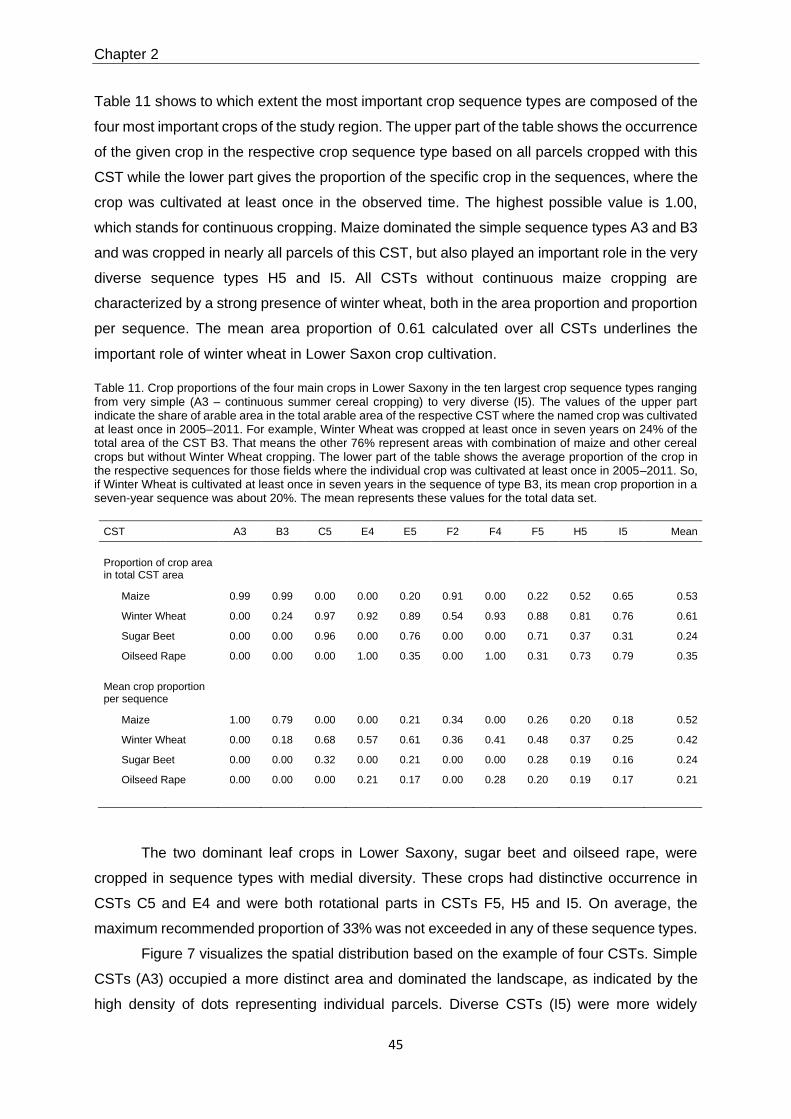
Chapter 2

45

Table 11 shows to which extent the most important crop sequence types are composed of the

four most important crops of the study region. The upper part of the table shows the occurrence

of the given crop in the respective crop sequence type based on all parcels cropped with this

CST while the lower part gives the proportion of the specific crop in the sequences, where the

crop was cultivated at least once in the observed time. The highest possible value is 1.00,

which stands for continuous cropping. Maize dominated the simple sequence types A3 and B3

and was cropped in nearly all parcels of this CST, but also played an important role in the very

diverse sequence types H5 and I5. All CSTs without continuous maize cropping are

characterized by a strong presence of winter wheat, both in the area proportion and proportion

per sequence. The mean area proportion of 0.61 calculated over all CSTs underlines the

important role of winter wheat in Lower Saxon crop cultivation.

Table 11. Crop proportions of the four main crops in Lower Saxony in the ten largest crop sequence types ranging from very simple (A3 – continuous summer cereal cropping) to very diverse (I5). The values of the upper part indicate the share of arable area in the total arable area of the respective CST where the named crop was cultivated at least once in 2005–2011. For example, Winter Wheat was cropped at least once in seven years on 24% of the total area of the CST B3. That means the other 76% represent areas with combination of maize and other cereal crops but without Winter Wheat cropping. The lower part of the table shows the average proportion of the crop in the respective sequences for those fields where the individual crop was cultivated at least once in 2005–2011. So, if Winter Wheat is cultivated at least once in seven years in the sequence of type B3, its mean crop proportion in a seven-year sequence was about 20%. The mean represents these values for the total data set.

CST A3 B3 C5 E4 E5 F2 F4 F5 H5 I5 Mean

Proportion of crop area in total CST area

Maize 0.99 0.99 0.00 0.00 0.20 0.91 0.00 0.22 0.52 0.65 0.53

Winter Wheat 0.00 0.24 0.97 0.92 0.89 0.54 0.93 0.88 0.81 0.76 0.61

Sugar Beet 0.00 0.00 0.96 0.00 0.76 0.00 0.00 0.71 0.37 0.31 0.24

Oilseed Rape 0.00 0.00 0.00 1.00 0.35 0.00 1.00 0.31 0.73 0.79 0.35

Mean crop proportion per sequence

Maize 1.00 0.79 0.00 0.00 0.21 0.34 0.00 0.26 0.20 0.18 0.52

Winter Wheat 0.00 0.18 0.68 0.57 0.61 0.36 0.41 0.48 0.37 0.25 0.42

Sugar Beet 0.00 0.00 0.32 0.00 0.21 0.00 0.00 0.28 0.19 0.16 0.24

Oilseed Rape 0.00 0.00 0.00 0.21 0.17 0.00 0.28 0.20 0.19 0.17 0.21

The two dominant leaf crops in Lower Saxony, sugar beet and oilseed rape, were

cropped in sequence types with medial diversity. These crops had distinctive occurrence in

CSTs C5 and E4 and were both rotational parts in CSTs F5, H5 and I5. On average, the

maximum recommended proportion of 33% was not exceeded in any of these sequence types.

Figure 7 visualizes the spatial distribution based on the example of four CSTs. Simple

CSTs (A3) occupied a more distinct area and dominated the landscape, as indicated by the

high density of dots representing individual parcels. Diverse CSTs (I5) were more widely

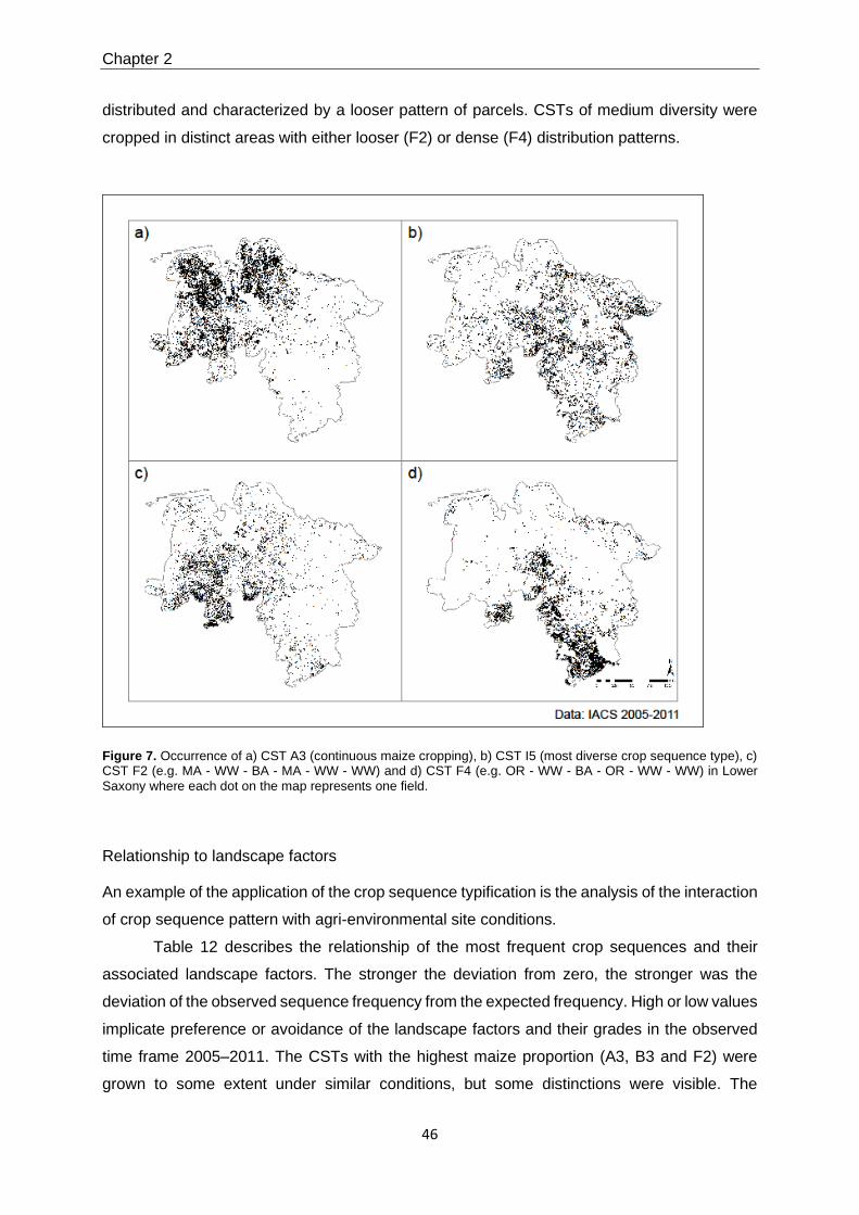
Chapter 2

46

distributed and characterized by a looser pattern of parcels. CSTs of medium diversity were

cropped in distinct areas with either looser (F2) or dense (F4) distribution patterns.

Figure 7. Occurrence of a) CST A3 (continuous maize cropping), b) CST I5 (most diverse crop sequence type), c) CST F2 (e.g. MA - WW - BA - MA - WW - WW) and d) CST F4 (e.g. OR - WW - BA - OR - WW - WW) in Lower

Saxony where each dot on the map represents one field.

Relationship to landscape factors

An example of the application of the crop sequence typification is the analysis of the interaction

of crop sequence pattern with agri-environmental site conditions.

Table 12 describes the relationship of the most frequent crop sequences and their

associated landscape factors. The stronger the deviation from zero, the stronger was the

deviation of the observed sequence frequency from the expected frequency. High or low values

implicate preference or avoidance of the landscape factors and their grades in the observed

time frame 2005–2011. The CSTs with the highest maize proportion (A3, B3 and F2) were

grown to some extent under similar conditions, but some distinctions were visible. The

Chapter 2

47

sequence type for continuous summer cereal (here maize) cropping (CST A3) was strongly

related to leveled regions with peaty soils, humid climate and intensive cattle farming. This

resulted in a regional concentration of this sequence type (Figure 7 a). The spatial relationship

of the three landscape variables was already reflected in the correlation matrix (Table 8). CSTs

B3 and F2 were cropped under similar conditions concerning the slope and precipitation but

were more frequently cropped on coarse soils. While parcels with dense summer cereal

cropping combined with one other crop (CST B3) were linked with intensive cattle farming and

partly with intensive pig and poultry farming, the diversified maize-cereal cropping (CST F2)

was characteristic for regions with intensive pig and poultry farming outside the peaty soil

regions.

Table 12. Deviation of observed CST frequencies from expected CST frequencies in percent characterizing the relation between the most frequent crop sequence types and attributed landscape variables.

Variable

CS Type A3 B3 C5 E4 E5 F2 F4 F5 H5 I5 All

others

Texture peat soil 19.2 11.6 -10.2 -10.0 -7.4 -0.9 -10.2 -7.3 -6.8 -4.1 0.5

coarse 5.1 10.8 -33.3 -29.1 -21.7 16.7 -29.3 -17.1 -6.2 7.6 7.2

medium -2.5 -2.7 -8.3 13.4 0.4 -5.6 13.1 -4.0 -0.9 -1.6 -0.1

med. fine -21.0 -19.0 51.4 24.5 27.6 -9.6 25.5 27.7 13.5 -1.7 -7.5

fine -0.7 -0.6 0.3 1.2 1.0 -0.5 0.9 0.7 0.4 -0.2 -0.1

Slope level 9.2 8.1 -4.5 -16.4 -2.5 4.4 -23.8 -2.7 -3.3 0.3 2.4

sloping -4.8 -4.3 -1.8 6.5 -0.3 -2.6 15.0 0.5 2.3 0.7 -1.2

mod. steep -4.4 -3.8 6.2 9.9 2.8 -1.8 8.8 2.2 1.0 -1.0 -1.2

Precipitation 500–600 -0.9 -0.5 0.3 -0.3 0.8 -0.7 -0.4 1.0 1.0 1.7 -0.2

(mm*y-1) 601–700 -14.2 -11.8 35.2 -0.1 25.4 -8.5 -4.7 23.9 7.8 8.0 -2.4

701–800 -6.9 -3.1 -2.5 2.7 -3.0 -1.9 2.2 -1.3 3.2 4.8 0.9

801–900 24.9 17.9 -29.8 -6.2 -21.0 11.0 -7.3 -21.7 -13.7 -15.1 2.4

901–1200 -3.0 -2.6 -3.3 3.9 -2.3 0.1 10.1 -1.9 1.7 0.6 -0.7

Cattle dens. 0.000 -1.6 -1.5 11.1 0.8 7.5 -1.5 -0.6 3.6 0.2 -0.7 -0.8

(LU/ha agric. a.) 0.001–0.245 -22.0 -19.5 51.5 17.2 29.9 -17.7 16.4 30.8 11.7 5.3 -5.2

0.246–0.509 -17.9 -12.9 -15.2 12.4 -4.2 1.7 18.6 -2.2 11.9 12.8 -0.8

0.510–0.954 -1.7 8.0 -23.1 -11.2 -15.8 17.0 -11.8 -12.2 -6.8 -2.9 4.8

0.955–2.930 43.1 25.9 -24.3 -19.2 -17.3 0.6 -22.6 -20.0 -17.1 -14.4 2.0

Pig/poultry dens. 0.000 -0.4 -0.7 6.2 0.2 3.5 -1.1 -0.4 1.8 0.1 0.0 -0.5

(LU/ha agric. a.) 0.001–0.045 8.0 -2.1 30.0 6.6 18.3 -14.5 3.6 15.3 0.9 -3.6 -4.7

0.046–0.160 -4.9 -9.0 6.7 16.1 8.0 -13.0 15.0 6.9 5.5 5.2 -2.6

0.161–0.556 -1.2 3.0 -19.3 -7.0 -11.0 2.6 -3.6 -10.0 -1.6 5.7 3.1

0.557–3.211 -1.5 8.8 -23.6 -15.9 -18.7 26.1 -14.6 -14.1 -4.8 -7.3 4.7

Chapter 2

48

Sequence types with moderate leaf crop and spring-sown crop amount but different

grades of structural diversity were represented in CSTs C5, E5, F5, H5 and I5. Their linkage

with landscape factors was obviously determined by the presence of sugar beet in the

sequence. The CST C5, with a lower structural diversity, and the sequence types E5 and F5,

with a higher structural diversity (for comparison see Table 10), were cropped under the same

site conditions - more frequently in regions with medium-fine soil texture, an annual

precipitation of 600–700 mm and low density of livestock farming - but the characterization of

the crop sequence types by the landscape-related variables was much more explicit in the

simple structured sequences than in the diverse sequences. The last applies also to other

CSTs.

The most diverse sequence types H5 and I5 were associated with a moderate humid

climate and a medium-high livestock density. The preferences in soil texture were different and

showed regional distribution on coarse (CST I5) and medium-fine soils (CST H5). The CST I5

was distributed in nearly every part of Lower Saxony with no significant regional concentration

(Figure 7 b).

Discussion

The typification and its applicability

So far a lot of approaches and methods exist for assessing crop rotation management,

even with the combined use of structural and functional characteristics. This approach of a

crop rotation typification is explicitly different from those that aim to evaluate crop rotations,

e.g. by a qualitative index. The crop sequence indicator presented by Leteinturier et al. (2006)

based on the Indigo method (Bockstaller and Girardin, 1996) is such an approach for assessing

the crop sequence composition as well as its quality. However, the translation of the rotation

properties into coefficients and their merger into a single value entails the risk of information

loss. So, the presented typology exposes the differences in cropping pattern and allows at the

same time the diversity of crop rotation practice to be determined and located. For example,

regions with a high amount of simple crop sequences and hotspots of vulnerability could be

identified.

In recent arable cropping the integration of a leaf crop in the crop rotation is not

obligatory at all. In Lower Saxony 39% of the area was cultivated without any leaf crop. Maize

has characteristics of leaf crops concerning the high amount of residues at the parcel and the

connected influence on the humus balance. The crop took the rotation place of leaf crops in

areas of the observed region which are characterized by a low leaf crop amount (Bennetzen

and Hake, 2009). This is due to external market factors (biogas production) on the one hand

Chapter 2

49

and specific characteristics of maize on the other hand like its high tolerance of short rotational

breaks and lower demands on soil quality compared with leaf crops like oil seed rape (for

details see the following section Simplicity and diversity).

A few limitations of the typology were found. The use of catch crop cultivation in Lower

Saxony could not be included in the study, since it was not part of the IACS data. It is

undeniable that this information would made the picture more complete. Furthermore, the

differentiation by sowing season limits the application of the typology approach to annual

cropping in temperate climate zones and excludes intercropping systems. Nevertheless, most

arable cultivation takes place in temperate climatic zones. So, the typology covers a wide range

of applications.

For this typology approach only crop sequences were processed which were clearly

identifiable over the observed time span due to constant number and size of parcels in the field

block. However, methods exist to deal with that problem. Levavasseur et al. (2016) devised a

tool which computes crop sequences using defined change rules in an algorithm. This tool

allows the tracing of crop sequences when no spatial geometry is available and has shown

good results in areas with small farm blocks. The facts that the observed crop area in Lower

Saxony is characterized by complex field blocks with a high number of parcels and that an

explicit spatial geometry for the year 2011 for all parcels was available for our study as well as

the large data volume, caused the preference of the spatially precise sequence analysis

instead of the maximum data exploitation. The latter would have been gone at the expense of

accuracy.

Simplicity and diversity

The recent picture of crop rotation practice in Lower Saxony is characterized by a high rate of

simplified cropping patterns especially in regions of intensive livestock farming as well as

intensive cash crop production under favorable cultivation conditions. This could be shown

clearly by demonstrating the proportions of simple CSTs. However, there was still a significant

proportion of diverse crop sequences in arable cropping practice. These diverse sequence

patterns are widely distributed across the study region on sites with different properties. This

widespread distribution without significant dependency on specific site conditions is due to the

high variety of crops summarized in one type.

Since the introduction of maize in the 1970s, this crop has been playing an important

role in the crop rotation practice of Lower Saxony. It is a cornerstone of feed production in the

regions of intensive livestock farming and it has become the main energy crop for biogas

production. The latter is a result of the support policy for renewable energy production in

Germany by the implementation of a national renewable energy law (EEG, 2004). Nearly one

Chapter 2

50

quarter of the arable area in Lower Saxony is cultivated with more than 50% maize ratio in the

crop sequence. This fact reveals the level of disregard of crop rotation rules and the level of

instability in the regional cropping systems. In dense maize rotations the demand for nutrients

is higher in order to realize dense maize cropping over several years. Kleijn and Verbeek

(2000) observed in their study on sandy soils in the Netherlands that maize-dominated crop

rotations were managed with a significantly higher input of nutrients than other rotations under

the same conditions. Dense maize cultivation increases the risk of arthropod pests like the

European corn borer (Ostrinia nubilalis) and the Western corn rootworm (Diabrotica virgifera

virgiferia). The most common answer to weeds, arthropod pests and fungal diseases in maize

production is currently the application of pesticides. According to the goals of Integrated Pest

Management, diversified cultivation is one important option to reduce the input of pesticides

combined with other measures (Meissle et al., 2010; Andert et al., 2016). Despite its negative

role in simple structured crop sequences, maize is a key component of many very diverse

sequences and can play an important role in interrupting the continuous cropping of winter-

sown crops and the corresponding accumulation of adapted weeds in several regions. So,

maize cropping is not only a threat to modern arable cropping, but also an opportunity for

building diverse crop sequence patterns.

Maize is a cereal that takes the functional role of a leaf crop like oilseed rape in the

cereal rotations of the livestock farming regions. This is reflected, for example, in the

comparison of the CSTs F2 (e.g. MA - WW - BA [- MA - WW - WW]) and F4 (e.g. OR - WW -

BA [- OR - WW - WW], abbreviations see Table 1). Both sequence types are characterized by

a high transition rate and three crops in the sequence. While the sequences of CST F2 are

cultivated without any leaf crop, the sequences of type F4 are pure winter-sown crop

sequences with a leaf crop proportion up to 0.33 per sequence. In Lower Saxony these two

types of crop sequences show a very similar structure, distinguished only by the supporting

crop which is cultivated in combination with the winter wheat and other winter cereals – maize

in CST F2 and oilseed rape in CST F4. As can be seen in the analysis of the relationship to

the chosen landscape variables (Table 12), the maize sequence F2 is related to coarse soil

texture on level sites in pig and poultry farming regions. In contrast, the oilseed rape sequence

F4 is principally cultivated in hilly humid regions characterized by medium-fine soil structure

and a low density of livestock farming. The site-condition-dependent preferences of the two

sequence types are reflected in their spatial distribution in Lower Saxony (Figure 7). So, maize

takes the place of oilseed rape in sites where the conditions do not provide a high yield of the

leaf crop and where the economic infrastructure allows or even requires the cultivation of

maize.

Chapter 2

51

Winter wheat was the most distributed crop in the Lower Saxon crop sequences during the

observed time span. The repeated cultivation of wheat for three years is fraught with risk for

yield instability and higher direct costs for fungicides and N fertilization. This is not only a topic

of the pure cereal rotations but potentially in future also for sequences with a very high crop

proportion of winter wheat, e.g. in high-yield regions with sugar beet cultivation (e.g. SB-WW-

WW-WW in CST C5). The integration of leaf crops like oilseed rape or grain legumes in the

rotation can offer an alternative. For the combination of two leaf crops with the same risks for

pathogenic organisms the problem of soil-borne pathogens must be considered. The high

attractiveness of oilseed rape as part of diverse rotations as well as of wheat-oriented rotations

can be attributed to its high profitability (Berry and Spink, 2006). As an effective break for

wheat, oilseed rape is an essential rotation crop in regions where wheat is the most profitable

crop (Kirkegaard et al., 2008). The cultivation of legumes widely lost its role in the investigated

area, except for organic farming. This is a consequence of decades of loss of legumes

importance for soil fertilization and animal nutrition due to cost effectiveness. In seven years

only 2% of the investigated area was cropped with legume in at least one year (8033 ha). Per

year the amount is stable at about 0.7% of the arable area. Stronger efforts in the development

of appropriate plant breeding and protection for legumes are necessary to make these crops

more attractive for farmers. It is a question for the future if the recent greening efforts for the

European agricultural policy will enhance the legumes role in the European crop rotation

systems.

Conclusion

The presented crop sequence typology is a generic method for analyzing comprehensive crop

sequence data sets of a defined area and time span to distinguish rotation practices by their

rotation structure and composition of crops with specific functions. It is applicable for pattern

search in a wide range of agricultural systems in temperate zones and for data with different

crop sequence lengths. The typification approach is inspired by existing historical crop rotation

systematizations but foregoes the principle of fixed rotation cycles to meet the recent farming

practice of flexible, short-term cropping plans. The application of the typology for a data set of

seven-year sequences in the arable area of north-western Germany showed a refined picture

of recent crop rotation practice. The ten most common sequence types cover the full range of

diversity. Diversified farming systems, which are generally more resilient to climate change

variabilities and promote ecosystem services, are still common in the observed farming region.

Agronomic research and extension service should further develop this potential by

strengthening farming system approaches and helping farmers adapt cropping patterns to

Chapter 2

52

future demands. For agricultural policy and land use planning the findings might help to adjust

measures to improve cropping diversity, as it becomes possible to locate simplicity and

complexity on a finer scale. Regarding maize, which was proven as a crop of both very simple

and very diverse sequences, it could be shown that the crops’ value for a sustainable land use

depends strongly on its intensity of cultivation.

References

Abson, D. J., Fraser, E. D. G., Benton T. G., 2013. Landscape diversity and the resilience of

agricultural returns: a portfolio analysis of land-use patterns and economic returns

from lowland agriculture. Agriculture & Food Security 2:2. DOI: 10.1186/2048-7010-2-

2.

Altieri, M. A., 1999. The ecological role of biodiversity in agroecosystems. Agric. Ecosyst.

Environ. 74, 19-31.

Andert, S., Bürger, J., Stein, S., Gerowitt, B., 2016. The influence of crop sequence on

fungicide and herbicide use intensities in North German arable farming. Eur. J. Agron.

77, 81-89.

Andreae, B., 1952. Fruchtfolgen und Fruchtfolgesysteme in Niedersachsen. Bren, W. Dorn.

Aurbacher, J., Dabbert, S., 2011. Generating crop sequences in land-use models using

maximum entropy and Markov chains. Agr. Syst. 104, 470-479.

Bachinger, J., Zander, P. 2007. ROTOR, a tool for generating and evaluating crop rotations

for organic farming systems. Eur. J. Agron. 26, 130-143.

Baeumer., K., 1990. Gestaltung der Fruchtfolge. In: Dierks, R. And Heitefuß, R., 1990.

Integrierter Landbau. BLV, München.

Bakker, M. M., Hatna, E., Kuhlman, T., Mücher, C. A., 2011. Changing environmental

characteristics of European cropland. Agr. Syst. 104 (7), 522-532.

Ball, B. C., Bingham, I., Rees, R. M., Watson, C. A., Litterick, A., 2005. The role of crop

rotations in determining soil structure and crop growth conditions. Canadian Journal

of Soil Science 85, 557-577.

Bennett, A. J., Bending, G. D., Chandler, D., Hilton, S., Mills, P., 2011. Meeting the demand

for crop production: the challenge of yield decline in crops grown in short rotations.

Biol. Rev. 87, 51-72. DOI: 101111/j.1469-185X.2011.00182.x

Bennetzen, J. L., Hake, S. C., (ed.) 2009. Handbook of Maize: Its Biology. Springer.

Berry, P. M., Spink, J. H., 2006. A physiological analysis of oilseed rape yields: Past and

future. The Journal of Agricultural Science 144 (9), 381-392.

Chapter 2

53

Berzsenyi, Z., Gyorffy, B., Lap, D., 2000. Effect of crop rotation and fertilization on maize and

wheat yields and yield stability in a long-term experiment. Eur. J. Agron. 13 (2-3),

225-244.

Blackshaw, R. E., Andersson, R.L., Lemerle, D., 2007. Chapter 3: Cultural weed

management. In: Upadyaya, M.K. and Blackshaw, R.E.: Non-chemical weed

management: Principles, concepts and technology. CAB International, Wallingford,

UK, pp. 35-48.

Bockstaller, C., Girardin, P., 1996. The crop sequence indicator: a tool to evaluate crop

rotations in relation to the requirements of Integrated Arable Farming Systems.

Aspects Appl. Biol. 47, 405-408.

Boller, E. F., Malavolta, C., Jörg, E., 1997. Guidelines for integrated production of arable

crops in Europe. IOBC Technical Guideline III. Bull. OILB Srop 20 (5), 5-19. ISBN 92-

9067-090-8.

Bowman, M. S., Zilberman, D., 2013. Economic factors affecting diversified farming systems.

Ecol. Soc. 18 (1), 33. DOI: 10.5751/ES-05574-180133.

Brinkmann, T., 1950: Das Fruchtfolgebild des deutschen Ackerbaues. Bonner

Universitätsbuchdruckerei, Bonn.

Castellazzi, M. S., Wood, G. A., Burgess, P.J., Morris, J., Conrad, K. F., Perry, J. N., 2008. A

systematic representation of crop rotations. Agr. Syst. 97, 26-33.

Dury, J., Garcia, F., Reynaud, A., Bergez, J.-E., 2013. Cropping-plan decision-making on

irrigated crop farms: A spatio-temporal analysis. Eur. J. Agron. 50, 1–10.

DWD (Deutscher Wetterdienst), 2014. Long-term average annual precipitation (1981-2010).

Online download via WebWerdis [accessed 06-03-2014].

EEG, 2004. Erneuerbare-Energien-Gesetz (Renewable Energies Act) of 21 July 2004

(Federal Law Gazette I p. 1918), last amended by Art. 1 Act of 7 November 2006

(Federal Law Gazette I p. 2550).

El Titi, A., Boller, E. F., Gendrier, J. P., 1993. Integrated production. Principles and technical

guidelines. IOBC/WPRS Bull. 16, 13-38.

European Commission, 2007 a. Thematic strategy on the sustainable use of pesticides.

Communication of the Commission of 12 July 2006 [COM(2006) 372]. URL: http://eur-

lex.europa.eu/legal-content/EN/TXT/?uri=URISERV%3Al28178 [accessed 18-04-

2016].

European Commission, 2007 b. Managing the agricultural budget wisely. Fact Sheet,

European Communities. URL:

http://ec.europa.eu/agriculture/sites/agriculture/files/cap-

funding/audit/pdf/2007_en.pdf [accessed 06-12-2016].

Chapter 2

54

European Commission, 2008. Agriculture: Member States agree in principle to abolish

obligatory set-aside. Press Release IP/08/1069, Brussels, 1 July 2008.

European Commission, 2011. Our life insurance, our natural capital: an EU biodiversity

strategy 2020. COM/2011/0244.

European Parliament, 2009. Directive 2009/128/EC of the European parliament and of the

council of 21 October 2009. Official Journal of the European Union (L 309/71).

European Parliament, 2013. Regulation (EU) No 1307/2013 of the European parliament and

of the council of 17 December 2013. Official Journal of the European Union (L

347/608).

European Soil Portal, 2014. The European Soil Database distribution version 2.0, European

Commission and the European Soil Bureau Network, CD-ROM, EUR 19945 EN.

Fraser, E.D.G., 2006. Crop diversification and trade liberalization: linking global trade and

local management through a regional case study. Agric. Hum. Values 23, 271–281.

Glemnitz, M., Wurbs, A., Roth, R., 2011. Derivation of regional crop sequences as an

indicator for potential GMO dispersal on large spatial scale. Ecol. Ind. 11, 964-973.

IAASTD (International Assessment on Agricultural Knowledge, Science and Technology for

Development), 2009. Global Report. Chapter 6: Options to enhance the impact of

AKST on development and sustainability goals. Island Press. URL:

http://www.unep.org/dewa/agassessment/reports/IAASTD/EN/Agriculture%20at%20a

%20Crossroads_Global%20Report%20(English).pdf [accessed 12-11-2015].

Kapsa, J. S., 2008. Important Threats in Potato Production and Integrated Pathogen/Pest

Management. Pot. Res. 51, 385-401.

Karlen, D.L., Varvel, G.E., Bullock, D.G., Cruse, R.M., 1994. Crop Rotations for the 21st

Century. Advances in Agronomy 53, 1-45.

Kay, S., Milenov, P., 2008. Status of the implementation of LPIS in the EU Member States.

Fact Sheet, European Commission. URL: http://ies-webarchive-

ext.jrc.it/mars/mars/content/download/995/6112/file/LPIS_study_MS_8203.pdf

[accessed 05-12-2015].

Kirkegaard, J., Christen, O., Krupinsky, J., Lyzell, D., 2008. Break crop benefits in temperate

wheat production. Field Crop Res. 107, 185-195.

Kleijn, D., Verbeek, M., 2000. Factors affecting the species composition of arable field

boundary vegetation. Appl. Ecol. 37, 256-266.

Klein Haneveld, W. K., Stegeman, A. W., 2005. Crop succession requirements in agricultural

production planning. European Journal of Operational Research 166 (2), 406-429.

Koennecke, G., 1967. Fruchtfolgen. VEB Deutscher Landwirtschaftsverlag, Berlin.

Chapter 2

55

Le Ber, F., Benoît, M., Schott, C., Mari, J.-F., Mignolet, C., 2006. Studying crop sequences

with CarrotAge, a HMM-based data mining software. Ecol. Modelling 191, 170-185.

Leenhardt, D., Angevin, F., Biarnès, A., Colbach, N., Mignolet, C., 2010. Describing and

locating cropping systems on a regional scale. A review. Agron. Sustain. Dev. 30 (1),

131–138.

Leteinturier, B., Herman, J. L., de Longueville, F., Quintin, L., Oger, R., 2006. Adaptation of a

crop sequence indicator based on a land parcel management system. Agric. Ecosyst.

Environ. 112, 324-334.

Levavasseur, F., Martin, P., Bouty, C, Barbottin, A., Bretagnolle, V., Thérond, O., Scheurer,

O., 2016. RPG Explorer: A new toll to ease the analysis of agricultural landscape

dynamics with the Land Parcel Identification System. Comput. Electron. Agr. 127,

541-552.

Liebman, M., Dyck, E., 1993. Crop rotation and intercropping strategies for weed

management. Ecol. Appl. 3, 92-122.

Lin, B. B., 2011. Resilience in agriculture through crop diversification: Adaptive management

for environmental change. BioScience 61 (3), 183-193.

Long, J. A., Lawrence, R. L., Miller, P. R., Marshall, L. A., 2014. Changes in field-level

cropping sequences: Indicators of shifting agricultural practices. Agric. Ecosyst.

Environ. 189, 11-20.

LSKN (Landesbetrieb für Statistik und Kommunikationstechnologie Niedersachsen), 2012.

Statistische Berichte Niedersachsen. Landwirtschaftszählung 2010, Brochure 1/A

(Landuse) and 4 (Livestock). Hannover.

Mari, J.-F., Le Ber, F., 2006.Temporal and spatial data mining with second-order hodden

markov model. Soft. Comput. 10, 406-414.

Meissle, M., Mouron, P., Musa, T., Bigler, F., Pons, X., Vasileiadis, V. P., Otto, S., Antichi, D.,

Kiss, J., Pálinkás, Z., Dorner, Z., van der Weide, R., Groten, J., Czembor, E.,

Adamczyk, J., Thibord, J.-B., Melander, B., Cordsen Nielsen, G., Poulsen, R. T.,

Zimmermann, O., Verschwele, A.& Oldenburg, E., 2010. Pests, pesticide use and

alternative options in European maize production: current status and future

prospects. J. Appl. Entomol. 134, 357-375.

Melander, B., Munier-Jolain, N., Charles, R., Wirth, J., Schwarz, J., van der Weide, R., Bonin,

L., Jensen, P. K., Kudsk, P., 2013. European perspectives on the adoption of

nonchemical weed management in reduced-tillage systems for arable crops. Weed

Technol. 27, 231-240.

Chapter 2

56

Rounsevell, M.D.A., Annetts, J.E., Audsley, E., Mayr, T., Reginster, I., 2003. Modelling the

spatial distribution of agricultural land use at the regional scale. Agric. Ecosyst.

Environ. 95 (2-3), 465-479.

Salomon-Monviola, J., Durand, P., Ferchaud, F., Oehler, F., Sorel, L., 2012. Modelling

spatial dynamics of cropping systems to assess agricultural practices at the

catchment scale. Computers and Electronics in Agriculture 81, 1-13.

Schönhart, M., Schmidt, E., Schneider, U. A., 2011. CropRota – A crop rotation model to

support integrated land use assessments. Europ. J. Agron. 34, 263-277.

Science for Environment Policy, 2015. Ecosystem Services and the Environment. In-depth

Report 11 produced for the European Commission, DG Environment by the Science

Communication Unit, UWE, Bristol. Available at: http://ec.europa.eu/science-

environment-policy [accessed 03-10-2015].

Smith, R.G.; Mortensen, D.A.; Ryan, M.R., 2009. A new hypothesis for the functional role of

diversity in mediating resource pools and weed-crop competition on agroecosystems.

Weed Research 50, 37-48.

Steinmann, H.-H., Dobers, S., 2013. Spatio-temporal analysis of crop rotations and crop

sequence patterns in Northern Germany: potential implications on plant health and

crop protection. J. Plant Dis. Protect. 120 (2), 85-94.

Stöckle, C. O., Donatelli, M., Nelson, R. 2003: CropSyst, a cropping systems simulation

model. Eur. J. Agron. 18, 289-307.

Tscharntke, T., Klein, A.M., Kruess, A., Steffan-Dewenter, I., Thies, C., 2005. Landscape

perspectives on agricultural intensification and biodiversity—ecosystem service

management. Ecol. Lett., 8, 857-874.

van der Zanden, E., Levers, C., Verburg, P. H., Kuemmerle, T., 2016. Representing

composition, spatial structure and management intensity of European agricultural

landscapes. A new typology. Landscape and Urban Planning 150, 36-49.

van Zanten, B.T., Verburg, P.H., Espinosa, M., Gomez-y-Paloma, S., Galimberti, G.,

Kantelhardt, J., Kapfer, M., Lefebvre, M., Manrique, R., Piorr, A., Raggi, M., Schaller,

L., Targetti, S., Zasada, I., Viaggi, D., 2014. European agricultural landscapes,

common agricultural policy and ecosystem services: a review. Agron. Sustain. Dev.,

34, 309-325.

Zhang, W., Ricketts, T.H., Kremen, C., Carney, K., Swinton, S.M., 2007. Ecosystem services

and dis-services to agriculture. Ecol. Econ., 64 (2), 253-260.

Xiao, Y., Mignolet, C., Mari, J.-F., Benoît, M., 2014. Modeling the spatial distribution of crop

sequences at a large regional scale using land-cover survey data: A case from

France. Comput. Electron. Agr. 102, 51-63.

57

__________________________________________________________________________

Chapter 3

Annual crop census data does not proper represent

actual crop rotation practice

__________________________________________________________________________

Chapter 3

58

Abstract

Crop rotation is often used as a criterion for assessing farming systems. The most common

technique to derive the crop rotation practice is to use the crop statistic of one year. With the

data of the actual crop rotation for the years 2005 till 2011 for the German federal state Lower

Saxony we compare the spatial crop pattern of one year with the temporal crop sequences of

the seven years. We grouped the crops depending on whether it is a leaf crop or a cereal crop

or a spring sown crop or a winter crop in crop sequence types. This is based on the perception

of former literature that today farmers often do not follow fixed crop rotations but more flexible

patterns according to the function of the crop in a crop sequence. The comparison of the

temporal and the spatial dimension of the crop sequence types showed that the derived crop

sequence types of the spatial one-year statistic overstate the very heterogenous crop

sequences and understate the less heterogeneous crop sequences.

Introduction

The interaction of spatial heterogeneity of landscape elements and the function and

biodiversity of ecosystems is a key concept of landscape ecology (Wiens, 2002; Turner, 2005).

The temporal dimension of landscape elements is fundamental as well in understanding these

interactions (Reynolds-Hogland and Mitchell, 2007). The organization of agricultural practices

by the farmers in space and time causes spatio-temporal heterogeneity of the agricultural

landscape and the agro-ecosystems. It is a result of the factors that the farmer must consider

like prevailing production condition (e.g. soil, water supply, climate), agronomic rules, market

demands and suppliers as well as political requirements. The result is a side-by-side of

different field works during the seasons. This spatio-temporal pattern at the field level, which

is not detectable by a one-shot view, is what Vasseur et al. (2013) defined as the “hidden”

heterogeneity. The hidden heterogeneity considers the temporal dimension of agricultural

cropping as it is caused by crop rotation. This temporal aspect is highly important for agro-

ecological studies, for example pollination ecology or insect-pest and antagonists’ ecology.

Vasseur et al. (2013) analyzed the intra-annual dynamics of a field as carabid habitat. The

temporal heterogeneity and the side-by-side of different agricultural practices during the year

requires nevertheless the heterogeneity of crops in space. The simplest approach for the

detection of the spatial heterogeneity of agricultural land use is to use the total number of crops

or land use types and define an index like the Shannon index (e.g. Monteleone et al. 2018).

But the type of crop and its physiological properties have different or similar functions

depending on the context, e.g. the plant height and density or seed-producing potential means

less or more benefit of the cover type for bird species. Fahrig et al. (2011) define functional

cover types depending on the resource benefit of the landscape cover for the individual

Chapter 3

59

animals, called the concept of functional landscape heterogeneity. It means the measurement

of heterogeneity based on the expected functions. Crop rotation is an important agricultural

instrument to maintain soil functions like water and nutrient use efficiency. A proper crop

rotation has the potential to reduce the risk of accumulating yield-reducing weeds and pests

and therefore to minimize the use of pesticides (Karlen et al., 1994). We distinguished in this

study the arable crops concerning their function in the crop rotation as leaf crops versus cereal

crops (dicot crops versus monocot crops) and spring sown crops versus autumn sown crops

(in the following named winter crops). The crop rotational function of these crop classification

concerns the different effects of the crops on the weed community and the potential of weed

accumulation (Bianchi et al., 2006). Weeds with specific seasonal growth periods may occur

in strong concentration in crop rotations with high share of crops with the same growing

season, like winter sown crops or spring sown crops (e.g. Alopecurus myosuriodes in winter

sown cereals). Alternating spring and winter sown crops in a crop rotation have positive effects

for the prevention of weed accumulation (Liebman and Dyck, 1993) as well as soil borne

pathogens. There are several effects of crop rotation on soil properties in theory. A higher crop

diversity and the placement of the soil cover period in different seasons has positive effects on

the soil microbial activity which influences the aggregate stability of soil organic matter

(McDaniel et al., 2014; Smith et al., 2014; Tiemann et al. 2015). An improved soil aggregate

stability by crop rotation resulted in a greater water stability compared to farming systems

without diverse crop rotations (Karlen et al., 1994). Crops with high rooting densities or rooting

depth improve the water infiltration and deposition of organic material and support other crops

with less rooting density.

This study compared the temporal and spatial heterogeneity of the arable crops concerning

their functional characteristics as crop rotation elements. Steinmann and Dobers (2013)

determined for agricultural practice in North-western Germany that most of the farmers tend to

change their crop order very dynamic. The result is a great variety of crop sequences which

seemed to have little in common with the actual definition of crop rotation. The aggregation of

the crops in groups related to their function within a crop rotation exposed patterns of temporal

sequences (Stein and Steinmann, 2018). We hypothesized that these patterns are significantly

different in the spatial and temporal dimension. This would include the question if the land use

statistics of one year can represent the actual crop rotation practice.

Materials and Methods

Research area

The study area is in Central Europe, in the North-western part of Germany, namely Lower

Saxony (DE9 in the European Nomenclature of Territorial Units for Statistics NUTS 1). Lower

Chapter 3

60

Saxony is characterized by a great variety of landscape types and types of farming. The main

cash crops are maize (Zea mays L.), winter wheat (Triticum aestivum L.), sugar beet (Beta

vulgaris subsp. vulgaris) and oilseed rape (Brassica napus). Typical crop rotations in Lower

Saxony are Oilseed rape - Winter wheat - Barley, Maize - Winter wheat - Winter wheat, Sugar

beet - Winter Wheat - Winter wheat and rotations with a high share of maize, depending on

the region (Stein and Steinmann 2018). The study area is influenced by a temperate climate

with annual precipitation ranges from 560 mm*yr-1 to 1200 mm*yr-1 with a mean of 750

mm*yr-1 (DWD, 2014).

Spatial and temporal crop sequences

We analyzed sequences of crops covering a time period of seven years, from 2005 till 2011.

The data handling and method is based on the pre-work of Stein and Steinmann (2018). The

data has been obtained from the Integrated Administration and Control System (IACS) which

records and stores high-resolution land use data using a Land Parcel Identification System

(LPIS). It was installed in all member states of the European Union to control and administrate

the farming subsidies of the European Agricultural Guarantee Fund (European Commission,

2007). Each land use unit in the LPIS has an individual ID for clear identification of the data

object and the attributed information of main crop for one cropping period. The data have some

characteristics which have to be taken into account for the data usability. There are small

inconsistencies in the data frame each year like duplicates (1.5% in 2011 for the observed

region). For scientific analysis the provided data give no indication about the corresponding

farm due to privacy issues. For our analysis of crop data, we calculate with a 2 km x 2 km grid

of reference areas.

The smallest land use unit in the LPIS is not consistent in the EU. Each country defines

its own smallest unit which can be a field block, a land parcel or a field. In Germany there are

also different systems used in each federal state. In Lower Saxony the LPIS defines the

smallest agricultural land use unit as a field parcel within a field block which is framed by stable

physical landscape elements. While the field block ID never changes, the land use unit ID may

change with changing field size and number of field parcels within the field block. So, for

analysis of crop sequences over several years only land use units with unchanging field size

and therefore with a consistent ID were usable. This applies to about a quarter of all arable

land use units which are about 371.600 ha in sum. The statistic calculation included the main

crop information of the years 2005 to 2011. The number of land use units per 2 km x 2 km grid

cell ranges from one to 120 with a mean of 11 units. Grid cells with less than 11 land use units

(56 % of the grid cells) were excluded to prevent a statistical bias by small populations. We

distinguished spatial crop pattern and temporal crop sequences. The temporal crop sequences

Chapter 3

61

are the main crops of the seven years between 2005 and 2011 while the spatial crop pattern

are the main crops of all land use units of one grid cell in the year 2011.

Sequences with more than two years of fallow or temporary grass were not included in

the analysis because we assumed that these are farming systems with a focus on extensive

grassland cultivation instead of arable farming. This assumption is based on the differentiation

approach of crop rotations in crop-livestock systems and cropping systems (Andreae, 1952;

Brinkmann, 1950).

Typification

A pre-step of analyzing the functional diversity of the crop sequences and crop pattern was the

typification of the sequences according to their proportion of leaf crops and spring sown crops

(Stein & Steinmann, 2018; Figure 8). Based on the cultivation advices after Baeumer (1990)

we distinguished the three groups of spring crop sequences i) pure winter crop rotation (x = 0),

ii) rotation with moderate spring crop amount (0 < x ≤ 0.5), iii) spring crop dominated rotation

(x > 0.5) and the three groups of leaf crop sequences i) no leaf crop (y = 0), ii) rotation with

moderate leaf crop ratio (0 < y ≤ 0.5), iii) leaf crop dominated rotation (y > 0.5). A combination

of these groups in a matrix result in nine different types of crop sequences (Stein and

Steinmann, 2018).

Figure 8. Matrix of crop sequence types derived from the amount of land use units with leaf crops and spring crops (after Stein & Steinmann, 2018).

The temporal crop sequences were assigned to the types by their leaf crop and spring

crop amount in the years 2005 and 2011 per land use unit (Figure 9). The spatial crop pattern

types were derived from the amount of leaf crops and spring crops of the land use units in one

grid cell in 2011.

Chapter 3

62

Figure 9. The comparison of the temporal and the spatial data.

Results

The comparison of the distribution among the nine types of the spatial crop occurrence (2011)

and the temporal crop sequences (2005-2011) showed parallels but also notable differences

(Table 13). One central result is that 40.4% of the land use units have the same type in the

years 2005-2011 and in 2011.

Table 13. Proportional occurrence of crop sequence type 1-9 in the land use units for the year 2011 and the years 2005-2011.

2005-2011

2011

1 2 3 4 5 6 7 8 9

1 <0.001 <0.001 <0.001 <0.001 <0.001 <0.001 0 0 0 0.002

2 0.005 0.031 0.026 0.006 0.009 0.002 0 0 <0.001 0.079

3 0.004 0.047 0.148 0.002 0.010 0.007 0 0 <0.001 0.219

4 0.002 0.003 <0.001 0.037 0.047 0.001 <0.001 <0.001 <0.001 0.091

5 0.014 0.061 0.034 0.133 0.166 0.022 <0.001 0.003 0.006 0.440

6 0.002 0.026 0.060 0.004 0.020 0.018 0 <0.001 0.004 0.134

7 <0.001 <0.001 0 0.003 0.004 <0.001 <0.001 <0.001 <0.001 0.008

8 <0.001 <0.001 <0.001 0.004 0.010 0.002 0 <0.001 0.002 0.021

9 <0.001 <0.001 <0.001 <0.001 0.001 0.002 0 <0.001 0.002 0.007

0.028 0.169 0.270 0.190 0.267 0.055 <0.001 0.005 0.015

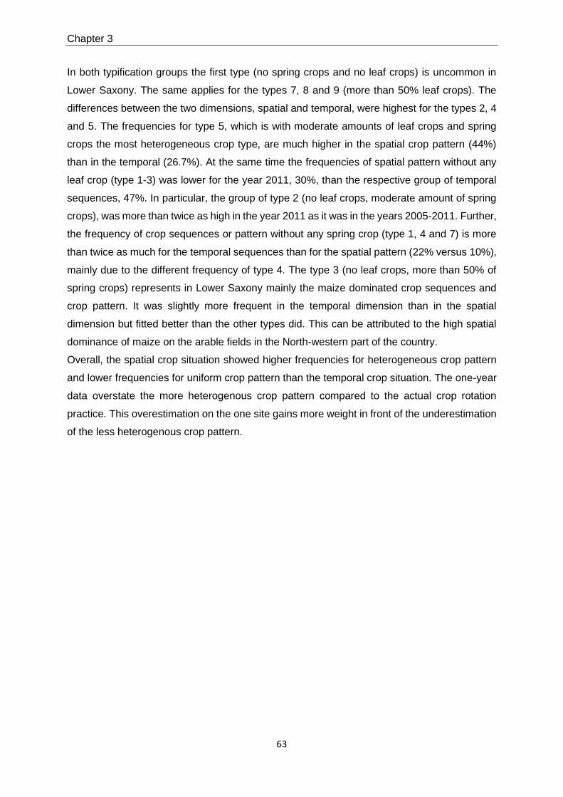
Chapter 3

63

In both typification groups the first type (no spring crops and no leaf crops) is uncommon in

Lower Saxony. The same applies for the types 7, 8 and 9 (more than 50% leaf crops). The

differences between the two dimensions, spatial and temporal, were highest for the types 2, 4

and 5. The frequencies for type 5, which is with moderate amounts of leaf crops and spring

crops the most heterogeneous crop type, are much higher in the spatial crop pattern (44%)

than in the temporal (26.7%). At the same time the frequencies of spatial pattern without any

leaf crop (type 1-3) was lower for the year 2011, 30%, than the respective group of temporal

sequences, 47%. In particular, the group of type 2 (no leaf crops, moderate amount of spring

crops), was more than twice as high in the year 2011 as it was in the years 2005-2011. Further,

the frequency of crop sequences or pattern without any spring crop (type 1, 4 and 7) is more

than twice as much for the temporal sequences than for the spatial pattern (22% versus 10%),

mainly due to the different frequency of type 4. The type 3 (no leaf crops, more than 50% of

spring crops) represents in Lower Saxony mainly the maize dominated crop sequences and

crop pattern. It was slightly more frequent in the temporal dimension than in the spatial

dimension but fitted better than the other types did. This can be attributed to the high spatial

dominance of maize on the arable fields in the North-western part of the country.

Overall, the spatial crop situation showed higher frequencies for heterogeneous crop pattern

and lower frequencies for uniform crop pattern than the temporal crop situation. The one-year

data overstate the more heterogenous crop pattern compared to the actual crop rotation

practice. This overestimation on the one site gains more weight in front of the underestimation

of the less heterogenous crop pattern.

Chapter 3

64

Figure 10. The proportion of matching temporal crop sequence types (2005-2011) per spatial crop pattern type (2011) in the corresponding 2 x 2 km grid cell in Lower Saxony.

Figure 10 shows that in Lower Saxony both assessment approaches, the spatial and

the temporal, matches very well in the northwestern part and in the southeastern part of the

area. In the mixed farming region of the Geest in the center of the state, the matching rate is

very low due to a higher heterogeneity of the actual crop rotations. This suggests that the

mismatching of the actual (temporal) and derived (spatial) crop sequences has a spatial

dimension which concerns mostly the heterogeneous regions.

Discussion

Crop diversification was one of the main topics of the Common Agricultural Policy (CAP) reform

in 2014 and is now a requirement for the direct payments (European Parliament, 2013). The

regulation defines the number of necessary crops for the agricultural area of the farm for the

specific year to assess the crop diversity. The assessment procedure of using the spatial crop

information of one year instead of crop data per field over several years approximates the

actual crop rotation. We compared the spatial crop pattern with the actual crop sequences.

About 60% of the land use units did not match. On a side note, this mismatching would be

even higher if we would have taken the actual crop species and not the grouped types. The

most interesting fact is that this mismatching is not evenly distributed over the functional types.

The spatial assessment pretends a heterogeneous crop situation that is not verifiable by the

actual temporal assessment. So, the land use statistic of one year could not fully represent the

Chapter 3

65

actual crop rotation or has to be used with limitations. This applies with variant degree to the

survey area, which showed regions with adequate comparability as well as regions with an

overestimation of heterogeneity (Figure 10). Taking the results of Stein & Steinmann (2018)

into account, the areas of high comparability are congruent with the areas where a high density

of less diverse crop rotation types were found. If other factors may have an influence on the

congruence of temporal and spatial crop heterogeneity, ought to be subject of future scientific

analysis.

Fahrig et al. 2011 used the term of functional diversity with regard to the landscape

ecology perspective and defined cover types in the spatial dimension by their functional

properties depending on the requirements of a species in classes ‘dangerous’, ‘beneficial’ and

‘neutral’. These classes implicate an evaluation of the usefulness of the landscape patches for

the single species. An evaluation like this was not the goal of our analysis, which focused on

grades of heterogeneity.

We distinguished in our analysis the cover types by their function for crop rotation and

soil cultivation. For the belowground perspective of agricultural land use and their function for

soil communities the temporal dimension with the change of crop, soil tillage and plant input is

much more relevant (Tiemann et al., 2015). We focused on two properties of the arable crops,

dicot crops versus monocot crops and the sowing seasons, autumn and spring. Furthermore,

there are other properties of crops which influence soil organic matter (SOM) stocks, water

infiltration and microbial community, e.g. the growing density (row crops versus cereal crops).

The distinction of leaf crops and cereal crops aims at crop properties like crop’s rooting depth

and input of plant residues which are important for the aboveground-belowground interactions

(McDaniel et al., 2014). The ratio of cereal versus leaf crops as well as the variation of planting

date have furthermore relevance for the pest regulation. Rotations with predominantly cereal

crops may risk a weed infestation (Zemanek et al. 1985; Liebman and Dyck, 1993). The

variation of the planting date in association with other management strategies (e.g. tillage) is

a measure to control weeds (Hakansson, 1982). Furthermore, the high ratio of cereal crops

may affect the soil health and soil functions negatively (Karlen et al., 1994).

The same crop type can be managed with different intensity – e.g. conventional, low

input, organic and no-till – which can have an effect on the SOM fractions and the C pool

(Grandy and Robertson, 2007). This cannot be displayed by the data we used.

The share of silage maize in the arable area of Lower Saxony has almost doubled in

the observed time period, from 15% in 2005 to 27% in 2011. This increase is linked with an

expansion of bio-energy plants and supporting political measures and is concentrated in Lower

Saxony mainly on regions in the North-western part where it is linked with established

structures of intensive livestock farming. The match of temporal crop sequence types and

Chapter 3

66

spatial crop pattern is for these regions of homogenous maize cropping very high. For the

mixed farming regions of the Geest we have a very low matching rate due to higher cropping

diversity. So, the method of the derived crop rotations based on one-year statistics represent

a false picture mostly for the mixed farming regions.

Conclusion

The comparison of the temporal with the spatial arrangement of crops showed specific

inconsistencies by the comparison of the leaf crop amount and the spring sown crop amount

in a crop sequence or a spatial crop pattern respectively. The spatial view of the main crops of

one single year gives more weight to the most heterogeneous crop pattern types and less

weight to the least heterogeneous types than it could be proven by the actual crop sequence

types of the temporal view. This particularly applies in areas with a diverse cropping structure.

In future, the method of deriving crop rotation practice by the spatial crop arrangement of one

year, e.g. by taking official statistics, has to be under review.

References

Andreae, B., 1952. Fruchtfolgen und Fruchtfolgesysteme in Niedersachsen. Bren, W. Dorn.

Baeumer., K., 1990. Gestaltung der Fruchtfolge. In: Dierks, R. And Heitefuß, R., 1990.

Integrierter Landbau. BLV, München.

Bianchi, F.J.J.A., Booji, C.J.H., Tscharntke, T., 2006. Sustainable pest regulation in

agricultural landscapes: a review on landscape composition, biodiversity and natural

pest control. Proc. R. Soc. B, 273, 1715-1727.

Brinkmann, T., 1950: Das Fruchtfolgebild des deutschen Ackerbaues. Bonner

Universitätsbuchdruckerei, Bonn.

Cushman, S. A., McGarigal, K., Neel, Mc C., 2008. Parsimony in landscape metrics:

strength, universality, and consistency. Ecol. Indic., 8, 691–703

http://dx.doi.org/10.1016/j.ecolind.2007.12.002

DWD (Deutscher Wetterdienst), 2014. Long-term average annual precipitation (1981-2010).

Online download via WebWerdis [accessed 06-03-2014].

European Commission, 2007. Managing the agricultural budget wisely. Fact Sheet,

European Communities. URL: http://ec.europa.eu/agriculture/sites/agriculture/

files/cap-funding/audit/pdf/2007_en.pdf [accessed 06-12-2016].

European Parliament, 2013. Regulation (EU) No 1307/2013 of the European parliament and

of the council of 17 December 2013. Official Journal of the European Union (L

347/608).

Chapter 3

67

Fahrig, L., Baudry, J., Brotons, L., Burel, F.G., Crist, T.O., Fuller, R.J., Sirami, C,

Siriwardena, G.M., Martin, J.-L., 2011. Functional landscape heterogeneity and

animal biodiversity in agricultural landscapes. Ecology Letters 14, 101-112.

Grandy, A., Robertson, G., 2007. Land-Use Intensity Effects on Soil Organic Carbon

Accumulation Rates and Mechanisms. Ecosystems, 10(1), 59-74.

Hakansson, S., 1982. Multiplication, growth and persistence of perennial weeds. Pages 123-

135 in: Holzner, W. and Numata, M. (Eds.). Biologyand ecology of weeds. Dr. W.

Junk, The Hague, The Netherlands.

Karlen, D.L., Varvel, G.E., Bullock, D.G., Cruse, R.M., 1994. Crop Rotations for the 21st

Century. Advances in Agronomy 53, 1-45.

Laisch, A., Blaschke, T., Haase, D., Herzog, F., Syrbe, R.-U., Tischendorf, L., Walz, U.,

2015. Understanding and quantifying landscape structure – A review on relevant

process characteristics, data models and landscape metrics. Ecological Modelling

295, 31-41.

Liebman, M., Dyck, E., 1993. Crop rotation and intercropping strategies for weed

management. Ecol. Appl. 3, 92-122.

McDaniel, M.D., Tiemann, L.K., Grandy, A.S., 2014. Does agricultural crop diversity enhance

soil microbioal biomass and organic matter dynamics? A meta-analysis. Ecol. Appl.,

24, 560-570.

McGarigal, K., Marks, B. J., 1995. FRAGSTATS: spatial pattern analysis program for

quantifying landscape structure. Pacific Northwest Research Station, Portland, Or.

(USA), General Technical Report PNW-GTR-351.

McGarigal, K., Cushman S. A., 2005. The gradient concept of landscape structure. In: J.

Wiens, M. Moss (Eds.), Issues and Perspectives in Landscape Ecology, Cambridge

University Press, Cambridge, 112-119.

Monteleone, M., Cammerino, A.R.B., Libutti, A., 2018. Agricultural “greening” and cropland

diversification trends: Potential contribution of agroenergy crops in Capitanata (South

Italy). Land Use Policy 70, 591-600. DOI: 10.1016/j.landusepol.2017.10.038

Reynolds-Hogland, M.J., Mitchell, M.S., 2007.Three axes of ecological studies. In:

Bissonette, J.A., Storch, I. (Eds.), Temporal Dimensions of Landscape Ecology.

Springer, USA, 174-194.

Smith, A.P., Marin-Spiotta, E., De Graaf, M.A., Balser, T., 2014. Microbial community

structure varies across soil organic matter pools during tropical land cover

changes.Soil Biol. Biochem. 77, 292-303.

Chapter 3

68

Steinmann, H.-H., Dobers, S., 2013. Spatio-temporal analysis of crop rotations and crop

sequence patterns in Northern Germany: potential implications on plant health and

crop protection. J. Plant Dis. Protect. 120 (2), 85-94.

Stein, S., Steinmann, H.-H., 2018. Identifying crop rotation practice by the typification of crop

sequence patterns for arable farming systems – A case study from Central Europe.

Europ. J. of Agronomy, 92, 30-40.

Tiemann, L.K., Grandy, A.S., Atkinson E.E., Marin-Spiotta, E., McDaniel, M.D., 2015. Crop

rotational diversity enhances belowground communities and functions in an

agroecosystem. Ecol. Letters, 18, 761-771.

Turner, M.G., 1989. Landscape ecology: the effect of pattern on process. Annu. Rev. Ecol.

Syst., 20, 171–197.

Turner, M.G., 2005. Landscape ecology: what is the state of science? Ann. Rev. Ecol. Syst.

36, 319-344.

Vasseur, C., Joannon, A., Burel, F., Meynard, J.M.Baudry, J., 2013. The cropping mosaic

system: How does the hidden heterogeneity of agricultural landscapes drive

arthropod populations? Agriculture, Ecosystems and Environment 166, 3-14.

Wiens, J. A., 2002. Central concepts and issues of landscape ecology. In: Gutzwiller, K. J.

(Ed.), Applying Landscape Ecology in Biological Conservation. Springer, New York,

3-21.

Zemanek, J., Mikulka, J., Ludva, L., Ludvova, A., 1985. The effect of longterm application of

herbicides on weed infestationand crop yieldsat the research station, Hnevceves.

Annals of the Research Institute for Crop Production Prague-Ruzyne 23, 99-118.

69

__________________________________________________________________________

General Discussion

__________________________________________________________________________

General Discussion

70

The main goal of my studies was to detect regional patterns of crop rotation practice in Lower

Saxony. The typification approach, presented in detail in the second chapter, focused on the

different functions of crops that support sustainable farming and serve the main goal of any

farmer, a sufficient and stable yield. It groups the seven-year crop sequences in types of more

and less diverse sequences, assuming that a diverse crop rotation has positive effects on the

ability of agroecosystems to generate ecosystem services (Altieri, 1999, Zhang et al., 2007).

Nevertheless, this assumption must be discussed. Generally, the rotation effect is expected to

increase yield due to improvements in soil structure and pest suppression as benefits from

rotation (Tiemann et al., 2015). Especially proving the direct linkage of crop rotation, soil

structure, and crop yield is not trivial (Karlen et al., 1994). Even if meta-analyses have shown

a positive effect of crop rotation on soil carbon and nitrogen, the soil structure, and the soil

microorganisms community (Ball et al., 2005; McDaniel et al., 2014; Venter et al., 2016), these

effects are difficult to separate from the impact of soil management, like tillage or fertilizer

application. The inclusion of legumes in crop rotations has the potential to enhance microbial

and enzyme activity in soil (Borase et al., 2020). However, during the observed period of time,

legume cropping was only present in 0.5 % of the fields in Lower Saxony.

The impact of crop rotation on weed density and weed diversity is also hard to prove.

While Liebman and Dyck (1993) showed a smaller impact of crop rotation than other measures

for weed control like herbicides and soil cultivation, other studies proved that the crop rotation

practice is an essential tool for any farmer influencing weed populations (Fried et al., 2008; de

Mol et al., 2015). However, Ulber et al. (2009) could not prove a connection between high crop

diversity and a high weed species richness for winter wheat stands in conventional cropping

systems. Crop rotation was found to have the strongest effect on weed density only in

combination with chemical weed management. This was also confirmed by studies of Bàrberi

et al. (1997) and Doucet et al. (1999), who suggested the combination of both as an effective

tool in integrated weed management. Also, the presence of cover crops has a stronger effect on

weed communities than crop rotation in general (Smith and Gross, 2007). Nevertheless, it is

essential for the assessment of crop rotation effect to distinguish between weed density and

weed diversity. Moreover, Glemnitz and Hufnagel (2009) recommend addressing the

functional groups of weeds for ecological evaluation of crop rotations. Functional diverse weed

communities as an implication of functional diverse crop rotations differ in their effect on and

the use of soil resources and compete less with the crop (Liebman & Dyck, 1993). So even a

potentially higher weed abundance in diverse crop rotations has no yield-reducing effect, and

an increase in weed diversity is a factor for less resource niche overlap and contributes to

reduced specific yield loss due to weeds (Jolliffe, 1997; Smith, et al., 2009). Sequences of

crops with similar character and management, such as cereals, have a lower diversity of weeds

General Discussion

71

between the crops (Smith et al., 2008). So, the dense cultivation of winter cereals in Lower

Saxonian regions with fertile soils potentially accumulate a range of problems for future

cropping.

The same applies to the geographical clusters of dense maize cropping on less

productive soils and in regions where intensive livestock farming is established. The

comparably small share of arable area in regions dominated by grassland is used by farmers

for the production of fodder with high energy potential, mainly maize. Here, we observe a high

concentration of one kind of crop in time and low concentration in space. The Renewable

Energy Act in 2004 caused an increase of maize cropping for bioenergy production not only in

these regions, but there the problem of a high share of maize in rotations is also more severe

because of the lack of alternative areas. A high share of maize in the rotation is also typical for

mixed farming regions with less productive soils, e.g. the districts Diepholz or the Heide regions

Lüneburg, Rotenburg, and Celle, where biogas production caused an increase of maize in the

rotation. These are the same regions where little consistency among the spatial heterogeneity

of the crops and their actual rotation heterogeneity was found (see chapter three). The dense

maize cropping on several fields was spatially arranged with other crop rotations simulating a

heterogeneity in space, which concealed the actual disregard of crop rotation rules on these

fields. Increased maize cultivation for energy production may have negative effects on

farmland wildlife (Gevers et al., 2011) and increases the risk of arthropod pests. However,

maize is not only a crop of less diverse rotations. As it was analyzed in the second chapter,

maize was often the only spring-sown crop in crop sequences that would be otherwise entirely

assembled with winter-sown crops. So, the inclusion of maize in winter crop rotations could

mean a useful break.

Crop rotation is strongly linked with soil tillage. The tendency of the last decades to

reduce tillage intensity and use conservation tillage instead is only possible with an increase

of herbicides and fertilizers if it is coupled with short crop rotations. Diversification of crop

rotations accompanied by the use of catch crops and perennial species bare the potential for

reducing the use of plant protection products by increasing the effect of biological control of

pests through natural enemies (LLG, 2014; Dunbar et al., 2016). This would be in line with the

goals of Integrated Pest Management (Meissle et al., 2010; Andert et al., 2016), which is also

recommended by the European Commission (Article 14 of Directive 2009/128/EG).

Crop rotation diversification also has the potential to increase the resilience of

agricultural systems by reducing risks from climate-change-related weather extremes (Bowles

et al., 2020). A broader portfolio of crops may, in the future, increase the stability of the total

yield at the national level in the face of limited water resources (Renard and Tilman, 2019).

General Discussion

72

The results of the present study showed that most of the Lower Saxonian farmers are

still following crop rotation rules, albeit in a flexible way and, in some regions, to a reduced

extent. Within a rotation, the crops may be exchanged flexibly according to their function within

the rotation, which requires a method for selecting crops by their role within the rotation to

identify crop rotation patterns. This was already recognized by Brinkmann (1950), who

distinguished the crops in leaf crops and cereal crops. Further differentiation in spring-sown

crops and winter-sown crops, presented in this study (chapter three), is an important extension

of this approach. It has to be mentioned that this recognition is a result of the cropping

circumstances in Lower Saxony with its high share of maize cultivation. However, even if the

presented typification method is strongly influenced by the research area and its crop portfolio,

it is, in general, applicable to other arable areas with one main crop per year.

The analysis of the crop-site interaction (as reported in chapters one and two) showed

that the farmers in Lower Saxony cultivate their crops still considering site conditions,

especially soil characteristics. The regional features of the crop-site interactions, especially of

the crop patterns, are very stable (Andreae, 1952). This mitigates the apprehension that

modern agriculture is more or less independent from the given site conditions (Antrop, 2005;

Bakker et al., 2013). The present study used site variables that are very stable over time. The

results may vary with short-term variables like market prices. But the subject of crop rotation

is a long-term one, fundamental for agricultural production in history and, hopefully, in the

future.

References

Altieri, M. A., 1999. The ecological role of biodiversity in agroecosystems. Agric. Ecosyst.

Environ. 74, 19-31.

Andert, S., Bürger, J., Stein, S., Gerowitt, B., 2016. The influence of crop sequence on

fungicide and herbicide use intensities in North German arable farming. Eur. J. Agron.

77, 81-89.

Andreae, B., 1952. Fruchtfolgen und Fruchtfolgesysteme in Niedersachsen. Bren, W. Dorn.

Antrop, M., 2005. Why landscapes of the past are important for the future. Landscape and

Urban Planning 70 (1/2), 21-34.

Bakker, M. M., Sonneveld, M. P. W., Brookhuis, B., Kuhlman, T., 2013. Trends in soil–land-

use relationships in the Netherlands between 1900 and 1990. Agr. Ecosyst. Environ.

181, 134-143.

Ball, B. C., Bingham, I., Rees, R. M., Watson, C. A., Litterick, A., 2005. The role of crop

rotations in determining soil structure and crop growth conditions. Canadian Journal of

Soil Science 85, 557-577.

General Discussion

73

Bàrberi, P., Silvestri, N., Bonarie, E., 1997. Weed communities of winter wheat as influenced

by input level and rotation. Weed Research 37, 301-313.

Borase, D.N., Nath, C.P., Hazra, K.K., Senthilkumar, M. Singh, S.S., Praharaj, C.S., Singh, U.,

Kumar, N., 2020. Long-term impact of diversified crop rotations and nutrient

management practices on soil microbial functions and soil enzymes activity, Ecological

Indicators, 114, 106322; DOI: 10.1016/j.ecolind.2020.106322.

Bowles, T.M., Mooshammer, M., Socolar, Y., Calderón, F., Cavigelli, M.A., Culman, S.W.,

Deen, W., Drury, C.F., Garcia y Garcia, A., Gaudin, A.C.M., Harkcom, W.S., Lehman,

R.M., Osborne, S.L., Robertson, G.P., Salerno, J., Schmer, M.R., Strock, J., Grandy,

A.S., 2020. Long-Term Evidence Shows that Crop-Rotation Diversification Increases

Agricultural Resilience to Adverse Growing Conditions in North America. One Earth, 2

(3), 284-293.

Brinkmann, T., 1950: Das Fruchtfolgebild des deutschen Ackerbaues. Bonner

Universitätsbuchdruckerei, Bonn.

De Mol, F., von Redwitz, C., Gerowitt, B., 2015. Weed species composition of maize fields in

Germany is influenced by site and crop sequence. Weed Research 55, 574-585, DOI:

10.1111/wre.12169.

Doucet, C., Weaver, S.E., Hamill, A.S., Zhang, J., 1999. Separating the effects of crop rotation

from weed management on weed density and diversity. Weed Science, 47,729-735.

Dunbar, M.W., Gassmann, A.J., O’Neal, M.E., 2016. Impacts of Rotation Schemes on Ground-

Dwelling Beneficial Arthropods. Environmental Entomology 45 (5), 1154-1160.

Fried, G., Norton, L.R., Reboud, X., 2008. Environmental and management factors determining

weed species composition and diversity in France. Agriculture, Ecosystems and

Environment 128, 68-76.

Gevers, J., Hoye, T. T., Topping, C. J., Glemnitz, M., Schröder, B., 2011. Biodiversity and the

mitigation of climate change through bioenergy: impacts of increased maize cultivation

on farmland wildlife. Global Change Biology Bioenergy 3, 6, 472-482.

Glemnitz, M., Hufnagel, J. (2009) Weed species diversity in energy cropping systems:

potentials and threats. In: 3rd Workshop of the EWRS Working Group "Weeds and

Biodiversity": Lleida, Spain 12 - 13 March 2009. Lleida, p. 17.

Jolliffe, P.A. (1997) Are mixed populations of plant speciesmore productive than pure stands?

Oikos 80, 595-602.

Liebman, M., Dyck, E., 1993. Crop rotation and intercropping strategies for weed management.

Ecol. Appl. 3, 92-122.

LLG - Landesanstalt für Landwirtschaft, Forsten und Gartenbau Sachsen-Anhalt, 2014.

Fruchtfolgen – gestern – heute – morgen. Bernburg.

General Discussion

74

McDaniel, M.D., Tiemann, L.K., Grandy, A.S., 2014. Does agricultural crop diversity enhance

soil microbioal biomass and organic matter dynamics? A meta-analysis. Ecol. Appl.,

24, 560-570.

Meissle, M., Mouron, P., Musa, T., Bigler, F., Pons, X., Vasileiadis, V. P., Otto, S., Antichi, D.,

Kiss, J., Pálinkás, Z., Dorner, Z., van der Weide, R., Groten, J., Czembor, E.,

Adamczyk, J., Thibord, J.-B., Melander, B., Cordsen Nielsen, G., Poulsen, R. T.,

Zimmermann, O., Verschwele, A.& Oldenburg, E., 2010. Pests, pesticide use and

alternative options in European maize production: current status and future prospects.

J. Appl. Entomol. 134, 357-375.

Renard, D., Tilman, D., 2019. National food production stabilized by crop diversity. Nature 571,

257-260.

Smith, R.G.; Mortensen, D.A.; Ryan, M.R., 2009. A new hypothesis for the functional role of

diversity in mediating resource pools and weed-crop competition on agroecosystems.

Weed Research 50, 37-48.

Tiemann, L.K., Grandy, A.S., Atkinson E.E., Marin-Spiotta, E., McDaniel, M.D., 2015. Crop

rotational diversity enhances belowground communities and functions in an

agroecosystem. Ecol. Letters, 18, 761-771.

Ulber L., Steinmann H.H., Klimek S. & Isselstein J. (2009) An on-farm approach to investigate

the impact of diversified crop rotations on weed species richness and composition in

winter wheat. Weed Research, 49, 534-543

Venter, Z.S., Jacobs, K., Hawkins, H.-J., 2016. The impact of crop rotation on soil micrbial

diversity: A meta-analysis. Pedobiologia 59 (4), 215-223.

Zhang, W., Ricketts, T.H., Kremen, C., Carney, K., Swinton, S.M., 2007. Ecosystem services

and dis-services to agriculture. Ecol. Econ., 64 (2), 253–260.

75

Summary

The aim of the present study was to detect patterns of crop rotation in an agricultural region in

the North-western part of Germany. It was analysed if and how the spatial distribution of the

crop rotation patterns depends on selected ecological and economical site variables. The

question arises in the light of the fast increase of maize acreage due to a booming biogas

production. This was a data-based study using crop information of all arable fields in Lower

Saxony which were funded with direct payments of the European Union agricultural fund during

the years 2005 till 2011. Information about the related farm was not included. For the spatial

localization only the digital field map of the year 2011 was available. Due to that, fields which

changed their size and frame and so changing their identification number were not detectable

over all seven years. However, about 24% of the arable parcels (122,956 records) could be

used for complete seven-year sequence analysis. In a first step, before analysing crop

rotations, the field data of the year 2011 were used to enlighten the relationship of crops with

selected site variables. A logistic regression analysis was used to build spatial clusters of crop

patterns which were compared with clusters of the following site variables: arable farming

potential, soil texture, slope, precipitation, biotope density, grassland proportion, cattle density,

pig and poultry density and farm size. The comparison showed a stronger relationship of

clustered crop pattern with clustered site pattern than the single crop-site relationship. Maize

and Winter wheat showed the clearest relation to site variables, especially the soil variables,

but with diverging preferences.

To reveal crop rotation patterns out of the wealth of crop sequences a typification

method was developed. This typification approach allows to group the crop sequences in two

steps, i) by their number of different crops and their number of transitions from one crop to

another, ii) by their amount of leaf crops and their amount of spring sown crops. The first step

addressed the structural aspects of the sequences and the second addressed the arable

functions of the crops in a rotation. The ten largest groups of crop sequence types derived by

this method were cropped on 60% of the investigated arable area. Among these ten types we

found types of low structural and functional diversity as well as the most diverse types in

significant extent. The largest type group (9.6%) contains crop sequences with four crops and

6-5 transitions in seven years as well as 1-3 leaf crops and 1-4 spring crops. The second

largest type group represents sequences which were permanently cropped with one cereal

spring sown crop (8.1%), this was maize here, actually. So, in Lower Saxony we found both

ends of the scale in a significant amount, the highly diverse crop sequences as well as the

sequences of continuous maize cropping. Maize dominated the most simple sequences but

played also an important role for the most diverse sequences and for the diversification of pure

76

winter crop stands. In the Geest region in Lower Saxony a number of rotation pattern with pure

cereal crop sequences showed that maize took the role of the winter leaf crop (Oil seed rape)

in the rotation, e.g. Maize-Winter Wheat-Winter Barley. One third of the arable area was

cropped with sequences with a moderate amount of leaf crops (1-3) and spring crops (1-4),

but nearly 40% showed any leaf crop and 20% any spring crop. So, Lower Saxony showed a

pleasingly high amount of diverse crop sequences on the one hand but on the other hand we

had nearly one third of the arable area cropped with only one or two crops, which is alarming.

The latter were strongly linked with a high cattle density and peaty soils. Generally, the ten

largest types showed specific relationships with the site variables and a spatial distribution

related to the distribution of the soil conditions in Lower Saxony. This allows the conclusion

that the crop rotation practice in Lower Saxony is related to the site condition in the respective

regions.

The spatial distribution of the clustered crop patterns of one year showed concordance

at the first view with the crop sequence patterns of the seven years. So, the third part of the

study examined the spatial congruency of the seven-year sequence data with the field data

from one year in a defined area around that sequence. All arable fields in one 2x2 km quadrant

of a raster were compared with the temporal crop sequences within this quadrant, according

to their amount of leaf crops and spring crops (equivalent to the second typification step). This

analysis showed an overestimation of the amount of the diverse crop sequence types and an

underestimation of the amount of simple crop sequence types in the one-year field data in

comparison with the actual crop sequences. This applies in particular for regions with

heterogenous crop patterns. So, the one-year crop statistic, which is commonly used to derive

the actual crop rotations, is not a proper data source in any case.

Summarizing the results of the data analysis it can be stated that most of the farmers

in Lower Saxony grow their crops in patterns which are inspired by crop rotation rules and used

in relation to the site conditions. Regions with less fertile soils and mixed farming are more

heterogenous than regions with very low or very high profitable soils. There is the dense maize

cropping of the livestock farming regions as well as the pure winter cereal rotations in the coast

regions which may lead to phytosanitary problems in the future if no measures of diversification

are implemented. Due to biogas production, the dense maize rotations are no longer only an

issue for intensive livestock farming regions. It is important to strengthen the development and

market conditions for neglected crops, especially legumes and summer cereals, to enhance

the diversification of crop rotations in future.

77

Zusammenfassung

Das Ziel dieser Arbeit war der Nachweis von Fruchtfolgemustern in einer

landwirtschaftlich geprägten Region im Nordwesten Deutschlands. Hierbei wurde untersucht

ob und wie die räumliche Verteilung von Fruchtfolgemustern im Zusammenhang mit

ausgewählten ökologischen und ökonomischen Landschaftsvariablen stehen. Diese Fragen

kamen vor dem Hintergrund einer rasch angestiegenen Maisanbaufläche als Folge einer

erhöhten Biogasproduktion auf. Dies ist eine Daten-basierte Analyse, welche die Anbaudaten

aller Ackerflächen in Niedersachsen nutzt, die in den Jahren 2005 bis 2011 durch

Direktzahlungen aus dem Agrarfonds der Europäischen Union gefördert wurden.

Informationen über die dazugehörigen Betriebe waren nicht enthalten. Für eine räumliche

Verortung der Felder war lediglich die digitale Schlagkarte des Jahres 2011 verfügbar. So

konnten Felder, welche ihren Feldzuschnitt oder die Größe und somit ihre ID-Nummer

änderten, nicht über alle sieben Jahre hinweg zurückverfolgt werden. Trotz allem konnten 24%

der Ackerflächen (122,956 Datensätze) für eine komplette siebenjährige Sequenzanalyse

genutzt werden. In einem ersten Schritt, noch vor der Auswertung der Fruchtfolgen, wurden

die Anbaudaten von 2011 herangezogen, um den Zusammenhang von Feldfrüchten mit

ausgewählten Landschaftsvariablen zu beleuchten. Mittels einer logistischen

Regressionsanalyse wurden Räume von Fruchtkombinationen definiert und mit Räumen von

kombiniert auftretender Landschaftsvariablen verglichen, im Folgenden: Ackerbauliches

Ertragspotenzial, Bodentextur, Hangneigung, Niederschlag, Biotopdichte, Graslandanteil,

Rinderdichte, Schwein- und Geflügeldichte sowie Betriebsgröße. Der Vergleich zeigte einen

stärkeren Zusammenhang zwischen Feldfruchtkombinationen und Variablenkombinationen

als zwischen einzelnen Feldfrüchten und einzelnen Variablen. Mais und Winterweizen zeigten

den deutlichsten Zusammenhang zu den Landschaftsvariablen, insbesondere zu den

Bodenvariablen, aber mit gegensätzlicher Präferenz.

Um Fruchtfolgemuster aus der Fülle an Fruchtsequenzen herauszulesen, wurde eine

Typisierungsmethode entwickelt. Dieser Typisierungsansatz ermöglichte eine Gruppierung

der Fruchtsequenzen in zwei Schritten, i) entsprechend ihrer Anzahl verschiedener Früchte

und ihrer Fruchtwechselanzahl, ii) nach ihrem Anteil an Blattfrüchten und ihrem Anteil an

Sommerungen. Der erste Schritt bezieht die strukturellen Aspekte der Fruchtsequenzen ein,

während der zweite Schritt die ackerbaulichen Funktionen der Feldfrüchte innerhalb der

Fruchtfolge adressiert. Die zehn größten Gruppen der Fruchtsequenztypen, die sich auf diese

Weise ableiten ließen, wurden auf 60% der untersuchten Ackerfläche angewandt. Unter

diesen zehn Typen befanden sich in signifikantem Umfang sowohl Typen mit geringer

struktureller und funktionaler Diversität als auch Typen der höchsten Diversitätsgruppen. Die

78

größte Typengruppe enthielt Fruchtsequenzen mit vier Früchten und 5-6 Fruchtwechseln in

sieben Jahren sowie 1-3 Blattfrüchten und 1-4 Sommerungen (9,6%). Die zweitgrößte

Typengruppe entspricht Sequenzen die permanent mit einem Sommergetreide bebaut (8,1%),

in diesem Fall Mais. In Niedersachsen finden sich also beide Extreme in bedeutender Menge,

die sehr diversen Fruchtsequenzen ebenso wie Sequenzen mit Mais im Daueranbau. Mais

dominiert die einfachsten Fruchtsequenzen, spielt jedoch auch eine wichtige Rolle in den sehr

diversen Sequenzen und für die Diversifizierung von reinen Winterungsfolgen. In der

niedersächsischen Geest zeigen einige Fruchtfolgemuster aus reinen Getreidesequenzen,

dass Mais die Funktion der Winterblattfrucht (hier Winter-Raps) in der Fruchtfolge

übernommen hat, z. B. Mais-Weizen-Gerste. Ein Drittel der Ackerflächen wurde mit

Sequenzen bestellt die eine moderate Menge an Blattfrüchten (1-3) und Sommerungen (1-4)

enthielten, aber fast 40% wurden ganz ohne Blattfrucht und 20% ohne Sommerung bebaut.

Niedersachsen zeigt also einerseits einen erfreulich hohen Anteil an diversen

Fruchtsequenzen, andererseits wurden nahezu ein Drittel der Ackerfläche mit nu rein oder

zwei Früchten in Sieben Jahren bestellt, was alarmierend ist. Letztere stehen in starkem

Zusammenhang mit einer hohen Rinderdichte und Moorböden. Im Allgemeinen zeigten die

zehn größten Typengruppen spezifische Zusammenhänge mit Landschaftsvariablen und eine

räumliche Verteilung, die der Verbreitung der Bodenverhältnisse in Niedersachsen folgt. Dies

legt den Schluss nahe, dass die Fruchtfolgepraxis in Niedersachsen in Zusammenhang mit

den Landschaftsbedingungen der entsprechenden Region steht.

Die räumliche Verteilung der geclusterten Fruchtmuster eines Jahres zeigen auf den

ersten Blick Übereinstimmungen mit den Fruchtsequenzmustern der sieben Jahre. Aus

diesem Grund widmet sich der dritte Teil der Studie der räumlichen Übereinstimmung der

Sieben-Jahres-Sequenzdaten mit den Felddaten eines Jahres in einem definierten Areal rund

um diese Sequenz. Alle Ackerflächen in einem 2 x 2 km Quadranten eines Rasters wurden mit

den zeitlichen Fruchtsequenzen innerhalb dieses Quadranten in Bezug auf ihren Blattfrucht-

und Sommerungsanteil verglichen (äquivalent zum zweiten Typisierungsschritt). Diese

Auswertung ergab eine Überschätzung der Menge der diversen Fruchtsequenztypen und eine

Unterschätzung des Anteils einfacher Fruchtsequenztypen in den einjährigen Daten

gegenüber den tatsächlichen Fruchtsequenzen. Dies gilt insbesondere für Regionen mit

heterogenen Fruchtmustern. Demnach ist die einjährige Anbaustatistik, welche im

Allgemeinen herangezogen wird, um Fruchtfolgen abzuleiten, nicht in jedem Fall hierfür

geeignet.

Die Ergebnisse führen zu dem Schluss, dass die Mehrheit der Landwirte in

Niedersachsen beim Anbau ihrer Feldfrüchte einem Muster folgen, welches sich an

Fruchtfolgeregeln und den Anbaubedingungen orientiert. Regionen mit Böden mit mittlerem

79

Ertragspotenzial und gemischtwirtschaftlichen Betrieben sind hierbei heterogener als

Regionen mit ertragsarmen und Regionen mit ertragsreichen Böden. Sowohl die dichten

Maisfruchtfolgen der Viehhaltungsregionen als auch die reinen Wintergetreidefolgen der

Küstenregionen können zukünftig zu phytosanitären Problemen führen, wenn keine

Maßnahmen zur Diversifizierung erfolgen. Als Folge der Biogasproduktion sind enge

Maisfruchtfolgen nicht mehr allein ein Thema der Viehhaltungsregionen. Umso wichtiger ist es

zukünftig die Züchtung vernachlässigter Feldfrüchte zu intensivieren und Marktbedingungen,

insbesondere für Leguminosen und Sommergetreide, zu verbessern, um die

Fruchtfolgediversifizierung zu fördern.

80

List of Publications

as to Mai 2020

Peer-reviewed journal articles

Stein, S., Steinmann, H.-H. (2020): Annual crop census data does not proper represent actual crop rotation practice. Manuscript

Stein, S., Steinmann, H.-H., Isselstein, J. (2019). Linking arable crop occurrence with site conditions by the use of highly resolved spatial data. Land MDPI, Open Access Journal, 8 (4), 1-14.

Stein, S., Steinmann, H.-H. (2018): Identifying crop rotation practice by the typification of crop sequence patterns for arable farming systems – A case study from Central Europe. European Journal of Agronomy 92, 30-40.

Andert, S.; Bürger, J.; Stein, S.; Gerowitt, B. (2016): The influence of crop sequence on fungicide and herbicide use intensities in North German arable farming. European Journal of Agronomy 77, 81-89.

Talks

Stein, S., Steinmann, H.-H. Fruchtfolgemuster in Niedersachsen – Ein Typisierungsansatz anhand quantitativer und qualitativer Merkmale. Institut für Zuckerrübenforschung, Göttingen, 19. März 2018, invited talk.

Stein, S.; Steinmann, H.-H. (2014): The situation of current crop rotations in Northern Germany: Risks and chances for future farming systems. IFSA Conference, Berlin, 1.-4. April 2014.

Stein, S.; Steinmann, H.-H. (2014): Der Einfluss von regionalen Faktoren auf die Wahl von Feldfrüchten und Fruchtfolgen. Mitt. Ges. Pflanzenbauwiss. 26, S. 48-49, Tagung der Gesellschaft für Pflanzenbauwissenschaften e.V., Wien, 16.-18. September 2014.

Stein, S.; Steinmann, H.-H. (2014): Aktuelle Fruchtfolgen und ihre Interaktion mit Region und Agrarstruktur. Julius-Kühn-Archiv: 447, 59. Deutsche Pflanzenschutztagung, Freiburg, 23.-26. September 2014.

Posters

Stein, S.; Steinmann, H.-H. (2018): Functional and structural diversity aspects of crop sequence typification approach. Landscape 2018 – Frontiers of agricultural landscape research, Berlin, 12-16.03.2018.

Stein, S.; Steinmann, H.-H. (2015): Temporal and spatial aspects of maize cropping in Northwestern Germany. Deutscher Kongress für Geographie, Berlin, 1.-6. Oktober 2015.

Further publications

Stein, S., Steinmann, H.-H.: Fruchtfolgen in der Landwirtschaft: Einheitsbrei oder doch noch Vielfalt? Natur und Landschaft. 2017-11-03.

81

Acknowledgements

This project was funded by the Federal Ministry of Food and Agriculture, Fachagentur

Nachwachsende Rohstoffe (grant number FKZ 12NR109 FNR). I am grateful to the Ministry

for Human Nutrition, Agriculture, Consumer Protection and Rural Development of

Niedersachsen (Lower Saxony), which provided administrative data.

I am very grateful to Prof. Dr. Johannes Isselstein for the inspiring and fruitful conversations

about my scientific work and for broaden my scientific horizon.

I would like to thank Dr. Horst-Henning Steinmann for offering me the opportunity to conduct

research on the interesting and diverse topic of crop rotations. I am very grateful for his tireless

support and his professional supervision of my project.

I thank Prof. Dr. Stefan Siebert for co-reviewing my thesis.

My acknowledgements also go to my colleges at the CBL, PD Dr. Martin Potthoff, Laura

Breitsameter, Armin Wiesner, Barbara Edler and Magdalena Werner for all the motivating and

helpful discussions on my research and many topics beyond, and for their friendship.

Ich danke meinem Mann Carsten Müller für seinen professionellen Rat, seine liebevolle

Ehrlichkeit und seinen Humor in meinen panischen Momenten und seine Geduld mit mir und

diesem Langzeitprojekt.

Meiner Schwester Claudia Stein danke ich für die zahllosen Spaziergänge mit meinen

Zwillingen, die die letzten fehlenden Zeilen doch noch möglich gemacht haben.

Und schließlich möchte ich meinen Eltern danken, für ihre immerwährende Unterstützung und

Liebe.