Stimulated Raman Scattering in Gas Filled

Hollow-Core Photonic Crystal Fibres

Stimulierte Raman-Streuung in mit Gas gefüllten Hohlkernfasern

June 2013

Der Naturwissenschaftlichen Fakultät

der Friedrich-Alexander-Universität

Erlangen-Nürnberg

Zur

Erlangung des Doktorgrades Dr. rer. nat.

vorgelegt von

Nguyen Manh Thang aus Hanoi, Vietnam

Als Dissertation genehmigt von der Naturwissenschaftlichen Fakultät at der Friedrich-Alexander- Universität at

Erlangen- Nürnberg

Tag der mündlichen Prüfung: 26.9.2013 Vorsitzender des Promotionsorgans: Prof.Dr. Johannes Barth Gutachter: Prof.Dr. Philip St. J. Russell Prof.Dr. Maria Chekhova

Abstract

In this thesis I use unique properties of hollow-core photonic crystal fibre (HC-PCF) to

study stimulated Raman scattering (SRS) in gaseous medium. HC-PCF offers excellent

abilities such as tight confinement of light and matter along diffractionless interaction

length in the micron-size core, low loss and adjustable guidance bandwidth. These allow

us to achieve extremely high Raman conversion efficiencies and to optimize optical

processes for a desired frequency range as well as exploring SRS regimes inaccessible in

conventional ways.

I first give an overview of the guidance mechanisms and fabrication techniques of

HC-PCF. There are two main types of HC-PCFs. Hollow-core bandgap fibre (PBG-PCF)

have quite low power loss and narrow guidance bandwidth. Hollow-core photonic crystal

fibres with Kagomé lattice (Kagomé-PCF) provide broadband guidance and higher loss.

The light-matter nonlinear interaction efficiency in HC-PCF has been shown several

orders of magnitude higher than those of previous approaches. Next, the theoretical

background of SRS is described in detail through both classical and quantum mechanical

pictures. Maxwell-Bloch equations governing the spatio-temporal evolution of light-gas

interaction system via SRS are also derived.

For application purposes, I performed a two consecutive stage pulse compression in

H2 gas-filled PBG-PCF by backward stimulated Raman scattering (BSRS). As a result, a

signal pulse 20 times shorter than that of the original pump pulse was efficiently

generated. Moreover, a new dynamical process generating a train of Raman pulses with

flexibly controllable peak intensities have been observed in transient BSRS. We also

have been able to generate a broad, mutually coherent, purely rotational Raman

frequency comb by a relatively simply setup consisting of a micro-chip pump laser

source and two H2 gas-filled HC-PCFs. Lastly, I consider the effect of the collision

between gaseous molecules and the fibre core on the spectral linewidth of forward

stimulated Raman scattering (FSRS) in a low gas pressure range.

Zusammenfassung

In dieser Arbeit nutze ich die einzigartigen Eigenschaften von photonischen

Hohlkernfasern (engl.: hollow-core photonic crystal fibre: HC-PCF), um stimulierte

Raman-Streuung (SRS) in gasförmigen Medien zu untersuchen. HC-PCF bieten

exzellente Möglichkeiten wie beispielsweise den Einschluss von Licht und Materie auf

engstem Raum und über lange Wechselwirkungslängen im mikrometer-großen

Faserkern, sowie geringe Transmissionverluste und einstellbare Transmissionbänder.

Dies erlaubt uns extrem hohe Raman-Konversionseffizienzen zu erreichen und die

optischen Prozesse für die gewünschten Frequenzbereiche zu optimieren. Darüber hinaus

können wir SRS-Bereiche erforschen, die auf herkömmliche Weise nicht zugänglich sind.

Ich werde zunächst einen Überblick über die Leitungsmechanismen und die

Herstellungsverfahren von photonischen Hohlkernfasern geben. Es gibt hauptsächlich

zwei verschiedene HC-PCF-Typen. Bandlücken-Hohlkernfasern (engl.: hollow-core

photonic bandgap fibre: PBG-PCF) haben sehr geringe Leistungsverluste und leiten in

einem schmalen Frequenzband. Hohlkernfasern mit Kagomé-Gitterstruktur (Kagomé-

PCF) erlauben breitbandige Lichtleitung, allerdings bei höheren Verlusten. Es ist

bekannt, dass die Licht-Materie-Wechselwirkungseffizienz für nichtlineare Effekte in

HC-PCF um mehrere Größenordnungen höher ist als mit herkömmlichen Methoden. Im

Anschluss an diese Kapitel wird der theoretische Hintergrund zur SRS im Detail erklärt,

ausgehend von sowohl klassischem als auch quantenmechanischem Bild. Dabei werden

unter anderem die Maxwell-Bloch-Gleichungen hergeleitet, die die raumzeitliche

Ausbreitung der Licht-Gas-Wechselwirkung bei SRS beschreiben.

Zu Anwendungszwecken habe ich durch stimulierte Raman-Rückstreuung (engl.:

backward stimulated Raman scattering: BSRS) zwei aufeinanderfolgende

Pulskompressionen in Wasserstoff-gefüllten PBG-PCF durchgeführt. Damit konnte auf

effiziente Weise ein Signalpuls erzeugt werden, der zwanzigmal kürzer als der

Ausgangpuls der Pumpquelle war. Darüber hinaus konnte ein neuer dynamischer Prozess

bei der transienten BRSR beobachtet werden, welcher einen Raman-Pulszug mit flexibel

kontrollierbarer Spitzenintensität erzeugt. Außerdem gelang es uns einen zugleich breiten

und kohärenten Raman-Frequenzkamm ausschließlich mit Hilfe von

Rotationsübergängen zu erzeugen. Der verhältnismäßig einfache Aufbau besteht

hauptsächlich aus einer Mikrochip-Pumplaserquelle und zwei Wasserstoff-gefüllten HC-

PCF. Abschließend befasse ich mich mit der spektralen Linienbreite der stimulierten

Raman-Vorwärtsstreuung (engl., forward stimulated Raman scattering: FSRS) bei

geringem Gasdruck, die maßgeblich von Zusammenstößen der Gasmoleküle mit der

Wand des Faserkerns beeinflusst wird.

Acknowledgements

Firstly, I am sincerely grateful for my supervisor Prof. Dr. Philip St.J. Russell whose give

me the continuous support during my research course. Thank you for giving me an

invaluable chance to work in such a highly scientific environment.

Secondly, I would like to thank Amir and Andy whose spend a lot of time to explain

clearly for me the dynamical processes in Raman scattering as well as nonlinear optics.

Thank you for your patient reading and corrections to my thesis. You not only help me in

job but also teach me the way to overcome the difficult problems in life. Amir, I learn

much about your careful characteristic. The thesis could not be completed without you.

Andy, thank you for sharing your plentiful knowledge in culture

I have a great time with Azhar, Patrick, Sarah, Nicolai and Xiao Ming. Thank you for

sharing my office and funny stories. Azhar, you are very friendly and thank you for your

help about computer problem and “Taj Mahal tea” gifts. Thank Sarah for translating

thesis abstract into German version.

I also would like to thank my all my colleagues Tran Xuan Truong, Xin Jiang, Martin

Finger, Barbara Trabold, Federico Belli, Michael Schmidberger, Anna Butsch, Oliver

Schmidt, Gordon Wong, Ana Maria Cubillas, Tijmen Euser, Johannes Koehler, Micheal

Frosz, David Novoa, Alessio Stefani, Thomas Weiss, Sebastian Bauerschmidt, Philipp

Hoelzer, Martin Butryn, Stanislaw Doerchner and Fatma Tuemer.

Finally, I would like to thank my parents, my wife and my daughter whose encourage

continuously me to complete my PhD work.

Contents

Chapter 1 Introduction ......................................................................................... 1 Chapter 2 Hollow-core photonic crystal fibres ....................................................... 4

2.1 Conventional fibre ............................................................................................. 4

2.2 Hollow-core photonic crystal fibre .................................................................. 5

2.3 Guidance via photonic bandgaps ...................................................................... 5

2.4 Density of states ............................................................................................ 8

2.5 Fabrication technique ...................................................................................... 10

2.6 Guidance via low density of states ................................................................. 11

2.7 HC-PCF enhances the gas-based nonlinear effect ........................................... 13 Chapter 3 Theoretical background of Raman scattering ................................... 18

3.1 Origin of Raman scattering ........................................................................... 18

3.2 Spontaneous and stimulated Raman scattering ............................................... 20

3.2.1 Spontaneous Raman scattering ................................................................. 20

3.2.2 Spontaneous versus stimulated Raman scattering ...................................... 25

3.3 The coupled wave equations and stimulated Raman scattering .......................... 27

3.3.1 Wave propagation ................................................................ 27

3.3.2 Stimulated Raman scattering ................................................................ 30

3.3.3 SRS in the language of optical phonons ..................................................... 32 3.3.4 Phase-matching diagram ................................................................ 33

3.3.5 The classical description ................................................................ 35

3.3.6 The semi-classical description .................................................................. 40

3.3.6.1 Density matrix formalism .................................................................. 40

3.3.6.1 Schematic of energy levels ................................................................ 43

3.3.6.1 Motion equation of density matrix ....................................................... 44

3.3.6.4 Transient regime in SRS .................................................................... 52 Chapter 4 Backward stimulated Raman scattering in H2 gas-filled PBG-PCF .... 55

4.1 Introduction .................................................................................................... 55

4.2 Backward and forward Raman gain asymmetry ............................................. 56

4.3 Motivation ................................................................................................... 60

4.4 Optical pulse compression via BSRS ............................................................. 61

4.4.1 Experimental setup ............................................................... 61

4.4.2 Results and discussion ............................................................... 63

4.4.3 Dynamical analysis of reverse-pumped Raman pulse ................................ 65

4.5 Generation of like-solitary pulse train .......................................................... 67

4.5.1 Experimental process and results .............................................................. 67

4.6 Conclusion .......................................................... 70 Chapter 5 Phase-coherent frequency comb generation in gas filled HC-PCFs . .71

5.1 Introduction ................................................................................................. 71

5.2 Purely rotational frequency comb generation ................................................. 72

5.3 Stable phase-locking charateristic in comb lines ............................................ 77

5.4 Summary .................................................................................................. 80

Chapter 6 Raman linewidth broadening in gas filled HC-PCF .............................. 81

6.1 Introduction ................................................................................................. 81

6.2 Analysis of Raman linewidth change in gas medium ....................................... 81

6.3 Experimental setup and results ..................................................................... 85

6.4 Conclusion .................................................................................................. 88 Chapter 7 Summary and outlook .............................................................................. 89 References ................................................................................................................... 95 Curriculum Vitae .......................................................................................................... 102

Chapter 1 Introduction

Raman scattering is a result of the interaction of light with the oscillation modes of

molecules constituting the scattering medium. It can be described as the scattering of

light from optical phonons, differing from acoustic phonons in Brillouin scattering [1,2].

Raman scattering is a two-photon inelastic scattering, where the frequency of scattered

photons is different from that of the incident photons, with the down-shifted frequency

referred to as Stokes scattering and the up-shifted frequency referred to as anti-Stokes

scattering. Raman scattering can occur in various media such as solid, liquid, gases and

plasma. It was first discovered in 1928 by C.V. Raman in liquids [3] and by G. Landsberg

in solid [4]. It had long become important for investigating the vibronic structure of

molecules and crystals. However, these initial experiments used sources with low photon-

density resulting in only a spontaneous regime where the scattered light is not coherent,

emitting in every direction and providing a negligible scattered efficiency only few parts

in 105 of the incident radiation [1]. After the coherent light source (laser) was invented in

1960, the first experiment in a stimulated regime was also accidentally observed in 1962

by J. Woodbury [5]. SRS has notably advantageous characteristics: the high conversion

efficiency to scattered frequency, high directionality, definite excitation threshold, quite

narrow linewidth compared with the spontaneous regime [2,6]. These make it an

excellent tool with a wide range of applications in areas such as high-resolution

spectroscopy [7], optical communication, frequency shifter, pulse compression [8], comb

frequency generation as well as ultrashort pulse synthesis [9,10].

Apart from the common research on the SRS in forward direction (FSRS) for frequency

shifting, backward SRS (BSRS) first observed in 1966 [1] is considered as a method for

amplification and generation the signal pulse of highly spatial quality from the pump

beam of poor spatial quality [13,14,15,16,17]. FSRS and BSRS are different in behavior.

The forward-traveling Stokes pulse just has access to the energy stored in the co-

propagating volume element of pump pulse envelop, the forward Stokes intensity is

limited by the initial pump. On the other hand, the backward-travelling Stokes is

amplified by encountering continuously with long pump pulse, resulting in a backward

1

signal intensity can be amplified to a value far in excess of the pump intensity [8]. This

mechanism has a promising potential in generation of powerful ultra-short pulses

[18,19,20].

For low-density media such as gases, the maximization of the SRS efficiency requires

following conditions: high intensity at low power, long effective interaction length and

good quality transverse beam profile. Initially, to reach the Raman threshold, the laser

beam was tightly focused to a small point by lens inside a gas cell. In this simple way, the

effective length of interaction is not longer than a few mm (~Rayleigh length) caused by

the strong diffraction limit of the focused laser beam, which results in the SRS efficiency

only a few percent [21]. Then, for increasing the effective interaction length, the laser

beam was coupled into multi-pass or high-finesse Fabry-Perot cavities [24, 25], or

hollow-core capillaries [22,23]. However, far better conversion efficiencies are obtained

when using HC-PCF as a gas-filled novel guidance system [26]. The light is confined

inside the small core of HC-PCF by means of photonic bandgap of the cladding. These

structures offer unique characteristics: the free-diffraction effective interaction length,

quite low loss attenuation, flexible in designing of guidance bands, small effective area

(~25µm2), single-mode transverse beam profile. These excellent characteristics make

HC-PCF a desired candidate for studying light-matter interactions in low-density media

at very low pump power level. This approach made the Raman threshold energy drop

significantly with only a single-pass interaction, much lower than that of the threshold of

unwanted other nonlinear processes such as self-phase modulation, self-focusing [27].

Choosing the suitable guidance band also allows us to optimize conversion to a desirable

frequency by getting rid of unwanted higher order rotational and vibrational Stokes and

anti-Stokes frequencies. As a result Raman energy threshold could reduce six orders of

lower than previously reported [28]. Moreover, it is possible to gain deeper insight into

the different states of SRS; good overviews can be found in [29,30,31,32,33].

In this thesis, I exploited novel characteristics of HC-PCF for carrying out experimental

studies in both backward SRS and forward SRS regimes. The outline of the thesis is as

following:

2

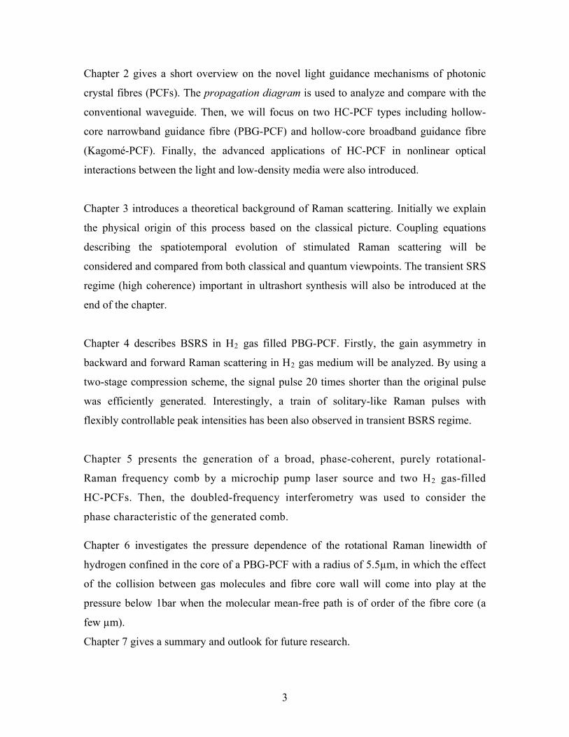
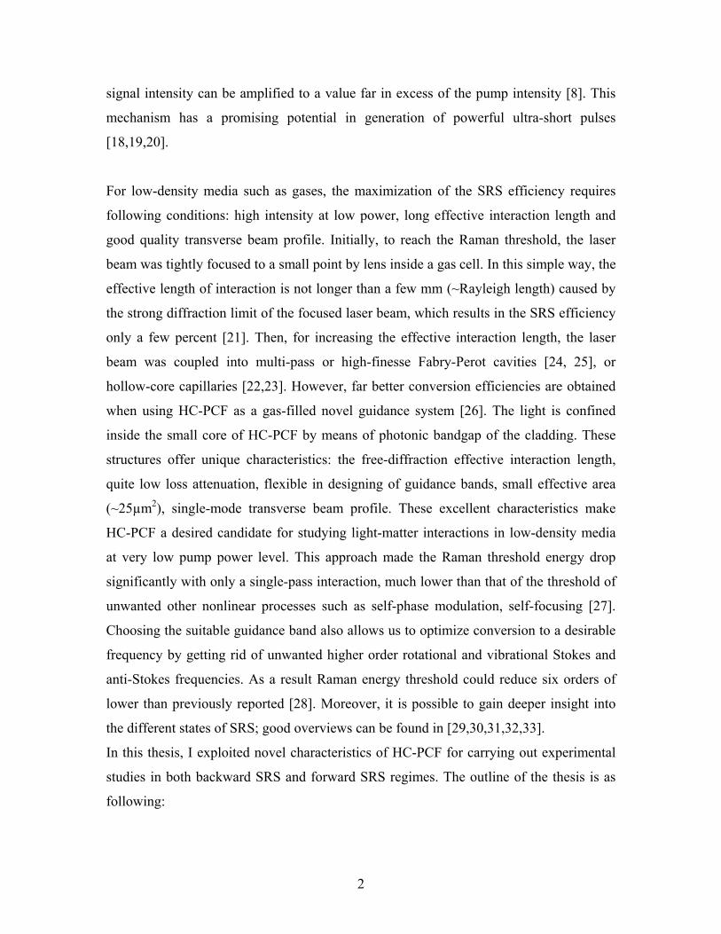
Chapter 2 gives a short overview on the novel light guidance mechanisms of photonic

crystal fibres (PCFs). The propagation diagram is used to analyze and compare with the

conventional waveguide. Then, we will focus on two HC-PCF types including hollow-

core narrowband guidance fibre (PBG-PCF) and hollow-core broadband guidance fibre

(Kagomé-PCF). Finally, the advanced applications of HC-PCF in nonlinear optical

interactions between the light and low-density media were also introduced.

Chapter 3 introduces a theoretical background of Raman scattering. Initially we explain

the physical origin of this process based on the classical picture. Coupling equations

describing the spatiotemporal evolution of stimulated Raman scattering will be

considered and compared from both classical and quantum viewpoints. The transient SRS

regime (high coherence) important in ultrashort synthesis will also be introduced at the

end of the chapter.

Chapter 4 describes BSRS in H2 gas filled PBG-PCF. Firstly, the gain asymmetry in

backward and forward Raman scattering in H2 gas medium will be analyzed. By using a

two-stage compression scheme, the signal pulse 20 times shorter than the original pulse

was efficiently generated. Interestingly, a train of solitary-like Raman pulses with

flexibly controllable peak intensities has been also observed in transient BSRS regime.

Chapter 5 presents the generation of a broad, phase-coherent, purely rotational-

Raman frequency comb by a microchip pump laser source and two H2 gas-filled

HC-PCFs. Then, the doubled-frequency interferometry was used to consider the

phase characteristic of the generated comb.

Chapter 6 investigates the pressure dependence of the rotational Raman linewidth of

hydrogen confined in the core of a PBG-PCF with a radius of 5.5µm, in which the effect

of the collision between gas molecules and fibre core wall will come into play at the

pressure below 1bar when the molecular mean-free path is of order of the fibre core (a

few µm).

Chapter 7 gives a summary and outlook for future research.

3

Chapter 2 Hollow-core photonic crystal fibres

I will introduce briefly optical properties of two types of HC-PCF, i.e. photonic bandgap

PCF (PBG-PCF) and kagomé-PCF. The reviewed material of this chapter is mainly based

on these references [27,34,37].

2.1 Conventional fibre

In order to distinguish conventional fibre clearly from HC-PCF, firstly we summarize

their guiding mechanism. Conventional “step-index” fibres operate by total internal

reflection (TIR). They consist of a solid core with the refractive index n1 surrounded by

an outer cladding of slightly lower refractive index n2<n1 [34]. Incident light rays are

completely reflected into the fibre core (TIR) if their incident angles (on the core-

cladding boundary) are smaller than that of a critical angle ⎟⎠⎞⎜

⎝⎛=≤ −

1

21cr n

nsinθθ . The

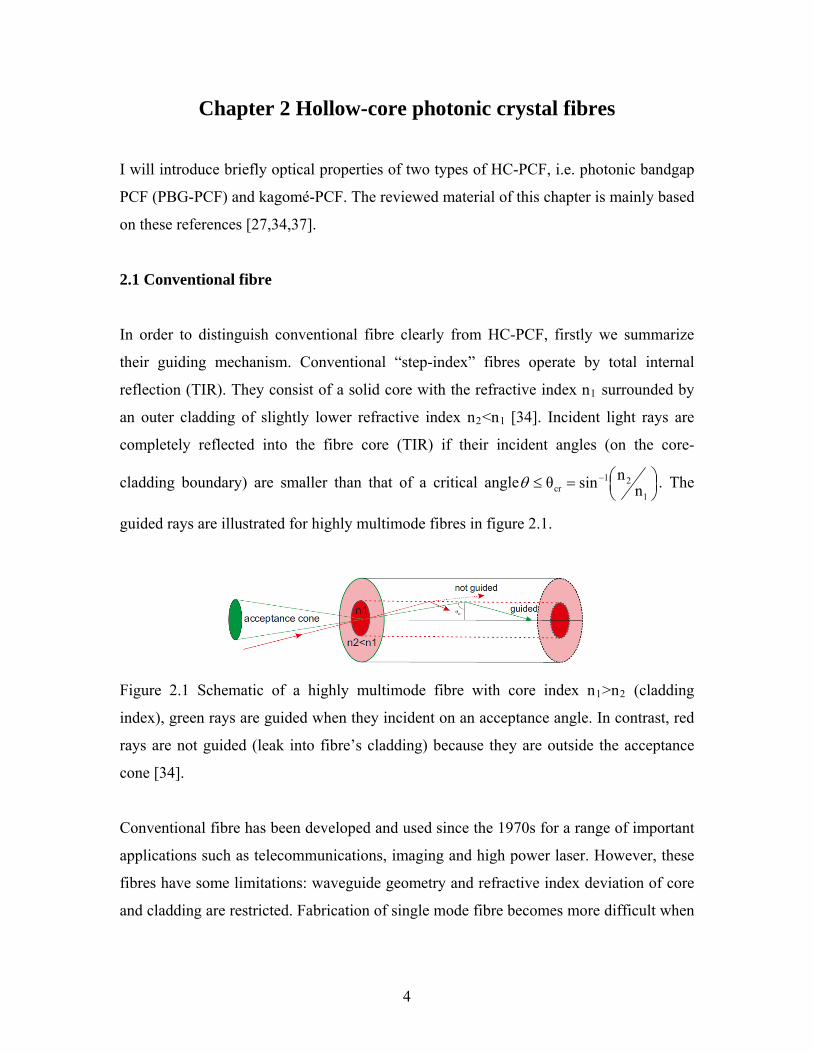
guided rays are illustrated for highly multimode fibres in figure 2.1.

Figure 2.1 Schematic of a highly multimode fibre with core index n1>n2 (cladding

index), green rays are guided when they incident on an acceptance angle. In contrast, red

rays are not guided (leak into fibre’s cladding) because they are outside the acceptance

one [34]. c

Conventional fibre has been developed and used since the 1970s for a range of important

applications such as telecommunications, imaging and high power laser. However, these

fibres have some limitations: waveguide geometry and refractive index deviation of core

and cladding are restricted. Fabrication of single mode fibre becomes more difficult when

4

guided wavelength gets shorter. Furthermore, for specialized applications, which require

hollow core, conventional fibres are impossible because of their dependence on TIR.

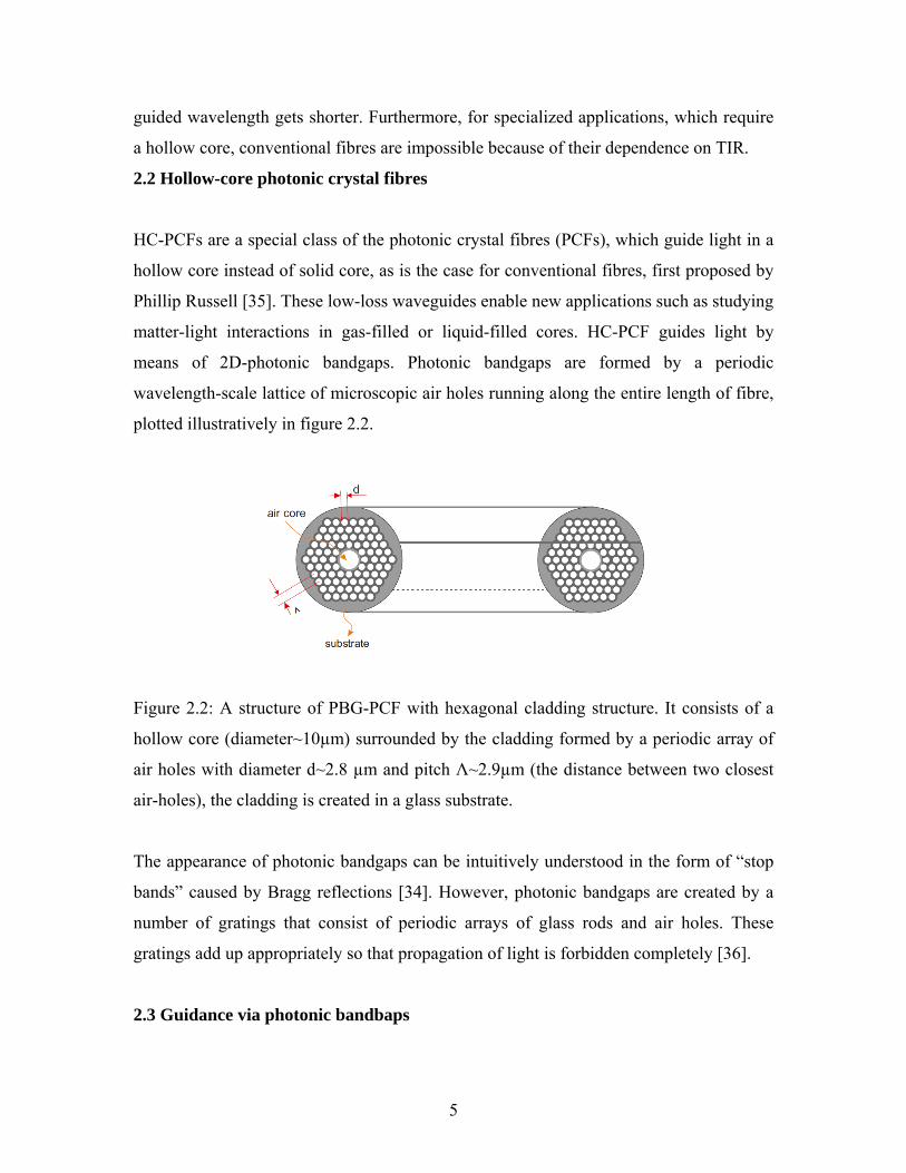
. Photonic bandgaps are formed by a periodic

avelength-scale lattice of microscopic air holes running along the entire length of fibre,

plotted illustratively in figure 2.2.

a

2.2 Hollow-core photonic crystal fibres

HC-PCFs are a special class of the photonic crystal fibres (PCFs), which guide light in a

hollow core instead of solid core, as is the case for conventional fibres, first proposed by

Phillip Russell [35]. These low-loss waveguides enable new applications such as studying

matter-light interactions in gas-filled or liquid-filled cores. HC-PCF guides light by

means of 2D-photonic bandgaps

w

Figure 2.2: A structure of PBG-PCF with hexagonal cladding structure. It consists of a

hollow core (diameter~10µm) surrounded by the cladding formed by a periodic array of

ir holes with diameter d~2.8 µm and pitch Λ~2.9µm (the distance between two closest

a

umber of gratings that consist of periodic arrays of glass rods and air holes. These

pagation of light is forbidden completely [36].

a

air-holes), the cladding is created in a glass substrate.

The appearance of photonic bandgaps can be intuitively understood in the form of “stop

bands” caused by Bragg reflections [34]. However, photonic bandgaps are created by

n

gratings add up appropriately so that pro

2.3 Guidance via photonic bandbaps

5

It is well known that when light is incident on any interface between materials, the

component of the wave-vector parallel to the interface is conserved [34]. In the fibre, if

the structure is invariant along its entire length, the interface of core and cladding is

always parallel to the fibre axis, labeled usually as z-axis, conserved vector is called

propagation constant, β . Propagation constant can be obtained by solving the Maxwell

equations (as Eq. (2.1) in section 2.4 below) and gives information on the dispersion of

fibres. Its maximu nk0 (m is 0nkβ ≤ ), with n being the refractive index of the

homogeneous medium and λ2π

0k = is the vacuum wave-vector corresponding to the

wavelengthλ . For a given value of 0nkβ > , light propagation is forbidden. Results in

light being confined in the higher index areas by TIR.

A very useful tool to describe regimes where light is able to propagate or be evanescent is

the propagation diagram, described in figure 2.3. The propagation diagram shows the

relation between propagation constant and light frequencies normalized to the pitch, Λ of

bre cladding. This diagram allows us to present clearly the propagation mechanisms of

light in conventional fibres as well as PCFs.

fi

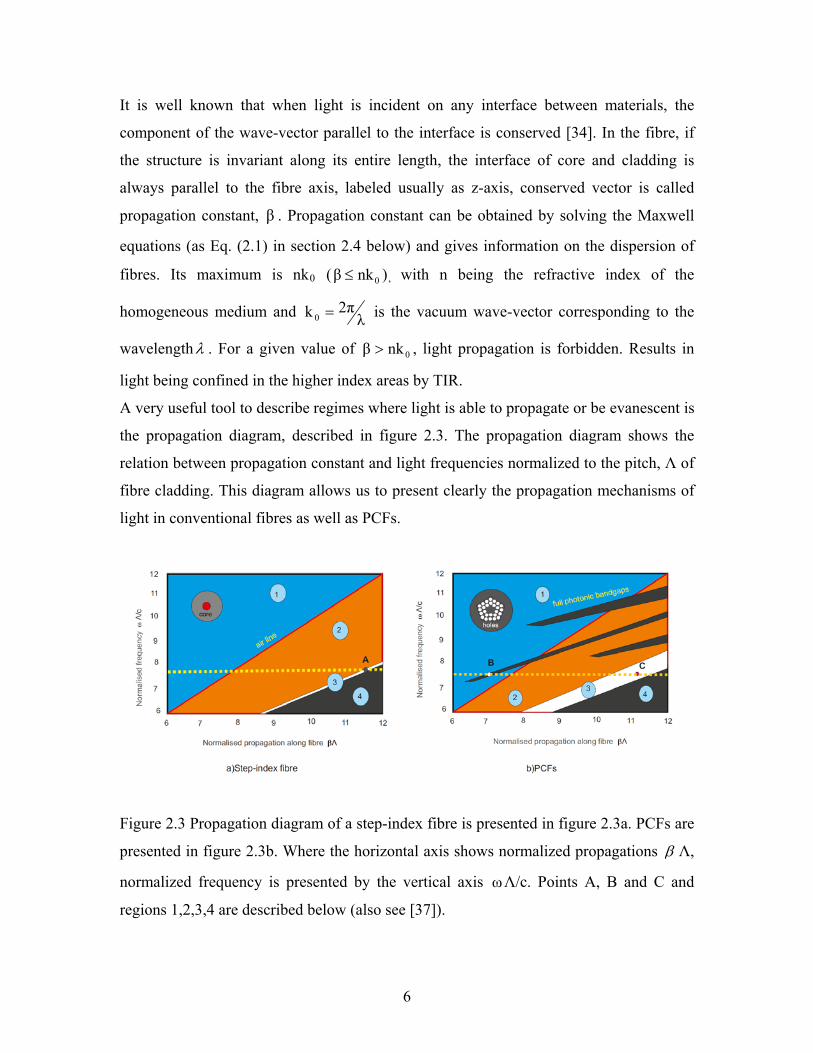
Figure 2.3 Propagation diagram of a step-index fibre is presented in figure 2.3a. PCFs are

presented in figure 2.3b. Where the horizontal axis shows normalized propagations β Λ,

ormalized frequency is presented by the vertical axis Λ/c. Points A, B and C and n ω

regions 1,2,3,4 are described below (also see [37]).

6

Propagation of step-index fibre composed for example of a Ge-doped silica core

and a pure silica cladding with slightly lower refrac , pr

regimes

tive index esented in figure 2.3a:

light can proRegion 1: pagate in all regions; air refractive index of 1nair0air knβ < ≈ ;

cladding index of 1.45n ≈ and solid core of 1.47n ≈cladding core .

<< li

kn such as point A in

gure 2.3a. This is TIR in conventional fibre.

regimes of PCFs with an average refractive index of micro-structured

an

ight propa

k

as TIR regim in conventional fibre, PCFs

average index of air-glass cladding is always smaller than that of pure glass core

Region 2: n ght can propagate in both fibre cladding and core but not

in air.

0cladding0air knβk

Region 3: 0coreknβ << light only propagate in fibre core0cladding

fi

Region 4: 0reknβ > no propagation with any refractive index of n.

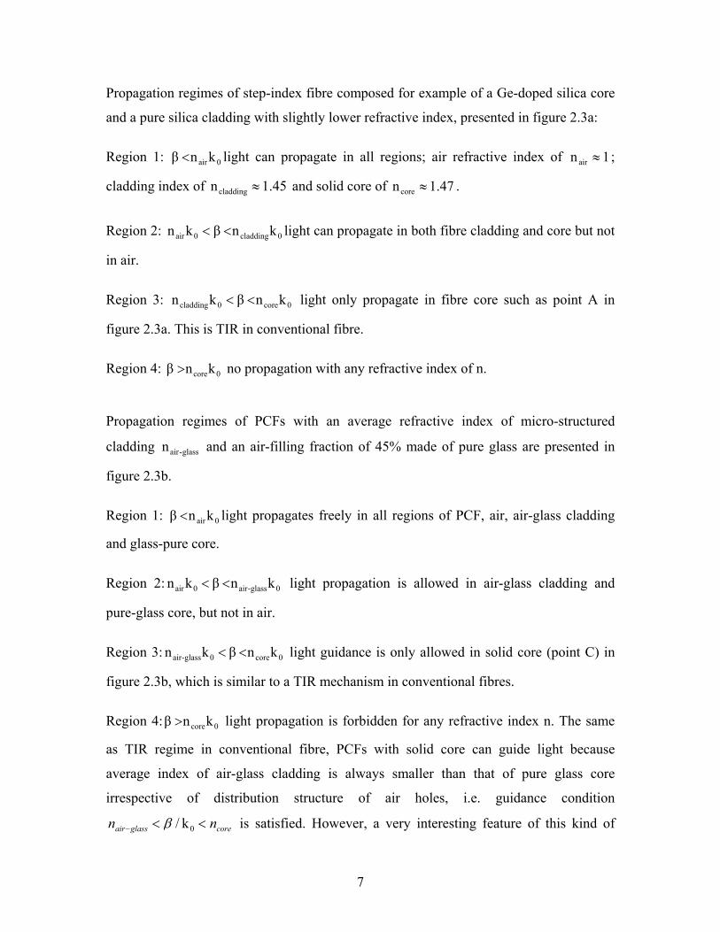
Propagation

co

cladding n d an air-filling fraction of 45% made of pure glass are presented in

figure 2.3b.

glass-air

Region 1: gates freely in all regions of PCF, air, air-glass cladding

and glass-pure core.

0air knβ < l

Region 2: light propagation is allowed in air-glass cladding and

pure-glass core, but not in air.

0glass-air0air knβkn <<

Region 3: 0coreknβn << light guidance is only allowed in solid core (point C) in

figure 2.3b, which is similar to a TIR mechanism in conventional fibres.

Region 4: 0coreknβ > light propagation is forbidden for any refractive index n. The same

with solid core can guide light because

irrespective of distribution structure of air holes, i.e. guidance condition

coreglassair nn <<− 0k/

0glass-air

e

β is satisfied. However, a very interesting feature of this kind of

7

PCF is that its core keeps single mode no matter how short is the wavelength of the

guided light, i.e. it is endlessly single mode (ESM-PCF). Conventional fibres, however,

tend to become multimode for shorter wavelengths [35].

bandgaps unique to PCF. By designing appropriately the cladding with periodic air-hole

arrays in the pure glass substrate, it is possible to form photonic bandgaps where light

propagation is forbidden at certain values of β . Full photonic bandgaps are presented by

black thin “fingers” in figure 2.3b. Photonic bandgaps are possible to appear in regions

1&2 and pass through the air line (diagonal line) to intersect the guided line at point B.

Points such as point B are only possible in

Moreover, PCF also contribute another light guidance mechanism, namely photonic

PCF. Hence, light propagation is possible in

cladding of air holes by mean of photonic

is impossible in conventional fibre, because hollow core has a

ractive index smaller than that of air-glass cladding material which does not satisfy the

resent qualitative

provides the information about the band structure or the range of prohibited wavelengths.

a desired propagation

order to get the DOS plot, Maxwell equations must be solved numerically using some

special methods [38,39]. Maxwell equations can be solved with as lue

y the equation (Eq.) below.

air (hollow-core) but not in the periodic

bandgaps. This mechanism

ref

requirement of TIR.

2.4 Density of states

Whereas the tool of the propagation diagram can be used to rep

information on the the position of photonic bandgaps, density of states (DOS) plot

This gives parameters for the fabrication of PBG-PCF with

wavelength ranges.

In2β eigenva s given

b

( ) ( )( )[ ] T2

TTTT20

2 HβHyx,rlnε)]Hyx,ε(rk[ =×∇×∇++∇ (2.1)

This form allows material di to be easily included.

spersion

8

Here the plane (x, y) is the transverse plane normal to the direction of propagation, z,

( )Trε is the dielectric constant at position rT (x . H s the transverse component

of magnetic field vector H.

,y) denoteT

cωk0 = is the vacuum wave-vector.

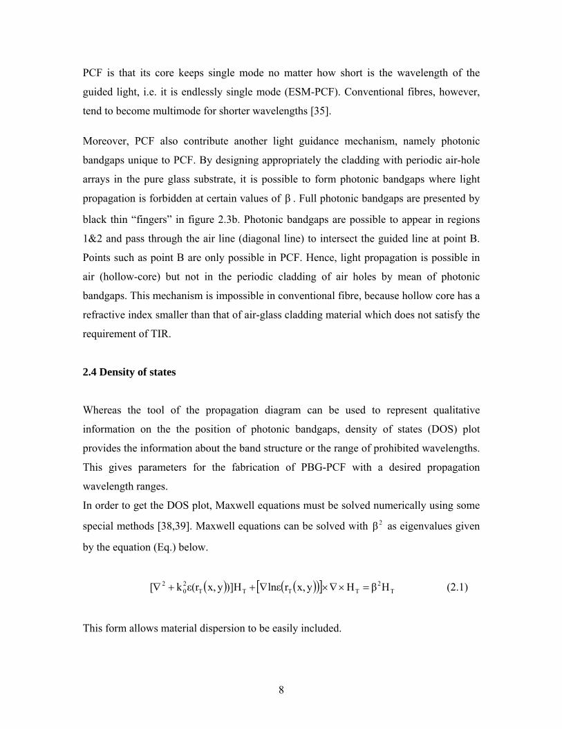
The plane-wave solution of (2.1) at fixed frequency shows a range of possible guided

cladding modes in propagation constant from to

ω

Λβ ( )Λdββ + at a particular normalized

frequency of on figure 2.4a. 0Λk

parameters for the cladding structure (2.4b) with pitch Λ =3 µm and d/Λ=0.98 [39].

Here, normalized frequency Λk

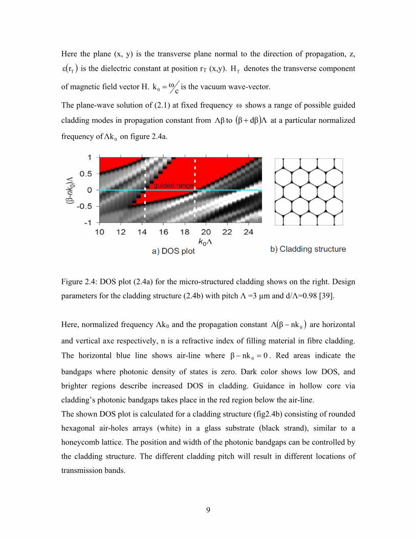
Figure 2.4: DOS plot (2.4a) for the micro-structured cladding shows on the right. Design

0 and the propagation constant ( )0nkβΛ − are horizontal

and vertical axe respectively, n is a refractive index of filling material in fibre cladding.

The horizontal blue line shows air-line where 0nkβ 0 =− . Red areas indicate the

is calculated for a cladding structure (fig2.4b) consisting of rounded

bandgaps where photonic density of states is zero. Dark color shows low DOS, and

brighter regions describe increased DOS in cladding. Guidance in hollow core via

cladding’s photonic bandgaps takes place in the red region below the air-line.

The shown DOS plot

hexagonal air-holes arrays (white) in a glass substrate (black strand), similar to a

honeycomb lattice. The position and width of the photonic bandgaps can be controlled by

the cladding structure. The different cladding pitch will result in different locations of

transmission bands.

9

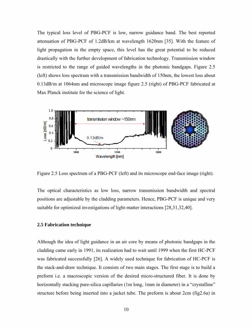
The typical loss level of PBG-PCF is low, narrow guidance band. The best reported

attenuation of PBG-PCF of 1.2dB/km at wavelength 1620nm [35]. With the feature of

light propagation in the empty space, this level has the great potential to be reduced

drastically with the further development of fabrication technology. Transmission window

restricted to the range of guided wavelengths in the photonic bandgaps. Figure 2.5

(left) shows loss spectrum with a transmission bandwidth of 150nm, the lowest loss about

0.13dB/m at 1064nm and microscope image figure 2.5 (right) of PBG-PCF fabricated at

Max Planck institute for the science of light.

is

Figure 2.5 Loss spectrum of a PBG-PCF (left) and its microscope end-face image (right).

as low loss, narrow transmission bandwidth and spectral

ositions are adjustable by the cladding parameters. Hence, PBG-PCF is unique and very

desired micro-structured fiber. It is done by

orizontally stacking pure-silica capillaries (1m long, 1mm in diameter) in a “crystalline”

structure before being inserted into a jacket tube. The preform is about 2cm (fig2.6a) in

The optical characteristics

p

suitable for optimized investigations of light-matter interactions [28,31,32,40].

2.5 Fabrication technique

Although the idea of light guidance in an air core by means of photonic bandgaps in the

cladding came early in 1991, its realization had to wait until 1999 when the first HC-PCF

was fabricated successfully [26]. A widely used technique for fabrication of HC-PCF is

the stack-and-draw technique. It consists of two main stages. The first stage is to build a

preform i.e. a macroscopic version of the

h

10

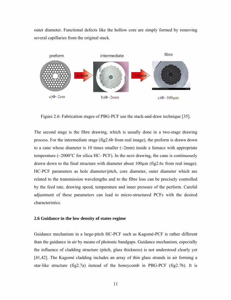
outer diameter. Functional defects like the hollow core are simply formed by removing

several capillaries from the original stack.

Figure 2.6: Fabrication stages of PBG-PCF use the stack-and-draw technique [35].

The second stage is the fibre drawing, which is usually done in a two-stage drawing

process. For the intermediate stage (fig2.6b from real image), the preform is drawn down

to a cane whose diameter is 10 times smaller (~2mm) inside a furnace with appropriate

temperature (~2000°C for silica HC- PCF). In the next drawing, the cane is continuously

drawn down to the final structure with diameter about 100µm (fig2.6c from real image).

HC-PCF parameters as hole diameter/pitch, core diameter, outer diameter which are

related to the transmission wavelengths and to the fibre loss can be precisely controlled

y the feed rate, drawing speed, temperature and inner pressure of the perform. Careful

ro-structured PCFs with the desired

haracteristics.

structure (fig2.7a) instead of the honeycomb in PBG-PCF (fig2.7b). It is

b

adjustment of these parameters can lead to mic

c

2.6 Guidance in the low density of states regime

Guidance mechanism in a large-pitch HC-PCF such as Kagomé-PCF is rather different

than the guidance in air by means of photonic bandgaps. Guidance mechanism, especially

the influence of cladding structure (pitch, glass thickness) is not understood clearly yet

[41,42]. The Kagomé cladding includes an array of thin glass strands in air forming a

star-like

11

established that the cladding structure does not exhibit any photonic bandgaps. Indeed,

wave guidance of the Kagomé lattice happens in the presence of low density of photonic

states.

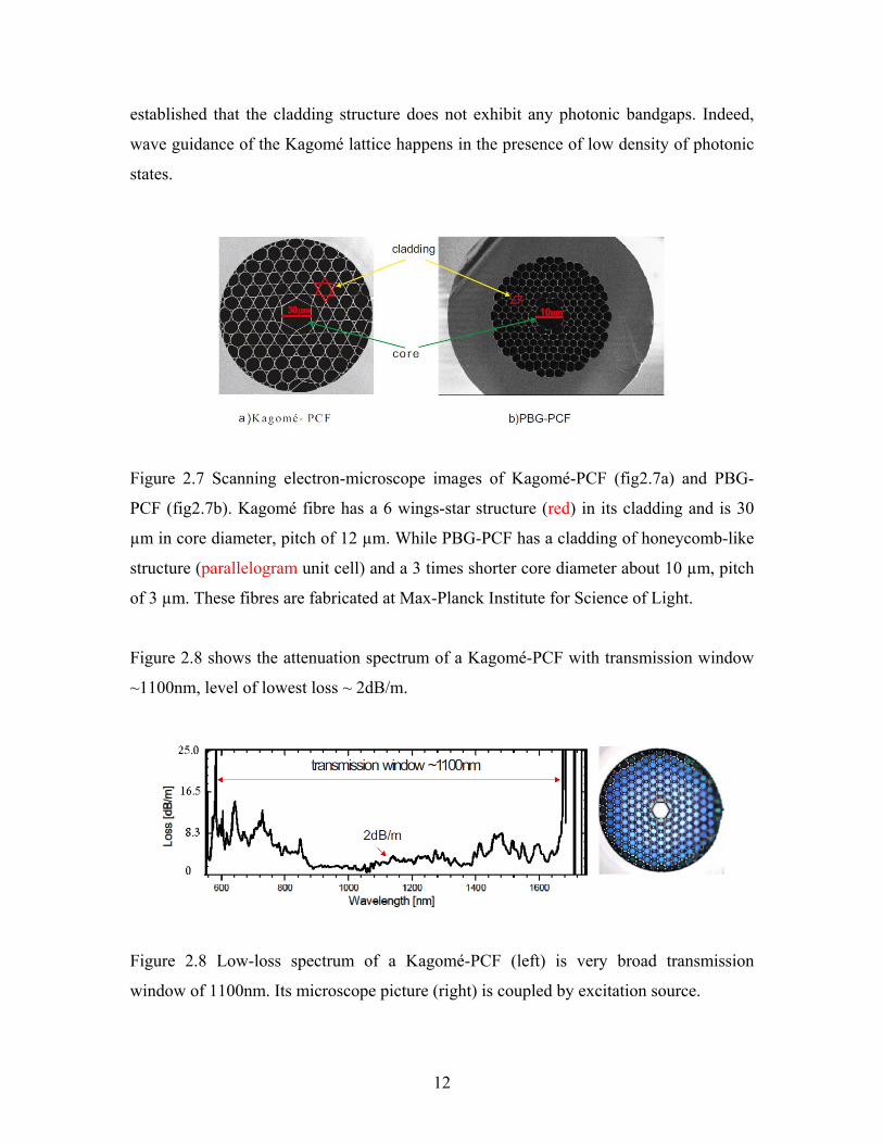
Figure 2.7 Scanning electron-microscope images of Kagomé-PCF (fig2.7a) and PBG-

PCF (fig2.7b). Kagomé fibre has a 6 wings-star structure (red) in its cladding and is 30

m in core diameter, pitch of 12 µm. While PBG-PCF has a cladding of honeycomb-like

ax-Planck Institute for Science of Light.

Figure 2.8 shows the attenuation spectrum of a Kagomé-PCF with transmission window

~1100nm, level of lowest loss ~ 2dB/m.

µ

structure (parallelogram unit cell) and a 3 times shorter core diameter about 10 µm, pitch

of 3 µm. These fibres are fabricated at M

Figure 2.8 Low-loss spectrum of a Kagomé-PCF (left) is very broad transmission

window of 1100nm. Its microscope picture (right) is coupled by excitation source.

12

Typically transmission window of Kagomé-PCF is much broader compared to ones

caused by bandgaps of PBG-PCF. Loss level can be down to 0.180dB/m a transmission

and can over 1200nm [41]. This fibre is useful for applications requiring a wide

ency comb generation [33,43],

ltraviolet generation [44].

order to get a feeling of the possible enhancement in the nonlinear light-matter

interaction we get by usin

experiment in free space) we defined a figure of merit M expressed as [27].

b

bandwidth of guided wavelengths such as Raman frequ

u

2.7 HC-PCF enhances the gas based nonlinear effect

In

g HC-PCFs (as compared when one performs the same

effeff A

LM λ= (2.2)

M is a function of Leff, the effective interaction length, λ the vacuum wavelength and

intensity of

SRS. In order to achieve that condition, there are some approaches as following:

2eff rπA ×= , the effective cross-section or area where r is the effective radius associated

to Aeff.

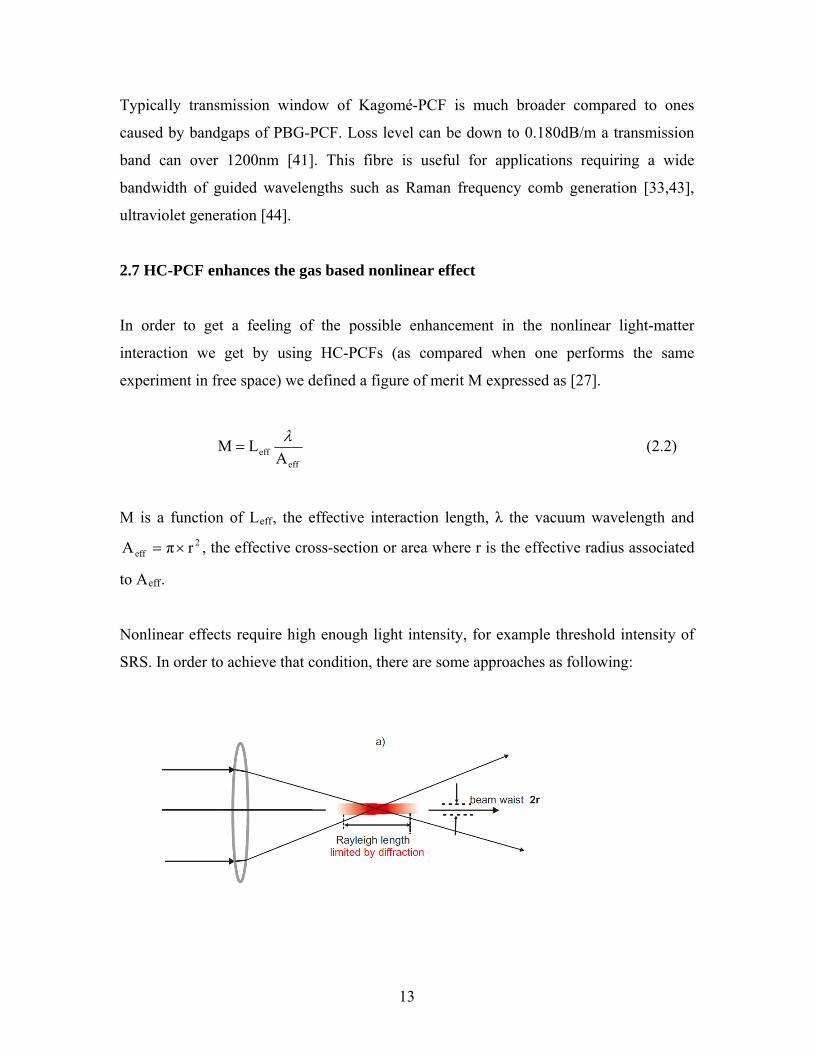
Nonlinear effects require high enough light intensity, for example threshold

13

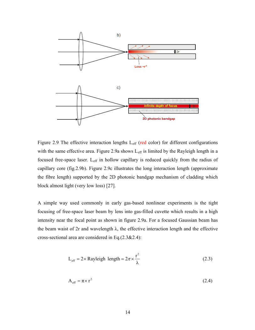
Figure 2.9 The effective interaction lengths Leff (red color) for different configurations

with the same effective area. Figure 2.9a shows Leff is limited by the Rayleigh length in a

focused free-space laser. Leff in hollow capillary is reduced quickly from the radius of

capillary core (fig.2.9b). Figure 2.9c illustrates the long interaction length (approximate

the fibre length) supported by the 2D photonic bandgap mechanism of cladding which

block almost light (very low loss) [27].

A simple way used commonly in early gas-based nonlinear experiments is the tight

focusing of free-space laser beam by lens into gas-filled cuvette which results in a high

intensity near the focal point as shown in figure 2.9a. For a focused Gaussian beam has

the beam waist of 2r and wavelength λ, the effective interaction length and the effective

cross-sectional area are considered in Eq.(2.3&2.4):

λr2lengthRayleigh 2L

2

eff ×=×= π (2.3)

2

eff rπA ×= (2.4)

14

The figure of merit for the focused Gaussian beam Mfb is written in Eq.(2.5):

2Mfb = (2.5)

It is clear that the effective cross-sectional area is smaller (or higher focused intensity)

Eq.(2.4), results in a shorter effective interaction length Leff Eq.(2.3) so that the two

counterbalance each others effect. Hence, tighter focusing is inefficient in increasing the

effect of matter-light nonlinear interaction.

Another approach to improve the nonlinear effect is the use of dielectric capillaries, or

metal-coated tubes [22,23]. This can increase the effective interaction length. However,

their propagation losses are very high, as illustrated in figure 2.9b.

For a dielectric capillary with an inner radius r, refractive index of glass n=1.5, the loss

rate for fundamental mode [22].

3

2

rλ4246.0 ×=α (2.6)

The effective interaction length is related to the length of capillary Lcapillary:

α1

αe1L

yαLcapillar

eff ≈−

=−

(2.7)

From Eq.(2.2, 2.6&2.7), we obtain the figure of merit for the hollow capillary

(normalized to Mfb) Mhc,

λr0.375Mhc ×≈ (2.8)

From Eq.(2.6) we note that the loss increase hugely (or the effective decrease of the

interaction length) as the inverse radius cubed (loss ~ 3r − ). For metal-coated tubes, loss is

15

even many orders of magnitude higher, particularly at optical frequencies where metals

absorb strongly [35].

An ideal configuration for effective gas-based nonlinear interactions needs to satisfy the

following requirements: diffraction-free, lossless, single-mode waveguide, core diameter

same as focused laser beam waist (~ µm). HC-PCF with the core radius r = 5 µm and an

achievable loss of 1.2dB/km [35] comes to this ideal situation. Hence, the effective

interaction length is approximated by the length of the fibre Lfibre and the normalized

figure of merit of HC-PCF become.

2fibre

2

αL

hcf rπλ

2L

2λ

rπ1

αe1M

fibre

×≈×

×−

=−

(2.9)

Eq. (2.9) shows that the figure of merit of HC-PCF increases quickly with the decrease of

core radius. Figure 2.9c illustrates he effective interaction length without the depth of

focus in HC-PCF. Light is confined tightly (high intensity) along the entire length of the

fibre.

Next, we compare the gas-based nonlinear effect for above approaches. Assume that

propagation wavelength (1µm), Lfibre=3m, refractive index of glass n=1.5, core radius is

changed in a range of 1-20µm. Figure 2.10 shows that figure of merit of HC-PCF with

loss of 195dB/km is about 8 orders of magnitude higher than that of capillary at the core

radius of 5µm (PBG-PCF) and about 4 orders of magnitude at radius of 15 µm (Kagomé-

PCF). Mfb of focused beam is invariant.

HC-PCFs with unique characteristics such as designable transmission window, very high

nonlinear effects are considered as the best candidate to study the light-matter interaction

in the low power regime in general and in gas-based nonlinear interactions in particular.

This thesis exploits these unique features to investigate stimulated Raman scattering in

hydrogen gas filled HC-PCF.

16

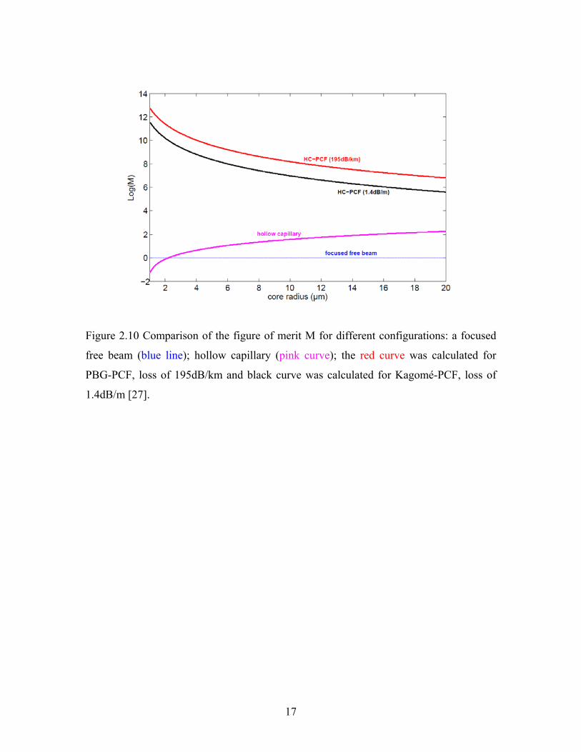
Figure 2.10 Comparison of the figure of merit M for different configurations: a focused

free beam (blue line); hollow capillary (pink curve); the red curve was calculated for

PBG-PCF, loss of 195dB/km and black curve was calculated for Kagomé-PCF, loss of

1.4dB/m [27].

17

Chapter 3 Theoretical background of Raman scattering

In this chapter I review the theoretical background behind stimulated Raman scattering.

This is mainly based on the references [1,2,45,46,53].

3.1 Origin of Raman scattering

Raman scattering is the result of the interaction of optical field pE~ [Vm-1] with the

oscillation excitations of the molecules in the Raman active medium. Although the

optical frequency is too high to follow by the nuclei of the molecule, it can cause the

distortion of electron cloud, making each molecule become polarized. On the other hand,

the electron potential depends on the nuclear coordinate. Hence, we can say that the

electronic polarizability α~ [m3] perturbed by the presence of nuclear oscillation. This

section is derived from [1,6,45,46].

Dynamically, the oscillations in diatomic molecules can be rotational, vibrational or

rotational-vibrational depending on the excitation conditions such as the polarization state

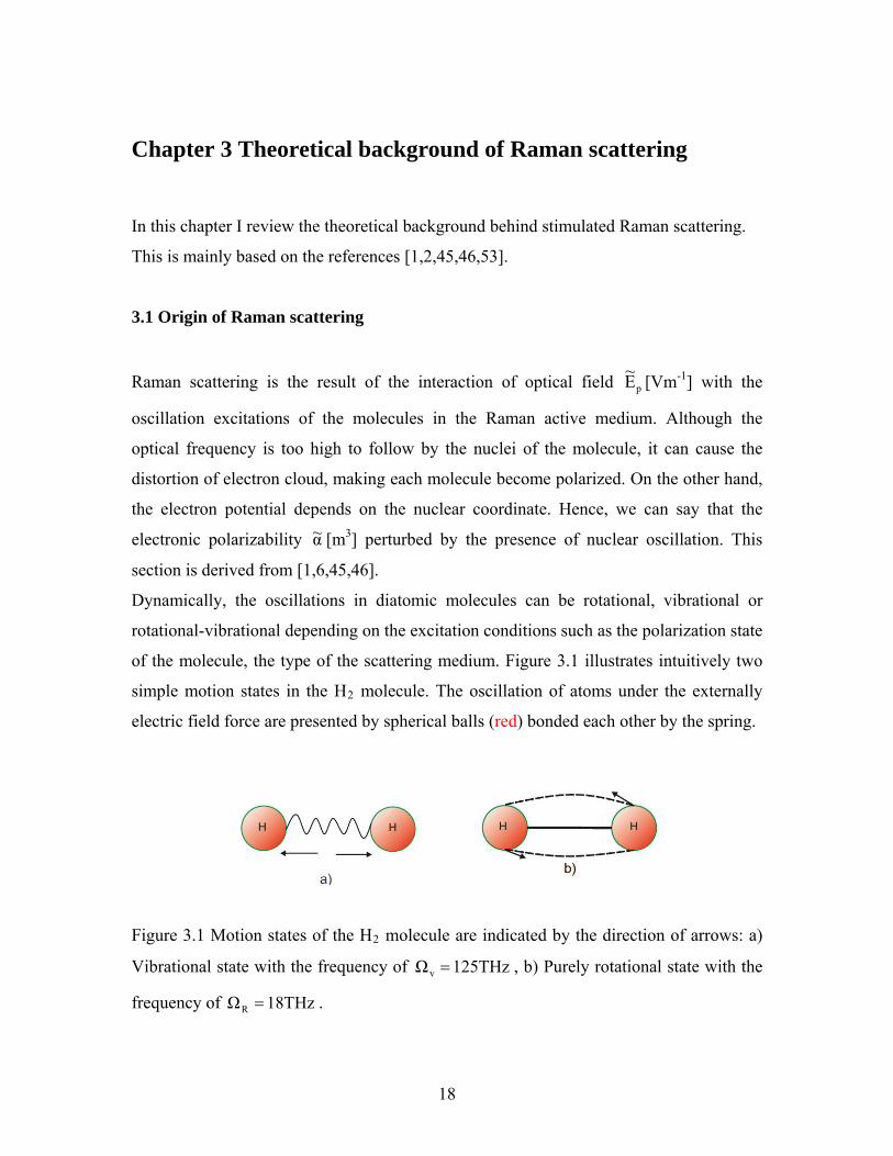
of the molecule, the type of the scattering medium. Figure 3.1 illustrates intuitively two

simple motion states in the H2 molecule. The oscillation of atoms under the externally

electric field force are presented by spherical balls (red) bonded each other by the spring.

Figure 3.1 Motion states of the H2 molecule are indicated by the direction of arrows: a)

Vibrational state with the frequency of 125THzΩv = , b) Purely rotational state with the

frequency of . 18THzΩR =

18

The different motions correspond to the frequencies of Raman excited transitions. At the

room temperature, the frequency of Raman excited transition for vibration of

(4155 cm125THzΩv =-1) and for rotation of 18THzΩR = are dominant [6].

In the context of our experiments, only the rotational Raman transition is considered.

However, the formalisms for the description of the Raman scattering used below are valid

for both states.

The induced electric dipole moment [Cm] likes a dipole emitter. Its magnitude is equal

the product of the strength of the applied field of and the Raman polarizability of

, expressed in Eq.(3.1).

μ~

(t)E~

( )tα~

( ) ( ) ( )tΕ~tα~εtμ~ p0= (3.1)

Where, [Cm0ε-1V-1] is the electric permittivity in vacuum.

We let is the motion coordinate or the deviation of the internuclear distance from its

equilibrium. It may either be the linear position in the vibrational motion or the angular

position in rotational motion. Then, can be expressed by the Taylor expansion in

motion coordinate

( )tq~

α(t)

( )tq~ (Placzek model) [1,46].

( ) ...q~qααq~α~

00 +⎟⎟

⎠

⎞⎜⎜⎝

⎛∂∂

+= (3.2)

The term of in Eq.(3.2) is the polarizability of the molecule at the absence of

oscillation, it can be approximated as constant in

0α

( )tq~ and contributes to the Rayleigh

scattering. The first order correction of 0q

α⎟⎟⎠

⎞⎜⎜⎝

⎛∂∂ is interpreted as the coupling strength

between the nuclei and electrons. The higher-order terms are responsible for the multi-

photon processes. The induced dipole moment makes the molecule polarized. The

macroscopic polarization of the scattered medium is obtained by the statistic sum of all

dipole moments per unit volume N[m-3].

19

( ) ( )tμ~NtΡ~ = (3.3)

Where [Cm( )tP~ -2] plays role as a source term in the Maxwell wave propagation

equations (section 3.3.1).

Raman scattering can be split into spontaneous and stimulated Raman scattering (SRS).

The former one is typically a weak excitation process of incoming intensity with the

Stokes transfer efficiency of only being about one millionth of the incident light

radiation. Spontaneous scattering is incoherent and its Stokes radiation can spread in any

directions. The latter is observed when excited with an intense laser beam. This

stimulated process increases the transfer efficiency and the coherence is much higher in

the spontaneous one leading to the emission process in a narrow cone in the backward

and forward direction.

Before the detail description of SRS is done as essential part of this chapter, we consider

some basic properties of the spontaneous and its relationship with the stimulated Raman

scattering.

3.2 Spontaneous and stimulated Raman scattering

3.2.1 Spontaneous Raman scattering

If the incident field is not strong enough and the scattered Stokes photons don’t

affect to the scattering process, then we talk about spontaneous Raman scattering.

According to the classical description, the oscillation can be featured by its amplitude and

phase. We assume the material excitation and the applied field are represented by

monochromatic plane waves propagating in z-direction. The following description is

referred from [1,46]

(t)E~

( ) ( )[ ]( c.cΩt-iexptz,Q21(t)q~ +Φ= ) (3.4)

20

( ) ( )[ ]( c.ctω-zkiexptz,E21(t)E~ pppp += ) (3.5)

Where Q(z,t) is the complex, time and space-dependent envelopes of the internuclear

motion, is the nuclear motion frequency (assumed that the nuclei are not moving

initially), is the phase of the nuclear mode oscillation established by random phases.

E

Ω

Φ

p(z,t) is the complex, time and its space dependent envelopes of the input fields, where

is the carrier frequency and its wavevector pω cωnk PP

P = , nP denotes the refractive

index of medium at the frequency of . C.c indicates as the complex conjugate

component, c is the velocity of light in vacuum.

Pω

Substitute Eq.(3.2,3.4&3.5) into Eq.(3.1), then the dipole moment is calculated as:

( )( )[ ] c.c-tΩ-ω-zkiexpEQqα

2μ~ ppp

*

0

0 +Φ⎟⎟⎠

⎞⎜⎜⎝

⎛∂∂

=ε

( )[ ]( )c.ctω-zkiexpEα ppp00 ++ ε

( )( )[ ] ...c.ctΩω-zkiexpQEqα

2 ppp0

0 ++Φ++⎟⎟⎠

⎞⎜⎜⎝

⎛∂∂

+ε (3.6)

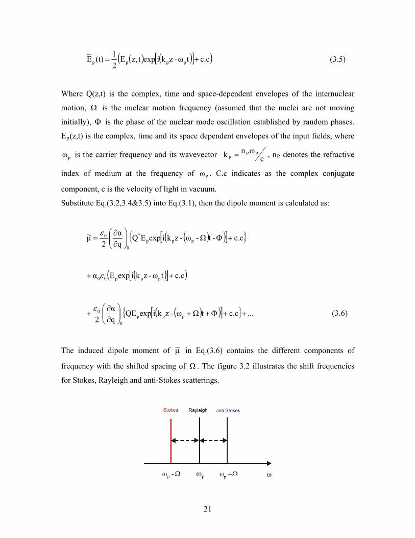
The induced dipole moment of μ~ in Eq.(3.6) contains the different components of

frequency with the shifted spacing of . The figure 3.2 illustrates the shift frequencies

for Stokes, Rayleigh and anti-Stokes scatterings.

Ω

21

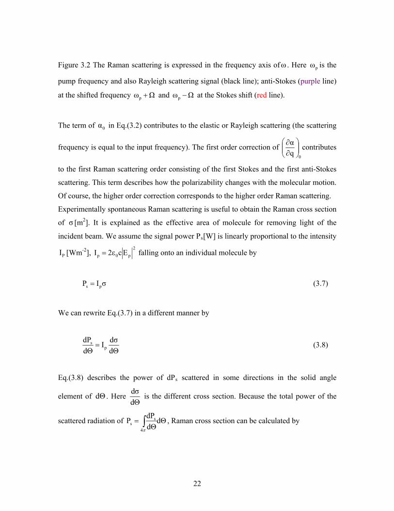
Figure 3.2 The Raman scattering is expressed in the frequency axis ofω . Here is the

pump frequency and also Rayleigh scattering signal (black line); anti-Stokes (purple line)

at the shifted frequency and

pω

Ωωp + Ωωp − at the Stokes shift (red line).

The term of in Eq.(3.2) contributes to the elastic or Rayleigh scattering (the scattering

frequency is equal to the input frequency). The first order correction of

0α

0qα⎟⎟⎠

⎞⎜⎜⎝

⎛∂∂ contributes

to the first Raman scattering order consisting of the first Stokes and the first anti-Stokes

scattering. This term describes how the polarizability changes with the molecular motion.

Of course, the higher order correction corresponds to the higher order Raman scattering.

Experimentally spontaneous Raman scattering is useful to obtain the Raman cross section

of [mσ 2]. It is explained as the effective area of molecule for removing light of the

incident beam. We assume the signal power Ps[W] is linearly proportional to the intensity

[WmPI -2], 2

p0p Ec2εI = falling onto an individual molecule by

σIP ps = (3.7)

We can rewrite Eq.(3.7) in a different manner by

dΘdσI

dΘdP

ps = (3.8)

Eq.(3.8) describes the power of dPs scattered in some directions in the solid angle

element of . Here dΘdΘdσ is the different cross section. Because the total power of the

scattered radiation of dΘdΘdPP

4

ss ∫=

π

, Raman cross section can be calculated by

22

dΘdΘdσσ

4π∫= (3.9)

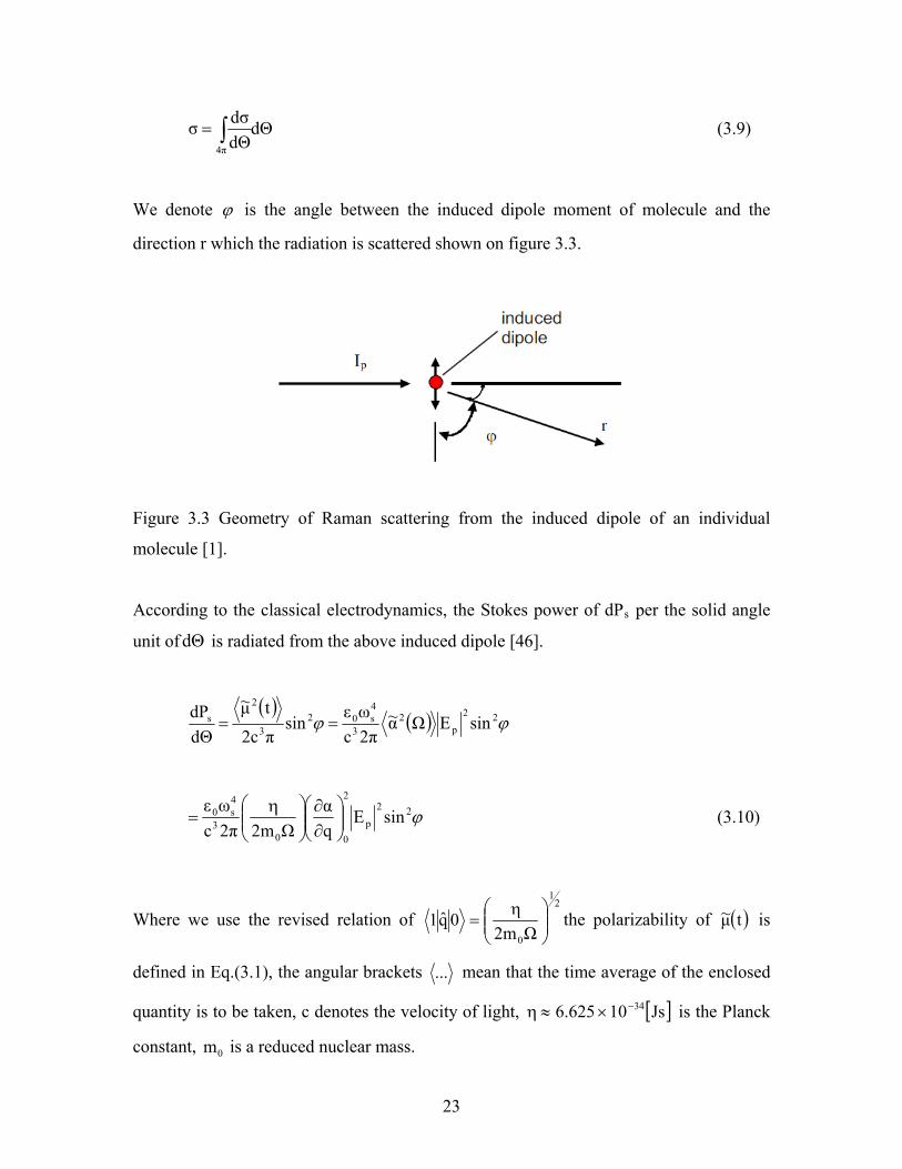
We denote ϕ is the angle between the induced dipole moment of molecule and the

direction r which the radiation is scattered shown on figure 3.3.

Figure 3.3 Geometry of Raman scattering from the induced dipole of an individual

molecule [1].

According to the classical electrodynamics, the Stokes power of dPs per the solid angle

unit of is radiated from the above induced dipole [dΘ 46].

( )( ) ϕϕ 22

p2

3

4s02

3

2s sinEΩα~

2πcωεsin

π2c

tμ~

dΘdP

==

ϕ22

p

2

003

4s0 sinE

qα

Ω2m2πcωε

⎟⎟⎠

⎞⎜⎜⎝

⎛∂∂

⎟⎟⎠

⎞⎜⎜⎝

⎛=

η (3.10)

Where we use the revised relation of 2

1

0Ω2m0q1 ⎟⎟

⎠

⎞⎜⎜⎝

⎛=

η the polarizability of ( )tμ~ is

defined in Eq.(3.1), the angular brackets ... mean that the time average of the enclosed

quantity is to be taken, c denotes the velocity of light, is the Planck

constant, is a reduced nuclear mass.

[ ]Js106.625 34−×≈η

0m

23

Because the angle dependence of dΘdPs is contained entirely in the quantity of .

Integrating Eq.(3.10), we have the total power emitted from the oscillating dipole

moment [46].

ϕ2sin

2

p

2

003

4s0

4π

ss E

qα

Ω2mπ2cωε

34πdΘ

dΘdPP ⎟⎟

⎠

⎞⎜⎜⎝

⎛∂∂

⎟⎟⎠

⎞⎜⎜⎝

⎛=== ∫

η (3.11)

From Eq.(3.8) and Eq.(3.10) we have the different cross section of spontaneous Raman

scattering:

ϕ22

004

4s1-

p sinqα

Ω2mc2ω

dΘdP)(I

dΘdσ

⎟⎟⎠

⎞⎜⎜⎝

⎛∂∂

⎟⎟⎠

⎞⎜⎜⎝

⎛==

η (3.12)

Here 2

p0p Ec2εI =

Combining Eq.(3.12) with Eq.(3.9) gives the total cross-section

( 2322

004

4s

4π

m10qα

Ω2m3c16πdΘ

dΘdσσ −≅⎟⎟

⎠

⎞⎜⎜⎝

⎛∂∂

⎟⎟⎠

⎞⎜⎜⎝

⎛== ∫

ηω ) (3.13)

Equation (3.11) shows that the classical model of the electrodynamics predict the power

of the first Stokes scattering depends on the incident light intensity (~2

pE ) with the scale

of 2

0qα⎟⎟⎠

⎞⎜⎜⎝

⎛∂∂ . Its phase (Eq.3.6) is dependent on the nuclear mode motions. In

equilibrium state, the motions of different molecules are random or the total phase of the

Stokes fields from the dipole emitters is uncorrelated. As a result the total field of the

Raman emission is incoherent in the spontaneous regime.

Φ

24

In order to describe explicitly the spatial evolution of spontaneous Raman process and its

connection with stimulated Raman scattering, it is useful to use the classical photon

occupation number formalism [47].

3.2.2 Spontaneous versus stimulated Raman scattering

At staring point, Sζ is defined as a probability per unit time for emitting a photon into

mode Stokes S and depends on the mean photon per mode in pump ( PN ) and Stokes

( SN ) beam by [1]

( 1NND SPS +=ζ ) (3.14)

Where, D denotes a proportional constant depending on the Raman medium. On the other

hand, the time rate of nS is given by SS

dtNd

ζ= , we can rewrite Eq.(3.14) as following.

( 1NNDdtNd

SPS += ) (3.15)

We assume the Stokes mode (corresponding to a Stokes wave) travels in the positive

direction-z in the medium of the refractive index n, we have the relation tncz = .

Associate this relation with Eq.(3.15) we get by

( 1NNDnc

dzNd

SPS += ) (3.16)

We consider two extreme situations.

• For a spontaneous case 1NS << , Eq.(3.16) becomes

25

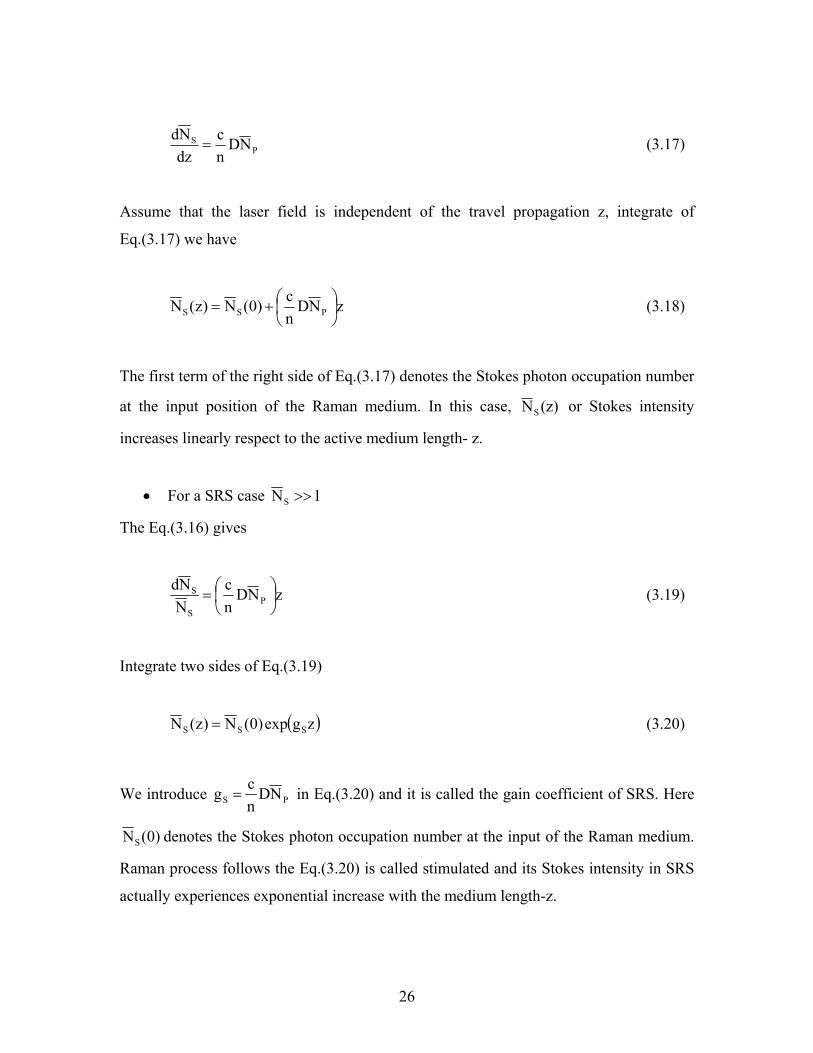
PS ND

nc

dzNd

= (3.17)

Assume that the laser field is independent of the travel propagation z, integrate of

Eq.(3.17) we have

zNDnc)0(N)z(N PSS ⎟

⎠⎞

⎜⎝⎛+= (3.18)

The first term of the right side of Eq.(3.17) denotes the Stokes photon occupation number

at the input position of the Raman medium. In this case, (z)NS or Stokes intensity

increases linearly respect to the active medium length- z.

• For a SRS case 1NS >>

The Eq.(3.16) gives

zNDnc

NNd

PS

S ⎟⎠⎞

⎜⎝⎛= (3.19)

Integrate two sides of Eq.(3.19)

( zgexp)0(N)z(N SSS = ) (3.20)

We introduce PS NDncg = in Eq.(3.20) and it is called the gain coefficient of SRS. Here

)0(NS denotes the Stokes photon occupation number at the input of the Raman medium.

Raman process follows the Eq.(3.20) is called stimulated and its Stokes intensity in SRS

actually experiences exponential increase with the medium length-z.

26

The relationship between SRS and spontaneous Raman scattering is expressed by the

Raman gain coefficient of in Eq.(3.20) and the Raman cross-section of in

Eq.(3.13). This relationship is given [1]

Sg σ

P2SP

2S

P23

S IΘσ

ωnωωN~c4Nπg ⎟

⎠⎞

⎜⎝⎛∂∂

Δ=

η (3.21)

Where, nS is a refractive index of the Stokes radiation, ⎟⎠⎞

⎜⎝⎛∂∂Θσ denotes the differential

spectral cross section, where is the total linewidth of the Stokes radiation, is an

element of solid angle. I

Δω Θd

P denotes the pump intensity of P

PPP Vn

N~cωI

η= , where V is the

effective volume of the Raman scattering, nP is the refractive index of the pump laser

wavelength.

3.3 The coupled wave equations and stimulated Raman scattering

The previous section provides an overview picture of the Raman scattering. However, it

can not reveal the information relating to the coherent interaction between the fields and

the molecules. This information becomes especially important when SRS occurs in

highly coherent regime (transient regime) where the pump pulse duration is comparable

or shorter than the relaxation time of the molecular coherence. This section describes

detail the coherent SRS interaction in terms of the coupled propagation approach in a

nonlinear optical media. Because the coherent excitation is dominant in SRS, the applied

electromagnetic fields can be treated suitably as a classical quantity [48].

3.3.1 Wave propagation

We consider a lossless nonlinear optical media with no free charge, no free current and

no magnetization. The travel of light obeys the Maxwell equation is derived from [1].

27

Ρ~tεc

1Ε~tc

1Ε~ 2

2

022

2

2 ∂∂

−=∂∂

+×∇×∇ (3.22)

Where, is the electric permittivity constant and the light velocity c in vacuum. Where 0ε

Ρ~ denotes the nonlinear polarization vector of the nonlinear optical medium depending

nonlinearly on the electric strength vector of the classical field of Ε~ .

The first term in Eq.(3.22) is analyzed as follow:

( ) Ε∇−Ε⋅∇∇=Ε×∇×∇ ~~ 2 (3.23)

Here, we have for most cases interested in nonlinear optics. For example, 0~ ≈Ε⋅∇ Ε~ is a

transversely, infinite plane wave. More general, it often demonstrated to be small for the

case of slowly varying amplitude approximation.

Inserting Eq.(3.23) into Eq.(3.22) we have

Ρ∂∂

=Ε∂∂

−Ε∇ ~1~1~2

2

022

2

22

tctc ε (3.24a)

D~1~2

2

20

2

tc ∂∂

=Ε∇ε

(3.24b)

Where the displacement field vector Ρ+Ε= ~~D~ 0ε

We split Ρ~ into two parts: a linear part of LΡ~ (depend linearly on the field of Ε~ ) and a

nonlinear part PN (depending nonlinearly on Ε~ ).

N1

0NL Ρ~Ε~χεΡ~Ρ~Ρ~ +=+= (3.25)

Here is the linear electric susceptibility 1χ

28

Hence N100 Ρ~Ε~χε~D~ ++Ε= ε (3.26)

We rewrite Eq.(3.26)

N

02 P~E~εnD~ += (3.27)

where 1χ1n += is the refractive index of the medium.

We substitute Eq.(3.27) into Eq.(3.24b) and obtain the general equation of wave

propagation in an isotropic, dispersionless optical nonlinear medium.

N2

2

02

2

2

22 P~

tμΕ~

tcnΕ~

∂∂

=∂∂

−∇ (3.28)

Here NP~ is on the right-hand side and acts as the source term of new components in

nonlinear optical interactions in general and in stimulated Raman scattering in particular.

Where is the magnetic permeability in vacuum. Assume the applied field of

the Raman active medium consists of j linearly polarized monochromatic plane waves

with the carrier frequency . Their respective wavevectors

-10

-20 εcμ =

jω cωnk jj

j = , where nj is the

refractive index corresponding to the jω . The solution of Eq.(3.28) can be written as

( ) ( )[ ](∑ +−±=j

jjj c.ctωzkiexptz,E21E~ ) (3.29)

( ) ( )[ ]( )∑ +−=j

jNj

N c.ctωiexptz,P21P~ (3.30)

Where, , are the temporal spatial complex envelope functions (defined as

Eq.(3.5)). The signs “ ” represent the propagation direction of the incident waves. We

take the plus (+) for forward propagation increasing the distance z, in contrast the minus

(-) for backward propagation reducing the distance z.

( )tz,PNj ( tz,E j )

±

29

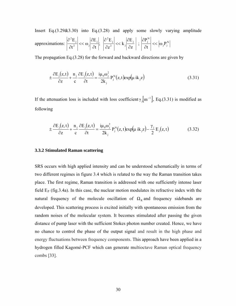
Insert Eq.(3.29&3.30) into Eq.(3.28) and apply some slowly varying amplitude

approximations: z

Ek

zE

;t

Eω

tE j

j2j

2j

j2j

2

∂

∂<<

∂

∂

∂

∂<<

∂

∂; N

jj

Nj Pωt

P <<∂

∂

The propagation Eq.(3.28) for the forward and backward directions are given by

( ) ( ) ( ) ( )zikexptz,P2kωiμ

ttz,Ε

cn

ztz,Ε

jNj

j

2j0jjj μ=

∂

∂+

∂

∂± (3.31)

If the attenuation loss is included with loss coefficient [ ]1j mγ − , Eq.(3.31) is modified as

following

( ) ( ) ( ) ( ) ( tz,Ε2γ

zikexptz,P2kωiμ

ttz,Ε

cn

ztz,Ε

jj

jNj

j

2j0jjj −=

∂

∂+

∂

∂± μ ) (3.32)

3.3.2 Stimulated Raman scattering

SRS occurs with high applied intensity and can be understood schematically in terms of

two different regimes in figure 3.4 which is related to the way the Raman transition takes

place. The first regime, Raman transition is addressed with one sufficiently intense laser

field EP (fig.3.4a). In this case, the nuclear motion modulates its refractive index with the

natural frequency of the molecule oscillation of and frequency sidebands are

developed. This scattering process is excited initially with spontaneous emission from the

random noises of the molecular system. It becomes stimulated after passing the given

distance of pump laser with the sufficient Stokes photon number created. Hence, we have

no chance to control the phase of the output signal and result in the high phase and

energy fluctuations between frequency components. This approach have been applied in a

hydrogen filled Kagomé-PCF which can generate multioctave Raman optical frequency

combs [

RΩ

33].

30

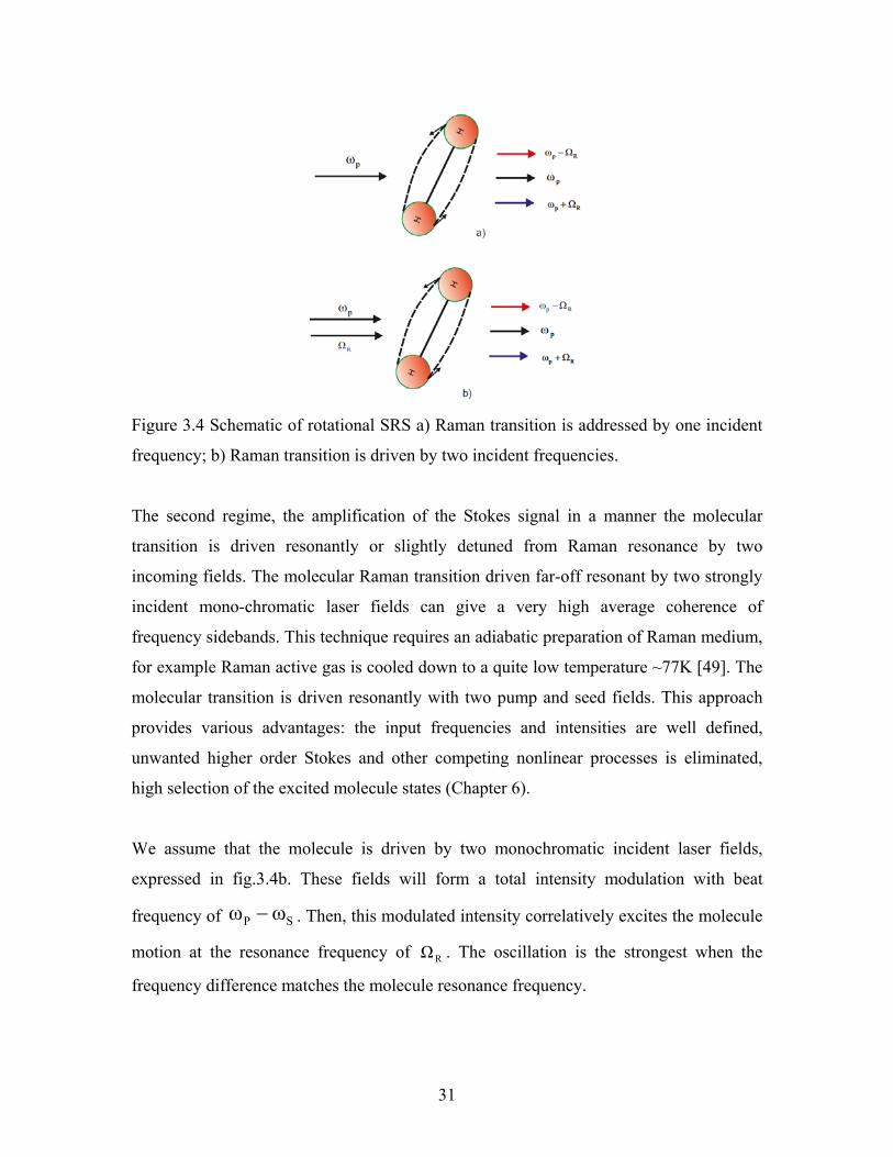
Figure 3.4 Schematic of rotational SRS a) Raman transition is addressed by one incident

frequency; b) Raman transition is driven by two incident frequencies.

The second regime, the amplification of the Stokes signal in a manner the molecular

transition is driven resonantly or slightly detuned from Raman resonance by two

incoming fields. The molecular Raman transition driven far-off resonant by two strongly

incident mono-chromatic laser fields can give a very high average coherence of

frequency sidebands. This technique requires an adiabatic preparation of Raman medium,

for example Raman active gas is cooled down to a quite low temperature ~77K [49]. The

molecular transition is driven resonantly with two pump and seed fields. This approach

provides various advantages: the input frequencies and intensities are well defined,

unwanted higher order Stokes and other competing nonlinear processes is eliminated,

high selection of the excited molecule states (Chapter 6).

We assume that the molecule is driven by two monochromatic incident laser fields,

expressed in fig.3.4b. These fields will form a total intensity modulation with beat

frequency of . Then, this modulated intensity correlatively excites the molecule

motion at the resonance frequency of . The oscillation is the strongest when the

frequency difference matches the molecule resonance frequency.

SP ωω −

RΩ

31

3.3.3 SRS in the language of optical phonons

Whereas spontaneous Raman scattering occurs with small number of scattered Stokes

photons and uncorrelated phases Φ of the individual oscillations (excitations), the SRS

has larger number of scattered Stokes photons in the scattered fields and the phases Φ of

the individual excitations are correlated. This collective excitation of the Raman active

medium can be considered as a coherent material excitation wave and material excitation

is called an optical phonon [2]. Optical phonons are analogous with photons and they

describe a special type of motion at the same angular frequency Ω as in the quantum

mechanical description. Each optical phonon has energy of Ωη as excited quanta of the

oscillation mode. The coherent wave of material excitation has no dispersion and an exact

analogy of the classical wave with the determined wavevector K (or wavelength) [50].

Hence, the optical phonon field of in Eq.(3.4) can be rewritten with by q~ KzΦ =

( ) ( )[ ]( c.cΩt-KziexptQ21t)(z,q~ += ) (3.33)

Where, Q(t) is the time dependent complex envelope functions of the optical phonon

amplitude. Like photons, optical phonons can be destroyed in collisions. The molecular

coherent decay is characterized by the rate 2Γ which is the inverse of the relaxation time

of the molecular coherence (duration for the coherence to relax to its

equilibrium). The collisions are mainly between molecules. The collisions with their

container wall may affect to the mutual correlation of excitations in the low pressure

gases filled micro-containers as HC-PCF [

-122 ΓT =

51]. In addition, the population decay from the

excited levels to the ground state also contributes slightly to the reduction of molecular

coherence (see 3.3.6 for more detail). Experimentally, we can obtain the coherent decay

rate by measuring the full width at half maximum of the Raman gain profile (FWHM). In

the next part, by using the language of optical phonons for the coherent material

excitation, we will express the full picture of SRS in the diagram of phase matching.

32

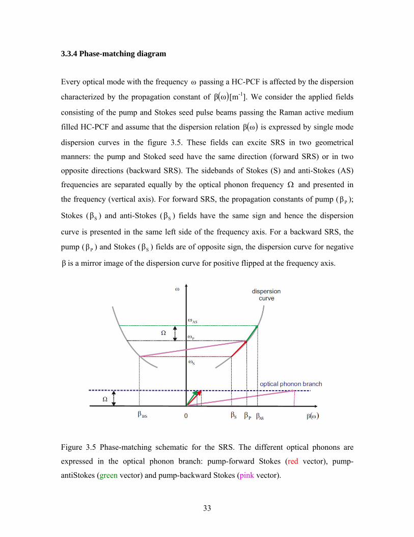
3.3.4 Phase-matching diagram

Every optical mode with the frequency passing a HC-PCF is affected by the dispersion

characterized by the propagation constant of

ω

( )ωβ [m-1]. We consider the applied fields

consisting of the pump and Stokes seed pulse beams passing the Raman active medium

filled HC-PCF and assume that the dispersion relation ( )ωβ is expressed by single mode

dispersion curves in the figure 3.5. These fields can excite SRS in two geometrical

manners: the pump and Stoked seed have the same direction (forward SRS) or in two

opposite directions (backward SRS). The sidebands of Stokes (S) and anti-Stokes (AS)

frequencies are separated equally by the optical phonon frequency Ω and presented in

the frequency (vertical axis). For forward SRS, the propagation constants of pump ( );

Stokes ( ) and anti-Stokes ( ) fields have the same sign and hence the dispersion

curve is presented in the same left side of the frequency axis. For a backward SRS, the

pump ( ) and Stokes ( ) fields are of opposite sign, the dispersion curve for negative

is a mirror image of the dispersion curve for positive flipped at the frequency axis.

Pβ

Sβ Sβ

Pβ Sβ

β

Figure 3.5 Phase-matching schematic for the SRS. The different optical phonons are

expressed in the optical phonon branch: pump-forward Stokes (red vector), pump-

antiStokes (green vector) and pump-backward Stokes (pink vector).

33

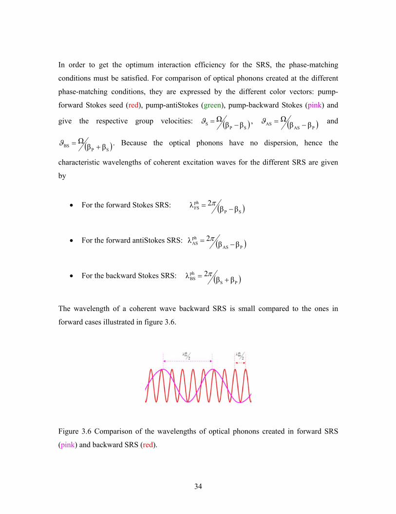
In order to get the optimum interaction efficiency for the SRS, the phase-matching

conditions must be satisfied. For comparison of optical phonons created at the different

phase-matching conditions, they are expressed by the different color vectors: pump-

forward Stokes seed (red), pump-antiStokes (green), pump-backward Stokes (pink) and

give the respective group velocities: ( )SPS ββ

Ω−=ϑ , ( )PAS

AS ββΩ

−=ϑ and

( )SPBS ββ

Ω+=ϑ . Because the optical phonons have no dispersion, hence the

characteristic wavelengths of coherent excitation waves for the different SRS are given

by

• For the forward Stokes SRS: ( )SP

phFS ββ

2λ −= π

• For the forward antiStokes SRS: ( )PAS

phAS ββ

2λ −= π

• For the backward Stokes SRS: ( )PS

phBS ββ

2λ += π

The wavelength of a coherent wave backward SRS is small compared to the ones in

forward cases illustrated in figure 3.6.

Figure 3.6 Comparison of the wavelengths of optical phonons created in forward SRS

(pink) and backward SRS (red).

34

In the next sections, we describe mathematically the coupling of a pair of applied pump

and Stokes seed fields with the coherent material excitation waves via a given Raman

active medium. The equations for the description of theses dynamical processes are

derived gradually by the classical and semi-classical approaches.

3.3.5 The classical description

In this approach, the coherent oscillation of the molecule system is approximated as a

classical harmonic oscillator and the dynamical equations for the coupled wave problem

are derived in the formalism of Lagrangian density [2]. The coupling parameter 0q

α⎟⎟⎠

⎞⎜⎜⎝

⎛∂∂ is

given by the classical Placzek model Eq.(3.2). We assume the Lagrangian densities for

the classical fields (Lrad), the oscillation field (Los) and the interaction field (Lint) in the

dilute (negligible dispersion), isotropic medium are given by

intosrad LLLL ++= (3.34)

Where ⎟⎟⎠

⎞⎜⎜⎝

⎛−= 2

0

20rad B~

μ1E~ε

21L (3.35)

( 2220os q~Ωq~Nm

21L −= & ) (3.36)

E~.E~q~qα

2NεE~.E~

2εNαE~.E~

2NεL

0

0000int ⎟⎟

⎠

⎞⎜⎜⎝

⎛∂∂

+== α (3.37)

Where and are the electric and magnetic field vectors, N is the number density of

molecules, denotes the reduced nuclear mass.

E~ B~

0m

Inserting Eq.(3.35-3.37) in the motion equation of Lagrangian density given by

35

0q~d

dLq~d

dLdtd

=−⎟⎟⎠

⎞⎜⎜⎝

⎛&

We receive

E~.E~qα

2mεq~Ω

dtq~dΓ2

dtq~d

00

022

2

⎟⎟⎠

⎞⎜⎜⎝

⎛∂∂

=++ (3.38)

Where denotes the phenomenologically added damping constant. Eq.(3.38) is

rewritten to

Γ

( ) ( ) ( )0

22

2

mt)(z,F~tz,q~Ω

dttz,q~dΓ2

dttz,q~d

=++ (3.39)

Where ( ) E~.E~qα

2εtF~

0

0⎟⎟⎠

⎞⎜⎜⎝

⎛∂∂

= plays the role of the applied force exerting on the oscillator

with the eigenfrequency of .Assume the applied field consists of two pump Ω E~ PE~ and

Stokes seed SE~ components. The total field can be written as

( ) ( )[ ] ( ) ( )[ ]( )c.cetz,Eetz,E21E~E~E~ tω-zki

Stω-zki

PSLSSPP ++=+= ± (3.40)

According to Eq.(3.39) only the time varying part of the stimulated force. The signs “± ”

represent the forward (+) and backward (-) SRS. below contributes dominantly to

the resonant process.

(t)F~

[ ]( c.ceEEqαε(t)F~ )tω(ω)zk(ki*

SP0

0SPSP +⎟⎟

⎠

⎞⎜⎜⎝

⎛∂∂

= −−μ ) (3.41)

36

Where the signs “μ ” represent the forward (-) and backward (+) SRS, the beat frequency

is the stimulating frequency. The exchange efficiency becomes optimum

when the stimulated frequency is equal to the resonant frequency Ω .

SPbeat ωωω −=

beatω

We substitute Eq.(3.33&3.41) into Eq.(3.39) and use the slowly varying amplitude

approximation q~Ωdt

q~d2

2

<< and Ω<<Γ . We obtain the temporal evolution equation for

the coherent envelop Q.

*SP

00

0 EEqα

2miεΓQ

dtdQ

⎟⎟⎠

⎞⎜⎜⎝

⎛∂∂

Ω=+ (3.42)

Here, ( )[ ]( )c.cΩt-Kzi-expq~21t)Q(z, +=

Next, we will consider the temporal-spatial evolution of the applied amplitudes by using

the propagation equations (3.32) for two incoming fields (j=P,S).

From Eq.(3.2&3.3) we can write the macroscopic polarization for the Raman active

medium consisting two components linear (L) and nonlinear (N) parts by

( ) ( ) ( ) ( ) ( )tz,E~tq~qαNεtz,E~Nεαtμ~NtΡ~

0000 ⎟⎟

⎠

⎞⎜⎜⎝

⎛∂∂

+== (3.43)

NL P~P~ += (3.44)

We substitute Eq.(3.33 & 3.40) into Eq.(3.43) and receive the nonlinear polarization for

the forward (+) and backward (-) travel of the field pumps.

( ) ( )tz,E~tq~qαNεP~

00

N⎟⎟⎠

⎞⎜⎜⎝

⎛∂∂

= (3.45)

37

[ ]( ) ( )[ ] ( )[ ]( )c.ceEeEc.cQeqα

4Nε tω-zki

Stω-zki

Ptzi

0

0 SSPP +++⎟⎟⎠

⎞⎜⎜⎝

⎛∂∂

= ±Ω−Κ (3.46)

( )[ ] ( )[ ]

⎭⎬⎫

⎩⎨⎧ ++⎟⎟

⎠

⎞⎜⎜⎝

⎛∂∂

= ± c.ceQE21eEQ

21

qαNε

21 tω-zki

Stω-zki

P*

00

PPSS (3.47)

NP

NS P~P~ +=

Where Ω=− SP ωω

We used the relation with the sign (-) for the forward SRS and the sign (+)

for backward case. We also assumed the nonlinear polarization does not contain the

frequency components (2

Κ=SP kk μ

Ω−Sωnd Stokes) and Ω+Pω (anti-Stokes). The parts of

Eq.(3.47) oscillating at the Stokes & pump frequencies are

( )[ ]⎟⎟⎠

⎞⎜⎜⎝

⎛+⎟⎟

⎠

⎞⎜⎜⎝

⎛∂∂

= ± c.ceEQqαNε

41P~ tω-zki

P*

00

NS

SS (3.48)

( )[ ]⎟⎟⎠

⎞⎜⎜⎝

⎛+⎟⎟

⎠

⎞⎜⎜⎝

⎛∂∂

= c.ceQEqαNε

41P~ tω-zki

S0

0NP

PP (3.49)

Comparing Eq.(3.30) with Eq.(3.48 & 4.49) we have the complex amplitudes

( ) (3.50) zkiP

*

0

0NS

SeEQqα

2NεP ±

⎟⎟⎠

⎞⎜⎜⎝

⎛∂∂

=

( zkiS

0

0NP

PeQEqα

2NεP~ ⎟⎟

⎠

⎞⎜⎜⎝

⎛∂∂

= ) (3.51)

Inserting Eq.(3.40,3.50&3.51) into Eq.(3.32) we obtain

38

For the pump field

PP

S0P

2P00PPP Ε

2γQE

qα

4kωεiNμ

tΕ

cn

zΕ

−⎟⎟⎠

⎞⎜⎜⎝

⎛∂∂

=∂∂

+∂∂ (3.52)

For the Stokes field

SS

P*

0S

2S00SSS Ε

2γEQ

qα

4kωεiNμ

tΕ

cn

zΕ

−⎟⎟⎠

⎞⎜⎜⎝

⎛∂∂

=∂∂

+∂∂

± (3.53)

Where nP,S are the pump and Stokes refractive index, kP,S are the pump and Stokes

wavevectors, are the loss coefficient of pump and Stokes respectively the set of

coupled-wave equations for SRS are Eq.(3.42,3.52&3.53).

SL γ&γ

PP

S0P

PPPP Ε2γQE

qα

c4niNω

tΕ

cn

zΕ

−⎟⎟⎠

⎞⎜⎜⎝

⎛∂∂

=∂∂

+∂∂ (3.54)

SS

P*

0S

SSSS Ε2γEQ

qα

c4niNω

tΕ

cn

zΕ

−⎟⎟⎠

⎞⎜⎜⎝

⎛∂∂

=∂∂

+∂∂

± (3.55)

*SP

00

0 EEqα

2miεΓQ

tQ

⎟⎟⎠

⎞⎜⎜⎝

⎛∂∂

Ω=+

∂∂ (3.56)

The classically harmonic model gives a qualitative description of the coherent Raman

state. However, it does not provide the quantized nature of optical phonons and hence the

lack of the contribution of the population occupation in the coupled-wave equations.

39

3.3.6 The semi-classical description

In this model the molecules are treated quantum mechanically using the density operator

formalism which has the ability of including the quantum mechanic characteristics of the

molecules. This section is adapted from [1,53].

3.3.6.1 Density matrix formalism

We review this formalism from the basic laws of quantum mechanics. According to

quantum mechanics, we can describe all the physical properties of a quantum system

(such as a molecule) in terms of a wave function ( )tr,Ψs of a known particular state s and

which obeys the Schrodinger equation [1].

( ) ( )tr,ΨHt

tr,Ψi ss

=∂

∂η (3.57)

VHH 0 += (3.58)

Where, is the Hamiltonian operator of the system consisting for a free operator

and interaction operator of . In order to determine how the wave function evolve in

time, it is often represented in the superposition of the eigenstates of the

Hamiltonian operator of .

H 0H

V

( )ru n

0H

( ) (r(t)uCtr,Ψ nn

ns ∑= ) (3.59)

Where are assumed to be orthonormal by the relation ( )ru n

( ) ( ) ( ) ( ) ⎢⎣

⎡≠=

=== ∫ mn 0mn 1

δdrrurururu mn3

n*mnm (3.60)

40

Where is the probability amplitude of the eigenstate of n. The expectation value of

any operator can be calculated by

( )tCn

A

( ) ( )tr,ΨAtr,ΨA ss= (3.61)

The angular brackets denote a quantum-mechanical average, the wave functions are

written in Dirac notation. The matrix element Amn of the operator is given by A

( ) ( )ruAruA nmmn = (3.62)

If the Hamiltonian operator and the initial state of the quantum system are known, the

time evolution of quantum system and its observable properties are described completely.

However, there are situations under which the state of system is not known precisely, for

example a collection of gas molecules where molecules can interact with each other by

means of collisions. Each collision, the wave function is modified. If the collision is

sufficiently weak, the modification may only relate to the change of the total phase of the

wave function. Therefore, the calculation for keeping track of the phase of each molecule

is impossible and the state of each molecule is unknown. Under such situations, the

density matrix formalism is adequate to present the system in a statistical manner. The

density matrix operator is defined by the relation

H

( ) ( )∑=s

sss tr,Ψtr,Ψpρ (3.63)

Where the index s runs over all of the possible states of the system, the quantity p(s) is

nonnegative and understood as a classical probability of that system which reflects the

lack of our knowledge about the actual quantum state. We can write p(s) under the

normalized fashion

41

(3.64) 1ps

s =∑

It is useful to determine the elements of the density matrix. Multiplying two sides of

Eq.(3.63) with ( )ru n and ( ) ru n , then we get the elements of the density matrix by

using Eq.(3.59&3.60).

sn

s

s*msmn CCpρ ∑= (3.65)

The indices of m,n run over all the energy eigenstates of the system and . The

elements of the density matrix have the following physical meanings:

*nmmn ρρ =

• The diagonal elements nnρ give the probability of the molecule being in energy

eigenstate n.

• The off-diagonal elements ( )nmρmn ≠ are generally complex numbers and

contain a phase, interpreted to be the coherence between levels m and n. It is only

nonzero when the coherent superposition of energy eigenstates m, n occurs and

proportional to the induced electric dipole moment of the molecule of ( )tμ .

In the case of the exact state of system is unknown, the expectation value of any

observable quantity A is given by the trace of the product matrix ( )Aρ

( ) ( )AρTrAρAn

nn ≡=∑ (3.66)

The evolution of the density matrix under the action of Hamiltonian operator in

Eq.(3.58) is given by

ρ H

[ ] nmnmnmnm ρH,ρitρ

Γ−=∂

∂η

(3.67)

42

Where, the damping terms are added phenomenologically. We also assumed that the

molecular coherence is zero in the thermal equilibrium state. We rewrite Eq.(3.67)

nmΓ

[ ] nmnmnmnmnmnm ρV,ρiρiωtρ

Γ−+=∂

∂η

(3.68)

We can rewrite Eq.(3.68) being more specific

( ) mn ρΓE~ρμμρiρiωtρ

nmnmν

νmνnmννnnmnmnm ≠−−+=∂

∂ ∑η (3.69)

( ) mn ρΓE~ρμμρitρ

nnnnν

νmνnmννnnn =−−=

∂∂ ∑η (3.70)

Here, we used the matrix representation : 0H nmnnm0, δEH = and η

mnnm

EEω −= denotes

the transition frequency between the energy eigenstates. Here for the off-

diagonal elements of density matrix is the damping rate for the coherence and

provides the decay rate of population. We also assumed that the energy interaction

operator is defined adequately by the electric dipole approximation

nmΓ

nnΓ

E~.μ-V = . Where

mnμnμm = and denotes the matrix elements of the dipole moment. Here we

used the electric dipole moment

*mnmn μμ =

( )tμ rather than the molecular polarizability ( )tα~ in

previous description.

3.3.6.2 Schematic of energy levels

We consider a collection of identical molecules. Each molecule begins in its ground state

1 may absorb a pump laser photon (red arrow) at the frequency and scatter a Stokes

photon (green arrow) with the frequency

Pω

21P ωω − which is near or equal the Stoke

43

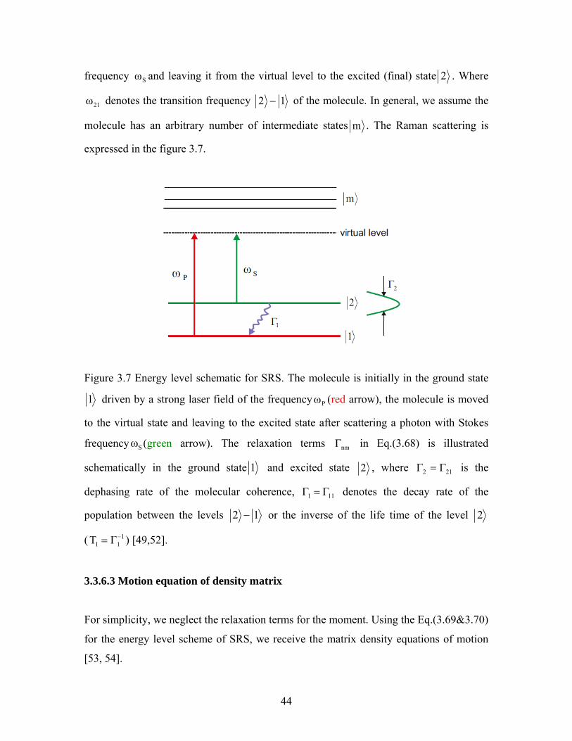
frequency and leaving it from the virtual level to the excited (final) stateSω 2 . Where

denotes the transition frequency 21ω 12 − of the molecule. In general, we assume the

molecule has an arbitrary number of intermediate states m . The Raman scattering is

expressed in the figure 3.7.

Figure 3.7 Energy level schematic for SRS. The molecule is initially in the ground state

1 driven by a strong laser field of the frequency (red arrow), the molecule is moved

to the virtual state and leaving to the excited state after scattering a photon with Stokes

frequency (green arrow). The relaxation terms

Pω

Sω nmΓ in Eq.(3.68) is illustrated

schematically in the ground state 1 and excited state 2 , where is the

dephasing rate of the molecular coherence,

212 Γ=Γ

111 Γ=Γ denotes the decay rate of the

population between the levels 12 − or the inverse of the life time of the level 2

( ) [111 ΓT −= 49,52].

3.3.6.3 Motion equation of density matrix

For simplicity, we neglect the relaxation terms for the moment. Using the Eq.(3.69&3.70)

for the energy level scheme of SRS, we receive the matrix density equations of motion

[53, 54].

44

( E~ρμμρiρ iωtρ

m2m1mm2m12112

21 ∑ −−=∂∂

η) (3.71)

( E~ρμμρitρ

m2mm2

*m2

*2m

22 ∑ −=∂∂

η) (3.72)

( E~ρμμρitρ

mm1m1

*m1

*m1

11 ∑ −=∂∂

η) (3.73)

( ) E~ρμiE~ρρμiiωtρ

212m11mm1mm1m1

ηη−−+=

∂∂ (3.74)

( ) E~ρμiE~ρρμiiωtρ

21m1mm22m22m2m

ηη+−−=

∂∂ (3.75)

We have assumed that the states 1 and 2 have a definite parity so that the diagonal

matrix elements of μ vanish (ˆ 0μμ 2211 == ). The excitation of the intermediate states

m is negligible. The total applied field SP E~E~E~ += , the index m runs over all of

possible intermediate states.

Integrating in time on both sides of Eq.(3.74&3.75) gives us

( ) ( ) ( )( ) ( ) ( ) ( )[ ] ( )ttiω212m11mm1m

t

0

tiωm1m1

m1m1 etE~tρμtE~tρtρμdtie0ρρ ′−′′−′′−′+= ∫η (3.76)

( ) ( ) ( )( ) ( ) ( ) ( )[ ] ( ) (3.77) ttiω21m1mm22m2

t

0

tiω2m2m

2m2m etE~tρμtE~tρtρμdtie0ρρ ′−′′−′′−′−= ∫η

Inserting Eq.(3.76&3.77) into Eq.(3.71), we have

45

+=∂∂

211221 ρ iωtρ

( ) ( )( ) ( ) ( ) ( ) ( ) ( ) ( )∑ ∫ ′−

⎥⎥⎦

⎤

⎢⎢⎣

⎡′′−′′−′′+

m

ttiω

**

212

m2

*

11mm1mm2

t

02

m1etρtE~tE~μtE~tE~tρtρμμtd1444 3444 21444444 3444444 21η

( ) ( )( ) ( ) ( ) ( ) ( ) ( ) ( )∑ ∫ ′−

⎥⎥⎦

⎤

⎢⎢⎣

⎡′′+′′−′′+

m

ttiω

**

212

1m

*

mm221mm2

t

02

2metρtE~tE~μtE~tE~tρtρμμtd1444 3444 21444444 3444444 21η

(3.78)

It is useful to express E and as below ~21ρ

( ) ( ) ( ) ( ) ( )( c.cetEetE21tE~tE~tE~ tiω

Stiω

PSPSP ++=+= −− ) 3.79a)

( ) ( ) ( ) ( ) ( )( c.cetEetE21tE~tE~tE~ tiω

Stiω

PSPSP +′+′=′+′=′ ′−′− ) (3.79b)

( ) ( )( c.cet21tρ tiω

2121 +′ℜ=′ ′− ) (3.79c)

Substituting Eq.(3.79) into Eq.(3.78) and assuming the exact Raman resonance occurs at

, then only those terms in Eq.(3.78) oscillating near the frequency are

kept. It is also noted that only two of 16 terms in (*) arising from

21PS ωωω −= 21ω

( ) ( )tE~tE~ ′ contribute to

the beat frequency 21PS ωωω =−

( ) ( ) ( ) ( ) tiω*S

t-iωP

tiω*S

t-iωP

SPSP etEetEetEetE ′′ ′+′

The same as in (**) only two components are retained

46

( ) ( ) ( ) ( ) tiω*S

t-iωS

tiω*P

t-iωP

SSPP etEetEetEetE ′′ ′+′

Then integrating in t´ and eliminating the frequency components containing the index m,

we have

+≈∂∂

211221 ρ iωtρ

( ) ( )( ) ( ) ( ) ( ) ( ) tiω-2tω-ωi*SP11mm

*1

21SP et8χietEtEtρtρiκ

41

ℜ−−+ −

( ) ( )( ) ( ) ( ) ( ) ( ) tiω-1tω-ωi*SPmm22

*1

21SP et8χietEtEtρtρiκ

41

ℜ+−+ − (3.80)

( ) ( )( ) ( ) ( ) ( ) ( ) ( ) tiω21tω-ωi*SP1122

*12112

21SP et8χχietEtEtρtρiκ

41ρ iω −− ℜ

−+−+= (3.81)

Where ωωω 21SP =−

∑ ⎟⎟⎠

⎞⎜⎜⎝

⎛+

+−

=m Sm1Pm1

1mm221 ωω1

ωω1μμ1κ

η

∑ ⎥⎦

⎤⎢⎣

⎡⎟⎟⎠

⎞⎜⎜⎝

⎛+

+−

+⎟⎟⎠

⎞⎜⎜⎝

⎛+

+−

=m Sm1Sm1

2S

Pm1Pm1

2P

21m21 ωω

1ωω

1Eωω

1ωω

1Eμ1χη

∑ ⎥⎦

⎤⎢⎣

⎡⎟⎟⎠

⎞⎜⎜⎝

⎛+

+−

+⎟⎟⎠

⎞⎜⎜⎝

⎛+

+−

=m Sm2Sm2

2S

Pm2Pm2

2P

22m22 ωω

1ωω

1Eωω

1ωω

1Eμ1χη

We rewrite Eq.(3.81)

47

( ) tiωtiω*SP1122

*12112

21 2121 e8ΔieEEρρiκ

41ρ iω

tρ −− ℜ+−+=∂∂ (3.81)

Where the Stark shift is expressed by 21 χχ −=Δ

Subtracting Eq.(3.72) from Eq.(3.73)

( ) ( )E~ρμρμμρμρitρρ

m2mm2m1m1

*m1

*m1

*m2

*2m

1122 ∑ −+−=∂−∂

η (3.82)

Replacing Eq.(3.76&3.77) into Eq.(3.82) and do some calculation similar to , we have 21ρ

( ) **SP

*1S

*P1

1122 EEiκ21EEiκ

21

tρρ

ℜ−ℜ=∂−∂ (3.83)

The population difference between the ground level 1 and excited level 2 to be

and write Eq.(3.81&3.83) under the slowly varying amplitude

functions.

( ) ( ) ( )tρtρtn 1122 −=

*SP

*1 EnEiκ

21

4Δi

t+ℜ=

∂∂ℜ (3.84)

**SP

*1S

*P1 EEiκ

21EEiκ

21

tn

ℜ−ℜ=∂∂ (3.85)

Where ( ) ( ) ( )( )c.cet21tρ ΩtKzi

21 +ℜ= −

21ω=Ω ; SP kkK −=

The equations (3.84&3.85) provide an adequate description of the resonant Raman

process where relaxation processes can be neglected, such as pump pulse duration is

much shorter than the relaxation time of material T

Pτ

2. They will be modified in the

48

presence of relaxation processes by adding the decay rate of the molecular coherence

formed and the decay rate of occupation photon numbers from the 2 level to 1

level respectively. We also assume the population difference

2Γ 1Γ

( ) 0ntn = in thermal

equilibrium [1].

( 01**

SP*1S

*P1 nnΓEEiκ

21EEiκ

21 )

tn

−−ℜ−ℜ=∂∂ (3.86)

ℜ−+ℜ=∂∂ℜ

2*SP

*1 ΓEnEiκ

21

4Δi

t (3.87)

In order to consider the meaning of the decay constants, we will examine the nature of

the solutions to these equations in the absence of applied fields [1].

From the Eq.(3.86), the solution for population difference n with E=0

[ ]t

T1

001en-n(0)nn(t)

−

+= (3.88)

Where -111 ΓT =

The Eq.(3.88) shows that the population inversion n relaxes from its initial value n(0) to

its thermal equilibrium value n0 in a time of the order of T1. Hence, T1 is called the

population relaxation time.

From the Eq.(3.87), the solution for coherence ℜ with E=0

[ ] tT1

tiω2121

tT1iω

221221

e(0)eρ(t)ρor (0)e(t)⎟⎟⎠

⎞⎜⎜⎝

⎛−

−⎟⎟⎠

⎞⎜⎜⎝

⎛+−

=ℜ=ℜ (3.89)

Where and assume -122 ΓT = 0=Δ

The solution (3.89) shows the coherence oscillates at the molecular transition frequency

and decays to zero in the characteristic time T21ω=Ω 2. It also can be explained more

49

directly by considering the expectation of the induced dipole moment oscillates near

the resonance frequency for E=0. Using Eq.(3.76, 3.77&3.89), we have the trace with the

density operator.

( )tμ

( ) ( ) [ ] tT1

tiω2121

m2m2mm1m1

221 ec.ce(t)(0)ρμρμρμtμ⎟⎟⎠

⎞⎜⎜⎝

⎛−

− +=+= ∑ (3.90)

This result shows that the induced dipole moment also oscillates at the frequency

and decays in a time of the order T21ω=Ω 2 as the coherence. So, it has the meaning of

the dipole dephasing time.

Using formula (3.66), the macroscopic polarization is calculated for wave propagation

equation (3.32)

( c.cρμρμN)μρNTr(Pm

2m2mm1m1N ++== ∑ ) (3.91)

Inserting Eq.(3.76&3.77) into Eq.(3.91) and only keep the terms oscillating near the

resonance frequency 21ω

( )[ ] ( )[ ] ⎟⎠⎞

⎜⎝⎛ +ℜ+ℜ= ± c.ceE

21eE

21

2NκP tω-zki

Stω-zki*

P

*1N PPSS

η (3.92)

The complex amplitude functions

( )zki*P

*1N

SSeE

2NκP ±ℜ=η (3.93a)

( )zkiS

*1N

PPeE

2NκP ℜ=η (3.93b)

Substituting Eq.(3.93) into Eq.(3.32)

50

For a pump field

PP

SS

P2

P

P

P Ε2γE

vvκ

tΕ

v1

zΕ

−ℜ⎟⎟⎠

⎞⎜⎜⎝

⎛=

∂∂

+∂∂

S

Piωω (3.94a)

For a Stokes field

SS

P*

2S

S

S Ε2γEκ

tΕ

v1

zΕ

−ℜ=∂∂

+∂∂

± i (3.94b)

Where, S

*1S0

2 4nκωcNμκ η

= and SP,

SP, ncv = denotes group velocities

The Eq.(3.86,3.87&3.94) describes detail the temporal-spatial evolution and the

interaction between the applied fields and the coherent excitation of material under the

quantum nature. Let us consider the connection the quantum mechanic model and the

classical mechanic model by the relation of the oscillated amplitude q and the molecular

coherence [( )tρ22 53].

The expectation value of the harmonically oscillated operator ( )tq is given by a trace

with the density operator ( )tρ

∑=nm

mnnmqρq (3.95)

In the case of classical harmonic oscillator, it corresponds to the ground 1 and the

excited 2 energy levels in quantum mechanic. Hence, the indexes m,n only get values 1

and 2.

( ) ( )12212112122121nm

mnnm ρρqqρqρqρq +=+== ∑ (3.96)

We let ,...2,1,0=ν are the oscillated quantum numbers. According to the quantum

harmonic oscillator [54], the elements of oscillated operator are given by.

51

( )⎟⎟⎠

⎞⎜⎛

+=η

⎜⎝

+ 1νω2m

q210

ν1,ν (3.97a)

Where 1,0=ν corresponds to the 1 and 2 levels in Eq.(3.7a). Hence Eq.(3.97a)

become s

( ) c.cρ2m

ρρqq 210

122121 +Ω

=+=η (3.97b)

Where

Comparison Eq.(3.54-3.56) with Eq.(3.86,3.87&3.94) and using the revised relation

we hav some conclusions:

ter,

21ω=Ω

(3.97a), e

*1

21

0Ω2mα ⎞⎛⎞⎛ ∂• The Raman coupling parame 2

00

κεq ⎟⎟

⎠⎜⎜⎝

=⎟⎟⎠

⎜⎜⎝ ∂

.

en the Stark shift, population inversion

effects are negligible

• Classical model is relatively adequate wh

( )0n0,Δ == .

ficie• The Raman gain coef nt, 2

2P21 Eκκ2

g =Γ

(3.98)

teristic of the created Stokes fields in SRS strongly

epends on the dephasing rate of coherenc

3.3.6.4 Transient regime in SRS

The temporal and spectral charac

d e 2Γ , the effective interaction length z, the

m

Raman gain g given in Eq.(3.98) as well as the pump duration Pτ . Hence, it is convenient

to determine the scattering regime of the syste by comparing the pump pulse duration

Pτ with the characteristic times 1τ & 2τ defined in Eq(3.99). This section is mainly

derived from [30, 52].

Γgz1τ = &

Γgτ =

z2 (3.99) 1

52

Spontaneous Raman scattering: The pump pulse duration is smaller than the

haracteristic time ). It is too short to provide a coherent emission from the

Stokes intensity

c 1τ ( 1P ττ <

generated Stokes photons.

( ) gz2SΓτz,I ≈ , where c

z-tτ = is the local time. The Stokes

the pulse pump duration

Steady state regime: The pump pulse duration is longer than the characteristic

ti between the

amplification is very low and independent from Pτ .

time 2τ ( 2P ττ > ). This regime causes the loss of the mutual phase correla on

Stokes and the initial pump fields by the effect of the collisional dephasing rate 2Γ .

Stokes intensity ( )πgz2

Γeτz,Igz

S ≈ , the Stokes intensity is also independent on romf the

tion as the

higher.

nt regime

uration lies in the range of the characteristic times, . In

hich the pulse pump duration is short enough that the dephasing rate of coherence

pulse pump dura spontaneous one, but the Raman amplification is much

Transie

Pτ

The pulse pump d 2P1 τττ <<

w 2Γ

has minimum effect during the generation time of the Stokes pulse but enough long that

the number of pump photons is sufficiently large to trigger a SRS process. The transient

regime is mostly interested by the Stokes field generated can retains the high molecular

coherence with the initial pump field which is important in coherent generation of

cascaded Raman scattering for ultrashort compression in a gas-filled capillary [55,56].

From Eq.(3.99), it is clear that the required range of pump duration for the transient

regime depend strongly on the net Raman gain gz. The higher net Raman gain, the wider

the range of pump pulse width and vice versa.

The evolution of Stokes intensity

53

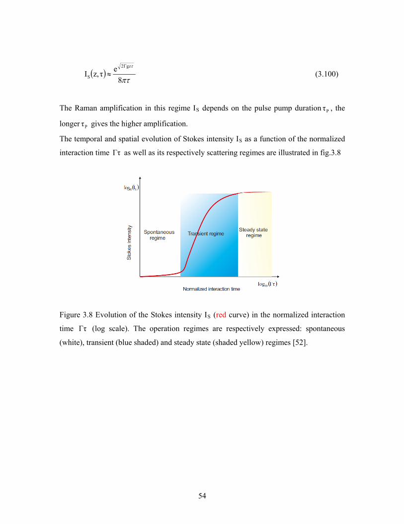
( )πτ

τ

8eτz,I

gz2

S

Γ

≈ (3.100)

The Raman amplification in this regime IS depends on the pulse pump duration , the

longer gives the higher amplification.

Pτ

Pτ

The temporal and spatial evolution of Stokes intensity IS as a function of the normalized

interaction time as well as its respectively scattering regimes are illustrated in fig.3.8 Γτ

Figure 3.8 Evolution of the Stokes intensity IS (red curve) in the normalized interaction

time (log scale). The operation regimes are respectively expressed: spontaneous

(white), transient (blue shaded) and steady state (shaded yellow) regimes [52].

Γτ

54

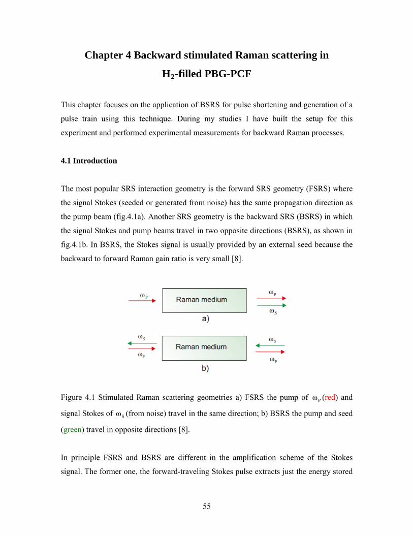
Chapter 4 Backward stimulated Raman scattering in

H2-filled PBG-PCF

This chapter focuses on the application of BSRS for pulse shortening and generation of a

pulse train using this technique. During my studies I have built the setup for this

experiment and performed experimental measurements for backward Raman processes.

4.1 Introduction

The most popular SRS interaction geometry is the forward SRS geometry (FSRS) where

the signal Stokes (seeded or generated from noise) has the same propagation direction as

the pump beam (fig.4.1a). Another SRS geometry is the backward SRS (BSRS) in which

the signal Stokes and pump beams travel in two opposite directions (BSRS), as shown in

fig.4.1b. In BSRS, the Stokes signal is usually provided by an external seed because the

backward to forward Raman gain ratio is very small [8].

Figure 4.1 Stimulated Raman scattering geometries a) FSRS the pump of (red) and

signal Stokes of (from noise) travel in the same direction; b) BSRS the pump and seed

(green) travel in opposite directions [8].

Pω

Sω

In principle FSRS and BSRS are different in the amplification scheme of the Stokes

signal. The former one, the forward-traveling Stokes pulse extracts just the energy stored

55

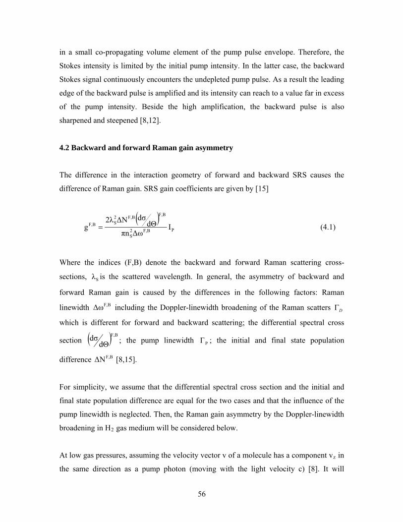
in a small co-propagating volume element of the pump pulse envelope. Therefore, the

Stokes intensity is limited by the initial pump intensity. In the latter case, the backward

Stokes signal continuously encounters the undepleted pump pulse. As a result the leading

edge of the backward pulse is amplified and its intensity can reach to a value far in excess

of the pump intensity. Beside the high amplification, the backward pulse is also

sharpened and steepened [8,12].

4.2 Backward and forward Raman gain asymmetry

The difference in the interaction geometry of forward and backward SRS causes the

difference of Raman gain. SRS gain coefficients are given by [15]

( )PBF,2

S

BF,BF,2SBF, I

ΔωπndΘ

dσΔN2λg = (4.1)

Where the indices (F,B) denote the backward and forward Raman scattering cross-

sections, is the scattered wavelength. In general, the asymmetry of backward and

forward Raman gain is caused by the differences in the following factors: Raman

linewidth including the Doppler-linewidth broadening of the Raman scatters

Sλ

BF,Δω DΓ

which is different for forward and backward scattering; the differential spectral cross

section ( ) BF,

dΘdσ ; the pump linewidth ; the initial and final state population

difference [

PΓ

BF,ΔN 8,15].

For simplicity, we assume that the differential spectral cross section and the initial and

final state population difference are equal for the two cases and that the influence of the

pump linewidth is neglected. Then, the Raman gain asymmetry by the Doppler-linewidth

broadening in H2 gas medium will be considered below.

At low gas pressures, assuming the velocity vector v of a molecule has a component vz in

the same direction as a pump photon (moving with the light velocity c) [8]. It will

56

provide a Doppler shift of cvω z

P− on the pump wave, cvω z

S− on the scattered wave in

forward direction, and the shift of cvω z

S+ on the scattered wave in backward direction.

Therefore, the net shift from Raman resonance in the forward Stokes wave of

( )cvωω z

SP −− and in the backward Stokes wave of ( )cvωω z

SP +− . Two scattering

processes are illustrated in figure 4.2. A pump photon (the blue-arrow curve) is

scattered by a hydrogen diatomic molecule (a black dumbbell), resulting in the emission

of a Stokes photon (the red-arrow curve) in the same direction as pump photon for

forward SRS (fig.4.2a) and in opposite direction with pump photon for backward SRS

(fig.4.2b).

Pω

sω

Figure 4.2 Motion diagram of Raman scattering: a) forward SRS; b) backward SRS

Using Maxwell-Boltzmann velocity distribution for the mean thermal velocity of

mT2kB , where T is the temperature in Kelvin (here we assume T= 298K) and m is the

H2 mass in the atomic units, kB is a Boltzmann constant. The Doppler line width in

forward and backward Raman scatterings are given as following [8,57]

For forward SRS

( )m

T2ln2kcωω2Γ BSPF

D−

= (4.2)

57

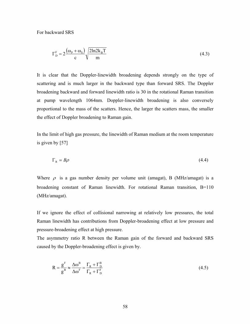
For backward SRS

( )m

T2ln2kcωω2Γ BSPF

D+

= (4.3)

It is clear that the Doppler-linewidth broadening depends strongly on the type of

scattering and is much larger in the backward type than forward SRS. The Doppler

broadening backward and forward linewidth ratio is 30 in the rotational Raman transition

at pump wavelength 1064nm. Doppler-linewidth broadening is also conversely

proportional to the mass of the scatters. Hence, the larger the scatters mass, the smaller

the effect of Doppler broadening to Raman gain.

In the limit of high gas pressure, the linewidth of Raman medium at the room temperature

is given by [57]

ρB=RΓ (4.4)

Where ρ is a gas number density per volume unit (amagat), B (MHz/amagat) is a

broadening constant of Raman linewidth. For rotational Raman transition, B=110

(MHz/amagat).

If we ignore the effect of collisional narrowing at relatively low pressures, the total

Raman linewidth has contributions from Doppler-broadening effect at low pressure and

pressure-broadening effect at high pressure.

The asymmetry ratio R between the Raman gain of the forward and backward SRS

caused by the Doppler-broadening effect is given by.

FDR

BDR

F

B

B

F

ΓΓ

ΔωΔω

ggR

+Γ+Γ

=≈= (4.5)

58

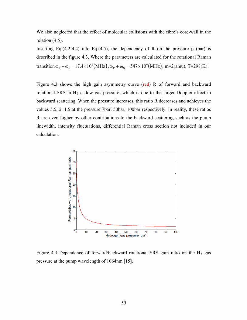
We also neglected that the effect of molecular collisions with the fibre’s core-wall in the

relation (4.5).

Inserting Eq.(4.2-4.4) into Eq.(4.5), the dependency of R on the pressure p (bar) is

described in the figure 4.3. Where the parameters are calculated for the rotational Raman

transition ,( )MHz1017.4ωω 6SP ×=− ( )MHz10547ωω 6

SP ×=+ , m=2(amu), T=298(K).

Figure 4.3 shows the high gain asymmetry curve (red) R of forward and backward

rotational SRS in H2 at low gas pressure, which is due to the larger Doppler effect in

backward scattering. When the pressure increases, this ratio R decreases and achieves the

values 5.5, 2, 1.5 at the pressure 7bar, 50bar, 100bar respectively. In reality, these ratios

R are even higher by other contributions to the backward scattering such as the pump

linewidth, intensity fluctuations, differential Raman cross section not included in our

calculation.

Figure 4.3 Dependence of forward/backward rotational SRS gain ratio on the H2 gas

pressure at the pump wavelength of 1064nm [15].

59

4.3 Motivation

The first backward Raman scattering was observed in 1966 [11]. The experimental

demonstration of 20 times amplification by backward Raman in liquid CS2 has been

performed impressively [12]. BSRS has several advantages over the forward case, which

results in its use in different applications such as high power amplification, pulse

shortening and wavefront conservation [12,58], converting poor quality pump beam to

high quality output beams [14,16,58] and high power ultraviolet excimer lasers [8].

Recently BSRS technique is emerging as a promising candidate in generating of powerful

ultra-short pulses in plasma. By pulse amplification in plasma it is possible to overcome

the limitation of the thermal damage encountered in the more traditional chirped pulse

amplification method [59,60,61].

SRS in gases offers many advantages over solids and liquids: high damage threshold, a

low linear absorption, less self-focusing. However, SRS in gaseous medium requires high

pump power for initiating stimulated Raman operation. In previous experiments done in

focused-beam geometry or capillaries, the pump power requirement is up to several MW

with a conversion efficiency of only a few percent from the initial pump energy [62,63].

The threshold is even higher for BSRS caused by the low backward Raman gain [64].

Moreover, pulse shortening becomes more difficult for light molecule such as H2 caused

by the large Doppler linewidth broadening (see Eq.(4.3)).

HC-PCF as a microcell offers an excellent guiding structure: diffraction-free long

interaction length allows light to be tightly confined during its propagation while the

flexibility in designing the position of the guidance band helps us to remove unwanted

higher order Raman components [28]. These excellent features make it become an

excellent candidate for the investigation of light interaction with gases or vapor filled into

its hollow-core. The very long interaction length of HC-PCF makes its net Raman gain

increase hugely. As a result the Raman threshold energy is quite low (six orders of

60

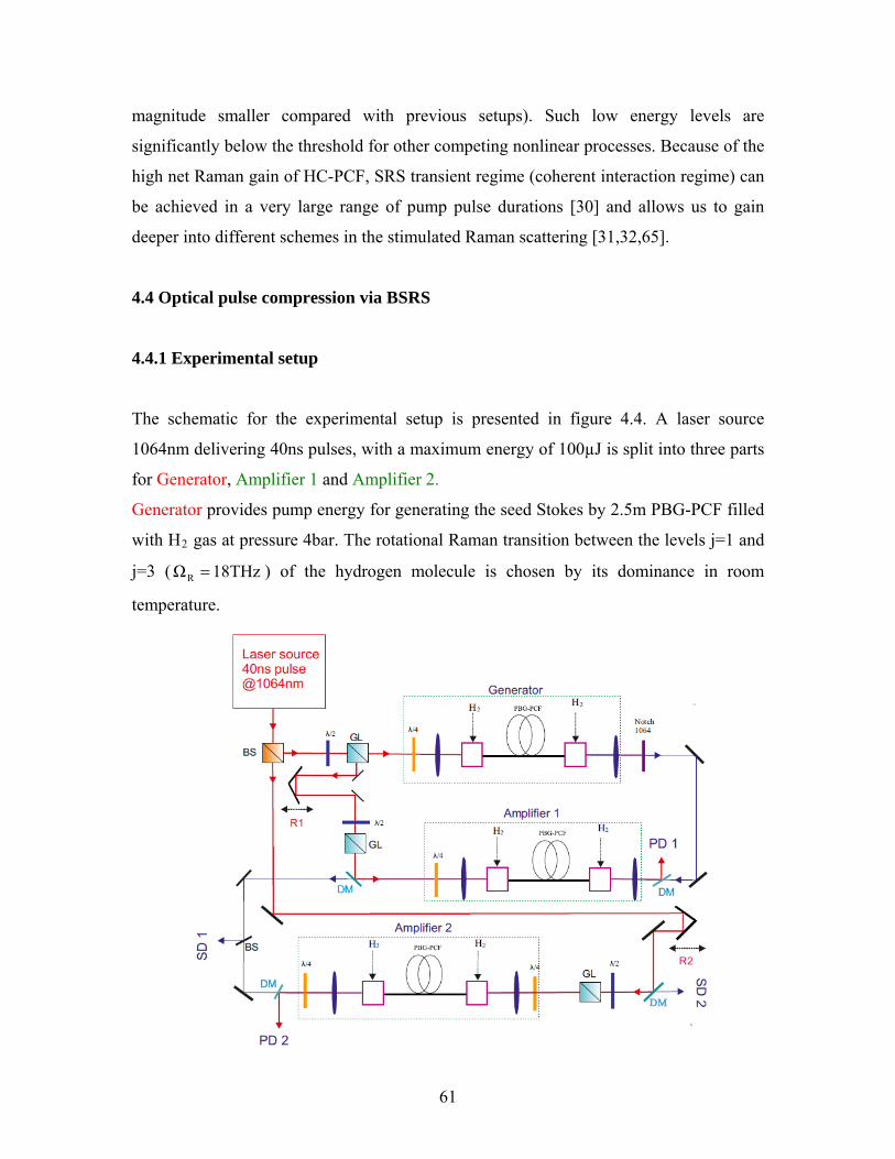
magnitude smaller compared with previous setups). Such low energy levels are

significantly below the threshold for other competing nonlinear processes. Because of the

high net Raman gain of HC-PCF, SRS transient regime (coherent interaction regime) can

be achieved in a very large range of pump pulse durations [30] and allows us to gain

deeper into different schemes in the stimulated Raman scattering [31,32,65].

4.4 Optical pulse compression via BSRS

4.4.1 Experimental setup

The schematic for the experimental setup is presented in figure 4.4. A laser source

1064nm delivering 40ns pulses, with a maximum energy of 100µJ is split into three parts

for Generator, Amplifier 1 and Amplifier 2.

Generator provides pump energy for generating the seed Stokes by 2.5m PBG-PCF filled

with H2 gas at pressure 4bar. The rotational Raman transition between the levels j=1 and

j=3 ( ) of the hydrogen molecule is chosen by its dominance in room

temperature.

18THzΩR =

61

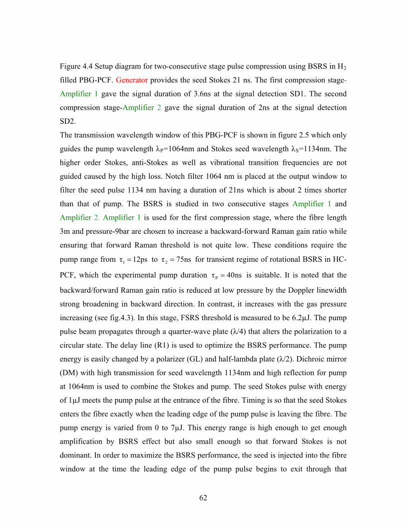
Figure 4.4 Setup diagram for two-consecutive stage pulse compression using BSRS in H2

filled PBG-PCF. Generator provides the seed Stokes 21 ns. The first compression stage-

Amplifier 1 gave the signal duration of 3.6ns at the signal detection SD1. The second

compression stage-Amplifier 2 gave the signal duration of 2ns at the signal detection

SD2.

The transmission wavelength window of this PBG-PCF is shown in figure 2.5 which only

guides the pump wavelength λP=1064nm and Stokes seed wavelength λS=1134nm. The

higher order Stokes, anti-Stokes as well as vibrational transition frequencies are not

guided caused by the high loss. Notch filter 1064 nm is placed at the output window to

filter the seed pulse 1134 nm having a duration of 21ns which is about 2 times shorter

than that of pump. The BSRS is studied in two consecutive stages Amplifier 1 and

Amplifier 2. Amplifier 1 is used for the first compression stage, where the fibre length

3m and pressure-9bar are chosen to increase a backward-forward Raman gain ratio while

ensuring that forward Raman threshold is not quite low. These conditions require the

pump range from to 12psτ1 = 75nsτ2 = for transient regime of rotational BSRS in HC-

PCF, which the experimental pump duration ns04τP = is suitable. It is noted that the

backward/forward Raman gain ratio is reduced at low pressure by the Doppler linewidth

strong broadening in backward direction. In contrast, it increases with the gas pressure

increasing (see fig.4.3). In this stage, FSRS threshold is measured to be 6.2µJ. The pump

pulse beam propagates through a quarter-wave plate (λ/4) that alters the polarization to a

circular state. The delay line (R1) is used to optimize the BSRS performance. The pump

energy is easily changed by a polarizer (GL) and half-lambda plate (λ/2). Dichroic mirror

(DM) with high transmission for seed wavelength 1134nm and high reflection for pump

at 1064nm is used to combine the Stokes and pump. The seed Stokes pulse with energy

of 1µJ meets the pump pulse at the entrance of the fibre. Timing is so that the seed Stokes

enters the fibre exactly when the leading edge of the pump pulse is leaving the fibre. The

pump energy is varied from 0 to 7µJ. This energy range is high enough to get enough

amplification by BSRS effect but also small enough so that forward Stokes is not

dominant. In order to maximize the BSRS performance, the seed is injected into the fibre

window at the time the leading edge of the pump pulse begins to exit through that

62

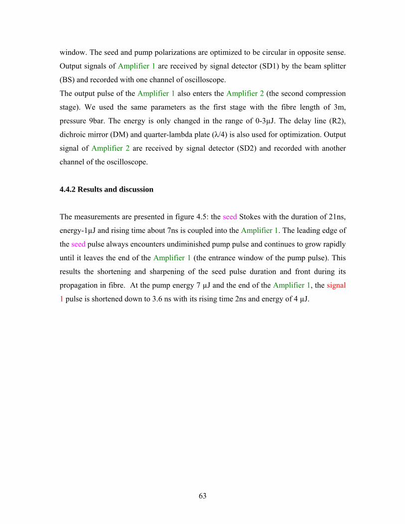
window. The seed and pump polarizations are optimized to be circular in opposite sense.

Output signals of Amplifier 1 are received by signal detector (SD1) by the beam splitter

(BS) and recorded with one channel of oscilloscope.

The output pulse of the Amplifier 1 also enters the Amplifier 2 (the second compression

stage). We used the same parameters as the first stage with the fibre length of 3m,

pressure 9bar. The energy is only changed in the range of 0-3µJ. The delay line (R2),

dichroic mirror (DM) and quarter-lambda plate (λ/4) is also used for optimization. Output

signal of Amplifier 2 are received by signal detector (SD2) and recorded with another

channel of the oscilloscope.

4.4.2 Results and discussion

The measurements are presented in figure 4.5: the seed Stokes with the duration of 21ns,

energy-1µJ and rising time about 7ns is coupled into the Amplifier 1. The leading edge of

the seed pulse always encounters undiminished pump pulse and continues to grow rapidly

until it leaves the end of the Amplifier 1 (the entrance window of the pump pulse). This

results the shortening and sharpening of the seed pulse duration and front during its

propagation in fibre. At the pump energy 7 µJ and the end of the Amplifier 1, the signal

1 pulse is shortened down to 3.6 ns with its rising time 2ns and energy of 4 µJ.

63

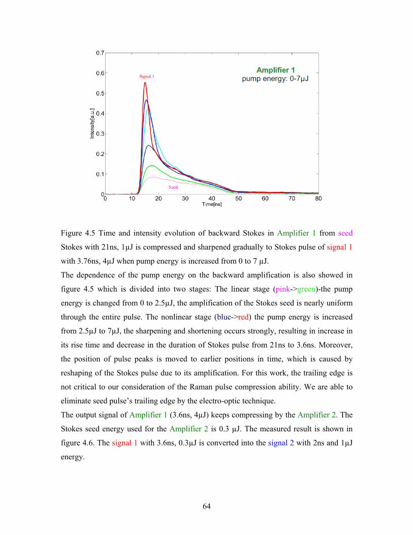
Figure 4.5 Time and intensity evolution of backward Stokes in Amplifier 1 from seed

Stokes with 21ns, 1µJ is compressed and sharpened gradually to Stokes pulse of signal 1

with 3.76ns, 4µJ when pump energy is increased from 0 to 7 µJ.

The dependence of the pump energy on the backward amplification is also showed in

figure 4.5 which is divided into two stages: The linear stage (pink->green)-the pump

energy is changed from 0 to 2.5µJ, the amplification of the Stokes seed is nearly uniform

through the entire pulse. The nonlinear stage (blue->red) the pump energy is increased

from 2.5µJ to 7µJ, the sharpening and shortening occurs strongly, resulting in increase in

its rise time and decrease in the duration of Stokes pulse from 21ns to 3.6ns. Moreover,

the position of pulse peaks is moved to earlier positions in time, which is caused by

reshaping of the Stokes pulse due to its amplification. For this work, the trailing edge is

not critical to our consideration of the Raman pulse compression ability. We are able to

eliminate seed pulse’s trailing edge by the electro-optic technique.

The output signal of Amplifier 1 (3.6ns, 4µJ) keeps compressing by the Amplifier 2. The

Stokes seed energy used for the Amplifier 2 is 0.3 µJ. The measured result is shown in

figure 4.6. The signal 1 with 3.6ns, 0.3µJ is converted into the signal 2 with 2ns and 1µJ

energy.

64

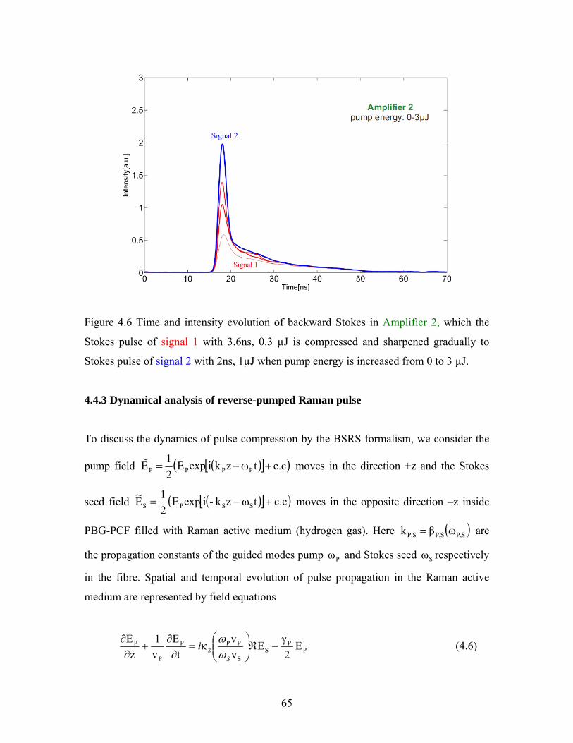
Figure 4.6 Time and intensity evolution of backward Stokes in Amplifier 2, which the

Stokes pulse of signal 1 with 3.6ns, 0.3 µJ is compressed and sharpened gradually to

Stokes pulse of signal 2 with 2ns, 1µJ when pump energy is increased from 0 to 3 µJ.

4.4.3 Dynamical analysis of reverse-pumped Raman pulse

To discuss the dynamics of pulse compression by the BSRS formalism, we consider the

pump field ( )[ ]( c.ctωzkiexpE21E~ PPPP +−= ) moves in the direction +z and the Stokes

seed field ( )[ ]( c.ctωzk-iexpE21E~ SSPS +−= ) moves in the opposite direction –z inside

PBG-PCF filled with Raman active medium (hydrogen gas). Here ( )SP,SP,SP, ωβk = are

the propagation constants of the guided modes pump and Stokes seed respectively

in the fibre. Spatial and temporal evolution of pulse propagation in the Raman active

medium are represented by field equations

Pω Sω

PP

SS

PP2

P

P

P Ε2γE

vvκ

tΕ

v1

zΕ

−ℜ⎟⎟⎠

⎞⎜⎜⎝

⎛=

∂∂

+∂∂

S

iωω (4.6)

65

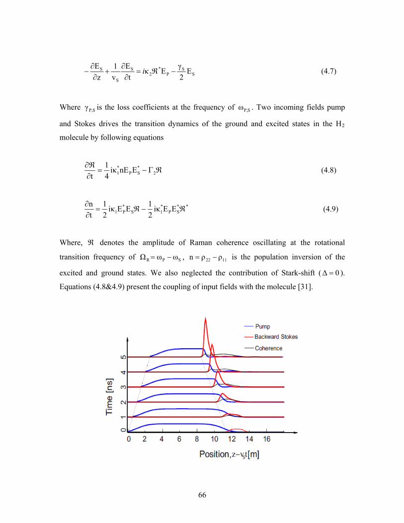
SS

P*

2S

S

S Ε2γEκ

tΕ

v1

zΕ

−ℜ=∂∂

+∂∂

− i (4.7)

Where is the loss coefficients at the frequency of . Two incoming fields pump

and Stokes drives the transition dynamics of the ground and excited states in the H

SP,γ SP,ω

2

molecule by following equations

ℜ−=∂∂ℜ

2*SP

*1 ΓEnEiκ

41

t (4.8)

**SP

*1S

*P1 EEiκ

21EEiκ

21

tn

ℜ−ℜ=∂∂ (4.9)

Where, denotes the amplitude of Raman coherence oscillating at the rotational

transition frequency of

ℜ

SPR ωωΩ −= , 1122 ρρn −= is the population inversion of the

excited and ground states. We also neglected the contribution of Stark-shift ( 0Δ = ).

Equations (4.8&4.9) present the coupling of input fields with the molecule [31].

66

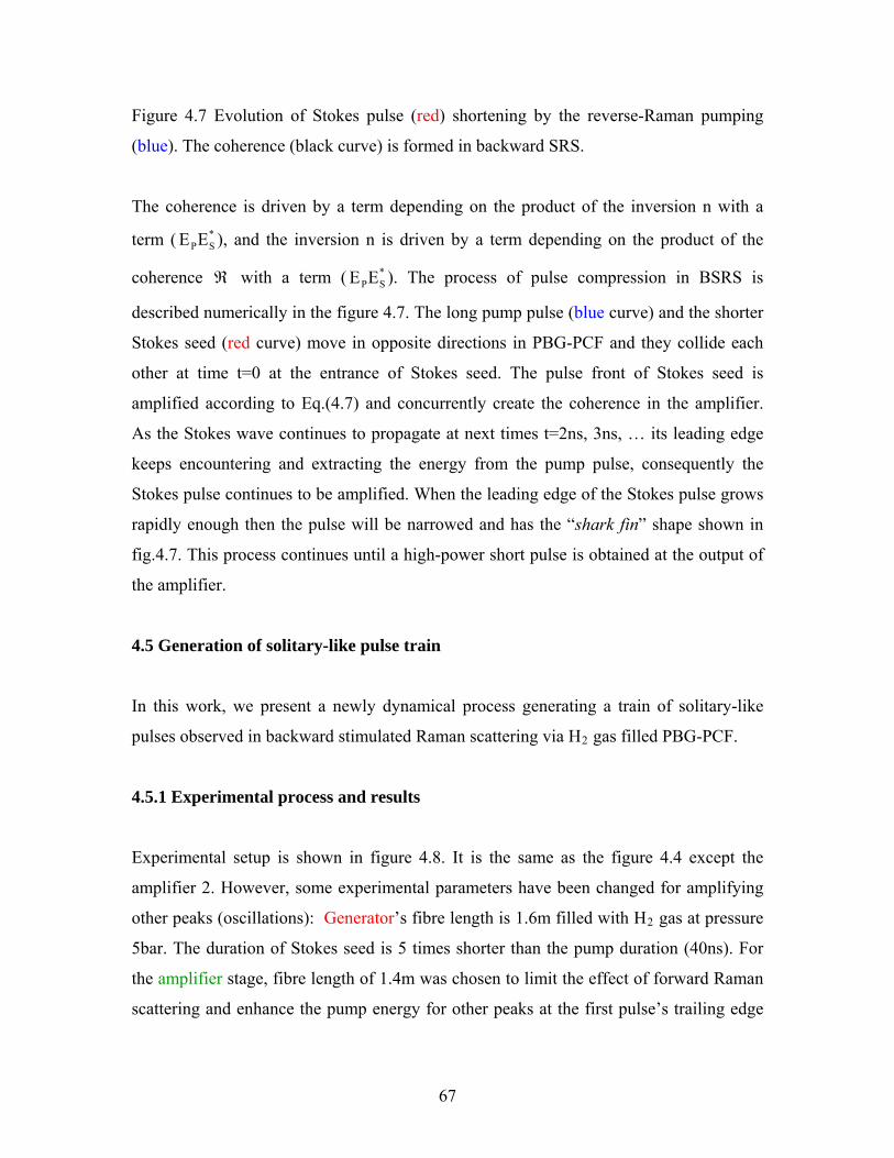
Figure 4.7 Evolution of Stokes pulse (red) shortening by the reverse-Raman pumping

(blue). The coherence (black curve) is formed in backward SRS.

The coherence is driven by a term depending on the product of the inversion n with a

term ( ), and the inversion n is driven by a term depending on the product of the

coherence with a term ( ). The process of pulse compression in BSRS is

described numerically in the figure 4.7. The long pump pulse (blue curve) and the shorter

Stokes seed (red curve) move in opposite directions in PBG-PCF and they collide each

other at time t=0 at the entrance of Stokes seed. The pulse front of Stokes seed is

amplified according to Eq.(4.7) and concurrently create the coherence in the amplifier.

As the Stokes wave continues to propagate at next times t=2ns, 3ns, … its leading edge

keeps encountering and extracting the energy from the pump pulse, consequently the

Stokes pulse continues to be amplified. When the leading edge of the Stokes pulse grows

rapidly enough then the pulse will be narrowed and has the “shark fin” shape shown in

fig.4.7. This process continues until a high-power short pulse is obtained at the output of

the amplifier.

*SPEE

ℜ *SPEE

4.5 Generation of solitary-like pulse train

In this work, we present a newly dynamical process generating a train of solitary-like

pulses observed in backward stimulated Raman scattering via H2 gas filled PBG-PCF.

4.5.1 Experimental process and results

Experimental setup is shown in figure 4.8. It is the same as the figure 4.4 except the

amplifier 2. However, some experimental parameters have been changed for amplifying

other peaks (oscillations): Generator’s fibre length is 1.6m filled with H2 gas at pressure

5bar. The duration of Stokes seed is 5 times shorter than the pump duration (40ns). For

the amplifier stage, fibre length of 1.4m was chosen to limit the effect of forward Raman

scattering and enhance the pump energy for other peaks at the first pulse’s trailing edge

67

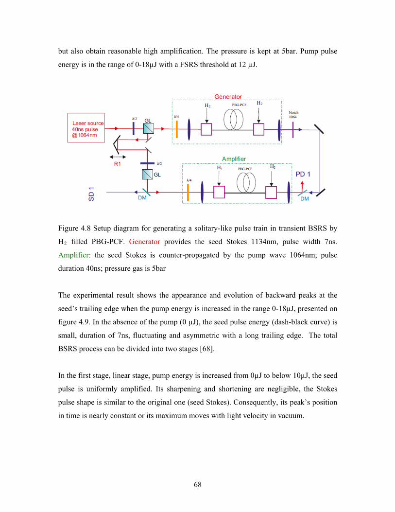
but also obtain reasonable high amplification. The pressure is kept at 5bar. Pump pulse

energy is in the range of 0-18µJ with a FSRS threshold at 12 µJ.

Figure 4.8 Setup diagram for generating a solitary-like pulse train in transient BSRS by

H2 filled PBG-PCF. Generator provides the seed Stokes 1134nm, pulse width 7ns.

Amplifier: the seed Stokes is counter-propagated by the pump wave 1064nm; pulse

duration 40ns; pressure gas is 5bar

The experimental result shows the appearance and evolution of backward peaks at the

seed’s trailing edge when the pump energy is increased in the range 0-18µJ, presented on

figure 4.9. In the absence of the pump (0 µJ), the seed pulse energy (dash-black curve) is

small, duration of 7ns, fluctuating and asymmetric with a long trailing edge. The total

BSRS process can be divided into two stages [68].

In the first stage, linear stage, pump energy is increased from 0µJ to below 10µJ, the seed

pulse is uniformly amplified. Its sharpening and shortening are negligible, the Stokes

pulse shape is similar to the original one (seed Stokes). Consequently, its peak’s position

in time is nearly constant or its maximum moves with light velocity in vacuum.

68

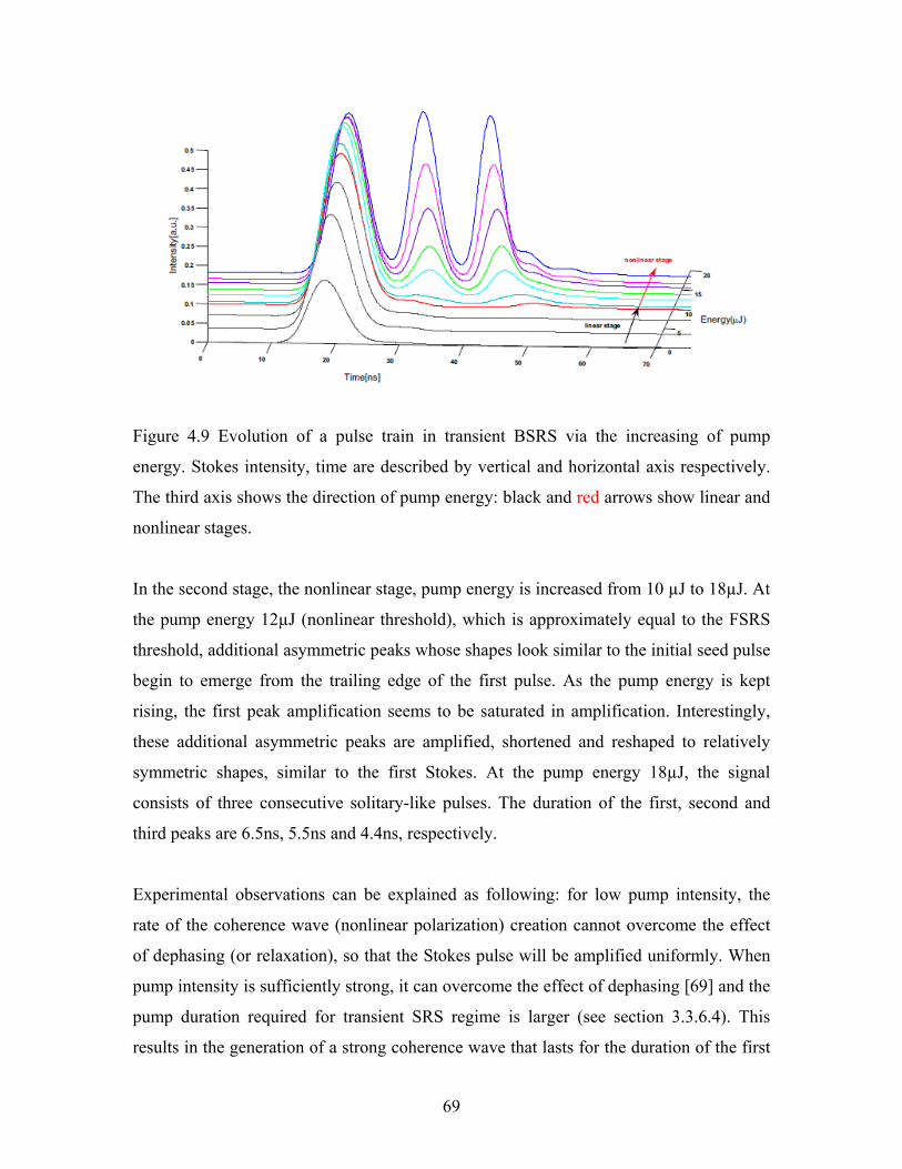
Figure 4.9 Evolution of a pulse train in transient BSRS via the increasing of pump

energy. Stokes intensity, time are described by vertical and horizontal axis respectively.

The third axis shows the direction of pump energy: black and red arrows show linear and

nonlinear stages.

In the second stage, the nonlinear stage, pump energy is increased from 10 µJ to 18µJ. At

the pump energy 12µJ (nonlinear threshold), which is approximately equal to the FSRS

threshold, additional asymmetric peaks whose shapes look similar to the initial seed pulse

begin to emerge from the trailing edge of the first pulse. As the pump energy is kept

rising, the first peak amplification seems to be saturated in amplification. Interestingly,

these additional asymmetric peaks are amplified, shortened and reshaped to relatively

symmetric shapes, similar to the first Stokes. At the pump energy 18µJ, the signal

consists of three consecutive solitary-like pulses. The duration of the first, second and

third peaks are 6.5ns, 5.5ns and 4.4ns, respectively.

Experimental observations can be explained as following: for low pump intensity, the

rate of the coherence wave (nonlinear polarization) creation cannot overcome the effect

of dephasing (or relaxation), so that the Stokes pulse will be amplified uniformly. When

pump intensity is sufficiently strong, it can overcome the effect of dephasing [69] and the

pump duration required for transient SRS regime is larger (see section 3.3.6.4). This

results in the generation of a strong coherence wave that lasts for the duration of the first

69

Stokes peak, creating a channel for back-flow of energy at its trailing edge to the pump

[31]. This part of the pump in turn can use the already existing coherence to amplify the

long trailing edge of the first Stokes peak, resulting in the generation of a multi-peak

structure. Peak number will be increased with the increasing of the interaction length,

pump duration and intensity.

One difficulty here is the presence of forward Stokes that results in the saturation of the

first peak intensity (seed). Moreover, the length of the active medium 1.4m is short

compared with the physical length of pump pulse-12m (40ns). This means that after the

passage of the first peak and its satellite through the fibre one could expect the

appearance of a similar dynamical behavior.

4.6 Conclusion

To summarize, by using the advanced characteristics of PBG-PCF we have generated

efficiently pulses 20 times shorter than that of original pump by using only a laser source

with low peak power (maximum 2.5kW) in hydrogen medium. Of course, this

experimental configuration is also applied to other gases and laser sources for optical

pulse compression. Other heavier gases such as CH4, SF6, CF4, SiH4, etc., providing the

higher backward/forward Raman gain ratio should also be interesting in this regard.

Hence, the Stokes amplification and shortening effects may be higher than in H2 gas [8].

The opto-electrical modulator may also be used to cut the leading edge of seed Stokes for

a shorter rising time. This may improve significantly the compression efficiency because

the shortening in transient stimulated Raman scattering depends significantly on the

rising time and the timing advancement of Stokes seed [66,67]. In the transient BSRS

regime, a new dynamical process generating a train of solitary-like Raman pulses with

flexibly controllable peak intensities have been observed.

70

Chapter 5 Phase-coherent Raman frequency comb in

gas filled HC-PCFs

For thus experiment I participated partly in performing the experiments for the generation

part of Raman frequency comb. This work was presented in [79].

5.1 Introduction

Optical frequency comb has a wide range of applications such as highly precise optical

atomic clocks and generation of ultrashort pulses which has led to measure and control of

previously inaccessible physical and chemical processes [70,71,72]. These applications

require mutual coherence, phase-coherent (stable relative phase) within precisely

equidistant comb lines [73,74,75,76]. Stimulated Raman scattering in gas has recently

been an attractive approach for creating a broadband frequency comb. It has been shown

that the spectra of frequency comb as much as four octaves can be adiabatically generated

in hydrogen gas medium by using two-pump lasers whose frequency difference nearly

equal to a resonant Raman transition [49]. Following efforts in controlling the carrier-

71

envelop phase (CEP) for the synthesis of the single-cycle or sub-cycle optical pulses have

been carried out. Normally, these approaches have to use complex setups, for example, a

cryogenic temperature system with the support of the phase modulator [77], the different

mixing of a pulsed dye laser and a pulsed Ti:Sapphire lasers [76], dual-wavelength laser

radiation locked on a single cavity [78].

In parallel developments, HC-PCF with Kagomé lattice possesses unique characteristics

such as low loss and dispersion, ultrabroad transmission bandwidth makes it an excellent

candidate for muti-octaves frequency comb. Kagomé-PCF for frequency comb generation

allows us to reduce six orders of magnitude in the required laser powers over previous

equivalent techniques [29]. Currently, frequency comb generation via H2 gas-filled HC-

PCF is mainly initiated from quantum fluctuations resulting in a broad frequency comb

consisting of both rotational and vibrational Raman lines [33] which is not convenient for

synthesizing ultrashort optical pulses [73,74]. In this work, we generated a broad,

mutually coherent, phase-coherent, purely rotational-Raman frequency comb using a

relatively simply setup consisting of a microchip pump laser source and two hydrogen-

filled HC-PCF [79].

5.2 Purely rotational Raman frequency comb generation

Previous schemes of Raman comb generation using gas filled HC-PCF mainly depend on

the spontaneous generation of Stokes field [29], where the molecular transition is driven

only one pump laser field. In the present work, the molecular transition is resonantly

driven from the frequency difference of two monochromatic pump and seed Stokes fields

(resonant excitation scheme). This approach provides some advantages: the well defined

input elements such as frequency, delay time and high selection of the molecular

excitation.

72

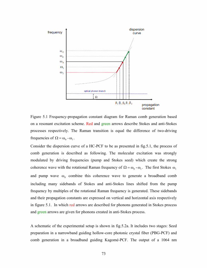
Figure 5.1 Frequency-propagation constant diagram for Raman comb generation based

on a resonant excitation scheme. Red and green arrows describe Stokes and anti-Stokes

processes respectively. The Raman transition is equal the difference of two-driving

frequencies of . 10 ω-ω=Ω

Consider the dispersion curve of a HC-PCF to be as presented in fig.5.1, the process of

comb generation is described as following. The molecular excitation was strongly

modulated by driving frequencies (pump and Stokes seed) which create the strong

coherence wave with the rotational Raman frequency of 10 ω-ω=Ω . The first Stokes

and pump wave combine this coherence wave to generate a broadband comb

including many sidebands of Stokes and anti-Stokes lines shifted from the pump

frequency by multiples of the rotational Raman frequency is generated. These sidebands

and their propagation constants are expressed on vertical and horizontal axis respectively

in figure 5.1. In which red arrows are described for phonons generated in Stokes process

and green arrows are given for phonons created in anti-Stokes process.

1ω

0ω

A schematic of the experimental setup is shown in fig.5.2a. It includes two stages: Seed

preparation in a narrowband guiding hollow-core photonic crystal fiber (PBG-PCF) and

comb generation in a broadband guiding Kagomé-PCF. The output of a 1064 nm

73

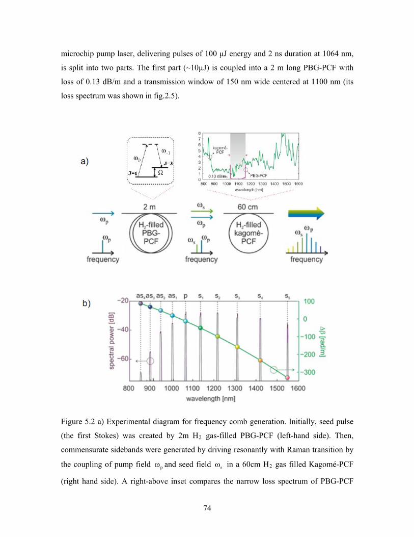
microchip pump laser, delivering pulses of 100 μJ energy and 2 ns duration at 1064 nm,

is split into two parts. The first part (~10µJ) is coupled into a 2 m long PBG-PCF with

loss of 0.13 dB/m and a transmission window of 150 nm wide centered at 1100 nm (its

loss spectrum was shown in fig.2.5).

Figure 5.2 a) Experimental diagram for frequency comb generation. Initially, seed pulse

(the first Stokes) was created by 2m H2 gas-filled PBG-PCF (left-hand side). Then,

commensurate sidebands were generated by driving resonantly with Raman transition by

the coupling of pump field and seed field in a 60cm Hpω sω 2 gas filled Kagomé-PCF

(right hand side). A right-above inset compares the narrow loss spectrum of PBG-PCF

74

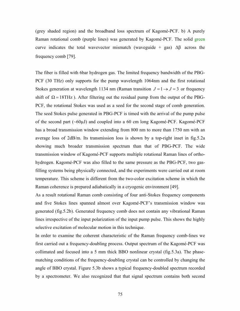
(grey shaded region) and the broadband loss spectrum of Kagomé-PCF. b) A purely

Raman rotational comb (purple lines) was generated by Kagomé-PCF. The solid green

curve indicates the total wavevector mismatch (waveguide + gas) across the

frequency comb [

Δβ

79].

The fiber is filled with 6bar hydrogen gas. The limited frequency bandwidth of the PBG-

PCF (30 THz) only supports for the pump wavelength 1064nm and the first rotational

Stokes generation at wavelength 1134 nm (Raman transition 31 =→= JJ or frequency

shift of ). After filtering out the residual pump from the output of the PBG-

PCF, the rotational Stokes was used as a seed for the second stage of comb generation.

The seed Stokes pulse generated in PBG-PCF is timed with the arrival of the pump pulse

of the second part (~60µJ) and coupled into a 60 cm long Kagomé-PCF. Kagomé-PCF

has a broad transmission window extending from 800 nm to more than 1750 nm with an

average loss of 2dB/m. Its transmission loss is shown by a top-right inset in fig.5.2a

showing much broader transmission spectrum than that of PBG-PCF. The wide

transmission window of Kagomé-PCF supports multiple rotational Raman lines of ortho-

hydrogen. Kagomé-PCF was also filled to the same pressure as the PBG-PCF, two gas-

filling systems being physically connected, and the experiments were carried out at room

temperature. This scheme is different from the two-color excitation scheme in which the

Raman coherence is prepared adiabatically in a cryogenic environment [

18THzΩ =

49].

As a result rotational Raman comb consisting of four anti-Stokes frequency components

and five Stokes lines spanned almost over Kagomé-PCF’s transmission window was

generated (fig.5.2b). Generated frequency comb does not contain any vibrational Raman

lines irrespective of the input polarization of the input pump pulse. This shows the highly

selective excitation of molecular motion in this technique.

In order to examine the coherent characteristic of the Raman frequency comb-lines we

first carried out a frequency-doubling process. Output spectrum of the Kagomé-PCF was

collimated and focused into a 5 mm thick BBO nonlinear crystal (fig.5.3a). The phase-

matching conditions of the frequency-doubling crystal can be controlled by changing the

angle of BBO crystal. Figure 5.3b shows a typical frequency-doubled spectrum recorded

by a spectrometer. We also recognized that that signal spectrum contains both second

75

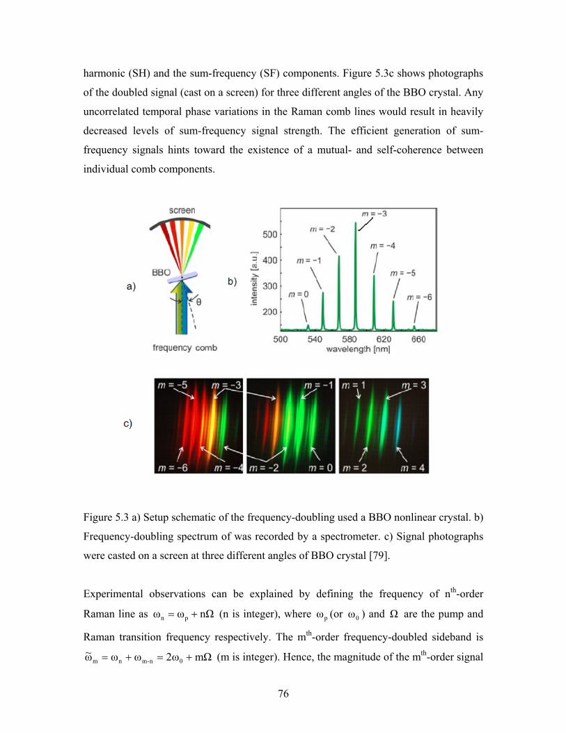
harmonic (SH) and the sum-frequency (SF) components. Figure 5.3c shows photographs

of the doubled signal (cast on a screen) for three different angles of the BBO crystal. Any

uncorrelated temporal phase variations in the Raman comb lines would result in heavily

decreased levels of sum-frequency signal strength. The efficient generation of sum-

frequency signals hints toward the existence of a mutual- and self-coherence between

individual comb components.

Figure 5.3 a) Setup schematic of the frequency-doubling used a BBO nonlinear crystal. b)

Frequency-doubling spectrum of was recorded by a spectrometer. c) Signal photographs

were casted on a screen at three different angles of BBO crystal [79].

Experimental observations can be explained by defining the frequency of nth-order

Raman line as (n is integer), where (or ) and are the pump and

Raman transition frequency respectively. The m

nΩωω pn += pω 0ω Ω

th-order frequency-doubled sideband is

mΩω2ωωω~ 0n-mnm +=+= (m is integer). Hence, the magnitude of the mth-order signal

76

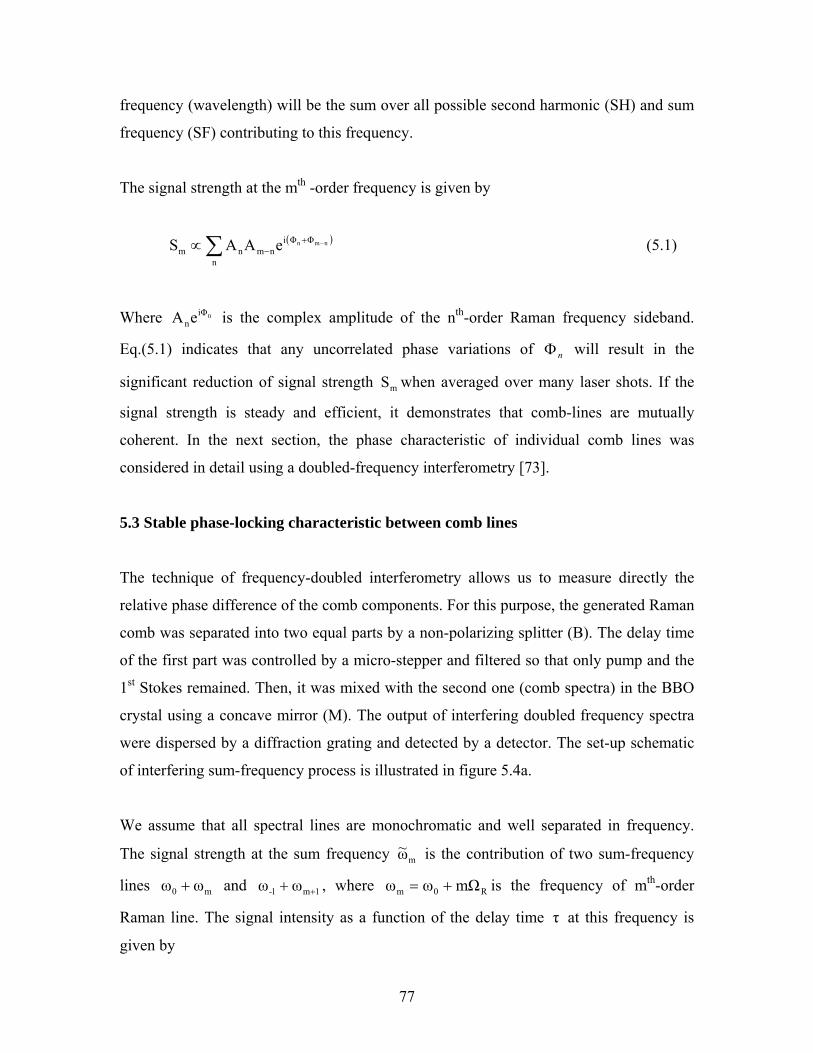
frequency (wavelength) will

he signal strength at the mth -order frequency is given by

(5.1)

Where is the complex amplitude of the nth-order Raman frequency sideband.

be the sum over all possible second harmonic (SH) and sum

frequency (SF) contributing to this frequency.

T

( )nmn ΦΦi

nnmnm eAAS −+

−∑∝

niΦneA

Eq.(5.1) indicates that any uncorrelated phase variations of nΦ will result in the

significant reduction of signal strength mS when averaged over m y laser shots. If the

signal strength is steady and efficient, it demonstrates that comb-lines are mutually

coherent. In the next section, the phase characteristic of individual comb lines was

considered in detail using a doubled-frequency interferometry [

an

73].

5.3 Stable phase-locking characteristic between comb lines

he technique of frequency-doubled interferometry allows us to measure directly the

e assume that all spectral lines are monochromatic and well separated in frequency.

T

relative phase difference of the comb components. For this purpose, the generated Raman

comb was separated into two equal parts by a non-polarizing splitter (B). The delay time

of the first part was controlled by a micro-stepper and filtered so that only pump and the

1st Stokes remained. Then, it was mixed with the second one (comb spectra) in the BBO

crystal using a concave mirror (M). The output of interfering doubled frequency spectra

were dispersed by a diffraction grating and detected by a detector. The set-up schematic

of interfering sum-frequency process is illustrated in figure 5.4a.

W

The signal strength at the sum frequency mω~ is the contribution of two sum-frequency

lines m0 ωω + and 1m1- ωω ++ , where R0m mΩωω += is the frequency of mth-order

Rama ty as a fun lay time τ at this frequency is n line. The signal intensi ction of the de

given by

77

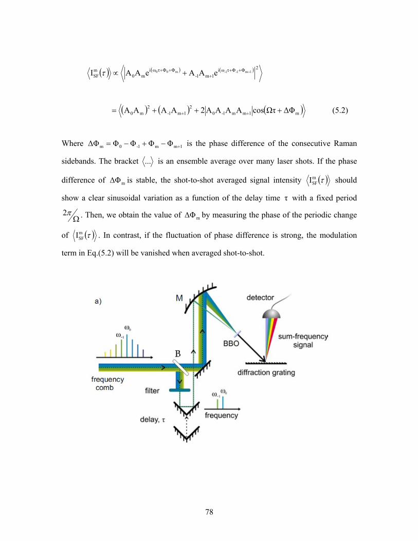
( ) ( ) ( ) 2ΦΦτωi1m1-

ΦΦτωim0

mSF

1m1-1-m00 eAAeAAI ++++

++ +∝τ

( ) ( ) ( )m1mm1-02

1m1-2

m0 ΔΦΩτcosAAAA2AAAA +++= ++ (5.2)

Where is the phase difference of the consecutive n

sidebands. The bracket

Rama1mm1-0m ΦΦΦΦΔΦ +−+−=

... is an ensemble average over many laser shots. If the phase

difference of is stable, the shot-to-shot averaged signal intensity m ( )ΔΦ τmSFI should

show a clear sinusoidal variation as a function of the delay time with a fixed period τ

Ωπ2 . Then, w tain the value of by measuring the phase of the periodic change e ob

of

mΔΦ

( )τmSF

I . In contrast, if the fluctuation of phase difference is strong, the modulation

term in Eq.(5.2) will be vanished when averaged shot-to-shot.

78

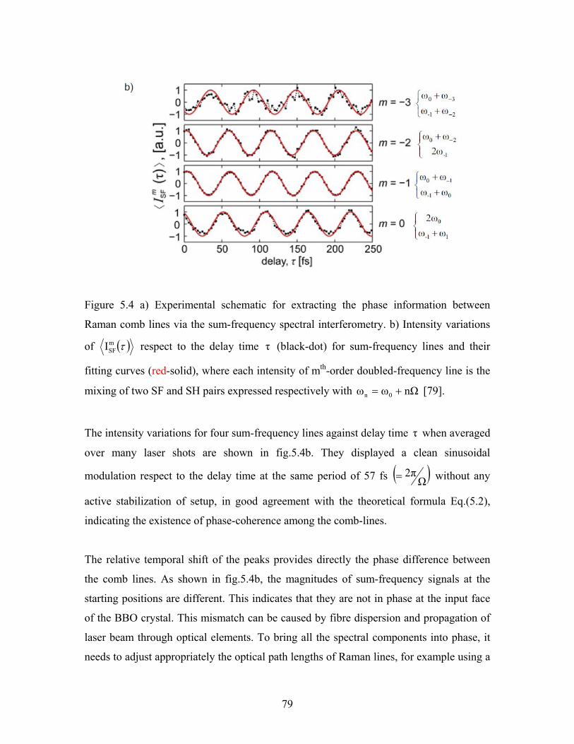
Figure 5.4 a) Experimental schematic for extracting the phase information between

Raman comb lines via the sum-frequency spectral interferometry. b) Intensity variations

of ( )τmSFI respect to the delay time (black-dot) for sum-frequency lines and their

fitting curves (red-solid), where each intensity of m

τ

th-order doubled-frequency line is the

mixing of two SF and SH pairs expressed respectively with nΩωω 0n += [79].

The intensity variations for four sum-frequency lines against delay time when averaged

over many laser shots are shown in fig.5.4b. They displayed a clean sinusoidal

modulation respect to the delay time at the same period of 57 fs

τ

( )Ω2π= without any

active stabilization of setup, in good agreement with the theoretical formula Eq.(5.2),

indicating the existence of phase-coherence among the comb-lines.

The relative temporal shift of the peaks provides directly the phase difference between

the comb lines. As shown in fig.5.4b, the magnitudes of sum-frequency signals at the

starting positions are different. This indicates that they are not in phase at the input face

of the BBO crystal. This mismatch can be caused by fibre dispersion and propagation of

laser beam through optical elements. To bring all the spectral components into phase, it

needs to adjust appropriately the optical path lengths of Raman lines, for example using a

79

pair of prisms [77] or a liquid crystal modulator [10]. This would result in the generation

a train of ultrashort pulses at a repetition rate of 18 THz.

The level of the phase-coherence will be affected by fiber dispersion because the efficient

coupling between the comb-lines relies on the same coherence wave being able to couple

efficiently between all the comb lines. If this is not the case, for example for Stokes and

anti-Stokes bands far away from the pump and first Stokes frequencies, uncorrelated

coherence waves will grow from noise and disturb the overall coherence of the system.

The rate of linear dephasing for the mth -order coherence wave (beat note signal) relative

to the 0th-order one is considered by the wavevector mismatch of the scattering system

(gas + fibre), plotted in fig.5.2b (solid-green

curve). Moreover, the nonlinear phase-locking can play an important role in maintaining

coherence, for example it can cause efficient anti-Stokes generation in gas-filled HC-

PCF, even in the presence of large linear phase-mismatch [

( ) ( ) coh1,0-

cohm1,-m01m1mm ββββββΔβ −=−−−= −−

80].

5.4 Summary

By using of the novel properties of Kagomé-PCF, we have generated efficiently a broad,

purely rotational Raman frequency comb in hydrogen gas. Sum-frequency spectral

interferometry confirms that these comb-lines are stable phase-coherent. From a practical

point of view, this makes the frequency comb attractive for Fourier synthesis of ultrashort

pulses. This scheme is much simpler than other methods requiring sophisticated setup

such as a two synchronized high-energy laser sources, a cryogenic environment and a

dual-wavelength injection-locked pulsed laser.

80

Chapter 6 Raman linewidth broadening in gas filled HC-PCFs

For the work presented here I carried out preliminary measurements of the Raman

linewidth using a different technique based on a PCF-based supercontinuum and a Fabry-

Perot. Setup was further improved using a narrowband laser source at Stokes frequency

and a pulsed nanosecond laser at pump frequency, as described in the text.

6.1 Introduction

It is known that the Raman spectral linewidth provides the important information on the

properties of the scattered medium, like the inter-molecular forces, the dephasing rate of

the molecular coherence and population. When Raman-active gases are tightly confined

in the micron-size cell like as in HC-PCF, it will result in further broadening of the

Doppler- and pressure-broadened Raman-gain linewidth by the collision between gas

molecules and the fibre core wall. This effect is particularly appreciable at low gas

81

pressures (below 1bar) where the molecular mean-free path is comparable with the fibre’s

core radius, on the order of a few microns [30]. However, this effect has not been studied

completely until now [81,82], probably because of the requirement of micro-size core

radius of gas cell. The invention of HC-PCF allows us realize this by experimental

measurement. In the present chapter, by using hollow-core bandgap fibre (PBG-PCF)

with a radius of 5.5µm, the effect of molecular core-wall collision on the rotational

spectral linewidth of S-branch of hydrogen in forward stimulated Raman scattering will

be considered.

6.2 Analysis of Raman linewidth change in gas medium

The dependence of Raman spectral shape and linewidth on the gas density is rather

complex. A simplified description of this is given in the figure 6.1.

For the low gas pressure region (<10mbar) where no significant molecular collision is

expected, the linewidth broadening is caused by the Doppler. This effect arises from the

frequency shift caused by the translational motion of gas molecules relative to a

spectrograph. Assume these motions to be in thermal equilibrium, their velocity

distribution will obey the Maxwell-Boltzmann distribution. This distribution contributes a

usual Gaussian spectral profile with its width determined by Eq.(4.2), Chapter 4. DΓ

( )m

T2ln2kωω2Γ BSPFD c

−= (6.1)

Where T is the temperature in Kelvin (here we assume T= 298K) and m is the H2 mass,

for rotational Raman transition, k(MHz1017.4ωω 6SP ×=− ) B=1.38.10-23 (JK-1)

Boltzmann constant, c=3.108m/s. The Doppler linewidth is shown with the black line in

figure 6.1.

82

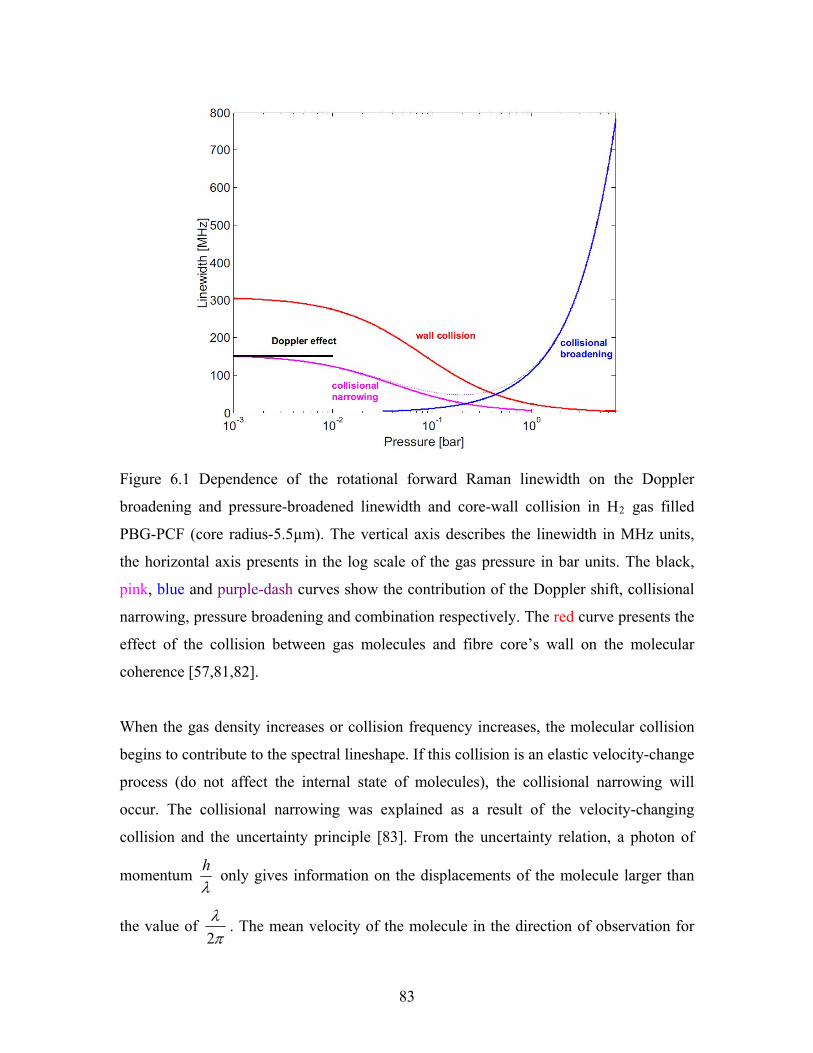
Figure 6.1 Dependence of the rotational forward Raman linewidth on the Doppler

broadening and pressure-broadened linewidth and core-wall collision in H2 gas filled

PBG-PCF (core radius-5.5µm). The vertical axis describes the linewidth in MHz units,

the horizontal axis presents in the log scale of the gas pressure in bar units. The black,

pink, blue and purple-dash curves show the contribution of the Doppler shift, collisional

narrowing, pressure broadening and combination respectively. The red curve presents the

effect of the collision between gas molecules and fibre core’s wall on the molecular

coherence [57,81,82].

When the gas density increases or collision frequency increases, the molecular collision

begins to contribute to the spectral lineshape. If this collision is an elastic velocity-change

process (do not affect the internal state of molecules), the collisional narrowing will

occur. The collisional narrowing was explained as a result of the velocity-changing

collision and the uncertainty principle [83]. From the uncertainty relation, a photon of

momentum λh only gives information on the displacements of the molecule larger than

the value of πλ

2. The mean velocity of the molecule in the direction of observation for

83

displacements of πλ

2 is considered by the Doppler shift on this photon. If collisions are

rare during the time that it takes a molecule to travel that displacement, the mean velocity

is the thermal velocity of the molecule. The Doppler shift will be proportional to this

velocity and the radiating molecules will contribute a Gaussian spectral profile whose

linewidth is expressed above, Eq.(6.1).

In contrast, many collisions of a molecule by increasing gas density, the mean velocity of

a molecule will reach zero as averaged over many collisions because the collisions take

the molecule through all possible velocity states. Hence, the mean velocity of a molecule

averaged over πλ

2 will be decreased, resulting in linewidth narrower than the usual

Doppler width. In the limit of high collision frequency between molecules, the velocity-

changing collision contributes a Lorentzian line profile and the linewidth is given

approximately by a diffusion model as

NΓ

ρAΓN = (6.2)

Where A=6.16 (MHz.amagat) is a coefficient for rotational Raman scattering,

proportional to the self- diffusion coefficient Do (cm2.amagat.s-1); ρ (amagat=1.1bar) is a

gas density. This model is divergent at zero gas density. The gas pressure dependence of

the linewidth is presented by the pink curve in figure 6.1.

In reality, as the gas density increases significantly (>1bar), it will cause the collisional

broadening by the internal state-changing in the gas molecules, leading to the disruption

of scattering. Collisional broadening contributes a Lorentzian line profile, the linewidth is

linearly proportional to the gas density, expressed by a blue curve in fig.6.1.

ρB=RΓ (6.3)

84

where B (MHz/amagat) is a broadening constant of rotational Raman linewidth B=110

(MHz/amagat) [57].

The further considerations of the gas density dependence of the linewidth giving the more

complete physical pictures have also been considered. For example, a “soft-collision”

model in which the velocity change in a single collision is much less than the mean-

thermal velocity [84], or a “hard-collision” model in which the velocity change in a

single collision is comparable to the mean-thermal velocity [85] that allow to cover the

gas pressure range between 0 and 1bar and eliminate the divergence at zero density in

diffusion model Eq.(6.2). When compared with the “hard-collision” model, the validity

of the diffusion model in Eq.(6.2) is restricted to densities higher than a cut-off density

137mbarΓ3.33Aρ

Dc == [57].

The dominant contribution to the linewidth broadening at the low gas pressure below

1bar is the collision between molecules and fibre’s core wall and is shown by the red

curve in figure 6.1. In this case, we assume that the molecules collide with the wall and

come back “fresh”, so that they lose coherence. The linewidth caused by the collision of

the core-wall collision is considered by [86].

⎟⎟⎠

⎞⎜⎜⎝

⎛+

=

c

2c

o2W

rl6.81ρr

D2.405Γ (6.4)

Where ρπσT4kl 2

B= is the mean free path, the average distance of a molecule travels

between successive collisions; kB(J.K-1) is a Boltzmann constant; Do =1.32 cm2.amagat.s-

1 is the molecular self-diffusion coefficient at the room temperature (298 K); ( )0A2.8σ =

is the collision diameter of the H2 molecule; rc =5.5µm, the radius of HC-PBG; ρ is the

gas density (amagat).

85

From above analysis, we predict the evolution of forward Raman linewidth in gas density

as following: if the collisional narrowing, collisional broadening and wall collision

processes are considered independent at gas density (the valid density of the

diffusion model), the convolution of several Lorentzian terms gives a Lorentzian with the

linewidth to be the sum of individual widths (moderate pressure region). When the

pressure (low pressure region), the dominant contribution of the molecular-wall

collision will govern the resulting line profile, namely a Lorentzian, with the linewidth is

given by in expression (6.4).

cρρ >

cρρ <

WΓ

6.3 Experimental setup and results

A schematic for measuring the Raman linewidth is illustrated in figure 6.2 consisting of

pump and probe lasers. The pump laser is a single-frequency laser producing the

wavelength 1064nm, pulse duration 17ns, 30MHz spectral linewidth. The probe one

is a CW tunable diode probe laser generating 80mW power, linewidth <1MHz.

They are combined on a dichroic mirror (DM) and focused into a 1.2m PBG-PCF-core

radius of 5.5µm filled with H

pumpω

tunableprobeω

2 gas. The transmission loss of PBG-PCF is shown in figure

2.5 (Chapter 2). The change of gas pressure is measured by a low pressure gauge (G).

The signal power was detected by the photodiode (PD) after filtering the output beam by

a bandpass filter-1134nm (BP). The small detuning range of the probe laser was

calibrated by a scanning confocal Fabry-Perot interferometer (FPI, free spectrum range,

4GHz; finesse, 500) and displayed by the oscilloscope.

86

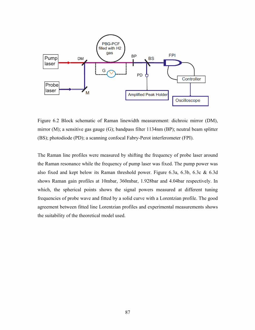
Figure 6.2 Block schematic of Raman linewidth measurement: dichroic mirror (DM),

mirror (M); a sensitive gas gauge (G); bandpass filter 1134nm (BP); neutral beam splitter

(BS); photodiode (PD); a scanning confocal Fabry-Perot interferometer (FPI).

The Raman line profiles were measured by shifting the frequency of probe laser around

the Raman resonance while the frequency of pump laser was fixed. The pump power was

also fixed and kept below its Raman threshold power. Figure 6.3a, 6.3b, 6.3c & 6.3d

shows Raman gain profiles at 10mbar, 360mbar, 1.928bar and 4.04bar respectively. In

which, the spherical points shows the signal powers measured at different tuning

frequencies of probe wave and fitted by a solid curve with a Lorentzian profile. The good

agreement between fitted line Lorentzian profiles and experimental measurements shows

the suitability of the theoretical model used.

87

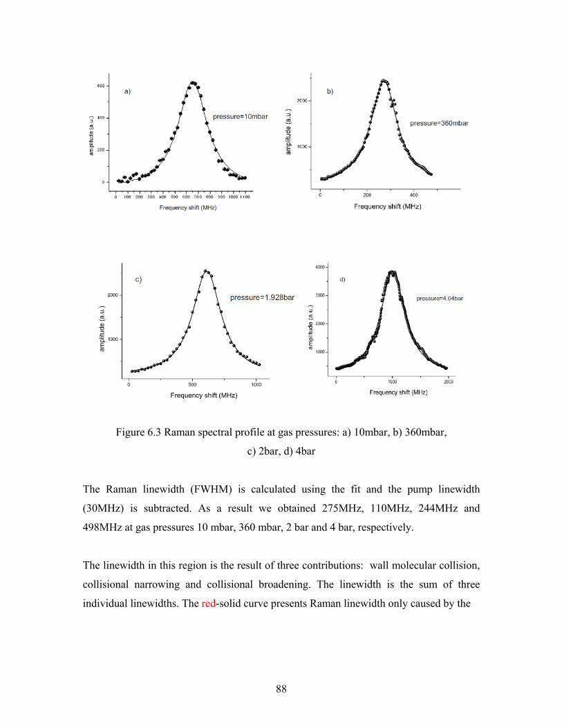
Figure 6.3 Raman spectral profile at gas pressures: a) 10mbar, b) 360mbar,

c) 2bar, d) 4bar

The Raman linewidth (FWHM) is calculated using the fit and the pump linewidth

(30MHz) is subtracted. As a result we obtained 275MHz, 110MHz, 244MHz and

498MHz at gas pressures 10 mbar, 360 mbar, 2 bar and 4 bar, respectively.

The linewidth in this region is the result of three contributions: wall molecular collision,

collisional narrowing and collisional broadening. The linewidth is the sum of three

individual linewidths. The red-solid curve presents Raman linewidth only caused by the

88

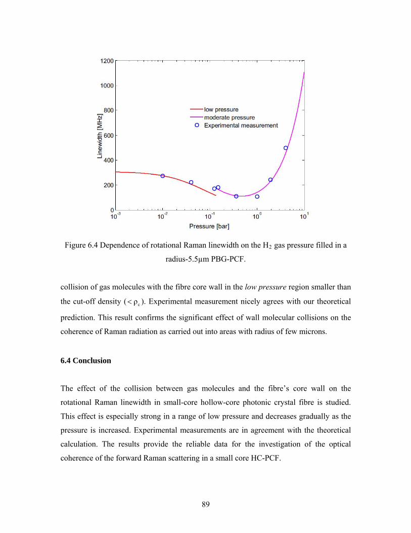
Figure 6.4 Dependence of rotational Raman linewidth on the H2 gas pressure filled in a

radius-5.5µm PBG-PCF.

collision of gas molecules with the fibre core wall in the low pressure region smaller than

the cut-off density ( ). Experimental measurement nicely agrees with our theoretical

prediction. This result confirms the significant effect of wall molecular collisions on the

coherence of Raman radiation as carried out into areas with radius of few microns.

cρ<

6.4 Conclusion

The effect of the collision between gas molecules and the fibre’s core wall on the

rotational Raman linewidth in small-core hollow-core photonic crystal fibre is studied.

This effect is especially strong in a range of low pressure and decreases gradually as the

pressure is increased. Experimental measurements are in agreement with the theoretical

calculation. The results provide the reliable data for the investigation of the optical

coherence of the forward Raman scattering in a small core HC-PCF.

89

Chapter 7 Summary and outlook

By exploiting the novel characteristics of HC-PCF, I have studied new interaction

regimes of the stimulated Raman scattering in hydrogen gas. In this chapter I summarize

the results of our studies and briefly mention possible further research directions of work

done here.

In chapter 2 I introduced the advanced properties and the potential applications of HC-

PCF. HC-PCF has novel characteristics such as low loss power, controllable transmission

window, diffraction-free interaction length and effective cross-section of only a few µm2.

As a result, the performance of HC-PCF in nonlinear interaction of light with low density

media is several orders of the magnitude higher than those of previous configurations.

These make HC-PCF become a desired candidate in maximizing the light-matter

interaction, particularly in the stimulated Raman scattering in gas.

The physical origin of Raman scattering and Maxwell-Bloch equations governing the

spatiotemporal evolution of the interaction between the laser fields and molecules in

Raman medium are described in the chapter 3. These equations are used to explain the

experimental observations in next chapters in both backward and forward stimulated

Raman scattering. SRS is divided into three regimes: spontaneous, transient and steady

state regimes. The transient regime providing the high coherence is important in

ultrashort pulse generation and easily achieved in HC-PCF by long pump durations.

Chapter 4 presents the stimulated backward Raman scattering in H2 gas filled PBG-PCF.

It includes two main results: optical pulse compression and multi-peak process in BSRS:

Optical pulse compression in a two stage pulse compression scheme: A low average

power laser source was split into three components for Stokes seed generation and its

further amplification in the first and second stages. The PBG-PCF used was filled with

H2 gas and had a narrow transmission bandwidth only supporting pump and the first

rotational Stokes wavelength. As a result the signal pulse 20 times shorter than that of

90

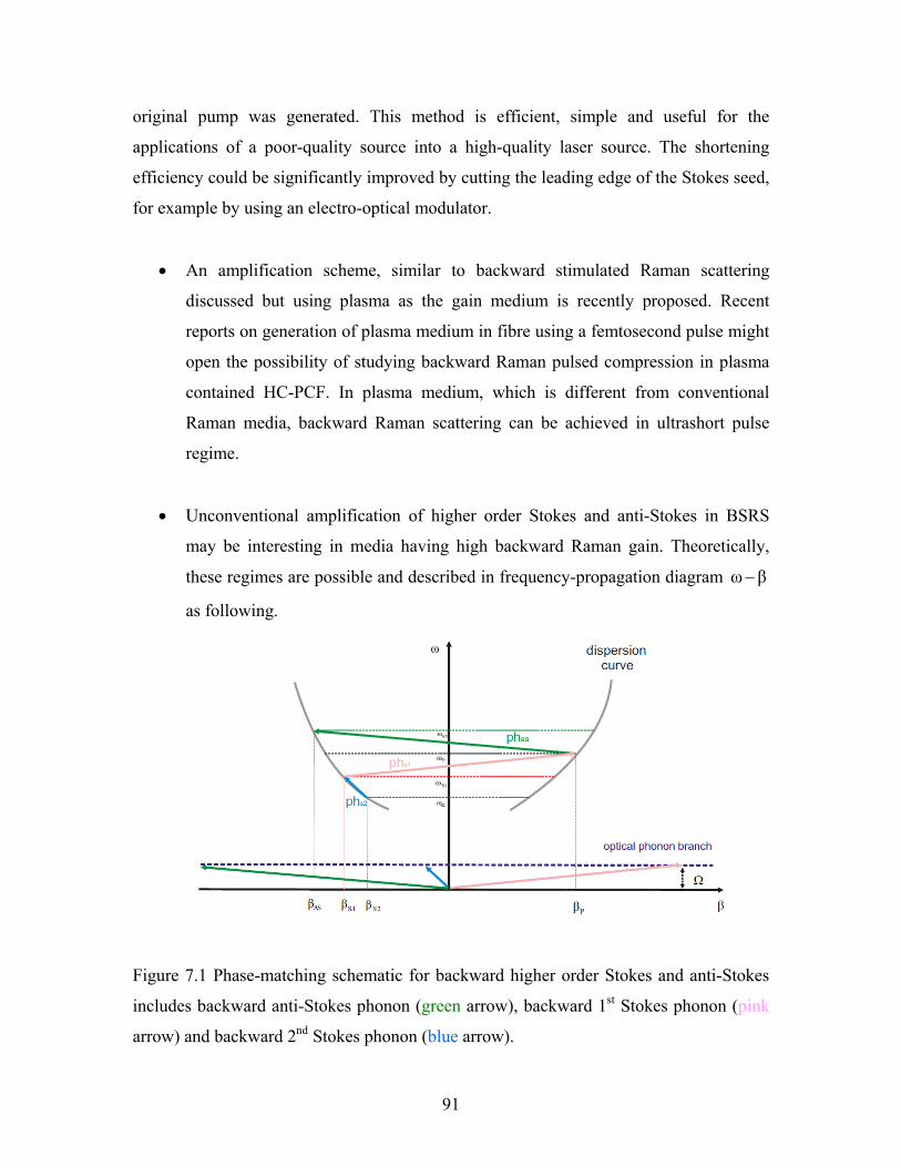
original pump was generated. This method is efficient, simple and useful for the

applications of a poor-quality source into a high-quality laser source. The shortening

efficiency could be significantly improved by cutting the leading edge of the Stokes seed,

for example by using an electro-optical modulator.

• An amplification scheme, similar to backward stimulated Raman scattering

discussed but using plasma as the gain medium is recently proposed. Recent

reports on generation of plasma medium in fibre using a femtosecond pulse might

open the possibility of studying backward Raman pulsed compression in plasma

contained HC-PCF. In plasma medium, which is different from conventional

Raman media, backward Raman scattering can be achieved in ultrashort pulse

regime.

• Unconventional amplification of higher order Stokes and anti-Stokes in BSRS

may be interesting in media having high backward Raman gain. Theoretically,

these regimes are possible and described in frequency-propagation diagram βω−

as following.

Figure 7.1 Phase-matching schematic for backward higher order Stokes and anti-Stokes

includes backward anti-Stokes phonon (green arrow), backward 1st Stokes phonon (pink

arrow) and backward 2nd Stokes phonon (blue arrow).

91

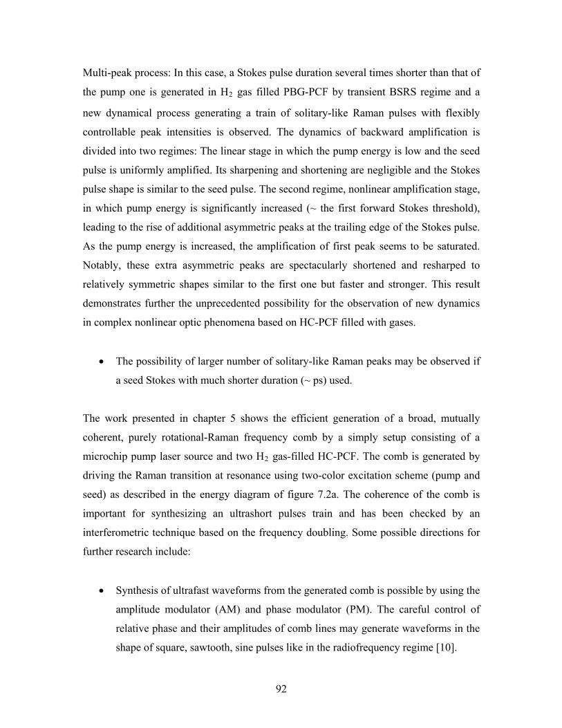
Multi-peak process: In this case, a Stokes pulse duration several times shorter than that of

the pump one is generated in H2 gas filled PBG-PCF by transient BSRS regime and a

new dynamical process generating a train of solitary-like Raman pulses with flexibly

controllable peak intensities is observed. The dynamics of backward amplification is

divided into two regimes: The linear stage in which the pump energy is low and the seed

pulse is uniformly amplified. Its sharpening and shortening are negligible and the Stokes

pulse shape is similar to the seed pulse. The second regime, nonlinear amplification stage,

in which pump energy is significantly increased (~ the first forward Stokes threshold),

leading to the rise of additional asymmetric peaks at the trailing edge of the Stokes pulse.

As the pump energy is increased, the amplification of first peak seems to be saturated.

Notably, these extra asymmetric peaks are spectacularly shortened and resharped to

relatively symmetric shapes similar to the first one but faster and stronger. This result

demonstrates further the unprecedented possibility for the observation of new dynamics

in complex nonlinear optic phenomena based on HC-PCF filled with gases.

• The possibility of larger number of solitary-like Raman peaks may be observed if

a seed Stokes with much shorter duration (~ ps) used.

The work presented in chapter 5 shows the efficient generation of a broad, mutually

coherent, purely rotational-Raman frequency comb by a simply setup consisting of a

microchip pump laser source and two H2 gas-filled HC-PCF. The comb is generated by

driving the Raman transition at resonance using two-color excitation scheme (pump and

seed) as described in the energy diagram of figure 7.2a. The coherence of the comb is

important for synthesizing an ultrashort pulses train and has been checked by an

interferometric technique based on the frequency doubling. Some possible directions for

further research include:

• Synthesis of ultrafast waveforms from the generated comb is possible by using the

amplitude modulator (AM) and phase modulator (PM). The careful control of

relative phase and their amplitudes of comb lines may generate waveforms in the

shape of square, sawtooth, sine pulses like in the radiofrequency regime [10].

92

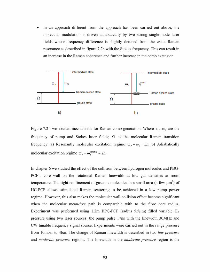
• In an approach different from the approach has been carried out above, the

molecular modulation is driven adiabatically by two strong single-mode laser

fields whose frequency difference is slightly detuned from the exact Raman

resonance as described in figure 7.2b with the Stokes frequency. This can result in

an increase in the Raman coherence and further increase in the comb extension.

Figure 7.2 Two excited mechanisms for Raman comb generation. Where are the

frequency of pump and Stokes laser fields;

SP ω;ω

Ω is the molecular Raman transition

frequency: a) Resonantly molecular excitation regime Ω=− SP ωω ; b) Adiabatically

molecular excitation regime . Ωωω tunableSP ≠−

In chapter 6 we studied the effect of the collision between hydrogen molecules and PBG-

PCF’s core wall on the rotational Raman linewidth at low gas densities at room

temperature. The tight confinement of gaseous molecules in a small area (a few µm2) of

HC-PCF allows stimulated Raman scattering to be achieved in a low pump power

regime. However, this also makes the molecular wall collision effect become significant

when the molecular mean-free path is comparable with to the fibre core radius.

Experiment was performed using 1.2m BPG-PCF (radius 5.5µm) filled variable H2

pressure using two laser sources: the pump pulse 17ns with the linewidth 30MHz and

CW tunable frequency signal source. Experiments were carried out in the range pressure

from 10mbar to 4bar. The change of Raman linewidth is described in two low pressure

and moderate pressure regions. The linewidth in the moderate pressure region is the

93

mixing of three contributions including of collisional narrowing, wall collision and

pressure broadening. The spectral broadening in the low pressure region is mainly

dominated by the collisions of gas molecules with fibre core wall. The good agreement

between the theoretical calculation and experimental data has shown the suitability of the

calculation model used. This result provides directly the information about the molecular

coherence and the Stokes build-up during Raman process. Further research plans could

include:

• Because the Raman linewidth caused by molecular wall collision depends

strongly on the fibre core radius, measurement of forward Raman scattering

linewidth for HC-PCF with different core radii will provide an interesting picture

about the effect of fibre core radius. Figure 7.3 shows the change in the Raman

linewidth as the fibre core radius is changed. Here blue, red and pink curves

describes the core radius r=3µm, r=5.5µm and 10µm respectively.

Figure 7.3 The change of Raman linewidth on the fibre core radii. The blue, red and

pink curves describes the Raman linewidth corresponding to the core radius r=3µm,

5.5µm and 10µm respectively.

94

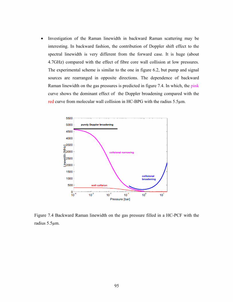
• Investigation of the Raman linewidth in backward Raman scattering may be

interesting. In backward fashion, the contribution of Doppler shift effect to the

spectral linewidth is very different from the forward case. It is huge (about

4.7GHz) compared with the effect of fibre core wall collision at low pressures.

The experimental scheme is similar to the one in figure 6.2, but pump and signal

sources are rearranged in opposite directions. The dependence of backward

Raman linewidth on the gas pressures is predicted in figure 7.4. In which, the pink

curve shows the dominant effect of the Doppler broadening compared with the

red curve from molecular wall collision in HC-BPG with the radius 5.5µm.

Figure 7.4 Backward Raman linewidth on the gas pressure filled in a HC-PCF with the

radius 5.5µm.

95

References

1. Boyd, R.W., Nonlinear optics2003: Academic press.

2. Shen, Y. and N. Bloembergen, Theory of stimulated Brillouin and Raman

scattering. Physical Review, 1965. 137(6A): p. A1787.

3. Raman, C., A new radiation. Indian Journal of physics, 1928. 2: p. 387-398.

4. Landsberg, G. and L. Mandelstam, A new occurrence in the light diffusion of

crystals. Naturwissenschaften, 1928. 16: p. 557-558.

5. Woodbury, E. and W. Ng, Ruby laser operation in the near IR. proc. IRE, 1962.

50(11): p. 2367.

6. Long, D.A., Quantum Mechanical Theory of Rayleigh and Raman

Scattering2002: Chapter 6, Wiley Online Library.

7. Owyoung, A., High-resolution cw stimulated Raman spectroscopy in molecular

hydrogen. Optics Letters, 1978. 2(4): p. 91-93.

8. Murray, J., et al., Raman pulse compression of excimer lasers for application to

laser fusion. Quantum Electronics, IEEE Journal of, 1979. 15(5): p. 342-368.

9. Shverdin, M., et al., Generation of a single-cycle optical pulse. Physical review

letters, 2005. 94(3): p. 033904.

10. Chan, H.-S., et al., Synthesis and measurement of ultrafast waveforms from five

discrete optical harmonics. Science, 2011. 331(6021): p. 1165-1168.

11. Maier, M., W. Kaiser, and J. Giordmaine, Intense light bursts in the stimulated

Raman effect. Physical review letters, 1966. 17(26): p. 1275-1277.

12. Maier, M., W. Kaiser, and J. Giordmaine, Backward stimulated Raman scattering.

Physical Review, 1969. 177(2): p. 580.

13. Jacobs, R.R., et al., High‐efficiency energy extraction in backward‐wave

Raman scattering. Applied Physics Letters, 1980. 37(3): p. 264-266.

14. Grasyuk, A.Z., et al., Compression of light pulses by stimulated Raman scattering

without a frequency shift. Soviet Journal of Quantum Electronics, 1989. 19(8): p.

1045.

15. Sentrayan, K., A. Michael, and V. Kushawaha, Intense backward Raman lasers in

CH 4 and H 2. Applied optics, 1993. 32(6): p. 930-934.

96

16. Schillinger, H. and K. Witte, Raman compression of iodine laser pulses. JOSA B,

1993. 10(6): p. 1040-1049.

17. Islam, N.R. and K. Sakuda, Wave-front reconstruction by backward-stimulated

Raman scattering in a multimode graded-index optical fiber. JOSA B, 1997.

14(11): p. 3238-3241.

18. Malkin, V., G. Shvets, and N. Fisch, Fast compression of laser beams to highly

overcritical powers. Physical review letters, 1999. 82(22): p. 4448-4451.

19. Ren, J., et al., A new method for generating ultraintense and ultrashort laser

pulses. Nature Physics, 2007. 3(10): p. 732-736.

20. Trines, R., et al., Simulations of efficient Raman amplification into the

multipetawatt regime. Nature Physics, 2010. 7(1): p. 87-92.

21. Minck, R., R. Terhune, and W. Rado, LASER‐STIMULATED RAMAN EFFECT

AND RESONANT FOUR‐PHOTON INTERACTIONS IN GASES H2, D2, AND

CH4. Applied Physics Letters, 1963. 3(10): p. 181-184.

22. Marcatili, E. and R. Schmeltzer, Hollow metallic and dielectric waveguides for

long distance optical transmission and lasers(Long distance optical transmission

in hollow dielectric and metal circular waveguides, examining normal mode

propagation). Bell System Technical Journal, 1964. 43: p. 1783-1809.

23. Rabinowitz, P., et al., Waveguide H 2 Raman laser. Applied optics, 1976. 15: p.

2005.

24. Trutna, W. and R. Byer, Multiple-pass Raman gain cell. Applied optics, 1980.

19(2): p. 301-312.

25. Meng, L., et al., Widely tunable continuous-wave Raman laser in diatomic

hydrogen pumped by an external-cavity diode laser. Optics Letters, 2000. 25(7):

p. 472-474.

26. Cregan, R., et al., Single-mode photonic band gap guidance of light in air.

Science, 1999. 285(5433): p. 1537-1539.

27. Benabid, F., et al., Stimulated Raman scattering in hydrogen-filled hollow-core

photonic crystal fiber. Science, 2002. 298(5592): p. 399-402.

28. Benabid, F., et al., Ultrahigh efficiency laser wavelength conversion in a gas-

filled hollow core photonic crystal fiber by pure stimulated rotational Raman

97

scattering in molecular hydrogen. Physical review letters, 2004. 93(12): p.

123903.

29. Couny, F., et al., Generation and photonic guidance of multi-octave optical-

frequency combs. Science, 2007. 318(5853): p. 1118-1121.

30. Couny, F., O. Carraz, and F. Benabid, Control of transient regime of stimulated

Raman scattering using hollow-core PCF. JOSA B, 2009. 26(6): p. 1209-1215.

31. Abdolvand, A., et al., Solitary Pulse Generation by Backward Raman Scattering

in H2-Filled Photonic Crystal Fibers. Physical review letters, 2009. 103(18): p.

183902.

32. Nazarkin, A., et al., Direct observation of self-similarity in evolution of transient

stimulated Raman scattering in gas-filled photonic crystal fibers. Physical review

letters, 2010. 105(17): p. 173902.

33. Wang, Y., et al., Quantum-Fluctuation-Initiated Coherence in Multioctave Raman

Optical Frequency Combs. Physical review letters, 2010. 105(12): p. 123603.

34. Saleh, B.E. and M.C. Teich, Fundamentals of photonics. Chapter 9, Vol. 32.

2007: Wiley-Interscience Hoboken, NJ.

35. Russell, P.S.J., Photonic-crystal fibers. Journal of lightwave technology, 2006.

24(12): p. 4729-4749.

36. Yeh, P., A. Yariv, and E. Marom, Theory of Bragg fiber. JOSA, 1978. 68(9): p.

1196-1201.

37. Russell, P., Photonic crystal fibers. Science, 2003. 299(5605): p. 358-362.

38. Pottage, J., et al., Robust photonic band gaps for hollow core guidance in PCF

made from high index glass. Optics Express, 2003. 11(22): p. 2854-2861.

39. Pearce, G., Plane-wave methods for modelling photonic crystal fibre. 2008.

40. Chugreev, A., et al., Manipulation of coherent Stokes light by transient stimulated

Raman scattering in gas filled hollow-core PCF. Optics Express, 2009. 17(11): p.

8822-8829.

41. Wang, Y., et al., Low loss broadband transmission in hypocycloid-core Kagome

hollow-core photonic crystal fiber. Optics Letters, 2011. 36(5): p. 669-671.

42. Abdolvand, A., Coherent Raman Interaction in Gas-Filled Hollow-Core Photonic

Crystal Fibers, 2011, Ph. D. thesis, Universität Erlangen-Nürnberg.

98

43. Nazarkin, A. and G. Korn, Pulse self-compression in the subcarrier cycle regime.

Physical review letters, 1999. 83(23): p. 4748-4751.

44. Travers, J.C., et al., Ultrafast nonlinear optics in gas-filled hollow-core photonic

crystal fibers [Invited]. JOSA B, 2011. 28(12): p. A11-A26.

45. Mukamel, S., Principles of nonlinear optical spectroscopy (Oxford series on

optical & imaging science 6). 1999.

46. Wang, C.-S., Theory of stimulated Raman scattering. Physical Review, 1969.

182(2): p. 482.

47. Hellwarth, R., Theory of stimulated Raman scattering. Physical Review, 1963.

130(5): p. 1850.

48. Penzkofer, A., A. Laubereau, and W. Kaiser, High intensity Raman interactions.

Progress in Quantum Electronics, 1978. 6: p. 55.

49. Sokolov, A.V., et al., Raman generation by phased and antiphased molecular

states. Physical review letters, 2000. 85(3): p. 562-565.

50. Glauber, R.J., The quantum theory of optical coherence. Physical Review, 1963.

130(6): p. 2529.

51. Arimondo, E., V Coherent Population Trapping in Laser Spectroscopy. Progress

in optics, 1996. 35: p. 257-354.

52. Raymer, M. and J. Mostowski, Stimulated Raman scattering: unified treatment of

spontaneous initiation and spatial propagation. Physical Review A, 1981. 24(4):

p. 1980.

53. Raymer, M., I. Walmsley, and E. Wolf, Progress in Optics XXVIII. Chapter

3,1990.

54. Sakurai, J.J., S.-F. Tuan, and E.D. Commins, Modern quantum mechanics.

American Journal of Physics, 1995. 63: p. 93.

55. Nazarkin, A., et al., Generation of multiple phase-locked Stokes and anti-Stokes

components in an impulsively excited Raman medium. Physical review letters,

1999. 83(13): p. 2560-2563.

56. Hilfer, G. and C.R. Menyuk, Stimulated Raman scattering in the transient limit.

JOSA B, 1990. 7(5): p. 739-749.

99

57. Herring, G., M.J. Dyer, and W.K. Bischel, Temperature and density dependence

of the linewidths and line shifts of the rotational Raman lines in N_ 2 and H_

2. Physical Review A, 1986. 34(3): p. 1944.

58. White, J.O., High-efficiency backward Stokes Raman conversion in deuterium.

JOSA B, 1990. 7(5): p. 785-789.

59. Malkin, V., G. Shvets, and N. Fisch, Ultra-powerful compact amplifiers for short

laser pulses. Physics of Plasmas, 2000. 7: p. 2232.

60. Ping, Y., et al., Interferometric measurements of plasma density in

microcapillaries and laser sparks. Physics of Plasmas, 2002. 9: p. 4756.

61. Malkin, V. and N. Fisch, Quasitransient backward Raman amplification of

powerful laser pulses in dense plasmas with multicharged ions. Physics of

Plasmas, 2010. 17: p. 073109.

62. Minck, R., E. Hagenlocker, and W. Rado, Stimulated pure rotational Raman

scattering in deuterium. Physical review letters, 1966. 17(5): p. 229-231.

63. Meng, L.S., P.A. Roos, and J.L. Carlsten, Continuous-wave rotational Raman

laser in H2. Optics Letters, 2002. 27(14): p. 1226-1228.

64. Culver, W., J. Vanderslice, and V. Townsend, CONTROLLED GENERATION OF

INTENSE LIGHT PULSES IN REVERSE‐PUMPED RAMAN LASERS. Applied

Physics Letters, 1968. 12(5): p. 189-190.

65. Ziemienczuk, M., et al., Intermodal stimulated Raman scattering in hydrogen-

filled hollow-core photonic crystal fiber. JOSA B, 2012. 29(7): p. 1563-1568.

66. Carman, R.L., et al., Theory of Stokes pulse shapes in transient stimulated Raman

scattering. Physical Review A, 1970. 2(1): p. 60.

67. Oraevsky, A.N., Superluminal waves in amplifying media. Physics-Uspekhi,

1998. 41(12): p. 1199-1209.

68. Bobroff, D. and H. Haus, Impulse response of active coupled wave systems.

Journal of Applied Physics, 1967. 38(1): p. 390-403.

69. Fuchs, V. and G. Beaudry, Effect of damping on nonlinear three− wave

interaction. Journal of Mathematical Physics, 1975. 16: p. 616.

100

70. Udem, T., et al., Absolute Optical Frequency Measurement of the Cesium D_ 1

Line with a Mode-Locked Laser. Physical review letters, 1999. 82(18): p. 3568-

3571.

71. Jones, D.J., et al., Carrier-envelope phase control of femtosecond mode-locked

lasers and direct optical frequency synthesis. Science, 2000. 288(5466): p. 635-

639.

72. Diddams, S., et al., An optical clock based on a single trapped 199Hg+ ion.

Science, 2001. 293(5531): p. 825-828.

73. Suzuki, T., N. Sawayama, and M. Katsuragawa, Spectral phase measurements for

broad Raman sidebands by using spectral interferometry. Optics Letters, 2008.

33(23): p. 2809-2811.

74. Wu, C., et al., Quantum theory of phase correlations in optical frequency combs

generated by stimulated Raman scattering. Physical Review A, 2010. 82(5): p.

53834.

75. Holzwarth, R., et al., Optical frequency synthesizer for precision spectroscopy.

Physical review letters, 2000. 85(11): p. 2264-2267.

76. Chen, W.-J., et al., Sub-single-cycle optical pulse train with constant carrier

envelope phase. Physical review letters, 2008. 100(16): p. 163906.

77. Hsieh, Z.-M., et al., Controlling the carrier-envelope phase of Raman-generated

periodic waveforms. Physical review letters, 2009. 102(21): p. 213902.

78. Suzuki, T., M. Hirai, and M. Katsuragawa, Octave-spanning Raman comb with

carrier envelope offset control. Physical review letters, 2008. 101(24): p. 243602.

79. Abdolvand, A., et al., Generation of a phase-locked Raman frequency comb in

gas-filled hollow-core photonic crystal fiber. Optics Letters, 2012. 37(21): p.

4362-4364.

80. Nazarkin, A., A. Abdolvand, and P.S.J. Russell, Optimizing anti-Stokes Raman

scattering in gas-filled hollow-core photonic crystal fibers. Physical Review A,

2009. 79(3): p. 031805.

81. Graf, M., et al., Doppler broadening and collisional relaxation effects in a lasing-

without-inversion experiment. Physical Review A, 1995. 51(5): p. 4030-4037.

101

82. Haverkort, J., H. Werij, and J. Woerdman, Numerical study of light-induced drift

of Na in noble gases. Physical Review A, 1988. 38(8): p. 4054.

83. Murray, J. and A. Javan, Effects of collisions on Raman line profiles of hydrogen

and deuterium gas. Journal of Molecular Spectroscopy, 1972. 42(1): p. 1-26.

84. Galatry, L., Simultaneous effect of Doppler and foreign gas broadening on

spectral lines. Physical Review, 1961. 122(4): p. 1218.

85. Gersten, J.I. and H.M. Foley, Combined Doppler and collision broadening.

JOSA, 1968. 58(7): p. 933-935.

86. Cussler, E.L., Diffusion: mass transfer in fluid systems1997: Cambridge

university press.

102