Stochastic Approaches to Thermal Relaxation of Open...
83
Stochastic Approaches to Thermal Relaxation of Open Quantum Systems Diplomarbeit zur Erlangung des wissenschaftlichen Grades Diplom-Physiker vorgelegt von Robert Biele geboren am 08.05.1985 in Freital Institut f¨ ur Theoretische Physik Fachrichtung Physik Fakult¨atf¨ ur Mathematik und Naturwissenschaften Technische Universit¨ at Dresden 2011
Transcript of Stochastic Approaches to Thermal Relaxation of Open...

Stochastic Approaches
to Thermal Relaxation
of Open Quantum Systems
Diplomarbeit
zur Erlangung des wissenschaftlichen Grades
Diplom-Physiker
vorgelegt von
Robert Biele
geboren am 08.05.1985 in Freital
Institut fur Theoretische Physik
Fachrichtung Physik
Fakultat fur Mathematik und Naturwissenschaften
Technische Universitat Dresden
2011

Eingereicht am 07.11.2011
1. Gutachter: Prof. Dr. Carsten Timm
2. Gutachter: Prof. Dr. Roberto D’Agosta

iii
Abstract
A systematic study of thermal relaxation processes with stochastic wave-function methods is pre-
sented. Throughout the thesis the relation between the stochastic wave-function method and the
well-established master equation approach to open quantum systems is demonstrated. Hence, the
results obtained with the help of the stochastic approach can be widely applied to the master equation
approach as well. Thermal relaxation processes in Markovian and non-Markovian system dynamics
are studied. As a result of these studies, the conditions for thermal relaxation of stochastic open sys-
tems are established and a time-convolutionless stochastic Schrodinger equation is presented. Besides
being local in time, this equation is able to describe thermal relaxation processes from first principles.
Starting from a microscopic model for the system-bath coupling, the bath correlation function and
the bath operators are derived. It is shown that the derived model satisfies the conditions for ther-
mal relaxation processes. In conclusion, this model together with the time-convolutionless stochastic
Schrodinger equation is numerically studied in respect to thermal relaxation.
Zusammenfassung
In dieser Arbeit wird eine systematische Untersuchung von thermischen Relaxationsprozessen mittels
stochastischer Methoden fur offene Quantensysteme vorgestellt. Im Verlauf der Arbeit wird immer
wieder auf das Verhaltnis zwischen der Beschreibung von offenen Quantensystemen mittels Master-
gleichungen und stochastischen Gleichungen hingewiesen. Daher konnen die Ergebnisse, die in der
stochastischen Beschreibung von offenen Quantensystem erlangt werden, weitgehend auf die Beschrei-
bung mittels Mastergleichungen ubertragen werden. Im Speziellen werden thermische Relaxation-
sprozesse in Markovischen und nicht-Markovischen Systemen untersucht. Als Ergebnis dieser Unter-
suchungen werden die Bedingungen fur die thermische Relaxation von stochastischen offenen Quanten-
systemen dargelegt und des Weiteren eine sogenannte time-convolutionless stochastische Schrodinger
vorgestellt. Diese Gleichung ist zum einen lokal in der Zeit, zum anderen auch in der Lage Relaxation-
sprozesse fur realistische Systeme zu beschreiben. Des Weiteren werden in dieser Arbeit, ausgehend
von einem mikroskopischen Modellsystem fur die Wechselwirkung zwischen System und Umgebung,
eine Bad-Korrelations-Funktion und die Kopplungsoperatoren hergeleitet. Abschließend wird dieses
Modell in Verbindung mit der time-convolutionless stochastischen Schrodingergleichung in Hinblick
auf thermische Relaxation numerisch untersucht.


Contents
1 Introduction 1
1.1 Motivation and Overview . . . . . . . . . . . . . . . . . . . . . . . . . . . . . . . . . . 1
1.2 Thesis Plan and Open Questions . . . . . . . . . . . . . . . . . . . . . . . . . . . . . . 3
2 Stochastic Description of Open Quantum Systems 5
2.1 Stochastic Schrodinger Equation . . . . . . . . . . . . . . . . . . . . . . . . . . . . . . 5
2.2 Properties and Interpretation . . . . . . . . . . . . . . . . . . . . . . . . . . . . . . . . 12
2.3 Tight Binding Model . . . . . . . . . . . . . . . . . . . . . . . . . . . . . . . . . . . . . 13
3 Markovian Stochastic Schrodinger Equation 17
3.1 Properties . . . . . . . . . . . . . . . . . . . . . . . . . . . . . . . . . . . . . . . . . . . 17
3.1.1 Ito Calculus . . . . . . . . . . . . . . . . . . . . . . . . . . . . . . . . . . . . . . 20
3.1.2 Norm Conservation and Non-Linear MSSE . . . . . . . . . . . . . . . . . . . . 22
3.1.3 The Corresponding Master Equation . . . . . . . . . . . . . . . . . . . . . . . . 24
3.2 Numerical Integration . . . . . . . . . . . . . . . . . . . . . . . . . . . . . . . . . . . . 25
3.2.1 Noise Generation . . . . . . . . . . . . . . . . . . . . . . . . . . . . . . . . . . . 25
3.2.2 Time-Discrete Approximations for the MSSE . . . . . . . . . . . . . . . . . . . 25
3.2.3 Results . . . . . . . . . . . . . . . . . . . . . . . . . . . . . . . . . . . . . . . . 27
3.3 Markovian Thermal Relaxation . . . . . . . . . . . . . . . . . . . . . . . . . . . . . . . 30
3.4 Local Coupling . . . . . . . . . . . . . . . . . . . . . . . . . . . . . . . . . . . . . . . . 33
4 Non-Markovian description of Open Quantum Systems 37
4.1 Non-Markovian Thermal Relaxation . . . . . . . . . . . . . . . . . . . . . . . . . . . . 38
4.1.1 The Corresponding Master Equation . . . . . . . . . . . . . . . . . . . . . . . . 38
4.1.2 Conditions for Thermal Relaxation . . . . . . . . . . . . . . . . . . . . . . . . . 42
4.1.3 Time-Convolutionless Stochastic Thermal Relaxation . . . . . . . . . . . . . . . 46
4.2 Microscopic Model for Thermal Relaxation . . . . . . . . . . . . . . . . . . . . . . . . 47
4.2.1 Model . . . . . . . . . . . . . . . . . . . . . . . . . . . . . . . . . . . . . . . . . 47
4.2.2 Bath Correlation Function . . . . . . . . . . . . . . . . . . . . . . . . . . . . . . 49
4.2.3 Power Spectrum and Detailed-Balance Relation . . . . . . . . . . . . . . . . . . 53
4.3 Numerical Implementation and Results . . . . . . . . . . . . . . . . . . . . . . . . . . . 55
4.3.1 Generating Correlated Noise . . . . . . . . . . . . . . . . . . . . . . . . . . . . 56
4.3.2 Advantages and Implementation of the Time-Convolutionless SSE . . . . . . . 60
4.3.3 Results . . . . . . . . . . . . . . . . . . . . . . . . . . . . . . . . . . . . . . . . 62
5 Conclusion and Outlook on Future Work 65
vi Contents
A Appendix 69
A.1 Expressions for the Bath Correlation Function . . . . . . . . . . . . . . . . . . . . . . 69
A.2 Matrix Elements for the Bath Operator S . . . . . . . . . . . . . . . . . . . . . . . . . 70
Bibliography 71


1 Introduction
1.1 Motivation and Overview
Description of Open Quantum Systems
The description of closed microscopic systems in the framework of quantum mechanics seems to be
an approximation. Realistic quantum systems must be regarded as open systems due to the fact that
any microscopic system is coupled to the omnipresent and uncontrollable environment. This coupling
can influence the system in an non-negligible way and can lead to energy dissipation or quantum
decoherence in the system. On the one hand, perfect isolation of quantum systems is not possible and,
on the other hand, the exact microscopic description of the dynamics of the macroscopic environment
and its influence on the system are not feasible. As a result, the demand for a simpler description of the
system and environment evolution in terms of the dynamics of an open system emerges. The theory
of open quantum systems plays an important role in many branches of physics, ranging from quantum
information over quantum optics to condensed matter physics and quantum computing. Furthermore,
it has remained an active research topic since the middle of the last century. During this period many
approaches to the description of open system dynamics have been developed. In this thesis we will
focus on two methods, namely quantum master equation and the stochastic wave-function methods.
Firstly, the quantum master equation method concentrates on the equation of motion of the
reduced density operator in the Fock sub-space of the relevant system. The von Neumann equation
is the exact equation of motion for a closed system that consists of the relevant system and the
environmental degrees of freedom. By starting from this equation one can derive equations of motion
for the density operator of the relevant system by tracing out the environmental degrees of freedom.
As a result, these derived quantum master equations describe the time evolution of the subsystem
influenced by the environment in the reduced Hilbert space. In this way, the first quantum master
equation was obtained by Pauli in 1928 [1]. This so-called Pauli master equation describes the evolution
of the diagonal elements of the density matrix under the assumption of a system which is weakly
perturbed by an additional term in the Hamiltonian. In 1957 A. G. Redfield derived the so-called
Redfield equation [2]. This time-local equation of motion can be widely applied to systems where
the dynamics of the environment are much faster than the system dynamics. The in 1976 derived
Lindblad master equation [3] is the most general master equation which is Markovian and preserves
the norm.
Worth mentioning is the so-called Nakajima-Zwanzig equation [4, 5] which is an exact equation for
the relevant degrees of freedom. The exactness has to be paid with an inhomogeneous term, which
consists of an integral over the whole history of the state and over a so-called memory kernel [6, 7].
This behaviour is called non-Markovian and considers completely the memory effects of the open
quantum system dynamics. However, this integro-differential equation is unfortunately as difficult to

2 1.1 Motivation and Overview
solve as the equation of motion for the total system. Therefore, approximations are needed in order
to access relevant dynamics in an analytical or even numerical way. In order to simplify and solve
the problem under weak coupling conditions, a perturbation expansion in powers of the interaction
Hamiltonian can be performed. This approximation leads to so-called perturbative master equations
[7, 8]. In addition, one can also expand the memory kernel around t or assume a finite width of
the kernel. Furthermore, by assuming a δ-correlated environment the non-Markovian behaviour is
neglected completely. This approximation leads to so-called Markovian quantum master equations.
The master equation formalism also considers that the subsystem evolves towards a statistical
mixture of states due to the coupling to the environment. For closed quantum systems we know that
the dynamics can alternatively be described by an equation of motion for the wave function. This
begs the question of whether there exists a description of open quantum system dynamics in terms of
a differential equation for the reduced wave function. As a result, the description of open quantum
systems by using stochastic wave-function methods has recently received a great deal of attention.
This method is either used as a numerical tool in order to resemble the respective quantum master
equation or even to allow calculations on problems which would otherwise be exceedingly complicated
[9, 10]. By using the wave function instead of the density matrix, one can significantly speed up
computer simulations as the dimension of the system increases [11, 12]. Furthermore, stochastic
wave-function methods are used as an alternative description of open quantum systems. It has been
shown that in the case of particle-particle interaction in the subsystem, the dynamics calculated with
the stochastic wave-function approach can differ from the dynamics obtained with the corresponding
master equation [13].
In the stochastic wave-function approach the dynamics of the open quantum system are described
by an ensemble of wave functions. Each member of this ensemble is evolving according to a so-called
stochastic Schrodinger equation. This equation considers not only the normal hermitian time
evolution of the subsystem, but also an additional term describing non-Markovian memory effect and
the coupling to the environment in a stochastic way. In the limit of a large ensemble this leads
to a description of the open quantum system dynamics. This approach is very much in the spirit of
Langevin, who applied Newtonian dynamics to a Brownian particle in order to describe the undergoing
random motion with the help of stochastic differential equations in 1908. This work was initiated by
the ground breaking paper by Albert Einstein on the Brownian motion three years before [14].
Thermal Relaxation
As a consequence of the laws of thermodynamics, one expects that a ‘small’ system, coupled to a
‘large’ heat bath in thermal equilibrium at temperature T , is driven in the long-time limit towards
thermal equilibrium with the same temperature. In order to describe realistic open quantum systems,
the equation of motion should be able to describe this relaxation behaviour. This relaxation towards
a steady state is a so-called nonequilibrium process.
Recently, nonequilibrium effects where a temperature gradient is converted into an electrical current
have received a great deal of attention [15–17]. These effects are conventionally described within a
single-particle scattering method [18, 19] which neglects the dynamical interaction with the thermal
baths. Recently, a study about thermoelectric effects in nanoscale junction using an open quantum
system approach has been proposed [20]. In this study, the system-bath coupling is described by
1.2 Thesis Plan and Open Questions 3
a heuristic model. In this model the system is forced to relax towards thermal equilibrium when
coupled to one environment globally. Whether this heuristic model is able to describe quantitate
thermal gradients within the Lindblad master equation approach is not proven. Nevertheless, in
contrast to the scattering approach these open quantum methods take local temperature variations
along the system into account. Whether these temperature variations are indeed present has been
verified experimentally [21]. From a technological point of view, the study of thermoelectric effects is
of great importance for improving the efficiency of thermoelectric materials.
1.2 Thesis Plan and Open Questions
Inspired by the work of Dubi and Di Ventra [20], who investigated thermal gradients in nanosystems
within the master equation approach, the question arises of whether these studies can be reproduced
within the stochastic wave-function approach. By taking a step back, thermal relaxation processes for
the stochastic approach to open quantum systems have to be investigated first of all. In particular,
one has to find the conditions for thermal relaxation processes for this approach. With respect to
the stochastic description, it is not precisely known in which way this conditions enter the stochastic
Schrodinger equation. Moreover, this begs the question of whether one can find a more fundamental
basis for these relaxation processes in comparison to the heuristic model used in the study of Dubi
and Di Ventra.
In addition, clarification as to whether the Markovian description is sufficient to describe thermal
relaxation processes and temperature gradients for realistic systems is necessary. However, it is also
important to consider whether the non-markovian description must also be applied as memory effects
can play a crucial role in these processes.
Another open question is how the stochastic wave-function approaches can be extended to particle-
particle interaction in terms of an effective single-particle wave function. This can most likely be
undertaken in the same spirit as done for the Hartree-Fock method or density functional theory. In
addition, one has to investigate how to construct an effective single-particle bath operator out of the
many-body operator.
In this thesis we will focus on the stochastic approach to open quantum system’s dynamics due
to the facts that, on the one hand, the wave-function approach is not as far discovered as the master
equation approach and therefore, needs to be investigated further. On the other hand, there are still
open questions linked to the mathematical underlying theory of non-Markovian stochastic processes.
To make the thesis easier to follow for the reader, we have conveniently divided it into three main, but
closely related, parts. In the first part a microscopic based derivation of the stochastic Schrodinger
equation will be presented due to Gaspard [22]. This deduction should give an insight into the
approximations done during the derivation and will introduce the important concepts of stochastic
wave-functions methods. The derived SSE is of non-Markovian type and describes the dynamics of
the open quantum system at the weak-coupling level.
In the second part we will consider stochastic-Markovian dynamics in the context of thermal re-
laxation. With the help of the Ito calculus the properties of the Markovian stochastic Schrodinger
equation and its relation to the master equation approach will be discussed. In addition to the thermal
relaxation of Markovian systems, we will try to consider temperature gradients in these systems.
4 1.2 Thesis Plan and Open Questions
Finally, the third part will discuss non-Markovian open quantum system dynamics. Within this
approach we will study the conditions for thermal relaxation. In addition, a microscopic model for the
system-bath coupling will be derived that is able to describe thermal relaxation processes. Further-
more, a time-local stochastic Schrodinger equation will be proposed that allows relaxation processes
and will be tested numerically.
2 Stochastic Description of Open Quantum
Systems
This chapter is dedicated to introduce the concepts of the stochastic wave-function method. This
describes open quantum system dynamics through the time evolution of a wave function instead of
the time evolution of the reduced density operator. Consequently, a stochastic Schrodinger equation
(SSE) will be derived by starting from an exact microscopic equation of motion for the total system
and tracing out the irrelevant degrees of freedom. The procedure will be based on an idea of Gaspard
and Nagaoka [22], however, modification of the original derivation has been done in order to emphasise
the performed approximations and make the deduction more compact and readable. This will help
the reader to understand the basic assumptions and underlying concepts at a microscopic level. In the
second part of the chapter it will be shown how to use these concepts for accessing physical quantities
as for example the expectation value of an operator or how to determine the physical state of an open
quantum system. The reason for introducing these methods in such a depth stems from the fact that
they are not covered by standard courses and it is neither a common nor a widespread method for
studying open quantum system dynamics.
In the last part of the chapter the simple tight-binding model will be introduced as a tool to
numerically investigate the rich behaviour of the stochastic wave-function approach and also for the
sake of accessing physical information of a lattice-like nanosystem coupled to a large environment
quite easily.
2.1 Stochastic Schrodinger Equation
The following derivation is based on an idea by Gaspard [22] in which a small subsystem is weakly
coupled to a large environment. By starting from the exact equation of motion for the combined
system, the Schrodinger equation can be split into two sub-equations with the help of the projection-
operator formalism of Feshbach [23, 24]. This will lead to a non-Markovian stochastic Schrodinger
equation in the reduced Hilbert space. The derivation and assumptions performed will be of great
importance for the derivation of the bath correlation function based on a microscopic model in chapter
4.
6 2.1 Stochastic Schrodinger Equation
Considering a system described by the Hamiltonian HS coupled to a large environment, given by
HB, through an interaction potential λW , the Schrodinger equation for the combined system reads
i∂t|Ψ(t) = (HS +HB + λW )|Ψ(t) . (2.1.1)
Here, we have set to one.
The interaction potential is assumed to be linear
W =
α
Sα Bα , (2.1.2)
in the operators Sα and Bα of the system and the environment, respectively. The question of whether
or not the interaction potential can be written in such a linear form will be addressed later. The total
wave function belongs to the Hilbert space spanned by a direct product of the Hilbert space of the
system, HS , with that of the bath, HB,
|Ψ ∈ HS ⊗HB . (2.1.3)
In addition, the environment, also called bath or heat bath in the following, is considered to be a large
system with a complete and orthonormal basis characterised as
1lB =
n
|nn|, HB|n = n|n, m|n = δmn . (2.1.4)
Therefore, the total wave function can be decomposed in this basis as
|Ψ(t) =
n
|φn(t) ⊗ |n . (2.1.5)
Moreover, the total wave function is normalised to unity,
1 = Ψ|Ψ =
n
φn|φn , (2.1.6)
implying that the coefficient wave functions |φn are not normalised and the square of their norm
describes the probability that the bath is in state |n. It is worth mentioning that the expectation
value of any operator OS ∈ HS can be written in this decomposition as
Ψ|OS |Ψ = trSρSOS
, (2.1.7)
where trS denotes the partial trace over the subsystem. This can be interpreted as the system being
in a statistical mixture of states represented by the system density matrix ρS =
n|φnφn|.
In order to extract information about the time evolution of these wave functions from the Schrodinger
equation of the combined system, the Feshbach projection-operator method [23, 24] is used.
Within this methods, projection operators that satisfy
P 2 = P = P †, Q2 = Q = Q†, P +Q = 1lT (2.1.8)

2.1 Stochastic Schrodinger Equation 7
are used in order to decompose the Schrodinger equation into two. These properties can be ensured
by choosing the operators as
P = 1lS ⊗ |ll| and Q = 1lS ⊗
n( =l)
|nn| . (2.1.9)
Hence, applying the operator P to the total wave function (2.1.5), extracts the lth coefficient wave
function,
P |Ψ = |φl ⊗ |l . (2.1.10)
Correspondingly, Q|Ψ contains the information of the other wave functions belonging to the statistical
ensemble.
Before applying the Feshbach projection-operator method, it is convenient to transform Eq. (2.1.1)
into the interaction picture,
i∂t|ΨI(t) = λW (t)|ΨI(t) . (2.1.11)
In addition, the total wave function and the potential in the interaction picture read
|ΨI(t) = eiHBteiHSt |Ψ(t) , (2.1.12)
W (t) = eiHStSαe−iHSt eiHBtBαe
−iHBt = Sα(t)Bα(t) . (2.1.13)
Now one can apply the projection operators in Eq. (2.1.9) to Eq. (2.1.11) leading to
i∂t P |ΨI(t) = λPW (t) P |ΨI(t)+ λPW (t)Q|ΨI(t) , (2.1.14)
i∂t Q|ΨI(t) = λQW (t)Q|ΨI(t)+ λQW (t) P |ΨI(t) . (2.1.15)
In order to obtain a closed differential equation for P |ΨI(t), one first has to solve Eq. (2.1.15) and
inserts its solution into Eq. (2.1.14). The second expression is an inhomogeneous linear differential
equation for Q|ΨI(t) and can be solved by the method of variation of constants
Q|ΨI(t) = U(t)Q|ΨI(0) − iλ
t
0
dt U(t− t)QW (t) P |ΨI(t) , (2.1.16)
where U(t) is the time evolution operator of the homogeneous differential equation for Eq. (2.1.15)
and obeys
i∂t U(t) = λQW (t)Q U(t) . (2.1.17)
Hence, U(t) describes the time evolution according to the influence of all n bath wave functions onto
the systems except the lth one. The influence on Q|ΨI due to the coupling between P |ΨI and Q|ΨIis described by the second term in Eq. (2.1.16). Inserting Eq. (2.1.16) into Eq. (2.1.14) leads to a

8 2.1 Stochastic Schrodinger Equation
differential equation for the coefficient wave function P |ΨI,
i∂t P |ΨI(t) = λPW (t) P |ΨI(t) (2.1.18)
+ λPW (t)
U(t)Q|ΨI(0) − iλ
t
0
dt U(t− t)QW (t) P |ΨI(t)
.
It is worth mentioning that until now no approximations have been done so that Eq. (2.1.18) describes
the exact time evolution of the lth coefficient of the total wave function. Therefore, it can be considered
as a good starting point for a derivation of a stochastic Schrodinger equation beyond the weak coupling
approximation.
However, we will now consider a subsystem which is weakly coupled to the bath in order to perform
a perturbation expansion in the coupling parameter λ of the evolution operator,
U(t) = 1l− iλ
t
0
dt1QW (t1)Q+ λ2
t
0
dt1
t1
0
dt2QW (t1)QQW (t2)Q+O(λ3) . (2.1.19)
Inserting this expression into Eq. (2.1.18) leads to
i∂t P |ΨI(t) = λPW (t) P |ΨI(t)+ λPW (t)Q|ΨI(0) (2.1.20)
− iλ2PW (t)
t
0
dtQW (t)Q|ΨI(0)+QW (t) P |ΨI(t
)
+O(λ3) ,
where the expansion has been truncated at second order in λ.
Multiplying from the left with l| and assuming that
l|Bα(t)|l = 0 , (2.1.21)
Eq. (2.1.20) simplifies to
i∂t|φl
I(t) = λ
α,β
n( =l)
Sα(t)l|Bα(t)|n − iλ
t
0
dt Sβ(t)l|Bα(t)Bβ(t
)|n|φn
I (0)
− iλ2
α,β
Sα(t)
t
0
dt Sβ(t)l|Bα(t)Bβ(t
)|l|φl
I(t) . (2.1.22)
The condition l|Bα(t)|l = 0 can always be fulfilled, either through a redefinition of the system
Hamiltonian HS or through the choice of the operators Bα. The forcing term
f(t) = λ
α,β
n( =l)
Sα(t)l|Bα(t)|n − iλ
t
0
dt Sβ(t)l|Bα(t)Bβ(t
)|n|φn
I (0) (2.1.23)

2.1 Stochastic Schrodinger Equation 9
describes the influence of all the other bath modes on the lth coefficient wave function. One can
see that the initial conditions |φn
I(0) enter as an essential ingredient. Assuming that at t = 0 the
subsystem is in a pure state and the bath is in thermal equilibrium, we can write the total density
operator as
ρT (0) = |φ(0)φ(0)|⊗ e−βHB
ZB
. (2.1.24)
This expression leads to an approximation for the initial wave function,
|Ψ(0) ≈ |φ(0) ⊗
n
e−βn
ZB
eiθn |n, (2.1.25)
where the θn are independent random phases uniformly distributed over the interval [0, 2π]. With the
help of Eq. (2.1.24) we are able to extract the initial coefficient wave functions
|φn(0) = n|Ψ(0) ≈ |φ(0)
e−βn
ZB
eiθn . (2.1.26)
Accordingly, all initial-state coefficient wave functions are proportional to the same initial state |φ(0).This can also be expressed by the lth one and leads to
|φn(0) ≈ |φl(0)e−β2 (n−l)ei(θn−θl) = |φn
I (0), (2.1.27)
which also coincides with the initial condition in the interaction picture. Hence, Eq. (2.1.23) can be
written as
f(t) ≈ λ
α
n( =l)
Sα(t)l|Bα(t)
|φl(0) − iλ
β
t
0
dt Sβ(t)Bβ(t
)|φl(0)|ne−
β2 (n−l)ei(θn−θl)
≈ λ
α
n( =l)
Sα(t)l|Bα(t)|n|φl
I(t)e−
β2 (n−l)ei(θn−θl)
= λ
α
γlα(t)Sα(t)|φl
I(t) . (2.1.28)
Here, we have assumed that the expression in the curly braces gives an approximation for the time
evolution of the lth coefficient wave function in the interaction picture up to second order in λ for
Eq. (2.1.22). Besides, the stochastic noise is included in
γlα(t) =
n( =l)
l|Bα(t)|ne−β2 (n−l)ei(θn−θl) , (2.1.29)
which depends on a specific coefficient wave function. In order to eliminate this dependence, a thermal
averaged is performed,
γα(t) =
l
e−β2 l
√ZB
γlα(t) =1√ZB
l
n( =l)
l|Bα(t)|ne−β2 nei(θn−θl) . (2.1.30)
10 2.1 Stochastic Schrodinger Equation
Additionally, the expectation value of an operator from the bath for a typical eigenstate |l is approx-imately equivalent to a thermal average of the temperature of the bath,1
l|Bα(t)Bβ(t)|l ≈ trB
ρeqBBα(t)Bβ(t
)=: Cαβ(t− t) . (2.1.31)
In this expression we have defined the bath correlation function Cαβ . Also the density operator
of the bath in thermal equilibrium is given by
ρeqB
=e−βHB
trB[e−βHB ]=
e−βHB
ZB
, (2.1.32)
with β being the inverse of the temperature.
If the bath is large enough, γα(t) consists of a sum with many complex oscillating terms which leads
to random Gaussian behaviour according to the central limit theorem. As a result of this, the noise
is characterised by its mean value and its variance. In addition, one can evaluate the characterising
properties of the noise,
γα(t) = 0 , (2.1.33)
γα(t)γβ(t) = 0 , (2.1.34)
γ∗α(t)γβ(t) = Cαβ(t− t) , (2.1.35)
where the equations ei(θn+θm) = 0, ei(θn−θm) = δnm and (2.1.21) have been used. In this expression
one can see that the bath correlation function is the covariance function of the noise. Collecting all
the information, transforming back into the partial Schrodinger picture of the system and setting
τ = t− t, one can simplify Eq. (2.1.20)
i∂t|φ(t) = HS |φ(t)+ λ
α
γα(t)Sα |φ(t)
− iλ2
α,β
Sα
t
0
dτ e−iHSτSβCαβ(τ) |φ(t− τ) . (2.1.36)
The index l has been suppressed since the lth coefficient wave function is a typical representative of the
statistical ensemble so that Eq. (2.1.36) is also valid for any system wave function. In this equation
one can see that the change of the wave function at time t depends not only on the current state |φ(t),it also depends on an integral over the whole history of the state in the interval [0, t]. This behaviour
is called non-Markovian, thus Eq. (2.1.36) will be called non-Markovian stochastic Schrodinger
equation (NMSSE).
In Eq. (2.1.36) the coupling of the bath to the subsystem is described in an approximate manner
and enters in the NMSSE through the bath correlation function and the stochastic noises γα(t) with
the properties (2.1.33)–(2.1.35). Thus, all the information about the time evolution of the bath and its
coupling to the subsystem is included in the bath correlation function. In most quantum optic cases
the dependence on the past of the wave function can be neglected. This is due to the fact that the
bath correlation function decays rapidly to zero one a time scale on which the system’s wave function
1For further information about the validity of this assumption see [25–30].
2.1 Stochastic Schrodinger Equation 11
varies significantly. For convenience, one neglects the non-Markovian behaviour by approximating the
time dependence of the bath correlation function by a δ-function,
Cαβ(t− t) ≈ Dαβδ(t− t), (2.1.37)
which is known under the name of a δ-correlated bath approximation. As a result of this approx-
imation, the NMSSE reduces to the Markovian stochastic Schrodinger equation (MSSE)
i∂t|φ(t) =HS + λ
α
γα(t)Sα − iλ2
2
α,β
SαSβDαβ
|φ(t) . (2.1.38)
The Baby and the Bath Water
With an idiomatic expression a professor of mine used to say:
‘Simplify, simplify, ...... but don’t throw out the baby with the bath water !’
He meant that one should be careful in performing approximations, keeping in mind which physical
truth the equation should contain after the approximation. The particular interest lies in a system -
bath coupling driving the system towards thermal equilibrium in the long-time limit. In chapter 4 it
will be shown that the Fourier transform of the bath correlation function, the power spectrum
Cαβ(ω) ≡∞
−∞
dt e−iωtCαβ(t) , (2.1.39)
has to fulfil the detailed-balance relation
Cαβ(−ω) = eβω Cβα(ω) , (2.1.40)
in order to ensure that the SSE drives the system at least close to a thermal equilibrium state (with
β being the inverse of the temperature). In the MSSE (2.1.38) the evolution of the bath and its
coupling to the system enters only as a factor in the equation of motion. Hence, one can expect
that the detailed-balance relation of the bath correlation function in not taken into account by the
δ-correlated bath approximation (2.1.37) and will ‘throw out the baby with the bath water’. This
means that the MSSE in the form (2.1.38) will most likely not be able to drive the system towards
thermal equilibrium, except one includes the detailed-balance relation in an artificial manner in the
coupling operators Sα. As might be expected, these operators from the Hilbert space of the subsystem
should not, for example, contain the information about the temperature of the bath.
Hence, this begs the question of whether or not a time-local stochastic Schrodinger equation can be
found which ensures that the system is driven towards thermal equilibrium. Therefore, an idea is to
approximate the NMSSE in a way which takes, on the one hand, the detailed-balance relation into
account and, on the other hand, simplifies the complicated non-Markovian behaviour.
An idea would be to set |φ(t − τ) ≈ |φ(t) in the memory term of the NMSSE (2.1.36). This
approximation can be justified in cases where the wave function will not change significantly at the
time scale on which the bath correlation C(τ) function decays to zero. With this ‘balanced Markovian

12 2.2 Properties and Interpretation
approximation’ the NMSSE simplifies to
i∂t|φ(t) =HS + λ
α
γα(t)Sα − iλ2
α,β
SαTαβSβ
|φ(t) , (2.1.41)
with the ‘balance operator’
Tαβ(t) =
t
0
dτ e−iHSτCαβ(τ) . (2.1.42)
This equation will be named balanced stochastic Schrodinger equation (BSSE). Due to its
time-locality the BSSE is relatively simple to implement numerically. Besides this, it also considers
the time structure of the bath correlation function. Consequently, we expect that this equation is able
to describe thermal relaxation processes. This will be proven in chapter 4.
2.2 Properties and Interpretation
Due to the coupling to the bath, the system will be driven into a statistical mixture of states although
a pure initial state was assumed. From the previous derivation we have seen that the stochastic
Schrodinger equation describes the time evolution of a typical member of this statistical ensemble. As
a result, a single evolution with the SSE will not contain the information of the full state. By starting
from an initial state |Ψ(0) the SSE will evolve the former in a non-deterministic way due to the
influence of dissimilar stochastic processes, leading to different trajectories as shown in figure 2.2.1.
On average, which is denoted by an over-line, one can gain physical information out of the stochastic
time evolution. The state at time t is characterised by the density operator of the system and can be
calculated from many realisations of the time evolution described by the SSE as
ρS(t) =|Ψ(t)Ψ(t)|Ψ(t)|Ψ(t)
≡ limN→∞
N
i=1|Ψi(t)Ψi(t)|
N
j=1Ψj(t)|Ψj(t)
. (2.2.1)
initial pure state
|Ψ(0)
|Ψ1(t)|Ψ2(t)
|Ψ3(t)
|ΨN (t)
... O(t) = Ψ(t)|O |Ψ(t)Ψ|Ψ
ρS(t) =|Ψ(t)Ψ(t)|Ψ(t)|Ψ(t)
Figure 2.2.1: Schematic representation of how to calculate physical quantities with the SSE.

2.3 Tight Binding Model 13
In this expression the denominator has been introduced to guarantee the normalisation due to the
fact that the norm of the wave function is only conserved on average for the stochastic Schrodinger
equation. This will be considered in more detail in the chapters 3 and 4 when the MSSE and NMSSE
will be discussed. Furthermore, the expectation values of an operator O can be calculated as
O(t) ≡ Ψ(t)| O |Ψ(t)Ψ|Ψ
. (2.2.2)
It is worth mentioning that the SSE is also able to describe systems having a non-pure initial state,
ρS(t) =
r
pr |Ψr(0)Ψr(0)| , (2.2.3)
defined in terms of the normalised system wave functions and their probabilities which sum up to one
in the usual way. The time evolution of the state for this initial non-pure condition can be calculated
as
ρS(t) =
r
pr|Ψr(t)Ψr(t)|Ψr(t)|Ψr(t)
. (2.2.4)
In the next section a concrete model for the system will be introduced, namely the tight-binding
model.
2.3 Tight Binding Model
The tight-binding model has been chosen as an example system to apply the previous considerations.
This choice is motivated by the fact that this model, being numerically simple to implement, still
allows us to investigate the physics of thermal transport. Comparing the tight-binding model with,
for example, the real space realisation of a Hamiltonian of atoms forming lattices or molecules, one only
has to deal with one grid point per atom, instead of approximately 1003 grid points per atom in 3D.2
This means a significant simplification for the simulation of bulk systems or large molecules. Figure
2.3.1 shows an atom configuration of the type we want to deal with. The orange dots correspond to
atoms at positions Rk and the electrons will move in this configuration influenced by the atoms.
The time-independent Schrodinger equation for a single electron reads
h|n = t+
k
vk|n = n|n , (2.3.1)
where t is the kinetic energy operator of the electron and
kvk is an effective potential generated by
the superposition of atom-centred spherical charge densities at positions Rk. In addition, it should
be mentioned that we are considering spin-less electrons throughout the thesis. In the tight-binding
model the electron is tightly bound to the atom to which it belongs. As a result, the wave function of
the electron will be rather similar to the atomic orbitals and one can take a linear combination of
2Here we have estimated the number of discretisation steps per dimension for a atom in a real-space calculation.

14 2.3 Tight Binding Model
Figure 2.3.1: Example atom configuration for the tight-binding model.
atomic orbitals (LCAO) in order to construct molecular orbitals,
|n =
kα
ckα |φkα , (2.3.2)
where φkα(r) are atomic orbitals of species α (e.g., 1s, 2p,...) located at the atom positions Rk. In the
following, we consider an orthonormal tight-binding model with only one species of atomic orbitals
(e.g., 1s),
φj |φi = δij . (2.3.3)
Inserting Eq. (2.3.2) into Eq. (2.3.1) and multiplying from the left with φj | leads to the matrix
equation
i
cihji =
i
ciδji (2.3.4)
with hji = φj |h|φi. The diagonal elements are
hii = φi|t+ vi|φi+
k =i
φi|vk|φi ≈ φi|t+ vi|φi = , (2.3.5)
where the crystal field terms
k =iφi|vk|φi have been neglected. For i = j we consider only the two
centre terms
hji = φj |t+ vj + vi|φi+
k =(i,j)
φj |vk|φi ≈ φj |t+ vj + vi|φi = −t . (2.3.6)
Consequently the final Hamiltonian for the two-centre tight-binding model in the nearest-
neighbour approximation in matrix form reads
hji =
for i = j
−t for |Ri −Rj | = a
0 otherwise
, (2.3.7)
2.3 Tight Binding Model 15
where a is the nearest-neighbour distance. The energies can be shifted by and the Hamiltonian can
be written in second-quantised form as
h = −t
i,j
c†icj + c†
jci, (2.3.8)
where c†icreates an electron at position Ri and i, j denotes nearest neighbours. The quantity t is
often called the hopping integral. In the limiting case of t → 0 it is impossible for the electron to hop to
the neighbouring sites. This tight-binding model is in general a many-body model for non-interacting
electrons, however, it can be extended to interacting electron systems, leading to Hubbard-like models.
In order to access the eigenfunctions of the tight-binding model one has to diagonalise the Hamiltonian
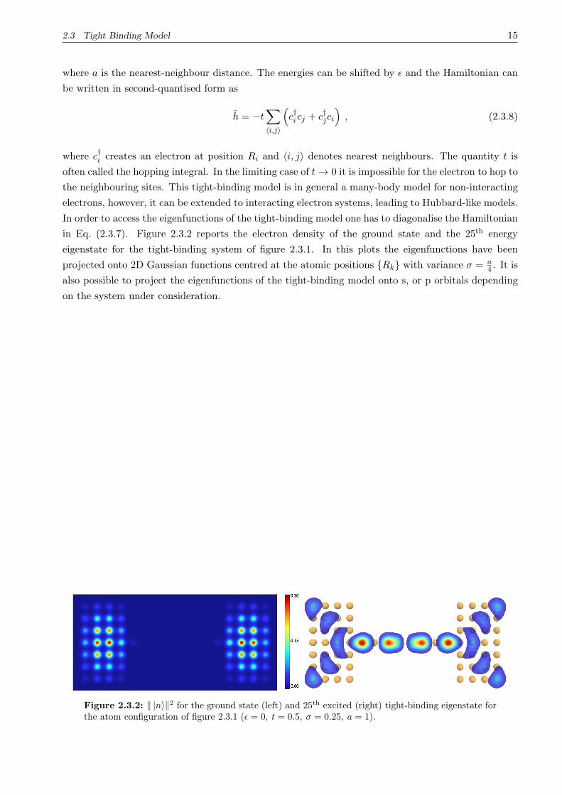
in Eq. (2.3.7). Figure 2.3.2 reports the electron density of the ground state and the 25th energy
eigenstate for the tight-binding system of figure 2.3.1. In this plots the eigenfunctions have been
projected onto 2D Gaussian functions centred at the atomic positions Rk with variance σ = a
4. It is
also possible to project the eigenfunctions of the tight-binding model onto s, or p orbitals depending
on the system under consideration.
Figure 2.3.2: |n2 for the ground state (left) and 25th excited (right) tight-binding eigenstate forthe atom configuration of figure 2.3.1 ( = 0, t = 0.5, σ = 0.25, a = 1).

3 Markovian Stochastic Schrodinger Equation
In this chapter we will consider the simplest representative of the family of stochastic Schrodinger
equations, namely the Markovian one. In this case one assumes that the bath correlation function can
be approximated by a δ-function. The question arises for which system-bath model this is a applied
assumption.
We are particularly interested in an equation of motion for the open quantum system which can
describe thermal relaxation processes. As mentioned in the previous chapter, this behaviour is closely
related to the time structure of the bath correlation function and enters through a non-Markovian
integral into the SSE. Consequently, in the last chapter a bath correlation function and coupling
operators S and B will be derived based on a microscopic model. Besides this, we will be able to
argue whether this model is suitable to describe non-Markovian thermal relaxation processes.
However, in this chapter we are more interested in a heuristic model for the system-bath coupling
in order to reach a better understanding of the underlying concepts of the stochastic description
of relaxation processes. Therefore, properties of the Markovian SSE and the corresponding master
equation will first be discussed with the help of stochastic calculus. This stochastic calculus for
Markovian processes is called Ito calculus and a short introduction into these concepts has to be given
before the properties of the MSSE can be discussed. In addition, a set of bath operators will be
introduced heuristically which will ensure that the Markovian SSE drives the system towards thermal
equilibrium in the long-time limit. This is very much in the spirit of the study of Dubi and Di Ventra
[20] mentioned in the introduction. Unlike in the non-Markovian case discussed in the next chapter,
this will not be based on a microscopic model.
3.1 Properties
In the previous chapter we have seen that the MSSE emerges from the NMSSE by a δ-correlated bath
approximation and that it describes the weak coupling of a system to a Markovian environment,
d|φ(t) =− iHS − iλ
α
γα(t)Sα − λ2
2
α,β
SαSβDαβ
|φ(t)dt , (3.1.1)
where the coupling is included in the white noises γα, with properties
γα(t) = 0 , (3.1.2)
γ∗α(t)γβ(t) = Dαβδ(t− t) . (3.1.3)
This form of the MSSE does not follow the standard rules of calculus. The state |φ(t) is a stochastic
function and its time derivation is not defined at any instant of time due to the white noise γ(t).
18 3.1 Properties
Moreover, the Markovian approximation leads to the scaling property
γ(t)dt ∝√dt , (3.1.4)
as a result the rules of calculus have to be adjusted according to the Ito calculus.3
The following lemma simplifies the MSSE in order to make the numerical implementation and
the argument about its properties clear. Besides, the simplified form of the MSSE is identical with
the heuristic MSSE derived in other contexts by Ghirardi and Pearle [35] or van Kampen [8]. This
form has been applied to various problems in physics, ranging from stochastic molecular dynamics
[36] over stochastic time-dependent current-density-functional theory [13] to path-integral formalisms
[37, 38]. Hence, the proof of the lemma will show the equivalence of the two approaches and is of
great importance for bringing the microscopic derived MSSE into the context of current research in
other fields.
Lemma 1. The MSSE (3.1.1) can be written as
d|φ(t) =
− iHS − 1
2
α
V †αVα
dt+
α
VαdWα
|φ(t) , (3.1.5)
with
dWα = 0 , (3.1.6)
dWα dW ∗β= δαβ dt , (3.1.7)
Vα = λ
dα
β
UαβSβ , (3.1.8)
where Uαβ is a unitary transformation which diagonalises Dαβ with corresponding eigenvalues dα.
Proof. In order to justify that the MSSE (3.1.1) derived by Gaspard can be written in the form (3.1.5),
one has to show that
−1
2
α
V †αVαdt = −λ2
2
α,β
SαSβDαβ , (3.1.9)
α
VαdWα = −iλ
α
γα(t)Sαdt , (3.1.10)
and that the new differential noise satisfies equations (3.1.6) and (3.1.7). This would imply that dW
can be assumed to be a differential increment of an underlying Wiener process, which will be defined in
subsection 3.1.1. First of all, one has to ensure the existence of a unitary transformation diagonalising
Dαβ .
As a result of the definition of the bath correlation function (2.1.31) and the assumption that the
coupling operators Bα are hermitian, one can conclude that
Cαβ(τ) = C∗βα
(−τ) . (3.1.11)
3The next subsection will give a brief introduction to Ito calculus. For a more complete treatment one can consult
[31–34].
3.1 Properties 19
As a result, Dαβ = D∗βα
and Dαβ can be represented by a hermitian matrix D. As a consequence, it
can be diagonalised by a unitary transformation U
D = U†dU , (3.1.12)
where d in this expression is the diagonal matrix containing the real eigenvalues dα.
Inserting Eq. (3.1.8) on the left hand side of Eq. (3.1.9) and Eq. (3.1.10) leads to
−1
2
α
V †αVαdt = −λ2
2
αβγ
dαS†γU
†γαUαβSβ
= −λ2
2
βγ
S†γSβDγβ , (3.1.13)
α
VαdWα = λ
α
dα
β
UαβSβdWα , (3.1.14)
where
Dγβ =
α
dαU†γαUαβ (3.1.15)
has been used. In addition, it can be shown that Eq. (3.1.14) leads to condition (3.1.10) by assuming
a transformation law for the noise,
dWα =−i√dα
j
U †jαγjdt . (3.1.16)
Inserting this expression into Eq. (3.1.14) and using the fact that S† = S lead to
−1
2
α
V †αVαdt = −λ2
2
αβ
SαSβDαβ , (3.1.17)
α
VαdWα = −iλ
βj
α
UαβSβU†jαγjdt
= −iλ
βj
Sβδjβγjdt
= −iλ
α
Sαγαdt , (3.1.18)
where
α
UαβU†jα
= δjβ (3.1.19)
had been used. This means that Eq. (3.1.9) and Eq. (3.1.10) are fulfilled and results in an expression
for the differential noise (3.1.16). As a result, one can conclude that dWα is characterised by its mean
20 3.1 Properties
value dWα = 0 and by the covariance
dWα(t) dW ∗β(t) =
1dαdβ
jk
U †jαU †∗
kβγ∗k(t)γj(t)dt dt
=1dαdβ
jk
U †jαUβkDkjδ(t
− t)dt dt
=δαβdαdαdβ
δ(t − t)dt dt
= δαβδ(t − t)dt dt , (3.1.20)
where
jk
U †jαUβkDkj = δαβdα (3.1.21)
has been applied. Finally, it can be argued that the auto-covariance dWα(t) dW ∗β(t) of the differential
noise is only non-vanishing for t = t. Therefore, we can define the noise as stationary and independent
differential increments of a Wiener process.4 By considering the defining property of the δ-function,
lim→0
−
δ(t)dt = 1 , (3.1.22)
and the Ito rules, one can conclude the scaling behaviour for the covariance function [39],
dWα dW ∗β= δαβdt . (3.1.23)
This implies a significant simplification for numerical and analytic purposes. Now the stochastic
processes are uncorrelated instead of connected through the matrix Dαβ . An important result of this
lemma is that dW scales on average as√dt, which is the main reason why the MSSE is not tractable
with the standard calculus and requires the Ito formalism. In the next section only the results and
rules of the Ito calculus needed in the thesis will be introduced. The interested reader can find more
detailed and mathematical treatment of stochastic calculus in [31–34].
3.1.1 Ito Calculus
The Ito calculus extends the methods of standard calculus to stochastic Wiener processes W . The
Wiener process is used to represent the integral of a Gaussian white-noise process ζ(t) as
W (t) =
t
0
ζ(t)dt . (3.1.24)
4The precise meaning of a stationary stochastic process can be seen from definition 4 in subsection 4.3.1.

3.1.1 Ito Calculus 21
A white-noise process is characterised by zero mean and a δ-correlated auto-covariance,
ζ(t) = 0 , (3.1.25)
ζ(t)ζ∗(t) = δ(t − t) . (3.1.26)
The name ‘white noise’ is motivated by the fact that the power spectrum of the δ-function is a constant,
which implies that on average all frequencies have equal weight.
Problems arises du to the fact that the Wiener process is nowhere differentiable, so strictly speaking
ζ(t) is not a conventional function of time and even worse it has infinite variation on any bounded
time interval. Therefore, the integral (3.1.24) cannot be interpreted as an ordinary Riemann integral
and integration with respect to a non-differentiable stochastic function has to be defined. In order to
avoid confusion with ordinary integration, the usual notation for the Ito integral is used,
W (t) =
t
0
dW (t) , (3.1.27)
where dW is the underlying infinitesimal random process of the Brownian motion. There are many
different approaches to assign a physical and mathematical meaning to the this stochastic integral.
Here, we will define the stochastic integrals as
I(t) =
t
0
g(t)dW (t) ≡ limN→∞
N−1
i=1
g(ti)W (ti+1)−W (ti)
, (3.1.28)
where g(t) is a test function and ti is a series of time steps with t1 = 0 and tN = t. As a conclusion,
the integral can be written in differential form,
dI = gdW . (3.1.29)
In this spirit, the differential version of the MSSE (3.1.5) can now be interpreted as an Ito integral
equation
|φ(t) = |φ(0)+t
0
− iHS − 1
2
α
V †αVα
|φ(t)dt +
t
0
α
Vα|φ(t)dWα(t) . (3.1.30)
In this equation the first integral is a standard Riemann integral, whereas the second one has to be
interpreted according to definition (3.1.28). Finally, we are able to assign a meaning to both, the
integral form of the MSSE (3.1.30) and the differential form (3.1.5). In order to increase the clearness
and readability we decided for to use of the differential notation in the following. Nevertheless,
one should keep in mind what is meant by these differential forms, namely they are connected with
definition (3.1.28). An important result, which will be used throughout this chapter is the Ito chain
rule [39], which in the language of quantum mechanics reads
d|φψ|
=
d|φ
ψ|+ |φ
dψ|
+
d|φ
dψ|
. (3.1.31)

22 3.1 Properties
In this equation φ(t) and ψ(t) are two states evolving according to the MSSE (3.1.5). In addition, the
simple rules of the Ito differentials should be kept in mind,
dWα dW ∗β= δαβdt , (3.1.32)
dWα dWβ = 0 , (3.1.33)
dWα dt = 0 . (3.1.34)
In this rules one see the advantage of the usage of a complex noise for the simulation of the MSSE in
contrast to real stochastic processes. Ito calculus only has to be considered if complex conjugation is
involved.
In the following, we will apply these rules in order do discuss the conservation of the norm within
the MSSE (3.1.5) and the correspondence to the master equations.
3.1.2 Norm Conservation and Non-Linear MSSE
Starting from a normalised initial state |φ(0), Eq. (3.1.5) evolves this process in time. By calculating
the infinitesimal Ito change in the norm squared according to Eq. (3.1.31) one finds
dφ2 = dφ|φ
=
dφ|
|φ+ φ|
d|φ
+
dφ|
d|φ
=
φ
−
α
V †αVαdt+
αβ
V †βVαdWα dW
∗β+
α
VαdWα +
β
V †βdW ∗
β
φ+O(dt
32 )
= O(√dt) . (3.1.35)
This implies that the norm is changing for a single random process of order√dt. Furthermore, by
considering the change of the norm on average, we conclude
dφ2 =φ
−
α
V †αVαdt+
αβ
V †βVαdWα dW ∗
β
φ+O(dt2)
=
φ
−
α
V †αVαdt+
αβ
V †βVαδαβ dt
φ+O(dt2)
= O(dt2) , (3.1.36)
where Eq. (3.1.34) has been applied. This means that the norm is conserved by the MSSE on average,
for a sufficiently large number of realisations and a small step size dt in the numerical integration.
As a result, expectation values of a single stochastic process do not have the usual physical meaning,
conclusions can only be drawn based on averaged expectation values calculated by Eq. (2.2.2). The non
norm-conserving behaviour can cause problems, for example the instability of numerical algorithms
or slow convergence of the results as a function of the number of realisations N , scaling with N−0.5.
Therefore, the question arises whether an equivalent stochastic equation can be found, which conserves
the norm with higher order. By considering the time evolution of a normalised raw process
ψ =φ
φ , (3.1.37)

3.1.2 Norm Conservation and Non-Linear MSSE 23
a higher order norm-conserving non-linear Markovian stochastic Schrodinger equation can be
derived [35],
d|ψ =− iHSdt+
α
− 1
2V †αVα +RαVα − 1
2R2
α
dt+ (Vα −Rα)dWα
|ψ (3.1.38)
with
Rα =1
2ψ|V †
α + Vα|ψ . (3.1.39)
From this equation one expects a higher numerical stability with respect to long-time evolutions and
better convergence behaviour on average for a lower number of realisation N . Similarly, one can verify
the change of the norm,
dψ2 =
αβ
ψ
− V †
αVα −R2
α +Rα(Vα + V †α)
dt+ (Vα + V †
α)dWα − 2RαdWα
+ (Vα −Rα)(V†β−Rβ)dWα dW
∗β
ψ+O(dt
32 )
=
αβ
ψ
− V †αVαdt+R2
αdt+ (V †β−Rβ)(Vα −Rα)dWα dW
∗β
ψ+O(dt
32 ) (3.1.40)
= O(dt) . (3.1.41)
For the change of the norm on average via the non-linear MSSE one finds
dψ2 =
αβ
ψ
− V †αVαdt+R2
αdt+ (V †β−Rβ)(Vα −Rα)dWα dW ∗
β
ψ+O(dt2)
=
αβ
ψ
− V †αVαdt+R2
αdt+ (V †β−Rβ)(Vα −Rα)δαβdt
ψ+O(dt2)
=
α
ψ
− V †αVα +R2
α + V †αVα −Rα(V
†α + Vα) +R2
α
ψdt+O(dt2)
=
α
ψ
2R2
α −Rα(V†α + Vα)
ψdt+O(dt2)
= O(dt2) . (3.1.42)
One can see that this results in an improvement in the norm-conserving behaviour for a single realisa-
tion. The price to pay is that we have to deal with a non-linear stochastic differential equation. The
question arises whether the linear and the non-linear MSSE describe different physics. Therefore, one
has to consider which are the physical quantities the SSE can describe. We have seen that the state
at time t has to be represented by a statistical mixture of wave functions or equivalently by a density
matrix. Hence, we will derive the master equations corresponding to the linear and non-linear MSSEs
on average and see whether these coincide.

24 3.1 Properties
3.1.3 The Corresponding Master Equation
The corresponding master equation for the non-linear MSSE can be found by considering the following
Ito differential
dρ = d|ψψ|
= d|ψ ψ|+ |ψdψ|+ d|ψ dψ| . (3.1.43)
Together with Eq. (3.1.34) this leads to the so-called Lindblad master equation [3] in diagonal
form,5
dρ =
− iHSdt+
α
− 1
2V †αVα +RαVα − 1
2R2
α
dt+ (Vα −Rα)dWα
ρ
+ ρ
HSdt+
β
− 1
2V †βVβ +RβV
†β− 1
2R2
β
dt+ (V †
β−Rβ)dW ∗
β
+
αβ
(Vα −Rα)dWα ρ (V†β−Rβ)dW ∗
β+O(dt2)
= − i[HS , ρ]dt+
α
− 1
2V †αVαρ−
1
2ρV †
αVα +Rα(Vαρ+ ρV †α)
−R2
αρ+ (Vα −Rα) ρ (V†α −Rα)
dt+O(dt2)
= − i[HS , ρ]dt−1
2
α
V †αVαρ+ ρV †
αVα − 2VαρV†α
dt , (3.1.44)
which is the most general type of Markovian master equation which is known to preserve not only the
norm but also positivity and hermiticity.
In the same spirit one shows that the corresponding master equation for the linear MSSE on average
is of Lindblad form as well,
dρ =
− iHSdt+
α
− 1
2V †αVαdt+ VαdWα
ρ
+ ρ
HSdt+
β
(−1
2V †βVβdt+ V †
βdW ∗
β
+
αβ
VαdWα ρ V†βdW ∗
β+O(dt2)
= − i[HS , ρ]dt+
α
− 1
2V †αVαρ−
1
2ρV †
αVα + Vα ρ V †α
dt+O(dt2)
= − i[HS , ρ]dt−1
2
α
V †αVαρ+ ρV †
αVα − 2VαρV†α
dt . (3.1.45)
In conclusion, one can see that the corresponding master equations are identical. As a result, the two
MSSEs describe the same time evolution of a statistical mixture of wave functions on average and
converge to the same density matrix at time t. This will be supported by considering the numerical
integration of the MSSEs for a tight-binding Hamiltonian in the next section.
5Where we have assumed that the many-body Hamiltonians are non-stochastic. However, if the Hamiltonian is stochas-
tic, one has to deal with an ensemble of Hamiltonians and the corresponding master equation will most likely differ
from the Lindblad form [13, 36].

3.2 Numerical Integration 25
3.2 Numerical Integration
In the following, we assume the reader to be familiar with the standard techniques of the implemen-
tation of a tight-binding model and a deterministic evolution. We discuss only the methods needed
for the numerical integration of stochastic processes. For example, we will discuss how the noise can
be generated and how numerical solutions of stochastic differential equations (SDE) can be found.
This differs completely from the numeric integration of deterministic ordinary differential equations
(ODE). Here, we will only consider Time-Discrete Approximations for finding the numerical
solution of the underlying SDE. Other methods are Monte Carlo Methods for SDE’s due to Boyce
[40] and time and space discretisation techniques proposed by Kushner and Dupuis [41, 42], which
leads to so-called Markov chains. Nearly all time-discrete approximation algorithms that are used for
the solution of ordinary differential equations will work very poorly for SDEs, having poor numerical
convergence or even worse leading to wrong results.
In the following, we shall consider a time discretisation of the time interval [0, T ] with equidistant
steps,
0 = t1 < t2 < . . . < tn = (n− 1)∆t < . . . < tM = T (3.2.1)
with ∆t =T
M − 1.
3.2.1 Noise Generation
In order to integrate stochastic differential equations, one first has to generate numerically the finite-
differences noise satisfying the properties
∆Wα = 0 , (3.2.2)
∆Wα∆W ∗β= ∆t δαβ . (3.2.3)
This can be easily generated by
∆W =
∆t
2(a+ i b) , (3.2.4)
where a and b are two independent real Gaussian random variables with mean zero and unit variance.
It is worth mentioning that one can generate uncorrelated noise as a result of lemma 1. In figure 3.2.1
one can see that the required properties (3.2.2) and (3.2.3) are fulfilled for a sufficiently large number
of realisations N of the stochastic process, where the error decreases as N−0.5. In the following, we
will consider the case of one bath operator in order not to confuse ourselves with too many indices.
However, one can extend the argumentation to the many bath operator case without problems.
3.2.2 Time-Discrete Approximations for the MSSE
The simplest time-discrete approximation is the stochastic generalisation of Euler’s method, called
Euler-Maruyama (E) [43]. Whereas the Euler algorithm for ODE’s has been further improved and
developed towards higher-order techniques, Euler-Maruyama is still the method of choice due to a
lack of efficient alternative algorithms [44]. Iterative schemes for the Euler-Maruyama can be written

26 3.2 Numerical Integration
101 102 103 104 105 106 107
N
10−5
10−4
10−3
10−2
10−1
100
|∆W ||∆W∆W |∆W∆W ∗
1√N
Figure 3.2.1: Dependence of the quality and properties of the simulated white noise (3.2.4) on thenumber of realisations N . One can see that the properties (3.2.2) and (3.2.3) are fulfilled (∆t = 0.1).
down for the linear (3.1.5) and non-linear MSSE (3.1.38),
|φE
n+1 =1l+
− iHS − 1
2V †V
∆t+ V∆W
|φE
n , (3.2.5)
|ψE
n+1 =1l+
− iHS − 1
2V †V +RV − 1
2R2
∆t+ (V −R)∆W
|ψE
n , (3.2.6)
where |φn = |φ(tn) and the discretisation in time (3.2.1) have been used. In the following, we
will compare different numerical approximations for the stochastic Markovian differential equation in
order to find an appropriate algorithm for our purposes. To this end, we will introduce a modified
Heun algorithm (mH) [6] for stochastic differential equations, which treats the deterministic part by
a standard Heun, while the stochastic part is treated in the Euler approximation,
|φmH
n+1 =1l+
1
2
A+ A(1l+ A∆t+ V∆W )
∆t+ V∆W
|φmH
n , (3.2.7)
|ψmH
n+1 =1l+
1
2
B + B(1l+ B∆t+ V∆W )
∆t+ (V −R)∆W
|ψmH
n (3.2.8)
with
A = −iHS − 1
2V †V , (3.2.9)
B = −iHS − 1
2V †V +RV − 1
2R2 . (3.2.10)

3.2.3 Results 27
In addition, the normal Heun algorithm (H) for the linear version of the MSSE reads
|φH
n+1 =1l+
1
2
A+ A(1l+ A∆t+ V∆W )
∆t+
1
2
V + V
1l+ A∆t+ V∆W
∆W
|φH
n . (3.2.11)
3.2.3 Results
We start by studying an easy example. A three-level tight-binding system with tight-binding pa-
rameters = 0 and t = 0.5. This system is interacting with the environment described by the bath
operator, expressed in the basis where the Hamiltonian is diagonal,
V ∼= λ
0 1 1
0 0 0
1 1 0
. (3.2.12)
Note the use of the symbol “∼=” instead of “=” here. This is a rather pedantic notation but emphasises
that the matrix is a representation of the abstract operator but is not equal to it. The bath operator V
drives the system into a steady state by introducing energy transitions towards the lowest and highest
energy level of the Hamiltonian. In the following, we will calculate the probabilities of occupying the
jth energy eigenstate,
pj(t) =
N
k=1φk(t)| |jj| |φk(t)
kφk(t)|φk(t) , (3.2.13)
for our three-level open quantum system. For a sufficiently large number of runs the solution should
coincide with the Lindblad master equation. The initial state is prepared as the highest energy
eigenstate. In figure 3.2.2 the results of the numerical integration of the linear MSSE by the Euler
method (3.2.5) can be seen for a different number of realisations N of the stochastic process. In these
plots the dots represent the solution of the Lindblad master equation and the lines the integration of
the MSSE. One can see that even a small number of realisations (N = 100) is sufficient to represent
the Lindblad master equation, particularly in respect to having a similar steady state in the long-time
0 5 10 15 20t
−0.2
0.0
0.2
0.4
0.6
0.8
1.0
1.2
p j
N = 1
p1p2p3
0 5 10 15 20t
−0.2
0.0
0.2
0.4
0.6
0.8
1.0
1.2
p j
N = 100
p1p2p3
Figure 3.2.2: Results of the integration of the linear MSSE by using the Euler-Maruyama method(3.2.5) for N = 1 (left) and N = 100 (right) realisations. The dots represent the integration of theLindblad master equation (∆t = 1
150 , λ = 0.5).

28 3.2 Numerical Integration
limit. The origin of this behaviour is twofold: First, the usage of complex noise leads to more stable
numerics and second the use of Eq. (3.2.13) accounts for the fact that the MSSE describes a non
norm-conserving evolution. A a lot of effort have been spent on finding the most stable numerical
way of how to calculate efficiently observables by the SSE. As a measure of the quality of a numerical
algorithm we define
χ ≡
M
n=1
3
j=1
pj(tn)− pLbj(tn)
3M, (3.2.14)
where pLbj(tn) are the probabilities calculated by the Lindblad master equation at time tn. Similarly,
we define the quantity
χ ≡
M
n=1
3
j=1
pj(tn)− pLbj(tn)
3M, (3.2.15)
where pj(tn) are the non-normalised probabilities calculated as
pj(t) =
N
k=1φk(t)| |jj| |φk(t)
N. (3.2.16)
The quantity χ has been introduced to investigate whether or not the normalisation in Eq. (3.2.13)
is necessary. A χ of 0.2 corresponds to a mean error of 20 percent per point for the algorithm used.
Hence, a larger value indicates that the scheme and step-size used is not appropriate for integrating
the MSSE.
Figure 3.2.3 shows the results. We have calculated the expectation values according to pj and pj ,
by using either a real or a complex noise. For the case of real noise and non-normalised expectation
values pj , the standard Heun approximation for ordinary differential equations fails in integrating the
MSSE (χ ≈ 6, independent of the discretisation), which implies that pj is not necessarily smaller than
one.
In all cases, the Euler-Maruyama approximation for the linear as well as for the non-linear MSSE
leads to the highest error, whereas χ is in a reasonable range ([0.01, 0.07]) when using Eq. (3.2.13).
For non-normalised averages (3.2.16), one can find wide a variation of χ in the range from 4 to
around 0.1, therefore this way of calculating observables is highly sensitive on ∆t. The modified Heun
algorithm leads to good results (error around 1%) when one calculates the expectation values according
to Eq. (3.2.13). According to these results, the usefulness of the non-linear MSSE is questionable.
Whereas no advantage can be found for the Euler method for the non-linear MSSE. A slight profit can
be gained in the case of the non-linear MSSE in combination with the modified Heun approximation.
As a result, we decided to calculate all expectation values as
O(t) ≡ Ψ(t)| O |Ψ(t)Ψ|Ψ
, (3.2.17)
tremendously decreasing the number of necessary realisations and allowing the use of larger step sizes
∆t. Furthermore, the use of complex noise seems to be numerically more stable due to the fact that
in this case Ito calculus needs only be applied when complex conjugation is involved. Nevertheless,
the modified Heun algorithm should be the method of choice and will be applied hereafter.

3.2.3 Results 29
0.02 0.04 0.06 0.08 0.10∆t
0.00
0.01
0.02
0.03
0.04
0.05
0.06
0.07
χ
complex noise
φE
ψE
φmH
φH
ψmH
0.02 0.04 0.06 0.08 0.10∆t
0
1
2
3
4
χ
complex noise
0.02 0.04 0.06 0.08 0.10∆t
0.00
0.01
0.02
0.03
0.04
0.05
0.06
0.07
χ
real noise
φE
ψE
φmH
φH
ψmH
0.02 0.04 0.06 0.08 0.10∆t
0
1
2
3
4
5
6
7
8
χ
real noise
Figure 3.2.3: Comparison of the quality for different numerical approximations for the MSSE (real[right] and complex noise [left]). The upper panels are calculated by Eq. (3.2.13) and lower panels byEq. (3.2.16) for N = 2000 and λ = 0.5.

30 3.3 Markovian Thermal Relaxation
3.3 Markovian Thermal Relaxation
As a consequence of the laws of thermodynamics, a ‘small’ system in contact with a ‘large’ heat bath
in thermal equilibrium at temperature T will be driven towards thermal equilibrium with the same
temperature in the long-time limit. This coupling enters the MSSE only through the bath operators
Vα. For the non-Markovian case we will see in chapter 4 that the time structure of the bath correlation
function is responsible for thermal relaxation processes. Hence, by the Markovian approximation
Cαβ(τ) ≈ Dαβδ(τ) (3.3.1)
one completely neglects this dynamics. Therefore, we will ensure that the system will reach thermal
equilibrium in the long-time limit by artificially including a detailed-balance relation in the bath
operators Vα. This will not be based on any microscopic model unlike in chapter 4. Instead, the only
requirement for the bath operators will be that the stationary state of the MSSE coincides with the
thermal-equilibrium density operator,
ρeqS
=e−βHS
trS(e−βHS )=
e−βHS
Z, (3.3.2)
corresponding to the bath temperature T = (kBβ)−1. In order to verify whether the MSSE is driven
towards thermal equilibrium, one has to consider the density operator described by the SSE as an
ensemble of wave functions. Alternatively, one can also study the corresponding master equation
(3.1.44) and ask whether the thermal-equilibrium density operator is a stationary state of this master
equation,
limt→∞
dρeqS(t)
dt= 0 . (3.3.3)
What is the simplest set of bath operators Vα satisfying this requirement? The sum over α in
the Lindblad master equation can be expressed by a sum over the energy eigenstates p and q, which
leads to the new notation Vpq. By considering the easiest case, where each bath operator Vpq from
the set Vpq consists only of one element in the energy basis of the system,
Vpq = λfpq|pq| , (3.3.4)
the Lindblad master equation can be written as
dρSdt
= −i[HS , ρS ]−1
2
pq
V †pqVpqρS + ρSV
†pqVpq − 2VpqρSV
†pq
= −i[HS , ρS ]−λ2
2
pq
|fpq|2|pp|ρS + ρS |qq|− 2q|ρS |q|pp|
. (3.3.5)
Note that the general expansion in the energy basis of the system would contain a sum over p and q
in Eq. (3.3.4). In the energy basis of the system condition (3.3.3) for this Lindblad form reads
0 =dρeqmn
dt= ρeqmn
p
|fpm|2 + |fpn|2
− 2
q
δmn ρeqqq| fmq|2 . (3.3.6)

3.3 Markovian Thermal Relaxation 31
In order to satisfy this condition one can for example set
|fpq|2 = e−12β(p−q) , (3.3.7)
which leads to
Vpq = λ e−14β(p−q)|pq| . (3.3.8)
With this set of bath operators we ensure that the Lindblad master equation has a stationary state
which coincides with the thermal equilibrium of the system. This implies that the corresponding
MSSE with the set of bath operators Vpq given in Eq. (3.3.8),
d|φ(t) =
− iHS − 1
2
p,q
V †pqVpq
dt+
p,q
VpqdWpq
|φ(t) , (3.3.9)
evolves any initial state |φ(0) to a final state at time t on a specific path given by a set of Wiener
processes. On average this should lead to a steady state, which coincides with the thermal equilibrium
of the system at temperature T . This is of diagonal form in the energy representation,
ρeqS
∼= 1
Z
e−β1 0 0
0 e−β2 0
0 0 e−β3
. (3.3.10)
Once more the three-level tight-binding model from the previous chapter will be considered. This
begs the question whether this system can be driven towards thermal equilibrium in the long-time
limit. Figure 3.3.1 indeed shows that the MSSE with Vpq given in Eq. (3.3.8) drives the three-level
system into a thermal-equilibrium state on average. The dots in panel (a) represent the diagonal
elements of the equilibrium density matrix (3.3.10) and one sees that the system reaches thermal
equilibrium. The off-diagonal components of the average density matrix decay to zero (b). In addition,
the diagonal elements evolve towards the probabilities e−βj as required. Besides, panels (c) and (d)
show that 10000 realisations of the stochastic process are sufficient in order to achieve agreement with
the Lindblad master equation by a maximum error of approximately 0.5% and the norm in conserved
to similar order.
32 3.3 Markovian Thermal Relaxation
0 10 20 30 40t
0.2
0.3
0.4
0.5
0.6
p j
(a)
ρeq00
ρeq11
ρeq22
0 10 20 30 40t
0.00
0.05
0.10
0.15
0.20
0.25
0.30
0.35
|ρpq| (
p=q)
(b)
0 5 10 15 20 25 30 35 40t
−0.010
−0.005
0.000
0.005
0.010
p j−
pLb
j
(c)
j=0j=1j=2
0 5 10 15 20 25 30 35t
0.994
0.996
0.998
1.000
1.002
1.004
ψ(t)|ψ
(t)
(d)
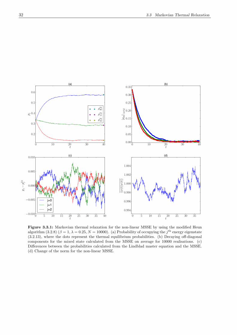
Figure 3.3.1: Markovian thermal relaxation for the non-linear MSSE by using the modified Heunalgorithm (3.2.8) (β = 1, λ = 0.25, N = 10000). (a) Probability of occupying the jth energy eigenstate(3.2.13), where the dots represent the thermal equilibrium probabilities. (b) Decaying off-diagonalcomponents for the mixed state calculated from the MSSE on average for 10000 realisations. (c)Differences between the probabilities calculated from the Lindblad master equation and the MSSE.(d) Change of the norm for the non-linear MSSE.

3.4 Local Coupling 33
3.4 Local Coupling
Since we are now able to describe thermal relaxation processes the next step is the description of
temperature gradients, giving us insight into thermal transport. In the same spirit as in the previous
chapter, we now want to couple two environments locally to our system, as shown in figure 3.4.1. The
two reservoirs are kept at different temperatures T1 and T2. The temperature gradient establishes, in
the long-time regime, some steady state, where an electric-potential difference is built up in order to
balance the thermal force acting on the electrons. At this steady state no current flows due to the
open-circuit conditions that we assume. With the help of this model we hope to get access to the
Seebeck coefficient and to further properties of thermal transport.
As a first test, we will consider a system consisting of 10 tight-binding sites as shown in figure 3.4.2.
Previously we have coupled one environment globally to the whole system with the help of a set of bath
operators Vpq. These bath operators describe transitions between the pth and qth energy eigenstates
of the total system Hamiltonian, as can be seen in the right part of the figure. In order to test our
model we propose the gedanken experiment. The system will be split into two subsystems (left side of
figure 3.4.2) with two environments acting on each part of the system at equal temperature. We know
from the previous section that the system on the right hand side, the combined system coupled globally
to one reservoir, will be driven towards thermal equilibrium of the total-system Hamiltonian. In the
other case, the left environment, described by the set of bath operators Vp1q1, introduces energy
transitions between the energy eigenstates of the Hamiltonian H1. Conversely, the right environment
is leading to energy transitions of the right subsystem described by H2. Are the two environments
that act separately able to drive the system towards thermal equilibrium of the total Hamiltonian as
well?
In the previous chapters we have not described how operators are expressed in our tight-binding
implementation. This will be done shortly in order to show how bath operators acting locally have
been constructed in the tight-binding basis of the combined system. Single-electron operators of the
10-sites system can be represented as 10 × 10 matrices in the tight-binding representation. As an
example, the total-system Hamiltonian H = H1 + H2 reads in the spatial representation (indicated
Why Open Quantum Systems?
General aspects:
‣ cannot have perfectly isolated quantum systems (closed QS)
‣ small effects play an important role in the dynamics (dissipation, decoherence)
‣ measurement implies contact with an environment
T1 T2>
Applications/ Research fields:
‣ Quantum computing / Quantum information theory
‣ (time-resolved) transport and optics
‣ driven quantum phase transitions
‣ thermal transport and thermoelectric materials
0.0
0.05
Robert Biele September 12, 2010 2/21Thermal Relaxation of Open Quantum SystemsFigure 3.4.1: Schematic representation of a temperature gradient in our 64-atom nanosystem ofsection 2.3.

34 3.4 Local Coupling
∼=HS2 , Vp2q2
T
HS1 , Vp1q1 H = HS1 +HS1 , Vpq
TT
t → ∞ρeq ∝ e−βH
t → ∞ρeq12 =?
1
2
3
4 5 6
7
8
9
10
Figure 3.4.2: Schematic representation of the proposed gedanken experiment for local coupling.
by (Ri, Rj))
H ∼=
-t 0 0 0 0 0 0 0 0-t -t -t 0 0 0 0 0 00 -t 0 0 0 0 0 0 00 -t 0 -t 0 0 0 0 00 0 0 -t -t 0 0 0 00 0 0 0 -t 0 -t 0 00 0 0 0 0 0 -t 0 00 0 0 0 0 -t -t -t -t0 0 0 0 0 0 0 -t 00 0 0 0 0 0 0 -t 0
(Ri,Rj)
, (3.4.1)
where the elements of the matrix are labeled according to figure 3.4.2. First of all, in order to express
the bath operators of the two subsystems in the matrix representation of the total system one has to
find the eigenvalues of H1 and H2,
Hi|pi = ip|pi . (3.4.2)
With this, one is able to construct the bath operators for the two subsystems
Vpiqi = λe−14β(
ip−
iq)|piqi| , (3.4.3)
given in the 5× 5 matrix representation of the sub-spaces through
V41,21∼= λ
0 0 0 0 0
0 0 0 e−14β(
12−
14) 0
0 0 0 0 00 0 0 0 00 0 0 0 0
(i,j)
= [V41,21 ]i,j , (3.4.4)
where we have chosen the bath operator of subsystem one, which describes transitions between the
fourth and the second energy eigenstates of H1 as an example. Finally, the operators from subsystem

3.4 Local Coupling 35
one are expressed in the matrix representation of the total system,
V 1
ij ∼=
U†1[Vp1q1 ]i,jU1
0 0 0 0 00 0 0 0 00 0 0 0 00 0 0 0 00 0 0 0 0
0 0 0 0 00 0 0 0 00 0 0 0 00 0 0 0 00 0 0 0 0
κ 0 0 0 00 κ 0 0 00 0 κ 0 00 0 0 κ 00 0 0 0 κ
(RiRj)
, (3.4.5)
where U†1[Vp1q1 ]i,jU1 unitarily transforms the matrix [Vp1q1 ]i,j from the energy basis into the spatial
representation of subsystem one. In the same spirit one can include Vp2q2 in the lower-right part of
a 10× 10 matrix. Finally, one obtains the set of bath operators for the total system,
Vab = V 1
ij ∪ V 2
ij . (3.4.6)
In Eq. (3.4.5) we have introduced the parameter κ, which describes how the set of bath operators from
subsystem one act onto the tight-binding sites of system two. In order to decouple the tight-binding
sites of subsystem two from the environment acting on system one, one has to set κ = 0. This means
that the left environment, coupled to system one, has no direct influence on the wave function at
positions of system two,
d φ(Ri)
i∈(6,7,8,9,10)
= 0 . (3.4.7)
This should indeed be the case in order to fulfil the concept of local coupling.
In figure 3.4.3 (right panel) one can see that the 10 level system with one global-acting environment
is approaching a steady state which coincide with the thermal equilibrium one. The dots in the panels
represent the thermal-equilibrium probabilities of occupying the corresponding energy eigenstates. In
0 50 100 150 200t
0.07
0.08
0.09
0.10
0.11
0.12
0.13
p j
0 50 100 150 200t
0.07
0.08
0.09
0.10
0.11
0.12
0.13
0.14
p j
two locally acting baths one globally coupled bath
0 50 100 150 200t
0.07
0.08
0.09
0.10
0.11
0.12
0.13
0.14
p j
j=0j=1j=2j=3j=4j=5j=6j=7j=8j=9
Figure 3.4.3: Relaxation process for the 10-sites tight-binding system of figure 3.4.2. Left: Relax-ation process for the case of two locally acting baths operators. Right: Thermal relaxation processfor one globally coupled reservoir. Points in both panels represent the equilibrium probabilities(β = 0.3, λ = 0.1, = 0, t = 0.5).
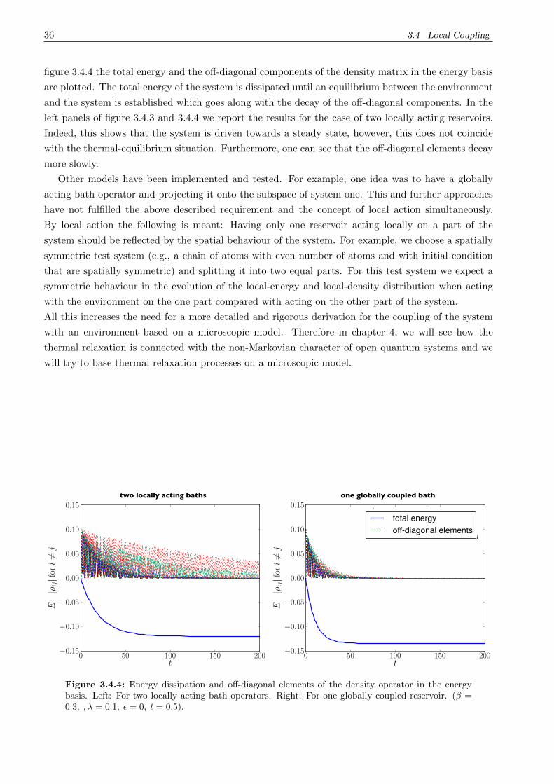
36 3.4 Local Coupling
figure 3.4.4 the total energy and the off-diagonal components of the density matrix in the energy basis
are plotted. The total energy of the system is dissipated until an equilibrium between the environment
and the system is established which goes along with the decay of the off-diagonal components. In the
left panels of figure 3.4.3 and 3.4.4 we report the results for the case of two locally acting reservoirs.
Indeed, this shows that the system is driven towards a steady state, however, this does not coincide
with the thermal-equilibrium situation. Furthermore, one can see that the off-diagonal elements decay
more slowly.
Other models have been implemented and tested. For example, one idea was to have a globally
acting bath operator and projecting it onto the subspace of system one. This and further approaches
have not fulfilled the above described requirement and the concept of local action simultaneously.
By local action the following is meant: Having only one reservoir acting locally on a part of the
system should be reflected by the spatial behaviour of the system. For example, we choose a spatially
symmetric test system (e.g., a chain of atoms with even number of atoms and with initial condition
that are spatially symmetric) and splitting it into two equal parts. For this test system we expect a
symmetric behaviour in the evolution of the local-energy and local-density distribution when acting
with the environment on the one part compared with acting on the other part of the system.
All this increases the need for a more detailed and rigorous derivation for the coupling of the system
with an environment based on a microscopic model. Therefore in chapter 4, we will see how the
thermal relaxation is connected with the non-Markovian character of open quantum systems and we
will try to base thermal relaxation processes on a microscopic model.
0 50 100 150 200t
−0.15
−0.10
−0.05
0.00
0.05
0.10
0.15
E|ρ
ij|for
i=j
0 50 100 150 200t
−0.15
−0.10
−0.05
0.00
0.05
0.10
0.15
E|ρ
ij|for
i=j
one globally coupled bath
0 50 100 150 200t
−0.8
−0.6
−0.4
−0.2
0.0
0.2
0.4
0.6
Eρ i
ji=
j
total energyoff-diagonal elements
two locally acting baths
Figure 3.4.4: Energy dissipation and off-diagonal elements of the density operator in the energybasis. Left: For two locally acting bath operators. Right: For one globally coupled reservoir. (β =0.3, ,λ = 0.1, = 0, t = 0.5).

4 Non-Markovian description of Open Quantum
Systems
Based on the analysis of thermal relaxation and local coupling in the Markovian dynamics in the
previous chapter, we have arrived at the conclusion that there is the need for a more fundamental
description of thermal relaxation processes. Therefore, by taking a step back and not assuming the
bath to be δ-correlated, we expect to gain deeper insight into relaxation processes and open system
dynamics. Hence, this chapter is dedicated to the description of non-Markovian dynamics through
the NMSSE
i∂t|φ(t) = HS |φ(t)+ λ
α
γα(t)Sα |φ(t)
− iλ2
α,β
Sα
t
0
dτ e−iHSτSβCαβ(τ) |φ(t− τ) , (4.0.1)
which has been derived at the end of section 2.1. The influence of the environment onto the system
enters through the bath correlation function Cαβ(τ) and the coloured noise with
γα(t) = 0 , (4.0.2)
γ∗α(t)γβ(t) = Cαβ(t− t) . (4.0.3)
In contrast to the Markovian picture of the previous chapter, the change of the wave function at
time t does not only depend on the present state but also on the history of the wave function. This
aspect does not appear in the description of closed quantum systems. In closed systems the future
is fully characterised by the present state and is independent of how the system evolved towards this
state in the past. The non-Markovian behaviour originates from the fact that the dynamics of the
closed system is expressed in the reduced Hilbert space of the system.
In the first part of the chapter we will focus on the theoretical foundations of stochastic thermal
relaxation. The question arises whether the NMSSE is able to drive the system towards thermal
equilibrium. In addition, it will be shown that the BSSE (2.1.41) suggested in chapter 2 does not
satisfy the requirements for thermal relaxation. However, from this lack of success we will reach an
idea of how to construct a time-local stochastic Schrodinger equation, which is able to describe thermal
relaxation processes from first principles. To this end, the corresponding master equation has to be
constructed, where in the non-Markovian case the Ito calculus cannot be applied. With the help of the
master equations we are then able to discuss the conditions for thermal relaxation. We will see that
the bath correlation function plays a pivotal role in these processes. To this end, the bath correlation
function Cαβ(τ) and the bath operators Sα will be derived starting from a specific microscopic model
38 4.1 Non-Markovian Thermal Relaxation
for the system-bath coupling. As a result, we will be able to judge whether the model is suitable
to describe thermal relaxation processes at a microscopic level. At the end of the chapter we will
numerically test the derived model and the time-convolutionless SSE.
4.1 Non-Markovian Thermal Relaxation
As we have seen in the previous chapters, the stochastic Schrodinger equation is able to describe
mixed-system dynamics by an ensemble of wave functions evolving under the influence of stochastic
processes. First of all, in order to investigate non-Markovian relaxation processes one has to find
the corresponding master equation. With this corresponding master equation one is able to address
the issues of steady states and conditions for thermal relaxation processes. As mentioned before, the
Ito calculus is only applicable for white-noise processes. However, in the non-Markovian case one
encounters with coloured noise which is not δ-correlated. A stochastic calculus for coloured noise
is not so extensively investigated as the Ito calculus. However, studies in the weakly or strongly
coloured-noise regime have been reported [45].
Therefore, one has to find an alternative procedure for deriving an equation of motion for the density
operator corresponding to the stochastic Schrodinger equation. Inspired by an idea of Gaspard [22], a
comparable master equation for the NMSSE up to fourth order in λ can be derived by performing a
perturbative expansion in λ. An idea for the future would be to take a closer look at non-Markovian
stochastic calculus and develop the former beyond perturbative approaches leading to a ‘correct’
corresponding equation on average.
4.1.1 The Corresponding Master Equation
A master equation corresponding to the non-Markovian SSE (4.0.1) can be derived in the spirit of
Gaspard [22] by performing a perturbative expansion in the coupling parameter λ and the resulting
equation reads
dρS(t)
dt= − i[HS , ρS(t)]
+ λ2
t
0
dτ
α,β
C∗αβ
(τ) Sα ρS(t) e−iHSτSβe
iHSτ
+ λ2
t
0
dτ
α,β
Cαβ(τ) e−iHSτSβe
iHSτ ρS(t) Sα
− λ2
t
0
dτ
α,β
Cαβ(τ) Sα e−iHSτSβeiHSτ ρS(t)
− λ2
t
0
dτ
α,β
C∗αβ
(τ) ρS(t) e−iHSτSβe
iHSτ Sα +O(λ4), (4.1.1)
where the operators Sα have been assumed to be hermitian. In the following, the former will be called
second-order master equation. At this point we will not go through the derivation due to the
4.1.1 The Corresponding Master Equation 39
fact that the procedure can be found in the literature [22]. Nevertheless, one can profit from working
through this type of deduction.
To this end, a corresponding master equation for the balanced stochastic Schrodinger equa-
tion,
i∂t|φ(t) =HS + λ
α
γα(t)Sα − iλ2
α,β
SαTαβSβ
|φ(t) , (4.1.2)
will be derived by using the perturbative approach due to Gaspard. In this equation T is given by
Tαβ(t) =
t
0
dτ e−iHSτCαβ(τ) . (4.1.3)
First of all, the balanced SSE has to be transformed into the interaction picture,
∂t|φI(t) = −λ
i γ(t)S(t) + λS(t)T (t)S(t)
|φI(t) , (4.1.4)
where the operator S(t) is given by
S(t) = eiHSt S e−iHSt (4.1.5)
and only the single-bath-operator case will be considered. The extension towards the general problem
can be done in a similar way. However, with this simplification a clearer derivation is achieved.
Furthermore, the expansion of the time-evolution operator up to second order in λ reads
|φI(t) ≈1lS − iλ
t
0
dt1 γ(t1)S(t1)− λ2
t
0
dt1 S(t1)T (t1)S(t1)
− λ2
t
0
dt1
t1
0
dt2 γ(t1)S(t1)γ(t2)S(t2)
|φI(0)+O(λ3) , (4.1.6)
correspondingly, this can be done for the ket vector,
φI(t)| ≈ φI(0)|1lS + iλ
t
0
dt1 γ∗(t1)S(t1)− λ2
t
0
dt1 S(t1)T†(t1)S(t1)
− λ2
t
0
dt1
t1
0
dt2 γ∗(t2)S(t2)γ
∗(t1)S(t1)
+O(λ3) . (4.1.7)

40 4.1 Non-Markovian Thermal Relaxation
Calculating the average density operator, |φI(t)φI(t)|, up to fourth order in λ results in
ρI(t) = ρI(0)− λ2
t
0
dt1
t1
0
dτ C∗(τ) ρI(0)S(t1)eiHSτS(t1)
− λ2
t
0
dt1
t1
0
dτ C(τ) S(t1)e−iHSτS(t1)ρI(0)
+ λ2
t
0
dt1
t
0
dt2 γ(t1)γ∗(t2) S(t1)ρI(0)S(t2) +O(λ4) , (4.1.8)
where we have used the following properties of the noise
γ(t) = 0 , (4.1.9)
γ∗(t) = 0 , (4.1.10)
γ(t)γ(t) = 0 , (4.1.11)
γ∗(t)γ∗(t) = 0 . (4.1.12)
The terms in λ3 have disappeared since the average of odd moments vanishes for Gaussian noise. By
using the identity
t
0
dt1
t
0
dt2 g(t1, t2) =
t
0
dt1
t1
0
dt2g(t1, t2) + g(t2, t1)
(4.1.13)
and
γ(t1)γ∗(t2) = C(t2 − t1) , (4.1.14)
the last term in Eq. (4.1.8) can be written as
λ2
t
0
dt1
t1
0
dt2C∗(t1 − t2) S(t1)ρI(0)S(t2) + λ2
t
0
dt1
t1
0
dt2C(t1 − t2) S(t2)ρI(0)S(t1) . (4.1.15)
4.1.1 The Corresponding Master Equation 41
After replacing t1 − t2 by τ and inserting this expression into Eq. (4.1.8), the equation simplifies to
ρI(t) = ρI(0)− λ2
t
0
dt1
t1
0
dτ C∗(τ) ρI(0)S(t1)eiHSτS(t1)
− λ2
t
0
dt1
t1
0
dτ C(τ) S(t1)e−iHSτS(t1)ρI(0)
+ λ2
t
0
dt1
t1
0
dτ C∗(τ) S(t1)ρI(0)S(t1 − τ)
+ λ2
t
0
dt1
t1
0
dτ C(τ) S(t1 − τ)ρI(0)S(t1) +O(λ4) . (4.1.16)
This can be differentiated with respect to t and using the relation ρI(t) = ρI(0)+O(λ2) for the density
matrix in the interaction picture, Eq. (4.1.16) can be written as
∂tρI(t) = − λ2
t
0
dτ C∗(τ) ρI(t)S(t)eiHSτS(t)− λ2
t
0
dτ C(τ) S(t)e−iHSτS(t)ρI(t)
+ λ2
t
0
dτ C∗(τ) S(t)ρI(t)S(t− τ) + λ2
t
0
dτ C(τ) S(t− τ)ρI(t)S(t) +O(λ4) . (4.1.17)
Transforming back into the Schrodinger picture leads to the desired master equation,
dρS(t)
dt= − i[HS , ρS(t)]
− λ2
t
0
dτ C∗(τ) ρS(t)S eiHSτS
− λ2
t
0
dτ C(τ) S e−iHSτSρS(t)
+ λ2
t
0
dτ C∗(τ) SρS(t)e−iHSτS eiHSτ
+ λ2
t
0
dτ C(τ) e−iHSτS eiHSτ ρS(t)S +O(λ4) . (4.1.18)
This master equation corresponds to the BSSE (2.1.41) up to fourth order and therefore will be called
balanced master equation.
In the next section, we will investigate whether the stationary state for these two master equations
is equivalent to the thermal equilibrium state and how this can be connected with the discrepancies
to second order in λ. We will see that the NMSSE is able to describe thermal relaxation processes
whereas the balanced SSE is not. This will give us an idea of how to construct a time-convolutionless

42 4.1 Non-Markovian Thermal Relaxation
SSE which is able to describe thermal relaxation processes.
Furthermore, changing ρ(t) to ρ(0) or ρ(τ) in the master equations (4.1.18) and (4.1.1) will not
change the correspondence to the SSEs with respect to the perturbative expansion. This means that
the perturbative approach by Gaspard may result in a variety of equations that correspond to the
SSE on average up to fourth order. This introduces a certain degree of arbitrariness into the master
equations and their derivations. This increases the demand for a unique mapping in terms of a
stochastic calculus for non-Markovian processes.
Notation and Convention
In order to make the following derivations more easily readable we will introduce or repeat the following
definitions and conventions:
Cαβ(τ) = trBρeqBBα(0)Bβ(τ)
bath correlation function
, (4.1.19)
Cαβ(ω) ≡∞
−∞
dτ e−iωτCαβ(τ)Fourier transform of Cαβ(τ)
, (4.1.20)
HCαβ(ω) ≡∞
0
dτ e−iωτCαβ(τ)‘half Fourier transform’ of Cαβ(τ)
. (4.1.21)
Furthermore, as in the previous chapters we avoid the use of the hat in cases where it is clear whether
or not an operator is meant.
4.1.2 Conditions for Thermal Relaxation
In the previous section we have derived the corresponding master equations for the non-Markovian
and balanced stochastic Schrodinger equations. In this section we will see under which conditions the
SSEs will drive the system towards a stationary state coinciding with the thermal-equilibrium density
operator,
ρeqS
=e−βHS
trS(e−βHS ), (4.1.22)
corresponding to the temperature of the bath, T = (kBβ)−1. By considering the following condition
limt→∞
dρeqS(t)
dt= 0 , (4.1.23)
we can investigate whether thermal relaxation is guaranteed. The second-order master equation (4.1.1)
can be simplified in the limit t → ∞:
dρS(t)
dt= − i[HS , ρS(t)] +
α
KαρS(t)Sα + SαρS(t)K
†α − SαKαρS(t)− ρS(t)K
†αSα
, (4.1.24)
where
Kα = λ2
β
∞
0
dτ Cαβ(τ)e−iHSτSβe
iHSτ . (4.1.25)

4.1.2 Conditions for Thermal Relaxation 43
This time-local evolution is the well-known Redfield master equation [2]. Hence, the question
arises under which conditions the thermal equilibrium density operator in Eq. (4.1.22) is a stationary
solution of the NMSSE and thus of the corresponding master equation (4.1.24). Condition (4.1.23)
and the fact that the equilibrium density operator commutes with the subsystem Hamiltonian imply
that the Redfield master equation assume the form
0 =dρeq
S
dt= Kρeq
SS + Sρeq
SK† − SKρeq
S− ρeq
SK†S . (4.1.26)
After changing to the energy basis of the system,
HS |n = n|n , (4.1.27)
S =
n,m
snm|nm| , (4.1.28)
and using the orthogonality properties of this basis, Eq. (4.1.26) can be written as
dρeqS
dt= λ2
n,m,l
|nl| snmsml
∞
0
dτ
C(τ)e−i(n−m)τe−βm + C∗(τ)e−i(m−l)τe−βm
− C(τ)e−i(m−l)τe−βl − C∗(τ)e−i(n−m)τe−βn
. (4.1.29)
We are interested in system independent conditions for the bath correlation function or for the operator
S under which the right hand side of Eq. (4.1.29) vanishes. From the definition of the bath correlation
function (4.1.19) and by assuming B to be a hermitian operator, one can conclude that
C∗(τ) = C(−τ) . (4.1.30)
As a result of this symmetry property, the half Fourier transform in Eq. (4.1.29) can be written as
HC(ω) =
∞
0
dτ C(τ)e−iωτ =1
2
∞
−∞
dτ C(τ)e−iωτ + i1
2i
∞
0
dτ
C(τ)e−iωτ − C∗(τ)eiωτ
=1
2C(ω) + iD(ω) (4.1.31)
with D(ω) being the imaginary part of the half Fourier transform. Therefore, C(ω) is a real-valued
function and furthermore, if the function HC(ω) is analytic in the upper complex half plane of ω and
vanishes faster than |ω|−1 as ω goes to infinity, one can apply the Kramers-Kronig relation [46, 47].
This relation connects the imaginary and the real part of a complex function,
D(ω) =1
2πP
∞
−∞
daC(a)
ω − a. (4.1.32)
Here, Pdenotes the Cauchy principal value of the integral. Later we will see for a specific expression
for the bath correlation function whether or not the assumptions for the Kramers-Kronig relation are
satisfied. Similarly, the half Fourier transform of the conjugate bath correlation function can be written

44 4.1 Non-Markovian Thermal Relaxation
as∞
0
dτ C∗(τ)e−iωτ = C(−ω) + i1
2πP
∞
−∞
daC(−a)
ω − a=
1
2C(−ω) + iF (ω) . (4.1.33)
Inserting equations (4.1.33) and (4.1.31) into Eq. (4.1.29) results in
dρeqS
dt= λ2
n,m,l
|nl| snmsml
12C(ωnm) + iD(ωnm)
e−βm
+12C(−ωml) + iF (ωml)
e−βm
−12C(ωml) + iD(ωml)
e−βl
−12C(−ωnm) + iF (ωnm)
e−βn
, (4.1.34)
where ωij = i − j . In order to satisfy the requirement of thermal relaxation this quantity has to
vanish. Assuming the detailed-balance relation
C(−ω) = eβω C(ω) , (4.1.35)
Eq. (4.1.34) simplifies to
dρeqS
dt= i λ2
n,m,l
|nl| snmsml
D(ωnm)e−βm + F (ωml)e
−βm
−D(ωml)e−βl − F (ωnm)e−βn
. (4.1.36)
The detailed-balance relation can be interpreted as the power spectrum of the noise. This power
spectrum has the characteristics that the probabilities for energy transitions in the system are bal-
anced according to Boltzmann statistics. It is worth mentioning that the expression (4.1.36) has only
imaginary components in the energy basis. Inserting the explicit integrals into Eq. (4.1.36) leads to
dρeqS
dt=
i λ2
2π
n,m,l
|nl| snmsml
∞
−∞
da
C(a)
1− e−β(n−m−a)
e−βm
ωmn − a
−C(a)
1− e−β(m−l−a)
e−βl
ωml − a
. (4.1.37)
In this expression there is no need to write the principal value anymore since the integral is no longer
singular. By taking a closer look at the diagonal components of Eq. (4.1.37), it can be shown that the
two terms cancel each other,
l| dρeq
S
dt|l = 0 . (4.1.38)
This can be shown by changing ωmn to −ωmn, changing the integration variable in the second integral
of Eq. (4.1.37) from a to −a, and applying the detailed-balance relation (4.1.35).
One can conclude that the NMSSE (2.1.36) has a stationary solution which coincides with the thermal-

4.1.2 Conditions for Thermal Relaxation 45
equilibrium state up to first order in λ. Furthermore, if the detailed-balance relation is satisfied, the
corresponding master equation (4.1.24) drives the system towards a stationary state that coincides
in the diagonal elements in the energy basis with the thermal-equilibrium state up to fourth order.
Additionally, neglecting either the off-diagonal components of the density matrix in the long-time
behaviour or the imaginary contribution of the half Fourier transform,
Im
∞
0
dτ C(τ)e−iωτ
= D(ω) ≈ 0 , (4.1.39)
the system will be driven towards equilibrium if the equation is considered up to fourth order. Con-
ventionally, one neglects the off-diagonal components in the long-time dynamics or one neglects the
imaginary part of the half Fourier transform in order to ensure thermal relaxation. The justification
for the second approximation is that this imaginary part can be included in the system Hamiltonian
[7], leading to the so-called Lamb shift. This means that the equilibrium density operator will not
commute with this effective Hamiltonian. Note that this Hamiltonian does not coincide with the sys-
tem Hamiltonian. Nevertheless, this energy shift will not introduce dissipative dynamics in the system
[6]. In order to ensure thermal-relaxation behaviour the bath correlation function should satisfy the
detailed-balance relation. Hence, by approximating Cαβ(τ) by a δ-function one neglects this property
of the bath correlation function. Therefore, we have included this property in an artificially manner
by incorporating these balanced transitions into the bath operators Sα in the pervious chapter.
Since we have now understood the origin of thermal relaxation processes in non-Markovian dy-
namics the next step is to check whether this is also valid for the balanced SSE (4.1.2). Thus one is
interested in whether the BSSE, which approximates the non-Markovian history of the system,
|φ(t− τ) ≈ |φ(t) , (4.1.40)
but still considers the time structure of the bath correlation function, is able to describe thermal
relaxation. Hence, we have to check whether the thermal-equilibrium density operator is a stationary
state in the limit t → ∞,
limt→∞
d ρeq(t)
dt?= 0 , (4.1.41)
for the balanced master equation (4.1.18). Using the fact that the system Hamiltonian commutes with
the equilibrium density operator and writing the former equation in the energy representation lead to
dρeqS
dt= λ2
n,k,m
|nk| snmsmk
∞
0
dτ
− C∗(τ)eimτe−βn − C(τ)e−imτe−βk (4.1.42)
+ C∗(τ)e−i(m−k)τe−βm + C(τ)e−i(n−m)τe−βm
+O(λ4) .

46 4.1 Non-Markovian Thermal Relaxation
With the help of equations (4.1.33) and (4.1.31) the former equation can be written as
dρeqS
dt= λ2
n,k,m
|nk| snmsmk
−12C(m) + iF (−m)
e−βn
−12C(m) + iD(m)
e−βk
+12C(−ωmk) + iF (ωmk)
e−βm
+12C(ωnm) + iD(ωnm)
e−βm
. (4.1.43)
By taking a closer look at the diagonal elements of the former equation, one can see that not even these
vanish. As a result, the BSSE will not be useful for the description of thermal relaxation processes.
4.1.3 Time-Convolutionless Stochastic Thermal Relaxation
The results of the previous section lead to an idea of how to construct a local-in-time SSE which is
able to describe thermal relaxation processes. Here, we present the time-convolutionless stochastic
Schrodinger equation (TCL SSE),
i∂t|φ(t) =HS + λ
α
γα(t)Sα − iλ2
α,β
Sα
t
0
dτ Cαβ(τ)e−iHSτSβ e+iHSτ
|φ(t) . (4.1.44)
This equation is an ansatz for a local-in-time SSE which is able to describe thermal relaxation processes.
In order to check whether this is satisfied the corresponding master equation will be derived. To do
that, the former equation has to be transformed into the interaction picture leading to
∂t|φI(t) = −λ
i
α
γα(t)Sα(t) + λ
α,β
Sα(t)
t
0
dτ Cαβ(τ) Sβ(t− τ)
|φI(t) . (4.1.45)
An expansion of the time-evolution operator up to second order in λ reads for the bra vector,
|φI(t) ≈1lS − iλ
α
t
0
dt1 γα(t1)Sα(t1)− λ2
α,β
t
0
dt1 Sα(t1)
t1
0
dτ Cαβ(τ) Sβ(t1 − τ)
− λ2
α,β
t
0
dt1
t1
0
dt2 γα(t1)Sα(t1)γβ(t2)Sβ(t2)
|φI(0)+O(λ3) . (4.1.46)
This equation can be used to calculate
ρI(t) = |φI(t)φI(t)| (4.1.47)
4.2 Microscopic Model for Thermal Relaxation 47
in the same spirit as in the derivation of the balanced master equation. The result reads in the
Schrodinger picture
dρS(t)
dt= − i[HS , ρS(t)]
+ λ2
t
0
dτ
α,β
C∗αβ
(τ) Sα ρS(t) e−iHSτSβe
iHSτ
+ λ2
t
0
dτ
α,β
Cαβ(τ) e−iHSτSβe
iHSτ ρS(t) Sα
− λ2
t
0
dτ
α,β
Cαβ(τ) Sα e−iHSτSβeiHSτ ρS(t)
− λ2
t
0
dτ
α,β
C∗αβ
(τ) ρS(t) e−iHSτSβe
iHSτ Sα +O(λ4) . (4.1.48)
This coincides with the second-order master equation (4.1.1) derived for the NMSSE up to fourth
order in λ. Therefore, the TCL SSE is able to describe thermal relaxation processes up to the same
order in λ as the NMSSE. However, the TCL SSE has the advantage of being local in time, leading to
a significant simplification for numerical purposes. In section 4.3.2 we will see how this equation can
be implemented numerically.
4.2 Microscopic Model for Thermal Relaxation
In this section, we will first derive an interaction potential W =
αSαBα for an electron coupled
to an electromagnetic field inside a cavity. This can also be extended to the case of many electrons.
Afterwards, we derive the bath correlation function Cαβ and investigate the coupling operators Sα and
Bα based on this microscopic model. In order to do so, we will perform a dipole approximation based
on the assumption that the typical length scale of our subsystem is small compared to the wavelengths
inside the cavity. In this approximation, we can assume the vector potential to be uniform in space,A(r, t) = A(t). Finally, we will be able to state whether the NMSSE is able to describe relaxation
processes based on this microscopic model.
4.2.1 Model
The minimal coupling Hamiltonian
HMC =
p− q A(r, t)
2
2m+ V (r) + qφ(r, t) (4.2.1)
describes a particle with charge q and mass m in an external potential V (r) coupled to an electro-
magnetic field. The relation between the electric and the magnetic field and their potentials are given
48 4.2 Microscopic Model for Thermal Relaxation
by
B(r, t) = ∇× A(r, t) , (4.2.2)
E(r, t) = − ∂
∂tA(r, t)− ∇φ(r, t) . (4.2.3)
As a result, the electric and magnetic fields are invariant under the gauge transformations
A = A+ ∇χ(r, t) , (4.2.4)
φ = φ− ∂
∂tχ(r, t) . (4.2.5)
Starting from a Coulomb gauge, ∇ · A = 0, and taking the gauge field
χ = −r · A(t) , (4.2.6)
leads to
A = A − ∇r · A(t)
= 0 , (4.2.7)
φ = φ − ∂
∂tχ = 0− r · ∂
∂tA(t) = −r · E(t) . (4.2.8)
Hence, the total Hamiltonian in Eq. (4.2.1), for N electrons interacting with the electromagnetic field
inside the cavity, can be written as
H =N
i=1
p2i
2me
+ V (ri)
+Hee − q
N
i=1
ri · E(t) +HB , (4.2.9)
where Hee describes the electron-electron interaction and HB is the Hamiltonian of the bath.
The expression for the interaction potential,
W = −q
i
ri · E(t) , (4.2.10)
now has to be quantised. By considering a tight-binding Hamiltonian for the subsystem,
HS = −t
p,l
c†pcl + c†
lcp=
p
Ωp†pp , (4.2.11)
where c†p creates an electron at position Rp and †p creates an electron in the pth energy state, the
position operator can be rewritten as
N
i=1
ri =
p,l
ψl |r|ψp†l p . (4.2.12)
In this equation ψl is the lth energy eigenfunction of the subsystem. Additionally, the electromagnetic-
field modes inside the cavity can be described as a collection of harmonic oscillators with frequencies
4.2.2 Bath Correlation Function 49
ωk,
HB =
k
ωkb†kbk , (4.2.13)
[bk, b†l] = δkl . (4.2.14)
As a result, the electric field can be written in second-quantised form as [48]
E(t) =
k
i pkbke
−iωkt − b†keiωkt
, (4.2.15)
where we have used
pk =
ωk
2V 0uk (4.2.16)
and uk is the polarisation unit vector of the kth mode. Finally, the interaction potential can be written
as
W =
l,p
glp†lp
k
ipkbke
−iωkt − b†keiωkt
=
α
SαBα (4.2.17)
with
glp = − qψl |r|ψpu , (4.2.18)
pk =
ωk
2V 0. (4.2.19)
For simplicity, we have assumed that each mode has the same polarisation direction, uk = u. One
can see that the coupling of an electron to the electromagnetic field of a cavity is linear in the system
and bath operators in dipole approximation. This has been assumed in the derivation of the SSE in
section 2.1.
4.2.2 Bath Correlation Function
In the following, the bath correlation function
Cαβ(t, t) = trB
ρeqBBα(t)Bβ(t
)
(4.2.20)
will be calculated, where we have some freedom in choosing the coupling operators Bα. In order to
obtain a more compact SSE and include all the degrees of freedoms of the bath in one correlation
function we choose the simplest case,
Bα(t) = B(t) =
k
ipkbke
−iωkt − b†keiωkt
. (4.2.21)
In this case B is a hermitian operator and thus leads to a symmetry property for the bath correlation
function,
C∗(t− t) = C(t − t) . (4.2.22)
50 4.2 Microscopic Model for Thermal Relaxation
With Eq. (4.2.21) the bath correlation function takes the form
Cαβ(t, t) = C(t, t) = −trB
ρeqB
k,j
pkpjbke
−iωkt − b†keiωkt
bje
−iωjt − b†
jeiωjt
, (4.2.23)
which is now independent of α and β. By using the notation
... = trBρeqB..., (4.2.24)
bk(t) = bke−iωkt , (4.2.25)
b†k(t) = b†
keiωkt , (4.2.26)
Eq. (4.2.23) can be written in a more compact form
C(t, t) = −
k,j
pkpjbk(t)bj(t) − b†
k(t)bj(t
) − bk(t)b†j(t)+ b†k(t)b†
j(t)
. (4.2.27)
The density operator of the bath in thermal equilibrium is given by
ρeqB
=e−βHB
trB(e−βHB ). (4.2.28)
It is possible to evaluate Eq. (4.2.27) further in the bosonic many-particle basis with the properties
|n1, n2, ...nk, ... = |n1|n2...|nk... , (4.2.29)
b†k|n1, n2, ...nk, ... =
√nk + 1|n1, n2, ...nk + 1, ... , (4.2.30)
bk|n1, n2, ...nk, ... =√nk|n1, n2, ...nk − 1, ... , (4.2.31)
HB|n1, n2, ...nk, ... =
i
ωini|n1, n2, ...nk, ... , (4.2.32)
n1, n2, ...nk, ...|n1, n
2, ...n
k, ... = δn1n
1δn2n
2...δnkn
k... . (4.2.33)
Furthermore, trB[ ... ] can be written in this basis as
trB[ ... ] =
n1,n2,...nk,...
n1, n2, ...nk, ... | ... |n1, n2, ...nk, ... , (4.2.34)
thus the terms b†k(t)b†
j(t) and bk(t)bj(t) vanish due to the properties (4.2.30)–(4.2.33) of the bosonic
many-particle basis. The term b†k(t)bj(t) can be simplified further leading to
b†k(t)bj(t
) =
n1,n2...,nk,...
n1, n2..., nk, ...ρeq
Bb†k(t)bj(t
)n1, n2..., nk, ...
=1
trB(e−βHB )δkj
∞
n1=0
n1|e−βω1n1 |n1...
∞
nk=0
nk|e−βωknk nkeiωk(t−t
)|nk
...
= δkjeiωk(t−t
)
∞
nk=0
e−βωknk nk
∞
nk=0
e−βωknk
−1
, (4.2.35)

4.2.2 Bath Correlation Function 51
where the number operator nk is given by nk = b†kbk and has eigenvalues nk. With the simplification
∞
nk=0
e−βωknk nk = − ∂
∂α
∞
nk=0
e−α
nk
α=βωk
=1− e−βωk
−2
e−βωk , (4.2.36)
where e−βωk < 1 has been assumed in order to ensure convergence of the geometric series,
b†k(t)bj(t) can finally be written as
b†k(t)bj(t
) = δkj eiωk(t−t
)
1
eβωk − 1= δkj e
iωk(t−t) n(β,ωk) . (4.2.37)
In this expression n(β,ωk) is the average occupation number of a bosonic state with frequency ωk at
temperature T = (kBβ)−1. The same procedure can be performed for the other non-vanishing term
in Eq. (4.2.27) and leads to
C(τ) =
k
p2k
n(β,ωk) + 1
e−iωkτ + n(β,ωk)e
iωkτ
, (4.2.38)
where τ = t− t. In order to calculate the sum of the bath modes one can replace these by an integral
over ω using the density of states,
k
... =
ω
D(ω)...dω (4.2.39)
with
D(ω) =ωd−1
πd−1cd. (4.2.40)
In this equation d = 2, 3 is the dimension of the cavity and c the speed of light. Furthermore,
one has to consider the dipole approximation made in the derivation of the interaction potential W .
The assumption that the subsystem is much smaller compared to the wavelengths λ of the cavity
corresponds to a maximum allowed frequency ωm in our bath spectrum. As a result, the integration
over ω goes from zero to ωm,
C(τ) =1
2V 0
ωm
0
dωD(ω)ω
n(β,ω) + 1
e−iωτ + n(β,ω)eiωτ
. (4.2.41)
The former equation is the final expression for the bath correlation function derived on a microscopic
basis. In the following, the properties of Eq. (4.2.41) will be discussed. It is worth mentioning that
the previous derivation is not only valid for an electronic system inside a cavity but also for a wide
class of system-bath couplings where the Hamiltonian of the bath is of harmonic form, for example
for phonons in a solid. In the case of electron-phonon coupling a smooth cut-off in the integral in
Eq. (4.2.41) can be chosen, which results in a less strongly oscillating bath correlation function and a
smooth power spectrum as we will see later.
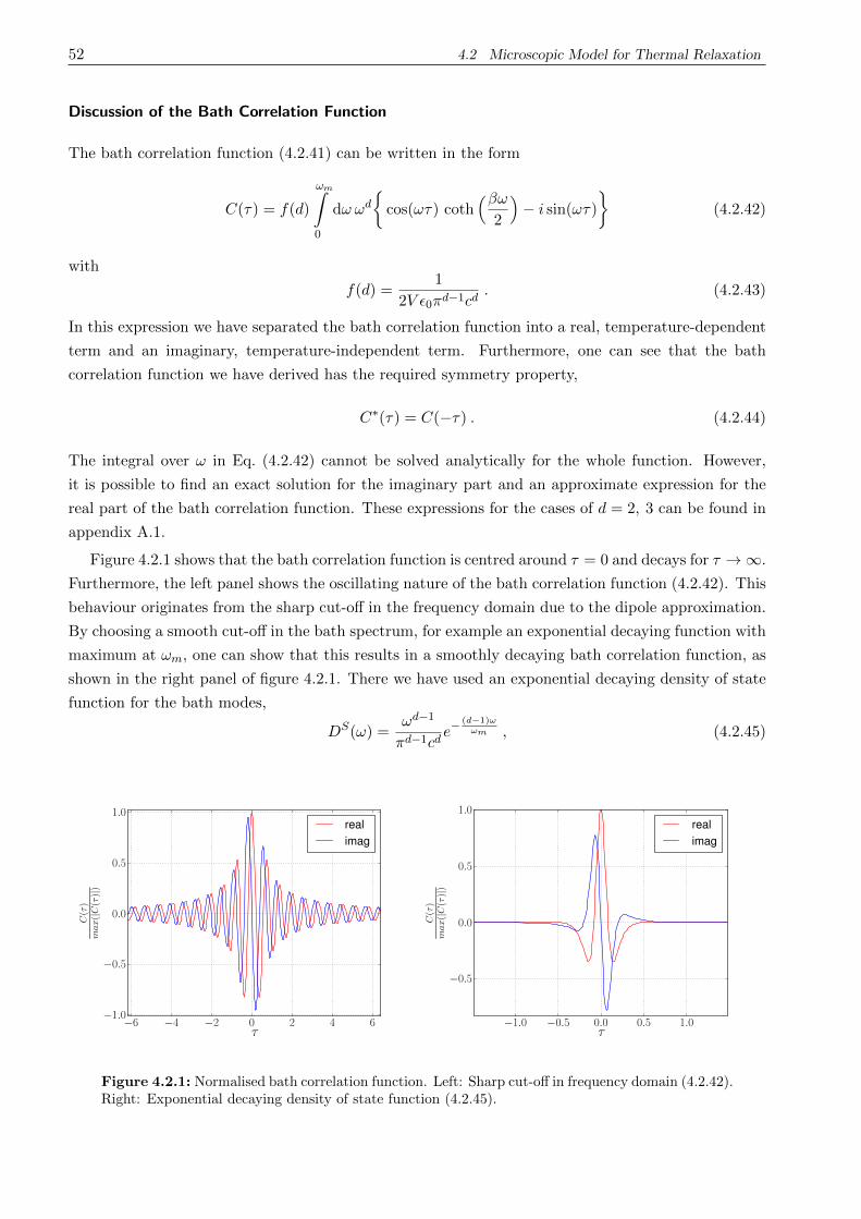
52 4.2 Microscopic Model for Thermal Relaxation
Discussion of the Bath Correlation Function
The bath correlation function (4.2.41) can be written in the form
C(τ) = f(d)
ωm
0
dω ωd
cos(ωτ) coth
βω2
− i sin(ωτ)
(4.2.42)
with
f(d) =1
2V 0πd−1cd. (4.2.43)
In this expression we have separated the bath correlation function into a real, temperature-dependent
term and an imaginary, temperature-independent term. Furthermore, one can see that the bath
correlation function we have derived has the required symmetry property,
C∗(τ) = C(−τ) . (4.2.44)
The integral over ω in Eq. (4.2.42) cannot be solved analytically for the whole function. However,
it is possible to find an exact solution for the imaginary part and an approximate expression for the
real part of the bath correlation function. These expressions for the cases of d = 2, 3 can be found in
appendix A.1.
Figure 4.2.1 shows that the bath correlation function is centred around τ = 0 and decays for τ → ∞.
Furthermore, the left panel shows the oscillating nature of the bath correlation function (4.2.42). This
behaviour originates from the sharp cut-off in the frequency domain due to the dipole approximation.
By choosing a smooth cut-off in the bath spectrum, for example an exponential decaying function with
maximum at ωm, one can show that this results in a smoothly decaying bath correlation function, as
shown in the right panel of figure 4.2.1. There we have used an exponential decaying density of state
function for the bath modes,
DS(ω) =ωd−1
πd−1cde−
(d−1)ωωm , (4.2.45)
−6 −4 −2 0 2 4 6τ
−1.0
−0.5
0.0
0.5
1.0
C(τ)
max
(|C(τ)|)
realimag
−1.0 −0.5 0.0 0.5 1.0τ
−0.5
0.0
0.5
1.0
C(τ)
max
(|C(τ)|)
realimag
Figure 4.2.1: Normalised bath correlation function. Left: Sharp cut-off in frequency domain (4.2.42).Right: Exponential decaying density of state function (4.2.45).

4.2.3 Power Spectrum and Detailed-Balance Relation 53
instead of a θ-function-like sharp cut-off in the frequency domain. In figure 4.2.2 one can see that an
increase of the cut-off frequency ωm leads to a decrease of the width (left panel) and an increase of the
amplitude (right panel). As a result one can expect a δ-function-like behaviour in the limit when ωm
goes to infinity. This begs the question whether the Markovian approximation can be performed for
the model under consideration. In order to obtain a δ-function-like behaviour of the bath correlation
function one has to choose a large cut-off frequency. As a result, the coupling strength grows drastically,
which will violate the weak coupling assumption of the underlying theory. Furthermore, due to the
dipole approximation there is a maximum allowed frequency in our bath spectrum, which also permits
the cut-off frequency to grow to infinity. For a typical system size of approximately 10 nm the cut-off
frequency is 3×10¹³Hz and ωm = 4.8 in the dimensionless units used in the plots. Due to this reasons,
the Markovian approximation cannot be applied for the system-bath coupling under consideration.
4.2.3 Power Spectrum and Detailed-Balance Relation
In this section we will calculate the Fourier transform of the bath correlation function, the so-called
power spectrum, and check whether the required detailed-balance relation is satisfied. Therefore,
C(Ω) =
∞
−∞
dτ e−iΩτC(τ) (4.2.46)
has to be calculated. This equation can be written as
C(Ω) = f(d)
ωm
0
dω ωd
∞
−∞
dτ
(n(β,ω) + 1) e−i(ω+Ω)τ + n(β,ω)e−i(Ω−ω)τ
, (4.2.47)
−5 0 5τ
0.0
0.2
0.4
0.6
0.8
|C(τ)|
max
(|C(τ)|)
ωm = 10ωm = 20ωm = 50ωm = 200
50 100 150 200 250 300ωm
0.0
0.5
1.0
1.5
2.0
max
(|C(τ)|)
×109
Figure 4.2.2: Dependence of the bath correlation function (4.2.42) on the cut-off frequency ωm
(f(d) = 1, β = 1, d = 3). Left: Normalised absolute value of C(τ,ωm). Right: Maximum value of|C(τ)| for different cut-off frequencies ωm.

54 4.2 Microscopic Model for Thermal Relaxation
where we have assumed that the order of integration can be exchanged. By using the identity for the
δ-function
δ(ω − a) =1
2π
∞
−∞
dt e−i(ω−a)t , (4.2.48)
the integration over τ can be performed and yields
C(Ω) = 2πf(d)
ωm
0
dω ωd
n(β,ω) + 1
δ(ω + Ω) + n(β,ω)δ(ω − Ω)
. (4.2.49)
Now the integration over ω can be performed,
C(Ω) = 2πf(d) Ωd
(−1)d
n(β,−Ω) + 1
θ(−Ω) θ(ωm + Ω)
+ n(β,Ω) θ(Ω) θ(ωm − Ω)
, (4.2.50)
where θ(x) is the Heaviside function defined as
θ(x) ≡
1 for x ≥ 0
0 otherwise. (4.2.51)
Eq. (4.2.50) can be simplified to
C(Ω) =
2πf(d)|Ω|d
n(β, |Ω|) + θ(−Ω)
for Ω ∈ [−ωm,ωm]
0 otherwise. (4.2.52)
Since we now have an analytical expression for the bath correlation function at hand, we can check
whether the detailed-balance relation
C(−Ω)e−βΩ = C(Ω) (4.2.53)
is satisfied. Therefore, by considering the the two cases
Ω > 0 :
C(Ω) = Ωd1
eβΩ − 1
C(−Ω) = ΩdeβΩ
eβΩ − 1
, (4.2.54)
Ω < 0 :
C(Ω) = (−Ω)de−βΩ
e−βΩ − 1
C(−Ω) = (−Ω)d1
e−βΩ − 1
, (4.2.55)
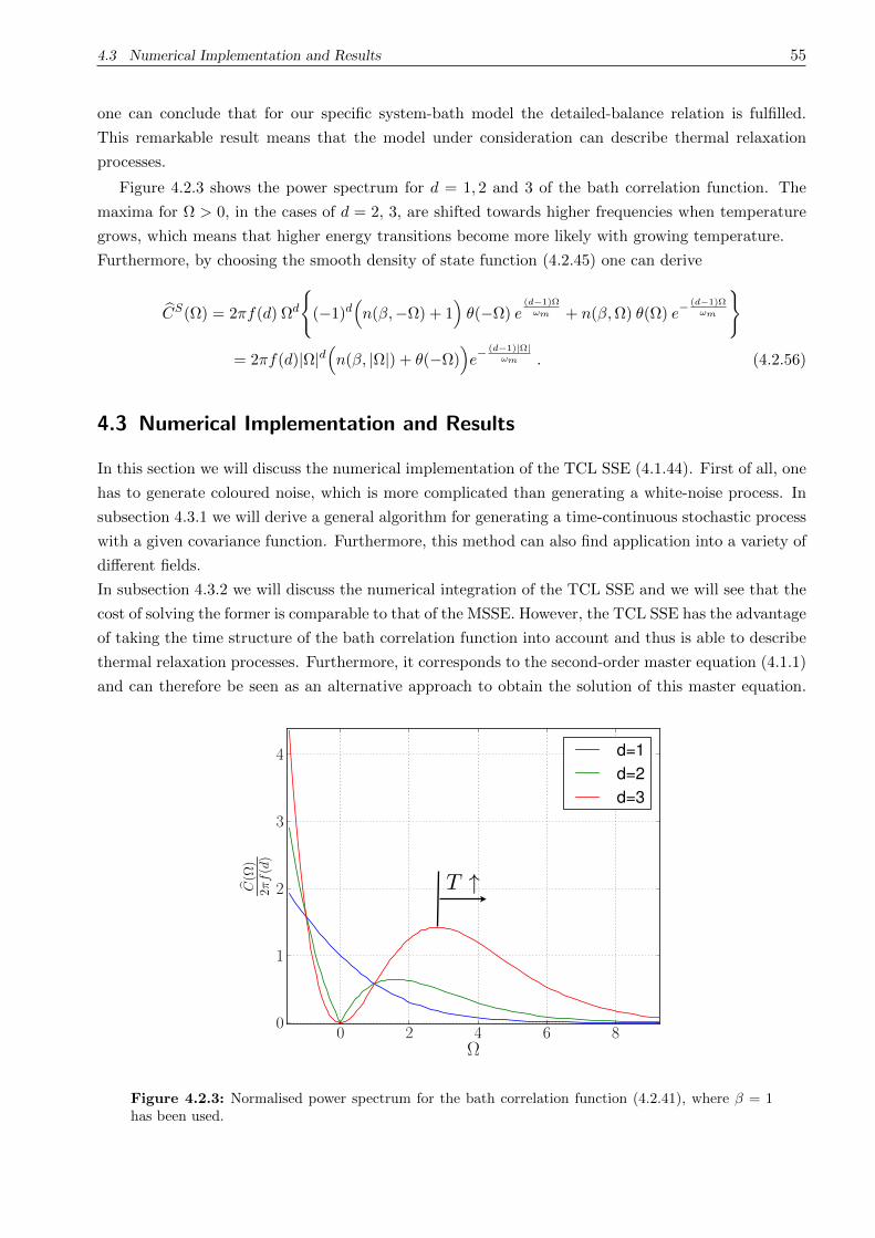
4.3 Numerical Implementation and Results 55
one can conclude that for our specific system-bath model the detailed-balance relation is fulfilled.
This remarkable result means that the model under consideration can describe thermal relaxation
processes.
Figure 4.2.3 shows the power spectrum for d = 1, 2 and 3 of the bath correlation function. The
maxima for Ω > 0, in the cases of d = 2, 3, are shifted towards higher frequencies when temperature
grows, which means that higher energy transitions become more likely with growing temperature.
Furthermore, by choosing the smooth density of state function (4.2.45) one can derive
CS(Ω) = 2πf(d) Ωd
(−1)d
n(β,−Ω) + 1
θ(−Ω) e
(d−1)Ωωm + n(β,Ω) θ(Ω) e−
(d−1)Ωωm
= 2πf(d)|Ω|dn(β, |Ω|) + θ(−Ω)
e−
(d−1)|Ω|ωm . (4.2.56)
4.3 Numerical Implementation and Results
In this section we will discuss the numerical implementation of the TCL SSE (4.1.44). First of all, one
has to generate coloured noise, which is more complicated than generating a white-noise process. In
subsection 4.3.1 we will derive a general algorithm for generating a time-continuous stochastic process
with a given covariance function. Furthermore, this method can also find application into a variety of
different fields.
In subsection 4.3.2 we will discuss the numerical integration of the TCL SSE and we will see that the
cost of solving the former is comparable to that of the MSSE. However, the TCL SSE has the advantage
of taking the time structure of the bath correlation function into account and thus is able to describe
thermal relaxation processes. Furthermore, it corresponds to the second-order master equation (4.1.1)
and can therefore be seen as an alternative approach to obtain the solution of this master equation.
0 2 4 6 8Ω
0
1
2
3
4
C(Ω
)2π
f(d)
d=1d=2d=3
T ↑
Figure 4.2.3: Normalised power spectrum for the bath correlation function (4.2.41), where β = 1has been used.

56 4.3 Numerical Implementation and Results
Especially when the size of the systems grows one expects advantaged of this wave-function approach
to open quantum systems as mentioned in the introduction.
4.3.1 Generating Correlated Noise
If one wants to calculate the dynamics of an open quantum system with the NMSSE (2.1.36) or the
TCL SSE (4.1.44) one has to generate a coloured noise γ(t) with the properties
γ(t) = 0 , (4.3.1)
γ(t1)γ(t2) = 0 , (4.3.2)
γ∗(t1)γ∗(t2) = 0 , (4.3.3)
γ(t1)γ∗(t2) = C(t2 − t1) . (4.3.4)
How can one generate such a time-continuous noise with vanishing mean and C(τ) as its covariance
function in an effective way? The fact that the bath correlation function is not given in an analytical
form for our model makes it more appropriate to use the expression for the power spectrum (4.2.52)
as an input for the noise generator.
In order to make this section more easily readable and to introduce the concepts of stochastic
time-continuous processes, we will introduce mathematical definitions and conventions needed.
Definition 1. The convolution is a mathematical operation on two functions f(t) and g(t) producing
a function (f ⊗ g)(t),
(f ⊗ g)(t) ≡∞
−∞
f(t− τ)g(τ)dτ . (4.3.5)
Definition 2. FT is a mathematical operation, called Fourier transform, acting on a function h(t)
as
FT[h(t)](ω) ≡∞
−∞
dt h(t)e−iωt . (4.3.6)
The inverse Fourier transform FT−1 acts on a function h(ω) and is defined as
FT−1[h(w)](t) ≡ 1
2π
∞
−∞
dω h(ω)eiωt . (4.3.7)
Definition 3. If x(t) is a complex stochastic process with mean x(t) = µ(t),6 the covariance func-
tion f(t1, t2) is defined as
f(t1, t2) ≡x(t1)− µ(t1)
x(t2)− µ(t2)
∗. (4.3.8)
6Note here that in general a continuos-stochastic process (e.g., a non-stationary process) can have a mean value that
depends on time. Nevertheless, for the microscopic model introduced in section 4.2 the noise is stationary. Hence, the
mean value is independent of time.
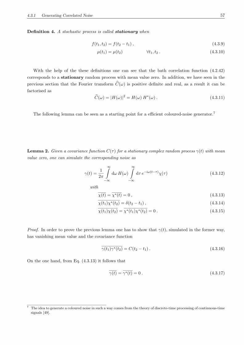
4.3.1 Generating Correlated Noise 57
Definition 4. A stochastic process is called stationary when
f(t1, t2) = f(t2 − t1) , (4.3.9)
µ(t1) = µ(t2) ∀t1, t2 . (4.3.10)
With the help of the these definitions one can see that the bath correlation function (4.2.42)
corresponds to a stationary random process with mean value zero. In addition, we have seen in the
previous section that the Fourier transform C(ω) is positive definite and real, as a result it can be
factorised asC(ω) = |H(ω)|2 = H(ω)H∗(ω) . (4.3.11)
The following lemma can be seen as a starting point for a efficient coloured-noise generator.7
Lemma 2. Given a covariance function C(τ) for a stationary complex random process γ(t) with mean
value zero, one can simulate the corresponding noise as
γ(t) =1
2π
∞
−∞
dωH(ω)
∞
−∞
dτ e−iω(t−τ)χ(τ) (4.3.12)
with
χ(t) = χ∗(t) = 0 , (4.3.13)
χ(t1)χ∗(t2) = δ(t2 − t1) , (4.3.14)
χ(t1)χ(t2) = χ∗(t1)χ∗(t2) = 0 . (4.3.15)
Proof. In order to prove the previous lemma one has to show that γ(t), simulated in the former way,
has vanishing mean value and the covariance function
γ(t1)γ∗(t2) = C(t2 − t1) . (4.3.16)
On the one hand, from Eq. (4.3.13) it follows that
γ(t) = γ∗(t) = 0 . (4.3.17)
7The idea to generate a coloured noise in such a way comes from the theory of discrete-time processing of continuous-time
signals [49].
58 4.3 Numerical Implementation and Results
On the other hand, one can calculate the covariance function for γ(t),
γ(t1)γ∗(t2) =1
4π2
dτ1 dτ2
dω1 dω2 e
−iω1(t1−τ1)H(ω1)H∗(ω2)e
iω2(t2−τ2)χ(τ1)χ∗(τ2)
=1
4π2
dτ1 dτ2
dω1 dω2 e
−iω1(t1−τ1)H(ω1)H∗(ω2)e
iω2(t2−τ2)δ(τ2 − τ1)
=1
4π2
dω1 dω2
dτ e−iτ(ω2−ω1)ei(ω2t2−ω1t1)H(ω1)H
∗(ω2)
=1
4π2
dω1 dω2 2πδ(ω2 − ω1)e
i(ω2t2−ω1t1)H(ω1)H∗(ω2)
=1
2π
dω eiω(t2−t1) C(ω)
= C(t2 − t1) . (4.3.18)
Here we have used Eq. (4.2.48) and the definition (4.1.20) of C(ω) as the Fourier transform of C(t) so
that the corresponding inverse Fourier transform is given by
C(t) =1
2π
∞
−∞
e+iωt C(ω)dω . (4.3.19)
According to lemma 2 one first has to simulate a δ-correlated noise with properties (4.3.13)–(4.3.15)
in order to generate a stationary random process with covariance function C(τ). Such a δ-correlated
noise χ(t) can be synthesised as
χ(t) ≡ a(t) + ib(t)√2
, (4.3.20)
where a(t) and b(t) are two independent real Gaussian white noises with
a(t) = b(t) = 0 , a(t1)b(t2) = 0 , (4.3.21)
a(t1)a(t2) = δ(t2 − t1) , b(t1)b(t2) = δ(t2 − t1) . (4.3.22)
As a result, χ(t) given by Eq. (4.3.20) satisfies the equations (4.3.13)–(4.3.15).
The numerical implementation of Eq. (4.3.12) is quite difficult due to the fact that two improper
integrals in time and frequency domain have to be performed. Hence, this begs the question whether
this can be simplified in order to make the numerical implementation more efficient and decrease the
error incurred by evaluating the two improper integrals numerically. With the help of definitions 1
and 2 one can write the complex conjugated of Eq. (4.3.12) in a more compact form,
γ∗(t) =FT−1[H∗(ω)]⊗ χ∗(t) . (4.3.23)
Using the convolution theorem,
FT[g ⊗ h] = FT[g] FT[h] (4.3.24)
4.3.1 Generating Correlated Noise 59
and the fact that the Fourier transform of a δ-correlated noise χ(t) is
χ(ω) ≡ FT[χ(t)] ⇒ χ(ω1)χ∗(ω2) = 2πδ(ω2 − ω1) , (4.3.25)
Eq. (4.3.23) can be written as
γ∗(t) =√2π FT−1
H∗(ω)χ∗(ω)
, (4.3.26)
where
χ(ω) =χ(ω)√2π
(4.3.27)
is a δ-correlated stochastic process in frequency domain. The former considerations lead to the final
coloured-noise generator presented in the following lemma.
Lemma 3. Given a covariance function C(τ) for a stationary complex random process γ(t) with
vanishing mean, one can generate the underlying noise as
γ(t) =
∞
−∞
dω√2π
C(ω) χ(ω) e−iωt , (4.3.28)
where χ(ω) is a stochastic process with
χ(ω) = 0 , (4.3.29)
χ(ω1)χ∗(ω2) = δ(ω2 − ω1) . (4.3.30)
Proof. It is indeed straightforward to prove the previous lemma by using the properties of the Fourier
transform and of the δ-correlated stochastic process in frequency domain,
γ(t1)γ∗(t2) =1
2π
∞
−∞
dω1
C(ω1)e
−iw1t1
∞
−∞
dω2
C∗(ω2)e
iw2t2χ(ω1)χ∗(ω2)
=1
2π
∞
−∞
dω C(ω)eiw(t2−t1)
= C(t2 − t1) . (4.3.31)
Due to lemma 3 one has to simulate δ-correlated noise in the frequency domain and then calculate
the Fourier transform of the product of the former noise with
C(ω). From a numerical point of
view, this requires only the calculation of one Fourier transform. With the help of the Fast Fourier
Transformation algorithm one can reach a scaling of M log2(M), where M is the number of time
steps of the numerical integration. Comparing this with the algorithm in lemma 2, which requires
the calculation of a Fourier transform and a convolution, a significant decrease in the numerical cost
can be achieved. Considering the fact that one has to average over many trajectories of a stochastic
process with M time steps, one can see the advantage that can be gained by the use of lemma 3.
60 4.3 Numerical Implementation and Results
4.3.2 Advantages and Implementation of the Time-Convolutionless SSE
This section shows how to implement the TCL SSE (4.1.44) highly efficient. As a result, the calcula-
tions performed by the TCL SSE are comparable fast to the calculations of the Markovian case. Due
to the fact that the time scale of the bath under consideration is much slower than the one of a typical
electronic system, it is advantageous to perform the numerical calculation in the interaction picture.
To this end, the TCL SSE needs to be transformed into the interaction picture,
i∂t|φI(t) =λ
α
γα(t)Sα(t)− iλ2
α,β
Sα(t)
t
0
dτ Cαβ(τ) Sβ(t− τ)|φI(t)
=λ
α
γα(t)Sα(t)− iλ2M(t)|φI(t) , (4.3.32)
where S(t) = eiHSt S e−iHSt is the corresponding operator to S in the interaction picture. As one can
see from the previous expression, it is possible to calculate the operator M(t) before the numerical
integration of the TCL SSE is performed. This has to be done only once and can then be used for
all the N realisations of the stochastic process and thus makes the numerical cost comparable to the
integration of the MSSE (2.1.38). The only difference is that a coloured noise has to be simulated
instead of a white-noise process. However, with the previously presented algorithm for the generation
of coloured noise this can be done most effectively. In addition, it is convenient to implement the TCL
SSE in the energy basis of the system and the TCL SSE thus reads for the single-bath-operator case
i∂tφl
I(t) =
k
λγ(t)Slk(t)− iλ2Mlk(t)
φk
I (t) , (4.3.33)
where φl
I(t) is the projection of the wave function onto the lth energy eigenstate and Mlk(t) represents
the matrix elements
Mlk(t) = l|M(t)|k . (4.3.34)
The trivial time dependence of the matrix Slk can also be evaluated before the calculation. Never-
theless, the integration in Mlk must be discretised. By considering the evolution on the time interval
tn ∈ [0, T ] with M steps (where the same convention as in Eq. (3.2.1) has been used), the time-
discretised matrix Mlk(tn) reads
Mlk(tn) = e−i(k−l)tn
j
SljSjk
tn
0
dτ C(τ)e−i(j−k)τ
≈ e−i(k−l)tn
j
SljSjk
n
m=1
C(tm)e−i(j−k)tm∆t . (4.3.35)
Hence, the bath operator S is given by the expression derived in section 4.2,
S = −q
l,p
ψl |r|ψpu †lp =
l,p
glp†lp . (4.3.36)

4.3.2 Advantages and Implementation of the Time-Convolutionless SSE 61
This leads to
Slk(tn) = e−i(k−l)tnglk , (4.3.37)
for the matrix elements in the interaction picture. After diagonalising the Hamiltonian, the matrix
elements glk can be calculated as described in appendix A.2. Collecting all the information, the final
implemented formula for a first-order integration scheme of the TCL SSE reads
φl
I(tn+1) ≈ φl
I(tn) +
k
− iλγ(tn)Slk(tn)− λ2Mlk(tn)
φk
I (tn)∆t . (4.3.38)
Comparing the numerical integration of the TCL SSE with that of the NMSSE, the former is by
far faster since it is local in time. Furthermore, in the perturbative approach by Gaspard both SSEs
lead to the same master equation. As a result, the TCL SSE is also able to describe thermal relaxation
processes. It is worth mentioning that the balanced SSE has similar numerical cost as the TCL SSE,
however, the BSSE is not suitable for the description of thermal relaxation as shown at the end of
subsection 4.1.2.
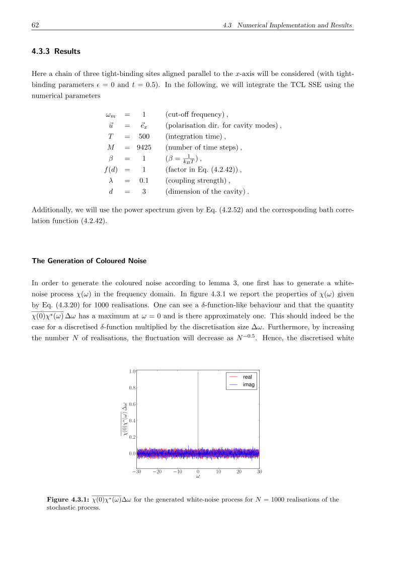
62 4.3 Numerical Implementation and Results
4.3.3 Results
Here a chain of three tight-binding sites aligned parallel to the x-axis will be considered (with tight-
binding parameters = 0 and t = 0.5). In the following, we will integrate the TCL SSE using the
numerical parameters
ωm = 1 (cut-off frequency) ,
u = ex (polarisation dir. for cavity modes) ,
T = 500 (integration time) ,
M = 9425 (number of time steps) ,
β = 1 (β = 1
kBT) ,
f(d) = 1 (factor in Eq. (4.2.42)) ,
λ = 0.1 (coupling strength) ,
d = 3 (dimension of the cavity) .
Additionally, we will use the power spectrum given by Eq. (4.2.52) and the corresponding bath corre-
lation function (4.2.42).
The Generation of Coloured Noise
In order to generate the coloured noise according to lemma 3, one first has to generate a white-
noise process χ(ω) in the frequency domain. In figure 4.3.1 we report the properties of χ(ω) given
by Eq. (4.3.20) for 1000 realisations. One can see a δ-function-like behaviour and that the quantity
χ(0)χ∗(ω)∆ω has a maximum at ω = 0 and is there approximately one. This should indeed be the
case for a discretised δ-function multiplied by the discretisation size ∆ω. Furthermore, by increasing
the number N of realisations, the fluctuation will decrease as N−0.5. Hence, the discretised white
−30 −20 −10 0 10 20 30ω
0.0
0.2
0.4
0.6
0.8
1.0
χ(0)χ
∗ (ω)∆
ω
realimag
Figure 4.3.1: χ(0)χ∗(ω)∆ω for the generated white-noise process for N = 1000 realisations of thestochastic process.

4.3.3 Results 63
noise has the correct scaling property and satisfies the normalisation condition for the δ-function,
∞
−∞
dω χ(0)χ∗(ω) = 1 . (4.3.39)
After one has generated the white noise one can simulate the coloured process using lemma 3.
In figure 4.3.2 we show a single realisation of the coloured-noise process. Not surprisingly, the noise
appears as a continuous function of time due to the fact that the time t enters Eq. (4.3.28) in a
non-stochastic form through the exponential function. Figure 4.3.3 shows the comparison between
the input power spectrum given by Eq. (4.2.52) and the power spectrum obtained from the generated
noise for an average over 90000 independent realisation. The correspondence appears satisfactory,
although a finite imaginary part is present throughout the frequency domain. In conclusion, the in
0 100 200 300 400 500t
−1.5
−1.0
−0.5
0.0
0.5
1.0
1.5
2.0
γ(t)
realimag
Figure 4.3.2: The real and imaginary part of a single realisation of the coloured noise generatedaccording to lemma 3. One can see that the noise appears as a continuous function of time.
−1.0 −0.5 0.0 0.5 1.0ω
0
2
4
6
8
10
T −Tdτ
e−iωτγ(0)γ
∗ (τ)
realimagC(ω)
Figure 4.3.3: Power spectrum for the coloured noise obtained from Eq. (4.3.28) for N = 90000. Theagreement of the input power spectrum given by Eq. (4.2.52) and the power spectrum obtained fromthe generated noise appears acceptable for N = 90000 realisations.

64 4.3 Numerical Implementation and Results
lemma 3 proposed method can be applied to generate a coloured noise with a given power spectrum.
Time-convolutionless Thermal Relaxation
In the following we will confirm whether the TCL SSE is able to describe thermal relaxation processes.
To this end, we will integrate the TCL SSE with the first-order integration scheme given by Eq. (4.3.38)
for the microscopic model considered in section 4.2. Figure 4.3.4 shows the probabilities pj of occupying
the jth energy eigenstate evolve in time towards the equilibrium values. It seems that the system has
not reached a proper steady state due to the existence of low-frequency oscillations in the dynamics.
This might be due to the fact that thermal equilibrium is reached for the limit t → ∞ which is not
considered here. Besides this, in subsection 4.1.2 we have seen that the imaginary part of the half
Fourier transform hinders the system to reach the thermal equilibrium precisely. However, in this
calculation we are not neglecting this term. In calculations with master equations this imaginary part
can be neglected effortless. However, in the stochastic wave-function approach this is more complicated
due to the fact that this term is connected with the stochastic noise on average. It should be in general
possible to neglect this term for the non-Markovian SSE but needs to be investigated further.
0 100 200 300 400 500t
0.0
0.2
0.4
0.6
0.8
p j
j =0j =1j =2
0 100 200 300 400 500t
−0.3
−0.2
−0.1
0.0
0.1
0.2
ρeq jj−p j
j =0j =1j =2
Figure 4.3.4: Time-convolutionless thermal relaxation for the microscopic model derived in section4.2. Left: Shows the probabilities pj of occupying the jth energy eigenstate calculated by Eq. (3.2.13).Right: Shows the differences between the calculated probabilities pj and the equilibrium probabilities.It appears that the system is evolving towards the thermal-equilibrium probabilities. Nevertheless,low-frequency oscillations seem still be present.
5 Conclusion and Outlook on Future Work
In this thesis we have presented a systematic study of thermal relaxation processes with respect to
stochastic wave-function methods. To this end, we have derived in chapter 2 a non-Markovian SSE
due to Gaspard [22] and have introduced the concepts of the stochastic description of open quantum
systems. With these concepts we have studied in chapter 3 thermal relaxation processes for Marko-
vian systems. The unsuccessful attempt to describe temperature gradients in Markovian systems has
resulted in the demand for a more fundamental description of thermal relaxation processes. There-
fore, we have studied relaxation processes in non-Markovian systems and have derived a microscopic
model for the system-bath coupling in chapter 4. On the one hand, this derived model satisfies the
approximations performed in the derivation of the non-Markovian SSE and, one the other hand, is
able to describe thermal relaxation processes. Furthermore, we have presented a time-local SSE which
is able to describe relaxation processes as well.
Markovian Dynamics
In chapter 3 we have studied stochastic Markovian dynamics in the context of thermal relaxation.
With the help of the Ito calculus the properties of the Markovian SSE and its relation to the master
equation approach had been presented. The stochastic behaviour of the MSSE and the fact that the
norm is not conserved for a single trajectory can cause unstable numerics. Hence, we have introduced
a non-linear SSE that conserves the norm in higher order than the linear SSE. Furthermore, we have
seen that both SSE’s correspond to the same master equation on average. We showed that the non-
linear as well as the linear version of the MSSE can be applied for efficient numerical calculation. By
calculating the expectation values according to Eq. (3.2.13) and using a complex noise, it tremendously
decreases the number of necessary realisations for the average and allows the use of larger step sizes
∆t. In this way, the linear SSE is comparable to the non-linear SSE with respect to the convergence
of numerical integrations. In addition, we have tested different discrete-time approximations for the
MSSE, namely with the Euler-Maruyama method, the modified Heun algorithm and the standard
Heun method. It had been found that the modified Heun algorithm is the most suitable method of
choice for our purposes. Furthermore, we have shown that the Markovian SSE is able to describe
thermal relaxation processes heuristically. However, the attempt to study qualitative temperature
gradients in open systems for this heuristic model has failed.
Non-Markovian Relaxation
In order to find a more fundamental description of thermal relaxation processes we have studied
non-Markovian dynamics. To this end, we have investigated the conditions of relaxation processes.
It had been found that the non-Markovian SSE corresponds to the second-order master equation
given by Eq. (4.1.1). For this master equation the long-time limit had been studied with respect to

66 Chapter 5. Conclusion and Outlook on Future Work
thermal relaxation. As a result, we have found that the bath correlation function has to satisfy the
detailed-balance relation (4.1.35) in order to ensure thermal relaxation for the non-Markovian SSE.
For the purpose of studying more realistic open quantum systems, we have considered a specific
model for the system-bath coupling. Namely an electronic system coupled to the electromagnetic
field of a cavity in dipole approximation. Starting from the minimal coupling Hamiltonian (4.2.1)
we have derived an interaction potential in second-quantised form, given by Eq. (4.2.17). With the
help of this potential we have calculated the bath correlation function and we have proven that the
detailed-balance relation is fulfilled. This means that the model under consideration is able to describe
thermal relaxation processes from first principles. In addition, we have suggested a time-local SSE
and have shown that this equation of motion is also able to describe thermal relaxation processes.
Furthermore, we have presented a general algorithm for generating a coloured noise with a given
correlation function, which find its application into a variety of different fields. Finally, we have
tested this algorithm numerically by integrating the time-convolutionless SSE for the model discussed
previously. To this end, we presented a first-order integration scheme for the time-local SSE and have
shown how to calculate the bath operators which enter the equation of motion.
Considering the open question we presented, we are now able to state the conditions for ther-
mal relaxation processes and we have seen how these conditions enters the stochastic Schrodinger
equation. Additionally, we have shown that thermal relaxation processes can be described from first
principles for the model under consideration. Furthermore, for the model of an electron coupled to the
electromagnetic field of a cavity, the Markovian approximation violates the conditions for relaxation
processes from first principles. Moreover, the time-convolutionless SSE is able to describe relaxation
processes from first principles and the cost of solving the former is comparable to that of the Marko-
vian SSE. Thus it can be seen as an alternative approach for the study of thermoelectricity besides
the Markovian approach.
Future Work
Since a better understanding of thermal relaxation processes has been reached, one can investigate
temperature gradients in non-Markovian open quantum system dynamics. This can allow a systematic
study of thermoelectric effects based on a microscopic model. Ideally this can lead to an idea of how
this could make thermoelectric materials more efficient. However, in order to reach a more realistic
description of the underlying processes, the model needs to be extended. A suggestion could be to
study the correlated dynamics of ions and electrons which are both coupled to the environment. A first
step in this direction has already been taken recently by the introduction of an approach to quantum
molecular dynamics [36].
In addition, the derived model for the interaction can be applied to a wide class of systems. An
idea would be to investigate the electron-phonon coupling in non-Markovian dynamics with respect to
thermal relaxation processes. With the help of this, one can, for example, study nanosystems placed
on the surface of a solid by considering the interaction of the phonon modes with the electrons in the
nanosystem.
Moreover, the description of particle-particle interaction in the stochastic wave-function approach
has the potential to be investigated. Recently an approach in this direction has been done by presenting
the theory of stochastic time-dependent current-density-functional [13]. An idea would be to apply this

67
theory first to the simple example of two interacting electrons in a tight-binding-like model. For this
case one is able to compare the effective single-particle approach with the original interacting many-
body problem. This will give insight to the question of how to construct single-particle bath operators
by starting from the exact bath operator for the many-body problem. Furthermore, considering
particle-particle interaction within the stochastic wave-function approach can contribute to the debate
of whether the stochastic approach differs from the master equation approach. If one is able to predict
a significant difference in the dynamics between both approaches, one might be able to suggest an
experiment that clarifies this conflict.

A Appendix
A.1 Expressions for the Bath Correlation Function
The bath correlation function
C(τ) =1
2V 0πd−1cd
ωm
0
dω ωd
cos(ωτ) coth
βω2
− i sin(ωτ)
(A.1.1)
for an electronic system coupled to an electromagnetic field inside a d-dimensional cavity, derived in
subsection 4.2.2, can be evaluated further. The imaginary term of the correlation function can be
integrated analytically and leads for d = 2, 3 to
Im[C2D(τ)] =−1
2V 0π c2
(2− τ2ω2
m) cos(ωmτ) + 2τωm sin(ωmτ)− 2
τ3
, (A.1.2)
Im[C3D(τ)] =−1
2V 0π2c3
τωm(6− τ2ω2
m) cos(τωm) + (3τ2ω2m − 6) sin(τωm)
τ4
. (A.1.3)
The real part of Eq. (A.1.1) cannot be evaluated analytically. However, it can be approximated by
splitting the integral from zero to ωm over the coth function into two integrals
Re[C(τ)] ≈ 1
2V 0πd−1cd
2β
0
dω ωd cos(ωτ)2
βω+
ωm
2β
dω ωd cos(ωτ)
, (A.1.4)
where in the first integration the coth(x) has been approximated by x−1 and in the second integration
by one. The integrals can be performed analytically, which leads to
Re[C2D(τ)] ≈ 1
2V 0πc2
−2τ
β
1 + cos
2τ
β
+ 2
τωm cos(ωmτ) + sin
2τ
β
−2− τ2ω2
m
sin(ωmτ)
τ3,
(A.1.5)
Re[C3D(τ)] ≈
6− 4τ
2
β2 cos2τ
β
− (6− 3τ2ω2
m) cos(τωm) + 8τ
βsin
2τ
β
+ τωm(τ2ω2
m − 6) sin(τωm)
τ42V 0π2c3.
(A.1.6)
70 A.2 Matrix Elements for the Bath Operator S
A.2 Matrix Elements for the Bath Operator S
In the following we will calculate the matrix elements glp for the derived bath operator,
S = −qψl |r|ψpu †lp =
l,p
glp†lp . (A.2.1)
The result is not only applicable for the TCL SSE but can also be used for the integration of for
example the NMSSE, the Redfield equation or for the second-order master equation (4.1.1). In order
to calculate the matrix elements glp, one has to introduce a spatial representation for the tight-binding
system. We have decided to use Gaussian functions centred at L atomic positions Rk, with this the
wave function can be represented for a 2D tight-binding model as
φ(x, y) =L
i=1
cif2D(x, y, Ri,σ) , (A.2.2)
where f2D(x, y, Ri,σ) are 2D Gaussian functions with variance σ centred at positions Rj = (xj , yj)
and the ci are complex coefficients. The normalised Gaussian functions reads
f2D(x, y, Ri,σ) =1√2πσ2
e−(x− xi)2 + (y − yi)2
4σ2 . (A.2.3)
By assuming that the bath modes inside the cavity are polarised in x-direction, we can derive
glp = −q
i,j
cilcjp
∗∞
−∞
dx
∞
−∞
dy f2D(x, y, Rj ,σ)f2D(x, y, Ri,σ)x
= −q
2
i,j
cilcjp
∗e−(xi − xj)2 + (yi − yj)2
8σ2 (xi + xj) , (A.2.4)
where cilis the ith tight-binding component of the lth energy eigenfunction of the system. Hence, the
time-discretised matrix elements for the bath operator in the interaction picture are
Slp(tn) = −q
2e−i(p−l)tn
i,j
cilcjp
∗e−(xi − xj)2 + (yi − yj)2
8σ2 (xi + xj) . (A.2.5)

Bibliography
[1] W. Pauli, Festschrift zum 60. Geburtstage A. Sommerfelds, 1928.
[2] A. G. Redfield, IBM J. Res. Dev. 1, 19 (1957).
[3] G. Lindblad, Comm. Math. Phys 48, 119 (1976).
[4] S. Nakajima, Prog. Theor. Phys. 20, 948 (1958).
[5] R. Zwanzig, J. Chem. Phys. 33, 1338 (1960).
[6] H.-P. Breuer and F. Petruccione, The Theory of Open Quantum Systems, Oxford University
Press, 2002.
[7] U. Weiss, Quantum Dissipative systems, World Scientific, Signapore, 1999.
[8] N. van Kampen, Stochastic Processes in Physics and Chemistry, Elsevier, 2007.
[9] J. Dalibard, Y. Castin, and K. Mø lmer, Phys. Rev. Lett. 68, 580 (1992).
[10] K. Mø lmer, Y. Castin, and J. Dalibard, J. Opt. Soc. Am. 10, 524 (1993).
[11] H. Breuer, W. Huber, and F. Petruccione, Comput. Phys. Commun. 104, 46 (1997).
[12] C. Gardiner, A. S. Parkins, and P. Zoller, Phys. Rev. A 46, 4363 (1992).
[13] R. D’Agosta and M. Di Ventra, Phys. Rev. B 78, 165105 (2008).
[14] A. Einstein, Ann. Phys. (Leipzig) 322, 549 (1905).
[15] v. H. Houten, L. W. Molenkamp, and C. W. J. Beenakker, Semicond. Sci. Technol. 7,
B215 (1992).
[16] M. Paulsson and D. Supriyo, Phys. Rev. B 67, 4 (2003).
[17] J. K. Freericks, V. Zlatic, and A. M. Shvaika, Phys. Rev. B 75, 16 (2007).
[18] P. N. Butcher, J. Phys.: Condens. Matter 2, 4869 (1990).
[19] H.-L. Engquist and P. W. Anderson, Phys. Rev. B 24, 1151 (1981).
[20] Y. Dubi and M. Di Ventra, Nano Lett. 9, 97 (2009).
[21] D. G. Cahill, W. K. Ford, K. E. Goodson, G. D. Mahan, A. Majumdar, H. J. Maris,
R. Merlin, and S. R. Phillpot, J. Appl. Phys. 93, 793 (2003).
[22] P. Gaspard and M. Nagaoka, J. Chem. Phys. 111, 5676 (1999).
72 A Bibliography
[23] H. Feshbach, Ann. Phys. (N.Y.) 19, 287 (1962).
[24] H. Feshbach, Ann. Phys. (N.Y.) 5, 357 (1958).
[25] M. V. Berry, J. Phys. A 10, 2083 (1977).
[26] A. Voros, Ann. Inst. Henri Poincare 24, 31 (1976).
[27] A. Voros, Ann. Inst. Henri Poincare 26, 343 (1977).
[28] M. Shapiro, J. Ronkin, and P. Brumer, Chem. Phys. Lett. 148, 177 (1988).
[29] S. Zelditch, Duke Mathematical Journal 55, 919 (1987).
[30] S. Hortikar and M. Srednicki, Phys. Rev. Lett. 80, 1646 (1998).
[31] M. Baxter and A. Rennie, Financial Calculus: An Introduction to Derivative Pricing, vol-
ume 9, Cambridge University Press, 1996.
[32] I. Karatzas and S. Shreve, Brownian Motion and Stochastic Calculus, Springer, New York,
2nd edition, 1991.
[33] P. Protter, Stochastic Integration and Differential Equations: A New Approach, Springer,
New York, 1995.
[34] J. Steele, Stochastic Calculus and Financial Applications, Springer, New York, 2001.
[35] G. Ghirardi and P. Pearle, Phys. Rev. A 42, 78 (1990).
[36] H. Appel and M. Di Ventra, Phys. Rev. B 80, 212303 (2009).
[37] W. Strunz, Phys. Rev. A 54, 2664 (1996).
[38] W. Strunz, Phys. Lett. A 9601 (1996).
[39] C. Gardiner, Handbook of Stochastic Methods, volume 55, Springer, 2003.
[40] W. Boyce, Adv. Appl. Probab. 10, 172 (1978).
[41] H. J. Kushner, Ann. Probab. 2, 40 (1974).
[42] H. J. Kushner and P. G. Dupuis, Numerical Methods for Stochastic Control Problems in
Continuous Time, volume 36, Springer, 2001.
[43] P. E. Kloeden and E. Platen, Numerical Solution of Stochastic Differential Equations,
Springer, 1999.
[44] P. Glasserman, Monte Carlo Methods in Financial Engineering, Springer, 2003.
[45] R. F. Fox, J. Stat. Phys. 46, 1145 (1987).
[46] R. Kronig, J. Opt. Soc. Am. 12, 547 (1926).
[47] J. S. Toll, Phys. Rev. 104, 1760 (1956).

A Bibliography 73
[48] W. Schleich, Quantum Optics in Phase Space, Wiley, 2001.
[49] A. Oppenheim and A. Willsky, Signals and Systems, Prentice Hall, 2nd edition, 1996.
Acknowledgment
First of all, I want to thank Prof. Roberto D’Agosta for time he has invested in me by helping
me trough this work and that he always lent me an ear.
I am also very thankful to Prof. Carsten Timm who gave me the possibility to write the thesis in
collaboration with the Nano-bio Spectroscopy Group in San Sebastian. With his constructive criticism
he has taught me a lot.
I am especially grateful to all the members of the Nano-bio Spectroscopy Group where I always
felt welcome throughout this year from the first day on. Also the discussion I had with them had been
extremely helpful.

Erklarung
Hiermit erklare ich, dass ich diese Arbeit im Rahmen der Betreuung im Institut fur Theoretische
Physik in Dresden und in der European Theoretical Spectroscopy Facility in San Sebastian ohne
unzulassige Hilfe Dritter verfasst und alle Quellen als solche gekennzeichnet habe.
Robert Biele
Dresden, den 04.11.2011