mediatum.ub.tum.demediatum.ub.tum.de/doc/997484/997484.pdf · TECHNISCHE UNIVERSITAT M UNCHEN...
187
Beyond Boolean Modeling in Systems Biology Dominik M. Wittmann CMB — IBIS Helmholtz Zentrum M¨ unchen Zentrum Mathematik Technische Universit¨ at M¨ unchen October 2010
Transcript of mediatum.ub.tum.demediatum.ub.tum.de/doc/997484/997484.pdf · TECHNISCHE UNIVERSITAT M UNCHEN...
Beyond Boolean Modeling
in
Systems Biology
Dominik M. Wittmann
CMB — IBIS
Helmholtz Zentrum
Munchen
Zentrum Mathematik
Technische Universitat
Munchen
October 2010

TECHNISCHE UNIVERSITAT MUNCHEN
Zentrum Mathematik — Lehrstuhl M12 (Biomathematik)
“Beyond Boolean Modeling in Systems Biology”
Dominik M. Wittmann
Vollstandiger Abdruck der von der Fakultat fur Mathematik der Technischen Uni-
versitat Munchen zur Erlangung des akademischen Grades eines
Doktors der Naturwissenschaften
genehmigten Dissertation.
Vorsitzender:
Univ.-Prof. Dr. Anusch Taraz
Prufer der Dissertation:
1. Univ.-Prof. Dr. Dr. Fabian J. Theis
2. Univ.-Prof. Dr. Rupert Lasser
3. Univ.-Prof. Dr. Alexander Bockmayr, Freie Universitat Berlin
(schriftliche Beurteilung)
Die Dissertation wurde am 7. Oktober 2010 bei der Technischen Universitat Munchen
eingereicht und durch die Fakultat fur Mathematik am 25. Marz 2011 angenommen.


To my auntin Memoriam

Acknowledgements
First and foremost, I would like to thank the many people who have accom-
panied me over the last three years.
My supervisor Prof. Fabian Theis, for his unwavering optimism, his en-
couragements and, of course, for his undertaking my introduction into the
world of science.
Profs. Rupert Lasser and Hans-Werner Mewes, who willingly agreed to
be members of my thesis committee, for their valuable comments and crit-
icisms.
Dr. Nilima Prakash, for her uplifting interest in our collaboration, her
imparting as much of her knowledge about neural development to me as I
could grasp, and for the patience all this required.
Florian, for many good advices — scientific ones and others —, some of
which I should have paid better attention to, for endless discussions about
science and related stuff, for coffee that deserves the name, and for many
useful comments on this thesis.
Daniel, my fellow mathematician, for keeping me connected to the world
of mathematics by organizing our seminars and workshops, for always read-
ily agreeing to discuss math problems with me, and for proof-reading this
thesis in as diligent a way as only he is capable of.
The entire CMB group, for some good collaborations and, of course, for
all our nice bbqs.
All the people at the IBIS, for a stimulating working atmosphere and
many nice chats during lunch or over a cup of coffee.
My “old” friends back in Regensburg, for never tiring of trying to convince
me that there is more to life than science.
My parents, for all their unconditional support, which nothing I could
write would do justice to.
Abstract
In this thesis, we mathematically investigate generalizations and modifications of Booleanmodels, as introduced in theoretical biology by Stuart Kauffman. A variable in a Boolean modelassumes only two values, zero and one. It develops in discrete time-steps, where its value at atime-point is determined by the values of some of the other variables at the previous time-pointaccording to a Boolean update function. Kauffman, at first, studied large-scale Boolean models,where the dependencies between variables as well as the update functions are chosen randomly.These random Boolean models are generic models of genome-wide regulatory networks. Theycan exhibit ordered and robust as well as chaotic and perturbation-prone dynamics. Kauffmanhypothesized that regulatory networks in living organisms operate at the boundary betweenboth dynamic regimes, which is called the critical boundary.
First, we relax the biologically implausible binary discretization and study random modelswhose variables take values in discrete, finite sets. The critical boundary of these models isdetermined analytically. It is an inverse proportionality between the average number of regula-tors per variable and a parameter measuring the heterogeneity of the update functions. If theseupdate functions are unbiased, i.e. assume each value with equal probability, the heterogeneityis minimal in the Boolean case; it does, however, not necessarily increase with the mean numberof discrete states per variable. By biasing the update functions the heterogeneity can be madearbitrarily small, allowing for increasing numbers of regulators per variable along the criticalboundary. We conclude by investigating the synchronization of ensembles of random models,which may, for instance, represent cells in an experimental sample.
Second, we study Boolean models that are derived from networks of signed interactions,such as gene regulatory networks, in which a genetic interaction can typically be classifiedas either activating or inhibiting. The update function of a variable is defined as a logicalcombination of the variable’s activating and inhibiting regulators. In particular, we focus onlarge-scale Boolean models derived from networks with randomly chosen signed interactions. Inthese models, we find multiple, intricately shaped critical boundaries. The computation of theseboundaries requires us to first study the fraction of variables being one. We can analyticallycharacterize the asymptotic dynamics of this quantity, which in numeric investigations exhibitsa rich dynamical behavior including period-doublings leading to chaos. Our results fit in nicelywith Kauffman’s hypothesis.
Third, a Boolean modeling approach within a systems biology project is presented, whichled to novel insights into the regulatory mechanisms underlying brain formation during embry-onic development. We use this example to outline a possible extension of Boolean models tocontinuous dynamical systems.
vi
Zusammenfassung
In dieser Dissertation werden Erweiterungen und Modifikationen von Booleschen Modellen,wie sie ursprunglich von Stuart Kauffman in der theoretischen Biologie eingefuhrt wurden,mathematisch untersucht. Eine Variable in einem Booleschen Modell kann nur zwei moglicheZustande annehmen, Null und Eins. Sie entwickelt sich in diskreten Zeitschritten, wobei ihrWert zu einem Zeitpunkt durch die Zustande einiger der anderen Variablen zum vorhergehendenZeitpunkt gemaß einer Booleschen Update-Funktion bestimmt wird. Kauffman untersuchtezunachst grosse Boolesche Modelle, in denen die Abhangigkeitsstruktur der Variablen sowie dieUpdate-Funktionen zufallig bestimmt werden. Diese Booleschen Zufallsmodelle sind generischeModelle genomweiter Regulationsnetzwerke. Sie konnen sowohl geordnetes, robustes als auchchaotisches, storungsanfalliges Verhalten zeigen. Kauffman stellte die Hypothese auf, dass re-gulatorische Netzwerke in lebenden Organismen an der Grenze der beiden dynamischen Regimeoperieren, die als kritische Grenze bezeichnet wird.
Zunachst geben wir die biologisch unplausible binare Diskretisierung auf und untersuchenZufallsmodelle, deren Variablen Werte aus endlichen, diskreten Mengen annehmen. Die kriti-sche Grenze dieser Modelle wird analytisch bestimmt. Sie ist eine inverse Proportionalitat zwi-schen der mittleren Anzahl der Regulatoren einer Variable und einem Heterogenitatsparameterder Update-Funktionen. Wenn diese Update-Funktionen unverzerrt sind, d.h. jeden Wert mitgleicher Wahrscheinlichkeit annehmen, ist die Heterogenitat im Booleschen Fall minimal, nimmtjedoch nicht notwendigerweise mit der mittleren Anzahl der moglichen Zustande einer Variablezu. Durch eine entsprechende Verzerrung der Booleschen Funktionen lasst sich die Heterogeni-tat beliebig verkleinern, was eine wachsende Anzahl an Regulatoren pro Variable entlang derkritischen Grenze erlaubt. Abschließend untersuchen wir die Synchronisation in Ensembles vonZufallsmodellen, die beispielsweise Zellen in einer experimentellen Probe reprasentieren.
Zum zweiten studieren wir Boolesche Modelle, die von Netzwerken mit gefarbten Kan-ten abgeleitet werden, wie beispielsweise Genregulationsnetzwerken, in denen genetische In-teraktionen typischerweise als aktivierend oder inhibierend klassifiziert werden konnen. DieUpdate-Funktion einer Variable wird als eine logische Kombination der aktivierenden und in-hibierenden Regulatoren dieser Variable definiert. Wir konzentrieren uns vor allem auf großeBoolesche Modelle, die von Netzwerken mit zufallig gewahlten, gefarbten Kanten abgeleitetwurden. In diesen Modellen finden sich mehrere, nicht-trivial geformte kritische Grenzen. Umsie berechnen zu konnen, mussen wir zunachst den Anteil der Variablen mit Wert Eins verste-hen. Wir charakterisieren das asymptotische Verhalten dieser Große analytisch; in numerischenUntersuchungen zeigt sie ein reichhaltiges dynamisches Verhalten wie Periodenverdopplungenhin zum Chaos. Unsere Ergebnisse lassen sich gut mit Kauffman’s Hypothese in Einklangbringen.
Zum dritten stellen wir einen Booleschen Modellierungsansatz innerhalb eines Systembiolo-gie Projektes vor, der neue Erkenntnisse uber die regulatorischen Grundlagen der Gehirnent-wicklung in Embryonen brachte. Anhand dieses Beispiels wird eine mogliche Erweiterung vonBooleschen Modellen hin zu kontinuierlichen dynamischen Systemen beschrieben.
vii

Contents
List of Figures xiii
List of Tables xv
Notation xvii
Glossary of general biological terms xix
List of abbreviations xxi
1 Introduction 1
2 Prerequisites 9
2.1 Prerequisites from graph theory . . . . . . . . . . . . . . . . . . . . . . . 10
2.2 Prerequisites from dynamical systems theory . . . . . . . . . . . . . . . 13
2.2.1 General notions from dynamical systems theory . . . . . . . . . . 13
2.2.2 Discrete dynamical systems . . . . . . . . . . . . . . . . . . . . . 16
2.2.3 Statistical properties of discrete dynamical systems . . . . . . . . 18
2.2.4 Maps on the interval . . . . . . . . . . . . . . . . . . . . . . . . . 21
2.3 Prerequisites from Boolean logic . . . . . . . . . . . . . . . . . . . . . . 28
2.4 Prerequisites from molecular biology . . . . . . . . . . . . . . . . . . . . 31
2.4.1 Gene expression and its regulation . . . . . . . . . . . . . . . . . 31
2.4.2 Gene regulation during neural development . . . . . . . . . . . . 35
3 Boolean models and Kauffman networks 39
3.1 Boolean models . . . . . . . . . . . . . . . . . . . . . . . . . . . . . . . . 40
3.2 Boolean models of regulatory networks . . . . . . . . . . . . . . . . . . . 41
3.3 Kauffman networks . . . . . . . . . . . . . . . . . . . . . . . . . . . . . . 43
ix
CONTENTS
3.4 Order parameters and phase transitions of Kauffman networks . . . . . 44
4 Multistate Kauffman networks 49
4.1 Motivation and outline . . . . . . . . . . . . . . . . . . . . . . . . . . . . 50
4.2 Multistate models and multistate Kauffman networks . . . . . . . . . . 51
4.2.1 Multistate models . . . . . . . . . . . . . . . . . . . . . . . . . . 51
4.2.2 Multistate Kauffman networks . . . . . . . . . . . . . . . . . . . 53
4.2.3 Parameters of multistate Kauffman networks . . . . . . . . . . . 54
4.3 Dynamic regimes of multistate Kauffman networks . . . . . . . . . . . . 55
4.3.1 The Hamming distance of a Kauffman network . . . . . . . . . . 55
4.3.2 Analysis of the Hamming distance and detection of a phase tran-
sition . . . . . . . . . . . . . . . . . . . . . . . . . . . . . . . . . 57
4.3.3 Unbiased update rules . . . . . . . . . . . . . . . . . . . . . . . . 60
4.3.4 Biased update rules . . . . . . . . . . . . . . . . . . . . . . . . . 61
4.3.5 Network simulations . . . . . . . . . . . . . . . . . . . . . . . . . 65
4.4 Ensembles of trajectories . . . . . . . . . . . . . . . . . . . . . . . . . . . 67
4.4.1 A dynamical system modeling ensembles of trajectories . . . . . 67
4.4.2 A generalized Hamming distance . . . . . . . . . . . . . . . . . . 70
4.4.3 Synchronization in ensembles of trajectories . . . . . . . . . . . . 72
4.4.4 Example and simulations . . . . . . . . . . . . . . . . . . . . . . 75
4.5 Discussion . . . . . . . . . . . . . . . . . . . . . . . . . . . . . . . . . . . 77
5 Kauffman networks with generic logics 81
5.1 Motivation and outline . . . . . . . . . . . . . . . . . . . . . . . . . . . . 82
5.2 Qualitative models and Kauffman networks with generic logics . . . . . 83
5.2.1 Mappings between qualitative and Boolean models . . . . . . . . 84
5.2.2 Kauffman networks with generic logics . . . . . . . . . . . . . . . 86
5.3 The truth-content of a Kauffman network with generic logic . . . . . . . 87
5.3.1 Iterations for the truth-content . . . . . . . . . . . . . . . . . . . 88
5.3.2 Properties of the iteration functions . . . . . . . . . . . . . . . . 91
5.3.3 Attractors of the truth-content and their basins of attraction . . 98
5.3.4 Truth-stability . . . . . . . . . . . . . . . . . . . . . . . . . . . . 103
5.4 Dynamic regimes of Kauffman networks with generic logics . . . . . . . 106
5.4.1 The Hamming distance of a Kauffman network with generic logic 107
x
CONTENTS
5.4.2 Iterations for the Hamming distance . . . . . . . . . . . . . . . . 108
5.4.3 Analysis of the Hamming distance and detection of a phase tran-
sition . . . . . . . . . . . . . . . . . . . . . . . . . . . . . . . . . 109
5.5 Numeric results and network simulations . . . . . . . . . . . . . . . . . . 113
5.5.1 Biologically reasonable parameters . . . . . . . . . . . . . . . . . 113
5.5.2 Numerical investigation of truth- and bit-stability . . . . . . . . 114
5.5.3 Network simulations . . . . . . . . . . . . . . . . . . . . . . . . . 117
5.6 Discussion . . . . . . . . . . . . . . . . . . . . . . . . . . . . . . . . . . . 122
6 Discrete and continuous models of the mid-hindbrain boundary 127
6.1 Motivation and outline . . . . . . . . . . . . . . . . . . . . . . . . . . . . 128
6.2 Inference of a Boolean model of the mid-hindbrain boundary . . . . . . 129
6.2.1 Data pre-processing . . . . . . . . . . . . . . . . . . . . . . . . . 130
6.2.2 The inverse problem . . . . . . . . . . . . . . . . . . . . . . . . . 131
6.2.3 Minimization of Boolean functions . . . . . . . . . . . . . . . . . 133
6.2.4 Predictions and experimental validation . . . . . . . . . . . . . . 136
6.2.5 A Boolean model of the mid-hindbrain boundary . . . . . . . . . 137
6.3 Boolean models and continuous dynamical systems: a proof-of-principle 140
6.3.1 The general approach . . . . . . . . . . . . . . . . . . . . . . . . 140
6.3.2 A continuous model of the mid-hindbrain boundary . . . . . . . 144
6.3.3 Numeric solution . . . . . . . . . . . . . . . . . . . . . . . . . . . 145
6.4 Discussion . . . . . . . . . . . . . . . . . . . . . . . . . . . . . . . . . . . 147
7 Conclusions and Outlook 149
7.1 Boolean modeling in systems biology . . . . . . . . . . . . . . . . . . . . 150
7.1.1 Possible extensions of the model of the mid-hindbrain boundary 150
7.1.2 Inverse problems under sparsity constraints . . . . . . . . . . . . 151
7.2 Random Boolean models . . . . . . . . . . . . . . . . . . . . . . . . . . . 151
7.2.1 Structure matters . . . . . . . . . . . . . . . . . . . . . . . . . . 152
7.2.2 Topology and dynamics . . . . . . . . . . . . . . . . . . . . . . . 153
7.2.3 The state-space of Kauffman networks with generic logics . . . . 154
Index 155
References 159
xi

CONTENTS
xii
List of Figures
2.1 Graph of the map Ψ from Example 2.3 . . . . . . . . . . . . . . . . . . . 19
2.2 Bifurcation diagram and Lyapunov exponents of the logistic equation . . 23
2.3 Gene expression and regulation . . . . . . . . . . . . . . . . . . . . . . . 32
2.4 Patterning of the neural tube . . . . . . . . . . . . . . . . . . . . . . . . 36
3.1 Hill kinetics . . . . . . . . . . . . . . . . . . . . . . . . . . . . . . . . . . 42
3.2 Simulations of standard Kauffman networks . . . . . . . . . . . . . . . . 46
4.1 Schematic plots of the Hamming distance of a multistate Kauffman net-
work . . . . . . . . . . . . . . . . . . . . . . . . . . . . . . . . . . . . . . 58
4.2 Multistate Kauffman networks with unbiased update rules . . . . . . . . 62
4.3 Multistate Kauffman networks with biased update rules . . . . . . . . . 68
4.4 Synchronization in ensembles of trajectories . . . . . . . . . . . . . . . . 78
5.1 Wg,a,Kpwq, g 0, 1, . . . , 7, from (5.4)–(5.11) for different values of a and
K . . . . . . . . . . . . . . . . . . . . . . . . . . . . . . . . . . . . . . . 90
5.2 Wg,a,Kpwq, g 0, 1, . . . , 7, from (5.4)–(5.11) for large K . . . . . . . . . 99
5.3 Plots of Wgpwq for proof of Theorem 5.3 . . . . . . . . . . . . . . . . . . 103
5.4 Stable periodic orbits of the truth-content of Kauffman networks with
generic logics . . . . . . . . . . . . . . . . . . . . . . . . . . . . . . . . . 115
5.5 Bifurcation diagrams of the truth-content of unbiased Kauffman net-
works with generic logics . . . . . . . . . . . . . . . . . . . . . . . . . . . 118
5.6 Bifurcation diagrams of the truth-content of Kauffman networks with
generic logics for biologically meaningful parameters . . . . . . . . . . . 119
5.7 Bifurcation diagrams of the truth-content of Kauffman networks with
generic logics and a bias towards inhibitors — part I . . . . . . . . . . . 120
xiii
LIST OF FIGURES
5.8 Bifurcation diagrams of the truth-content of Kauffman networks with
generic logics and a bias towards inhibitors — part II . . . . . . . . . . 121
5.9 “Simulated” bifurcation diagrams of the truth-content of Kauffman net-
works with generic logics . . . . . . . . . . . . . . . . . . . . . . . . . . . 123
5.10 “Simulated” critical connectivities of Kauffman networks with generic
logics . . . . . . . . . . . . . . . . . . . . . . . . . . . . . . . . . . . . . . 124
6.1 Gene expression around the mid-hindbrain boundary at E10.5 . . . . . . 132
6.2 Karnaugh-Veitch maps for the update rules of the Boolean model of the
mid-hindbrain boundary . . . . . . . . . . . . . . . . . . . . . . . . . . . 135
6.3 Time-course of Wnt1 expression in the midbrain and at the mid-hindbrain
boundary after implantation of Fgf8-coated beads . . . . . . . . . . . . . 138
6.4 Regulatory network at the mid-hindbrain boundary obtained from liter-
ature data . . . . . . . . . . . . . . . . . . . . . . . . . . . . . . . . . . . 139
6.5 Gene expression at the mid-hindbrain boundary between E8.5 and E10.5
under wild-type and loss-of-function conditions . . . . . . . . . . . . . . 141
6.6 Boolean update functions and Hill kinetics . . . . . . . . . . . . . . . . . 142
xiv
List of Tables
2.1 Truth-tables of the Boolean operators . . . . . . . . . . . . . . . . . . . 30
4.1 Coefficients αi for Equations (4.31) and (4.32) . . . . . . . . . . . . . . . 77
5.1 Enumeration of all eight generic logics. . . . . . . . . . . . . . . . . . . . 85
6.1 Time-course of Fgf8 and En expression at the mid-hindbrain boundary
in Wnt1 mutants . . . . . . . . . . . . . . . . . . . . . . . . . . . . . 146
xv

LIST OF TABLES
xvi
Notation
a fraction of activating edges, proba-
bility for an edge to be activating,
a 1 r
A attractor of a dynamical system
αpxq Alpha-limit set of x
b net rate for reproduction and starva-
tion in the logistic equation
BpAq basin of attraction of A
Bg,a,K basin of attraction of Lg,a,K
Bδ pwq δ-neighborhood of w
c Hill exponent, degree of cooperativ-
ity
dptq Hamming distance of a Kauffman
network (order parameter)
dg,a,Kptq Hamming distance of a Kauffman
network with generic logic pg, a,Kq
(order parameter)
D iteration function for the Hamming
distance dptq of a Kauffman network
Dg,a,K iteration function for the Hamming
distance dg,a,Kptq of a Kauffman net-
work with generic logic pg, a,Kq
δx1,x2 Kronecker symbol
δx Dirac mass on x
E set of edges of G
Ec center subspace
Es stable subspace
Eu unstable subspace
fi update rule of node i
f vector of update rules, transfer func-
tion, f pfiqNi1
g generic logic
G graph
G random graph
Gpm,Nq Erdos-Renyi graph
G pPinq configuration model
γpxq orbit of x
γEuler Euler-Mascheroni constant, γEuler
0.5772
i node in G
I interval
J Jacobian matrix
Ki connectivity of node i
K mean connectivity of a Kauffman
network, mean of Pin
K Kauffman network
Lg,a,K attractor of the truth-content
wg,a,Kptq
`pζ, zq probability for ζ fields which are ran-
domly filled according to distribution
PS to contain z different entries
M number of edges in G
m mean of 1S, S Pnos
m1 mean of 1pS 1q, S Pnos
µ invariant measure
N number of nodes in G
Npiq neighbors/predecessors of node i
Ntpiq t-th generation predecessors of node
i, N1piq Npiq
ν Lebesgue measure
ωpxq Omega-limit set of x
pS heterogeneity of distribution PS
xvii
NOTATION
p heterogeneity of a Kauffman net-
work, p °Pnos pSq pS
Pin in-degree distribution
Pnos distribution of number of states
PS distribution of entries of update rules
Pretpiq predecessors of node i up to
the t-th generation, Pretpiq
pNτ piq | τ 0, 1, . . . , tq
Φ evolution function of a dynamical
system
r fraction of inhibiting edges, proba-
bility for an edge to be inhibiting,
r 1 a
ρ density of measure µ with respect to
Lebesgue measure ν
Si number of states of node i
S vector of number of states, S
pSiqNi1
Σi range of node i, Σi
t0, 1, . . . , Si 1u
t time
T time-domain of a dynamical system
u magnetization bias of a Kauffman
network
V set of nodes of G
wg,a,Kptq truth-content of a Kauffman network
with generic logic pg, a,Kq
Wg,a,K iteration function for the truth-
content wg,a,Kptq of a Kauffman net-
work with generic logic pg, a,Kq
Wsloc stable local manifold
Wuloc unstable local manifold
X state-space of a dynamical sys-
tem/Boolean algebra
xviii
Glossary of
general
biological terms
anterior
in direction of the head
caudal
towards the spinal cord
dorsal
towards the back
ectopic
expressed in an abnormal place
endogenous
expressed in a normal, unmanipulated
fashion as in a wild-type individual
explant
Here, explant means an isolated part of
tissue from an animal harvested in a ster-
ile manner. Cells are kept in their natural
environment in the hope to mimic the in
vivo situation as closely as possible.
gain-of-function experiment
In a gain-of-function experiment, the
translation of a target gene is amplified,
either by adding additional copies of that
gene on the DNA or by increasing its tran-
scription rate.
gastrulation
an early phase in embryonic development,
during which the morphology of the em-
bryo changes and the three germ layers are
formed
in situ hybridization
an experimental technique that allows lo-
calization of a specific DNA or RNA se-
quence in parts of a tissue (in situ). If the
tissue is small enough, the sequence can
be localized in the entire tissue in a whole
mount in situ hybridization.
in vitro
in a controlled environment such as a test
tube or Petri dish
in vivo
in the living organism
loss-of-function experiment
In a loss-of-function experiment, a target
gene is deactivated either by deletion of
that gene from the DNA or by inactiva-
tion of the protein.
otic vesicle
the precursor of the membranous
labyrinth of the internal ear
posterior
in direction of the tail
rostral
towards the forebrain
secreted factor/protein
Secreted factors are proteins that are se-
creted from the expressing cells and able
to diffuse through the intercellular matrix.
somite
Somites are a segmented structure in the
vertebrate embryo next to the neural tube.
Their periodic formation provides a nat-
ural time-measure for early embryonic
stages. In the mouse embryo, for in-
stance, about one somite is formed every
two hours.
ventral
towards the front
xix

GLOSSARY OF GENERAL BIOLOGICAL TERMS
xx
List of
abbreviations
acim
absolutely continuous invariant measure,
21
acip
absolutely continuous invariant probabil-
ity measure, 21
BM
Boolean model, 40
CNF
conjunctive normal form, 31
DNA
deoxyribonucleic acid, 31
DNF
disjunctive normal form, 31
i.s.L.
in the sense of Lyapunov, 14
IsO
isthmic organizer, 35
KN
Kauffman network, 43
KNGL
Kauffman network with generic logic, 86
KNMB
Kauffman network with magnetization
bias, 43
MHB
mid-hindbrain boundary, 35
miRNA
micro RNA, 33
MKN
multistate Kauffman network, 53
MM
multistate model, 51
mRNA
messenger RNA, 33
ncRNA
non-coding RNA, 33
ODE
ordinary differential equation, 144
PDE
partial differential equation, 144
QM
qualitative model, 83
RNA
ribonucleic acid, 33
rRNA
ribosomal RNA, 33
RSP
regular fixed (steady) point, 143
SKN
standard Kauffman network, 43
SSP
singular fixed (steady) point, 143
tRNA
transfer RNA, 33
xxi

LIST OF ABBREVIATIONS
xxii
1
Introduction
If the Lord Almighty had consulted me
before embarking upon Creation,
I should have recommended something simpler.
Alfonso X, King of Castile and Leon
A surprising result from the Human Genome Project is, without doubt, that the
human genome consists of considerably less genes than previously assumed. While first
estimates placed the size of the human genome at around 105 106 genes, we now
know that it consists of around 20000. Even more surprisingly, lower organisms, such
as plants, often turn out to possess considerably larger genomes. To put it bluntly,
this leads to the question of how the 20000 human genes can contain the blueprint for
something as complex as the human brain, when the 40000 rice genes encode no more
than little grains.
We now know that it is not the number of genes that is responsible for the complexity
of an organism, but its ability to specifically and accurately control the expression of
genes. As the expression of a gene is tightly regulated by the products of other genes,
a cell’s gene expression profile is the emergent property of a complex system of genetic
1
1. INTRODUCTION
interactions. Hence, after the giant task of decoding entire genomes, we now face
the even bigger challenge of unraveling the regulatory interdependencies between the
discovered genes.
This challenge is what Stuart Kauffman’s book “Origins of Order: Self-Organiza-
tion and Selection in Evolution” [Kauffman, 1993] is all about. Kauffman tackles this
daunting task in the spirit of mathematical modeling. In doing so, he heeds Einstein’s
advice that “a model should be as simple as possible, but no simpler; as complicated
as necessary, but no more.” The Boolean models of gene regulation that he puts for-
ward are, arguably, one of the simplest kinds of models for complex dynamic systems.
In a Boolean model of a gene regulatory network, genes are described by binary vari-
ables taking only discrete values 0 or 1. They develop in discrete time-steps. At each
time-point, the value of a variable is determined by a so-called update rule that de-
terministically depends upon the values of some of the other variables, the so-called
inputs, at the previous time-point. The average number of inputs per variable is called
the (mean) connectivity of the Boolean model. Update rules are often expressed in
terms of Boolean operators, such as NOT, AND and OR, which gives the name to these
models.
In his seminal paper, Kauffman [1969] proposed large-scale random Boolean models
— later called Kauffman networks — as generic models of gene regulatory networks.
Here, the inputs as well as the update rule of a variable are chosen randomly. Kauffman
argues that “proto-organisms probably were randomly aggregated nets of chemical
reactions.” By investigating random Boolean models he wishes to test “the hypothesis
that contemporary organisms are also randomly constructed molecular automata.”
Despite their simplicity, Boolean models and Kauffman networks already capture
salient features of complex dynamic systems and, thus, allow to study their properties
within a well-defined, accessible environment. For these reasons, they are popular tools
in theoretical biology and especially within the newly emerging field of systems biology.
In theoretical biology, Kauffman networks are discussed under the slogan “Living
at the edge of chaos.” We will explain in the course of this thesis that, depending on
their connectivity, Kauffman networks exhibit three characteristic dynamical behaviors,
which we term frozen (ordered), critical and chaotic. For low connectivities, they
are in the frozen or ordered phase. Here, their dynamics are dominated by short-
periodic oscillations and are robust against external perturbations. As the number
2
of inputs increases, Kauffman networks undergo a phase transition and switch into
the chaotic phase. Their time-courses no longer show a clear oscillatory behavior and
they are highly sensitive to perturbations. The boundary between the frozen and
chaotic phase is called the critical boundary or critical connectivity. Kauffman [1993]
argues that properties from the frozen as well as the chaotic phase, viz robustness and
adaptability, are important for the evolution of living organisms, and that, consequently,
their regulatory networks need to be poised at criticality, i.e. “at the edge of chaos.”
Interestingly, the (mean) connectivities of gene regulatory networks found in lower
organisms are all around two, which, as we will see, is precisely the critical connectivity
of the random Boolean models introduced by Kauffman.
Besides the study of Kauffman networks, many small- and medium-scale Boolean
models of specific biological processes have been manually curated. Such models have
been an integrative part of many systems biology research projects over the last years
[Saez-Rodriguez et al., 2007, 2009; Samaga et al., 2009; Schlatter et al., 2009; Wittmann
et al., 2009a]. They were used to analyze biological processes with the main goal of
generating hypothesis and predictions, e.g. about possible regulatory interactions.
Overview of this thesis
Considering the simplicity of Boolean models, it stands to reason to extend and modify
them in the hope to bring them closer to biological reality and to further enhance their
explanatory power. In this thesis, we study such extensions and modifications.
They are motivated from a biological point of view, by a desire to remedy certain
inadequacies of Boolean models as models of gene regulatory networks. They are in-
vestigated from a biomathematical point of view, e.g. by analyzing dynamical systems
which describe interesting quantities of modified Kauffman networks. As is typically
the case in the theory of Kauffman networks, these quantities will be obtained in mean-
field approximations and will describe generic properties in ensembles of networks. In
this thesis, we will only briefly touch these deep relations between Kauffman networks
and concepts from statistical physics. Instead, we will focus on mathematically ana-
lyzing the dynamical behavior of the mean-field quantities. Finally, the usefulness of a
possible extension of Boolean models to continuous dynamical systems is demonstrated
in a systems biology application.
3
1. INTRODUCTION
Chapter 2 contains necessary prerequisites from graph theory, dynamic systems
theory and Boolean algebra. It also provides a short introduction into the molecular
basis of gene regulation and sets the stage for our biological application in chapter 6.
Explanations of frequently used basic biological terms can also be found in the glossary
on page xix. Chapter 3 then introduces Boolean models and Kauffman networks. It
also provides some background information from statistical physics.
In chapter 4, we generalize Boolean Kauffman networks by softening the hard
binary discretization and allowing variables to assume values in general discrete, fi-
nite sets. These multistate Kauffman networks are generic models of gene regulatory
networks, in which genes are known to assume more than two functionally different
expression levels. We analytically determine the critical connectivity that separates
the biologically unfavorable frozen and chaotic phases (Theorem 4.1). This connectiv-
ity is inversely proportional to a parameter which measures the heterogeneity of the
update rules. If these update rules are unbiased, i.e. assume each value equiproba-
bly, the critical connectivity decreases when we leave the Boolean case and allow for
multiple states, albeit it does not necessarily depend on the mean number of discrete
states per variable. This decrease might lead to biologically unrealistic situations; we
are, however, able to demonstrate that the critical connectivity can be re-increased by
sufficiently biasing the update rules. The theory of Boolean Kauffman networks is ob-
tained as a special case of our more general statements. We conclude by investigating
the synchronization behavior of multistate Kauffman networks. All analytic results are
further corroborated by network simulations.
In chapter 5 we formally introduce qualitative models of gene regulatory networks
as directed graphs with signed edges according to whether a genetic interaction is acti-
vating or inhibiting. Qualitative models are what we typically obtain from experiments.
They contain less information than a Boolean model, whose update rules also precisely
specify the interplay of the various regulators of a gene. We propose to systemati-
cally convert qualitative into Boolean models via so-called generic logics, which allow
combination of activating and inhibiting influences into an update rule.
We investigate Kauffman networks whose update rules are generated by generic
logics. Similar to the bias for update rules from chapter 4, we introduce a bias towards
activating edges. We begin by studying the truth-content of Kauffman networks with
generic logics, which is an approximation of the fraction of ones (more precisely, of the
4
fraction of variables being one). The asymptotic behavior of this quantity is shown to
be essentially independent of the initial conditions, and its attractor is characterized
(Theorems 5.1, 5.2 and 5.3). We continue with numeric analyses of the truth-content.
Especially for small (biologically implausible) fractions of activating edges, the truth-
content exhibits a rich dynamical behavior including period-doublings leading to chaos
as the connectivity of the network grows. In the biologically plausible case of larger
fractions of activating edges and small connectivities, the truth-content has stable sta-
tionary dynamics. We define truth-stable Kauffman networks with generic logics as
networks whose truth-contents exhibit non-chaotic dynamics.
Our results about the truth-content of Kauffman networks with generic logics allow
us to derive a criterion for phase transitions in these networks (Theorems 5.5 and 5.6).
In numeric analyses we find multiple, intricately shaped critical boundaries, which fit
nicely into the theory of “Living at the edge of chaos.” Simulations further strengthen
the significance of our analytic results.
In chapter 6 we conclude with a systems biology application. We use this applica-
tion to outline a possible extension of Boolean models to continuous dynamical systems.
The biological process we study is an aspect of brain formation during embryonic devel-
opment viz differentiation of mid- and hindbrain. The differentiation of these two brain
regions is mediated inter alia by molecular signals emitted from the so-called isthmic
organizer, in particular, by Fgf8 and Wnt1 proteins. The isthmic organizer is charac-
terized by a well-defined pattern of locally restricted gene expression domains around
the boundary between prospective mid- and hindbrain, the mid-hindbrain boundary.
This pattern is established and maintained by a gene regulatory network that is not
yet understood in full detail.
In a first step, we set up a Boolean model of this regulatory network. To this
end, we show that a Boolean analysis of the characteristic spatial gene expression pat-
terns at the murine mid-hindbrain boundary reveals key regulatory interactions. Our
analysis employs techniques from computational logic for the minimization of Boolean
functions. In particular, we predict a maintaining rather than inducing effect of Fgf8
on Wnt1 expression, an issue that remained unclear from published data. We provide
experimental evidence that Fgf8, in fact, only maintains but does not induce Wnt1
5
1. INTRODUCTION
expression around the murine mid-hindbrain boundary.1 In combination with previ-
ously validated interactions, this finding allows us to construct a Boolean model of the
regulatory network at the mid-hindbrain boundary.
We then outline a possible way of transforming Boolean models into continuous
dynamical systems with switch-like interactions and briefly discuss the dynamical be-
havior of these systems, in particular, with respect to fixed points. We apply the
transformation to our Boolean model of the mid-hindbrain boundary. Simulations of
the resulting continuous system show that it is, indeed, competent to reproduce impor-
tant biological phenomena, such as refinements and sharpenings of expression patterns,
that could not have been captured by the Boolean model.
Main scientific contributions
Here, the main contributions of this thesis are summarized and the respective ma-
nuscripts by the author are referenced. Some of these works laid the foundation for
collaborations; manuscripts having arisen therefrom are also cited.
Chapter 4
• A general class of multistate Kauffman networks is introduced, and a criterion
for phase transitions is derived [Wittmann et al., 2010].
• A dynamical system is presented and analyzed that models ensembles of networks
as well as Kauffman networks with fuzzy logics [Wittmann and Theis, 2010a]. It
allows, for instance, to investigate the synchronization behavior of these ensem-
bles.
Chapter 5
• The concept of generic logics as a way to link qualitative and Boolean models is
introduced and studied [Wittmann and Theis, 2010b].
1Collaboration with Nilima Prakash (Institute of Developmental Genetics, Helmholtz Zentrum
Munchen)
6
• The class of Kauffman networks with generic logics is introduced and investigated
for critical phenomena. To the best of our knowledge, it is the first class of KNs
exhibiting multiple critical connectivities [Wittmann and Theis, 2010b].
Chapter 6
• A method for the analysis of spatial expression patterns is presented [Wittmann
et al., 2009a]. Applied to the gene expression profile at the mid-hindbrain bound-
ary several genetic interactions are predicted. Unknown interactions have been
experimentally validated.
• The first mathematical model of gene regulation at the mid-hindbrain boundary
is presented [Wittmann et al., 2009a]. It is further analyzed by Ansorg et al.
[2010] and Breindl et al. [2010].
• A possible transformation of Boolean models into continuous dynamical systems
is outlined [Wittmann et al., 2009b], which is also available in our MATLAB
modeling toolbox ODEfy [Krumsiek et al., 2010].
7

1. INTRODUCTION
8
2
Prerequisites
Was man nicht weiß, das eben brauchte man,
Und was man weiß, kann man nicht brauchen.
Faust, Johann Wolfgang von Goethe
According to Eykhoff [1974], a mathematical model is “a representation of the
essential aspects of an existing system (or a system to be constructed) which presents
knowledge of that system in usable form.” Mathematical models may take many forms.
It is probably one of Newton’s chief merits to have developed the language of differential
equations and dynamical systems for the statement of his laws of motion and gravity. In
many fields of science, including biomathematics, mathematical models are ever since
formulated in this language. Over the last decade, however, a new language has been
established, that of graphs and complex networks. It proved particularly suitable to
describe all kinds of complex systems, ranging from the Internet to biological systems,
such as gene regulation [Albert and Barabasi, 2002].
In this thesis, we speak both languages and are now going to introduce the necessary
concepts and techniques from each (sections 2.1 and 2.2). We will also need some
9
2. PREREQUISITES
vocabulary from Boolean algebra (section 2.3). After these mathematical prerequisites,
we familiarize the reader with the basic principles of gene expression and its regulation
as well as with our biological application from chapter 6 (section 2.4).
2.1 Prerequisites from graph theory
The study of networks has gained importance in all fields of science which require the
analysis of complex relational data. It dates back to the year 1736 when Leonard Euler
published his famous paper “Seven Bridges of Konigsberg.” The mathematical descrip-
tion of vertices and edges introduced by Euler in this publication was the foundation of
graph theory, the branch of mathematics that became the framework of complex net-
works theory. For this reason, we now introduce the basics of this field of mathematics,
for details we refer the reader to the “Modern Graph Theory” by Bollobas [1998].
Definition 2.1 (graph). An undirected (directed) graph G is an ordered pair of disjointsets pV,Eq such that V H and E is a set of unordered (ordered) pairs of elements ofV . The elements of V are the nodes of G, the elements of E are called edges.
The numbers of elements in V and E are called the order and size of G; they are
denoted by N and M , respectively. A node is usually referred to by its order i in the
set V . In an undirected graph, two nodes i, i1 P V are called adjacent (neighbors) if
pi, i1q P E. In this case, the edge pi, i1q is said to be incident in nodes i and i1, or to
join the two nodes; the two nodes i and i1 are called the end-nodes of edge pi, i1q. In a
directed graph, a node i is called predecessor or input of a node i1 and, conversely, i1 is
called successor or target of i if piÑ i1q P E.
For some node i in an undirected graph we let Npiq denote the set of its neighbors;
in the case of a directed graph, Npiq will denote the set of predecessors of i. In the latter
case, we inductively define the tuple of the t-th generation predecessors of i, Ntpiq :pNpi1q | i1 P Nt1piqq, t 1, 2, . . ., where N0piq piq. (Clearly, N1piq Npiq.) Finally,
we let Pretpiq pNτ piq | τ 0, 1, . . . , tq, t 0, 1, . . ., denote the tuple of predecessors
of i up to the t-th generation.
In an undirected graph, the degree (connectivity) Ki of a node i is the number
of incident edges. In the directed case, one distinguishes between the in-degree and
out-degree of i, which are, of course, defined as the number of inputs and targets of i,
respectively. In this thesis, we use the terms degree and connectivity also for directed
10
2.1 Prerequisites from graph theory
graphs and, by convention, refer to the in-degree. A basic topological characterization
of a graph G is given by its degree distribution P pKq, defined as the probability that
a node chosen uniformly at random has degree K or, equivalently, as the fraction of
nodes in the graph having degree K. In directed graphs we work with the (in-)degree
distribution Pin pKq.A signature of a graph G pV,Eq is a mapping σ : E Ñ t,u. A graph together
with a signature is called signed graph. In addition to the purely topological information
about interactions in a network provided by an (unsigned) graph, a signed graph also
specifies the type of the interactions. For each signature σ of G we denote the inverted
signature by σ, i.e. for each edge e P E
σ peq " if σ peq if σ peq .
Random graphs
Starting with the pioneering work of Erdos and Renyi [1959], a new line of research
began, focusing on average properties of families of graphs. The central object of study
in this subfield of graph theory is a random graph. Most generally, we can define
a random graph as a probability space whose elements are graphs. The probability
measure is often defined via a random process which yields graphs as realizations.
Such a random process is also called generative model . In here, we focus on random
graphs with a fixed number of nodes.
An important example for random graphs is the Erdos-Renyi graph, which we
present in its version for directed graphs.
Example 2.1 (Erdos-Renyi graph). For 0 ¤ m ¤ 1, let Gpm,Nq be the probabilityspace of all 2N
2(directed) graphs on N nodes, where the probability of a graph with
M edges is mM p1 mqN2M . Gpm,Nq is called Erdos-Renyi graph. An equivalentdefinition is given by the following generative model, which yields graphs on N nodes:A graph on N nodes is constructed by including each of the N2 possible (directed)edges independently with probability m.
Now, suppose we are given some random graph G, and consider the following random
experiment. Pick a realization of G and choose one of its nodes uniformly at random,
we call it i. The distribution of the random variable Ki is called the degree distribution
11
2. PREREQUISITES
of G. If G Gpm,Nq is an Erdos-Renyi graph, the degree distribution is the binomial
distribution
P pKi Kq N
K
mKp1mqNK ,
as each of the N nodes is independently chosen to be an input of i with probability
m. In the limit of large N , where mN M constant, this can be approximated by a
Poisson distribution
P pKi Kq MKeM
K!.
In the undirected case, it is a non-trivial task to define a random graph with a given
degree distribution. In the directed case, however, this is easy.
Example 2.2 (configuration model). Let Pin pKq, K 1, 2, . . . ,Kmax, Kmax ¤ N , bea distribution. We let G pPinq denote the space of all graphs on N nodes whose in-degrees are bounded by Kmax. We turn G pPinq into a probability space by defining agenerative model that yields realizations in G pPinq: For each node i pick its in-degreeKi randomly according to Pin and choose its Ki inputs randomly from among the Nnodes with equal probability. This generative model is called configuration model .
Often, random graphs are studied in the thermodynamic limit of large N . Here, we
have the following important lemma, which we generalize from Hilhorst and Nijmeijer
[1987].
Lemma 2.1. Let Kmax ¥ 1. There exists a sequence ptN qN¥Kmaxsuch that tN Ñ 8
as N Ñ 8 satisfying the following: For N ¥ Kmax let G be a realization of a randomgraph G pPinq on N nodes, where Pin as in Example 2.2. Then, the probability that forsome node i of G equals occur among the Pretpiq for 0 ¤ t ¤ tN is on the order ofOpNαq with α 0. In other words, the probability for the subgraph on Pretpiq to beacyclic as an undirected graph approaches 1 as N grows.
Proof. Let N ¥ Kmax. The following holds for a realization of a random graph G pPinqon N nodes and some randomly chosen node i: The size of Pretpiq is bounded by
|Pretpiq| ¤$&% 1Kmax . . .Kt
max Kt1
max 1Kmax 1
, Kmax ¡ 1
t , Kmax 1 .
The probability that equals occur among the Pretpiq is bounded by
1|Pretpiq|¹k1
1 k
N
1
2N1|Pretpiq| p|Pretpiq| 1q O
N2|Pretpiq|4
.
12
2.2 Prerequisites from dynamical systems theory
This is of order OpNαq with α 0 if we keep t restricted to 1 ¤ t ¤ tN , where
tN
$'&'%
βlogpNq
2 log pKmaxq , with β 1 , if Kmax ¡ 1
Nβ , with β 12, if Kmax 1 .
One commonly refers to this lemma by claiming that “in the thermodynamic limit
we may assume inputs to be independent.” We will explain this statement in Remark
4.4.
In the following, unless specified otherwise, a graph will always be directed, and a
random graph will always be given by the configuration model from Example 2.2.
2.2 Prerequisites from dynamical systems theory
For the general introduction to dynamical systems in sections 2.2.1–2.2.3 we follow
the book by Guckenheimer and Holmes [1990]. For an account of dynamical systems
as biomathematical models we refer the reader to the textbooks about mathematical
biology by Murray [2002] and De Vries et al. [2006].
2.2.1 General notions from dynamical systems theory
Let us straightaway give the most important definition.
Definition 2.2 (dynamical system). A dynamical system is a tuple pT,X,Φq consistingof a monoid T , a set X, and a function Φ : T X Ñ X satisfying Φp0, xq x andΦ pt2,Φ pt1, xqq Φ pt1 t2, xq. The function Φ is called the evolution function of thedynamical system. The set X is called state-space.
2.2.1.1 Orbits and invariant sets
Fixing x P X, the function Φx : T Ñ X, t ÞÑ Φpt, xq is called flow through x and its
graph γpxq : tΦxptq | t P T u is called orbit or trajectory of x. A subset U X of the
state-space is called invariant if for all x P U it holds γpxq U .
Let us now discuss several types of orbits. A point x P X is called fixed point or
equilibrium if Φpt, xq x for all t P T . In this case, the orbit of x is a singleton,
γpxq txu. An orbit γpxq of x is called periodic if there exists τ P T such that
13
2. PREREQUISITES
Φpt, xq Φpt τ, xq for all t P T . The smallest such τ is called the period of γpxq.Each point in γpxq is called τ -periodic point .
Often, T represents time and one chooses T N0,Z,R0 or R. If T Z or T Rone distinguishes between positive and negative invariant sets. A set U X is positive
(negative) invariant, if for all x P U and t ¥ 0 (t ¤ 0) it holds Φpt, xq P U .
Of particular interest is the asymptotic behavior of a dynamical system in the limit
of large times. We now introduce several notions to characterize this behavior. For
this, we let X be a metric space with metric d. This metric then induces a distance
function for points x P X and sets U X
distpx, Uq infx1PU
dpx, x1q .
2.2.1.2 Types of stability
We begin with the central concepts of Lyapunov and orbital stability . An orbit γpxq is
called stable in the sense of Lyapunov (i.s.L.) if for all ε ¡ 0 there is δ ¡ 0 such that
dx, x1
δ ùñ dΦpt, xq,Φpt, x1q ε for all t ¥ 0 .
Otherwise, γpxq is called unstable i.s.L. If γpxq is stable and, moreover, there is δ0 ¡ 0
such that
dx, x1
δ0 ùñ limtÑ8
dΦpt, xq,Φpt, x1q 0 ,
then γpxq is called asymptotically stable i.s.L. The orbit γpxq is called neutrally stable
if it is stable but not asymptotically stable.
If γpxq is a stable orbit i.s.L. the two orbits γpxq and γpx1q remain “synchronized”
provided x and x1 are sufficiently close in the sense of the above definition. Orbital
stability is a weaker concept of stability that relaxes the requirement of synchrony. An
invariant set U X is called orbitally stable if for all ε ¡ 0 there exists δ ¡ 0 such that
distpx, Uq δ ùñ dist pΦpt, xq, Uq ε for all t ¥ 0 .
Otherwise, U is called orbitally unstable. If U is orbitally stable and, moreover, there
is δ0 ¡ 0 such that
distpx, Uq δ0 ùñ limtÑ8
dist pΦpt, xq, Uq 0
then U is called orbitally asymptotically stable.
In this thesis, unless specified otherwise, we always work with the concept of Lya-
punov stability.
14
2.2 Prerequisites from dynamical systems theory
2.2.1.3 ω-limit points and attractors
Another important concept for the characterization of a system’s long-time behavior
are ω-limit points. A point x is called an ω-limit point of some x0 P X if there is a
sequence of times ptqqq¥0 such that tq Ñ 8 and Φ ptq, x0q Ñ x as q Ñ 8. If T Z or
T R we can also define α-limit points as limits of sequences Φ ptq, x0q where tq Ñ 8.
The sets ω px0q and α px0q of all ω-limit points and α-limit points of x0 are called the
ω-limit set and α-limit set of x0.
A more global description of the asymptotic dynamics can be given in terms of the
attractors of a dynamical system. We call a closed, invariant set A X attracting , if
there is some neighborhood U A of A such that Φpt, xq P U for t ¥ 0 and Φpt, xq Ñ A
as tÑ 8, for all x P U . A repelling set is defined analogously, replacing t by t. The
attractors of a dynamical system are its “minimal” or “irreducible” attracting sets. We
follow Guckenheimer and Holmes [1990] and make
Definition 2.3 (attractor, preliminary1). An attractor is an attracting set A X thatcontains a dense orbit.
We already got to know important examples of attracting and repelling sets.
Remark 2.1. Any asymptotically stable fixed point or periodic orbit is an attractor.Any unstable fixed point or periodic orbit is a repelling set.
2.2.1.4 Types of dynamical systems
We now list several types of dynamical systems. In a real, time-continuous dynamical
system we have T R, X Rn. Moreover, we require that for all x P X the flow
Φx : T Ñ X, t ÞÑ Φpt, xq through x and for all t P T the function Φt : X Ñ X,
x ÞÑ Φpt, xq are continuous. The set of functions tΦtut is a group with identity Φ0 and
inverse Φ1t Φt.
Each system of autonomous first order differential equations
9x ϕpxq , x P Rn ,
with a vector field ϕ : Rn Ñ Rn induces a time-continuous dynamical system if the
pertaining initial value problems
9x ϕpxqxp0q x0
(2.1)
1In section 2.2.3.1 we will somewhat relax this definition.
15
2. PREREQUISITES
have globally unique solutions for all x0 P X. According to the theorem by Picard-
Lindelof, see e.g. Coddington and Levinson [1972], this is, in particular, the case if ϕ
is globally Lipschitz-continuous. The evolution function Φ of the dynamical system is
given by the fundamental solution of (2.1). The fixed points of the dynamical system
are the zeros of the vector field ϕ.
The discrete models of gene regulation presented in this thesis give rise to dynamical
systems where X is some finite discrete set and T N0. We will study mean-field
quantities of these models, which are described by dynamical systems with X Rn
and T N0. The first kind of dynamical systems will be introduced in chapter 3. In
the remainder of this section, let us speak about dynamical systems with X Rn and
T N0 or T Z.
2.2.2 Discrete dynamical systems
Let X Rn and T N0 or T Z. We consider time-discrete dynamical systems
defined by a Cl-map Ψ : Rn Ñ Rn. If T Z we require Ψ to be a diffeomorphism.
The evolution function of the dynamical system is given by Φpt, xq Ψtpxq. If T Z,
we define Ψt Ψ1
t for t 0. In other words, an orbit γ pxp0qq of this dynamical
system is given by the iteration
xpt 1q Ψ pxptqq . (2.2)
2.2.2.1 Linear discrete dynamical systems
Let us begin with the simple case of linear Ψ. Then xpfq 0 is a fixed point of system
(2.2).
Proposition 2.1 (stability criteria). We have the following stability criteria for xpfq.
• If |λ| 1 for all eigenvalues λ of Ψ, then xpfq is asymptotically stable.
• If |λ| ¤ 1 and λ semisimple if |λ| 1 for all eigenvalues λ of Ψ, then xpfq isstable.
• Otherwise xpfq is unstable.
16
2.2 Prerequisites from dynamical systems theory
To describe the dynamics of (2.2) one often writes Rn as the direct sum of the
so-called stable, unstable and center subspaces, Rn Es ` Eu ` Ec, where
Es : span t(generalized) eigenvectors λ of Ψ | |λ| 1uEu : span t(generalized) eigenvectors λ of Ψ | |λ| ¡ 1uEc : span t(generalized) eigenvectors λ of Ψ | |λ| 1u .
Observe that, in general, the generalized eigenspaces of Ψ are invariant sets.
2.2.2.2 Non-linear discrete dynamical systems
Now, consider again the case of general Ψ and suppose xpfq is a fixed point of system
(2.2). We ask if we can describe the local behavior of system (2.2) around xpfq by the
linearized system
xpt 1q Jxptq (2.3)
with J DΨ|xpfq . In mathematical terms, we ask if the two systems are locally
conjugate at xpfq, i.e. if there exists a homeomorphism h defined in a neighborhood U
of xpfq which maps orbits of system (2.2) locally on orbits of system (2.3)
h pΨpxqq Jhpxq for all x P U .
In general, this is not the case. However, we have such a statement if the fixed point
xpfq is hyperbolic, i.e. if J has no eigenvalues on the unit circle.
Theorem 2.1 (Hartman-Grobman). If the fixed point xpfq is hyperbolic, the two sys-tems (2.2) and (2.3) are locally conjugate at xpfq via a homeomorphism h, which pre-serves the orientation of orbits.
As h preserves the orientation of orbits, the Hartman-Grobman theorem implies
Corollary 2.1. In the situation of Theorem 2.1, the type of stability of xpfq (withrespect to system (2.2)) is equal to the type of stability of ξpfq 0 with respect tosystem (2.3).
In the case of general xpfq, we have the following (weaker) stability criterion.
17
2. PREREQUISITES
Theorem 2.2 (linear stability analysis). If any eigenvalue of J DΨ|xpfq has absolutevalue larger than one, the fixed point xpfq of system (2.2) is unstable. If all eigenvaluesof J have absolute value smaller than one, the fixed point xpfq is asymptotically stable.If the largest eigenvalue modulus is one, the stability of xpfq cannot be determined bya linear analysis alone, but depends on higher-order terms. We also refer to suchequilibria as critical fixed points.
Remark 2.2. The study of a τ -periodic orbit γxppq
can be reduced to the analysis of
the fixed point xppq of the map Ψτ . This is to say, we simply define J as
J DΨτ |xppq ¹
xPγpxppqqDΨ|x
in Theorem 2.2.
If T Z (and Ψ is a Cl-diffeomorphism), one also has a (local) generalization of
the stable and unstable subspaces to non-linear systems. Let U be a sufficiently small
open neighborhood of the fixed point xpfq. We define the sets
Wsloc
xpfq
!x P U | Ψtpxq P U @ t ¥ 0 and lim
tÑ8Ψtpxq xpfq
)Wuloc
xpfq
"x P U | Ψtpxq P U @ t ¤ 0 and lim
tÑ8Ψtpxq xpfq
*.
Theorem 2.3 (stable and unstable local manifolds). The two sets Wsloc
xpfq
and
Wuloc
xpfq
are Cl-manifolds as well as positive and negative invariant sets of system
(2.2). They are tangent to the stable and unstable subspaces Es and Eu of system (2.3)at xpfq, respectively, and can be represented as graphs of functions
ws : U X Es Ñ Eu ` Ec andwu : U X Eu Ñ Es ` Ec .
We call Wsloc
xpfq
and Wu
loc
xpfq
the stable and unstable manifold of system (2.2)
at xpfq.
2.2.3 Statistical properties of discrete dynamical systems
There are two general approaches to the study of dynamical systems, we shall call them
the geometric and the statistical approach. The goal of the geometric approach, that we
have, so far, followed, is to (qualitatively) draw a phase portrait of the dynamical system
18
2.2 Prerequisites from dynamical systems theory
−2 −1 0 1 2−2
−1.5
−1
−0.5
0
0.5
1
1.5
2
x
Ψ(x
)
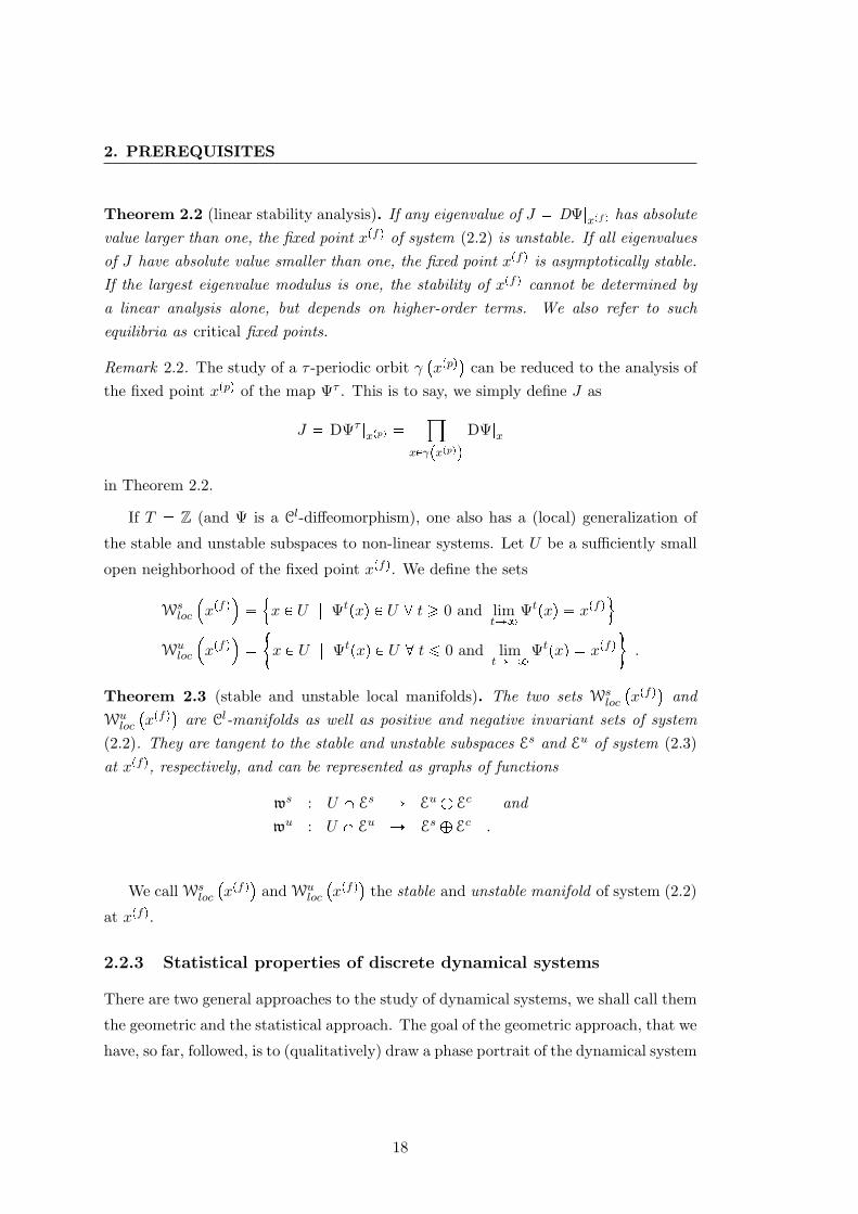
Figure 2.1: Ad Example 2.3. Graph of the map Ψ. The origin is a repellent fixed pointand the ω-limit set of Lebesgue-almost all points.
under study. The statistical approach, which we are going to outline in the following,
looks for typical properties and behaviors of a system. The distinction between typical
and exceptional properties requires the use of a measure. In here, this measure will
always be the Lebesgue measure ν. We still consider the time-discrete dynamical system
from (2.2).
2.2.3.1 Metric attractors
Let us first re-think Definition 2.3 of an attractor. Collet and Eckman [1980], in adopt-
ing the statistical point of view, describe an attractor as “the set of points to which
most points evolve.” This is to say, an attractor should (at least partially) describe
the generic behavior of a dynamical system. The following example taken from Milnor
[1985] shows that Definition 2.3 is unable to meet this requirement.
Example 2.3. Consider the dynamical system T N0, X R and Φpt, xq Ψtpxq with
Ψpxq #
4x1 x2
2, if |x| ¤ 1
0 , everywhere else.
By inspection of the graph of Ψ (cf. Figure 2.1) one observes that orbits of Lebesgue-almost all points from the real line ultimately end up in the origin. Exceptions are thetwo unstable fixed points where the graph intersects with the diagonal. The origin,however, is an unstable fixed point and no attractor according to Definition 2.3.
19
2. PREREQUISITES
From now on, we adopt the definition of attractor given by Milnor [1985]. This def-
inition is motivated by the idea that an attractor should represent the generic behavior
of a considerable portion of initial conditions. Let us make this a precise mathematical
notion. For an invariant set U X, we let
BpUq : tx P X | ωpxq Uu
denote the basin of attraction of U . In other words, BpUq consists of all points that
asymptotically end up in U . An attracting set A is called globally attracting , if XzBpAqhas measure zero. We now make
Definition 2.4 (metric attractor, Milnor [1985]). A (metric) attractor (attractor inthe sense of Milnor) is a (forward) invariant set A satisfying the following.
• The basin of attraction BpAq has positive Lebesgue measure.
• If A1 is another (forward) invariant set, which is strictly contained in A, thenBpAqzBpA1q has positive measure.
If XzBpAq is a measure zero set, we call A a global attractor.
Note that an attractor with positive measure need not attract anything outside of
itself.
2.2.3.2 Invariant and natural measures
A central concept in the statistical description of dynamical systems is that of a measure
describing the long-time distribution of orbits. We call a Borel measure µ invariant for
Ψ if µΨ1pUq µpUq for every measurable subset U X. An invariant measure µ
is a natural measure for Ψ if
µ limtÑ8
1t
t1
τ0
δΨτ pxq (2.4)
for all x in a set of positive Lebesgue measure, where δΨτ pxq denotes the Dirac mass on
Ψτ pxq. The limit in (2.4) means convergence of measures in the weak sense.1
If system (2.2) has a periodic attractor, there exists a natural measure for Ψ, viz
equally weighted point masses on the points of the attractor. In this case, the measure1A sequence of measures µt on X is said to converge weakly to the measure µ if lim inftÑ8 µtpUq ¥
µpUq for all open subsets U X.
20
2.2 Prerequisites from dynamical systems theory
has no density. We shall be particularly interested in the converse case. According to
the Radon-Nikodym theorem, see e.g. Shilov and Gurevich [1966], a measure µ that is
absolutely continuous with respect to the Lebesgue measure ν,1 has a density ρ with
respect to ν, µpUq ³U ρdν. We write acim for an absolutely continuous (with respect
to ν) invariant measure and acip if the measure is, moreover, a probability measure.
2.2.3.3 Lyapunov exponents
In the geometric approach we introduced the local stability analysis of fixed and periodic
points, cf. Theorem 2.2. Lyapunov exponents generalize the idea of eigenvalues (of a
local linearization) to give averaged contraction and expansion rates along a general
orbit, i.e. an orbit which need not be a fixed or periodic point. At each point xptq of a
(forward) orbit pxptqqt¥0 these contraction and expansion rates are measured along n
orthogonal directions and given by the singular values of the Jacobian Jptq DΨt|xp0q,i.e. by the eigenvalues of
JptqJptqJ12. The Lyapunov exponents at xp0q are defined
as the logarithms of the eigenvalues of the matrix
Λ : limtÑ8
JptqJptqJ1p2tq
, (2.5)
provided this limit exists. Given an invariant measure µ for Ψ, the multiplicative ergodic
theorem, see e.g. Ruelle [1979], guarantees existence of this limit for µ-almost all xp0qif DΨ is Holder continuous.
2.2.4 Maps on the interval
We now describe discrete dynamical systems induced by maps on the interval from a
statistical point of view. Hence, we still consider the time-discrete dynamical system
from (2.2) but now in the special case where Ψ is an endomorphism of a real interval
I rα, βs R. For a comprehensive treatment of this topic, see the books by Collet
and Eckman [1980] as well as by De Melo and van Strien [1993] or the review by
Thunberg [2001]. In the following, we often refer to attractors, orbits, etc. of system
(2.2) as attractors, orbits, etc. of the map Ψ.
1This means that νpAq 0 implies µpAq 0.
21
2. PREREQUISITES
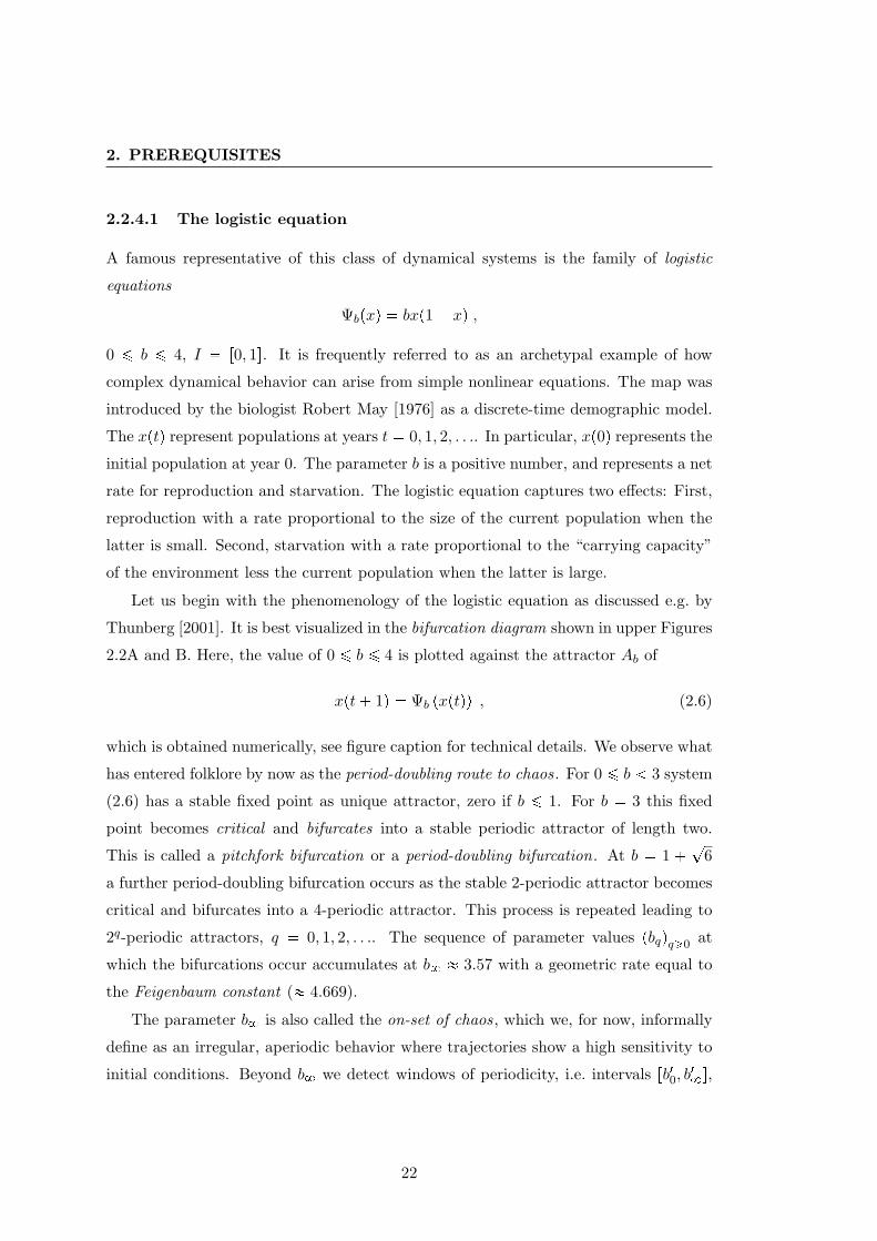
2.2.4.1 The logistic equation
A famous representative of this class of dynamical systems is the family of logistic
equations
Ψbpxq bxp1 xq ,
0 ¤ b ¤ 4, I r0, 1s. It is frequently referred to as an archetypal example of how
complex dynamical behavior can arise from simple nonlinear equations. The map was
introduced by the biologist Robert May [1976] as a discrete-time demographic model.
The xptq represent populations at years t 0, 1, 2, . . .. In particular, xp0q represents the
initial population at year 0. The parameter b is a positive number, and represents a net
rate for reproduction and starvation. The logistic equation captures two effects: First,
reproduction with a rate proportional to the size of the current population when the
latter is small. Second, starvation with a rate proportional to the “carrying capacity”
of the environment less the current population when the latter is large.
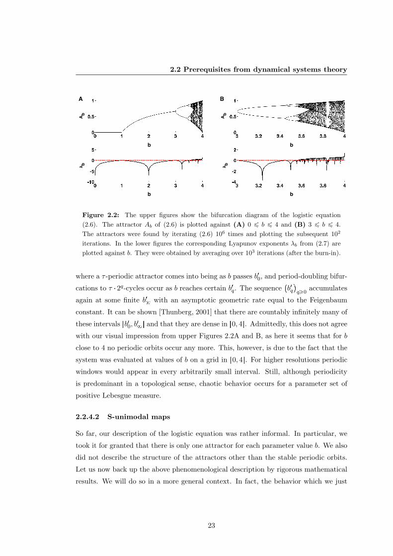
Let us begin with the phenomenology of the logistic equation as discussed e.g. by
Thunberg [2001]. It is best visualized in the bifurcation diagram shown in upper Figures
2.2A and B. Here, the value of 0 ¤ b ¤ 4 is plotted against the attractor Ab of
xpt 1q Ψb pxptqq , (2.6)
which is obtained numerically, see figure caption for technical details. We observe what
has entered folklore by now as the period-doubling route to chaos. For 0 ¤ b 3 system
(2.6) has a stable fixed point as unique attractor, zero if b ¤ 1. For b 3 this fixed
point becomes critical and bifurcates into a stable periodic attractor of length two.
This is called a pitchfork bifurcation or a period-doubling bifurcation. At b 1 ?6
a further period-doubling bifurcation occurs as the stable 2-periodic attractor becomes
critical and bifurcates into a 4-periodic attractor. This process is repeated leading to
2q-periodic attractors, q 0, 1, 2, . . .. The sequence of parameter values pbqqq¥0 at
which the bifurcations occur accumulates at b8 3.57 with a geometric rate equal to
the Feigenbaum constant ( 4.669).
The parameter b8 is also called the on-set of chaos, which we, for now, informally
define as an irregular, aperiodic behavior where trajectories show a high sensitivity to
initial conditions. Beyond b8 we detect windows of periodicity, i.e. intervals rb10, b18s,
22
2.2 Prerequisites from dynamical systems theory
A B
b
b
b
b
λ bλ bA b A b
Figure 2.2: The upper figures show the bifurcation diagram of the logistic equation(2.6). The attractor Ab of (2.6) is plotted against (A) 0 ¤ b ¤ 4 and (B) 3 ¤ b ¤ 4.The attractors were found by iterating (2.6) 106 times and plotting the subsequent 102
iterations. In the lower figures the corresponding Lyapunov exponents λb from (2.7) areplotted against b. They were obtained by averaging over 103 iterations (after the burn-in).
where a τ -periodic attractor comes into being as b passes b10, and period-doubling bifur-
cations to τ 2q-cycles occur as b reaches certain b1q. The sequenceb1qq¥0
accumulates
again at some finite b18 with an asymptotic geometric rate equal to the Feigenbaum
constant. It can be shown [Thunberg, 2001] that there are countably infinitely many of
these intervals rb10, b18s and that they are dense in r0, 4s. Admittedly, this does not agree
with our visual impression from upper Figures 2.2A and B, as here it seems that for b
close to 4 no periodic orbits occur any more. This, however, is due to the fact that the
system was evaluated at values of b on a grid in r0, 4s. For higher resolutions periodic
windows would appear in every arbitrarily small interval. Still, although periodicity
is predominant in a topological sense, chaotic behavior occurs for a parameter set of
positive Lebesgue measure.
2.2.4.2 S-unimodal maps
So far, our description of the logistic equation was rather informal. In particular, we
took it for granted that there is only one attractor for each parameter value b. We also
did not describe the structure of the attractors other than the stable periodic orbits.
Let us now back up the above phenomenological description by rigorous mathematical
results. We will do so in a more general context. In fact, the behavior which we just
23
2. PREREQUISITES
delineated is not specific to the logistic equation, but the generic behavior of a large
class of maps, the so-called S-unimodal functions. In chapter 5 we will make use of this
theory, which we now outline in the remainder of this section.
Let I rα, βs R again be an interval. Before defining the class of S-unimodal
functions, let us introduce and discuss their crucial properties. A first important prop-
erty of an S-unimodal function Ψ is that its Schwarzian derivative
S Ψ Ψ3
Ψ1 3
2
Ψ2
Ψ1
2
,
where defined, is negative. We recall that the Schwarzian derivative satisfies the fol-
lowing chain rule.
Proposition 2.2 (chain rule of the Schwarzian derivative). Let Θ,Ψ P C3pIq. Then
SpΘ Ψqpxq S Θ pΨpxqq Ψ1pxq2 S Ψpxq
for x P I.
The importance of a negative Schwarzian derivative for the dynamics of iterations
was realized by David Singer [1978], who proved
Theorem 2.4 (Singer [1978]). If γ is a stable periodic orbit of a function Ψ : I Ñ I
with negative Schwarzian derivative, then at least one local extremum of Ψ, i.e. a criticalpoint of Ψ or an endpoint of I, approaches γ under the iteration Ψ.
Before turning our attention to the intricate dynamics of S-unimodal functions, let
us take care of two rather uninteresting cases, that will nonetheless be needed below.
Lemma 2.2. 1. If a continuous function Ψ : I Ñ I with unique fixed point xpfq ismonotonously increasing on at least
α, xpfq
or at least
xpfq, β
, then xpfq is a
globally attracting fixed point.
2. If Ψ : I Ñ I is a monotonously decreasing C3 function with negative Schwarzianderivative, then Ψ has a global attractor, which is either a fixed point or a 2-cycle.
Proof. We show the first claim in the case that Ψ is increasing onα, xpfq
. Observe
that Ψpxq ¡ x for all x P α, xpfq and Ψpxq x for all x P xpfq, β. The fixed pointattracts
α, xpfq
, as each trajectory starting in this interval is increasing and bounded
from above by xpfq and, thus, converges to what has to be xpfq. A trajectory startingin
xpfq, β
either stays in this interval or travels into
α, xpfq
. The latter case has
24
2.2 Prerequisites from dynamical systems theory
already been taken care of. In the first case, the trajectory is decreasing and boundedfrom below by xpfq and, thus, converges to what has to be xpfq.
Now assume a situation as in the second claim. Observe that Ψ2 is monotonouslyincreasing. Hence, for x P I the sequences
Ψ2tpxq
t¥0and
Ψ2t1pxq
t¥0are monoto-
nous as well as bounded and thus converge to xeven and xodd, respectively. Graphically,the trajectory of x either spirals out and approaches a 2-cycle or spirals in and ap-proaches a 2-cycle or a fixed point. In each case, the ω-limit set ωpxq
xeven, xodd(
attracts all points between x and xeven and all points between Ψpxq and xodd. Thus, allattractors of Ψ are either fixed points or periodic attractors of length 2. By Theorem2.4 there can be at most two such attractors as each of them attracts either of theendpoints of I. The attractor of α attracts all of rα,Ψpαqs. Since Ψpβq Ψpαq bothendpoints are attracted by the same attractor.
The second crucial property of S-unimodal functions is that they possess exactly
one “hump.” This “hump” is a critical point usually assumed to be a maximum. It
needs to be non-degenerate, i.e. a critical point with non-vanishing second derivative.
Sometimes such a point is also called quadratic critical point.
Let us now formally define the class of S-unimodal functions.
Definition 2.5 (S-unimodal function). A function Ψ : I Ñ I is called S-unimodal if itsatisfies the following.
(S1) Ψ is a C3 function. The Schwarzian derivative S Ψ, where defined, is negative.
(S2) Ψ possesses a unique non-degenerate maximum xpcq P pα, βq, Ψ2xpcq
0, andΨ1pxq 0 for all x xpcq. Ψ is strictly increasing on
α, xpcq
and strictly
decreasing onxpcq, β
.
(S3) Ψxpcq
β and Ψ2xpcq
α.
As already mentioned, the crucial properties are (S1) and (S2). According to Theo-
rem 2.4 they imply that an S-unimodal function possesses at most three stable periodic
attractors. One commonly assumes some additional technical condition on the bound-
aries of I in order to guarantee uniqueness of the attractor. We choose (S3), which is
a popular choice (cf. e.g. Thunberg [2001]) but by no means the only possibility.
Remark 2.3. It can easily be seen that any quadratic function has negative Schwarzianderivative. In particular, the maps Ψb from the logistic equation (2.6) are S-unimodalfunctions.
25
2. PREREQUISITES
The following Theorem gives a characterization of the possible attractors of S-
unimodal maps.
Theorem 2.5 (Blokh and Lyubich [1991]). An S-unimodal function Ψ : I Ñ I has aunqiue attractor A, such that ωpxq A for Lebesgue-almost all x P I. The attractor Ais one of the following types:
1. an asymptotically stable periodic orbit,
2. a Cantor set of measure zero,
3. a finite union of intervals with a dense orbit.
In the first two cases, A is the Omega-limit set of the critical point, A ωxpcq
.
2.2.4.3 Formal definitions of chaos
We already described the “period-doubling route to chaos” of the logistic equation and
informally introduced chaos as irregular, aperiodic behavior where trajectories show
a high sensitivity to initial conditions. Unfortunately, there is no generally accepted
formal definition of chaos. One possibility is to define a dynamical system as chaotic
if it admits an acip. The following proposition (cf. e.g. Thunberg [2001], Theorem 9)
shows that, according to this criterion, chaotic behavior of S-unimodal functions can
only take place on interval attractors.
Proposition 2.3. Let Ψ : I Ñ I be an S-unimodal map. If Ψ has a periodic attrac-tor, or a Cantor attractor, then Ψ admits a unique natural measure supported on theattractor. If Ψ admits an acip µ, then µ is a natural measure and the attractor A ofΨ is an interval attractor. In both cases, the natural measure describes the distributionfor almost all initial conditions.
Another way to define chaos is via Lyapunov exponents. As already explained, they
measure the rate of contraction or expansion along an orbit pxptqqt¥0 and are defined
as the logarithms of the eigenvalues of matrix Λ from (2.5), provided the defining limit
exists. For maps on the interval, this definition simplifies and the Lyapunov exponent
at xp0q is given by
λ pxp0qq limtÑ8
1t
t1
τ0
lnΨ1 pxpτqq . (2.7)
With respect to the existence of λ pxp0qq and the dependence on xp0q we have the
following result.
26
2.2 Prerequisites from dynamical systems theory
Proposition 2.4 (Keller [1990]). The Lyapunov exponent λ pxp0qq from (2.7) existsfor Lebesgue-almost all xp0q if Ψ is S-unimodal. In this case, λ λ pxp0qq is identicalfor almost all xp0q.
This allows us to define the dynamical system induced by Ψ as chaotic if λ is positive
(for almost all initial conditions).
We have given two possible formal definitions of chaos. Luckily, one can prove that
for S-unimodal maps they are equivalent.
Theorem 2.6 (Keller [1990]). Let Ψ : I Ñ I be an S-unimodal map. Then Ψ admitsan acip if and only if the Lyapunov exponent λ λ pxp0qq from (2.7) is positive (forLebesgue-almost all xp0q P I). If λ is negative, then Ψ has a periodic attractor.
We now come back to the example of the logistic equation from the beginning of
this section for a visualization of these results. Lower Figures 2.2A and B show the
Lyapunov exponents λb of the logistic equation (2.6). We observe λb ¤ 0 in the periodic
windows and λb 0 at each bifurcation value of b.
A further possible criterion for chaos is the sensitive dependence on initial conditions
defined by Guckenheimer [1979].
Definition 2.6 (sensitive dependence, Guckenheimer [1979]). A map Ψ exhibits asensitive dependence on initial conditions, if there is a set I I of positive measureand an ε ¡ 0 such that for any x P I and any neighborhood U of x, there is x1 P U anda t0 ¥ 0 with d
Ψt0pxq,Ψt0px1q ¡ ε.
For general (not necessarily S-unimodal) Ψ, it is often assumed that this kind of
sensitive dependence on initial conditions is equivalent to Ψ having positive Lyapunov
exponents. In Demir and Kocak [2001] two examples are given showing that this is, in
general, wrong. We may have sensitive dependence and negative Lyapunov exponents,
as well as positive Lyapunov exponents and no sensitive dependence. For S-unimodal
maps Ψ, however, the following result holds.
Theorem 2.7 (Guckenheimer [1979]). An S-unimodal map Ψ with a periodic attractordoes not have sensitive dependence on initial conditions. An S-unimodal map Ψ withan interval attractor has sensitive dependence on initial conditions.
27
2. PREREQUISITES
Note that the interval attractor in the claim of Theorem 2.7 need not necessarily
support an acip. Thus, for an S-unimodal map, sensitive dependence on initial condi-
tions is a weaker requirement than having positive Lyapunov exponent or, equivalently,
admitting an acip.
2.2.4.4 Families of S-unimodal maps
We finally turn our attention to parametrized families of S-unimodal maps, such as the
family of logistic equations from (2.6). A natural question is how the three possible
attractor types from Theorem 2.5 are distributed over the parameter space. The fol-
lowing theorem shows that the second type (Cantor set) appears only for a measure
zero set of parameter values.
Theorem 2.8 (Avila et al. [2003]1). Let tΨbubPU , U R, be an analytic family of S-unimodal functions Ψb : I Ñ I. Then, for Lebesgue-almost all parameter values b P Uthe map Ψb has either a periodic attractor or an interval attractor supporting an acip.
Remark 2.4. We conclude that in the situation of Theorem 2.8 there is, essentially, adichotomy: Either an S-unimodal map Ψb has a unique stable periodic attractor and nosensitive dependence on initial conditions, or it has an interval attractor with positiveLyapunov exponent supporting an acip and sensitive dependence on initial conditions.We refer to the latter case as chaos.
2.3 Prerequisites from Boolean logic
The modern formalization of mathematical logic was founded by George Boole, a self-
educated English mathematician. He introduced his algebraic formalization of logic at
first in a minor publication, “The Mathematical Analysis of Logic”, which he extended
to his more substantial book “The Laws of Thought” [Boole, 1854]. For a modern
treatment of the topic, see e.g. the introduction by Givant and Halmos [2009]. Here, a
Boolean algebra is defined as follows.
Definition 2.7 (Boolean algebra). A Boolean algebra is a tuple pX,^,_, , 0, 1q con-sisting of a set X, two binary operations ^ (AND, conjunction) and _ (OR, disjunc-tion), a unary operation (complement , negation), and two distinct elements 0 and 1,such that the following hold for x, y, z P X.
1In Avila et al. [2003] this theorem is proven for the class of quasiquadratic mappings. As discussed
ibidem this class contains the S-unimodal functions.
28
2.3 Prerequisites from Boolean logic
Associativity: x_ py _ zq px_ yq _ z and x^ py ^ zq px^ yq ^ z.
Commutativity: x_ y y _ x and x^ y y ^ x.
Absorption: x_ px^ yq x and x^ px_ yq x.
Distributivity: x^ py _ zq px^ yq _ px^ zq.
Complements: x_ x 1 and x^ x 0.
In other words, a Boolean algebra is a complemented distributive lattice.
The two complement-axioms are sometimes also called “The law of the excluded
middle” and “The law of noncontradiction.” Together with “The law of identity” they
make up the classic Aristotelian laws of thought . The above irredundant axioms imply
Proposition 2.5 (laws from Boolean algebra). For elements x, y, z of a Boolean algebrait holds:
second distributive law: x_ py ^ zq px_ yq ^ px_ zq.
Idempotency: x^ x x and x_ x x.
Neutral elements: x^ 1 x and x_ 0 x.
Extremal elements: x^ 0 0 and x_ 1 1.
Involution: p xq x.
De Morgan’s Laws: px^ yq x_ y and px_ yq x^ y.
Duality: 0 1 and 1 0.
In any Boolean algebra the two binary operations ^ and _ are dual under the DeMorgan’s Laws.
Example 2.4. In this thesis, we typically work with the simplest Boolean algebra. It isthe generic set with two elements t0, 1u, and the operators ^, _ and are defined as inTable 2.1. We like to refer to the values 0 and 1 as “false” and “true” or “off” and “on.”In biological applications we may interpret them, more meaningfully, as “inactive” and“active”, or “not expressed” and “expressed.”
29
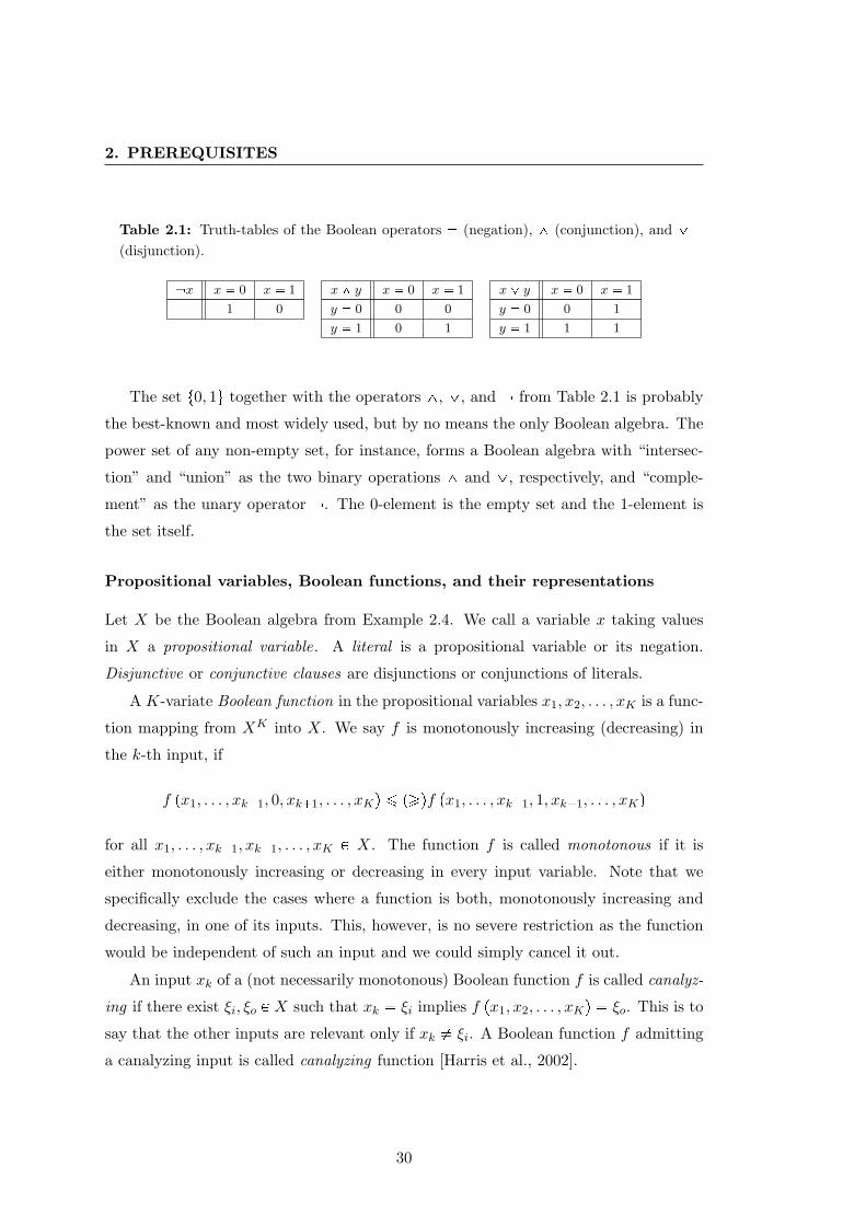
2. PREREQUISITES
Table 2.1: Truth-tables of the Boolean operators (negation), ^ (conjunction), and _(disjunction).
x x 0 x 1 x^ y x 0 x 1 x_ y x 0 x 1
1 0 y 0 0 0 y 0 0 1
y 1 0 1 y 1 1 1
The set t0, 1u together with the operators ^, _, and from Table 2.1 is probably
the best-known and most widely used, but by no means the only Boolean algebra. The
power set of any non-empty set, for instance, forms a Boolean algebra with “intersec-
tion” and “union” as the two binary operations ^ and _, respectively, and “comple-
ment” as the unary operator . The 0-element is the empty set and the 1-element is
the set itself.
Propositional variables, Boolean functions, and their representations
Let X be the Boolean algebra from Example 2.4. We call a variable x taking values
in X a propositional variable. A literal is a propositional variable or its negation.
Disjunctive or conjunctive clauses are disjunctions or conjunctions of literals.
A K-variate Boolean function in the propositional variables x1, x2, . . . , xK is a func-
tion mapping from XK into X. We say f is monotonously increasing (decreasing) in
the k-th input, if
f px1, . . . , xk1, 0, xk1, . . . , xKq ¤ p¥qf px1, . . . , xk1, 1, xk1, . . . , xKq
for all x1, . . . , xk1, xk1, . . . , xK P X. The function f is called monotonous if it is
either monotonously increasing or decreasing in every input variable. Note that we
specifically exclude the cases where a function is both, monotonously increasing and
decreasing, in one of its inputs. This, however, is no severe restriction as the function
would be independent of such an input and we could simply cancel it out.
An input xk of a (not necessarily monotonous) Boolean function f is called canalyz-
ing if there exist ξi, ξo P X such that xk ξi implies f px1, x2, . . . , xKq ξo. This is to
say that the other inputs are relevant only if xk ξi. A Boolean function f admitting
a canalyzing input is called canalyzing function [Harris et al., 2002].
30
2.4 Prerequisites from molecular biology
The simplest representation of a Boolean function f is its truth-table, a table with
two columns listing all 2K possible inputs and the corresponding output values of
f . It is often beneficial to rearrange the table, e.g. as a K-dimensional cube. A
particular clever way of visualizing truth-tables are Karnaugh-Veitch maps [Karnaugh,
1953; Veitch, 1952]; we will demonstrate their use and usefulness in chapter 6.
There is no unique way of expressing f as a propositional formula in its inputs
x1, x2, . . . , xK . The expression
f px1, . . . , xKq ª
pξ1,...,ξKqPXK |fpξ1,...,ξKq1
©k|ξk1
xk
^
©k|ξk0
xk
(2.8)
is called the full disjunctive normal form of f . The outer disjunction runs over all true-
entries of the truth-table of f . In general, any representation of f as a disjunction of
conjunctive clauses is called disjunctive normal form (DNF). The dual representation
as a conjunction of disjunctive clauses is called conjunctive normal form (CNF). Here,
“dual” means duality under the De Morgan’s Laws.
2.4 Prerequisites from molecular biology
Before introducing Kauffman’s Boolean models of gene regulation in chapter 3, we
wish to briefly discuss their biological background (section 2.4.1); for details we refer
the reader to any textbook on molecular biology, e.g. the one by Lodish and Berk [2008].
The reader is also encouraged to consult the glossary on page xix as well as Figure 2.3
for a visualization of the following explanations. In section 2.4.2, we then introduce the
biological example that we will be discussing in chapter 6.
2.4.1 Gene expression and its regulation
All information required for the development and functioning of a living organism is
stored in its DNA, which can be thought of as a long sequence of letters. Almost all
cells of the organism contain a complete copy of its DNA. Genes are the functional
subunits of this DNA.
31
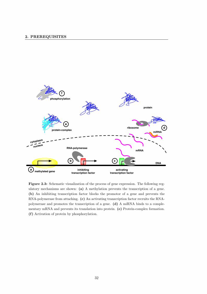
2. PREREQUISITES
methylated gene
RNA-polymerase
inhibiting transcription factor
activating transcription factor
mRNA
miRNAribosome
protein
protein-complex
phosphorylation
nucleuscytoplasm
DNA
a
b c
de
f
Figure 2.3: Schematic visualization of the process of gene expression. The following reg-ulatory mechanisms are shown: (a) A methylation prevents the transcription of a gene.(b) An inhibiting transcription factor blocks the promotor of a gene and prevents theRNA-polymerase from attaching. (c) An activating transcription factor recruits the RNA-polymerase and promotes the transcription of a gene. (d) A miRNA binds to a comple-mentary mRNA and prevents its translation into protein. (e) Protein-complex formation.(f) Activation of protein by phosphorylation.
32
2.4 Prerequisites from molecular biology
2.4.1.1 Gene expression
In principle, the expression of a gene works as follows. The piece of DNA encoding
for the gene is copied in a process called transcription and an RNA transcript is as-
sembled by an enzyme called RNA-polymerase. In some cases, these RNAs are (after
some additional processing) already the final gene products. Examples for this are
ribosomal RNAs (rRNA), transfer RNAs (tRNA) or non-coding RNAs (ncRNA) such
as microRNAs (miRNA); we will discuss these RNA types in the course of this section.
When talking about genes, however, one typically refers to protein-coding genes.
Here, the RNA transcript is called messenger RNA (mRNA) and is used as a blueprint
for protein synthesis. This process is carried out by cell organelles called ribosoms.
These are macromolecules consisting inter alia of the already mentioned rRNAs. The
translation of mRNA into protein occurs according to specific rules, the so-called genetic
code, which are executed by the tRNAs mentioned above. After synthesis, proteins
often require other proteins for being functional. Either, they are active only as part
of a protein-complex , or they need to be activated by enzymes through modifications
such as phosphorylation.
We now address two questions:
1. Why does a cell need to control its gene expression?
2. What are the possible regulatory mechanisms controlling the expression of genes
and the functionality of their products?
2.4.1.2 The need for control
In order to reproduce, multi-cellular organisms need to regenerate an entire organism
from a single fertilized egg cell. During this process, the cells of an embryo need not
only divide and grow, but also need to become specified and must differentiate into
all cell types of the organism in a precise spatio-temporal order. This differentiation
of embryonic stem cells is possible only because cells can accurately and specifically
express genes which determine their cell-fates. We will study an aspect of this process
in vertebrates in chapter 6, cf. also section 2.4.2. Similarly, in the adult organism, gene
regulation guarantees and mediates the life-long supply of cells from adult stem cells.
The immune system in higher organisms relies on cells which are able to detect
potentially harmful antigens and subsequently re-arrange their gene expression enabling
33
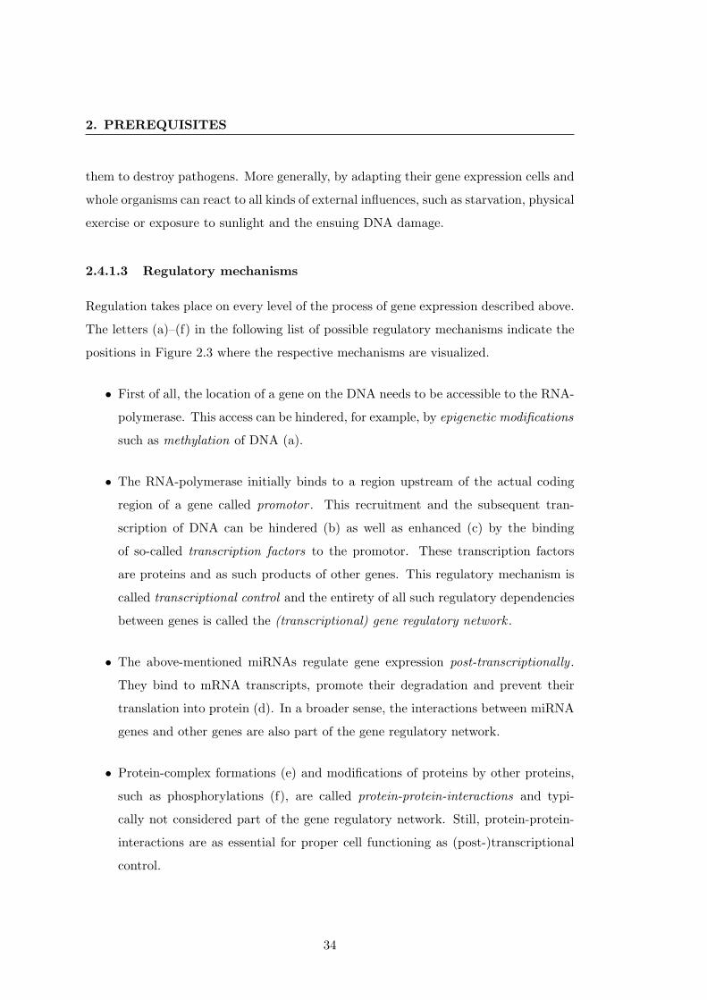
2. PREREQUISITES
them to destroy pathogens. More generally, by adapting their gene expression cells and
whole organisms can react to all kinds of external influences, such as starvation, physical
exercise or exposure to sunlight and the ensuing DNA damage.
2.4.1.3 Regulatory mechanisms
Regulation takes place on every level of the process of gene expression described above.
The letters (a)–(f) in the following list of possible regulatory mechanisms indicate the
positions in Figure 2.3 where the respective mechanisms are visualized.
• First of all, the location of a gene on the DNA needs to be accessible to the RNA-
polymerase. This access can be hindered, for example, by epigenetic modifications
such as methylation of DNA (a).
• The RNA-polymerase initially binds to a region upstream of the actual coding
region of a gene called promotor . This recruitment and the subsequent tran-
scription of DNA can be hindered (b) as well as enhanced (c) by the binding
of so-called transcription factors to the promotor. These transcription factors
are proteins and as such products of other genes. This regulatory mechanism is
called transcriptional control and the entirety of all such regulatory dependencies
between genes is called the (transcriptional) gene regulatory network .
• The above-mentioned miRNAs regulate gene expression post-transcriptionally .
They bind to mRNA transcripts, promote their degradation and prevent their
translation into protein (d). In a broader sense, the interactions between miRNA
genes and other genes are also part of the gene regulatory network.
• Protein-complex formations (e) and modifications of proteins by other proteins,
such as phosphorylations (f), are called protein-protein-interactions and typi-
cally not considered part of the gene regulatory network. Still, protein-protein-
interactions are as essential for proper cell functioning as (post-)transcriptional
control.
34
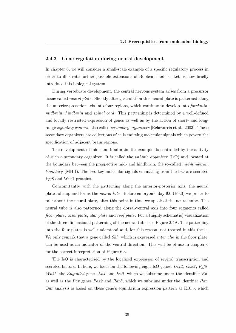
2.4 Prerequisites from molecular biology
2.4.2 Gene regulation during neural development
In chapter 6, we will consider a small-scale example of a specific regulatory process in
order to illustrate further possible extensions of Boolean models. Let us now briefly
introduce this biological system.
During vertebrate development, the central nervous system arises from a precursor
tissue called neural plate. Shortly after gastrulation this neural plate is patterned along
the anterior-posterior axis into four regions, which continue to develop into forebrain,
midbrain, hindbrain and spinal cord . This patterning is determined by a well-defined
and locally restricted expression of genes as well as by the action of short- and long-
range signaling centers, also called secondary organizers [Echevarria et al., 2003]. These
secondary organizers are collections of cells emitting molecular signals which govern the
specification of adjacent brain regions.
The development of mid- and hindbrain, for example, is controlled by the activity
of such a secondary organizer. It is called the isthmic organizer (IsO) and located at
the boundary between the prospective mid- and hindbrain, the so-called mid-hindbrain
boundary (MHB). The two key molecular signals emanating from the IsO are secreted
Fgf8 and Wnt1 proteins.
Concomitantly with the patterning along the anterior-posterior axis, the neural
plate rolls up and forms the neural tube. Before embryonic day 9.0 (E9.0) we prefer to
talk about the neural plate, after this point in time we speak of the neural tube. The
neural tube is also patterned along the dorsal-ventral axis into four segments called
floor plate, basal plate, alar plate and roof plate. For a (highly schematic) visualization
of the three-dimensional patterning of the neural tube, see Figure 2.4A. The patterning
into the four plates is well understood and, for this reason, not treated in this thesis.
We only remark that a gene called Shh, which is expressed inter alia in the floor plate,
can be used as an indicator of the ventral direction. This will be of use in chapter 6
for the correct interpretation of Figure 6.3.
The IsO is characterized by the localized expression of several transcription and
secreted factors. In here, we focus on the following eight IsO genes: Otx2 , Gbx2 , Fgf8 ,
Wnt1 , the Engrailed genes En1 and En2 , which we subsume under the identifier En,
as well as the Pax genes Pax2 and Pax5 , which we subsume under the identifier Pax .
Our analysis is based on these gene’s equilibrium expression pattern at E10.5, which
35
2. PREREQUISITES
dorsal-ventral
Mes MetMHB
E10.5Otx2, Gbx2, Fgf8, Wnt1, En, Pax
anterior-posteriorfore
brain
midbrain
hindbrain
spinalcordMHB
floorplate
basalplate
alarplate
roofplate
A B
Figure 2.4: (A) Patterning of the neural tube (highly schematic) along the anterior-posterior axis into forebrain, midbrain, hindbrain, and spinal cord as well as along thedorsal-ventral axis into floor plate, basal plate, alar plate, and roof plate. (B) Dorsal close-up view of the MHB region in the anterior neural tube of an E10.5 mouse embryo, anteriorto the left. Colored regions indicate the equilibrium expression domains of the (groups of)IsO genes Otx2 , Gbx2 , Fgf8 , Wnt1 , En, and Pax . Abbreviations: Mes, mesencephalon(midbrain); MHB, mid-hindbrain boundary; Met, metencephalon (hindbrain).
is displayed schematically in Figure 2.4B. This expression pattern was derived from
various in situ hybridization experiments, for a review see e.g. Wurst and Bally-Cuif
[2001], in particular, Figure 1c therein.
The initial expression of Otx2 and Gbx2 in the anterior and posterior neural plate,
respectively, defines the position of the prospective fore-/midbrain (Otx2 +/Gbx2 –) and
hindbrain/spinal cord (Otx2 –/Gbx2 +), respectively [Acampora et al., 1997; Wassar-
man et al., 1997]. The position of the MHB is set at the expression interface of these
two transcription factors [Broccoli et al., 1999; Li et al., 2005; Millet et al., 1999]. Sub-
sequently, expression of Wnt1 at the rostral border of the MHB in the caudal midbrain,
and of Fgf8 at the caudal border of the MHB in the rostral hindbrain is initiated in-
dependently of a requirement of Otx2 and Gbx2 for this process [Li and Joyner, 2001;
Martinez-Barbera et al., 2001]. Fgf8 plays a pivotal role in IsO patterning activity [Chi
et al., 2003; Lee et al., 1997], and Wnt1 regulates midbrain development and is required
for the maintenance of the MHB [McMahon et al., 1990; Thomas and Capecchi, 1990].
The Engrailed genes En1 and En2 are both expressed across the boundary [Davis
et al., 1988], yet their expression domains are not fully equivalent. They have been
36
2.4 Prerequisites from molecular biology
shown to be targets of Wnt1 in the midbrain [Danielian and McMahon, 1996] and to
regulate the expression of Fgf8 [Gemel et al., 1999]. Similarly to Engrailed, Pax5 is
also expressed across the boundary [Rowitch and McMahon, 1995], whereas expression
of Pax2 is restricted to the caudal part of the isthmic organizer [Bouchard et al., 2000].
Analysis of Pax2 -deficient embryos [Ye et al., 2001] has suggested an essential role of
Pax2 for the induction of Fgf8 . In short, it has been demonstrated that by E10.5 these
genes have become interdependent and form the core module of a regulatory network
that guarantees the stable maintenance of their specific expression patterns [Wurst and
Bally-Cuif, 2001].
Although a great deal of experimental effort has been made, this regulatory network
is not yet understood in full detail. In chapter 6, we show that a data-based inference
of Boolean models yields new insights into gene regulation at the MHB and can be
used to design validation experiments.
37

2. PREREQUISITES
38
3
Boolean models and Kauffman
networks
To be, Or not to be.
Hamlet, William Shakespeare
This thesis is about models of gene regulatory networks. However, we do not at-
tempt to model all the different levels of control, which we described in section 2.4.1.3,
in mechanistic detail. Rather, we consider an abstraction and simplification thereof. In
the models we introduce in this chapter, we normally do not distinguish between DNA,
RNAs and proteins. Rather, variables may represent any biological entity. Their states
are not described by concentrations or actual molecule numbers, but by two abstract
categories whose interpretation may vary between different variables. We, therefore,
like to speak of generic categories, such as “true” and “false”, “on” and “off”, or “is”
and “is not.” Thus, the models describe the complex system of gene regulation in terms
of classic Shakespearean choices. These choices are not based on any kinetic or bio-
physical laws. Instead the state of a variable is determined by an abstract combination
39
3. BOOLEAN MODELS AND KAUFFMAN NETWORKS
of inputs from some of the other variables.
3.1 Boolean models
In this section, we introduce Boolean models of gene regulation. We will do so from
a network perspective. So, let G pV,Eq denote a (directed) graph of order N with
nodes V t1, 2, . . . , Nu and edges pi1 Ñ iq P E V V . The predecessors (inputs)
of a node i are denoted by i1 i2 iKi , where Ki is the node’s in-degree. We
straightaway make
Definition 3.1 (Boolean model). A Boolean model (BM) is a tuple pG, fq consistingof a graph G and a vector of Boolean functions f pfiqNi1, fi : t0, 1uKi Ñ t0, 1u. TheBoolean function fi is called update rule or update function of node i and the vector ofupdate rules f (as a function from t0, 1uN Ñ t0, 1uN ) is called transfer function of theBoolean model.
Remark 3.1. Each BM pG, fq gives rise to a time-discrete dynamical system as follows:To each node i we associate a time-dependent discrete variable xiptq P t0, 1u, xptq pxiptqqNi1. The evolution of xptq is determined by the iteration
xpt 1q f pxptqq , t 0, 1, 2, . . . ,
where the i-th component is given by
xipt 1q fi
xi1ptq, xi2ptq, . . . , xiKi ptq
. (3.1)
In this thesis, we only consider the above synchronous updating, for different updatepolicies, see e.g. Chavez et al. [2005], Faure et al. [2006] and Greil et al. [2007].
In the following, we will refer to trajectories of the dynamical system from Remark
3.1 as trajectories of the BM pG, fq.The state-space of the dynamical system from Remark 3.1 is the discrete, finite set
X t0, 1uN . We turn it into a metric space by defining the Hamming distance d of
x pxiqNi1 P X and x1 px1iqNi1 P X as
dx,x1
1N
N
i1
1 δxi,x1i
,
where δxi,x1i is the Kronecker symbol. As measure we simply use the counting mea-
sure. Due to the finite state-space we can then easily characterize the ω-limit sets and
attractors.
40
3.2 Boolean models of regulatory networks
Proposition 3.1. Consider the dynamical system defined in Remark 3.1. The ω-limitset of each point is either a fixed point or a periodic orbit. The same is true for theattractors of the dynamical system.
Dynamical systems induced by BMs are, arguably, the simplest kind of dynami-
cal systems one can think of. They are time-discrete and, in addition, restrict their
variables to the smallest non-trivial set of values t0, 1u. Still, they exhibit interesting
dynamics as we shall see in the course of this thesis.
The update rules of BMs are often specified in terms of logical expressions. The
inputs of an update rule fi : t0, 1uKi Ñ t0, 1u are then thought of as propositional
variables assuming values in the two-element Boolean algebra from Example 2.4, and
the update rule is stated using the operators ^, _ and from this structure, cf. Table
2.1. In a biological application, these propositional formulas often allow for the inter-
pretation of an update rule as the (logical) combination of activating and inhibiting
regulatory interactions.
3.2 Boolean models of regulatory networks
As already mentioned, the update rules of BMs do obviously not reflect any kinetic or
biophysical laws. So, why can one expect the dynamical systems induced by BMs to be
acceptable models of the intricate regulatory mechanisms explained in section 2.4.1.3?
To answer this question it helps to take a look at the reasons for the complexity of gene
regulation.
One reason are cooperative effects between transcription factors. Cooperativity
exists, if a bound transcription factor protein increases (positive cooperativity) or de-
creases (negative cooperativity) the affinity of the promotor for further proteins. The
same mechanisms are found in the allosteric regulation of enzymes, i.e. the regula-
tion of an enzyme’s activity by binding an (activating or inhibiting) effector molecule.
The standard kinetic that describes these cooperative biochemical reactions is the Hill
kinetic [Hill, 1910]. If x denotes the (unit-normalized) concentration of some activat-
ing transcription factor, the activity h of the target promotor can be modeled ceteris
paribus as
hpc, xq xc
xc θc , (3.2)
41
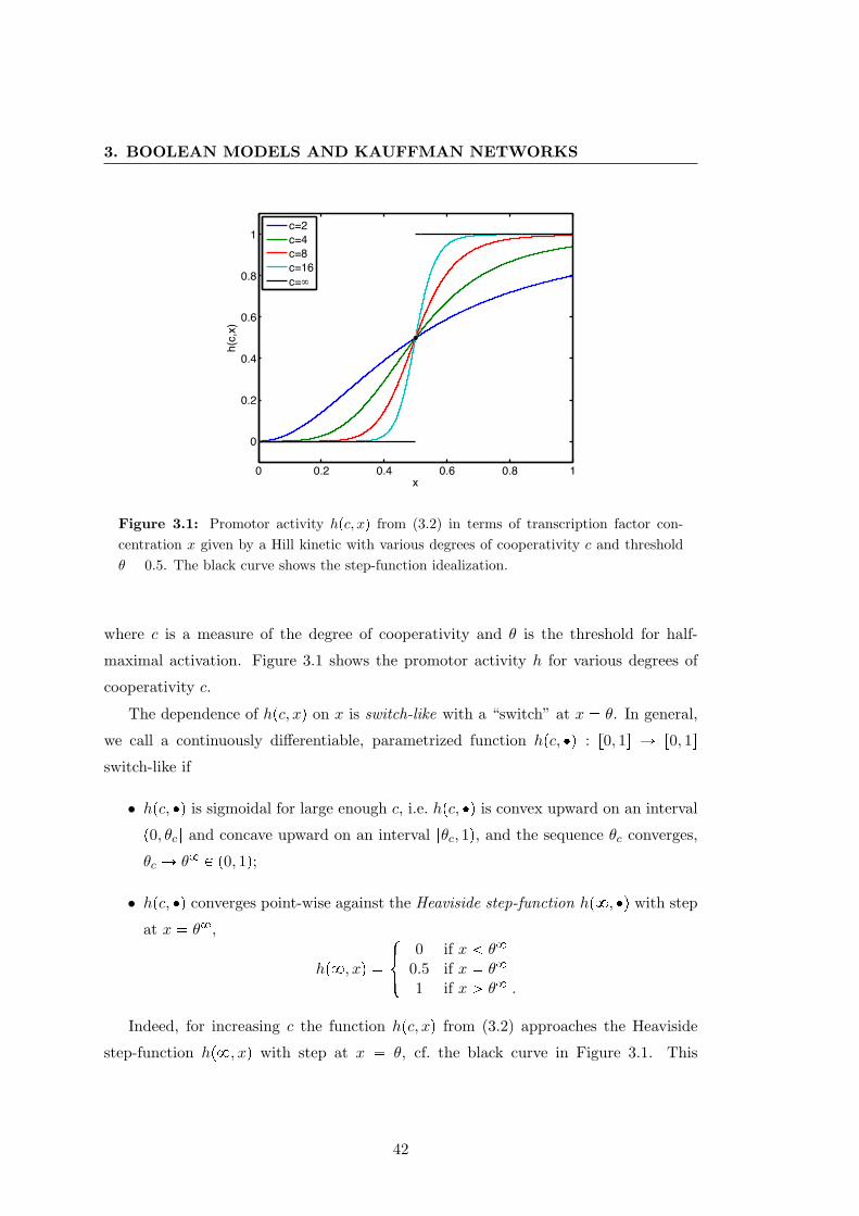
3. BOOLEAN MODELS AND KAUFFMAN NETWORKS
0 0.2 0.4 0.6 0.8 1
0
0.2
0.4
0.6
0.8
1
x
h(c,
x)c=2c=4c=8c=16c=∞
Figure 3.1: Promotor activity hpc, xq from (3.2) in terms of transcription factor con-centration x given by a Hill kinetic with various degrees of cooperativity c and thresholdθ 0.5. The black curve shows the step-function idealization.
where c is a measure of the degree of cooperativity and θ is the threshold for half-
maximal activation. Figure 3.1 shows the promotor activity h for various degrees of
cooperativity c.
The dependence of hpc, xq on x is switch-like with a “switch” at x θ. In general,
we call a continuously differentiable, parametrized function hpc, q : r0, 1s Ñ r0, 1sswitch-like if
• hpc, q is sigmoidal for large enough c, i.e. hpc, q is convex upward on an interval
p0, θcs and concave upward on an interval rθc, 1q, and the sequence θc converges,
θc Ñ θ8 P p0, 1q;
• hpc, q converges point-wise against the Heaviside step-function hp8, q with step
at x θ8,
hp8, xq $&%
0 if x θ8
0.5 if x θ8
1 if x ¡ θ8 .
Indeed, for increasing c the function hpc, xq from (3.2) approaches the Heaviside
step-function hp8, xq with step at x θ, cf. the black curve in Figure 3.1. This
42
3.3 Kauffman networks
step-function now takes only two values on r0, 1sz tθu, which we can identify with the
Boolean algebra t0, 1u. Thus, we may see BMs as idealizations of networks of switch-
like interactions [Theis et al., 2010]. Whether or not this approximation is justified,
more precisely, whether or not the degree of cooperativity is high enough to justify this
approximation, has to be decided anew in each modeling application.
3.3 Kauffman networks
Let us now introduce the random “Kauffman-versions” of BMs.
Definition 3.2 (Kauffman network). A Kauffman network (KN) is a probability spacewhose elements are BMs.
To turn spaces of BMs into probability spaces, one defines generative models yielding
BMs as realizations. Common to all these BMs is that they are based on a graph G.
In here, this graph will always be a random graph G pPinq defined by the configuration
model from Example 2.2. In order to specify our generative models it, thus, remains
to define how the update rules of the BM are realized.
Let us now present the KN originally introduced by Kauffman and a generalization
thereof. The standard Kauffman network (SKN) with parameters N (order) and K
(connectivity) is given by the following random process:
(K1) Create a realization of the random graph G pPinq with Pin δK .
(K2) For each node i, i 1, 2, . . . , N , define the update rule fi by filling the entries of
the pertaining truth-table with 0 and 1 with equal probabilities.
A generalization hereof is the Kauffman network with magnetization bias (KNMB).
Here, we have an additional parameter u (the so-called magnetization bias1) and replace
step (K2) from above by
(K2’) For each node i, i 1, 2, . . . , N , define the update rule fi by filling the entries of
the pertaining truth-table with 0 and 1 with probabilities u and 1u, respectively.
In Kauffman [1969] the SKN is introduced. The generalization to KNsMB is due to
Bastolla and Parisi [1996]. Also different degree distributions of the random graph have
been investigated [Aldana, 2003; Fox and Hill, 2001].1The term magnetization bias originates in an analogy between KNs and networks of atomic spins,
which are very small magnets.
43
3. BOOLEAN MODELS AND KAUFFMAN NETWORKS
3.4 Order parameters and phase transitions of Kauffman
networks
When studying KNs, we are not interested in the properties of a particular realization,
but we rather search for generic properties in the ensemble of all realizations of a KN.
Kauffman [1969], for instance, addresses the following questions.
It is a fundamental question whether metabolic stability and epigenesis re-quire the genetic regulatory circuits to be precisely constructed. Has a fortu-nate evolutionary history selected only nets of highly ordered circuits whichalone insure metabolic stability; or are stability and epigenesis, even in netsof randomly interconnected regulatory circuits, to be expected as the probableconsequence of as yet unknown mathematical laws? Are living things moreakin to precisely programmed automata selected by evolution, or to randomlyassembled automata whose characteristic behavior reflects their unorderlyconstruction, no matter how evolution selected the surviving forms?
Kauffman himself could show by computational experiments that KNs with low con-
nectivities exhibit surprisingly ordered structures and are able to give insights into
biological phenomena such as cell replication or lineage differentiation. With increas-
ing connectivities this order seems to disappear.
Soon the close relation between KNs and the concept of a phase transition from
statistical physics was realized. Originally, this concept denotes the transitions between
two or more different physical phases of one medium, like ice, water and gas [Kadanoff,
2000]. At the point of phase transition certain properties of this medium change, mostly
in a discontinuous fashion, in response to a change of some external condition, such as
temperature or pressure. A liquid, for instance, may become gas when heated to the
boiling point, leading to a sharp increase in its volume. Phase transitions are typically
detected by monitoring an order parameter . For phase transitions from solid to liquid
or from liquid to gas, for example, this order parameter is the density of the medium.
In a number of studies by Derrida and Pomeau [1986], Derrida and Stauffer [1986]
as well as Flyvbjerg [1988], Kauffman’s experimental observations were explained by
creating an analogy between KNs and physical media undergoing phase transitions. In
KNs, the external condition is the connectivity. Several order parameters have been
proposed [Derrida and Pomeau, 1986; Flyvbjerg, 1988; Luque and Sole, 1997, 2000],
44
3.4 Order parameters and phase transitions of Kauffman networks
all yielding the same phase transition criterion. The Hamming distance between two
initially differing time-courses is, arguably, the most intuitive. The definition of this
order parameter is motivated by the hallmark of chaos: a sensitivity to small pertur-
bations. This suggests to detect phase transitions by monitoring how the (Hamming)
distance between two nearby configurations evolves over time, i.e. whether it increases
or decreases.
We do not review any theoretical details at this point, as we will study a more
general version of KNs than KNsMB in chapter 4. In the course of this chapter, we will
obtain the theory of SKNs and KNsMB as corollaries to more general statements. In
particular, we will see that the order parameter has stationary dynamics, i.e. a globally
attracting fixed point, and we will determine the critical connectivity at which the
phase transition occurs. Below this connectivity the globally attracting equilibrium of
the Hamming distance is zero, above the critical connectivity it is strictly positive.
We say a KN is in the frozen or ordered phase if the Hamming distance has a
stationary value of zero, otherwise the KN is said to be in the chaotic phase. KNs at
the point of phase transition are called critical . Some authors prefer the term regime
over phase. It has been shown that the ordered phase is characterized by small stable
attractors, whereas in the chaotic phase long-periodic orbits frequently occur [Aldana
et al., 2003]. A more intuitive characterization of these two phases can be given in terms
of “damage spreading” (percolation). Assume that a realization of a KN is damaged
in one node, i.e. the state of this node is flipped. In the chaotic regime the Hamming
distance will increase, i.e. this damage will spread through the network, whereas in the
ordered regime the Hamming distance will vanish, i.e. the network is able to “repair”
this damage over time.
To visualize this, we generate realizations of SKNs with connectivities K 1, K 2, and K 3, simulate each twice with initial conditions differing by a (normalized)
Hamming distance of 0.1, and plot the resulting time-courses in Figure 3.2. We will see
in chapter 4 (Remark 4.5) that SKNs with these connectivities are frozen, critical and
chaotic. Below the two time-courses their Hamming distance is shown. In the frozen
networks this Hamming distance decreases to its equilibrium zero, in the critical and
chaotic networks it eventually fluctuates around strictly positive values. In the critical
network this value is comparable to the initial distance, whereas in the chaotic network
the Hamming distance increases from its initial value.
45
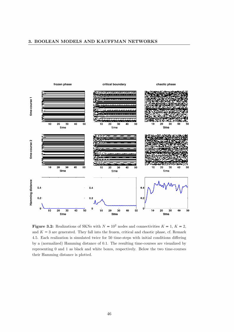
3. BOOLEAN MODELS AND KAUFFMAN NETWORKS
chaotic phase
time-
cour
se 1
Ham
min
g di
stan
cetim
e-co
urse
2
frozen phase critical boundary
Figure 3.2: Realizations of SKNs with N 102 nodes and connectivities K 1, K 2,and K 3 are generated. They fall into the frozen, critical and chaotic phase, cf. Remark4.5. Each realization is simulated twice for 50 time-steps with initial conditions differingby a (normalized) Hamming distance of 0.1. The resulting time-courses are visualized byrepresenting 0 and 1 as black and white boxes, respectively. Below the two time-coursestheir Hamming distance is plotted.
46
3.4 Order parameters and phase transitions of Kauffman networks
The study of KNs has found its way into popular science by the slogan “Living at
the edge of chaos.” Kauffman [1993] hypothesized that regulatory networks in living
organisms operate in the frozen regime but close to (at the edge of) the chaotic regime,
i.e. near a phase transition. The first part of this hypothesis is well supported by
other authors who all claim that robustness is a crucial property of biological systems
[Kitano, 2004]. The second part can only be understood in the light of evolution. For
natural selection to work, small changes, such as mutations, need to have an effect.
Kauffman argues that fully robust networks, which are completely insensitive to small
perturbations, do not have the ability to evolve over time by natural selection. Hence,
evolvable living organisms operate near a chaotic regime. A nice corroboration of
Kauffman’s hypothesis is the finding that the (average) connectivity of gene regulatory
networks in lower organisms is, indeed, around the critical connectivity of SKNs, see
Balleza et al. [2008] and references therein.
47

3. BOOLEAN MODELS AND KAUFFMAN NETWORKS
48
4
Multistate Kauffman networks
They fashioned a tomb for thee, O holy and high one
The Cretans, always liars, evil beasts, idle bellies!
But thou art not dead: thou livest and abidest forever,
For in thee we live and move and have our being.
Cretica, Epimenides
The above poem by the Cretan philosopher Epimenides of Knossos is the first
version of what is known in logic as the liar’s paradox . This paradox arises when
one interprets Epimenides’ statement that all Cretans are liars as a self-referential
statement. Epimenides, after all, was a Cretan himself. Today, the liar’s paradox
exists in many forms; in its most simplistic one it headlines the essay “This title is
false” by Isalan and Morrison [2009], which they published last year in Nature.
They argue that it is self-reference what makes all the difference in genetic regula-
tion. Typical descriptions of regulatory interactions, such as “This gene represses it-
self.” or “Gene A activates gene B. Gene B inhibits gene A.”, are, indeed, self-referential.
Isalan and Morrison continue to explain that in gene regulation these seemingly para-
doxical situations are resolved either in time or space, leading to temporal oscillations
49
4. MULTISTATE KAUFFMAN NETWORKS
or spatial patterns. In fact, temporal oscillations are found e.g. during cell cycle or
in the circadian rhythm, and Alan Turing [1990]1 showed that even from small self-
referential motifs such as “Gene A activates gene B. Gene B inhibits gene A.” complex
spatial patterns may emerge.
There is a third possibility how a self-referential situation can be resolved: By intro-
ducing additional truth-values besides the classic “false” and “true”, such as “partially
true.” In a biological context, these truth-values could be interpreted as “medium con-
centration” or “weakly active.” The solution of a self-referential regulation would then
be homeostasis.
4.1 Motivation and outline
Aesthetic philosophy aside, in many down-to-earth modeling efforts the discretization
of continuous biological quantities into binary “on”–“off” categories was found to be
insufficient. In fact, it has been demonstrated that genes may well have more than two
functionally different expression levels [Setty et al., 2003]. To alleviate this issue, in
some modeling applications the Boolean “on”–“off” categories are extended to multiple
discrete states, leading to multistate models [Faure et al., 2009; Sanchez and Thieffry,
2001; Thomas, 1991].
Studies of KNs with multiple states, let us call them multistate Kauffman networks,
are scarce [Sole et al., 2000] and restricted to the biologically implausible case where
all nodes have the same number of discrete states. In this chapter, which follows
Wittmann et al. [2010] as well as Wittmann and Theis [2010a], we investigate a more
general class of multistate KNs with respect to critical phenomena. In particular,
contrary to previous studies, the number of discrete states is not fixed for all nodes
but follows a distribution. We formally introduce the Hamming distance between two
trajectories as an order parameter and show that a transition between a frozen and
a chaotic regime takes place in multistate KNs of this class. The critical boundary is
analytically determined as a relation between the mean connectivity and a parameter
describing the heterogeneity of the update rules, cf. Theorem 4.1.
We study two distributions of update rules in more detail. First, we analyze mul-
tistate KNs with unbiased update rules, which generalize the (Boolean) SKNs. We
1Reprint of Turing’s original publication
50
4.2 Multistate models and multistate Kauffman networks
find that allowing nodes to assume multiple states lowers the critical connectivity as
compared to the Boolean case, the limit being a biologically implausible connectivity of
1, cf. Remark 4.5. Interestingly however, the critical connectivity does not necessarily
decrease with the mean number of states per node. Second, we study multistate KNs
with biased update rules, which generalize the (Boolean) KNsMB. In section 4.3.4.2, we
show that the critical connectivity can be made arbitrarily large by biasing the update
rules towards one of the discrete states. In the case of (Boolean) KNsMB, this simply
means choosing the magnetization bias either sufficiently large or small. In particular,
we can poise multistate KNs with biologically plausible connectivities at criticality (at
the edge of chaos). Our analytic results are backed up by simulations.
Subsequently, we extend the analysis of the Hamming distance (between two trajec-
tories) by looking at ensembles of trajectories. This can be motivated from a biological
point of view, as in molecular biology experimental data are often average concentra-
tions in cell cultures, which can be thought of as ensembles of trajectories of a multistate
model. A dynamical system describing the synchronization behavior of such ensem-
bles is introduced and analyzed. In a low-dimensional example the analytic results are
validated by simulations.
4.2 Multistate models and multistate Kauffman networks
Let us now formally introduce our first generalization of BMs and KNs. In this chapter,
G pV,Eq again denotes a (directed) graph of order N with nodes V t1, 2, . . . , Nuand edges pi1 Ñ iq P E V V . The predecessors (inputs) of a node i are denoted by
i1 i2 iKi , where Ki is the node’s in-degree.
4.2.1 Multistate models
Generalizing Definition 3.1 of BMs we make
Definition 4.1 (multistate model). A multistate model (MM) is a triple pG,S, fq whichconsists of a graph G, a vector S pSiqNi1 of numbers of states defining the rangesΣi : t0, 1, . . . , Si 1u of nodes i 1, 2, . . . , N , and a vector of discrete functionsf pfiqNi1, fi :
±Kik1 Σik Ñ Σi. The discrete function fi is called update rule or update
function of node i and the vector of update rules f (as a function from±Ni1 Σi ѱN
i1 Σi) is called transfer function of the MM.
51
4. MULTISTATE KAUFFMAN NETWORKS
Remark 4.1. A BM is the special case of a MM where all Si 2. Conversely, we canstill express an update rule fi of a MM using the Boolean operators ^ and _ from Table2.1. We do so, by relating the truth-values of the equations “fipxi1 , xi2 , . . . , xiKi q s”,s P Σi, to the truth-values of the equations “xik ξk”, k 1, 2, . . .Ki, ξk P Σik :
fi
xi1 , xi2 , . . . , xiKi
s ðñ
ªpξ1,ξ2,...,ξKiq|fipξ1,ξ2,...,ξKiqs
Ki©k1
pxik ξkq
This is a generalization of the full DNF of a Boolean function from (2.8). The disjunc-tion on the right-hand side runs over all input combinations of fi with output values. For each combination, the inner conjunction is true if and only if the combinationagrees with the values of the variables xik .
Similarly to BMs, MMs give rise to dynamical systems.
Remark 4.2. Each MM pG,S, fq gives rise to a time-discrete dynamical system asfollows: To each node i we associate a time-dependent discrete variable xiptq P Σi,xptq pxiptqqNi1. The evolution of xptq is determined by the iteration
xpt 1q f pxptqq , t 0, 1, 2, . . . ,
where the i-th component is given by
xipt 1q fi
xi1ptq, xi2ptq, . . . , xiKi ptq
. (4.1)
Again we only consider the above synchronous updating.
In the following, we will refer to trajectories of the dynamical system from Remark
4.2 as trajectories of the MM pG,S, fq.The state-space of the dynamical system from Remark 4.2 is the discrete, finite set
X ±Ni1 Σi. We proceed as in the Boolean case, i.e. we define the Hamming distance
d of x pxiqNi1 P X and x1 px1iqNi1 P X as
dx,x1
1N
N
i1
1 δxi,x1i
,
and use the counting measure. Our results about the ω-limit sets and attractors of
BMs, cf. Proposition 3.1, generalize to the multistate case.
Proposition 4.1. Consider the dynamical system defined in Remark 4.2. The ω-limitset of each point is either a fixed point or a periodic orbit. The same is true for theattractors of this dynamical system.
52
4.2 Multistate models and multistate Kauffman networks
4.2.2 Multistate Kauffman networks
We now define the random “Kauffman-version” of MMs.
Definition 4.2 (multistate Kauffman network). In general, a multistate Kauffmannetwork (MKN) is a probability space whose elements are MMs.
In this thesis, by MKN we always mean the following generative model for MMs on
N nodes. It is defined for
• an in-degree distribution Pin pKq, K 1, 2, . . . ,Kmax,
• a distribution of numbers of states Pnos pSq, S 2, 3, . . . , Smax, and
• distributions PSpsq, s 0, 1, . . . , S 1, of entries of update rules for all S 2, 3, . . . , Smax.
Realizations are generated by
(M1) creating a realization of the random graph G pPinq,
(M2) for each node i, i 1, 2, . . . , N , choosing its number of states Si randomly from
the probability distribution Pnos,
(M3) for each node i, i 1, 2, . . . , N , choosing the values of fi randomly from the
probability distribution PSi .
Note that in (M3) the distribution PSi does not depend on the node i but only on its
number of states Si.
In the following, we consider, in particular, two examples for the distributions PS .
In section 4.3.3, we treat unbiased update rules sampled from the discrete uniform
distributions
PSpsq 1S, s 0, 1, . . . , S 1 . (4.2)
In the special case of all Si 2 and delta-distributed in-degree, the study of the
distribution from (4.2) yields the theory of SKNs.
In section 4.3.4, we then study biased update rules sampled from the distributions
PSpsq $&%
u s 01 uS 1
s 1, 2, . . . , S 1(4.3)
53
4. MULTISTATE KAUFFMAN NETWORKS
for some 0 u 1. If Si 2, this simply means that the update function fi evaluates
to 0 with a certain probability 0 u 1 and to 1 with probability 1 u. Thus, if all
Si 2 and the in-degree is delta-distributed, the study of the distribution from (4.3)
yields the theory of KNsMB.
4.2.3 Parameters of multistate Kauffman networks
Let K be a MKN. We conclude this section by defining and discussing some effective
parameters of K that will be needed in the following.
• We define the heterogeneity pS of the distributions PS , S 2, 3, . . . , Smax, as
pS S1
s0
PSpsq p1 PSpsqq , (4.4)
• the heterogeneity p of K as
p Smax
S2
Pnos pSq pS , (4.5)
• and the mean connectivity K of K as
K Kmax¸K1
Pin pKqK . (4.6)
Remark 4.3. From (M3) it follows that the probability for a generated update rule fito yield two different values for two different arguments depends only on PSi (where Siis the number of states of node i) and is equal to the heterogeneity pSi of PSi .
Lemma 4.1. The heterogeneity pS becomes maximal if PS is the discrete uniformdistribution from (4.2). In this case, pS pS 1qS.
Proof. The existence of a global maximum follows from the extreme value theorem.Now assume that π1 PS ps1q π2 PS ps2q. Then, for π pπ1 π2q 2 it holds that
2π p1 πq π1 π2 pπ1 π2q22
¡ π1 π2 pπ1 π2q22
pπ1 π2q22
π1p1 π1q π2p1 π2q .
54
4.3 Dynamic regimes of multistate Kauffman networks
Hence, the distribution
P 1Spsq #PSpsq s R ts1, s2uπ s P ts1, s2u
yields a strictly larger value for pS . In case of uniform PS one computes
pS S1
s0
1S
S 1S
S 1S
.
It follows
Corollary 4.1. For any choice of PS, pS 1 and p 1.
4.3 Dynamic regimes of multistate Kauffman networks
Let again K be a MKN as defined in section 4.2.2. As outlined in section 3.4 one
detects phase transitions by monitoring the evolution of an order parameter, which, in
the context of KNs, is often the Hamming distance between two trajectories.
4.3.1 The Hamming distance of a Kauffman network
Before we can formally define our order parameter, we need to state a technical conse-
quence of (M3).
Lemma 4.2. Let d0 P r0, 1s and consider the following random experiment: Generatea realization of K. Choose two configurations xp0q and x1p0q whose components differ,xip0q x1ip0q, with probability d0. Iterate the configurations one time-step yielding xp1qand x1p1q, respectively. We define the random variable d as the Hamming distanced pxp1q,x1p1qq. Then, it holds
E pdq Kmax¸K1
Pin pKqSmax
S2
Pnos pSq
1 p1 d0qKpS
.
In particular, E pdq is independent of how the actual values in xp0q and x1p0q are chosen,but depends only on the probability d0 for them to differ.
55
4. MULTISTATE KAUFFMAN NETWORKS
Proof. Let us introduce identically distributed Bernoulli random variables di, i 1, 2, . . . , N , defined as 1 if xip1q x1ip1q and as 0 otherwise. It then holds d p1Nq°N
i1 di, and, consequently,
E pdq 1N
N
i11
E pdi1q E pdiq pq
for any i.Given Ki and Si, the conditional expectation E pdi | Ki, Siq is equal to the proba-
bility that
fi
xi1p0q, xi2p0q, . . . , xiKi p0q
fi
x1i1p0q, x1i2p0q, . . . , x1iKi p0q
. p:q
According to Remark 4.3 the probability for p:q is equal to pSi given the two argu-ments
xi1p0q, xi2p0q, . . . , xiKi p0q
and
x1i1p0q, x1i2p0q, . . . , x1iKi p0q
are not identical.
The events that inputs differ between both configurations, xikp0q x1ikp0q, are inde-pendent as in the configuration model the inputs ik of i are chosen randomly from V .The probability for each of these events is d0. Thus, the probability for the argumentsto differ (in at least one component) is given by 1 p1 d0qKi . Hence, the probabilityfor p:q is equal to
1 p1 d0qKi
pSi .
Finally, recall that Ki and Si are chosen according to the distributions Pin pKq andPnos pSq. Thus, averaging over Ki and Si yields
E pdiq Kmax¸K1
Pin pKqSmax
S2
Pnos pSq
1 p1 d0qKpS
,
and the claim follows from pq.
Lemma 4.2 states that the expected Hamming distance between two configurations
evolves independently of the actual values in these configurations. In chapter 5, we
will introduce a new class of KNs for which this no longer holds: The evolution of
the Hamming distance will depend on the actual values in the configurations, more
precisely, on the fractions of 1’s and 0’s. For now, however, Lemma 4.2 allows us to
make
Definition 4.3 (Hamming distance of a MKN). The Hamming distance of K is asequence pdptqqt¥0 which is consistent in the sense of the following random experiment:Pick a realization of K, create two configurations xp0q and x1p0q whose componentsdiffer with probability dptq, and iterate them one time-step yielding configurations xp1qand x1p1q. Then, dpt 1q is the expected Hamming distance between xp1q and x1p1q.
56
4.3 Dynamic regimes of multistate Kauffman networks
Remark 4.4. We, of course, want the Hamming distance of K to be a good approxima-tion of the Hamming distance
1N
N
i1
1 δxiptq,x1iptq
between two trajectories xptq and x1ptq of a specific realization of K. We will demon-strate that this is, indeed, the case in large networks by simulations in section 4.3.5.From a theoretical point of view, however, the above approximation is a priori notjustified. The issue is that in the proof of Lemma 4.2 it is crucial that we may as-sume the inputs ik of a node i to be independent. At time-points t ¥ 1, however, thisassumption is obviously not valid as in a realization of K the inputs of i might havecommon predecessors. The reason why we still obtain good approximations in largenetworks, is given by Lemma 2.1. Here, it was shown that in the thermodynamic limitof large N the probability for common predecessors vanishes.
4.3.2 Analysis of the Hamming distance and detection of a phase
transition
The Hamming distance of K naturally depends on the initial distance dp0q. In the
following, we take care of this issue by proving that the asymptotic behavior of dptq is
identical for almost all initial conditions. For this we use that, as shown in Lemma 4.2,
the Hamming distance pdptqqt¥0 of K obeys the iteration
dpt 1q D pdptqq
:Kmax¸K1
Pin pKqSmax
S2
Pnos pSq
1 p1 dptqqKpS
. (4.7)
Lemma 4.3. For the dynamical system (4.7) three possibilities exist.
1. It has a hyperbolic, globally attracting fixed point at d 0.
2. The fixed point d is still globally attracting, but critical.
3. The fixed point d is repelling and an additional fixed point d P p0, 1q existswhich attracts p0, 1s.
Proof. Clearly, Dp0q 0, so d is a fixed point. First, suppose that Pin p1q 1. ThenDpdq is linear with slope p 1 and (4.7) falls into category 1. Now, consider a general
57
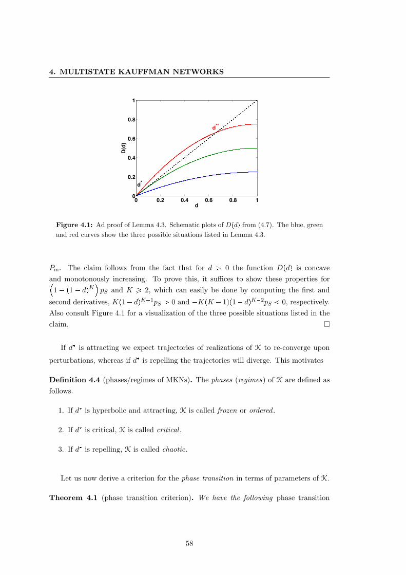
4. MULTISTATE KAUFFMAN NETWORKS
0 0.2 0.4 0.6 0.8 10
0.2
0.4
0.6
0.8
1
d
D(d
)
d*
d**
Figure 4.1: Ad proof of Lemma 4.3. Schematic plots of Dpdq from (4.7). The blue, greenand red curves show the three possible situations listed in Lemma 4.3.
Pin. The claim follows from the fact that for d ¡ 0 the function Dpdq is concaveand monotonously increasing. To prove this, it suffices to show these properties for
1 p1 dqKpS and K ¥ 2, which can easily be done by computing the first and
second derivatives, Kp1 dqK1pS ¡ 0 and KpK 1qp1 dqK2pS 0, respectively.Also consult Figure 4.1 for a visualization of the three possible situations listed in theclaim.
If d is attracting we expect trajectories of realizations of K to re-converge upon
perturbations, whereas if d is repelling the trajectories will diverge. This motivates
Definition 4.4 (phases/regimes of MKNs). The phases (regimes) of K are defined asfollows.
1. If d is hyperbolic and attracting, K is called frozen or ordered .
2. If d is critical, K is called critical .
3. If d is repelling, K is called chaotic.
Let us now derive a criterion for the phase transition in terms of parameters of K.
Theorem 4.1 (phase transition criterion). We have the following phase transition
58
4.3 Dynamic regimes of multistate Kauffman networks
criterion in terms of the parameters p and K from (4.5) and (4.6).
pK
$'&'% 1 ordered regime 1 critical boundary¡ 1 chaotic regime .
(4.8)
Proof. Linearizing D from (4.7) about d yields
dDdd
d
Kmax¸K1
Pin pKqSmax
S2
Pnos pSqKpS
Kmax¸K1
Pin pKqKp pK .
The claim follows from Theorem 2.2.
Corollary 4.2. MKNs with a mean connectivity K below (above) the critical connec-tivity
Kcrit 1
p(4.9)
are frozen (chaotic).
A nice intuitive interpretation of Theorem 4.1 is given in terms of “damage spread-
ing.” Assume that at time t the state of a realization of a MKN is damaged in one
node, i.e. the state of this node is flipped. On average, this node affects K other nodes
at the next time-step t 1. The parameter p is the mean probability that a change
of input, indeed, leads to a change of output in an update rule. The product pK thus
gives the mean number of damaged (flipped) nodes at time t 1. Inductively, we see
that in the case pK ¡ 1 damage will spread through the network, whereas in the case
pK 1 the network is able to “repair” damage over time.
We observe that the phase transition depends only on the first moments K and p.
Typically, K can be easily computed once the underlying network structure is known.
The computation of p is more involved, as we shall see in the following sections where
we compute this quantity for unbiased as well as biased update rules.
59
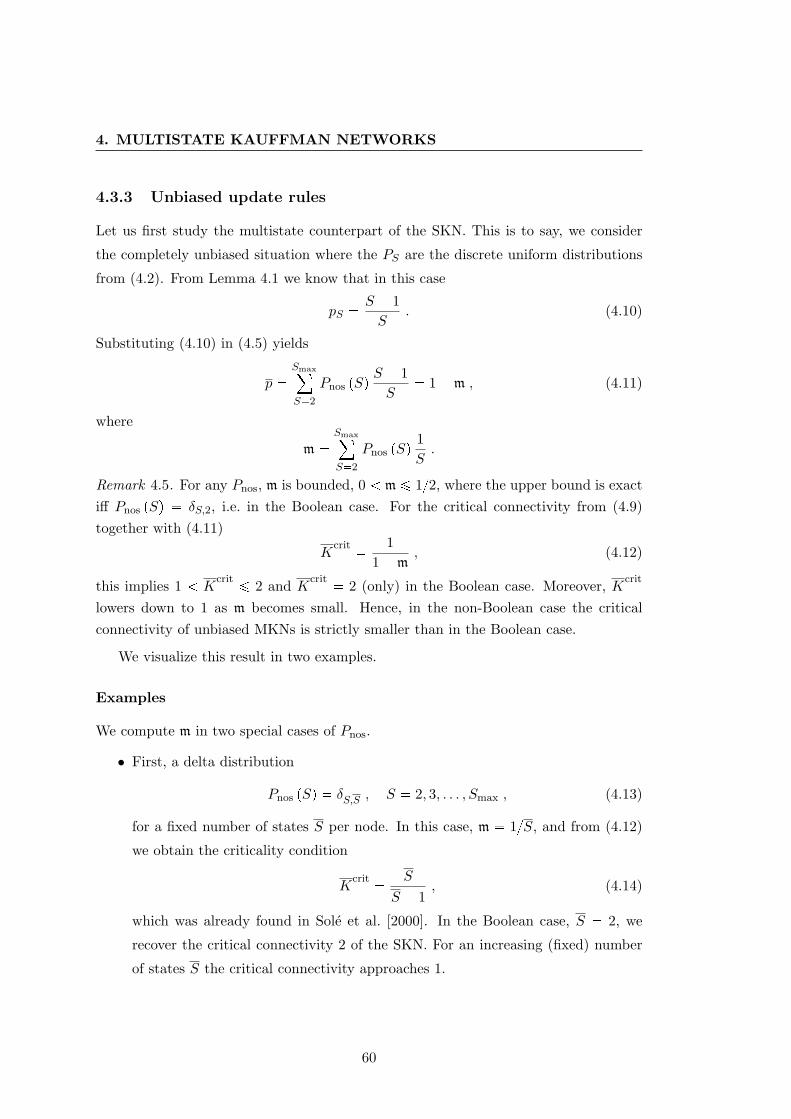
4. MULTISTATE KAUFFMAN NETWORKS
4.3.3 Unbiased update rules
Let us first study the multistate counterpart of the SKN. This is to say, we consider
the completely unbiased situation where the PS are the discrete uniform distributions
from (4.2). From Lemma 4.1 we know that in this case
pS S 1S
. (4.10)
Substituting (4.10) in (4.5) yields
p Smax
S2
Pnos pSq S 1S
1m , (4.11)
where
m Smax
S2
Pnos pSq 1S.
Remark 4.5. For any Pnos, m is bounded, 0 m ¤ 12, where the upper bound is exactiff Pnos pSq δS,2, i.e. in the Boolean case. For the critical connectivity from (4.9)together with (4.11)
Kcrit 1
1m, (4.12)
this implies 1 Kcrit ¤ 2 and K
crit 2 (only) in the Boolean case. Moreover, Kcrit
lowers down to 1 as m becomes small. Hence, in the non-Boolean case the criticalconnectivity of unbiased MKNs is strictly smaller than in the Boolean case.
We visualize this result in two examples.
Examples
We compute m in two special cases of Pnos.
• First, a delta distribution
Pnos pSq δS,S , S 2, 3, . . . , Smax , (4.13)
for a fixed number of states S per node. In this case, m 1S, and from (4.12)
we obtain the criticality condition
Kcrit S
S 1, (4.14)
which was already found in Sole et al. [2000]. In the Boolean case, S 2, we
recover the critical connectivity 2 of the SKN. For an increasing (fixed) number
of states S the critical connectivity approaches 1.
60
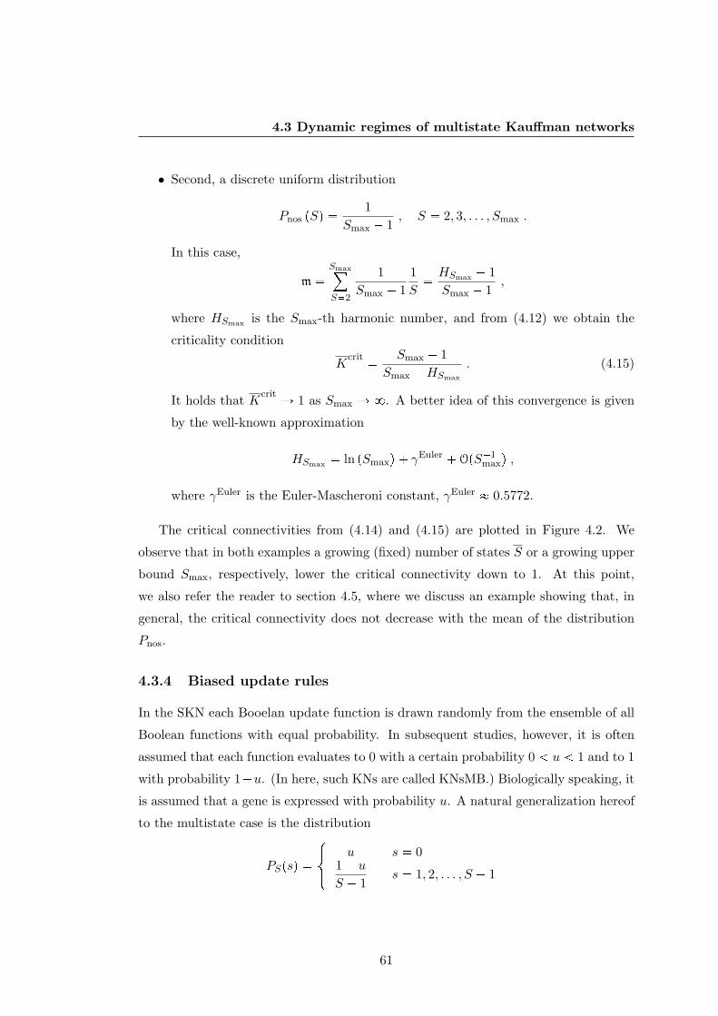
4.3 Dynamic regimes of multistate Kauffman networks
• Second, a discrete uniform distribution
Pnos pSq 1Smax 1
, S 2, 3, . . . , Smax .
In this case,
m Smax
S2
1Smax 1
1S HSmax 1
Smax 1,
where HSmax is the Smax-th harmonic number, and from (4.12) we obtain the
criticality condition
Kcrit Smax 1
Smax HSmax
. (4.15)
It holds that Kcrit Ñ 1 as Smax Ñ 8. A better idea of this convergence is given
by the well-known approximation
HSmax ln pSmaxq γEuler OpS1maxq ,
where γEuler is the Euler-Mascheroni constant, γEuler 0.5772.
The critical connectivities from (4.14) and (4.15) are plotted in Figure 4.2. We
observe that in both examples a growing (fixed) number of states S or a growing upper
bound Smax, respectively, lower the critical connectivity down to 1. At this point,
we also refer the reader to section 4.5, where we discuss an example showing that, in
general, the critical connectivity does not decrease with the mean of the distribution
Pnos.
4.3.4 Biased update rules
In the SKN each Booelan update function is drawn randomly from the ensemble of all
Boolean functions with equal probability. In subsequent studies, however, it is often
assumed that each function evaluates to 0 with a certain probability 0 u 1 and to 1
with probability 1u. (In here, such KNs are called KNsMB.) Biologically speaking, it
is assumed that a gene is expressed with probability u. A natural generalization hereof
to the multistate case is the distribution
PSpsq $&%
u s 01 uS 1
s 1, 2, . . . , S 1
61
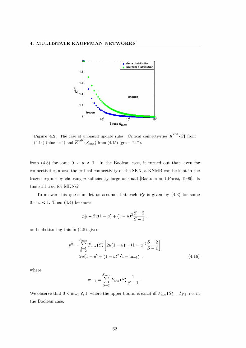
4. MULTISTATE KAUFFMAN NETWORKS
101 102 1031
1.2
1.4
1.6
1.8
2
frozen
chaotic
delta distributionuniform distribution
S resp Smax
Kcr
it
Figure 4.2: The case of unbiased update rules. Critical connectivities Kcrit
S
from
(4.14) (blue “”) and KcritpSmaxq from (4.15) (green “”).
from (4.3) for some 0 u 1. In the Boolean case, it turned out that, even for
connectivities above the critical connectivity of the SKN, a KNMB can be kept in the
frozen regime by choosing u sufficiently large or small [Bastolla and Parisi, 1996]. Is
this still true for MKNs?
To answer this question, let us assume that each PS is given by (4.3) for some
0 u 1. Then (4.4) becomes
puS 2up1 uq p1 uq2S 2S 1
,
and substituting this in (4.5) gives
pu Smax
S2
Pnos pSq2up1 uq p1 uq2S 2
S 1
2up1 uq p1 uq2 p1m1q , (4.16)
where
m1 Smax
S2
Pnos pSq 1S 1
.
We observe that 0 m1 ¤ 1, where the upper bound is exact iff Pnos pSq δS,2, i.e. in
the Boolean case.
62
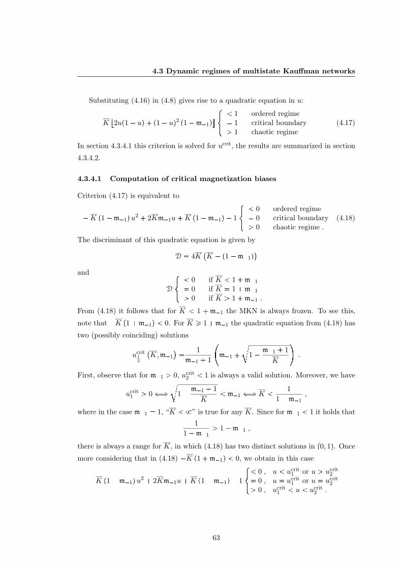
4.3 Dynamic regimes of multistate Kauffman networks
Substituting (4.16) in (4.8) gives rise to a quadratic equation in u:
K2up1 uq p1 uq2 p1m1q
$&% 1 ordered regime 1 critical boundary¡ 1 chaotic regime
(4.17)
In section 4.3.4.1 this criterion is solved for ucrit, the results are summarized in section
4.3.4.2.
4.3.4.1 Computation of critical magnetization biases
Criterion (4.17) is equivalent to
K p1m1qu2 2Km1uK p1m1q 1
$&% 0 ordered regime 0 critical boundary¡ 0 chaotic regime .
(4.18)
The discriminant of this quadratic equation is given by
D 4KK p1m1q
and
D
$&% 0 if K 1m1
0 if K 1m1
¡ 0 if K ¡ 1m1 .
From (4.18) it follows that for K 1 m1 the MKN is always frozen. To see this,
note that K p1m1q 0. For K ¥ 1m1 the quadratic equation from (4.18) has
two (possibly coinciding) solutions
ucrit12
K,m1
1m1 1
m1
c1 m1 1
K
.
First, observe that for m1 ¡ 0, ucrit2 1 is always a valid solution. Moreover, we have
ucrit1 ¡ 0 ðñ
c1 m1 1
K m1 ðñ K 1
1m1,
where in the case m1 1, “K 8” is true for any K. Since for m1 1 it holds that
11m1
¡ 1m1 ,
there is always a range for K, in which (4.18) has two distinct solutions in p0, 1q. Once
more considering that in (4.18) K p1m1q 0, we obtain in this case
K p1m1qu2 2Km1uK p1m1q 1
$&% 0 , u ucrit
1 or u ¡ ucrit2
0 , u ucrit1 or u ucrit
2
¡ 0 , ucrit1 u ucrit
2 .
63
4. MULTISTATE KAUFFMAN NETWORKS
4.3.4.2 The critical boundary in the case of biased update rules
Summing up, we have the following phase transitions:
(a) For K 1m1 the MKN is always frozen.
(b) For K 1m1 the MKN is critical if and only if
u ucritp1m1,m1q m1
m1 1, (4.19)
otherwise it is frozen.
(c) In the Boolean case, i.e. m1 1, and for K ¡ 1m1 2 the critical
boundary is described by
ucrit12
K, 1
12
1
c1 2
K
P p0, 1q . (4.20)
For
ucrit1
K, 1
u ucrit2
K, 1
the MKN is chaotic, otherwise it is frozen. This agrees with previous results
about Boolean KNs [Bastolla and Parisi, 1996].
(d) For m1 1 and 1p1m1q ¡ K ¡ 1m1 the critical boundary is described
by
ucrit12
K,m1
1m1 1
m1
c1 m1 1
K
P p0, 1q . (4.21)
For
ucrit1
K,m1
u ucrit2
K,m1
the MKN is chaotic, otherwise it is frozen. For K 1p1m1q, ucrit
1 0 is not
a valid solution for u anymore, as we require u P p0, 1q.
(e) For m1 1 and K ¥ 1p1m1q the critical boundary is described by
ucritK,m1
1m1 1
m1
c1 m1 1
K
P p0, 1q , (4.22)
for larger values of u the MKN is frozen, otherwise it is chaotic.
64
4.3 Dynamic regimes of multistate Kauffman networks
We chose to solve the criticality condition (4.17) for ucrit (and not Kcrit), as from
this presentation we easily see that for any values of K and m1 a MKN is kept in
its frozen regime by choosing a sufficiently large u. Thus, our motivating question can
be answered in the affirmative: Biasing update rules towards one of the discrete states
indeed increases the critical connectivity, from a theoretical point of view, even beyond
any bound.
In the Boolean case, the critical weights ucrit12 from (4.20) are, of course, symmetric
about 12, cf. case (c) in the above classification. In MKNs there still is a range of
connectivities where we can freeze a network by choosing either sufficiently large or
sufficiently small weights, cf. case (d). For higher connectivities, however, the option
of choosing small weights ceases to exist, cf. case (e). Intuitively speaking, even if we
set the weight to zero, the heterogeneity among the remaining states would still be
too large. Mathematically, this is reflected in the solution ucrit1 from (4.21) becoming
negative.
Now, suppose Pnos is a delta-distribution with a fixed number of states S. Then,
the upper bound K 1 m1 of case (a) in the above classification is precisely the
critical connectivity Kcrit of the unbiased MKN from (4.12). Furthermore, in case (b)
the critical value ucrit from (4.19) is equal to 1S. In agreement with Lemma 4.1, we
see that, if the connectivity of a MKN with biased update rules is below the critical
connectivity Kcrit (of the unbiased MKN), this MKN will always be frozen, as the
heterogeneity is already maximal in the unbiased situation. If its connectivity is equal
to Kcrit, it is critical if and only if the bias u is chosen in such a way that the resulting
PS is uniform. (The MKN then, of course, becomes unbiased.) Above Kcrit, we can
freeze any MKN by choosing a sufficiently heavy bias. For a visualization of the above
classification and discussion, see Figure 4.3A.
4.3.5 Network simulations
To further visualize our results, we choose six realizations of frozen, critical and chaotic
MKNs, cf. Figure 4.3B–K. Each network has N 100 nodes and each node has S 3
states, i.e. m1 12. We consider two delta-distributed degrees at K 2 (shown in B–
F) and K 4 (shown in G–K). For each connectivity we generate a frozen, critical and
chaotic network by sampling the update rules from distribution (4.3). For the frozen
networks we set u 0.95, for the critical networks we set u ucritp2, 12q 0.8604
65
4. MULTISTATE KAUFFMAN NETWORKS
and ucritp4, 12q 23 from (4.22), respectively, and for the chaotic networks we set
u 13. Observe that the latter choice leads to the unbiased distribution from (4.2).
Blue, green and red markers in subfigure A show the position of these values of u in
the K-u-plane. The blue markers lie above the critical boundary in the frozen regime,
both green markers are located on the critical boundary, and the red markers are in
midst the chaotic regime.
Subfigures B and G show Dpdq from (4.7) for both connectivities, K 2 as well
as K 4, and the three respective values of u. For the frozen networks (blue curves)
d 0 is the only fixed point and it is globally attracting. The fixed point d becomes
critical in the critical networks (green curves), and in the chaotic networks (red curves)
an additional fixed point d exists, which is now the global attractor. The additional
fixed points lie at d 0.498 in B and at d 0.661 in G.
For each of the six networks, two initial configurations xp0q and x1p0q with Hamming
distance dp0q 0.1 are chosen and each is iterated for 50 time-steps. Plots of the
simulated Hamming distance
dptq N
i1
1 δxiptq,x1iptq
between the two trajectories xptq and x1ptq for the six networks are shown in subfigures
C (K 2) and H (K 4). In the frozen networks (blue curves) the Hamming
distance quickly reaches its stationary value 0 indicating that both trajectories have
re-converged. If we discard the first 20 time-steps, the Hamming distances fluctuate
around 0.501 in the chaotic network with connectivity 2 and around 0.663 in the chaotic
network with connectivity 4, cf. the red curves and the dashed mean-lines in subfigures
C and H, respectively. These means agree well with the values of the “mean-field
attractors” d 0.498 and d 0.661, respectively. This is a nice corroboration of
our analytical studies.
Subfigures D–F and I–K show the time-course xiptq, i 1, 2, . . . , 25, t 1, 2, . . . 50,
for the frozen, critical and chaotic networks with K 2 and K 4. The three
states of a node are represented as black, grey and white boxes. In D and I, both
frozen networks quickly reach an equilibrium. While the critical networks in E and J
exhibit clear short-periodic oscillations after approximately 10 time-steps, no pattern
or periodicity is discernible in the chaotic networks in F and K. We know, of course,
66
4.4 Ensembles of trajectories
that ultimately also the chaotic networks will fall into a periodic orbit due to the finite
size of the state-space, cf. Proposition 4.1. Note that subfigures C–F as well as H–K
all have the same X-axis, namely time running from 1 to 50 as indicated in F and K.
4.4 Ensembles of trajectories
The Hamming distance looks at the similarity of two trajectories. More generally, we
could ask how a whole ensemble of trajectories behaves. A biological motivation for this
question is that in molecular biology experimental data are often average concentrations
in cell cultures. Mathematically, such a cell culture can be modeled as an ensemble of
trajectories of the same MM.
4.4.1 A dynamical system modeling ensembles of trajectories
Let pG,S, fq be a MM. In order to describe ensembles of trajectories of pG,S, fq and
relative frequencies therein, we consider time-courses of distributions over the Σi, i 1, 2, . . . , N .
Remark 4.6. The MM pG,S, fq gives rise to a time-discrete dynamical system as follows.To each node i we associate a time-dependent variable
xiptq
x0i ptqx1i ptq...
xSi1i ptq
,
¸sPΣi
xsi ptq 1 ,
describing distributions over Σi. We let xptq pxiptqqNi1. The evolution of xptq isgoverned by the iteration xpt1q f pxptqq, t 0, 1, 2, . . ., where f is defined such that
xsi pt 1q ¸
pξ1,ξ2,...,ξKiq|fipξ1,ξ2,...,ξKiqs
Ki¹k1
xξkik ptq , (4.23)
s P Σi, i 1, 2, . . . , N .
We call trajectories of the dynamical system from Remark 4.6 f -trajectories of
pG,S, fq, in order to tell them apart from trajectories of the dynamical system from
Remark 4.2.
67
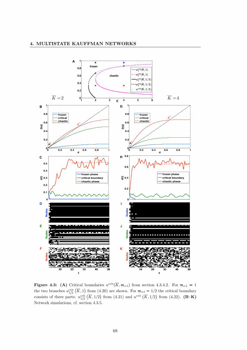
4. MULTISTATE KAUFFMAN NETWORKS
0
0.1
0.2
0.3
0.4
0.5
d(t)
frozen phasecritical boundarychaotic phase
0 0.2 0.4 0.6 0.8 10
0.2
0.4
0.6
0.8
1
d
D(d)
d*
d**frozencriticalchaotic
0 0.2 0.4 0.6 0.8 10
0.2
0.4
0.6
0.8
1
d
D(d)
d*
d**
frozencriticalchaotic
A
Nod
esN
odes
Nod
es
J
K
0
0.2
0.4
0.6
0.8
d(t)
frozen phasecritical boundarychaotic phase
H
I
Nod
esN
odes
Nod
es
E
F
C
D
1 2 3 4 5 60
0.2
0.4
0.6
0.8
1
K
chaotic
frozenucri t
1 ( K , 1 )
ucri t2 ( K , 1 )
ucri t1 ( K , 1 / 2 )
ucri t2 ( K , 1 / 2 )
ucri t( K , 1 / 2 )
GB
K = 2 K = 4
Figure 4.3: (A) Critical boundaries ucritpK,m1q from section 4.3.4.2. For m1 1the two branches ucrit
12
K, 1
from (4.20) are shown. For m1 12 the critical boundary
consists of three parts: ucrit12
K, 12
from (4.21) and ucrit
K, 12
from (4.22). (B–K)
Network simulations, cf. section 4.3.5.
68
4.4 Ensembles of trajectories
Remark 4.7. The right-hand side of (4.23) is the probability for fi to yield value s
given that its inputs ik are independent and assume values ξk P Σik with probabil-ities given by xξkik ptq. Now, suppose the MM pG,S, fq is given as a realization of aMKN with large N . Then, in the N -dependent time-domain r0, tN s from Lemma2.1, in which we may assume the inputs of a node to be independent, the dynamicalsystem from Remark 4.6 describes the evolution of probability distributions over theranges Σi of the nodes i 1, 2, . . . , N . More precisely, if at time t we choose valuesxiptq P Σi according to the distributions xiptq, then xipt 1q contains the probabilitiesfor xipt 1q fi
xi1ptq, xi2ptq, . . . , xiKi ptq
to be equal to the s P Σi. For this rea-
son, f -trajectories can be approximated by relative frequencies in large ensembles oftrajectories of pG,S, fq.
A node i is called deterministic at time t, if xsi ptq 1 for some s P Σi. If all
nodes are deterministic at t, we call the state xptq deterministic. Let Ξ denote the
canonical bijection between the states x of the dynamical system from Remark 4.2 and
the deterministic states x of the dynamical system from Remark 4.6. This is to say
that component-wise Ξ maps xi P Σi on the probability distribution
xsi "
1 , if s xi0 , otherwise
, s P Σi ,
over Σi.
Proposition 4.2. The function f maps deterministic states onto deterministic states,and the diagram ±N
i1 ΣiΞ //
f
Ξ±N
i1 Σi
f
±Ni1 Σi
Ξ // Ξ±N
i1 Σi
commutes. So f is compatible with f .
Proof. We fix x pxiqNi1 P±Ni1 Σi and let x pxiqNi1 be its image under Ξ. The
function f maps a component xi on the distribution
¸pξ1,ξ2,...,ξKiq|fipξ1,ξ2,...,ξKiqs
Ki¹k1
xξkik
sPΣi
.
69
4. MULTISTATE KAUFFMAN NETWORKS
The only non-zero contribution to the sum over the pξ1, ξ2, . . . , ξKiq is the combinationξk xik , k 1, 2, . . . ,Ki, which is included if and only if s fi
xi1 , xi2 , . . . , xiKi
. In
this case,±Kik1 x
ξkik 1. Hence, xi is mapped by f onto the distribution pysqsPΣi ,
ys #
1 , if s fi
xi1 , xi2 , . . . , xiKi
0 , otherwise
, s P Σi .
We, thus, see that the image of x under f is deterministic and given by the image off pxq under Ξ.
4.4.2 A generalized Hamming distance
Let K be a MKN. To avoid drowning the main ideas in too cumbersome formulae, we
restrict ourselves to the special case of a MKN with Pnos δS . We begin by stating
some technical preliminaries, which will be needed in the following. Let `pζ, zq denote
the probability that ζ fields, which are randomly filled with numbers 0, 1, . . . , S 1
according to PS , contain exactly z different elements. For a vector pκζqSζ1, we simply
write ` ppκζq, zq instead of `±S
ζ1 ζκζ , z
. Concise formulas for the `pζ, zq are difficult
to compute, and one has to resort to exhaustive enumeration. We can, however, prove
the following relations.
Lemma 4.4. 1. For any S and PS we have `p1, 1q ¡ `p2, 2q ¡ ¡ ` pS, Sq.
2. For S 3 and any P3 we have ` p2, 2q ¤ ` p3, 2q.
3. For any S and PS we have ` p1, 1q ¥ ` p2, 1q ¥ ¥ ` pS, 1q with equalities if andonly if PS is a degenerate delta-distribution.
Proof. Claims 1 and 3 are obvious. To prove statement 2, we let πs : P3psq, s Pt0, 1, 2u, and compute
` p2, 2q 2 rπ0π1 π0π2 π1π2s as well as
`p3, 2q 3π2
0π1 π20π2 π2
1π0 π21π2 π2
2π0 π22π1
.
After substituting π2 1 π0 π1, the equation `p2, 2q `p3, 2q has solutions
πp 1
2q0 pπ1q 1 10π1 9π2
1 p3π1 1qa
1 10π1 9π21
2 p9π1 1q .
On the unit interval, the solutions πp12q0 pπ1q are real for 0 ¤ π1 19, π1 13, andπ1 1. For 0 π1 19, πp1q0 pπ1q 0 and π
p2q0 pπ1q ¡ 1 are invalid solutions (they
70
4.4 Ensembles of trajectories
need to be probabilities!). Hence, `p2, 2q `p3, 2q has four distinct solutions pπ0, π1, π2qin r0, 1s3: p0, 0, 1q, p1, 0, 0q, p13, 13, 13q, and p0, 1, 0q. One easily computes that, forinstance, `p2, 2q 12 34 `p3, 2q if pπ0, π1, π2q p12, 12, 0q. This proves`p2, 2q ¤ `p3, 2q on r0, 1s3 with equality at the four distinct solutions from above.
According to Definition 4.3, the Hamming distance pdptqqt¥0 of K is a sequence of
probabilities that for some random realization a node i has two different values in two
different trajectories. Now, if we are given a large ensemble of trajectories we can again
ask how likely it is that i has at least two different values in the whole ensemble. Since
we are dealing with multistate KNs we may even ask how likely it is that i assumes
exactly z different values in the ensemble, where z 1, 2, . . . , S. For this reason, we
now study the average number of non-zero entries in f -trajectories xptq. We begin by
stating the counterpart of Lemma 4.2.
Lemma 4.5. LetZζp0qS
ζ1,°Sζ1 Z
ζp0q 1, be a distribution. Consider the fol-lowing random experiment: Generate a realization of K. Choose a configuration xp0qin a way such that the probability for a distribution xip0q to have (exactly) ζ non-zeroentries is given by Zζp0q, ζ 1, 2, . . . , S. Iterate xp0q one time-step under f yieldingconfiguration xp1q. Then, the probability Zzp1q that for a randomly chosen node i thedistribution xip1q has (exactly) z non-zero entries, z 1, 2, . . . , S, is given by
Zzp1q Kmax¸K1
Pin pKq¸
κ1...κSK
K
κ1, . . . , κS
S¹ζ1
Zζp0q
κζ ` ppκζq , zq .In particular, Zzp1q is independent of how the actual values in xp0q are chosen butdepends only on the probabilities Zζp0q for the distributions xip0q to have ζ non-zeroentries, ζ 1, 2, . . . , S.
Proof. Consider a realization of K and a randomly chosen node i. We describe itsinputs by a vector pκ1, κ2, . . . , κSq indicating the number of inputs with 1, 2, . . . , S non-zero entries in xp0q. Clearly, κ1 κ2 . . . κS Ki. Recall that in the configurationmodel the inputs ik of i are chosen randomly from V . Hence, the probability for theconfiguration pκζqSζ1 is given by
Ki
κ1, . . . , κS
S¹ζ1
Zζp0q
κζ.
The number of different tuples pξ1, ξ2, . . . , ξKiq satisfying±Kik1 x
ξkikp0q 0 in (4.23) is±S
ζ1 ζκζ . The x
fipξ1,ξ2,...,ξKiqi p1q belonging to these tuples are the different non-zero
71
4. MULTISTATE KAUFFMAN NETWORKS
entries of xip1q. The probability that their number is equal to z is ` ppκζq , zq. Averagingover Ki yields the claim.
Instead of the Hamming distance pdptqqt¥0 of K we can, therefore, also study a se-
quence Zptq pZzptqqSz1 P RS which is consistent in the sense of Lemma 4.5, i.e. gov-
erned by the iteration
Zpt 1q C pZptqq , (4.24)
where the z-th component Cz pZptqq of the right-hand side is given by
Kmax¸K1
Pin pKq¸
κ1...κSK
K
κ1, . . . , κS
S¹ζ1
Zζptq
κζ ` ppκζq , zq , (4.25)
z 1, 2, . . . , S.
Remark 4.8. Once more, we argue that, for large N , Lemma 2.1 allows us to assumethe inputs of a node to be independent in a realization of K. We can, thus, approximateZzptq by the fraction of nodes with z non-zero entries in a f -trajectory xptq of a specificrealization of K. By Remark 4.7, we can also approximate Zzptq by the fraction of nodeswith z different states in a large (Ω " S) ensemble of trajectories xqptq, q 1, 2, . . . ,Ω,of a specific realization of K,
Zzptq 1N#
!i | pxqi ptqqΩq1 has z different components.
), (4.26)
z 1, 2, . . . , S. We will use this approximation in section 4.4.4.
4.4.3 Synchronization in ensembles of trajectories
Especially when conducting transcriptome-wide measurements, e.g. by microarrays, we
want the single cells in our experimental sample to act synchronously, as only then the
experimentally observed average concentrations are representative of the single cells.
Intuitively, one would expect that for frozen MKNs, an ensemble of trajectories of a
realization converges, whereas for chaotic MKNs it diverges. Let us first check, if this
can also be analytically seen from system (4.24).
To this end, we investigate the fixed point Z p1, 0, . . . , 0q of (4.24). It corresponds
to an ensemble of identical trajectories. (That Z is, indeed, a fixed point can be
easily seen; note Cz pZq `p1, zq.) We now show that the stability properties of Z
change precisely at the critical boundary of K. The distributions Zptq live on the affine
hyperplane of RS defined by°Sz1 Z
zptq 1. In order to take derivatives, we choose as
72
4.4 Ensembles of trajectories
a global chart the projection on the first S 1 coordinates. We remark that the choice
of charts, in general, does affect the Jacobian, but not its eigenvalues, as a change of
charts merely means a change of basis in the tangent space. Hence, this choice is not
crucial for stability analyses.
Let us now compute the Jacobian J DC|Z of C at Z. First, consider the case
of fixed K. In global coordinates we can write:
CzZ1, . . . , ZS1
¸κ1...κSK
K
κ1, . . . , κS
S1¹ζ1
Zζ
κζ 1S1
ζ1
Zζ
κS
` ppκζq , zq
Differentiating with respect to Zs yields
BCzBZs
¸κ1...κSK
K
κ1, . . . , κS
` ppκζq , zq
¹ζs,S
Zζ
κζ pZsqκs κS1
S1
ζ1
Zζ
κS1
κs pZsqκs1
1
S1
ζ1
Zζ
κS ,
where, formally, 0 01 0. The evaluation of this term at Z is
BCzBZs
Z K ` ps, zq K ` pS, zq .
To see this, note that the only non-zero contributions to the sum over the pκ1, . . . , κSqare the combinations pK, 0, . . . , 0, 0q and pK 1, 0, . . . , 0, 1q if s 1, and the combi-
nations κ1 K 1, . . . , κs 1, . . . , κS 0 and κ1 K 1, . . . , κs 0, . . . , κS 1 if
s 1.
For general Pin it follows
BCzBZs
Z
Kmax¸K1
Pin pKqK r` ps, zq ` pS, zqs K r` ps, zq ` pS, zqs ,
and we obtain
J K
` p1, 1q ` p2, 1q ` pS 1, 1q0 ` p2, 2q ` pS 1, 2q...
.... . .
...0 0 ` pS 1, S 1q
` pS, 1q ` pS, 1q ` pS, 1q` pS, 2q ` pS, 2q ` pS, 2q
......
. . ....
` pS, S 1q ` pS, S 1q ` pS, S 1q
. (4.27)
73
4. MULTISTATE KAUFFMAN NETWORKS
Lemma 4.6. The eigenvalues of J are K ` ps, sq, s 2, 3, . . . , S.
Proof. According to (4.27), we write J K pJ1 J2q with pS1qpS1q matrices J1
and J2. J2 consists of identical columns a. We extend J1 to an S S upper triangularmatrix J 11 by an S-th row p0, 0, . . . , `pS, Sqq and column p`pS, 1q, `pS, 2q, . . . , `pS, SqqJ aJ, `pS, SqJ. Let s P t2, 3, . . . , Su and vs
vζs
Sζ1
be an eigenvector to the eigen-
value `ps, sq of J 11. As J 11 is a left-stochastic matrix, it follows from `ps, sqvs J 11vs
that `ps, sq°Sζ1 v
ζs
°Sζ1 v
ζs . Thus,
°Sζ1 v
ζs 0, since `ps, sq 1. As J2 consists of
identical columns a this implies J2
vζs
S1
ζ1 vSs a. It follows
pJ1 J2qvζs
S1
ζ1 pJ1 | aq
vζs
Sζ1
vSs a J2
vζs
S1
ζ1
`ps, sqvζs
S1
ζ1 vSs a vSs a
`ps, sqvζs
S1
ζ1,
which shows that K`ps, sq is an eigenvalue of J .
From Lemma 4.4.1 it follows that the largest eigenvalue is K ` p2, 2q. Further note
that ` p2, 2q °S1s0 PSpsq p1 PSpsqq pS p. The phase transition criterion from
Theorem 4.1 together with Theorem 2.2, thus, implies
Theorem 4.2. The dynamic regimes of MKNs from Definition 4.4 have the followingcharacteristics.
frozen regime: Z is a hyperbolic and asymptotically stable fixed point.
critical boundary: The fixed point Z is critical.
chaotic regime: The fixed point Z is unstable.
Thus, our intuition about synchronization in ensembles of trajectories agrees with
the behavior of system (4.24). Whereas for frozen MKNs we may expect ensembles to
synchronize over time, this will not be the case for chaotic MKNs. In other words, we
have derived a further characterization of the dynamic regimes from Definition 4.4. We
remark that the dynamical system from (4.24) can also be used to study the behavior
of KNs with an extension of Boolean logic called fuzzy logic [Wittmann and Theis,
2010a].
74
4.4 Ensembles of trajectories
4.4.4 Example and simulations
We finish by detailing the behavior of the distributions Zptq in a specific example, more
precisely, in the case S 3. The distribution P3 will be assumed to be non-degenerate,
i.e. P3psq 1 for all s P t0, 1, 2u. We work again in the projection of (4.24) on the first
two coordinates. Hence, we are dealing with the planar system
Z1pt 1qZ2pt 1q
C1
Z1ptq, Z2ptq
C2Z1ptq, Z2ptq
. (4.28)
Lemma 4.7. There exist functions Z21
Z1
and Z2
2
Z1
around Z, which satisfy
C1Z1, Z2
1
Z1
Z1 and C2Z1, Z2
2
Z1
Z2, respectively. Moreover,
dZ21
dZ1p1q K r` p1, 1q ` p3, 1qs 1
K r` p2, 1q ` p3, 1qs and (4.29)
dZ22
dZ1p1q K` p3, 2q
K r` p2, 2q ` p3, 2qs 1. (4.30)
Proof. From (4.27) we read off
B C1Z1, Z2
Z1
BZ2
Z
K r` p2, 1q ` p3, 1qs and
B C2Z1, Z2
Z2
BZ2
Z
K r` p2, 2q ` p3, 2qs 1 .
By Lemma 4.4.3 and 4.4.2 these derivatives do not vanish. (Recall that we assumed P3
to be non-degenerate.) The claim follows from the implicit function theorem.
Lemma 4.8. It holds dZ22dZ1 p1q 0. Moreover, the dynamic regimes of MKNs from
Definition 4.4 have the following characteristics:
frozen regime:dZ2
1
dZ1p1q ¡ 1 ,
dZ22
dZ1p1q ¡ 1 .
critical boundary:dZ2
1
dZ1p1q 1 ,
dZ22
dZ1p1q 1 .
chaotic regime:dZ2
1
dZ1p1q 1 ,
dZ22
dZ1p1q 1 .
75
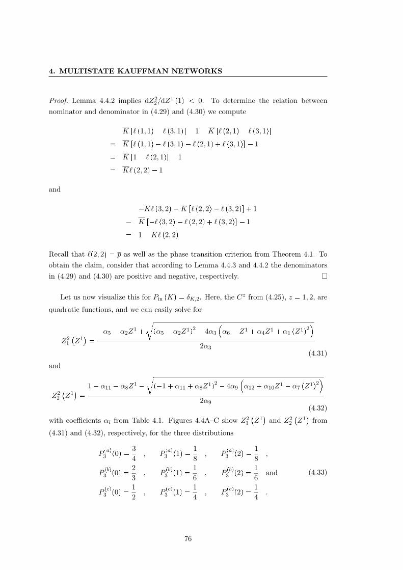
4. MULTISTATE KAUFFMAN NETWORKS
Proof. Lemma 4.4.2 implies dZ22dZ1 p1q 0. To determine the relation between
nominator and denominator in (4.29) and (4.30) we compute
K r` p1, 1q ` p3, 1qs 1K r` p2, 1q ` p3, 1qs K r` p1, 1q ` p3, 1q ` p2, 1q ` p3, 1qs 1
K r1 ` p2, 1qs 1
K` p2, 2q 1
and
K` p3, 2q K r` p2, 2q ` p3, 2qs 1
K r` p3, 2q ` p2, 2q ` p3, 2qs 1
1K` p2, 2q
Recall that `p2, 2q p as well as the phase transition criterion from Theorem 4.1. Toobtain the claim, consider that according to Lemma 4.4.3 and 4.4.2 the denominatorsin (4.29) and (4.30) are positive and negative, respectively.
Let us now visualize this for Pin pKq δK,2. Here, the Cz from (4.25), z 1, 2, are
quadratic functions, and we can easily solve for
Z21
Z1
α5 α2Z1
cpα5 α2Z1q2 4α3
α6 Z1 α4Z1 α1 pZ1q2
2α3
(4.31)
and
Z22
Z1
1 α11 α8Z1
cp1 α11 α8Z1q2 4α9
α12 α10Z1 α7 pZ1q2
2α9
(4.32)
with coefficients αi from Table 4.1. Figures 4.4A–C show Z21
Z1
and Z2
2
Z1
from
(4.31) and (4.32), respectively, for the three distributions
Ppaq3 p0q 3
4, P
paq3 p1q 1
8, P
paq3 p2q 1
8,
Ppbq3 p0q 2
3, P
pbq3 p1q 1
6, P
pbq3 p2q 1
6and
Ppcq3 p0q 1
2, P
pcq3 p1q 1
4, P
pcq3 p2q 1
4.
(4.33)
76
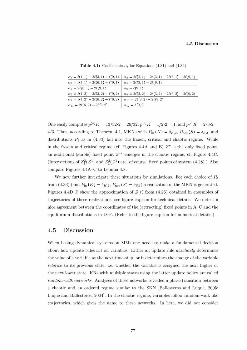
4.5 Discussion
Table 4.1: Coefficients αi for Equations (4.31) and (4.32)
α1 `p1, 1q 2`p3, 1q `p9, 1q α2 2`p2, 1q 2`p3, 1q 2`p6, 1q 2`p9, 1q
α3 `p4, 1q 2`p6, 1q `p9, 1q α4 2`p3, 1q 2`p9, 1q
α5 2`p6, 1q 2`p9, 1q α6 `p9, 1q
α7 `p1, 2q 2`p3, 2q `p9, 2q α8 2`p2, 2q 2`p3, 2q 2`p6, 2q 2`p9, 2q
α9 `p4, 2q 2`p6, 2q `p9, 2q α10 2`p3, 2q 2`p9, 2q
α11 2`p6, 2q 2`p9, 2q α12 `p9, 2q
One easily computes ppaqK 13322 2632, ppbqK 122 1, and ppcqK 232 43. Thus, according to Theorem 4.1, MKNs with Pin pKq δK,2, Pnos pSq δS,3, and
distributions P3 as in (4.33) fall into the frozen, critical and chaotic regime. While
in the frozen and critical regime (cf. Figures 4.4A and B) Z is the only fixed point,
an additional (stable) fixed point Z emerges in the chaotic regime, cf. Figure 4.4C.
(Intersections of Z21 pZ1q and Z2
2 pZ1q are, of course, fixed points of system (4.28).) Also
compare Figures 4.4A–C to Lemma 4.8.
We now further investigate these situations by simulations. For each choice of P3
from (4.33) (and Pin pKq δK,2, Pnos pSq δS,3) a realization of the MKN is generated.
Figures 4.4D–F show the approximation of Zptq from (4.26) obtained in ensembles of
trajectories of these realizations, see figure caption for technical details. We detect a
nice agreement between the coordinates of the (attracting) fixed points in A–C and the
equilibrium distributions in D–F. (Refer to the figure caption for numerical details.)
4.5 Discussion
When basing dynamical systems on MMs one needs to make a fundamental decision
about how update rules act on variables. Either an update rule absolutely determines
the value of a variable at the next time-step, or it determines the change of the variable
relative to its previous state, i.e. whether the variable is assigned the next higher or
the next lower state. KNs with multiple states using the latter update policy are called
random-walk networks. Analyses of these networks revealed a phase transition between
a chaotic and an ordered regime similar to the SKN [Ballesteros and Luque, 2005;
Luque and Ballesteros, 2004]. In the chaotic regime, variables follow random-walk like
trajectories, which gives the name to these networks. In here, we did not consider
77
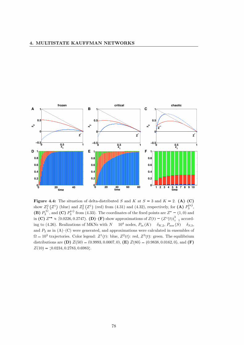
4. MULTISTATE KAUFFMAN NETWORKS
0 0.5 10.5
0
0.5
1
z1
z 2
Z*
0 0.5 10.5
0
0.5
1
z1
z 2
Z*
0 0.5 10.5
0
0.5
1
z1z 2
Z*
Z**
A CB
1 2 3 4 5 6 7 8 9 100
0.2
0.4
0.6
0.8
1
time0 20 400
0.2
0.4
0.6
0.8
1
time0 20 40 60 800
0.2
0.4
0.6
0.8
1
time
D FE
frozen critical chaotic
Figure 4.4: The situation of delta-distributed S and K at S 3 and K 2. (A)–(C)show Z2
1
Z1
(blue) and Z2
2
Z1
(red) from (4.31) and (4.32), respectively, for (A) P paq
3 ,(B) P pbq
3 , and (C) P pcq3 from (4.33). The coordinates of the fixed points are Z p1, 0q and
in (C) Z p0.0226, 0.2747q. (D)–(F) show approximations of Zptq pZzptqq3z1 accord-
ing to (4.26). Realizations of MKNs with N 104 nodes, Pin pKq δK,2, Pnos pSq δS,3,and P3 as in (A)–(C) were generated, and approximations were calculated in ensembles ofΩ 103 trajectories. Color legend: Z1ptq: blue, Z2ptq: red, Z3ptq: green. The equilibriumdistributions are (D) Zp50q p0.9993, 0.0007, 0q, (E) Zp80q p0.9838, 0.0162, 0q, and (F)Zp10q p0.0234, 0.2783, 0.6983q.
78
4.5 Discussion
random-walk networks but KNs with multiple states using the first update policy; we
referred to them as MKNs.
Previous studies of MKNs by Sole et al. [2000] are restricted to the biologically
implausible case in which all nodes have the same number of states. In agreement
with our more general results, it has been shown that in the case of unbiased update
rules an increasing number of states decreases the critical connectivity down to 1. It is
tempting to assume that this stays true (at least in a qualitative sense) when replacing
the (fixed) number of states by the mean of a non-degenerate distribution. However,
our results demonstrate that, in general, this is wrong. From the critical connectivity
in (4.12) we see that the crucial parameter is not the mean number of states, but the
mean m of the reciprocal number of states.
Generally speaking, the mean of a strictly positive, non-constant random variable
S and the mean of 1S are related by
E
1S
¡ 1
E pSq ,
for a proof see e.g. Kendall et al. [1987]. Furthermore, we can easily come up with a
distribution
P pS 2q s 1s
and PS s2
1sfor s P N, such that EpSq Ñ 8 but E p1Sq Ñ 12 as s Ñ 8. Setting Pnos P , the
critical connectivity from (4.12) increases up to 2 as sÑ8, although the mean number
of states grows beyond any bound.
In this chapter, we investigated a general class of MKNs and demonstrated that they
exhibit a phase transition from frozen to chaotic behavior as the connectivity of the
network grows. To this end, we formally introduced the Hamming distance between
two configurations as an order parameter for MKNs and investigated its dynamical
behavior. The critical boundary between the frozen and chaotic phase was determined
analytically. In its most general representation (4.9) the critical connectivity is inversely
proportional to the heterogeneity p from (4.5) of the MKN. This parameter becomes
maximal if the update rules are unbiased, i.e. assume each value with equal probability,
cf. Lemma 4.1. It is minimal (zero), if the update rules are constant functions.
In particular, we saw that SKNs as introduced by Kauffman [1969] have a critical
connectivity of two, cf. Remark 4.5. Below this connectivity they exhibit stable dynam-
ics, whereas above this connectivity their dynamics are unstable and highly sensitive
79
4. MULTISTATE KAUFFMAN NETWORKS
to perturbations. Bearing this in mind, let us recall the questions which Kauffman
[1969] set out to answer, cf. section 3.4. We have now seen that stable dynamics are,
indeed, to be expected in nets of randomly interconnected regulatory circuits, provided
they are sufficiently sparse. Stability does not require the circuits to be precisely con-
structed, but only places an upper bound on their connectivity. Kauffman [1993] called
this generic stability of sparsely connected KNs “order for free.” He argues that reg-
ulatory networks in living organisms benefit from this “order for free” as well as from
the variability of a nearby chaotic regime.
Our analysis of unbiased MKNs, however, showed that the region in which we get
“order for free” shrinks, when we leave the Boolean case and allow for multiple states,
cf. Remark 4.5. Yet, we also demonstrated that each MKN can be kept in the ordered
regime by putting a sufficiently heavy bias on one of the states, cf. section 4.3.4.2. From
a biological point of view, this may indicate that in real genetic networks the update
functions have a base level of activation and deviations thereof constitute well-defined
exceptions.
At this point, we caution that all our results and their interpretation apply to
Kauffman’s idealization of gene regulatory networks, their significance for the real bio-
logical systems should, as always, be treated with wariness. Still, there are promising
attempts, e.g. by Balleza et al. [2008] and Kauffman et al. [2003], to bridge the gap
between the theoretical concept of a KN and real genetic networks.
Finally, we took a look at ensembles of trajectories as an extension to the study
of the Hamming distance between two trajectories. We were able to characterize the
different regimes of MKNs in terms of the synchronization behavior of such ensem-
bles. In an example, we demonstrated that our analytic computations agree well with
simulation results.
80
5
Kauffman networks with generic
logics
You want the truth?
You can’t handle the truth!
Jack Nicholson in “A Few Good Men”
The last decades witnessed a series of technological breakthroughs in the life-
sciences. We can now monitor the entire gene or protein profile of cells and study
epistatic relationships by gain- and loss-of-function experiments. Information about
whether or not a gene is expressed in a specific cell type or tissue is readily available, as
is information about activating and inhibiting regulatory interactions. Naturally, one
always wishes for more accurate and comprehensive data, but compared to what was
possible and available some twenty years ago the wealth of information is remarkable.
It more and more turns out that, at least from a modeler’s point of view, the integration
of available information into predictive models is as much a problem as is the possible
lack of further important information. In a way, we already have the truth, we just
cannot handle it.
81
5. KAUFFMAN NETWORKS WITH GENERIC LOGICS
In less abstract terms, information about pairwise genetic interactions can typically
be obtained experimentally. The question how the various regulatory influences on a
gene interact in order to determine its expression, however, is combinatorially complex
and often intractable.
5.1 Motivation and outline
Theoretical biologists often distinguish between qualitative and Boolean models of gene
regulatory networks. Qualitative models are typically defined as directed signed graphs.
The nodes represent genes, the edges positive (activating) and negative (inhibiting)
regulatory interactions. Qualitative models may already yield valuable information,
e.g. about multistationarity or oscillations [Thomas, 1978]. However, in general they
do not allow for time-course simulations as the interplay of a gene’s regulators is not
specified. This additional information is provided in BMs. Here, each node is assigned
an update function, which defines the node’s value depending upon the values of the
node’s regulators at the previous time-point.
The information required for the setup of a qualitative model can be obtained
e.g. from gain- or loss-of-function experiments, or on a larger scale from bioinformatics
resources. The inference of Boolean update functions from biological data, however,
is not as straightforward. Therefore, heuristic modeling approaches for the automated
conversion of qualitative into Boolean models have been proposed. The standardized
qualitative dynamical systems approach, for instance, was successfully used to model T
helper cell differentiation [Mendoza and Xenarios, 2006]. Several reverse engineering
approaches also rely on such transformations [Bulashevska and Eils, 2005; Martin et al.,
2007]. In our modeling toolbox ODEfy [Krumsiek et al., 2010] a unifying framework
for all these transformations is established via so-called generic logics. These are tuples
of Boolean operators that allow to define a node’s update rule by linking its activators
and inhibitors according to a specific pattern. A complementary approach that cannot
be treated within the framework of generic logics are threshold update rules as used in
Li et al. [2004] or Rohlf and Bornholdt [2002].
In this chapter, which follows Wittmann and Theis [2010b], we study KNs generated
by generic logics. We formally introduce this class of KNs in section 5.2. Due to
their prominent role in the study of SKNs and KNsMB our main goal is to analyze
82
5.2 Qualitative models and Kauffman networks with generic logics
phase transitions in these KNs. We already mentioned that a phase transition can be
understood as a change of the percolation behavior in realizations of a KN, and that in
SKNs or KNsMB this percolation is independent of the actual states of the associated
dynamical system, cf. Lemma 4.2. In this chapter, we will see that this is no longer
true for realizations of a KN with generic logics.
For this reason, we begin in section 5.3 by studying a quantity which we call the
truth-content of a KN. It is defined as the probability for a node to be true (one). In
large KNs the truth-content can be approximated by the fraction of ones in a trajectory
xptq of a realization. In KNsMB the truth-content has stationary dynamics with an
equilibrium given by the magnetization bias. For KNs with generic logics we are able
to prove that the dynamics of the truth-content are essentially dynamics of S-unimodal
functions as described in sections 2.2.4.1 and 2.2.4.2. In numeric analyses, this truth-
content, indeed, exhibits the characteristic, rich dynamical behaviors of these functions
including period-doublings leading to chaos. We prove that the truth-content of KNs
with generic logics possesses a unique attractor and characterize it, cf. Theorems 5.1,
5.2 and 5.3. This allows us to define truth-stable KNs as networks whose truth-contents
exhibit non-chaotic dynamics.
In section 5.4, we use the results from the previous section to derive a criterion
for phase transitions in KNs with generic logics, cf. Theorems 5.5 and 5.6. Section
5.5 concludes the mathematical part of this chapter by numerical analyses and further
confirms the validity of our results by simulations. Finally, in section 5.6, we discuss
our results with respect to their biological implications.
5.2 Qualitative models and Kauffman networks with ge-
neric logics
In this chapter, G pV,Eq will again denote a (directed) graph of order N with nodes
V t1, 2, . . . , Nu and edges pi1 Ñ iq P E V V . The predecessors (inputs) of a node
i are denoted by i1 i2 iKi , where Ki is the node’s in-degree.
Definition 5.1 (qualitative model). A qualitative model (QM) is a tuple pG, σq con-sisting of a graph G and a signature σ : E Ñ t,u of G. We call an input ik of anode i activating if σ pik Ñ iq and inhibiting if σ pik Ñ iq .
83
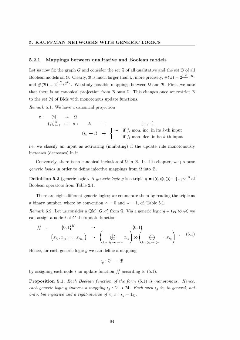
5. KAUFFMAN NETWORKS WITH GENERIC LOGICS
5.2.1 Mappings between qualitative and Boolean models
Let us now fix the graph G and consider the set Q of all qualitative and the set B of all
Boolean models on G. Clearly, B is much larger than Q; more precisely, #pQq 2°Ni1Ki
and #pBq 2°Ni1 2Ki . We study possible mappings between Q and B. First, we note
that there is no canonical projection from B onto Q. This changes once we restrict B
to the set M of BMs with monotonous update functions.
Remark 5.1. We have a canonical projection
π : M Q
pfiqNi1 ÞÑ σ : E Ñ t,u
pik Ñ iq ÞÑ# if fi mon. inc. in its k-th input if fi mon. dec. in its k-th input
i.e. we classify an input as activating (inhibiting) if the update rule monotonouslyincreases (decreases) in it.
Conversely, there is no canonical inclusion of Q in B. In this chapter, we propose
generic logics in order to define injective mappings from Q into B.
Definition 5.2 (generic logic). A generic logic g is a triple g p`,b,aq P t^,_u3 ofBoolean operators from Table 2.1.
There are eight different generic logics; we enumerate them by reading the triple as
a binary number, where by convention ^ 0 and _ 1, cf. Table 5.1.
Remark 5.2. Let us consider a QM pG, σq from Q. Via a generic logic g p`,b,aq wecan assign a node i of G the update function
fgi : t0, 1uKi Ñ t0, 1uxi1 , xi2 , . . . , xiKi
ÞÑ
àk|σpikÑiq
xik
b ák|σpikÑiq
xik
. (5.1)
Hence, for each generic logic g we can define a mapping
ιg : Q ÝÑ B
by assigning each node i an update function fgi according to (5.1).
Proposition 5.1. Each Boolean function of the form (5.1) is monotonous. Hence,each generic logic g induces a mapping ιg : Q Ñ M. Each such ιg is, in general, notonto, but injective and a right-inverse of π, π ιg 1Q.
84
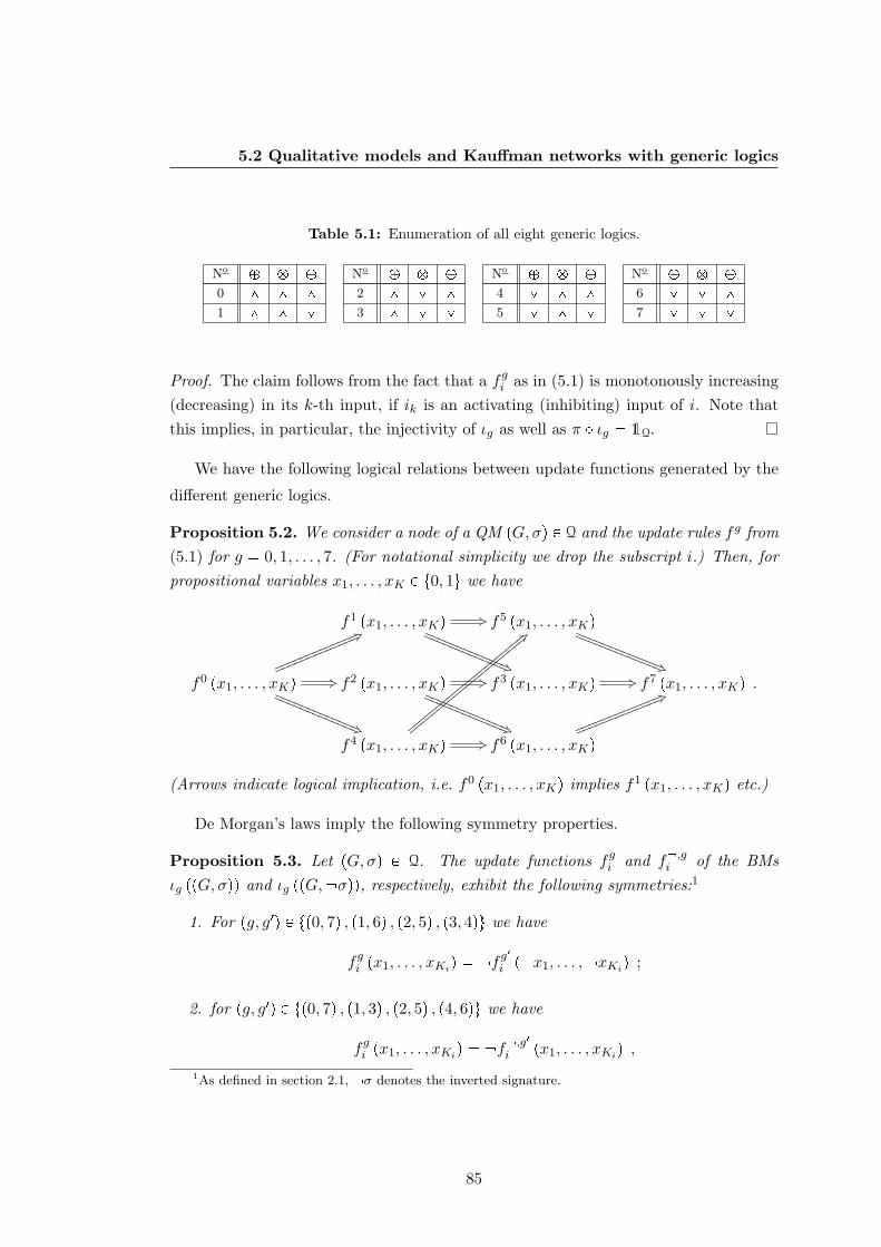
5.2 Qualitative models and Kauffman networks with generic logics
Table 5.1: Enumeration of all eight generic logics.
No ` b a No ` b a No ` b a No ` b a
0 ^ ^ ^ 2 ^ _ ^ 4 _ ^ ^ 6 _ _ ^
1 ^ ^ _ 3 ^ _ _ 5 _ ^ _ 7 _ _ _
Proof. The claim follows from the fact that a fgi as in (5.1) is monotonously increasing(decreasing) in its k-th input, if ik is an activating (inhibiting) input of i. Note thatthis implies, in particular, the injectivity of ιg as well as π ιg 1Q.
We have the following logical relations between update functions generated by the
different generic logics.
Proposition 5.2. We consider a node of a QM pG, σq P Q and the update rules fg from(5.1) for g 0, 1, . . . , 7. (For notational simplicity we drop the subscript i.) Then, forpropositional variables x1, . . . , xK P t0, 1u we have
f1 px1, . . . , xKq +3
$,RRRRRRRRRRRRR
RRRRRRRRRRRRRf5 px1, . . . , xKq
%-RRRRRRRRRRRRR
RRRRRRRRRRRRR
f0 px1, . . . , xKq
2:lllllllllllll
lllllllllllll+3
$,RRRRRRRRRRRRR
RRRRRRRRRRRRRf2 px1, . . . , xKq +3
$,RRRRRRRRRRRRR
RRRRRRRRRRRRRf3 px1, . . . , xKq +3 f7 px1, . . . , xKq .
f4 px1, . . . , xKq
8@yyyyyyyyyyyyyyyyyyyyy
yyyyyyyyyyyyyyyyyyyyy+3 f6 px1, . . . , xKq
19lllllllllllll
lllllllllllll
(Arrows indicate logical implication, i.e. f0 px1, . . . , xKq implies f1 px1, . . . , xKq etc.)
De Morgan’s laws imply the following symmetry properties.
Proposition 5.3. Let pG, σq P Q. The update functions fgi and f ,gi of the BMsιg ppG, σqq and ιg ppG, σqq, respectively, exhibit the following symmetries:1
1. For pg, g1q P tp0, 7q , p1, 6q , p2, 5q , p3, 4qu we have
fgi px1, . . . , xKiq fg1
i p x1, . . . , xKiq ;
2. for pg, g1q P tp0, 7q , p1, 3q , p2, 5q , p4, 6qu we have
fgi px1, . . . , xKiq f ,g1
i px1, . . . , xKiq ,1As defined in section 2.1, σ denotes the inverted signature.
85
5. KAUFFMAN NETWORKS WITH GENERIC LOGICS
where x1, . . . , xKi P t0, 1u are propositional variables.
Proposition 5.3.1 implies
Corollary 5.1. Let pG, σq be a QM and consider the BMs pG, fgq ιg ppG, σqq, g 0, 1, . . . , 7. For pg, g1q P tp0, 7q , p1, 6q , p2, 5q , p3, 4qu the dynamical systems xpt 1q fg pxptqq and ypt 1q fg
1 pyptqq from Remark 3.1 are topologically conjugate viacomponent-wise negation on t0, 1uN .
5.2.2 Kauffman networks with generic logics
Let us now define the class of KNs which will be the subject of the following investi-
gations. We refer to them as Kauffman networks with generic logics (KNGL). Each
KNGL is specified by four parameters: the order N , the generic logic g, the connec-
tivity K and an activation bias a P r0, 1s. As we will always consider the limit of
large N we typically omit the parameter N and specify a KNGL by the tuple pg, a,Kq.Realizations pG, fq of a KNGL pg, a,Kq (of order N) are constructed according to the
following random process.
(G1) Create a realization of the random graph G pPinq with Pin δK .
(G2) Define a signature σ of G by setting σ pik Ñ iq with probability a and
σ pik Ñ iq with probability r 1 a for each edge ik Ñ i of G. We obtain
a qualitative model pG, σq.
(G3) Set pG, fq ιg ppG, σqq.
In other words, G will always be a graph with fixed connectivity K for all nodes.
Different generative models for G remain to be investigated, see the outlook in section
7.2.2. Similarly to KNsMB, we introduce a bias a and classify an edge as activating or
inhibiting with probabilities a and r 1 a, respectively.
Remark 5.3. Note that for K 1, KNsGL are critical KNs where only “copy” and“invert” are used as update rules. These KNs are well understood and we refer theinterested reader to Drossel [2005].
In the following, g P t0, 1, . . . , 7u always denotes the generic logic, 0 ¤ a ¤ 1 the
bias towards activations, and K P N the connectivity of a KNGL. We point out once
more that K is the fixed connectivity of a regular graph and cannot be interpreted as
a mean connectivity.
86
5.3 The truth-content of a Kauffman network with generic logic
5.3 The truth-content of a Kauffman network with generic
logic
As explained above, we first turn our attention to a quantity we call the truth-content
of a KN. We introduce this concept for general KNs and only later restrict ourselves to
KNsGL. So, at first let K be a general KN.
Definition 5.3 (truth-content of a KN). The truth-content of K is a sequence pwptqqt¥0
which is consistent in the sense of the following random experiment: Pick a realizationof K, create a configuration xp0q whose components are 1 with probability wptq, anditerate it one time-step yielding configuration xp1q. Then, wpt 1q is the probabilityfor a component of xp1q to be 1.
Remark 5.4. Lemma 2.1 allows us to approximate the truth-content of K by the fractionof ones
wptq 1N
N
i1
xiptq (5.2)
in a trajectory xptq of a specific realization of K provided N is sufficiently large. Wefurther illustrate this by simulations in section 5.5.3.
The truth-content of a KN with magnetization bias u exhibits a rather uninteresting
dynamical behavior.
Remark 5.5. In a KN with magnetization bias u we have wptq u for all t ¡ 0.
The proof that KNs with canalyzing update rules are always frozen, cf. Kauffman
et al. [2004], also involves computing the truth-content. However, also for this par-
ticular choice of update rules wptq has stationary equilibrium dynamics. Let us now
see how wptq behaves in KNsGL and whether a more interesting dynamical behavior
can be observed. We let K pg, a,Kq be a KNGL and denote its truth-content by
pwg,a,Kptqqt¥0. If no ambiguity exists, we simply write wgptq instead of wg,a,Kptq.First, we take care of the issue that the truth-content wgptq of K depends on the
initial condition wgp0q. To this end, we prove that the asymptotic behavior of wgptqis identical for almost all initial conditions. We consider this a result in its own right.
Moreover, it will allow us to derive a criterion for phase transitions in section 5.4.
We proceed as follows. In section 5.3.1 we describe the truth-content wgptq of K by
an iteration. Section 5.3.2 then lists some useful properties of the iteration functions.
87
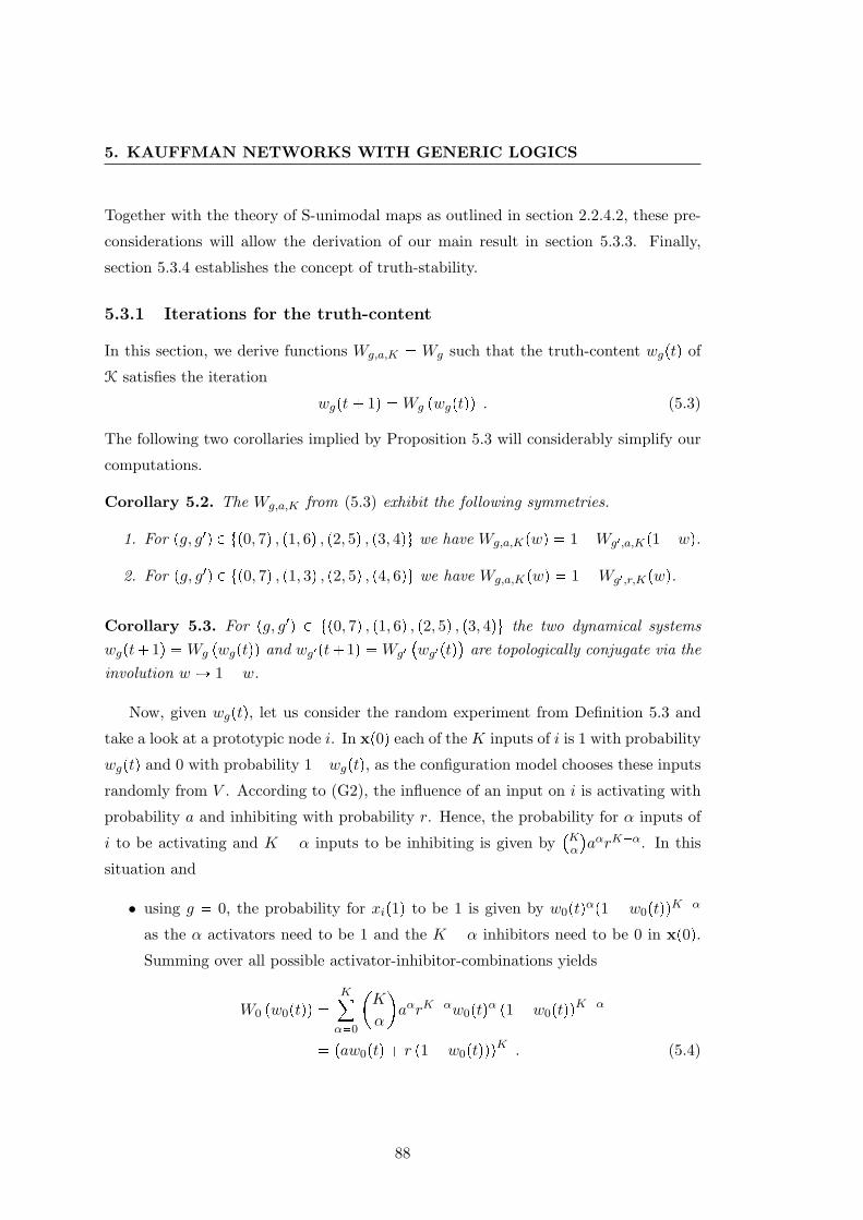
5. KAUFFMAN NETWORKS WITH GENERIC LOGICS
Together with the theory of S-unimodal maps as outlined in section 2.2.4.2, these pre-
considerations will allow the derivation of our main result in section 5.3.3. Finally,
section 5.3.4 establishes the concept of truth-stability.
5.3.1 Iterations for the truth-content
In this section, we derive functions Wg,a,K Wg such that the truth-content wgptq of
K satisfies the iteration
wgpt 1q Wg pwgptqq . (5.3)
The following two corollaries implied by Proposition 5.3 will considerably simplify our
computations.
Corollary 5.2. The Wg,a,K from (5.3) exhibit the following symmetries.
1. For pg, g1q P tp0, 7q , p1, 6q , p2, 5q , p3, 4qu we have Wg,a,Kpwq 1Wg1,a,Kp1wq.
2. For pg, g1q P tp0, 7q , p1, 3q , p2, 5q , p4, 6qu we have Wg,a,Kpwq 1Wg1,r,Kpwq.
Corollary 5.3. For pg, g1q P tp0, 7q , p1, 6q , p2, 5q , p3, 4qu the two dynamical systemswgpt 1q Wg pwgptqq and wg1pt 1q Wg1
wg1ptq
are topologically conjugate via the
involution w ÞÑ 1 w.
Now, given wgptq, let us consider the random experiment from Definition 5.3 and
take a look at a prototypic node i. In xp0q each of the K inputs of i is 1 with probability
wgptq and 0 with probability 1wgptq, as the configuration model chooses these inputs
randomly from V . According to (G2), the influence of an input on i is activating with
probability a and inhibiting with probability r. Hence, the probability for α inputs of
i to be activating and K α inputs to be inhibiting is given byKα
aαrKα. In this
situation and
• using g 0, the probability for xip1q to be 1 is given by w0ptqαp1 w0ptqqKαas the α activators need to be 1 and the K α inhibitors need to be 0 in xp0q.Summing over all possible activator-inhibitor-combinations yields
W0 pw0ptqq K
α0
K
α
aαrKαw0ptqα p1 w0ptqqKα
paw0ptq r p1 w0ptqqqK . (5.4)
88
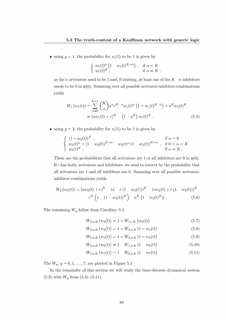
5.3 The truth-content of a Kauffman network with generic logic
• using g 1, the probability for xip1q to be 1 is given by"w1ptqα
1 w1ptqKα
, if α K
w1ptqK , if α K ,
as the α activators need to be 1 and, if existing, at least one of the Kα inhibitors
needs to be 0 in xp0q. Summing over all possible activator-inhibitor-combinations
yields
W1 pw1ptqq K1
α0
K
α
aαrKαw1ptqα
1 w1ptqKα
aKw1ptqK
paw1ptq rqK 1 aKw1ptqK . (5.5)
• using g 2, the probability for xip1q to be 1 is given by$&%p1 w2ptqqK , if α 0w2ptqα p1 w2ptqqKα w2ptqα p1 w2ptqqKα , if 0 α Kw2ptqK , if α K .
These are the probabilities that all activators are 1 or all inhibitors are 0 in xp0q.If i has both, activators and inhibitors, we need to correct by the probability that
all activators are 1 and all inhibitors are 0. Summing over all possible activator-
inhibitor-combinations yields
W2 pw2ptqq paw2ptq rqK pa r p1 w2ptqqqK paw2ptq r p1 w2ptqqqK
rK
1 p1 w2ptqqK aK
1 w2ptqK. (5.6)
The remaining Wg follow from Corollary 5.2.
W3,a,K pw3ptqq 1W1,r,K pw3ptqq (5.7)
W4,a,K pw4ptqq 1W3,a,K p1 w4ptqq (5.8)
W5,a,K pw5ptqq 1W2,a,K p1 w5ptqq (5.9)
W6,a,K pw6ptqq 1W1,a,K p1 w6ptqq (5.10)
W7,a,K pw7ptqq 1W0,a,K p1 w7ptqq (5.11)
The Wg, g 0, 1, . . . , 7, are plotted in Figure 5.1.
In the remainder of this section we will study the time-discrete dynamical system
(5.3) with Wg from (5.4)–(5.11).
89
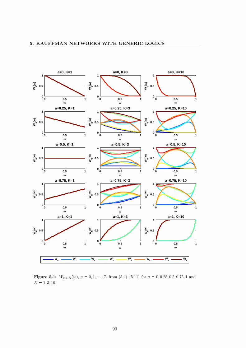
5. KAUFFMAN NETWORKS WITH GENERIC LOGICS
0 0.5 10
0.5
1a=0, K=1
w
Wg(w
)
0 0.5 10
0.5
1a=0, K=3
w
Wg(w
)
0 0.5 10
0.5
1a=0, K=10
w
Wg(w
)
0 0.5 10
0.5
1a=0.25, K=1
w
Wg(w
)
0 0.5 10
0.5
1a=0.25, K=3
w
Wg(w
)
0 0.5 10
0.5
1a=0.25, K=10
w
Wg(w
)
0 0.5 10
0.5
1a=0.5, K=1
w
Wg(w
)
0 0.5 10
0.5
1a=0.5, K=3
w
Wg(w
)
0 0.5 10
0.5
1a=0.5, K=10
w
Wg(w
)
0 0.5 10
0.5
1a=0.75, K=1
w
Wg(w
)
0 0.5 10
0.5
1a=0.75, K=3
w
Wg(w
)
0 0.5 10
0.5
1a=0.75, K=10
w
Wg(w
)
0 0.5 10
0.5
1a=1, K=1
w
Wg(w
)
0 0.5 10
0.5
1a=1, K=3
w
Wg(w
)
0 0.5 10
0.5
1a=1, K=10
w
Wg(w
)
W0
W1
W2
W3
W4
W5
W6
W7
Figure 5.1: Wg,a,Kpwq, g 0, 1, . . . , 7, from (5.4)–(5.11) for a 0, 0.25, 0.5, 0.75, 1 andK 1, 3, 10.
90
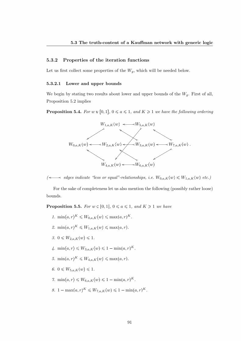
5.3 The truth-content of a Kauffman network with generic logic
5.3.2 Properties of the iteration functions
Let us first collect some properties of the Wg, which will be needed below.
5.3.2.1 Lower and upper bounds
We begin by stating two results about lower and upper bounds of the Wg. First of all,
Proposition 5.2 implies
Proposition 5.4. For w P r0, 1s, 0 ¤ a ¤ 1, and K ¥ 1 we have the following ordering
W1,a,Kpwq oo ooee
eeLLLLLLLLLLW5,a,Kpwq
ff
ffLLLLLLLLLL
W0,a,Kpwqyy
yyssssssssssoo oo
ee
eeKKKKKKKKKKW2,a,Kpwq oo oo
ee
eeLLLLLLLLLLW3,a,Kpwq oo oo W7,a,Kpwq .
W4,a,Kpwq
oo oo W6,a,Kpwq
xx
xxrrrrrrrrrr
( oo oo edges indicate “less or equal”-relationships, i.e. W0,a,Kpwq ¤W1,a,Kpwq etc.)
For the sake of completeness let us also mention the following (possibly rather loose)
bounds.
Proposition 5.5. For w P r0, 1s, 0 ¤ a ¤ 1, and K ¥ 1 we have
1. minpa, rqK ¤W0,a,Kpwq ¤ maxpa, rqK .
2. minpa, rqK ¤W1,a,Kpwq ¤ maxpa, rq.
3. 0 ¤W2,a,Kpwq ¤ 1.
4. minpa, rq ¤W3,a,Kpwq ¤ 1minpa, rqK .
5. minpa, rqK ¤W4,a,Kpwq ¤ maxpa, rq.
6. 0 ¤W5,a,Kpwq ¤ 1.
7. minpa, rq ¤W6,a,Kpwq ¤ 1minpa, rqK .
8. 1maxpa, rqK ¤W7,a,Kpwq ¤ 1minpa, rqK .
91
5. KAUFFMAN NETWORKS WITH GENERIC LOGICS
Proof. Claim 1 is obvious as W0pwq is monotonous. If a ¡ r (a r), W0pwq increases(decreases) from rK to aK . The lower bound in claim 2 follows from part 1 andProposition 5.4. For the upper bound we reason
W1,a,Kpwq ¤ awK r wK pawqK
¤#wKpa 1 aq r wKpa rq r ¤ r , if a ¤ r
rwK a wK pawqK ¤ wKpr 1 aq a a , if a ¡ r .
The remainder of the claim follows from Corollary 5.2.
5.3.2.2 Extreme and asymptotic cases
This section takes care of all extreme and asymptotic cases. Trivial computations show
Proposition 5.6. The following hold.
1. For g P t0, 1, 4, 5u we have Wgp0q rK and Wgp1q aK . For g P t2, 3, 6, 7u wehave Wgp0q 1 aK and Wgp1q 1 rK .
2. Let a 1. For g P t0, 1, 2, 3u we have Wg,1,Kpwq wK . For g P t4, 5, 6, 7u wehave Wg,1,Kpwq 1 p1 wqK .
3. Let a 0. For g P t0, 2, 4, 6u we have Wg,0,Kpwq p1 wqK . For g P t1, 3, 5, 7uwe have Wg,0,Kpwq 1 wK .
4. Let K 1. For all g P t0, 1, . . . , 7u we have Wg,a,1pwq aw rp1 wq.
5. Let 0 w 1 and 0 a 1. For g P t0, 1, 2, 4u we have Wg,a,Kpwq Ñ 0 asK Ñ8. For g P t3, 5, 6, 7u we have Wg,a,Kpwq Ñ 1 as K Ñ8.
Proposition 5.6 has an intuitive explanation:
• In 1. the decisive characteristic is the operator b that links the group of activators
and inhibitors. In the case b ^, viz g 0, 1, 4, 5, the only chance for a node to
be switched on if w 0 (w 1) is that all its inputs are inhibitors (activators).
Conversely, in the case b _, viz g 2, 3, 6, 7, the only chance for a node to be
switched on if w 0 (w 1) is that not all its inputs are activators (inhibitors).
• In 2. the decisive characteristic is the operator ` that links the activators. In the
case ` ^, viz g 0, 1, 2, 3, if the fraction of activators increases, the probability
92
5.3 The truth-content of a Kauffman network with generic logic
for a node to be switched on approaches the probability that all its inputs are
on. Conversely, in the case ` _, viz g 4, 5, 6, 7, if the fraction of activators
increases, the probability for a node to be switched on approaches the probability
that any of its inputs is on.
• In 3. the decisive characteristic is the operator a that links the inhibitors. In
the case a ^, viz g 0, 2, 4, 6, if the fraction of activators decreases, the
probability for a node to be switched on approaches the probability that all its
inputs are off. Conversely, in the case a _, viz g 1, 3, 5, 7, if the fraction of
activators decreases, the probability for a node to be switched on approaches the
probability that any of its inputs is off.
• In 5. the decisive characteristic is the number of _’s in g. First, note that, unless
a 0 or a 1, the number of both, activators and inhibitors, increases with K.
Now, if there are less than two _’s in g, viz g 0, 1, 2, 4, all activators need to be
on and/or all inhibitors need to be off for a node to be switched on. Clearly, the
probability for this tends to zero as the connectivity increases unless w 0 or
w 1. Conversely, if there are more than one _’s in g, viz g 3, 5, 6, 7, it suffices
that any activator is on and/or any inhibitor is off for a node to be switched on.
Clearly, the probability for this tends to one as the number of inputs increases
unless w 0 or w 1.
5.3.2.3 The general shape of the iteration functions
In between the extreme cases from Proposition 5.6 the shapes of the Wg are character-
ized by
Proposition 5.7. Let K ¥ 2 and 0 a 1.
1. W0 is convex on r0, 1s and increasing (decreasing) if a ¡ r (a r).
2. W7 is concave on r0, 1s and increasing (decreasing) if a r (a ¡ r).
3. W2 is convex on r0, 1s and has exactly one critical point wpcq2 , which is non-degenerate and coincides with the global minimum.
4. W5 is concave on r0, 1s and has exactly one critical point wpcq5 , which is non-degenerate and coincides with the global maximum.
93
5. KAUFFMAN NETWORKS WITH GENERIC LOGICS
5. Let g P t1, 3, 4, 6u. Wg has at most one critical point wpcqg and at most oneinflection point wpiqg . If existing, wpcqg is non-degenerate. If no inflection pointexists, also no critical point can exist. In the case that both exist, wpiqg w
pcqg if
g P t1, 3u, and wpiqg ¡ wpcqg if g P t4, 6u.
6. We can subdivide r0, 1s into three intervals I11
0, wpiq1
, I2
1 wpiq1 , w
pcq1
,
I31
wpcq1 , 1
such that W1 is convex-increasing on I1
1 , concave-increasing on I21 ,
and concave-decreasing on I31 . If there is no critical (inflection) point in r0, 1s
then I31 H (I2
1 I31 H).
7. We can subdivide r0, 1s into three intervals I13
0, wpiq3
, I2
3 wpiq3 , w
pcq3
,
I33
wpcq3 , 1
such that W3 is concave-decreasing on I1
3 , convex-decreasing on I23 ,
and convex-increasing on I33 . If there is no critical (inflection) point in r0, 1s then
I33 H (I2
3 I33 H).
8. We can subdivide r0, 1s into three intervals I14
0, wpcq4
, I2
4 wpcq4 , w
piq4
,
I34
wpiq4 , 1
such that W4 is concave-increasing on I1
4 , concave-decreasing onI2
4 , and convex-decreasing on I34 . If there is no critical (inflection) point in r0, 1s
then I14 H (I1
4 I24 H).
9. We can subdivide r0, 1s into three intervals I16
0, wpcq6
, I2
6 wpcq6 , w
piq6
,
I36
wpiq6 , 1
such that W6 is convex-decreasing on I1
6 , convex-increasing on I26 ,
and concave-increasing on I36 . If there is no critical (inflection) point in r0, 1s
then I16 H (I1
6 I26 H).
Proof. The case g 0 is obvious. The characterization of the shape of W1 can beobtained as follows: If K 2 there is obviously at most one critical point and noinflection point. In the case K ¥ 3 the zeros of the first and second derivatives of W1
are simple and given by
wpcq1 r
vpcq1 a
and wpiq1 r
vpiq1 a
,
where vpcq1
K1 1 aK
aand
vpiq1
K2 1 aK
a2.
This implies that there is at most one critical and one inflection point of W1 in r0, 1sas possible negative solutions for vpciq1 lead to values wpciq1 0. One easily verifiesthat W 1
1p0q KarK1 ¡ 0 and W 21 p0q KpK 1qa2rK2 ¡ 0. Now, suppose a
94
5.3 The truth-content of a Kauffman network with generic logic
critical point wpcq1 P p0, 1q exists. It follows that wpcq1 is a local maximum, which impliesW 2
1
wpcq1
0. Thus, there has to be an inflection point 0 w
piq1 w
pcq1 . If there is no
critical point in p0, 1q the function W1 is increasing on r0, 1s and I31 H. If, moreover,
there is no inflection point either, the function W1 is also convex on r0, 1s and I21 H.
In the case g 2 one can check that
W 22 pwq KpK 1q
a2 paw rqK2 r2 pa rp1 wqqK2
pa rq2 paw rp1 wqqK2 rKp1 wqK2 aKwK2
is positive for 0 w 1. (We have a2paw rqK2 ¡ pa rq2 paw rp1 wqqK2 fora ¥ 0.5, and r2pa rp1 wqqK2 ¡ pa rq2 paw rp1 wqqK2 for a 0.5.) Hence,W2 is convex on r0, 1s. The claim follows from W 1
2p0q Kr 0 and W 12p1q Ka ¡ 0.
The shapes of W3,W4,W5,W6 and W7 can be obtained from Corollary 5.2.
Corollary 5.4. Let 0 a 1 and K ¥ 1. For each g P t0, 1, . . . , 7u, Wg has exactlyone fixed point.
Proof. For K 1, see Proposition 5.6.4. For K ¥ 2 the claim follows from Propositions5.6.1 and 5.7. A little work remains to be done in the case g 1 (and g 6) as functionswith a shape as W1 could have multiple fixed points. However, we can rule out thispossibility as W1 and W 1
1 are bounded from above by Hpwq paw rqK and H 1pwq,respectively. The function H is convex and increasing and has fixed points 0 wh 1and 1. The fixed point wh is attracting and H 1pwhq 1. Any fixed point of W1 liesin the interval p0, whq, and, thus, the derivative of W1 in a fixed point wpfq1 satisfiesW 1
1
wpfq1
H 1
wpfq1
H 1 pwhq 1 as H is convex. Hence, W1 cannot have more
than one fixed point as in this case in at least one fixed point the derivative would haveto be greater than 1 (the diagonal would be crossed from below).
5.3.2.4 The limit of large connectivities
In this section, we investigate the limit of large K in more detail. This is of particular
importance to our numerical analyses in section 5.5, as here we will, of course, only be
able to portray the dynamic behavior up to some finite K. We begin by studying the
existence of critical points of Wg, g P t1, 3, 4, 6u. Recall that, in general, we can only
limit the number of critical points but not guarantee existence, cf. Proposition 5.7.5.
Proposition 5.8. Let g P t1, 3, 4, 6u and 0 a 1. For sufficiently large K, Wg
has a critical point wpcqg and an inflection point wpiqg in p0, 1q. For g P t1, 3u we have
95
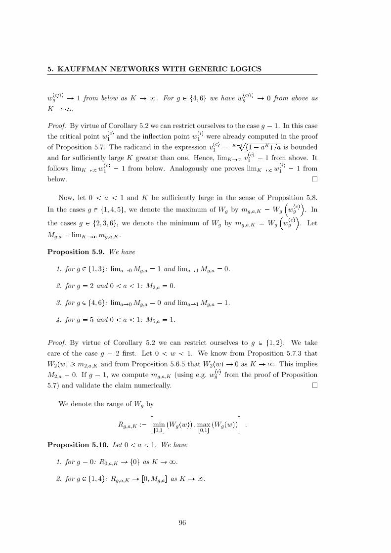
5. KAUFFMAN NETWORKS WITH GENERIC LOGICS
wpciqg Ñ 1 from below as K Ñ 8. For g P t4, 6u we have w
pciqg Ñ 0 from above as
K Ñ8.
Proof. By virtue of Corollary 5.2 we can restrict ourselves to the case g 1. In this casethe critical point wpcq1 and the inflection point wpiq1 were already computed in the proofof Proposition 5.7. The radicand in the expression v
pcq1 K1
ap1 aKq a is bounded
and for sufficiently large K greater than one. Hence, limKÑ8 vpcq1 1 from above. It
follows limKÑ8wpcq1 1 from below. Analogously one proves limKÑ8w
piq1 1 from
below.
Now, let 0 a 1 and K be sufficiently large in the sense of Proposition 5.8.
In the cases g P t1, 4, 5u, we denote the maximum of Wg by mg,a,K Wg
wpcqg
. In
the cases g P t2, 3, 6u, we denote the minimum of Wg by mg,a,K Wg
wpcqg
. Let
Mg,a limKÑ8mg,a,K .
Proposition 5.9. We have
1. for g P t1, 3u: limaÑ0Mg,a 1 and limaÑ1Mg,a 0.
2. for g 2 and 0 a 1: M2,a 0.
3. for g P t4, 6u: limaÑ0Mg,a 0 and limaÑ1Mg,a 1.
4. for g 5 and 0 a 1: M5,a 1.
Proof. By virtue of Corollary 5.2 we can restrict ourselves to g P t1, 2u. We takecare of the case g 2 first. Let 0 w 1. We know from Proposition 5.7.3 thatW2pwq ¥ m2,a,K and from Proposition 5.6.5 that W2pwq Ñ 0 as K Ñ 8. This impliesM2,a 0. If g 1, we compute mg,a,K (using e.g. wpcqg from the proof of Proposition5.7) and validate the claim numerically.
We denote the range of Wg by
Rg,a,K :minr0,1s
pWgpwqq ,maxr0,1s
pWgpwqq.
Proposition 5.10. Let 0 a 1. We have
1. for g 0: R0,a,K Ñ t0u as K Ñ8.
2. for g P t1, 4u: Rg,a,K Ñ r0,Mg,as as K Ñ8.
96
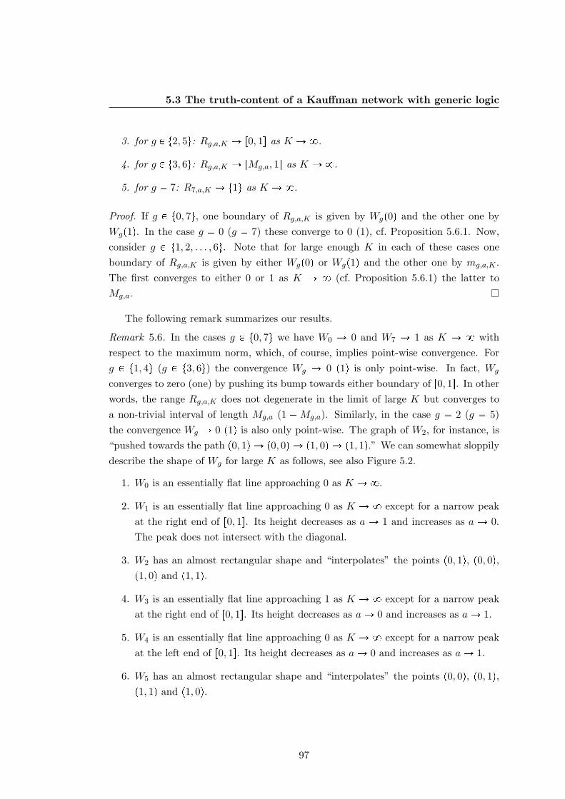
5.3 The truth-content of a Kauffman network with generic logic
3. for g P t2, 5u: Rg,a,K Ñ r0, 1s as K Ñ8.
4. for g P t3, 6u: Rg,a,K Ñ rMg,a, 1s as K Ñ8.
5. for g 7: R7,a,K Ñ t1u as K Ñ8.
Proof. If g P t0, 7u, one boundary of Rg,a,K is given by Wgp0q and the other one byWgp1q. In the case g 0 (g 7) these converge to 0 (1), cf. Proposition 5.6.1. Now,consider g P t1, 2, . . . , 6u. Note that for large enough K in each of these cases oneboundary of Rg,a,K is given by either Wgp0q or Wgp1q and the other one by mg,a,K .The first converges to either 0 or 1 as K Ñ 8 (cf. Proposition 5.6.1) the latter toMg,a.
The following remark summarizes our results.
Remark 5.6. In the cases g P t0, 7u we have W0 Ñ 0 and W7 Ñ 1 as K Ñ 8 withrespect to the maximum norm, which, of course, implies point-wise convergence. Forg P t1, 4u (g P t3, 6u) the convergence Wg Ñ 0 p1q is only point-wise. In fact, Wg
converges to zero (one) by pushing its bump towards either boundary of r0, 1s. In otherwords, the range Rg,a,K does not degenerate in the limit of large K but converges toa non-trivial interval of length Mg,a (1 Mg,a). Similarly, in the case g 2 (g 5)the convergence Wg Ñ 0 p1q is also only point-wise. The graph of W2, for instance, is“pushed towards the path p0, 1q Ñ p0, 0q Ñ p1, 0q Ñ p1, 1q.” We can somewhat sloppilydescribe the shape of Wg for large K as follows, see also Figure 5.2.
1. W0 is an essentially flat line approaching 0 as K Ñ8.
2. W1 is an essentially flat line approaching 0 as K Ñ 8 except for a narrow peakat the right end of r0, 1s. Its height decreases as a Ñ 1 and increases as a Ñ 0.The peak does not intersect with the diagonal.
3. W2 has an almost rectangular shape and “interpolates” the points p0, 1q, p0, 0q,p1, 0q and p1, 1q.
4. W3 is an essentially flat line approaching 1 as K Ñ 8 except for a narrow peakat the right end of r0, 1s. Its height decreases as aÑ 0 and increases as aÑ 1.
5. W4 is an essentially flat line approaching 0 as K Ñ 8 except for a narrow peakat the left end of r0, 1s. Its height decreases as aÑ 0 and increases as aÑ 1.
6. W5 has an almost rectangular shape and “interpolates” the points p0, 0q, p0, 1q,p1, 1q and p1, 0q.
97
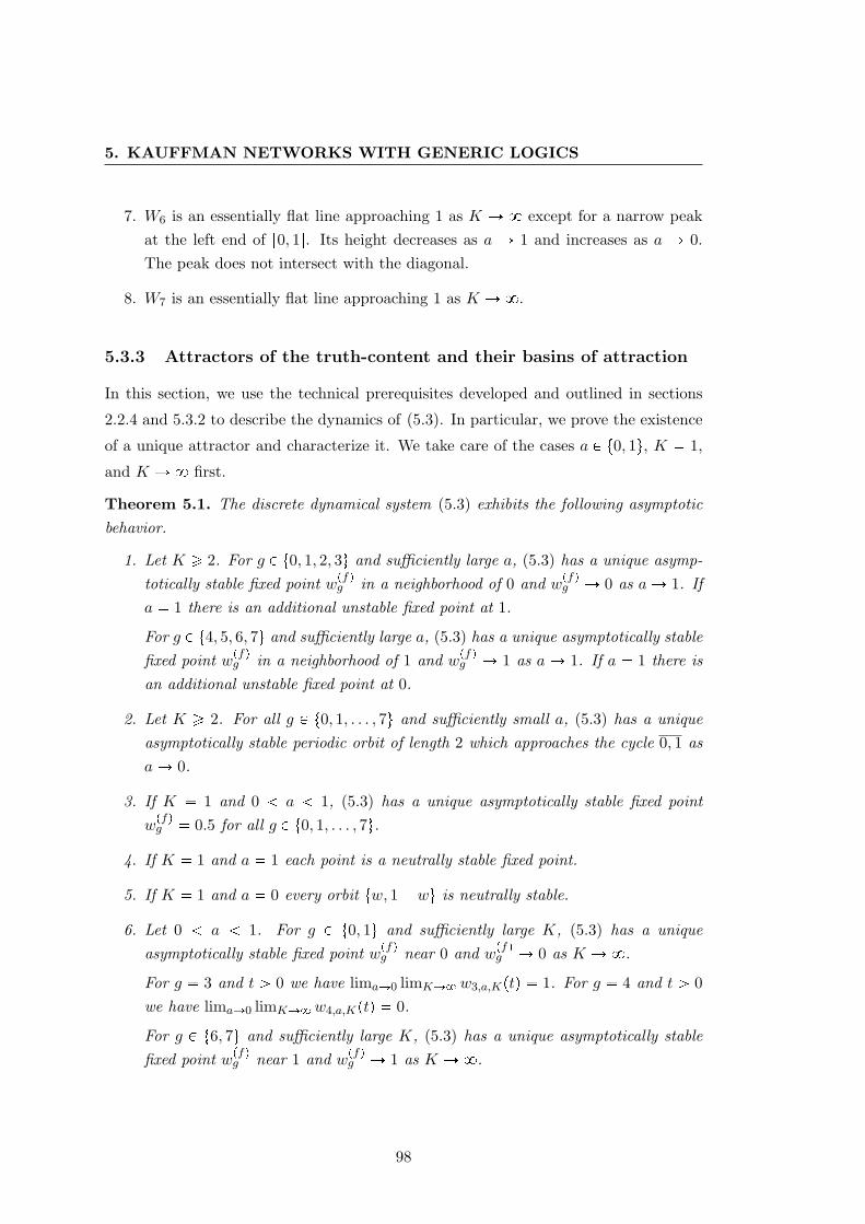
5. KAUFFMAN NETWORKS WITH GENERIC LOGICS
7. W6 is an essentially flat line approaching 1 as K Ñ 8 except for a narrow peakat the left end of r0, 1s. Its height decreases as a Ñ 1 and increases as a Ñ 0.The peak does not intersect with the diagonal.
8. W7 is an essentially flat line approaching 1 as K Ñ8.
5.3.3 Attractors of the truth-content and their basins of attraction
In this section, we use the technical prerequisites developed and outlined in sections
2.2.4 and 5.3.2 to describe the dynamics of (5.3). In particular, we prove the existence
of a unique attractor and characterize it. We take care of the cases a P t0, 1u, K 1,
and K Ñ8 first.
Theorem 5.1. The discrete dynamical system (5.3) exhibits the following asymptoticbehavior.
1. Let K ¥ 2. For g P t0, 1, 2, 3u and sufficiently large a, (5.3) has a unique asymp-totically stable fixed point wpfqg in a neighborhood of 0 and wpfqg Ñ 0 as aÑ 1. Ifa 1 there is an additional unstable fixed point at 1.
For g P t4, 5, 6, 7u and sufficiently large a, (5.3) has a unique asymptotically stablefixed point wpfqg in a neighborhood of 1 and w
pfqg Ñ 1 as aÑ 1. If a 1 there is
an additional unstable fixed point at 0.
2. Let K ¥ 2. For all g P t0, 1, . . . , 7u and sufficiently small a, (5.3) has a uniqueasymptotically stable periodic orbit of length 2 which approaches the cycle 0, 1 asaÑ 0.
3. If K 1 and 0 a 1, (5.3) has a unique asymptotically stable fixed pointwpfqg 0.5 for all g P t0, 1, . . . , 7u.
4. If K 1 and a 1 each point is a neutrally stable fixed point.
5. If K 1 and a 0 every orbit tw, 1 wu is neutrally stable.
6. Let 0 a 1. For g P t0, 1u and sufficiently large K, (5.3) has a uniqueasymptotically stable fixed point wpfqg near 0 and wpfqg Ñ 0 as K Ñ8.
For g 3 and t ¡ 0 we have limaÑ0 limKÑ8w3,a,Kptq 1. For g 4 and t ¡ 0we have limaÑ0 limKÑ8w4,a,Kptq 0.
For g P t6, 7u and sufficiently large K, (5.3) has a unique asymptotically stablefixed point wpfqg near 1 and wpfqg Ñ 1 as K Ñ8.
98
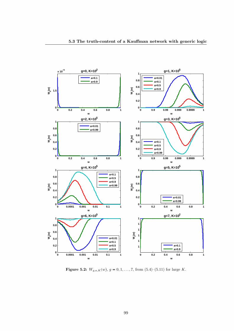
5.3 The truth-content of a Kauffman network with generic logic
0 0.2 0.4 0.6 0.8 10
1.5
x 10−5
w
W0(w
)
g=0, K=102
a=0.1a=0.9
0 0.9 0.99 0.999 0.9999 10
0.2
0.4
0.6
0.8
1
w
W1(w
)
g=1, K=105
a=0.01a=0.1a=0.5a=0.9
0 0.2 0.4 0.6 0.8 10
0.2
0.4
0.6
0.8
1
w
W2(w
)
g=2, K=105
a=0.01a=0.99
0 0.9 0.99 0.999 0.9999 10
0.2
0.4
0.6
0.8
1
w
W3(w
)
g=3, K=105
a=0.1a=0.5a=0.9a=0.99
0 0.2 0.4 0.6 0.8 1
1
1
1
1
1
1
w
W7(w
)
g=7, K=102
a=0.1a=0.9
0 0.0001 0.001 0.01 0.1 10
0.2
0.4
0.6
0.8
1
w
W6(w
)
g=6, K=105
a=0.01a=0.1a=0.5a=0.9
0 0.2 0.4 0.6 0.8 10
0.2
0.4
0.6
0.8
1
w
W5(w
)
g=5, K=105
a=0.01a=0.99
0 0.0001 0.001 0.01 0.1 10
0.2
0.4
0.6
0.8
1
w
W4(w
)
g=4, K=105
a=0.1a=0.5a=0.9a=0.99
Figure 5.2: Wg,a,Kpwq, g 0, 1, . . . , 7, from (5.4)–(5.11) for large K.
99
5. KAUFFMAN NETWORKS WITH GENERIC LOGICS
All asymptotically stable fixed points or periodic orbits are global attractors.
Proof. Claims 1 and 2 are obvious from Proposition 5.6.2 and 5.6.3 if a 1 or a 0,respectively. Since the existence of asymptotically stable periodic orbits is an openproperty and since Wg,a,K depends analytically on a, this extends to neighborhoodsof a 1 and a 0, respectively. Claims 3–5 follow from Proposition 5.6.4. Claim 6follows from Remark 5.6.
Now, let K ¥ 2. We begin by proving
Lemma 5.1. Let K ¥ 2. For g P t0, 7u we have SWg,a,K 0 (where defined) ifa 0.5, and SWg,a,K 0 (where defined) if a 0.5. For g P t1, 2, . . . , 6u we haveSWg 0 (where defined).
Proof. By the chain rule from Proposition 2.2 and the symmetry properties from Corol-lary 5.2 it suffices to consider g P t0, 1, 2u. If K 2, Wg is a quadratic polynomialunless g 0 and a 0.5 in which case Wg is constant. Thus, the Schwarzian derivativeis negative or zero, respectively. Now suppose K ¥ 3. The case g 0 follows from
W 10pwqW3
0 pwq 32W 2
0 pwq2 12K2pK 1qpa rq4 paw rp1 wqq2K4 pK 1q .
If g P t1, 2u we have
W 1gpwqW3
g pwq 32W 2g pwq2
32K2pK 1q2
K 2
p32qpK 1qHpw, 1qHpw, 3q Hpw, 2q2
, pq
where
Hpw,αq
$''''''&''''''%
aK 1
wKα aαpaw rqKα , if g 1
aαpaw rqKα p1qαrα pa rp1 wqqKαpa rqα paw rp1 wqqKαp1qαrKp1 wqKα aKwKα , if g 2 ,
α 1, 2, 3. We denote the summands in the above expressions of the Hpw,αq byvqpw,αq, q 1, 2 if g 1 and q 1, 2, 3, 4, 5 if g 2.
As p32qK2pK 1q2 ¡ 0, we only need to take care of the bracketed expressionin pq. If Hpw, 1qHpw, 3q ¤ 0 it immediately follows that pq 0. Otherwise, the
100
5.3 The truth-content of a Kauffman network with generic logic
bracketed expression in pq is strictly smaller than Hpw, 1qHpw, 3q Hpw, 2q2. Thiscan be further simplified to
Hpw, 1qHpw, 3q Hpw, 2q2 ¸q,q1
vqpw, 1qvq1pw, 3q vqpw, 2qvq1pw, 2q
¸qq1
vqpw, 1qvq1pw, 3q vqpw, 2qvq1pw, 2q
, p:q
as vqpw, 1qvqpw, 3q vqpw, 2q2 0 for q 1, 2 if g 1 and q 1, 2, 3, 4, 5 if g 2. Onenow proves the claim by showing that the expression in p:q is non-positive. In the caseg 1, one can, for instance, compute
p:q aK 1
wK1a3paw rqK3
aK 1wK3apaw rqK1
2aK 1
wK2a2paw rqK2
a aK 1wK3paw rqK3
a2w2 paw rq2 2awpaw rq
a aK 1wK3paw rqK3r2 ¤ 0 .
Now, suppose g P t0, 7u. The simple forms of W0 and W7 allow us to analytically
describe (or, at least, narrow down) the asymptotic behavior of (5.3).
Theorem 5.2. Let K ¥ 2, 0 ¤ a ¤ 1, and g P t0, 7u. Iteration (5.3) has a uniqueglobal periodic attractor A. For a ¥ 0.5 the attractor A is an asymptotically stablefixed point. In particular, A
0.5K(
if a 0.5. For each 0 a 0.5 there existsK0 K0paq such that for any K ¡ K0 the attractor A is an asymptotically stable fixedpoint. Otherwise it is either an asymptotically stable fixed point or periodic orbit oflength 2.
Proof. By virtue of Corollary 5.3 we restrict ourselves to g 0. Let us first considerthe case a ¥ 0.5. Here, W0 is monotonously increasing, and the claim follows fromLemma 2.2.1. If a 0.5, we have W0pwq 0.5K .
Now, let 0 a 0.5. Here, W0 is monotonously decreasing, and the claim followsfrom Lemma 2.2.2 together with Lemma 5.1. To show existence of K0paq we reason asfollows. It holds
W 2
0
2 pwq pKpa rqq2 pr pa rqW0pwqqK2 pK 1q pr pa rqwqK2 pa rqrr pa rqpK 1qW0pwqs .
101
5. KAUFFMAN NETWORKS WITH GENERIC LOGICS
The sign of this derivative is determined by r pa rqpK 1qW0pwq. As a function ofW0pwq, this expression has a unique zero at
W0pwq r
pa rqpK 1q . pq
For sufficiently large K ¡ K0paq we have W0pwq ¤ rK rpparqpK1qq and pq isnot satisfied for any 0 ¤ w ¤ 1. Thus, W 2
0 is concave on r0, 1s. Moreover, note that W0
is decreasing, and, consequently, W 20 is increasing. Hence W 2
0 has exactly one stablefixed point.
The case a 0 was already taken care of in Theorem 5.1.2.
Let us now consider the remaining cases g P t1, 2, . . . , 6u. Due to the more compli-
cated expressions of Wg we can only obtain weaker results than in Theorem 5.2.
Theorem 5.3. Let K ¥ 2, 0 ¤ a ¤ 1, and g P t1, 2, . . . , 6u. The iteration (5.3) has aunique global attractor, which is one of the following types:
1. an asymptotically stable periodic orbit,
2. a Cantor set of measure zero,
3. a finite union of intervals with a dense orbit.
Proof. By virtue of Corollary 5.3 we restrict ourselves to g P t1, 4, 5u. Recall the shapeof these Wg as described in Proposition 5.7. We already remarked that they haveexactly one fixed point, cf. Corollary 5.4. We denote the maximizing argument of Wg
by wmaxg , i.e. wmax
g wpcqg is the critical point or wmax
g is a boundary point of r0, 1s.Case (a): If the maximum Wmax
g Wg
wmaxg
of Wg lies below or on the diagonal,
i.e. Wmaxg ¤ wmax
g , the iteration has a unique stable fixed point with full basin ofattraction. This follows from Lemma 2.2.1 as Wg is increasing above the diagonal. Thetwo shapes of Wg for which this occurs are shown schematically in Figures 5.3A, B.
The delicate point is what happens if the maximum is located above the diagonal,i.e. Wmax
g ¡ wmaxg . The three shapes of Wg for which this occurs are shown schemati-
cally in Figures 5.3C–E. We subdivide r0, 1s into three intervals I1 0,Wg
Wmaxg
,
I2 Wg
Wmaxg
,Wmax
g
, and I3
Wmaxg , 1
. Trajectories of points in I1 ulti-
mately land in I2; points in I3 are mapped into I1 and thus later into I2. Moreover,Wg pI2q I2. Hence, we can restrict Wg to I2.1
1I2 is the so-called dynamical core of Wg.
102
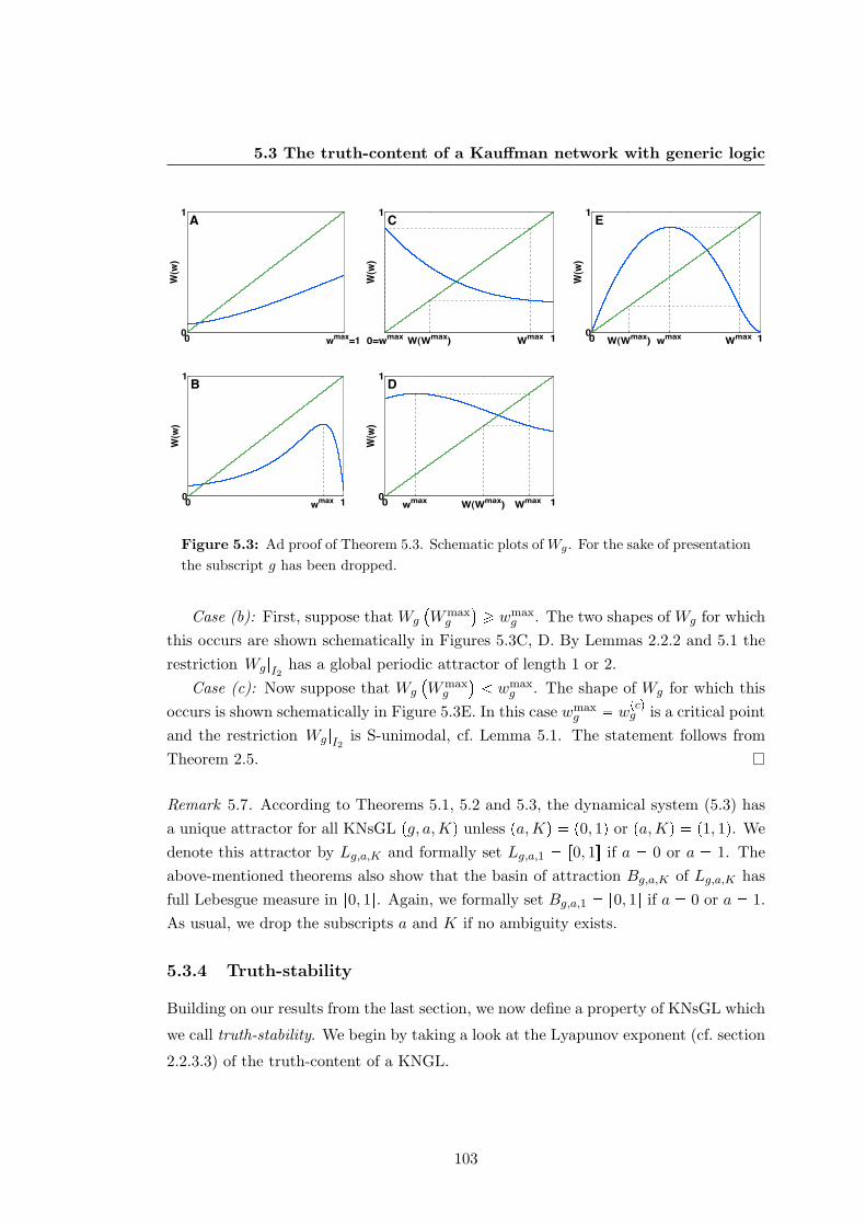
5.3 The truth-content of a Kauffman network with generic logic
0
1
0 wmax 1
W(w
)
1
0=wmax W(Wmax) Wmax 1
W(w
)
0
1
0 wmax W(Wmax) Wmax 1
W(w
)
0
1
0 W(Wmax) wmax Wmax 1
W(w
)
0
1
0 wmax=1
W(w
)
A EC
B D
Figure 5.3: Ad proof of Theorem 5.3. Schematic plots of Wg. For the sake of presentationthe subscript g has been dropped.
Case (b): First, suppose that Wg
Wmaxg
¥ wmaxg . The two shapes of Wg for which
this occurs are shown schematically in Figures 5.3C, D. By Lemmas 2.2.2 and 5.1 therestriction Wg|I2 has a global periodic attractor of length 1 or 2.
Case (c): Now suppose that Wg
Wmaxg
wmaxg . The shape of Wg for which this
occurs is shown schematically in Figure 5.3E. In this case wmaxg w
pcqg is a critical point
and the restriction Wg|I2 is S-unimodal, cf. Lemma 5.1. The statement follows fromTheorem 2.5.
Remark 5.7. According to Theorems 5.1, 5.2 and 5.3, the dynamical system (5.3) hasa unique attractor for all KNsGL pg, a,Kq unless pa,Kq p0, 1q or pa,Kq p1, 1q. Wedenote this attractor by Lg,a,K and formally set Lg,a,1 r0, 1s if a 0 or a 1. Theabove-mentioned theorems also show that the basin of attraction Bg,a,K of Lg,a,K hasfull Lebesgue measure in r0, 1s. Again, we formally set Bg,a,1 r0, 1s if a 0 or a 1.As usual, we drop the subscripts a and K if no ambiguity exists.
5.3.4 Truth-stability
Building on our results from the last section, we now define a property of KNsGL which
we call truth-stability. We begin by taking a look at the Lyapunov exponent (cf. section
2.2.3.3) of the truth-content of a KNGL.
103
5. KAUFFMAN NETWORKS WITH GENERIC LOGICS
Proposition 5.11. Let g P t0, 1, . . . , 7u, 0 ¤ a ¤ 1, and K ¥ 1. For Lebesgue-almostall wgp0q P r0, 1s the Lyapunov exponent
λg λg,a,K limtÑ8
1t
t1
τ0
lnW 1
g pwgpτqq , (5.12)
exists.1 In this case, it is identical for almost all wgp0q P r0, 1s. Moreover,
1. λg ¡ 0 ðñ Wg admits an acip.
2. λg 0 ùñ Lg is a periodic attractor.
Proof. By virtue of Corollary 5.2.1 we restrict ourselves to g P t0, 1, 4, 5u. If K 1 anda P t0, 1u we have λg,a,1 0, and the dynamical system (5.3) possesses neutrally stableorbits, cf. Theorem 5.1.4 and 5.1.5. Now, let pa,Kq p0, 1q and pa,Kq p1, 1q. If Lgis a periodic attractor, λg exists for all wgp0q P Bg, more precisely,
λg 1|Lg|
¸wPLg
lnW 1
g pwq .
As Lg is stable it follows that λg ¤ 0. It is also evident that a periodic attractor Lgcannot support an acip.
Thus, it remains to prove the claims for g P t1, 4, 5u, if the shape of Wg is asdescribed in case (c) from the proof of Theorem 5.3, (cf. Figure 5.3E), as in all othercases Lg is a periodic attractor. By the reasoning from the proof of Theorem 5.3 wesee that in this case all trajectories are trajectories of S-unimodal functions, possiblyafter discarding finitely many iteration-steps. The claims follow from Proposition 2.4and Theorem 2.6.
With respect to sensitive dependence on initial conditions (cf. Definition 2.6) of the
truth-content we have the following result.
Proposition 5.12. Let g P t0, 1, . . . , 7u, 0 ¤ a ¤ 1, and K ¥ 1. If the map Wg hasa periodic attractor, it does not have sensitive dependence on initial conditions. In thecase it has an interval attractor, it has sensitive dependence on initial conditions.
Proof. We denote the euclidean distance by ‘dist’ and the δ-neighborhood of somepoint w by Bδ pwq. First, suppose Wg has a (global) periodic attractor as well assensitive dependence on initial conditions. Then, there exist ε ¡ 0 and a point
1Here, we include the possibility that λg 8.
104
5.3 The truth-content of a Kauffman network with generic logic
wp0q P Bg such that for any neighborhood U of wp0q there is w P U and t ¥ 0 withdist
W tgpwp0qq,W t
gpwq ¡ ε. Let wppq be a periodic point of Wg. As wppq is stable
there is δ ¡ 0 such that distW tgpw1q,W t
gpw2q ε for all w1, w2 P Bδ
wppq
and all
t ¥ 0. As wp0q P Bg there is t0 such that W t0g pwp0qq P Bδ
wppq
. From the conti-
nuity of Wg it follows that there is δ0 ¡ 0 such that for all w P Bδ0pwp0qq we havedist
W tgpwp0qq,W t
gpwq ε for 0 ¤ t ¤ t0 and W t0
g pwq P Bδ
wppq
. This implies
distW tgpwp0qq,W t
gpwq ε for all w P Bδ0pwp0qq and all t ¥ 0 — a contradiction to the
sensitive dependence on initial conditions.In the proof of Theorem 5.3 we saw that, if Wg has an interval attractor, it has
to be as shown in Figure 5.3E, as otherwise a periodic attractor would exist. We alsosaw that in this case the non-transient dynamics of Wg are dynamics of an S-unimodalfunction. The claim follows from Theorem 2.7.
Now, recall that in parametrized families of S-unimodal functions there is a di-
chotomy except for a measure zero set of parameters, cf. Remark 2.4. The following
Theorem shows that this implies also a dichotomy for KNsGL.
Theorem 5.4. Let g P t0, 1, . . . , 7u. Except for a measure zero set of parameters pa,Kqthe dynamical system (5.3) has either a global periodic attractor and no sensitive de-pendence on initial conditions or an interval attractor with positive Lyapunov exponentsupporting an acip and sensitive dependence on initial conditions.
Proof. Again, we denote neighborhoods of points by B pq. As the Lebesgue measure iscountably additive, it suffices to prove the theorem for fixed K. Let A denote the set ofparameters a such that (5.3) has neither a periodic attractor nor an interval attractorsupporting an acip. We show that A is a Lebesgue measure zero set, νpAq 0. Tothis end, suppose that the converse is true. Then Lebesgue’s density theorem, seee.g. Wheeden and Zygmund [1977], implies the existence of a point a0 P A such thatν pBε pa0q XAq ¡ 0 for all ε ¡ 0. Since a0 P A the shape of Wg,a0,K has to be as shownin Figure 5.3E as otherwise Wg,a0,K would have a periodic attractor, cf. the reasoningin the proof of Theorem 5.3. Wg,a,K depends analytically on a, and, consequently,there exists an interval AI Bε0 pa0q containing a0 such that Wg,a,K has a shape asshown in Figure 5.3E for all a P AI . Hence, the non-transient dynamics of the familypWg,a,KqaPAI are the dynamics of S-unimodal functions, cf. case (c) in the proof ofTheorem 5.3. Theorem 2.8 implies ν
AXAI
0 which is a contradiction. The claimfollows from Propositions 5.11 and 5.12.
Theorem 5.4 motivates
105
5. KAUFFMAN NETWORKS WITH GENERIC LOGICS
Definition 5.4 (truth-stable). A KNGL pg, a,Kq is called truth-stable if Lg,a,K is aperiodic attractor.
In truth-stable networks the truth-content wgptq has non-chaotic dynamics. Theo-
rems 5.1 and 5.2 imply
Corollary 5.5. We have the following sufficient conditions for the truth-stability of aKNGL pg, a,Kq.
1. K 1 and 0 a 1.
2. K ¥ 2 and a sufficiently small or sufficiently large.
3. g P t0, 7u, pa,Kq p0, 1q, and pa,Kq p1, 1q.
The truth-stability in the remaining cases is investigated numerically in section 5.5.
5.4 Dynamic regimes of Kauffman networks with generic
logics
In truth-stable KNsGL the truth-content wgptq is a stable quantity, i.e. upon pertur-
bations this quantity will converge back to its unique attractor. In realizations we,
therefore, expect the fraction of ones in a trajectory to re-converge upon perturbations.
This, however, does not necessarily imply that also the trajectory itself will re-converge
(in the Boolean state-space). This property is exactly what distinguishes frozen from
chaotic KNs. In frozen KNs flips of single bits will not propagate through the network
but will be eradicated over time. For this reason, we will also call frozen (chaotic)
KNsGL bit-stable (bit-unstable) in the following.
Let us now investigate how truth-stable KNsGL behave with respect to possible
phase transitions. In this section, we analytically determine their critical boundary
using again the Hamming distance between two trajectories as an order parameter.
Throughout this section, K pg, a,Kq will always be a truth-stable KNGL with truth-
content pwgptqqt¥0.
106
5.4 Dynamic regimes of Kauffman networks with generic logics
5.4.1 The Hamming distance of a Kauffman network with generic
logic
We use again the Hamming distance between two trajectories as an order parameter to
detect phase transitions in KNsGL. In chapter 4 we saw that in KNsMB the behavior
of this Hamming distance is controlled by the mean connectivity K as well as by the
heterogeneity p of the KN, cf. Theorem 4.1. According to Remark 4.3, the heterogeneity
is the probability for a generated update rule fi to yield two different values for two
different arguments. In KNsMB this probability depends only on the magnetization
bias. In KNsGL, however, it depends also on whether the inputs are 0 or 1: Suppose,
for instance, that an update rule was generated using g 0p^,^,^q and that one
of its inputs is flipped. Now, this will only have an effect on the output if all further
inputs are 1 in the case they are activators and 0 in the case they are inhibitors. This
explains why we went to such great lengths to understand the truth-content of KNsGL
in the previous section. We modify Definition 4.3 accordingly and obtain
Definition 5.5 (order parameter for KNsGL). The Hamming distance of K is a se-quence pdg,a,Kptqqt¥0 which is consistent in the sense of the following random experi-ment: Pick a realization of K. Create two configurations xp0q and x1p0q whose com-ponents differ with probability dg,a,Kptq and whose identical components are 1 withprobability wgptq. Iterate xp0q and x1p0q one time-step yielding configurations xp1qand x1p1q. Then, dg,a,Kpt 1q is the expected Hamming distance between xp1q andx1p1q. If no ambiguity exists, we simply write dgptq instead of dg,a,Kptq.
Remark 5.8. Two clarifications are in order.
1. As argued in Remark 4.4, Lemma 2.1 allows us to approximate the Hammingdistance of K by the Hamming distance
1N
N
i1
1 δxiptq,x1iptq
between two trajectories xptq and x1ptq of a specific realization of K provided N
is sufficiently large. We will demonstrate this by simulations in section 5.5.3.
2. Apart from the initial distance dg,a,Kp0q, the Hamming distance also dependson the initial truth-content wg,a,Kp0q of K. This seems a problem, as in 1. theinitial fractions of ones in the trajectories xptq and x1ptq might differ. However,we know from Remark 5.7 that the asymptotic behavior of wgptq is (almost)
107
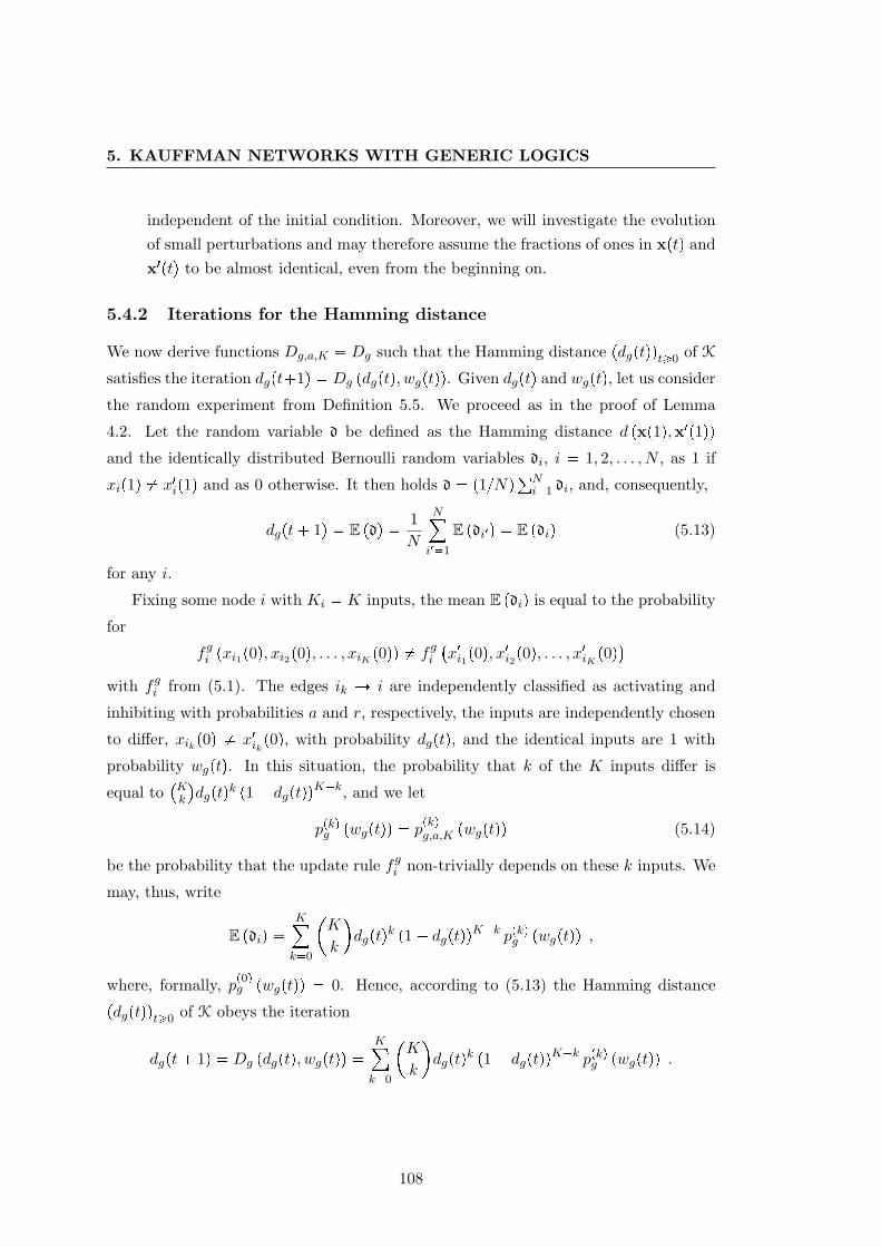
5. KAUFFMAN NETWORKS WITH GENERIC LOGICS
independent of the initial condition. Moreover, we will investigate the evolutionof small perturbations and may therefore assume the fractions of ones in xptq andx1ptq to be almost identical, even from the beginning on.
5.4.2 Iterations for the Hamming distance
We now derive functions Dg,a,K Dg such that the Hamming distance pdgptqqt¥0 of K
satisfies the iteration dgpt1q Dg pdgptq, wgptqq. Given dgptq and wgptq, let us consider
the random experiment from Definition 5.5. We proceed as in the proof of Lemma
4.2. Let the random variable d be defined as the Hamming distance d pxp1q,x1p1qqand the identically distributed Bernoulli random variables di, i 1, 2, . . . , N , as 1 if
xip1q x1ip1q and as 0 otherwise. It then holds d p1Nq°Ni1 di, and, consequently,
dgpt 1q E pdq 1N
N
i11
E pdi1q E pdiq (5.13)
for any i.
Fixing some node i with Ki K inputs, the mean E pdiq is equal to the probability
for
fgi pxi1p0q, xi2p0q, . . . , xiK p0qq fgix1i1p0q, x1i2p0q, . . . , x1iK p0q
with fgi from (5.1). The edges ik Ñ i are independently classified as activating and
inhibiting with probabilities a and r, respectively, the inputs are independently chosen
to differ, xikp0q x1ikp0q, with probability dgptq, and the identical inputs are 1 with
probability wgptq. In this situation, the probability that k of the K inputs differ is
equal toKk
dgptqk p1 dgptqqKk, and we let
ppkqg pwgptqq ppkqg,a,K pwgptqq (5.14)
be the probability that the update rule fgi non-trivially depends on these k inputs. We
may, thus, write
E pdiq K
k0
K
k
dgptqk p1 dgptqqKk ppkqg pwgptqq ,
where, formally, pp0qg pwgptqq 0. Hence, according to (5.13) the Hamming distance
pdgptqqt¥0 of K obeys the iteration
dgpt 1q Dg pdgptq, wgptqq K
k0
K
k
dgptqk p1 dgptqqKk ppkqg pwgptqq .
108
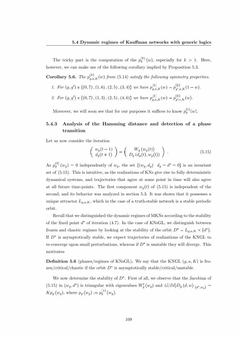
5.4 Dynamic regimes of Kauffman networks with generic logics
The tricky part is the computation of the ppkqg pwq, especially for k ¡ 1. Here,
however, we can make use of the following corollary implied by Proposition 5.3.
Corollary 5.6. The ppkqg,a,Kpwq from (5.14) satisfy the following symmetry properties.
1. For pg, g1q P tp0, 7q , p1, 6q , p2, 5q , p3, 4qu we have ppkqg,a,Kpwq ppkqg1,a,Kp1 wq.
2. For pg, g1q P tp0, 7q , p1, 3q , p2, 5q , p4, 6qu we have ppkqg,a,Kpwq ppkqg1,r,Kpwq.
Moreover, we will soon see that for our purposes it suffices to know pp1qg pwq.
5.4.3 Analysis of the Hamming distance and detection of a phase
transition
Let us now consider the iterationwgpt 1qdgpt 1q
Wg pwgptqq
Dg pdgptq, wgptqq. (5.15)
As pp0qg pwgq 0 independently of wg, the set tpwg, dgq | dg d 0u is an invariant
set of (5.15). This is intuitive, as the realizations of KNs give rise to fully deterministic
dynamical systems, and trajectories that agree at some point in time will also agree
at all future time-points. The first component wgptq of (5.15) is independent of the
second, and its behavior was analyzed in section 5.3. It was shown that it possesses a
unique attractor Lg,a,K , which in the case of a truth-stable network is a stable periodic
orbit.
Recall that we distinguished the dynamic regimes of MKNs according to the stability
of the fixed point d of iteration (4.7). In the case of KNsGL, we distinguish between
frozen and chaotic regimes by looking at the stability of the orbit D Lg,a,K tdu.If D is asymptotically stable, we expect trajectories of realizations of the KNGL to
re-converge upon small perturbations, whereas if D is unstable they will diverge. This
motivates
Definition 5.6 (phases/regimes of KNsGL). We say that the KNGL pg, a,Kq is fro-zen/critical/chaotic if the orbit D is asymptotically stable/critical/unstable.
We now determine the stability of D. First of all, we observe that the Jacobian of
(5.15) in pwg, dq is triangular with eigenvalues W 1g pwgq and pBBdqDg pd,wq|pd,wgq
Kpg pwgq, where pg pwgq : pp1qg pwgq.
109
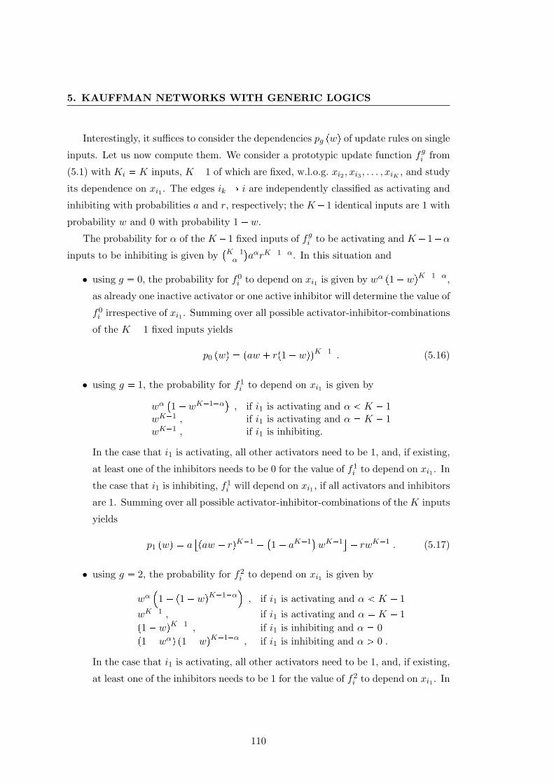
5. KAUFFMAN NETWORKS WITH GENERIC LOGICS
Interestingly, it suffices to consider the dependencies pg pwq of update rules on single
inputs. Let us now compute them. We consider a prototypic update function fgi from
(5.1) with Ki K inputs, K 1 of which are fixed, w.l.o.g. xi2 , xi3 , . . . , xiK , and study
its dependence on xi1 . The edges ik Ñ i are independently classified as activating and
inhibiting with probabilities a and r, respectively; the K1 identical inputs are 1 with
probability w and 0 with probability 1 w.
The probability for α of the K1 fixed inputs of fgi to be activating and K1αinputs to be inhibiting is given by
K1α
aαrK1α. In this situation and
• using g 0, the probability for f0i to depend on xi1 is given by wα p1 wqK1α,
as already one inactive activator or one active inhibitor will determine the value of
f0i irrespective of xi1 . Summing over all possible activator-inhibitor-combinations
of the K 1 fixed inputs yields
p0 pwq paw rp1 wqqK1 . (5.16)
• using g 1, the probability for f1i to depend on xi1 is given by
wα1 wK1α
, if i1 is activating and α K 1
wK1 , if i1 is activating and α K 1wK1 , if i1 is inhibiting.
In the case that i1 is activating, all other activators need to be 1, and, if existing,
at least one of the inhibitors needs to be 0 for the value of f1i to depend on xi1 . In
the case that i1 is inhibiting, f1i will depend on xi1 , if all activators and inhibitors
are 1. Summing over all possible activator-inhibitor-combinations of the K inputs
yields
p1 pwq apaw rqK1
1 aK1wK1
rwK1 . (5.17)
• using g 2, the probability for f2i to depend on xi1 is given by
wα
1 p1 wqK1α, if i1 is activating and α K 1
wK1 , if i1 is activating and α K 1p1 wqK1 , if i1 is inhibiting and α 0p1 wαq p1 wqK1α , if i1 is inhibiting and α ¡ 0 .
In the case that i1 is activating, all other activators need to be 1, and, if existing,
at least one of the inhibitors needs to be 1 for the value of f2i to depend on xi1 . In
110
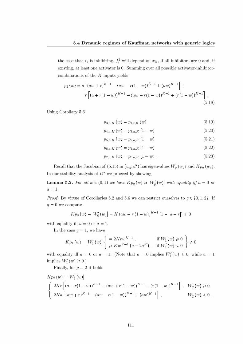
5.4 Dynamic regimes of Kauffman networks with generic logics
the case that i1 is inhibiting, f2i will depend on xi1 , if all inhibitors are 0 and, if
existing, at least one activator is 0. Summing over all possible activator-inhibitor-
combinations of the K inputs yields
p2 pwq apaw rqK1 paw rp1 wqqK1 pawqK1
rpa rp1 wqqK1 paw rp1 wqqK1 prp1 wqqK1
.
(5.18)
Using Corollary 5.6
p3,a,K pwq p1,r,K pwq (5.19)
p4,a,K pwq p3,a,K p1 wq (5.20)
p5,a,K pwq p2,a,K p1 wq (5.21)
p6,a,K pwq p1,a,K p1 wq (5.22)
p7,a,K pwq p0,a,K p1 wq . (5.23)
Recall that the Jacobian of (5.15) in pwg, dq has eigenvalues W 1g pwgq and Kpg pwgq.
In our stability analysis of D we proceed by showing
Lemma 5.2. For all w P p0, 1q we have Kpg pwq ¥W 1
g pwq with equality iff a 0 or
a 1.
Proof. By virtue of Corollaries 5.2 and 5.6 we can restrict ourselves to g P t0, 1, 2u. Ifg 0 we compute
Kp0 pwq W 1
0 pwq K paw r p1 wqqK1 p1 |a r|q ¥ 0
with equality iff a 0 or a 1.In the case g 1, we have
Kp1 pwq W 1
1 pwq # 2KrwK1 , if W 1
1 pwq ¥ 0¥ KwK1
a 2aK
, if W 1
1 pwq 0
+¥ 0
with equality iff a 0 or a 1. (Note that a 0 implies W 11 pwq ¤ 0, while a 1
implies W 11 pwq ¥ 0.)
Finally, for g 2 it holds
Kp2 pwq W 1
2 pwq $&
%2Kr
pa rp1 wqqK1 paw rp1 wqqK1 prp1 wqqK1
, W 1
2 pwq ¥ 0
2Kapaw rqK1 paw rp1 wqqK1 pawqK1
, W 1
2 pwq 0 .
111
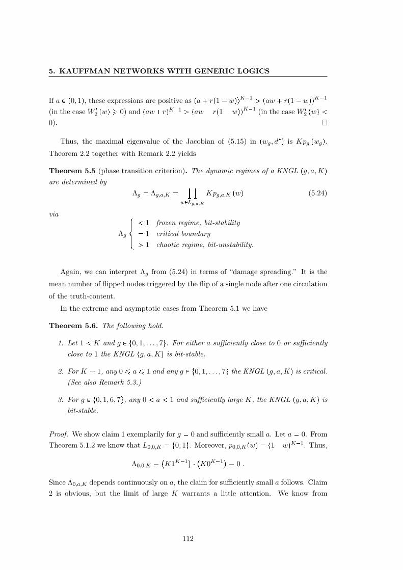
5. KAUFFMAN NETWORKS WITH GENERIC LOGICS
If a P p0, 1q, these expressions are positive as pa rp1 wqqK1 ¡ paw rp1 wqqK1
(in the case W 12 pwq ¥ 0) and pawrqK1 ¡ paw rp1 wqqK1 (in the case W 1
2 pwq 0).
Thus, the maximal eigenvalue of the Jacobian of (5.15) in pwg, dq is Kpg pwgq.Theorem 2.2 together with Remark 2.2 yields
Theorem 5.5 (phase transition criterion). The dynamic regimes of a KNGL pg, a,Kqare determined by
Λg Λg,a,K ¹
wPLg,a,K
Kpg,a,K pwq (5.24)
via
Λg
$'&'% 1 frozen regime, bit-stability 1 critical boundary¡ 1 chaotic regime, bit-unstability.
Again, we can interpret Λg from (5.24) in terms of “damage spreading.” It is the
mean number of flipped nodes triggered by the flip of a single node after one circulation
of the truth-content.
In the extreme and asymptotic cases from Theorem 5.1 we have
Theorem 5.6. The following hold.
1. Let 1 K and g P t0, 1, . . . , 7u. For either a sufficiently close to 0 or sufficientlyclose to 1 the KNGL pg, a,Kq is bit-stable.
2. For K 1, any 0 ¤ a ¤ 1 and any g P t0, 1, . . . , 7u the KNGL pg, a,Kq is critical.(See also Remark 5.3.)
3. For g P t0, 1, 6, 7u, any 0 a 1 and sufficiently large K, the KNGL pg, a,Kq isbit-stable.
Proof. We show claim 1 exemplarily for g 0 and sufficiently small a. Let a 0. FromTheorem 5.1.2 we know that L0,0,K t0, 1u. Moreover, p0,0,Kpwq p1wqK1. Thus,
Λ0,0,K K1K1
K0K1 0 .
Since Λ0,a,K depends continuously on a, the claim for sufficiently small a follows. Claim2 is obvious, but the limit of large K warrants a little attention. We know from
112
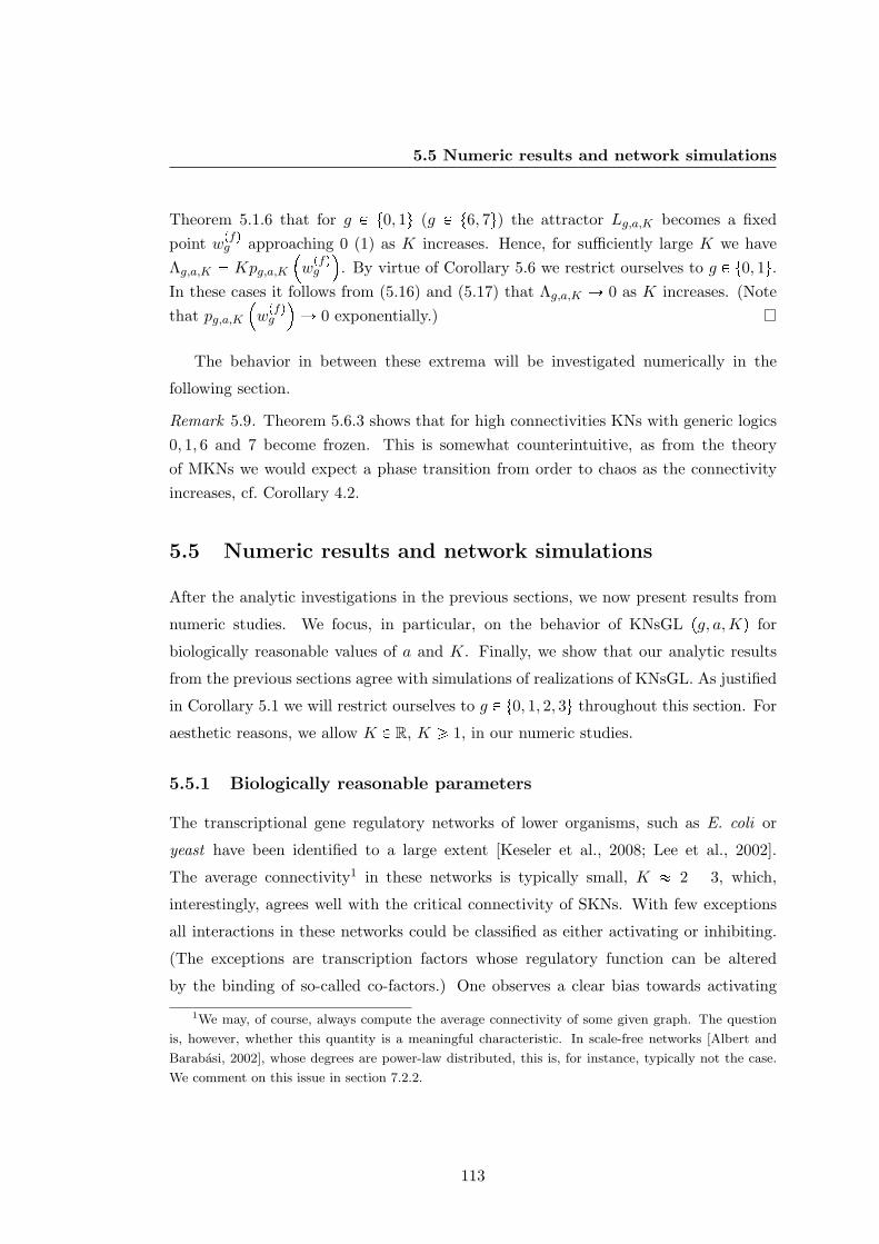
5.5 Numeric results and network simulations
Theorem 5.1.6 that for g P t0, 1u (g P t6, 7u) the attractor Lg,a,K becomes a fixedpoint wpfqg approaching 0 (1) as K increases. Hence, for sufficiently large K we haveΛg,a,K Kpg,a,K
wpfqg
. By virtue of Corollary 5.6 we restrict ourselves to g P t0, 1u.
In these cases it follows from (5.16) and (5.17) that Λg,a,K Ñ 0 as K increases. (Notethat pg,a,K
wpfqg
Ñ 0 exponentially.)
The behavior in between these extrema will be investigated numerically in the
following section.
Remark 5.9. Theorem 5.6.3 shows that for high connectivities KNs with generic logics0, 1, 6 and 7 become frozen. This is somewhat counterintuitive, as from the theoryof MKNs we would expect a phase transition from order to chaos as the connectivityincreases, cf. Corollary 4.2.
5.5 Numeric results and network simulations
After the analytic investigations in the previous sections, we now present results from
numeric studies. We focus, in particular, on the behavior of KNsGL pg, a,Kq for
biologically reasonable values of a and K. Finally, we show that our analytic results
from the previous sections agree with simulations of realizations of KNsGL. As justified
in Corollary 5.1 we will restrict ourselves to g P t0, 1, 2, 3u throughout this section. For
aesthetic reasons, we allow K P R, K ¥ 1, in our numeric studies.
5.5.1 Biologically reasonable parameters
The transcriptional gene regulatory networks of lower organisms, such as E. coli or
yeast have been identified to a large extent [Keseler et al., 2008; Lee et al., 2002].
The average connectivity1 in these networks is typically small, K 2 3, which,
interestingly, agrees well with the critical connectivity of SKNs. With few exceptions
all interactions in these networks could be classified as either activating or inhibiting.
(The exceptions are transcription factors whose regulatory function can be altered
by the binding of so-called co-factors.) One observes a clear bias towards activating
1We may, of course, always compute the average connectivity of some given graph. The question
is, however, whether this quantity is a meaningful characteristic. In scale-free networks [Albert and
Barabasi, 2002], whose degrees are power-law distributed, this is, for instance, typically not the case.
We comment on this issue in section 7.2.2.
113
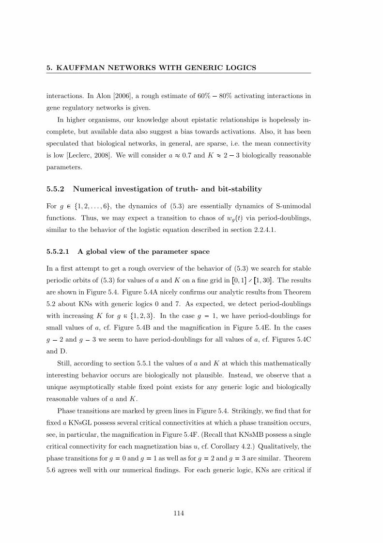
5. KAUFFMAN NETWORKS WITH GENERIC LOGICS
interactions. In Alon [2006], a rough estimate of 60% 80% activating interactions in
gene regulatory networks is given.
In higher organisms, our knowledge about epistatic relationships is hopelessly in-
complete, but available data also suggest a bias towards activations. Also, it has been
speculated that biological networks, in general, are sparse, i.e. the mean connectivity
is low [Leclerc, 2008]. We will consider a 0.7 and K 2 3 biologically reasonable
parameters.
5.5.2 Numerical investigation of truth- and bit-stability
For g P t1, 2, . . . , 6u, the dynamics of (5.3) are essentially dynamics of S-unimodal
functions. Thus, we may expect a transition to chaos of wgptq via period-doublings,
similar to the behavior of the logistic equation described in section 2.2.4.1.
5.5.2.1 A global view of the parameter space
In a first attempt to get a rough overview of the behavior of (5.3) we search for stable
periodic orbits of (5.3) for values of a and K on a fine grid in r0, 1sr1, 30s. The results
are shown in Figure 5.4. Figure 5.4A nicely confirms our analytic results from Theorem
5.2 about KNs with generic logics 0 and 7. As expected, we detect period-doublings
with increasing K for g P t1, 2, 3u. In the case g 1, we have period-doublings for
small values of a, cf. Figure 5.4B and the magnification in Figure 5.4E. In the cases
g 2 and g 3 we seem to have period-doublings for all values of a, cf. Figures 5.4C
and D.
Still, according to section 5.5.1 the values of a and K at which this mathematically
interesting behavior occurs are biologically not plausible. Instead, we observe that a
unique asymptotically stable fixed point exists for any generic logic and biologically
reasonable values of a and K.
Phase transitions are marked by green lines in Figure 5.4. Strikingly, we find that for
fixed a KNsGL possess several critical connectivities at which a phase transition occurs,
see, in particular, the magnification in Figure 5.4F. (Recall that KNsMB possess a single
critical connectivity for each magnetization bias u, cf. Corollary 4.2.) Qualitatively, the
phase transitions for g 0 and g 1 as well as for g 2 and g 3 are similar. Theorem
5.6 agrees well with our numerical findings. For each generic logic, KNs are critical if
114
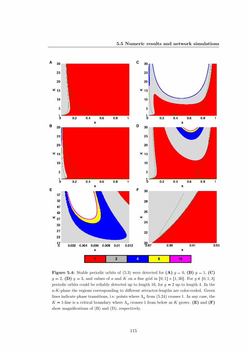
5.5 Numeric results and network simulations
FE
DB
A C
1 2 4 8 16
Figure 5.4: Stable periodic orbits of (5.3) were detected for (A) g 0, (B) g 1, (C)g 2, (D) g 3, and values of a and K on a fine grid in r0, 1s r1, 30s. For g P t0, 1, 3uperiodic orbits could be reliably detected up to length 16, for g 2 up to length 4. In thea-K-plane the regions corresponding to different attractor-lengths are color-coded. Greenlines indicate phase transitions, i.e. points where Λg from (5.24) crosses 1. In any case, theK 1-line is a critical boundary where Λg crosses 1 from below as K grows. (E) and (F)show magnifications of (B) and (D), respectively.
115
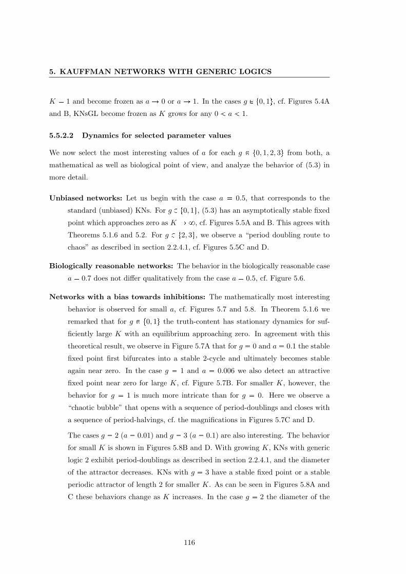
5. KAUFFMAN NETWORKS WITH GENERIC LOGICS
K 1 and become frozen as a Ñ 0 or a Ñ 1. In the cases g P t0, 1u, cf. Figures 5.4A
and B, KNsGL become frozen as K grows for any 0 a 1.
5.5.2.2 Dynamics for selected parameter values
We now select the most interesting values of a for each g P t0, 1, 2, 3u from both, a
mathematical as well as biological point of view, and analyze the behavior of (5.3) in
more detail.
Unbiased networks: Let us begin with the case a 0.5, that corresponds to the
standard (unbiased) KNs. For g P t0, 1u, (5.3) has an asymptotically stable fixed
point which approaches zero as K Ñ8, cf. Figures 5.5A and B. This agrees with
Theorems 5.1.6 and 5.2. For g P t2, 3u, we observe a “period doubling route to
chaos” as described in section 2.2.4.1, cf. Figures 5.5C and D.
Biologically reasonable networks: The behavior in the biologically reasonable case
a 0.7 does not differ qualitatively from the case a 0.5, cf. Figure 5.6.
Networks with a bias towards inhibitions: The mathematically most interesting
behavior is observed for small a, cf. Figures 5.7 and 5.8. In Theorem 5.1.6 we
remarked that for g P t0, 1u the truth-content has stationary dynamics for suf-
ficiently large K with an equilibrium approaching zero. In agreement with this
theoretical result, we observe in Figure 5.7A that for g 0 and a 0.1 the stable
fixed point first bifurcates into a stable 2-cycle and ultimately becomes stable
again near zero. In the case g 1 and a 0.006 we also detect an attractive
fixed point near zero for large K, cf. Figure 5.7B. For smaller K, however, the
behavior for g 1 is much more intricate than for g 0. Here we observe a
“chaotic bubble” that opens with a sequence of period-doublings and closes with
a sequence of period-halvings, cf. the magnifications in Figures 5.7C and D.
The cases g 2 (a 0.01) and g 3 (a 0.1) are also interesting. The behavior
for small K is shown in Figures 5.8B and D. With growing K, KNs with generic
logic 2 exhibit period-doublings as described in section 2.2.4.1, and the diameter
of the attractor decreases. KNs with g 3 have a stable fixed point or a stable
periodic attractor of length 2 for smaller K. As can be seen in Figures 5.8A and
C these behaviors change as K increases. In the case g 2 the diameter of the
116
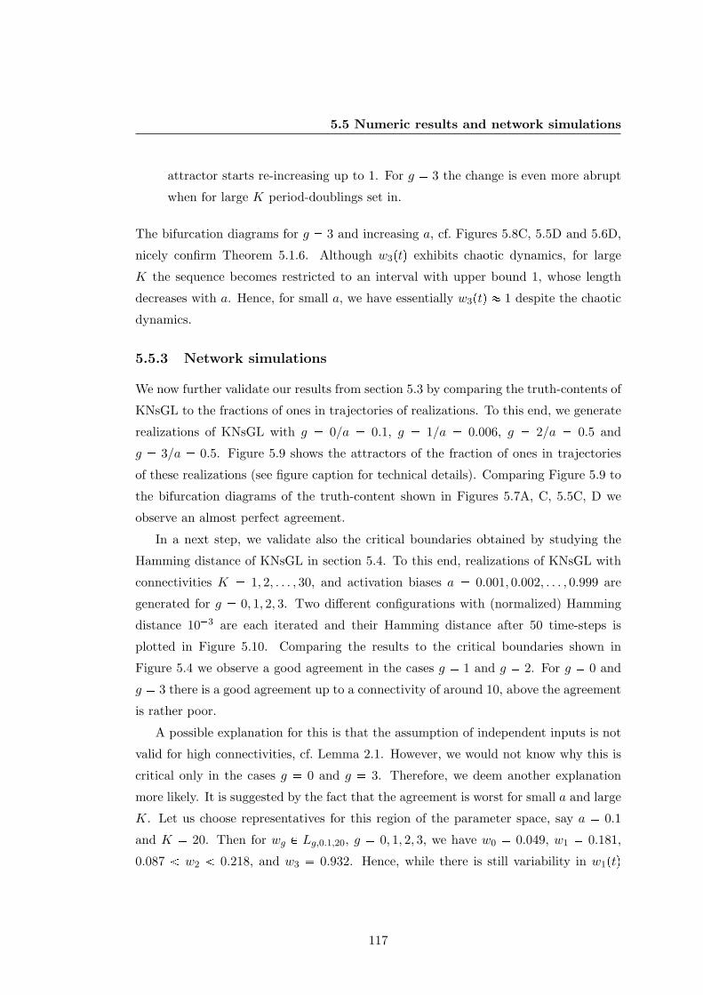
5.5 Numeric results and network simulations
attractor starts re-increasing up to 1. For g 3 the change is even more abrupt
when for large K period-doublings set in.
The bifurcation diagrams for g 3 and increasing a, cf. Figures 5.8C, 5.5D and 5.6D,
nicely confirm Theorem 5.1.6. Although w3ptq exhibits chaotic dynamics, for large
K the sequence becomes restricted to an interval with upper bound 1, whose length
decreases with a. Hence, for small a, we have essentially w3ptq 1 despite the chaotic
dynamics.
5.5.3 Network simulations
We now further validate our results from section 5.3 by comparing the truth-contents of
KNsGL to the fractions of ones in trajectories of realizations. To this end, we generate
realizations of KNsGL with g 0/a 0.1, g 1/a 0.006, g 2/a 0.5 and
g 3/a 0.5. Figure 5.9 shows the attractors of the fraction of ones in trajectories
of these realizations (see figure caption for technical details). Comparing Figure 5.9 to
the bifurcation diagrams of the truth-content shown in Figures 5.7A, C, 5.5C, D we
observe an almost perfect agreement.
In a next step, we validate also the critical boundaries obtained by studying the
Hamming distance of KNsGL in section 5.4. To this end, realizations of KNsGL with
connectivities K 1, 2, . . . , 30, and activation biases a 0.001, 0.002, . . . , 0.999 are
generated for g 0, 1, 2, 3. Two different configurations with (normalized) Hamming
distance 103 are each iterated and their Hamming distance after 50 time-steps is
plotted in Figure 5.10. Comparing the results to the critical boundaries shown in
Figure 5.4 we observe a good agreement in the cases g 1 and g 2. For g 0 and
g 3 there is a good agreement up to a connectivity of around 10, above the agreement
is rather poor.
A possible explanation for this is that the assumption of independent inputs is not
valid for high connectivities, cf. Lemma 2.1. However, we would not know why this is
critical only in the cases g 0 and g 3. Therefore, we deem another explanation
more likely. It is suggested by the fact that the agreement is worst for small a and large
K. Let us choose representatives for this region of the parameter space, say a 0.1
and K 20. Then for wg P Lg,0.1,20, g 0, 1, 2, 3, we have w0 0.049, w1 0.181,
0.087 w2 0.218, and w3 0.932. Hence, while there is still variability in w1ptq
117
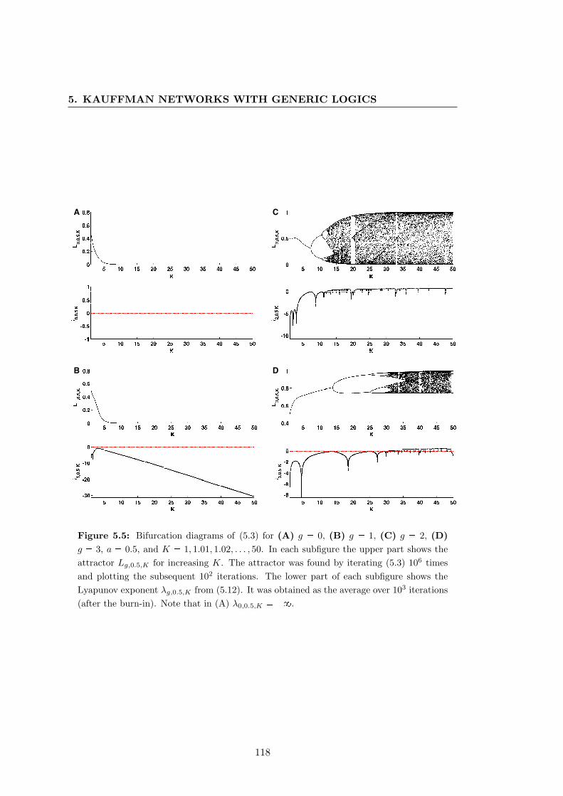
5. KAUFFMAN NETWORKS WITH GENERIC LOGICS
A
DB
C
Figure 5.5: Bifurcation diagrams of (5.3) for (A) g 0, (B) g 1, (C) g 2, (D)g 3, a 0.5, and K 1, 1.01, 1.02, . . . , 50. In each subfigure the upper part shows theattractor Lg,0.5,K for increasing K. The attractor was found by iterating (5.3) 106 timesand plotting the subsequent 102 iterations. The lower part of each subfigure shows theLyapunov exponent λg,0.5,K from (5.12). It was obtained as the average over 103 iterations(after the burn-in). Note that in (A) λ0,0.5,K 8.
118
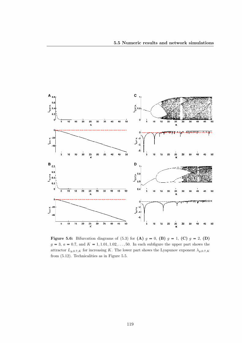
5.5 Numeric results and network simulations
A
DB
C
Figure 5.6: Bifurcation diagrams of (5.3) for (A) g 0, (B) g 1, (C) g 2, (D)g 3, a 0.7, and K 1, 1.01, 1.02, . . . , 50. In each subfigure the upper part shows theattractor Lg,0.7,K for increasing K. The lower part shows the Lyapunov exponent λg,0.7,K
from (5.12). Technicalities as in Figure 5.5.
119
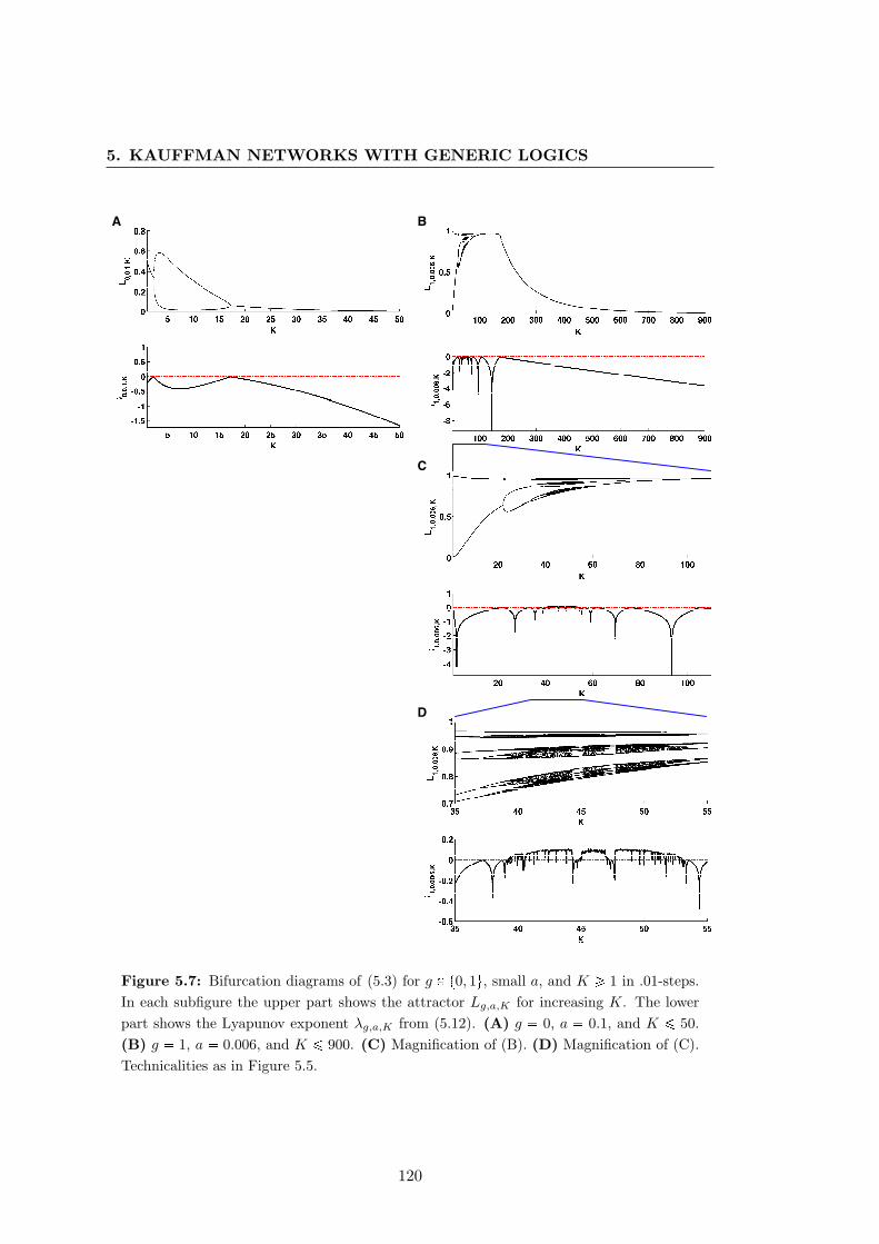
5. KAUFFMAN NETWORKS WITH GENERIC LOGICS
A B
D
C
Figure 5.7: Bifurcation diagrams of (5.3) for g P t0, 1u, small a, and K ¥ 1 in .01-steps.In each subfigure the upper part shows the attractor Lg,a,K for increasing K. The lowerpart shows the Lyapunov exponent λg,a,K from (5.12). (A) g 0, a 0.1, and K ¤ 50.(B) g 1, a 0.006, and K ¤ 900. (C) Magnification of (B). (D) Magnification of (C).Technicalities as in Figure 5.5.
120
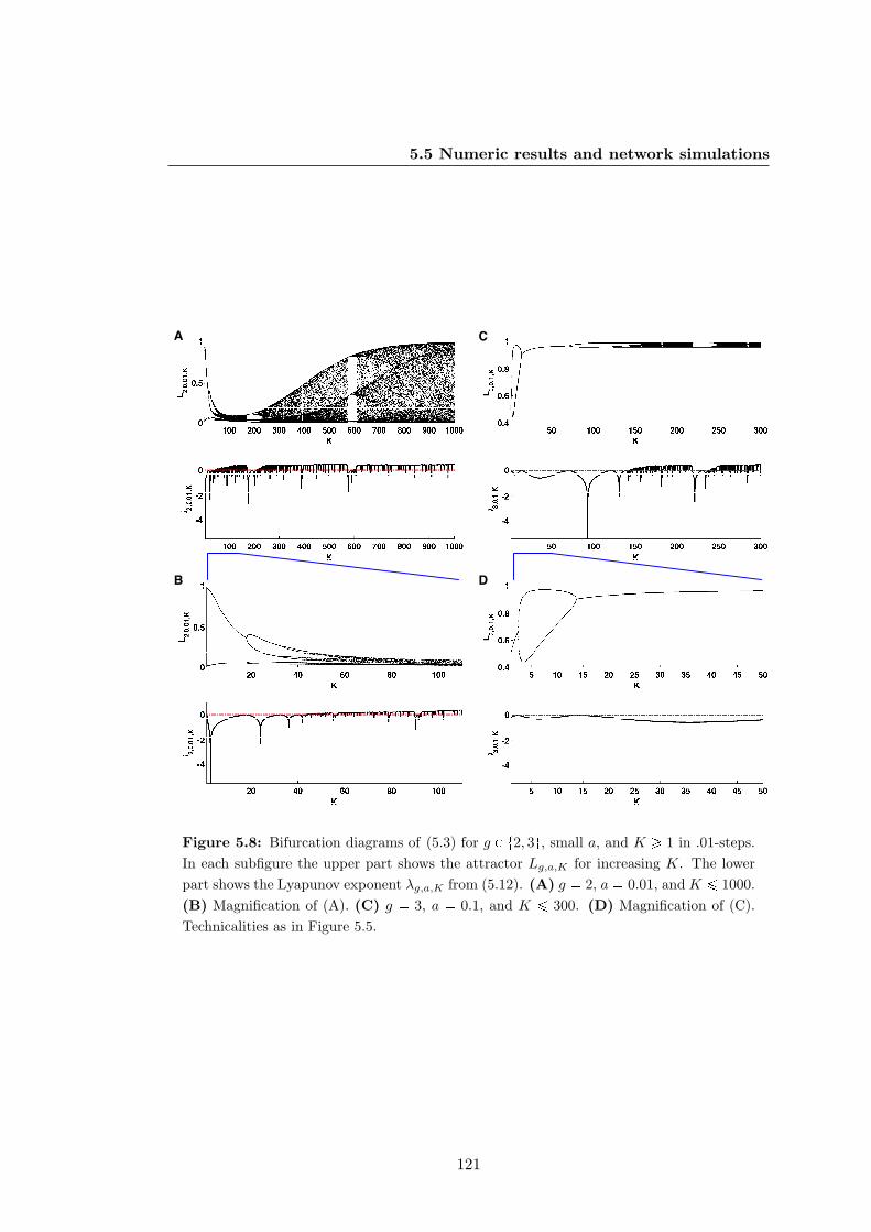
5.5 Numeric results and network simulations
EB
A
D
C
Figure 5.8: Bifurcation diagrams of (5.3) for g P t2, 3u, small a, and K ¥ 1 in .01-steps.In each subfigure the upper part shows the attractor Lg,a,K for increasing K. The lowerpart shows the Lyapunov exponent λg,a,K from (5.12). (A) g 2, a 0.01, and K ¤ 1000.(B) Magnification of (A). (C) g 3, a 0.1, and K ¤ 300. (D) Magnification of (C).Technicalities as in Figure 5.5.
121
5. KAUFFMAN NETWORKS WITH GENERIC LOGICS
and w2ptq, the values of w0ptq and w3ptq are pushed towards 0 and 1, respectively. This
implies that trajectories of realizations of KNsGL with these parameters are almost
identical to p0, 0, . . . , 0q and p1, 1, . . . , 1q, respectively, and, thus, likely to coincide due
to finite size effects.
5.6 Discussion
Accepting Kauffman’s hypothesis about “Living at the edge of chaos”, cf. section 3.4,
which generic logic g from Table 5.1 is most reasonable from a biological point of view?
Let us take a look at Figure 5.4 and the region of biologically meaningful parameter
values a 0.7 and K 2 3. For g P t0, 1u KNsGL are frozen for these parameter
values but quite far away from a critical boundary. However, for g P t2, 3u a critical
boundary crosses right through this region of the a-K-plane. In particular, for g 3
we find a “frozen headland” in midst of the chaotic regime stretching out to a 0.7.
Also in the simulation results shown in Figure 5.10D we detect a rather big region of
critical networks around a 0.7 and 2 ¤ K ¤ 3.
Interestingly, g 3 (more precisely, its symmetric counterpart g 4) has been
considered biologically meaningful by several authors. This case corresponds to the
standardized qualitative dynamical systems approach [Mendoza and Xenarios, 2006]. It
has also been successfully employed in the analysis of immunology microarray datasets
[Martin et al., 2007]. Biologically speaking, in all these studies it is assumed that a gene
is expressed if any of its activators and none of its inhibitors is active. In other words,
the regulating activators and inhibitors are assumed to be functionally equivalent or
acting in an additive fashion.
Starting point of our investigations in this chapter were what we called qualitative
and Boolean models of gene regulatory networks. A QM is the language of biology, it
is a graphical representation of biological knowledge. A BM on the other hand gives
rise to a dynamical system, which is something mathematicians like to talk about. We
then introduced the concept of generic logics and showed that they induce a mapping
from qualitative to Boolean models.
Since the study of BMs in theoretical biology originated in the study of KNs, we
deemed it appropriate to investigate KNs obtained by applying generic logics to QMs.
We began by studying the truth-content of these networks, i.e. the mean-field fraction of
122
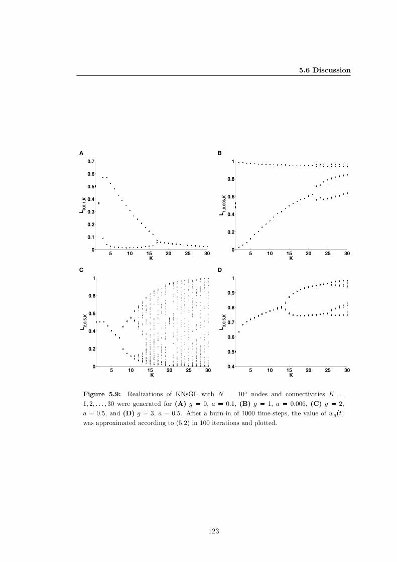
5.6 Discussion
5 10 15 20 25 300
0.2
0.4
0.6
0.8
1
K
L 2,0.
5,K
5 10 15 20 25 300
0.1
0.2
0.3
0.4
0.5
0.6
0.7
K
L 0,0.
1,K
5 10 15 20 25 300
0.2
0.4
0.6
0.8
1
K
L 1,0.
006,
K
5 10 15 20 25 300.4
0.5
0.6
0.7
0.8
0.9
1
K
L 3,0.
5,K
A B
C D
Figure 5.9: Realizations of KNsGL with N 105 nodes and connectivities K
1, 2, . . . , 30 were generated for (A) g 0, a 0.1, (B) g 1, a 0.006, (C) g 2,a 0.5, and (D) g 3, a 0.5. After a burn-in of 1000 time-steps, the value of wgptq
was approximated according to (5.2) in 100 iterations and plotted.
123
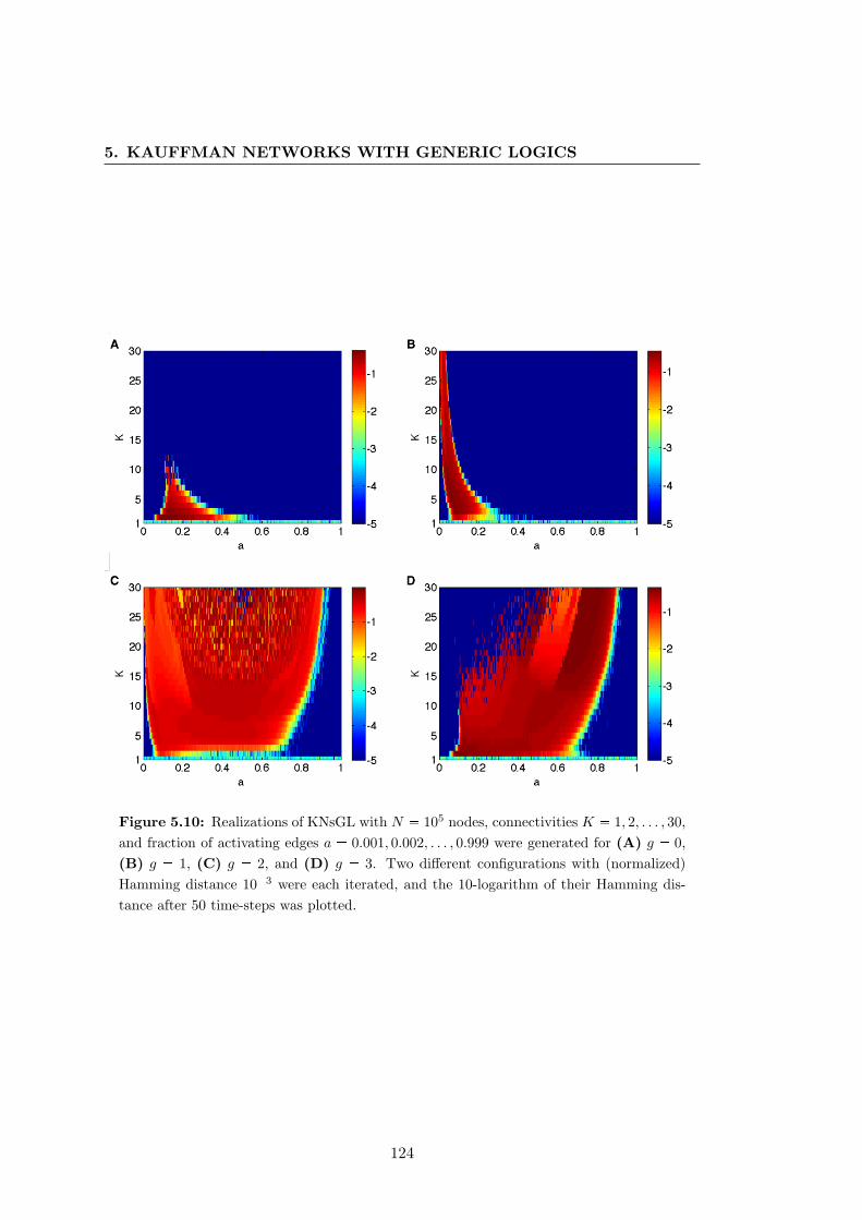
5. KAUFFMAN NETWORKS WITH GENERIC LOGICS
Figure 5.10: Realizations of KNsGL with N 105 nodes, connectivities K 1, 2, . . . , 30,and fraction of activating edges a 0.001, 0.002, . . . , 0.999 were generated for (A) g 0,(B) g 1, (C) g 2, and (D) g 3. Two different configurations with (normalized)Hamming distance 103 were each iterated, and the 10-logarithm of their Hamming dis-tance after 50 time-steps was plotted.
124
5.6 Discussion
ones, and analytically characterized the attractor of this quantity. For parameter values
selected from both, a mathematical as well as a biological point of view, we numerically
computed the bifurcation diagrams of the truth-content. These investigations revealed
a rich dynamical behavior including period-doublings leading to chaos as the network
connectivity increases. In a next step, we defined a criterion for phase transitions. We
found that in contrast to KNsMB, KNsGL possess multiple, intricately shaped critical
boundaries. Simulations further strengthened the significance of our results.
Our findings are also interesting from a biological point of view. First of all, we
observed that with biologically reasonable fractions of activators a and network connec-
tivities K the truth-content has stationary dynamics for all generic logics. Oscillations
of the truth-content — biologically speaking, of the total gene expression — would
be economically disadvantageous for cells, especially in the case of large amplitudes,
as massive amounts of mRNA and protein would have to be assembled and degraded
during each cycle. Moreover, we found that KNs with the biologically plausible generic
logics g 3 and g 4 are near criticality for realistic fractions of activators a and
network connectivities K.
125

5. KAUFFMAN NETWORKS WITH GENERIC LOGICS
126
6
Discrete and continuous models
of the mid-hindbrain boundary
Prediction is very difficult,
especially about the future.
Niels Bohr
There are many notions of what “systems biology” is. A popular one was con-
ceived of by Hiroaki Kitano [2002]. For him, systems biology is characterized by a
hypothesis-driven “research cycle” iterating between computational modeling and wet-
lab experiments. The overall goal of the computational modeling part is the generation
of predictions such as potential genetic interactions, which can then be experimentally
validated or falsified. Especially when available data are scarce and of qualitative na-
ture, BMs can be beneficially employed to this purpose, as we shall see in the course
of this chapter.
Using BMs to model specific biological processes, however, one quickly discovers
that not all biological phenomena can be equally well reproduced by these models.
127
6. DISCRETE AND CONTINUOUS MODELS OF THE MHB
BMs are typically well suited to capture differentiation processes, where the common
modeling assumption is that attractors of the dynamical system induced by the BM
correspond to different cell types, lineages or tissues. This will also be our “working
hypothesis” in the following, when we model the differentiation of mid- and hindbrain.
BMs as defined herein are, however, less suitable to capture quantitative effects in a
precise temporal order due to the unrealistic time-discrete synchronous updating in the
associated dynamical systems. These effects fall into the realm of (time-)continuous
dynamical systems.
6.1 Motivation and outline
In this chapter, which follows Wittmann et al. [2009a] and Wittmann et al. [2009b],
we venture a glimpse at a possible way of transforming BMs into real time-continuous
dynamical systems. We review some results about fixed points in discrete and con-
tinuous dynamical systems based on the same BM. In general, however, the dynamics
of both systems may differ vastly, and any such transformation should primarily be
regarded as a heuristic modeling approach. We validate this approach in section 6.3
from a biological point of view, by applying it to a BM of a specific biological process
— differentiation of mid- and hindbrain during vertebrate development —, which we
already introduced in section 2.4.2. To be precise, the BM will be a model of the reg-
ulatory network between the IsO genes Otx2 , Gbx2 , Fgf8 , Wnt1 , En, and Pax . Its
key functionality will be the stable maintenance of these’s genes expression patterns
around the MHB at E10.5 as shown in Figure 2.4B.
We develop the BM in section 6.2. To this end, we describe a methodology for
the inference of regulatory interactions by systematic logical analyses of spatial gene
expression patterns. As our information about gene expression at the MHB is of purely
qualitative nature, it is only natural to base this analysis on BMs. For the determination
of the update rules our methodology employs techniques that were originally devised
to optimize logic circuits in order to facilitate their hardware implementation.
Applied to the wild-type gene expression pattern at the MHB (cf. Figure 2.4B) our
method predicts several genetic interactions, which well agree with published data. In
this context, an unclarified experimental issue is the reported ectopic induction of Wnt1
by Fgf8 in gain-of-function experiments performed in vitro and in vivo [Adams et al.,
128
6.2 Inference of a Boolean model of the mid-hindbrain boundary
2000; Bally-Cuif and Wassef, 1994; Liu and Joyner, 2001; Liu et al., 1999]. As Fgf8
expression in the anterior neural plate initiates several hours after Wnt1 , and as Wnt1
is expressed in a very broad domain at the time most experimental manipulations took
place [Crossley and Martin, 1995; McMahon et al., 1992], the ectopic maintenance of
Wnt1 expression by Fgf8 might have been mis-interpreted as an ectopic activation. Our
analysis, indeed, predicts that Fgf8 and Wnt1 signaling are dependent on each other for
stable maintenance, but Fgf8 is not sufficient to ectopically induce Wnt1 expression.
We validate this prediction experimentally by performing a time-course analysis of
Wnt1 expression after implantation of Fgf8-coated beads into mouse anterior neural
plate/tube explants.1 Thus, our analysis clarifies epistatic relationships at the MHB,
especially between the two key patterning molecules Fgf8 and Wnt1. In a subsequent
step, the results of our analysis combined with published data allow construction of a
BM that is able to explain the stable maintenance of the characteristic gene expression
patterns at the MHB.
These expression patterns are the result of a refinement and sharpening of initially
blurred expression domains. A natural question is if our model is able to reproduce
this process in a correct spatio-temporal order. The coarse-grained state-space and
the unrealistic time-discrete synchronous updating of dynamical systems induced by
BMs, however, prevent us from addressing this question. As an outlook we, therefore,
present a possible way of transforming BMs into real time-continuous dynamical sys-
tems (section 6.3). We apply this transformation to our BM of the MHB. Simulations
of the resulting continuous system show that it is, indeed, competent to reproduce the
observed refinement and sharpening of expression domains under wild-type as well as
several loss-of-function conditions.
6.2 Inference of a Boolean model of the mid-hindbrain
boundary
In this section, we describe a way of inferring BMs from spatial gene expression patterns.
Our primary object is to obtain new biological insights into gene regulation at the MHB.
We will, therefore, extensively discuss the results of our Boolean modeling approach
1Collaboration with Nilima Prakash (Institute of Developmental Genetics, Helmholtz Zentrum
Munchen)
129
6. DISCRETE AND CONTINUOUS MODELS OF THE MHB
with respect to their biological plausibility and relevance. For this reason, this section
will be more biological in tone than the other parts of this thesis. The reader may,
however, skip this entire section. All one needs to know in order to be able to follow
the remainder of this chapter is the BM from (6.3). We begin by the necessary pre-
processing of available data.
6.2.1 Data pre-processing
We subdivide the expression patterns of the IsO genes Otx2 , Gbx2 , Fgf8 , Wnt1 , En,
and Pax at E10.5 into six compartments I-VI, cf. the dashed lines in Figures 6.1A and
6.1B. As is typically the case with Boolean analyses, this pre-processing of biological
data is to a certain extent artificial and an over-simplification of biological reality. It
is, however, necessary as it allows us to represent the expression patterns as Boolean
matrices (see Figure 6.1C), which constitute the data basis for our analysis.
The morphological entity of the MHB is located between compartments III and IV.
Other than that, this partitioning is based on the expression patterns of the IsO genes
and not on morphological properties. Compartments I-III correspond to the prospective
midbrain (Otx2 +/Gbx2 –) and IV-VI to the prospective hindbrain (Otx2 –/Gbx2 +).
The boundary compartments III and IV are characterized by the expression of Wnt1
and Fgf8 , respectively. We assume that the secreted Wnt1 and Fgf8 proteins are
still present in compartments II and V due to passive or active diffusion [Scholpp and
Brand, 2004; Strigini and Cohen, 2000], whereas compartments I and VI are devoid of
these secreted factors as they are farthest away from the MHB. So, all in all, the six
compartments are characterized as follows.
(I) Only Otx2 is expressed.
(II) Otx2 , En, and Pax are expressed. Secreted Wnt1 protein is present.
(III) Otx2 , En, Pax , and Wnt1 are expressed. Secreted Wnt1 and Fgf8 proteins are
present.
(IV) Gbx2 , En, Pax , and Fgf8 are expressed. Secreted Wnt1 and Fgf8 proteins are
present.
(V) Gbx2 , En, and Pax are expressed. Secreted Fgf8 protein is present.
130
6.2 Inference of a Boolean model of the mid-hindbrain boundary
(VI) Only Gbx2 is expressed.
The crucial point is that this expression pattern is stably maintained by a regulatory
network between the IsO genes. In the following section we demonstrate that key
genetic interactions of this network can be obtained already by analyzing only this
spatial information.
6.2.2 The inverse problem
So far, information about genetic interactions at the MHB has been obtained mainly
from the analyses of gene expression patterns (by in situ hybridization) and epistatic
relationships between these genes in gain-of-function and loss-of-function mutant mice.
The task of elucidating gene regulation at the MHB, therefore, leads to the theoretical
challenge of inferring as much information as possible about the structure of multi-
cellular regulatory networks from their spatial expression patterns. To this end, we
now describe a methodology for the inference of regulatory interactions by systematic
logical analyses of spatial gene expression patterns.
These analyses are based on a Boolean model pG, fq. In case of the MHB example,
we set G equal to the fully connected directed graph (without self-loops) on six nodes,
which represent (in this order) the (groups of) genes Otx2 , Gbx2 , Fgf8 , Wnt1 , En,
and Pax . For the sake of clarity, we will use otx, gbx, fgf,wnt, en, and pax as node
indices. The left-hand table in Figure 6.1C shows a Boolean representation of these
gene’s expression patterns around the MHB. The right-hand table displays protein
expression also taking into account diffusion of secreted Fgf8 and Wnt1 protein into
regions adjacent to their mRNA expression domains. We denote the columns of the
left-hand table by xI ,xII ,xIII ,xIV ,xV ,xV I , and the columns of the right-hand table
by x1I ,x1II ,x
1III ,x
1IV ,x
1V ,x
1V I . We already remarked that the stable maintenance of
these patterns is a key function of the regulatory network between the IsO genes. In
mathematical terms, the conditions that need to be satisfied by the transfer function f
are
xj fx1j, j I, II, . . . , V I . (6.1)
Conditions (6.1) partially define the update rules fi, i otx, gbx, fgf,wnt, en, pax.
Naturally, there are many ways of extending them to their full domain, which is why
we need to impose further constraints. This is best done in terms of the Boolean
131
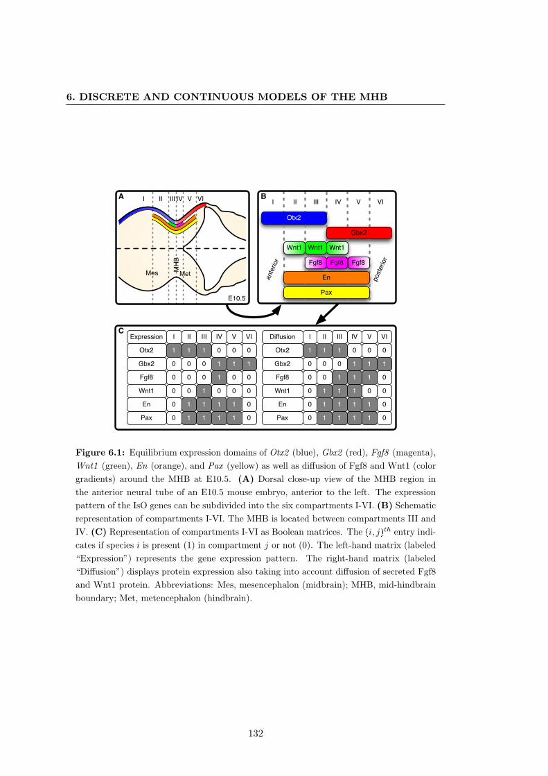
6. DISCRETE AND CONTINUOUS MODELS OF THE MHB
A
C
B
Otx2
Gbx2
Wnt1
Fgf8
Pax
En
Wnt1 Wnt1
Fgf8Fgf8anterior
posterior
I II III IV V VI
110 11Pax 0
0
1
1
V
0
Gbx2
0
10 1
0
Expression
0
0
1
0
En
Otx2 01
Fgf8
1
0
IV
1
0
II
0 10
1
0
0
1
1
0
0
Wnt1 0
VIIIII
110 11Pax 0
0
1
1
V
0
Gbx2
0
10 1
1
Diffusion
1
0
1
1
En
Otx2 01
Fgf8
1
0
IV
1
0
II
0 10
1
0
0
1
1
0
0
Wnt1 1
VIIIII
I II III IV V VI
Mes MetMHB
E10.5
Figure 6.1: Equilibrium expression domains of Otx2 (blue), Gbx2 (red), Fgf8 (magenta),Wnt1 (green), En (orange), and Pax (yellow) as well as diffusion of Fgf8 and Wnt1 (colorgradients) around the MHB at E10.5. (A) Dorsal close-up view of the MHB region inthe anterior neural tube of an E10.5 mouse embryo, anterior to the left. The expressionpattern of the IsO genes can be subdivided into the six compartments I-VI. (B) Schematicrepresentation of compartments I-VI. The MHB is located between compartments III andIV. (C) Representation of compartments I-VI as Boolean matrices. The pi, jqth entry indi-cates if species i is present (1) in compartment j or not (0). The left-hand matrix (labeled“Expression”) represents the gene expression pattern. The right-hand matrix (labeled“Diffusion”) displays protein expression also taking into account diffusion of secreted Fgf8and Wnt1 protein. Abbreviations: Mes, mesencephalon (midbrain); MHB, mid-hindbrainboundary; Met, metencephalon (hindbrain).
132
6.2 Inference of a Boolean model of the mid-hindbrain boundary
expressions describing the update rules. A possible regularization would, for instance,
be the restriction to a certain class of Boolean functions such as canalyzing functions,1
or functions generated by one of the generic logics introduced in chapter 5. Which
regularization proves most effective has to be figured out anew in each application. In
the example of the MHB, a suitable choice was to extend the partially defined update
rules under the regularization that the resulting fi be minimal with respect to the
length of the shortest representing Boolean expression in DNF. This analysis is based
on the assumption that the thus obtained minimal BM reflects the core module of the
real network.
6.2.3 Minimization of Boolean functions
Standard ways of finding minimal Boolean expressions for (partially filled) truth-
tables are either Karnaugh-Veitch maps [Karnaugh, 1953; Veitch, 1952] or the Quine-
McCluskey algorithm [McCluskey and Bartee, 1962; Quine, 1952] — two functionally
equivalent approaches. Karnaugh-Veitch maps are a clever graphical representation of
truth-tables. They transform the problem of finding minimal Boolean expressions into
the problem of finding a maximal-size covering of either the true- or the false-entries.
For small functions (typically no more than five inputs) the latter problem can be eas-
ily solved by inspection. For larger functions the Quine-McCluskey algorithm can be
used instead, whose tabular form is less illustrative but easier to implement. However,
also the Quine-McCluskey algorithm has a limited range of applicability, as it tries to
solve a problem which has been shown to be NP-complete, cf. the Cook-Levine The-
orem about the Boolean satisfiability problem [Cook, 1971]. Therefore, in the case of
large systems, heuristic methods like the Espresso algorithm [Brayton, 1984; Rudell
and Sangiovanni-Vincentelli, 1987] may be more suitable.
Here we outline how minimal Boolean expressions for partially defined update rules
can be found by using Karnaugh-Veitch maps. Each of our Boolean update functions
fi, i otx, gbx, fgf,wnt, en, pax, can be represented as a truth-table with 25 32 entries.
Conditions (6.1) allow to specify at most six entries in each truth-table. The remaining
entries are indetermined “don’t cares.” These truth-tables are now represented as
Karnaugh-Veitch maps, see Figure 6.2. Actually, these maps are three-dimensional1A possible justification for this restriction is that in lower organisms most genes have one canalyzing
regulator [Harris et al., 2002].
133
6. DISCRETE AND CONTINUOUS MODELS OF THE MHB
cubes but for better presentability the cube was sliced up and the two layers put next
to each other. Moreover, the green as well as the blue sides are identified, so each “slice”
is actually a torus. By inspection, we now determine a covering of the true-entries by
rectangular boxes of size 1, 2, 4, 8, 16 or 32 such that the following hold.
• No false-entry is contained in any of the boxes.
• All true-entries are contained in at least one box.
• The boxes have maximal size.
• The number of boxes is minimal.
Note that there may be multiple coverings satisfying these conditions. In Figure 6.2
all suitable coverings are shown. From each box in these coverings a conjunctive clause
is built, where variables appearing both, negated and non-negated within the box, are
omitted. These conjunctive clauses are linked by disjunction and give a minimal DNF
of the Boolean expression. We illustrate this using
ffgf : t0, 1u5 ÝÑ t0, 1upxotx, xgbx, xwnt, xen, xpaxq ÞÝÑ ffgf pxotx, xgbx, xwnt, xen, xpaxq
as a showcase. Two coverings satisfying the above conditions could be found, each
consisting of only one box, cf. the dashed and solid red boxes in Figure 6.2B. Let
us choose the first (dashed lines). Here the only variables that do not appear both,
negated as well as non-negated, are xotx (which appears only as xotx) and xwnt (which
appears only as xwnt). Consequently, the conjunction term for this box is xotx^xwnt.
Similarly, minimal expressions for the remaining update rules can be found from the
maps in Figure 6.2, and we obtain:
fotx pxgbx, xfgf, xwnt, xen, xpaxq xgbx
fgbx pxotx, xfgf, xwnt, xen, xpaxq xotx
ffgf pxotx, xgbx, xwnt, xen, xpaxq xwnt ^"
xgbx
xotx
*
fwnt pxotx, xgbx, xfgf, xen, xpaxq xfgf ^"
xotx
xgbx
*fen pxotx, xgbx, xfgf, xwnt, xpaxq xpax
fpax pxotx, xgbx, xfgf, xwnt, xenq xen .
(6.2)
In the case of Fgf8 and Wnt1 two equally minimal expressions could be found, indicated
by the factors in curly brackets, one of which has to be included.
134
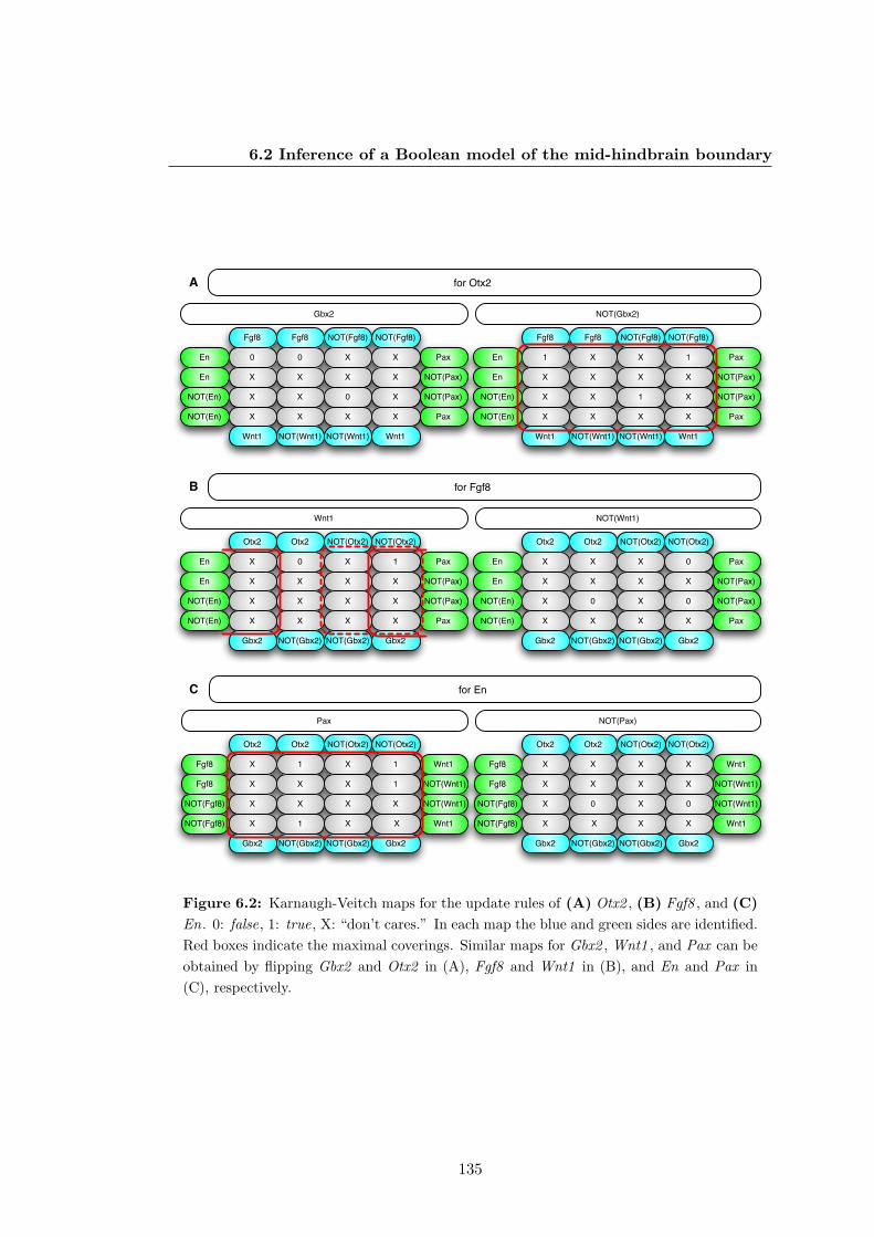
6.2 Inference of a Boolean model of the mid-hindbrain boundary
NOT(Wnt1)Wnt1 NOT(Wnt1) Wnt1
X XNOT(En) X PaxX
XNOT(En) 0 XX NOT(Pax)
XX XEn NOT(Pax)X
PaxX00En X
NOT(Fgf8)NOT(Fgf8)Fgf8Fgf8
Gbx2
NOT(Wnt1)Wnt1 NOT(Wnt1) Wnt1
X XNOT(En) X PaxX
XNOT(En) 1 XX NOT(Pax)
XX XEn NOT(Pax)X
Pax1X1En X
NOT(Fgf8)NOT(Fgf8)Fgf8Fgf8
NOT(Gbx2)
for Otx2 .A
NOT(Gbx2)Gbx2 NOT(Gbx2) Gbx2
X XNOT(En) X PaxX
XNOT(En) X XX NOT(Pax)
XX XEn NOT(Pax)X
Pax10XEn X
NOT(Otx2)NOT(Otx2)Otx2Otx2
Wnt1
NOT(Gbx2)Gbx2 NOT(Gbx2) Gbx2
X XNOT(En) X PaxX
XNOT(En) X 00 NOT(Pax)
XX XEn NOT(Pax)X
Pax0XXEn X
NOT(Otx2)NOT(Otx2)Otx2Otx2
NOT(Wnt1)
for Fgf8 .B
NOT(Gbx2)Gbx2 NOT(Gbx2) Gbx2
X 1NOT(Fgf8) X Wnt1X
XNOT(Fgf8) X XX NOT(Wnt1)
XX XFgf8 NOT(Wnt1)1
Wnt111XFgf8 X
NOT(Otx2)NOT(Otx2)Otx2Otx2
Pax
NOT(Gbx2)Gbx2 NOT(Gbx2) Gbx2
X XNOT(Fgf8) X Wnt1X
XNOT(Fgf8) X 00 NOT(Wnt1)
XX XFgf8 NOT(Wnt1)X
Wnt1XXXFgf8 X
NOT(Otx2)NOT(Otx2)Otx2Otx2
NOT(Pax)
for En .C
Figure 6.2: Karnaugh-Veitch maps for the update rules of (A) Otx2 , (B) Fgf8 , and (C)En. 0: false, 1: true, X: “don’t cares.” In each map the blue and green sides are identified.Red boxes indicate the maximal coverings. Similar maps for Gbx2 , Wnt1 , and Pax can beobtained by flipping Gbx2 and Otx2 in (A), Fgf8 and Wnt1 in (B), and En and Pax in(C), respectively.
135
6. DISCRETE AND CONTINUOUS MODELS OF THE MHB
6.2.4 Predictions and experimental validation
The minimal update rules from (6.2) show that, in addition to the mutual inhibition of
Otx2 and Gbx2 , these two transcription factors have antagonistic effects on Fgf8 and
Wnt1 expression. This agrees well with experimental results showing that opposing
interactions between Otx2 and Gbx2 are required for the positioning and refinement
of the MHB [Li and Joyner, 2001; Simeone, 2000]. Furthermore, a mutual positive
regulation between En and Pax was predicted which is well supported by experimental
results from Song et al. [2000], Liu and Joyner [2001] as well as Bouchard et al. [2005].
Finally, our analysis revealed that Fgf8 and Wnt1 require each other for their stable
maintenance, but are not sufficient to induce each other’s expression, as the respective
update rules contain at least one additional factor. The early loss of Fgf8 expression
in Wnt1 mutants by nine-somites [Lee et al., 1997] indeed suggests that Wnt1 is
directly required for the maintenance of Fgf8 expression [Prakash and Wurst, 2004].
We subsequently set out to validate also the prediction that Fgf8 is, in turn, necessary
for the maintenance but not sufficient for the induction of Wnt1 expression.
To find out if Fgf8 only maintains or de novo induces Wnt1 expression in vivo,
we performed a time-course analysis of Wnt1 expression after implantation of Fgf8-
coated beads into mouse anterior neural plate (E8.0-E8.5) or tube (E9.0-E9.5) explants,1
cf. Figure 6.3. In E8.0-E8.5 anterior neural plate explants (Figure 6.3A), Wnt1 expres-
sion retracted from its originally broad expression domain in the prospective midbrain
(control side of explant incubated for 6 h) and was confined to the dorsal side of the
midbrain and to the rostral border of the MHB in the control side of explants incu-
bated for 18 and 24 h. Fgf8-coated beads implanted within or close to the endogenous
Wnt1 expression domain in the midbrain (Otx2 +/Gbx2 – territory, not shown) main-
tained Wnt1 expression within but not outside of this domain over 24 h (compare with
contralateral control side of the explants). Notably, Fgf8-coated beads placed outside
the endogenous Wnt1 expression domain in the rostral hindbrain (Otx2 –/Gbx2 + ter-
ritory, not shown) or forebrain (Otx2 +/Gbx2 – territory) did not induce ectopic Wnt1
transcription at any time-point analyzed, as predicted by our logical analysis.
1Explant cultures of anterior neural plates/tubes (open-book preparations) from wild-type
(C57BL/6) mouse embryos were essentially prepared as reported by Echevarrıa et al. [2001]. Bead
preparation is described in Prakash et al. [2006]. Explants were fixed in fresh 4% paraformaldehyde for
4 hours at 4 C and whole mount in situ hybridization was carried out using standard procedures.
136
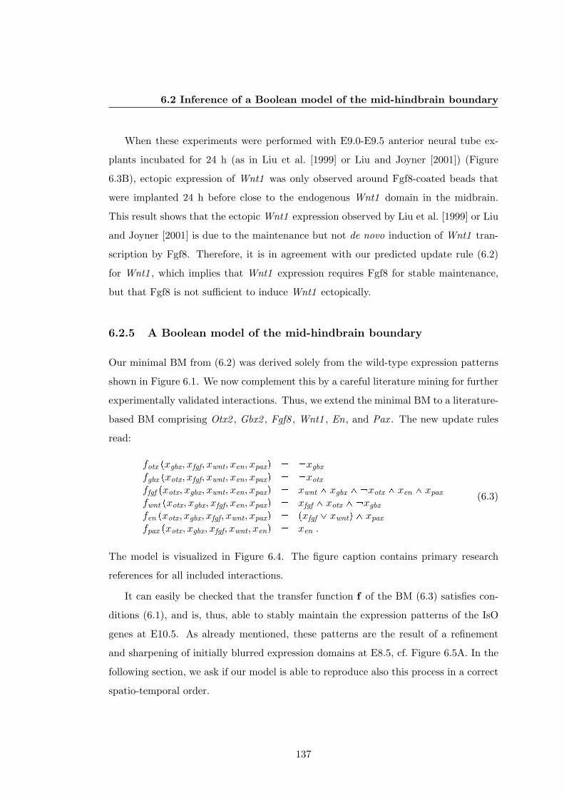
6.2 Inference of a Boolean model of the mid-hindbrain boundary
When these experiments were performed with E9.0-E9.5 anterior neural tube ex-
plants incubated for 24 h (as in Liu et al. [1999] or Liu and Joyner [2001]) (Figure
6.3B), ectopic expression of Wnt1 was only observed around Fgf8-coated beads that
were implanted 24 h before close to the endogenous Wnt1 domain in the midbrain.
This result shows that the ectopic Wnt1 expression observed by Liu et al. [1999] or Liu
and Joyner [2001] is due to the maintenance but not de novo induction of Wnt1 tran-
scription by Fgf8. Therefore, it is in agreement with our predicted update rule (6.2)
for Wnt1 , which implies that Wnt1 expression requires Fgf8 for stable maintenance,
but that Fgf8 is not sufficient to induce Wnt1 ectopically.
6.2.5 A Boolean model of the mid-hindbrain boundary
Our minimal BM from (6.2) was derived solely from the wild-type expression patterns
shown in Figure 6.1. We now complement this by a careful literature mining for further
experimentally validated interactions. Thus, we extend the minimal BM to a literature-
based BM comprising Otx2 , Gbx2 , Fgf8 , Wnt1 , En, and Pax . The new update rules
read:
fotx pxgbx, xfgf, xwnt, xen, xpaxq xgbx
fgbx pxotx, xfgf, xwnt, xen, xpaxq xotx
ffgf pxotx, xgbx, xwnt, xen, xpaxq xwnt ^ xgbx ^ xotx ^ xen ^ xpax
fwnt pxotx, xgbx, xfgf, xen, xpaxq xfgf ^ xotx ^ xgbx
fen pxotx, xgbx, xfgf, xwnt, xpaxq pxfgf _ xwntq ^ xpax
fpax pxotx, xgbx, xfgf, xwnt, xenq xen .
(6.3)
The model is visualized in Figure 6.4. The figure caption contains primary research
references for all included interactions.
It can easily be checked that the transfer function f of the BM (6.3) satisfies con-
ditions (6.1), and is, thus, able to stably maintain the expression patterns of the IsO
genes at E10.5. As already mentioned, these patterns are the result of a refinement
and sharpening of initially blurred expression domains at E8.5, cf. Figure 6.5A. In the
following section, we ask if our model is able to reproduce also this process in a correct
spatio-temporal order.
137
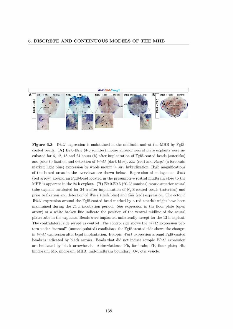
6. DISCRETE AND CONTINUOUS MODELS OF THE MHB
Figure 6.3: Wnt1 expression is maintained in the midbrain and at the MHB by Fgf8-coated beads. (A) E8.0-E8.5 (4-6 somites) mouse anterior neural plate explants were in-cubated for 6, 12, 18 and 24 hours (h) after implantation of Fgf8-coated beads (asterisks)and prior to fixation and detection of Wnt1 (dark blue), Shh (red) and Foxg1 (a forebrainmarker; light blue) expression by whole mount in situ hybridization. High magnificationsof the boxed areas in the overviews are shown below. Repression of endogenous Wnt1(red arrow) around an Fgf8-bead located in the presumptive rostral hindbrain close to theMHB is apparent in the 24 h explant. (B) E9.0-E9.5 (20-25 somites) mouse anterior neuraltube explant incubated for 24 h after implantation of Fgf8-coated beads (asterisks) andprior to fixation and detection of Wnt1 (dark blue) and Shh (red) expression. The ectopicWnt1 expression around the Fgf8-coated bead marked by a red asterisk might have beenmaintained during the 24 h incubation period. Shh expression in the floor plate (openarrow) or a white broken line indicate the position of the ventral midline of the neuralplate/tube in the explants. Beads were implanted unilaterally except for the 12 h explant.The contralateral side served as control. The control side shows the Wnt1 expression pat-tern under “normal” (unmanipulated) conditions, the Fgf8-treated side shows the changesin Wnt1 expression after bead implantation. Ectopic Wnt1 expression around Fgf8-coatedbeads is indicated by black arrows. Beads that did not induce ectopic Wnt1 expressionare indicated by black arrowheads. Abbreviations: Fb, forebrain; FP, floor plate; Hb,hindbrain; Mb, midbrain; MHB, mid-hindbrain boundary; Ov, otic vesicle.
138
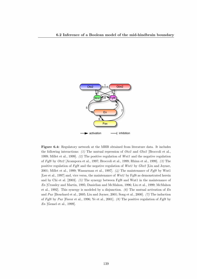
6.2 Inference of a Boolean model of the mid-hindbrain boundary
Otx2 Gbx2
Wnt1 Fgf8
En
Pax
1
2 3
5
4
6
7
8
activation inhibition
Figure 6.4: Regulatory network at the MHB obtained from literature data. It includesthe following interactions: (1) The mutual repression of Otx2 and Gbx2 [Broccoli et al.,1999; Millet et al., 1999]. (2) The positive regulation of Wnt1 and the negative regulationof Fgf8 by Otx2 [Acampora et al., 1997; Broccoli et al., 1999; Rhinn et al., 1999]. (3) Thepositive regulation of Fgf8 and the negative regulation of Wnt1 by Gbx2 [Liu and Joyner,2001; Millet et al., 1999; Wassarman et al., 1997]. (4) The maintenance of Fgf8 by Wnt1[Lee et al., 1997] and, vice versa, the maintenance of Wnt1 by Fgf8 as demonstrated hereinand by Chi et al. [2003]. (5) The synergy between Fgf8 and Wnt1 in the maintenance ofEn [Crossley and Martin, 1995; Danielian and McMahon, 1996; Liu et al., 1999; McMahonet al., 1992]. This synergy is modeled by a disjunction. (6) The mutual activation of Enand Pax [Bouchard et al., 2005; Liu and Joyner, 2001; Song et al., 2000]. (7) The inductionof Fgf8 by Pax [Favor et al., 1996; Ye et al., 2001]. (8) The positive regulation of Fgf8 byEn [Gemel et al., 1999].
139
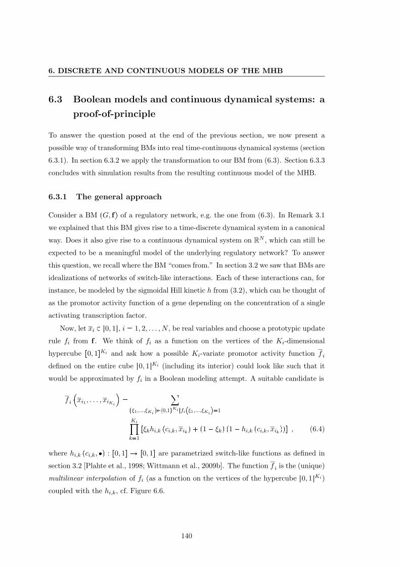
6. DISCRETE AND CONTINUOUS MODELS OF THE MHB
6.3 Boolean models and continuous dynamical systems: a
proof-of-principle
To answer the question posed at the end of the previous section, we now present a
possible way of transforming BMs into real time-continuous dynamical systems (section
6.3.1). In section 6.3.2 we apply the transformation to our BM from (6.3). Section 6.3.3
concludes with simulation results from the resulting continuous model of the MHB.
6.3.1 The general approach
Consider a BM pG, fq of a regulatory network, e.g. the one from (6.3). In Remark 3.1
we explained that this BM gives rise to a time-discrete dynamical system in a canonical
way. Does it also give rise to a continuous dynamical system on RN , which can still be
expected to be a meaningful model of the underlying regulatory network? To answer
this question, we recall where the BM “comes from.” In section 3.2 we saw that BMs are
idealizations of networks of switch-like interactions. Each of these interactions can, for
instance, be modeled by the sigmoidal Hill kinetic h from (3.2), which can be thought of
as the promotor activity function of a gene depending on the concentration of a single
activating transcription factor.
Now, let xi P r0, 1s, i 1, 2, . . . , N , be real variables and choose a prototypic update
rule fi from f . We think of fi as a function on the vertices of the Ki-dimensional
hypercube r0, 1sKi and ask how a possible Ki-variate promotor activity function f i
defined on the entire cube r0, 1sKi (including its interior) could look like such that it
would be approximated by fi in a Boolean modeling attempt. A suitable candidate is
f i
xi1 , . . . , xiKi
¸pξ1,...,ξKiqPt0,1uKi |fipξ1,...,ξKiq1
Ki¹k1
rξkhi,k pci,k, xikq p1 ξkq p1 hi,k pci,k, xikqqs , (6.4)
where hi,k pci,k, q : r0, 1s Ñ r0, 1s are parametrized switch-like functions as defined in
section 3.2 [Plahte et al., 1998; Wittmann et al., 2009b]. The function f i is the (unique)
multilinear interpolation of fi (as a function on the vertices of the hypercube r0, 1sKi)coupled with the hi,k, cf. Figure 6.6.
140
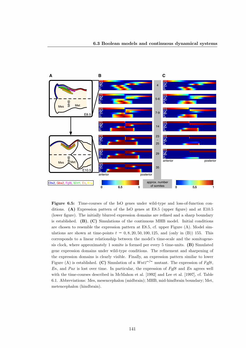
6.3 Boolean models and continuous dynamical systems
Mes MetMHB
E10.5
E8.5
A B C
4
5-6
7-9
14
23-
25
29
approx. number of somites
Otx2, Gbx2, Fgf8, Wnt1, En, Pax
35
anterior
anterior posterior
posterior
Mes MetMHB
Figure 6.5: Time-courses of the IsO genes under wild-type and loss-of-function con-ditions. (A) Expression pattern of the IsO genes at E8.5 (upper figure) and at E10.5(lower figure). The initially blurred expression domains are refined and a sharp boundaryis established. (B), (C) Simulations of the continuous MHB model. Initial conditionsare chosen to resemble the expression pattern at E8.5, cf. upper Figure (A). Model sim-ulations are shown at time-points t 0, 8, 20, 50, 100, 125, and (only in (B)) 155. Thiscorresponds to a linear relationship between the model’s time-scale and the somitogene-sis clock, where approximately 1 somite is formed per every 5 time-units. (B) Simulatedgene expression domains under wild-type conditions. The refinement and sharpening ofthe expression domains is clearly visible. Finally, an expression pattern similar to lowerFigure (A) is established. (C) Simulation of a Wnt1 mutant. The expression of Fgf8 ,En, and Pax is lost over time. In particular, the expression of Fgf8 and En agrees wellwith the time-courses described in McMahon et al. [1992] and Lee et al. [1997], cf. Table6.1. Abbreviations: Mes, mesencephalon (midbrain); MHB, mid-hindbrain boundary; Met,metencephalon (hindbrain).
141
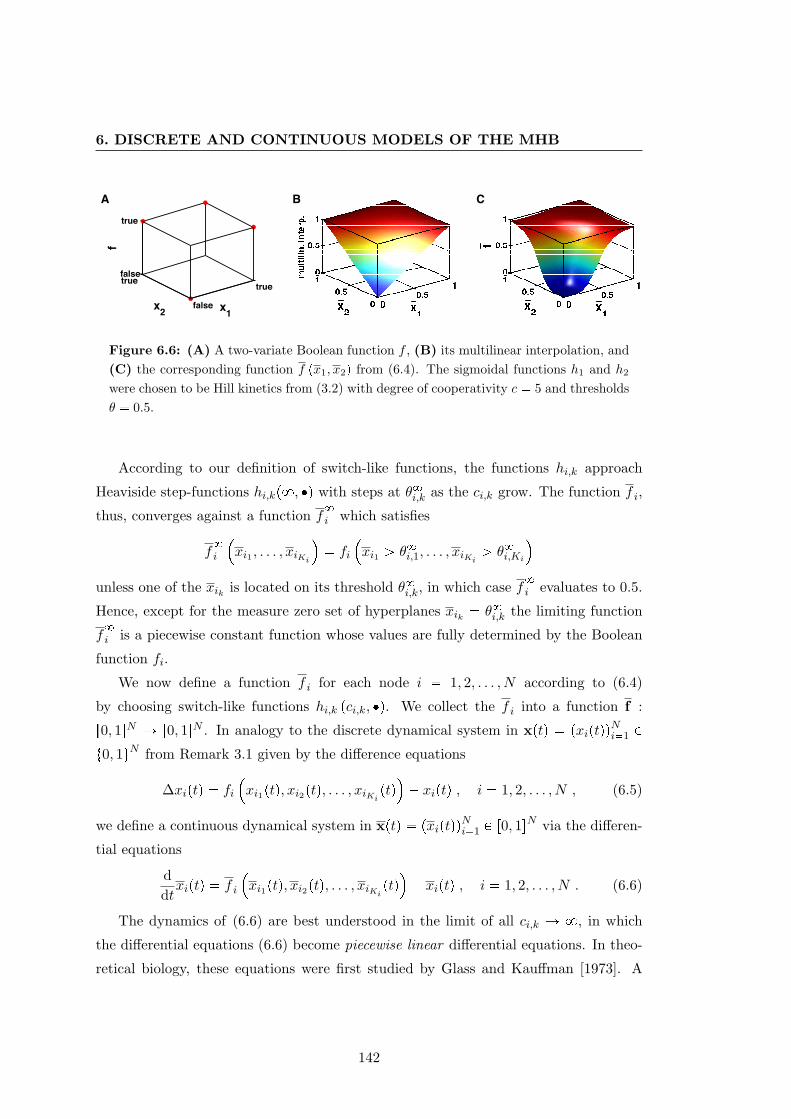
6. DISCRETE AND CONTINUOUS MODELS OF THE MHB
false
truetruefalse
true
x1x2
f
A B C
Figure 6.6: (A) A two-variate Boolean function f , (B) its multilinear interpolation, and(C) the corresponding function f px1, x2q from (6.4). The sigmoidal functions h1 and h2
were chosen to be Hill kinetics from (3.2) with degree of cooperativity c 5 and thresholdsθ 0.5.
According to our definition of switch-like functions, the functions hi,k approach
Heaviside step-functions hi,kp8, q with steps at θ8i,k as the ci,k grow. The function f i,
thus, converges against a function f8i which satisfies
f8i
xi1 , . . . , xiKi
fi
xi1 ¡ θ8i,1, . . . , xiKi ¡ θ8i,Ki
unless one of the xik is located on its threshold θ8i,k, in which case f8i evaluates to 0.5.
Hence, except for the measure zero set of hyperplanes xik θ8i,k the limiting function
f8i is a piecewise constant function whose values are fully determined by the Boolean
function fi.
We now define a function f i for each node i 1, 2, . . . , N according to (6.4)
by choosing switch-like functions hi,k pci,k, q. We collect the f i into a function f :
r0, 1sN Ñ r0, 1sN . In analogy to the discrete dynamical system in xptq pxiptqqNi1 Pt0, 1uN from Remark 3.1 given by the difference equations
∆xiptq fi
xi1ptq, xi2ptq, . . . , xiKi ptq
xiptq , i 1, 2, . . . , N , (6.5)
we define a continuous dynamical system in xptq pxiptqqNi1 P r0, 1sN via the differen-
tial equations
ddtxiptq f i
xi1ptq, xi2ptq, . . . , xiKi ptq
xiptq , i 1, 2, . . . , N . (6.6)
The dynamics of (6.6) are best understood in the limit of all ci,k Ñ 8, in which
the differential equations (6.6) become piecewise linear differential equations. In theo-
retical biology, these equations were first studied by Glass and Kauffman [1973]. A
142
6.3 Boolean models and continuous dynamical systems
mathematically rigorous treatment within the framework of differential inclusions can
be found in de Jong et al. [2004]. Fixed points of systems of piecewise linear differential
equations were investigated by El Snoussi and Thomas [1993] as well as by Mestl et al.
[1995]. In general, there are two classes of fixed points: regular fixed (steady) points
(RSP) and singular fixed (steady) points (SSP). In a SSP at least one variable xi lies
on a threshold, whereas in RSPs all variables are located beside their thresholds. RSPs
are always (asymptotically) stable and in 1-1-relation with fixed points of system (6.5).
SSPs may but need not be stable. They do not correspond to fixed points of system
(6.5). An algorithmic approach to detecting RSPs and SSPs in systems of piecewise
linear differential equations has been presented in de Jong and Page [2008].
Generalizations of the above results to the case of sufficiently large but finite ci,k
via the implicit function theorem exist. With respect to RSPs, the following statement
was proven in Wittmann et al. [2009b].
Proposition 6.1. Consider the two dynamical systems from (6.5) and (6.6), and sup-pose the switch-like functions hi,k pci,k, q in the f i from (6.4) are given by Hill kineticsfrom (3.2). Let xpfq P t0, 1uN be a fixed point of (6.5). Then, for sufficiently largeci,k there exists an asymptotically stable fixed point xpfq pci,kq P r0, 1sN of (6.6) in aneighborhood of xpfq and
limmin ci,kÑ8
xpfq pci,kq xpfq .
The case of SSPs is more involved and taken care of in Plahte et al. [1998]. In
general, it is difficult to give explicit lower bounds for the ci,k, such that the approx-
imation of sigmoidal functions by step-functions is valid from a dynamical point of
view. Even more critical is, of course, the transition from the time-discrete system
(6.5) to the time-continuous system (6.6). To see this, it suffices to recall the intricate
dynamical behavior of the (discrete time) logistic equation from section 2.2.4.1, and to
consider that according to the Poincare-Bendixson theorem, see e.g. Guckenheimer and
Holmes [1990], any one-dimensional continuous dynamical system has either stationary
or periodic behavior. Nonetheless, small-scale [Omholt et al., 1998] as well as large-
scale [Wittmann et al., 2009b] examples exhibit evidence that biologically meaningful,
continuous models may arise from the above modeling approach. In the following, we
provide further such evidence.
143
6. DISCRETE AND CONTINUOUS MODELS OF THE MHB
6.3.2 A continuous model of the mid-hindbrain boundary
In this section, we derive a continuous dynamical system from the BM in (6.3). The
model’s variables xipj, tq, i otx, gbx, fgf,wnt, en, pax, depend on time and the now
continuous spatial variable j P r0, 1s, which is to say we model the neural tube as a
one-dimensional interval.
With Otx2 , Gbx2 , En, and Pax we do not differentiate between mRNA and protein.
In the case of Fgf8 and Wnt1 , however, we need to introduce two additional variables
x extfgf pj, tq and x ext
wntpj, tq in order to account for the diffusion of secreted Fgf8 and Wnt1
protein. They are governed by the reaction-diffusion equations
BBtx
exti pj, tq αixipj, tq βix ext
i pj, tq γi B2
Bj2x exti pj, tq , i fgf,wnt , (6.7)
with translation rates αi, degradation rates βi, and diffusion rates γi, i fgf,wnt. In
here, we use the parameter values from Wittmann et al. [2009a] and Ansorg et al.
[2010], αi γi 1 and βi 0.8.
For i otx, gbx, fgf,wnt, en, pax, we define functions f i according to (6.4) choosing
all hi,k equal to a Hill kinetic from (3.2) with degree of cooperativity c 5 and threshold
θ 0.1. The equations
BBtxotxpj, tq fotx
xgbxpj, tq, x ext
fgf pj, tq, x extwntpj, tq, xenpj, tq, xpaxpj, tq
xotxpj, tq
BBtxgbxpj, tq fgbx
xotxpj, tq, x ext
fgf pj, tq, x extwntpj, tq, xenpj, tq, xpaxpj, tq
xgbxpj, tq
BBtxfgfpj, tq f fgf
xotxpj, tq, xgbxpj, tq, x ext
wntpj, tq, xenpj, tq, xpaxpj, tq xfgfpj, tq
BBtxwntpj, tq fwnt
xotxpj, tq, xgbxpj, tq, x ext
fgf pj, tq, xenpj, tq, xpaxpj, tq xwntpj, tq
BBtxenpj, tq fen
xotxpj, tq, xgbxpj, tq, x ext
fgf pj, tq, x extwntpj, tq, xpaxpj, tq
xenpj, tq
BBtxpaxpj, tq fpax
xotxpj, tq, xgbxpj, tq, x ext
fgf pj, tq, x extwntpj, tq, xenpj, tq
xpaxpj, tq
(6.8)
then describe the regulatory network at the MHB at a single spatial position j P r0, 1s.Equations (6.7) together with (6.8) constitute a system of partial (PDE) and ordinary
(ODE) differential equations.
In the following simulations, initial conditions at t 0 are chosen to mimic the fuzzy
expression patterns at E8.5, cf. upper Figure 6.5A. They are obtained by specifying
144
6.3 Boolean models and continuous dynamical systems
the boundaries as well as the maximum of the expression profile of each gene and
interpolating these points by cubic splines. In detail, the points are:
Otx2 : xotxp0, 0q 1, xotxp0.5, 0q 0, xotxp1, 0q 0
Gbx2 : xgbxp0, 0q 0, xgbxp0.5, 0q 0, xgbxp1, 0q 1
Fgf8 : xfgfp0, 0q 0, xfgfp0.45, 0q 0, xfgfp0.625, 0q 1, xfgfp0.8, 0q 0, xfgfp1, 0q 0
Fgf8: x extfgf p0, 0q 0, x ext
fgf p0.45, 0q 0, x extfgf p0.625, 0q 1, x ext
fgf p0.8, 0q 0, x extfgf p1, 0q 0
Wnt1 : xwntp0, 0q 0, xwntp0.2, 0q 0, xwntp0.375, 0q 1, xwntp0.55, 0q 0, xwntp1, 0q 0
Wnt1: x extwntp0, 0q 0, x ext
wntp0.2, 0q 0, x extwntp0.375, 0q 1, x ext
wntp0.55, 0q 0, x extwntp1, 0q 0
En: xenp0, 0q 0, xenp0.25, 0q 0, xenp0.425, 0q 1, xenp0.6, 0q 0, xenp1, 0q 0
Pax : xpaxp0, 0q 0, xpaxp0.3, 0q 0, xpaxp0.475, 0q 1, xpaxp0.65, 0q 0, xpaxp1, 0q 0
For the simulation of a Wnt1 mutant, the above initial conditions are used, but
the initial values xwntpj, 0q and x extwntpj, 0q, j P r0, 1s, are set to zero. Also the promotor
activity function fwnt and the translation rate αwnt of Wnt1-protein are set to zero.
For the reaction-diffusion equations (6.7) homogenous Dirichlet boundary conditions
are chosen. In the following, we simply refer to this initial value boundary problem as
“continuous MHB model.”
6.3.3 Numeric solution
Let us conclude by showing simulations of the continuous MHB model. Equations (6.7)
together with (6.8) constitute a system of ODEs and PDEs. For the numeric integration
of this system we used the MATLAB solver pdepe, which implements the method of
lines, see e.g. Schiesser and Griffiths [2009]. In general, the method of lines reduces a
system of PDEs to a (much larger) system of ODEs, which is then solved using standard
ODE solvers. In our case, this standard solver was the stiff MATLAB solver ode15s.
On a one-dimensional interval I, the method of lines uses spatial difference operators
to approximate the spatial differential operators at grid points jq P I. For this spatial
discretization of Equations (6.7) we did not use an equidistant grid but one that is
condensed around j 0.5 (MHB) in order to account for arising discontinuities in the
limit of large times. For each grid point jq and each variable we obtained an ODE (in
145
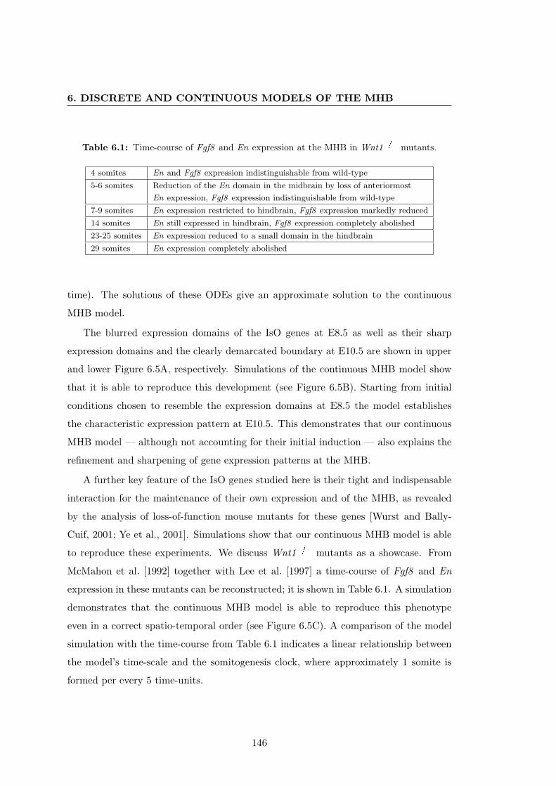
6. DISCRETE AND CONTINUOUS MODELS OF THE MHB
Table 6.1: Time-course of Fgf8 and En expression at the MHB in Wnt1 mutants.
4 somites En and Fgf8 expression indistinguishable from wild-type
5-6 somites Reduction of the En domain in the midbrain by loss of anteriormost
En expression, Fgf8 expression indistinguishable from wild-type
7-9 somites En expression restricted to hindbrain, Fgf8 expression markedly reduced
14 somites En still expressed in hindbrain, Fgf8 expression completely abolished
23-25 somites En expression reduced to a small domain in the hindbrain
29 somites En expression completely abolished
time). The solutions of these ODEs give an approximate solution to the continuous
MHB model.
The blurred expression domains of the IsO genes at E8.5 as well as their sharp
expression domains and the clearly demarcated boundary at E10.5 are shown in upper
and lower Figure 6.5A, respectively. Simulations of the continuous MHB model show
that it is able to reproduce this development (see Figure 6.5B). Starting from initial
conditions chosen to resemble the expression domains at E8.5 the model establishes
the characteristic expression pattern at E10.5. This demonstrates that our continuous
MHB model — although not accounting for their initial induction — also explains the
refinement and sharpening of gene expression patterns at the MHB.
A further key feature of the IsO genes studied here is their tight and indispensable
interaction for the maintenance of their own expression and of the MHB, as revealed
by the analysis of loss-of-function mouse mutants for these genes [Wurst and Bally-
Cuif, 2001; Ye et al., 2001]. Simulations show that our continuous MHB model is able
to reproduce these experiments. We discuss Wnt1 mutants as a showcase. From
McMahon et al. [1992] together with Lee et al. [1997] a time-course of Fgf8 and En
expression in these mutants can be reconstructed; it is shown in Table 6.1. A simulation
demonstrates that the continuous MHB model is able to reproduce this phenotype
even in a correct spatio-temporal order (see Figure 6.5C). A comparison of the model
simulation with the time-course from Table 6.1 indicates a linear relationship between
the model’s time-scale and the somitogenesis clock, where approximately 1 somite is
formed per every 5 time-units.
146
6.4 Discussion
6.4 Discussion
We demonstrated that similar to temporal expression patterns, also spatial expression
patterns can be used to gain information about the structure of regulatory networks.
In particular, we showed that the characteristic expression patterns of key IsO genes
reveal a maintaining effect of Fgf8 on Wnt1 expression — a prediction we also validated
experimentally. The presented method allows to harness qualitative experimental re-
sults like snapshots of expression patterns for model construction in systems biology.
This is exemplified by our BM of gene regulation at the MHB.
Gene regulation is a highly non-linear process due to the cooperative binding ex-
hibited by many macromolecules such as DNA. Here, cooperativity means that the
macromolecule’s affinity for its ligand changes with the amount of ligand already bound.
Mathematically, gene regulatory networks can, therefore, be thought of as complex sys-
tems with switch-like interactions. Below a certain threshold a regulator has no or little
influence on its target, while above this threshold the effect of the regulator on its tar-
get saturates rapidly to a constant level. BMs and the dynamical system from Remark
3.1 idealize this “switching behavior” and completely ignore the transition between the
“low influence” and “saturated influence” states. This may be a severe simplification,
but has the advantage that no information about regulatory mechanisms and kinetic
parameters is needed.
If, in addition to a BM, this information is provided, a continuous dynamical system
of switch-like interactions, such as (6.6) with activation functions f i from (6.4), can be
set up. The dynamic behavior of this system, of course, greatly depends on the precise
nature of the additional mechanistic and kinetic information. For this reason, general
mathematical results about the relation between the discrete and possible continuous
dynamical systems based on the same BM are hard to obtain. They are, however,
available in the limit where switch-like interactions become Heaviside step-functions
and the continuous system becomes a system of piecewise linear differential equations.
The dynamics of these systems can be characterized in terms of the underlying BM
once the switching thresholds are fixed [de Jong et al., 2004].
Systems of piecewise linear differential equations are still simplistic idealizations
of gene regulatory mechanisms, and one would wish for systems incorporating realistic
147

6. DISCRETE AND CONTINUOUS MODELS OF THE MHB
kinetics such as the Hill kinetic from (3.2). We used our BM of the MHB for a proof-of-
principle, that — given these realistic kinetics — one may, indeed, obtain a meaningful
continuous dynamical system from a BM, whose explanatory power is increased as
compared to the discrete dynamical system from Remark 3.1. Taken together, the
simulations of our continuous MHB model show that it captures certain salient features
of mid-hindbrain differentiation that could not have been analyzed with a BM alone.
148
7
Conclusions and Outlook
Now this is not the end.
It is not even the beginning of the end.
But it is, perhaps, the end of the beginning.
Winston Churchill
Arguably, there are two avenues of research in mathematical modeling of biological
systems, and in both Boolean models are frequently used. The first focuses on small-
and medium-scale models of specific biological processes. Such models are used to
analyze these processes, with the main goal of obtaining new biological insights. The
second direction is the study of generic properties, especially in the context of regulatory
networks. Kauffman’s contributions fall into this category. Predominantly done by
physicists, works in this direction often study mean-field quantities and properties of
ensembles of large-scale models.
149
7. CONCLUSIONS AND OUTLOOK
7.1 Boolean modeling in systems biology
The first line of research has gained particular importance in the newly emerging field
of systems biology. In systems biology, experimentalists and theoreticians make a
concerted effort to unravel the functionality of complex biological systems in a holistic
fashion [Kitano, 2002]. Especially in the context of gene regulation, Boolean models are
frequently employed by the theoreticians involved in a systems biology project [Saez-
Rodriguez et al., 2007, 2009; Samaga et al., 2009; Schlatter et al., 2009; Wittmann
et al., 2009a].
In this thesis, we discussed one such project. We presented a method to glean
information about genetic interactions from spatial gene expression profiles. The key
idea is to use available data to partially define the update rules of a Boolean model, and
to extend them under regularization constraints. In here, this constraint was minimality
of the resulting Boolean expressions. Using this method, we set up a Boolean model of
the gene regulatory network at the mid-hindbrain boundary. Along the way, a newly
predicted genetic interaction was experimentally validated.
7.1.1 Possible extensions of the model of the mid-hindbrain boundary
From a biological point of view, our model of the mid-hindbrain boundary can be
extended in several ways. Further investigations of the two key patterning molecules
Fgf8 and Wnt1, for instance, will require inclusion of known modulators of the Fgf8
signaling pathway such as the Fgf inhibitors Sprouty [Chambers et al., 2000; Minowada
et al., 1999], Sef [Furthauer et al., 2002] or Mkp3 [Echevarria et al., 2005; Li et al., 2007].
In the present model these regulators at the signal transduction level are not considered.
Being widely coexpressed with Fgf8 , they are assumed to fine-tune Fgf8 expression
itself and the expression of Fgf8 target genes by negative feedback modulations. This
exquisite regulation of Fgf8 agrees well with results demonstrating a concentration-
dependent effect of Fgf8 signaling [Liu et al., 1999; Sato et al., 2001]. Inclusion of
these fine-tuning mechanisms will, therefore, require a detailed kinetic model of Fgf8
signaling at the mid-hindbrain boundary. To this end, existing kinetic models of the
Fgf pathway, e.g. the one by Yamada et al. [2004], could be adapted.
Fgf8 and Wnt1 , however, are not the only important regulators of mid-hindbrain
development. Further crucial genes, that we are considering for inclusion in our model,
150
7.2 Random Boolean models
are Lmx1b [Guo et al., 2007, 2008; Matsunaga et al., 2002] and Grg4 [Puelles et al.,
2004; Sugiyama et al., 2000]. They are of particular importance for possible extensions
of our model which aim at including related processes, such as the specification of cell
populations in the patterning field. The mid-hindbrain boundary not only controls
patterning of the mid- and rostral hindbrain, but also controls the location and size of
several neuronal populations [Brodski et al., 2003]. One could envision hybrid-models
integrating pattern formation and spatial differentiation with fate decisions of single
cells.
At some point, we will also have to abandon our simplifying assumptions with
respect to En1 and En2 as well as Pax2 and Pax5 , and consider a more refined picture
of Engrailed and Pax expression patterns and interactions. Such extensions will be
particularly interesting in spatially higher-dimensional models that take into account
the dorsal-ventral patterning of the neural plate/tube as well. A critical issue in these
higher-dimensional models is the topological alteration at around E9.0 when the neural
plate becomes the neural tube, as for non-symmetric initial conditions discontinuities
arise at the junction where the two edges of the neural plate fuse together. We are
planning on modeling this situation as a free moving boundary problem.
7.1.2 Inverse problems under sparsity constraints
From a theoretical point of view, predicting genetic interactions by solving inverse
problems under sparsity constraints seems a promising and interesting idea that merits
further research efforts. Especially for larger numbers of genes, however, additional
constraints might be beneficial. One could, for example, look for minimal canalyzing
update rules or minimal update rules generated by one of the generic logics. This will
require adaption of either the Quine-McCluskey algorithm or of one of the heuristic
minimizers. As always, the lack of suitable testing data sets is an issue, and probably
one will have to resort to synthetic toy data for performance evaluations.
7.2 Random Boolean models
As mentioned above, a major contribution to the second line of research is the work by
Stuart Kauffman. In his seminal paper, Kauffman [1969] proposes large-scale random
Boolean models — in here, we called them Kauffman networks — as generic models
151
7. CONCLUSIONS AND OUTLOOK
of gene regulatory networks. Kauffman [1993] hypothesized that regulatory networks
in evolvable, living organisms can only operate in a frozen regime but close to (at the
edge of) a chaotic regime.
We began by defining a general class of Kauffman networks. In particular, we
relaxed the binary Boolean classification and considered general discrete, finite sets.
The cardinalities of these sets followed a general distribution, as did the in-degrees
and the entries of the update rules. We investigated these Kauffman networks with
respect to critical phenomena. Our results are a generalization of the well-known case
of random Boolean models as introduced by Kauffman. We could also generalize the
finding by Bastolla and Parisi [1996] that any Kauffman network can be kept in its
frozen regime by sufficiently biasing the update rules.
We then introduced the concept of generic logics, which allows to build Boolean
models from networks of signed interactions by logically linking the activating and
inhibiting regulators of a node according to a specific pattern. The class of Kauffman
networks whose realizations are obtained using generic logics was studied. We, first,
analyzed the truth-content of these networks, which is a mean-field approximation of the
fraction of ones. Analytic and numeric investigations showed that this quantity exhibits
a rich dynamical behavior including period-doublings leading to chaos. In a next step,
we found that, surprisingly, Kauffman networks with generic logics possess multiple,
intricately shaped critical boundaries. In particular, for a biologically plausible generic
logic the region of biologically reasonable network parameters is enclosed by a critical
boundary. Hence, these parameters need not even be particularly fine-tuned in order
for the network to be near criticality but may vary over quite some range. This finding
fits in nicely with Kauffman’s hypothesis.
7.2.1 Structure matters
Update rules in the original Kauffman network are random functions without any struc-
tural properties, such as monotonicity or canalyzing inputs. The same is true for the
update rules of the multistate Kauffman networks studied herein. The regulators of a
gene, however, exert their regulatory influences by mechanistic processes, such as the
binding of transcription factors to promotor regions of the DNA, and these mechanistic
processes should give the activation function of a gene certain structural properties. A
simple abstraction hereof are qualitative models, in which biochemical mechanisms are
152
7.2 Random Boolean models
reflected in the classification of interactions as either activating or inhibiting. We in-
vestigated Kauffman networks with structured update rules that are derived from such
qualitative models. Our results show that this additional structure greatly influences
the dynamics of these networks.
The reader might find it interesting to compare this discussion to Balleza et al.
[2008]. In this study, Boolean dynamics are implemented on the gene regulatory net-
works of S. cerevisiae, E. coli, and B. subtilis. The update rules are constructed as
(unstructured) random functions evaluating to 1 with a probability equal to the av-
erage fraction of expressed genes in hundreds of microarray experiments. While such
approaches certainly increase the biological plausibility and relevance of Kauffman net-
works as models of gene regulation, it might still be necessary to also take into account
structural information, e.g. about activating and inhibiting regulatory interactions.
7.2.2 Topology and dynamics
Another issue is that topological properties, such as degree distributions, also play a
pivotal role in the study of complex networks. For this reason, it is somewhat unsat-
isfactory that in standard Kauffman networks this degree distribution is taken to be a
simple delta distribution. In this thesis, we studied Kauffman networks with (unstruc-
tured update rules and) general degree distributions on finite supports similar to Fox
and Hill [2001] or Aldana [2003]. In agreement with these studies, we found, however,
that the phase transition of such Kauffman networks completely ignores all topological
properties but the mean connectivity.
We have first results demonstrating that this is not the case with Kauffman networks
generated by generic logics. If we base these Kauffman networks on an Erdos-Renyi
graph from Example 2.1, for instance, their in-degrees are Poisson distributed, cf. sec-
tion 2.1. We could already show that also in this case the truth-content is governed
by an iteration function with negative Schwarzian derivative. This awakens hopes that
we will be able to treat this case similarly to our proceeding inhere. In preliminary nu-
meric analyses the truth-content, indeed, appears to possess a unique attractor. These
analyses, however, also reveal that the critical boundaries in the case of an Erdos-Renyi
graph differ qualitatively from the ones shown in Figure 5.4.
A comprehensive discussion of Kauffman networks with generic logics on different
topologies is an interesting subject for future work. On the one hand, it would, of course,
153

7. CONCLUSIONS AND OUTLOOK
be intriguing to use real-world networks, such as the transcriptional gene regulatory
networks from E. coli or yeast [Keseler et al., 2008; Lee et al., 2002]. On the other
hand, for more systematic analyses, lattices and random graphs, such as the Erdos-
Renyi graph from Example 2.1, small-world networks generated according to Watts and
Strogatz [1998], or scale-free networks obtained via preferential attachment [Barabasi
and Albert, 1999], might be better suited.
7.2.3 The state-space of Kauffman networks with generic logics
Furthermore, the structure of the Boolean state-space of Kauffman networks with
generic logics needs to be analyzed in detail. Similarly to Samuelsson and Troein
[2003], one could attempt to compute the average number and length of attractors in
these networks. For truth-stable networks, it will be particularly interesting to see how
the lengths of attractors (in the Boolean state-space) are related to the length of the
attractor of the truth-content. Intuitively, one would expect the former to be multiples
of the latter.
154
Index
activation bias, 86
algorithm
Espresso, 133
Quine-McCluskey, 133
allosteric regulation, 41
Aristotelian laws of thought, 29
attractor, 15
global, 20
metric, 20
basin of attraction, 20
bifurcation, 22
period-doubling, 22
pitchfork, 22
bifurcation diagram, 22, 118–121
Boolean algebra, 28
laws from, 29
Boolean minimization, 133
Boolean satisfiability problem, 133
chaos
formal definition, 26
living at the edge of, 47
on-set of, 22
period-doubling route to, 22
clause
conjunctive, 30
disjunctive, 30
complement, 28
configuration model, 12
conjugate, 17
conjunction, 28
connectivity, 10
critical, 45
mean, 54
cooperativity, 41
negative, 41
positive, 41
degree, 10
in-, 10
out-, 10
degree distribution, 11
of a random graph, 11
differential equation, 15
piecewise linear, 142
reaction-diffusion, 144
differentiation
stem cell, 33
T helper cell, 82
disjunction, 28
DNA, 31
methylation of, 34
don’t cares, 133
dynamical system, 13
linear discrete, 16
continuous, 15
discrete, 16
non-linear discrete, 17
standardized qualitative, 82
edge, 10
incident, 10
ensemble, 67
epigenetic modification, 34
equilibrium, 13
Feigenbaum constant, 22
Fgf8-coated bead, 129, 136
flow, 13
forebrain, 35
function
155
INDEX
Boolean, 30
canalyzing Boolean, 30
evolution, 13
Heaviside step-, 42
monotonous Boolean, 30
S-unimodal, 25
switch-like, 42
transfer, 40, 51
update, 40, 51
gene, 31
expression, 33
protein-coding, 33
regulatory network, 34
gene regulation
post-transcriptional, 34
transcriptional, 34
generic logic, 84
genetic code, 33
graph, 10
Erdos-Renyi, 11
order of a, 10
random, 11
signed, 11
size of a, 10
Hamming distance
as a metric, 40, 52
as an order parameter, 45, 56, 107
heterogeneity, 54
Hill kinetic, 41
hindbrain, 35
Human Genome Project, 1
immune system, 33
input, 10
activating, 83
canalyzing, 30
inhibiting, 83
inverse problem, 131
isthmic organizer, 35
Karnaugh-Veitch map, 31, 133
Kauffman network, 43
bit-stable, 106
multistate, 53
standard, 43
truth-content of a, 87
truth-stable, 106
with generic logic, 86
with magnetization bias, 43
liar’s paradox, 49
literal, 30
logistic equation, 22
Lyapunov exponent, 21
magnetization bias, 43
manifold
stable, 18
unstable, 18
MATLAB, 145
ode15s, 145
ODEfy, 7, 82
pdepe, 145
measure
invariant, 20
natural, 20
method of lines, 145
mid-hindbrain boundary, 35
midbrain, 35
model
Boolean, 40
generative, 11
multistate, 51
qualitative, 83
multilinear interpolation, 140
negation, 28
neighbor, 10
neural plate, 35
neural tube, 35
node, 10
end-, 10
adjacent, 10
deterministic, 69
normal form
conjunctive, 31
disjunctive, 31
full disjunctive, 31
orbit, 13
156
INDEX
period of, 14
periodic, 13
order parameter, 44
phase, 44, 58, 109
chaotic, 45, 58
critical, 45, 58
frozen, 45, 58
ordered, 45, 58
phase transition, 44
in KNsGL, 109
in MKNs, 59
phosphorylation, 33
plate
alar, 35
basal, 35
floor, 35
roof, 35
point
α-limit, 15
ω-limit, 15
critical fixed, 18
fixed, 13
non-degenerate critical, 25
periodic, 14
quadratic critical, 25
regular fixed, 143
singular fixed, 143
predecessor, 10
prediction, 127
promotor, 34
propositional variable, 30
protein-complex, 33
protein-protein-interaction, 34
regime, 45, 58, 109
reverse engineering, 82
ribosom, 33
RNA
messenger, 33
micro, 33
non-coding, 33
polymerase, 33
ribosomal, 33
transcript, 33
transfer, 33
Schwarzian derivative, 24
secondary organizer, 35
self-referential, 49
sensitive dependence, 27
set
attracting, 15
globally attracting, 20
invariant, 13
negative invariant, 14
of α-limit points, 15
of ω-limit points, 15
positive invariant, 14
repelling, 15
signaling center, 35
signature, 11
inverted, 11
spinal cord, 35
stability
asymptotical, 14
criteria for, 16
in the sense of Lyapunov, 14
neutral, 14
orbital, 14
state-space, 13
stem cell
adult, 33
embryonic, 33
subspace
center, 17
stable, 17
unstable, 17
successor, 10
systems biology, 127
loop, 127
target, 10
theorem
about stable and unstable manifolds, 18
Cook-Levine, 133
Hartman-Grobman, 17
Singer, 24
thermodynamic limit, 12
trajectory, 13
157

INDEX
of a BM, 40
of a MM, 52
transcription, 33
factor, 34
translation, 33
truth-table, 31
update rule, 40, 51
biased, 61
threshold, 82
unbiased, 60
158
References
D. Acampora, V. Avantaggiato, F. Tuorto, and A. Sime-
one. Genetic control of brain morphogenesis through
Otx gene dosage requirement. Development, 124(18):3639–
3650, 1997. 36, 139
K. A. Adams, J. M. Maida, J. A. Golden, and R. D. Riddle.
The transcription factor Lmx1b maintains Wnt1 expres-
sion within the isthmic organizer. Development, 127(9):
1857–1867, 2000. 128
R. Albert and A. Barabasi. Statistical mechanics of complex
networks. Rev Mod Phys, 74(1):47–97, 2002. 9, 113
M. Aldana. Boolean dynamics of networks with scale-free
topology. Physica D, 185(1):45–66, 2003. 43, 153
M. Aldana, S. Coppersmith, and L. P. Kadanoff. Boolean dy-
namics with random couplings. In Perspectives and Prob-
lems in Nonlinear Science: A Celebratory Volume in Honor
of Lawrence Sirovich, pages 23–89. Springer Verlag, 2003.
45
U. Alon. An Introduction to Systems Biology: Design Principles
of Biological Circuits. CRC Press, 2006. 114
M. Ansorg, F. Blochl, W. zu Castell, F. J. Theis, and D. M.
Wittmann. Gene regulation at the mid-hindbrain bound-
ary: Study of a mathematical model in the stationary
limit. International Journal of Biomathematics and Bio-
statistics, in press, 2010. 7, 144
A. Avila, M. Lyubich, and W. De Melo. Regular or stochas-
tic dynamics in real analytic families of unimodal maps.
Invent Math, 154(3):451–550, 2003. 28
F. Ballesteros and B. Luque. Order-disorder phase transition
in random-walk networks. Phys Rev E, 71(3):31104, 2005.
77
E. Balleza, E. R. Alvarez-Buylla, A. Chaos, S. A. Kauffman,
I. Shmulevich, and M. Aldana. Critical dynamics in ge-
netic regulatory networks: examples from four kingdoms.
PLoS One, 3(6):e2456, 2008. 47, 80, 153
L. Bally-Cuif and M. Wassef. Ectopic induction and reor-
ganization of Wnt-1 expression in quail/chick chimeras.
Development, 120(12):3379–3394, 1994. 129
A. Barabasi and R. Albert. Emergence of scaling in random
networks. Science, 286(5439):509–512, 1999. 154
U. Bastolla and G. Parisi. Closing probabilities in the Kauff-
man model: an annealed computation. Physica D, 98(1):
1–25, 1996. 43, 62, 64, 152
A. M. Blokh and M. Y. Lyubich. Measurable dynamics of
S-unimodal maps of the interval. In Annales scientifiques
de l’Ecole normale superieure, volume 24, pages 545–573.
Elsevier, 1991. 26
B. Bollobas. Modern graph theory. Springer Verlag, 1998. 10
G. Boole. An investigation of the laws of thought: on which are
founded the mathematical theories of logic and probabilities.
Walton and Maberly, 1854. 28
M. Bouchard, P. Pfeffer, and M. Busslinger. Functional equiv-
alence of the transcription factors Pax2 and Pax5 in mouse
development. Development, 127(17):3703–3713, 2000. 37
M. Bouchard, D. Grote, S. E. Craven, Q. Sun, P. Steinlein,
and M. Busslinger. Identification of Pax2-regulated genes
by expression profiling of the mid-hindbrain organizer re-
gion. Development, 132(11):2633–2643, 2005. 136, 139
R. Brayton. Logic minimization algorithms for VLSI synthesis.
Springer Verlag, 1984. 133
C. Breindl, S. Waldherr, D. M. Wittmann, F. J. Theis, and
F. Allgower. Steady state robustness of qualitative gene
regulation networks. Int J Robust Nonlinear Control, under
review, 2010. 7
V. Broccoli, E. Boncinelli, and W. Wurst. The caudal limit of
Otx2 expression positions the isthmic organizer. Nature,
401(6749):164–168, 1999. 36, 139
C. Brodski, D. Weisenhorn, M. Signore, I. Sillaber, M. Oester-
held, V. Broccoli, D. Acampora, A. Simeone, and
W. Wurst. Location and size of dopaminergic and sero-
tonergic cell populations are controlled by the position
of the midbrain-hindbrain organizer. J Neurosci, 23(10):
4199–4207, 2003. 151
S. Bulashevska and R. Eils. Inferring genetic regulatory logic
from expression data. Bioinformatics, 21(11):2706–2713,
2005. 82
D. Chambers, A. Medhurst, F. Walsh, J. Price, and I. Ma-
son. Differential Display of Genes Expressed at the
Midbrain–Hindbrain Junction Identifies sprouty2: An
FGF8-Inducible Member of a Family of Intracellular FGF
Antagonists. Mol Cell Neurosci, 15(1):22–35, 2000. 150
M. Chavez, R. Albert, and E. Sontag. Robustness and fragility
of boolean models for genetic regulatory networks. J Theor
Biol, 235(3):431–449, 2005. 40
C. Chi, S. Martinez, W. Wurst, and G. Martin. The isthmic
organizer signal FGF8 is required for cell survival in the
prospective midbrain and cerebellum. Development, 130
(12):2633–2644, 2003. 36, 139
E. Coddington and N. Levinson. Theory of ordinary differen-
tial equations. Tata McGraw-Hill, 1972. 16
P. Collet and J. P. Eckman. Iterated maps on the interval as
dynamical systems. Birkhauser, 1980. 19, 21
S. Cook. The complexity of theorem-proving procedures. In
Proceedings of the third annual ACM symposium on Theory
of computing, pages 151–158. ACM New York, NY, USA,
1971. 133
159
REFERENCES
P. Crossley and G. Martin. The mouse Fgf8 gene encodes a
family of polypeptides and is expressed in regions that di-
rect outgrowth and patterning in the developing embryo.
Development, 121(2):439–451, 1995. 129, 139
P. Danielian and A. McMahon. Engrailed-1 as a target of the
Wnt-1 signalling pathway in vertebrate midbrain develop-
ment. Nature, 383(6598):332–334, 1996. 37, 139
C. A. Davis, S. E. Noble-Topham, J. Rossant, and A. L.
Joyner. Expression of the homeo box-containing gene en-2
delineates a specific region of the developing mouse brain.
Genes Dev, 2(3):361–371, 1988. 36
H. de Jong and M. Page. Search for Steady States of
Piecewise-Linear Differential Equation Models of Genetic
Regulatory Networks. IEEE/ACM Trans Comput Biol
Bioinf, 5(2):208–222, 2008. 143
H. de Jong, J. Gouze, C. Hernandez, M. Page, T. Sari, and
J. Geiselmann. Qualitative simulation of genetic regula-
tory networks using piecewise-linear models. Bull Math
Biol, 66(2):301–340, 2004. 143, 147
W. De Melo and S. van Strien. One-dimensional dynamics.
Springer Verlag, 1993. 21
G. De Vries, T. Hillen, M. Lewis, B. Schonfisch, and J. Muller.
A course in mathematical biology: quantitative modeling
with mathematical and computational methods. Society for
Industrial Mathematics, 2006. 13
B. Demir and S. Kocak. A note on positive Lyapunov expo-
nent and sensitive dependence on initial conditions. Chaos
Soliton Fract, 12(11):2119–2121, 2001. 27
B. Derrida and Y. Pomeau. Random networks of automata: a
simple annealed approximation. Europhys Lett, 1(2):45–49,
1986. 44
B. Derrida and D. Stauffer. Phase transitions in two dimen-
sional Kauffman cellular automata. Europhys Lett, 2(10):
739–745, 1986. 44
B. Drossel. Number of attractors in random Boolean net-
works. Phys Rev E, 72(1):16110–16114, 2005. 86
D. Echevarrıa, C. Vieira, and S. Martinez. Mammalian neural
tube grafting experiments: an in vitro system for mouse
experimental embryology. Int J Dev Biol, 45(8):895–902,
2001. 136
D. Echevarria, C. Vieira, L. Gimeno, and S. Martinez. Neu-
roepithelial secondary organizers and cell fate specification
in the developing brain. Brain Res Rev, 43(2):179–191,
2003. 35
D. Echevarria, S. Martinez, S. Marques, V. Lucas-Teixeira,
and J. Belo. Mkp3 is a negative feedback modulator of
Fgf8 signaling in the mammalian isthmic organizer. Dev
Biol, 277(1):114–128, 2005. 150
H. El Snoussi and R. Thomas. Logical identification of all
steady states: The concept of feedback loop characteristic
states. Bull Math Biol, 55(5):973–991, 1993. 143
P. Erdos and A. Renyi. On random graphs I. Publ. Math.
Debrecen, 6:290–297, 1959. 11
P. Eykhoff. System identification: parameter and state estima-
tion. Wiley New York, 1974. 9
A. Faure, A. Naldi, C. Chaouiya, and D. Thieffry. Dynami-
cal analysis of a generic boolean model for the control of
the mammalian cell cycle. Bioinformatics, 22(14):124–131,
2006. 40
A. Faure, A. Naldi, F. Lopez, C. Chaouiya, A. Ciliberto, and
D. Thieffry. Modular logical modelling of the budding
yeast cell cycle. Mol BioSyst, 5(12):1787–1796, 2009. 50
J. Favor, R. Sandulache, A. Neuhauser-Klaus, W. Pretsch,
B. Chatterjee, E. Senft, W. Wurst, V. Blanquet,
P. Grimes, R. Sporle, et al. The mouse Pax2(1Neu) mu-
tation is identical to a human PAX2 mutation in a family
with renal-coloboma syndrome and results in developmen-
tal defects of the brain, ear, eye, and kidney. Proc Natl
Acad Sci U S A, 93(24):13870–13875, 1996. 139
H. Flyvbjerg. An order parameter for networks of automata.
J Phys A: Math Gen, 21(19):L955–L960, 1988. 44
J. Fox and C. Hill. From topology to dynamics in biochemical
networks. Chaos, 11(4):809–815, 2001. 43, 153
M. Furthauer, W. Lin, S. Ang, B. Thisse, and C. Thisse. Sef
is a feedback-induced antagonist of Ras/MAPK-mediated
FGF signalling. Nat Cell Biol, 4(2):170–174, 2002. 150
J. Gemel, C. Jacobsen, and C. MacArthur. Fibroblast Growth
Factor-8 Expression Is Regulated by Intronic Engrailed
and Pbx1-binding Sites. J Biol Chem, 274(9):6020–6026,
1999. 37, 139
S. Givant and P. Halmos. Introduction to Boolean algebras.
Springer Verlag, 2009. 28
L. Glass and S. A. Kauffman. The logical analysis of con-
tinuous, non-linear biochemical control networks. J Theor
Biol, 39(1):103–129, 1973. 142
F. Greil, B. Drossel, and J. Sattler. Critical kauffman net-
works under deterministic asynchronous update. New J
Phys, 9:373, 2007. 40
J. Guckenheimer. Sensitive dependence to initial conditions
for one dimensional maps. Commun Math Phys, 70(2):133–
160, 1979. 27
J. Guckenheimer and P. Holmes. Nonlinear oscillations, dy-
namical systems, and bifurcations of vector fields. Springer
Verlag, 1990. 13, 15, 143
C. Guo, H.-Y. Qiu, Y. Huang, H. Chen, R.-Q. Yang, S.-D.
Chen, R. L. Johnson, Z.-F. Chen, and Y.-Q. Ding. Lmx1b
is essential for Fgf8 and Wnt1 expression in the isthmic
organizer during tectum and cerebellum development in
mice. Development, 134(2):317–325, 2007. 151
C. Guo, H.-Y. Qiu, M. Shi, Y. Huang, R. L. Johnson, M. Ru-
binstein, S.-D. Chen, and Y.-Q. Ding. Lmx1b-controlled
isthmic organizer is essential for development of midbrain
dopaminergic neurons. J Neurosci, 28(52):14097–14106,
2008. 151
S. Harris, B. Sawhill, A. Wuensche, and S. A. Kauffman. A
model of transcriptional regulatory networks based on bi-
ases in the observed regulation rules. Complexity, 7(4):
23–40, 2002. 30, 133
160
REFERENCES
H. J. Hilhorst and M. Nijmeijer. On the approach of the sta-
tionary state in Kauffman’s random Boolean network. J
Phys, 48(2):185–191, 1987. 12
A. Hill. The possible effects of the aggregation of the
molecules of haemoglobin on its dissociation curves. J
Physiol, 40:4–7, 1910. 41
M. Isalan and M. Morrison. This title is false. Nature, 458
(7241):969, 2009. 49
L. Kadanoff. Statistical physics: statics, dynamics and renor-
malization. World Scientific, 2000. 44
M. Karnaugh. The map method for synthesis of combinational
logic circuits. Trans Am Inst Electr Eng, 72(9):593–599,
1953. 31, 133
S. A. Kauffman. Metabolic stability and epigenesis in ran-
domly constructed genetic nets. J Theor Biol, 22(3):437–
467, 1969. 2, 43, 44, 79, 80, 151
S. A. Kauffman. The origins of order: Self organization and se-
lection in evolution. Oxford University Press, USA, 1993.
2, 3, 47, 80, 152
S. A. Kauffman, C. Peterson, B. Samuelsson, and C. Troein.
Random Boolean network models and the yeast transcrip-
tional network. Proc Natl Acad Sci U S A, 100(25):14796–
14799, 2003. 80
S. A. Kauffman, C. Peterson, B. Samuelsson, and C. Troein.
Genetic networks with canalyzing Boolean rules are always
stable. Proc Natl Acad Sci U S A, 101(49):17102–17107,
2004. 87
G. Keller. Exponents, attractors and Hopf decompositions for
interval maps. Ergod Theor Dyn Syst, 10(4):717–744, 1990.
27
M. Kendall, A. Stuart, and J. Ord. Kendall’s advanced theory
of statistics. Oxford University Press, USA, 1987. 79
I. M. Keseler, C. Bonavides-Martinez, J. Collado-Vides,
S. Gama-Castro, R. P. Gunsalus, D. Aaron Johnson,
M. Krummenacker, L. M. Nolan, S. Paley, I. T. Paulsen,
et al. EcoCyc: a comprehensive view of Escherichia coli
biology. Nucleic acids res, 37:D464–D470, 2008. 113, 154
H. Kitano. Systems Biology: A Brief Overview. Science, 295
(5560):1662–1664, 2002. 127, 150
H. Kitano. Biological robustness. Nat Rev Genet, 5(11):826–
837, 11 2004. 47
J. Krumsiek, S. Poelsterl, D. M. Wittmann, and F. J. Theis.
Odefy - from discrete to continuous models. BMC Bioinf,
11:233, 2010. 7, 82
R. D. Leclerc. Survival of the sparsest: robust gene networks
are parsimonious. Mol Syst Biol, 4:213, 2008. 114
S. Lee, P. Danielian, B. Fritzsch, and A. McMahon. Evi-
dence that FGF8 signalling from the midbrain-hindbrain
junction regulates growth and polarity in the developing
midbrain. Development, 124(5):959–969, 1997. 36, 136,
139, 141, 146
T. I. Lee, N. J. Rinaldi, F. Robert, D. T. Odom, Z. Bar-
Joseph, G. K. Gerber, N. M. Hannett, C. T. Harbison,
C. M. Thompson, I. Simon, et al. Transcriptional regu-
latory networks in Saccharomyces cerevisiae. Science, 298
(5594):799–804, 2002. 113, 154
C. Li, D. Scott, E. Hatch, X. Tian, and S. Mansour. Dusp6
(Mkp3) is a negative feedback regulator of FGF-stimulated
ERK signaling during mouse development. Development,
134(1):167–176, 2007. 150
F. Li, T. Long, Y. Lu, Q. Quyang, and C. Tang. The yeast
cell-cycle network is robustly designed. Proc Natl Acad Sci
U S A, 101(14):4781–4786, 2004. 82
J. Y. Li and A. L. Joyner. Otx2 and gbx2 are required for
refinement and not induction of mid hindbrain gene ex-
pression. Development, 128(24):4979–4991, 2001. 36, 136
J. Y. H. Li, Z. Lao, and A. L. Joyner. New regulatory in-
teractions and cellular responses in the isthmic organizer
region revealed by altering gbx2 expression. Development,
132(8):1971–1981, 2005. 36
A. Liu and A. Joyner. EN and GBX2 play essential
roles downstream of FGF8 in patterning the mouse
mid/hindbrain region. Development, 128(2):181–191, 2001.
129, 136, 137, 139
A. Liu, K. Losos, and A. L. Joyner. FGF8 can activate Gbx2
and transform regions of the rostral mouse brain into a
hindbrain fate. Development, 126(21):4827–4838, 1999.
129, 137, 139, 150
H. Lodish and A. Berk. Molecular cell biology. WH Freeman,
2008. 31
B. Luque and F. Ballesteros. Random walk networks. Physica
A, 342(1-2):207–213, 2004. 77
B. Luque and R. Sole. Phase transitions in random networks:
Simple analytic determination of critical points. Phys Rev
E, 55(1):257–260, 1997. 44
B. Luque and R. Sole. Lyapunov exponents in random
Boolean networks. Physica A, 284(1–4):33–45, 2000. 44
S. Martin, Z. Zhang, A. Martino, and J.-L. Faulon. Boolean
dynamics of genetic regulatory networks inferred from mi-
croarray time series data. Bioinformatics, 23(7):866–874,
2007. 82, 122
J. Martinez-Barbera, M. Signore, P. Boyl, E. Puelles,
D. Acampora, R. Gogoi, F. Schubert, A. Lumsden, and
A. Simeone. Regionalisation of anterior neuroectoderm
and its competence in responding to forebrain and mid-
brain inducing activities depend on mutual antagonism
between OTX2 and GBX2. Development, 128(23):4789–
4800, 2001. 36
E. Matsunaga, T. Katahira, and H. Nakamura. Role of lmx1b
and wnt1 in mesencephalon and metencephalon develop-
ment. Development, 129(22):5296–5277, 2002. 151
R. May. Simple mathematical models with very complicated
dynamics. Nature, 261(5560):459–467, 1976. 22
E. McCluskey and T. Bartee. A survey of switching circuit
theory. McGraw-Hill, 1962. 133
161
REFERENCES
A. McMahon, A. Bradley, K. Thomas, M. Capecchi,
P. Danielian, Y. Echelard, G. Vassileva, and A. McMahon.
The Wnt-1 (int-1) proto-oncogene is required for develop-
ment of a large region of the mouse brain. Cell, 62(6):
1073–1085, 1990. 36
A. McMahon, A. Joyner, A. Bradley, and J. McMahon. The
midbrain-hindbrain phenotype of Wnt-1-/Wnt-1-mice re-
sults from stepwise deletion of engrailed-expressing cells
by 9.5 days postcoitum. Cell, 69(4):581–595, 1992. 129,
139, 141, 146
L. Mendoza and I. Xenarios. A method for the generation of
standardized qualitative dynamical systems of regulatory
networks. Theor Biol Med Model, 3:13, 2006. 82, 122
T. Mestl, E. Plahte, and S. W. Omholt. A mathematical
framework for describing and analysing gene regulatory
networks. J Theor Biol, 176(2):291–300, 1995. 143
S. Millet, K. Campbell, D. J. Epstein, K. Losos, E. Harris,
and A. L. Joyner. A role for gbx2 in repression of otx2
and positioning the mid/hindbrain organizer. Nature, 401
(6749):161–164, 1999. 36, 139
J. Milnor. On the concept of attractor. Commun Math Phys,
99(2):177–195, 1985. 19, 20
G. Minowada, L. A. Jarvis, C. L. Chi, A. Neubuser, X. Sun,
N. Hacohen, M. A. Krasnow, and G. R. Martin. Verte-
brate sprouty genes are induced by fgf signaling and can
cause chondrodysplasia when overexpressed. Development,
126(20):4465–4475, 1999. 150
J. Murray. Mathematical biology: an introduction. Springer
Verlag, 2002. 13
S. W. Omholt, X. Kefang, Ø. Andersen, and E. Plahte. De-
scription and analysis of switchlike regulatory networks
exemplified by a model of cellular iron homeostasis. J
Theor Biol, 195(3):339–350, 1998. 143
E. Plahte, T. Mestl, and S. W. Omholt. A methodological
basis for description and analysis of systems with complex
switch-like interactions. J Math Biol, 36(4):321–348, 1998.
140, 143
N. Prakash and W. Wurst. Specification of midbrain territory.
Cell Tissue Res, 318(1):5–14, 2004. 136
N. Prakash, C. Brodski, T. Naserke, E. Puelles, R. Gogoi,
A. Hall, M. Panhuysen, D. Echevarria, L. Sussel,
D. Weisenhorn, S. Martinez, E. Arenas, A. Simeone, and
W. Wurst. A Wnt1-regulated genetic network controls the
identity and fate of midbrain-dopaminergic progenitors in
vivo. Development, 133(1):89–98, 2006. 136
E. Puelles, A. Annino, F. Tuorto, A. Usiello, D. Acampora,
T. Czerny, C. Brodski, S. Ang, W. Wurst, and A. Simeone.
Otx2 regulates the extent, identity and fate of neuronal
progenitor domains in the ventral midbrain. Development,
131(9):2037–2048, 2004. 151
W. Quine. The problem of simplifying truth functions. Am
Math Mon, 59(8):521–531, 1952. 133
M. Rhinn, A. Dierich, M. Le Meur, and S. Ang. Cell au-
tonomous and non-cell autonomous functions of Otx2 in
patterning the rostral brain. Development, 126(19):4295–
4304, 1999. 139
T. Rohlf and S. Bornholdt. Criticality in random threshold
networks: annealed approximation and beyond. Physica
A, 310(1–2):245–259, 2002. 82
D. Rowitch and A. McMahon. Pax-2 expression in the murine
neural plate precedes and encompasses the expression do-
mains of Wnt-1 and En-1. Mech Dev, 52(1):3–8, 1995. 37
R. Rudell and A. Sangiovanni-Vincentelli. Multiple-valued
minimization for PLA optimization. IEEE Trans Comput
Aided Des Integr Circuits Syst, 6(5):727–750, 1987. 133
D. Ruelle. Sensitive dependence on initial condition and tur-
bulent behavior of dynamical systems. Ann N.Y. Acad Sci,
316(1):408–416, 1979. 21
J. Saez-Rodriguez, L. Simeoni, J. A. Lindquist, R. Hemen-
way, U. Bommhardt, B. Arndt, U.-U. Haus, R. Weisman-
tel, E. D. Gilles, S. Klamt, and B. Schraven. A logical
model provides insights into t cell receptor signaling. PLoS
Comput Biol, 3(8):e163, 2007. 3, 150
J. Saez-Rodriguez, L. G. Alexopoulos, J. Epperlein, R. Sam-
aga, D. A. Lauffenburger, S. Klamt, and P. K. Sorger.
Discrete logic modelling as a means to link protein sig-
nalling networks with functional analysis of mammalian
signal transduction. Mol Syst Biol, 5:331, 2009. 3, 150
R. Samaga, J. Saez-Rodriguez, L. G. Alexopoulos, P. K.
Sorger, and S. Klamt. The logic of egfr/erbb signaling:
theoretical properties and analysis of high-throughput
data. PLoS Comput Biol, 5(8):e1000438, 2009. 3, 150
B. Samuelsson and C. Troein. Superpolynomial Growth in
the Number of Attractors in Kauffman Networks. Phys
Rev Lett, 90(9):98701–98704, 2003. 154
L. Sanchez and D. Thieffry. A logical analysis of the
Drosophila gap-gene system. J Theor Biol, 211(2):115–
141, 2001. 50
T. Sato, I. Araki, and H. Nakamura. Inductive signal and
tissue responsiveness defining the tectum and the cerebel-
lum. Development, 128(13):2461–2469, 2001. 150
W. Schiesser and G. Griffiths. A compendium of partial differ-
ential equation models: method of lines analysis with MAT-
LAB. Cambridge University Press New York, NY, USA,
2009. 145
R. Schlatter, K. Schmich, I. Avalos Vizcarra, P. Scheurich,
T. Sauter, C. Borner, M. Ederer, I. Merfort, and
O. Sawodny. On/off and beyond–a boolean model of apop-
tosis. PLoS Comput Biol, 5(12):e1000595, 2009. 3, 150
S. Scholpp and M. Brand. Endocytosis controls spreading and
effective signaling range of fgf8 protein. Curr Biol, 14(20):
1834–1841, 2004. 130
Y. Setty, A. E. Mayo, M. G. Surette, and U. Alon. Detailed
map of a cis-regulatory input function. Proc Natl Acad Sci
U S A, 100(13):7702–7707, 2003. 50
G. Shilov and B. Gurevich. Integral, measure and derivative:
a unified approach. Prentice-Hall, 1966. 21
A. Simeone. Positioning the isthmic organizer: where otx2
and gbx2 meet. Trends Genet, 16(6):237–240, 2000. 136
162
REFERENCES
D. Singer. Stable orbits and bifurcation of maps of the inter-
val. SIAM J Appl Math, 35(2):260–267, 1978. 24
R. V. Sole, B. Luque, and S. A. Kauffman. Phase transi-
tions in random networks with multiple states. Work-
ing Papers 00-02-011, Santa Fe Institute, 2000. URL
http://ideas.repec.org/p/wop/safiwp/00-02-011.html. 50, 60,
79
D. Song, G. Chalepakis, P. Gruss, and A. Joyner. Two
Pax2/5/8-binding sites in Engrailed2 are required for
proper initiation of endogenous mid-hindbrain expression.
Mech Dev, 90(2):155–165, 2000. 136, 139
M. Strigini and S. M. Cohen. Wingless gradient formation in
the drosophila wing. Curr Biol, 10(6):293–300, 2000. 130
S. Sugiyama, J. Funahashi, and H. Nakamura. Antagonizing
Activity of Chick Grg4 against Tectum-Organizing Activ-
ity. Dev Biol, 221(1):168–180, 2000. 151
F. J. Theis, S. Bohl, and U. Klingmuller. Theoretical anal-
ysis of time-to-peak responses in biological reaction net-
works. Bull Math Biol, epub ahead of print:1–26, 2010.
URL http://dx.doi.org/10.1007/s11538-010-9548-x. 43
K. Thomas and M. Capecchi. Targeted disruption of the
murine int-1 proto-oncogene resulting in severe abnormal-
ities in midbrain and cerebellar development. Nature, 346
(6287):847–850, 1990. 36
R. Thomas. Logical analysis of systems comprising feedback
loops. J Theor Biol, 73(4):631–656, 1978. 82
R. Thomas. Regulatory networks seen as asynchronous au-
tomata: A logical description. J Theor Biol, 153(1):1–23,
1991. 50
H. Thunberg. Periodicity versus chaos in one-dimensional dy-
namics. SIAM rev, 43(1):3–30, 2001. 21, 22, 23, 25, 26
A. Turing. The chemical basis of morphogenesis. Bull Math
Biol, 52(1):153–197, 1990. 50
E. Veitch. A chart method for simplifying truth functions. In
Proceedings of the 1952 ACM national meeting (Pittsburgh),
pages 127–133. ACM New York, NY, USA, 1952. 31, 133
K. Wassarman, M. Lewandoski, K. Campbell, A. Joyner,
J. Rubenstein, S. Martinez, and G. Martin. Specification
of the anterior hindbrain and establishment of a normal
mid/hindbrain organizer is dependent on Gbx2 gene func-
tion. Development, 124(15):2923–2934, 1997. 36, 139
D. Watts and S. Strogatz. Collective dynamics of ‘small-
world’ networks. Nature, 393(6684):440–442, 1998. 154
R. Wheeden and A. Zygmund. Measure and integral: an intro-
duction to real analysis. CRC Press, 1977. 105
D. M. Wittmann and F. J. Theis. Dynamic regimes of random
fuzzy logic networks. New J Phys, under review, 2010a. 6,
50, 74
D. M. Wittmann and F. J. Theis. Truth-content and phase
transitions of random boolean networks with generic log-
ics. SIAM J Appl Dyn Syst, under review, 2010b. 6, 7,
82
D. M. Wittmann, F. Blochl, D. Trumbach, W. Wurst,
N. Prakash, and F. J. Theis. Spatial analysis of expression
patterns predicts genetic interactions at the mid-hindbrain
boundary. PLoS Comput Biol, 5(11):e1000569, 2009a. 3,
7, 128, 144, 150
D. M. Wittmann, J. Krumsiek, J. Saez-Rodriguez, D. A.
Lauffenburger, S. Klamt, and F. J. Theis. Transforming
Boolean Models to Continuous Models: Methodology and
Application to T-Cell Receptor Signaling. BMC Syst Biol,
3:98, 2009b. 7, 128, 140, 143
D. M. Wittmann, C. Marr, and F. J. Theis. Biologically
meaningful update rules increase the critical connectivity
of generalized kauffman networks. J Theor Biol, 266(3):
436–448, 2010. 6, 50
W. Wurst and L. Bally-Cuif. Neural plate patterning: Up-
stream and downstream of the isthmic organizer. Nat Rev
Neurosci, 2(2):99–108, 2001. 36, 37, 146
S. Yamada, T. Taketomi, and A. Yoshimura. Model analy-
sis of difference between EGF pathway and FGF pathway.
Biochem Biophys Res Commun, 314(4):1113–1120, 2004.
150
W. Ye, M. Bouchard, D. Stone, and A. Rosenthal. Distinct
regulators control the expression of the mid-hindbrain or-
ganizer signal fgf8. Nat Neurosci, 4(12):1175–1181, 2001.
37, 139, 146
163