
Testing Market Imperfections via Genetic Programming · FOREX Foreign Exchange FS Fuzzy Systems GA...
161
Testing Market Imperfections via Genetic Programming Dissertation zur Erlangung des Doktorgrades der Wirtschaftswissenschaften (Dr. oec.) Fakult¨atWirtschafts- und Sozialwissenschaften Universit¨ at Hohenheim Lehrstuhl f¨ ur Bankwirtschaft und Finanzdienstleistungen vorgelegt von Sebastian Jansen aus Bonn 2010
Transcript of Testing Market Imperfections via Genetic Programming · FOREX Foreign Exchange FS Fuzzy Systems GA...

Testing Market Imperfections
via Genetic Programming
Dissertation zur Erlangung des Doktorgrades
der Wirtschaftswissenschaften (Dr. oec.)
Fakultat Wirtschafts-
und Sozialwissenschaften
Universitat Hohenheim
Lehrstuhl fur Bankwirtschaft
und Finanzdienstleistungen
vorgelegt von
Sebastian Jansen
aus Bonn
2010

Dekan: Prof. Dr. Dirk Hachmeister
1. berichtende Person: Prof. Dr. Hans-Peter Burghof
2. berichtende Person: Prof. Dr. Stefan Kirn
3. berichtende Person: Prof. Dr. Gunter Schmidt
Eingereicht am: 03.05.2010
Mundliche Prufung am: 17.03.2011
Die vorliegende Arbeit wurde am 11. Februar 2011 von der Fakultat
Wirtschafts- und Sozialwissenschaften der Universitat Hohenheim
als Dissertation zur Erlangung des Doktorgrades der Wirtschaftswis-
senschaften angenommen.

Danksagung
Zu Beginn der Dissertation mochte ich die Moglichkeit nutzen, mich ausdrucklich
bei denjenigen zu bedanken, die entscheidend zur Entstehung der vorliegenden Ar-
beit beigetragen haben. Zu allererst gilt mein Dank Prof. Dr. Hans-Peter Burghof,
der sich bereit erklart hat, die Arbeit zu betreuen. Seiner fachlichen Neugier und
Aufgeschlossenheit ist es zu verdanken, dass uberhaupt ein scheinbar ausgetretenes
Sujet wie Markteffizienz noch einmal Gegenstand einer Dissertation geworden ist,
in diesem Fall mit einer zumindest erklarungsbedurftigen Methodik namens Genetic
Programming, mit der man ublicherweise eher Dinge des technischen Alltags wie Am-
pelschaltungen oder Tragflachen von Flugzeugen optimiert. Prof. Burghof hat meine
anfangs noch recht unklare Projektskizze vom Testen evolutionarer computergener-
ierter Handelssysteme in die finanzwirtschaftliche Forschung (in diesem Fall Testen von
Markteffizienz) uberfuhrt, mich motiviert, immer wieder Denkanstoße gegeben und die
Arbeit aus der ein oder anderen Sackgasse gefuhrt. Weiterhin mochte ich mich herzlich
bei Prof. Dr. Stefan Kirn bedanken, der sich bereit erklart hat, als Zweitgutachter
aufzutreten. Mein Dank gilt ebenfalls Prof. Dr.-Ing. Gunter Schmidt vom Lehrstuhl
fur Informations- und Technologiemanagement der Universitat des Saarlandes fur
wertvolles Feedback zu meiner Arbeit und fur sein Drittgutachten. Aus technischer
Sicht gebuhrt Sara Silva von der Evolutionary and Complex Systems Group der Uni-
versity of Coimbra in Portugal mein Dank. Ohne ihre Software GPLAB ware diese
Arbeit vermutlich unmoglich gewesen. Besonders hervorzuheben ist auch ihre sehr
schnelle Reaktion auf einen Bug, der das Projekt zu einem vorubergehenden Stillstand
verdammt hatte. Außerdem danke ich Herrn Jan Christoph Kinne fur seine zahlre-
ichen klugen Denkanstoße aus Sicht eines Mathematikers, die mir geholfen haben, mein
eigenes Projekt besser zu verstehen und zu hinterfragen. Last but not least mochte ich
mich herzlich bei meinen Eltern bedanken, die mich stets moralisch (und finanziell)
wahrend meiner gesamten Ausbildung kompromisslos unterstutzt haben.
Bonn, April 2010
List of Tables
9.1 A basic Koza tableau. . . . . . . . . . . . . . . . . . . . . . . . 48
13.1 Summary statistics for daily returns. . . . . . . . . . . . . . . . 64
13.2 DAX 5:1 c = 0.5 revolving strategy results. . . . . . . . . . . . . 91
13.3a 3-years training and 1-year out-of-sample DAX results. . . . . . 93
13.3b 3-years training and 1-year out-of-sample DAX results. . . . . . 94
13.4a 3-years training and 2-years out-of-sample DAX results. . . . . 95
13.4b 3-years training and 2-years out-of-sample DAX results. . . . . 96
13.5a 3-years training and 3-years out-of-sample DAX results. . . . . 97
13.5b 3-years training and 3-years out-of-sample DAX results. . . . . 98
13.6a 5-years training and 1-year out-of-sample DAX results. . . . . . 99
13.6b 5-years training and 1-year out-of-sample DAX results. . . . . . 100
13.7a 5-years training and 2-years out-of-sample DAX results. . . . . 101
13.7b 5-years training and 2-years out-of-sample DAX results. . . . . 102
13.8a 5-years training and 3-years out-of-sample DAX results. . . . . 103
13.8b 5-years training and 3-years out-of-sample DAX results. . . . . 104
13.9 Best Genetic Programming trading rules for the DAX. . . . . . 105
13.10 Hang Seng 3:1 c = 0.25 revolving strategy results. . . . . . . . . 114
13.11a 3-years training and 1-year out-of-sample Hang Seng results. . 115
13.11b 3-years training and 1-year out-of-sample Hang Seng results. . 116
13.12a 3-years training and 2-years out-of-sample Hang Seng results. . 117
13.12b 3-years training and 2-years out-of-sample Hang Seng results. . 118
13.13a 3-years training and 3-years out-of-sample Hang Seng results. . 119
13.13b 3-years training and 3-years out-of-sample Hang Seng results. . 120
13.14a 5-years training and 1-year out-of-sample Hang Seng results. . 121
13.14b 5-years training and 1-years out-of-sample Hang Seng results. . 122
13.15a 5-years training and 2-years out-of-sample Hang Seng results. . 123
13.15b 5-years training and 2-years out-of-sample Hang Seng results. . 124
13.16a 5-years training and 3-years out-of-sample Hang Seng results. . 125
13.16b 5-years training and 3-years out-of-sample Hang Seng results. . 126
13.17 Best Genetic Programming trading rules for the Hang Seng. . . 127
IV
List of Figures
4.1 An overview of computer-based trading systems. . . . . . . . . . . 6
4.2 A typical one-layer feed-forward neural network. . . . . . . . . . . 8
4.3 Three common activation functions for Artificial Neural Networks. 9
4.4 A technical trading rule in Genetic Programming tree-like struc-
ture taken from Potvin et al. (2004). . . . . . . . . . . . . . . . . 11
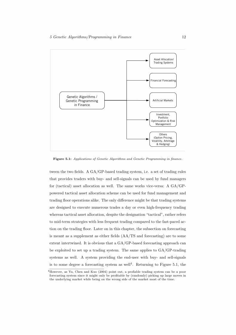
5.1 Applications of Genetic Algorithms and Genetic Programming in
finance. . . . . . . . . . . . . . . . . . . . . . . . . . . . . . . . . 12
9.1 Crossover example . . . . . . . . . . . . . . . . . . . . . . . . . . 44
9.2 A basic Genetic Programming flowchart. . . . . . . . . . . . . . . 49
13.1 DAX time series data from January 1997 - December 2007 and
associated log-returns. . . . . . . . . . . . . . . . . . . . . . . . . 63
13.2 Hang Seng time series data from January 1997 - December 2007
and associated log-returns. . . . . . . . . . . . . . . . . . . . . . . 64
13.3 Tree structure of successful DAX trading rules. . . . . . . . . . . 89
13.4 Equity curves for 3:1 and 5:1 revolving Genetic Programming
strategies for the DAX for c=0.25 and c=0.5. . . . . . . . . . . . 91
13.5 Kernel smoothing density estimates for 3:1 and 5:1 DAX scenar-
ios for c=0.25 and c=0.5. . . . . . . . . . . . . . . . . . . . . . . 92
13.6 Tree structure of successful Hang Seng trading rules. . . . . . . . 111
13.7 Equity curves for 3:1 and 5:1 revolving Genetic Programming
strategies for the Hang Seng for c=0.25 and c=0.5. . . . . . . . . 113
13.8 Kernel smoothing density estimates for 3:1 and 5:1 Hang Seng
scenarios for c=0.25 and c=0.5. . . . . . . . . . . . . . . . . . . 114
V
List of Abbreviations
AA/TS Asset Allocation/Trading Systems
ANN Artifical Neural Network
AR Auto-Regressive
ARCH Auto-Regressive Conditional Heteroscedasticity
ARMA Auto-Regressive Moving Average
CAPM Capital Asset Pricing Model
CPU Central Processing Unit
DD Downside Deviation
EA Evolutionary Algorithms
EC Evolutionary Computing
EMH Efficient Markets Hypothesis
ETF Exchange Traded Funds
EURIBOR Euro Interbank Offered Rate
FIBOR Frankfurt Interbank Offered Rate
FOREX Foreign Exchange
FS Fuzzy Systems
GA Genetic Algorithms
GA/GP Genetic Algorithms/Genetic Programming
GARCH Generalized Auto-Regressive Conditional Heteroscedasticity
GP Genetic Programming
GPLAB Genetic Programming Laboratory
HIBOR Hong Kong Interbank Offered Rate
KBES Knowledge-Based Expert System
LISP List Processor
MA Moving Average
MAR Minimum Acceptable Rate of Return
MTS Mechanical Trading System
TTR Technical Trading Rule
VI
Contents
I Introduction + Motivation 1
1 Evolutionary Algorithms 1
2 Motivation 2
II Applications of Evolutionary Algorithms in Asset
Allocation and Trading Systems 4
3 Introduction 4
4 Computer-Based Trading Systems 4
4.1 Some Remarks on Technical Trading Rules . . . . . . . . . . . . 5
4.2 Computer-Aided Trading Systems . . . . . . . . . . . . . . . . . 5
4.2.1 Knowledge-Based Expert-Trading Systems . . . . . . . . . 6
4.2.2 Mechanical Trading Systems . . . . . . . . . . . . . . . . 6
4.2.3 Artificial Neural Networks . . . . . . . . . . . . . . . . . . 7
4.2.4 Fuzzy Trading Systems . . . . . . . . . . . . . . . . . . . 8
4.2.5 Evolutionary Algorithms . . . . . . . . . . . . . . . . . . . 9
4.2.5.1 Genetic Algorithms . . . . . . . . . . . . . . . . 9
4.2.5.2 Genetic Programming . . . . . . . . . . . . . . . 10
5 Genetic Algorithms/Programming in Finance 11
5.1 Genetic Algorithms/Programming in Asset Allocation and Trad-
ing Systems . . . . . . . . . . . . . . . . . . . . . . . . . . . . . . 13
5.1.1 Stock Markets . . . . . . . . . . . . . . . . . . . . . . . . 13
5.1.2 Foreign Exchange Markets . . . . . . . . . . . . . . . . . . 24
5.1.3 Futures and Bond Markets . . . . . . . . . . . . . . . . . 28
5.2 Hybrid Models . . . . . . . . . . . . . . . . . . . . . . . . . . . . 31
5.2.1 Neuro-Genetic Hybrid Models . . . . . . . . . . . . . . . . 31
5.2.2 Fuzzy-Genetic Hybrid Models . . . . . . . . . . . . . . . . 32
5.3 Evolutionary Modeling in Forecasting . . . . . . . . . . . . . . . 33
VII

CONTENTS VIII
III The Mechanics of Genetic Programming 36
6 Introductory Remarks 36
7 Historical Overview 36
8 Why use Genetic Programming? 37
8.1 Financial Markets and Nonlinear Dynamics . . . . . . . . . . . . 38
8.2 General Properties of Genetic Programming . . . . . . . . . . . . 39
9 The Basics of Genetic Programming 41
9.1 GP-Parameters for Tree Phenotypes . . . . . . . . . . . . . . . . 41
9.1.1 Terminal Set . . . . . . . . . . . . . . . . . . . . . . . . . 41
9.1.2 Function Set . . . . . . . . . . . . . . . . . . . . . . . . . 41
9.1.3 (Maximum)-Depth . . . . . . . . . . . . . . . . . . . . . . 42
9.1.4 How to grow Trees . . . . . . . . . . . . . . . . . . . . . . 42
9.2 Genetic Operators . . . . . . . . . . . . . . . . . . . . . . . . . . 43
9.2.1 Crossover . . . . . . . . . . . . . . . . . . . . . . . . . . . 43
9.2.2 Mutation . . . . . . . . . . . . . . . . . . . . . . . . . . . 45
9.2.3 Reproduction . . . . . . . . . . . . . . . . . . . . . . . . . 46
9.3 Fitness Function and Selection . . . . . . . . . . . . . . . . . . . 46
9.4 Parameter Choice . . . . . . . . . . . . . . . . . . . . . . . . . . . 47
9.5 A Basic GP Run . . . . . . . . . . . . . . . . . . . . . . . . . . . 47
10 Why does Genetic Programming work? 49
10.1 Prize’s Theorem . . . . . . . . . . . . . . . . . . . . . . . . . . . 50
10.2 Schema Theory and Building Block Hypothesis . . . . . . . . . . 51
10.2.1 Koza’s Schema Theorem . . . . . . . . . . . . . . . . . . . 52
10.2.2 O’Reilly’s Schema Theorem . . . . . . . . . . . . . . . . . 53
10.2.3 Other Schema Theorems . . . . . . . . . . . . . . . . . . . 54
10.2.4 Criticisms of Schema Theorems . . . . . . . . . . . . . . . 54
10.2.5 Genetic Programming vs. Random Search . . . . . . . . . 54
10.3 Concluding Remarks . . . . . . . . . . . . . . . . . . . . . . . . . 55
CONTENTS IX
IV Testing Stock Market Efficiency via Genetic Pro-
gramming 56
11 Introduction 56
12 Some brief Remarks on Market Efficiency 56
12.1 Definition and Implications of the Efficient Markets Hypothesis . 57
12.2 Techniques for Testing Market Efficiency . . . . . . . . . . . . . . 59
13 Testing Stock Market Efficiency via Genetic Programming 61
13.1 Introduction . . . . . . . . . . . . . . . . . . . . . . . . . . . . . . 61
13.2 Implementation . . . . . . . . . . . . . . . . . . . . . . . . . . . . 61
13.2.1 Technical Aspects . . . . . . . . . . . . . . . . . . . . . . 61
13.2.2 Data+Stylized Facts . . . . . . . . . . . . . . . . . . . . . 62
13.2.3 Trading Rule Inputs . . . . . . . . . . . . . . . . . . . . . 64
13.2.4 Fitness Function . . . . . . . . . . . . . . . . . . . . . . . 66
13.2.5 Choice of In- and Out-of-Sample Periods . . . . . . . . . . 72
13.2.6 Genetic Programming Setup . . . . . . . . . . . . . . . . 75
13.3 Genetic Programming Market Efficiency Tests . . . . . . . . . . . 79
13.3.1 Testing the DAX . . . . . . . . . . . . . . . . . . . . . . . 79
13.3.1.1 Introductory Remarks . . . . . . . . . . . . . . . 79
13.3.1.2 Test Results . . . . . . . . . . . . . . . . . . . . 81
13.3.1.3 Structure of Trading Rules . . . . . . . . . . . . 87
13.3.1.4 Long Term Genetic Programming Performance . 89
13.3.2 Testing the Hang Seng . . . . . . . . . . . . . . . . . . . . 106
13.3.2.1 Test Results . . . . . . . . . . . . . . . . . . . . 106
13.3.2.2 Structure of Trading Rules . . . . . . . . . . . . 110
13.3.2.3 Long Term Genetic Programming Performance . 112
13.4 Conclusions about Market Efficiency in the DAX and the Hang
Seng . . . . . . . . . . . . . . . . . . . . . . . . . . . . . . . . . . 128
V Summary and Conclusion 131
14 Genetic Programming and Market Efficiency 131

CONTENTS X
15 Directions for Future Research 131
References 136
1
Part I
Introduction + Motivation
1 Evolutionary Algorithms
Evolutionary Algorithms (EA) are tools for heuristic optimization based on sim-
ulation of evolutionary processes in Nature. While the class of EA comprises
several subclasses of algorithms which will be briefly addressed later, so-called
Genetic Algorithms (GA) and Genetic Programming (GP) have emerged as the
two most widely used techniques. After the pioneering theoretical framework
was introduced by Holland (1975), GA gradually made their way from theoret-
ical biology to applied mathematics, physics, chemistry, computer science and
engineering. Based on Holland’s foundation, Koza (1992) introduced GP in or-
der to refine the evolutionary approach to optimization problems. Applications
of GA and GP are manifold, ranging from applications as diverse as minimiza-
tion of sonic boom on supersonic aircraft (Karr et al., 2003) and traffic signal
timing optimization (Sun et al., 2003) to evolutionary optimization of molecular
docking (Yang, 2003), a component of rational drug design, to name just a few.
A glimpse of the wealth of real-world applications is presented in Cantu-Paz
(2003).
During the last couple of years, GA and GP have become an important tool in
economics and finance as well. GA and GP constitute a promising approach to
modeling the highly complex dynamics of financial markets and numerous arti-
cles on GA and GP with applications to finance have been published. However,
the total number of publications is surprisingly low compared to other topics in
finance such as artificial neural networks, behavioral finance or credit risk. Al-
though the reasons may be numerous, it is quite likely that, especially in terms
of evolutionary modeling of trading strategies, considerable efforts are made
at private institutions such as banks. Given the assumption that GA/GP are
a suitable tool for modeling and forecasting financial asset returns, approaches
that prove to be profitable in some way remain, for obvious reasons, undisclosed.
2 Motivation 2
This might partly explain the somewhat sporadic and fragmented research in
this field. Nevertheless, a sufficient amount of material has been published and
several articles have found their way into prestigious journals thus underlining
the suitability and acceptance of the approach among the academic community.
The thesis is organized as follows: The next chapter presents a literature re-
view followed by a thorough discussion of the basics of GP in the third chapter.
The fourth chapter presents the setup and results for the application of GP-
optimized trading rules to the DAX and the Hang Seng. The final chapter
provides a summary and conclusion.
2 Motivation
First of all, it must be emphasized that this section is just a very brief intro-
duction and that the points made here are elaborated upon later in the thesis.
Basically, the motivation for the thesis at hand is, unsurprisingly, to test whether
stock markets are efficient. The efficient markets hypothesis (EMH) was first
formulated by Fama (1970) and roughly speaking says that the participants
in a financial market efficiently use all information so that all information is
priced into the market in such a way that no profits from a particular trading
strategy should be in excess of a passive buy-and-hold investment in the same
market1. While the EMH was widely accepted in academics at first, a con-
siderable number of papers have questioned the validity of the EMH. In their
seminal paper, Brock et al. (1992) reported profitable trading strategies for the
S&P 500 which sparked further research into the validity of the EMH. Profitable
trading strategies for stock markets have also been reported by Jegadeesh and
Titman (1993), Bessembinder and Chan (1995), Huang (1995) and Kwon and
Kish (2002), to name a few. LeBaron (1999) also reported successful trading
rules in the FOREX market as did Raj and Thurston (1996) for futures. These
findings are seriously shaking the assumption of efficient markets, even in its
weakest form (assumed impossibility to forecast returns based on past prices of
1This definition is rather imprecise. An exact definition of the EMH will be given in the fourthchapter.
2 Motivation 3
the underlying security)2. From a GP point of view, the paper by Brock et al.
(1992) and the follow-up literature were at the core of an entirely new branch in
the EMH literature that is dedicated to finding trading rules by means of evo-
lutionary optimization. The basic line of reasoning was that if it was possible
to find trading rules with econometric techniques it might also be worthwhile
to do so using methods from computional intelligence such as the already ex-
isting GA introduced by Holland (1975) and the new technique GP introduced
by Koza (1992). The advent of GP emphasized the capabilities of optimization
techniques inspired by evolutionary processes found in Nature. Furthermore,
computers had become powerful enough to deal with computationally demand-
ing applications such as GP. The first attempts at using GA/GP were made by
Bauer (1992, 1994), Neely et al. (1997) and most notably Allen and Karjalainen
(1999). However GA/GP-related financial market research is still quite limited
as will be seen in the upcoming literature review. Particularly striking is the
lack of thorough research in terms of particular stock markets since most of the
existing contributions focus on U.S. markets. Therefore, the thesis at hand ex-
tends the literature to other major indices such as the German DAX and Hong
Kong’s Hang Seng and checks whether GP can provide an answer to one of the
major topics in finance, i.e. are markets efficient?
2Admittedly, there are also opposing points of view concerning profitability of trading strategiessuch as Hudson et al. (1996), Bessembinder and Chan (1998), Brown et al. (1998) and mostnotably Chen and Kuo (2001).
4
Part II
Applications of Evolutionary
Algorithms in Asset Allocation
and Trading Systems
3 Introduction
This chapter aims at reviewing the current state of literature on applications
of GA/GP in finance, with emphasis on asset allocation and trading systems.
Hybrid models, i.e. crossing EA with competing techniques such as neural
networks for example, will be considered as well. Last but not least, the existing
literature on GA/GP based forecasting will also be covered as it is closely linked
to the search for profitable trading systems using GA/GP. The remainder of the
chapter is organized as follows: As a precursor to a discussion of applications
of GA/GP in asset allocation and trading systems (AA/TS), several computer-
aided trading systems will be presented in the fourth section. At this stage, the
mechanics of GA/GP will be outlined as well, albeit in a very brief fashion3. The
fifth section constitutes the mainstay of this chapter and reviews the literature
on GA/GP-applications in AA/TS. The section ends with a brief discussion of
hybrid models and applications of GA/GP in forecasting.
4 Computer-Based Trading Systems
The aim of the upcoming section is to introduce the concept of technical trading
rules as building blocks for computer-based trading systems (with one of them
being GA/GP) which will then be briefly discussed.
3A full-scale presentation of GA/GP including a thorough discussion of all parameters involvedare the main topic of the third chapter of the thesis.
4.1 Some Remarks on Technical Trading Rules 5
4.1 Some Remarks on Technical Trading Rules
Technical trading rules (TTR) are a set of rules used by traders and portfolio
managers to buy and sell securities on financial markets. Basically, the idea is to
predict future prices based on past prices. The probably most well-known rule
is the moving average rule as shown in equation (13.1) which comes in various
flavours such as the 200-day moving average advocated by Granville (1976).
Apart from this classic indicator, other inputs such as daily high/lows, trading
volume and volatility are also used frequently. A compilation of some popular
rules is found in Babcock (1989). TTR are widely used by market practicioners.
In contrast to this, in academia financial markets were believed to follow a
random walk (Fama, 1965a, 1965b) thus rendering any trading rule useless from
a theoretical point of view. The closely related EMH questioned any gains from
particular trading patterns as well (Fama, 1970). Although several publications
reported profitable trading strategies such as Basu (1977) and French (1980) for
stock markets and Sweeney (1986) for the foreign exchange market (FOREX),
it was not until 1988 that Lo and McKinlay showed that markets do not follow
random walks, a fact that was taken for granted until then by practitioners. As
TTR can be implemented by computer systems, several computer-based trading
systems exist, with one of them being GA/GP. Examples of an algorithm capable
of detecting classic trading patterns such as head-shoulder-head are presented in
Lo et al. (2000). An overview of the general requirements for a suitable trading
system and the design process is given in Pardo (1992).
4.2 Computer-Aided Trading Systems
Sophisticated and thus computer-based techniques such as GA/GP are avail-
able to develop trading models. The upcoming discussion aims at giving an
overview of these techniques. However, a thorough discussion of the strengths
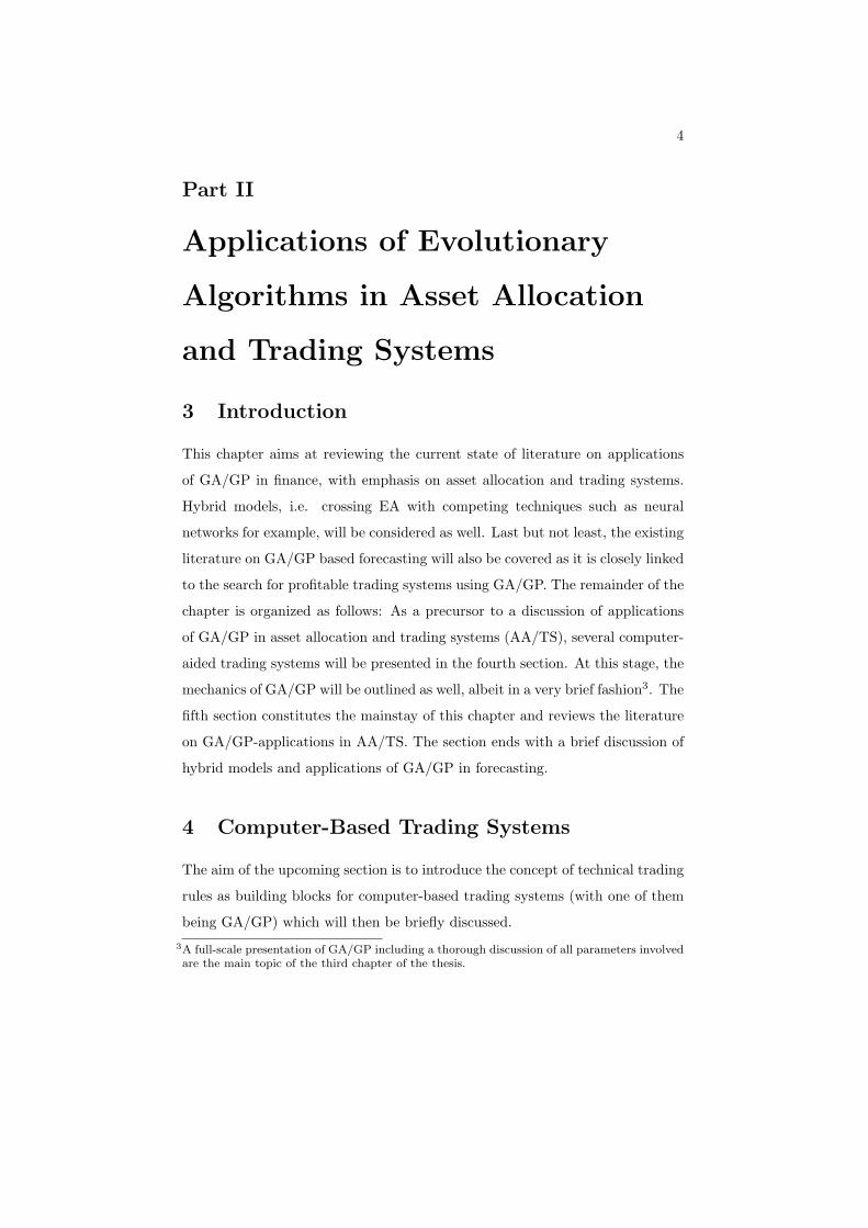
and weaknesses of each technique is beyond the scope of the thesis. An account
of computer-based trading systems is given in Figure 4.1.
4.2 Computer-Aided Trading Systems 6
Knowledge-Based(Expert)-Trading
Systems
Artificial Neural Networks
Evolutionary Algorithms Genetic AlgorithmsGenetic Programming
Expert Systems
Genetic Algorithms
Genetic Programming
Neural Networks
Mechanical Trading Systems
Applied to:
Fuzzy Systems
Figure 4.1: An overview of computer-based trading systems.
4.2.1 Knowledge-Based Expert-Trading Systems
With reference to Medsker (1995), Knowledge-Based Expert-(Trading) Systems
(KBES) perform reasoning using a set of previously established rules. These
rules are stored in a knowledge base and are fed-forward to a so-called inference
engine which then provides the end-user with advice. As an example, Deboeck
(1994) reports that a large brokerage firm set up a KBES by collecting not
less than 600 trading rules from their traders. The system was then employed
to provide inference based on these rules to assist in trading operations. The
case illustrates the main drawback of KBES, i. e. high complexity and difficult
maintenance since the knowledge-base has to be checked for consistency/validity
and has to be updated frequently.
4.2.2 Mechanical Trading Systems
Mechnical Trading Systems (MTS) are a more complex implementation of TTR.
An arbitrarily large array of rules can be easily implemented with the help of
a computer system. The system then uses simple if-then-reasoning to generate
4.2 Computer-Aided Trading Systems 7
buy- and sell-signals which can either be passed on to the trader (if the system
is designed as an advice-giving support platform) or can be executed directly
via computer. Deboeck (1994) presents a combination of 5- and 20-day moving
averages for the S&P 500 as an example of a very basic mechanical trading sys-
tem. Varying levels of complexity can be used to improve trading performance.
However, as Deboeck (1994) points out, MTS are generally prone to overfitting.
He reports that the majority of trading systems are not very profitable from a
historical point of view, at least in terms of profitability vs. risk.
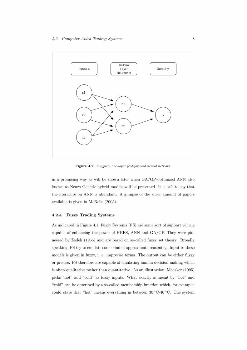
4.2.3 Artificial Neural Networks
Artifical Neural Networks (ANN) try to imitate biological neural networks as
those found in human brains. ANN are made up of three main components:
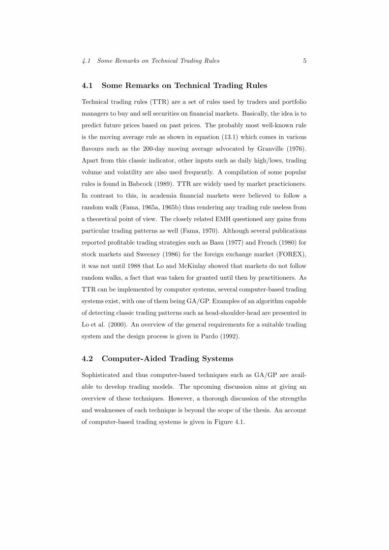
The inputs x, followed by hidden layers n and an output y. A typical so-called
feed-forward network is depicted in Figure 4.2. The neurons n can be thought
of as electrical impulses that are triggered by the inputs x. The neurons then
fire an impulse which results in an output y. The neuron firing mechanism
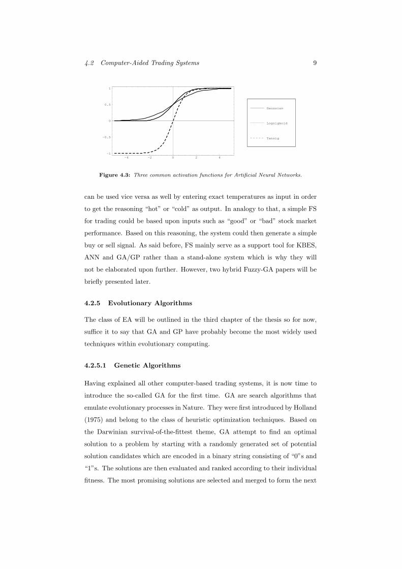
is triggered by an activation function. The weighted sum of inputs serves as
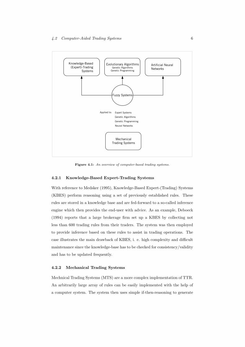
input to this activation function. The three most common activation functions
are the so-called sigmoid, tansig and Gaussian activation function as depicted
in Figure 4.3. The exact functional forms can be found in McNelis (2005).
Each activation function has the common attribute of triggering a response
once a certain threshold value has been exceeded just in analogy to biological
systems. A single snowflake on a bare hand does not trigger the feeling of
cold whereas many snowflakes in sum trigger this sensation. If the threshold
value is not exceeded, the activation function literally remains silent. ANN
are a quite established technique. They are particularly interesting because it
can be shown that they are capable of approximating any nonlinear function to
infinitely accurate precision (McNelis, 2005). Although ANN differ substantially
from GA/GP, they are in a certain sense a direct competitor to the latter as
they serve the same purpose, i.e. modeling nonlinear dynamics. Although
the question which approach is more suitable for modeling financial markets is
intriguing it would deserve a thesis in its own right. Therefore, this issue will
not be addressed further. However, the best of two worlds can be combined
4.2 Computer-Aided Trading Systems 8
Inputs xHidden Layer
Neurons nOutput y
x1x1
x2
x3
y
n2
n1
Figure 4.2: A typical one-layer feed-forward neural network.
in a promising way as will be shown later when GA/GP-optimized ANN also
known as Neuro-Genetic hybrid models will be presented. It is safe to say that
the literature on ANN is abundant. A glimpse of the sheer amount of papers
available is given in McNelis (2005).
4.2.4 Fuzzy Trading Systems
As indicated in Figure 4.1, Fuzzy Systems (FS) are some sort of support vehicle
capable of enhancing the power of KBES, ANN and GA/GP. They were pio-
neered by Zadeh (1965) and are based on so-called fuzzy set theory. Broadly
speaking, FS try to emulate some kind of approximate reasoning. Input to these
models is given in fuzzy, i. e. imprecise terms. The output can be either fuzzy
or precise. FS therefore are capable of emulating human decision making which
is often qualitative rather than quantitative. As an illustration, Medsker (1995)
picks “hot” and “cold” as fuzzy inputs. What exactly is meant by “hot” and
“cold” can be described by a so-called membership function which, for example,
could state that “hot” means everything in between 30 C-40 C. The system
4.2 Computer-Aided Trading Systems 9
-4 -2 0 2 4-1
-0.5
0
0.5
1
Tansig
Logsigmoid
Gaussian
Figure 4.3: Three common activation functions for Artificial Neural Networks.
can be used vice versa as well by entering exact temperatures as input in order
to get the reasoning “hot” or “cold” as output. In analogy to that, a simple FS
for trading could be based upon inputs such as “good” or “bad” stock market
performance. Based on this reasoning, the system could then generate a simple
buy or sell signal. As said before, FS mainly serve as a support tool for KBES,
ANN and GA/GP rather than a stand-alone system which is why they will
not be elaborated upon further. However, two hybrid Fuzzy-GA papers will be
briefly presented later.
4.2.5 Evolutionary Algorithms
The class of EA will be outlined in the third chapter of the thesis so for now,
suffice it to say that GA and GP have probably become the most widely used
techniques within evolutionary computing.
4.2.5.1 Genetic Algorithms
Having explained all other computer-based trading systems, it is now time to
introduce the so-called GA for the first time. GA are search algorithms that
emulate evolutionary processes in Nature. They were first introduced by Holland
(1975) and belong to the class of heuristic optimization techniques. Based on
the Darwinian survival-of-the-fittest theme, GA attempt to find an optimal
solution to a problem by starting with a randomly generated set of potential
solution candidates which are encoded in a binary string consisting of “0”s and
“1”s. The solutions are then evaluated and ranked according to their individual
fitness. The most promising solutions are selected and merged to form the next
4.2 Computer-Aided Trading Systems 10
generation. During this process, random mutations occur to ensure that the
search process covers a wide set of the search space. To put it in a nutshell, a
basic GA works as follows:
1. Random generation of potential solutions to a problem.
2. Calculation of their respective fitness.
3. Select best solutions, merge (crossover) and apply mutation.
4. Re-evaluate fitness , select best candidates.
5. Iterative repetition of (3) and (4) until no further improvements in fitness
can be achieved.
As Goldberg (1993) points out, GA are particularly appealing as an optimization
technique since, unlike analytical approaches, they do not impose any require-
ments such as continuity and existence of derivatives on the underlying function
to be optimized.
4.2.5.2 Genetic Programming
An important extension of the Holland (1975) GA is so-called GP first intro-
duced by Koza (1992). Basically, GP incorporates the main attributes of GA,
i.e. efficient search of the solution space by applying a fitness measure (excess
returns for example) to the solution candidates that are subject to operators
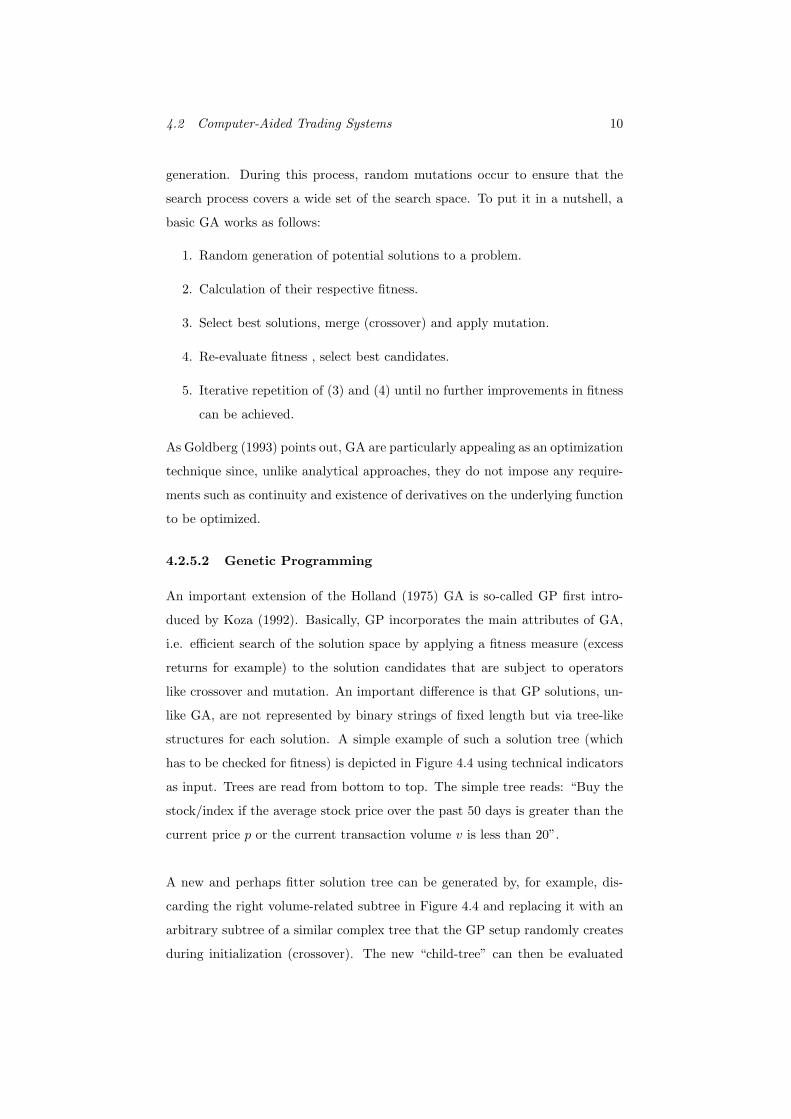
like crossover and mutation. An important difference is that GP solutions, un-
like GA, are not represented by binary strings of fixed length but via tree-like
structures for each solution. A simple example of such a solution tree (which
has to be checked for fitness) is depicted in Figure 4.4 using technical indicators
as input. Trees are read from bottom to top. The simple tree reads: “Buy the
stock/index if the average stock price over the past 50 days is greater than the
current price p or the current transaction volume v is less than 20”.
A new and perhaps fitter solution tree can be generated by, for example, dis-
carding the right volume-related subtree in Figure 4.4 and replacing it with an
arbitrary subtree of a similar complex tree that the GP setup randomly creates
during initialization (crossover). The new “child-tree” can then be evaluated
5 Genetic Algorithms/Programming in Finance 11
avg
price 50
> <
20v
or
p
Figure 4.4: A technical trading rule in Genetic Programming tree-like structure taken fromPotvin et al. (2004).
once more. The tree in Figure 4.4 is just based on a limited range of operators.
An overview of operators available to GP will be given in the third chapter of
the thesis. Solution trees can vary in complexity (that is in depth of subtrees
and number of nodes) and are generally more flexible than GA especially when
the structure of the solution is not known a priori. For example, GA can only
operate with a fixed amount of variables whereas a GP approach can vary the
amount of variables and indicators used allowing for a more flexible design.
Now that all computer-based trading systems as shown in Figure 4.1 have been
briefly reviewed, it is time to discuss applications of GA/GP in finance.
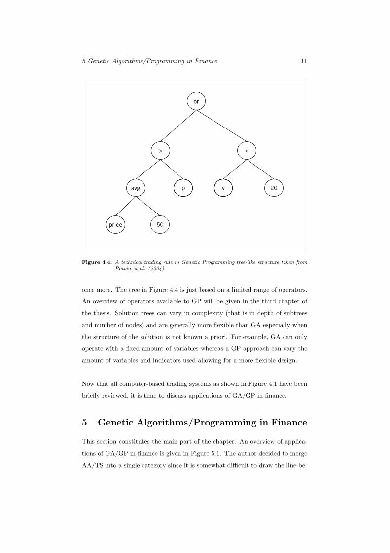
5 Genetic Algorithms/Programming in Finance
This section constitutes the main part of the chapter. An overview of applica-
tions of GA/GP in finance is given in Figure 5.1. The author decided to merge
AA/TS into a single category since it is somewhat difficult to draw the line be-
5 Genetic Algorithms/Programming in Finance 12
Asset Allocation/Trading Systems
Genetic Algorithms / Genetic Programming
in FinanceArtificial Markets
Investment, Portfolio
Optimization & Risk Management
Financial Forecasting
Others(Option Pricing,
Volatility, Arbitrage & Hedging)
Figure 5.1: Applications of Genetic Algorithms and Genetic Programming in finance.
tween the two fields. A GA/GP-based trading system, i.e. a set of trading rules
that provides traders with buy- and sell-signals can be used by fund managers
for (tactical) asset allocation as well. The same works vice-versa: A GA/GP-
powered tactical asset allocation scheme can be used for fund management and
trading floor operations alike. The only difference might be that trading systems
are designed to execute numerous trades a day or even high-frequency trading
whereas tactical asset allocation, despite the designation “tactical”, rather refers
to mid-term strategies with less frequent trading compared to the fast-paced ac-
tion on the trading floor. Later on in this chapter, the subsection on forecasting
is meant as a supplement as either fields (AA/TS and forecasting) are to some
extent intertwined. It is obvious that a GA/GP-based forecasting approach can
be exploited to set up a trading system. The same applies to GA/GP-trading
systems as well. A system providing the end-user with buy- and sell-signals
is to some degree a forecasting system as well4. Returning to Figure 5.1, the4However, as Yu, Chen and Kuo (2004) point out, a profiable trading system can be a poorforecasting system since it might only be profitable by (randomly) picking up large moves inthe underlying market while being on the wrong side of the market most of the time.
5.1 Genetic Algorithms/Programming in Asset Allocation and TradingSystems 13
lower three fields will not be elaborated upon further. They are covered in Chen
(2002a, 2002b).
5.1 Genetic Algorithms/Programming in Asset Allocation
and Trading Systems
Although GA were devoloped in the seventies of the last century and further
developed in the eighties, it was not until the nineties that they found their way
into AA/TS. The most likely reason for this might be the assumption of financial
markets following random walks and the EMH which, on a theoretical level,
contradicted profits from trading rules. This paradigm was seriously questioned
by Lo and McKinlay (1988) who showed that markets do not follow random
walks and by Brock et al. (1992) with their seminal article. Brock et al. (1992)
tested popular trading rules over a 90-year horizon in the S&P 500. The rules
included 20 different moving average rules and six versions of the trading-range
break rule. They found that both classes of rules work well which translates into
buy signals generating 12% annual return on average and sell signals generating
7% loss per year on average. These findings seriously contradicted the EMH.
Brock et al. (1992) laid the groundwork for further research into trading models
and eventually GA/GP for AA/TS. Since then, several contributions made their
way into prestigious journals thus underlining the suitability and acceptance of
the approach among the research community.
5.1.1 Stock Markets
The first attempt (to the best of the author’s knowledge) at creating a tactical
asset allocation scheme was made by Bauer and Liepins (1992). They illustrate
the usefulness of GA by providing a fund switching example. They assume that
an investor can either invest 100% of his assets in an S&P 500 fund or alterna-
tively in a small-firm equity fund on a monthly basis. The investment horizon
is five years and the investor aims to maximize terminal wealth. An investment
strategy can be translated into a binary string consisting of “0”s (invest in S&P
500) and “1”s (invest in small-firms fund) for every month within a five year
horizon. Therefore, 212x5 ≈ 1 quintilion strategies exist. Since the performance
of either investment is ex-post known, the optimum strategy can be easily calcu-
5.1 Genetic Algorithms/Programming in Asset Allocation and TradingSystems 14
lated by hand by simply determining for every month within the 5-year horizon
which investment performed better. The data used ranged from 1926-1985 and
was split into consecutive 5-year subsamples. The authors find that their GA
quickly converged to a (near-) optimum in all twelve 5-year subperiods. The op-
timal solution was found in 7 out of 12 periods, for the five remaining subperiods
the solution yielded by the GA was in excess of 99% of the optimum on average.
The authors then modify the algorithm to account for transaction costs which
is easily implemented. Although the optimal solution was now found in only 43
out of 120 trials compared to 105 out of 120 trials in the first example, GA still
proved powerful. In the 77 remaining cases, the solution was always within a
10% margin of the optimum. As a further refinement, the authors add two addi-
tional investment alternatives to the investor’s set of choices, namely long-term
government bonds and Treasury bills, making computation more cumbersome.
Nevertheless, GA was still able to find near optimal solutions which were 94.5%
on average of the optimal solution. Although the study can be critizised on
grounds of being too simplistic, lack of out-of-sample testing and most notably
ex-post data snooping, it still shows the power and flexibility of GA as a tool
for tactical asset allocation.
Bauer (1994) presents a comprehensive account of GA-driven investment strate-
gies. He focuses on stock and bond markets5. One of the most striking features
of the study is, like Ammann and Zenkner (2003), the use of macroeconomic
variables as input to the GA whereas most of the literature relies on technical
indicators such as (lagged) prices, moving averages etc. as will be seen later.
Bauer (1994) picks ten macroeconomic variables found to have the highest cor-
relation with excess returns in the S&P 500 over the T-bill; among them indices
for U.S. inflation, production levels and unemployment. The benchmark is a
classic buy-and-hold strategy in the S&P 500, the alternative investment is a
long position in (virtually) default-free T-bills. The training data ranges from
1984-1988. The resulting trading rules are applied out-of-sample from 1989-
1992. Typical trading rules look like: If inflation > (<) threshold value AND
(OR) production level < (>) threshold value OR (AND) unemployment > (<)
5The results for the U.S. government and U.S. corporate bond market will be covered later.
5.1 Genetic Algorithms/Programming in Asset Allocation and TradingSystems 15
threshold value, then buy the index, else invest in T-bills6. For the 1989-1992
holdout period, the author reports a negative excess return on average (14.96%
vs. 18.46% for buy-and-hold). But he also finds that, though unable to beat
buy-and-hold, the trading rules significantly reduced risk as the rules were on
average only 8 months long in the markets on a yearly basis instead of being
exposed over the whole 12 months like buy-and-hold. As a result, the portfolio
made up of GA-generated trading rules earned 81% of the buy-and-hold bench-
mark but with only 75% percent of the associated risk. Furthermore, a hedge
portfolio consisting of a portfolio with the best trading rules and a portfolio
with the worst trading rules was constructed. The idea was to go long on the
good rules and to go short on the bad rules. The author finds that the long
portfolio outperformed the short portfolio for the entire holdout period opening
up avenues for profitable investments. In conclusion, although the Bauer (1994)
GA did not beat buy-and-hold in the S&P 500, it reduced risk by a significant
amount.
An interesting variation is Frick et al. (1996) who, as an intriguing feature,
use Frankfurt stock exchange data (1989-1994) for their study. Another feature
setting their paper apart from others is that inputs to the GA are based on a
popular heuristic method called point & figure charts. Basically, this type of
chart depicts the presence and strength of price reversals for a particular stock
or entire index7. The setup in the study first creates appropriate point & figure
charts based on historic price data of each share in the DAX which are then
converted into a binary representation. By combining the data extracted from
the individual charts, resistance and support levels for each share can be com-
puted and trading rules can be created. The performance of these rules is then
compared with the riskless rate/market return and the expected, risk-adjusted
return within the established CAPM framework for the time frame considered.
If the return was higher than the just mentioned benchmarks, a buy-signal was
emitted, otherwise a sell signal. The DAX served as a proxy for market return
and the FIBOR8 was used as the riskless rate. The authors report an average6With the recent advent of Exchange Traded Funds (ETF), it is possible to buy an entire indexdirectly. Therefore, the problem translates into when to buy an ETF.
7The exact procedure is described in Tolke (1992).8Frankfurt Interbank Offered Rate.
5.1 Genetic Algorithms/Programming in Asset Allocation and TradingSystems 16
winning percentage of 60%, i.e. the buy- and sell-signals based on GA-powered
trading rules were correct 60% of time on average with single rules being correct
in excess of 70% of time which illustrates the potential power of GA. However,
performance is found to degrade over time during the out-of-sample test period.
Unfortunately, the authors do not investigate the profitability of their findings
and do not elaborate further on the results of their study.
Kassicieh et al. (1997) adapt the Bauer (1994) approach to find optimal switch-
ing strategies between the S&P500 and T-bills on a monthly basis using macroe-
conomic inputs with the highest correlation to the S&P 500. Based on the data
sample (1958-1993), the authors find that GA performance in terms of terminal
wealth is close to that of the ex-post known perfect switching strategy between
the two asset classes.
Fyfe et al. (1999) focus on a single stock, namely a property investment firm
called Land Securities plc to check whether profitable GP-trading rules exist.
The data range from 1980-1997, technical indicators were used as input to GP.
The GP approach succeeds in finding a profitable trading rule that beats the
buy-and-hold benchmark. Overall profit during the entire holdout period was
407.8% vs. 335.5% for buy-and-hold. Further analysis showed that the most
profitable rule had never issued a sell signal (although the authors report that
this almost had been the case during the october 1987 crash) and instead only
took long positions for certain periods. Therefore, the authors term the rule
“timing-specific buy-and-hold” referring to the fact that the rule found is noth-
ing more than a slightly more sophisticated buy-and-hold rule. Based on these
findings, the authors conclude that the market (at least the market for Land
Securities plc) is quite efficient9.
Allen and Karjalainen (1999) use GP to develop a trading system for the S&P
500. The data set covers 1929-1995. The algorithm was designed to find optimal
trading rules on a daily basis and yields in-the-market and out-of-the-market9It might be considered a weakness of the study that it just focuses on a single listed stockrather than a wider selection of stocks or an entire index. This shortcoming was addressed inFyfe et al. (2005).
5.1 Genetic Algorithms/Programming in Asset Allocation and TradingSystems 17
signals which translates into “buy-the-index” and “stay-out-of-the-market and
earn the risk-free rate”. The rules are compared with a standard buy-and-hold
strategy. Technical indicators were used as input such as moving averages and
trading range breaks. The setup allowed for a free search of parameters in the
solution space. Artifical indicators such as a 183-day moving average could
emerge during GP runs. Therefore, it was up to the GP to find out the optimal
length of a moving average or exact numerical specification of a trading range
break resulting in more flexible trading rules. To guard against data snooping, a
5-year training period was selected followed by a 2-year validation period during
which the best rules accumulated thus far were tested again. The final selec-
tion was then applied out-of-sample to the rest of the data until 1995. With
realistic transaction costs, the algorithm was unable to consistently outperform
the benchmark. However, the authors show that the timing strategies have
some forecasting ability as volatility is lower when the strategies indicate to be
in-the-market compared to out-of-the-market days. Averaged over all trading
rules and out-of-sample periods, the volatility of annual trading rule returns
is 10% opposed to 14.1% for the S&P 500 during the same period. Further-
more, the authors report that volatility can be further reduced by setting up
a portfolio of rules to diversify risk. If an equal amount of capital is put in
each of the strategies found by GP for a particular trading period, volatility
can be further reduced to 8.7% on average. As a consequence, even though the
rules fail to beat the market, the authors argue that the notably lower volatility
might appeal to investors on a risk-adjusted basis10. Due to the lack of consis-
tent outperformance of the timing strategies vis-a-vis buy-and-hold, the authors
conclude that the EMH holds.
Bhattacharyya and Mehta (2002) develop a GP-trading system for the S&P 500
as well. High, low, closing prices, moving averages, and variances of high and
low prices for succeeding time windows were chosen as input for the algorithm.
The data ranged from 1983-1997. The authors report an average excess return
over the buy-and-hold-benchmark of 4.41% for the out-of-sample period after
ten years of training. Interestingly and consistent with Bauer (1994), Allen and
10The volatility-reducing effect will be subject to further investigation as part of this thesis.
5.1 Genetic Algorithms/Programming in Asset Allocation and TradingSystems 18
Karjalainen (1999) and Ammann and Zenkner (2003), the power of the timing
strategies is reported to diminish during prolonged out-of-sample application
indicating major structural breaks in the underlying market dynamics11.
Pereira (2002) looks at the Australian stock exchange ASX to test a GA frame-
work. The data ranged from 1982-1997, technical indicators were taken as inputs
to the GA. Typical transaction costs of 10 basis points were considered. On a
risk-adjusted basis, the trading rules found almost consistently outperform the
buy-and-hold benchmark during the out-of-sample test period. However, the
profitability of the trading rules is found to decline over time. In addition, a
refinement to the methodology to account for thinly traded shares (so-called
non-synchronous trading/return measurement bias) lead to a meltdown of risk-
adjusted excess returns. As an interesting result and in-line with Allen and
Karjalainen (1999), the author notes that the trading rules are long in the mar-
ket when volatility of returns is low whereas they tend to stay out of the market
when volatility is high, indicating some timing/forecasting potential of the rules.
An innovative approach to GP-trading is presented in Thomas and Sycara
(2002). The design of their GP setup allows for the inclusion of stock-specific
messages posted on internet message boards. The message volume on two
boards, namely YAHOO! and Lycos Finance is taken as input to the algorithm.
The data are based on the top 10% by internet message traffice volume of the
Russell 1000 index ranging from Jan. 1998 until Dec. 2001 (68 stocks in total).
As a first step, the message traffic data for each share was collected resulting in
a new time series of message traffic for each stock. The GP setup was tasked
to yield buy- or sell-signals based on a pre-defined threshold level of message
data. The idea was that once a certain threshold level had been exceeded, a
rare (negative) stock-specific event had occured which should be interpreted as
a sell signal. If a single stock is shorted, a long position in a broader market, i.
e. the Russell 1000 is taken. The benchmark to the switching strategy between
individual stocks and a broad index was a simple buy-and-hold strategy in the
appropriate stock. The results of the study are positive: While the buy-and-hold11The main focus of the paper is on the choice and impact of different fitness functions and
lengths of training and out-of-sample periods on GP-performance.
5.1 Genetic Algorithms/Programming in Asset Allocation and TradingSystems 19
strategy earned 126.21% over the entire test period, the GP approach earned
164.36%. The Sharpe ratio is reportedly superior as well (1.15 vs. 1.74915).
Using a bootstrap test, the authors show that their results are statistically sig-
nificant. As part of further anaylsis, the authors checked whether the internet
message traffic just echoed information contained in other data as well such as
lagged trading volume or lagged return. They find, despite some correlation
between the variables, that internet message traffic does contain unique infor-
mation about the underlying stock. They conclude that the inclusion of “soft”
factors such as message board traffic seems promising as part of a GP-based
trading system.
Becker and Seshadri (2003a) pick up the setup and results from Allen and Kar-
jalainen (1999) and fine-tune their search algorithm in different ways. They use
monthly rather than daily data to reduce trading frequency, different fitness
measures and most importantly reduce the complexity of the search space by
restricting the amount of operators and indicators used for GP. The training
period ranges from 1960-1990 and the resulting rules are tested from 1991-2002.
The benchmark investment was once more a long position in the index. Inter-
estingly, the authors find that the leaner and improved algorithm succeeds in
consistently outperforming the buy-and-hold benchmark in the out-of-sample
period at a statistically signficant level. Unfortunately, their report is rather
brief and therefore they do not elaborate further on their results. As a conclu-
sion, it seems that (overly) complex GP implementations result in sub-optimal
performance.
Another study is Ammann and Zenkner (2003). Based on five macroeconomic
variables, namely interest rate spreads, default spreads, dividend returns, GNP
and inflation for the U.S., the authors try to find an optimal asset allocation
scheme. Assets can either be invested 100% in the S&P 500 or 100% in 3-month
T-Bills which are virtually risk-free. As a benchmark, a standard buy-and-hold
strategy was chosen. Based on data ranging from 1980-2000, the strategy to
be derived should point out on a daily basis whether to invest in the market or
not. The ratio of in-sample years to out-of-sample years was 5:5, 5:1 and 5:10,
5.1 Genetic Algorithms/Programming in Asset Allocation and TradingSystems 20
i.e. five years of training data applied to the next 5 years out-of-sample and so
on. The GA yielded an excess return of 3.47% during the eighties accompanied
by a Sharpe ratio of 1.17 vs. 0.66 for the buy-and-hold benchmark. In contrast
to this, the GA performs worse during the nineties and yields slightly nega-
tive excess returns. The authors explain this finding by referring to different
market conditions and structural breaks. While the GA performs well during
the volatile eighties, the sustained long-term upward trend during the nineties
seems to favour the buy-and-hold strategy which, by definition, is always long
in-the-market. However, the timing strategy derived by the GA yields slightly
better Sharpe ratios (0.71 vs. 0.68) which shows that, on a risk-adjusted basis,
the GA performed better than buy-and-hold despite negative absolute returns.
In addition to that, the timing strategy yields superior average Sharpe ratios
compared to the buy-and-hold benchmark throughout the entire 20-year data
range (0.85 vs. 0.70). The authors further report that the amount of switches
between asset classes is surprisingly low indicating that the GA picks up long
term trends rather than reacting to short-term noise in the market12. As a
by-product, this reduces total transaction costs which otherwise might cause a
meltdown of excess returns generated by a timing strategy.
Neely (2003b) applies GP to the S&P 500 closely following the approach by
Allen and Karjalainen (1999). The data range from 1929-1995. 5-year training
periods were followed by a 2-year selection period. The best rules obtained were
then tested out-of-sample on the remaining data. Including realistic transac-
tion costs of 25 basis points, the author finds that GP generally underperforms
a buy-and-hold strategy on a risk-adjusted basis. Therefore, he concludes that
the EMH holds.
Setzkorn et al. (2003) use a GP framework just based on moving averages
of various lengths to be determined by the GP algorithm to trade in the S&P
500. The approach features both a simple and a more complex setup. The data
range from 1990-2001 on a daily basis and, as usual, was split up into train-
ing, validation and out-of-sample periods. Most notably, neither the single nor12This might be one of the benefits from selecting macroeconomic variables rather than technical
indicators as input to a GA/GP setup.
5.1 Genetic Algorithms/Programming in Asset Allocation and TradingSystems 21
the complex setup succeeded in beating the buy-and-hold benchmark. Another
noteworthy result is that the complex GP is found to be prone to overfitting
resulting in a good fit during the training period and a poor fit in out-of-sample
testing. In contrast to this, the simple algorithm performed worse during train-
ing, but better during out-of-sample than the complex algorithm. The authors
consider the exclusive use of moving averages as indicators as the likely reason
for the overall poor performance of their approach.
Potvin et al. (2004) apply a GP framework to the Toronto stock exchange.
One of the special features of their study is that trading rules for fourteen indi-
vidual stocks are derived rather than focusing on an entire index. The authors
argue that this should allow for more individual and possibly more profitable
trading rules. Furthermore, the methodology allows for the inclusion of short
sales which would otherwise be difficult to implement when dealing with indices.
Technical indicators like stock prices and trading volume are once more input
to the algorithm; the data range from 1992-2000. The fourteen stocks were
chosen to represent fourteen different industries in the TSE 300 index. In the
end, GP underperforms the buy-and-hold benchmark on average. However, the
stock-specific results are better; nine out of fourteen stocks show positive excess
returns during the out-of-sample period. The overall poor performance is found
to be caused only by a minority of stocks. Further analysis showed that when
the benchmark buy-and-hold returns are close to zero or slightly negative, the
GP-trading rules are profitable, implying a timing strategy to apply the trading
rules when markets are stable or declining.
A more recent contribution is Fyfe et al. (2005), who apply and extend their
framework (Fyfe et al., 1999) to the S&P 500, the S&P Auto and the S&P Bank
index with data ranging from 1990-1999. In contrast to their previous study,
they look for risk-adjusted excess returns. Although GP does find rules that
easily outperform buy-and-hold, the picture changes after taking transaction
costs into account and adjusting for risk. Under these restrictions, GP gen-
erally underperforms the appropriate buy-and-hold benchmark except for the
S&P Auto where the algorithm partially outperforms the benchmark on a risk-
5.1 Genetic Algorithms/Programming in Asset Allocation and TradingSystems 22
adjusted basis. In defense of their study, the authors argue that their results
might appeal to risk-seeking investors or investors with a context-dependent
attitude towards risk13.
Lipinski (2007) applies two refined GA to trade in stocks from the Paris stock ex-
change (in particular the automaker Renault stock) using data from 1999-2004.
Training periods are 60 days followed by 20 days out-of-sample testing. The
evolved trading rules beat the buy-and-hold benchmark regardless of which GA
was used but the author finds that the more profitable algorithm also is more
demanding in terms of CPU time.
Navet and Chen (2008) investigate GP performance on the New York stock ex-
change. Based on time series data of several stocks traded during 2000-2006,
the authors explore the performance of GP trading rules based on a classifica-
tion scheme distinguishing between stocks with high entropy and low entropy14
using a variety of statistical techniques. The results are mixed with GP out-
performing the benchmark for 3 out of 8 stocks. Interestingly, the authors find
that GP performance, contrary to intuition, does not depend on the level of en-
tropy (≈ “predictability”) of a stock and conclude that predictability is neither
a necessary nor sufficient condition for profitability.
Apart from FOREX markets, Chen et al. (2008) also explore GP performance
for eight stock markets (USA, UK, Canada, Germany, Spain, Japan, Taiwan,
Singapore). The data cover 1989-2004 and are divided into rolling time frames
of five years training followed by five years of validation and two years of out-of-
sample testing. GP is found to consistently outperform buy-and-hold through-
out all periods in the Tawainese market. In constrast, GP performance yields
no outperformance in the other markets, among them the German DAX. The
authors point out that the Taiwanese market has a quite different pattern com-
pared to the other markets. In these markets, bull-markets are closely followed13For example, the non-risk adjusted return of the GP-trading rules including 0.5% transaction
costs for the S&P banks was 62.88% vs. just 20.72% for buy-and-hold during the 1995-1999period.
14Loosely speaking a measure of future uncertainty of a dynamic process whose past is com-pletely known.
5.1 Genetic Algorithms/Programming in Asset Allocation and TradingSystems 23
by bear-markets which may lure GP into a buy-and-hold strategy during train-
ing and validation which eventually results in poor performance in the out-
of-sample (bear-)market. As an interesting addition, the authors repeat their
approach and allow for the possibility of short sales. However, GP performance
does not improve in general. As another exercise, GP and buy-and-hold are
compared with the performance of 21 human-generated trading rules. While
these strategies generally underperform buy-and-hold and GP in bull markets,
some of them manage to beat GP and buy-and-hold in all markets during a
bearish period.
Drezewski and Sepielak (2008) focus on the Warsaw stock exchange for testing
GP performance. Using data from 2001-2006 they find that GP outperforms
buy-and-hold when applied out-of-sample to the same stocks that were used for
training. In addition, the authors investigate how well GP is able to generalize
beyond a selected stock by using a set of random stocks for training and a differ-
ent set of random stocks for out-of-sample testing. However, the result are poor
leading to the conclusion that GP fails to find general rules. As an interesting
sidenote, the authors elaborate on GP convergence (i.e. GP fitness as a function
of generations) and report that most of the fitness is achieved after rougly 25-75
generations (though they used 500 generations in total for each run) indicating
that using more generations only results in very little additional fitness at the
cost of dramatically increased CPU time.
For the sake of completeness, two more papers should be mentioned at this
stage which are not based on “plain-vanilla” GA/GP-methodology but never-
theless share some common features with the studies reviewed so far. The first
one is Yu et al. (2004) who use GP to find TTR for the S&P 500. They apply a
refinement to the usual GP approach by using so-called λ-abstraction. Based on
data ranging from 1982-2002, the standard GP (which is used as a comparison)
is able to outperform the buy-and-hold benchmark; the λ-abstraction enhanced
GP is able to improve upon the already positive results. The authors note that
the outperformance is achieved in all market conditions which makes their ap-
proach a robust tool for profitable trading.
5.1 Genetic Algorithms/Programming in Asset Allocation and TradingSystems 24
Another study worth mentioning is O’Neill et al. (2002) who, apart from the
FTSE 100 and NIKKEI, also look at the German DAX. However, the approach
is based on a different technique in evolutionary modeling called grammatical
evolution which constitutes a class of its own. Therefore, the results are only
partially comparable to the results of other studies presented in the literature
review. Based on data ranging from 1991-1997 (DAX/NIKKEI) and 1984-1997
(FTSE 100), the performance of the approach is mixed. For the FTSE 100, the
grammatical evolution technique slightly outperforms buy-and-hold while this
benchmark is clearly surpassed in the case of the NIKKEI. Performance for the
DAX is reportedly poor; the authors consider overfitting to be the likely reason
for the poor results.
5.1.2 Foreign Exchange Markets
Neely et al. (1997) presented the first approach at using GP in FOREX markets.
Six major exchange rates against the USD plus two cross-rates were subject of
the study. The data ranged from 1974-1995. The training period for GP was
1975-1977, followed by a validation period from 1978-1980. Out-of-sample tests
were conducted on the data for 1981-1995. Inputs for the GP setup were max-
ima, minima of prices, lagged prices, moving averages etc.. The algorithm was
designed to yield simple buy- or sell-signals on a daily basis. The benchmark
was simply zero return. The authors argue that a buy-and-hold strategy is
not well-defined in FOREX markets since it always depends on the location of
the investor whether she makes profits or not. For example, if the USD/EUR
buy-and-hold return is positive for an U.S. investor, the converse is true for an
European investor. Despite transaction costs, the authors find strong evidence
of economically significant excess returns by using GP-evolved trading rules
across the board with an overall average return for the out-of-sample period
of 2.87% for all six currencies. Interestingly, the overall performance could be
further improved by setting up a so-called median-rule portfolio, i. e. adopting
an investment strategy that went long in a rate when more than 50 out of 100
rules turned out to be long in the market rather than just following the single
best rule out of 100 rules generated per rate. The adoption of the median rule
5.1 Genetic Algorithms/Programming in Asset Allocation and TradingSystems 25
portfolio pushed average excess returns across all rates from 2.87% to 3.67%15.
Although the authors stress that their generated rules are higly nested and com-
plex, it turns out that one of the most profitable rules was as simple as “take
a long position at time t if the minimum exchange rate over period t − 1 and
t − 2 is greater than the 250-day moving average”. Further analysis of overall
performance showed that the excess returns were not caused by implicit risk
premia. In the end, the authors regard their findings as further evidence for
inefficencies in the FOREX market.
In very much the same fashion, Neely and Weller (1999) shed further light
on the power of GP trading rules in the FOREX market by extending existing
analysis on the now defunct European Monetary System (EMS). Six European
currencies against DM were subject of the study. The training period ranged
from 1979-1983, validation period from 1983-1986 and the rules were tested
out-of-sample from 1986-1996. Input to the GP setup were once more technical
indicators. Mean excess returns from GP trading were found to be positive
across the board (except for the DM/NGL rate), albeit not as high as in Neely
et al. (1997). Average overall excess return was 1.62% which could be further
improved by adopting the already mentioned median portfolio rule to 2.16%.
The authors point out that the performance of GP had been probably damp-
ened by the fixed rate bandwiths which were the most notable feature of the
EMS. Further analysis showed that the excess returns could not be explained
as compensation for higher risk. As a by-product, the trading rules were found
to have some predictive ability in terms of market timing, i. e. when to be
in-the-market and when to be out-of-the-market. In conclusion, the results for
the EMS were in-line with the earlier findings for the USD-denominated market
as shown in Neely et al. (1997).
Colin (2000) presents, in very much the same fashion as Colin (1994), a general
framework for GP-assisted trading, this time with a real-world application to
the FOREX market. A variety of technical trading indicators is used as in-15While this still does not seem to be too much, it must be emphasized that the figures are
average figures, shadowing the fact that the excess return in the USD/DM rate was in excessof 6%.
5.1 Genetic Algorithms/Programming in Asset Allocation and TradingSystems 26
put for GP, among them oscillators, relative strength indices and directional
movement indices. In total, Colin (2000) relies on seventeen different indica-
tors popular among practicioners. Subject of the study are the USD/CHF and
USD/JPY rates. The training period ranges from 1974-1981, validation period
from 1981-1988 and test period from 1988-1995. By applying the best GP-
generated trading rules, the author reports an average return of 6.5% and 7%,
respectively for the two rates.
A noteworthy extension of the two contributions by Neely et al. just presented
is Neely and Weller (2001). While the basic scope and setup largely remain
the same, the GP setup is now provided with historical data on Federal Re-
serve interventions in FOREX markets to determine how excess returns found
in previous papers relate to central bank action. Therefore, indicator variables
signaling intervention via “buy USD”, “no intervention”, “sell USD“ were added
on top of the usual market data that served as input. The authors find some ev-
idence of improved excess returns with monetary interventions for the US/GBP
and US/CHF rates, but they also find that the positive impact declines over
time. In contrast, the USD/DM and USD/JPY returns are even negatively
affected by the inclusion of intervention data. Given the overall inconclusive
results, the authors do not find evidence for the hypothesis that central bank
intervention could be one of the causes for profitability of TTR. They argue
that profitable trading is rather caused by strong and persistent trends in the
FOREX market.
Dempster and Jones (2001) use technical indicators like moving averages and
relative strength indices (six indicators in total). The intra-day data ranges
from 1989-1996 on a 15-minute basis. Opposed to Neely et al. (1997) and Neely
and Weller (1999, 2001, 2003a), the inputs for GP are based on a combination of
existing, real-world indicators like the readily available 250-day moving average
rather than letting GP derive artificial indicators. Furthermore, the setup al-
lows for real two-way trading including short-selling instead of just determining
whether to be in-the-market or out-of-the-market. The authors report mixed
results. While they manage to find simple rules that earn up to 7% annually
5.1 Genetic Algorithms/Programming in Asset Allocation and TradingSystems 27
in the GBP/USD market at a statistically significant level, overall performance
of the portfolio of trading rules is just about 5%. However, as they point out,
their results are encouraging enough to justify further research.
Despite the (mostly) encouraging results, all three studies by Neely et al. share
a common shortcoming, i. e. trading signals are based on daily data leading to
highly unrealistic results such as trading frequencies ranging from once every
two weeks to once in three months on average. As this phenomenon does not
realistically reflect the speculative, fast-paced and higly liquid FOREX mar-
ket, Neely and Weller (2003a) address this issue by applying their established
framework to intra-day data and trading. In addition to the exchange rate and
interest rate differentials, variables for the hour of the day were included in the
input data for the GP setup as well. Training, selection and test periods were
adjusted accordingly (2-months, 2-months, 7-months), the data are from 1996.
As far as market quotes are concerned, half-hourly averages were used. As a
result, the authors report that GP was not able to produce any excess returns
for any currency considered (USD/DEM, USD/CHF, USD/JPY, USD/GBP)
when taking realistic transaction costs into account. They argue that the sur-
prising results which contradict the findings of their previous studies might be
explained by the uneven division of capital allocated to trade in the FOREX
market at different time horizons. They guess that most of the volume is gen-
erated by traders who close their position at the end of the day rather than
investing with weekly or monthly horizons.
Austin et al. (2004) develop a GP intraday-trading framework for several cur-
rencies. Typical inputs include moving averages, stochastic oscillators, relative
strength indices etc.. For the 1994-1998 period, trading is reported to be prof-
itable out-of-sample after including realistic transaction costs. Annualized re-
turn for the GBP/USD was 13.07%, 4.29% for the USD/CHF and -0.37% for
the USD/JPY rate16.
Tsao and Chen (2004) take a theoretical approach by investigating the per-
16The authors do not elaborate further on their approach and results. Their system was devel-oped in close collaboration with HSBC Global Markets and is therefore highly proprietary.
5.1 Genetic Algorithms/Programming in Asset Allocation and TradingSystems 28
formance of GA for six different classes of time-series models, among them the
classic ARMA, ARCH and GARCH processes. Rather than just testing GA on
empirical data, the authors use Monte Carlo simulations based on these pro-
cesses to evaluate the performance of GA vs. buy-and-hold taking into account
returns, risk (Sharpe ratio), winning probability and a so-called luck-coefficent
which loosely speaking tests whether an outperformance is based on just a few
lucky trades. They find that GA performs particularly well in both linear-
and nonlinear deterministic (chaotic) environments whereas they fail in nonlin-
ear stochastic processes. As an empirical application, GA is tasked to evolve
trading rules for EUR/USD and USD/JPY time series from January 1999 until
April 1999. After establishing that the return series is fitted well by a mixture of
MA(1) and GARCH processes (for which GA proved superior to buy-and-hold
in the first part of the paper), GA is then shown to outperform the benchmark
in terms of return, Sharpe ratio and winning probability.
The most recent contribution is Chen et al. (2008). They explore GP per-
formance for eight major currencies (among them USD, DEM, JPY) using data
from 1992-2004 divided into rolling 3:3:2 schemes, i.e. 3 years training plus 3
years validation period followed by a 2-year out-of-sample period. They report
that GP generally fails at generating better returns than buy-and-hold. How-
ever, they extend their data and adapt their data division scheme to match the
setup used in Neely et al. (1997) and Neely and Weller (1999) and find that GP
is able to outperform the benchmark in 10 out of 12 scenarios at statistically sig-
nificant levels. The authors conclude that the design of a data division scheme
is paramount for GP performance. They particularly stress the importance of
the length of a training period which should neither be too long nor too short
for GP to pick up a pattern.
5.1.3 Futures and Bond Markets
GA/GP have found their way into futures markets as well. Wang (2000) applies
GP to the S&P 500 futures market. Based on daily data and technical indica-
tors such as moving averages, trading range breaks, volume etc. ranging from
1985-1998, the author picks GP-evolved trading rules based on 2-year train-
5.1 Genetic Algorithms/Programming in Asset Allocation and TradingSystems 29
ing periods and applies them out-of-sample. The benchmark is a buy-and-hold
strategy which consists of a long position in 2 S&P 500 futures contracts all the
time. In contrast to this, the GP-based rules were designed to yield five different
signals: long 2 contracts, long 1 contract, neutral (i. e. zero investment), short
1 contract, short 2 contracts (short-selling is assumed to be feasible, at least for
institutional investors). Basically, Wang (2000) finds that GP-performance in
the S&P 500 futures market is inconsistent. While some generated rules beat
the benchmark, their overall power is limited often resulting in slightly negative
excess returns when taking transaction costs into account. Overall performance
seems to be better when markets are volatile whereas the GP-rules reportedly
have difficulties in picking up sustained upward trends. Interestingly, although
being unable to beat the benchmark, the GP-rules often converge to the buy-
and-hold benchmark, i. e. 2 contracts long. The author notes that U.S. equity
returns in the twentieth century (and therefore the higly-correlated futures mar-
kets) have been the highest of all countries making it difficult for GP to beat
buy-and-hold.
In spirit of Allen and Karjalainen (1999), Karjalainen (2002) investigates the
performance of a GP trading system for the S&P 500 futures market. The data
range from 1982-1993. Inputs were moving averages, maximum/minimum of
past prices, lagged prices etc.. The benchmark was once more a buy-and-hold
strategy, i. e. a rolled over long position in a single S&P 500 futures contract.
It turned out that the GP-based trading rules slightly outperform the bench-
mark for the 1988-1993 out-of-sample period. Further analysis showed that a
portfolio of trading rules results in a superior annualized Sharpe ratio which is
in-line with the findings in Allen and Karjalainen (1999) for the equity market.
Therefore, GP-based timing strategies apparently reduce volatility by a signifi-
cant amount while roughly matching buy-and-hold.
Tsang and Lajbcygier (2002) also explore evolutionary trading in futures. As
a special feature, they make use of a standard GA and a Split Search GA17.17Basically, the idea is to start the GA search using two different input sets of variables for
the starting solutions, one using variables from class x, the other using variables from classy. Solutions from the two separated evolutionary processes are allowed to eventually crossover in analogy to two slightly different species (say two different kinds of giant lizards on the
5.1 Genetic Algorithms/Programming in Asset Allocation and TradingSystems 30
Basically, the data consist of daily highs and lows plus opening and closing
prices for eight commodities between 1988 and 1998. The authors use a rolling-
time frame of one year in-sample training followed by subsequent one year out-
of-sample application throughout the entire data sample. The input data for
GA consists of the classic filter rule (buy or sell contract when prices have de-
creased/increased by more than x%) and a moving average filter rule which
translates the classic filter rule concept to a smoothed time-series creating so-
called percentage envelopes or volatility bands. Fitness of the trading rules is
measured using the Sharpe ratio, benchmark strategy was buy-and-hold (only
one contract long/short at any one time). The authors report that the Split
Search GA and the standard GA only marginally beat the benchmark and that
the results are not statistically significant. After changing the fitness measure
to incorporate a take-profit mechanism plus the number of winning trades, the
results improve but still lack statistical significance. Finally, the authors note
that the difference in performance between the split island GA and the standard
GA was almost statistically significant. In defense of their study, they point out
that the primary goal was to show how GA performance can be improved by
using modified GA and fitness functions that do not solely focus on total prof-
itability.
Apart from the S&P 500, Bauer (1994) also looks at the U.S. government and
corporate bond market. The approach is basically the same as already discussed
in the section on equity markets. This time, the variables with the highest corre-
lation with the spread between the long maturity Treasury bonds and the short
maturity T-bills are the 1-month change in U.S. stock prices, economic growth
momentum indicators, changes in unemployment levels and 3-month changes in
consumer installment debt. The alternative investment to going long in Trea-
sury bonds is going long in Treasury bills. In addition, a switching strategy
between corporate- and Treasury bonds is considered using basically the same
input variables. For the Treasury bonds/Treasury bills case study, the author
reports an average return of the portfolio of GA-trading rules of 10.51% vs.
14.35% for buy-and-hold for the 1989-1991 out-of-sample period clearly miss-
Galapagos islands) living on two separate islands that sometimes, by crossing the water inbetween, manage to mate.
5.2 Hybrid Models 31
ing the benchmark. In contrast, the trading rules switching between corporate
bonds and Treasury bonds slightly outperform the buy-and-hold benchmark
for the same period (15.40% vs. 14.17%). As far as hedge portfolios are con-
cerned (going long on a portfolio of good rules and going short on a portfolio
of bad rules), the long portfolio partly outperforms the short portfolio in the
case of Treasury bonds during the holdout period whereas the corporate bond
hedge portfolio almost consistently outperformed the associated short portfolio.
In conclusion, the Bauer (1994) approach seems to succeed in finding profitable
Treasury/corporate bond market switching rules whereas the proposed Treasury
Bills/Treasury Bonds switching rules perform poorly.
5.2 Hybrid Models
Figure 4.1 showcases the general framework of computer-aided trading systems
with its main components, namely KBES, MTS, FS, ANN and GA/GP. A
branch of the literature available focuses on combining two or more of these
technologies, i.e. so-called hybrid models. Hybrid models are particularly pop-
ular in terms of GA/GP used to optimize ANN, nevertheless other hybrid ap-
proaches, such as a blend of GA/GP with FS, have been investigated as well
with the main goal of merging the best of two worlds into a unified approach.
A thorough discussion of the hybrid literature is beyond the scope of the thesis.
Nevertheless, for the sake of completeness and for illustrative purposes, two hy-
brid models will be briefly reviewed to show how classic GA/GP-methodology
can be extended to enhance performance of a trading system.
5.2.1 Neuro-Genetic Hybrid Models
A typical paper on this issue is Harland (1999). The main goal of his paper
is to develop a hybrid Neuro-Genetic model for trading the US T-Bond future.
As input, the author derived price transformations from underlying price data
resulting in momentum indicators with different lags. Additionally, the data
were enhanced by including similar momentum indicators from the positively
correlated S&P 500 future. Next, the author set up a neural net based on these
inputs and at this stage, GA come into play. With reference to Figure 4.2, a
GA was used to run through a vast amount of possible neural net architectures
5.2 Hybrid Models 32
in order to optimize the output (i. e. convergence on the training data set).
This was achieved by determining the optimal number of hidden layers of the
ANN by using GA. The results indicate that the final model mostly outperforms
a roll-over buy-and-hold strategy in T-Bond futures during the out-of-sample
test period. The amount of winning trades is reported to be significantly higher
than 50%.
A similar approach is presented in Kwon and Moon (2003), who apply a Neuro-
Genetic framework to trade various stocks on the New York stock exchange and
NASDAQ. The genetically evolved neuronal networks are able to outperform
buy-and-hold. In addition, a comparison between GA-evolved ANN and stand-
alone ANN shows that the use of GA considerably enhances the performance of
neural nets. However, neither Harland (1999) nor Kwon and Moon (2003) in-
vestigate the question whether neuro-genetic hybrids deliver better performance
than GA/GP-only based approaches.
Azzini and Tettamanzi (2008) also use a neuro-genetic hybrid to find profitable
trading strategies for the stock of Italian car company Fiat using closing prices,
moving averages and other technical indicators ranging from 2003 until 2006 on
the Milan stock exchange. They find that their models yield significant excess
returns on a risk-adjusted basis.
5.2.2 Fuzzy-Genetic Hybrid Models
A Fuzzy-Genetic hybrid is disscussed in Lam et al. (2002). They pick typi-
cal TTR and fuzzify them which translates into rules such as “if the relative
strength index is high, then buy”. Profitable combinations of these rules were
then evolved using a GA. Applied to five different stocks that trade on the
NASDAQ, the Fuzzy-GA hybrid is found to indicate the right market-timing
signal in 68.3% of cases and yields an average return of 11.1%. As an interesting
extension, the algorithm is redesigned to incorporate feedback from profitabil-
ity during out-of-sample testing to evaluate whether the system needs to be
recalibrated by retraining. The dynamic retraining approach leads to improved
profits of 51.5% with 67.8% of trades being profitable.
5.3 Evolutionary Modeling in Forecasting 33
A similar approach is discussed in Costa Pereira and Tettamanzi (2006). Using
open, high, low, closing prices, exponential moving averages and stochastic os-
cillators, suitable intra-day trading rules are evolved using a Split Search GA as
presented in Tsang and Lajbcygier (2002). The results are then fuzzified into
human-interpretable rules. The trading rules are applied to the Dow Jones,
Nikkei 225 and single stocks in different markets. Based on 2-,3- and 5-years
of training (2002-2006 maximum), out-of-sample (first half of 2007) GA perfor-
mance is superior to buy-and-hold for the Dow Jones both in terms of excess
return and risk-adjusted return as indicated by the Sharpe ratio whereas the
approach fails to outperform the benchmark in the Nikkei 225 and the single
stocks considered.
5.3 Evolutionary Modeling in Forecasting
At this stage, some comments on GA/GP-based forecasting are in order. Dur-
ing compilation of the literature review, it turned out that forecasting is to
a certain degree intertwined with AA/TS. A suitable forecasting system may
be exploited to form the basis of a profitable trading system. Furthermore,
the relation sometimes works vice-versa as well. For instance, Pereira (2002)
notes that the trading rules found for the Australian stock exchange apparently
possess some forecasting power since, based on relevant technical market data,
they suggest long positions when volatility of returns is low and stay out-of-the-
market when volatility of returns is high. Similar findings have been reported
by Allen and Karjalainen (1999). As a rule of thumb, forecasting models can be
distinguished from AA/TS by the fact that they rather explore the correctness
of their predictions instead of exhaustingly exploring profitability. Therefore,
in a strict sense, the already presented paper by Frick et al. (1996) could be
considered to fall into this category as well. For the sake of completeness and
to “get the big picture”, forecasting papers based on GA/GP will be briefly
reviewed to outline the links between GA/GP-based AA/TS and forecasting.
The first contributions to the issue are Chen and Yeh (1996, 1997) who em-
phasize the distinction between predictability and profitability when testing the
5.3 Evolutionary Modeling in Forecasting 34
EMH. They investigate the forecasting power of GP-based models of stock re-
turns against the random walk hypothesis using subsets of the S&P 500 and
the Tawainese stock exchange TAIEX ranging from 1971 to 1994. Based on the
function set and inclusion of constants and lagged returns as sole inputs, the
resulting GP forecasts are (non-)linear autoregressive models18. The authors
find that using larger training samples tend to make the EMH seem valid as
GP forecasts largely fail at beating the random walk hypothesis. Interestingly,
the random walk hypothesis, i.e. E(rt|Ωt−1) = 0 where rt denotes the return
today based on yesterday’s information set Ωt−1), is proposed by GP several
times as the best forecasting rule. Things look different when using shorter
training samples as GP tends to forecast returns better than the random walk
hypothesis. The authors note that the forecasts get better when using more
generations during the GP evolution process thus increasing CPU time=search
cost. Chen and Yeh conclude that even though the EMH sometimes may not
be 100% valid, it might be too costly (from a computing/search cost of view)
to exploit possible weaknesses.
Another forecasting paper closely related to the preceeding discussion is Li and
Tsang (1999) who use a GP approach to forecast whether it is possible to achieve
a return greater than r within the next n trading days in the Dow Jones index.
Input to the algorithm were once more technical indicators (moving averages,
trading rule breaks, filter rules). The authors use a standard GP design for
searching over a large set of trading rules. Based on r = 2.2%, n = 21, the
authors find that their methodology yields better forecasts than a purely ran-
dom alternative. The results are generally confirmed in a similarly designed
follow-up study (Li and Tsang, 2002).
Another example illustrating a forecasting approach is Kaboudan (2000, 2002).
The most notable difference to the trading system papers presented so far is
that the author does not derive trading strategies directly using GP, but rather
uses GP to evolve suitable regression models that forecast stock prices. Techni-
cal indicators were used as input to the GP regression model evolver with the18The linear case may emerge as well of course if considered fit enough by GP.

5.3 Evolutionary Modeling in Forecasting 35
main goal of forecasting one-day-ahead intra-day high and lows for four stocks
from the New York stock exchange and NASDAQ composite. Compared to a
naive forecast (tomorrow’s high and low equal today’s high and low), the GP ap-
proach is found to perform slightly better, with accuracy oscillating around 55%.
As already pointed out, though forecasting and AA/TS are to some extent
intertwined, GA/GP in forecasting applications constitute a class of its own
within research directed at evolutionary modeling of financial markets. There-
fore, a thorough discussion of the contributions published so far is beyond the
scope of this thesis.
Now that applications of EA in AA/TS have been reviewed, it is time to take
a closer look at the inner workings of GP.
36
Part III
The Mechanics of Genetic
Programming
6 Introductory Remarks
The main goal of this chapter is to explain the mechanics of GP prior to pre-
senting real-world case studies on testing stock market efficiency using GP. The
chapter is organized as follows. The next section gives a brief account of the
development of GP from a historical point of view, followed by a brief discussion
of the strengths and weaknesses of GP methodology. The basics of GP are then
thoroughly discussed which constitutes the main part of the chapter followed by
some remarks on parameter choice which is paramount to successful application
of GP. The next section aims at providing more insight into the question as to
why GP works from a theoretical point of view. The chapter ends with some
concluding remarks.
7 Historical Overview
GP belongs to a field called Evolutionary Computing (EC) in computer sci-
ence19. EC comprises different optimization techniques that all share the com-
mon theme of emulating evolutionary processes found in Nature. Early attempts
at implementing this idea date back to the mid-sixties with the works of Fogel
et al. (1965, 1966) who proposed a technique termed Evolutionary Program-
ming20. Later, in the mid-seventies, Holland (1975) introduced the concept of
GA. At about the same time, Rechenberg (1973) developed a similar technique
called Evolutionary Strategies. Two decades later, Koza (1992) invented GP.
Koza’s main intention was to create a framework for self-programming comput-
ers. With the help of GP, program code could be expressed as a hierarchical
tree-like structure originally encoded in the LISP (LISt Processor) programming
19Note that EC and the term EA are interchangeable.20The basics of Evolutionary Programming are explained in Eiben and Smith (2003).
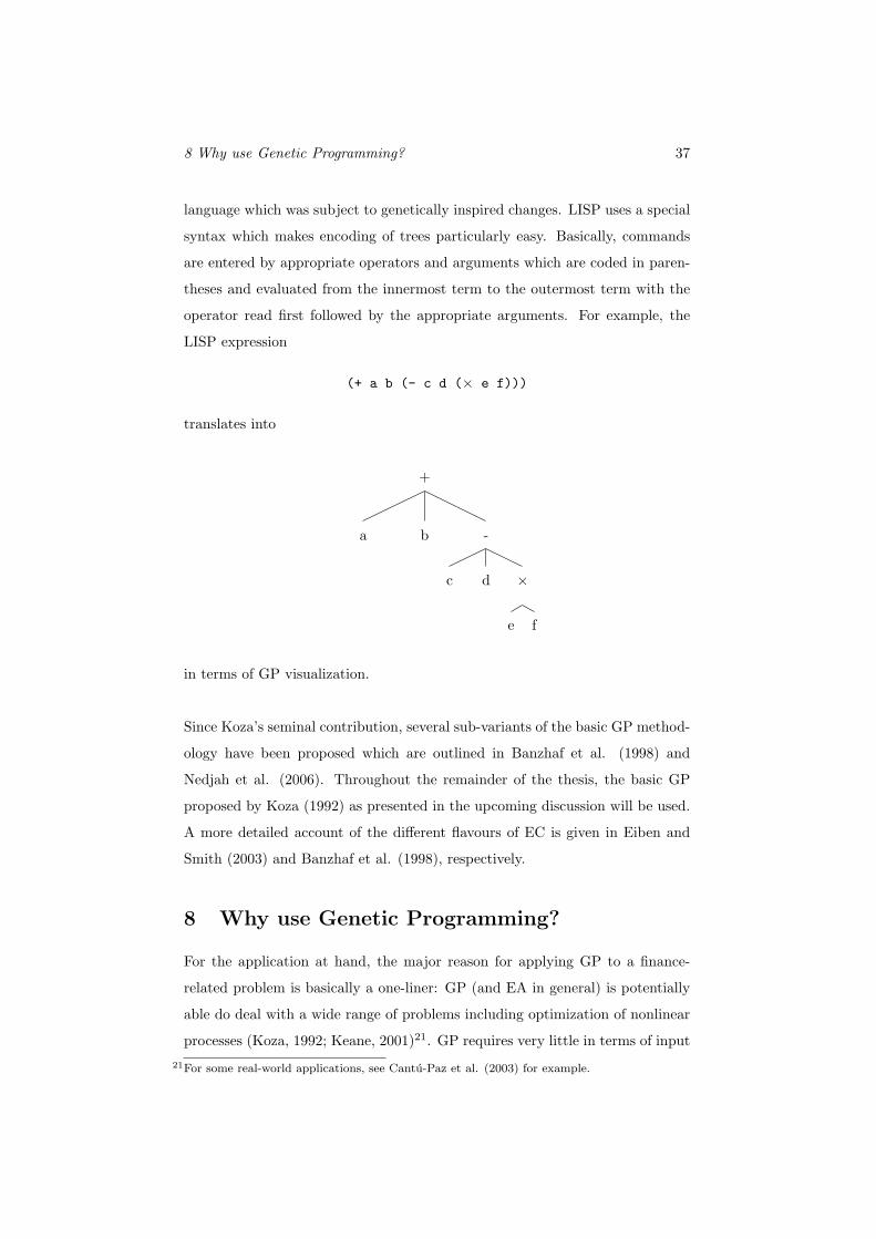
8 Why use Genetic Programming? 37
language which was subject to genetically inspired changes. LISP uses a special
syntax which makes encoding of trees particularly easy. Basically, commands
are entered by appropriate operators and arguments which are coded in paren-
theses and evaluated from the innermost term to the outermost term with the
operator read first followed by the appropriate arguments. For example, the
LISP expression
(+ a b (- c d (× e f)))
translates into
+
a b -
c d ×
e f
in terms of GP visualization.
Since Koza’s seminal contribution, several sub-variants of the basic GP method-
ology have been proposed which are outlined in Banzhaf et al. (1998) and
Nedjah et al. (2006). Throughout the remainder of the thesis, the basic GP
proposed by Koza (1992) as presented in the upcoming discussion will be used.
A more detailed account of the different flavours of EC is given in Eiben and
Smith (2003) and Banzhaf et al. (1998), respectively.
8 Why use Genetic Programming?
For the application at hand, the major reason for applying GP to a finance-
related problem is basically a one-liner: GP (and EA in general) is potentially
able do deal with a wide range of problems including optimization of nonlinear
processes (Koza, 1992; Keane, 2001)21. GP requires very little in terms of input
21For some real-world applications, see Cantu-Paz et al. (2003) for example.
8.1 Financial Markets and Nonlinear Dynamics 38
to solve an optimization task and builds, or better said, evolves potentially
suitable computer programs (=trading rules) to solve a given problem. There
is considerable evidence that financial markets are highly nonlinear which will
be elaborated upon in the next subsection.
8.1 Financial Markets and Nonlinear Dynamics
One of the major topics in finance is the analysis of asset returns as a building
block for modeling financial markets with the ultimate aim of deriving profitable
investment strategies with as-low-as-possible risk. Doing so requires qualifica-
tion and quantification of the economic variables that inherently drive financial
markets and a suitable modeling method. A technique for modeling markets
are linear regression models. Among this class are standard econometric models
like AR(p) and MA(q) processes and, as a blend of the latter two, ARMA (p,q)
models. Although well-established and quite popular, the linear approach lacks
explanatory power too often which is illustrated in Franses and van Dijk (2000).
Therefore, alternative and possibly more sophisticated techniques are needed to
capture the complex dynamics of financial markets.
There is considerable evidence that markets are driven by nonlinear dynam-
ics. Several tests have been developed capable of detecting nonlinearities in
time series data such as Tsay (1986) and Brock et al. (1987). For example,
Scheinkman and LeBaron (1989) employ the so-called BDS-Statistics derived
in Brock et al. (1987) to test weekly return data from 1928-1985 of the CRSP
(Center for Research in Securities Prices) value-weighted U.S. stock index. The
analysis is extended in Brock et al. (1991) to include S&P 500 data for the
same period. The authors find evidence of nonlinearities for both indices. Hsieh
(1989) checks exchange rates for nonlinearities. The data consist of daily closing
prices from 1974-1983 for the Canadian Dollar, Deutsche Mark, Japanese Yen
and Swiss Franc each quoted in U.S. Dollar. The test results suggest strong
nonlinearities in the data across all five currencies. Franses and van Dijk (2000)
make use of an ANN to detect nonlinearities and find evidence across all major
currencies as well. They extend their approach to include international stock
markets and find evidence of nonlinear dynamics across the globe, namely for
8.2 General Properties of Genetic Programming 39
the Frankfurt, Paris, London, New York, Hong Kong, Singapore and Tokyo
stock market indices.
As far as modeling nonlinearities is concerned, the classic ARCH (p,q) (En-
gle, 1982) and GARCH (p,q) (Bollerslev, 1986) models are probably the most
widely used technique. In addition, many other approaches with different lev-
els of sophistication and requirements in terms of their suitability to model an
underlying process are available. An overview of alternative techniques is given
in Tong (1990). Returning to a more general level, the line of reasoning for
applying GP to financial markets is as follows: Markets are driven by nonlinear
processes and GP is in theory capable of dealing with nonlinearities. Therefore,
the idea is to let GP evolve trading rules in a financial market and check whether
the results comply with the EMH.
8.2 General Properties of Genetic Programming
The discussion so far focused on the link between GP and financial markets. On
a more general level, some points can be made as to what makes GP a promising
algorithm for problem solving. According to Keane (2001), EC-based techniques
and thus GP have the following advantages over more traditional techniques:
• Applicable to a wide range of problems
• Low development and application cost
• Easily incorporated into other methods (hybridization)
• Solutions are interpretable
• Can be run interactively and allow for incorporation of user-proposed so-
lutions
• Often provides many alternative solutions.
In contrast, some of the drawbacks are:
• No guarantee for optimal solution within finite time
8.2 General Properties of Genetic Programming 40
• Weak theoretical basis
• May need parameter tuning for good performance
• Often computationally intensive and thus slow.
As far as the pros are concerned, the wide applicability of EC regardless of
the underlying process and the interpretability of solutions are by far the most
attractive properties, especially in comparison to neural nets which are often
powerful but difficult to interpret due to the “black box” property. Concerning
real-world applications in finance, Bauer (1994) points out that GA are well
suited for easily checking functional relationships between economic variables
without resorting to complicated yet often unsatisfying econometric techniques.
In terms of easy hybridization, the papers by Harland (1999), Lam et al. (2002)
and Kwon and Moon (2003) demonstrated how GP/GA can be merged with
other techniques to form a unified approach.
A serious drawback is the lack of theoretical foundation which particularly af-
fects GP whereas the theory behind GA is somewhat better understood22. This
issue will be addressed in more detail later. Another serious issue is the lack
of general rules for parameter choice and the associated fact that the impact
of parameter choice on GP results is not well understood, at least in finance
applications (Navet and Chen, 2007).
Having casually outlined the genesis and reasons for using GP, it is now time
for a more detailed approach. Before doing so, it must be emphasized that the
following topics are fairly standard material that is extensively covered in the
original source Koza (1992) and Banzhaf et al. (1998). These references provide
an in-depth discussion of GP while the following basic definitions are meant to
help understand real-world GP applications, i.e. testing stock market efficiency.22In modern GA theory, GA are interpreted as Markov processes which considerably facilitates
derivation of analytical results, see Reeves and Rowe (2003) for details.
9 The Basics of Genetic Programming 41
9 The Basics of Genetic Programming
9.1 GP-Parameters for Tree Phenotypes
As already pointed out before, GP-based solution candidates for an optimization
problem are encoded in a hierachical tree-like structure. The size, shape and
contents of these trees is controlled by a variety of parameters and sets which
are next on the agenda.
9.1.1 Terminal Set
The terminal set T is the set of all inputs to a GP system including constants
and zero argument functions. Casually speaking, T defines the contents of the
leaves of a GP-tree.
9.1.2 Function Set
The function set Fconsists of the statements, operators and functions avail-
able for a GP system.
A wide range of functions is possible such as
• Boolean operators: AND, OR, NOT, XOR23
• Comparison operators: ≤, ≥, <, >
• Arithmetic functions: +, -, ×, ÷
• Mathematical functions: sin, cos, exp, log, sqrt
• Conditional statements: IF, THEN, ELSE, CASE, SWITCH.
Further functions such as loops (while...do etc.) and variable assignment func-
tions are available as well. Generally speaking, there are virtually no limits to
functions for GP, i. e. almost any function can be used. This allows for extreme
flexibility in terms of the solution found by GP. Nevertheless, it is crucial for
function sets that they comply with the so-called closure property. The clo-
sure property states that all functions should be able to deal with any constant23eXclusive OR, or casually speaking “either of the two, but not both”.
9.1 GP-Parameters for Tree Phenotypes 42
from the terminal set and any value returned by a function from the function
set, otherwise the GP run could fail. Examples are the well-known “divide by
zero”-error or the log of a negative number which, depending on function and
terminal set, may occur during a GP run. Fortunately, the toolkit GPLAB run-
ning on Matlab which will be used throughout the thesis automatically takes
care of the closure requirement24.
Another important concept is the sufficiency property. The sufficiency prop-
erty states that the terminal set and the function set should be selected in such
a way that GP potentially can find an acceptable solution. For example, it is
highly unlikely that GP will capture an even trivial nonlinear relationship if it
is only based on the spartanic function set Fi = +,−,×. Extending Fi to
Fj = +,−,×,÷, exp, log, sqrt will likely result in a higher chance of finding
a nonlinear relationship. However, a too complex function and/or terminal set
might result in an extremely large search space leading to poor results as well.
Koza (1992) points out that in the end, it is up to the user to decide whether the
sufficiency property is met based on the individual optimization task at hand.
9.1.3 (Maximum)-Depth
The depth of a node is defined as the minimal number of nodes that must be
traversed to get from the root node of the tree to the selected node. The closely
related maximum depth refers to the largest distance between the root node
and the outermost terminals. Broadly speaking, the maximum depth defines
the size/complexity of solution candidates.
9.1.4 How to grow Trees
Combining the sets and parameters just discussed, the question remains how to
initialize tree-based GP solutions in the very first generation Gt0 . Koza (1992)
distinguishes between two methods called grow and full. The grow method
randomly selects nodes from both the function and terminal set. The only ex-24As an illustrative example, this can be achieved by making use of a so-called protected division
operator that simply returns one if division by zero would occur otherwise. To guard againstthe log of a negative number, the absolute value of the argument is taken to prevent the GPrun from crashing. Other potential violations of the closure property are handled by similarspecial operators during runtime. See Silva (2007) for details.
9.2 Genetic Operators 43
ception is the root node which is exclusively based on the function set. When a
branch reaches a terminal node it is cut off even if the maximum depth would
allow for another level of branching. Therefore, the grow method produces trees
of irregular shape.
In contrast, the full method selects nodes from the function set only until the
maximum depth has been reached. Then it selects terminals only. As a result,
every tree branch has the full maximum depth, trees are regularly shaped. Koza
(1992) suggests using the so-called ramped half-and-half method, i. e. 50% of
the initial generation uses grow and the other 50% uses the full method in order
to ensure a wide genetic variety of solutions to start with.
Having outlined the basic ingredients for determining tree phenotypes, it is now
time to give an account of the parameters that control evolutionary dynamics.
9.2 Genetic Operators
9.2.1 Crossover
The crossover operator controls swapping of genetic material between two indi-
vidual trees (parents). Two parents are chosen from an initial population based
on their respective fitness25. Once two parent trees have been selected, a ran-
dom subtree in either parent tree is selected. They are then swapped between
the two parents resulting in two children. The process is illustrated in Figure 9.1.
Crossover is probably the most important operator in GP. By splitting and mix-
ing (already promising) parental genes, crossover is in theory assumed to breed
children solutions with improved fitness. However, there is considerable debate
as to whether potential solutions really profit from crossover. While Koza (1992)
argues that crossover likely preserves good solutions and builds even better so-
lutions, Banzhaf et al. (1998) question the overall beneficial effect of crossover.
They argue that crossover does not distinguish between good and bad building
blocks thus potentially ripping apart promising subtrees of a parent solution. In
a standard regression application, Nordin et al. (1995) and Nordin and Banzhaf
25See subsection 9.3.
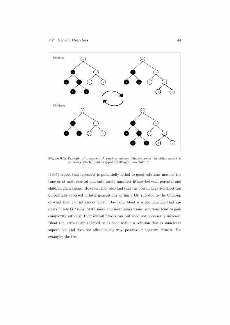
9.2 Genetic Operators 44
a
or
> -
ed+
cb
a
and
* +
cb
a
or
* -
edb a
and
> +
c+
cb
<
d
<
d
Parents:
Children:
e
e
e
Figure 9.1: Example of crossover: A random subtree (shaded nodes) in either parent israndomly selected and swapped resulting in two children.
(1995) report that crossover is potentially lethal to good solutions most of the
time or at most neutral and only rarely improves fitness between parental and
children generations. However, they also find that the overall negative effect can
be partially reversed in later generations within a GP run due to the build-up
of what they call introns or bloat. Basically, bloat is a phenomenon that ap-
pears in late GP runs. With more and more generations, solutions tend to gain
complexity although their overall fitness can but need not necessarily increase.
Bloat (or introns) are referred to as code within a solution that is somewhat
superfluous and does not affect in any way, positive or negative, fitness. For
example, the tree
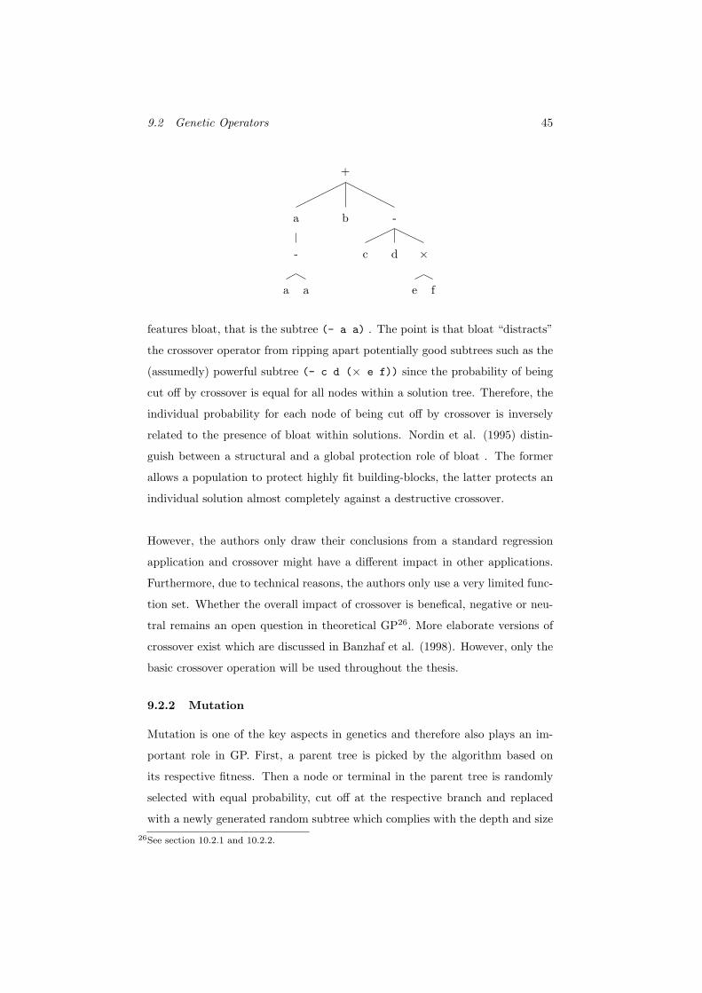
9.2 Genetic Operators 45
+
a
-
a a
b -
c d ×
e f
features bloat, that is the subtree (- a a) . The point is that bloat “distracts”
the crossover operator from ripping apart potentially good subtrees such as the
(assumedly) powerful subtree (- c d (× e f)) since the probability of being
cut off by crossover is equal for all nodes within a solution tree. Therefore, the
individual probability for each node of being cut off by crossover is inversely
related to the presence of bloat within solutions. Nordin et al. (1995) distin-
guish between a structural and a global protection role of bloat . The former
allows a population to protect highly fit building-blocks, the latter protects an
individual solution almost completely against a destructive crossover.
However, the authors only draw their conclusions from a standard regression
application and crossover might have a different impact in other applications.
Furthermore, due to technical reasons, the authors only use a very limited func-
tion set. Whether the overall impact of crossover is benefical, negative or neu-
tral remains an open question in theoretical GP26. More elaborate versions of
crossover exist which are discussed in Banzhaf et al. (1998). However, only the
basic crossover operation will be used throughout the thesis.
9.2.2 Mutation
Mutation is one of the key aspects in genetics and therefore also plays an im-
portant role in GP. First, a parent tree is picked by the algorithm based on
its respective fitness. Then a node or terminal in the parent tree is randomly
selected with equal probability, cut off at the respective branch and replaced
with a newly generated random subtree which complies with the depth and size26See section 10.2.1 and 10.2.2.
9.3 Fitness Function and Selection 46
parameters for the respective GP run in order to avoid excessive bloat27. After
this procedure, the child tree is inserted into the new population. Mutation
basically aims at introducing (hopefully promising) new genetic material into
the gene pool.
9.2.3 Reproduction
Reproduction is the easiest operator in GP. It is asexual, meaning that a mem-
ber of the population is chosen based on fitness and copied unchanged into the
next generation28. Reproduction constitutes so-to-say a safe haven for (already
good) solutions to be carried over to the next generation since the competing
crossover operator must not necessarily yield better offspring. Therefore, re-
production ensures that a pre-defined proportion of good genes is passed on to
the next generation without suffering from the effects of crossover and mutation.
More genetic operators like permutation, editing and encapsulation are de-
scribed in Koza (1992) and Banzhaf et al. (1998). However, these operators
will not play a role in the subsequent discussion.
9.3 Fitness Function and Selection
Fitness is defined as a measure of how well a solution candidate is adapted to
the environment. The primary purpose of fitness within GP is to determine
the quality of a solution in order to assign individual probabilites for passing on
genes to the next generation. Fitter candidates should be allowed to live on with
a higher probability than less fit solutions. The selection algorithm determines
the way an individual is selected for crossover, mutation and reproduction. A
variety of selection schemes exist with so-called fitness-proportional selection
being the most popular. Given a population of n individuals with respective
fitness f(i) ∀ i = 1, ..., n, the probability pi for individual i to pass on its traits
to the next generation (via crossover, mutation or reproduction) under fitness-
proportional selection is given as27The newly generated subtree is created again by using either the full, grow or ramped half-
and-half method. See section 9.1.4.28Similarly to cloning in genetics. For some reason, the term reproduction rather than cloning
is used in GP literature.
9.4 Parameter Choice 47
pi =f(i)∑ni=1 f(i)
. (9.1)
Another important selection algorithm is the so-called tournament selection.
Rather than evaluating an entire population, a subset of the population is ran-
domly chosen. The member solutions contained in this subset then compete
against each other. The better solutions are cleared for reproduction with mu-
tation and replace the worse solutions. They are then inserted back in the pop-
ulation. By working with subsets of populations, tournament selection saves a
considerable amount of CPU time which is why it has become a popular tool in
GP. When using tournament selection, an additional parameter for controlling
tournament size ts has to be set. A small ts results in a low selection pres-
sure, a high ts in a higher selection pressure. This potentially helps to quickly
achieve convergence (that is, no better solutions can be found in further gen-
erations) within a GP run. However, only fitness-proportional selection will be
used throughout the thesis.
9.4 Parameter Choice
According to Koza (1992), the most important parameters are the population
sizeM and the maximum number of generations Gmax. Depending on the com-
plexity of the problem to be solved, higher values for these parameter tend to
yield better solutions at the cost of increased CPU time. As much of GP is
based on heuristics, there is no general rule as to how to optimally set param-
eters. Instead, Koza (1992) suggests a rule-of-thumb approach that has shown
decent performance across a variety of applications from different fields29. In
GP literature, the so-called Koza tableau is an established way of presenting a
particular GP setup. An example is given in Table 9.1.
9.5 A Basic GP Run
Summarizing the discussion so far, a basic GP run involves the following steps:29In Koza (1992), applications range from artifical ants which, by means of GP-optimized move-
ments, gather a maximum of food in their habitat to strategic decision making for game-theoretic applications.
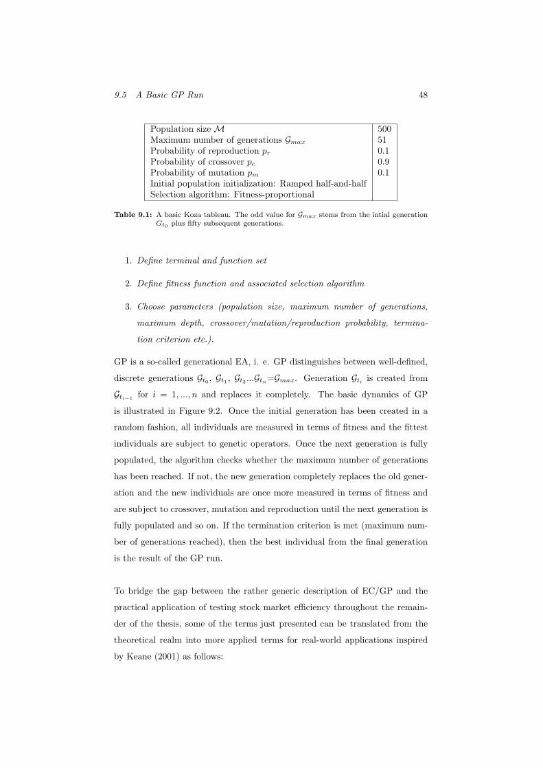
9.5 A Basic GP Run 48
Population size M 500Maximum number of generations Gmax 51Probability of reproduction pr 0.1Probability of crossover pc 0.9Probability of mutation pm 0.1Initial population initialization: Ramped half-and-halfSelection algorithm: Fitness-proportional
Table 9.1: A basic Koza tableau. The odd value for Gmax stems from the intial generationGt0 plus fifty subsequent generations.
1. Define terminal and function set
2. Define fitness function and associated selection algorithm
3. Choose parameters (population size, maximum number of generations,
maximum depth, crossover/mutation/reproduction probability, termina-
tion criterion etc.).
GP is a so-called generational EA, i. e. GP distinguishes between well-defined,
discrete generations Gt0 , Gt1 , Gt2 ...Gtn=Gmax. Generation Gti is created from
Gti−1 for i = 1, ..., n and replaces it completely. The basic dynamics of GP
is illustrated in Figure 9.2. Once the initial generation has been created in a
random fashion, all individuals are measured in terms of fitness and the fittest
individuals are subject to genetic operators. Once the next generation is fully
populated, the algorithm checks whether the maximum number of generations
has been reached. If not, the new generation completely replaces the old gener-
ation and the new individuals are once more measured in terms of fitness and
are subject to crossover, mutation and reproduction until the next generation is
fully populated and so on. If the termination criterion is met (maximum num-
ber of generations reached), then the best individual from the final generation
is the result of the GP run.
To bridge the gap between the rather generic description of EC/GP and the
practical application of testing stock market efficiency throughout the remain-
der of the thesis, some of the terms just presented can be translated from the
theoretical realm into more applied terms for real-world applications inspired
by Keane (2001) as follows:
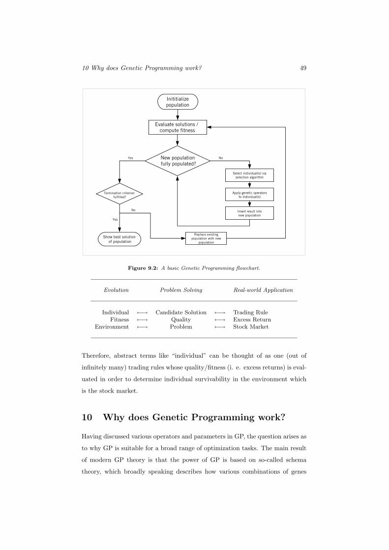
10 Why does Genetic Programming work? 49
Figure 9.2: A basic Genetic Programming flowchart.
Evolution Problem Solving Real-world Application
Individual ←→ Candidate Solution ←→ Trading RuleFitness ←→ Quality ←→ Excess Return
Environment ←→ Problem ←→ Stock Market
Therefore, abstract terms like “individual” can be thought of as one (out of
infinitely many) trading rules whose quality/fitness (i. e. excess returns) is eval-
uated in order to determine individual survivability in the environment which
is the stock market.
10 Why does Genetic Programming work?
Having discussed various operators and parameters in GP, the question arises as
to why GP is suitable for a broad range of optimization tasks. The main result
of modern GP theory is that the power of GP is based on so-called schema
theory, which broadly speaking describes how various combinations of genes

10.1 Prize’s Theorem 50
evolve throughout a GP run. The upcoming discussion aims at shedding some
light at schema theory in an informal way. A more rigorous and comprehensive
account of schema theory is given in Langdon and Poli (2002). But prior to a
more concise discussion of schema theory, a very general result from population
genetics will be presented first.
10.1 Prize’s Theorem
An important analytical result from population genetics was proposed by Prize
(1970) and reformulated by Langdon and Poli (2002) for use with GP. Basically,
the theorem relates the change in frequency of a gene within a population from
generation Gti to Gti+1 to the covariance between individual fitness (=number
of offspring) and the frequency of a given gene in Gti as follows.
∆Q =cov(z, q)
z·∑zi∆qiMz
(10.1)
where:
Q = Frequency of a given gene/linear combination of genes in the population
∆Q = Change in Q from one generation to the next
qi = Frequency of the gene in individual i
∆qi = Change in frequency of the gene in individual i
zi = Number of offspring produced by individual i (≈ fitness of individual i)
z = Mean number of children produced.
M = Size of initial population
(10.1) holds for a single gene or any linear function of any number of genes.
According to Prize (1970), the term at the right in (10.1) cancels out on average,
i. e.
E[∑
zi∆qi]
= 0 (10.2)
and can therefore be omitted. As a matter of personal taste, equation (10.1)
can be written in a slightly more intuitive way by substituting cov(z, q) and
10.2 Schema Theory and Building Block Hypothesis 51
considering (10.2) which yields
∆Q =ρzq · σq · σz
z(10.3)
The most striking feature in (10.3) is the correlation coefficient ρzq which trans-
lates into∆Q ↑ 0 < ρzq ≤ 1
∆Q = 0 ρzq = 0
∆Q ↓ 0 > ρzq ≥ −1
Therefore, if there is a positive relationship between the mean number of chil-
dren (i. e. fitness) and the presence of a particular gene or linear combination of
genes, the respective genetic material will spread further in future generations
whereas the frequency remains unchanged if ρzq = 0. The respective gene/genes
might become extinct in the long run if 0 > ρzq ≥ −1.
Alternatively, Prize prefers to recast equation (10.1) in terms of a linear re-
gression model by substituting cov(z, q) which results in
∆Q =cov(z, q)
z= βzq
σ2q
z(10.4)
with the usual interpretation for the slope coefficient βzq from econometrics.
Interestingly, Prize’s Theorem implicitely considers fitness to be the only factor
affecting gene frequency within a population as, due to (10.2), the effects of
crossover and mutation have no significant impact on average. Despite this
point of view, Altenberg (1994) and Langdon and Poli (2002) argue that the
theorem can be applied to GP as well. However, albeit in some highly artifical
and complex scenarios, Langdon and Poli (2002) show that (10.2) does not
always hold.
10.2 Schema Theory and Building Block Hypothesis
The basic idea as to why GP works is based on schema theory. A schema is
a similarity template that encompasses certain compononents, or to put it in
Koza’s (1992) words: “...the set of all individual trees from a population that
contain, as subtrees, one or more specified subtrees. That is, a schema is a
10.2 Schema Theory and Building Block Hypothesis 52
set...sharing common features”. For example, the schema H=[(+ x y), (× 2 x)]
stands for all trees that include at least one occurence of the subtree (+ x y) or
at least one occurence of the subtree (× 2 x). Under the assumption that trees
that contain the schema H have on average higher fitness, schema theory aims
at analyzing how a schema propagates from generation to generation within a
GP run under the effects of selection, recombination, crossover and mutation.
As a more universal definiton of a schemaH, the “#”-character which stands for
“don’t care” can be used as shown in O’Reilly (1995) and O’Reilly and Oppacher
(1995). For example, the schema H=[(× # x)] stands for all trees that include
any element from the function set F or the terminal set T multiplied by x.
Therefore, the schema H can be matched several times within a single program.
Several schema theorems have been proposed out of which two proposals will be
discussed to give an idea how GP is able to find solutions in the search space.
10.2.1 Koza’s Schema Theorem
The first, albeit informal approach at schema theory was proposed by Koza
(1992). He argues that programs containing good schemata have on average
higher fitness values than competing programs within the same generation.
Higher fitness results in a higher probability of reproduction. Following this line
of reasoning, good schemata will live on and will be combined by the crossover
operator to even better schemata. As it is more likely that crossover disrupts a
complex schema, small schemata will profit from crossover; good but complex
schemata are likely to get disrupted by crossover. This leads to the evolution of
small but powerful schemata throughout the generations of a GP run which are
then combined by crossover to even better solutions. Over time, this leads GP
to search more promising parts of the solution space and, to put it in Koza’s
words ”...concentrates the search of the solution space into subspaces of LISP
S-expressions of ever-decreasing dimensionality and ever-inreasing fitness”. The
final solution is then evolved as a blend of various small but powerful schemata
which is known as the so-called building block hypothesis. Interestingly, Koza
does not further comment on the mutation operator and considers crossover to
be the only operator that powers GP. Consequently, he uses pm = 0 in his real-
world applications. As another issue, Koza considers the crossover operator to
10.2 Schema Theory and Building Block Hypothesis 53
preserve good, albeit small, schemata. This point of view is highly contested.
Banzhaf et al. (1998) point out the ambiguities of the crossover operator which,
due to space constraints, would be inappropriate to discuss here further.
10.2.2 O’Reilly’s Schema Theorem
Koza’s work was formalized by O’Reilly (1995) and O’Reilly and Oppacher
(1995). For fitness-proportionate selection and the special case of pm = 0 (no
mutation), the following can be shown to hold.
E[i(H, t+ 1)] ≥ i(H, t) · f(H, t)f(t)
·
1− pc ·
Pd(H,t)︷ ︸︸ ︷max
h∈Pop(t)Pd(H, h, t)
(10.5)
where i(H, t+1) denotes the number of instances of a schemaH in generation t+
1, i(H, t) the number of instances of schema H in generation t, f(H, t) the mean
fitness of all instances of H30 and f(t) the average fitness in generation t. The
constant pc stands for crossover probability and Pd(H, h, t) for the probability
of destruction of schema H in program h in generation t due to crossover31. As
Pd(H, h, t) varies between different programs (=tree-encoded solutions) within
the same generation, the authors decided to make use of a maximum operator
which results in expression (10.5). However, this causes estimates of i(H, t+1) to
be very conservative as criticized by Banzhaf et al. (1998) and Langdon and Poli
(2002). Furthermore, Pd(H, t) varies from generation to generation. O’Reilly
and Oppacher (1995) admit that due to the variability of Pd(H, t), no real
hypotheses about the propagation and creation of building blocks can be made.
Consequently, the question as to whether crossover has on average a destructive
or preserving effect on building blocks remains open32which illustrates the often
criticized weak theoretical foundation of GP. Furthermore, O’Reilly’s approach
does not consider the effect of mutation which would complicate analysis even
more.30This can be computed as the weighted sum of the fitnesses of the solutions that match H,
using as weights the ratios between the number of instances of H that each program containsand the total number of instances of H in the population.
31This is defined as the ratio between the number of links in the tree fragments plus the numberof links connecting them of H in h and the total number of crossover locations in h.
32In contrast to Koza (1992) who argues that crossover generally preserves good schemata. Adetailed discussion of the ambiguous role of crossover in GP can be found in Banzhaf et al.(1998).
10.2 Schema Theory and Building Block Hypothesis 54
10.2.3 Other Schema Theorems
Other schema theorems apart from O’Reilly (1995) and O’Reilly and Oppacher
(1995) have been proposed. An analytical result for the frequency of a program
in Gt+1 was first proposed by Altenberg (1994), followed by Whigham (1995,
1996a, 1996b), Rosca (1997) and Langdon and Poli (2002).
The difficulty with all the approaches just mentioned is that, although still being
analytically tractable, they exhibit considerable complexity which mirrors the
complexity of the underlying GP structure, particularly the ever changing shape
of solution trees due to the effects of crossover and mutation. Consequently, the
terms derived are quite complex and little intuitive. An in-depth discussion of
these results is given in Langdon and Poli (2002).
10.2.4 Criticisms of Schema Theorems
Schema theorems can be criticized on grounds of being of little use in practical
GP applications. As seen in (10.5) for example, schema theorems usually only
work with expected values which, at the end of a GP run, makes it hard to use
a theorem recursively to predict GP behaviour from generation to generation33.
Furthermore, schema theorems only give lower bounds rather than exact results.
However, Langdon and Poli (2002) overcome these weaknesses at the expense
of tractability. They find some support for the building block hypothesis but
also stress that building blocks need not necessarily be of the short, low-order
and highly fit type.
10.2.5 Genetic Programming vs. Random Search
The discussion so far has pointed out the inherent evolutionary dynamics within
GP that pushes the algorithm to find better solutions from generation to gener-
ation. This makes it highly unlikely that GP solutions are just results of blind
random search. Koza (1992) provides several informal arguments against the
blind random search thesis by stressing the fact that GP usually starts with a
very low fitness in the inital generation34 and then improves fitness throughout33Unless one assumes the population to be infinite which is unhelpful in real-world applications.34Which, by the way, is simple random search unlike the following generations.
10.3 Concluding Remarks 55
the generations often yielding very good solutions at the end of a run. He argues
that this process from zero to surprisingly good solutions alone is proof that GP
is not blind random search. From a more empircal point of view, Koza (1992)
also runs a number of experiments pitting GP against blind random search using
up to 10 million random solutions and finds that random search is in neither
case superior to GP. Rather the opposite is true with GP beating random search
very clearly in all experiments conducted. He concludes that with GP being su-
perior to blind random search, it is highly unlikely that GP just comes up with
solutions that could have been found by blind random search as well.
10.3 Concluding Remarks
For the remainder of the thesis suffice it to say that the informal building block
hypothesis brought forward by Koza (1992), despite some arguable weaknesses35
and side-by-side with the universally applicable Prize’s Theorem has some ex-
planatory power as to how GP seeks the solution space and is able to find
near-optimal solutions to optimization problems. The chapter demonstrates
that GP, while being a suitable and often powerful optimization technique as
seen in the second chapter of the thesis, arguably has a weak theoretical basis
compared to other established techniques.
35See Nordin et al. (1995a, 1995b), Banzhaf et al. (1998) and Langdon and Poli (2002).
56
Part IV
Testing Stock Market Efficiency
via Genetic Programming
11 Introduction
After the literature review in the second chapter and the discussion of the inner
workings of GP in the third chapter it is now time to apply GP to test stock
market efficiency. The basic outline of the chapter is as follows. The next section
briefly reviews the definition and implications of market efficiency followed by
a brief account of market efficiency tests that have been used in the past. The
following section is the nucleus of the thesis and presents the technical setup
and test results for two stock markets, namely the German DAX and Hong
Kong’s main index, the Hang Seng. After an extensive discussion of the results
obtained, the chapter concludes with some final remarks on market efficiency
from a GP point of view.
12 Some brief Remarks on Market Efficiency
First of all it must be emphasized that the upcoming discussion does not even
attempt at giving a comprehensive account of the efficient market literature. It
is safe-to-say that research on this issue is abundant and Fama (1970) already
points out that it is difficult to do justice to all contributions published so far.
Unsurprisingly, the task has not become any easier almost forty years later to put
it mildly. The abundance of research is mirrored in a dedicated category in the
Journal of Economic Literature (JEL) classification scheme36. Consequently,
and to avoid losing focus, only the landmark survey articles on market efficiency
will be considered with the ultimate goal of setting the stage for the author’s
personal contribution to the issue and to show how the GP-based approach fits
into the big picture.36JEL Code G14.
12.1 Definition and Implications of the Efficient Markets Hypothesis 57
12.1 Definition and Implications of the Efficient Markets
Hypothesis
To make the EMH work, two assumptions are necessary (Fama, 1970):
1. Market equilibrium can be expressed in terms of expected returns.
2. The set of all information available at time t concerning a security, φt, is
fully exploited by market participants for formation of expected returns.
Adopting the setup from Fama (1970), condition (1) can be formally expressed
as
E(pi,t+1|φt) = [1 + E(ri,t+1|φt)] pit (12.1)
where pi,t+1 denotes the price of security i (which is a random variable as
indicated by the tilde) at time t + 1, φt the set of all information available at
time t concerning a particular security, ri,t+1 the return of security i at time t+1
(once more a random variable) and pit stands for the price of security i at time t.
The assumption that market equilibrium can be expressed in terms of expected
returns implies that returns in excess of the equilibrium expected returns should
be inexistent provided φt is fully exploited by the market participants. Formally,
the following is assumed to hold. Defining the excess returns of security i at
time t+ 1 as
xi,t+1 = ri,t+1 − E(ri,t+1|φt) (12.2)
where ri,t+1 denotes the observed return at r + 1, the EMH implies that
E(xi,t+1|φt) = 0 (12.3)
i. e. the martingale property must hold. Particularly important for the thesis
at hand is the special case
E(pi,t+1|φt) ≥ pit (12.4)
or alternatively
E(ri,t+1|φt) ≥ 0 (12.5)
12.1 Definition and Implications of the Efficient Markets Hypothesis 58
in (12.1) which, in case of a strict inequality, denotes the submartingale prop-
erty. Therefore, prices may increase but not in excess of expected equilibrium
prices at t + 1. This implies that abnormal returns (returns in excess of equi-
librium expected returns) cannot be achieved by any trading system.
The EMH can be divided into three broad categories which in turn can be
verified empirically (Fama, 1970; Jensen, 1978):
1. Weak efficiency: The information set φt only contains the past prices
of a security up to time t
2. Semi-strong efficiency: All past prices plus all other publicly available
information up to time t are contained in the information set φt
3. Strong efficiency: All information, including insider information up to
time t make up the information set φt.
With the inclusion of risk-adjustment and transaction costs, a more refined ver-
sion of the EMH was formulated by Jensen (1978) who stated that ”a market
is efficient with respect to the information set φt if it is impossible to make
economic profits by trading on the basis of information set φt”, where the term
”economic profits” means risk-adjusted returns net of all costs.
Basically, the thesis revolves around this particular issue. Under the EMH,
no trading system should be able to beat a simple buy-and-hold strategy in
the same security (or index as will be the case in the subsequent analysis). If
a GP-powered trading system defies the implications stated above after risk-
adjustment and inclusion of appropriate transaction costs, the validity of the
EMH may become questionable, at least during certain periods of time in a se-
curity market. In the thesis at hand, it is up to GP to find such trading systems,
provided they exist at all.
Another important concept in connection with the EMH is the random walk
hypothesis first brought forward by Bachelier (1900) and Samuelson (1965).
12.2 Techniques for Testing Market Efficiency 59
Basically, if prices follow a random walk, price changes should be white noise
which is in line with the EMH. Therefore, the random walk hypothesis im-
plicitely addresses EMH issues as well so as a by-product, the random walk
hypothesis will be tested as well to some degree in the thesis at hand.
12.2 Techniques for Testing Market Efficiency
As pointed out in the introduction of the chapter, the author does not even
remotely attempt at giving a review of EMH literature. Instead, only the basic
test techniques will be briefly discussed in order to see how GP fits into the
picture. Fama (1991) proposes three categories for EMH tests, namely
• tests for return predictability (weak efficiency)
• event studies (semi-strong efficiency)
• tests for private information (strong efficiency).
The empirical literature published so far mainly focuses on the first and second
EMH category (weak and semi-strong efficiency) whereas the third (strong effi-
ciency), which is a rather strong assumption, has only been rarely tested. The
thesis itself can be categorized under the weak efficiency tests as only input data
based on closing prices will be used.
As Fama (1970) points out, any empirical test for efficiency requires a defi-
nition of the information set φt. It is clear that there is no general consensus
as to what constitutes φt. By picking a reasonable selection of variables, only
one out of infinitely many information sets can be used to test for market effi-
ciency37. As a workaround, tests have to be based on a proxy set of information
that most investors agree on. This applies to both semi-strong and strong-form
efficiency tests. In contrast, weak-form tests are quite easy to implement as
price/return data are clearly defined and readily available at low cost to virtu-
ally every market participant. Weak and semi-strong empirical EMH tests may
be based on (in no particular order):
37For example, mostly economic variables should be contained in φt whereas some investorsmight prefer the inclusion of somewhat far-fetched variables such as the frequency of sunspotsor the amount of rain on Wall Street. Therefore, the one and only φt does not exist.
12.2 Techniques for Testing Market Efficiency 60
• Statistical tests of indepedence/tests of white noise (random walk) (Fama,
1965)
• Return predictability tests/seasonal anomalies tests (Fama and French,
1988)
• Event studies (Miller and Reilly, 1987)
• Direct tests of trading rules/trading systems (Alexander, 1961; Brock et
al., 1992; Ratner and Leal, 1999)
• Volatility tests (Shiller, 1979)
• Cointegration tests/tests for bubbles (Islam and Watanapalachaikul, 2005)
whereas strong-form empirical EMH tests mainly rely on tests of private, i.e.
insider information. Agents having some sort of insider information concerning
a security may be corporate insiders, stock exchange specialists, stock analysts
and money managers. As a classic example, Niederhoffer and Osborne (1966)
focus on the informational advantage of stock exchange specialists. Other exam-
ples of strong-form tests include Scholes (1972), Jaffe (1974) and Seyhun (1986).
As can be seen in the enumeration above, the thesis at hand being based on
computer-generated and GP-optimized trading rules fits into the category of
direct tests of trading rules/systems pioneered by Alexander (1961)38. The list
above is by no means exhaustive, however most of the existing literature on the
EMH fits into one of the categories just mentioned. A detailed account of EMH-
tests can be found in Fama (1970, 1991) and Bollerslev and Hodrick (1994).
Summarizing the discussion and considering Islam and Watanapalchaikul (2005),
major challenges to the EMH arise from
• empirical tests whose results do not support EMH
• shortcomings in statistical and mathematical modelling38It should be noted that the exisiting GP/GA literature as discussed in the second chapter
fits into this category as well. Another sub-category of trading system tests is the abundantliterature on neural networks. This gives just a glimpse of the vast empirical EMH literature.
13 Testing Stock Market Efficiency via Genetic Programming 61
• predictability of excess volatility and mean reversion
• speculative bubbles
• complex nonlinear dynamics in financial markets.
The last item is particularly important for the thesis as GP has been mainly
designed for nonlinear optimization. Having roughly outlined the fields of EMH
research, it is now time to set the stage for a GP-based approach to testing the
EMH.
13 Testing Stock Market Efficiency via Genetic
Programming
13.1 Introduction
The upcoming discussion is made up of two subsections. The first deals with
implementation issues and describes the setup necessary to find trading rules
using GP. The remaining subsection is the core of this chapter and the thesis
presenting, analyzing and discussing the out-of-sample results obtained from
running the GP algorithm for two stock markets, namely the DAX and the
Hang Seng. The choice of the DAX and Hang Seng is motivated by the lack of
GP-related research on these markets. Additionally, it is tempting to compare
the results obtained as the two markets fall into different categories: The highly
liquid and well-established DAX which is more likely to be efficient vs. a highly
volatile emerging market where subtle inefficiencies may be, if they exist at all,
easier to find. It is up to GP to uncover possible subtle inefficiencies by deriving
optimized trading rules.
13.2 Implementation
13.2.1 Technical Aspects
In order to implement a GP algorithm, the first issue is the choice of a suitable
software framework. The original implementation as proposed by Koza (1992)
is based on the LISP language which is one of the oldest high-level programming
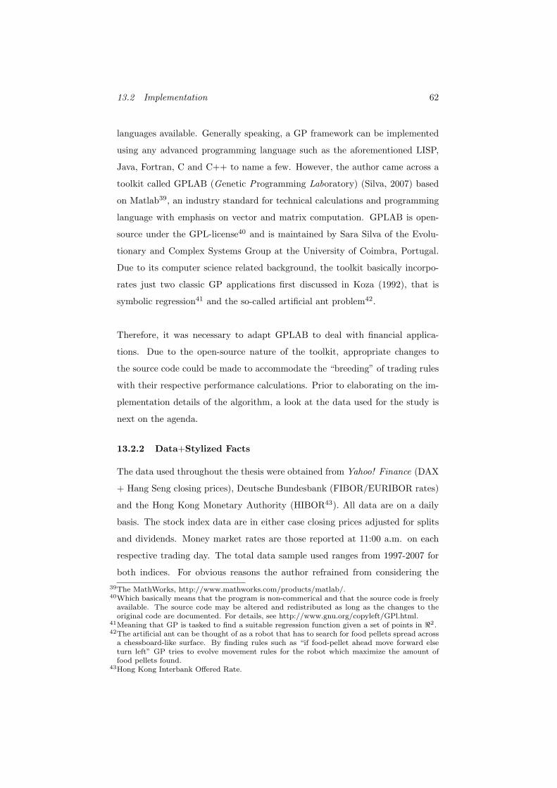
13.2 Implementation 62
languages available. Generally speaking, a GP framework can be implemented
using any advanced programming language such as the aforementioned LISP,
Java, Fortran, C and C++ to name a few. However, the author came across a
toolkit called GPLAB (Genetic Programming Laboratory) (Silva, 2007) based
on Matlab39, an industry standard for technical calculations and programming
language with emphasis on vector and matrix computation. GPLAB is open-
source under the GPL-license40 and is maintained by Sara Silva of the Evolu-
tionary and Complex Systems Group at the University of Coimbra, Portugal.
Due to its computer science related background, the toolkit basically incorpo-
rates just two classic GP applications first discussed in Koza (1992), that is
symbolic regression41 and the so-called artificial ant problem42.
Therefore, it was necessary to adapt GPLAB to deal with financial applica-
tions. Due to the open-source nature of the toolkit, appropriate changes to
the source code could be made to accommodate the “breeding” of trading rules
with their respective performance calculations. Prior to elaborating on the im-
plementation details of the algorithm, a look at the data used for the study is
next on the agenda.
13.2.2 Data+Stylized Facts
The data used throughout the thesis were obtained from Yahoo! Finance (DAX
+ Hang Seng closing prices), Deutsche Bundesbank (FIBOR/EURIBOR rates)
and the Hong Kong Monetary Authority (HIBOR43). All data are on a daily
basis. The stock index data are in either case closing prices adjusted for splits
and dividends. Money market rates are those reported at 11:00 a.m. on each
respective trading day. The total data sample used ranges from 1997-2007 for
both indices. For obvious reasons the author refrained from considering the39The MathWorks, http://www.mathworks.com/products/matlab/.40Which basically means that the program is non-commerical and that the source code is freely
available. The source code may be altered and redistributed as long as the changes to theoriginal code are documented. For details, see http://www.gnu.org/copyleft/GPl.html.
41Meaning that GP is tasked to find a suitable regression function given a set of points in <2.42The artificial ant can be thought of as a robot that has to search for food pellets spread across
a chessboard-like surface. By finding rules such as “if food-pellet ahead move forward elseturn left” GP tries to evolve movement rules for the robot which maximize the amount offood pellets found.
43Hong Kong Interbank Offered Rate.
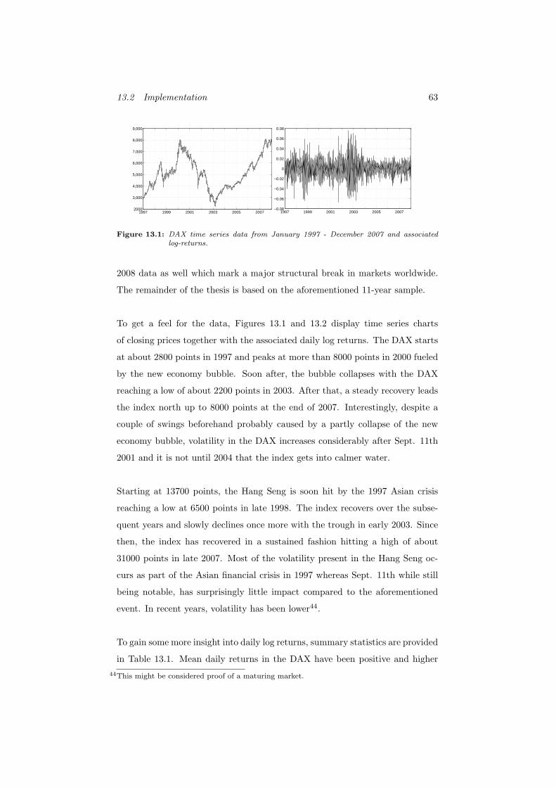
13.2 Implementation 63
1997 1999 2001 2003 2005 20072000
3,000
4,000
5,000
6,000
7,000
8,000
9,000
1997 1999 2001 2003 2005 2007−0.08
−0.06
−0.04
−0.02
0
0.02
0.04
0.06
0.08
Figure 13.1: DAX time series data from January 1997 - December 2007 and associatedlog-returns.
2008 data as well which mark a major structural break in markets worldwide.
The remainder of the thesis is based on the aforementioned 11-year sample.
To get a feel for the data, Figures 13.1 and 13.2 display time series charts
of closing prices together with the associated daily log returns. The DAX starts
at about 2800 points in 1997 and peaks at more than 8000 points in 2000 fueled
by the new economy bubble. Soon after, the bubble collapses with the DAX
reaching a low of about 2200 points in 2003. After that, a steady recovery leads
the index north up to 8000 points at the end of 2007. Interestingly, despite a
couple of swings beforehand probably caused by a partly collapse of the new
economy bubble, volatility in the DAX increases considerably after Sept. 11th
2001 and it is not until 2004 that the index gets into calmer water.
Starting at 13700 points, the Hang Seng is soon hit by the 1997 Asian crisis
reaching a low at 6500 points in late 1998. The index recovers over the subse-
quent years and slowly declines once more with the trough in early 2003. Since
then, the index has recovered in a sustained fashion hitting a high of about
31000 points in late 2007. Most of the volatility present in the Hang Seng oc-
curs as part of the Asian financial crisis in 1997 whereas Sept. 11th while still
being notable, has surprisingly little impact compared to the aforementioned
event. In recent years, volatility has been lower44.
To gain some more insight into daily log returns, summary statistics are provided
in Table 13.1. Mean daily returns in the DAX have been positive and higher44This might be considered proof of a maturing market.
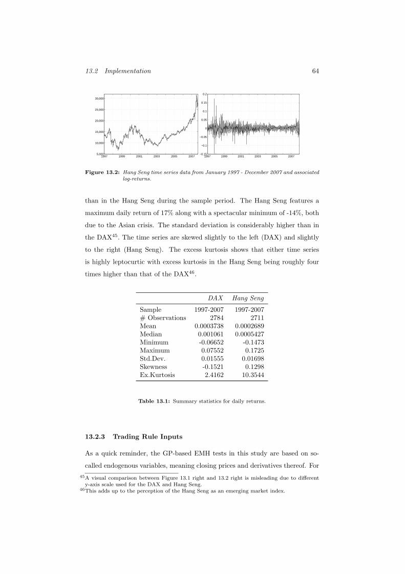
13.2 Implementation 64
1997 1999 2001 2003 2005 20075,000
10,000
15,000
20,000
25,000
30,000
1997 1999 2001 2003 2005 2007−0.15
−0.1
−0.05
0
0.05
0.1
0.15
0.2
Figure 13.2: Hang Seng time series data from January 1997 - December 2007 and associatedlog-returns.
than in the Hang Seng during the sample period. The Hang Seng features a
maximum daily return of 17% along with a spectacular minimum of -14%, both
due to the Asian crisis. The standard deviation is considerably higher than in
the DAX45. The time series are skewed slightly to the left (DAX) and slightly
to the right (Hang Seng). The excess kurtosis shows that either time series
is highly leptocurtic with excess kurtosis in the Hang Seng being roughly four
times higher than that of the DAX46.
DAX Hang Seng
Sample 1997-2007 1997-2007# Observations 2784 2711Mean 0.0003738 0.0002689Median 0.001061 0.0005427Minimum -0.06652 -0.1473Maximum 0.07552 0.1725Std.Dev. 0.01555 0.01698Skewness -0.1521 0.1298Ex.Kurtosis 2.4162 10.3544
Table 13.1: Summary statistics for daily returns.
13.2.3 Trading Rule Inputs
As a quick reminder, the GP-based EMH tests in this study are based on so-
called endogenous variables, meaning closing prices and derivatives thereof. For45A visual comparison between Figure 13.1 right and 13.2 right is misleading due to different
y-axis scale used for the DAX and Hang Seng.46This adds up to the perception of the Hang Seng as an emerging market index.
13.2 Implementation 65
the application at hand, rather traditional and basic input variables have been
chosen. All inputs are based on end-of-day closing prices adjusted for splits
and dividends. Figures 13.1 and 13.2 show some degree of non-stationarity,
particulary for the Hang Seng47. As this may be harmful to GP performance,
the data have been normalized by dividing each closing price by its respective
250-day moving average which is the standard procedure used in Neely et al.
(1997), Neely and Weller (1999) and Allen and Karjalainen (1999)48. Since
this would mean the loss of approximately one year consisting of roughly 250
trading days for either data sample, data from 1996 have been added to compute
normalized data for the core input sample 1997-2007. After normalization, the
data hover around 1. As most of the data are between 0.8 and 1.2, constants
in steps of 0.01 within this interval have been chosen as additional terminals49
making rules such as X1 < 1.04 possible. A refined input with smaller terminal
steps and/or a wider interval for terminals would not necessarily result in better
rules by spanning a solution space that may be too big for GP to perform
satisfactory (Koza, 1992). Despite normalization of closing prices, all return
calculations are based on non-normalized data. In addition to closing prices,
moving averages, max- and minima and lagged variables are available as input
as well. All three indicators are derived from the normalized closing price series.
The moving average indicator of length θ at time t is defined as:
MAt(θ) =1θ
θ−1∑i=0
Pt−i ∀θ ∈ 1, 2, 3, .... (13.1)
Maxima and minima over different time frames θ are implemented as:
Pmaxt (θ) = Max [Pt−1, ..., Pt−θ] (13.2)
Pmint (θ) = Min [Pt−1, ..., Pt−θ] (13.3)
47For a formal investigation, a unit-root test would be necessary. The author is aware of thisbut deliberately chose to skip the test in order to avoid losing focus. Even if the hypothesisof a unit-root would be rejected for the DAX, it would not seem sensible to conduct furtherGP studies with non-normalized data for the DAX and normalized data for the Hang Seng(which clearly is non-stationary).
48In fact, the use of non-normalized data has been shown to degrade GP performance (Chen etal., 2008).
49See chapter 9.1.1.
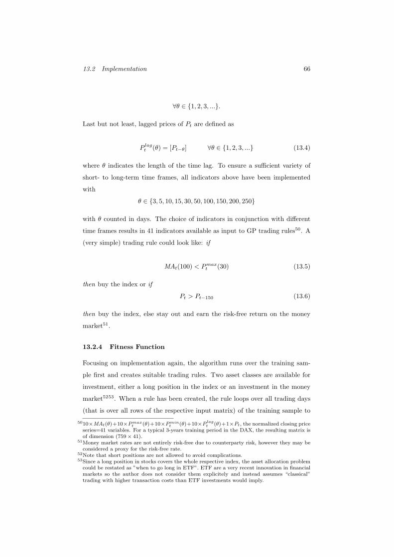
13.2 Implementation 66
∀θ ∈ 1, 2, 3, ....
Last but not least, lagged prices of Pt are defined as
P lagt (θ) = [Pt−θ] ∀θ ∈ 1, 2, 3, ... (13.4)
where θ indicates the length of the time lag. To ensure a sufficient variety of
short- to long-term time frames, all indicators above have been implemented
with
θ ∈ 3, 5, 10, 15, 30, 50, 100, 150, 200, 250
with θ counted in days. The choice of indicators in conjunction with different
time frames results in 41 indicators available as input to GP trading rules50. A
(very simple) trading rule could look like: if
MAt(100) < Pmaxt (30) (13.5)
then buy the index or if
Pt > Pt−150 (13.6)
then buy the index, else stay out and earn the risk-free return on the money
market51.
13.2.4 Fitness Function
Focusing on implementation again, the algorithm runs over the training sam-
ple first and creates suitable trading rules. Two asset classes are available for
investment, either a long position in the index or an investment in the money
market5253. When a rule has been created, the rule loops over all trading days
(that is over all rows of the respective input matrix) of the training sample to
5010×MAt(θ)+10×Pmaxt (θ)+10×Pmin
t (θ)+10×P lagt (θ)+1×Pt, the normalized closing price
series=41 variables. For a typical 3-years training period in the DAX, the resulting matrix isof dimension (759× 41).
51Money market rates are not entirely risk-free due to counterparty risk, however they may beconsidered a proxy for the risk-free rate.
52Note that short positions are not allowed to avoid complications.53Since a long position in stocks covers the whole respective index, the asset allocation problem
could be restated as ”when to go long in ETF”. ETF are a very recent innovation in financialmarkets so the author does not consider them explicitely and instead assumes “classical”trading with higher transaction costs than ETF investments would imply.
13.2 Implementation 67
determine whether the particular rule is true or false for a particular trading day.
The result is a binary matrix with dimensions (1×759) for 3-years training and
(1 × 1265) for 5-years training with “0” indicating an out-of-the-market posi-
tion for a particular trading day and “1” indicating an in-the-market position54.
As all calculations are based on end-of-day closing prices, the position sug-
gested by the GP trading rule is entered into the following day. This introduces
a so-called slippage error. Slippage means that the very first quote the next
day is not necessarily equal to the closing price the day before. However, this
problem which is also pointed out in Dempster and Jones (2001) is dealt with
by using a conservative estimate of transaction costs. Therefore, part of this
slippage is accounted for in a relatively high transaction cost (25 and 50 basis
points).
Focusing again on the binary matrix indicating which position to take each day,
a zero position for a particular day triggers a FIBOR/EURIBOR or HIBOR
investment the next day. The daily return from an out-of-the-market position
equals
rf (t) = log(1 + rf,monthly)
δ(13.7)
with rf,monthly denoting the prevailing 1-month money market rate. δ indicates
the mean number of trading days per year. As seen in Table 13.1, the total
number of trading days for the DAX over 11 years is 2785 which equals δ = 253
trading days per year on average. Things look slightly different for the Hang
Seng. As the total number of trading days is just 2723, the respective mean is
247 so that in the Hang Seng case, the equation above is used with δ = 247
trading days.
The shortest money market rate is the 1-month interbank rate in both markets
and will be used throughout the thesis. All calculations are based on business
days rather than actual calendar days. Therefore, in case of a prolonged out-of-54Matrix dimensions are based on the assumption that the mean number of trading days in the
DAX is 253. For the Hang Seng, the mean number of trading days is 247 so the respectivematrices become slightly shorter.
13.2 Implementation 68
market position, the code checks whether an out-position exists for more than
22 business days which approximately equals a calendar month with 30 days.
If so, the investment has reached maturity and if an out-position has to be
prolonged further, a rollover occurs adapting the respective new 1-month rate.
This rule of thumb introduces a marginal error since EURIBOR and HIBOR
are calculated as actual360 . It might happen that a prolonged out-position actually
misses the correct revolving date since 22 business days may mean a 30-days+
position in actual calendar terms due to weekends and national holidays. The
consideration of business days only has been chosen to avoid the tedious exer-
cise of determing weekends and national holidays for the extensive data samples
used in this study. As daily variances of interbank rates are quite low compared
to stock prices, the error from missing the correct rollover date by 1- or 2 days
may be considered as marginal. Last but not least, the use of δ = 247, 253
rather than δ = 360 in (13.7) at first sight overstates the return from a money-
market position but the effect should even out since only business days earn
interest rather than calendar days. The difficulties of calculating appropriate
daily risk-free rates from longer maturities are discussed in Vaihekoski (2009).
To sum up the discussion, calculation of daily risk-free rates is not abolutely
precise but the total effect on GP returns should be marginal. Some authors of
GP studies do not even include the possibility for earning a risk-free rate at all
(see Chen et al., 2002)55.
If an in-the-market position is indicated by GP, the return πi (open position
at bi, close, sell at si) including transaction costs c is calculated as (Allen and
Karjalainen, 1999):
55The author of the thesis had an informal discussion with a senior fund manager during whichthe manager pointed out that money market returns are so low compared to a strategy thatis in the market at the right time for just a couple of days that the money market could besafely excluded from the study. Nevertheless, the author decided to include at least a proxyfor the risk-free rate.
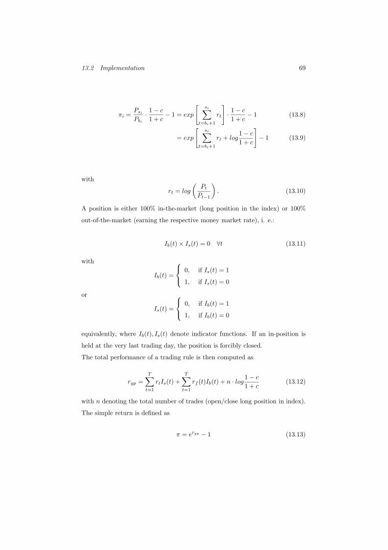
13.2 Implementation 69
πi =Psi
Pbi
· 1− c1 + c
− 1 = exp
[si∑
t=bi+1
rt
]· 1− c
1 + c− 1 (13.8)
= exp
[si∑
t=bi+1
rt + log1− c1 + c
]− 1 (13.9)
with
rt = log
(PtPt−1
). (13.10)
A position is either 100% in-the-market (long position in the index) or 100%
out-of-the-market (earning the respective money market rate), i. e.:
Ib(t)× Is(t) = 0 ∀t (13.11)
with
Ib(t) =
0, if Is(t) = 1
1, if Is(t) = 0
or
Is(t) =
0, if Ib(t) = 1
1, if Ib(t) = 0
equivalently, where Ib(t), Is(t) denote indicator functions. If an in-position is
held at the very last trading day, the position is forcibly closed.
The total performance of a trading rule is then computed as
rgp =T∑t=1
rtIs(t) +T∑t=1
rf (t)Ib(t) + n · log 1− c1 + c
(13.12)
with n denoting the total number of trades (open/close long position in index).
The simple return is defined as
π = ergp − 1 (13.13)
13.2 Implementation 70
and the return from a buy-and-hold strategy over the respective period is
rbh =T∑t=1
rt + log1− c1 + c
. (13.14)
Then the fitness=excess return of a trading rule is calculated as
∆r = rgp − rbh. (13.15)
The evolutionary process of creating a rule and evaluating its performance as
described in equations (13.8)-(13.15) is repeated over and over again until the
number of individuals and number of generations requirement of the GP algo-
rithm has been met56.
Trading rules should be robust against overfitting. This is sometimes difficult
as the training data may contain some noise patterns that might get picked
up by the GP algorithm. However, finding technical trading rules is based on
the assumption that there are some regularities in the underlying data. Telling
these apart from noise patterns is one of the tasks GP has to deal with. Ide-
ally, GP should be able to generalize trading rules beyond the training sample.
Therefore, the data samples used in this study are divided into training and
subsequent out-of-sample periods.
The fittest trading rule from in-sample is applied out-of-sample. Return cal-
culation is the same as in-sample except that only the best trading rule found
during training is applied out-of-sample57.
It is paramount to the analysis that excess returns still persist after appropriate
risk adjustment. As a measure of return to risk, the Sortino ratio (Sortino and
Price, 1994) will be used throughout the thesis. The original implementation
of the GP algorithm included the classic Sharpe ratio (Sharpe, 1966) as risk-
adjusted performance measure. However, it turned out during evaluation of the
trading rules that returns frequently did not meet the implicit requirement of56The process is depicted in Figure 9.2.57Therefore, out-of-sample calculations are straightforward in contrast to the complex evolu-
tionary breeding of rules during in-sample training.
13.2 Implementation 71
being normally distributed. Rules that spent prolonged periods of time out-
of-the-market were particularly affected by this since they tend to gather a lot
of very small absolute returns from money market investments while incurring
substantial losses during a few in-the-market days (excess kurtosis). This pat-
tern led to overly optimistic Sharpe ratios and consequently, the Sharpe ratio
approach had to be abandoned in order to avoid biased results.
The Sortino ratio is a variation of the Sharpe ratio that is more robust when
dealing with skewed distributions (Chaudry and Johnson, 2008). As a distinct
feature, it only considers downside deviation (DD) (Sortino and van der Meer,
1991) that occurs when returns fall below the so-called minimum acceptable
rate of return (MAR). When returns exceed the MAR, the respective upside
risk is not taken into account which is intuitive from an investor’s point of view.
Therefore, downside risk is penalized whereas upside risk is neutral within the
Sortino ratio framework58. Adopting the notation from Chaudry and Johnson
(2008), the Sortino ratio can be formally defined as follows. The mth order
lower partial moment is defined as:
LPM =1N
N∑t=1
(rt − L)mI(rt ≤ L), (13.16)
with
I =
0, if rt > L
1, if rt ≤ L
where L is some threshold, N the number of returns and rt the return at time
t. (13.16) is a general risk measure and can be adapted for a number of special
cases with one of them being DD. Setting m = 2 and L = MAR in (13.16) yields
the downside deviation:
DD2 =1N
N∑t=1
(rt −MAR)2I(rt ≤ MAR) (13.17)
58As a sidenote, Chen et al. (2008) suggest to take downside risk into account in future GPstudies.
13.2 Implementation 72
with
I =
0, if rt > MAR
1, if rt ≤ MAR
Next is the choice of a suitable MAR. As the Sortino ratio serves as a per-
formance measurement geared towards evaluating mutual fund performance, a
natural choice would be the risk-free rate. Alternatively, a benchmark rate like
the return on an index could be chosen. However, in the thesis at hand, MAR
has been set to zero. This is mainly for convenience as it simplifies calculation.
However, other benchmarks like those mentioned above could have been chosen
as well. With α defined as the average return minus benchmark (MAR = 0),
the Sortino ratio can be stated as
Sortino =α
DD. (13.18)
The results obtained from the trading rules using (13.18) are based on daily
data. To annualize the results, (13.18) is scaled by√m, i.e.
Sortino(p.a.) =α
DD×√m. (13.19)
All Sortino ratios reported in the subsequent discussion are annualized with
m = 253 for the DAX and m = 247 for the Hang Seng, respectively. Now that
fitness calculation of GP trading rules has been discussed it is time to elaborate
on the choice of datasets on which the trading rules are generated and tested.
13.2.5 Choice of In- and Out-of-Sample Periods
As seen in Allen and Karjalainen (1999), Neely (2003b) and others, sample
periods for GP-optimized trading rules are typically divided into an in-sample
training and consecutive out-of-sample application period. In contrast to other
contributions59, the author chose a rather recent sample (1997-2007) for either
59See for example Allen and Karjalainen (1999) who use data from 1929-1995.

13.2 Implementation 73
index. Consequently, the extremely long periods in Allen and Karjalainen (1999)
are not feasible60. As training sample, 3-, and 5-years have been chosen which
is roughly in line with existing literature. The idea is that longer in-sample pe-
riods provide more training input to the GP algorithm so that it can potentially
pick up the distinctive features of a time series more easily. Shorter training
periods (less than 3 years) do not seem sensible and are not used in any of the
existing papers the author is aware of. The author conducted some experiments
with 10-year training periods but due to the limits of the overall data sample,
this scenario could only be tested with a single one-year out-of-sample period.
Unfortunately, the results were poor despite the possibility for GP to train with
a set of data that includes a full economic cycle. Consequently, the author did
not further investigate this issue and results will not be covered further in the
subsequent analysis.
Out-of-sample periods in the thesis range from 1- to 3-years. The rationale
for not using longer periods is that the author believes that nowadays markets
are so fast-paced and in constant change that any long-term GP approach is
likely ill-fated. This view is supported by Ammann and Zenkner (2003) who
use a rather recent data sample of the S&P 500 and find that even the best
rules (which at best match the performance of buy-and-hold) implode after less
than 2 years time. To summarize, the following periods have been analyzed:
Training periods in-sample : out-of-sample
• 3:1
• 3:2
• 3:3
• 5:1
• 5:2
• 5:3
for either index. For example, 5:2 reads “5-years in-sample training followed by
2-years out-of-sample data” and so on.
60The DAX was nonexistent until 1987.

13.2 Implementation 74
A rolling time window approach extensively used throughout the literature61
has been adopted for the upcoming analysis. For a 3-year training period, the
first 3 years (1997-1998-1999) are taken as breeding ground for GP-optimized
trading rules. The best rule found during a run on the training sample is then
applied out-of-sample, i.e. the year (2000) data for the 1-year out-of-sample
scenario. The time window then rolls to the right on an imaginary time scale
axis. The next training sample is comprised of the years (1998-1999-2000), out-
of-sample is (2001) and so on. The same applies to the 5-year training samples
and the 2-and 3-years out-of-sample scenarios.
The rationale behind the use of separate in-sample training/learning and out-
of-sample application data is obvious. As the most promising rule has evolved
from training data and is subsequently applied out-of-sample, the final result
is not based on ex-post data snooping. So in a certain sense, GP-optimized
trading rules are ex-ante optimal.
As a final remark, some contributions such as as Allen and Karjalainen (1999)
and Neely (2003b) make use of so-called validation periods set in between the
training and out-of-sample period. Promising trading rules are first tested dur-
ing the validation period and the best rule is then allowed to proceed to out-
of-sample testing. Therefore, a further level of selection is introduced so that,
in theory, the problem of overfitting is alleviated. While the concept is in-
tuitively appealing, Navet and Chen (2007) point out that “the usefulness of
validation,..., is still an open question” in their recent survey article. They argue
that validation may be useful in stable markets62 but also point out that it may
be potentially harmful when markets are moving fast into different directions.
Rules learned during the training sample would be outdated when they finally
reach the out-of-sample phase thus resulting in poor performance.
Having just argued that out-of-sample periods have been deliberately chosen
to be quite short (1-3 years) in order to adapt to today’s fast-paced markets,
61See Allen and Karjalainen (1999), Ammann and Zenkner (2003) and Neely (2003b).62Meaning markets where training, validation and out-of-sample set roughly feature the same
pattern.
13.2 Implementation 75
the author of the thesis chose not to include a validation period63. Last but not
least, Chen and Kuo (2003a) even question the usefulness of validation periods.
13.2.6 Genetic Programming Setup
First of all, the issue of parameter choice for GP is nicely commented in Chen et
al. (2008): “In particular, GP is notorious for its large number of user-supplied
parameters, and the current research is not enough to allow us to inquire whether
these parameters may impact the performance of GP.”
No less than 62 parameters have to be set in GPLAB prior to a run with some of
them being paramount such as how to initiate the very first generation (ramped
half-and-half), which sampling method to use (fitness-proportional selection)
etc. while others are less important and are only concerned with administrative
overhead. In order to avoid excessive discussion of parameter settings, only the
most important ones will be briefly addressed. Further information on the com-
plete parameter set used is available from the author upon request.
The initial generation is created using the ramped half-and-half method64 as
suggested by Koza (1992) to ensure a sufficient variety of starting individuals to
choose from. Selection of individuals is based on fitness-proportional selection65.
The two main operators driving evolution are crossover and mutation. Both are
used with automatic probability adjustment66. The third operator used is repro-
duction (copy & paste of individuals between two generations) which is always
fixed at 10% probability throughout all GP runs.
While the overall goal of the thesis is to test for market efficiency making as
good use of GP methodology as possible, some minor confessions are necessary63As a side effect, inclusion of a validation period would have resulted in higher program code
complexity and even more CPU time.64See 9.1.4.65See chapter 9.3. GPLAB offers tournament selection as well, however this did not improve
upon the results during some casual testing.66This basically means that after creation of the initial generation, mutation and crossover
probabilities are chosen at random. The algorithm keeps track of the origin of the individualsthrough several subsequent generations and adapts operator probabilities based on the fitnessof the individuals obtained so far. If the fittest individuals so far originated from crossover thencrossover probability is increased in subsequent generations, mutation probability is decreasedaccordingly and vice versa. More details can be found in Davis (1989).

13.2 Implementation 76
to make the approach feasible. One of these confessions is that total depth
of trees (and thus trading rule complexity) is limited to 7 levels rather than
allowing GP to freely evolve rules up to very high complexity. This has two
reasons: First, the aim is to find trading rules that are as easily interpretable as
possible (despite the limits set, trees at times still tend to get quite complex and
thus difficult to interpret). Second, from a practical point of view it all boils
down to CPU time. In order to get acceptable performance, tree complexity
has to be limited. Furthermore, is is noteworthy that more complex trees do
not necessarily yield better solutions. The results might even be worse due to
the risk of overfitting67. Chen et al. (2008) find that more complex rules are
not correlated with higher profits. Even more interesting, node complexity of
the successful rules is very often less than 10 in all stock markets used in the
study.
In this context, another parameter comes into play. Based on Silva and Almeida
(2003), GPLAB offers to set a dynamic depth limit. This basically means that
a dynamic slack depth limit is maintained to keep solutions as simple as possi-
ble unless a new solution found is more complex and superior to the solutions
found before68. In this case, the depth limit is slackened to accomodate the
more complex but better rule. However, there is still an absolute depth limit in
place which eventually overrides the dynamic deepening of trees. Though this
technique has not been used in any financial application the author is aware
of, it has proved to contain complexity/bloat quite effectively in non-financial
applications69.
Another parameter deals with which individuals should enter a new generation.
For all runs, the parameter was set to “replace” which basically means that once
all individuals for a new generation have been created, all of them are used to
completely replace the former generation regardless of their fitness70. This is67See Koza (1992) for details.68The dynamic depth limit is set automatically. For example, assuming that the best solution
from the initial generation consists of 4 levels, the dynamic level could be set to 4. Conse-quently, all individuals of the next generation that do not comply with this setting have to befitter than the existing solutions that set the standard, otherwise they will be rejected. Afterthe second generation, a new dynamic level may be set and so on.
69See Silva and Almeida (2003).70Newer individuals need not be fitter than older ones by definition. GPLAB offers elitism as

13.2 Implementation 77
also called generational mode.
Next is the function set used to link the terminals consisting of closing prices,
moving averages, maxima/minima, and lagged prices. The choice of appropri-
ate function sets for GP has been rarely addressed in the literature. Wang and
Soule (2004) investigate the performance of different function sets for different
problems but the results are of little use for the application at hand. Most
notably, they point out that a too large function set may unnecessarily increase
the search space making it difficult for GP to find good solutions.
Therefore, the choice of a suitable function set is just based on intuition and a
basic idea of what the rules might look like71. The functions used in all runs
are:
• +, -, ×, ÷
• ln, sqrt
• <, >
• and, or.
The operators “and” and “or” are of type boolean72 with “and” evaluating as
true if the input arguments are both nonzero and “or” evaluating as true unless
the two input arguments are both zero73. More functions/operators could have
been used as well but some considerations on algorithm efficiency led to the
rejection of a broader function set. As already pointed out, the availability of
too many functions to choose from may result in a dramatically increased search
space rendering GP unable to find acceptable solutions at all74. Therefore, func-
tions such as exp, sin, cos have been deliberately excluded from the function
set. Navet and Chen (2007) point out the lack of guidelines for choosing a suit-
able function set so the decision of omitting exp, sin, cos is rather arbitrary.
Apart from theoretical aspects, some thoughts on the nature of trading rules
an alternative. In this case, the best 50% of the old generation and the best 50% of the newlycreated individuals enter the new generation.
71This may sound like a contradiction as one of GP’s most appealing features is its ability tocome up with innovative and in some way “far-fetched” solutions a human mind would havenever thought of. However, for practical reasons some sort of limited function set has to beused.
72Boolean means that they either evaluate as true=1 or false=0.73This will become clearer later when dealing with the structure of trading rules.74See Koza (1992), Chen et al. (2002), Wang and Soule (2004), Navet and Chen (2007).
13.2 Implementation 78
support the choice of a limited function set. For example, operators like not, ≤
and ≥ have been deliberately omitted as in the first case it might be easier for
the algorithm to find positive rather than negated trading rules. Concerning
the second and third case, it is unlikely that strict equality will arise during a
run75. In contrast, the non-strict cases < and > are contained in the standard
function set and may be considered important from an intuitive point of view.
With their inclusion, simple and well-known popular strategies like trading range
breaks and trend-following rules are possible with GP. These basic rules may be
valuable building blocks for more elaborate rules depending on the “creativity”
of GP. Therefore, it seems sensible to include these functions in the function set.
Last but not least the choice of number of individuals and generations for a
run has to be made. The existing financial literature rarely elaborates on this.
Neely et al. (1997) and Wang (2000) use 100 generations with 100 individu-
als76. However, Koza (1992) already pointed out the inherent risk of overfitting
when using too many generations and individuals77. This was experimentally
confirmed by Chen and Kuo (2003a) using synthetic time series78.
Therefore, and for the sake of saving CPU time, the author stuck with the
25/50 approach (meaning 25 generations with 50 individuals each) advocated
by Koza (1992) because it has proved to deliver satisfying results for a number
of different applications using acceptable CPU time79. Furthermore, from an
empirical finance point of view, the choice of “just” 25 generations is in-line
with and Ammann and Zenkner (2003) and Drezewski and Sepielak (2008) who
report that using considerably more generations only marginally improves fit-
ness.75As far as input matrices are concerned, it would be a rare coincidence that two input values
are the same. By using basic arithmetic operators GP might be able to to come up with anequality during the course of a run, however with six decimal places this is highly unlikely.
76As a sidenote, Neely et al. (1997) report that it took several weeks to compute the results ona workstation.
77Which interestingly leads again to the question what “too many” means. As already pointedout, there are no theoretical results concerning optimal parameter choice in GP, at least inGP applications to financial time series.
78Interestingly, they also find that underfitting more likely occurs than overfitting in their exper-iments. However, they do not investigate the delicate balance between too few (=underfitting)generations/indivduals and too many (=overfitting).
79Fortunately, GP algorithms theoretically scale almost linearly and not exponentially (it mightbe more than linear if more complex trees than before are created within the extra generations).
13.3 Genetic Programming Market Efficiency Tests 79
This was confirmed for the application at hand by some experiments with more
individuals and generations conducted by the author which did not improve
upon the results80 and in some cases resulted in significant overfitting. Conse-
quently, and to save CPU time, the 25/50-approach was adopted. All results
have been computed on an Intel Core 2 Duo 2.2 Ghz, 4GB RAM running Mat-
lab R2007b on Mac OS-X 10.5.6.
Now that data inputs, fitness calculation and GP setup have been discussed it
is time to take a look at the results obtained from the GP algorithm.
13.3 Genetic Programming Market Efficiency Tests
13.3.1 Testing the DAX
13.3.1.1 Introductory Remarks
The results obtained for the DAX are presented in Tables 13.3a - 13.8b. Each
13.Xa table is accompanied by a respective 13.Xb table containing some ad-
ditional figures to help analyzing the results. The 13.Xa tables feature excess
return, excess Sortino ratio, number of trades, number of buy- and sell-days,
volatility during buy- and sell-days81 and mean return thereof for three different
levels of transaction costs.
In spirit of Allen and Karjalainen (1999) and Pereira (2002), statistical tests
can be used to extend the analysis. The tables indicate the difference between
mean daily GP-returns during buy- and sell-days (rb − rs) and the difference
between GP-buy-days and “buy-and-hold-buy-days”82 (rb − rm), respectively.
It is straightforward to check the results for significance using a t-test. The first
test statistics for GP-buy- and sell-days is defined as:80Convergence, meaning that fitness does not improve anymore throughout further generations,
was usually achieved after 15-20 generations during runs.81Allen and Karjalainen (1999) find that volatility is lower on GP buy-days than sell-days which
inspired the author to look at volatility as well.82Which is of course always in-the-market.
13.3 Genetic Programming Market Efficiency Tests 80
tbuy−sell =rbuy − rsell
σpool√
1Nbuy
+ 1Nsell
(13.20)
where σpool denotes the pooled variance
σpool =
√(n1 − 1)s2
1 + (n2 − 1)s22
n1 + n2 − 2(13.21)
with n1,2 and s1,2 denoting the respective sample size and standard deviation.
Hypothesis testing works as follows:
H0 : rbuy − rsell ≤ 0
H1 : rbuy − rsell > 0.
In a similar fashion, testing the difference between GP-buy and “buy-and-hold-
buy”-days is done via
tbuy =rbuy − rm
σpool√
1Nbuy
+ 1N
(13.22)
with σpool defined as in (13.21) and
H0 : rbuy − rm ≤ 0
H1 : rbuy − rm > 0.
Tables 13.Xb contain the returns from the GP-rules and buy-and-hold plus the
difference between the two on an annualized basis. The same applies to the
Sortino ratios for GP and buy-and-hold.
As a final remark before discussing the tables, it is tempting to relate the results
to the existing literature presented in the second chapter of the thesis. How-
ever, it is quite difficult to draw comparisons since these studies are often based
on similar but not exactly the same methodology (GA rather than GP or GP
13.3 Genetic Programming Market Efficiency Tests 81
hybridized with fuzzy systems or neural nets) and were obtained from different
stock markets or even asset classes such as futures and FOREX83. As another
hurdle, the studies make use of differing total data samples, differing data divi-
sion schemes, differing trading rule inputs and differing parameter settings, with
the latter being particularly unhelpful for comparing results84. Therefore, only
very few points in terms of relating the results obtained to existing studies will
be made in the upcoming discussion and, due to the reasons just mentioned,
should be taken with care.
13.3.1.2 Test Results
As a first impression, GP-generated trading rules generally yield negative re-
sults in terms of excess return and, even more important, excess Sortino ratio
throughout most of the scenarios in Tables 13.3a - 13.8a. These key figures
may imply that GP fails at beating a buy-and-hold strategy. However, further
analysis reveals some cases of what may be some subtle inefficiencies in a highly
mature and liquid market.
Apart from two cases of buy-and-hold, two successful GP trading rules are re-
ported in Table 13.3a, Panel A, namely the 99-01/02 scenario and the 04-06/07
scenario. The first one is a special case since the out-of-sample year 2002 was
marked by huge losses in the wake of Sept. 11th. The rule avoids a stock market
investment most of the time which results in greatly reduced losses vs. buy-and-
hold. The successful 04-06/07 rule surpasses buy-and-hold on a risk-adjusted
basis as well. Another point worth mentioning is that the 02-04/05 and the
04-06/07 apparently have some forecasting power in terms of market direction,
though the evidence is weak. The statistical significance for the 04-06/07 rule
may explain the superior excess return and Sortino ratio. The algorithm ap-
parently learned to distinguish between good and bad days in the index and
switched out-of-the-market when returns were negative. The rule is long most83Only Chen et al. (2008) briefly address the DAX, fortunately with “plain-vanilla GP”, whereas
Setzkorn et al. (1996) do not elaborate on their results. The Hang Seng has not been coveredat all by the existing literature to the best of the author’s knowledge.
84Even if all other ingridients were equal, a slight difference in parameters alone or even a singleparameter may result in considerable changes in GP performance. Navet and Chen (2007)point out that the impact of changes in parameter settings on GP performance is not wellunderstood.
13.3 Genetic Programming Market Efficiency Tests 82
of the time earning positive returns which by design results in a superior Sortino
ratio. However, one has to bear in mind that the trading rule was generated
under unrealistically low transaction costs of 0.1%. This may have led GP to
trade too frequently during in-sample training resulting in a high in-sample
fitness. Even though the rule outperforms buy-and-hold during out-of-sample
testing (interestingly with just two trades), the respective rule perhaps would
not have emerged in-sample under a more realistic (meaning higher) transaction
costs. As a consequence, the 0.1% transaction cost scenarios are unrealistic and
mainly serve for robustness checks rather than drawing inference about market
efficiency. Therefore, they will not be addressed in-depth in further discussion.
This applies to all scenarios.
The results under a more realistic transaction cost of 0.25% comply with the
EMH as the best rules found are either buy-and-hold or negative in terms of
excess return and excess Sortino ratio. During the later out-of-sample years, GP
lags well behind the benchmark which is not too surprising given the sustained
upward trend in the index throughout this period85 making it very hard to beat
the benchmark.
Panel C in Table 13.3a yields some interesting results as well. Excess returns
and Sortino ratios are positive in three out of eight scenarios with one being
the special post Sept. 11th case. Interestingly, the best rule found is the same
as in the 0.1% transaction cost case. Despite different transaction costs, the
algorithm comes up with the same trading rule which apparently shows that
there seems to be no better solution from a GP point of view. Another point
worth mentioning in this context is that transaction costs do not seem to have
an impact on trading frequency as the frequency is basically the same regard-
less of transaction costs. This will be elaborated upon later in more detail. The
97-99/00 and the 04-06/07 case beat buy-and hold though the excess Sortino
ratio is only marginally positive. In addition, the two GP-rules are quite mun-
dane since they stay out-of-the-market for just a couple of days so they may be
termed ”smart buy-and-hold”. Apart from excess returns/Sortino ratios, it is
85See Figure 13.1.
13.3 Genetic Programming Market Efficiency Tests 83
noteworthy that the volatility during buy-days tends to be slightly higher than
during sell-days. This applies to all levels of transaction costs. Furthermore,
(rb − rm) is never significant.
Stretching the out-of-sample period to two years as reported in Table 13.4a gen-
erally does not seem to change the picture. For c = 0.25, results are negative
across the board except for a single buy-and-hold case. The first rule for c = 0.5
yields a marginal excess return and Sortino ratio. The rule once more is almost-
buy-and-hold (“smart buy-and-hold”). The 98-00/01-02 rule underperforms the
benchmark in contrast to Chen et al. (2008) who report a statistically signif-
icant GP outperformance for the 2001-2002 DAX out-of-sample period using
their setup of 5-years training plus 5-years validation period followed by 2-years
out-of-sample testing for c = 0.5. The post-Sept. 11th scenario (99-01/02-03) is
more striking. The GP rule for the aforementioned period yields a considerable
outperformance mainly due to prolonged out-of-the-market periods. Neverthe-
less the rule just earns an almost zero return in absolute terms (0.00567 p.a., see
Table 13.4b). This is mainly the same story told for the 1-year out-of-sample
results (Table 13.3a, 13.3b) where the same rule yields a zero return (0.002771
p.a.) as well. However, the rule looks better in terms of excess return and
Sortino ratio because buy-and-hold sustained tremendous losses during the first
quarters after Sept. 11th whereas the market slightly recovered during the sub-
sequent quarters which are covered in the 2-years out-of-sample scenario. Due
to this slight recovery, the gap between GP and buy-and-hold narrows. The
00-02/03-04 scenario clearly misses the benchmark which is in line with Chen
et al. (2008) for the same period.
As seen before, (rb − rm) is always insignificant as was the case in the 1-year
out-of-sample scenario.
Another case of the post-Sept. 11th market condition is depicted in Table 13.5a
Panel C (3-years out-of-sample). Absolute returns are slightly negative this
time (-0.010501 p.a., see Table 13.5b) and the gap between GP and buy-and-
hold narrows once more. Volatility between buy- and sell-days is roughly equal.

13.3 Genetic Programming Market Efficiency Tests 84
The other rules in Table 13.5a are not particularly interesting due to either poor
performance or unrealistic transaction costs.
The results obtained from extending the training sample from 3- to 5-years
are next on the agenda. Table 13.6a once more highlights the post-Sept. 11th
market conditions. The trading rule derived under c = 0.5 even manages to
outperform the rule derived under c = 0.2586. The latter excessively jumps in-
and out-of-the-market87 and volatility during buy-days is considerably higher.
In addition, the rule is insignificant in terms of market direction forecasting
power88.
The c = 0.5 rule just executes a single trade and maintains a prolonged out-of-
the-market position. In contrast to the c = 0.25 rule, volatility during buy-days
is considerably lower than during sell-days. Interestingly, the 98-02/03 rule in
Panel B fails in terms of excess return but yields a better Sortino ratio than the
benchmark investment89.
With a two-year out-of-sample period (Table 13.7a, 13.7b), two rules with pos-
itive excess return and Sortino ratio emerge. The c = 0.25 rule gets into calmer
water and just executes 6 more trades in the second year after 15 trades during
the first out-of-sample year (Table 13.6a) resulting in 21 trades in total. As seen
before, volatility during buy-days is still higher than during sell-days.
The c = 0.5 rule just adds another trade during the second out-of-sample
year and shares the results observed during 1-year out-of-sample, namely lower
volatility during buy-days. The other rules reported in Table 13.7a perform
poorly across the board.
86However, both rules still yield negative absolute returns (-0.293879 p.a./-0.043641 p.a., seeTable 13.6b.
8715 trades within a single year is quite a lot compared to the rules discussed so far.88This is unfortunate as the rule is somewhat intriguing since it manages to outperform buy-
and-hold not by simply staying out-of-the-market but by jumping right into the market 15times even in such a poor market condition as seen in 2002, yet it manages to outperformbuy-and-hold. However, the higher volatility coupled with the insignificant market timing issomewhat disappointing.
89This is the only case where excess returns are negative but risk-adjusted returns positive.
13.3 Genetic Programming Market Efficiency Tests 85
For the 5:3 scenario in Table 13.8a, the 97-01/02-04 rule for c = 0.25 and c = 0.5
stick out. Volatility during in-days is lower for the latter rule. As already seen
before, the c = 0.25 rule trades quite often (though trading takes place only
during the first two out-of-sample years, see Table 13.7a) and the c = 0.5 rule
also does not enter into any new trades after the second out-of-sample year
(see Table 13.7a). Consequently, excess returns and Sortino ratios, while still in
positive territory, melt down. The c = 0.25 rule stays in-the-market during the
third year which result in the same excess return but lower Sortino ratio com-
pared to the 2-year out-of-sample case wheras the c = 0.5 strategy continues to
stay out-of-the-market during the third out-of-sample year thus suffering both
in terms of excess return and Sortino ratio due to a sustained upward trend in
the benchmark90.
At this stage, some comments on the impact of transaction costs on trading
frequency are in order. As already seen in the scenarios using 3-years training,
GP generally seems to be unaffacted by transaction costs which is somewhat
counterintuitive since one would expect trading frequency to decrease when
transaction costs increase. However, this behaviour can be observed in the
5-year training results. Though the pattern is weak during the 1-year out-of-
sample case, it is more discernible in the 2- and 3-year out-of-sample results.
It apparently takes some time until the effect emerges. In addition, GP does
not seem to care much about whether transaction costs are c = 0.1 or c = 0.25,
but c = 0.5 seems to change the picture resulting in lower trading frequencies.
Trading frequencies are generally speaking quite low which is in line with Navet
and Chen (2007) and Chen et al. (2008)91.
Summing up the most important results just presented, the following points can
be made for the DAX:
• GP-generated trading rules fail at consistently beating buy-and-hold on a
risk-adjusted basis thus indicating market efficiency...90The timing of a GP trading rule (0=money market, 1=stock market) can be easily visualized
on a horizontal time scale to reveal which position was taken at a particular day/month/year.However, the author felt that providing this chart for every single trading rule would not addmuch information and thus refrained from including it in the discussion.
91They report trading frequencies of 1-9 trades for two years out-of-sample.

13.3 Genetic Programming Market Efficiency Tests 86
• but at least 3 rules outperform buy-and-hold on a risk-adjusted basis in
the wake of Sept. 11th
• 2 more rules marginally beat buy-and-hold by staying in-the-market ex-
cept for a few days
• yet GP rules have no statistically significant forecasting power.
The last item is particularly important. The ability of GP to outperform the
benchmark seems to be based on the ability to switch out-of-the market to avoid
losses rather than picking the right in-days. However, it apparently does so on
a level that is below statistical significance.
The successful rules found for the DAX are compiled in Table 13.9. In to-
tal, five rules yield positive excess returns and Sortino ratios whereas one rule
yielded a negative excess return but positive Sortino ratio which is why it has
been included as well in 13.9 for further analysis. At least three out of six rules92
are affected by the post-Sept. 11th market turmoil where GP proved useful by
finding ex-ante “near-optimal” rules that beat the market.
Leaving aside the post-Sept. 11th market conditions, the 97-99/...c05 rule yields
slightly better risk-adjusted returns during the year 2000. However, the out-
performance melts down when stretching the out-of-sample period one year
further. The 04-06/...c05 rule is the “smart-buy-and-hold”-rule that is almost
always long except for a couple of days and yields only marginal excess returns.
As a general impression, excess Sortino ratios seem to decline over the years for
the rules indicating that they lose power as time progresses which is in line with
the findings in Ammann and Zenkner (2003).
92The 98-02/...c025 rule is debatable.
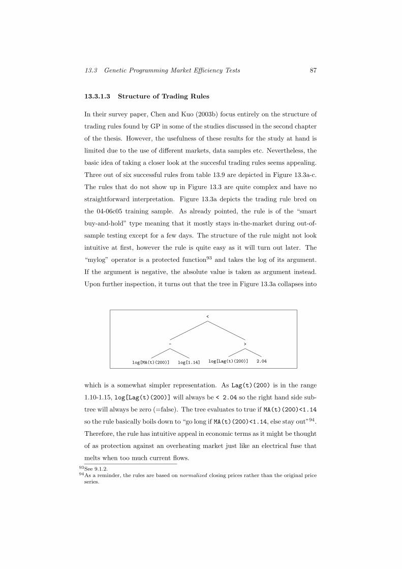
13.3 Genetic Programming Market Efficiency Tests 87
13.3.1.3 Structure of Trading Rules
In their survey paper, Chen and Kuo (2003b) focus entirely on the structure of
trading rules found by GP in some of the studies discussed in the second chapter
of the thesis. However, the usefulness of these results for the study at hand is
limited due to the use of different markets, data samples etc. Nevertheless, the
basic idea of taking a closer look at the succesful trading rules seems appealing.
Three out of six successful rules from table 13.9 are depicted in Figure 13.3a-c.
The rules that do not show up in Figure 13.3 are quite complex and have no
straightforward interpretation. Figure 13.3a depicts the trading rule bred on
the 04-06c05 training sample. As already pointed, the rule is of the “smart
buy-and-hold” type meaning that it mostly stays in-the-market during out-of-
sample testing except for a few days. The structure of the rule might not look
intuitive at first, however the rule is quite easy as it will turn out later. The
“mylog” operator is a protected function93 and takes the log of its argument.
If the argument is negative, the absolute value is taken as argument instead.
Upon further inspection, it turns out that the tree in Figure 13.3a collapses into
<
-
log[MA(t)(200)] log[1.14]
>
log[Lag(t)(200)] 2.04
which is a somewhat simpler representation. As Lag(t)(200) is in the range
1.10-1.15, log[Lag(t)(200)] will always be < 2.04 so the right hand side sub-
tree will always be zero (=false). The tree evaluates to true if MA(t)(200)<1.14
so the rule basically boils down to “go long if MA(t)(200)<1.14, else stay out”94.
Therefore, the rule has intuitive appeal in economic terms as it might be thought
of as protection against an overheating market just like an electrical fuse that
melts when too much current flows.93See 9.1.2.94As a reminder, the rules are based on normalized closing prices rather than the original price
series.
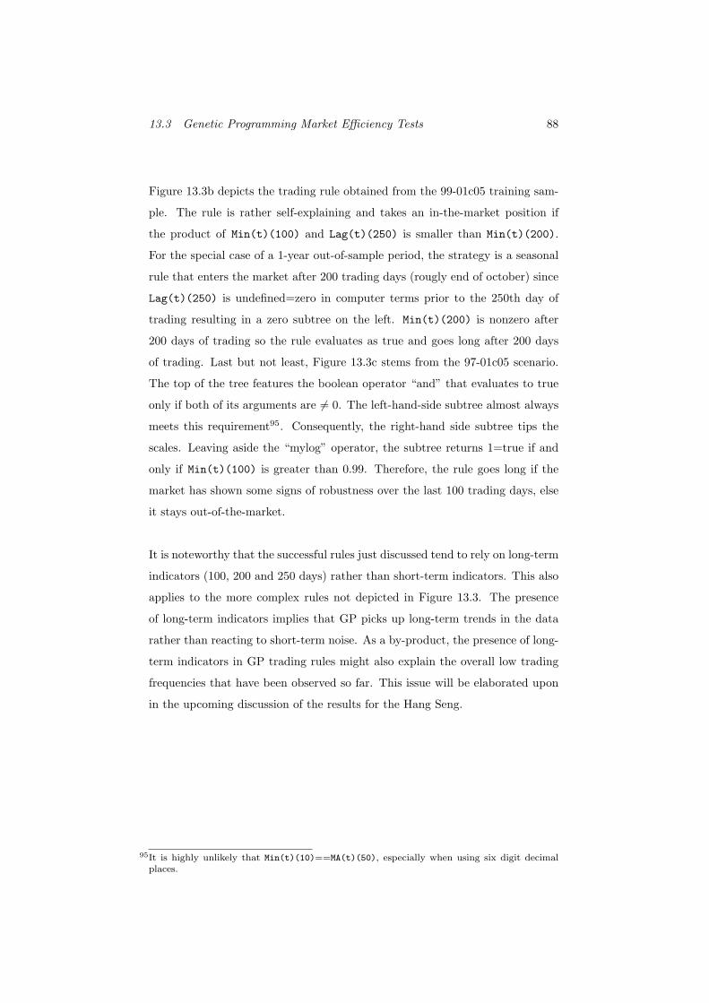
13.3 Genetic Programming Market Efficiency Tests 88
Figure 13.3b depicts the trading rule obtained from the 99-01c05 training sam-
ple. The rule is rather self-explaining and takes an in-the-market position if
the product of Min(t)(100) and Lag(t)(250) is smaller than Min(t)(200).
For the special case of a 1-year out-of-sample period, the strategy is a seasonal
rule that enters the market after 200 trading days (rougly end of october) since
Lag(t)(250) is undefined=zero in computer terms prior to the 250th day of
trading resulting in a zero subtree on the left. Min(t)(200) is nonzero after
200 days of trading so the rule evaluates as true and goes long after 200 days
of trading. Last but not least, Figure 13.3c stems from the 97-01c05 scenario.
The top of the tree features the boolean operator “and” that evaluates to true
only if both of its arguments are 6= 0. The left-hand-side subtree almost always
meets this requirement95. Consequently, the right-hand side subtree tips the
scales. Leaving aside the “mylog” operator, the subtree returns 1=true if and
only if Min(t)(100) is greater than 0.99. Therefore, the rule goes long if the
market has shown some signs of robustness over the last 100 trading days, else
it stays out-of-the-market.
It is noteworthy that the successful rules just discussed tend to rely on long-term
indicators (100, 200 and 250 days) rather than short-term indicators. This also
applies to the more complex rules not depicted in Figure 13.3. The presence
of long-term indicators implies that GP picks up long-term trends in the data
rather than reacting to short-term noise. As a by-product, the presence of long-
term indicators in GP trading rules might also explain the overall low trading
frequencies that have been observed so far. This issue will be elaborated upon
in the upcoming discussion of the results for the Hang Seng.
95It is highly unlikely that Min(t)(10)==MA(t)(50), especially when using six digit decimalplaces.
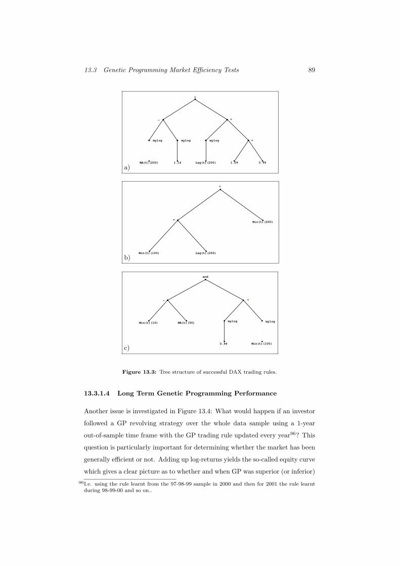
13.3 Genetic Programming Market Efficiency Tests 89
a)MA(t)(200)
mylog
1.14
mylog
−
Lag(t)(200)
mylog
1.09 0.95
+
>
<
b)Min(t)(100) Lag(t)(250)
*Min(t)(200)
<
c)
Min(t)(10) MA(t)(50)
−
0.99
mylog
Min(t)(100)
mylog
<
and
Figure 13.3: Tree structure of successful DAX trading rules.
13.3.1.4 Long Term Genetic Programming Performance
Another issue is investigated in Figure 13.4: What would happen if an investor
followed a GP revolving strategy over the whole data sample using a 1-year
out-of-sample time frame with the GP trading rule updated every year96? This
question is particularly important for determining whether the market has been
generally efficient or not. Adding up log-returns yields the so-called equity curve
which gives a clear picture as to whether and when GP was superior (or inferior)96I.e. using the rule learnt from the 97-98-99 sample in 2000 and then for 2001 the rule learnt
during 98-99-00 and so on..
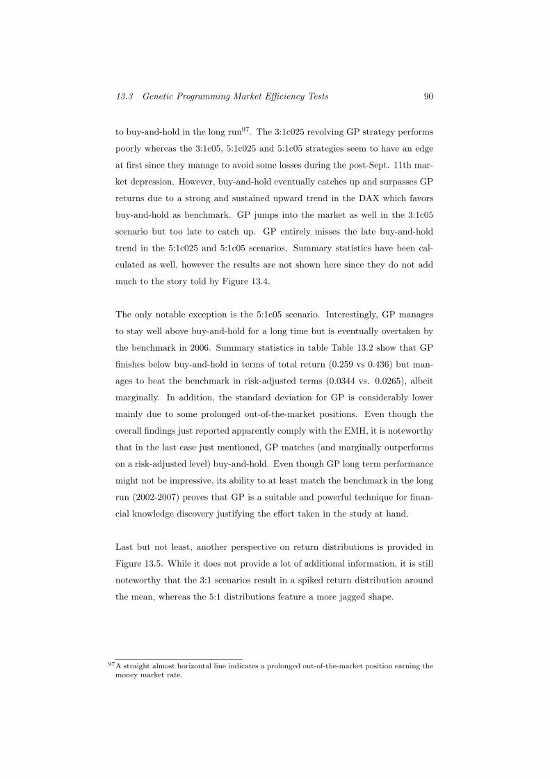
13.3 Genetic Programming Market Efficiency Tests 90
to buy-and-hold in the long run97. The 3:1c025 revolving GP strategy performs
poorly whereas the 3:1c05, 5:1c025 and 5:1c05 strategies seem to have an edge
at first since they manage to avoid some losses during the post-Sept. 11th mar-
ket depression. However, buy-and-hold eventually catches up and surpasses GP
returns due to a strong and sustained upward trend in the DAX which favors
buy-and-hold as benchmark. GP jumps into the market as well in the 3:1c05
scenario but too late to catch up. GP entirely misses the late buy-and-hold
trend in the 5:1c025 and 5:1c05 scenarios. Summary statistics have been cal-
culated as well, however the results are not shown here since they do not add
much to the story told by Figure 13.4.
The only notable exception is the 5:1c05 scenario. Interestingly, GP manages
to stay well above buy-and-hold for a long time but is eventually overtaken by
the benchmark in 2006. Summary statistics in table Table 13.2 show that GP
finishes below buy-and-hold in terms of total return (0.259 vs 0.436) but man-
ages to beat the benchmark in risk-adjusted terms (0.0344 vs. 0.0265), albeit
marginally. In addition, the standard deviation for GP is considerably lower
mainly due to some prolonged out-of-the-market positions. Even though the
overall findings just reported apparently comply with the EMH, it is noteworthy
that in the last case just mentioned, GP matches (and marginally outperforms
on a risk-adjusted level) buy-and-hold. Even though GP long term performance
might not be impressive, its ability to at least match the benchmark in the long
run (2002-2007) proves that GP is a suitable and powerful technique for finan-
cial knowledge discovery justifying the effort taken in the study at hand.
Last but not least, another perspective on return distributions is provided in
Figure 13.5. While it does not provide a lot of additional information, it is still
noteworthy that the 3:1 scenarios result in a spiked return distribution around
the mean, whereas the 5:1 distributions feature a more jagged shape.
97A straight almost horizontal line indicates a prolonged out-of-the-market position earning themoney market rate.
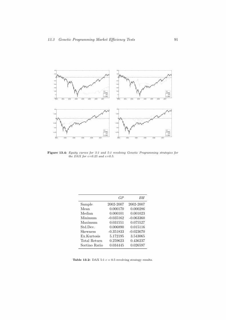
13.3 Genetic Programming Market Efficiency Tests 91
2000 2001 2002 2003 2004 2005 2006 2007−1.2
−1
−0.8
−0.6
−0.4
−0.2
−0
0.2
0.4
GP
BH
3:1c=0.25
2000 2001 2002 2003 2004 2005 2006 2007−1.2
−1
−0.8
−0.6
−0.4
−0.2
−0
0.2
0.4
GP
BH
3:1c=0.50
2002 2003 2004 2005 2006 2007−1
−0.75
−0.5
−0.25
0
0.25
0.5
GP
BH
5:1c=0.25
2002 2003 2004 2005 2006 2007−1
−0.75
−0.5
−0.25
0
0.25
0.5
GP
BH
5:1c=0.50
Figure 13.4: Equity curves for 3:1 and 5:1 revolving Genetic Programming strategies forthe DAX for c=0.25 and c=0.5.
GP BH
Sample 2002-2007 2002-2007Mean 0.000170 0.000286Median 0.000101 0.001023Minimum -0.035162 -0.063360Maximum 0.031551 0.075527Std.Dev. 0.006890 0.015116Skewness -0.351833 -0.023670Ex.Kurtosis 5.172195 3.543065Total Return 0.259623 0.436237Sortino Ratio 0.034445 0.026597
Table 13.2: DAX 5:1 c = 0.5 revolving strategy results.
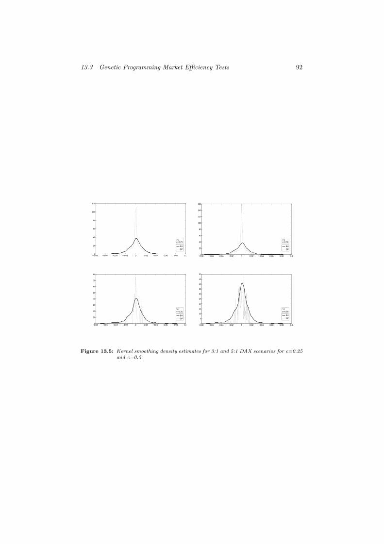
13.3 Genetic Programming Market Efficiency Tests 92
−0.08 −0.06 −0.04 −0.02 0 0.02 0.04 0.06 0.08 0.10
20
40
60
80
100
120
BH
GP
3:1c=0.25
−0.08 −0.06 −0.04 −0.02 0 0.02 0.04 0.06 0.08 0.10
20
40
60
80
100
120
140
160
BH
GP
3:1c=0.50
−0.08 −0.06 −0.04 −0.02 0 0.02 0.04 0.06 0.08 0.10
10
20
30
40
50
60
70
80
BH
GP
5:1c=0.25
−0.08 −0.06 −0.04 −0.02 0 0.02 0.04 0.06 0.08 0.10
5
10
15
20
25
30
35
40
45
50
BH
GP
5:1c=0.50
Figure 13.5: Kernel smoothing density estimates for 3:1 and 5:1 DAX scenarios for c=0.25and c=0.5.
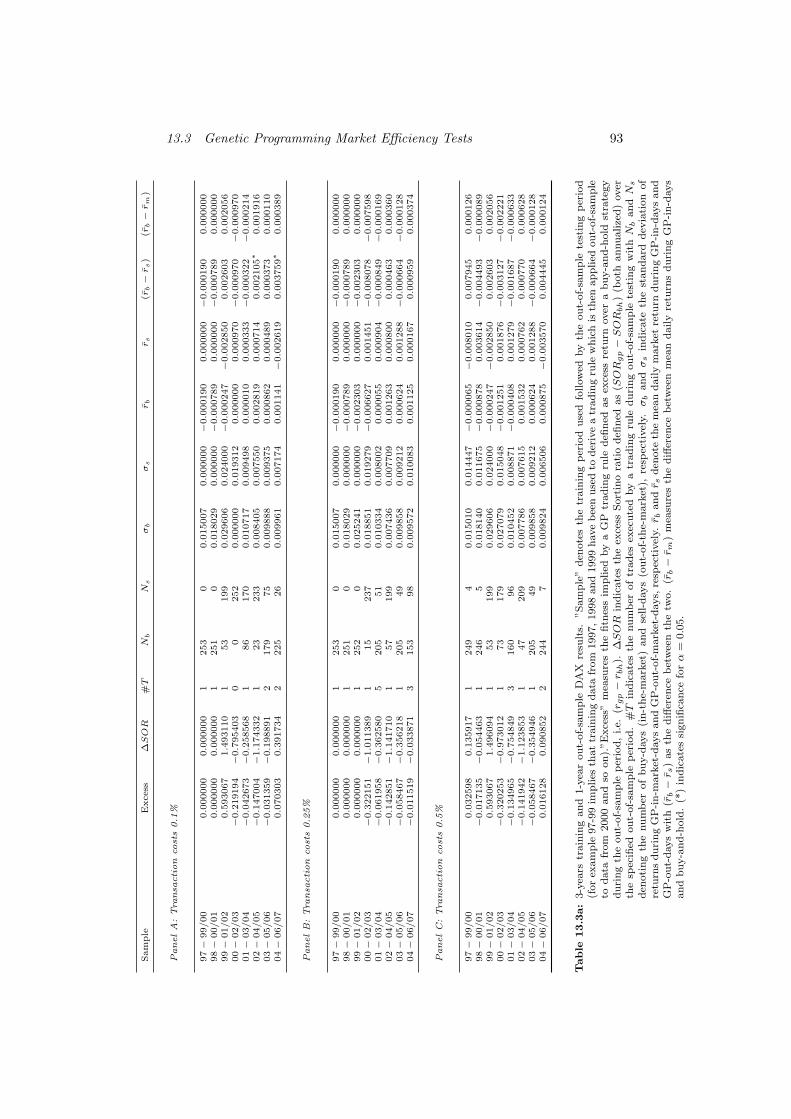
13.3 Genetic Programming Market Efficiency Tests 93Sam
ple
Excess
∆SOR
#T
Nb
Ns
σb
σs
rb
rs
(rb−r
s)
(rb−r
m)
PanelA
:Tra
nsa
ction
cost
s0.1
%
97−
99/00
0.0
00000
0.0
00000
1253
00.0
15007
0.0
00000−
0.0
00190
0.0
00000−
0.0
00190
0.0
00000
98−
00/01
0.0
00000
0.0
00000
1251
00.0
18029
0.0
00000−
0.0
00789
0.0
00000−
0.0
00789
0.0
00000
99−
01/02
0.5
93067
1.4
93110
153
199
0.0
29606
0.0
24000−
0.0
00247−
0.0
02850
0.0
02603
0.0
02056
00−
02/03
−0.2
19194−
0.7
95403
00
252
0.0
00000
0.0
19312
0.0
00000
0.0
00970−
0.0
00970
−0.0
00970
01−
03/04
−0.0
42673−
0.2
58568
186
170
0.0
10717
0.0
09498
0.0
00010
0.0
00333−
0.0
00322
−0.0
00214
02−
04/05
−0.1
47004−
1.1
74332
123
233
0.0
08405
0.0
07550
0.0
02819
0.0
00714
0.0
02105∗
0.0
01916
03−
05/06
−0.0
31359−
0.1
98891
2179
75
0.0
09888
0.0
09375
0.0
00862
0.0
00489
0.0
00373
0.0
00110
04−
06/07
0.0
70303
0.3
91734
2225
26
0.0
09961
0.0
07174
0.0
01141−
0.0
02619
0.0
03759∗
0.0
00389
PanelB:Tra
nsa
ction
cost
s0.2
5%
97−
99/00
0.0
00000
0.0
00000
1253
00.0
15007
0.0
00000−
0.0
00190
0.0
00000−
0.0
00190
0.0
00000
98−
00/01
0.0
00000
0.0
00000
1251
00.0
18029
0.0
00000−
0.0
00789
0.0
00000−
0.0
00789
0.0
00000
99−
01/02
0.0
00000
0.0
00000
1252
00.0
25241
0.0
00000−
0.0
02303
0.0
00000−
0.0
02303
0.0
00000
00−
02/03
−0.3
22151−
1.0
11389
115
237
0.0
18851
0.0
19279−
0.0
06627
0.0
01451−
0.0
08078
−0.0
07598
01−
03/04
−0.0
61958−
0.3
62580
5205
51
0.0
10334
0.0
08002
0.0
00055
0.0
00904−
0.0
00849
−0.0
00169
02−
04/05
−0.1
42851−
1.1
41710
157
199
0.0
07436
0.0
07709
0.0
01263
0.0
00800
0.0
00463
0.0
00360
03−
05/06
−0.0
58467−
0.3
56218
1205
49
0.0
09858
0.0
09212
0.0
00624
0.0
01288−
0.0
00664
−0.0
00128
04−
06/07
−0.0
11519−
0.0
33871
3153
98
0.0
09572
0.0
10083
0.0
01125
0.0
00167
0.0
00959
0.0
00374
PanelC:Tra
nsa
ction
cost
s0.5
%
97−
99/00
0.0
32598
0.1
35917
1249
40.0
15010
0.0
14447−
0.0
00065−
0.0
08010
0.0
07945
0.0
00126
98−
00/01
−0.0
17135−
0.0
54463
1246
50.0
18140
0.0
11675−
0.0
00878
0.0
03614−
0.0
04493
−0.0
00089
99−
01/02
0.5
93067
1.4
96094
153
199
0.0
29606
0.0
24000−
0.0
00247−
0.0
02850
0.0
02603
0.0
02056
00−
02/03
−0.3
20253−
0.9
73012
173
179
0.0
27079
0.0
15048−
0.0
01251
0.0
01876−
0.0
03127
−0.0
02221
01−
03/04
−0.1
34965−
0.7
54849
3160
96
0.0
10452
0.0
08871−
0.0
00408
0.0
01279−
0.0
01687
−0.0
00633
02−
04/05
−0.1
41942−
1.1
23853
147
209
0.0
07786
0.0
07615
0.0
01532
0.0
00762
0.0
00770
0.0
00628
03−
05/06
−0.0
58467−
0.3
54946
1205
49
0.0
09858
0.0
09212
0.0
00624
0.0
01288−
0.0
00664
−0.0
00128
04−
06/07
0.0
16128
0.0
90852
2244
70.0
09824
0.0
06506
0.0
00875−
0.0
03570
0.0
04445
0.0
00124
Table
13.3
a:
3-y
ears
train
ing
an
d1-y
ear
ou
t-of-
sam
ple
DA
Xre
sult
s.”S
am
ple
”d
enote
sth
etr
ain
ing
per
iod
use
dfo
llow
edby
the
ou
t-of-
sam
ple
test
ing
per
iod
(for
exam
ple
97-9
9im
plies
that
train
ing
data
from
1997,
1998
and
1999
have
bee
nu
sed
tod
eriv
ea
trad
ing
rule
wh
ich
isth
enap
plied
ou
t-of-
sam
ple
tod
ata
from
2000
an
dso
on
).”E
xce
ss”
mea
sure
sth
efi
tnes
sim
plied
by
aG
Ptr
ad
ing
rule
defi
ned
as
exce
ssre
turn
over
ab
uy-a
nd
-hold
stra
tegy
du
rin
gth
eou
t-of-
sam
ple
per
iod
,i.e.
(rgp−r b
h).
∆SOR
ind
icate
sth
eex
cess
Sort
ino
rati
od
efin
edas
(SOR
gp−SOR
bh
)(b
oth
an
nu
alize
d)
over
the
spec
ified
ou
t-of-
sam
ple
per
iod
.#T
ind
icate
sth
enu
mb
erof
trad
esex
ecu
ted
by
atr
ad
ing
rule
du
rin
gou
t-of-
sam
ple
test
ing
wit
hN
ban
dN
s
den
oti
ng
the
nu
mb
erof
bu
y-d
ays
(in
-th
e-m
ark
et)
an
dse
ll-d
ays
(ou
t-of-
the-
mark
et),
resp
ecti
vel
y.σ
ban
dσ
sin
dic
ate
the
stan
dard
dev
iati
on
of
retu
rns
du
rin
gG
P-i
n-m
ark
et-d
ays
an
dG
P-o
ut-
of-
mark
et-d
ays,
resp
ecti
vel
y.r b
an
dr s
den
ote
the
mea
nd
aily
mark
etre
turn
du
rin
gG
P-i
n-d
ays
an
dG
P-o
ut-
days
wit
h(r
b−r s
)as
the
diff
eren
ceb
etw
een
the
two.
(rb−r m
)m
easu
res
the
diff
eren
ceb
etw
een
mea
nd
aily
retu
rns
du
rin
gG
P-i
n-d
ays
an
db
uy-a
nd
-hold
.(*
)in
dic
ate
ssi
gn
ifica
nce
forα
=0.0
5.
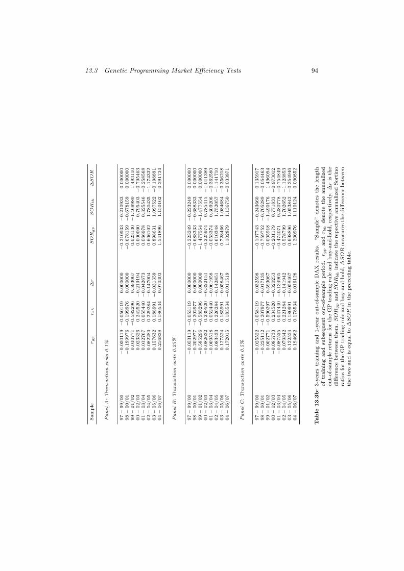
13.3 Genetic Programming Market Efficiency Tests 94
Sam
ple
rg
pr
bh
∆r
SOR
gp
SOR
bh
∆SOR
PanelA
:Tra
nsa
ction
cost
s0.1
%
97−
99/00
−0.0
50119−
0.0
50119
0.0
00000
−0.2
10933−
0.2
10933
0.0
00000
98−
00/01
−0.1
99976−
0.1
99976
0.0
00000
−0.6
78159−
0.6
78159
0.0
00000
99−
01/02
0.0
10771−
0.5
82296
0.5
93067
0.0
23130−
1.4
69980
1.4
93110
00−
02/03
0.0
23326
0.2
42520−
0.2
19194
0.0
00000
0.7
95403−
0.7
95403
01−
03/04
0.0
12767
0.0
55440−
0.0
42673
0.0
66978
0.3
25546−
0.2
58568
02−
04/05
0.0
82280
0.2
29284−
0.1
47004
0.6
06102
1.7
80435−
1.1
74332
03−
05/06
0.1
57632
0.1
88991−
0.0
31359
0.8
98631
1.0
97522−
0.1
98891
04−
06/07
0.2
56838
0.1
86534
0.0
70303
1.5
41896
1.1
50162
0.3
91734
PanelB:Tra
nsa
ction
cost
s0.2
5%
97−
99/00
−0.0
53119−
0.0
53119
0.0
00000
−0.2
23249−
0.2
23249
0.0
00000
98−
00/01
−0.2
02977−
0.2
02977
0.0
00000
−0.6
88333−
0.6
88333
0.0
00000
99−
01/02
−0.5
85296−
0.5
85296
0.0
00000
−1.4
77554−
1.4
77554
0.0
00000
00−
02/03
−0.0
82632
0.2
39520−
0.3
22151
−0.2
25974
0.7
85415−
1.0
11389
01−
03/04
−0.0
09518
0.0
52440−
0.0
61958
−0.0
53374
0.3
09206−
0.3
62580
02−
04/05
0.0
83433
0.2
26284−
0.1
42851
0.6
10348
1.7
52057−
1.1
41710
03−
05/06
0.1
27524
0.1
85991−
0.0
58467
0.7
28466
1.0
84684−
0.3
56218
04−
06/07
0.1
72015
0.1
83534−
0.0
11519
1.1
02879
1.1
36750−
0.0
33871
PanelC:Tra
nsa
ction
cost
s0.5
%
97−
99/00
−0.0
25522−
0.0
58119
0.0
32598
−0.1
07743−
0.2
43660
0.1
35917
98−
00/01
−0.2
25112−
0.2
07977−
0.0
17135
−0.7
59752−
0.7
05289−
0.0
54463
99−
01/02
0.0
02771−
0.5
90297
0.5
93067
0.0
05918−
1.4
90176
1.4
96094
00−
02/03
−0.0
85733
0.2
34520−
0.3
20253
−0.2
01179
0.7
71833−
0.9
73012
01−
03/04
−0.0
87525
0.0
47440−
0.1
34965
−0.4
74071
0.2
80778−
0.7
54849
02−
04/05
0.0
79342
0.2
21284−
0.1
41942
0.5
78799
1.7
02652−
1.1
23853
03−
05/06
0.1
22524
0.1
80991−
0.0
58467
0.6
98896
1.0
53842−
0.3
54946
04−
06/07
0.1
94662
0.1
78534
0.0
16128
1.2
00976
1.1
10124
0.0
90852
Table
13.3
b:
3-y
ears
train
ing
an
d1-y
ear
ou
t-of-
sam
ple
DA
Xre
sult
s.“S
am
ple
”d
enote
sth
ele
ngth
of
train
ing
an
dsu
bse
qu
ent
ou
t-of-
sam
ple
per
iod
.r g
pan
dr b
hd
enote
the
an
nu
alize
dou
t-of-
sam
ple
retu
rns
for
the
GP
trad
ing
rule
an
db
uy-a
nd
-hold
,re
spec
tivel
y.∆r
isth
ed
iffer
ence
bet
wee
nth
em.SOR
gp
an
dSOR
bh
ind
icate
the
rep
ecti
ve
an
nuali
zed
Sort
ino
rati
os
for
the
GP
trad
ing
rule
an
db
uy-a
nd
-hold
,∆SOR
mea
sure
sth
ed
iffer
ence
bet
wee
nth
etw
oan
dis
equ
al
to∆SOR
inth
ep
rece
din
gta
ble
.
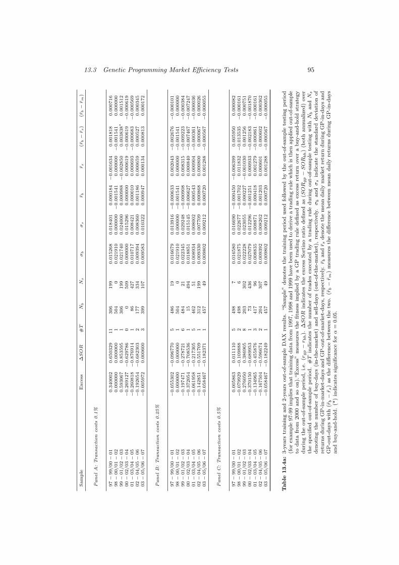
13.3 Genetic Programming Market Efficiency Tests 95Sam
ple
Excess
∆SOR
#T
Nb
Ns
σb
σs
rb
rs
(rb−r
s)
(rb−r
m)
PanelA
:Tra
nsa
ction
cost
s0.1
%
97−
99/00−
01
0.3
40002
0.6
50329
11
306
199
0.0
15268
0.0
18401
0.0
00184−
0.0
01634
0.0
01818
0.0
00716
98−
00/01−
02
0.0
00000
0.0
00000
1504
00.0
21910
0.0
00000−
0.0
01541
0.0
00000−
0.0
01541
0.0
00000
99−
01/02−
03
0.5
93067
0.8
53595
1306
199
0.0
21740
0.0
24000
0.0
00988−
0.0
02850
0.0
03838∗
0.0
01512
00−
02/03−
04
−0.2
69127−
0.6
29786
00
509
0.0
00000
0.0
15296
0.0
00000
0.0
00619−
0.0
00619−
0.0
00619
01−
03/04−
05
−0.2
60818−
0.8
76914
186
427
0.0
10717
0.0
08421
0.0
00010
0.0
00693−
0.0
00683−
0.0
00569
02−
04/05−
06
−0.1
92654−
0.6
82303
2177
334
0.0
09394
0.0
08360
0.0
01186
0.0
00659
0.0
00527
0.0
00345
03−
05/06−
07
−0.0
05972
0.0
00600
3399
107
0.0
09583
0.0
10322
0.0
00947
0.0
00134
0.0
00813
0.0
00172
PanelB:Tra
nsa
ction
cost
s0.2
5%
97−
99/00−
01
−0.0
55302−
0.0
96770
5486
19
0.0
16679
0.0
13916−
0.0
00633
0.0
02043−
0.0
02676−
0.0
00101
98−
00/01−
02
0.0
00000
0.0
00000
1504
00.0
21910
0.0
00000−
0.0
01541
0.0
00000−
0.0
01541
0.0
00000
99−
01/02−
03
−0.1
97471−
0.2
78721
6484
21
0.0
22345
0.0
29248−
0.0
00908
0.0
08315−
0.0
09223−
0.0
00384
00−
02/03−
04
−0.3
72054−
0.7
08536
115
494
0.0
18851
0.0
15145−
0.0
06627
0.0
00840−
0.0
07467−
0.0
07247
01−
03/04−
05
−0.0
61958−
0.2
17305
5462
51
0.0
08934
0.0
08002
0.0
00543
0.0
00904−
0.0
00361−
0.0
00036
02−
04/05−
06
−0.1
42851−
0.5
51709
1312
199
0.0
09330
0.0
07709
0.0
00868
0.0
00800
0.0
00067
0.0
00026
03−
05/06−
07
−0.0
58467−
0.1
82371
1457
49
0.0
09802
0.0
09212
0.0
00720
0.0
01288−
0.0
00567−
0.0
00055
PanelC:Tra
nsa
ction
cost
s0.5
%
97−
99/00−
01
0.0
05863
0.0
11110
5498
70.0
16580
0.0
16690−
0.0
00450−
0.0
06399
0.0
05950
0.0
00082
98−
00/01−
02
−0.0
79929−
0.1
09888
2498
60.0
21875
0.0
22677−
0.0
01702
0.0
11832−
0.0
13535−
0.0
00161
99−
01/02−
03
0.2
76050
0.3
86905
8203
302
0.0
22228
0.0
23055
0.0
00227−
0.0
01030
0.0
01256
0.0
00751
00−
02/03−
04
−0.3
70150−
0.6
89953
173
436
0.0
27079
0.0
12296−
0.0
01251
0.0
00933−
0.0
02183−
0.0
01870
01−
03/04−
05
−0.1
34965−
0.4
55876
3417
96
0.0
08835
0.0
08871
0.0
00418
0.0
01279−
0.0
00861−
0.0
00161
02−
04/05−
06
−0.1
67504−
0.5
96674
2204
307
0.0
09392
0.0
08262
0.0
01203
0.0
00601
0.0
00602
0.0
00362
03−
05/06−
07
−0.0
58467−
0.1
82249
1457
49
0.0
09802
0.0
09212
0.0
00720
0.0
01288−
0.0
00567−
0.0
00055
Table
13.4
a:
3-y
ears
train
ing
an
d2-y
ears
ou
t-of-
sam
ple
DA
Xre
sult
s.“S
am
ple
”d
enote
sth
etr
ain
ing
per
iod
use
dfo
llow
edby
the
ou
t-of-
sam
ple
test
ing
per
iod
(for
exam
ple
97-9
9im
plies
that
train
ing
data
from
1997,
1998
and
1999
have
bee
nu
sed
tod
eriv
ea
trad
ing
rule
wh
ich
isth
enap
plied
ou
t-of-
sam
ple
tod
ata
from
2000
an
dso
on
).“E
xce
ss”
mea
sure
sth
efi
tnes
sim
plied
by
aG
Ptr
ad
ing
rule
defi
ned
as
exce
ssre
turn
over
ab
uy-a
nd
-hold
stra
tegy
du
rin
gth
eou
t-of-
sam
ple
per
iod
,i.e.
(rgp−r b
h).
∆SOR
ind
icate
sth
eex
cess
Sort
ino
rati
od
efin
edas
(SOR
gp−SOR
bh
)(b
oth
an
nu
alize
d)
over
the
spec
ified
ou
t-of-
sam
ple
per
iod
.#T
ind
icate
sth
enu
mb
erof
trad
esex
ecu
ted
by
atr
ad
ing
rule
du
rin
gou
t-of-
sam
ple
test
ing
wit
hN
ban
dN
s
den
oti
ng
the
nu
mb
erof
bu
y-d
ays
(in
-th
e-m
ark
et)
an
dse
ll-d
ays
(ou
t-of-
the-
mark
et),
resp
ecti
vel
y.σ
ban
dσ
sin
dic
ate
the
stan
dard
dev
iati
on
of
retu
rns
du
rin
gG
P-i
n-m
ark
et-d
ays
an
dG
P-o
ut-
of-
mark
et-d
ays,
resp
ecti
vel
y.r b
an
dr s
den
ote
the
mea
nd
aily
mark
etre
turn
du
rin
gG
P-i
n-d
ays
an
dG
P-o
ut-
days
wit
h(r
b−r s
)as
the
diff
eren
ceb
etw
een
the
two.
(rb−r m
)m
easu
res
the
diff
eren
ceb
etw
een
mea
nd
aily
retu
rns
du
rin
gG
P-i
n-d
ays
an
db
uy-a
nd
-hold
.(*
)in
dic
ate
ssi
gn
ifica
nce
forα
=0.0
5.
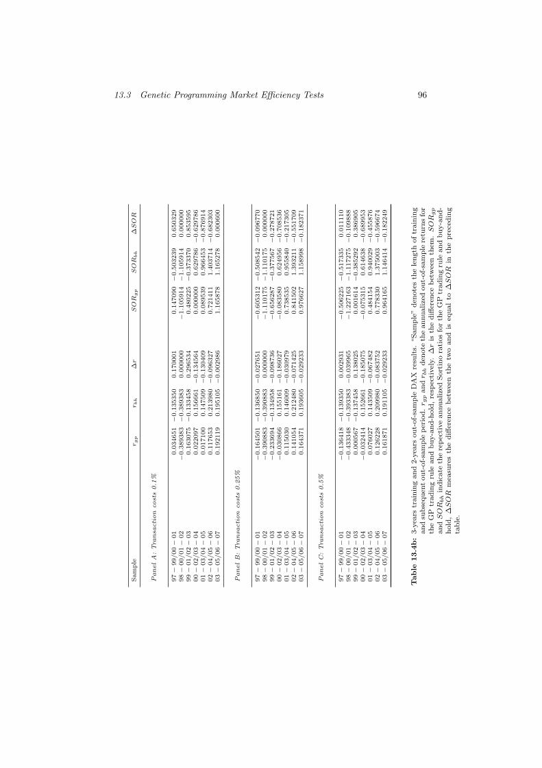
13.3 Genetic Programming Market Efficiency Tests 96
Sam
ple
rg
pr
bh
∆r
SOR
gp
SOR
bh
∆SOR
PanelA
:Tra
nsa
ction
cost
s0.1
%
97−
99/00−
01
0.0
34651−
0.1
35350
0.1
70001
0.1
47090−
0.5
03239
0.6
50329
98−
00/01−
02
−0.3
89383−
0.3
89383
0.0
00000
−1.1
05914−
1.1
05914
0.0
00000
99−
01/02−
03
0.1
63075−
0.1
33458
0.2
96534
0.4
80225−
0.3
73370
0.8
53595
00−
02/03−
04
0.0
22097
0.1
56661−
0.1
34564
0.0
00000
0.6
29786−
0.6
29786
01−
03/04−
05
0.0
17100
0.1
47509−
0.1
30409
0.0
89539
0.9
66453−
0.8
76914
02−
04/05−
06
0.1
17653
0.2
13980−
0.0
96327
0.7
21411
1.4
03714−
0.6
82303
03−
05/06−
07
0.1
92119
0.1
95105−
0.0
02986
1.1
65878
1.1
65278
0.0
00600
PanelB:Tra
nsa
ction
cost
s0.2
5%
97−
99/00−
01
−0.1
64501−
0.1
36850−
0.0
27651
−0.6
05312−
0.5
08542−
0.0
96770
98−
00/01−
02
−0.3
90883−
0.3
90883
0.0
00000
−1.1
10175−
1.1
10175
0.0
00000
99−
01/02−
03
−0.2
33694−
0.1
34958−
0.0
98736
−0.6
56287−
0.3
77567−
0.2
78721
00−
02/03−
04
−0.0
30866
0.1
55161−
0.1
86027
−0.0
83580
0.6
24956−
0.7
08536
01−
03/04−
05
0.1
15030
0.1
46009−
0.0
30979
0.7
38535
0.9
55840−
0.2
17305
02−
04/05−
06
0.1
41054
0.2
12480−
0.0
71425
0.8
41502
1.3
93211−
0.5
51709
03−
05/06−
07
0.1
64371
0.1
93605−
0.0
29233
0.9
76627
1.1
58998−
0.1
82371
PanelC:Tra
nsa
ction
cost
s0.5
%
97−
99/00−
01
−0.1
36418−
0.1
39350
0.0
02931
−0.5
06225−
0.5
17335
0.0
11110
98−
00/01−
02
−0.4
33348−
0.3
93383−
0.0
39965
−1.2
27163−
1.1
17275−
0.1
09888
99−
01/02−
03
0.0
00567−
0.1
37458
0.1
38025
0.0
01614−
0.3
85292
0.3
86905
00−
02/03−
04
−0.0
32414
0.1
52661−
0.1
85075
−0.0
75315
0.6
14638−
0.6
89953
01−
03/04−
05
0.0
76027
0.1
43509−
0.0
67482
0.4
84154
0.9
40029−
0.4
55876
02−
04/05−
06
0.1
26228
0.2
09980−
0.0
83752
0.7
78330
1.3
75003−
0.5
96674
03−
05/06−
07
0.1
61871
0.1
91105−
0.0
29233
0.9
64165
1.1
46414−
0.1
82249
Table
13.4
b:
3-y
ears
train
ing
an
d2-y
ears
ou
t-of-
sam
ple
DA
Xre
sult
s.“S
am
ple
”d
enote
sth
ele
ngth
of
train
ing
an
dsu
bse
qu
ent
ou
t-of-
sam
ple
per
iod
.r g
pan
dr b
hd
enote
the
an
nu
alize
dou
t-of-
sam
ple
retu
rns
for
the
GP
trad
ing
rule
an
db
uy-a
nd
-hold
,re
spec
tivel
y.∆r
isth
ed
iffer
ence
bet
wee
nth
em.SOR
gp
an
dSOR
bh
ind
icate
the
rep
ecti
ve
an
nu
alize
dS
ort
ino
rati
os
for
the
GP
trad
ing
rule
an
db
uy-a
nd
-h
old
,∆SOR
mea
sure
sth
ed
iffer
ence
bet
wee
nth
etw
oan
dis
equ
al
to∆SOR
inth
ep
rece
din
gta
ble
.
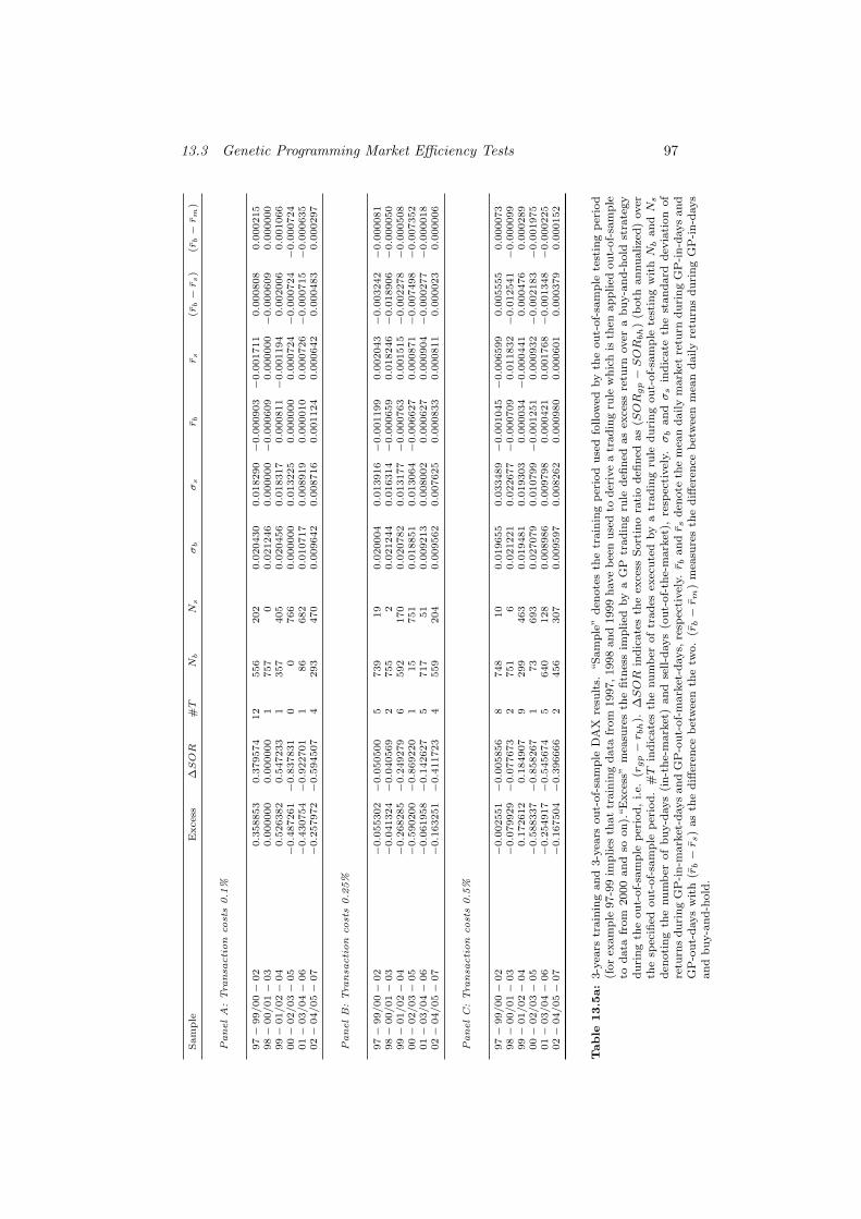
13.3 Genetic Programming Market Efficiency Tests 97
Sam
ple
Excess
∆SOR
#T
Nb
Ns
σb
σs
rb
rs
(rb−r
s)
(rb−r
m)
PanelA
:Tra
nsa
ction
cost
s0.1
%
97−
99/00−
02
0.3
58853
0.3
79574
12
556
202
0.0
20430
0.0
18290−
0.0
00903−
0.0
01711
0.0
00808
0.0
00215
98−
00/01−
03
0.0
00000
0.0
00000
1757
00.0
21246
0.0
00000−
0.0
00609
0.0
00000−
0.0
00609
0.0
00000
99−
01/02−
04
0.5
26382
0.5
47233
1357
405
0.0
20456
0.0
18317
0.0
00811−
0.0
01194
0.0
02006
0.0
01066
00−
02/03−
05
−0.4
87261−
0.8
37831
00
766
0.0
00000
0.0
13225
0.0
00000
0.0
00724−
0.0
00724−
0.0
00724
01−
03/04−
06
−0.4
30754−
0.9
22701
186
682
0.0
10717
0.0
08919
0.0
00010
0.0
00726−
0.0
00715−
0.0
00635
02−
04/05−
07
−0.2
57972−
0.5
94507
4293
470
0.0
09642
0.0
08716
0.0
01124
0.0
00642
0.0
00483
0.0
00297
PanelB:Tra
nsa
ction
cost
s0.2
5%
97−
99/00−
02
−0.0
55302−
0.0
50500
5739
19
0.0
20004
0.0
13916−
0.0
01199
0.0
02043−
0.0
03242−
0.0
00081
98−
00/01−
03
−0.0
41324−
0.0
40569
2755
20.0
21244
0.0
16314−
0.0
00659
0.0
18246−
0.0
18906−
0.0
00050
99−
01/02−
04
−0.2
68285−
0.2
49279
6592
170
0.0
20782
0.0
13177−
0.0
00763
0.0
01515−
0.0
02278−
0.0
00508
00−
02/03−
05
−0.5
90200−
0.8
69220
115
751
0.0
18851
0.0
13064−
0.0
06627
0.0
00871−
0.0
07498−
0.0
07352
01−
03/04−
06
−0.0
61958−
0.1
42627
5717
51
0.0
09213
0.0
08002
0.0
00627
0.0
00904−
0.0
00277−
0.0
00018
02−
04/05−
07
−0.1
63251−
0.4
11723
4559
204
0.0
09562
0.0
07625
0.0
00833
0.0
00811
0.0
00023
0.0
00006
PanelC:Tra
nsa
ction
cost
s0.5
%
97−
99/00−
02
−0.0
02551−
0.0
05856
8748
10
0.0
19655
0.0
33489−
0.0
01045−
0.0
06599
0.0
05555
0.0
00073
98−
00/01−
03
−0.0
79929−
0.0
77673
2751
60.0
21221
0.0
22677−
0.0
00709
0.0
11832−
0.0
12541−
0.0
00099
99−
01/02−
04
0.1
72612
0.1
84907
9299
463
0.0
19481
0.0
19303
0.0
00034−
0.0
00441
0.0
00476
0.0
00289
00−
02/03−
05
−0.5
88337−
0.8
58267
173
693
0.0
27079
0.0
10799−
0.0
01251
0.0
00932−
0.0
02183−
0.0
01975
01−
03/04−
06
−0.2
54917−
0.5
45674
5640
128
0.0
08986
0.0
09798
0.0
00421
0.0
01768−
0.0
01348−
0.0
00225
02−
04/05−
07
−0.1
67504−
0.3
96666
2456
307
0.0
09597
0.0
08262
0.0
00980
0.0
00601
0.0
00379
0.0
00152
Table
13.5
a:
3-y
ears
train
ing
an
d3-y
ears
ou
t-of-
sam
ple
DA
Xre
sult
s.“S
am
ple
”d
enote
sth
etr
ain
ing
per
iod
use
dfo
llow
edby
the
ou
t-of-
sam
ple
test
ing
per
iod
(for
exam
ple
97-9
9im
plies
that
train
ing
data
from
1997,
1998
and
1999
have
bee
nu
sed
tod
eriv
ea
trad
ing
rule
wh
ich
isth
enap
plied
ou
t-of-
sam
ple
tod
ata
from
2000
an
dso
on
).“E
xce
ss”
mea
sure
sth
efi
tnes
sim
plied
by
aG
Ptr
ad
ing
rule
defi
ned
as
exce
ssre
turn
over
ab
uy-a
nd
-hold
stra
tegy
du
rin
gth
eou
t-of-
sam
ple
per
iod
,i.e.
(rgp−r b
h).
∆SOR
ind
icate
sth
eex
cess
Sort
ino
rati
od
efin
edas
(SOR
gp−SOR
bh
)(b
oth
an
nu
alize
d)
over
the
spec
ified
ou
t-of-
sam
ple
per
iod
.#T
ind
icate
sth
enu
mb
erof
trad
esex
ecu
ted
by
atr
ad
ing
rule
du
rin
gou
t-of-
sam
ple
test
ing
wit
hN
ban
dN
s
den
oti
ng
the
nu
mb
erof
bu
y-d
ays
(in
-th
e-m
ark
et)
an
dse
ll-d
ays
(ou
t-of-
the-
mark
et),
resp
ecti
vel
y.σ
ban
dσ
sin
dic
ate
the
stan
dard
dev
iati
on
of
retu
rns
du
rin
gG
P-i
n-m
ark
et-d
ays
an
dG
P-o
ut-
of-
mark
et-d
ays,
resp
ecti
vel
y.r b
an
dr s
den
ote
the
mea
nd
aily
mark
etre
turn
du
rin
gG
P-i
n-d
ays
an
dG
P-o
ut-
days
wit
h(r
b−r s
)as
the
diff
eren
ceb
etw
een
the
two.
(rb−r m
)m
easu
res
the
diff
eren
ceb
etw
een
mea
nd
aily
retu
rns
du
rin
gG
P-i
n-d
ays
an
db
uy-a
nd
-hold
.
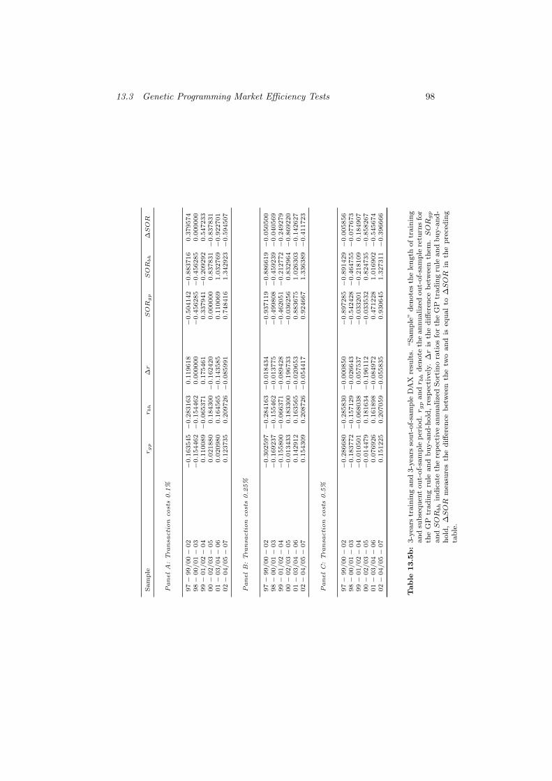
13.3 Genetic Programming Market Efficiency Tests 98
Sam
ple
rg
pr
bh
∆r
SOR
gp
SOR
bh
∆SOR
PanelA
:Tra
nsa
ction
cost
s0.1
%
97−
99/00−
02
−0.1
63545−
0.2
83163
0.1
19618
−0.5
04142−
0.8
83716
0.3
79574
98−
00/01−
03
−0.1
54462−
0.1
54462
0.0
00000
−0.4
56285−
0.4
56285
0.0
00000
99−
01/02−
04
0.1
10089−
0.0
65371
0.1
75461
0.3
37941−
0.2
09292
0.5
47233
00−
02/03−
05
0.0
21880
0.1
84300−
0.1
62420
0.0
00000
0.8
37831−
0.8
37831
01−
03/04−
06
0.0
20980
0.1
64565−
0.1
43585
0.1
10069
1.0
32769−
0.9
22701
02−
04/05−
07
0.1
23735
0.2
09726−
0.0
85991
0.7
48416
1.3
42923−
0.5
94507
PanelB:Tra
nsa
ction
cost
s0.2
5%
97−
99/00−
02
−0.3
02597−
0.2
84163−
0.0
18434
−0.9
37119−
0.8
86619−
0.0
50500
98−
00/01−
03
−0.1
69237−
0.1
55462−
0.0
13775
−0.4
99808−
0.4
59239−
0.0
40569
99−
01/02−
04
−0.1
55800−
0.0
66371−
0.0
89428
−0.4
62051−
0.2
12772−
0.2
49279
00−
02/03−
05
−0.0
13433
0.1
83300−
0.1
96733
−0.0
36256
0.8
32964−
0.8
69220
01−
03/04−
06
0.1
42912
0.1
63565−
0.0
20653
0.8
83675
1.0
26303−
0.1
42627
02−
04/05−
07
0.1
54309
0.2
08726−
0.0
54417
0.9
24667
1.3
36389−
0.4
11723
PanelC:Tra
nsa
ction
cost
s0.5
%
97−
99/00−
02
−0.2
86680−
0.2
85830−
0.0
00850
−0.8
97285−
0.8
91429−
0.0
05856
98−
00/01−
03
−0.1
83772−
0.1
57129−
0.0
26643
−0.5
42428−
0.4
64755−
0.0
77673
99−
01/02−
04
−0.0
10501−
0.0
68038
0.0
57537
−0.0
33201−
0.2
18109
0.1
84907
00−
02/03−
05
−0.0
14479
0.1
81634−
0.1
96112
−0.0
33532
0.8
24735−
0.8
58267
01−
03/04−
06
0.0
76926
0.1
61898−
0.0
84972
0.4
71228
1.0
16902−
0.5
45674
02−
04/05−
07
0.1
51225
0.2
07059−
0.0
55835
0.9
30645
1.3
27311−
0.3
96666
Table
13.5
b:
3-y
ears
train
ing
an
d3-y
ears
sou
t-of-
sam
ple
DA
Xre
sult
s.“S
am
ple
”den
ote
sth
ele
ngth
of
train
ing
an
dsu
bse
qu
ent
ou
t-of-
sam
ple
per
iod
.r g
pan
dr b
hd
enote
the
an
nu
alize
dou
t-of-
sam
ple
retu
rns
for
the
GP
trad
ing
rule
an
db
uy-a
nd
-hold
,re
spec
tivel
y.∆r
isth
ed
iffer
ence
bet
wee
nth
em.SOR
gp
an
dSOR
bh
ind
icate
the
rep
ecti
ve
an
nu
alize
dS
ort
ino
rati
os
for
the
GP
trad
ing
rule
an
db
uy-a
nd
-h
old
,∆SOR
mea
sure
sth
ed
iffer
ence
bet
wee
nth
etw
oan
dis
equ
al
to∆SOR
inth
ep
rece
din
gta
ble
.
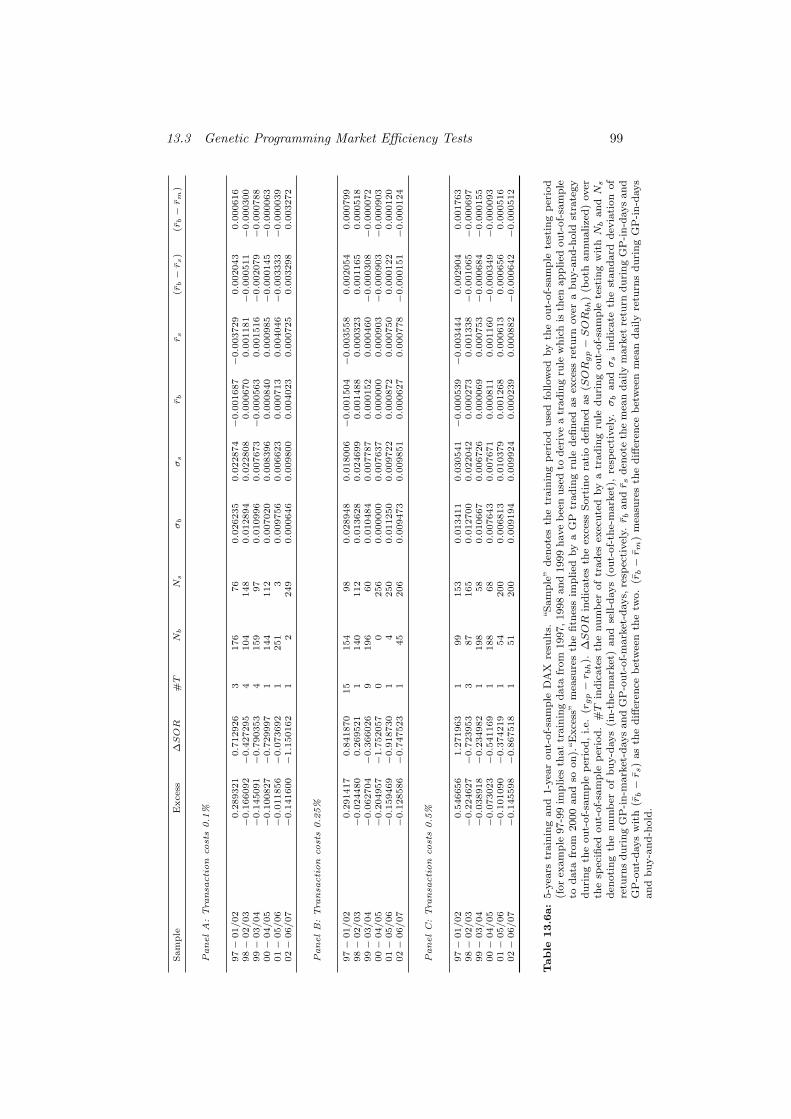
13.3 Genetic Programming Market Efficiency Tests 99
Sam
ple
Excess
∆SOR
#T
Nb
Ns
σb
σs
rb
rs
(rb−r
s)
(rb−r
m)
PanelA
:Tra
nsa
ction
cost
s0.1
%
97−
01/02
0.2
89321
0.7
12926
3176
76
0.0
26235
0.0
22874−
0.0
01687−
0.0
03729
0.0
02043
0.0
00616
98−
02/03
−0.1
66092−
0.4
27295
4104
148
0.0
12894
0.0
22808
0.0
00670
0.0
01181−
0.0
00511
−0.0
00300
99−
03/04
−0.1
45091−
0.7
90353
4159
97
0.0
10996
0.0
07673−
0.0
00563
0.0
01516−
0.0
02079
−0.0
00788
00−
04/05
−0.1
00827−
0.7
29997
1144
112
0.0
07020
0.0
08396
0.0
00840
0.0
00985−
0.0
00145
−0.0
00063
01−
05/06
−0.0
11856−
0.0
73692
1251
30.0
09756
0.0
06623
0.0
00713
0.0
04046−
0.0
03333
−0.0
00039
02−
06/07
−0.1
41600−
1.1
50162
12
249
0.0
00646
0.0
09800
0.0
04023
0.0
00725
0.0
03298
0.0
03272
PanelB:Tra
nsa
ction
cost
s0.2
5%
97−
01/02
0.2
91417
0.8
41870
15
154
98
0.0
28948
0.0
18006−
0.0
01504−
0.0
03558
0.0
02054
0.0
00799
98−
02/03
−0.0
24480
0.2
69521
1140
112
0.0
13628
0.0
24699
0.0
01488
0.0
00323
0.0
01165
0.0
00518
99−
03/04
−0.0
62704−
0.3
66026
9196
60
0.0
10484
0.0
07787
0.0
00152
0.0
00460−
0.0
00308
−0.0
00072
00−
04/05
−0.2
04957−
1.7
52057
00
256
0.0
00000
0.0
07637
0.0
00000
0.0
00903−
0.0
00903
−0.0
00903
01−
05/06
−0.1
59469−
0.9
18730
14
250
0.0
11250
0.0
09722
0.0
00872
0.0
00750
0.0
00122
0.0
00120
02−
06/07
−0.1
28586−
0.7
47523
145
206
0.0
09473
0.0
09851
0.0
00627
0.0
00778−
0.0
00151
−0.0
00124
PanelC:Tra
nsa
ction
cost
s0.5
%
97−
01/02
0.5
46656
1.2
71963
199
153
0.0
13411
0.0
30541−
0.0
00539−
0.0
03444
0.0
02904
0.0
01763
98−
02/03
−0.2
24627−
0.7
23953
387
165
0.0
12700
0.0
22042
0.0
00273
0.0
01338−
0.0
01065
−0.0
00697
99−
03/04
−0.0
38918−
0.2
34982
1198
58
0.0
10667
0.0
06726
0.0
00069
0.0
00753−
0.0
00684
−0.0
00155
00−
04/05
−0.0
73023−
0.5
41169
1188
68
0.0
07643
0.0
07671
0.0
00811
0.0
01160−
0.0
00349
−0.0
00093
01−
05/06
−0.1
01090−
0.3
74219
154
200
0.0
06813
0.0
10379
0.0
01268
0.0
00613
0.0
00656
0.0
00516
02−
06/07
−0.1
45598−
0.8
67518
151
200
0.0
09194
0.0
09924
0.0
00239
0.0
00882−
0.0
00642
−0.0
00512
Table
13.6
a:
5-y
ears
train
ing
an
d1-y
ear
ou
t-of-
sam
ple
DA
Xre
sult
s.“S
am
ple
”d
enote
sth
etr
ain
ing
per
iod
use
dfo
llow
edby
the
ou
t-of-
sam
ple
test
ing
per
iod
(for
exam
ple
97-9
9im
plies
that
train
ing
data
from
1997,
1998
and
1999
have
bee
nu
sed
tod
eriv
ea
trad
ing
rule
wh
ich
isth
enap
plied
ou
t-of-
sam
ple
tod
ata
from
2000
an
dso
on
).“E
xce
ss”
mea
sure
sth
efi
tnes
sim
plied
by
aG
Ptr
ad
ing
rule
defi
ned
as
exce
ssre
turn
over
ab
uy-a
nd
-hold
stra
tegy
du
rin
gth
eou
t-of-
sam
ple
per
iod
,i.e.
(rgp−r b
h).
∆SOR
ind
icate
sth
eex
cess
Sort
ino
rati
od
efin
edas
(SOR
gp−SOR
bh
)(b
oth
an
nu
alize
d)
over
the
spec
ified
ou
t-of-
sam
ple
per
iod
.#T
ind
icate
sth
enu
mb
erof
trad
esex
ecu
ted
by
atr
ad
ing
rule
du
rin
gou
t-of-
sam
ple
test
ing
wit
hN
ban
dN
s
den
oti
ng
the
nu
mb
erof
bu
y-d
ays
(in
-th
e-m
ark
et)
an
dse
ll-d
ays
(ou
t-of-
the-
mark
et),
resp
ecti
vel
y.σ
ban
dσ
sin
dic
ate
the
stan
dard
dev
iati
on
of
retu
rns
du
rin
gG
P-i
n-m
ark
et-d
ays
an
dG
P-o
ut-
of-
mark
et-d
ays,
resp
ecti
vel
y.r b
an
dr s
den
ote
the
mea
nd
aily
mark
etre
turn
du
rin
gG
P-i
n-d
ays
an
dG
P-o
ut-
days
wit
h(r
b−r s
)as
the
diff
eren
ceb
etw
een
the
two.
(rb−r m
)m
easu
res
the
diff
eren
ceb
etw
een
mea
nd
aily
retu
rns
du
rin
gG
P-i
n-d
ays
an
db
uy-a
nd
-hold
.
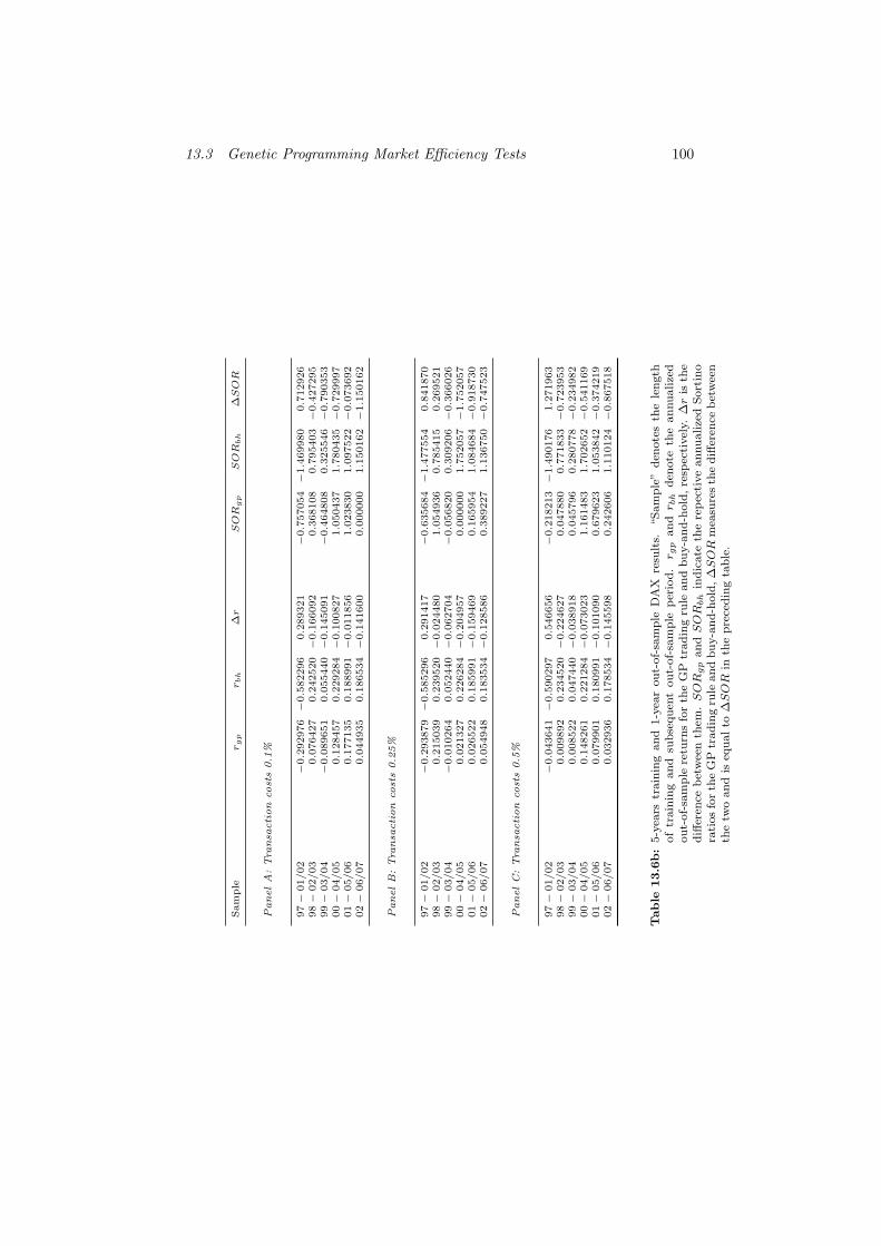
13.3 Genetic Programming Market Efficiency Tests 100
Sam
ple
rg
pr
bh
∆r
SOR
gp
SOR
bh
∆SOR
PanelA
:Tra
nsa
ction
cost
s0.1
%
97−
01/02
−0.2
92976−
0.5
82296
0.2
89321
−0.7
57054−
1.4
69980
0.7
12926
98−
02/03
0.0
76427
0.2
42520−
0.1
66092
0.3
68108
0.7
95403−
0.4
27295
99−
03/04
−0.0
89651
0.0
55440−
0.1
45091
−0.4
64808
0.3
25546−
0.7
90353
00−
04/05
0.1
28457
0.2
29284−
0.1
00827
1.0
50437
1.7
80435−
0.7
29997
01−
05/06
0.1
77135
0.1
88991−
0.0
11856
1.0
23830
1.0
97522−
0.0
73692
02−
06/07
0.0
44935
0.1
86534−
0.1
41600
0.0
00000
1.1
50162−
1.1
50162
PanelB:Tra
nsa
ction
cost
s0.2
5%
97−
01/02
−0.2
93879−
0.5
85296
0.2
91417
−0.6
35684−
1.4
77554
0.8
41870
98−
02/03
0.2
15039
0.2
39520−
0.0
24480
1.0
54936
0.7
85415
0.2
69521
99−
03/04
−0.0
10264
0.0
52440−
0.0
62704
−0.0
56820
0.3
09206−
0.3
66026
00−
04/05
0.0
21327
0.2
26284−
0.2
04957
0.0
00000
1.7
52057−
1.7
52057
01−
05/06
0.0
26522
0.1
85991−
0.1
59469
0.1
65954
1.0
84684−
0.9
18730
02−
06/07
0.0
54948
0.1
83534−
0.1
28586
0.3
89227
1.1
36750−
0.7
47523
PanelC:Tra
nsa
ction
cost
s0.5
%
97−
01/02
−0.0
43641−
0.5
90297
0.5
46656
−0.2
18213−
1.4
90176
1.2
71963
98−
02/03
0.0
09892
0.2
34520−
0.2
24627
0.0
47880
0.7
71833−
0.7
23953
99−
03/04
0.0
08522
0.0
47440−
0.0
38918
0.0
45796
0.2
80778−
0.2
34982
00−
04/05
0.1
48261
0.2
21284−
0.0
73023
1.1
61483
1.7
02652−
0.5
41169
01−
05/06
0.0
79901
0.1
80991−
0.1
01090
0.6
79623
1.0
53842−
0.3
74219
02−
06/07
0.0
32936
0.1
78534−
0.1
45598
0.2
42606
1.1
10124−
0.8
67518
Table
13.6
b:
5-y
ears
train
ing
an
d1-y
ear
ou
t-of-
sam
ple
DA
Xre
sult
s.“S
am
ple
”d
enote
sth
ele
ngth
of
train
ing
an
dsu
bse
qu
ent
ou
t-of-
sam
ple
per
iod
.r g
pan
dr b
hd
enote
the
an
nu
alize
dou
t-of-
sam
ple
retu
rns
for
the
GP
trad
ing
rule
an
db
uy-a
nd
-hold
,re
spec
tivel
y.∆r
isth
ed
iffer
ence
bet
wee
nth
em.SOR
gp
an
dSOR
bh
ind
icate
the
rep
ecti
ve
an
nuali
zed
Sort
ino
rati
os
for
the
GP
trad
ing
rule
an
db
uy-a
nd
-hold
,∆SOR
mea
sure
sth
ed
iffer
ence
bet
wee
nth
etw
oan
dis
equ
al
to∆SOR
inth
ep
rece
din
gta
ble
.
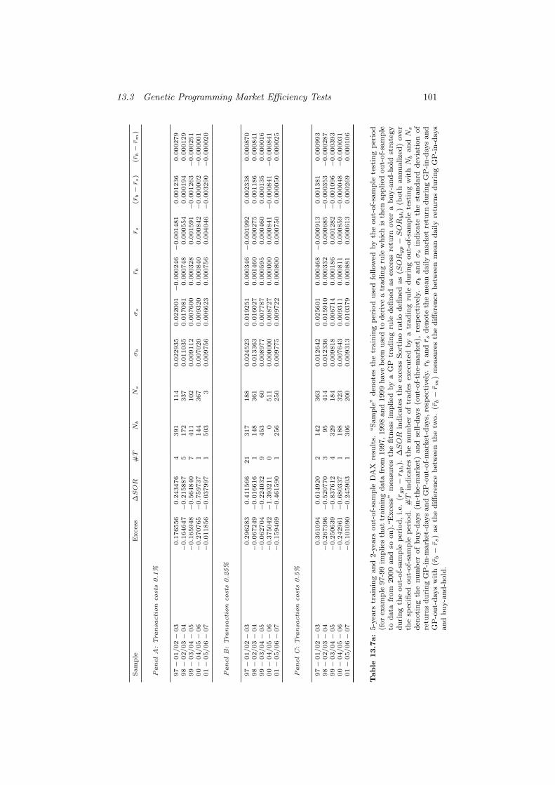
13.3 Genetic Programming Market Efficiency Tests 101
Sam
ple
Excess
∆SOR
#T
Nb
Ns
σb
σs
rb
rs
(rb−r
s)
(rb−r
m)
PanelA
:Tra
nsa
ction
cost
s0.1
%
97−
01/02−
03
0.1
76556
0.2
43476
4391
114
0.0
22935
0.0
22001−
0.0
00246−
0.0
01481
0.0
01236
0.0
00279
98−
02/03−
04
−0.1
64647−
0.2
15887
5172
337
0.0
11035
0.0
17081
0.0
00748
0.0
00554
0.0
00194
0.0
00129
99−
03/04−
05
−0.1
65948−
0.5
64840
7411
102
0.0
09112
0.0
07600
0.0
00328
0.0
01591−
0.0
01263−
0.0
00251
00−
04/05−
06
−0.2
70765−
0.7
59737
1144
367
0.0
07020
0.0
09320
0.0
00840
0.0
00842−
0.0
00002−
0.0
00001
01−
05/06−
07
−0.0
11856−
0.0
37997
1503
30.0
09756
0.0
06623
0.0
00756
0.0
04046−
0.0
03290−
0.0
00020
PanelB:Tra
nsa
ction
cost
s0.2
5%
97−
01/02−
03
0.2
96283
0.4
11566
21
317
188
0.0
24523
0.0
19251
0.0
00346−
0.0
01992
0.0
02338
0.0
00870
98−
02/03−
04
−0.0
67249−
0.0
16616
1148
361
0.0
13363
0.0
16027
0.0
01460
0.0
00275
0.0
01186
0.0
00841
99−
03/04−
05
−0.0
62704−
0.2
24032
9453
60
0.0
08977
0.0
07787
0.0
00595
0.0
00460
0.0
00135
0.0
00016
00−
04/05−
06
−0.3
75042−
1.3
93211
00
511
0.0
00000
0.0
08727
0.0
00000
0.0
00841−
0.0
00841−
0.0
00841
01−
05/06−
07
−0.1
59469−
0.4
61590
1256
250
0.0
09775
0.0
09722
0.0
00800
0.0
00750
0.0
00050
0.0
00025
PanelC:Tra
nsa
ction
cost
s0.5
%
97−
01/02−
03
0.3
61094
0.6
14920
2142
363
0.0
12642
0.0
25601
0.0
00468−
0.0
00913
0.0
01381
0.0
00993
98−
02/03−
04
−0.2
67396−
0.5
20770
395
414
0.0
12336
0.0
15910
0.0
00332
0.0
00685−
0.0
00353−
0.0
00287
99−
03/04−
05
−0.2
50639−
0.8
37612
4329
184
0.0
09818
0.0
06714
0.0
00186
0.0
01282−
0.0
01096−
0.0
00393
00−
04/05−
06
−0.2
42961−
0.6
80337
1188
323
0.0
07643
0.0
09311
0.0
00811
0.0
00859−
0.0
00048−
0.0
00031
01−
05/06−
07
−0.1
01090−
0.2
45903
1306
200
0.0
09313
0.0
10379
0.0
00881
0.0
00613
0.0
00269
0.0
00106
Table
13.7
a:
5-y
ears
train
ing
an
d2-y
ears
ou
t-of-
sam
ple
DA
Xre
sult
s.“S
am
ple
”d
enote
sth
etr
ain
ing
per
iod
use
dfo
llow
edby
the
ou
t-of-
sam
ple
test
ing
per
iod
(for
exam
ple
97-9
9im
plies
that
train
ing
data
from
1997,
1998
and
1999
have
bee
nu
sed
tod
eriv
ea
trad
ing
rule
wh
ich
isth
enap
plied
ou
t-of-
sam
ple
tod
ata
from
2000
an
dso
on
).“E
xce
ss”
mea
sure
sth
efi
tnes
sim
plied
by
aG
Ptr
ad
ing
rule
defi
ned
as
exce
ssre
turn
over
ab
uy-a
nd
-hold
stra
tegy
du
rin
gth
eou
t-of-
sam
ple
per
iod
,i.e.
(rgp−r b
h).
∆SOR
ind
icate
sth
eex
cess
Sort
ino
rati
od
efin
edas
(SOR
gp−SOR
bh
)(b
oth
an
nu
alize
d)
over
the
spec
ified
ou
t-of-
sam
ple
per
iod
.#T
ind
icate
sth
enu
mb
erof
trad
esex
ecu
ted
by
atr
ad
ing
rule
du
rin
gou
t-of-
sam
ple
test
ing
wit
hN
ban
dN
s
den
oti
ng
the
nu
mb
erof
bu
y-d
ays
(in
-th
e-m
ark
et)
an
dse
ll-d
ays
(ou
t-of-
the-
mark
et),
resp
ecti
vel
y.σ
ban
dσ
sin
dic
ate
the
stan
dard
dev
iati
on
of
retu
rns
du
rin
gG
P-i
n-m
ark
et-d
ays
an
dG
P-o
ut-
of-
mark
et-d
ays,
resp
ecti
vel
y.r b
an
dr s
den
ote
the
mea
nd
aily
mark
etre
turn
du
rin
gG
P-i
n-d
ays
an
dG
P-o
ut-
days
wit
h(r
b−r s
)as
the
diff
eren
ceb
etw
een
the
two.
(rb−r m
)m
easu
res
the
diff
eren
ceb
etw
een
mea
nd
aily
retu
rns
du
rin
gG
P-i
n-d
ays
an
db
uy-a
nd
-hold
.
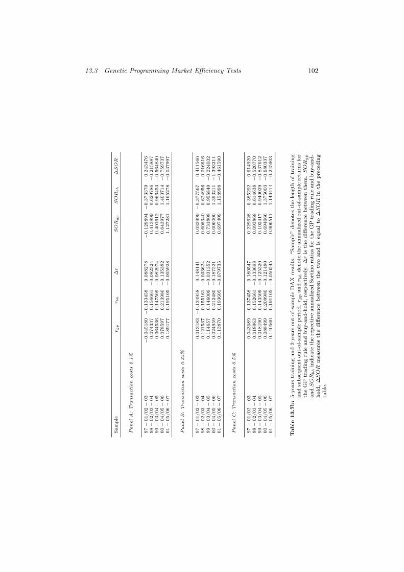
13.3 Genetic Programming Market Efficiency Tests 102
Sam
ple
rg
pr
bh
∆r
SOR
gp
SOR
bh
∆SOR
PanelA
:Tra
nsa
ction
cost
s0.1
%
97−
01/02−
03
−0.0
45180−
0.1
33458
0.0
88278
−0.1
29894−
0.3
73370
0.2
43476
98−
02/03−
04
0.0
74337
0.1
56661−
0.0
82324
0.4
13899
0.6
29786−
0.2
15887
99−
03/04−
05
0.0
64536
0.1
47509−
0.0
82974
0.4
01612
0.9
66453−
0.5
64840
00−
04/05−
06
0.0
78597
0.2
13980−
0.1
35382
0.6
43977
1.4
03714−
0.7
59737
01−
05/06−
07
0.1
89177
0.1
95105−
0.0
05928
1.1
27281
1.1
65278−
0.0
37997
PanelB:Tra
nsa
ction
cost
s0.2
5%
97−
01/02−
03
0.0
13183−
0.1
34958
0.1
48141
0.0
33999−
0.3
77567
0.4
11566
98−
02/03−
04
0.1
21537
0.1
55161−
0.0
33624
0.6
08340
0.6
24956−
0.0
16616
99−
03/04−
05
0.1
14657
0.1
46009−
0.0
31352
0.7
31808
0.9
55840−
0.2
24032
00−
04/05−
06
0.0
24959
0.2
12480−
0.1
87521
0.0
00000
1.3
93211−
1.3
93211
01−
05/06−
07
0.1
13870
0.1
93605−
0.0
79735
0.6
97409
1.1
58998−
0.4
61590
PanelC:Tra
nsa
ction
cost
s0.5
%
97−
01/02−
03
0.0
43089−
0.1
37458
0.1
80547
0.2
29628−
0.3
85292
0.6
14920
98−
02/03−
04
0.0
18963
0.1
52661−
0.1
33698
0.0
93868
0.6
14638−
0.5
20770
99−
03/04−
05
0.0
18190
0.1
43509−
0.1
25320
0.1
02417
0.9
40029−
0.8
37612
00−
04/05−
06
0.0
88499
0.2
09980−
0.1
21480
0.6
94666
1.3
75003−
0.6
80337
01−
05/06−
07
0.1
40560
0.1
91105−
0.0
50545
0.9
00511
1.1
46414−
0.2
45903
Table
13.7
b:
5-y
ears
train
ing
an
d2-y
ears
ou
t-of-
sam
ple
DA
Xre
sult
s.“S
am
ple
”d
enote
sth
ele
ngth
of
train
ing
an
dsu
bse
qu
ent
ou
t-of-
sam
ple
per
iod
.r g
pan
dr b
hd
enote
the
an
nu
alize
dou
t-of-
sam
ple
retu
rns
for
the
GP
trad
ing
rule
an
db
uy-a
nd
-hold
,re
spec
tivel
y.∆r
isth
ed
iffer
ence
bet
wee
nth
em.SOR
gp
an
dSOR
bh
ind
icate
the
rep
ecti
ve
an
nu
alize
dS
ort
ino
rati
os
for
the
GP
trad
ing
rule
an
db
uy-a
nd
-h
old
,∆SOR
mea
sure
sth
ed
iffer
ence
bet
wee
nth
etw
oan
dis
equ
al
to∆SOR
inth
ep
rece
din
gta
ble
.
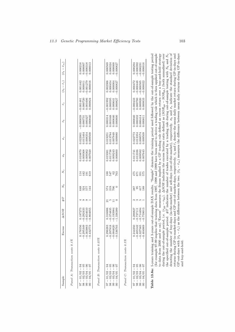
13.3 Genetic Programming Market Efficiency Tests 103
Sam
ple
Excess
∆SOR
#T
Nb
Ns
σb
σs
rb
rs
(rb−r
s)
(rb−r
m)
PanelA
:Tra
nsa
ction
cost
s0.1
%
97−
01/02−
04
0.1
76556
0.1
87273
4648
114
0.0
18870
0.0
22001−
0.0
00039−
0.0
01481
0.0
01442
0.0
00216
98−
02/03−
05
−0.2
95349−
0.2
92433
9324
442
0.0
09368
0.0
15464
0.0
00731
0.0
00720
0.0
00011
0.0
00007
99−
03/04−
06
−0.3
03883−
0.6
54610
9577
191
0.0
09362
0.0
08354
0.0
00327
0.0
01606−
0.0
01279−
0.0
00318
00−
04/05−
07
−0.4
32773−
0.8
04055
1144
619
0.0
07020
0.0
09500
0.0
00840
0.0
00824
0.0
00016
0.0
00013
PanelB:Tra
nsa
ction
cost
s0.2
5%
97−
01/02−
04
0.2
96283
0.3
16006
21
574
188
0.0
19381
0.0
19251
0.0
00314−
0.0
01992
0.0
02306
0.0
00569
98−
02/03−
05
−0.2
97818−
0.3
74835
5219
547
0.0
11738
0.0
13784
0.0
01048
0.0
00595
0.0
00454
0.0
00324
99−
03/04−
06
−0.0
84620−
0.1
93984
11
706
62
0.0
09243
0.0
07840
0.0
00646
0.0
00641
0.0
00004
0.0
00000
00−
04/05−
07
−0.5
36703−
1.3
36389
00
763
0.0
00000
0.0
09080
0.0
00000
0.0
00827−
0.0
00827−
0.0
00827
PanelC:Tra
nsa
ction
cost
s0.5
%
97−
01/02−
04
0.2
44350
0.2
88827
2287
475
0.0
11741
0.0
22773
0.0
00040−
0.0
00433
0.0
00472
0.0
00294
98−
02/03−
05
−0.4
85542−
0.7
27111
395
671
0.0
12336
0.0
13354
0.0
00332
0.0
00780−
0.0
00448−
0.0
00392
99−
03/04−
06
−0.3
27565−
0.7
14494
5417
351
0.0
09582
0.0
08574
0.0
00414
0.0
00920−
0.0
00505−
0.0
00231
00−
04/05−
07
−0.4
04969−
0.7
59013
1188
575
0.0
07643
0.0
09509
0.0
00811
0.0
00833−
0.0
00022−
0.0
00016
Table
13.8
a:
5-y
ears
train
ing
an
d3-y
ears
ou
t-of-
sam
ple
DA
Xre
sult
s.“S
am
ple
”d
enote
sth
etr
ain
ing
per
iod
use
dfo
llow
edby
the
ou
t-of-
sam
ple
test
ing
per
iod
(for
exam
ple
97-9
9im
plies
that
train
ing
data
from
1997,
1998
and
1999
have
bee
nu
sed
tod
eriv
ea
trad
ing
rule
wh
ich
isth
enap
plied
ou
t-of-
sam
ple
tod
ata
from
2000
an
dso
on
).“E
xce
ss”
mea
sure
sth
efi
tnes
sim
plied
by
aG
Ptr
ad
ing
rule
defi
ned
as
exce
ssre
turn
over
ab
uy-a
nd
-hold
stra
tegy
du
rin
gth
eou
t-of-
sam
ple
per
iod
,i.e.
(rgp−r b
h).
∆SOR
ind
icate
sth
eex
cess
Sort
ino
rati
od
efin
edas
(SOR
gp−SOR
bh
)(b
oth
an
nu
alize
d)
over
the
spec
ified
ou
t-of-
sam
ple
per
iod
.#T
ind
icate
sth
enu
mb
erof
trad
esex
ecu
ted
by
atr
ad
ing
rule
du
rin
gou
t-of-
sam
ple
test
ing
wit
hN
ban
dN
s
den
oti
ng
the
nu
mb
erof
bu
y-d
ays
(in
-th
e-m
ark
et)
an
dse
ll-d
ays
(ou
t-of-
the-
mark
et),
resp
ecti
vel
y.σ
ban
dσ
sin
dic
ate
the
stan
dard
dev
iati
on
of
retu
rns
du
rin
gG
P-i
n-m
ark
et-d
ays
an
dG
P-o
ut-
of-
mark
et-d
ays,
resp
ecti
vel
y.r b
an
dr s
den
ote
the
mea
nd
aily
mark
etre
turn
du
rin
gG
P-i
n-d
ays
an
dG
P-o
ut-
days
wit
h(r
b−r s
)as
the
diff
eren
ceb
etw
een
the
two.
(rb−r m
)m
easu
res
the
diff
eren
ceb
etw
een
mea
nd
aily
retu
rns
du
rin
gG
P-i
n-d
ays
an
db
uy-a
nd
-hold
.
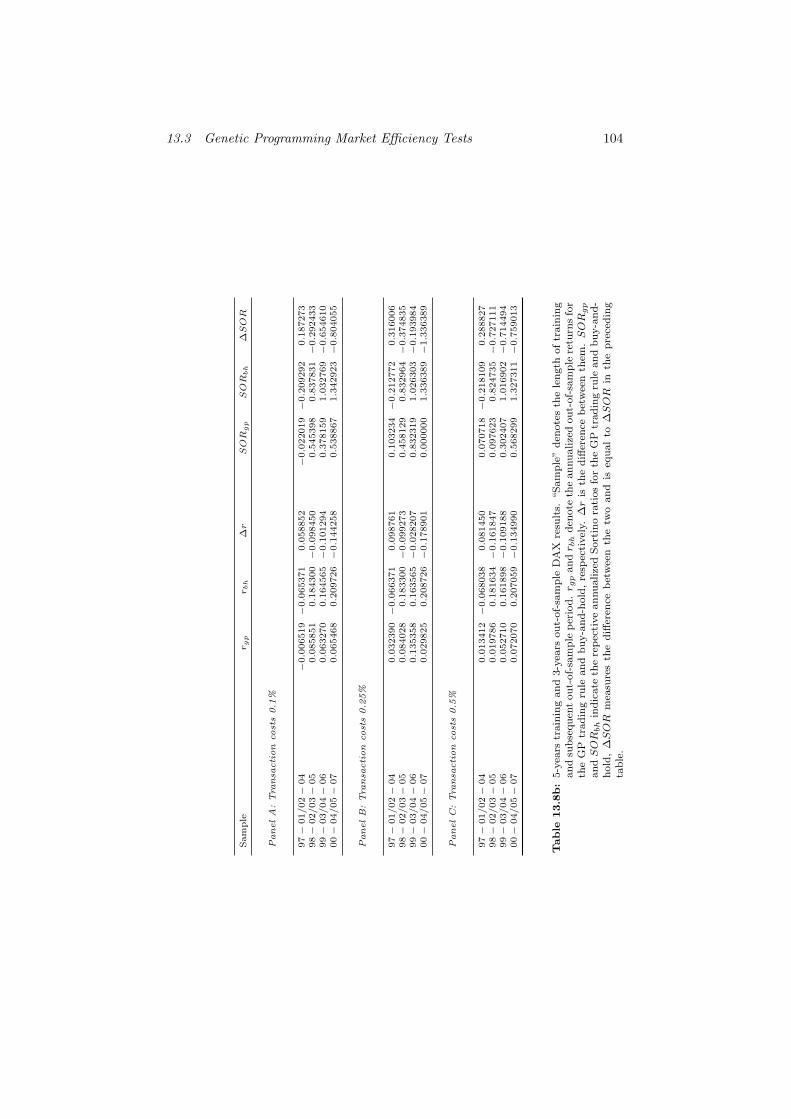
13.3 Genetic Programming Market Efficiency Tests 104
Sam
ple
rg
pr
bh
∆r
SOR
gp
SOR
bh
∆SOR
PanelA
:Tra
nsa
ction
cost
s0.1
%
97−
01/02−
04
−0.0
06519−
0.0
65371
0.0
58852
−0.0
22019−
0.2
09292
0.1
87273
98−
02/03−
05
0.0
85851
0.1
84300−
0.0
98450
0.5
45398
0.8
37831−
0.2
92433
99−
03/04−
06
0.0
63270
0.1
64565−
0.1
01294
0.3
78159
1.0
32769−
0.6
54610
00−
04/05−
07
0.0
65468
0.2
09726−
0.1
44258
0.5
38867
1.3
42923−
0.8
04055
PanelB:Tra
nsa
ction
cost
s0.2
5%
97−
01/02−
04
0.0
32390−
0.0
66371
0.0
98761
0.1
03234−
0.2
12772
0.3
16006
98−
02/03−
05
0.0
84028
0.1
83300−
0.0
99273
0.4
58129
0.8
32964−
0.3
74835
99−
03/04−
06
0.1
35358
0.1
63565−
0.0
28207
0.8
32319
1.0
26303−
0.1
93984
00−
04/05−
07
0.0
29825
0.2
08726−
0.1
78901
0.0
00000
1.3
36389−
1.3
36389
PanelC:Tra
nsa
ction
cost
s0.5
%
97−
01/02−
04
0.0
13412−
0.0
68038
0.0
81450
0.0
70718−
0.2
18109
0.2
88827
98−
02/03−
05
0.0
19786
0.1
81634−
0.1
61847
0.0
97623
0.8
24735−
0.7
27111
99−
03/04−
06
0.0
52710
0.1
61898−
0.1
09188
0.3
02407
1.0
16902−
0.7
14494
00−
04/05−
07
0.0
72070
0.2
07059−
0.1
34990
0.5
68299
1.3
27311−
0.7
59013
Table
13.8
b:
5-y
ears
train
ing
an
d3-y
ears
ou
t-of-
sam
ple
DA
Xre
sult
s.“S
am
ple
”d
enote
sth
ele
ngth
of
train
ing
an
dsu
bse
qu
ent
ou
t-of-
sam
ple
per
iod
.r g
pan
dr b
hd
enote
the
an
nu
alize
dou
t-of-
sam
ple
retu
rns
for
the
GP
trad
ing
rule
an
db
uy-a
nd
-hold
,re
spec
tivel
y.∆r
isth
ed
iffer
ence
bet
wee
nth
em.SOR
gp
an
dSOR
bh
ind
icate
the
rep
ecti
ve
an
nu
alize
dS
ort
ino
rati
os
for
the
GP
trad
ing
rule
an
db
uy-a
nd
-h
old
,∆SOR
mea
sure
sth
ed
iffer
ence
bet
wee
nth
etw
oan
dis
equ
al
to∆SOR
inth
ep
rece
din
gta
ble
.
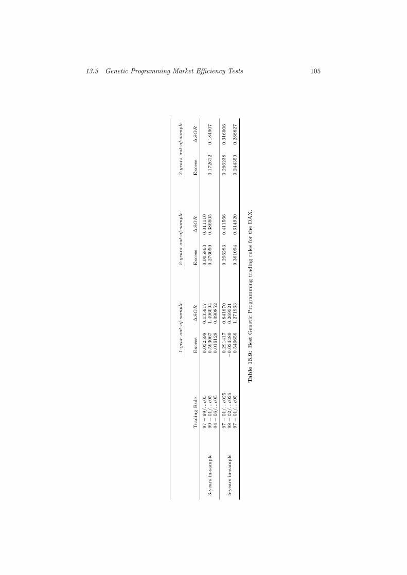
13.3 Genetic Programming Market Efficiency Tests 105
1-y
ear
out-of-sa
mple
2-y
ears
out-of-sa
mple
3-y
ears
out-of-sa
mple
Tra
din
gR
ule
Excess
∆SOR
Excess
∆SOR
Excess
∆SOR
3-y
ears
in-s
am
ple
97−
99/...c
05
0.0
32598
0.1
35917
0.0
05863
0.0
11110
99−
01/...c
05
0.5
93067
1.4
96094
0.2
76050
0.3
86905
0.1
72612
0.1
84907
04−
06/...c
05
0.0
16128
0.0
90852
5-y
ears
in-s
am
ple
97−
01/...c
025
0.2
91417
0.8
41870
0.2
96283
0.4
11566
0.2
96238
0.3
16006
98−
02/...c
025
−0.0
24480
0.2
69521
97−
01/...c
05
0.5
46656
1.2
71963
0.3
61094
0.6
14920
0.2
44350
0.2
88827
Table
13.9
:B
est
Gen
etic
Pro
gra
mm
ing
trad
ing
rule
sfo
rth
eD
AX
.
13.3 Genetic Programming Market Efficiency Tests 106
13.3.2 Testing the Hang Seng
13.3.2.1 Test Results
Hang Seng results have been compiled in Tables 13.11a - 13.16a and adopt the
already familiar table layout from the DAX scenarios. As already pointed out
before, all scenarios under unrealistcally low transaction costs of c = 0.1 will
not be addressed in-depth and only serve for comparative statics.
Two GP rules manage to outperform buy-and-hold under c = 0.25 in Table
13.11a. The first rule (97-99/00) is one of the rare instances where GP always
stays out-of-the-market. This might reflect the aftermath of the Asian crisis
starting in 1997 which coincides with the training period of the GP algorithm98.
Rolling the time window forward by one year results once more in an out-
performance compared to buy-and-hold, this time with a real timing strategy.
Interestingly, the strategy starts with a prolonged out-of-the-market position
and switches into the market shortly before Sept. 11th99. As this is the only
trade the rule executes, it remains in-the-market even after Sept. 11th. Despite
the unfortunate timing the rule yields just a small negative absolute return
(-0.015305 p.a. see Table 13.11b) vs. a massive -0.270973 p.a. loss for buy-and-
hold which at first sight seems puzzling. Some further analysis showed that the
market was already down roughly 23% before Sept. 11th so this event did not
add up much to the losses already incurred in the Hang Seng100. This explains
the surprisingly good performance of the rule despite the, from an intuitive
point of view, unfortunate timing101. Furthermore, volatility during buy-days
is higher than during sell-days and timing abilities of the rule are insignificant. A
replication of buy-and-hold is suggested for the 99-01/02 and 01-03/04 scenarios.
Focusing on the c = 0.5 panel, two rules emerge that beat buy-and-hold on98The impact of the Asian crisis is easily spotted in Figure 13.2.99As a general remark, GP investment positions can be easily superimposed on the respective
time series using Matlab, however the author chose not to include these charts in order tosave space.
100The heavy losses may be attributed to a massive outbreak of Severe Acute Respiratory Syn-drome (SARS) also known as bird flu in 2001.
101As a sidenote, it is interesting that the DAX (and most likely all western stock indices) werefar more affected by Sept. 11th than the Hang Seng.
13.3 Genetic Programming Market Efficiency Tests 107
a risk-adjusted basis. The 98-00/01c05 rule repeats the unfortunate timing of
the rule discussed above (staying out and then switching in shortly before Sept.
11th) once more but switches out-of-the-market after 51 days rather than stay-
ing in until the end of the year. As most of the total loss in 2001 already occurred
before Sept. 11th, the rule manages to cut losses considerably (-0.165865 p.a.
vs. -0.275973 p.a., see Table 13.11b). Volatility during buy-days is once more
higher than during sell days (0.025094 vs. 0.015039). The 99-01/02c05 rule
yields positive results as well. It only takes a single in-the-market position in
the mid of the trading year to cut losses considerably (-0.143000 vs. -0.206992
see Table 13.11b). Unfortunately, the difference (rb − rs) and (rb − rm) are in
neither case statistically significant. Leaving aside the c = 0.1 rules, the remain-
ing GP rules clearly underperform the benchmark. Similar to the results from
the DAX, trading frequencies seems to be quite unaffected by transaction costs.
The impact of transaction costs will become more visible in the later scenarios
with a 5-year training horizon.
Stretching the horizon to two years out-of-sample yields similar results (Ta-
ble 13.12a). The rules obtained during the 97-99 and 98-00 training sample
outperform buy-and-hold in terms of excess return and excess Sortino ratio for
both transaction costs scenarios (c = 0.25 and c = 0.5). Interestingly, the
same rules execute at most a single trade during the first out-of-sample year
(see Table 13.11a) whereas trading activity picks up during the second year. As
already observed before, volatility during in-days is higher than during out-days.
Returning to Table 13.12a, some brief remarks on the c = 0.1 rules are in order.
Despite the unrealistically low transaction cost, the algorithm did not find any
successful trading rule in scenarios where the c = 0.25 and c = 0.5 rules failed as
well to beat buy-and-hold. This might hint at market efficiency for these partic-
ular periods in the market since even with extremely low transaction costs (and
thus the possibility of almost zero transaction costs), no technical trading rule
could be found that beats the benchmark. This applies to both the 3:1 and the
3:2 scenarios illustrated in Tables 13.11a and 13.12a. The 03-05/06(-07) case is
an exception that yields positive returns while the same scenario under higher
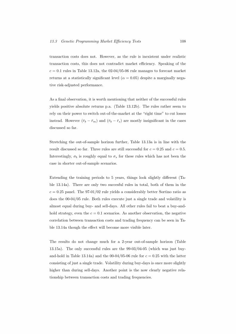
13.3 Genetic Programming Market Efficiency Tests 108
transaction costs does not. However, as the rule is inexistent under realistic
transaction costs, this does not contradict market efficiency. Speaking of the
c = 0.1 rules in Table 13.12a, the 02-04/05-06 rule manages to forecast market
returns at a statistically significant level (α = 0.05) despite a marginally nega-
tive risk-adjusted performance.
As a final observation, it is worth mentioning that neither of the successful rules
yields positive absolute returns p.a. (Table 13.12b). The rules rather seem to
rely on their power to switch out-of-the-market at the “right time” to cut losses
instead. However (rb − rm) and (rb − rs) are mostly insignificant in the cases
discussed so far.
Stretching the out-of-sample horizon further, Table 13.13a is in line with the
result discussed so far. Three rules are still successful for c = 0.25 and c = 0.5.
Interestingly, σb is roughly equal to σs for these rules which has not been the
case in shorter out-of-sample scenarios.
Extending the training periods to 5 years, things look slightly different (Ta-
ble 13.14a). There are only two succesful rules in total, both of them in the
c = 0.25 panel. The 97-01/02 rule yields a considerably better Sortino ratio as
does the 00-04/05 rule. Both rules execute just a single trade and volatility is
almost equal during buy- and sell-days. All other rules fail to beat a buy-and-
hold strategy, even the c = 0.1 scenarios. As another observation, the negative
correlation between transaction costs and trading frequency can be seen in Ta-
ble 13.14a though the effect will become more visible later.
The results do not change much for a 2-year out-of-sample horizon (Table
13.15a). The only successful rules are the 99-03/04-05 (which was just buy-
and-hold in Table 13.14a) and the 00-04/05-06 rule for c = 0.25 with the latter
consisting of just a single trade. Volatility during buy-days is once more slightly
higher than during sell-days. Another point is the now clearly negative rela-
tionship between transaction costs and trading frequencies.
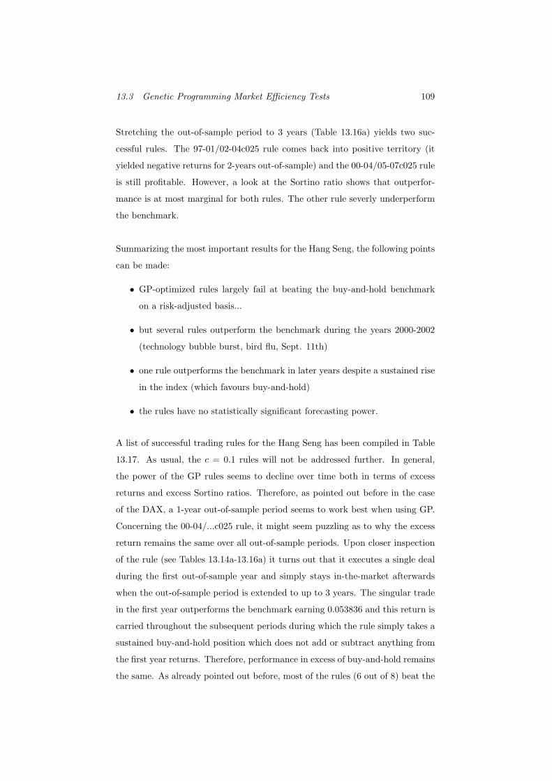
13.3 Genetic Programming Market Efficiency Tests 109
Stretching the out-of-sample period to 3 years (Table 13.16a) yields two suc-
cessful rules. The 97-01/02-04c025 rule comes back into positive territory (it
yielded negative returns for 2-years out-of-sample) and the 00-04/05-07c025 rule
is still profitable. However, a look at the Sortino ratio shows that outperfor-
mance is at most marginal for both rules. The other rule severly underperform
the benchmark.
Summarizing the most important results for the Hang Seng, the following points
can be made:
• GP-optimized rules largely fail at beating the buy-and-hold benchmark
on a risk-adjusted basis...
• but several rules outperform the benchmark during the years 2000-2002
(technology bubble burst, bird flu, Sept. 11th)
• one rule outperforms the benchmark in later years despite a sustained rise
in the index (which favours buy-and-hold)
• the rules have no statistically significant forecasting power.
A list of successful trading rules for the Hang Seng has been compiled in Table
13.17. As usual, the c = 0.1 rules will not be addressed further. In general,
the power of the GP rules seems to decline over time both in terms of excess
returns and excess Sortino ratios. Therefore, as pointed out before in the case
of the DAX, a 1-year out-of-sample period seems to work best when using GP.
Concerning the 00-04/...c025 rule, it might seem puzzling as to why the excess
return remains the same over all out-of-sample periods. Upon closer inspection
of the rule (see Tables 13.14a-13.16a) it turns out that it executes a single deal
during the first out-of-sample year and simply stays in-the-market afterwards
when the out-of-sample period is extended to up to 3 years. The singular trade
in the first year outperforms the benchmark earning 0.053836 and this return is
carried throughout the subsequent periods during which the rule simply takes a
sustained buy-and-hold position which does not add or subtract anything from
the first year returns. Therefore, performance in excess of buy-and-hold remains
the same. As already pointed out before, most of the rules (6 out of 8) beat the
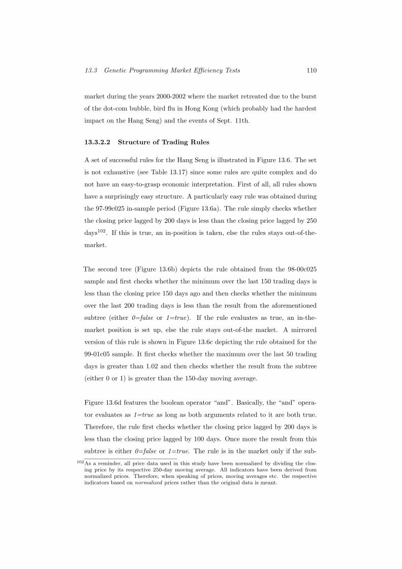
13.3 Genetic Programming Market Efficiency Tests 110
market during the years 2000-2002 where the market retreated due to the burst
of the dot-com bubble, bird flu in Hong Kong (which probably had the hardest
impact on the Hang Seng) and the events of Sept. 11th.
13.3.2.2 Structure of Trading Rules
A set of successful rules for the Hang Seng is illustrated in Figure 13.6. The set
is not exhaustive (see Table 13.17) since some rules are quite complex and do
not have an easy-to-grasp economic interpretation. First of all, all rules shown
have a surprisingly easy structure. A particularly easy rule was obtained during
the 97-99c025 in-sample period (Figure 13.6a). The rule simply checks whether
the closing price lagged by 200 days is less than the closing price lagged by 250
days102. If this is true, an in-position is taken, else the rules stays out-of-the-
market.
The second tree (Figure 13.6b) depicts the rule obtained from the 98-00c025
sample and first checks whether the minimum over the last 150 trading days is
less than the closing price 150 days ago and then checks whether the minimum
over the last 200 trading days is less than the result from the aforementioned
subtree (either 0=false or 1=true). If the rule evaluates as true, an in-the-
market position is set up, else the rule stays out-of-the market. A mirrored
version of this rule is shown in Figure 13.6c depicting the rule obtained for the
99-01c05 sample. It first checks whether the maximum over the last 50 trading
days is greater than 1.02 and then checks whether the result from the subtree
(either 0 or 1) is greater than the 150-day moving average.
Figure 13.6d features the boolean operator “and”. Basically, the “and” opera-
tor evaluates as 1=true as long as both arguments related to it are both true.
Therefore, the rule first checks whether the closing price lagged by 200 days is
less than the closing price lagged by 100 days. Once more the result from this
subtree is either 0=false or 1=true. The rule is in the market only if the sub-102As a reminder, all price data used in this study have been normalized by dividing the clos-
ing price by its respective 250-day moving average. All indicators have been derived fromnormalized prices. Therefore, when speaking of prices, moving averages etc. the respectiveindicators based on normalized prices rather than the original data is meant.
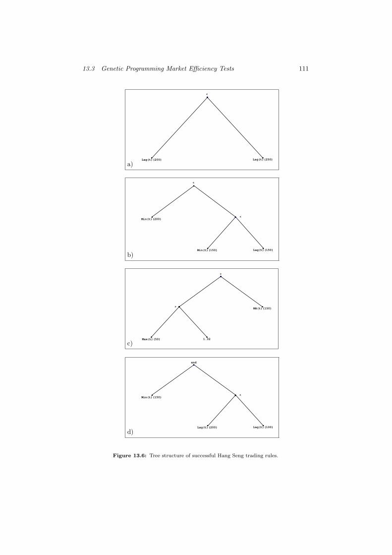
13.3 Genetic Programming Market Efficiency Tests 111
a)Lag(t)(200) Lag(t)(250)
<
b)
Min(t)(200)
Min(t)(150) Lag(t)(150)
<
<
c)Max(t)(50) 1.02
>MA(t)(150)
>
d)
Min(t)(150)
Lag(t)(200) Lag(t)(100)
<
and
Figure 13.6: Tree structure of successful Hang Seng trading rules.
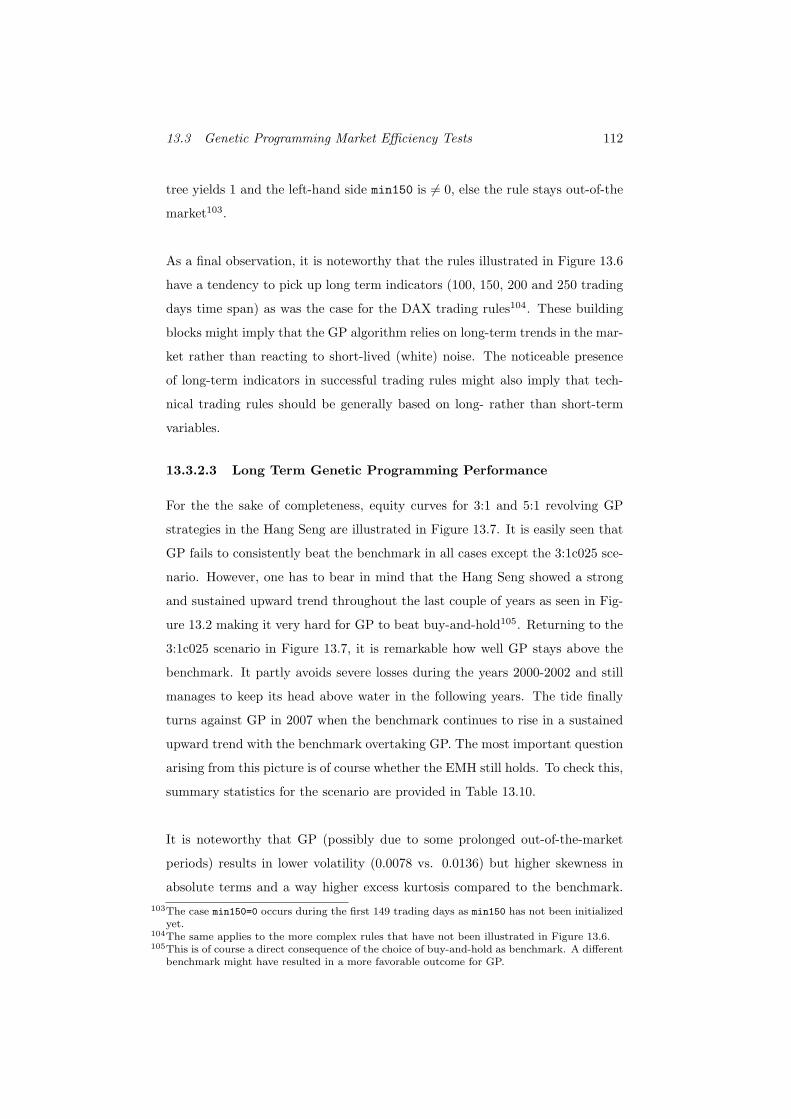
13.3 Genetic Programming Market Efficiency Tests 112
tree yields 1 and the left-hand side min150 is 6= 0, else the rule stays out-of-the
market103.
As a final observation, it is noteworthy that the rules illustrated in Figure 13.6
have a tendency to pick up long term indicators (100, 150, 200 and 250 trading
days time span) as was the case for the DAX trading rules104. These building
blocks might imply that the GP algorithm relies on long-term trends in the mar-
ket rather than reacting to short-lived (white) noise. The noticeable presence
of long-term indicators in successful trading rules might also imply that tech-
nical trading rules should be generally based on long- rather than short-term
variables.
13.3.2.3 Long Term Genetic Programming Performance
For the the sake of completeness, equity curves for 3:1 and 5:1 revolving GP
strategies in the Hang Seng are illustrated in Figure 13.7. It is easily seen that
GP fails to consistently beat the benchmark in all cases except the 3:1c025 sce-
nario. However, one has to bear in mind that the Hang Seng showed a strong
and sustained upward trend throughout the last couple of years as seen in Fig-
ure 13.2 making it very hard for GP to beat buy-and-hold105. Returning to the
3:1c025 scenario in Figure 13.7, it is remarkable how well GP stays above the
benchmark. It partly avoids severe losses during the years 2000-2002 and still
manages to keep its head above water in the following years. The tide finally
turns against GP in 2007 when the benchmark continues to rise in a sustained
upward trend with the benchmark overtaking GP. The most important question
arising from this picture is of course whether the EMH still holds. To check this,
summary statistics for the scenario are provided in Table 13.10.
It is noteworthy that GP (possibly due to some prolonged out-of-the-market
periods) results in lower volatility (0.0078 vs. 0.0136) but higher skewness in
absolute terms and a way higher excess kurtosis compared to the benchmark.103The case min150=0 occurs during the first 149 trading days as min150 has not been initialized
yet.104The same applies to the more complex rules that have not been illustrated in Figure 13.6.105This is of course a direct consequence of the choice of buy-and-hold as benchmark. A different
benchmark might have resulted in a more favorable outcome for GP.
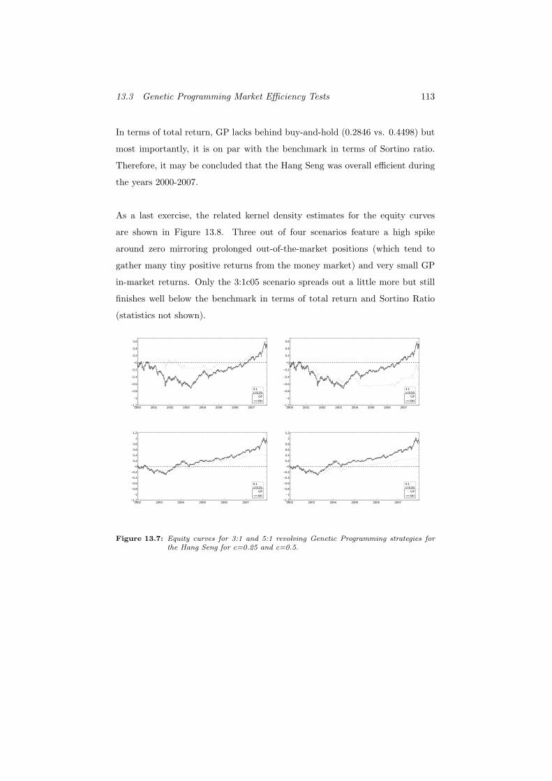
13.3 Genetic Programming Market Efficiency Tests 113
In terms of total return, GP lacks behind buy-and-hold (0.2846 vs. 0.4498) but
most importantly, it is on par with the benchmark in terms of Sortino ratio.
Therefore, it may be concluded that the Hang Seng was overall efficient during
the years 2000-2007.
As a last exercise, the related kernel density estimates for the equity curves
are shown in Figure 13.8. Three out of four scenarios feature a high spike
around zero mirroring prolonged out-of-the-market positions (which tend to
gather many tiny positive returns from the money market) and very small GP
in-market returns. Only the 3:1c05 scenario spreads out a little more but still
finishes well below the benchmark in terms of total return and Sortino Ratio
(statistics not shown).
2000 2001 2002 2003 2004 2005 2006 2007−1.2
−1
−0.8
−0.6
−0.4
−0.2
−0
0.2
0.4
0.6
GP
BH
3:1c=0.25
2000 2001 2002 2003 2004 2005 2006 2007−1.2
−1
−0.8
−0.6
−0.4
−0.2
−0
0.2
0.4
0.6
GP
BH
3:1c=0.50
2002 2003 2004 2005 2006 2007−1.2
−1
−0.8
−0.6
−0.4
−0.2
−0
0.2
0.4
0.6
0.8
1
1.2
GP
BH
5:1c=0.25
2002 2003 2004 2005 2006 2007−1.2
−1
−0.8
−0.6
−0.4
−0.2
−0
0.2
0.4
0.6
0.8
1
1.2
GP
BH
5:1c=0.50
Figure 13.7: Equity curves for 3:1 and 5:1 revolving Genetic Programming strategies forthe Hang Seng for c=0.25 and c=0.5.
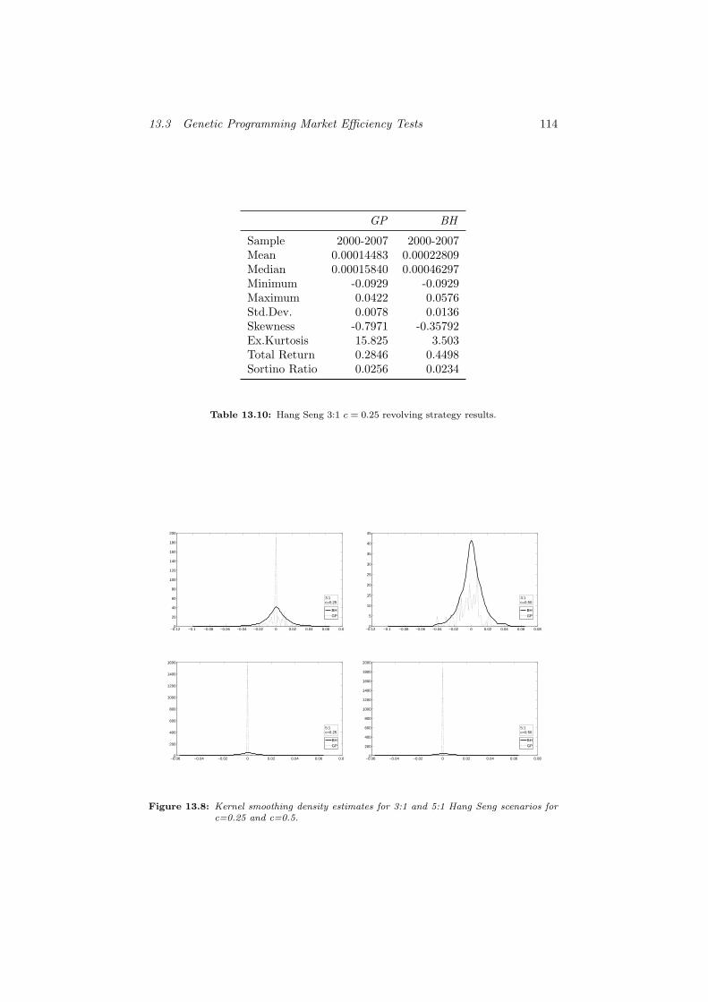
13.3 Genetic Programming Market Efficiency Tests 114
GP BH
Sample 2000-2007 2000-2007Mean 0.00014483 0.00022809Median 0.00015840 0.00046297Minimum -0.0929 -0.0929Maximum 0.0422 0.0576Std.Dev. 0.0078 0.0136Skewness -0.7971 -0.35792Ex.Kurtosis 15.825 3.503Total Return 0.2846 0.4498Sortino Ratio 0.0256 0.0234
Table 13.10: Hang Seng 3:1 c = 0.25 revolving strategy results.
−0.12 −0.1 −0.08 −0.06 −0.04 −0.02 0 0.02 0.04 0.06 0.080
20
40
60
80
100
120
140
160
180
200
BH
GP
3:1c=0.25
−0.12 −0.1 −0.08 −0.06 −0.04 −0.02 0 0.02 0.04 0.06 0.080
5
10
15
20
25
30
35
40
45
BH
GP
3:1c=0.50
−0.06 −0.04 −0.02 0 0.02 0.04 0.06 0.080
200
400
600
800
1000
1200
1400
1600
BH
GP
5:1c=0.25
−0.06 −0.04 −0.02 0 0.02 0.04 0.06 0.080
200
400
600
800
1000
1200
1400
1600
1800
2000
BH
GP
5:1c=0.50
Figure 13.8: Kernel smoothing density estimates for 3:1 and 5:1 Hang Seng scenarios forc=0.25 and c=0.5.
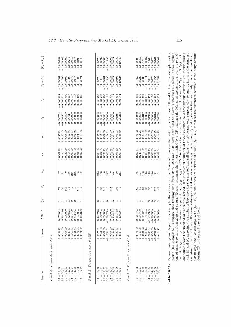
13.3 Genetic Programming Market Efficiency Tests 115Sam
ple
Excess
∆SOR
#T
Nb
Ns
σb
σs
rb
rs
(rb−r
s)
(rb−r
m)
PanelA
:Tra
nsa
ction
cost
s0.1
%
97−
99/00
0.0
19813
0.0
79968
1179
67
0.0
20146
0.0
18723−
0.0
00758−
0.0
00068−
0.0
00691
−0.0
00188
98−
00/01
0.0
51160
0.2
86270
2151
91
0.0
19557
0.0
13755−
0.0
01507−
0.0
00421−
0.0
01086
−0.0
00408
99−
01/02
0.0
00000
0.0
00000
1246
00.0
12209
0.0
00000−
0.0
00809
0.0
00000−
0.0
00809
0.0
00000
00−
02/03
−0.2
63177−
1.7
23528
371
176
0.0
11694
0.0
10264
0.0
00417
0.0
01507−
0.0
01090
−0.0
00777
01−
03/04
−0.1
01171−
0.6
60709
00
248
0.0
00000
0.0
10277
0.0
00000−
0.0
00577
0.0
00577
−0.0
00419
02−
04/05
−0.0
15833−
0.3
31433
00
246
0.0
00000
0.0
07258
0.0
00000
0.0
00178−
0.0
00178
−0.0
00178
03−
05/06
−0.0
77375−
0.5
58935
1211
35
0.0
09196
0.0
08651
0.0
00980
0.0
02369−
0.0
01389
−0.0
00198
04−
06/07
0.0
17007−
0.1
02322
1145
99
0.0
19292
0.0
11498
0.0
02063−
0.0
00008
0.0
02071
0.0
00840
PanelB:Tra
nsa
ction
cost
s0.2
5%
97−
99/00
0.2
02731
0.4
46743
00
246
0.0
00000
0.0
19733
0.0
00000−
0.0
00570
0.0
00570
0.0
00570
98−
00/01
0.2
55669
0.9
35284
192
150
0.0
20765
0.0
15361−
0.0
00407−
0.0
01523
0.0
01116
0.0
00692
99−
01/02
0.0
00000
0.0
00000
1246
00.0
12213
0.0
00000−
0.0
00801
0.0
00000−
0.0
00801
0.0
00000
00−
02/03
−0.2
79931−
1.8
96715
00
247
0.0
00000
0.0
10681
0.0
00000
0.0
01193−
0.0
01193
−0.0
01193
01−
03/04
0.0
00000
0.0
00000
1248
00.0
10278
0.0
00000
0.0
00427
0.0
00000
0.0
00427
0.0
00000
02−
04/05
−0.0
12833−
0.3
05865
00
246
0.0
00000
0.0
07258
0.0
00000
0.0
00178−
0.0
00178
−0.0
00178
03−
05/06
−0.0
43383−
0.3
59742
1196
50
0.0
09542
0.0
07293
0.0
01217
0.0
01023
0.0
00194
0.0
00039
04−
06/07
−0.2
36797−
1.1
06381
11
243
0.0
00000
0.0
16569
0.0
20272
0.0
01144
0.0
19128
0.0
19049
PanelC:Tra
nsa
ction
cost
s0.5
%
97−
99/00
−0.0
17500−
0.0
20753
1180
66
0.0
20271
0.0
18292−
0.0
00960
0.0
00492−
0.0
01452
−0.0
00390
98−
00/01
0.1
10108
0.5
90780
151
191
0.0
24961
0.0
15025−
0.0
03656−
0.0
00416−
0.0
03239
−0.0
02557
99−
01/02
0.0
63992
0.3
78851
163
183
0.0
11297
0.0
12499−
0.0
02317−
0.0
00279−
0.0
02039
−0.0
01516
00−
02/03
−0.2
59144−
1.6
96425
1102
145
0.0
10989
0.0
10452
0.0
00306
0.0
01817−
0.0
01511
−0.0
00887
01−
03/04
−0.2
99134−
1.8
22383
3130
118
0.0
09743
0.0
10539−
0.0
01340
0.0
02373−
0.0
03713
−0.0
01766
02−
04/05
−0.0
07833−
0.2
63583
00
246
0.0
00000
0.0
07258
0.0
00000
0.0
00178−
0.0
00178
−0.0
00178
03−
05/06
−0.0
79027−
0.5
30141
3225
21
0.0
09324
0.0
06385
0.0
01010
0.0
02965−
0.0
01955
−0.0
00167
04−
06/07
−0.0
40182−
0.2
80656
2146
98
0.0
19304
0.0
11432
0.0
01726
0.0
00473
0.0
01253
0.0
00503
Table
13.1
1a:
3-y
ears
train
ing
an
d1-y
ear
ou
t-of-
sam
ple
Han
gS
eng
resu
lts.
“S
am
ple
”d
enote
sth
etr
ain
ing
per
iod
use
dfo
llow
edby
the
ou
t-of-
sam
ple
test
ing
per
iod
(for
exam
ple
97-9
9im
plies
that
train
ing
data
from
1997,
1998
an
d1999
have
bee
nu
sed
tod
eriv
ea
trad
ing
rule
wh
ich
isth
enap
plied
ou
t-of-
sam
ple
tod
ata
from
2000
an
dso
on
).“E
xce
ss”
mea
sure
sth
efi
tnes
sim
pli
edby
aG
Ptr
ad
ing
rule
defi
ned
as
exce
ssre
turn
over
ab
uy-a
nd
-h
old
stra
tegy
du
rin
gth
eou
t-of-
sam
ple
per
iod
,i.e.
(rgp−r b
h).
∆SOR
ind
icate
sth
eex
cess
Sort
ino
rati
od
efin
edas
(SOR
gp−SOR
bh
)(b
oth
an
nu
alize
d)
over
the
spec
ified
ou
t-of-
sam
ple
per
iod
.#T
ind
icate
sth
enu
mb
erof
trad
esex
ecu
ted
by
atr
ad
ing
rule
duri
ng
ou
t-of-
sam
ple
test
ing
wit
hN
ban
dN
sd
enoti
ng
the
nu
mb
erof
bu
y-d
ays
(in
-th
e-m
ark
et)
an
dse
ll-d
ays
(ou
t-of-
the-
mark
et),
resp
ecti
vel
y.σ
ban
dσ
sin
dic
ate
the
stan
dard
dev
iati
on
of
retu
rns
du
rin
gG
P-i
n-m
ark
et-d
ays
an
dG
P-o
ut-
of-
mark
et-d
ays,
resp
ecti
vel
y.r b
an
dr s
den
ote
the
mea
nd
aily
mark
etre
turn
du
rin
gG
P-i
n-d
ays
an
dG
P-o
ut-
days
wit
h(r
b−r s
)as
the
diff
eren
ceb
etw
een
the
two.
(rb−r m
)m
easu
res
the
diff
eren
ceb
etw
een
mea
nd
aily
retu
rns
du
rin
gG
P-i
n-d
ays
an
db
uy-a
nd
-hold
.
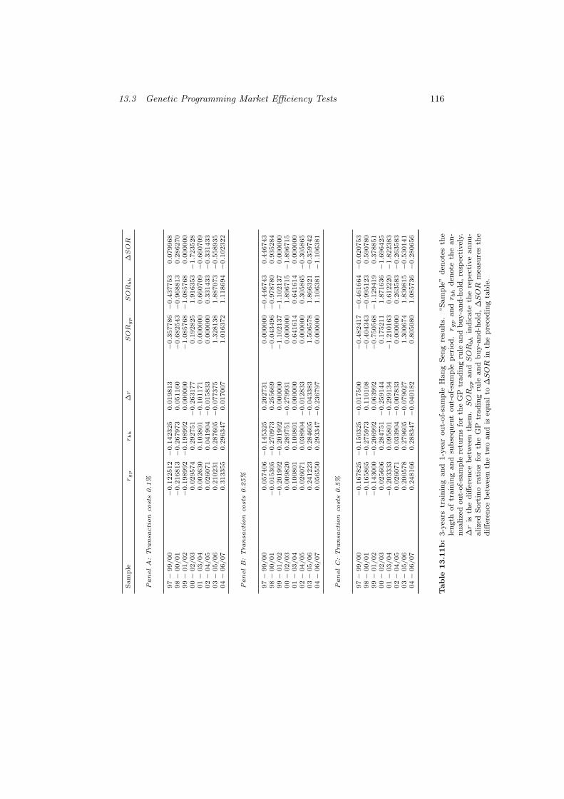
13.3 Genetic Programming Market Efficiency Tests 116
Sam
ple
rg
pr
bh
∆r
SOR
gp
SOR
bh
∆SOR
PanelA
:Tra
nsa
ction
cost
s0.1
%
97−
99/00
−0.1
22512−
0.1
42325
0.0
19813
−0.3
57786−
0.4
37753
0.0
79968
98−
00/01
−0.2
16813−
0.2
67973
0.0
51160
−0.6
82543−
0.9
68813
0.2
86270
99−
01/02
−0.1
98992−
0.1
98992
0.0
00000
−1.0
85768−
1.0
85768
0.0
00000
00−
02/03
0.0
29574
0.2
92751−
0.2
63177
0.1
92825
1.9
16353−
1.7
23528
01−
03/04
0.0
02630
0.1
03801−
0.1
01171
0.0
00000
0.6
60709−
0.6
60709
02−
04/05
0.0
26071
0.0
41904−
0.0
15833
0.0
00000
0.3
31433−
0.3
31433
03−
05/06
0.2
10231
0.2
87605−
0.0
77375
1.3
28138
1.8
87073−
0.5
58935
04−
06/07
0.3
13355
0.2
96347
0.0
17007
1.0
16372
1.1
18694−
0.1
02322
PanelB:Tra
nsa
ction
cost
s0.2
5%
97−
99/00
0.0
57406−
0.1
45325
0.2
02731
0.0
00000−
0.4
46743
0.4
46743
98−
00/01
−0.0
15305−
0.2
70973
0.2
55669
−0.0
43496−
0.9
78780
0.9
35284
99−
01/02
−0.2
01992−
0.2
01992
0.0
00000
−1.1
02137−
1.1
02137
0.0
00000
00−
02/03
0.0
09820
0.2
89751−
0.2
79931
0.0
00000
1.8
96715−
1.8
96715
01−
03/04
0.1
00801
0.1
00801
0.0
00000
0.6
41614
0.6
41614
0.0
00000
02−
04/05
0.0
26071
0.0
38904−
0.0
12833
0.0
00000
0.3
05865−
0.3
05865
03−
05/06
0.2
41223
0.2
84605−
0.0
43383
1.5
06578
1.8
66321−
0.3
59742
04−
06/07
0.0
56550
0.2
93347−
0.2
36797
0.0
00000
1.1
06381−
1.1
06381
PanelC:Tra
nsa
ction
cost
s0.5
%
97−
99/00
−0.1
67825−
0.1
50325−
0.0
17500
−0.4
82417−
0.4
61664−
0.0
20753
98−
00/01
−0.1
65865−
0.2
75973
0.1
10108
−0.4
04343−
0.9
95123
0.5
90780
99−
01/02
−0.1
43000−
0.2
06992
0.0
63992
−0.7
50568−
1.1
29419
0.3
78851
00−
02/03
0.0
25606
0.2
84751−
0.2
59144
0.1
75211
1.8
71636−
1.6
96425
01−
03/04
−0.2
03333
0.0
95801−
0.2
99134
−1.2
10163
0.6
12220−
1.8
22383
02−
04/05
0.0
26071
0.0
33904−
0.0
07833
0.0
00000
0.2
63583−
0.2
63583
03−
05/06
0.2
00578
0.2
79605−
0.0
79027
1.3
00674
1.8
30815−
0.5
30141
04−
06/07
0.2
48166
0.2
88347−
0.0
40182
0.8
05080
1.0
85736−
0.2
80656
Table
13.1
1b:
3-y
ears
train
ing
an
d1-y
ear
ou
t-of-
sam
ple
Han
gS
eng
resu
lts.
“S
am
ple
”d
enote
sth
ele
ngth
of
train
ing
an
dsu
bse
qu
ent
ou
t-of-
sam
ple
per
iod
.r g
pan
dr b
hd
enote
the
an
-nu
alize
dou
t-of-
sam
ple
retu
rns
for
the
GP
trad
ing
rule
an
db
uy-a
nd
-hold
,re
spec
tivel
y.∆r
isth
ed
iffer
ence
bet
wee
nth
em.SOR
gp
an
dSOR
bh
ind
icate
the
rep
ecti
ve
an
nu
-alize
dS
ort
ino
rati
os
for
the
GP
trad
ing
rule
an
db
uy-a
nd
-hold
,∆SOR
mea
sure
sth
ed
iffer
ence
bet
wee
nth
etw
oan
dis
equ
al
to∆SOR
inth
ep
rece
din
gta
ble
.
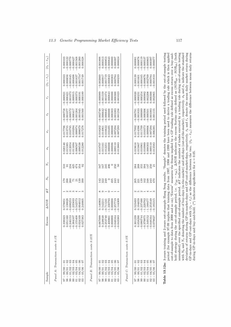
13.3 Genetic Programming Market Efficiency Tests 117Sam
ple
Excess
∆SOR
#T
Nb
Ns
σb
σs
rb
rs
(rb−r
s)
(rb−r
m)
PanelA
:Tra
nsa
ction
cost
s0.1
%
97−
99/00−
01
0.3
38323
0.5
78051
1179
310
0.0
20146
0.0
17796−
0.0
00758−
0.0
00921
0.0
00163
0.0
00103
98−
00/01−
02
0.0
51160
0.1
38828
2398
91
0.0
15385
0.0
13755−
0.0
01077−
0.0
00421−
0.0
00656−
0.0
00122
99−
01/02−
03
−0.2
46153−
0.6
98253
3260
234
0.0
12054
0.0
10795−
0.0
00572
0.0
01073−
0.0
01645−
0.0
00779
00−
02/03−
04
−0.3
84107−
1.2
35833
371
425
0.0
11694
0.0
10294
0.0
00417
0.0
00915−
0.0
00498−
0.0
00427
01−
03/04−
05
−0.1
55408−
0.5
42573
421
474
0.0
06567
0.0
08974−
0.0
01264
0.0
00373−
0.0
01637−
0.0
01568
02−
04/05−
06
−0.0
24109−
0.0
04012
1139
354
0.0
08538
0.0
08079
0.0
01945
0.0
00191
0.0
01754∗
0.0
01260
03−
05/06−
07
0.0
27383
0.2
40005
3399
92
0.0
12280
0.0
17278
0.0
01560−
0.0
00189
0.0
01749
0.0
00328
PanelB:Tra
nsa
ction
cost
s0.2
5%
97−
99/00−
01
0.0
67099
0.1
46903
8142
347
0.0
19707
0.0
18202−
0.0
02749−
0.0
00089−
0.0
02660−
0.0
01888
98−
00/01−
02
0.2
48648
0.5
42211
9322
167
0.0
15161
0.0
14961−
0.0
00642−
0.0
01559
0.0
00917
0.0
00313
99−
01/02−
03
−0.2
53740−
0.7
11241
1249
245
0.0
12251
0.0
10622−
0.0
00645
0.0
01074−
0.0
01719−
0.0
00853
00−
02/03−
04
−0.4
00861−
1.3
30793
00
496
0.0
00000
0.0
10495
0.0
00000
0.0
00843−
0.0
00843−
0.0
00843
01−
03/04−
05
0.0
00000
0.0
00000
1495
00.0
08886
0.0
00000
0.0
00303
0.0
00000
0.0
00303
0.0
00000
02−
04/05−
06
−0.0
48164−
0.2
57719
1243
250
0.0
09110
0.0
07294
0.0
01083
0.0
00300
0.0
00784
0.0
00397
03−
05/06−
07
−0.0
43383−
0.1
44309
1441
50
0.0
13883
0.0
07293
0.0
01256
0.0
01023
0.0
00233
0.0
00024
PanelC:Tra
nsa
ction
cost
s0.5
%
97−
99/00−
01
0.3
01239
0.5
23493
2205
284
0.0
19616
0.0
17992−
0.0
00781−
0.0
00920
0.0
00139
0.0
00081
98−
00/01−
02
0.0
58290
0.1
94659
5221
268
0.0
15867
0.0
14396−
0.0
01833−
0.0
00231−
0.0
01601−
0.0
00878
99−
01/02−
03
−0.0
80744−
0.2
37490
2139
355
0.0
10961
0.0
11709
0.0
00089
0.0
00254−
0.0
00165−
0.0
00119
00−
02/03−
04
−0.3
79975−
1.2
20762
1102
394
0.0
10989
0.0
10373
0.0
00306
0.0
00982−
0.0
00676−
0.0
00537
01−
03/04−
05
−0.3
49152−
1.1
88477
4348
147
0.0
08303
0.0
09906−
0.0
00501
0.0
02208−
0.0
02709−
0.0
00805
02−
04/05−
06
−0.0
48164−
0.2
53549
1243
250
0.0
09110
0.0
07294
0.0
01083
0.0
00300
0.0
00784
0.0
00397
03−
05/06−
07
−0.0
79027−
0.1
85315
3470
21
0.0
13583
0.0
06385
0.0
01155
0.0
02965−
0.0
01810−
0.0
00077
Table
13.1
2a:
3-y
ears
train
ing
an
d2-y
ears
ou
t-of-
sam
ple
Han
gS
eng
resu
lts.
“S
am
ple
”d
enote
sth
etr
ain
ing
per
iod
use
dfo
llow
edby
the
ou
t-of-
sam
ple
test
ing
per
iod
(for
exam
ple
97-9
9im
plies
that
train
ing
data
from
1997,
1998
an
d1999
have
bee
nu
sed
tod
eriv
ea
trad
ing
rule
wh
ich
isth
enap
plied
ou
t-of-
sam
ple
tod
ata
from
2000
an
dso
on
).“E
xce
ss”
mea
sure
sth
efi
tnes
sim
pli
edby
aG
Ptr
ad
ing
rule
defi
ned
as
exce
ssre
turn
over
ab
uy-a
nd
-h
old
stra
tegy
du
rin
gth
eou
t-of-
sam
ple
per
iod
,i.e.
(rgp−r b
h).
∆SOR
ind
icate
sth
eex
cess
Sort
ino
rati
od
efin
edas
(SOR
gp−SOR
bh
)(b
oth
an
nu
alize
d)
over
the
spec
ified
ou
t-of-
sam
ple
per
iod
.#T
ind
icate
sth
enu
mb
erof
trad
esex
ecu
ted
by
atr
ad
ing
rule
duri
ng
ou
t-of-
sam
ple
test
ing
wit
hN
ban
dN
sd
enoti
ng
the
nu
mb
erof
bu
y-d
ays
(in
-th
e-m
ark
et)
an
dse
ll-d
ays
(ou
t-of-
the-
mark
et),
resp
ecti
vel
y.σ
ban
dσ
sin
dic
ate
the
stan
dard
dev
iati
on
of
retu
rns
du
rin
gG
P-i
n-m
ark
et-d
ays
an
dG
P-o
ut-
of-
mark
et-d
ays,
resp
ecti
vel
y.r b
an
dr s
den
ote
the
mea
nd
aily
mark
etre
turn
du
rin
gG
P-i
n-d
ays
an
dG
P-o
ut-
days
wit
h(r
b−r s
)as
the
diff
eren
ceb
etw
een
the
two.
(rb−r m
)m
easu
res
the
diff
eren
ceb
etw
een
mea
nd
aily
retu
rns
du
rin
gG
P-i
n-d
ays
an
db
uy-a
nd
-hold
.(*
)in
dic
ate
ssi
gn
ifica
nce
forα
=0.0
5.
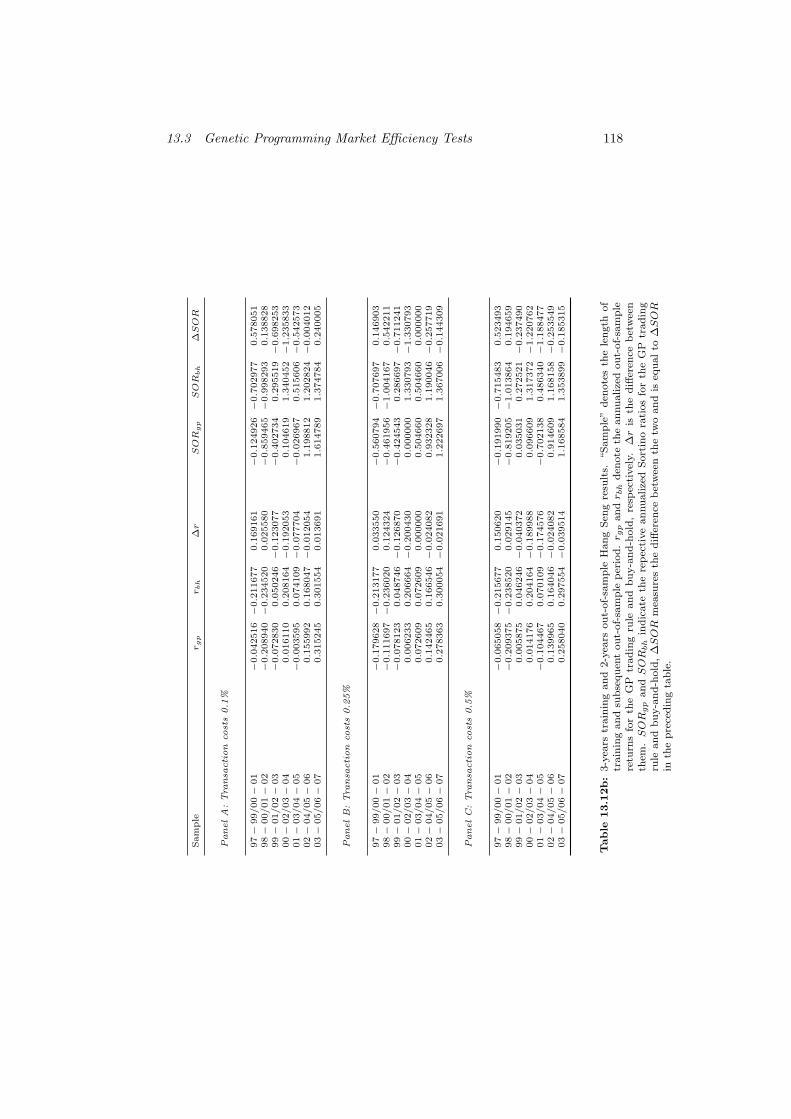
13.3 Genetic Programming Market Efficiency Tests 118
Sam
ple
rg
pr
bh
∆r
SOR
gp
SOR
bh
∆SOR
PanelA
:Tra
nsa
ction
cost
s0.1
%
97−
99/00−
01
−0.0
42516−
0.2
11677
0.1
69161
−0.1
24926−
0.7
02977
0.5
78051
98−
00/01−
02
−0.2
08940−
0.2
34520
0.0
25580
−0.8
59465−
0.9
98293
0.1
38828
99−
01/02−
03
−0.0
72830
0.0
50246−
0.1
23077
−0.4
02734
0.2
95519−
0.6
98253
00−
02/03−
04
0.0
16110
0.2
08164−
0.1
92053
0.1
04619
1.3
40452−
1.2
35833
01−
03/04−
05
−0.0
03595
0.0
74109−
0.0
77704
−0.0
26967
0.5
15606−
0.5
42573
02−
04/05−
06
0.1
55992
0.1
68047−
0.0
12054
1.1
98812
1.2
02824−
0.0
04012
03−
05/06−
07
0.3
15245
0.3
01554
0.0
13691
1.6
14789
1.3
74784
0.2
40005
PanelB:Tra
nsa
ction
cost
s0.2
5%
97−
99/00−
01
−0.1
79628−
0.2
13177
0.0
33550
−0.5
60794−
0.7
07697
0.1
46903
98−
00/01−
02
−0.1
11697−
0.2
36020
0.1
24324
−0.4
61956−
1.0
04167
0.5
42211
99−
01/02−
03
−0.0
78123
0.0
48746−
0.1
26870
−0.4
24543
0.2
86697−
0.7
11241
00−
02/03−
04
0.0
06233
0.2
06664−
0.2
00430
0.0
00000
1.3
30793−
1.3
30793
01−
03/04−
05
0.0
72609
0.0
72609
0.0
00000
0.5
04660
0.5
04660
0.0
00000
02−
04/05−
06
0.1
42465
0.1
66546−
0.0
24082
0.9
32328
1.1
90046−
0.2
57719
03−
05/06−
07
0.2
78363
0.3
00054−
0.0
21691
1.2
22697
1.3
67006−
0.1
44309
PanelC:Tra
nsa
ction
cost
s0.5
%
97−
99/00−
01
−0.0
65058−
0.2
15677
0.1
50620
−0.1
91990−
0.7
15483
0.5
23493
98−
00/01−
02
−0.2
09375−
0.2
38520
0.0
29145
−0.8
19205−
1.0
13864
0.1
94659
99−
01/02−
03
0.0
05875
0.0
46246−
0.0
40372
0.0
35031
0.2
72521−
0.2
37490
00−
02/03−
04
0.0
14176
0.2
04164−
0.1
89988
0.0
96609
1.3
17372−
1.2
20762
01−
03/04−
05
−0.1
04467
0.0
70109−
0.1
74576
−0.7
02138
0.4
86340−
1.1
88477
02−
04/05−
06
0.1
39965
0.1
64046−
0.0
24082
0.9
14609
1.1
68158−
0.2
53549
03−
05/06−
07
0.2
58040
0.2
97554−
0.0
39514
1.1
68584
1.3
53899−
0.1
85315
Table
13.1
2b:
3-y
ears
train
ing
an
d2-y
ears
ou
t-of-
sam
ple
Han
gS
eng
resu
lts.
“S
am
ple
”d
enote
sth
ele
ngth
of
train
ing
an
dsu
bse
qu
ent
ou
t-of-
sam
ple
per
iod
.r g
pan
dr b
hd
enote
the
an
nu
alize
dou
t-of-
sam
ple
retu
rns
for
the
GP
trad
ing
rule
an
db
uy-a
nd
-hold
,re
spec
tivel
y.∆r
isth
ed
iffer
ence
bet
wee
nth
em.SOR
gp
an
dSOR
bh
ind
icate
the
rep
ecti
ve
an
nu
alize
dS
ort
ino
rati
os
for
the
GP
trad
ing
rule
an
db
uy-a
nd
-hold
,∆SOR
mea
sure
sth
ed
iffer
ence
bet
wee
nth
etw
oan
dis
equ
al
to∆SOR
inth
ep
rece
din
gta
ble
.
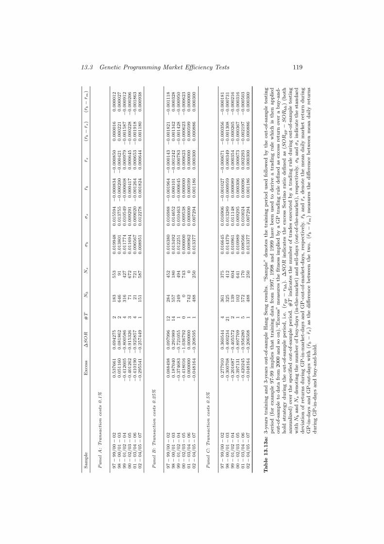
13.3 Genetic Programming Market Efficiency Tests 119
Sam
ple
Excess
∆SOR
#T
Nb
Ns
σb
σs
rb
rs
(rb−r
s)
(rb−r
m)
PanelA
:Tra
nsa
ction
cost
s0.1
%
97−
99/00−
02
0.5
37661
0.6
94275
2183
553
0.0
19948
0.0
15594−
0.0
00834−
0.0
00850
0.0
00016
0.0
00012
98−
00/01−
03
0.0
51160
0.0
81862
2646
91
0.0
13801
0.0
13755−
0.0
00200−
0.0
00421
0.0
00221
0.0
00027
99−
01/02−
04
−0.4
12605−
0.8
00586
4316
427
0.0
11774
0.0
10549−
0.0
00608
0.0
00979−
0.0
01587−
0.0
00912
00−
02/03−
05
−0.4
01262−
0.9
15326
371
672
0.0
11694
0.0
09291
0.0
00417
0.0
00645−
0.0
00228−
0.0
00206
01−
03/04−
06
−0.4
10190−
0.9
25857
421
721
0.0
06567
0.0
09020−
0.0
01264
0.0
00653−
0.0
01918−
0.0
01863
02−
04/05−
07
−0.2
95541−
0.2
57449
1151
587
0.0
08951
0.0
12278
0.0
01824
0.0
00644
0.0
01180
0.0
00938
PanelB:Tra
nsa
ction
cost
s0.2
5%
97−
99/00−
02
0.0
88498
0.0
97996
12
284
452
0.0
16380
0.0
16988−
0.0
01964−
0.0
00143−
0.0
01821−
0.0
01118
98−
00/01−
03
0.1
87040
0.2
91989
14
557
180
0.0
13492
0.0
14652
0.0
00101−
0.0
01242
0.0
01342
0.0
00328
99−
01/02−
04
−0.3
74683−
0.7
21055
1249
494
0.0
12251
0.0
10463−
0.0
00645
0.0
00783−
0.0
01428−
0.0
00950
00−
02/03−
05
−0.4
18016−
1.0
36792
00
743
0.0
00000
0.0
09538
0.0
00000
0.0
00623−
0.0
00623−
0.0
00623
01−
03/04−
06
0.0
00000
0.0
00000
1742
00.0
08962
0.0
00000
0.0
00599
0.0
00000
0.0
00599
0.0
00000
02−
04/05−
07
−0.0
48164−
0.2
08595
1488
250
0.0
13377
0.0
07294
0.0
01186
0.0
00300
0.0
00886
0.0
00300
PanelC:Tra
nsa
ction
cost
s0.5
%
97−
99/00−
02
0.2
77910
0.3
60544
4361
375
0.0
16645
0.0
16906−
0.0
01027−
0.0
00671−
0.0
00356−
0.0
00181
98−
00/01−
03
−0.3
00708−
0.4
00234
21
325
412
0.0
14379
0.0
13289−
0.0
00959
0.0
00349−
0.0
01308−
0.0
00731
99−
01/02−
04
−0.2
01687−
0.4
05572
2139
604
0.0
10961
0.0
11148
0.0
00089
0.0
00354−
0.0
00265−
0.0
00216
00−
02/03−
05
−0.3
97131−
0.8
97709
1102
641
0.0
10989
0.0
09295
0.0
00306
0.0
00673−
0.0
00367−
0.0
00316
01−
03/04−
06
−0.4
20245−
0.9
56280
5572
170
0.0
08566
0.0
10024
0.0
00096
0.0
02293−
0.0
02197−
0.0
00503
02−
04/05−
07
−0.0
48164−
0.2
06508
1488
250
0.0
13377
0.0
07294
0.0
01186
0.0
00300
0.0
00886
0.0
00300
Table
13.1
3a:
3-y
ears
train
ing
an
d3-y
ears
ou
t-of-
sam
ple
Han
gS
eng
resu
lts.
“S
am
ple
”d
enote
sth
etr
ain
ing
per
iod
use
dfo
llow
edby
the
ou
t-of-
sam
ple
test
ing
per
iod
(for
exam
ple
97-9
9im
plies
that
train
ing
data
from
1997,
1998
an
d1999
have
bee
nu
sed
tod
eriv
ea
trad
ing
rule
wh
ich
isth
enap
plied
ou
t-of-
sam
ple
tod
ata
from
2000
an
dso
on
).“E
xce
ss”
mea
sure
sth
efi
tnes
sim
pli
edby
aG
Ptr
ad
ing
rule
defi
ned
as
exce
ssre
turn
over
ab
uy-a
nd
-h
old
stra
tegy
du
rin
gth
eou
t-of-
sam
ple
per
iod
,i.e.
(rgp−r b
h).
∆SOR
ind
icate
sth
eex
cess
Sort
ino
rati
od
efin
edas
(SOR
gp−SOR
bh
)(b
oth
an
nu
alize
d)
over
the
spec
ified
ou
t-of-
sam
ple
per
iod
.#T
ind
icate
sth
enu
mb
erof
trad
esex
ecu
ted
by
atr
ad
ing
rule
duri
ng
ou
t-of-
sam
ple
test
ing
wit
hN
ban
dN
sd
enoti
ng
the
nu
mb
erof
bu
y-d
ays
(in
-th
e-m
ark
et)
an
dse
ll-d
ays
(ou
t-of-
the-
mark
et),
resp
ecti
vel
y.σ
ban
dσ
sin
dic
ate
the
stan
dard
dev
iati
on
of
retu
rns
du
rin
gG
P-i
n-m
ark
et-d
ays
an
dG
P-o
ut-
of-
mark
et-d
ays,
resp
ecti
vel
y.r b
an
dr s
den
ote
the
mea
nd
aily
mark
etre
turn
du
rin
gG
P-i
n-d
ays
an
dG
P-o
ut-
days
wit
h(r
b−r s
)as
the
diff
eren
ceb
etw
een
the
two.
(rb−r m
)m
easu
res
the
diff
eren
ceb
etw
een
mea
nd
aily
retu
rns
du
rin
gG
P-i
n-d
ays
an
db
uy-a
nd
-hold
.
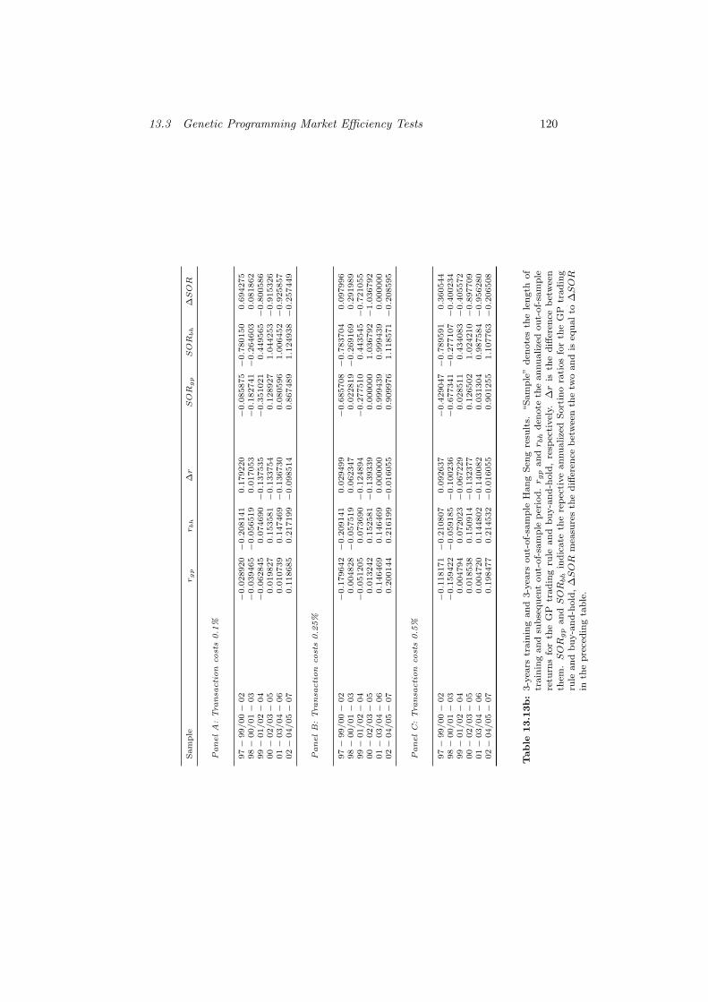
13.3 Genetic Programming Market Efficiency Tests 120
Sam
ple
rg
pr
bh
∆r
SOR
gp
SOR
bh
∆SOR
PanelA
:Tra
nsa
ction
cost
s0.1
%
97−
99/00−
02
−0.0
28920−
0.2
08141
0.1
79220
−0.0
85875−
0.7
80150
0.6
94275
98−
00/01−
03
−0.0
39465−
0.0
56519
0.0
17053
−0.1
82741−
0.2
64603
0.0
81862
99−
01/02−
04
−0.0
62845
0.0
74690−
0.1
37535
−0.3
51021
0.4
49565−
0.8
00586
00−
02/03−
05
0.0
19827
0.1
53581−
0.1
33754
0.1
28927
1.0
44253−
0.9
15326
01−
03/04−
06
0.0
10739
0.1
47469−
0.1
36730
0.0
80596
1.0
06452−
0.9
25857
02−
04/05−
07
0.1
18685
0.2
17199−
0.0
98514
0.8
67489
1.1
24938−
0.2
57449
PanelB:Tra
nsa
ction
cost
s0.2
5%
97−
99/00−
02
−0.1
79642−
0.2
09141
0.0
29499
−0.6
85708−
0.7
83704
0.0
97996
98−
00/01−
03
0.0
04828−
0.0
57519
0.0
62347
0.0
22819−
0.2
69169
0.2
91989
99−
01/02−
04
−0.0
51205
0.0
73690−
0.1
24894
−0.2
77510
0.4
43545−
0.7
21055
00−
02/03−
05
0.0
13242
0.1
52581−
0.1
39339
0.0
00000
1.0
36792−
1.0
36792
01−
03/04−
06
0.1
46469
0.1
46469
0.0
00000
0.9
99439
0.9
99439
0.0
00000
02−
04/05−
07
0.2
00144
0.2
16199−
0.0
16055
0.9
09976
1.1
18571−
0.2
08595
PanelC:Tra
nsa
ction
cost
s0.5
%
97−
99/00−
02
−0.1
18171−
0.2
10807
0.0
92637
−0.4
29047−
0.7
89591
0.3
60544
98−
00/01−
03
−0.1
59422−
0.0
59185−
0.1
00236
−0.6
77341−
0.2
77107−
0.4
00234
99−
01/02−
04
0.0
04794
0.0
72023−
0.0
67229
0.0
28511
0.4
34083−
0.4
05572
00−
02/03−
05
0.0
18538
0.1
50914−
0.1
32377
0.1
26502
1.0
24210−
0.8
97709
01−
03/04−
06
0.0
04720
0.1
44802−
0.1
40082
0.0
31304
0.9
87584−
0.9
56280
02−
04/05−
07
0.1
98477
0.2
14532−
0.0
16055
0.9
01255
1.1
07763−
0.2
06508
Table
13.1
3b:
3-y
ears
train
ing
an
d3-y
ears
ou
t-of-
sam
ple
Han
gS
eng
resu
lts.
“S
am
ple
”d
enote
sth
ele
ngth
of
train
ing
an
dsu
bse
qu
ent
ou
t-of-
sam
ple
per
iod
.r g
pan
dr b
hd
enote
the
an
nu
alize
dou
t-of-
sam
ple
retu
rns
for
the
GP
trad
ing
rule
an
db
uy-a
nd
-hold
,re
spec
tivel
y.∆r
isth
ed
iffer
ence
bet
wee
nth
em.SOR
gp
an
dSOR
bh
ind
icate
the
rep
ecti
ve
an
nu
alize
dS
ort
ino
rati
os
for
the
GP
trad
ing
rule
an
db
uy-a
nd
-hold
,∆SOR
mea
sure
sth
ed
iffer
ence
bet
wee
nth
etw
oan
dis
equ
al
to∆SOR
inth
ep
rece
din
gta
ble
.
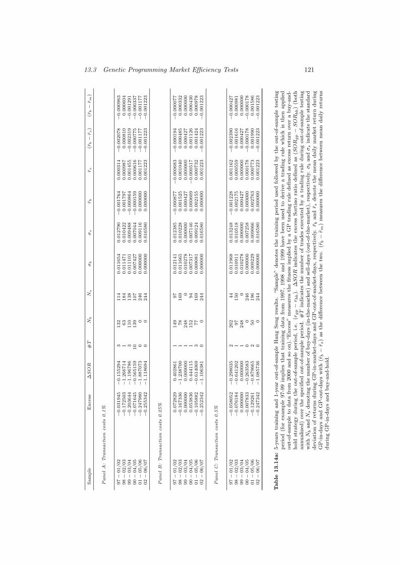
13.3 Genetic Programming Market Efficiency Tests 121
Sam
ple
Excess
∆SOR
#T
Nb
Ns
σb
σs
rb
rs
(rb−r
s)
(rb−r
m)
PanelA
:Tra
nsa
ction
cost
s0.1
%
97−
01/02
−0.0
31945−
0.1
55294
3132
114
0.0
11654
0.0
12790−
0.0
01764
0.0
00314−
0.0
02078
−0.0
00963
98−
02/03
−0.1
72503−
1.2
66714
163
184
0.0
11471
0.0
10422
0.0
01797
0.0
00987
0.0
00810
0.0
00604
99−
03/04
−0.2
03644−
1.1
96786
3110
138
0.0
11101
0.0
09488−
0.0
00864
0.0
01455−
0.0
02319
−0.0
01291
00−
04/05
−0.0
71645−
0.5
65159
10
139
107
0.0
07427
0.0
07044−
0.0
00159
0.0
00616−
0.0
00775
−0.0
00337
01−
05/06
−0.2
47980−
1.8
87073
00
246
0.0
00000
0.0
09116
0.0
00000
0.0
01177−
0.0
01177
−0.0
01177
02−
06/07
−0.2
55342−
1.1
18694
00
244
0.0
00000
0.0
16580
0.0
00000
0.0
01223−
0.0
01223
−0.0
01223
PanelB:Tra
nsa
ction
cost
s0.2
5%
97−
01/02
0.0
72829
0.4
02861
1149
97
0.0
12141
0.0
12385−
0.0
00877−
0.0
00683−
0.0
00194
−0.0
00077
98−
02/03
−0.1
67336−
1.2
38700
178
169
0.0
11665
0.0
10228
0.0
01525
0.0
01040
0.0
00485
0.0
00332
99−
03/04
0.0
00000
0.0
00000
1248
00.0
10278
0.0
00000
0.0
00427
0.0
00000
0.0
00427
0.0
00000
00−
04/05
0.0
53836
0.4
44115
1152
94
0.0
07317
0.0
07146
0.0
00609−
0.0
00517
0.0
01126
0.0
00430
01−
05/06
−0.1
05882−
0.6
14069
377
169
0.0
09081
0.0
09124
0.0
02155
0.0
00732
0.0
01424
0.0
00978
02−
06/07
−0.2
52342−
1.1
06381
00
244
0.0
00000
0.0
16580
0.0
00000
0.0
01223−
0.0
01223
−0.0
01223
PanelC:Tra
nsa
ction
cost
s0.5
%
97−
01/02
−0.0
58052−
0.2
98035
2202
44
0.0
11968
0.0
13248−
0.0
01228
0.0
01162−
0.0
02390
−0.0
00427
98−
02/03
−0.0
76184−
0.6
41202
197
150
0.0
10911
0.0
10518
0.0
02175
0.0
00559
0.0
01616
0.0
00981
99−
03/04
0.0
00000
0.0
00000
1248
00.0
10278
0.0
00000
0.0
00427
0.0
00000
0.0
00427
0.0
00000
00−
04/05
−0.0
07833−
0.2
63583
00
246
0.0
00000
0.0
07258
0.0
00000
0.0
00178−
0.0
00178
−0.0
00178
01−
05/06
−0.1
29261−
0.8
79665
250
196
0.0
09229
0.0
09066
0.0
02763
0.0
00773
0.0
01990
0.0
01586
02−
06/07
−0.2
47342−
1.0
85736
00
244
0.0
00000
0.0
16580
0.0
00000
0.0
01223−
0.0
01223
−0.0
01223
Table
13.1
4a:
5-y
ears
train
ing
an
d1-y
ear
ou
t-of-
sam
ple
Han
gS
eng
resu
lts.
“S
am
ple
”d
enote
sth
etr
ain
ing
per
iod
use
dfo
llow
edby
the
ou
t-of-
sam
ple
test
ing
per
iod
(for
exam
ple
97-9
9im
plies
that
train
ing
data
from
1997,
1998
an
d1999
have
bee
nu
sed
tod
eriv
ea
trad
ing
rule
wh
ich
isth
enap
plied
ou
t-of-
sam
ple
tod
ata
from
2000
an
dso
on
).“E
xce
ss”
mea
sure
sth
efi
tnes
sim
pli
edby
aG
Ptr
ad
ing
rule
defi
ned
as
exce
ssre
turn
over
ab
uy-a
nd
-h
old
stra
tegy
du
rin
gth
eou
t-of-
sam
ple
per
iod
,i.e.
(rgp−r b
h).
∆SOR
ind
icate
sth
eex
cess
Sort
ino
rati
od
efin
edas
(SOR
gp−SOR
bh
)(b
oth
an
nu
alize
d)
over
the
spec
ified
ou
t-of-
sam
ple
per
iod
.#T
ind
icate
sth
enu
mb
erof
trad
esex
ecu
ted
by
atr
ad
ing
rule
duri
ng
ou
t-of-
sam
ple
test
ing
wit
hN
ban
dN
sd
enoti
ng
the
nu
mb
erof
bu
y-d
ays
(in
-th
e-m
ark
et)
an
dse
ll-d
ays
(ou
t-of-
the-
mark
et),
resp
ecti
vel
y.σ
ban
dσ
sin
dic
ate
the
stan
dard
dev
iati
on
of
retu
rns
du
rin
gG
P-i
n-m
ark
et-d
ays
an
dG
P-o
ut-
of-
mark
et-d
ays,
resp
ecti
vel
y.r b
an
dr s
den
ote
the
mea
nd
aily
mark
etre
turn
du
rin
gG
P-i
n-d
ays
an
dG
P-o
ut-
days
wit
h(r
b−r s
)as
the
diff
eren
ceb
etw
een
the
two.
(rb−r m
)m
easu
res
the
diff
eren
ceb
etw
een
mea
nd
aily
retu
rns
du
rin
gG
P-i
n-d
ays
an
db
uy-a
nd
-hold
.
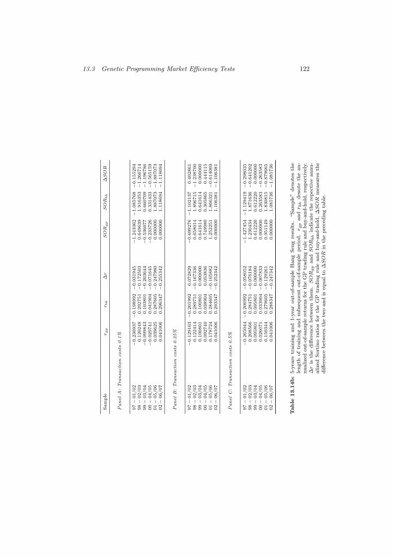
13.3 Genetic Programming Market Efficiency Tests 122
Sam
ple
rg
pr
bh
∆r
SOR
gp
SOR
bh
∆SOR
PanelA
:Tra
nsa
ction
cost
s0.1
%
97−
01/02
−0.2
30937−
0.1
98992−
0.0
31945
−1.2
41062−
1.0
85768−
0.1
55294
98−
02/03
0.1
20248
0.2
92751−
0.1
72503
0.6
49639
1.9
16353−
1.2
66714
99−
03/04
−0.0
99843
0.1
03801−
0.2
03644
−0.5
36077
0.6
60709−
1.1
96786
00−
04/05
−0.0
29741
0.0
41904−
0.0
71645
−0.2
33726
0.3
31433−
0.5
65159
01−
05/06
0.0
39625
0.2
87605−
0.2
47980
0.0
00000
1.8
87073−
1.8
87073
02−
06/07
0.0
41006
0.2
96347−
0.2
55342
0.0
00000
1.1
18694−
1.1
18694
PanelB:Tra
nsa
ction
cost
s0.2
5%
97−
01/02
−0.1
29163−
0.2
01992
0.0
72829
−0.6
99276−
1.1
02137
0.4
02861
98−
02/03
0.1
22414
0.2
89751−
0.1
67336
0.6
58014
1.8
96715−
1.2
38700
99−
03/04
0.1
00801
0.1
00801
0.0
00000
0.6
41614
0.6
41614
0.0
00000
00−
04/05
0.0
92740
0.0
38904
0.0
53836
0.7
49980
0.3
05865
0.4
44115
01−
05/06
0.1
78724
0.2
84605−
0.1
05882
1.2
52251
1.8
66321−
0.6
14069
02−
06/07
0.0
41006
0.2
93347−
0.2
52342
0.0
00000
1.1
06381−
1.1
06381
PanelC:Tra
nsa
ction
cost
s0.5
%
97−
01/02
−0.2
65044−
0.2
06992−
0.0
58052
−1.4
27454−
1.1
29419−
0.2
98035
98−
02/03
0.2
08566
0.2
84751−
0.0
76184
1.2
30434
1.8
71636−
0.6
41202
99−
03/04
0.0
95801
0.0
95801
0.0
00000
0.6
12220
0.6
12220
0.0
00000
00−
04/05
0.0
26071
0.0
33904−
0.0
07833
0.0
00000
0.2
63583−
0.2
63583
01−
05/06
0.1
50344
0.2
79605−
0.1
29261
0.9
51149
1.8
30815−
0.8
79665
02−
06/07
0.0
41006
0.2
88347−
0.2
47342
0.0
00000
1.0
85736−
1.0
85736
Table
13.1
4b:
5-y
ears
train
ing
an
d1-y
ear
ou
t-of-
sam
ple
Han
gS
eng
resu
lts.
“S
am
ple
”d
enote
sth
ele
ngth
of
train
ing
an
dsu
bse
qu
ent
ou
t-of-
sam
ple
per
iod
.r g
pan
dr b
hd
enote
the
an
-nu
alize
dou
t-of-
sam
ple
retu
rns
for
the
GP
trad
ing
rule
an
db
uy-a
nd
-hold
,re
spec
tivel
y.∆r
isth
ed
iffer
ence
bet
wee
nth
em.SOR
gp
an
dSOR
bh
ind
icate
the
rep
ecti
ve
an
nu
-alize
dS
ort
ino
rati
os
for
the
GP
trad
ing
rule
an
db
uy-a
nd
-hold
,∆SOR
mea
sure
sth
ed
iffer
ence
bet
wee
nth
etw
oan
dis
equ
al
to∆SOR
inth
ep
rece
din
gta
ble
.
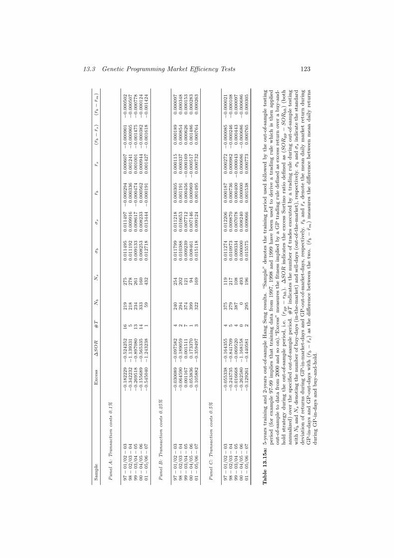
13.3 Genetic Programming Market Efficiency Tests 123
Sam
ple
Excess
∆SOR
#T
Nb
Ns
σb
σs
rb
rs
(rb−r
s)
(rb−r
m)
PanelA
:Tra
nsa
ction
cost
s0.1
%
97−
01/02−
03
−0.1
82229−
0.5
24252
16
219
275
0.0
11495
0.0
11497−
0.0
00294
0.0
00607−
0.0
00901−
0.0
00502
98−
02/03−
04
−0.3
42232−
1.1
39331
5218
278
0.0
11192
0.0
09916
0.0
00336
0.0
01241−
0.0
00905−
0.0
00507
99−
03/04−
05
−0.2
69518−
0.8
97080
13
234
261
0.0
09133
0.0
08617−
0.0
00474
0.0
01001−
0.0
01475−
0.0
00778
00−
04/05−
06
−0.1
55689−
0.5
65335
14
333
160
0.0
08253
0.0
08233
0.0
00562
0.0
00944−
0.0
00382−
0.0
00124
01−
05/06−
07
−0.5
45040−
1.2
43238
159
432
0.0
12718
0.0
13444−
0.0
00191
0.0
01427−
0.0
01618−
0.0
01424
PanelB:Tra
nsa
ction
cost
s0.2
5%
97−
01/02−
03
−0.0
30089−
0.0
97582
4240
254
0.0
11799
0.0
11218
0.0
00305
0.0
00115
0.0
00189
0.0
00097
98−
02/03−
04
−0.0
64590−
0.1
89059
2294
202
0.0
10388
0.0
10653
0.0
01191
0.0
00337
0.0
00854
0.0
00348
99−
03/04−
05
0.0
01167
0.0
01511
7374
121
0.0
09239
0.0
07712
0.0
00456−
0.0
00169
0.0
00626
0.0
00153
00−
04/05−
06
0.0
53836
0.1
73370
1399
94
0.0
08461
0.0
07146
0.0
00969−
0.0
00517
0.0
01486
0.0
00283
01−
05/06−
07
−0.1
05882−
0.3
59497
3322
169
0.0
15118
0.0
09124
0.0
01495
0.0
00732
0.0
00764
0.0
00263
PanelC:Tra
nsa
ction
cost
s0.5
%
97−
01/02−
03
−0.0
55338−
0.1
64355
4375
119
0.0
11274
0.0
12206
0.0
00187
0.0
00272−
0.0
00085−
0.0
00021
98−
02/03−
04
−0.2
43735−
0.8
41709
5279
217
0.0
10973
0.0
09870
0.0
00736
0.0
00982−
0.0
00246−
0.0
00108
99−
03/04−
05
−0.0
16668−
0.0
69520
4387
108
0.0
09334
0.0
07078
0.0
00400−
0.0
00043
0.0
00443
0.0
00097
00−
04/05−
06
−0.2
62580−
1.1
68158
00
493
0.0
00000
0.0
08240
0.0
00000
0.0
00686−
0.0
00686−
0.0
00686
01−
05/06−
07
−0.1
29261−
0.4
40581
2295
196
0.0
15575
0.0
09066
0.0
01538
0.0
00773
0.0
00765
0.0
00305
Table
13.1
5a:
5-y
ears
train
ing
an
d2-y
ears
ou
t-of-
sam
ple
Han
gS
eng
resu
lts.
“S
am
ple
”d
enote
sth
etr
ain
ing
per
iod
use
dfo
llow
edby
the
ou
t-of-
sam
ple
test
ing
per
iod
(for
exam
ple
97-9
9im
plies
that
train
ing
data
from
1997,
1998
an
d1999
have
bee
nu
sed
tod
eriv
ea
trad
ing
rule
wh
ich
isth
enap
plied
ou
t-of-
sam
ple
tod
ata
from
2000
an
dso
on
).“E
xce
ss”
mea
sure
sth
efi
tnes
sim
pli
edby
aG
Ptr
ad
ing
rule
defi
ned
as
exce
ssre
turn
over
ab
uy-a
nd
-h
old
stra
tegy
du
rin
gth
eou
t-of-
sam
ple
per
iod
,i.e.
(rgp−r b
h).
∆SOR
ind
icate
sth
eex
cess
Sort
ino
rati
od
efin
edas
(SOR
gp−SOR
bh
)(b
oth
an
nu
alize
d)
over
the
spec
ified
ou
t-of-
sam
ple
per
iod
.#T
ind
icate
sth
enu
mb
erof
trad
esex
ecu
ted
by
atr
ad
ing
rule
duri
ng
ou
t-of-
sam
ple
test
ing
wit
hN
ban
dN
sd
enoti
ng
the
nu
mb
erof
bu
y-d
ays
(in
-th
e-m
ark
et)
an
dse
ll-d
ays
(ou
t-of-
the-
mark
et),
resp
ecti
vel
y.σ
ban
dσ
sin
dic
ate
the
stan
dard
dev
iati
on
of
retu
rns
du
rin
gG
P-i
n-m
ark
et-d
ays
an
dG
P-o
ut-
of-
mark
et-d
ays,
resp
ecti
vel
y.r b
an
dr s
den
ote
the
mea
nd
aily
mark
etre
turn
du
rin
gG
P-i
n-d
ays
an
dG
P-o
ut-
days
wit
h(r
b−r s
)as
the
diff
eren
ceb
etw
een
the
two.
(rb−r m
)m
easu
res
the
diff
eren
ceb
etw
een
mea
nd
aily
retu
rns
du
rin
gG
P-i
n-d
ays
an
db
uy-a
nd
-hold
.
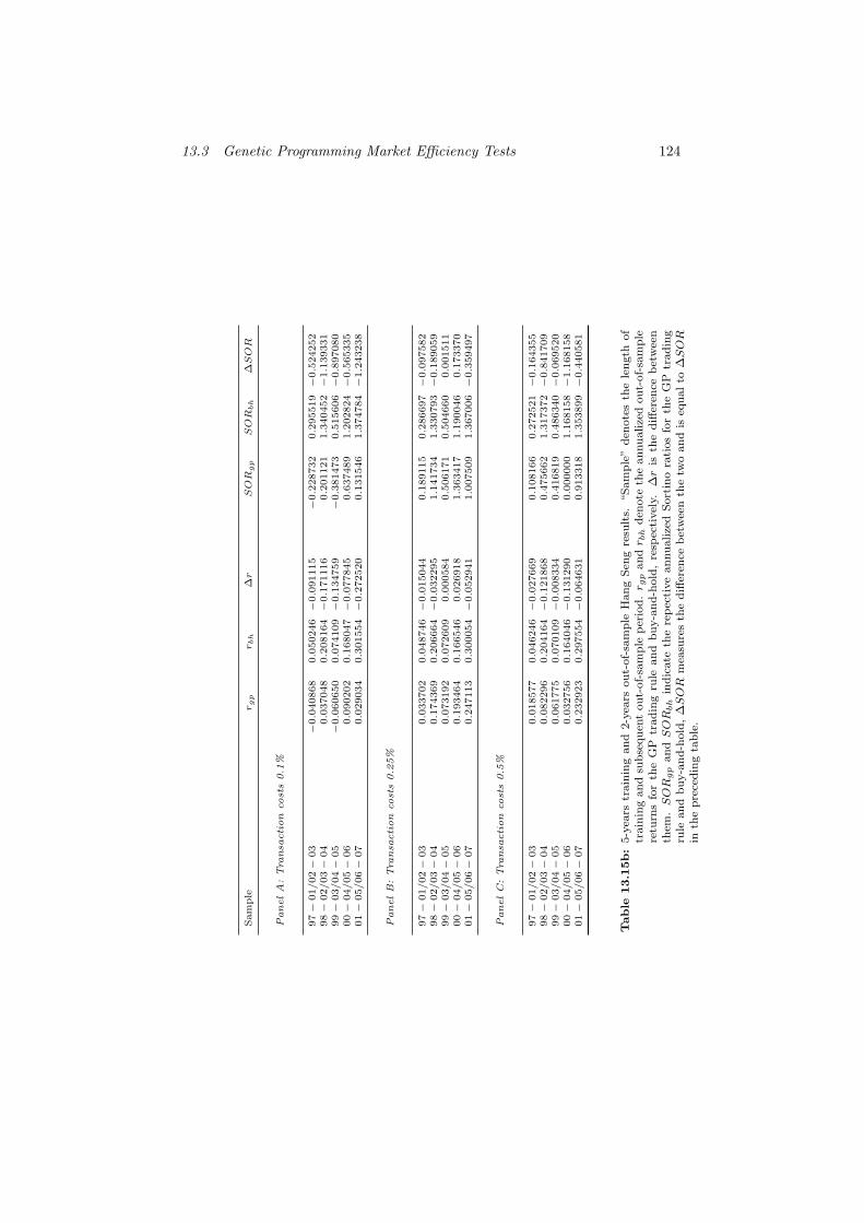
13.3 Genetic Programming Market Efficiency Tests 124
Sam
ple
rg
pr
bh
∆r
SOR
gp
SOR
bh
∆SOR
PanelA
:Tra
nsa
ction
cost
s0.1
%
97−
01/02−
03
−0.0
40868
0.0
50246−
0.0
91115
−0.2
28732
0.2
95519−
0.5
24252
98−
02/03−
04
0.0
37048
0.2
08164−
0.1
71116
0.2
01121
1.3
40452−
1.1
39331
99−
03/04−
05
−0.0
60650
0.0
74109−
0.1
34759
−0.3
81473
0.5
15606−
0.8
97080
00−
04/05−
06
0.0
90202
0.1
68047−
0.0
77845
0.6
37489
1.2
02824−
0.5
65335
01−
05/06−
07
0.0
29034
0.3
01554−
0.2
72520
0.1
31546
1.3
74784−
1.2
43238
PanelB:Tra
nsa
ction
cost
s0.2
5%
97−
01/02−
03
0.0
33702
0.0
48746−
0.0
15044
0.1
89115
0.2
86697−
0.0
97582
98−
02/03−
04
0.1
74369
0.2
06664−
0.0
32295
1.1
41734
1.3
30793−
0.1
89059
99−
03/04−
05
0.0
73192
0.0
72609
0.0
00584
0.5
06171
0.5
04660
0.0
01511
00−
04/05−
06
0.1
93464
0.1
66546
0.0
26918
1.3
63417
1.1
90046
0.1
73370
01−
05/06−
07
0.2
47113
0.3
00054−
0.0
52941
1.0
07509
1.3
67006−
0.3
59497
PanelC:Tra
nsa
ction
cost
s0.5
%
97−
01/02−
03
0.0
18577
0.0
46246−
0.0
27669
0.1
08166
0.2
72521−
0.1
64355
98−
02/03−
04
0.0
82296
0.2
04164−
0.1
21868
0.4
75662
1.3
17372−
0.8
41709
99−
03/04−
05
0.0
61775
0.0
70109−
0.0
08334
0.4
16819
0.4
86340−
0.0
69520
00−
04/05−
06
0.0
32756
0.1
64046−
0.1
31290
0.0
00000
1.1
68158−
1.1
68158
01−
05/06−
07
0.2
32923
0.2
97554−
0.0
64631
0.9
13318
1.3
53899−
0.4
40581
Table
13.1
5b:
5-y
ears
train
ing
an
d2-y
ears
ou
t-of-
sam
ple
Han
gS
eng
resu
lts.
“S
am
ple
”d
enote
sth
ele
ngth
of
train
ing
an
dsu
bse
qu
ent
ou
t-of-
sam
ple
per
iod
.r g
pan
dr b
hd
enote
the
an
nu
alize
dou
t-of-
sam
ple
retu
rns
for
the
GP
trad
ing
rule
an
db
uy-a
nd
-hold
,re
spec
tivel
y.∆r
isth
ed
iffer
ence
bet
wee
nth
em.SOR
gp
an
dSOR
bh
ind
icate
the
rep
ecti
ve
an
nu
alize
dS
ort
ino
rati
os
for
the
GP
trad
ing
rule
an
db
uy-a
nd
-hold
,∆SOR
mea
sure
sth
ed
iffer
ence
bet
wee
nth
etw
oan
dis
equ
al
to∆SOR
inth
ep
rece
din
gta
ble
.
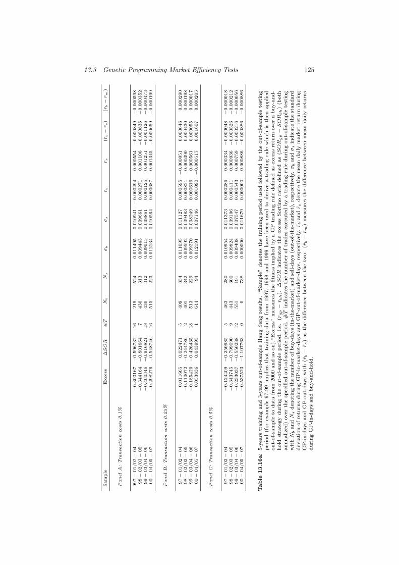
13.3 Genetic Programming Market Efficiency Tests 125
Sam
ple
Excess
∆SOR
#T
Nb
Ns
σb
σs
rb
rs
(rb−r
s)
(rb−r
m)
PanelA
:Tra
nsa
ction
cost
s0.1
%
997−
01/02−
04
−0.3
03167−
0.5
96732
16
219
524
0.0
11495
0.0
10941−
0.0
00294
0.0
00554−
0.0
00849−
0.0
00598
98−
02/03−
05
−0.3
44164−
0.8
01664
7430
313
0.0
09443
0.0
09661
0.0
00271
0.0
01106−
0.0
00835−
0.0
00352
99−
03/04−
06
−0.4
00346−
0.9
16821
18
430
312
0.0
09015
0.0
08861
0.0
00125
0.0
01251−
0.0
01126−
0.0
00473
00−
04/05−
07
−0.2
98276−
0.5
48746
16
515
223
0.0
12134
0.0
10564
0.0
00687
0.0
01345−
0.0
00659−
0.0
00199
PanelB:Tra
nsa
ction
cost
s0.2
5%
97−
01/02−
04
0.0
11665
0.0
22471
5409
334
0.0
11095
0.0
11127
0.0
00595−
0.0
00051
0.0
00646
0.0
00290
98−
02/03−
05
−0.1
10072−
0.2
44786
2401
342
0.0
09592
0.0
09483
0.0
00821
0.0
00390
0.0
00430
0.0
00198
99−
03/04−
06
−0.1
85420−
0.4
26435
18
513
229
0.0
09270
0.0
08249
0.0
00616
0.0
00561
0.0
00055
0.0
00017
00−
04/05−
07
0.0
53836
0.0
43995
1644
94
0.0
12191
0.0
07146
0.0
01090−
0.0
00517
0.0
01607
0.0
00205
PanelC:Tra
nsa
ction
cost
s0.5
%
97−
01/02−
04
−0.1
24409−
0.2
50985
5463
280
0.0
10954
0.0
11373
0.0
00286
0.0
00334−
0.0
00048−
0.0
00018
98−
02/03−
05
−0.3
43745−
0.7
99090
9443
300
0.0
09824
0.0
09106
0.0
00411
0.0
00936−
0.0
00526−
0.0
00212
99−
03/04−
06
−0.2
33037−
0.5
50238
12
551
191
0.0
09408
0.0
07547
0.0
00543
0.0
00759−
0.0
00216−
0.0
00056
00−
04/05−
07
−0.5
37523−
1.1
07763
00
738
0.0
00000
0.0
11679
0.0
00000
0.0
00886−
0.0
00886−
0.0
00886
Table
13.1
6a:
5-y
ears
train
ing
an
d3-y
ears
ou
t-of-
sam
ple
Han
gS
eng
resu
lts.
“S
am
ple
”d
enote
sth
etr
ain
ing
per
iod
use
dfo
llow
edby
the
ou
t-of-
sam
ple
test
ing
per
iod
(for
exam
ple
97-9
9im
plies
that
train
ing
data
from
1997,
1998
an
d1999
have
bee
nu
sed
tod
eriv
ea
trad
ing
rule
wh
ich
isth
enap
plied
ou
t-of-
sam
ple
tod
ata
from
2000
an
dso
on
).“E
xce
ss”
mea
sure
sth
efi
tnes
sim
pli
edby
aG
Ptr
ad
ing
rule
defi
ned
as
exce
ssre
turn
over
ab
uy-a
nd
-h
old
stra
tegy
du
rin
gth
eou
t-of-
sam
ple
per
iod
,i.e.
(rgp−r b
h).
∆SOR
ind
icate
sth
eex
cess
Sort
ino
rati
od
efin
edas
(SOR
gp−SOR
bh
)(b
oth
an
nu
alize
d)
over
the
spec
ified
ou
t-of-
sam
ple
per
iod
.#T
ind
icate
sth
enu
mb
erof
trad
esex
ecu
ted
by
atr
ad
ing
rule
duri
ng
ou
t-of-
sam
ple
test
ing
wit
hN
ban
dN
sd
enoti
ng
the
nu
mb
erof
bu
y-d
ays
(in
-th
e-m
ark
et)
an
dse
ll-d
ays
(ou
t-of-
the-
mark
et),
resp
ecti
vel
y.σ
ban
dσ
sin
dic
ate
the
stan
dard
dev
iati
on
of
retu
rns
du
rin
gG
P-i
n-m
ark
et-d
ays
an
dG
P-o
ut-
of-
mark
et-d
ays,
resp
ecti
vel
y.r b
an
dr s
den
ote
the
mea
nd
aily
mark
etre
turn
du
rin
gG
P-i
n-d
ays
an
dG
P-o
ut-
days
wit
h(r
b−r s
)as
the
diff
eren
ceb
etw
een
the
two.
(rb−r m
)m
easu
res
the
diff
eren
ceb
etw
een
mea
nd
aily
retu
rns
du
rin
gG
P-i
n-d
ays
an
db
uy-a
nd
-hold
.
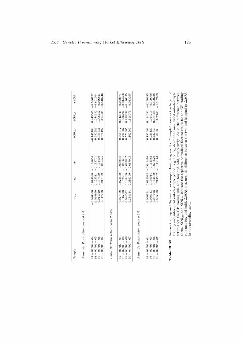
13.3 Genetic Programming Market Efficiency Tests 126
Sam
ple
rg
pr
bh
∆r
SOR
gp
SOR
bh
∆SOR
PanelA
:Tra
nsa
ction
cost
s0.1
%
97−
01/02−
04
−0.0
26366
0.0
74690−
0.1
01056
−0.1
47168
0.4
49565−
0.5
96732
98−
02/03−
05
0.0
38860
0.1
53581−
0.1
14721
0.2
42589
1.0
44253−
0.8
01664
99−
03/04−
06
0.0
14020
0.1
47469−
0.1
33449
0.0
89631
1.0
06452−
0.9
16821
00−
04/05−
07
0.1
17773
0.2
17199−
0.0
99425
0.5
76192
1.1
24938−
0.5
48746
PanelB:Tra
nsa
ction
cost
s0.2
5%
97−
01/02−
04
0.0
77578
0.0
73690
0.0
03888
0.4
66017
0.4
43545
0.0
22471
98−
02/03−
05
0.1
15890
0.1
52581−
0.0
36691
0.7
92007
1.0
36792−
0.2
44786
99−
03/04−
06
0.0
84662
0.1
46469−
0.0
61807
0.5
73005
0.9
99439−
0.4
26435
00−
04/05−
07
0.2
34144
0.2
16199
0.0
17945
1.1
62566
1.1
18571
0.0
43995
PanelC:Tra
nsa
ction
cost
s0.5
%
97−
01/02−
04
0.0
30554
0.0
72023−
0.0
41470
0.1
83099
0.4
34083−
0.2
50985
98−
02/03−
05
0.0
36333
0.1
50914−
0.1
14582
0.2
25120
1.0
24210−
0.7
99090
99−
03/04−
06
0.0
67123
0.1
44802−
0.0
77679
0.4
37346
0.9
87584−
0.5
50238
00−
04/05−
07
0.0
35358
0.2
14532−
0.1
79174
0.0
00000
1.1
07763−
1.1
07763
Table
13.1
6b:
5-y
ears
train
ing
an
d3-y
ears
ou
t-of-
sam
ple
Han
gS
eng
resu
lts.
“S
am
ple
”d
enote
sth
ele
ngth
of
train
ing
an
dsu
bse
qu
ent
ou
t-of-
sam
ple
per
iod
.r g
pan
dr b
hd
enote
the
an
nu
alize
dou
t-of-
sam
ple
retu
rns
for
the
GP
trad
ing
rule
an
db
uy-a
nd
-hold
,re
spec
tivel
y.∆r
isth
ed
iffer
ence
bet
wee
nth
em.SOR
gp
an
dSOR
bh
ind
icate
the
rep
ecti
ve
an
nu
alize
dS
ort
ino
rati
os
for
the
GP
trad
ing
rule
an
db
uy-a
nd
-hold
,∆SOR
mea
sure
sth
ed
iffer
ence
bet
wee
nth
etw
oan
dis
equ
al
to∆SOR
inth
ep
rece
din
gta
ble
.
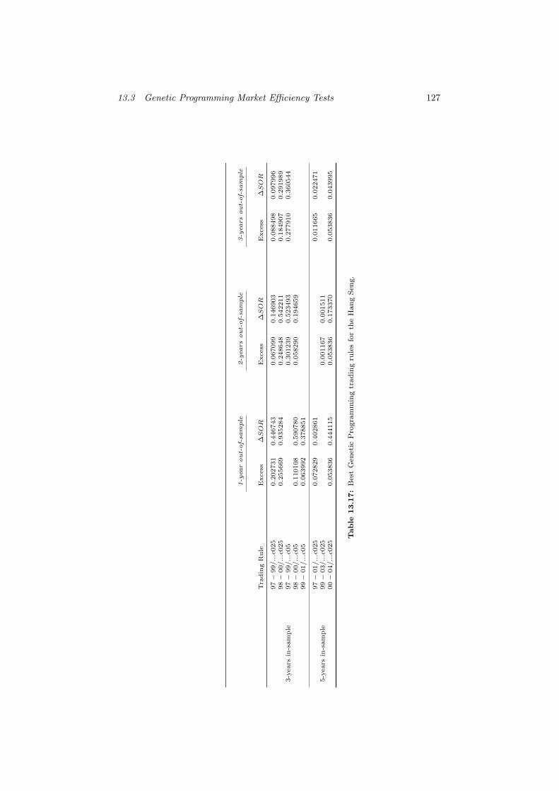
13.3 Genetic Programming Market Efficiency Tests 127
1-y
ear
out-of-sa
mple
2-y
ears
out-of-sa
mple
3-y
ears
out-of-sa
mple
Tra
din
gR
ule
Excess
∆SOR
Excess
∆SOR
Excess
∆SOR
3-y
ears
in-s
am
ple
97−
99/...c
025
0.2
02731
0.4
46743
0.0
67099
0.1
46903
0.0
88498
0.0
97996
98−
00/...c
025
0.2
55669
0.9
35284
0.2
48648
0.5
42211
0.1
84907
0.2
91989
97−
99/...c
05
0.3
01239
0.5
23493
0.2
77910
0.3
60544
98−
00/...c
05
0.1
10108
0.5
90780
0.0
58290
0.1
94659
99−
01/...c
05
0.0
63992
0.3
78851
5-y
ears
in-s
am
ple
97−
01/...c
025
0.0
72829
0.4
02861
0.0
11665
0.0
22471
99−
03/...c
025
0.0
01167
0.0
01511
00−
04/...c
025
0.0
53836
0.4
44115
0.0
53836
0.1
73370
0.0
53836
0.0
43995
Table
13.1
7:
Bes
tG
enet
icP
rogra
mm
ing
trad
ing
rule
sfo
rth
eH
an
gS
eng.
13.4 Conclusions about Market Efficiency in the DAX and the Hang Seng128
13.4 Conclusions about Market Efficiency in the DAX and
the Hang Seng
Jensen (1978) considered markets to be efficient if there are no gains from trad-
ing based on available information after risk adjustment and transaction costs.
In the thesis at hand, GP was tasked to find trading rules based on the most
common set of information, i. e. closing prices106 therefore testing for weak
market efficiency. Appropriate transaction costs (c = 0.25, 0.5) were included in
the analysis and the Sortino ratio acted as a measure for risk-adjusted returns.
The results of the GP-optimized trading rules in terms of market efficiency in-
dicate that in general, the EMH apparently holds for both the DAX and the
Hang Seng for the combined out-of-sample period as the analysis of long term
GP performance107 at best showed marginal (DAX) and zero (Hang Seng) risk-
adjusted excess returns after transaction costs.
However, the picture is not so clear on a smaller level. A couple of rules outper-
formed the benchmark in both indices. What is even more interesting is that
one rule in the Hang Seng managed to do so in an overall rising market108. For
realistic transaction costs, GP beats the benchmark on a risk-adjusted basis in
13 out of 72 scenarios for the DAX and 17 out of 72 scenarios for the Hang Seng.
In addition, some of the successful rules have a surprisingly easy structure109. It
is debatable whether any technical analyst would have coincidentally come up
with the rules suggested by GP as his/her human brainchild, however one has
to bear in mind that the concept of GP was well-known and available already at
the beginning of the data sample in the year 2000. It must also be emphasized
that the rules, due to the data division scheme and rolling time-frame approach,
are so-to-say ex-ante optimal, i. e. GP as a machine learning tool evolved trad-
ing rules from training samples that were then applied blindly to data unknown
to the algorithm beforehand and GP still managed to beat the benchmark in
a considerable amount of cases. Some of these rules, particularly those during
the 2002 out-of-sample year in the DAX, manage to beat the benchmark by106Which are available to anybody at a very low or even no cost at all.107The scenarios with updated trading rules at each year’s beginning.108The 00-04/...c025 rule managed to outperform the benchmark on a risk-adjusted basis.109See Figures 13.3 and 13.6.
13.4 Conclusions about Market Efficiency in the DAX and the Hang Seng129
simply switching out-of-the-market and staying there thus saving the investor
from tremendous losses in the index. This also applies to the Hang Seng for the
years 2000-2002 as most of the successful rules come from that bearish market
period. Critics might argue that this outperformance is not very convincing as
a human investor would also have switched out-of-the-market during a market
meltdown. However, apart from the fact that the choice of straight buy-and-
hold as benchmark come hell or high water is simply a design decision for the
study at hand110, a human investor does not ex-ante know whether the mar-
ket is already in a meltdown neither does he know how long it will take the
market to bottom out and how much losses will still be incurred (neither does
GP) and when to re-enter the market. In contrast, GP, while it also cannot tell
the future, comes up with a quantifiable strategy for this period which simply
suggests to stay out-of-the-market for a prolonged period of time and eventually
go long again. This is what GP independently recommends in both markets so
it it highly unlikely that these rules simply emerged by chance.
Why is it then that GP (almost) fails in the long-run? Chen and Navet (2006,
2007) investigate this issue and point out the distinction between efficient mar-
ket and inefficent algorithms, so the question is which of the two is the reason
for this finding? It might be that markets have indeed been simply efficient for
the period 2000-2007 used in this study, however things would look differently
if one would just take say the 2000-2003 sample. In this case, particularly the
DAX would look all but efficient. Chen et al. (2008) emphasize the link be-
tween market conditions during traing and out-of-sample period. They argue
that in a steadily rising market, the best possible outcome for GP often is to
simply replicate buy-and-hold. There may be better strategies but finding them
might be very hard for GP - provided they exist at all. Both DAX and Hang
Seng feature sustained upward trends from the year 2003-2007 which tipped the
scales in favour of buy-and-hold. Therefore, the failure of GP in the long run
may be partly due to the design decision to take a rather recent data sample.
One of the consequences for future studies might be to focus on a market that
has shown a rather trendless/mean reverting pattern during the last couple of
110Buy-and-hold by design favours GP during bearish markets while the opposite is true forbullish markets.

13.4 Conclusions about Market Efficiency in the DAX and the Hang Seng130
years111.
Another issue might be inherent deficiencies in the GP algorithm. As already
pointed out, the issue of parameter settings within GP is particularly important
and unfortunately, as pointed out in Chen et al. (2008), is not well understood.
In addition, the choice of a suitable function set for GP is still in open issue
(Navet and Chen, 2007). Therefore, the question as to whether the results might
be improved by using different sets of parameters and function sets is still open
as well.
111Further directions for future research will be pointed out in the next chapter.
131
Part V
Summary and Conclusion
14 Genetic Programming and Market Efficiency
The thesis started with a literature review followed by a technical chapter which
presented the inner workings of GP. The next chapter dealt with the applica-
tion of GP-optimized trading rules to the DAX and the Hang Seng. The results
indicated that GP performance depends on market cycles; it manages to beat
the buy-and-hold benchmark even after risk adjustment and transaction costs
in bear markets whereas, in the case of the DAX, GP at best marginally out-
performs the benchmark during a bullish market cycle as seen in the years
2003-2007. Things look slightly different for the Hang Seng as GP in one case
even manages to beat the benchmark by a considerable margin during an over-
all upward trend in the market. Therefore, these results imply that the EMH
does not always hold. However, the results from applying a yearly updated
GP trading rule to the whole data sample showed only a very marginal risk-
adjusted outperformance in the DAX and no outperformance in the Hang Seng.
Nevertheless it must be emphasized that GP questions the absolute validity of
the EMH as one might have expected that GP would generally fail at beating
the respective benchmarks. This has been proven wrong given the amount of
instances where GP outperforms the benchmark and at times even does so when
the market apparently seems to be efficient by exhibiting a strong upward trend.
Therefore, though GP maybe failed to deliver the ultimate proof that markets
are inefficient, it casts at least some doubts on the validity of the EMH and
implies that the EMH does not always hold.
15 Directions for Future Research
During the writing of the thesis at hand, a couple of ideas for further GP
research came to the author’s mind which justify a thesis on their own. The
author hopes that one of these issues will eventually be picked up to continue
15 Directions for Future Research 132
this line of research. Referring to the literature review in the second chapter, a
typical GP application for testing market efficiency consists of:
1. Choice of a particular market/asset class
2. Choice of input variables, data sample and data division scheme
3. Parameter settings, choice of function set and selection algorithm
4. Choice of fitness function and benchmark strategy.
These items provide endless variation of GP-related research. Based on the
the literature review and the experience gained as part of the study at hand,
directions for future research can be narrowed down to a more reasonable and
promising perspective that may assist in a better understanding of financial
markets and the mechanics of GP.
From a personal point of view, the existing literature might be extended by
investigating GP performance using macroeconomic variables. So far only Bauer
(1994) and Ammann and Zenkner (2003) use fundamental variables such as
inflation, growth and interest rate spreads as input and report encouraging
results. Major sources of inspiration for macroeconomic GP inputs also come
from the existing literature on modeling excess returns. Promising candidates
for macroeconomic GP inputs are (in no particular order):
• dividend yields
(Fama and French, 1989; Chen, 1991; Bekaert and Hodrick, 1992; Pe-
saran and Timmermann, 1995; Olson and Mossmann, 2001; Dopke et
al., 2008)
• T-bill rates from 1-12 months
(Breen et al., 1989; Chen, 1991; Pesaran and Timmermann, 1995; Olson
and Mossmann, 2001; Dopke et al., 2008)
• term spread
(Keim and Stambaugh, 1986; Chen, 1991; Bekaert and Hodrick, 1992;
Olson and Mossmann, 2001; Fama and French, 1989, Dopke et al., 2008)
15 Directions for Future Research 133
• default spread
(Fama and French, 1989; Chen, 1991; Olson and Mossmann, 2001)
• inflation
(Pesaran and Timmermann, 1995; Olson and Mossmann, 2001)
• changes in industrial production/GNP growth
(Chen, 1991; Pesaran and Timmermann, 1995; Olson and Mossmann,
2001 ).
Even though the prospect of finding evidence against the EMH may be limited,
the use of macroeconomic variables may yield further insight into the relation-
ship between stock markets and the overall macroeconomic environment and
may point out major structural breaks in stock markets. Another promising
avenue for GP applied to stock markets may be to look for possible inefficien-
cies on a much smaller scale using high-frequency price data. Seasoned market
participants may argue that ineffiencies build up and exist just for a couple of
seconds. Therefore, using a finer search grid may yield results that contradict
the EMH112. However, this would also require way more data and is technically
more demanding in terms of CPU time.
Concerning other asset classes, the GP literature on FOREX markets does not
seem to offer much space for a further contribution. As currencies can be ba-
sically traded anywhere in the world, the distinction between different market-
places such as for stocks does not exist. The author feels that the various papers
by Neely et al. adequately cover the topic and cannot be much improved upon
except for using a more up-to-date data sample. More surprisingly, it turned
out that the bond market has almost not been covered at all by the existing
literature. The only approach the author is aware of is Bauer (1994), who uses
a classic GA to switch between long- and short-term government bonds on the
one hand and between risky corporate bond and safe-haven government bonds
on the other hand. Though the reported results are mixed, the lack of research112All existing studies including this study use daily and sometimes even monthly data. From a
personal point of view, using high-frequency data is the most promising avenue of research.
15 Directions for Future Research 134
on this issue opens up avenues for further experiments. It would be worthwhile
to re-investigate the bond market application proposed by Bauer (1994) for Eu-
ropean corporate bonds/government bonds using a GP setup with appropriate
inputs such as growth and inflation expectations, price momentum, value of
equities vs. bonds and flows into mutual bond funds.
A gap exists in the literature as well when it comes to commodity markets.
However, commoditiy futures might be difficult to implement in GP since this
market is plagued probably more than others by (extremely) high volatility,
many speculative traders and highly disrupted trading patterns. This might
explain the lack of research directed at this market. Regarding other markets,
it would also be worthwhile to investigate derivative markets, especially the
market for credit derivatives.
The impact of parameter choice within a GP framework is not well understood
(Chen et al., 2008). Depending on parameter settings, the search space may
not be covered thoroughly. It might be interesting to test several parameter
sets to better understand how GP discovers trading rules in a market. It might
prove beneficial to conduct this kind of comparative statics on an artificial time
series first and then try to match this time series with real-world data. As
another avenue for future research, several studies advocate tinkering with the
fitness function rather than with the underyling parameters such as crossover
and mutation rates to fine-tune results (Amman and Zenkner, 2003; Becker and
Seshadri, 2003b; Navet and Chen, 2007). The fitness function is at the core
of evolutionary modeling of financial markets. While the usual approach is to
simply measure excess returns, more sophisticated fitness functions could be
employed. For example, volatility could be included as well in a (appropriately
weighted) fitness function as well as a complexity-penalizing factor that kicks
in once too many trades (and therefore too much transaction costs) would be
carried out during the training period as shown in Becker and Seshadri (2003b).
Variations thereof, including appropriate weighting schemes, could be another
avenue for future resarch. Navet and Chen (2007) present a wealth of further
ideas on how the literature on GP can be improved upon. Most of the issues

15 Directions for Future Research 135
addressed in their paper are still an open question at the time of this writing
(March 2010).
REFERENCES 136
References
[1] Alexander, S. (1961). Price Movements in Speculative Markets: Trends
or Random Walks. Industrial Management Review 2, 7-26.
[2] Allen, F. and Karjalainen, R. (1999). Using Genetic Algorithms to Find
Technical Trading Rules. Journal of Financial Economics 51, 245-271.
[3] Altenberg, L. (1994). The evolution of evolvability in genetic program-
ming. In: Kinnear, K.E. (ed.), Advances in Genetic Programming, MIT
Press.
[4] Ammann, M. and Zenkner, C. (2003). Tactical Asset Allocation mit
Genetischen Algorithmen. Schweizerische Zeitschrift fur Volkswirtschaft
und Statistik 139(1), 1-40.
[5] Austin, M. P., Bates, G., Dempster, M., Leemans, V., Williams, S.
N. (2004). Adaptive systems for foreign exchange trading. Quantitative
Finance 4(4), 37-45.
[6] Azzini, A. and Tettamanzi, A.G.B. (2008). Evolutionary Single-Position
Automated Trading. In: Giacobini, M. et al. (eds.), Proceedings of the
European Workshop on Evolutionary Computation in Finance and Eco-
nomics, EVOFIN 08, Springer-Verlag.
[7] Babcock, B. (1989). The Dow Jones-Irwin Guide to Trading Systems,
Dow Jones-Irwin.
[8] Bachelier, L. (1900). Theorie de la Speculation, Annales Scientifiques de
l’Ecole Normale Superieure, III-17, 21-86.
[9] Banzhaf, W., Nordin, P., Keller, R. E. and Francone, F. D. (1998).
Genetic Programming-An Introduction: On the Automatic Evolution of
Computer Programs and Its Applications, Morgan Kaufmann Publishers.
[10] Basu, S. (1977). Investment Performance of Common Stocks in Relation
to Their Price-Earnings Ratios: A Test of the Efficient Market Hypothesis.
Journal of Finance 32(3), 663-682.
REFERENCES 137
[11] Bauer, R. J. and Liepins, G. E. (1992). Genetic Algorithms and Com-
puterized Trading Strategies. In: O’Leary, D. E., Watkins, R. R. (eds.),
Expert Systems in Finance, North Holland.
[12] Bauer, R. J. (1994). Genetic Algorithms and Investment Strategies, John
Wiley & Sons.
[13] Becker, L. A. and Seshadri, M. (2003a). GP-evolved technical trading
rules can outperform buy and hold. In: Proceedings of the Sixth Interna-
tional Conference on Computational Intelligence and Natural Computing,
Embassy Suites Hotel and Conference Center, Cary, North Carolina.
[14] Becker, L. A. and Seshadri, M. (2003b). Comprehensibility and overfit-
ting avoidance in genetic programming for technical trading rules. Tech-
nical Report, Worcester Polytechnic Institute.
[15] Bekaert, G. and Hodrick, R. J. (1992). Characterizing Predictable Com-
ponents in Excess Returns on Equity and Foreign Exchange Markets.
Journal of Finance 47(2), 467-509.
[16] Bessembinder, H. and Chan, K. (1995). The Profitability of Technical
Trading Rules in the Asian Stock Markets. Pacific Basin Finance Journal
3, 257-284.
[17] Bessembinder, H. and Chan, K. (1998). Market Efficiency and the Re-
turns to Technical Analysis. Financal Management 27, 5-17.
[18] Bhattacharyya, S. and Mehta, K. (2002). Evolutionary Induction of
Trading Models. In: Chen, S.-H. (ed.), Evolutionary Computation in Eco-
nomics and Finance, Physica-Verlag.
[19] Bollerslev, T. (1986). Generalized Autoregressive Conditional Het-
eroskedasticity. Journal of Econometrics 31, 307-327.
[20] Bollerslev, T. and Hodrick, R. J. (1994). Financial Market Efficiency
Tests. In: Pesaram, H. and Wickens, M. (eds.), Handbook of Applied
Econometrics Vol. I, Basil Blackwell.
REFERENCES 138
[21] Breen, W., Glosten, L. R. and Jagannathan, R. (1989). Economic Sig-
nificance of Predictable Variations in Stock Index Returns. Journal of
Finance 44(5), 1177-1189.
[22] Brock, W. A., Dechert, W. and Scheinkman, J. (1987). A Test for Inde-
pendence based on the Correlation Dimension. University of Wisconsin,
Madison, University of Houston and University of Chicago.
[23] Brock, W. A., Hsieh, D. A. and LeBaron, B. (1991). Nonlinear Dynam-
ics, Chaos and Instability: Statistical Theory and Economic Evidence,
MIT Press.
[24] Brock, W. A., Lakonishok, J. and LeBaron, B. (1992). Simple Technical
Trading Rules and the Stochastic Properties of Stock Returns. Journal of
Finance 47, 1731-1764.
[25] Brown, S., Goetzmann, W. and Kumar, A. (1998). The Dow Theory:
William Peter Hamilton’s Track Record Reconsidered. Journal of Finance
53(4), 1311-1333.
[26] Cantu-Paz, E. et al. (eds.) (2003). Genetic and Evolutionary Computa-
tion - GECCO 2003: Genetic and Evolutionary Computation Conference,
Chicago, IL, Proceedings: Pt. 2, Springer-Verlag.
[27] Chaudry, A. and Johnson, H. L. (2008). The Efficacy of the Sortino Ratio
and Other Benchmarked Performance Measures Under Skewed Return
Distributions. Australian Journal of Management 32, 485-502.
[28] Chen, N. (1991). Financial Investment Opportunities and the Macroe-
conomy. Journal of Finance 46(2), 529-554.
[29] Chen, S.-H. and Yeh, C.-H. (1996). Genetic Programming and the Effi-
cient Market Hypothesis. In: Genetic Programming 1996: Proceedings of
the First Annual Conference, Stanford University, CA, USA, MIT Press.
[30] Chen, S.-H. and Yeh, C.-H. (1997). Toward a computable approach to
the efficient market hypothesis: An application of genetic programming.
Journal of Economic Dynamics and Control 21, 1043-1063.
REFERENCES 139
[31] Chen, S.-H. and Kuo, T.-W. (2001). Trading strategies on trial: A com-
prehensive review of 21 practical trading strategies over 56 listed stocks.
In: Proceedings of the Fourth International Conference on Computational
Intelligence and Multimedia Applications (ICCIMA 2001), 66-71, IEEE
Computer Society Press.
[32] Chen, S.-H. (ed.) (2002a). Evolutionary Computation in Economics and
Finance, Physica-Verlag.
[33] Chen, S.-H. (ed.) (2002b). Genetic Algorithms and Genetic Program-
ming in Computational Finance, Kluwer Academic Publishers.
[34] Chen, S.-H., Kuo, T.-W. and Y.-P. Shieh (2002). Genetic programming:
A tutorial with the software simple GP. In: Chen, S.-H. (ed.), Genetic
Algorithms and Genetic Programming in Computational Finance, 55-77,
Kluwer Academic Publishers.
[35] Chen, S.-H. and Kuo, T.-W. (2003a). Overfitting or poor learning: A
critique of current financial applications of GP. In: Ryan, C., Soule, T.,
Keijzer, M., Tsang, E., Poli, R. and Costa, E. (eds.), Proceedings of the
Sixth European Conference on Genetic Programming (EuroGP-2003), Es-
sex, Lecture Notes in Computer Science 2610, 24-46, Springer-Verlag.
[36] Chen, S.-H. and Kuo, T.-W. (2003b). Discovering hidden patterns with
genetic programming. In: Chen, S.-H and Wang, P. P. (eds.), Computa-
tional Intelligence in Economics and Finance, 329-347, Springer-Verlag.
[37] Chen, S.-H. and Navet, N. (2006). Pretests for genetic programming
evolved trading programs: zero-intelligence strategies and lottery trad-
ing. In: King, I., Wang, J., Chan, L. and Wang, D.L. (eds.), Neural In-
formation Processing, 13th International Conference ICONIP 2006 Hong
Kong, Proceedings, Part III, Lecture Notes in Computer Science, 450-460,
Springer-Verlag.
[38] Chen, S.-H. and Navet, N. (2007). Failure of Genetic-Programming In-
duced Trading Strategies: Distinguishing between Efficient Markets and
Inefficient Algorithms. In: Chen, S.-H., Wang, P. P. and Kuo, T.-W.
REFERENCES 140
(eds.), Computational Intelligence in Economics and Finance Vol. II.,
Springer-Verlag.
[39] Chen, S.-H., Kuo, T.-W. and Hoi, K.-M. (2008). Genetic Programming
and Financial Trading: How Much About ”What We Know”. In: Zopouni-
dis, C., Doumpos, M. and Pardalos, P. M. (eds.), Handbook of Financial
Engineering, Springer-Verlag.
[40] Colin, A. M. (1994). Genetic Algorithms for Financial Modeling. In:
Deboeck, G. J. (ed.), Trading on the Edge: Neural, Genetic, and Fuzzy
Systems for Chaotic Financial Markets, John Wiley & Sons.
[41] Colin, A. M. (2000). A genetic programming-based approach to genera-
tion of foreign exchange trading models. In: Barnett, W. A. et al. (eds.),
Commerce, Complexity, and Evolution. Proceedings of the Twelfth Inter-
national Symposium in Economic Theory and Econometrics, Cambridge
University Press.
[42] Costa Pereira, C. da and Tettamanzi, A. G. B. (2006). Fuzzy-
Evolutionary Modeling for Single-Position Day Trading. In: Brabazon,
A. and O’Neill, M. (eds.), Natural Computing in Computational Finance,
Studies in Computational Intelligence 100, Springer-Verlag.
[43] Davis, L. (1989). Adapting operator probabilities in genetic algorithms.
In: Schaffer, J.D. (ed.), Proceedings of the Third International Conference
on Genetic Algorithms 61-69, Morgan Kaufmann.
[44] Deboeck, G. J. (1994). Trading on the Edge: Neural, Genetic, and
Fuzzy Systems for Chaotic Financial Markets, John Wiley & Sons.
[45] Dempster, M. and Jones, C. (2001). A real-time adaptive trading system
using genetic programming. Quantitative Finance 1, 397-413.
[46] Dopke, J., Hartmann, D. and Pierdzioch, C. (2008). Real-time macroe-
conomic data and ex ante stock return predictability. International Review
of Financial Analysis 17, 274-290.
[47] Drezewski, R. and Sepielak, J. (2008). Evolutionary System for Gener-
ating Investment Strategies. In: Giacobini, M. et al. (eds.), Proceedings
REFERENCES 141
of the European Workshop on Evolutionary Computation in Finance and
Economics, EVOFIN 08, Springer-Verlag.
[48] Eiben, A. J., Smith, J. E. (2003). Introduction to Evolutionary Com-
puting, Springer-Verlag.
[49] Engle, R. F. (1982). Autoregressive Conditional Heteroscedasticity with
Estimates of the Variance of United Kingdom Inflation. Econometrica 50,
987-1007.
[50] Fama, E. F. (1965a). The Behavior of Stock-Market Prices. The Journal
of Business 38(1), 34-105.
[51] Fama, E. F. (1965b). Random Walks in Stock Market Prices. Financial
Analysts Journal 21(5), 5559.
[52] Fama, E. F. (1970). Efficient capital markets: A review of theory and
empirical work. Journal of Finance 25, 383-417.
[53] Fama, E. F. and French, K. R. (1988). Dividend Yields and Expected
Stock Returns. Journal of Financial Economics 22, 3-25.
[54] Fama, E. F. and French, K. R. (1989). Business Conditions and Expected
Returns on Stocks and Bonds. Journal of Financial Economics 25, 23-49.
[55] Fama, E. F. (1991). Efficient capital markets: II. Journal of Finance 46,
1575-1617.
[56] Fogel, L. J., Owens, A. J. and Walsh, M. J. (1965). Artificial Intelligence
through a simulation of evolution. In: Callahan, A., Maxfield, M. and Fo-
gel, L. J. (eds.), Biophysics and Cybernetic Systems. Spartan, Washington
DC.
[57] Fogel, L. J., Owens, A. J. and Walsh, M. J. (1966). Artificial Intelligence
through Simulated Evolution, Wiley.
[58] Franses, P. H., van Dijk, D. (2000). Non-Linear Time Series Models in
Empirical Finance, Cambridge University Press.
[59] French, K. (1980). Stock Returns and the Weekend Effect. Journal of
Financial Economics 5, 55-69.
REFERENCES 142
[60] Frick, A., Herrmann, R., Kreidler, M., Narr, A., Sesse, D. (1996). A
Genetic-Based Approach for the Derivation of Trading Strategies on the
German Stock Market. In: Amari, S., Xu, L., King, I., Leung, K. (eds.),
Progress in Neural Information Processing, Vol. 2, Springer-Verlag.
[61] Fyfe, C., Marney, J. P. and Tarbert, H. (1999). Technical analysis versus
market efficiency - a genetic programming approach. Applied Financial
Economics 9, 183-191.
[62] Fyfe, C., Marney, J. P. and Tarbert, H. (2005). Risk Adjusted Returns
from Technical Trading: a Genetic Programming Approach. Applied Fi-
nancial Economics 15, 1073-1077.
[63] Gang, W. and Soule, T. (2004). How to choose appropriate function
sets for GP. In: Keijzer, M., O’Reilly, U.M., Lucas, S.M., Costa, E. and
Soule, T. (eds.), Genetic Programming 7th European Conference EuroGP
2004, Proceedings, Lecture Notes in Computer Science, 198-207, Springer-
Verlag.
[64] Goldberg, D. (1989). Genetic Algorithms in Search, Optimization and
Machine Learning, Addison-Wesley.
[65] Granville, J. E. (1976). New Strategy of Daily Stock Market Timing for
Maximum Profit, Prentice-Hall.
[66] Harland, Zac (1999). Using Nonlinear Neurogenetic Models with Profit
Related Objective Functions to Trade the US T-bond Future. In: Abu-
Mostafa, Y. S., LeBaron, B. et al. (eds.), Computational Finance 1999,
MIT Press.
[67] Holland, J. J. (1975). Adaption in Natural and Artificial Systems, Uni-
versity of Michigan Press.
[68] Hsieh, D. A. (1989). Testing for Nonlinear Dependence in Daily Foreign
Exchange Rates. Journal of Business 62, 339-368.
[69] Huang, Y. S. (1995). The Trading Performance of Filter Rules On the
Taiwan Sotck Exchange. Applied Financial Economics 5, 391-395.
REFERENCES 143
[70] Hudson, R., Dempsey, M. and Keasey, K. (1996). A Note on the Weak
Form of Efficiency of Capital Markets: The Application of Simple Tech-
nical Trading Rules to the U.K. Stock Markets 1935-1994. Journal of
Banking and Finance 20, 1121-1132.
[71] Islam, S.M.N. and Watanapalachaikul, S. (2005). Empirical Finance.
Physica Series Contributions to Economics, Springer-Verlag.
[72] Jaffe, J. F. (1974). Special information and insider trading. Journal of
Business 47, 410-428.
[73] Jegadeesh, N. and Titman, S. (1993). Returns to buying winners and
selling losers: Implication for stock market efficiency. Journal of Finance
48, 65-91.
[74] Jensen, Michael C. (1978). Some anomalous evidence regarding market
efficiency. Journal of Financial Economics 6(23), 95-101.
[75] Kaboudan, M. A. (2000). Genetic Programming Prediction of Stock
Prices. Computational Economics 16(3), 207-236.
[76] Kaboudan, M. A. (2002). GP Forecasts of Stock Prices for Profitable
Trading. In: S.-H. Chen (ed.), Evolutionary Computation in Economics
and Finance, Physica-Verlag.
[77] Karjalainen, R. (2002). Evolving technical trading rules for S&P futures.
In: Acar, E., Satchell, S. (eds.), Advanced Trading Rules, Butterworth-
Heinemann.
[78] Karr, C. L., Bowersox, R., Singh, V. (2003). Minimization of Sonic Boom
on Supersonic Aircraft Using an Evolutionary Algorithm. In: Cantu-Paz,
E. et al. (eds.), Genetic and Evolutionary Computation - GECCO 2003:
Genetic and Evolutionary Computation Conference, Chicago, IL, Pro-
ceedings: Pt. 2, Springer-Verlag.
[79] Kassicieh, S. K., Paez, T. L. and Vora, G. (1997). Investment decisions
using genetic algorithms. In: Proceedings of the 30th Hawaii International
Conference on System Sciences, IEEE Computer Society.
REFERENCES 144
[80] Keane, A. (2001). An Introduction to Evolutionary Computing in Design
Search and Optimization. In: Kallel, L., Naudts, B. and Rogers, A. (eds.),
Theoretical Aspects of Evolutionary Computing, Springer-Verlag.
[81] Keim, D. B. and Stambaugh, R. F. (1986). Predicting Returns in the
Stock and Bond Market. Journal of Financial Economics 17, 357-390.
[82] Koza, J. R. (1992). Genetic Programming: On the Programming of
Computers by Means of Natural Selection, MIT Press.
[83] Kwon, K.-Y. and Kish, R.J. (2002). A comparative study of techni-
cal trading strategies and return predictability: an extension of Brock,
Lakonishok, and LeBaron (1992) using NYSE and NASDAQ indices. The
Quarterly Review of Economics and Finance 42, 611-631.
[84] Kwon, Y.-K., Moon, B.-R. (2003). Daily Stock Prediction Using Neuro-
genetic Hybrids. In: Cantu-Paz, E. et al. (eds.), Genetic and Evolutionary
Computation - GECCO 2003: Genetic and Evolutionary Computation
Conference, Chicago, IL, Proceedings: Pt. 2, Springer-Verlag.
[85] Lam, S. S., Lam, K. P. and Ng, H. S. (2002). Genetic Fuzzy Expert
Trading System For NASDAQ Stock Market Timing. In: Chen, S.-H.
(ed.), Genetic Algorithms and Genetic Programming in Computational
Finance, Kluwer Academic Publishers.
[86] Langdon, W. B. and Poli, R. (2002). Foundations of Genetic Program-
ming, Springer-Verlag.
[87] LeBaron, B. (1999). Technical Trading Rule Profitability and Foregin
Exchange Intervention. Journal of International Economics 49, 125-143.
[88] Li, J. and Tsang, P. K. (1999). Investment Decision Making Using FGP:
A Case Study. In: Angeline, P. J. et al. (eds.), Proceedings of the Congress
on Evolutionary Computation, Vol. 2, 1253-1259, IEEE Press.
[89] Li, J., Tsang, P. K. (2002). EDDIE for financial forecasting. In: Chen,
S.-H., (ed.), Genetic Algorithms and Genetic Programming in Computa-
tional Finance, 161-174, Kluwer Academic Press.
REFERENCES 145
[90] Lipinski, P. (2007). ECGA vs. BOA in discovering stock market trad-
ing experts. Proceedings of the Genetic and Evolutionary Computation
Conference (GECCO 2007), 531-538, ACM Press.
[91] Lo, A. W., MacKinlay, A. C. (1988). Stock Market Prices do not Follow
Random Walks: Evidence from a Simple Specification Test. Review of
Financial Studies 1(1), 41-66.
[92] Lo, A. W., Mamaysky, H. and Wang, J. (2000). Foundations of Technical
Analysis: Computational Algorithms, Statistical Inference, and Empirical
Implementation. Journal of Finance 55, 1705-1765.
[93] McNelis, P. D. (2005). Neural Networks in Finance: Gaining Predicitive
Edge in the Market, Elsevier Academic Press.
[94] Medsker, L. R. (1995). Hybrid Intelligent Systems, Kluwer Academic
Publishers.
[95] Miller, R. E. and Reilly, F. K. (1987). An Examination of Mispricing,
Returns and Uncertainty for Initial Public Offerings. Financial Manage-
ment 16, 32-38.
[96] Navet, N. and Chen, S.-H. (2007). Financial Data Mining
with Genetic Programming: A Survey and Look Forward. In-
vited paper at the 56th session of the International Statis-
tical Institute (ISI 2007), Lisboa, Portugal. Downloadable at
http://www.loria.fr/∼nnavet/publi/ISI2007 NN SHC AT.pdf.
[97] Navet, N. and Chen, S.-H. (2008). On Predictability and Profitability.
Would GP Induced Trading Rules be Sensitive to the Observed Entropy of
Time Series? In: Brabazon, T. and O’Neill, M. (eds.), Natural Computing
in Computational Finance, Springer-Verlag.
[98] Nedjah, N., Abraham, A. and de Macedo Mourelle, L. (eds.) (2006). Ge-
netic Systems Programming : Theory and Experiences, Springer-Verlag.
[99] Neely, C., Weller, P. and Dittmar, R. (1997). Is Technical Analysis in the
Foreign Exchange Market Profitable? A Genetic Programming Approach.
Journal of Financial and Quantitative Analysis 32(4), 405-426.
REFERENCES 146
[100] Neely, C. and Weller, P. A. (1999). Technical Trading Rules in the Eu-
ropean Monetary System. Journal of International Money and Finance
18(3), 429-458.
[101] Neely, C. and Weller, P. A. (2001). Technical analysis and central bank
intervention. Journal of International Money and Finance 20(7), 949-970.
[102] Neely, C. and Weller, P. A. (2003a). Intraday technical trading in the
foreign exchange market. Journal of International Money and Finance
22(2), 223-237.
[103] Neely, C. (2003b). Risk-adjusted, ex ante, optimal technical trading rules
in equity markets. International Review of Economics & Finance 12(1),
69-87.
[104] Niederhoffer, V. and Osborne, M. F. M. (1966). Market making and
reversal on the stock exchange. Journal of the American Statistical Asso-
ciation 61, 897-916.
[105] Nordin, P., Francone, F. and Banzhaf, W. (1995). Explicitly defined
introns and destructive crossover in genetic programming. In: Rosca, J.
P. (ed.), Proceedings of the Workshop on Genetic Programming: From
Theory to Real-World Applications, 6-22, Tahoe City, CA.
[106] Nordin, P. and Banzhaf, W. (1995). Complexity compression and evo-
lution. In: Eshelman, L. (ed.), Genetic Algorithms: Proceedings of the
Sixth International Conference (ICGA95), 310-317, Pittsburgh, PA, Mor-
gan Kaufmann.
[107] Olson, D. and Mossman, C. (2001). Cross-Correlations and Predictability
of Stock Returns. Journal of Forecasting 20(2), 145-60.
[108] O’Neill, M., Brabazon, A. and Ryan, C. (2002). Forecasting Market In-
dices using Evolutionary Automatic Programming. In: Chen, S.-H. (ed.),
Genetic Algorithms and Genetic Programming in Computational Finance,
Kluwer Academic Publishers.
REFERENCES 147
[109] O’Reilly, U.-M. (1995). An Analysis of Genetic Programming. PhD the-
sis, Carleton University, Ottawa Carleton Institute for Computer Science,
Ottawa, Ontario, Canada.
[110] O’Reilly, U.-M. and Oppacher, F. (1995). The troubling aspects of a
building block hypothesis for genetic programming. In: Whitley, L.D.
and Vose, M.D. (eds.), Foundation of Genetic Algorithms 3, Estes Park,
Colorado, USA, Morgan Kaufmann.
[111] Pardo, R. (1992). Design, Testing, and Optimization of Trading Systems,
John Wiley & Sons.
[112] Pereira, R. (2002). Forecasting ability but no profitability: An empirical
evaluation of genetic algorithm-optimised technical trading rules. In: S.-H.
Chen (ed.), Evolutionary Computation in Economics and Finance, 287-
310, Physica-Verlag.
[113] Pesaran, M. and Timmermann, A. (1995). Predictability of stock re-
turns: Robustness and economic significance. Journal of Finance 50, 1201-
1228.
[114] Potvin, J.-Y., Soriano, P. and Vallee, M. (2004). Generating trading
rules on the stock markets with genetic programming. Computers & Op-
erations Research 31(7), 1033-1047.
[115] Price, G. R. (1970). Selection and Covariance. Nature 227, 520-521.
[116] Raj, M. and Thurston, D. (1996). Effectiveness of Simple Technical Trad-
ing Rules in the Hong Kong Futures Market. Applied Economic Letters 3,
33-36.
[117] Ratner, M. and Leal, R.P.C. (1999). Tests of technical trading strategies
in the emerging markets of Latin America and Asia. Journal of Banking
and Finance 23, 1887-1905.
[118] Rechenberg, I. (1973). Evolutionsstrategie: Optimierung Technischer
Systeme nach Prinzipien der Biologischen Evolution, Fromman-Hozlboog-
Verlag.
REFERENCES 148
[119] Reeves, C. R. and Rowe, J. E. (2003). Genetic Algorithms - Principles
and Perspectives: A Guide to GA Theory, Kluwer Academic Publishers.
[120] Rosca, J. P. (1997). Analysis of complexity drift in genetic programming.
In: Koza, J. R., Kalyanmoy, D., Dorigo, M., Fogel, D. B., Garzon, M. H.,
Iba, H. and Riolo, R. L. (eds.), Genetic Programming 1997: Proceedings
of the Second Annual Conference, Stanford University, CA, USA, Morgan
Kaufmann.
[121] Samuelson, P. A. (1965). Proof that properly anticipated prices fluctu-
ate randomly. Industrial Management Review 6, 41-49.
[122] Scheinkman, J. and LeBaron, B. (1989). Nonlinear Dynamics and Stock
Returns. Journal of Business 62, 311-337.
[123] Scholes, M. (1972). The market for securities: Substitution versus price
pressure and the effects of information on share prices. Journal of Business
45, 179-211.
[124] Seyhun, H. N. (1986). Insiders’ profits, cost of trading and market effi-
ciency. Journal of Financial Economics 16, 189-212.
[125] Setzkorn, C., Dipietro, L. and Purshouse, R. (2003). Evolving Rule-
Based Trading Systems. Technical report, ULCS-02-005, Department of
Computer Science, University of Liverpool.
[126] Sharpe, W. F. (1966). Mutual Fund Performance. Journal of Business
39, 119-138.
[127] Shiller, Robert J. (1979). The Volatility of Long-Term Interest Rates
and Expectations Models of the Term Structure. The Journal of Political
Economy 87(6), 1190-1219.
[128] Silva, S. and Almeida, J. (2003). Dynamic maximum tree depth - a simple
technique for avoiding bloat in tree-based GP. In: Cantu-Paz, E. et al.
(eds.), Genetic and Evolutionary Computation - GECCO 2003: Genetic
and Evolutionary Computation Conference, Chicago, IL, Proceedings: Pt.
2, Springer-Verlag.
REFERENCES 149
[129] Silva, S. (2007). GPLAB - A Genetic Programming Toolbox for
MATLAB. ECOS - Evolutionary and Complex Systems Group, Uni-
versity of Coimbra, Portugal. Manual + Software downloadable at
http://gplab.sourceforge.net/download.html.
[130] Sortino, F. A. and van der Meer, R. (1991). Downside Risk. The Journal
of Portfolio Management 17(4), 27-31.
[131] Sortino, F. A. and Price, L. (1994). Performance Measurement in a
Downside Risk Framework. Journal of Investing 3(3), 59-64.
[132] Sun, D., Benekohal, R. F. and Waller, S. T. (2003). Multi-objective
Traffic Signal Timing Optimization Using Non-dominated Sorting Genetic
Algorithm II. In: Cantu-Paz, E. et al. (eds.), Genetic and Evolutionary
Computation - GECCO 2003: Genetic and Evolutionary Computation
Conference, Chicago, IL, Proceedings: Pt. 2, Springer-Verlag.
[133] Sweeney, J. (1986). Beating the Foreign Exchange Market. Journal of
Finance 41, 163-182.
[134] Thomas, J. D. and Sycara, K. (2002). Genetic Programming and the
Predictive Power of Internet Message Traffic. In: Chen, S.-H. (ed.), Ge-
netic Algorithms and Genetic Programming in Computational Finance,
Kluwer Academic Publishers.
[135] Tolke, F. W. (1992). Exchange Rate Analysis with Point & Figure
Charts, Peter Lang Verlag.
[136] Tong, H. (1990). Non-Linear Time Series: A Dynamical Systems Ap-
proach, Oxford University Press.
[137] Tsang, R. and Lajbcygier, P. (2002). Optimizing Technical Trading
Strategies with Split Search Genetic Algorithms. In: Shen, S.-H. (ed.),
Evolutionary Computation in Economics and Finance, Physica-Verlag.
[138] Tsao, C.-Y. and Chen, S.-H. (2004). Statistical analysis of genetic algo-
rithms in discovering technical trading strategies. Advances in Economet-
rics 17, 1-43.
REFERENCES 150
[139] Tsay, R. (1986). Nonlinearity Tests for Time Series. Biometrika 73, 461-
466.
[140] Vaihekoski, M. (2009). A Note on the Calculation of the risk-free
Rate for Tests of Asset Pricing Models. Working Paper. Downloadable
at http://www2.lut.fi/∼vaihekos/mv research.html#wps.
[141] Wang, G. and Soule, T. (2004). How to Choose Appropriate Function
Sets for Genetic Programming. In: Keijzer, M., O’Reilly, U. M., Lucas, S.
M., Costa, E. and Soule, T. (eds.), Genetic Programming 7th European
Conference EuroGP 2004, Proceedings, Volume 3003 of LNCS, 198-207,
Springer-Verlag.
[142] Wang, J. (2000). Trading and hedging in S&P 500 spot and futures
markets using genetic programming. Journal of Futures Markets 20, 911-
942.
[143] Whigham, P. A. (1995). A schema theorem for context-free grammars.
In: 1995 IEEE Conference on Evolutionary Computation, Volume 1, pages
178-181, Perth, Australia, IEEE Press.
[144] Whigham, P. A. (1996a). Search bias, language bias, and genetic pro-
gramming. In: Koza, J. R., Goldberg, D. B., Fogel, D. B. and Riolo, R.
L. (eds.), Genetic Programming 1996: Proceedings of the First Annual
Conference, 230-237, Stanford University, CA, USA, MIT Press.
[145] Whigham, P. A. (1996b). Grammatical Bias for Evolutionary Learning,
PhD thesis, School of Computer Science, University College, University
of New South Wales, Australian Defence Force Academy, Canberra, Aus-
tralia.
[146] Yang, J. M. (2003). An Evolutionary Approach for Molecular Dock-
ing. In: Cantu-Paz, E. et al. (eds.), Genetic and Evolutionary Computa-
tion - GECCO 2003: Genetic and Evolutionary Computation Conference,
Chicago, IL, Proceedings: Pt. 2, Springer-Verlag.
[147] Yu, T., Chen, S.-H. and Kuo, T.-W. (2004). Discovering Financial Tech-
nical Trading Rules Using Genetic Programming With Lambda Abstrac-

REFERENCES 151
tion. In: O’Reilly, U.-M. et al. (eds.), Genetic Programming Theory and
Practice II, Springer-Verlag.
[148] Zadeh, L. A. (1965). Fuzzy Sets. Information and Control 8, 338-353.