econstor www.econstor.eu

Der Open-Access-Publikationsserver der ZBW – Leibniz-Informationszentrum WirtschaftThe Open Access Publication Server of the ZBW – Leibniz Information Centre for Economics

Standard-Nutzungsbedingungen:

Die Dokumente auf EconStor dürfen zu eigenen wissenschaftlichenZwecken und zum Privatgebrauch gespeichert und kopiert werden.

Sie dürfen die Dokumente nicht für öffentliche oder kommerzielleZwecke vervielfältigen, öffentlich ausstellen, öffentlich zugänglichmachen, vertreiben oder anderweitig nutzen.

Sofern die Verfasser die Dokumente unter Open-Content-Lizenzen(insbesondere CC-Lizenzen) zur Verfügung gestellt haben sollten,gelten abweichend von diesen Nutzungsbedingungen die in der dortgenannten Lizenz gewährten Nutzungsrechte.

Terms of use:

Documents in EconStor may be saved and copied for yourpersonal and scholarly purposes.

You are not to copy documents for public or commercialpurposes, to exhibit the documents publicly, to make thempublicly available on the internet, or to distribute or otherwiseuse the documents in public.

If the documents have been made available under an OpenContent Licence (especially Creative Commons Licences), youmay exercise further usage rights as specified in the indicatedlicence.

zbw Leibniz-Informationszentrum WirtschaftLeibniz Information Centre for Economics

Kohler, Wilhelm; Smolka, Marcel

Working Paper

Global Sourcing of Heterogeneous Firms: Theoryand Evidence

CESifo Working Paper, No. 5184

Provided in Cooperation with:Ifo Institute – Leibniz Institute for Economic Research at the University ofMunich

Suggested Citation: Kohler, Wilhelm; Smolka, Marcel (2015) : Global Sourcing ofHeterogeneous Firms: Theory and Evidence, CESifo Working Paper, No. 5184

This Version is available at:http://hdl.handle.net/10419/107316

Global Sourcing of Heterogeneous Firms: Theory and Evidence

Wilhelm Kohler Marcel Smolka

CESIFO WORKING PAPER NO. 5184 CATEGORY 8: TRADE POLICY

JANUARY 2015

An electronic version of the paper may be downloaded • from the SSRN website: www.SSRN.com • from the RePEc website: www.RePEc.org

• from the CESifo website: Twww.CESifo-group.org/wp T

CESifo Working Paper No. 5184

Global Sourcing of Heterogeneous Firms: Theory and Evidence

Abstract

This paper investigates the role of firm productivity in drawing firm boundaries in global sourcing. Our analysis focuses on how productivity affects the allocation of ownership rights between the headquarter of a firm and an intermediate input supplier (vertical integration vs. outsourcing), as well as the location of intermediate input production (offshore vs. domestic). Unlike previous work, we allow for a fully flexible productivity effect with varying magnitude and sign across different industries. Our estimation strategy is motivated by the canonical economic model of sourcing due to Antràs & Helpman (2004). This model invokes the property rights theory of the firm in order to pin down firm boundaries as the outcome of an interaction between firm heterogeneity and the industry’s sourcing intensity (i.e. the importance of inputs sourced from suppliers relative to headquarter inputs). We demonstrate that, at the level of the firm, the model implies a productivity effect that varies not just in magnitude (and potentially non-monotonically), but also in sign with the sourcing intensity of the industry. To estimate the effects empirically, we use Spanish firm-level data from the Encuesta sobre Estrategias Empresariales (ESEE). We find a pattern of effects whereby productivity stimulates vertical integration in industries of low sourcing intensity, but favors outsourcing in industries of high sourcing intensity. Moreover, we find that productivity boosts offshoring throughout all industries, with the effect increasing monotonically in the sourcing intensity. Our results lend strong empirical support to the property rights view of the firm in the global economy.

JEL-Code: F120, F190, F230, L220, L230.

Keywords: global sourcing, incomplete contracts, firm productivity, firm-level data.

Wilhelm Kohler

University of Tübingen Mohlstr. 36

Germany – 72074 Tübingen wilhelm.kohler@uni-tuebingen.de

Marcel Smolka Aarhus University

Fuglesangs Allé 4, Building 2632 Denmark – 8210 Aarhus V

msmolka@econ.au.dk January 2015 We would like to thank Pol Antràs, Fabrice Defever, Christian Dustmann, Jörn Kleinert, Anders Laugesen, Hong Ma, Jagadeesh Sivadasan, and Jens Südekum for helpful comments and discussions. Preliminary versions of this paper have been presented at various universities and conferences in Aarhus, Ann Arbor, Beijing, Brussels, Düsseldorf, Glasgow, London, Nottingham, Rome, Stuttgart-Hohenheim, Tübingen, and Würzburg. Peter Eppinger, Christian Glebe, and Marc-Manuel Sindlinger have provided excellent research assistance. Financial support from the Volkswagen Foundation under the project “Europe’s Global Linkages and the Impact of the Financial Crisis: Policies for Sustainable Trade, Capital Flows, and Migration” is gratefully acknowledged. Part of this paper was written while Marcel Smolka was enrolled as a visiting PhD student at University College London (UCL). The hospitality of the Department of Economics at UCL is gratefully acknowledged.

1 Introduction

One of the oldest and most intricate questions in economics is what determines the boundaries offirms. What motivates firms to seek control over certain parts of the value chain, beyond the degreeof influence afforded by market transactions? Why do some firms seek more control than others?Why might firms aim for different degrees of control when operating in different markets? Over thepast 15 years, interest in these questions was spurred by the empirical observation that the share ofinternational trade that takes place within the firm boundaries of control has been increasing throughtime and, perhaps more importantly, that this share varies a lot across countries, industries and firms;see Antras (2014a).

In this paper, we investigate the role of firm productivity in drawing firm boundaries in globalsourcing. Do more productive firms deploy a different control structure over the production of theirinputs? Do they seek more or less control, and why? Is the firm’s productivity important also forthe decision to source its inputs internationally, in the global economy, rather than in the domesticeconomy? And if so, what determines just how important it is? In this paper, we propose a novelapproach to address these questions, and we apply this approach to firm-level data from Spain toprovide new empirical answers. Our analysis focuses on how productivity affects the allocation ofownership rights between the headquarter of a firm and an intermediate input supplier (verticalintegration vs. outsourcing), as well as the location of intermediate input production (offshore vs.domestic). Importantly, the estimation strategy we develop provides for a highly flexible productivityeffect with varying magnitude and sign across different industries.

Our empirical strategy is motivated by two observations. First, ownership as well as offshoringdecisions of heterogeneous firms are issues of considerable interest for academics and policymakersalike, as evidenced by a large body of literature; see Antras (2014a). Secondly, assuming a uniformproductivity effect, as the literature typically does, is problematic, since it conflicts with the canonicalmodel of sourcing due to Antras & Helpman (2004) (AH model). This model assumes a setting ofincomplete contracts and relationship-specific inputs, and combines the property rights theory of thefirm (Grossman & Hart, 1986; Hart & Moore, 1990) with a heterogeneous firm model of internationaltrade.1 In doing so, it pins down firm boundaries as the outcome of an interaction between twoindustry-specific parameters: the degree of firm heterogeneity (i.e. the productivity dispersion in anindustry) and what we call the sourcing intensity of production (i.e. the importance of inputs sourcedfrom suppliers relative to headquarter inputs). In this paper, we take a firm-level perspective on theAH model and demonstrate that, at the level of the firm, the model implies a productivity effect thatvaries not just in magnitude (and potentially non-monotonically), but also in sign with the sourcingintensity of the industry.

Our paper contributes to the literature on global sourcing in various ways. First, we develop afirm-level perspective on the AH model, and derive testable firm-level propositions about the effectof productivity on sourcing behavior. Secondly, we propose a flexibly parameterized within-industryestimator, without imposing a linear or unidirectional productivity effect. By using variation insourcing and productivity across firms within industries, we address potential endogeneity problemsarising from unobserved industry heterogeneity (such as unobservable fixed costs of sourcing). Finally,we test our firm-level propositions on an unusually rich Spanish survey data set covering both theallocation of ownership rights between headquarters and intermediate input suppliers (ownership

1Antras (2003) introduces the property rights approach to trade; for a survey of the approach see Antras (2014b).The AH model extends Antras (2003) by allowing for firms to be heterogeneous in their productivity, as in Melitz(2003). An older strand of literature, dating back to Coase (1937), uses the transaction cost approach to addresscontract incompleteness; for a comparison in the context of input trade see Antras (2014a).

1

margin) and the location of intermediate input production (offshoring margin).

We begin with a rigorous firm-level view on the AH model. The focus lies on the interaction betweenthe firm’s productivity and the industry’s sourcing intensity (assumed exogenous to the firm). Wefirst note that in industries of high sourcing intensity, where the use of sourced intermediate inputspromises higher marginal returns, outsourcing the input supply comes with lower per-unit productioncosts than vertical integration. The exact opposite holds true in industries of low sourcing intensity,where the headquarter inputs loom large in the production process. These results are not surprising,as they derive from the well-known property rights theory of the firm: ownership rights are optimallyassigned to the party undertaking the more important investment (Grossman & Hart, 1986; Hart &Moore, 1990). However, the corresponding implications for the firm-level productivity effect have, inour view, not received sufficient attention in the literature on global sourcing. In particular, sincethe firm’s productivity magnifies any per-unit production cost advantage, its effect at the ownershipmargin can clearly go either way: favoring outsourcing in industries of high sourcing intensity, andvertical integration in industries of low sourcing intensity. This theoretical ambiguity may rationalizeseemingly contradictory firm-level results on the productivity effect found in the empirical literature(Defever & Toubal, 2013; Corcos et al., 2013).

We then study the productivity effect across the entire interval of possible sourcing intensities. Wefirst demonstrate for both margins of sourcing that the effect varies in a potentially non-monotonicway when scaling up the industry’s sourcing intensity. Yet, for a plausible parameter subspace ofthe model we find a monotonic relationship: the productivity effect is more favorable to outsourcing(and less so to vertical integration) in more sourcing-intensive industries. The reason for this rela-tionship is intuitive: gradually increasing the sourcing intensity makes outsourcing more and moreattractive in terms of per-unit production costs, as suggested by property rights theory. Hence, dueto magnification, the productivity effect becomes more and more favorable to the use of outsourcing.A different pattern emerges at the offshoring margin. Our assumption of lower input prices abroadrenders offshoring desirable, as firms benefit from the associated per-unit cost savings. Hence, firmswith a higher productivity are more likely to choose offshoring throughout all industries irrespectiveof their sourcing intensity. However, we show that the strength of the productivity effect varies withthe sourcing intensity of the industry, and that it may do so in non-monotonic ways.

Our theoretical results call for an empirical approach that investigates the effect of firm productivityacross different industries. The approach needs to be flexible enough to capture the potentiallycomplex variation of the productivity effect across industries. We propose a simple within-industryestimator that accommodates the productivity effect as a flexible function of the industry’s sourcingintensity. Importantly, we let the data inform us about the exact shape of this function, allowingboth the magnitude and the direction of the effect to vary in non-monotonic ways. Identificationis based on variation in sourcing behavior and productivity across firms within industries, coupledwith cross-industry variation in sourcing intensity. This strategy avoids endogeneity problems due tounobserved heterogeneity at the industry-level. An important case in point are unobservable fixedcosts of sourcing (allowed to differ across sourcing strategies). These also pose a formidable empiricalchallenge for studies using industry-level rather than firm-level data (Yeaple, 2006; Nunn & Trefler,2008; Bernard et al., 2010; Nunn & Trefler, 2013), as the industry equilibrium in the AH model ishighly sensitive to alternative fixed cost configurations (Antras & Helpman, 2004).

We investigate the effect of firm productivity using the Spanish Survey on Business Strategies(“Encuesta Sobre Estrategias Empresariales” — ESEE). Important for our analysis, the ESEE dataset is one of the very few data sets that cover both firm-level margins of sourcing, the ownership

2

as well as the offshoring margin.2 Moreover, the data document ownership and offshoring decisionsseparately for different sourcing locations (foreign versus domestic) and ownership structures (ver-tically integrated versus outsourced), respectively. This essentially allows us to provide a twofoldanalysis of the productivity effects at both margins of sourcing. The ESEE data are representativefor the manufacturing sector in Spain, and distinguish between 20 industries based on the NACE-2009 classification. Importantly, the industries differ sharply in their production technology, coveringlabor-intensive activities such as textiles production as well as capital-intensive activities such asmetal and chemical manufacturing. We use these differences in technology as a source of identifyingvariation in our empirical analysis.

Our empirical investigation demonstrates that the effect of firm productivity on firms’ sourcingbehavior exhibits marked differences between industries. The differences we find are consistent withthe firm-level propositions that we derive from the AH model. Thus, our results lend empirical supportto a property rights view of the firm in the global economy. We find that productivity stimulatesvertical integration in industries of low sourcing intensity, but discourages vertical integration inindustries of high sourcing intensity. The strongest effect, found towards the bottom of the distributionof sourcing intensities, implies that a doubling of productivity increases the probability of verticalintegration by 10 percentage points. Overall, the effects we find are large enough to be relevant, ifjudged against the low incidence of vertical integration observed in our data, where just about tenpercent of all firms pursue strategies of vertical integration. Moreover, our estimations reveal that,as we move along the distribution of sourcing intensities, the productivity effect becomes graduallyless favorable to vertical integration (and more so to outsourcing). This monotonic adjustment isviolated only for an extremely low sourcing intensity that is rarely observed in the data. Strikingly,we find almost no difference in the pattern of productivity effects across the two sourcing locations:the domestic and the foreign economy. Moreover, we find that gains in productivity push firmstowards offshoring throughout all industries, but the strength of the effect varies significantly acrossindustries. The strongest effect is found at the upper end of the distribution of sourcing intensities,where a doubling of productivity increases the likelihood of offshoring by around 15 percentage points.

The structure of our paper is as follows. In the next section we adopt a firm-level view on the AHmodel, and derive firm-level propositions amenable to empirical testing. In Section 3 we present thedata set we use in the empirical analysis and describe salient features regarding firms’ global sourcingdecisions. Section 4 discusses our estimation strategy and presents the results. Section 5 concludes.

2 A firm-level view on the AH model

In this section we develop a firm-level view on the AH model and we provide a theoretical analysis ofthe effect of firm productivity on the sourcing behavior of firms. We first recall the assumptions ofthe AH model; we then present the setup for decision making at the firm-level; and we finally derivefirm-level propositions about the productivity effect.

2We have used the ESEE data in previous research. In Kohler & Smolka (2011, 2012), we document that on averageacross industries vertical integration firms and offshoring firms are more productive than outsourcing firms and non-offshoring firms, respectively. In Kohler & Smolka (2014), we demonstrate that this is due to firms self-selecting intosourcing strategies based on their productivity. See Tomiura (2007) and Federico (2010, 2012) for related research basedon, respectively, Japanese and Italian firm-level data.

3

2.1 Model assumptions

Firms (or headquarters) produce differentiated varieties of a final good by entering a production rela-tionship with an input supplier. Production relies on two types of intermediates, a headquarter inputprovided by the firm and a manufacturing component provided by the supplier. Both intermediatesare essential for the production of the final good, and both are highly customized. The headquarterinput is produced domestically, while input suppliers may either be located in the domestic economy(h = d) or the foreign economy (h = f). Customization of the intermediates for a specific variety ofthe final good has two consequences. First, due to impossible third party verification, the two agentscannot enter an enforceable contract about the exact quality of the intermediates to be delivered.And secondly, once produced both intermediates are entirely relationship-specific and have no useoutside the production relationship. As a result, the two agents bargain about sharing the revenuegenerated from producing and selling the final good.

Ex-post Nash bargaining is based on a certain underlying bargaining power of the headquarter,relative to the input supplier, as well as on ex-post outside options of the two agents. Under anoutsourcing relationship (j = o), either party’s outside option is normalized to zero. Under integration(j = v), the headquarter acquires a property right that secures part of the revenue in case bargainingbreaks down. Hence, integration affords the headquarter a strictly positive outside option. Once anagreement has been reached, the final good is produced, with revenue generated on monopolisticallycompetitive markets, and shared according to the bargaining agreement. In the preceding stage, thetwo agents decide about the quantities of their intermediates to produce, based on expected revenueshares as well as the marginal costs prevailing in their respective locations. And finally, in the firststage of the game, anticipating decisions in all subsequent stages, the headquarter decides whether tosecure participation of a foreign or a domestic input supplier, and whether to rely on an outsourcingor an integrated production relationship.3

We refer to `h as the inverse unit cost of the supplier’s input, with a value equal to `d if it isproduced domestically, and `f if it is produced abroad. Following Antras & Helpman (2004), weassume `d < `f , which implies a foreign cost advantage for the manufacturing component. Withoutloss of generality, we normalize the unit cost for the headquarter input to unity. The ex-post revenueshare accruing to the headquarter is denoted by mj , so that 1−mj accrues to the input supplier. Theoutside option deriving from the residual property right implies that mv > mo. Each combinationof location and ownership structure of sourcing requires its own fixed cost Fhj which is specific tothe industry that a firm belongs to. Importantly, our analysis is completely general regarding theconfiguration of fixed cost for the different sourcing strategies.

To nail down the headquarter’s choice of a sourcing strategy h, j, Antras & Helpman (2004) makethree further assumptions: i) a Cobb-Douglas technology for final goods production, ii) a uniform andconstant perceived price elasticity of demand for the final good, and iii) a zero ex-ante outside optionof the input supplier. Assumptions i) and ii) generate concavity of the revenue function. Assumptioniii) ties down the participation constraint such that the return the input supplier may expect fromentering the production relationship is zero.

3Antras & Helpman (2008) introduce varying degrees of contractibility to study how contracting institutions affectthe relative prevalence of vertical integration and outsourcing. Schwarz & Sudekum (2014) assume a continuum ofintermediates supplied by multiple suppliers, allowing for mixed ownership structures (i.e. co-existence of integrationand outsourcing at the level of the firm). Antras & Chor (2013) study ownership decisions at uniquely sequenced stagesalong the value-added chain of production. Bache & Laugesen (2014) enrich the revenue side of the model by addingan export activity, and they study the effects of different types of trade liberalization.

4

2.2 Setup for decision making

We write Π(`h,mj ; ζ, θ) for the headquarter’s maximum operating profit, given the sourcing strategyh, j. In this expression, ζ denotes the industry-specific elasticity of final output with respect tothe intermediate sourced from the input supplier. We call ζ the sourcing intensity of the industry.Finally, θ denotes total factor productivity which differs across firms active in the same industry.4

The headquarter’s operating profit is equal to its revenue share minus the cost of the headquarterinput, plus a lump-sum transfer to the supplier that secures the supplier’s participation. It is easyto show that this profit is equal to the total revenue from the production relationship minus the costof both intermediates. Defining Π(`h,mj ; ζ, θ) as the maximum profit implies that the levels of bothintermediates have been chosen optimally, given the sourcing strategy h, j.

The headquarter’s choice of the sourcing strategy h, j is then dictated by

maxh,jΠ(`h,mj ; ζ, θ)− Fhj. (1)

Antras & Helpman (2004) show that under the above assumptions we have

Π(`h,mj ; ζ, θ) = Z(`h,mj ; ζ)θε−1, (2)

where ε > 1 denotes the perceived price elasticity of demand for final goods (in absolute value), andwhere

Z(`h,mj ; ζ) := Az(mj ; ζ)C(`h,mj ; ζ), (3)

z(mj ; ζ) := 1− ε− 1

ε

[mj(1− ζ) + (1−mj)ζ

], (4)

and C(`h,mj ; ζ) :=[m1−ζj (`h(1−mj))

ζ]ε−1

. (5)

In these definitions, A captures the general equilibrium interrelationship between different sectors.For the exact meaning of A, see Appendix A. For the purpose of our analysis in this paper, we treatA as a constant. The term C(`h,mj ; ζ)ε−1 may be interpreted as the inverse minimum unit-costfunction for the final good, dual to the assumed Cobb-Douglas technology, with the prices of the twoinputs inflated by 1/mj and 1/(1 −mj), respectively. Thus, the hold-up problem acts like an inputtax, implying a lower than optimal overall input provision (and lower revenue) as well as a distortedinput mix, unless mj = 0.5.

The decision rule (1) requires a discrete comparison of the operating profit for `h = `d, `f andmj = mo,mv. To describe this comparison, we introduce the following definitions:

∆`Π(mj ; ζ, θ) := Π(`f ,mj ; ζ, θ)−Π(`d,mj ; ζ, θ), j = v, o (6)

∆mΠ(`h; ζ, θ) := Π(`h,mv; ζ, θ)−Π(`h,mo; ζ, θ), h = d, f (7)

∆`Fj := Ffj − Fdj , j = v, o (8)

and ∆mFh := Fhv − Fho. h = d, f (9)

Definitions analogous to (6) and (7) hold for ∆`Z(mj ; ζ) and ∆mZ(`h; ζ). The term ∆`Π(mj ; ζ, θ)gives the difference in operating profits between the two locations of sourcing, conditional on theownership structure j. It measures the location advantage of offshoring, and is strictly positive due

4To avoid cluttered notation, we abstain from indexing firms and industries until we get to the point where it isnecessary.

5

to `d < `f . In a similar way, ∆mΠ(`h; ζ, θ) is the profit difference between vertical integrationand outsourcing in sourcing location h. If positive, this difference indicates a strategic advantage ofintegration. If it is negative, the strategic advantage lies with outsourcing. The terms ∆`Fj and ∆mFhmeasure the industry-specific fixed cost disadvantages of offshoring and integration, respectively.Either term can be positive or negative.

The fact that the sign of ∆mΠ(`h; ζ, θ) is ambiguous reflects a non-monotonic relationship betweenthe headquarter’s profit and its revenue share mj . Vertically integrating the supplier (and thusacquiring control rights in the input produced by the supplier) gives the headquarter a larger expost share of the production revenue, mv > mo. However, anticipating a lower ex-post revenueshare for itself, the supplier will bring a lower quantity of its input to the production relationshipex-ante, thereby reducing the overall production revenue. Hence, vertical integration is preferred tooutsourcing in terms of operating profits only if the supplier’s input is not too important for theproduction relationship as a whole (i.e. if the industry’s sourcing intensity ζ is not too high). This isthe central trade-off generated by the hold-up problem in both Antras (2003) and Antras & Helpman(2004).

2.3 The effect of firm productivity

The effect of firm productivity at both the ownership and the offshoring margin is found by examiningthe responsiveness of ∆mΠ(`h; ζ, θ) and ∆`Π(mj ; ζ, θ), respectively, with respect to changes in θ.Examining the modularity properties of these functions with respect to both θ and ζ allows us tocharacterize the productivity effect along the distribution of ζ:5

Proposition 1 (ownership margin of sourcing, conditional on location).The effect of firm productivity on ∆mΠ(`h; ζ, θ)

(a) is heterogeneous across industries and of ambiguous sign: In industries with a low enoughsourcing intensity, ζ < ζ∗, a higher productivity increases ∆mΠ(`h; ζ, θ), thus favoring verticalintegration, and conversely in industries with a high enough sourcing intensity, ζ > ζ∗. For theknife-edge case of ζ = ζ∗ the effect is zero.

(b) The productivity effect varies monotonically with ζ ∈[ζ, ζ], being more favorable to outsourcing

in more sourcing-intensive industries (with ζ < ζ∗ < ζ). For a plausible parameter subspace of

the model the interval[ζ, ζ]

is large.

Proof. The productivity effect is found as ∂∆mΠ(`h; ζ, θ)/ ∂θ = (ε− 1)∆mZ(`h; ζ)θε−2. Proposition1 and Lemma 3 in Antras (2003) imply that the ratio Z(`h,mv; ζ)/Z(`h,mo; ζ) is monotonicallydecreasing in ζ, with a unique threshold ζ∗ implicitly defined through Z(`h,mv; ζ, θ)/Z(`h,mo; ζ, θ) =1. Hence, the difference ∆mZ(`h; ζ) is strictly positive for ζ < ζ∗, strictly negative for ζ > ζ∗, andequal to zero for ζ = ζ∗. This proves part (a) of the proposition. We prove part (b) of the propositionin Appendix B.1, by showing that Π(·) is submodular with respect to m and ζ for a large and plausibleparameter subspace of the model.

Figure 1 illustrates Proposition 1. The solid lines depict the difference in operating profits betweenvertical integration and outsourcing, ∆mΠ(`h; ζ, θ) = ∆mZ(`h; ζ)θε−1, as a linear function of Θ :=

5See Appendix B.1 for an exact definition of the modularity properties we employ in order to investigate the effect offirm productivity across different industries. We propose a “modularity view” on firm-level sourcing decisions in Kohler& Smolka (2011). Mrazowa & Neary (2013) point out more generally that modularity properties lie at the heart of theselection effects discussed in modern trade literature focusing on firm heterogeneity.

6

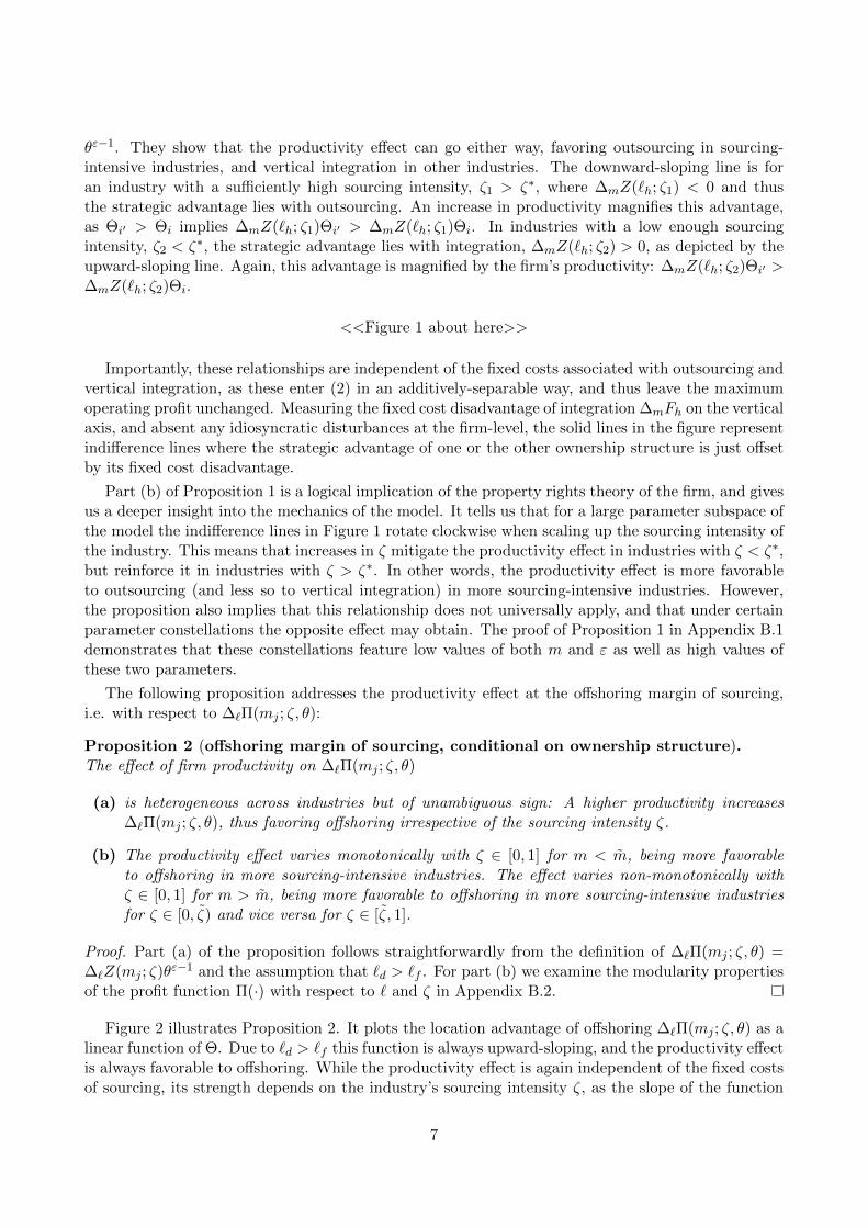
θε−1. They show that the productivity effect can go either way, favoring outsourcing in sourcing-intensive industries, and vertical integration in other industries. The downward-sloping line is foran industry with a sufficiently high sourcing intensity, ζ1 > ζ∗, where ∆mZ(`h; ζ1) < 0 and thusthe strategic advantage lies with outsourcing. An increase in productivity magnifies this advantage,as Θi′ > Θi implies ∆mZ(`h; ζ1)Θi′ > ∆mZ(`h; ζ1)Θi. In industries with a low enough sourcingintensity, ζ2 < ζ∗, the strategic advantage lies with integration, ∆mZ(`h; ζ2) > 0, as depicted by theupward-sloping line. Again, this advantage is magnified by the firm’s productivity: ∆mZ(`h; ζ2)Θi′ >∆mZ(`h; ζ2)Θi.

<<Figure 1 about here>>

Importantly, these relationships are independent of the fixed costs associated with outsourcing andvertical integration, as these enter (2) in an additively-separable way, and thus leave the maximumoperating profit unchanged. Measuring the fixed cost disadvantage of integration ∆mFh on the verticalaxis, and absent any idiosyncratic disturbances at the firm-level, the solid lines in the figure representindifference lines where the strategic advantage of one or the other ownership structure is just offsetby its fixed cost disadvantage.

Part (b) of Proposition 1 is a logical implication of the property rights theory of the firm, and givesus a deeper insight into the mechanics of the model. It tells us that for a large parameter subspace ofthe model the indifference lines in Figure 1 rotate clockwise when scaling up the sourcing intensity ofthe industry. This means that increases in ζ mitigate the productivity effect in industries with ζ < ζ∗,but reinforce it in industries with ζ > ζ∗. In other words, the productivity effect is more favorableto outsourcing (and less so to vertical integration) in more sourcing-intensive industries. However,the proposition also implies that this relationship does not universally apply, and that under certainparameter constellations the opposite effect may obtain. The proof of Proposition 1 in Appendix B.1demonstrates that these constellations feature low values of both m and ε as well as high values ofthese two parameters.

The following proposition addresses the productivity effect at the offshoring margin of sourcing,i.e. with respect to ∆`Π(mj ; ζ, θ):

Proposition 2 (offshoring margin of sourcing, conditional on ownership structure).The effect of firm productivity on ∆`Π(mj ; ζ, θ)

(a) is heterogeneous across industries but of unambiguous sign: A higher productivity increases∆`Π(mj ; ζ, θ), thus favoring offshoring irrespective of the sourcing intensity ζ.

(b) The productivity effect varies monotonically with ζ ∈ [0, 1] for m < m, being more favorableto offshoring in more sourcing-intensive industries. The effect varies non-monotonically withζ ∈ [0, 1] for m > m, being more favorable to offshoring in more sourcing-intensive industriesfor ζ ∈ [0, ζ) and vice versa for ζ ∈ [ζ, 1].

Proof. Part (a) of the proposition follows straightforwardly from the definition of ∆`Π(mj ; ζ, θ) =∆`Z(mj ; ζ)θε−1 and the assumption that `d > `f . For part (b) we examine the modularity propertiesof the profit function Π(·) with respect to ` and ζ in Appendix B.2.

Figure 2 illustrates Proposition 2. It plots the location advantage of offshoring ∆`Π(mj ; ζ, θ) as alinear function of Θ. Due to `d > `f this function is always upward-sloping, and the productivity effectis always favorable to offshoring. While the productivity effect is again independent of the fixed costsof sourcing, its strength depends on the industry’s sourcing intensity ζ, as the slope of the function

7

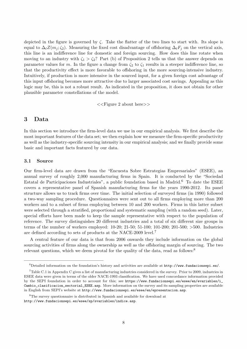
depicted in the figure is governed by ζ. Take the flatter of the two lines to start with. Its slope isequal to ∆`Z(mj ; ζ2). Measuring the fixed cost disadvantage of offshoring ∆`Fj on the vertical axis,this line is an indifference line for domestic and foreign sourcing. How does this line rotate whenmoving to an industry with ζ1 > ζ2? Part (b) of Proposition 2 tells us that the answer depends onparameter values for m. In the figure a change from ζ2 to ζ1 results in a steeper indifference line, sothat the productivity effect is more favorable to offshoring in the more sourcing-intensive industry.Intuitively, if production is more intensive in the sourced input, for a given foreign cost advantage ofthis input offshoring becomes more attractive due to larger associated cost savings. Appealing as thislogic may be, this is not a robust result. As indicated in the proposition, it does not obtain for otherplausible parameter constellations of the model.

<<Figure 2 about here>>

3 Data

In this section we introduce the firm-level data we use in our empirical analysis. We first describe themost important features of the data set; we then explain how we measure the firm-specific productivityas well as the industry-specific sourcing intensity in our empirical analysis; and we finally provide somebasic and important facts featured by our data.

3.1 Source

Our firm-level data are drawn from the “Encuesta Sobre Estrategias Empresariales” (ESEE), anannual survey of roughly 2,000 manufacturing firms in Spain. It is conducted by the “SociedadEstatal de Participaciones Industriales”, a public foundation based in Madrid.6 To date the ESEEcovers a representative panel of Spanish manufacturing firms for the years 1990-2012. Its panelstructure allows us to track firms over time. The initial selection of surveyed firms (in 1990) followeda two-way sampling procedure. Questionnaires were sent out to all firms employing more than 200workers and to a subset of firms employing between 10 and 200 workers. Firms in this latter subsetwere selected through a stratified, proportional and systematic sampling (with a random seed). Later,special efforts have been made to keep the sample representative with respect to the population ofreference. The survey distinguishes 20 different industries and a total of six different size groups interms of the number of workers employed: 10-20; 21-50; 51-100; 101-200; 201-500; >500. Industriesare defined according to sets of products at the NACE-2009 level.7

A central feature of our data is that from 2006 onwards they include information on the globalsourcing activities of firms along the ownership as well as the offshoring margin of sourcing. The tworelevant questions, which we deem pivotal for the quality of the data, read as follows:8

6Detailed information on the foundation’s history and activities are available at http://www.fundacionsepi.es/.

7Table C.1 in Appendix C gives a list of manufacturing industries considered in the survey. Prior to 2009, industries inESEE data were given in terms of the older NACE-1993 classification. We have used concordance information providedby the SEPI foundation in order to account for this; see https://www.fundacionsepi.es/esee/en/evariables/i_

Cambio_clasificacion_sectorial_ESEE.asp. More information on the survey and its sampling properties are availablein English from SEPI’s website at http://www.fundacionsepi.es/esee/en/epresentacion.asp.

8The survey questionnaire is distributed in Spanish and available for download athttp://www.fundacionsepi.es/esee/sp/svariables/indice.asp.

8

1. Of the total amount of purchases of goods and services that you incorporate (transform) in theproduction process, indicate − according to the type of supplier − the percentage that theserepresent in the total amount of purchases of your firm in [year].

(a) Spanish suppliers that belong to your group of companies or that participate in your firm’sjoint capital. [yes/no] / [if yes, then percentage rate]

(b) Other suppliers located in Spain. [yes/no]/[if yes, then percentage rate]

2. For the year [year], indicate whether you imported goods and services that you incorporate(transform) in the production process, and the percentage that theses imports − according to thetype of supplier − represent in the total value of your imports. [yes/no]

(a) From suppliers that belong to your group of companies and/or from foreign firms thatparticipate in your firm’s joint capital. [yes/no]/[if yes, then percentage rate]

(b) From other foreign firms. [yes/no]/[if yes, then percentage rate]

We use answers to question 1.(a) to construct a dummy variable for domestic integration (abbreviatedDI) that takes on the value one if the firm answers “yes”, and zero if it answers “no”. We proceedaccordingly for domestic outsourcing (question 1.(b): DO), foreign integration (question 2.(a): FI),and foreign outsourcing (question 2.(b): FO). We then characterize each observation (i.e. firm-year combination) through a tuple of variables Ω = 〈DI,DO,FI, FO〉. For example, we attachΩ = 〈1, 0, 1, 0〉 to any firm that reports to source inputs from both a foreign and a domestic integratedsupplier in a given year (but not from an independent supplier in Spain or abroad). It will sometimesprove convenient to refer to Ω as a set of tuples. An example is: Ω = 〈1, 0, 1, 0〉, 〈0, 0, 1, 0〉, whichwe write in shorthand as Ω = 〈·, 0, 1, 0〉.

3.2 Firm-specific productivity

A pivotal variable in our empirical analysis is a firm’s productivity level θ. We employ two measuresof firm productivity. In the main part of the paper we use labor productivity, defined as value addedover effective work-hours. Value added is given by the real total production value plus other operatingincome (i.e., income from rent and leasing, industrial property, commissions, and certain services),minus the real total expenditure on intermediate inputs and external services. To check the robustnessof the results obtained, we use a measure of total factor productivity (based on semi-parametricestimations of industry-specific production functions, as suggested by Olley & Pakes (1996)). Detailson this estimation can be found in Appendix C.

3.3 Industry-specific sourcing intensity

The key variable at the industry level is the sourcing intensity of production ζ. This variable is notdirectly observed. On a very fundamental level, ζ reflects the extent to which the input suppliers arebound to bear the costs of production, and 1 − ζ reflects the cost share borne by the headquarterfirms. What determines the extent of cost sharing between input suppliers and headquarter firms?Antras (2003) argues that the costs of physical capital are easier to share than the costs of laborinputs, and that headquarter firms primarily provide (or pre-finance) machinery and specialized toolsand equipment, or assist their suppliers in the acquisition of capital equipment and raw materials (as

9

reported in Dunning (1993, 455-456)).9 Therefore, in the logic of the AH model, the headquarterinput carries more weight in the production of capital-intensive goods than in the production oflabor-intensive goods. It has thus become common practice in empirical work to proxy 1 − ζ byan industry-specific measure of capital intensity; see Antras (2003), Yeaple (2006), Nunn & Trefler(2008), and Federico (2012). We proceed similarly in our empirical analysis, and use the (reversed)scale of industry-specific capital intensities to represent ζ (normalized to the unit interval [0, 1]). Theindustry-specific capital intensity is given by the “typical” capital intensity (the median value) weobserve in the industry over the period from 2000 to 2012.10 The industries Leather & Footwearand Textile & Wearing Apparel plausibly emerge with the most sourcing-intensive production. Theindustries Beverages and Ferrous Metals & Non-Ferrous Metals, in contrast, feature the least sourcing-intensive production.11

3.4 Basic facts

Figure 3 displays the evolution of firms engaged in different sourcing strategies. We define sourcingstrategies in a mutually inclusive way, so that a firm counts for more than one sourcing strategy ifit reports multiple ways of sourcing. We distinguish between domestic outsourcing (Ω = 〈·, 1, ·, ·〉),domestic integration (Ω = 〈1, ·, ·, ·〉), foreign outsourcing (Ω = 〈·, ·, ·, 1〉), and foreign integration(Ω = 〈·, ·, 1, ·〉).12 The figure shows pronounced differences in the fractions of firms choosing aparticular sourcing strategy. It also shows that these fractions remain roughly constant over time.Domestic outsourcing is almost universally used (roughly 90% of firms), followed by foreign outsourc-ing (30%), domestic integration (10%), and foreign integration (5%). Thus, as far as the relativeimportance of sourcing strategies is concerned, we find a pattern similar to those observed for otherindustrialized countries such as Japan (Tomiura, 2007) and Italy (Federico, 2010, 2012).13

<<Figure 3 about here>>

Figure 4 shows that the use of sourcing strategies strongly depends on firm size. The figure displaysthe fractions of firms engaged in different sourcing strategies in 2012, the most recent year availablein our data set. It does so separately for the six different firm size groups, with relative frequenciesindicated by bars. As firms employing 10 to 50 workers represent about 90% of all firms in Spanishmanufacturing, their use of sourcing strategies closely resembles the picture displayed in Figure 3.However, larger firms show a markedly stronger engagement in both foreign sourcing and verticalintegration. In particular, strategies of foreign as well as vertical integration are each used by morethan 40% of the very large firms (those with more than 500 employees). For foreign outsourcing thenumber is even higher, at more than 70%.

9Other references consistent with this idea and discussed in Antras (2003) are Milgrom & Roberts (1993), Aoki (1990,25), and Young et al. (1985).

10The capital intensity is defined as the real value sum of real estate, construction and equipment over the averagenumber of workers during the year. We employ sampling weights to correct for deviations from random sampling.

11Figure C.1 in Appendix C shows that firms in our sample are concentrated in industries with sourcing intensitiesabove 0.3.

12There is a fifth group which we call “non-sourcing” firms (Ω = 〈0, 0, 0, 0〉) since they report zero volumes for inputsourcing.

13We have also investigated the importance of different sourcing strategies in terms of the value of sourcing. First,we have computed the value shares for each sourcing strategy as firm averages. And secondly, we have computed thevalue shares at the industry level. In either case we find the same (ordinal) ranking of sourcing strategies as displayedin Figure 3.

10

<<Figure 4 about here>>

Figure 5 illustrates that firms using vertically integrated production relationships are strongly con-centrated in industries of low sourcing intensity (those producing beverages, certain metal products,and chemical products). Outsourcing relationships, in contrast, are considerably more important,relative to vertical integration, in sourcing-intensive industries (those producing leather & footwearor textiles). The between-industry differences we observe in the data are remarkable. In the industryLeather & Furniture, the industry with the highest sourcing intensity, the share of firms sourcinginputs intra-firm is almost zero. For Beverages, the industry with the lowest sourcing intensity, thisshare is 20%. Our findings for Spain resemble those found for the U.S. For instance, Figure 1 inAntras (2003) documents that the share of related-party imports in total U.S. imports is the higher,the higher the capital intensity of the industry. Figure 6 shows that firms engaging in offshoring(whether through outsourcing or vertical integration) are not equally distributed across industries.However, differences in the prevalence of offshoring firms between industries are difficult to explainwith the sourcing intensity of production: Figure 6 reveals no clear association between the twovariables. For example, in the industry Chemical & Pharmaceutical Products, almost 60% of firmsengage in offshoring. In the industry Mineral Products (Non-Metal Products), in contrast, the shareis around 15%, although the two industries are similarly sourcing-intensive (in the vicinity of 0.4).

<<Figures 5 and 6 about here>>

4 Empirical analysis

Our theoretical results call for a flexible empirical model that allows us to investigate the productivityeffect along the distribution of sourcing intensities. In this section, we first describe the empiricalmodel we use to estimate the effects at the ownership margin of sourcing, and present the results weobtain from this model; we then repeat the same exercise focusing on the offshoring margin of sourcing;and we finally describe the results of an extensive robustness analysis carried out to substantiate ourfindings.

4.1 The ownership margin of sourcing

Empirical model. Let firms be indexed by i = 1, . . . , I, and industries by s = 1, . . . , S. We use Isto denote the set of firms belonging to industry s. We index time by t and define

Λit,h(`h; ζs, θit) := ∆mΠ(`h; ζs, θit)−∆mFst,h + µit,h, i ∈ Is, (10)

as firm i’s total profit difference between vertical integration and outsourcing in location h = f, d attime t, where µit,h is a composite term summarizing all effects unrelated to the economic mechanismunderlying the AH model of sourcing. We assume that this term is the sum of a deterministic part,µit,h, and a stochastic part, µit,h, the latter representing unobserved heterogeneity at the firm-level.We want to allow for the fixed cost disadvantage of vertical integration to differ across industries, andto change through time:

∆mFst,h = ∆mFs,h + ∆mFt,h. (11)

We face a number of challenges when transforming (10) into an empirical model that can be estimatedwith our data. First, Λit,h(`h; ζs, θit) is a latent variable that is not observed by the econometrician.

11

In the estimation, we therefore revert to a binary variable, denoted by INTit,h, indicating the sign ofΛit,h(`h; ζs, θit), as revealed through the firm’s observed choice of ownership structure:

INTit,h =

1 if Λit,h(`h; ζs, θit) ≥ 0,0 otherwise.

Our data feature firms reporting multiple ways of sourcing, as we have seen in the previous section.Thus, we are facing fuzzy data, compared to the theoretical model where different ways of sourcingare mutually exclusive events. Our response to this challenge is to find and impose suitable samplerestrictions that generate an empirical decision model for the ownership margin of sourcing as framedin the AH model. We do so separately for the two locations of sourcing, constructing two disjointsamples, one of offshoring firms and one of domestically sourcing firms. These samples are denotedby sets of tuples Ωf and Ωd, to be defined below.

Secondly, there is heterogeneity at the industry-level and at the firm-level that determines the fixedcost difference ∆mFst,h and feeds into µit,h. Failing to account for this heterogeneity risks introducingan endogeneity bias into the estimation. We address this problem by extending the model to includean industry fixed effect γs,h, a year fixed effect γt,h, and a number of time-varying firm-specific covari-ates.14 The fixed effects capture the two fixed cost components, ∆mFs,h and ∆mFt,h, alongside othertime-invariant industry-specific parameters (such as skill intensity, R&D intensity, or external finan-cial dependence), and time trends common to all industries. The firm-specific variables included tocontrol for within-industry heterogeneity in dimensions other than productivity are: capital intensity,skill intensity and export volume.15

Finally, we must account for the complex nature of ∆mΠ(`h; ζs, θit) and allow for a flexible pro-ductivity effect along the distribution of sourcing intensities. We do so by employing a polynomialregression framework where firm productivity is interacted with a higher-order polynomial for theindustry-specific sourcing intensity. We stack the indeterminates of the polynomial into the columnvector ΓK

(ζs) = (ζ0s , ζ

1s , . . . , ζ

Ks

)′. The model we estimate for the ownership margin of sourcing thus

reads as follows:

Pr(INTit,h = 1|·) = Pr (Λit,h(`h; ζs, θit) ≥ 0)

= Pr(∆mΠ(`h; ζs, θit)−∆mFst,h + µit,h + µit,h ≥ 0

)= Pr

(λ · ΓK(ζs)× θit + γs,h + γt,h + β ·Xit ≥ −µit,h

)= G

(λ · ΓK(ζs)× θit + γs,h + γt,h + β ·Xit

), i ∈ Is,Ωit ∈ Ωh, (12)

where G is a cumulative distribution function implicitly defined by the distribution of µit,h, λ =(λ0, λ1, . . . , λK) are the parameters of interest, and Xit = (X1it, . . . , XLit)

′ is a column vector oftime-variant firm-specific control variables (along with a vector of coefficients β = (β1, . . . , βL) tobe estimated). Notice that in this equation the industry-specific effect γs,h absorbs the main (i.e.,non-interaction) effects of the polynomial for the industry’s sourcing intensity, and that Ωh representsthe sample either of offshoring or of domestically sourcing firms.

We assume that µit,h is uniformly distributed with E[µit,h|·] = 0, so that the polynomial regressionframework in (12) simplifies to a linear probability model (LPM):16

E[INTit,h|·] = Pr(INTit,h = 1|·) = λ · ΓK(ζs)× θit + γs,h + γt,h + β ·Xit, i ∈ Is,Ωit ∈ Ωh. (13)

14See Table C.3 in Appendix C for a definition of these variables.

15See Bernard et al. (2012) for a survey of these dimensions of firm heterogeneity, and Corcos et al. (2013) for relatedevidence.

16For the LPM to be consistent and unbiased, we must assume that[λ · ΓK(ζs)× θit + γs,h + γt,h + β ·Xit

]∈ [0, 1]

12

The restriction to observations that satisfy Ωit ∈ Ωh is crucial. Our aim is to identify the productivityeffect from a sample of firms that behave differently at the ownership margin of sourcing but identicallyotherwise. For foreign sourcing, h = f , we construct a sample of offshoring firms, similar to the onesstudied in Defever & Toubal (2013) and Corcos et al. (2013). In particular, we impose Ωf = 〈·, 1, ·, 1〉and define INTit,f to equal one if Ωit ∈ 〈·, 1, 1, 1〉, and zero if Ωit ∈ 〈·, 1, 0, 1〉. Hence, our LPMcompares offshoring firms that engage in vertical integration (FIit = 1 ∧ FOit = 1) with those thatdo not (FIit = 0 ∧ FOit = 1), discarding observations with DOit = 0, but allowing for both DIit = 0and DIit = 1.17

For h = d we construct a sample of domestically sourcing firms excluding all firms engaged in someform of offshoring. We impose Ωd = 〈·, 1, 0, 0〉 and define INTit,d to equal one if Ωit = 〈1, 1, 0, 0〉,and zero if Ωit = 〈0, 1, 0, 0〉. This is a comparison of domestically sourcing firms that choose verticalintegration (DIit = 1∧DOit = 1) with those that do not (DIit = 0∧DOit = 1). Importantly, becauseΩf and Ωd are disjoint sets, our empirical analysis involves two self-contained and independent testsof Proposition 1.

Results. We estimate Equation (13) separately on the samples Ωf and Ωd, using OLS. Statisticalinference is based on robust standard errors clustered by firm, i.e., we allow for arbitrary forms ofboth heteroskedasticity and autocorrelation. In view of Proposition 1, our primary interest lies withλ · ΓK(ζ), which is an estimate of the productivity effect ∂∆mΠ(`h; ζ, θ)/ ∂θ. For all degrees of thepolynomial ΓK(ζ) larger than zero, K > 0, this estimate is a function of the industry’s sourcingintensity ζ. In stressing a productivity effect that is heterogeneous across industries, Proposition 1clearly calls for K > 0. Indeed, part (b) of the proposition calls for K > 1, since this would allow fora non-monotonic relationship between the productivity effect and the sourcing intensity.

Figure 7 depicts the estimated polynomials using the sample of offshoring firms Ωf . Figure 8 doesthe same for the sample of domestically sourcing firms Ωd. In each case we present polynomials up toK = 5. The estimate for K = 0 gives us the average productivity effect across industries. A positiveestimate means that the likelihood of vertical integration is increasing in productivity, which is whatwe find with a significance level of 5 percent for both offshoring and domestically sourcing firms.These results corroborate our earlier findings of a “productivity premium” on vertical integrationover outsourcing (Kohler & Smolka, 2011, 2014).

Higher degree polynomials capture heterogeneity in the productivity effect across industries. Our

for all observations. We use the LPM instead of a non-linear probability model (such as the Probit model), becausethe interaction effect is not identified in a non-linear model with industry fixed effects. To see this, notice that in anon-linear model the interaction effect emerges as (dropping firm and industry indices):

∂2 Pr(INT = 1|·)∂θ∂ζ

= G′(·)×∂(λ · ΓK(ζ)

)∂ζ

+G′′(·)×

(∂(λ · ΓK(ζ)× θ

)∂ζ

+∂γ

∂ζ

)× λ · ΓK(ζ).

Since the industry fixed effect, γs,h in Equation (12), absorbs the main effects of the polynomials for the industry’ssourcing intensity, the derivative ∂γ/∂ζ is not identified (and neither, therefore, is the interaction effect).

17Unlike most of the literature, our data allow us to condition on, or control for, the firm’s domestic sourcing strategies.As for domestic outsourcing, we restrict the sample to observations with DOit = 1, since this strategy is adopted byvirtually all offshoring firms that we observe; see Figure 3. However, we have verified that our results do not changeif we allow for DOit = 0 and include the variable DOit as a control in the regression. As for domestic integration,we allow for both DIit = 1 and DIit = 0 (for reasons of sample size), but we have verified that our results are notdriven by the correlation between DIit and FIit. We have done so by including DIit as an explanatory variable in theregression, and by dropping either firms with DIit = 1 or firms with DIit = 0 from the sample. Another feature of ourdata is that a large majority of observations with FIit = 1 also exhibit FOit = 1 (87% in 2012), which leads us to dropobservations with FOit = 0. However, our results do not change in any significant way when keeping these observationsin the sample.

13

results attest to strong and significant heterogeneity, although the degree of heterogeneity is somewhatmore pronounced, and the R2-values consistently higher, for offshoring firms than for domesticallysourcing firms. The heterogeneity follows a clear pattern: gains in productivity tend to push firmstowards vertical integration in the lower range of the distribution of sourcing intensities, and towardsoutsourcing in the upper range of the distribution. Moreover, for an interior range of sourcing in-tensities (those around the knife-edge case of ζ∗ ≈ 0.7), this relationship is monotonic, whereby ahigher sourcing intensity tilts the effect of productivity away from vertical integration and towardsoutsourcing. Importantly, these results show up consistently across the two locations of sourcing,domestic and foreign, and hence provide strong empirical evidence for Proposition 1 and the coreeconomic mechanism featured in Antras & Helpman (2004).

<<Figures 7 and 8 about here>>

How are we to select among the models represented by different polynomials? Table 1 presents theresults of a formal statistical procedure of model selection. To gauge the relevance of the marginalpolynomial order introduced into the model, we test whether the estimate of λK is significantlydifferent from zero in each of the models K = 0, . . . , 5 (odd-numbered columns). To examine therelevance of quadratic, cubic, and higher-order polynomials, we perform a series of Wald tests (even-numbered columns). Based on this procedure, the preferred model among those depicted in Figure 7is K = 3.18 This specification supports Proposition 1, as it features a maximum for the productivityeffect at ζ ≈ 0.3, indicating non-monotonic adjustment at the lower end of the distribution of ζ,while revealing monotonic adjustment in the larger neighborhood of ζ∗ ≈ 0.7 where the productivityeffect is muted. This means that virtually all our data fall into the part of the distribution where theproductivity effect implies monotonic adjustment.19

Figure 8 displays the estimation results obtained for the sample of domestically sourcing firmsΩd. The figure portrays a picture of heterogeneity across industries that is very similar to what wehave found for offshoring firms above. However, the fit is not as good (judged by the R2-values) aswith foreign sourcing. Moreover, columns (3) and (4) of Table 1 reveal that the preferred polynomialis of first (instead of third) degree, with λ1 < 0 at the 5 percent significance level. This impliesmonotonicity of the productivity effect in the sourcing intensity, with productivity becoming evermore favorable to outsourcing as we move up along the distribution of sourcing intensities.

4.2 The offshoring margin of sourcing

Empirical model. We define firm i’s total profit difference between foreign and domestic sourcingunder ownership structure j = v, o at time t as

Λit,j(mj ; ζs, θit) := ∆`Π(mj ; ζs, θit)−∆`Fst,j + µit,j , i ∈ Is, (14)

where ∆`Fst,j is defined in analogy to ∆mFst,h in (11). Proceeding as before we specify the followingLPM for the ownership margin of sourcing:

E[FORit,j |·] = Pr(FORit,j = 1|·) = λ · ΓK(ζs)× θit + γs,j + γt,j + β ·Xit, i ∈ Is,Ωit ∈ Ωj , (15)

18This choice appears broadly consistent with the values of the Akaike Information Criterion (AIC) and the BayesianInformation Criterion (BIC) given in Figure 7. However, we prefer the above procedure over the AIC and BIC, becausethe latter contain no information about the absolute quality of the models considered.

19About 98 percent of the observations in our sample (and 19 out of 20 industries) feature ζ > 0.3, as indicated bythe vertical lines in the figures; see also the histogram in Figure C.1. The Beverages industry is thus the only industryto the left of the vertical lines (at ζ = 0).

14

where

FORit,j =

1 if Λit,j(mj ; ζs, θit) ≥ 0,0 otherwise.

We estimate this model on two disjoint samples, using Ωv to denote the sample of integrating firmsand Ωo to denote the sample of outsourcing firms. As for integrating firms, j = v, we employΩv = 〈1, 1, ., 0〉 and define FORit,v to take on the value one if Ωit = 〈1, 1, 1, 0〉 and zero otherwise.We thus compare integrating firms that choose offshoring with those that do not.20 This involves adrastic reduction in sample size (down to 701 observations and 288 firms in our benchmark estimates),so that the estimation results obtained must be interpreted with caution.21 As for outsourcing firms,j = o, we impose Ωo = 〈0, 1, 0, .〉 and set FORit,o = 1 if Ωit = 〈0, 1, 0, 1〉 and FORit,o = 0 otherwise.This involves a comparison between outsourcing firms engaged in offshoring and those that are not.

Results. Against the backdrop of Proposition 2, our primary interest lies with λ · ΓK(ζs), which isthe estimated effect of a change in firm productivity θ on ∆`Π(mj ; ζ, θ), the profit difference betweenoffshoring and domestic sourcing. As with the ownership margin of sourcing, the proposition stressesheterogeneity of the productivity effect across industries, but unlike Proposition 1 it holds that theproductivity effect is unambiguously positive, meaning that in all industries offshoring becomes moreattractive as the firm becomes more productive. Moreover, for a relatively large parameter subspace,the effect is monotonically increasing in the sourcing intensity over the entire interval ζ ∈ [0, 1]. Ifnon-monotonic, the productivity effect is rising in ζ for low values of ζ, and falling in ζ for high valuesof ζ.

<<Figures 9 and 10 about here>>

Figures 9 and 10 present the estimated polynomials for the samples Ωv and Ωo, respectively. Again,heterogeneity of the productivity effect calls for a polynomial of degree K > 0, but for completenesswe also present the average effect obtained by setting K = 0. For integrating firms, the averageproductivity effect is estimated with a positive sign, but not significantly different from zero, whereasfor outsourcing firms it is positive at the 1 percent significance level, and quantitatively important,with a margin of 6 percentage points. For both samples we observe significant heterogeneity, judgedby the estimated coefficients λ1 along with the corresponding significance levels in columns (5) and(7) of Table 1, and in both cases the Wald test leads us to select the first degree polynomial as ourpreferred model. Thus, while non-monotonicity is a distinct theoretical possibility, our estimationsuggests that it is not an empirically relevant phenomenon at the offshoring margin of sourcing.Moreover, the estimated productivity effect is positive for virtually all observations in the sample(ζ > 0.3), and λ1 > 0 means that the pattern of heterogeneity across industries is as expected frompart (b) of Proposition 1. Thus, productivity is the more favorable to offshoring, the higher thesourcing intensity, and this is true for both vertical integration and outsourcing.

4.3 Robustness analysis and extensions

Next, we investigate the robustness of our estimation results with respect to changes in the estimationsample as well as some modifications to, and extensions of, our baseline models. We describe eachstep of this analysis in turn and briefly summarize the main results obtained.

20As before, due to the large incidence of domestic outsourcing, we include observations with DOit = 1 and dropthose with DOit = 0. Keeping the latter group of observations in the sample and controlling for DOit in the regressiondoes not make a significant difference for the results we obtain.

21Although these concerns are corroborated by standard regression model diagnostics, in the interest of completenesswe report and comment on all estimation results in the text.

15

Richer specification of fixed costs. In the baseline models above, we assume that changes inthe fixed cost differences over time occur equally in all industries, and that firms active in the sameindustry face the same fixed cost disadvantage of integration and offshoring, respectively. Theseassumptions might be considered as being too strong to be plausible. Consider for example therecent improvements in transport and communication technology that have rendered offshoring moreattractive over the past decade. It is easy to imagine that some industries (e.g. those intensive incomplex capital goods) have benefitted more from this development than other industries. This leadsus to expect that changes in the fixed cost disadvantage of offshoring do not apply equally to allindustries, but are, instead, specific to the industry. Also, it seems likely that larger firms featurea different fixed cost profile than smaller firms. We allow for these possibilities by extending ourbaseline models to include industry-and-year fixed effects γst,b (rather than just industry fixed effectsγs,b and year fixed effects γt,b) as well as size group fixed effects γg,b, where g is an index for the sixfirm size groups and b = h, j. This extension gives rise to a more ambitious model where identificationcomes from between-firm variation in sourcing and productivity within size groups and industry-yearpairs. We report the results of this extension under Model (B) in Table 2 (for convenience restrictedto the case of K = 1). We may conclude that the core insights of our benchmark models easily survivein this extended model.

Region-specific effects. In the baseline models above, we do not distinguish between differentsourcing locations other than domestic versus foreign. This is due to data limitations, as the sourcingactivities are reported at the level of the firm, and not disaggregated by source country. Our firm-levelanalysis could thus suffer from omitted variables or aggregation bias. We address these concerns in twodifferent ways. First, as the data include the origin of firms’ imports, we augment the model for theownership margin to include dummy variables for the different import regions reported in our data.These are the European Union; Latin America; the rest of the OECD; and the rest of the world. Sucha model allows, for example, for a fixed cost disadvantage of integration that is specific to the regionfrom which the firm is sourcing its inputs, and thus reduces the risk of omitted variables bias. Model(C) in Table 2 reveals reassuring robustness also with respect to this modification. And secondly,in order to address a possible aggregration bias, we restrict the sample to firms receiving all theirimports from the European Union. This is a data-driven modification, as a sizable fraction of firmswith positive imports restrict their importing activities (and thus their sourcing) to the EuropeanUnion (about 38 percent of importers in the sample in 2012). Importers extending their activitiesbeyond the EU typically do so in addition to importing from the EU. The estimation results (notreported) do not indicate aggregation bias.

Other sources of firm-level heterogeneity. Our model uses two sources of variation in the datato identify the parameters in λ. The first is variation in productivity between firms within industries,and the second is variation in sourcing intensity between industries. This approach has the advantagethat the variation in the variables of interest is large. Under the given set of assumptions, the OLSestimator is asymptotically consistent. However, if there is an omitted firm-specific variable that iscorrelated with the other covariates, the estimates suffer from omitted variables bias due to unobservedheterogeneity. A more satisfying approach could therefore be to exploit the within-firm variation inthe data over time, along with the variation between industries. This would allow us to control forany time-invariant firm-specific variable that influences the firm’s decision in favor of one or the othersourcing strategy.22 However, because of the sample restrictions employed, there is very little within-

22One way to get rid of these variables is to within-transform the data and compute all variables relative to thefirm-specific mean value over time. The so-called within-group estimator (or fixed effects estimator) is asymptoticallyconsistent, independently of whether the (time-invariant) firm-specific variables are correlated with the other covariatesor not.

16

firm variation in the dependent variable that could be exploited for identification purposes.23 We musttherefore follow an alternative route to reduce the risk of an omitted variables bias. In particular, wetest for other sources of firm heterogeneity that are correlated with, respectively, the firm’s ownershipand offshoring decisions by augmenting the model to include further time-varying firm-level controls:age; employment; R&D intensity; service intensity; debt ratio; capacity utilization; and fixed effectsfor the type of good produced (consumption, intermediate, or undefined). A detailed description ofthese variables can be found in Appendix C; the results for the parameters of interest are reportedunder Model (D) in Table 2. Again, the outcome is a high degree of robustness.

Exclusion of foreign-owned firms. In our baseline estimations, we include firms irrespective ofwhether they are foreign owned or owned domestically. To the extent that firms in Spain are boundto source inputs from their foreign parental companies, the property rights model might not be anaccurate representation of the firm-supplier production relationship. To see whether our results areupheld in a sample of domestically owned firms, we drop observations where foreign investors ownmore than 50% of the Spanish firm’s joint capital. Model (E) in Table 2 yields reassuring robustnessresults also in this dimension.

Trimming estimator. A necessary condition for OLS to be consistent and unbiased in the LPM isthat the linear predictions of the model fall into the unit interval. We have checked for violations ofthis condition in all our benchmark models, and found sizable fractions of the data where the linearpredictions are negative. For example, approximately 11 percent of the data deliver such predictionsin each of the models for the ownership margin; see Figure C.2 in Appendix C.24 Hence, we havereason to believe that our estimates of λ are neither consistent nor unbiased. The results reported inHorrace & Oaxaca (2006), however, suggest that the problem can be addressed by using a “trimming”estimator which excludes the critical observations from the estimation sample. We have done so inup to three iterations and succeeded in gradually reducing the fraction of critical observations. Theresults reported under Models (F) to (H) in Table 2, if anything, strengthen the conclusions we havedrawn from our baseline models above.

Probit model. Another way to address the drawbacks of the LPM is to estimate a non-linear Probitmodel. In our case, this means that the function G in Equation (12) is the cumulative distributionfunction of the normal distribution. Although the interaction effect between the productivity and thesourcing intensity is not identified in such a model (as we have shown earlier in footnote 16), we canstill identify and consistently estimate the parameters in λ. We have done so for K = 1, and ourProbit estimates of λ0 and λ1 can serve as an indication of whether the LPM used for our baselinemodels suffers from severe misspecification. Overall, the results we obtain with the Probit estimatordo not indicate misspecification; see Model (I) in Table 2.

Outliers with respect to θ. To see if our estimation results are driven by productivity outliers inthe sample, we have re-estimated our baseline models excluding the most productive as well as theleast productive firms (top and bottom 1%) in each industry-year pair from the sample. We do notfind that they are; see Model (J) in Table 2.

Outliers with respect to ζ. The Beverages industry is by far the least sourcing-intensive industryin our sample (ζ = 0). The industry is more than twice as capital-intensive as the second mostcapital-intensive industry (Ferrous Metals & Non-Ferrous Metals).25 Excluding this industry from

23Although we use data for seven years (2006 to 2012), over that period the typical number of years in which weobserve a firm is three (with gaps).

24The problem seems less severe for modelling the offshoring margin based on Ωo, where less than 3 percent of thedata deliver predictions outside the unit interval.

25The logged capital intensities are 4.94 and 4.19 for the industries Beverages and Ferrous Metals & Non-Ferrous

17

the sample reinforces our interpretation of substantial heterogeneity in the productivity effect acrossindustries; see Model (K) in Table 2.

Alternative measure of productivity. In our baseline estimations, we use real value added overeffective work-hours as a measure of firm productivity. Alternatively, we use total factor productivity(TFP) in our estimations. We apply the Olley & Pakes (1996) estimation algorithm, henceforth calledOPA, in order to estimate industry-specific production functions. Against the benchmark of theseestimates, we recover each firm’s TFP level as a firm-specific, time-variant variable. More details onthe TFP estimation can be found in Appendix C. The results reported under Model (L) in Table2 reveal that using this alternative measure of productivity does not change the conclusions of ouranalysis.

Alternative measure of sourcing intensity. For our baseline estimations, we construct thesourcing intensity of production based on the median capital intensity of firms active in a particularindustry (over the period 2000-2012). This is our preferred measure as the median statistic is robustto outliers. Alternatively, we use the mean of capital intensity, to find that the results are upheld;see Model (M) in Table 2.

Sourcing shares as dependent variables. We have so far used the discrete choice framework tomodel the probability of a firm to choose the one or the other of two sourcing strategies. An alternativeview on the data is to look at the quantitative importance of the different sourcing strategies, measuredby the volume of input sourcing. This information is available in our data; see the survey questionspresented in Section 3.1. We exploit this variation in the data by using firm-specific relative sourcingvolumes as dependent variables in the estimation (rather than dummy variables). As for the ownershipmargin, we use the share of intra-firm sourcing in the total volume of sourcing (specific to the foreigneconomy, h = f , or the domestic economy, h = d). As for the offshoring margin, we use the share offoreign sourcing in the total volume of sourcing (specific to integrated suppliers, j = v, or outsourcedsuppliers, j = o). Overall, the estimation results we obtain for these models are largely consistentwith those from our baseline estimations; see Model (N) in Table 2.

Number of foreign affiliates. Although we cannot assign sourcing volumes reported by the firmto specific countries or transactions, we do have information on the number and location of thefirm’s foreign affiliates. This allows us to open up a further perspective on the ownership margin ofsourcing. From our theoretical analysis we can expect more productive firms to be more inclined tovertical integration (and thus have more foreign affiliates) in industries of low sourcing intensity, andconversely in industries of high sourcing intensity. Hence, we estimate the following model by OLS:

#Foreign-affiliatesit,f = λ0 · θit + λ1 · (ζs × θit) + γs,f + γt,f + β ·Xit + ξit,f , i ∈ Is,Ωit ∈ Ωf , (16)

where #Foreign-affiliatesit,f is the number of foreign affiliates of firm i in year t, and ξit,f is an errorterm with zero conditional mean. The results reported in Table 3 are consistent with the propertyrights theory of the firm.

Further industry interactions. We have so far focused on differences in the productivity effectacross the distribution of sourcing intensities. However, industries exhibit important differences alsoin other dimensions, and the productivity effect might also be responsive to these other differences.To see to what extent the interaction effects between the firm’s productivity and the industry’ssourcing intensity are driven by other industry characteristics, we augment the model to includeinteractions between firm productivity and a number of important industry variables: skill intensity;R&D intensity; service intensity; and external financial dependence (derived from Rajan & Zingales

Metals, respectively.

18

(1998)). All of these variables, except for skill intensity, are positively correlated with the sourcingintensity; see Table C.2 in Appendix C. The results reported in Tables 4 and 5 indicate that thesourcing intensity is the only industry characteristic that consistently and significantly determines theproductivity effect at both margins of sourcing. However, the results also suggest that productivityinteracts with other industry characteristics. For example, in the sample of offshoring firms, theskill intensity of an industry seems to co-determine the productivity effect: in more skill-intensiveindustries the productivity effect is more favorable to vertical integration. This result is consistentwith the empirical literature on intra-firm trade, where skill intensity and capital intensity have beenused interchangeably to proxy the importance of headquarter inputs at the industry-level.

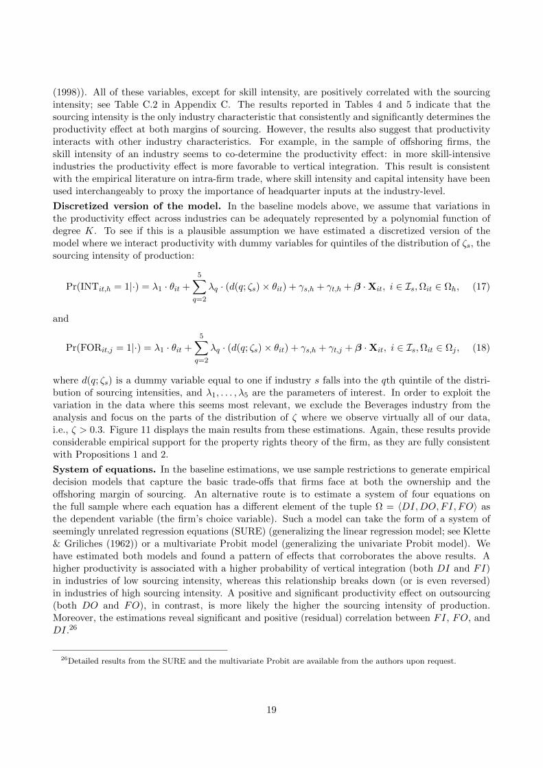
Discretized version of the model. In the baseline models above, we assume that variations inthe productivity effect across industries can be adequately represented by a polynomial function ofdegree K. To see if this is a plausible assumption we have estimated a discretized version of themodel where we interact productivity with dummy variables for quintiles of the distribution of ζs, thesourcing intensity of production:

Pr(INTit,h = 1|·) = λ1 · θit +

5∑q=2

λq · (d(q; ζs)× θit) + γs,h + γt,h + β ·Xit, i ∈ Is,Ωit ∈ Ωh, (17)

and

Pr(FORit,j = 1|·) = λ1 · θit +

5∑q=2

λq · (d(q; ζs)× θit) + γs,h + γt,j + β ·Xit, i ∈ Is,Ωit ∈ Ωj , (18)

where d(q; ζs) is a dummy variable equal to one if industry s falls into the qth quintile of the distri-bution of sourcing intensities, and λ1, . . . , λ5 are the parameters of interest. In order to exploit thevariation in the data where this seems most relevant, we exclude the Beverages industry from theanalysis and focus on the parts of the distribution of ζ where we observe virtually all of our data,i.e., ζ > 0.3. Figure 11 displays the main results from these estimations. Again, these results provideconsiderable empirical support for the property rights theory of the firm, as they are fully consistentwith Propositions 1 and 2.

System of equations. In the baseline estimations, we use sample restrictions to generate empiricaldecision models that capture the basic trade-offs that firms face at both the ownership and theoffshoring margin of sourcing. An alternative route is to estimate a system of four equations onthe full sample where each equation has a different element of the tuple Ω = 〈DI,DO,FI, FO〉 asthe dependent variable (the firm’s choice variable). Such a model can take the form of a system ofseemingly unrelated regression equations (SURE) (generalizing the linear regression model; see Klette& Griliches (1962)) or a multivariate Probit model (generalizing the univariate Probit model). Wehave estimated both models and found a pattern of effects that corroborates the above results. Ahigher productivity is associated with a higher probability of vertical integration (both DI and FI)in industries of low sourcing intensity, whereas this relationship breaks down (or is even reversed)in industries of high sourcing intensity. A positive and significant productivity effect on outsourcing(both DO and FO), in contrast, is more likely the higher the sourcing intensity of production.Moreover, the estimations reveal significant and positive (residual) correlation between FI, FO, andDI.26

26Detailed results from the SURE and the multivariate Probit are available from the authors upon request.

19

5 Conclusions

We draw two main conclusions from our analysis. First, we believe our results amount to considerableempirical support of the property rights model of global sourcing (Antras & Helpman, 2004). We haveshown that in this model firms respond very differently to gains in productivity if their technologiesrequire a differential mix of sourced inputs and headquarter inputs (the sourcing intensity of produc-tion). The model predicts distinct cross-industry patterns of firm-level responses at the ownership aswell as the offshoring margin of sourcing, and the empirical results we present in this paper clearlydemonstrate that these predictions find empirical support in Spanish firm-level data.

We have placed special emphasis on the ambiguity of the firm-level response at the ownershipmargin of sourcing, which is an important, yet overlooked theoretical implication of the propertyrights model. In particular, a higher productivity pushes firms towards vertical integration in thoseindustries where headquarter inputs play a major role in production, and towards outsourcing inindustries where they are less important. Moreover, we have demonstrated that the productivityeffect is potentially non-monotonic in the sourcing intensity at both the ownership and the offshoringmargin of sourcing. However, employing a suitably flexible estimation framework that allows us tocapture such non-monotonicity (if present), our empirical results point to a monotonic adjustment.At the ownership margin, we observe that a higher sourcing intensity renders the productivity effectmore favorable to outsourcing. At the offshoring margin, it makes the productivity effect work morestrongly in favor of offshoring.

Secondly, our results have interesting implications for scenarios of technological change and glob-alization. Suppose that due to technological progress firms headquartered in industrialized countriesexperience a uniform increase in their productivity. Our results imply that the share of multinationalfirms will consequently increase in those industries where headquarter inputs loom large (capital-intensive industries), and decrease where they are of relatively minor importance (labor-intensiveindustries). Because multinational firms are effectively transmitting technological knowledge acrossborders (Guadalupe et al., 2012), this has far-reaching implications for technology diffusion and in-dustrial structure in developing countries. In particular, what starts out as a neutral technologicalimprovement in industrialized countries will, through its effect at the ownership margin of sourcing,arrive as a non-neutral technological improvement in developing countries, favoring input suppliersin capital-intensive industries.

As regards offshoring, our results suggest, not surprisingly, that in this scenario of technologicalprogress firms in all industries will see offshoring become more attractive, as they are better ableto exploit the foreign cost advantage associated with offshoring. However, the effects will be feltdifferently across industries, thus accelerating job turnover in some industries more than in others.Importantly, the cross-industry differences that we find are explained by the sourcing intensity ofproduction, independently of the prevalence of routine and impersonal tasks (Blinder, 2009; Beckeret al., 2013; Ebenstein et al., 2014).

20

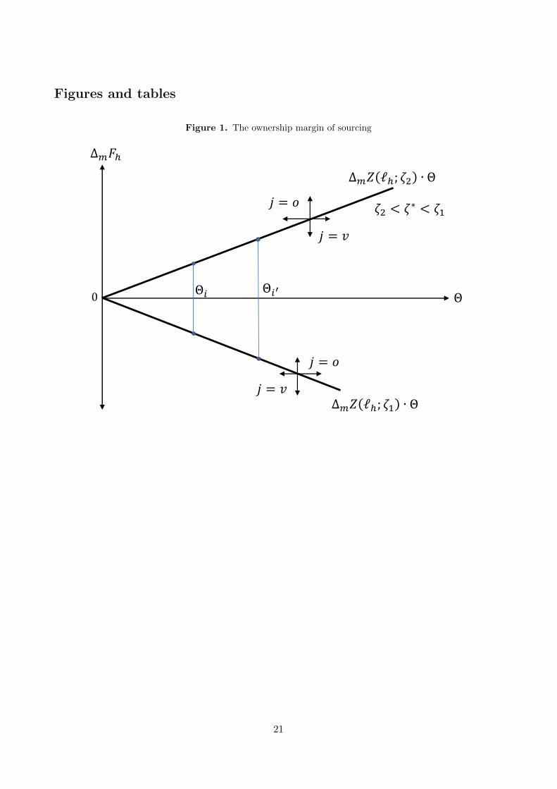
Figures and tables

Figure 1. The ownership margin of sourcing

Θ

Δ𝑚𝐹ℎ

𝑗 = 𝑜

𝑗 = 𝑣

𝑗 = 𝑣

𝑗 = 𝑜

0

𝜁2 < 𝜁∗ < 𝜁1

∆𝑚𝑍(ℓℎ; 𝜁1) ∙ Θ

∆𝑚𝑍(ℓℎ; 𝜁2) ∙ Θ

Θ𝑖

Θ𝑖′

21

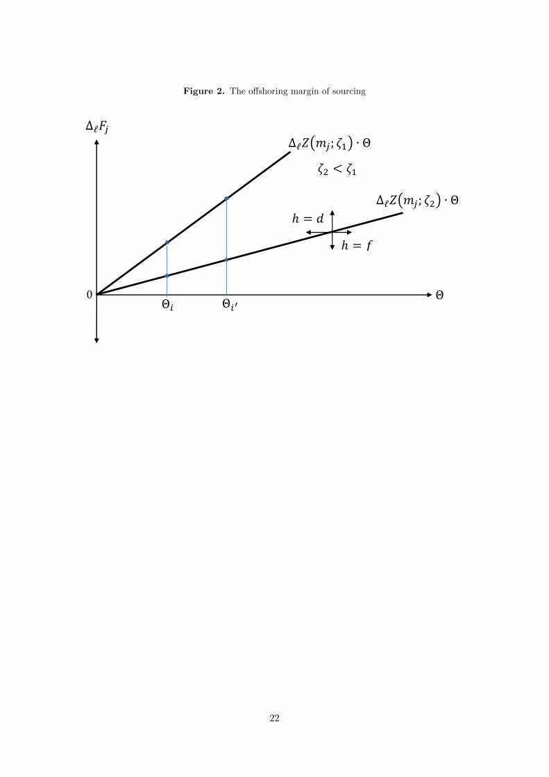
Figure 2. The offshoring margin of sourcing

Θ

Δℓ𝐹𝑗

∆ℓ𝑍(𝑚𝑗; 𝜁2) ∙ Θ

ℎ = 𝑑

ℎ = 𝑓

0 Θ𝑖

Θ𝑖′

∆ℓ𝑍(𝑚𝑗; 𝜁1) ∙ Θ

𝜁2 < 𝜁1

22

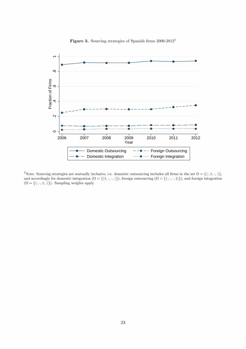
Figure 3. Sourcing strategies of Spanish firms 2006-2012†

0.2

.4.6

.81

Fra

ctio

n of

Firm

s

2006 2007 2008 2009 2010 2011 2012Year

Domestic Outsourcing Foreign OutsourcingDomestic Integration Foreign Integration

†Note: Sourcing strategies are mutually inclusive, i.e. domestic outsourcing includes all firms in the set Ω = 〈·, 1, ·, ·〉,and accordingly for domestic integration (Ω = 〈1, ·, ·, ·〉), foreign outsourcing (Ω = 〈·, ·, ·, 1〉), and foreign integration(Ω = 〈·, ·, 1, ·〉). Sampling weights apply.

23

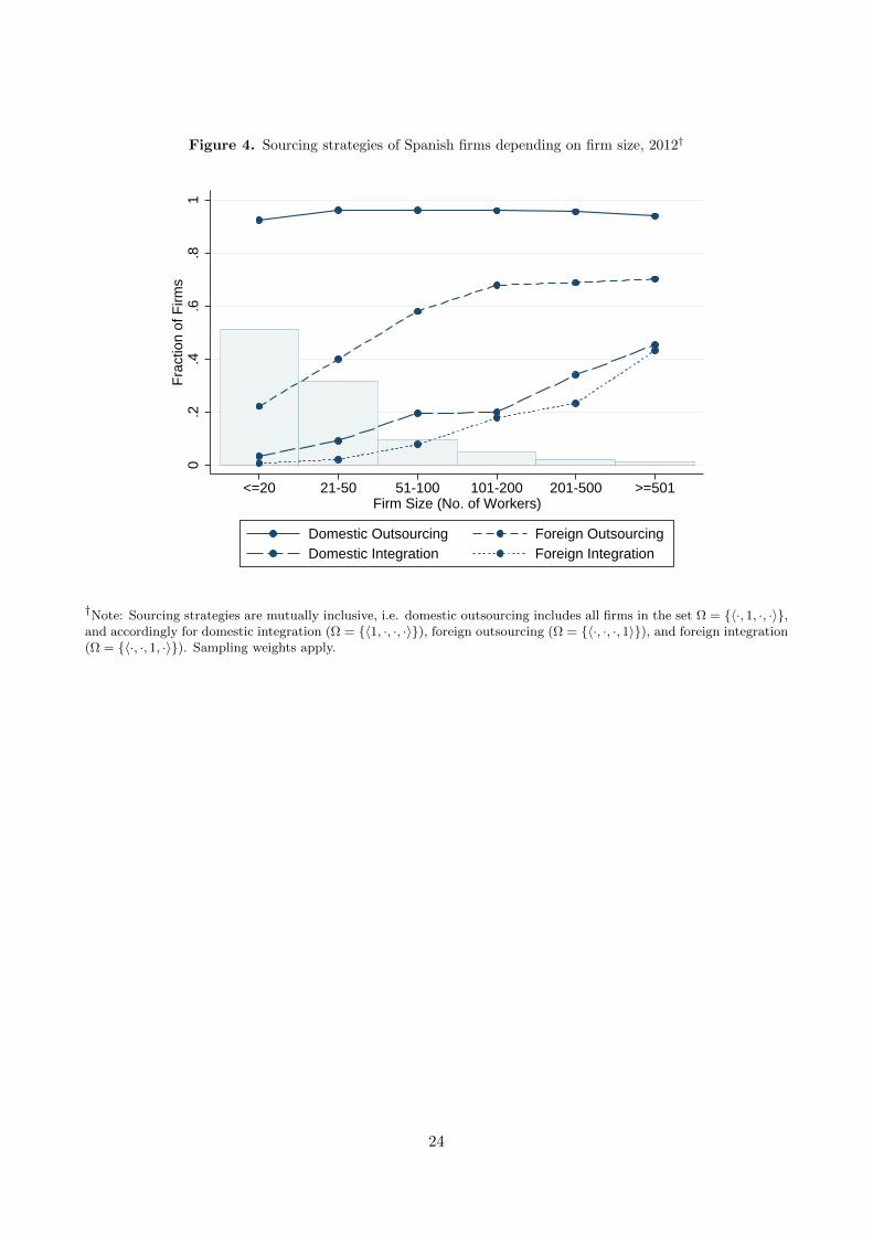
Figure 4. Sourcing strategies of Spanish firms depending on firm size, 2012†

0.2

.4.6

.81

Fra

ctio

n of

Firm

s

<=20 21-50 51-100 101-200 201-500 >=501Firm Size (No. of Workers)

Domestic Outsourcing Foreign OutsourcingDomestic Integration Foreign Integration

†Note: Sourcing strategies are mutually inclusive, i.e. domestic outsourcing includes all firms in the set Ω = 〈·, 1, ·, ·〉,and accordingly for domestic integration (Ω = 〈1, ·, ·, ·〉), foreign outsourcing (Ω = 〈·, ·, ·, 1〉), and foreign integration(Ω = 〈·, ·, 1, ·〉). Sampling weights apply.

24

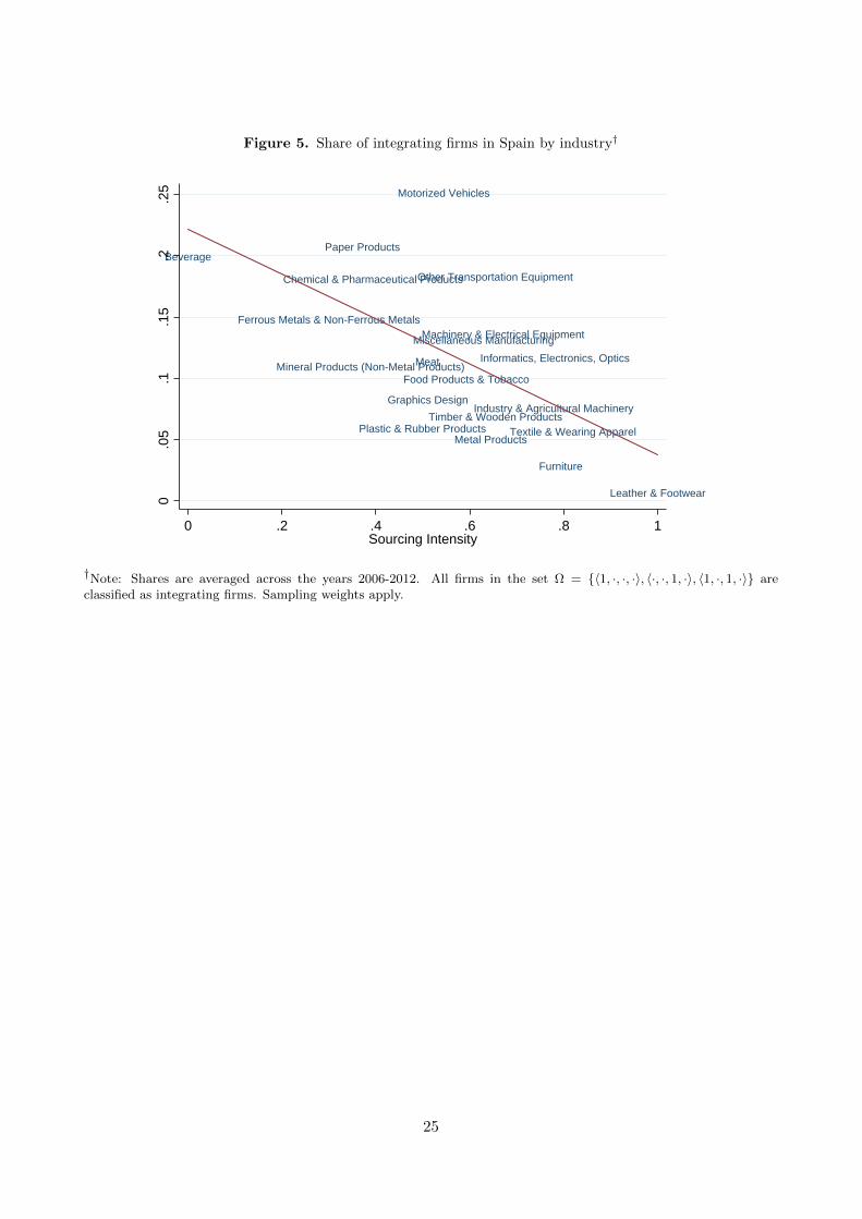
Figure 5. Share of integrating firms in Spain by industry†

Beverage

Ferrous Metals & Non-Ferrous Metals

Paper Products

Mineral Products (Non-Metal Products)

Chemical & Pharmaceutical Products

Plastic & Rubber Products

Meat

Graphics Design

Motorized Vehicles

Food Products & Tobacco

Miscellaneous Manufacturing

Metal Products

Other Transportation Equipment

Timber & Wooden Products

Machinery & Electrical Equipment

Industry & Agricultural Machinery

Informatics, Electronics, Optics

Furniture

Textile & Wearing Apparel

Leather & Footwear

0.0

5.1

.15

.2.2

5

0 .2 .4 .6 .8 1Sourcing Intensity

†Note: Shares are averaged across the years 2006-2012. All firms in the set Ω = 〈1, ·, ·, ·〉, 〈·, ·, 1, ·〉, 〈1, ·, 1, ·〉 areclassified as integrating firms. Sampling weights apply.

25

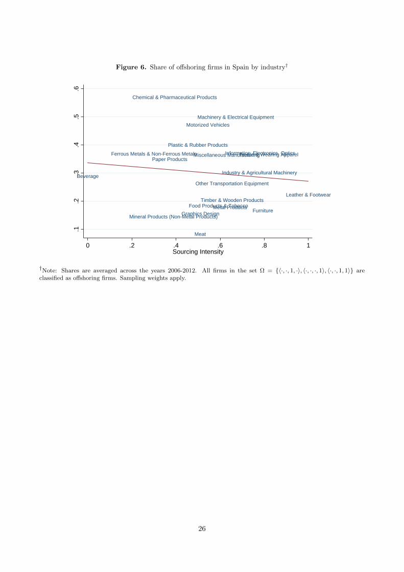
Figure 6. Share of offshoring firms in Spain by industry†

Beverage

Ferrous Metals & Non-Ferrous MetalsPaper Products

Mineral Products (Non-Metal Products)

Chemical & Pharmaceutical Products

Plastic & Rubber Products

Meat

Graphics Design

Motorized Vehicles

Food Products & Tobacco

Miscellaneous Manufacturing

Metal Products

Other Transportation Equipment

Timber & Wooden Products

Machinery & Electrical Equipment

Industry & Agricultural Machinery

Informatics, Electronics, Optics

Furniture

Textile & Wearing Apparel

Leather & Footwear

.1.2

.3.4

.5.6

0 .2 .4 .6 .8 1Sourcing Intensity

†Note: Shares are averaged across the years 2006-2012. All firms in the set Ω = 〈·, ·, 1, ·〉, 〈·, ·, ·, 1〉, 〈·, ·, 1, 1〉 areclassified as offshoring firms. Sampling weights apply.

26

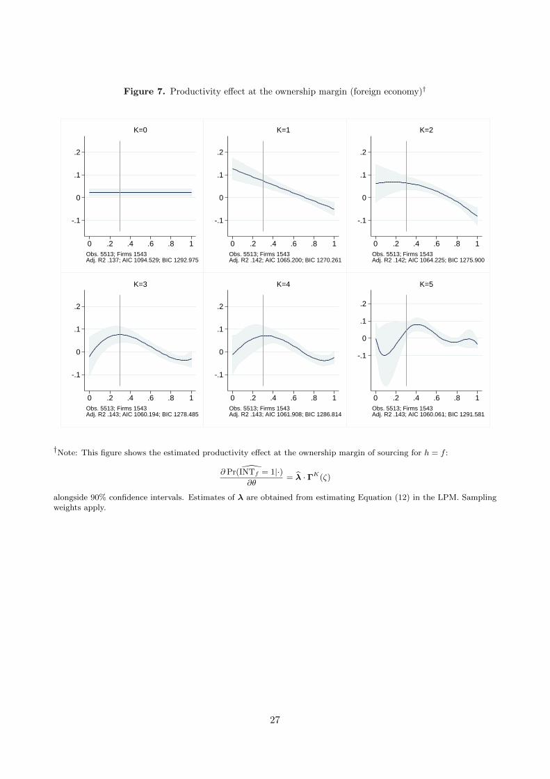
Figure 7. Productivity effect at the ownership margin (foreign economy)†

-.1

0

.1

.2

0 .2 .4 .6 .8 1Obs. 5513; Firms 1543Adj. R2 .137; AIC 1094.529; BIC 1292.975

K=0

-.1

0

.1

.2

0 .2 .4 .6 .8 1Obs. 5513; Firms 1543Adj. R2 .142; AIC 1065.200; BIC 1270.261

K=1

-.1

0

.1

.2

0 .2 .4 .6 .8 1Obs. 5513; Firms 1543Adj. R2 .142; AIC 1064.225; BIC 1275.900

K=2

-.1

0

.1

.2

0 .2 .4 .6 .8 1Obs. 5513; Firms 1543Adj. R2 .143; AIC 1060.194; BIC 1278.485

K=3

-.1

0

.1

.2

0 .2 .4 .6 .8 1Obs. 5513; Firms 1543Adj. R2 .143; AIC 1061.908; BIC 1286.814

K=4

-.1

0

.1

.2

0 .2 .4 .6 .8 1Obs. 5513; Firms 1543Adj. R2 .143; AIC 1060.061; BIC 1291.581

K=5

†Note: This figure shows the estimated productivity effect at the ownership margin of sourcing for h = f :

∂ Pr(INTf = 1|·)∂θ

= λ · ΓK(ζ)

alongside 90% confidence intervals. Estimates of λ are obtained from estimating Equation (12) in the LPM. Samplingweights apply.

27

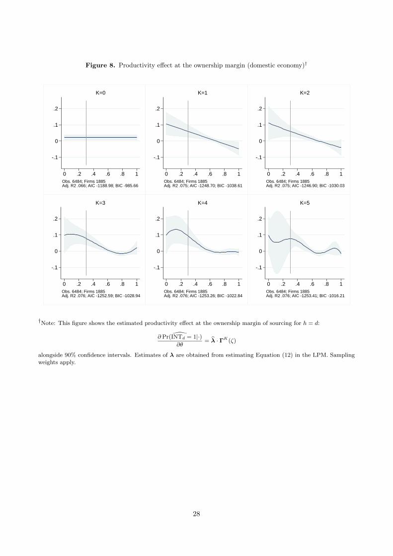
Figure 8. Productivity effect at the ownership margin (domestic economy)†

-.1

0

.1

.2

0 .2 .4 .6 .8 1Obs. 6484; Firms 1885Adj. R2 .066; AIC -1188.98; BIC -985.66

K=0

-.1

0

.1

.2

0 .2 .4 .6 .8 1Obs. 6484; Firms 1885Adj. R2 .075; AIC -1248.70; BIC -1038.61

K=1

-.1

0

.1

.2

0 .2 .4 .6 .8 1Obs. 6484; Firms 1885Adj. R2 .075; AIC -1246.90; BIC -1030.03

K=2

-.1

0

.1

.2

0 .2 .4 .6 .8 1Obs. 6484; Firms 1885Adj. R2 .076; AIC -1252.59; BIC -1028.94

K=3

-.1

0

.1

.2

0 .2 .4 .6 .8 1Obs. 6484; Firms 1885Adj. R2 .076; AIC -1253.26; BIC -1022.84

K=4

-.1

0

.1

.2

0 .2 .4 .6 .8 1Obs. 6484; Firms 1885Adj. R2 .076; AIC -1253.41; BIC -1016.21

K=5

†Note: This figure shows the estimated productivity effect at the ownership margin of sourcing for h = d:

∂ Pr(INTd = 1|·)∂θ

= λ · ΓK(ζ)

alongside 90% confidence intervals. Estimates of λ are obtained from estimating Equation (12) in the LPM. Samplingweights apply.

28

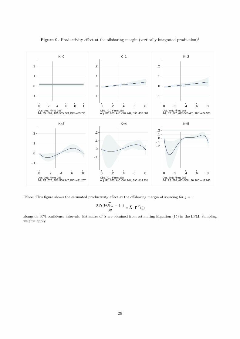
Figure 9. Productivity effect at the offshoring margin (vertically integrated production)†

-.1

0

.1

.2

0 .2 .4 .6 .8 1Obs. 701; Firms 288Adj. R2 .069; AIC -565.743; BIC -433.721

K=0

-.1

0

.1

.2

0 .2 .4 .6 .8Obs. 701; Firms 288Adj. R2 .073; AIC -567.444; BIC -430.869

K=1

-.1

0

.1

.2

0 .2 .4 .6 .8Obs. 701; Firms 288Adj. R2 .072; AIC -565.451; BIC -424.323

K=2

-.1

0

.1

.2

0 .2 .4 .6 .8Obs. 701; Firms 288Adj. R2 .075; AIC -566.947; BIC -421.267

K=3

-.1

0

.1

.2

0 .2 .4 .6 .8Obs. 701; Firms 288Adj. R2 .073; AIC -564.964; BIC -414.731

K=4

-.2-.1

0.1.2

0 .2 .4 .6 .8Obs. 701; Firms 288Adj. R2 .076; AIC -568.176; BIC -417.943

K=5

†Note: This figure shows the estimated productivity effect at the offshoring margin of sourcing for j = v:

∂ Pr(FORv = 1|·)∂θ

= λ · ΓK(ζ)

alongside 90% confidence intervals. Estimates of λ are obtained from estimating Equation (15) in the LPM. Samplingweights apply.

29

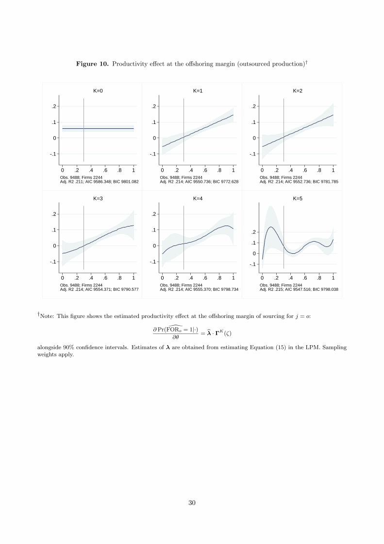
Figure 10. Productivity effect at the offshoring margin (outsourced production)†

-.1

0

.1

.2

0 .2 .4 .6 .8 1Obs. 9488; Firms 2244Adj. R2 .211; AIC 9586.348; BIC 9801.082

K=0

-.1

0

.1

.2

0 .2 .4 .6 .8 1Obs. 9488; Firms 2244Adj. R2 .214; AIC 9550.736; BIC 9772.628

K=1

-.1

0

.1

.2

0 .2 .4 .6 .8 1Obs. 9488; Firms 2244Adj. R2 .214; AIC 9552.736; BIC 9781.785

K=2

-.1

0

.1

.2

0 .2 .4 .6 .8 1Obs. 9488; Firms 2244Adj. R2 .214; AIC 9554.371; BIC 9790.577

K=3

-.1

0

.1

.2

0 .2 .4 .6 .8 1Obs. 9488; Firms 2244Adj. R2 .214; AIC 9555.370; BIC 9798.734

K=4

-.1

0

.1

.2

0 .2 .4 .6 .8 1Obs. 9488; Firms 2244Adj. R2 .215; AIC 9547.516; BIC 9798.038

K=5

†Note: This figure shows the estimated productivity effect at the offshoring margin of sourcing for j = o:

∂ Pr(FORo = 1|·)∂θ

= λ · ΓK(ζ)

alongside 90% confidence intervals. Estimates of λ are obtained from estimating Equation (15) in the LPM. Samplingweights apply.

30

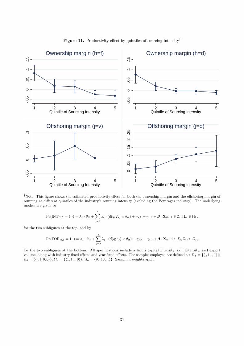
Figure 11. Productivity effect by quintiles of sourcing intensity†

-.0

50

.05

.1.1

5

1 2 3 4 5Quintile of Sourcing Intensity

Ownership margin (h=f)

-.0

50

.05

.1.1

5

1 2 3 4 5Quintile of Sourcing Intensity

Ownership margin (h=d)

-.0

50

.05

.1

1 2 3 4 5Quintile of Sourcing Intensity

Offshoring margin (j=v)0

.05

.1.1

5.2

.25

1 2 3 4 5Quintile of Sourcing Intensity

Offshoring margin (j=o)

†Note: This figure shows the estimated productivity effect for both the ownership margin and the offshoring margin ofsourcing at different quintiles of the industry’s sourcing intensity (excluding the Beverages industry). The underlyingmodels are given by

Pr(INTit,h = 1|·) = λ1 · θit +

5∑q=2

λq · (d(q; ζs)× θit) + γs,h + γt,h + β ·Xit, i ∈ Is,Ωit ∈ Ωh,

for the two subfigures at the top, and by

Pr(FORit,j = 1|·) = λ1 · θit +

5∑q=2

λq · (d(q; ζs)× θit) + γs,h + γt,j + β ·Xit, i ∈ Is,Ωit ∈ Ωj ,

for the two subfigures at the bottom. All specifications include a firm’s capital intensity, skill intensity, and exportvolume, along with industry fixed effects and year fixed effects. The samples employed are defined as: Ωf = 〈·, 1, ·, 1〉;Ωd = 〈·, 1, 0, 0〉; Ωv = 〈1, 1, ., 0〉; Ωo = 〈0, 1, 0, .〉. Sampling weights apply.

31

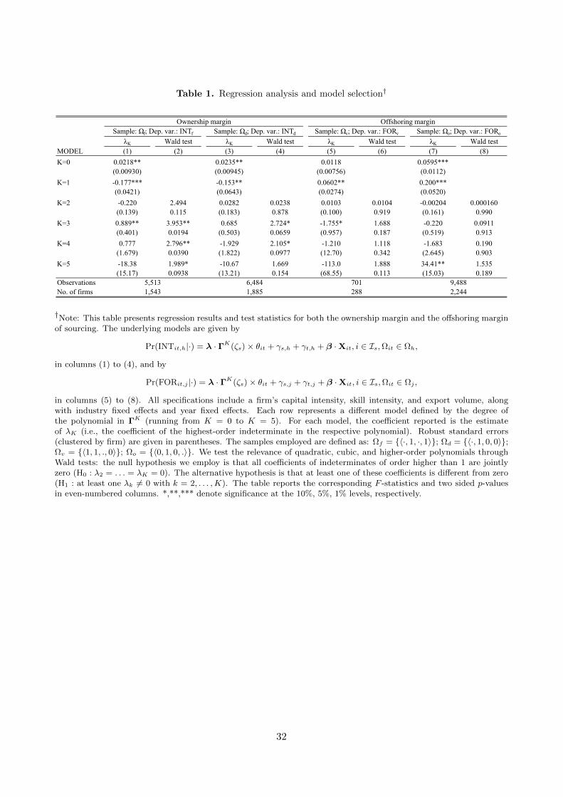
Table 1. Regression analysis and model selection†

λK Wald test λK Wald test λK Wald test λK Wald testMODEL (1) (2) (3) (4) (5) (6) (7) (8)

K=0 0.0218** 0.0235** 0.0118 0.0595***(0.00930) (0.00945) (0.00756) (0.0112)

K=1 -0.177*** -0.153** 0.0602** 0.200***(0.0421) (0.0643) (0.0274) (0.0520)

K=2 -0.220 2.494 0.0282 0.0238 0.0103 0.0104 -0.00204 0.000160(0.139) 0.115 (0.183) 0.878 (0.100) 0.919 (0.161) 0.990

K=3 0.889** 3.953** 0.685 2.724* -1.755* 1.688 -0.220 0.0911(0.401) 0.0194 (0.503) 0.0659 (0.957) 0.187 (0.519) 0.913

K=4 0.777 2.796** -1.929 2.105* -1.210 1.118 -1.683 0.190(1.679) 0.0390 (1.822) 0.0977 (12.70) 0.342 (2.645) 0.903

K=5 -18.38 1.989* -10.67 1.669 -113.0 1.888 34.41** 1.535(15.17) 0.0938 (13.21) 0.154 (68.55) 0.113 (15.03) 0.189

ObservationsNo. of firms

Sample: Ωf; Dep. var.: INTf Sample: Ωd; Dep. var.: INTd Sample: Ωo; Dep. var.: FORo

Ownership margin Offshoring marginSample: Ωv; Dep. var.: FORv

5,5131,543

701288

9,4882,244

6,4841,885

†Note: This table presents regression results and test statistics for both the ownership margin and the offshoring marginof sourcing. The underlying models are given by

Pr(INTit,h|·) = λ · ΓK(ζs)× θit + γs,h + γt,h + β ·Xit, i ∈ Is,Ωit ∈ Ωh,

in columns (1) to (4), and by

Pr(FORit,j |·) = λ · ΓK(ζs)× θit + γs,j + γt,j + β ·Xit, i ∈ Is,Ωit ∈ Ωj ,

in columns (5) to (8). All specifications include a firm’s capital intensity, skill intensity, and export volume, alongwith industry fixed effects and year fixed effects. Each row represents a different model defined by the degree ofthe polynomial in ΓK (running from K = 0 to K = 5). For each model, the coefficient reported is the estimateof λK (i.e., the coefficient of the highest-order indeterminate in the respective polynomial). Robust standard errors(clustered by firm) are given in parentheses. The samples employed are defined as: Ωf = 〈·, 1, ·, 1〉; Ωd = 〈·, 1, 0, 0〉;Ωv = 〈1, 1, ., 0〉; Ωo = 〈0, 1, 0, .〉. We test the relevance of quadratic, cubic, and higher-order polynomials throughWald tests: the null hypothesis we employ is that all coefficients of indeterminates of order higher than 1 are jointlyzero (H0 : λ2 = . . . = λK = 0). The alternative hypothesis is that at least one of these coefficients is different from zero(H1 : at least one λk 6= 0 with k = 2, . . . ,K). The table reports the corresponding F -statistics and two sided p-valuesin even-numbered columns. *,**,*** denote significance at the 10%, 5%, 1% levels, respectively.

32

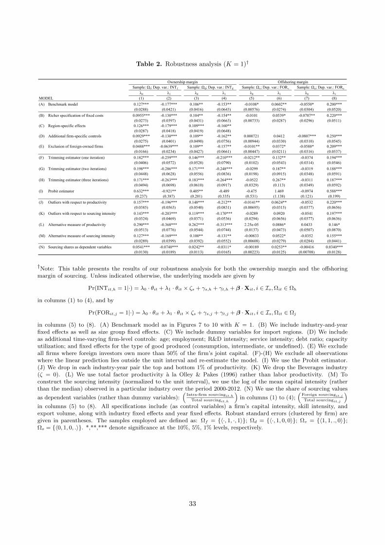
Table 2. Robustness analysis (K = 1)†

λ0 λ1 λ0 λ1 λ0 λ1 λ0 λ1

MODEL (1) (2) (3) (4) (5) (6) (7) (8)

(A) Benchmark model 0.127*** -0.177*** 0.106** -0.153** -0.0108* 0.0602** -0.0550* 0.200***(0.0288) (0.0421) (0.0416) (0.0643) (0.00576) (0.0274) (0.0304) (0.0520)

(B) Richer specification of fixed costs 0.0955*** -0.130*** 0.104** -0.154** -0.0101 0.0539* -0.0707** 0.220***(0.0273) (0.0397) (0.0431) (0.0663) (0.00733) (0.0287) (0.0296) (0.0511)

(C) Region-specific effects 0.126*** -0.179*** 0.109*** -0.160**(0.0287) (0.0418) (0.0419) (0.0648)

(D) Additional firm-specific controls 0.0929*** -0.130*** 0.109** -0.162** 0.000721 0.0412 -0.0807*** 0.250***(0.0275) (0.0401) (0.0490) (0.0756) (0.00944) (0.0330) (0.0310) (0.0545)

(E) Exclusion of foreign-owned firms 0.0488*** -0.0639*** 0.109** -0.157** -0.0101** 0.0372* -0.0588* 0.209***(0.0166) (0.0234) (0.0427) (0.0661) (0.00447) (0.0211) (0.0316) (0.0537)

(F) Trimming estimator (one iteration) 0.182*** -0.259*** 0.146*** -0.210*** -0.0212** 0.132** -0.0374 0.194***(0.0406) (0.0572) (0.0528) (0.0790) (0.0102) (0.0543) (0.0314) (0.0546)

(G) Trimming estimator (two iterations) 0.198*** -0.286*** 0.171*** -0.248*** -0.0299 0.187** -0.0319 0.188***(0.0448) (0.0628) (0.0556) (0.0836) (0.0198) (0.0915) (0.0348) (0.0591)

(H) Trimming estimator (three iterations) 0.171*** -0.263*** 0.183*** -0.264*** -0.0522 0.267** -0.0311 0.187***(0.0494) (0.0698) (0.0610) (0.0917) (0.0329) (0.113) (0.0349) (0.0592)

(I) Probit estimator 0.632*** -0.921** 0.405** -0.489 -0.475 1.469 -0.0974 0.588***(0.237) (0.387) (0.201) (0.335) (0.531) (1.138) (0.121) (0.199)

(J) Outliers with respect to productivity 0.157*** -0.196*** 0.148*** -0.212** -0.0141** 0.0624** -0.0532 0.220***(0.0385) (0.0563) (0.0540) (0.0831) (0.00695) (0.0315) (0.0377) (0.0656)

(K) Outliers with respect to sourcing intensity 0.143*** -0.203*** 0.119*** -0.170*** -0.0289 0.0920 -0.0541 0.197***(0.0324) (0.0469) (0.0371) (0.0536) (0.0294) (0.0656) (0.0377) (0.0636)

(L) Alternative measure of productivity 0.290*** -0.368*** 0.262*** -0.313*** 2.25e-05 0.0886* 0.0433 0.146*(0.0513) (0.0776) (0.0544) (0.0744) (0.0137) (0.0473) (0.0507) (0.0870)

(M) Alternative measure of sourcing intensity 0.127*** -0.169*** 0.100** -0.131** -0.00833 0.0522* -0.0352 0.155***(0.0289) (0.0399) (0.0392) (0.0552) (0.00608) (0.0279) (0.0284) (0.0441)

(N) Sourcing shares as dependent variables 0.0541*** -0.0740*** 0.0242** -0.0311* -0.00189 0.0253** -0.00416 0.0340***(0.0130) (0.0189) (0.0113) (0.0165) (0.00223) (0.0125) (0.00708) (0.0128)

Ownership margin Offshoring marginSample: Ωf; Dep. var.: INTf Sample: Ωd; Dep. var.: INTd Sample: Ωv; Dep. var.: FORv Sample: Ωo; Dep. var.: FORo

†Note: This table presents the results of our robustness analysis for both the ownership margin and the offshoringmargin of sourcing. Unless indicated otherwise, the underlying models are given by

Pr(INTit,h = 1|·) = λ0 · θit + λ1 · θit × ζs + γs,h + γt,h + β ·Xit, i ∈ Is,Ωit ∈ Ωh

in columns (1) to (4), and by

Pr(FORit,j = 1|·) = λ0 · θit + λ1 · θit × ζs + γs,j + γt,j + β ·Xit, i ∈ Is,Ωit ∈ Ωj

in columns (5) to (8). (A) Benchmark model as in Figures 7 to 10 with K = 1. (B) We include industry-and-yearfixed effects as well as size group fixed effects. (C) We include dummy variables for import regions. (D) We includeas additional time-varying firm-level controls: age; employment; R&D intensity; service intensity; debt ratio; capacityutilization; and fixed effects for the type of good produced (consumption, intermediate, or undefined). (E) We excludeall firms where foreign investors own more than 50% of the firm’s joint capital. (F)-(H) We exclude all observationswhere the linear prediction lies outside the unit interval and re-estimate the model. (I) We use the Probit estimator.(J) We drop in each industry-year pair the top and bottom 1% of productivity. (K) We drop the Beverages industry(ζ = 0). (L) We use total factor productivity a la Olley & Pakes (1996) rather than labor productivity. (M) Toconstruct the sourcing intensity (normalized to the unit interval), we use the log of the mean capital intensity (ratherthan the median) observed in a particular industry over the period 2000-2012. (N) We use the share of sourcing values

as dependent variables (rather than dummy variables):(

Intra-firm sourcingit,h

Total sourcingit,h

)in columns (1) to (4);

(Foreign sourcingit,j

Total sourcingit,j

)in columns (5) to (8). All specifications include (as control variables) a firm’s capital intensity, skill intensity, andexport volume, along with industry fixed effects and year fixed effects. Robust standard errors (clustered by firm) aregiven in parentheses. The samples employed are defined as: Ωf = 〈·, 1, ·, 1〉; Ωd = 〈·, 1, 0, 0〉; Ωv = 〈1, 1, ., 0〉;Ωo = 〈0, 1, 0, .〉. *,**,*** denote significance at the 10%, 5%, 1% levels, respectively.

33

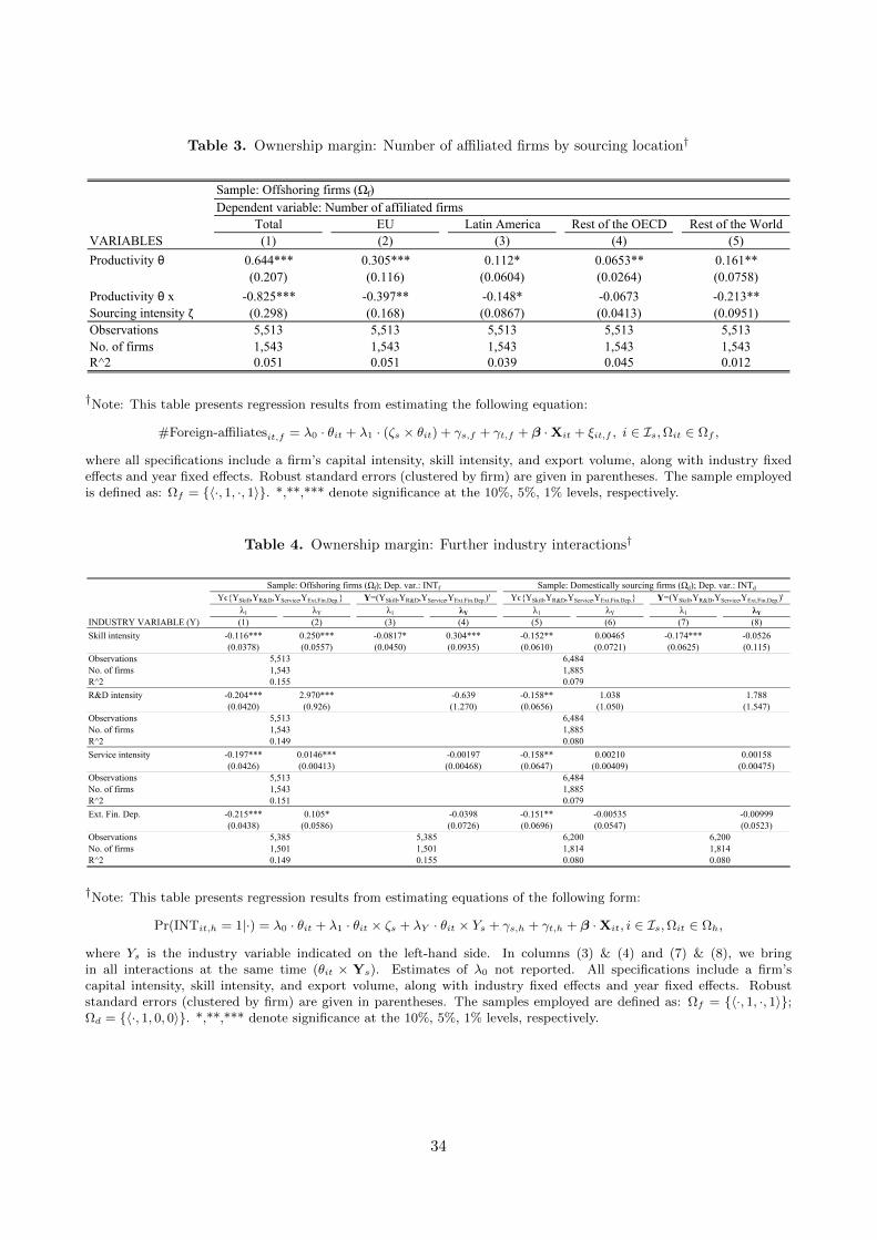
Table 3. Ownership margin: Number of affiliated firms by sourcing location†

Total EU Latin America Rest of the OECD Rest of the WorldVARIABLES (1) (2) (3) (4) (5)

Productivity θ 0.644*** 0.305*** 0.112* 0.0653** 0.161**(0.207) (0.116) (0.0604) (0.0264) (0.0758)

Productivity θ x -0.825*** -0.397** -0.148* -0.0673 -0.213**Sourcing intensity ζ (0.298) (0.168) (0.0867) (0.0413) (0.0951)Observations 5,513 5,513 5,513 5,513 5,513No. of firms 1,543 1,543 1,543 1,543 1,543R^2 0.051 0.051 0.039 0.045 0.012

Sample: Offshoring firms (Ωf)Dependent variable: Number of affiliated firms

†Note: This table presents regression results from estimating the following equation:

#Foreign-affiliatesit,f = λ0 · θit + λ1 · (ζs × θit) + γs,f + γt,f + β ·Xit + ξit,f , i ∈ Is,Ωit ∈ Ωf ,

where all specifications include a firm’s capital intensity, skill intensity, and export volume, along with industry fixedeffects and year fixed effects. Robust standard errors (clustered by firm) are given in parentheses. The sample employedis defined as: Ωf = 〈·, 1, ·, 1〉. *,**,*** denote significance at the 10%, 5%, 1% levels, respectively.

Table 4. Ownership margin: Further industry interactions†

λ1 λY λ1 λY λ1 λY λ1 λYINDUSTRY VARIABLE (Y) (1) (2) (3) (4) (5) (6) (7) (8)

Skill intensity -0.116*** 0.250*** -0.0817* 0.304*** -0.152** 0.00465 -0.174*** -0.0526(0.0378) (0.0557) (0.0450) (0.0935) (0.0610) (0.0721) (0.0625) (0.115)

ObservationsNo. of firmsR^2

R&D intensity -0.204*** 2.970*** -0.639 -0.158** 1.038 1.788(0.0420) (0.926) (1.270) (0.0656) (1.050) (1.547)

ObservationsNo. of firmsR^2

Service intensity -0.197*** 0.0146*** -0.00197 -0.158** 0.00210 0.00158(0.0426) (0.00413) (0.00468) (0.0647) (0.00409) (0.00475)

ObservationsNo. of firmsR^2

Ext. Fin. Dep. -0.215*** 0.105* -0.0398 -0.151** -0.00535 -0.00999(0.0438) (0.0586) (0.0726) (0.0696) (0.0547) (0.0523)

ObservationsNo. of firmsR^2 0.149

6,2001,8140.0800.155

Sample: Offshoring firms (Ωf); Dep. var.: INTf Sample: Domestically sourcing firms (Ωd); Dep. var.: INTd

YϵYSkill,YR&D,YService,YExt.Fin.Dep. Y=(YSkill,YR&D,YService,YExt.Fin.Dep.)' YϵYSkill,YR&D,YService,YExt.Fin.Dep. Y=(YSkill,YR&D,YService,YExt.Fin.Dep.)'

0.155

5,3851,501

1,5430.149

5,5131,5430.151

5,3851,501

6,4841,8850.079

5,513 6,484

5,5131,543

1,8850.080

6,4841,8850.079

6,2001,8140.080

†Note: This table presents regression results from estimating equations of the following form:

Pr(INTit,h = 1|·) = λ0 · θit + λ1 · θit × ζs + λY · θit × Ys + γs,h + γt,h + β ·Xit, i ∈ Is,Ωit ∈ Ωh,

where Ys is the industry variable indicated on the left-hand side. In columns (3) & (4) and (7) & (8), we bringin all interactions at the same time (θit × Ys). Estimates of λ0 not reported. All specifications include a firm’scapital intensity, skill intensity, and export volume, along with industry fixed effects and year fixed effects. Robuststandard errors (clustered by firm) are given in parentheses. The samples employed are defined as: Ωf = 〈·, 1, ·, 1〉;Ωd = 〈·, 1, 0, 0〉. *,**,*** denote significance at the 10%, 5%, 1% levels, respectively.

34

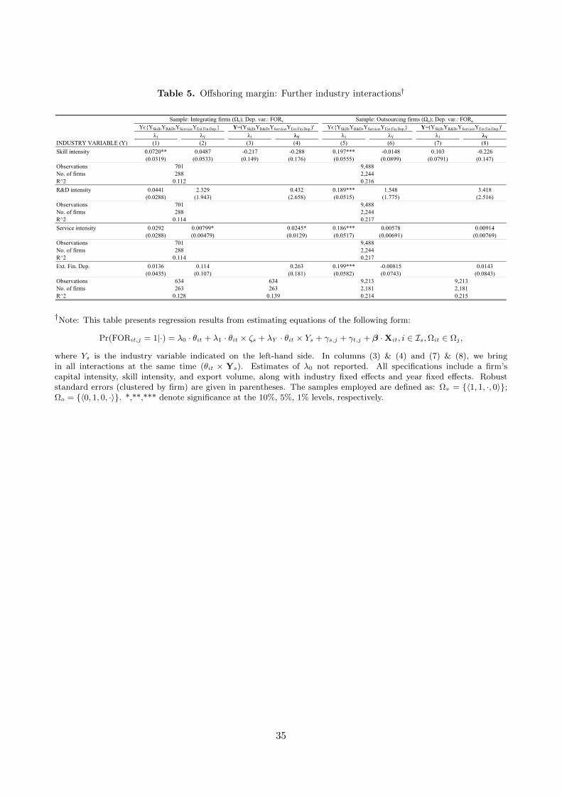
Table 5. Offshoring margin: Further industry interactions†

λ1 λY λ1 λY λ1 λY λ1 λYINDUSTRY VARIABLE (Y) (1) (2) (3) (4) (5) (6) (7) (8)

Skill intensity 0.0720** 0.0487 -0.217 -0.288 0.197*** -0.0148 0.103 -0.226(0.0319) (0.0533) (0.149) (0.176) (0.0555) (0.0899) (0.0791) (0.147)

ObservationsNo. of firmsR^2

R&D intensity 0.0441 2.329 0.432 0.189*** 1.548 3.418(0.0288) (1.943) (2.658) (0.0515) (1.775) (2.516)

ObservationsNo. of firmsR^2

Service intensity 0.0292 0.00799* 0.0245* 0.186*** 0.00578 0.00914(0.0288) (0.00479) (0.0129) (0.0517) (0.00691) (0.00769)

ObservationsNo. of firmsR^2

Ext. Fin. Dep. 0.0136 0.114 0.263 0.199*** -0.00815 0.0143(0.0435) (0.107) (0.181) (0.0582) (0.0743) (0.0843)

ObservationsNo. of firmsR^2

701288

0.112

Sample: Integrating firms (Ωv); Dep. var.: FORv Sample: Outsourcing firms (Ωo); Dep. var.: FORo

YϵYSkill,YR&D,YService,YExt.Fin.Dep. Y=(YSkill,YR&D,YService,YExt.Fin.Dep.)' YϵYSkill,YR&D,YService,YExt.Fin.Dep. Y=(YSkill,YR&D,YService,YExt.Fin.Dep.)'

9,4882,2440.216

0.114

634263

0.128

701288

0.114

701288

634263

0.139

9,2132,1810.214 0.215

9,4882,2440.217

9,2132,181

9,4882,2440.217

†Note: This table presents regression results from estimating equations of the following form:

Pr(FORit,j = 1|·) = λ0 · θit + λ1 · θit × ζs + λY · θit × Ys + γs,j + γt,j + β ·Xit, i ∈ Is,Ωit ∈ Ωj ,

where Ys is the industry variable indicated on the left-hand side. In columns (3) & (4) and (7) & (8), we bringin all interactions at the same time (θit × Ys). Estimates of λ0 not reported. All specifications include a firm’scapital intensity, skill intensity, and export volume, along with industry fixed effects and year fixed effects. Robuststandard errors (clustered by firm) are given in parentheses. The samples employed are defined as: Ωv = 〈1, 1, ·, 0〉;Ωo = 〈0, 1, 0, ·〉. *,**,*** denote significance at the 10%, 5%, 1% levels, respectively.

35

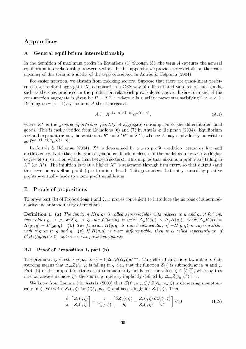
Appendices

A General equilibrium interrelationship

In the definition of maximum profits in Equations (1) through (5), the term A captures the generalequilibrium interrelationship between sectors. In this appendix we provide more details on the exactmeaning of this term in a model of the type considered in Antras & Helpman (2004).

For easier notation, we abstain from indexing sectors. Suppose that there are quasi-linear prefer-ences over sectoral aggregates X, composed in a CES way of differentiated varieties of final goods,such as the ones produced in the production relationship considered above. Inverse demand of theconsumption aggregate is given by P = Xκ−1, where κ is a utility parameter satisfying 0 < κ < 1.Defining α := (ε− 1)/ε, the term A then emerges as

A := X∗(κ−α)/(1−α)αα/(1−α), (A.1)

where X∗ is the general equilibrium quantity of aggregate consumption of the differentiated finalgoods. This is easily verified from Equations (6) and (7) in Antras & Helpman (2004). Equilibriumsectoral expenditure may be written as R∗ := X∗P ∗ = X∗κ, whence A may equivalently be writtenas R∗ε+(1−ε)/καα/(1−α).

In Antras & Helpman (2004), X∗ is determined by a zero profit condition, assuming free andcostless entry. Note that this type of general equilibrium closure of the model assumes α > κ (higherdegree of substitution within than between sectors). This implies that maximum profits are falling inX∗ (or R∗). The intuition is that a higher X∗ is generated through firm entry, so that output (andthus revenue as well as profits) per firm is reduced. This guarantees that entry caused by positiveprofits eventually leads to a zero profit equilibrium.

B Proofs of propositions

To prove part (b) of Propositions 1 and 2, it proves convenient to introduce the notions of supermod-ularity and submodularity of functions.

Definition 1. (a) The function H(g, q) is called supermodular with respect to g and q, if for anytwo values g1 > g0 and q1 > q0 the following is true: ∆gH(q1) > ∆gH(q0), where ∆gH(q) :=H(g1, q) − H(g0, q). (b) The function H(g, q) is called submodular, if −H(g, q) is supermodularwith respect to g and q. (c) If H(g, q) is twice differentiable, then it is called supermodular, if∂2H/(∂g∂q) > 0, and vice versa for submodularity.

B.1 Proof of Proposition 1, part (b)

The productivity effect is equal to (ε − 1)∆mZ(`h; ζ)θε−2. This effect being more favorable to out-sourcing means that ∆mZ(`h; ζ) is falling in ζ, i.e., that the function Z(·) is submodular in m and ζ.Part (b) of the proposition states that submodularity holds true for values ζ ∈

[ζ, ζ], whereby this

interval always includes ζ∗, the sourcing intensity implicitly defined by ∆mZ(`h; ζ∗) = 0.

We know from Lemma 3 in Antras (2003) that Z(`h,mv; ζ)/Z(`h,mo; ζ) is decreasing monotoni-cally in ζ. We write Zv(·, ζ) for Z(`h,mv; ζ) and accordingly for Zo(·, ζ). Then

∂

∂ζ

[Zv(·, ζ)

Zo(·, ζ)

]=

1

Zo(·, ζ)

[∂Zv(·, ζ)

∂ζ− Zv(·, ζ)

Zo(·, ζ)

∂Zo(·, ζ)

∂ζ

]< 0 (B.2)

36

By definition, we have Zv(·,ζ∗)Zo(·,ζ∗) = 1, whence

∂Zv(·, ζ∗)∂ζ

− ∂Zo(·, ζ∗)∂ζ

< 0. (B.3)

The definition of ∆mZ(`h; ζ) then implies that

∂

∂ζ∆mZ(`h; ζ∗) =

[∂Zv(·, ζ∗)

∂ζ− ∂Zo(·, ζ∗)

∂ζ

]< 0. (B.4)

This proves that in the neighborhood of ζ∗ the function ∆mZ(`h; ζ) is unambiguously falling in ζ. Inother words, the interval

[ζ, ζ]

includes ζ∗.

Proposition 1(b) also states that the interval[ζ, ζ]

is large for plausible parameter constellations. Inview of definition 1, we invoke twice differentiability of the maximum profit function, which allows us

to prove this by investigating ∂2Z(·,m)∂m∂ζ = ∂2Z(·,ζ)

∂ζ∂m , this latter equality following from Young’s theorem.

The interval[ζ, ζ]

is defined such that for ζ ∈[ζ, ζ]

the cross-derivative ∂2Z∂ζ∂m is negative. It proves

convenient to work with lnZ, using the decomposition

∂2Z

∂ζ∂m= Z

∂2 lnZ

∂ζ∂m+∂ lnZ

∂ζ

∂Z

∂m. (B.5)

Remember that

Z = AzC, (B.6)

with z = 1− ε− 1

ε[m(1− ζ) + (1−m)ζ] (B.7)

and C =[m1−ζ [`(1−m)]ζ

]ε−1. (B.8)

To explore the interval[ζ, ζ], we proceed in three steps. First, we show that ∂2 lnZ

∂ζ∂m is always

negative. Second, we show that each of the two terms ∂ lnZ∂ζ and ∂Z

∂m is ambiguous, that ∂ lnZ∂ζ

∂Z∂m is

ambiguous as well, and that positive values of ∂ lnZ∂ζ

∂Z∂m potentially dominate the sign of (B.5). We

show that this holds true in particular for large values of m. This will prove that submodularity ofZ(·) in m and ζ does not obtain throughout the entire parameter space of the model. The third step

explores the sign of ∂2Z∂ζ∂m by means of numerical simulations, in order to see how the values of ζ and

ζ vary over the entire range of values for m ∈ [0, 1] as well as with different values of ε.

The first term on the right-hand side of (B.5) may be written as

∂ lnZ

∂ζ=∂ ln z

∂ζ+∂ lnC

∂ζ. (B.9)

In view of (B.6), note that the partial equilibrium nature of our analysis allows us to set ∂ lnA∂ζ equal

to zero. We have

∂ lnC

∂ζ= (ε− 1)

∂

∂ζ[(1− ζ) lnm+ ζ [ln `+ ln(1−m)]] (B.10)

= (ε− 1) [ln `+ ln(1−m)− lnm] . (B.11)

∂ ln z

∂ζ=

1

z

∂z

∂ζ=

1

z

[−ε− 1

ε(1−m−m)

](B.12)

=ε− 1

ε

2m− 1

z. (B.13)

37

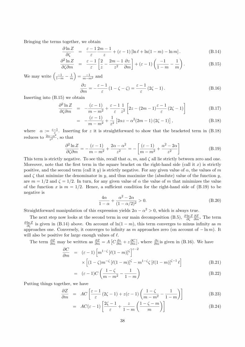
Bringing the terms together, we obtain

∂ lnZ

∂ζ=

ε− 1

ε

2m− 1

z+ (ε− 1) [ln `+ ln(1−m)− lnm] . (B.14)

∂2 lnZ

∂ζ∂m=

ε− 1

ε

[2

z− 2m− 1

z2∂z

∂m

]+ (ε− 1)

(−1

1−m− 1

m

). (B.15)

We may write(−11−m −

1m

)= −1

m−m2 and

∂z

∂m= −ε− 1

ε(1− ζ − ζ) =

ε− 1

ε(2ζ − 1) . (B.16)

Inserting into (B.15) we obtain

∂2 lnZ

∂ζ∂m= − (ε− 1)

m−m2+ε− 1

ε

1

z2

[2z − (2m− 1)

ε− 1

ε(2ζ − 1)

](B.17)

= − (ε− 1)

m−m2+

1

z2[2αz − α2(2m− 1) (2ζ − 1)

], (B.18)

where α := ε−1ε . Inserting for z it is straightforward to show that the bracketed term in (B.18)

reduces to 2α−α2

z2 , so that

∂2 lnZ

∂ζ∂m= − (ε− 1)

m−m2+

2α− α2

z2= −

[(ε− 1)

m−m2+α2 − 2α

z2

](B.19)

This term is strictly negative. To see this, recall that α, m, and ζ all lie strictly between zero and one.Moreover, note that the first term in the square bracket on the right-hand side (call it x) is strictlypositive, and the second term (call it y) is strictly negative. For any given value of α, the values of mand ζ that minimize the denominator in y, and thus maximize the (absolute) value of the function y,are m = 1/2 and ζ = 1/2. In turn, for any given value of α the value of m that minimizes the valueof the function x is m = 1/2. Hence, a sufficient condition for the right-hand side of (B.19) to benegative is

4α

1− α+

α2 − 2α

(1− α/2)2> 0. (B.20)

Straightforward manipulation of this expression yields 2α− α2 > 0, which is always true.

The next step now looks at the second term in our main decomposition (B.5), ∂ lnZ∂ζ

∂Z∂m . The term

∂ lnZ∂ζ is given in (B.14) above. On account of ln(1 −m), this term converges to minus infinity as m

approaches one. Conversely, it converges to infinity as m approaches zero (on account of − lnm). Itwill also be positive for large enough values of `.

The term ∂Z∂m may be written as ∂Z

∂m = A[C ∂z∂m + z ∂C∂m

], where ∂z

∂m is given in (B.16). We have

∂C

∂m= (ε− 1)

[m1−ζ [`(1−m)]ζ

]ε−2×[(1− ζ)m−ζ [`(1−m)]ζ −m1−ζζ [`(1−m)]ζ−1 `

](B.21)

= (ε− 1)C

(1− ζm−m2

− 1

1−m

)(B.22)

Putting things together, we have

∂Z

∂m= AC

[ε− 1

ε(2ζ − 1) + z(ε− 1)

(1− ζm−m2

− 1

1−m

)](B.23)

= AC(ε− 1)

[2ζ − 1

ε+

z

1−m

(1− ζ −m

m

)](B.24)

38

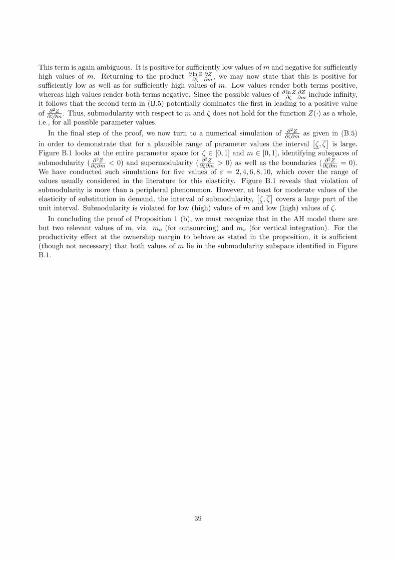
This term is again ambiguous. It is positive for sufficiently low values of m and negative for sufficientlyhigh values of m. Returning to the product ∂ lnZ

∂ζ∂Z∂m , we may now state that this is positive for

sufficiently low as well as for sufficiently high values of m. Low values render both terms positive,whereas high values render both terms negative. Since the possible values of ∂ lnZ

∂ζ∂Z∂m include infinity,

it follows that the second term in (B.5) potentially dominates the first in leading to a positive value

of ∂2Z∂ζ∂m . Thus, submodularity with respect to m and ζ does not hold for the function Z(·) as a whole,

i.e., for all possible parameter values.

In the final step of the proof, we now turn to a numerical simulation of ∂2Z∂ζ∂m as given in (B.5)

in order to demonstrate that for a plausible range of parameter values the interval[ζ, ζ]

is large.Figure B.1 looks at the entire parameter space for ζ ∈ [0, 1] and m ∈ [0, 1], identifying subspaces of

submodularity ( ∂2Z∂ζ∂m < 0) and supermodularity ( ∂2Z

∂ζ∂m > 0) as well as the boundaries ( ∂2Z∂ζ∂m = 0).

We have conducted such simulations for five values of ε = 2, 4, 6, 8, 10, which cover the range ofvalues usually considered in the literature for this elasticity. Figure B.1 reveals that violation ofsubmodularity is more than a peripheral phenomenon. However, at least for moderate values of theelasticity of substitution in demand, the interval of submodularity,

[ζ, ζ]

covers a large part of theunit interval. Submodularity is violated for low (high) values of m and low (high) values of ζ.

In concluding the proof of Proposition 1 (b), we must recognize that in the AH model there arebut two relevant values of m, viz. mo (for outsourcing) and mv (for vertical integration). For theproductivity effect at the ownership margin to behave as stated in the proposition, it is sufficient(though not necessary) that both values of m lie in the submodularity subspace identified in FigureB.1.

39

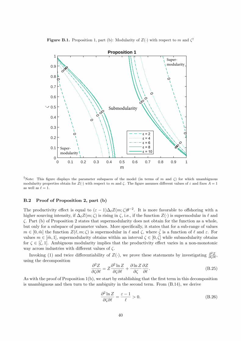
Figure B.1. Proposition 1, part (b): Modularity of Z(·) with respect to m and ζ†

0

0 0

0

0

0

0

0

0

0

0

0

0

0

0

0

0

0

0

0

Proposition 1

m0 0.1 0.2 0.3 0.4 0.5 0.6 0.7 0.8 0.9 1

1

0

0.1

0.2

0.3

0.4

0.5

0.6

0.7

0.8

0.9

1

Submodularity

Super-modularity

Super-modularity

†Note: This figure displays the parameter subspaces of the model (in terms of m and ζ) for which unambiguousmodularity properties obtain for Z(·) with respect to m and ζ. The figure assumes different values of ε and fixes A = 1as well as ` = 1.

B.2 Proof of Proposition 2, part (b)

The productivity effect is equal to (ε − 1)∆`Z(m; ζ)θ−2. It is more favorable to offshoring with ahigher sourcing intensity, if ∆`Z(m; ζ) is rising in ζ, i.e., if the function Z(·) is supermodular in ` andζ. Part (b) of Proposition 2 states that supermodularity does not obtain for the function as a whole,but only for a subspace of parameter values. More specifically, it states that for a sub-range of valuesm ∈ [0, m] the function Z(`,m; ζ) is supermodular in ` and ζ, where ζ is a function of ` and ε. Forvalues m ∈ [m, 1], supermodularity obtains within an interval ζ ∈ [0, ζ] while submodularity obtainsfor ζ ∈ [ζ, 1]. Ambiguous modularity implies that the productivity effect varies in a non-monotonicway across industries with different values of ζ.

Invoking (1) and twice differentiability of Z(·), we prove these statements by investigating ∂2Z∂ζ∂` ,

using the decomposition∂2Z

∂ζ∂`= Z

∂2 lnZ

∂ζ∂`+∂ lnZ

∂ζ

∂Z

∂`. (B.25)

As with the proof of Proposition 1(b), we start by establishing that the first term in this decompositionis unambiguous and then turn to the ambiguity in the second term. From (B.14), we derive

∂2 lnZ

∂ζ∂`=ε− 1

`> 0. (B.26)

40

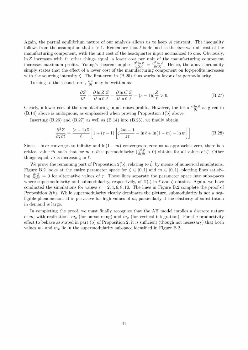
Again, the partial equilibrium nature of our analysis allows us to keep A constant. The inequalityfollows from the assumption that ε > 1. Remember that ` is defined as the inverse unit cost of themanufacturing component, with the unit cost of the headquarter input normalized to one. Obviously,lnZ increases with `: other things equal, a lower cost per unit of the manufacturing componentincreases maximum profits. Young’s theorem implies ∂2 lnZ

∂ζ∂` = ∂2 lnZ∂`∂ζ . Hence, the above inequality

simply states that the effect of a lower cost of the manufacturing component on log-profits increaseswith the sourcing intensity ζ. The first term in (B.25) thus works in favor of supermodularity.

Turning to the second term, ∂Z∂` may be written as

∂Z

∂`=∂ lnZ

∂ ln `

Z

`=∂ lnC

∂ ln `

Z

`= (ε− 1)ζ

Z

`> 0. (B.27)

Clearly, a lower cost of the manufacturing input raises profits. However, the term ∂ lnZ∂ζ as given in

(B.14) above is ambiguous, as emphasized when proving Proposition 1(b) above.

Inserting (B.26) and (B.27) as well as (B.14) into (B.25), we finally obtain

∂2Z

∂ζ∂`=

(ε− 1)Z

`

[1 + (ε− 1)

[ζ

2m− 1

zε+ ln `+ ln(1−m)− lnm

]]. (B.28)

Since − lnm converges to infinity and ln(1 −m) converges to zero as m approaches zero, there is a

critical value m, such that for m < m supermodularity ( ∂2Z

∂ζ∂` > 0) obtains for all values of ζ. Otherthings equal, m is increasing in `.

We prove the remaining part of Proposition 2(b), relating to ζ, by means of numerical simulations.Figure B.2 looks at the entire parameter space for ζ ∈ [0, 1] and m ∈ [0, 1], plotting lines satisfy-

ing ∂2Z∂ζ∂` = 0 for alternative values of ε. These lines separate the parameter space into subs-paces

where supermodularity and submodularity, respectively, of Z(·) in ` and ζ obtains. Again, we haveconducted the simulations for values ε = 2, 4, 6, 8, 10. The lines in Figure B.2 complete the proof ofProposition 2(b). While supermodularity clearly dominates the picture, submodularity is not a neg-ligible phenomenon. It is pervasive for high values of m, particularly if the elasticity of substitutionin demand is large.

In completing the proof, we must finally recognize that the AH model implies a discrete natureof m, with realizations mo (for outsourcing) and mv (for vertical integration). For the productivityeffect to behave as stated in part (b) of Proposition 2, it is sufficient (though not necessary) that bothvalues mo and mv lie in the supermodularity subspace identified in Figure B.2.

41

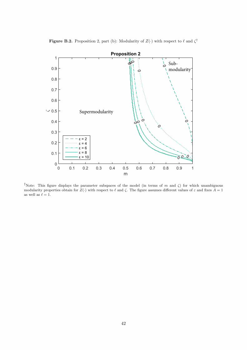
Figure B.2. Proposition 2, part (b): Modularity of Z(·) with respect to ` and ζ†

0

00

0

0

0

0

0

0

0

0

00

Proposition 2

m0 0.1 0.2 0.3 0.4 0.5 0.6 0.7 0.8 0.9 1

1

0

0.1

0.2

0.3

0.4

0.5

0.6

0.7

0.8

0.9

1

Supermodularity

Sub-modularity

†Note: This figure displays the parameter subspaces of the model (in terms of m and ζ) for which unambiguousmodularity properties obtain for Z(·) with respect to ` and ζ. The figure assumes different values of ε and fixes A = 1as well as ` = 1.

42

C Data appendix

Figure C.1. Histogram for the sourcing intensity of production†

0.0

5.1

.15

.2F

ract

ion

of F

irms

0 .2 .4 .6 .8 1Sourcing Intensity

†Note: Distribution as of 2012. Bins have width 0.05.

43

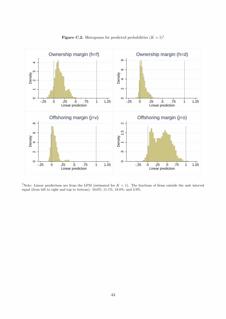
Figure C.2. Histograms for predicted probabilities (K = 1)†0

12

34

Den

sity

-.25 0 .25 .5 .75 1 1.25Linear prediction

Ownership margin (h=f)

02

46

8D

ensi

ty

-.25 0 .25 .5 .75 1 1.25Linear prediction

Ownership margin (h=d)

02

46

8D

ensi

ty

-.25 0 .25 .5 .75 1 1.25Linear prediction

Offshoring margin (j=v)0

.51

1.5

2D

ensi

ty

-.25 0 .25 .5 .75 1 1.25Linear prediction

Offshoring margin (j=o)

†Note: Linear predictions are from the LPM (estimated for K = 1). The fractions of firms outside the unit intervalequal (from left to right and top to bottom): 10.6%; 11.1%; 19.8%; and 2.9%.

44

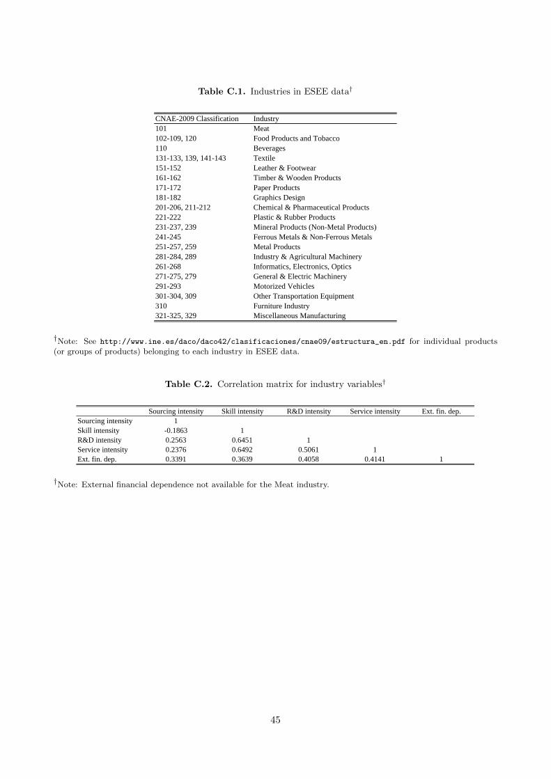
Table C.1. Industries in ESEE data†

CNAE-2009 Classification Industry101 Meat102-109, 120 Food Products and Tobacco110 Beverages131-133, 139, 141-143 Textile151-152 Leather & Footwear161-162 Timber & Wooden Products171-172 Paper Products181-182 Graphics Design201-206, 211-212 Chemical & Pharmaceutical Products221-222 Plastic & Rubber Products231-237, 239 Mineral Products (Non-Metal Products)241-245 Ferrous Metals & Non-Ferrous Metals251-257, 259 Metal Products281-284, 289 Industry & Agricultural Machinery261-268 Informatics, Electronics, Optics271-275, 279 General & Electric Machinery291-293 Motorized Vehicles301-304, 309 Other Transportation Equipment310 Furniture Industry321-325, 329 Miscellaneous Manufacturing

†Note: See http://www.ine.es/daco/daco42/clasificaciones/cnae09/estructura_en.pdf for individual products(or groups of products) belonging to each industry in ESEE data.

Table C.2. Correlation matrix for industry variables†

Sourcing intensity Skill intensity R&D intensity Service intensity Ext. fin. dep.Sourcing intensity 1Skill intensity -0.1863 1R&D intensity 0.2563 0.6451 1Service intensity 0.2376 0.6492 0.5061 1Ext. fin. dep. 0.3391 0.3639 0.4058 0.4141 1

†Note: External financial dependence not available for the Meat industry.

45

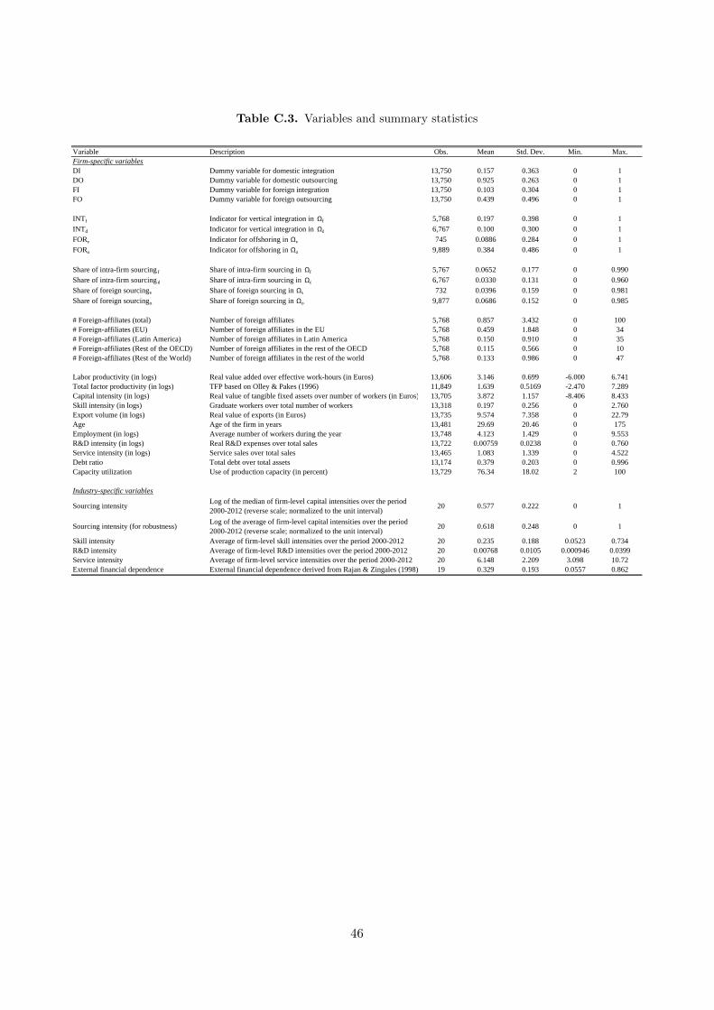
Table C.3. Variables and summary statistics

Variable Description Obs. Mean Std. Dev. Min. Max.Firm-specific variablesDI Dummy variable for domestic integration 13,750 0.157 0.363 0 1DO Dummy variable for domestic outsourcing 13,750 0.925 0.263 0 1FI Dummy variable for foreign integration 13,750 0.103 0.304 0 1FO Dummy variable for foreign outsourcing 13,750 0.439 0.496 0 1

INTf Indicator for vertical integration in Ωf 5,768 0.197 0.398 0 1INTd Indicator for vertical integration in Ωd 6,767 0.100 0.300 0 1FORv Indicator for offshoring in Ωv 745 0.0886 0.284 0 1FORo Indicator for offshoring in Ωo 9,889 0.384 0.486 0 1

Share of intra-firm sourcing f Share of intra-firm sourcing in Ωf 5,767 0.0652 0.177 0 0.990Share of intra-firm sourcing d Share of intra-firm sourcing in Ωd 6,767 0.0330 0.131 0 0.960Share of foreign sourcingv Share of foreign sourcing in Ωv 732 0.0396 0.159 0 0.981Share of foreign sourcingo Share of foreign sourcing in Ωo 9,877 0.0686 0.152 0 0.985

# Foreign-affiliates (total) Number of foreign affiliates 5,768 0.857 3.432 0 100# Foreign-affiliates (EU) Number of foreign affiliates in the EU 5,768 0.459 1.848 0 34# Foreign-affiliates (Latin America) Number of foreign affiliates in Latin America 5,768 0.150 0.910 0 35# Foreign-affiliates (Rest of the OECD) Number of foreign affiliates in the rest of the OECD 5,768 0.115 0.566 0 10# Foreign-affiliates (Rest of the World) Number of foreign affiliates in the rest of the world 5,768 0.133 0.986 0 47

Labor productivity (in logs) Real value added over effective work-hours (in Euros) 13,606 3.146 0.699 -6.000 6.741Total factor productivity (in logs) TFP based on Olley & Pakes (1996) 11,849 1.639 0.5169 -2.470 7.289Capital intensity (in logs) Real value of tangible fixed assets over number of workers (in Euros) 13,705 3.872 1.157 -8.406 8.433Skill intensity (in logs) Graduate workers over total number of workers 13,318 0.197 0.256 0 2.760Export volume (in logs) Real value of exports (in Euros) 13,735 9.574 7.358 0 22.79Age Age of the firm in years 13,481 29.69 20.46 0 175Employment (in logs) Average number of workers during the year 13,748 4.123 1.429 0 9.553R&D intensity (in logs) Real R&D expenses over total sales 13,722 0.00759 0.0238 0 0.760Service intensity (in logs) Service sales over total sales 13,465 1.083 1.339 0 4.522Debt ratio Total debt over total assets 13,174 0.379 0.203 0 0.996Capacity utilization Use of production capacity (in percent) 13,729 76.34 18.02 2 100

Industry-specific variables

Sourcing intensity Log of the median of firm-level capital intensities over the period 2000-2012 (reverse scale; normalized to the unit interval) 20 0.577 0.222 0 1

Sourcing intensity (for robustness) Log of the average of firm-level capital intensities over the period 2000-2012 (reverse scale; normalized to the unit interval) 20 0.618 0.248 0 1

Skill intensity Average of firm-level skill intensities over the period 2000-2012 20 0.235 0.188 0.0523 0.734R&D intensity Average of firm-level R&D intensities over the period 2000-2012 20 0.00768 0.0105 0.000946 0.0399Service intensity Average of firm-level service intensities over the period 2000-2012 20 6.148 2.209 3.098 10.72External financial dependence External financial dependence derived from Rajan & Zingales (1998) 19 0.329 0.193 0.0557 0.862

46

Alternative measure of productivity. As an alternative measure of firm productivity, we employtotal factor productivity estimated with the estimation algorithm developed by Olley & Pakes (1996).We feed the algorithm with ESEE data from 2000-2011. More specifically, we use annual informationon each firm’s value added, investment, capital stock, labor employment, and exit decisions. Valueadded is the sum of the total production value plus other operating income (i.e., income from rentand leasing, industrial property, commissions, and certain services), minus the total expenditure onintermediate inputs and external services, expressed in constant 2010 prices. Investment is the realtotal investment value in real estate, construction, and equipment. The capital stock is the real valueof real estate, construction, and equipment. Labor employment is measured in effective work-hours.Exit decisions of firms allows us to distinguish between firms shutting down production and firmsstaying in the market, but exiting the ESEE panel.

References

Antras, P. (2003). Firms, contracts, and trade structure. Quarterly Journal of Economics, 118 (4),1375–1418.

Antras, P. (2014a). Global Production: Firms, Contracts, and Trade Structure. UnpublishedManuscript (CREI Lectures on Macroeconomics 2010).

Antras, P. (2014b). Grossman-Hart (1986) goes global: Incomplete contracts, property rights, andthe international organization of production. Journal of Law, Economics, and Organization, 30 (1),118–175.

Antras, P., & Chor, D. (2013). Organizing the global value chain. Econometrica, 81 (6), 2127–2204.

Antras, P., & Helpman, E. (2004). Global sourcing. Journal of Political Economy , 112 (3), 552–580.

Antras, P., & Helpman, E. (2008). Contractual frictions and global sourcing. In E. Helpman, D. Marin,& T. Verdier (Eds.) The Organization of Firms in a Global Economy , chap. 1, (pp. 9–54). HarvardUniversity Press: Cambridge, MA.

Aoki, M. (1990). Toward an economic model of the Japanese firm. Journal of Economic Literature,28 (1), 1–27.

Bache, P. A., & Laugesen, A. (2014). Trade liberalisation and vertical integration. Economics WorkingPapers 2013-14, Aarhus University.

Becker, S. O., Ekholm, K., & Muendler, M.-A. (2013). Offshoring and the onshore composition oftasks and skills. Journal of International Economics, 90 (1), 91 – 106.

Bernard, A. B., Jensen, J. B., Redding, S. J., & Schott, P. K. (2010). Intrafirm trade and productcontractibility. American Economic Review: Papers & Proceedings, 100 (2), 444–448.

Bernard, A. B., Jensen, J. B., Redding, S. J., & Schott, P. K. (2012). The empirics of firm hetero-geneity and international trade. Annual Review of Economics, 4 (1), 283–313.

Blinder, A. (2009). Offshoring: Big deal, or business as usual? In B. M. Friedman (Ed.) Offshoringof American Jobs. What Response from U.S. Economic Policy? , chap. 2, (pp. 19–60). Cambridge,MA: MIT Press.

Coase, R. H. (1937). The nature of the firm. Economica, 4 (16), 386–405.

47

Corcos, G., Irac, D. M., Mion, G., & Verdier, T. (2013). The determinants of intrafirm trade: Evidencefrom French firms. Review of Economics and Statistics, 95 (3), 825–838.

Defever, F., & Toubal, F. (2013). Productivity, relationship-specific inputs and the sourcing modesof multinationals. Journal of Economic Behavior & Organization, 94 , 345–357.

Dunning, J. H. (1993). Multinational Enterprises and the Global Economy . Addison Wesley Longman,Inc.

Ebenstein, A., Harrison, A., McMillan, M., & Phillips, S. (2014). Estimating the impact of trade andoffshoring on American workers using the current population surveys. Review of Economics andStatistics, 96 (4), 581–595.

Federico, S. (2010). Outsourcing versus integration at home or abroad. Empirica, 37 (1), 47–63.

Federico, S. (2012). Headquarter intensity and the choice between outsourcing versus integration athome or abroad. Industrial and Corporate Change, 21 (1), 1–22.

Grossman, S. J., & Hart, O. D. (1986). The costs and benefits of ownership: A theory of vertical andlateral integration. Journal of Political Economy , 94 (4), 691–719.

Guadalupe, M., Kuzmina, O., & Thomas, C. (2012). Innovation and foreign ownership. AmericanEconomic Review , 102 (7), 3594–3627.

Hart, O., & Moore, J. (1990). Property rights and the nature of the firm. Journal of PoliticalEconomy, University of Chicago Press, 98 (6), 1119–1158.

Horrace, W. C., & Oaxaca, R. L. (2006). Results on the bias and inconsistency of ordinary leastsquares for the linear probability model. Economics Letters, 90 (3), 321–327.

Klette, T. J., & Griliches, Z. (1962). An efficient method of estimating seemingly unrelated regressionequations and tests for aggregation bias. Journal of the American Statistical Association, 57 (298),348–368.

Kohler, W., & Smolka, M. (2011). Sourcing premia with incomplete contracts: Theory and evidence.B.E. Journal of Economic Analysis and Policy , 11 (1), 1–37.

Kohler, W., & Smolka, M. (2012). Global sourcing: Evidence from Spanish firm-level data. In R. M.Stern (Ed.) Quantitative Analysis of Newly Evolving Patterns of International Trade, chap. 4, (pp.139–189). World Scientific Studies in International Economics.

Kohler, W., & Smolka, M. (2014). Global sourcing and firm selection. Economics Letters, 124 (3),411–415.

Melitz, M. J. (2003). The impact of trade on intra-industry reallocations and aggregate industryproductivity. Econometrica, 71 (6), 1695–1725.

Milgrom, P., & Roberts, J. (1993). Johnson Controls Inc., Automotive Systems Group: The George-town, Kentucky Plant. Stanford Graduate School of Business Case S-BE-9.

Mrazowa, M., & Neary, P. (2013). Selection effects with heterogeneous firms. Mimeo, University ofOxford, Department of Economics.

48

Nunn, N., & Trefler, D. (2008). The boundaries of the multinational firm: An empirical analysis.In E. Helpman, D. Marin, & T. Verdier (Eds.) The Organization of Firms in a Global Economy ,chap. 2, (pp. 55–83). Harvard University Press: Cambridge, MA.

Nunn, N., & Trefler, D. (2013). Incomplete contracts and the boundaries of the multinational firm.Journal of Economic Behavior & Organization, 94 , 330–344.

Olley, G. S., & Pakes, A. (1996). The dynamics of productivity in the telecommunications equipmentindustry. Econometrica, 64 (6), 1263–1297.

Rajan, R. G., & Zingales, L. (1998). Financial dependence and growth. American Economic Review ,88 (3), 559–586.

Schwarz, C., & Sudekum, J. (2014). Global sourcing of complex production processes. Journal ofInternational Economics, 93 (1), 123–139.

Tomiura, E. (2007). Foreign outsourcing, exporting, and FDI: A productivity comparison at the firmlevel. Journal of International Economics, 72 (1), 113–127.

Yeaple, S. R. (2006). Offshoring, foreign direct investment, and the structure of U.S. trade. Journalof the European Economic Association, 4 (2-3), 602–611.

Young, S., Hood, N., & Hamill, J. (1985). Decision-making in foreign-owned multinational subsidiariesin the United Kingdom. ILO Multinational Enterprises Programme Working Paper No. 35, Geneva:International Labor Office.

49