TikZ and pgf - KTUG, KTSproject.ktug.org/dvipdfmx/sample/misc/pgfmanual-v1-dvipdfmx.pdf · Fur...

TikZ and pgfManual for Version 1.01

.

.

..

.

.

..

.. .

.

. ..

.

.

. ..

.

.

.

..

...

.

.

...

.

...

.

.

.

.

\tikzstyle{level 1}=[sibling angle=120]



\tikzstyle{every node}=[fill]

\tikzstyle{edge from parent}=[snake=expanding waves,segment length=1mm,segment angle=10,draw]

\tikz [grow cyclic,shape=circle,very thick,level distance=13mm,cap=round]

\node {} child [color=\A] foreach \A in {red,green,blue}

{ node {} child [color=\A!50!\B] foreach \B in {red,green,blue}

{ node {} child [color=\A!50!\B!50!\C] foreach \C in {black,gray,white}

{ node {} }

}

};

1

Fur meinen Vater, damit er noch viele schone TEX-Graphiken erschaffen kann.

2

The TikZ and pgf Packages

Manual for Version 1.01http://sourceforge.net/projects/pgf

Till Tantaumailto:[email protected]

May 29, 2008

Contents

I Getting Started 11

1 Introduction 121.1 Structure of the System . . . . . . . . . . . . . . . . . . . . . . . . . . . . . . . . . . . . . . . . . 121.2 Comparison with Other Graphics Packages . . . . . . . . . . . . . . . . . . . . . . . . . . . . . . 131.3 Utilities: Page Management . . . . . . . . . . . . . . . . . . . . . . . . . . . . . . . . . . . . . . 131.4 How to Read This Manual . . . . . . . . . . . . . . . . . . . . . . . . . . . . . . . . . . . . . . . 131.5 Getting Help . . . . . . . . . . . . . . . . . . . . . . . . . . . . . . . . . . . . . . . . . . . . . . . 14

2 Installation 152.1 Package and Driver Versions . . . . . . . . . . . . . . . . . . . . . . . . . . . . . . . . . . . . . . 152.2 Installing Prebundled Packages . . . . . . . . . . . . . . . . . . . . . . . . . . . . . . . . . . . . 15

2.2.1 Debian . . . . . . . . . . . . . . . . . . . . . . . . . . . . . . . . . . . . . . . . . . . . . . 152.2.2 MiKTeX . . . . . . . . . . . . . . . . . . . . . . . . . . . . . . . . . . . . . . . . . . . . . 15

2.3 Installation in a texmf Tree . . . . . . . . . . . . . . . . . . . . . . . . . . . . . . . . . . . . . . 162.3.1 Installation that Keeps Everything Together . . . . . . . . . . . . . . . . . . . . . . . . . 162.3.2 Installation that is TDS-Compliant . . . . . . . . . . . . . . . . . . . . . . . . . . . . . . 16

2.4 Updating the Installation . . . . . . . . . . . . . . . . . . . . . . . . . . . . . . . . . . . . . . . . 162.5 License: The GNU Public License, Version 2 . . . . . . . . . . . . . . . . . . . . . . . . . . . . . 17

2.5.1 Preamble . . . . . . . . . . . . . . . . . . . . . . . . . . . . . . . . . . . . . . . . . . . . . 172.5.2 Terms and Conditions For Copying, Distribution and Modification . . . . . . . . . . . . 172.5.3 No Warranty . . . . . . . . . . . . . . . . . . . . . . . . . . . . . . . . . . . . . . . . . . 20

3 Tutorial: A Picture for Karl’s Students 213.1 Problem Statement . . . . . . . . . . . . . . . . . . . . . . . . . . . . . . . . . . . . . . . . . . . 213.2 Setting up the Environment . . . . . . . . . . . . . . . . . . . . . . . . . . . . . . . . . . . . . . 21

3.2.1 Setting up the Environment in LATEX . . . . . . . . . . . . . . . . . . . . . . . . . . . . . 223.2.2 Setting up the Environment in Plain TEX . . . . . . . . . . . . . . . . . . . . . . . . . . 22

3.3 Straight Path Construction . . . . . . . . . . . . . . . . . . . . . . . . . . . . . . . . . . . . . . . 233.4 Curved Path Construction . . . . . . . . . . . . . . . . . . . . . . . . . . . . . . . . . . . . . . . 233.5 Circle Path Construction . . . . . . . . . . . . . . . . . . . . . . . . . . . . . . . . . . . . . . . . 243.6 Rectangle Path Construction . . . . . . . . . . . . . . . . . . . . . . . . . . . . . . . . . . . . . . 243.7 Grid Path Construction . . . . . . . . . . . . . . . . . . . . . . . . . . . . . . . . . . . . . . . . . 243.8 Adding a Touch of Style . . . . . . . . . . . . . . . . . . . . . . . . . . . . . . . . . . . . . . . . 253.9 Drawing Options . . . . . . . . . . . . . . . . . . . . . . . . . . . . . . . . . . . . . . . . . . . . 263.10 Arc Path Construction . . . . . . . . . . . . . . . . . . . . . . . . . . . . . . . . . . . . . . . . . 26

3

3.11 Clipping a Path . . . . . . . . . . . . . . . . . . . . . . . . . . . . . . . . . . . . . . . . . . . . . 273.12 Parabola and Sine Path Construction . . . . . . . . . . . . . . . . . . . . . . . . . . . . . . . . . 283.13 Filling and Drawing . . . . . . . . . . . . . . . . . . . . . . . . . . . . . . . . . . . . . . . . . . . 283.14 Shading . . . . . . . . . . . . . . . . . . . . . . . . . . . . . . . . . . . . . . . . . . . . . . . . . 293.15 Specifying Coordinates . . . . . . . . . . . . . . . . . . . . . . . . . . . . . . . . . . . . . . . . . 293.16 Adding Arrow Tips . . . . . . . . . . . . . . . . . . . . . . . . . . . . . . . . . . . . . . . . . . . 313.17 Scoping . . . . . . . . . . . . . . . . . . . . . . . . . . . . . . . . . . . . . . . . . . . . . . . . . . 323.18 Transformations . . . . . . . . . . . . . . . . . . . . . . . . . . . . . . . . . . . . . . . . . . . . . 323.19 Repeating Things: For-Loops . . . . . . . . . . . . . . . . . . . . . . . . . . . . . . . . . . . . . 333.20 Adding Text . . . . . . . . . . . . . . . . . . . . . . . . . . . . . . . . . . . . . . . . . . . . . . . 343.21 Nodes . . . . . . . . . . . . . . . . . . . . . . . . . . . . . . . . . . . . . . . . . . . . . . . . . . . 37

4 Guidelines on Graphics 394.1 Should You Follow Guidelines? . . . . . . . . . . . . . . . . . . . . . . . . . . . . . . . . . . . . . 394.2 Planning the Time Needed for the Creation of Graphics . . . . . . . . . . . . . . . . . . . . . . 394.3 Workflow for Creating a Graphic . . . . . . . . . . . . . . . . . . . . . . . . . . . . . . . . . . . 404.4 Linking Graphics With the Main Text . . . . . . . . . . . . . . . . . . . . . . . . . . . . . . . . 404.5 Consistency Between Graphics and Text . . . . . . . . . . . . . . . . . . . . . . . . . . . . . . . 414.6 Labels in Graphics . . . . . . . . . . . . . . . . . . . . . . . . . . . . . . . . . . . . . . . . . . . 424.7 Plots and Charts . . . . . . . . . . . . . . . . . . . . . . . . . . . . . . . . . . . . . . . . . . . . 424.8 Attention and Distraction . . . . . . . . . . . . . . . . . . . . . . . . . . . . . . . . . . . . . . . 45

5 Input and Output Formats 475.1 Supported Input Formats . . . . . . . . . . . . . . . . . . . . . . . . . . . . . . . . . . . . . . . . 47

5.1.1 Using the LATEX Format . . . . . . . . . . . . . . . . . . . . . . . . . . . . . . . . . . . . 475.1.2 Using the Plain TEX Format . . . . . . . . . . . . . . . . . . . . . . . . . . . . . . . . . . 475.1.3 Using the ConTEXt Format . . . . . . . . . . . . . . . . . . . . . . . . . . . . . . . . . . 47

5.2 Supported Output Formats . . . . . . . . . . . . . . . . . . . . . . . . . . . . . . . . . . . . . . . 475.2.1 Selecting the Backend Driver . . . . . . . . . . . . . . . . . . . . . . . . . . . . . . . . . 485.2.2 Producing PDF Output . . . . . . . . . . . . . . . . . . . . . . . . . . . . . . . . . . . . 485.2.3 Producing PostScript Output . . . . . . . . . . . . . . . . . . . . . . . . . . . . . . . . . 495.2.4 Producing HTML / SVG Output . . . . . . . . . . . . . . . . . . . . . . . . . . . . . . . 49

II TikZ ist kein Zeichenprogramm 51

6 Design Principles 526.1 Special Syntax For Specifying Points . . . . . . . . . . . . . . . . . . . . . . . . . . . . . . . . . 526.2 Special Syntax For Path Specifications . . . . . . . . . . . . . . . . . . . . . . . . . . . . . . . . 526.3 Actions on Paths . . . . . . . . . . . . . . . . . . . . . . . . . . . . . . . . . . . . . . . . . . . . 536.4 Key-Value Syntax for Graphic Parameters . . . . . . . . . . . . . . . . . . . . . . . . . . . . . . 536.5 Special Syntax for Specifying Nodes . . . . . . . . . . . . . . . . . . . . . . . . . . . . . . . . . . 536.6 Special Syntax for Specifying Trees . . . . . . . . . . . . . . . . . . . . . . . . . . . . . . . . . . 536.7 Grouping of Graphic Parameters . . . . . . . . . . . . . . . . . . . . . . . . . . . . . . . . . . . 546.8 Coordinate Transformation System . . . . . . . . . . . . . . . . . . . . . . . . . . . . . . . . . . 55

7 Hierarchical Structures: Package, Environments, Scopes, and Styles 567.1 Loading the Package . . . . . . . . . . . . . . . . . . . . . . . . . . . . . . . . . . . . . . . . . . 567.2 Creating a Picture . . . . . . . . . . . . . . . . . . . . . . . . . . . . . . . . . . . . . . . . . . . . 56

7.2.1 Creating a Picture Using an Environment . . . . . . . . . . . . . . . . . . . . . . . . . . 567.2.2 Creating a Picture Using a Command . . . . . . . . . . . . . . . . . . . . . . . . . . . . . 577.2.3 Adding a Background . . . . . . . . . . . . . . . . . . . . . . . . . . . . . . . . . . . . . . 58

7.3 Using Scopes to Structure a Picture . . . . . . . . . . . . . . . . . . . . . . . . . . . . . . . . . . 587.4 Using Scopes Inside Paths . . . . . . . . . . . . . . . . . . . . . . . . . . . . . . . . . . . . . . . 597.5 Using Styles to Manage How Pictures Look . . . . . . . . . . . . . . . . . . . . . . . . . . . . . 59

4

8 Specifying Coordinates 618.1 Coordinates and Coordinate Options . . . . . . . . . . . . . . . . . . . . . . . . . . . . . . . . . 618.2 Simple Coordinates . . . . . . . . . . . . . . . . . . . . . . . . . . . . . . . . . . . . . . . . . . . 618.3 Polar Coordinates . . . . . . . . . . . . . . . . . . . . . . . . . . . . . . . . . . . . . . . . . . . . 618.4 Xy- and Xyz-Coordinates . . . . . . . . . . . . . . . . . . . . . . . . . . . . . . . . . . . . . . . . 618.5 Node Coordinates . . . . . . . . . . . . . . . . . . . . . . . . . . . . . . . . . . . . . . . . . . . . 62

8.5.1 Named Anchor Coordinates . . . . . . . . . . . . . . . . . . . . . . . . . . . . . . . . . . 628.5.2 Angle Anchor Coordinates . . . . . . . . . . . . . . . . . . . . . . . . . . . . . . . . . . . 628.5.3 Anchor-Free Node Coordinates . . . . . . . . . . . . . . . . . . . . . . . . . . . . . . . . 62

8.6 Intersection Coordinates . . . . . . . . . . . . . . . . . . . . . . . . . . . . . . . . . . . . . . . . 638.6.1 Intersection of Two Lines . . . . . . . . . . . . . . . . . . . . . . . . . . . . . . . . . . . . 638.6.2 Intersection of Horizontal and Vertical Lines . . . . . . . . . . . . . . . . . . . . . . . . . 64

8.7 Relative and Incremental Coordinates . . . . . . . . . . . . . . . . . . . . . . . . . . . . . . . . . 64

9 Syntax for Path Specifications 659.1 The Move-To Operation . . . . . . . . . . . . . . . . . . . . . . . . . . . . . . . . . . . . . . . . 669.2 The Line-To Operation . . . . . . . . . . . . . . . . . . . . . . . . . . . . . . . . . . . . . . . . . 66

9.2.1 Straight Lines . . . . . . . . . . . . . . . . . . . . . . . . . . . . . . . . . . . . . . . . . . 669.2.2 Horizontal and Vertical Lines . . . . . . . . . . . . . . . . . . . . . . . . . . . . . . . . . 679.2.3 Snaked Lines . . . . . . . . . . . . . . . . . . . . . . . . . . . . . . . . . . . . . . . . . . 67

9.3 The Curve-To Operation . . . . . . . . . . . . . . . . . . . . . . . . . . . . . . . . . . . . . . . . 709.4 The Cycle Operation . . . . . . . . . . . . . . . . . . . . . . . . . . . . . . . . . . . . . . . . . . 719.5 The Rectangle Operation . . . . . . . . . . . . . . . . . . . . . . . . . . . . . . . . . . . . . . . . 719.6 Rounding Corners . . . . . . . . . . . . . . . . . . . . . . . . . . . . . . . . . . . . . . . . . . . . 729.7 The Circle and Ellipse Operations . . . . . . . . . . . . . . . . . . . . . . . . . . . . . . . . . . . 729.8 The Arc Operation . . . . . . . . . . . . . . . . . . . . . . . . . . . . . . . . . . . . . . . . . . . 739.9 The Grid Operation . . . . . . . . . . . . . . . . . . . . . . . . . . . . . . . . . . . . . . . . . . . 739.10 The Parabola Operation . . . . . . . . . . . . . . . . . . . . . . . . . . . . . . . . . . . . . . . . 749.11 The Sine and Cosine Operation . . . . . . . . . . . . . . . . . . . . . . . . . . . . . . . . . . . . 759.12 The Plot Operation . . . . . . . . . . . . . . . . . . . . . . . . . . . . . . . . . . . . . . . . . . . 76

9.12.1 Plotting Points Given Inline . . . . . . . . . . . . . . . . . . . . . . . . . . . . . . . . . . 769.12.2 Plotting Points Read From an External File . . . . . . . . . . . . . . . . . . . . . . . . . 779.12.3 Plotting a Function . . . . . . . . . . . . . . . . . . . . . . . . . . . . . . . . . . . . . . . 779.12.4 Placing Marks on the Plot . . . . . . . . . . . . . . . . . . . . . . . . . . . . . . . . . . . 799.12.5 Smooth Plots, Sharp Plots, and Comb Plots . . . . . . . . . . . . . . . . . . . . . . . . . 80

9.13 The Scoping Operation . . . . . . . . . . . . . . . . . . . . . . . . . . . . . . . . . . . . . . . . . 829.14 The Node Operation . . . . . . . . . . . . . . . . . . . . . . . . . . . . . . . . . . . . . . . . . . 82

10 Actions on Paths 8310.1 Specifying a Color . . . . . . . . . . . . . . . . . . . . . . . . . . . . . . . . . . . . . . . . . . . . 8410.2 Drawing a Path . . . . . . . . . . . . . . . . . . . . . . . . . . . . . . . . . . . . . . . . . . . . . 84

10.2.1 Graphic Parameters: Line Width, Line Cap, and Line Join . . . . . . . . . . . . . . . . . 8510.2.2 Graphic Parameters: Dash Pattern . . . . . . . . . . . . . . . . . . . . . . . . . . . . . . 8610.2.3 Graphic Parameters: Draw Opacity . . . . . . . . . . . . . . . . . . . . . . . . . . . . . . 8710.2.4 Graphic Parameters: Arrow Tips . . . . . . . . . . . . . . . . . . . . . . . . . . . . . . . 8810.2.5 Graphic Parameters: Double Lines and Bordered Lines . . . . . . . . . . . . . . . . . . . 90

10.3 Filling a Path . . . . . . . . . . . . . . . . . . . . . . . . . . . . . . . . . . . . . . . . . . . . . . 9010.3.1 Graphic Parameters: Interior Rules . . . . . . . . . . . . . . . . . . . . . . . . . . . . . . 9110.3.2 Graphic Parameters: Fill Opacity . . . . . . . . . . . . . . . . . . . . . . . . . . . . . . . 92

10.4 Shading a Path . . . . . . . . . . . . . . . . . . . . . . . . . . . . . . . . . . . . . . . . . . . . . 9210.4.1 Choosing a Shading Type . . . . . . . . . . . . . . . . . . . . . . . . . . . . . . . . . . . 9310.4.2 Choosing a Shading Color . . . . . . . . . . . . . . . . . . . . . . . . . . . . . . . . . . . 94

10.5 Establishing a Bounding Box . . . . . . . . . . . . . . . . . . . . . . . . . . . . . . . . . . . . . . 9510.6 Using a Path For Clipping . . . . . . . . . . . . . . . . . . . . . . . . . . . . . . . . . . . . . . . 95

5

11 Nodes 9711.1 Nodes and Their Shapes . . . . . . . . . . . . . . . . . . . . . . . . . . . . . . . . . . . . . . . . 9711.2 Multi-Part Nodes . . . . . . . . . . . . . . . . . . . . . . . . . . . . . . . . . . . . . . . . . . . . 9811.3 Options for the Text in Nodes . . . . . . . . . . . . . . . . . . . . . . . . . . . . . . . . . . . . . 9911.4 Placing Nodes Using Anchors . . . . . . . . . . . . . . . . . . . . . . . . . . . . . . . . . . . . . 10111.5 Transformations . . . . . . . . . . . . . . . . . . . . . . . . . . . . . . . . . . . . . . . . . . . . . 10311.6 Placing Nodes on a Line or Curve . . . . . . . . . . . . . . . . . . . . . . . . . . . . . . . . . . . 104

11.6.1 Explicit Use of the Position Option . . . . . . . . . . . . . . . . . . . . . . . . . . . . . . 10411.6.2 Implicit Use of the Position Option . . . . . . . . . . . . . . . . . . . . . . . . . . . . . . 105

11.7 Connecting Nodes . . . . . . . . . . . . . . . . . . . . . . . . . . . . . . . . . . . . . . . . . . . . 10611.8 Predefined Shapes . . . . . . . . . . . . . . . . . . . . . . . . . . . . . . . . . . . . . . . . . . . . 107

12 Making Trees Grow 10912.1 Introduction to the Child Operation . . . . . . . . . . . . . . . . . . . . . . . . . . . . . . . . . . 10912.2 Child Paths and the Child Nodes . . . . . . . . . . . . . . . . . . . . . . . . . . . . . . . . . . . 11012.3 Naming Child Nodes . . . . . . . . . . . . . . . . . . . . . . . . . . . . . . . . . . . . . . . . . . 11112.4 Specifying Options for Trees and Children . . . . . . . . . . . . . . . . . . . . . . . . . . . . . . 11112.5 Placing Child Nodes . . . . . . . . . . . . . . . . . . . . . . . . . . . . . . . . . . . . . . . . . . 11312.6 Edges From the Parent Node . . . . . . . . . . . . . . . . . . . . . . . . . . . . . . . . . . . . . . 116

13 Transformations 11913.1 The Different Coordinate Systems . . . . . . . . . . . . . . . . . . . . . . . . . . . . . . . . . . . 11913.2 The Xy- and Xyz-Coordinate Systems . . . . . . . . . . . . . . . . . . . . . . . . . . . . . . . . 11913.3 Coordinate Transformations . . . . . . . . . . . . . . . . . . . . . . . . . . . . . . . . . . . . . . 120

III Libraries and Utilities 124

14 Libraries 12514.1 Arrow Tip Library . . . . . . . . . . . . . . . . . . . . . . . . . . . . . . . . . . . . . . . . . . . 125

14.1.1 Triangular Arrow Tips . . . . . . . . . . . . . . . . . . . . . . . . . . . . . . . . . . . . . 12514.1.2 Barbed Arrow Tips . . . . . . . . . . . . . . . . . . . . . . . . . . . . . . . . . . . . . . . 12514.1.3 Bracket-Like Arrow Tips . . . . . . . . . . . . . . . . . . . . . . . . . . . . . . . . . . . . 12514.1.4 Circle and Diamond Arrow Tips . . . . . . . . . . . . . . . . . . . . . . . . . . . . . . . . 12514.1.5 Partial Arrow Tips . . . . . . . . . . . . . . . . . . . . . . . . . . . . . . . . . . . . . . . 12614.1.6 Line Caps . . . . . . . . . . . . . . . . . . . . . . . . . . . . . . . . . . . . . . . . . . . . 126

14.2 Snake Library . . . . . . . . . . . . . . . . . . . . . . . . . . . . . . . . . . . . . . . . . . . . . . 12614.3 Plot Handler Library . . . . . . . . . . . . . . . . . . . . . . . . . . . . . . . . . . . . . . . . . . 129

14.3.1 Curve Plot Handlers . . . . . . . . . . . . . . . . . . . . . . . . . . . . . . . . . . . . . . 12914.3.2 Comb Plot Handlers . . . . . . . . . . . . . . . . . . . . . . . . . . . . . . . . . . . . . . 13014.3.3 Mark Plot Handler . . . . . . . . . . . . . . . . . . . . . . . . . . . . . . . . . . . . . . . 131

14.4 Plot Mark Library . . . . . . . . . . . . . . . . . . . . . . . . . . . . . . . . . . . . . . . . . . . . 13214.5 Shape Library . . . . . . . . . . . . . . . . . . . . . . . . . . . . . . . . . . . . . . . . . . . . . . 13214.6 Tree Library . . . . . . . . . . . . . . . . . . . . . . . . . . . . . . . . . . . . . . . . . . . . . . . 135

14.6.1 Growth Functions . . . . . . . . . . . . . . . . . . . . . . . . . . . . . . . . . . . . . . . . 13614.6.2 Edges From Parent . . . . . . . . . . . . . . . . . . . . . . . . . . . . . . . . . . . . . . . 137

14.7 Background Library . . . . . . . . . . . . . . . . . . . . . . . . . . . . . . . . . . . . . . . . . . . 13814.8 Automata Drawing Library . . . . . . . . . . . . . . . . . . . . . . . . . . . . . . . . . . . . . . 140

15 Repeating Things: The Foreach Statement 142

6

16 Page Management 14616.1 Basic Usage . . . . . . . . . . . . . . . . . . . . . . . . . . . . . . . . . . . . . . . . . . . . . . . 14616.2 The Predefined Layouts . . . . . . . . . . . . . . . . . . . . . . . . . . . . . . . . . . . . . . . . . 14716.3 Defining a Layout . . . . . . . . . . . . . . . . . . . . . . . . . . . . . . . . . . . . . . . . . . . . 15016.4 Creating Logical Pages . . . . . . . . . . . . . . . . . . . . . . . . . . . . . . . . . . . . . . . . . 152

17 Extended Color Support 154

IV The Basic Layer 155

18 Design Principles 15618.1 Core and Optional Packages . . . . . . . . . . . . . . . . . . . . . . . . . . . . . . . . . . . . . . 15618.2 Communicating with the Basic Layer via Macros . . . . . . . . . . . . . . . . . . . . . . . . . . 15618.3 Path-Centered Approach . . . . . . . . . . . . . . . . . . . . . . . . . . . . . . . . . . . . . . . . 15718.4 Coordinate Versus Canvas Transformations . . . . . . . . . . . . . . . . . . . . . . . . . . . . . . 157

19 Hierarchical Structures: Package, Environments, Scopes, and Text 15819.1 Overview . . . . . . . . . . . . . . . . . . . . . . . . . . . . . . . . . . . . . . . . . . . . . . . . . 158

19.1.1 The Hierarchical Structure of the Package . . . . . . . . . . . . . . . . . . . . . . . . . . 15819.1.2 The Hierarchical Structure of Graphics . . . . . . . . . . . . . . . . . . . . . . . . . . . . 158

19.2 The Hierarchical Structure of the Package . . . . . . . . . . . . . . . . . . . . . . . . . . . . . . 15919.2.1 The Main Package . . . . . . . . . . . . . . . . . . . . . . . . . . . . . . . . . . . . . . . 15919.2.2 The Core Package . . . . . . . . . . . . . . . . . . . . . . . . . . . . . . . . . . . . . . . . 16019.2.3 The Optional Basic Layer Packages . . . . . . . . . . . . . . . . . . . . . . . . . . . . . . 160

19.3 The Hierarchical Structure of the Graphics . . . . . . . . . . . . . . . . . . . . . . . . . . . . . . 16019.3.1 The Main Environment . . . . . . . . . . . . . . . . . . . . . . . . . . . . . . . . . . . . . 16019.3.2 Graphic Scope Environments . . . . . . . . . . . . . . . . . . . . . . . . . . . . . . . . . 16219.3.3 Inserting Text and Images . . . . . . . . . . . . . . . . . . . . . . . . . . . . . . . . . . . 163

20 Specifying Coordinates 16620.1 Overview . . . . . . . . . . . . . . . . . . . . . . . . . . . . . . . . . . . . . . . . . . . . . . . . . 16620.2 Basic Coordinate Commands . . . . . . . . . . . . . . . . . . . . . . . . . . . . . . . . . . . . . . 16620.3 Coordinates in the Xy- and Xyz-Coordinate Systems . . . . . . . . . . . . . . . . . . . . . . . . 16620.4 Building Coordinates From Other Coordinates . . . . . . . . . . . . . . . . . . . . . . . . . . . . 167

20.4.1 Basic Manipulations of Coordinates . . . . . . . . . . . . . . . . . . . . . . . . . . . . . . 16720.4.2 Points Traveling along Lines and Curves . . . . . . . . . . . . . . . . . . . . . . . . . . . 16820.4.3 Points on Borders of Objects . . . . . . . . . . . . . . . . . . . . . . . . . . . . . . . . . . 16920.4.4 Points on the Intersection of Lines . . . . . . . . . . . . . . . . . . . . . . . . . . . . . . 170

20.5 Extracting Coordinates . . . . . . . . . . . . . . . . . . . . . . . . . . . . . . . . . . . . . . . . . 17020.6 Internals of How Point Commands Work . . . . . . . . . . . . . . . . . . . . . . . . . . . . . . . 171

21 Constructing Paths 17221.1 Overview . . . . . . . . . . . . . . . . . . . . . . . . . . . . . . . . . . . . . . . . . . . . . . . . . 17221.2 The Move-To Path Operation . . . . . . . . . . . . . . . . . . . . . . . . . . . . . . . . . . . . . 17221.3 The Line-To Path Operation . . . . . . . . . . . . . . . . . . . . . . . . . . . . . . . . . . . . . . 17321.4 The Curve-To Path Operation . . . . . . . . . . . . . . . . . . . . . . . . . . . . . . . . . . . . . 17321.5 The Close Path Operation . . . . . . . . . . . . . . . . . . . . . . . . . . . . . . . . . . . . . . . 17421.6 Arc, Ellipse and Circle Path Operations . . . . . . . . . . . . . . . . . . . . . . . . . . . . . . . 17421.7 Rectangle Path Operations . . . . . . . . . . . . . . . . . . . . . . . . . . . . . . . . . . . . . . . 17521.8 The Grid Path Operation . . . . . . . . . . . . . . . . . . . . . . . . . . . . . . . . . . . . . . . . 17621.9 The Parabola Path Operation . . . . . . . . . . . . . . . . . . . . . . . . . . . . . . . . . . . . . 17721.10 Sine and Cosine Path Operations . . . . . . . . . . . . . . . . . . . . . . . . . . . . . . . . . . . 17721.11 Plot Path Operations . . . . . . . . . . . . . . . . . . . . . . . . . . . . . . . . . . . . . . . . . . 17821.12 Rounded Corners . . . . . . . . . . . . . . . . . . . . . . . . . . . . . . . . . . . . . . . . . . . . 178

7

21.13 Internal Tracking of Bounding Boxes for Paths and Pictures . . . . . . . . . . . . . . . . . . . . 179

22 Snakes 18122.1 Overview . . . . . . . . . . . . . . . . . . . . . . . . . . . . . . . . . . . . . . . . . . . . . . . . . 18122.2 Declaring a Snake . . . . . . . . . . . . . . . . . . . . . . . . . . . . . . . . . . . . . . . . . . . . 181

22.2.1 Segments . . . . . . . . . . . . . . . . . . . . . . . . . . . . . . . . . . . . . . . . . . . . . 18122.2.2 Snake Automata . . . . . . . . . . . . . . . . . . . . . . . . . . . . . . . . . . . . . . . . 18122.2.3 The Snake Declaration Command . . . . . . . . . . . . . . . . . . . . . . . . . . . . . . . 18222.2.4 Predefined Snakes . . . . . . . . . . . . . . . . . . . . . . . . . . . . . . . . . . . . . . . . 184

22.3 Using Snakes . . . . . . . . . . . . . . . . . . . . . . . . . . . . . . . . . . . . . . . . . . . . . . . 184

23 Using Paths 18623.1 Overview . . . . . . . . . . . . . . . . . . . . . . . . . . . . . . . . . . . . . . . . . . . . . . . . . 18623.2 Stroking a Path . . . . . . . . . . . . . . . . . . . . . . . . . . . . . . . . . . . . . . . . . . . . . 187

23.2.1 Graphic Parameter: Line Width . . . . . . . . . . . . . . . . . . . . . . . . . . . . . . . . 18723.2.2 Graphic Parameter: Caps and Joins . . . . . . . . . . . . . . . . . . . . . . . . . . . . . . 18723.2.3 Graphic Parameter: Dashing . . . . . . . . . . . . . . . . . . . . . . . . . . . . . . . . . . 18823.2.4 Graphic Parameter: Stroke Color . . . . . . . . . . . . . . . . . . . . . . . . . . . . . . . 18823.2.5 Graphic Parameter: Stroke Opacity . . . . . . . . . . . . . . . . . . . . . . . . . . . . . . 18823.2.6 Graphic Parameter: Arrows . . . . . . . . . . . . . . . . . . . . . . . . . . . . . . . . . . 189

23.3 Filling a Path . . . . . . . . . . . . . . . . . . . . . . . . . . . . . . . . . . . . . . . . . . . . . . 19023.3.1 Graphic Parameter: Interior Rule . . . . . . . . . . . . . . . . . . . . . . . . . . . . . . . 19023.3.2 Graphic Parameter: Filling Color . . . . . . . . . . . . . . . . . . . . . . . . . . . . . . . 19023.3.3 Graphic Parameter: Fill Opacity . . . . . . . . . . . . . . . . . . . . . . . . . . . . . . . 191

23.4 Clipping a Path . . . . . . . . . . . . . . . . . . . . . . . . . . . . . . . . . . . . . . . . . . . . . 19123.5 Using a Path as a Bounding Box . . . . . . . . . . . . . . . . . . . . . . . . . . . . . . . . . . . 191

24 Arrow Tips 19224.1 Overview . . . . . . . . . . . . . . . . . . . . . . . . . . . . . . . . . . . . . . . . . . . . . . . . . 192

24.1.1 When Does PGF Draw Arrow Tips? . . . . . . . . . . . . . . . . . . . . . . . . . . . . . 19224.1.2 Meta-Arrow Tips . . . . . . . . . . . . . . . . . . . . . . . . . . . . . . . . . . . . . . . . 192

24.2 Declaring an Arrow Tip Kind . . . . . . . . . . . . . . . . . . . . . . . . . . . . . . . . . . . . . 19324.3 Declaring a Derived Arrow Tip Kind . . . . . . . . . . . . . . . . . . . . . . . . . . . . . . . . . 19624.4 Using an Arrow Tip Kind . . . . . . . . . . . . . . . . . . . . . . . . . . . . . . . . . . . . . . . 19724.5 Predefined Arrow Tip Kinds . . . . . . . . . . . . . . . . . . . . . . . . . . . . . . . . . . . . . . 198

25 Nodes and Shapes 19925.1 Overview . . . . . . . . . . . . . . . . . . . . . . . . . . . . . . . . . . . . . . . . . . . . . . . . . 199

25.1.1 Creating and Referencing Nodes . . . . . . . . . . . . . . . . . . . . . . . . . . . . . . . . 19925.1.2 Anchors . . . . . . . . . . . . . . . . . . . . . . . . . . . . . . . . . . . . . . . . . . . . . 19925.1.3 Layers of a Shape . . . . . . . . . . . . . . . . . . . . . . . . . . . . . . . . . . . . . . . . 19925.1.4 Node Parts . . . . . . . . . . . . . . . . . . . . . . . . . . . . . . . . . . . . . . . . . . . . 200

25.2 Creating Nodes . . . . . . . . . . . . . . . . . . . . . . . . . . . . . . . . . . . . . . . . . . . . . 20025.3 Using Anchors . . . . . . . . . . . . . . . . . . . . . . . . . . . . . . . . . . . . . . . . . . . . . . 20325.4 Declaring New Shapes . . . . . . . . . . . . . . . . . . . . . . . . . . . . . . . . . . . . . . . . . 204

25.4.1 What Must Be Defined For a Shape? . . . . . . . . . . . . . . . . . . . . . . . . . . . . . 20425.4.2 Normal Anchors Versus Saved Anchors . . . . . . . . . . . . . . . . . . . . . . . . . . . . 20425.4.3 Command for Declaring New Shapes . . . . . . . . . . . . . . . . . . . . . . . . . . . . . 205

25.5 Predefined Shapes . . . . . . . . . . . . . . . . . . . . . . . . . . . . . . . . . . . . . . . . . . . . 210

8

26 Coordinate and Canvas Transformations 21326.1 Overview . . . . . . . . . . . . . . . . . . . . . . . . . . . . . . . . . . . . . . . . . . . . . . . . . 21326.2 Coordinate Transformations . . . . . . . . . . . . . . . . . . . . . . . . . . . . . . . . . . . . . . 213

26.2.1 How PGF Keeps Track of the Coordinate Transformation Matrix . . . . . . . . . . . . . 21326.2.2 Commands for Relative Coordinate Transformations . . . . . . . . . . . . . . . . . . . . 21326.2.3 Commands for Absolute Coordinate Transformations . . . . . . . . . . . . . . . . . . . . 21726.2.4 Saving and Restoring the Coordinate Transformation Matrix . . . . . . . . . . . . . . . . 217

26.3 Canvas Transformations . . . . . . . . . . . . . . . . . . . . . . . . . . . . . . . . . . . . . . . . 218

27 Declaring and Using Images 22027.1 Overview . . . . . . . . . . . . . . . . . . . . . . . . . . . . . . . . . . . . . . . . . . . . . . . . . 22027.2 Declaring an Image . . . . . . . . . . . . . . . . . . . . . . . . . . . . . . . . . . . . . . . . . . . 22027.3 Using an Image . . . . . . . . . . . . . . . . . . . . . . . . . . . . . . . . . . . . . . . . . . . . . 22127.4 Masking an Image . . . . . . . . . . . . . . . . . . . . . . . . . . . . . . . . . . . . . . . . . . . . 222

28 Declaring and Using Shadings 22428.1 Overview . . . . . . . . . . . . . . . . . . . . . . . . . . . . . . . . . . . . . . . . . . . . . . . . . 22428.2 Declaring Shadings . . . . . . . . . . . . . . . . . . . . . . . . . . . . . . . . . . . . . . . . . . . 22428.3 Using Shadings . . . . . . . . . . . . . . . . . . . . . . . . . . . . . . . . . . . . . . . . . . . . . 225

29 Creating Plots 22929.1 Overview . . . . . . . . . . . . . . . . . . . . . . . . . . . . . . . . . . . . . . . . . . . . . . . . . 229

29.1.1 When Should One Use PGF for Generating Plots? . . . . . . . . . . . . . . . . . . . . . 22929.1.2 How PGF Handles Plots . . . . . . . . . . . . . . . . . . . . . . . . . . . . . . . . . . . . 229

29.2 Generating Plot Streams . . . . . . . . . . . . . . . . . . . . . . . . . . . . . . . . . . . . . . . . 23029.2.1 Basic Building Blocks of Plot Streams . . . . . . . . . . . . . . . . . . . . . . . . . . . . 23029.2.2 Commands That Generate Plot Streams . . . . . . . . . . . . . . . . . . . . . . . . . . . 230

29.3 Plot Handlers . . . . . . . . . . . . . . . . . . . . . . . . . . . . . . . . . . . . . . . . . . . . . . 232

30 Layered Graphics 23430.1 Overview . . . . . . . . . . . . . . . . . . . . . . . . . . . . . . . . . . . . . . . . . . . . . . . . . 23430.2 Declaring Layers . . . . . . . . . . . . . . . . . . . . . . . . . . . . . . . . . . . . . . . . . . . . . 23430.3 Using Layers . . . . . . . . . . . . . . . . . . . . . . . . . . . . . . . . . . . . . . . . . . . . . . . 234

31 Quick Commands 23631.1 Quick Path Construction Commands . . . . . . . . . . . . . . . . . . . . . . . . . . . . . . . . . 23631.2 Quick Path Usage Commands . . . . . . . . . . . . . . . . . . . . . . . . . . . . . . . . . . . . . 23731.3 Quick Text Box Commands . . . . . . . . . . . . . . . . . . . . . . . . . . . . . . . . . . . . . . 237

V The System Layer 238

32 Design of the System Layer 23932.1 Driver Files . . . . . . . . . . . . . . . . . . . . . . . . . . . . . . . . . . . . . . . . . . . . . . . 23932.2 Common Definition Files . . . . . . . . . . . . . . . . . . . . . . . . . . . . . . . . . . . . . . . . 239

33 Commands of the System Layer 24033.1 Beginning and Ending a Stream of System Commands . . . . . . . . . . . . . . . . . . . . . . . 24033.2 Path Construction System Commands . . . . . . . . . . . . . . . . . . . . . . . . . . . . . . . . 24133.3 Canvas Transformation System Commands . . . . . . . . . . . . . . . . . . . . . . . . . . . . . . 24233.4 Stroking, Filling, and Clipping System Commands . . . . . . . . . . . . . . . . . . . . . . . . . . 24233.5 Graphic State Option System Commands . . . . . . . . . . . . . . . . . . . . . . . . . . . . . . . 24333.6 Color System Commands . . . . . . . . . . . . . . . . . . . . . . . . . . . . . . . . . . . . . . . . 24433.7 Scoping System Commands . . . . . . . . . . . . . . . . . . . . . . . . . . . . . . . . . . . . . . 24633.8 Image System Commands . . . . . . . . . . . . . . . . . . . . . . . . . . . . . . . . . . . . . . . 246

9

33.9 Shading System Commands . . . . . . . . . . . . . . . . . . . . . . . . . . . . . . . . . . . . . . 24733.10 Reusable Objects System Commands . . . . . . . . . . . . . . . . . . . . . . . . . . . . . . . . . 24833.11 Invisibility System Commands . . . . . . . . . . . . . . . . . . . . . . . . . . . . . . . . . . . . . 24833.12 Internal Conversion Commands . . . . . . . . . . . . . . . . . . . . . . . . . . . . . . . . . . . . 248

34 The Soft Path Subsystem 25034.1 Path Creation Process . . . . . . . . . . . . . . . . . . . . . . . . . . . . . . . . . . . . . . . . . 25034.2 Starting and Ending a Soft Path . . . . . . . . . . . . . . . . . . . . . . . . . . . . . . . . . . . . 25134.3 Soft Path Creation Commands . . . . . . . . . . . . . . . . . . . . . . . . . . . . . . . . . . . . . 25134.4 The Soft Path Data Structure . . . . . . . . . . . . . . . . . . . . . . . . . . . . . . . . . . . . . 251

35 The Protocol Subsystem 253

VI References and Index 254

Index 255

10

Part I

Getting StartedThis part is intended to help you get started with the pgf package. First, the installation process is explained;however, the system will typically be already installed on your system, so this can often be skipped. Next, ashort tutorial is given that explains the most often used commands and concepts of TikZ, without going intoany of the glorious details. At the end of this section you will find some, hopefully useful, hints on how to create“good” graphics in general. The information in this section is not specific to pgf.

.

\tikz \draw[thick,rounded corners=8pt]

(0,0) -- (0,2) -- (1,3.25) -- (2,2) -- (2,0) -- (0,2) -- (2,2) -- (0,0) -- (2,0);

11

1 Introduction

The pgf package, where “pgf” is supposed to mean “portable graphics format” (or “pretty, good, functional”if you prefer. . . ), is a package for creating graphics in an “inline” manner. The package defines a number ofTEX commands that draw graphics. For example, the code \tikz \draw (0pt,0pt) -- (20pt,6pt); yieldsthe line

.

and the code \tikz \fill[orange] (1ex,1ex) circle (1ex); yields

.

.In a sense, when using pgf you “program” your graphics, just as you “program” your document when using

TEX. This means that you get the advantages of the “TEX-approach to typesetting” also for your graphics:quick creation of simple graphics, precise positioning, the use of macros, often superior typography. You alsoinherit all the disadvantages: steep learning curve, no wysiwyg, small changes require a long recompilationtime, and the code does not really “show” how things will look like.

1.1 Structure of the System

The pgf system consists of different layers:

System layer: This layer provides a complete abstraction of what is going on “in the driver.” The driver is aprogram like dvips or dvipdfm that takes a .dvi file as input and generates a .ps or a .pdf file. (Thepdftex program also counts as a driver, even though it does not take a .dvi file as input. Never mind.)Each driver has its own syntax for the generation of graphics, causing headaches to everyone who wants tocreate graphics in a portable way. pgf’s system layer “abstracts away” these differences. For example, thesystem command \pgfsys@lineto{10pt}{10pt} extends the current path to the coordinate (10pt, 10pt)of the current {pgfpicture}. Depending on whether dvips, dvipdfm, or pdftex is used to process thedocument, the system command will be converted to different \special commands.

The system layer is as “minimalistic” as possible since each additional command makes it more work toport pgf to a new driver. Currently, only drivers that produce PostScript or pdf output are supportedand only few of these (hence the name portable graphics format is currently a bit boastful). However, inprinciple, the system layer could be ported to many different drivers quite easily. It should even be possibleto produce, say, svg output in conjunction with tex4ht.

As a user, you will not use the system layer directly.

Basic layer: The basic layer provides a set of basic commands that allow you to produce complex graphicsin a much easier way than by using the system layer directly. For example, the system layer providesno commands for creating circles since circles can be composed from the more basic Bezier curves (well,almost). However, as a user you will want to have a simple command to create circles (at least I do)instead of having to write down half a page of Bezier curve support coordinates. Thus, the basic layerprovides a command \pgfpathcircle that generates the necessary curve coordinates for you.

The basic layer is consists of a core, which consists of several interdependent packages that can only beloaded en bloc, and additional packages that extend the core by more special-purpose commands like nodemanagement or a plotting interface. For instance, the beamer package uses the core, but not all of theadditional packages of the basic layer.

Frontend layer: A frontend (of which there can be several) is a set of commands or a special syntax thatmakes using the basic layer easier. A problem with directly using the basic layer is that code written forthis layer is often too “verbose.” For example, to draw a simple triangle, you may need as many as fivecommands when using the basic layer: One for beginning a path at the first corner of the triangle, one forextending the path to the second corner, one for going to the third, one for closing the path, and one foractually painting the triangle (as opposed to filling it). With the tikz frontend all this boils down to asingle simple metafont-like command:

\draw (0,0) -- (1,0) -- (1,1) -- cycle;

There are different frontends:

12

• The TikZ frontend is the “natural” frontend for pgf. It gives you access to all features of pgf, butit is intended to be easy to use. The syntax is a mixture of metafont and pstricks and someideas of myself. This frontend is neither a complete metafont compatibility layer nor a pstrickscompatibility layer and it is not intended to become either.

• The pgfpict2e frontend reimplements the standard LATEX {picture} environment and commandslike \line or \vector using the pgf basic layer. This layer is not really “necessary” since thepict2e.sty package does at least as good a job at reimplementing the {picture} environment.Rather, the idea behind this package is to have a simple demonstration of how a frontend can beimplemented.

It would be possible to implement a pgftricks frontend that maps pstricks commands to pgf commands.However, I have not done this and even if fully implemented, many things that work in pstricks will notwork, namely whenever some pstricks command relies too heavily on PostScript trickery. Nevertheless,such a package might be useful in some situations.

As a user of pgf you will use the commands of a frontend plus perhaps some commands of the basic layer.For this reason, this manual explains the frontends first, then the basic layer, and finally the system layer.

1.2 Comparison with Other Graphics Packages

There were two main motivations for creating pgf:

1. The standard LATEX {picture} environment is not powerful enough to create anything but really simplegraphics. This is certainly not due to a lack of knowledge or imagination on the part of LATEX’s designer(s).Rather, this is the price paid for the {picture} environment’s portability: It works together with allbackend drivers.

2. The {pstricks} package is certainly powerful enough to create any conceivable kind of graphic, but itis not portable at all. Most importantly, it does not work with pdftex nor with any other driver thatproduces anything but PostScript code.

The pgf package is a trade-off between portability and expressive power. It is not as portable as {picture}and perhaps not quite as powerful as {pspicture}. However, it is more powerful than {picture} and moreportable than {pspicture}.

1.3 Utilities: Page Management

The pgf package include a special subpackage called pgfpages, which is used to assemble several pages intoa single page. This package is not really about creating graphics, but it is part of pgf nevertheless, mostlybecause its implementation uses pgf heavily.

The subpackage pgfpages provides commands for assembling several “virtual pages” into a single “physicalpage.” The idea is that whenever TEX has a page ready for “shipout,” pgfpages interrupts this shipout andinstead stores the page to be shipped out in a special box. When enough “virtual pages” have been accumulatedin this way, they are scaled down and arranged on a “physical page,” which then really shipped out. Thismechanism allows you to create “two page on one page” versions of a document directly inside LATEX withoutthe use of any external programs.

However, pgfpages can do quite a lot more than that. You can use it to put logos and watermark on pages,print up to 16 pages on one page, add borders to pages, and more.

1.4 How to Read This Manual

This manual describes both the design of the pgf system and its usage. The organization is very roughlyaccording to “user-friendliness.” The commands and subpackages that are easiest and most frequently used aredescribed first, more low-level and esoteric features are discussed later.

If you have not yet installed pgf, please read the installation first. Second, it might be a good idea to readthe tutorial. Finally, you might wish to skim through the description of TikZ. Typically, you will not need to

13

read the sections on the basic layer. You will only need to read the part on the system layer if you intend towrite your own frontend or if you wish to port pgf to a new driver.

The “public” commands and environments provided by the pgf package are described throughout the text.In each such description, the described command, environment or option is printed in red. Text shown in greenis optional and can be left out.

1.5 Getting Help

When you need help with pgf and TikZ, please do the following:

1. Read the manual, at least the part that has to do with your problem.

2. If that does not solve the problem, try having a look at the sourceforge development page for pgf and TikZ(see the title of this document). Perhaps someone has already reported a similar problem and someonehas found a solution.

3. On the website you will find numerous forums for getting help. There, you can write to help forums, filebug reports, join mailing lists, and so on.

4. Before you file a bug report, especially a bug report concerning the installation, make sure that this isreally a bug. In particular, have a look at the .log file that results when you TEX your files. This .log fileshould show that all the right files are loaded from the right directories. Nearly all installation problemscan be resolved by looking at the .log file.

5. As a last resort you can try to email me (the author). I do not mind getting emails, I simply get way toomany of them. Because of this, I cannot guarantee that your emails will be answered timely or even atall. Your chances that your problem will be fixed are somewhat higher if you mail to the pgf mailing list(naturally, I read this list and answer questions when I have the time).

6. Please, do not phone me in my office. If you need a hotline, buy a commercial product.

14

2 Installation

There are different ways of installing pgf, depending on your system and needs, and you may need to installother packages as well as, see below. Before installing, you may wish to review the gpl license under which thepackage is distributed, see Section 2.5.

Typically, the package will already be installed on your system. Naturally, in this case you do not need toworry about the installation process at all and you can skip the rest of this section.

2.1 Package and Driver Versions

This documentation is part of version 1.01 of the pgf package. In order to run pgf, you need a reasonablyrecent TEX installation. When using LATEX, you need the following packages installed (newer versions shouldalso work):

• xcolor version 2.00.

• xkeyval version 1.8, if you wish to use TikZ.

With plain TEX, xcolor is not needed, but you obviously do not get its (full) functionality.Currently, pgf supports the following backend drivers:

• pdftex version 0.14 or higher. Earlier versions do not work.

• dvips version 5.94a or higher. Earlier versions may also work.

• dvipdfm version 0.13.2c or higher. Earlier versions may also work.

• tex4ht version 2003-05-05 or higher. Earlier versions may also work.

• vtex version 8.46a or higher. Earlier versions may also work.

• textures version 2.1 or higher. Earlier versions may also work.

Currently, pgf supports the following formats:

• latex with complete functionality.

• plain with complete functionality, except for graphics inclusion, which works only for pdfTEX.

• context should work as plain, but I have not tried it.

For more details, see Section 5.

2.2 Installing Prebundled Packages

I do not create or manage prebundled packages of pgf, but, fortunately, nice other people do. I cannot givedetailed instructions on how to install these packages, since I do not manage them, but I can tell you were tofind them. If you have a problem with installing, you might wish to have a look at the Debian page or theMikTEX page first.

2.2.1 Debian

The command “aptitude install pgf” should do the trick. Sit back and relax. In detail, the followingpackages are installed:

http://packages.debian.org/pgf

http://packages.debian.org/latex-xcolor

2.2.2 MiKTeX

For MiKTEX, use the update wizard to install the (latest versions of the) packages called pgf, xcolor, andxkeyval.

15

2.3 Installation in a texmf Tree

For a permanent installation, you place the files of the the pgf package in an appropriate texmf tree.When you ask TEX to use a certain class or package, it usually looks for the necessary files in so-called texmf

trees. These trees are simply huge directories that contain these files. By default, TEX looks for files in threedifferent texmf trees:

• The root texmf tree, which is usually located at /usr/share/texmf/ or c:\texmf\ or somewhere similar.

• The local texmf tree, which is usually located at /usr/local/share/texmf/ or c:\localtexmf\ or some-where similar.

• Your personal texmf tree, which is usually located in your home directory at ~/texmf/ or ~/Library/texmf/.

You should install the packages either in the local tree or in your personal tree, depending on whether youhave write access to the local tree. Installation in the root tree can cause problems, since an update of the wholeTEX installation will replace this whole tree.

2.3.1 Installation that Keeps Everything Together

Once you have located the right texmf tree, you must decide whether you want to install pgf in such a waythat “all its files are kept in one place” or whether you want to be “tds-compliant,” where tds means “TEXdirectory structure.”

If you want to keep “everything in one place,” inside the texmf tree that you have chosen create a sub-sub-directory called texmf/tex/generic/pgf or texmf/tex/generic/pgf-1.01, if you prefer. Then place all filesof the pgf package in this directory. Finally, rebuild TEX’s filename database. This is done by running thecommand texhash or mktexlsr (they are the same). In MikTEX, there is a menu option to do this.

2.3.2 Installation that is TDS-Compliant

While the above installation process is the most “natural” one and although I would like to recommend itsince it makes updating and managing the pgf package easy, it is not tds-compliant. If you want to be tds-compliant, proceed as follows: (If you do not know what tds-compliant means, you probably do not want to betds-compliant.)

The .tar file of the pgf package contains the following files and directories at its root: README, doc, generic,plain, and latex. You should “merge” each of the four directories with the following directories texmf/doc,texmf/tex/generic, texmf/tex/plain, and texmf/tex/latex. For example, in the .tar file the doc directorycontains just the directory pgf, and this directory has to be moved to texmf/doc/pgf. The root README file canbe ignored since it is reproduced in doc/pgf/README.

You may also consider keeping everything in one place and using symbolic links to point from the tds-compliant directories to the central installation.

For a more detailed explanation of the standard installation process of packages, you might wish to consulthttp://www.ctan.org/installationadvice/. However, note that the pgf package does not come with a .insfile (simply skip that part).

2.4 Updating the Installation

To update your installation from a previous version, all you need to do is to replace everything in the directorytexmf/tex/generic/pgf with the files of the new version (or in all the directories where pgf was installed, ifyou chose a tds-compliant installation). The easiest way to do this is to first delete the old version and thenproceed as described above. Sometimes, there are changes in the syntax of certain command from version toversion. If things no longer work that used to work, you may wish to have a look at the release notes and at thechange log.

16

2.5 License: The GNU Public License, Version 2

The pgf package is distributed under the gnu public license, version 2. In detail, this means the following (thefollowing text is copyrighted by the Free Software Foundation):

2.5.1 Preamble

The licenses for most software are designed to take away your freedom to share and change it. By contrast,the gnu General Public License is intended to guarantee your freedom to share and change free software—tomake sure the software is free for all its users. This General Public License applies to most of the Free SoftwareFoundation’s software and to any other program whose authors commit to using it. (Some other Free SoftwareFoundation software is covered by the gnu Library General Public License instead.) You can apply it to yourprograms, too.

When we speak of free software, we are referring to freedom, not price. Our General Public Licenses aredesigned to make sure that you have the freedom to distribute copies of free software (and charge for this serviceif you wish), that you receive source code or can get it if you want it, that you can change the software or usepieces of it in new free programs; and that you know you can do these things.

To protect your rights, we need to make restrictions that forbid anyone to deny you these rights or to ask youto surrender the rights. These restrictions translate to certain responsibilities for you if you distribute copies ofthe software, or if you modify it.

For example, if you distribute copies of such a program, whether gratis or for a fee, you must give therecipients all the rights that you have. You must make sure that they, too, receive or can get the source code.And you must show them these terms so they know their rights.

We protect your rights with two steps: (1) copyright the software, and (2) offer you this license which givesyou legal permission to copy, distribute and/or modify the software.

Also, for each author’s protection and ours, we want to make certain that everyone understands that thereis no warranty for this free software. If the software is modified by someone else and passed on, we want itsrecipients to know that what they have is not the original, so that any problems introduced by others will notreflect on the original authors’ reputations.

Finally, any free program is threatened constantly by software patents. We wish to avoid the danger thatredistributors of a free program will individually obtain patent licenses, in effect making the program proprietary.To prevent this, we have made it clear that any patent must be licensed for everyone’s free use or not licensedat all.

The precise terms and conditions for copying, distribution and modification follow.

2.5.2 Terms and Conditions For Copying, Distribution and Modification

0. This License applies to any program or other work which contains a notice placed by the copyright holdersaying it may be distributed under the terms of this General Public License. The “Program”, below,refers to any such program or work, and a “work based on the Program” means either the Program orany derivative work under copyright law: that is to say, a work containing the Program or a portion of it,either verbatim or with modifications and/or translated into another language. (Hereinafter, translationis included without limitation in the term “modification”.) Each licensee is addressed as “you”.

Activities other than copying, distribution and modification are not covered by this License; they areoutside its scope. The act of running the Program is not restricted, and the output from the Program iscovered only if its contents constitute a work based on the Program (independent of having been made byrunning the Program). Whether that is true depends on what the Program does.

1. You may copy and distribute verbatim copies of the Program’s source code as you receive it, in any medium,provided that you conspicuously and appropriately publish on each copy an appropriate copyright noticeand disclaimer of warranty; keep intact all the notices that refer to this License and to the absence of anywarranty; and give any other recipients of the Program a copy of this License along with the Program.

You may charge a fee for the physical act of transferring a copy, and you may at your option offer warrantyprotection in exchange for a fee.

17

2. You may modify your copy or copies of the Program or any portion of it, thus forming a work based on theProgram, and copy and distribute such modifications or work under the terms of Section 1 above, providedthat you also meet all of these conditions:

(a) You must cause the modified files to carry prominent notices stating that you changed the files andthe date of any change.

(b) You must cause any work that you distribute or publish, that in whole or in part contains or is derivedfrom the Program or any part thereof, to be licensed as a whole at no charge to all third parties underthe terms of this License.

(c) If the modified program normally reads commands interactively when run, you must cause it, whenstarted running for such interactive use in the most ordinary way, to print or display an announcementincluding an appropriate copyright notice and a notice that there is no warranty (or else, saying thatyou provide a warranty) and that users may redistribute the program under these conditions, andtelling the user how to view a copy of this License. (Exception: if the Program itself is interactivebut does not normally print such an announcement, your work based on the Program is not requiredto print an announcement.)

These requirements apply to the modified work as a whole. If identifiable sections of that work are notderived from the Program, and can be reasonably considered independent and separate works in themselves,then this License, and its terms, do not apply to those sections when you distribute them as separate works.But when you distribute the same sections as part of a whole which is a work based on the Program, thedistribution of the whole must be on the terms of this License, whose permissions for other licensees extendto the entire whole, and thus to each and every part regardless of who wrote it.

Thus, it is not the intent of this section to claim rights or contest your rights to work written entirely byyou; rather, the intent is to exercise the right to control the distribution of derivative or collective worksbased on the Program.

In addition, mere aggregation of another work not based on the Program with the Program (or with awork based on the Program) on a volume of a storage or distribution medium does not bring the otherwork under the scope of this License.

3. You may copy and distribute the Program (or a work based on it, under Section 2) in object code orexecutable form under the terms of Sections 1 and 2 above provided that you also do one of the following:

(a) Accompany it with the complete corresponding machine-readable source code, which must be dis-tributed under the terms of Sections 1 and 2 above on a medium customarily used for softwareinterchange; or,

(b) Accompany it with a written offer, valid for at least three years, to give any third party, for a chargeno more than your cost of physically performing source distribution, a complete machine-readablecopy of the corresponding source code, to be distributed under the terms of Sections 1 and 2 aboveon a medium customarily used for software interchange; or,

(c) Accompany it with the information you received as to the offer to distribute corresponding sourcecode. (This alternative is allowed only for noncommercial distribution and only if you received theprogram in object code or executable form with such an offer, in accord with Subsubsection b above.)

The source code for a work means the preferred form of the work for making modifications to it. Foran executable work, complete source code means all the source code for all modules it contains, plus anyassociated interface definition files, plus the scripts used to control compilation and installation of theexecutable. However, as a special exception, the source code distributed need not include anything that isnormally distributed (in either source or binary form) with the major components (compiler, kernel, andso on) of the operating system on which the executable runs, unless that component itself accompaniesthe executable.

If distribution of executable or object code is made by offering access to copy from a designated place,then offering equivalent access to copy the source code from the same place counts as distribution of thesource code, even though third parties are not compelled to copy the source along with the object code.

18

4. You may not copy, modify, sublicense, or distribute the Program except as expressly provided under thisLicense. Any attempt otherwise to copy, modify, sublicense or distribute the Program is void, and willautomatically terminate your rights under this License. However, parties who have received copies, orrights, from you under this License will not have their licenses terminated so long as such parties remainin full compliance.

5. You are not required to accept this License, since you have not signed it. However, nothing else grantsyou permission to modify or distribute the Program or its derivative works. These actions are prohibitedby law if you do not accept this License. Therefore, by modifying or distributing the Program (or anywork based on the Program), you indicate your acceptance of this License to do so, and all its terms andconditions for copying, distributing or modifying the Program or works based on it.

6. Each time you redistribute the Program (or any work based on the Program), the recipient automaticallyreceives a license from the original licensor to copy, distribute or modify the Program subject to theseterms and conditions. You may not impose any further restrictions on the recipients’ exercise of the rightsgranted herein. You are not responsible for enforcing compliance by third parties to this License.

7. If, as a consequence of a court judgment or allegation of patent infringement or for any other reason (notlimited to patent issues), conditions are imposed on you (whether by court order, agreement or otherwise)that contradict the conditions of this License, they do not excuse you from the conditions of this License.If you cannot distribute so as to satisfy simultaneously your obligations under this License and any otherpertinent obligations, then as a consequence you may not distribute the Program at all. For example, if apatent license would not permit royalty-free redistribution of the Program by all those who receive copiesdirectly or indirectly through you, then the only way you could satisfy both it and this License would beto refrain entirely from distribution of the Program.

If any portion of this section is held invalid or unenforceable under any particular circumstance, the balanceof the section is intended to apply and the section as a whole is intended to apply in other circumstances.

It is not the purpose of this section to induce you to infringe any patents or other property right claimsor to contest validity of any such claims; this section has the sole purpose of protecting the integrity ofthe free software distribution system, which is implemented by public license practices. Many people havemade generous contributions to the wide range of software distributed through that system in relianceon consistent application of that system; it is up to the author/donor to decide if he or she is willing todistribute software through any other system and a licensee cannot impose that choice.

This section is intended to make thoroughly clear what is believed to be a consequence of the rest of thisLicense.

8. If the distribution and/or use of the Program is restricted in certain countries either by patents or bycopyrighted interfaces, the original copyright holder who places the Program under this License may addan explicit geographical distribution limitation excluding those countries, so that distribution is permittedonly in or among countries not thus excluded. In such case, this License incorporates the limitation as ifwritten in the body of this License.

9. The Free Software Foundation may publish revised and/or new versions of the General Public License fromtime to time. Such new versions will be similar in spirit to the present version, but may differ in detail toaddress new problems or concerns.

Each version is given a distinguishing version number. If the Program specifies a version number ofthis License which applies to it and “any later version”, you have the option of following the terms andconditions either of that version or of any later version published by the Free Software Foundation. If theProgram does not specify a version number of this License, you may choose any version ever published bythe Free Software Foundation.

10. If you wish to incorporate parts of the Program into other free programs whose distribution conditions aredifferent, write to the author to ask for permission. For software which is copyrighted by the Free SoftwareFoundation, write to the Free Software Foundation; we sometimes make exceptions for this. Our decisionwill be guided by the two goals of preserving the free status of all derivatives of our free software and ofpromoting the sharing and reuse of software generally.

19

2.5.3 No Warranty

10. Because the program is licensed free of charge, there is no warranty for the program, to the extent permittedby applicable law. Except when otherwise stated in writing the copyright holders and/or other partiesprovide the program “as is” without warranty of any kind, either expressed or implied, including, but notlimited to, the implied warranties of merchantability and fitness for a particular purpose. The entire riskas to the quality and performance of the program is with you. Should the program prove defective, youassume the cost of all necessary servicing, repair or correction.

11. In no event unless required by applicable law or agreed to in writing will any copyright holder, or any otherparty who may modify and/or redistribute the program as permitted above, be liable to you for damages,including any general, special, incidental or consequential damages arising out of the use or inability touse the program (including but not limited to loss of data or data being rendered inaccurate or lossessustained by you or third parties or a failure of the program to operate with any other programs), even ifsuch holder or other party has been advised of the possibility of such damages.

20

3 Tutorial: A Picture for Karl’s Students

This tutorial is intended for new users of pgf and TikZ. It does not give an exhaustive account of all the featuresof TikZ or pgf, just of those that you are likely to use right away.

Karl is a math and chemistry high-school teacher. He used to create the graphics in his worksheets andexams using LATEX’s {picture} environment. While the results were acceptable, creating the graphics oftenturned out to be a lengthy process. Also, there tended to be problems with lines having slightly wrong anglesand circles also seemed to be hard to get right. Naturally, his students could not care less whether the lines hadthe exact right angles and they find Karl’s exams too difficult no matter how nicely they were drawn. But Karlwas never entirely satisfied with the result.

Karl’s son, who was even less satisfied with the results (he did not have to take the exams, after all), toldKarl that he might wish to try out a new package for creating graphics. A bit confusingly, this package seems tohave two names: First, Karl had to download and install a package called pgf. Then it turns out that inside thispackage there is another package called TikZ, which is supposed to stand for “TikZ ist kein Zeichenprogramm.”Karl finds this all a bit strange and TikZ seems to indicate that the package does not do what he needs. However,having used gnu software for quite some time and “gnu not being Unix,” there seems to be hope yet. His sonassures him that TikZ’s name is intended to warn people that TikZ is not a program that you can use to drawgraphics with your mouse or tablet. Rather, it is more like a “graphics language.”

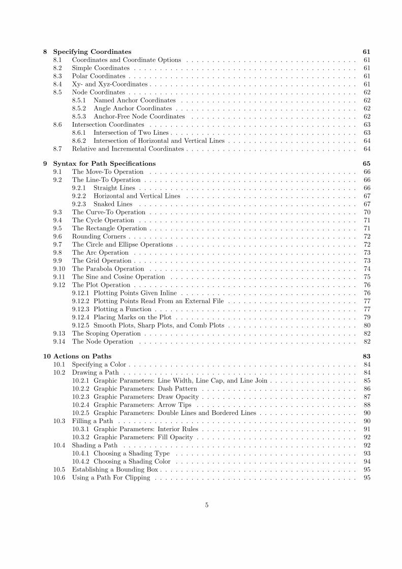
3.1 Problem Statement

Karl wants to put a graphic on the next worksheet for his students. He is currently teaching his students aboutsine and cosine. What he would like to have is something that looks like this (ideally):

.

.

x

.

y

.

−1

.

−12

.

1

.

−1

.

−12

.

12

.

1

.

α

.

sinα

.

cos α

.

tanα =sinα

cos α

.

The angle α is 30◦ in the example(π/6 in radians). The sine of α, whichis the height of the red line, is

sinα = 1/2.

By the Theorem of Pythagoras wehave cos2 α + sin2 α = 1. Thus thelength of the blue line, which is thecosine of α, must be

cos α =√

1 − 1/4 = 12

√3.

This shows that tanα, which is theheight of the orange line, is

tanα =sinα

cos α= 1/

√3.

3.2 Setting up the Environment

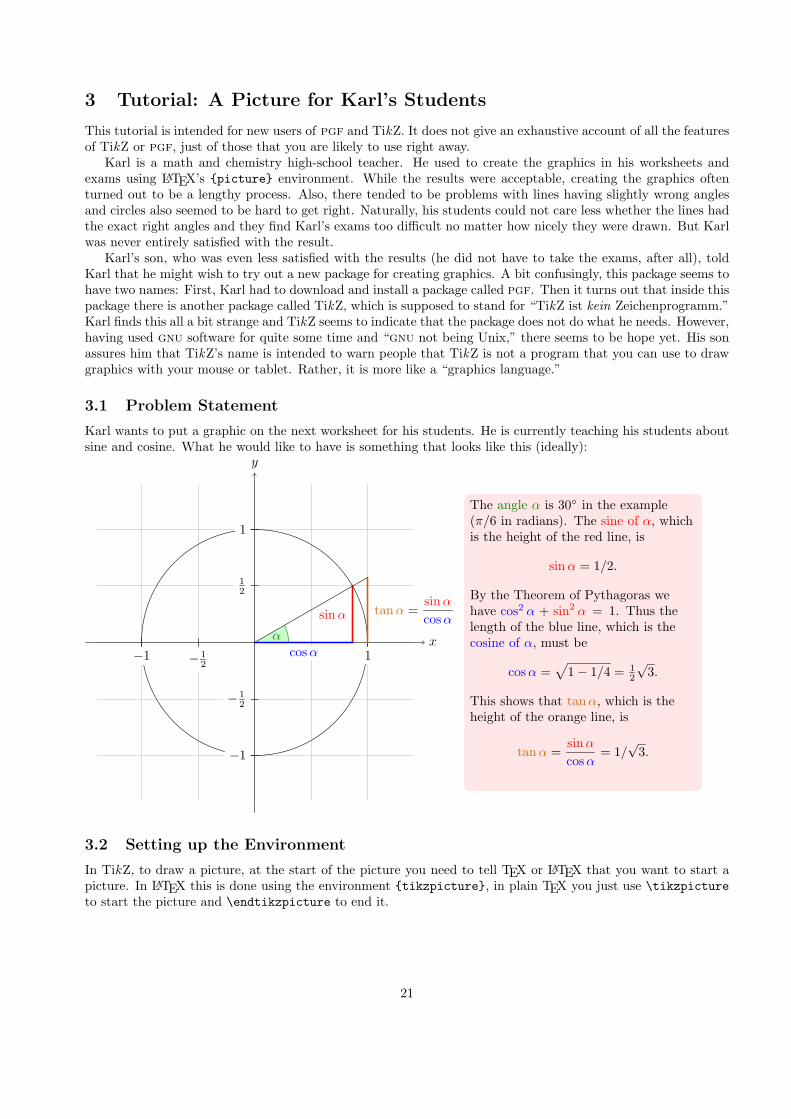
In TikZ, to draw a picture, at the start of the picture you need to tell TEX or LATEX that you want to start apicture. In LATEX this is done using the environment {tikzpicture}, in plain TEX you just use \tikzpictureto start the picture and \endtikzpicture to end it.

21

3.2.1 Setting up the Environment in LATEX

Karl, being a LATEX user, thus sets up his file as follows:

\documentclass{article} % say

\usepackage{tikz}

\begin{document}

We are working on

\begin{tikzpicture}

\draw (-1.5,0) -- (1.5,0);

\draw (0,-1.5) -- (0,1.5);

\end{tikzpicture}.

\end{document}

When executed, that is, run via pdflatex or via latex followed by dvips, the resulting will contain somethingthat looks like this:

We are working on

.

.

We are working on

\begin{tikzpicture}

\draw (-1.5,0) -- (1.5,0);

\draw (0,-1.5) -- (0,1.5);

\end{tikzpicture}.

Admittedly, not quite the whole picture, yet, but we do have the axes established. Well, not quite, but wehave the lines that make up the axes drawn. Karl suddenly has a sinking feeling that the picture is still someway off.

Let’s have a more detailed look at the code. First, the package tikz is loaded. This package is a so-called“frontend” to the basic pgf system. The basic layer, which is also described in this manual, is somewhat more,well, basic and thus harder to use. The frontend makes things easier by providing a simpler syntax.

Inside the environment there are two \draw commands. They mean: “The path, which is specified followingthe command up to the semicolon, should be drawn.” The first path is specified as (-1.5,0) -- (0,1.5),which means “a straight line from the point at position (−1.5, 0) to the point at position (0, 1.5).” Here, thepositions are specified within a special coordinate system in which, initially, one unit is 1cm.

Karl is quite pleased to note that the environment automatically reserves enough space to encompass thepicture.

3.2.2 Setting up the Environment in Plain TEX

Karl’s wife Gerda, who also happens to be a math teacher, is not a LATEX user, but uses plain TEX sinceshe prefers to do things “the old way.” She can also use TikZ. Instead of \usepackage{tikz} she hasto write \input tikz.tex and instead of \begin{tikzpicture} she writes \tikzpicture and instead of\end{tikzpicture} she writes \endtikzpicture.

Thus, she would use:

%% Plain TeX file

\input tikz.tex

\baselineskip=12pt

\hsize=6.3truein

\vsize=8.7truein

We are working on

\tikzpicture

\draw (-1.5,0) -- (1.5,0);

\draw (0,-1.5) -- (0,1.5);

\endtikzpicture.

\bye

Gerda can typeset this file using either pdftex or tex together with dvips. TikZ will automatically discernwhich driver she is using. If she wishes to use dvipdfm together with tex, she either needs to modify the filepgf.cfg or can write \def\pgfsysdriver{pgfsys-dvipdfm.def} somewhere before she inputs tikz.tex orpgf.tex.

22

3.3 Straight Path Construction

The basic building block of all pictures in TikZ is the path. A path is a series of straight lines and curves that areconnected (that is not the whole picture, but let us ignore the complications for the moment). You start a pathby specifying the coordinates of the start position as a point in round brackets, as in (0,0). This is followedby a series of “path extension operations.” The simplest is --, which we used already. It must be followed byanother coordinate and it extends the path in a straight line to this new position. For example, if we were toturn the two paths of the axes into one path, the following would result:

.

\tikz \draw (-1.5,0) -- (1.5,0) -- (0,-1.5) -- (0,1.5);

Karl is a bit confused by the fact that there is no {tikzpicture} environment, here. Instead, the littlecommand \tikz is used. This command either takes one argument (starting with an opening brace as in\tikz{\draw (0,0) -- (1.5,0)}, which yields

.

) or collects everything up to the next semicolon andputs it inside a {tikzpicture} environment. As a rule of thumb, all TikZ graphic drawing commands mustoccur as an argument of \tikz or inside a {tikzpicture} environment. Fortunately, the command \draw willonly be defined inside this environment, so there is little chance that you will accidentally do something wronghere.

3.4 Curved Path Construction

The next thing Karl wants to do is to draw the circle. For this, straight lines obviously will not do. Instead,we need some way to draw curves. For this, TikZ provides a special syntax. One or two “control points” areneeded. The math behind them is not quite trivial, but here is the basic idea: Suppose you are at point x andthe first control point is y. Then the curve will start “going in the direction of y at x,” that is, the tangent ofthe curve at x will point toward y. Next, suppose the curve should end at z and the second support point is w.Then the curve will, indeed, end at z and the tangent of the curve at point z will go through w.

Here is an example (the control points have been added for clarity):

.

\begin{tikzpicture}

\filldraw [gray] (0,0) circle (2pt)

(1,1) circle (2pt)

(2,1) circle (2pt)

(2,0) circle (2pt);

\draw (0,0) .. controls (1,1) and (2,1) .. (2,0);

\end{tikzpicture}

The general syntax for extending a path in a “curved” way is .. controls ⟨first control point⟩ and ⟨secondcontrol point⟩ .. ⟨end point⟩. You can leave out the and ⟨second control point⟩, which causes the first one to beused twice.

So, Karl can now add the first half circle to the picture:

.

\begin{tikzpicture}

\draw (-1.5,0) -- (1.5,0);

\draw (0,-1.5) -- (0,1.5);

\draw (-1,0) .. controls (-1,0.555) and (-0.555,1) .. (0,1)

.. controls (0.555,1) and (1,0.555) .. (1,0);

\end{tikzpicture}

Karl is happy with the result, but finds specifying circles in this way to be extremely awkward. Fortunately,there is a much simpler way.

23

3.5 Circle Path Construction

In order to draw a circle, the path construction operation circle can be used. This operation is followed by aradius in round brackets as in the following example: (Note that the previous position is used as the center ofthe circle.)

.

\tikz \draw (0,0) circle (10pt);

You can also append an ellipse to the path using the ellipse operation. Instead of a single radius you canspecify two of them, one for the x-direction and one for the y-direction, separated by and:

.

\tikz \draw (0,0) ellipse (20pt and 10pt);

To draw an ellipse whose axes are not horizontal and vertical, but point in an arbitrary direction (a “turnedellipse” like

.

) you can use transformations, which are explained later. The code for the little ellipse is\tikz \draw[rotate=30] (0,0) ellipse (6pt and 3pt);, by the way.

So, returning to Karl’s problem, he can write \draw (0,0) circle (1cm); to draw the circle:

.

\begin{tikzpicture}

\draw (-1.5,0) -- (1.5,0);

\draw (0,-1.5) -- (0,1.5);

\draw (0,0) circle (1cm);

\end{tikzpicture}

At this point, Karl is a bit alarmed that the circle is so small when he wants the final picture to be muchbigger. He is pleased to learn that TikZ has powerful transformation options and scaling everything by a factorof three is very easy. But let us leave the size as it is for the moment to save some space.

3.6 Rectangle Path Construction

The next things we would like to have is the grid in the background. There are several ways to produce it. Forexample, one might draw lots of rectangles. Since rectangles are so common, there is a special syntax for them:To add a rectangle to the current path, use the rectangle path construction operation. This operation shouldbe followed by another coordinate and will append a rectangle to the path such that the previous coordinateand the next coordinates are corners of the rectangle. So, let us add two rectangles to the picture:

.

\begin{tikzpicture}

\draw (-1.5,0) -- (1.5,0);

\draw (0,-1.5) -- (0,1.5);


\draw (0,0) rectangle (0.5,0.5);

\draw (-0.5,-0.5) rectangle (-1,-1);

\end{tikzpicture}

While this may be nice in other situations, this is not really leading anywhere with Karl’s problem: First,we would need an awful lot of these rectangles and then there is the border that is not “closed.”

So, Karl is about to resort to simply drawing four vertical and four horizontal lines using the nice \drawcommand, when he learns that there is a grid path construction operation.

3.7 Grid Path Construction

The grid path operation adds a grid to the current path. It will add lines making up a grid that fills the rectanglewhose one corner is the current point and whose other corner is the point following the grid operation. For

24

example, the code \tikz \draw[step=2pt] (0,0) grid (10pt,10pt); produces

.

. Note how the optionalargument for \draw can be used to specify a grid width (there are also xstep and ystep to define the steppingsindependently). As Karl will learn soon, there are lots of things that can be influenced using such options.

For Karl, the following code could be used:

.

\begin{tikzpicture}

\draw (-1.5,0) -- (1.5,0);

\draw (0,-1.5) -- (0,1.5);


\draw[step=.5cm] (-1.4,-1.4) grid (1.4,1.4);

\end{tikzpicture}

Having another look at the desired picture, Karl notices that it would be nice for the grid to be more subdued.(His son told him that grids tend to be distracting if they are not subdued.) To subdue the grid, Karl addstwo more options to the \draw command that draws the grid. First, he uses the color gray for the grid lines.Second, he reduces the line width to very thin. Finally, he swaps the ordering of the commands so that thegrid is drawn first and everything else on top.

.

\begin{tikzpicture}

\draw[step=.5cm,gray,very thin] (-1.4,-1.4) grid (1.4,1.4);

\draw (-1.5,0) -- (1.5,0);

\draw (0,-1.5) -- (0,1.5);


\end{tikzpicture}

3.8 Adding a Touch of Style

Instead of the options gray,very thin Karl could also have said style=help lines. Styles are predefined setsof options that can be used to organize how a graphic is drawn. By saying style=help lines you say “use thestyle that I (or someone else) has set for drawing help lines.” If Karl decides, at some later point, that gridsshould be drawn, say, using the color blue!50 instead of gray, he could say the following:

\tikzstyle help lines=[color=blue!50,very thin]

Alternatively, he could have said the following:

\tikzstyle help lines+=[color=blue!50]

This would have added the color=blue!50 option. The help lines style would now contain two coloroptions, but the second would override the first.

Using styles makes your graphics code more flexible. You can change the way things look easily in a consistentmanner.

To build a hierarchy of styles you can have one style use another. So in order to define a style Karl’s gridthat is based on the grid style Karl could say

\tikzstyle Karl’s grid=[style=help lines,color=blue!50]

...

\draw[style=Karl’s grid] (0,0) grid (5,5);

You can also leave out the style=. Thus, whenever TikZ encounters an options that it does not know about,it will check whether this option happens to be the name of a style. If so, the style is used. Thus, Karl couldalso have written:

\tikzstyle Karl’s grid=[help lines,color=blue!50]

...

\draw[Karl’s grid] (0,0) grid (5,5);

25

For some styles, like the very thin style, it is pretty clear what the style does and there is no need to saystyle=very thin. For other styles, like help lines, it seems more natural to me to say style=help lines.But, mainly, this is a matter of taste.

3.9 Drawing Options

Karl wonders what other options there are that influence how a path is drawn. He saw already that thecolor=⟨color⟩ option can be used to set the line’s color. The option draw=⟨color⟩ does nearly the same, only itsets the color for the lines only and a different color can be used for filling (Karl will need this when he fills thearc for the angle).

He saw that the style very thin yields very thin lines. Karl is not really surprised by this and neither ishe surprised to learn that thin yields thin lines, thick yields thick lines, very thick yields very thick lines,ultra thick yields really, really thick lines and ultra thin yields lines that are so thin that low-resolutionprinters and displays will have trouble showing them. He wonders what gives lines of “normal” thickness. Itturns out that thin is the correct choice. This seems strange to Karl, but his son explains him that LATEXhas two commands called \thinlines and \thicklines and that \thinlines gives the line width of “normal”lines, more precisely, of the thickness that, say, the stem of a letter like “T” or “i” has. Nevertheless, Karl wouldlike to know whether there is anything “in the middle” between thin and thick. There is: semithick.

Another useful thing one can do with lines is to dash or dot them. For this, the two styles dashed and dottedcan be used, yielding

.

and

.

. Both options also exist in a loose and a dense version, called loosely dashed,densely dashed, loosely dotted, and densely dotted. If he really, really needs to, Karl can also definemuch more complex dashing patterns with the dash pattern option, but his son insists that dashing is to beused with utmost care and mostly distracts. Karl’s son claims that complicated dashing patterns are evil. Karl’sstudents do not care about dashing patterns.

3.10 Arc Path Construction

Our next obstacle is to draw the arc for the angle. For this, the arc path construction operation is useful, whichdraws part of a circle or ellipse. This arc operation must be followed by a triple in rounded brackets, where thecomponents of the triple are separated by colons. The first two components are angles, the last one is a radius.An example would be (10:80:10pt), which means “an arc from 10 degrees to 80 degrees on a circle of radius10pt.” Karl obviously needs an arc from 0◦ to 30◦. The radius should be something relatively small, perhapsaround one third of the circle’s radius. This gives: (0:30:3mm).

When one uses the arc path construction operation, the specified arc will be added with its starting point atthe current position. So, we first have to “get there.”

.

\begin{tikzpicture}


\draw (-1.5,0) -- (1.5,0);

\draw (0,-1.5) -- (0,1.5);


\draw (3mm,0mm) arc (0:30:3mm);

\end{tikzpicture}

Karl thinks this is really a bit small and he cannot continue unless he learns how to do scaling. For this, hecan add the [scale=3] option. He could add this option to each \draw command, but that would be awkward.Instead, he adds it to the whole environment, which causes this option to apply to everything within.

26

.

\begin{tikzpicture}[scale=3]


\draw (-1.5,0) -- (1.5,0);

\draw (0,-1.5) -- (0,1.5);



\end{tikzpicture}

As for circles, you can specify “two” radii in order to get an elliptical arc.

.

\tikz \draw (0,0) arc (0:315:1.75cm and 1cm);

3.11 Clipping a Path

In order to save space in this manual, it would be nice to clip Karl’s graphics a bit so that we can focus on the“interesting” parts. Clipping is pretty easy in TikZ. You can use the \clip command clip all subsequent drawing.It works like \draw, only it does not draw anything, but uses the given path to clip everything subsequently.

.


\clip (-0.1,-0.2) rectangle (1.1,0.75);


\draw (-1.5,0) -- (1.5,0);

\draw (0,-1.5) -- (0,1.5);



\end{tikzpicture}

You can also do both at the same time: Draw and clip a path. For this, use the \draw command and addthe clip option. (This is not the whole picture: You can also use the \clip command and add the draw option.Well, that is also not the whole picture: In reality, \draw is just a shorthand for \path[draw] and \clip is ashorthand for \path[clip] and you could also say \path[draw,clip].) Here is an example:

27

.


\clip[draw] (0.5,0.5) circle (.6cm);


\draw (-1.5,0) -- (1.5,0);

\draw (0,-1.5) -- (0,1.5);



\end{tikzpicture}

3.12 Parabola and Sine Path Construction

Although Karl does not need them for his picture, he is pleased to learn that there are parabola and sin andcos path operations for adding parabolas and sine and cosine curves to the current path. For the parabolaoperation, the current point will lie on the parabola as well as the point given after the parabola operation.Consider the following example:

.

\tikz \draw (0,0) rectangle (1,1) (0,0) parabola (1,1);

It is also possible to place the bend somewhere else:

.

\tikz \draw[x=1pt,y=1pt] (0,0) parabola bend (4,16) (6,12);

The operations sin and cos add a sine or cosine curve in the interval [0, π/2] such that the previous currentpoint is at the start of the curve and the curve ends at the given end point. Here are two examples:

A sine

.

curve. A sine \tikz \draw[x=1ex,y=1ex] (0,0) sin (1.57,1); curve.

.

\tikz \draw[x=1.57ex,y=1ex] (0,0) sin (1,1) cos (2,0) sin (3,-1) cos (4,0)

(0,1) cos (1,0) sin (2,-1) cos (3,0) sin (4,1);

3.13 Filling and Drawing

Returning to the picture, Karl now wants the angle to be “filled” with a very light green. For this he uses \fillinstead of \draw. Here is what Karl does:

.


\clip (-0.1,-0.2) rectangle (1.1,0.75);


\draw (-1.5,0) -- (1.5,0);

\draw (0,-1.5) -- (0,1.5);


\fill[green!20!white] (0,0) -- (3mm,0mm) arc (0:30:3mm) -- (0,0);

\end{tikzpicture}

The color green!20!white means 20% green and 80% white mixed together. Such color expression arepossible since pgf uses Uwe Kern’s xcolor package, see the documentation of that package for details on colorexpressions.

What would have happened, if Karl had not “closed” the path using --(0,0) at the end? In this case, thepath is closed automatically, so this could have been omitted. Indeed, it would even have been better to writethe following, instead:

\fill[green!20!white] (0,0) -- (3mm,0mm) arc (0:30:3mm) -- cycle;

The --cycle causes the current path to be closed (actually the current part of the current path) by smoothlyjoining the first and last point. To appreciate the difference, consider the following example:

28

.

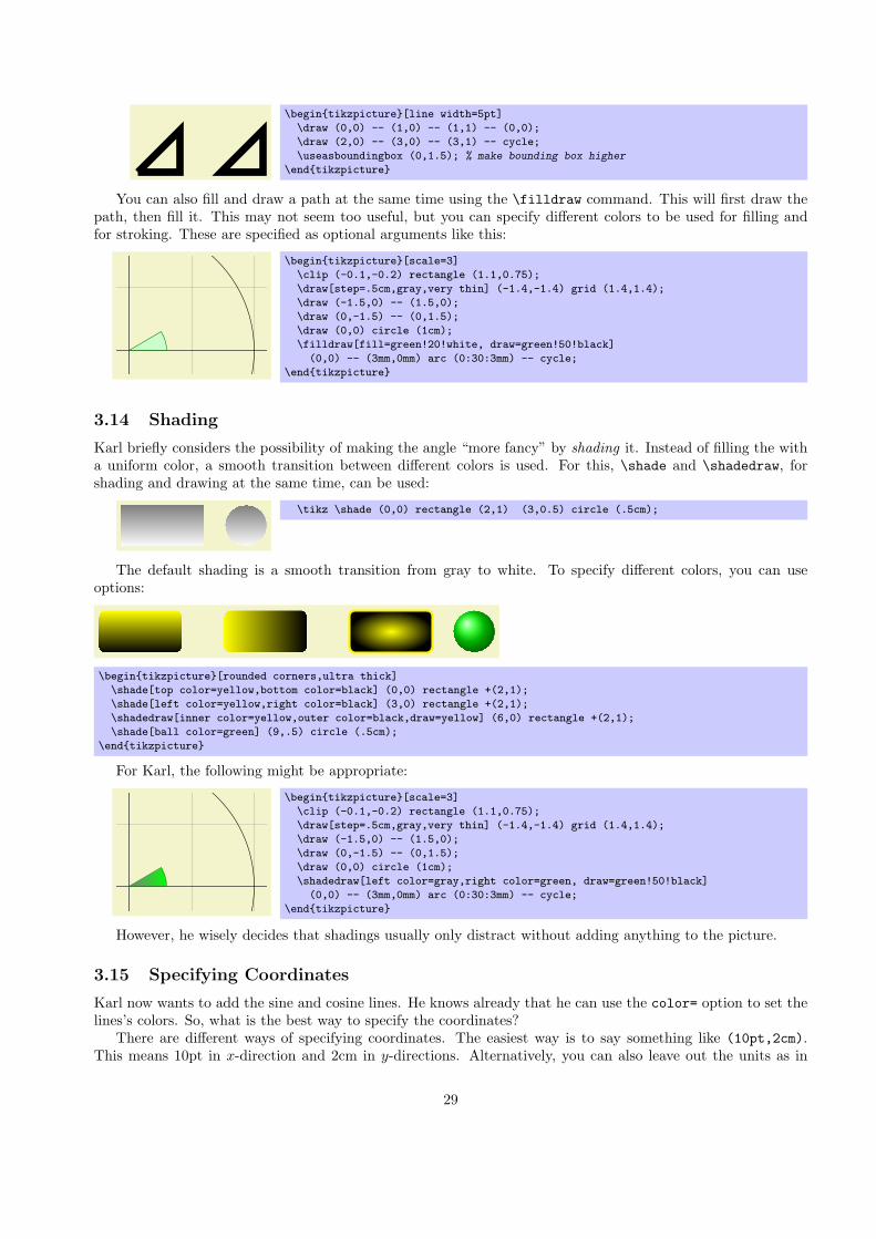
\begin{tikzpicture}[line width=5pt]

\draw (0,0) -- (1,0) -- (1,1) -- (0,0);

\draw (2,0) -- (3,0) -- (3,1) -- cycle;

\useasboundingbox (0,1.5); % make bounding box higher

\end{tikzpicture}

You can also fill and draw a path at the same time using the \filldraw command. This will first draw thepath, then fill it. This may not seem too useful, but you can specify different colors to be used for filling andfor stroking. These are specified as optional arguments like this:

.


\clip (-0.1,-0.2) rectangle (1.1,0.75);


\draw (-1.5,0) -- (1.5,0);

\draw (0,-1.5) -- (0,1.5);


\filldraw[fill=green!20!white, draw=green!50!black]

(0,0) -- (3mm,0mm) arc (0:30:3mm) -- cycle;

\end{tikzpicture}

3.14 Shading

Karl briefly considers the possibility of making the angle “more fancy” by shading it. Instead of filling the witha uniform color, a smooth transition between different colors is used. For this, \shade and \shadedraw, forshading and drawing at the same time, can be used:

.

.

\tikz \shade (0,0) rectangle (2,1) (3,0.5) circle (.5cm);

The default shading is a smooth transition from gray to white. To specify different colors, you can useoptions:

.

.

.

. .

\begin{tikzpicture}[rounded corners,ultra thick]

\shade[top color=yellow,bottom color=black] (0,0) rectangle +(2,1);

\shade[left color=yellow,right color=black] (3,0) rectangle +(2,1);

\shadedraw[inner color=yellow,outer color=black,draw=yellow] (6,0) rectangle +(2,1);

\shade[ball color=green] (9,.5) circle (.5cm);

\end{tikzpicture}

For Karl, the following might be appropriate:

.

.


\clip (-0.1,-0.2) rectangle (1.1,0.75);


\draw (-1.5,0) -- (1.5,0);

\draw (0,-1.5) -- (0,1.5);


\shadedraw[left color=gray,right color=green, draw=green!50!black]

(0,0) -- (3mm,0mm) arc (0:30:3mm) -- cycle;

\end{tikzpicture}

However, he wisely decides that shadings usually only distract without adding anything to the picture.

3.15 Specifying Coordinates

Karl now wants to add the sine and cosine lines. He knows already that he can use the color= option to set thelines’s colors. So, what is the best way to specify the coordinates?

There are different ways of specifying coordinates. The easiest way is to say something like (10pt,2cm).This means 10pt in x-direction and 2cm in y-directions. Alternatively, you can also leave out the units as in

29

(1,2), which means “one times the current x-vector plus twice the current y-vector.” These vectors default to1cm in the x-direction and 1cm in the y-direction, respectively.

In order to specify points in polar coordinates, use the notation (30:1cm), which means 1cm in direction 30degree. This is obviously quite useful to “get to the point (cos 30◦, sin 30◦) on the circle.”

You can add a single + sign in front of a coordinate or two of them as in +(1cm,0cm) or ++(0cm,2cm).Such coordinates are interpreted differently: The first form means “1cm upwards from the previous specifiedposition” and the second means “2cm to the right of the previous specified position, making this the new specifiedposition.” For example, we can draw the sine line as follows:

.


\clip (-0.1,-0.2) rectangle (1.1,0.75);


\draw (-1.5,0) -- (1.5,0);

\draw (0,-1.5) -- (0,1.5);


\filldraw[fill=green!20,draw=green!50!black]

(0,0) -- (3mm,0mm) arc (0:30:3mm) -- cycle;

\draw[red,very thick] (30:1cm) -- +(0,-0.5);

\end{tikzpicture}

Karl used the fact sin 30◦ = 1/2. However, he very much doubts that his students know this, so it would benice to have a way of specifying “the point straight down from (30:1cm) that lies on the x-axis.” This is, indeed,possible using a special syntax: Karl can write (30:1cm |- 0,0). In general, the meaning of (⟨p⟩ |- ⟨q⟩) is“the intersection of a vertical line through p and a horizontal line through q.”

Next, let us draw the cosine line. One way would be to say (30:1cm |- 0,0) -- (0,0). Another way isthe following: we “continue” from where the sine ends:

.


\clip (-0.1,-0.2) rectangle (1.1,0.75);


\draw (-1.5,0) -- (1.5,0);

\draw (0,-1.5) -- (0,1.5);


\filldraw[fill=green!20,draw=green!50!black] (0,0) -- (3mm,0mm) arc

(0:30:3mm) -- cycle;


\draw[blue,very thick] (30:1cm) ++(0,-0.5) -- (0,0);

\end{tikzpicture}

Note the there is no -- between (30:1cm) and +(0,-0.5). In detail, this path is interpreted as follows: “First,the (30:1cm) tells me to move by pen to (cos 30◦, 1/2). Next, there comes another coordinate specification, soI move my pen there without drawing anything. This new point is half a unit down from the last position, thusit is at (cos 30◦, 0). Finally, I move the pen to the origin, but this time drawing something (because of the --).”

To appreciate the difference between + and ++ consider the following example:

.

\begin{tikzpicture}

\def\rectanglepath{-- ++(1cm,0cm) -- ++(0cm,1cm) -- ++(-1cm,0cm) -- cycle}

\draw (0,0) \rectanglepath;

\draw (1.5,0) \rectanglepath;

\end{tikzpicture}

By comparison, when using a single +, the coordinates are different:

.

\begin{tikzpicture}

\def\rectanglepath{-- +(1cm,0cm) -- +(1cm,1cm) -- +(0cm,1cm) -- cycle}

\draw (0,0) \rectanglepath;

\draw (1.5,0) \rectanglepath;

\end{tikzpicture}

Naturally, all of this could have been written more clearly and more economically like this (either with asingle of a double +):

.

\tikz \draw (0,0) rectangle +(1,1) (1.5,0) rectangle +(1,1);

30

Karl is left with the line for tanα, which seems difficult to specify using transformations and polar coordinates.For this he needs another way of specifying coordinates: Karl can specify intersections of lines as coordinates.The line for tanα starts at (1, 0) and goes upward to a point that is at the intersection of a line going “up” anda line going from the origin through (30:1cm). The syntax for this point is the following:

\draw[very thick,orange] (1,0) -- (intersection of 1,0--1,1 and 0,0--30:1cm);

In the following, two final examples of how to use relative positioning are presented. Note that the transfor-mation options, which are explained later, are often more useful for shifting than relative positioning.

.

\begin{tikzpicture}[scale=0.5]

\draw (0,0) -- (90:1cm) arc (90:360:1cm) arc (0:30:1cm) -- cycle;

\draw (60:5pt) -- +(30:1cm) arc (30:90:1cm) -- cycle;

\draw (3,0) +(0:1cm) -- +(72:1cm) -- +(144:1cm) -- +(216:1cm) --

+(288:1cm) -- cycle;

\end{tikzpicture}

3.16 Adding Arrow Tips

Karl now wants to add the little arrow tips at the end of the axes. He has noticed that in many plots, evenin scientific journals, these arrow tips seem to missing, presumably because the generating programs cannotproduce them. Karl thinks arrow tips belong at the end of axes. His son agrees. His students do not care aboutarrow tips.

It turns out that adding arrow tips is pretty easy: Karl adds the option -> to the drawing commands for theaxes:

.


\clip (-0.1,-0.2) rectangle (1.1,1.51);


\draw[->] (-1.5,0) -- (1.5,0);

\draw[->] (0,-1.5) -- (0,1.5);



(0:30:3mm) -- cycle;


\draw[blue,very thick] (30:1cm) ++(0,-0.5) -- (0,0);

\draw[orange,very thick] (1,0) -- (intersection of 1,0--1,1 and 0,0--30:1cm);

\end{tikzpicture}

If Karl had used the option <- instead of ->, arrow tips would have been put at the beginning of the path.The option <-> puts arrow tips at both ends of the path.

There are certain restrictions to the kind of paths to which arrow tips can be added. As a rule of thumb, youcan add arrow tips only to a single open “line.” For example, you should not try to add tips to, say, a rectangleor a circle. (You can try, but no guarantees as to what will happen now or in future versions.) However, youcan add arrow tips to curved paths and to paths that have several segments, as in the following examples:

.

\begin{tikzpicture}

\draw [<->] (0,0) arc (180:30:10pt);

\draw [<->] (1,0) -- (1.5cm,10pt) -- (2cm,0pt) -- (2.5cm,10pt);

\end{tikzpicture}

Karl has a more detailed look at the arrow that TikZ puts at the end. It looks like this when he zoomsit:

.

. The shape seems vaguely familiar and, indeed, this is exactly the end of TEX’s standard arrow used insomething like f : A → B.

Karl likes the arrow, especially since it is not “as thick” as the arrows offered by many other packages.However, he expects that, sometimes, he might need to use some other kinds of arrow. To do so, Karl can say>=⟨right arrow tip kind⟩, where ⟨right arrow tip kind⟩ is a special arrow tip specification. For example, if Karlsays >=stealth, then he tells TikZ that he would like “stealth-fighter-like” arrow tips:

31

.

\begin{tikzpicture}[>=stealth]

\draw [->] (0,0) arc (180:30:10pt);

\draw [<<-,very thick] (1,0) -- (1.5cm,10pt) -- (2cm,0pt) -- (2.5cm,10pt);

\end{tikzpicture}

Karl wonders whether such a military name for the arrow type is really necessary. He is not really mollifiedwhen his son tells him that Microsoft’s PowerPoint uses the same name. He decides to have his students discussthis at some point.

In addition to stealth there are several other predefined arrow tip kinds Karl can choose from, see Sec-tion 14.1. Furthermore, he can define arrows types himself, if he needs new ones.

3.17 Scoping

Karl saw already that there are numerous graphic options that affect how paths are rendered. Often, he wouldlike to apply certain options to a whole set of graphic commands. For example, Karl might wish to draw threepaths using a thick pen, but would like everything else to be drawn “normally.”

If Karl wishes to set a certain graphic option for the whole picture, he can simply pass this option to the \tikzcommand or to the {tikzpicture} environment (Gerda would pass the options to \tikzpicture). However,if Karl wants to apply graphic options to a local group, he put these commands inside a {scope} environment(Gerda uses \scope and \endscope). This environment takes graphic options as an optional argument andthese options apply to everything inside the scope, but not to anything outside.

Here is an example:

.

\begin{tikzpicture}[ultra thick]

\draw (0,0) -- (0,1);

\begin{scope}[thin]

\draw (1,0) -- (1,1);

\draw (2,0) -- (2,1);

\end{scope}

\draw (3,0) -- (3,1);

\end{tikzpicture}

Scoping has another interesting effect: Any changes to the clipping area are local to the scope. Thus, if yousay \clip somewhere inside a scope, the effect of the \clip command ends at the end of the scope. This isuseful since there is no other way of “enlarging” the clipping area.

Karl has also already seen that giving options to commands like \draw apply only to that command.In turns out that the situation is slightly more complex. First, options to a command like \draw arenot really options to the command, but they are “path options” and can be given anywhere on thepath. So, instead of \draw[thin] (0,0) -- (1,0); one can also write \draw (0,0) [thin] -- (1,0); or\draw (0,0) -- (1,0) [thin];; all of these have the same effect. This might seem strange since in the lastcase, it would appear that the thin should take effect only “after” the line from (0, 0) to (1, 0) has been draw.However, most graphic options only apply to the whole path. Indeed, if you say both thin and thick on thesame path, the last option given will “win.”

When reading the above, Karl notices that only “most” graphic options apply to the whole path. Indeed, alltransformation options do not apply to the whole path, but only to “everything following them on the path.”We will have a more detailed look at this in a moment. Nevertheless, all options given during a path constructionapply only to this path.

3.18 Transformations

When you specify a coordinate like (1cm,1cm), where is that coordinate placed on the page? To determine theposition, TikZ, TEX, and pdf or PostScript all apply certain transformations to the given coordinate in orderto determine the finally position on the page.

TikZ provides numerous options that allow you to transform coordinates in pgf’s private coordinate system.For example, the xshift option allows you to shift all subsequent points by a certain amount:

.

\tikz \draw (0,0) -- (0,0.5) [xshift=2pt] (0,0) -- (0,0.5);

32

It is important to note that you can change transformation “in the middle of a path,” a feature that is notsupported by pdf or PostScript. The reason is that pgf keeps track of its own transformation matrix.

Here is a more complicated example:

.

\begin{tikzpicture}[even odd rule,rounded corners=2pt,x=10pt,y=10pt]

\filldraw[fill=examplefill] (0,0) rectangle (1,1)

[xshift=5pt,yshift=5pt] (0,0) rectangle (1,1)

[rotate=30] (-1,-1) rectangle (2,2);

\end{tikzpicture}

The most useful transformations are xshift and yshift for shifting, shift for shifting to a given point asin shift={(1,0)} or shift={+(0,0)} (the braces are necessary so that TEX does not mistake the comma forseparating options), rotate for rotating by a certain angle (there is also a rotate around for rotating arounda given point), scale for scaling by a certain factor, xscale and yscale for scaling only in the x- or y-direction(xscale=-1 is a flip), and xslant and yslant for slanting. If these transformation and those that I have notmentioned are not sufficient, the cm option allows you to apply an arbitrary transformation matrix. Karl’sstudents, by the way, do not know what a transformation matrix is.

3.19 Repeating Things: For-Loops

Karl’s next aim is to add little ticks on the axes at positions −1, −1/2, 1/2, and 1. For this, it would be nice touse some kind of “loop,” especially since he wishes to do the same thing at each of these positions. There aredifferent packages for doing this. LATEX has its own internal command for this, pstricks comes along with thepowerful \mulitdo command. All of these can be used together with pgf and TikZ, so if you are familiar withthem, feel free to use them. pgf introduces yet another command, called \foreach, which I introduced since Icould never remember the syntax of the other packages. \foreach is defined in the package pgffor and can beused independently of pgf. TikZ includes it automatically.

In its basic form, the \foreach command is easy to use:

x = 1, x = 2, x = 3, \foreach \x in {1,2,3} {$x =\x$, }

The general syntax is \foreach ⟨variable⟩ in {⟨list of values⟩} ⟨commands⟩. Inside the ⟨commands⟩, the⟨variable⟩ will be assigned to the different values. If the ⟨commands⟩ do not start with a brace, everything upto the next semicolon is used as ⟨commands⟩.

For Karl and the ticks on the axes, he could use the following code:

.


\clip (-0.1,-0.2) rectangle (1.1,1.51);



(0:30:3mm) -- cycle;

\draw[->] (-1.5,0) -- (1.5,0);

\draw[->] (0,-1.5) -- (0,1.5);


\foreach \x in {-1cm,-0.5cm,1cm}

\draw (\x,-1pt) -- (\x,1pt);

\foreach \y in {-1cm,-0.5cm,0.5cm,1cm}

\draw (-1pt,\y) -- (1pt,\y);

\end{tikzpicture}

As a matter of fact, there are many different ways of creating the ticks. For example, Karl could have putthe \draw ...; inside curly braces. He could also have used, say,

\foreach \x in {-1,-0.5,1}

\draw[xshift=\x cm] (0pt,-1pt) -- (0pt,1pt);

Karl is curious what would happen in a more complicated situation where there are, say, 20 ticks. It seemsbothersome to explicitly mention all these numbers in the set for \foreach. Indeed, it is possible to use ...inside the \foreach statement to iterate over a large number of values (which must, however, be dimensionlessreal numbers) as in the following example:

33

.

\tikz \foreach \x in {1,...,10}

\draw (\x,0) circle (0.4cm);

If you provide two numbers before the ..., the \foreach statement will use their difference for the stepping:

.

\tikz \foreach \x in {-1,-0.5,...,1}

\draw (\x cm,-1pt) -- (\x cm,1pt);

We can also nest loops to create interesting effects:

.

.

1,1

.

1,2

.

1,3

.

1,4

.

1,5

.

2,1

.

2,2

.

2,3

.

2,4

.

2,5

.

3,1

.

3,2

.

3,3

.

3,4

.

3,5

.

4,1

.

4,2

.

4,3

.

4,4

.

4,5

.

5,1

.

5,2

.

5,3

.

5,4

.

5,5

.

7,1

.

7,2

.

7,3

.

7,4

.

7,5

.

8,1

.

8,2

.

8,3

.

8,4

.

8,5

.

9,1

.

9,2

.

9,3

.

9,4

.

9,5

.

10,1

.

10,2

.

10,3

.

10,4

.

10,5

.

11,1

.

11,2

.

11,3

.

11,4

.

11,5

.

12,1

.

12,2

.

12,3

.

12,4

.

12,5

\begin{tikzpicture}

\foreach \x in {1,2,...,5,7,8,...,12}

\foreach \y in {1,...,5}

{

\draw (\x,\y) +(-.5,-.5) rectangle ++(.5,.5);

\draw (\x,\y) node{\x,\y};

}

\end{tikzpicture}

The \foreach statement can do even trickier stuff, but the above gives the idea.

3.20 Adding Text

Karl is, by now, quite satisfied with the picture. However, the most important parts, namely the labels, are stillmissing!

TikZ offers an easy-to-use and powerful system for adding text and, more generally, complex shapes to apicture at specific positions. The basic idea is the following: When TikZ is constructing a path and encountersthe keyword node in the middle of a path, it reads a node specification. The keyword node is typically followedby some options and then some text between curly braces. This text is put inside a normal TEX box (if thenode specification directly follows a coordinate, which is usually the case, TikZ is able to perform some magicso that it is even possible to use verbatim text inside the boxes) and then placed at the current position, thatis, at the last specified position (possibly shifted a bit, according to the given options). However, all nodes aredrawn only after the path has been completely drawn/filled/shaded/clipped/whatever.

.

.

Text at node 1

.

Text at node 2\begin{tikzpicture}

\draw (0,0) rectangle (2,2);

\draw (0.5,0.5) node [fill=examplefill]

{Text at \verb!node 1!}

-- (1.5,1.5) node {Text at \verb!node 2!};

\end{tikzpicture}

Obviously, Karl would not only like to place nodes on the last specified position, but also to the left orthe right of these positions. For this, every node object that you put in your picture is equipped with severalanchors. For example, the north anchor is in the middle at the upper end of the shape, the south anchor is at

34

the bottom and the north east anchor is in the upper right corner. When you given the option anchor=north,the text will be placed such that this northern anchor will lie on the current position and the text is, thus, belowthe current position. Karl uses this to draw the ticks as follows:

.

.

−1

.

−0.5

.

1

.

−1

.

−0.5

.

0.5

.

1


\clip (-0.6,-0.2) rectangle (0.6,1.51);

\draw[step=.5cm,style=help lines] (-1.4,-1.4) grid (1.4,1.4);


(0,0) -- (3mm,0mm) arc (0:30:3mm) -- cycle;

\draw[->] (-1.5,0) -- (1.5,0); \draw[->] (0,-1.5) -- (0,1.5);


\foreach \x in {-1,-0.5,1}

\draw (\x cm,1pt) -- (\x cm,-1pt) node[anchor=north] {$\x$};

\foreach \y in {-1,-0.5,0.5,1}

\draw (1pt,\y cm) -- (-1pt,\y cm) node[anchor=east] {$\y$};

\end{tikzpicture}

This is quite nice, already. Using these anchors, Karl can now add most of the other text elements. However,Karl thinks that, though “correct,” it is quite counter-intuitive that in order to place something below a givenpoint, he has to use the north anchor. For this reason, there is an option called below, which does the sameas anchor=north. Similarly, above right does the same as anchor=south east. In addition, below takes anoptional dimension argument. If given, the shape will additionally be shifted downwards by the given amount.So, below=1pt can be used to put a text label below some point and, additionally shift it 1pt downwards.

Karl is not quite satisfied with the ticks. He would like to have 1/2 or 12 shown instead of 0.5, partly to show

off the nice capabilities of TEX and TikZ, partly because for positions like 1/3 or π it is certainly very muchpreferable to have the “mathematical” tick there instead of just the “numeric” tick. His students, on the otherhand, prefer 0.5 over 1/2 since they are not too fond of fractions in general.

Karl now faces a problem: For the \foreach statement, the position \x should still be given as 0.5 sinceTikZ will not know where \frac{1}{2} is supposed to be. On the other hand, the typeset text should reallybe \frac{1}{2}. To solve this problem, \foreach offers a special syntax: Instead of having one variable \x,Karl can specify two (or even more) variables separated by a slash as in \x / \xtext. Then, the elements inthe set over which \foreach iterates must also be of the form ⟨first⟩/⟨second⟩. In each iteration, \x will be setto ⟨first⟩ and \xtext will be set to ⟨second⟩. If no ⟨second⟩ is given, the ⟨first⟩ will be used again. So, here isthe new code for the ticks:

.

.

−1

.

−12

.

1

.

−1

.

−12

.

12

.

1


\clip (-0.6,-0.2) rectangle (0.6,1.51);

\draw[step=.5cm,style=help lines] (-1.4,-1.4) grid (1.4,1.4);


(0,0) -- (3mm,0mm) arc (0:30:3mm) -- cycle;

\draw[->] (-1.5,0) -- (1.5,0); \draw[->] (0,-1.5) -- (0,1.5);


\foreach \x/\xtext in {-1, -0.5/-\frac{1}{2}, 1}

\draw (\x cm,1pt) -- (\x cm,-1pt) node[anchor=north] {$\xtext$};

\foreach \y/\ytext in {-1, -0.5/-\frac{1}{2}, 0.5/\frac{1}{2}, 1}

\draw (1pt,\y cm) -- (-1pt,\y cm) node[anchor=east] {$\ytext$};

\end{tikzpicture}

Karl is quite pleased with the result, but his son points out that this is still not perfectly satisfactory: Thegrid and the circle interfere with the numbers and decrease their legibility. Karl is not very concerned by this (hisstudents do not even notice), but his son insists that there is an easy solution: Karl can add the [fill=white]option to fill out the background of the text shape with a white color.

The next thing Karl wants to do is to add the labels like sinα. For this, he would like to place a label “inthe middle of line.” To do so, instead of specifying the label node {$\sin\alpha$} directly after one of theendpoints of the line (which would place the label at that endpoint), Karl can give the label directly after the

35

--, before the coordinate. By default, this places the label in the middle of the line, but the pos= options canbe used to modify this. Also, options like near start and near end can be used to modify this position:

.

.

sinα

.

cos α

.

tanα =sinα

cos α

.

−1

.

−12

.

1

.

−1

.

−12

.

12

.

1


\clip (-2,-0.2) rectangle (2,0.8);



(0:30:3mm) -- cycle;

\draw[->] (-1.5,0) -- (1.5,0) coordinate (x axis);

\draw[->] (0,-1.5) -- (0,1.5) coordinate (y axis);


\draw[very thick,red]

(30:1cm) -- node[left=1pt,fill=white] {$\sin \alpha$} (30:1cm |- x axis);

\draw[very thick,blue]

(30:1cm |- x axis) -- node[below=2pt,fill=white] {$\cos \alpha$} (0,0);

\draw[very thick,orange] (1,0) -- node [right=1pt,fill=white]

{$\displaystyle \tan \alpha \color{black}=

\frac{{\color{red}\sin \alpha}}{\color{blue}\cos \alpha}$}

(intersection of 0,0--30:1cm and 1,0--1,1) coordinate (t);

\draw (0,0) -- (t);

\foreach \x/\xtext in {-1, -0.5/-\frac{1}{2}, 1}

\draw (\x cm,1pt) -- (\x cm,-1pt) node[anchor=north,fill=white] {$\xtext$};

\foreach \y/\ytext in {-1, -0.5/-\frac{1}{2}, 0.5/\frac{1}{2}, 1}

\draw (1pt,\y cm) -- (-1pt,\y cm) node[anchor=east,fill=white] {$\ytext$};

\end{tikzpicture}

You can also position labels on curves and, by adding the sloped option, have them rotated such that theymatch the line’s slope. Here is an example:

.

.

near start

.

midway

.

very near end

\begin{tikzpicture}

\draw (0,0) .. controls (6,1) and (9,1) ..

node[near start,sloped,above] {near start}

node {midway}

node[very near end,sloped,below] {very near end} (12,0);

\end{tikzpicture}

It remains to draw the explanatory text at the right of the picture. The main difficulty here lies in limitingthe width of the text “label,” which is quite long, so that line breaking is used. Fortunately, Karl can use theoption text width=6cm to get the desired effect. So, here is the full code:

36

\begin{tikzpicture}[scale=3,cap=round]

% Local definitions

\def\costhirty{0.8660256}

% Colors

\colorlet{anglecolor}{green!50!black}

\colorlet{sincolor}{red}

\colorlet{tancolor}{orange!80!black}

\colorlet{coscolor}{blue}

% Styles

\tikzstyle{axes}=[]

\tikzstyle{important line}=[very thick]

\tikzstyle{information text}=[rounded corners,fill=red!10,inner sep=1ex]

% The graphic

\draw[style=help lines,step=0.5cm] (-1.4,-1.4) grid (1.4,1.4);


\begin{scope}[style=axes]

\draw[->] (-1.5,0) -- (1.5,0) node[right] {$x$} coordinate(x axis);

\draw[->] (0,-1.5) -- (0,1.5) node[above] {$y$} coordinate(y axis);

\foreach \x/\xtext in {-1, -.5/-\frac{1}{2}, 1}

\draw[xshift=\x cm] (0pt,1pt) -- (0pt,-1pt) node[below,fill=white] {$\xtext$};

\foreach \y/\ytext in {-1, -.5/-\frac{1}{2}, .5/\frac{1}{2}, 1}

\draw[yshift=\y cm] (1pt,0pt) -- (-1pt,0pt) node[left,fill=white] {$\ytext$};

\end{scope}

\filldraw[fill=green!20,draw=anglecolor] (0,0) -- (3mm,0pt) arc(0:30:3mm);

\draw (15:2mm) node[anglecolor] {$\alpha$};

\draw[style=important line,sincolor]

(30:1cm) -- node[left=1pt,fill=white] {$\sin \alpha$} (30:1cm |- x axis);

\draw[style=important line,coscolor]

(30:1cm |- x axis) -- node[below=2pt,fill=white] {$\cos \alpha$} (0,0);

\draw[style=important line,tancolor] (1,0) -- node[right=1pt,fill=white] {

$\displaystyle \tan \alpha \color{black}=

\frac{{\color{sincolor}\sin \alpha}}{\color{coscolor}\cos \alpha}$}

(intersection of 0,0--30:1cm and 1,0--1,1) coordinate (t);

\draw (0,0) -- (t);

\draw[xshift=1.85cm]

node[right,text width=6cm,style=information text]

{

The {\color{anglecolor} angle $\alpha$} is $30^\circ$ in the

example ($\pi/6$ in radians). The {\color{sincolor}sine of

$\alpha$}, which is the height of the red line, is

\[

{\color{sincolor} \sin \alpha} = 1/2.

\]

By the Theorem of Pythagoras ...

};

\end{tikzpicture}

3.21 Nodes

Placing text at a given position is just a special case of a more general underlying mechanism. When you say\draw (0,0) node{text};, what actually happens is that a rectangular node, anchored at its center, is putat position (0, 0). On top of the rectangular node the text text is drawn. Since no action is specified forthe rectangle (like draw or fill), the rectangle is actually discarded and only the text is shown. However, by

37

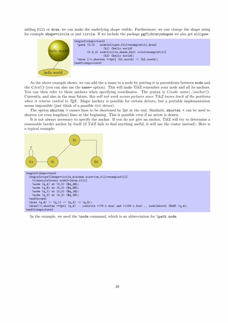
adding fill or draw, we can make the underlying shape visible. Furthermore, we can change the shape usingfor example shape=circle or just circle. If we include the package pgflibraryshapes we also get ellipse:

.

.

hello world

..

hello world

\begin{tikzpicture}

\path (0,0) node[ellipse,fill=examplefill,draw]

(h1) {hello world}

(0.5,2) node[circle,shade,ball color=examplefill]

(h2) {hello world};

\draw [->,shorten >=2pt] (h1.north) -- (h2.south);

\end{tikzpicture}

As the above example shows, we can add the a name to a node by putting it in parentheses between node andthe {⟨text⟩} (you can also use the name= option). This will make TikZ remember your node and all its anchors.You can then refer to these anchors when specifying coordinates. The syntax is (⟨node name⟩.⟨anchor⟩).Currently, and also in the near future, this will not work across pictures since TikZ looses track of the positionswhen it returns control to TEX. Magic hackery is possible for certain drivers, but a portable implementationseems impossible (just think of a possible svg driver).

The option shorten > causes lines to be shortened by 2pt at the end. Similarly, shorten < can be used toshorten (or even lengthen) lines at the beginning. This is possible even if no arrow is drawn.

It is not always necessary to specify the anchor. If you do not give an anchor, TikZ will try to determine areasonable border anchor by itself (if TikZ fails to find anything useful, it will use the center instead). Here isa typical example:

.

.

qA

.

qE

.

q1

.

q2

.

x

\begin{tikzpicture}

\begin{scope}[shape=circle,minimum size=1cm,fill=examplefill]

\tikzstyle{every node}=[draw,fill]

\node (q_A) at (0,0) {$q_A$};

\node (q_E) at (6,0) {$q_E$};

\node (q_1) at (2,0) {$q_1$};

\node (q_2) at (4,2) {$q_2$};

\end{scope}

\draw (q_A) -- (q_1) -- (q_2) -| (q_E);

\draw[->,shorten >=2pt] (q_A) .. controls +(75:1.4cm) and +(105:1.4cm) .. node[above] {$x$} (q_A);

\end{tikzpicture}

In the example, we used the \node command, which is an abbreviation for \path node.

38

4 Guidelines on Graphics

The present section is not about pgf or TikZ, but about general guidelines and principles concerning the creationof graphics for scientific presentations, papers, and books.

The guidelines in this section come from different sources. Many of them are just what I would like toclaim is “common sense,” some reflect my personal experience (though, hopefully, not my personal preferences),some come from books (the bibliography is still missing, sorry) on graphic design and typography. The mostinfluential source are the brilliant books by Edward Tufte. While I do not agree with everything written in thesebooks, many of Tufte’s arguments are so convincing that I decided to repeat them in the following guidelines.

4.1 Should You Follow Guidelines?

The first thing you should ask yourself when someone presents a bunch of guidelines is: Should I really followthese guidelines? This is an important questions, because there are good reasons not to follow general guidelines.

• The person who setup the guidelines may have had other objectives than you do. For example, a guidelinemight say “use the color red for emphasis.” While this guideline makes perfect sense for, say, a presentationusing a projector, red “color” has the opposite effect of “emphasis” when printed using a black-and-whiteprinter.

Guidelines were almost always setup to address a specific situation. If you are not in this situation,following a guideline can do more harm than good.

• The basic rule of typography is: “Every rule can be broken, as long as you are aware that you are breakinga rule.” This rule also applies to graphics. Phrased differently, the basic rule states: “The only mistakesin typography are things done is ignorance.”

When you are aware of a rule and when you decide that breaking the rule has a desirable effect, break therule.

• Some guidelines are simply wrong, but everyone follows them out of tradition or is forced to do so. Myfavorite example is a guideline a software company I used to work for has set in a big project: Allprogrammers had to declare the parameters of functions in increasing order of size. So, one-byte parametersshould come first, then two-byte parameters, and so on.

This guideline is total nonsense. An (arguably) sensible guideline is “parameters must be declared alpha-betically” so that parameters are easier to find. Another (arguably) sensible guideline is “parameters mustbe declared in decreasing order of size” so that less byte-alignment cache misses occur when the stack isaccessed. The guideline the company used maximized cache misses and resulted in a more or less randomordering so that programmers constantly had to look up the parameter ordering.

So, before you apply a guideline or choose not to apply it, ask yourself these questions:

1. Does this guideline really address my situation?

2. If you do the opposite a guideline says you should do, will the advantages outweigh the disadvantages thisguideline was supposed to prevent?

4.2 Planning the Time Needed for the Creation of Graphics

When you create a paper with numerous graphics, the time needed to create these graphics becomes an importantfactor. How much time should you calculate for the creation of graphics?

As a general rule, assume that a graphic will need as much time to create as would a text of the same length.For example, when I write a paper, I need about one hour per page for the first draft. Later, I need betweentwo and four hours per page for revisions. Thus, I expect to need about half an hour for the creation of a firstdraft of a half page graphic. Later on, I expect another one to two hours before the final graphic is finished.

In many publications, even in good journals, the authors and editors have obviously invested a lot of timeon the text, but seem to have spend about five minutes to create all of the graphics. Graphics often seem tohave been added as an “afterthought” or look like a screen shot of whatever the authors’s statistical software

39

shows them. As will be argued later on, the graphics that programs like gnuplot produce by default are ofpoor quality.

Creating informative graphics that help the reader and that fit together with the main text is a difficult,lengthy process.

• Treat graphics as first-class citizens of your papers. They deserve as much time and energy as the textdoes.

• Arguably, the creation of graphics deserves even more time than the writing of the main text since moreattention will be paid to the graphics and they will be looked at first.

• Plan as much time for the creation and revision of a graphic as you would plan for text of the same size.

• Difficult graphics with a high information density may require even more time.

• Very simple graphics will require less time, but most likely you do not want to have “very simple graphics”in your paper, anyway; just as you would not like to have a “very simple text” of the same size.

4.3 Workflow for Creating a Graphic

When you write a (scientific) paper, you will most likely follow the following pattern: You have some results/ideasthat you would like to report about. The creation of the paper will typically start with compiling a rough outline.Then, the different sections are filled with text to create a first draft. This draft is then revised repeatedly until,often after substantial revision, a final paper results. In a good journal paper there is typically not be a singlesentence that has survived unmodified from the first draft.

Creating a graphics follows the same pattern:

• Decide on what the graphic should communicate. Make this a conscious decision, that is, determine “Whatis the graphic supposed to tell the reader?”

• Create an “outline,” that is, the rough overall “shape” of the graphic, containing the most crucial elements.Often, it is useful to do this using pencil and paper.

• Fill out the finer details of the graphic to create a first draft.

• Revise the graphic repeatedly along with the rest of the paper.

4.4 Linking Graphics With the Main Text

Graphics can be placed at different places in a text. Either, they can be inlined, meaning they are somewhere“in the middle of the text” or they can be placed in standalone “figures.” Since printers (the people) like to havetheir pages “filled,” (both for aesthetic and economic reasons) standalone figures may traditionally be placed onpages in the document far removed from the main text that refers to them. LATEX and TEX tend to encouragethis “drifting away” of graphics for technical reasons.

When a graphic is inlined, it will more or less automatically be linked with the main text in the sense thatthe labels of the graphic will be implicitly explained by the surrounding text. Also, the main text will typicallymake it clear what the graphic is about and what is shown.

Quite differently, a standalone figure will often be viewed at a time when the main text that this graphicbelongs to either has not yet been read or has been read some time ago. For this reason, you should follow thefollowing guidelines when creating standalone figures:

• Standalone figures should have a caption than should make them “understandable by themselves.”

For example, suppose a graphic shows an example of the different stages of a quicksort algorithm. Thenthe figure’s caption should, at the very least, inform the reader that “The figure shows the different stagesof the quicksort algorithm introduced on page xyz.” and not just “Quicksort algorithm.”

40

• A good caption adds as much context information as possible. For example, you could say: “The figureshows the different stages of the quicksort algorithm introduced on page xyz. In the first line, the pivotelement 5 is chosen. This causes. . . ” While this information can also be given in the main text, puttingit in the caption will ensure that the context is kept. Do not feel afraid of a 5-line caption. (Your editormay hate you for this. Consider hating them back.)

• Reference the graphic in your main text as in “For an example of quicksort ‘in action,’ see Figure 2.1 onpage xyz.”

• Most books on style and typography recommend that you do not use abbreviations as in “Fig. 2.1” butwrite “Figure 2.1.”

The main argument against abbreviations is that “a period is too valuable to waste it on an abbreviation.”The idea is that a period will make the reader assume that the sentence ends after “Fig” and it takes a“conscious backtracking” to realize that the sentence did not end after all.

The argument in favor of abbreviations is that they save space.

Personally, I am not really convinced by either argument. On the one hand, I have not yet seen any hardevidence that abbreviations slow readers down. On the other hand, abbreviating all “Figure” by “Fig.” ismost unlikely to save even a single line in most documents.

I avoid abbreviations.

4.5 Consistency Between Graphics and Text

Perhaps the most common “mistake” people do when creating graphics (remember that a “mistake” in designis always just “ignorance”) is to have a mismatch between the way their graphics look and the way their textlooks.

It is quite common that authors use several different programs for creating the graphics of a paper. Anauthor might produce some plots using gnuplot, a diagram using xfig, and include an .eps graphic a coauthorcontributed using some unknown program. All these graphics will, most likely, use different line widths, differentfonts, and have different sizes. In addition, authors often use options like [height=5cm] when including graphicsto scale them to some “nice size.”

If the same approach were taken to writing the main text, every section would be written in a different fontat a different size. In some sections all theorems would be underlined, in another they would be printed all inuppercase letters, and in another in red. In addition, the margins would be different on each page.

Readers and editors would not tolerate a text if it were written in this fashion, but with graphics they oftenhave to.

To create consistency between graphics and text, stick to the following guidelines:

• Do not scale graphics.

This means that when generating graphics using an external program, create them “at the right size.”

• Use the same font(s) both in graphics and the body text.

• Use the same line width in text and graphics.

The “line width” for normal text is the width of the stem of letters like T. For TEX, this is usually 0.4 pt.However, some journals will not accept graphics with a normal line width below 0.5 pt.

• When using colors, use a consistent color coding in the text and in graphics. For example, if red issupposed to alert the reader to something in the main text, use red also in graphics for important partsof the graphic. If blue is used for structural elements like headlines and section titles, use blue also forstructural elements of your graphic.

However, graphics may also use a logical intrinsic color coding. For example, no matter what colors younormally use, readers will generally assume, say, that the color green as “positive, go, ok” and red as “alert,warning, action.”

Creating consistency when using different graphic programs is almost impossible. For this reason, you shouldconsider sticking to a single graphic program.

41

4.6 Labels in Graphics

Almost all graphics will contain labels, that is, pieces of text that explain parts of the graphics. When placinglabels, stick to the following guidelines:

• Follow the rule of consistency when placing labels. You should do so in two ways: First, be consistent withthe main text, that is, use the same font as the main text also for labels. Second, be consistent betweenlabels, that is, if you format some labels in some particular way, format all labels in this way.

• In addition to using the same fonts in text and graphics, you should also use the same notation. Forexample, if you write 1/2 in your main text, also use “1/2” as labels in graphics, not “0.5”. A π is a “π”and not “3.141”. Finally, e−iπ is “e−iπ”, not “−1”, let alone “-1”.

• Labels should be legible. They should not only have a reasonably large size, they also should not beobscured by lines or other text. This also applies to of lines and text behind the labels.

• Labels should be “in place.” Whenever there is enough space, labels should be placed next to the thingthey label. Only if necessary, add a (subdued) line from the label to the labeled object. Try to avoidlabels that only reference explanations in external legends. Reader have to jump back and forth betweenthe explanation and the object that is described.

• Consider subduing “unimportant” labels using, for example, a gray color. This will keep the focus on theactual graphic.

4.7 Plots and Charts

One of the most frequent kind of graphics, especially in scientific papers, are plots. They come in a large variety,including simple line plots, parametric plots, three dimensional plots, pie charts, and many more.

Unfortunately, plots are notoriously hard to get right. Partly, the default settings of programs like gnuplotor Excel are to blame for this since these programs make it very convenient to create bad plots.

The first question you should ask yourself when creating a plot is the following:

• Are there enough data points to merit a plot?

If the answer is “not really,” use a table.A typical situation where a plot is unnecessary is when people present a few numbers in a bar diagram.

Here is a real-life example: At the end of a seminar a lecturer asked the participants for feedback. Of the50 participants, 30 returned the feedback form. According to the feedback, three participants considered theseminar “very good,” nine considered it “good,” ten “ok,” eight “bad,” and no one thought that the seminarwas “very bad.”

A simple way of summing up this information is the following table:

Rating given Participants (out of 50)who gave this rating

Percentage

“very good” 3 6%“good” 9 18%“ok” 10 20%“bad” 8 16%“very bad” 0 0%

none 20 40%

What the lecturer did was to visualize the data using a 3D bar diagram. It looked like this:

42

.

.

0

.

20

.

40

.

60

.

80

.

100

.

very

good

.

good

.

ok

.

bad .

very

bad

Both the table and the “plot” have about the same size. If your first thought is “the graphic looks nicer thanthe table,” try to answer the following questions based on the information in the table or in the graphic:

1. How many participants where there?

2. How many participants returned the feedback form?

3. What percentage of the participants returned the feedback form?

4. How many participants checked “very good”?

5. What percentage out of all participants checked “very good”?

6. Did more than a quarter of the participants check “bad” or “very bad”?

7. What percentage of the participants that returned the form checked “very good”?

Sadly, the graphic does not allow us to answer a single one of these questions. The table answers all of themdirectly, except for the last one. In essence, the information density of the graphic is very nearly zero. The tablehas a much higher information density; despite the fact that it uses quite a lot of white space to present a fewnumbers.

Here is the list of things that went wrong with the 3D-bar diagram:

• The whole graphic is dominated by irritating background lines.

• It is not clear what the numbers at the left mean; presumably percentages, but it might also be the absolutenumber of participants.

• The labels at the bottom are rotated, making them hard to read.

(In the real presentation that I saw, the text was rendered at a very low resolution with about 10 by 6pixels per letter with wrong kerning, making the rotated text almost impossible to read.)

• The third dimension adds complexity to the graphic without adding information.

• The three dimensional setup makes it much harder to gauge the height of the bars correctly. Consider the“bad” bar. It the number this bar stands for more than 20 or less? While the front of the bar is below the20 line, the back of the bar (which counts) is above.

• It is impossible to tell which numbers are represented by the bars. Thus, the bars needlessly hide theinformation these bars are all about.

• What do the bar heights add up to? Is it 100% or 60%?

• Does the bar for “very bad” represent 0 or 1?

• Why are the bars blue?

43

You might argue that in the example the exact numbers are not important for the graphic. The importantthings is the “message,” which is that there are more “very good” and “good” ratings than “bad” and “verybad.” However, to convey this message either use a sentence that says so or use a graphic that conveys thismessage more clearly:

.

.

Ratings given by50 participants

.

“ok”: 10 (20%).

none: 20 (40%)

.

“very good”: 3 (6%)

.

“good”: 9 (18%)

.

“bad”: 8 (16%)

.

“very bad”: 0 (0%)

The above graphic has about the same information density as the table (about the same size and the samenumbers are shown). In addition, one can directly “see” that there are more good or very good ratings than badones. One can also “see” that the number of people who gave no rating at all is not negligible, which is quitecommon for feedback forms.

Charts are not always a good idea. Let us look at an example that I redrew from a pie chart in Die Zeit,June 4th, 2005:

.

.

Kohle ist am wichtigstenEnergiemix bei der deutschen Stromerzeugung 2004

.

Gesamte Netto-Stromerzeugung in Prozent, in Milliarden Kilowattstunden (Mrd. kWh)

.

.

9,4%

.

27,8%

.

25,6%

.

22,3%

.

10,4%

.

Regenerative (53,7 kWh)/davon Wind 4,4% (25,0 kWh)

.

Kernenergie

.

(158,4 kWh)

.

Braunkohle (146,0 kWh)

.

Steinkohle (127,1 kWh)

.

Erdgas (59,2 kWh)

.

Mineralolprodukte (9,2 kWh) 1,6%

.

Sonstige (16,5 kWh) 2,9%

This graphic has been redrawn in TikZ, but the original looks very similar.At first sight, the graphic looks “nice and informative,” but there are a lot of things that went wrong:

• The chart is three dimensional. However, the shadings add nothing “information-wise,” at best, theydistract.

• In a 3D-pie-chart the relative sizes are very strongly distorted. For example, the area taken up by the graycolor of “Braunkohle” is larger than the area taken up by the green color of “Kernenergie” despite the factthat the percentage of Braunkohle is less than the percentage of Kernenergie.

• The 3D-distortion gets worse for small areas. The area of “Regenerative” somewhat larger than the areaof “Erdgas.” The area of “Wind” is slightly smaller than the area of “Mineralolprodukte” although thepercentage of Wind is nearly three times larger than the percentage of Mineralolprodukte.

44

In the last case, the different sizes are only partly due to distortion. The designer(s) of the original graphichave also made the “Wind” slice too small, even taking distortion into account. (Just compare the size of“Wind” to “Regenerative” in general.)

• According to its caption, this chart is supposed to inform us that coal was the most important energysource in Germany in 2004. Ignoring the strong distortions caused by the superfluous and misleading3D-setup, it takes quite a while for this message to get across.

Coal as an energy source is split up into two slices: one for “Steinkohle” and one for “Braunkohle” (twodifferent kinds of coal). When you add them up, you see that the whole lower half of the pie chart is takenup by coal.

The two areas for the different kinds of coal are not visually linked at all. Rather, two different colors areused, the labels are on different sides of the graphic. By comparison, “Regenerative” and “Wind” are veryclosely linked.

• The color coding of the graphic follows no logical pattern at all. Why is nuclear energy green? Regenerativeenergy is light blue, “other sources” are blue. It seems more like a joke that the area for “Braunkohle”(which literally translates to “brown coal”) is stone gray, while the area for “Steinkohle” (which literallytranslates to “stone coal”) is brown.

• The area with the lightest color is used for “Erdgas.” This area stands out most because of the brightercolor. However, for this chart “Erdgas” is not really important at all.

Edward Tufte calls graphics like the above “chart junk.”Here are a few recommendations that may help you avoid producing chart junk:

• Do not use 3D pie charts. They are evil.

• Consider using a table instead of a pie chart.

• Due not apply colors randomly; use them to direct the readers’s focus and to group things.

• Do not use background patterns, like a crosshatch or diagonal lines, instead of colors. They distract.Background patterns in information graphics are evil.

4.8 Attention and Distraction

Pick up your favorite fiction novel and have a look at a typical page. You will notice that the page is veryuniform. Nothing is there to distract the reader while reading; no large headlines, no bold text, no large whiteareas. Indeed, even when the author does wish to emphasize something, this is done using italic letters. Suchletters blend nicely with the main text—at a distance you will not be able to tell whether a page contains italicletters, but you would notice a single bold word immediately. The reason novels are typeset this way is thefollowing paradigm: Avoid distractions.

Good typography (like good organization) is something you do not notice. The job of typography is to makereading the text, that is, “absorbing” its information content, as effortless as possible. For a novel, readersabsorb the content by reading the text line-by-line, as if they were listening to someone telling the story. In thissituation anything on the page that distracts the eye from going quickly and evenly from line to line will makethe text harder to read.

Now, pick up your favorite weekly magazine or newspaper and have a look at a typical page. You will noticethat there is quite a lot “going on” on the page. Fonts are used at different sizes and in different arrangements,the text is organized in narrow columns, typically interleaved with pictures. The reason magazines are typesetin this way is another paradigm: Steer attention.

Readers will not read a magazine like a novel. Instead of reading a magazine line-by-line, we use headlinesand short abstracts to check whether we want to read a certain article or not. The job of typography is to steerour attention to these abstracts and headlines, first. Once we have decided that we want to read an article,however, we no longer tolerate distractions, which is why the main text of articles is typeset exactly the sameway as a novel.

45

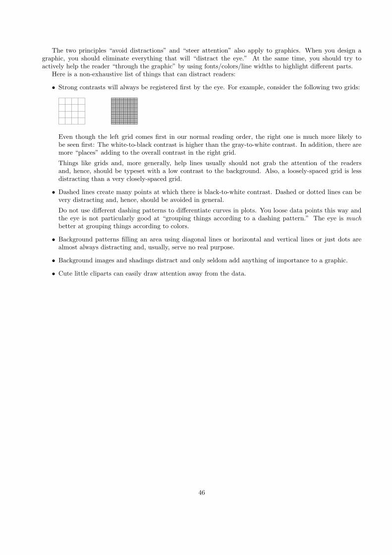
The two principles “avoid distractions” and “steer attention” also apply to graphics. When you design agraphic, you should eliminate everything that will “distract the eye.” At the same time, you should try toactively help the reader “through the graphic” by using fonts/colors/line widths to highlight different parts.

Here is a non-exhaustive list of things that can distract readers:

• Strong contrasts will always be registered first by the eye. For example, consider the following two grids:

.

Even though the left grid comes first in our normal reading order, the right one is much more likely tobe seen first: The white-to-black contrast is higher than the gray-to-white contrast. In addition, there aremore “places” adding to the overall contrast in the right grid.

Things like grids and, more generally, help lines usually should not grab the attention of the readersand, hence, should be typeset with a low contrast to the background. Also, a loosely-spaced grid is lessdistracting than a very closely-spaced grid.

• Dashed lines create many points at which there is black-to-white contrast. Dashed or dotted lines can bevery distracting and, hence, should be avoided in general.

Do not use different dashing patterns to differentiate curves in plots. You loose data points this way andthe eye is not particularly good at “grouping things according to a dashing pattern.” The eye is muchbetter at grouping things according to colors.

• Background patterns filling an area using diagonal lines or horizontal and vertical lines or just dots arealmost always distracting and, usually, serve no real purpose.

• Background images and shadings distract and only seldom add anything of importance to a graphic.

• Cute little cliparts can easily draw attention away from the data.

46

5 Input and Output Formats

TEX was designed to be a flexible system. This is true both for the input for TEX as well as for the output. Thepresent section explains which input formats there are and how they are supported by pgf. It also explainswhich different output formats can be produced.

5.1 Supported Input Formats

TEX does not prescribe exactly how your input should be formatted. While it is customary that, say, an openingbrace starts a scope in TEX, this is by no means necessary. Likewise, it is customary that environments startwith \begin, but TEX could not really care less about the exact command name.

Even though TEX can be reconfigured, users can not. For this reason, certain input formats specify aset of commands and conventions how input for TEX should be formatted. There are currently three “major”formats: Donald Knuth’s original plain TEX format, Leslie Lamport’s popular LATEX format, and Hans Hangen’sConTEXt format.

5.1.1 Using the LATEX Format

Using pgf and TikZ with the LATEX format is easy: You say \usepackage{pgf} or \usepackage{tikz}. Usually,that is all you need to do, all configuration will be done automatically and (hopefully) correctly.

The style files used for the LATEX format reside in the subdirectory latex/pgf/ of the pgf-system. Mainly,what these files do is to include files in the directory generic/pgf. For example, here is the content of the filelatex/pgf/frontends/tikz.sty:

% Copyright 2005 by Till Tantau <[email protected]>.

%

% This program can be redistributed and/or modified under the terms

% of the GNU Public License, version 2.

\RequirePackage{pgf,calc,pgffor,pgflibraryplothandlers,xkeyval}

\input{tikz.code}

\endinput

The files in the generic/pgf directory do the actual work.

5.1.2 Using the Plain TEX Format

When using the plain TEX format, you say \input{pgf.tex} or \input{tikz.tex}. Instead of \begin{pgfpicture}and \end{pgfpicture} you use \pgfpicture and \endpicture.

Unlike for the LATEX format, pgf is not as good at discerning the appropriate configuration for the plainTEX format. In particular, it can only automatically determine the correct output format if you use pdftex ortex plus dvips. For all other output formats you need to set the macro \pgfsysdriver to the correct value.See the description of using output formats later on.

pgf was originally written for use with LATEX and this shows in a number of places. Nevertheless, the plainTEX support is reasonably good.

Like the LATEX style files, the plain TEX files like tikz.tex also just include the correct tikz.code.tex file.

5.1.3 Using the ConTEXt Format

Currently, there is no special support for the ConTEXt format. Rather, you have to use pgf and TikZ as if youwere using the plain TEX format when using ConTEXt. This may change in the future.

5.2 Supported Output Formats

An output format is a format in which TEX outputs the text it has typeset. Producing the output is (concep-tually) a two-stage process:

47

1. TEX typesets your text and graphics. The result of this typesetting is mainly a long list of letter–coordinatepairs, plus (possibly) some “special” commands. This long list of pairs is written to something called a.dvi-file.

2. Some other program reads this .dvi-file and translates the letter–coordinate pairs into, say, PostScriptcommands for placing the given letter at the given coordinate.

The classical example of this process is the combination of latex and dvips. The latex program (which isjust the tex program called with the LATEX-macros preinstalled) produces a .dvi-file as its output. The dvipsprogram takes this output and produces a .ps-file (a PostScript) file. Possibly, this file is further converted using,say, ps2pdf, whose name is supposed to mean “PostScript to PDF.” Another example of programs using thisprocess is the combination of tex and dvipdfm. The dvipdfm program takes a .dvi-file as input and translatesthe letter–coordinate pairs therein into pdf-commands, resulting in a .pdf file directly. Finally, the tex4ht isalso a program that takes a .dvi-file and produces an output, this time it is a .html file. The programs pdftexand pdflatex are special: They directly produce a .pdf-file without the intermediate .dvi-stage. However,from the programmer’s point of view they behave exactly as if there where an intermediate stage.

Normally, TEX only produces letter–coordinate pairs as its “output.” This obviously makes is difficult thodraw, say, a curve. For this, “special” commands can be used. Unfortunately, these special commands are notthe same for the different programs that process the .dvi-file. Indeed, every program that takes a .dvi-file asinput has a totally different syntax for the special commands.

One of the main jobs of pgf is to “abstract way” the difference in the syntax of the different programs.However, this means that support for each program has to be “programmed,” which is a time-consuming andcomplicated process.

5.2.1 Selecting the Backend Driver

When TEX typesets your document, it does not know which program you are going to use to transform the.dvi-file. If your .dvi-file does not contain any special commands, this would be fine; but these days almost all.dvi-files contain lots of special commands. It is thus necessary to tell TEX which program you are going to uselater on.

Unfortunately, there is no “standard” way of telling this to TEX. For the LATEX format a sophisticatedmechanism exists inside the graphics package and pgf plugs into this mechanism. For other formats and whenthis plugging does not work as expected, it is necessary to tell pgf directly which program you are going touse. This is done by redefining the macro \pgfsysdriver to an appropriate value before you load pgf. If youare going to use the dvips program, you set this macro to the value pgfsys-dvips.def; if you use pdftex orpdflatex, you set it to pgfsys-pdftex.def; and so on. In the following, details of the support of the differentprograms are discussed.

5.2.2 Producing PDF Output

pgf supports three programs that produce pdf output (pdf means “portable document format” and wasinvented by the Adobe company): dvipdfm, pdftex, and vtex. The pdflatex program is the same as thepdftex program: it uses a different input format, but the output is exactly the same.

File pgfsys-pdftex.def

This is the driver file for use with pdfTEX, that is, with the pdftex or pdflatex command. It includespgfsys-common-pdf.def.This driver has the “complete” functionality. This means, everything pgf “can do at all” is implementedin this driver.

File pgfsys-dvipdfm.def

This is a driver file for use with (la)tex followed by dvipdfm. It includes pgfsys-common-pdf.def.This driver supports most of pgf’s features, but there are some restrictions:

1. In LATEX mode it uses graphicx for the graphics inclusion and does not support masking.

48

2. In plain TEX mode it does not support image inclusion.

File pgfsys-vtex.def

This is the driver file for use with the commercial vtex program. Even though is will produce pdf output,it includes pgfsys-common-postscript.def. Note that the vtex program can produce both Postscriptand pdf output, depending on the command line parameters. However, whether you produce Postscript orpdf output does not change anything with respect to the driver.This driver supports most of pgf’s features, except for the following restrictions:



3. Shading is fully implemented, but yields the same quality as the implementation for dvips.

4. Opacity is not implemented at all.

It is also possible to produce a .pdf-file by first producing a PostScript file (see below) and then using aPostScript-to-pdf conversion program like ps2pdf or the Acrobat Distiller.

5.2.3 Producing PostScript Output

File pgfsys-dvips.def

This is a driver file for use with (la)tex followed by dvips. It includes pgfsys-common-postscript.def.This driver also supports most of pgf’s features, except for the following restrictions:



3. Shading is fully implemented, but the results will not be as good as with a driver producing .pdf asoutput.

4. Opacity works only in conjunction with newer versions of GhostScript.

File pgfsys-textures.def

This is a driver file for use with the textures program. It includes pgfsys-common-postscript.def.This driver has exactly the same restrictions as the driver for dvips.

You can also use the vtex program together with pgfsys-vtex.def to produce Postscript output.

5.2.4 Producing HTML / SVG Output

The tex4ht program converts .dvi-files to .html-files. While the html-format cannot be used to draw graphics,the svg-format can. Using the following driver, you can ask pgf to produce an svg-picture for each pgf graphicin your text.

File pgfsys-tex4ht.def

This is a driver file for use with the tex4ht program. It includes pgfsys-common-svg.def.When using this driver you should be aware of the following restrictions:

1. In LATEX mode it uses graphicx for the graphics inclusion.


3. Text inside pgfpictures is not supported very well. The reason is that the svg specification currentlydoes not support text very well and it is also not possible to correctly “escape back” to html. Allthese problems will hopefully disappear in the future, but currently only two kinds of text workreasonably well: First, plain text without math mode, special characters or anything else special.Second, very simple mathematical text that contains subscripts or superscripts. Even then, variablesare not correctly set in italics and, in general, text simple does not look very nice.

49

4. If you use text that contains anything special, even something as simple as $\alpha$, this may corruptthe graphic since text4ht does not always produce valid xml code. So, once more, stick to very simplenode text inside graphics. Sorry.

5. Unlike for other output formats, the bounding box of a picture “really crops” the picture.

The driver basically works as follows: When a {pgfpicture} is started, appropriate \special commandsare used to directed the output of tex4ht to a new file called \jobname-xxx.svg, where xxx is a numberthat is increased for each graphic. Then, till the end of the picture, each (system layer) graphic commandcreates a specials that insert appropriate svg literal text into the output file. The exact details are a bitcomplicated since the imaging model and the processing model of PostScript/pdf and svg are not quitethe same; but they are “close enough” for pgf’s purposes.

50

Part II

TikZ ist kein Zeichenprogramm

.

.

α

.

β

.

γ

.

δ

.

E

.

F

.

A

.

B

.

C

.

D

.

When we assume that AB and CDare parallel, i. e., AB ∥ CD, then α = δand β = γ.

\begin{tikzpicture}

\draw[fill=yellow] (0,0) -- (60:.75cm) arc (60:180:.75cm);

\draw(120:0.4cm) node {$\alpha$};

\draw[fill=green!30] (0,0) -- (right:.75cm) arc (0:60:.75cm);

\draw(30:0.5cm) node {$\beta$};

\begin{scope}[shift={(60:2cm)}]

\draw[fill=green!30] (0,0) -- (180:.75cm) arc (180:240:.75cm);

\draw (30:-0.5cm) node {$\gamma$};

\draw[fill=yellow] (0,0) -- (240:.75cm) arc (240:360:.75cm);

\draw (-60:0.4cm) node {$\delta$};

\end{scope}

\begin{scope}[thick]

\draw (60:-1cm) node[fill=white] {$E$} -- (60:3cm) node[fill=white] {$F$};

\draw[red] (-2,0) node[left] {$A$} -- (3,0) node[right]{$B$};

\draw[blue,shift={(60:2cm)}] (-3,0) node[left] {$C$} -- (2,0) node[right]{$D$};

\draw[shift={(60:1cm)},xshift=4cm]

node [right,text width=6cm,rounded corners,fill=red!20,inner sep=1ex]

{

When we assume that $\color{red}AB$ and $\color{blue}CD$ are

parallel, i.\,e., ${\color{red}AB} \mathbin{\|} \color{blue}CD$,

then $\alpha = \delta$ and $\beta = \gamma$.

};

\end{scope}

\end{tikzpicture}

51

6 Design Principles

This section describes the design principles behind the TikZ frontend, where TikZ means “TikZ ist kein Zeichen-programm.” To use TikZ, as a LATEX user say \usepackage{tikz} somewhere in the preamble, as a plain TEXuser say \input tikz.tex. TikZ’s job is to make your life easier by providing an easy-to-learn and easy-to-usesyntax for describing graphics.

The commands and syntax of TikZ were influenced by several sources. The basic command names and thenotion of path operations is taken from metafont, the option mechanism comes from pstricks, the notion ofstyles is reminiscent of svg. To make it all work together, some compromises were necessary. I also added someideas of my own, like meta-arrows and coordinate transformations.

The following basic design principles underlie TikZ:

1. Special syntax for specifying points.

2. Special syntax for path specifications.

3. Actions on paths.

4. Key-value syntax for graphic parameters.

5. Special syntax for nodes.

6. Special syntax for trees.

7. Grouping of graphic parameters.

8. Coordinate transformation system.

6.1 Special Syntax For Specifying Points

TikZ provides a special syntax for specifying points and coordinates. In the simplest case, you provide two TEXdimensions, separated by commas, in round brackets as in (1cm,2pt).

You can also specify a point in polar coordinates by using a colon instead of a comma as in (30:1cm), whichmeans “1cm in a 30 degrees direction.”

If you do not provide a unit, as in (2,1), you specify a point in pgf’s xy-coordinate system. By default, theunit x-vector goes 1cm to the right and the unit y-vector goes 1cm upward.

By specifying three numbers as in (1,1,1) you specify a point in pgf’s xyz-coordinate system.It is also possible to use an anchor of a previously defined shape as in (first node.south).You can add two plus signs before a coordinate as in ++(1cm,0pt). This means “1cm to the right of the

last point used.” This allows you to easily specify relative movements. For example, (1,0) ++(1,0) ++(0,1)specifies the three coordinates (1,0), then (2,0), and (2,1).

Finally, instead of two plus signs, you can also add a single one. This also specifies a point in a relativemanner, but it does not “change” the current point used in subsequent relative commands. For example,(1,0) +(1,0) +(0,1) specifies the three coordinates (1,0), then (2,0), and (1,1).

6.2 Special Syntax For Path Specifications

When creating a picture using TikZ, your main job is the specification of paths. A path is a series of straightor curved lines, which need not be connected. TikZ makes it easy to specify paths, partly using the syntax ofmetapost. For example, to specify a triangular path you use

(5pt,0pt) -- (0pt,0pt) -- (0pt,5pt) -- cycle

and you get

.

when you draw this path.

52

6.3 Actions on Paths

A path is just a series of straight and curved lines, but it is not yet specified what should happen with it. Onecan draw a path, fill a path, shade it, clip it, or do any combination of these. Drawing (also known as stroking)can be thought of as taking a pen of a certain thickness and moving it along the path, thereby drawing on thecanvas. Filling means that the interior of the path is filled with a uniform color. Obviously, filling makes senseonly for closed paths and a path is automatically closed prior to filling, if necessary.

Given a path as in \path (0,0) rectangle (2ex,1ex);, you can draw it by adding the draw option asin \path[draw] (0,0) rectangle (2ex,1ex);, which yields

.

. The \draw command is just an abbreviationfor \path[draw]. To fill a path, use the fill option or the \fill command, which is an abbreviation for\path[fill]. The \filldraw command is an abbreviation for \path[fill,draw]. Shading is caused by theshade option (there are \shade and \shadedraw abbreviations) and clipping by the clip option. There is isalso a \clip command, which does the same as \path[clip], but not commands like \drawclip. Use, say,\draw[clip] or \path[draw,clip] instead.

All of these commands can only be used inside {tikzpicture} environments.TikZ allows you to use different colors for filling and stroking.

6.4 Key-Value Syntax for Graphic Parameters

Whenever TikZ draws or fills a path, a large number of graphic parameters influenced the rendering. Examplesinclude the colors used, the dashing pattern, the clipping area, the line width, and many others. In TikZ, allthese options are specified as lists of so called key-value pairs, as in color=red, that are passed as optionalparameters to the path drawing and filling commands. This usage is similar to pstricks. For example, thefollowing will draw a thick, red triangle;

.

\tikz \draw[line width=2pt,color=red] (1,0) -- (0,0) -- (1,0) -- cycle;

6.5 Special Syntax for Specifying Nodes

TikZ introduces a special syntax for adding text or, more generally, nodes to a graphic. When you specify apath, add nodes as in the following example:

.

.

text

\tikz \draw (1,1) node {text} -- (2,2);

Nodes are inserted at the current position of the path, but only after the path has been rendered. Whenspecial options are given, as in \draw (1,1) node[circle,draw] {text};, the text is not just put at thecurrent position. Rather, it is surrounded by a circle and this circle is “drawn.”

You can add a name to a node for later reference either by using the option name=⟨node name⟩ or by statingthe node name in parentheses outside the text as in node[circle](name){text}.

Predefined shapes include rectangle, circle, and ellipse, but it is possible (though a bit challenging) todefine new shapes.

6.6 Special Syntax for Specifying Trees

In addition to the “node syntax,” TikZ also introduces a special syntax for drawing trees. The syntax isintergrated with the special node syntax and only few new commands need to be remebered. In essence, a nodecan be followed by any number of children, each introduced by the keyword child. The children are nodesthemselves, each of which may have children in turn.

53

.

.root

.left

.right

.child

.child

\begin{tikzpicture}

\node {root}

child {node {left}}

child {node {right}

child {node {child}}


};

\end{tikzpicture}

Since trees are made up from nodes, it is possible to use options to modify the way trees are drawn. Hereare two examples of the above tree, redrawn with different options:

.

.

root

.

left

.

right

.

child

.

child

\begin{tikzpicture}[edge from parent fork down]

\tikzstyle{every node}=[fill=red!30,rounded corners]

\tikzstyle{edge from parent}=[red,-o,thick,draw]

\node {root}

child {node {left}}

child {node {right}



};

\end{tikzpicture}

.

.

.

root

.

.

left

.

.

right

.

.

child

.

.

child\begin{tikzpicture}

[parent anchor=east,child anchor=west,grow=east]

\tikzstyle{every node}=[ball color=red,circle,text=white]

\tikzstyle{edge from parent}=[draw,dashed,thick,red]

\node {root}

child {node {left}}

child {node {right}



};

\end{tikzpicture}

6.7 Grouping of Graphic Parameters

Graphic parameters should often apply to several path drawing or filling commands. For example, we maywish to draw numerous lines all with the same line width of 1pt. For this, we put these commands in a{scope} environment that takes the desired graphic options as an optional parameter. Naturally, the specifiedgraphic parameters apply only to the drawing and filling commands inside the environment. Furthermore, nested{scope} environments or individual drawing commands can override the graphic parameters of outer {scope}environments. In the following example, three red lines, two green lines, and one blue line are drawn:

.

\begin{tikzpicture}

\begin{scope}[color=red]

\draw (0mm,10mm) -- (10mm,10mm);

\draw (0mm, 8mm) -- (10mm, 8mm);

\draw (0mm, 6mm) -- (10mm, 6mm);

\end{scope}

\begin{scope}[color=green]

\draw (0mm, 4mm) -- (10mm, 4mm);

\draw (0mm, 2mm) -- (10mm, 2mm);

\draw[color=blue] (0mm, 0mm) -- (10mm, 0mm);

\end{scope}

\end{tikzpicture}

The {tikzpicture} environment itself also behaves like a {scope} environment, that is, you can specifygraphic parameters using an optional argument. These optional apply to all commands in the picture.

54

6.8 Coordinate Transformation System

TikZ relies entirely on pgf’s coordinate transformation system to perform transformations. pgf also supportscanvas transformations, a more low-level transformation system, but this system is not accessible from TikZ.There are two reasons for this: First, the canvas transformation must be used with great care and often resultsin “bad” graphics with changing line width and text in wrong sizes. Second, pgf looses track of where nodesand shapes are positioned when canvas transformations are used.

For more details on the difference between coordinate transformations and canvas transformations see Sec-tion 18.4.

55

7 Hierarchical Structures:Package, Environments, Scopes, and Styles

The present section explains how your files should be structured when you use TikZ. On the top level, you needto include the tikz package. In the main text, each graphic needs to be put in a {tikzpicture} environment.Inside these environments, you can use {scope} environments to create internal groups. Inside the scopes youuse \path commands to actually draw something. On all levels (except for the package level), graphic optionscan be given that apply to everything within the environment.

7.1 Loading the Package

\usepackage{tikz} % LATEX\input tikz.tex % plain TEX\input tikz.tex % ConTEXt

This package does not have any options.This will automatically load the pgf package and several other stuff that TikZ needs (like the xkeyvalpackage).pgf needs to know what TEX driver you are intending to use. In most cases pgf is clever enough todetermine the correct driver for you; this is true in particular if you LATEX. Currently, the only situationwhere pgf cannot know the driver “by itself” is when you use plain TEX or ConTEXt together with dvipdfm.In this case, you have to write \def\pgfsysdriver{pgfsys-dvipdfm.def} before you input tikz.tex.

7.2 Creating a Picture

7.2.1 Creating a Picture Using an Environment

The “outermost” scope of TikZ is the {tikzpicture} environment. You may give drawing commands onlyinside this environment, giving them outside (as is possible in many other packages) will result in chaos.

In TikZ, the way graphics are rendered is strongly influenced by graphic options. For example, there is anoption for setting the color used for drawing, another for setting the color used for filling, and also more obscureones like the option for setting the prefix used in the filenames of temporary files written while plotting functionsusing an external program. The graphic options are nearly always specified in a so-called key-value style. (The“nearly always” refers to the name of nodes, which can also be specified differently.) All graphic options arelocal to the {tikzpicture} to which they apply.

\begin{tikzpicture}[⟨options⟩]⟨environment contents⟩

\end{tikzpicture}

All TikZ commands should be given inside this environment, except for the \tikzstyle command. Unlikeother packages, it is not possible to use, say, \pgfpathmoveto outside this environment and doing so willresult in chaos. For TikZ, commands like \path are only defined inside this environment, so there is littlechance that you will do something wrong here.When this environment is encountered, the ⟨options⟩ are parsed. All options given here will apply to thewhole picture.Next, the contents of the environment is processed and the graphic commands therein are put into abox. Non-graphic text is suppressed as well as possible, but non-pgf commands inside a {tikzpicture}environment should not produce any “output” since this may totally scramble the positioning system of thebackend drivers. The suppressing of normal text, by the way, is done by temporarily switching the font to\nullfont. You can, however, “escape back” to normal TEX typesetting. This happens, for example, whenyou specify a node.At the end of the environment, pgf tries to make a good guess at a good guess at the bounding box ofthe graphic and then resizes the box such that the box has this size. To “make its guess,” everytime pgfencounters a coordinate, it updates the bound box’s size such that it encompasses all these coordinates.

56

This will usually give a good approximation at the bounding box, but will not always be accurate. First, theline thickness is not taken into account. Second, controls points of a curve often lie far “outside” the curveand make the bounding box too large. In this case, you should use the [use as bounding box] option.The following option influences the baseline of the resulting picture:

• baseline=⟨dimension⟩ Normally, the lower end of the picture is put on the baseline of the surroundingtext. For example, when you give the code \tikz\draw(0,0)circle(.5ex);, pgf will find out thatthe lower end of the picture is at −.5ex and that the upper end is at .5ex. Then, the lower end will beput on the baseline, resulting in the following:

.

.Using this option, you can specify that the picture should be raised or lowered such that the height⟨dimension⟩ is on the baseline. For example, tikz[baseline=0pt]\draw(0,0)circle(.5ex); yields

.

since, now, the baseline is on the height of the x-axis. If you omit the ⟨dimensions⟩, 0pt is assumedas default.This options is often useful for “inlined” graphics as in

A

.

B $A \mathbin{\tikz[baseline] \draw[->>] (0pt,.5ex) -- (3ex,.5ex);} B$

• execute at begin picture=⟨code⟩ This option can be used to install some code that will be executedat the beginning of the picture. This option must be given in the argument of the {tikzpicture}environment itself since this option will not have an effect otherwise. After all, the picture has already“started” later on.This option is mainly used in styles like the every picture style to execute certain code at the startof a picture.

• execute at end picture=⟨code⟩ This option installs some code that will be executed at the end ofthe picture. Using this option multiple times will cause the code to accumulate. This option must alsobe given in the optional argument of the {tikzpicture} environment.

.

.

X

.

Y \begin{tikzpicture}[execute at end picture=%

{

\begin{pgfonlayer}{background}

\path[fill=yellow,rounded corners]

(current bounding box.south west) rectangle

(current bounding box.north east);

\end{pgfonlayer}

}]

\node at (0,0) {X};

\node at (2,1) {Y};

\end{tikzpicture}

All options “end” at the end of the picture. To set an option “globally” you can use the following style:

• style=every picture This style is installed at the beginning of each picture.

\tikzstyle{every picture}=[semithick]

In plain TEX, you should use instead the following commands:

\tikzpicture[⟨options⟩]⟨environment contents⟩

\endtikzpicture

7.2.2 Creating a Picture Using a Command

The following two commands are used for “small” graphics.

\tikz[⟨options⟩]{⟨commands⟩}This command places the ⟨commands⟩ inside a {tikzpicture} environment and adds a semicolon at theend. This is just a convenience.

57

The ⟨commands⟩ may not contain a paragraph (an empty line). This is a precaution to ensure that usersreally use this command only for small graphics.

Example: \tikz{\draw (0,0) rectangle (2ex,1ex)} yields

.

\tikz[⟨options⟩]⟨text⟩;If the ⟨text⟩ does not start with an opening brace, the end of the ⟨text⟩ is the next semicolon that isencountered.

Example: \tikz \draw (0,0) rectangle (2ex,1ex); yields

.

7.2.3 Adding a Background

By default, pictures do not have any background, that is, they are “transparent” on all parts on which you donot draw anything. You may instead wish to have a colored background behind your picture or a black framearound it or lines above and below it or some other kind of decoration.

Since backgrounds are often not needed at all, the definition of styles for adding backgrounds has been putin the library package pgflibrarytikzbackgrounds. This package is documented in Section 14.7.

7.3 Using Scopes to Structure a Picture

Inside a {tikzpicture} environment you can create scopes using the {scope} environment. This environmentis available only inside the {tikzpicture} environment, so once more, there is little chance of doing anythingwrong.

\begin{scope}[⟨options⟩]⟨environment contents⟩

\end{scope}

All ⟨options⟩ are local to the ⟨environment contents⟩. Furthermore, the clipping path is also local to theenvironment, that is, any clipping done inside the environment “ends” at its end.

.

\begin{tikzpicture}

\begin{scope}[red]

\draw (0mm,0mm) -- (10mm,0mm);


\end{scope}


\begin{scope}[green]



\draw[blue] (0mm,5mm) -- (10mm,5mm);

\end{scope}

\end{tikzpicture}

The following style influences scopes:

• style=every scope This style is installed at the beginning of every scope. I do not know really knowwhat this might be good for, but who knows?

The following options are useful for scopes:

• execute at begin scope=⟨code⟩ This option install some code that will be executed at the beginningof the scope. This option must be given in the argument of the {scope} environment.The effect applies only to the current scope, not to subscopes.

• execute at end scope=⟨code⟩ This option installs some code that will be executed at the end of thecurrent scope. Using this option multiple times will cause the code to accumulate. This option mustalso be given in the optional argument of the {scope} environment.Again, the effect applies only to the current scope, not to subscopes.

In plain TEX, you use the following commands instead:

58

\scope[⟨options⟩]⟨environment contents⟩

\endscope

7.4 Using Scopes Inside Paths

The \path command, which is described in much more detail in later sections, also takes graphic options. Theseoptions are local to the path. Furthermore, it is possible to create local scopes within a path simply by usingcurly braces as in

.

\tikz \draw (0,0) -- (1,1)

{[rounded corners] -- (2,0) -- (3,1)}

-- (3,0) -- (2,1);

Note that many options apply only to the path as a whole and cannot be scoped in this way. For example,it is not possible to scope the color of the path. See the explanations in the section on paths for more details.

Finally, certain elements that you specify in the argument to the \path command also take local options.For example, a node specification takes options. In this case, the options apply only to the node, not to thesurrounding path.

7.5 Using Styles to Manage How Pictures Look

There is a way of organizing sets of graphic options “orthogonally” to the normal scoping mechanism. Forexample, you might wish all your “help lines” to be drawn in a certain way like, say, gray and thin (do not dashthem, that distracts). For this, you can use styles.

A style is simply a set of graphic options that is predefined at some point. Once a style has been defined, itcan be used anywhere using the style option:

• style=⟨style name⟩ invokes all options that are currently set in the ⟨style name⟩. An example of a styleis the predefined help lines style, which you should use for lines in the background like grid lines orconstruction lines. You can easily define new styles and modify existing ones.

.

\begin{tikzpicture}

\draw (0,0) grid +(2,2);

\draw[style=help lines] (2,0) grid +(2,2);

\end{tikzpicture}

\tikzstyle⟨style name⟩+=[⟨options⟩]This command defines the style ⟨style name⟩. Whenever it is used using the style=⟨style name⟩ command,the ⟨options⟩ will be invoked. It is permissible that a style invokes another style using the style= commandinside the ⟨options⟩, which allows you to build hierarchies of styles. Naturally, you should not create cyclicdependencies.If the style already has a predefined meaning, it will unceremoniously be redefined without a warning.

.

\tikzstyle{help lines}=[blue!50,very thin]

\begin{tikzpicture}

\draw (0,0) grid +(2,2);


\end{tikzpicture}

If the optional + is given, the options are added to the existing definition:

59

.

\tikzstyle{help lines}+=[dashed]% aaarghhh!!!

\begin{tikzpicture}

\draw (0,0) grid +(2,2);


\end{tikzpicture}

It is also possible to set a style using an option:

• set style={{⟨style name⟩}+=[⟨options⟩]} This option has the same effect as saying \tikzstyle beforethe argument of the option.

.

\begin{tikzpicture}[set style={{help lines}+=[dashed]}]

\draw (0,0) grid +(2,2);


\end{tikzpicture}

60

8 Specifying Coordinates

8.1 Coordinates and Coordinate Options

A coordinate is a position in a picture. TikZ uses a special syntax for specifying coordinates. Coordinates arealways put in round brackets. The general syntax is ([⟨options⟩]⟨coordinate specification⟩).

It is possible to give options that apply only to a single coordinate, although this makes sense for transfor-mation options only. To give transformation options for a single coordinate, give these options at the beginningin brackets:

.

\begin{tikzpicture}

\draw[style=help lines] (0,0) grid (3,2);

\draw (0,0) -- (1,1);

\draw[red] (0,0) -- ([xshift=3pt] 1,1);

\draw (1,0) -- +(30:2cm);

\draw[red] (1,0) -- +([shift=(135:5pt)] 30:2cm);

\end{tikzpicture}

8.2 Simple Coordinates

The simplest way to specify coordinates is as a comma-separated pair of TEX dimensions as in (1cm,2pt) or(2cm,\textheight). As can be seen, different units can be mixed. The coordinate specified in this way means“1cm to the right and 2pt up from the origin of the picture.” You can also write things like (1cm+2pt,2pt)since the calc package is used.

8.3 Polar Coordinates

You can also specify coordinates in polar coordinates. In this case, you specify an angle and a distance, separatedby a colon as in (30:1cm). The angle must always be given in degrees and should be between −360 and 720.

.

\tikz \draw (0cm,0cm) -- (30:1cm) -- (60:1cm) -- (90:1cm)

-- (120:1cm) -- (150:1cm) -- (180:1cm);

Instead of an angle given as a number you can also use certain words. For example, up is the same as 90,so that you can write \tikz \draw (0,0) -- (2ex,0pt) -- +(up:1ex); and get

.

. Apart from up you canuse down, left, right, north, south, west, east, north east, north west, south east, south west, all ofwhich have their natural meaning.

8.4 Xy- and Xyz-Coordinates

You can specify coordinates in pgf’s xy-coordinate system. In this case, you provide two unit-free numbers,separated by a comma as in (2,-3). This means “add twice the current pgf x-vector and subtract three timesthe y-vector.” By default, the x-vector points 1cm to the right, the y-vector points 1cm upwards, but this canbe changed arbitrarily using the x and y graphic options.

Similarly, you can specify coordinates in the xyz-coordinate system. The only difference to the xy-coordinatesis that you specify three numbers separated by commas as in (1,2,3). This is interpreted as “once the x-vector plus twice the y-vector plus three times the z-vector.” The default z-vector points to

(− 1√

2cm,− 1√

2cm

).

Consider the following example:

.

\begin{tikzpicture}[->]

\draw (0,0,0) -- (1,0,0);

\draw (0,0,0) -- (0,1,0);

\draw (0,0,0) -- (0,0,1);

\end{tikzpicture}

61

8.5 Node Coordinates

In pgf and in TikZ it is quite easy to define a node that you wish to reference at a later point. Once you havedefined a node, there are different ways of referencing points of the node.

8.5.1 Named Anchor Coordinates

An anchor coordinate is a point in a node that you have previously defined using the node operation. The syntaxis (⟨node name⟩.⟨anchor⟩), where ⟨node name⟩ is the name that was previously used to name the node usingthe name=⟨node name⟩ option or the special node name syntax. Here is an example:

.

.

class Shape

.

class Rectangle

.

class Circle

.

class Ellipse

\begin{tikzpicture}

\node (shape) at (0,2) [draw] {|class Shape|};

\node (rect) at (-2,0) [draw] {|class Rectangle|};

\node (circle) at (2,0) [draw] {|class Circle|};

\node (ellipse) at (6,0) [draw] {|class Ellipse|};

\draw (circle.north) |- (0,1);

\draw (ellipse.north) |- (0,1);

\draw[-open triangle 90] (rect.north) |- (0,1) -| (shape.south);

\end{tikzpicture}

Section 11.8 explain which anchors are available for the basic shapes.

8.5.2 Angle Anchor Coordinates

In addition to the named anchors, it is possible to use the syntax ⟨node name⟩.⟨angle⟩ to name a point of thenode’s border. This point is the coordinate where a ray shot from the center in the given angle hits the border.Here is an example:

.

.

start

\begin{tikzpicture}

\node (start) [draw,shape=ellipse] {start};

\foreach \angle in {-90, -80, ..., 90}

\draw (start.\angle) .. controls +(\angle:1cm) and +(-1,0) .. (2.5,0);

\end{tikzpicture}

8.5.3 Anchor-Free Node Coordinates

It is also possible to just “leave out” the anchor and have TikZ calculate an appropriate border position for you.Here is an example:

62

.

.

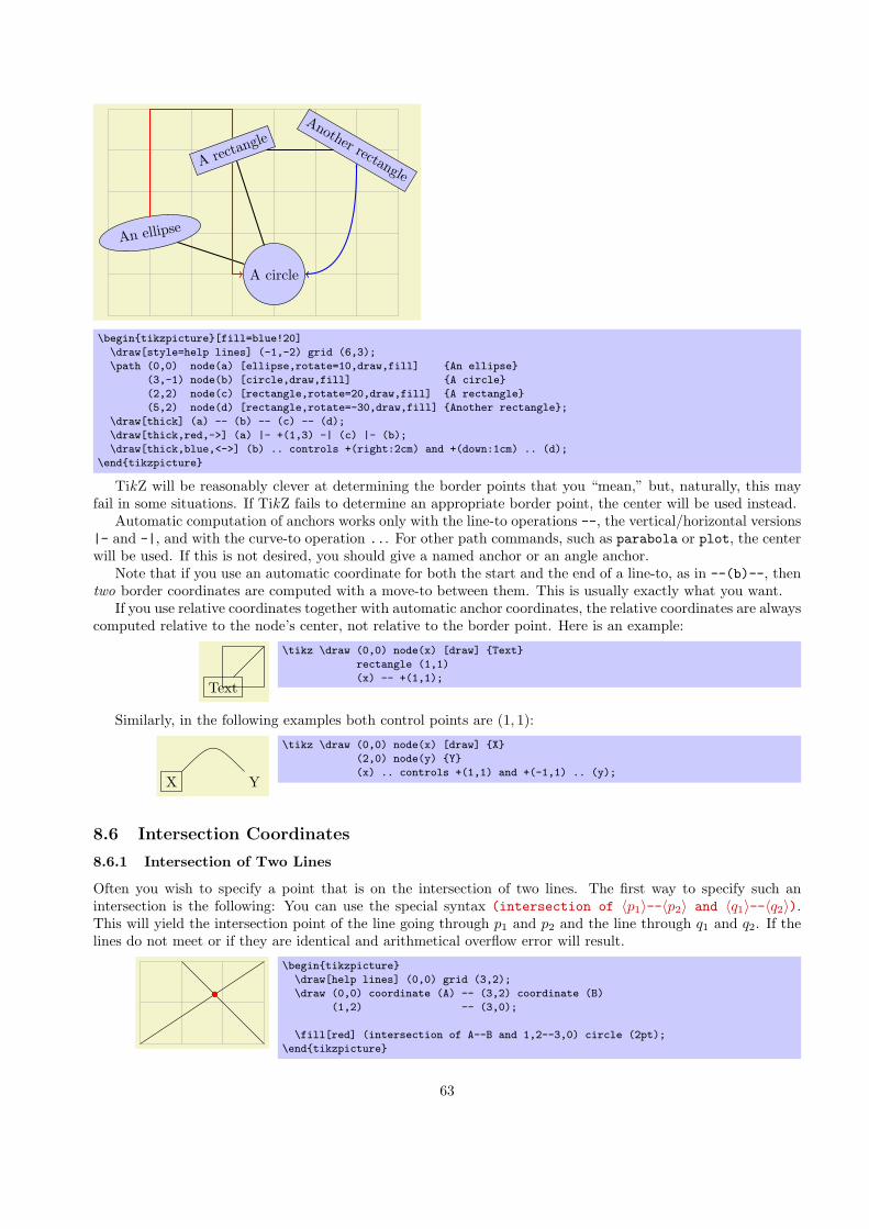
An ellipse

.

A circle.

A rectangle

.

Another rectangle

\begin{tikzpicture}[fill=blue!20]

\draw[style=help lines] (-1,-2) grid (6,3);

\path (0,0) node(a) [ellipse,rotate=10,draw,fill] {An ellipse}

(3,-1) node(b) [circle,draw,fill] {A circle}

(2,2) node(c) [rectangle,rotate=20,draw,fill] {A rectangle}

(5,2) node(d) [rectangle,rotate=-30,draw,fill] {Another rectangle};

\draw[thick] (a) -- (b) -- (c) -- (d);

\draw[thick,red,->] (a) |- +(1,3) -| (c) |- (b);

\draw[thick,blue,<->] (b) .. controls +(right:2cm) and +(down:1cm) .. (d);

\end{tikzpicture}

TikZ will be reasonably clever at determining the border points that you “mean,” but, naturally, this mayfail in some situations. If TikZ fails to determine an appropriate border point, the center will be used instead.

Automatic computation of anchors works only with the line-to operations --, the vertical/horizontal versions|- and -|, and with the curve-to operation ... For other path commands, such as parabola or plot, the centerwill be used. If this is not desired, you should give a named anchor or an angle anchor.

Note that if you use an automatic coordinate for both the start and the end of a line-to, as in --(b)--, thentwo border coordinates are computed with a move-to between them. This is usually exactly what you want.

If you use relative coordinates together with automatic anchor coordinates, the relative coordinates are alwayscomputed relative to the node’s center, not relative to the border point. Here is an example:

.

.

Text

\tikz \draw (0,0) node(x) [draw] {Text}

rectangle (1,1)

(x) -- +(1,1);

Similarly, in the following examples both control points are (1, 1):

.

.

X

.

Y

\tikz \draw (0,0) node(x) [draw] {X}

(2,0) node(y) {Y}

(x) .. controls +(1,1) and +(-1,1) .. (y);

8.6 Intersection Coordinates

8.6.1 Intersection of Two Lines

Often you wish to specify a point that is on the intersection of two lines. The first way to specify such anintersection is the following: You can use the special syntax (intersection of ⟨p1⟩--⟨p2⟩ and ⟨q1⟩--⟨q2⟩).This will yield the intersection point of the line going through p1 and p2 and the line through q1 and q2. If thelines do not meet or if they are identical and arithmetical overflow error will result.

.

\begin{tikzpicture}

\draw[help lines] (0,0) grid (3,2);

\draw (0,0) coordinate (A) -- (3,2) coordinate (B)

(1,2) -- (3,0);

\fill[red] (intersection of A--B and 1,2--3,0) circle (2pt);

\end{tikzpicture}

63

8.6.2 Intersection of Horizontal and Vertical Lines

A frequent special case of intersections is the intersection of a vertical line going through a point p and ahorizontal line going through some other point q. For this situation there is a special, shorter, syntax: You cansay either (⟨p⟩ |- ⟨q⟩) or (⟨q⟩ -| ⟨p⟩).

For example, (2,1 |- 3,4) and (3,4 -| 2,1) both yield the same as (2,4) (provided the xy-coordinatesystem has not been modified).

The most useful application of the syntax is to draw a line up to some point on a vertical or horizontal line.Here is an example:

.

.

p1

.

p2

.

q1

.

q2\begin{tikzpicture}

\path (30:1cm) node(p1) {$p_1$} (75:1cm) node(p2) {$p_2$};

\draw (-0.2,0) -- (1.2,0) node(xline)[right] {$q_1$};

\draw (2,-0.2) -- (2,1.2) node(yline)[above] {$q_2$};

\draw[->] (p1) -- (p1 |- xline);

\draw[->] (p2) -- (p2 |- xline);

\draw[->] (p1) -- (p1 -| yline);

\draw[->] (p2) -- (p2 -| yline);

\end{tikzpicture}

8.7 Relative and Incremental Coordinates

You can prefix coordinates by ++ to make them “relative.” A coordinate such as ++(1cm,0pt) means “1cm tothe right of the previous position.” Relative coordinates are often useful in “local” contexts:

.

\begin{tikzpicture}

\draw (0,0) -- ++(1,0) -- ++(0,1) -- ++(-1,0) -- cycle;

\draw (2,0) -- ++(1,0) -- ++(0,1) -- ++(-1,0) -- cycle;

\draw (1.5,1.5) -- ++(1,0) -- ++(0,1) -- ++(-1,0) -- cycle;

\end{tikzpicture}

Instead of ++ you can also use a single +. This also specifies a relative coordinate, but it does not “update” thecurrent point for subsequent usages of relative coordinates. Thus, you can use this notation to specify numerouspoints, all relative to the same “initial” point:

.

\begin{tikzpicture}

\draw (0,0) -- +(1,0) -- +(1,1) -- +(0,1) -- cycle;

\draw (2,0) -- +(1,0) -- +(1,1) -- +(0,1) -- cycle;

\draw (1.5,1.5) -- +(1,0) -- +(1,1) -- +(0,1) -- cycle;

\end{tikzpicture}

There is one special situation, where relative coordinates are interpreted differently. If you use a relativecoordinate as a control point of a Bezier curve, the following rule applies: First, a relative first control point istaken relative to the beginning of the curve. Second, a relative second control point is taken relative to the endof the curve. Third, a relative end point of a curve is taken relative to the start of the curve.

This special behavior makes it easy to specify that a curve should “leave or arrives from a certain direction”at the start or end. In the following example, the curve “leaves” at 30◦ and “arrives” at 60◦:

.

\begin{tikzpicture}

\draw (1,0) .. controls +(30:1cm) and +(60:1cm) .. (3,-1);

\draw[gray,->] (1,0) -- +(30:1cm);

\draw[gray,<-] (3,-1) -- +(60:1cm);

\end{tikzpicture}

64

9 Syntax for Path Specifications

A path is a series of straight and curved line segments. It is specified following a \path command and thespecification must follow a special syntax, which is described in the subsections of the present section.

\path⟨specification⟩;This command is available only inside a {tikzpicture} environment.The ⟨specification⟩ is a long stream of path operations. Most of these path operations tell TikZ how thepath is build. For example, when you write --(0,0), you use a line-to operation and it means “continuethe path from wherever you are to the origin.”At any point where TikZ expects a path operation, you can also give some graphic options, which is a listof options in brackets, such as [rounded corners]. These options can have different effects:

1. Some options take “immediate” effect and apply to all subsequent path operations on the path. Forexample, the rounded corners option will round all following corners, but not the corners “before”and if the sharp corners is given later on the path (in a new set of brackets), the rounding effect willend.

.

\tikz \draw (0,0) -- (1,1)

[rounded corners] -- (2,0) -- (3,1)

[sharp corners] -- (3,0) -- (2,1);

Another example are the transformation options, which also apply only to subsequent coordinates.

2. The options that have immediate effect can be “scoped” by putting part of a path in curly braces. Forexample, the above example could also be written as follows:

.

\tikz \draw (0,0) -- (1,1)

{[rounded corners] -- (2,0) -- (3,1)}

-- (3,0) -- (2,1);

3. Some options only apply to the path as a whole. For example, the color= option for determining thecolor used for, say, drawing the path always applies to all parts of the path. If several different colorsare given for different parts of the path, only the last one (on the outermost scope) “wins”:

.

\tikz \draw (0,0) -- (1,1)

[color=red] -- (2,0) -- (3,1)

[color=blue] -- (3,0) -- (2,1);

Most options are of this type. In the above example, we would have had to “split up” the path intoseveral \path commands:

.

\tikz{\draw (0,0) -- (1,1);

\draw [color=red] (2,0) -- (3,1);

\draw [color=blue] (3,0) -- (2,1);}

By default, the \path command does “nothing” with the path, it just “throws it away.” Thus, if you write\path(0,0)--(1,1);, nothing is drawn in your picture. The only effect is that the area occupied by thepicture is (possibly) enlarged so that the path fits inside the area. To actually “do” something with thepath, an option like draw or fill must be given somewhere on the path. Commands like \draw do thisimplicitly.Finally, it is also possible to give node specifications on a path. Such specifications can come at differentlocations, but they are always allowed when a normal path operation could follow. A node specificationstarts with node. Basically, the effect is to typeset the node’s text as normal TEX text and to place it atthe “current location” on the path. The details are explained in Section 11.

65

Note, however, that the nodes are not part of the path in any way. Rather, after everything has been donewith the path what is specified by the path options (like filling and drawing the path due to a fill and adraw option somewhere in the ⟨specification⟩), the nodes are added in a post-processing step.The following style influences scopes:

• style=every path This style is installed at the beginning of every path. This can be useful for(temporarily) adding, say, the draw option to everything in a scope.

.

.

\begin{tikzpicture}[fill=examplefill] % only sets the color

\tikzstyle{every path}=[draw] % all paths are drawn

\fill (0,0) rectangle +(1,1);

\shade (2,0) rectangle +(1,1);

\end{tikzpicture}

9.1 The Move-To Operation

The perhaps simplest operation is the move-to operation, which is specified by just giving a coordinate where apath operation is expected.

\path . . . ⟨coordinate⟩ . . . ;The move-to operation normally starts a path at a certain point. This does not cause a line segment to becreated, but it specifies the starting point of the next segment. If a path is already under construction, thatis, if several segments have already been created, a move-to operation will start a new part of the path thatis not connected to any of the previous segments.

.

\begin{tikzpicture}

\draw (0,0) --(2,0) (0,1) --(2,1);

\end{tikzpicture}

In the specification (0,0) --(2,0) (0,1) --(2,1) two move-to operations are specified: (0,0) and (0,1).The other two operations, namely --(2,0) and --(2,1) are line-to operations, described next.

9.2 The Line-To Operation

9.2.1 Straight Lines

\path . . . --⟨coordinate⟩ . . . ;The line-to operation extends the current path from the current point in a straight line to the givencoordinate. The “current point” is the endpoint of the previous drawing operation or the point specified bya prior move-to operation.You use two minus signs followed by a coordinate in round brackets. You can add spaces before and afterthe --.When a line-to operation is used and some path segment has just been constructed, for example by anotherline-to operation, the two line segments become joined. This means that if they are drawn, the point wherethey meet is “joined” smoothly. To appreciate the difference, consider the following two examples: In theleft example, the path consists of two path segments that are not joined, but that happen to share a point,while in the right example a smooth join is shown.

.


\draw (0,0) --(1,1) (1,1) --(2,0);

\draw (3,0) -- (4,1) -- (5,0);


\end{tikzpicture}

66

9.2.2 Horizontal and Vertical Lines

Sometimes you want to connect two points via straight lines that are only horizontal and vertical. For this, youcan use two path construction operations.

\path . . . -|⟨coordinate⟩ . . . ;This operation means “first horizontal, then vertical.”

.

.

A

.

B\begin{tikzpicture}

\draw (0,0) node(a) [draw] {A} (1,1) node(b) [draw] {B};

\draw (a.north) |- (b.west);

\draw[color=red] (a.east) -| (2,1.5) -| (b.north);

\end{tikzpicture}

\path . . . |-⟨coordinate⟩ . . . ;This operations means “first vertical, then horizontal.”

9.2.3 Snaked Lines

The line-to operation can not only be used to append straight lines to the path, but also “snaked” lines (calledthus because they look a little bit like snakes seen from above).

TikZ and pgf use a concept that I termed snakes for appending such “squiggly” lines. A snake specifies away of extending a path between two points in a “fancy manner.”

Normally, a snake will just connect the start point to the end point without starting new subpaths. Thus,a path containing a snaked line can, nevetheless, still be used for filling. However, this is not always the case.Some snakes consist of numerous unconnected segments. “Lines” consisting of such snakes cannot be used asthe borders of enclosed areas.

Here are some examples of snakes in action:

.

\begin{tikzpicture}[thick]

\draw (0,3) -- (3,3);

\draw[snake=zigzag] (0,2.5) -- (3,2.5);

\draw[snake=brace] (0,2) -- (3,2);

\draw[snake=triangles] (0,1.5) -- (3,1.5);

\draw[snake=coil,segment length=4pt] (0,1) -- (3,1);

\draw[snake=coil,segment aspect=0] (0,.5) -- (3,.5);

\draw[snake=expanding waves,segment angle=7] (0,0) -- (3,0);

\end{tikzpicture}

.

\begin{tikzpicture}

\filldraw[fill=red!20,snake=bumps] (0,0) rectangle (3,2);

\end{tikzpicture}

.

\begin{tikzpicture}

\filldraw[fill=blue!20] (0,3)

[snake=saw] -- (3,3)

[snake=coil,segment aspect=0] -- (2,1)

[snake=bumps] -| (0,3);

\end{tikzpicture}

No special path operation is needed to use a snake. Instead, you use the following option to “switch on”snaking:

67

• snake=⟨snake name⟩ This option causes the snake ⟨snake name⟩ to be used for subsequent line-to opera-tions. So, whenever you use the -- syntax to specify that a straight line should be added to the path, asnake to this path will be added instead. Snakes will also be used when you use the -| and |- syntax andalso when you use the rectangle operation. Snakes will not be used when you use the curve-to operationnor when any other “curved” line is added to the path.

This option has to be given anew for each path. However, you can also leave out the ⟨snake name⟩. Inthis case, the enclosing scope’s ⟨snake name⟩ is used. Thus, you can specify a “standard” snake name forscope and then just say \draw[snake] every time this snake should actually be used.

The ⟨snake name⟩ none is special. It can be used to switch off snaking after it has been switched on on apath.

A bit strangely, no valid ⟨snake names⟩ are defined by TikZ by default. Instead, you have to includethe library package pgflibrarysnakes. This package defines numerous snakes, see Section 14.2 for thecomplete list.

Most snakes can be configured. For example, for a snake that looks like a sine curve, you might wish tochange the amplitude or the frequency. There are numerous options that influence these parameters. Not alloptions apply to all snakes, see Section 14.2 once more for details.

• gap before snakes=⟨dimension⟩ This option allows you to add a certain “gap” to the snake at its be-ginning. The snake will not start at the current point; instead the start point of the snake is move be⟨dimension⟩ in the direction of the target.

.

\begin{tikzpicture}


\draw[snake=zigzag] (0,1) -- ++(3,1);

\draw[snake=zigzag,gap before snake=1cm] (0,0) -- ++(3,1);

\end{tikzpicture}

• gap after snake=⟨dimension⟩ This option has the same effect as gap before snake, only it affects theend of the snake, which will “end early.”

• gap around snake=⟨dimension⟩ This option sets the gap before and after the gap to ⟨dimension⟩.

.

\begin{tikzpicture}


\draw[snake=brace] (0,1) -- ++(3,1);

\draw[snake=brace,gap around snake=5mm] (0,0) -- ++(3,1);

\end{tikzpicture}

• line before snake=⟨dimension⟩ This option works like gap before snake, only it will connect the cur-rent point with a straight line to the start of the snake.

.

\begin{tikzpicture}


\draw[snake=zigzag] (0,1) -- ++(3,1);

\draw[snake=zigzag,line before snake=1cm] (0,0) -- ++(3,1);

\end{tikzpicture}

• line after snake=⟨dimension⟩ Works line gap after snake, only it adds a straight line.

• line around snake=⟨dimension⟩ Works line gap around snake, only it adds straight lines.

68

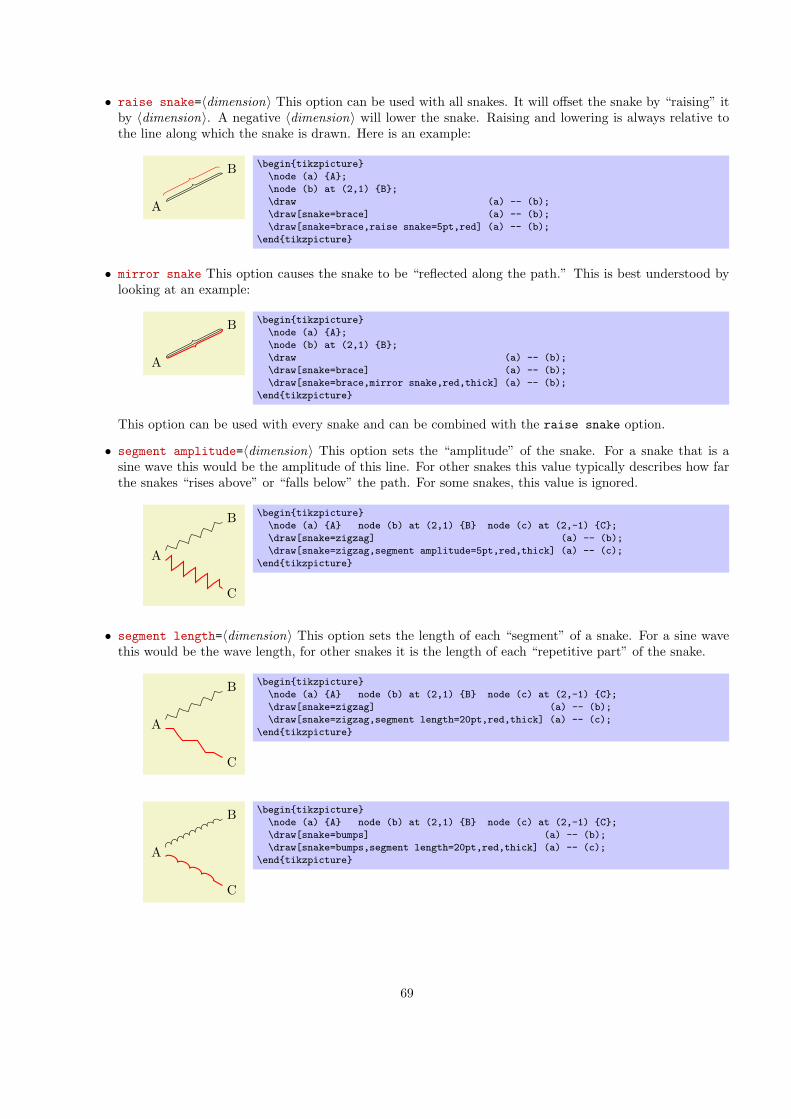
• raise snake=⟨dimension⟩ This option can be used with all snakes. It will offset the snake by “raising” itby ⟨dimension⟩. A negative ⟨dimension⟩ will lower the snake. Raising and lowering is always relative tothe line along which the snake is drawn. Here is an example:

.

.

A

.

B \begin{tikzpicture}

\node (a) {A};

\node (b) at (2,1) {B};

\draw (a) -- (b);

\draw[snake=brace] (a) -- (b);

\draw[snake=brace,raise snake=5pt,red] (a) -- (b);

\end{tikzpicture}

• mirror snake This option causes the snake to be “reflected along the path.” This is best understood bylooking at an example:

.

.

A

.


\node (a) {A};

\node (b) at (2,1) {B};

\draw (a) -- (b);

\draw[snake=brace] (a) -- (b);

\draw[snake=brace,mirror snake,red,thick] (a) -- (b);

\end{tikzpicture}

This option can be used with every snake and can be combined with the raise snake option.

• segment amplitude=⟨dimension⟩ This option sets the “amplitude” of the snake. For a snake that is asine wave this would be the amplitude of this line. For other snakes this value typically describes how farthe snakes “rises above” or “falls below” the path. For some snakes, this value is ignored.

.

.

A

.

B

.

C

\begin{tikzpicture}

\node (a) {A} node (b) at (2,1) {B} node (c) at (2,-1) {C};

\draw[snake=zigzag] (a) -- (b);

\draw[snake=zigzag,segment amplitude=5pt,red,thick] (a) -- (c);

\end{tikzpicture}

• segment length=⟨dimension⟩ This option sets the length of each “segment” of a snake. For a sine wavethis would be the wave length, for other snakes it is the length of each “repetitive part” of the snake.

.

.

A

.

B

.

C

\begin{tikzpicture}


\draw[snake=zigzag] (a) -- (b);

\draw[snake=zigzag,segment length=20pt,red,thick] (a) -- (c);

\end{tikzpicture}

.

.

A

.

B

.

C

\begin{tikzpicture}


\draw[snake=bumps] (a) -- (b);

\draw[snake=bumps,segment length=20pt,red,thick] (a) -- (c);

\end{tikzpicture}

69

• segment object length=⟨dimension⟩ This option sets the length of the objects inside each segment of asnake. This option is only used for snakes in which each segment contains an object like a triangle or astar.

.

.

A

.

B

.

C

\begin{tikzpicture}


\draw[snake=triangles] (a) -- (b);

\draw[snake=triangles,segment object length=8pt,red,thick] (a) -- (c);

\end{tikzpicture}

• segment angle=⟨degrees⟩ This option sets an angle that is interpreted in a snake-specific way. For example,the waves and expanding waves snakes interpret this as (half the) opening angle of the wave. The bordersnake uses this value for the angle of the little ticks.

.

.

A

.

B \begin{tikzpicture}[segment amplitude=10pt]

\node (a) {A} node (b) at (2,0) {B};

\draw[snake=border] (a) -- (b);

\draw[snake=border,segment angle=20,red,thick] (a) -- (b);

\end{tikzpicture}

.

.

A

.

B

.

A

.

B

\begin{tikzpicture}[segment amplitude=10pt]

\node (a) {A} node (b) at (2,0) {B};

\node (a’) at (0,-1) {A} node (b’) at (2,-1) {B};

\draw[snake=expanding waves] (a) -- (b);

\draw[snake=expanding waves,segment angle=20,red,thick] (a’) -- (b’);

\end{tikzpicture}

• segment aspect=⟨ratio⟩ This option sets an aspect ratio that is interpreted in a snake-specific way. Forexample, for the coils snake this describes the “direction” from which the coil is viewed.

.

.

A

.

B

.

C

\begin{tikzpicture}[segment amplitude=5pt,segment length=5pt]


\draw[snake=coil] (a) -- (b);

\draw[snake=coil,segment aspect=0,red,thick] (a) -- (c);

\end{tikzpicture}

It is possible to define new snakes, but this cannot be done inside TikZ. You need to use the command\pgfdeclaresnake from the basic level directly, see Section 22.

The following styles define combinations of segment settings that may be useful:

• style=snake triangles 45 Installs a snake the consists of little triangles with an opening angle of 45◦.



9.3 The Curve-To Operation

The curve-to operation allows you to extend a path using a Bezier curve.

70

\path . . . ..controls⟨c⟩and⟨d⟩..⟨y⟩ . . . ;This operation extends the current path from the current point, let us call it x, via a curve to a the currentpoint y. The curve is a cubic Bezier curve. For such a curve, apart from y, you also specify two controlpoints c and d. The idea is that the curve starts at x, “heading” in the direction of c. Mathematicallyspoken, the tangent of the curve at x goes through c. Similarly, the curve ends at y, “coming from” theother control point, d. The larger the distance between x and c and between d and y, the larger the curvewill be.If the “and⟨d⟩” part is not given, d is assumed to be equal to c.

.

\begin{tikzpicture}

\draw[line width=10pt] (0,0) .. controls (1,1) .. (4,0)

.. controls (5,0) and (5,1) .. (4,1);

\draw[color=gray] (0,0) -- (1,1) -- (4,0) -- (5,0) -- (5,1) -- (4,1);

\end{tikzpicture}

As with the line-to operation, it makes a difference whether two curves are joined because they resultedfrom consecutive curve-to or line-to operations, or whether they just happen to have the same ending:

.


\draw (0,0) -- (1,1) (1,1) .. controls (1,0) and (2,0) .. (2,0);

\draw (3,0) -- (4,1) .. controls (4,0) and (5,0) .. (5,0);


\end{tikzpicture}

9.4 The Cycle Operation

\path . . . --cycle . . . ;This operation adds a straight line from the current point to the last point specified by a move-to operation.Note that this need not be the beginning of the path. Furthermore, a smooth join is created between thefirst segment created after the last move-to operation and the straight line appended by the cycle operation.Consider the following example. In the left example, two triangles are created using three straight lines,but they are not joined at the ends. In the second example cycle operations are used.

.


\draw (0,0) -- (1,1) -- (1,0) -- (0,0) (2,0) -- (3,1) -- (3,0) -- (2,0);

\draw (5,0) -- (6,1) -- (6,0) -- cycle (7,0) -- (8,1) -- (8,0) -- cycle;


\end{tikzpicture}

9.5 The Rectangle Operation

A rectangle can obviously be created using four straight lines and a cycle operation. However, since rectanglesare needed so often, a special syntax is available for them.

71

\path . . . rectangle⟨corner⟩ . . . ;When this operation is used, one corner will be the current point, another corner is given by ⟨corner⟩, whichbecomes the new current point.

.

\begin{tikzpicture}

\draw (0,0) rectangle (1,1);

\draw (.5,1) rectangle (2,0.5) (3,0) rectangle (3.5,1.5) -- (2,0);

\end{tikzpicture}

9.6 Rounding Corners

All of the path construction operations mentioned up to now are influenced by the following option:

• rounded corners=⟨inset⟩ When this option is in force, all corners (places where a line is continued eithervia line-to or a curve-to operation) are replaced by little arcs so that the corner becomes smooth.

.

\tikz \draw [rounded corners] (0,0) -- (1,1)

-- (2,0) .. controls (3,1) .. (4,0);

The ⟨inset⟩ describes how big the corner is. Note that the ⟨inset⟩ is not scaled along if you use a scalingoption like scale=2.

.

\begin{tikzpicture}

\draw[color=gray,very thin] (10pt,15pt) circle (10pt);

\draw[rounded corners=10pt] (0,0) -- (0pt,25pt) -- (40pt,25pt);

\end{tikzpicture}

You can switch the rounded corners on and off “in the middle of path” and different corners in the samepath can have different corner radii:

.

\begin{tikzpicture}

\draw (0,0) [rounded corners=10pt] -- (1,1) -- (2,1)

[sharp corners] -- (2,0)

[rounded corners=5pt] -- cycle;

\end{tikzpicture}

Here is a rectangle with rounded corners:

.

\tikz \draw[rounded corners=1ex] (0,0) rectangle (20pt,2ex);

You should be aware, that there are several pitfalls when using this option. First, the rounded corner willonly be an arc (part of a circle) if the angle is 90◦. In other cases, the rounded corner will still be round,but “not as nice.”

Second, if there are very short line segments in a path, the “rounding” may cause inadverted effects. Insuch case it may be necessary to temporarily switch off the rounding using sharp corners.

• sharp corners This options switches off any rounding on subsequent corners of the path.

9.7 The Circle and Ellipse Operations

A circle can be approximated well using four Bezier curves. However, it is difficult to do so correctly. For thisreason, a special syntax is available for adding such an approximation of a circle to the current path.

\path . . . circle(⟨radius⟩) . . . ;The center of the circle is given by the current point. The new current point of the path will remain to bethe center of the circle.

72

\path . . . ellipse(⟨half width⟩ and ⟨half height⟩) . . . ;Note that you can add spaces after ellipse, but you have to place spaces around and.

.

\begin{tikzpicture}

\draw (1,0) circle (.5cm);

\draw (3,0) ellipse (1cm and .5cm) -- ++(3,0) circle (.5cm)

-- ++(2,-.5) circle (.25cm);

\end{tikzpicture}

9.8 The Arc Operation

The arc operation allows you to add an arc to the current path.

\path . . . arc(⟨start angle⟩:⟨end angle⟩:⟨radius⟩/⟨half height⟩) . . . ;The arc operation adds a part of a circle of the given radius between the given angles. The arc will start atthe current point and will end at the end of the arc.

.

\begin{tikzpicture}

\draw (0,0) arc (180:90:1cm) -- (2,.5) arc (90:0:1cm);

\draw (4,0) -- +(30:1cm) arc (30:60:1cm) -- cycle;

\draw (8,0) arc (0:270:1cm/.5cm) -- cycle;

\end{tikzpicture}

.

.

α

.

β

\begin{tikzpicture}

\draw (-1,0) -- +(3.5,0);

\draw (1,0) ++(210:2cm) -- +(30:4cm);

\draw (1,0) +(0:1cm) arc (0:30:1cm);

\draw (1,0) +(180:1cm) arc (180:210:1cm);

\path (1,0) ++(15:.75cm) node{$\alpha$};

\path (1,0) ++(15:-.75cm) node{$\beta$};

\end{tikzpicture}

9.9 The Grid Operation

You can add a grid to the current path using the grid path operation.

\path . . . grid[⟨options⟩]⟨corner⟩ . . . ;This operations adss a grid filling a rectangle whose two corners are given by ⟨corner⟩ and by the previouscoordinate. Thus, the typical way in which a grid is drawn is \draw (1,1) grid (3,3);, which yields agrid filling the rectangle whose corners are at (1, 1) and (3, 3). All coordinate transformations apply to thegrid.

.

\tikz[rotate=30] \draw[step=1mm] (0,0) grid (2,2);

73

The stepping of the grid is governed by the following options:

• step=⟨dimension⟩ sets the stepping in both the x and y-direction.

• xstep=⟨dimension⟩ sets the stepping in the x-direction.

• ystep=⟨dimension⟩ sets the stepping in the y-direction.

It is important to note that the grid is always “phased” such that it contains the point (0, 0) if that pointhappens to be inside the rectangle. Thus, the grid does not always have an intersection at the corner points;this occurs only if the corner points are multiples of the stepping. Note that due to rounding errors, the“last” lines of a grid may be omitted. In this case, you have to add an epsilon to the corner points.The following style is useful for drawing grids:

• style=help lines This style makes lines “subdued” by using thin gray lines for them. However, thisstyle is not installed automatically and you have to say for example:

.

\tikz \draw[style=help lines] (0,0) grid (3,3);

9.10 The Parabola Operation

The parabola path operation continues the current path with a parabola. A parabola is a (shifted and scaled)curve defined by the equation f(x) = x2 and looks like this:

.

.

\path . . . parabola[⟨options⟩]bend⟨bend coordinate⟩⟨coordinate⟩ . . . ;This operation adds a parabola through the current point and the given ⟨coordinate⟩. If the bend is given, itspecifies where the bend should go; the ⟨options⟩ can also be used to specify where the bend is. By default,the bend is at the old current point.

.

\begin{tikzpicture}

\draw (0,0) rectangle (1,1.5)

(0,0) parabola (1,1.5);

\draw[xshift=1.5cm] (0,0) rectangle (1,1.5)

(0,0) parabola[bend at end] (1,1.5);

\draw[xshift=3cm] (0,0) rectangle (1,1.5)

(0,0) parabola bend (.75,1.75) (1,1.5);

\end{tikzpicture}

The following options influence parabolas:

• bend=⟨coordinate⟩ Has the same effect as saying bend⟨coordinate⟩ outside the ⟨options⟩. The optionspecifies that the bend of the parabola should be at the given ⟨coordinate⟩. You have to take careyourself that the bend position is a “valid” position; which means that if there is no parabola of theform f(x) = ax2 + bx+ c that goes through the old current point, the given bend, and the new currentpoint, the result will not be a parabola.There is one special property of the ⟨coordinate⟩: When a relative coordinate is given like +(0,0), theposition relative to which this coordinate is “flexible.” More precisely, this position lies somewhere ona line from the old current point to the new current point. The exact position depends on the nextoption.

• bend pos=⟨fraction⟩ Specifies where the “previous” point is relative to which the bend is calculated.The previous point will be at the ⟨fraction⟩th part of the line from the old current point to the newcurrent point.

74

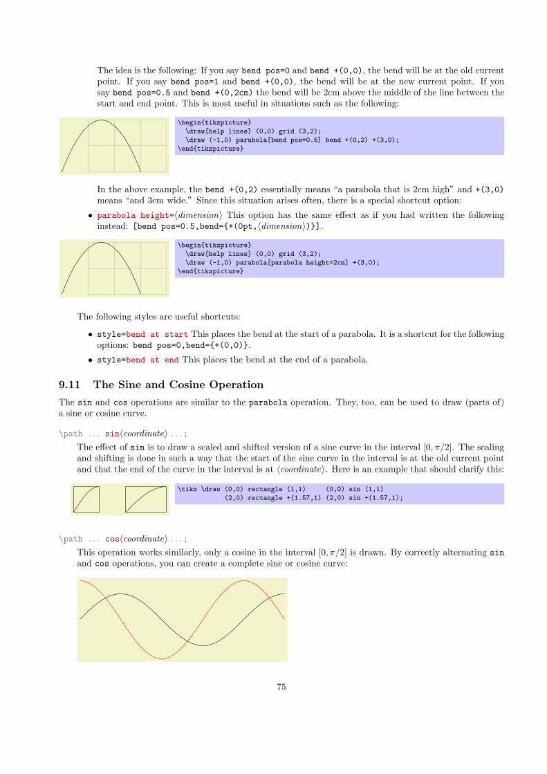
The idea is the following: If you say bend pos=0 and bend +(0,0), the bend will be at the old currentpoint. If you say bend pos=1 and bend +(0,0), the bend will be at the new current point. If yousay bend pos=0.5 and bend +(0,2cm) the bend will be 2cm above the middle of the line between thestart and end point. This is most useful in situations such as the following:

.

\begin{tikzpicture}


\draw (-1,0) parabola[bend pos=0.5] bend +(0,2) +(3,0);

\end{tikzpicture}

In the above example, the bend +(0,2) essentially means “a parabola that is 2cm high” and +(3,0)means “and 3cm wide.” Since this situation arises often, there is a special shortcut option:

• parabola height=⟨dimension⟩ This option has the same effect as if you had written the followinginstead: [bend pos=0.5,bend={+(0pt,⟨dimension⟩)}].

.

\begin{tikzpicture}


\draw (-1,0) parabola[parabola height=2cm] +(3,0);

\end{tikzpicture}

The following styles are useful shortcuts:

• style=bend at start This places the bend at the start of a parabola. It is a shortcut for the followingoptions: bend pos=0,bend={+(0,0)}.

• style=bend at end This places the bend at the end of a parabola.

9.11 The Sine and Cosine Operation

The sin and cos operations are similar to the parabola operation. They, too, can be used to draw (parts of)a sine or cosine curve.

\path . . . sin⟨coordinate⟩ . . . ;The effect of sin is to draw a scaled and shifted version of a sine curve in the interval [0, π/2]. The scalingand shifting is done in such a way that the start of the sine curve in the interval is at the old current pointand that the end of the curve in the interval is at ⟨coordinate⟩. Here is an example that should clarify this:

.

\tikz \draw (0,0) rectangle (1,1) (0,0) sin (1,1)

(2,0) rectangle +(1.57,1) (2,0) sin +(1.57,1);

\path . . . cos⟨coordinate⟩ . . . ;This operation works similarly, only a cosine in the interval [0, π/2] is drawn. By correctly alternating sinand cos operations, you can create a complete sine or cosine curve:

.

75

\begin{tikzpicture}[xscale=1.57]

\draw (0,0) sin (1,1) cos (2,0) sin (3,-1) cos (4,0) sin (5,1);

\draw[color=red] (0,1.5) cos (1,0) sin (2,-1.5) cos (3,0) sin (4,1.5) cos (5,0);

\end{tikzpicture}

Note that there is no way to (conveniently) draw an interval on a sine or cosine curve whose end points arenot multiples of π/2.

9.12 The Plot Operation

The plot operation can be used to append a line or curve to the path that goes through a large number ofcoordinates. These coordinates are either given in a simple list of coordinates or they are read from some file.

The syntax of the plot comes in different versions.

\path . . . --plot⟨further arguments⟩ . . . ;This operation plots the curve through the coordinates specified in the ⟨further arguments⟩. The current(sub)path is simply continued, that is, a line-to operation to the first point of the curve is implicitly added.The details of the ⟨further arguments⟩ will be explained in a moment.

\path . . . plot⟨further arguments⟩ . . . ;This operation plots the curve through the coordinates specified in the ⟨further arguments⟩ by first “moving”to the first coordinate of the curve.

The ⟨further arguments⟩ are used in three different ways to specifying the coordinates of the points to beplotted:

1. --plot[⟨local options⟩]coordinates{⟨coordinate 1 ⟩⟨coordinate 2 ⟩. . . ⟨coordinate n⟩}

2. --plot[⟨local options⟩]file{⟨filename⟩}

3. --plot[⟨local options⟩]function{⟨gnuplot formula⟩}

These different ways are explained in the following.

9.12.1 Plotting Points Given Inline

In the first two cases, the points are given directly in the TEX-file as in the following example:

.

\tikz \draw plot coordinates {(0,0) (1,1) (2,0) (3,1) (2,1) (10:2cm)};

Here is an example showing the difference between plot and --plot:

.

\begin{tikzpicture}

\draw (0,0) -- (1,1) plot coordinates {(2,0) (4,0)};

\draw[color=red,xshift=5cm]

(0,0) -- (1,1) -- plot coordinates {(2,0) (4,0)};

\end{tikzpicture}

76

9.12.2 Plotting Points Read From an External File

The second way of specifying points is to put them in an external file named ⟨filename⟩. Currently, the only fileformat that TikZ allows is the following: Each line of the ⟨filename⟩ should contain one line starting with twonumbers, separated by a space. Anything following the two numbers on the line is ignored. Also, lines startingwith a % or a # are ignored as well as empty lines. (This is exactly the format that gnuplot produces when yousay set terminal table.) If necessary, more formats will be supported in the future, but it is usually easy toproduce a file containing data in this form.

.

\tikz \draw plot[mark=x,smooth] file {plots/pgfmanual-sine.table};

The file plots/pgfmanual-sine.table reads:

#Curve 0, 20 points

#x y type

0.00000 0.00000 i

0.52632 0.50235 i

1.05263 0.86873 i

1.57895 0.99997 i

...

9.47368 -0.04889 i

10.00000 -0.54402 i

It was produced from the following source, using gnuplot:

set terminal table

set output "../plots/pgfmanual-sine.table"

set format "%.5f"

set samples 20

plot [x=0:10] sin(x)

The ⟨local options⟩ of the plot operation are local to each plot and do not affect other plots “on the samepath.” For example, plot[yshift=1cm] will locally shift the plot 1cm upward. Remember, however, that mostoptions can only be applied to paths as a whole. For example, plot[red] does not have the effect of makingthe plot red. After all, you are trying to “locally” make part of the path red, which is not possible.

9.12.3 Plotting a Function

Often, you will want to plot points that are given via a function like f(x) = x sinx. Unfortunately, TEX doesnot really have enough computational power to generate the points on such a function efficiently (it is a textprocessing program, after all). However, if you allow it, TEX can try to call external programs that can easilyproduce the necessary points. Currently, TikZ knows how to call gnuplot.

When TikZ encounters your operation plot[id=⟨id⟩] function{x*sin(x)} for the first time, it will create afile called ⟨prefix ⟩⟨id⟩.gnuplot, where ⟨prefix ⟩ is \jobname. by default, that is, the name of you main .tex file.If no ⟨id⟩ is given, it will be empty, which is alright, but it is better when each plot has a unique ⟨id⟩ for reasonsexplained in a moment. Next, TikZ writes some initialization code into this file followed by plot x*sin(x).The initialization code sets up things such that the plot operation will write the coordinates into another filecalled ⟨prefix ⟩⟨id⟩.table. Finally, this table file is read as if you had said plot file{⟨prefix ⟩⟨id⟩.table}.

For the plotting mechanism to work, two conditions must be met:

1. You must have allowed TEX to call external programs. This is often switched off by default since thisis a security risk (you might, without knowing, run a TEX file that calls all sorts of “bad” commands).To enable this “calling external programs” a command line option must be given to the TEX program.Usually, it is called something like shell-escape or enable-write18. For example, for my pdflatex theoption --shell-escape can be given.

77

2. You must have installed the gnuplot program and TEX must find it when compiling your file.

Unfortunately, these conditions will not always be met. Especially if you pass some source to a coauthor andthe coauthor does not have gnuplot installed, he or she will have trouble compiling your files.

For this reason, TikZ behaves differently when you compile your graphic for the second time: If upon reachingplot[id=⟨id⟩] function{...} the file ⟨prefix ⟩⟨id⟩.table already exists and if the ⟨prefix ⟩⟨id⟩.gnuplot filecontains what TikZ thinks that it “should” contain, the .table file is immediately read without trying to calla gnuplot program. This approach has the following advantages:

1. If you pass a bundle of your .tex file and all .gnuplot and .table files to someone else, that person canTEX the .tex file without having to have gnuplot installed.

2. If the \write18 feature is switched off for security reasons (a good idea), then, upon the first compilationof the .tex file, the .gnuplot will still be generated, but not the .table file. You can then simply callgnuplot “by hand” for each .gnuplot file, which will produce all necessary .table files.

3. If you change the function that you wish to plot or its domain, TikZ will automatically try to regeneratethe .table file.

4. If, out of laziness, you do not provide an id, the same .gnuplot will be used for different plots, but thisis not a problem since the .table will automatically be regenerated for each plot on-the-fly. Note: If youintend to share your files with someone else, always use an id, so that the file can by typeset without havinggnuplot installed. Also, having unique ids for each plot will improve compilation speed since no externalprograms need to be called, unless it is really necessary.

When you use plot function{⟨gnuplot formula⟩}, the ⟨gnuplot formula⟩ must be given in the gnuplotsyntax, whose details are beyond the scope of this manual. Here is the ultra-condensed essence: Use x asthe variable and use the C-syntax for normal plots, use t as the variable for parametric plots. Here are someexamples:

.

.

x

.

f(x)

.

f(x) = x

.

f(x) = sin x

.

f(x) = 120ex

\begin{tikzpicture}[domain=0:4]

\draw[very thin,color=gray] (-0.1,-1.1) grid (3.9,3.9);

\draw[->] (-0.2,0) -- (4.2,0) node[right] {$x$};

\draw[->] (0,-1.2) -- (0,4.2) node[above] {$f(x)$};

\draw[color=red] plot[id=x] function{x} node[right] {$f(x) =x$};

\draw[color=blue] plot[id=sin] function{sin(x)} node[right] {$f(x) = \sin x$};

\draw[color=orange] plot[id=exp] function{0.05*exp(x)} node[right] {$f(x) = \frac{1}{20} \mathrm e^x$};

\end{tikzpicture}

The following options influence the plot:

• samples=⟨number⟩ sets the number of samples used in the plot. The default is 25.

78

• domain=⟨start⟩:⟨end⟩ sets the domain between which the samples are taken. The default is -5:5.

• parametric=⟨true or false⟩ sets whether the plot is a parametric plot. If true, then t must be used insteadof x as the parameter and two comma-separated functions must be given in the ⟨gnuplot formula⟩. Anexample is the following:

.

\tikz \draw[scale=0.5,domain=-3.141:3.141,smooth]

plot[parametric,id=parametric-example] function{t*sin(t),t*cos(t)};

• id=⟨id⟩ sets the identifier of the current plot. This should be a unique identifier for each plot (thoughthings will also work if it is not, but not as well, see the explanations above). The ⟨id⟩ will be part of afilename, so it should not contain anything fancy like * or $.

• prefix=⟨prefix ⟩ is put before each plot file name. The default is \jobname., but if you have many plots,it might be better to use, say plots/ and have all plots placed in a directory. You have to create thedirectory yourself.

• raw gnuplot causes the ⟨gnuplot formula⟩ to be passed on to gnuplot without setting up the samples orthe plot operation. Thus, you could write

plot[raw gnuplot,id=raw-example] function{set samples 25; plot sin(x)}

This can be useful for complicated things that need to be passed to gnuplot. However, for really com-plicated situations you should create a special external generating gnuplot file and use the file-syntaxto include the table “by hand.”

The following styles influence the plot:

• style=every plot This style is installed in each plot, that is, as if you always said

plot[style=every plot,...]

This is most useful for globally setting a prefix for all plots by saying:

\tikzstyle{every plot}=[prefix=plots/]

9.12.4 Placing Marks on the Plot

As we saw already, it is possible to add marks to a plot using the mark option. When this option is used, a copyof the plot mark is placed on each point of the plot. Note that the marks are placed after the whole path hasbeen drawn/filled/shaded. In this respect, they are handled like text nodes.

In detail, the following options govern how marks are drawn:

• mark=⟨mark mnemonic⟩ Sets the mark to a mnemonic that has previously been defined using the\pgfdeclareplotmark. By default, *, +, and x are available, which draw a filled circle, a plus, and across as marks. Many more marks become available when the library pgflibraryplotmarks is loaded.Section 14.3.3 lists the available plot marks.

One plot mark is special: the ball plot mark is available only it TikZ. The ball color determines theballs’s color. Do not use this option with large number of marks since it will take very long to render inPostScript.Option Effect

mark=ball

.

.

.

.

.

79

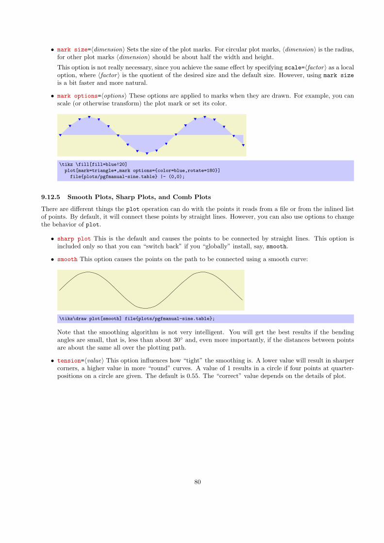
• mark size=⟨dimension⟩ Sets the size of the plot marks. For circular plot marks, ⟨dimension⟩ is the radius,for other plot marks ⟨dimension⟩ should be about half the width and height.

This option is not really necessary, since you achieve the same effect by specifying scale=⟨factor⟩ as a localoption, where ⟨factor⟩ is the quotient of the desired size and the default size. However, using mark sizeis a bit faster and more natural.

• mark options=⟨options⟩ These options are applied to marks when they are drawn. For example, you canscale (or otherwise transform) the plot mark or set its color.

.

\tikz \fill[fill=blue!20]

plot[mark=triangle*,mark options={color=blue,rotate=180}]

file{plots/pgfmanual-sine.table} |- (0,0);

9.12.5 Smooth Plots, Sharp Plots, and Comb Plots

There are different things the plot operation can do with the points it reads from a file or from the inlined listof points. By default, it will connect these points by straight lines. However, you can also use options to changethe behavior of plot.

• sharp plot This is the default and causes the points to be connected by straight lines. This option isincluded only so that you can “switch back” if you “globally” install, say, smooth.

• smooth This option causes the points on the path to be connected using a smooth curve:

.

\tikz\draw plot[smooth] file{plots/pgfmanual-sine.table};

Note that the smoothing algorithm is not very intelligent. You will get the best results if the bendingangles are small, that is, less than about 30◦ and, even more importantly, if the distances between pointsare about the same all over the plotting path.

• tension=⟨value⟩ This option influences how “tight” the smoothing is. A lower value will result in sharpercorners, a higher value in more “round” curves. A value of 1 results in a circle if four points at quarter-positions on a circle are given. The default is 0.55. The “correct” value depends on the details of plot.

80

.

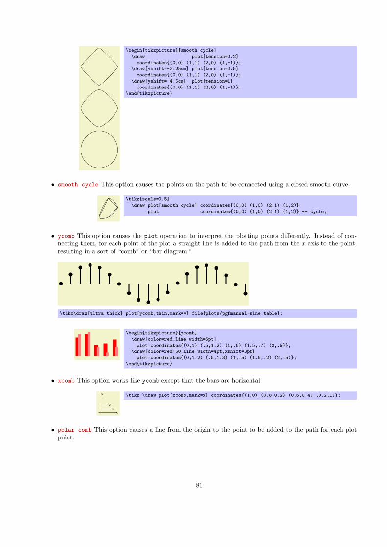
\begin{tikzpicture}[smooth cycle]

\draw plot[tension=0.2]

coordinates{(0,0) (1,1) (2,0) (1,-1)};

\draw[yshift=-2.25cm] plot[tension=0.5]

coordinates{(0,0) (1,1) (2,0) (1,-1)};

\draw[yshift=-4.5cm] plot[tension=1]

coordinates{(0,0) (1,1) (2,0) (1,-1)};

\end{tikzpicture}

• smooth cycle This option causes the points on the path to be connected using a closed smooth curve.

.

\tikz[scale=0.5]

\draw plot[smooth cycle] coordinates{(0,0) (1,0) (2,1) (1,2)}

plot coordinates{(0,0) (1,0) (2,1) (1,2)} -- cycle;

• ycomb This option causes the plot operation to interpret the plotting points differently. Instead of con-necting them, for each point of the plot a straight line is added to the path from the x-axis to the point,resulting in a sort of “comb” or “bar diagram.”

.

\tikz\draw[ultra thick] plot[ycomb,thin,mark=*] file{plots/pgfmanual-sine.table};

.

\begin{tikzpicture}[ycomb]

\draw[color=red,line width=6pt]

plot coordinates{(0,1) (.5,1.2) (1,.6) (1.5,.7) (2,.9)};

\draw[color=red!50,line width=4pt,xshift=3pt]

plot coordinates{(0,1.2) (.5,1.3) (1,.5) (1.5,.2) (2,.5)};

\end{tikzpicture}

• xcomb This option works like ycomb except that the bars are horizontal.

.

\tikz \draw plot[xcomb,mark=x] coordinates{(1,0) (0.8,0.2) (0.6,0.4) (0.2,1)};

• polar comb This option causes a line from the origin to the point to be added to the path for each plotpoint.

81

.

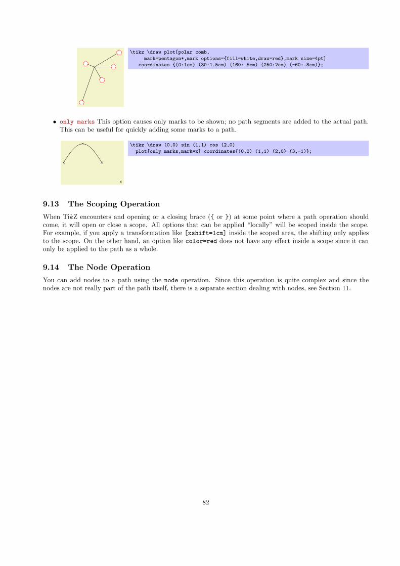
\tikz \draw plot[polar comb,

mark=pentagon*,mark options={fill=white,draw=red},mark size=4pt]

coordinates {(0:1cm) (30:1.5cm) (160:.5cm) (250:2cm) (-60:.8cm)};

• only marks This option causes only marks to be shown; no path segments are added to the actual path.This can be useful for quickly adding some marks to a path.

.

\tikz \draw (0,0) sin (1,1) cos (2,0)

plot[only marks,mark=x] coordinates{(0,0) (1,1) (2,0) (3,-1)};

9.13 The Scoping Operation

When TikZ encounters and opening or a closing brace ({ or }) at some point where a path operation shouldcome, it will open or close a scope. All options that can be applied “locally” will be scoped inside the scope.For example, if you apply a transformation like [xshift=1cm] inside the scoped area, the shifting only appliesto the scope. On the other hand, an option like color=red does not have any effect inside a scope since it canonly be applied to the path as a whole.

9.14 The Node Operation

You can add nodes to a path using the node operation. Since this operation is quite complex and since thenodes are not really part of the path itself, there is a separate section dealing with nodes, see Section 11.

82

10 Actions on Paths

Once a path has been constructed, different things can be done with it. It can be drawn (or stroked) with a“pen,” it can be filled with a color or shading, it can be used for clipping subsequent drawing, it can be used tospecify the extend of the picture—or any combination of these actions at the same time.

To decide what is to be done with a path, two methods can be used. First, you can use a special-purposecommand like \draw to indicate that the path should be drawn. However, commands like \draw and \fill arejust abbreviations for special cases of the more general method: Here, the \path command is used to specifythe path. Then, options encountered on the path indicate what should be done with the path.

For example, \path (0,0) circle (1cm); means “This is a path consisting of a circle around the origin.Do not do anything with it (throw it away).” However, if the option draw is encountered anywhere on thepath, the circle will be drawn. “Anywhere” is any point on the path where an option can be given, which iseverywhere where a path command like circle (1cm) or rectangle (1,1) or even just (0,0) would also beallowed. Thus, the following commands all draw the same circle:

\path [draw] (0,0) circle (1cm);

\path (0,0) [draw] circle (1cm);

\path (0,0) circle (1cm) [draw];

Finally, \draw (0,0) circle (1cm); also draws a path, because \draw is an abbreviation for \path [draw]and thus the command expands to the first line of the above example.

Similarly, \fill is an abbreviation for \path[fill] and \filldraw is an abbreviation for the command\path[fill,draw]. Since options accumulate, the following commands all have the same effect:

\path [draw,fill] (0,0) circle (1cm);

\path [draw] [fill] (0,0) circle (1cm);

\path [fill] (0,0) circle (1cm) [draw];

\draw [fill] (0,0) circle (1cm);

\fill (0,0) [draw] circle (1cm);

\filldraw (0,0) circle (1cm);

In the following subsection the different actions are explained that can be performed on a path. The fol-lowing commands are abbreviations for certain sets of actions, but for many useful combinations there are noabbreviations:

\draw

Inside {tikzpicture} this is an abbreviation for \path[draw].

\fill

Inside {tikzpicture} this is an abbreviation for \path[fill].

\filldraw

Inside {tikzpicture} this is an abbreviation for \path[fill,draw].

\shade

Inside {tikzpicture} this is an abbreviation for \path[shade].

\shadedraw

Inside {tikzpicture} this is an abbreviation for \path[shade,draw].

\clip

Inside {tikzpicture} this is an abbreviation for \path[clip].

\useasboundingbox

Inside {tikzpicture} this is an abbreviation for \path[use as bounding box].

\node

Inside {tikzpicture} this is an abbreviation for \path node. Note that, for once, node is not an optionbut a path operation.

83

\coordinate

Inside {tikzpicture} this is an abbreviation for \path coordinate.

10.1 Specifying a Color

The most unspecific option for setting colors is the following:

• color=⟨color name⟩This option sets the color that is used for fill, drawing, and text inside the currentscope. Any special settings for filling colors or drawing colors are immediately “overruled” by this option.

The ⟨color name⟩ is the name of a previously defined color. For LATEX users, this is just a normal “LATEX-color” and the xcolor extensions are allows. Here is an example:

.

\tikz \fill[color=red!20] (0,0) circle (1ex);

It is possible to “leave out” the color= part and you can also write:

.

\tikz \fill[red!20] (0,0) circle (1ex);

What happens is that every option that TikZ does not know, like red!20, gets a “second chance” as acolor name.

For plain TEX users, it is not so easy to specify colors since plain TEX has no “standardized” color namingmechanism. Because of this, pgf emulates the xcolor package, though the emulation is extremely basic(more precisely, what I could hack together in two hours or so). The emulation allows you to do thefollowing:

– Specify a new color using \definecolor. Only the two color models gray and rgb are supported.

Example: \definecolor{orange}{rgb}{1,0.5,0}

– Use \colorlet to define a new color based on an old one. Here, the ! mechanism is supported,though only “once” (use multiple \colorlet for more fancy colors).

Example: \colorlet{lightgray}{black!25}

– Use \color{⟨color name⟩} to set the color in the current TEX group. \aftergroup-hackery is usedto restore the color after the group.

As pointed out above, the color= option applies to “everything” (except to shadings), which is not alwayswhat you want. Because of this, there are several more specialized color options. For example, the draw=option sets the color used for drawing, but does not modify the color used for filling. These color options aredocumented where the path action they influence is described.

10.2 Drawing a Path

You can draw a path using the following option:

• draw=⟨color⟩ Causes the path to be drawn. “Drawing” (also known as “stroking”) can be thought of aspicking up a pen and moving it along the path, thereby leaving “ink” on the canvas.

There are numerous parameters that influence how a line is drawn, like the thickness or the dash pattern.These options are explained below.

If the optional ⟨color⟩ argument is given, drawing is done using the given ⟨color⟩. This color can bedifferent from the current filling color, which allows you to draw and fill a path with different colors. If no⟨color⟩ argument is given, the last usage of the color= option is used.

If the special color name none is given, this option causes drawing to be “switched off.” This is useful if astyle has previously switched on drawing and you locally wish to undo this effect.

84

Although this option is normally used on paths to indicate that the path should be drawn, it also makessense to use the option with a {scope} or {tikzpicture} environment. However, this will not cause allpath to drawn. Instead, this just sets the ⟨color⟩ to be used for drawing paths inside the environment.

.

\begin{tikzpicture}

\path[draw=red] (0,0) -- (1,1) -- (2,1) circle (10pt);

\end{tikzpicture}

The following subsections list the different options that influence how a path is drawn. All of these optionsonly have an effect if the draw options is given (directly or indirectly).

10.2.1 Graphic Parameters: Line Width, Line Cap, and Line Join

• line width=⟨dimension⟩ Specifies the line width. Note the space. Default: 0.4pt.

.

\tikz \draw[line width=5pt] (0,0) -- (1cm,1.5ex);

There are a number of predefined styles that provide more “natural” ways of setting the line width. You canalso redefine these styles. Remember that you can leave out the style= when setting a style.

• style=ultra thin Sets the line width to 0.1pt.

.

\tikz \draw[ultra thin] (0,0) -- (1cm,1.5ex);

• style=very thin Sets the line width to 0.2pt.

.

\tikz \draw[very thin] (0,0) -- (1cm,1.5ex);

• style=thin Sets the line width to 0.4pt.

.

\tikz \draw[thin] (0,0) -- (1cm,1.5ex);

• style=semithick Sets the line width to 0.6pt.

.

\tikz \draw[semithick] (0,0) -- (1cm,1.5ex);

• style=thick Sets the line width to 0.8pt.

.

\tikz \draw[thick] (0,0) -- (1cm,1.5ex);

• style=very thick Sets the line width to 1.2pt.

.

\tikz \draw[very thick] (0,0) -- (1cm,1.5ex);

• style=ultra thick Sets the line width to 1.6pt.

.

\tikz \draw[ultra thick] (0,0) -- (1cm,1.5ex);

85

• cap=⟨type⟩ Specifies how lines “end.” Permissible ⟨type⟩ are round, rect, and butt (default). They havethe following effects:

.

\begin{tikzpicture}

\begin{scope}[line width=10pt]

\draw[cap=rect] (0,0 ) -- (1,0);

\draw[cap=butt] (0,.5) -- (1,.5);

\draw[cap=round] (0,1 ) -- (1,1);

\end{scope}

\draw[white,line width=1pt]

(0,0 ) -- (1,0) (0,.5) -- (1,.5) (0,1 ) -- (1,1);

\end{tikzpicture}

• join=⟨type⟩ Specifies how lines “join.” Permissible ⟨type⟩ are round, bevel, and miter (default). Theyhave the following effects:

.


\draw[join=round] (0,0) -- ++(.5,1) -- ++(.5,-1);

\draw[join=bevel] (1.25,0) -- ++(.5,1) -- ++(.5,-1);

\draw[join=miter] (2.5,0) -- ++(.5,1) -- ++(.5,-1);

\useasboundingbox (0,1.5); % make bounding box bigger

\end{tikzpicture}

• miter limit=⟨factor⟩ When you use the miter join and there is a very sharp corner (a small angle), themiter join may protrude very far over the actual joining point. In this case, if it were to protrude by morethan ⟨factor⟩ times the line width, the miter join is replaced by a bevel join. Default value is 10.

.


\draw (0,0) -- ++(5,.5) -- ++(-5,.5);

\draw[miter limit=25] (6,0) -- ++(5,.5) -- ++(-5,.5);

\useasboundingbox (14,0); % make bounding box bigger

\end{tikzpicture}

10.2.2 Graphic Parameters: Dash Pattern

• dash pattern=⟨dash pattern⟩ Sets the dashing pattern. The syntax is the same as in metafont. Forexample on 2pt off 3pt on 4pt off 4pt means “draw 2pt, then leave out 3pt, then draw 4pt oncemore, then leave out 4pt again, repeat”.

.

\begin{tikzpicture}[dash pattern=on 2pt off 3pt on 4pt off 4pt]

\draw (0pt,0pt) -- (3.5cm,0pt);

\end{tikzpicture}

• dash phase=⟨dash phase⟩ Shifts the start of the dash pattern by ⟨phase⟩.

.

\begin{tikzpicture}[dash pattern=on 20pt off 10pt]

\draw[dash phase=0pt] (0pt,3pt) -- (3.5cm,3pt);

\draw[dash phase=10pt] (0pt,0pt) -- (3.5cm,0pt);

\end{tikzpicture}

As for the line thickness, some predefined styles allow you to set the dashing conveniently.

• style=solid Shorthand for setting a solid line as “dash pattern.” This is the default.

.

\tikz \draw[solid] (0pt,0pt) -- (50pt,0pt);

86

• style=dotted Shorthand for setting a dotted dash pattern.

.

\tikz \draw[dotted] (0pt,0pt) -- (50pt,0pt);

• style=densely dotted Shorthand for setting a densely dotted dash pattern.

.

\tikz \draw[densely dotted] (0pt,0pt) -- (50pt,0pt);

• style=loosely dotted Shorthand for setting a loosely dotted dash pattern.

.

\tikz \draw[loosely dotted] (0pt,0pt) -- (50pt,0pt);

• style=dashed Shorthand for setting a dashed dash pattern.

.

\tikz \draw[dashed] (0pt,0pt) -- (50pt,0pt);

• style=densely dashed Shorthand for setting a densely dashed dash pattern.

.

\tikz \draw[densely dashed] (0pt,0pt) -- (50pt,0pt);

• style=loosely dashed Shorthand for setting a loosely dashed dash pattern.

.

\tikz \draw[loosely dashed] (0pt,0pt) -- (50pt,0pt);

10.2.3 Graphic Parameters: Draw Opacity

When a line is drawn, it will normally “obscure” everything behind it as if you has used perfectly opaque ink.It is also possible to ask TikZ to use an ink that is a little bit (or a big bit) transparent. To do so, use thefollowing option:

• draw opacity=⟨value⟩ This option sets “how transparent” lines should be. A value of 1 means “fullyopaque” or “not transparent at all,” a value of 0 means “fully transparent” or “invisible.” A value of 0.5yields lines that are semitransparent.

Note that when you use PostScript as your output format, this option works only with recent versions ofGhostScript.

.

\begin{tikzpicture}[line width=1ex]

\draw (0,0) -- (3,1);

\filldraw [fill=examplefill,draw opacity=0.5] (1,0) rectangle (2,1);

\end{tikzpicture}

Note that the draw opacity options only sets the opacity of drawn lines. The opacity of fillings is set usingthe option fill opacity (documented in Section 10.3.2. The option opacity sets both at the same time.

• opacity=⟨value⟩ Sets both the drawing and filling opacity to ⟨value⟩.The following predefined styles make it easier to use this option:

– style=transparent Makes everything totally transparent and, hence, invisible.

.

\tikz{\fill[red] (0,0) rectangle (1,0.5);

\fill[transparent,red] (0.5,0) rectangle (1.5,0.25); }

– style=ultra nearly transparent Makes everything, well, ultra nearly transparent.

.


\fill[ultra nearly transparent] (0.5,0) rectangle (1.5,0.25); }

87

– style=very nearly transparent

.


\fill[very nearly transparent] (0.5,0) rectangle (1.5,0.25); }

– style=nearly transparent

.


\fill[nearly transparent] (0.5,0) rectangle (1.5,0.25); }

– style=semitransparent

.


\fill[semitransparent] (0.5,0) rectangle (1.5,0.25); }

– style=nearly opaque

.


\fill[nearly opaque] (0.5,0) rectangle (1.5,0.25); }

– style=very nearly opaque

.


\fill[very nearly opaque] (0.5,0) rectangle (1.5,0.25); }

– style=ultra nearly opaque

.


\fill[ultra nearly opaque] (0.5,0) rectangle (1.5,0.25); }

– style=opaque This yields completely opaque drawings, which is the default.

.


\fill[opaque] (0.5,0) rectangle (1.5,0.25); }

10.2.4 Graphic Parameters: Arrow Tips

When you draw a line, you can add arrow tips at the ends. It is only possible to add one arrow tip at the startand one at the end. If the path consists of several segments, only the last segment gets arrow tips. The behaviorfor paths that are closed is not specified and may change in the future.

• arrows=⟨start arrow kind⟩-⟨end arrow kind⟩ This option sets the start and end arrow tips (an empty valueas in -> indicates that no arrow tip should be drawn at the start).

Note: Since the arrow option is so often used, you can leave out the text arrows=. What happens is thatevery option that contains a - is interpreted as an arrow specification.

.

\begin{tikzpicture}

\draw[->] (0,0) -- (1,0);

\draw[o-stealth] (0,0.3) -- (1,0.3);

\end{tikzpicture}

The permissible values are all predefined arrow tips, though you can also define new arrow tip kinds asexplained in Section 24. This is often necessary to obtain “double” arrow tips and arrow tips that havea fixed size. Since pgflibraryarrows is loaded by default, all arrow tips described in Section 14.1 areavailable.

One arrow tip kind is special: > (and all arrow tip kinds containing the arrow tip kind such as << or >|).This arrow tip type is not fixed. Rather, you can redefine it using the >= option, see below.

Example: You can also combine arrow tip types as in

88

.


\draw[to reversed-to] (0,0) .. controls +(.5,0) and +(-.5,-.5) .. +(1.5,1);

\draw[[-latex reversed] (1,0) .. controls +(.5,0) and +(-.5,-.5) .. +(1.5,1);

\draw[latex-)] (2,0) .. controls +(.5,0) and +(-.5,-.5) .. +(1.5,1);

\useasboundingbox (-.1,-.1) rectangle (3.1,1.1); % make bounding box bigger

\end{tikzpicture}

• >=⟨end arrow kind⟩ This option can be used to redefine the “standard” arrow tip >. The idea is thatdifferent people have different ideas what arrow tip kind should normally be used. I prefer the arrow tip ofTEX’s \to command (which is used in things like f : A → B). Other people will prefer LATEX’s standardarrow tip, which looks like this:

.

. Since the arrow tip kind > is certainly the most “natural” one to use,it is kept free of any predefined meaning. Instead, you can change it by saying >=to to set the “standard”arrow tip kind to TEX’s arrow tip, whereas >=latex will set it to LATEX’s arrow tip and >=stealth willuse a pstricks-like arrow tip.

Apart from redefining the arrow tip kind > (and < for the start), this option also redefines the followingarrow tip kinds: > and < as the swapped version of ⟨end arrow kind⟩, << and >> as doubled versions, >>and << as swapped doubled versions, and |< and >| as arrow tips ending with a vertical bar.

.


\begin{scope}[>=latex]

\draw[->] (0pt,6ex) -- (1cm,6ex);

\draw[>->>] (0pt,5ex) -- (1cm,5ex);

\draw[|<->|] (0pt,4ex) -- (1cm,4ex);

\end{scope}

\begin{scope}[>=diamond]

\draw[->] (0pt,2ex) -- (1cm,2ex);

\draw[>->>] (0pt,1ex) -- (1cm,1ex);

\draw[|<->|] (0pt,0ex) -- (1cm,0ex);

\end{scope}

\end{tikzpicture}

• shorten >=⟨dimension⟩ This option will shorten the end of lines by the given ⟨dimension⟩. If you specifyan arrow tip, lines are already shortened a bit such that the arrow tip touches the specified endpoint anddoes not “protrude over” this point. Here is an example:

.


\useasboundingbox (0,-1.5) rectangle (3.5,1.5);

\draw[red] (0,0) -- (3,0);

\draw[gray,->] (0,0) -- (3,0);

\end{tikzpicture}

The shorten > option allows you to shorten the end on the line additionally by the given distance. Thisoption can also be useful if you have not specified an arrow tip at all.

.


\useasboundingbox (0,-1.5) rectangle (3.5,1.5);

\draw[red] (0,0) -- (3,0);

\draw[-to,shorten >=10pt,gray] (0,0) -- (3,0);

\end{tikzpicture}

• shorten <=⟨dimension⟩ works like shorten >, but for the start.

89

10.2.5 Graphic Parameters: Double Lines and Bordered Lines

• double=⟨core color⟩ This option causes “two” lines to be drawn instead of a single one. However, this isnot what really happens. In reality, the path is drawn twice. First, with the normal drawing color, secondlywith the ⟨core color⟩, which is normally white. Upon the second drawing, the line width is reduced. Thenet effect is that it appears as if two lines had been drawn and this works well even with complicated,curved paths:

.

\tikz \draw[double]

plot[smooth cycle] coordinates{(0,0) (1,1) (1,0) (0,1)};

You can also use the doubling option to create an effect in which a line seems to have a certain “border”:

.

\begin{tikzpicture}

\draw (0,0) -- (1,1);

\draw[draw=white,double=red,very thick] (0,1) -- (1,0);

\end{tikzpicture}

• double distance=⟨dimension⟩ Sets the distance the “two” lines are spaced apart (default is 0.6pt). Inreality, this is the thickness of the line that is used to draw the path for the second time. The thickness ofthe first time the path is drawn is twice the normal line width plus the given ⟨dimension⟩. As a side-effect,this option “selects” the double option.

.

\begin{tikzpicture}

\draw[very thick,double] (0,0) arc (180:90:1cm);

\draw[very thick,double distance=2pt] (1,0) arc (180:90:1cm);

\draw[thin,double distance=2pt] (2,0) arc (180:90:1cm);

\end{tikzpicture}

10.3 Filling a Path

To fill a path, use the following option:

• fill=⟨color⟩ This option causes the path to be filled. All unclosed parts of the path are first closed, ifnecessary. Then, the area enclosed by the path is filled with the current filling color, which is either thelast color set using the general color= option or the optional color ⟨color⟩. For self-intersection paths andfor paths consisting of several closed areas, the “enclosed area” is somewhat complicated to define andtwo different definitions exist, namely the nonzero winding number rule and the even odd rule, see theexplanation of these options, below.

Just as for the draw option, setting ⟨color⟩ to none disables filling locally.

.

\begin{tikzpicture}

\fill (0,0) -- (1,1) -- (2,1);

\fill (4,0) circle (.5cm) (4.5,0) circle (.5cm);

\fill[even odd rule] (6,0) circle (.5cm) (6.5,0) circle (.5cm);

\fill (8,0) -- (9,1) -- (10,0) circle (.5cm);

\end{tikzpicture}

If the fill option is used together with the draw option (either because both are given as options orbecause a \filldraw command is used), the path is filled first, then the path is drawn second. This isespecially useful if different colors are selected for drawing and for filling. Even if the same color is used,

90

there is a difference between this command and a plain fill: A “filldrawn” area will be slightly largerthan a filled area because of the thickness of the “pen.”

.

\begin{tikzpicture}[fill=examplefill,line width=5pt]

\filldraw (0,0) -- (1,1) -- (2,1);

\filldraw (4,0) circle (.5cm) (4.5,0) circle (.5cm);

\filldraw[even odd rule] (6,0) circle (.5cm) (6.5,0) circle (.5cm);

\filldraw (8,0) -- (9,1) -- (10,0) circle (.5cm);

\end{tikzpicture}

10.3.1 Graphic Parameters: Interior Rules

The following two options can be used to decide how interior points should be determined:

• nonzero rule If this rule is used (which is the default), the following method is used to determine whethera given point is “inside” the path: From the point, shoot a ray in some direction towards infinity (thedirection is chosen such that no strange borderline cases occur). Then the ray may hit the path. Wheneverit hits the path, we increase or decrease a counter, which is initially zero. If the ray hits the path as thepath goes “from left to right” (relative to the ray), the counter is increased, otherwise it is decreased.Then, at the end, we check whether the counter is nonzero (hence the name). If so, the point is deemedto lie “inside,” otherwise it is “outside.” Sounds complicated? It is.

.

.

crossings: −1 + 1 = 0

.

crossings: 1 + 1 = 2

\begin{tikzpicture}

\filldraw[fill=examplefill]

% Clockwise rectangle

(0,0) -- (0,1) -- (1,1) -- (1,0) -- cycle

% Counter-clockwise rectangle

(0.25,0.25) -- (0.75,0.25) -- (0.75,0.75) -- (0.25,0.75) -- cycle;

\draw[->] (0,1) (.4,1);

\draw[->] (0.75,0.75) (0.3,.75);

\draw[->] (0.5,0.5) -- +(0,1) node[above] {crossings: $-1+1 = 0$};

\begin{scope}[yshift=-3cm]

\filldraw[fill=examplefill]


(0,0) -- (0,1) -- (1,1) -- (1,0) -- cycle


(0.25,0.25) -- (0.25,0.75) -- (0.75,0.75) -- (0.75,0.25) -- cycle;

\draw[->] (0,1) (.4,1);

\draw[->] (0.25,0.75) (0.4,.75);

\draw[->] (0.5,0.5) -- +(0,1) node[above] {crossings: $1+1 = 2$};

\end{scope}

\end{tikzpicture}

• even odd rule This option causes a different method to be used for determining the inside and outsideof paths. While it is less flexible, it turns out to be more intuitive.

With this method, we also shoot rays from the point for which we wish to determine whether it is insideor outside the filling area. However, this time we only count how often we “hit” the path and declare thepoint to be “inside” if the number of hits is odd.

Using the even-odd rule, it is easy to “drill holes” into a path.

91

.

.

crossings: 1 + 1 = 2 \begin{tikzpicture}

\filldraw[fill=examplefill,even odd rule]

(0,0) rectangle (1,1) (0.5,0.5) circle (0.4cm);

\draw[->] (0.5,0.5) -- +(0,1) [above] node{crossings: $1+1 = 2$};

\end{tikzpicture}

10.3.2 Graphic Parameters: Fill Opacity

Analogously to the draw opacity, you can also set the filling opacity:

• fill opacity=⟨value⟩ This option sets the opacity of fillings. In addition to filling operations, this opacityalso applies to text and images.

Note, again, that when you use PostScript as your output format, this option works only with recentversions of GhostScript.

.

\begin{tikzpicture}[thick,fill opacity=0.5]

\filldraw[fill=red] (0:1cm) circle (12mm);

\filldraw[fill=green] (120:1cm) circle (12mm);

\filldraw[fill=blue] (-120:1cm) circle (12mm);

\end{tikzpicture}

.

.

A

.


\fill[red] (0,0) rectangle (3,2);

\node at (0,0) {\huge A};

\node[fill opacity=0.5] at (3,2) {\huge B};

\end{tikzpicture}

10.4 Shading a Path

You can shade a path using the shade option. A shading is like a filling, only the shading changes its colorsmoothly from one color to another.

• shade Causes the path to be shaded using the currently selected shading (more on this later). If thisoption is used together with the draw option, then the path is first shaded, then drawn.

It is not an error to use this option together with the fill option, but it makes no sense.

.

.

\tikz \shade (0,0) circle (1ex);

.

.

\tikz \shadedraw (0,0) circle (1ex);

For some shadings it is not really clear how they can “fill” the path. For example, the ball shading normallylooks like this:

.

.

. How is this supposed to shade a rectangle? Or a triangle?To solve this problem, the predefined shadings like ball or axis fill a large rectangle completely in a sensible

way. Then, when the shading is used to “shade” a path, what actually happens is that the path is temporarilyused for clipping and then the rectangular shading is drawn, scaled and shifted such that all parts of the pathare filled.

92

10.4.1 Choosing a Shading Type

The default shading is a smooth transition from gray to white and from above to bottom. However, othershadings are also possible, for example a shading that will sweep a color from the center to the corners outward.To choose the shading, you can use the shading= option, which will also automatically invoke the shade option.Note that this does not change the shading color, only the way the colors sweep. For changing the colors, otheroptions are needed, which are explained below.

• shading=⟨name⟩ This selects a shading named ⟨name⟩. The following shadings are predefined:

– axis This is the default shading in which the color changes gradually between three horizontal lines.The top line is at the top (uppermost) point of the path, the middle is in the middle, the bottom lineis at the bottom of the path.

.

.

\tikz \shadedraw [shading=axis] (0,0) rectangle (1,1);

The default top color is gray, the default bottom color is white, the default middle is the “middle” ofthese two.

– radial This shading fills the path with a gradual sweep from a certain color in the middle to anothercolor at the border. If the path is a circle, the outer color will be reached exactly at the border. Ifthe shading is not a circle, the outer color will continue a bit towards the corners. The default innercolor is gray, the default outer color is white.

.

.

\tikz \shadedraw [shading=radial] (0,0) rectangle (1,1);

– ball This shading fills the path with a shading that “looks like a ball.” The default “color” of theball is blue (for no particular reason).

.

.

\tikz \shadedraw [shading=ball] (0,0) rectangle (1,1);

.

.

\tikz \shadedraw [shading=ball] (0,0) circle (.5cm);

• shading angle=⟨degrees⟩ This option rotates the shading (not the path!) by the given angle. For example,we can turn a top-to-bottom axis shading into a left-to-right shading by rotating it by 90◦.

.

.

\tikz \shadedraw [shading=axis,shading angle=90] (0,0) rectangle (1,1);

You can also define new shading types yourself. However, for this, you need to use the basic layer directly,which is, well, more basic and harder to use. Details on how to create a shading appropriate for filling paths aregiven in Section 28.3.

93

10.4.2 Choosing a Shading Color

The following options can be used to change the colors used for shadings. When one of these options is given,the shade option is automatically selected and also the “right” shading.

• top color=⟨color⟩ This option prescribes the color to be used at the top in an axis shading. When thisoption is given, several things happen:

1. The shade option is selected.2. The shading=axis option is selected.3. The middle color of the axis shading is set to the average of the given top color ⟨color⟩ and of whatever

color is currently selected for the bottom.4. The rotation angle of the shading is set to 0.

.

.

\tikz \draw[top color=red] (0,0) rectangle (2,1);

• bottom color=⟨color⟩ This option works like top color, only for the bottom color.

• middle color=⟨color⟩ This option specifies the color for the middle of an axis shading. It also sets theshade and shading=axis options, but it does not change the rotation angle.

Note: Since both top color and bottom color change the middle color, this option should be given lastif all of these options need to be given:

.

.

\tikz \draw[top color=white,bottom color=black,middle color=red]

(0,0) rectangle (2,1);

• left color=⟨color⟩ This option does exactly the same as top color, except that the shading angle is setto 90◦.

• right color=⟨color⟩ Works like left color.

• inner color=⟨color⟩ This option sets the color used at the center of a radial shading. When this optionis used, the shade and shading=radial options are set.

.

.

\tikz \draw[inner color=red] (0,0) rectangle (2,1);

• outer color=⟨color⟩ This option sets the color used at the border and outside of a radial shading.

.

.

\tikz \draw[outer color=red,inner color=white]

(0,0) rectangle (2,1);

• ball color=⟨color⟩ This option sets the color used for the ball shading. It sets the shade andshading=ball options. Note that the ball will never “completely” have the color ⟨color⟩. At its “highlight”spot a certain amount of white is mixed in, at the border a certain amount of black. Because of this, italso makes sense to say ball color=white or ball color=black

.

. . .

\begin{tikzpicture}

\shade[ball color=white] (0,0) circle (2ex);

\shade[ball color=red] (1,0) circle (2ex);

\shade[ball color=black] (2,0) circle (2ex);

\end{tikzpicture}

94

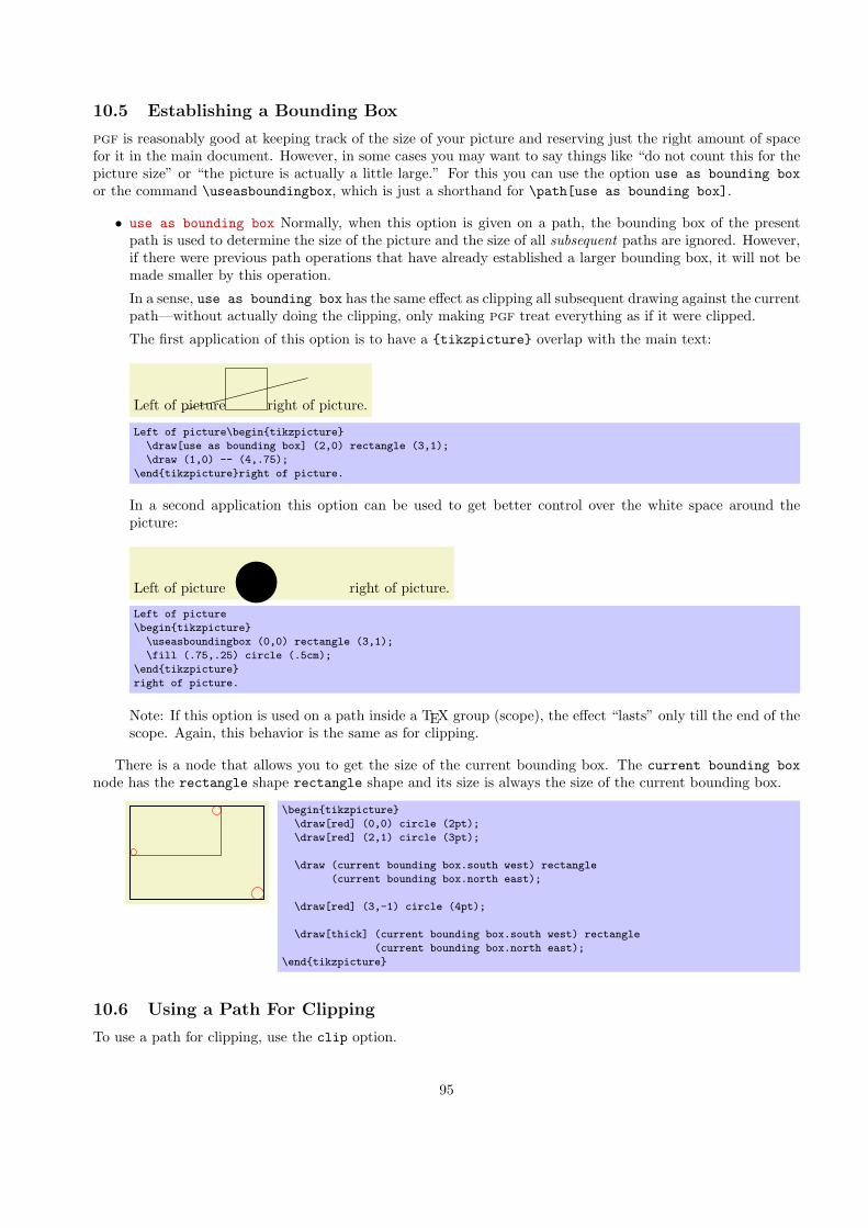
10.5 Establishing a Bounding Box

pgf is reasonably good at keeping track of the size of your picture and reserving just the right amount of spacefor it in the main document. However, in some cases you may want to say things like “do not count this for thepicture size” or “the picture is actually a little large.” For this you can use the option use as bounding boxor the command \useasboundingbox, which is just a shorthand for \path[use as bounding box].

• use as bounding box Normally, when this option is given on a path, the bounding box of the presentpath is used to determine the size of the picture and the size of all subsequent paths are ignored. However,if there were previous path operations that have already established a larger bounding box, it will not bemade smaller by this operation.

In a sense, use as bounding box has the same effect as clipping all subsequent drawing against the currentpath—without actually doing the clipping, only making pgf treat everything as if it were clipped.

The first application of this option is to have a {tikzpicture} overlap with the main text:

Left of picture

.

right of picture.

Left of picture\begin{tikzpicture}

\draw[use as bounding box] (2,0) rectangle (3,1);

\draw (1,0) -- (4,.75);

\end{tikzpicture}right of picture.

In a second application this option can be used to get better control over the white space around thepicture:

Left of picture

.

right of picture.

Left of picture

\begin{tikzpicture}

\useasboundingbox (0,0) rectangle (3,1);

\fill (.75,.25) circle (.5cm);

\end{tikzpicture}

right of picture.

Note: If this option is used on a path inside a TEX group (scope), the effect “lasts” only till the end of thescope. Again, this behavior is the same as for clipping.

There is a node that allows you to get the size of the current bounding box. The current bounding boxnode has the rectangle shape rectangle shape and its size is always the size of the current bounding box.

.

\begin{tikzpicture}

\draw[red] (0,0) circle (2pt);

\draw[red] (2,1) circle (3pt);

\draw (current bounding box.south west) rectangle


\draw[red] (3,-1) circle (4pt);

\draw[thick] (current bounding box.south west) rectangle


\end{tikzpicture}

10.6 Using a Path For Clipping

To use a path for clipping, use the clip option.

95

• clip This option causes all subsequent drawings to be clipped against the current path and the size ofsubsequent paths will not be important for the picture size. If you clip against a self-intersecting path,the even-odd rule or the nonzero winding number rule is used to determine whether a point is inside oroutside the clipping region.

The clipping path is a graphic state parameter, so it will be reset at the end of the current scope. Multipleclippings accumulate, that is, clipping is always done against the intersection of all clipping areas that havebeen specified inside the current scopes. The only way of enlarging the clipping area is to end a {scope}.

.

\begin{tikzpicture}

\draw[clip] (0,0) circle (1cm);

\fill[red] (1,0) circle (1cm);

\end{tikzpicture}

It is usually a very good idea to apply the clip option only to the first path command in a scope.

If you “only wish to clip” and do not wish to draw anything, you can use the \clip command, which is ashorthand for \path[clip].

.

\begin{tikzpicture}

\clip (0,0) circle (1cm);

\fill[red] (1,0) circle (1cm);

\end{tikzpicture}

To keep clipping local, use {scope} environments as in the following example:

.

\begin{tikzpicture}

\draw (0,0) -- ( 0:1cm);

\draw (0,0) -- (10:1cm);

\draw (0,0) -- (20:1cm);

\draw (0,0) -- (30:1cm);

\begin{scope}[fill=red]

\fill[clip] (0.2,0.2) rectangle (0.5,0.5);

\draw (0,0) -- (40:1cm);

\draw (0,0) -- (50:1cm);

\draw (0,0) -- (60:1cm);

\end{scope}

\draw (0,0) -- (70:1cm);

\draw (0,0) -- (80:1cm);

\draw (0,0) -- (90:1cm);

\end{tikzpicture}

There is a slightly annoying catch: You cannot specify certain graphic options for the command used forclipping. For example, in the above code we could not have moved the fill=red to the \fill command.The reasons for this have to do with the internals of the pdf specification. You do not want to know thedetails. It is best simply not to specify any options for these commands.

96

11 Nodes

11.1 Nodes and Their Shapes

TikZ offers an easy way of adding so-called nodes to your pictures. In the simplest case, a node is just sometext that is placed at some coordinate. However, a node can also have a border drawn around it or have a morecomplex background and foreground. Indeed, some nodes do not have a text at all, but consist solely of thebackground. You can name nodes so that you can reference their coordinates later in the picture. However,nodes cannot be referenced across different pictures.

There are no special TEX commands for adding a node to a picture; rather, there is path operation called nodefor this. Nodes are created whenever TikZ encounters node or coordinate at a point on a path where it wouldexpect a normal path operation (like -- (1,1) or sin (1,1)). It is also possible to give node specificationsinside certain path operations as explained later.

The node operation is typically followed by some options, which apply only to the node. Then, you canoptionally name the node by providing a name in round braces. Lastly, for the node operation you must providesome label text for the node in curly braces, while for the coordinate operation you may not. The node isplaced at the current position of the path after the path has been drawn. Thus, all nodes are drawn “on top” ofthe path and retained until the path is complete. If there are several nodes on a path, they are drawn on top ofthe path in the order they are encountered.

.

.

first node

.

second node

.

third node \tikz \fill[fill=examplefill]

(0,0) node {first node}

-- (1,1) node {second node}

-- (0,2) node {third node};

The syntax for specifying nodes is the following:

\path . . . node[⟨options⟩](⟨name⟩)at(⟨coordinate⟩){⟨text⟩} . . . ;The effect of at is to place the node at the coordinate given after at and not, as would normally be thecase, at the last position. The at syntax is not available when a node is given inside a path operation (itwould not make any sense, there).The (⟨name⟩) is a name for later reference and it is optional. You may also add the option name=⟨name⟩to the ⟨option⟩ list; it has the same effect.

• name=⟨node name⟩ assigns a name to the node for later reference. Since this is a “high-level” name(drivers never know of it), you can use spaces, number, letters, or whatever you like when naming anode. Thus, you can name a node just 1 or perhaps start of chart or even y_1. Your node nameshould not contain any punctuation like a dot, a comma, or a colon since these are used to detect whatkind of coordinate you mean when you reference a node.

The ⟨options⟩ is an optional list of options that apply only to the node and have no effect outside. The otherway round, most “outside” options also apply to the node, but not all. For example, the “outside” rotationdoes not apply to nodes (unless some special options are used, sigh). Also, the outside path action, likedraw or fill, never applies to the node and must be given in the node (unless some special other optionsare used, deep sigh).As mentioned before, we can add a border and even a background to a node:

.

.

first node

.

second node

.

third node \tikz \fill[fill=examplefill]

(0,0) node {first node}

-- (1,1) node[draw] {second node}

-- (0,2) node[fill=red!20,draw,double,rounded corners] {third node};

97

The “border” is actually just a special case of a much more general mechanism. Each node has a certainshape which, by default, is a rectangle. However, we can also ask TikZ to use a circle shape instead or anellipse shape (you have to include pgflibraryshapes for the latter shape):

.

.

first node

.

second node

.

third node

\tikz \fill[fill=examplefill]

(0,0) node{first node}

-- (1,1) node[ellipse,draw] {second node}

-- (0,2) node[circle,fill=red!20] {third node};

In the future, there might be much more complicated shapes available such as, say, a shape for a resistoror a shape for a state of a finite automaton or a shape for a uml class. Unfortunately, creating new shapesis a bit tricky and makes it necessary to use the basic layer directly. Life is hard.To select the shape of a node, the following option is used:

• shape=⟨shape name⟩ select the shape either of the current node or, when this option is not given insidea node but somewhere outside, the shape of all nodes in the current scope.Since this option is used often, you can leave out the shape=. When TikZ encounters an option likecircle that it does not know, it will, after everything else has failed, check whether this option is thename of some shape. If so, that shape is selected as if you had said shape=⟨shape name⟩.By default, the following shapes are available: rectangle, circle, coordinate, and, when the packagepgflibraryshapes is loaded, also ellipse. Details of these shapes, like their anchors and size options,are discussed in Section 11.8.

The following styles influences how nodes are rendered:

• style=every node This style is installed at the beginning of every node.

.

.

A

.


\tikzstyle{every node}=[draw]

\draw (0,0) node {A} -- (1,1) node {B};

\end{tikzpicture}

• style=every ⟨shape ⟩ node These styles are installed at the beginning of a node of a given ⟨shape⟩.For example, every rectangle node is used for rectangle nodes, and so on.

.

.

A

.


\tikzstyle{every rectangle node}=[draw]

\tikzstyle{every circle node}= [draw,double]

\draw (0,0) node[rectangle] {A} -- (1,1) node[circle] {B};

\end{tikzpicture}

The is a special syntax for specifying “light-weighed” nodes:

\path . . . coordinate[⟨options⟩](⟨name⟩)at(⟨coordinate⟩) . . . ;This has the same effect asnode[shape=coordinate][⟨options⟩](⟨name⟩)at(⟨coordinate⟩){},where the at part might be missing.

11.2 Multi-Part Nodes

Most nodes just have a single simple text label. However, nodes of a more complicated shapes might be madeup from several node parts. For example, in automata theory a so-called Moore state has a state name, drawn

98

in the upper part of the state circle, and an output text, drawn in the lower part of the state circle. Thesetwo parts are quite independent. Similarly, a uml class shape would have a name part, a method part, and anattributes part. Different molecule shape might use parts for the different atoms to be drawn at the differentpositions, and so on.

Both pgf and TikZ support such multipart nodes. On the lower level, pgf provides a system for specifyingthat a shape consists of several parts. On the TikZ level, you specify the different node parts by using thefollowing command:

\nodepart{⟨part name⟩}This command can only be used inside the ⟨text⟩ argument of a node path operation. It works a little bitlike a \part command in LATEX. It will stop the typesetting of whatever node part was typeset until nowand then start putting all following text into the node part named ⟨part name⟩—until another \partnameis encountered or until the node ⟨text⟩ ends.

.

.

q1

.

00

\begin{tikzpicture}

\node [state with output,draw,double,fill=red!20]

{

% No \nodepart has been used, yet. So, the following is put in the

% ‘‘text’’ node part by default.

$q_1$

\nodepart{output} % Ok, end ‘‘text’’ part, start ‘‘output’’ part

$00$

}; % output part ended.

\end{tikzpicture}

You will have to lookup which parts are defined by a shape.The following styles influences node parts:

• style=every ⟨part name ⟩ node part This style is installed at the beginning of every node partnamed ⟨part name⟩.

.

.

q1

.

00

\tikzstyle{every output node part}=[red]

\tikz \node [state with output,draw] {$q_1$ \nodepart{output} $00$};

11.3 Options for the Text in Nodes

The simplest option for the text in nodes is its color. Normally, this color is just the last color installed usingcolor=, possibly inherited from another scope. However, it is possible to specificly set the color used for textusing the following option:

• text=⟨color⟩ Sets the color to be used for text labels. A color= option will immediately override thisoption.

.

.

red

.

red

.

red \begin{tikzpicture}

\draw[red] (0,0) -- +(1,1) node[above] {red};

\draw[text=red] (1,0) -- +(1,1) node[above] {red};

\draw (2,0) -- +(1,1) node[above,red] {red};

\end{tikzpicture}

Just like the color itself, you may also wish to set the opacity of the text only. For this, use the followingoption:

• text opacity=⟨value⟩ Sets the opacity of text labels.

99

.

.

Upper node

.

Lower node

\begin{tikzpicture}

\draw[line width=2mm,blue!50,cap=round] (0,0) grid (3,2);

\tikzstyle{every node}=[fill,draw]

\node[opacity=0.5] at (1.5,2) {Upper node};

\node[draw opacity=0.8,fill opacity=0.2,text opacity=1]

at (1.5,0) {Lower node};

\end{tikzpicture}

Next, you may wish to adjust the font used for the text. Use the following option for this:

• font=⟨font commands⟩ Sets the font used for text labels.

.

.

italic \begin{tikzpicture}

\draw[font=\itshape] (1,0) -- +(1,1) node[above] {italic};

\end{tikzpicture}

A perhaps more useful example is the following:

.

.

state

.

output

\tikzstyle{every text node part}=[font=\itshape]

\tikzstyle{every output node part}=[font=\footnotesize]

\tikzstyle{every state with output node}=[draw]

\tikz \node [state with output] {state \nodepart{output} output};

Normally, when a node is typeset, all the text you give in the braces is but in one long line (in an \hbox, tobe precise) and the node will become as wide as necessary.

You can change this behaviour using the following options. They allow you to limit the width of a node(naturally, at the expense of its height).

• text width=⟨dimension⟩ This option will put the text of a node in a box of the given width (more precisely,in a {minipage} of this width; for plain TEX a rudimentary “minipage emulation” is used).

If the node text is not as wide as ⟨dimension⟩, it will nevertheless be put in a box of this width. If it islarger, line breaking will be done.

By default, when this option is given, a ragged right border will be used. This is sensible since, typically,these boxes are narrow and justifying the text looks ugly.

.

.

This is a demon-stration text forshowing how linebreaking works.

\tikz \draw (0,0) node[fill=examplefill,text width=3cm]

{This is a demonstration text for showing how line breaking works.};

• text justified causes the text to be justified instead of (right)ragged. Use this only with pretty broadnodes.

.

.


\tikz \draw (0,0) node[fill=examplefill,text width=3cm,text justified]


In the above example, TEX complains (rightfully) about three very badly typeset lines. (For this manualI asked TEX to stop complaining by using \hbadness=10000, but this is a foul deed, indeed.)

100

• text ragged causes the text to be typeset with a ragged right. This uses the original plain TEX definitionof a ragged right border, in which TEX will try to balance the right border as well as possible. This is thedefault.

.

.


\tikz \draw (0,0) node[fill=examplefill,text width=3cm,text ragged]


• text badly ragged causes the right border to be ragged in the LATEX-style, in which no balancing occurs.This looks ugly, but it may be useful for very narrow boxes and when you wish to avoid hyphenations.

.

.

This is ademonstration textfor showing howline breakingworks.

\tikz \draw (0,0) node[fill=examplefill,text width=3cm,text badly ragged]


• text centered centers the text, but tries to balance the lines.

.

.


\tikz \draw (0,0) node[fill=examplefill,text width=3cm,text centered]


• text badly centered centers the text, without balancing the lines.

.

.

This is ademonstration textfor showing how

line breakingworks.

\tikz \draw (0,0) node[fill=examplefill,text width=3cm,text badly centered]


11.4 Placing Nodes Using Anchors

When you place a node at some coordinate, the node is centered on this coordinate by default. This is oftenundesirable and it would be better to have the node to the right or above the actual coordinate.

pgf uses a so-called anchoring mechanism to give you a very fine control over the placement. The idea issimple: Imaging a node of rectangular shape of a certain size. pgf defines numerous anchor positions in theshape. For example to upper right corner is called, well, not “upper right anchor,” but the north east anchorof the shape. The center of the shape has an anchor called center on top of it, and so on. Here are someexamples (a complete list is given in Section 11.8).

.

.

Big node

.

north

.

north east

.

north west

.

west

.

east

.

base

Now, when you place a node at a certain coordinate, you can ask TikZ to place the node shifted around insuch a way that a certain anchor is at the coordinate. In the following example, we ask TikZ to shift the first

101

node such that its north east anchor is at coordinate (0,0) and that the west anchor of the second node is atcoordinate (1,1).

.

.

first node

.

second node

\tikz \draw (0,0) node[anchor=north east] {first node}

rectangle (1,1) node[anchor=west] {second node};

Since the default anchor is center, the default behaviour is to shift the node in such a way that it is centeredon the current position.

• anchor=⟨anchor name⟩ causes the node to be shifted such that it’s anchor ⟨anchor name⟩ lies on thecurrent coordinate.

The only anchor that is present in all shapes is center. However, most shapes will at least define anchors inall “compass directions.” Furthermore, the standard shapes also define a base anchor, as well as base westand base east, for placing things on the baseline of the text.

The standard shapes also define a mid anchor (and mid west and mid east). This anchor is half theheight of the character “x” above the base line. This anchor is useful for vertically centering multiplenodes that have different heights and depth. Here is an example:

.

.

x

.

y

.

t

.

x

.

y

.

t

.

x

.

y

.

t\begin{tikzpicture}[scale=3,transform shape]

% First, center alignment -> wobbles

\draw[anchor=center] (0,1) node{x} -- (0.5,1) node{y} -- (1,1) node{t};

% Second, base alignment -> no wobble, but too high

\draw[anchor=base] (0,.5) node{x} -- (0.5,.5) node{y} -- (1,.5) node{t};

% Third, mid alignment

\draw[anchor=mid] (0,0) node{x} -- (0.5,0) node{y} -- (1,0) node{t};

\end{tikzpicture}

Unfortunately, while perfectly logical, it is often rather counter-intuitive that in order to place a node abovea given point, you need to specify the south anchor. For this reason, there are some useful options that allowyou to select the standard anchors more intuitively:

• above=⟨offset⟩ does the same as anchor=south. If the ⟨offset⟩ is specified, the node is additionally shiftedupwards by the given ⟨offset⟩.

.

.

above \tikz \fill (0,0) circle (2pt) node[above] {above};

.

.

above \tikz \fill (0,0) circle (2pt) node[above=2pt] {above};

102

• above left=⟨offset⟩ does the same as anchor=south east. If the ⟨offset⟩ is specified, the node is addi-tionally shifted upwards and right by ⟨offset⟩.

.

.

above left \tikz \fill (0,0) circle (2pt) node[above left] {above left};

.

.

above left \tikz \fill (0,0) circle (2pt) node[above left=2pt] {above left};

• above right=⟨offset⟩ does the same as anchor=south west.

.

.

above right \tikz \fill (0,0) circle (2pt) node[above right] {above right};

• left=⟨offset⟩ does the same as anchor=east.

.

.

left \tikz \fill (0,0) circle (2pt) node[left] {left};

• right=⟨offset⟩ does the same as anchor=west.

• below=⟨offset⟩ does the same as anchor=north.

• below left=⟨offset⟩ does the same as anchor=north east.

• below right=⟨offset⟩ does the same as anchor=north west.

11.5 Transformations

It is possible to transform nodes, but, by default, transformations do not apply to nodes. The reason is thatyou usually do not want your text to be scaled or rotated even if the main graphic is transformed. Scaling textis evil, rotating slightly less so.

However, sometimes you do wish to transform a node, for example, it certainly sometimes makes sense torotate a node by 90 degrees. There are two ways in which you can achieve this:

1. You can use the following option:

• transform shape causes the current “external” transformation matrix to be applied to the shape.For example, if you said \tikz[scale=3] and then say node[transform shape] {X}, you will get a“huge” X in your graphic.

2. You can give transformation option inside the option list of the node. These transformations always applyto the node.

.

.

A

.

B

.

A

.

B

.

A

.




\draw (1,0) node{A}

(2,0) node[rotate=90,scale=1.5] {B};

\draw[rotate=30] (1,0) node{A}

(2,0) node[rotate=90,scale=1.5] {B};

\draw[rotate=60] (1,0) node[transform shape] {A}

(2,0) node[transform shape,rotate=90,scale=1.5] {B};

\end{tikzpicture}

103

11.6 Placing Nodes on a Line or Curve

Until now, we always placed node on a coordinate that is mentioned in the path. Often, however, we wish toplace nodes on “the middle” of a line and we do not wish to compute these coordinates “by hand.” To facilitatesuch placements, TikZ allows you to specify that a certain node should be somewhere “on” a line. There aretwo ways of specifying this: Either explicitly by using the pos option or implicitly by placing the node “inside”a path operation. These two ways are described in the following.

11.6.1 Explicit Use of the Position Option

• pos=⟨fraction⟩ When this option is given, the node is not anchored on the last coordinate. Rather, it isanchored on some point on the line from the previous coordinate to the current point. The ⟨fraction⟩dictates how “far” on the line the point should be. A ⟨fraction⟩ or 0 is the previous coordinate, 1 is thecurrent one, everything else is in between. In particular, 0.5 is the middle.

Now, what is “the previous line”? This depends on the previous path construction operation.

In the simplest case, the previous path operation was a “line-to” operation, that is, a --⟨coordinate⟩operation:

.

.

0

.

1/2

.

9/10 \tikz \draw (0,0) -- (3,1)

node[pos=0]{0} node[pos=0.5]{1/2} node[pos=0.9]{9/10};

The next case is the curve-to operation (the .. operation). In this case, the “middle” of the curve, that is,the position 0.5 is not necessarily the point at the exact half distance on the line. Rather, it is some pointat “time” 0.5 of a point traveling from the start of the curve, where it is at time 0, to the end of the curve,which it reaches at time 0.5. The “speed” of the point depends on the length of the support vectors (thevectors that connect the start and end points to the control points). The exact math is a bit complicated(depending on your point of view, of course); you may wish to consult a good book on computer graphicsand Bezier curves if you are intrigued.

.

.

0

.

0.125

.

0.25

.

0.375

.

0.5

.

0.625

.

0.75

.

0.875

.

1 \tikz \draw (0,0) .. controls +(right:3.5cm) and +(right:3.5cm) .. (0,3)

\foreach \p in {0,0.125,...,1} {node[pos=\p]{\p}};

Another interesting case are the horizontal/vertical line-to operations |- and -|. For them, the position(or time) 0.5 is exactly the corner point.

.

.

0

.

1/2

.

9/10 \tikz \draw (0,0) |- (3,1)


.

.

0

.

1/2

.

9/10 \tikz \draw (0,0) -| (3,1)


For all other path construction operations, the position placement does not work, currently. This willhopefully change in the future (especially for the arc operation).

104

• sloped This option causes the node to be rotated such that a horizontal line becomes a tangent to thecurve. The rotation will always be done in such a way that text is never “upside down.” If you really needupside down text, use [rotate=180].

.

.

0

.

0.25

.

0.5

.

0.75

.

1 \tikz \draw (0,0) .. controls +(up:2cm) and +(left:2cm) .. (1,3)

\foreach \p in {0,0.25,...,1} {node[sloped,above,pos=\p]{\p}};

.

.

x

.

y

\begin{tikzpicture}[->]

\draw (0,0) -- (2,0.5) node[midway,sloped,above] {$x$};

\draw (2,-.5) -- (0,0) node[midway,sloped,below] {$y$};

\end{tikzpicture}

There exist styles for specifying positions a bit less “technically”:

• style=midway is set to pos=0.5.

.

.

at end

.

very near end

.

near end

.

midway

.

near start

.

very near start

.

at start

\tikz \draw (0,0) .. controls +(up:2cm) and +(left:3cm) .. (1,5)

node[at end] {|at end|}

node[very near end] {|very near end|}

node[near end] {|near end|}

node[midway] {|midway|}

node[near start] {|near start|}

node[very near start] {|very near start|}

node[at start] {|at start|};

• style=near start is set to pos=0.25.

• style=near end is set to pos=0.75.

• style=very near start is set to pos=0.125.

• style=very near end is set to pos=0.875.

• style=at start is set to pos=0.

• style=at end is set to pos=1.

11.6.2 Implicit Use of the Position Option

When you wish to place a node on the line (0,0) -- (1,1), it is natural to specify the node not following the(1,1), but “somewhere in the middle.” This is, indeed, possible and you can write (0,0) -- node{a} (1,1)to place a node midway between (0,0) and (1,1).

105

What happens is the following: The syntax of the line-to path operation is actually -- node⟨nodespecification⟩⟨coordinate⟩. (It is even possible to give multiple nodes in this way.) When the optional nodeis encountered, that is, when the -- is directly followed by node, then the specification(s) are read and “storedaway.” Then, after the ⟨coordinate⟩ has finally been reached, they are inserted again, but with the pos optionset.

There are two things to note about this: When a node specification is “stored,” its catcodes become fixed.This means that you cannot use overly complicated verbatim text in them. If you really need, say, a verbatimtext, you will have to put it in a normal node following the coordinate and add the pos option.

Second, which pos is chosen for the node? The position is inherited from the surrounding scope. However,this holds only for nodes specified in this implicit way. Thus, if you add the option [near end] to a scope, thisdoes not mean that all nodes given in this scope will be put on near the end of lines. Only the nodes for whichan implicit pos is added will be placed near the end. Typically, this is what you want. Here are some examplesthat should make this clearer:

.

.

A

.

B

.

C

.

D

\begin{tikzpicture}[near end]

\draw (0cm,4em) -- (3cm,4em) node{A};

\draw (0cm,3em) -- node{B} (3cm,3em);

\draw (0cm,2em) -- node[midway] {C} (3cm,2em);

\draw (0cm,1em) -- (3cm,1em) node[midway] {D} ;

\end{tikzpicture}

Like the line-to operation, the curve-to operation .. also allows you to specify nodes “inside” the operation.After both the first .. and also after the second .. you can place node specifications. Like for the -- operation,these will be collected and then reinserted after the operation with the pos option set.

11.7 Connecting Nodes

Once you have defined a node and given it a name, you can use this name to reference it. This can be donein two ways, see also Section 8.5. Suppose you have said \path(0,0) node(x) {Hello World!}; in order todefine a node named x.

1. Once the node x has been defined, you can use (x.⟨anchor⟩) wherever you would normally use a normalcoordinate. This will yield the position at which the given ⟨anchor⟩ is in the picture. Note that transfor-mations do not apply to this coordinate, that is, (x.north) will be the northern anchor of x even if youhave said scale=3 or xshift=4cm. This is usually what you would expect.

2. You can also just use (x) as a coordinate. In most cases, this gives the same coordinate as (x.center).Indeed, if the shape of x is coordinate, then (x) and (x.center) have exactly the same effect.

However, for most other shapes, some path construction operations like -- try to be “clever” when thisthey are asked to draw a line from such a coordinate or to such a coordinate. When you say (x)--(1,1),the -- path operation will not draw a line from the center of x, but from the border of x in the directiongoing towards (1,1). Likewise, (1,1)--(x) will also have the line end on the border in the directioncoming from (1,1).

In addition to --, the curve-to path operation .. and the path operations -| and |- will also handle nodeswithout anchors correctly. Here is an example, see also Section 8.5:

.

.

Hello World!

.

∫ 2

1xdx

.

label

.

label

106

\begin{tikzpicture}

\path (0,0) node (x) {Hello World!}

(3,1) node[circle,draw](y) {$\int_1^2 x \mathrm d x$};

\draw[->,blue] (x) -- (y);

\draw[->,red] (x) -| node[near start,below] {label} (y);

\draw[->,orange] (x) .. controls +(up:1cm) and +(left:1cm) .. node[above,sloped] {label} (y);

\end{tikzpicture}

11.8 Predefined Shapes

pgf and TikZ define three shapes, by default:

• rectangle,

• circle, and

• coordinate.

By loading library packages, you can define more shapes. Currently, the package pgflibraryshapes defines

• ellipse.

The exact behaviour of these shapes differs, shapes defined for more special purposes (like a, say, transistorshape) will have even more custom behaviors. However, there are some options that apply to most shapes:

• inner sep=⟨dimension⟩ An additional (invisible) separation space of ⟨dimension⟩ will be added inside theshape, between the text and the shape’s background path. The effect is as if you had added appropriatehorizontal and vertical skips at the beginning and end of the text to make it a bit “larger.” The defaultinner sep is the size of a normal space.

.

.

tight

.

loose

.

default \begin{tikzpicture}

\draw (0,0) node[inner sep=0pt,draw] {tight}

(0cm,2em) node[inner sep=5pt,draw] {loose}

(0cm,4em) node[fill=examplefill] {default};

\end{tikzpicture}

• inner xsep=⟨dimension⟩ Specifies the inner separation in the x-direction, only.

• inner ysep=⟨dimension⟩ Specifies the inner separation in the y-direction, only.

• outer sep=⟨dimension⟩ This option adds an additional (invisible) separation space of ⟨dimension⟩ outsidethe background path. The main effect of this option is that all anchors will move a little “to the outside.”

The default for this option is half the line width. When the default is used and when the background pathis draw, the anchors will lie exactly on the “outside border” of the path (not on the path itself). Whenthe shape is filled, but not drawn, this may not be desirable. In this case, the outer sep should be set tozero point.

.

.

filled

.

drawn\begin{tikzpicture}

\draw[line width=5pt]

(0,0) node[outer sep=0pt,fill=examplefill] (f) {filled}

(2,0) node[inner sep=.5\pgflinewidth+2pt,draw] (d) {drawn};

\draw[->] (1,-1) -- (f);

\draw[->] (1,-1) -- (d);

\end{tikzpicture}

• outer xsep=⟨dimension⟩ Specifies the outer separation in the x-direction, only.

• outer ysep=⟨dimension⟩ Specifies the outer separation in the y-direction, only.

107

• minimum height=⟨dimension⟩ This option ensures that the height of the shape (including the inner, butignoring the outer separation) will be at least ⟨dimension⟩. Thus, if the text plus the inner separationis not at least as large as ⟨dimension⟩, the shape will be enlarged appropriately. However, if the text isalready larger than ⟨dimension⟩, the shape will not be shrunk.

.

.

1cm

.

0cm\begin{tikzpicture}

\draw (0,0) node[minimum height=1cm,draw] {1cm}

(2,0) node[minimum height=0cm,draw] {0cm};

\end{tikzpicture}

• minimum width=⟨dimension⟩ same as minimum height, only for the width.

.

.

3 × 2

\begin{tikzpicture}

\draw (0,0) node[minimum height=2cm,minimum width=3cm,draw] {$3 \times 2$};

\end{tikzpicture}

• minimum size=⟨dimension⟩ sets both the minimum height and width at the same time.

.

.

square

.

circle

\begin{tikzpicture}

\draw (0,0) node[minimum size=2cm,draw] {square};

\draw (0,-2) node[minimum size=2cm,draw,circle] {circle};

\end{tikzpicture}

The coordinate shape is handled in a special way by TikZ. When a node x whose shape is coordinateis used as a coordinate (x), this has the same effect as if you had said (x.center). None of the special “lineshortening rules” apply in this case. This can be useful since, normally, the line shortening causes paths to besegmented and they cannot be used for filling. Here is an example that demonstrates the difference:

.

. .

..

\begin{tikzpicture}


\path[yshift=1.5cm,shape=rectangle]

(0,0) node(a1){} (1,0) node(a2){}

(1,1) node(a3){} (0,1) node(a4){};

\filldraw[fill=examplefill] (a1) -- (a2) -- (a3) -- (a4);

\path[shape=coordinate]

(0,0) coordinate(b1) (1,0) coordinate(b2)

(1,1) coordinate(b3) (0,1) coordinate(b4);

\filldraw[fill=examplefill] (b1) -- (b2) -- (b3) -- (b4);

\end{tikzpicture}

108

12 Making Trees Grow

12.1 Introduction to the Child Operation

Trees are a common way of visualizing hierarchical structures. A simple tree looks like this:

.

.

root

.

left

.

right

.

child

.

child

\begin{tikzpicture}

\node {root}

child {node {left}}

child {node {right}



};

\end{tikzpicture}

Admittedly, in reality trees are more likely to grow upward and not downward as above. You can tell whetherthe author of a paper is a mathematician or a computer scientist by looking at the direction their trees grow.A computer scientist’s trees will grow downward while a mathematician’s tree will grow upward. Naturally, thecorrect way is the mathematician’s way, which can be specify as follows:

.

.

root

.

left

.

right

.

child

.

child \begin{tikzpicture}

\node {root} [grow’=up]

child {node {left}}

child {node {right}



};

\end{tikzpicture}

In TikZ, trees are specified by adding children to a node on a path using the child operation:

\path . . . child[⟨options⟩]foreach⟨variables⟩in{⟨values⟩}{⟨child path⟩} . . . ;This operation should directly follow a completed node operation or another child operation, although itis permissible that the first child operation is preceded by options (we will come to that).When a node operation like node {X} is followed by child, TikZ starts counting the number of child nodesthat follow the original node {X}. For this, it scans the input and stores away each child and its argumentsuntil it reaches a path operation that is not a child. Note that this will fix the character codes of all textinside the child arguments, which means, in essence, that you cannot use verbatim text inside the nodesinside a child. Sorry.Once the children have been collected and counted, TikZ starts generating the child nodes. For each childof a parent node TikZ computes an appropriate position where the child is placed. For each child, thecoordinate system is transformed so that the origin is at this position. Then the ⟨child path⟩ is drawn.Typically, the child path just consists of a node specification, which results in a node being drawn at thechild’s position. Finally, an edge is drawn from the first node in the ⟨child path⟩ to the parent node.The optional foreach part (note that there is no backslash before foreach) allows you to specify multiplechildren in a single child command. The idea is the following: A \foreach statement is (internally) usedto iterate over the list of ⟨values⟩. For each value in this list, a new child is added to the node. The syntaxfor ⟨variables⟩ and for ⟨values⟩ is the same as for the \foreach statement, see Section 15. For example,when you say

node {root} child [red] foreach \name in {1,2} {node {\name}}

the effect will be the same as if you had said

node {root} child[red] {node {1}} child[ref] {node {2}}

109

When you write

node {root} child[\pos] foreach \name/\pos in {1/left,2/right} {node[\pos] {\name}}

the effect will be the same as for

node {root} child[left] {node[left] {1}} child[right] {node[right] {2}}

You can nest things as in the following example:

.

\begin{tikzpicture}[level distance=4mm]

\tikzstyle{level 1}=[sibling distance=8mm]



\coordinate

child foreach \x in {0,1}

{child foreach \y in {0,1}

{child foreach \z in {0,1}}};

\end{tikzpicture}

The details and options for this operation are described in the rest of this present section.

12.2 Child Paths and the Child Nodes

For each child of a root node, its ⟨child path⟩ is inserted at a specific location in the picture (the placementrules are discussed in Section 12.5). The first node in the ⟨child path⟩, if it exists, is special and called the childnode. If there is no first node in the ⟨child path⟩, that is, if the ⟨child path⟩ is missing (including the curlybraces) or if it does not start with node or with coordinate, then an empty child node of shape coordinate isautomatically added.

Consider the example \node {x} child {node {y}} child;. For the first child, the ⟨child path⟩ has thechild node node {y}. For the second child, no child node is specified and, thus, it is just coordinate.

As for any normal node, you can give the child node a name, shift it around, or use options to influence howit is rendered.

.

.

root

.

left

.

right

\begin{tikzpicture}

\node[rectangle,draw] {root}

child {node[circle,draw] (left node) {left}}

child {node[ellipse,draw] (right node) {right}};

\draw[dashed,->] (left node) -- (right node);

\end{tikzpicture}

In many cases, the ⟨child path⟩ will just consist of a specification of a child node and, possibly, children ofthis child node. However, the node specification may be followed by arbitrary other material that will be addedto the picture, transformed to the child’s coordinate system. For your convenience, a move-to (0,0) operationis inserted automatically at the beginning of the path. Here is an example:

.

.

root \begin{tikzpicture}

\node {root}

child {[fill] circle (2pt)}

child {[fill] circle (2pt)};

\end{tikzpicture}

At the end of the ⟨child path⟩ you may add a special path operation called edge from parent. If thisoperation is not given by yourself somewhere on the path, it will be automatically added at the end. This optioncauses a connecting edge from the parent node to the child node to be added to the path. By giving optionsto this operation you can influence how the edge is rendered. Also, nodes following the edge from parentoperation will be placed on this edge, see Section 12.6 for details.

To sum up:

1. The child path starts with a node specification. If it is not there, it is added automatically.

110

2. The child path ends with a edge from parent operation, possibly followed by nodes to be put on thisedge. If the operation is not given at the end, it is added automatically.

12.3 Naming Child Nodes

Child nodes can be named like any other node using either the name option or the special syntax in which thename of the node is placed in round parentheses between the node operation and the node’s text.

If you do not assign a name to a child node, TikZ will automatically assign a name as follows: Assume thatthe name of the parent node is, say, parent. (If you did not assign a name to the parent, TikZ will do so itself,but that name will not be user-accessible.) The first child of parent will be named parent-1, the second childis named parent-2, and so on.

This naming convention works recursively. If the second child parent-2 has children, then the first of thesechildren will be called parent-2-1 and the second parent-2-2 and so on.

If you assign a name to a child node yourself, no name is generated automatically (the node does not havetwo names). However, “counting continues,” which means that the third child of parent is called parent-3independently of whether you have assigned names to the first and/or second child of parent.

Here is an example:

.

.

root

.

root-1

.

root-2

.

special

.

root-2-2

\begin{tikzpicture}

\node (root) {root}

child

child {

child {coordinate (special)}

child

};

\node at (root-1) {root-1};

\node at (root-2) {root-2};

\node at (special) {special};

\node at (root-2-2) {root-2-2};

\end{tikzpicture}

12.4 Specifying Options for Trees and Children

Each child may have its own ⟨options⟩, which apply to “the whole child,” including all of its grandchildren.Here is an example:

.



\coordinate

child[red] {child child}

child[green] {child child[blue]};

\end{tikzpicture}

The options of the root node have no effect on the children since the options of a node are always “local” tothat node. Because of this, the edges in the following tree are black, not red.

.

.

root \begin{tikzpicture}[thick]

\node [red] {root}

child

child;

\end{tikzpicture}

This raises the problem of how to set options for all children. Naturally, you could always set options for thewhole path as in \path [red] node {root} child child; but this is bothersome in some situations. Instead,it is easier to give the options before the first child as follows:

111

.

.root \begin{tikzpicture}[thick]

\node [red] {root}

[green] % option applies to all children

child

child;

\end{tikzpicture}

Here is the set of rules:

1. Options for the whole tree are given before the root node.

2. Options for the root node are given directly to the node operation of the root.

3. Options for all children can be given between the root node and the first child.

4. Options applying to a specific child path are given as options to the child operation.

5. Options applying to the node of a child, but not to the whole child path, are given as options to the nodecommand inside the ⟨child path⟩.

\begin{tikzpicture}

\path

[...] % Options apply to the whole tree

node[...] {root} % Options apply to the root node only

[...] % Options apply to all children

child[...] % Options apply to this child and all its children

{

node[...] {} % Options apply to the child node only

...

}

child[...] % Options apply to this child and all its children

;

\end{tikzpicture}

There are additional styles that influence how children are rendered:

• style=every child This style is used at the beginning of each child, as if you had given the options tothe child operation.

• style=every child node This style is used at the beginning of each child node in addition to theevery node style.

• style=level ⟨number ⟩ This style is used at the beginning of each set of children, where ⟨number⟩ is thecurrent level in the current tree. For example, when you say \node {x} child child;, then the stylelevel 1 is used before the first child. If this first child has children itself, then level 2 would be usedfor them.

.

.




\node {root}

child { child child }

child { child child child };

\end{tikzpicture}

112

12.5 Placing Child Nodes

Perhaps the most difficult part in drawing a tree is the correct layout of the children. Typically, the childrenhave different sizes and it is not easy to arrange them in such a manner that not too much space is wasted, thechildren do not overlap, and they are either evenly spaced or their centers are evenly distributed. Calculatinggood positions is especially difficult since a good position for the first child may depend on the size of the lastchild.

In TikZ, a comparatively simple approach is taken to placing the children. In order to compute a child’sposition, all that is taken into account is the number of the current child in the list of children and the number ofchildren in this list. Thus, if a node has five children, then there is a fixed position for the first child, a positionfor the second child, and so on. These positions do not depend on the size of the children and, hence, childrencan easily overlap. However, since you can use options to shift individual children a bit, this is not as great aproblem as it may seem.

Although the placement of the children only depends on their number in the list of children and the totalnumber of children, everything else about the placement is highly configurable. You can change the distancebetween children (appropriately called the sibling distance) and the distance between levels of the tree.These distances may change from level to level. The direction in which the tree grows can be changed globallyand for parts of the tree. You can even specify your own “growth function” to arrange children on a circle oralong special lines or curves.

The default growth function works as follows: Assume that we are given a node and five children. Thesechildren will be placed on a line with their centers (or, more generally, with their anchors) spaced apart by thecurrent sibling distance. The line is orthogonal to the current direction of growth, which is set with the growand grow’ option (the latter option reverses the ordering of the children). The distance from the line to theparent node is given by the level distance.

.

.

root

.

1

.

2

.

3

.

4

.

sibl

ing

dist

ance

.

level distance

\begin{tikzpicture}

\path [help lines]

node (root) {root}

[grow=-10]

child {node {1}}

child {node {2}}

child {node {3}}

child {node {4}};

\draw[|<->|,thick] (root-1.center)

-- node[above,sloped] {sibling distance} (root-2.center);

\draw[|<->|,thick] (root.center)

-- node[above,sloped] {level distance} +(-10:\tikzleveldistance);

\end{tikzpicture}

Here is a detailed description of the options:

• level distance=⟨distance⟩ This option allows you to change the distance between different levels of thetree, more precisely, between the parent and the line on which its children are arranged. When given to asingle child, this will set the distance for this child only.

.

.


\node {root}

[level distance=20mm]

child

child {

[level distance=5mm]

child

child

child

}

child[level distance=10mm];

\end{tikzpicture}

113

.

.root \begin{tikzpicture}

\tikzstyle{level 1}=[level distance=10mm]

\tikzstyle{level 2}=[level distance=5mm]

\node {root}

child

child {

child

child[level distance=10mm]

child

}

child;

\end{tikzpicture}

• sibling distance=⟨distance⟩ This option specifies the distance between the anchors of the children of aparent node.

.





\coordinate

child {

child {child child}

child {child child}

}

child {

child {child child}

child {child child}

};

\end{tikzpicture}

.

.

31

.

30

.

20

.

5

.

4

.

10

.

9

.

1

.

20

.

19

.

1

.

18


\tikzstyle{every node}=[fill=red!60,circle,inner sep=1pt]

\tikzstyle{level 1}=[sibling distance=20mm,

set style={{every node}+=[fill=red!45]}]





\node {31}

child {node {30}

child {node {20}

child {node {5}}

child {node {4}}

}

child {node {10}

child {node {9}}

child {node {1}}

}

}

child {node {20}

child {node {19}

child {node {1}}

child[fill=none] {edge from parent[draw=none]}

}

child {node {18}}

};

\end{tikzpicture}

• grow=⟨direction⟩ This option is used to define the ⟨direction⟩ in which the tree will grow. The ⟨direction⟩can either be an angle in degrees or one of the following special text strings: down, up, left, right, north,south, east, west, north east, north west, south east, and south west. All of these have “theirobvious meaning,” so, say, south west is the same as the angle −135◦.

As a side effect, this option installs the default growth function.

114

In addition to setting the direction, this option also has a seemingly strange effect: It sets the siblingdistance for the current level to 0pt, but leaves the sibling distance for later levels unchanged.

This somewhat strange behaviour has a highly desirable effect: If you give this option before the list ofchildren of a node starts, the “current level” is still the parent level. Each child will be on a later level and,hence, the sibling distance will be as specified originally. This will cause the children to be neatly alignedin a line orthogonal to the given ⟨direction⟩. However, if you give this option locally to a single child, then“current level” will be the same as the child’s level. The zero sibling distance will then cause the childto be placed exactly at a point at distance level distance in the direction ⟨direction⟩. However, thechildren of the child will be placed “normally” on a line orthogonal to the ⟨direction⟩.These placement effects are best demonstrated by some examples:

.

.

root

\tikz \node {root} [grow=right] child child;

.

.

root \tikz \node {root} [grow=south west] child child;

.

.

root\begin{tikzpicture}[level distance=10mm,sibling distance=5mm]

\node {root}

[grow=down]

child

child

child[grow=right] {

child child child

};

\end{tikzpicture}

.

.

C

.

H

.

H

.

H

.

C

.

H

.

H

.

H

.

This is wrong!

\begin{tikzpicture}[level distance=2em]

\node {C}

child[grow=up] {node {H}}

child[grow=left] {node {H}}

child[grow=down] {node {H}}

child[grow=right] {node {C}

child[grow=up] {node {H}}

child[grow=right] {node {H}}

child[grow=down] {node {H}}

edge from parent[double]

coordinate (wrong)

};

\draw[<-,red] ([yshift=-2mm]wrong) -- +(0,-1)

node[below]{This is wrong!};

\end{tikzpicture}

.

.

start node

.

end

.

the middle is here \begin{tikzpicture}

\node[rectangle,draw] (a) at (0,0) {start node};

\node[rectangle,draw] (b) at (2,1) {end};

\draw (a) -- (b)

node[coordinate,midway] {}

child[grow=100,<-] {node[above] {the middle is here}};

\end{tikzpicture}

115

• grow’=⟨direction⟩ This option has the same effect as grow, only the children are arranged in the oppositeorder.

• growth function=⟨macro name⟩ This rather low-level option allows you to set a new growth function.The ⟨macro name⟩ must be the name of a macro without parameters. This macro will be called for eachchild of a node.

The effect of executing the macro should be the following: It should transform the coordinate system insuch a way that the origin becomes the place where the current child should be anchored. When the macrois called, the current coordinate system will be setup such that the anchor of the parent node is in theorigin. Thus, in each call, the ⟨macro name⟩ must essentially do a shift to the child’s origin. When themacro is called, the TEX counter \tikznumberofchildren will be set to the total number of children ofthe parent node and the counter \tikznumberofcurrentchild will be set to the number of the currentchild.

The macro may, in addition to shifting the coordinate system, also transform the coordinate system further.For example, it could be rotated or scaled.

Additional growth functions are defined in the library, see Section 14.6.

12.6 Edges From the Parent Node

Every child node is connected to its parent node via a special kind of edge called the edge from parent. Thisedge is added to the ⟨child path⟩ when the following path operation is encountered:

\path . . . edge from parent[⟨options⟩] . . . ;This path operation can only be used inside ⟨child paths⟩ and should be given at the end, possibly followedby node specifications (we will come to that). If a ⟨child path⟩ does not contain this operation, it will beadded at the end of the ⟨child path⟩ automatically.This operation has several effects. The most important is that it inserts the current “edge from parentpath” into the child path. The edge from parent path can be set using the following option:

• edge from parent path=⟨path⟩ This options allows you to set the edge from parent path to a newpath. The default for this path is the following:

(\tikzparentnode\tikzparentanchor) -- (\tikzchildnode\tikzchildanchor)

The \tikzparentnode is a macro that will expand to the name of the parent node. This works evenwhen you have not assigned a name to the parent node, in this case an internal name is automaticallygenerated. The \tikzchildnode is a macro that expands to the name of the child node. The two...anchor macros are empty by default. So, what is essentially inserted is just the path segment(\tikzparentnode) -- (\tikzchildnode); which is exactly an edge from the parent to the child.You can modify this edge from parent path to achieve all sorts of effects. For example, we could replacethe straight line by a curve as follows:

.

.

root

.

left

.

right

.

child

.

child

\begin{tikzpicture}[edge from parent path=

{(\tikzparentnode.south) .. controls +(0,-1) and +(0,1)

.. (\tikzchildnode.north)}]

\node {root}

child {node {left}}

child {node {right}



};

\end{tikzpicture}

Further useful edge from parent paths are defined in the tree library, see Section 14.6.As said before, the anchors in the default edge from parent path are empty. However, you can setthem using the following options:

116

– child anchor=⟨anchor⟩ Specifies the anchor where the edge from parent meets the child node bysetting the macro \tikzchildanchor to .⟨anchor⟩.If you specify border as the ⟨anchor⟩, then the macro \tikzchildanchor is set to the emptystring. The effect of this is that the edge from the parent will meet the child on the border at anautomatically calculated position.

.

.

root

.

left

.

right

.

child

.

child

\begin{tikzpicture}

\node {root}

[child anchor=north]

child {node {left} edge from parent[dashed]}

child {node {right}


child {node {child} edge from parent[draw=none]}

};

\end{tikzpicture}

– parent anchor=⟨anchor⟩ This option works the same way as the child anchor, only for theparent.

Besides inserting the edge from parent path, the edge from parent operation has another effect: The⟨options⟩ are inserted directly before the edge from parent path and the following style is also installedprior to inserting the path:

• style=edge from parent This style is inserted right before the edge from parent path and before the⟨options⟩ are inserted. By default, it just draws the edge from parent, but you can use it to make theedge look different.

.

.

root

.

left

.

right

.

child

.

child

\begin{tikzpicture}

\tikzstyle{edge from parent}=[draw,red,thick]

\node {root}

child {node {left} edge from parent[dashed]}

child {node {right}


child {node {child} edge from parent[draw=none]}

};

\end{tikzpicture}

Note: The ⟨options⟩ inserted before the edge from parent path is added apply to the whole child path. Thus,it is not possible to, say, draw a circle in red as part of the child path and then have an edge to parent inblue. However, as always, the child node is a node and can be drawn in a totally different way.Finally, the edge from parent operation has one more effect: It causes all nodes following the operationto be placed on the edge. This is the same effect as if you had added the pos option to all these nodes, seealso Section 11.6.1.As an example, consider the following code:

\node (root) {} child {node (child) {} edge to parent node {label}};

The edge to parent operation and the following node operation will, together, have the same effect as ifwe had said:

(root) -- (child) node [pos=0.5] {label}

Here is a more complicated example:

117

.

.root

.left

.a

.b

.right

.child

.c

.child

.x

\begin{tikzpicture}

\node {root}

child {

node {left}

edge from parent

node[left] {a}

node[right] {b}

}

child {

node {right}

child {

node {child}

edge from parent

node[left] {c}

}


edge from parent

node[near end] {x}

};

\end{tikzpicture}

118

13 Transformations

pgf has a powerful transformation mechanism that is similar to the transformation capabilities of metafont.The present section explains how you can access it in TikZ.

13.1 The Different Coordinate Systems

It is a long process from a coordinate like, say, (1, 2) or (1cm, 5mathrmpt), to the position a point is finallyplaced on the display or paper. In order to find out where the point should go, it is constantly “transformed,”which means that it is mostly shifted around and possibly rotated, slanted, scaled, and otherwise mutilated.

In detail, (at least) the following transformations are applied to a coordinate like (1, 2) before a point on thescreen is chosen:

1. pgf interprets a coordinate like (1, 2) in its xy-coordinate system as “add the current x-vector once andthe current y-vector twice to obtain the new point.”

2. pgf applies its coordinate transformation matrix to the resulting coordinate. This yields the final positionof the point inside the picture.

3. The backend driver (like dvips or pdftex) adds transformation commands such the coordinate is shiftedto the correct position in TEX’s page coordinate system.

4. pdf (or PostScript) apply the canvas transformation matrix to the point, which can once more change theposition on the page.

5. The viewer application or the printer applies the device transformation matrix to transform the coordinateto its final pixel coordinate on the screen or paper.

In reality, the process is even more involved, but the above should give the idea: A point is constantlytransformed by changes of the coordinate system.

In TikZ, you only have access to the first two coordinate systems: The xy-coordinate system and thecoordinate transformation matrix (these will be explained later). pgf also allows you to change the canvastransformation matrix, but you have to use commands of the core layer directly to do so and you “better knowwhat you are doing” when you do this. The moment you start modifying the canvas matrix, pgf immediatelylooses track of all coordinates and shapes, anchors, and bounding box computations will no longer work.

13.2 The Xy- and Xyz-Coordinate Systems

The first and easiest coordinate systems are pgf’s xy- and xyz-coordinate systems. The idea is very simple:Whenever you specify a coordinate like (2,3) this means 2vx + 3vy, where vx is the current x-vector and vy isthe current y-vector. Similarly, the coordinate (1,2,3) means vx + 2vy + 3vz.

Unlike other packages, pgf does not insist that vx actually has a y-component of 0, that is, that it is ahorizontal vector. Instead, the x-vector can point anywhere you want. Naturally, normally you will want thex-vector to point horizontally.

One undesirable effect of this flexibility is that it is not possible to provide mixed coordinates as in (1, 2pt).Life is hard.

To change the x-, y-, and z-vectors, you can use the following options:

• x=⟨dimension⟩ Sets the x-vector of pgf’s xyz-coordinate system to point ⟨dimension⟩ to the right, thatis, to (⟨dimension⟩, 0pt). The default is 1cm.

.

\begin{tikzpicture}

\draw (0,0) -- +(1,0);

\draw[x=2cm,color=red] (0,0.1) -- +(1,0);

\end{tikzpicture}

119

.

\tikz \draw[x=1.5cm] (0,0) grid (2,2);

The last example shows that the size of steppings in grids, just like all other dimensions, are not affectedby the x-vector. After all, the x-vector is only used to determine the coordinate of the upper right cornerof the grid.

• x=⟨coordinate⟩ Sets the x-vector of pgf’s xyz-coordinate system to the specified ⟨coordinate⟩. If⟨coordinate⟩ contains a comma, it must be put in braces.

.

\begin{tikzpicture}

\draw (0,0) -- (1,0);

\draw[x={(2cm,0.5cm)},color=red] (0,0) -- (1,0);

\end{tikzpicture}

You can use this, for example, to exchange the meaning of the x- and y-coordinate.

.

\begin{tikzpicture}[smooth]

\draw plot coordinates{(1,0) (2,0.5) (3,0) (3,1)};

\draw[x={(0cm,1cm)},y={(1cm,0cm)},color=red]

plot coordinates{(1,0) (2,0.5) (3,0) (3,1)};

\end{tikzpicture}

• y=⟨value⟩ Works like the x= option, only if ⟨value⟩ is a dimension, the resulting vector points to (0, ⟨value⟩).

• z=⟨value⟩ Works like the z= option, but now a dimension is means the point (⟨value⟩, ⟨value⟩).

.

\begin{tikzpicture}[z=-1cm,->,thick]

\draw[color=red] (0,0,0) -- (1,0,0);

\draw[color=blue] (0,0,0) -- (0,1,0);

\draw[color=orange] (0,0,0) -- (0,0,1);

\end{tikzpicture}

13.3 Coordinate Transformations

pgf and TikZ allow you to specify coordinate transformations. Whenever you specify a coordinate as in (1,0)or (1cm,1pt) or (30:2cm), this coordinate is first “reduced” to a position of the form “x points to the rightand y points upwards.” For example, (1in,5pt) is reduced to “72 72

100 points to the right and 5 points upwards”and (90:100pt) means “0pt to the right and 100 points upwards.”

The next step is to apply the current coordinate transformation matrix to the coordinate. For example, thecoordinate transformation matrix might currently be set such that it adds a certain constant to the x value.Also, it might be setup such that it, say, exchanges the x and y value. In general, any “standard” transformationlike translation, rotation, slanting, or scaling or any combination thereof is possible. (Internally, pgf keeps trackof a coordinate transformation matrix very much like the concatenation matrix used by pdf or PostScript.)

120

.

\begin{tikzpicture}


\draw (0,0) rectangle (1,0.5);

\begin{scope}[xshift=1cm]

\draw [red] (0,0) rectangle (1,0.5);

\draw[yshift=1cm] [blue] (0,0) rectangle (1,0.5);

\draw[rotate=30] [orange] (0,0) rectangle (1,0.5);

\end{scope}

\end{tikzpicture}

The most important aspect of the coordinate transformation matrix is that it applies to coordinates only! Inparticular, the coordinate transformation has no effect on things like the line width or the dash pattern or theshading angle. In certain cases, it is not immediately clear whether the coordinate transformation matrix shouldapply to a certain dimension. For example, should the coordinate transformation matrix apply to grids? (Itdoes.) And what about the size of arced corners? (It does not.) The general rule is “If there is no ‘coordinate’involved, even ‘indirectly,’ the matrix is not applied.” However, sometimes, you simply have to try or look it upin the documentation whether the matrix will be applied.

Setting the matrix cannot be done directly. Rather, all you can do is to “add” another transformation tothe current matrix. However, all transformations are local to the current TEX-group. All transformations areadded using graphic options, which are described below.

Transformations apply immediately when they are encountered “in the middle of a path” and they applyonly to the coordinates on the path following the transformation option.

.

\tikz \draw (0,0) rectangle (1,0.5) [xshift=2cm] (0,0) rectangle (1,0.5);

A final word of warning: You should refrain from using “aggressive” transformations like a scaling of afactor of 10000. The reason is that all transformations are done using TEX, which has a fairly low accuracy.Furthermore, in certain situations it is necessary that TikZ inverts the current transformation matrix and thiswill fail if the transformation matrix is badly conditioned or even singular (if you do not know what singularmatrices are, you are blessed).

• shift={⟨coordinate⟩} adds the ⟨coordinate⟩ to all coordinates.

.

\begin{tikzpicture}


\draw (0,0) -- (1,1) -- (1,0);

\draw[shift={(1,1)},blue] (0,0) -- (1,1) -- (1,0);

\draw[shift={(30:1cm)},red] (0,0) -- (1,1) -- (1,0);

\end{tikzpicture}

• xshift=⟨dimension⟩ adds ⟨dimension⟩ to the x value of all coordinates.

.

\begin{tikzpicture}


\draw (0,0) -- (1,1) -- (1,0);

\draw[xshift=2cm,blue] (0,0) -- (1,1) -- (1,0);

\draw[xshift=-10pt,red] (0,0) -- (1,1) -- (1,0);

\end{tikzpicture}

• yshift=⟨dimension⟩ adds ⟨dimension⟩ to the y value of all coordinates.

• scale=⟨factor⟩ multiplies all coordinates by the given ⟨factor⟩. The ⟨factor⟩ should not be excessivelylarge in absolute terms or very near to zero.

121

.

\begin{tikzpicture}


\draw (0,0) -- (1,1) -- (1,0);

\draw[scale=2,blue] (0,0) -- (1,1) -- (1,0);

\draw[scale=-1,red] (0,0) -- (1,1) -- (1,0);

\end{tikzpicture}

• xscale=⟨factor⟩ multiplies only the x-value of all coordinates by the given ⟨factor⟩.

.

\begin{tikzpicture}


\draw (0,0) -- (1,1) -- (1,0);

\draw[xscale=2,blue] (0,0) -- (1,1) -- (1,0);

\draw[xscale=-1,red] (0,0) -- (1,1) -- (1,0);

\end{tikzpicture}

• yscale=⟨factor⟩ multiplies only the y-value of all coordinates by ⟨factor⟩.

• xslant=⟨factor⟩ slants the coordinate horizontally by the given ⟨factor⟩:

.

\begin{tikzpicture}


\draw (0,0) -- (1,1) -- (1,0);

\draw[xslant=2,blue] (0,0) -- (1,1) -- (1,0);

\draw[xslant=-1,red] (0,0) -- (1,1) -- (1,0);

\end{tikzpicture}

• yslant=⟨factor⟩ slants the coordinate vertically by the given ⟨factor⟩:

.

\begin{tikzpicture}


\draw (0,0) -- (1,1) -- (1,0);

\draw[yslant=2,blue] (0,0) -- (1,1) -- (1,0);

\draw[yslant=-1,red] (0,0) -- (1,1) -- (1,0);

\end{tikzpicture}

• rotate=⟨degree⟩ rotates the coordinate system by ⟨degree⟩:

.

\begin{tikzpicture}


\draw (0,0) -- (1,1) -- (1,0);

\draw[rotate=40,blue] (0,0) -- (1,1) -- (1,0);

\draw[rotate=-20,red] (0,0) -- (1,1) -- (1,0);

\end{tikzpicture}

• rotate around={⟨degree⟩:⟨coordinate⟩} rotates the coordinate system by ⟨degree⟩ around the point⟨coordinate⟩.

122

.

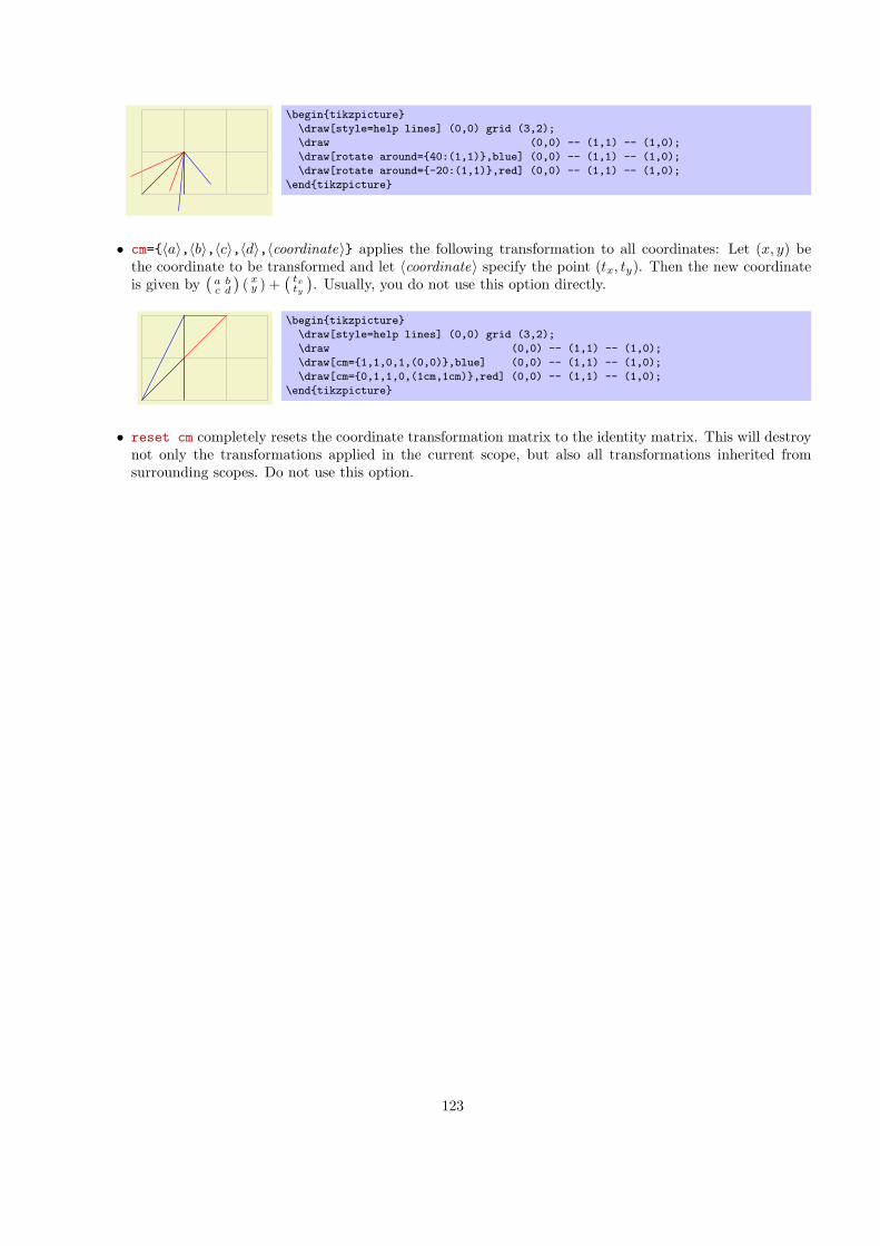
\begin{tikzpicture}


\draw (0,0) -- (1,1) -- (1,0);

\draw[rotate around={40:(1,1)},blue] (0,0) -- (1,1) -- (1,0);

\draw[rotate around={-20:(1,1)},red] (0,0) -- (1,1) -- (1,0);

\end{tikzpicture}

• cm={⟨a⟩,⟨b⟩,⟨c⟩,⟨d⟩,⟨coordinate⟩} applies the following transformation to all coordinates: Let (x, y) bethe coordinate to be transformed and let ⟨coordinate⟩ specify the point (tx, ty). Then the new coordinateis given by

(a bc d

)( x

y ) +( tx

ty

). Usually, you do not use this option directly.

.

\begin{tikzpicture}


\draw (0,0) -- (1,1) -- (1,0);

\draw[cm={1,1,0,1,(0,0)},blue] (0,0) -- (1,1) -- (1,0);

\draw[cm={0,1,1,0,(1cm,1cm)},red] (0,0) -- (1,1) -- (1,0);

\end{tikzpicture}

• reset cm completely resets the coordinate transformation matrix to the identity matrix. This will destroynot only the transformations applied in the current scope, but also all transformations inherited fromsurrounding scopes. Do not use this option.

123

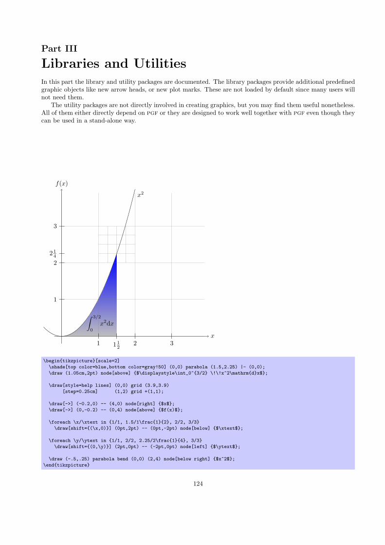
Part III

Libraries and UtilitiesIn this part the library and utility packages are documented. The library packages provide additional predefinedgraphic objects like new arrow heads, or new plot marks. These are not loaded by default since many users willnot need them.

The utility packages are not directly involved in creating graphics, but you may find them useful nonetheless.All of them either directly depend on pgf or they are designed to work well together with pgf even though theycan be used in a stand-alone way.

.

.

.

∫ 3/2

0

x2dx

.

x

.

f(x)

.

1

.

1 12

.

2

.

3

.

1

.

2

.

2 14

.

3

.

x2


\shade[top color=blue,bottom color=gray!50] (0,0) parabola (1.5,2.25) |- (0,0);

\draw (1.05cm,2pt) node[above] {$\displaystyle\int_0^{3/2} \!\!x^2\mathrm{d}x$};

\draw[style=help lines] (0,0) grid (3.9,3.9)

[step=0.25cm] (1,2) grid +(1,1);

\draw[->] (-0.2,0) -- (4,0) node[right] {$x$};

\draw[->] (0,-0.2) -- (0,4) node[above] {$f(x)$};

\foreach \x/\xtext in {1/1, 1.5/1\frac{1}{2}, 2/2, 3/3}

\draw[shift={(\x,0)}] (0pt,2pt) -- (0pt,-2pt) node[below] {$\xtext$};

\foreach \y/\ytext in {1/1, 2/2, 2.25/2\frac{1}{4}, 3/3}

\draw[shift={(0,\y)}] (2pt,0pt) -- (-2pt,0pt) node[left] {$\ytext$};

\draw (-.5,.25) parabola bend (0,0) (2,4) node[below right] {$x^2$};

\end{tikzpicture}

124

14 Libraries

14.1 Arrow Tip Library

\usepackage{pgflibraryarrows} % LATEX\input pgflibraryarrows.tex % plain TEX\input pgflibraryarrows.tex % ConTEXt

The package defines additional arrow tips, which are described below. See page 198 for the arrows tips thatare defined by default. Note that neither the standard packages nor this package defines an arrow namecontaining > or <. These are left for the user to defined as he or she sees fit.

14.1.1 Triangular Arrow Tips

latex’ yields thick

.

and thin

.

latex’ reversed yields thick

.

and thin

.

stealth’ yields thick

.

and thin

.

stealth’ reversed yields thick

.

and thin

.

triangle 90 yields thick

.

and thin

.

triangle 90 reversed yields thick

.

and thin

.


.

and thin

.


.

and thin

.


.

and thin

.


.

and thin

.

open triangle 90 yields thick

.

and thin

.

open triangle 90 reversed yields thick

.

and thin

.


.

and thin

.


.

and thin

.


.

and thin

.


.

and thin

.

14.1.2 Barbed Arrow Tips

angle 90 yields thick

.

and thin

.

angle 90 reversed yields thick

.

and thin

.


.

and thin

.


.

and thin

.


.

and thin

.


.

and thin

.

hooks yields thick

.

and thin

.

hooks reversed yields thick

.

and thin

.

14.1.3 Bracket-Like Arrow Tips

[-] yields thick

.

and thin

.

]-[ yields thick

.

and thin

.

(-) yields thick

.

and thin

.

)-( yields thick

.

and thin

.

14.1.4 Circle and Diamond Arrow Tips

o yields thick

.

and thin

.

* yields thick

.

and thin

.

diamond yields thick

.

and thin

.

open diamond yields thick

.

and thin

.

125

14.1.5 Partial Arrow Tips

left to yields thick

.

and thin

.

left to reversed yields thick

.

and thin

.

right to yields thick

.

and thin

.

right to reversed yields thick

.

and thin

.

left hook yields thick

.

and thin

.

left hook reversed yields thick

.

and thin

.

right hook yields thick

.

and thin

.

right hook reversed yields thick

.

and thin

.

14.1.6 Line Caps

round cap yields for line width 1ex

.

butt cap yields for line width 1ex

.

triangle 90 cap yields for line width 1ex

.

triangle 90 cap reversed yields for line width 1ex

.

fast cap yields for line width 1ex

.

fast cap reversed yields for line width 1ex

.

14.2 Snake Library

\usepackage{pgflibrarysnakes} % LATEX\input pgflibrarysnakes.tex % plain TEX\input pgflibrarysnakes.tex % ConTEXt

This library package defines basic snakes. Section 9.2.3 explains how snakes are used in TikZ, Section 22explains how new snakes can be defined.The snakes are influenced by the current values of parameters like \pgfsnakesegmentamplitude. Onlythis parameter and \pgfsnakesegmentlength are proper TEX dimensions, all other parameters are TEXmacros.In TikZ, each parameter can be set using an option having the parameters name minus the \pgfsnake part.

Snake border

This snake adds straight lines the path that are at a specific angle to the line toward the target. The idea isto add these little lines to indicate the “border” or an area. The following parameters influence the snake:

• \pgfsnakesegmentlength determines the distance between consecutive ticks.

• \pgfsnakesegmentamplitude determines the length of the ticks.

• \pgfsnakesegmentangle determines the angle between the ticks and the line toward the target.

.

\tikz{\draw (0,0) rectangle (3,1)

[snake=border,segment angle=-45] (0,0) rectangle (3,1);}

Snake brace

This snake adds a long brace to the path. The left and right end of the brace will be exactly on the startand endpoint of the snake. The following parameters influence the snake:

• \pgfsnakesegmentamplitude determines how much the brace rises above the path.

• \pgfsnakesegmentaspect determines the fraction of the total length where the “middle part” of thebrace will be.

.

\tikz{\draw[snake=brace,segment aspect=0.25] (0,0) -- (3,0);}

126

Snake bumps

This snake consists of little half ellipses. The following parameters influence the snake:

• \pgfsnakesegmentamplitude determines the height of the half ellipse.

• \pgfsnakesegmentlength determines the width of the half ellipse.

.

\tikz{\draw[snake=bumps] (0,0) -- (3,0);}

Snake coil

This snake adds a coil to the path. To understand how this works, imagine a three-dimensional spring. Thespring’s axis points along the line toward the target. Then, we “view” the spring from a certain angle. Ifwe look “straight from the side” we will see a perfect sine curve, if we look “more from the front” we willsee a coil. The following parameters influence the snake:

• \pgfsnakesegmentamplitude determines how much the coil rises above the path and falls below it.Thus, this is the radius of the coil.

• \pgfsnakesegmentlength determines the distance between two consecutive “curls.” Thus, when thespring is see “from the side” this will be the wave length of the sine curve.

• \pgfsnakesegmentaspect determines the “viewing direction.” A value of 0 means “looking from theside” and a value of 0.5, which is the default, means “look more from the front.”

.

\begin{tikzpicture}[segment amplitude=10pt]

\draw[snake=coil] (0,1) -- (3,1);

\draw[snake=coil,segment aspect=0] (0,0) -- (3,0);

\end{tikzpicture}

Snake expanding waves

This snake adds arcs to the path that get bigger along the line towards the target. The following parametersinfluence the snake:

• \pgfsnakesegmentlength determines the distance between consecutive arcs.

• \pgfsnakesegmentangle determines the opening angle below and above the path. Thus, the totalopening angle is twice this angle.

.

\tikz{\draw[snake=expanding waves] (0,0) -- (3,0);}

Snake saw

This snake looks like the blade of a saw. The following parameters influence the snake:

• \pgfsnakesegmentamplitude determines how much each spike raises above the straight line.

• \pgfsnakesegmentlength determines the length each spike.

127

.

\tikz{\draw[snake=saw] (0,0) -- (3,0);}

Snake snake

This snake is the “architypical” snake: It looks like a snake seen from above. More precisely, the snake is asine wave with a “softened” start and ending. The following parameters influence the snake:

• \pgfsnakesegmentamplitude determines the sine wave’s amplitude.

• \pgfsnakesegmentlength determines the sine wave’s wave length.

.

\tikz{\draw[snake=snake] (0,0) -- (3,0);}

Snake ticks

This snake adds straight lines the path that are orthogonal to the line toward the target. The followingparameters influence the snake:

• \pgfsnakesegmentlength determines the distance between consecutive ticks.

• \pgfsnakesegmentamplitude determines half the length of the ticks.

.

\tikz{\draw[snake=ticks] (0,0) -- (3,0);}

Snake triangles

This snake adds triangles to the path that point toward the target. The following parameters influence thesnake:

• \pgfsnakesegmentlength determines the distance between consecutive triangles.

• \pgfsnakesegmentamplitude determines half the length of the triangle side that is orthogonal to thepath.

• \pgfsnakesegmentobjectlength determines the height of the triangle.

.

\tikz{\draw[snake=triangles] (0,0) -- (3,0);}

Snake waves

This snake adds arcs to the path that have a constant size. The following parameters influence the snake:

• \pgfsnakesegmentlength determines the distance between consecutive arcs.

• \pgfsnakesegmentangle determines the opening angle below and above the path. Thus, the totalopening angle is twice this angle.

• \pgfsnakesegmentamplitude determines the radius of each arc.

.

\tikz{\draw[snake=waves] (0,0) -- (3,0);}

Snake zigzag

This snake looks like a zig-zag line. The following parameters influence the snake:

• \pgfsnakesegmentamplitude determines how much the zig-zag lines raises above and falls below astraight line to the target point.

• \pgfsnakesegmentlength determines the length of a complete “up-down” cycle.

.

\tikz{\draw[snake=zigzag] (0,0) -- (3,0);}

128

14.3 Plot Handler Library

\usepackage{pgflibraryplothandlers} % LATEX\input pgflibraryplothandlers.tex % plain TEX\input pgflibraryplothandlers.tex % ConTEXt

This library packages defines additional plot handlers, see Section 29.3 for an introduction to plot handlers.The additional handlers are described in the following.

14.3.1 Curve Plot Handlers

\pgfplothandlercurveto

This handler will issue a \pgfpathcurveto command for each point of the plot, except possiblyfor the first. As for the line-to handler, what happens with the first point can be specified using\pgfsetmovetofirstplotpoint or \pgfsetlinetofirstplotpoint.Obviously, the \pgfpathcurveto command needs, in addition to the points on the path, some controlpoints. These are generated automatically using a somewhat “dumb” algorithm: Suppose you have threepoints x, y, and z on the curve such that y is between x and z:

.

.

x

.

y

.

z

\begin{tikzpicture}

\draw[gray] (0,0) node {x} (1,1) node {y} (2,.5) node {z};


\pgfplotstreamstart

\pgfplotstreampoint{\pgfpoint{0cm}{0cm}}


\pgfplotstreampoint{\pgfpoint{2cm}{.5cm}}

\pgfplotstreamend

\pgfusepath{stroke}

\end{tikzpicture}

In order to determine the control points of the curve at the point y, the handler computes the vector z − xand scales it by the tension factor (see below). Let us call the resulting vector s. Then y + s and y − s willbe the control points around y. The first control point at the beginning of the curve will be the beginningitself, once more; likewise the last control point is the end itself.

\pgfsetplottension{⟨value⟩}Sets the factor used by the curve plot handlers to determine the distance of the control points from thepoints they control. The higher the curvature of the curve points, the higher this value should be. A valueof 1 will cause four points at quarter positions of a circle to be connected using a circle. The default is 0.5.

.

.

x

.

y

.

z

\begin{tikzpicture}


\pgfsetplottension{0.75}


\pgfplotstreamstart



\pgfplotstreampoint{\pgfpoint{2cm}{0.5cm}}

\pgfplotstreamend

\pgfusepath{stroke}

\end{tikzpicture}

\pgfplothandlerclosedcurve

This handler works like the curve-to plot handler, only it will add a new part to the current path that is aclosed curve through the plot points.

129

.

.

x.

y

.

z

\begin{tikzpicture}



\pgfplotstreamstart




\pgfplotstreamend

\pgfusepath{stroke}

\end{tikzpicture}

14.3.2 Comb Plot Handlers

There are three “comb” plot handlers. There name stems from the fact that the plots they produce look like“combs” (more or less).

\pgfplothandlerxcomb

This handler converts each point in the plot stream into a line from the y-axis to the point’s coordinate,resulting in a “horizontal comb.”

.

.

x

.

y

.

z

\begin{tikzpicture}


\pgfplothandlerxcomb

\pgfplotstreamstart




\pgfplotstreamend

\pgfusepath{stroke}

\end{tikzpicture}

\pgfplothandlerycomb

This handler converts each point in the plot stream into a line from the x-axis to the point’s coordinate,resulting in a “vertical comb.”This handler is useful for creating “bar diagrams.”

.

.

x

.

y

.

z

\begin{tikzpicture}


\pgfplothandlerycomb

\pgfplotstreamstart




\pgfplotstreamend

\pgfusepath{stroke}

\end{tikzpicture}

\pgfplothandlerpolarcomb

This handler converts each point in the plot stream into a line from the origin to the point’s coordinate.

.

.

x

.

y

.

z

\begin{tikzpicture}


\pgfplothandlerpolarcomb

\pgfplotstreamstart




\pgfplotstreamend

\pgfusepath{stroke}

\end{tikzpicture}

130

14.3.3 Mark Plot Handler

\pgfplothandlermark{⟨mark code⟩}This command will execute the ⟨mark code⟩ for each point of the plot, but each time the coordinatetransformation matrix will be setup such that the origin is at the position of the point to be plotted. Thisway, if the ⟨mark code⟩ draws a little circle around the origin, little circles will be drawn at each point ofthe plot.

.

.

x

.

y

.

z

\begin{tikzpicture}


\pgfplothandlermark{\pgfpathcircle{\pgfpointorigin}{4pt}\pgfusepath{stroke}}

\pgfplotstreamstart




\pgfplotstreamend

\pgfusepath{stroke}

\end{tikzpicture}

Typically, the ⟨code⟩ will be \pgfuseplotmark{⟨plot mark name⟩}, where ⟨plot mark name⟩ is the name ofa predefined plot mark.

\pgfuseplotmark{⟨plot mark name⟩}Draws the given ⟨plot mark name⟩ at the origin. The ⟨plot mark name⟩ must previously have been declaredusing \pgfdeclareplotmark.

.

.

x

.

y

.

z

\begin{tikzpicture}


\pgfplothandlermark{\pgfuseplotmark{pentagon}}

\pgfplotstreamstart




\pgfplotstreamend

\pgfusepath{stroke}

\end{tikzpicture}

\pgfdeclareplotmark{⟨plot mark name⟩}{⟨code⟩}Declares a plot mark for later used with the \pgfuseplotmark command.

.

.

x

.

y

.

z

\pgfdeclareplotmark{my plot mark}

{\pgfpathcircle{\pgfpoint{0cm}{1ex}}{1ex}\pgfusepathqstroke}

\begin{tikzpicture}


\pgfplothandlermark{\pgfuseplotmark{my plot mark}}

\pgfplotstreamstart




\pgfplotstreamend

\pgfusepath{stroke}

\end{tikzpicture}

\pgfsetplotmarksize{⟨dimension⟩}This command sets the TEX dimension \pgfplotmarksize to ⟨dimension⟩. This dimension is a “recom-mendation” for plot mark code at which size the plot mark should be drawn; plot mark code may choose toignore this ⟨dimension⟩ altogether. For circles, ⟨dimension⟩ should be the radius, for other shapes it shouldbe about half the width/height.The predefined plot marks all take this dimension into account.

131

.

.

x.

y

.

z

\begin{tikzpicture}


\pgfsetplotmarksize{1ex}

\pgfplothandlermark{\pgfuseplotmark{*}}

\pgfplotstreamstart




\pgfplotstreamend

\pgfusepath{stroke}

\end{tikzpicture}

\pgfplotmarksize

A TEX dimension that is a “recommendation” for the size of plot marks.

The following plot marks are predefined (the filling color has been set to yellow):

\pgfuseplotmark{*}

.

\pgfuseplotmark{x}

.

\pgfuseplotmark{+}

.

14.4 Plot Mark Library

\usepackage{pgflibraryplotmarks} % LATEX\input pgflibraryplotmarks.tex % plain TEX\input pgflibraryplotmarks.tex % ConTEXt

When this package is loaded, the following plot marks are defined in addition to *, x, and + (the filling colorhas been set to a dark yellow):

\pgfuseplotmark{-}

.

\pgfuseplotmark{|}

.

\pgfuseplotmark{o}

.

\pgfuseplotmark{asterisk}

.

\pgfuseplotmark{star}

.

\pgfuseplotmark{oplus}

.

\pgfuseplotmark{oplus*}

.

\pgfuseplotmark{otimes}

.

\pgfuseplotmark{otimes*}

.

\pgfuseplotmark{square}

.

\pgfuseplotmark{square*}

.

\pgfuseplotmark{triangle}

.

\pgfuseplotmark{triangle*}

.

\pgfuseplotmark{diamond}

.

\pgfuseplotmark{diamond*}

.

\pgfuseplotmark{pentagon}

.

\pgfuseplotmark{pentagon*}

.

14.5 Shape Library

\usepackage{pgflibraryshapes} % LATEX\input pgflibraryshapes.tex % plain TEX\input pgflibraryshapes.tex % ConTEXt

This library packages defines additional shapes, which are described in the following.

Shape cross out

132

This shape “crosses out” the node. Its foreground path are simply two diagonal lines that between thecorners of the node’s bounding box. Here is an example:

.

.

cross out

\begin{tikzpicture}


\node [cross out,draw=red] at (1.5,1) {cross out};

\end{tikzpicture}

A useful application is inside text as in the following example:

Cross

.

.

me out! Cross \tikz[baseline] \node [cross out,draw,anchor=text] {me}; out!

This shape inherits all anchors from the rectangle shape, see also the following figure:

.

.

cross out

.

(s.north west)

.

(s.north)

.

(s.north east)

.

(s.west)

.

(s.center)

.

(s.east)

.

(s.mid west)

.

(s.mid)

.

(s.mid east)

.

(s.base west)

.

(s.base)

.

(s.base east)

.

(s.south west)

.

(s.south)

.

(s.south east)

.

(s.text)

.

(s.10)

.

(s.130)

\Huge

\begin{tikzpicture}

\node[name=s,shape=cross out,style=shape example] {cross out\vrule width 1pt height 2cm};

\foreach \anchor/\placement in

{north west/above left, north/above, north east/above right,

west/left, center/above, east/right,

mid west/right, mid/above, mid east/left,

base west/left, base/below, base east/right,

south west/below left, south/below, south east/below right,

text/left, 10/right, 130/above}

\draw[shift=(s.\anchor)] plot[mark=x] coordinates{(0,0)}

node[\placement] {\scriptsize\texttt{(s.\anchor)}};

\end{tikzpicture}

Shape ellipse

This shape is an ellipse tightly fitting the text box, if no inner separation is given. The following figureshows the anchors this shape defines; the anchors 10 and 130 are example of border anchors.

133

.

.

Ellipse .

(s.north west)

.

(s.north)

.

(s.north east)

.

(s.west)

.

(s.center)

.

(s.east)

.

(s.mid west)

.

(s.mid)

.

(s.mid east)

.

(s.base west)

.

(s.base)

.

(s.base east)

.

(s.south west)

.

(s.south)

.

(s.south east)

.

(s.text)

.

(s.10)

.

(s.130)

\Huge

\begin{tikzpicture}

\node[name=s,shape=ellipse,style=shape example] {Ellipse\vrule width 1pt height 2cm};










\end{tikzpicture}

Shape forbidden sign

This shape places the node inside a circle with a diagonal from the lower left to the upper right added. Thecircle is part of the background, the diagonal line part of the foreground path; thus, the diagonal line is ontop of the text.

.

.

Smoking

\begin{tikzpicture}

\node [forbidden sign,line width=1ex,draw=red,fill=white] {Smoking};

\end{tikzpicture}

The shape inherits all anchors from the circle shape, see also the following figure:

134

.

.

Forbidden.

(s.north west)

.

(s.north)

.

(s.north east)

.

(s.west)

.

(s.center)

.

(s.east)

.

(s.mid west)

.

(s.mid)

.

(s.mid east)

.

(s.base west)

.

(s.base)

.

(s.base east)

.

(s.south west)

.

(s.south)

.

(s.south east)

.

(s.text)

.

(s.10)

.

(s.130)

\Huge

\begin{tikzpicture}

\node[name=s,shape=forbidden sign,style=shape example] {Forbidden\vrule width 1pt height 2cm};










\end{tikzpicture}

Shape strike out

This shape is idential to the cross out shape, only its foreground path consists of a single line from thelower left to the upper right.

Strike

.

.

me out! Strike \tikz[baseline] \node [strike out,draw,anchor=text] {me}; out!

See the cross out shape for the anchors.

14.6 Tree Library

\usepackage{pgflibrarytikztrees} % LATEX\input pgflibrarytikztrees.tex % plain TEX\input pgflibrarytikztrees.tex % ConTEXt

This packages defines styles to be used when drawing trees.

135

14.6.1 Growth Functions

The package pgflibrarytikztrees defines two new growth functions. They are installed using the followingoptions:

• grow via three points=one child at (⟨x ⟩) and two children at (⟨y⟩) and (⟨z ⟩) This option in-stalls a growth function that works as follows: If a parent node has just one child, this child is placed at⟨x ⟩. If the parent node has two children, these are placed at ⟨y⟩ and ⟨z ⟩. If the parent node has more thantwo children, the children are placed at points that are linearly extrapolated from the three points ⟨x ⟩,⟨y⟩, and ⟨z ⟩. In detail, the position is x + n−1

2 (y − x) + (c − 1)(z − y), where n is the number of childrenand c is the number of the current child (starting with 1).

The net effect of all this is that if you have a certain “linear arrangement” in mind and use this optionto specify the placement of a single child and of two children, then any number of children will be placedcorrectly.

Here are some arrangements based on this growth function. We start with a simple “above” arrangement:

.

.

one

.

two

.

three

.

four

\begin{tikzpicture}[grow via three points={%

one child at (0,1) and two children at (-.5,1) and (.5,1)}]

\node at (0,0) {one} child;

\node at (0,-1.5) {two} child child;

\node at (0,-3) {three} child child child;

\node at (0,-4.5) {four} child child child child;

\end{tikzpicture}

The next arrangement places children above, but “grows only to the right.”

.

.

one

.

two

.

three

.

four


one child at (0,1) and two children at (0,1) and (1,1)}]





\end{tikzpicture}

In the final arrangement, the children are placed along a line going down and right.

136

.

.one

.two

.three

.four


one child at (-1,-.5) and two children at (-1,-.5) and (0,-.75)}]





\end{tikzpicture}

These examples should make it clear how you can create new styles to arrange your children along a line.

• style=grow cyclic This style causes the children to be arranged “on a circle.” For this, the children areplaced at distance \tikzleveldistance from the parent node, but not on a straight line, but points on acircle. Instead of a sibling distance, there is a sibling angle that denotes the angle between two givenchildren.

– sibling angle=⟨angle⟩ Sets the angle between siblings in the grow cyclic style.

Note that this function will rotate the coordinate system of the children to ensure that the grandchildrenwill grow in the right direction.

.

\begin{tikzpicture}[grow cyclic]

\tikzstyle{level 1}=[level distance=8mm,sibling angle=60]



\coordinate [rotate=-90] % going down

child foreach \x in {1,2,3}

{child foreach \x in {1,2,3}

{child foreach \x in {1,2,3}}};

\end{tikzpicture}

14.6.2 Edges From Parent

The following styles can be used to modify how the edges from parents are drawn:

• style=edge from parent fork down This style will draw a line from the parent downwards (for half thelevel distance) and then on to the child using only horizontal and vertical lines.

.

.

root

.

left

.

right

.

child

.

child

\begin{tikzpicture}

\node {root}

[edge from parent fork down]

child {node {left}}

child {node {right}

child[child anchor=north east] {node {child}}


};

\end{tikzpicture}

• style=edge from parent fork right This style behaves similarly, only it will first draw its edge to theright.

137

.

.

root

.

left.

right

.

child.

child \begin{tikzpicture}

\node {root}

[edge from parent fork right,grow=right]

child {node {left}}

child {node {right}



};

\end{tikzpicture}

• style=edge from parent fork left behaves similary.

• style=edge from parent fork up behaves similary.

14.7 Background Library

\usepackage{pgflibrarytikzbackgrounds} % LATEX\input pgflibrarytikzbackgrounds.tex % plain TEX\input pgflibrarytikzbackgrounds.tex % ConTEXt

This packages defines “backgrounds” for pictures. This does not refer to background pictures, but ratherto frames drawn around and behind pictures. For example, this package allows you to just add the framedoption to a picture to get a rectangular box around your picture or gridded to put a grid behind yourpicture.

When this package is loaded, the following styles become available:

• style=show background rectangle This style causes a rectangle to be drawn behind your graphic. Thisstyle option must be given to the {tikzpicture} environment or to the \tikz command.

.

\begin{tikzpicture}[show background rectangle]

\draw (0,0) ellipse (10mm and 5mm);

\end{tikzpicture}

The size of the background rectangle is determined as follows: We start with the bounding box of thepicture. Then, a certain separator distance is added on the sides. This distance can be different for the x-and y-directions and can be set using the following options:

– inner frame xsep=⟨dimension⟩ Sets the additional horizontal separator distance for the backgroundrectangle. The default is 1ex.

– inner frame ysep=⟨dimension⟩ Same for the vertical separator distance.– inner frame sep=⟨dimension⟩ sets the horizontal and vertical separator distances simultaneously.

The following two styles make setting the inner separator a bit easier to remember:

– style=tight background Sets the inner frame separator to 0pt. The background rectangle will havethe size of the bounding box.

– style=loose background Sets the inner frame separator to 2ex.

You can influence how the background rectangle is rendered by setting the following style:

– style=background rectangle This style dictates how the background rectangle is drawn or filled.By default this style is set to draw, which causes the path of the background rectangle to be drawn inthe usual way. Setting this style to, say, fill=blue!20 causes a light blue background to be addedto the picture. You can also use more fancy settings as shown in the following example:

.

.

\tikzstyle{background rectangle}=

[double,ultra thick,draw=red,top color=blue,rounded corners]



\end{tikzpicture}

138

Naturally, no one in their right mind would use the above, but here is a nice background:

.

\tikzstyle{background rectangle}=

[draw=blue!50,fill=blue!20,rounded corners=1ex]



\end{tikzpicture}

• style=framed This is a shorthand for show background rectangle.

• style=show background grid This style behaves similarly to the show background rectangle style, butit will not use a rectangle path, but a grid. The lower left and upper right corner of the grid is computedin the same way as for the background rectangle:

.

\begin{tikzpicture}[show background grid]


\end{tikzpicture}

You can influence the background grid by setting the following style:

– style=background grid This style dictates how the background grid path is drawn. The default isdraw,help lines.

.

\tikzstyle{background grid}=[thick,draw=red,step=.5cm]

\begin{tikzpicture}[show background grid]


\end{tikzpicture}

This option can be combined with the framed option (use the framed option first):

.

\tikzstyle{background grid}=[thick,draw=red,step=.5cm]

\tikzstyle{background rectangle}=[rounded corners,fill=yellow]

\begin{tikzpicture}[framed,gridded]


\end{tikzpicture}

– style=gridded This is a shorthand for show background grid.

• style=show background top This style causes a single line to be drawn at the top of the backgroundrectangle. Normally, the line coincides exactly with the top line of the background rectangle:

.

\tikzstyle{background rectangle}=[fill=yellow]

\begin{tikzpicture}[framed,show background top]


\end{tikzpicture}

The following option allows you to lengthen (or shorten) the line:

– outer frame xsep=⟨dimension⟩ The ⟨dimension⟩ is added at the left and right side of the line.

.

\tikzstyle{background rectangle}=[fill=yellow]

\begin{tikzpicture}

[framed,show background top,outer frame xsep=1ex]


\end{tikzpicture}

– outer frame ysep=⟨dimension⟩ This option does not apply to the top line, but to the left and rightlines, see below.

139

– outer frame sep=⟨dimension⟩ Sets both the x- and y-separation.

.

\tikzstyle{background rectangle}=[fill=blue!20]

\begin{tikzpicture}

[outer frame sep=1ex,%

show background top,%

show background bottom,%

show background left,%

show background right]


\end{tikzpicture}

You can influence how the line is drawn grid by setting the following style:

– style=background top Default is draw.

.

\tikzstyle{background rectangle}=[fill=blue!20]

\tikzstyle{background top}=[draw=blue!50,line width=1ex]

\begin{tikzpicture}[framed,show background top]


\end{tikzpicture}

• style=show background bottom works like the style for the top line.

• style=show background left works like the style for the top line.

• style=show background right works like the style for the top line.

14.8 Automata Drawing Library

\usepackage{pgflibraryautomata} % LATEX\input pgflibraryautomata.tex % plain TEX\input pgflibraryautomata.tex % ConTEXt

This packages, which is still under construction, provides shapes and styles for drawing automata.

Shape state

This shape is currently just an alias for the circle shape. However, it is useful to have another shapestate since one can then say, for example, the the style every state shape should be set to some specialvalue.

Shape state with output

This shape is a multi-part shape. The main part (the text part) is the name of the state as in the stateshape. The second part is called output. This node part is drawn in the lower part of the node, separatedfrom the upper part by a line.

.

.

q1

.

00

\begin{tikzpicture}

\node [state with output,draw,double,fill=red!20]

{

$q_1$

\nodepart{output}

$00$

};

\end{tikzpicture}

The shape inherits all anchors from the circle shape and defines the output anchor in addition. See alsothe following figure:

140

.

.

state name

.

output.

(s.north west)

.

(s.north)

.

(s.north east)

.

(s.west)

.

(s.center)

.

(s.east)

.

(s.mid west)

.

(s.mid)

.

(s.mid east)

.

(s.base west)

.

(s.base)

.

(s.base east)

.

(s.south west)

.

(s.south)

.

(s.south east)

.

(s.text)

.

(s.output) .

(s.130)

\Huge

\begin{tikzpicture}

\node[name=s,shape=state with output,style=shape example] {state name\nodepart{output}output};



west/left, center/below, east/right,




text/left, output/left, 130/above}



\end{tikzpicture}

141

15 Repeating Things: The Foreach Statement

In this section the package pgffor.sty is described. It can be used independently of pgf, but it works partic-ularly well together with pgf and TikZ.

When you say \usepackage{pgffor}, two commands are defined: \foreach and \breakforeach. Theirbehaviour is described in the following:

\foreach ⟨variables⟩ in {⟨list⟩} ⟨commands⟩The syntax of this command is a bit complicated, so let us go through it step-by-step.In the easiest case, ⟨variables⟩ is a single TEX-command like \x or \point. (If you want to have some fun,you can also use active characters. If you do not know what active characters are, you are blessed.)Still in the easiest case, ⟨list⟩ is a comma-separated list of values. Anything can be used as a value, butnumbers are most likely.Finally, in the easiest case, ⟨commands⟩ is some TEX-text in curly braces.With all these assumptions, the \foreach statement will execute the ⟨commands⟩ repeatedly, once for everyelement of the ⟨list⟩. Each time the ⟨commands⟩ are executed, the ⟨variable⟩ will be set to the current valueof the list item.

[1][2][3][0] \foreach \x in {1,2,3,0} {[\x]}

Syntax for the commands. Let use move on to a more complicated setting. The first complication occurswhen the ⟨commands⟩ are not some text in curly braces. If the \foreach statement does not encounter anopening brace, it will instead scan everything up to the next semicolon and use this as ⟨commands⟩. Thisis most useful in situations like the following:

.

\tikz

\foreach \x in {0,1,2,3}

\draw (\x,0) circle (0.2cm);

However, the “reading till the next semicolon” is not the whole truth. There is another rule: If a \foreachstatement is directly followed by another \foreach statement, this second foreach statement is collected as⟨commands⟩. This allows you to write the following:

.

\begin{tikzpicture}

\foreach \x in {0,1,2,3}

\foreach \y in {0,1,2,3}

{

\draw (\x,\y) circle (0.2cm);

\fill (\x,\y) circle (0.1cm);

}

\end{tikzpicture}

The dots notation. The second complication concerns the ⟨list⟩. If this ⟨list⟩ contains the list item “...”,this list item is replaced by the “missing values.” More precisely, the following happens:Normally, when a list item ... is encountered, there should already have been two list items before it,which where numbers. Examples of numbers are 1, -10, or -0.24. Let us call these numbers x and y andlet d := y − x be their difference. Next, there should also be one number following the three dots, let uscall this number z.In this situation, the part of the list reading “x,y,...,z” is replaced by “x, x + d, x + 2d, x + 3d, . . . ,x + md,” where the last dots are semantic dots, not syntactic dots. The value m is the largest number suchthat x + md ≤ z if d is positive or such that x + md ≥ z if d is negative.Perhaps it is best to explain this by some examples: The following ⟨list⟩ have the same effects:\foreach \x in {1,2,...,6} {\x, } yields 1, 2, 3, 4, 5, 6,

142

\foreach \x in {1,2,3,...,6} {\x, } yields 1, 2, 3, 4, 5, 6,\foreach \x in {1,3,...,11} {\x, } yields 1, 3, 5, 7, 9, 11,\foreach \x in {1,3,...,10} {\x, } yields 1, 3, 5, 7, 9,\foreach \x in {0,0.1,...,0.5} {\x, } yields 0, 0.1, 0.20001, 0.30002, 0.40002,\foreach \x in {a,b,9,8,...,1,2,2.125,...,2.5} {\x, } yields a, b, 9, 8, 7, 6, 5, 4, 3, 2, 1, 2, 2.125,2.25, 2.375, 2.5,As can be seen, for fractional steps that are not multiples of 2−n for some small n, rounding errors canoccur pretty easily. Thus, in the second last case, 0.5 should probably be replaced by 0.501 for robustness.There is yet another special case for the ... statement: If the ... is used right after the first item in thelist, that is, if there is an x, but no y, the difference d obviously cannot be computed and is set to 1 if thenumber z following the dots is larger than x and is set to −1 if z is smaller:\foreach \x in {1,...,6} {\x, } yields 1, 2, 3, 4, 5, 6,\foreach \x in {9,...,3.5} {\x, } yields 9, 8, 7, 6, 5, 4,

Special handling of pairs. Different list items are separated by commas. However, this causes a problemwhen the list items contain commas themselves as pairs like (0,1) do. In this case, you should put theitems containing commas in braces as in {(0,1)}. However, since pairs are such a natural and useful case,they get a special treatment by the \foreach statement. When a list item starts with a ( everything up tothe next ) is made part of the item. Thus, we can write things like the following:

.

\tikz

\foreach \position in {(0,0), (1,1), (2,0), (3,1)}

\draw \position rectangle +(.25,.5);

Using the foreach-statement inside paths. TikZ allows you to use a \foreach statement inside apath construction. In such a case, the ⟨commands⟩ must be path construction commands. Here are twoexamples:

.

\tikz

\draw (0,0)

\foreach \x in {1,...,3}

{ -- (\x,1) -- (\x,0) }

;

.

\tikz \draw \foreach \p in {1,...,3} {(\p,1)--(\p,3) (1,\p)--(3,\p)};

Multiple variables. You will often wish to iterate over two variables at the same time. Since you cannest \foreach loops, this is normally straight-forward. However, you sometimes wish variables to iterate“simultaneously.” For example, we might be given a list of edges that connect two coordinates and mightwish to iterate over these edges. While doing so, we would like the source and target of the edges to be setto two different variables.To achieve this, you can use the following syntax: The ⟨variables⟩ may not only be a single TEX-variable.Instead, it can also be a list of variables separated by slashes (/). In this case the list items can also be listsof values separated by slashes.Assuming that the ⟨variables⟩ and the list items are lists of values, each time the ⟨commands⟩ are executed,each of the variables in ⟨variables⟩ is set to one part of the list making up the current list item. Here is anexample to clarify this:

143

Example: \foreach \x / \y in {1/2,a/b} {‘‘\x\ and \y’’} yields “1 and 2”“a and b”.If some entry in the ⟨list⟩ does not have “enough” slashes, the last entry will be repeated. Here is anexample:

.

.

0

.

1

.

2

.

3

.

e \begin{tikzpicture}

\foreach \x/\xtext in {0,...,3,2.72 / e}

\draw (\x,0) node{$\xtext$};

\end{tikzpicture}

Here are more useful examples:

.

.

a

.

b

.

c

.

d\begin{tikzpicture}

% Define some coordinates:

\tikzstyle{every node}=[draw,fill]

\path[shape=circle,fill=examplefill]

(0,0) node(a) {a}

(2,0.55) node(b) {b}

(1,1.5) node(c) {c}

(2,1.75) node(d) {d};

% Draw some connections:

\foreach \source/\target in {a/b, b/c, c/a, c/d}

\draw (\source) .. controls +(.75cm,0pt) and +(-.75cm,0pt)..(\target);

\end{tikzpicture}

.

\begin{tikzpicture}

% Let’s draw circles at interesting points:

\foreach \x / \y / \diameter in {0 / 0 / 2mm, 1 / 1 / 3mm, 2 / 0 / 1mm}

\draw (\x,\y) circle (\diameter);

% Same effect

\foreach \center/\diameter in {{(0,0)/2mm}, {(1,1)/3mm}, {(2,0)/1mm}}

\draw[yshift=2.5cm] \center circle (\diameter);

\end{tikzpicture}

.

.

3

.

2

.

1

.

12

.

11

.

10

.

9

.

8

.

7

.

6

.

5

.

4

144

\begin{tikzpicture}[cap=round,line width=3pt]

\filldraw [fill=examplefill] (0,0) circle (2cm);

\foreach \angle / \label in

{0/3, 30/2, 60/1, 90/12, 120/11, 150/10, 180/9,

210/8, 240/7, 270/6, 300/5, 330/4}

{

\draw[line width=1pt] (\angle:1.8cm) -- (\angle:2cm);

\draw (\angle:1.4cm) node{\textsf{\label}};

}

\foreach \angle in {0,90,180,270}

\draw[line width=2pt] (\angle:1.6cm) -- (\angle:2cm);

\draw (0,0) -- (120:0.8cm); % hour

\draw (0,0) -- (90:1cm); % minute

\end{tikzpicture}%

.

.

.

.

.

.

.

.

.

.

.

.

.

.

.

.

.

\tikz[shading=ball]

\foreach \x / \cola in {0/red,1/green,2/blue,3/yellow}

\foreach \y / \colb in {0/red,1/green,2/blue,3/yellow}

\shade[ball color=\cola!50!\colb] (\x,\y) circle (0.4cm);

\breakforeach

If this command is given inside a \foreach command, no further executions of the ⟨commands⟩ will occur.However, the current execution of the ⟨commands⟩ is continued normally, so it is probably best to use thiscommand only at the end of a \foreach command.

.

\begin{tikzpicture}

\foreach \x in {1,...,4}

\foreach \y in {1,...,4}

{

\fill[red!50] (\x,\y) ellipse (3pt and 6pt);

\ifnum \x<\y

\breakforeach

\fi

}

\end{tikzpicture}

145

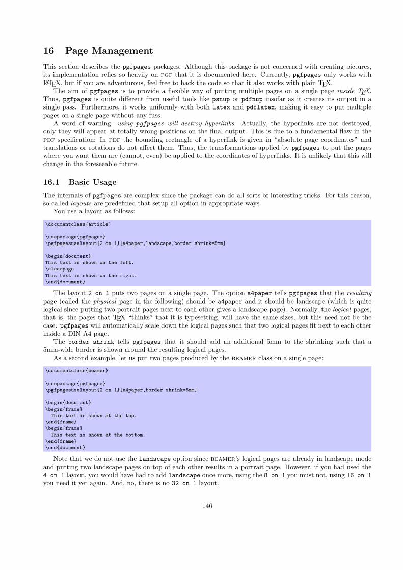
16 Page Management

This section describes the pgfpages packages. Although this package is not concerned with creating pictures,its implementation relies so heavily on pgf that it is documented here. Currently, pgfpages only works withLATEX, but if you are adventurous, feel free to hack the code so that it also works with plain TEX.

The aim of pgfpages is to provide a flexible way of putting multiple pages on a single page inside TEX.Thus, pgfpages is quite different from useful tools like psnup or pdfnup insofar as it creates its output in asingle pass. Furthermore, it works uniformly with both latex and pdflatex, making it easy to put multiplepages on a single page without any fuss.

A word of warning: using pgfpages will destroy hyperlinks. Actually, the hyperlinks are not destroyed,only they will appear at totally wrong positions on the final output. This is due to a fundamental flaw in thepdf specification: In pdf the bounding rectangle of a hyperlink is given in “absolute page coordinates” andtranslations or rotations do not affect them. Thus, the transformations applied by pgfpages to put the pageswhere you want them are (cannot, even) be applied to the coordinates of hyperlinks. It is unlikely that this willchange in the foreseeable future.

16.1 Basic Usage

The internals of pgfpages are complex since the package can do all sorts of interesting tricks. For this reason,so-called layouts are predefined that setup all option in appropriate ways.

You use a layout as follows:

\documentclass{article}

\usepackage{pgfpages}

\pgfpagesuselayout{2 on 1}[a4paper,landscape,border shrink=5mm]

\begin{document}

This text is shown on the left.

\clearpage

This text is shown on the right.

\end{document}

The layout 2 on 1 puts two pages on a single page. The option a4paper tells pgfpages that the resultingpage (called the physical page in the following) should be a4paper and it should be landscape (which is quitelogical since putting two portrait pages next to each other gives a landscape page). Normally, the logical pages,that is, the pages that TEX “thinks” that it is typesetting, will have the same sizes, but this need not be thecase. pgfpages will automatically scale down the logical pages such that two logical pages fit next to each otherinside a DIN A4 page.

The border shrink tells pgfpages that it should add an additional 5mm to the shrinking such that a5mm-wide border is shown around the resulting logical pages.

As a second example, let us put two pages produced by the beamer class on a single page:

\documentclass{beamer}


\pgfpagesuselayout{2 on 1}[a4paper,border shrink=5mm]

\begin{document}

\begin{frame}

This text is shown at the top.

\end{frame}

\begin{frame}

This text is shown at the bottom.

\end{frame}

\end{document}

Note that we do not use the landscape option since beamer’s logical pages are already in landscape modeand putting two landscape pages on top of each other results in a portrait page. However, if you had used the4 on 1 layout, you would have had to add landscape once more, using the 8 on 1 you must not, using 16 on 1you need it yet again. And, no, there is no 32 on 1 layout.

146

Another word of caution: using pgfpages will produce wrong page numbers in the .aux file. The reason isthat TEX instantiates the page numbers when writing an .aux file only when the physical page is shipped out.Fortunately, this problem is easy to fix: First, typeset our file normally without using the \pgfpagesuselayoutcommand (just put the comment marker % before it) Then, rerun TEX with the \pgfpagesuselayout commandincluded and add the command \nofiles. This command ensures that the .aux file is not modified, which isexactly what you want. So, to typeset the above example, you should actually first TEX the following file:



%%\pgfpagesuselayout{2 on 1}[a4paper,landscape,border shrink=5mm]

%%\nofiles

\begin{document}


\clearpage


\end{document}

and then typeset



\pgfpagesuselayout{2 on 1}[a4paper,landscape,border shrink=5mm]

\nofiles

\begin{document}


\clearpage


\end{document}

The final basic example is the resize to layout (it works a bit like a hypothetical 1 on 1 layout). Thislayout resizes the logical page such that is fits the specified physical size. Since this does not change the pagenumbering, you need not worry about the .aux files with this layout. For example, adding the following lineswill ensure that the physical output will fit on DIN A4 paper:


\pgfpagesuselayout{resize to}[a4paper]

This can be very useful when you have to handle lots of papers that are typeset for, say, letter paper and youhave an A4 printer or the other way round. For example, the following article will be fit for printing on letterpaper:

\documentclass[a4paper]{article}

%% a4 is currently the logical size and also the physical size


\pgfpagesuselayout{resize to}[letterpaper]

%% a4 is still the logical size, but letter is the physical one

\begin{document}

\title{My Great Article}

...

\end{document}

16.2 The Predefined Layouts

This section explains the predefined layouts in more detail. You select a layout using the following command:

\pgfpagesuselayout{⟨layout⟩}[⟨options⟩]Installs the specified ⟨layout⟩ with the given ⟨options⟩ set. The predefined layouts and their permissibleoptions are explained below.

147

If this function is called multiple times, only the last call “wins.” You can thereby overwrite any previoussettings. In particular, layouts do not accumulate.

Example: \pgfpagesuselayout{resize to}[a4paper]

\pgfpagesuselayout{resize to}[⟨options⟩]This layout is used to resize every logical page to a specified physical size. To determine the target size, thefollowing options may be given:

• physical paper height=⟨size⟩ sets the height of the physical pape size to ⟨size⟩.• physical paper width=⟨size⟩ sets the width of the physical pape size to ⟨size⟩.• a0paper sets the physical page size to DIN A0 paper.

• a1paper sets the physical page size to DIN A1 paper.






• letterpaper sets the physical page size to the American letter paper size.

• legalpaper sets the physical page size to the American legal paper size.

• executivepaper sets the physical page size to the American executive paper size.

• landscape swaps the height and the width of the physical paper.

• border shrink=⟨size⟩ additionally reduces the size of the logical page on the physical page by ⟨size⟩.

\pgfpagesuselayout{2 on 1}[⟨options⟩]Puts two logical pages alongside each other on each physical page if the logical height is larger than thelogical width (logical pages are in portrait mode). Otherwise, two logical pages are put on top of eachother (logical pages are in landscape mode). When using this layout, it is advisable to use the \nofilescommand, but this is not done automatically.The same ⟨options⟩ as for the resize to layout an be used, plus the following option:

• odd numbered pages right places the first page on the right.

\pgfpagesuselayout{4 on 1}[⟨options⟩]Puts four logical pages on a single physical page. The same ⟨options⟩ as for the resize to layout an beused.

\pgfpagesuselayout{8 on 1}[⟨options⟩]Puts eight logical pages on a single physical page. As for 2 on 1, the orientation depends on whether thelogical pages are in landscape mode or in portrait mode.

\pgfpagesuselayout{16 on 1}[⟨options⟩]This is for the ceo.

\pgfpagesuselayout{rounded corners}[⟨options⟩]This layout adds “rounded corners” to every page, which, supposedly, looks nicer during presentations withprojectors (personally, I doubt this). This is done by (possibly) resizing the page to the physical page size.Then four black rectangles are drawn in each corner. Next, a clipping region is set up that contains allof the logical page except for little rounded corners. Finally, the logical page is draw, clipped against theclipping region.Note that every logical page should fill its background for this to work.In addition to the ⟨options⟩ that can be given to resize to the following options may be given.

148

• corner width=⟨size⟩ specifies the size of the corner.

\documentclass{beamer}


\pgfpagesuselayout{rounded corners}[corner width=5pt]

\begin{document}

...

\end{document}

\pgfpagesuselayout{two screens with lagging second}[⟨options⟩]This layout puts two logical pages alongside each other. The second page always shows what the main pageshowed on the previous physical page. Thus, the second page “lags behind” the main page. This can beuseful when you have to projectors attached to your computer and can show different parts of a physicalpage on different projectors.The following ⟨options⟩ may be given:

• second right puts the second page right of the main page. This will make the physical pages twiceas wide as the logical pages, but it will retain the height.

• second left puts the second page left, otherwise it behave the same as second right.• second bottom puts the second page below the main page. This make the physical pages twice as

high as the logical ones.• second top works like second bottom.

\pgfpagesuselayout{two screens with optional second}[⟨options⟩]This layout works similarly to two screens with lagging second. The difference is that the contentsof the second screen only changes when one of the commands \pgfshipoutlogicalpage{2}{⟨box ⟩} or\pgfcurrentpagewillbelogicalpage{2} is called. The first puts the given ⟨box ⟩ on the second page. Thesecond specifies that the current page should be put there, once it is finished.The same options as for two screens with lagging second may be given.

You can define your own predefined layouts using the following command:

\pgfpagesdeclarelayout{⟨layout⟩}{⟨before actions⟩}{⟨after actions⟩}This command predefines a ⟨layout⟩ that can later be installed using the \pgfpagesuselayout command.When \pgfpagesuselayout{⟨layout⟩}[⟨options⟩] is called, the following happens: First, the ⟨beforeactions⟩ are executed. They can be used, for example, to setup default values for keys. Next,\setkeys{pgfpagesuselayoutoption}{⟨options⟩} is executed. Finally, the ⟨after actions⟩ are executed.Here is an example:

\pgfpagesdeclarelayout{resize to}

{

\def\pgfpageoptionborder{0pt}

}

{

\pgfpagesphysicalpageoptions

{%

logical pages=1,%

physical height=\pgfpageoptionheight,%

physical width=\pgfpageoptionwidth%

}

\pgfpageslogicalpageoptions{1}

{%

resized width=\pgfphysicalwidth,%

resized height=\pgfphysicalheight,%

border shrink=\pgfpageoptionborder,%

center=\pgfpoint{.5\pgfphysicalwidth}{.5\pgfphysicalheight}%

}%

}

149

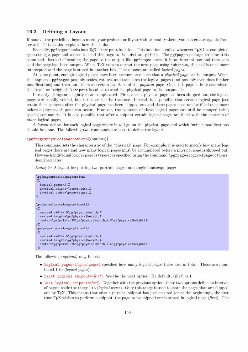
16.3 Defining a Layout

If none of the predefined layouts meets your problem or if you wish to modify them, you can create layouts fromscratch. This section explains how this is done.

Basically, pgfpages hooks into TEX’s \shipout function. This function is called whenever TEX has completedtypesetting a page and wishes to send this page to the .dvi or .pdf file. The pgfpages package redefines thiscommand. Instead of sending the page to the output file, pgfpages stores it in an internal box and then actsas if the page had been output. When TEX tries to output the next page using \shipout, this call is once moreintercepted and the page is stored in another box. These boxes are called logical pages.

At some point, enough logical pages have been accumulated such that a physical page can be output. Whenthis happens, pgfpages possibly scales, rotates, and translates the logical pages (and possibly even does furthermodifications) and then puts them at certain positions of the physical page. Once this page is fully assembled,the “real” or “original” \shipout is called to send the physical page to the output file.

In reality, things are slightly more complicated. First, once a physical page has been shipped out, the logicalpages are usually voided, but this need not be the case. Instead, it is possible that certain logical page justretain their contents after the physical page has been shipped out and these pages need not be filled once morebefore a physical shipout can occur. However, the contents of these logical pages can still be changed usingspecial commands. It is also possible that after a shipout certain logical pages are filled with the contents ofother logical pages.

A layout defines for each logical page where it will go on the physical page and which further modificationsshould be done. The following two commands are used to define the layout:

\pgfpagesphysicalpageoptions{⟨options⟩}This command sets the characteristic of the “physical” page. For example, it is used to specify how many log-ical pages there are and how many logical pages must be accumulated before a physical page is shipped out.How each individual logical page is typeset is specified using the command \pgfpageslogicalpageoptions,described later.

Example: A layout for putting two portrait pages on a single landscape page:

\pgfpagesphysicalpageoptions

{%

logical pages=2,%

physical height=\paperwidth,%

physical width=\paperheight,%

}


{%

resized width=.5\pgfphysicalwidth,%



}%


{%




}%

The following ⟨options⟩ may be set:

• logical pages=⟨logical pages⟩ specified how many logical pages there are, in total. These are num-bered 1 to ⟨logical pages⟩.

• first logical shipout=⟨first⟩. See the the next option. By default, ⟨first⟩ is 1.

• last logical shipout=⟨last⟩. Together with the previous option, these two options define an intervalof pages inside the range 1 to ⟨logical pages⟩. Only this range is used to store the pages that are shippedout by TEX. This means that after a physical shipout has just occured (or at the beginning), the firsttime TEX wishes to perform a shipout, the page to be shipped out is stored in logical page ⟨first⟩. The

150

next time TEX performs a shipout, the page is stored in logical page ⟨first⟩ + 1 and so on, until thelogical page ⟨last⟩ is also filled. Once this happens, a physical shipout occurs and the process startsonce more.Note that logical pages that lie outside the interval between ⟨first⟩ and ⟨last⟩ are filled only indirectlyor when special commands are used.By default, ⟨last⟩ equals ⟨logical pages⟩.

• current logical shipout=⟨current⟩ changes an internal counter such that TEX’s next logical shipoutwill be stored in logical page ⟨current⟩.This option can be used to “warp” the logical page filling mechanism to a certain page. You can bothskip logical pages and overwrite already filled logical pages. After the logical page ⟨current⟩ has beenfilled, the internal counter is incremented normally as if the logical page ⟨current⟩ had been “reached”normally. If you specify a ⟨current⟩ larger to ⟨last⟩, a physical shipout will occur after the logical page⟨current⟩ has been filled.

• physical height=⟨height⟩ specifies the height of the physical pages. This height is typically differentfrom the normal \paperheight, which is used by TEX for its typesetting and page breaking purposes.

• physical width=⟨width⟩ specifies the physical width.

\pgfpageslogicalpageoptions{⟨logical page number⟩}{⟨options⟩}This command is used to specify where the logical page number ⟨logical page number⟩ will be placed on thephysical page. In addition, this command can be used to install additional “code” to be executed when thispage is put on the physical page.The number ⟨logical page number⟩ should be between 1 and ⟨logical pages⟩, which has previously beeninstalled using the \pgfpagesphysicalpageoptions command.The following ⟨options⟩ may be given:

• center=⟨pgf point⟩ specifies the center of the logical page inside the physical page as a pgf-point. Theorigin of the coordinate system of the physical page is at the lower left corner.


{% center logical page on middle of left side




}

• resized width=⟨size⟩ specifies the width that the logical page should have at most on the physicalpage. To achieve this width, the pages is scaled down appropriately or more. The “or more” part canhappen if the resize height option is also used. In this case, the scaling is chosen such that boththe specified height and width are met. The aspect ratio of a logical page is not modified.

• resized height=⟨height⟩ specifies the maximum height of the logical page.

• original width=⟨width⟩ specifies the width the TEX “thinks” that the logical page has. This width is\paperwidth at the point of invocation, by default. Note that setting this width to something differentfrom \paperwidth does not change the \pagewidth during TEX’s typesetting. You have to do thatyourself.You need this option only for special logical pages that have a height or width different from the normalone and for which you will (later on) set these sizes yourself.

• original height=⟨height⟩ works like original width.

• scale=⟨factor⟩ scales the page by at least the given ⟨factor⟩. A ⟨factor⟩ of 0.5 will half the size of thepage, a factor or 2 will double the size. “At least” means that if options like resize height are givenand if the scaling required to meet that option is less than ⟨factor⟩, that other scaling is used instead.

• xscale=⟨factor⟩ scales the logical page along the x-axis by the given ⟨factor⟩. This scaling is doneindependently of any other scaling. Mostly, this option is useful for a factor of -1, which flips the pagealong the y-axis. The aspect ratio is not kept.

151

• yscale=⟨factor⟩ works like xscale, only for the y-axis.

• rotation=⟨degree⟩ rotates the page by ⟨degree⟩ around its center. Use a degree of 90 or -90 to gofrom portrait to landscape and back. The rotation need not be a multiple of 90.

• copy from=⟨logical page number⟩. Normally, after a physical shipout has occured, all logical pages arevoided in a loop. However, if this option is given, the current logical page is filled with the contents ofthe old logical page number ⟨logical page number⟩.Example: Have logical page 2 retain its contents:

\pgfpageslogicalpageoptions{2}{copy from=2}

Example: Let logical page 2 show what logical page 1 showed on the just-shipped-out physical page:

\pgfpageslogicalpageoptions{2}{copy from=1}

• border shrink=⟨size⟩ specifies an addition reduction of the size to which the page is page is scaleddown.

• border code=⟨code⟩. When this option is given, the ⟨code⟩ is executed before the page boxis inserted with a path preinstalled that is a rectangle around the current logical page. Thus,setting ⟨code⟩ to \pgfstroke draws a rectangle around the logical page. Setting ⟨code⟩ to\pgfsetlinewidth{3pt}\pgfstroke results in a thick (ugly) frame. Adding dashes and filling canresult in arbitrarily funky and distracting borders.You can also call \pgfdiscardpath and add your own path construction code (for example to painta rectangle with rounded corners). The coordinate system is setup in such a way that a rectanglestarting at the origin and having the height and width of TEX-box 0 will result in a rectangle fillingexactly the logical page currently being put on the physical page. The logical page is inserted afterthese commands have been executed.

Example: Add a rectangle around the page:

\pgfpageslogicalpageoptions{1}{border code=\pgfstroke}

• corner width=⟨size⟩ adds black “rounded corners” to the page. See the description of the predefinedlayout rounded corners on page 148.

16.4 Creating Logical Pages

Logical pages are created whenever a TEX thinks that a page is full and performs a \shipout command. Thiswill cause pgfpages to store the box that was supposed to be shipped out internally until enough logical pageshave been collected such that a physical shipout can occur.

Normally, whenever a logical shipout occurs that current page is stored in logical page number ⟨currentlogical page⟩. This counter is then incremented, until it is larger than ⟨last logical shipout⟩. You can, however,directly change the value of ⟨current logical page⟩ by calling \pgfpagesphysicalpageoptions.

Another way to set the contents of a logical page is to use the following command:

\pgfpagesshipoutlogicalpage{⟨number⟩}⟨box ⟩This command sets to logical page ⟨number⟩ to ⟨box ⟩. The ⟨box ⟩ should be the code of a TEX box command.This command does not influence the counter ⟨current logical page⟩ and does not cause a physical shipout.

\pgfpagesshipoutlogicalpage{0}\vbox{Hi!}

This command can be used to set the contents of logical pages that are normally not filled.

The final way of setting a logical page is using the following command:

152

\pgfpagescurrentpagewillbelogicalpage{⟨number⟩}When the current TEX page has been typeset, it will be become the given logical page ⟨number⟩. Thiscommand “interrupts” the normal order of logical pages, that is, it behaves like the previous command anddoes not update the ⟨current logical page⟩ counter.

\pgfpagesuselayout{two screens with optional second}

...

Text for main page.

\clearpage

\pgfpagescurrentpagewillbelogicalpage{2}

Text that goes to second page

\clearpage

Text for main page.

153

17 Extended Color Support

This section documents the package xxcolor, which is currently distributed as part of pgf. This packageextends the xcolor package, written by Uwe Kern, which in turn extends the color package. I hope that thecommands in xxcolor will some day migrate to xcolor, such that this package becomes superfluous.

The main aim of the xxcolor package is to provide an environment inside which all colors are “washed out”or “dimmed.” This is useful in numerous situations and must typically be achieved in a roundabout manner ifsuch an environment is not available.

\begin{colormixin}{⟨mix-in specification⟩}⟨environment contents⟩

\end{colormixin}

The mix-in specification is applied to all colors inside the environment. At the beginning of the environment,the mix-in is applied to the current color, i. e., the color that was in effect before the environment started.A mix-in specification is a number between 0 and 100 followed by an exclamation mark and a color name.When a \color command is encountered inside a mix-in environment, the number states what percentageof the desired color should be used. The rest is “filled up” with the color given in the mix-in specification.Thus, a mix-in specification like 90!blue will mix in 10% of blue into everything, whereas 25!white willmake everything nearly white.

Red text,washed-outred text, washed-outblue text, darkwashed-out blue text,dark washed-out greentext, back towashed-out bluetext,and back to red.

\begin{minipage}{3.5cm}\raggedright

\color{red}Red text,%

\begin{colormixin}{25!white}

washed-out red text,

\color{blue} washed-out blue text,

\begin{colormixin}{25!black}

dark washed-out blue text,

\color{green} dark washed-out green text,%

\end{colormixin}

back to washed-out blue text,%

\end{colormixin}

and back to red.

\end{minipage}%

Note that the environment only changes colors that have been installed using the standard LATEX \colorcommand. In particular, the colors in images are not changed. There is, however, some support offered bythe commands \pgfuseimage and \pgfuseshading. If the first command is invoked inside a colormixinenvironment with the parameter, say, 50!black on an image with the name foo, the command will first checkwhether there is also a defined image with the name foo.!50!black. If so, this image is used instead. Thisallows you to provide a different image for this case. If you nest colormixin environments, the different mix-insare all appended. For example, inside the inner environment of the above example, \pgfuseimage{foo} wouldfirst check whether there exists an image named foo.!50!white!25!black.

\colorcurrentmixin

Expands to the current accumulated mix-in. Each nesting of a colormixin adds a mix-in to this list.

!75!white should be “!75!white”!75!black!75!white should be “!75!black!75!white”!50!white!75!black!75!white should be “!50!white!75!black!75!white”\begin{minipage}{\linewidth-6pt}\raggedright


\colorcurrentmixin\ should be ‘‘!75!white’’\par

\begin{colormixin}{75!black}

\colorcurrentmixin\ should be ‘‘!75!black!75!white’’\par


\colorcurrentmixin\ should be ‘‘!50!white!75!black!75!white’’\par

\end{colormixin}

\end{colormixin}

\end{colormixin}

\end{minipage}

154

Part IV

The Basic Layer

.

.

x(t)

.

y(t)

.

−1

.

2

.

−1

.

1

.

2

.

3

.

(x(t), y(t)

)= (t sin 1

t , t cos 1t )

.

( 2π , 0)

\begin{tikzpicture}

\draw[gray,very thin] (-1.9,-1.9) grid (2.9,3.9)

[step=0.25cm] (-1,-1) grid (1,1);

\draw[blue] (1,-2.1) -- (1,4.1); % asymptote

\draw[->] (-2,0) -- (3,0) node[right] {$x(t)$};

\draw[->] (0,-2) -- (0,4) node[above] {$y(t)$};

\foreach \pos in {-1,2}

\draw[shift={(\pos,0)}] (0pt,2pt) -- (0pt,-2pt) node[below] {$\pos$};

\foreach \pos in {-1,1,2,3}

\draw[shift={(0,\pos)}] (2pt,0pt) -- (-2pt,0pt) node[left] {$\pos$};

\fill (0,0) circle (0.064cm);

\draw[thick,parametric,domain=0.4:1.5,samples=200]

% The plot is reparameterised such that there are more samples

% near the center.

plot[id=asymptotic-example] function{(t*t*t)*sin(1/(t*t*t)),(t*t*t)*cos(1/(t*t*t))}

node[right] {$\bigl(x(t),y(t)\bigr) = (t\sin \frac{1}{t}, t\cos \frac{1}{t})$};

\fill[red] (0.63662,0) circle (2pt)

node [below right,fill=white,yshift=-4pt] {$(\frac{2}{\pi},0)$};

\end{tikzpicture}

155

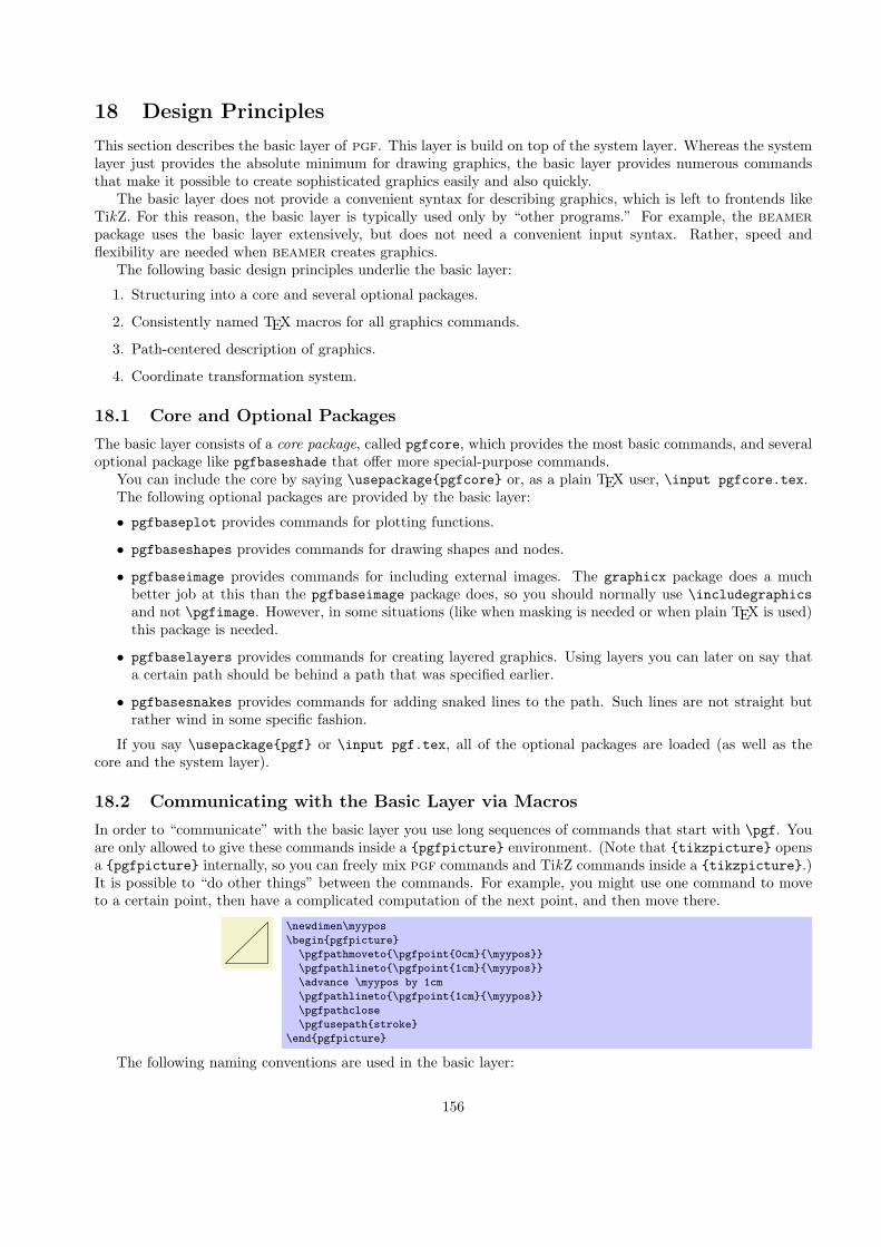
18 Design Principles

This section describes the basic layer of pgf. This layer is build on top of the system layer. Whereas the systemlayer just provides the absolute minimum for drawing graphics, the basic layer provides numerous commandsthat make it possible to create sophisticated graphics easily and also quickly.

The basic layer does not provide a convenient syntax for describing graphics, which is left to frontends likeTikZ. For this reason, the basic layer is typically used only by “other programs.” For example, the beamerpackage uses the basic layer extensively, but does not need a convenient input syntax. Rather, speed andflexibility are needed when beamer creates graphics.

The following basic design principles underlie the basic layer:

1. Structuring into a core and several optional packages.

2. Consistently named TEX macros for all graphics commands.

3. Path-centered description of graphics.

4. Coordinate transformation system.

18.1 Core and Optional Packages

The basic layer consists of a core package, called pgfcore, which provides the most basic commands, and severaloptional package like pgfbaseshade that offer more special-purpose commands.

You can include the core by saying \usepackage{pgfcore} or, as a plain TEX user, \input pgfcore.tex.The following optional packages are provided by the basic layer:

• pgfbaseplot provides commands for plotting functions.

• pgfbaseshapes provides commands for drawing shapes and nodes.

• pgfbaseimage provides commands for including external images. The graphicx package does a muchbetter job at this than the pgfbaseimage package does, so you should normally use \includegraphicsand not \pgfimage. However, in some situations (like when masking is needed or when plain TEX is used)this package is needed.

• pgfbaselayers provides commands for creating layered graphics. Using layers you can later on say thata certain path should be behind a path that was specified earlier.

• pgfbasesnakes provides commands for adding snaked lines to the path. Such lines are not straight butrather wind in some specific fashion.

If you say \usepackage{pgf} or \input pgf.tex, all of the optional packages are loaded (as well as thecore and the system layer).

18.2 Communicating with the Basic Layer via Macros

In order to “communicate” with the basic layer you use long sequences of commands that start with \pgf. Youare only allowed to give these commands inside a {pgfpicture} environment. (Note that {tikzpicture} opensa {pgfpicture} internally, so you can freely mix pgf commands and TikZ commands inside a {tikzpicture}.)It is possible to “do other things” between the commands. For example, you might use one command to moveto a certain point, then have a complicated computation of the next point, and then move there.

.

\newdimen\myypos

\begin{pgfpicture}

\pgfpathmoveto{\pgfpoint{0cm}{\myypos}}

\pgfpathlineto{\pgfpoint{1cm}{\myypos}}

\advance \myypos by 1cm

\pgfpathlineto{\pgfpoint{1cm}{\myypos}}

\pgfpathclose

\pgfusepath{stroke}

\end{pgfpicture}

The following naming conventions are used in the basic layer:

156

1. All commands and environments start with pgf.

2. All commands that specify a point (a coordinate) start with \pgfpoint.

3. All commands that extend the current path start with \pgfpath.

4. All commands that set/change a graphics parameter start with \pgfset.

5. All commands that use a previously declared object (like a path, image or shading) start with \pgfuse.

6. All commands having to do with coordinate transformations start with \pgftransform.

7. All commands having to do with arrow tips start with \pgfarrows.

8. All commands for “quickly” extending or drawing a path start with \pgfpathq or \pgfusepathq.

18.3 Path-Centered Approach

In pgf the most important entity is the path. All graphics are composed of numerous paths that can be stroked,filled, shaded, or clipped against. Paths can be closed or open, they can self-intersect and consist of unconnectedparts.

Paths are first constructed and then used. In order to construct a path, you can use commands starting with\pgfpath. Each time such a command is called, the current path is extended in some way.

Once a path has been completely constructed, you can use it using the command \pgfusepath. Dependingon the parameters given to this command, the path will be stroked (drawn) or filled or subsequent drawings willbe clipped against this path.

18.4 Coordinate Versus Canvas Transformations

pgf provides two transformation systems: pgf’s own coordinate transformation matrix and pdf’s or PostScript’scanvas transformation matrix. These two systems are quite different. Whereas a scaling by a factor of, say, 2 ofthe canvas causes everything to be scaled by this factor (including the thickness of lines and text), a scaling oftwo in the coordinate system causes only the coordinates to be scaled, but not the line width nor text.

By default, all transformations only apply to the coordinate transformation system. However, using thecommand \pgflowlevel it is possible to apply a transformation to the canvas.

Coordinate transformations are often preferable over canvas transformations. Text and lines that are trans-formed using canvas transformations suffer from differing sizes and lines whose thickness differs depending onwhether the line is horizontal or vertical. To appreciate the difference, consider the following two “circles” bothof which have been scaled in the x-direction by a factor of 3 and by a factor of 0.5 in the y-direction. The leftcircle uses a canvas transformation, the right uses pgf’s coordinate transformation (some viewers will renderthe left graphic incorrectly since they do no apply the low-level transformation the way they should):

.

.

canvas

.

coordinate

157

19 Hierarchical Structures:Package, Environments, Scopes, and Text

19.1 Overview

pgf uses two kinds of hierarchical structuring: First, the package itself is structured hierarchically, consistingof different packages that are built on top of each other. Second, pgf allows you to structure your graphicshierarchically using environments and scopes.

19.1.1 The Hierarchical Structure of the Package

The pgf system consists of several layers:

System layer. The lowest layer is called the system layer, though it might also be called “driver layer” or per-haps “backend layer.” Its job is to provide an abstraction of the details of which driver is used to transformthe .dvi file. The system layer is implemented by the package pgfsys, which will load appropriate driverfiles as needed.

The system layer is documented in Part V.

Basic layer. The basic layer is loaded by the package pgf. Some applications do not need all of the functionalityof the basic layer, so it is possible to load only the pgfcore and some other packages starting with pgfbase.

The basic layer is documented in the present part.

Frontend layer. The frontend layer is not loaded by a single packages. Rather, different packages, like TikZor pgfpict2e, are different frontends to the basic layer.

The TikZ frontend is documented in Part II.

Each layer will automatically load the necessary files of the layers below it.In addition to the packages of these layers, there are also some library packages. These packages provide

additional definitions of things like new arrow tips or new plot handlers.The library packages are documented in Part III.

19.1.2 The Hierarchical Structure of Graphics

Graphics in pgf are typically structured hierarchically. Hierarchical structuring can be used to identify groupsof graphical elements that are to be treated “in the same way.” For example, you might group together a numberof paths, all of which are to be drawn in red. Then, when you decide later on that you like them to be drawnin, say, blue, all you have to do is to change the color once.

The general mechanism underlying hierarchical structuring is known as scoping in computer science. Theidea is that all changes to the general “state” of the graphic that are done inside a scope are local to that scope.So, if you change the color inside a scope, this does not affect the color used outside the scope. Likewise, whenyou change the line width in a scope, the line width outside is not changed, and so on.

There are different ways of starting and ending scopes of graphic parameters. Unfortunately, these scopesare sometimes “in conflict” with each other and it is sometimes not immediately clear which scopes apply. Inessence, the following scoping mechanisms are available:

1. The “outermost” scope supported by pgf is the {pgfpicture} environment. All changes to the graphicstate done inside a {pgfpicture} are local to that picture.

In general, it is not possible to set graphic parameters globally outside any {pgfpicture} environments.Thus, you can not say \pgfsetlinewidth{1pt} at the beginning of your document to have a default linewidth of one point. Rather, you have to (re)set all graphic parameters inside each {pgfpicture}. (If thisis too bothersome, try defining some macro that does the job for you.)

158

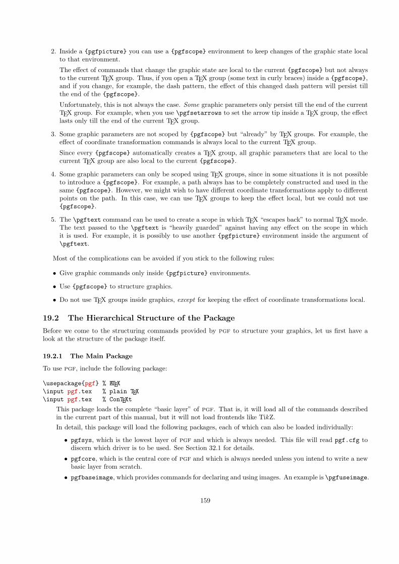
2. Inside a {pgfpicture} you can use a {pgfscope} environment to keep changes of the graphic state localto that environment.

The effect of commands that change the graphic state are local to the current {pgfscope} but not alwaysto the current TEX group. Thus, if you open a TEX group (some text in curly braces) inside a {pgfscope},and if you change, for example, the dash pattern, the effect of this changed dash pattern will persist tillthe end of the {pgfscope}.

Unfortunately, this is not always the case. Some graphic parameters only persist till the end of the currentTEX group. For example, when you use \pgfsetarrows to set the arrow tip inside a TEX group, the effectlasts only till the end of the current TEX group.

3. Some graphic parameters are not scoped by {pgfscope} but “already” by TEX groups. For example, theeffect of coordinate transformation commands is always local to the current TEX group.

Since every {pgfscope} automatically creates a TEX group, all graphic parameters that are local to thecurrent TEX group are also local to the current {pgfscope}.

4. Some graphic parameters can only be scoped using TEX groups, since in some situations it is not possibleto introduce a {pgfscope}. For example, a path always has to be completely constructed and used in thesame {pgfscope}. However, we might wish to have different coordinate transformations apply to differentpoints on the path. In this case, we can use TEX groups to keep the effect local, but we could not use{pgfscope}.

5. The \pgftext command can be used to create a scope in which TEX “escapes back” to normal TEX mode.The text passed to the \pgftext is “heavily guarded” against having any effect on the scope in whichit is used. For example, it is possibly to use another {pgfpicture} environment inside the argument of\pgftext.

Most of the complications can be avoided if you stick to the following rules:

• Give graphic commands only inside {pgfpicture} environments.

• Use {pgfscope} to structure graphics.

• Do not use TEX groups inside graphics, except for keeping the effect of coordinate transformations local.

19.2 The Hierarchical Structure of the Package

Before we come to the structuring commands provided by pgf to structure your graphics, let us first have alook at the structure of the package itself.

19.2.1 The Main Package

To use pgf, include the following package:

\usepackage{pgf} % LATEX\input pgf.tex % plain TEX\input pgf.tex % ConTEXt

This package loads the complete “basic layer” of pgf. That is, it will load all of the commands describedin the current part of this manual, but it will not load frontends like TikZ.In detail, this package will load the following packages, each of which can also be loaded individually:

• pgfsys, which is the lowest layer of pgf and which is always needed. This file will read pgf.cfg todiscern which driver is to be used. See Section 32.1 for details.

• pgfcore, which is the central core of pgf and which is always needed unless you intend to write a newbasic layer from scratch.

• pgfbaseimage, which provides commands for declaring and using images. An example is \pgfuseimage.

159

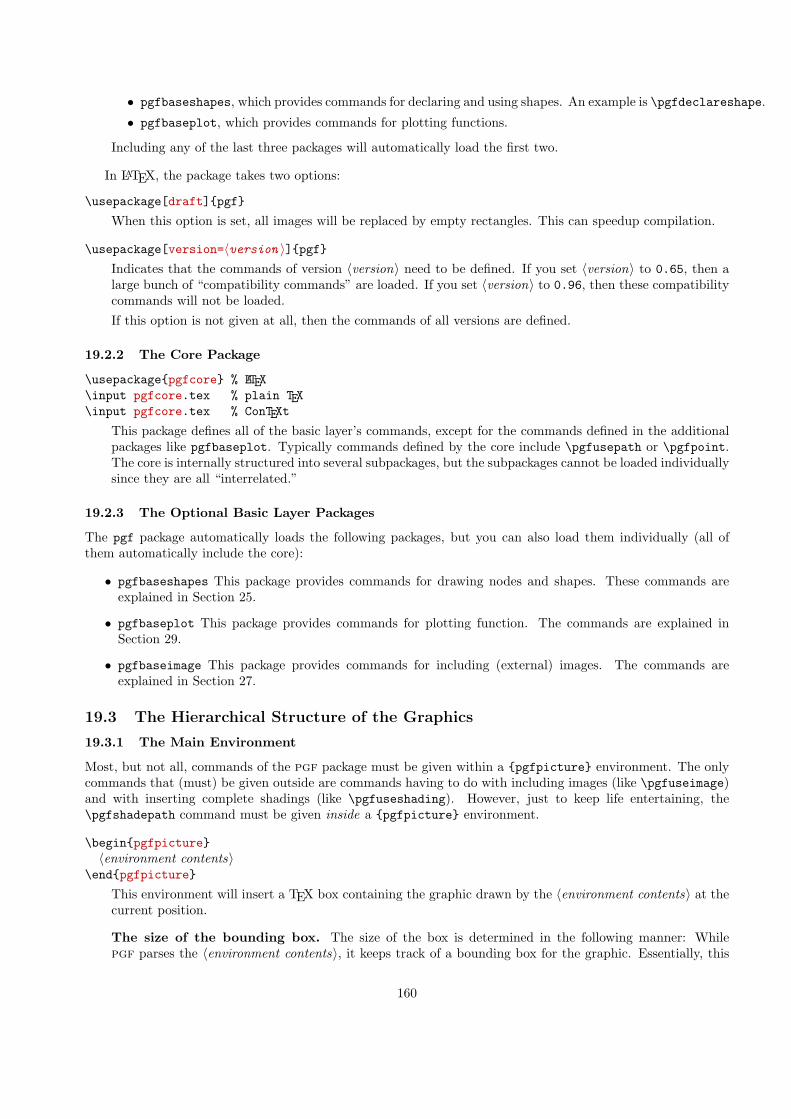
• pgfbaseshapes, which provides commands for declaring and using shapes. An example is \pgfdeclareshape.

• pgfbaseplot, which provides commands for plotting functions.

Including any of the last three packages will automatically load the first two.

In LATEX, the package takes two options:

\usepackage[draft]{pgf}

When this option is set, all images will be replaced by empty rectangles. This can speedup compilation.

\usepackage[version=⟨version ⟩]{pgf}Indicates that the commands of version ⟨version⟩ need to be defined. If you set ⟨version⟩ to 0.65, then alarge bunch of “compatibility commands” are loaded. If you set ⟨version⟩ to 0.96, then these compatibilitycommands will not be loaded.If this option is not given at all, then the commands of all versions are defined.

19.2.2 The Core Package

\usepackage{pgfcore} % LATEX\input pgfcore.tex % plain TEX\input pgfcore.tex % ConTEXt

This package defines all of the basic layer’s commands, except for the commands defined in the additionalpackages like pgfbaseplot. Typically commands defined by the core include \pgfusepath or \pgfpoint.The core is internally structured into several subpackages, but the subpackages cannot be loaded individuallysince they are all “interrelated.”

19.2.3 The Optional Basic Layer Packages

The pgf package automatically loads the following packages, but you can also load them individually (all ofthem automatically include the core):

• pgfbaseshapes This package provides commands for drawing nodes and shapes. These commands areexplained in Section 25.

• pgfbaseplot This package provides commands for plotting function. The commands are explained inSection 29.

• pgfbaseimage This package provides commands for including (external) images. The commands areexplained in Section 27.

19.3 The Hierarchical Structure of the Graphics

19.3.1 The Main Environment

Most, but not all, commands of the pgf package must be given within a {pgfpicture} environment. The onlycommands that (must) be given outside are commands having to do with including images (like \pgfuseimage)and with inserting complete shadings (like \pgfuseshading). However, just to keep life entertaining, the\pgfshadepath command must be given inside a {pgfpicture} environment.

\begin{pgfpicture}⟨environment contents⟩

\end{pgfpicture}

This environment will insert a TEX box containing the graphic drawn by the ⟨environment contents⟩ at thecurrent position.

The size of the bounding box. The size of the box is determined in the following manner: Whilepgf parses the ⟨environment contents⟩, it keeps track of a bounding box for the graphic. Essentially, this

160

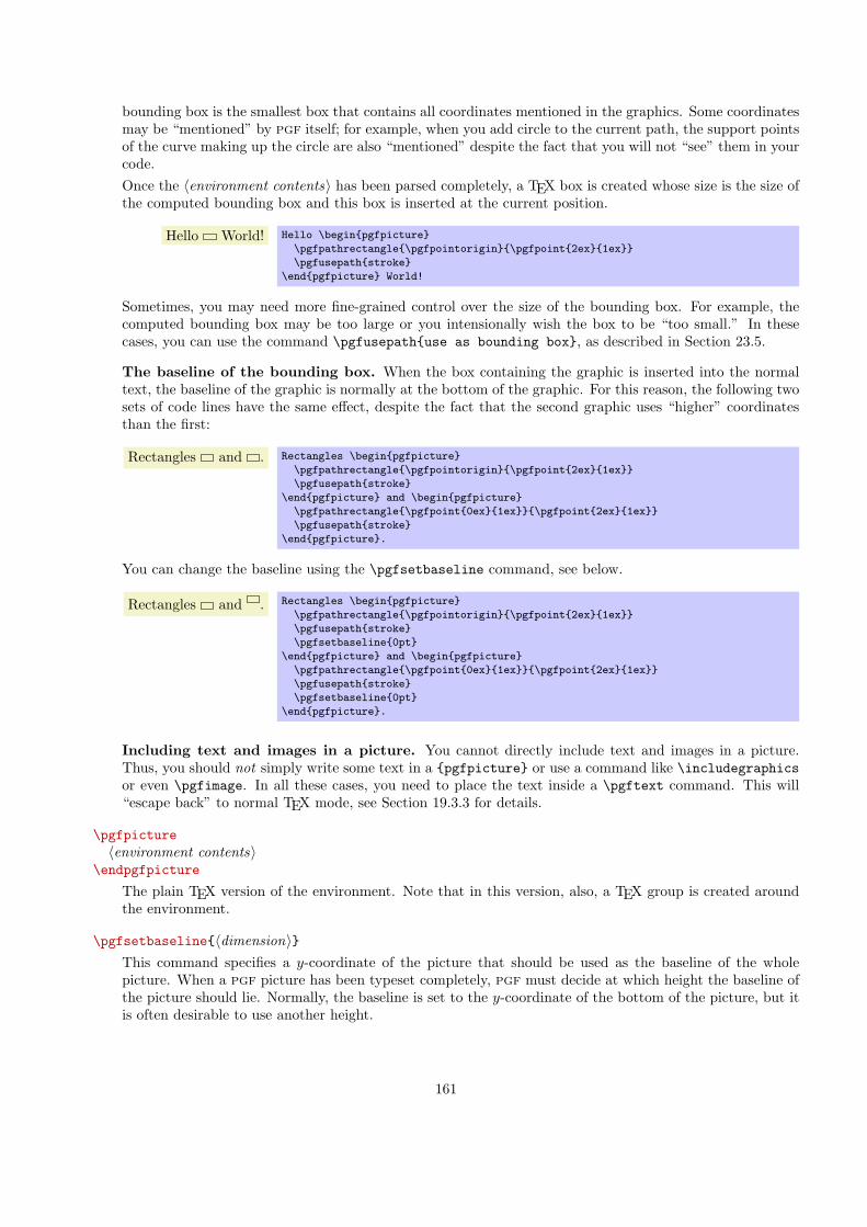
bounding box is the smallest box that contains all coordinates mentioned in the graphics. Some coordinatesmay be “mentioned” by pgf itself; for example, when you add circle to the current path, the support pointsof the curve making up the circle are also “mentioned” despite the fact that you will not “see” them in yourcode.Once the ⟨environment contents⟩ has been parsed completely, a TEX box is created whose size is the size ofthe computed bounding box and this box is inserted at the current position.

Hello

.

World! Hello \begin{pgfpicture}

\pgfpathrectangle{\pgfpointorigin}{\pgfpoint{2ex}{1ex}}

\pgfusepath{stroke}

\end{pgfpicture} World!

Sometimes, you may need more fine-grained control over the size of the bounding box. For example, thecomputed bounding box may be too large or you intensionally wish the box to be “too small.” In thesecases, you can use the command \pgfusepath{use as bounding box}, as described in Section 23.5.

The baseline of the bounding box. When the box containing the graphic is inserted into the normaltext, the baseline of the graphic is normally at the bottom of the graphic. For this reason, the following twosets of code lines have the same effect, despite the fact that the second graphic uses “higher” coordinatesthan the first:

Rectangles

.

and

.

. Rectangles \begin{pgfpicture}


\pgfusepath{stroke}

\end{pgfpicture} and \begin{pgfpicture}

\pgfpathrectangle{\pgfpoint{0ex}{1ex}}{\pgfpoint{2ex}{1ex}}

\pgfusepath{stroke}

\end{pgfpicture}.

You can change the baseline using the \pgfsetbaseline command, see below.

Rectangles

.

and

.

. Rectangles \begin{pgfpicture}


\pgfusepath{stroke}

\pgfsetbaseline{0pt}

\end{pgfpicture} and \begin{pgfpicture}


\pgfusepath{stroke}

\pgfsetbaseline{0pt}

\end{pgfpicture}.

Including text and images in a picture. You cannot directly include text and images in a picture.Thus, you should not simply write some text in a {pgfpicture} or use a command like \includegraphicsor even \pgfimage. In all these cases, you need to place the text inside a \pgftext command. This will“escape back” to normal TEX mode, see Section 19.3.3 for details.

\pgfpicture⟨environment contents⟩

\endpgfpicture

The plain TEX version of the environment. Note that in this version, also, a TEX group is created aroundthe environment.

\pgfsetbaseline{⟨dimension⟩}This command specifies a y-coordinate of the picture that should be used as the baseline of the wholepicture. When a pgf picture has been typeset completely, pgf must decide at which height the baseline ofthe picture should lie. Normally, the baseline is set to the y-coordinate of the bottom of the picture, but itis often desirable to use another height.

161

Text

.

,

.

,

.

,

.

. Text \tikz{\pgfpathcircle{\pgfpointorigin}{1ex}\pgfusepath{stroke}},

\tikz{\pgfsetbaseline{0pt}

\pgfpathcircle{\pgfpointorigin}{1ex}\pgfusepath{stroke}},

\tikz{\pgfsetbaseline{.5ex}

\pgfpathcircle{\pgfpointorigin}{1ex}\pgfusepath{stroke}},

\tikz{\pgfsetbaseline{-1ex}

\pgfpathcircle{\pgfpointorigin}{1ex}\pgfusepath{stroke}}.

19.3.2 Graphic Scope Environments

Inside a {pgfpicture} environment you can substructure your picture using the following environment:

\begin{pgfscope}⟨environment contents⟩

\end{pgfscope}

All changes to the graphic state done inside this environment are local to the environment. The graphicstate includes the following:

• The line width.

• The stroke and fill colors.

• The dash pattern.

• The line join and cap.

• The miter limit.

• The canvas transformation matrix.

• The clipping path.

Other parameters may also influence how graphics are rendered, but they are not part of the graphic state.For example, the arrow tip kind is not part of the graphic state and the effect of commands setting the arrowtip kind are local to the current TEX group, not to the current {pgfscope}. However, since {pgfscope}starts and ends a TEX group automatically, a {pgfscope} can be used to limit the effect of, say, commandsthat set the arrow tip kind.

.

\begin{pgfpicture}

\begin{pgfscope}

{

\pgfsetlinewidth{2pt}


\pgfusepath{stroke}

}


\pgfusepath{stroke}

\end{pgfscope}


\pgfusepath{stroke}

\end{pgfpicture}

.

\begin{pgfpicture}

\begin{pgfscope}

{

\pgfsetarrows{-to}

\pgfpathmoveto{\pgfpointorigin}\pgfpathlineto{\pgfpoint{2ex}{2ex}}

\pgfusepath{stroke}

}

\pgfpathmoveto{\pgfpoint{3ex}{0ex}}\pgfpathlineto{\pgfpoint{5ex}{2ex}}

\pgfusepath{stroke}

\end{pgfscope}

\pgfpathmoveto{\pgfpoint{6ex}{0ex}}\pgfpathlineto{\pgfpoint{8ex}{2ex}}

\pgfusepath{stroke}

\end{pgfpicture}

162

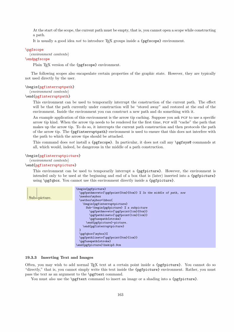
At the start of the scope, the current path must be empty, that is, you cannot open a scope while constructinga path.It is usually a good idea not to introduce TEX groups inside a {pgfscope} environment.

\pgfscope⟨environment contents⟩

\endpgfscope

Plain TEX version of the {pgfscope} environment.

The following scopes also encapsulate certain properties of the graphic state. However, they are typicallynot used directly by the user.

\begin{pgfinterruptpath}⟨environment contents⟩

\end{pgfinterruptpath}

This environment can be used to temporarily interrupt the construction of the current path. The effectwill be that the path currently under construction will be “stored away” and restored at the end of theenvironment. Inside the environment you can construct a new path and do something with it.An example application of this environment is the arrow tip caching. Suppose you ask pgf to use a specificarrow tip kind. When the arrow tip needs to be rendered for the first time, pgf will “cache” the path thatmakes up the arrow tip. To do so, it interrupts the current path construction and then protocols the pathof the arrow tip. The {pgfinterruptpath} environment is used to ensure that this does not interfere withthe path to which the arrow tips should be attached.This command does not install a {pgfscope}. In particular, it does not call any \pgfsys@ commands atall, which would, indeed, be dangerous in the middle of a path construction.

\begin{pgfinterruptpicture}⟨environment contents⟩

\end{pgfinterruptpicture}

This environment can be used to temporarily interrupt a {pgfpicture}. However, the environment isintended only to be used at the beginning and end of a box that is (later) inserted into a {pgfpicture}using \pgfqbox. You cannot use this environment directly inside a {pgfpicture}.

.

.

Sub-

.

-picture.

\begin{pgfpicture}

\pgfpathmoveto{\pgfpoint{0cm}{0cm}} % In the middle of path, now

\newbox\mybox

\setbox\mybox=\hbox{

\begin{pgfinterruptpicture}

Sub-\begin{pgfpicture} % a subpicture

\pgfpathmoveto{\pgfpoint{1cm}{0cm}}

\pgfpathlineto{\pgfpoint{1cm}{1cm}}

\pgfusepath{stroke}

\end{pgfpicture}-picture.

\end{pgfinterruptpicture}

}

\pgfqbox{\mybox}%


\pgfusepath{stroke}

\end{pgfpicture}\hskip3.9cm

19.3.3 Inserting Text and Images

Often, you may wish to add normal TEX text at a certain point inside a {pgfpicture}. You cannot do so“directly,” that is, you cannot simply write this text inside the {pgfpicture} environment. Rather, you mustpass the text as an argument to the \pgftext command.

You must also use the \pgftext command to insert an image or a shading into a {pgfpicture}.

163

\pgftext[⟨options⟩]{⟨text⟩}This command will typeset ⟨text⟩ in normal TEX mode and insert the resulting box into the {pgfpicture}.The bounding box of the graphic will be updated so that all of the text box is inside. Be default, the textbox is centered at the origin, but this can be changed either by giving appropriate ⟨options⟩ or by applyingan appropriate coordinate transformation beforehand.The ⟨text⟩ may contain verbatim text. (In other words, the ⟨text⟩ “argument” is not a normal argument,but is put in a box and some \aftergroup hackery is used to find the end of the box.)pgf’s current (high-level) coordinate transformation is synchronized with the canvas transformation matrixtemporarily when the text box is inserted. The effect is that if there is currently a high-level rotation of,say, 30 degrees, the ⟨text⟩ will also be rotated by thirty degrees. If you do not want this effect, you have to(possibly temporarily) reset the high-level transformation matrix.The following ⟨options⟩ may be given as conveniences:

• left causes the text box to be placed such that its left border is on the origin.

.

.

lovely\tikz{\draw[help lines] (-1,-.5) grid (1,.5);

\pgftext[left] {lovely}}

• right causes the text box to be placed such that its right border is on the origin.

.

.


\pgftext[right] {lovely}}

• top causes the text box to be placed such that its top is on the origin. This option can be used togetherwith the left or right option.

.

.

lovely

\tikz{\draw[help lines] (-1,-.5) grid (1,.5);

\pgftext[top] {lovely}}

.

.

lovely


\pgftext[top,right] {lovely}}

• bottom causes the text box to be placed such that its bottom is on the origin.

.

.


\pgftext[bottom] {lovely}}

.

.


\pgftext[bottom,right] {lovely}}

• base causes the text box to be placed such that its baseline is on the origin.

.

.


\pgftext[base] {lovely}}

.

.


\pgftext[base,right] {lovely}}

164

• at=⟨point⟩ Translates the origin (that is, the point where the text is shown) to ⟨point⟩.

.

.


\pgftext[base,at={\pgfpoint{1cm}{0cm}}] {lovely}}

• x=⟨dimension⟩ Translates the origin by ⟨dimension⟩ along the x-axis.

.

.

lovely


\pgftext[base,x=1cm,y=-0.5cm] {lovely}}

• y=⟨dimension⟩ works like the x option.

• rotate=⟨degree⟩ Rotates the coordinate system by ⟨degree⟩. This will also rotate the text box.

.

.

lovely


\pgftext[base,x=1cm,y=-0.5cm,rotate=30] {lovely}}

165

20 Specifying Coordinates

20.1 Overview

Most pgf commands expect you to provide the coordinates of a point (also called coordinate) inside your picture.Points are always “local” to your picture, that is, they never refer to an absolute position on the page, but toa position inside the current {pgfpicture} environment. To specify a coordinate you can use commands thatstart with \pgfpoint.

20.2 Basic Coordinate Commands

The following commands are the most basic for specifying a coordinate.

\pgfpoint{⟨x coordinate⟩}{⟨y coordinate⟩}Yields a point location. The coordinates are given as TEX dimensions.

.

\begin{tikzpicture}


\pgfpathcircle{\pgfpoint{1cm}{1cm}} {2pt}

\pgfpathcircle{\pgfpoint{2cm}{5pt}} {2pt}

\pgfpathcircle{\pgfpoint{0pt}{.5in}}{2pt}

\pgfusepath{fill}

\end{tikzpicture}

\pgfpointorigin

Yields the origin. Same as \pgfpoint{0pt}{0pt}.

\pgfpointpolar{⟨degree⟩}{⟨radius⟩}Yields a point location given in polar coordinates. You can specify the angle only in degrees, radians arenot supported, currently.

.

\begin{tikzpicture}


\foreach \angle in {0,10,...,90}

{\pgfpathcircle{\pgfpointpolar{\angle}{1cm}}{2pt}}

\pgfusepath{fill}

\end{tikzpicture}

20.3 Coordinates in the Xy- and Xyz-Coordinate Systems

Coordinates can also be specified as multiples of an x-vector and a y-vector. Normally, the x-vector points onecentimeter in the x-direction and the y-vector points one centimeter in the y-direction, but using the commands\pgfsetxvec and \pgfsetyvec they can be changed. Note that the x- and y-vector do not necessarily point“horizontally” and “vertically.”

It is also possible to specify a point as a multiple of three vectors, the x-, y-, and z-vector. This is useful forcreating simple three dimensional graphics.

\pgfpointxy{⟨sx⟩}{⟨sy⟩}Yields a point that is situated at sx times the x-vector plus sy times the y-vector.

.

\begin{tikzpicture}


\pgfpathmoveto{\pgfpointxy{1}{0}}

\pgfpathlineto{\pgfpointxy{2}{2}}

\pgfusepath{stroke}

\end{tikzpicture}

166

\pgfpointxyz{⟨sx⟩}{⟨sy⟩}{⟨sz⟩}Yields a point that is situated at sx times the x-vector plus sy times the y-vector plus sz times the z-vector.

.

\begin{pgfpicture}

\pgfsetarrowsend{to}

\pgfpathmoveto{\pgfpointorigin}

\pgfpathlineto{\pgfpointxyz{0}{0}{1}}

\pgfusepath{stroke}



\pgfusepath{stroke}



\pgfusepath{stroke}

\end{pgfpicture}

\pgfsetxvec{⟨point⟩}Sets that current x-vector for usage in the xyz-coordinate system.

Example:

.

\begin{tikzpicture}




\pgfusepath{stroke}

\color{red}

\pgfsetxvec{\pgfpoint{0.75cm}{0cm}}



\pgfusepath{stroke}

\end{tikzpicture}

\pgfsetyvec{⟨point⟩}Works like \pgfsetyvec.

\pgfsetzvec{⟨point⟩}Works like \pgfsetzvec.

20.4 Building Coordinates From Other Coordinates

Many commands allow you to construct a coordinate in terms of other coordinates.

20.4.1 Basic Manipulations of Coordinates

\pgfpointadd{⟨v1⟩}{⟨v2⟩}Returns the sum vector ⟨v1⟩ + ⟨v2⟩.

.

\begin{tikzpicture}


\pgfpathcircle{\pgfpointadd{\pgfpoint{1cm}{0cm}}{\pgfpoint{1cm}{1cm}}}{2pt}

\pgfusepath{fill}

\end{tikzpicture}

167

\pgfpointscale{⟨factor⟩}{⟨coordinate⟩}Returns the vector ⟨factor⟩⟨coordinate⟩.

.

\begin{tikzpicture}


\pgfpathcircle{\pgfpointscale{1.5}{\pgfpoint{1cm}{0cm}}}{2pt}

\pgfusepath{fill}

\end{tikzpicture}

\pgfpointdiff{⟨start⟩}{⟨end⟩}Returns the difference vector ⟨end⟩ − ⟨start⟩.

.

\begin{tikzpicture}


\pgfpathcircle{\pgfpointdiff{\pgfpoint{1cm}{0cm}}{\pgfpoint{1cm}{1cm}}}{2pt}

\pgfusepath{fill}

\end{tikzpicture}

\pgfpointnormalised{⟨point⟩}This command returns a normalized version of ⟨point⟩, that is, a vector of length 1pt pointing in thedirection of ⟨point⟩. If ⟨point⟩ is the 0-vector or extremely short, a vector of length 1pt pointing upwards isreturned.This command is not implemented by calculating the length of the vector, but rather by calculating theangle of the vector and then using (something equivalent to) the \pgfpointpolar command. This ensuresthat the point will really have length 1pt, but it is not guaranteed that the vector will precisely point inthe direction of ⟨point⟩ due to the fact that the polar tables are accurate only up to one degree. Normally,this is not a problem.

.

\begin{tikzpicture}


\pgfpathcircle{\pgfpoint{2cm}{1cm}}{2pt}

\pgfpathcircle{\pgfpointscale{20}

{\pgfpointnormalised{\pgfpoint{2cm}{1cm}}}}{2pt}

\pgfusepath{fill}

\end{tikzpicture}

20.4.2 Points Traveling along Lines and Curves

The commands in this section allow you to specify points on a line or a curve. Imaging a point “traveling” alonga curve from some point p to another point q. At time t = 0 the point is at p and at time t = 1 it is at q andat time, say, t = 1/2 it is “somewhere in the middle.” The exact location at time t = 1/2 will not necessarilybe the “halfway point,” that is, the point whose distance on the curve from p and q is equal. Rather, the exactlocation will depend on the “speed” at which the point is traveling, which in turn depends on the lengths of thesupport vectors in a complicated manner. If you are interested in the details, please see a good book on Beziercurves.

\pgfpointlineattime{⟨time t⟩}{⟨point p⟩}{⟨point q⟩}Yields a point that is the tth fraction between p and q, that is, p + t(q − p). For t = 1/2 this is the middleof p and q.

168

.

.

0

.

0.25

.

0.5

.

0.75

.

1

.

1.25 \begin{tikzpicture}




\pgfusepath{stroke}

\foreach \t in {0,0.25,...,1.25}

{\pgftext[at=

\pgfpointlineattime{\t}{\pgfpointorigin}{\pgfpoint{2cm}{2cm}}]{\t}}

\end{tikzpicture}

\pgfpointlineatdistance{⟨distance⟩}{⟨start point⟩}{⟨end point⟩}Yields a point that is located ⟨distance⟩ many units removed from the start point in the direction of the endpoint. In other words, this is the point that results if we travel ⟨distance⟩ steps from ⟨start point⟩ towards⟨end point⟩.

Example:

.

.

0pt

.

20pt

.

40pt

.

70pt\begin{tikzpicture}




\pgfusepath{stroke}

\foreach \d in {0pt,20pt,40pt,70pt}

{\pgftext[at=

\pgfpointlineatdistance{\d}{\pgfpointorigin}{\pgfpoint{3cm}{2cm}}]{\d}}

\end{tikzpicture}

\pgfpointcurveattime{⟨time t⟩}{⟨point p⟩}{⟨point s1⟩}{⟨point s2⟩}{⟨point q⟩}Yields a point that is on the Bezier curve from p to q with the support points s1 and s2. The time t is usedto determine the location, where t = 0 yields p and t = 1 yields q.

.

.

0

.

0.25

.

0.5

.

0.75

.

1 \begin{tikzpicture}



\pgfpathcurveto

{\pgfpoint{0cm}{2cm}}{\pgfpoint{0cm}{2cm}}{\pgfpoint{3cm}{2cm}}

\pgfusepath{stroke}

\foreach \t in {0,0.25,0.5,0.75,1}

{\pgftext[at=\pgfpointcurveattime{\t}{\pgfpointorigin}

{\pgfpoint{0cm}{2cm}}


{\pgfpoint{3cm}{2cm}}]{\t}}

\end{tikzpicture}

20.4.3 Points on Borders of Objects

The following commands are useful for specifying a point that lies on the border of special shapes. They areused, for example, by the shape mechanism to determine border points of shapes.

\pgfpointborderrectangle{⟨direction point⟩}{⟨corner⟩}This command returns a point that lies on the intersection of a line starting at the origin and going towardsthe point ⟨direction point⟩ and a rectangle whose center is in the origin and whose upper right corner is at⟨corner⟩.The ⟨direction point⟩ should have length “about 1pt,” but it will be normalized automatically. Nevertheless,the “nearer” the length is to 1pt, the less rounding errors.

169

.

\begin{tikzpicture}

\draw[help lines] (0,0) grid (2,1.5);

\pgfpathrectanglecorners{\pgfpoint{-1cm}{-1.25cm}}{\pgfpoint{1cm}{1.25cm}}

\pgfusepath{stroke}

\pgfpathcircle{\pgfpoint{5pt}{5pt}}{2pt}

\pgfpathcircle{\pgfpoint{-10pt}{5pt}}{2pt}

\pgfusepath{fill}

\color{red}

\pgfpathcircle{\pgfpointborderrectangle

{\pgfpoint{5pt}{5pt}}{\pgfpoint{1cm}{1.25cm}}}{2pt}

\pgfpathcircle{\pgfpointborderrectangle

{\pgfpoint{-10pt}{5pt}}{\pgfpoint{1cm}{1.25cm}}}{2pt}

\pgfusepath{fill}

\end{tikzpicture}

\pgfpointborderellipse{⟨direction point⟩}{⟨corner⟩}This command works like the corresponding command for rectangles, only this time the ⟨corner⟩ is thecorner of the bounding rectangle of an ellipse.

.

\begin{tikzpicture}

\draw[help lines] (0,0) grid (2,1.5);

\pgfpathellipse{\pgfpointorigin}{\pgfpoint{1cm}{0cm}}{\pgfpoint{0cm}{1.25cm}}

\pgfusepath{stroke}

\pgfpathcircle{\pgfpoint{5pt}{5pt}}{2pt}

\pgfpathcircle{\pgfpoint{-10pt}{5pt}}{2pt}

\pgfusepath{fill}

\color{red}

\pgfpathcircle{\pgfpointborderellipse

{\pgfpoint{5pt}{5pt}}{\pgfpoint{1cm}{1.25cm}}}{2pt}

\pgfpathcircle{\pgfpointborderellipse

{\pgfpoint{-10pt}{5pt}}{\pgfpoint{1cm}{1.25cm}}}{2pt}

\pgfusepath{fill}

\end{tikzpicture}

20.4.4 Points on the Intersection of Lines

\pgfpointintersectionoflines{⟨p⟩}{⟨q⟩}{⟨s⟩}{⟨t⟩}This command returns the intersection of a line going through p and q and a line going through s and t. Ifthe lines do not intersection, an arithmetic overflow will occur.

.

\begin{tikzpicture}


\draw (.5,0) -- (2,2);

\draw (1,2) -- (2,0);

\pgfpathcircle{%

\pgfpointintersectionoflines

{\pgfpointxy{.5}{0}}{\pgfpointxy{2}{2}}

{\pgfpointxy{1}{2}}{\pgfpointxy{2}{0}}}

{2pt}

\pgfusepath{stroke}

\end{tikzpicture}

20.5 Extracting Coordinates

There are two commands that can be used to “extract” the x- or y-coordinate of a coordinate.

\pgfextractx{⟨dimension⟩}{⟨point⟩}Sets the TEX-⟨dimension⟩ to the x-coordinate of the point.

170

\newdimen\mydim

\pgfextractx{\mydim}{\pgfpoint{2cm}{4pt}}

%% \mydim is now 2cm

\pgfextracty{⟨dimension⟩}{⟨point⟩}Like \pgfextractx, except for the y-coordinate.

20.6 Internals of How Point Commands Work

As a normal user of pgf you do not need to read this section. It is relevant only if you need to understand howthe point commands work internally.

When a command like \pgfpoint{1cm}{2pt} is called, all that happens is that the two TEX-dimensionvariables \pgf@x and \pgf@y are set to 1cm and 2pt, respectively. A command like \pgfpathmoveto that takesa coordinate as parameter will just execute this parameter and then use the values of \pgf@x and \pgf@y as thecoordinates to which it will move the pen on the current path.

since commands like \pgfpointnormalised modify other variables besides \pgf@x and \pgf@y during thecomputation of the final values of \pgf@x and \pgf@y, it is a good idea to enclose a call of a command like\pgfpoint in a TEX-scope and then make the changes of \pgf@x and \pgf@y global as in the following example:

...

{ % open scope

\pgfpointnormalised{\pgfpoint{1cm}{1cm}}

\global\pgf@x=\pgf@x % make the change of \pgf@x persist past the scope

\global\pgf@y=\pgf@y % make the change of \pgf@y persist past the scope

}

% \pgf@x and \pgf@y are now set correctly, all other variables are

% unchanged

Since this situation arises very often, the macro \pgf@process can be used to perform the above code:

\pgf@process{⟨code⟩}Executes the ⟨code⟩ in a scope and then makes \pgf@x and \pgf@y global.

Note that this macro is used often internally. For this reason, it is not a good idea to keep anything importantin the variables \pgf@x and \pgf@y since they will be overwritten and changed frequently. Instead, intermediatevalues can ge stored in the TEX-dimensions \pgf@xa, \pgf@xb, \pgf@xc and their y-counterparts \pgf@ya,\pgf@yb, pgf@yc. For example, here is the code of the command \pgfpointadd:

\def\pgfpointadd#1#2{%

\pgf@process{#1}%

\pgf@xa=\pgf@x%

\pgf@ya=\pgf@y%

\pgf@process{#2}%

\advance\pgf@x by\pgf@xa%

\advance\pgf@y by\pgf@ya}

171

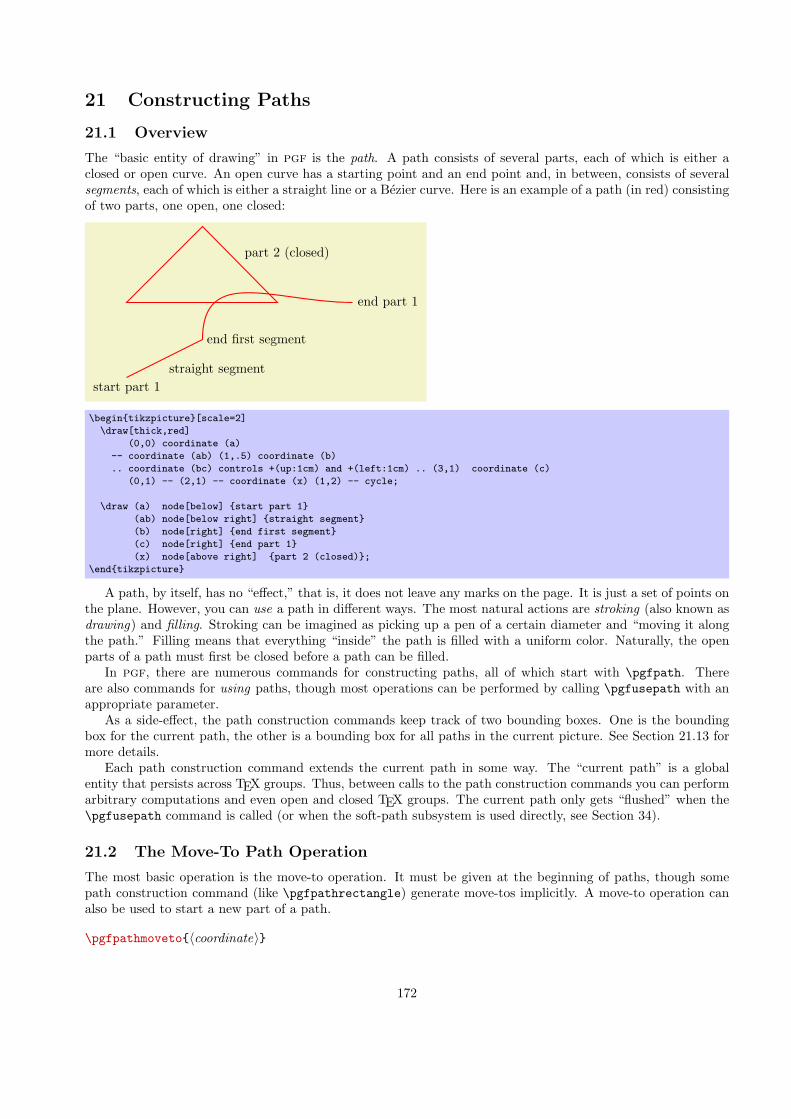
21 Constructing Paths

21.1 Overview

The “basic entity of drawing” in pgf is the path. A path consists of several parts, each of which is either aclosed or open curve. An open curve has a starting point and an end point and, in between, consists of severalsegments, each of which is either a straight line or a Bezier curve. Here is an example of a path (in red) consistingof two parts, one open, one closed:

.

.

start part 1

.

straight segment

.

end first segment

.

end part 1

.

part 2 (closed)


\draw[thick,red]

(0,0) coordinate (a)

-- coordinate (ab) (1,.5) coordinate (b)

.. coordinate (bc) controls +(up:1cm) and +(left:1cm) .. (3,1) coordinate (c)

(0,1) -- (2,1) -- coordinate (x) (1,2) -- cycle;

\draw (a) node[below] {start part 1}

(ab) node[below right] {straight segment}

(b) node[right] {end first segment}

(c) node[right] {end part 1}

(x) node[above right] {part 2 (closed)};

\end{tikzpicture}

A path, by itself, has no “effect,” that is, it does not leave any marks on the page. It is just a set of points onthe plane. However, you can use a path in different ways. The most natural actions are stroking (also known asdrawing) and filling. Stroking can be imagined as picking up a pen of a certain diameter and “moving it alongthe path.” Filling means that everything “inside” the path is filled with a uniform color. Naturally, the openparts of a path must first be closed before a path can be filled.

In pgf, there are numerous commands for constructing paths, all of which start with \pgfpath. Thereare also commands for using paths, though most operations can be performed by calling \pgfusepath with anappropriate parameter.

As a side-effect, the path construction commands keep track of two bounding boxes. One is the boundingbox for the current path, the other is a bounding box for all paths in the current picture. See Section 21.13 formore details.

Each path construction command extends the current path in some way. The “current path” is a globalentity that persists across TEX groups. Thus, between calls to the path construction commands you can performarbitrary computations and even open and closed TEX groups. The current path only gets “flushed” when the\pgfusepath command is called (or when the soft-path subsystem is used directly, see Section 34).

21.2 The Move-To Path Operation

The most basic operation is the move-to operation. It must be given at the beginning of paths, though somepath construction command (like \pgfpathrectangle) generate move-tos implicitly. A move-to operation canalso be used to start a new part of a path.

\pgfpathmoveto{⟨coordinate⟩}

172

This command expects a pgf-coordinate like \pgfpointorigin as its parameter. When the current pathis empty, this operation will start the path at the given ⟨coordinate⟩. If a path has already been partlyconstructed, this command will end the current part of the path and start a new one.

.

\begin{pgfpicture}




\pgfpathlineto{\pgfpoint{3cm}{0.5cm}}


\pgfsetfillcolor{examplefill}

\pgfusepath{fill,stroke}

\end{pgfpicture}

.

\begin{pgfpicture}




\pgfpathmoveto{\pgfpoint{2cm}{1cm}} % New part





\end{pgfpicture}

The command will apply the current coordinate transformation matrix to ⟨coordinate⟩ before using it.The command will update the bounding box of the current path and picture, if necessary.

21.3 The Line-To Path Operation

\pgfpathlineto{⟨coordinate⟩}This command extends the current path in a straight line to the given ⟨coordinate⟩. If this command isgiven at the beginning of path without any other path construction command given before (in particularwithout a move-to operation), the TEX file may compile without an error message, but a viewer applicationmay display an error message when trying to render the picture.

.

\begin{pgfpicture}






\end{pgfpicture}

The command will apply the current coordinate transformation matrix to ⟨coordinate⟩ before using it.The command will update the bounding box of the current path and picture, if necessary.

21.4 The Curve-To Path Operation

\pgfpathcurveto{⟨support 1 ⟩}{⟨support 2 ⟩}{⟨coordinate⟩}This command extends the current path with a Bezier curve from the last point of the path to ⟨coordinate⟩.The ⟨support 1 ⟩ and ⟨support 2 ⟩ are the first and second support point of the Bezier curve. For moreinformation on Bezier curve, please consult a standard textbook on computer graphics.Like the line-to command, this command may not be the first path construction command in a path.

173

.

\begin{pgfpicture}


\pgfpathcurveto




\end{pgfpicture}

The command will apply the current coordinate transformation matrix to ⟨coordinate⟩ before using it.The command will update the bounding box of the current path and picture, if necessary. However, thebounding box is simply made large enough such that it encompasses all of the support points and the⟨coordinate⟩. This will guarantee that the curve is completely inside the bounding box, but the boundingbox will typically be quite a bit too large. It is not clear (to me) how this can be avoided without resortingto “some serious math” in order to calculate a precise bounding box.

21.5 The Close Path Operation

\pgfpathclose

This command closes the current part of the path by appending a straight line to the start point of thecurrent part. Note that there is a difference between closing a path and using the line-to operation to adda straight line to the start of the current path. The difference is demonstrated by the upper corners of thetriangles in the following example:

.

\begin{tikzpicture}




\pgfpathlineto{\pgfpoint{0cm}{-1cm}}

\pgfpathlineto{\pgfpoint{1cm}{-1cm}}

\pgfpathclose

\pgfpathmoveto{\pgfpoint{2.5cm}{1cm}}

\pgfpathlineto{\pgfpoint{1.5cm}{-1cm}}

\pgfpathlineto{\pgfpoint{2.5cm}{-1cm}}

\pgfpathlineto{\pgfpoint{2.5cm}{1cm}}

\pgfusepath{stroke}

\end{tikzpicture}

21.6 Arc, Ellipse and Circle Path Operations

The path construction commands that we have discussed up to now are sufficient to create all paths that canbe created “at all.” However, it is useful to have special commands to create certain shapes, like circles, thatarise often in practice.

In the following, the commands for adding (parts of) (transformed) circles to a path are described.

\pgfpatharc{⟨start angle⟩}{⟨end angle⟩}{⟨radius⟩}This command appends a part of a circle (or an ellipse) to the current path. Imaging the curve between⟨start angle⟩ and ⟨end angle⟩ on a circle of radius ⟨radius⟩ (if ⟨start angle⟩ < ⟨end angle⟩, the curve goesaround the circle counterclockwise, otherwise clockwise). This curve is now moved such that the pointwhere the curve starts is the previous last point of the path. Note that this command will not start a newpart of the path, which is important for example for filling purposes.

.

\begin{tikzpicture}




\pgfpatharc{180}{90}{.5cm}


\pgfpatharc{90}{-45}{.5cm}

\pgfusepath{fill}

\end{tikzpicture}

174

Saying \pgfpatharc{0}{360}{1cm} “nearly” gives you a full circle. The “nearly” refers to the fact thatthe circle will not be closed. You can close it using \pgfpathclose.The ⟨radius⟩ need not always be a single TEX dimension. Instead, it can also contain a slash, in which caseit must consist of two dimensions separated by this slash. In this case the first dimension is the x-radiusand the second the y-radius of the ellipse from which the curve is taken:

.

\begin{tikzpicture}



\pgfpatharc{180}{45}{2cm/1cm}

\pgfusepath{draw}

\end{tikzpicture}

The axes of the circle or ellipse from which the arc is “taken” always point up and right. However, thecurrent coordinate transformation matrix will have an effect on the arc. This can be used to, say, rotate anarc:

.

\begin{tikzpicture}


\pgftransformrotate{30}


\pgfpatharc{180}{45}{2cm/1cm}

\pgfusepath{draw}

\end{tikzpicture}

The command will update the bounding box of the current path and picture, if necessary. Unless rotationor shearing transformations are applied, the bounding box will be tight.

\pgfpathellipse{⟨center⟩}{⟨first axis⟩}{⟨second axis⟩}The effect of this command is to append an ellipse to the current path (if the path is not empty, a new partis started). The ellipse’s center will be ⟨center⟩ and ⟨first axis⟩ and ⟨second axis⟩ are the axis vectors. Thesame effect as this command can also be achieved using an appropriate sequence of move-to, arc, and closeoperations, but this command is easier and faster.

.

\begin{tikzpicture}


\pgfpathellipse{\pgfpoint{1cm}{0cm}}

{\pgfpoint{1.5cm}{0cm}}


\pgfusepath{draw}

\color{red}

\pgfpathellipse{\pgfpoint{1cm}{0cm}}


{\pgfpoint{-0.5cm}{0.5cm}}

\pgfusepath{draw}

\end{tikzpicture}

The command will apply coordinate transformations to all coordinates of the ellipse. However, the coordi-nate transformations are applied only after the ellipse is “finished conceptually.” Thus, a transformationof 1cm to the right will simply shift the ellipse one centimeter to the right; it will not add 1cm to thex-coordinates of the two axis vectors.The command will update the bounding box of the current path and picture, if necessary.

\pgfpathcirlce{⟨center⟩}{⟨radius⟩}A shorthand for \pgfpathellipse applied to ⟨center⟩ and the two axis vectors (⟨radius⟩, 0) and (0, ⟨radius⟩).

21.7 Rectangle Path Operations

Another shape that arises frequently is the rectangle. Two commands can be used to add a rectangle to thecurrent path. Both commands will start a new part of the path.

175

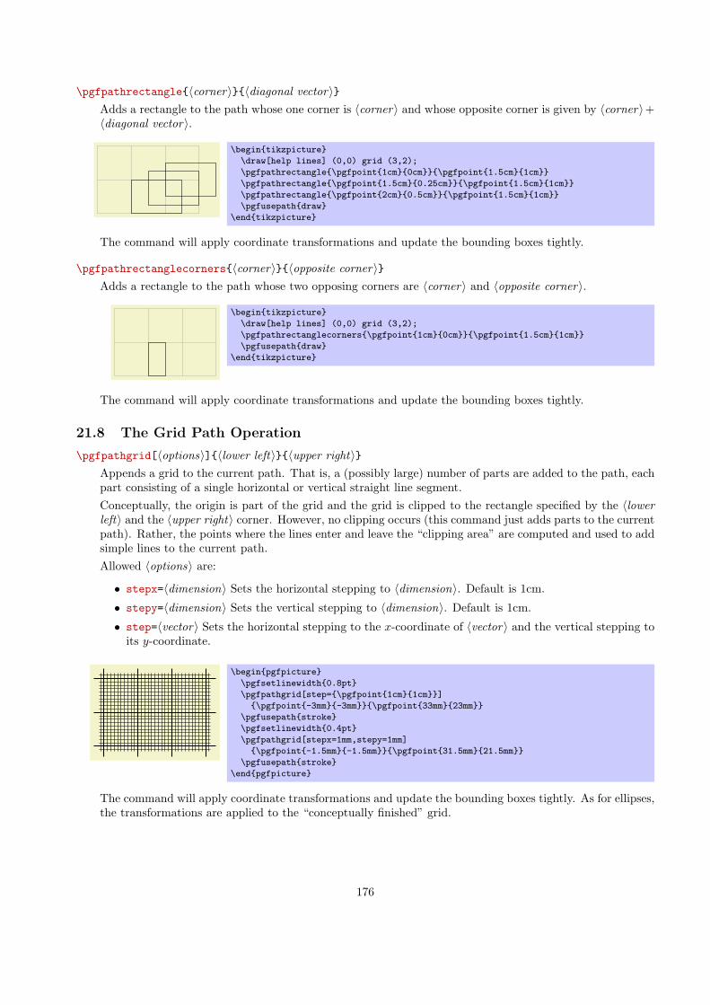
\pgfpathrectangle{⟨corner⟩}{⟨diagonal vector⟩}Adds a rectangle to the path whose one corner is ⟨corner⟩ and whose opposite corner is given by ⟨corner⟩+⟨diagonal vector⟩.

.

\begin{tikzpicture}


\pgfpathrectangle{\pgfpoint{1cm}{0cm}}{\pgfpoint{1.5cm}{1cm}}

\pgfpathrectangle{\pgfpoint{1.5cm}{0.25cm}}{\pgfpoint{1.5cm}{1cm}}

\pgfpathrectangle{\pgfpoint{2cm}{0.5cm}}{\pgfpoint{1.5cm}{1cm}}

\pgfusepath{draw}

\end{tikzpicture}

The command will apply coordinate transformations and update the bounding boxes tightly.

\pgfpathrectanglecorners{⟨corner⟩}{⟨opposite corner⟩}Adds a rectangle to the path whose two opposing corners are ⟨corner⟩ and ⟨opposite corner⟩.

.

\begin{tikzpicture}


\pgfpathrectanglecorners{\pgfpoint{1cm}{0cm}}{\pgfpoint{1.5cm}{1cm}}

\pgfusepath{draw}

\end{tikzpicture}

The command will apply coordinate transformations and update the bounding boxes tightly.

21.8 The Grid Path Operation

\pgfpathgrid[⟨options⟩]{⟨lower left⟩}{⟨upper right⟩}Appends a grid to the current path. That is, a (possibly large) number of parts are added to the path, eachpart consisting of a single horizontal or vertical straight line segment.Conceptually, the origin is part of the grid and the grid is clipped to the rectangle specified by the ⟨lowerleft⟩ and the ⟨upper right⟩ corner. However, no clipping occurs (this command just adds parts to the currentpath). Rather, the points where the lines enter and leave the “clipping area” are computed and used to addsimple lines to the current path.Allowed ⟨options⟩ are:

• stepx=⟨dimension⟩ Sets the horizontal stepping to ⟨dimension⟩. Default is 1cm.

• stepy=⟨dimension⟩ Sets the vertical stepping to ⟨dimension⟩. Default is 1cm.

• step=⟨vector⟩ Sets the horizontal stepping to the x-coordinate of ⟨vector⟩ and the vertical stepping toits y-coordinate.

.

\begin{pgfpicture}

\pgfsetlinewidth{0.8pt}

\pgfpathgrid[step={\pgfpoint{1cm}{1cm}}]

{\pgfpoint{-3mm}{-3mm}}{\pgfpoint{33mm}{23mm}}

\pgfusepath{stroke}

\pgfsetlinewidth{0.4pt}

\pgfpathgrid[stepx=1mm,stepy=1mm]

{\pgfpoint{-1.5mm}{-1.5mm}}{\pgfpoint{31.5mm}{21.5mm}}

\pgfusepath{stroke}

\end{pgfpicture}

The command will apply coordinate transformations and update the bounding boxes tightly. As for ellipses,the transformations are applied to the “conceptually finished” grid.

176

.

\begin{pgfpicture}


\pgfpathgrid[stepx=1mm,stepy=2mm]{\pgfpoint{0mm}{0mm}}{\pgfpoint{30mm}{30mm}}

\pgfusepath{stroke}

\end{pgfpicture}

21.9 The Parabola Path Operation

\pgfpathparabola{⟨bend vector⟩}{⟨end vector⟩}This command appends two half-parabolas to the current path. The first starts at the current point andends at the current point plus ⟨bend vector⟩. At his point, it has its bend. The second half parabola startsat that bend point and end at point that is given by the bend plus ⟨end vector⟩.If you set ⟨end vector⟩ to the null vector, you append only a half parabola that goes from the current pointto the bend; by setting ⟨bend vector⟩ to the null vector, you append only a half parabola that goes to currentpoint plus ⟨end vector⟩ and has its bend at the current point.It is not possible to use this command to draw a part of a parabola that does not contain the bend.

.

\begin{pgfpicture}

% Half-parabola going ‘‘up and right’’


\pgfpathparabola{\pgfpointorigin}{\pgfpoint{2cm}{4cm}}

\color{red}

\pgfusepath{stroke}

% Half-parabola going ‘‘down and right’’


\pgfpathparabola{\pgfpoint{-2cm}{4cm}}{\pgfpointorigin}

\color{blue}

\pgfusepath{stroke}

% Full parabola

\pgfpathmoveto{\pgfpoint{-2cm}{2cm}}

\pgfpathparabola{\pgfpoint{1cm}{-1cm}}{\pgfpoint{2cm}{4cm}}

\color{orange}

\pgfusepath{stroke}

\end{pgfpicture}

The command will apply coordinate transformations and update the bounding boxes.

21.10 Sine and Cosine Path Operations

Sine and cosine curves often need to be drawn and the following commands may help with this. However, theyonly allow you to append sine and cosine curves in intervals that are multiples of π/2.

\pgfpathsine{⟨vector⟩}This command appends a sine curve in the interval [0, π/2] to the current path. The sine curve is squeezedor stretched such that the curve starts at the current point and ends at the current point plus ⟨vector⟩.

177

.

\begin{tikzpicture}



\pgfpathsine{\pgfpoint{1cm}{1cm}}

\pgfusepath{stroke}

\color{red}


\pgfpathsine{\pgfpoint{-2cm}{-2cm}}

\pgfusepath{stroke}

\end{tikzpicture}


\pgfpathcosine{⟨vector⟩}This command appends a cosine curve in the interval [0, π/2] to the current path. The curve is squeezed orstretched such that the curve starts at the current point and ends at the current point plus ⟨vector⟩. Usingseveral sine and cosine operations in sequence allows you to produce a complete sine or cosine curve

.

\begin{pgfpicture}


\pgfpathsine{\pgfpoint{1cm}{1cm}}

\pgfpathcosine{\pgfpoint{1cm}{-1cm}}

\pgfpathsine{\pgfpoint{1cm}{-1cm}}

\pgfpathcosine{\pgfpoint{1cm}{1cm}}



\end{pgfpicture}


21.11 Plot Path Operations

There exist several commands for appending plots to a path. These commands are available through the packagepgfbaseplot. They are documented in Section 29.

21.12 Rounded Corners

Normally, when you connect two straight line segments or when you connect two curves that end and start “atdifferent angles” you get “sharp corners” between the lines or curves. In some cases it is desirable to produce“rounded corners” instead. Thus, the lines or curves should be shortened a bit and then connected by arcs.

pgf offers an easy way to achieve this effect, by calling the following two commands.

\pgfsetcornersarced{⟨point⟩}This command causes all subsequent corners to be replaced by little arcs. The effect of this command laststill the end of the current TEX scope.The ⟨point⟩ dictates how large the corner arc will be. Consider a corner made by two lines l and r andassume that the line l comes first on the path. The x-dimension of the ⟨point⟩ decides by how much theline l will be shortened, the y-dimension of ⟨point⟩ decides by how much the line r will be shortened. Then,the shortened lines are connected by an arc.

.

\begin{tikzpicture}


\pgfsetcornersarced{\pgfpoint{5mm}{5mm}}

\pgfpathrectanglecorners{\pgfpointorigin}{\pgfpoint{3cm}{2cm}}

\pgfusepath{stroke}

\end{tikzpicture}

178

.

\begin{tikzpicture}


\pgfsetcornersarced{\pgfpoint{10mm}{5mm}}

% 10mm entering,

% 5mm leaving.




\pgfpathcurveto




\pgfusepath{stroke}

\end{tikzpicture}

If the x- and y-coordinates of ⟨point⟩ are the same and the corner is a right angle, you will get a perfectquarter circle (well, not quite perfect, but perfect up to six decimals). When the angle is not 90◦, you onlyget a fair approximation.More or less “all” corners will be rounded, even the corner generated by a \pgfpathclose command. (Theauthor is a bit proud of this feature.)

.

\begin{pgfpicture}

\pgfsetcornersarced{\pgfpoint{4pt}{4pt}}

\pgfpathmoveto{\pgfpointpolar{0}{1cm}}

\pgfpathlineto{\pgfpointpolar{72}{1cm}}




\pgfpathclose

\pgfusepath{stroke}

\end{pgfpicture}

To return to normal (unrounded) corners, use \pgfsetcornersarced{\pgfpointorigin}.Note that the rounding will produce strange and undesirable effects if the lines at the corners are too short.In this case the shortening may cause the lines to “suddenly extend over the other end” which is rarelydesirable.

21.13 Internal Tracking of Bounding Boxes for Paths and Pictures

The path construction commands keep track of two bounding boxes: One for the current path, which is resetwhenever the path is used and thereby flushed, and a bounding box for the current {pgfpicture}.

The bounding boxes are not accessible by “normal” macros. Rather, two sets of four dimension variables areused for this, all of which contain the letter @.

\pgf@pathminx

The minimum x-coordinate “mentioned” in the current path. Initially, this is set to 16000pt.

\pgf@pathmaxx

The maximum x-coordinate “mentioned” in the current path. Initially, this is set to −16000pt.

\pgf@pathminy

The minimum y-coordinate “mentioned” in the current path. Initially, this is set to 16000pt.

\pgf@pathmaxy

The maximum y-coordinate “mentioned” in the current path. Initially, this is set to −16000pt.

\pgf@picminx

The minimum x-coordinate “mentioned” in the current picture. Initially, this is set to 16000pt.

179

\pgf@picmaxx

The maximum x-coordinate “mentioned” in the current picture. Initially, this is set to −16000pt.

\pgf@picminy

The minimum y-coordinate “mentioned” in the current picture. Initially, this is set to 16000pt.

\pgf@picmaxy

The maximum y-coordinate “mentioned” in the current picture. Initially, this is set to −16000pt.

Each time a path construction command is called, the above variables are (globally) updated. To facilitatethis, you can use the following command:

\pgf@protocolsizes{⟨x-dimension⟩}{⟨y-dimension⟩}Updates all of the above dimension in such a way that the point specified by the two arguments is inside bothbounding boxes. For the picture’s bounding box this updating occurs only if \ifpgf@relevantforpicturesizeis true, see below.

For the bounding box of the picture it is not always desirable that every path construction command affectsthis bounding box. For example, if you have just used a clip command, you do not want anything outside theclipping area to affect the bounding box. For this reason, there exists a special “TEX if” that (locally) decideswhether updating should be applied to the picture’s bounding box. Clipping will set this if to false, as willcertain other commands.

\pgf@relevantforpicturesizefalse

Suppresses updating of the picture’s bounding box.

\pgf@relevantforpicturesizetrue

Causes updating of the picture’s bounding box.

180

22 Snakes

22.1 Overview

A snake is a “way of adding a winding line to a path.” To be a bit more precise, you use snakes to extend thepath and the commands for using snakes start with \pgfpath. However, snakes do not necessarily extend thepath using line-to and curve-to operations; rather, they can also contain move-to operations and, thereby, causethe path to be split into many subpaths.

As an example, let us consider a simple snake like the zigzag snake. It looks like this:

.

\begin{tikzpicture}

\draw[snake=zigzag] (0,0) -- (3,0);

\draw[snake=zigzag] (0,-.5) -- (3,-1);

\end{tikzpicture}

The above example demonstrates the two key features of snakes:

1. Snakes are made up from little segments that are repeated several times. For the zigzag snake thesesegements look like this:

.

.

2. Snakes “follow along a straight to the target point.” Thus, when the target point is not to the right of thestart point, the snake is rotated appropriately.

In order to use snakes, they first have to be declared. This declaration contains a detailed description of howeach segement of the snake looks like and in what ordering the different possible segments are used.

Once a snake has been declared, it can be used. For this you specify a target point and a snaked line will beadded from the last point current point to the target point.

22.2 Declaring a Snake

22.2.1 Segments

When you declare a snake, you provide a description of how the different segments of the snake will be rendered.The description of each segment should be given in a way as if the target of the snaked line where at (+∞, 0)and as if the segment’s start where at the origin. Thus, for example, the segment of the zigzag might be definedusing the following code:

\pgfpathlineto{\pgfpoint{5pt}{5pt}}

\pgfpathlineto{\pgfpoint{15pt}{-5pt}}


pgf will ensure that an appropriate coordinate transformation is in place when the snake segment is addedto the path such that the snake segment actually points in the right direction. Also subsequent snake segmentswill be transformed such that they are “further along the line” toward the target. All transformations are setupautomatically.

Note that we did not use a \pgfpathmoveto{\pgfpointorigin} at the beginning of the segment code. Doingso would subdivide the path into numerous subpath. Rather, we assume that the previous segment caused thecurrent point to be at the origin.

While we can now describe segments, we still need a way to “stop” the snake. Also, pgf needs to knowthe width of the different snake segments such that it can translate the next segment correctly. Even though itwould be possible to compute all this information automatically, pgf does not do so and you have to providethe information “by hand” for each segment.

22.2.2 Snake Automata

Up to now our snakes only have one segment that is repeated again and again. However, we might also like tohave different segments and use rules to describe which segment should be used where. For example, we mighthave special segments at the start and at the end.

For snakes we use a mechanism known in computer science as finite automata to describe which segment isused in each part of the snake. The idea is the following: For the first segment we start in a special state called

181

the initial state. In this state, and also in all other state later, pgf first computes how much space is left onthe snake. That is, pgf keeps track of the distance to the target. Attached to each state there is a set of rulesof the following form: “If the remaining distance is less than x, switch to state q.” pgf checks for each of theserules whether it applies and, if so, immediately switches to state q.

Only if none of the rules tell us to switch to another state, pgf will execute the state’s code. This code willadd a segment to the path. In addition to the rules there is also width parameter attached to each state. pgfthen translates the coordinate system by this width and reduces the remaining distance. Then, pgf either staysin the current state or switches to another state, depending on yet another property attached of the state.

The whole process stops when a special state called final is reached. The segment of this state is added tothe path immediately (it is often empty, though) and the process ends.

22.2.3 The Snake Declaration Command

\pgfdeclaresnake{⟨name⟩}{⟨initial state⟩}{⟨states⟩}This command declares a new snake called ⟨name⟩. The ⟨states⟩ argument contains a description of thesnake automaton’s states and the transitions between them. The ⟨initial state⟩ is the state in which theautomaton starts.The ⟨states⟩ argument should consist of \state commands, one for each state of the snake automaton. The\state command is defined only when the ⟨states⟩ argument is executed.

.

\pgfdeclaresnake{example snake}{initial}

{

\state{initial}[width=10pt]

{






}

\state{final}

{

\pgfpathlineto{\pgfpoint{\pgfsnakeremainingdistance}{0pt}}

}

}

\tikz{\draw[snake=example snake] (0,0) -- (3,0);

\draw[snake=example snake] (0,-1) -- (3,-3);}

The \state command works as follows:

\state{⟨name⟩}[⟨options⟩]{⟨code⟩}This command declares a new state inside the current snake automaton. The state is names ⟨name⟩.When pgf is in state ⟨name⟩, the following things happen:

1. The ⟨options⟩ are parsed. This may lead, see below, to a state switch. When this happens, thefollowing steps are not executed. The ⟨options⟩ are executed one after the other in the given order.If an option causes a state switch, the switch is immediate, even if later options might cause adifferent state switch.

2. The ⟨code⟩ is executed. When this happens, the coordinate transformation will be setup such thatthe origin is at the start of the segment and such that the target lies in the direction “east.”

3. After the ⟨code⟩ has been executed, the state switches to whatever state has been specified insidethe ⟨options⟩ using the next state option. If no next state has been specified, the state staysthe same.

The following options are allowed inside the ⟨options⟩:• switch if less than=⟨dimension⟩ to ⟨new state⟩ When this option is encountered, pgf checks

whether the remaining distance to the target is less than ⟨dimension⟩. If so, an immediate stateswitch to ⟨new state⟩ occurs.

182

• width=⟨dimension⟩ This option tells pgf the width of the segment if it is appended to the path. Thecoordinate system will, afterward, be translated by ⟨dimension⟩ to ensure that the next segmentstarts where the current one ended.In addition, this option will cause an immediate switch to the state final if the remaining distanceis less than ⟨dimension⟩. The effect is the same as if you had said switch if less than=⟨dimension⟩ to finaljust before the width option.

• next state=⟨new state⟩ After the segment has been added to the path, a state switch to ⟨newstate⟩ is performed. If this option is not given, the next state is the same as the current state.

There are two dimensions that are useful inside snake automata:

\pgfsnakeremainingdistance

This TEX dimension holds the remaining distance to the target.

\pgfsnakecompleteddistance

This TEX dimension holds the distance already completed on the snake.

As a final example we present a more complicated snake that makes use of the different options:

.

\pgfdeclaresnake{complicated example snake}{initial}

{

\state{initial}[width=5pt,next state=up]

{ \pgfpathlineto{\pgfpoint{5pt}{0pt}} }

\state{up}[width=5pt,next state=down]

{

\ifdim\pgfsnakeremainingdistance>\pgfsnakecompleteddistance

% Growing

\pgfpathlineto{\pgfpoint{0pt}{\pgfsnakecompleteddistance}}

\pgfpathlineto{\pgfpoint{5pt}{\pgfsnakecompleteddistance}}


\else

% Shrinking

\pgfpathlineto{\pgfpoint{0pt}{\pgfsnakeremainingdistance}}

\pgfpathlineto{\pgfpoint{5pt}{\pgfsnakeremainingdistance}}


\fi%

}

\state{down}[width=5pt,next state=up]

{

\ifdim\pgfsnakeremainingdistance>\pgfsnakecompleteddistance

% Growing

\pgfpathlineto{\pgfpoint{0pt}{-\pgfsnakecompleteddistance}}

\pgfpathlineto{\pgfpoint{5pt}{-\pgfsnakecompleteddistance}}


\else

% Shrinking

\pgfpathlineto{\pgfpoint{0pt}{-\pgfsnakeremainingdistance}}

\pgfpathlineto{\pgfpoint{5pt}{-\pgfsnakeremainingdistance}}


\fi%

}

\state{final}

{

\pgfpathlineto{\pgfpoint{\pgfsnakeremainingdistance}{0pt}}

}

}

\begin{tikzpicture}[snake=complicated example snake]

\draw[snake] (0,0) -- (3,0);

\fill[red!50,snake,rounded corners=2pt] (.5,-2) -- ++(2.5,-2.5)

[snake=none] -- ++(0,-.5) -| (0,-2) -- cycle;

\end{tikzpicture}

183

22.2.4 Predefined Snakes

Only two very simple and basic snakes are predefined when you load pgf. For more interesting snakes you canuse the package pgflibrarysnakes.

Snake lineto

This most trivial of all snakes is simply a straight line. This snake is typically not used in a “stand alone”fashion. Rather, it is useful as a “subsnake” of the \pgfsnakesto command.

Snake moveto

Arguably, this snake is even simpler than the previous snake. This snake consists of a simple move-tooperation. Like the lineto snake, it is useful as a “subsnake” of the \pgfsnakesto command.

22.3 Using Snakes

Three commands can be used to use a snake.

\pgfpathsnakealongvector{⟨snake⟩}{⟨length⟩}{⟨vector⟩}This command will append the ⟨snake⟩ to the current path. The length of the snake is given by ⟨length⟩.The ⟨vector⟩ should be a normalizes vector (a vector having length 1pt) pointing in the direction in whichthe snake should grow.

.

\begin{tikzpicture}



\pgfpathsnakealongvector{zigzag}{2cm}{\pgfpointpolar{30}{1pt}}

\pgfusepath{stroke}

\end{tikzpicture}

\pgfpathsnakesto{⟨snake list⟩}{⟨target⟩}This command will append the snakes in the ⟨snake list⟩ to the current path such that it ends at ⟨point⟩.This command calls the previous one (repeatedly, possibly) after having computed the distance from thecurrent point to ⟨target⟩ and normalized the vector connecting the current point to the target.The ⟨snake list⟩ is a comma-separated list of pairs consisting of a snake name in curly braces and a distancein curly braces. For example, a snake list might be {lineto}{1cm},{moveto}{2cm}. This is interpreted asfollows: Use a lineto snake for the first centimeter of the way to the ⟨target⟩, then use the moveto snakefor the next two centimeters.No attempt is made to check or ensure that the distances of the “subsnakes’ add up to the distnacefrom the current point to the ⟨target⟩. However, it is possible to refer to this distance inside the⟨snake list⟩: While the snake list is processed, the two TEX-dimensions \pgfsnakeremainingdistanceand \pgfsnakecompleteddistance will be set to the correct values. For example, consider the examplefrom a above, consisting of a lineto and a moveto snake. Suppose the distance to ⟨target⟩ where 5cm.Then, when the length of the first subsnake is computed, the remaining distance willbe set to 5cm and thecompleted distance to 0cm. When the length of the second subsnake is computed, the remaining distancewil be 4cm and the completed distance will be 1cm.Here are some useful examles: {zigzag}{\pgfsnakeremainingdistance} is a ⟨snake list⟩ that consistsonly of a zigzag snake whose length is the total distance from the current point to the ⟨target⟩. Next, toget a snake that is a zigzag snake that is preceeded and succeeded by 3mm of lineto, you can use thefollowing:

184

.

\begin{tikzpicture}

\draw[help lines](0,0) grid (3,2);


\pgfpathsnakesto{%

{lineto}{3mm},%

{zigzag}{\pgfsnakeremainingdistance-6mm},%

{lineto}{3mm}}


\pgfusepath{stroke}

\end{tikzpicture}

Note that the computation of the distance may be imprecise. In general, the placement precision of thesnakes will not be perfect.

\pgfpathsnaketo{⟨snake⟩}{⟨target⟩}This command is just a shortcut for calling \pgfpathsnakesto for a single snake whose length is\pgfsnakeremainingdistance.

.

\begin{tikzpicture}



\pgfpathsnaketo{zigzag}{\pgfpoint{3cm}{2cm}}

\pgfusepath{stroke}

\end{tikzpicture}

As was already mentioned, when each segment of the snake is added to the path, an appropriate coordinatetransformation will be in force. It is sometimes useful to add an additional transformation locally. For example,by reflecting everything around the x-axis right before each segment is added, the snake will effectively bemirrored along the path. The following command allows you to install such a “last minute transformation.”

\pgfsetsnakesegmenttransformation{⟨code⟩}The ⟨code⟩ will be executed at the very beginning of each segment. Normally, this be a transformationcommand that changes the y-axis in some way.

185

23 Using Paths

23.1 Overview

Once a path has been constructed, it can be used in different ways. For example, you can draw the path or fillit or use it for clipping.

Numerous graph parameters influence how a path will be rendered. For example, when you draw a path, theline width is important as well as the dashing pattern. The options that govern how paths are rendered can allbe set with commands starting with \pgfset. All options that influence how a path is rendered always influencethe complete path. Thus, it is not possible to draw part of a path using, say, a red color and drawing anotherpart using a green color. To achieve such an effect, you must use two paths.

In detail, paths can be used in the following ways:

1. You can stroke (also known as draw) a path.

2. You can fill a path with a uniform color.

3. You can clip subsequent renderings against the path.

4. You can shade a path.

5. You can use the path as bounding box for the whole picture.

You can also perform any combination of the above, though it makes no sense to fill and shade a path at thesame time.

To perform (a combination of) the first three actions, you can use the following command:

\pgfusepath{⟨actions⟩}Applies the given ⟨actions⟩ to the current path. Afterwards, the current path is (globally) empty. Thefollowing actions are possible:

• fill fills the path. See Section 23.3 for further details.

.

\begin{pgfpicture}




\pgfusepath{fill}

\end{pgfpicture}

• stroke strokes the path. See Section 23.2 for further details.

.

\begin{pgfpicture}




\pgfusepath{stroke}

\end{pgfpicture}

• clip clips all subsequent drawings against the path. See Section 23.4 for further details.

.

\begin{pgfpicture}




\pgfusepath{stroke,clip}

\pgfpathcircle{\pgfpoint{1cm}{1cm}}{0.5cm}

\pgfusepath{fill}

\end{pgfpicture}

• discard discards the path, that is, it is not used at all. Giving this option (alone) has the same effectas giving an empty options list.

186

When more than one of the first three actions are given, they are applied in the above ordering, regardlessof their ordering in ⟨actions⟩. Thus, {stroke,fill} and {fill,stroke} have the same effect.

To shade a path, use the \pgfshadepath command, which is explained in Section 28.

23.2 Stroking a Path

When you use \pgfusepath{stroke} to stroke a path, several graphic parameters influence how the path isdrawn. The commands for setting these parameters are explained in the following.

Note that all graphic parameters apply to the path as a whole, never only to a part of it.All graphic parameters are local to the current {pgfscope}, but they persists past TEX groups, except for

the interior rule (even-odd or nonzero) and the arrow tip kinds. The latter graphic parameters only persist tillthe end of the current TEX group, but this may change in the future, so do not count on this.

23.2.1 Graphic Parameter: Line Width

\pgfsetlinewidth{⟨line width⟩}This command sets the line width for subsequent strokes (in the current pgfscope). The line width is givenas a normal TEX dimension like 0.4pt or 1mm.

.

\begin{pgfpicture}

\pgfsetlinewidth{1mm}

\pgfpathmoveto{\pgfpoint{0mm}{0mm}}

\pgfpathlineto{\pgfpoint{2cm}{0mm}}

\pgfusepath{stroke}

\pgfsetlinewidth{2\pgflinewidth} % double in size



\pgfusepath{stroke}

\end{pgfpicture}

\pgflinewidth

You can access the current line width via the TEX dimension \pgflinewidth. It will be set to the correctline width, that is, even when a TEX group closed, the value will be correct since it is set globally, but whena {pgfscope} closes, the value is set to the correct value it had before the scope.

23.2.2 Graphic Parameter: Caps and Joins

\pgfsetbuttcap

Sets the line cap to a butt cap. See Section 10.2.1 for an explanation of what this is.

\pgfsetroundcap

Sets the line cap to a round cap. See again Section 10.2.1.

\pgfsetrectcap

Sets the line cap to a square cap. See again Section 10.2.1.

\pgfsetroundjoin

Sets the line join to a round join. See again Section 10.2.1.

\pgfsetbeveljoin

Sets the line join to a bevel join. See again Section 10.2.1.

\pgfsetmiterjoin

Sets the line join to a miter join. See again Section 10.2.1.

\pgfsetmiterlimit{⟨miter limit factor⟩}Sets the miter limit to ⟨miter limit factor⟩. See again Section 10.2.1.

187

23.2.3 Graphic Parameter: Dashing

\pgfsetdash{⟨list of even length of dimensions⟩}{⟨phase⟩}Sets the dashing of a line. The first entry in the list specifies the length of the first solid part of the list.The second entry specifies the length of the following gap. Then comes the length of the second solid part,following by the length of the second gap, and so on. The ⟨phase⟩ specifies where the first solid part startsrelative to the beginning of the line.

.

\begin{pgfpicture}

\pgfsetdash{{0.5cm}{0.5cm}{0.1cm}{0.2cm}}{0cm}



\pgfusepath{stroke}

\pgfsetdash{{0.5cm}{0.5cm}{0.1cm}{0.2cm}}{0.1cm}



\pgfusepath{stroke}

\pgfsetdash{{0.5cm}{0.5cm}{0.1cm}{0.2cm}}{0.2cm}



\pgfusepath{stroke}

\end{pgfpicture}

Use \pgfsetdash{}{0pt} to get a solid dashing.

23.2.4 Graphic Parameter: Stroke Color

\pgfsetstrokecolor{⟨color⟩}Sets the color used for stroking lines to ⟨color⟩, where ⟨color⟩ is a LATEX color like red or black!20!red.Unlike the \color command, the effect of this command lasts till the end of the current {pgfscope} andnot till the end of the current TEX group.The color used for stroking may be different from the color used for filling. However, a \color commandwill always “immediately override” any special settings for the stroke and fill colors.In plain TEX, this command will also work, but the problem of defining a color arises. After all, plainTEX does not provide LATEX colors. For this reason, pgf implements a minimalistic “emulation” of the\definecolor, \colorlet, and \color commands. Only gray-scale and rgb colors are supported. Formost cases this turns out to be enough.

.

\begin{pgfpicture}


\color{red}

\pgfpathcircle{\pgfpoint{0cm}{0cm}}{3mm} \pgfusepath{fill,stroke}

\pgfsetstrokecolor{black}


\color{red}


\end{pgfpicture}

\pgfsetcolor{⟨color⟩}Sets both the stroke and fill color. The difference to the normal \color command is that the effect laststill the end of the current {pgfscope}, not only till the end of the current TEX group.

23.2.5 Graphic Parameter: Stroke Opacity

\pgfsetstrokeopacity{⟨value⟩}Sets the opacity of stroking operations. The ⟨value⟩ should be a number between 0 and 1, where 1 means“fully opaque” and 0 means “fully transparent.” A value like 0.5 will cause paths to be stroked in asemitransparent way.

188

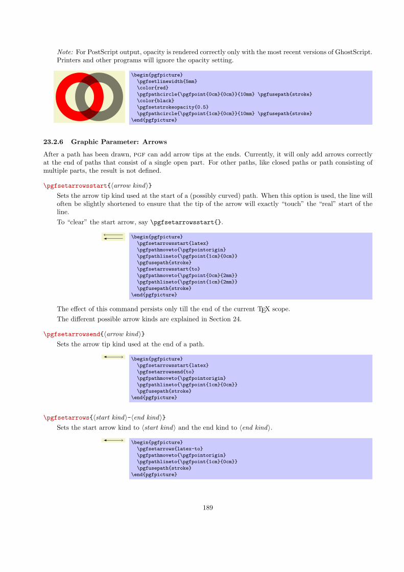
Note: For PostScript output, opacity is rendered correctly only with the most recent versions of GhostScript.Printers and other programs will ignore the opacity setting.

.

\begin{pgfpicture}

\pgfsetlinewidth{5mm}

\color{red}

\pgfpathcircle{\pgfpoint{0cm}{0cm}}{10mm} \pgfusepath{stroke}

\color{black}

\pgfsetstrokeopacity{0.5}

\pgfpathcircle{\pgfpoint{1cm}{0cm}}{10mm} \pgfusepath{stroke}

\end{pgfpicture}

23.2.6 Graphic Parameter: Arrows

After a path has been drawn, pgf can add arrow tips at the ends. Currently, it will only add arrows correctlyat the end of paths that consist of a single open part. For other paths, like closed paths or path consisting ofmultiple parts, the result is not defined.

\pgfsetarrowsstart{⟨arrow kind⟩}Sets the arrow tip kind used at the start of a (possibly curved) path. When this option is used, the line willoften be slightly shortened to ensure that the tip of the arrow will exactly “touch” the “real” start of theline.To “clear” the start arrow, say \pgfsetarrowsstart{}.

.

\begin{pgfpicture}

\pgfsetarrowsstart{latex}



\pgfusepath{stroke}

\pgfsetarrowsstart{to}

\pgfpathmoveto{\pgfpoint{0cm}{2mm}}


\pgfusepath{stroke}

\end{pgfpicture}

The effect of this command persists only till the end of the current TEX scope.The different possible arrow kinds are explained in Section 24.

\pgfsetarrowsend{⟨arrow kind⟩}Sets the arrow tip kind used at the end of a path.

.

\begin{pgfpicture}


\pgfsetarrowsend{to}



\pgfusepath{stroke}

\end{pgfpicture}

\pgfsetarrows{⟨start kind⟩-⟨end kind⟩}Sets the start arrow kind to ⟨start kind⟩ and the end kind to ⟨end kind⟩.

.

\begin{pgfpicture}

\pgfsetarrows{latex-to}



\pgfusepath{stroke}

\end{pgfpicture}

189

\pgfsetshortenstart{⟨dimension⟩}This command will shortened the start of every stroked path by the given dimension. This shortening isdone in addition to automatic shortening done by a start arrow, but it can be used even if no start arrowis given.This command is useful if you wish arrows or lines to “stop shortly before” a given point.

.

\begin{pgfpicture}

\pgfpathcircle{\pgfpointorigin}{5mm}

\pgfusepath{stroke}

\pgfsetarrows{latex-}

\pgfsetshortenstart{4pt}

\pgfpathmoveto{\pgfpoint{5mm}{0cm}} % would be on the circle


\pgfusepath{stroke}

\end{pgfpicture}

\pgfsetshortenend{⟨dimension⟩}Works like \pgfsetshortenstart.

23.3 Filling a Path

Filling a path means coloring every interior point of the path with the current fill color. It is not always obviouswhether a point is “inside” a path when the path is self-intersecting and/or consists or multiple parts. In thiscase either the nonzero winding number rule or the even-odd crossing number rule is used to decide, which pointslie “inside.” These rules are explained in Section 10.3.

23.3.1 Graphic Parameter: Interior Rule

You can set which rule is used using the following commands:

\pgfseteorule

Dictates that the even-odd rule is used in subsequent fillings in the current TEX scope. Thus, for once, theeffect of this command does not persist past the current TEX scope.

.

\begin{pgfpicture}

\pgfseteorule

\pgfpathcircle{\pgfpoint{0mm}{0cm}}{7mm}


\pgfusepath{fill}

\end{pgfpicture}

\pgfsetnonzerorule

Dictates that the nonzero winding number rule is used in subsequent fillings in the current TEX scope. Thisis the default.

.

\begin{pgfpicture}

\pgfsetnonzerorule



\pgfusepath{fill}

\end{pgfpicture}

23.3.2 Graphic Parameter: Filling Color

\pgfsetfillcolor{⟨color⟩}Sets the color used for filling paths to ⟨color⟩. Like the stroke color, the effect lasts only till the next use of\color.

190

23.3.3 Graphic Parameter: Fill Opacity

\pgfsetfillopacity{⟨value⟩}Sets the opacity of filling operations. As for stroking, the ⟨value⟩ should be a number between 0 and 1.The “filling transparency” will also be used for text and images.

.

\begin{tikzpicture}

\pgfsetfillopacity{0.5}

\fill[red] (90:1cm) circle (11mm);

\fill[green] (210:1cm) circle (11mm);

\fill[blue] (-30:1cm) circle (11mm);

\end{tikzpicture}

23.4 Clipping a Path

When you add the clip option, the current path is used for clipping subsequent drawings. The same rule asfor filling is used to decide whether a point is inside or outside the path, that is, either the even-odd rule or thenonzero rule.

Clipping never enlarges the clipping area. Thus, when you clip against a certain path and then clip againagainst another path, you clip against the intersection of both.

The only way to enlarge the clipping path is to end the {pgfscope} in which the clipping was done. At theend of a {pgfscope} the clipping path that was in force at the beginning of the scope is reinstalled.

23.5 Using a Path as a Bounding Box

When you add the use as bounding box option, the bounding box of the picture will be enlarged such thatthe path in encompassed, but any subsequent paths of the current TEX scope will not have any effect on the sizeof the bounding box. Typically, you use this command at the very beginning of a {pgfpicture} environment.

Left

.

right. Left

\begin{pgfpicture}


\pgfusepath{use as bounding box} % draws nothing

\pgfpathcircle{\pgfpointorigin}{2ex}

\pgfusepath{stroke}

\end{pgfpicture}

right.

191

24 Arrow Tips

24.1 Overview

24.1.1 When Does PGF Draw Arrow Tips?

pgf offers an interface for placing arrow tips at the end of lines. The interface works as follows:

1. You (or someone else) assigns a name to a certain kind of arrow tips. For example, the arrow tip latex isthe arrow tip used by the standard LATEX picture environment; the arrow tip to looks like the tip of thearrow in TEX’s \to command; and so on.This is done once at the beginning of the document.

2. Inside some picture, at some point you specify that in the current scope from now on you would like tipsof, say, kind to to be added at the end and/or beginning of all paths.When an arrow kind has been installed and when pgf is about to stroke a path, the following thingshappen:

(a) The beginning and/or end of the path is shortened appropriately.(b) The path is stroked.(c) The arrow tip is drawn at the beginning and/or end of the path, appropriately rotated and appropri-

ately resized.

In the above description, there are a number of “appropriately.” The exact details are not quite trivial anddescribed later on.

24.1.2 Meta-Arrow Tips

In pgf, arrows are “meta-arrows” in the same way that fonts in TEX are “meta-fonts.” When a meta-arrow isresized, it is not simply scaled, but a possibly complicated transformation is applied to the size.

A meta-font is not one particular font at a specific size with a specific stroke width (and with a large numberof other parameters being fixed). Rather, it is a “blueprint” (actually, more like a program) for generating sucha font at a particular size and width. This allows the designer of a meta-font to make sure that, say, the fontis somewhat thicker and wider at very small sizes. To appreciate the difference: Compare the following texts:“Berlin” and “

.

.

Berlin”. The first is a “normal” text, the second is the tiny version scaled by a factor of two.Obviously, the first look better. Now, compare “

.

.

Berlin” and “Berlin”. This time, the normal text was scaled down,while the second text is a “normal” tiny text. The second text is easier to read.

pgf’s meta-arrows work in a similar fashion: The shape of an arrow tip can vary according to the line widthof the arrow tip is used. Thus, an arrow tip drawn at a line width of 5pt will typically not be five times as largeas an arrow tip of line width 1pt. Instead, the size of the arrow will get bigger only slowly as the line widthincreases.

To appreciate the difference, here are the latex and to arrows, as drawn by pgf at four different sizes:

.

.

line width is 0.1pt

.

line width is 0.4pt

.

line width is 1.2pt

.

line width is 5pt

.

line width is 0.1pt

.

line width is 0.4pt

.

line width is 1.2pt

.

line width is 5pt

Here, by comparison, is the same arrow when it is simply “resized” (as done by most programs):

.

.

line width is 0.1pt

.

line width is 0.4pt

.

line width is 1.2pt

.

line width is 5pt

.

line width is 0.1pt

.

line width is 0.4pt

.

line width is 1.2pt

.

line width is 5pt

192

As can be seen, simple scaling produces arrow tips that are way too large at larger sizes and way too smallat smaller sizes.

24.2 Declaring an Arrow Tip Kind

To declare an arrow kind “from scratch,” the following command is used:

\pgfarrowsdeclare{⟨start name⟩}{⟨end name⟩}{⟨extend code⟩}{⟨arrow tip code⟩}This command declares a new arrow kind. An arrow kind has two names, which will typically be the same.When the arrow tip needs to be drawn, the ⟨arrow tip code⟩ will be invoked, but the canvas transformationis setup beforehand to a rotation such that when an arrow tip pointing right is specified, the arrow tip thatis actually drawn points in the direction of the line.

Naming the arrow kind. The ⟨start name⟩ is the name used for the arrow tip when it is at the start ofa path, the ⟨end name⟩ is the name used at the end of a path. For example, the arrow kind that looks likea parenthesis has the ⟨start name⟩ ( and the ⟨end name⟩ ) so that you can say \pgfsetarrows{(-)} tospecify that you want parenthesis arrows and both ends.The ⟨end name⟩ and ⟨start name⟩ can be quite arbitrary and may contain spaces.

Basics of the arrow tip code. Let us next have a look at the ⟨arrow tip code⟩. This code will be used todraw the arrow tip when pgf thinks this is necessary. The code should draw an arrow that “points right,”which means that is should draw an arrow at the end of a line coming from the left and ending at the origin.As an example, suppose we wanted to declare an arrow tip consisting of two arcs, that is, we want the arrowtip to look more or less like the red part of the following picture:

.


\draw (-2,0) -- (0,0);

\draw[red,join=round,cap=round]

(-10pt,10pt) arc (180:270:10pt) arc (90:180:10pt);

\end{tikzpicture}

We could use the following as ⟨arrow tip code⟩ for this:

\pgfarrowsdeclare{arcs}{arcs}{...}

{

\pgfsetdash{}{0pt} % do not dash

\pgfsetroundjoin % fix join

\pgfsetroundcap % fix cap

\pgfpathmoveto{\pgfpoint{-10pt}{10pt}}

\pgfpatharc{180}{270}{10pt}

\pgfpatharc{90}{180}{10pt}

\pgfusepathqstroke

}

Indeed, when the ... is set appropriately (in a moment), we can write the following:

.

\begin{tikzpicture}

\draw[-arcs,line width=3pt] (-2,0) -- (0,0);

\draw[arcs-arcs,line width=1pt] (-2,-1.5) -- (0,-1);

\useasboundingbox (-2,-2) rectangle (0,0.75);

\end{tikzpicture}

As can be seen in the second example, the arrow tip is automatically rotated as needed when the arrow isdrawn. This is achieved by a canvas rotation.

Special considerations about the arrow tip code. There are several things you need to be aware ofwhen designing arrow tip code:

193

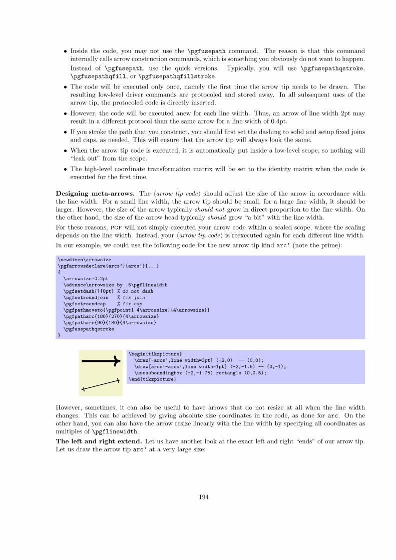
• Inside the code, you may not use the \pgfusepath command. The reason is that this commandinternally calls arrow construction commands, which is something you obviously do not want to happen.Instead of \pgfusepath, use the quick versions. Typically, you will use \pgfusepathqstroke,\pgfusepathqfill, or \pgfusepathqfillstroke.

• The code will be executed only once, namely the first time the arrow tip needs to be drawn. Theresulting low-level driver commands are protocoled and stored away. In all subsequent uses of thearrow tip, the protocoled code is directly inserted.

• However, the code will be executed anew for each line width. Thus, an arrow of line width 2pt mayresult in a different protocol than the same arrow for a line width of 0.4pt.

• If you stroke the path that you construct, you should first set the dashing to solid and setup fixed joinsand caps, as needed. This will ensure that the arrow tip will always look the same.

• When the arrow tip code is executed, it is automatically put inside a low-level scope, so nothing will“leak out” from the scope.

• The high-level coordinate transformation matrix will be set to the identity matrix when the code isexecuted for the first time.

Designing meta-arrows. The ⟨arrow tip code⟩ should adjust the size of the arrow in accordance withthe line width. For a small line width, the arrow tip should be small, for a large line width, it should belarger. However, the size of the arrow typically should not grow in direct proportion to the line width. Onthe other hand, the size of the arrow head typically should grow “a bit” with the line width.For these reasons, pgf will not simply executed your arrow code within a scaled scope, where the scalingdepends on the line width. Instead, your ⟨arrow tip code⟩ is reexecuted again for each different line width.In our example, we could use the following code for the new arrow tip kind arc’ (note the prime):

\newdimen\arrowsize

\pgfarrowsdeclare{arcs’}{arcs’}{...}

{

\arrowsize=0.2pt

\advance\arrowsize by .5\pgflinewidth




\pgfpathmoveto{\pgfpoint{-4\arrowsize}{4\arrowsize}}

\pgfpatharc{180}{270}{4\arrowsize}


\pgfusepathqstroke

}

.

\begin{tikzpicture}

\draw[-arcs’,line width=3pt] (-2,0) -- (0,0);

\draw[arcs’-arcs’,line width=1pt] (-2,-1.5) -- (0,-1);

\useasboundingbox (-2,-1.75) rectangle (0,0.5);

\end{tikzpicture}

However, sometimes, it can also be useful to have arrows that do not resize at all when the line widthchanges. This can be achieved by giving absolute size coordinates in the code, as done for arc. On theother hand, you can also have the arrow resize linearly with the line width by specifying all coordinates asmultiples of \pgflinewidth.The left and right extend. Let us have another look at the exact left and right “ends” of our arrow tip.Let us draw the arrow tip arc’ at a very large size:

194

.

\begin{tikzpicture}

\draw[help lines] (-2,-1) grid (1,1);

\draw[line width=10pt,-arcs’] (-2,0) -- (0,0);

\draw[line width=2pt,white] (-2,0) -- (0,0);

\end{tikzpicture}

As one can see, the arrow tip does not “touch” the origin as it should, but protrudes a little over the origin.One remedy to this undesirable effect is to change the code of the arrow tip such that everything is shiftedhalf an \arrowsize to the left. While this will cause the arrow tip to touch the origin, the line itself willthen interfere with the arrow: The arrow tip will be partly “hidden” by the line itself.pgf uses a different approach to solving the problem: The ⟨extend code⟩ argument can be used to “tell”pgf how much the arrow protrudes over the origin. The argument is also used to tell pgf where the “left”end of the arrow is. However, this number is important only when the arrow is being reversed or composedwith other arrow tips.Once pgf knows the right extend of an arrow kind, it can shorten lines by this amount when drawingarrows.Here is a picture that shows what the visualizes the extends. The arrow tip itself is shown in red once more:

.

.

right extend

.

left extend

.

origin

The ⟨extend code⟩ is normal TEX code that is executed whenever pgf wants to know how far the arrow tip willprotrude to the right and left. The code should call the following two commands: \pgfarrowsrightextendand \pgfarrowsleftextend. Both arguments take one argument that specifies the size. Here is the finalcode for the arc’’ arrow tip:

195

.

\pgfarrowsdeclare{arcs’’}{arcs’’}

{

\arrowsize=0.2pt


\pgfarrowsleftextend{-4\arrowsize-.5\pgflinewidth}

\pgfarrowsrightextend{.5\pgflinewidth}

}

{

\arrowsize=0.2pt





\pgfpathmoveto{\pgfpoint{-4\arrowsize}{4\arrowsize}}


\pgfusepathqstroke



\pgfusepathqstroke

}

\begin{tikzpicture}

\draw[help lines] (-2,-1) grid (1,1);

\draw[line width=10pt,-arcs’’] (-2,0) -- (0,0);

\draw[line width=2pt,white] (-2,0) -- (0,0);

\end{tikzpicture}

24.3 Declaring a Derived Arrow Tip Kind

It is possible to declare arrow kinds in terms of existing ones. For these command to work correctly, the left andright extends must be set correctly.

\pgfarrowsdeclarealias{⟨start name⟩}{⟨end name⟩}{⟨old start name⟩}{⟨old end name⟩}This command can be used to create an alias (another name) for an existing arrow kind.

.

\pgfarrowsdeclarealias{<}{>}{arcs’’}{arcs’’}%

\begin{tikzpicture}

\pgfsetarrows{<->}

\pgfsetlinewidth{1ex}



\pgfusepath{stroke}

\useasboundingbox (-0.25,-0.25) rectangle (3.75,2.25);

\end{tikzpicture}

\pgfarrowsdeclarereversed{⟨start name⟩}{⟨end name⟩}{⟨old start name⟩}{⟨old end name⟩}This command creates a new arrow kind that is the “reverse” of an existing arrow kind. The (automaticallycerated) code of the new arrow kind will contain a flip of the canvas and the meanings of the left and rightextend will be reversed.

.

\pgfarrowsdeclarereversed{arcs reversed}{arcs reversed}{arcs’’}{arcs’’}%

\begin{tikzpicture}

\pgfsetarrows{arcs reversed-arcs reversed}




\pgfusepath{stroke}


\end{tikzpicture}

\pgfarrowsdeclarecombine*[⟨offset⟩]{⟨start name⟩}{⟨end name⟩}{⟨first start name⟩}{⟨first end name⟩}{⟨second start name⟩}{⟨second end name⟩}

196

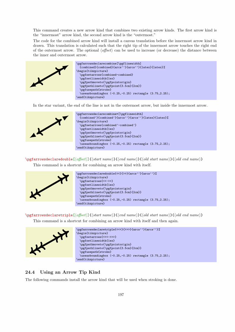
This command creates a new arrow kind that combines two existing arrow kinds. The first arrow kind isthe “innermost” arrow kind, the second arrow kind is the “outermost.”The code for the combined arrow kind will install a canvas translation before the innermost arrow kind indrawn. This translation is calculated such that the right tip of the innermost arrow touches the right endof the outermost arrow. The optional ⟨offset⟩ can be used to increase (or decrease) the distance betweenthe inner and outermost arrow.

.

\pgfarrowsdeclarecombine[\pgflinewidth]

{combined}{combined}{arcs’’}{arcs’’}{latex}{latex}%

\begin{tikzpicture}

\pgfsetarrows{combined-combined}




\pgfusepath{stroke}


\end{tikzpicture}

In the star variant, the end of the line is not in the outermost arrow, but inside the innermost arrow.

.

\pgfarrowsdeclarecombine*[\pgflinewidth]

{combined’}{combined’}{arcs’’}{arcs’’}{latex}{latex}%

\begin{tikzpicture}

\pgfsetarrows{combined’-combined’}




\pgfusepath{stroke}


\end{tikzpicture}

\pgfarrowsdeclaredouble[⟨offset⟩]{⟨start name⟩}{⟨end name⟩}{⟨old start name⟩}{⟨old end name⟩}This command is a shortcut for combining an arrow kind with itself.

.

\pgfarrowsdeclaredouble{<<}{>>}{arcs’’}{arcs’’}%

\begin{tikzpicture}

\pgfsetarrows{<<->>}




\pgfusepath{stroke}


\end{tikzpicture}

\pgfarrowsdeclaretriple[⟨offset⟩]{⟨start name⟩}{⟨end name⟩}{⟨old start name⟩}{⟨old end name⟩}This command is a shortcut for combining an arrow kind with itself and then again.

.

\pgfarrowsdeclaretriple{<<<}{>>>}{arcs’’}{arcs’’}%

\begin{tikzpicture}

\pgfsetarrows{<<<->>>}




\pgfusepath{stroke}


\end{tikzpicture}

24.4 Using an Arrow Tip Kind

The following commands install the arrow kind that will be used when stroking is done.

197

\pgfsetarrowsstart{⟨start arrow kind⟩}Installs the given ⟨start arrow kind⟩ for all subsequent strokes in the in the current TEX-group. If ⟨startarrow kind⟩ is empty, no arrow tips will be drawn at the start of the last segment of paths.

.

\begin{tikzpicture}





\pgfusepath{stroke}


\end{tikzpicture}

\pgfsetarrowsend{⟨start arrow kind⟩}Like \pgfsetarrowsstart, only for the end of the arrow.

.

\begin{tikzpicture}

\pgfsetarrowsend{latex}




\pgfusepath{stroke}


\end{tikzpicture}

Warning: If the compatibility mode is active (which is the default), there also exist old commands called\pgfsetstartarrow and \pgfsetendarrow, which are incompatible with the meta-arrow management.

\pgfsetarrows{⟨start kind⟩-⟨end kind⟩}Calls \pgfsetarrowsstart for ⟨start kind⟩ and \pgfsetarrowsend for ⟨end kind⟩.

.

\begin{tikzpicture}

\pgfsetarrows{latex-to}




\pgfusepath{stroke}


\end{tikzpicture}

24.5 Predefined Arrow Tip Kinds

The following arrow tip kinds are always defined:

stealth-stealth yields thick

.

and thin

.

stealth reversed-stealth reversed yields thick

.

and thin

.

to-to yields thick

.

and thin

.

to reversed-to reversed yields thick

.

and thin

.

latex-latex yields thick

.

and thin

.

latex reversed-latex reversed yields thick

.

and thin

.

|-| yields thick

.

and thin

.

For further arrow tips, see page 125.

198

25 Nodes and Shapes

This section describes the pgfbaseshapes package.

\usepackage{pgfbaseshapes} % LATEX\input pgfbaseshapes.tex % plain TEX\input pgfbaseshapes.tex % ConTEXt

This package defines commands both for creating nodes and for creating shapes. The package is loadedautomatically by pgf, but you can load it manually if you have only included pgfcore.

25.1 Overview

pgf comes with a sophisticated set of commands for creating nodes and shapes. A node is a graphical objectthat consists (typically) of (one or more) text labels and some additional stroked or filled paths. Each node hasa certain shape, which may be something simple like a rectangle or a circle, but it may also be somethingcomplicated like a uml class diagram (this shape is currently not implemented, though). Different nodes thathave the same shape may look quite different, however, since shapes (need not) specify whether the shape pathis stroked or filled.

25.1.1 Creating and Referencing Nodes

You create a node by calling the macro \pgfnode or the more general \pgfmultipartnode. These macrotakes several parameters and draws the requested shape at a certain position. In addition, it will “remember”the node’s position within the current {pgfpicture}. You can then, later on, refer to the node’s position.Coordinate transformations are “fully supported,” which means that if you used coordinate transformations toshift or rotate the shape of a node, the node’s position will still be correctly determined by pgf. This is not thecase if you use canvas transformations, instead.

25.1.2 Anchors

An important property of a node or a shape in general are its anchors. Anchors are “important” positions in ashape. For example, the center anchor lies at the center of a shape, the north anchor is usually “at the top, inthe middle” of a shape, the text anchor is the lower left corner of the shape’s text label (if present), and so on.

Anchors are important both when you create a node and when you reference it. When you create a node,you specify the node’s “position” by asking pgf to place the shape in such a way that a certain anchor lies at acertain point. For example, you might ask that the node is placed such that the north anchor is at the origin.This will effectively cause the node to be placed below the origin.

When you reference a node, you always reference an anchor of the node. For example, when you request the“north anchor of the node just placed” you will get the origin. However, you can also request the “south anchorof this node,” which will give you a point somewhere below the origin. When a coordinate transformation wasin force at the time of creation of a node, all anchors are also transformed accordingly.

25.1.3 Layers of a Shape

The simplest shape, the coordinate, has just one anchor, namely the center, and a label (which is usuallyempty). More complicated shapes like the rectangle shape also have a background path. This is a pgf-paththat is defined by the shape. The shape does not prescribe what should happen with the path: When a node iscreated this path may be stroked (resulting in a frame around the label), filled (resulting in a background colorfor the text), or just discarded.

Although most shapes consist just of a background path plus some label text, when a shape is drawn, up toseven different layers are drawn:

1. The “behind the background layer.” Unlike the background path, which be used in different ways bydifferent nodes, the graphic commands given for this layer will always stroke or always fill the path theyconstruct. They might also insert some text that is “behind everything.”

199

2. The background path layer. How this path is used depends on how the arguments of the \pgfnodecommand.

3. The “before the background path layer.” This layer works like the first one, only the commands of thislayer are executed after the background path has been used (in whatever way the creator of the nodechose).

4. The label layer. This layer inserts the node’s text box(es).

5. The “behind the foreground layer.” This layer, like the first layer, once more contains graphic commandsthat are “simply executed.”

6. The foreground path layer. This path is treated in the same way as the background path, only it is drawnonly after the label text has been drawn.

7. The “before the foreground layer.”

Which of these layers are actually used depends on the shape.

25.1.4 Node Parts

A shape typically does not consist only of different background and foreground paths, but it may also have textlabels. Indeed, for many shapes the text labels are the more important part of the shape.

Most shapes will have only one text label. In this case, this text label is simply passed as a parameter to the\pgfnode command. When the node is drawn, the text label is shifted around such that its lower left corner isat the text anchor of the node.

More complicated shapes may have more than one text label. Nodes of such shapes are called multipartnodes. The different node parts are simply the different text labels. For example, a uml class shape mighthave a class name part, a method part and an attributes part. Indeed, single part nodes are a special case ofmultipart nodes: They only have one part named text.

When a shape is declared, you must specify the node parts. There is a simple command called \nodepartsthat takes a list of the part names as input. When you create a node of a multipart shape, for each part of thenode you must have setup a TEX-box containing the text of the part. For a part named XYZ you must setup thebox \pgfnodepartXYZbox. The box will be placed at the anchor XYZ. See the description of \pgfmultipartnodefor more details.

25.2 Creating Nodes

You create a node using on of the following commands:

\pgfnode{⟨shape⟩}{⟨anchor⟩}{⟨label text⟩}{⟨name⟩}{⟨path usage command⟩}This command creates a new node. The ⟨shape⟩ of the node must have been declared previously using\pgfdeclareshape.The shape is shifted such that the ⟨anchor⟩ is at the origin. In order to place the shape somewhere else,use the coordinate transformation prior to calling this command.The ⟨name⟩ is a name for later reference. If no name is given, nothing will be “saved” for the node, it willjust be drawn.The ⟨path usage command⟩ is executed for the background and the foreground path (if the shape definesthem).

.

.

Hello World

.

Hello World

200

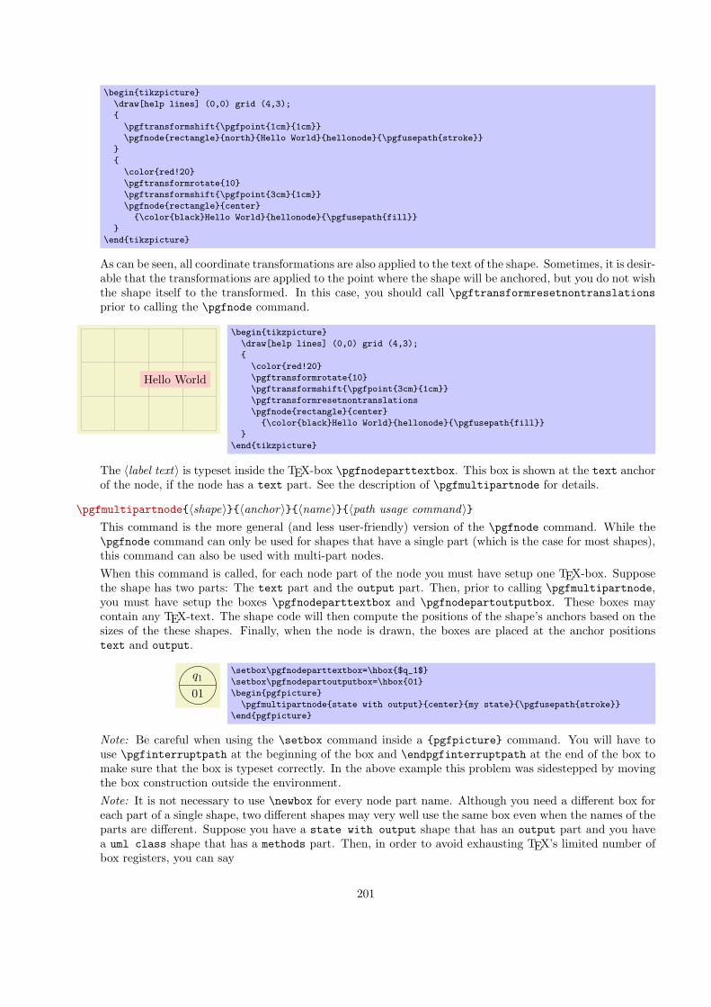
\begin{tikzpicture}


{

\pgftransformshift{\pgfpoint{1cm}{1cm}}

\pgfnode{rectangle}{north}{Hello World}{hellonode}{\pgfusepath{stroke}}

}

{

\color{red!20}



\pgfnode{rectangle}{center}

{\color{black}Hello World}{hellonode}{\pgfusepath{fill}}

}

\end{tikzpicture}

As can be seen, all coordinate transformations are also applied to the text of the shape. Sometimes, it is desir-able that the transformations are applied to the point where the shape will be anchored, but you do not wishthe shape itself to the transformed. In this case, you should call \pgftransformresetnontranslationsprior to calling the \pgfnode command.

.

.

Hello World

\begin{tikzpicture}


{

\color{red!20}



\pgftransformresetnontranslations

\pgfnode{rectangle}{center}

{\color{black}Hello World}{hellonode}{\pgfusepath{fill}}

}

\end{tikzpicture}

The ⟨label text⟩ is typeset inside the TEX-box \pgfnodeparttextbox. This box is shown at the text anchorof the node, if the node has a text part. See the description of \pgfmultipartnode for details.

\pgfmultipartnode{⟨shape⟩}{⟨anchor⟩}{⟨name⟩}{⟨path usage command⟩}This command is the more general (and less user-friendly) version of the \pgfnode command. While the\pgfnode command can only be used for shapes that have a single part (which is the case for most shapes),this command can also be used with multi-part nodes.When this command is called, for each node part of the node you must have setup one TEX-box. Supposethe shape has two parts: The text part and the output part. Then, prior to calling \pgfmultipartnode,you must have setup the boxes \pgfnodeparttextbox and \pgfnodepartoutputbox. These boxes maycontain any TEX-text. The shape code will then compute the positions of the shape’s anchors based on thesizes of the these shapes. Finally, when the node is drawn, the boxes are placed at the anchor positionstext and output.

.

.

q1

.

01

\setbox\pgfnodeparttextbox=\hbox{$q_1$}

\setbox\pgfnodepartoutputbox=\hbox{01}

\begin{pgfpicture}

\pgfmultipartnode{state with output}{center}{my state}{\pgfusepath{stroke}}

\end{pgfpicture}

Note: Be careful when using the \setbox command inside a {pgfpicture} command. You will have touse \pgfinterruptpath at the beginning of the box and \endpgfinterruptpath at the end of the box tomake sure that the box is typeset correctly. In the above example this problem was sidestepped by movingthe box construction outside the environment.Note: It is not necessary to use \newbox for every node part name. Although you need a different box foreach part of a single shape, two different shapes may very well use the same box even when the names of theparts are different. Suppose you have a state with output shape that has an output part and you havea uml class shape that has a methods part. Then, in order to avoid exhausting TEX’s limited number ofbox registers, you can say

201

\newbox\pgfnodepartoutputbox

\let\pgfnodepartmethodsbox=\pgfnodepartoutputbox

Also, when you have a node part name with spaces like class name, it may be useful to create an alias:

\newbox\mybox

\expandafter\let\csname pgfnodepartclass namebox\endcsname=\mybox

There are a number of values that have an influence on the size of a node. These parameters can be changedusing the following commands:

\pgfsetshapeminwidth{⟨dimension⟩}This command sets the macro \pgfshapeminwidth to ⟨dimension⟩. This dimension is the recommendedminimum width of a shape. Thus, when a shape is drawn and when the shape’s width would be smallerthan ⟨dimension⟩, the shape’s width is enlarged by adding some empty space.Note that this value is just a recommendation. A shape may choose to ignore the value of \pgfshapeminwidth.

.

.

Hello World

\begin{tikzpicture}

\draw[help lines] (-2,0) grid (2,1);

\pgfsetshapeminwidth{3cm}

\pgfnode{rectangle}{center}{Hello World}{}{\pgfusepath{stroke}}

\end{tikzpicture}

\pgfsetshapeminheight{⟨dimension⟩}Works like \pgfsetshapeminwidth.

\pgfsetshapeinnerxsep{⟨dimension⟩}This command sets the macro \pgfshapeinnerxsep to ⟨dimension⟩. This dimension is the recommendedhorizontal inner separation between the label text and the background path. As before, this value is just arecommendation and a shape may choose to ignore the value of \pgfshapeinnerxsep.

.

.

Hello World

\begin{tikzpicture}


\pgfsetshapeinnerxsep{1cm}

\pgfnode{rectangle}{center}{Hello World}{}{\pgfusepath{stroke}}

\end{tikzpicture}

\pgfsetshapeinnerysep{⟨dimension⟩}Works like \pgfsetshapeinnerysep.

\pgfsetshapeouterxsep{⟨dimension⟩}This command sets the macro \pgfshapeouterxsep to ⟨dimension⟩. This dimension is the recommendedhorizontal outer separation between the background path and the “outer anchors.” For example, if⟨dimension⟩ is 1cm then the east anchor will be 1cm to the right of the right border of the backgroundpath.As before, this value is just a recommendation.

202

.

.

Hello World

\begin{tikzpicture}


\pgfsetshapeouterxsep{.5cm}

\pgfnode{rectangle}{center}{Hello World}{x}{\pgfusepath{stroke}}

\pgfpathcircle{\pgfpointanchor{x}{north}}{2pt}

\pgfpathcircle{\pgfpointanchor{x}{south}}{2pt}

\pgfpathcircle{\pgfpointanchor{x}{east}}{2pt}

\pgfpathcircle{\pgfpointanchor{x}{west}}{2pt}

\pgfpathcircle{\pgfpointanchor{x}{north east}}{2pt}

\pgfusepath{fill}

\end{tikzpicture}

\pgfsetshapeouterysep{⟨dimension⟩}Works like \pgfsetshapeouterysep.

25.3 Using Anchors

Each shape defines a set of anchors. We saw already that the anchors are used when the shape is drawn:the shape is placed in such a way that the given anchor is at the origin (which in turn is typically translatedsomewhere else).

One has to look up the set of anchors of each shape, there is no “default” set of anchors, except for thecenter anchor, which should always be present. Also, most shapes will declare anchors like north or east, butthis is not guaranteed.

Once a node has been defined, you can refer to its anchors using the following commands:

\pgfpointanchor{⟨node⟩}{⟨anchor⟩}This command is another “point command” like the commands described in Section 20. It returns thecoordinate of the given ⟨anchor⟩ in the given ⟨node⟩. The command can be used in commands like\pgfpathmoveto.

.

.

HelloWorld

!\begin{pgfpicture}


\pgfnode{rectangle}{center}{Hello World!}{x}{\pgfusepath{stroke}}

\pgfpathcircle{\pgfpointanchor{x}{north}}{2pt}

\pgfpathcircle{\pgfpointanchor{x}{south}}{2pt}

\pgfpathcircle{\pgfpointanchor{x}{east}}{2pt}

\pgfpathcircle{\pgfpointanchor{x}{west}}{2pt}

\pgfpathcircle{\pgfpointanchor{x}{north east}}{2pt}

\pgfusepath{fill}

\end{pgfpicture}

In the above example, you may have noticed something curious: The rotation transformation is still in forcewhen the anchors are invoked, but it does not seem to have an effect. You might expect that the rotationshould apply to the already rotated points once more.However, \pgfpointanchor returns a point that takes the current transformation matrix into account:The inverse transformation to the current coordinate transformation is applied to an anchor point beforereturning it.This behavior may seem a bit strange, but you will find it very natural in most cases. If you really want toapply a transformation to an anchor point (for example, to “shift it away” a little bit), you have to invoke\pgfpointanchor without any transformations in force. Here is an example:

203

.

.Hello

World!

\begin{pgfpicture}



{

\pgftransformreset

\pgfpointanchor{x}{east}

\xdef\mycoordinate{\noexpand\pgfpoint{\the\pgf@x}{\the\pgf@y}}

}

\pgfpathcircle{\mycoordinate}{2pt}

\pgfusepath{fill}

\end{pgfpicture}

\pgfpointshapeborder{⟨node⟩}{⟨point⟩}This command returns the point on the border of the shape that lies on a straight line from the center ofthe node to ⟨point⟩. For complex shapes it is not guaranteed that this point will actually lie on the border,it may be on the border of a “simplified” version of the shape.

.

.

HelloWorld

!

\begin{pgfpicture}

\begin{pgfscope}



\end{pgfscope}

\pgfpathcircle{\pgfpointshapeborder{x}{\pgfpoint{2cm}{1cm}}}{2pt}

\pgfpathcircle{\pgfpoint{2cm}{1cm}}{2pt}

\pgfpathcircle{\pgfpointshapeborder{x}{\pgfpoint{-1cm}{1cm}}}{2pt}

\pgfpathcircle{\pgfpoint{-1cm}{1cm}}{2pt}

\pgfusepath{fill}

\end{pgfpicture}

25.4 Declaring New Shapes

Defining a shape is, unfortunately, a not-quite-trivial process. The reason is that shapes need to be both veryflexible (their size will vary greatly according to circumstances) and they need to be constructed reasonably“fast.” pgf must be able to handle pictures with several hundreds of nodes and documents with thousands ofnodes in total. It would not do if pgf had to compute and store, say, dozens of anchor positions for every node.

25.4.1 What Must Be Defined For a Shape?

In order to define a new shape, you must provide:

• a shape name,

• code for computing the saved anchors and saved dimensions,

• code for computing anchor positions in terms of the saved anchors,

• optionally code for the background path and foreground path,

• optionally code for things to be drawn before or behind the background and foreground paths.

• optionally a list of node parts.

25.4.2 Normal Anchors Versus Saved Anchors

Anchors are special places in shape. For example, the north east anchor, which is a normal anchor, lies at theupper right corner of the rectangle shape, as does \northeast, which is a saved anchor. The difference is thefollowing: saved anchors are computed and stored for each node, anchors are only computed as needed. The useronly has access to the normal anchors, but a normal anchor can just “copy” or “pass through” the location of asaved anchor.

204

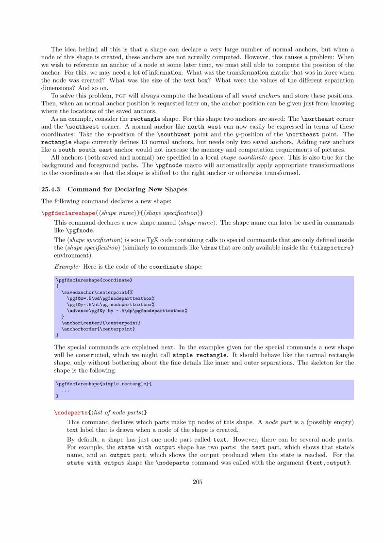
The idea behind all this is that a shape can declare a very large number of normal anchors, but when anode of this shape is created, these anchors are not actually computed. However, this causes a problem: Whenwe wish to reference an anchor of a node at some later time, we must still able to compute the position of theanchor. For this, we may need a lot of information: What was the transformation matrix that was in force whenthe node was created? What was the size of the text box? What were the values of the different separationdimensions? And so on.

To solve this problem, pgf will always compute the locations of all saved anchors and store these positions.Then, when an normal anchor position is requested later on, the anchor position can be given just from knowingwhere the locations of the saved anchors.

As an example, consider the rectangle shape. For this shape two anchors are saved: The \northeast cornerand the \southwest corner. A normal anchor like north west can now easily be expressed in terms of thesecoordinates: Take the x-position of the \southwest point and the y-position of the \northeast point. Therectangle shape currently defines 13 normal anchors, but needs only two saved anchors. Adding new anchorslike a south south east anchor would not increase the memory and computation requirements of pictures.

All anchors (both saved and normal) are specified in a local shape coordinate space. This is also true for thebackground and foreground paths. The \pgfnode macro will automatically apply appropriate transformationsto the coordinates so that the shape is shifted to the right anchor or otherwise transformed.

25.4.3 Command for Declaring New Shapes

The following command declares a new shape:

\pgfdeclareshape{⟨shape name⟩}{⟨shape specification⟩}This command declares a new shape named ⟨shape name⟩. The shape name can later be used in commandslike \pgfnode.The ⟨shape specification⟩ is some TEX code containing calls to special commands that are only defined insidethe ⟨shape specification⟩ (similarly to commands like \draw that are only available inside the {tikzpicture}environment).

Example: Here is the code of the coordinate shape:

\pgfdeclareshape{coordinate}

{

\savedanchor\centerpoint{%

\pgf@x=.5\wd\pgfnodeparttextbox%

\pgf@y=.5\ht\pgfnodeparttextbox%

\advance\pgf@y by -.5\dp\pgfnodeparttextbox%

}

\anchor{center}{\centerpoint}

\anchorborder{\centerpoint}

}

The special commands are explained next. In the examples given for the special commands a new shapewill be constructed, which we might call simple rectangle. It should behave like the normal rectangleshape, only without bothering about the fine details like inner and outer separations. The skeleton for theshape is the following.

\pgfdeclareshape{simple rectangle}{

...

}

\nodeparts{⟨list of node parts⟩}This command declares which parts make up nodes of this shape. A node part is a (possibly empty)text label that is drawn when a node of the shape is created.By default, a shape has just one node part called text. However, there can be several node parts.For example, the state with output shape has two parts: the text part, which shows that state’sname, and an output part, which shows the output produced when the state is reached. For thestate with output shape the \nodeparts command was called with the argument {text,output}.

205

When a multipart node is created, the text labels are drawn in the sequences listed in the ⟨list of nodeparts⟩. For each node part there you must have declared one anchor and the TEX-box of the partis placed at this anchor. For a node part called XYZ the TEX-box \pgfnodepartXYZbox is placed atanchor XYZ.

\savedanchor{⟨command⟩}{⟨code⟩}This command declares a saved anchor. The argument ⟨command⟩ should be a TEX macro name like\centerpoint.The ⟨code⟩ will be executed each time \pgfnode (or \pgfmultipartnode) is called to create a node ofthe shape ⟨shape name⟩. When the ⟨code⟩ is executed, the TEX-boxes of the node parts will containthe text labels of the node. Possibly, these box are void. For example, if there is just a text part, thenode \pgfnodeparttextbox will be setup when the ⟨code⟩ is executed.The ⟨code⟩ can use the width, height, and depth of the box(es) to compute the location of the savedanchor. In addition, the ⟨code⟩ can take into account the values of dimensions like \pgfshapeminwidthor \pgfshapeinnerxsep. Furthermore, the ⟨code⟩ can take into consideration the values of any furthershape-specific variables that are set at the moment when \pgfnode is called.The net effect of the ⟨code⟩ should be to set the two TEX dimensions \pgf@x and \pgf@y. One way toachieve this is to say \pgfpoint{⟨x value⟩}{⟨y value⟩} at the end of the ⟨code⟩, but you can also justset these variables. The values that \pgf@x and \pgf@y have after the code has been executed, let uscall them x and y, will be recorded and stored together with the node that is created by the command\pgfnode.The macro ⟨command⟩ is defined to be \pgfpoint{x}{y}. However, the ⟨command⟩ is only locallydefined while anchor positions are being computed. Thus, it is possible to use very simple names for⟨command⟩, like \center or \a, without causing a name-clash. (To be precise, very simple ⟨command⟩names will clash with existing names, but only locally inside the computation of anchor positions; andwe do not need the normal \center command during these computations.)For our simple rectangle shape, we will need only one saved anchor: The upper right corner. Thelower left corner could either be the origin or the “mirrored” upper right corner, depending on whetherwe want the text label to have its lower left corner at the origin or whether the text label should becentered on the origin. Either will be fine, for the final shape this will make no difference since theshape will be shifted anyway. So, let us assume that the text label is centered on the origin (this willbe specified later on using the text anchor). We get the following code for the upper right corner:

\savedanchor{\upperrightcorner}{

\pgf@y=.5\ht\pgfnodeparttextbox % height of the box, ignoring the depth

\pgf@x=.5\wd\pgfnodeparttextbox % width of the box

}

If we wanted to take, say, the \pgfshapeminwidth into account, we could use the following code:

\savedanchor{\upperrightcorner}{

\pgf@y=.\ht\pgfnodeparttextbox % height of the box

\pgf@x=.\wd\pgfnodeparttextbox % width of the box

\setlength{\pgf@xa}{\pgfshapeminwidth}

\ifdim\pgf@x<.5\pgf@xa

\pgf@x=.5\pgf@xa

\fi

}

Note that we could not have written .5\pgfshapeminwidth since the minium width is stored in a“plain text macro,” not as a real dimension. So if \pgfshapeminwidth depth were 2cm, writing.5\pgfshapeminwidth would yield the same as .52cm.In the “real” rectangle shape the code is somewhat more complex, but you get the basic idea.

\saveddimen{⟨command⟩}{⟨code⟩}This command is similar to \savedanchor, only instead of setting ⟨command⟩ to \pgfpoint{x}{y},the ⟨command⟩ is set just to (the value of) x.

206

In the simple rectangle shape we might use a saved dimension to store the depth of the shape box.

\shapedimen{\depth}{

\pgf@x=\dp\pgfnodeparttextbox

}

\anchor{⟨name⟩}{⟨code⟩}This command declares an anchor named ⟨name⟩. Unlike for saved anchors, the ⟨code⟩ will not beexecuted each time a node is declared. Rather, the ⟨code⟩ is only executed when the anchor is specificallyrequested; either for anchoring the node during its creation or as a position in the shape referencedlater on.The ⟨name⟩ is a quite arbitrary string that is not “passed down” to the system level. Thus, names likesouth or 1 or :: would all be fine.A saved anchor is not automatically also a normal anchor. If you wish to give the users access to asaved anchor you must declare a normal anchor that just returns the position of the saved anchor.When the ⟨code⟩ is executed, all saved anchor macros will be defined. Thus, you can reference themin your ⟨code⟩. The effect of the ⟨code⟩ should be to set the values of \pgf@x and \pgf@y to thecoordinates of the anchor.Let us consider some example for the simple rectangle shape. First, we would like to make the upperright corner publicly available, for example as north east:

\anchor{north east}{\upperrightcorner}

The \upperrightcorner macro will set \pgf@x and \pgf@y to the coordinates of the upper rightcorner. Thus, \pgf@x and \pgf@y will have exactly the right values at the end of the anchor’s code.Next, let us define a north west anchor. For this anchor, we can negate the \pgf@x variable:

\anchor{north west}{

\upperrightcorner

\pgf@x=-\pgf@x

}

Finally, it is a good idea to always define a center anchor, which will be the default location for ashape.

\anchor{center}{\pgfpointorigin}

You might wonder whether we should not take into consideration that the node is not placed at theorigin, but has been shifted somewhere. However, the anchor positions are always specified in theshape’s “private” coordinate system. The “outer” transformation that has been applied to the shapeupon its creation is applied automatically to the coordinates returned by the anchor’s ⟨code⟩.Out simple rectangle only has one text label (node part) called text. This is the default situation,so we need not do anything. For the text node part we must setup a text anchor. This anchor isused upon creation of a node to determine the lower left corner of the text label (within the privatecoordinate system of the shape). By default, the text anchor is at the origin, but you may change this.For example, we would say

\anchor{text}{%

\upperrightcorner%

\pgf@x=-\pgf@x%

\pgf@y=-\pgf@y%

}

to center the text label on the origin in the shape coordinate space. Note that we could not havewritten the following:

\anchor{text}{\pgfpoint{-.5\wd\pgfnodeparttextbox}{-.5\ht\pgfnodeparttextbox}}

207

Do you see why this is wrong? The problem is that the box \pgfnodeparttextbox will most likely nothave the correct size when the anchor is computed. After all, the anchor position might be recomputedat a time when several other nodes have been created.If a shape has several node parts, we would have to define an anchor for each part.

\anchorborder{⟨code⟩}A border anchor is an anchor point on the border of the shape. What exactly is considered as the“border” of the shape depends on the shape.When the user request a point on the border of the shape using the \pgfpointshapeborder command,the ⟨code⟩ will be executed to discern this point. When the execution of the ⟨code⟩ starts, the dimensions\pgf@x and \pgf@y will have been set to a location p in the shape’s coordinate system. It is now the jobof the ⟨code⟩ to setup \pgf@x and \pgf@y such that they specify the point on the shape’s border thatlies on a straight line from the shape’s center to the point p. Usually, this is a somewhat complicatedcomputation, involving many case distinctions and some basic math.For our simple rectangle we must compute a point on the border of a rectangle whose one corneris the origin (ignoring the depth for simplicity) and whose other corner is \upperrightcorner. Thefollowing code might be used:

\anchorborder{%

% Call a function that computes a border point. Since this

% function will modify dimensions like \pgf@x, we must move them to

% other dimensions.

\@tempdima=\pgf@x

\@tempdimb=\pgf@y

\pgfpointborderrectangle{\pgfpoint{\@tempdima}{\@tempdimb}}{\upperrightcorner}

}

\backgroundpath{⟨code⟩}This command specifies the path that “makes up” the background of the shape. Note that the shapecannot prescribe what is going to happen with the path: It might be drawn, shaded, filled, or eventhrown away. If you want to specify that something should “always” happen when this shape is drawn(for example, if the shape is a stop-sign, we always want it to be filled with a red color), you can usecommands like \beforebackgroundpath, explained below.When the ⟨code⟩ is executed, all saved anchors will be in effect. The ⟨code⟩ should contain pathconstruction commands.For our simple rectangle, the following code might be used:

\backgroundpath{

\pgfpathrectanglecorners

{\upperrightcorner}

{\pgfpointscale{-1}{\upperrightcorner}}

}

As the name suggests, the background path is used “behind” the text labels. Thus, this path is usedfirst, then the text labels are drawn, possibly obscuring part of the path.

\foregroundpath{⟨code⟩}This command works like \backgroundpath, only it is invoked after the text labels have been drawn.This means that this path can possibly obscure (part of) the text labels.

\behindbackgroundpath{⟨code⟩}Unlike the previous two commands, ⟨code⟩ should not only construct a path, it should also use thispath in whatever way is appropriate. For example, the ⟨code⟩ might fill some area with a uniform color.Whatever the ⟨code⟩ does, it does it first. This means that any drawing done by ⟨code⟩ will be evenbehind the background path.Note that the ⟨code⟩ is protected with a {pgfscope}.

208

\beforebackgroundpath{⟨code⟩}This command works like \behindbackgroundpath, only the ⟨code⟩ is executed after the backgroundpath has been used, but before the texts label are drawn.

\behindforegroundpath{⟨code⟩}The ⟨code⟩ is executed after the text labels have been drawn, but before the foreground path is used.

\beforeforegroundpath{⟨code⟩}This ⟨code⟩ is executed at the very end.

\inheritsavedanchors[from={⟨another shape name⟩}]This command allows you to inherit the code for saved anchors from ⟨another shape name⟩. The ideais that if you wish to create a new shape that is just a small modification of a another shape, you canrecycle the code used for ⟨another shape name⟩.The effect of this command is the same as if you had called \savedanchor and \saveddimen foreach saved anchor or saved dimension declared in ⟨another shape name⟩. Thus, it is not possible to“selectively” inherit only some saved anchors, you always have to inherit all saved anchors from anothershape. However, you can inherit the saved anchors of more than one shape by calling this commandseveral times.

\inheritbehindbackgroundpath[from={⟨another shape name⟩}]This command can be used to inherit the code used for the drawings behind the background path from⟨another shape name⟩.

\inheritbackgroundpath[from={⟨another shape name⟩}]Inherits the background path code from ⟨another shape name⟩.

\inheritbeforebackgroundpath[from={⟨another shape name⟩}]Inherits the before background path code from ⟨another shape name⟩.

\inheritbehindforegroundpath[from={⟨another shape name⟩}]Inherits the behind foreground path code from ⟨another shape name⟩.

\inheritforegroundpath[from={⟨another shape name⟩}]Inherits the foreground path code from ⟨another shape name⟩.

\inheritbeforeforegroundpath[from={⟨another shape name⟩}]Inherits the before foreground path code from ⟨another shape name⟩.

\inheritanchor[from={⟨another shape name⟩}]{⟨name⟩}Inherits the code of one specific anchor named ⟨name⟩ from ⟨another shape name⟩. Thus, unlike savedanchors, which must be inherited collectively, normal anchors can and must be inherited individually.

\inheritanchorborder[from={⟨another shape name⟩}]Inherits the border anchor code from ⟨another shape name⟩.

The following example shows how a shape can be defined that relies heavily on inheritance:

209

.

.

.

Remark

.

Use Case

\pgfdeclareshape{document}{

\inheritsavedanchors[from=rectangle] % this is nearly a rectangle

\inheritanchorborder[from=rectangle]

\inheritanchor[from=rectangle]{center}

\inheritanchor[from=rectangle]{north}

\inheritanchor[from=rectangle]{south}

\inheritanchor[from=rectangle]{west}

\inheritanchor[from=rectangle]{east}

% ... and possibly more

\backgroundpath{% this is new

% store lower right in xa/ya and upper right in xb/yb

\southwest \pgf@xa=\pgf@x \pgf@ya=\pgf@y

\northeast \pgf@xb=\pgf@x \pgf@yb=\pgf@y

% compute corner of ‘‘flipped page’’

\pgf@xc=\pgf@xb \advance\pgf@xc by-5pt % this should be a parameter

\pgf@yc=\pgf@yb \advance\pgf@yc by-5pt

% construct main path

\pgfpathmoveto{\pgfpoint{\pgf@xa}{\pgf@ya}}

\pgfpathlineto{\pgfpoint{\pgf@xa}{\pgf@yb}}

\pgfpathlineto{\pgfpoint{\pgf@xc}{\pgf@yb}}

\pgfpathlineto{\pgfpoint{\pgf@xb}{\pgf@yc}}

\pgfpathlineto{\pgfpoint{\pgf@xb}{\pgf@ya}}

\pgfpathclose

% add little corner

\pgfpathmoveto{\pgfpoint{\pgf@xc}{\pgf@yb}}

\pgfpathlineto{\pgfpoint{\pgf@xc}{\pgf@yc}}

\pgfpathlineto{\pgfpoint{\pgf@xb}{\pgf@yc}}

\pgfpathlineto{\pgfpoint{\pgf@xc}{\pgf@yc}}

}

}\hskip-1.2cm

\begin{tikzpicture}

\node[shade,draw,shape=document,inner sep=2ex] (x) {Remark};

\node[fill=examplefill,draw,ellipse,double]

at ([shift=(-80:3cm)]x) (y) {Use Case};

\draw[dashed] (x) -- (y);

\end{tikzpicture}

25.5 Predefined Shapes

Shape coordinate

The coordinate is mainly intended to be used to store locations using the node mechanism. This shapedoes not have any background path and options like draw have no effect on it. Also, it does not have anynode parts, so no text is drawn when this shape is used.TikZ handles this shape in a special way, see Section 11.8.

Shape rectangle

This shape is a rectangle tightly fitting the text box. Use inner or outer separation to increase the distancebetween the text box and the border and the anchors. The following figure shows the anchors defined bythis shape; the anchors 10 and 130 are example of border anchors.

210

.

.

Rectangle.

(s.north west)

.

(s.north)

.

(s.north east)

.

(s.west)

.

(s.center)

.

(s.east)

.

(s.mid west)

.

(s.mid)

.

(s.mid east)

.

(s.base west)

.

(s.base)

.

(s.base east)

.

(s.south west)

.

(s.south)

.

(s.south east)

.

(s.text)

.

(s.10)

.

(s.130)

\Huge

\begin{tikzpicture}

\node[name=s,shape=rectangle,style=shape example] {Rectangle\vrule width 1pt height 2cm};








\draw[shift=(s.\anchor)] plot[mark=x] coordinates {(0,0)}


\end{tikzpicture}

Shape circle

This shape is a circle tightly fitting the text box.

.

.

Circle

.

(s.north west)

.

(s.north)

.

(s.north east)

.

(s.west)

.

(s.center)

.

(s.east)

.

(s.mid west)

.

(s.mid)

.

(s.mid east)

.

(s.base west)

.

(s.base)

.

(s.base east)

.

(s.south west)

.

(s.south)

.

(s.south east)

.

(s.text)

.

(s.10)

.

(s.130)

211

\Huge

\begin{tikzpicture}

\node[name=s,shape=circle,style=shape example] {Circle\vrule width 1pt height 2cm};








\draw[shift=(s.\anchor)] plot[mark=x] coordinates {(0,0)}


\end{tikzpicture}

212

26 Coordinate and Canvas Transformations

26.1 Overview

pgf offers two different ways of scaling, shifting, and rotating (these operations are generally known as trans-formations) graphics: You can apply coordinate transformations to all coordinates and you can apply canvastransformations to the canvas on which you draw. (The names “coordinate” and “canvas” transformations arenot standard, I introduce them only for the purposes of this manual.)

The difference is the following:

• As the name “coordinate transformation” suggests, coordinate transformations apply only to coordi-nates. For example, when you specify a coordinate like \pgfpoint{1cm}{2cm} and you wish to “use”this coordinate—for example as an argument to a \pgfpathmoveto command—then the coordinate trans-formation matrix is applied to the coordinate, resulting in a new coordinate. Continuing the example, ifthe current coordinate transformation is “scale by a factor of two,” the coordinate \pgfpoint{1cm}{2cm}actually designates the point (2cm, 4cm).

Note that coordinate transformations apply only to coordinates. They do not apply to, say, line width orshadings or text.

• The effect of a “canvas transformation” like “scale by a factor of two” can be imagined as follows: Youfirst draw your picture on a “rubber canvas” normally. Then, once you are done, the whole canvas istransformed, in this case stretched by a factor of two. In the resulting image everything will be larger:Text, lines, coordinates, and shadings.

In many cases, it is preferable that you use coordinate transformations and not canvas transformations.When canvas transformations are used, pgf looses track of the coordinates of nodes and shapes. Also, canvastransformations often cause undesirable effects like changing text size. For these reasons, pgf makes it easy tosetup the coordinate transformation, but a bit harder to change the canvas transformation.

26.2 Coordinate Transformations

26.2.1 How PGF Keeps Track of the Coordinate Transformation Matrix

pgf has an internal coordinate transformation matrix. This matrix is applied to coordinates “in certain situa-tions.” This means that the matrix is not always applied to every coordinate “no matter what.” Rather, pgftries to be reasonably smart at when and how this matrix should be applied. The most prominent examples arethe path construction commands, which apply the coordinate transformation matrix to their inputs.

The coordinate transformation matrix consists of four numbers a, b, c, and d, and two dimensions s andt. When the coordinate transformation matrix is applied to a coordinate (x, y) the new coordinate (ax + by +s, cx+dy + t) results. For more details on how transformation matrices work in general, please see, for example,the pdf or PostScript reference or a textbook on computer graphics.

The coordinate transformation matrix is equal to the identity matrix at the beginning. More precisely, a = 1,b = 0, c = 0, d = 1, s = 0pt, and t = 0pt.

The different coordinate transformation commands will modify the matrix by concatenating it with anothertransformation matrix. This way the effect of applying several transformation commands will accumulate.

The coordinate transformation matrix is local to the current TEX group (unlike the canvas transformationmatrix, which is local to the current {pgfscope}). Thus, the effect of adding a coordinate transformation tothe coordinate transformation matrix will last only till the end of the current TEX group.

26.2.2 Commands for Relative Coordinate Transformations

The following commands add a basic coordinate transformation to the current coordinate transformation matrix.For all commands, the transformation is applied in addition to any previous coordinate transformations.

\pgftransformshift{⟨point⟩}Shifts coordinates by ⟨point⟩.

213

.

\begin{tikzpicture}


\draw (0,0) -- (2,1) -- (1,0);


\draw[red] (0,0) -- (2,1) -- (1,0);

\end{tikzpicture}

\pgftransformxshift{⟨dimensions⟩}Shifts coordinates by ⟨dimension⟩ along the x-axis.

.

\begin{tikzpicture}


\draw (0,0) -- (2,1) -- (1,0);

\pgftransformxshift{.5cm}

\draw[red] (0,0) -- (2,1) -- (1,0);

\end{tikzpicture}

\pgftransformyshift{⟨dimensions⟩}Like \pgftransformxshift, only for the y-axis.

\pgftransformscale{⟨factor⟩}Scales coordinates by ⟨factor⟩.

.

\begin{tikzpicture}


\draw (0,0) -- (2,1) -- (1,0);

\pgftransformscale{.75}

\draw[red] (0,0) -- (2,1) -- (1,0);

\end{tikzpicture}

\pgftransformxscale{⟨factor⟩}Scales coordinates by ⟨factor⟩ in the x-direction.

.

\begin{tikzpicture}


\draw (0,0) -- (2,1) -- (1,0);

\pgftransformxscale{.75}

\draw[red] (0,0) -- (2,1) -- (1,0);

\end{tikzpicture}

\pgftransformyscale{⟨factor⟩}Like \pgftransformxscale, only for the y-axis.

\pgftransformxslant{⟨factor⟩}Slants coordinates by ⟨factor⟩ in the x-direction. Here, a factor of 1 means 45◦.

.

\begin{tikzpicture}


\draw (0,0) -- (2,1) -- (1,0);

\pgftransformxslant{.5}

\draw[red] (0,0) -- (2,1) -- (1,0);

\end{tikzpicture}

214

\pgftransformyslant{⟨factor⟩}Slants coordinates by ⟨factor⟩ in the y-direction.

.

\begin{tikzpicture}


\draw (0,0) -- (2,1) -- (1,0);

\pgftransformyslant{-1}

\draw[red] (0,0) -- (2,1) -- (1,0);

\end{tikzpicture}

\pgftransformrotate{⟨degrees⟩}Rotates coordinates counterclockwise by ⟨degrees⟩.

.

\begin{tikzpicture}


\draw (0,0) -- (2,1) -- (1,0);


\draw[red] (0,0) -- (2,1) -- (1,0);

\end{tikzpicture}

\pgftransformcm{⟨a⟩}{⟨b⟩}{⟨c⟩}{⟨d⟩}{⟨point⟩}Applies the transformation matrix given by a, b, c, and d and the shift ⟨point⟩ to coordinates (in additionto any previous transformations already in force).

.

\begin{tikzpicture}


\draw (0,0) -- (2,1) -- (1,0);

\pgftransformcm{1}{1}{0}{1}{\pgfpoint{.25cm}{.25cm}}

\draw[red] (0,0) -- (2,1) -- (1,0);

\end{tikzpicture}

\pgftransformarrow{⟨start⟩}{⟨end⟩}Shift coordinates to the end of the line going from ⟨start⟩ to ⟨end⟩ with the correct rotation.

.

.

tip

\begin{tikzpicture}


\draw (0,0) -- (3,1);

\pgftransformarrow{\pgfpointorigin}{\pgfpoint{3cm}{1cm}}

\pgftext{tip}

\end{tikzpicture}

\pgftransformlineattime{⟨time⟩}{⟨start⟩}{⟨end⟩}Shifts coordinates by a specific point on a line at a specific time. The point by which the coordinate isshifted is calculated by calling \pgfpointlineattime, see Section 20.4.2.In addition to shifting the coordinate, a rotation may also be applied. Whether this is the case depends onwhether the TEX if \ifpgfslopedattime is set to true or not.

.

.

Hi!

\begin{tikzpicture}


\draw (0,0) -- (2,1);

\pgftransformlineattime{.25}{\pgfpointorigin}{\pgfpoint{2cm}{1cm}}

\pgftext{Hi!}

\end{tikzpicture}

215

.

.

Hi!

\begin{tikzpicture}


\draw (0,0) -- (2,1);

\pgfslopedattimetrue


\pgftext{Hi!}

\end{tikzpicture}

There is another TEX if that influences this command. If you set \ifpgfresetnontranslationattime totrue, then, between shifting the coordinate and (possibly) rotating/sloping the coordinate, the command\pgftransformresetnontranslations is called. See the description of this command for details.

.

.

Hi!

\begin{tikzpicture}


\pgftransformscale{1.5}

\draw (0,0) -- (2,1);


\pgfresetnontranslationattimefalse


\pgftext{Hi!}

\end{tikzpicture}

.

.

Hi!

\begin{tikzpicture}


\pgftransformscale{1.5}

\draw (0,0) -- (2,1);


\pgfresetnontranslationattimetrue


\pgftext{Hi!}

\end{tikzpicture}

\pgftransformcurveattime{⟨time⟩}{⟨start⟩}{⟨first support⟩}{⟨second support⟩}{⟨end⟩}Shifts coordinates by a specific point on a curve at a specific time, see Section 20.4.2 once more.As for the line-at-time transformation command, \ifpgfslopedattime decides whether an additional ro-tation should be applied.

.

.

Hi!

\begin{tikzpicture}



\pgftransformcurveattime{.25}{\pgfpointorigin}


\pgftext{Hi!}

\end{tikzpicture}

.

.

Hi!

\begin{tikzpicture}




\pgftransformcurveattime{.25}{\pgfpointorigin}


\pgftext{Hi!}

\end{tikzpicture}

The value of \ifpgfresetnontranslationsattime is also taken into account.

\ifpgfslopedattime

Decides whether the “at time” transformation commands also rotate coordinates or not.

\ifpgfresetnontranslationsattime

Decides whether the “at time” transformation commands should reset the non-translations between shiftingand rotating.

216

26.2.3 Commands for Absolute Coordinate Transformations

The coordinate transformation commands introduced up to now are always applied in addition to any previoustransformations. In contrast, the commands presented in the following can be used to change the transformationmatrix “absolutely.” Note that this is, in general, dangerous and will often produce unexpected effects. Youshould use these commands only if you really know what you are doing.

\pgftransformreset

Resets the coordinate transformation matrix to the identity matrix. Thus, once this command is given notransformations are applied till the end of the scope.

.

\begin{tikzpicture}



\draw (0,0) -- (2,1) -- (1,0);

\pgftransformreset

\draw[red] (0,0) -- (2,1) -- (1,0);

\end{tikzpicture}


This command sets the a, b, c, and d part of the coordinate transformation matrix to a = 1, b = 0, c = 0,and d = 1. However, the current shifting of the matrix is not modified.The effect of this command is that any rotation/scaling/slanting is undone in the current TEX group, butthe origin is not “moved back.”This command is mostly useful directly before a \pgftext command to ensure that the text is not scaledor rotated.

.

.

rotate

d

.

shifted only

\begin{tikzpicture}


\pgftransformscale{2}


\pgftransformxshift{1cm}

{\color{red}\pgftext{rotated}}


\pgftext{shifted only}

\end{tikzpicture}

\pgftransforminvert

Replaces the coordinate transformation matrix by a coordinate transformation matrix that “exactly undoesthe original transformation.” For example, if the original transformation was “scale by 2 and then shiftright by 1cm” the new one is “shift left by 1cm and then scale by 1/2.”This command will produce an error if the determinant of the matrix is too small, that is, if the matrix isnear-singular.

.

\begin{tikzpicture}



\draw (0,0) -- (2,1) -- (1,0);

\pgftransforminvert

\draw[red] (0,0) -- (2,1) -- (1,0);

\end{tikzpicture}

26.2.4 Saving and Restoring the Coordinate Transformation Matrix

There are two commands for saving and restoring coordinate transformation matrices.

217

\pgfgettransform{⟨macro⟩}This command will (locally) define ⟨macro⟩ to a representation of the current coordinate transformationmatrix. This matrix can later on be reinstalled using \pgfsettransform.

\pgfsettransform{⟨macro⟩}Reinstalls a coordinate transformation matrix that was previously saved using \pgfgettransform.

26.3 Canvas Transformations

The canvas transformation matrix is not managed by pgf, but by the output format like pdf or PostScript. Allthe pgf does is to call appropriate low-level \pgfsys@ commands to change the canvas transformation matrix.

Unlike coordinate transformations, canvas transformations apply to “everything,” including images, text,shadings, line thickness, and so on. The idea is that a canvas transformation really stretches and deforms thecanvas after the graphic is finished.

Unlike coordinate transformations, canvas transformations are local to the current {pgfscope}, not to thecurrent TEX group. This is due to the fact that they are managed by the backend driver, not by TEX or pgf.

Unlike the coordinate transformation matrix, it is not possible to “reset” the canvas transformation matrix.The only way to change it is to concatenate it with another canvas transformation matrix or to end the current{pgfscope}.

Unlike coordinate transformations, pgf does not “keep track” of canvas transformations. In particular, itwill not be able to correctly save the coordinates of shapes or nodes when a canvas transformation is used.

pgf does not offer a whole set of special commands for modifying the canvas transformation matrix. Instead,different commands allow you to concatenate the canvas transformation matrix with a coordinate transformationmatrix (and there are numerous commands for specifying a coordinate transformation, see the previous section).

\pgflowlevelsynccm

This command concatenates the canvas transformation matrix with the current coordinate transformationmatrix. Afterward, the coordinate transformation matrix is reset.The effect of this command is to “synchronize” the coordinate transformation matrix and the canvas trans-formation matrix. All transformations that were previously applied by the coordinate transformationsmatrix are now applied by the canvas transformation matrix.

.

\begin{tikzpicture}



\pgftransformscale{5}

\draw (0,0) -- (0.4,.2);

\pgftransformxshift{0.2cm}

\pgflowlevelsynccm

\draw[red] (0,0) -- (0.4,.2);

\end{tikzpicture}

\pgflowlevel{⟨transformation code⟩}This command concatenates the canvas transformation matrix with the coordinate transformation specifiedby ⟨transformation code⟩.

.

\begin{tikzpicture}



\pgflowlevel{\pgftransformscale{5}}

\draw (0,0) -- (0.4,.2);

\end{tikzpicture}

\pgflowlevelobj{⟨transformation code⟩}{⟨code⟩}This command creates a local {pgfscope}. Inside this scope, \pgflowlevel is first called with the argument⟨transformation code⟩, then the ⟨code⟩ is inserted.

218

.

\begin{tikzpicture}



\pgflowlevelobj{\pgftransformscale{5}} {\draw (0,0) -- (0.4,.2);}

\pgflowlevelobj{\pgftransformxshift{-1cm}}{\draw (0,0) -- (0.4,.2);}

\end{tikzpicture}

\begin{pgflowlevelscope}{⟨transformation code⟩}⟨environment contents⟩

\end{pgflowlevelscope}

This environment first surrounds the ⟨environment contents⟩ by a {pgfscope}. Then it calls \pgflowlevelwith the argument ⟨transformation code⟩.

.

\begin{tikzpicture}



\begin{pgflowlevelscope}{\pgftransformscale{5}}

\draw (0,0) -- (0.4,.2);


\begin{pgflowlevelscope}{\pgftransformxshift{-1cm}}

\draw (0,0) -- (0.4,.2);


\end{tikzpicture}

219

27 Declaring and Using Images

This section describes the pgfbaseimage package.

\usepackage{pgfbaseimage} % LATEX\input pgfbaseimage.tex % plain TEX\input pgfbaseimage.tex % ConTEXt

This package offers an abstraction of the image inclusion process. It is loaded automatically by pgf, butyou can load it manually if you have only included pgfcore.

27.1 Overview

To be quite frank, LATEX’s \includegraphics is designed better than pgfbaseimage. For this reason, I recom-mend that you use the standard image inclusion mechanism of your format. Thus, LATEX users are encouragedto use \includegraphics to include images.

However, there are reasons why you might need to use the image inclusion facilities of pgf:

• There is no standard image inclusion mechanism in your format. For example, plain TEX does not haveone, so pgf’s inclusion mechanism is “better than nothing.”

However, this applies only to the pdftex backend. For all other backends, pgf currently maps its commandsback to the graphicx package. Thus, in plain TEX, this does not really help. It might be a good ideato fix this in the future such that pgf becomes independent of LATEX, thereby providing a uniform imageabstraction for all formats.

• You wish to use masking. This is a feature that is only supported by pgf, though I hope that someonewill implement this also for the graphics package in LATEX in the future.

Whatever your choice, you can still use the usual image inclusion facilities of the graphics package.The general approach taken by pgf to including an image is the following: First, \pgfdeclareimage declares

the image. This must be done prior to the first use of the image. Once you have declared an image, you caninsert it into the text using \pgfuseimage. The advantage of this two-phase approach is that, at least for pdf,the image data will only be included once in the file. This can drastically reduce the file size if you use an imagerepeatedly, for example in an overlay. However, there is also a command called \pgfimage that declares andthen immediately uses the image.

To speedup the compilation, you may wish to use the following class option:

\usepackage[draft]{pgf}

In draft mode boxes showing the image name replace the images. It is checked whether the image files exist,but they are not read. If either height or width is not given, 1cm is used instead.

27.2 Declaring an Image

\pgfdeclareimage[⟨options⟩]{⟨image name⟩}{⟨filename⟩}Declares an image, but does not paint anything. To draw the image, use \pgfuseimage{⟨image name⟩}.The ⟨filename⟩ may not have an extension. For pdf, the extensions .pdf, .jpg, and .png will automaticallytried. For PostScript, the extensions .eps, .epsi, and .ps will be tried.The following options are possible:

• height=⟨dimension⟩ sets the height of the image. If the width is not specified simultaneously, theaspect ratio of the image is kept.

• width=⟨dimension⟩ sets the width of the image. If the height is not specified simultaneously, the aspectratio of the image is kept.

• page=⟨page number⟩ selects a given page number from a multipage document. Specifying this optionwill have the following effect: first, pgf tries to find a file named

⟨filename⟩.page⟨page number⟩.⟨extension⟩

220

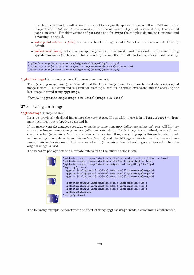
If such a file is found, it will be used instead of the originally specified filename. If not, pgf inserts theimage stored in ⟨filename⟩.⟨extension⟩ and if a recent version of pdflatex is used, only the selectedpage is inserted. For older versions of pdflatex and for dvips the complete document is inserted anda warning is printed.

• interpolate=⟨true or false⟩ selects whether the image should “smoothed” when zoomed. False bydefault.

• mask=⟨mask name⟩ selects a transparency mask. The mask must previously be declared using\pgfdeclaremask (see below). This option only has an effect for pdf. Not all viewers support masking.

\pgfdeclareimage[interpolate=true,height=1cm]{image1}{pgf-tu-logo}

\pgfdeclareimage[interpolate=true,width=1cm,height=1cm]{image2}{pgf-tu-logo}


\pgfaliasimage{⟨new image name⟩}{⟨existing image name⟩}The {⟨existing image name⟩} is “cloned” and the {⟨new image name⟩} can now be used whenever originalimage is used. This command is useful for creating aliases for alternate extensions and for accessing thelast image inserted using \pgfimage.

Example: \pgfaliasimage{image.!30!white}{image.!25!white}

27.3 Using an Image

\pgfuseimage{⟨image name⟩}Inserts a previously declared image into the normal text. If you wish to use it in a {pgfpicture} environ-ment, you must put a \pgftext around it.If the macro \pgfalternateextension expands to some nonempty ⟨alternate extension⟩, pgf will first tryto use the image names ⟨image name⟩.⟨alternate extension⟩. If this image is not defined, pgf will nextcheck whether ⟨alternate extension⟩ contains a ! character. If so, everything up to this exclamation markand including it is deleted from ⟨alternate extension⟩ and the pgf again tries to use the image ⟨imagename⟩.⟨alternate extension⟩. This is repeated until ⟨alternate extension⟩ no longer contains a !. Then theoriginal image is used.The xxcolor package sets the alternate extension to the current color mixin.

.

.

.

.

\pgfdeclareimage[interpolate=true,width=1cm,height=1cm]{image1}{pgf-tu-logo}

\pgfdeclareimage[interpolate=true,width=1cm]{image2}{pgf-tu-logo}


\begin{pgfpicture}

\pgftext[at=\pgfpoint{1cm}{5cm},left,base]{\pgfuseimage{image1}}



\pgfpathrectangle{\pgfpoint{1cm}{5cm}}{\pgfpoint{1cm}{1cm}}



\pgfusepath{stroke}

\end{pgfpicture}

The following example demonstrates the effect of using \pgfuseimage inside a color mixin environment.

221

.

.

.

.

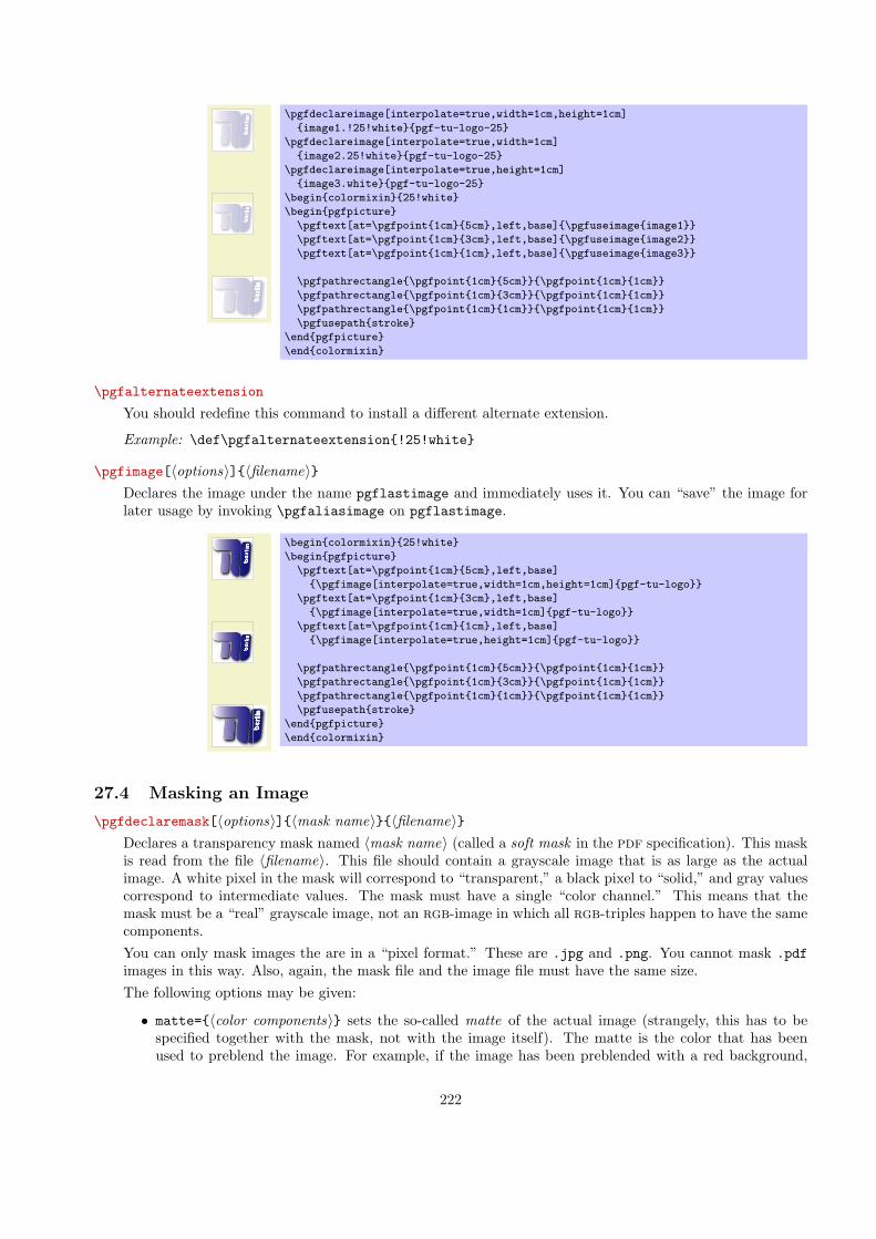
\pgfdeclareimage[interpolate=true,width=1cm,height=1cm]

{image1.!25!white}{pgf-tu-logo-25}

\pgfdeclareimage[interpolate=true,width=1cm]

{image2.25!white}{pgf-tu-logo-25}

\pgfdeclareimage[interpolate=true,height=1cm]

{image3.white}{pgf-tu-logo-25}


\begin{pgfpicture}







\pgfusepath{stroke}

\end{pgfpicture}

\end{colormixin}

\pgfalternateextension

You should redefine this command to install a different alternate extension.

Example: \def\pgfalternateextension{!25!white}

\pgfimage[⟨options⟩]{⟨filename⟩}Declares the image under the name pgflastimage and immediately uses it. You can “save” the image forlater usage by invoking \pgfaliasimage on pgflastimage.

.

.

.

.


\begin{pgfpicture}

\pgftext[at=\pgfpoint{1cm}{5cm},left,base]

{\pgfimage[interpolate=true,width=1cm,height=1cm]{pgf-tu-logo}}


{\pgfimage[interpolate=true,width=1cm]{pgf-tu-logo}}


{\pgfimage[interpolate=true,height=1cm]{pgf-tu-logo}}




\pgfusepath{stroke}

\end{pgfpicture}

\end{colormixin}

27.4 Masking an Image

\pgfdeclaremask[⟨options⟩]{⟨mask name⟩}{⟨filename⟩}Declares a transparency mask named ⟨mask name⟩ (called a soft mask in the pdf specification). This maskis read from the file ⟨filename⟩. This file should contain a grayscale image that is as large as the actualimage. A white pixel in the mask will correspond to “transparent,” a black pixel to “solid,” and gray valuescorrespond to intermediate values. The mask must have a single “color channel.” This means that themask must be a “real” grayscale image, not an rgb-image in which all rgb-triples happen to have the samecomponents.You can only mask images the are in a “pixel format.” These are .jpg and .png. You cannot mask .pdfimages in this way. Also, again, the mask file and the image file must have the same size.The following options may be given:

• matte={⟨color components⟩} sets the so-called matte of the actual image (strangely, this has to bespecified together with the mask, not with the image itself). The matte is the color that has beenused to preblend the image. For example, if the image has been preblended with a red background,

222

then ⟨color components⟩ should be set to {1 0 0}. The default is {1 1 1}, which is white in the rgbmodel.The matte is specified in terms of the parent’s image color space. Thus, if the parent is a grayscaleimage, the matte has to be set to {1}.

Example:

%% Draw a large colorful background

\pgfdeclarehorizontalshading{colorful}{5cm}{color(0cm)=(red);

color(2cm)=(green); color(4cm)=(blue); color(6cm)=(red);

color(8cm)=(green); color(10cm)=(blue); color(12cm)=(red);

color(14cm)=(green)}

\hbox{\pgfuseshading{colorful}\hskip-14cm\hskip1cm

\pgfimage[height=4cm]{pgf-apple}\hskip1cm

\pgfimage[height=4cm]{pgf-apple-mask}\hskip1cm

\pgfdeclaremask[matte={1 1 1}]{mymask}{pgf-apple-mask}

\pgfimage[mask=mymask,height=4cm,interpolate=true]{pgf-apple}}

223

28 Declaring and Using Shadings

28.1 Overview

A shading is an area in which the color changes smoothly between different colors. Similarly to an image, ashading must first be declared before it can be used. Also similarly to an image, a shading is put into a TEX-box.Hence, in order to include a shading in a {pgfpicture}, you have to use \pgftext around it.

There are three kinds of shadings: horizontal, vertical, and radial shadings. However, you can rotate andclip shadings like any other graphics object, which allows you to create more complicated shadings. Horizontalshadings could be created by rotating a vertical shading by 90 degrees, but explicit commands for creating bothhorizontal and vertical shadings are included for convenience.

Once you have declared a shading, you can insert it into text using the command \pgfuseshading. This com-mand cannot be used directly in a {pgfpicture}, you have to put a \pgftext around it. The second commandfor using shadings, \pgfshadepath, on the other hand, can only be used inside {pgfpicture} environments. Itwill “fill” the current path with the shading.

A horizontal shading is a horizontal bar of a certain height whose color changes smoothly. You must at leastspecify the colors at the left and at the right end of the bar, but you can also add color specifications for pointsin between. For example, suppose you which to create a bar that is red at the left end, green in the middle, andblue at the end. Suppose you would like the bar to be 4cm long. This could be specified as follows:

rgb(0cm)=(1,0,0); rgb(2cm)=(0,1,0); rgb(4cm)=(0,0,1)

This line means that at 0cm (the left end) of the bar, the color should be red, which has red-green-blue(rgb) components (1,0,0). At 2cm, the bar should be green, and at 4cm it should be blue. Instead of rgb, youcan currently also specify gray as color model, in which case only one value is needed, or color, in which caseyou must provide the name of a color in parentheses. In a color specification the individual specifications mustbe separated using a semicolon, which may be followed by a whitespace (like a space or a newline). Individualspecifications must be given in increasing order.

28.2 Declaring Shadings

\pgfdeclarehorizontalshading[⟨color list⟩]{⟨shading name⟩}{⟨shading height⟩}{⟨color specification⟩}Declares a horizontal shading named ⟨shading name⟩ of the specified ⟨height⟩ with the specified colors. Thelength of the bar is deduced automatically from the maximum dimension in the specification.

\pgfdeclarehorizontalshading{myshadingA}

{1cm}{rgb(0cm)=(1,0,0); color(2cm)=(green); color(4cm)=(blue)}

\pgfuseshading{myshadingA}

The effect of the ⟨color list⟩, which is a comma-separated list of colors, is the following: Normally, when thislist is empty, once a shading has been declared, it becomes “frozen.” This means that even if you change acolor that was used in the declaration of the shading later on, the shading will not change. By specifyinga ⟨color list⟩ you can specify that the shading should be recalculated whenever one of the colors listed inthe list changes (this includes effects like color mixins). Thus, when you specify a ⟨color list⟩, wheneverthe shading is used, pgf first converts the colors in the list to rgb triples using the current values of thecolors and taking any mixins and blends into account. If the resulting rgb triples have not yet been used,a new shading is internally created and used. Note that if the option ⟨color list⟩ is used, then no shading iscreated until the first use of \pgfuseshading. In particular, the colors mentioned in the shading need notbe defined when the declaration is given.When a shading is recalculated because of a change in the colors mentioned in ⟨color list⟩, the completeshading is recalculated. Thus even colors not mentioned in the list will be used with their current values,not with the values they had upon declaration.

224

\pgfdeclarehorizontalshading[mycolor]{myshadingB}

{1cm}{rgb(0cm)=(1,0,0); color(2cm)=(mycolor)}

\colorlet{mycolor}{green}

\pgfuseshading{myshadingB}

\colorlet{mycolor}{blue}

\pgfuseshading{myshadingB}

\pgfdeclareverticalshading[⟨color list⟩]{⟨shading name⟩}{⟨shading width⟩}{⟨color specification⟩}Declares a vertical shading named ⟨shading name⟩ of the specified ⟨width⟩. The height of the bar is deducedautomatically. The effect of ⟨color list⟩ is the same as for horizontal shadings.

\pgfdeclareverticalshading{myshadingC}

{4cm}{rgb(0cm)=(1,0,0); rgb(1.5cm)=(0,1,0); rgb(2cm)=(0,0,1)}

\pgfuseshading{myshadingC}

\pgfdeclareradialshading[⟨color list⟩]{⟨shading name⟩}{⟨center point⟩}{⟨color specification⟩}Declares an radial shading. A radial shading is a circle whose inner color changes as specified by the colorspecification. Assuming that the center of the shading is at the origin, the color of the center will be thecolor specified for 0cm and the color of the border of the circle will be the color for the maximum dimensiongiven in the ⟨color specified⟩. This maximum will also be the radius of the circle. If the ⟨center point⟩ isnot at the origin, the whole shading inside the circle (whose size remains exactly the same) will be distortedsuch that the given center now has the color specified for 0cm. The effect of ⟨color list⟩ is the same as forhorizontal shadings.

\pgfdeclareradialshading{sphere}{\pgfpoint{0.5cm}{0.5cm}}%

{rgb(0cm)=(0.9,0,0);

rgb(0.7cm)=(0.7,0,0);

rgb(1cm)=(0.5,0,0);

rgb(1.05cm)=(1,1,1)}

\pgfuseshading{sphere}

28.3 Using Shadings

\pgfuseshading{⟨shading name⟩}Inserts a previously declared shading into the text. If you wish to use it in a pgfpicture environment, youshould put a \pgfbox around it.

.

..

\begin{pgfpicture}

\pgfdeclareverticalshading{myshadingD}

{20pt}{color(0pt)=(red); color(20pt)=(blue)}

\pgftext[at=\pgfpoint{1cm}{0cm}] {\pgfuseshading{myshadingD}}

\pgftext[at=\pgfpoint{2cm}{0.5cm}]{\pgfuseshading{myshadingD}}

\end{pgfpicture}

\pgfshadepath{⟨shading name⟩}{⟨angle⟩}This command must be used inside a {pgfpicture} environment. The effect is a bit complex, so let us goover it step by step.First, pgf will setup a local scope.Second, it uses the current path to clip everything inside this scope. However, the current path is once moreavailable after the scope, so it can be used, for example, to stroke it.Now, the ⟨shading name⟩ should be a shading whose width and height are 100 bp, that is, 100 big points.pgf has a look at the bounding box of the current path. This bounding box is computed automatically

225

when a path is computed; however, it can sometimes be (quite a bit) too large, especially when complicatedcurves are involved.Inside the scope, the low-level transformation matrix is modified. The center of the shading is translated(moved) such that it lies on the center of the bounding box of the path. The low-level coordinate systemis also scaled such that the shading “covers” the shading (the details are a bit more complex, see below).Finally, the coordinate system is rotated by ⟨angle⟩.After everything has been set up, the shading is inserted. Due to the transformations and clippings, theeffect will be that the shading seems to “fill” the path.If both the path and the shadings were always rectangles and if rotation were never involved, it would beeasy to scale shadings such they always cover the path. However, when a vertical shading is rotated, it mustobviously be “magnified” so that it still covers the path. Things get worse when the path is not a rectangleitself.For these reasons, things work slightly differently “in reality.” The shading is scaled and translated suchthat the the point (50bp, 50bp), which is the middle of the shading, is at the middle of the path and suchthat the the point (25bp, 25bp) is at the lower left corner of the path and that (75bp, 75bp) is at upper rightcorner.In other words, only the center quarter of the shading will actually “survive the clipping” if the path isa rectangle. If the path is not a rectangle, but, say, a circle, even less is seen of the shading. Here is anexample that demonstrates this effect:

.

.

.

. .

\pgfdeclareverticalshading{myshadingE}{100bp}

{color(0bp)=(red); color(25bp)=(green); color(75bp)=(blue); color(100bp)=(black)}

\pgfuseshading{myshadingE}

\hskip 1cm

\begin{pgfpicture}

\pgfpathrectangle{\pgfpointorigin}{\pgfpoint{2cm}{1cm}}

\pgfshadepath{myshadingE}{0}

\pgfusepath{stroke}



\pgfusepath{stroke}



\pgfusepath{stroke}

\pgfpathcircle{\pgfpoint{9cm}{1cm}}{1cm}


\pgfusepath{stroke}

\end{pgfpicture}

As can be seen above in the last case, the “hidden” part of the shading actually can become visible if theshading is rotated. The reason is that it is scaled as if no rotation took place, then the rotation is done.The following graphics show which part of the shading are actually shown:

226

.

..

first two applications

..

third application

..

fourth application

\pgfdeclareverticalshading{myshadingF}{100bp}


\begin{tikzpicture}

\draw (50bp,50bp) node {\pgfuseshading{myshadingF}};

\draw[white,thick] (25bp,25bp) rectangle (75bp,75bp);

\draw (50bp,0bp) node[below] {first two applications};


\draw (50bp,50bp) node{\pgfuseshading{myshadingF}};

\draw[rotate around={45:(50bp,50bp)},white,thick] (25bp,25bp) rectangle (75bp,75bp);

\draw (50bp,0bp) node[below] {third application};

\end{scope}


\draw (50bp,50bp) node{\pgfuseshading{myshadingF}};

\draw[white,thick] (50bp,50bp) circle (25bp);

\draw (50bp,0bp) node[below] {fourth application};

\end{scope}

\end{tikzpicture}

An advantage of this approach is that when you rotate a radial shading, no distortion is introduced:

.

.

.

.

\pgfdeclareradialshading{ballshading}{\pgfpoint{-10bp}{10bp}}

{color(0bp)=(red!15!white); color(9bp)=(red!75!white);

color(18bp)=(red!70!black); color(25bp)=(red!50!black); color(50bp)=(black)}

\pgfuseshading{ballshading}

\hskip 1cm

\begin{pgfpicture}


\pgfshadepath{ballshading}{0}

\pgfusepath{}



\pgfusepath{}



\pgfusepath{}

\end{pgfpicture}

If you specify a rotation of 90◦ and if the path is not a square, but an elongated rectangle, the “desired”effect results: The shading will exactly vary between the colors at the 25bp and 75bp boundaries. Here isan example:

227

.

.

.

.

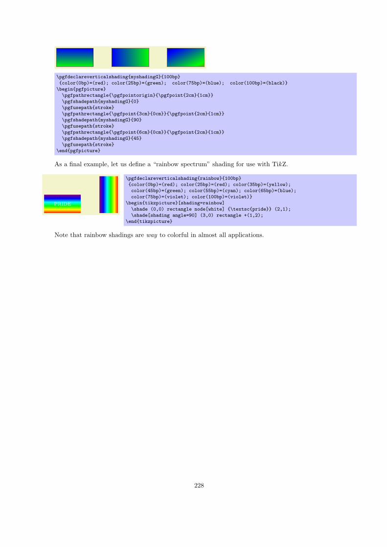
\pgfdeclareverticalshading{myshadingG}{100bp}


\begin{pgfpicture}


\pgfshadepath{myshadingG}{0}

\pgfusepath{stroke}



\pgfusepath{stroke}



\pgfusepath{stroke}

\end{pgfpicture}

As a final example, let us define a “rainbow spectrum” shading for use with TikZ.

.

.

.

pride.

\pgfdeclareverticalshading{rainbow}{100bp}

{color(0bp)=(red); color(25bp)=(red); color(35bp)=(yellow);

color(45bp)=(green); color(55bp)=(cyan); color(65bp)=(blue);

color(75bp)=(violet); color(100bp)=(violet)}

\begin{tikzpicture}[shading=rainbow]

\shade (0,0) rectangle node[white] {\textsc{pride}} (2,1);

\shade[shading angle=90] (3,0) rectangle +(1,2);

\end{tikzpicture}

Note that rainbow shadings are way to colorful in almost all applications.

228

29 Creating Plots

This section describes the pgfbaseplot package.

\usepackage{pgfbaseplot} % LATEX\input pgfbaseplot.tex % plain TEX\input pgfbaseplot.tex % ConTEXt

This package provides a set of commands that are intended to make it reasonably easy to plot functionsusing pgf. It is loaded automatically by pgf, but you can load it manually if you have only includedpgfcore.

29.1 Overview

29.1.1 When Should One Use PGF for Generating Plots?

There exist many powerful programs that produce plots, examples are gnuplot or mathematica. Theseprograms can produce two different kinds of output: First, they can output a complete plot picture in a certainformat (like pdf) that includes all low-level commands necessary for drawing the complete plot (including axesand labels). Second, they can usually also produce “just plain data” in the form of a long list of coordinates.Most of the powerful programs consider it a to be “a bit boring” to just output tabled data and very muchprefer to produce fancy pictures. Nevertheless, when coaxed, they can also provide the plain data.

The plotting mechanism described in the following deals only with plotting data given in the form of a listof coordinates. Thus, this section is about using pgf to turn lists of coordinates into plots.

Note that is often not necessary to use pgf for this. Programs like gnuplot can produce very sophisticatedplots and it is usually much easier to simply include these plots as a finished pdf or PostScript graphics.

However, there are a number of reasons why you may wish to invest time and energy into mastering the pgfcommands for creating plots:

• Virtually all plots produced by “external programs” use different fonts from the one used in your document.

• Even worse, formulas will look totally different, if they can be rendered at all.

• Line width will usually be too large or too small.

• Scaling effects upon inclusion can create a mismatch between sizes in the plot and sizes in the text.

• The automatic grid generated by most programs is mostly distracting.

• The automatic ticks generated by most programs are cryptic numerics. (Try adding a tick reading “π” atthe right point.)

• Most programs make it very easy to create “chart junk” in a most convenient fashion. All show, no content.

• Arrows and plot marks will almost never match the arrows used in the rest of the document.

The above list is not exhaustive, unfortunately.

29.1.2 How PGF Handles Plots

pgf (conceptually) uses a two-stage process for generating plots. First, a plot stream must be produced. Thisstream consists (more or less) of a large number of coordinates. Second a plot handler is applied to the stream.A plot handler “does something” with the stream. The standard handler will issue line-to operations to thecoordinates in the stream. However, a handler might also try to issue appropriate curve-to operations in orderto smooth the curve. A handler may even do something else entirely, like writing each coordinate to anotherstream, thereby duplicating the original stream.

Both for the creation of streams and the handling of streams different sets of commands exist. The com-mands for creating streams start with \pgfplotstream, the commands for setting the handler start with\pgfplothandler.

229

29.2 Generating Plot Streams

29.2.1 Basic Building Blocks of Plot Streams

A plot stream is a (long) sequence of the following three commands:

1. \pgfplotstreamstart,

2. \pgfplotstreampoint, and

3. \pgfplotstreamend.

Between calls of these commands arbitrary other code may be called. Obviously, the stream should start withthe first command and end with the last command. Here is an example of a plot stream:

\pgfplotstreamstart


\newdimen\mydim

\mydim=2cm

\pgfplotstreampoint{\pgfpoint{\mydim}{2cm}}

\advance \mydim by 3cm

\pgfplotstreampoint{\pgfpoint{\mydim}{2cm}}

\pgfplotstreamend

\pgfplotstreamstart

This command signals that a plot stream starts. The effect of this command is to call the internal command\pgf@plotstreamstart, which is set by the current plot handler to do whatever needs to be done at thebeginning of the plot.

\pgfplotstreampoint{⟨point⟩}This command adds a ⟨point⟩ to the current plot stream. The effect of this command is to call the internalcommand \pgf@plotstreampoint, which is also set by the current plot handler. This command should now“handle” the point in some sensible way. For example, a line-to command might be issued for the point.

\pgfplotstreamend

This command signals that a plot stream ends. It calls \pgf@plotstreamend, which should now do anynecessary “cleanup.”

Note that plot streams are not buffered, that is, the different points are handled immediately. However, usingthe recording handler, it is possible to record a stream.

29.2.2 Commands That Generate Plot Streams

Plot streams can be created “by hand” as in the earlier example. However, most of the time the coordinateswill be produced internally by some command. For example, the \pgfplotxyfile reads a file and converts itinto a plot stream.

\pgfplotxyfile{⟨filename⟩}This command will try to open the file ⟨filename⟩. If this succeeds, it will convert the file contents intoa plot stream as follows: A \pgfplotstreamstart is issued. Then, each nonempty line of the file shouldstart with two numbers separated by a space, such as 0.1 1 or 100 -.3. Anything following the numbersis ignored.Each pair ⟨x ⟩ and ⟨y⟩ of numbers is converted into one plot stream point in the xy-coordinate system. Thus,a line like

2 -5 some text

is turned into

230

\pgfplotstreampoint{\pgfpointxy{2}{-5}}

The two characters % and # are also allowed in a file and they are both treated as comment characters.Thus, a line starting with either of them is empty and, hence, ignored.When the file has been read completely, \pgfplotstreamend is called.

\pgfplotxyzfile{⟨filename⟩}This command works like \pgfplotxyfile, only three numbers are expected on each non-empty line. Theyare converted into points in the xyz-coordinate system. Consider, the following file:

% Some comments

# more comments

2 -5 1 first entry

2 -.2 2 second entry

2 -5 2 third entry

It is turned into the following stream:

\pgfplotstreamstart

\pgfplotstreampoint{\pgfpointxyz{2}{-5}{1}}

\pgfplotstreampoint{\pgfpointxyz{2}{-.2}{2}}

\pgfplotstreampoint{\pgfpointxyz{2}{-5}{2}}

\pgfplotstreamend

Currently, there is no command that can decide automatically whether the xy-coordinate system should beused or whether the xyz-system should be used. However, it would not be terribly difficult to write a “smartfile reader” that parses coordinate files a bit more intelligently.

\pgfplotgnuplot[⟨prefix ⟩]{⟨function⟩}This command will “try” to call the gnuplot program to generate the coordinates of the ⟨function⟩. Indetail, the following happens:This command works with two files: ⟨prefix ⟩.gnuplot and ⟨prefix ⟩.table. If the optional argument ⟨prefix ⟩is not given, it is set to \jobname.Let us start with the situation where none of these files exists. Then pgf will first generate the file⟨prefix ⟩.gnuplot. In this file it writes

set terminal table; set output "#1.table"; set format "%.5f"

where #1 is replaced by ⟨prefix ⟩. Then, in a second line, it writes the text ⟨function⟩.Next, pgf will try to invoke the program gnuplot with the argument ⟨prefix ⟩.gnuplot. This call may ormay not succeed, depending on whether the \write18 mechanism (also known as shell escape) is switchedon and whether the gnuplot program is available.Assuming that the call succeeded, the next step is to invoke \pgfplotxyfile on the file ⟨prefix ⟩.table;which is exactly the file that has just been created by gnuplot.

.

\begin{tikzpicture}

\draw[help lines] (0,-1) grid (4,1);

\pgfplothandlerlineto

\pgfplotgnuplot[plots/pgfplotgnuplot-example]{plot [x=0:3.5] x*sin(x)}

\pgfusepath{stroke}

\end{tikzpicture}

The more difficult situation arises when the .gnuplot file exists, which will be the case on the second runof TEX on the TEX file. In this case pgf will read this file and check whether it contains exactly what pgf

231

“would have written” into this file. If this is not the case, the file contents is overwritten with what “shouldbe there” and, as above, gnuplot is invoked to generate a new .table file. However, if the file contents is“as expected,” the external gnuplot program is not called. Instead, the ⟨prefix ⟩.table file is immediatelyread.As explained in Section 9.12.3, the net effect of the above mechanism is that gnuplot is called as littleas possible and that when you pass along the .gnuplot and .table files with your .tex file to someoneelse, that person can TEX the .tex file without having gnuplot installed and without having the \write18mechanism switched on.

29.3 Plot Handlers

A plot handler prescribes what “should be done” with a plot stream. You must set the plot handler before thestream starts. The following commands install the most basic plot handlers; more plot handlers are defined inthe file pgflibraryplothandlers, which is documented in Section 14.3.

All plot handlers work by setting redefining the following three macros: \pgf@plotstreamstart, \pgf@plotstreampoint,and \pgf@plotstreamend.


This handler will issue a \pgfpathlineto command for each point of the plot, except possibly for the first.What happens with the first point can be specified using the two commands described below.

.

\begin{pgfpicture}



\pgfplotstreamstart





\pgfplotstreamend

\pgfusepath{stroke}

\end{pgfpicture}

\pgfsetmovetofirstplotpoint

Specifies that the line-to plot handler (and also some other plot handlers) should issue a move-to commandfor the first point of the plot instead of a line-to. This will start a new part of the current path, which isnot always, but often, desirable. This is the default.

\pgfsetlinetofirstplotpoint

Specifies that plot handlers should issue a line-to command for the first point of the plot.

.

\begin{pgfpicture}


\pgfsetlinetofirstplotpoint


\pgfplotstreamstart





\pgfplotstreamend

\pgfusepath{stroke}

\end{pgfpicture}

\pgfplothandlerdiscard

This handler will simply throw away the stream.

232

\pgfplothandlerrecord{⟨macro⟩}When this handler is installed, each time a plot stream command is called, this command will be appendedto ⟨macros⟩. Thus, at the end of the stream, ⟨macro⟩ will contain all the commands that were issued on thestream. You can then install another handler and invoke ⟨macro⟩ to “replay” the stream (possibly manytimes).

.

\begin{pgfpicture}

\pgfplothandlerrecord{\mystream}

\pgfplotstreamstart





\pgfplotstreamend


\mystream


\mystream

\pgfusepath{stroke}

\end{pgfpicture}

233

30 Layered Graphics

\usepackage{pgfbaselayers} % LATEX\input pgfbaselayers.tex % plain TEX\input pgfbaselayers.tex % ConTEXt

This package provides a commands and environments for composing a picture from multiple layers. Thepackage is loaded automatically by pgf, but you can load it manually if you have only included pgfcore.

30.1 Overview

pgf provides a layering mechanism for composing graphics from multiple layers. (This mechanism is not beconfused with the conceptual “software layers” the pgf system is composed of.) Layers are often used ingraphic programs. The idea is that you can draw on the different layers in any order. So you might startdrawing something on the “background” layer, then something on the “foreground” layer, then something onthe “middle” layer, and then something on the background layer once more, and so on. At the end, no matter inwhich ordering you drew on the different layers, the layers are “stacked on top of each other” in a fixed orderingto produce the final picture. Thus, anything drawn on the middle layer would come on top of everything of thebackground layer.

Normally, you do not need to use different layers since you will have little trouble “ordering” your graphiccommands in such a way that layers are superfluous. However, in certain situations you only “know” what youshould draw behind something else after the “something else” has been drawn.

For example, suppose you wish to draw a yellow background behind your picture. The background shouldbe as large as the bounding box of the picture, plus a little border. If you know the size of the bounding box ofthe picture at its beginning, this is easy to accomplish. However, in general this is not the case and you needto create a “background” layer in addition to the standard “main” layer. Then, at the end of the picture, whenthe bounding box has been established, you can add a rectangle of the appropriate size to the picture.

30.2 Declaring Layers

In pgf layers are referenced using names. The standard layer, which is a bit special in certain ways, is calledmain. If nothing else is specified, all graphic commands are added to the main layer. You can declare a newlayer using the following command:

\pgfdeclarelayer{⟨name⟩}This command declares a layer named ⟨name⟩ for later use. Mainly, this will setup some internal bookkeep-ing.

The next step toward using a layer is to tell pgf which layers will be part of the actual picture and whichwill be their ordering. Thus, it is possible to have more layers declared than are actually used.

\pgfsetlayers{⟨layer list⟩}This command, which should be used outside a {pgfpicture} environment, tells pgf which layers will beused in pictures. They are stacked on top of each other in the order given. The layer main should alwaysbe part of the list. Here is an example:

\pgfdeclarelayer{background}

\pgfdeclarelayer{foreground}

\pgfsetlayers{background,main,foreground}

30.3 Using Layers

Once the layers of your picture have been declared, you can start to “fill” them. As said before, all graphicscommands are normally added to the main layer. Using the {pgfonlayer} environment, you can tell pgf thatcertain commands should, instead, be added to the given layer.

234

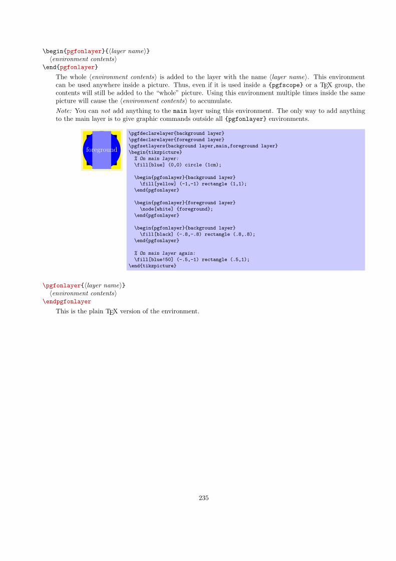
\begin{pgfonlayer}{⟨layer name⟩}⟨environment contents⟩

\end{pgfonlayer}

The whole ⟨environment contents⟩ is added to the layer with the name ⟨layer name⟩. This environmentcan be used anywhere inside a picture. Thus, even if it is used inside a {pgfscope} or a TEX group, thecontents will still be added to the “whole” picture. Using this environment multiple times inside the samepicture will cause the ⟨environment contents⟩ to accumulate.Note: You can not add anything to the main layer using this environment. The only way to add anythingto the main layer is to give graphic commands outside all {pgfonlayer} environments.

.

.

foreground

\pgfdeclarelayer{background layer}

\pgfdeclarelayer{foreground layer}

\pgfsetlayers{background layer,main,foreground layer}

\begin{tikzpicture}

% On main layer:

\fill[blue] (0,0) circle (1cm);

\begin{pgfonlayer}{background layer}

\fill[yellow] (-1,-1) rectangle (1,1);

\end{pgfonlayer}

\begin{pgfonlayer}{foreground layer}

\node[white] {foreground};

\end{pgfonlayer}

\begin{pgfonlayer}{background layer}

\fill[black] (-.8,-.8) rectangle (.8,.8);

\end{pgfonlayer}

% On main layer again:

\fill[blue!50] (-.5,-1) rectangle (.5,1);

\end{tikzpicture}

\pgfonlayer{⟨layer name⟩}⟨environment contents⟩

\endpgfonlayer

This is the plain TEX version of the environment.

235

31 Quick Commands

This section explains the “quick” commands of pgf. These commands are executed more quickly than thenormal commands of pgf, but offer less functionality. You should use these commands only if you either have avery large number of commands that need to be processed or if you expect your commands to be executed veryoften.

31.1 Quick Path Construction Commands

The difference between the quick and the normal path commands is that the quick path commands

• do not keep track of the bounding boxes,

• do not allow you to arc corners,

• do not apply coordinate transformations.

However, they do use the soft-path subsystem (see Section 34 for details), which allows you to mix quick andnormal path commands arbitrarily.

All quick path construction commands start with \pgfpathq.

\pgfpathqmoveto{⟨x dimension⟩}{⟨y dimension⟩}Either starts a path or starts a new part of a path at the coordinate (⟨x dimension⟩, ⟨y dimension⟩). Thecoordinate is not transformed by the current coordinate transformation matrix. However, any low-leveltransformations apply.

.

\begin{tikzpicture}


\pgftransformxshift{1cm}

\pgfpathqmoveto{0pt}{0pt} % not transformed

\pgfpathqlineto{1cm}{1cm} % not transformed


\pgfusepath{stroke}

\end{tikzpicture}

\pgfpathqlineto{⟨x dimension⟩}{⟨y dimension⟩}The quick version of the line-to operation.

\pgfpathqcurveto{⟨s1x⟩}{⟨s1

y⟩}{⟨s2x⟩}{⟨s2

y⟩}{⟨tx⟩}{⟨ty⟩}The quick version of the curve-to operation. The first support point is (s1

x, s1y), the second support point is

(s2x, s2

y), and the target is (tx, ty).

.

\begin{tikzpicture}


\pgfpathqmoveto{0pt}{0pt}

\pgfpathqcurveto{1cm}{1cm}{2cm}{1cm}{3cm}{0cm}

\pgfusepath{stroke}

\end{tikzpicture}

\pgfpathqcircle{⟨radius⟩}Adds a radius around the origin of the given ⟨radius⟩. This command is orders of magnitude faster than\pgfcircle{\pgfpointorigin}{⟨radius⟩}.

.

\begin{tikzpicture}


\pgfpathqcircle{10pt}


\pgfusepath{stroke,fill}

\end{tikzpicture}

236

31.2 Quick Path Usage Commands

The quick path usage commands perform similar tasks as \pgfusepath, but they

• do not add arrows,

• do not modify the path in any way, in particular,

• ends are not shortened,

• corners are not replaced by arcs.

Note that you have to use the quick versions in the code of arrow tip definitions since, inside these definition,you obviously do not want arrows to be drawn.

\pgfusepathqstroke

Strokes the path without further ado. No arrows are drawn, no corners are arced.

.

\begin{pgfpicture}

\pgfpathqcircle{5pt}

\pgfusepathqstroke

\end{pgfpicture}

\pgfusepathqfill

Fills the path without further ado.

\pgfusepathqfillstroke

Fills and then strokes the path without further ado.

\pgfusepathqclip

Clips all subsequent drawings against the current path. The path is not processed.

31.3 Quick Text Box Commands

\pgfqbox{⟨box number⟩}This command inserts a TEX box into a {pgfpicture} by “escaping” to TEX, inserting the box number⟨box number⟩ at the origin, and then returning to the typesetting the picture.

\pgfqboxsynced{⟨box number⟩}This command works similarly to the \pgfqbox command. However, before inserting the text in ⟨boxnumber⟩, the current coordinate transformation matrix is applied to the current canvas transformationmatrix (is it “synced” with this matrix, hence the name).Thus, this command basically has the same effect as if you first called \pgflowlevelsynccm followed by\pgfqbox. However, this command will use \hskip and \raise commands for the “translational part”of the coordinate transformation matrix, instead of adding the translational part to the current canvastransformation matrix directly. Both methods have the same effect (box ⟨box number⟩ is translated whereit should), but the method used by \pgfqboxsynced ensures that hyperlinks are placed correctly. Note thatscaling and rotation will not (cannot, even) apply to hyperlinks.

237

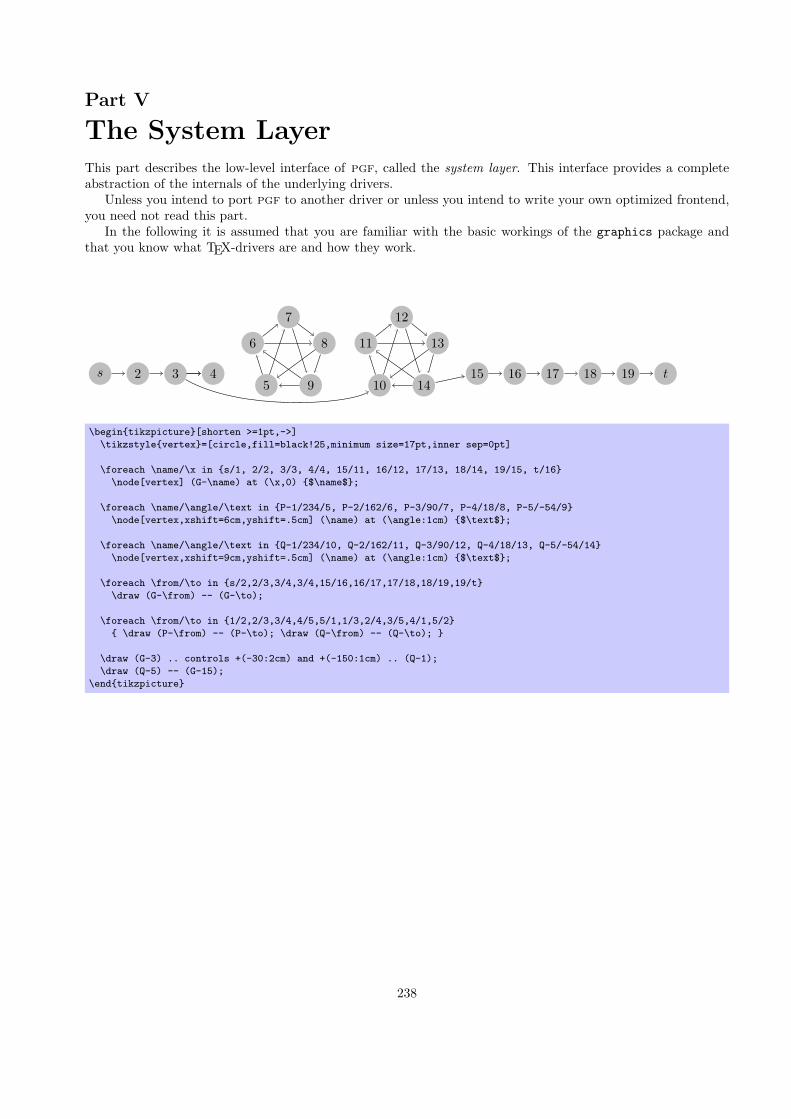
Part V

The System LayerThis part describes the low-level interface of pgf, called the system layer. This interface provides a completeabstraction of the internals of the underlying drivers.

Unless you intend to port pgf to another driver or unless you intend to write your own optimized frontend,you need not read this part.

In the following it is assumed that you are familiar with the basic workings of the graphics package andthat you know what TEX-drivers are and how they work.

.

.

s

.

2

.

3

.

4

.

15

.

16

.

17

.

18

.

19

.

t

.

5

.

6

.

7

.

8

.

9

.

10

.

11

.

12

.

13

.

14

\begin{tikzpicture}[shorten >=1pt,->]

\tikzstyle{vertex}=[circle,fill=black!25,minimum size=17pt,inner sep=0pt]

\foreach \name/\x in {s/1, 2/2, 3/3, 4/4, 15/11, 16/12, 17/13, 18/14, 19/15, t/16}

\node[vertex] (G-\name) at (\x,0) {$\name$};

\foreach \name/\angle/\text in {P-1/234/5, P-2/162/6, P-3/90/7, P-4/18/8, P-5/-54/9}

\node[vertex,xshift=6cm,yshift=.5cm] (\name) at (\angle:1cm) {$\text$};

\foreach \name/\angle/\text in {Q-1/234/10, Q-2/162/11, Q-3/90/12, Q-4/18/13, Q-5/-54/14}

\node[vertex,xshift=9cm,yshift=.5cm] (\name) at (\angle:1cm) {$\text$};

\foreach \from/\to in {s/2,2/3,3/4,3/4,15/16,16/17,17/18,18/19,19/t}

\draw (G-\from) -- (G-\to);

\foreach \from/\to in {1/2,2/3,3/4,4/5,5/1,1/3,2/4,3/5,4/1,5/2}

{ \draw (P-\from) -- (P-\to); \draw (Q-\from) -- (Q-\to); }

\draw (G-3) .. controls +(-30:2cm) and +(-150:1cm) .. (Q-1);

\draw (Q-5) -- (G-15);

\end{tikzpicture}

238

32 Design of the System Layer

32.1 Driver Files

The pgf system layer mainly consists of a large number of commands starting with \pgfsys@. These commandswill be called system commands in the following. The higher layers “interface” with the system layer by callingthese commands. The higher layers should never use \special commands directly or even check whether\pdfoutput is defined. Instead, all drawing requests should be “channeled” through the system commands.

The system layer is loaded and setup by the following package:

\usepackage{pgfsys} % LATEX\input pgfsys.tex % plain TEX\input pgfsys.tex % ConTEXt

This file provides “default implementations” of all system commands, but most simply produce a warningthat they are not implemented. The actual implementations of the system commands for a particular driverlike, say, pdftex reside in files called pgfsys-xxxx.sty, where xxxx is the driver name. These will be calleddriver files in the following.When pgfsys.sty is loaded, it will try to determine which driver is used by loading pgf.cfg. Thisfile should setup the macro \pgfsysdriver appropriately. The, pgfsys.sty will input the appropriatepgfsys-⟨drivername⟩.sty.

\pgfsysdriver

This macro should expand to the name of the driver to be used by pgfsys. The default from pgf.cfg ispgfsys-\Gin@driver. This is very likely to be correct if you are using LATEX. For plain TEX, the macrowill be set to pgfsys-pdftex.def if pdftex is used and to pgfsys-dvips.def otherwise.

File pgf.cfg

This file should setup the command \pgfsysdriver correctly. If \pgfsysdriver is already set to somevalue, the driver normally should not change it. Otherwise, it should make a “good guess” at which driverwill be appropriate.

The currently supported backend drivers are discussed in Section 5.2.

32.2 Common Definition Files

Some drivers share many \pgfsys@ commands. For the reason, files defining these “common” commands areavailable. These files are not usable alone.

File pgfsys-common-postscript

This file defines some \pgfsys@ commands so that they produce appropriate PostScript code.

File pgfsys-common-pdf

This file defines some \pgfsys@ commands so that they produce appropriate pdf code.

239

33 Commands of the System Layer

33.1 Beginning and Ending a Stream of System Commands

A “user” of the pgf system layer (like the basic layer or a frontend) will interface with the system layer bycalling a stream of commands starting with \pgfsys@. From the system layer’s point of view, these commandsform a long stream. Between calls to the system layer, control goes back to the user.

The driver files implement system layer commands by inserting \special commands that implement thedesired operation. For example, \pgfsys@stroke will be mapped to \special{pdf: S} by the driver file forpdftex.

For many drivers, when such a stream of specials starts, it is necessary to install an appropriate transfor-mation and perhaps perform some more bureaucratic tasks. For this reason, every stream will start with a\pgfsys@beginpicture and will end with a corresponding ending command.

\pgfsys@beginpicture

Called at the beginning of a {pgfpicture}. This command should “setup things.”Most drivers will need to implement this command.

\pgfsys@endpicture

Called at the end of a pgfpicture.Most drivers will need to implement this command.

\pgfsys@typesetpicturebox{⟨box ⟩}Called after a {pgfpicture} has been typeset. The picture will have been put in box ⟨box ⟩. This commandshould insert the box into the normal text. The box ⟨box ⟩ will still be a “raw” box that contains only the\special’s that make up the description of the picture. The job of this command is to resize and shift⟨box ⟩ according to the baseline shift and the size of the box.This command has a default implementation and need not be implemented by a driver file.

\pgfsys@beginpurepicture

This version of the \pgfsys@beginpicture picture command can be used for pictures that are guaranteednot to contain any escaped boxes (see below). In this case, a driver might provide a more compact versionof the command.This command has a default implementation and need not be implemented by a driver file.

\pgfsys@endpurepicture

Called at the end of a “pure” {pgfpicture}.This command has a default implementation and need not be implemented by a driver file.

Inside a stream it is sometimes necessary to “escape” back into normal typesetting mode; for example toinsert some normal text, but with all of the current transformations and clippings being in force. For thisescaping, the following command is used:

\pgfsys@hbox{⟨box number⟩}Called to insert a (horizontal) TeX box inside a {pgfpicture}.Most drivers will need to (re-)implement this command.

\pgfsys@hboxsynced{⟨box number⟩}Called to insert a (horizontal) TeX box inside a {pgfpicture}, but with the current coordiante transfor-mation matrix synced with the canvas transformation matrix.This command should do the same as if you used \pgflowlevelsynccm followed by \pgfsys@hbox. However,the default implementation of this command will use a “TeX-translation” for the translation part of thetransformation matrix. This will ensure that hyperlinks “survive” at least translations. On the otherhand, a driver may choose to revert to a simpler implementation. This is done, for example, for the svgimplementation, where a TEX-translation makes no sense.

240

33.2 Path Construction System Commands

\pgfsys@moveto{⟨x ⟩}{⟨y⟩}This command is used to start a path at a specific point (x, y) or to move the current point of the currentpath to (x, y) without drawing anything upon stroking (the current path is “interrupted”).Both ⟨x ⟩ and ⟨y⟩ are given as TEX dimensions. It is the driver’s job to transform these to the coordinatesystem of the backend. Typically, this means converting the TEX dimension into a dimensionless multipleof 1

72 in. The function \pgf@sys@bp helps with this conversion.

Example: Draw a line from (10pt, 10pt) to the origin of the picture.

\pgfsys@moveto{10pt}{10pt}

\pgfsys@lineto{0pt}{0pt}

\pgfsys@stroke

This command is protocoled, see Section 35.

\pgfsys@lineto{⟨x ⟩}{⟨y⟩}Continue the current path to (x, y) with a straight line.This command is protocoled, see Section 35.

\pgfsys@curveto{⟨x1⟩}{⟨y1⟩}{⟨x2⟩}{⟨y2⟩}{⟨x3⟩}{⟨y3⟩}Continue the current path to (x3, y3) with a Bezier curve that has the two control points (x1, y1) and(x2, y2).

Example: Draw a good approximation of a quarter circle:


\pgfsys@curveto{10pt}{5.55pt}{5.55pt}{10pt}{0pt}{10pt}

\pgfsys@stroke

This command is protocoled, see Section 35.

\pgfsys@rect{⟨x ⟩}{⟨y⟩}{⟨width⟩}{⟨height⟩}Append a rectangle to the current path whose lower left corner is at (x, y) and whose width and height inbig points are given by ⟨width⟩ and ⟨height⟩.This command can be “mapped back” to \pgfsys@moveto and \pgfsys@lineto commands, but it isincluded since pdf has a special, quick version of this command.This command is protocoled, see Section 35.

\pgfsys@closepath

Close the current path. This results in joining the current point of the path with the point specified by thelast \pgfsys@moveto operation. Typically, this is preferable over using \pgfsys@lineto to the last pointspecified by a \pgfsys@moveto, since the line starting at this point and the line ending at this point willbe smoothly joined by \pgfsys@closepath.

Example: Consider


\pgfsys@lineto{10bp}{10bp}


\pgfsys@closepath

\pgfsys@stroke

and

\pgfsys@moveto{0bp}{0bp}




\pgfsys@stroke

241

The difference between the above will be that in the second triangle the corner at the origin will be wrong;it will just be the overlay of two lines going in different directions, not a sharp pointed corner.This command is protocoled, see Section 35.

33.3 Canvas Transformation System Commands

\pgfsys@transformcm{⟨a⟩}{⟨b⟩}{⟨c⟩}{⟨d⟩}{⟨e⟩}{⟨f ⟩}Perform a concatenation of the canvas transformation matrix with the matrix given by the values ⟨a⟩ to⟨f ⟩, see the pdf or PostScript manual for details. The values ⟨a⟩ to ⟨d⟩ are dimensionless factors, ⟨e⟩ and⟨f ⟩ are TEX dimensions

Example: \pgfsys@transformcm{1}{0}{0}{1}{1cm}{1cm}.This command is protocoled, see Section 35.

\pgfsys@transformshift{⟨x displacement⟩}{⟨y displacement⟩}This command will change the origin of the canvas to (x, y).This command has a default implementation and need not be implemented by a driver file.This command is protocoled, see Section 35.

\pgfsys@transformxyscale{⟨x scale⟩}{⟨y scale⟩}This command will scale the canvas (and everything that is drawn) by a factor of ⟨x scale⟩ in the x-directionand ⟨y scale⟩ in the y-direction. Note that this applies to everything, including lines. So a scaled line willhave a different width and may even have a different width when going along the x-axis and when goingalong the y-axis, if the scaling is different in these directions. Usually, you do not want this.This command has a default implementation and need not be implemented by a driver file.This command is protocoled, see Section 35.

33.4 Stroking, Filling, and Clipping System Commands

\pgfsys@stroke

Stroke the current path (as if it were drawn with a pen). A number of graphic state parameters influencethis, which can be set using appropriate system commands described later.

Line width The “thickness” of the line. A width of 0 is the thinnest width renderable on the device. Ona high-resolution printer this may become invisible and should be avoided. A good choice is 0.4pt,which is the default.

Stroke color This special color is used for stroking. If it is not set, the current color is used.

Cap The cap describes how the endings of lines are drawn. A round cap adds a little half circle to theseendings. A butt cap ends the lines exactly at the end (or start) point without anything added. Arectangular cap ends the lines like the butt cap, but the lines protrude over the endpoint by the linethickness. (See also the pdf manual.) If the path has been closed, no cap is drawn.

Join This describes how a bend (a join) in a path is rendered. A round join draws bends using small arcs.A bevel join just draws the two lines and then fills the join minimally so that it becomes convex. Amiter join extends the lines so that they form a single sharp corner, but only up to a certain miterlimit. (See the pdf manual once more.)

Dash The line may be dashed according to a dashing pattern.

Clipping area If a clipping area is established, only those parts of the path that are inside the clippingarea will be drawn.

In addition to stroking a path, the path may also be used for clipping after it has been stroked. This willhappen if the \pgfsys@clipnext is used prior to this command, see there for details.This command is protocoled, see Section 35.

242

\pgfsys@closestroke

This command should have the same effect as first closing the path and then stroking it.This command has a default implementation and need not be implemented by a driver file.This command is protocoled, see Section 35.

\pgfsys@fill

This command fills the area surrounded by the current path. If the path has not yet been closed, it is closedprior to filling. The path itself is not stroked. For self-intersecting paths or paths consisting of multipleparts, the nonzero winding number rule is used to determine whether a point is inside or outside the path,except if \ifpgfsys@eorule holds – in which case the even-odd rule should be used. (See the pdf orPostScript manual for details.)The following graphic state parameters influence the filling:

Interior rule If \ifpgfsys@eorule is set, the even-odd rule is used, otherwise the non-zero winding num-ber rule.

Fill color If the fill color is not especially set, the current color is used.Clipping area If a clipping area is established, only those parts of the filling area that are inside the

clipping area will be drawn.

In addition to filling the path, the path will also be used for clipping if \pgfsys@clipnext is used prior tothis command.This command is protocoled, see Section 35.

\pgfsys@fillstroke

First, the path is filled, then the path is stroked. If the fill and stroke colors are the same (or if they arenot specified and the current color is used), this yields almost the same as a \pgfsys@fill. However, dueto the line thickness of the stroked path, the fill-stroked area will be slightly larger.In addition to stroking and filling the path, the path will also be used for clipping if \pgfsys@clipnext isused prior to this command.This command is protocoled, see Section 35.

\pgfsys@discardpath

Normally, this command should “throw away” the current path. However, after \pgfsys@clipnext hasbeen called, the current path should subsequently be used for clipping. See \pgfsys@clipnext for details.This command is protocoled, see Section 35.

\pgfsys@clipnext

This command should be issued after a path has been constructed, but before it has been stroked and/orfilled or discarded. When the command is used, the next stroking/filling/discarding command will first beexecuted normally. Then, afterwards, the just-used path will be used for subsequent clipping. If there hasalready been a clipping region, this region is intersected with the new clipping path (the clipping cannotget bigger). The nonzero winding number rule is used to determine whether a point is inside or outside theclipping area or the even-odd rule, depending on whether \ifpgfsys@eorule holds.

33.5 Graphic State Option System Commands

\pgfsys@setlinewidth{⟨width⟩}Sets the width of lines, when stroked, to ⟨width⟩, which must be a TEX dimension.This command is protocoled, see Section 35.

\pgfsys@buttcap

Sets the cap to a butt cap. See \[email protected] command is protocoled, see Section 35.

243

\pgfsys@roundcap

Sets the cap to a round cap. See \[email protected] command is protocoled, see Section 35.

\pgfsys@rectcap

Sets the cap to a rectangular cap. See \[email protected] command is protocoled, see Section 35.

\pgfsys@miterjoin

Sets the join to a miter join. See \[email protected] command is protocoled, see Section 35.

\pgfsys@setmiterlimit{⟨factor⟩}Sets the miter limit of lines to ⟨factor⟩. See the pdf or PostScript for details on what the miter limit is.This command is protocoled, see Section 35.

\pgfsys@roundjoin

Sets the join to a round join. See \[email protected] command is protocoled, see Section 35.

\pgfsys@beveljoin

Sets the join to a bevel join. See \[email protected] command is protocoled, see Section 35.

\pgfsys@setdash{⟨pattern⟩}{⟨phase⟩}Sets the dashing patter. ⟨pattern⟩ should be a list of TEX dimensions lengths separated by commas. ⟨phase⟩should be a single dimension.

Example: \pgfsys@setdash{3pt,3pt}{0pt}

The list of values in ⟨pattern⟩ is used to determine the lengths of the “on” phases of the dashing and of the“off” phases. For example, if ⟨pattern⟩ is 3bp,4bp, then the dashing pattern is “3bp on followed by 4bp off,followed by 3bp on, followed by 4bp off, and so on.” A pattern of .5pt,4pt,3pt,1.5pt means “.5pt on,4pt off, 3pt on, 1.5pt off, .5pt on, . . . ” If the number of entries is odd, the last one is used twice, so 3ptmeans “3pt on, 3pt off, 3pt on, 3pt off, . . . ” An empty list means “always on.”The second argument determines the “phase” of the pattern. For example, for a pattern of 3bp,4bp and aphase of 1bp, the pattern would start: “2bp on, 4bp off, 3bp on, 4bp off, 3bp on, 4bp off, . . . ”This command is protocoled, see Section 35.

\ifpgfsys@eorule

Determines whether the even odd rule is used for filling and clipping or not.

\pgfsys@stroke@opacity{⟨value⟩}Sets the opacity of stroking operations.

\pgfsys@fill@opacity{⟨value⟩}Sets the opacity of filling operations.

33.6 Color System Commands

The pgf system layer provides a number of system commands for setting colors. These command coexist withcommands from the color and xcolor package, which perform similar functions. However, the color packagedoes not support having two different colors for stroking and filling, which is a useful feature that is supported

244

by pgf. For this reason, the pgf system layer offers commands for setting these colors separatedly. Also, plainTEX profits from the fact that pgf can set colors.

For pdf, implementing these color commands is easy since pdf supports different stroking and filling colorsdirectly. For PostScript, a more complicated approach is needed in which the colors need to be stored in specialPostScript variables that are set whenever a stroking or a filling operation is done.

\pgfsys@color@rgb{⟨red⟩}{⟨green⟩}{⟨blue⟩}Sets the color used for stroking and filling operations to the given red/green/blue tuple (numbers between0 and 1).This command is protocoled, see Section 35.

\pgfsys@color@rgb@stroke{⟨red⟩}{⟨green⟩}{⟨blue⟩}Sets the color used for stroking operations to the given red/green/blue tuple (numbers between 0 and 1).

Example: Make stroked text dark red: \pgfsys@color@rgb@stroke{0.5}{0}{0}The special stroking color is only used if the stroking color has been set since the last \color or\pgfsys@color@xxx command. Thus, each \color command will reset both the stroking and filling colorsby calling \pgfsys@[email protected] command is protocoled, see Section 35.

\pgfsys@color@rgb@fill{⟨red⟩}{⟨green⟩}{⟨blue⟩}Sets the color used for filling operations to the given red/green/blue tuple (numbers between 0 and 1). Thiscolor may be different from the stroking color.This command is protocoled, see Section 35.

\pgfsys@color@cmyk{⟨cyan⟩}{⟨magenta⟩}{⟨yellow⟩}{⟨black⟩}Sets the color used for stroking and filling operations to the given cymk tuple (numbers between 0 and 1).This command is protocoled, see Section 35.

\pgfsys@color@cmyk@stroke{⟨cyan⟩}{⟨magenta⟩}{⟨yellow⟩}{⟨black⟩}Sets the color used for stroking operations to the given cymk tuple (numbers between 0 and 1).This command is protocoled, see Section 35.

\pgfsys@color@cmyk@fill{⟨cyan⟩}{⟨magenta⟩}{⟨yellow⟩}{⟨black⟩}Sets the color used for filling operations to the given cymk tuple (numbers between 0 and 1).This command is protocoled, see Section 35.

\pgfsys@color@cmy{⟨cyan⟩}{⟨magenta⟩}{⟨yellow⟩}Sets the color used for stroking and filling operations to the given cym tuple (numbers between 0 and 1).This command is protocoled, see Section 35.

\pgfsys@color@cmy@stroke{⟨cyan⟩}{⟨magenta⟩}{⟨yellow⟩}Sets the color used for stroking operations to the given cym tuple (numbers between 0 and 1).This command is protocoled, see Section 35.

\pgfsys@color@cmy@fill{⟨cyan⟩}{⟨magenta⟩}{⟨yellow⟩}Sets the color used for filling operations to the given cym tuple (numbers between 0 and 1).This command is protocoled, see Section 35.

\pgfsys@color@gray{⟨black⟩}Sets the color used for stroking and filling operations to the given black value, where 0 means black and 1means white.This command is protocoled, see Section 35.

245

\pgfsys@color@gray@stroke{⟨black⟩}Sets the color used for stroking operations to the given black value, where 0 means black and 1 means white.This command is protocoled, see Section 35.

\pgfsys@color@gray@fill{⟨black⟩}Sets the color used for filling operations to the given black value, where 0 means black and 1 means white.This command is protocoled, see Section 35.

\pgfsys@color@reset

This command will be called when the \color command is used. It should purge any internal settings ofstroking and filling color. After this call, till the next use of a command like \pgfsys@color@rgb@fill,the current color installed by the \color command should be used.If the TEX-if \pgfsys@color@reset@inorder is set to true, this command may “assume” that any call toa color command that sets the fill or stroke color came “before” the call to this command and may try tooptimize the output accordingly.An example of an incorrect “out of order” call would be using \pgfsys@color@reset at the beginning ofa box that is constructed using \setbox. Then, when the box is constructed, no special fill or stroke colormight be in force. However, when the box is later on inserted at some point, a special fill color might alreadyhave been set. In this case, this command is not guaranteed to reset the color correctly.

\pgfsys@color@reset@inordertrue

Sets the optimized “in order” version of the color resetting. This is the default.

\pgfsys@color@reset@inorderfalse

Switches off the optimized color resetting.

\pgfsys@color@unstacked{⟨LATEX color⟩}This slightly obscure command causes the color stack to be tricked. When called, this command should setthe current color to ⟨LATEX color⟩ without causing any change in the color stack.

Example: \pgfsys@color@unstacked{red}

33.7 Scoping System Commands

The scoping commands are used to keep changes of the graphics state local.

\pgfsys@beginscope

Saves the current graphic state on a graphic state stack. All changes to the graphic state parametersmentioned for \pgfsys@stroke and \pgfsys@fill will be local to the current graphic state and the oldvalues will be restored after \pgfsys@endscope is used.Warning: pdf and PostScript differ with respect to the question of whether the current path is part ofthe graphic state or not. For this reason, you should never use this command unless the path is currentlyempty. For example, it might be a good idea to use \pgfsys@discardpath prior to calling this command.This command is protocoled, see Section 35.

\pgfsys@endscope

Restores the last saved graphic state.This command is protocoled, see Section 35.

33.8 Image System Commands

The system layer provides some commands for image inclusion.

246

\pgfsys@imagesuffixlist

This macro should expand to a list of suffixes, separated by ‘:’, that will be tried when searching for animage.

Example: \def\pgfsys@imagesuffixlist{eps:epsi:ps}

\pgfsys@defineimage

Called, when an image should be defined.This command does not take any parameters. Instead, certain macros will be preinstalled with appropriatevalues when this command is invoked. These are:

• \pgf@filename File name of the image to be defined.• \pgf@imagewidth Will be set to the desired (scaled) width of the image.• \pgf@imageheight Will be set to the desired (scaled) height of the image.

If this macro and also the height macro are empty, the image should have its “natural” size.If exactly only of them is specified, the undefined value the image is scaled so that the aspect ratio iskept.If both are set, the image is scaled in both directions independently, possibly changing the aspect ratio.

The following macros presumable mostly make sense for drivers that can handle pdf:

• \pgf@imagepage The desired page number to be extracted from a multi-page “image.”• \pgf@imagemask If set, it will be set to /SMask x 0 R where x is the pdf object number of a soft

mask to be applied to the image.• \pgf@imageinterpolate If set, it will be set to /Interpolate true or /Interpolate false, indi-

cating whether the image should be interpolated in pdf.

The command should now setup the macro \pgf@image such that calling this macro will result in typesettingthe image. Thus, \pgf@image is the “return value” of the command.This command has a default implementation and need not be implemented by a driver file.

\pgfsys@definemask

This command declares a mask for usage with images. It works similar to \pgfsys@defineimage: Certainmacros are set when the command is called. The result should be to set the macro \pgf@mask to a pdfobject count that can subsequently be used as a soft mask. The following macros will be set when thiscommand is invoked:

• \pgf@filename File name of the mask to be defined.• \pgf@maskmatte The so-called matte of the mask (see the pdf documentation for details). The matte

is a color specification consisting of 1, 3 or 4 numbers between 0 and 1. The number of numbersdepends on the number of color channels in the image (not in the mask!). It will be assumed that theimage has been preblended with this color.

33.9 Shading System Commands

\pgfsys@horishading{⟨name⟩}{⟨height⟩}{⟨specification⟩}Declares a horizontal shading for later use. The effect of this command should be the definition of amacro called \@pgfshading⟨name⟩! (or \csname @pdfshading⟨name⟩!\endcsname, to be precise). Wheninvoked, this new macro should insert a shading at the current position.⟨name⟩ is the name of the shading, which is also used in the output macro name. ⟨height⟩ is the heightof the shading and must be given as a TeX dimension like 2cm or 10pt. ⟨specification⟩ is a shading colorspecification as specified in Section 28. The shading specification implicitly fixes the width of the shading.When \@pgfshading⟨name⟩! is invoked, it should insert a box of height ⟨height⟩ and the width implicit inthe shading declaration.

247

\pgfsys@vertshading{⟨name⟩}{⟨width⟩}{⟨specification⟩}Like the horizontal version, only for vertical shadings. This time, the height of the shading is implicit in⟨specification⟩ and the width is given as ⟨width⟩.

\pgfsys@radialshading{⟨name⟩}{⟨starting point⟩}{⟨specification⟩}Declares a radial shading. Like the previous macros, this command should setup the macro \@pgfshading⟨name⟩!,which upon invocation should insert a radial shading whose size is implicit in ⟨specification⟩.The parameter ⟨starting point⟩ is a pgf point specifying the inner starting point of the shading.

33.10 Reusable Objects System Commands

\pgfsys@invoke{⟨literals⟩}This command gets protocoled literals and should insert them into the .pdf or .dvi file using an appropriate\special.

\pgfsys@defobject{⟨name⟩}{⟨lower left⟩}{⟨upper right⟩}{⟨code⟩}Declares an object for later use. The idea is that the object can be precached in some way and thenbe rendered more quickly when used several times. For example, an arrow head might be defined andprerendered in this way.The parameter ⟨name⟩ is the name for later use. ⟨lower left⟩ and ⟨upper right⟩ are pgf points specifying abounding box for the object. ⟨code⟩ is the code for the object. The code should not be too fancy.This command has a default implementation and need not be implemented by a driver file.

\pgfsys@useobject{⟨name⟩}{⟨extra code⟩}Renders a previously declared object. The first parameter is the name of the the object. The secondparameter is extra code that should be executed right before the object is rendered. Typically, this will besome transformation code.This command has a default implementation and need not be implemented by a driver file.

33.11 Invisibility System Commands

All drawing or stroking or text rendering between calls of the following commands should be suppressed. Asimilar effect can be achieved by clipping against an empty region, but the following commands do not open agraphics scope and can be opened and closed “orthogonally” to other scopes.

\pgfsys@begininvisible

Between this command and the closing \pgfsys@endinvisible all output should be suppressed. Nothingshould be drawn at all, which includes all paths, images and shadings. However, no groups (neither TEXgroups nor graphic state groups) should be opened by this command.This command has a default implementation and need not be implemented by a driver file.This command is protocoled, see Section 35.

\pgfsys@endinvisible

Ends the invisibility section, unless invisibility blocks have been nested. In this case, only the “last” onerestores visibility.This command has a default implementation and need not be implemented by a driver file.This command is protocoled, see Section 35.

33.12 Internal Conversion Commands

The system commands take TEX dimensions as input, but the dimensions that have to be inserted into pdf andPostScript files need to be dimensionless values that are interpreted as multiples of 1

72 in. For example, the TEX

248

dimension 2bp should be inserted as 2 into a pdf file and the TEX dimension 10pt as 9.9626401. To make thisconversion easier, the following command may be useful:

\pgf@sys@bp{⟨dimension⟩}Inserts how many multiples of 1

72 in the ⟨dimension⟩ is into the current protocol stream (buffered).

Example: \pgf@sys@bp{\pgf@x} or \pgf@sys@bp{1cm}.

Note that this command is not a system command that can/needs to be overwritten by a driver.

249

34 The Soft Path Subsystem

This section describes a set of commands for creating soft paths as opposed to the commands of the previoussection, which created hard paths. A soft path is a path that can still be “changed” or “molded.” Once you(or the pgf system) is satisfied with a soft path, it is turned into a hard path, which can be inserted into theresulting .pdf or .ps file.

Note that the commands described in this section are “high-level” in the sense that they are not implementedin driver files, but rather directly by the pgf-system layer. For this reason, the commands for creating soft pathsdo not start with \pgfsys@, but rather with \pgfsyssoftpath@. On the other hand, as a user you will neveruse these commands directly, so they are described as part of the low-level interface.

34.1 Path Creation Process

When the user writes a command like \draw (0bp,0bp) -- (10bp,0bp); quite a lot happens behind the scenes:

1. The frontend command is translated by TikZ into commands of the basic layer. In essence, the commandis translated to something like

\pgfpathmoveto{\pgfpoint{0bp}{0bp}}

\pgfpathlineto{\pgfpoint{10bp}{0bp}}

\pgfusepath{stroke}

2. The \pgfpathxxxx command do not directly call “hard” commands like \pgfsys@xxxx. Instead, the com-mand \pgfpathmoveto invokes a special command called \pgfsyssoftpath@moveto and \pgfpathlinetoinvokes \pgfsyssoftpath@lineto.

The \pgfsyssoftpath@xxxx commands, which are described below, construct a soft path. Each time sucha command is used, special tokens are added to the end of an internal macro that stores the soft pathcurrently being constructed.

3. When the \pgfusepath is encountered, the soft path stored in the internal macro is “invoked.” Onlynow does a special macro iterate over the soft path. For each line-to or move-to operation on this path itcalls an appropriate \pgfsys@moveto or \pgfsys@lineto in order to, finally, create the desired hard path,namely, the string of literals in the .pdf or .ps file.

4. After the path has been invoked, \pgfsys@stroke is called to insert the literal for stroking the path.

Why such a complicated process? Why not have \pgfpathlineto directly call \pgfsys@lineto and be donewith it? There are two reasons:

1. The pdf specification requires that a path is not interrupted by any non-path-construction commands.Thus, the following code will result in a corrupted .pdf:

\pgfsys@moveto{0}{0}

\pgfsys@setlinewidth{1}

\pgfsys@lineto{10}{0}

\pgfsys@stroke

Such corrupt code is tolerated by most viewers, but not always. It is much better to create only (reasonably)legal code.

2. A soft path can still be changed, while a hard path is fixed. For example, one can still change the startingand end points of a soft path or do optimizations on it. Such transformations are not possible on hardpaths.

250

34.2 Starting and Ending a Soft Path

No special action must be taken in order to start the creation of a soft path. Rather, each time a command like\pgfsyssoftpath@lineto is called, a special token is added to the (global) current soft path being constructed.

However, you can access and change the current soft path. In this way, it is possible to store a soft path, tomanipulate it, or to invoke it.

\pgfsyssoftpath@getcurrentpath{⟨macro name⟩}This command will store the current soft path in ⟨macro name⟩.

\pgfsyssoftpath@setcurrentpath{⟨macro name⟩}This command will set the current soft path to be the path stored in ⟨macro name⟩. This macro shouldstore a path that has previously been extracted using the \pgfsyssoftpath@getcurrentpath commandand has possibly been modified subsequently.

\pgfsyssoftpath@invokecurrentpath

This command will turn the current soft path in a “hard” path. To do so, it iterates over the soft path andcalls an appropriate \pgfsys@xxxx command for each element of the path. Note that the current soft pathis not changed by this command. Thus, in order to start a new soft path after the old one has been invokedand is no longer needed, you need to set the current soft path to be empty. This may seems strange, but itis often useful to immediately use the last soft path again.

\pgfsyssoftpath@flushcurrentpath

This command will invoke the current soft path and then set it to be empty.

34.3 Soft Path Creation Commands

\pgfsyssoftpath@moveto{⟨x ⟩}{⟨y⟩}This command appends a “move-to” segment to the current soft path. The coordinates ⟨x ⟩ and ⟨y⟩ aregiven as normal TEX dimensions.

Example: One way to draw a line:

\pgfsyssoftpath@moveto{0pt}{0pt}

\pgfsyssoftpath@lineto{10pt}{10pt}

\pgfsyssoftpath@flushcurrentpath

\pgfsys@stroke

\pgfsyssoftpath@lineto{⟨x ⟩}{⟨y⟩}Appends a “line-to” segment to the current soft path.

\pgfsyssoftpath@curveto{⟨a⟩}{⟨b⟩}{⟨c⟩}{⟨d⟩}{⟨x ⟩}{⟨y⟩}Appends a “curve-to” segment to the current soft path with controls (a, b) and (c, d).

\pgfsyssoftpath@rect{⟨lower left x ⟩}{⟨lower left y⟩}{⟨width⟩}{⟨height⟩}Appends a rectangle segment to the current soft path.

\pgfsyssoftpath@closepath

Appends a “close-path” segment to the current soft path.

34.4 The Soft Path Data Structure

A soft path is stored in a standardized way, which makes it possible to modify it before it becomes “hard.”Basically, a soft path is a long sequence of triples. Each triple starts with a token that identifies what is goingon. This token is followed by two dimensions in braces. For example, the following is a soft path that means“the path starts at (0bp, 0bp) and then continues in a straight line to (10bp, 0bp).”

251

\pgfsyssoftpath@movetotoken{0bp}{0bp}\pgfsyssoftpath@linetotoken{10bp}{0bp}

A curve-to is hard to express in this way since we need six numbers to express it, not two. For this reasons,a curve-to is expressed using three triples as follows: The command

\pgfsyssoftpath@curveto{1bp}{2bp}{3bp}{4bp}{5bp}{6bp}

results in the following three triples:

\pgfsyssoftpath@curvetosupportatoken{1bp}{2bp}

\pgfsyssoftpath@curvetosupportbtoken{3bp}{4bp}

\pgfsyssoftpath@curvetotoken{5bp}{6bp}

These three triples must always “remain together.” Thus, a lonely supportbtoken is forbidden.In details, the following tokens exist:

• \pgfsyssoftpath@movetotoken indicates a move-to operation. The two following numbers indicate theposition to which the current point should be moved.

• \pgfsyssoftpath@linetotoken indicates a line-to operation.

• \pgfsyssoftpath@curvetosupportatoken indicates the first control point of a curve-to operation. Thetriple must be followed by a \pgfsyssoftpath@curvetosupportbtoken.

• \pgfsyssoftpath@curvetosupportbtoken indicates the second control point of a curve-to operation. Thetriple must be followed by a \pgfsyssoftpath@curvetotoken.

• \pgfsyssoftpath@curvetotoken indicates the target of a curve-to operation.

• \pgfsyssoftpath@rectcornertoken indicates the corner of a rectangle on the soft path. The triple mustbe followed by a \pgfsyssoftpath@rectsizetoken.

• \pgfsyssoftpath@rectsizetoken indicates the size of a rectangle on the soft path.

• \pgfsyssoftpath@closepath indicates that the subpath begun with the last move-to operation shouldbe closed. The parameter numbers are currently not important, but if set to anything different from{0pt}{0pt}, they should be set to the coordinate of the original move-to operation to which the path“returns” now.

252

35 The Protocol Subsystem

This section describes commands for protocolling literal text created by pgf. The idea is that some literal text,like the string of commands used to draw an arrow head, will be used over and over again in a picture. It is thenmuch more efficient to compute the necessary literal text just once and to quickly insert it “in a single sweep.”

When protocolling is “switched on,” there is a “current protocol” to which literal text gets appended. Onceall commands that needed to be protocoled have been issued, the protocol can be obtained and stored using\pgfsysprotocol@getcurrentprotocol. At any point, the current protocol can be changed using a corre-sponding setting command. Finally, \pgfsysprotocol@invokecurrentprotocol is used to insert the protocoledcommands into the .pdf or .dvi file.

Only those \pgfsys@ commands can be protocolled that use the command \pgfsysprotocol@literal in-terally. For example, the definition of \pgfsys@moveto in pgfsys-common-pdf.def is

\def\pgfsys@moveto#1#2{\pgfsysprotocol@literal{#1 #2 m}}

All “normal” system-level commands can be protocolled. However, commands for creating or invokingshadings, images, or whole pictures require special \special’s and cannot be protocolled.

\pgfsysprotocol@literalbuffered{⟨literal text⟩}Adds the ⟨literal text⟩ to the current protocol, after it has been “\edefed.” This command will alwaysprotocol.

\pgfsysprotocol@literal{⟨literal text⟩}First calls \pgfsysprotocol@literalbuffered on ⟨literal text⟩. Then, if protocolling is currently switchedoff, the ⟨literal text⟩ is passed on to \pgfsys@invoke.

\pgfsysprotocol@bufferedtrue

Turns on protocolling. All subsequent calls of \pgfsysprotocol@literal will append their argument tothe current protocol.

\pgfsysprotocol@bufferedfalse

Turns off protocolling. Subsequent calls of \pgfsysprotocol@literal directly insert their argument intothe current .pdf or .ps.Note that if the current protocol is not empty when protocolling is switched off, the next call to\pgfsysprotocol@literal will first flush the current protocol, that is, insert it into the file.

\pgfsysprotocol@getcurrentprotocol{⟨macro name⟩}Stores the current protocol in ⟨macro name⟩ for later use.

\pgfsysprotocol@setcurrentprotocol{⟨macro name⟩}Sets the current protocol to ⟨macro name⟩.

\pgfsysprotocol@invokecurrentprotocol

Inserts the text stored in the current protocol into the .pdf or .dvi file. This does not change the currentprotocol.

\pgfsysprotocol@flushcurrentprotocol

First inserts the current protocol, then sets the current protocol to the empty string.

253

Part VI

References and Index

.

.

s

.

t

\begin{tikzpicture}

\draw[line width=0.3cm,color=red!30,cap=round,join=round] (0,0)--(2,0)--(2,5);

\draw[help lines] (-2.5,-2.5) grid (5.5,7.5);

\draw[very thick] (1,-1)--(-1,-1)--(-1,1)--(0,1)--(0,0)--

(1,0)--(1,-1)--(3,-1)--(3,2)--(2,2)--(2,3)--(3,3)--

(3,5)--(1,5)--(1,4)--(0,4)--(0,6)--(1,6)--(1,5)

(3,3)--(4,3)--(4,5)--(3,5)--(3,6)

(3,-1)--(4,-1);

\draw[below left] (0,0) node(s){$s$};

\draw[below left] (2,5) node(t){$t$};

\fill (0,0) circle (0.06cm) (2,5) circle (0.06cm);

\draw[->,rounded corners=0.2cm,shorten >=2pt]

(1.5,0.5)-- ++(0,-1)-- ++(1,0)-- ++(0,2)-- ++(-1,0)-- ++(0,2)-- ++(1,0)--

++(0,1)-- ++(-1,0)-- ++(0,-1)-- ++(-2,0)-- ++(0,3)-- ++(2,0)-- ++(0,-1)--

++(1,0)-- ++(0,1)-- ++(1,0)-- ++(0,-1)-- ++(1,0)-- ++(0,-3)-- ++(-2,0)--

++(1,0)-- ++(0,-3)-- ++(1,0)-- ++(0,-1)-- ++(-6,0)-- ++(0,3)-- ++(2,0)--

++(0,-1)-- ++(1,0);

\end{tikzpicture}

254

Index

This index only contains automatically generated entries. A good index should also contain carefully selectedkeywords. This index is not a good index.

( arrow tip, 125) arrow tip, 125* arrow tip, 125* plot mark, 132| arrow tip, 198| plot mark, 132+ plot mark, 132- plot mark, 132-- path operation, 66-| path operation, 67|- path operation, 67--cycle path operation, 71--plot path operation, 76.. path operation, 71> option, 89[ arrow tip, 125⟨shape name ⟩ option, 98] arrow tip, 12516 on 1 layout, 1482 on 1 layout, 1484 on 1 layout, 1488 on 1 layout, 148

above option, 102above left option, 103above right option, 103\anchor, 207anchor option, 102\anchorborder, 208angle 45 arrow tip, 125angle 45 reversed arrow tip, 125angle 60 arrow tip, 125angle 60 reversed arrow tip, 125angle 90 arrow tip, 125angle 90 reversed arrow tip, 125arc path operation, 73Arrow tips

(, 125), 125*, 125|, 198[, 125], 125angle 45, 125angle 45 reversed, 125angle 60, 125angle 60 reversed, 125angle 90, 125angle 90 reversed, 125butt cap, 126diamond, 125fast cap, 126

fast cap reversed, 126hooks, 125hooks reversed, 125latex, 198latex reversed, 198latex’, 125latex’ reversed, 125left hook, 126left hook reversed, 126left to, 126left to reversed, 126o, 125open diamond, 125open triangle 45, 125open triangle 45 reversed, 125open triangle 60, 125open triangle 60 reversed, 125open triangle 90, 125open triangle 90 reversed, 125right hook, 126right hook reversed, 126right to, 126right to reversed, 126round cap, 126stealth, 198stealth reversed, 198stealth’, 125stealth’ reversed, 125to, 198to reversed, 198triangle 45, 125triangle 45 reversed, 125triangle 60, 125triangle 60 reversed, 125triangle 90, 125triangle 90 cap, 126triangle 90 cap reversed, 126triangle 90 reversed, 125

arrows option, 88asterisk plot mark, 132at option, 165at end style, 105at start style, 105

background grid style, 139background rectangle style, 138background top style, 140\backgroundpath, 208ball plot mark, 79ball color option, 94base option, 164baseline option, 57

255

\beforebackgroundpath, 209\beforeforegroundpath, 209\behindbackgroundpath, 208\behindforegroundpath, 209below option, 103below left option, 103below right option, 103bend option, 74bend at end style, 75bend at start style, 75bend pos option, 74border snake, 126bottom option, 164bottom color option, 94brace snake, 126\breakforeach, 145bumps snake, 127butt cap arrow tip, 126

cap option, 86child path operation, 109child anchor option, 117circle path operation, 72circle shape, 211\clip, 83clip option, 96cm option, 123coil snake, 127color option, 84color option option, 84\colorcurrentmixin, 154colormixin environment, 154\coordinate, 84coordinate path operation, 98coordinate shape, 210cos path operation, 75cross out shape, 132

dash pattern option, 86dash phase option, 86dashed style, 87densely dashed style, 87densely dotted style, 87diamond arrow tip, 125diamond plot mark, 132diamond* plot mark, 132domain option, 79dotted style, 87double option, 90double distance option, 90draft package option, 160, 220\draw, 83draw option, 84draw opacity option, 87

edge from parent path operation, 116edge from parent style, 117edge from parent fork down style, 137edge from parent fork left style, 138

edge from parent fork right style, 137edge from parent fork up style, 138edge from parent path option, 116ellipse path operation, 73ellipse shape, 133⟨empty⟩ path operation, 66Environments

colormixin, 154pgfinterruptpath, 163pgfinterruptpicture, 163pgflowlevelscope, 219pgfonlayer, 235pgfpicture, 160, 161pgfscope, 162, 163scope, 58, 59tikzpicture, 56, 57

even odd rule option, 91every ⟨part name ⟩ node part style, 99every ⟨shape ⟩ node style, 98every child style, 112every child node style, 112every node style, 98every path style, 66every picture style, 57every plot style, 79every scope style, 58execute at begin picture option, 57execute at begin scope option, 58execute at end picture option, 57execute at end scope option, 58expanding waves snake, 127

fast cap arrow tip, 126fast cap reversed arrow tip, 126File, see Packages and files\fill, 83fill option, 90fill opacity option, 92\filldraw, 83font option, 100forbidden sign shape, 134\foreach, 142\foregroundpath, 208framed style, 139

gap after snake option, 68gap around snake option, 68gap before snakes option, 68Graphic options

>, 89⟨shape name ⟩, 98above, 102above left, 103above right, 103anchor, 102arrows, 88at, 165ball color, 94base, 164

256

baseline, 57below, 103below left, 103below right, 103bend, 74bend pos, 74bottom, 164bottom color, 94cap, 86child anchor, 117clip, 96cm, 123color, 84color option, 84dash pattern, 86dash phase, 86domain, 79double, 90double distance, 90draw, 84draw opacity, 87edge from parent path, 116even odd rule, 91execute at begin picture, 57execute at begin scope, 58execute at end picture, 57execute at end scope, 58fill, 90fill opacity, 92font, 100gap after snake, 68gap around snake, 68gap before snakes, 68grow, 114grow via three points, 136grow’, 116growth function, 116id, 79inner color, 94inner frame sep, 138inner frame xsep, 138inner frame ysep, 138inner sep, 107inner xsep, 107inner ysep, 107join, 86left, 103, 164left color, 94level distance, 113line after snake, 68line around snake, 68line before snake, 68line width, 85mark, 79mark options, 80mark size, 80middle color, 94minimum height, 108minimum size, 108

minimum width, 108mirror snake, 69miter limit, 86name, 97next state, 183nonzero rule, 91only marks, 82opacity, 87outer color, 94outer frame sep, 140outer frame xsep, 139outer frame ysep, 139outer sep, 107outer xsep, 107outer ysep, 107parabola height, 75parametric, 79parent anchor, 117polar comb, 81pos, 104prefix, 79raise snake, 69raw gnuplot, 79reset cm, 123right, 103, 164right color, 94rotate, 122, 165rotate around, 122rounded corners, 72samples, 78scale, 121segment amplitude, 69segment angle, 70segment aspect, 70segment length, 69segment object length, 70set style, 60shade, 92shading, 93shading angle, 93shape, 98sharp corners, 72sharp plot, 80shift, 121shorten <, 89shorten >, 89sibling angle, 137sibling distance, 114sloped, 105smooth, 80smooth cycle, 81snake, 68step, 74, 176stepx, 176stepy, 176style, 59switch if less than, 182tension, 80text, 99

257

text badly centered, 101text badly ragged, 101text centered, 101text justified, 100text opacity, 99text ragged, 101text width, 100top, 164top color, 94transform shape, 103use as bounding box, 95width, 183x, 119, 120, 165xcomb, 81xscale, 122xshift, 121xslant, 122xstep, 74y, 120, 165ycomb, 81yscale, 122yshift, 121yslant, 122ystep, 74z, 120

grid path operation, 73gridded style, 139grow option, 114grow cyclic style, 137grow via three points option, 136grow’ option, 116growth function option, 116

help lines style, 74hooks arrow tip, 125hooks reversed arrow tip, 125

id option, 79\ifpgfresetnontranslationsattime, 216\ifpgfslopedattime, 216\ifpgfsys@eorule, 244\inheritanchor, 209\inheritanchorborder, 209\inheritbackgroundpath, 209\inheritbeforebackgroundpath, 209\inheritbeforeforegroundpath, 209\inheritbehindbackgroundpath, 209\inheritbehindforegroundpath, 209\inheritforegroundpath, 209\inheritsavedanchors, 209inner color option, 94inner frame sep option, 138inner frame xsep option, 138inner frame ysep option, 138inner sep option, 107inner xsep option, 107inner ysep option, 107

join option, 86

latex arrow tip, 198latex reversed arrow tip, 198latex’ arrow tip, 125latex’ reversed arrow tip, 125Layout, see Page layoutleft option, 103, 164left color option, 94left hook arrow tip, 126left hook reversed arrow tip, 126left to arrow tip, 126left to reversed arrow tip, 126level ⟨number ⟩ style, 112level distance option, 113line after snake option, 68line around snake option, 68line before snake option, 68line width option, 85lineto snake, 184loose background style, 138loosely dashed style, 87loosely dotted style, 87

mark option, 79mark options option, 80mark size option, 80middle color option, 94midway style, 105minimum height option, 108minimum size option, 108minimum width option, 108mirror snake option, 69miter limit option, 86moveto snake, 184

name option, 97near end style, 105near start style, 105nearly opaque style, 88nearly transparent style, 88next state option, 183\node, 83node path operation, 97\nodepart, 99\nodeparts, 205nonzero rule option, 91

o arrow tip, 125o plot mark, 132only marks option, 82opacity option, 87opaque style, 88open diamond arrow tip, 125open triangle 45 arrow tip, 125open triangle 45 reversed arrow tip, 125open triangle 60 arrow tip, 125open triangle 60 reversed arrow tip, 125open triangle 90 arrow tip, 125open triangle 90 reversed arrow tip, 125oplus plot mark, 132

258

oplus* plot mark, 132Options for graphics, see Graphic optionsOptions for packages, see Package optionsotimes plot mark, 132otimes* plot mark, 132outer color option, 94outer frame sep option, 140outer frame xsep option, 139outer frame ysep option, 139outer sep option, 107outer xsep option, 107outer ysep option, 107

Package options for pgfdraft, 160, 220version=⟨version ⟩, 160

Packages and filespgf, 159pgf.cfg, 239pgfbaseimage, 220pgfbaselayers, 234pgfbaseplot, 229pgfbaseshapes, 199pgfcore, 160pgflibraryarrows, 125pgflibraryautomata, 140pgflibraryplothandlers, 129pgflibraryplotmarks, 132pgflibraryshapes, 132pgflibrarysnakes, 126pgflibrarytikzbackgrounds, 138pgflibrarytikztrees, 135pgfsys, 239pgfsys-common-pdf, 239pgfsys-common-postscript, 239pgfsys-dvipdfm.def, 48pgfsys-dvips.def, 49pgfsys-pdftex.def, 48pgfsys-tex4ht.def, 49pgfsys-textures.def, 49pgfsys-vtex.def, 49tikz, 56

Page layouts16 on 1, 1482 on 1, 1484 on 1, 1488 on 1, 148resize to, 148rounded corners, 148two screens with lagging second, 149two screens with optional second, 149

parabola path operation, 74parabola height option, 75parametric option, 79parent anchor option, 117\path, 65Path operations

--, 66-|, 67

|-, 67--cycle, 71--plot, 76.., 71arc, 73child, 109circle, 72coordinate, 98cos, 75edge from parent, 116ellipse, 73⟨empty ⟩, 66grid, 73node, 97parabola, 74plot, 76rectangle, 72sin, 75

pentagon plot mark, 132pentagon* plot mark, 132pgf package, 159pgf.cfg file, 239\pgf@pathmaxx, 179\pgf@pathmaxy, 179\pgf@pathminx, 179\pgf@pathminy, 179\pgf@picmaxx, 180\pgf@picmaxy, 180\pgf@picminx, 179\pgf@picminy, 180\pgf@process, 171\pgf@protocolsizes, 180\pgf@relevantforpicturesizefalse, 180\pgf@relevantforpicturesizetrue, 180\pgf@sys@bp, 249\pgfaliasimage, 221\pgfalternateextension, 222\pgfarrowsdeclare, 193\pgfarrowsdeclarealias, 196\pgfarrowsdeclarecombine, 196\pgfarrowsdeclaredouble, 197\pgfarrowsdeclarereversed, 196\pgfarrowsdeclaretriple, 197pgfbaseimage package, 220pgfbaselayers package, 234pgfbaseplot package, 229pgfbaseshapes package, 199pgfcore package, 160\pgfdeclarehorizontalshading, 224\pgfdeclareimage, 220\pgfdeclarelayer, 234\pgfdeclaremask, 222\pgfdeclareplotmark, 131\pgfdeclareradialshading, 225\pgfdeclareshape, 205\pgfdeclaresnake, 182\pgfdeclareverticalshading, 225\pgfextractx, 170\pgfextracty, 171

259

\pgfgettransform, 218\pgfimage, 222pgfinterruptpath environment, 163pgfinterruptpicture environment, 163pgflibraryarrows package, 125pgflibraryautomata package, 140pgflibraryplothandlers package, 129pgflibraryplotmarks package, 132pgflibraryshapes package, 132pgflibrarysnakes package, 126pgflibrarytikzbackgrounds package, 138pgflibrarytikztrees package, 135\pgflinewidth, 187\pgflowlevel, 218\pgflowlevelobj, 218pgflowlevelscope environment, 219\pgflowlevelsynccm, 218\pgfmultipartnode, 201\pgfnode, 200pgfonlayer environment, 235\pgfpagescurrentpagewillbelogicalpage, 153\pgfpagesdeclarelayout, 149\pgfpageslogicalpageoptions, 151\pgfpagesphysicalpageoptions, 150\pgfpagesshipoutlogicalpage, 152\pgfpagesuselayout, 147\pgfpatharc, 174\pgfpathcirlce, 175\pgfpathclose, 174\pgfpathcosine, 178\pgfpathcurveto, 173\pgfpathellipse, 175\pgfpathgrid, 176\pgfpathlineto, 173\pgfpathmoveto, 172\pgfpathparabola, 177\pgfpathqcircle, 236\pgfpathqcurveto, 236\pgfpathqlineto, 236\pgfpathqmoveto, 236\pgfpathrectangle, 176\pgfpathrectanglecorners, 176\pgfpathsine, 177\pgfpathsnakealongvector, 184\pgfpathsnakesto, 184\pgfpathsnaketo, 185pgfpicture environment, 160, 161\pgfplotgnuplot, 231\pgfplothandlerclosedcurve, 129\pgfplothandlercurveto, 129\pgfplothandlerdiscard, 232\pgfplothandlerlineto, 232\pgfplothandlermark, 131\pgfplothandlerpolarcomb, 130\pgfplothandlerrecord, 233\pgfplothandlerxcomb, 130\pgfplothandlerycomb, 130\pgfplotmarksize, 132\pgfplotstreamend, 230

\pgfplotstreampoint, 230\pgfplotstreamstart, 230\pgfplotxyfile, 230\pgfplotxyzfile, 231\pgfpoint, 166\pgfpointadd, 167\pgfpointanchor, 203\pgfpointborderellipse, 170\pgfpointborderrectangle, 169\pgfpointcurveattime, 169\pgfpointdiff, 168\pgfpointintersectionoflines, 170\pgfpointlineatdistance, 169\pgfpointlineattime, 168\pgfpointnormalised, 168\pgfpointorigin, 166\pgfpointpolar, 166\pgfpointscale, 168\pgfpointshapeborder, 204\pgfpointxy, 166\pgfpointxyz, 167\pgfqbox, 237\pgfqboxsynced, 237pgfscope environment, 162, 163\pgfsetarrows, 189, 198\pgfsetarrowsend, 189, 198\pgfsetarrowsstart, 189, 198\pgfsetbaseline, 161\pgfsetbeveljoin, 187\pgfsetbuttcap, 187\pgfsetcolor, 188\pgfsetcornersarced, 178\pgfsetdash, 188\pgfseteorule, 190\pgfsetfillcolor, 190\pgfsetfillopacity, 191\pgfsetlayers, 234\pgfsetlinetofirstplotpoint, 232\pgfsetlinewidth, 187\pgfsetmiterjoin, 187\pgfsetmiterlimit, 187\pgfsetmovetofirstplotpoint, 232\pgfsetnonzerorule, 190\pgfsetplotmarksize, 131\pgfsetplottension, 129\pgfsetrectcap, 187\pgfsetroundcap, 187\pgfsetroundjoin, 187\pgfsetshapeinnerxsep, 202\pgfsetshapeinnerysep, 202\pgfsetshapeminheight, 202\pgfsetshapeminwidth, 202\pgfsetshapeouterxsep, 202\pgfsetshapeouterysep, 203\pgfsetshortenend, 190\pgfsetshortenstart, 190\pgfsetsnakesegmenttransformation, 185\pgfsetstrokecolor, 188\pgfsetstrokeopacity, 188

260

\pgfsettransform, 218\pgfsetxvec, 167\pgfsetyvec, 167\pgfsetzvec, 167\pgfshadepath, 225\pgfsnakecompleteddistance, 183\pgfsnakeremainingdistance, 183pgfsys package, 239pgfsys-common-pdf file, 239pgfsys-common-postscript file, 239pgfsys-dvipdfm.def file, 48pgfsys-dvips.def file, 49pgfsys-pdftex.def file, 48pgfsys-tex4ht.def file, 49pgfsys-textures.def file, 49pgfsys-vtex.def file, 49\pgfsys@begininvisible, 248\pgfsys@beginpicture, 240\pgfsys@beginpurepicture, 240\pgfsys@beginscope, 246\pgfsys@beveljoin, 244\pgfsys@buttcap, 243\pgfsys@clipnext, 243\pgfsys@closepath, 241\pgfsys@closestroke, 243\pgfsys@color@cmy, 245\pgfsys@color@cmy@fill, 245\pgfsys@color@cmy@stroke, 245\pgfsys@color@cmyk, 245\pgfsys@color@cmyk@fill, 245\pgfsys@color@cmyk@stroke, 245\pgfsys@color@gray, 245\pgfsys@color@gray@fill, 246\pgfsys@color@gray@stroke, 246\pgfsys@color@reset, 246\pgfsys@color@reset@inorderfalse, 246\pgfsys@color@reset@inordertrue, 246\pgfsys@color@rgb, 245\pgfsys@color@rgb@fill, 245\pgfsys@color@rgb@stroke, 245\pgfsys@color@unstacked, 246\pgfsys@curveto, 241\pgfsys@defineimage, 247\pgfsys@definemask, 247\pgfsys@defobject, 248\pgfsys@discardpath, 243\pgfsys@endinvisible, 248\pgfsys@endpicture, 240\pgfsys@endpurepicture, 240\pgfsys@endscope, 246\pgfsys@fill, 243\pgfsys@fill@opacity, 244\pgfsys@fillstroke, 243\pgfsys@hbox, 240\pgfsys@hboxsynced, 240\pgfsys@horishading, 247\pgfsys@imagesuffixlist, 247\pgfsys@invoke, 248\pgfsys@lineto, 241

\pgfsys@miterjoin, 244\pgfsys@moveto, 241\pgfsys@radialshading, 248\pgfsys@rect, 241\pgfsys@rectcap, 244\pgfsys@roundcap, 244\pgfsys@roundjoin, 244\pgfsys@setdash, 244\pgfsys@setlinewidth, 243\pgfsys@setmiterlimit, 244\pgfsys@stroke, 242\pgfsys@stroke@opacity, 244\pgfsys@transformcm, 242\pgfsys@transformshift, 242\pgfsys@transformxyscale, 242\pgfsys@typesetpicturebox, 240\pgfsys@useobject, 248\pgfsys@vertshading, 248\pgfsysdriver, 239\pgfsysprotocol@bufferedfalse, 253\pgfsysprotocol@bufferedtrue, 253\pgfsysprotocol@flushcurrentprotocol, 253\pgfsysprotocol@getcurrentprotocol, 253\pgfsysprotocol@invokecurrentprotocol, 253\pgfsysprotocol@literal, 253\pgfsysprotocol@literalbuffered, 253\pgfsysprotocol@setcurrentprotocol, 253\pgfsyssoftpath@closepath, 251\pgfsyssoftpath@curveto, 251\pgfsyssoftpath@flushcurrentpath, 251\pgfsyssoftpath@getcurrentpath, 251\pgfsyssoftpath@invokecurrentpath, 251\pgfsyssoftpath@lineto, 251\pgfsyssoftpath@moveto, 251\pgfsyssoftpath@rect, 251\pgfsyssoftpath@setcurrentpath, 251\pgftext, 164\pgftransformarrow, 215\pgftransformcm, 215\pgftransformcurveattime, 216\pgftransforminvert, 217\pgftransformlineattime, 215\pgftransformreset, 217\pgftransformresetnontranslations, 217\pgftransformrotate, 215\pgftransformscale, 214\pgftransformshift, 213\pgftransformxscale, 214\pgftransformxshift, 214\pgftransformxslant, 214\pgftransformyscale, 214\pgftransformyshift, 214\pgftransformyslant, 215\pgfuseimage, 221\pgfusepath, 186\pgfusepathqclip, 237\pgfusepathqfill, 237\pgfusepathqfillstroke, 237\pgfusepathqstroke, 237

261

\pgfuseplotmark, 131\pgfuseshading, 225plot path operation, 76Plot marks

*, 132|, 132+, 132-, 132asterisk, 132ball, 79diamond, 132diamond*, 132o, 132oplus, 132oplus*, 132otimes, 132otimes*, 132pentagon, 132pentagon*, 132square, 132square*, 132star, 132triangle, 132triangle*, 132x, 132

polar comb option, 81pos option, 104prefix option, 79

raise snake option, 69raw gnuplot option, 79rectangle path operation, 72rectangle shape, 210reset cm option, 123resize to layout, 148right option, 103, 164right color option, 94right hook arrow tip, 126right hook reversed arrow tip, 126right to arrow tip, 126right to reversed arrow tip, 126rotate option, 122, 165rotate around option, 122round cap arrow tip, 126rounded corners layout, 148rounded corners option, 72

samples option, 78\savedanchor, 206\saveddimen, 206saw snake, 127scale option, 121scope environment, 58, 59segment amplitude option, 69segment angle option, 70segment aspect option, 70segment length option, 69segment object length option, 70semithick style, 85

semitransparent style, 88set style option, 60\shade, 83shade option, 92\shadedraw, 83shading option, 93shading angle option, 93shape option, 98Shapes

circle, 211coordinate, 210cross out, 132ellipse, 133forbidden sign, 134rectangle, 210state, 140state with output, 140strike out, 135

sharp corners option, 72sharp plot option, 80shift option, 121shorten < option, 89shorten > option, 89show background bottom style, 140show background grid style, 139show background left style, 140show background rectangle style, 138show background right style, 140show background top style, 139sibling angle option, 137sibling distance option, 114sin path operation, 75sloped option, 105smooth option, 80smooth cycle option, 81snake option, 68snake snake, 128snake triangles 45 style, 70snake triangles 60 style, 70snake triangles 90 style, 70Snakes

border, 126brace, 126bumps, 127coil, 127expanding waves, 127lineto, 184moveto, 184saw, 127snake, 128ticks, 128triangles, 128waves, 128zigzag, 128

solid style, 86square plot mark, 132square* plot mark, 132star plot mark, 132\state, 182

262

state shape, 140state with output shape, 140stealth arrow tip, 198stealth reversed arrow tip, 198stealth’ arrow tip, 125stealth’ reversed arrow tip, 125step option, 74, 176stepx option, 176stepy option, 176strike out shape, 135style option, 59Styles

at end, 105at start, 105background grid, 139background rectangle, 138background top, 140bend at end, 75bend at start, 75dashed, 87densely dashed, 87densely dotted, 87dotted, 87edge from parent, 117edge from parent fork down, 137edge from parent fork left, 138edge from parent fork right, 137edge from parent fork up, 138every ⟨part name ⟩ node part, 99every ⟨shape ⟩ node, 98every child, 112every child node, 112every node, 98every path, 66every picture, 57every plot, 79every scope, 58framed, 139gridded, 139grow cyclic, 137help lines, 74level ⟨number ⟩, 112loose background, 138loosely dashed, 87loosely dotted, 87midway, 105near end, 105near start, 105nearly opaque, 88nearly transparent, 88opaque, 88semithick, 85semitransparent, 88show background bottom, 140show background grid, 139show background left, 140show background rectangle, 138show background right, 140show background top, 139

snake triangles 45, 70snake triangles 60, 70snake triangles 90, 70solid, 86thick, 85thin, 85tight background, 138transparent, 87ultra nearly opaque, 88ultra nearly transparent, 87ultra thick, 85ultra thin, 85very near end, 105very near start, 105very nearly opaque, 88very nearly transparent, 88very thick, 85very thin, 85

switch if less than option, 182

tension option, 80text option, 99text badly centered option, 101text badly ragged option, 101text centered option, 101text justified option, 100text opacity option, 99text ragged option, 101text width option, 100thick style, 85thin style, 85ticks snake, 128tight background style, 138\tikz, 57, 58tikz package, 56tikzpicture environment, 56, 57\tikzstyle, 59to arrow tip, 198to reversed arrow tip, 198top option, 164top color option, 94transform shape option, 103transparent style, 87triangle plot mark, 132triangle 45 arrow tip, 125triangle 45 reversed arrow tip, 125triangle 60 arrow tip, 125triangle 60 reversed arrow tip, 125triangle 90 arrow tip, 125triangle 90 cap arrow tip, 126triangle 90 cap reversed arrow tip, 126triangle 90 reversed arrow tip, 125triangle* plot mark, 132triangles snake, 128two screens with lagging second layout, 149two screens with optional second layout, 149

ultra nearly opaque style, 88ultra nearly transparent style, 87

263

ultra thick style, 85ultra thin style, 85use as bounding box option, 95\useasboundingbox, 83

version=⟨version ⟩ package option, 160very near end style, 105very near start style, 105very nearly opaque style, 88very nearly transparent style, 88very thick style, 85very thin style, 85

waves snake, 128width option, 183

x option, 119, 120, 165x plot mark, 132xcomb option, 81xscale option, 122xshift option, 121xslant option, 122xstep option, 74

y option, 120, 165ycomb option, 81yscale option, 122yshift option, 121yslant option, 122ystep option, 74

z option, 120zigzag snake, 128

264

TikZ and pgf - KTUG, KTSproject.ktug.org/dvipdfmx/sample/misc/pgfmanual-v1-dvipdfmx.pdf · Fur...

Documents

Transcript of TikZ and pgf - KTUG, KTSproject.ktug.org/dvipdfmx/sample/misc/pgfmanual-v1-dvipdfmx.pdf · Fur...