Post Event Report der Enterprise VDi Strategies 2013 Konferenz in Berlin

Time-optimal Winning Strategiesin Infinite Games
(Zeit-optimale Gewinnstrategien in unendlichen Spielen)
von
Martin ZimmermannMatrikelnummer 250702
DIPLOMARBEIT
im Studiengang Informatik
vorgelegt der Fakultat fur
Mathematik, Informatik und Naturwissenschaften der
Rheinisch-Westfalischen Technischen Hochschule Aachen
angefertigt am
LEHRSTUHL FUR INFORMATIK VII
Logik und Theorie diskreter Systeme
Prof. Dr. Dr.h.c. Wolfgang Thomas


Ich versichere hiermit, dass ich diese Arbeit selbstandig verfasst habe. Ich habe keineanderen als die angegebenen Quellen und Hilfsmittel benutzt sowie Zitate kenntlichgemacht.
Aachen, den 22. Januar 2009 (Martin Zimmermann)
iii

iv

Abstract
Infinite Games are an important tool in the synthesis of finite-state controllers for reactivesystems. The interaction between the environment and the system is modeled by a finitegraph. The specification that has to be satisfied by the controlled system is translatedinto a winning condition on the infinite paths of the graph. Then, a winning strategyis a controller that is correct with respect to the given specification. Winning strategiesare often finitely described by automata with output.
While classical optimization of synthesized controllers focuses on the size of theautomaton we consider a different quality measure. Many winning conditions allow anatural definition of waiting times that reflect periods of waiting in the original system.We investigate time-optimal strategies for Request-Response Games, Poset Games - anovel type of infinite games that extends Request-Response Games - and games withwinning conditions in Parametric Linear Temporal Logic. Here, the temporal operatorsof classical Temporal Logics can be subscribed with free variables that represent boundson the satisfaction. Then, one is interested in winning strategies with respect to optimalvaluations of the free variables. The optimization objective, maximization respectivelyminimization of the variable values, depends on the formula.
For Request-Response Games and Poset Games, we prove the existence of time-optimal finite-state winning strategies. For games with winning conditions in ParametricLinear Temporal Logic, we prove that optimal winning strategies are computable forsolitary games.
v

vi

Contents
Abstract v
1 Introduction 1
2 Preliminaries 7
2.1 Numbers, Words, and Trees 7
2.2 Automata on Infinite Words 8
2.3 Linear Temporal Logic 9
2.4 Arenas, Plays, and Games 9
2.5 Winning Conditions 11
2.6 Strategies and Positional Strategies 12
2.7 Finite-State Strategies and Game Reductions 14
2.8 Unravelings and Restricted Arenas 17
2.9 Basic Results 18
vii

3 Request-Response Games 21
3.1 Solving Request-Response Games 23
3.2 Time-optimal Strategies for Request-Response Games 24
3.2.1 Strategy Improvement for Request-Response Games 28
3.2.2 Reducing Request-Response Games to Mean-Payoff Games 37
4 Poset Games 41
4.1 Posets and Poset Games 43
4.2 Solving Poset Games 45
4.3 Time-optimal Strategies for Poset Games 50
4.3.1 Strategy Improvement for Poset Games 53
4.3.2 Reducing Poset Games to Mean-Payoff Games 63
5 Solitary PLTL Games 69
5.1 Parametric Linear Temporal Logic 71
5.2 PLTL Games 77
5.2.1 Solitary Unipolar PLTL Games 81
5.3 Non-uniform Semantics for PLTL Games 99
6 Conclusion 103
Bibliography 107
Index 111
Symbol Index 115
viii

To Heike


Chapter 1
Introduction
Game Theory first came to prominence in 1944 with the seminal book [43] by Morgen-stern and von Neumann, and was subsequently developed into an interdisciplinary field,which covers economics, biology, political science, and computer science amongst otherfields. Nowadays, there is an abundance of different games tailored to model certainaspects of nature, society, or mathematics that can in general be categorized along thefollowing dimensions.
Players: From single-player games over games with finitely many players to games withinfinitely many players.
Moves: The players choose their actions simultaneously or sequentially.
Duration: From a single action to games of infinite duration.
Payoffs: Are the gains and losses of the players balanced or not.
Cooperation: Do the players aim to maximize their own payoff or the payoff of a coalitionthey belong to.
Information: Do the players observe all actions or is there uncertainty about the stateof the game.
Classically, there are two ways to represent games. A game in normal form consistsof a finite set of actions and a payoff function for each player. Every player choosesan action (without knowledge of the choices of the other players) and the payoff isdetermined from the tuple of chosen actions. The hand game Rock Paper Scissors canbe seen as a game in normal form. Two players simultaneously pick one of the followingactions: rock, paper, or scissors. The outcome is determined by the combination ofthe choices: rock blunts scissors, paper covers rock, and scissors cut paper. Strategiescan either be pure, i.e., each player picks an action, or mixed, i.e., each player picks aprobability distribution over the set of actions. Combinations of strategies such that it isdisadvantageous for every player to unilaterally change her strategy, so called Equilibria,are a key concept of game theory. An early milestone of Game Theory is the existenceof equilibria in mixed strategies due to Nash [42].

2 1 Introduction
A game in extensive form is played on a tree of finite height, where a token is placedat the root. Each non-terminal node belongs to one of the players who decides to whichsuccessor the token is moved if it reaches that node. The terminal nodes are marked witha payoff for each player. Tic Tac Toe, for example, can easily be modeled in extensiveform.
Two other flavors of games can be found in logics. Game semantics define satisfactionof a formula ϕ in a structure A as a game between two players, Verifier, who tries toprove A |= ϕ, and Falsifier, who tries to prove A �|= ϕ. The positions of the gameare the subformulae of ϕ. For example, a disjunction ϕ1 ∨ ϕ2 is satisfied, if one of theϕi is satisfied. Therefore, disjunctions belong to Verifier and she can move to eitherone of the disjuncts. A universally quantified formula ∀xϕ is unsatisfiable if there isan element a of A such that ϕ[x\a] is unsatisfiable. Consequently, the positions ∀xϕbelong to Falsifier and he can move to ϕ[x\a] for every a. For First-Order logic, theseModel-Checking Games are Reachability Games with finite plays only, while Model-Checking Games for Fixed-Point logics have infinite plays. Parity Games, for example,are the Model-Checking Games for the modal µ-Calculus [18, 17]. This explains theimportance of Parity Games for verification and the ongoing efforts in determining theexact complexity of solving them. We return to this question later on.
Model Comparison Games on the other hand are a tool to prove inexpressibilityresults. Such a game is played on two structures A and B. The existence of a winningstrategy for the first player is equivalent to the indistinguishability of A and B for thelogic under consideration. Thus, if one can exhibit a winning strategy for two structuresthat differ in some property, then this property cannot be expressed in the correspondinglogic. Ehrenfeucht-Fraisse Games [14, 21] are used to prove that two structures satisfyexactly the same First-Order formulae, while the modal µ-Calculus (and all the TemporalLogics it subsumes) is bisimulation invariant, a notion which can be defined by a gameas well.
The type of game we are interested in arose in the 1960s from the theory of automataon infinite objects. The breakthrough of this theory was Buchi’s proof that the MonadicSecond Order Theory of the natural numbers with the successor relation is decidable [5].This was the first in a long line of decidability results which culminated in Rabin’sTree Theorem [47], which proves the decidability of the Monadic Second Order Logicof the Binary Tree. All these results rely on the expressive equivalence of a logic andan appropriate automaton model, for example Buchi Automata on infinite words andRabin Tree Automata on infinite trees for the results mentioned above. This equivalenceis also the origin of Model-Checking [10], where a specification is translated into anautomaton. Then, the well-developed techniques of automata theory can be applied tocheck whether the system satisfies the specification. This approach is implemented innumerous verification tools and is well-established in industrial applications.
Seeing automata from a different angle, Church posed in 1957 the following probleminspired by the synthesis of switching circuits [8]: given a specification on two bitstreams,an input stream and an output stream, compute a finite automaton with output that

3
computes for every input stream an output stream, such that the pair of streams satisfiesthe specification. This problem can easily be turned into a game between an environmentand a controller. The players choose bits in alternation, the first player constructs theinput sequence, and the second player constructs the output sequence while trying tosatisfy the specification. The controller’s winning strategy, if it is finitely describable, canbe converted into a circuit that is guaranteed to satisfy the specification on its behavior.Buchi and Landweber [6] were able to solve the synthesis problem for specifications inMonadic Second Order Logic. A key element of their proof was the determinization ofautomata on infinite words due to McNaughton [39].
Subsequently, the setting was generalized to model systems for program verifica-tion. The main characteristics of this type of games are reactiveness, the programcompetes against an adversarial environment, and infinite duration, which models thenon-terminating nature of controllers, drivers and operating systems. An infinite gameis played on a graph whose set of vertices is partitioned into the positions of Player0 and 1. The two players construct an infinite path by moving a token through thegraph. After ω moves, the winner is determined. A strategy for Player i is a lookuptable that contains a successor for each finite play ending in a vertex of Player i. In thissetting, Martin was able to prove his far-reaching Borel Determinacy Theorem [37]: inevery game whose set of winning paths for Player 0 is a Borel set, one of the playershas a winning strategy. The Borel sets are induced by a topology on infinite words andencompass almost all winning conditions discussed in the literature. These conditionsare often acceptance conditions of automata on infinite objects that were transfered togames, for example the Buchi and Co-Buchi, Muller, Rabin, Streett, and Parity condi-tions (confer [25] for details). Others, like Reachability, Safety, and Request-Responseconditions [54] are defined for games, but are less compelling as acceptance conditionsfor automata.
Arguably, the most important question in the theory of infinite games concerns thecomplexity of solving Parity Games. Positional determinacy [17, 41] places the problemin NP ∩ coNP and Jurdzinski [31] improved this to UP ∩ coUP. Several algorithmshave been presented ([32, 4, 48] amongst others) over the course of time, the best withsubexponential running time [33]. Another promising algorithm was presented by Vogeand Jurdzinski [52], whose time complexity is still an open problem. It is unknownwhether there exists a polynomial-time algorithm.
Muller, Rabin, Streett, and Request-Response Games cannot be won with positionalstrategies, but with finite-state strategies. The quality of such a strategy is typicallymeasured in the size of its memory. Matching upper and lower bounds hold for Muller,Rabin, and Streett Games [13] and for Request-Response Games [54]. Since the lowerbounds are worst case results, one can still try to minimize the size of a given winningstrategy. As finite-state strategies are nothing more than automata with output, ortransducers, one can apply automata minimization techniques to the underlying mem-ory structure. However, a minimization algorithm only minimizes the size of the mem-ory structure, but does not change the strategy. While this implies the correctness ofthe minimization, it cannot always yield a smallest strategy as it might be necessary

4 1 Introduction
to change the strategy. Winning strategies for Request-Response Games and Staiger-Wagner Games (weak Muller Games) can be minimized by altering the strategy theautomaton implements [27].
In this work, we are interested in another kind of quality. Many winning conditionsallow an intuitive definition of waiting times.
Reachability Games: The number of moves before the token reaches one of the designatedvertices.
Buchi Games: The number of moves between the visits of designated vertices.
Co-Buchi Games: The number of moves before the token reaches the designated verticesfor good.
Parity Games: The number of moves between the visits of a vertex of maximal colorthat is seen infinitely often.
Request-Response Games: The number of moves between a request and the subsequentresponse.
In some games there are infinitely many waiting times that have to be aggregated. Itis natural to ask whether there are optimal strategies that minimize the (aggregated)waiting times. For Reachability, Buchi, and Co-Buchi Games, the attractor-based al-gorithms [25] compute optimal winning strategies. For Parity Games, there are twooptimizations goals: firstly to maximize the highest even color that is seen infinitelyoften (without visiting a higher odd color infinitely often), and secondly to minimize theintervals between visits of that color. The strategy improvement algorithm from [52]computes optimal strategies in the following sense: its first priority is to maximize thehighest even color that is seen infinitely often and its second priority is to minimize thewaiting times between the visits of that color.
With the same goal in mind, finitary Parity and Streett Games are introduced [7]. Inthese games, Player 0 wins only if there is a bound on the waiting times. Determinacyand memory requirements can be proven and algorithms solving finitary games (seealso [28]) exist.
Time-optimal strategies for Request-Response Games were first investigated by Wall-meier [53] and extended by Horn et. al. [29]. If the waiting times are aggregated bytaking the average mean of the accumulated waiting times, then optimal finite-statestrategies exist and can be computed effectively.
For games with winning conditions in Linear Temporal Logic (LTL), one can intro-duce bounded operators to obtain a quantitative notion of satisfaction. The boundedeventuality F≤10ϕ should be read as ”ϕ holds within the next 10 steps”. There is a longhistory of extensions of LTL with such constructs. We want to mention two such logics.
Parametric Linear Temporal Logic [1] adds an abundance of additional operators toLTL, parameterized both by constants and variables. Satisfaction is then defined withrespect to a variable valuation and turns into an optimization problem: find the bestvaluation such that ϕ holds with respect to that valuation. The Satisfiability problemand Model-Checking can be decided as well as several natural optimization problems.
5
Prompt-LTL [35] adds the operator prompt-eventually Fp to LTL with the followingsemantics. The formula Fpϕ is satisfied if there is some fixed k such that ϕ is satisfiedwithin k steps. Model-Checking and realizability, a game-theoretic problem in spirit ofChurch’s synthesis problem, are decidable for Prompt-LTL.
In another line of research Gimbert and Zielonka [22, 23] determined necessary andsufficient conditions for games that have optimal positional strategies. This class in-cludes Parity Games, Mean-Payoff Games [15], and Discounted Payoff Games [55]. Also,there are tight connections between discounted games and discounted versions of theµ-Calculus [24, 11, 20].
Outline
Following this introduction, we fix our notation and present the components of infinitegames in Chapter 2. Also, we introduce some useful tools for solving games and statebasic results about infinite games which we will rely on throughout this thesis. The restof this work is devoted to the definition and computation of waiting time based qualitymeasures for strategies in infinite games.
We begin with Request-Response Games, for which a framework for defining time-optimal strategies was already developed by Wallmeier [53]. Waiting times are definedin the natural way and the quality of a play is measured in the long term average of thewaiting times. This framework is extended slightly by Horn et. al. [29] and time-optimalfinite-state winning strategies can be computed in both frameworks. We present anotherproof in Chapter 3 for two reasons. Firstly, the presentation in [29] is erroneous. We fixand complement this proof. By doing this, we obtain a flexible proof technique that canbe applied to other winning conditions as well.
We do this for Poset Games in Chapter 4, a novel winning condition extendingthe Request-Response winning condition: responses are replaced by a poset of eventsand a request is responded by an embedding of these events. This allows to expressmore complicated conditions, for example problems from planning and scheduling thatcannot be modeled by a Request-Response winning condition. After covering some basicnotions of Order Theory, Poset Games are defined formally and solved by a reduction toBuchi Games. To complete this introductory treatment, we prove that this reduction isasymptotically optimal. Then, we turn our attention to the quality of a strategy. Waitingtimes are given by the length of the interval between the request and the completion ofthe corresponding embedding. The main theorem of this chapter states the existenceof time-optimal finite-state winning strategies. We close the chapter by discussing thedifferences between the frameworks when applied to Request-Response Games.
For Request-Response Games and Poset Games, the existence of time-optimal finite-state winning strategies is proved in Chapter 3 and Chapter 4, respectively. Both proofsconsist of two steps. The first one is to show that for every strategy of small value thereis another strategy, whose value is equal or smaller that bounds the waiting times. Tothis end, a strategy improvement operator is defined that deletes costly loops. Thisoperator is applied infinitely often and the limit of these strategies bounds all waiting

6 1 Introduction
times. The value of an optimal strategy can be bounded from above by the value ofthe finite-state strategy obtained from the reduction to Buchi Games, which impliesthat an optimal strategy bounds the waiting times. In the second step, the game isreduced to a Mean-Payoff Game, such that the values of the two games coincide. Sinceoptimal strategies for Mean-Payoff Games can be computed, this suffices to prove thattime-optimal finite-state winning strategies exist and can be computed effectively.
In Chapter 5 winning conditions in Parametric Linear Temporal Logic are analyzed.Following prior work on satisfiability and Model-Checking of Parametric Linear Tem-poral logic by Alur et. al. [1], we focus on two fragments, one obtained by adding theoperator F≤x, the other by adding G≤y to LTL, where x and y are free variables. Then,one can ask whether Player 0 wins a game with respect to some, infinitely many, orall variable valuations. We adapt the techniques developed for Satisfiability and Model-Checking to infinite games and are able to prove that these questions and several naturaloptimization problems can be solved effectively for solitary games. Some of the decisionproblems are also decidable for two-player games, but most decision problems and alloptimization problems remain open for two-player games.
Chapter 6 concludes this work and gives some hints to open problems and futureresearch. The memory of the optimal strategies computed in Chapter 3 and 4 is verylarge, but we give some pointers that should allow a dramatic reduction of the size.Another interesting aspect is the trade-off between the size of a finite-state winningstrategy and its quality. Concerning games with winning conditions in Parametric LinearTemporal Logic, the major open question is the analysis of two-player games. We hintat some problems one encounters when trying to adapt the techniques for solitary gamesto two-player games.
Acknowledgements
I would like to thank Prof. Wolfgang Thomas for his guidance and encouragementthroughout my work. Further, I am grateful for an inspiring discussion with FlorianHorn about Request-Response Games, which ultimately lead to the proof presented inChapter 3. I would also like to thank Prof. Wolfgang Thomas and Prof. Joost-PieterKatoen for examining this thesis.
Furthermore, I am very grateful to Ingo Felscher, Michael Holtmann, Bernd Puchala,Torsten Sattler, Alex Spelten, and Nadine Wacker for proofreading this thesis, especiallyto Nadine and Torsten, who mastered the whole work. Also, I am thankful to VolkerKamin, Martin Plucker, and Torsten Sattler for their companionship during the yearsstudying together. You guys made things a lot easier.
I am deeply indebted to my parents whose support made my academic studies pos-sible. Thank you for everything.
Finally, I want to thank Nadine Wacker for challenging me every day. And for justbeing the way you are. Mavericks 95, Bucks 93.

Chapter 2
Preliminaries
In this section, we fix our notation and state some results. After beginning with the mostbasic definitions in Section 2.1, we introduce automata on infinite words in Section 2.2and Linear Temporal Logic in Section 2.3. Afterwards, we focus on games by definingthe different components of a game: arenas and plays in Section 2.4, winning conditionsin Section 2.5, and strategies in Section 2.6. Finite-state strategies and game reductions,two closely related concepts, are presented in Section 2.7. While game reductions expandthe arena, a strategy restricts the set of possible plays in an arena. The various kinds ofrestrictions are introduced in Section 2.8. To conclude the chapter, we state some resultsabout games in Section 2.9, on which we rely throughout this thesis. This chapter onlycovers concepts important to our cause, defining and computing time-optimal winningstrategies for infinite games. Hence, many interesting aspects of infinite games are notdiscussed here. For a more thorough introduction to the theory of automata on infinitewords and infinite games, we refer the reader to [25, 51, 50].
2.1 Numbers, Words, and Trees
The set of non-negative integers is denoted by N = {0, 1, 2, . . .}. For a natural numbern let [n] = {1, . . . , n}, especially [0] = ∅. For a set S denote the powerset of S by 2S andthe cardinality of S by |S|. An enumeration of a finite set S is a bijection e : [|S|] → S.
An alphabet Σ is a finite, non-empty set of letters or symbols, Σ∗ is the set of (finite)words over Σ, ε ∈ Σ∗ denotes the empty word, and Σ+ = Σ∗\{ε} is the set of non-emptywords over Σ. Concatenation of words is denoted by juxtaposition, and the length ofa word w is denoted by |w|. An infinite word α over Σ is denoted by α = α0α1α2 . . .,where αn ∈ Σ for all n ∈ N. The set of all infinite words over Σ is Σω. A language L isa set L ⊆ Σ∗ or L ⊆ Σω.
A word x is a prefix of y, written x y, if y = xz for some word z, and x is a properprefix of y, written x � y, if x y and x �= y. Similarly, a word x is a prefix of anω-word α, written x � α, if α = xβ for some ω-word β. Given L ⊆ Σ∗ or L ⊆ Σω letPref(L) be the set of prefixes of the (ω-) words in L. A word x is an infix of a finite

8 2 Preliminaries
word y if there exist words y1, y2 such that y = y1xy2, and x is an infix of an infiniteword α, if x is infix of some prefix of α. A word x is a subword of y if x = x1 · · · xn andthere exist words y0, . . . , yn ∈ Σ∗ such that y = y0x1y1 · · · yn−1xnyn. An ω-word α isultimately periodic, if α = xyω for some x, y ∈ Σ∗.
For an ω-word α = α0α1α2 . . . ∈ Σω, let
Occ(α) = {a ∈ Σ | ∃n : αn = a}
be the occurrence set of α and
Inf(α) = {a ∈ Σ | ∃ωn : αn = a}
be the infinity set of α. The occurrence set of a finite word w is defined analogously.Given a word w′ = wx, the left quotient of w from w′ is w−1w′ = x. This operation
can be lifted to languages L ⊆ Σ∗ and w ∈ Σ∗. The left quotient of w from L isw−1L = {x ∈ Σ∗ |wx ∈ L }.
A prefix-closed set of words L ⊆ Σ∗ induces the tree T(L) = (L,E) where the set ofedges is given by E = {(w,wa) | w,wa ∈ L, a ∈ Σ}. Similarly, K ⊆ Σω induces a treewith vertex set V = Pref(K). However, there might exist infinite paths of T(Pref(K))that are not in K. Given a tree T(L) for some L ⊆ Σ∗ and w ∈ L, let T(L)�w = T(w−1L)be the subtree of T(L) rooted in w.
Given a sequence (wn)n∈N of finite words such that wn � wn+1 for all n, limn→∞wn
denotes the unique ω-word α, such that wn � α for every n.Let (fn)n∈N be a sequence of functions fn : A → B and f : A → B. We say that
(fn)n∈N converges to the limit f , limn→∞ fn = f , if
∀a ∈ A∃na ∈ N ∀n ≥ na : fn(a) = f(a).
Otherwise, (fn)n∈N diverges. Obviously, if (fn)n∈N converges, then the limit f is uniquelydetermined.
2.2 Automata on Infinite Words
A Buchi automaton A = (Q,Σ, q0,∆, F ) consists of a finite set Q of states, a finitealphabet Σ, an initial state q0 ∈ Q, a transition relation ∆ ⊆ Q × Σ × Q, and a setF ⊆ Q of final states. A Muller Automaton is a tuple M = (Q,Σ, q0,∆,F) where Q, Σ,q0, and ∆ are as above and F ⊆ 2Q.
A run of an automaton on an ω-word α = α0α1α2 . . . ∈ Σω is an infinite sequenceρ = ρ0ρ1ρ2 . . . ∈ Qω such that ρ0 = q0 and (ρn, αn, ρn+1) ∈ ∆ for all n. The automatonA accepts α, if there exists a run ρ of A on α such that Inf(ρ) ∩ F �= ∅, and Maccepts α, if there exists a run ρ of M on α such that Inf(ρ) ∈ F . The language ofan automaton, L(A) and L(M), respectively, is the set of ω-words accepted by thecorresponding automaton.

2.3 Linear Temporal Logic 9
An automaton is deterministic, if for every (s, a) ∈ Q × Σ there is exactly one s′
such that (s, a, s′) ∈ ∆, i.e., ∆ is equivalent to a function δ : Q × Σ → Q. Non-deterministic Buchi Automata and deterministic Muller Automata (and many othertypes of automata) accept the same class of languages, the so-called regular languages.
2.3 Linear Temporal Logic
Let P be a set of atomic propositions. A labeled graph G = (V,E, l) consists of a set Vof vertices, a set E ⊆ V × V of edges, and a labeling function l : V → 2P .
The set LTL of Linear Temporal Logic formulae is defined inductively by
• p ∈ LTL and ¬p ∈ LTL if p ∈ P ,
• ϕ ∧ ψ ∈ LTL and ϕ ∨ ψ ∈ LTL if ϕ,ψ ∈ LTL, and
• Xϕ ∈ LTL, ϕUψ ∈ LTL, and ϕRψ ∈ LTL if ϕ,ψ ∈ LTL.
Additionally, we define tt = p ∨ ¬p and ff = p ∧ ¬p for some p ∈ P , Fϕ = ttUϕand Gϕ = ffRϕ. The size of ϕ, denoted by |ϕ|, is defined as the number of distinctsubformulae of ϕ.
Let G = (V,E, l) be a labeled graph and ρ = ρ0ρ1ρ2 . . . ∈ V ω a path in G. Thesatisfaction relation |= is defined inductively by
• (ρ, n) |= p iff p ∈ l(ρn),
• (ρ, n) |= ¬p iff p /∈ l(ρn),
• (ρ, n) |= ϕ ∧ ψ iff (ρ, n) |= ϕ and (ρ, n) |= ψ,
• (ρ, n) |= ϕ ∨ ψ iff (ρ, n) |= ϕ or (ρ, n) |= ψ,
• (ρ, n) |= Xϕ iff (ρ, n+ 1) |= ϕ,
• (ρ, n) |= ϕUψ iff ∃k ≥ 0 such that (ρ, n + k) |= ψ and ∀l < k : (ρ, n+ l) |= ϕ, and
• (ρ, n) |= ϕRψ iff ∀k ≥ 0: either (ρ, n+ k) |= ψ or ∃l < k such that (ρ, n + l) |= ϕ.
Finally, define ρ |= ϕ, if (ρ, 0) |= ϕ. In this case, we say ρ is a model of ϕ. Although,we only allow negation of atomic propositions LTL is closed under negation, due to theduality of ∧ and ∨, by ¬Xϕ ≡ X¬ϕ, and ¬(ϕUψ) ≡ (¬ϕ)R(¬ψ). A formula ϕ ∈ LTLdefines the (regular [5]) language L(ϕ) of ω-words over the alphabet 2P , consisting ofthe ω-words that are a model of ϕ.
2.4 Arenas, Plays, and Games
The games we consider in this thesis are turn-based two-player games of perfect informa-tion and infinite duration. They are played on a directed graph equipped with a partitionof the vertices that determines the positions of Player 0 and Player 1. The positions ofPlayer 0 are drawn as circles whereas Player 1’s positions are drawn as rectangles. Forpronominal convenience, we assume that Player 0 is female while Player 1 is male.

10 2 Preliminaries
To begin a play a token is placed at an initial vertex. Then, at every step the player,at whose position the token sits, moves the token along an edge to another vertex. Thisway, the players build up a play, an infinite sequence of vertices. After ω steps theoutcome of the play is determined. Most of the games we consider are zero-sum games,i.e., one of the players wins a play while the other one loses it. In the following, weintroduce the basic ingredients of infinite games.
An arena G = (V, V0, V1, E) consists of a finite, directed graph (V,E) where thevertex set V is the disjoint union of the positions of Player 0, V0, and the positions ofPlayer 1, V1. The moves are given by the edge relation E ⊆ V × V , which we requireto contain at least one outgoing edge for every vertex. A solitary arena for Player i isan arena (V, V0, V1, E) such that V1−i = ∅. Equivalently, one could allow every vertex inV1−i to have exactly one successor. Then, Player 1 − i has only one legal move at everyposition, which could also be made by Player i.
We disallow dead ends in order to avoid the nuisance of defining the winner of finiteplays. This does not impose a restriction since every arena with dead ends can beequipped with a sink. However, the modification has to respect the intended winningcondition. This depends on the actual winning condition and the way finite plays endingin dead ends are scored. Finally, we consider only finite arenas. Some results we presentdo only hold for these, because they rely on counting arguments. However, all definitionsare applicable to infinite arenas without modifications.
A play ρ = ρ0ρ1ρ2 . . . is an infinite sequence of vertices such that (ρn, ρn+1) ∈ E forall n. In proofs, we have to deal with finite prefixes of plays. All suitable definitions forinfinite plays are defined for finite prefixes accordingly, but are not explicitly stated.
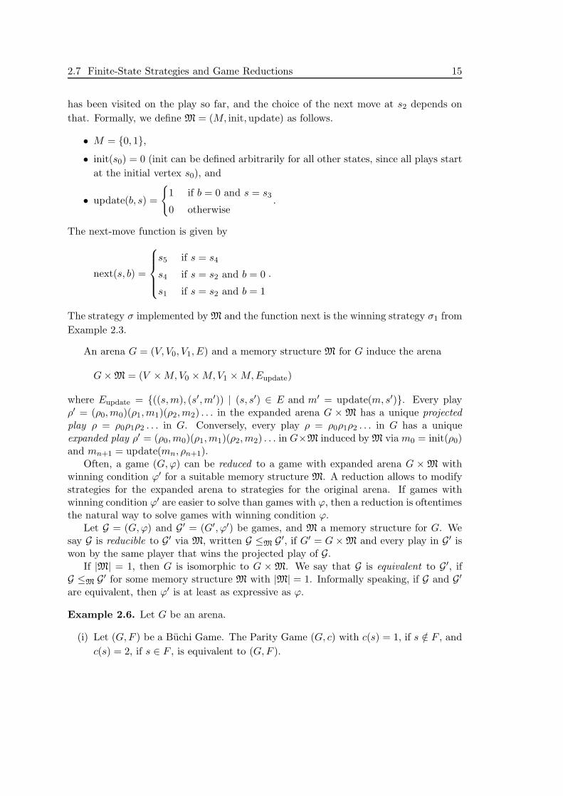
Example 2.1. To illustrate the definitions above, consider the arena G = (V, V0, V1, E)depicted in Figure 2.1, which is our running example throughout this chapter. Thepositions of Player 0 are V0 = {s2, s4}, Player 1’s positions are V1 = {s0, s1, s3, s5}. Thearcs denote the possible moves. A possible play in G is ρ = s0s2s4s5s3s
ω1 .
s0
s1
s2
s3
s4
s5
Figure 2.1: The arena G

2.5 Winning Conditions 11
A game G = (G,ϕ) consists of an arena G = (V, V0, V1, E) and a winning conditionϕ specifying the set of winning plays Win ⊆ V ω. A play ρ is won by Player 0, ifρ ∈ Win. Otherwise, it is won by Player 1. In the following, we often consider gameswith designated initial vertex: an initialized game (G, s, ϕ) consists of a game (G,ϕ) anda vertex s of G. In such a game, all plays start in s. Finally, a solitary game for Player iis a game played in a solitary arena for Player i.
2.5 Winning Conditions
The most general outcome of a play is a payoff for each player. This is modeled by payofffunctions pi for Player i specifying the payoff pi(ρ) for every play ρ. Yet, most games,both in real life and in mathematics, are antagonistic: the gain of a player is the loss ofthe other player. Mathematically speaking, the payoffs for every play sum up to zero.Accordingly, such games are called zero-sum games. For most of our purposes we caneven abstract from an actual payoff and just declare a winner for each play. Then, theother player loses the play. This corresponds to the general definition of a game fromabove employing a set of winning plays for Player 0. We stick to this with the exceptionof one type of games that is introduced at the end of this section.
While it would suffice to specify the set Win of winning plays for Player 0 directly,games typically employ a winning condition ϕ that defines Win indirectly. The advantagelies in the intuitive nature of these winning conditions, which simplifies reasoning aboutthose games considerably.
Nevertheless, we begin in an abstract setting: the Borel Hierarchy consists of ω-lan-guages and is build up from a class of basic languages, comprised of the open sets Z ·Σω
for Z ⊆ Σ∗, by applying complementation and countable union. To avoid delving intotopology, we refer the curious reader to [34]. We just observe that every regular languageis a Borel set , a set contained in the Borel Hierarchy.
G is a Borel Game [37], if the set of winning plays is a Borel set. This broad class,which encompasses most of the zero-sum games that can be found in literature, is ofinterest, since it enjoys useful properties. As it is often easy to show that a set of winningplays, defined by a winning condition ϕ, is Borel, this is often the first step in the analysisof a new type of game.
As hinted at above, the set of winning plays is typically given implicitly by a winningcondition ϕ, oftentimes as requirements on Occ(ρ) or Inf(ρ). Several conditions havebeen investigated in the literature. We introduce here only those that are of interest toour work.
Buchi Games: ϕ = F ⊆ V and ρ ∈ Win iff Inf(ρ) ∩ F �= ∅.
Generalized Buchi Games: ϕ = (Fj)j=1,...,k where Fj ⊆ V and ρ ∈ Win iff Inf(ρ)∩Fj �= ∅for all j ∈ [k].
Request-Response Games: ϕ = (Qj , Pj)j=1,...,k, where Qj, Pj ⊆ V , and ρ ∈ Win iff∀j ∀n(ρn ∈ Qj → ∃n′ ≥ n : ρn′ ∈ Pj).

12 2 Preliminaries
Muller Games: ϕ = F ⊆ 2V and ρ ∈ Win iff Inf(ρ) ∈ F .
Parity Games: ϕ = c : V → [k], for some k, and ρ ∈ Win iff max(Inf(c(ρ))) is even.Here, c is a coloring of the arena’s vertices. For a play ρ = ρ0ρ1ρ2 . . . ∈ V ω letc(ρ) = c(ρ0)c(ρ1)c(ρ2) . . ..
LTL Games: ϕ ∈ LTL and ρ ∈ Win iff ρ |= ϕ. Here, the graph underlying the arena isassumed to be labeled.
It is easy to show that all conditions introduced above define a Borel set of winningplays. An important subclass of Borel Games are regular games, games whose winningplays for Player 0 form a regular language.
Example 2.2. We continue Example 2.1 by specifying two games with arena G.
(i) The initialized Borel Game G1 = (G, s0,Win) with Win = {ρ | {s1, s3} ⊆ Occ(ρ)}.The play s0s2s4s5s3s
ω1 is won by Player 0 whereas the play (s0s2s1)ω is won by
Player 1.
(ii) The Buchi Game G2 = (G,F ) with F = {s1}. The play s3(s2s4)ω is won byPlayer 1; however, Player 0 can do better with s3(s2s1s0)ω, for example, a playthat she wins.
A class of games that does not fit into the framework outlined above are Mean-Payoff Games [15]. They are not zero-sum and the payoffs are defined by an integer-labeling of the edges. The players try to maximize respectively minimize certain meansof the sum of labels seen on a play. A (initialized) Mean-Payoff Game G = (G, s, d, l)consists of an arena G = (V, V0, V1, E), an initial vertex s ∈ V , d ∈ N, and a functionl : E → {−d, . . . , d} assigning integer labels to the edges. For a play ρ = ρ0ρ1ρ2 . . .define the gain v0(ρ) for Player 0,
v0(ρ) = lim infn→∞
1n
n−1∑i=0
l(ρi, ρi+1),
and the loss v1(ρ) for Player 1,
v1(ρ) = lim supn→∞
1n
n−1∑i=0
l(ρi, ρi+1).
Player 0 tries to maximize v0(ρ) whereas Player 1 tries to minimize v1(ρ). Obviously,the gain for Player 0 is never higher than the loss for Player 1.
2.6 Strategies and Positional Strategies
After introducing the way infinite games are played, we now consider the most importantand interesting aspect of games: how to choose the next move? In general, this decision

2.6 Strategies and Positional Strategies 13
may depend on the history of the play, the sequence of moves made by the playersso far. Strategies are introduced in this general sense, but typically a more restrictivenotion suffices, which limits the amount of information about the history that is used todetermine the next move. The most extreme choice is to use no information at all, i.e.,the choice of the next move depends only on the current position of the token. It turnsout that several games can be won with those simple strategies.
Let G = (V, V0, V1, E) be an arena. A strategy for Player i is a (partial) mappingσ : V ∗Vi → V such that (s, σ(ws)) ∈ E for all w ∈ V ∗ and all s ∈ Vi. The set ofall strategies for Player i (in a fixed arena) is denoted by Γi. We denote strategies forPlayer 0 (and the indefinite Player i) by σ and strategies for Player 1 by τ .
A play ρ0ρ1ρ2 . . . is played according to σ or is consistent with σ, if ρn+1 = σ(ρ0 . . . ρn)for every ρn ∈ Vi. The strategy σ is a winning strategy for Player i from s ∈ V , if everyplay starting in s that is played according to σ is won by Player i.
The winning region Wi of Player i is
Wi = {s ∈ V | Player i has a winning strategy from s}.
Obviously, we have W0 ∩W1 for every game. A game is determined , if W0 ∪W1 = V ,i.e., from every vertex, one of the players has a winning strategy. An initialized game(G, s, ϕ) is won by Player i, if she has a winning strategy from s. Otherwise she loses thegame. Determinacy means that exactly one of the players wins (G, s, ϕ) while the otherone loses the game. This is trivially true for a single play, but not for a game in general.Nevertheless, all zero-sum games we consider in this thesis are determined. Note thatour definition of determinacy is not applicable to games that are not zero-sum; however,the definition can be extended accordingly. Solving a game G amounts to determiningW0 and W1 and corresponding winning strategies.
A rather restrictive notion of strategies is obtained by prohibiting the use of anyinformation about the history of the play. The choice of the next move only dependson the vertex the token is at. Nevertheless, these strategies suffice to win many kindsof games. Formally, we say a strategy σ for Player i is positional , if σ(ws) = σ(w′s)for all w,w′ ∈ V ∗ and all s ∈ Vi. Hence, a positional strategy is fully specified by amapping that assigns a successor to every vertex in Vi. We use both representationsinterchangeably.
Example 2.3. Again, we continue Example 2.1 by defining winning strategies for thetwo games defined in Example 2.2.
(i) For G1, with initial vertex s0, the winning condition for Player 0 requires the tokento visit both s1 and s3. Therefore, Player 0 cannot move the token to s1 as soon asit reaches s2 after the first move of Player 1. Rather, she has to move it via s4 tos5 first, from which Player 1 has only one choice, namely, to move the token to s3.From there, he can either move the token to s1 directly, and lose thereby, or move

14 2 Preliminaries
it to s2, from where Player 0 can move it to s1, and again win the play in doingso. The remainder of the play is irrelevant, then. Thus, we define the strategy σ1
for Player 0 for a finite play w and s ∈ V0 as follows
σ1(ws) =
⎧⎪⎪⎨⎪⎪⎩s4 if s = s2 and s3 /∈ Occ(w)
s1 if s = s2 and s3 ∈ Occ(w)
s5 if s = s4
As reasoned above, σ1 is a winning strategy for Player 0 in G1. Note however, thatσ1 is not positional.
(ii) For the Buchi Game G2, the winning condition requires the token to visit s1 infi-nitely often. We define a positional strategy σ2 by σ2(s2) = s1 and σ2(s4) = s5. Itis easy to verify that every play consistent with σ2 visits s1 infinitely often. Thus,σ2 is a winning strategy from every vertex for Player 0 in G2.
2.7 Finite-State Strategies and Game Reductions
A compromise between a positional strategy and a strategy with infinite domain is astrategy with memory. Here, the decision about the next move does not take into accountthe complete history, but some abstraction of it. Thus, two different histories can havethe same abstraction and therefore share the same next move. Oftentimes, there areonly finitely many abstractions; hence, the strategy is realizable with finite memory.Nevertheless, we give all definitions as general as possible.
Let G = (V, V0, V1, E) be an arena. A memory structure M = (M, init,update) for Gconsists of a non-empty set M of memory states, an initialization function init : V →M ,and an update function update : M × V →M .
The memory content reached after w = w0 . . . wn ∈ V +, update∗(w), is defined in-ductively by update∗(w0) = init(w0) and
update∗(w0 . . . wn) = update(update∗(w0 . . . wn−1), wn).
A function next : Vi×M → V is a next-move function for Player i, if (s,next(s,m)) ∈ Efor all m ∈M and s ∈ Vi. A next-move function induces a strategy with memory M forPlayer i via σ(w0 . . . wn) = next(wn,update∗(w0 . . . wn)).
We call the strategy σ finite-state, if M is finite. We call |M | the size of M and(slightly abusive) the size of an induced (finite-state) strategy.
Remark 2.4. If |M | = 1, then is σ positional.
Example 2.5. The winning strategy σ1 from Example 2.3 for G1 from Example 2.2 canbe implemented as finite-state strategy. The memory is used to remember whether s3
2.7 Finite-State Strategies and Game Reductions 15
has been visited on the play so far, and the choice of the next move at s2 depends onthat. Formally, we define M = (M, init,update) as follows.
• M = {0, 1},
• init(s0) = 0 (init can be defined arbitrarily for all other states, since all plays startat the initial vertex s0), and
• update(b, s) =
{1 if b = 0 and s = s3
0 otherwise.
The next-move function is given by
next(s, b) =
⎧⎪⎪⎨⎪⎪⎩s5 if s = s4
s4 if s = s2 and b = 0
s1 if s = s2 and b = 1
.
The strategy σ implemented by M and the function next is the winning strategy σ1 fromExample 2.3.
An arena G = (V, V0, V1, E) and a memory structure M for G induce the arena
G× M = (V ×M,V0 ×M,V1 ×M,Eupdate)
where Eupdate = {((s,m), (s′,m′)) | (s, s′) ∈ E and m′ = update(m, s′)}. Every playρ′ = (ρ0,m0)(ρ1,m1)(ρ2,m2) . . . in the expanded arena G × M has a unique projectedplay ρ = ρ0ρ1ρ2 . . . in G. Conversely, every play ρ = ρ0ρ1ρ2 . . . in G has a uniqueexpanded play ρ′ = (ρ0,m0)(ρ1,m1)(ρ2,m2) . . . in G×M induced by M via m0 = init(ρ0)and mn+1 = update(mn, ρn+1).
Often, a game (G,ϕ) can be reduced to a game with expanded arena G × M withwinning condition ϕ′ for a suitable memory structure M. A reduction allows to modifystrategies for the expanded arena to strategies for the original arena. If games withwinning condition ϕ′ are easier to solve than games with ϕ, then a reduction is oftentimesthe natural way to solve games with winning condition ϕ.
Let G = (G,ϕ) and G′ = (G′, ϕ′) be games, and M a memory structure for G. Wesay G is reducible to G′ via M, written G ≤M G′, if G′ = G× M and every play in G′ iswon by the same player that wins the projected play of G.
If |M| = 1, then G is isomorphic to G × M. We say that G is equivalent to G′, ifG ≤M G′ for some memory structure M with |M| = 1. Informally speaking, if G and G′
are equivalent, then ϕ′ is at least as expressive as ϕ.
Example 2.6. Let G be an arena.
(i) Let (G,F ) be a Buchi Game. The Parity Game (G, c) with c(s) = 1, if s /∈ F , andc(s) = 2, if s ∈ F , is equivalent to (G,F ).
16 2 Preliminaries
(ii) Let (G, c) be a Parity Game. The Muller Game (G,F) is equivalent to (G, c), ifF ∈ F iff max{c(s) | s ∈ F} is even.
Our main interest in game reductions is their usage in solving games. But beforewe state the reduction theorem, we define the composition of memory structures. Thisallows us to give a more general statement than the one that is used in most reductions,which is an easy corollary. Let M = (M, init,update) be a memory structure for anarena G and let M′ = (M ′, init′,update′) be a memory structure for G×M. We obtaina memory structure M′′ = M × M′ = (M ′′, init′′,update′′) for G where M ′′ = M ×M ′,init′′(s) = (init(s), init′(s, init(s))), and
update′′((m,m′), s) = (update(m, s),update′(m′, (s,update(m, s)))).
Theorem 2.7 (Reduction Theorem). Let M = (M, init,update) be a memory struc-ture for an arena G and M′ = (M ′, init′,update′) be a memory structure for G × M.Furthermore, let G and G′ be games with arena G respectively G × M. If G ≤M G′ andPlayer i has a winning strategy σ′ with memory M′ for G′ from position (s0, init(s0)),then she also has a winning strategy σ with memory M × M′ for G from s0.
Proof. Let σ′ be induced by next′ : (Vi ×M) ×M ′ → V ×M . We need to define anext-move function next : Vi × (M ×M ′) → V such that it induces a winning strategyσ for G. For (s,m) ∈ Vi ×M and m′ ∈ M ′ such that next′((s,m),m′) = (s′,m′′), letnext(s, (m,m′)) = s′.
Let ρ = ρ0ρ1ρ2 . . . be a play according to σ in G such that ρ0 = s0. Furthermore, letρ′ = (ρ0,m0)(ρ1,m1)(ρ2,m2) . . . and ρ′′ = (ρ0, (m0,m
′0))(ρ1, (m1,m
′1))(ρ2, (m2,m
′2)) . . .
be the unique expanded plays in G′ = G×M respectively in G×(M×M′). By definition,we have (ρ0,m0) = (s0, init(s0)). Thus, if ρ′ is played according to σ′, then it is wonby Player i. Since G ≤M G′, ρ is then won by Player i as well. Hence, σ is a winningstrategy for Player i from s for G.
So, it remains to show that ρ′ is consistent with σ′: let (ρn,mn) ∈ Vi ×M . We haveρn+1 = σ(ρ0 . . . ρn) = next(ρn, (mn,m
′n)). Since next(ρn, (mn,m
′n)) is the first compo-
nent of next′((ρn,mn),m′n), we have next′((ρn,mn),m′
n) = (ρn+1,m) for some m ∈ M .Since ((ρn,mn), (ρn+1,m)) is an edge of G×M, we have m = update(mn, ρn+1) = mn+1.Hence, we have σ′((ρ0,m0) . . . (ρn,mn)) = next′((ρn,mn),m′
n) = (ρn+1,mn+1) for all(ρn,mn) ∈ Vi ×M . Therefore, ρ′ is played according to σ′.
Corollary 2.8. Let G′ = G×M, σ′ be a strategy in G and σ be the induced strategy inG as above. Furthermore, let ρ and ρ′ be plays in G consistent with σ respectively in G′
consistent with σ′.
(i) The expanded play of ρ is consistent with σ′.
(ii) The projected play of ρ′ is consistent with σ.

2.8 Unravelings and Restricted Arenas 17
Another important consequence of the theorem is concerned with the case of posi-tional winning strategies for G′.
Corollary 2.9. If G ≤M G′ and Player i has a positional winning strategy for G′ fromposition (s, init(s)), then she has a winning strategy with memory M for G from s.
The last corollary relates the winning regions of the two games.
Corollary 2.10. If G ≤M G′ and W ′i is the winning region of Player i in G′, then
Wi = {s ∈ V | (s, init(s)) ∈W ′i} is the winning region of Player i in G.
Example 2.11. Let G = (G,ϕ) be a regular game, i.e., the set of winning plays forPlayer 0, Win ⊆ V ω, is a regular language. Then, Win is the language accepted by somedeterministic Muller Automaton M = (Q,V, q0, δ,F) [25]. Define M = (Q, init,update)where init(s) = q0 for all s ∈ V and update = δ. Finally, define the Muller GameG′ = (G× M,F ′) where
{(v1, q1), . . . , (vn, qn)} ∈ F ′ ⇔ {q1, . . . , qn} ∈ F .
Then, we have G ≤M G′, i.e., every regular ame can be reduced to a Muller Game.
2.8 Unravelings and Restricted Arenas
Given an arena G = (V, V0, V1, E) and an initial vertex s ∈ V let, TG,s = (V ∗, V ∗0 , V
∗1 , E
∗)be the unraveling of G from s where V ∗ is the set of finite plays of G starting in s, V ∗
i
contains exactly those plays in V ∗ that end in a vertex of Vi, and (ws′, ws′s′′) ∈ E∗ iffws′s′′ ∈ V ∗ and (s′, s′′) ∈ E. A play ρ∗ = (ρ0)(ρ0ρ1)(ρ0ρ1ρ2) . . . in TG,s starting in s isuniquely determined by the sequence ρ = ρ0ρ1ρ2 . . ., which is a play in G starting in s.Conversely, every play in G determines a unique play in TG,s. Thus, we denote plays inTG,s by the respective play in G.
Also, every winning condition for G can be translated into a winning condition forthe unraveled arena such that the winner of a play ρ in G and its counterpart ρ∗ in TG,s
are the same. Finally, a strategy σ∗ for TG,s can be transformed into a strategy σ in Gby σ(ρ0 . . . ρn) = σ∗((ρ0) . . . (ρ0 . . . ρn)). The reverse transformation, from a strategy σin G into a strategy σ∗ for TG,s, is given by σ∗((ρ0) . . . (ρ0 . . . ρn)) = σ(ρ0 . . . ρn).
Thus, we can reason about an arena G or its unraveling TG,s and translate theresults back and forth. The main benefit of reasoning about the unraveling insteadof the original arena is that TG,s is a tree, thus every strategy σ∗ is positional. Thisconsiderably simplifies the discussion about arbitrary strategies for an arena.
For a strategy σ for Player i in G let TσG,s be the restriction of TG,s to those plays
that are consistent with σ. Every vertex in V ∗i has exactly one child in the restricted
unraveling. Conversely, every subtree obtained from TG,s by deleting all but one child(and the subtrees rooted in these vertices) of every vertex in V ∗
i induces a strategy for
18 2 Preliminaries
Player i. For strategies σ and τ for Player 0 respectively 1 let Tσ,τG,s be the restriction to
the unique play that is consistent with σ and τ .For a finite play w denote the subtree of TG,s rooted in w by TG,s�w. The definitions
for TσG,s�w and T
σ,τG,s�w are analogous.
For positional strategies in G, we do not need to take the detour via the unraveling todefine restricted arenas: let G = (V, V0, V1, E) be an arena and σ : Vi → V a positionalstrategy for Player i. The restriction of G to σ is G�σ = (V, V0, V1, E
′) where
E′ = {(s, σ(s)) | s ∈ Vi} ∪ {(s, s′) ∈ E | s ∈ V1−i}.
Note that the unraveling ofG�σ from s is TσG,s. Also, G�σ is a solitary game for Player 1−i
(in the wider sense discussed above).For s ∈ V , and strategies σ and τ for Player 0 respectively Player 1, we define the
play ρ(s, σ, τ) = ρ0ρ1ρ2 . . . where ρ0 = s and
ρn+1 =
{σ(ρ0 . . . ρn) if ρn ∈ V0
τ(ρ0 . . . ρn) if ρn ∈ V1
.
Again, ρ(s, σ, τ) is equal to the only play in Tσ,τG,s. If both strategies are positional, then
ρ(s, σ, τ) is the only play in (G�σ)�τ starting in s. If G is a solitary arena for Player 0,then we have ρ(s, σ, τ) = ρ(s, σ, τ ′) for all strategies τ and τ ′ for Player 1, i.e., thestrategy of Player 1 is irrelevant. Therefore, we can write ρ(s, σ) for short. We use thesame notation for Player 1, if there is no ambiguity.
Remark 2.12. Let σ and τ be finite-state strategies for Player 0 respectively Player 1.Then, ρ(s, σ, τ) is ultimately periodic.
2.9 Basic Results
To conclude this chapter, we state some results about the various games introduced sofar, which are used in the later chapters. The most general one concerns Borel Games.
Theorem 2.13 ([37]). Borel Games are determined.
This result immediately implies the determinacy of all games introduced above (saveMean-Payoff Games, for which our notion of determinacy does not apply). However,pure determinacy is generally not enough. Positional or finite-state strategies suffice towin the games introduced above. A game is positionally determined if from every vertexone of the players has a positional winning strategy. Analogously, a game is determinedwith finite-state strategies, if from every vertex one of the players has a finite-statewinning strategy. The existence of finite-state winning strategies is typically proven bya reduction to a simpler game. The following result is a cornerstone of the theory ofinfinite games.
2.9 Basic Results 19
Theorem 2.14 ([17]). Parity Games are positionally determined.
As Buchi Games are a special case of Parity Games, we obtain a similar result.
Corollary 2.15. Buchi Games are positionally determined.
Proof. The Buchi Game (G,F ) is equivalent to the Parity Game over G with coloringc, where c(s) = 2 for s ∈ F and c(s) = 1 for s /∈ F
Determinacy of Muller Games can be derived most easily from the positional de-terminacy of Parity Games by a reduction, although it was first proven directly in [6].The memory structure used in the reduction keeps record of the vertices, ordered bytheir latest visit in the play up to that position, equipped with a marker that signalsthe infinity set of a play. This structure, called latest appearance record (LAR), is animprovement of the order vector, introduced by McNaughton [38]. A formal expositioncan be found in [25]. We just note that the size of the memory is bounded by (|G|+ 1)! .
Theorem 2.16 ([26]). Muller Games are reducible to Parity Games with finite memory.Thus, they are determined with finite-state strategies.
Another corollary completes the discussion about regular games started in Exam-ple 2.11.
Corollary 2.17. Every regular game is determined and both players have finite-statewinning strategies.
Proof. Combine the construction from Example 2.11 and Theorem 2.16.
The last type of zero-sum game we deal with here are LTL Games. They are a specialcase of the regular games discussed in Corollary 2.17, which is the key to the proof ofthe following theorem.
Theorem 2.18. LTL Games are finite-state determined.
We also note the complexity of solving LTL Games, as we use them as target forreductions.
Theorem 2.19 ([49, 45]). Solving LTL Games is 2EXPTIME-complete. Solving soli-tary LTL Games is PSPACE-complete.
The complexity of solving games for several syntactic fragments of LTL is discussedin great detail by Alur and La Torre [3]. They show that the restriction to a subset ofthe operators can lower the complexity drastically.
Lastly, we consider Mean-Payoff Games. Since they are not zero-sum games, ournotion of determinacy does not apply here. Instead, we say that a strategy σ for Player 0guarantees v ∈ R for her if v0(ρ) ≥ v for all ρ consistent with σ. Similarly, τ for Player 1guarantees v ∈ R for him if v1(ρ) ≤ v for all ρ consistent with τ .

20 2 Preliminaries
Theorem 2.20 ([15, 55]). Let (G, s, d, l) be an initialized Mean-Payoff Game. Thereexists a value vM (G) and positional strategies σ and τ such that σ and τ guaranteevM (G) for Player 0 respectively Player 1. Furthermore, the value and the strategies areeffectively computable.
Notice that the strategies σ and τ are optimal in the sense that there are no strategiesthat guarantee a better value for one of the players. Assume there is a strategy σ′ forPlayer 0 that guarantees v0 > vM (G). Then
vM (G) < v0 = v0(ρ(v, σ′, τ)) ≤ v1(ρ(s, σ′, τ)) ≤ vM (G),
which is a contradiction. Analogously, there is no strategy τ ′ for Player 1 that guaranteesv1 < vM (G). Also, we have v0(ρ(s, σ, τ)) = v1(ρ(s, σ, τ)) = vM (G).

Chapter 3
Request-Response Games
Request-Response Games, first introduced by Wallmeier et. al. [54], are characterized bya very intuitive winning condition: some vertices of the arena are designated as requestswhile others are responses. Player 0’s goal is to respond to every request. Formally,the winning condition of G = (G, (Qj , Pj)j=1,...,k) consists of a finite collection of pairs(Qj , Pj), where Qj and Pj are subsets of the arena’s vertices. We call the pair (Qj , Pj)the j-th (Request-Response) condition. A request (of condition j) is a visit of a vertexin Qj and a response (of condition j) is a visit of a vertex in Pj. Furthermore, a requestof condition j is open after a finite play if there was a request of condition j that hasnot yet been responded. It is Player 0’s goal to answer every request of condition j by asubsequent response, where a single response answers all open requests accepted so far.Formally, Player 0 wins a play ρ, iff
∀j ∀n(ρn ∈ Qj → ∃n′ ≥ n : ρn′ ∈ Pj).
If we label the arena such that l(s) = {qj | s ∈ Qj} ∪ {pj | s ∈ Pj}, then the set ofwinning plays is also specified by the LTL formula
ϕ :=k∧
j=1
G (qj → Fpj) .
Thus, G is equivalent to the LTL Game (G,ϕ). Conversely, every (generalized) Buchi-Game can easily be reduced to an equivalent Request-Response Game.
A classical example for controller synthesis is a busy intersection with traffic lights,equipped with sensors in the streets that detect cars waiting at a red light, and pedestrianlights with buttons for waiting pedestrians. The arena consists of vertices encoding thestate of the system: the colors of the lights and flags for the requests. All undesirable(read: unsafe, i.e., too many green lights) states are ignored. The transitions modelthe changes of the color, sensor readings, and pushed buttons. If a light changes togreen, its flag is set to false. The desired behavior, every request by a waiting car

22 3 Request-Response Games
or pedestrian is granted, can be modeled by a Request-Response pair for every light.This example illustrates the need for time-optimal winning strategies. A traffic lightthat is green every other day satisfies the specification, but is not useful at all. Everyrequest should be served as soon as possible. Nevertheless, it might be advantageousto prioritize some Request-Response conditions over others, for example if one of thestreets is a major thoroughfare and the other is a small side street. All this can beimplemented in the framework we introduce in this Chapter. However, the frameworkignores multiple requests, thus the light with the most cars waiting is not served first.In Chapter 4 we discuss how to factor this in as well.
The intuitive notion of open requests naturally leads the way to the definition ofwaiting times: every time a condition is requested that is not open at the moment, aclock is started. This clock is stopped as soon as the request is responded. All requestsof a condition that is already open at that moment are ignored. Thus, instead of justdetermining winning strategies, we are now interested in time-optimal strategies, i.e.,strategies that minimize the waiting times. This changes the strategy problem froma decision problem to an optimization problem. Since a play is infinite, we need toaggregate the periods of waiting for a response to define the measure of a strategy.Then, the value of a strategy is the worst value of the plays consistent with the strategy.
A rather simple choice for aggregation is to uniformly bound the waiting times.Such a bound can be found by showing the existence of finite-state winning strategies:Request-Response Games are easily reducible to Buchi Games by keeping track of theopen requests in an extra component of the expanded arena. The set F is chosen suchthat F is visited infinitely often iff no request is open indefinitely. This reduction doesnot only prove determinacy of Request-Response Games but also gives an upper boundon the waiting times: by playing according to the finite-state strategy derived from thereduction, Player 0 ensures that every request is open for at most |G| ·k moves, providedthat she has a winning strategy at all. However, this bound needs not to be optimal.
It might be desirable for Player 0 to keep one request open for more steps thanshe has to in order to satisfy other requests more quickly. This is especially true incases where the conditions have different priorities, which can be modeled by penaltyfunctions that aggravate the waiting times. Thus, the global bound on the waiting timemight be very high, but the average waiting time decreases. This shows the need for anapproach that aggregates the waiting times over the infinite duration of the play, therebypermitting a trade-off between the conditions. The average number of open request, theaverage waiting time, and the average accumulated waiting time are three types ofaggregations discussed by Wallmeier [53]. He argues that only the latter one meets alldesired properties of such a measurement: the winner of a game can be determinedfrom its value and longer waiting times are increasingly penalized. Horn et. al. [29]showed that, with respect to the average accumulated waiting time, optimal finite-statestrategies exist and can be computed. We will repeat this proof here, since it contains anerror (in the proof of Proposition 9) which requires a modification of the proof technique.This is done in this chapter, in order to adapt the corrected technique to a novel winningcondition presented in Chapter 4.
3.1 Solving Request-Response Games 23
The proof consists of two steps. First, we show that it is not optimal to keep arequest open arbitrarily long, but that there exists a bound such that waiting timesabove that bound are not worthwhile. The following observation is key: if a condition isopen long enough, then the play visits a vertex twice such that the waiting times for allother conditions are higher at the second visit than they were at the first visit. Hence,Player 0 can play after the first visit as if it was the second visit. Thus, she skips aportion of the play without neglecting the other conditions. By skipping only costlyloops, Player 0 can ensure that the value of the play decreases. Applying this infinitelyoften shows that an optimal strategy uniformly bounds the waiting times.
Thus, we can restrict our search for an optimal winning strategy to a finite domain.The second step of the proof consists of a straight-forward reduction from the problemof finding an optimal strategy for Request-Response Games to the same problem forMean-Payoff Games. The memory of the expanded arena is used to keep track of thewaiting times. The first step guarantees that this arena is still finite.
This chapter is structured as follows: we begin by reducing Request-Response Gamesto Buchi Games in Section 3.1, a result which has a corollary that turns out to be usefulto us. In Section 3.2, we define waiting times and the value of a play and discuss someproperties. Then, we are able to state the main theorem of this chapter and spendthe rest of it to prove the theorem: in Subsection 3.2.1 we carry out the first step,showing that for every strategy of small value, there is another strategy of even smallervalue that additionally bounds the waiting times of all conditions. The second step, thereduction to Mean-Payoff Games, is presented in Subsection 3.2.2. For the remainderof this chapter, let G = (V, V0, V1, E) be an arena and let G = (G, s0, (Qj , Pj)j=1,...,k) bean initialized Request-Response Game.
3.1 Solving Request-Response Games
Request-Response Games are reducible to Buchi Games. This implies determinacy of Gand the existence of finite-state winning strategies. We present the proof here, since itgives a bound on the value of an optimal strategy, which we present in Section 3.2, afterwe have given all necessary definitions.
Theorem 3.1 ([54]). Request-Response Games are reducible to Buchi Games.
Proof. The memory is used to keep track of the open requests. Furthermore, a counteris used to check that no condition is open indefinitely. Every time the counter changesits value a final state is visited. Therefore, we have to take precautions if there is onlyone condition: if k = 1, then we add another condition (Q2, P2) with Q2 = P2 = ∅. LetM = (M, init,update) where
• M = 2[k] × [k] × {0, 1},
• init(s) = ({j ∈ [k] | s ∈ Qj\Pj}, 1, 0), and
24 3 Request-Response Games
• update((M,m, f), s) = (M ′,m′, f ′) where
◦ M ′ = (M ∪ {j ∈ [k] | s ∈ Qj})\{j ∈ [k] | s ∈ Pj},
◦ m′ =
{m if m ∈M ′
(m mod k) + 1 otherwise, and
◦ f ′ =
{0 if m = m′
1 otherwise.
To complete the definition of the Buchi Game, we specify the set F = V ×2[k]× [k]×{1}of recurring states. So, we define G′ = (G×M, F ) and have to show G ≤M G′. Therefore,let ρ = ρ0ρ1ρ2 . . . be a play in G and
ρ′ = (ρ0, (M0,m0, f0))(ρ1, (M1,m1, f1))(ρ2, (M2,m2, f2)) . . .
be the unique expanded play in G× M.
Player 1 wins ρ
⇔ ∃j ∃n′ : (ρn ∈ Qj ∧ ∀n ≥ n′ : ρn /∈ Pj)
⇔ ∃j ∀ωn : j ∈Mn
⇔ ∃j ∀ωn : mn = j
⇔ ∀ωn : f ′n = 0
⇔ ∀ωn : ρ′n �∈ F
⇔ Player 1 wins ρ′
This reduction is asymptotically optimal.
Lemma 3.2 ([54]). There is a family of initialized Request-Response Games (Gn)n∈N
such that
(i) the size of the arena of Gn is linear in n,
(ii) the number of Request-Response conditions of Gn is linear in n,
(iii) Player 0 wins Gn, but
(iv) she has no finite-state winning strategy of size less than n · 2n.
3.2 Time-optimal Strategies for Request-Response Games
In this section, we begin the treatment of time-optimal strategies for Request-ResponseGames by formalizing the intuitive notion of waiting times and by defining the valueof a strategy, following [29]. The waiting time for condition j, tj : V ∗ → N, is definedinductively by tj(ε) = 0 and
3.2 Time-optimal Strategies for Request-Response Games 25
• If tj(w) = 0, then tj(ws) =
{1 if s ∈ Qj\Pj
0 otherwise
• If tj(w) > 0, then tj(ws) =
{0 if s ∈ Pj
tj(w) + 1 otherwise.
Let t(w) = (t1(w), . . . , tk(w)) be the waiting time vector . We compare vectors compo-nentwise, i.e., t(x) ≤ t(y) iff tj(x) ≤ tj(y) for all j. A strategy σ for Player 0 uniformlybounds the waiting time for condition j to B, if tj(w) ≤ B for all finite plays w consistentwith σ. From the definition of tj we can directly derive the following remark about theevolution of the waiting time.
Remark 3.3. tj(x) ≤ tj(y) implies tj(xs) ≤ tj(ys) for all x, y ∈ V ∗ and all s ∈ V .
The value of a play is determined by the average accumulated waiting time. However,we want to be able to prioritize some conditions. Thus, we use a penalty function fj forevery condition j to define the value of a play. We require fj to be strictly increasing,since otherwise longer stretches of open requests could be desirable. Even worse, if wechoose fj to be a constant function, i.e., the penalty for an open request is the same,no matter how long the request is open already, then there are no optimal finite-statestrategies as we show in Example 3.4.
So, given a family (fj : N → N)j=1,...,k of strictly increasing penalty functions, define
• the penalty for condition j after w: pj(w) = fj(tj(w)),
• the penalty after w: p(w) =∑k
j=1 pj(w),
• the value of a play vR(ρ) = lim supn→∞ 1n
∑n−1i=0 p(ρ0 . . . ρi), and
• the value of a strategy vR(σ) = supτ∈Γ1vR(ρ(s0, σ, τ)).
A strategy σ for Player 0 is optimal , if vR(σ) ≤ vR(σ′) for all σ′ ∈ Γ0.
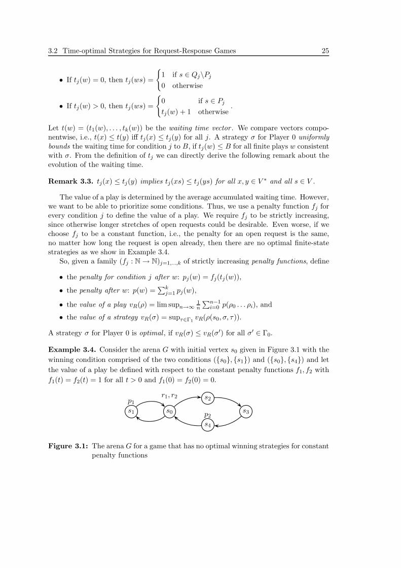
Example 3.4. Consider the arena G with initial vertex s0 given in Figure 3.1 with thewinning condition comprised of the two conditions ({s0}, {s1}) and ({s0}, {s4}) and letthe value of a play be defined with respect to the constant penalty functions f1, f2 withf1(t) = f2(t) = 1 for all t > 0 and f1(0) = f2(0) = 0.
s0s1 s3
s2
s4
r1, r2p1
p2
Figure 3.1: The arena G for a game that has no optimal winning strategies for constantpenalty functions

26 3 Request-Response Games
Note that every winning strategy has to use both loops infinitely often. However,using the left loop twice instead of the right loop once in a play ρ0 . . . ρn−1 decreases∑n−1
i=0
∑2j=1 fj(tj(ρ0 . . . ρi)) by one. Thus, for a given finite-state strategy σ, the unique
resulting play ρ(s, σ) = xyω is ultimately periodic, by Remark 2.12. The period y visitsthe right loop at least once. Also, since G is a solitary arena, we have vR(ρ) = vR(σ).
Let y′ result from y by replacing every visit of the right loop by two visits of theleft loop and let ρ′ = x(yy′)ω. This play is realized by a finite-state strategy σ′. Then,vR(ρ′) < vR(ρ) and therefore vR(σ′) = vR(ρ′) < vR(ρ) = vR(σ). Thus, Player 0 has nooptimal finite-state strategy.
We continue by some simple, but useful, observations about the value of a playrespectively a strategy.
Lemma 3.5. Let ρ be a play and σ a strategy for Player 0.
(i) If vR(ρ) <∞, then Player 0 wins ρ.
(ii) If vR(σ) <∞, then σ is a winning strategy for Player 0.
Proof. (i) Consider the contraposition: let ρ = ρ0ρ1ρ2 . . . be winning for Player 1. Then,there exists a condition j that is requested at some ρn, but never responded at any ρn+n′ .Then
tj(ρ0 . . . ρn+n′) = n′ ≤ fj(tj(ρ0 . . . ρn+n′)) ≤ p(ρ0 . . . ρn+n′),
since fj is strictly increasing. Thus,
1n+ n′
n+n′−1∑i=0
p(ρ0 . . . ρi) ≥ 1n+ n′
· n′ · (n′ − 1)
2=
n′ − 12 · ( n
n′ + 1)
for all n′ ∈ N, which diverges to infinity. Therefore, vR(ρ) = ∞.(ii) Towards a contradiction assume σ is not a winning strategy. Then, there ex-
ists a strategy τ for Player 1 such that the play ρ(s0, σ, τ) is won by Player 1. Then,vR(ρ(s0, σ, τ)) = ∞ by (i) and therefore vR(σ) = ∞, which yields the desired contradic-tion.
The other implication of the statements does not hold: Player 0 can win a play, evenif its value diverges. An example is a play such that the waiting time for a condition isnot uniformly bounded, but every request is responded eventually. However, we showthat this is not necessary. If Player 0 wins a game, then she can also win and uniformlybound the waiting times.
Now, we return to the reduction of Request-Response Games to Buchi Games. Thestrategy induced by the reduction uniformly bounds the waiting time in terms of the

3.2 Time-optimal Strategies for Request-Response Games 27
size of the arena and the number of Request-Response conditions. This also bounds thevalue of an optimal strategy. Our interest in the proof of Theorem 3.1 stems from thefollowing corollary.
Corollary 3.6. If Player 0 wins G, then she also has a winning strategy σ such thatvR(σ) ≤ ∑k
j=1 fj(|G| · k) = : bR(G).
Proof. Let Player 0 win G. Then, she also has a positional winning strategy σ′ from(s0, init(s0)) in G′ from Theorem 3.1. Consider a play ρ′ in G× M�σ′ and assume thatthere is an infix w of ρ′ of length greater than |G| such that w does not contain a vertexfrom F . This implies the existence of a play, played according to σ′ that visits F onlyfinitely often, which contradicts the fact that σ′ is a winning strategy. Hence, everyinfix of length greater than |G| of a play ρ that is consistent with σ′ visits F at leastonce. This means that the m-component of the memory state of ρ′ changes after atmost |G| moves. This component ranges over [k]; hence, after at most |G| · k moves,the m-component has cycled through all possible values. Thus, every j cannot be in theM -component of more than |G| · k consecutive memory states. The index j leaves theM -component at a vertex (s′,m′) of ρ′ if s′ ∈ Pj .
Now, consider a play ρ = ρ0ρ0ρ2 . . . of G according to the winning strategy σ obtainedby the reduction. It is a projection of a play according to σ′, which directly impliestj(ρ0 . . . ρn) ≤ |G| · k for all n and all j ∈ [k]. Thus,
1n
n−1∑i=0
p(ρ0 . . . ρi) =1n
n−1∑i=0
k∑j=1
fj(tj(ρ0 . . . ρi))
≤ 1n
n−1∑i=0
k∑j=1
fj(|G| · k)
=k∑
j=1
fj(|G| · k) = bR(G).
This implies vR(ρ) ≤ bR(G) for every play ρ consistent with σ. Therefore, we obtainvR(σ) ≤ bR(G).
This completes our preparation and we are now able to state the main theorem ofthis chapter; The rest of this chapter is devoted to prove it. This result was alreadyclaimed in [29]. We present a new proof here, which can be adapted to other winningconditions. Nevertheless, the definition of the strategy improvement operator and theresults about it are from [29]. Then, we deviate and define an improvement schemetransforming a winning strategy into a winning strategy that additionally bounds allwaiting times, without increasing the value of the strategy.

28 3 Request-Response Games
Theorem 3.7. If Player 0 wins G, then she also has an optimal winning strategy.Furthermore, this strategy is finite-state and effectively computable.
The proof consists of two major steps. The first one, presented in Subsection 3.2.1,is to prove that from every winning strategy of value less than bR(G), we can constructanother winning strategy with smaller value that uniformly bounds the waiting timesfor all conditions. This is achieved by improving the strategy repeatedly with a strategyimprovement operator that deletes costly loops of the plays consistent with the strategyunder consideration. Hence, if Player 0 wins G, then vR(σ) ≤ bR(G) for the optimalwinning strategy σ by Theorem 3.1 and Corollary 3.6. Thus, an optimal strategy alsobounds the waiting times for all conditions. These bounds allow us to find an optimalstrategy in the second step by reducing the Request-Response Game to a Mean-PayoffGame, presented in Subsection 3.2.2. The expanded game is constructed such that theplays of both games have the same value. Thus, an optimal positional strategy for theMean-Payoff Game, which exists by Theorem 2.20, induces an optimal strategy for theRequest-Response Game.
3.2.1 Strategy Improvement for Request-Response Games
In this subsection, we prove the following statement: if Player 0 has a winning strategyof value less than bR(G), then she also has a strategy of smaller or equal value, whichuniformly bounds the waiting times of all conditions. Let σ0 be a winning strategy forPlayer 0 with value vR(σ0) ≤ bR(G). Inductively, we define strategies σ1, . . . , σk withthe following properties.
• All strategies are winning strategies for Player 0,
• bR(G) ≥ vR(σ0) ≥ vR(σ1) ≥ · · · ≥ vR(σk), and
• σj uniformly bounds the waiting times for all conditions j′ ≤ j to some boundthat only depends on the size of the arena and the number of Request-Responseconditions.
The first part of this subsection repeats work of Horn et. al. [29]. A strategy improvementoperator is defined for every condition and we show that the value does not increase,if the strategy is improved. In the second part of this subsection, which contains novelmaterial, we define an improvement scheme which applies each strategy improvementoperator infinitely often to a given winning strategy σj−1, obtaining the limit strategyσj. Here, our proof differs from the work in [29], which applies the strategy improvementoperator for condition only once. Afterwards, we have to lift the properties of a singleimprovement step to the limit of the improved strategies. Then, we are able to provethat the limit strategies do bound the waiting times.
Intuitively, the strategy σj from above is defined as σj−1 unless the waiting time forcondition j exceeds some bound. In this case, Player 0 skips loops in which the request isnot responded. However, she also has to make sure that she does not miss a response ofsome other condition that might be open from that point onwards. Therefore, she only

3.2 Time-optimal Strategies for Request-Response Games 29
skips loops in which the waiting time of all conditions at the end of the loop is greaterthan the waiting time at the beginning. By deleting loops, she might form new loops thatcould be deleted, also. Therefore, the strategy improvement operator has to be appliedinfinitely often. If there are no more loops to skip, then the length of an infix, in whicha request is open continuously, can be bounded. Mathematically speaking, we applythe strategy improvement operator infinitely often and define σj to be the limit of theimproved strategies. In the following, we introduce the strategy improvement operatorIj for the j-th condition and discuss some useful properties as presented in [29]. Theseproperties are then lifted to the limit of the improved strategies.
Given a winning strategy σ such that vR(σ) ≤ bR(G), we define the improved strategyIj(σ) as a strategy with memory M = (M, init,update) and next-move function next asfollows: The set of memory states M consists of finite plays played according to σ andis defined implicitly. The initialization function is given by init(s0) = s0. The updatefunction is going to be defined such that the last vertex of w and update∗(w) are equal.So, when defining update(w, s) for w ∈M and s ∈ V , we can assume that the last vertexof w and s are connected by an edge in G. We consider two cases.
If condition j is not even open or Player 0 has not waited too long, she continuesto play according to σ. Therefore, we define update(w, s) = ws if tj(ws) ≤ f−1
j (bR(G)).If she has waited too long, she looks ahead to skip a loop that she would have playedaccording to σ, but which does not contain a response of condition j. However, shehas to make sure that she does not carelessly skip responses of the other conditions ifthey are open. Thus, if tj(ws) > f−1
j (bR(G)), consider the tree obtained from TσG,s0
�ws
by deleting on every path the subtrees attached to the first vertex belonging to Pj.This tree is finite, since every infinite path corresponds to a losing play for Player 0played according to σ. This cannot happen, since σ is a winning strategy. Now considerthe set of vertices z of the tree, such that z ends in s and t(ws) ≤ t(z). This set isnon-empty as it contains ws. Let z′s be a vertex of maximal depth in this set. Then,update(w, s) = z′s.
To finish the definition of the strategy, we define next(s,w) = σ(w). It is clear thatthe last vertices of w and update∗(w) are equal for every prefix w consistent with Ij(σ),and that Ij behaves as intended, i.e., w is a subword of update∗(w) for every w consistentwith Ij(σ). Also, update∗ is monotonous with respect to the prefix relation, i.e., if x y,then also update∗(x) update∗(y). Furthermore, in both cases of the definition, theupdated memory is a prefix of a play according to σ.
Lemma 3.8 ([29]). update∗(w) is consistent with σ for all w consistent with Ij(σ).
Proof. By induction over w: every play starts in s0, so the induction base is trivial,as update∗(s0) = init(s0) = s0 holds. For the induction step, let w = ρ0 . . . ρn beplayed according to Ij(σ). Applying the induction hypothesis, we can assume thatupdate∗(ρ0 . . . ρn−1) is consistent with σ. By definition of update we have
update∗(ρ0 . . . ρn) = update(update∗(ρ0 . . . ρn−1), ρn).
30 3 Request-Response Games
Furthermore, as noted above, the last vertex of update∗(ρ0 . . . ρn−1) is ρn−1. Finally, ifρn−1 ∈ V0, then
ρn = Ij(σ)(ρ0 . . . ρn−1) (3.1)
= next(ρn−1,update∗(ρ0 . . . ρn−1))
= σ(update∗(ρ0 . . . ρn−1)).
Analogously to the definition, we consider two cases: either, we have
update(update∗(ρ0 . . . ρn−1), ρn) = update∗(ρ0 . . . ρn−1)ρn.
Then, by induction hypothesis and (3.1), update∗(ρ0 . . . ρn) is consistent with σj−1.Otherwise, in the second case of the definition, we have
update(update∗(ρ0 . . . ρn−1), ρn) = update∗(ρ0 . . . ρn−1)ρnz′,
where z′ is a path in TσG,s0
�update∗(ρ0...ρn−1)ρn. Together with the induction hypothesis
and (3.1), this shows that update∗(ρ0 . . . ρn) is consistent with σ.
This allows us to bound the waiting time of a finite play by the waiting time of itsmemory content.
Lemma 3.9 ([29]). t(w) ≤ t(update∗(w)) for all w consistent with Ij(σ).
Proof. By induction over w. The base case is t(s0) = t(init(s0)) = t(update∗(s0)).For the induction step we can assume t(w) ≤ t(update∗(w)). By Remark 3.3, we gett(ws) ≤ t(update∗(w)s). Now consider two cases: if tj(update∗(w)s) ≤ f−1
j (bR(G)), wehave
update∗(ws) = update(update∗(w), s) = update∗(w)s
and thus
t(ws) ≤ t(update∗(w)s) = t(update∗(ws)).
On the other hand, if tj(update∗(w)s) > f−1j (bR(G)), we have
update∗(ws) = update(update∗(w), s) = zs
where t(zs) ≥ t(update∗(w)s) and thus
t(ws) ≤ t(update∗(w)s) ≤ t(zs) = t(update∗(ws)).
This result implies that the uniform bounds of σ are also realized by Ij(σ).
3.2 Time-optimal Strategies for Request-Response Games 31
Lemma 3.10 ([29]). If σ uniformly bounds the waiting time for some condition j′ toB, so does Ij(σ).
Proof. We have tj′(w) ≤ B for all finite plays w consistent with σ. Now, let w bea play consistent with Ij(σ). Since update∗(w) is played according to σ we concludetj′(update∗(w)) ≤ B and tj′(w) ≤ tj′(update∗(w)) by Lemma 3.9. Thus, Ij(σ) uniformlybounds the waiting time for condition j′ to B.
Now, we show that the value of the improved strategy does not increase, applyingLemma 3.9.
Lemma 3.11 ([29]). vR(Ij(σ)) ≤ vR(σ).
Proof. For ρ = ρ0ρ1ρ2 . . . let
update∗(ρ) = limn→∞update∗(ρ0 . . . ρn),
which is consistent with σ for every play ρ consistent with Ij(σ) by Lemma 3.8. Weshow vR(ρ) ≤ vR(update∗(ρ)) for all ρ consistent with Ij(σ), which implies the claim.To this end, we define
S = {w′ � update∗(ρ) | ¬∃w � ρ : update∗(w) = w′}.
S contains exactly the vertices of the loops skipped by Player 0. Let w′ ∈ S: by definitionof update, we know tj(w′) > f−1
j (bR(G)) and thus p(w′) > bR(G) ≥ vR(σ). Hence,
lim supn→∞
1n
n−1∑i=0
p(update∗(ρ0 . . . ρi)) ≤ vR(update∗(ρ)) (3.2)
since the average decreases, if the summation omits the summands for the prefixesin S. Now, let w � ρ: we have t(w) ≤ t(update∗(w)) by Lemma 3.9 and thereforep(w) ≤ p(update∗(w)). Thus,
1n
n−1∑i=0
p(ρ0 . . . ρi) ≤ 1n
n−1∑i=0
p(update∗(ρ0 . . . ρi)).
The latter term converges to a value less than or equal to vR(update∗(ρ)) by (3.2). Thus,we conclude vR(ρ) ≤ vR(update∗(ρ)).
We can immediately conclude that σj is a winning strategy for Player 0.
Corollary 3.12 ([29]). Ij(σ) is a winning strategy for Player 0, if σ is a winningstrategy.
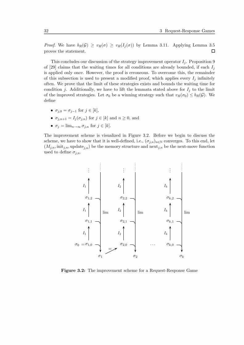
32 3 Request-Response Games
Proof. We have bR(G) ≥ vR(σ) ≥ vR(Ij(σ)) by Lemma 3.11. Applying Lemma 3.5proves the statement.
This concludes our discussion of the strategy improvement operator Ij. Proposition 9of [29] claims that the waiting times for all conditions are already bounded, if each Ijis applied only once. However, the proof is erroneous. To overcome this, the remainderof this subsection is used to present a modified proof, which applies every Ij infinitelyoften. We prove that the limit of these strategies exists and bounds the waiting time forcondition j. Additionally, we have to lift the lemmata stated above for Ij to the limitof the improved strategies. Let σ0 be a winning strategy such that vR(σ0) ≤ bR(G). Wedefine
• σj,0 = σj−1 for j ∈ [k],
• σj,n+1 = Ij(σj,n) for j ∈ [k] and n ≥ 0, and
• σj = limn→∞ σj,n for j ∈ [k].
The improvement scheme is visualized in Figure 3.2. Before we begin to discuss thescheme, we have to show that it is well-defined, i.e., (σj,n)n∈N converges. To this end, let(Mj,n, initj,n,updatej,n) be the memory structure and nextj,n be the next-move functionused to define σj,n.
σ0 σ1,0
σ1,1
σ1,2
σ1
σ2,0
σ2,1
σ2,2
σ2
σk,0
σk,1
σk,2
σk
=
I1
I1
I1
I2
I2
I2
Ik
Ik
Ik
lim lim lim
=
......
...
. . .
Figure 3.2: The improvement scheme for a Request-Response Game

3.2 Time-optimal Strategies for Request-Response Games 33
Lemma 3.13. Let j ∈ [k]. Then, limn→∞ σj,n exists.
Proof. First, we show by induction that (update∗j,n)n∈N converges to the identity func-tion: for the induction base, we have update∗j,n(s0) = s0 for all n. Now assume thatupdate∗j,n(w) = w for all n ≥ nw. If tj(ws) ≤ f−1
j (bR(G)), then updatej,n(w, s) = ws.Hence, update∗j,n(ws) = ws for all n ≥ nw = nws. Thus, let tj(ws) > f−1
j (bR(G)) and letTn be T
σj,n−1
G,s0�ws limited to the first visit of Pj . By definition, update∗j,n(ws) is a vertex
of Tn. Since every path in Tn is a path in Tn−1 from which some loops might be deleted,the size of the Tn is decreasing. Finally, if Tn = Tn+1, then we have Tn′ = Tn for alln′ ≥ n. Thus, there is an index nws ≥ nw such that the Tn are equal for all n ≥ nws.From that index on, we have updatej,n(w, s) = ws and thus update∗j,n(ws) = ws. Thus,the sequence of the update functions converges to the identity function.
Now, we have
σj,n(ρ0 . . . ρi)
=nextj,n(ρi,update∗j,n(ρ0 . . . ρi))
=nextj,n(ρi, ρ0 . . . ρi)
=σj,n−1(ρ0 . . . ρi)
for all plays ρ0 . . . ρi and all sufficiently large n. Thus, (σj,n)n∈N converges.
Remark 3.14. x y implies nx ≤ ny for all x and y.
To complete the discussion we lift the results stated in the Lemmata 3.10 and 3.11for a single improvement step to the limit of the infinitely many improvement steps.Therefore, we need to compose the functions update∗j,n in a backwards manner in orderto determine for every play ρ′ consistent with σj the play ρ consistent with σj−1 suchthat ρ′ is obtained from ρ by skipping some loops. This can be done, since (σj,n)n∈N
converges. So, every finite play w that is consistent with σj, is consistent with almostall σj,n. To this end, we define update∗j,[m,n] for 1 ≤ m ≤ n by
update∗j,[m,m](w) = update∗j,m(w)
and
update∗j,[m,n+1](w) = update∗j,[m,n](update∗j,n+1(w)).
Example 3.15. This construction is illustrated in Figure 3.3, where a request of jis open in the dashed intervals. Assume x is consistent with σ3,n. Then, we havex2 = update∗j,3(x) = update∗j,[3,3](x), which is consistent with σj,2. Applying update∗j,2,we obtain x1 = update∗j,2(x2) = update∗j,[2,3](x), which is consistent with σj,1. Finally,we apply update∗j,1, and obtain x0 = update∗j,1(x1) = update∗j,[1,3](x), which is consistentwith σj,0 = σj−1.

34 3 Request-Response Games
x
x2 = updatej,3(x)
x1 = updatej,2(x2)
x0 = updatej,1(x1)� �� �
skipped
� �� �
skipped
� �� �
skipped
Figure 3.3: Reconstruction of a play with update∗j,[m,n]
This reconstruction can be generalized. Applying Lemma 3.8 inductively, we canshow that update∗j,[m,n](w) is a finite play consistent with σj,m−1 for every play w consis-tent with σj,n. Especially update∗j,[1,nw](w) is consistent with σj,0 = σj−1. Analogously,applying Lemma 3.9 inductively, we get t(w) ≤ t(update∗j,[m,n](w)) for all w consistentwith σn.
As (σj,n)n∈N converges, we are able to reconstruct the original play for every playthat is consistent with σj, i.e., with the limit of the σj,n. For every finite play x accordingto σj, there is an nx such that update∗j,n(x) = x for all n ≥ nx. We define update∗j,ω by
updatej,ω(x) = update∗j,[1,nx](x).
Example 3.16. Going back to Figure 3.3, assume nx ≤ 3, i.e., x is consistent withσj,n for all n ≥ 3 and especially σj. Then, we have update∗j,ω(x) = x0, which is a playconsistent with σj−1.
Again, by the remarks from above, we know that update∗j,ω(x) is consistent with σj−1
and t(x) ≤ t(update∗j,ω(x)) for every play x consistent with σj. Now we are able to liftthe results to the limit of the improvement steps.
Lemma 3.17. Let j ∈ [k].
(i) If σj−1 uniformly bounds the waiting time for condition j′ to B, then so does σj .
(ii) vR(σj) ≤ vR(σj−1).
Proof. Both proofs are analogous to the proofs of Lemma 3.10 and Lemma 3.11 withupdate∗j,ω instead of update∗.
3.2 Time-optimal Strategies for Request-Response Games 35
(i) We have tj′(x) ≤ B for all finite plays x consistent with σj−1. Now, let x be aplay consistent with σj. Since update∗j,ω(x) is a prefix of a play according to σj−1 weconclude tj′(x) ≤ tj′(update∗j,ω(x)) ≤ B. Thus, σj uniformly bounds the waiting timefor condition j′.
(ii) For ρ = ρ0ρ1ρ2 . . . let
update∗j,ω(ρ) = limn→∞update∗j,ω(ρ0 . . . ρn),
which is consistent with σj−1 for every play ρ consistent with σj. Again, we showvR(ρ) ≤ vR(update∗j,ω(ρ)) for all ρ consistent with σj , which implies the claim. To thisend, we define
S = {x′ � update∗j,ω(ρ) | ¬∃x � ρ : update∗j,ω(x) = x′}.
Here, S contains exactly the vertices of the loops skipped by Player 0 throughout all im-provement steps. Let x′ ∈ S, then tj(x′) > f−1
j (bR(G)) still holds, as every improvementstep only deletes loops of update∗j,ω(ρ) after a waiting time of at least f−1
j (bR(G)) steps.Thus, p(x′) > bR(G) ≥ vR(σ) and
lim supn→∞
1n
n−1∑i=0
p(update∗(ρ0 . . . ρi)) ≤ vR(update∗(ρ)) (3.3)
since the average decreases, if the summation omits the summands for the prefixes in S.Lastly, let x � ρ. We have t(x) ≤ t(update∗j,ω(x)) by the above remarks and therefore
p(x) ≤ p(update∗j,ω(x)). Thus,
1n
n−1∑i=0
p(ρ0 . . . ρi) ≤ 1n
n−1∑i=0
p(update∗(ρ0 . . . ρi)).
The latter term converges to a value less than or equal to vR(update∗(ρ)) by (3.3). Thus,we conclude vR(ρ) ≤ vR(update∗(ρ)).
Again, we obtain the following corollary.
Corollary 3.18. σj is a winning strategy for Player 0 for all j ∈ [k].
Proof. We have bR(G) ≥ vR(σ0) ≥ vR(σ1) . . . ≥ vR(σj) by Lemma 3.17. ApplyingLemma 3.5 yields the result.
It remains to show that σj uniformly bounds the waiting time for condition j. Asequence t1, . . . , tn ∈ N
k of vectors is called non-dickson, if there is no pair of indices1 ≤ i < j ≤ n such that ti ≤ tj . If the vectors are waiting time vectors of a play suchthat condition j is open continuously, then the strategy improvement operator Ij does
36 3 Request-Response Games
not skip a loop in that period. Dickson’s Lemma [12] guarantees that such a sequencecannot be infinite, but this does not suffice for our purpose. Since the entries in ourvectors can only increase by one, be reset to zero or stay zero, we are able to obtain afinite bound that only depends on the number of conditions and the size of the arena.
Let w1 and w2 be finite plays such that w1 � w2. We say that the prefixes w1
and w2 are dickson save condition j if the last vertices of w1 and w2 are equal andtj′(w1) ≤ tj′(w2) for all j′ �= j. Now, let xy be a play. We say that y is non-dickson savecondition j if xy does not have a pair of dickson prefixes that both contain a non-emptypart of y. If y is non-dickson save condition j, then there is no loop in y that is deleted bythe strategy improvement operator Ij . We bound the length of such a sequence in termsof the size of the arena and the number of conditions by a function b, following [53].
If there is only one condition, namely j, there must not be a state repetition in y.Thus, the length of a non-dickson sequence can be bounded by the number of verticesin |G|; hence, we define b(m, 1) := m. Now assume that there are k + 1 conditions.Every condition j′ �= j has to be requested and responded at least once in every infix oflength b(|G|, k): assume condition j′ does not. Then its waiting time is non-decreasingthroughout the infix and two dickson prefixes for the other k conditions that exist byassumption, are also dickson for k + 1 conditions, which is what we try to avoid. Thus,the waiting times are bounded by b(|G|, k) after an initial prefix of length b(|G|, k). Thus,there cannot be more than
b(|G|, k) + |G| · b(|G|, k)k
steps without two dickson prefixes. Thus,
b(m,k + 1) := b(m,k) +m · b(m,k)k.
Lemma 3.19. σj uniformly bounds the waiting time for condition j tof−1
j (bR(G)) + b(|G|, k).
Proof. Towards a contradiction, assume that there is a play w consistent with σj suchthat tj(w) > f−1
j (bR(G)) + b(|G|, k) and let w = xy such that |y| = b(|G|, k) + 1. Then,tj(xy′) > f−1
j (bR(G)) for all y′ y, y′ �= ε. Furthermore, there exists an N such thatupdate∗j,N(xy′) = xy′ for all y′ y. Thus, y is a non-dickson sequence since there cannotbe two dickson prefixes in y, as they would be skipped by Ij at some stage n. But thisyields the desired contradiction as |y| = b(|G|, k) + 1 contradicts the definition of b.
The preceding results are now combined to prove the existence of a winning strategywith value less than or equal to the original strategy’s value that additionally uniformlybounds all waiting times.
Lemma 3.20. For every winning strategy σ0 for G for Player 0 of value vR(σ0) ≤ bR(G),there is a winning strategy σk that uniformly bounds the waiting time for all conditionsj ∈ [k] to f−1
j (bR(G)) + b(|G|, k). Furthermore, vR(σk) ≤ vR(σ0).

3.2 Time-optimal Strategies for Request-Response Games 37
Proof. By induction over j. The strategy σj is a winning strategy by Corollary 3.12and by induction hypothesis. It uniformly bounds the waiting time for condition j tof−1
j (bR(G)) + b(|G|, k) by Lemma 3.19 and the waiting time for the conditions j′ < j
to f−1j′ (bR(G)) + b(|G|, k) by induction hypothesis and by Lemma 3.17. Furthermore,
vR(σj) ≤ vR(σj−1) ≤ σ0 by Lemma 3.17 and by induction hypothesis.
This concludes the first step: we have proved that the search for an optimal strategycan be restricted to a finite domain.
3.2.2 Reducing Request-Response Games to Mean-Payoff Games
This subsection concludes the proof of Theorem 3.7 by constructing a Mean-Payoff Gamewhose plays are the plays of G annotated with their (bounded) waiting times. Thisconstruction is from [29], while the correctness proof is our own work. Lemma 3.20guarantees that the waiting times can be bounded by
bj := f−1j (bR(G)) + b(|G|, k).
So, Player 0 can play optimally without ever keeping a request open for more than bjsteps. If a waiting time grows too big, then the play in the expanded arena ends up ina sink component. Thus, the expanded arena is finite. To construct it, we define thememory structure M = (M, init,update) where
• M =(∏k
j=1{0, . . . , bj})∪ {m↑},
• init(s) = (t1, . . . , tk) where tj = 1 if s ∈ Qj\Pj and tj = 0 otherwise, and
• update is given by
◦ update(m↑, s) = m↑ for all vertices s,◦ if (t1, . . . , tk) such that tj = bj and s /∈ Pj for some j, then
update((t1, . . . , tk), s) = m↑, and◦ otherwise update((t1, . . . , tk), s) = (t′1, . . . , t′k) where
t′j =
⎧⎪⎪⎪⎪⎨⎪⎪⎪⎪⎩
0 if tj = 0 and s /∈ Qj\Pj
1 if tj = 0 and s ∈ Qj\Pj
0 if tj > 0 and s ∈ Pj
tj + 1 if tj > 0 and s /∈ Pj
.
Since in a Mean-Payoff Game it is Player 1’s goal to minimize the limit superior of theaverage edge weights, we have to switch the Player’s positions. We define V ′
0 = V1 ×M ,V ′
1 = V0 ×M and G′ = (V ×M,V ′0 , V
′1 , Eupdate). To complete the definition of the game,
we need to give the weight function l: Let
d =k∑
j=1
fj(bj + 1).

38 3 Request-Response Games
Then, l((s,m), (s′,m↑)) = d for all (s,m) ∈ V ×M and
l((s, (t1, . . . , tk)), (s′, (t′1, . . . , t′k))) =
k∑j=1
fj(tj).
Now, we define the Mean-Payoff Game G′ = (G′, (s0, init(s0)), d, l).The following remark lists some simple observations about the connections between
the plays of G and G′.
Remark 3.21. (i) Let update(w) �= m↑. Then, t(w) = update∗(w). Furthermore,update∗(w) = m↑ iff there exists a prefix w′ w such that tj(w′) > bj for some j.
(ii) Let ρ be a play in G such that the waiting time for every condition j is uniformlybounded by bj and let ρ′ be the expanded play in G′. Then, vR(ρ) = v1(ρ′).
(iii) Let ρ′ be a play in G′ that does not visit a vertex with memory state m↑ and ρ theprojected play in G. Then, v1(ρ′) = vR(ρ).
Now, we are able to prove Theorem 3.7, which stated that Player 0 has an optimalwinning strategy if she wins G.
Proof. We begin by relating strategies and values for Player 0 for G and Player 1 in G′.Let σ be a strategy for Player 0 for G that uniformly bounds the waiting times for all j
to bj. We define τ ′ for Player 1 in G′ by τ ′((ρ0,m0) . . . (ρn,mn)) = σ(ρ0 . . . ρn). We claimτ ′ guarantees vR(σ) for Player 1 in G′. Assume it does not. Then, Player 0 has a strategyσ′ for G′ such that v1(ρ(s0, σ′, τ ′)) > vR(σ). The projected play ρ of ρ(s0, σ′, τ ′) isconsistent with σ by construction of τ ′. Thus, vR(σ) ≥ vR(ρ) = v1(ρ(s0, σ′, τ ′)) > vR(σ)by Remark 3.21 (ii), which amounts to a contradiction.
Conversely, let τ ′ be a strategy for Player 1 in G′ that guarantees a loss d′ < d.Thus, no play consistent with τ ′ visits a vertex with memory state m↑. Let σ be thestrategy for Player 0 for G induced by τ ′ via G ≤M G′. We claim vR(σ) ≤ d′. AssumePlayer 1 has a strategy τ for G such that vR(ρ(s0, σ, τ)) > d′. The expanded play ρ′ ofρ(s0, σ′, τ ′) is consistent with τ ′ by Lemma 2.8. Thus, d′ ≥ v1(ρ′) = vR(ρ(s0, σ, τ)) > d′
by Remark 3.21 (iii), which again amounts to a contradiction.Now, we can begin with the actual proof: since Player 0 wins G, Corollary 3.6 and
Lemma 3.20 guarantee that she also has a winning strategy σ that uniformly bounds thewaiting times for all conditions j to bj . Let τ ′ be the induced strategy for Player 1 inG′. Every play consistent with τ ′ does not reach a vertex with memory state m↑. Thus,this strategy guarantees a loss less than d. Hence, also vM (G′) < d.
Let τopt be a positional strategy guaranteeing vM (G′) for Player 1 in G′. We showthat the strategy σopt induced by G ≤M G′ and τopt is an optimal winning strategy forPlayer 0 for G. This suffices, since σopt is finite-state with memory M and effectivelycomputable by Theorem 2.20.

3.2 Time-optimal Strategies for Request-Response Games 39
By the remarks above, we have vR(σopt) = vM (G′). To conclude the proof, we assumetowards a contradiction that σopt is not optimal, i.e., there is a strategy σ for Player 0 forG such that vR(σ) < vR(σopt). By Lemma 3.20, we can assume without loss of generalitythat σ uniformly bounds the waiting time for condition j to bj. Then, the strategy τ ′
for Player 1 in G′ induced by σ guarantees vR(σ) < vR(σopt) = vM (G′), which is thecontradiction we were looking for, since τopt is optimal for G′.
Corollary 3.22. The value vR(σ) of an optimal strategy for Player 0 is effectivelycomputable.
Proof. Construct G′ and compute vM (G′). If vM (G′) = d, then Player 0 loses G andvR(σ) = ∞ for every strategy σ for Player 0. Otherwise, let σ be the optimal strategyfor G from Theorem 3.7. The values vM (G′) and vR(σ) coincide.

Chapter 4
Poset Games
Request-Response Games offer many desirable properties like an intuitive winning con-dition suitable for real-life applications, finite-state determinacy, and the existence offinite-state time-optimal winning strategies. However, their winning condition is notflexible enough to model many interesting synthesis problems, since it can only specify asingle event that answers a response. Consider the intersection example from Chapter 3and assume there is also a level crossing at that intersection. Then, if a train arrives, alllights have to be changed to red (independently of each other), then the boom barrierhas to be lowered, and then the train may cross the street. The barrier can be raised,after the train has left the crossing. This sequence of events cannot be modeled by aRequest-Response winning condition.
To obtain a new class of games with a more flexible winning condition while retainingthe good characteristics of Request-Response Games, we replace the responses by a finiteset of events. Additionally, we allow a partial ordering of the events, as it is often givenin planning problems. Then, Player 0 has to satisfy the events in an order that iscompatible with the required ordering. Mathematically speaking, the responses form afinite poset and Player 0’s goal is to visit vertices of the arena that allow an embeddingof the requested poset. The events triggered by an approaching train can be modeledby a poset. Lowering the boom barrier has to be preceded by changing all lights to red,and is followed by an all-clear signal for the train. Finally, the boom may be raised onlyif the train has left the crossing.
As intended, the Poset winning condition carries over the intuitive notion of waitingtimes: every time a request is encountered, a clock is started that is not stopped until allevents have been satisfied in a compatible order. Compared to Request-Response Games,there is a conceptual difference. In the case of overlapping embeddings there might beseveral active clocks for a single condition. In contrast, in Request-Response Gamesthere is a single clock for every condition. Requests that are encountered, while anotherrequest of that condition is still open, are ignored. Since Request-Response Games area special case of Poset Games, the framework with multiple clocks is applicable to themas well. This establishes an alternative for defining time-optimal strategies for Request-Response Games.

42 4 Poset Games
The value of a play in a Poset Game is the limit of the average accumulated valueof all active clocks. So, there is a new kind of trade-off: it still might be worthwhile tokeep a request open longer than it has to be, in order to respond to another conditionmore quickly. But it might also be worthwhile to accept several requests of the samecondition while responding to another request. As discussed earlier, this approach pe-nalizes Player 0 for every request that is encountered, not only for the first one. Thisseems to be reasonable in many applications like the traffic light example from aboveor an elevator system. In these examples, multiple requests indicate importance of thecorresponding response and should be answered first (assuming that the users do nottry to cheat the system).
Another example that motivates the analysis of Poset Games is an elevator system,where one can ensure that certain floors are served first (the executive floor, for example).Lastly, aspects of planning can be modeled by a Poset winning condition. In Critical-Path scheduling [30], a planning problem consists of a finite set of tasks and someordering relation between them. This ordering could state that the roof of a housecan only be build if the walls are brought up completely, while the mail box and thewindows are independent of each other. To model planning in an infinite game, thearena has designated vertices that allow to begin a certain task and others that signalthe completion of a task. The Poset winning condition can be used to specify the orderingconstraints of the tasks. Then, Player 0 has to determine a plan for every request. Notethat the embeddings might overlap, however. Hence, she wins by constructing one anda half houses, if a second house is requested while she is only half done with the firsthouse. These anomalies have to be ruled out by manipulating the arena, since the Posetwinning condition is not expressive enough to prohibit such events.
We begin this chapter with some background from Order Theory and define PosetGames in Section 4.1. Afterwards, we solve Poset Games by reducing them to BuchiGames in Section 4.2. This implies determinacy of Poset Games with finite-state strate-gies. Afterwards, we define our framework for time-optimal strategies by introducingwaiting times in Section 4.3 and state the main theorem of this chapter: if Player 0 winsa Poset Game, then she also has an optimal winning strategy, which is finite-state andeffectively computable. We adapt the corrected proof technique for Request-ResponseGames due to Wallmeier, Horn et. al. [53, 29], which we presented in Chapter 3, toobtain similar results for Poset Games: we show that Player 0 can skip loops, if a re-quest is open for a long time. Iterating this, we show that for every winning strategyfor Player 0, there is another winning strategy whose value is not higher and addition-ally bounds the waiting times for all conditions. This is especially true for an optimalstrategy, which therefore can be assumed to bound all waiting times. The improvementof winning strategies is presented in Subsection 4.3.1. As the optimal winning strategybounds all waiting times, it can be found by a reduction to Mean-Payoff Games presentedin Subsection 4.3.2. Since a Request-Response Game can be seen as a Poset Game, thereare two frameworks for defining time-optimal winning strategies for Request-ResponseGames. We close this chapter by discussing the differences between the two approaches.

4.1 Posets and Poset Games 43
4.1 Posets and Poset Games
We begin by introducing exactly the amount of Order Theory we need to deal with PosetGames in the remainder of this chapter. These games are then defined formally to closethis section.
A partially ordered set , or poset for short, P = (D,�) consists of a non-empty domainD and a binary relation � over D that is
• reflexive: d � d for all d ∈ D,
• antisymmetric: d � d′ and d′ � d implies d = d′, and
• transitive: d � d′ and d′ � d′′ implies d � d′′.
A labeled poset (D,�, l) is a poset with an additional labeling function l : D → P for aset P of atomic propositions. If D is finite, we define the transitive reduction �red byd �red d′ iff d �= d′ and there is no d′′ such that d′′ �= d, d′′ �= d′, and d � d′′ � d′. Thereduction �red contains all the essential information of �, i.e., the reflexive and transitiveclosure of �red is �. The transitive reduction is also the basis of Hasse diagrams, agraphical representation of finite posets. In such a diagram, the elements of the domainare drawn as vertices and a directed edge from d to d′ denotes the ordering relationd �red d′. By reducing �, most posets can be clearly represented in a graphic withoutlosing any information.
Example 4.1. (2S ,⊆) is a poset for every set S. A Hasse Diagram for (2{a,b},⊆) isgiven in the upper part of Figure 4.1. The solid edges represent the transitive reductiongraphically.
∅
{a} {b}
{a, b}
ρ
{{a, b}} {∅} {∅} {{a}} {{b}}{{a, b}}{{b}}{{a, b}} {∅} {{a}} {∅}
Figure 4.1: A poset P and an embedding f of P in ρ
A subset D′ ⊆ D of a poset P = (D,�) is upwards-closed , if d ∈ D′ and d � d′ implyd′ ∈ D′. Dually, D′ ⊆ D is downwards-closed , if d ∈ D′ and d′ � d imply d′ ∈ D′. Thecomplement of an upwards-closed subset is downwards-closed, and vice versa. We denote

44 4 Poset Games
the set of non-empty upwards-closed subsets of D by Up(P) and the set of non-emptydownwards-closed subsets by Down(P). The number of non-empty downwards-closed(and upwards-closed) subsets of a poset can be bounded from below by |D| and fromabove by 2|D| − 1. Notice that we disregard the empty set.
Given a labeled graph (V,E, lG), a path ρ = ρ0ρ1ρ2 . . . of G, and a finite labeledposet P = (D,�, lP ), an embedding of P in ρ is a function f : D → N such thatlP (d) ∈ lG(ρf(d)) and d � d′ implies f(d) ≤ f(d′). The length of an embedding f ismaxd∈D f(d), and it is minimal , if its length is minimal in the set of all embeddings, i.e.,maxd∈D f(d) ≤ maxd∈D f ′(d) for all embeddings f ′. An embedding of P in a finite pathw is defined analogously.
Example 4.2. Figure 4.1 shows an embedding f of P = (2{a,b},⊆, l) where l(S) = S
for every S ⊆ {a, b}. The labeling of ρ is given by the subsets below the positions. Thelength of f is 7, but it is not a minimal embedding.
Every subset D′ ⊆ D induces a poset by restricting � to D′ ×D′. Thus, closed setsand embeddings are also defined for subsets of a poset. Furthermore, every embeddingof a downwards-closed subset D′ in a finite play x can be completed to an embedding ofD in xy, if D\D′ can be embedded in y. Hence, a poset can be embedded element byelement.
To define Poset Games, we generalize Request-Response Games by replacing theresponses by labeled posets, and require that a request is responded by an embedding ofthat poset. A (initialized) Poset Game (G, s0, (qj ,Pj)j=1,...,k) consists of a labeled arenaG with labeling function lG, an initial vertex s0, and a finite collection of (Request-Poset)conditions (qj ,Pj), where the request qj ∈ P is a proposition and Pj = (Dj ,�j , lj) isa finite, labeled poset. We assume tacitly that the domains of the posets are pairwisedisjoint. Player 0’s goal is to answer every request qj by an embedding of Pj . Thus, wedefine ρ = ρ0ρ1ρ2 . . . ∈ Win iff
∀j ∀n (qj ∈ lG(ρn) → ρnρn+1ρn+2 . . . allows an embedding of Pj) .
Again, a request of condition j is a vertex s such that qj ∈ lG(s). A response of thatrequest is a finite play w starting in s that allows an embedding of Pj . If w does notallow an embedding, then the request is still open after w. However, unlike in Request-Response Games, the notion of an open request is no longer binary, but it can be refined:we say that D ⊆ Dj is open after the finite play ρ0 . . . ρn, if there was a request at positionk ≤ n such that the elements in Dj\D could be embedded in ρk . . . ρn, but no supersetof Dj\D could be embedded in this suffix. This means Player 0 was able to embed theelements of Dj\D (which form a downwards-closed subset by the requirements on anembedding) and the elements of D (which form an upwards-closed subset) have to beembedded yet.
Example 4.3. Let Dj = {d1, d2, d3}, �j be specified by d1 �redj d2 �red
j d3, andlj(d) = d for all d ∈ Dj . Finally, let (qj, (Dj ,�j, lj)) be a condition and ρ as in Figure 4.2.

4.2 Solving Poset Games 45
The positions of ρ are denoted above and the sets below are the labels of each position.The vertices ρ0, ρ3, ρ6, and ρ7 are requests, Dj is open after the finite play ρ0ρ1, andthere are three open requests after ρ0 . . . ρ6: The set Dj from the request at ρ6, {d2, d3}from the request at ρ3, and {d3} from the request at ρ0. All requests are respondedcompletely with ρ9.
ρ
{qj} ∅ {d1} {qj} {d2} {d1} {qj} {qj, d1} ∅ {d2, d3} ∅
ρ0 ρ1 ρ2 ρ3 ρ4 ρ5 ρ6 ρ7 ρ8 ρ9 ρ10
Figure 4.2: A play with (open) requests
4.2 Solving Poset Games
In this section, we solve Poset Games by a reduction to Buchi Games. The idea is touse memory to keep track of the requests that have not yet been responded completely.However, it is not sufficient to store a subset of Dj only, which represents open elementsthat still have to be embedded, and require that no element stays in that set indefinitely.
Example 4.4. Consider a game with a single condition composed of a request q anda poset ({d1, d2} �) with d1 � d2 (for the sake of readability, we omit the labelingfunctions), and the play ρ in Figure 4.3. After every finite prefix of ρ, d2 has to beembedded once more, since every time it is embedded and the latest request is responded,it is requested again, but cannot be embedded, since d1 blocks it.
ρ
q d1 q, d2 d1 q, d2 d1 q, d2 d1 q, d2 d1 q, d2
Figure 4.3: A play ρ with overlapping embeddings
This example demonstrates the need for a finer memory structure to store openrequests. For every request of condition j, we keep track of those elements of Dj thatare already embedded and those that are still open. Since there is a set for every request,we can determine, whether every request is responded eventually. By adding a clock toevery such set, which measures the length of the embedding, we lay the groundwork fordefining the waiting times in Section 4.3.

46 4 Poset Games
Formally, we define the set of open requests of condition j after the finite play winductively by Openj(ε) = ∅ and
Openj(ws) = {(Embj(D, s), t + 1) | (D, t) ∈ Openj(w) ∪ {(Newj(s), 0)}}\{∅} × N
where
Newj(s) =
{Dj if qj ∈ lG(s)∅ otherwise
and
Embj(D, s) = {d ∈ D | ∃d′ ∈ D : d′ �j d and lj(d′) /∈ lG(s)}.
Newj signals a new request and adds the domain Dj to the set of open requests. Tocompute the embedding monotonically, Embj determines those elements of D ∈ Up(Pj)that cannot be embedded in s since their or some smaller element’s labeling is notcompatible with the labeling of s. Finally, Openj takes the open requests of w andembeds as many elements as possible into s, thereby determining the open requests ofws: If (D, t + 1) ∈ Openj(ρ0 . . . ρn), then there was a request of condition j at positionn− t, and the elements of Dj\D can be embedded into ρn−t . . . ρn, and Player 0 has toembed all elements of D to respond to the request. For every t, there is at most oneD ∈ Up(Pj) such that (D, t) ∈ Openj(w). Also, Openj(w) contains only upwards-closedsubsets of Dj, which can be shown by an easy induction. The number of open requestsD of condition j after w is
sj,D(w) = |{t | (D, t) ∈ Openj(w)}|.
Example 4.5. Consider the play ρ from Example 4.4 once more: The open requestsOpenj(w) toggle between {({d1, d2}, 1)} and {({d2}, 2)}
We say that D ∈ Up(Pj) is open indefinitely in ρ = ρ0ρ1ρ2 . . ., if there exists nsuch that (D, t) ∈ Openj(ρ0 . . . ρn+t) for all t. In the next lemma we show that thischaracterizes the losing plays for Player 0.
Lemma 4.6. Let ρ = ρ0ρ1ρ2 . . . be a play and j ∈ [k].
(i) If Player 0 wins ρ, then (Openj(ρ0 . . . ρn))n∈N induces a minimal embedding fn ofPj in ρnρn+1ρn+2 . . . for every n such that qj ∈ lG(ρn).
(ii) ρ is won by Player 0 iff there is no D ∈ Up(Pj) that is D open indefinitely.
Proof. We begin by defining the sequence (Dn,t)t∈N for every request of condition j
at position n by Dn,0 = Embj(Dj , ρn) and Dn,t+1 = Embj(Dn,t, ρn+t+1). We haveDn,t ⊇ Dn,t+1 and (Dn,t, t+ 1) ∈ Openj(ρ0 . . . ρn+t), if Dn,t �= ∅.

4.2 Solving Poset Games 47
(i) Let qj ∈ lG(ρn) and let f be a minimal embedding of Pj in ρnρn+1ρn+2 . . .,whose existence is guaranteed, since ρ is won by Player 0. We define the embeddingfn by fn(d) = min{t | d /∈ Dn,t}. We show that fn is well-defined and minimal byproving d /∈ Dn,f(d) by Noetherian induction (on �red
j ) over d. Let d ∈ Dj . Towards acontradiction, assume d ∈ Dn,f(d).
If f(d) = 0, then d ∈ Dn,0 = Embj(Dj , ρn), i.e., there exists a d′ ∈ Dj suchthat d′ �j d and lj(d′) /∈ lG(ρn). Since d′ �j d implies f(d′) = 0, and we concludelj(d′) ∈ lG(ρn+f(d′)), which yields the desired contradiction.
If f(d) = t + 1, then d ∈ Dn,t+1 = Embj(Dn,t, ρn+t+1), i.e., there exists a d′ ∈ Dn,t
such that d′ �j d and lj(d′) /∈ lG(ρn+t+1). Since f is an embedding, lj(d) ∈ lG(ρn+f(d)),which rules out d′ = d. Thus, d′ �red
j d, which allows us to apply the induction hypothesisto obtain d′ /∈ Dn,f(d′). If f(d′) < t + 1, then d′ /∈ Dn,t, since Dn,f(d′) ⊇ Dn,t. On theother hand, f(d′) = t + 1 implies lj(d′) ∈ lG(ρn+t+1). So, both cases yield the desiredcontradiction.
(ii) We have
Openj(ρ0 . . . ρn) = {(Dn′,t, t+ 1) | n′ + t = n, qj ∈ lG(ρn′), and Dn′,t �= ∅},
which can be verified by an easy induction. In (i) we have seen that (Dn,t)n∈N convergesto the empty set for every n, if Player 0 wins ρ. Thus, there cannot be a D ∈ Up(Pj)that is open indefinitely. On the other hand, if there is no D ∈ Up(Pj) that is openindefinitely, then (Dn,t)n∈N converges to the empty set for every n. We define an em-bedding fn for every n such that q ∈ lG(ρn), analogously to the one defined in (i) byfn(d) = min{t | d /∈ Dn,t}. It remains to show that fn is an embedding: The element dleaves (Dn,t)n∈N at fn(d) iff the labeling requirement is fulfilled, by definition of Embj.Also,
min{t | d′ /∈ Dn,t} = fn(d′) > fn(d) = min{t | d /∈ Dn,t}
for d′ �j d contradicts the definition of Embj .
We now prove that Poset Games are reducible to Buchi Games. This implies deter-minacy with finite-state strategies. Additionally, this reduction gives an upper bound onthe value of an optimal winning strategy for Player 0, a corollary stated in Section 4.3after having introduced waiting times and values of strategies.
Theorem 4.7. Poset Games are reducible to Buchi Games.
The first idea is to use the memory to store the sets openj (without the clocks toobtain a finite memory structure) and employ a cyclic counter to ensure that no D isopen indefinitely. While this is correct due to Lemma 4.6, we can do better than adouble exponential blow-up. We have seen in Example 4.4 that just keeping track ofthe elements of the domains that still have to be embedded does not generate enough

48 4 Poset Games
information to decide the winner of a play. An element could be in that set since itis either requested and embedded infinitely often (as in the example), or it cannot beembedded at all. The extra information needed can be generated by marking everyposition the element could be mapped to. In the example, there are infinitely manypositions of ρ that allow an embedding of d2. Thus, we need two different subsets ofDj : The set Oj contains the elements that still have to be embedded, i.e., the union ofthe sets in Openj. The set Mj contains exactly those elements that could be embeddedin the last vertex of the finite play. Then, a play is good for Player 0 if every elementthat is indefinitely in Oj is infinitely often contained in Mj . This can be checked usinga cyclic counter.
Proof. We begin the definition of the memory structure with the counter that cyclesthrough the elements of the domains. By enumerating Dj consecutively in an ordercompatible with �j we are able to give a better bound on the value of the inducedstrategy. Therefore, let ej : [|Dj |] → Dj be an enumeration of Dj such that d � d′
implies e−1j (d) ≤ e−1
j (d′), let l =∑k
j=1 |Dj |, and define e : [l] → ⋃kj=1{j} ×Dj by
e
⎛⎝
⎛⎝j′−1∑
j=1
|Dj |⎞⎠ + h
⎞⎠ = (j′, ej′(h)) for h ∈ [|Dj′ |].
e is an enumeration with the desired properties. We assume without loss of generalityl > 1, since the counter does not cycle if l = 1.
We define the memory structure M = (M, init,update) with memory
M =k∏
j=1
(Up(Pj) × 2Dj ) × [l] × {0, 1},
initialization function
init(s) = (Emb1(New1(s)), ∅, . . . ,Embk(Newk(s)), ∅, 1, 0),
and update function
update((O1,M1, . . . , Ok,Mk,m, f), s) = (O′1,M
′1, . . . , O
′k,M
′k,m
′, f ′)
where
• O′j =
{Embj(Dj , s) if qj ∈ lG(s)
Embj(Oj , s) if qj /∈ lG(s),
• M ′j = {d ∈ O′
j | lj(d) ∈ lG(s)},

4.2 Solving Poset Games 49
• m′ =
{(m mod l) + 1 if e(m) = (j, d) and d /∈ O′
j or d ∈M ′j
m if e(m) = (j, d) and d ∈ O′j and d /∈M ′
j
, and
• f ′ =
{1 if m �= m′
0 otherwise.
It is easy to verify that the update function is well-defined, i.e., O′j is upwards-closed if
Oj is upwards-closed. Finally, let
F = V ×k∏
j=1
(Up(Pj) × 2Dj ) × [l] × {1}
and G′ = (G× M, F ) be the Buchi Game in the expanded arena.It remains to show G ≤M G′. Let ρ = ρ0ρ1ρ2 . . . be a play of G and ρ′ = ρ′0ρ
′1ρ
′2 . . .
the unique expanded play in G′ where ρ′n = (ρn, (On1 ,M
n1 , . . . , O
nk ,M
nk ,m
n, fn)).Let ρ be winning for Player 0 and assume towards a contradiction that ρ′ is winning
for Player 1. Then, the counter stops at some position n′ with some value c and doesnot change anymore. This means d ∈ On
j and d /∈Mnj for all n ≥ n′, where e(c) = (j, d).
If condition j is requested infinitely often in ρ, then Pj is embedded infinitely oftenin ρ. Thus, there are infinitely many n such that d ∈ Mn
j , which yields the desiredcontradiction. On the other hand, if there is a final request at position n, then there isalso an embedding f of Pj in ρnρn+1ρn+2 . . .. It holds On+t
j = {d ∈ Dj | f(d) > t}. Thus,the Oj-component is empty from some position onwards, which again is a contradiction.
Now, let ρ′ be winning for Player 0. For every n such that qj ∈ lG(ρn), we have toconstruct an embedding fn of Pj in ρnρn+1ρn+2 . . .. Since ρ′ is won by Player 0, thereare infinitely many positions n′ such that d /∈ On′
j or d ∈Mn′j .
Let qj ∈ lG(ρn). We define the sequence (Dn,t)t∈N by Dn,0 = Embj(Dj , ρn) andDn,t+1 = Embj(Dn,t, ρn+t+1). We have Dn,t ⊆ On+t
j for all t, which can be verified byan easy induction. Also, Dn,t ⊇ Dn,t+1 for all t. Now, if Dn,t = ∅ for some t, then thesequence induces fn by fn(d) = min{t | d /∈ Dn,t} as we have shown in the proof ofLemma 4.6 (ii). Hence, it remains to be shown that for every d ∈ Dj there is a t suchthat d /∈ Dn,t.
Towards a contradiction, assume there exists t such that ∅ �= Dn,t = Dn,t′ for allt′ ≥ t, and let d be minimal in Dn,t, i.e., there is no d′ �= d such that d′ �j d andd′ ∈ Dn,t. Thus, d ∈ On+t′
j for all t′ ≥ t. Since ρ′ is winning for Player 0, there is somet′ > t such that d ∈Mn+t′
j , which implies that d can be embedded in ρn+t′ , i.e., we haved /∈ Embj(Dn,t′−1, ρn+t′) = Dn,t′ , which yields the desired contradiction.
Note that by the choice of e, it takes at most l + |Dj | visits to a vertex of F after arequest to complete the embedding fn.

50 4 Poset Games
M is essentially a deterministic automaton, which can be turned into a Buchi Au-tomaton with set F of accepting states defined similarly to the one in the proof above.
Corollary 4.8. Poset Games are regular.
In an implementation the size of the memory structure can be reduced drasticallysince every state with Mj �⊆ Oj is not reachable. However, for our purposes this opti-mization is not necessary. The size of M can be bounded by
|M | =
⎛⎝ k∏
j=1
|Up(Pj)| · 2|Dj |
⎞⎠ ·
⎛⎝ k∑
j=1
|Dj |⎞⎠ · 2
≤⎛⎝ k∏
j=1
22·|Dj |
⎞⎠ · l · 2
=(
22·�kj=1 |Dj |
)· l · 2
= l · 22·l+1
We finish this section by proving that the reduction presented here is asymptoticallyoptimal.
Lemma 4.9. There is a family of initialized Poset Games (Gn)n∈N such that
(i) the size of the arena of Gn is linear in n,
(ii) the sum of the cardinalities of the posets’ domains is linear in n,
(iii) Player 0 wins Gn, but
(iv) she has no finite-state winning strategy of size less than n · 2n.
Proof. Every Request-Response Game with k Request-Response conditions is equivalentto a Poset Game with k Poset conditions whose domains are singletons. So, we can usethe games from Lemma 3.2 and translate them into Poset Games Gn. The first threestatements are clear. For the last claim, assume Player 0 has a finite-state strategy ofsize smaller than n · 2n. This is also a small finite-state winning strategy for the originalRequest-Response Game, which yields a contradiction.
4.3 Time-optimal Strategies for Poset Games
In this section we define waiting times for Poset Games and values for strategies, discusssome simple properties, and state the main theorem about Poset Games.
Unlike waiting times for Request-Response Games, which ignore a request while anearlier request of the same condition is already open, waiting times for Poset Games

4.3 Time-optimal Strategies for Poset Games 51
are defined for every request. For Request-Response Games there is a single clock forevery condition. It is started if a request occurs and stops as soon as it is responded,ignoring all intermediate requests. For Poset Games, a clock is started for every request.Hence, there are possibly several active clocks for a single condition at the same time.We introduced these clocks already when we defined the set of open requests Openj. Toaggregate the clock values to the value of a play, we take the limit of the accumulatedsum of the different clocks for all open requests. Again, we employ a family of strictlyincreasing penalty functions (fj : N → N)j=1...k to be able to prioritize certain conditions.We define for D ∈ Up(Pj)
• the totalized waiting time for D after w: tj,D(w) =∑
(D,t)∈Openj(w) t,
• the totalized waiting time for condition j after w: tj(w) =∑
D∈Up(Pj)tj,D(w),
• the penalty for condition j after w: pj(w) = fj(tj(w)),
• the penalty after w: p(w) =∑k
j=1 pj(w),
• the value of a play ρ: vP (ρ) = lim supn→∞1n
∑n−1i=0 p(ρ0 . . . ρi), and
• the value of a strategy σ: vP (σ) = supτ∈Γ1vP (ρ(s0, σ, τ)).
A strategy σ for Player 0 is optimal if vP (σ) ≤ vP (σ′) for all strategies σ′.
The following Lemma is the analogon of Lemma 3.5 for Poset Games and its proofgoes along the same lines: if Player 1 wins a play, then the waiting times increase withouta bound and its value diverges.
Lemma 4.10. Let ρ be a play and σ a strategy for Player 0.
(i) If vP (ρ) <∞, then Player 0 wins ρ.
(ii) If vP (σ) <∞, then σ is a winning strategy for Player 0.
Note that the other directions of the statements are false. There is a play of infinitevalue that is won by Player 0.
There are two different kinds of bounds on the waiting time. Firstly, the clocks canbe bounded which implies that the length of every embedding is bounded. Secondly, thesum of the clocks can be bounded which indirectly bounds the lengths of the embeddings.Both approaches are intimately tied and we use their interplay throughout this chapter.Let σ be a strategy for Player 0 and D ∈ Up(Pj) for some condition j.
• σ uniformly bounds the waiting time for D to B, if t ≤ B for all (D, t) ∈ Openj(w)and for all finite plays w consistent with σ.
• σ uniformly bounds the totalized waiting time for D to B, if tj,D(w) ≤ B for allfinite plays w consistent with σ.
The following statements are easily derived from the definitions above.

52 4 Poset Games
Remark 4.11. Let σ be a strategy for Player 0.
(i) If σ uniformly bounds the waiting time for all D ∈ Up(Pj) to B, then every requestof condition j is responded by an embedding of Pj whose length is at most B.
(ii) If σ uniformly bounds the totalized waiting time for all D ∈ Up(Pj) to B, thenevery request of condition j is responded by an embedding of Pj whose length is atmost B.
(iii) If σ uniformly bounds the waiting time for D to B, then σ also uniformly boundsthe totalized waiting time for D to B·(B+1)
2 .
(iv) If σ uniformly bounds the totalized waiting time for D to B, then σ also uniformlybounds the waiting time for D to B.
Now, we can pick up the reduction of Poset Games to Buchi Games and show thatif Player 0 wins G, then the value of an optimal strategy can be bounded in terms of thesize of the arena and in the size of the winning condition.
Corollary 4.12. Let l =∑k
j=1 |Dj |. If Player 0 wins G, then
vP (σ) ≤k∑
j=1
fj
(|Up(Pj)| |G|(l + |Dj |)(|G|(l + |Dj |) + 1)
2
)= : bP (G)
for an optimal strategy σ.
Proof. We go along the lines of the proof of Corollary 3.6. Let σ′ be the positionalwinning strategy for G′ from Theorem 4.7 and σ be the induced finite-state strategy forG. There is no infix of length |G| of a play ρ′ played according to σ′ that does not visitF at least once. If there is such an infix, then there is a loop in that infix in which novertex of F is visited. Moving through that loop indefinitely is consistent with σ′. Thus,it is not a winning strategy for Player 0, contrary to our assumptions. Therefore, thecounter m changes its value after at most |G| steps. In the proof of Theorem 4.7 thecounter is constructed in a way that it takes at most l + |Dj | visits to a state in F tocomplete an embedding after a request in the projected play. Hence, the length of everyembedding of Pj in a play consistent with σ is bounded by |G| · (l + |Dj |), which gives
tj,D(w) ≤ |G| · (l + |Dj |) · (|G| · (l + |Dj |) + 1)2
for every finite play w consistent with σ, by Remark 4.11 (iii). We obtain
1n
n−1∑i=0
p(ρ0 . . . ρi) =1n
n−1∑i=1
k∑j=1
fj
⎛⎝ ∑
D∈Up(Pj )
tj,D(ρ0 . . . ρi)
⎞⎠

4.3 Time-optimal Strategies for Poset Games 53
≤ 1n
n−1∑i=1
k∑j=1
fj
⎛⎝ ∑
D∈Up(Pj)
|G|(l + |Dj |)(|G|(l + |Dj |) + 1)2
⎞⎠
=k∑
j=1
fj
(|Up(Pj)| |G|(l + |Dj |)(|G|(l + |Dj |) + 1)
2
)= bP (G)
for every play ρ = ρ0ρ1ρ2 . . . that is played according to σ. Hence, vP (ρ) ≤ bP (G) forevery play ρ consistent with σ.
We now state the main theorem of this chapter and spend the next two subsectionsproving it. In Subsection 4.3.1, we show that an optimal winning strategy uniformlybounds the totalized waiting times for all D ∈ Up(Pj). This allows us to reduce theproblem of searching an optimal strategy for Poset Games to the same problem forMean-Payoff Games, which is presented in Subsection 4.3.2. The proof idea is similarto the corresponding proof for Request-Response Games; however, we have to refine thefirst step to overcome the possible overlapping of embeddings.
Theorem 4.13. If Player 0 wins a Poset Game G, then she also has a finite-stateoptimal winning strategy which is effectively computable.
4.3.1 Strategy Improvement for Poset Games
In this Subsection, we do the first step of proving Theorem 4.13. Therefore, we adapt thetechnique described in Subsection 3.2.1 to Poset Games. In a play of a Request-ResponseGame, Player 0 skips a loop if the waiting time for condition j exceeds a certain boundand the condition is not responded in that loop, i.e., the loop is between a request and aresponse. Additionally, she has to take care that she does not miss responses of the otherconditions. Therefore, she only skips a loop if the waiting times for all other conditionsare higher at the end of the loop than they were at the beginning. In a Poset Gamethe situation is more complicated. Player 0 cannot just skip an arbitrary loop betweena request and the end of the corresponding embedding since the positions to which anelement is embedded must not be deleted. So, she can only skip loops in between thosepositions. This is illustrated in Figure 4.4. Player 0 can skip loops in the intervals Ibetween the positions where d1 and d2 hold and the positions where d2 and d3 hold,respectively.
ρ
q d1 d2 d3
I︷ ︸︸ ︷ I︷ ︸︸ ︷ I︷ ︸︸ ︷
Figure 4.4: The intervals I where Player 0 can improve her strategy

54 4 Poset Games
So, we define a strategy improvement operator for each such interval. Again, thewaiting times for the other conditions and all of their open requests have to be respected.Thus, we require that the totalized waiting time for every D′ ∈ Up(Pj′) for every j′ ishigher at the end of the loop than it was at the beginning. However, there is anotherdifference in the waiting time framework. In a Poset Game there might be several activeclocks at a given time. Thus, the totalized waiting time can increase by more thanone unit in a single step. The correctness of the strategy improvement operator Ij forRequest-Response Games was based on Remark 3.3, which states that tj(x) ≤ tj(y)implies tj(xs) ≤ tj(ys). An easy induction then proves that skipping loops does onlydecrease the waiting times. However, this does not hold for the totalized waiting timein a Poset Game: consider finite plays x, y such that Openj(x) = {(D, 1), (D, 2)} andOpenj(y) = {(D, 3)}. Then, tj,D(x) = 3 = tj,D(y). Now, assume that no element of Dcan be embedded in s. Then, tj,D(xs) = 4, but tj,D(ys) = 3. So, we have to strengthenthe condition that determines the loops to skip. The problem in the example is causedby the fact that there are two active clocks for D at x but only one at y. So, the growthof the totalized waiting time of two clocks outgrows the totalized waiting time of a singleclock. It turns out that this is the only reason for a violation of the desired inequality.
Lemma 4.14. Let x, y ∈ V ∗ and s ∈ V such that tj,D(x) ≤ tj,D(y) and sj,D(x) ≤ sj,D(y)for all j ∈ [k] and all D ∈ Up(Pj). Then, tj,D(xs) ≤ tj,D(ys) and sj,D(xs) ≤ sj,D(ys)for all j ∈ [k] and all D ∈ Up(Pj).
Proof. We have
tj,D(xs)
=∑
(D,t)∈Openj(xs)
t
=|{Embj(Newj(s), s) ∩ {D}}| +∑
(D′,t′)∈Openj(x):
Emb(D′,s)=D
(t′ + 1)
=|{Embj(Newj(s), s) ∩ {D}}| +∑
D′∈Up(Pj):Emb(D′,s)=D
(tj,D′(x) + sj,D′(x))
≤|{Embj(Newj(s), s) ∩ {D}}| +∑
D′∈Up(Pj):Emb(D′,s)=D
(tj,D′(y) + sj,D′(y))
=|{Embj(Newj(s), s) ∩ {D}}| +∑
(D′,t′)∈Openj(y):
Emb(D′,s)=D
(t′ + 1)
=∑
(D,t)∈Openj(ys)
t
=tj,D(ys)

4.3 Time-optimal Strategies for Poset Games 55
and
sj,D(xs)
=|{t | (D, t) ∈ Openj(xs)}|=|{Embj(Newj(s), s) ∩ {D}}| +
∑(D′,t′)∈Openj(x):
Emb(D′,s)=D
|{t′ | (D′, t′) ∈ Openj(x)}|
=|{Embj(Newj(s), s) ∩ {D}}| +∑
(D′,t′)∈Up(Pj ):Emb(D′,s)=D
sj,D′(x)
≤|{Embj(Newj(s), s) ∩ {D}}| +∑
(D′,t′)∈Up(Pj ):Emb(D′,s)=D
sj,D′(y)
=|{Embj(Newj(s), s) ∩ {D}}| +∑
(D′,t′)∈Openj(y):
Emb(D′,s)=D
|{t′ | (D′, t′) ∈ Openj(y)}|
=|{t | (D, t) ∈ Openj(ys)}|=sj,D(ys).
Note that an open request is always an upwards-closed subset of the domain. Hence,we define the strategy improvement operator Ij,D for every subset D ∈ Up(Pj). Givena winning strategy σ so that vP (σ) ≤ bP (G), the strategy Ij,D(σ) is defined using amemory structure M = (M, init,update). The set of memory states M is a subset of thefinite plays consistent with σ and defined implicitly. The initialization function is givenby init(s0) = s0. We define the update function such that the following invariant holds:the last vertices of w and update∗(w) are equal for every play w consistent with Ij,D(σ).
Player 0 only skips loops if the totalized waiting time for D is guaranteed to behigher than the value of the strategy. Then, the value of the play does not increase fromtaking the shortcut. Thus, if tj,D(ws) ≤ f−1
j (bP (G)), let update(w, s) = ws. Hence,if the totalized waiting time is small, then she copies the original play according to σ.Otherwise, if tj,D(ws) > f−1
j (bP (G)) consider the unraveling TσG,s0
�ws restricted to thosepaths wsx such that Openj(wsx′) ∩ ({D} × N) �= ∅ for all x′ x. This tree is finite,since σ is a winning strategy. The set of finite plays zs ending in s in the restrictedunraveling such that tj′,D′(zs) ≥ tj′,D′(ws) and sj′,D′(zs) ≥ sj′,D′(ws) for all j′ ∈ [k]and all D′ ∈ Up(Pj′) is non-empty as it contains ws. Let zs be a play of maximal lengthin that set. Then, update(ws) = zs. So, if the totalized waiting time for D is sufficientlyhigh, then Player 0 looks ahead for a loop such that the totalized waiting times for allsubsets D′ ∈ Up(Pj′) are higher at the end of the loop than they were at the beginning.Then, she jumps ahead and continues to play as if she had finished the loop already.The condition on the subsets D′ ensures that she does not miss a vertex that she has tovisit in order to embed an element of the posets.

56 4 Poset Games
It is clear that the invariant is satisfied in both cases of the definition: the last verticesof update∗(w) and w are equal. Finally, let next(ws, s) = σ(ws). This concludes thedefinition of the improved strategy Ij,D(σ).
The following Lemma is an easy adaptation of the corresponding result for the strat-egy improvement operator for Request-Response Games. The proof is the same as theone for Lemma 3.8.
Lemma 4.15. update∗(w) is consistent with σ for all w consistent with Ij,D(σ).
For the next result, the analogon of Lemma 3.9, we apply Lemma 4.14.
Lemma 4.16. Let σ be a winning strategy for Player 0 in G, j ∈ [k], and D ∈ Up(Pj).Then, tj′,D′(w) ≤ tj′,D′(update∗(w)) for all w consistent with Ij,D(σ), for all j′ ∈ [k]and all D′ ∈ Up(Pj′).
Proof. By induction over w, we prove the stronger claim tj′,D′(w) ≤ tj′,D′(update∗(w))and sj′,D′(w) ≤ sj′,D′(update∗(w)) for all w consistent with Ij,D(σ). The induction baseis clear as every play starts in s0 and we have s0 = init(s0) = update∗(s0). By theinduction hypothesis, we can assume
tj′,D′(w) ≤ tj′,D′(update∗(w)) and sj′,D′(w) ≤ sj′,D′(update∗(w))
for all j′ ∈ [k] and all D′ ∈ Up(Pj′). Furthermore, Lemma 4.14 gives
tj′,D′(ws) ≤ tj′,D′(update∗(w)s) and sj′,D′(ws) ≤ sj′,D′(update∗(w)s).
There are two possibilities for update∗(ws). If tj,D(update∗(w)s) ≤ f−1j (bP (G)), then
update∗(ws) = update(update∗(w), s) = update∗(w)s.
Thus,
tj′,D′(ws) ≤ tj′,D′(update∗(w)s) = tj′,D′update∗(ws)
and
sj′,D′(ws) ≤ sj′,D′(update∗(w)s) = sj′,D′update∗(ws).
If tj,D(update∗(w)s) > f−1j (bP (G)), then
update∗(ws) = update(update∗(w), s) = zs
where tj′,D′(zs) ≥ tj′,D′(update∗(w)s) and sj′,D′(zs) ≥ sj′,D′(update∗(w)s) by definition

4.3 Time-optimal Strategies for Poset Games 57
of Ij,D. Hence,
tj′,D′(ws) ≤ tj′,D′(update∗(w)s) ≤ tj′,D′(zs) = tj′,D′(update∗(ws))
and
sj′,D′(ws) ≤ sj′,D′(update∗(w)s) ≤ sj′,D′(zs) = sj′,D′(update∗(ws))
for all j′ ∈ [k] and all D′ ∈ Up(Pj′).
The following results are again easy implications of Lemma 4.16. They conclude thediscussion of the strategy improvement operator for Poset Games.
Lemma 4.17. Let σ be a winning strategy for Player 0 for G, j ∈ [k], and D ∈ Up(Pj).
(i) If σ bounds the totalized waiting time for some D′ ∈ Up(Pj) to B, then so doesIj,D(σ).
(ii) vP (Ij,D(σ)) ≤ vP (σ).
(iii) Ij,D(σ) is a winning strategy for Player 0, if σ is a winning strategy for her.
We now explain how to improve a given strategy by applying the strategy improve-ment operators. Every interval in which a request is continuously open is divided intoseveral smaller intervals by the positions into which an element of the poset is embedded.The order of improvement reduces the early subintervals, those with large D, first andthen the later ones, with small D.
Example 4.18. Consider the play ρ, depicted in Figure 4.5, of a game with a singlecondition (q, (D,�)) where D = {d1, d2, d3} and d1 �red d2 �red d3 (again, we ignore thelabeling functions). The improvement scheme to be defined starts with the improvementwith respect to D, then with respect to {d2, d3} and finally with respect to {d3}.
ρ
q d1 d2 d3
Ij,{d1,d2,d3}︷ ︸︸ ︷ Ij,{d2,d3
}︷ ︸︸ ︷ Ij,{d3}︷ ︸︸ ︷
Figure 4.5: The order of improvement with Ij,D for D ⊆ {d1, d2, d3}
Thus, if the strategy is improved with respect to some D ∈ Up(Pj), then we aresure that the earlier subintervals are already improved and do not have to be changed(for condition j). The order of improvement is given by an enumeration of the upwards-closed subsets of Dj for every j: for j ∈ [k], let cj = |Up(Pj)| and ej : [cj ] → Up(Pj) be
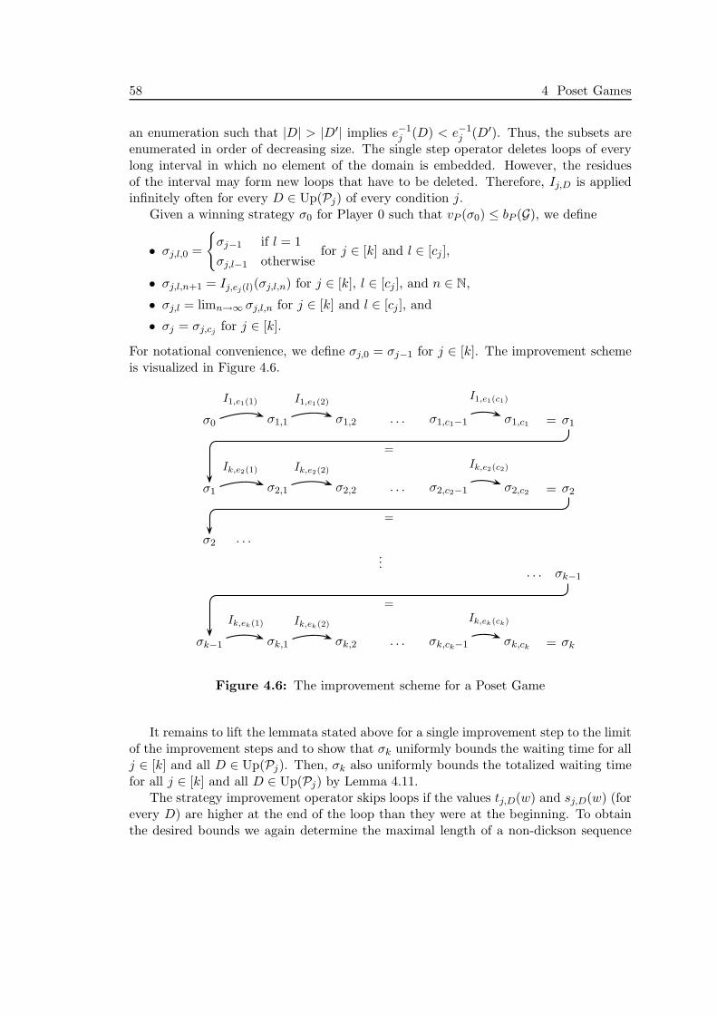
58 4 Poset Games
an enumeration such that |D| > |D′| implies e−1j (D) < e−1
j (D′). Thus, the subsets areenumerated in order of decreasing size. The single step operator deletes loops of everylong interval in which no element of the domain is embedded. However, the residuesof the interval may form new loops that have to be deleted. Therefore, Ij,D is appliedinfinitely often for every D ∈ Up(Pj) of every condition j.
Given a winning strategy σ0 for Player 0 such that vP (σ0) ≤ bP (G), we define
• σj,l,0 =
{σj−1 if l = 1σj,l−1 otherwise
for j ∈ [k] and l ∈ [cj ],
• σj,l,n+1 = Ij,ej(l)(σj,l,n) for j ∈ [k], l ∈ [cj ], and n ∈ N,
• σj,l = limn→∞ σj,l,n for j ∈ [k] and l ∈ [cj ], and
• σj = σj,cj for j ∈ [k].
For notational convenience, we define σj,0 = σj−1 for j ∈ [k]. The improvement schemeis visualized in Figure 4.6.
σ0 σ1,1 σ1,2 σ1,c1−1 σ1,c1 σ1=. . .
σ1 σ2,1 σ2,2 σ2,c2−1 σ2,c2 σ2=. . .
σ2
σk−1
. . .
. . .
...
σk−1 σk,1 σk,2 σk,ck−1 σk,ck σk=. . .
I1,e1(1) I1,e1(2)I1,e1(c1)
Ik,e2(1) Ik,e2(2)Ik,e2(c2)
Ik,ek(1) Ik,ek(2)Ik,ek(ck)
=
=
=
Figure 4.6: The improvement scheme for a Poset Game
It remains to lift the lemmata stated above for a single improvement step to the limitof the improvement steps and to show that σk uniformly bounds the waiting time for allj ∈ [k] and all D ∈ Up(Pj). Then, σk also uniformly bounds the totalized waiting timefor all j ∈ [k] and all D ∈ Up(Pj) by Lemma 4.11.
The strategy improvement operator skips loops if the values tj,D(w) and sj,D(w) (forevery D) are higher at the end of the loop than they were at the beginning. To obtainthe desired bounds we again determine the maximal length of a non-dickson sequence

4.3 Time-optimal Strategies for Poset Games 59
[12] of vectors containing these values, which can only increase, be reset to zero or stayzero. This results in a bound that depends only on the number of vertices of the arenaand the number of upwards-closed subsets.
Let w1 and w2 be finite plays such that w1 � w2, and let D ∈ Up(Pj). We saythat w1 and w2 are dickson save D iff the last vertices of w1 and w2 are equal andtj′,D′(w1) ≤ tj′,D′(w2) and sj′,D′(w1) ≤ sj′,D′(w2) for all j′ and all D′ ∈ Up(Pj′) suchthat D �= D′. If w1 and w2 are dickson save D, the totalized waiting time for D is highenough and strictly increasing in between w1 and w2, then the strategy improvementoperator Ij,D deletes the loop (w1)−1w2.
Now, let xy be a finite play. We say that y is non-dickson save D if xy does nothave a pair of dickson prefixes that both do contain a non-empty part of y. The strategyimprovement operator Ij,D does not delete any loops in a prefix that is non-dickson saveD. We bound the length of a non-dickson sequence in terms of the size of the arena andthe number of upwards-closed subsets by a function b.
If there is only one subset, namely D, then there must not be a state repetition in y.Thus, the length of a non-dickson sequence can be bounded by the number of verticesin |G|; hence, we define b(m, 1) := m. Now, assume there are k + 1 subsets. If tj′,D′
is non-decreasing for some subset D′ with D′ �= D for more than b(|G|, k) steps (whichimplies that sj′,D′ is non-decreasing as well), then there are two dickson prefixes, withrespect to the other k subsets in that infix that are also dickson for all k + 1 subsets.Hence, in every non-dickson sequence the value tj′,D′ for every subset D′ �= D has to bereset to 0 in every infix of length b(|G|, k). If tj′,D′(x) = 0, then we can bound tj′,D′(xy)and sj′,D′(xy) by
|y| · (|y| + 1)2
.
Altogether, the values in a non-dickson sequence are bounded by
b(|G|, k) · (b(|G|, k) + 1)2
after an initial prefix of length b(|G|, k). Thus, there cannot be more than
b(|G|, k) + |G| ·(b(|G|, k) · (b(|G|, k) + 1)
2
)2k
steps without a pair of dickson prefixes, which gives
b(m,k + 1) := b(m,k) +m ·(b(m,k) · (b(m,k) + 1)
2
)2k
.
The exponent 2k is due to the fact that the vectors contain two value for each subsetD′ ∈ Up(Pj′), i.e., tj′,D′(w) and sj′,D′(w).

60 4 Poset Games
Now, we state the last technical Lemma which sums up all properties of the im-provement scheme we need. Afterwards, we conclude the first step by putting the piecestogether.
Lemma 4.19. Let j ∈ [k], l ∈ [cj ], and e(l) = (j,D). Then
(i) (update∗j,l,n)n∈N converges to the identity function.
(ii) limn→∞ σj,l,n exists.
(iii) If σj,l−1 uniformly bounds the totalized waiting time for D′ ∈ Up(Pj′) for some j′,then so does σj,l.
(iv) vP (σj,l) ≤ vP (σj,l−1).
(v) σj,l uniformly bounds the waiting time for D to
bj,D := f−1j (bP (G)) + (|Dj\D| + 1) · b
⎛⎝|G|,
k∑j=1
|Up(Pj)|⎞⎠ .
Proof. (i) We proceed by induction: we have update∗j,l,n(s0) = s0 for all n. Now, assumeupdate∗j,l,n(w) = w for all n ≥ nw. If tj,D(ws) ≤ f−1
j (bP (G)), then updatej,l,n(w, s) = ws
and therefore also update∗j,l,n(ws) = ws for all n ≥ nw.Thus, let tj(ws) > f−1
j (bP (G)) and let Tn be Tσj,l,n−1
G,s0�ws restricted to the maxi-
mal paths that continuously contain D in their set of open requests. By definition,update∗j,l,n(ws) is a vertex of Tn. Since every path in Tn is a path in Tn−1 from whichsome loops might be deleted the size of the Tn is decreasing. Finally, if Tn = Tn+1, thenwe have Tn′ = Tn for all n′ ≥ n. Thus, there is an index nws ≥ nw such that the Tn
are equal for all n ≥ nws. From that index on we have updatej,l,n(w, s) = ws and thusupdate∗j,l,n(ws) = ws.
(ii) By (i), we have
σj,l,n(ρ0 . . . ρi)
=nextj,l,n(ρi,update∗j,n(ρ0 . . . ρi))
=nextj,l,n(ρi, ρ0 . . . ρi)
=σj,l,n−1(ρ0 . . . ρi)
for all finite plays ρ0 . . . ρi and all sufficiently large n. Thus, (σj,l,n)n∈N converges.
For the next two claims we need to introduce some additional but familiar notation.For an explanation we refer to Figure 3.3. For 1 ≤ m ≤ n define update∗j,l,[m,n] byupdate∗j,l,[m,m](w) = update∗j,l,m(w) and
update∗j,l,[m,n+1](w) = update∗j,l,[m,n](update∗j,l,n+1(w)).

4.3 Time-optimal Strategies for Poset Games 61
Applying Lemma 4.15 inductively, we can show that update∗j,l,[m,n](w) is a finite playconsistent with σj,l,m−1 for every play w consistent with σj,l,n. Analogously, applyingLemma 4.16 inductively, we get t(w) ≤ t(update∗j,l,[m,n](w)) for all w consistent with σn.
We have shown in the proof of Lemma 4.19 (i) that for every finite play x accordingto σj,l there is an nx such that update∗j,l,n(x) = x for all n ≥ nx. We define update∗j,l,ω byupdatej,l,ω(x) = update∗j,l,[1,nx](x). By the remarks above, we know that update∗j,l,ω(x)is consistent with σj,l−1 and t(x) ≤ t(update∗j,l,ω(x)) for every play x consistent with σj,l.
(iii) We have tj′,D′(x) ≤ B for all finite plays x consistent with σj,l−1. Now, let x bea play consistent with σj,l. Then, update∗j,l,ω(x) is a prefix of a play according to σj,l−1.Hence, tj′,D′(x) ≤ tj′,D′(update∗j,l,ω(x)) ≤ B. Thus, σj,l uniformly bounds the totalizedwaiting time for D′.
(iv) For a play ρ = ρ0ρ1ρ2 . . ., let update∗j,l,ω(ρ) = limn→∞ update∗j,l,ω(ρ0 . . . ρn). Thelimit update∗j,l,ω(ρ) is a play consistent with σj,l−1 for every play ρ consistent with σj,l.We show vP (ρ) ≤ vP (update∗j,ω(ρ)) for all ρ consistent with σj,l, which implies the claim.To this end, we define
S = {x′ � update∗j,l,ω(ρ) | ¬∃x � ρ : update∗j,l,ω(x) = x′}.
S contains exactly the vertices of the loops skipped by Player 0 throughout the improve-ment steps. Let x′ ∈ S; then, tj(x′) > f−1
j (bP (G)) holds, as every improvement step onlydeletes loops of update∗j,l,ω(ρ) after a waiting time of at least f−1
j (bP (G)) steps. Thus,p(x′) > bP (G) ≥ vP (σ) and
lim supn→∞
1n
n−1∑i=0
p(update∗j,l(ρ0 . . . ρi)) ≤ vP (update∗j,l(ρ)) (4.1)
since the average decreases if the summation omits the summands for the prefixes in S.Now, let x � ρ: We have t(x) ≤ t(update∗j,l,ω(x)) and therefore p(x) ≤ p(update∗j,l,ω(x)).Thus,
1n
n−1∑i=0
p(ρ0 . . . ρi) ≤ 1n
n−1∑i=0
p(update∗j,l(ρ0 . . . ρi)).
The latter term converges to a value less than or equal to vP (update∗j,l(ρ)), by (4.1).Thus, we conclude vP (ρ) ≤ vP (update∗j,l(ρ)).
(v) The last claim is proven by induction over l. There are at most |Dj\D| intervalsin between the elements of Dj that were embedded already. By induction hypothesis,we can assume that the claim holds for all those intervals, i.e., for all D′ ∈ Up(Pj) suchthat |D′| > |D|, since e−1(j,D′) < e−1(j,D). Now, assume there is a play w consistentwith σj,l such that (D, t) ∈ Openj(w) for some t > bj,D and let w = xy such that

62 4 Poset Games
|y| = d(|G|,∑kj=1 |Up(Pj)|) + 1. From the induction hypothesis and the fact that the
waiting times for all D′ that could precede D are already bounded, we can conclude that
(D, f−1j (bP (G)) + (|D\Dj |) · b(|G|,
k∑j=1
|Up(Pj)|) + 1 + |y′|) ∈ Openj(xy′)
for all y′ y. The situation is depicted in Figure 4.7: the length of the first two intervalsI is bounded by induction hypothesis. Thus, if the waiting time is longer than bj,D, thenthe last interval is longer than b(|G|,∑k
j=1(|Up(Pj)|)).
ρ
q d1 d2 d3
I︷ ︸︸ ︷ I︷ ︸︸ ︷ I′︷ ︸︸ ︷
Figure 4.7: The inductive step for Lemma 4.19 (v): the intervals I are short by induc-tion hypothesis. Thus, I ′ is long
Finally, there exists N such that update∗j,l,N(xy′) = xy′ for all y′ y. Thus, y isnon-dickson save D, which contradicts the definition of d.
Now, we can wrap things up by stating the final lemma of the first part, which givesus the desired bound on the waiting times of an optimal strategy.
Lemma 4.20. For every winning strategy σ0 for G for Player 0 of value vP (σ0) ≤ bP (G),there is a winning strategy σk that bounds the totalized waiting time for all j ∈ [k] andall D ∈ Up(Pj) to bj,D·(bj,D+1)
2 . Furthermore, vP (σk) ≤ vP (σ0).
Proof. By induction over l. From Lemma 4.19 (iii) and (v) and Remark 4.11 we con-clude that σk bounds the totalized waiting time for all j ∈ [k] and all D ∈ Up(Pj)to bj,D ·(bj,D+1)
2 . Analogously, vP (σk) ≤ vP (σ0) ≤ bP (G) by induction hypothesis, byLemma 4.19 (iv), and by the assumption on σ0. Thus, σk is a winning strategy byLemma 4.10 (ii).
This concludes the first step. We have proved that the search for an optimal strategycan be restricted to a finite domain. In the second step, we construct a Mean-PayoffGame whose plays are the plays of G annotated with their totalized waiting times.Lemma 4.20 allows us to bound the totalized waiting time for D ∈ Up(Pj) to bj,D ·(bj,D+1)
2 ,and thereby also the size of the expanded arena. Then, we find an optimal strategy forthe Poset Game by determining the optimal strategy in a Mean-Payoff Game.

4.3 Time-optimal Strategies for Poset Games 63
4.3.2 Reducing Poset Games to Mean-Payoff Games
This subsection is devoted to the second step of the proof of Theorem 4.13, the reductionto Mean-Payoff Games. In the expanded arena, we need to keep track of the totalizedwaiting time tj,D. To be able to compute tj,D(ws) from tj,D(w) locally we need to knowsj,D(w) as well. The bound on tj,D(w) obtained in the first part of the proof also boundssj,D(w). Thus, let Fj be the set of functions
f : Up(Pj) → N such that f(D) ≤ bj,D · (bj,D + 1)2
for all D ∈ Up(Pj). Every Fj is obviously finite.Remember that Newj(s) returns Dj if s is a request for condition j, and ∅ otherwise.
Furthermore, Embj(D, s) is the set of elements in D that could not be embedded to thevertex s. Formally,
Newj(s) =
{Dj if qj ∈ lG(s)∅ otherwise
and
Embj(D, s) = {d ∈ D | ∃d′ ∈ D : d′ �j d and lj(d′) /∈ lG(s)}.
We define the memory structure M = (M, init,update) where
• M =∏k
j=1(Fj × Fj) ∪ {m↑},
• init(s) = (time1, size1, . . . , timek, sizek) where
timej(D) = sizej(D) =
{1 if Embj(Newj(s), s) = D
0 otherwise
for all D ∈ Up(Pj), and
• The update function is given by update(m↑, s) = m↑ for all vertices s. Otherwise,if m = (time1, size1, . . . , timek, sizek) ∈M define time′j and size′j by
time′j(D) = |Embj(Newj(s), s) ∩ {D}| +∑
D′∈Up(Pj):Embj(D′,s)=D
(timej(D′) + sizej(D′))
and
size′j(D) = |Embj(Newj(s), s) ∩ {D}| +∑
D′∈Up(Pj ):Embj(D′,s)=D
sizej(D′)

64 4 Poset Games
for all D ∈ Up(Pj). If time′j /∈ Fj for some j, i.e., there exists D ∈ Up(Pj)
such that time′j(D) > bj,D ·(bj,D+1)2 , then we define update(m, s) = m↑, otherwise
update(m, s) = (time′1, size′1, . . . , time′k, size′k).
Since it is Player 1’s goal to minimize the limit superior of the average edge weights in aMean-Payoff Game we have to switch the Player’s positions, i.e., we define V ′
0 = V1×M ,V ′
1 = V0 ×M and G′ = (V ×M,V ′0 , V
′1 , Eupdate). Let
d =k∑
j=1
fj(bj,D · (bj,D + 1)
2+ 1)
where fj is the penalty function for condition j. To complete the definition of thegame we need to define the weight function l: We define l((s,m), (s′,m↑)) = d for all(s,m) ∈ V ×M and
l((s, (time1, size1, . . . , timek, sizek)), (s′, (time′1, size′1, . . . , time′k, size′k)))
=k∑
j=1
fj
⎛⎝ ∑
D∈Up(Pj )
timej(D)
⎞⎠
where fj is again the penalty function. Now, let G′ = (G′, (s0, init(s0)), d, l) be theMean-Payoff Game in the expanded arena.
The following lemma shows that the values for a play G and the expanded plays inG′ are equal.
Lemma 4.21. Let w be a finite play of G.
(i) Let update(w) = (time1, size1, . . . , timek, sizek). Then, timej(D) = tj,D(w) andsizej(D) = sj,D(w).
(ii) If update(w) = m↑, then there exists a prefix w′ of w and a D ∈ Up(Pj) such thattj,D(w′) > bj,D ·(bj,D+1)
2 .
(iii) Let ρ be a play in G such that the totalized waiting times for all j ∈ [k] and allD ∈ Up(Pj) are uniformly bounded by bj,D ·(bj,D+1)
2 , and let ρ′ be the expanded playin G′. Then, vP (ρ) = v1(ρ′).
(iv) Let ρ′ be a play in G′ that does not visit a vertex with memory state m↑, and let ρbe the projected play in G. Then, v1(ρ′) = vP (ρ).
Proof. (i) By induction over w: for the base case w = s notice that tj,D(s) ∈ {0, 1}. Wehave
tj,D(s) = 1 ⇔ (D, 1) ∈ Openj(s)
⇔ D = Embj(Newj(s), s) ⇔ timej(D) = 1,

4.3 Time-optimal Strategies for Poset Games 65
and
tj,D(s) = 0 ⇔ (D, 1) /∈ Openj(s)
⇔ D �= Embj(Newj(s), s) ⇔ timej(D) = 0.
Also, sj,D(s) ∈ {0, 1} and
sj,D(w) = 1 ⇔ Openj(s) ∩ {D} × N = {(D, 1)}⇔ tj,D = 1 ⇔ timej(D) = 1 ⇔ sizej(D) = 1,
and
sj,D(w) = 0 ⇔ Openj(s) ∩ {D} × N = ∅⇔ tj,D = 0 ⇔ timej(D) = 0 ⇔ sizej(D) = 0.
For the induction step, let update∗(w) = (time1, size1, . . . , timek, sizek) and similarlyupdate∗(ws) = (time′1, size′1, . . . , time′k, size′k). By induction hypothesis, we can assumetimej(D) = tj,D(w) and sizej(D) = sj,D(w). We have
tj,D(ws)
=∑
(D,t)∈Openj(ws)
t
=|Embj(Newj(s), s) ∩ {D}| +∑
(D′,t′)∈Openj(w):
Embj(D′,s)=D
(t′ + 1)
=|Embj(Newj(s), s) ∩ {D}| +∑
(D′,t′)∈Up(Pj ):Embj(D′,s)=D
(tj,D′(w) + sj,D′(w))
=|Embj(Newj(s), s) ∩ {D}| +∑
D′∈Up(Pj):Embj(D′,s)=D
(timej(D′) + sizej(D′))
=time′j(D),
and
sj,D(ws)
=|{t | (D, t) ∈ Openj(ws)}|=|{Embj(Newj(s), s) ∩ {D}}| +
∑D′∈Up(Pj ):
Emb(D′,s)=D
|{t′ | (D′, t′) ∈ Openj(w)}|

66 4 Poset Games
=|{Embj(Newj(s), s) ∩ {D}}| +∑
D′∈Up(Pj):Emb(D′,s)=D
sj,D′(w)
=|Embj(Newj(s), s) ∩ {D}| +∑
D′∈Up(Pj ):Embj(D
′,s)=D
sizej(D′)
=size′j(D).
(ii) Let w′ be the longest prefix of w such that update∗(w′) �= m↑ and s the nextvertex of w after w′. Furthermore, let update∗(w′) = (time1, size1, . . . , timek, sizek).Thus, timej(D) = tj,D(w) by (i). We define time′j and size′j by
time′j(D) = |Embj(Newj(s), s) ∩ {D}| +∑
D′∈Up(Pj):Embj(D′,s)=D
(timej(D′) + sizej(D′))
and
size′j(D) = |Embj(Newj(s), s) ∩ {D}| +∑
D′∈Up(Pj):Embj(D
′,s)=D
sizej(D′),
respectively. Analogous to the proof in (i), we can show that time′j(D) = tj,D(ws) and
size′j(D) = sj,D(ws). Assume tj,D(w′) ≤ bj,D·(bj,D+1)2 for all D ∈ Up(Pj) and all j ∈ [k].
Then, update((time1, size1, . . . , timek, sizek), s) = update∗(w′s) �= m↑ which contradictsour assumption on w′. Thus, tj,D(w′) > bj,D ·(bj,D+1)
2 for some D ∈ Up(Pj) and some j.(iii) and (iv) are easy implications of (i) and (ii).
Now, we are able to prove Theorem 4.13.
Proof. We begin by relating strategies and values for Player 0 for G and Player 1 in G′.Let σ be a strategy for Player 0 for G that uniformly bounds the totalized waiting
times for all conditions D ∈ Up(Pj) to bj,D·(bj,D+1)2 . We define the strategy τ ′ for
Player 1 in G′ by τ ′((ρ0,m0) . . . (ρn,mn)) = σ(ρ0 . . . ρn). We claim τ ′ guarantees vP (σ)for Player 1 in G′. Assume it does not. Then, Player 0 has a strategy σ′ for G′ suchthat v1(ρ(s0, σ′, τ ′)) > vP (σ). The projected play ρ of ρ(s0, σ′, τ ′) is consistent with σ byconstruction of τ ′. Thus, vP (σ) ≥ vP (ρ) = v1(ρ(s0, σ′, τ ′)) > vP (σ) by Lemma 4.21 (iii),which yields the desired contradiction.
Conversely, let τ ′ be a strategy for Player 1 in G′ that guarantees a loss d′ < d.Thus, no play consistent with τ ′ visits a vertex with memory state m↑. Let σ be thestrategy for Player 0 for G induced by τ ′ via G ≤M G′. We claim vP (σ) ≤ d′. AssumePlayer 1 has a strategy τ for G such that vP (ρ(s0, σ, τ)) > d′. The expanded play ρ′ of

4.3 Time-optimal Strategies for Poset Games 67
ρ(s0, σ, τ) is consistent with τ ′ by Lemma 2.8. Thus, d′ ≥ v1(ρ′) = vP (ρ(s0, σ, τ)) > d′
by Lemma 4.21 (iv), which again amounts to a contradiction.Now, we can begin with the actual proof: since Player 0 wins G, Corollary 4.12 and
Lemma 4.20 guarantee that she also has a winning strategy σ that uniformly boundsthe waiting times for all D ∈ Up(Pj) to bj,D·(bj,D+1)
2 . Let τ ′ be the induced strategy forPlayer 1 in G′. Every play consistent with τ ′ does not reach a vertex with memory statem↑. Thus, this strategy guarantees a loss less than d. Hence, vM (G′) < d.
Let τopt be a positional strategy guaranteeing vM (G′) for Player 1 in G′. We showthat the strategy σopt induced by G ≤M G′ and τopt is an optimal winning strategy forPlayer 0 for G. This suffices since σopt is finite-state with memory M and effectivelycomputable by Theorem 2.20.
By the remarks above, we have vP (σopt) = vM (G′). To conclude the proof we assumethat σopt is not optimal, i.e., Player 0 has a strategy σ for G such that vP (σ) < vP (σopt).By Lemma 4.20, we can assume without loss of generality that σ uniformly bounds thetotalized waiting times for all D ∈ Up(Pj) to bj,D ·(bj,D+1)
2 . Then, the strategy τ ′ forPlayer 1 in G′ induced by σ guarantees vP (σ) < vP (σopt) = vM (G′). This amounts to acontradiction, since τopt is optimal for G′.
Corollary 4.22. The value vP (σ) of an optimal strategy σ is effectively computable.
Proof. Construct G′ and compute vM (G′). If vM (G′) = d, then Player 0 loses G andv(σ) = ∞ for every strategy σ. Otherwise, the value of an optimal strategy for thePoset Games coincides with vM (G′).
Every Request-Response Game is a Poset Game where every domain is a singleton.Formally, given a Request-Response Game G = (G, s0, (Qj , Pj)j=1,...,k) construct thePoset Game G′ = (G, s0, (qj ,Pj)j=1,...,k) where Pj = ({pj}, {(pj , pj)}, lj) and lj(pj) = pj.The labeling lG of the arena G is defined by lG(s) = {qj | s ∈ Qj} ∪ {pj | s ∈ Pj}. Thegames G and G′ are obviously equivalent.
Hence, both frameworks for defining time-optimal strategies are applicable to G.Either use the framework for Request-Response Games or construct G′ first, and thenuse the framework for Poset Games. We have already seen that the waiting times forRequest-Response Games are defined by a single clock for every condition that is startedby request and stopped by the first response. All subsequent requests of a conditionthat occur while the clock is still running are ignored. Waiting times for Poset Gameshave to be defined differently since the embeddings for different requests may overlap(see Figure 4.3). Thus, for every request of a condition a new clock is started and isnot stopped until the corresponding poset is embedded. Thus, in a Poset Game G′
constructed from a Request-Response Game, requests occurring while another requestis open, are not ignored. Therefore, the value of a play or a strategy for Player 0,respectively, is smaller in the Request-Response Game setting than in the Poset Gamesetting, if the values are defined with respect to the same penalty functions.

68 4 Poset Games
Lemma 4.23. Let ρ be a play and σ a strategy for Player 0.
(i) vR(ρ) ≤ vP (ρ).
(ii) vR(σ) ≤ vP (σ).
Proof. (i) We prove ({pj}, tj(ρ0 . . . ρn)) ∈ Openj(ρ0 . . . ρn), if tj(ρ0 . . . ρn) > 0, whichimplies the claim. Here, tj is the waiting time function for the Request-Response Game.Let tj(ρ0 . . . ρn) = 1. Then, ρn ∈ Qj\Pj by definition of tj. Therefore, qj ∈ lG(s)but pj /∈ lG(s), by definition of lG. Hence, it holds ({pj}, 1) ∈ Openj(ρ0). Now, lettj(ρ0 . . . ρn+1) = t + 1 > 1. Then, tj(ρ0 . . . ρn) = t and we can apply the inductionhypothesis and obtain ({pj}, t) ∈ Openj(ρ0 . . . ρn). Furthermore, since the waiting timeis not reset to zero at ρn+1, it holds pj /∈ lG(ρn+1). Thus, Embj({pj}, ρn+1) = {pj}which implies ({pj}, t + 1) ∈ Openj(ρ0 . . . ρnρn+1).
(ii) We have
vR(σ) = supτ∈Γ1
vR(ρ(s0, σ, τ)) ≤ supτ∈Γ1
vP (ρ(s0, σ, τ)) = vP (σ),
where the inequality is due to (i).

Chapter 5
Solitary PLTL Games
Temporal Logics reason about propositions that change over the course of time. Consideran atomic proposition p. The formula Fp is satisfied, if p is true some time in thefuture. The formula Gp is satisfied, if p is continuously true from now on. If thetime is assumed to be discrete, i.e., the domain of the time steps is discrete, then Xpis satisfied, if p holds after the next time step. If the time is continuous, then X isdisregarded. Derived from Tense Logic [46], Temporal Logic was at first applied toprogram verification by Pnueli [44]. There, the time domain is given by the executionsof a system under consideration, thus it is discrete (typically N). Two paradigms ofTemporal Logic can be identified by their treatment of time. The semantics of LinearTemporal Logic [44], (see Section 2.3), are defined with respect to a single time line. Inthe context of verification, this means that an LTL formula is evaluated with respectto a single execution. The system satisfies the formula, if every execution is a modelof the formula. Branching Time Logics like CTL [9] and CTL∗ [16] on the other hand,are defined with respect to several time lines. They allow to express requirements likeif a request is encountered, then there is the possibility that this request is responded.However, there might be another execution that does not respond this request. Thus,branching time can be utilized to model unpredictability of the system. The differencesbetween the two paradigms are discussed in [36]. Both flavors of Temporal Logic aretoday widely used in Formal Verification of closed systems by Model-Checking Tools.We focus on LTL, as we employ formulae as winning conditions to determine the winnerof a play.
Typical properties expressible in LTL are liveness properties Fp, specifying somethinggood will happen, and safety properties Gp, specifying that nothing bad ever happens.Nesting the operators, one can express the Buchi condition, i.e., infinitely often p byGFp, for example. Also, Request-Response, Parity and Muller winning conditions areexpressible in LTL.
The main advantages of LTL are the variable-free syntax and intuitive semantics,which make it suitable for practical applications. However, there is also a drawback.The semantics of Fp do only require p to be satisfied some time in the future, without

70 5 Solitary PLTL Games
specifying a bound. This behavior is undesirable in applications, where the user isgenerally interested in prompt satisfaction. Also, the semantics of Gp, which require pto be true from now on ad infinitum might be to strong, while it would suffice that pholds as long as possible. It is easy to see that there are no such bounds intrinsic tothe semantics of LTL (unlike for CTL, where the number of states of the graph providessuch a bound [9]), i.e., if Fp is satisfied, then there is also a bound B such that p is truewithin the next B steps. Consider the formula ϕ = FGp and the graph G in Figure 5.1.Every path of G is a model of ϕ, but there is no bound b such that Gp is satisfied withinthe next b steps on all paths.
p ∅ p
Figure 5.1: A graph without a fixed bound for FGp
One way to overcome this is to subscript the temporal operators by bounds and adirection, i.e., F≤5 and F>5 for example. Several so called real-time or quantitative logicshave been introduced with this capability. For example, Metric Temporal Logic [2] orReal-Time CTL [19]. However, they require the user to know the bounds in advance,which is typically not feasible. Also, if a system satisfies a parameterized formula,there is no information on how tight the bounds are. Even more importantly, addingparameterized operators does not increase the expressivity of LTL, as F≤2p is equivalentto the formula p ∨ Xp ∨ XXp.
To relieve the user from determining the bounds and to allow the search for optimalbounds, the constants can be replaced by variables. Then, F≤xp is true, if p is truewithin the next x steps, where x is a free variable. Satisfaction is then defined withrespect to a variable valuation. Thus, given a specification and a system, one can askwhether there is a valuation such that the specification holds, or even determine anoptimal valuation. This extension of LTL, called Parametric Linear Temporal Logic,was introduced by Alur et. al. [1].
In this chapter, we use Parametric Linear Temporal Logic to specify winning condi-tions for infinite games. This is an extension of LTL Games with parameterized winningconditions that allows a clear specification of time-optimal strategies. Player 0’s goalis to minimize the waiting time x for formulae F≤xψ and G>xψ and to maximize thebound y for formulae G≤yψ and F>y. A PLTL Game G consists of an arena and awinning condition ϕ. The winner of a game is determined with respect to a valuationα. Player 0 wins a play of G, if the play is a model of ϕ with respect to α. Accordingly,Player 0 wins G with respect to α, if she has a strategy such that every play consistentwith this strategy is won by her. This induces a set W0
G consisting of the good valuationsfor Player 0. Thus, the questions of emptiness, finiteness and universality arise. Also,one can search for optimal strategies for Player 0.
5.1 Parametric Linear Temporal Logic 71
This chapter is structured as follows. We introduce PLTL in Section 5.1 and presentsome simple results from [1] which encompass the typical treatment of a new logic. Afterdefining syntax and semantics, we consider dualities of the temporal operators and showthat the set of parameterized temporal operators can be restricted to F≤x and G≤y
without losing any expressive power. The formulae built from the classical temporaloperators and F≤x form the fragment PLTLF while the fragment PLTLG is definedanalogously. Most of the remainder of this chapter is concerned with these unipolarfragments, which have good decidability properties while the questions for the full logicare mostly open [1]. However, there is evidence that the full logic is too strong. Wereiterate the findings at the end of Section 5.1. As Model-Checking is a special case ofsynthesis, we restrict our attention to these fragments when defining PLTL Games inSection 5.2. The main part of this section is devoted to two technical lemmata that arethe key to the main theorems about PLTL Games. For unipolar solitary games, it isdecidable whether Player i wins a PLTL Game with respect to some, all or only finitelymany valuations. Furthermore, for these games optimal valuations are computable. Forsolitary PLTLG Games, a proof from [1] can be adapted to our cause easily and anothertheorem (without proof) from that paper can be adapted to solitary PLTLF Games.Our technical lemma for PLTLF games establishes a similar result (with slightly higherbounds). We close this chapter by considering alternative semantics for PLTL Gamesin Section 5.3. Instead of requiring that the winning condition holds on all plays withrespect to a fixed valuation, it requires that there is a valuation for every play, suchthat the winning condition holds with respect to that valuation on that particular play.Thus, the valuation is not uniform for all plays, but there might be different valuationsfor different plays. We analyze these semantics and draw comparisons to the standardsemantics introduced in Section 5.2.
5.1 Parametric Linear Temporal Logic
Parametric Linear Temporal Logic extends Linear Temporal Logic with temporal oper-ators that can be subscripted by variables. We begin this section by defining the syntaxand semantics of PLTL and by discussing some elementary properties before we close itby stating the results.
Let P be a set of atomic propositions and Y and X be two disjoint sets of vari-ables. Parametric Linear Temporal Logic, PLTL for short, extends the syntax of LinearTemporal Logic introduced in Section 2.3 by a parameterized version of every temporaloperator (but X, which has no reasonable parameterized version). A parameter is eithera variable or a non-negative integer, a constant parameter. We explain the need for twodisjoint sets of variables later in this section. We define the set PLTL of ParametricLinear Temporal Logic formulae inductively by
• p,¬p ∈ PLTL if p ∈ P ,
• ϕ ∧ ψ,ϕ ∨ ψ ∈ PLTL if ϕ,ψ ∈ PLTL,

72 5 Solitary PLTL Games
• Xϕ,Fϕ,Gϕ,ϕUψ,ϕRψ ∈ PLTL if ϕ,ψ ∈ PLTL,
• F≤xϕ,G≤yϕ,ϕU≤xψ,ϕR≤yψ ∈ PLTL if ϕ,ψ ∈ PLTL, x ∈ X ∪ N, y ∈ Y ∪ N, and
• F>yϕ,G>xϕ,ϕU>yψ,ϕR>xψ ∈ PLTL if ϕ,ψ ∈ PLTL, x ∈ X ∪ N, y ∈ Y ∪ N.
There are several complexity measures of a formula ϕ that are used later on. The set ofvariables of ϕ, var(ϕ), and the set of constants of ϕ, con(ϕ), are defined in the obviousway. Furthermore, let
• nϕ be the number of distinct subformulae of ϕ,
• kϕ be the number of temporal operators of ϕ parameterized by a variable, and
• cϕ be the product of all non-zero constants that parameterize operators in ϕ.
To define the semantics of PLTL, we need to know the values of the variables: avaluation is a mapping α : X ∪ Y → N. By convention, we compare valuations compo-nentwise, i.e., α ≤ β iff α(z) ≤ β(z) for all z ∈ X ∪ Y. Thus, ≤ is a partial order onthe set of all valuations, and we can speak of upwards-closed and downwards-closed setsof valuations. Oftentimes, when dealing with a fixed formula ϕ, we implicitly assumethat a valuation is a mapping α : var(ϕ) → N, if it is opportune. The following facts areuseful throughout this chapter.
Remark 5.1. Let α0 be the valuation that maps every variable to zero.
(i) A downwards-closed set of valuations is non-empty iff it contains α0.
(ii) An upwards-closed set of valuations is universal iff it contains α0.
(iii) An upwards-closed set of valuations is infinite iff it is non-empty.
To deal with temporal operators parameterized by constants more conveniently, weextend the domain of α to X ∪Y∪N and define α(c) = c for all c ∈ N. Let ρ = ρ0ρ1ρ2 . . .be a path of a labeled graph (V,E, l). Satisfaction of a formula ϕ instantiated by α atposition n of ρ, written (ρ, n, α) |= ϕ, is defined inductively by
• (ρ, n, α) |= p iff p ∈ l(ρn),
• (ρ, n, α) |= ¬p iff p /∈ l(ρn),
• (ρ, n, α) |= ϕ ∧ ψ iff (ρ, n, α) |= ϕ and (ρ, n, α) |= ψ
• (ρ, n, α) |= ϕ ∨ ψ iff (ρ, n, α) |= ϕ or (ρ, n, α) |= ψ,
• (ρ, n, α) |= Xϕ iff (ρ, n + 1, α) |= ϕ,
• (ρ, n, α) |= Fϕ iff there exists k ≥ 0 such that (ρ, n + k, α) |= ϕ,
• (ρ, n, α) |= Gϕ iff for all ≥ 0: (ρ, n + k, α) |= ϕ,
• (ρ, n, α) |= ϕUψ iff there exists k ≥ 0 such that (ρ, n+ k, α) |= ψ and for all l suchthat 0 ≤ l < k: (ρ, n+ l, α) |= ψ,
• (ρ, n, α) |= ϕRψ iff for all k ≥ 0: either (ρ, n+ k, α) |= ψ or there exists l < k suchthat (ρ, n + l, α) |= ϕ,
5.1 Parametric Linear Temporal Logic 73
• (ρ, n, α) |= F≤xϕ iff there exists k ≤ α(x) such that (ρ, n+ k, α) |= ϕ,
• (ρ, n, α) |= G≤yϕ iff for all k ≤ α(y): (ρ, n+ k, α) |= ϕ,
• (ρ, n, α) |= ϕU≤xψ iff there exists k ≤ α(x) such that (ρ, n+ k, α) |= ψ and for alll such that 0 ≤ l < k: (ρ, n + l, α) |= ψ,
• (ρ, n, α) |= ϕR≤yψ iff for all k ≤ α(y): either (ρ, n+k, α) |= ψ or there exists l < ksuch that (ρ, n+ l, α) |= ϕ,
• (ρ, n, α) |= F>yϕ iff there exists k > α(y) such that (ρ, n + k, α) |= ϕ,
• (ρ, n, α) |= G>xϕ iff for all k > α(x): (ρ, n + k, α) |= ϕ,
• (ρ, n, α) |= ϕU>yψ iff there exists k > α(y) such that (ρ, n+ k, α) |= ψ and for alll such that 0 ≤ l < k: (ρ, n + l, α) |= ψ, and
• (ρ, n, α) |= ϕR>xψ iff for all k > α(x): either (ρ, n + k, α) |= ψ or there existsl < k such that (ρ, n + l, α) |= ϕ.
Finally, ρ is a model of ϕ instantiated by α, (ρ, α) |= ϕ iff (ρ, 0, α) |= ϕ.A valuation α makes ϕ satisfiable, if there exists a labeled path ρ of some labeled
graph such that (ρ, α) |= ϕ. Analogously, α makes ϕ valid, if (ρ, α) |= ϕ for all pathsρ of all labeled graphs. This defines the sets S(ϕ) and V (ϕ) containing the valuationsthat make ϕ satisfiable respectively valid.
Let G be a fixed labeled graph. We say that α makes ϕ satisfiable in G if there existsa path ρ of G such that (ρ, 0, α) |= ϕ, and that α makes ϕ valid in G if (ρ, 0, α) |= ϕ forevery path ρ of G. This defines the sets S(G,ϕ) and V (G,ϕ) containing the valuationsthat make ϕ satisfiable respectively valid in G. Problems regarding S(ϕ) can obviouslybe reduced to the same problems for S(G,ϕ), where G is a graph whose paths coincidewith all labeled paths for the propositions occurring in ϕ. The same observation can bemade for the validity sets V (ϕ) and V (G,ϕ).
Remark 5.2. Although, we do only allow negation of atomic propositions, PLTL isclosed under negation as witnessed by the dualities for LTL and the following dualitiesof the parameterized operators.
¬F≤xϕ ≡ G≤y¬ϕ¬F>xϕ ≡ G>y¬ϕ
¬(ϕU≤xψ) ≡ (¬ϕ)R≤y(¬ψ)
¬(ϕU>xψ) ≡ (¬ϕ)R>y(¬ψ)
Thus, every negation can be pushed to the atomic formulae p and ¬p. Removing doublenegations then gives an equivalent formula in negation normal form, as it is required bythe syntax of PLTL.
We abuse our notation slightly and write ¬ϕ for the PLTL formula obtained by thisprocedure.

74 5 Solitary PLTL Games
Remark 5.3. Let ϕ be a PLTL formula and G a labeled graph. Then,
(i) S(ϕ) = V (¬ϕ), and
(ii) S(G,ϕ) = V (G,¬ϕ).
As with classical LTL, many temporal operators are just syntactic sugar, as theycan be defined in terms of a small set of basic operators. We state some straightfor-ward equivalences and dualities that allow us to supersede all but two parameterizedoperators [1].
Fϕ ≡ ttUϕ
Gϕ ≡ ffRϕ
ϕU≤xψ ≡ (ϕUψ) ∧ F≤xψ
ϕR≤yψ ≡ (ϕRψ) ∨ G≤yψ
F>yϕ ≡ G≤yFXϕ
G>xϕ ≡ F≤xGXϕ
ϕU>yψ ≡ G≤y(ϕ ∧X(ϕUψ))ϕR>xψ ≡ F≤x(ϕ ∨X(ϕRψ))
This allows us to restrict our attention to the parameterized operators F≤x and G≤y
along with the unparameterized operators X, U, and R while still retaining closureunder negation, since F≤x and G≤y are dual. Also, replacing the operators leads onlyto a linear increase of the formula’s complexity. The number of distinct subformulaenϕ grows by a constant number in every rewriting step. The number of subformulaeparameterized with variables kϕ and the product of the non-zero constants cϕ remainunchanged. Also, the variables used in the original formula and in the rewritten formulaare the same. The length measured in symbols might grow exponentially, though.
The parameterized operators are obviously monotone, either upwards as F≤y ordownwards as G≤y, for example. Consider a parameterized eventuality: if it is satisfiedin no more than k steps, then it also satisfied in no more than k+1 steps. Dually, considera parameterized always: if a formula holds for the next k steps, then it also holds forthe next k − 1 steps. The same observations can be made for all other parameterizedoperators, also.
Remark 5.4 ([1]). Let α, β be valuations such that α(x) < β(x) and α(y) > β(y) forsome x ∈ X ∪ N and y ∈ Y ∪ N. Then,
(ρ, n, α) |= F≤xϕ implies (ρ, n, β) |= F≤xϕ,
(ρ, n, α) |= G≤yϕ implies (ρ, n, β) |= G≤yϕ,
(ρ, n, α) |= ϕU≤xψ implies (ρ, n, β) |= ϕU≤xψ,
(ρ, n, α) |= ϕR≤yψ implies (ρ, n, β) |= ϕR≤yψ,
5.1 Parametric Linear Temporal Logic 75
(ρ, n, α) |= F>yϕ implies (ρ, n, β) |= F>yϕ,
(ρ, n, α) |= G>xϕ implies (ρ, n, β) |= G>xϕ,
(ρ, n, α) |= ϕU>yψ implies (ρ, n, β) |= ϕU>yψ, and
(ρ, n, α) |= ϕR>xψ implies (ρ, n, β) |= ϕR>xψ.
Therefore, the operators parameterized with x ∈ X are called upwards-monotone,while the operators parameterized with y ∈ Y are called downwards-monotone. Thesets S(ϕ), V (ϕ) and their analogons for labeled graphs are upwards-closed respec-tively downwards-closed, if ϕ contains only upwards-monotone respectively downwards-monotone operators. This can be shown by an easy induction over the constructionof ϕ, applying Remark 5.4 for every parameterized operator. Since we can expressall upwards-monotone operators with F≤x and all downwards-monotone operators withG≤y, these fragments can be defined by allowing only one of the two parameterizedoperators: the fragment PLTLF consists of all formulae build from atomic propositionsand their negations by the boolean connectives, the standard temporal operators, tem-poral operators parameterized by constants c ∈ N and F≤x for x ∈ X . Analogously, thefragment PLTLG consists of all formulae build from the atomic propositions and theirnegations by the boolean connectives, the standard temporal operators, temporal oper-ators parameterized by constants c ∈ N and G≤y for y ∈ Y. Since the monotonicity of aparameterized operator can be seen as its polarity, we call formulae in those fragmentsunipolar . As F≤x and G≤y are dual, the fragments are dual as well.
Remark 5.5. If ϕ ∈ PLTLF, then ¬ϕ ∈ PLTLG and if ϕ ∈ PLTLG, then ¬ϕ ∈ PLTLF.
For a formula ϕ and a valuation α, let α(ϕ) be the formula obtained by replacingevery variable z ∈ X ∪ Y by α(z). The resulting formula is a PLTL formula withoutvariables, i.e., every parameterized operator is parameterized by a constant.
Lemma 5.6 ([1]). For every valuation α and every PLTL formula ϕ, there is an LTLformula ϕ′ such that for all ρ and all n
(ρ, n, α) |= ϕ⇔ (ρ, n, α) |= α(ϕ) ⇔ (ρ, n) |= ϕ′.
Proof. The first equivalence is trivial. For the second, define ψn∧ and ψn∨ by ψ0∧ = ψ0∨ = ψ
and ψj+1∧ = ψ ∧ Xψj
∧ respectively ψj+1∨ = ψ ∨ Xψj
∨. Then, the following equivalenceshold.
(ρ, n, α) |= F≤kψ iff (ρ, n) |= ψk∨
(ρ, n, α) |= G≤kψ iff (ρ, n) |= ψk∧
Thus, we can inductively replace every subformula F≤kψ or G≤kψ of α(ϕ) by an LTLformula. This suffices by the above remarks.

76 5 Solitary PLTL Games
In the following we use α(ϕ) also to denote the LTL formula ϕ′ equivalent to thePLTL formula α(ϕ), if it is clear from the context which formula we mean. The size ofthe LTL formula α(ϕ) is linear in nϕ +
∑z∈var(ϕ) α(z)+
∑c∈con(ϕ) c, which is exponential
in the size of α, if we use a binary encoding for α(z). Lemma 5.6 allows us to reducesatisfiability and validity of PLTL formulae with respect to a fixed valuation α to thecorresponding problems for LTL formulae.
We close this section by presenting the results of [1].
Theorem 5.7 ([1]). Let ϕ be a unipolar PLTL formula and G a labeled graph. Theemptiness, universality, and finiteness problem for S(ϕ) and S(G,ϕ) are decidable.
The results for PLTLG formulae are proven, and for PLTLF formulae a proof idea ispresented. We will adapt these proofs to games in Section 5.2. From these results, onecan also easily derive the solution to several natural optimization problems.
Theorem 5.8 ([1]). Let G a labeled graph.
(i) Let ϕ be a PLTLG formula.
• maxα∈S(ϕ) maxy∈var(ϕ) α(y),
• maxα∈S(ϕ) min y ∈ var(ϕ)α(y),
• maxα∈S(G,ϕ) maxy∈var(ϕ) α(y), and
• maxα∈S(G,ϕ) min y ∈ var(ϕ)α(y)
are computable.
(ii) Let ϕ be a PLTLF formula.
• minα∈S(ϕ) miny∈var(ϕ) α(y),
• minα∈S(ϕ) max y ∈ var(ϕ)α(y),
• minα∈S(G,ϕ) miny∈var(ϕ) α(y), and
• minα∈S(G,ϕ) max y ∈ var(ϕ)α(y)
are computable.
The situation for full PLTL is more complicated. While emptiness and universalityfor S(ϕ) are still decidable, the question whether S(ϕ) contains a valuation α such thatα(x) = α(y) is undecidable. This can be seen easily by considering an even strongerlogic. If we allow temporal operators subscripted with = x (with the obvious semantics),then the logic can encode terminating runs of a Turing Machine. Then, all interestingquestions, like the emptiness of S(ϕ), become undecidable. Also, this explains the needfor two disjoint sets of variables, one for the downwards-monotone operators and one forthe upwards-monotone operators. If we allow z to parameterize both types of operators,then equality subscripts can be encoded easily.

5.2 PLTL Games 77
5.2 PLTL Games
In this section, we will define games with winning conditions in PLTL, focusing onunipolar formulae, again. After discussing some simple observations about these games,we will prove two technical lemmata, on which the main theorems of this section rely.
A (initialized) PLTL Game G = (G, s, ϕ) consists of an arena G, an initial vertex s ofthe arena and a winning condition ϕ ∈ PLTL. Additionally, we say that G is a PLTLF
Game if ϕ ∈ PLTLF, and similarly, that G is a PLTLG Game if ϕ ∈ PLTLG. We callthese games unipolar .
The definition of a PLTL Game does not fit properly into the framework for gameswe defined in Section 2.4, since ϕ alone does not define a set of winning plays. Pairedwith a valuation α, we define ρ ∈ Win ⇔ (ρ, α) |= ϕ. We say Player i wins G withrespect to α if she has a winning strategy with respect to α, i.e., every play consistentwith σ is a model of the winning condition with respect to α. Since ϕ for a fixed α isequivalent to an LTL formula, a game for a fixed α is nothing more than an LTL game(albeit the PLTL formula is presumably shorter than the equivalent LTL formula). Onthe positive side, this means that a PLTL Game for a fixed α can be solved using thetechniques for LTL Games and finite-state determinacy carries over. On the negativeside, this means that a PLTL game for a fixed valuation is not particularly interesting.Therefore, we are not interested in a single valuation but in the set of valuations suchthat Player 0 has a winning strategy for the game with these valuations. Since we dealwith a fixed game, we can assume that valuations are only defined for the variablesappearing in ϕ. Formally, we define the set of valuations that let Player i win G,
WiG = {α | Player i wins (G, s, α(ϕ))}.
As we have seen above, the membership problem α ∈ WiG can be solved by determining
the winner of the LTL game (G, s, α(ϕ)). So, we turn our attention to the questionsof emptiness, universality, and finiteness of the set Wi
G. Since games are tightly relatedto satisfiability and validity of their winning conditions, we also focus on the unipolarfragments, which turned out to have nice decidability properties. Also, the strategyproblem is no longer a decision problem, but more of an optimization problem: what isthe optimal valuation α, such that Player i can win G with respect to α. The optimalityof a valuation depends on the winning condition ϕ. A natural approach is to minimizeα(x) for the variables x of parameterized eventualities F≤x, and to maximize α(y) forthe variables y of parameterized always’ G≤y. Since there might be a trade-off betweenmaximizing some values and minimizing the others, we again retreat to unipolar games,as there is a natural preference order for valuations in these cases.
Example 5.9. We have seen in Chapter 3 that the Request-Response winning condi-tion can be expressed by an LTL formulae. The eventualities can be parameterized byvariables to find optimal global bounds on the waiting times. Given a Request-ResponseGame G = (G, s, (Qj , Pj)j=1,...,k) we label G by l(s) = {qj | s ∈ Qj} ∪ {pj | s ∈ Pj} and
78 5 Solitary PLTL Games
define the PLTLF Game G′ = (G, s, ϕ) where
ϕ :=k∧
j=1
G(qj → F≤xjpj
).
Alternatively, the eventualities can be parameterized by a single variable, thereby en-forcing the same bound for all conditions.
Lemma 5.10. Let G be a Request-Response Game and G′ the corresponding PLTLF
Game. Player 0 wins G iff W0G′ �= ∅. Furthermore, if α ∈ W0
G′, then there exists awinning strategy σ for Player 0 that bounds the waiting time for condition j to α(xj).
Proof. If Player 0 wins G, then she also has a finite-state winning strategy σ of sizek2k+1, by Theorem 3.1, that bounds the waiting times to |G| · k by Corollary 3.6. Letα(xj) = |G| · k for all xj. Then, σ is a winning strategy for G with respect to α. Thus,α ∈ W0
G. The other direction and the second statement are obvious.
In an LTL Game with winning condition ϕ, Player 0’s goal is to move the token suchthat every play is a model of ϕ. If she cannot fulfill this, i.e., she has no winning strategy,then Player 1 has a winning strategy for this game. So, he can move the token in a waythat every play is a model of ¬ϕ. If we swap the roles of the two players, then Player 0has a winning strategy for the game with winning condition ¬ϕ. This duality is usefulthroughout this chapter. Formally, for an arena G = (V, V0, V1, E), let G = (V, V1, V0, E)be the dual arena, where the two players swap their positions. Obviously, the dual arenaof G is G. Also, a strategy for one of the players in G is a strategy for the other player inG. Given a PLTL Game G = (G, s0, ϕ), the dual game is G = (G, s0,¬ϕ). Remark 5.5implies that the dual game of a PLTLG Game is a PLTLF Game and vice versa.
Lemma 5.11. Let α be a valuation and G a PLTL Game. Player i wins G with respectto α iff Player 1 − i wins G with respect to α.
Proof. Player 0 wins (G, s0, α(ϕ)) iff she has a strategy σ such that every play consistentwith σ is a model of α(ϕ). Thus, the same strategy σ is a strategy for Player 1 in G suchthat all plays consistent with σ are models of α(ϕ). Hence, Player 1 wins (G, s0,¬ϕ).The reasoning for Player 1 is analogous due to determinacy of LTL Games. For theother direction of the statement, use ¬¬ϕ = ϕ and G = G.
The sets WiG enjoy two types of dualities, which we rely on in the following. The
first one is due to determinacy of LTL Games, by Theorem 2.18.
Lemma 5.12. Let G be a PLTL Game. Then
(i) W0G is the complement of W1
G.
(ii) WiG = W1−i
G .
5.2 PLTL Games 79
The monotonicity of the parameterized operators gives rise to the first results.
Lemma 5.13. Let GG be a PLTLG Game and GF be a PLTLF Game.
(i) The sets W0GG
and W1GF
are downwards-closed.
(ii) The sets W0GF
and W1GG
are upwards-closed.
Proof. We do the proofs for W0GG
and W0GF
. For the other sets, apply Lemma 5.12 (ii)and Remark 5.5. Let ϕG and ϕF be the winning conditions of GG respectively GF.
(i) Let α ∈ W0GG
and α ≥ β. Then, Player 0 has a winning strategy σ for GG
with respect to α, i.e., (ρ, α) |= ϕG for every play ρ consistent with σ. Then, an easyinduction over the structure of ϕG with repeated applications of Remark 5.4 for everyparameterized always yields (ρ, β) |= ϕG. Thus, σ is also a winning strategy for GG withrespect to β.
(ii) The proof goes along the lines of (i): if Player 0 has a winning strategy σ for GF
with respect to α, then every play consistent with σ is a model of the winning conditionwith respect to α. Applying Remark 5.4, one can easily show that every such play isalso a model with respect to β, which finishes the proof.
Combining these closure properties with Remark 5.1 yields the first decision proce-dures.
Corollary 5.14. Let GG be a PLTLG Game and GF be a PLTLF Game, and α0 thevaluation that maps every variable to zero.
(i) The emptiness of W0GG
and W1GF
is decidable by determining the winner of GG
respectively GF with respect to α0.
(ii) The universality of W0GF
and W1GG
is decidable by determining the winner of GF
respectively GG with respect to α0.
The finiteness problem for a PLTLF Game coincides with the emptiness problem byexploiting upwards-closure of W0
GF.
Remark 5.15. Let GF = (G, s, ϕ) be a PLTLF Game. Then, W0GF
is infinite iff it isnon-empty.
The finiteness problem for a PLTLG Game G = (G, s, ϕ) can be reduced to theuniversality problem for a (simpler) PLTLG game. We assume that ϕ has at least onetemporal operator parameterized with a variable, since the problem is trivial, otherwise.The set W0
G is infinite iff there is a variable y ∈ var(ϕ) such that y is mapped toinfinitely many values by the valuations in W0
G. By downwards-closure we can assumethat all other variables are mapped to zero. Furthermore, if y is mapped to infinitelymany values, then it is mapped to all possible values, again by downwards-closure. Tocombine this, we define ϕy to be the formula obtained from ϕ by replacing every variablez �= y by 0 and Gy = (G, s, ϕy).

80 5 Solitary PLTL Games
Lemma 5.16. Let G = (G, s, ϕ) be a PLTLG Game and Gy defined as above. W0G is
infinite, iff W0Gy
is universal for some variable y ∈ var(ϕ).
Proof. Let W0G be infinite. Then, there is a variable y ∈ var(ϕ) such that y is mapped
to infinitely many different values by the valuations in W0G . Without loss of generality,
we can assume that every variable z �= y is mapped to zero by each one of the infinitelymany valuations, due to downwards-closure. Restrictions of these valuations are alsocontained in W0
Gy. Thus, W0
Gyis infinite as well. Since there is only a single variable in
ϕy, W0G ⊆ N. Every infinite, downwards-closed subset of N is equal to N. Thus, W0
Gyis
universal.Conversely, every α ∈ W0
Gycan be expanded to a valuation α′ for G by mapping
z �= y to zero, which is contained in W0G . Thus, W0
G is infinite, if W0Gy
is universal.
So, to decide whether W0GG
is infinite can be done by solving kϕ many universalityproblems. Note also that ϕy has only one variable; hence, kϕy = 1, which decreasesthe size of the bound in Corollary 5.22, which proves the decidability of the universalityproblem for solitary PLTLG Games.
Before we turn our attention to solitary games, we state two Lemmata that apply theresults obtained for solitary games to the satisfiability and validity problem for PLTLand to non-solitary games.
Remark 5.17. Let ϕ be a PLTL formula and G = (V,E, l) a labeled graph. Definethe solitary arenas G0 = (G,V, ∅, E) and G1 = (G, ∅, V,E) and the solitary gamesG0 = (G0, s, ϕ) and G1 = (G1, s, ϕ). Then, S(G,ϕ) = W0
G0and V (G,ϕ) = W0
G1.
So, the work of [1] can be embedded into our game-theoretic framework and ourresults are applicable.
Lemma 5.18. Let G = (G, s, ϕ) be a PLTL Game with arena G = (V, V0, V1, E). Definethe solitary arenas G0 = (V, V, ∅, E) and G1 = (V, ∅, V,E) and the solitary games PLTLG0 = (G0, s, ϕ) and G1 = (G1, s, ϕ) for Player 0 respectively 1. Then, W0
G1⊆ W0
G ⊆ W0G0
and W1G1
⊇ W1G ⊇ W1
G0.
Proof. Let α ∈ W0G1
. Since G1 is solitary for Player 1, we have (ρ, α) |= ϕ for every playρ of G1. Now, let σ be a strategy for Player 0 in G. Every play consistent with σ in G
is a play in G1, and therefore also a model of ϕ with respect to α. Thus, α ∈ W0G.
Let α ∈ W0G and σ be a winning strategy for Player 0 for G with respect to α. We
expand σ for the arena G0 by picking an arbitrary successor s′ for every s ∈ V1 (in G)and define σ(ws) = s′. Every play that is consistent with σ in G0 is consistent with σ
in G. Thus, every play consistent with σ is a model of ϕ with respect to α. Hence, σ isa winning strategy for Player 0 in G0 with respect to α. Thus, α ∈ W0
G0.
The second claim follows from the first one and Lemma 5.12 (i).
5.2 PLTL Games 81
In the next section, we show that emptiness, universality, and finiteness of WiG are
decidable, if G is unipolar and solitary. Combining this with Lemma 5.18, we obtainsome necessary and some sufficient conditions for the emptiness and universality of W i
Gfor unipolar two-player PLTL Games.
Also, we have seen in Corollary 5.14 that the emptiness of W0G and the universality
of W1G for a PLTLG game and the emptiness of W1
G and the universality of W0G for a
PLTLF game are decidable. This gives even stronger conditions.
5.2.1 Solitary Unipolar PLTL Games
In the following subsection, we deal with the emptiness, universality, and finiteness ofthe sets Wi
G for solitary unipolar PLTL Games. There are several combinations of thePlayer i′, in whose arena the game is played, the Player i, in whose set Wi
G we areinterested in, the type of winning condition, either PLTLG or PLTLF, and the problem,one of the three mentioned above. Here, Lemma 5.12 comes in handy, since we can solvea great deal of combinations by the various dualities of the sets Wi
G . We have alreadyseen in Corollary 5.14 that the closure properties of Wi
G (for unipolar games) imply asimple solution to some of the problems. For the other cases, it suffices to considersolitary games for Player 0: we show that the W0
G for PLTLG Games are also upwards-closed above a certain bound, in addition to being downwards-closed. Dually, the W0
Gfor PLTLF Games are downwards-closed above a certain bound, in addition to beingupwards-closed. Building on these additional closure properties, it can be shown thatthere is a single valuation that determines the universality of W0
G for a PLTLG gamerespectively the emptiness of W0
G for a PLTLF game.In a solitary game for Player 0, a strategy determines a unique play that is consistent
with that strategy. Similarly, every play determines a unique strategy for Player 0.Thus, we can reason about plays instead of strategies. For PLTLG Games we show thatif Player 0 wins with respect to a large fixed α, then she also wins for all β that areeven larger. Thus, W0
G is also upwards-closed above a certain bound that depends onlyon the game. Let G≤yψ be a subformula of ϕ. The key idea is that if α(y) is large,then ψ holds for a long period of time after every position where G≤yψ holds. We finda loop in that period that can be repeated, thereby prolonging the time that ψ holds.However, we have to make sure that the truth of other subformulae does not change.Lemma 5.19 proves that we can always find such a loop, if α is just big enough. Thereasoning for PLTLF Games is dual: we show that W0
G is downwards-closed above abound. Let F≤xψ be a subformula of ϕ. Instead of repeating loops, we delete loops,thereby shortening the waiting time till ψ holds, for every position where F≤xψ holds.We show that the valuations corresponding to those bounds determine the universalityrespectively the emptiness of W0
G .
We begin by stating the two technical lemmata, one for PLTLG Games, and theother for PLTLF Games, each followed by a corollary solving the universality respectivelyemptiness problem. Then we state the main theorems of this chapter. The first one wrapsup the discussion about the emptiness, universality, and finiteness problem for solitary

82 5 Solitary PLTL Games
unipolar PLTL Games while the second shows that the solutions to various optimizationproblems regarding the sets Wi
G for solitary unipolar games can be computed effectively.In the following, n ∈ N is called a position of an infinite play ρ = ρ0ρ1ρ2 . . ., and
is used to denote ρn as well. An interval is a subset {n, n + 1, . . . , n + l} of N, and itslength is l+ 1. Often, we identify infixes ρn . . . ρn+l of ρ with the interval induced by itspositions.
A technical Lemma for solitary PLTLG Games
Let GG be a solitary PLTLF Game. To deal with the universality problem for W0GG
weshow that there exists a valuation α that depends only on GG such that α ∈ W0
GGiff
W0GG
is universal. This is also the key to the solution of the finiteness problem. We showα ∈ W0
GGimplies β ∈ W0
GGfor all β ≥ α. Thus, if α ∈ W0
GG, then W0
GGis also upwards-
closed above α. Combining the two types of closure shows that W0GG
is universal, iffα ∈ W0
GG. So, α determines the universality of W0
GG.
It remains to show that such a valuation α exists. Since GG is a solitary game forPlayer 0, a strategy σ determines a single play ρ(s0, σ) that is consistent with σ. If α(y)is large, then every position of ρ(s0, σ), where a subformula G≤yψ holds, is followed bya long interval in which ψ holds at every position. If this interval is not as long as β(y),then we find a loop in that interval, which Player 0 can repeat while maintaining thesatisfaction of the winning condition with respect to β now. We begin the proof by somesimplifications, then construct the new strategy, which is just a single play, and provethe correctness of the construction. This proof is an adaption of a proof from [1].
Lemma 5.19. Let GG = (G, s0, ϕ) be a solitary PLTLG Game for Player 0, and α andβ valuations such that β(y) ≥ α(y) ≥ 2|G|cϕkϕ2nϕ for all parameters y ∈ var(ϕ). Then,α ∈ W0
GGimplies β ∈ W0
GG.
Proof. If ϕ does not contain a temporal operator parameterized by a variable, then theclaim is trivially true. So, in the following we can assume that there is at least onevariable in ϕ.
Since G is a solitary game for Player 0, it suffices to prove the following: if there existsa play ρ of G such that (ρ, α) |= ϕ, then there exists a play ρ′ of G such that (ρ′, β) |= ϕ.Without loss of generality we can assume that every variable y occurs at most once inϕ. If not, rename the other occurrence to some fresh variable y′ and expand α and β byα(y′) = α(y) and β(y′) = β(y). Now, given a variable z of ϕ, define αz(z) = α(z) + 1and αz(y) = α(y) for all y �= z. The valuation β can be obtained from α by a sequenceof αz. Thus, we can reformulate our statement again: if there exists a play ρ of G suchthat (ρ, α) |= ϕ, then there exists a play ρ′ of G such that (ρ′, αz) |= ϕ.
Suppose G≤zψz is the subformula indexed with z. The crucial case is a position n
of ρ where G≤zψz holds, but ψz holds only at the next α(z) positions, but not α(z) + 1positions. Our goal is to repeat a loop of ρ such that ψz holds for more than α(z) positions

5.2 PLTL Games 83
in the resulting play. However, we have to ensure that all other subformulae are satisfiedby the new play. Therefore, we only repeat loops such that the same subformulae of ϕhold at the first respectively last position of the loop and the subformulae G≤yψy do notchange their truth value throughout the loop. The temporal operators parameterizedwith constants have to be treated special, to make sure that the bound is not violatedby repeating the loop. Therefore, we have to add additional formulae to the set ofsubformulae: for a PLTLG formula ϕG define the closure of ϕ cl(ϕG) inductively by
• cl(p) = {p}, and cl(¬p) = {¬p},
• cl(γ ∧ δ) = {γ ∧ δ} ∪ cl(γ) ∪ cl(δ),
• cl(γ ∨ δ) = {γ1 ∨ δ} ∪ cl(γ) ∪ cl(δ),
• cl(Xγ) = {Xγ} ∪ cl(γ),
• cl(γUδ) = {γUδ} ∪ cl(γ) ∪ cl(δ),
• cl(γRδ) = {γRδ} ∪ cl(γ) ∪ cl(δ),
• cl(F≤cγ) = {F≤d | d ∈ [c]} ∪ cl(γ),
• cl(G≤cγ) = {G≤d | d ∈ [c]} ∪ cl(γ), and
• cl(G≤yγ) = {G≤yγ} ∪ cl(γ),
A subset C ⊆ cl(ϕG) is called monotone, if F≤dγ ∈ C implies F≤d′γ ∈ C for all d < d′
and G≤dγ ∈ C implies G≤d′γ ∈ C for all d′ < d. This reflects the monotonicity of theparameterized operators. The number of monotone subsets of cl(ϕ) can be bounded bycϕ2nϕ . For a position n of ρ let
πn = {ψ ∈ cl(ϕ) | (ρ, n, α) |= ψ}.
Every πn is monotone.For y ∈ var(ϕ) let G≤yψy the unique subformula parameterized by y. A position n
of ρ is y-critical, if G≤yψy ∈ πn, but G≤yψy /∈ πn+1. Then, πn+k contains ψy for allk ≤ α(z), but ψy /∈ πn+α(z)+1. The interval {n+1, . . . , n+α(z)} is an y-critical interval.Some simple facts about y-critical intervals I: we have G≤yψy /∈ πn for all n ∈ I. Also, ifG≤yψy ∈ πn, then it holds also for all positions n+ k until the beginning of an y-criticalinterval is reached.
So, if α(z) is large enough, we find two positions in every z-critical interval such thattheir vertices and the set of satisfied subformulae are equal. The next lemma deals withthe operators parameterized with variables.
Lemma 5.20. Every z-critical interval I contains a subinterval J of length |G|cϕ2nϕ +1such that for every y ∈ Y, either G≤yψy holds at all positions in J or G≤yψy holds atno position in J .

84 5 Solitary PLTL Games
Proof. Since α(z) ≥ 2|G|cϕkϕ2nϕ = : d, we know that the length of I is at least d. LetI ′ denote the initial interval of I of length d. By the facts from above, the truth valueof a formula G≤yψy can change at most twice in I ′. If G≤yψy ∈ πn, but G≤yψy /∈ πn+1,then n + 1 is the beginning of an y-critical interval, which is at least as long as I ′ anddoes not contain a position where G≤yψy holds. Since there are kϕ − 1 variables y �= z
in ϕ such that their parameterized subformula could change its truth value, there areat most 2(kϕ − 1) changes in I ′, which split I ′ in at most 2kϕ − 1 subintervals withoutchanges, of which one’s length is at least d
2kϕ−1 ≥ |G|cϕ2nϕ + 1.
πn is a monotone subset of cl(ϕ), and there are at most cϕ2nϕ monotone subsets.Thus, we can find two positions nb < ne in every z-critical interval such that
• πnb= πne ,
• the vertices ρnband ρne are equal,
• for all variables y ∈ var(ϕ) either G≤yψy ∈ πk for all nb ≤ k ≤ ne or G≤yψy /∈ πk
for all nb ≤ k ≤ ne.
The last statement is satisfied by the subinterval J as in Lemma 5.20 and the first twostatements by a simple counting argument, which applies to J as well.
ρnb+1 . . . ρne forms a non-trivial loop in G, the same subformulae of ϕ hold at thebeginning of the loop respectively at the end of the loop, and the subformulae para-meterized by variables do not change their truth values in the loop. So, such a loop isrepeated in every critical interval to prolong the truth of ψy. For a z-critical intervalI of ρ let nI
b and nIe be the smallest positions of I that satisfy the conditions above.
We denote ρnIb+1 . . . ρ
Ine
by ∆(I). Now we are able to define the new play ρ′: for everyz-critical interval I of ρ, we repeat ∆(I) once. We call the first occurrence of ∆(I) themaster and the second one the copy.
To conclude the proof, we have to verify that ρ′ has the desired properties. It is aplay of G, since we repeat only loops of the original play. It remains to prove that theconstruction does eliminate all z-critical intervals and preserves the truth of the othersubformulae.
Repeating the ∆(I) induces a mapping f : N → N from the positions of ρ′ to thepositions of ρ, mapping a position of ρ′ to its original position in ρ. This is shown inFigure 5.2.
Lemma 5.21. Let ψ ∈ cl(ϕ). If (ρ, f(n), α) |= ψ, then (ρ′, n, αz) |= ψ
Proof. We have f(n + 1) = f(n) + 1 unless n is the last vertex of a segment that isrepeated beginning at vertex n+ 1 in ρ′. In this situation, f(n+ 1) = f(n)− k for somek > 1 (the length of the segment being repeated) and πf(n) = πf(n)−k−1. We proceed byinduction over the construction of ψ.

5.2 PLTL Games 85
ρ
ρ′
f
∆(I)︷ ︸︸ ︷z-critical interval I︷ ︸︸ ︷
︸ ︷︷ ︸master
︸ ︷︷ ︸copy
nIb
nIb+1 nI
e
Figure 5.2: The construction of ρ′ from ρ. The dashed interval I is z-critical
• The base case, atomic propositions and their negations, is immediate since thevertices at position f(n) in ρ and n in ρ′ are equal by construction.
• Conjunctions and disjunctions are inductively true, since they are defined locally.
• ψ = Xϑ: (ρ, f(n), α) |= Xϑ, thus (ρ, f(n) + 1, β) |= ϑ. If f(n+ 1) = f(n) + 1, then(ρ′, n+ 1, αz) |= ϑ by induction hypothesis, and therefore (ρ′, n, αz)X |= ϑ.
If f(n+ 1) = f(n) − k for some k > 1, then f(n) is the last position of a segment∆(I) that is repeated in ρ′ beginning at position n+ 1. By, construction, we haveπf(n)−k−1 = πf(n), thus (ρ, f(n) − k − 1, α) |= Xϑ and (ρ, f(n) − k, α) |= ϑ. Byf(n+ 1) = f(n) − k and induction hypothesis (ρ, n+ 1, αz) |= Xϑ.
• ψ = γUϑ: (ρ, f(n), α) |= γUϑ. Then, there exists a smallest k ≥ 0 such that(ρ, f(n) + k, α) |= ϑ and (ρ, f(n) + l, α) |= γ for all l such that 0 ≤ l < k.
If f(n) is not in some segment ∆(I) that is repeated, then there might be somesegments in between the positions f(n) + 1 and f(n) + k (inclusive) that arerepeated, but γ holds at all those positions, so repeating segments does no harm:there is a k′ ≥ k such that f(n+ k′) = f(n) + k such that (ρ, f(n + l), α) |= γ forall l such that 0 ≤ l ≤ k′. Thus, by induction hypothesis (ρ′, n + k′, αz) |= ϑ and(ρ′, n+ l, αz) |= γ for all l such that 0 ≤ l ≤ k′. Hence, (ρ′, n, αz) |= γUϑ.
Now assume that f(n) is in some segment that is repeated, but f(n) + k is in thesame segment. Then, f(n+l) = f(n)+l for all l such that 0 ≤ l ≤ k by constructionof f . Thus, by induction hypothesis (ρ′, n + k, αz) |= ϑ and (ρ′, n + l, αz) |= γ forall l such that 0 ≤ l < k and again (ρ′, n, αz) |= γUϑ.
For the last case, assume f(n) is in some ∆(I) that is repeated and f(n) + k isnot in that segment. The case where n is in the copy of ∆(I) in ρ′ is analogous to

86 5 Solitary PLTL Games
the first case. Thus, let n be in the master of ∆(I). Note that there is no positionf(n) + k for some k ≥ 0 in ∆(I) such that ϑ holds at f(n) + k since k is minimal.Hence, γUϑ ∈ πf(n)+r holds at the last position of ∆(I). Then, γUϑ holds atthe last position before ∆(I) begins. Thus, it also holds at the first position of ∆,since γ does not hold at the last position before ∆(I). Now, either there is a prefixof ∆ such that this prefix is a (finite) model of γUϑ or γ holds at all positions of∆(I). In both cases, we have an k′ ≥ 0 such that ϑ holds at position f(n + k′)and γ holds at all positions l′ such that 0 ≥ l′ < l. Again, by induction hypothesis(ρ′, n, αz) |= γUϑ.
• ψ = γRϑ: (ρ, f(n), α) |= γRϑ, thus for every k either (ρ, n + k, α) |= ϑ or thereexists an l < k and (ρ, n+ l, α) |= γ,
First, if there exists a (without loss of generality minimal) position f(n) + k, forsome k ≥ 0, such that (ρ, f(n) + k, α) |= γ, then (ρ, f(n) + l, α) |= ϑ for all l suchthat 0 ≤ l ≤ k. With arguments analogous to the ones for the previous case, we canshow that there is a k′ ≥ k such that f(n+ k′) = f(n) + k and (ρ, f(n) + l, α) |= ϑ
for all l such that 0 ≤ l ≤ k′. Thus, by induction hypothesis (ρ′, n, αz) |= γRϑ.
If there is no position f(n) + k, for some k ≥ 0, such that (ρ, f(n) + k, α) |= γ,then (ρ, f(n) + l, α) |= ϑ for all l ≥ 0. If n is not in the master of some ∆(I), weimmediately conclude (ρ, f(n+ l), α) |= ϑ for all l ≥ 0, and by induction hypothesis(ρ′, n+ l, αz) |= ϑ for all l ≥ 0, which implies (ρ′, n, αz) |= γRϑ.
If n is in a master, then we use the fact that γRϑ holds at the last position of∆(I) and therefore also at the last position before ∆(I) begins. Since γ does nothold at that position, γRϑ also holds at the first position of ∆(I). Thus, there iseither a prefix of of ∆ such that γ holds at the last position and ϑ at all positionsof the prefix or ϑ holds at all positions of ∆(I).
In the first case, let k > 0 be maximal with (ρ, f(n)− k, α) |= γ such that f(n)− kis still in ∆(I). There is a k′ such that f(n+k′) = f(n)−k and (ρ, f(n+ l), α) |= ϑ
for all l such that 0 ≤ l ≤ k′. Thus, by induction hypothesis (ρ′, n, αz) |= γRϑ.
In the second case, we can directly conclude (ρ, f(n+ l), α) |= ϑ for all l ≥ 0. Then,as above, (ρ′, n, αz) |= γRϑ
• ψ = G≤cϑ for c ∈ N: let (ρ, f(n), α) |= G≤cϑ. We show (ρ, f(n+ l), α) |= G≤c−lϑ
for all l ≤ c by induction. Then, (ρ, f(n+ l), α) |= ϑ and (ρ′, n+ l, αz) |= ϑ for alll ≤ c, by induction hypothesis, which means (ρ′, n, αz) |= G≤cϑ.
The base case l = 0 is clear by the choice of f(n). Now, consider l > 0. Iff(n+ l) = f(n+ l− 1) + 1, then (ρ, f(n+ l− 1), α) |= G≤c−(l−1)ϑ directly implies(ρ, f(n+l), α) |= G≤c−lϑ. If f(n+l) = f(n+l−1)−k for some k > 0, i.e., f(n+l−1)is the last position of a segment that is repeated beginning at the next position,

5.2 PLTL Games 87
we have πf(n+l−1) = πf(n+l−1)−k−1. Thus, (ρ, f(n+ l−1)−k−1, α) |= G≤c−(l−1)ϑ
and therefore (ρ, f(n+ l − 1) − k, α) |= G≤c−l)ϑ.
• ψ = F≤cϑ for c ∈ N: let (ρ, f(n), α) |= F≤cϑ. Analogously to the previouscase, we show that for all l ≤ c either (ρ, f(n + l′), α) |= ϑ for some l′ ≤ l or(ρ, f(n+ l), α) |= F≤c−lϑ. Then, there is some k ≤ c such that (ρ, f(n+k), α) |= ϑ,thus, by induction hypothesis (ρ′, n+ k, αz) |= ϑ and also (ρ′, n, αz) |= F≤cϑ.
The base case l = 0 is again clear. Thus, let l > 0 and (ρ, f(n+ l′), α) �|= ϑ for alll′ ≤ l. If f(n+ l) = f(n+ l−1)+1, then we can conclude (ρ, f(n+ l), α) |= F≤c−lϑ
from (ρ, f(n + l − 1), α) |= F≤c−(l−1)ϑ and (ρ, f(n+ l), α) �|= ϑ.
If f(n+ l) = f(n+ l−1)−k for some k > 0, then again πf(n+l−1) = πf(n+l−1)−k−1.Thus, (ρ, f(n + l − 1) − k − 1, α) |= F≤c−(l−1)ϑ and (ρ, f(n + l − 1) − k, α) �|= ϑ,therefore we conclude (ρ, f(n+ l − 1) − k, α) |= F≤c−l)ϑ.
• ψ = F≤yϑ for y ∈ Y: the choice of the repeated segment guarantees that the truthvalue of a formula F≤yψy stays the same throughout the segment that is repeatedand also coincides with the truth value of the last position before the loop. Wedistinguish two cases.
Let y �= z and (ρ, f(n), α) |= G≤yϑ, i.e., (ρ, f(n) + l, α) |= ϑ for all l ≤ α(y). Ifn is in the master of some segment ∆(I), we know that ϑ holds at all positionsof this segment, since the truth value of G≤yϑ does not change throughout ∆(I).Also, repeating a segment ∆(I) in between f(n) and f(n) + α(y) does no harm,since ϑ holds at all positions of the segment. Thus, for every l ≤ α(y) we have(ρ, f(n + l), α) |= ϑ and (ρ′, n + l, αz) |= ϑ by induction hypothesis. Therefore,(ρ′, n+ l, αz) |= F≤yϑ.
Now consider y = z and let (ρ, f(n), α) |= G≤zϑ, i.e., (ρ, f(n) + l, α) |= ϑ for alll ≤ α(z). If f(n) is not z-critical, then (ρ, f(n)+α(z)+1, α) |= ϑ. In this case, thereare no segments repeated in between f(n) and f(n) +α(z) and f(n+ l) = f(n) + l
holds for all l ≤ α(z) + 1. Thus, by induction hypothesis we get (ρ, n+ l, αz) |= ϑ
for all l ≤ αz(z) and (ρ, n, αz) |= G≤zϑ. If f(n) is z-critical, then f(n) is thebeginning of a z-critical interval, of which a non-empty subinterval is repeated.Thus, we again obtain (ρ, f(n + l), α) |= ϑ for all l ≤ α(z) + 1 and by inductionhypothesis (ρ′, n+ l, αz) |= ϑ for all l ≤ αz(z); hence, (ρ, n, αz) |= G≤zϑ.
To finish the proof of Lemma 5.19, we apply Lemma 5.21 to ϕ and n = 0. Sincef(0) = 0 and (ρ, 0, α) |= ϕ by assumption, we obtain (ρ′, 0, αz) |= ϕ. This suffices asdiscussed above.
Corollary 5.22. Let GG = (G, s, ϕ) be a PLTLG Game, and α(y) = 2|G|cϕkϕ2nϕ forall y ∈ var(ϕ). Then, W0
GGis universal iff α ∈ W0
GG.

88 5 Solitary PLTL Games
Proof. One direction is trivial. Thus, let α ∈ W0GG
and β be some valuation. Ifβ ≤ α, then β ∈ W0
GGby downwards-closure of W0
GG, and if β ≥ α, then β ∈ W0
GG
by Lemma 5.19. If β is incomparable to α, then let k = max{β(y) | y ∈ var(ϕ)} andβk(y) = k for all y ∈ var(ϕ). We have βk ≥ α, which implies βk ∈ W0
GGby Lemma 5.19.
The downwards-closure of W0GG
and βk ≥ β finishes the proof.
A technical Lemma for solitary PLTLF Games
Let GF be a solitary PLTLF Game. To deal with the emptiness problem for W0GF
weshow that there exists a valuation β that depends only on GF such that β ∈ W0
GFiff
W0GF
is non-empty. This result also implies the solution of the universality and finitenessproblem for W1
GGby Lemma 5.12. To this end, we show that W0
GFis also downwards-
closed above β. By combining both closure properties we show that β does determinethe emptiness of W0
GF. To prove the downwards-closure, we proceed dually to the proof
of Lemma 5.19. Since G is a solitary game, we have to reason about a single play only,which we manipulate. If ψ holds on that play within the next β(x) steps of a position,but not within α(x) steps, then we delete a loop in that interval to get the position whereψ holds closer. Again, we have to take care of the other subformulae, especially makingsure that we do not delete loops that contain the only position where a subformula holds.If we delete the only position where p holds, then the subformula Fp will no longer holdbefore the loop. Again, we begin by simplifying the statement to one that speaks abouta single play and a single variable that is decreased. Then, we construct the new playand proof the correctness. A statement similar to the following appears in [1], but noproof is given.
Lemma 5.23. Let G = (G, s, ϕ) be a solitary PLTLF Game for Player 1, α and β
valuations such that β(x) ≥ α(x) ≥ (2cϕ2nϕ + 1) · (|G|cϕ2nϕ + 1) for all parametersx ∈ var(ϕ). Then β ∈ W0
G implies α ∈ W0G.
Proof. If ϕ does not contain a temporal operator parameterized by a variable, then theclaim is trivially true. So, in the following we can assume that there is at least onevariable in ϕ.
G is a solitary game; hence, it suffices to prove the following: if there exists a playρ of G such that (ρ, α) |= ϕ, then there exists a play ρ′ of G such that (ρ′, β) |= ϕ.We can assume that every variable x occurs at most once in ϕ. If not, we rename oneoccurrence and expand the valuations accordingly. Now, given a variable z of ϕ, defineβ(z) = β(z) − 1 and βz(x) = β(x) for all x �= z. The valuation α can be obtained fromβ by a sequence of βz. Thus, we can reformulate our statement again: if there exists aplay ρ of G such that (ρ, β) |= ϕ, then there exists a play ρ′ of G such that (ρ′, βz) |= ϕ.Suppose G≤zψz is the subformula indexed with z. The crucial case is a position n ofρ where F≤zψz holds, but ψz only holds at position n + α(z), but not at any earlierposition. Our goal is to delete a loop of ρ such that ψz holds in less than α(z) positions

5.2 PLTL Games 89
in the resulting play. Again, we have to ensure that all other subformulae are satisfiedby the new play. But it does not suffice to delete loops where the same subformulae ofϕ hold at the first respectively last position of the loop, since we might delete a positionthat satisfies a certain subformula ψ. Now assume Fψ is another subformula. Then, Fψholds at the beginning of the loop and we would guarantee that there is a later positionin ρ that satisfies ψ, but there is no guarantee that this position is not deleted, again.Thus, we would keep promising the satisfaction of ψ without ever actually delivering.So, we have to adapt our construction to rule out such a situation. Therefore, we deleteonly loops for which we can guarantee that every formula, that holds in the deleted loop,also holds at a position that is not deleted. For the parameterized operators, we haveto ensure that those alternative positions are close-by.
For a PLTLF formula ϕF define the closure cl(ϕF) inductively by
• cl(p) = {p}, and cl(¬p) = {¬p},
• cl(γ ∧ δ) = {γ ∧ δ} ∪ cl(γ) ∪ cl(δ),
• cl(γ ∨ δ) = {γ1 ∨ δ} ∪ cl(γ) ∪ cl(δ),
• cl(Xγ) = {Xγ} ∪ cl(γ),
• cl(γUδ) = {γUδ} ∪ cl(γ) ∪ cl(δ),
• cl(γRδ) = {γRδ} ∪ cl(γ) ∪ cl(δ),
• cl(F≤cγ) = {F≤d | d ∈ [c]} ∪ cl(γ),
• cl(G≤cγ) = {G≤d | d ∈ [c]} ∪ cl(γ), and
• cl(F≤xγ) = {F≤xγ} ∪ cl(γ),
A set C ⊆ cl(ϕG) is called monotone if F≤dγ ∈ C implies F≤d′γ ∈ C for all d < d′ andG≤dγ ∈ C implies G≤d′γ ∈ C for all d′ < d. The number of monotone subsets of cl(ϕ)can be bounded by cϕ2nϕ . For a position n of ρ let
πn = {ψ ∈ cl(ϕ) | (ρ, n, β) |= ψ}.
Every πn is monotone. Furthermore, a finite union of monotone subsets of cl(ϕ) ismonotone.
For x ∈ var(ϕ) let G≤xψx be the unique subformula parameterized by x. A positionn of ρ is x-critical, if F≤xψx ∈ πn, but ψx /∈ πn+k for all 0 ≤ k ≤ β(z) − 1. The interval{n, . . . , n+ β(z) − 1} is an x-critical interval.
As there are at most cϕ2nϕ monotone subsets of cl(ϕ), every interval of length(|G|cϕ2nϕ + 1) of ρ contains two positions n1 and n2 such that ρn1 = ρn2 and πn1 = πn2.For every z-critical interval I we decompose its initial interval of length (2cϕ2nϕ + 1) ·(|G|cϕ2nϕ + 1), into k := (2cϕ2nϕ + 1) · (|G|cϕ2nϕ + 1) intervals I1, . . . , Ik of length(|G|cϕ2nϕ + 1) and define Πj =
⋃i∈Ij
πi for all j ∈ [k]. Every Πj is monotone, so by

90 5 Solitary PLTL Games
the pigeon-hole principle there is at least one monotone C ⊆ cl(ϕ) such that there existj1 < j2 < j3 with Πj1 = Πj2 = Πj3.
To sum up, we can find two positions nb < ne in every z-critical segment I such that
• πnb= πne ,
• the vertices ρnband ρne are equal, and
• for every ψ ∈ cl(ϕ) such that (ρ, n, β) |= ψ for some nb ≤ n ≤ ne, there are twopositions k1 and k2 of I such that
◦ k1 < nb and ne < k2,
◦ k2 − k1 ≤ (2cϕ2nϕ + 1) · (|G|cϕ2nϕ + 1), and
◦ (ρ, k1, β) |= ψ and (ρ, k2, β) |= ψ.
Thus, ρnb+1 . . . ρne forms a non-trivial loop in G, the same subformulae of ϕ hold atthe beginning of the loop respectively at the end of the loop and every subformula thatholds at some position of the loop also holds at some other position of the interval nottoo far away.
For a z-critical segment I of ρ let nIb and nI
e be the smallest positions of I that satisfythe conditions above. We denote ρnI
b+1 . . . ρIne
by ∆(I). Now we are able to define thenew play ρ′: for every z-critical interval I of ρ, we delete ∆(I). To conclude the proof,we have to verify that ρ′ has the desired properties. It is a play of G, since we deleteonly loops of the original play. It remains to prove that the construction did eliminateall z-critical intervals and preserve the truth of the other subformulae. The deletion ofthe ∆(I) induces a mapping f : N → N from the positions of ρ′ to the positions of ρ,mapping a position of ρ′ to its original position in ρ. This is shown in Figure 5.3.
ρ
ρ′
f
︸ ︷︷ ︸∆(I)
z-critical interval I︷ ︸︸ ︷nI
bnI
b+1 nIe
Figure 5.3: The construction of ρ′ from ρ. The dashed interval I is z-critical

5.2 PLTL Games 91
Lemma 5.24. Let ψ ∈ cl(ϕ). If (ρ, f(n), β) |= ψ, then (ρ′, n, βz) |= ψ
Proof. Notice that f(n+1) = f(n)+1 unless f(n) is the last vertex before a deleted loopbeginning at position f(n) + 1. In this situation, f(n+ 1) = f(n) + k+ 1 for some k > 0(the length of the loop being deleted) and πf(n) = πf(n)+k. We proceed by inductionover the construction of ψ.
• The base case, atomic propositions and their negations, is immediate since thevertices at position f(n) in ρ and n in ρ′ are equal by construction.
• Conjunctions and disjunctions are inductively true, since they are defined locally.
• ψ = Xϑ: (ρ, f(n), β) |= Xϑ, thus (ρ, f(n) + 1, β) |= ϑ. If f(n+ 1) = f(n) + 1, then(ρ′, n+ 1, βz) |= ϑ by induction hypothesis, and therefore (ρ′, n, βz) |= Xϑ.
If f(n+ 1) = f(n) + k + 1 for some k > 0, then f(n) + 1 is the first position of adeleted interval ∆(I) of length k and f(n + 1) = f(n) + k + 1. By, construction,we have πf(n) = πf(n)+k, thus (ρ, f(n) + k, β) |= Xϑ and (ρ, f(n) + k + 1, β) |= ϑ.By f(n+ 1) = f(n) + k + 1 and induction hypothesis (ρ, n + 1, βz) |= Xϑ.
• ψ = γUϑ: (ρ, f(n), β) |= γUϑ, thus there exists a smallest k ≥ 0 such that(ρ, f(n) + k, β) |= ϑ and (ρ, f(n) + l, β) |= γ for all l such that 0 ≤ l < k.
If f(n)+k is not in some deleted interval, then f(n)+k = f(n+k′) for some k′ ≤ k.By induction hypothesis, we conclude (ρ′, n + k′, βz) |= ϑ and (ρ′, n + l′, βz) |= γ
for all l′ such that 0 ≤ l < k′. Thus, (ρ′, n, βz) |= γUϑ.
Now assume that the position f(n) + k is in some deleted interval ∆(I). Since(ρ, f(n) + k, β) |= ϑ, the choice of ∆(I) guarantees the existence of a positionk′ > k in I\∆(I) such that (ρ, f(n) + k′, β) |= ϑ. Furthermore, γUϑ holds at thebeginning of ∆(I), thus also at the end. Thus, γ also holds at every position fromf(n) to f(n) + k′− 1, with perhaps the exception of some deleted positions. Thus,(ρ′, n, βz) |= γUϑ by induction hypothesis.
• ψ = γRϑ: (ρ, f(n), β) |= γRϑ, thus for every k either (ρ, n + k, β) |= ϑ or thereexists l such that l < k and (ρ, n + l, β) |= γ,
First, assume there is a k ≥ 0 such that (ρ, f(n) + k, β) |= γ. Let k be minimalwith this property. Then, (ρ, f(n) + l, β) |= ϑ for all l such that 0 ≤ l ≤ k. Witharguments analogous to the ones for the previous case, we can show that there isa k′ ≥ k that is not deleted, such that f(n) + k′) |= ϑ and (ρ, f(n) + l, β) |= ϑ forall l that are not deleted and such that 0 ≤ l ≤ k′. Thus, by induction hypothesis(ρ′, n, βz) |= γRϑ.
If there is no position f(n)+k, for some k ≥ 0, such that (ρ, f(n)+k, β) |= γ, then(ρ, f(n) + l, β) |= ϑ for all l ≥ 0. Now, we immediately conclude (ρ′, n+ l, βz) |= ϑ
for all l ≥ 0 by induction hypothesis, which implies (ρ′, n, βz) |= γRϑ.

92 5 Solitary PLTL Games
• ψ = G≤cϑ for c ∈ N: let (ρ, f(n), β) |= G≤cϑ. We show (ρ, f(n+ l), β) |= G≤c−lϑ
for all l ≤ c by induction. Then, especially (ρ, f(n + l), β) |= ϑ and thus byinduction hypothesis (ρ′, n+ l, βz) |= ϑ for all l ≤ c. Then, (ρ′, n, βz) |= G≤cϑ.
The base case l = 0 is clear by the choice of f(n). Now, consider l > 0. Iff(n+ l) = f(n+ l− 1) + 1, then (ρ, f(n+ l− 1), β) |= G≤c−(l−1)ϑ directly implies(ρ, f(n+ l), β) |= G≤c−lϑ.
If f(n + l) = f(n + l − 1) + k + 1 for some k > 0, i.e., f(n + l − 1) is thelast position before a deleted loop, we have πf(n+l−1) = πf(n+l−1)+k. Therefore,(ρ, f(n + l − 1) + k, β) |= G≤c−(l−1)ϑ and (ρ, f(n + l − 1) + k + 1, β) |= G≤c−l)ϑ,i.e., (ρ, f(n+ l), β) |= G≤c−l)ϑ.
• ψ = F≤cϑ for c ∈ N: let (ρ, f(n), β) |= F≤cϑ. Analogously to the previouscase, we show that for all l ≤ c either (ρ, f(n + l′), β) |= ϑ for some l′ ≤ l or(ρ, f(n+ l), β) |= F≤c−lϑ. Then, there is some k ≤ c such that (ρ, f(n+k), β) |= ϑ,thus, by induction hypothesis (ρ′, n + k, βz) |= ϑ and also (ρ′, n, βz) |= F≤cϑ.
The base case l = 0 is again clear. Thus, let l > 0 and (ρ, f(n+ l′), β) �|= ϑ for alll′ ≤ l. If f(n+ l) = f(n+ l−1)+1, then we can conclude (ρ, f(n+ l), β) |= F≤c−lϑ
from (ρ, f(n+ l − 1), β) |= F≤c−(l−1)ϑ and (ρ, f(n+ l), β) �|= ϑ.
If f(n+ l) = f(n+ l−1)+k+1 for some k > 0, then again πf(n+l−1) = πf(n+l−1)+k.Thus, (ρ, f(n+ l−1) +k, β) |= F≤c−(l−1) and (ρ, f(n+ l−1) +k, β) �|= ϑ, thereforewe conclude (ρ, f(n+ l − 1) + k + 1, β) |= F≤c−l), i.e., (ρ, f(n+ l), β) |= F≤c−l).
• ψ = F≤xψx for x ∈ var(ϕ): let (ρ, f(n)+k, β) |= F≤xψx, thus (ρ, f(n)+k, β) |= ψx
for some k ≤ β(x).
First, let x �= z. Notice that f(n) cannot be in a deleted interval by definition off and that deleting positions in between f(n) and f(n) + k does no harm. In thiscase, there exists a k′ ≤ k such that f(n+ k′) = f(n) + k and (ρ′, n+ k′, βz) |= ψx
by induction hypothesis, and therefore also (ρ′, n, βz) |= F≤xψx.
Now assume that the position f(n)+k is in some deleted interval ∆(I). The choiceof ∆(I) guarantees the existence of two positions k1 and k2 of I\∆(I) such that
k1 < k < k2, k2 − k1 ≤ (2cϕ2nϕ + 1) · (|G|cϕ2nϕ + 1) ≤ β(x),
and ψx holds at k1 and k2. There is a l ∈ {k1, k2} such that f(n) ≤ l ≤ f(n)+β(x):if k1 < f(n), then
k2 = k1 + (k2 − k1) < f(n) + (k2 − k1) ≤ f(n) + β(x).
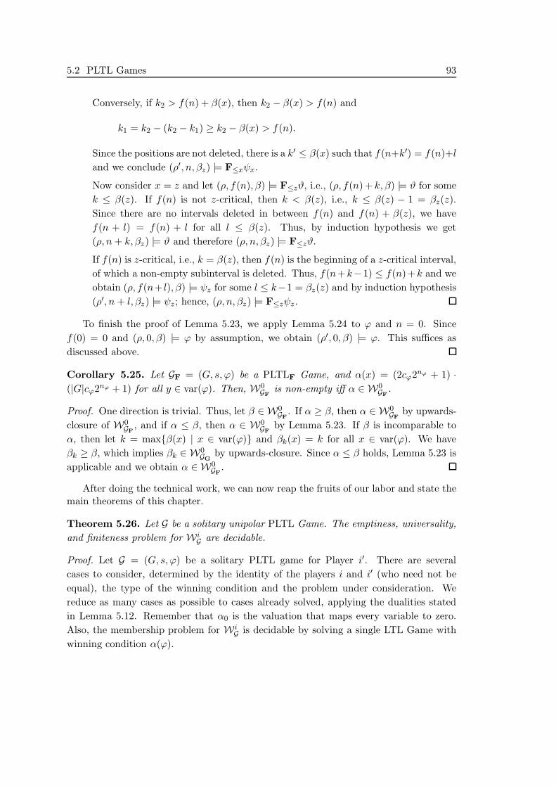
5.2 PLTL Games 93
Conversely, if k2 > f(n) + β(x), then k2 − β(x) > f(n) and
k1 = k2 − (k2 − k1) ≥ k2 − β(x) > f(n).
Since the positions are not deleted, there is a k′ ≤ β(x) such that f(n+k′) = f(n)+land we conclude (ρ′, n, βz) |= F≤xψx.
Now consider x = z and let (ρ, f(n), β) |= F≤zϑ, i.e., (ρ, f(n) + k, β) |= ϑ for somek ≤ β(z). If f(n) is not z-critical, then k < β(z), i.e., k ≤ β(z) − 1 = βz(z).Since there are no intervals deleted in between f(n) and f(n) + β(z), we havef(n + l) = f(n) + l for all l ≤ β(z). Thus, by induction hypothesis we get(ρ, n+ k, βz) |= ϑ and therefore (ρ, n, βz) |= F≤zϑ.
If f(n) is z-critical, i.e., k = β(z), then f(n) is the beginning of a z-critical interval,of which a non-empty subinterval is deleted. Thus, f(n+k−1) ≤ f(n) +k and weobtain (ρ, f(n+ l), β) |= ψz for some l ≤ k−1 = βz(z) and by induction hypothesis(ρ′, n+ l, βz) |= ψz; hence, (ρ, n, βz) |= F≤zψz.
To finish the proof of Lemma 5.23, we apply Lemma 5.24 to ϕ and n = 0. Sincef(0) = 0 and (ρ, 0, β) |= ϕ by assumption, we obtain (ρ′, 0, β) |= ϕ. This suffices asdiscussed above.
Corollary 5.25. Let GF = (G, s, ϕ) be a PLTLF Game, and α(x) = (2cϕ2nϕ + 1) ·(|G|cϕ2nϕ + 1) for all y ∈ var(ϕ). Then, W0
GFis non-empty iff α ∈ W0
GF.
Proof. One direction is trivial. Thus, let β ∈ W0GF
. If α ≥ β, then α ∈ W0GF
by upwards-closure of W0
GF, and if α ≤ β, then α ∈ W0
GFby Lemma 5.23. If β is incomparable to
α, then let k = max{β(x) | x ∈ var(ϕ)} and βk(x) = k for all x ∈ var(ϕ). We haveβk ≥ β, which implies βk ∈ W0
GGby upwards-closure. Since α ≤ β holds, Lemma 5.23 is
applicable and we obtain α ∈ W0GF
.
After doing the technical work, we can now reap the fruits of our labor and state themain theorems of this chapter.
Theorem 5.26. Let G be a solitary unipolar PLTL Game. The emptiness, universality,and finiteness problem for Wi
G are decidable.
Proof. Let G = (G, s, ϕ) be a solitary PLTL game for Player i′. There are severalcases to consider, determined by the identity of the players i and i′ (who need not beequal), the type of the winning condition and the problem under consideration. Wereduce as many cases as possible to cases already solved, applying the dualities statedin Lemma 5.12. Remember that α0 is the valuation that maps every variable to zero.Also, the membership problem for Wi
G is decidable by solving a single LTL Game withwinning condition α(ϕ).

94 5 Solitary PLTL Games
(i) Let G be solitary for Player 0 and ϕ ∈ PLTLG.
• By Corollary 5.14 (i), W0G is non-empty iff it contains α0.
• For the universality problem of W0G see Corollary 5.22.
(ii) Let G be solitary for Player 0 and ϕ ∈ PLTLF.
• For the emptiness problem of W0G see Corollary 5.25.
• By Corollary 5.14 (ii), W0G is universal iff it contains α0.
(iii) Let G be solitary for Player 0 and ϕ an arbitrary unipolar formula. The emptinessand universality problem for W1
G can be decided by considering the complements,again: by Lemma 5.12 (i), W1
G is empty iff W0G is universal, and W1
G is universal iffW0
G is empty. These problems were shown to be decidable in (i) respectively (ii).
(iv) Let G be solitary for Player 1 and ϕ an arbitrary unipolar formula. The empti-ness and universality problem for W1
G can be solved exploiting dualities. ByLemma 5.12 (ii), W1
G = W0G, where G is a solitary game for Player 0 with unipolar
winning condition. This is the setting of (i) respectively (ii)
(v) Let G be solitary for Player 1 and ϕ an arbitrary unipolar formula. The emptinessand universality problem for W0
G can be decided by considering the complements:by Lemma 5.12 (i), W0
G is empty iff W1G is universal, and W0
G is universal iff W1G is
empty. Each of the latter problems is decidable by (iv).
(vi) Now, just the finiteness problems remain. The solution is symmetric: let G be asolitary game for Player 0 or 1.
• If G is a PLTLG Game, then let Gy for all y ∈ var(ϕ) be defined as forLemma 5.16. The Lemma states that W0
G is infinite iff W 0Gy
is universal forsome y. Since Gy is still a solitary PLTLG game we can apply (i) respec-tively (v).
• If G is a PLTLF Game, then W0G is infinite iff it is non-empty, which was
shown to be decidable in (ii) respectively (v).
• For W1G (and both types of winning conditions) we again consider the dual
game and obtain W1G = W0
G . The finiteness problem for the latter set wasjust discussed above.
As we have reasoned above, the strategy problem for PLTL Games is more of anoptimization problem than it is a decision problem. Foremost, a PLTL game is not evena game in the strict sense, since a winning condition ϕ does not specify the winningplays. Furthermore, for a fixed valuation, the game is equal to an LTL game, a well-known class of games that have been studied extensively. The natural question is toask for an optimal strategy: given the winning condition F≤xp, what is the minimal
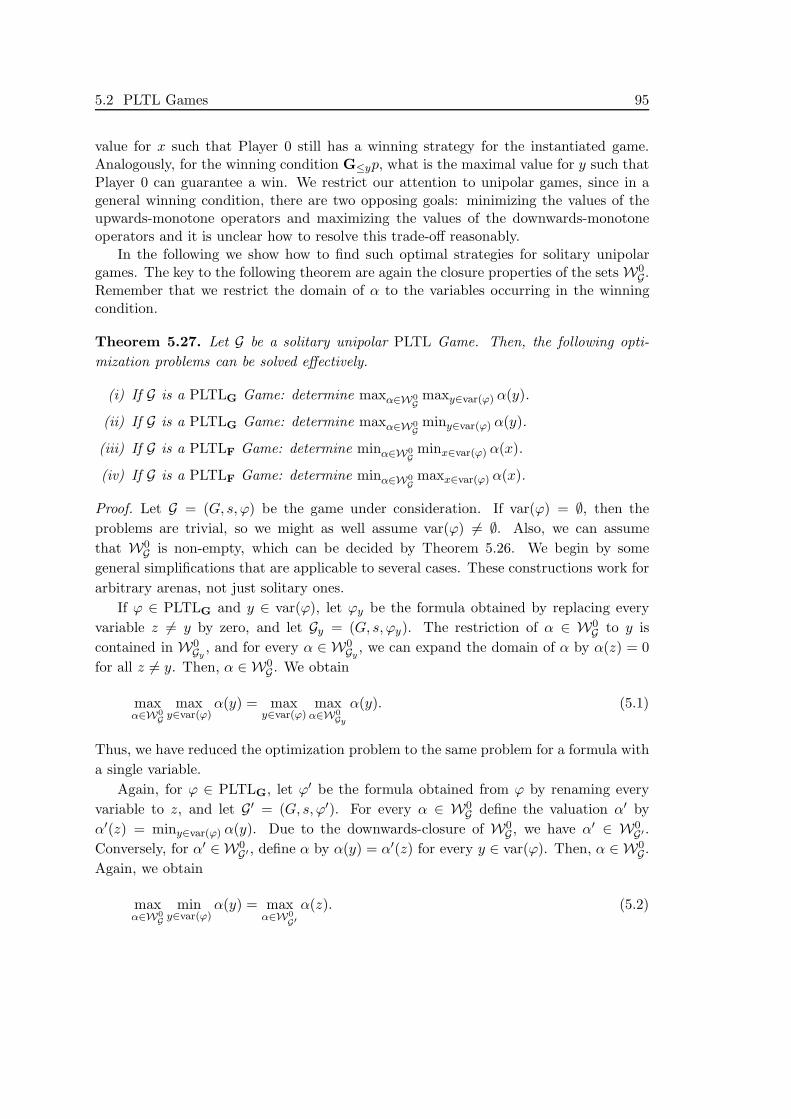
5.2 PLTL Games 95
value for x such that Player 0 still has a winning strategy for the instantiated game.Analogously, for the winning condition G≤yp, what is the maximal value for y such thatPlayer 0 can guarantee a win. We restrict our attention to unipolar games, since in ageneral winning condition, there are two opposing goals: minimizing the values of theupwards-monotone operators and maximizing the values of the downwards-monotoneoperators and it is unclear how to resolve this trade-off reasonably.
In the following we show how to find such optimal strategies for solitary unipolargames. The key to the following theorem are again the closure properties of the sets W0
G.Remember that we restrict the domain of α to the variables occurring in the winningcondition.
Theorem 5.27. Let G be a solitary unipolar PLTL Game. Then, the following opti-mization problems can be solved effectively.
(i) If G is a PLTLG Game: determine maxα∈W0G
maxy∈var(ϕ) α(y).
(ii) If G is a PLTLG Game: determine maxα∈W0G
miny∈var(ϕ) α(y).
(iii) If G is a PLTLF Game: determine minα∈W0G
minx∈var(ϕ) α(x).
(iv) If G is a PLTLF Game: determine minα∈W0G
maxx∈var(ϕ) α(x).
Proof. Let G = (G, s, ϕ) be the game under consideration. If var(ϕ) = ∅, then theproblems are trivial, so we might as well assume var(ϕ) �= ∅. Also, we can assumethat W0
G is non-empty, which can be decided by Theorem 5.26. We begin by somegeneral simplifications that are applicable to several cases. These constructions work forarbitrary arenas, not just solitary ones.
If ϕ ∈ PLTLG and y ∈ var(ϕ), let ϕy be the formula obtained by replacing everyvariable z �= y by zero, and let Gy = (G, s, ϕy). The restriction of α ∈ W0
G to y iscontained in W0
Gy, and for every α ∈ W0
Gy, we can expand the domain of α by α(z) = 0
for all z �= y. Then, α ∈ W0G . We obtain
maxα∈W0
Gmax
y∈var(ϕ)α(y) = max
y∈var(ϕ)max
α∈W0Gy
α(y). (5.1)
Thus, we have reduced the optimization problem to the same problem for a formula witha single variable.
Again, for ϕ ∈ PLTLG, let ϕ′ be the formula obtained from ϕ by renaming everyvariable to z, and let G′ = (G, s, ϕ′). For every α ∈ W0
G define the valuation α′ byα′(z) = miny∈var(ϕ) α(y). Due to the downwards-closure of W0
G , we have α′ ∈ W0G′ .
Conversely, for α′ ∈ W0G′ , define α by α(y) = α′(z) for every y ∈ var(ϕ). Then, α ∈ W0
G.Again, we obtain
maxα∈W0
Gmin
y∈var(ϕ)α(y) = max
α∈W0G′α(z). (5.2)

96 5 Solitary PLTL Games
So, this problem can be reduced to the same problem for a formula with a single variable.A dual construction is possible for ϕ ∈ PLTLF: let ϕ′ be the formula obtained from
ϕ by renaming every variable to z, and let G′ = (G, s, ϕ′). Again, for α ∈ WG , we defineα′ by α′(z) = maxx∈var(ϕ). Due to upwards-closure, we have α′ ∈ W0
G′ . Conversely, forα′ ∈ W0
G′ , we define α by α(x) = α′(z) for all x ∈ var(ϕ). Then, α ∈ W0G . Then, we
obtain
minα∈W0
Gmax
x∈var(ϕ)α(x) = min
α∈W0G′α(z), (5.3)
which gives a reduction to the problem for a formula with a single variable.Note that a general construction similar to the one employing Gy for a PLTLF Game is
not possible, since there is no equivalent to fixing all but one variable to zero. Minimizingthe minimum value turns out to be the most involved case.
The actual proof consists of two steps. First we solve the optimization problems forsolitary games for Player 0. Solitary games for Player 1 can then be treated by an easyreduction using the dualities of the sets Wi
G.
• Let G be a solitary game for Player 0.
(i) and (ii) By (5.1) and (5.2), it suffices to determine max0WG α(y), where G is
a PLTLG Game whose winning condition ϕ has a single variable y. ModifyingLemma 5.19 for a formula with a |var(ϕ)| = 1, we can restrict the maximum to
maxα∈W0
Gα(y) < |G|cϕ2nϕ + 1 or max
α∈W0Gα(y) = ∞.
The second case can be tested by Corollary 5.22: We have maxα∈W0Gyα(y) = ∞ iff
W0G is infinite, which is equivalent to W0
G being universal by downwards-closure. Ifthe maximum is not ∞, then we can do binary search in the interval [0, |G|cϕ2nϕ ],which is correct by downwards-closure. Doing this, we need to determine thewinner of at most log2(2|G|cϕ2nϕ) LTL Games.
(iii) Let G = (G, s, ϕ) be a PLTLF Game, solitary for Player 0, such that W0G is
non-empty, and let nG = (2cϕ2nϕ + 1) · (|G|cϕ2nϕ + 1). By Corollary 5.25, W0G
contains α with α(x) = nG for all x ∈ var(ϕ). Thus,
minα∈W0
Gmin
xα(x) ≤ nG .
To determine, whether the minimum is even smaller, the emptiness problem for allW0
Gx,nhas to be solved for all x ∈ var(ϕ) and all n < nG , where Gx,n is obtained
from G by replacing the variable x of the winning condition ϕ by n. The smallestn such that W0
Gx,nis non-empty for some x, is equal to minα∈W0
GF
minx α(x). This

5.2 PLTL Games 97
n can be determined in two ways. Either by incrementing n beginning at zerolooping through all variables x ∈ var(ϕ). Alternatively, a binary search in theinterval [0, nG − 1] can be done for every variable x. In the second approach, theupper bound can be adjusted, if a smaller upper bound was found; however, allvariables have to be considered, whereas in the first approach, the search can beterminated, as soon as a non-empty set W0
Gx,nis discovered.
(iv) Again, by (5.3), it suffices to consider a PLTLF Game G whose winning con-dition has a single variable x. Lemma 5.23 bounds minα∈W0
Gα(x) from above by
nG = (2cϕx2nϕx + 1) · (|G|cϕx2nϕx + 1); hence, we can apply binary search, again.This time, the winner of at most log2(nG) LTL Games have to be determined.
• Let G be a solitary game for Player 1.
(i) and (ii) By (5.1) and (5.2), it suffices to consider a game G whose winningcondition ϕ has a single variable y: we have
maxα∈W0
Gα(y) = min
α∈W1Gα(y) − 1 = min
α∈W0Gα(y) − 1 = min
α∈W0G
minyα(y) − 1
by the closure properties of W0G and W1
G and Lemma 5.12. Since G is solitary forPlayer 0, we know how to minimize the minimum of the values, which also solvesour original problem.
(iii) This case is exceptional as it does not employ a reduction to a solitary gamefor Player 0. Instead, we proceed as for a solitary game for Player 0: let α be thevaluation mapping every variable of ϕ to nG = 2|G|cϕkϕ2nϕ + 1. The complementof W0
G , the set W1G , is not universal by assumption. Thus, it cannot contain α by
Lemma 5.19 and Lemma 5.12 (ii). Hence, α ∈ W0G . This gives an upper bound on
the value we are interested in. So, we can again check all W0Gx,n
for non-emptiness,where Gx,n is defined as in case (iii) above.
(iv) This time, due to (5.3), it suffices to consider a game G whose winning conditionhas a single variable x. We have
minα∈W0
Gα(z) = max
α∈W1Gα(x) + 1 = max
α∈W0Gα(x) + 1 = max
α∈W0G
maxyα(x) + 1,
by the closure properties of W0G and W1
G and Lemma 5.12. The game G is againsolitary for Player 0.
Note that the missing problems, the ones with leading min for PLTLG conditions,and the ones with leading max for PLTLF conditions are trivial, since these optima areeither undefined, if W0
G is empty, or they are 0 by downwards-closure respectively ∞by upwards-closure. Also, the missing optimization problems for W1
G can be solved bydualizing the games according to Lemma 5.12 (ii).
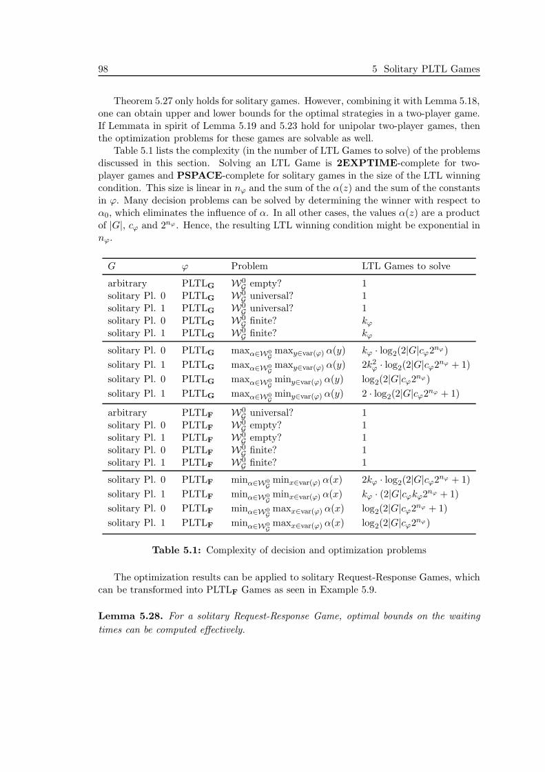
98 5 Solitary PLTL Games
Theorem 5.27 only holds for solitary games. However, combining it with Lemma 5.18,one can obtain upper and lower bounds for the optimal strategies in a two-player game.If Lemmata in spirit of Lemma 5.19 and 5.23 hold for unipolar two-player games, thenthe optimization problems for these games are solvable as well.
Table 5.1 lists the complexity (in the number of LTL Games to solve) of the problemsdiscussed in this section. Solving an LTL Game is 2EXPTIME-complete for two-player games and PSPACE-complete for solitary games in the size of the LTL winningcondition. This size is linear in nϕ and the sum of the α(z) and the sum of the constantsin ϕ. Many decision problems can be solved by determining the winner with respect toα0, which eliminates the influence of α. In all other cases, the values α(z) are a productof |G|, cϕ and 2nϕ . Hence, the resulting LTL winning condition might be exponential innϕ.
G ϕ Problem LTL Games to solve
arbitrary PLTLG W0G empty? 1
solitary Pl. 0 PLTLG W0G universal? 1
solitary Pl. 1 PLTLG W0G universal? 1
solitary Pl. 0 PLTLG W0G finite? kϕ
solitary Pl. 1 PLTLG W0G finite? kϕ
solitary Pl. 0 PLTLG maxα∈W0G
maxy∈var(ϕ) α(y) kϕ · log2(2|G|cϕ2nϕ)solitary Pl. 1 PLTLG maxα∈W0
Gmaxy∈var(ϕ) α(y) 2k2
ϕ · log2(2|G|cϕ2nϕ + 1)solitary Pl. 0 PLTLG maxα∈W0
Gminy∈var(ϕ) α(y) log2(2|G|cϕ2nϕ)
solitary Pl. 1 PLTLG maxα∈W0G
miny∈var(ϕ) α(y) 2 · log2(2|G|cϕ2nϕ + 1)
arbitrary PLTLF W0G universal? 1
solitary Pl. 0 PLTLF W0G empty? 1
solitary Pl. 1 PLTLF W0G empty? 1
solitary Pl. 0 PLTLF W0G finite? 1
solitary Pl. 1 PLTLF W0G finite? 1
solitary Pl. 0 PLTLF minα∈W0G
minx∈var(ϕ) α(x) 2kϕ · log2(2|G|cϕ2nϕ + 1)solitary Pl. 1 PLTLF minα∈W0
Gminx∈var(ϕ) α(x) kϕ · (2|G|cϕkϕ2nϕ + 1)
solitary Pl. 0 PLTLF minα∈W0G
maxx∈var(ϕ) α(x) log2(2|G|cϕ2nϕ + 1)solitary Pl. 1 PLTLF minα∈W0
Gmaxx∈var(ϕ) α(x) log2(2|G|cϕ2nϕ)
Table 5.1: Complexity of decision and optimization problems
The optimization results can be applied to solitary Request-Response Games, whichcan be transformed into PLTLF Games as seen in Example 5.9.
Lemma 5.28. For a solitary Request-Response Game, optimal bounds on the waitingtimes can be computed effectively.
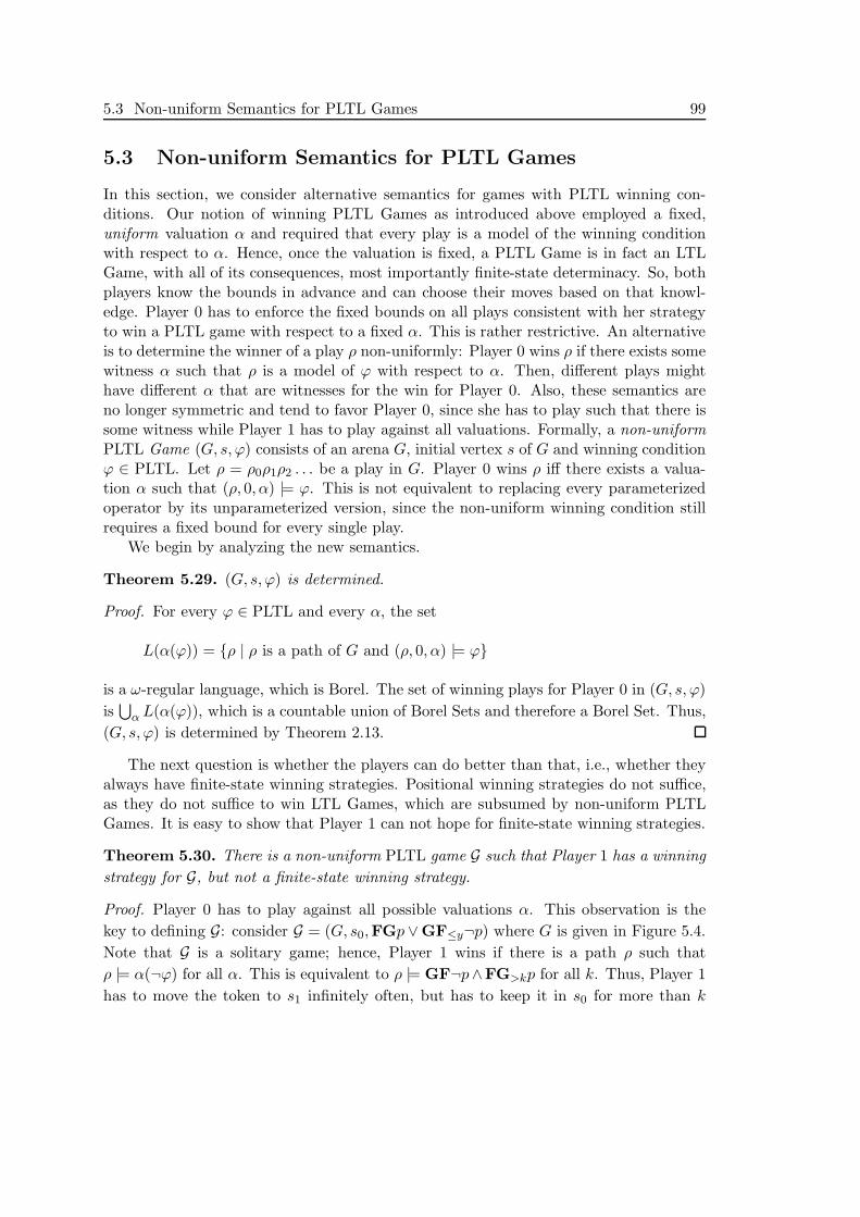
5.3 Non-uniform Semantics for PLTL Games 99
5.3 Non-uniform Semantics for PLTL Games
In this section, we consider alternative semantics for games with PLTL winning con-ditions. Our notion of winning PLTL Games as introduced above employed a fixed,uniform valuation α and required that every play is a model of the winning conditionwith respect to α. Hence, once the valuation is fixed, a PLTL Game is in fact an LTLGame, with all of its consequences, most importantly finite-state determinacy. So, bothplayers know the bounds in advance and can choose their moves based on that knowl-edge. Player 0 has to enforce the fixed bounds on all plays consistent with her strategyto win a PLTL game with respect to a fixed α. This is rather restrictive. An alternativeis to determine the winner of a play ρ non-uniformly: Player 0 wins ρ if there exists somewitness α such that ρ is a model of ϕ with respect to α. Then, different plays mighthave different α that are witnesses for the win for Player 0. Also, these semantics areno longer symmetric and tend to favor Player 0, since she has to play such that there issome witness while Player 1 has to play against all valuations. Formally, a non-uniformPLTL Game (G, s, ϕ) consists of an arena G, initial vertex s of G and winning conditionϕ ∈ PLTL. Let ρ = ρ0ρ1ρ2 . . . be a play in G. Player 0 wins ρ iff there exists a valua-tion α such that (ρ, 0, α) |= ϕ. This is not equivalent to replacing every parameterizedoperator by its unparameterized version, since the non-uniform winning condition stillrequires a fixed bound for every single play.
We begin by analyzing the new semantics.
Theorem 5.29. (G, s, ϕ) is determined.
Proof. For every ϕ ∈ PLTL and every α, the set
L(α(ϕ)) = {ρ | ρ is a path of G and (ρ, 0, α) |= ϕ}
is a ω-regular language, which is Borel. The set of winning plays for Player 0 in (G, s, ϕ)is
⋃α L(α(ϕ)), which is a countable union of Borel Sets and therefore a Borel Set. Thus,
(G, s, ϕ) is determined by Theorem 2.13.
The next question is whether the players can do better than that, i.e., whether theyalways have finite-state winning strategies. Positional winning strategies do not suffice,as they do not suffice to win LTL Games, which are subsumed by non-uniform PLTLGames. It is easy to show that Player 1 can not hope for finite-state winning strategies.
Theorem 5.30. There is a non-uniform PLTL game G such that Player 1 has a winningstrategy for G, but not a finite-state winning strategy.
Proof. Player 0 has to play against all possible valuations α. This observation is thekey to defining G: consider G = (G, s0,FGp ∨GF≤y¬p) where G is given in Figure 5.4.Note that G is a solitary game; hence, Player 1 wins if there is a path ρ such thatρ |= α(¬ϕ) for all α. This is equivalent to ρ |= GF¬p∧FG>kp for all k. Thus, Player 1has to move the token to s1 infinitely often, but has to keep it in s0 for more than k

100 5 Solitary PLTL Games
consecutive moves for every k: for the play ρ = s0s1s0s0s1s0s0s0s1s0s0s0s0 . . . we have(ρ, 0, α) �|= FGp ∨ GF≤y¬p for all valuations α. Thus, Player 1 wins G1.
s0 s1p
Figure 5.4: The arena G for Theorem 5.30
To complete the proof, assume that Player 1 has a finite-state strategy τ . Since G is asolitary game, there is exactly one play ρ consistent with τ , which is ultimately periodicby Remark 2.12, i.e., ρ = xyω for some finite play xy. However, every ultimately periodicplay is won by Player 0. Thus, Player 1 cannot have a finite-state winning strategy.
The question for Player 0 remains open. The first idea, to force her to measure thelength of some interval and require her to wait even longer at another vertex, but thenleaving it, cannot be specified by an PLTL formula, due to the use of distinct variablesfor upwards-monotone and downwards-monotone operators.
Another important question deals with the relation of classical PLTL games andnon-uniform PLTL games. We begin by considering PLTL games and consider theiranalogons with non-uniform semantics. If Player 0 has a winning strategy for G withrespect to a fixed α, i.e., W0
G �= ∅, then Player 0 wins G with non-uniform semantics aswell. If W0
G = ∅, then the situation is different.
Lemma 5.31. (i) There is a PLTL Game such that W0G = ∅, but Player 0 wins G
with non-uniform semantics.
(ii) There is a PLTL Game such that W0G = ∅ and Player 1 wins G with non-uniform
semantics.
Proof. (i) Consider the arena G in Figure 5.5 and the game (G, s0,F≤p ∨ G¬p). Wehave W0
G = ∅, since Player 0 can keep the token in s0 for more than α(y) moves andthen move it to s1 for every α, thereby winning the play. On the other hand, for everyplay ρ in G, there is a valuation α such that (ρ, 0, α) |= F≤p ∨ G¬p. Hence, Player 0wins the game with non-uniform semantics.
s0 s1p
Figure 5.5: The arena G for Lemma 5.31 (i)
5.3 Non-uniform Semantics for PLTL Games 101
(ii) This is trivially true, just pick a game with variable-free winning condition thatPlayer 0 does not win.
One case of the other direction, from non-uniform semantics to classical semantics,is easy, again. If Player 0 does not win G with non-uniform semantics, then there is noα such that she wins G with respect to α. The other case would imply a solution to thequestion of finite-state determinacy. Assume that the fact that Player 0 wins G withnon-uniform semantics implies W0
G �= ∅. Then Player 0 can use the finite-state winningstrategy σ for G with respect to some α ∈ W0
G to win G with non-uniform semantics aswell. This gives an alternative way of proving finite-state determinacy (for Player 0) ofnon-uniform PLTL Games.
Lemma 5.32. If G is a win for Player 0 with non-uniform semantics implies W0G �= ∅,
then Player 0 has a finite-state winning strategy for G with non-uniform semantics.
Note that results in spirit of Lemma 5.19 and 5.23 for unipolar two-player gameswould imply that Player 0 has finite-state winning strategies for unipolar PLTL Gameswith non-uniform semantics.


Chapter 6
Conclusion
In this work, we investigated the definition of time-optimal strategies based on naturalnotions of waiting times for several winning conditions for infinite games on graphs.This research is motivated by the fact that these waiting times typically correspond toperiods of waiting in the system modeled by the arena. This quality measure of a winningstrategy is defined semantically, as opposed to the memory size needed to implement thestrategy. Both are important in applications, but historically, attention was only paidto the memory size. Only recently, strategies were evaluated in terms of the quality ofthe plays it allows. While winning is still a binary notion, i.e., we considered zero-sumgames, there are winning plays for Player 0 that are less desirable than others.
The games considered here, Request-Response, Poset, and PLTL Games are char-acterized by plays that might contain infinitely many (independent) periods of waiting;hence, the waiting times have to be aggregated appropriately. For the former two winningconditions, the limit of the accumulated waiting times is used to aggregate the waitingtimes. This approach penalizes longer waiting times increasingly stronger, which is de-sirable in applications. For games with PLTL winning conditions, we employed boundedtemporal operators. This amounts to imposing global bounds on the waiting times foreventualities, for example.
For Request-Response Games and Poset Games we proved the existence of time-optimal finite-state winning strategies. The proof technique employed is very flexibleand can be applied to other winning conditions as well, if they meet some requirements:waiting times are triggered by a single request and can be computed locally for every step.Also, if the waiting times are high, then the corresponding interval has to contain loopsthat can be skipped. For solitary unipolar PLTL Games we proved that it is decidable,whether a player wins a game with respect to some, infinitely many, or all valuations.Furthermore, optimal strategies are computable for these games as well. For for two-player unipolar games some of the decision problems are proven to be decidable andnecessary and sufficient conditions are given. Lastly, alternative semantics were definedand compared to the standard semantics. Non-uniform PLTL games are determined,but finite-state strategies do no longer suffice, unlike in PLTL Games.

104 6 Conclusion
The investigation of time-optimal strategies is far from being finished. We did notonly obtain existence results for Request-Response and Poset Games. But the techniquespresented to synthesize winning strategies, based on reductions to Mean-Payoff Games,do not allow a sensible implementation, since the memory requirements of the strategiesare very high. Also, for PLTL Games, most problems for two-player games are stillopen. We will conclude this thesis by discussing the open problems just mentioned andby giving some pointers to future research.
Open Questions and Further Research
As mentioned above, the size of the memory structure used to determine time-optimalwinning strategies in Request-Response and Poset Games prevents an implementation.However, a careful analysis of the maximal length of non-dickson sequences of waitingtime vectors should improve the situation drastically. The following observation is key:if there are |G| moves in which no open request is responded, then this infix contains aloop that is deleted by the strategy improvement operators, as the waiting times increasemonotonically. Thus, there is at least one response of a condition in every such infix,which bounds the possible values occurring in these vectors. Furthermore, the waitingtime vectors evolve synchronously if they are not reset to zero, which limits the length ofa non-dickson sequence. Hence, we believe that the waiting times can be bounded by asmaller bound than b(n, k). If this bound can be lowered sufficiently, then the synthesisalgorithm could be implemented. To complement this, one should determine matchinglower bounds on the length of a non-dickson sequence of waiting time vectors.
Another interesting aspect is the trade-off between the size of a finite-state strategyand its value. If there is some connection between the two magnitudes, then approxi-mation algorithms might be applicable. These algorithms determine a strategy whosevalue is only a constant factor higher than the optimal value, but whose memory require-ments are lower. Finally, the usefulness of heuristic solutions to the problem of findingtime-optimal strategies should be researched.
The most pressing questions for unipolar PLTL Games are the open problems fortwo-player games, namely, the emptiness, universality, and finiteness problem for W0
Gand the optimization problems. Counterparts of the technical lemmata proved for soli-tary games are not directly clear, as there is no longer a single play that has to bemanipulated, but the restricted unraveling of the game with respect to a given winningstrategy for Player 0. A straightforward idea is to manipulate each play at a time.But when repeating (or deleting) intervals of a single play, one has to pay attention to(possibly infinitely many) other plays that share the prefix that is manipulated. Thecritical intervals of these plays might overlap in a way that there is no safe interval in thecommon prefix. This problem can be avoided by reasoning about runs of a deterministicautomaton accepting exactly the winning plays (with respect to the fixed valuation).However, a run of the automaton cannot have a state repetition in a critical interval, asit has to count the length of the interval. Also, retreating to non-deterministic or alter-

105
nating automata does not help, since such an automaton might have to be in differentstates, depending on the continuation of the play. Finally, reasoning with finite-statestrategies does not seem helpful, as the size of a strategy is always higher than the lengthof a critical interval. Hence, there is no (memory) state repetition in a critical interval.The bounds involved in the two technical lemmata do not coincide, which hints at aninfluence of the size of V0 (respectively V1) on these bounds.
Another open problem is the exact complexity of solving the emptiness, universality,and finiteness problem for W0
G , as well as the complexity of the optimization problems.The results for LTL Games give lower bounds, and the translation of PLTL to LTL(with respect to a fixed valuation), which increases the size of the formula linearly inthe values of the variables, gives upper bounds on the complexities.
Lastly, we want to mention an idea related to time-optimal strategies: Muller Gamesdo not have a clear definition of waiting times. Instead, McNaughton investigated thefollowing question [40]: can a referee decide the winner of an infinite play after a finiteplay of a certain duration, depending on the winning condition and the arena? Forpositionally determined games, a play can be stopped as soon as a vertex is visited for thesecond time. McNaughton discusses a scoring function for finite plays and appropriatechoices for the duration of the play. However, no formal results are given, as he wasinterested in devising games to be played by humans. But, as finite-state strategiessuffice to win Muller Games, the play can be stopped after a finite time. Then, thereferee can analyze the loops of the finite play. However, such a play will have severalloops and he has to determine the winner based on the right loops, i.e., a player mightnot win a play, but is able to force some loops, that could mislead the referee.

Bibliography
[1] Rajeev Alur, Kousha Etessami, Salvatore La Torre, and Doron Peled. Parametrictemporal logic for ”model measuring”. In ICALP, pages 159–168, 1999.
[2] Rajeev Alur and Thomas A. Henzinger. Real-time logics: Complexity and expres-siveness. Inf. Comput., 104(1):35–77, 1993.
[3] Rajeev Alur and Salvatore La Torre. Deterministic generators and games for LTLfragments. ACM Trans. Comput. Log., 5(1):1–25, 2004.
[4] Henrik Bjorklund, Sven Sandberg, and Sergei G. Vorobyov. A discrete subexponen-tial algorithm for parity games. In STACS, pages 663–674, 2003.
[5] Julius R. Buchi. On a decision method in restricted second order arithmetic. InErnest Nagel, Patrick Suppes, and Alfred Tarski, editors, Proceedings of the 1960International Congress on Logic, Methodology and Philosophy of Science, pages1–11. Stanford University Press, June 1962.
[6] Julius R. Buchi and Lawrence H. Landweber. Solving sequential conditions by finite-state strategies. Transactions of the American Mathematical Society, 138:295–311,April 1969.
[7] Krishnendu Chatterjee and Thomas A. Henzinger. Finitary winning in ω-regulargames. In TACAS, pages 257–271, 2006.
[8] Alonzo Church. Applications of recursive arithmetic to the problem of circuit syn-thesis. In Summaries of the Summer Institute of Symbolic Logic, Cornell Univ.,Ithaca, N.Y., volume I, pages 3–50, 1957.
[9] Edmund M. Clarke and E. Allen Emerson. Design and synthesis of synchronizationskeletons using branching-time temporal logic. In Logic of Programs, pages 52–71,1981.
[10] Edmund M. Clarke, Orna Grumberg, and Doron Peled. Model Checking. MITPress, 1999.
[11] Luca de Alfaro, Thomas A. Henzinger, and Rupak Majumdar. Discounting thefuture in systems theory. In ICALP, pages 1022–1037, 2003.

108 Bibliography
[12] Leonard E. Dickson. Finiteness of the odd perfect and primitive abundant numberswith n distinct prime factors. American Journal of Mathematics, 35(4):413–422,1913.
[13] Stefan Dziembowski, Marcin Jurdzinski, and Igor Walukiewicz. How much memoryis needed to win infinite games? In LICS, pages 99–110, 1997.
[14] Andrzej Ehrenfeucht. An application of games to the completeness problem forformalized theories. Fundamenta Mathematicae, 49:129–141, 1961.
[15] Andrzej Ehrenfeucht and Jan Mycielski. Positional strategies for mean payoff games.International Journal of Game Theory, 8(2):109–113, June 1979.
[16] E. Allen Emerson and Joseph Y. Halpern. “sometimes” and “not never” revisited:On branching versus linear time. In POPL, pages 127–140, 1983.
[17] E. Allen Emerson and Charanjit S. Jutla. Tree automata, µ-calculus and determi-nacy (extended abstract). In FOCS, pages 368–377, 1991.
[18] E. Allen Emerson, Charanjit S. Jutla, and A. Prasad Sistla. On model-checking forfragments of µ-calculus. In CAV, pages 385–396, 1993.
[19] E. Allen Emerson, Aloysius K. Mok, A. Prasad Sistla, and Jai Srinivasan. Quanti-tative temporal reasoning. In CAV, pages 136–145, 1990.
[20] Diana Fischer, Erich Gradel, and �Lukasz Kaiser. Model checking games for thequantitative µ-calculus. In STACS, pages 301–312, 2008.
[21] Roland Fraisse. Sur quelques classifications des systemes de relations. In Publica-tions Scientifiques de l’Universite d’Alger, volume 1 of A, pages 35–182, 1954.
[22] Hugo Gimbert and Wieslaw Zielonka. When can you play positionally? In MFCS,pages 686–697, 2004.
[23] Hugo Gimbert and Wieslaw Zielonka. Games where you can play optimally withoutany memory. In CONCUR, pages 428–442, 2005.
[24] Hugo Gimbert and Wieslaw Zielonka. Deterministic priority mean-payoff games aslimits of discounted games. In ICALP (2), pages 312–323, 2006.
[25] Erich Gradel, Wolfgang Thomas, and Thomas Wilke, editors. Automata, Logics,and Infinite Games: A Guide to Current Research [outcome of a Dagstuhl seminar,February 2001], volume 2500 of Lecture Notes in Computer Science. Springer, 2002.
[26] Yuri Gurevich and Leo Harrington. Trees, automata, and games. In STOC, pages60–65, 1982.
[27] Michael Holtmann and Christof Loding. Memory reduction for strategies in infinitegames. In CIAA, pages 253–264, 2007.

Bibliography 109
[28] Florian Horn. Faster algorithms for finitary games. In TACAS, pages 472–484,2007.
[29] Florian Horn, Wolfgang Thomas, and Nico Wallmeier. Optimal strategy synthesisin request-response games. In ATVA, pages 361–373, 2008.
[30] Jr James E. Kelley and Morgan R. Walker. Critical-path planning and scheduling.In IRE-AIEE-ACM ’59 (Eastern): Papers presented at the December 1-3, 1959,eastern joint IRE-AIEE-ACM computer conference, pages 160–173, New York, NY,USA, 1959. ACM.
[31] Marcin Jurdzinski. Deciding the winner in parity games is in UP ∩ co − UP. Inf.Process. Lett., 68(3):119–124, 1998.
[32] Marcin Jurdzinski. Small progress measures for solving parity games. In STACS,pages 290–301, 2000.
[33] Marcin Jurdzinski, Mike Paterson, and Uri Zwick. A deterministic subexponentialalgorithm for solving parity games. In SODA, pages 117–123, 2006.
[34] Alexander S. Kechris. Classical Descriptive Set Theory (Graduate Texts in Mathe-matics). Springer, January 1995.
[35] Orna Kupferman, Nir Piterman, and Moshe Y. Vardi. From liveness to promptness.In CAV, pages 406–419, 2007.
[36] Leslie Lamport. “sometime” is sometimes “not never” - on the temporal logic ofprograms. In POPL, pages 174–185, 1980.
[37] Donald A. Martin. Borel determinacy. Annals of Mathematics, 102:363–371, 1975.
[38] Robert McNaughton. Finite-state infinite games. Technical report, MassachusettsInstitute of Technology, 1965.
[39] Robert McNaughton. Testing and generating infinite sequences by a finite automa-ton. Information and Control, 9(5):521–530, 1966.
[40] Robert McNaughton. Playing infinite games in finite time. In A Half-Century ofAutomata Theory, pages 73–91, 2000.
[41] Andrzej W. Mostowski. Games with forbidden positions. Technical Report 78,Instytut Matematyki, University of Gdansk, 1991.
[42] John Nash. Non-cooperative games. The Annals of Mathematics, 54(2):286–295,September 1951.
[43] John Von Neumann and Oskar Morgenstern. Theory of Games and Economic Be-havior. Princeton University Press, 1944.
110 Bibliography
[44] Amir Pnueli. The temporal logic of programs. In FOCS, pages 46–57, 1977.
[45] Amir Pnueli and Roni Rosner. On the synthesis of a reactive module. In POPL,pages 179–190, 1989.
[46] Arthur Prior. Past, Present and Future. Oxford University Press, 1967.
[47] Micheal O. Rabin. Decidability of second-order theories and automata on infinitetrees. Transactions of the American Mathematical Society, 141:1–35, 1969.
[48] Sven Schewe. Solving parity games in big steps. In FSTTCS, pages 449–460, 2007.
[49] A. Prasad Sistla and Edmund M. Clarke. The complexity of propositional lineartemporal logics. In STOC, pages 159–168, 1982.
[50] Wolfgang Thomas. Automata on infinite objects. In Handbook of Theoretical Com-puter Science, Volume B: Formal Models and Sematics (B), pages 133–192. MITPress, 1990.
[51] Wolfgang Thomas. Languages, automata, and logic. In Handbook of Formal Lan-guages, pages 389–455. Springer, 1997.
[52] Jens Voge and Marcin Jurdzinski. A discrete strategy improvement algorithm forsolving parity games. In CAV, pages 202–215, 2000.
[53] Nico Wallmeier. Strategien in unendlichen Spielen mit Liveness-Gewinnbedin-gungen: Syntheseverfahren, Optimierung und Implementierung. PhD thesis, RWTHAachen University, 2008.
[54] Nico Wallmeier, Patrick Hutten, and Wolfgang Thomas. Symbolic synthesis offinite-state controllers for request-response specifications. In CIAA, pages 11–22,2003.
[55] Uri Zwick and Mike Paterson. The complexity of mean payoff games on graphs.Theor. Comput. Sci., 158(1&2):343–359, 1996.

Index
arena, 10dual, 78expanded, 15restricted, 18solitary, 10
atomic propositions, 9, 43automaton
Buchi, 8deterministic, 8Muller, 8
BuchiAutomaton, 8Game, 11
BorelGame, 11Hierarchy, 11set, 11
closeddownwards, 43upwards, 43
closure, 83, 89coloring, 12condition
Poset, 44Request-Response, 21
consistent, 13constant, 71convergence, 8
determinacy, 13finite-state, 19positional, 19
deterministic automaton, 8dickson
save D, 59save j, 36
divergence, 8downwards
closed, 43monotone, 75
dualarena, 78game, 78
embedding, 44minimal, 44
enumeration, 7expanded
arena, 15play, 15
finite-statedeterminacy, 19strategy, 14
formulaLTL, 9PLTL, 71PLTLF, 75PLTLG, 75unipolar, 75
gain, 12game, 11
Buchi, 11Borel, 11dual, 78equivalent, 15generalized Buchi, 11LTL, 12Muller, 12
112 Index
non-uniform PLTL, 99Parity, 12PLTL, 77PLTLF, 77PLTLG, 77reduction, 15regular, 12Request-Response, 11solitary, 11solving a, 13unipolar, 77zero-sum, 11
generalized BuchiGame, 11
graph, 9
Hasse diagram, 43
infix, 7initialization function, 14initialized game, 11interval, 82
labeledgraph, 9poset, 43
labeling function, 9, 43language, 7latest appearance record, 19length of an embedding, 44limit
of a sequence of functions, 8of a sequence of words, 8
Linear Temporal Logic, 9loss, 12LTL, 9
formulae, 9Game, 12
Mean-Payoff Game, 12memory
states, 14structure, 14
minimal embedding, 44model, 9, 73
monotone, 83, 89downwards, 75upwards, 75
MullerAutomaton, 8Game, 12
next-move function, 14non-dickson
play save D, 59play save j, 36
non-uniform PLTL Game, 99
open request, 21, 44optimal strategy, 25, 51
parameter, 71Parametric Linear Temporal Logic, 71Parity Game, 12partially ordered set, see posetpenalty, 25, 51
for condition j, 25for condition j, 51function, 25, 51
play, 10expanded, 15non-dickson save D, 59non-dickson save j, 36played according σ, 13winning, 11
Player 0, 9Player 1, 9PLTL
formulae, 71Game, 77–101
PLTL Gamenon-uniform, 99
PLTLF, 75formula, 75game, 77
PLTLG, 75formula, 75game, 77
poset, 43

Index 113
Game, 44–67position, 82positional
determinacy, 19strategy, 13
prefix, 7projected play, 15
reduction, 15regular game, 12request, 21, 44
open, 21, 44that is open indefinitely, 46
Request-Poset condition, 44Request-Response
condition, 21Game, 11, 21–39
response, 21, 44restricted
arena, 18unraveling, 18
satisfaction relation, 9, 72set of open requests, 46size
of a finite-state strategy, 14of a formula, 9of a memory structure, 14
solitaryarena, 10game, 11
solving a game, 13strategy, 13
finite-state, 14improvement operator, 29, 55optimal, 25, 51positional, 13winning, 13with memory, 14
subword, 8
totalized waiting time, 51transitive reduction, 43
ultimately periodic, 8
uniformly bounds, 25, 51unipolar
formula, 75game, 77
unraveling, 17restricted, 18
update function, 14upwards
closed, 43monotone, 75
valuation, 72value
of a game, 20of a play, 25of a play in a Poset Game, 51of a strategy, 25, 51
variable, 71
waiting time, 24totalized, 51vector, 25
winninga play, 11an initialized game, 13condition, 11plays, 11region, 13strategy, 13
zero-sum game, 11


Symbol Index
(Q,P ) Request-Response condition, 21
[n] {1, . . . , n}, 7
≤M game reduction, 15
� partial ordering relation, 43
�red transitive reduction of �, 43
|= satisfaction relation, 9
2S powerset of S, 7
� proper prefix ordering, 7
prefix ordering, 7
|S| cardinality of S, 7
|ϕ| size of ϕ, 9
|w| length of w, 7
A Buchi Automaton, 8
α(ϕ) ϕ instantiated by α, 75
bP (G) Bound on vP (σ) of optimal σ in Poset Game G, 52
bR(G) Bound on vR(σ) of optimal σ in Request-Response Game G, 27
cl(ϕ) closure of ϕ, 83
con(ϕ) constants of ϕ, 72
cϕ product of the constants in ϕ, 72
D domain of a poset, 43
Down(P) downwards-closed subsets of D, 44
E edges, 9
116 Symbol Index
ε empty word, 7
fj penalty function for condition j, 25
G arena or graph, 9
G dual arena, 78
G game, 11
G dual game, 78
Γ0 strategies for Player 0, 13
Γ1 strategies for Player 1, 13
G�σ G restricted by σ, 18
G× M expanded arena, 15
Ij strategy improvement operator for condition j, 29
Ij,D strategy improvement operator for D ∈ Up(Pj), 55
Inf(α) infinity set of α, 8
init initialization function, 14
kϕ number of operators of ϕ parameterized with variable, 72
l labeling function, 9
L(A) language of A, 8
L(M) language of M, 8
limn→∞ fn limit of the functions fn, 8
limn→∞wn limit of the words wn, 8
LTL LTL formulae, 9
M Muller Automaton, 8
M memory structure, 14
M memory states, 14
M × M′ composition of memory structures, 16
N non-negative integers, 7
next next-move function, 14
nϕ number of subformulae in ϕ, 72
Occ(α) occurrence set of α, 8
Symbol Index 117
Openj set of open requests, 46
P poset, 43
P atomic propositions, 9
pj(w) penalty for condition j after w, 25
PLTL PLTL formulae, 71
PLTLF PLTL formulae without parameterized always, 75
PLTLG PLTL formulae without parameterized eventualities, 75
Pref(L) set of prefixes of L, 7
p(w) penalty after w, 25
ρ play, 10
ρ(s, σ, τ) play starting in s consistent with σ and τ , 18
S(G,ϕ) valuations that make ϕ satisfiable in G, 73
S(ϕ) valuations that make ϕ satisfiable, 73
Σ alphabet, 7
σ strategy for Player 0, 13
Σω infinite words over Σ, 7
Σ+ non-empty finite words over Σ, 7
Σ∗ finite words over Σ, 7
sj,D number of open requests D after w, 46
t waiting time vector, 25
τ strategy for Player 1, 13
TG,s unraveling of G from s, 17
TG,s�w subtree of TG,s rooted in w, 18
TσG,s restriction of TG,s by σ, 17
TσG,s�w subtree of Tσ
G,s rooted in w, 18
Tσ,τG,s restriction of TG,s by σ and τ , 18
Tσ,τG,s�w subtree of T
σ,τG,s rooted in w, 18
tj waiting time for condition j, 24
tj totalized waiting time for j, 51

118 Symbol Index
tj,D totalized waiting time for D, 51
T(L) tree induced by language L, 8
T(L)�w subtree of T(L) rooted in w, 8
Up(P) upwards-closed subsets of D, 44
update update function, 14
update∗ memory content after w, 14
V vertices, 9
V (G,ϕ) valuations that make ϕ valid in G, 73
V (ϕ) valuations that make ϕ valid, 73
V0 Player 0’s positions, 10
v0 gain for Player 0, 12
V1 Player 1’s positions, 10
v1 loss for Player 1, 12
var(ϕ) variables of ϕ, 72
vM (G) value of G in a Mean-Payoff Game, 20
vP (ρ) value of ρ in a Poset Game, 51
vP (σ) value of σ, 51
vR(ρ) value of ρ in a Request-Response Game, 25
vR(σ) value of σ in a Request-Response Game, 25
W0 winning region of Player 0, 13
W1 winning region of Player 1, 13
W0G valuations that let Player 0 win G, 77
W1G valuations that let Player 1 win G, 77
Win winning plays for Player 0, 11
w−1L left quotient of w from L, 8
w−1w′ left quotient of w from w′, 8
X variables, 71
Y variables, 71