Two- and Three-Dimensional Tomography of Radiated Power ...

Two- and Three-Dimensional Tomography of Radiated Power using Imaging Bolometers in Toroidal Devices

Byron J. Peterson

National Institute for Fusion ScienceSOKENDAI

R. Sano (QST), J. H. Jang, S. Oh (NFRI), K. Mukai (NIFS, SOKENDAI), S. N. Pandya (IPR),

W. Choe (KAIST), N. Iwama (NIFS)

The 3rd IAEA Technical Meeting on ‘Fusion Data Processing, Validation and Analysis’, 28th to 31st May, 2019, Vienna, Austria. O-16

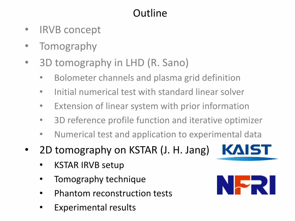
Outline

• IRVB concept

• Tomography

• 3D tomography in LHD (R. Sano)

• Bolometer channels and plasma grid definition

• Initial numerical test with standard linear solver

• Extension of linear system with prior information

• 3D reference profile function and iterative optimizer

• Numerical test and application to experimental data

• 2D tomography on KSTAR (J. H. Jang)

• KSTAR IRVB setup

• Tomography technique

• Phantom reconstruction tests

• Experimental results

2-D

Laplacian

Imaging Bolometer (IRVB) Concept

2lkt

P

f

radrad =

1)( 4

0

4

−

= −

f

BSbb

kt

TT

foil thermal

diffusivity

Calculate Prad from foil T using 2D heat diffusion equation

black body cooling term

plasma radiated power

is determined by solving

heat diffusion equation

foil thermal

conductivity foil

thickness

bolometer

pixel area

IRVB pinhole camera

B.J. Peterson et al., Rev. Sci. Instrum. 74 (2003) 2040.

2

2

2

21

y

T

x

T

t

Tbbrad

+

=

++−

ther

ma

l

dif

fusi

vio

n

to f

ram

e

IR measured

by camera

copper frame

Th

in f

oil

copper frame

lig

ht

shie

ld

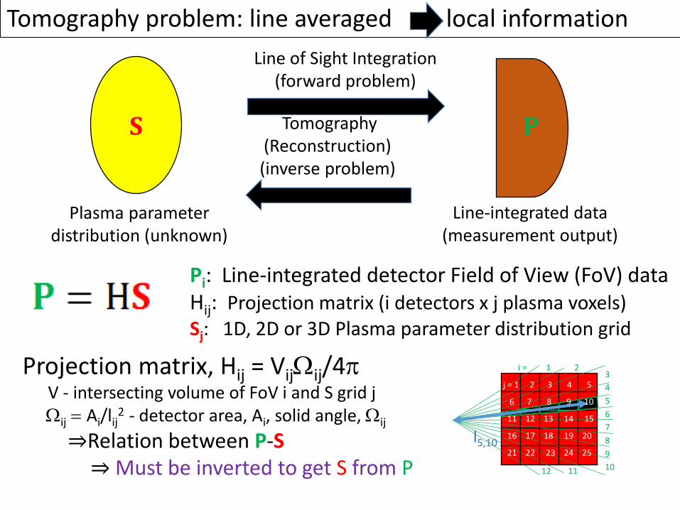
Line of Sight Integration(forward problem)

Tomography(Reconstruction)(inverse problem)

Tomography problem: line averaged local information

Pi: Line-integrated detector Field of View (FoV) dataHij: Projection matrix (i detectors x j plasma voxels)Sj: 1D, 2D or 3D Plasma parameter distribution grid

Projection matrix, Hij = Vijij/4pV - intersecting volume of FoV i and S grid jij = Ai/lij

2 - detector area, Ai, solid angle, ij

⇒Relation between P-S ⇒ Must be inverted to get S from P

Plasma parameter distribution (unknown)

Line-integrated data(measurement output)

𝐒 𝐏

j = 1 2 3 4 5

6 7 8 9 10

11 12 13 14 15

16 17 18 19 20

21 22 23 24 25

i = 1 2 3

4

5

6

7

8

9

1012 11

l5,10

Outline

• IRVB concept

• Tomography












Plasma voxel(grid element)(cylindrical coordinate)Horizontal(R): 5 cm

54 divisions (2.4 m < R < 5.1 m)Vertical (Z): 5cm

52 divisions (-1.3 m < Z < 1.3 m)Toroidal(φ): 1 degree

360 divisionsTotal number of voxels: 1,010,880

ROI (Region of Interest) voxel (tomography target): masking process, helical periodicity (n=10)

⇒ 16,188 voxels (0°<φ<18°)

Diagnostics（IRVB × 4）

IRVB channels: 1008+1008+560+620=3,196ch

𝐏 (3196 ch)𝐒 16188 voxelsH (3196 × 16188)Helical periodicity

IRVBs and plasma voxels are designed as 3D tomography system

Sight line without periodicitySight line with periodicity

10-O6-T

6.5-U

6.5-L

𝐏 = H𝐒

RoI

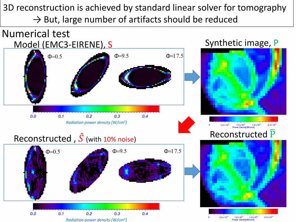
Model (EMC3-EIRENE), S

Reconstructed , መ𝑆 (with 10% noise)

Synthetic image, P

Reconstructed P

3D reconstruction is achieved by standard linear solver for tomography→ But, large number of artifacts should be reduced

Radiation power density (W/cm3)


Φ=0.5 Φ=9.5 Φ=17.5

Φ=0.5 Φ=9.5 Φ=17.5

Numerical test

Standard linear solver is extended by prior information

Lagrange function

Λ 𝐒 = γ C𝐒 2 +H𝐒 − 𝐏 2

M

H:Projection matrix

P: Integrated data

S :Plasma parameter distribution

M:Total number of diagnostics

channels

γ : Regularization parameter

C : Identity matrix

Extended solver (with prior information )

Λ 𝐒 = γ C (𝐒 − α𝐦) 2 +H𝐒 − 𝐏 2

M

𝐦:Reference profile

(prior information)

α:Weighting factor

Euclidean distance between reference profile and reconstructed profile

Lagrange function

Standard linear solver (Tikhonov regularization)

Extended by 𝐦

R. Sano et al., Rev. Sci. Instrum. 87, 11D440 (2016).

Flow of 3D tomography with prior information

Reference profile is processed as a rough estimationby diagnostics data and knowledge of plasma

IRVB imagesReference

processing

(fitting)

3D reference profile, 𝐦

Reconstruction (extended)Prior information

Reconstruction (standard)Weighting factor 𝛼 is fixed to 0.5(by numerical test results)

𝐏

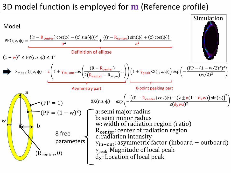
Model

PP r, z, ϕ =r − Rcenter cos ϕ − z sin ϕ 2

b2+

r − Rcenter sin ϕ + z cos ϕ 2

a2

1 − w 2 ≤ PP r, z, ϕ ≤ 12

Smodel r, z, ϕ = c 1 + γin−outcosR − Rcenter

2 Rcenter − Redge

π 1 + γpeakXX r, z, ϕ exp −(PP − 1 − Τw 2 2)2

( Τw 2)2

Definition of ellipse

Asymmetry part X-point peaking parta

bw

(Rcenter, 0)

(PP = 1)

(PP = 1 − w 2)

XX r, z, ϕ = exp −R − Rcenter cos ϕ − z ± a 1 − dXw sin ϕ

2

2 dXwa2

3D model function is employed for 𝐦 (Reference profile)

b: semi minor radiusa: semi major radius

w:width of radiation region (ratio)

γin−out: asymmetric factor (inboard − outboard)γpeak:Magnitude of local peak

c: radiation intensityRcenter: center of radiation region

dX: Location of local peak

8 free parameters

Simulation

Initial parameters

Normalized experimentalImage (IRVB data)

Normalized model projection (Model)

Reference profile is processed to fit IRVB image to model projection

Mean square error (normalized)

Number of calculation for 1 iteration = 3𝑛2 + 2𝑛 (𝑛 = 5)

Parameter scanning is individually carried out for each IRVB (U, L)

𝑏 1,𝑎

1,𝑤

1,𝛾

𝑖−𝑜1,𝛾

𝑝1,𝑅

1,𝑐1,𝑑

𝑋1

(𝑏0, 𝑎0, 𝑤0, 𝛾𝑖−𝑜0, 𝛾𝑝0, 𝑅0 ,𝑐0, 𝑑𝑋0)

R scan(n)

c scan (n)

𝛾𝑝 − 𝑑𝑋scan (n x n)

w-𝛾𝑎 scan (n x n)(𝑏0, 𝑎0, 𝑤1, 𝛾𝑖−𝑜1, 𝛾𝑝0, 𝑅0,𝑐0, 𝑑𝑋0)

b-a scan (n x n)(𝑏1, 𝑎1, 𝑤0, 𝛾𝑖−𝑜0, 𝛾𝑝0, 𝑅0 ,𝑐0, 𝑑𝑋0)

(𝑏0, 𝑎0, 𝑤0, 𝛾𝑖−𝑜0, 𝛾𝑝0, 𝑅1,𝑐0, 𝑑𝑋0)

(𝑏0, 𝑎0, 𝑤0, 𝛾𝑖−𝑜0, 𝛾𝑝1, 𝑅0, 𝑐0, 𝑑𝑋1)

(𝑏0, 𝑎0, 𝑤0, 𝛾𝑖−𝑜0, 𝛾𝑝0, 𝑅0, 𝑐1, 𝑑𝑋0)

𝑎𝑏

2

, 𝜀𝑛2,

H𝒎𝐏

Iteration until convergence

1st 2nd 3rd

5th 7th 9th

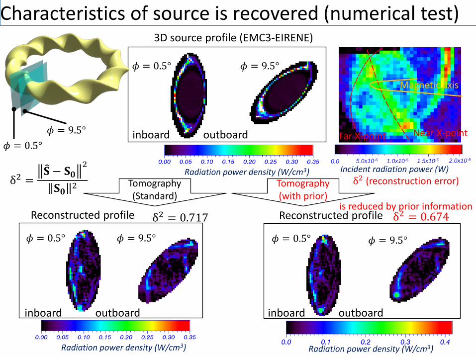
𝜙 = 0.5° 𝜙 = 9.5°

Incident radiation power (W)5.0x10-6 1.0x10-5 1.5x10-5 2.0x10-50.0


𝜙 = 0.5°

𝜙 = 9.5°

3D source profile (EMC3-EIRENE)

Tomography(Standard)

δ2 =𝐒 − 𝐒𝟎

2

𝐒𝟎2

Characteristics of source is recovered (numerical test)

𝜙 = 0.5° 𝜙 = 9.5°


Reconstructed profile δ2 = 0.674

inboard outboard

inboard outboard

𝜙 = 0.5° 𝜙 = 9.5°


Reconstructed profile δ2 = 0.717

Tomography(with prior)

inboard outboard

δ2 (reconstruction error)

is reduced by prior information

Magnetic axis

Near X-pointFar X-point

Experimental reconstruction become easily understandable by prior information (artifacts are suppressed)

Edge radiation

Core radiation (Radiation collapse)

Standard solver (Tikhonov) Extended solver (with prior )

Edge radiation

Core radiation (Radiation collapse)

Negative values:Number=3299 voxelsTotal =-111.00




Outline

• IRVB concept

• Tomography












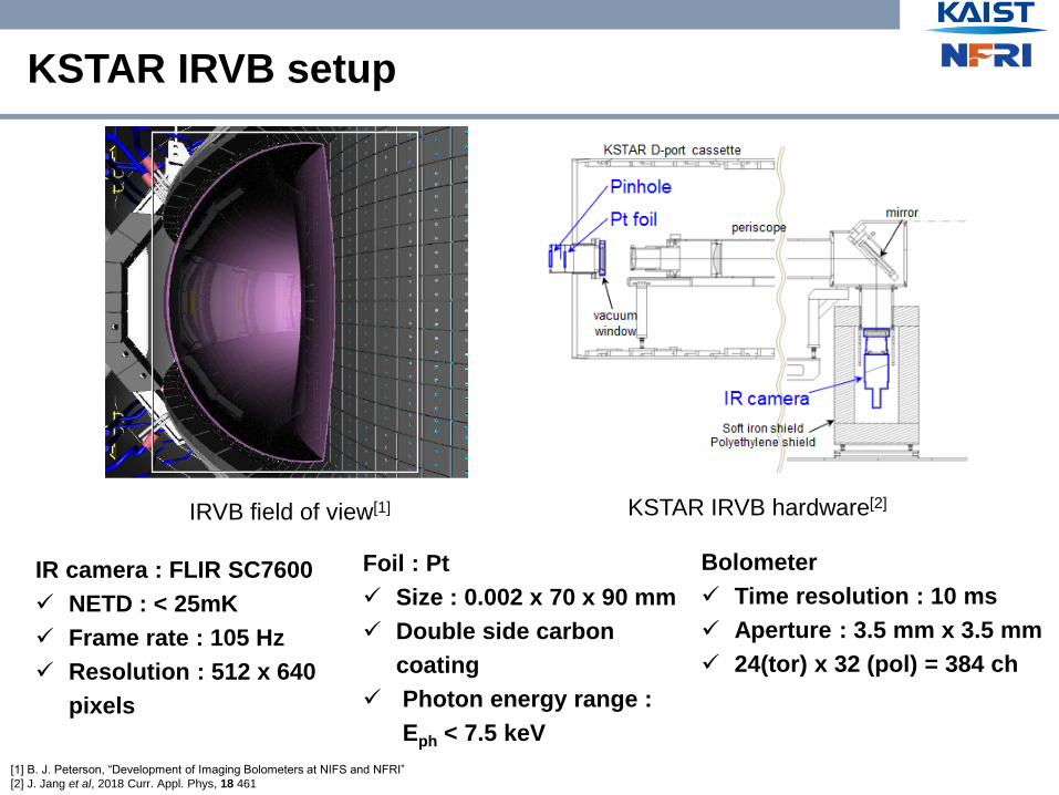
KSTAR IRVB setup

KSTAR IRVB hardware[2]

[1] B. J. Peterson, “Development of Imaging Bolometers at NIFS and NFRI”

[2] J. Jang et al, 2018 Curr. Appl. Phys, 18 461

IRVB field of view[1]

IR camera : FLIR SC7600

✓ NETD : < 25mK

✓ Frame rate : 105 Hz

✓ Resolution : 512 x 640

pixels

Foil : Pt

✓ Size : 0.002 x 70 x 90 mm

✓ Double side carbon

coating

✓ Photon energy range :

Eph < 7.5 keV

Bolometer

✓ Time resolution : 10 ms

✓ Aperture : 3.5 mm x 3.5 mm

✓ 24(tor) x 32 (pol) = 384 ch

Tomographic reconstruction technique

Phillips-Thikhonov method*

• Minimizing J = mean squared error +

signal variation𝑱 = 𝒇 −𝑾 ∙ 𝒈 𝟐/𝑴 + 𝜸 𝑳 ∙ 𝒈 𝟐

• P-T solution (𝜕𝑱/𝜕𝒈𝒊 = 𝟎)

𝐠 𝛄 = 𝐖𝐓 ∙ 𝐖 +𝐌𝛄𝐋𝐓 ∙ 𝐋−𝟏

∙ 𝐖𝐓 ∙ 𝐟

g : Reconstructed image

γ : Optimal regularization parameter

L : Laplacian

• GCV statistics : optimized γ

→ accuracy vs smoothness

→ high γ : smooth, inaccurate

→ low γ : accurate, unstable to noise

Ill-posed problem

𝐟 = 𝐖 ∙ 𝐠f : Line-integrated image

W : Weight matrix

g : Local emission profile (2-D)

Tangential line integration Local emission profile

(poloidal cross-section)

3-D geometry

(with toroidal symmetry)

IRVB image

Line-integration

Reconstruction

Tomography: A non-invasive imaging tool for observing the inner structure of

the plasmas

▪ Line-integrated raw data → tomography is essential

KSTAR IRVB Tomography setup

✓ Reconstruction grid : 1.2 < R < 2.4 m, -1.5 < Z < 1.5 m

→ Divided by 63 x 150 plasma pixels (2 cm x 2 cm for each)

✓ First wall geometry of KSTAR is applied in tomography code

KSTAR vacuum

vessel

Bolometer pixelPlasma pixel

FoilAperture

(b)(a)

Boundary condition of

KSTAR IRVB tomography

Open

Closed

Region between

Passive Stabilizers

(-0.5m < Z < 0.5m)

εb ≠ 0

No emission

on boundary

εb = 0

KSTAR IRVB line of sight

(description for plasma pixel and bolometer pixel)

Phantom reconstruction tests (1)

✓ Accuracy of KSTAR IRVB tomography is validated by reconstruction of

various synthetic images (phantoms)

✓ Total radiated power

𝑃𝑟𝑎𝑑 = 𝐴𝑝𝑖𝑥𝑒𝑙 × 2𝜋σ𝑅 ∙ 𝜖 𝑅, 𝑍

( 𝜖 𝑅, 𝑍 : 𝑒𝑚𝑖𝑠𝑠𝑖𝑣𝑖𝑡𝑦 𝑎𝑡 (𝑅, 𝑍) )

✓ Reconstruction error

erecon (%) =𝜖𝑝ℎ𝑎𝑛𝑡𝑜𝑚−𝜖𝑟𝑒𝑐𝑜𝑛

𝜖𝑝ℎ𝑎𝑛𝑡𝑜𝑚× 100

Synthetic image for

continuum radiation in KSTAR H-mode

→ Reconstructed well

Reconstruction erecon (%)Phantom

Reconstruction erecon (%)Phantom

More complicated phantoms[1] can also be

reconstructed well (Above : inter-ELM radiation

pattern, below : during ELM)

[1] J. Jang et al, 2018 Curr. Appl. Phys, 18 461

Reconstruction erecon (%)

d)

b)a)

c)

Phantom erecon (%)ReconstructionPhantom

a) D-shape + Hot spots in b) X-point, c) inboard and d) outboard divertor *

(10% noise added to line-integrated signal)*J. Jang et al, Rev. Sci. Instrum. (2018)

✓ High reconstruction accuracy near first wall in KSTAR

→ useful for impurity seeding exp. or plasma-divertor detachment


Spatial resolution of IRVB tomography

✓ Spatial resolution of IRVB tomography

~ 9 cm

: Two gaussian peak with 9 cm gap

can be distinguished

(10% noise added to line-integrated

signal)

ReconstructionPhantom


▪ Phantom

▪ Reconstruction

50% of

peak

Exp1) ELM mitigation by Kr seeding

✓ 1.7x1019 Kr particles injected

✓ ELM suppression (~5𝜏𝐸)

✓ ELM mitigation (~10𝜏𝐸 to the end of shot)

• 50% reduction in ∆𝑊𝐸𝐿𝑀 × 𝑓𝐸𝐿𝑀

ത𝑛𝑒(1019 m-2)

Te,ECE

(keV)

Dα

(1019)

Wdia

(MJ)

Prad

(MW)

Kr

H89L

time (s)

Prad

Prad,core

core

pedestal

Supp. Miti.

Kr signal

(a.u.)

Plasma

radiation

(kW/m3)

6.8s (before Kr seeding)

7.8s (natural ELM)

8.7s (ELM suppression)

9.4s (ELM mitigation)

Kr ion

density

(nKr) (m-3)

8.7s (Supp) 9.4s (Miti)6.8s 7.8s

IRVB plays crucial role in impurity study in KSTAR

7 8 9 10

Kr

time (s)

Prad

Prad,core

core

pedestal

Supp.

ത𝑛𝑒(1019 m-2)

Te,ECE

(keV)

Dα

(1019)

Wdia

(MJ)

Prad

(MW)

H89L

Kr signal

(a.u.)

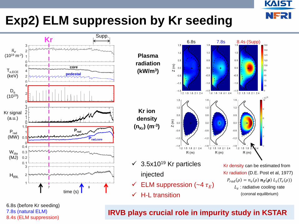
Exp2) ELM suppression by Kr seeding

✓ 3.5x1019 Kr particles

injected

✓ ELM suppression (~4 𝜏𝐸)

✓ H-L transition

Plasma

radiation

(kW/m3)

Kr ion

density

(nKr) (m-3)


7.8s (natural ELM)

8.4s (ELM suppression)

8.4s (Supp)6.8s 7.8s

IRVB plays crucial role in impurity study in KSTAR

Kr density can be estimated from

Kr radiation (D.E. Post et al, 1977)

𝑃𝑟𝑎𝑑 𝜌 = 𝑛𝑒 𝜌 𝒏𝒁 𝝆 𝐿𝑧(𝑇𝑒(𝜌))

𝐿𝑧 : radiative cooling rate

(coronal equilibrium)

7 8

Exp 3) ITB formation by Kr seeding

✓ total 5.2x1019 Kr particles injected

✓ ELM mitigation → H-L back transition → ITB formation

✓ Ti and Te profiles shows strong core peaking

✓ Relation between Kr and ITB formation is still under investigation

Te (keV)

Ti (keV)

𝜌


9.0s (before ITB formation)

11.0s (before ITB formation)

ITB

ITB

Kr ITB

ത𝑛𝑒(1019/m2)

Ip (kA)

Wtot

(kJ)

Dα

(1019)

Prad

(kW)

Te,ECE

(keV)

PNBI

(MW)

time (s)

𝜌

9.0s

(Before ITB)

11.0s

(After ITB)Plasma

radiation

(kW/m3)

Kr ion

density

(m-3)

Conclusions

• IRVBs can be applied to toroidal devices for the purpose of 2D and 3D tomography of radiated power

• In helical devices 3D tomography is desirable, but difficult• Improvements can be made using prior information

• In a tokamak with a tangential view• 2D profiles can be obtained with good spatial resolution in core and

divertor by assuming toroidal symmetry

• Also total power estimates can be provided.

• In KSTAR IRVB is the only bolometer and is providing both 2D profiles and total power estimates.

Future work

• 2D tomography of radiation in helical devices using IRVBs assuming radiation is constant on a field line• Should be applicable to both LHD and W7-X

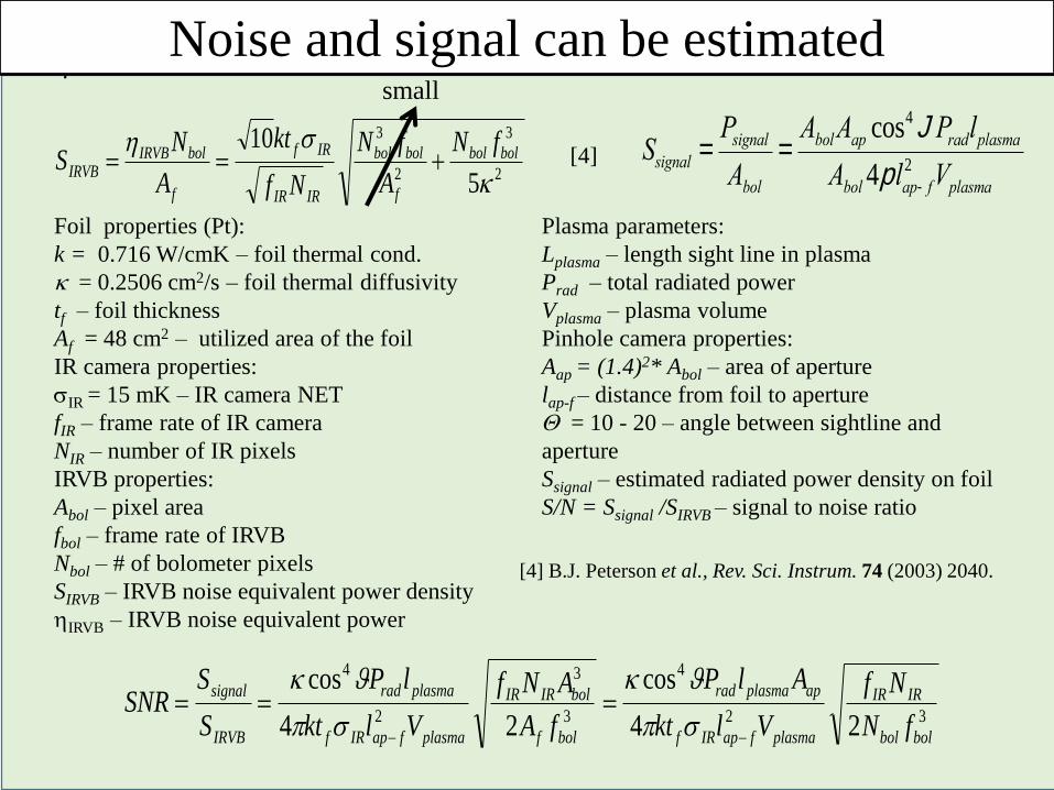
Noise and signal can be estimated.

Ssignal =Psignal

Abol=AbolAap cos4 JPradlplasma

Abol4plap- f2 Vplasma

32

4

3

3

2

4

24

cos

24

cos

bolbol

IRIR

plasmafapIRf

applasmarad

bolf

bolIRIR

plasmafapIRf

plasmarad

IRVB

signal

fN

Nf

Vlkt

AlP

fA

ANf

Vlkt

lP

S

SSNR

−−

===p

p

Foil properties (Pt):

k = 0.716 W/cmK – foil thermal cond.

= 0.2506 cm2/s – foil thermal diffusivity

tf – foil thickness

Af = 48 cm2 – utilized area of the foil

IR camera properties:

IR = 15 mK – IR camera NET

fIR – frame rate of IR camera

NIR – number of IR pixels

IRVB properties:

Abol – pixel area

fbol – frame rate of IRVB

Nbol – # of bolometer pixels

SIRVB – IRVB noise equivalent power density

hIRVB – IRVB noise equivalent power

Plasma parameters:

Lplasma – length sight line in plasma

Prad – total radiated power

Vplasma – plasma volume

Pinhole camera properties:

Aap = (1.4)2* Abol – area of aperture

lap-f – distance from foil to aperture

Q = 10 - 20 – angle between sightline and

aperture

Ssignal – estimated radiated power density on foil

S/N = Ssignal /SIRVB – signal to noise ratio

2

3

2

3

5

10

h bolbol

f

bolbol

IRIR

IRf

f

bolIRVBIRVB

fN

A

fN

Nf

kt

A

NS +==

small

[4] B.J. Peterson et al., Rev. Sci. Instrum. 74 (2003) 2040.

[4]



d)

b)a)

c)



*J. Jang et al, Rev. Sci. Instrum. (2018)




d)

b)a)

c)



*J. Jang et al, Rev. Sci. Instrum. (2018)



Phantom reconstruction tests (+10% noise)

Spatial resolution of IRVB tomography


~ 9 cm





▪ Phantom

▪ Reconstruction

50% of

peak

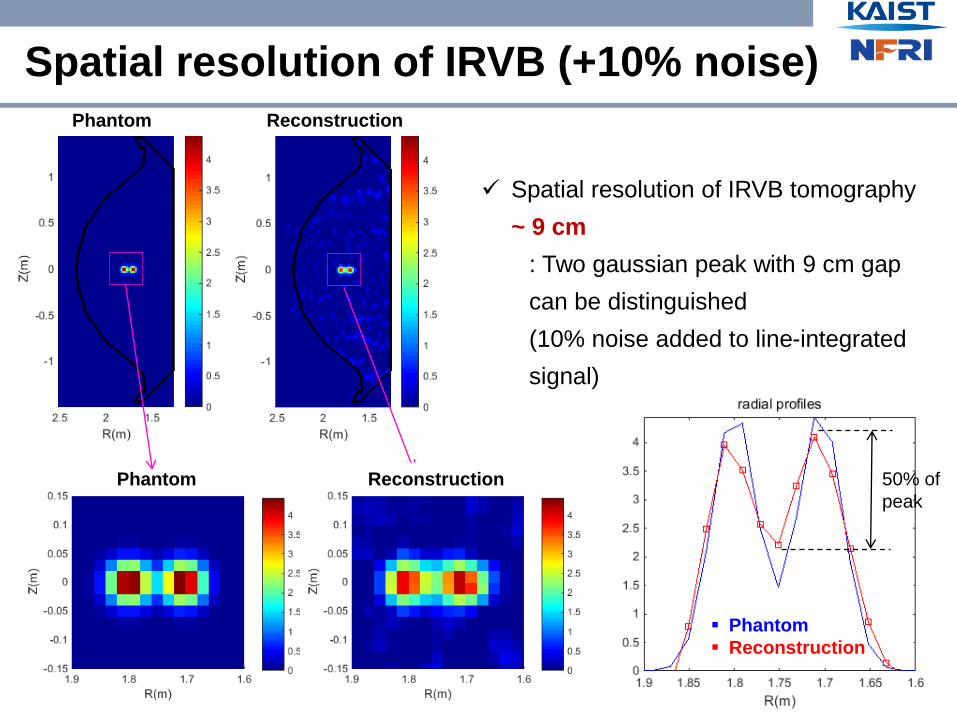
Spatial resolution of IRVB (+10% noise)


~ 9 cm



(10% noise added to line-integrated

signal)



▪ Phantom

▪ Reconstruction

50% of

peak

Two- and Three-Dimensional Tomography of Radiated Power ...

Documents

Transcript of Two- and Three-Dimensional Tomography of Radiated Power ...