


Sprachen
Seiten
Rechtliche

Nuclear Structure with
Unitarily Transformed Two-Body plus
Phenomenological Three-Body Interactions
Vom Fachbereich Physik
der Technischen Universitat Darmstadt
zur Erlangung des Grades
eines Doktors der Naturwissenschaften
(Dr. rer. nat.)
genehmigte
Dissertation
von
Dipl.-Phys. Anneke Gunther
aus Eckernforde
Darmstadt 2011
D17

Referent: Prof. Dr. Robert Roth
Korreferent: Prof. Dr. Jochen Wambach
Tag der Einreichung: 14.12.2010
Tag der Prufung: 02.02.2011
Summary
The importance of three-nucleon forces for a variety of nuclear structure phenomena
is apparent in various investigations. This thesis provides a first step towards the
inclusion of realistic three-nucleon forces by studying simple phenomenological three-
body interactions.
The Unitary Correlation Operator Method (UCOM) and the Similarity Renormaliza-
tion Group (SRG) provide two different approaches to derive soft phase-shift equivalent
nucleon-nucleon (NN) interactions via unitary transformations. Although their moti-
vations are quite different the NN interactions obtained with the two methods exhibit
some similarities.
The application of the UCOM- or SRG-transformed Argonne V18 potential in the
Hartree-Fock (HF) approximation and including the second-order energy corrections
emerging from many-body perturbation theory (MBPT) reveals that the systematics
of experimental ground-state energies can be reproduced by some of the interactions
considering a series of closed-shell nuclei across the whole nuclear chart. However,
charge radii are systematically underestimated, especially for intermediate and heavy
nuclei. This discrepancy to experimental data is expected to result from neglected
three-nucleon interactions.
As first ansatz for a three-nucleon force, we consider a finite-range three-body
interaction of Gaussian shape. Its influence on ground-state energies and charge radii
is discussed in detail on the basis of HF plus MBPT calculations and shows a significant
improvement in the description of experimental data.
As the handling of the Gaussian three-body interaction is time-extensive, we show
that it can be replaced by a regularized three-body contact interaction exhibiting a very
similar behavior. An extensive study characterizes its properties in detail and confirms
the improvements with respect to nuclear properties. To take into account information
of an exact numerical solution of the nuclear eigenvalue problem, the No-Core Shell
Model is applied to calculate the 4He ground-state energy.
As they are of direct interest for nuclear astrophysics collective excitation modes,
namely giant resonances, are investigated in the framework of the Random Phase
Approximation. Including the full three-body interaction would be very time-demanding.
Therefore, a density-dependent two-body interaction is used instead. This simple in-
teraction leads to a significant improvement in the description of the isovector dipole
and isoscalar quadrupole resonances while the isoscalar monopole resonances remain
in good agreement with experimental data compared to the results obtained with pure
unitarily transformed two-body interactions.
iii

iv
ZusammenfassungEine Vielzahl von Kernstrukturuntersuchungen belegt, dass Dreinukleonenkrafte
einen wesentlichen Einfluß auf verschiedene Observablen haben. Als ersten Schritt
hin zur Verwendung von realistischen Dreinukleonenkraften werden in dieser Arbeit
einfache phanomenologische Dreiteilchenwechselwirkungen untersucht.
Sowohl die Methode der Unitaren Korrelatoren (UCOM) als auch die Ahnlichkeits-
Renormierungsgruppe (SRG) verwenden unitare Transformationen, um weiche streu-
phasenaquivalente Nukleon-Nukleon (NN) Wechselwirkungen abzuleiten. Obwohl die
beiden Methoden von unterschiedlichen Ansatzen ausgehen, weisen die aus dem
realistischen Argonne V18 Potential gewonnenen NN Wechselwirkungen eine Reihe
von Gemeinsamkeiten auf.
Auf der Grundlage der Hartree-Fock (HF) Methode und der Vielteilchenstorungs-
theorie (MBPT) zweiter Ordnung kann die Systematik der Grundzustandsenergien einer
Reihe von Kernen mit abgeschlossenen Schalen mit Hilfe einiger der unitar trans-
formierten NN Wechselwirkungen uber die gesamte Nuklidkarte hinweg reproduziert
werden. Die Ladungsradien werden dagegen systematisch zu klein vorhergesagt, ins-
besondere fur mittelschwere und schwere Kerne. Es wird erwartet, dass diese Ab-
weichungen auf vernachlassigte Dreiteilchenwechselwirkungen zuruckzufuhren sind.
Als erster Ansatz wird der Einfluß einer gaußformigen Dreiteilchenwechselwirkung
im Rahmen von HF und MBPT untersucht, was zu einer deutlich besseren Beschreibung
der experimentellen Daten fuhrt.
Da Rechnungen mit der gaußformigen Dreiteilchenwechselwirkung sehr zeitaufwan-
dig sind, wird sie durch eine regularisierte Dreiteilchenkontaktwechselwirkung ersetzt,
die vergleichbare Ergebnisse liefert. Die Eigenschaften dieser Wechselwirkung werden
untersucht und die verbesserte Beschreibung von Grundzustandsobservablen bestatigt.
Um einen Referenzpunkt aus einer exakten numerischen Losung des nuklearen Eigen-
wertproblems zu erhalten, wird die 4He Grundzustandsenergie im Rahmen des No-Core
Schalenmodells berechnet.
Abschließend werden kollektive Anregungen, die besonders fur Anwendungen in
der nuklearen Astrophysik interessant sind, im Rahmen der Random Phase Approxi-
mation studiert. Da die Verwendung der Dreiteilchenkontaktwechselwirkung in dieser
Methode zu zeitaufwandig ware, wird sie durch eine dichteabhangige Zweiteilchenwech-
selwirkung ersetzt. Verglichen mit den Ergebnissen von reinen unitar transformierten
Zweiteilchenwechselwirkungen fuhrt die Einbeziehung der phanomenologischen Wech-
selwirkung zu einer deutlichen Verbesserung bei der Beschreibung der isovektoriellen
Dipol- und der isoskalaren Quadrupolriesenresonanzen, wahrend die isoskalaren Mono-
polriesenresonanzen gleichbleibend gut reproduziert werden.
v

vi
Contents
1 Introduction 1
2 Unitarily Transformed Interactions 72.1 Realistic Nucleon-Nucleon Potentials . . . . . . . . . . . . . . . . . . 7
2.2 Unitary Correlation Operator Method . . . . . . . . . . . . . . . . . . 9
2.2.1 Correlation Operators . . . . . . . . . . . . . . . . . . . . . . 10
2.2.2 Correlated Wave Functions . . . . . . . . . . . . . . . . . . . 12
2.2.3 Cluster Expansion . . . . . . . . . . . . . . . . . . . . . . . . 15
2.2.4 Correlated Interaction . . . . . . . . . . . . . . . . . . . . . . 16
2.2.5 Correlated Two-Body Matrix Elements . . . . . . . . . . . . . 19
2.2.6 Optimal Correlation Functions . . . . . . . . . . . . . . . . . . 23
2.3 Similarity Renormalization Group . . . . . . . . . . . . . . . . . . . . 27
2.3.1 SRG Flow Equation . . . . . . . . . . . . . . . . . . . . . . . 27
2.3.2 Evolution of Two-Body Matrix Elements . . . . . . . . . . . . 28
2.3.3 Evolved Wave Functions and Matrix Elements . . . . . . . . . 30
2.3.4 Connections between UCOM and SRG . . . . . . . . . . . . . 32
2.3.5 SRG-Generated UCOM Correlation Functions . . . . . . . . . . 34
3 Many-Body Calculations 413.1 The Hartree-Fock Method . . . . . . . . . . . . . . . . . . . . . . . . 41
3.2 Ground-State Energies and Charge Radii . . . . . . . . . . . . . . . . 44
3.3 Single-Particle Spectra . . . . . . . . . . . . . . . . . . . . . . . . . . 52
3.4 Low-Order Many-Body Perturbation Theory . . . . . . . . . . . . . . 55
3.5 Second-Order Energy Corrections . . . . . . . . . . . . . . . . . . . . 59
4 Gaussian Three-Body Interaction 654.1 Calculation of Matrix Elements . . . . . . . . . . . . . . . . . . . . . 65
4.1.1 Cartesian Matrix Elements . . . . . . . . . . . . . . . . . . . . 66
4.1.2 Coordinate Transformation . . . . . . . . . . . . . . . . . . . 68
vii
4.2 Ground-State Energies and Charge Radii . . . . . . . . . . . . . . . . 71
4.3 Perturbative Energy Corrections . . . . . . . . . . . . . . . . . . . . . 77
5 Three-Body Contact Interaction 815.1 Calculation of Matrix Elements . . . . . . . . . . . . . . . . . . . . . 81
5.2 Ground-State Energies and Charge Radii . . . . . . . . . . . . . . . . 87
5.3 Single-Particle Spectra . . . . . . . . . . . . . . . . . . . . . . . . . . 91
5.4 Perturbative Energy Corrections . . . . . . . . . . . . . . . . . . . . . 94
6 Few-Body Calculations 1036.1 The No-Core Shell Model . . . . . . . . . . . . . . . . . . . . . . . . 103
6.2 4He Ground-State Energy . . . . . . . . . . . . . . . . . . . . . . . . 104
7 Collective Excitations 1077.1 Random Phase Approximation . . . . . . . . . . . . . . . . . . . . . . 107
7.2 Multipole Transitions . . . . . . . . . . . . . . . . . . . . . . . . . . . 109
7.3 Sum Rules . . . . . . . . . . . . . . . . . . . . . . . . . . . . . . . . 110
7.4 Giant Resonances . . . . . . . . . . . . . . . . . . . . . . . . . . . . 114
7.4.1 Isoscalar Giant Monopole Resonance . . . . . . . . . . . . . . 115
7.4.2 Isovector Giant Dipole Resonance . . . . . . . . . . . . . . . . 122
7.4.3 Isoscalar Giant Quadrupole Resonance . . . . . . . . . . . . . 126
7.4.4 Comparison of Giant Resonances . . . . . . . . . . . . . . . . 130
8 Conclusions 133
A Derivation of the Hartree-Fock Equations 139A.1 The Variational Principle . . . . . . . . . . . . . . . . . . . . . . . . . 139
A.2 The Hartree-Fock Method . . . . . . . . . . . . . . . . . . . . . . . . 140
B Basic Concepts of Perturbation Theory 147
C Basic Concepts of the Random Phase Approximation 149
D Normal Ordering 153
E Figures 155E.1 Hartree-Fock Results for the Contact Interaction . . . . . . . . . . . . 155
viii
E.2 Perturbative Energy Corrections for the Contact Interaction . . . . . . 158
E.3 Collective Excitations . . . . . . . . . . . . . . . . . . . . . . . . . . 160
F Notation 165
ix

x
Chapter 1
Introduction
The existence of a diversity of chemical elements is the most fundamental precondition
for the existence of our planet earth. During the cooling of the universe after the
big bang no elements heavier than lithium were formed. Only some of the chemical
elements up to iron are produced by fusion in the inner cores of stars. For the production
of all other elements hotter and denser environments are required, which appear in
different astrophysical scenarios such as red giants, novae, and supernovae. Nuclear
astrophysics aims at the modeling of nucleosynthesis via various processes like the rapid
neutron capture process (r-process) that proceeds in supernovae. On the basis of the
r-process the existence of most neutron-rich nuclei up to the neutron dripline can be
understood. In contrast, the slow neutron capture process (s-process) stays close to
the valley of stability, while the rapid proton capture process (rp-process) covers the
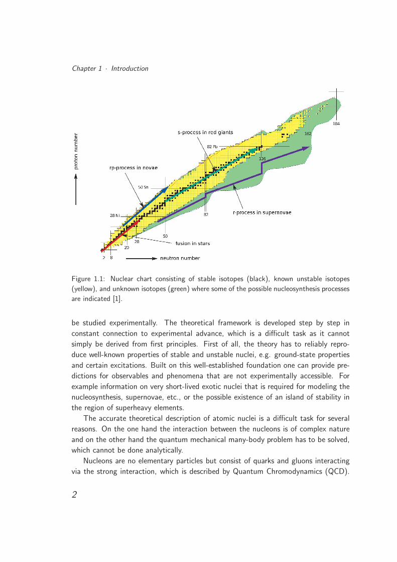
proton-rich part of the nuclear chart. These nucleosynthesis processes are sketched
in Figure 1.1, where the nuclear chart consisting of the stable elements, the known
unstable isotopes, and the nuclei that are expected to exist but are (still) unknown is
shown. To allow for reliable statements about the various nucleosynthesis processes a
detailed fundamental knowledge of atomic nuclei, stable as well as unstable and exotic
ones, is indispensable.
The properties of stable nuclei have been investigated in numerous experiments, e.g.
at various accelerator facilities, since a long time. In recent years experimental tech-
niques for the study of unstable and exotic nuclei have been developed. Nonetheless,
a reliable theoretical framework is inevitable, on the one hand to explain experimental
observations and to offer guidelines for the development of further experiments and
on the other hand to provide reliable predictions for exotic nuclei that cannot (yet)
1
Chapter 1 · Introduction
Figure 1.1: Nuclear chart consisting of stable isotopes (black), known unstable isotopes
(yellow), and unknown isotopes (green) where some of the possible nucleosynthesis processes
are indicated [1].
be studied experimentally. The theoretical framework is developed step by step in
constant connection to experimental advance, which is a difficult task as it cannot
simply be derived from first principles. First of all, the theory has to reliably repro-
duce well-known properties of stable and unstable nuclei, e.g. ground-state properties
and certain excitations. Built on this well-established foundation one can provide pre-
dictions for observables and phenomena that are not experimentally accessible. For
example information on very short-lived exotic nuclei that is required for modeling the
nucleosynthesis, supernovae, etc., or the possible existence of an island of stability in
the region of superheavy elements.
The accurate theoretical description of atomic nuclei is a difficult task for several
reasons. On the one hand the interaction between the nucleons is of complex nature
and on the other hand the quantum mechanical many-body problem has to be solved,
which cannot be done analytically.
Nucleons are no elementary particles but consist of quarks and gluons interacting
via the strong interaction, which is described by Quantum Chromodynamics (QCD).
2
Unfortunately, in the low-energy regime relevant for nuclear physics the QCD cannot
be treated perturbatively, which means that the nuclear interaction cannot be easily
derived from QCD. The most consistent approach to this problem currently available
is provided by chiral effective field theory, where the nucleons and pions are regarded
as relevant degrees of freedom and chiral symmetry is taken into account. It is, thus,
possible to derive a systematic expansion of an effective nuclear interaction in the
framework of chiral perturbation theory. One advantage of this approach is that it
offers consistent three-body and higher many-body interactions in addition to the two-
nucleon interaction [2]. However, these chiral interactions are not yet well-studied
and especially the inclusion of suitable three-body interactions may lead to unforeseen
effects [3, 4].
A more established approach to nuclear interactions is given by the so-called realistic
potentials, e.g. the Argonne V18 [5], CD-Bonn [6], and Nijmegen [7] potentials, which
reproduce experimental two-nucleon observables like scattering phase-shifts with high
precision. The Argonne V18 is a combination of the one-pion exchange describing the
long-range behavior and phenomenological intermediate and short-range terms.
A closer inspection of the realistic potentials reveals that their momentum space
representations contain large off-diagonal matrix elements due to strong short-range
correlations induced by the nuclear interaction, i.e. low-momentum states are con-
nected to states with high-lying momenta. The short-range correlations are mainly
caused by the hard core, i.e., the strong short-range repulsion in the central part of
the interaction, and tensor forces. Consequently, large model spaces are required to
obtain converged results in the framework of various many-body methods. For light
nuclei, the corresponding computational effort may still be manageable. But at least
for the investigation of intermediate and heavy nuclei such large model spaces cannot
be handled.
A solution to this problem is offered by different approaches. The Unitary Correla-
tion Operator Method (UCOM) [8–10] was developed to facilitate the convergence of
calculations in moderate model spaces by constructing a soft interaction via a unitary
transformation. To build the unitary transformation operator short-range central and
tensor correlations are considered explicitly. The transformation is designed such that
the resulting interaction is phase-shift equivalent to the underlying bare potential. In
momentum space the UCOM transformation leads to a suppression of off-diagonal
matrix elements and thus to a band-diagonal structure of the Hamiltonian, which in
turn improves the convergence behavior significantly.
The transformed interactions obtained with the Similarity Renormalization Group
(SRG) [10, 11] exhibit several similarities with the UCOM-transformed interactions,
3
Chapter 1 · Introduction
although the SRG starts from a different motivation. The idea of SRG is to use a
renormalization group flow equation in order to pre-diagonalize the Hamilton matrix
with respect to a given basis. When choosing the appropriate generator for the transfor-
mation the resulting interaction is, like the UCOM-transformed interaction, phase-shift
equivalent to the underlying interaction and exhibits a band-diagonal structure with
respect to momentum-space matrix elements. Both types of unitary transformations
lead to a decoupling of low and high momenta.
The properties of the different unitarily transformed nucleon-nucleon (NN) inter-
actions can be investigated by applying various many-body methods for the study of
different observables. A diversity of many-body approaches is available, each with its
inherent advantages and limitations. The No-Core Shell Model (NCSM) performs an
exact diagonalization of the Hamilton matrix but it is restricted to light nuclei [12].
For the investigation of intermediate and heavy nuclei mean-field approaches like the
Hartree-Fock (HF) method are suitable [13]. In the HF approximation the use of the
bare Argonne V18 would not even yield bound nuclei. Thus, using a transformed in-
teraction is inevitable. The HF states are not capable of describing any correlations.
For that purpose, many-body perturbation theory (MBPT) can be applied on top of
the HF results.
Using these methods one can study simultaneously the properties of the NN inter-
actions and their influence on different ground-state observables. For the investigation
of excited states, the Random Phase Approximation (RPA) proves to be an appropriate
method, which is also based on HF results [14]. This method is especially suited for
the investigation of collective excitations such as giant resonances, which are of direct
interest for applications in nuclear astrophysics.
By construction, the unitarily transformed interactions contain irreducible contri-
butions to all particle numbers, but they are truncated at the two-body level discarding
three-body and higher many-body forces. The investigation of ground-state proper-
ties of closed-shell nuclei across the whole nuclear chart reveals systematic deviations
from experimental data, e.g. charge radii are underestimated. This is expected to
result from neglected genuine and induced three-body forces. In recent years, it be-
came clear that the consideration of three-body forces is inevitable for an accurate
description of atomic nuclei. The most consistent way of including three-body forces
would be to start from the chiral two- plus three-nucleon interaction and perform the
unitary transformations including all terms up to three-body level. As this approach
was only investigated very recently [3, 4], we choose a more pragmatic approach by
supplementing the unitarily transformed two-nucleon interactions by phenomenological
three-body forces.
4
The aim of this thesis is on the one hand to investigate the impact of simple
phenomenological three-body forces on different observables and on the other hand to
establish an efficient handling of three-body interactions and to extend the many-body
methods such that three-body terms can be included in a computationally feasible
manner.
In order to provide a complete and consistent discussion of the influence of phe-
nomenological three-body interactions, we start by considering the pure NN interac-
tions. The Argonne V18 is used as starting point for the construction of soft phase-shift
equivalent NN interactions via UCOM and SRG. In Chapter 2, the UCOM and SRG
approaches are presented in some detail.
In Chapter 3 we will derive the formalism required for the application of unitarily
transformed two-body plus phenomenological three-body interactions in the Hartree-
Fock approximation and in many-body perturbation theory. Furthermore, we will in-
vestigate ground-state energies and charge radii of closed-shell nuclei across the whole
nuclear chart on the basis of pure two-body interactions. These studies reveal that
the charge radii are systematically underestimated for intermediate and heavy nuclei.
Thus, the necessity of including three-body interactions is demonstrated.
As a first ansatz for a phenomenological three-body interaction we introduce a
finite-range three-body interaction of Gaussian shape in Chapter 4. After the cal-
culation of the three-body matrix elements, the impact of the Gaussian three-body
interaction on ground-state energies and charge radii is discussed in detail. The three-
body interaction is first included in the HF method as we want to determine the free
parameters of this interaction such that the experimental charge radii are reproduced
across the whole nuclear chart. Unfortunately, the Gaussian three-body interaction
requires an enormous computational effort, which inhibits calculations in model spaces
large enough to warrant convergence. We can show, however, that the results ob-
tained with the Gaussian three-body interaction are similar to those of a regularized
three-body contact interaction.
The matrix elements of the regularized contact interaction are derived in Chap-
ter 5. As for the Gaussian interaction, the parameters of the contact interaction are
determined on the basis of HF calculations in order to reproduce the experimental
charge radii. Subsequently, the influence of long-range correlations is studied in the
framework of many-body perturbation theory. The handling of the three-body contact
interaction is efficient such that calculations in large model spaces are feasible.
In Chapter 6 the three-body contact interaction is included in the No-Core Shell
Model. After a short discussion of the formalism, the NCSM is used to confirm the
choice of the parameters on the basis of an exact calculation of the 4He ground-state
5
Chapter 1 · Introduction
energy.
Finally, we focus on excited states in the framework of the Random Phase Approxi-
mation in Chapter 7. The inclusion of the three-body contact interaction in RPA would
be computationally too demanding. Therefore, it is replaced by a density-dependent
two-body contact interaction, which is approximately equivalent in this case. The RPA
is especially suitable for the study of collective excitations, e.g. giant resonances.
The main statements of this work are summarized in Chapter 8 together with a
prospect on continuative investigations.
This work is complemented by several appendices. In Appendices A – C the basic
concepts of the applied many-body methods are summarized. In Appendix D the normal
ordering of a general three-body interaction is derived as a possibility to provide an
effective two-body interaction. In Appendix E supplementary figures are collected, that
complete the set of figures discussed in Chapters 5 and 7 but reveal no further physical
insight. Finally, frequently used symbols and acronyms are listed in Appendix F.
6
Chapter 2
Unitarily Transformed Interactions
In this chapter we discuss the different transformed nucleon-nucleon (NN) potentials
that provide the starting point for the subsequent investigations. We start by summa-
rizing the main aspects of the realistic Argonne V18 potential in Section 2.1, which
will be used for all calculations discussed in this thesis. Since the bare Argonne V18
potential is not suitable for performing efficient many-body calculations in finite model
spaces, we will introduce two approaches, namely the Unitary Correlation Operator
Method (UCOM) in Section 2.2 and the Similarity Renormalization Group (SRG) in
Section 2.3, which both provide a possibility to generate a soft interaction suitable for
the application in different many-body methods.
2.1 Realistic Nucleon-Nucleon Potentials
Realistic NN potentials are designed to reproduce phase shifts in scattering experiments
and other low-energy two-body observables with high precision. Therefore, they prove
to be a good starting point for nuclear structure calculations. Among the various
realistic nucleon-nucleon potentials we will only consider the Argonne V18 [5], which
will be used in the subsequent investigations. The Argonne V18 is a nonrelativistic
potential with a local operator structure that has been fit directly to both pp and
np data as well as low-energy nn scattering parameters and deuteron properties. The
potential consists of an electromagnetic part, a one-pion-exchange part describing the
long-range behavior, and an intermediate and short-range phenomenological part:
v = vEM + vπ + vR . (2.1)
7
Chapter 2 · Unitarily Transformed Interactions
0 1 2 3r [ fm]
-100
0
100
200
.
vc ST(r
)[M
eV] v c
00(r)
v c01(r)
v c10(r)
v c11(r)
0 1 2 3r [ fm]
0
50
100
150
200
.
vl2 ST(r
)[M
eV]
v l200(r)
v l201(r)
v l210(r)
v l211(r)
0 1 2 3r [ fm]
-150
-100
-50
0
50
100
.
vls ST(r
)[M
eV]
v ls10(r)
v ls11(r)
0 1 2 3r [ fm]
-150
-100
-50
0
50
100
.
vls
2ST(r
)[M
eV]
v ls210 (r)
v ls211 (r)
0 1 2 3r [ fm]
-150
-100
-50
0
50
100
.
vt ST(r
)[M
eV]
v t10(r)
v t11(r)
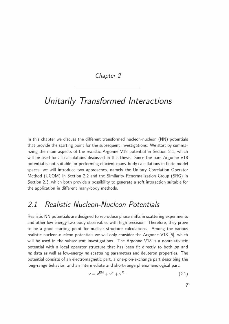
Figure 2.1: Radial dependencies of the Argonne V18 potential for the different contributions
in the respective spin-isospin channels.
8
2.2 · Unitary Correlation Operator Method
The phenomenological part is expressed as a sum of central, quadratic angular
momentum, tensor, spin-orbit and quadratic spin-orbit terms:
vRST = v c
ST (r) + v l2ST (r)L2 + v t
ST (r)S12 + v lsST (r)L·S + v ls2
ST (r)(L·S)2 . (2.2)
The radial dependencies v iST (r) are parameterized in an appropriate manner and fit to
experimental data. For illustration the radial dependencies are displayed in Figure 2.1
for the respective spin-isospin channels, where to the tensor part the contribution
emerging from the one-pion exchange has been added.
Alternatively, the strong interaction potential can be projected into an operator
format with 18 terms:
vij =
18∑
p=1
vp(rij)Opij , (2.3)
giving the potential its name. Of these 18 operators, 14 are charge-independent while
three are charge-dependent and one is charge-asymmetric.
2.2 Unitary Correlation Operator Method
The development of realistic NN potentials reproducing experimental data with high
precision, like the Argonne V18, is the basis for an ab initio description of nuclei.
Due to the enormous computational effort, these investigations are restricted to light
nuclei. For the description of heavier nuclei, while staying as close as possible to
an ab initio treatment of the many-body problem, the many-body Hilbert space has
to be truncated to a smaller subspace. The combination of realistic NN potentials
with simple many-body states, e.g. a superposition of Slater-determinants, reveals
a fundamental problem: The strong short-range correlations induced by the nuclear
interaction cannot be adequately described by simple many-body states in a small
Hilbert space.
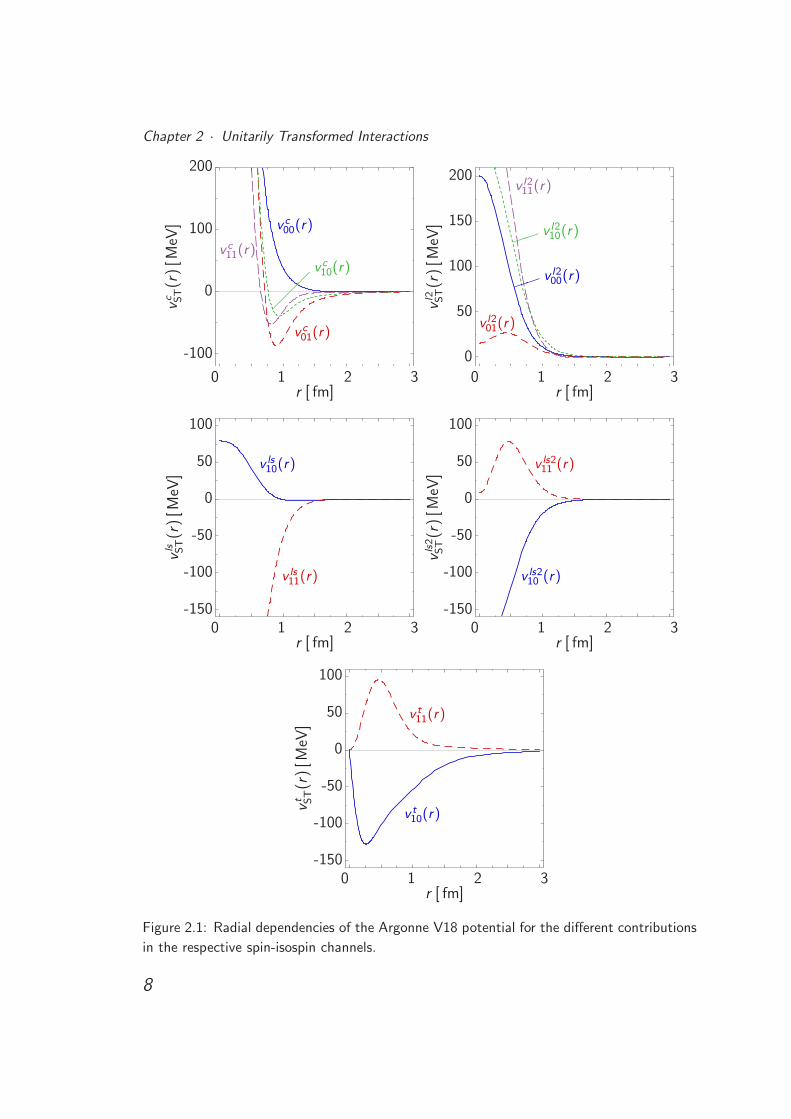
These correlations are already revealed in the deuteron solution, which is visual-
ized in Figure 2.2, where the spin-projected two-body density resulting from an exact
calculation based on the Argonne V18 potential is shown [9, 15]. The repulsive core
of the interaction leads to a suppression of the two-body density at small interparticle
distances, while the effect of the tensor force is manifested in the strong dependence on
the relative distance and the spin alignments leading to the ”doughnut” and ”dump-
bell” shapes for antiparallel and parallel spins, respectively.
The Unitary Correlation Operator Method (UCOM) [8–10,15] was developed in or-
der to handle this problem by explicitly dealing with the strong short-range correlations
9
Chapter 2 · Unitarily Transformed Interactions
MS = 01√2(∣∣↑↓⟩
+∣∣↓↑⟩)
MS = ±1∣∣↑↑⟩,∣∣↓↓⟩
⟨S⟩
↑
Figure 2.2: Two-body density of the deuteron calculated with the AV18 potential and pro-
jected onto the two possibilities of antiparallel spins (left) and parallel spins (right). Shown
are the isodensity surfaces for (2)1MS
= 0.005 fm−3 (taken from [15]).
induced by the nuclear interaction by means of a unitary transformation. The main
features of the Unitary Correlation Operator Method will be discussed in the following
subsections.
2.2.1 Correlation Operators
The idea of the UCOM is to imprint the short-range correlations into a simple many-
body state |Ψ〉 that can be a Slater-determinant in the simplest case. This is achieved
via a state-independent unitary transformation using the correlation operator C:
|Ψ〉 = C|Ψ〉 , (2.4)
leading to a correlated state |Ψ〉 that is no longer a Slater determinant due to the
complex structure of the short-range correlations [8–10,15]. Instead of correlating the
many-body state one can also perform a unitary transformation of the operators
O = C†OC , (2.5)
which are then evaluated in the untransformed model space. These two approaches
are equivalent as we can see by considering expectation values or matrix elements:
⟨Ψ∣∣O∣∣Ψ′ ⟩ =
⟨Ψ∣∣C†OC
∣∣Ψ′ ⟩ =⟨Ψ∣∣ O∣∣Ψ′ ⟩ . (2.6)
Hence, one can choose the form that is technically more advantageous for the respective
application.
10
2.2 · Unitary Correlation Operator Method
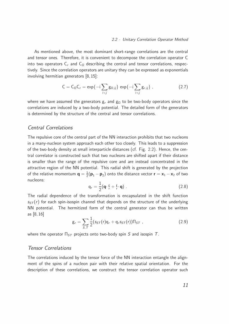
As mentioned above, the most dominant short-range correlations are the central
and tensor ones. Therefore, it is convenient to decompose the correlation operator C
into two operators Cr and CΩ describing the central and tensor correlations, respec-
tively. Since the correlation operators are unitary they can be expressed as exponentials
involving hermitian generators [8, 15]:
C = CΩCr = exp−i∑
i<j
gΩ,ij exp−i∑
i<j
gr ,ij , (2.7)
where we have assumed the generators gr and gΩ to be two-body operators since the
correlations are induced by a two-body potential. The detailed form of the generators
is determined by the structure of the central and tensor correlations.
Central Correlations
The repulsive core of the central part of the NN interaction prohibits that two nucleons
in a many-nucleon system approach each other too closely. This leads to a suppression
of the two-body density at small interparticle distances (cf. Fig. 2.2). Hence, the cen-
tral correlator is constructed such that two nucleons are shifted apart if their distance
is smaller than the range of the repulsive core and are instead concentrated in the
attractive region of the NN potential. This radial shift is generated by the projection
of the relative momentum q = 12(p1 −p2) onto the distance vector r = x1 − x2 of two
nucleons:
qr =1
2(q· r
r+ r
r· q) . (2.8)
The radial dependence of the transformation is encapsulated in the shift function
sST (r) for each spin-isospin channel that depends on the structure of the underlying
NN potential. The hermitized form of the central generator can thus be written
as [8, 16]
gr =∑
S,T
1
2(sST (r)qr + qrsST (r))ΠST , (2.9)
where the operator ΠST projects onto two-body spin S and isospin T .
Tensor Correlations
The correlations induced by the tensor force of the NN interaction entangle the align-
ment of the spins of a nucleon pair with their relative spatial orientation. For the
description of these correlations, we construct the tensor correlation operator such
11
Chapter 2 · Unitarily Transformed Interactions
that it only acts on the orbital part of the relative wave function of two nucleons.
Therefore, we define the orbital momentum operator qΩ:
qΩ = q − r
rqr =
1
2r2(L × r − r × L) (2.10)
with the relative orbital angular momentum operator L = r × q, which generates
shifts orthogonal to the radial momentum rrqr . The complex structure of the tensor
correlations can be described by the tensor operator S12(r, qΩ), where the general
tensor operator of rank 2 reads
S12(a, b) =3
2[(σ1· a)(σ2· b) + (σ1· b)(σ2· a)] − 1
2(σ1·σ2)(a· b + b· a) . (2.11)
Therefore, this operator is used to construct the generator for the tensor correlator
[9, 17]
gΩ =∑
T
ϑT (r)S12(r, qΩ)Π1T , (2.12)
where the function ϑT (r) describes the size and distance dependence of the transverse
shift. The tensor operator S12(r, qΩ) entering in this generator has the same structure
as the standard tensor operator S12 = S12(rr, r
r) generating the tensor force.
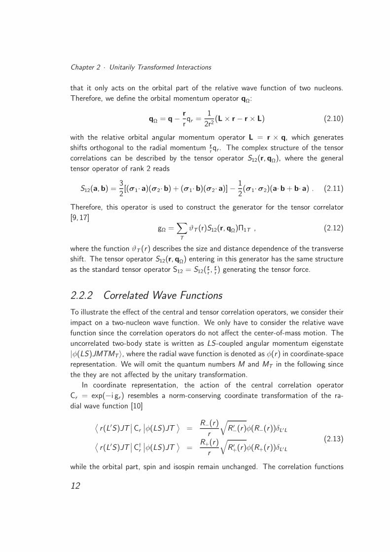
2.2.2 Correlated Wave Functions
To illustrate the effect of the central and tensor correlation operators, we consider their
impact on a two-nucleon wave function. We only have to consider the relative wave
function since the correlation operators do not affect the center-of-mass motion. The
uncorrelated two-body state is written as LS-coupled angular momentum eigenstate
|φ(LS)JMTMT〉, where the radial wave function is denoted as φ(r) in coordinate-space
representation. We will omit the quantum numbers M and MT in the following since
the they are not affected by the unitary transformation.
In coordinate representation, the action of the central correlation operator
Cr = exp(−i gr) resembles a norm-conserving coordinate transformation of the ra-
dial wave function [10]
⟨r(L′S)JT
∣∣Cr
∣∣φ(LS)JT⟩
=R−(r)
r
√R ′−(r)φ(R−(r))δL′L
⟨r(L′S)JT
∣∣C†r
∣∣φ(LS)JT⟩
=R+(r)
r
√R ′
+(r)φ(R+(r))δL′L
(2.13)
while the orbital part, spin and isospin remain unchanged. The correlation functions
12
2.2 · Unitary Correlation Operator Method
R±(r) are mutually inverse, R±(R∓(r)) = r , and are connected to the shift function
s(r) by the integral equation
∫ R±(r)
r
dξ
s(ξ)= ±1 , (2.14)
where we have suppressed the (S , T )-dependence for brevity. For slowly varying shift
functions, the correlation functions can be approximated by
R±(r) ≈ r ± s(r) . (2.15)
This illustrates that two nucleons having the distance r are shifted by the distance
s(r).
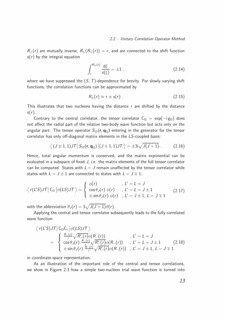
Contrary to the central correlator, the tensor correlator CΩ = exp(−i gΩ) does
not affect the radial part of the relative two-body wave function but acts only on the
angular part. The tensor operator S12(r, qΩ) entering in the generator for the tensor
correlator has only off-diagonal matrix elements in the LS-coupled basis:
⟨(J ± 1, 1)JT
∣∣ S12(r, qΩ)∣∣(J ∓ 1, 1)JT
⟩= ±3i
√J(J + 1) . (2.16)
Hence, total angular momentum is conserved, and the matrix exponential can be
evaluated in a subspace of fixed J , i.e. the matrix elements of the full tensor correlator
can be computed. States with L = J remain unaffected by the tensor correlator while
states with L = J ± 1 are connected to states with L = J ∓ 1:
⟨r(L′S)JT
∣∣CΩ
∣∣φ(LS)JT⟩
=
φ(r) , L′ = L = J
cos θJ(r) φ(r) , L′ = L = J ± 1
± sin θJ(r) φ(r) , L′ = J ± 1, L = J ∓ 1(2.17)
with the abbreviation θJ(r) = 3√
J(J + 1)ϑ(r).
Applying the central and tensor correlator subsequently leads to the fully correlated
wave function
⟨r(L′S)JT
∣∣CΩCr
∣∣φ(LS)JT⟩
=
R−(r)r
√R ′−(r)φ(R−(r)) , L′ = L = J
cos θJ(r)R−(r)
r
√R ′−(r)φ(R−(r)) , L′ = L = J ± 1
± sin θJ(r)R−(r)
r
√R ′−(r)φ(R−(r)) , L′ = J ± 1, L = J ∓ 1
(2.18)
in coordinate-space representation.
As an illustration of the important role of the central and tensor correlations,
we show in Figure 2.3 how a simple two-nucleon trial wave function is turned into
13
Chapter 2 · Unitarily Transformed Interactions
0
0.1
0.2
0.3
0.4
0.5
0.6
.
φL(r
)[a
rb.
units
] (a)〈r|φ0〉
L = 0
0
0.1
0.2
0.3
0.4
0.5
.
φL(r
)[a
rb.
units
] (b)〈r|Cr |φ0〉
L = 0
0 1 2 3 4 5r [fm]
0
0.1
0.2
0.3
0.4
0.5
.
φL(r
)[a
rb.
units
] (c)〈r|CΩCr |φ0〉
L = 0
L = 2
0
0.05
0.1
0.15
0.2
.
R+
(r)−
r[f
m] (d)
0 1 2 3 4 5r [fm]
0
0.02
0.04
0.06
0.08
.
ϑ(r
)
(e)
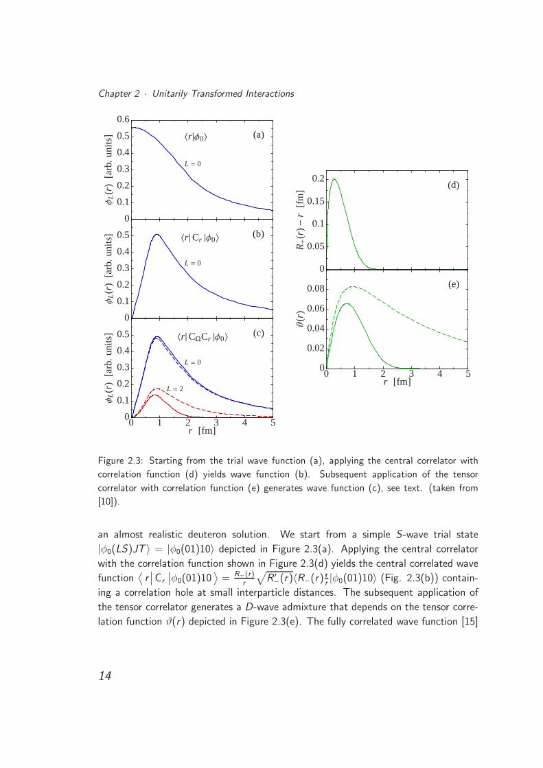
Figure 2.3: Starting from the trial wave function (a), applying the central correlator with
correlation function (d) yields wave function (b). Subsequent application of the tensor
correlator with correlation function (e) generates wave function (c), see text. (taken from
[10]).
an almost realistic deuteron solution. We start from a simple S-wave trial state
|φ0(LS)JT 〉 = |φ0(01)10〉 depicted in Figure 2.3(a). Applying the central correlator
with the correlation function shown in Figure 2.3(d) yields the central correlated wave
function⟨r∣∣Cr
∣∣φ0(01)10⟩
= R−(r)r
√R ′−(r)〈R−(r) r
r|φ0(01)10〉 (Fig. 2.3(b)) contain-
ing a correlation hole at small interparticle distances. The subsequent application of
the tensor correlator generates a D-wave admixture that depends on the tensor corre-
lation function ϑ(r) depicted in Figure 2.3(e). The fully correlated wave function [15]
14
2.2 · Unitary Correlation Operator Method
⟨r∣∣CΩCr
∣∣φ0(01)10⟩
= cos(3√
2ϑ(r))R−(r)
r
√R ′−(r)〈R−(r) r
r|φ0(01)10〉
+ sin(3√
2ϑ(r))R−(r)
r
√R ′−(r)〈R−(r) r
r|φ0(21)10〉
(2.19)
is shown in Figure 2.3(c). In order to generate a realistic deuteron wave function the
tensor correlation needs to be of long range (dashed curve in Figure 2.3). But the
aim of the UCOM is to cover only short-range state-independent correlations. The
long-range correlations have to be described by the many-body model space. Thus,
we will restrict the range of the tensor correlation function leading to the solid curves
in Figure 2.3(c) and (e).
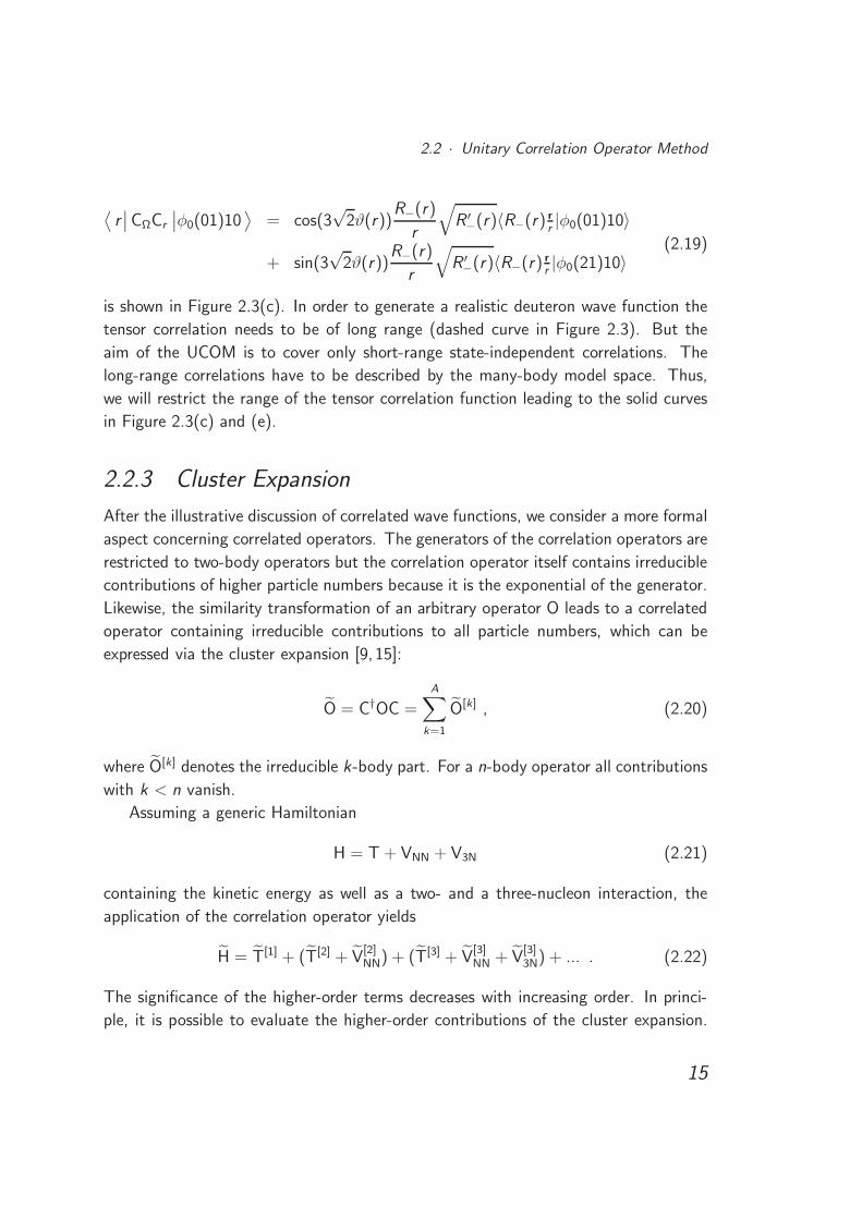
2.2.3 Cluster Expansion
After the illustrative discussion of correlated wave functions, we consider a more formal
aspect concerning correlated operators. The generators of the correlation operators are
restricted to two-body operators but the correlation operator itself contains irreducible
contributions of higher particle numbers because it is the exponential of the generator.
Likewise, the similarity transformation of an arbitrary operator O leads to a correlated
operator containing irreducible contributions to all particle numbers, which can be
expressed via the cluster expansion [9, 15]:
O = C†OC =
A∑
k=1
O[k] , (2.20)
where O[k] denotes the irreducible k-body part. For a n-body operator all contributions
with k < n vanish.
Assuming a generic Hamiltonian
H = T + VNN + V3N (2.21)
containing the kinetic energy as well as a two- and a three-nucleon interaction, the
application of the correlation operator yields
H = T[1] + (T[2] + V[2]NN) + (T[3] + V
[3]NN + V
[3]3N) + ... . (2.22)
The significance of the higher-order terms decreases with increasing order. In princi-
ple, it is possible to evaluate the higher-order contributions of the cluster expansion.
15
Chapter 2 · Unitarily Transformed Interactions
However, already the calculation of the third order and its inclusion in many-body cal-
culations is very involved. Therefore, we restrict ourselves to the evaluation of the first
and second order of the cluster expansion which leads to the two-body approximation
of a general operator O
OC2 = O[1] + O[2] . (2.23)
For the Hamiltonian this reads
HC2 = T[1] + (T[2] + V[2]NN) ≡ T + VUCOM , (2.24)
where T[1] = T and the correlated interaction VUCOM is defined as the two-body
part of the correlated Hamiltonian containing the correlated kinetic energy and the
correlated NN potential. The parameters of the correlation functions will be adjusted
such that the term T[3] + V[3]NN + V
[3]3N becomes small, i.e. the induced third order
of the cluster expansion and genuine three-body forces cancel each other to a large
extent. Nonetheless, the application of different many-body methods reveals that
three-body forces – induced and genuine – are not negligible [10,13,18,19]. Therefore,
we mimic the omitted three-body contributions by introducing phenomenological three-
body forces, and investigate their impact on different observables. This approach
provides a first step towards the inclusion of realistic three-body forces.
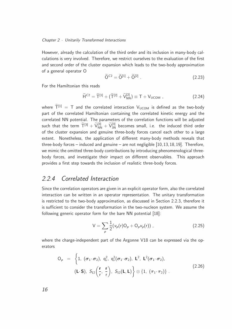
2.2.4 Correlated Interaction
Since the correlation operators are given in an explicit operator form, also the correlated
interaction can be written in an operator representation. The unitary transformation
is restricted to the two-body approximation, as discussed in Section 2.2.3, therefore it
is sufficient to consider the transformation in the two-nucleon system. We assume the
following generic operator form for the bare NN potential [18]:
V =∑
p
1
2(vp(r)Op + Opvp(r)) , (2.25)
where the charge-independent part of the Argonne V18 can be expressed via the op-
erators
Op =
1, (σ1·σ2), q2
r , q2r (σ1·σ2), L2, L2(σ1·σ2),
(L·S), S12
(r
r,
r
r
), S12(L,L)
⊗ 1, (τ 1· τ 2) .
(2.26)
16
2.2 · Unitary Correlation Operator Method
For simplicity, the charge-dependent terms are not considered here although they are
included in the correlated interaction VUCOM.
The kinetic energy in two-body space is split into a center-of-mass contribution
tcm, which is not affected by the UCOM transformation and a relative contribution trel,
which is in turn divided into a radial and an angular part:
T = tcm + trel = tcm + tr + tΩ = tcm +1
mN
(q2
r +L2
r2
)(2.27)
with the nucleon mass mN .
As the correlated interaction can be written as VUCOM = C†rC
†ΩHCΩCr −T, we start
with the application of the tensor correlator to the required operators.
Tensor Correlated Hamiltonian
To evaluate the transformation with the tensor correlation operator we can use the
Baker-Campbell-Hausdorff expansion [15, 18]
C†ΩOCΩ = exp(igΩ) O exp(−igΩ) = O + i [gΩ, O] +
i2
2![gΩ, [gΩ, O]] + ... . (2.28)
In general, this expansion yields an infinite series. Only for some operators, the simi-
larity transformation can be evaluated exactly.
Firstly, the distance operator r is invariant under the transformation:
C†ΩrCΩ = r (2.29)
since it commutes with the tensor generator gΩ. For the radial momentum q2r , the
expansion terminates after the second order and yields
C†Ωq2
r CΩ = q2r − ϑ′(r)qr + qrϑ
′(r)S12(r, qΩ) + ϑ′(r)S12(r, qΩ)2 (2.30)
with S12(r, qΩ)2 = 9S2 + 3(L·S) + (L·S)2. For all other basic operators the Baker-
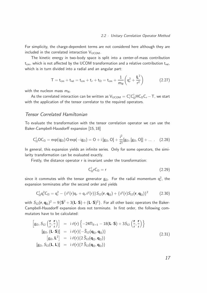
Campbell-Hausdorff expansion does not terminate. In first order, the following com-
mutators have to be calculated:
[gΩ, S12
(r
r,r
r
)]= iϑ(r)
−24ΠS=1 − 18(L·S) + 3S12
(r
r,r
r
)
[gΩ, (L·S)] = iϑ(r)−S12(qΩ, qΩ)[gΩ,L2
]= iϑ(r)2 S12(qΩ, qΩ)
[gΩ, S12(L,L)] = iϑ(r)7 S12(qΩ, qΩ)
(2.31)
17
Chapter 2 · Unitarily Transformed Interactions
with the abbreviation
S12(qΩ, qΩ) = 2r2S12(qΩ, qΩ) + S12(L,L) − 1
2S12
(r
r,r
r
). (2.32)
Through the evaluation of the first-order commutators, the additional tensor operator
S12(qΩ, qΩ) is generated, which will in turn generate further operators in the next
order. In order to yield a closed representation of the tensor correlated operators,
one, therefore, has to truncate the number of newly emerging operators. Usually,
contributions beyond the third order in angular and orbital angular momentum are
neglected.
Central and Tensor Correlated Hamiltonian
Contrary to the tensor correlations, the central correlations can be evaluated analyt-
ically for all relevant operators. Starting with the distance operator r, the picture of
a coordinate transformation, which we have already introduced in Section 2.2.2, is
confirmed [15, 18]:
C†r rCr = R+(r) (2.33)
with the correlation function R+(r). Due to the unitarity of the correlation operators,
C†r = C−1
r , an arbitrary function of r transforms as
C†r f (r)Cr = f (C†
r rCr ) = f (R+(r)) . (2.34)
This affects especially the radial dependencies of the various contributions of the NN
potential. The correlation of the components of the relative momentum operator read
C†rqrCr =
1√R ′
+(r)qr
1√R ′
+(r), C†
rqΩCr =r
R+(r)qΩ , (2.35)
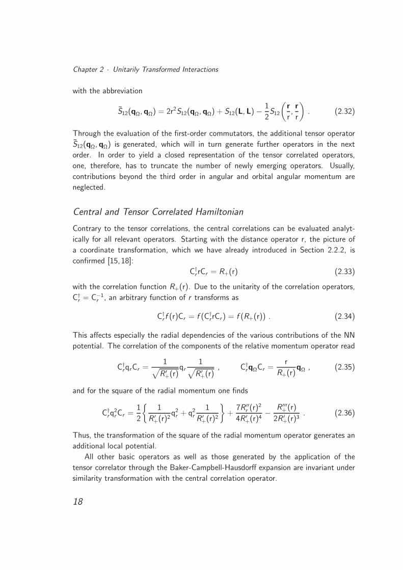
and for the square of the radial momentum one finds
C†rq
2r Cr =
1
2
1
R ′+(r)2
q2r + q2
r
1
R ′+(r)2
+
7R ′′r (r)2
4R ′+(r)4
− R ′′′+ (r)
2R ′+(r)3
. (2.36)
Thus, the transformation of the square of the radial momentum operator generates an
additional local potential.
All other basic operators as well as those generated by the application of the
tensor correlator through the Baker-Campbell-Hausdorff expansion are invariant under
similarity transformation with the central correlation operator.
18
2.2 · Unitary Correlation Operator Method
Correlated Interaction VUCOM
Collecting the terms for the different central and tensor correlated operators, we can
formulate the correlated interaction VUCOM, which can – like the underlying bare NN
potential – be written in a closed operator representation [10, 18]:
VUCOM =∑
p
1
2[Vp(r)Op + OpVp(r)] (2.37)
containing the operators
Op =
1, (σ1·σ2), q2
r , q2r (σ1·σ2), L2, L2(σ1·σ2), (L·S),
S12
(r
r,
r
r
), S12(L,L), S12(qΩ, qΩ), qrS12(r, qΩ),
L2(L·S), L2S12(qΩ, qΩ), ...
⊗ 1, (τ 1· τ 2) .
(2.38)
These are not all operators generated by the Baker-Campbell-Hausdorff expansion
during the tensor transformation, however, the inclusion of these terms is sufficient for
most applications.
The examination of the effect of the similarity transformations using the central
and tensor correlation operators shows how the application of the correlators changes
the operator structure of the bare potential. The central correlator reduces the short-
range repulsion in the local part while creating an additional nonlocal repulsion, and the
tensor correlator generates additional central and new nonlocal tensor contributions.
The operator representation of the correlated interaction is of great advantage for
the application in many-body methods that are not based on a simple oscillator or
plane-wave basis. Furthermore, the UCOM allows for a straightforward investigation
of different observables, since one only has to transform all operators of interest in the
same way as the Hamiltonian.
Due to the finite range of the correlation functions s(r) and ϑ(r), the correlation
operators act as unit operators at large distances. Hence, asymptotic properties of
a two-body wave function are preserved, i.e., the correlated interaction is phase-shift
equivalent to the underlying bare NN potential.
2.2.5 Correlated Two-Body Matrix Elements
For the application in different many-body methods two-body matrix elements of the
correlated interaction are required. The calculation of matrix elements discussed in the
19
Chapter 2 · Unitarily Transformed Interactions
following is independent of the particular choice of the basis, however, throughout this
thesis we will only apply the harmonic oscillator basis. The two-body states are divided
into a center-of-mass and a relative state via a Talmi-Moshinsky transformation. Since
the unitary transformation does not affect the center-of-mass part, we only have to
calculate the relative matrix elements
⟨n(LS)JMTMT
∣∣VUCOM
∣∣n′(L′S)JMTMT
⟩=
⟨n(LS)JMTMT
∣∣C†rC
†ΩHintCΩCr − Tint
∣∣n′(L′S)JMTMT
⟩, (2.39)
where we assume LS-coupled basis states |n(LS)JMTMT〉 with radial quantum number
n and use the intrinsic Hamiltonian Hint containing the intrinsic kinetic energy Tint (cf.
Sec. 3.1). The corresponding wave function will be denoted as φn,L(r) and the radial
wave function as un,L(r):
〈r(LS)JMTMT |n(LS)JMTMT〉 = φn,L(r) =un,L(r)
r. (2.40)
The NN interaction explicitly depends on the isospin projection quantum number MT
through Coulomb and other charge-dependent terms. Nevertheless, we will omit this
quantum number as well as the projection M of total angular momentum in the fol-
lowing, since we again only discuss the charge-independent contributions.
The calculation of matrix elements can be performed in different ways. One pos-
sible approach is to use the operator representation of the correlated interaction and
evaluate the matrix elements directly. However, for the formulation of a closed operator
representation it was necessary to truncate the Baker-Campbell-Hausdorff expansion
employed for the evaluation of the tensor correlations. When calculating matrix ele-
ments, this approximation can be avoided if we apply the tensor correlator to the basis
states. The central correlator will still be applied to the operators as this transforma-
tion is given by a simple and exact expression. Therefore, we have to rearrange the
order of the correlation operators by exploiting the identity
C†rC
†Ω Hint CΩCr = (C†
rC†ΩCr )C
†r Hint Cr (C
†rCΩCr )
= C†ΩC†
r Hint Cr CΩ ,(2.41)
where the ”centrally correlated” tensor correlator is given by
CΩ = C†rCΩCr = exp[−iϑ(R+(r))S12(r, qΩ)] . (2.42)
As already discussed in Section 2.2.2, the tensor correlator acts on LS-coupled two-
body wave functions in the following way [10]:
20
2.2 · Unitary Correlation Operator Method
⟨r(L′S)JT
∣∣ CΩ
∣∣n(LS)JT⟩
=
φn,L(r) , L′ = L = J
cos θJ(r) φn,L(r) , L′ = L = J ± 1
± sin θJ(r) φn,L(r) , L′ = J ± 1, L = J ∓ 1(2.43)
with θJ(r) = 3√
J(J + 1)ϑ(R+(r)). Thus, two-body states with L = J remain un-
changed while states with L = J ± 1 are coupled to states with L = J ∓ 1. Based on
these relations, the correlated two-body matrix elements can be evaluated exactly.
We again consider the operator set
O =
1, (σ1·σ2), q2
r , q2r (σ1·σ2), L2, L2(σ1·σ2),
(L·S), S12
(r
r,
r
r
), S12(L,L)
⊗ 1, (τ 1· τ 2)
(2.44)
containing the operators to express the charge-independent part of the Argonne V18.
Firstly, we calculate the matrix elements for the local contributions of the form V (r)O
which fulfill the condition [r, O] = [qr , O] = 0, i.e. all operators of the set (2.44)
except the q2r terms.
On the diagonal matrix elements with L = L′ = J , the tensor correlator acts like
the unit operator, i.e. they are only affected by the central correlator, yielding [10,18]
⟨n(JS)JT
∣∣C†rC
†ΩV (r)OCΩCr
∣∣n′(JS)JT⟩
=∫dr u⋆
n,J(r)un′,J(r)V (r)⟨(JS)JT
∣∣O∣∣(JS)JT
⟩ (2.45)
in coordinate representation. The correlated radial dependence of the potential is
simply given by V (r) = V (R+(r)). Applying the tensor correlator to the states, we
obtain for the diagonal matrix elements with L = L′ = J ∓ 1
⟨n(J ∓ 1, 1)JT
∣∣C†rC
†ΩV (r)OCΩCr
∣∣n′(J ∓ 1, 1)JT⟩
=∫dr u⋆
n,J∓1(r)un′,J∓1(r)V (r)
×[⟨
(J ∓ 1, 1)JT∣∣O∣∣(J ∓ 1, 1)JT
⟩cos2 θJ(r)
+⟨(J ± 1, 1)JT
∣∣O∣∣(J ± 1, 1)JT
⟩sin2 θJ(r)
±⟨(J ∓ 1, 1)JT
∣∣O∣∣(J ± 1, 1)JT
⟩2 cos θJ(r) sin θJ(r)
]
(2.46)
21
Chapter 2 · Unitarily Transformed Interactions
with θJ(r) = θJ(R+(r)). Finally, the off-diagonal matrix elements with L = J ∓ 1 and
L′ = J ± 1 are given by
⟨n(J ∓ 1, 1)JT
∣∣C†rC
†ΩV (r)OCΩCr
∣∣n′(J ± 1, 1)JT⟩
=∫dr u⋆
n,J∓1(r)un′,J±1(r)V (r)
×[⟨
(J ∓ 1, 1)JT∣∣O∣∣(J ± 1, 1)JT
⟩cos2 θJ(r)
−⟨(J ± 1, 1)JT
∣∣O∣∣(J ∓ 1, 1)JT
⟩sin2 θJ(r)
∓⟨(J ∓ 1, 1)JT
∣∣O∣∣(J ∓ 1, 1)JT
⟩cos θJ(r) sin θJ(r)
±⟨(J ± 1, 1)JT
∣∣O∣∣(J ± 1, 1)JT
⟩sin θJ(r) cos θJ(r)
].
(2.47)
Hence, for the evaluation of the matrix elements we have to calculate the integrals
of the radial wave functions as well as the matrix elements of the operators O in
LS-coupled angular momentum states. The off-diagonal matrix elements on the right-
hand-side of Eqs. (2.46) and (2.47) vanish for all operators except for the standard
tensor operator S12(rr, r
r) which simplifies these relations significantly.
The correlated matrix elements reveal the effect of the tensor correlator leading to
an admixture of components with ∆L = ±2 to the states, as we have already seen in
Section 2.2.2.
For the radial momentum the full unitary transformation is applied to the operator
Vqr =1
2[q2
r V (r) + V (r)q2r ] , (2.48)
since it is given by a closed exact expression. The application of the tensor correlator
yields
C†ΩVqrCΩ =
1
2[q2
r V (r) + V (r)q2r ] + V (r)[ϑ′(r)S12(r, qΩ)]2
−[qrV (r)ϑ′(r) + ϑ′(r)V (r)qr ]S12(r, qΩ) .(2.49)
After including the central correlations, the following expression is derived for the
diagonal matrix elements with L = L′ = J :
22
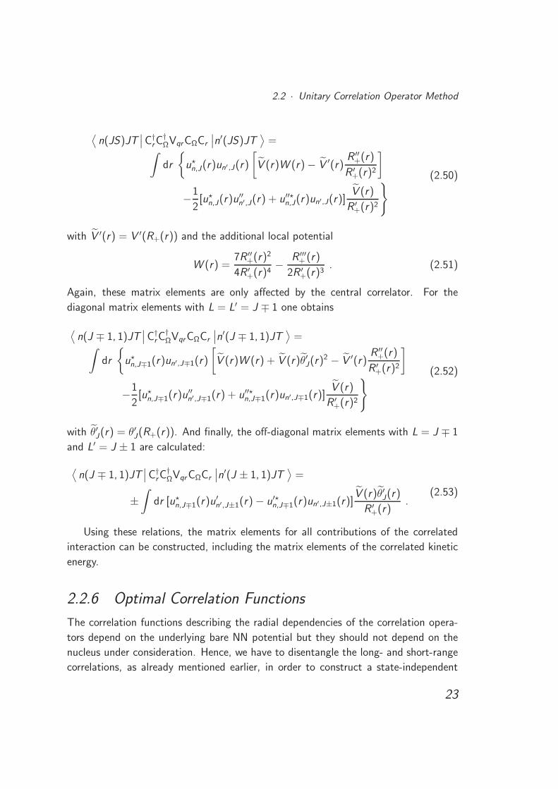
2.2 · Unitary Correlation Operator Method
⟨n(JS)JT
∣∣C†rC
†ΩVqrCΩCr
∣∣n′(JS)JT⟩
=∫
dr
u⋆
n,J(r)un′,J(r)
[V (r)W (r) − V ′(r)
R ′′+(r)
R ′+(r)2
]
−1
2[u⋆
n,J(r)u′′n′,J(r) + u′′⋆
n,J(r)un′,J(r)]V (r)
R ′+(r)2
(2.50)
with V ′(r) = V ′(R+(r)) and the additional local potential
W (r) =7R ′′
+(r)2
4R ′+(r)4
− R ′′′+ (r)
2R ′+(r)3
. (2.51)
Again, these matrix elements are only affected by the central correlator. For the
diagonal matrix elements with L = L′ = J ∓ 1 one obtains
⟨n(J ∓ 1, 1)JT
∣∣C†rC
†ΩVqrCΩCr
∣∣n′(J ∓ 1, 1)JT⟩
=∫
dr
u⋆
n,J∓1(r)un′,J∓1(r)
[V (r)W (r) + V (r)θ′J(r)
2 − V ′(r)R ′′
+(r)
R ′+(r)2
]
−1
2[u⋆
n,J∓1(r)u′′n′,J∓1(r) + u′′⋆
n,J∓1(r)un′,J∓1(r)]V (r)
R ′+(r)2
(2.52)
with θ′J(r) = θ′J(R+(r)). And finally, the off-diagonal matrix elements with L = J ∓ 1
and L′ = J ± 1 are calculated:
⟨n(J ∓ 1, 1)JT
∣∣C†rC
†ΩVqrCΩCr
∣∣n′(J ± 1, 1)JT⟩
=
±∫
dr [u⋆n,J∓1(r)u
′n′,J±1(r) − u′⋆
n,J∓1(r)un′,J±1(r)]V (r)θ′J(r)
R ′+(r)
.(2.53)
Using these relations, the matrix elements for all contributions of the correlated
interaction can be constructed, including the matrix elements of the correlated kinetic
energy.
2.2.6 Optimal Correlation Functions
The correlation functions describing the radial dependencies of the correlation opera-
tors depend on the underlying bare NN potential but they should not depend on the
nucleus under consideration. Hence, we have to disentangle the long- and short-range
correlations, as already mentioned earlier, in order to construct a state-independent
23
Chapter 2 · Unitarily Transformed Interactions
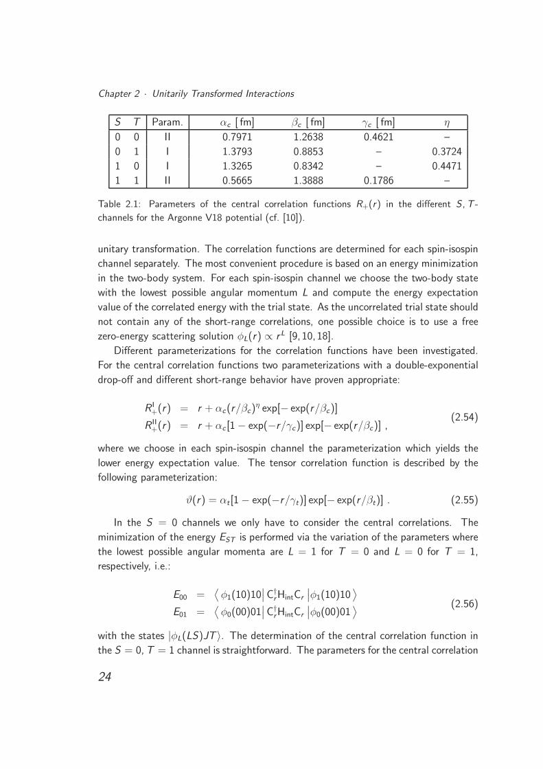
S T Param. αc [ fm] βc [ fm] γc [ fm] η
0 0 II 0.7971 1.2638 0.4621 –
0 1 I 1.3793 0.8853 – 0.3724
1 0 I 1.3265 0.8342 – 0.4471
1 1 II 0.5665 1.3888 0.1786 –
Table 2.1: Parameters of the central correlation functions R+(r) in the different S , T -
channels for the Argonne V18 potential (cf. [10]).
unitary transformation. The correlation functions are determined for each spin-isospin
channel separately. The most convenient procedure is based on an energy minimization
in the two-body system. For each spin-isospin channel we choose the two-body state
with the lowest possible angular momentum L and compute the energy expectation
value of the correlated energy with the trial state. As the uncorrelated trial state should
not contain any of the short-range correlations, one possible choice is to use a free
zero-energy scattering solution φL(r) ∝ rL [9, 10, 18].
Different parameterizations for the correlation functions have been investigated.
For the central correlation functions two parameterizations with a double-exponential
drop-off and different short-range behavior have proven appropriate:
R I+(r) = r + αc(r/βc)
η exp[− exp(r/βc)]
R II+(r) = r + αc [1 − exp(−r/γc)] exp[− exp(r/βc)] ,
(2.54)
where we choose in each spin-isospin channel the parameterization which yields the
lower energy expectation value. The tensor correlation function is described by the
following parameterization:
ϑ(r) = αt [1 − exp(−r/γt)] exp[− exp(r/βt)] . (2.55)
In the S = 0 channels we only have to consider the central correlations. The
minimization of the energy EST is performed via the variation of the parameters where
the lowest possible angular momenta are L = 1 for T = 0 and L = 0 for T = 1,
respectively, i.e.:
E00 =⟨φ1(10)10
∣∣C†rHintCr
∣∣φ1(10)10⟩
E01 =⟨φ0(00)01
∣∣C†rHintCr
∣∣φ0(00)01⟩ (2.56)
with the states |φL(LS)JT 〉. The determination of the central correlation function in
the S = 0, T = 1 channel is straightforward. The parameters for the central correlation
24
2.2 · Unitary Correlation Operator Method
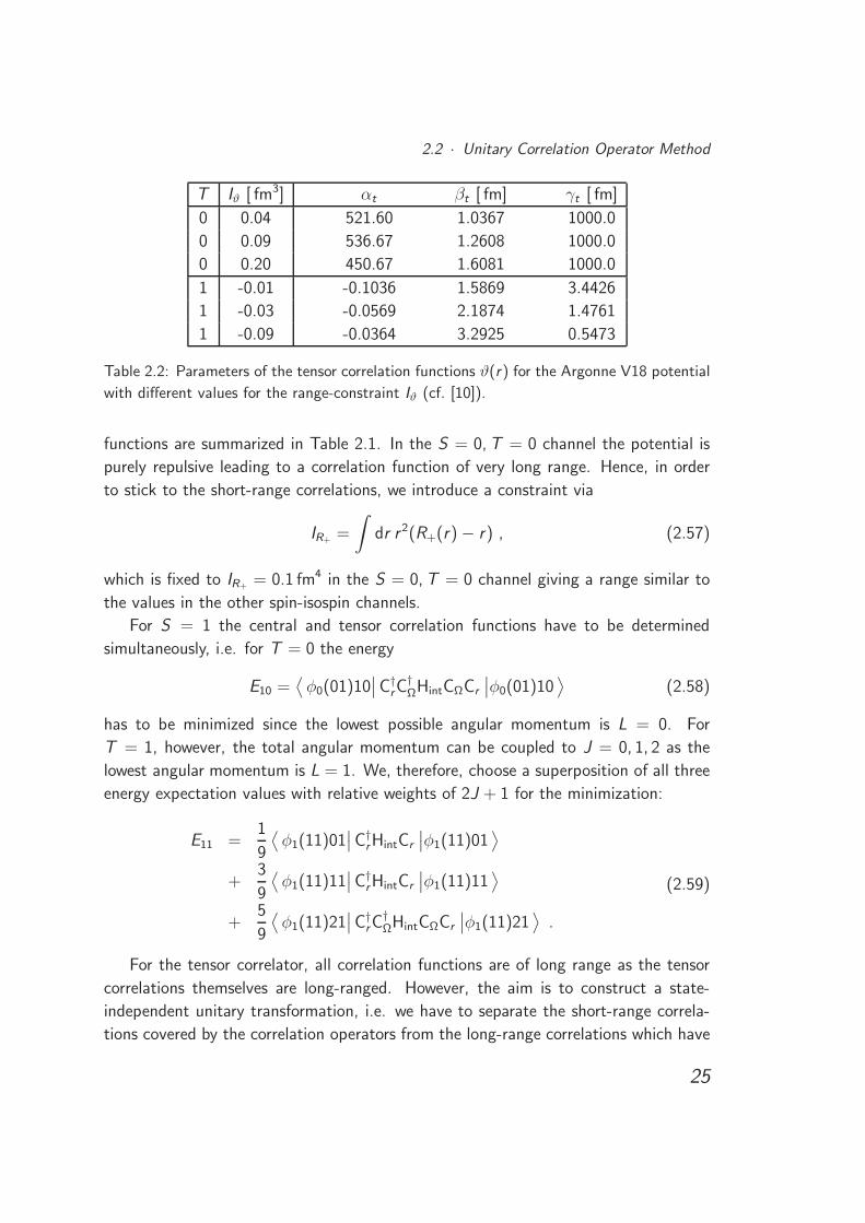
T Iϑ [ fm3] αt βt [ fm] γt [ fm]
0 0.04 521.60 1.0367 1000.0
0 0.09 536.67 1.2608 1000.0
0 0.20 450.67 1.6081 1000.0
1 -0.01 -0.1036 1.5869 3.4426
1 -0.03 -0.0569 2.1874 1.4761
1 -0.09 -0.0364 3.2925 0.5473
Table 2.2: Parameters of the tensor correlation functions ϑ(r) for the Argonne V18 potential
with different values for the range-constraint Iϑ (cf. [10]).
functions are summarized in Table 2.1. In the S = 0, T = 0 channel the potential is
purely repulsive leading to a correlation function of very long range. Hence, in order
to stick to the short-range correlations, we introduce a constraint via
IR+ =
∫dr r 2(R+(r) − r) , (2.57)
which is fixed to IR+ = 0.1 fm4 in the S = 0, T = 0 channel giving a range similar to
the values in the other spin-isospin channels.
For S = 1 the central and tensor correlation functions have to be determined
simultaneously, i.e. for T = 0 the energy
E10 =⟨φ0(01)10
∣∣C†rC
†ΩHintCΩCr
∣∣φ0(01)10⟩
(2.58)
has to be minimized since the lowest possible angular momentum is L = 0. For
T = 1, however, the total angular momentum can be coupled to J = 0, 1, 2 as the
lowest angular momentum is L = 1. We, therefore, choose a superposition of all three
energy expectation values with relative weights of 2J + 1 for the minimization:
E11 =1
9
⟨φ1(11)01
∣∣C†rHintCr
∣∣φ1(11)01⟩
+3
9
⟨φ1(11)11
∣∣C†rHintCr
∣∣φ1(11)11⟩
+5
9
⟨φ1(11)21
∣∣C†rC
†ΩHintCΩCr
∣∣φ1(11)21⟩
.
(2.59)
For the tensor correlator, all correlation functions are of long range as the tensor
correlations themselves are long-ranged. However, the aim is to construct a state-
independent unitary transformation, i.e. we have to separate the short-range correla-
tions covered by the correlation operators from the long-range correlations which have
25
Chapter 2 · Unitarily Transformed Interactions
0 1 2 3r [fm]
0
0.05
0.1
0.15
0.2
0.25
.
R+(r
)−
r[fm
] T = 0
1 2 3r [fm]
T = 1
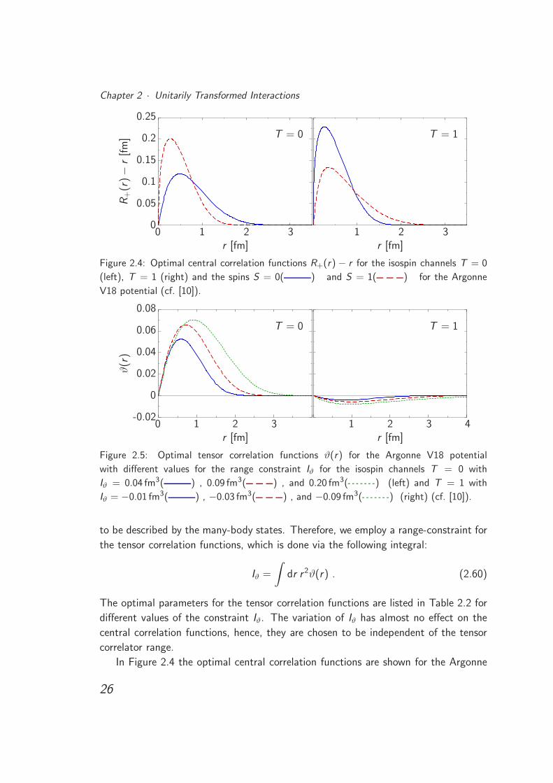
Figure 2.4: Optimal central correlation functions R+(r) − r for the isospin channels T = 0
(left), T = 1 (right) and the spins S = 0( ) and S = 1( ) for the Argonne
V18 potential (cf. [10]).
0 1 2 3r [fm]
-0.02
0
0.02
0.04
0.06
0.08
.
ϑ(r
)
T = 0
1 2 3 4r [fm]
T = 1
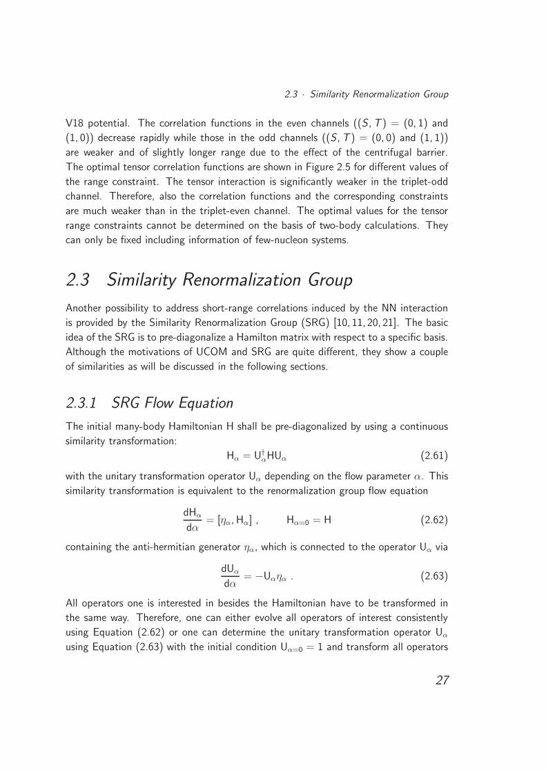
Figure 2.5: Optimal tensor correlation functions ϑ(r) for the Argonne V18 potential
with different values for the range constraint Iϑ for the isospin channels T = 0 with
Iϑ = 0.04 fm3( ) , 0.09 fm3( ) , and 0.20 fm3( ) (left) and T = 1 with
Iϑ = −0.01 fm3( ) , −0.03 fm3( ) , and −0.09 fm3( ) (right) (cf. [10]).
to be described by the many-body states. Therefore, we employ a range-constraint for
the tensor correlation functions, which is done via the following integral:
Iϑ =
∫dr r 2ϑ(r) . (2.60)
The optimal parameters for the tensor correlation functions are listed in Table 2.2 for
different values of the constraint Iϑ. The variation of Iϑ has almost no effect on the
central correlation functions, hence, they are chosen to be independent of the tensor
correlator range.
In Figure 2.4 the optimal central correlation functions are shown for the Argonne
26
2.3 · Similarity Renormalization Group
V18 potential. The correlation functions in the even channels ((S , T ) = (0, 1) and
(1, 0)) decrease rapidly while those in the odd channels ((S , T ) = (0, 0) and (1, 1))
are weaker and of slightly longer range due to the effect of the centrifugal barrier.
The optimal tensor correlation functions are shown in Figure 2.5 for different values of
the range constraint. The tensor interaction is significantly weaker in the triplet-odd
channel. Therefore, also the correlation functions and the corresponding constraints
are much weaker than in the triplet-even channel. The optimal values for the tensor
range constraints cannot be determined on the basis of two-body calculations. They
can only be fixed including information of few-nucleon systems.
2.3 Similarity Renormalization Group
Another possibility to address short-range correlations induced by the NN interaction
is provided by the Similarity Renormalization Group (SRG) [10, 11, 20, 21]. The basic
idea of the SRG is to pre-diagonalize a Hamilton matrix with respect to a specific basis.
Although the motivations of UCOM and SRG are quite different, they show a couple
of similarities as will be discussed in the following sections.
2.3.1 SRG Flow Equation
The initial many-body Hamiltonian H shall be pre-diagonalized by using a continuous
similarity transformation:
Hα = U†αHUα (2.61)
with the unitary transformation operator Uα depending on the flow parameter α. This
similarity transformation is equivalent to the renormalization group flow equation
dHα
dα= [ηα, Hα] , Hα=0 = H (2.62)
containing the anti-hermitian generator ηα, which is connected to the operator Uα via
dUα
dα= −Uαηα . (2.63)
All operators one is interested in besides the Hamiltonian have to be transformed in
the same way. Therefore, one can either evolve all operators of interest consistently
using Equation (2.62) or one can determine the unitary transformation operator Uα
using Equation (2.63) with the initial condition Uα=0 = 1 and transform all operators
27
Chapter 2 · Unitarily Transformed Interactions
of interest via Equation (2.61). Since the generator ηα generally depends on the flow
parameter in a nontrivial way, the unitary operator is not simply given by an exponential
of the generator but can be expressed via a Dyson series.
Before solving the flow equation (2.62) or the similarity transformation (2.61) one
has to choose a generator suitable for the specific problem. We will deal with A-
nucleon systems leading to evolved operators that contain up to A-body contributions
even if starting from a Hamiltonian with two-body operators at most. Therefore, the
following approximation is employed, similar to the two-body approximation of the
cluster expansion in the UCOM. We use the operator defining the basis with respect
to which the Hamiltonian shall be diagonalized, which is a two-body operator in our
case, and perform the evolution in two-body space, hence, discarding three-body and
higher contributions. The corresponding generator is defined as
ηα = (2µ)2 [Tint, Hα] = 2µ [q2, Hα] (2.64)
with the intrinsic kinetic energy Tint = T − Tcm = q2
2µin the two-body system [10,
11, 21, 22]. The prefactor of the commutator is chosen such that the flow parameter
has the dimension [α] = fm4. It can be understood easily why the commutator with
the evolved Hamiltonian is used in the definition of the generator: If the evolved
Hamiltonian is diagonal with respect to the eigenbasis of the intrinsic kinetic energy,
the commutator vanishes and the flow evolution reaches a trivial fix point. The square
of the two-body relative momentum operator can be written as a sum of a radial and
an angular part:
q2 = q2r +
L2
r2, qr =
1
2
(q· r
r+
r
r· q)
. (2.65)
Hence, the two-body Hamiltonian Hα is diagonalized in a simultaneous eigenbasis of q2r
and L2
r2, i.e. in a partial-wave momentum space representation the matrix elements of
the Hamiltonian are driven towards a band-diagonal structure with respect to relative
momentum (q, q′) and orbital angular momentum (L, L′).
2.3.2 Evolution of Two-Body Matrix Elements
We start from a Hamiltonian H = Tint + VNN consisting of the intrinsic kinetic energy
Tint and two-body interaction VNN. Similar to the correlated interaction VUCOM the
evolved interaction Vα is defined such that it contains all α-dependent terms of the
evolved Hamiltonian Hα, which includes the evolved intrinsic kinetic energy:
Hα = Tint + Vα . (2.66)
28
2.3 · Similarity Renormalization Group
Since the intrinsic kinetic energy is chosen such that it is independent of α, the flow
evolution of the Hamiltonian is reduced to the evolution of the interaction Vα. With
the generator (2.64) the flow equation reads
dHα
dα=
dVα
dα= [ηα, Hα] = (2µ)2[[Tint, Vα], Tint + Vα] . (2.67)
This flow evolution can most conveniently be evaluated on the level of matrix elements
[10, 23]. Since the square of the relative momentum operator q2 enters into the
generator, we choose the partial-wave momentum eigenbasis |q(LS)JMTMT 〉. The
projection quantum numbers M and MT will be omitted for brevity in the following.
Thus, we have to derive evolution equations for the matrix elements
V (JLL′ST )α (q, q′) =
⟨q(LS)JT
∣∣Vα
∣∣q′(L′S)JT⟩
(2.68)
from Equation (2.67). The result can be written in a generic form:
dVα(q, q′)
dα= −(q2 − q′2)2 Vα(q, q′)
+ 2µ
∫dQ Q2(q2 + q′2 − 2Q2) Vα(q, Q)Vα(Q, q′) ,
(2.69)
where we simply have
Vα(q, q′) = V (JJJST )α (q, q′) (2.70)
for non-coupled partial waves with L = L′ = J .
For S = 1, angular momenta with ∆L = ±2 are coupled due to the tensor force.
Thus, for the flow equations in the coupled channels, the Vα(q, q′) are defined as 2×2
matrices
Vα(q, q′) =
(V
(JLLST )α (q, q′) V
(JLL′ST )α (q, q′)
V(JL′LST )α (q, q′) V
(JL′L′ST )α (q, q′)
)(2.71)
containing the matrix elements with the possible combinations of the orbital angular
momenta L = J−1 and L′ = J +1. Due to the properties of the generator (2.64), each
non-coupled partial wave and each set of coupled partial waves evolves independently
of the other channels.
As mentioned above, not only the Hamiltonian but all operators of interest have
to be evolved in the same way. The evolution of all operators has to be done simulta-
neously since they are coupled to the evolution of the Hamiltonian via the generator.
29
Chapter 2 · Unitarily Transformed Interactions
(a) α = 0 fm4 (b) α = 0.001 fm4 (c) α = 0.01 fm4 (d) α = 0.04 fm4
3S
13S
1−
3D
1
0 1 2 3 4 5 6r [fm]
0
0.1
0.2
0.3
0.4
0.5
.
φL(r
)[a
rb.
units
]
0 1 2 3 4 5 6r [fm]
0 1 2 3 4 5 6r [fm]
0 1 2 3 4 5 6r [fm]
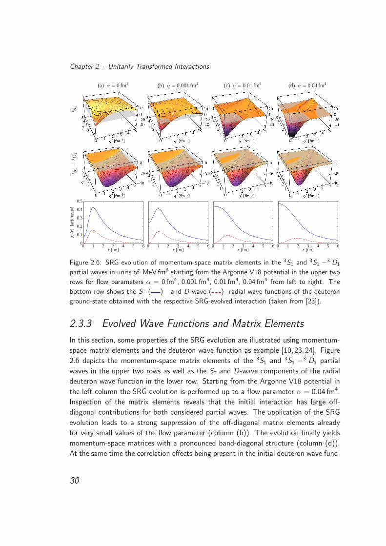
Figure 2.6: SRG evolution of momentum-space matrix elements in the 3S1 and 3S1 −3 D1
partial waves in units of MeV fm3 starting from the Argonne V18 potential in the upper two
rows for flow parameters α = 0 fm4, 0.001 fm4, 0.01 fm4, 0.04 fm4 from left to right. The
bottom row shows the S- ( ) and D-wave ( ) radial wave functions of the deuteron
ground-state obtained with the respective SRG-evolved interaction (taken from [23]).
2.3.3 Evolved Wave Functions and Matrix Elements
In this section, some properties of the SRG evolution are illustrated using momentum-
space matrix elements and the deuteron wave function as example [10,23,24]. Figure
2.6 depicts the momentum-space matrix elements of the 3S1 and 3S1 −3 D1 partial
waves in the upper two rows as well as the S- and D-wave components of the radial
deuteron wave function in the lower row. Starting from the Argonne V18 potential in
the left column the SRG evolution is performed up to a flow parameter α = 0.04 fm4.
Inspection of the matrix elements reveals that the initial interaction has large off-
diagonal contributions for both considered partial waves. The application of the SRG
evolution leads to a strong suppression of the off-diagonal matrix elements already
for very small values of the flow parameter (column (b)). The evolution finally yields
momentum-space matrices with a pronounced band-diagonal structure (column (d)).
At the same time the correlation effects being present in the initial deuteron wave func-
30
2.3 · Similarity Renormalization Group
. 1S 03S 1
3S 1 −3D1
Arg
onne
V18
UC
OM
(var
.)U
CO
M(S
RG
)SR
G
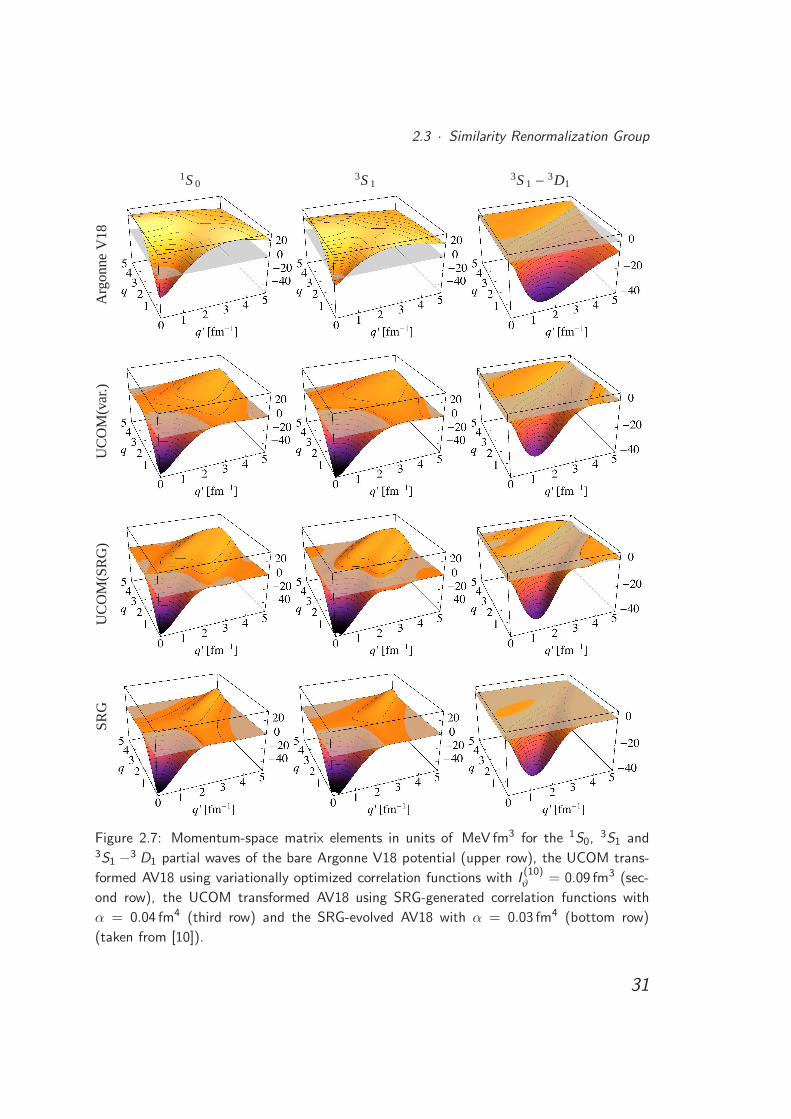
Figure 2.7: Momentum-space matrix elements in units of MeV fm3 for the 1S0, 3S1 and3S1 −3 D1 partial waves of the bare Argonne V18 potential (upper row), the UCOM trans-
formed AV18 using variationally optimized correlation functions with I(10)ϑ = 0.09 fm3 (sec-
ond row), the UCOM transformed AV18 using SRG-generated correlation functions with
α = 0.04 fm4 (third row) and the SRG-evolved AV18 with α = 0.03 fm4 (bottom row)
(taken from [10]).
31
Chapter 2 · Unitarily Transformed Interactions
tion are eliminated throughout the SRG evolution, i.e. the correlation hole at small
interparticle distances caused by the repulsive core vanishes and the D-wave admixture
due to the tensor force becomes much weaker. Hence, the SRG flow evolution resem-
bles the application of the UCOM central and tensor correlators discussed in Section
2.2.2 (Fig. 2.3).
Finally, we compare the momentum-space matrix elements of the different inter-
actions obtained via the UCOM and SRG transformations. Figure 2.7 shows matrix
elements using the 1S0,3S1 and 3S1 −3 D1 partial waves as an example. The main
features are comparable in all partial waves. The upper row shows the matrix elements
of the initial Argonne V18 potential, which show large off-diagonal contributions in all
considered partial waves. The two middle rows show the AV18 transformed via the
UCOM using correlation functions obtained via energy minimization, and using SRG-
generated correlation functions, and the bottom row shows the SRG-evolved AV18.
All three transformed interactions show some common features that are also mani-
fested in the momentum space matrix elements. In all partial waves, the off-diagonal
contributions are suppressed while the low-momentum parts are enhanced yielding a
band-diagonal structure. In other words, all unitary transformations lead to a de-
coupling of low-momentum and high-momentum states, which in turn improves the
convergence properties of the unitarily transformed interactions compared to the initial
bare interaction.
On the other hand, the investigation of the momentum-space matrix elements also
reveals some differences between the approaches. The SRG evolution yields almost
perfect band-diagonal matrices, while the UCOM transformations lead to a broader
band falling off more slowly with increasing distance from the diagonal. Here, using
the variationally optimized correlation functions produces an even broader plateau of
non-vanishing matrix elements along the diagonal regarding the 1S0 and 3S1 partial
waves than the application of SRG-generated correlation functions. The band-diagonal
structure being not as perfect as for the SRG-evolved interaction is due to the limited
flexibility of the UCOM approach compared to the SRG (cf. Sec. 2.3.4).
2.3.4 Connections between UCOM and SRG
The UCOM and the SRG both aim at the construction of soft interactions. Though
their starting points are quite different, there are also some connections between the
two approaches [10,22–25]. Firstly, both methods use unitary transformations to con-
struct a manifold of interactions that are all phase-shift equivalent to the underlying
potential. In the course of the transformations, both approaches generate irreducible
32
2.3 · Similarity Renormalization Group
many-body operators even if starting from a pure two-body potential. For computa-
tional reasons we have restricted both approaches to two-body operators. However,
different many-body calculations reveal that the neglected higher-order contributions
play an important role if we want to describe properties of nuclei beyond the lightest
isotopes [10, 13, 18, 19, 23]. The evaluation of the three-body contributions of the
UCOM and SRG transformations is in principle possible but very involved [26]. Hence,
for first investigations of the importance of the omitted higher orders we will introduce
phenomenological three-body forces, which can be included in the calculations more
easily and demand less computing time.
Further similarities between the UCOM and the SRG are manifested if we compare
the UCOM generators gr and gΩ with the initial SRG generator η0. We consider an
interaction
V =∑
p
vp(r)Op (2.72)
that contains the operators of the charge-independent part of the Argonne V18 poten-
tial (cf. Eq. (2.26)). The evaluation of the generator at α = 0 using this interaction
yields
η0 =i
2(qrS(r) + S(r)qr ) + i Θ(r)S12(r, qΩ) (2.73)
with the operator-valued functions
S(r) = −1
µ
(∑
p
v ′p(r)Op
), Θ(r) = −2
µ
vt(r)
r2. (2.74)
Therefore, one finds the same operator structure for the initial SRG generator as for
the sum of the UCOM generators gr and gΩ (Eqs. (2.9) and (2.12)). This means
that both methods deal with the same kind of short-range correlations induced by the
nuclear interaction, although they start from different motivations: the SRG aims at
a pre-diagonalization of the Hamilton matrix while the UCOM explicitly addresses the
short-range central and tensor correlations. Furthermore, we can deduce from this
connection, that the most important terms are covered by the UCOM correlators.
A closer look at Eqs. (2.73) and (2.74) also reveals some differences between the
two approaches. The UCOM correlation functions s(r) and ϑ(r) only depend on the
respective spin-isospin channel while the operator valued function S(r) also depends on
the respective partial wave. Hence, the UCOM generators represent a simplification
compared to the SRG generator. The UCOM generators could also be made more
flexible by introducing separate correlation functions for each partial wave. Neverthe-
less, the SRG evolution drives the Hamiltonian towards a band-diagonal structure more
33
Chapter 2 · Unitarily Transformed Interactions
efficiently than the UCOM transformation since the SRG uses a dynamical generator
that changes its structure during the evolution in order to perform the diagonalization
in an optimal way (cf. Sec. 2.3.3). In contrast, the UCOM performs only one unitary
transformation using static generators.
2.3.5 SRG-Generated UCOM Correlation Functions
In view of the connections between UCOM and SRG discussed in the previous section,
one is prompted to extract UCOM correlation functions from the SRG evolution. This
is achieved by the following procedure [10, 23, 25]: Starting from a given interaction,
the SRG flow equations are solved up to a specific flow parameter α yielding the
momentum space matrix elements Vα(q, q′) for a certain partial wave. Subsequently,
a set of coordinate-space wave functions is determined by solving the two-body problem
based on the evolved matrix elements. Finally, the correlation functions are derived
via a mapping of the two-body wave function of the SRG-evolved interaction onto the
corresponding wave function of the initial interaction.
To illustrate the mapping procedure, we start with the two-body eigenstate |ϕ(α)〉of the evolved interaction and the corresponding state |ϕ(0)〉 of the initial interaction,
both having the same energy eigenvalue. The correlation functions of the correlation
operator C are determined such that they map these two states onto each other:
|ϕ(0)〉 = C|ϕ(α)〉 = CΩCr |ϕ(α)〉 . (2.75)
First, we consider non-coupled partial waves with L = J , where the two-body states
can be written as
|ϕ(0)〉 = |φ(0)(LS)JT 〉|ϕ(α)〉 = |φ(α)(LS)JT 〉 .
(2.76)
In this case we only have to consider central correlations. Using the relations for the
central correlated two-body wave functions derived in Section 2.2.2 (Eq. (2.13)), we
find the following equation for the determination of the central correlation function
R−(r):
φ(0)(r) =R−(r)
r
√R ′−(r) φ(α)(R−(r)) . (2.77)
The wave functions are assumed to be real-valued. By formal integration we can
deduce an implicit integral equation:
R−(r)3 = 3
∫ r
0
dξ ξ2 φ(0)(ξ)2
φ(α)(R−(ξ))2, (2.78)
34
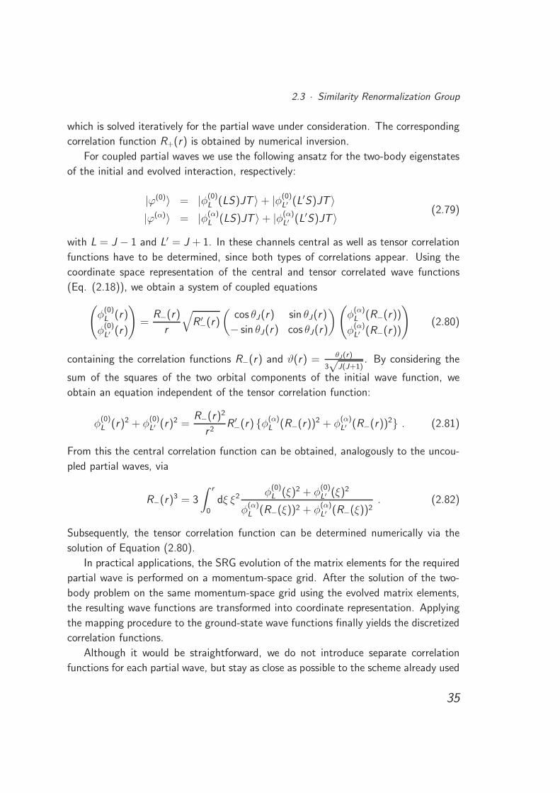
2.3 · Similarity Renormalization Group
which is solved iteratively for the partial wave under consideration. The corresponding
correlation function R+(r) is obtained by numerical inversion.
For coupled partial waves we use the following ansatz for the two-body eigenstates
of the initial and evolved interaction, respectively:
|ϕ(0)〉 = |φ(0)L (LS)JT 〉 + |φ(0)
L′ (L′S)JT 〉|ϕ(α)〉 = |φ(α)
L (LS)JT 〉 + |φ(α)L′ (L′S)JT 〉
(2.79)
with L = J − 1 and L′ = J + 1. In these channels central as well as tensor correlation
functions have to be determined, since both types of correlations appear. Using the
coordinate space representation of the central and tensor correlated wave functions
(Eq. (2.18)), we obtain a system of coupled equations
(φ
(0)L (r)
φ(0)L′ (r)
)=
R−(r)
r
√R ′−(r)
(cos θJ(r) sin θJ(r)
− sin θJ(r) cos θJ(r)
)(φ
(α)L (R−(r))
φ(α)L′ (R−(r))
)(2.80)
containing the correlation functions R−(r) and ϑ(r) = θJ(r)
3√
J(J+1). By considering the
sum of the squares of the two orbital components of the initial wave function, we
obtain an equation independent of the tensor correlation function:
φ(0)L (r)2 + φ
(0)L′ (r)2 =
R−(r)2
r 2R ′−(r) φ(α)
L (R−(r))2 + φ(α)L′ (R−(r))2 . (2.81)
From this the central correlation function can be obtained, analogously to the uncou-
pled partial waves, via
R−(r)3 = 3
∫ r
0
dξ ξ2 φ(0)L (ξ)2 + φ
(0)L′ (ξ)2
φ(α)L (R−(ξ))2 + φ
(α)L′ (R−(ξ))2
. (2.82)
Subsequently, the tensor correlation function can be determined numerically via the
solution of Equation (2.80).
In practical applications, the SRG evolution of the matrix elements for the required
partial wave is performed on a momentum-space grid. After the solution of the two-
body problem on the same momentum-space grid using the evolved matrix elements,
the resulting wave functions are transformed into coordinate representation. Applying
the mapping procedure to the ground-state wave functions finally yields the discretized
correlation functions.
Although it would be straightforward, we do not introduce separate correlation
functions for each partial wave, but stay as close as possible to the scheme already used
35
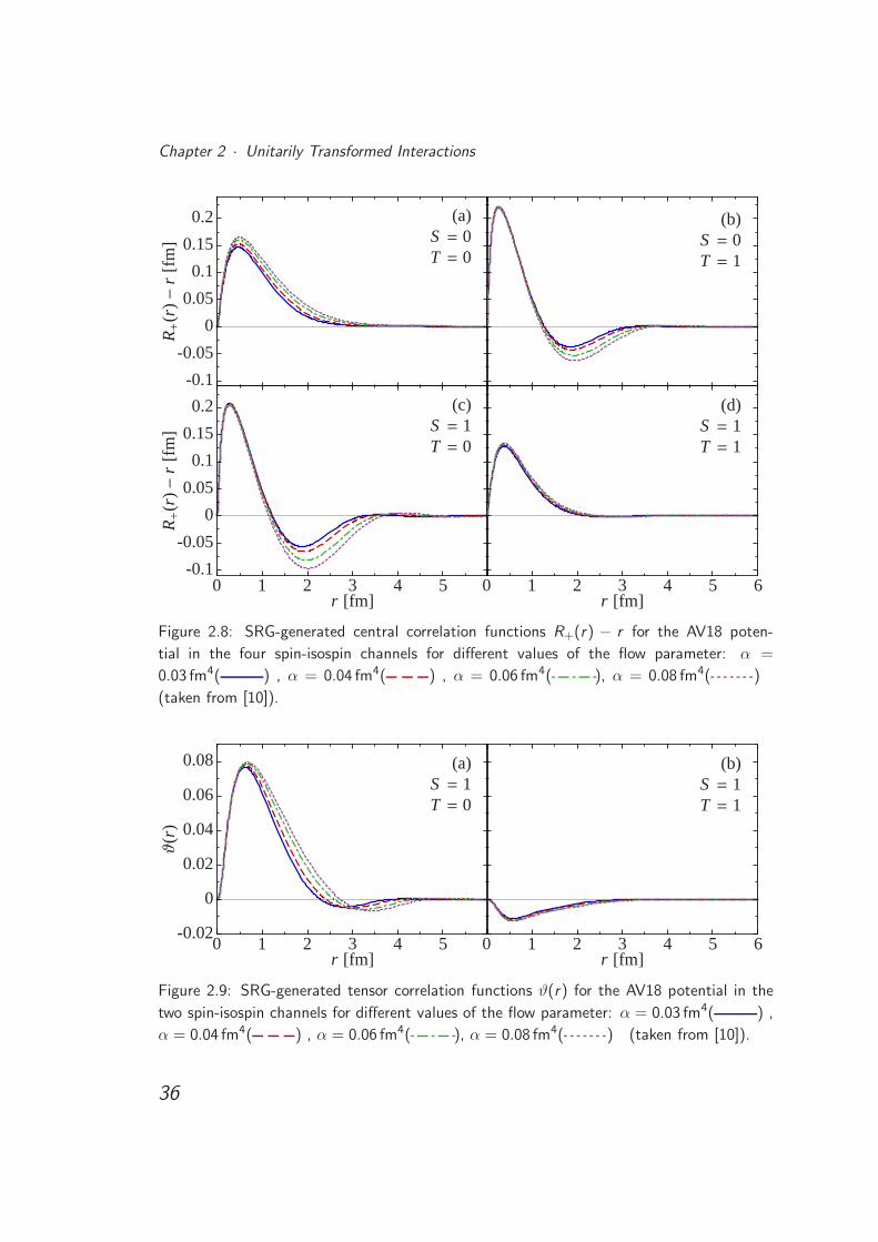
Chapter 2 · Unitarily Transformed Interactions
-0.1
-0.05
0
0.05
0.1
0.15
0.2
.
R+(r
)−r
[fm
]
(a)S = 0T = 0
(b)S = 0T = 1
0 1 2 3 4 5r [fm]
-0.1
-0.05
0
0.05
0.1
0.15
0.2
.
R+(r
)−r
[fm
]
(c)S = 1T = 0
0 1 2 3 4 5 6r [fm]
(d)S = 1T = 1
Figure 2.8: SRG-generated central correlation functions R+(r) − r for the AV18 poten-
tial in the four spin-isospin channels for different values of the flow parameter: α =
0.03 fm4( ) , α = 0.04 fm4( ) , α = 0.06 fm4( ), α = 0.08 fm4( )
(taken from [10]).
0 1 2 3 4 5r [fm]
-0.02
0
0.02
0.04
0.06
0.08
.
ϑ(r
)
(a)S = 1T = 0
0 1 2 3 4 5 6r [fm]
(b)S = 1T = 1
Figure 2.9: SRG-generated tensor correlation functions ϑ(r) for the AV18 potential in the
two spin-isospin channels for different values of the flow parameter: α = 0.03 fm4( ) ,
α = 0.04 fm4( ) , α = 0.06 fm4( ), α = 0.08 fm4( ) (taken from [10]).
36
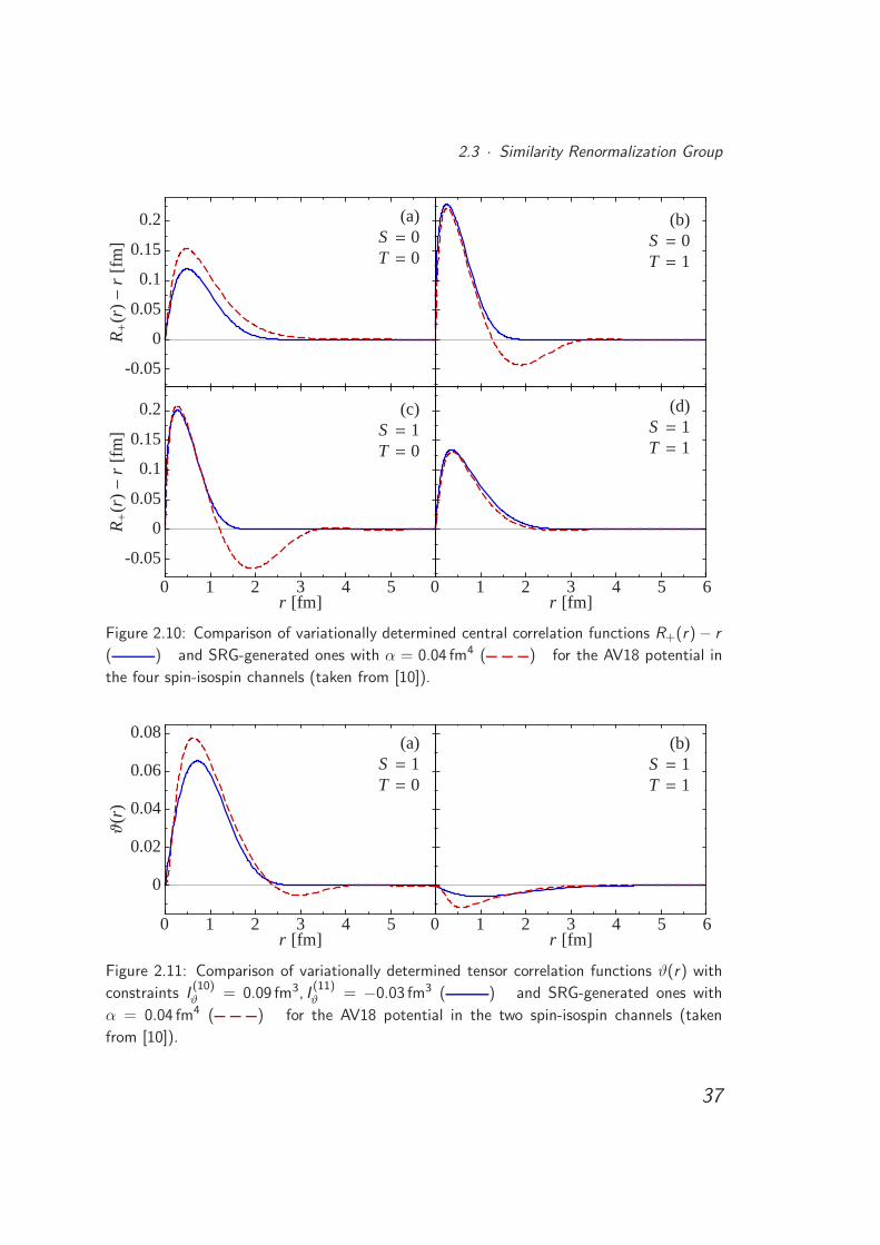
2.3 · Similarity Renormalization Group
-0.05
0
0.05
0.1
0.15
0.2
.
R+(r
)−r
[fm
]
(a)S = 0T = 0
(b)S = 0T = 1
0 1 2 3 4 5r [fm]
-0.05
0
0.05
0.1
0.15
0.2
.
R+(r
)−r
[fm
]
(c)S = 1T = 0
0 1 2 3 4 5 6r [fm]
(d)S = 1T = 1
Figure 2.10: Comparison of variationally determined central correlation functions R+(r) − r
( ) and SRG-generated ones with α = 0.04 fm4 ( ) for the AV18 potential in
the four spin-isospin channels (taken from [10]).
0 1 2 3 4 5r [fm]
0
0.02
0.04
0.06
0.08
.
ϑ(r
)
(a)S = 1T = 0
0 1 2 3 4 5 6r [fm]
(b)S = 1T = 1
Figure 2.11: Comparison of variationally determined tensor correlation functions ϑ(r) with
constraints I(10)ϑ = 0.09 fm3, I
(11)ϑ = −0.03 fm3 ( ) and SRG-generated ones with
α = 0.04 fm4 ( ) for the AV18 potential in the two spin-isospin channels (taken
from [10]).
37
Chapter 2 · Unitarily Transformed Interactions
for the variationally determined correlation functions. That means, that we distinguish
the possible spin-isospin channels and only consider the lowest angular momenta in
the respective channel [10]. Hence, for the determination of the central correlation
functions in the spin-singlet channels we use the 1S0 partial wave for T = 1 and
the 1P1 partial wave for T = 0. In the spin-triplet channel, both central and tensor
correlation functions have to be calculated. For T = 0 this is straightforward by using
the deuteron solution in the coupled 3S1 −3 D1 partial wave. But for T = 1 the
lowest allowed angular momentum is L = 1 so that the total angular momentum can
be coupled to J = 0, 1, 2. There are several possibilities to deal with this ambiguity,
currently the most convenient scheme is to create a pseudo interaction by averaging
the 3P0,3P1 and 3P2 partial waves with a relative weight 2J +1 and use its eigenstates
for the mapping procedure. We extract the correlation functions of the SRG evolution
by using the energetically lowest states in the respective spin-isospin channel.
Contrary to the correlation functions determined via an energy minimization we do
not have to introduce additional range constraints. The only parameter is the flow
parameter α that enters the central and tensor correlation functions in a consistent
way.
In Figs. 2.8 and 2.9 we show the dependencies of the central and tensor correlation
functions on the flow parameter, respectively. The range of all correlation functions
increases with increasing flow parameter. This can be understood in the following way:
The flow evolution starts by suppressing the matrix elements at high-lying momenta,
i.e. small inter-particle distances. With increasing flow parameter, also the matrix
elements involving lower momenta are driven towards a band-diagonal structure, i.e.
in coordinate space the wave functions are modified at larger distances, leading to
longer-ranged correlation functions.
The SRG-generated central and tensor correlation functions are compared to those
determined via an energy minimization in Figs. 2.10 and 2.11, respectively. The pa-
rameters were chosen such that both sets of correlators yield approximately the same
ground-state energy of 4He in a No-Core Shell Model calculation, i.e. α = 0.04 fm4
for the SRG-generated correlation functions and for the variationally optimized ten-
sor correlation functions the range constraints are Iϑ = 0.09 fm3 for T = 0 and
Iϑ = −0.03 fm3 for T = 1. In the S = 0, T = 0 channel the shapes of both cen-
tral correlation functions are very similar, but the variationally optimized correlation
function is somewhat weaker and of smaller range, which can be explained by the addi-
tional constraint introduced in Section 2.2.6. In the even channels (S = 0, T = 1 and
S = 1, T = 0), where the dominant central correlations appear, the correlation func-
tions nicely agree at small distances. But the SRG-generated functions have a negative
38
2.3 · Similarity Renormalization Group
contribution around 2 fm while the variationally optimized correlation functions simply
fall off to zero. The behavior of the latter is caused by the chosen parameterization
which does not allow for negative parts. Possibly, the agreement at intermediate dis-
tances could be improved if one would apply parameterizations that are more flexible.
The shape of the SRG-generated correlation functions reveals that the attractive re-
gion of the interaction is exploited by shifting probability amplitude of both smaller
and larger inter-particle distances towards the potential minimum. Finally, in the odd
S = 1, T = 1 channel both types of central correlation functions agree very well.
Figure 2.11 shows that the agreement of the tensor correlation functions is not as
good as for the central correlation functions. This is again explained by the artificial
range constraints of the variationally optimized tensor correlation functions. For T = 0
the SRG-generated correlation function shows a negative part, which is much weaker
than for the corresponding central correlation function.
39

Chapter 2 · Unitarily Transformed Interactions
40
Chapter 3
Many-Body Calculations
As a starting point to characterize the properties of the unitarily transformed two-body
interactions discussed in Chapter 2 we will apply the Hartree-Fock method to calculate
binding energies and charge radii across the whole nuclear chart. The derivation of the
general Hartree-Fock equations applied to a Hamiltonian containing a two-body and a
three-body interaction is summarized in Appendix A, in Section 3.1 we will discuss the
practical application of the Hartree-Fock method adapted to our specific requirements.
Subsequently, we will examine the properties of different two-body interactions by
considering HF ground-state energies and charge radii of selected closed-shell nuclei in
Section 3.2 and single-particle spectra in Section 3.3.
To estimate the importance of long-range correlations we apply low-order many-
body perturbation theory on top of the Hartree-Fock results. We will derive the second-
order energy correction in Section 3.4, again on the basis of a two- plus three-body
interaction. To conclude the discussion based on pure two-body interactions, we will
investigate the perturbative energy corrections for the different two-body interactions
in Section 3.5.
3.1 The Hartree-Fock Method
In the Hartree-Fock approximation the many-body state is represented by a single
Slater determinant [13]:
|HF〉 = A(|ϕα1〉 ⊗ |ϕα2
〉 ⊗ · · · ⊗ |ϕαA〉) , (3.1)
41
Chapter 3 · Many-Body Calculations
where A denotes the antisymmetrization operator acting on the A-body product state
|ϕα1〉 ⊗ |ϕα2
〉 ⊗ · · · ⊗ |ϕαA〉. The minimization of the energy expectation value is
performed by using the single-particle states |ϕα〉 as variational degrees of freedom.
Since this simple many-body state is not capable of describing the complex correla-
tions induced by the nuclear interaction, it is crucial to employ an appropriate unitarily
transformed NN interaction in connection with the HF method incorporating at least
parts of the correlations. The Hamiltonian entering the HF equations consists of the
kinetic energy T, a transformed NN interaction VNN and a phenomenological 3N in-
teraction V3N [13, 19, 27]:
Hint = T − Tcm + VNN + V3N =
= Tint + VNN + V3N = H(2)int + V3N .
(3.2)
The unitarily transformed interaction VNN includes all Coulomb and charge-dependent
terms. In order to approximately account for the center-of-mass contribution to the
energy, the center-of-mass kinetic energy Tcm has been subtracted yielding the intrinsic
kinetic energy Tint, which can be written as a pure two-body operator:
Tint =1
Aµ
A∑
i<j
q2ij (3.3)
with the reduced nucleon mass µ = mN/2 and the relative two-body momentum
operator q. Thus, the Hamiltonian only contains two- and three-body operators.
We choose the eigenstates |nljmmt〉 of the spherical harmonic oscillator as basis
for the calculations. The HF single-particle states can be expanded in the following
way:
|ϕα〉 = |νljmmt〉 =∑
n
C (νljmmt )n |nljmmt〉 , (3.4)
where only states with the same quantum numbers l , j and m can contribute as we as-
sume spherical symmetry. Furthermore, we will only consider nuclei with closed j-shells
in the following, i.e. the expansion coefficients can be chosen to be independent of the
projection quantum number m: C(νljmmt)n = C
(νljmt)n . These expansion coefficients are
used as variational parameters for the minimization of the energy expectation value.
Thus, the HF equations can be written as∑
n′1
h(l1j1mt1 )
n1n′1
C(ν1l1j1mt1 )
n′1= ε(ν1l1j1mt1 )C
(ν1l1j1mt1 )n1 (3.5)
with the single-particle energies ε(νljmt). The matrix elements of the single-particle
Hamiltonian
42
3.1 · The Hartree-Fock Method
h(l1j1mt1 )
n1n′1
=∑
l2j2mt2
∑
n2n′2
H(l1j1mt1 ,l2j2mt2 )
n1n2,n′1n′2
(l2j2mt2 )
n′2n2
+1
2
∑
l2j2mt2
∑
l3j3mt3
∑
n2n3n′2n
′3
V(l1j1mt1 ,l2j2mt2 ,l3j3mt3 )
3N, n1n2n3,n′1n′2n
′3
(l2j2mt2 )
n′2n2
(l3j3mt3 )
n′3n3
(3.6)
consist of the matrix elements H(l1j1mt1 ,l2j2mt2 )
n1n2,n′1n′2
of the two-body part of the Hamil-
tonian H(2)int = Tint + VNN and the matrix elements of the three-body interaction
V(l1j1mt1 ,l2j2mt2 ,l3j3mt3 )
3N, n1n2n3,n′1n′2n
′3
. The one-body density matrix is defined by
(ljmt)n′n =
∑
ν
(2j + 1)C(νljmt)⋆
n′ C (νljmt )n , (3.7)
The single-particle Hamiltonian itself depends on the coefficients C(νljmt)n via the one-
body density matrix revealing the non-linearity of the HF equations.
The m-averaged antisymmetric matrix elements of the two-body part of the Hamil-
tonian entering into the eigenvalue problem (3.5) can be expressed by using uncoupled
two-body matrix elements:
H(l1j1mt1 ,l2j2mt2 )
n1n2,n′1n′2
=1
(2j1 + 1)(2j2 + 1)(3.8)
×∑
m1 m2
⟨n1l1j1m1mt1 , n2l2j2m2mt2
∣∣H(2)int
∣∣n′1l1j1m1mt1 , n
′2l2j2m2mt2
⟩.
However, it is more convenient to start from jj-coupled two-body matrix elements:
H(l1j1mt1 ,l2j2mt2 )
n1n2,n′1n′2
=∑
JTMT
(2J + 1)
(2j1 + 1)(2j2 + 1)c(
12
12
mt1 mt2
∣∣∣ T
MT
)2
×⟨n1l1j1, n2l2j2; JTMT
∣∣H(2)int
∣∣n′1l1j1, n
′2l2j2; JTMT
⟩ (3.9)
with the Clebsch-Gordan coefficient c(
12
12
mt1 mt2
∣∣∣ T
MT
).
The matrix elements of the two-body interactions are most conveniently calculated
in a basis of LS-coupled relative two-body states and they have to be transformed into
jj-coupled matrix elements for the application in Hartree-Fock and other methods.
In addition the matrix elements of the three-body interaction are required. They will
be calculated in Chapter 4 for a finite-range three-body interaction with Gaussian shape
and in Chapter 5 for a regularized three-body contact interaction. In the following, we
will discuss HF calculations based on pure two-body interactions.
43
Chapter 3 · Many-Body Calculations
3.2 Ground-State Energies and Charge Radii
We start by discussing some results obtained with pure unitarily transformed two-
body interactions. While the properties of the transformed interactions were studied in
Section 2.3.3 by considering momentum-space matrix elements, we now perform many-
body calculations to investigate some other aspects of the pure two-body interactions
before including three-body forces.
The matrix elements of the transformed two-body interaction as well as those of
any other observables, especially the intrinsic kinetic energy and the charge radius, are
computed beforehand for each basis size and oscillator parameter separately and stored
to disk. This procedure allows for an efficient solution of the Hartree-Fock eigenvalue
problem on the one hand and on the other hand the matrix elements can be used as
input for different many-body methods without calculating them again. The solution
of the HF equations is performed in an iterative fashion until full self-consistency is
reached.
In the following, we will consider ground-state energies (cf. Eq. (A.33)) as well
as charge radii for selected nuclei across the whole nuclear chart. In order to preserve
spherical symmetry only closed-shell nuclei are investigated. The operators of the
mean-square radii can be written in a translationally invariant form [24,28]:
rms =1
A
∑
i
(xi −Xcm)2 =1
2A2
∑
ij
r2ij (3.10)
rpms =1
AZ
∑
ij
r2ijΠp −
1
2A2
∑
ij
r2ij (3.11)
rnms =1
AN
∑
ij
r2ijΠn −
1
2A2
∑
ij
r2ij , (3.12)
where rms denotes the radius operator for a nucleon and rp/nms for a proton/neutron. The
point root-mean-square (rms) radius rrms is obtained by calculating the square-root of
the expectation value of the mean-square radius operator for the HF ground-state.
In principle, one would have to use the unitarily transformed radius operators. For
the UCOM transformation using variationally optimized correlators, however, it was
shown that the difference between the correlated and the uncorrelated charge radii is
marginal [13]. Therefore, we will discuss uncorrelated charge radii in the following. The
impact of the SRG transformation on the charge radii has not yet been investigated,
but we neglect it nonetheless.
44
3.2 · Ground-State Energies and Charge Radii
UCOM(SRG) standard UCOM using SRG-generated correlation functions
S-UCOM(SRG) S-wave only UCOM using SRG-generated correlation functions
SRG standard SRG
S-SRG S-wave only SRG
Table 3.1: Acronyms for the four different families of unitarily transformed interactions.
To obtain the charge radius rch one has to add the standard corrections for proton
and neutron size:
rch =
√r 2p,rms + r 2
p,ch +N
Zr 2n,ch , (3.13)
where we use
rp,ch = 0.8768 fm , r 2n,ch = −0.116 fm2 (3.14)
for the proton and neutron charge radii [29].
We employ the UCOM and the SRG to obtain a manifold of phase-shift equivalent
transformed NN potentials depending on one parameter. When applying the standard
SRG evolution all partial waves are transformed consistently. However, it is also possible
to restrict the SRG evolution to the relative S-partial waves, i.e. the 1S0 and the coupled3S1 −3 D1 partial waves, since the short-range correlations are most dominant in these
channels. For higher angular momenta the wave functions are suppressed at short
distances due to the centrifugal barrier, i.e. the effects of short-range correlations are
not as pronounced as in the S-wave channels.
For the UCOM transformation we use correlation functions obtained from the SRG
evolution. In each spin-isospin channel the lowest partial waves are considered for the
determination of the correlation functions. Subsequently, these correlation functions
are used to transform all partial waves consistently. In contrast to this standard UCOM,
we can also correlate the S-partial waves only, i.e. the 1S0 and the coupled 3S1 −3 D1
partial waves, in analogy to the restricted SRG evolution. Note that in this case already
the SRG evolution is restricted to the S-partial waves as the higher partial waves are
not required for the determination of the correlation functions.
In the following we will consider these four different classes of unitarily transformed
two-body interactions, the corresponding acronyms are listed in Table 3.1.
The harmonic-oscillator basis is truncated with respect to the major oscillator quan-
tum number e = 2n + l ≤ emax. Additional constraints for the radial quantum number
n or the orbital angular momentum l are possible. A truncation at emax = 10 is
sufficient to obtain converged Hartree-Fock results (cf. Sec. 3.5).
45

Chapter 3 · Many-Body Calculations
Isotope 4He 16O 24O 34Si 40Ca 48Ca 48Ni 56Ni 60Ni
aHO [ fm] 1.3 1.8 1.9 1.9 2.0 2.0 2.0 2.0 2.0
Isotope 78Ni 88Sr 90Zr 100Sn 114Sn 132Sn 146Gd 208Pb
aHO [ fm] 2.1 2.2 2.2 2.2 2.2 2.2 2.2 2.4
Table 3.2: Optimal oscillator lengths for the considered closed-shell nuclei.
To perform the Hartree-Fock calculations we, first of all, have to choose the oscilla-
tor parameter aHO defining the width of the oscillator potential. In former applications
the oscillator parameter was fixed for each nucleus separately by minimizing the HF
energy. However, when perturbative corrections are included, the oscillator lengths
can no longer be determined via an energy minimization, since perturbation theory
does not obey the variational principle. Therefore, we will apply a different scheme
for the determination of the oscillator lengths, i.e. instead of ground-state energies we
consider charge radii. We choose the oscillator parameter such that the experimental
charge radius is approximately reproduced by a Slater determinant which is built of
the harmonic-oscillator single-particle states with the lowest energies. For those nuclei,
where no experimental value for the charge radius is available, we have to estimate
the oscillator parameter. The advantage of this procedure is that the oscillator pa-
rameter is independent of the respective two- and three-body interactions. Hence, we
can stick to the once determined set of oscillator parameters throughout all following
calculations. The resulting values are summarized in Table 3.2.
Figures 3.1 and 3.2 show the ground-state energies per nucleon (upper panel) and
the charge radii (lower panel) for selected closed-shell nuclei across the whole nuclear
chart obtained from HF calculations based on the UCOM(SRG) and S-UCOM(SRG)
interactions, respectively. The different symbols indicate different values of the flow
parameter. In both cases, the smallest value of the flow parameter, i.e. α = 0.04 fm4, is
chosen such that the experimental 4He ground-state energy is reproduced in converged
No-Core Shell Model (NCSM) calculations. Therefore, calculations with the pure two-
body interaction are performed using this flow parameter. Nonetheless, we investigate
the influence of the flow parameter, and especially examine the properties of two-
body interactions with larger flow parameters as they will be required when including
a repulsive three-body interaction. Figures 3.1 and 3.2 show that the HF ground-state
energies calculated with α = 0.04 fm4 reproduce the systematics of the experimental
data except for an almost constant shift. In case of the UCOM(SRG) interaction
all nuclei are underbound by about 2.5 to 3.5 MeV per nucleon, while for the S-
UCOM(SRG) interaction the ground-state energies per nucleon differ from experiment
46
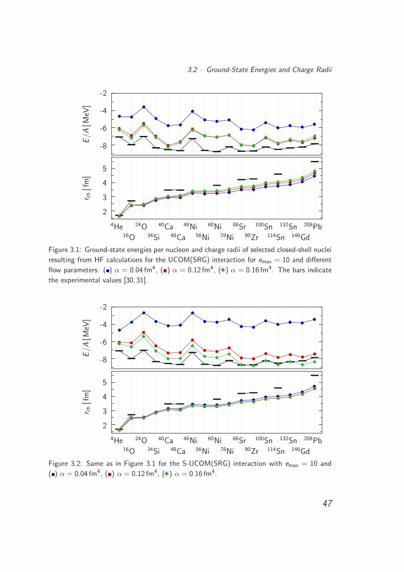
3.2 · Ground-State Energies and Charge Radii
-8
-6
-4
-2
.
E/A
[MeV
]
2
3
4
5
.
r ch[f
m]
4He16O
24O34Si
40Ca48Ca
48Ni56Ni
60Ni78Ni
88Sr90Zr
100Sn114Sn
132Sn146Gd
208Pb
Figure 3.1: Ground-state energies per nucleon and charge radii of selected closed-shell nuclei
resulting from HF calculations for the UCOM(SRG) interaction for emax = 10 and different
flow parameters: () α = 0.04 fm4, () α = 0.12 fm4, ( ) α = 0.16 fm4. The bars indicate
the experimental values [30, 31].
-8
-6
-4
-2
.
E/A
[MeV
]
2
3
4
5
.
r ch[f
m]
4He16O
24O34Si
40Ca48Ca
48Ni56Ni
60Ni78Ni
88Sr90Zr
100Sn114Sn
132Sn146Gd
208Pb
Figure 3.2: Same as in Figure 3.1 for the S-UCOM(SRG) interaction with emax = 10 and
() α = 0.04 fm4, () α = 0.12 fm4, ( ) α = 0.16 fm4.
47
Chapter 3 · Many-Body Calculations
by about 4 to 5 MeV. With increasing flow parameter the difference to the experimental
binding energies diminishes, in case of the S-UCOM(SRG) interaction the trend of the
experimental energies is no longer reproduced, i.e. the light nuclei are underbound
while the heaviest nuclei are already overbound for the largest flow parameter. The
gain of binding energy with increasing flow parameter can be understood by considering
the meaning of the flow parameter. With increasing flow parameter, the range of the
derived correlation functions increases as well. Hence, correlations of longer range are
covered by the UCOM transformation and are thus included effectively already on the
HF level leading to an improved reproduction of the experimental binding energies.
Nonetheless, for calculations based on the pure two-body interaction one chooses the
flow parameter α = 0.04 fm4 for the above-mentioned reason. Furthermore, missing
long-range correlations can be included by using second-order many-body perturbation
theory on top of the HF results, which will entail a lowering of the ground-state energies
(cf. Sec. 3.5).
Figure 3.1 reveals a further interesting feature of the UCOM(SRG) interaction. If
we compare the ground-state energies calculated with the flow parameter α = 0.16 fm4
to those calculated with α = 0.12 fm4, we find that for light nuclei the trend to lower
energies is confirmed while we observe the opposite trend for the heaviest nuclei.
With increasing flow parameter correlations of longer range are included in the UCOM
transformation, but only the short-range correlations are state-independent. Hence,
for α = 0.16 fm4 the UCOM transformation obviously becomes state-dependent due
to the long range of the correlation functions, which is reflected in the trend of the
binding energies.
The charge radii shown in the lower parts of Figures 3.1 and 3.2 are significantly
smaller than the experimental values for both the UCOM(SRG) and the S-UCOM(SRG)
interaction. The variation of the charge radii with increasing flow parameter is much
weaker than in case of the ground-state energies. For the UCOM(SRG) interaction
the charge radii slightly increase with increasing flow parameter. In contrast, the radii
decrease with increasing flow parameter in case of the S-UCOM(SRG) interaction.
In Figures 3.3 and 3.4 the ground-state energies and charge radii obtained with
the SRG and S-SRG interaction for different flow parameters are displayed. Again,
the smallest flow parameter is chosen such that the experimental 4He ground-state
energy is reproduced in a converged NCSM calculation, which is α = 0.03 fm4 for
these interactions. For the SRG interaction the binding energy per nucleon increases
rapidly with increasing mass number leading to a strong overbinding of intermediate
and heavy nuclei. With increasing flow parameter this systematic deviation is even
more dramatic. At the same time the charge radii are significantly too small, e.g. for
48
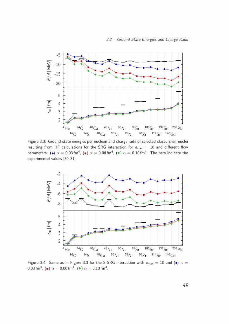
3.2 · Ground-State Energies and Charge Radii
-20
-15
-10
-5
.
E/A
[MeV
]
2
3
4
5
.
r ch[f
m]
4He16O
24O34Si
40Ca48Ca
48Ni56Ni
60Ni78Ni
88Sr90Zr
100Sn114Sn
132Sn146Gd
208Pb
Figure 3.3: Ground-state energies per nucleon and charge radii of selected closed-shell nuclei
resulting from HF calculations for the SRG interaction for emax = 10 and different flow
parameters: () α = 0.03 fm4, () α = 0.06 fm4, ( ) α = 0.10 fm4. The bars indicate the
experimental values [30, 31].
-8
-6
-4
-2
.
E/A
[MeV
]
2
3
4
5
.
r ch[f
m]
4He16O
24O34Si
40Ca48Ca
48Ni56Ni
60Ni78Ni
88Sr90Zr
100Sn114Sn
132Sn146Gd
208Pb
Figure 3.4: Same as in Figure 3.3 for the S-SRG interaction with emax = 10 and () α =
0.03 fm4, () α = 0.06 fm4, ( ) α = 0.10 fm4.
49
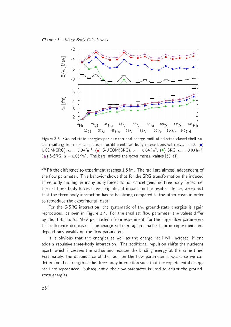
Chapter 3 · Many-Body Calculations
-8
-6
-4
-2
.
E/A
[MeV
]
2
3
4
5
.
r ch[f
m]
4He16O
24O34Si
40Ca48Ca
48Ni56Ni
60Ni78Ni
88Sr90Zr
100Sn114Sn
132Sn146Gd
208Pb
Figure 3.5: Ground-state energies per nucleon and charge radii of selected closed-shell nu-
clei resulting from HF calculations for different two-body interactions with emax = 10: ()
UCOM(SRG), α = 0.04 fm4; () S-UCOM(SRG), α = 0.04 fm4; ( ) SRG, α = 0.03 fm4;
(N) S-SRG, α = 0.03 fm4. The bars indicate the experimental values [30, 31].
208Pb the difference to experiment reaches 1.5 fm. The radii are almost independent of
the flow parameter. This behavior shows that for the SRG transformation the induced
three-body and higher many-body forces do not cancel genuine three-body forces, i.e.
the net three-body forces have a significant impact on the results. Hence, we expect
that the three-body interaction has to be strong compared to the other cases in order
to reproduce the experimental data.
For the S-SRG interaction, the systematic of the ground-state energies is again
reproduced, as seen in Figure 3.4. For the smallest flow parameter the values differ
by about 4.5 to 5.5 MeV per nucleon from experiment, for the larger flow parameters
this difference decreases. The charge radii are again smaller than in experiment and
depend only weakly on the flow parameter.
It is obvious that the energies as well as the charge radii will increase, if one
adds a repulsive three-body interaction. The additional repulsion shifts the nucleons
apart, which increases the radius and reduces the binding energy at the same time.
Fortunately, the dependence of the radii on the flow parameter is weak, so we can
determine the strength of the three-body interaction such that the experimental charge
radii are reproduced. Subsequently, the flow parameter is used to adjust the ground-
state energies.
50
3.2 · Ground-State Energies and Charge Radii
Figure 3.5 shows a comparison of the results of the four different interactions, each
with the flow parameter one uses for calculations with the pure two-body interaction,
in order to emphasize the differences between these interactions. First we compare
the UCOM(SRG) with the SRG interactions, which have some inherent differences as
seen from the HF ground-state energies and charge radii. The UCOM transformation
is designed to describe short-range correlations which are most dominant in the lowest
partial waves. Hence, the higher partial waves are not treated in an optimal way by the
UCOM transformation. Since short-range correlations are more and more suppressed in
higher partial waves due to the centrifugal barrier, this non-optimal pre-diagonalization
of the higher partial waves only leads to minor effects. In contrast, in SRG each
partial wave is evolved separately leading to an optimal pre-diagonalization also for
higher partial waves resulting in faster convergence than in case of the UCOM(SRG)
interaction [10]. Evidently, this entails larger contributions from three- and many-body
forces which in turn yields strongly overbound nuclei with small radii as shown in Figure
3.5.
Next, we compare the UCOM(SRG) and SRG interactions with S-UCOM(SRG) and
S-SRG, respectively. As mentioned above, UCOM aims at the description of short-
range correlations which are most dominant in the lowest partial waves. Therefore, the
higher partial waves are not correlated in an optimal manner. The UCOM transforma-
tion generates repulsion in higher partial waves, which is not evident from Figure 3.5,
but becomes apparent for larger flow parameters. Consequently, we will need a weaker
three-body force to supplement the UCOM(SRG) interaction than for S-UCOM(SRG)
as we will discuss in Chapter 5.
In the S-SRG approach only the S-partial waves are evolved as well. Compared to
the HF results of the SRG interaction this also leads to an improved description of the
charge radii. As the nuclei are strongly overbound when using the SRG interaction,
the S-SRG interaction yields also an improvement in the description of ground-state
energies.
The S-UCOM(SRG) and the S-SRG interaction both yield very similar results for
ground-state energies and charge radii in the HF approximation.
Considering the UCOM(SRG), S-UCOM(SRG) and S-SRG interactions, the ground-
state energies of all considered closed-shell nuclei differ from experiment, but their
description can be improved by including long-range correlations, e.g. in the frame-
work of many-body perturbation theory. The charge radii are systematically smaller
than the experimental values for all four types of two-body interactions. However, this
discrepancy cannot be covered by the inclusion of long-range correlations but is an
evidence for the omitted three- and many-body forces of the respective interaction.
51
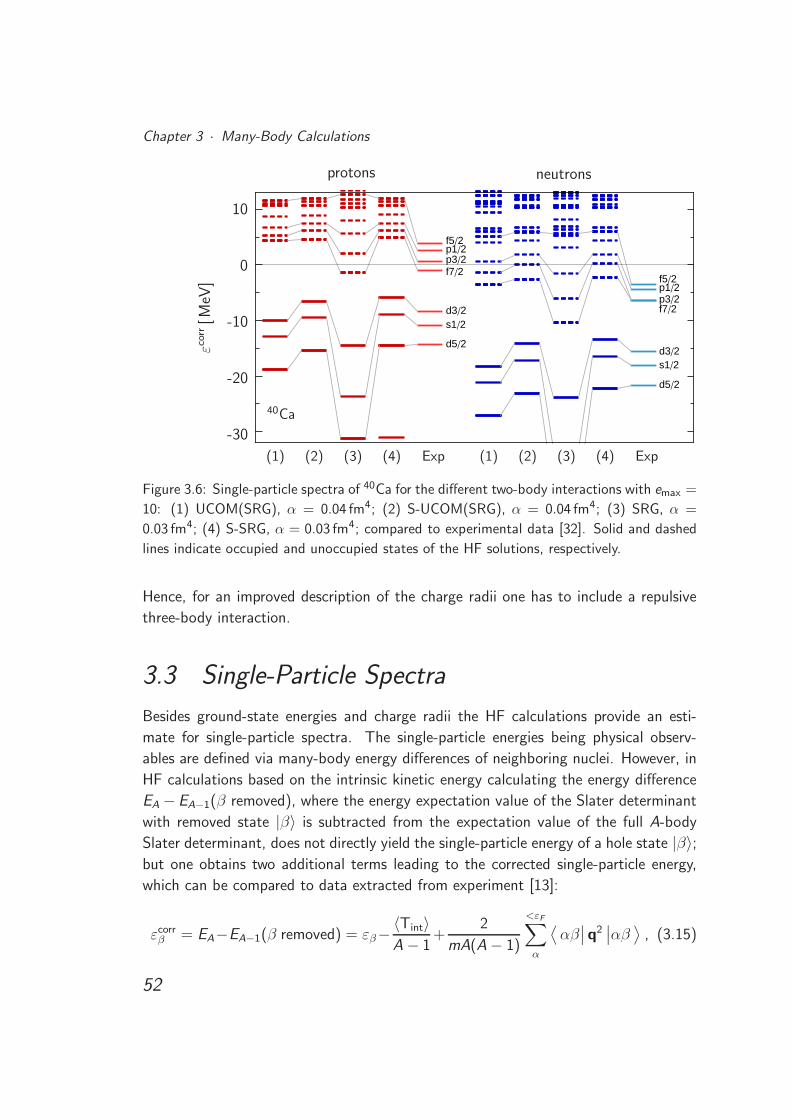
Chapter 3 · Many-Body Calculations
d52
s12d32
f72p32p12f52
d52
s12d32
f72p32p12f52
-30
-20
-10
0
10
.
εcor
r[M
eV]
protons neutrons
(1) (2) (3) (4) Exp (1) (2) (3) (4) Exp
40Ca
Figure 3.6: Single-particle spectra of 40Ca for the different two-body interactions with emax =
10: (1) UCOM(SRG), α = 0.04 fm4; (2) S-UCOM(SRG), α = 0.04 fm4; (3) SRG, α =
0.03 fm4; (4) S-SRG, α = 0.03 fm4; compared to experimental data [32]. Solid and dashed
lines indicate occupied and unoccupied states of the HF solutions, respectively.
Hence, for an improved description of the charge radii one has to include a repulsive
three-body interaction.
3.3 Single-Particle Spectra
Besides ground-state energies and charge radii the HF calculations provide an esti-
mate for single-particle spectra. The single-particle energies being physical observ-
ables are defined via many-body energy differences of neighboring nuclei. However, in
HF calculations based on the intrinsic kinetic energy calculating the energy difference
EA − EA−1(β removed), where the energy expectation value of the Slater determinant
with removed state |β〉 is subtracted from the expectation value of the full A-body
Slater determinant, does not directly yield the single-particle energy of a hole state |β〉;but one obtains two additional terms leading to the corrected single-particle energy,
which can be compared to data extracted from experiment [13]:
εcorrβ = EA−EA−1(β removed) = εβ−
〈Tint〉A − 1
+2
mA(A − 1)
<εF∑
α
⟨αβ∣∣ q2
∣∣αβ⟩
, (3.15)
52
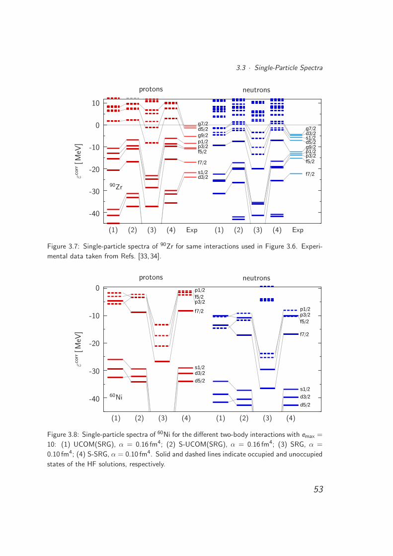
3.3 · Single-Particle Spectra
d32s12
f72
f52p32p12g92
g72d52
f72
f52p32p12g92d52
d32s12
g72
-40
-30
-20
-10
0
10
.
εcor
r[M
eV]
protons neutrons
(1) (2) (3) (4) Exp (1) (2) (3) (4) Exp
90Zr
Figure 3.7: Single-particle spectra of 90Zr for same interactions used in Figure 3.6. Experi-
mental data taken from Refs. [33, 34].
d32
d52
s12
f72
f52p12
p32
d32
d52
s12
f72
f52
p12p32
-40
-30
-20
-10
0
.
εcor
r[M
eV]
protons neutrons
(1) (2) (3) (4) (1) (2) (3) (4)
60Ni
Figure 3.8: Single-particle spectra of 60Ni for the different two-body interactions with emax =
10: (1) UCOM(SRG), α = 0.16 fm4; (2) S-UCOM(SRG), α = 0.16 fm4; (3) SRG, α =
0.10 fm4; (4) S-SRG, α = 0.10 fm4. Solid and dashed lines indicate occupied and unoccupied
states of the HF solutions, respectively.
53
Chapter 3 · Many-Body Calculations
where 〈Tint〉 is the expectation value of the intrinsic kinetic energy. For particle states
the single-particle energy reads
εcorrβ = EA+1(β added)− EA = εβ −
〈Tint〉A + 1
− 2
mA(A + 1)
<εF∑
α
⟨αβ∣∣ q2
∣∣αβ⟩
. (3.16)
We can use these corrected single-particle energies to investigate the properties of the
four different two-body interactions introduced in the previous section. However, one
has to be careful with the interpretation of single-particle spectra since they are no
direct experimental observable.
Figure 3.6 shows the single-particle spectra for 40Ca obtained with the four different
two-body interactions in comparison to experimental estimates for the single-particle
energies. The order of the levels is in nice agreement with experiment. But for
all four interaction types the Fermi gap is overestimated and especially the spectra
calculated with the SRG interaction are spread too wide compared with experiment.
As a second example, the single-particle spectra of 90Zr are shown in Figure 3.7, where
one can observe similar features as for 40Ca. The level ordering is mainly reproduced
by the UCOM(SRG), S-UCOM(SRG) and S-SRG interactions, while there are some
interchanged levels in case of the SRG interaction. The level spacings are overestimated
by all four interactions, especially by the SRG interaction. This behavior shows the
connection between radii and level spacings of single-particle spectra: On the basis of
the SRG interaction the smallest radii were observed, which entails the largest level
spacings.
The single-particle spectra of most of the other considered nuclei show a similar
behavior, hence, they are not displayed here.
Like in the case of ground-state energies and charge radii, the S-UCOM(SRG) and
the S-SRG interactions yield very similar single-particle spectra which confirms that
these two interactions have a number of common properties.
It is expected that the inclusion of a repulsive three-body interaction will improve
the description of the single-particle spectra. The additional repulsion will shift the
nucleons apart from each other which results in larger radii as well as a reduction of
the level spacings.
On the other hand, increasing the flow parameter may also lead to unintentional
effects. As an example, the spectra of 60Ni are shown in Figure 3.8 using the largest flow
parameters for each two-body interaction. For both the proton and the neutron spectra
one can observe, that the Fermi gap collapses and even occupied and unoccupied levels
are interchanged. These effects are most pronounced in the spectra calculated with
the UCOM(SRG) interaction. They are observed also in the spectra of several other
54
3.4 · Low-Order Many-Body Perturbation Theory
nuclei, but the corresponding spectra are not shown here. The collapse of the Fermi
gap as well as the interchanging of particle and hole states might lead to problems,
when applying many-body perturbation theory on top of these HF results. We will
come back to this point in Section 3.5 and in Chapter 5, where the three-body contact
interaction is considered.
3.4 Low-Order Many-Body Perturbation Theory
As discussed in the previous sections, the Hartree-Fock method is not capable of de-
scribing correlations. The short-range correlations are included by the unitarily trans-
formed NN interactions while the long-range correlations have to be covered by the
many-body states. The single Slater determinant used in the Hartree-Fock method
cannot describe these correlations. One possibility to include long-range correlations
is to apply many-body perturbation theory on top of the HF results. This approach
will allow us to disentangle the effects of long-range correlations from the impact of
three-body forces.
The basic concept of general perturbation theory is summarized in Appendix B.
In the following, we will illustrate the formalism of many-body perturbation theory
(MBPT) including two- and three-body interactions.
As we apply MBPT on top of the HF results, we start from the same intrinsic
Hamiltonian
Hint = Tint + VNN + V3N = H(2)int + V3N (3.17)
containing the intrinsic kinetic energy Tint, a transformed two-body interaction VNN
and a phenomenological three-body interaction V3N. In order to apply perturbation
theory, we have to find a decomposition of the Hamiltonian of the form
Hint = H0 + W , (3.18)
with the unperturbed Hamiltonian H0, whose eigensystem has already been solved,
and the perturbation W. In the HF eigenbasis only the diagonal matrix elements of
the Hamiltonian contribute when calculating the HF energy. Hence, the unperturbed
Hamiltonian H0 can be expressed via the creation and annihilation operators a† and a,
respectively, in the following way [27]:
55
Chapter 3 · Many-Body Calculations
H0 =1
2
∑
ν1ν2
⟨ν1ν2
∣∣H(2)int
∣∣ν1ν2
⟩a†ν1
a†ν2aν2
aν1
+1
6
∑
ν1ν2ν3
⟨ν1ν2ν3
∣∣V3N
∣∣ν1ν2ν3
⟩a†ν1
a†ν2a†ν3
aν3aν2
aν1,
(3.19)
where the matrix elements are understood to be antisymmetrized. Thus, the pertur-
bation W consists of the off-diagonal part of the Hamiltonian Hint in HF basis:
W =1
4
∑
ν1ν2κ1κ2
⟨ν1ν2
∣∣H(2)int
∣∣κ1κ2
⟩a†ν1
a†ν2aκ2
aκ1
+1
36
∑
ν1ν2ν3κ1κ2κ3
⟨ν1ν2ν3
∣∣V3N
∣∣κ1κ2κ3
⟩a†ν1
a†ν2a†ν3
aκ3aκ2
aκ1,
(3.20)
where the antisymmetric two-body states |ν1ν2〉 and |κ1κ2〉 as well as the three-body
states |ν1ν2ν2〉 and |κ1κ2κ3〉 must differ in at least one single-particle state, respec-
tively.
Since we start from the HF solution, the unperturbed ground-state energy is the
HF energy: E(0)0 = EHF, while the first-order correction vanishes: E
(0)1 = 0. Thus
the second order provides the leading correction to the HF ground-state energy. The
generic form of the second-order energy correction can be written as (cf. Eq. (B.14)):
E(2)0 =
∑
nn 6=0
|〈Ψ(0)0 |W|Ψ(0)
n 〉|2
E(0)0 − E
(0)n
, (3.21)
where the unperturbed state |Ψ(0)0 〉 is the HF ground-state and the states |Ψ(0)
n 〉 are
n-particle-n-hole (npnh, n = 1, 2, 3, ...) excitations of the HF ground-state.
The HF Hamiltonian is constructed such that it does not connect the HF ground-
state with 1p1h excitations [35]:
⟨HF∣∣Hint
∣∣HFph
⟩= 0 , (3.22)
where |HFph〉 denotes the HF state with one particle removed from state |h〉 below the
Fermi energy (hole state) and one particle added to state |p〉 above the Fermi energy
(particle state). Since the Hamiltonian contains up to three-body operators we have to
consider 2p2h as well as 3p3h excitations of the HF ground-state. For the derivation of
the second order energy correction we consider the two-body part of the Hamiltonian
H(2)int and the three-body interaction V3N separately.
56
3.4 · Low-Order Many-Body Perturbation Theory
Energy Correction for H(2)int
Considering the two-body part of the Hamiltonian we only have to take into account
2p2h excitations written as |HFpp′
hh′〉. Thus, the second order energy correction reads
E(2)0 (H
(2)int ) =
1
4
<εF∑
hh′
>εF∑
pp′
|⟨HF∣∣H(2)
int
∣∣HFpp′
hh′
⟩|2
EHF − EHFpp′
hh′
, (3.23)
where the summations cover the holes h, h′ below the Fermi energy εF and the particles
p, p′ above the Fermi energy. The energy denominator can be approximated via the
single-particle energies of the respective particle and hole states:
EHF − EHFpp′
hh′≈ εh + εh′ − εp − εp′ . (3.24)
The 2p2h excitation is generated via the application of the creation and annihilation
operators to the HF ground-state:
|HFpp′
hh′〉 = a†pa
†p′ah′ah|HF〉 . (3.25)
Together with the two-body part of the Hamiltonian written in second quantization
H(2)int =
1
4
∑
ν1ν2κ1κ2
⟨ν1ν2
∣∣H(2)int
∣∣κ1κ2
⟩a†ν1
a†ν2aκ2
aκ1(3.26)
we obtain the following expression for the energy correction:
E(2)0 (H
(2)int ) =
1
64
<εF∑
hh′
>εF∑
pp′
∑
ν1ν2κ1κ2
|⟨ν1ν2
∣∣H(2)int
∣∣κ1κ2
⟩ ⟨HF∣∣ a†ν1
a†ν2aκ2
aκ1a†pa
†p′ah′ah
∣∣HF⟩|2
εh + εh′ − εp − εp′.
(3.27)
Since the HF ground-state is given by a Slater determinant, the numerator can be
evaluated to
∑
ν1ν2κ1κ2
⟨ν1ν2
∣∣H(2)int
∣∣κ1κ2
⟩ ⟨HF∣∣ a†ν1
a†ν2aκ2
aκ1a†pa
†p′ah′ah
∣∣HF⟩
=∑
ν1ν2κ1κ2
⟨ν1ν2
∣∣H(2)int
∣∣κ1κ2
⟩ δν1hδν2h
′δκ2p′δκ1p − δν1h′δν2hδκ2p′δκ1p
−δν1hδν2h′δκ2pδκ1p′ + δν1h
′δν2hδκ2pδκ1p′
=⟨hh′∣∣H(2)
int
∣∣pp′ ⟩−⟨h′h∣∣H(2)
int
∣∣pp′ ⟩
−⟨hh′∣∣H(2)
int
∣∣p′p⟩+⟨h′h∣∣H(2)
int
∣∣p′p⟩
.
(3.28)
57
Chapter 3 · Many-Body Calculations
Inserting this relation, the final expression for the second order energy correction emerg-
ing from the two-body part of the Hamiltonian is obtained [13]:
E(2)0 (H
(2)int ) =
1
4
<εF∑
hh′
>εF∑
pp′
|⟨hh′∣∣H(2)
int
∣∣pp′ ⟩ |2εh + εh′ − εp − εp′
. (3.29)
Energy Correction for V3N
For the second-order energy correction emerging from the three-body interaction, we
have to consider 2p2h as well as 3p3h excitations of the HF ground-state:
E(2)0 (V3N) =
1
4
<εF∑
hh′
>εF∑
pp′
|⟨HF∣∣V3N
∣∣HFpp′
hh′
⟩|2
EHF − EHFpp′
hh′
+1
36
<εF∑
hh′h′′
>εF∑
pp′p′′
|⟨HF∣∣V3N
∣∣HFpp′p′′
hh′h′′
⟩|2
EHF − EHFpp′p′′
hh′h′′
.
(3.30)
In analogy to the 2p2h excitations, the 3p3h excitations of the HF state are expressed
as
|HFpp′p′′
hh′h′′〉 = a†pa
†p′a
†p′′ah′′ah′ah|HF〉 , (3.31)
and the three-body interaction is written in second quantization
V3N =1
36
∑
ν1ν2ν3κ1κ2κ3
⟨ν1ν2ν3
∣∣V3N
∣∣κ1κ2κ3
⟩a†ν1
a†ν2a†ν3
aκ3aκ2
aκ1. (3.32)
Performing the analogous steps as discussed in the previous passage, the energy cor-
rection can be reformulated to
E(2)0 (V3N) =
1
4
<εF∑
hh′
>εF∑
pp′
∣∣∣∣∣<εF∑h
⟨hh′h
∣∣V3N
∣∣pp′h⟩∣∣∣∣∣
2
εh + εh′ − εp − εp′
+1
36
<εF∑
hh′h′′
>εF∑
pp′p′′
|⟨hh′h′′∣∣V3N
∣∣pp′p′′ ⟩ |2εh + εh′ + εh′′ − εp − εp′ − εp′′
.
(3.33)
Combining Eqs. (3.29) and (3.33) the final expression for the full second order
energy correction is obtained [19, 27]:
58
3.5 · Second-Order Energy Corrections
E(2)0 =
1
4
<εF∑
hh′
>εF∑
pp′
∣∣∣∣∣⟨hh′∣∣H(2)
int
∣∣pp′ ⟩+<εF∑h
⟨hh′h
∣∣V3N
∣∣pp′h⟩∣∣∣∣∣
2
εh + εh′ − εp − εp′
+1
36
<εF∑
hh′h′′
>εF∑
pp′p′′
|⟨hh′h′′∣∣V3N
∣∣pp′p′′ ⟩ |2εh + εh′ + εh′′ − εp − εp′ − εp′′
.
(3.34)
First of all, it is obvious that this expression reduces to the energy correction for a
pure two-body Hamiltonian (Eq. (3.29)) if all three-body matrix elements are set to
zero.
The additional computational effort of calculating the second-order energy correc-
tion in many-body perturbation theory including a three-body interaction compared to
the effort using a pure two-body interaction can be roughly estimated by having a closer
look at Equation (3.34). There is one additional sum over three-body matrix elements
in the term for the 2p2h excitations. As this sum only runs over occupied states with
respect to the HF ground-state, the required computing time will be moderate un-
der the assumption that the three-body matrix elements are calculated beforehand, in
analogy to the handling of the two-body matrix elements. But for the 3p3h term there
are in addition to the three sums over occupied states also three sums over unoccupied
states which make the computation very time-consuming.
3.5 Second-Order Energy Corrections
In this section we will investigate the perturbative energy corrections for the Hartree-
Fock results obtained with the pure two-body interactions discussed in Section 3.2.
We will consider the same set of closed-shell nuclei with the same oscillator lengths.
We consider only the second order energy correction of many-body perturbation
theory as the calculation of higher orders would become too time-consuming when
including a three-body interaction. For the UCOM interaction using variationally op-
timized correlators it was shown for some light nuclei that the third order MBPT
corrections are small [13]. However, one has to be careful with the interpretation of
the second order MBPT corrections as they provide only an estimate of the influence
of long-range correlations as the convergence of higher orders is not guaranteed [36].
As mentioned in Section 3.3 some properties of the HF solutions, revealed in the
single-particle spectra, might lead to problems when calculating the second-order en-
59
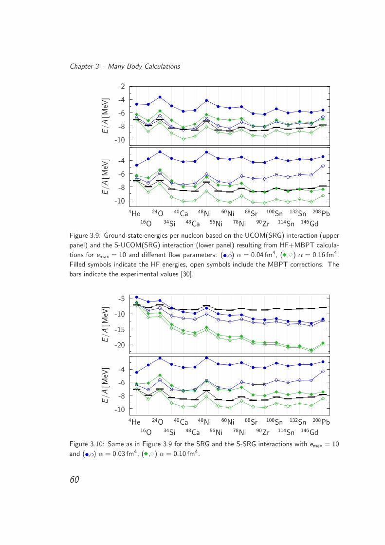
Chapter 3 · Many-Body Calculations
-10
-8
-6
-4
-2
.
E/A
[MeV
]
-10
-8
-6
-4
.
E/A
[MeV
]
4He16O
24O34Si
40Ca48Ca
48Ni56Ni
60Ni78Ni
88Sr90Zr
100Sn114Sn
132Sn146Gd
208Pb
Figure 3.9: Ground-state energies per nucleon based on the UCOM(SRG) interaction (upper
panel) and the S-UCOM(SRG) interaction (lower panel) resulting from HF+MBPT calcula-
tions for emax = 10 and different flow parameters: (,) α = 0.04 fm4, ( , ) α = 0.16 fm4.
Filled symbols indicate the HF energies, open symbols include the MBPT corrections. The
bars indicate the experimental values [30].
-20
-15
-10
-5
.
E/A
[MeV
]
-10
-8
-6
-4
.
E/A
[MeV
]
4He16O
24O34Si
40Ca48Ca
48Ni56Ni
60Ni78Ni
88Sr90Zr
100Sn114Sn
132Sn146Gd
208Pb
Figure 3.10: Same as in Figure 3.9 for the SRG and the S-SRG interactions with emax = 10
and (,) α = 0.03 fm4, ( , ) α = 0.10 fm4.
60
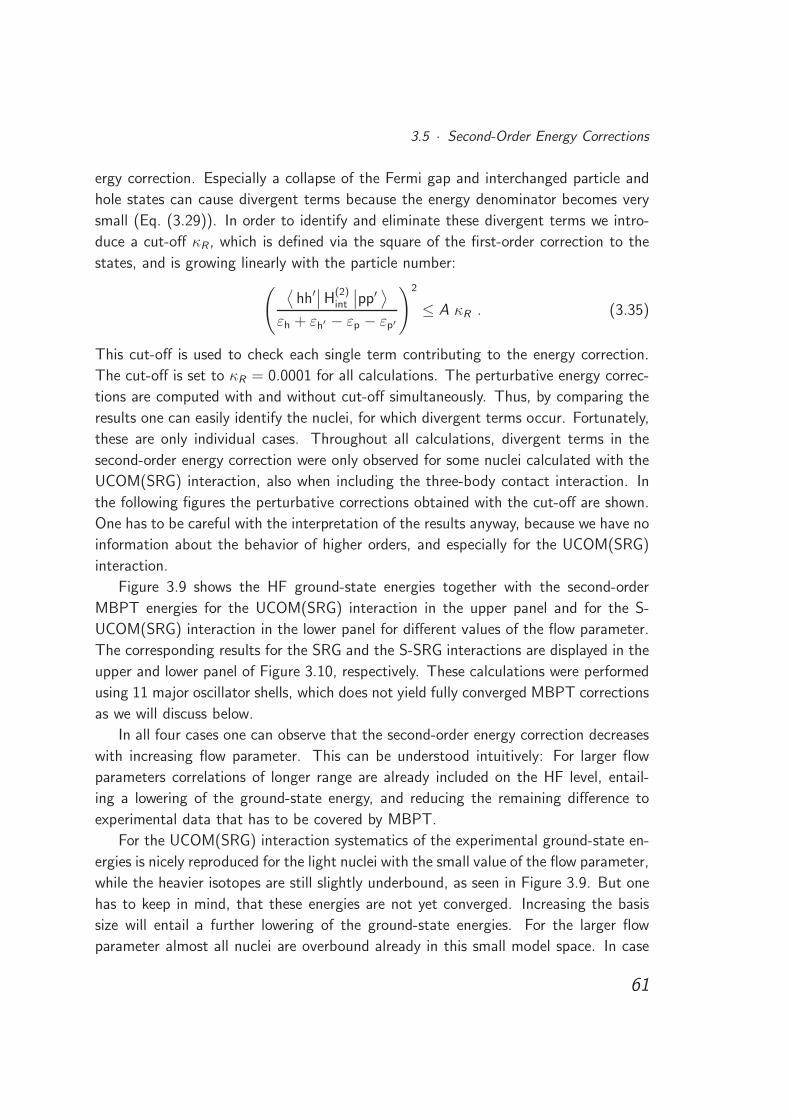
3.5 · Second-Order Energy Corrections
ergy correction. Especially a collapse of the Fermi gap and interchanged particle and
hole states can cause divergent terms because the energy denominator becomes very
small (Eq. (3.29)). In order to identify and eliminate these divergent terms we intro-
duce a cut-off κR , which is defined via the square of the first-order correction to the
states, and is growing linearly with the particle number:
( ⟨hh′∣∣H(2)
int
∣∣pp′ ⟩
εh + εh′ − εp − εp′
)2
≤ A κR . (3.35)
This cut-off is used to check each single term contributing to the energy correction.
The cut-off is set to κR = 0.0001 for all calculations. The perturbative energy correc-
tions are computed with and without cut-off simultaneously. Thus, by comparing the
results one can easily identify the nuclei, for which divergent terms occur. Fortunately,
these are only individual cases. Throughout all calculations, divergent terms in the
second-order energy correction were only observed for some nuclei calculated with the
UCOM(SRG) interaction, also when including the three-body contact interaction. In
the following figures the perturbative corrections obtained with the cut-off are shown.
One has to be careful with the interpretation of the results anyway, because we have no
information about the behavior of higher orders, and especially for the UCOM(SRG)
interaction.
Figure 3.9 shows the HF ground-state energies together with the second-order
MBPT energies for the UCOM(SRG) interaction in the upper panel and for the S-
UCOM(SRG) interaction in the lower panel for different values of the flow parameter.
The corresponding results for the SRG and the S-SRG interactions are displayed in the
upper and lower panel of Figure 3.10, respectively. These calculations were performed
using 11 major oscillator shells, which does not yield fully converged MBPT corrections
as we will discuss below.
In all four cases one can observe that the second-order energy correction decreases
with increasing flow parameter. This can be understood intuitively: For larger flow
parameters correlations of longer range are already included on the HF level, entail-
ing a lowering of the ground-state energy, and reducing the remaining difference to
experimental data that has to be covered by MBPT.
For the UCOM(SRG) interaction systematics of the experimental ground-state en-
ergies is nicely reproduced for the light nuclei with the small value of the flow parameter,
while the heavier isotopes are still slightly underbound, as seen in Figure 3.9. But one
has to keep in mind, that these energies are not yet converged. Increasing the basis
size will entail a further lowering of the ground-state energies. For the larger flow
parameter almost all nuclei are overbound already in this small model space. In case
61
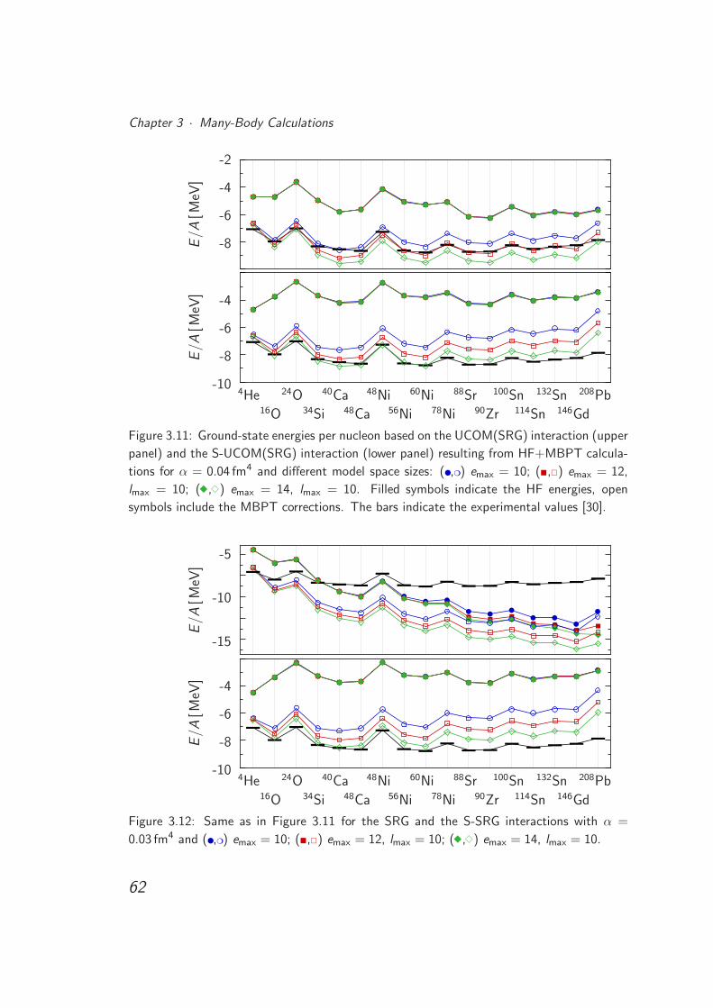
Chapter 3 · Many-Body Calculations
-8
-6
-4
-2
.
E/A
[MeV
]
-10
-8
-6
-4
.
E/A
[MeV
]
4He16O
24O34Si
40Ca48Ca
48Ni56Ni
60Ni78Ni
88Sr90Zr
100Sn114Sn
132Sn146Gd
208Pb
Figure 3.11: Ground-state energies per nucleon based on the UCOM(SRG) interaction (upper
panel) and the S-UCOM(SRG) interaction (lower panel) resulting from HF+MBPT calcula-
tions for α = 0.04 fm4 and different model space sizes: (,) emax = 10; (,) emax = 12,
lmax = 10; ( , ) emax = 14, lmax = 10. Filled symbols indicate the HF energies, open
symbols include the MBPT corrections. The bars indicate the experimental values [30].
-15
-10
-5
.
E/A
[MeV
]
-10
-8
-6
-4
.
E/A
[MeV
]
4He16O
24O34Si
40Ca48Ca
48Ni56Ni
60Ni78Ni
88Sr90Zr
100Sn114Sn
132Sn146Gd
208Pb
Figure 3.12: Same as in Figure 3.11 for the SRG and the S-SRG interactions with α =
0.03 fm4 and (,) emax = 10; (,) emax = 12, lmax = 10; ( , ) emax = 14, lmax = 10.
62
3.5 · Second-Order Energy Corrections
of the S-UCOM(SRG) and the S-SRG interaction the nuclei are still underbound when
using the small flow parameter and overbound for the larger flow parameter (Figs. 3.9
and 3.10). The energies calculated with the SRG interaction are significantly too low
already on the HF level, the second-order MBPT corrections cannot improve this trend
(Fig. 3.10).
Finally, we investigate the dependence of the second-order MBPT energy correc-
tions on the basis size emax. Therefore, we consider three model spaces, the smallest
with emax = 10, the second with emax = 12 with an additional truncation of the orbital
angular momentum at lmax = 10, and the largest considered model space is emax = 14,
lmax = 10.
Figure 3.11 shows the ground-state energies calculated with the UCOM(SRG) and
S-UCOM(SRG) interactions in the upper and lower part, respectively, using the flow
parameter α = 0.04 fm4 and the basis sizes mentioned above. The HF energies are fully
converged while the perturbative corrections are not yet converged, even for the largest
model space. In case of the UCOM(SRG) interaction the lowering of the ground-state
energies with increasing model space leads to a slight overbinding for most nuclei.
For the S-UCOM(SRG) interaction a reasonable agreement with experimental data is
achieved for the largest basis size, where one has to keep in mind that these energies
are not yet converged.
The ground-state energies obtained with the SRG and S-SRG interactions are shown
in Figure 3.12 using the flow parameter α = 0.03 fm4. For the SRG interaction even
the HF energies of the heaviest nuclei are not converged. Hence, the perturbative
corrections are not converged either. The results of the S-SRG interaction exhibit
an agreement with experiment which is comparable to those of the S-UCOM(SRG)
interaction keeping in mind the same limitations.
Regarding the UCOM(SRG), S-UCOM(SRG) and S-SRG interactions it is pos-
sible to achieve reasonable agreement with experimental data when calculating the
ground-state energies in the HF approximation and adding the second-order perturba-
tive corrections. The charge radii have not been considered in this section as it was
shown that the influence of many-body perturbation theory on charge radii is only
marginal [13]. Hence, to improve the description of charge radii we have to include a
repulsive three-body interaction in our calculations. We will then exploit the fact that
the considered nuclei are overbound on the basis of HF plus MBPT for larger values
of the flow parameter as a repulsive three-body interaction will counteract this trend.
63

Chapter 3 · Many-Body Calculations
64
Chapter 4
Gaussian Three-Body Interaction
In Chapter 3 we have discussed some properties of pure two-body interactions. The
investigation of ground-state energies and charge radii on the basis of HF plus MBPT
calculations has revealed that a three-body interaction is necessary for a quantitative
description of nuclear properties. We, therefore, introduce a finite-range three-body
interaction of Gaussian shape. First, the matrix elements of the Gaussian three-body
interaction are calculated in Section 4.1 and are then included in the HF approximation
(Sec. 4.2) and in many-body perturbation theory (Sec. 4.3).
4.1 Calculation of Matrix Elements
A Gaussian three-body interaction is a simple interaction of finite range, which can be
written as
VG3N = CG
3N exp
− 1
a23N
(r1 − r2)2 + (r2 − r3)
2 + (r3 − r1)2
(4.1)
with variable strength CG3N and range a3N.
The matrix elements are calculated in the harmonic-oscillator basis. In coordinate
space representation the matrix elements can be evaluated in spherical or cartesian co-
ordinates. Using spherical coordinates, it is convenient to calculate the matrix elements
in relative states. Since for various many-body methods the matrix elements need to
be calculated with respect to single-particle states a double Talmi-Moshinsky trans-
formation [37, 38], which is numerically costly, has to be applied. When calculating
65
Chapter 4 · Gaussian Three-Body Interaction
the matrix elements in cartesian coordinates one has to perform a transformation into
the spherical single-particle quantum numbers, which is time-consuming, too. Since
the latter option is computationally less costly, we evaluate the three-body matrix ele-
ments in cartesian single-particle coordinates and apply a transformation into spherical
coordinates subsequently.
4.1.1 Cartesian Matrix Elements
To evaluate the three-body matrix elements in the eigenbasis of the cartesian harmonic
oscillator, we start by considering three-body product states and perform the antisym-
metrization at the end. With the cartesian harmonic-oscillator quantum numbers nx ,
ny and nz the matrix elements read in coordinate representation:
〈nx1ny1
nz1, nx2
ny2nz2
, nx3ny3
nz3|VG
3N|n′x1
n′y1
n′z1
, n′x2
n′y2
n′z2
, n′x3
n′y3
n′z3〉
=
∫d3r1 d3r2 d3r3 Φ∗
nx1ny1nz1(r1)Φ
∗nx2ny2nz2
(r2)Φ∗nx3ny3nz3
(r3)
×CG3N exp
− 1
a23N
(r1 − r2)2 + (r2 − r3)
2 + (r3 − r1)2
×Φn′x1n′y1
n′z1(r1)Φn′x2
n′y2n′z2
(r2)Φn′x3n′y3
n′z3(r3) . (4.2)
The coordinate representation of the eigenstates of the harmonic oscillator Φnxny nz(r)
can be written as a product of three independent functions:
Φnxny nz(r) = ϕnx
(x)ϕny(y)ϕnz
(z) , (4.3)
where the one-dimensional wave function is given by
ϕnx(x) = Nnx
Hnx
(x
aHO
)exp
− x2
2a2HO
(4.4)
with the oscillator length aHO, the normalization factor Nnx= (
√π aHO 2nx nx !)
−1/2,
and the Hermite polynomials Hnx(x) [39]. Inserting the harmonic-oscillator wave func-
tions (4.3) into the expression for the matrix element, we can separate the three
66
4.1 · Calculation of Matrix Elements
cartesian dimensions:
〈nx1ny1
nz1, nx2
ny2nz2
, nx3ny3
nz3|VG
3N|n′x1
n′y1
n′z1
, n′x2
n′y2
n′z2
, n′x3
n′y3
n′z3〉
= CG3N
∫dx1 dx2 dx3 ϕnx1
(x1) ϕnx2(x2) ϕnx3
(x3) ϕn′x1(x1) ϕn′x2
(x2) ϕn′x3(x3)
×exp
− 1
a23N
(x1 − x2)2 + (x2 − x3)
2 + (x3 − x1)2
×∫
dy1 dy2 dy3 ϕny1(y1) ϕny2
(y2) ϕny3(y3) ϕn′y1
(y1) ϕn′y2(y2) ϕn′y3
(y3)
×exp
− 1
a23N
(y1 − y2)2 + (y2 − y3)
2 + (y3 − y1)2
×∫
dz1 dz2 dz3 ϕnz1(z1) ϕnz2
(z2) ϕnz3(z3) ϕn′z1
(z1) ϕn′z2(z2) ϕn′z3
(z3)
×exp
− 1
a23N
(z1 − z2)2 + (z2 − z3)
2 + (z3 − z1)2
≡ CG3N Inx(x1, x2, x3) Iny(y1, y2, y3) Inz(z1, z2, z3) . (4.5)
Hence, the matrix element is split into a product of three equivalent integrals. For
the further discussion we consider the integral Inx(x1, x2, x3). By inserting the one-
dimensional wave functions (4.4) we can reformulate the integral:
Inx(x1, x2, x3)
= N
∫dx1 dx2 dx3 Hnx1
(x1
aHO
)Hnx2
(x2
aHO
)Hnx3
(x3
aHO
)
×Hn′x1
(x1
aHO
)Hn′x2
(x2
aHO
)Hn′x3
(x3
aHO
)exp
− 1
a2HO
(x21 + x2
2 + x23 )
×exp
− 1
a23N
(x1 − x2)2 + (x2 − x3)
2 + (x3 − x1)2
= N
∫dx1 Hnx1
(x1
aHO
)Hn′x1
(x1
aHO
)exp
−(
1
a2HO
+2
a23N
)x21
×∫
dx2 Hnx2
(x2
aHO
)Hn′x2
(x2
aHO
)exp
−(
1
a2HO
+2
a23N
)x22 +
2x1
a23N
x2
×∫
dx3 Hnx3
(x3
aHO
)Hn′x3
(x3
aHO
)exp
−(
1
a2HO
+2
a23N
)x23 +
2(x1 + x2)
a23N
x3
with the normalization factor N = Nnx1Nnx2
Nnx3Nn′x1
Nn′x2Nn′x3
. We are not able to
provide an analytic solution for these integrals in a closed expression. Therefore, we
calculate them numerically and ensure the agreement with analytical values for some
67
Chapter 4 · Gaussian Three-Body Interaction
chosen sets of quantum numbers. The numerical calculation of a three-dimensional
integral is rather elaborate. Fortunately, these integrals can be computed by performing
three one-dimensional integrations. We start with the innermost integral and consider
(x1+x2) as a parameter, i.e. we solve the integral for a set of values for this parameter.
The result is inserted in the next integral, where we take x1 as parameter and follow
the same procedure. Finally, by using these results we can solve the outermost integral.
The numerical integration is performed via the application of the trapezoidal rule.
The program Mathematica [40] is capable of providing an exact solution of the three-
dimensional integral Inx(x1, x2, x3) if the quantum numbers are sufficiently small. We
are thus able to guarantee a sufficient accuracy of the numerical calculation.
For applications in many-body methods we have to perform a transformation of
these matrix elements from the cartesian harmonic oscillator into the spherical one.
4.1.2 Coordinate Transformation
In order to convert the three-body matrix elements the single-particle states of the
cartesian harmonic oscillator have to be transformed into spherical ones:
|nlml〉 =∑
nxny nz
|nxnynz〉〈nxnynz |nlml〉 , (4.6)
where the eigenstates of the spherical harmonic oscillator are defined via the principal
quantum number n and angular momentum l with projection ml . The transformation
coefficients 〈nxnynz |nlml〉 can be determined using the generating functions of the har-
monic oscillator wave functions [41]. The generating function of the three-dimensional
cartesian harmonic oscillator reads
F (x , y , z ; x0, y0, z0)
=∞∑
nx=0
∞∑
ny=0
∞∑
nz=0
1
nx ! ny ! nz !exp
− x2 + y 2 + z2
2a2HO
×Hnx
(x
aHO
)Hny
(y
aHO
)Hnz
(z
aHO
)(x0
aHO
)nx(
y0
aHO
)ny(
z0
aHO
)nz
. (4.7)
The eigenfunctions of the cartesian harmonic oscillator can be obtained by deriving
the generating function with respect to x0, y0, and z0 and evaluating the derivation
at x0 = y0 = z0 = 0. The generating function for the spherical harmonic oscillator is
68
4.1 · Calculation of Matrix Elements
given by
F (r ,ϑ,ϕ; r0,ϑ0,ϕ0)
=∞∑
n=0
∞∑
l=0
l∑
ml=−l
2π3/2(−1)n
Γ(n + l + 32)exp
− r 2
2a2HO
(r
aHO
)l
×L[l+ 1
2]
n
(r 2
a2HO
)Ylml
(ϑ,ϕ)Y ∗lml
(ϑ0,ϕ0)
(r0
aHO
)2n+l
. (4.8)
The coordinate representation of the eigenfunctions of the spherical harmonic oscillator
can again be obtained out of the derivatives of the corresponding generating function
with respect to r0, ϑ0, and ϕ0 and reads
ψnlml(r ,ϑ,ϕ) = Nnl exp
− r 2
2a2HO
(r
aHO
)l
L[l+ 1
2]
n
(r 2
a2HO
)Ylml
(ϑ,ϕ) (4.9)
with the normalization factor Nnl =√
2 n!a3HOΓ(n+l+3/2)
, the Laguerre polynomials
L[l+ 1
2]
n
(r2
a2HO
), and the spherical harmonics Ylml
(ϑ,ϕ).
Identifying these eigenfunctions in Equation (4.8) as well as the eigenfunctions (4.4)
of the cartesian harmonic oscillator in Equation (4.7), we find the following relation:
∞∑
nx=0
∞∑
ny =0
∞∑
nz=0
1
nx ! ny ! nz ! NnxNny
Nnz
|nxnynz〉xnx
0 yny
0 znz
0
=∞∑
n=0
∞∑
l=0
l∑
ml=−l
2π3/2(−1)n
Γ(n + l + 32)Nnl
|nlml〉Y ∗lml
(ϑ0,ϕ0)r2n+l0 , (4.10)
where we use the ket representation of the wave functions as we aim at the derivation
of the transformation coefficients 〈nxnynz |nlml〉. For this purpose we have to express
the spherical coordinates in cartesian ones. Therefore, we need the binomial formula
(x + y)n =n∑
k=0
(n
k
)xn−ky k , (4.11)
and the spherical harmonics in cartesian coordinates [42]
r lYlml(x , y , z) =
√2l + 1
4π(l + ml)!(l − ml)!
×∑
pqs
1
p! q! s!
(− x + i y
2
)p(x − i y
2
)q
z s (4.12)
69
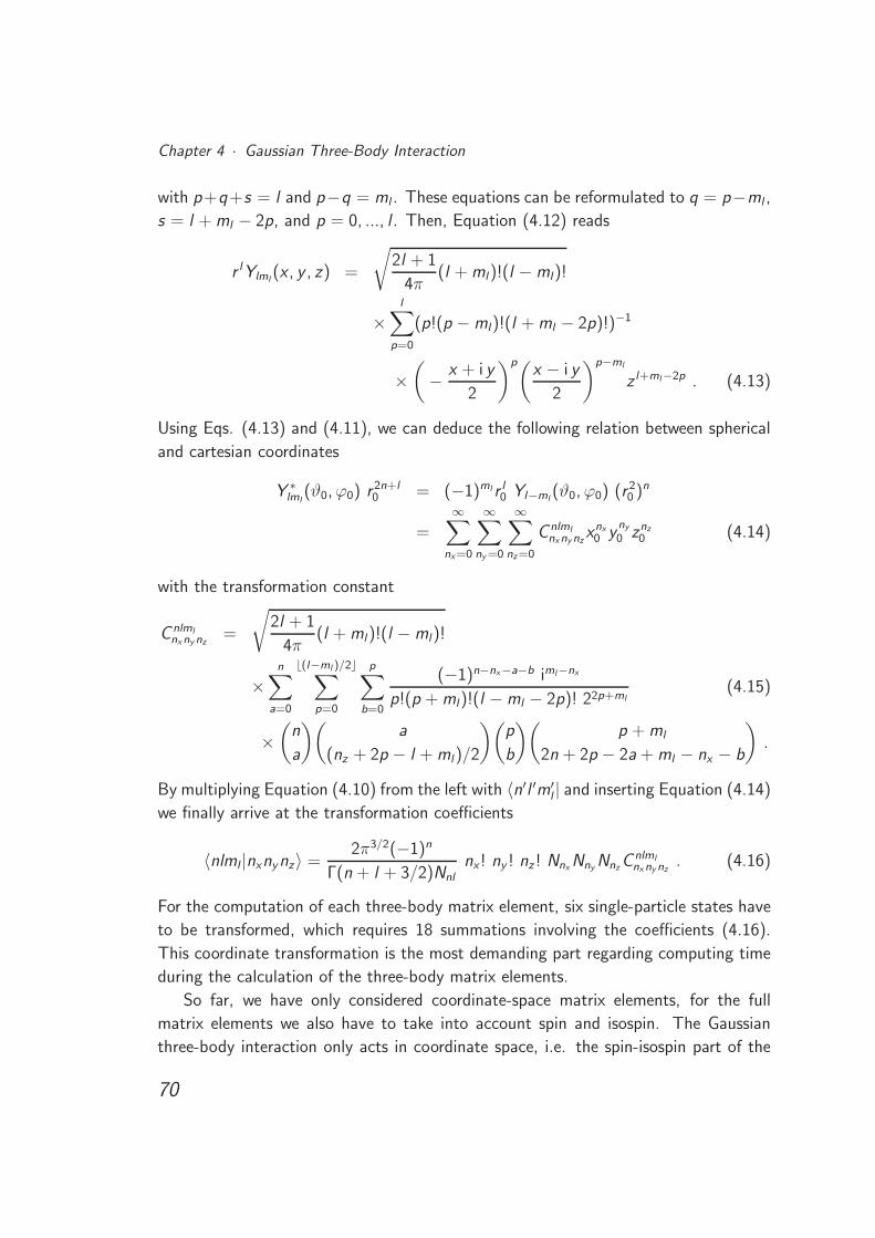
Chapter 4 · Gaussian Three-Body Interaction
with p+q+s = l and p−q = ml . These equations can be reformulated to q = p−ml ,
s = l + ml − 2p, and p = 0, ..., l . Then, Equation (4.12) reads
r lYlml(x , y , z) =
√2l + 1
4π(l + ml)!(l − ml)!
×l∑
p=0
(p!(p − ml)!(l + ml − 2p)!)−1
×(− x + i y
2
)p(x − i y
2
)p−ml
z l+ml−2p . (4.13)
Using Eqs. (4.13) and (4.11), we can deduce the following relation between spherical
and cartesian coordinates
Y ∗lml
(ϑ0,ϕ0) r 2n+l0 = (−1)ml r l
0 Yl−ml(ϑ0,ϕ0) (r 2
0 )n
=∞∑
nx=0
∞∑
ny=0
∞∑
nz=0
C nlmlnxnynz
xnx
0 yny
0 znz
0 (4.14)
with the transformation constant
C nlmlnxny nz
=
√2l + 1
4π(l + ml)!(l − ml)!
×n∑
a=0
⌊(l−ml )/2⌋∑
p=0
p∑
b=0
(−1)n−nx−a−b iml−nx
p!(p + ml)!(l − ml − 2p)! 22p+ml(4.15)
×(
n
a
)(a
(nz + 2p − l + ml)/2
)(p
b
)(p + ml
2n + 2p − 2a + ml − nx − b
).
By multiplying Equation (4.10) from the left with 〈n′l ′m′l | and inserting Equation (4.14)
we finally arrive at the transformation coefficients
〈nlml |nxnynz〉 =2π3/2(−1)n
Γ(n + l + 3/2)Nnl
nx ! ny ! nz ! NnxNny
NnzC nlml
nxnynz. (4.16)
For the computation of each three-body matrix element, six single-particle states have
to be transformed, which requires 18 summations involving the coefficients (4.16).
This coordinate transformation is the most demanding part regarding computing time
during the calculation of the three-body matrix elements.
So far, we have only considered coordinate-space matrix elements, for the full
matrix elements we also have to take into account spin and isospin. The Gaussian
three-body interaction only acts in coordinate space, i.e. the spin-isospin part of the
70
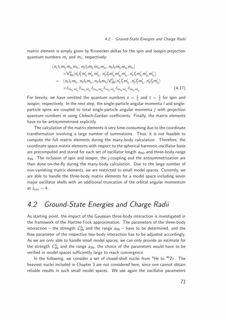
4.2 · Ground-State Energies and Charge Radii
matrix element is simply given by Kronecker deltas for the spin and isospin projection
quantum numbers ms and mt , respectively:
〈n1l1ml1ms1mt1 , n2l2ml2ms2mt2 , n3l3ml3ms3mt3 |×VG
3N|n′1l
′1m
′l1m′
s1m′
t1, n′
2l′2m
′l2m′
s2m′
t2, n′
3l′3m
′l3m′
s3m′
t3〉
= 〈n1l1ml1, n2l2ml2 , n3l3ml3 |VG3N|n′
1l′1m
′l1, n′
2l′2m
′l2, n′
3l′3m
′l3〉
×δms1m′s1δms2m′
s2δms3m′
s3δmt1m′
t1δmt2m′
t2δmt3m′
t3. (4.17)
For brevity, we have omitted the quantum numbers s = 12
and t = 12
for spin and
isospin, respectively. In the next step, the single-particle angular momenta l and single-
particle spins are coupled to total single-particle angular momenta j with projection
quantum numbers m using Clebsch-Gordan coefficients. Finally, the matrix elements
have to be antisymmetrized explicitly.
The calculation of the matrix elements is very time-consuming due to the coordinate
transformation involving a large number of summations. Thus, it is not feasible to
compute the full matrix elements during the many-body calculation. Therefore, the
coordinate space matrix elements with respect to the spherical harmonic-oscillator basis
are precomputed and stored for each set of oscillator length aHO and three-body range
a3N. The inclusion of spin and isospin, the j-coupling and the antisymmetrization are
then done on-the-fly during the many-body calculation. Due to the large number of
non-vanishing matrix elements, we are restricted to small model spaces. Currently, we
are able to handle the three-body matrix elements for a model space including seven
major oscillator shells with an additional truncation of the orbital angular momentum
at lmax = 4.
4.2 Ground-State Energies and Charge Radii
As starting point, the impact of the Gaussian three-body interaction is investigated in
the framework of the Hartree-Fock approximation. The parameters of the three-body
interaction – the strength CG3N and the range a3N – have to be determined, and the
flow parameter of the respective two-body interaction has to be adjusted accordingly.
As we are only able to handle small model spaces, we can only provide an estimate for
the strength CG3N and the range a3N, the choice of the parameters would have to be
verified in model spaces sufficiently large to reach convergence.
In the following, we consider a set of closed-shell nuclei from 4He to 90Zr. The
heaviest nuclei included in Chapter 3 are not considered here, since one cannot obtain
reliable results in such small model spaces. We use again the oscillator parameters
71
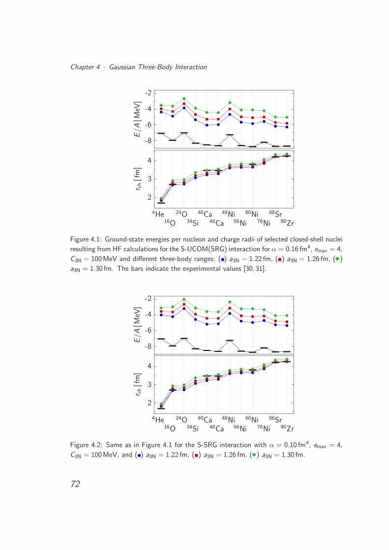
Chapter 4 · Gaussian Three-Body Interaction
-8
-6
-4
-2
.
E/A
[MeV
]
2
3
4
.
r ch[f
m]
4He16O
24O34Si
40Ca48Ca
48Ni56Ni
60Ni78Ni
88Sr90Zr
Figure 4.1: Ground-state energies per nucleon and charge radii of selected closed-shell nuclei
resulting from HF calculations for the S-UCOM(SRG) interaction for α = 0.16 fm4, emax = 4,
C3N = 100 MeV and different three-body ranges: () a3N = 1.22 fm, () a3N = 1.26 fm, ( )
a3N = 1.30 fm. The bars indicate the experimental values [30, 31].
-8
-6
-4
-2
.
E/A
[MeV
]
2
3
4
.
r ch[f
m]
4He16O
24O34Si
40Ca48Ca
48Ni56Ni
60Ni78Ni
88Sr90Zr
Figure 4.2: Same as in Figure 4.1 for the S-SRG interaction with α = 0.10 fm4, emax = 4,
C3N = 100 MeV, and () a3N = 1.22 fm, () a3N = 1.26 fm, ( ) a3N = 1.30 fm.
72
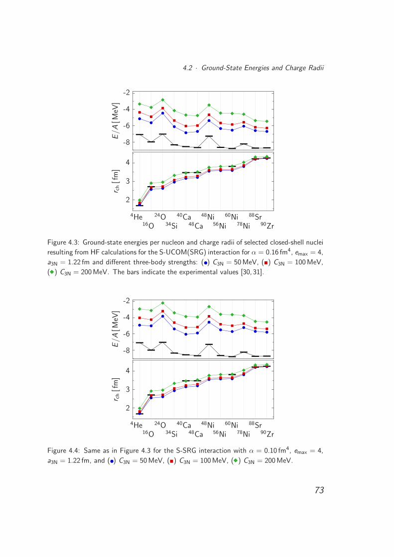
4.2 · Ground-State Energies and Charge Radii
-8
-6
-4
-2
.
E/A
[MeV
]
2
3
4
.
r ch[f
m]
4He16O
24O34Si
40Ca48Ca
48Ni56Ni
60Ni78Ni
88Sr90Zr
Figure 4.3: Ground-state energies per nucleon and charge radii of selected closed-shell nuclei
resulting from HF calculations for the S-UCOM(SRG) interaction for α = 0.16 fm4, emax = 4,
a3N = 1.22 fm and different three-body strengths: () C3N = 50 MeV, () C3N = 100 MeV,
( ) C3N = 200 MeV. The bars indicate the experimental values [30, 31].
-8
-6
-4
-2
.
E/A
[MeV
]
2
3
4
.
r ch[f
m]
4He16O
24O34Si
40Ca48Ca
48Ni56Ni
60Ni78Ni
88Sr90Zr
Figure 4.4: Same as in Figure 4.3 for the S-SRG interaction with α = 0.10 fm4, emax = 4,
a3N = 1.22 fm, and () C3N = 50 MeV, () C3N = 100 MeV, ( ) C3N = 200 MeV.
73
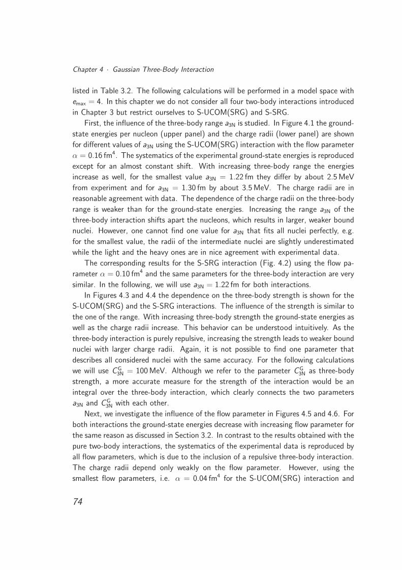
Chapter 4 · Gaussian Three-Body Interaction
listed in Table 3.2. The following calculations will be performed in a model space with
emax = 4. In this chapter we do not consider all four two-body interactions introduced
in Chapter 3 but restrict ourselves to S-UCOM(SRG) and S-SRG.
First, the influence of the three-body range a3N is studied. In Figure 4.1 the ground-
state energies per nucleon (upper panel) and the charge radii (lower panel) are shown
for different values of a3N using the S-UCOM(SRG) interaction with the flow parameter
α = 0.16 fm4. The systematics of the experimental ground-state energies is reproduced
except for an almost constant shift. With increasing three-body range the energies
increase as well, for the smallest value a3N = 1.22 fm they differ by about 2.5 MeV
from experiment and for a3N = 1.30 fm by about 3.5 MeV. The charge radii are in
reasonable agreement with data. The dependence of the charge radii on the three-body
range is weaker than for the ground-state energies. Increasing the range a3N of the
three-body interaction shifts apart the nucleons, which results in larger, weaker bound
nuclei. However, one cannot find one value for a3N that fits all nuclei perfectly, e.g.
for the smallest value, the radii of the intermediate nuclei are slightly underestimated
while the light and the heavy ones are in nice agreement with experimental data.
The corresponding results for the S-SRG interaction (Fig. 4.2) using the flow pa-
rameter α = 0.10 fm4 and the same parameters for the three-body interaction are very
similar. In the following, we will use a3N = 1.22 fm for both interactions.
In Figures 4.3 and 4.4 the dependence on the three-body strength is shown for the
S-UCOM(SRG) and the S-SRG interactions. The influence of the strength is similar to
the one of the range. With increasing three-body strength the ground-state energies as
well as the charge radii increase. This behavior can be understood intuitively. As the
three-body interaction is purely repulsive, increasing the strength leads to weaker bound
nuclei with larger charge radii. Again, it is not possible to find one parameter that
describes all considered nuclei with the same accuracy. For the following calculations
we will use CG3N = 100 MeV. Although we refer to the parameter CG
3N as three-body
strength, a more accurate measure for the strength of the interaction would be an
integral over the three-body interaction, which clearly connects the two parameters
a3N and CG3N with each other.
Next, we investigate the influence of the flow parameter in Figures 4.5 and 4.6. For
both interactions the ground-state energies decrease with increasing flow parameter for
the same reason as discussed in Section 3.2. In contrast to the results obtained with the
pure two-body interactions, the systematics of the experimental data is reproduced by
all flow parameters, which is due to the inclusion of a repulsive three-body interaction.
The charge radii depend only weakly on the flow parameter. However, using the
smallest flow parameters, i.e. α = 0.04 fm4 for the S-UCOM(SRG) interaction and
74
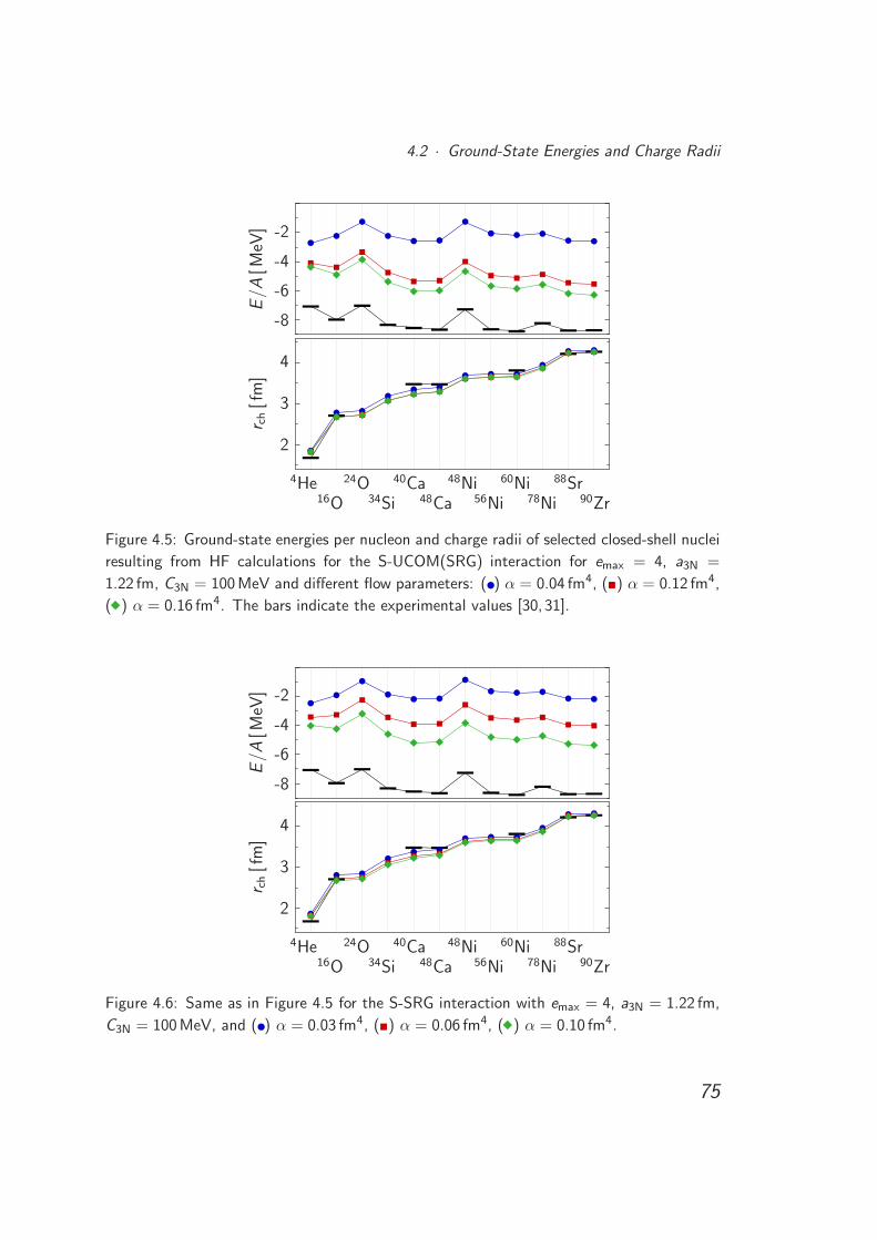
4.2 · Ground-State Energies and Charge Radii
-8
-6
-4
-2
.
E/A
[MeV
]
2
3
4
.
r ch[f
m]
4He16O
24O34Si
40Ca48Ca
48Ni56Ni
60Ni78Ni
88Sr90Zr
Figure 4.5: Ground-state energies per nucleon and charge radii of selected closed-shell nuclei
resulting from HF calculations for the S-UCOM(SRG) interaction for emax = 4, a3N =
1.22 fm, C3N = 100 MeV and different flow parameters: () α = 0.04 fm4, () α = 0.12 fm4,
( ) α = 0.16 fm4. The bars indicate the experimental values [30, 31].
-8
-6
-4
-2
.
E/A
[MeV
]
2
3
4
.
r ch[f
m]
4He16O
24O34Si
40Ca48Ca
48Ni56Ni
60Ni78Ni
88Sr90Zr
Figure 4.6: Same as in Figure 4.5 for the S-SRG interaction with emax = 4, a3N = 1.22 fm,
C3N = 100 MeV, and () α = 0.03 fm4, () α = 0.06 fm4, ( ) α = 0.10 fm4.
75
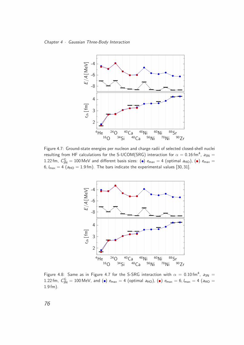
Chapter 4 · Gaussian Three-Body Interaction
-8
-6
-4
.E/A
[MeV
]
2
3
4
.
r ch[f
m]
4He16O
24O34Si
40Ca48Ca
48Ni56Ni
60Ni78Ni
88Sr90Zr
Figure 4.7: Ground-state energies per nucleon and charge radii of selected closed-shell nuclei
resulting from HF calculations for the S-UCOM(SRG) interaction for α = 0.16 fm4, a3N =
1.22 fm, CG3N = 100 MeV and different basis sizes: () emax = 4 (optimal aHO), () emax =
6, lmax = 4 (aHO = 1.9 fm). The bars indicate the experimental values [30, 31].
-8
-6
-4
.
E/A
[MeV
]
2
3
4
.
r ch[f
m]
4He16O
24O34Si
40Ca48Ca
48Ni56Ni
60Ni78Ni
88Sr90Zr
Figure 4.8: Same as in Figure 4.7 for the S-SRG interaction with α = 0.10 fm4, a3N =
1.22 fm, CG3N = 100 MeV, and () emax = 4 (optimal aHO), () emax = 6, lmax = 4 (aHO =
1.9 fm).
76
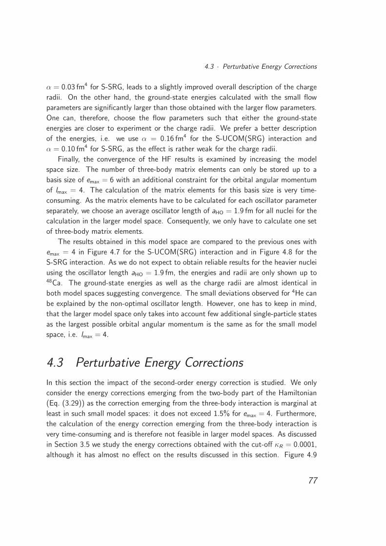
4.3 · Perturbative Energy Corrections
α = 0.03 fm4 for S-SRG, leads to a slightly improved overall description of the charge
radii. On the other hand, the ground-state energies calculated with the small flow
parameters are significantly larger than those obtained with the larger flow parameters.
One can, therefore, choose the flow parameters such that either the ground-state
energies are closer to experiment or the charge radii. We prefer a better description
of the energies, i.e. we use α = 0.16 fm4 for the S-UCOM(SRG) interaction and
α = 0.10 fm4 for S-SRG, as the effect is rather weak for the charge radii.
Finally, the convergence of the HF results is examined by increasing the model
space size. The number of three-body matrix elements can only be stored up to a
basis size of emax = 6 with an additional constraint for the orbital angular momentum
of lmax = 4. The calculation of the matrix elements for this basis size is very time-
consuming. As the matrix elements have to be calculated for each oscillator parameter
separately, we choose an average oscillator length of aHO = 1.9 fm for all nuclei for the
calculation in the larger model space. Consequently, we only have to calculate one set
of three-body matrix elements.
The results obtained in this model space are compared to the previous ones with
emax = 4 in Figure 4.7 for the S-UCOM(SRG) interaction and in Figure 4.8 for the
S-SRG interaction. As we do not expect to obtain reliable results for the heavier nuclei
using the oscillator length aHO = 1.9 fm, the energies and radii are only shown up to48Ca. The ground-state energies as well as the charge radii are almost identical in
both model spaces suggesting convergence. The small deviations observed for 4He can
be explained by the non-optimal oscillator length. However, one has to keep in mind,
that the larger model space only takes into account few additional single-particle states
as the largest possible orbital angular momentum is the same as for the small model
space, i.e. lmax = 4.
4.3 Perturbative Energy Corrections
In this section the impact of the second-order energy correction is studied. We only
consider the energy corrections emerging from the two-body part of the Hamiltonian
(Eq. (3.29)) as the correction emerging from the three-body interaction is marginal at
least in such small model spaces: it does not exceed 1.5% for emax = 4. Furthermore,
the calculation of the energy correction emerging from the three-body interaction is
very time-consuming and is therefore not feasible in larger model spaces. As discussed
in Section 3.5 we study the energy corrections obtained with the cut-off κR = 0.0001,
although it has almost no effect on the results discussed in this section. Figure 4.9
77
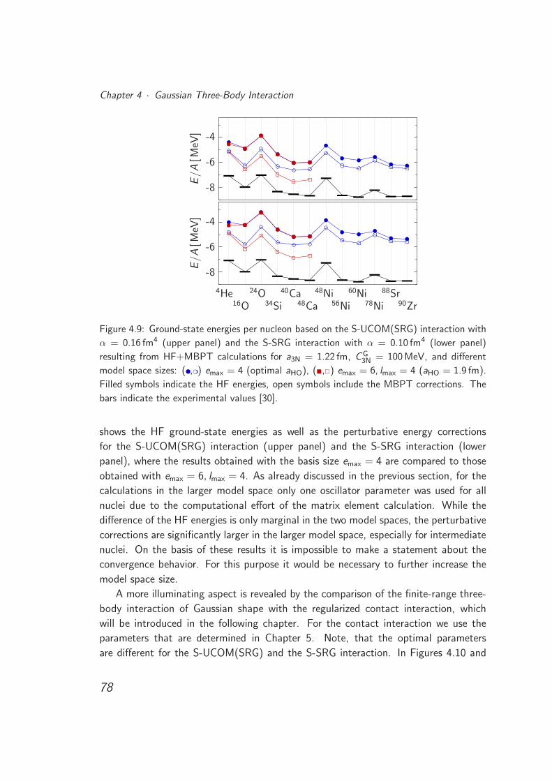
Chapter 4 · Gaussian Three-Body Interaction
-8
-6
-4
.E/A
[MeV
]
-8
-6
-4
.
E/A
[MeV
]
4He16O
24O34Si
40Ca48Ca
48Ni56Ni
60Ni78Ni
88Sr90Zr
Figure 4.9: Ground-state energies per nucleon based on the S-UCOM(SRG) interaction with
α = 0.16 fm4 (upper panel) and the S-SRG interaction with α = 0.10 fm4 (lower panel)
resulting from HF+MBPT calculations for a3N = 1.22 fm, CG3N = 100 MeV, and different
model space sizes: (,) emax = 4 (optimal aHO), (,) emax = 6, lmax = 4 (aHO = 1.9 fm).
Filled symbols indicate the HF energies, open symbols include the MBPT corrections. The
bars indicate the experimental values [30].
shows the HF ground-state energies as well as the perturbative energy corrections
for the S-UCOM(SRG) interaction (upper panel) and the S-SRG interaction (lower
panel), where the results obtained with the basis size emax = 4 are compared to those
obtained with emax = 6, lmax = 4. As already discussed in the previous section, for the
calculations in the larger model space only one oscillator parameter was used for all
nuclei due to the computational effort of the matrix element calculation. While the
difference of the HF energies is only marginal in the two model spaces, the perturbative
corrections are significantly larger in the larger model space, especially for intermediate
nuclei. On the basis of these results it is impossible to make a statement about the
convergence behavior. For this purpose it would be necessary to further increase the
model space size.
A more illuminating aspect is revealed by the comparison of the finite-range three-
body interaction of Gaussian shape with the regularized contact interaction, which
will be introduced in the following chapter. For the contact interaction we use the
parameters that are determined in Chapter 5. Note, that the optimal parameters
are different for the S-UCOM(SRG) and the S-SRG interaction. In Figures 4.10 and
78
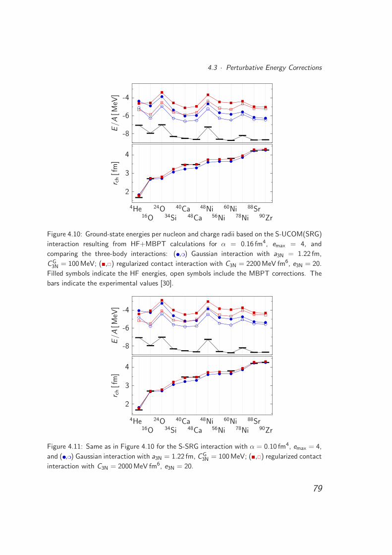
4.3 · Perturbative Energy Corrections
-8
-6
-4
.
E/A
[MeV
]
2
3
4
.
r ch[f
m]
4He16O
24O34Si
40Ca48Ca
48Ni56Ni
60Ni78Ni
88Sr90Zr
Figure 4.10: Ground-state energies per nucleon and charge radii based on the S-UCOM(SRG)
interaction resulting from HF+MBPT calculations for α = 0.16 fm4, emax = 4, and
comparing the three-body interactions: (,) Gaussian interaction with a3N = 1.22 fm,
CG3N = 100 MeV; (,) regularized contact interaction with C3N = 2200 MeV fm6, e3N = 20.
Filled symbols indicate the HF energies, open symbols include the MBPT corrections. The
bars indicate the experimental values [30].
-8
-6
-4
.
E/A
[MeV
]
2
3
4
.
r ch[f
m]
4He16O
24O34Si
40Ca48Ca
48Ni56Ni
60Ni78Ni
88Sr90Zr
Figure 4.11: Same as in Figure 4.10 for the S-SRG interaction with α = 0.10 fm4, emax = 4,
and (,) Gaussian interaction with a3N = 1.22 fm, CG3N = 100 MeV; (,) regularized contact
interaction with C3N = 2000 MeV fm6, e3N = 20.
79
Chapter 4 · Gaussian Three-Body Interaction
4.11 the HF ground-state energies together with the perturbative corrections emerging
from the two-body Hamiltonian and the charge radii are shown for the S-UCOM(SRG)
and the S-SRG interactions in a model space including five major oscillator shells.
The comparison of the Gaussian three-body interaction with the regularized contact
interaction reveals that the latter yields slightly less binding energy for intermediate
and heavy nuclei on the HF level. This discrepancy could be reduced by an adjustment
of the parameters. The perturbative energy corrections are almost identical for both
interactions across the whole nuclear chart, which is not surprising as the corrections
are only calculated for the two-body interactions being the same in both cases. The
calculated charge radii are similar for both three-body interactions, but the overall
agreement with experimental data is slightly better for the contact interaction. The
results are very similar for both underlying two-body interactions.
On the basis of these results, we can motivate the following strategy: The Gaus-
sian three-body interaction is the most simple finite-range three-body interaction, but
we can only handle it in very small model spaces. The calculation of the matrix el-
ements of the regularized three-body contact interaction is much more efficient and
this interaction can also be included in larger model spaces. We have shown that
both three-body interactions yield comparable results in small model spaces. We will,
therefore, perform further studies on the basis of the regularized contact interaction.
As this three-body interaction can be included in various many-body methods and in
sufficiently large model spaces, this procedure allows for reliable investigations.
80
Chapter 5
Three-Body Contact Interaction
In Chapter 4 we have seen that already the most simple finite-range three-body force
of Gaussian shape proves to be an enormous computational challenge. In this case,
it was not possible to perform calculations in sufficiently large Hilbert spaces allowing
for reliable converged calculations. In order to investigate the impact of three-body
forces and to develop strategies for the handling of three-body matrix elements we
introduce a three-body contact interaction. In this chapter we discuss the calculation
of the matrix elements of a regularized three-body contact interaction in Section 5.1.
Subsequently, the Hartree-Fock method is used to calculate ground-state energies and
charge radii in Section 5.2 as well as single-particle spectra in Section 5.3. In Section 5.4
the second-order energy corrections emerging from many-body perturbation theory are
discussed.
5.1 Calculation of Matrix Elements
In the following, we discuss the calculation of the matrix elements of a three-body
contact interaction which is supplemented by a cut-off introduced at the end of this
section. The three-body contact interaction can be written as
V3N = C3N δ(3)(x1 − x2)δ(3)(x1 − x3) (5.1)
with variable strength C3N, and δ(3)(x) being the Dirac delta distribution in three
dimensions. The strength C3N of the three-body interaction will be positive since the
interaction has to be repulsive in order to increase the charge radii (cf. Sec. 3.2).
81
Chapter 5 · Three-Body Contact Interaction
Considering general three-body interactions it is common to calculate the matrix
elements in a basis that is based on Jacobi coordinates. But for applications in many-
body methods the matrix elements have to be transformed into the m-scheme, i.e.
using independent single-particle states, which is computationally very demanding for
a three-body interaction. In contrast, the matrix elements of a contact interaction
can be directly evaluated in the m-scheme, which is of great advantage compared to
general three-body forces. The calculation of these matrix elements has already been
discussed in my diploma thesis [27], but since it is the most essential ingredient for the
following investigations it will be recapitulated in this section.
The matrix elements are calculated in the harmonic-oscillator basis. We start
with three-body product states in coordinate space. Since the three-body contact
interaction does not affect spin and isospin, we will neglect these quantum numbers
for the moment. The antisymmetrization will be performed explicitly in the end.
Introducing the coordinate-space representation of the harmonic-oscillator states, the
matrix elements can be expressed as
〈n1l1ml1, n2l2ml2 , n3l3ml3 |V3N|n′1l
′1m
′l1, n′
2l′2m
′l2, n′
3l′3m
′l3〉
=
∫d3x1d
3x2d3x3〈n1l1ml1|x1〉〈n2l2ml2|x2〉〈n3l3ml3|x3〉
×C3N δ(3)(x1 − x2) δ(3)(x1 − x3)〈x1|n′
1l′1m
′l1〉〈x2|n′
2l′2m
′l2〉〈x3|n′
3l′3m
′l3〉
(5.2)
with the principal quantum number n, angular momentum l and projection quantum
number ml of the harmonic oscillator states. By introducing the relative coordinates
r12 = x1 − x2 and r13 = x1 − x3 we can directly exploit the properties of the delta
distributions and evaluate six of the nine integrals:
∫d3x1d
3x2d3x3〈n1l1ml1|x1〉〈n2l2ml2 |x2〉〈n3l3ml3 |x3〉
×C3N δ(3)(x1 − x2) δ(3)(x1 − x3)〈x1|n′
1l′1m
′l1〉〈x2|n′
2l′2m
′l2〉〈x3|n′
3l′3m
′l3〉
=
∫d3x1d
3r12d3r13〈n1l1ml1 |x1〉〈n2l2ml2 |x1 − r12〉〈n3l3ml3 |x1 − r13〉
×C3N δ(3)(r12) δ(3)(r13)〈x1|n′
1l′1m
′l1〉〈x1 − r12|n′
2l′2m
′l2〉〈x1 − r13|n′
3l′3m
′l3〉
= C3N
∫d3x1〈n1l1ml1 |x1〉〈n2l2ml2 |x1〉〈n3l3ml3 |x1〉
×〈x1|n′1l
′1m
′l1〉〈x1|n′
2l′2m
′l2〉〈x1|n′
3l′3m
′l3〉 . (5.3)
In coordinate space, the harmonic-oscillator eigenfunctions are composed of a real-
valued radial part Rnl(x) and an angular part represented by the spherical harmonics
82
5.1 · Calculation of Matrix Elements
Ylml(Ω) [39]:
〈x|nlml〉 = Rnl(x)Ylml(Ω) . (5.4)
Inserting this representation into Equation (5.3) one arrives at
〈n1l1ml1 , n2l2ml2, n3l3ml3 |V3N|n′1l
′1m
′l1, n′
2l′2m
′l2, n′
3l′3m
′l3〉
= C3N
∫dx1x
21Rn1l1(x1)Rn2l2(x1)Rn3l3(x1)Rn′1l
′1(x1)Rn′2l
′2(x1)Rn′3l
′3(x1)
×∫
dΩ Y ∗l1ml1
(Ω)Y ∗l2ml2
(Ω)Y ∗l3ml3
(Ω)Yl ′1m′l1(Ω)Yl ′2m
′l2(Ω)Yl ′3m
′l3(Ω) . (5.5)
The integral over the six radial wavefunctions has to be calculated numerically while
the integral over the six spherical harmonics can be evaluated analytically. The product
of three spherical harmonics can be reduced to one spherical harmonic:
Yl1ml1(Ω)Yl2ml2
(Ω)Yl3ml3(Ω)
=∑
L1ML1
√(2l1 + 1)(2l2 + 1)
4π(2L1 + 1)c(
l1 l2
0 0
∣∣∣ L1
0
)c(
l1 l2ml1
ml2
∣∣∣ L1
ML1
)YL1ML1
(Ω)Yl3ml3(Ω)
=∑
L1ML1
√(2l1 + 1)(2l2 + 1)
4π(2L1 + 1)c(
l1 l2
0 0
∣∣∣ L1
0
)c(
l1 l2ml1
ml2
∣∣∣ L1
ML1
)
×∑
L2ML2
√(2L1 + 1)(2l3 + 1)
4π(2L2 + 1)c(
L1 l3
0 0
∣∣∣ L2
0
)c(
L1 l3
ML1ml3
∣∣∣ L2
ML2
)YL2ML2
(Ω) (5.6)
with the Clebsch-Gordan coefficients c(
l1 l2ml1
ml2
∣∣∣ L
ML
). Using this relation we can eval-
83
Chapter 5 · Three-Body Contact Interaction
uate the angular part of the integral:
∫dΩ Y ∗
l1ml1(Ω)Y ∗
l2ml2(Ω)Y ∗
l3ml3(Ω)Yl ′1m
′l1(Ω)Yl ′2m
′l2(Ω)Yl ′3m
′l3(Ω)
=∑
L1ML1L2ML2
√(2l1 + 1)(2l2 + 1)
4π(2L1 + 1)
√(2L1 + 1)(2l3 + 1)
4π(2L2 + 1)
×c(
l1 l2
0 0
∣∣∣ L1
0
)c(
l1 l2ml1
ml2
∣∣∣ L1
ML1
)c(
L1 l3
0 0
∣∣∣ L2
0
)c(
L1 l3
ML1ml3
∣∣∣ L2
ML2
)
×∑
L′1M′
L1L′2M′
L2
√(2l ′1 + 1)(2l ′2 + 1)
4π(2L′1 + 1)
√(2L′
1 + 1)(2l ′3 + 1)
4π(2L′2 + 1)
×c(
l ′1 l ′2
0 0
∣∣∣ L′1
0
)c
(l ′1 l ′2
m′l1
m′l2
∣∣∣∣L′
1
M′L1
)c(
L′1 l ′3
0 0
∣∣∣ L′2
0
)c
(L′
1 l ′3
M′L1
m′l3
∣∣∣∣L′
2
M′L2
)
×∫
dΩ Y ∗L2ML2
(Ω)YL′2M
′L2
(Ω)︸ ︷︷ ︸
=δL2L′2δML2
M′L2
=∑
L1L2L′1
ML1ML2
M′L1
√(2l1 + 1)(2l2 + 1)(2l3 + 1)(2l ′1 + 1)(2l ′2 + 1)(2l ′3 + 1)
16π2(2L2 + 1)
×c(
l1 l2
0 0
∣∣∣ L1
0
)c(
l1 l2ml1
ml2
∣∣∣ L1
ML1
)c(
L1 l3
0 0
∣∣∣ L2
0
)c(
L1 l3
ML1ml3
∣∣∣ L2
ML2
)
×c(
l ′1 l ′2
0 0
∣∣∣ L′1
0
)c
(l ′1 l ′2
m′l1
m′l2
∣∣∣∣L′
1
M′L1
)c(
L′1 l ′3
0 0
∣∣∣ L2
0
)c
(L′
1 l ′3
M′L1
m′l3
∣∣∣ L2
ML2
). (5.7)
Hence, the calculation of the angular integral is reduced to six summations over a
number of Clebsch-Gordan coefficients.
For the complete matrix element we have to include spin and isospin degrees of
freedom. As the three-body contact interaction only acts in coordinate space, the
evaluation of matrix elements simply yields Kronecker deltas for the spin and isospin
projection quantum numbers ms and mt , respectively:
〈n1l1ml1ms1mt1 , n2l2ml2ms2mt2 , n3l3ml3ms3mt3 |× V3N|n′
1l′1m
′l1m′
s1m′
t1, n′
2l′2m
′l2m′
s2m′
t2, n′
3l′3m
′l3m′
s3m′
t3〉
= 〈n1l1ml1 , n2l2ml2, n3l3ml3 |V3N|n′1l
′1m
′l1, n′
2l′2m
′l2, n′
3l′3m
′l3〉
× δms1m′s1δms2m′
s2δms3m′
s3δmt1m′
t1δmt2m′
t2δmt3m′
t3. (5.8)
84
5.1 · Calculation of Matrix Elements
For brevity, we have omitted the quantum numbers s = 12
and t = 12
for spin and
isospin, respectively.
For the practical application of the three-body interaction in various many-body
methods, the single-particle angular momenta li and spins si have to be coupled to
total single-particle angular momenta ji . This is achieved by inserting a number of
Clebsch-Gordan coefficients yielding the j-coupled three-body matrix elements
〈n1l1j1m1mt1 , n2l2j2m2mt2 , n3l3j3m3mt3 |×V3N|n′
1l′1j
′1m
′1m
′t1, n′
2l′2j
′2m
′2m
′t2, n′
3l′3j
′3m
′3m
′t3〉
=∑
ml1...m′
l3ms1 ...m′
s3
c(
l112
ml1ms1
∣∣∣ j1m1
)c(
l212
ml2ms2
∣∣∣ j2m2
)c(
l312
ml3ms3
∣∣∣ j3m3
)
×c
(l ′1
12
m′l1
m′s1
∣∣∣ j ′1
m′1
)c
(l ′2
12
m′l2
m′s2
∣∣∣ j ′2
m′2
)c
(l ′3
12
m′l3
m′s3
∣∣∣ j ′3
m′3
)
×〈n1l1ml1ms1mt1 , n2l2ml2ms2mt2 , n3l3ml3ms3mt3 |×V3N|n′
1l′1m
′l1m′
s1m′
t1, n′
2l′2m
′l2m′
s2m′
t2, n′
3l′3m
′l3m′
s3m′
t3〉
=∑
ml1...m′
l3ms1 ...m′
s3
c(
l112
ml1ms1
∣∣∣ j1m1
)c(
l212
ml2ms2
∣∣∣ j2m2
)c(
l312
ml3ms3
∣∣∣ j3m3
)
×c
(l ′1
12
m′l1
m′s1
∣∣∣ j ′1
m′1
)c
(l ′2
12
m′l2
m′s2
∣∣∣ j ′2
m′2
)c
(l ′3
12
m′l3
m′s3
∣∣∣ j ′3
m′3
)
×C3N
∫dx x2Rn1l1(x)Rn2l2(x)Rn3l3(x)Rn′1l
′1(x)Rn′2l
′2(x)Rn′3l
′3(x)
× 1
16π2
√(2l1 + 1)(2l2 + 1)(2l3 + 1)(2l ′1 + 1)(2l ′2 + 1)(2l ′3 + 1)
×∑
L1L2L′1
ML1ML2
M′L1
1
(2L2 + 1)c(
l1 l2
0 0
∣∣∣ L1
0
)c(
L1 l3
0 0
∣∣∣ L2
0
)c(
l ′1 l ′2
0 0
∣∣∣ L′1
0
)c(
L′1 l ′3
0 0
∣∣∣ L2
0
)
×c(
l1 l2ml1
ml2
∣∣∣ L1
ML1
)c(
L1 l3
ML1ml3
∣∣∣ L2
ML2
)c
(l ′1 l ′2
m′l1
m′l2
∣∣∣∣L′
1
M′L1
)c
(L′
1 l ′3
M′L1
m′l3
∣∣∣ L2
ML2
)
×δms1m′s1δms2m′
s2δms3m′
s3δmt1m′
t1δmt2m′
t2δmt3m′
t3. (5.9)
For an efficient calculation of the three-body matrix elements it is advantageous to
evaluate as many as possible of these 18 sums analytically. Therefore, one can evaluate
the Kronecker deltas and exploit the condition m1 + m2 = M in the Clebsch-Gordan
85
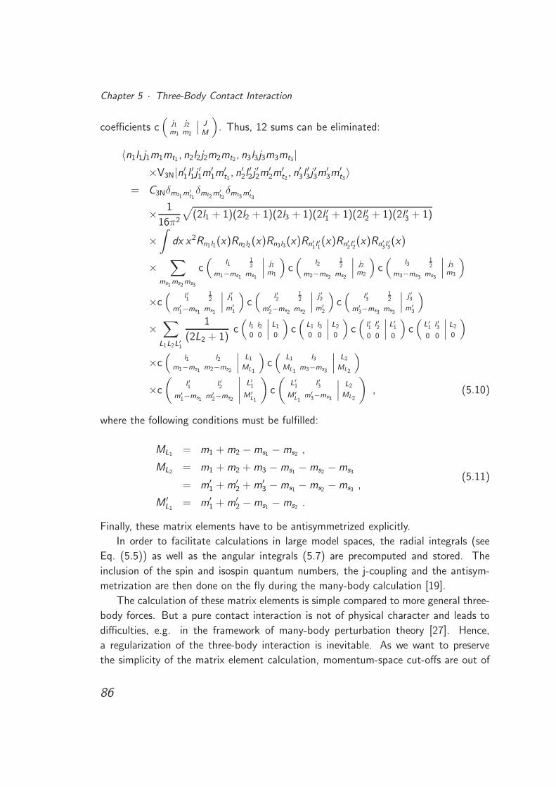
Chapter 5 · Three-Body Contact Interaction
coefficients c(
j1 j2m1 m2
∣∣ J
M
). Thus, 12 sums can be eliminated:
〈n1l1j1m1mt1 , n2l2j2m2mt2 , n3l3j3m3mt3 |×V3N|n′
1l′1j
′1m
′1m
′t1, n′
2l′2j
′2m
′2m
′t2, n′
3l′3j
′3m
′3m
′t3〉
= C3Nδmt1m′t1δmt2m′
t2δmt3m′
t3
× 1
16π2
√(2l1 + 1)(2l2 + 1)(2l3 + 1)(2l ′1 + 1)(2l ′2 + 1)(2l ′3 + 1)
×∫
dx x2Rn1l1(x)Rn2l2(x)Rn3l3(x)Rn′1l′1(x)Rn′2l
′2(x)Rn′3l
′3(x)
×∑
ms1ms2ms3
c(
l112
m1−ms1 ms1
∣∣∣ j1m1
)c(
l212
m2−ms2 ms2
∣∣∣ j2m2
)c(
l312
m3−ms3 ms3
∣∣∣ j3m3
)
×c(
l ′112
m′1−ms1 ms1
∣∣∣ j ′1
m′1
)c(
l ′212
m′2−ms2 ms2
∣∣∣ j ′2
m′2
)c(
l ′312
m′3−ms3 ms3
∣∣∣ j ′3
m′3
)
×∑
L1L2L′1
1
(2L2 + 1)c(
l1 l2
0 0
∣∣∣ L1
0
)c(
L1 l3
0 0
∣∣∣ L2
0
)c(
l ′1 l ′2
0 0
∣∣∣ L′1
0
)c(
L′1 l ′3
0 0
∣∣∣ L2
0
)
×c(
l1 l2
m1−ms1 m2−ms2
∣∣∣ L1
ML1
)c(
L1 l3
ML1m3−ms3
∣∣∣ L2
ML2
)
×c
(l ′1 l ′2
m′1−ms1 m′
2−ms2
∣∣∣∣L′
1
M′L1
)c
(L′
1 l ′3
M′L1
m′3−ms3
∣∣∣ L2
ML2
), (5.10)
where the following conditions must be fulfilled:
ML1= m1 + m2 − ms1 − ms2 ,
ML2= m1 + m2 + m3 − ms1 − ms2 − ms3
= m′1 + m′
2 + m′3 − ms1 − ms2 − ms3 ,
M ′L1
= m′1 + m′
2 − ms1 − ms2 .
(5.11)
Finally, these matrix elements have to be antisymmetrized explicitly.
In order to facilitate calculations in large model spaces, the radial integrals (see
Eq. (5.5)) as well as the angular integrals (5.7) are precomputed and stored. The
inclusion of the spin and isospin quantum numbers, the j-coupling and the antisym-
metrization are then done on the fly during the many-body calculation [19].
The calculation of these matrix elements is simple compared to more general three-
body forces. But a pure contact interaction is not of physical character and leads to
difficulties, e.g. in the framework of many-body perturbation theory [27]. Hence,
a regularization of the three-body interaction is inevitable. As we want to preserve
the simplicity of the matrix element calculation, momentum-space cut-offs are out of
86
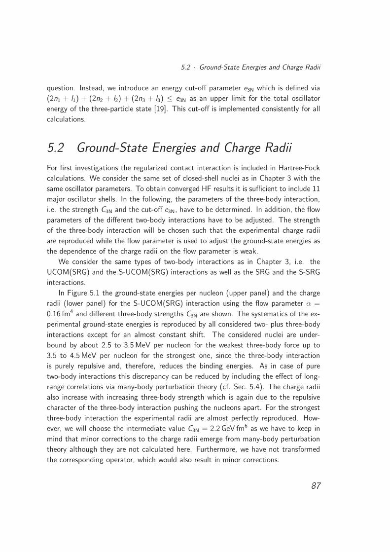
5.2 · Ground-State Energies and Charge Radii
question. Instead, we introduce an energy cut-off parameter e3N which is defined via
(2n1 + l1) + (2n2 + l2) + (2n3 + l3) ≤ e3N as an upper limit for the total oscillator
energy of the three-particle state [19]. This cut-off is implemented consistently for all
calculations.
5.2 Ground-State Energies and Charge Radii
For first investigations the regularized contact interaction is included in Hartree-Fock
calculations. We consider the same set of closed-shell nuclei as in Chapter 3 with the
same oscillator parameters. To obtain converged HF results it is sufficient to include 11
major oscillator shells. In the following, the parameters of the three-body interaction,
i.e. the strength C3N and the cut-off e3N, have to be determined. In addition, the flow
parameters of the different two-body interactions have to be adjusted. The strength
of the three-body interaction will be chosen such that the experimental charge radii
are reproduced while the flow parameter is used to adjust the ground-state energies as
the dependence of the charge radii on the flow parameter is weak.
We consider the same types of two-body interactions as in Chapter 3, i.e. the
UCOM(SRG) and the S-UCOM(SRG) interactions as well as the SRG and the S-SRG
interactions.
In Figure 5.1 the ground-state energies per nucleon (upper panel) and the charge
radii (lower panel) for the S-UCOM(SRG) interaction using the flow parameter α =
0.16 fm4 and different three-body strengths C3N are shown. The systematics of the ex-
perimental ground-state energies is reproduced by all considered two- plus three-body
interactions except for an almost constant shift. The considered nuclei are under-
bound by about 2.5 to 3.5 MeV per nucleon for the weakest three-body force up to
3.5 to 4.5 MeV per nucleon for the strongest one, since the three-body interaction
is purely repulsive and, therefore, reduces the binding energies. As in case of pure
two-body interactions this discrepancy can be reduced by including the effect of long-
range correlations via many-body perturbation theory (cf. Sec. 5.4). The charge radii
also increase with increasing three-body strength which is again due to the repulsive
character of the three-body interaction pushing the nucleons apart. For the strongest
three-body interaction the experimental radii are almost perfectly reproduced. How-
ever, we will choose the intermediate value C3N = 2.2 GeV fm6 as we have to keep in
mind that minor corrections to the charge radii emerge from many-body perturbation
theory although they are not calculated here. Furthermore, we have not transformed
the corresponding operator, which would also result in minor corrections.
87
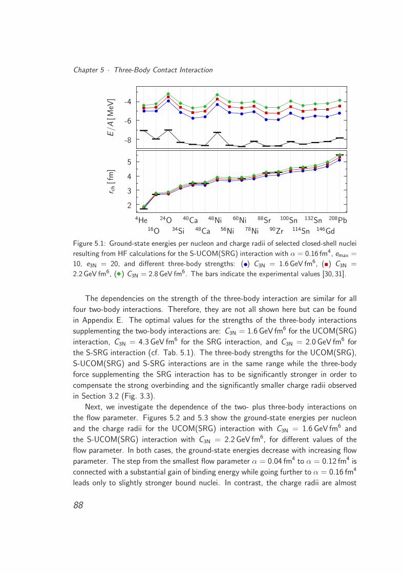
Chapter 5 · Three-Body Contact Interaction
-8
-6
-4
.
E/A
[MeV
]
2
3
4
5
.
r ch[f
m]
4He16O
24O34Si
40Ca48Ca
48Ni56Ni
60Ni78Ni
88Sr90Zr
100Sn114Sn
132Sn146Gd
208Pb
Figure 5.1: Ground-state energies per nucleon and charge radii of selected closed-shell nuclei
resulting from HF calculations for the S-UCOM(SRG) interaction with α = 0.16 fm4, emax =
10, e3N = 20, and different three-body strengths: () C3N = 1.6 GeV fm6, () C3N =
2.2 GeV fm6, ( ) C3N = 2.8 GeV fm6. The bars indicate the experimental values [30, 31].
The dependencies on the strength of the three-body interaction are similar for all
four two-body interactions. Therefore, they are not all shown here but can be found
in Appendix E. The optimal values for the strengths of the three-body interactions
supplementing the two-body interactions are: C3N = 1.6 GeV fm6 for the UCOM(SRG)
interaction, C3N = 4.3 GeV fm6 for the SRG interaction, and C3N = 2.0 GeV fm6 for
the S-SRG interaction (cf. Tab. 5.1). The three-body strengths for the UCOM(SRG),
S-UCOM(SRG) and S-SRG interactions are in the same range while the three-body
force supplementing the SRG interaction has to be significantly stronger in order to
compensate the strong overbinding and the significantly smaller charge radii observed
in Section 3.2 (Fig. 3.3).
Next, we investigate the dependence of the two- plus three-body interactions on
the flow parameter. Figures 5.2 and 5.3 show the ground-state energies per nucleon
and the charge radii for the UCOM(SRG) interaction with C3N = 1.6 GeV fm6 and
the S-UCOM(SRG) interaction with C3N = 2.2 GeV fm6, for different values of the
flow parameter. In both cases, the ground-state energies decrease with increasing flow
parameter. The step from the smallest flow parameter α = 0.04 fm4 to α = 0.12 fm4 is
connected with a substantial gain of binding energy while going further to α = 0.16 fm4
leads only to slightly stronger bound nuclei. In contrast, the charge radii are almost
88
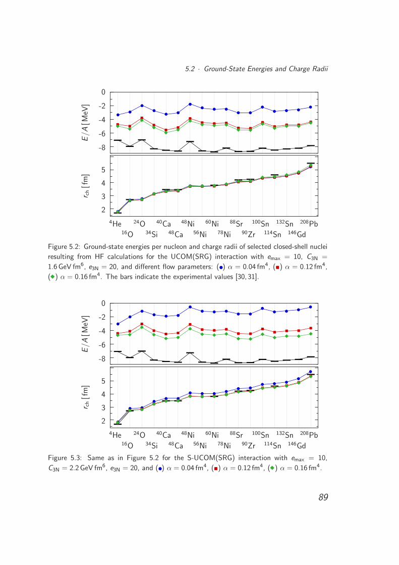
5.2 · Ground-State Energies and Charge Radii
-8
-6
-4
-2
0
.
E/A
[MeV
]
2
3
4
5
.
r ch[f
m]
4He16O
24O34Si
40Ca48Ca
48Ni56Ni
60Ni78Ni
88Sr90Zr
100Sn114Sn
132Sn146Gd
208Pb
Figure 5.2: Ground-state energies per nucleon and charge radii of selected closed-shell nuclei
resulting from HF calculations for the UCOM(SRG) interaction with emax = 10, C3N =
1.6 GeV fm6, e3N = 20, and different flow parameters: () α = 0.04 fm4, () α = 0.12 fm4,
( ) α = 0.16 fm4. The bars indicate the experimental values [30, 31].
-8
-6
-4
-2
0
.
E/A
[MeV
]
2
3
4
5
.
r ch[f
m]
4He16O
24O34Si
40Ca48Ca
48Ni56Ni
60Ni78Ni
88Sr90Zr
100Sn114Sn
132Sn146Gd
208Pb
Figure 5.3: Same as in Figure 5.2 for the S-UCOM(SRG) interaction with emax = 10,
C3N = 2.2 GeV fm6, e3N = 20, and () α = 0.04 fm4, () α = 0.12 fm4, ( ) α = 0.16 fm4.
89
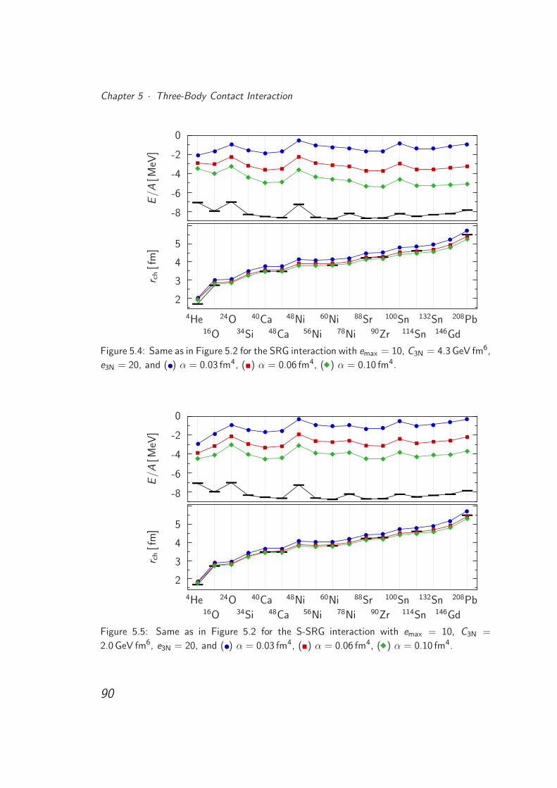
Chapter 5 · Three-Body Contact Interaction
-8
-6
-4
-2
0
.
E/A
[MeV
]
2
3
4
5
.
r ch[f
m]
4He16O
24O34Si
40Ca48Ca
48Ni56Ni
60Ni78Ni
88Sr90Zr
100Sn114Sn
132Sn146Gd
208Pb
Figure 5.4: Same as in Figure 5.2 for the SRG interaction with emax = 10, C3N = 4.3 GeV fm6,
e3N = 20, and () α = 0.03 fm4, () α = 0.06 fm4, ( ) α = 0.10 fm4.
-8
-6
-4
-2
0
.
E/A
[MeV
]
2
3
4
5
.
r ch[f
m]
4He16O
24O34Si
40Ca48Ca
48Ni56Ni
60Ni78Ni
88Sr90Zr
100Sn114Sn
132Sn146Gd
208Pb
Figure 5.5: Same as in Figure 5.2 for the S-SRG interaction with emax = 10, C3N =
2.0 GeV fm6, e3N = 20, and () α = 0.03 fm4, () α = 0.06 fm4, ( ) α = 0.10 fm4.
90
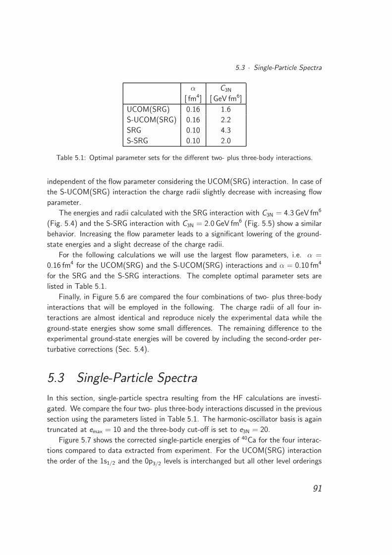
5.3 · Single-Particle Spectra
α C3N
[ fm4] [ GeV fm6]
UCOM(SRG) 0.16 1.6
S-UCOM(SRG) 0.16 2.2
SRG 0.10 4.3
S-SRG 0.10 2.0
Table 5.1: Optimal parameter sets for the different two- plus three-body interactions.
independent of the flow parameter considering the UCOM(SRG) interaction. In case of
the S-UCOM(SRG) interaction the charge radii slightly decrease with increasing flow
parameter.
The energies and radii calculated with the SRG interaction with C3N = 4.3 GeV fm6
(Fig. 5.4) and the S-SRG interaction with C3N = 2.0 GeV fm6 (Fig. 5.5) show a similar
behavior. Increasing the flow parameter leads to a significant lowering of the ground-
state energies and a slight decrease of the charge radii.
For the following calculations we will use the largest flow parameters, i.e. α =
0.16 fm4 for the UCOM(SRG) and the S-UCOM(SRG) interactions and α = 0.10 fm4
for the SRG and the S-SRG interactions. The complete optimal parameter sets are
listed in Table 5.1.
Finally, in Figure 5.6 are compared the four combinations of two- plus three-body
interactions that will be employed in the following. The charge radii of all four in-
teractions are almost identical and reproduce nicely the experimental data while the
ground-state energies show some small differences. The remaining difference to the
experimental ground-state energies will be covered by including the second-order per-
turbative corrections (Sec. 5.4).
5.3 Single-Particle Spectra
In this section, single-particle spectra resulting from the HF calculations are investi-
gated. We compare the four two- plus three-body interactions discussed in the previous
section using the parameters listed in Table 5.1. The harmonic-oscillator basis is again
truncated at emax = 10 and the three-body cut-off is set to e3N = 20.
Figure 5.7 shows the corrected single-particle energies of 40Ca for the four interac-
tions compared to data extracted from experiment. For the UCOM(SRG) interaction
the order of the 1s1/2 and the 0p3/2 levels is interchanged but all other level orderings
91
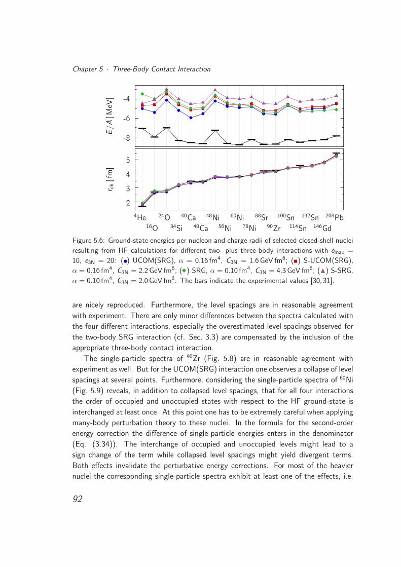
Chapter 5 · Three-Body Contact Interaction
-8
-6
-4
.
E/A
[MeV
]
2
3
4
5
.
r ch[f
m]
4He16O
24O34Si
40Ca48Ca
48Ni56Ni
60Ni78Ni
88Sr90Zr
100Sn114Sn
132Sn146Gd
208Pb
Figure 5.6: Ground-state energies per nucleon and charge radii of selected closed-shell nuclei
resulting from HF calculations for different two- plus three-body interactions with emax =
10, e3N = 20: () UCOM(SRG), α = 0.16 fm4, C3N = 1.6 GeV fm6; () S-UCOM(SRG),
α = 0.16 fm4, C3N = 2.2 GeV fm6; ( ) SRG, α = 0.10 fm4, C3N = 4.3 GeV fm6; (N) S-SRG,
α = 0.10 fm4, C3N = 2.0 GeV fm6. The bars indicate the experimental values [30, 31].
are nicely reproduced. Furthermore, the level spacings are in reasonable agreement
with experiment. There are only minor differences between the spectra calculated with
the four different interactions, especially the overestimated level spacings observed for
the two-body SRG interaction (cf. Sec. 3.3) are compensated by the inclusion of the
appropriate three-body contact interaction.
The single-particle spectra of 90Zr (Fig. 5.8) are in reasonable agreement with
experiment as well. But for the UCOM(SRG) interaction one observes a collapse of level
spacings at several points. Furthermore, considering the single-particle spectra of 60Ni
(Fig. 5.9) reveals, in addition to collapsed level spacings, that for all four interactions
the order of occupied and unoccupied states with respect to the HF ground-state is
interchanged at least once. At this point one has to be extremely careful when applying
many-body perturbation theory to these nuclei. In the formula for the second-order
energy correction the difference of single-particle energies enters in the denominator
(Eq. (3.34)). The interchange of occupied and unoccupied levels might lead to a
sign change of the term while collapsed level spacings might yield divergent terms.
Both effects invalidate the perturbative energy corrections. For most of the heavier
nuclei the corresponding single-particle spectra exhibit at least one of the effects, i.e.
92
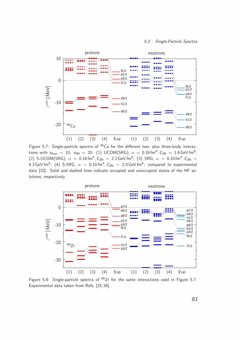
5.3 · Single-Particle Spectra
d52
s12
d32
f72p32p12f52
d52
s12
d32
f72p32p12f52
-20
-10
0
10
.
εcor
r[M
eV]
protons neutrons
(1) (2) (3) (4) Exp (1) (2) (3) (4) Exp
40Ca
Figure 5.7: Single-particle spectra of 40Ca for the different two- plus three-body interac-
tions with emax = 10, e3N = 20: (1) UCOM(SRG), α = 0.16 fm4, C3N = 1.6 GeV fm6;
(2) S-UCOM(SRG), α = 0.16 fm4, C3N = 2.2 GeV fm6; (3) SRG, α = 0.10 fm4, C3N =
4.3 GeV fm6; (4) S-SRG, α = 0.10 fm4, C3N = 2.0 GeV fm6; compared to experimental
data [32]. Solid and dashed lines indicate occupied and unoccupied states of the HF so-
lutions, respectively.
d32s12
f72
f52p32p12
g92
g72d52
f72
f52p32p12g92d52
d32s12
g72
-30
-20
-10
0
.
εcor
r[M
eV]
protons neutrons
(1) (2) (3) (4) Exp (1) (2) (3) (4) Exp
90Zr
Figure 5.8: Single-particle spectra of 90Zr for the same interactions used in Figure 5.7.
Experimental data taken from Refs. [33, 34].
93
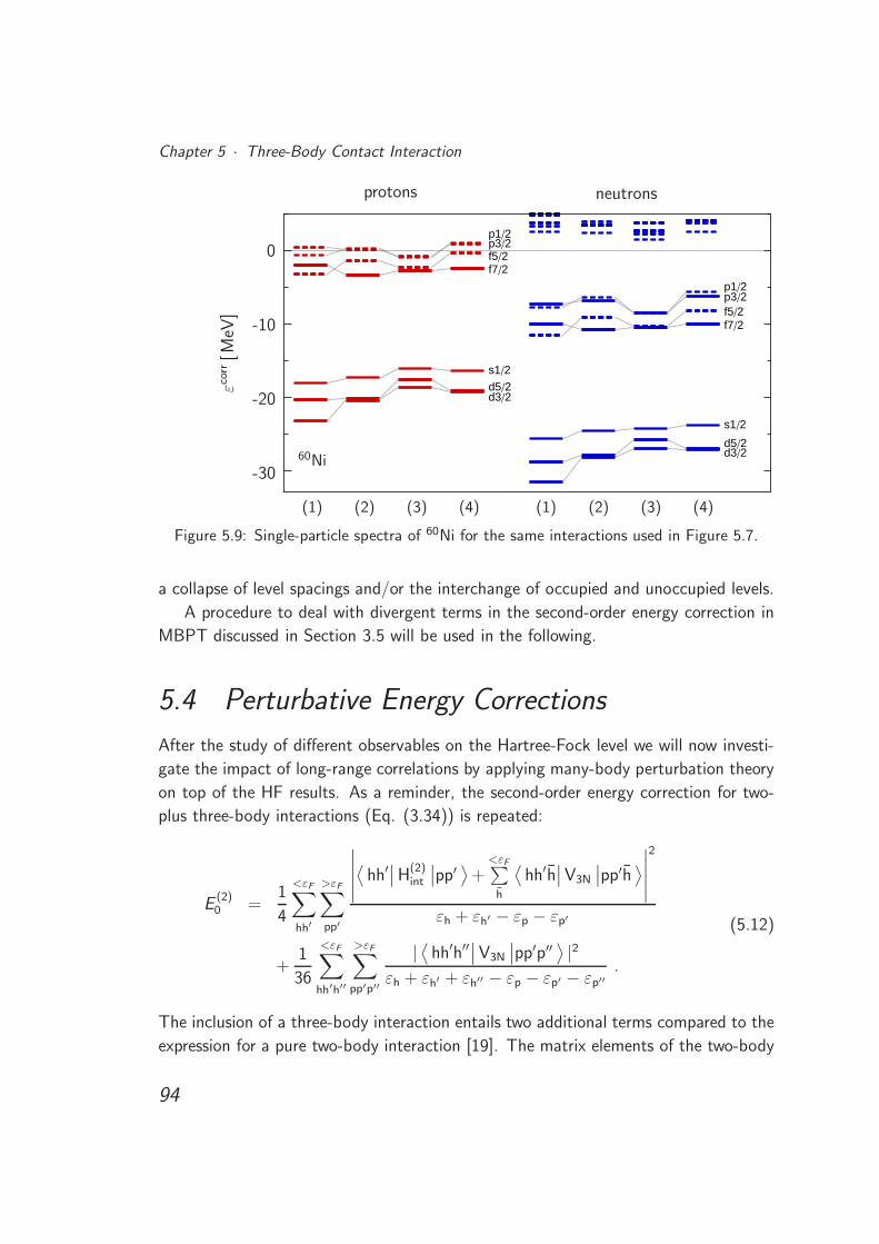
Chapter 5 · Three-Body Contact Interaction
d32d52
s12
f72f52
p12p32
d32d52
s12
f72f52
p12p32
-30
-20
-10
0
.
εcor
r[M
eV]
protons neutrons
(1) (2) (3) (4) (1) (2) (3) (4)
60Ni
Figure 5.9: Single-particle spectra of 60Ni for the same interactions used in Figure 5.7.
a collapse of level spacings and/or the interchange of occupied and unoccupied levels.
A procedure to deal with divergent terms in the second-order energy correction in
MBPT discussed in Section 3.5 will be used in the following.
5.4 Perturbative Energy Corrections
After the study of different observables on the Hartree-Fock level we will now investi-
gate the impact of long-range correlations by applying many-body perturbation theory
on top of the HF results. As a reminder, the second-order energy correction for two-
plus three-body interactions (Eq. (3.34)) is repeated:
E(2)0 =
1
4
<εF∑
hh′
>εF∑
pp′
∣∣∣∣∣⟨hh′∣∣H(2)
int
∣∣pp′ ⟩+<εF∑h
⟨hh′h
∣∣V3N
∣∣pp′h⟩∣∣∣∣∣
2
εh + εh′ − εp − εp′
+1
36
<εF∑
hh′h′′
>εF∑
pp′p′′
|⟨hh′h′′∣∣V3N
∣∣pp′p′′ ⟩ |2εh + εh′ + εh′′ − εp − εp′ − εp′′
.
(5.12)
The inclusion of a three-body interaction entails two additional terms compared to the
expression for a pure two-body interaction [19]. The matrix elements of the two-body
94
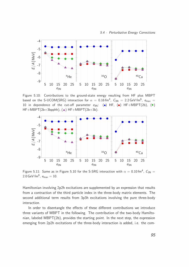
5.4 · Perturbative Energy Corrections
5 10 15 20 25e3N
-9
-8
-7
-6
-5
-4
.
E/A
[MeV
]
4He
5 10 15 20 25e3N
16O
5 10 15 20 25e3N
40Ca
Figure 5.10: Contributions to the ground-state energy resulting from HF plus MBPT
based on the S-UCOM(SRG) interaction for α = 0.16 fm4, C3N = 2.2 GeV fm6, emax =
10 in dependence of the cut-off parameter e3N: () HF, () HF+MBPT(2b), ( )
HF+MBPT(2b+3bpphh), (N) HF+MBPT(2b+3b).
5 10 15 20 25e3N
-9
-8
-7
-6
-5
-4
.
E/A
[MeV
]
4He
5 10 15 20 25e3N
16O
5 10 15 20 25e3N
40Ca
Figure 5.11: Same as in Figure 5.10 for the S-SRG interaction with α = 0.10 fm4, C3N =
2.0 GeV fm6, emax = 10.
Hamiltonian involving 2p2h excitations are supplemented by an expression that results
from a contraction of the third particle index in the three-body matrix elements. The
second additional term results from 3p3h excitations involving the pure three-body
interaction.
In order to disentangle the effects of these different contributions we introduce
three variants of MBPT in the following. The contribution of the two-body Hamilto-
nian, labeled MBPT(2b), provides the starting point. In the next step, the expression
emerging from 2p2h excitations of the three-body interaction is added, i.e. the com-
95
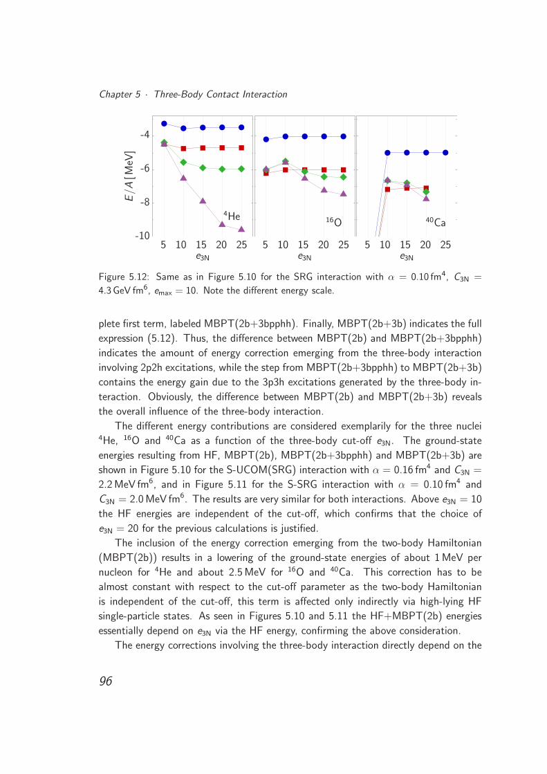
Chapter 5 · Three-Body Contact Interaction
5 10 15 20 25e3N
-10
-8
-6
-4
.
E/A
[MeV
]
4He
5 10 15 20 25e3N
16O
5 10 15 20 25e3N
40Ca
Figure 5.12: Same as in Figure 5.10 for the SRG interaction with α = 0.10 fm4, C3N =
4.3 GeV fm6, emax = 10. Note the different energy scale.
plete first term, labeled MBPT(2b+3bpphh). Finally, MBPT(2b+3b) indicates the full
expression (5.12). Thus, the difference between MBPT(2b) and MBPT(2b+3bpphh)
indicates the amount of energy correction emerging from the three-body interaction
involving 2p2h excitations, while the step from MBPT(2b+3bpphh) to MBPT(2b+3b)
contains the energy gain due to the 3p3h excitations generated by the three-body in-
teraction. Obviously, the difference between MBPT(2b) and MBPT(2b+3b) reveals
the overall influence of the three-body interaction.
The different energy contributions are considered exemplarily for the three nuclei4He, 16O and 40Ca as a function of the three-body cut-off e3N. The ground-state
energies resulting from HF, MBPT(2b), MBPT(2b+3bpphh) and MBPT(2b+3b) are
shown in Figure 5.10 for the S-UCOM(SRG) interaction with α = 0.16 fm4 and C3N =
2.2 MeV fm6, and in Figure 5.11 for the S-SRG interaction with α = 0.10 fm4 and
C3N = 2.0 MeV fm6. The results are very similar for both interactions. Above e3N = 10
the HF energies are independent of the cut-off, which confirms that the choice of
e3N = 20 for the previous calculations is justified.
The inclusion of the energy correction emerging from the two-body Hamiltonian
(MBPT(2b)) results in a lowering of the ground-state energies of about 1 MeV per
nucleon for 4He and about 2.5 MeV for 16O and 40Ca. This correction has to be
almost constant with respect to the cut-off parameter as the two-body Hamiltonian
is independent of the cut-off, this term is affected only indirectly via high-lying HF
single-particle states. As seen in Figures 5.10 and 5.11 the HF+MBPT(2b) energies
essentially depend on e3N via the HF energy, confirming the above consideration.
The energy corrections involving the three-body interaction directly depend on the
96
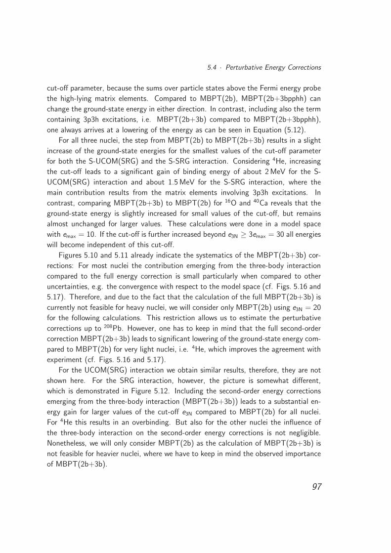
5.4 · Perturbative Energy Corrections
cut-off parameter, because the sums over particle states above the Fermi energy probe
the high-lying matrix elements. Compared to MBPT(2b), MBPT(2b+3bpphh) can
change the ground-state energy in either direction. In contrast, including also the term
containing 3p3h excitations, i.e. MBPT(2b+3b) compared to MBPT(2b+3bpphh),
one always arrives at a lowering of the energy as can be seen in Equation (5.12).
For all three nuclei, the step from MBPT(2b) to MBPT(2b+3b) results in a slight
increase of the ground-state energies for the smallest values of the cut-off parameter
for both the S-UCOM(SRG) and the S-SRG interaction. Considering 4He, increasing
the cut-off leads to a significant gain of binding energy of about 2 MeV for the S-
UCOM(SRG) interaction and about 1.5 MeV for the S-SRG interaction, where the
main contribution results from the matrix elements involving 3p3h excitations. In
contrast, comparing MBPT(2b+3b) to MBPT(2b) for 16O and 40Ca reveals that the
ground-state energy is slightly increased for small values of the cut-off, but remains
almost unchanged for larger values. These calculations were done in a model space
with emax = 10. If the cut-off is further increased beyond e3N ≥ 3emax = 30 all energies
will become independent of this cut-off.
Figures 5.10 and 5.11 already indicate the systematics of the MBPT(2b+3b) cor-
rections: For most nuclei the contribution emerging from the three-body interaction
compared to the full energy correction is small particularly when compared to other
uncertainties, e.g. the convergence with respect to the model space (cf. Figs. 5.16 and
5.17). Therefore, and due to the fact that the calculation of the full MBPT(2b+3b) is
currently not feasible for heavy nuclei, we will consider only MBPT(2b) using e3N = 20
for the following calculations. This restriction allows us to estimate the perturbative
corrections up to 208Pb. However, one has to keep in mind that the full second-order
correction MBPT(2b+3b) leads to significant lowering of the ground-state energy com-
pared to MBPT(2b) for very light nuclei, i.e. 4He, which improves the agreement with
experiment (cf. Figs. 5.16 and 5.17).
For the UCOM(SRG) interaction we obtain similar results, therefore, they are not
shown here. For the SRG interaction, however, the picture is somewhat different,
which is demonstrated in Figure 5.12. Including the second-order energy corrections
emerging from the three-body interaction (MBPT(2b+3b)) leads to a substantial en-
ergy gain for larger values of the cut-off e3N compared to MBPT(2b) for all nuclei.
For 4He this results in an overbinding. But also for the other nuclei the influence of
the three-body interaction on the second-order energy corrections is not negligible.
Nonetheless, we will only consider MBPT(2b) as the calculation of MBPT(2b+3b) is
not feasible for heavier nuclei, where we have to keep in mind the observed importance
of MBPT(2b+3b).
97
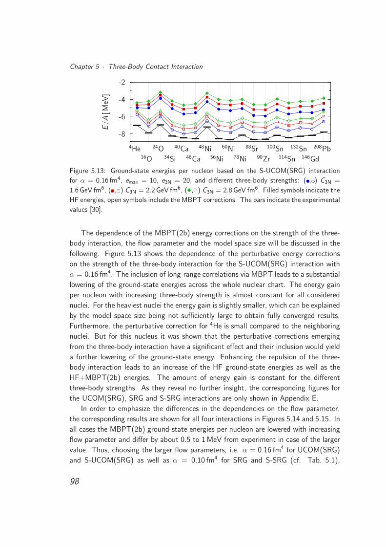
Chapter 5 · Three-Body Contact Interaction
-8
-6
-4
-2
.
E/A
[MeV
]
4He16O
24O34Si
40Ca48Ca
48Ni56Ni
60Ni78Ni
88Sr90Zr
100Sn114Sn
132Sn146Gd
208Pb
Figure 5.13: Ground-state energies per nucleon based on the S-UCOM(SRG) interaction
for α = 0.16 fm4, emax = 10, e3N = 20, and different three-body strengths: (,) C3N =
1.6 GeV fm6, (,) C3N = 2.2 GeV fm6, ( , ) C3N = 2.8 GeV fm6. Filled symbols indicate the
HF energies, open symbols include the MBPT corrections. The bars indicate the experimental
values [30].
The dependence of the MBPT(2b) energy corrections on the strength of the three-
body interaction, the flow parameter and the model space size will be discussed in the
following. Figure 5.13 shows the dependence of the perturbative energy corrections
on the strength of the three-body interaction for the S-UCOM(SRG) interaction with
α = 0.16 fm4. The inclusion of long-range correlations via MBPT leads to a substantial
lowering of the ground-state energies across the whole nuclear chart. The energy gain
per nucleon with increasing three-body strength is almost constant for all considered
nuclei. For the heaviest nuclei the energy gain is slightly smaller, which can be explained
by the model space size being not sufficiently large to obtain fully converged results.
Furthermore, the perturbative correction for 4He is small compared to the neighboring
nuclei. But for this nucleus it was shown that the perturbative corrections emerging
from the three-body interaction have a significant effect and their inclusion would yield
a further lowering of the ground-state energy. Enhancing the repulsion of the three-
body interaction leads to an increase of the HF ground-state energies as well as the
HF+MBPT(2b) energies. The amount of energy gain is constant for the different
three-body strengths. As they reveal no further insight, the corresponding figures for
the UCOM(SRG), SRG and S-SRG interactions are only shown in Appendix E.
In order to emphasize the differences in the dependencies on the flow parameter,
the corresponding results are shown for all four interactions in Figures 5.14 and 5.15. In
all cases the MBPT(2b) ground-state energies per nucleon are lowered with increasing
flow parameter and differ by about 0.5 to 1 MeV from experiment in case of the larger
value. Thus, choosing the larger flow parameters, i.e. α = 0.16 fm4 for UCOM(SRG)
and S-UCOM(SRG) as well as α = 0.10 fm4 for SRG and S-SRG (cf. Tab. 5.1),
98
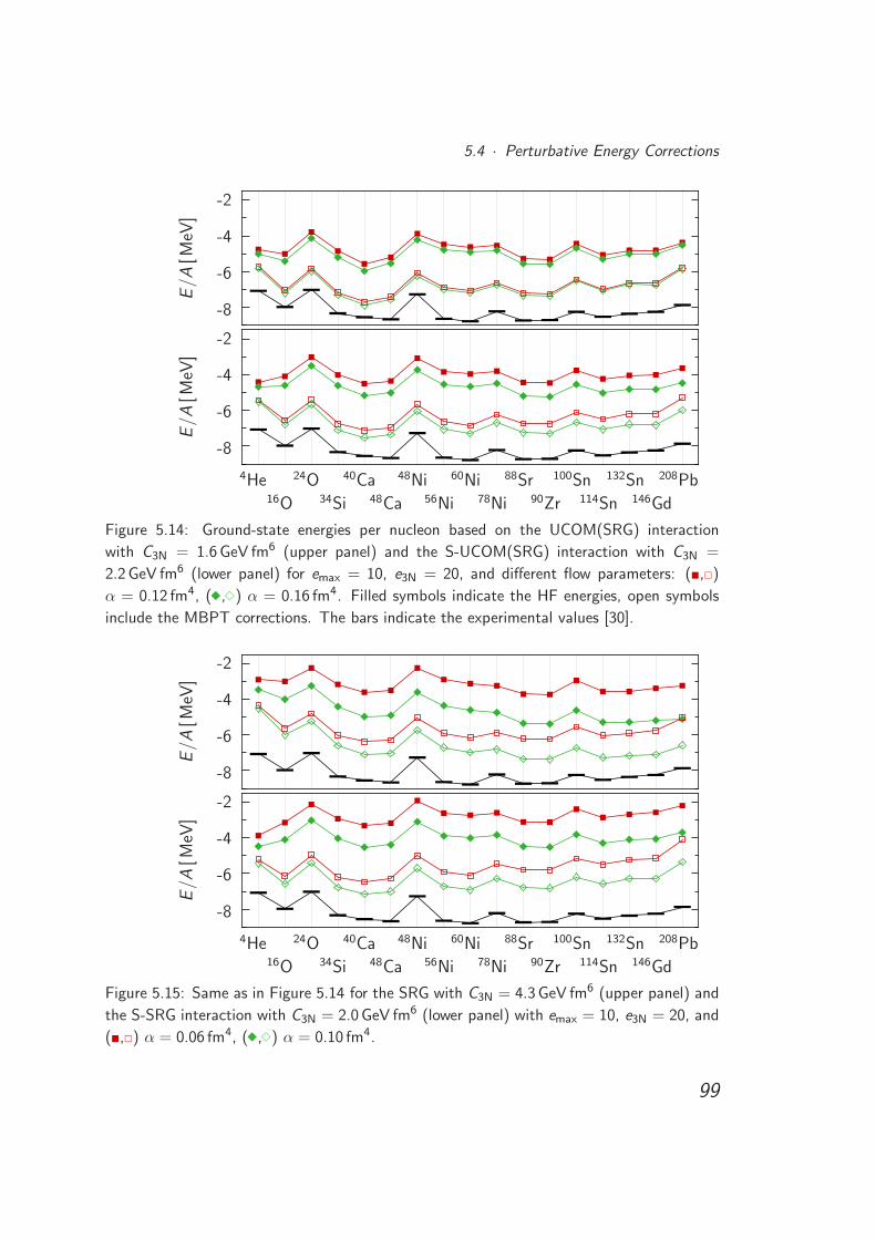
5.4 · Perturbative Energy Corrections
-8
-6
-4
-2
.
E/A
[MeV
]
-8
-6
-4
-2
.
E/A
[MeV
]
4He16O
24O34Si
40Ca48Ca
48Ni56Ni
60Ni78Ni
88Sr90Zr
100Sn114Sn
132Sn146Gd
208Pb
Figure 5.14: Ground-state energies per nucleon based on the UCOM(SRG) interaction
with C3N = 1.6 GeV fm6 (upper panel) and the S-UCOM(SRG) interaction with C3N =
2.2 GeV fm6 (lower panel) for emax = 10, e3N = 20, and different flow parameters: (,)
α = 0.12 fm4, ( , ) α = 0.16 fm4. Filled symbols indicate the HF energies, open symbols
include the MBPT corrections. The bars indicate the experimental values [30].
-8
-6
-4
-2
.
E/A
[MeV
]
-8
-6
-4
-2
.
E/A
[MeV
]
4He16O
24O34Si
40Ca48Ca
48Ni56Ni
60Ni78Ni
88Sr90Zr
100Sn114Sn
132Sn146Gd
208Pb
Figure 5.15: Same as in Figure 5.14 for the SRG with C3N = 4.3 GeV fm6 (upper panel) and
the S-SRG interaction with C3N = 2.0 GeV fm6 (lower panel) with emax = 10, e3N = 20, and
(,) α = 0.06 fm4, ( , ) α = 0.10 fm4.
99
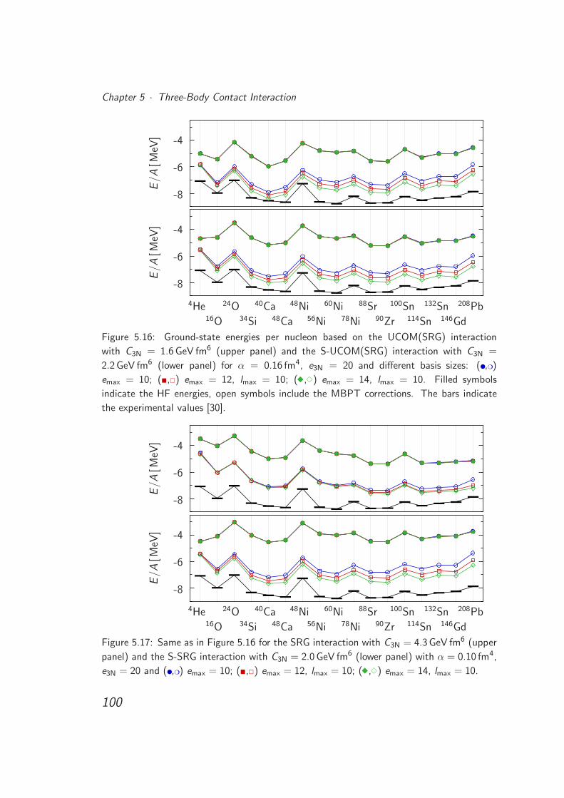
Chapter 5 · Three-Body Contact Interaction
-8
-6
-4
.
E/A
[MeV
]
-8
-6
-4
.
E/A
[MeV
]
4He16O
24O34Si
40Ca48Ca
48Ni56Ni
60Ni78Ni
88Sr90Zr
100Sn114Sn
132Sn146Gd
208Pb
Figure 5.16: Ground-state energies per nucleon based on the UCOM(SRG) interaction
with C3N = 1.6 GeV fm6 (upper panel) and the S-UCOM(SRG) interaction with C3N =
2.2 GeV fm6 (lower panel) for α = 0.16 fm4, e3N = 20 and different basis sizes: (,)
emax = 10; (,) emax = 12, lmax = 10; ( , ) emax = 14, lmax = 10. Filled symbols
indicate the HF energies, open symbols include the MBPT corrections. The bars indicate
the experimental values [30].
-8
-6
-4
.
E/A
[MeV
]
-8
-6
-4
.
E/A
[MeV
]
4He16O
24O34Si
40Ca48Ca
48Ni56Ni
60Ni78Ni
88Sr90Zr
100Sn114Sn
132Sn146Gd
208Pb
Figure 5.17: Same as in Figure 5.16 for the SRG interaction with C3N = 4.3 GeV fm6 (upper
panel) and the S-SRG interaction with C3N = 2.0 GeV fm6 (lower panel) with α = 0.10 fm4,
e3N = 20 and (,) emax = 10; (,) emax = 12, lmax = 10; ( , ) emax = 14, lmax = 10.
100
5.4 · Perturbative Energy Corrections
for further investigations seems appropriate. As already observed on the basis of pure
two-body interactions the perturbative energy corrections decrease with increasing flow
parameter. In contrast to the results obtained with the pure two-body interactions,
the respective three-body interaction compensates for the overbinding observed for the
larger values of the flow parameter (cf. Sec. 3.5, especially Figures 3.9 and 3.10).
Finally, the convergence of the MBPT(2b) energies is examined by increasing the
model space size in Figures 5.16 and 5.17. For the UCOM(SRG), the S-UCOM(SRG)
and the S-SRG interactions with the appropriate three-body interactions the MBPT
energies are not yet converged, even for the largest basis size. But as the considered
nuclei are still slightly underbound an extrapolation to infinite basis sizes would result
in a reasonable agreement with the experimental ground-state energies. However, one
has to keep in mind that the second-order perturbative energy corrections only serve
as an estimate as already discussed in Section 3.5. The picture is somewhat different
for the SRG interaction where the MBPT(2b) energies are converged, but still exhibit
a significant difference to experiment, especially for the light and intermediate nuclei.
But for this interaction we have demonstrated in Figure 5.12 that the influence of
the energy corrections emerging from the three-body interaction is significantly larger.
Therefore, including these terms would improve the agreement with the experimental
ground-state energies.
101

Chapter 5 · Three-Body Contact Interaction
102
Chapter 6
Few-Body Calculations
In the previous chapters we have used the Hartree-Fock method and many-body per-
turbation theory, which both aim at an approximate solution of the nuclear many-body
problem. We will now focus on an exact solution in the famework of the No-Core Shell
Model (NCSM). We will briefly introduce the NCSM in Section 6.1 and calculate the4He ground-state energy in Section 6.2.
6.1 The No-Core Shell Model
The No-Core Shell Model [12, 43] aims at an exact numerical solution of the nuclear
eigenvalue problem
H|Ψn〉 = En|Ψn〉 , (6.1)
where we again use the Hamiltonian
H = Tint + VNN + V3N (6.2)
consisting of the intrinsic kinetic energy Tint, the two-nucleon interaction VNN, and the
three-nucleon interaction V3N. The eigenvalue problem is solved by diagonalizing the
Hamilton matrix. Therefore, we have to choose a many-body basis, which is given by
Slater determinants |Φν〉 built of single-particle harmonic-oscillator eigenstates. The
eigenstates of the Hamiltonian are expanded in these Slater determinants:
|Ψn〉 =∑
ν
C nν |Φν〉 . (6.3)
103
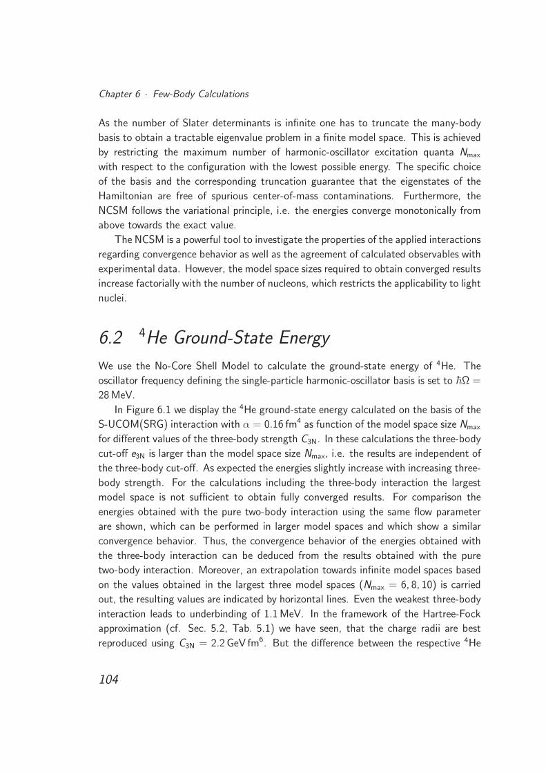
Chapter 6 · Few-Body Calculations
As the number of Slater determinants is infinite one has to truncate the many-body
basis to obtain a tractable eigenvalue problem in a finite model space. This is achieved
by restricting the maximum number of harmonic-oscillator excitation quanta Nmax
with respect to the configuration with the lowest possible energy. The specific choice
of the basis and the corresponding truncation guarantee that the eigenstates of the
Hamiltonian are free of spurious center-of-mass contaminations. Furthermore, the
NCSM follows the variational principle, i.e. the energies converge monotonically from
above towards the exact value.
The NCSM is a powerful tool to investigate the properties of the applied interactions
regarding convergence behavior as well as the agreement of calculated observables with
experimental data. However, the model space sizes required to obtain converged results
increase factorially with the number of nucleons, which restricts the applicability to light
nuclei.
6.2 4He Ground-State Energy
We use the No-Core Shell Model to calculate the ground-state energy of 4He. The
oscillator frequency defining the single-particle harmonic-oscillator basis is set to ~Ω =
28 MeV.
In Figure 6.1 we display the 4He ground-state energy calculated on the basis of the
S-UCOM(SRG) interaction with α = 0.16 fm4 as function of the model space size Nmax
for different values of the three-body strength C3N. In these calculations the three-body
cut-off e3N is larger than the model space size Nmax, i.e. the results are independent of
the three-body cut-off. As expected the energies slightly increase with increasing three-
body strength. For the calculations including the three-body interaction the largest
model space is not sufficient to obtain fully converged results. For comparison the
energies obtained with the pure two-body interaction using the same flow parameter
are shown, which can be performed in larger model spaces and which show a similar
convergence behavior. Thus, the convergence behavior of the energies obtained with
the three-body interaction can be deduced from the results obtained with the pure
two-body interaction. Moreover, an extrapolation towards infinite model spaces based
on the values obtained in the largest three model spaces (Nmax = 6, 8, 10) is carried
out, the resulting values are indicated by horizontal lines. Even the weakest three-body
interaction leads to underbinding of 1.1 MeV. In the framework of the Hartree-Fock
approximation (cf. Sec. 5.2, Tab. 5.1) we have seen, that the charge radii are best
reproduced using C3N = 2.2 GeV fm6. But the difference between the respective 4He
104
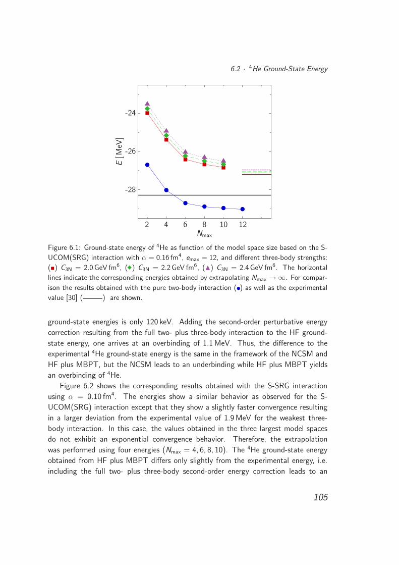
6.2 · 4He Ground-State Energy
2 4 6 8 10 12Nmax
-28
-26
-24
.
E[M
eV]
Figure 6.1: Ground-state energy of 4He as function of the model space size based on the S-
UCOM(SRG) interaction with α = 0.16 fm4, emax = 12, and different three-body strengths:
() C3N = 2.0 GeV fm6, ( ) C3N = 2.2 GeV fm6, (N) C3N = 2.4 GeV fm6. The horizontal
lines indicate the corresponding energies obtained by extrapolating Nmax → ∞. For compar-
ison the results obtained with the pure two-body interaction () as well as the experimental
value [30] ( ) are shown.
ground-state energies is only 120 keV. Adding the second-order perturbative energy
correction resulting from the full two- plus three-body interaction to the HF ground-
state energy, one arrives at an overbinding of 1.1 MeV. Thus, the difference to the
experimental 4He ground-state energy is the same in the framework of the NCSM and
HF plus MBPT, but the NCSM leads to an underbinding while HF plus MBPT yields
an overbinding of 4He.
Figure 6.2 shows the corresponding results obtained with the S-SRG interaction
using α = 0.10 fm4. The energies show a similar behavior as observed for the S-
UCOM(SRG) interaction except that they show a slightly faster convergence resulting
in a larger deviation from the experimental value of 1.9 MeV for the weakest three-
body interaction. In this case, the values obtained in the three largest model spaces
do not exhibit an exponential convergence behavior. Therefore, the extrapolation
was performed using four energies (Nmax = 4, 6, 8, 10). The 4He ground-state energy
obtained from HF plus MBPT differs only slightly from the experimental energy, i.e.
including the full two- plus three-body second-order energy correction leads to an
105
Chapter 6 · Few-Body Calculations
2 4 6 8 10 12Nmax
-28
-26
-24
.
E[M
eV]
Figure 6.2: Same as in Figure 6.1 for the S-SRG interaction with α = 0.10 fm4, emax =
12, and () C3N = 2.0 GeV fm6, ( ) C3N = 2.2 GeV fm6, (N) C3N = 2.4 GeV fm6. For
comparison: () pure two-body interaction, ( ) experiment [30].
overbinding of 130 keV.
For a consistent study one would also have to investigate the dependencies of the4He ground-state energy on the flow parameter α and the oscillator frequency Ω, where
the dependence on the oscillator frequency is expected to be weak [10].
In summary, the 4He ground-state energies obtained with the three-body contact
interaction differ from the experimental value by 1 to 2 MeV, which is a promising
result but still leaves room for improvement. In principle, it is possible to choose the
parameters such that the experimental 4He ground-state energy is reproduced, but
obviously this would also change the results for the charge radii on the basis of the HF
approximation.
106
Chapter 7
Collective Excitations
In the previous chapters we have studied ground-state properties of nuclei across the
whole nuclear chart. In this chapter we will focus on excited states, particularly collec-
tive excitations. On the one hand the investigation of collective excitations provides
valuable information about the underlying interaction. On the other hand, a detailed
knowledge especially of giant resonances provides information on properties of nuclear
matter and is important for various applications, e.g. in nuclear astrophysics for the
understanding of supernovae. A suitable method for the investigation of collective
excitation modes is the Random Phase Approximation (RPA) based self-consistently
on a Hartree-Fock calculation. The general RPA equations are derived in Appendix C.
In the following we will outline the RPA on the basis of unitarily transformed two-body
interactions in Section 7.1, where the three-body contact interaction is replaced by a
density-dependent two-body interaction. After introducing multipole transition oper-
ators in Section 7.2, we will discuss the energy-weighted sum rules in Section 7.3 to
ensure the proper implementation of the RPA. Finally, the response functions obtained
for three different excitation modes will be investigated in detail in Section 7.4.
7.1 Random Phase Approximation
The Random Phase Approximation is based on Hartree-Fock single-particle states.
Therefore, as in the HF method, we would prefer to use the intrinsic Hamiltonian Hint
containing the intrinsic kinetic energy Tint = T − Tcm, the unitarily transformed two-
body interaction VNN as well as the phenomenological three-body interaction V3N. The
107

Chapter 7 · Collective Excitations
inclusion of the full three-body interaction in RPA calculations is, however, very time-
extensive. Fortunately, for Hartree-Fock calculations of even-even nuclei the three-
body contact interaction (without regularization) is equivalent to a density-dependent
two-body interaction [44, 45]
VNN[] =C3N
6(1 + Pσ)
(r1 + r2
2
)δ(3)(r1 − r2) (7.1)
with the spin-exchange operator Pσ. This equivalence holds also for RPA [46]. The
Hamiltonian thus reads
Hint = Tint + VNN + VNN[] . (7.2)
Note, that for the HF calculations providing the basis for RPA the density-dependent
two-body interaction is employed instead of the three-body contact interaction for
consistency. The only difference is that in this way the three-body interaction enters
without the cut-off e3N in the HF method. In the following we will refer to the three-
body interaction although it is technically included as density-dependent two-body
interaction.
As already in the previous chapters, we will restrict our studies to spherically sym-
metric nuclei so that the single-particle angular momenta can be coupled to good total
angular momentum J indicating the multipolarity of the respective collective state.
The excited states are generated by the operators Q†ν,JM (cf. Eq. (C.2)):
Q†ν,JM |Ψ0〉 = |Ψν〉 , Qν,JM |Ψ0〉 = 0 (7.3)
with the RPA ground-state |Ψ0〉 = |RPA〉. The excitation operators are formulated in
the coupled representation [47, 48]
Q†ν,JM =
∑
ph
(X ν,JMph AJ,M†
ph − (−1)J−MY ν,JMph AJ,−M
ph ) , (7.4)
where the summation includes all particle-hole (ph) excitations of the HF ground-state,
and
AJ,M†
ph =∑
mpmh
c(
jp jhmp mh
∣∣ J
M
)(−1)jh−mh a†jpmp
ajhmh(7.5)
represents the ph-creation operator built of the single-particle creation and annihilation
operators a†jm and ajm, respectively. The RPA equations are written as
(AJ BJ
BJ⋆
AJ⋆
)(X ν,JM
Y ν,JM
)= ~ων
(1 0
0 −1
)(X ν,JM
Y ν,JM
)(7.6)
108
7.2 · Multipole Transitions
with the amplitudes X ν,JMph and Y ν,JM
ph , and the RPA eigenvalues ~ων . For the derivation
of this eigenvalue problem one has to exploit the quasi-boson approximation, and the
RPA ground-state is approximated by the HF ground-state (cf. Appendix C). Thus,
the matrices AJ and BJ are obtained from
AJphp′h′ =
⟨HF∣∣[[
AJ,Mph , Hint
], AJ,M†
p′h′
] ∣∣HF⟩
BJphp′h′ = −
⟨HF∣∣[[
AJ,Mph , Hint
], (−1)J−MAJ,−M
p′h′
] ∣∣HF⟩
.(7.7)
7.2 Multipole Transitions
In the following, we will investigate the impact of the three-body contact interaction
on electric multipole transitions. The reduced transition probability
BT (EJ , J0 → Jν) = BTJ (ων) =
1
2J0 + 1|〈ν||QT
J ||0〉|2 (7.8)
describes the response on these excitation modes [14,48]. The reduced matrix element
〈ν||QTJ ||0〉 connects the initial state |0〉, which is the ground-state in our case, with
the final state |ν〉 via the multipole transition operator QTJ . In the following we will
consider isoscalar monopole (ISM) excitations for which the transition operator is given
by
Q000 =
A∑
i=1
x2i Y00(ϑi ,ϕi) , (7.9)
isovector dipole (IVD) excitations with the transition operator
Q11M = e
A∑
i=1
τ(i)3 xi Y1M(ϑi ,ϕi) , (7.10)
as well as the isoscalar quadrupole (ISQ) excitation operator
Q02M = e
A∑
i=1
x2i Y2M(ϑi ,ϕi) (7.11)
with the elementary charge e, the third component of the isospin τ3 and the spherical
harmonics YJM(ϑ,ϕ). As unitarily transformed NN potentials enter in the Hamiltonian,
the transition operators should be transformed consistently. However, for the UCOM
109
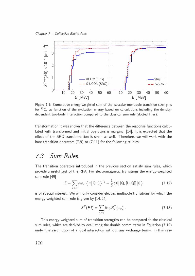
Chapter 7 · Collective Excitations
10 20 30 40 50 60E [ MeV]
0
1
2
3
.
ST
=0(E
0)×
10−
4[e
2fm
4]
UCOM(SRG)
S-UCOM(SRG)
10 20 30 40 50 60E [ MeV]
SRG
S-SRG
Figure 7.1: Cumulative energy-weighted sum of the isoscalar monopole transition strengths
for 40Ca as function of the excitation energy based on calculations including the density-
dependent two-body interaction compared to the classical sum rule (dotted lines).
transformation it was shown that the difference between the response functions calcu-
lated with transformed and initial operators is marginal [14]. It is expected that the
effect of the SRG transformation is small as well. Therefore, we will work with the
bare transition operators (7.9) to (7.11) for the following studies.
7.3 Sum Rules
The transition operators introduced in the previous section satisfy sum rules, which
provide a useful test of the RPA. For electromagnetic transitions the energy-weighted
sum rule [49]
S =∑
ν>0
~ων |⟨ν∣∣Q∣∣0⟩|2 =
1
2
⟨0∣∣ [Q, [H, Q]]
∣∣0⟩
(7.12)
is of special interest. We will only consider electric multipole transitions for which the
energy-weighted sum rule is given by [14, 24]
ST (EJ) =∑
ν>0
~ωνBTJ (ων) . (7.13)
This energy-weighted sum of transition strengths can be compared to the classical
sum rules, which are derived by evaluating the double commutator in Equation (7.12)
under the assumption of a local interaction without any exchange terms. In this case
110
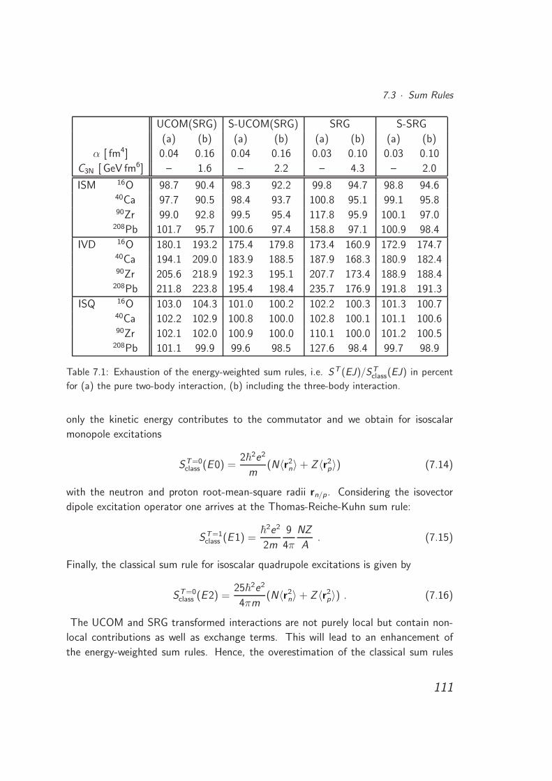
7.3 · Sum Rules
UCOM(SRG) S-UCOM(SRG) SRG S-SRG
(a) (b) (a) (b) (a) (b) (a) (b)
α [ fm4] 0.04 0.16 0.04 0.16 0.03 0.10 0.03 0.10
C3N [ GeV fm6] – 1.6 – 2.2 – 4.3 – 2.0
ISM 16O 98.7 90.4 98.3 92.2 99.8 94.7 98.8 94.640Ca 97.7 90.5 98.4 93.7 100.8 95.1 99.1 95.890Zr 99.0 92.8 99.5 95.4 117.8 95.9 100.1 97.0
208Pb 101.7 95.7 100.6 97.4 158.8 97.1 100.9 98.4
IVD 16O 180.1 193.2 175.4 179.8 173.4 160.9 172.9 174.740Ca 194.1 209.0 183.9 188.5 187.9 168.3 180.9 182.490Zr 205.6 218.9 192.3 195.1 207.7 173.4 188.9 188.4
208Pb 211.8 223.8 195.4 198.4 235.7 176.9 191.8 191.3
ISQ 16O 103.0 104.3 101.0 100.2 102.2 100.3 101.3 100.740Ca 102.2 102.9 100.8 100.0 102.8 100.1 101.1 100.690Zr 102.1 102.0 100.9 100.0 110.1 100.0 101.2 100.5
208Pb 101.1 99.9 99.6 98.5 127.6 98.4 99.7 98.9
Table 7.1: Exhaustion of the energy-weighted sum rules, i.e. ST (EJ)/STclass(EJ) in percent
for (a) the pure two-body interaction, (b) including the three-body interaction.
only the kinetic energy contributes to the commutator and we obtain for isoscalar
monopole excitations
ST=0class (E0) =
2~2e2
m(N〈r2
n〉 + Z 〈r2p〉) (7.14)
with the neutron and proton root-mean-square radii rn/p. Considering the isovector
dipole excitation operator one arrives at the Thomas-Reiche-Kuhn sum rule:
ST=1class (E1) =
~2e2
2m
9
4π
NZ
A. (7.15)
Finally, the classical sum rule for isoscalar quadrupole excitations is given by
ST=0class (E2) =
25~2e2
4πm(N〈r2
n〉 + Z 〈r2p〉) . (7.16)
The UCOM and SRG transformed interactions are not purely local but contain non-
local contributions as well as exchange terms. This will lead to an enhancement of
the energy-weighted sum rules. Hence, the overestimation of the classical sum rules
111
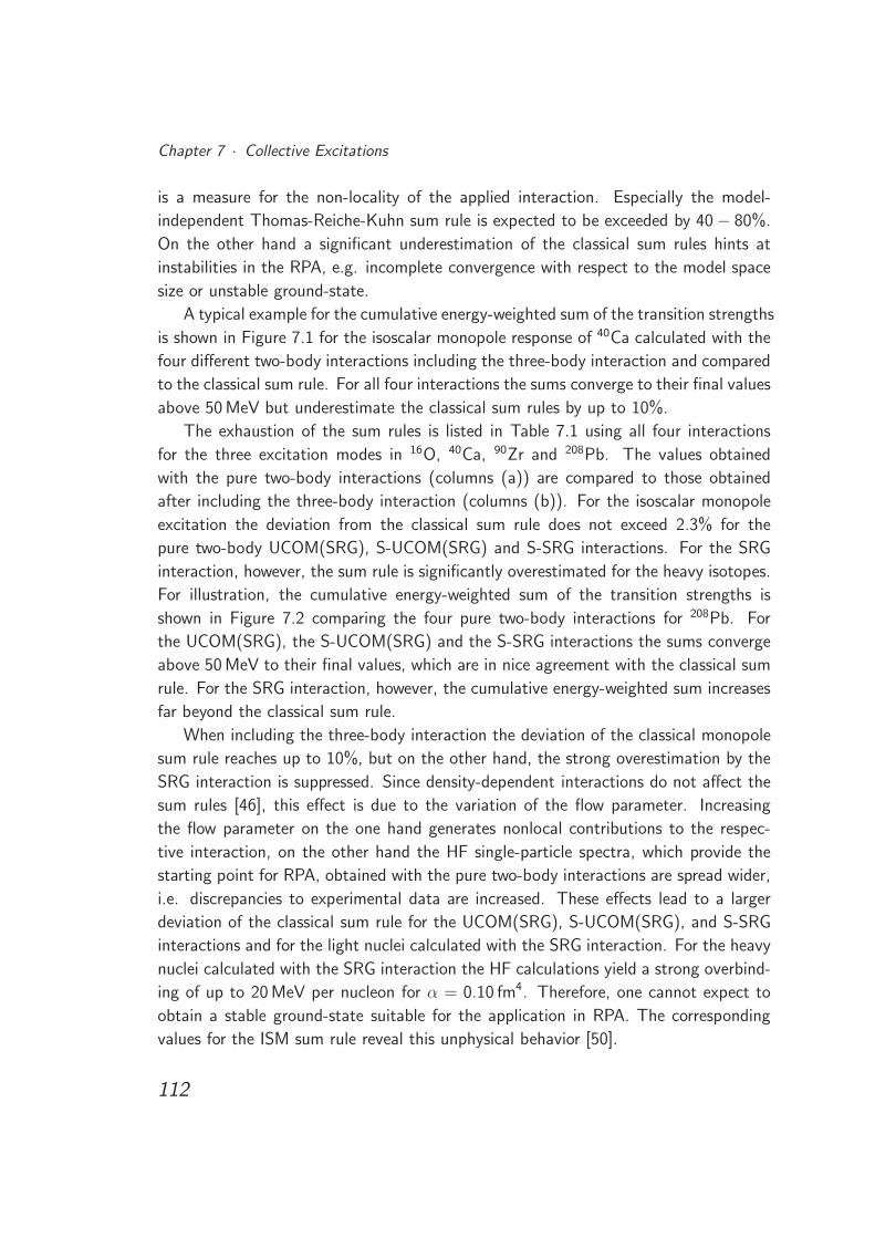
Chapter 7 · Collective Excitations
is a measure for the non-locality of the applied interaction. Especially the model-
independent Thomas-Reiche-Kuhn sum rule is expected to be exceeded by 40 − 80%.
On the other hand a significant underestimation of the classical sum rules hints at
instabilities in the RPA, e.g. incomplete convergence with respect to the model space
size or unstable ground-state.
A typical example for the cumulative energy-weighted sum of the transition strengths
is shown in Figure 7.1 for the isoscalar monopole response of 40Ca calculated with the
four different two-body interactions including the three-body interaction and compared
to the classical sum rule. For all four interactions the sums converge to their final values
above 50 MeV but underestimate the classical sum rules by up to 10%.
The exhaustion of the sum rules is listed in Table 7.1 using all four interactions
for the three excitation modes in 16O, 40Ca, 90Zr and 208Pb. The values obtained
with the pure two-body interactions (columns (a)) are compared to those obtained
after including the three-body interaction (columns (b)). For the isoscalar monopole
excitation the deviation from the classical sum rule does not exceed 2.3% for the
pure two-body UCOM(SRG), S-UCOM(SRG) and S-SRG interactions. For the SRG
interaction, however, the sum rule is significantly overestimated for the heavy isotopes.
For illustration, the cumulative energy-weighted sum of the transition strengths is
shown in Figure 7.2 comparing the four pure two-body interactions for 208Pb. For
the UCOM(SRG), the S-UCOM(SRG) and the S-SRG interactions the sums converge
above 50 MeV to their final values, which are in nice agreement with the classical sum
rule. For the SRG interaction, however, the cumulative energy-weighted sum increases
far beyond the classical sum rule.
When including the three-body interaction the deviation of the classical monopole
sum rule reaches up to 10%, but on the other hand, the strong overestimation by the
SRG interaction is suppressed. Since density-dependent interactions do not affect the
sum rules [46], this effect is due to the variation of the flow parameter. Increasing
the flow parameter on the one hand generates nonlocal contributions to the respec-
tive interaction, on the other hand the HF single-particle spectra, which provide the
starting point for RPA, obtained with the pure two-body interactions are spread wider,
i.e. discrepancies to experimental data are increased. These effects lead to a larger
deviation of the classical sum rule for the UCOM(SRG), S-UCOM(SRG), and S-SRG
interactions and for the light nuclei calculated with the SRG interaction. For the heavy
nuclei calculated with the SRG interaction the HF calculations yield a strong overbind-
ing of up to 20 MeV per nucleon for α = 0.10 fm4. Therefore, one cannot expect to
obtain a stable ground-state suitable for the application in RPA. The corresponding
values for the ISM sum rule reveal this unphysical behavior [50].
112
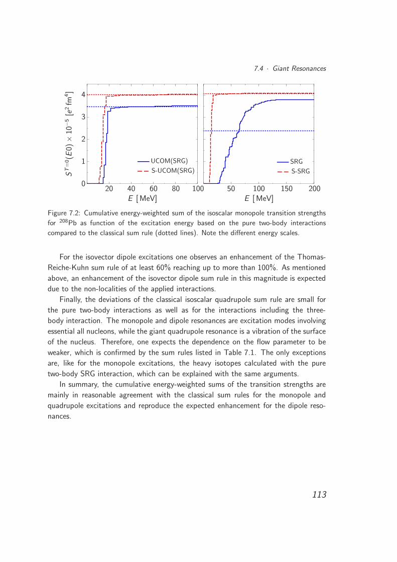
7.4 · Giant Resonances
20 40 60 80 100E [ MeV]
0
1
2
3
4
.
ST
=0(E
0)×
10−
5[e
2fm
4]
UCOM(SRG)
S-UCOM(SRG)
50 100 150 200E [ MeV]
SRG
S-SRG
Figure 7.2: Cumulative energy-weighted sum of the isoscalar monopole transition strengths
for 208Pb as function of the excitation energy based on the pure two-body interactions
compared to the classical sum rule (dotted lines). Note the different energy scales.
For the isovector dipole excitations one observes an enhancement of the Thomas-
Reiche-Kuhn sum rule of at least 60% reaching up to more than 100%. As mentioned
above, an enhancement of the isovector dipole sum rule in this magnitude is expected
due to the non-localities of the applied interactions.
Finally, the deviations of the classical isoscalar quadrupole sum rule are small for
the pure two-body interactions as well as for the interactions including the three-
body interaction. The monopole and dipole resonances are excitation modes involving
essential all nucleons, while the giant quadrupole resonance is a vibration of the surface
of the nucleus. Therefore, one expects the dependence on the flow parameter to be
weaker, which is confirmed by the sum rules listed in Table 7.1. The only exceptions
are, like for the monopole excitations, the heavy isotopes calculated with the pure
two-body SRG interaction, which can be explained with the same arguments.
In summary, the cumulative energy-weighted sums of the transition strengths are
mainly in reasonable agreement with the classical sum rules for the monopole and
quadrupole excitations and reproduce the expected enhancement for the dipole reso-
nances.
113
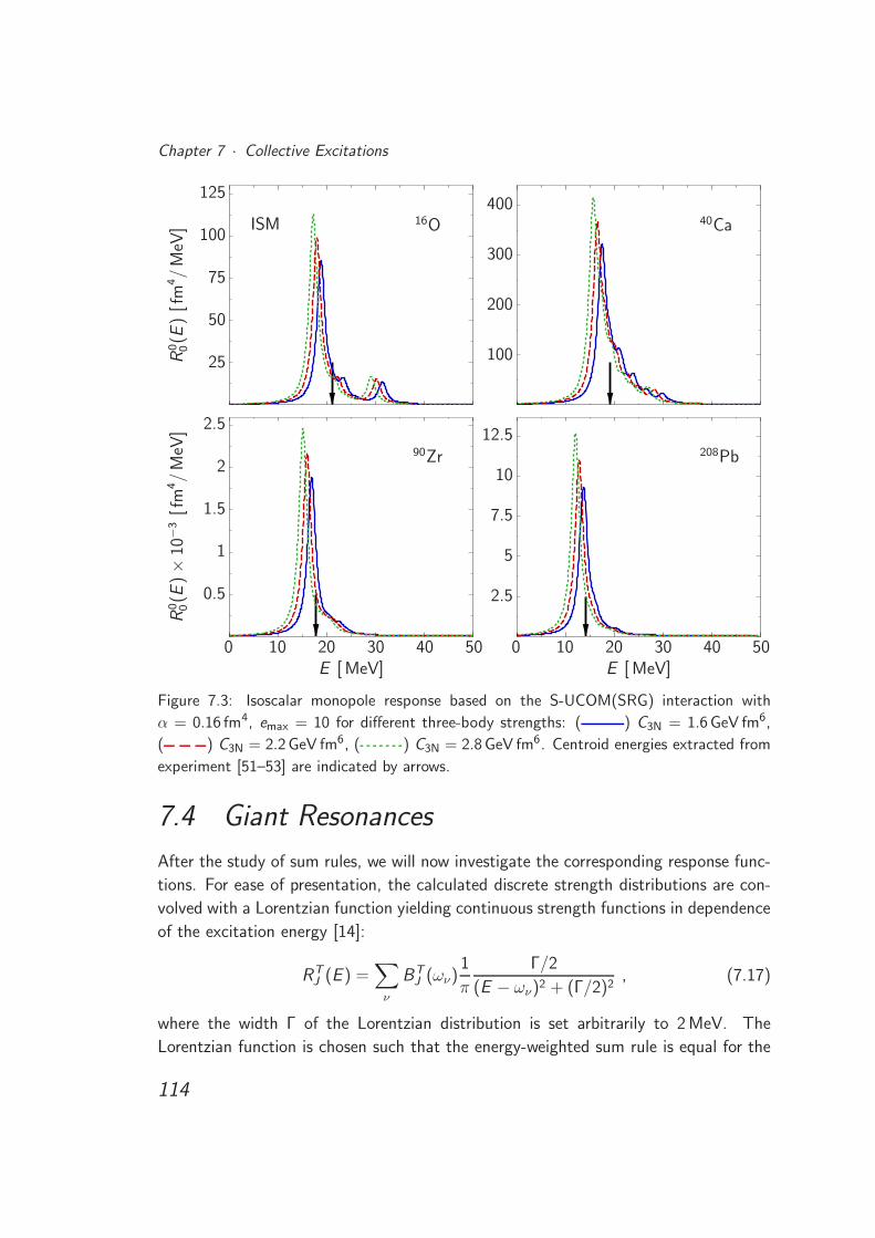
Chapter 7 · Collective Excitations
25
50
75
100
125
.
R0 0(E
)[f
m4/
MeV
] 16OISM
100
200
300
400
.
40Ca
0 10 20 30 40 50E [ MeV]
0.5
1
1.5
2
2.5
.
R0 0(E
)×
10−
3[f
m4/
MeV
]
90Zr
0 10 20 30 40 50E [ MeV]
2.5
5
7.5
10
12.5
.
208Pb
Figure 7.3: Isoscalar monopole response based on the S-UCOM(SRG) interaction with
α = 0.16 fm4, emax = 10 for different three-body strengths: ( ) C3N = 1.6 GeV fm6,
( ) C3N = 2.2 GeV fm6, ( ) C3N = 2.8 GeV fm6. Centroid energies extracted from
experiment [51–53] are indicated by arrows.
7.4 Giant Resonances
After the study of sum rules, we will now investigate the corresponding response func-
tions. For ease of presentation, the calculated discrete strength distributions are con-
volved with a Lorentzian function yielding continuous strength functions in dependence
of the excitation energy [14]:
RTJ (E ) =
∑
ν
BTJ (ων)
1
π
Γ/2
(E − ων)2 + (Γ/2)2, (7.17)
where the width Γ of the Lorentzian distribution is set arbitrarily to 2 MeV. The
Lorentzian function is chosen such that the energy-weighted sum rule is equal for the
114
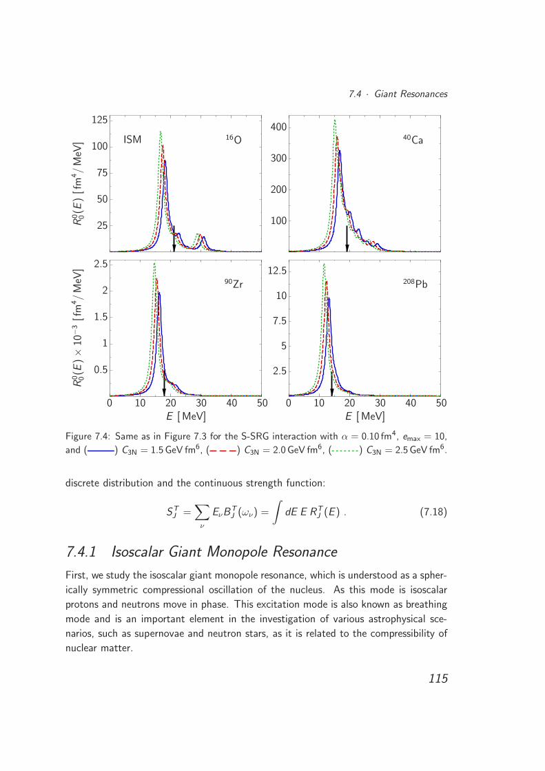
7.4 · Giant Resonances
25
50
75
100
125
.
R0 0(E
)[f
m4/
MeV
] 16OISM
100
200
300
400
.
40Ca
0 10 20 30 40 50E [ MeV]
0.5
1
1.5
2
2.5
.
R0 0(E
)×
10−
3[f
m4/
MeV
]
90Zr
0 10 20 30 40 50E [ MeV]
2.5
5
7.5
10
12.5
.
208Pb
Figure 7.4: Same as in Figure 7.3 for the S-SRG interaction with α = 0.10 fm4, emax = 10,
and ( ) C3N = 1.5 GeV fm6, ( ) C3N = 2.0 GeV fm6, ( ) C3N = 2.5 GeV fm6.
discrete distribution and the continuous strength function:
STJ =
∑
ν
EνBTJ (ων) =
∫dE E RT
J (E ) . (7.18)
7.4.1 Isoscalar Giant Monopole Resonance
First, we study the isoscalar giant monopole resonance, which is understood as a spher-
ically symmetric compressional oscillation of the nucleus. As this mode is isoscalar
protons and neutrons move in phase. This excitation mode is also known as breathing
mode and is an important element in the investigation of various astrophysical sce-
narios, such as supernovae and neutron stars, as it is related to the compressibility of
nuclear matter.
115
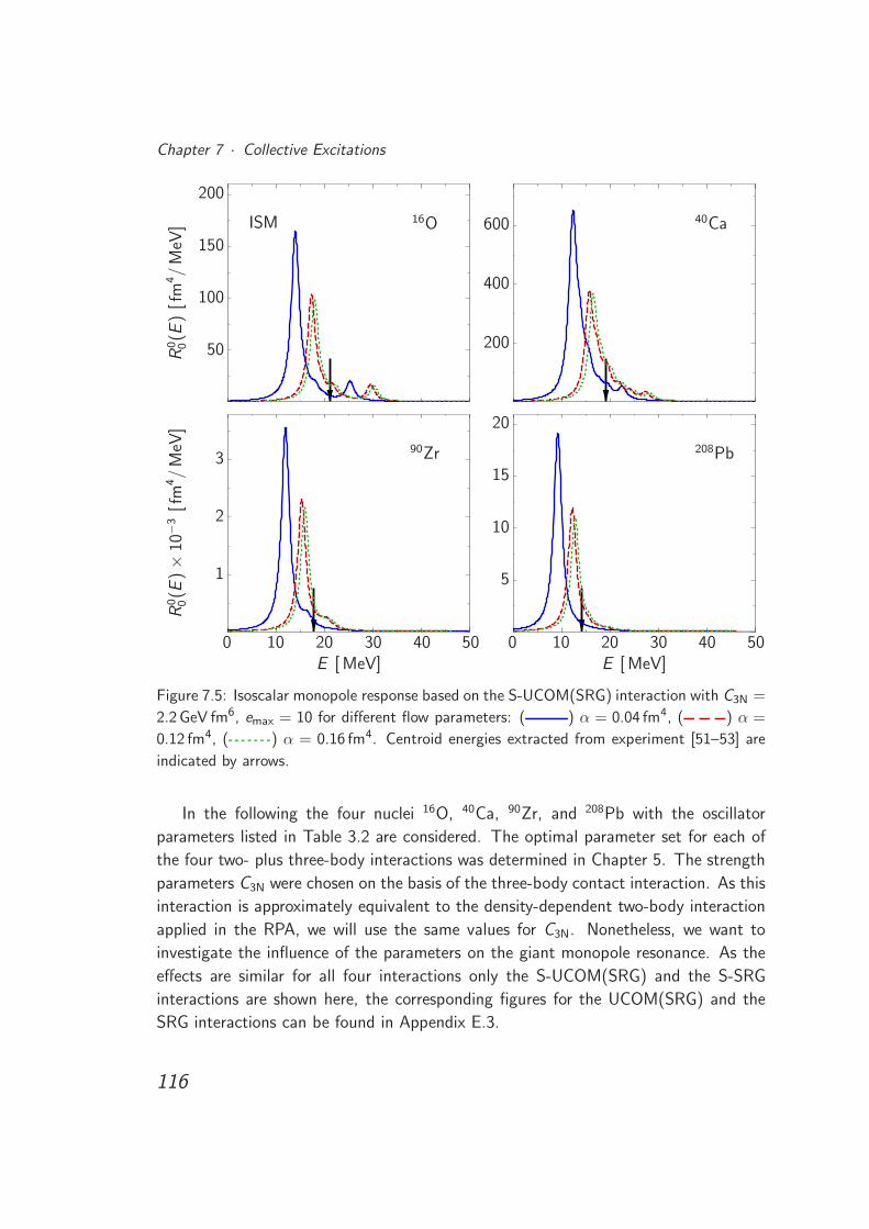
Chapter 7 · Collective Excitations
50
100
150
200
.
R0 0(E
)[f
m4/
MeV
] 16OISM
200
400
600
.
40Ca
0 10 20 30 40 50E [ MeV]
1
2
3
.
R0 0(E
)×
10−
3[f
m4/
MeV
]
90Zr
0 10 20 30 40 50E [ MeV]
5
10
15
20
.
208Pb
Figure 7.5: Isoscalar monopole response based on the S-UCOM(SRG) interaction with C3N =
2.2 GeV fm6, emax = 10 for different flow parameters: ( ) α = 0.04 fm4, ( ) α =
0.12 fm4, ( ) α = 0.16 fm4. Centroid energies extracted from experiment [51–53] are
indicated by arrows.
In the following the four nuclei 16O, 40Ca, 90Zr, and 208Pb with the oscillator
parameters listed in Table 3.2 are considered. The optimal parameter set for each of
the four two- plus three-body interactions was determined in Chapter 5. The strength
parameters C3N were chosen on the basis of the three-body contact interaction. As this
interaction is approximately equivalent to the density-dependent two-body interaction
applied in the RPA, we will use the same values for C3N. Nonetheless, we want to
investigate the influence of the parameters on the giant monopole resonance. As the
effects are similar for all four interactions only the S-UCOM(SRG) and the S-SRG
interactions are shown here, the corresponding figures for the UCOM(SRG) and the
SRG interactions can be found in Appendix E.3.
116
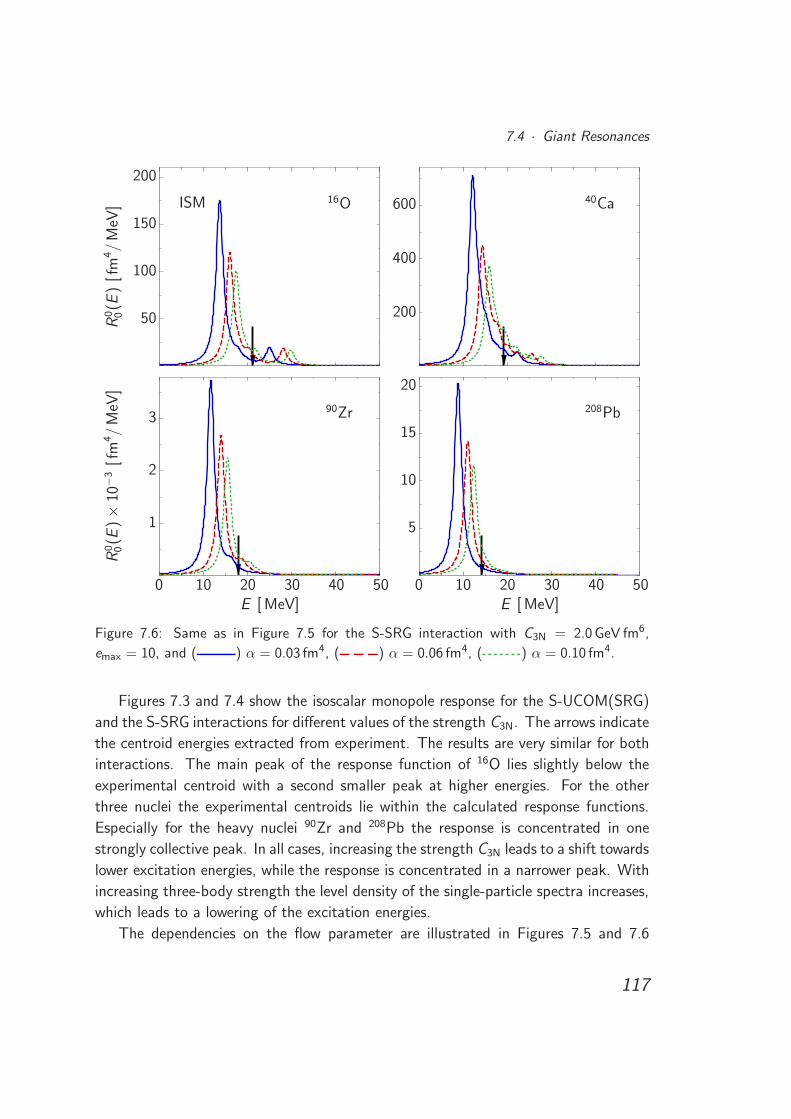
7.4 · Giant Resonances
50
100
150
200
.
R0 0(E
)[f
m4/
MeV
] 16OISM
200
400
600
.
40Ca
0 10 20 30 40 50E [ MeV]
1
2
3
.
R0 0(E
)×
10−
3[f
m4/
MeV
]
90Zr
0 10 20 30 40 50E [ MeV]
5
10
15
20
.
208Pb
Figure 7.6: Same as in Figure 7.5 for the S-SRG interaction with C3N = 2.0 GeV fm6,
emax = 10, and ( ) α = 0.03 fm4, ( ) α = 0.06 fm4, ( ) α = 0.10 fm4.
Figures 7.3 and 7.4 show the isoscalar monopole response for the S-UCOM(SRG)
and the S-SRG interactions for different values of the strength C3N. The arrows indicate
the centroid energies extracted from experiment. The results are very similar for both
interactions. The main peak of the response function of 16O lies slightly below the
experimental centroid with a second smaller peak at higher energies. For the other
three nuclei the experimental centroids lie within the calculated response functions.
Especially for the heavy nuclei 90Zr and 208Pb the response is concentrated in one
strongly collective peak. In all cases, increasing the strength C3N leads to a shift towards
lower excitation energies, while the response is concentrated in a narrower peak. With
increasing three-body strength the level density of the single-particle spectra increases,
which leads to a lowering of the excitation energies.
The dependencies on the flow parameter are illustrated in Figures 7.5 and 7.6
117
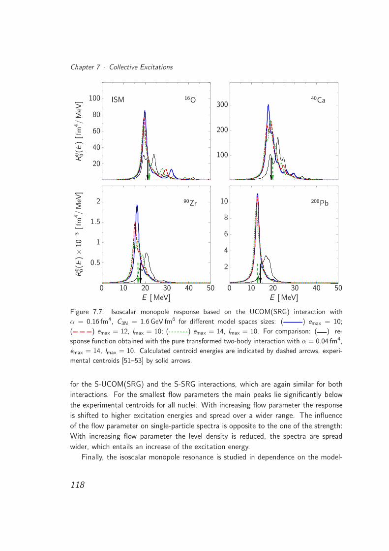
Chapter 7 · Collective Excitations
20
40
60
80
100
.
R0 0(E
)[f
m4/
MeV
] 16OISM
100
200
300
.
40Ca
0 10 20 30 40 50E [ MeV]
0.5
1
1.5
2
.
R0 0(E
)×
10−
3[f
m4/
MeV
]
90Zr
0 10 20 30 40 50E [ MeV]
2
4
6
8
10
.
208Pb
Figure 7.7: Isoscalar monopole response based on the UCOM(SRG) interaction with
α = 0.16 fm4, C3N = 1.6 GeV fm6 for different model spaces sizes: ( ) emax = 10;
( ) emax = 12, lmax = 10; ( ) emax = 14, lmax = 10. For comparison: ( ) re-
sponse function obtained with the pure transformed two-body interaction with α = 0.04 fm4,
emax = 14, lmax = 10. Calculated centroid energies are indicated by dashed arrows, experi-
mental centroids [51–53] by solid arrows.
for the S-UCOM(SRG) and the S-SRG interactions, which are again similar for both
interactions. For the smallest flow parameters the main peaks lie significantly below
the experimental centroids for all nuclei. With increasing flow parameter the response
is shifted to higher excitation energies and spread over a wider range. The influence
of the flow parameter on single-particle spectra is opposite to the one of the strength:
With increasing flow parameter the level density is reduced, the spectra are spread
wider, which entails an increase of the excitation energy.
Finally, the isoscalar monopole resonance is studied in dependence on the model-
118
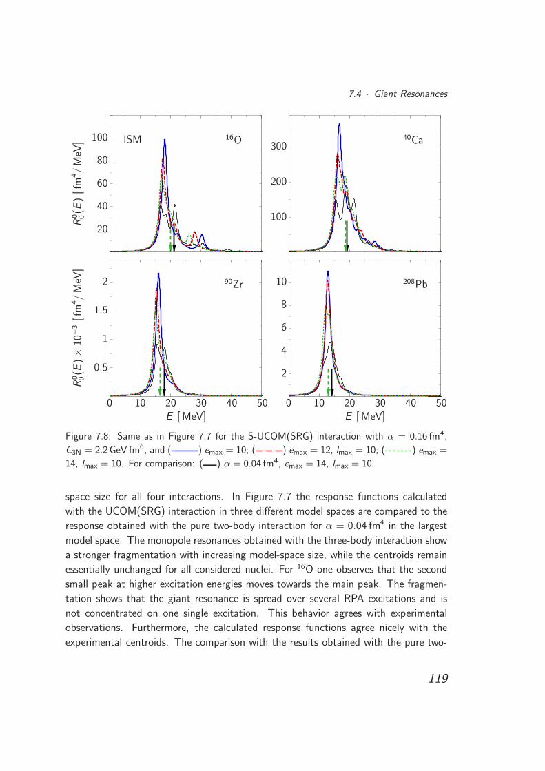
7.4 · Giant Resonances
20
40
60
80
100
.
R0 0(E
)[f
m4/
MeV
] 16OISM
100
200
300
.
40Ca
0 10 20 30 40 50E [ MeV]
0.5
1
1.5
2
.
R0 0(E
)×
10−
3[f
m4/
MeV
]
90Zr
0 10 20 30 40 50E [ MeV]
2
4
6
8
10
.
208Pb
Figure 7.8: Same as in Figure 7.7 for the S-UCOM(SRG) interaction with α = 0.16 fm4,
C3N = 2.2 GeV fm6, and ( ) emax = 10; ( ) emax = 12, lmax = 10; ( ) emax =
14, lmax = 10. For comparison: ( ) α = 0.04 fm4, emax = 14, lmax = 10.
space size for all four interactions. In Figure 7.7 the response functions calculated
with the UCOM(SRG) interaction in three different model spaces are compared to the
response obtained with the pure two-body interaction for α = 0.04 fm4 in the largest
model space. The monopole resonances obtained with the three-body interaction show
a stronger fragmentation with increasing model-space size, while the centroids remain
essentially unchanged for all considered nuclei. For 16O one observes that the second
small peak at higher excitation energies moves towards the main peak. The fragmen-
tation shows that the giant resonance is spread over several RPA excitations and is
not concentrated on one single excitation. This behavior agrees with experimental
observations. Furthermore, the calculated response functions agree nicely with the
experimental centroids. The comparison with the results obtained with the pure two-
119
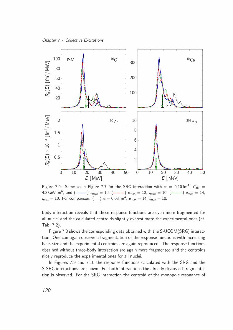
Chapter 7 · Collective Excitations
20
40
60
80
100
.
R0 0(E
)[f
m4/
MeV
] 16OISM
100
200
300
.
40Ca
0 10 20 30 40 50E [ MeV]
0.5
1
1.5
2
.
R0 0(E
)×
10−
3[f
m4/
MeV
]
90Zr
0 10 20 30 40 50E [ MeV]
2
4
6
8
10
.
208Pb
Figure 7.9: Same as in Figure 7.7 for the SRG interaction with α = 0.10 fm4, C3N =
4.3 GeV fm6, and ( ) emax = 10; ( ) emax = 12, lmax = 10; ( ) emax = 14,
lmax = 10. For comparison: ( ) α = 0.03 fm4, emax = 14, lmax = 10.
body interaction reveals that these response functions are even more fragmented for
all nuclei and the calculated centroids slightly overestimate the experimental ones (cf.
Tab. 7.2).
Figure 7.8 shows the corresponding data obtained with the S-UCOM(SRG) interac-
tion. One can again observe a fragmentation of the response functions with increasing
basis size and the experimental centroids are again reproduced. The response functions
obtained without three-body interaction are again more fragmented and the centroids
nicely reproduce the experimental ones for all nuclei.
In Figures 7.9 and 7.10 the response functions calculated with the SRG and the
S-SRG interactions are shown. For both interactions the already discussed fragmenta-
tion is observed. For the SRG interaction the centroid of the monopole resonance of
120
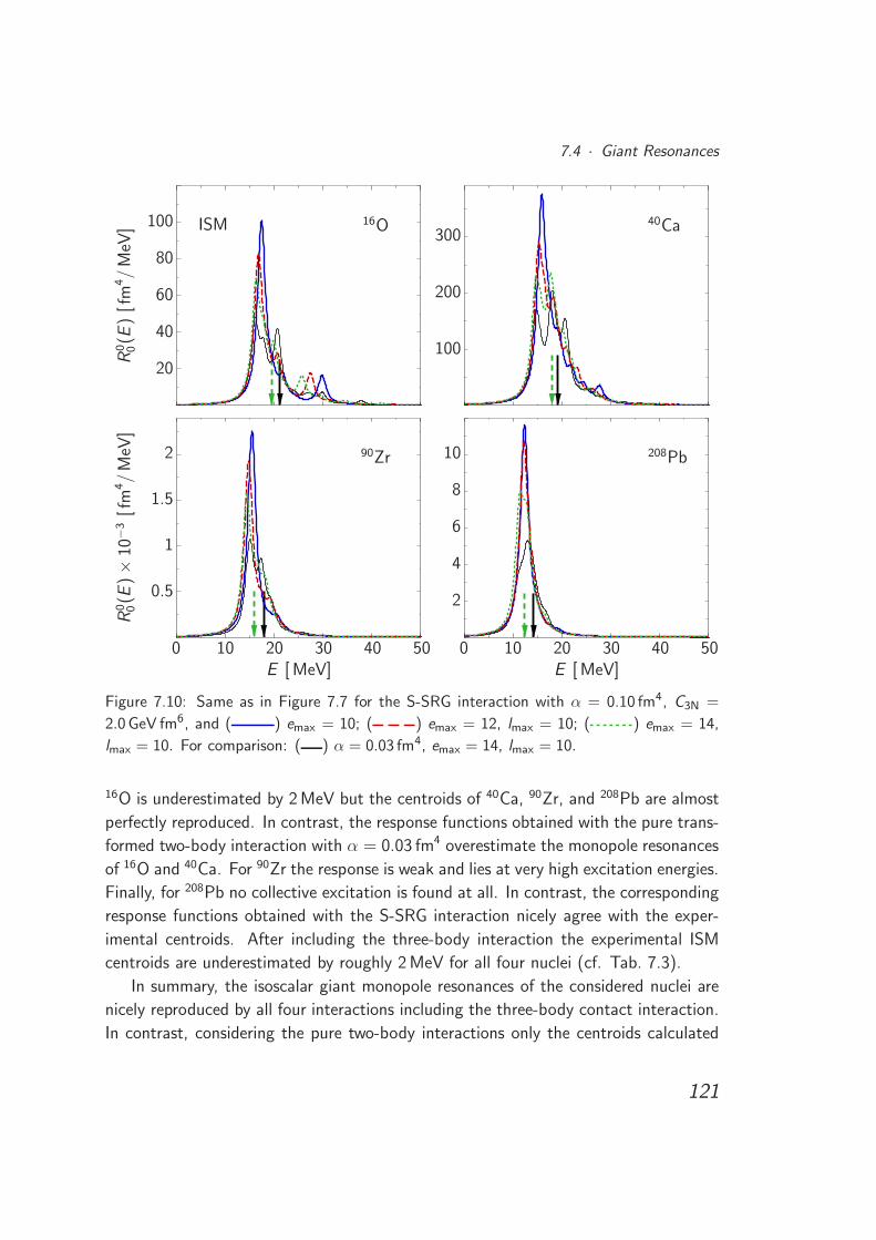
7.4 · Giant Resonances
20
40
60
80
100
.
R0 0(E
)[f
m4/
MeV
] 16OISM
100
200
300
.
40Ca
0 10 20 30 40 50E [ MeV]
0.5
1
1.5
2
.
R0 0(E
)×
10−
3[f
m4/
MeV
]
90Zr
0 10 20 30 40 50E [ MeV]
2
4
6
8
10
.
208Pb
Figure 7.10: Same as in Figure 7.7 for the S-SRG interaction with α = 0.10 fm4, C3N =
2.0 GeV fm6, and ( ) emax = 10; ( ) emax = 12, lmax = 10; ( ) emax = 14,
lmax = 10. For comparison: ( ) α = 0.03 fm4, emax = 14, lmax = 10.
16O is underestimated by 2 MeV but the centroids of 40Ca, 90Zr, and 208Pb are almost
perfectly reproduced. In contrast, the response functions obtained with the pure trans-
formed two-body interaction with α = 0.03 fm4 overestimate the monopole resonances
of 16O and 40Ca. For 90Zr the response is weak and lies at very high excitation energies.
Finally, for 208Pb no collective excitation is found at all. In contrast, the corresponding
response functions obtained with the S-SRG interaction nicely agree with the exper-
imental centroids. After including the three-body interaction the experimental ISM
centroids are underestimated by roughly 2 MeV for all four nuclei (cf. Tab. 7.3).
In summary, the isoscalar giant monopole resonances of the considered nuclei are
nicely reproduced by all four interactions including the three-body contact interaction.
In contrast, considering the pure two-body interactions only the centroids calculated
121
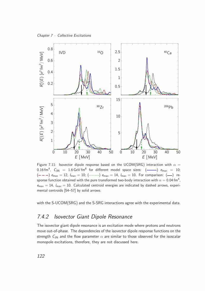
Chapter 7 · Collective Excitations
0.2
0.4
0.6
0.8
.
R1 1(E
)[e
2fm
2/
MeV
] 16OIVD
0.5
1
1.5
2
2.5
.
40Ca
0 10 20 30 40 50E [ MeV]
1
2
3
4
5
.
R1 1(E
)[e
2fm
2/
MeV
] 90Zr
0 10 20 30 40 50E [ MeV]
5
10
15
.
208Pb
Figure 7.11: Isovector dipole response based on the UCOM(SRG) interaction with α =
0.16 fm4, C3N = 1.6 GeV fm6 for different model space sizes: ( ) emax = 10;
( ) emax = 12, lmax = 10; ( ) emax = 14, lmax = 10. For comparison: ( ) re-
sponse function obtained with the pure transformed two-body interaction with α = 0.04 fm4,
emax = 14, lmax = 10. Calculated centroid energies are indicated by dashed arrows, experi-
mental centroids [54–57] by solid arrows.
with the S-UCOM(SRG) and the S-SRG interactions agree with the experimental data.
7.4.2 Isovector Giant Dipole Resonance
The isovector giant dipole resonance is an excitation mode where protons and neutrons
move out-of-phase. The dependencies of the isovector dipole response functions on the
strength C3N and the flow parameter α are similar to those observed for the isoscalar
monopole excitations, therefore, they are not discussed here.
122
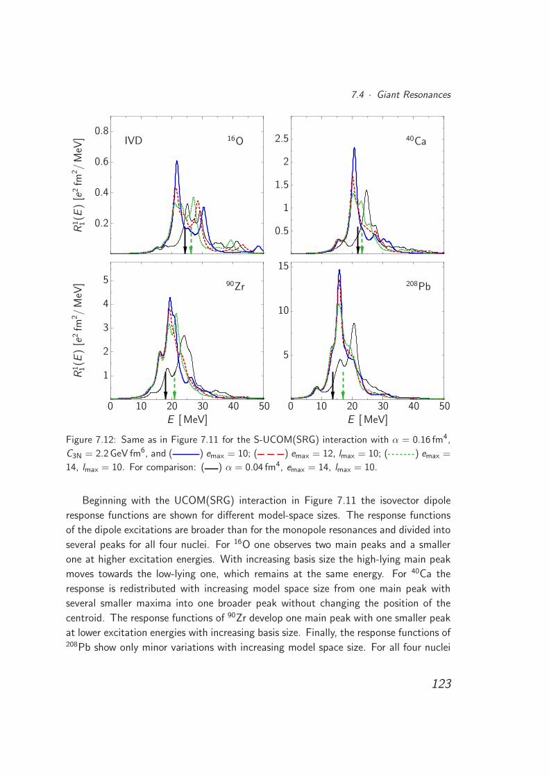
7.4 · Giant Resonances
0.2
0.4
0.6
0.8
.
R1 1(E
)[e
2fm
2/
MeV
] 16OIVD
0.5
1
1.5
2
2.5
.
40Ca
0 10 20 30 40 50E [ MeV]
1
2
3
4
5
.
R1 1(E
)[e
2fm
2/
MeV
] 90Zr
0 10 20 30 40 50E [ MeV]
5
10
15
.
208Pb
Figure 7.12: Same as in Figure 7.11 for the S-UCOM(SRG) interaction with α = 0.16 fm4,
C3N = 2.2 GeV fm6, and ( ) emax = 10; ( ) emax = 12, lmax = 10; ( ) emax =
14, lmax = 10. For comparison: ( ) α = 0.04 fm4, emax = 14, lmax = 10.
Beginning with the UCOM(SRG) interaction in Figure 7.11 the isovector dipole
response functions are shown for different model-space sizes. The response functions
of the dipole excitations are broader than for the monopole resonances and divided into
several peaks for all four nuclei. For 16O one observes two main peaks and a smaller
one at higher excitation energies. With increasing basis size the high-lying main peak
moves towards the low-lying one, which remains at the same energy. For 40Ca the
response is redistributed with increasing model space size from one main peak with
several smaller maxima into one broader peak without changing the position of the
centroid. The response functions of 90Zr develop one main peak with one smaller peak
at lower excitation energies with increasing basis size. Finally, the response functions of208Pb show only minor variations with increasing model space size. For all four nuclei
123
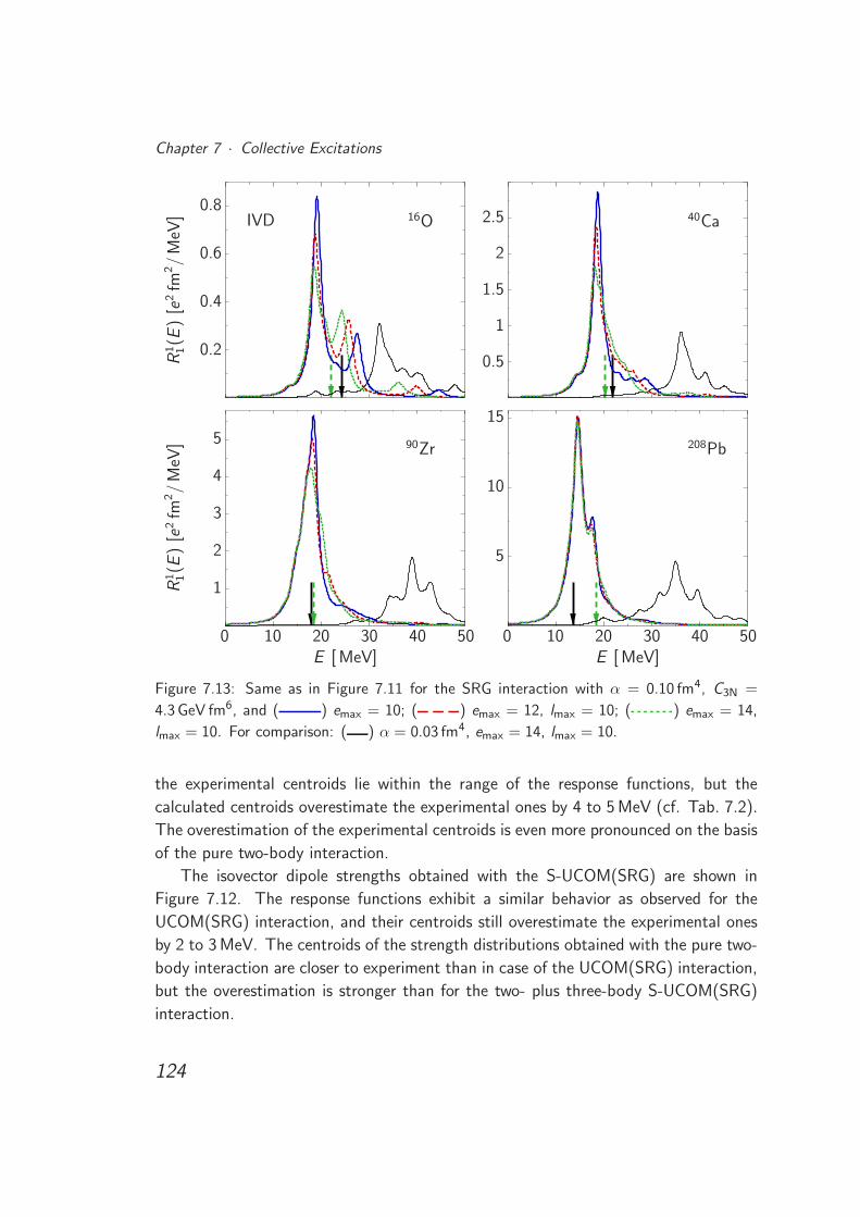
Chapter 7 · Collective Excitations
0.2
0.4
0.6
0.8
.
R1 1(E
)[e
2fm
2/
MeV
] 16OIVD
0.5
1
1.5
2
2.5
.
40Ca
0 10 20 30 40 50E [ MeV]
1
2
3
4
5
.
R1 1(E
)[e
2fm
2/
MeV
] 90Zr
0 10 20 30 40 50E [ MeV]
5
10
15
.
208Pb
Figure 7.13: Same as in Figure 7.11 for the SRG interaction with α = 0.10 fm4, C3N =
4.3 GeV fm6, and ( ) emax = 10; ( ) emax = 12, lmax = 10; ( ) emax = 14,
lmax = 10. For comparison: ( ) α = 0.03 fm4, emax = 14, lmax = 10.
the experimental centroids lie within the range of the response functions, but the
calculated centroids overestimate the experimental ones by 4 to 5 MeV (cf. Tab. 7.2).
The overestimation of the experimental centroids is even more pronounced on the basis
of the pure two-body interaction.
The isovector dipole strengths obtained with the S-UCOM(SRG) are shown in
Figure 7.12. The response functions exhibit a similar behavior as observed for the
UCOM(SRG) interaction, and their centroids still overestimate the experimental ones
by 2 to 3 MeV. The centroids of the strength distributions obtained with the pure two-
body interaction are closer to experiment than in case of the UCOM(SRG) interaction,
but the overestimation is stronger than for the two- plus three-body S-UCOM(SRG)
interaction.
124
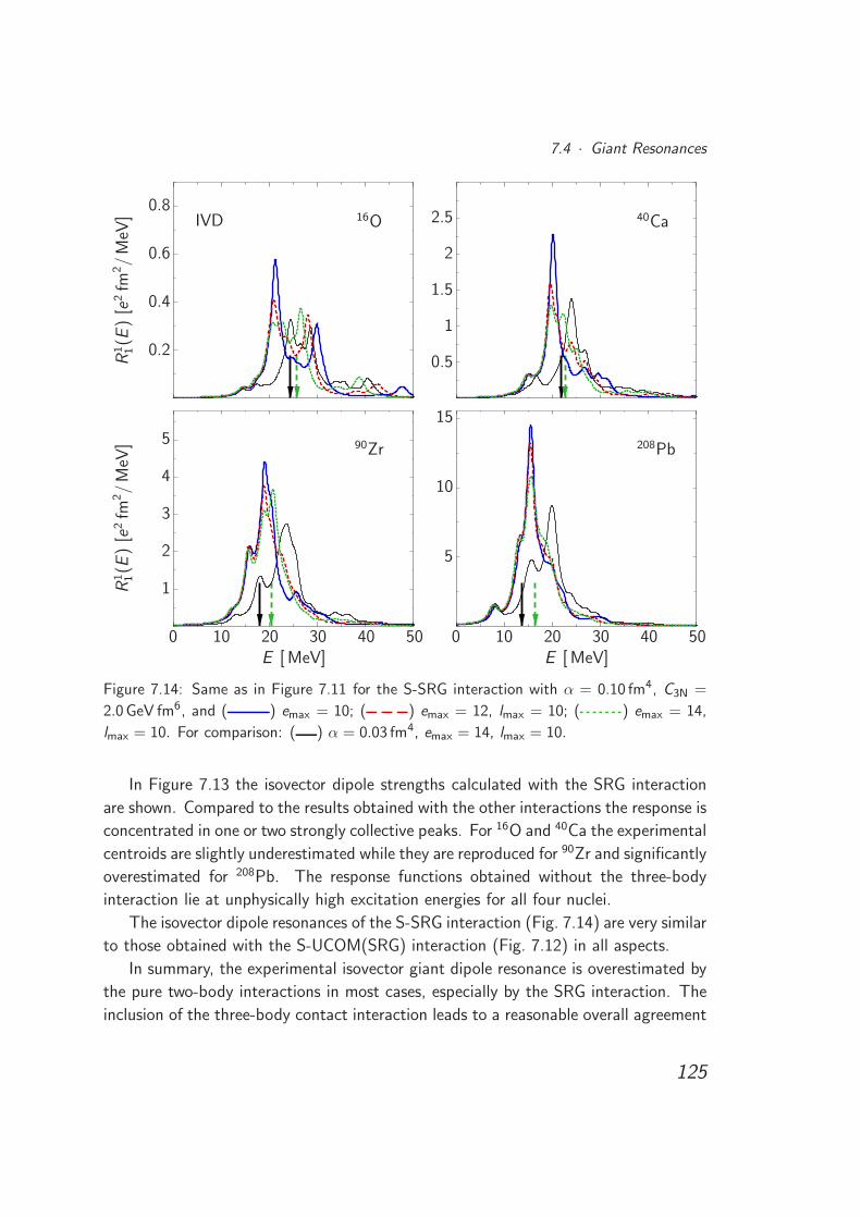
7.4 · Giant Resonances
0.2
0.4
0.6
0.8
.
R1 1(E
)[e
2fm
2/
MeV
] 16OIVD
0.5
1
1.5
2
2.5
.
40Ca
0 10 20 30 40 50E [ MeV]
1
2
3
4
5
.
R1 1(E
)[e
2fm
2/
MeV
] 90Zr
0 10 20 30 40 50E [ MeV]
5
10
15
.
208Pb
Figure 7.14: Same as in Figure 7.11 for the S-SRG interaction with α = 0.10 fm4, C3N =
2.0 GeV fm6, and ( ) emax = 10; ( ) emax = 12, lmax = 10; ( ) emax = 14,
lmax = 10. For comparison: ( ) α = 0.03 fm4, emax = 14, lmax = 10.
In Figure 7.13 the isovector dipole strengths calculated with the SRG interaction
are shown. Compared to the results obtained with the other interactions the response is
concentrated in one or two strongly collective peaks. For 16O and 40Ca the experimental
centroids are slightly underestimated while they are reproduced for 90Zr and significantly
overestimated for 208Pb. The response functions obtained without the three-body
interaction lie at unphysically high excitation energies for all four nuclei.
The isovector dipole resonances of the S-SRG interaction (Fig. 7.14) are very similar
to those obtained with the S-UCOM(SRG) interaction (Fig. 7.12) in all aspects.
In summary, the experimental isovector giant dipole resonance is overestimated by
the pure two-body interactions in most cases, especially by the SRG interaction. The
inclusion of the three-body contact interaction leads to a reasonable overall agreement
125
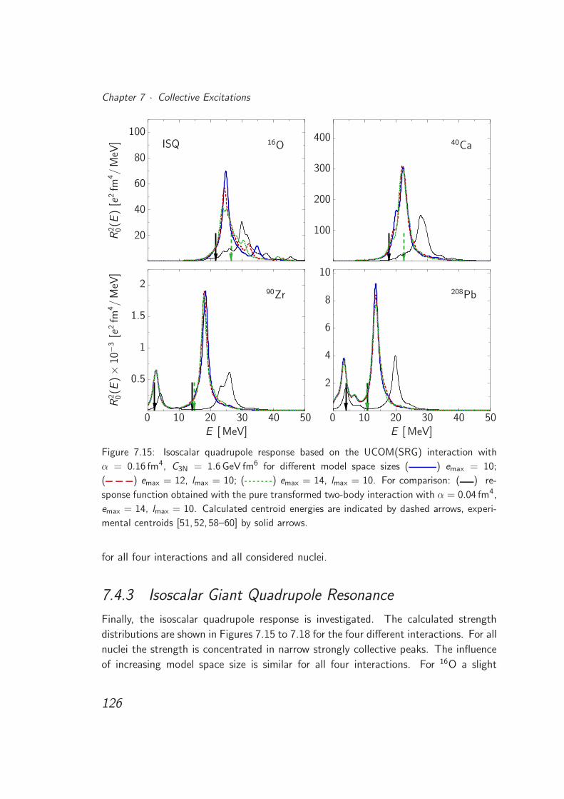
Chapter 7 · Collective Excitations
20
40
60
80
100
.
R2 0(E
)[e
2fm
4/
MeV
] 16OISQ
100
200
300
400
.
40Ca
0 10 20 30 40 50E [ MeV]
0.5
1
1.5
2
. R2 0(E
)×
10−
3[e
2fm
4/
MeV
]
90Zr
0 10 20 30 40 50E [ MeV]
2
4
6
8
10
.
208Pb
Figure 7.15: Isoscalar quadrupole response based on the UCOM(SRG) interaction with
α = 0.16 fm4, C3N = 1.6 GeV fm6 for different model space sizes ( ) emax = 10;
( ) emax = 12, lmax = 10; ( ) emax = 14, lmax = 10. For comparison: ( ) re-
sponse function obtained with the pure transformed two-body interaction with α = 0.04 fm4,
emax = 14, lmax = 10. Calculated centroid energies are indicated by dashed arrows, experi-
mental centroids [51, 52, 58–60] by solid arrows.
for all four interactions and all considered nuclei.
7.4.3 Isoscalar Giant Quadrupole Resonance
Finally, the isoscalar quadrupole response is investigated. The calculated strength
distributions are shown in Figures 7.15 to 7.18 for the four different interactions. For all
nuclei the strength is concentrated in narrow strongly collective peaks. The influence
of increasing model space size is similar for all four interactions. For 16O a slight
126
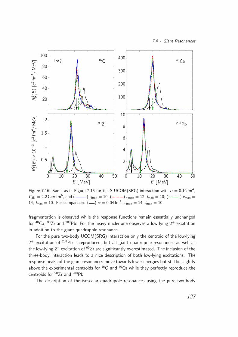
7.4 · Giant Resonances
20
40
60
80
100
.
R2 0(E
)[e
2fm
4/
MeV
] 16OISQ
100
200
300
400
.
40Ca
0 10 20 30 40 50E [ MeV]
0.5
1
1.5
2
. R2 0(E
)×
10−
3[e
2fm
4/
MeV
]
90Zr
0 10 20 30 40 50E [ MeV]
2
4
6
8
10
.
208Pb
Figure 7.16: Same as in Figure 7.15 for the S-UCOM(SRG) interaction with α = 0.16 fm4,
C3N = 2.2 GeV fm6, and ( ) emax = 10; ( ) emax = 12, lmax = 10; ( ) emax =
14, lmax = 10. For comparison: ( ) α = 0.04 fm4, emax = 14, lmax = 10.
fragmentation is observed while the response functions remain essentially unchanged
for 40Ca, 90Zr and 208Pb. For the heavy nuclei one observes a low-lying 2+ excitation
in addition to the giant quadrupole resonance.
For the pure two-body UCOM(SRG) interaction only the centroid of the low-lying
2+ excitation of 208Pb is reproduced, but all giant quadrupole resonances as well as
the low-lying 2+ excitation of 90Zr are significantly overestimated. The inclusion of the
three-body interaction leads to a nice description of both low-lying excitations. The
response peaks of the giant resonances move towards lower energies but still lie slightly
above the experimental centroids for 16O and 40Ca while they perfectly reproduce the
centroids for 90Zr and 208Pb.
The description of the isoscalar quadrupole resonances using the pure two-body
127
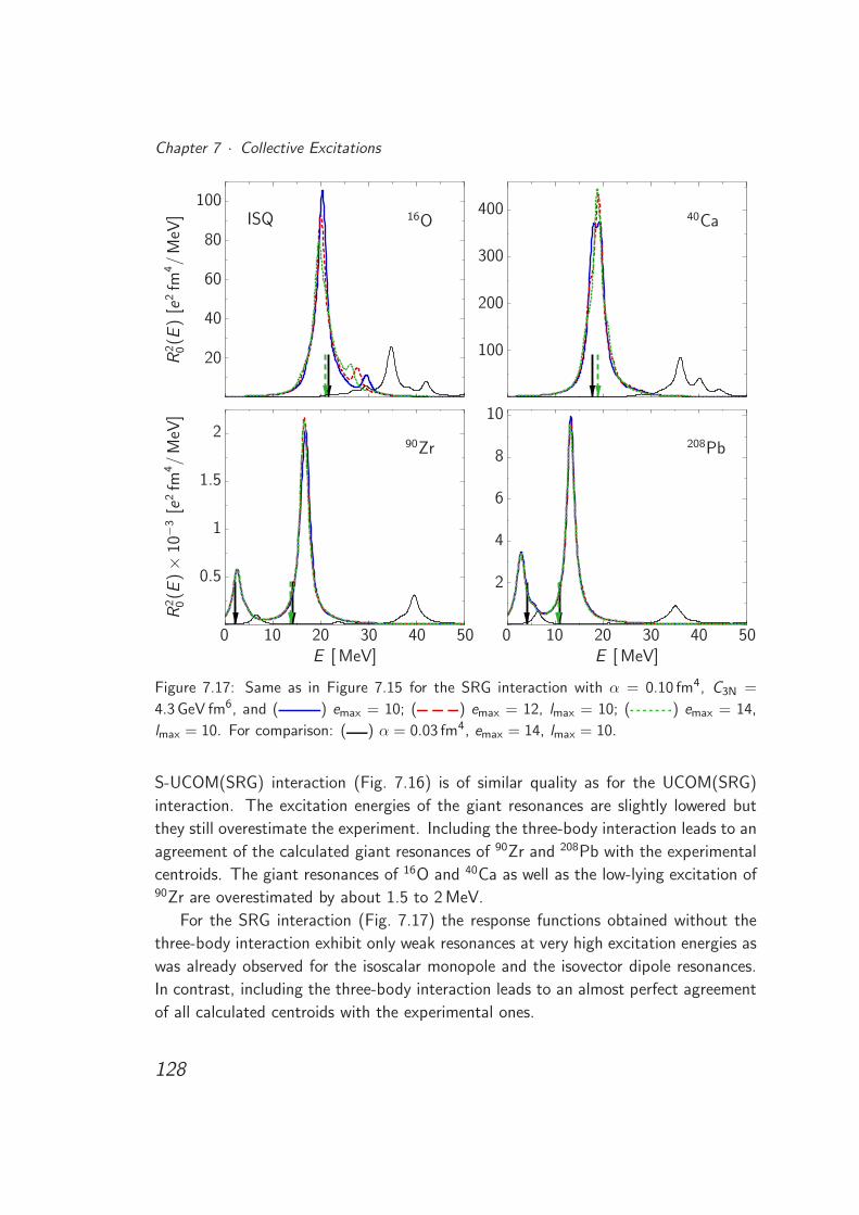
Chapter 7 · Collective Excitations
20
40
60
80
100
.
R2 0(E
)[e
2fm
4/
MeV
] 16OISQ
100
200
300
400
.
40Ca
0 10 20 30 40 50E [ MeV]
0.5
1
1.5
2
. R2 0(E
)×
10−
3[e
2fm
4/
MeV
]
90Zr
0 10 20 30 40 50E [ MeV]
2
4
6
8
10
.
208Pb
Figure 7.17: Same as in Figure 7.15 for the SRG interaction with α = 0.10 fm4, C3N =
4.3 GeV fm6, and ( ) emax = 10; ( ) emax = 12, lmax = 10; ( ) emax = 14,
lmax = 10. For comparison: ( ) α = 0.03 fm4, emax = 14, lmax = 10.
S-UCOM(SRG) interaction (Fig. 7.16) is of similar quality as for the UCOM(SRG)
interaction. The excitation energies of the giant resonances are slightly lowered but
they still overestimate the experiment. Including the three-body interaction leads to an
agreement of the calculated giant resonances of 90Zr and 208Pb with the experimental
centroids. The giant resonances of 16O and 40Ca as well as the low-lying excitation of90Zr are overestimated by about 1.5 to 2 MeV.
For the SRG interaction (Fig. 7.17) the response functions obtained without the
three-body interaction exhibit only weak resonances at very high excitation energies as
was already observed for the isoscalar monopole and the isovector dipole resonances.
In contrast, including the three-body interaction leads to an almost perfect agreement
of all calculated centroids with the experimental ones.
128
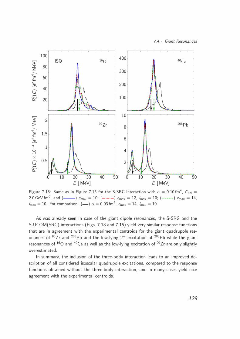
7.4 · Giant Resonances
20
40
60
80
100
.
R2 0(E
)[e
2fm
4/
MeV
] 16OISQ
100
200
300
400
.
40Ca
0 10 20 30 40 50E [ MeV]
0.5
1
1.5
2
. R2 0(E
)×
10−
3[e
2fm
4/
MeV
]
90Zr
0 10 20 30 40 50E [ MeV]
2
4
6
8
10
.
208Pb
Figure 7.18: Same as in Figure 7.15 for the S-SRG interaction with α = 0.10 fm4, C3N =
2.0 GeV fm6, and ( ) emax = 10; ( ) emax = 12, lmax = 10; ( ) emax = 14,
lmax = 10. For comparison: ( ) α = 0.03 fm4, emax = 14, lmax = 10.
As was already seen in case of the giant dipole resonances, the S-SRG and the
S-UCOM(SRG) interactions (Figs. 7.18 and 7.15) yield very similar response functions
that are in agreement with the experimental centroids for the giant quadrupole res-
onances of 90Zr and 208Pb and the low-lying 2+ excitation of 208Pb while the giant
resonances of 16O and 40Ca as well as the low-lying excitation of 90Zr are only slightly
overestimated.
In summary, the inclusion of the three-body interaction leads to an improved de-
scription of all considered isoscalar quadrupole excitations, compared to the response
functions obtained without the three-body interaction, and in many cases yield nice
agreement with the experimental centroids.
129
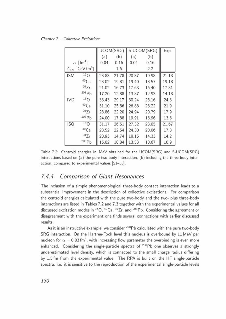
Chapter 7 · Collective Excitations
UCOM(SRG) S-UCOM(SRG) Exp.
(a) (b) (a) (b)
α [ fm4] 0.04 0.16 0.04 0.16
C3N [ GeV fm6] – 1.6 – 2.2
ISM 16O 23.83 21.78 20.87 19.98 21.1340Ca 23.02 19.81 19.40 18.57 19.1890Zr 21.02 16.73 17.63 16.40 17.81
208Pb 17.20 12.88 13.87 12.93 14.18
IVD 16O 33.43 29.17 30.24 26.16 24.340Ca 31.10 25.86 26.88 23.22 21.990Zr 28.86 22.20 24.94 20.79 17.9
208Pb 24.00 17.88 19.91 16.96 13.6
ISQ 16O 31.17 26.51 27.32 23.05 21.6740Ca 28.52 22.54 24.30 20.06 17.890Zr 20.93 14.74 18.15 14.33 14.2
208Pb 16.02 10.84 13.53 10.67 10.9
Table 7.2: Centroid energies in MeV obtained for the UCOM(SRG) and S-UCOM(SRG)
interactions based on (a) the pure two-body interaction, (b) including the three-body inter-
action, compared to experimental values [51–58].
7.4.4 Comparison of Giant Resonances
The inclusion of a simple phenomenological three-body contact interaction leads to a
substantial improvement in the description of collective excitations. For comparison
the centroid energies calculated with the pure two-body and the two- plus three-body
interactions are listed in Tables 7.2 and 7.3 together with the experimental values for all
discussed excitation modes in 16O, 40Ca, 90Zr, and 208Pb. Considering the agreement or
disagreement with the experiment one finds several connections with earlier discussed
results.
As it is an instructive example, we consider 208Pb calculated with the pure two-body
SRG interaction. On the Hartree-Fock level this nucleus is overbound by 11 MeV per
nucleon for α = 0.03 fm4, with increasing flow parameter the overbinding is even more
enhanced. Considering the single-particle spectra of 208Pb one observes a strongly
underestimated level density, which is connected to the small charge radius differing
by 1.5 fm from the experimental value. The RPA is built on the HF single-particle
spectra, i.e. it is sensitive to the reproduction of the experimental single-particle levels
130
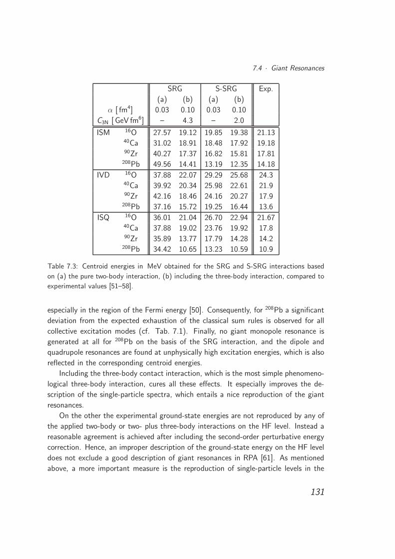
7.4 · Giant Resonances
SRG S-SRG Exp.
(a) (b) (a) (b)
α [ fm4] 0.03 0.10 0.03 0.10
C3N [ GeV fm6] – 4.3 – 2.0
ISM 16O 27.57 19.12 19.85 19.38 21.1340Ca 31.02 18.91 18.48 17.92 19.1890Zr 40.27 17.37 16.82 15.81 17.81
208Pb 49.56 14.41 13.19 12.35 14.18
IVD 16O 37.88 22.07 29.29 25.68 24.340Ca 39.92 20.34 25.98 22.61 21.990Zr 42.16 18.46 24.16 20.27 17.9
208Pb 37.16 15.72 19.25 16.44 13.6
ISQ 16O 36.01 21.04 26.70 22.94 21.6740Ca 37.88 19.02 23.76 19.92 17.890Zr 35.89 13.77 17.79 14.28 14.2
208Pb 34.42 10.65 13.23 10.59 10.9
Table 7.3: Centroid energies in MeV obtained for the SRG and S-SRG interactions based
on (a) the pure two-body interaction, (b) including the three-body interaction, compared to
experimental values [51–58].
especially in the region of the Fermi energy [50]. Consequently, for 208Pb a significant
deviation from the expected exhaustion of the classical sum rules is observed for all
collective excitation modes (cf. Tab. 7.1). Finally, no giant monopole resonance is
generated at all for 208Pb on the basis of the SRG interaction, and the dipole and
quadrupole resonances are found at unphysically high excitation energies, which is also
reflected in the corresponding centroid energies.
Including the three-body contact interaction, which is the most simple phenomeno-
logical three-body interaction, cures all these effects. It especially improves the de-
scription of the single-particle spectra, which entails a nice reproduction of the giant
resonances.
On the other the experimental ground-state energies are not reproduced by any of
the applied two-body or two- plus three-body interactions on the HF level. Instead a
reasonable agreement is achieved after including the second-order perturbative energy
correction. Hence, an improper description of the ground-state energy on the HF level
does not exclude a good description of giant resonances in RPA [61]. As mentioned
above, a more important measure is the reproduction of single-particle levels in the
131
Chapter 7 · Collective Excitations
region of the Fermi energy.
The additional repulsion of the three-body interaction increases the level density of
single-particle spectra on the Hartree-Fock level, which entails a lowering of the excita-
tion energies of the isovector dipole and the isoscalar quadrupole giant resonances, and
in part of the isoscalar monopole giant resonance compared to the response functions
obtained with the pure two-body interactions. This results in an improved agreement of
calculated centroid energies with the experimental ones for the dipole and quadrupole
giant resonances. The giant monopole resonances are already nicely reproduced by the
pure two-body S-UCOM(SRG) and S-SRG interactions. This agreement is maintained
after including the three-body interaction.
The impact of the three-body contact interaction is especially pronounced in case
of the SRG interaction. But one has to be careful with these results, because the
three-body strength is roughly twice as large as for the other interactions and might
lead to problems when considering other observables.
Up to now only centroid energies were compared with experimental data. A more
sophisticated insight could be obtained by comparing the experimental response func-
tions with the calculated ones.
132
Chapter 8
Conclusions
The importance of three-nucleon interactions is demonstrated in various nuclear struc-
ture investigations based on pure nucleon-nucleon interactions. As a first step towards
the consistent inclusion of realistic three-body forces we study simple phenomenolog-
ical three-body interactions. We develop an appropriate scheme for the handling of
three-body matrix elements and derive the formal application of three-body forces in
various many-body methods.
The nuclear interaction induces complex correlations, such as the strong short-
range repulsion and tensor correlations. Due to these correlations large model spaces
are required to reach convergence. To facilitate calculations in tractable model spaces
the Unitary Correlation Operator Method and the Similarity Renormalization Group
are discussed as two different approaches to generate soft phase-shift equivalent in-
teractions via unitary transformations. Although the motivations of both methods
are quite different, the resulting interactions show a number of similarities, e.g. they
exhibit a band-diagonal structure with respect to momentum space matrix elements.
These methods are used to obtain four different classes of two-body interactions out
of the realistic Argonne V18 potential. Beside the standard UCOM(SRG) and SRG
interactions, where all partial waves are transformed consistently, we employ the S-
UCOM(SRG) and S-SRG interactions, where only the S-waves undergo the respective
unitary transformations.
To investigate ground-state energies and charge radii of selected closed-shell nuclei
across the whole nuclear chart the four different two-body interactions are used in the
Hartree-Fock approximation. While the systematics of the experimental ground-state
energies is reproduced by the UCOM(SRG), S-UCOM(SRG) and S-SRG interactions
133
Chapter 8 · Conclusions
except for a constant shift, the SRG interaction leads to a strong overbinding of
intermediate and heavy nuclei. The charge radii are systematically underestimated by
all four interactions. The HF ground-state is described by a single Slater determinant,
which is not capable of describing any correlations. The short-range correlations are
covered by the unitary transformations while the long-range correlations have to be
described by the many-body states, e.g., by applying many-body perturbation theory
on top of the HF results. Including the second-order perturbative corrections leads to a
reasonable agreement with experimental ground-state energies for the UCOM(SRG), S-
UCOM(SRG) and S-SRG interactions, while the perturbative corrections to the charge
radii are negligible. For the SRG interaction most nuclei are already overbound on the
HF level, and second-order perturbation theory cannot improve these results.
On the level of the HF approximation also single-particle spectra are examined. The
general description of the level ordering agrees rather well with experimental spectra,
but the level spacings, and especially the Fermi gap, are significantly overestimated.
The flow parameters used for these calculations are determined for each interaction
such that the experimental 4He ground-state energy is reproduced in a No-Core Shell
Model calculation, i.e. the flow parameter is chosen considering a four-nucleon system
only. Therefore, it is a remarkable result, that the systematics of the experimental
ground-state energies is reproduced across the whole nuclear chart on the basis of
HF plus MBPT calculations. Nonetheless, the results obtained with the pure two-
body interactions show some systematic deviations from experimental data, e.g. the
charge radii cannot be accurately reproduced by pure two-body interactions and the
description of single-particle spectra leaves room for improvement. To reduce these
deviations introducing a repulsive three-body interaction is inevitable.
The first ansatz for a phenomenological three-body interaction is a finite-range
interaction of Gaussian shape. The matrix elements are most conveniently calculated
in a basis of cartesian harmonic oscillator eigenstates and subsequently transformed
into a basis of spherical harmonic oscillator eigenstates. Only the S-UCOM and the
S-SRG interactions are supplemented by the Gaussian three-body interaction. The free
parameters, the strength and the range, are determined on the basis of HF calculations
such that the experimental charge radii are approximately reproduced across the whole
nuclear chart. Unfortunately, the matrix element calculation is very time-consuming re-
stricting the applicability of the Gaussian three-body interaction to small model spaces.
Since the influence of the Gaussian interaction on the second-order energy corrections
is only marginal, we consider only the corrections obtained with the two-body interac-
tions. The small model spaces avoid the convergence of the HF plus MBPT results.
But we are able to show that the ground-state energies and charge radii obtained with
134
the Gaussian three-body interaction are similar to the corresponding results obtained
with a regularized three-body contact interaction.
The matrix elements of the three-body contact interaction can directly be cal-
culated in a basis of spherical harmonic-oscillator eigenstates. The structure of the
regularized contact interaction entails that the matrix element computation is very ef-
ficient compared to the Gaussian three-body interaction. Thus, the contact interaction
is also manageable in large model spaces. The contact interaction is employed in con-
nection with all four unitarily transformed two-body interactions. For each underlying
two-body interaction the three-body strength is again chosen such that the HF charge
radii are in agreement with the experimental ones. For the SRG interaction the three-
body strength is roughly twice as large as for the other three two-body interactions.
After the inclusion of the three-body interaction the trend of the experimental ground-
state energies is reproduced except for an almost constant shift on the basis of all four
two-body interactions. Furthermore, in the description of single-particle spectra, the
level spacings are reduced due to the additional repulsion. Only for the UCOM(SRG)
interaction some inaccuracies appear in the description of single-particle spectra. The
inclusion of the perturbative corrections yields a reasonable agreement with experi-
mental data, although we have not yet reached complete convergence. However, these
results must not be overstated as the perturbative corrections are only calculated for
the two-body interactions and one has to keep in mind the inherent limitations of
MBPT.
To obtain a reference point from an exact diagonalization of the Hamilton matrix
we include the regularized contact interaction in the No-Core Shell Model. Using
the parameter sets optimized to reproduce experimental charge radii across the whole
nuclear chart, NCSM calculations based on the S-UCOM(SRG) and S-SRG interactions
result in an underbinding of 4He of about 1 to 2 MeV.
As giant resonances are of direct interest for applications in nuclear astrophysics,
the influence of the three-body contact interaction on these collective excitation modes
is investigated. The Random Phase Approximation provides a suitable framework for
the investigation of collective excitations. As including the full three-body interac-
tion in the RPA would be too time-consuming we replace it by a density-dependent
two-body contact interaction, which is equivalent in this case except for the regu-
larization. We study extensively isoscalar monopole, isovector dipole, and isoscalar
quadrupole excitations. Considering the pure two-body interactions, especially the
SRG interaction, strongly overestimates the experimental excitation energies of the
considered giant resonances. The giant monopole resonance is generally in agreement
with the experimental centroids for the pure two-body interactions while the giant
135
Chapter 8 · Conclusions
dipole and giant quadrupole resonances are significantly overestimated. The inclusion
of the three-body contact via the density-dependent two-body interaction leads to a
reasonable description of all three excitation modes for all four interactions.
Summarizing the preceding studies one can conclude that the UCOM(SRG) inter-
action shows problems in the description of single-particle spectra and accordingly in
the application of MBPT. The SRG interaction has to be supplemented by a stronger
three-body interaction in order to compensate the strong overbinding observed on the
HF plus MBPT level. As the regularized contact interaction is a phenomenological in-
teraction with a simple structure, e.g. no spin-isospin dependence, one would prefer it
to be as weak as possible. The S-UCOM(SRG) and the S-SRG interactions both yield
very similar results in all aspects of nuclear properties and, furthermore, their results
agree well with experimental data in the framework of various many-body methods
for nuclei across the whole nuclear chart. Therefore, one would choose one of these
interactions for further investigations, e.g. predictions for exotic nuclei. To perform
the next step towards the study of exotic nuclei a number of further important and
interesting investigations remain to be examined.
First of all, there are some minor aspects related to the calculation of charge
radii. The three-body strength can be chosen such that the radii are in almost perfect
agreement with experimental data for all considered nuclei. Therefore, it is worthwhile
to examine also minor corrections to the radii, which are the unitary transformation of
the radius operator and the calculation of the perturbative corrections for the radii.
The studies in the framework of the No-Core Shell Model can be extended to
investigate nuclei beside 4He up to the mid p-shell. Beyond this mass region the
Importance Truncated No-Core Shell Model can be applied to examine even heavier
nuclei [62]. Furthermore, the study of the influence of the three-body interaction on
the Tjon line is an interesting aspect.
Throughout this thesis only closed-shell nuclei were examined. For a profound un-
derstanding one has to extend the studies to open-shell nuclei, e.g. in the framework
of the Hartree-Fock-Bogoliubov method and the Quasiparticle Random Phase Approx-
imation [24, 48, 63]; but also degenerate many-body perturbation theory [64] and the
(Importance Truncated) No-Core Shell Model can be applied.
Already the handling of the most simple three-body interaction requires an enor-
mous computational effort. But one would like to include three-body interactions in
all aspects that are considered on the basis of pure two-body interactions. Further-
more, one would like to study more general three-body interactions, which exhibit a
more complex structure, e.g. the chiral interactions. One possibility to derive of an
effective two-body interaction is provided by the normal ordering [65]. The three-body
136
interaction is reformulated into a zero- plus one- plus two-body interaction with a
residual three-body interaction, which is discussed in Appendix D. The influence of
the residual three-body interaction on various observables is expected to be negligible.
This assumption can be verified by using the contact interaction in the framework of
many-body perturbation theory and the No-Core Shell Model.
In summary, the investigation of simple phenomenological three-nucleon interac-
tions proves to be a versatile tool to improve the description of various observables
across the whole nuclear chart using different many-body methods as well as to develop
an efficient procedure for the handling of three-body matrix elements.
137

Chapter 8 · Conclusions
138
Appendix A
Derivation of the Hartree-Fock Equations
For the derivation of the general Hartree-Fock equations, we first discuss the variational
principle which is used to deduce an average single-particle potential out of the NN
plus 3N interaction.
A.1 The Variational Principle
The solution of the exact Schrodinger equation
H|Ψ〉 = E |Ψ〉 (A.1)
is equivalent to the variation
δE [|Ψ〉] = E [|Ψ〉 + |δΨ〉] − E [|Ψ〉] = 0 , (A.2)
where we regard the energy E as a functional of the state |Ψ〉 [49, 66]:
E [|Ψ〉] =〈Ψ|H|Ψ〉〈Ψ|Ψ〉 . (A.3)
The state |Ψ〉 + |δΨ〉 denotes an infinitesimal but arbitrary variation of the state |Ψ〉with 〈δΨ|δΨ〉 ≪ 1. Discarding higher orders in |δΨ〉 the variation leads to
δE [|Ψ〉] =1
〈Ψ|Ψ〉
〈δΨ|H|Ψ〉 + 〈Ψ|H|δΨ〉 − 〈Ψ|H|Ψ〉
〈Ψ|Ψ〉 (〈δΨ|Ψ〉 + 〈Ψ|δΨ〉)
. (A.4)
139
Appendix A · Derivation of the Hartree-Fock Equations
Together with the condition of stationarity the variation reads
〈δΨ|(H − E )|Ψ〉 + 〈Ψ|(H − E )|δΨ〉 = 0 . (A.5)
Since |δΨ〉 is arbitrary the variation can be carried out over i |δΨ〉 as well:
−i〈δΨ|(H − E )|Ψ〉 + i〈Ψ|(H − E )|δΨ〉 = 0 . (A.6)
Together with Equation (A.5) this yields the operator equation
〈δΨ|(H − E )|Ψ〉 = 0 (A.7)
which is equivalent to the Schrodinger equation since |δΨ〉 is an arbitrary state.
In practical applications one is usually restricted to mathematically simple wave
functions for the variation. If the exact solution is not contained in the set of trial
wave functions the variation yields only an approximation. The variational principle is
especially appropriate to determine ground-states since it can be shown that
E [|Ψ〉] ≥ E0 , (A.8)
i.e. the exact ground state energy E0 is always the lower bound of the variational
calculation. To verify this inequality we only have to expand the trial state |Ψ〉 in the
eigenbasis |n〉 of the Hamiltonian:
|Ψ〉 =∑
n
cn|n〉 with H|n〉 = En|n〉 . (A.9)
Inserting this expansion in the energy expectation value (A.3) yields
E [|Ψ〉] =
∑n,m
c∗ncm〈n|H|m〉∑n
|cn|2=
∑n
|cn|2En
∑n
|cn|2≥
∑n
|cn|2E0
∑n
|cn|2= E0 , (A.10)
where we have assumed E0 ≤ E1 ≤ E2 ≤ .... Hence, for the approximation of the
ground-state we only have to carry out an energy minimization by varying the trial
state.
A.2 The Hartree-Fock Method
In the Hartree-Fock (HF) method, which we use for the description of an A-fermion
system, one uses a single Slater determinant
|Φ〉 = a†1a†2 ... a†A|0〉 (A.11)
140
A.2 · The Hartree-Fock Method
as trial state [49, 66]. The energy minimization is performed via the variation of the
single-particle states |ϕk〉 = a†k |0〉. We work on the basis of a complete and orthogonal
set of single-particle states |χl〉 with the corresponding creation operators c†l , which
are the spherical harmonic-oscillator states in our case. The HF single-particle states
are expanded in this basis:
|ϕk〉 =∞∑
l=1
Dlk |χl〉 and a†k =∞∑
l=1
Dlkc†l , (A.12)
where we have to determine the expansion coefficients Dlk . The transformation D is
unitary since both single-particle bases, |ϕk〉 and |χl〉, are complete and orthog-
onal.
It is not possible to determine the expansion coefficients Dlk in an unambiguous
way because Slater determinants are – apart from a phase – invariant under unitary
transformations which do not mix particle and hole states. This means that the energy
minimization will only mark a single-particle subspace which can be represented more
conveniently by the single-particle density matrix (1)ll ′ = 〈χl |(1)|χl ′〉. We can express
the single-particle density via the expansion coefficients as
(1)ll ′ = 〈Φ|c†l ′cl |Φ〉 =
∞∑
k,k′
DlkD∗l ′k′〈Φ|a†k′ak |Φ〉 =
A∑
k=1
DlkD∗l ′k (A.13)
since (1) is diagonal in the single-particle basis a†k with eigenvalues 1 for occupied and
0 for unoccupied states. Since we have an unambiguous relation between the Slater
determinant |Φ〉 and the single-particle density (1) we will use the density matrix
elements as variational parameters. The density matrix of a Slater determinant is
hermitian and idempotent:
((1))† = (1) and ((1))2 = (1) , (A.14)
i.e. we have to perform the variation under the constraint (A.14).
To carry out the variation we have to express the energy functional via the single-
particle density matrix. Therefore, we start with the Hamiltonian in the basis c†l
141
Appendix A · Derivation of the Hartree-Fock Equations
[27, 49, 66]:
H =∞∑
aa
taa c†aca
+1
4
∞∑
abab
V(2)
ab,abc†ac
†bcbca
+1
36
∞∑
abcabc
V(3)
abc,abcc†ac
†bc
†ccccbca (A.15)
with the one-body matrix elements of the kinetic energy
taa = 〈χa|T|χa〉 , (A.16)
the antisymmetric two-body matrix elements of the NN interaction
V(2)
ab,ab= a〈χaχb|V(2)|χaχb〉a , (A.17)
and the antisymmetric three-body matrix elements of the 3N interaction
V(3)
abc,abc= a〈χaχbχc |V(3)|χaχbχc〉a . (A.18)
Thus, the energy expectation value reads
E [|Φ〉] =∞∑
aa
taa 〈Φ|c†aca|Φ〉
+1
4
∞∑
abab
V(2)
ab,ab〈Φ|c†ac†bcbca|Φ〉
+1
36
∞∑
abcabc
V(3)
abc,abc〈Φ|c†ac†bc†ccccbca|Φ〉
=∞∑
aa
taa (1)aa +
1
4
∞∑
abab
V(2)
ab,ab
(2)
ab,ab+
1
36
∞∑
abcabc
V(3)
abc,abc
(3)
abc,abc(A.19)
with the two-particle density matrix (2) and the three-particle density matrix (3) which
can be expressed via the single-particle density matrix, since the state |Φ〉 is a Slater
determinant:
(2)
ab,ab=
(1)aa
(1)
bb−
(1)ab
(1)
ba(A.20)
(3)
abc,abc=
(1)aa
(1)
bb
(1)cc +
(1)ac
(1)
ba
(1)cb +
(1)ab
(1)
bc
(1)ca
−(1)aa
(1)
bc
(1)cb −
(1)ab
(1)
ba
(1)cc −
(1)ac
(1)
bb
(1)ca . (A.21)
142
A.2 · The Hartree-Fock Method
Inserting these relations in Equation (A.19) yields the energy as functional of the
single-particle density matrix:
E [(1)] =
∞∑
aa
taa (1)aa +
1
2
∞∑
abab
V(2)
ab,ab
(1)aa
(1)
bb+
1
6
∞∑
abcabc
V(3)
abc,abc
(1)aa
(1)
bb
(1)cc . (A.22)
If we take into account only the linear terms in δ(1) the variation of the energy
functional reads
δE [(1)] =
∞∑
aa
taa δ(1)aa
+1
2
∞∑
abab
V(2)
ab,ab(δ
(1)aa
(1)
bb+
(1)aa δ
(1)
bb)
+1
6
∞∑
abcabc
V(3)
abc,abc(δ
(1)aa
(1)
bb
(1)cc +
(1)aa δ
(1)
bb
(1)cc +
(1)aa
(1)
bbδ
(1)cc )
=∞∑
aa
taa +
∞∑
bb
V(2)
ab,ab
(1)
bb+
1
2
∞∑
bcbc
V(3)
abc,abc
(1)
bb
(1)cc
δ
(1)aa . (A.23)
In the last equation we can identify the single-particle potential
uaa[(1)] =
∞∑
bb
V(2)
ab,ab
(1)
bb+
1
2
∞∑
bcbc
V(3)
abc,abc
(1)
bb
(1)cc (A.24)
depending on the single-particle density matrix. Together with the kinetic energy we
get the matrix elements of the single-particle Hamiltonian
haa[(1)] = taa + uaa[
(1)] . (A.25)
The variational equation can thus be written as
δE [(1)] =∞∑
aa
haa[(1)]δ
(1)aa = 0 . (A.26)
Here, we have to remember the constraints (A.14). A small variation of the den-
sity matrix (1) + δ(1) still has to describe a Slater determinant, hence it has to be
idempotent: ((1) + δ(1))2 = (1) + δ(1) which leads to the following conditions:
(1)δ(1)(1) = 0 and (1 − (1))δ(1)(1 − (1)) = 0 . (A.27)
143
Appendix A · Derivation of the Hartree-Fock Equations
In the Hartree-Fock basis the single-particle density is diagonal, i.e. in order to satisfy
the conditions (A.27) the variation can only take place between occupied (hole) and
unoccupied (particle) states. This means that the variation is restricted to ph (particle-
hole) and hp matrix elements of (1) in the HF basis. On the other hand, Equation
(A.26) reveals that the single-particle Hamiltonian can only consist of non-vanishing
pp and hh matrix elements in the HF basis. In other words, the commutator of the
single-particle Hamiltonian and the single-particle density has to vanish:
[h[(1)], (1)] = 0 . (A.28)
This means that the single-particle Hamiltonian and the single-particle density have a
simultaneous eigenbasis. Hence, instead of solving the commutator equation we can
convert Equation (A.28) into the eigenvalue problem:
h[(1)]|ϕk〉 = εk |ϕk〉 , (A.29)
which defines the single-particle Hartree-Fock states |ϕk〉 and the corresponding single-
particle energies εk . Finally, we transform this eigenvalue problem into the basis |χl〉:∞∑
a
haa[(1)]Dak = εkDak . (A.30)
Inserting the single-particle Hamiltonian (A.25) and the density matrix (A.13) we obtain
the Hartree-Fock equations
∞∑
a
taa +
A∑
i=1
∞∑
bb
V(2)
ab,abDbiD
∗bi
+1
2
A∑
i ,j=1
∞∑
bcbc
V(3)
abc,abcDbiD
∗biDc jD
∗cj
Dak = εkDak . (A.31)
This set of equations represents a nonlinear eigenvalue problem which can be solved
by applying an iterative scheme in order to obtain a self-consistent solution for the
coefficients Dlk .
The A single-particle states with the lowest single-particle energies are used for the
construction of the Hartree-Fock ground-state:
|HF〉 = |Φ〉 = a†1a†2 ... a†A|0〉 , (A.32)
144
A.2 · The Hartree-Fock Method
which is again a single Slater determinant. The energy expectation value of the HF
state is given by
E [|HF〉] = 〈HF|H|HF〉
=A∑
i=1
〈ϕi |T|ϕi〉 +1
2
A∑
i ,j=1
a〈ϕiϕj |V(2)|ϕiϕj〉a
+1
6
A∑
i ,j ,k=1
a〈ϕiϕjϕk |V(3)|ϕiϕjϕk〉a
=A∑
i=1
ǫi −1
2
A∑
i ,j=1
a〈ϕiϕj |V(2)|ϕiϕj〉a
−1
3
A∑
i ,j ,k=1
a〈ϕiϕjϕk |V(3)|ϕiϕjϕk〉a , (A.33)
which means that the ground-state energy is not equal to the sum of the A lowest
single-particle energies.
145

Appendix A · Derivation of the Hartree-Fock Equations
146
Appendix B
Basic Concepts of Perturbation Theory
Perturbation theory provides a procedure to solve eigenvalue problems of the following
form:
H|Φi 〉 = (H0 + W)|Φi〉 = Ei |Φi〉 . (B.1)
The Hamiltonian H can be divided into one part H0 with known eigenvalues E(0)i and
eigenstates |Ψ(0)i 〉: H0|Ψ(0)
i 〉 = E(0)i |Ψ(0)
i 〉, and the perturbation W which has to be
small compared to H0 with respect to its contributions to the full eigenvalues. In this
case, it is possible to formulate an expansion that approximates the eigenvalues Ei and
eigenstates |Φi〉 of the full Hamiltonian step by step starting from E(0)i and |Ψ(0)
i 〉,respectively.
For the formal expansion, the parameter λ is introduced [35]:
H = H0 + λW . (B.2)
Expressing the eigenenergies and eigenstates via power series yields
Ei = E(0)i + λE
(1)i + λ2E
(2)i + ... (B.3)
|Φi〉 = |Ψ(0)i 〉 + λ|Ψ(1)
i 〉 + λ2|Ψ(2)i 〉 + ... . (B.4)
The unperturbed states are assumed to be normalized: 〈Ψ(0)i |Ψ(0)
i 〉 = 1. Furthermore,
the following relation is obtained by inserting the power series (B.4) into the normal-
ization condition 〈Ψ(0)i |Φi〉 = 1 under the requirement that the resulting equation is
valid for arbitrary values of λ:
〈Ψ(0)i |Ψ(n)
i 〉 = 0 , n ≥ 1 . (B.5)
147

Appendix B · Basic Concepts of Perturbation Theory
Inserting the power series (B.3) and (B.4) into the Schrodinger equation and sorting
in powers of λ yields
λ0 : H0|Ψ(0)i 〉 = E
(0)i |Ψ(0)
i 〉 (B.6)
λ1 : H0|Ψ(1)i 〉 + W|Ψ(0)
i 〉 = E(0)i |Ψ(1)
i 〉 + E(1)i |Ψ(0)
i 〉 (B.7)
λ2 : H0|Ψ(2)i 〉 + W|Ψ(1)
i 〉 = E(0)i |Ψ(2)
i 〉 + E(1)i |Ψ(1)
i 〉 + E(2)i |Ψ(0)
i 〉 (B.8)...
After multiplication with 〈Ψ(0)i | and using Equation (B.5) we obtain the energies
λ0 : E(0)i = 〈Ψ(0)
i |H0|Ψ(0)i 〉 (B.9)
λ1 : E(1)i = 〈Ψ(0)
i |W|Ψ(0)i 〉 (B.10)
λ2 : E(2)i = 〈Ψ(0)
i |W|Ψ(1)i 〉 (B.11)
...
Hence, the first order energy correction is given by the expectation value of the per-
turbation W with the unperturbed states |Ψ(0)i 〉. For the determination of the second
order correction, the first order states |Ψ(1)i 〉 have to expressed via the unperturbed
states. Therefore, Equation (B.7) is multiplied by 〈Ψ(0)n | yielding
〈Ψ(0)n |Ψ(1)
i 〉 =〈Ψ(0)
n |W|Ψ(0)i 〉
E(0)i − E
(0)n
, (B.12)
which is inserted in the expansion
|Ψ(1)i 〉 =
∑
n
c(1)n |Ψ(0)
n 〉 =∑
nn 6=i
|Ψ(0)n 〉〈Ψ(0)
n |Ψ(1)i 〉 . (B.13)
Together with Equation (B.11) the second order energy correction is obtained:
E(2)i =
∑
nn 6=i
|〈Ψ(0)i |W|Ψ(0)
n 〉|2
E(0)i − E
(0)n
. (B.14)
The third and higher orders can be determined in an analogous manner. However,
they are not needed throughout this thesis.
148
Appendix C
Basic Concepts of the Random Phase
Approximation
Collective excitations can be investigated by applying the Random Phase Approxima-
tion (RPA) [47–49,63] on the basis of a HF solution. For the derivation of the general
RPA equations we start from the exact Schrodinger equation
H|Ψν〉 = Eν |Ψν〉 , (C.1)
and define the operators Q†ν and Qν such that the excited state |Ψν〉 is created by the
application of Q†ν to the ground-state |Ψ0〉:
|Ψν〉 = Q†ν |Ψ0〉 and Qν |Ψ0〉 = 0 . (C.2)
Formally these operators can be written as
Q†ν = |Ψν〉〈Ψ0| and Qν = |Ψ0〉〈Ψν| . (C.3)
Using these operators, the Schrodinger equation can be transformed into the equivalent
equation of motion
[H, Q†ν]|Ψ0〉 = (Eν − E0)Q
†ν |Ψ0〉 . (C.4)
Multiplying this equation from the left with an arbitrary state 〈Ψ0|δQ and inserting
terms of the form 〈Ψ0|Q†ν = 〈Ψ0|HQ†
ν = 0 we arrive at
〈Ψ0|[δQ, [H, Q†ν]]|Ψ0〉 = (Eν − E0)〈Ψ0|[δQ, Q†
ν]|Ψ0〉 . (C.5)
149
Appendix C · Basic Concepts of the Random Phase Approximation
This final form of the equation of motion is exact since the variation
δQ†|Ψ0〉 =∑
ν 6=0
δcνQ†ν |Ψ0〉 =
∑
ν 6=0
δcν |Ψν〉 (C.6)
exhausting the whole Hilbert space is arbitrary but orthogonal to the ground-state.
A crucial task is the choice of the specific form of the excitation operators Q†ν . If
the exact ground-state is approximated by the HF state and the operators Q†ν describe
1p1h excitations of the HF state, the resultant equations build the Tamm-Dancoff
method. However, in RPA an improved ansatz for the excitation operators is chosen:
Q†ν =
∑
mi
X(ν)mi a†mai −
∑
mi
Y(ν)mi a†i am . (C.7)
Here and in the following, the indices i , j refer to states below the Fermi energy, i.e.
εi , εj ≤ εF with respect to the HF single-particle energies, and the indices m, n refer
to states above the Fermi energy, i.e. εm, εn ≥ εF . Hence, the operators a†mai and
a†i am can be interpreted as ph-creation and ph-annihilation operators, respectively. The
ground-state |Ψ0〉 = |RPA〉 is defined consistently via
Qν |RPA〉 = 0 , (C.8)
which can be understood as the HF ground-state containing additional ph-correlations.
The variation
δQ†|RPA〉 =∑
mi
δX(ν)mi a†mai |RPA〉 −
∑
mi
δY(ν)mi a†i am|RPA〉 (C.9)
has to be performed independently for the two types of coefficients, X(ν)mi and Y
(ν)mi ,
yielding a set of two coupled equations
〈RPA|[a†i am, [H, Q†ν]]|RPA〉 = ERPA
ν 〈RPA|[a†i am, Q†ν]|RPA〉
〈RPA|[a†mai , [H, Q†ν]]|RPA〉 = ERPA
ν 〈RPA|[a†mai , Q†ν]|RPA〉
(C.10)
with the excitation energy ERPAν = Eν−E0. These equations, that define the excitation
operators Q†ν via the coefficient matrices X
(ν)mi and Y
(ν)mi , cannot be solved directly since
the RPA ground-state is unknown. One can determine the RPA ground-state and the
coefficient matrices simultaneously by applying an iterative scheme which is known
as extended RPA. However, we will only use the standard RPA where an additional
approximation is made in order to avoid the iteration procedure.
150
For the calculation of expectation values we assume that the RPA ground-state
does not differ significantly from the HF state:
〈RPA|[a†i am, a†naj ]|RPA〉 = δijδmn − δmn〈RPA|aja†i |RPA〉 − δij〈RPA|a†nam|RPA〉
≈ 〈HF|[a†i am, a†naj ]|HF〉 = δijδmn . (C.11)
This is known as quasi-boson approximation as it would be exact if the ph-creation and
-annihilation operators were bosonic operators. Within this approximation, the abso-
lute squares of the amplitudes X(ν)mi and Y
(ν)mi directly give the probability of finding the
states a†mai |RPA〉 and a†i am|RPA〉, respectively, in the excited state |Ψν〉. Thus, the
matrix elements of the one-body transition density (1) read
(1)νmi = 〈RPA|a†i am|Ψν〉 = 〈RPA|[a†i am, Q†
ν]|RPA〉≈ 〈HF|[a†i am, Q†
ν]|HF〉 = X(ν)mi
(1)νim = 〈RPA|a†mai |Ψν〉 = 〈RPA|[a†mai , Q
†ν]|RPA〉
≈ 〈HF|[a†mai , Q†ν]|HF〉 = Y
(ν)mi .
(C.12)
The RPA is well-suited for the description of collective states which can be under-
stood by looking closer at the quasi-boson approximation (C.11). This approximation
is valid if many coefficients X(ν)mi are of the same order of magnitude, i.e. for excited
states with collective character. Furthermore, the correlated ground-state |RPA〉 is
approximated by the HF state which is only justified if the ground-state correlations
are small, i.e. the amplitudes Y(ν)mi have to be small compared to X
(ν)mi .
The RPA equations can now be written in a compact matrix form
(A B
B⋆ A⋆
)(X (ν)
Y (ν)
)= ERPA
ν
(1 0
0 −1
)(X (ν)
Y (ν)
)(C.13)
with the hermitian matrix A
Ami ,nj = 〈HF|[a†i am, [H, a†naj ]]|HF〉 = (εm − εi)δmnδij + Vmj ,in (C.14)
and the symmetric matrix B
Bmi ,nj = −〈HF|[a†i am, [H, a†j an]]|HF〉 = Vmn,ij . (C.15)
In the RPA equations enter the matrix elements Vmj ,in between 1p1h-states of a general
two-body interaction as well as matrix elements Vmn,ij between 2p2h states.
151
Appendix C · Basic Concepts of the Random Phase Approximation
The energy eigenvalues ERPAν are not necessarily real-valued since the non-hermitian
eigenvalue problem (C.13) contains the metric tensor ( 1 00 −1 ). The solutions of the RPA
equations fulfill the orthogonality relation
δµν =∑
mi
(X(µ)⋆
mi X(ν)mi − Y
(µ)⋆
mi Y(ν)mi ) (C.16)
as well as the closure relation
δmnδij =∑
ν
(X(ν)⋆
mi X(ν)nj − Y
(ν)⋆
mi Y(ν)nj ) . (C.17)
The energy expectation value of the RPA ground-state
〈RPA|H|RPA〉 = 〈HF|H|HF〉 −∑
ν
ERPAν
∑
mi
|Y (ν)mi |2 (C.18)
is always lower than the HF energy as it takes into account higher correlations. How-
ever, the RPA-energy can even fall below the exact ground-state energy since it does
not follow from a variational principle due to the approximations that were made during
the derivation of the standard RPA equations.
The RPA ground-state defined by Equation (C.8) can be written as
|RPA〉 = N0 exp
1
2
∑
minj
Zmi ,nja†maia
†naj
|HF〉 (C.19)
with the normalization constant N0 and∑mi
X(ν)⋆
mi Zmi ,nj = Y(ν)⋆
nj , i.e. the RPA ground-
state is a coherent state of 2p2h-excitations of the HF ground-state.
152
Appendix D
Normal Ordering
For various applications including a three-body interaction is not feasible. Via the
normal ordering one can derive an effective zero- plus one- plus two-body interaction
with a residual three-body interaction, whose impact is expected to be negligible [65].
The normal ordering is defined with respect to a reference state, which is the Hartree-
Fock ground-state in our case, as
aαa†β =
−a†βaα for εα > εF , εβ > εF
aαa†β = −a†βaα for εα > εF , εβ < εF
aαa†β = −a†βaα for εα < εF , εβ > εF
aαa†β for εα < εF , εβ < εF
, (D.1)
where a†β and aα create and annihilate a fermion with single-particle energy εβ and εα,
respectively, and εF indicates the Fermi-energy.
By rearranging the summands the normal ordered form of a general three-body
interaction is obtained [65]:
1
36
∑
pqrstu
〈pqr ||stu〉a†pa†qa†rauatas (D.2)
=1
6
∑
ijk
〈ijk||ijk〉 +1
2
∑
ijpq
〈ijp||ijq〉a†paq +1
4
∑
ipqrs
〈ipq||irs〉a†pa†qasar
+1
36
∑
pqrstu
〈pqr ||stu〉a†pa†qa†rauatas ,
where 〈pqr ||stu〉 denote the antisymmetrized three-body matrix elements. The indices
i , j , k label occupied orbitals of the reference state while p, q, r , s, t, u refer to all
153
Appendix D · Normal Ordering
orbitals. The normal ordering of four and six creation and annihilation operators
follows directly from the extension of definition (D.1).
In our existing programs for the various many-body methods enter the interactions
not in the normal ordered but in the standard form. In principle, it is possible to
change the program structure, however, it is more convenient to express the one- and
two-body normal ordered interactions via the standard forms.
The normal ordered form of the one-body interaction reads
∑
ijpq
〈ijp||ijq〉a†paq =∑
ijk
〈ijk||ijk〉 +∑
ijpq
〈ijp||ijq〉a†paq , (D.3)
and for the two-body interaction we find
1
4
∑
ipqrs
〈ipq||irs〉a†pa†qasar (D.4)
=1
2
∑
ijk
〈ijk||ijk〉 +∑
ijpq
〈ijp||ijq〉a†paq +1
4
∑
ipqrs
〈ipq||irs〉a†pa†qasar .
Thus, the normal ordered three-body interaction can be rewritten:
1
36
∑
pqrstu
〈pqr ||stu〉a†pa†qa†rauatas (D.5)
=1
6
∑
ijk
〈ijk||ijk〉 − 1
18
∑
ijpq
〈ijp||ijq〉a†paq +1
4
∑
ipqrs
〈ipq||irs〉a†pa†qasar
+1
36
∑
pqrstu
〈pqr ||stu〉a†pa†qa†rauatas .
After discarding the residual three-body term 136
∑pqrstu〈pqr ||stu〉a†pa†qa†rauatas the
effective interaction can be easily included in all existing program codes for various
many-body methods.
154
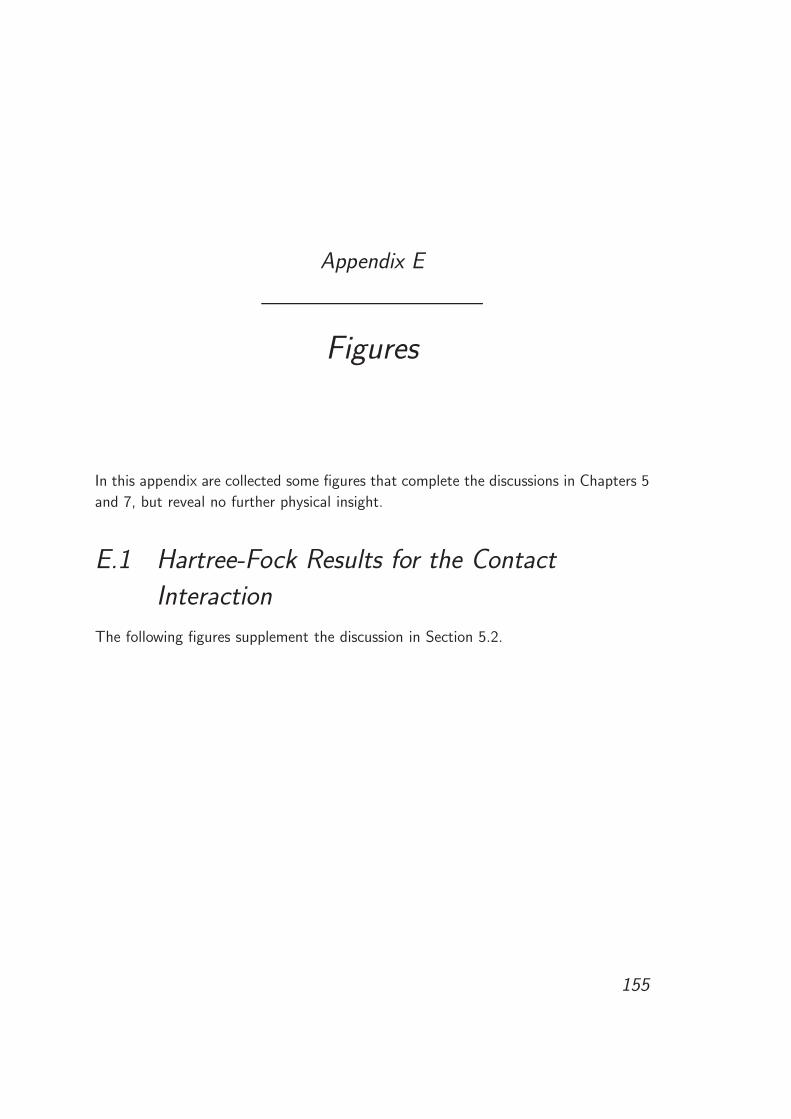
Appendix E
Figures
In this appendix are collected some figures that complete the discussions in Chapters 5
and 7, but reveal no further physical insight.
E.1 Hartree-Fock Results for the Contact
Interaction
The following figures supplement the discussion in Section 5.2.
155
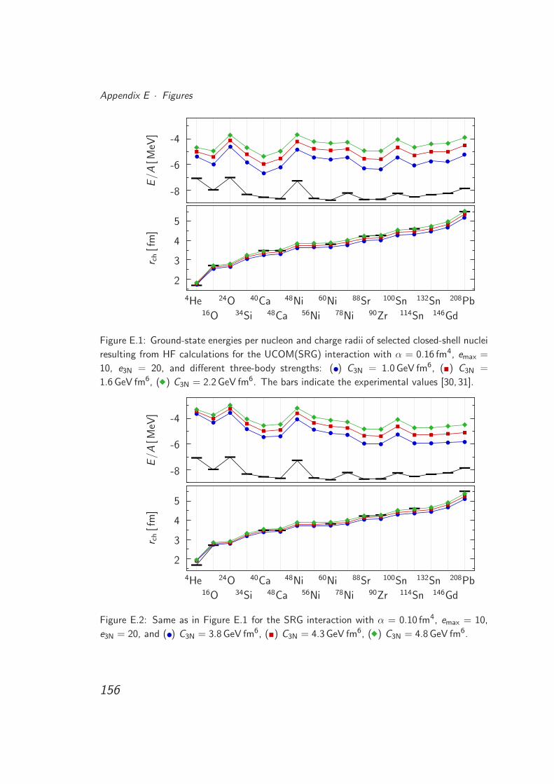
Appendix E · Figures
-8
-6
-4
.
E/A
[MeV
]
2
3
4
5
.
r ch[f
m]
4He16O
24O34Si
40Ca48Ca
48Ni56Ni
60Ni78Ni
88Sr90Zr
100Sn114Sn
132Sn146Gd
208Pb
Figure E.1: Ground-state energies per nucleon and charge radii of selected closed-shell nuclei
resulting from HF calculations for the UCOM(SRG) interaction with α = 0.16 fm4, emax =
10, e3N = 20, and different three-body strengths: () C3N = 1.0 GeV fm6, () C3N =
1.6 GeV fm6, ( ) C3N = 2.2 GeV fm6. The bars indicate the experimental values [30, 31].
-8
-6
-4
.
E/A
[MeV
]
2
3
4
5
.
r ch[f
m]
4He16O
24O34Si
40Ca48Ca
48Ni56Ni
60Ni78Ni
88Sr90Zr
100Sn114Sn
132Sn146Gd
208Pb
Figure E.2: Same as in Figure E.1 for the SRG interaction with α = 0.10 fm4, emax = 10,
e3N = 20, and () C3N = 3.8 GeV fm6, () C3N = 4.3 GeV fm6, ( ) C3N = 4.8 GeV fm6.
156
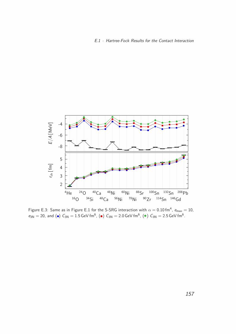
E.1 · Hartree-Fock Results for the Contact Interaction
-8
-6
-4
.
E/A
[MeV
]
2
3
4
5
.
r ch[f
m]
4He16O
24O34Si
40Ca48Ca
48Ni56Ni
60Ni78Ni
88Sr90Zr
100Sn114Sn
132Sn146Gd
208Pb
Figure E.3: Same as in Figure E.1 for the S-SRG interaction with α = 0.10 fm4, emax = 10,
e3N = 20, and () C3N = 1.5 GeV fm6, () C3N = 2.0 GeV fm6, ( ) C3N = 2.5 GeV fm6.
157
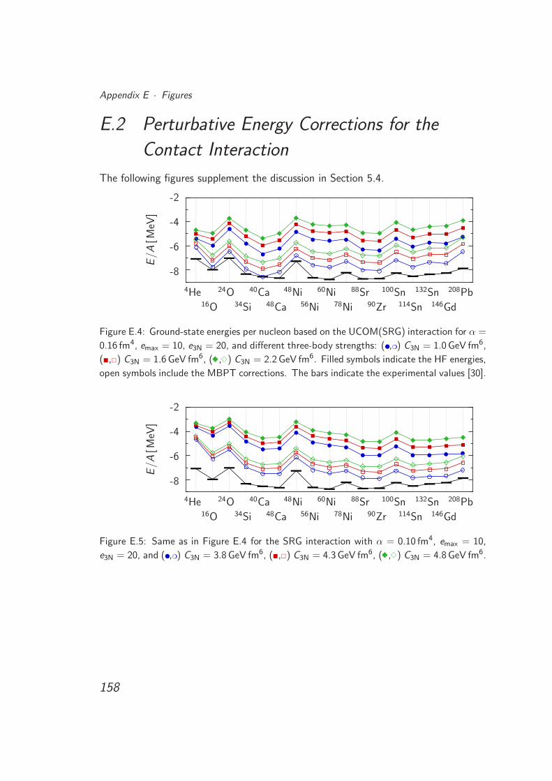
Appendix E · Figures
E.2 Perturbative Energy Corrections for the
Contact Interaction
The following figures supplement the discussion in Section 5.4.
-8
-6
-4
-2
.
E/A
[MeV
]
4He16O
24O34Si
40Ca48Ca
48Ni56Ni
60Ni78Ni
88Sr90Zr
100Sn114Sn
132Sn146Gd
208Pb
Figure E.4: Ground-state energies per nucleon based on the UCOM(SRG) interaction for α =
0.16 fm4, emax = 10, e3N = 20, and different three-body strengths: (,) C3N = 1.0 GeV fm6,
(,) C3N = 1.6 GeV fm6, ( , ) C3N = 2.2 GeV fm6. Filled symbols indicate the HF energies,
open symbols include the MBPT corrections. The bars indicate the experimental values [30].
-8
-6
-4
-2
.
E/A
[MeV
]
4He16O
24O34Si
40Ca48Ca
48Ni56Ni
60Ni78Ni
88Sr90Zr
100Sn114Sn
132Sn146Gd
208Pb
Figure E.5: Same as in Figure E.4 for the SRG interaction with α = 0.10 fm4, emax = 10,
e3N = 20, and (,) C3N = 3.8 GeV fm6, (,) C3N = 4.3 GeV fm6, ( , ) C3N = 4.8 GeV fm6.
158

E.2 · Perturbative Energy Corrections for the Contact Interaction
-8
-6
-4
-2
.
E/A
[MeV
]
4He16O
24O34Si
40Ca48Ca
48Ni56Ni
60Ni78Ni
88Sr90Zr
100Sn114Sn
132Sn146Gd
208Pb
Figure E.6: Same as in Figure E.4 for the S-SRG interaction with α = 0.10 fm4, emax = 10,
e3N = 20, and (,) C3N = 1.5 GeV fm6, (,) C3N = 2.0 GeV fm6, ( , ) C3N = 2.5 GeV fm6.
159
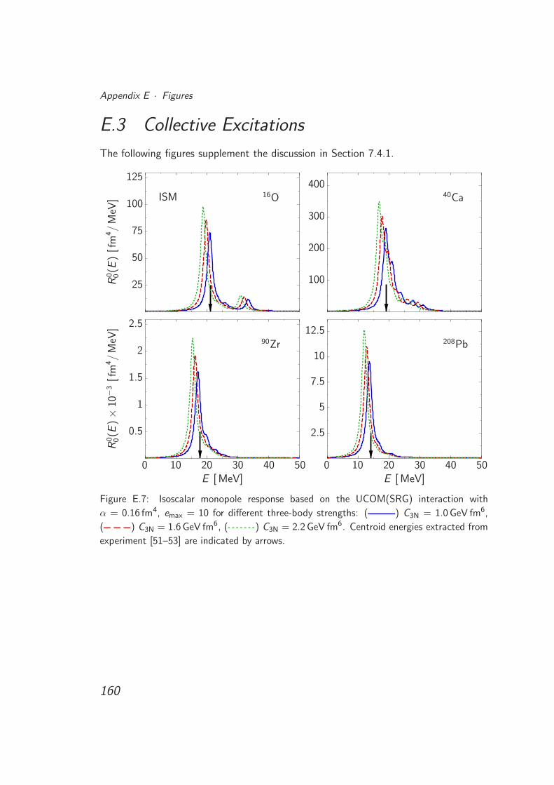
Appendix E · Figures
E.3 Collective Excitations
The following figures supplement the discussion in Section 7.4.1.
25
50
75
100
125
.
R0 0(E
)[f
m4/
MeV
] 16OISM
100
200
300
400
.
40Ca
0 10 20 30 40 50E [ MeV]
0.5
1
1.5
2
2.5
.
R0 0(E
)×
10−
3[f
m4/
MeV
]
90Zr
0 10 20 30 40 50E [ MeV]
2.5
5
7.5
10
12.5
.
208Pb
Figure E.7: Isoscalar monopole response based on the UCOM(SRG) interaction with
α = 0.16 fm4, emax = 10 for different three-body strengths: ( ) C3N = 1.0 GeV fm6,
( ) C3N = 1.6 GeV fm6, ( ) C3N = 2.2 GeV fm6. Centroid energies extracted from
experiment [51–53] are indicated by arrows.
160
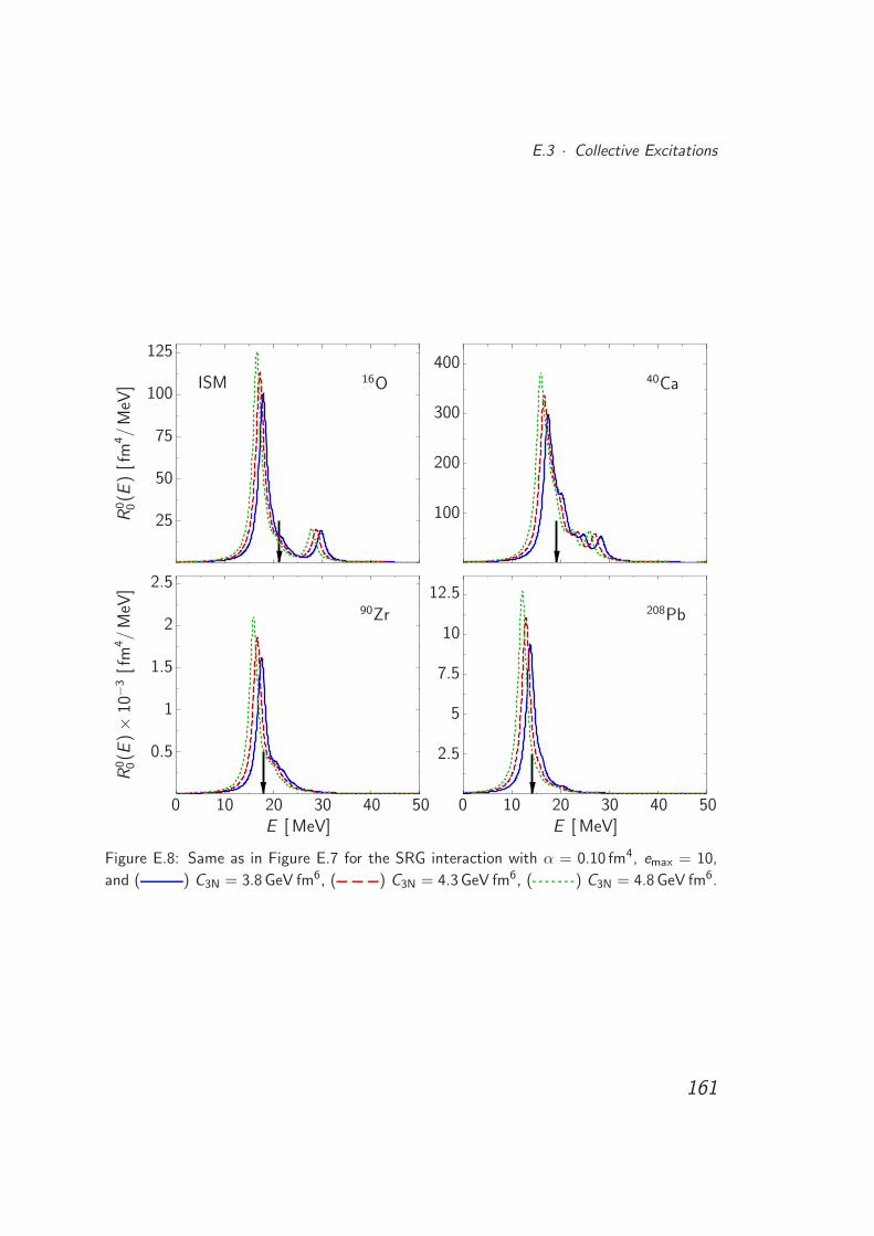
E.3 · Collective Excitations
25
50
75
100
125
.
R0 0(E
)[f
m4/
MeV
] 16OISM
100
200
300
400
.
40Ca
0 10 20 30 40 50E [ MeV]
0.5
1
1.5
2
2.5
.
R0 0(E
)×
10−
3[f
m4/
MeV
]
90Zr
0 10 20 30 40 50E [ MeV]
2.5
5
7.5
10
12.5
.
208Pb
Figure E.8: Same as in Figure E.7 for the SRG interaction with α = 0.10 fm4, emax = 10,
and ( ) C3N = 3.8 GeV fm6, ( ) C3N = 4.3 GeV fm6, ( ) C3N = 4.8 GeV fm6.
161
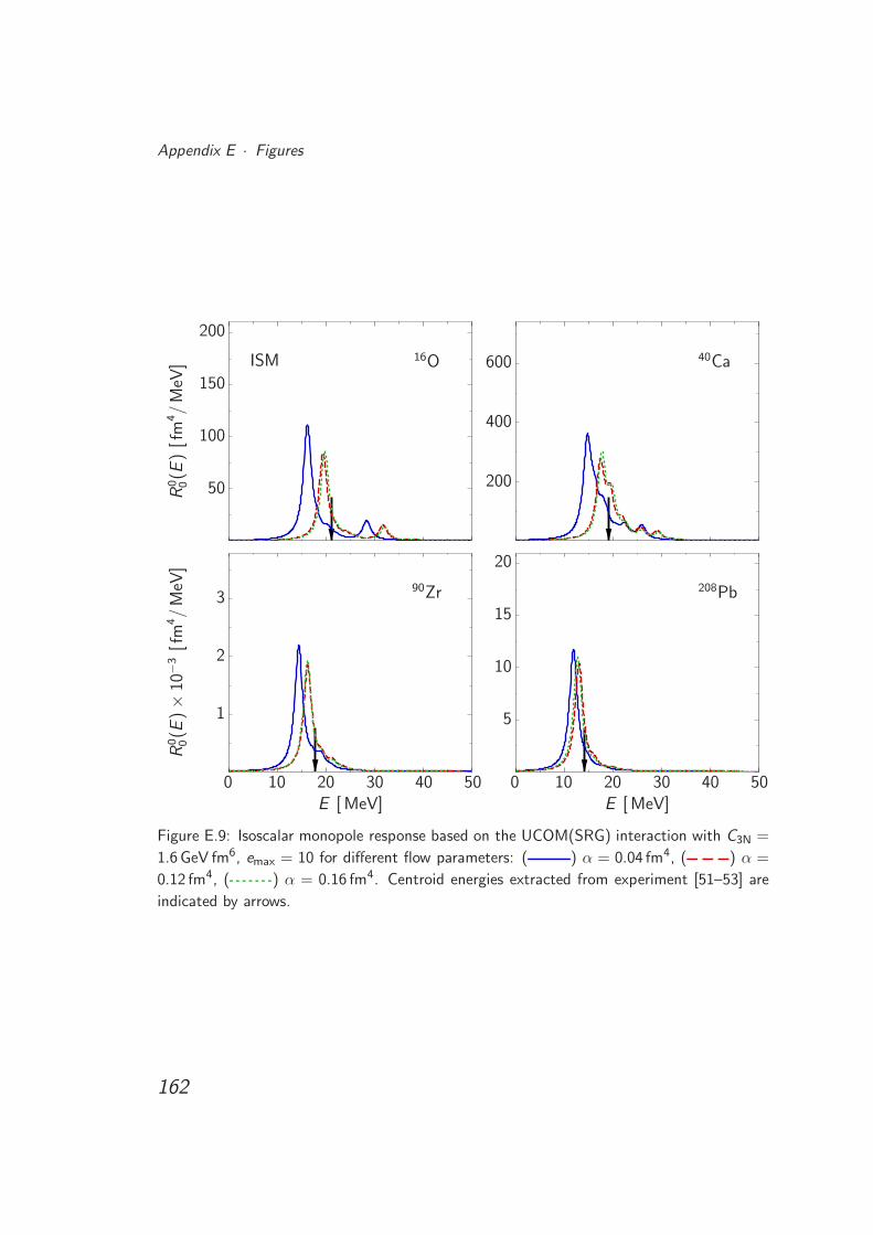
Appendix E · Figures
50
100
150
200
.
R0 0(E
)[f
m4/
MeV
] 16OISM
200
400
600
.
40Ca
0 10 20 30 40 50E [ MeV]
1
2
3
.
R0 0(E
)×
10−
3[f
m4/
MeV
]
90Zr
0 10 20 30 40 50E [ MeV]
5
10
15
20
.
208Pb
Figure E.9: Isoscalar monopole response based on the UCOM(SRG) interaction with C3N =
1.6 GeV fm6, emax = 10 for different flow parameters: ( ) α = 0.04 fm4, ( ) α =
0.12 fm4, ( ) α = 0.16 fm4. Centroid energies extracted from experiment [51–53] are
indicated by arrows.
162
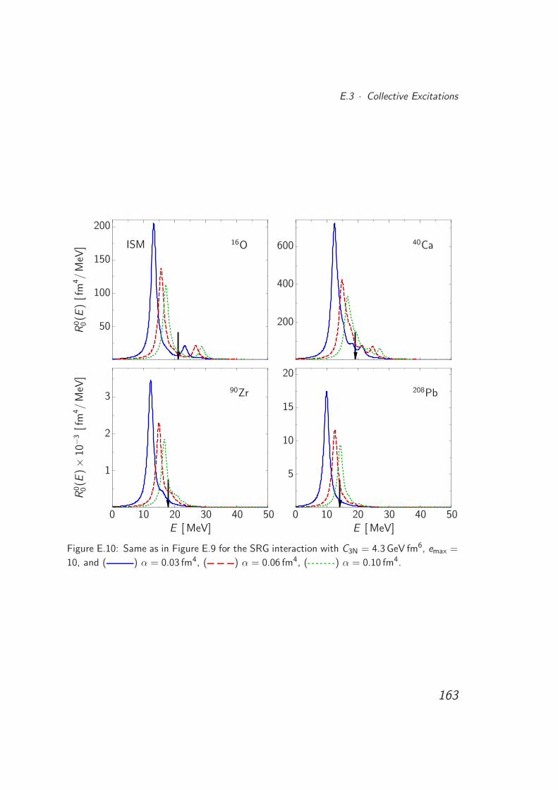
E.3 · Collective Excitations
50
100
150
200
.
R0 0(E
)[f
m4/
MeV
] 16OISM
200
400
600
.
40Ca
0 10 20 30 40 50E [ MeV]
1
2
3
.
R0 0(E
)×
10−
3[f
m4/
MeV
]
90Zr
0 10 20 30 40 50E [ MeV]
5
10
15
20
.
208Pb
Figure E.10: Same as in Figure E.9 for the SRG interaction with C3N = 4.3 GeV fm6, emax =
10, and ( ) α = 0.03 fm4, ( ) α = 0.06 fm4, ( ) α = 0.10 fm4.
163

Appendix E · Figures
164
Appendix F
Notation
In the following, some frequently appearing symbols and acronyms are listed.
Quantum Numbers
e major harmonic oscillator quantum number
n principal harmonic oscillator quantum number
nx cartesian harmonic oscillator quantum number
l , ml single-particle orbital angular momentum
s, ms single-particle spin
j , m single-particle total angular momentum
t, mt single-particle isospin
L, ML total orbital angular momentum
J , M total angular momentum
T , MT total isospin
165
Appendix F · Notation
Symbols
N neutron number
Z proton number
A mass number
ǫF Fermi energy
mN nucleon mass
c(
j1 j2m1 m2
∣∣ J
M
)Clebsch-Gordan coefficient
Operators
H Hamiltonian
T kinetic energy
VNN two-body interaction
V3N three-body interaction
C, Cr , CΩ correlation operators: general, central, tensor
O arbitrary correlated operator
x position operator
qr radial momentum operator
qΩ orbital angular momentum operator
L orbital angular momentum
S spin
Π projection operator
166
Acronyms
NN nucleon-nucleon
3N three-nucleon
AV18 Argonne V18
UCOM Unitary Correlation Operator Method
SRG Similarity Renormalization Group
HF Hartree-Fock
MBPT Many-Body Perturbation Theory
NCSM No-Core Shell Model
RPA Random Phase Approximation
ISM Isoscalar Monopole
IVD Isovector Dipole
ISQ Isoscalar Quadrupole
167

Appendix F · Notation
168
Bibliography
[1] Komitee fur Hadronen-und Kernphysik. Hadronen- und Kernphysik – Status und Per-
spektiven, 2003.
[2] Evgeny Epelbaum. Few-nucleon forces and systems in chiral effective field theory. Prog.
Part. Nucl. Phys., 57:654–741, 2006.
[3] J. Langhammer. Consistent chiral three-nucleon interactions in nuclear structure. Mas-
ter’s thesis, TU Darmstadt, 2010.
[4] A. Calci. Ab initio nuclear structure with SRG-transformed chiral NN plus NNN inter-
actions. Master’s thesis, TU Darmstadt, 2010.
[5] R. B. Wiringa, V. G. J. Stoks, and R. Schiavilla. An accurate nucleon-nucleon potential
with charge independence breaking. Phys. Rev., C51:38–51, 1995.
[6] R. Machleidt. The high-precision, charge-dependent bonn nucleon-nucleon potential
(cd-bonn). Phys. Rev., C63:024001, 2001.
[7] V. G. J. Stoks, R. A. M. Klomp, C. P. F. Terheggen, and J. J. de Swart. Construction
of high quality nn potential models. Phys. Rev., C49:2950–2962, 1994.
[8] H. Feldmeier, T. Neff, R. Roth, and J. Schnack. A unitary correlation operator method.
Nucl. Phys., A632:61–95, 1998.
[9] Thomas Neff and Hans Feldmeier. Tensor correlations in the unitary correlation operator
method. Nucl. Phys., A713:311, 2003.
[10] Robert Roth, Thomas Neff, and Hans Feldmeier. Nuclear Structure in the Framework
of the Unitary Correlation Operator Method. Prog. Part. Nucl. Phys., 65:50–93, 2010.
[11] S. K. Bogner, R. J. Furnstahl, and R. J. Perry. Similarity Renormalization Group for
Nucleon-Nucleon Interactions. Phys. Rev., C75:061001, 2007.
[12] P. Navratil, G. P. Kamuntavicius, and B. R. Barrett. Few-nucleon systems in transla-
tionally invariant harmonic oscillator basis. Phys. Rev., C61:044001, 2000.
169
[13] R. Roth, P. Papakonstantinou, N. Paar, H. Hergert, T. Neff, and H. Feldmeier. Hartree-
fock and many-body perturbation theory with correlated realistic nn-interactions. Phys.
Rev., C73:044312, 2006.
[14] N. Paar, P. Papakonstantinou, H. Hergert, and R. Roth. Collective multipole excitations
based on correlated realistic nucleon-nucleon interactions. Phys. Rev., C74:014318,
2006.
[15] R. Roth, T. Neff, H. Hergert, and H. Feldmeier. Nuclear structure based on correlated
realistic nucleon- nucleon potentials. Nucl. Phys., A745:3, 2004.
[16] R. Roth. Effektive Wechselwirkungen fur Quantenflussigkeiten und Quantengase. PhD
thesis, TU Darmstadt, 2000.
[17] T. Neff. Short-Ranged Central and Tensor Correlations in Nuclear Many-Body Systems.
PhD thesis, TU Darmstadt, 2002.
[18] R. Roth, H. Hergert, P. Papakonstantinou, T. Neff, and H. Feldmeier. Matrix elements
and few-body calculations within the unitary correlation operator method. Phys. Rev.,
C72:034002, 2005.
[19] A. Gunther, R. Roth, H. Hergert, and S. Reinhardt. Systematics of binding energies and
radii based on realistic two-nucleon plus phenomenological three-nucleon interactions.
Phys. Rev., C82:024319, 2010.
[20] Franz J. Wegner. Flow equations for hamiltonians. Phys. Rep., 348:77–89, 2001.
[21] Sergio Szpigel and Robert J. Perry. The similarity renormalization group. In A. N.
Mitra, editor, Quantum Field Theory. A 20th Century Profile. Hindustan Publishing
Co., New Delhi, 2000.
[22] H. Hergert and R. Roth. The unitary correlation operator method from a similarity
renormalization group perspective. Phys. Rev., C75:051001, 2007.
[23] R. Roth, S. Reinhardt, and H. Hergert. Unitary Correlation Operator Method and Sim-
ilarity Renormalization Group: Connections and Differences. Phys. Rev., C77:064003,
2008.
[24] H. Hergert. An Ab-Initio Approach to Pairing Phenomena Using Modern Effective
Interactions. PhD thesis, TU Darmstadt, 2008.
[25] S. Reinhardt. Comparison and Connection of the Similarity Renormalization Group and
the Unitary Correlation Operator Method. Diploma thesis, TU Darmstadt, 2008.
170
[26] E. D. Jurgenson, P. Navratil, and R. J. Furnstahl. Evolution of Nuclear Many-Body
Forces with the Similarity Renormalization Group. Phys. Rev. Lett., 103:082501, 2009.
[27] A. Zapp. Kernstruktur mit effektiven Dreiteilchenpotentialen. Diploma thesis, TU
Darmstadt, 2006.
[28] R. Roth. Die Methode der unitaren Korrelatoren und ihre Anwendung auf kurzreich-
weitig abstoßende Nukleon-Nukleon-Wechselwirkungen. Diploma thesis, TU Darmstadt,
1997.
[29] S. Eidelman et al. Review of particle physics. Phys. Lett., B592:1, 2004.
[30] G. Audi and A. H. Wapstra. The 1995 update to the atomic mass evaluation. Nucl.
Phys., A595:409–480, 1995.
[31] H. De Vries, C. W. De Jager, and C. De Vries. Nuclear charge-density-distribution
parameters from elastic electron scattering. At. Data Nucl. Data Tables, 36(3):495 –
536, 1987.
[32] V. I. Isakov, K. I. Erokhina, H. Mach, M. Sanchez-Vega, and B. Fogelberg. On the
difference between proton and neutron spin-orbit splittings in nuclei. Eur. Phys. J.,
A14:29–36, 2002.
[33] Y. Wang, C. C. Foster, R. D. Polak, J. Rapaport, and E. J. Stephenson. Proton- 90Zr
mean field between -60 and +185 MeV from a dispersive optical model analysis. Phys.
Rev., C47:2677–2689, 1993.
[34] J. P. Delaroche, Y. Wang, and J. Rapaport. Neutron- 90Zr mean field from a dispersive
optical model analysis. Phys. Rev., C39:391–404, 1989.
[35] A. Szabo and N. S. Ostlund. Modern Quantum Chemistry. Dover Publications,
Mineaola, New York, 1st edition, 1996.
[36] Robert Roth and Joachim Langhammer. Pade-resummed high-order perturbation theory
for nuclear structure calculations. Phys. Lett., B683:272–277, 2010.
[37] I. Talmi. Nuclear spectroscopy with harmonic-oscillator wave functions. Helv. Phys.
Acta, 25:185, 1952.
[38] M. Moshinsky. Transformation brackets for harmonic oscillator functions. Nucl. Phys.,
13:104, 1959.
[39] C. Cohen-Tannoudji, B. Diu, and F. Laloe. Quantenmechanik. Walter de Gruyter GmbH
& Co. KG, Berlin, 2nd edition, 1999.
171
[40] http://www.wolfram.com/products/mathematica/index.html.
[41] L. Chaos-Cador and E. Ley-Koo. Common generating functions of complete harmonic
oscillator wave functions and transformation brackets in D dimensions. Int. J. Quant.
Chem., 97:844–853, 2004.
[42] D. A. Varshalovich, A. N. Moskalev, and V. K. Khersonskii. Quantum Theory of Angular
Momentum. World Scientific, 1988.
[43] P. Navratil, J. P. Vary, and B. R. Barrett. Large basis ab initio no-core shell model and
its application to c-12. Phys. Rev., C62:054311, 2000.
[44] D. Vautherin and D. M. Brink. Hartree-Fock calculations with Skyrme’s interaction. 1.
Spherical nuclei. Phys. Rev., C5:626–647, 1972.
[45] M. Waroquier, K. Heyde, and H. Vincx. Antisymmetry in the three-nucleon interaction
matrix elements. Phys. Rev., C13:1664–1673, 1976.
[46] O. Bohigas, A. M. Lane, and J. Martorell. Sum Rules for Nuclear Collective Excitations.
Phys. Rept., 51:267, 1979.
[47] D. J. Rowe. Nuclear Collective Motion. Methuen and Co. Ltd., London, 1st edition,
1970.
[48] J. Suhonen. From Nucleons to Nucleus. Concepts of Microscopic Nuclear Theory.
Springer, Berlin, 1st edition, 2007.
[49] P. Ring and P. Schuck. The Nuclear Many-Body Problem. Springer, 1st edition, 1980.
[50] H. Hergert. personal communication.
[51] Y. W. Lui, H. L. Clark, and D. H. Youngblood. Giant resonances in 16O. Phys. Rev.,
C64:064308, 2001.
[52] D. H. Youngblood, Y. W. Lui, and H. L. Clark. Isoscalar E0, E1, and E2 strength in40Ca. Phys. Rev., C63:067301, 2001.
[53] D. H. Youngblood, H. L. Clark, and Y. W. Lui. Incompressibility of Nuclear Matter
from the Giant Monopole Resonance. Phys. Rev. Lett., 82:691–694, 1999.
[54] S. F. LeBrun, A. M. Nathan, and S. D. Hoblit. Photon scattering in the giant dipole
resonance region of 16O. Phys. Rev., C35:2005–2010, 1987.
[55] A. Veyssiere, H. Beil, R. Bergere, P. Carlos, A. Lepretre, and A. De Miniac. A study of
the photoneutron contribution to the giant dipole resonance of s-d shell nuclei. Nucl.
Phys. A, 227(3):513 – 540, 1974.
172
[56] B. L. Berman et al. Photoneutron Cross Sections for 90Zr, 91Zr, 92Zr, 94Zr, and 89Y.
Phys. Rev., 162:1098–1111, 1967.
[57] A. Veyssiere, H. Beil, R. Bergere, P. Carlos, and A. Lepretre. Photoneutron cross
sections of 208Pb and 197Au. Nucl. Phys. A, 159(2):561 – 576, 1970.
[58] F. E. Bertrand, G. R. Satchler, D. J. Horen, and A. van der Woude. Systematics of
the isoscalar giant monopole resonance from 60 MeV inelastic proton scattering. Phys.
Lett. B, 80(3):198 – 202, 1979.
[59] S. Raman, C. W. G. Nestor, Jr, and P. Tikkanen. Transition probability from the
ground to the first- excited 2+ state of even-even nuclides. Atom. Data Nucl. Data
Tabl., 78:1–128, 2001.
[60] J. Heisenberg, Jechiel Lichtenstadt, Costas N. Papanicolas, and J. S. McCarthy. Exci-
tation of low lying natural parity levels in 208Pb by inelastic electron scattering. Phys.
Rev., C25:2292–2308, 1982.
[61] P. Papakonstantinou. personal communication.
[62] Robert Roth. Importance Truncation for Large-Scale Configuration Interaction Ap-
proaches. Phys. Rev., C79:064324, 2009.
[63] K. L. G. Heyde. The Nuclear Shell Model. Springer, Berlin, Heidelberg, 2nd edition,
1994.
[64] C. Stumpf. Entartete Vielteilchen-Storungstheorie und Pade-Resummation fur Kern-
spektren. Bachelor thesis, TU Darmstadt, 2010.
[65] G. Hagen, T. Papenbrock, D. J. Dean, A. Schwenk, A. Nogga, M. W loch, and
P. Piecuch. Coupled-cluster theory for three-body Hamiltonians. Phys. Rev.,
C76:034302, 2007.
[66] R. Roth. Theoretische Kernphysik, WS 2007/2008. Vorlesungsskript.
173

174
Danksagung
Im Laufe meiner Doktorarbeit haben mich viele Leute unterstutzt.
An erster Stelle mochte ich mich bei Professor Robert Roth bedanken. Durch die
Arbeit in seiner Gruppe habe ich viel gelernt. Er hat es auf vorbildliche Weise vestanden,
den optimalen Mittelweg zu finden: Auf der einen Seite gewahrte er ein selbst gewahltes
Maß an Freiraum und auf der anderen Seite stand er stets als Ansprechpartner zur
Verfugung.
Professor Jochen Wambach danke ich fur die Ubernahme des Zweitgutachtens.
Die TNP++ Gruppe hat wahrend der vergangenen Jahre fur eine anregende Ar-
beitsatmosphare gesorgt. Dabei mochte ich besonders Joachim Langhammer, Angelo
Calci und Panagiota Papakonstantinou hervorheben, die diese Arbeit Korrektur gelesen
haben. Panagiota hat mir außerdem ihren RPA Code zur Verfugung gestellt. Obwohl
Heiko Hergert inzwischen nicht mehr bei uns ist, hat er stets schnell und zuverlassig
zur Beantwortung meiner Fragen beigetragen.
Bei der TU Darmstadt bedanke ich fur die Gewahrung eines Promotionsstipendi-
ums.
Der Deutschen Forschungsgemeinschaft danke ich fur die Unterstutzung im Rah-
men des Sonderforschungsbereiches 634.
Nicht zuletzt mochte ich an dieser Stelle meine Familie erwahnen, die mich alle
nach Kraften und in unterschiedlicher Weise unterstutzt haben.
Besonderer Dank geht an Marc und an Wienke fur ihre ansteckende Lebensfreude.
Danke an alle!

Lebenslauf
Name: Anneke Ingeluise Gunther, geb. Zapp
Geburtsdatum: 13. Mai 1983
Geburtsort: Eckernforde
Staatsangehorigkeit: deutsch
Familienstand: verheiratet, 1 Kind
Bildungsweg
8/1989 – 7/1990 Besuch der Grundschule Krempe, Schleswig-Holstein
8/1990 – 7/1992 Besusch der Deutschen Botschaftsschule Addis Abeba, Athiopien
(Grundschule)
8/1992 – 7/1996 Besuch der Deutschen Botschaftsschule Addis Abeba, Athiopien (Gym-
nasium)
8/1996 – 6/2001 Besuch des Nordsee-Gymnasium-Busum, Schleswig-Holstein
6/2001 Abitur
9/2001 – 7/2003 Studium der Physik an der Christian-Albrechts-Universitat Kiel
7/2003 Vordiplom Physik
10/2003 – 12/2006 Studium der Physik an der TU Darmstadt
12/2005 – 11/2006 Anfertigung der Diplomarbeit ”Kernstruktur mit effektiven Drei-
teilchenpotentialen”
12/2006 Diplom
seit 1/2007 Promotionsstudium an der TU Darmstadt und Anfertigung der Disser-
tation
1/2007 – 4/2010 Stipendiatin eines Promotionsstipendiums der TU Darmstadt
seit 5/2010 Wissenschaftliche Mitarbeiterin am Institut fur Kernphysik
Top Related