Über die Verwendung von Copula-Funktionen im quantitativen
150
¨ Uber die Verwendung von Copula-Funktionen im quantitativen Risikomanagement und in der Untersuchung von Bankenkrisen INAUGURALDISSERTATION zur Erlangung der W ¨ urde eines Doktors der Wirtschaftswissenschaft der Fakult¨ at f¨ ur Wirtschaftswissenschaft der Ruhr-Universit¨ at Bochum vorgelegt von Diplom-Kaufmann Gregor Nikolaus Felix Weiß aus Kamen 2010
Transcript of Über die Verwendung von Copula-Funktionen im quantitativen
Uber die Verwendung von Copula-Funktionen im quantitativen
Risikomanagement und in der Untersuchung von Bankenkrisen
INAUGURALDISSERTATION
zur
Erlangung der Wurde
eines Doktors der
Wirtschaftswissenschaft
der
Fakultat fur Wirtschaftswissenschaft
der
Ruhr-Universitat Bochum
vorgelegt von
Diplom-KaufmannGregor Nikolaus Felix Weiß
aus Kamen2010

i
Dekan: Prof. Dr. Stephan PaulReferent: Prof. Dr. Stephan PaulKoreferent: Prof. Dr. Manfred LoschTag der mundlichen Prufung: 10. Februar 2010
Inhaltsverzeichnis
Inhaltsverzeichnis . . . . . . . . . . . . . . . . . . . . . . . . . . . . . . . . . v
Abbildungsverzeichnis . . . . . . . . . . . . . . . . . . . . . . . . . . . . . . viii
1 Einleitung 1
1.1 Einfuhrung in die Thematik und Motivation . . . . . . . . . . . . . . . . 1
1.2 Zusammenfassung und Publikationsdetails . . . . . . . . . . . . . . . . . 6
2 Copula-Funktionen 10
2.1 Einleitung . . . . . . . . . . . . . . . . . . . . . . . . . . . . . . . . . . 10
2.2 Charakteristika von Copula-Funktionen . . . . . . . . . . . . . . . . . . 11
2.3 Anwendungsmoglichkeiten von Copula-Funktionen im Risikomanagement 17
3 Uber die Vorteilhaftigkeit von Copula-GARCH-Modellen im finanzwirtschaft-
lichen Risikomanagement 19
3.1 Einleitung . . . . . . . . . . . . . . . . . . . . . . . . . . . . . . . . . . 19
3.2 Literaturuberblick und Hypothesenbildung . . . . . . . . . . . . . . . . . 21
3.3 Univariate VaR-Schatzung mithilfe von GARCH-Prozessen . . . . . . . . 26
3.4 Multivariate VaR-Schatzung mithilfe von Korrelationen und Copula-Funk-
tionen . . . . . . . . . . . . . . . . . . . . . . . . . . . . . . . . . . . . 28
3.4.1 Aggregation des Value-at-Risks auf Portfolioebene mithilfe von
Korrelationen . . . . . . . . . . . . . . . . . . . . . . . . . . . . 28
3.4.2 Copula-Modelle zur Ermittlung des Gesamtrisikos . . . . . . . . 29
3.4.2.1 Grundlagen der Copula-Theorie . . . . . . . . . . . . . 29
3.4.2.2 Parametrische Copulas . . . . . . . . . . . . . . . . . 30
3.4.2.3 Parameterschatzung . . . . . . . . . . . . . . . . . . . 32
3.4.2.4 Anpassungstests zur Prufung der Gute einer Copula-
Schatzung . . . . . . . . . . . . . . . . . . . . . . . . 34
ii
INHALTSVERZEICHNIS iii
3.4.2.5 Bestimmung des Portfolio-Value-at-Risks . . . . . . . 36
3.5 Empirische Untersuchung . . . . . . . . . . . . . . . . . . . . . . . . . . 37
3.5.1 Datenbasis . . . . . . . . . . . . . . . . . . . . . . . . . . . . . 37
3.5.2 Univariate Schatzung . . . . . . . . . . . . . . . . . . . . . . . . 40
3.5.3 Multivariate Schatzung . . . . . . . . . . . . . . . . . . . . . . . 40
3.6 Zusammenfassung . . . . . . . . . . . . . . . . . . . . . . . . . . . . . 54
4 Copula Parameter Estimation - Numerical Considerations And Implications
For Risk Management 56
4.1 Introduction . . . . . . . . . . . . . . . . . . . . . . . . . . . . . . . . . 56
4.2 Copula parameter estimation . . . . . . . . . . . . . . . . . . . . . . . . 58
4.2.1 Parametric copulas . . . . . . . . . . . . . . . . . . . . . . . . . 59
4.2.2 Parameter estimation via maximum-likelihood . . . . . . . . . . 61
4.2.3 Minimum-distance estimators . . . . . . . . . . . . . . . . . . . 62
4.2.3.1 Minimum-distance estimators based on the empirical
copula process . . . . . . . . . . . . . . . . . . . . . . 62
4.2.3.2 Minimum-distance estimators based on Kendall’s de-
pendence function . . . . . . . . . . . . . . . . . . . . 64
4.2.3.3 Minimum-distance estimators based on Rosenblatt’s trans-
form . . . . . . . . . . . . . . . . . . . . . . . . . . . 64
4.2.4 Numerical properties of the copula parameter estimators . . . . . 65
4.3 Simulation study . . . . . . . . . . . . . . . . . . . . . . . . . . . . . . 68
4.3.1 Design of the simulation study . . . . . . . . . . . . . . . . . . . 68
4.3.2 Results . . . . . . . . . . . . . . . . . . . . . . . . . . . . . . . 69
4.3.2.1 Comparison of the mean bias and MSE . . . . . . . . . 75
4.3.2.2 Results concerning the sample size and dimensionality . 76
4.3.2.3 Results concerning the computational complexity . . . 76
4.4 Empirical Examples . . . . . . . . . . . . . . . . . . . . . . . . . . . . . 77
4.4.1 Data and model description . . . . . . . . . . . . . . . . . . . . 77
INHALTSVERZEICHNIS iv
4.4.2 Results and discussion . . . . . . . . . . . . . . . . . . . . . . . 81
4.5 Conclusions . . . . . . . . . . . . . . . . . . . . . . . . . . . . . . . . . 84
5 Bank Contagion 85
5.1 Einfuhrung . . . . . . . . . . . . . . . . . . . . . . . . . . . . . . . . . 85
5.2 Definition des Begriffes bank contagion . . . . . . . . . . . . . . . . . . 86
5.3 Ubertragungskanale und Ursachen finanzwirtschaftlicher Krisen . . . . . 88
6 Analysing Bank Contagion with Copulæ - Evidence from the Subprime and
Japan’s banking crises 91
6.1 Introduction . . . . . . . . . . . . . . . . . . . . . . . . . . . . . . . . . 91
6.2 Bank contagion and lenders of last resort . . . . . . . . . . . . . . . . . . 94
6.3 Methodology . . . . . . . . . . . . . . . . . . . . . . . . . . . . . . . . 95
6.3.1 GARCH-filtering and abnormal returns . . . . . . . . . . . . . . 95
6.3.2 Some preliminary copula theory . . . . . . . . . . . . . . . . . . 97
6.3.3 Detecting contagion effects with copulae . . . . . . . . . . . . . 102
6.4 Data and empirical findings . . . . . . . . . . . . . . . . . . . . . . . . . 105
6.4.1 Panel A: Germany 2006-2008 . . . . . . . . . . . . . . . . . . . 105
6.4.1.1 Sample description and ARMA-GARCH-modelling . . 105
6.4.1.2 Abnormal returns . . . . . . . . . . . . . . . . . . . . 107
6.4.1.3 Detecting contagion effects by the use of copulae . . . 109
6.4.1.4 Robustness checks . . . . . . . . . . . . . . . . . . . . 112
6.4.2 Panel B: Japan 1994-1999 . . . . . . . . . . . . . . . . . . . . . 117
6.4.2.1 Sample description and ARMA-GARCH-modelling . . 117
6.4.2.2 Events and abnormal returns . . . . . . . . . . . . . . 117
6.4.2.3 Copula Analysis . . . . . . . . . . . . . . . . . . . . . 121
6.5 Conclusion . . . . . . . . . . . . . . . . . . . . . . . . . . . . . . . . . 123
A Literatur 126
INHALTSVERZEICHNIS v
B Empirical observators for the MD-estimators based on Kendall’s dependence
function 137
C Outline of the L-BFGS-B algorithm 139
Tabellenverzeichnis
3.1 Deskriptive Statistiken und Hypothesentests . . . . . . . . . . . . . . . . 39
3.2 Uberprufung von Hypothese 1 . . . . . . . . . . . . . . . . . . . . . . . 44
3.3 Uberprufung von Hypothese 2 . . . . . . . . . . . . . . . . . . . . . . . 45
3.4 Uberprufung von Hypothese 3 . . . . . . . . . . . . . . . . . . . . . . . 47
3.5 Uberprufung der generellen Vorteilhaftigkeit parametrischer Copulas . . . 49
3.6 Uberprufung von Hypothese 4 . . . . . . . . . . . . . . . . . . . . . . . 50
3.7 Ergebnisse der Anpassungstests fur die VaR-Schatzung. . . . . . . . . . . 52
3.8 Ergebnisse der Anpassungstests fur die Conditional-VaR-Schatzung. . . . 53
4.1 Bias, MSE, efficiency and mean computation time of the PML- and MD-
estimators (Gaussian copula) . . . . . . . . . . . . . . . . . . . . . . . . 70
4.2 Bias, MSE, efficiency and mean computation time of the PML- and MD-
estimators (Student’s t copula) . . . . . . . . . . . . . . . . . . . . . . . 71
4.3 Bias, MSE, efficiency and mean computation time of the PML- and MD-
estimators (Clayton copula) . . . . . . . . . . . . . . . . . . . . . . . . . 72
4.4 Bias, MSE, efficiency and mean computation time of the PML- and MD-
estimators (Frank copula) . . . . . . . . . . . . . . . . . . . . . . . . . . 73
4.5 Bias, MSE, efficiency and mean computation time of the PML- and MD-
estimators (Gumbel copula) . . . . . . . . . . . . . . . . . . . . . . . . . 74
4.6 Summary statistics for the log return series of the aggregated asset classes. 78
4.7 Results for the VaR and ES-estimations averaged over all 100 bivariate
portfolios. . . . . . . . . . . . . . . . . . . . . . . . . . . . . . . . . . . 82
6.1 Panel A: Summary statistics, hypothesis tests and Bravais-Pearson corre-
lation coefficients for the unfiltered return series . . . . . . . . . . . . . . 106
vi
TABELLENVERZEICHNIS vii
6.2 Panel A: Model specifications, estimated ARMA(p1,q1)-GARCH(p2,q2)
parameters, LM test and Ljung-Box test statistics (p-values) for the filte-
red returns. . . . . . . . . . . . . . . . . . . . . . . . . . . . . . . . . . 107
6.3 Panel A: Cumulative abnormal returns (CAR) in per cent and parameter
estimates for the market models. . . . . . . . . . . . . . . . . . . . . . . 109
6.4 Panel A: AIC for the different copula mixture models and time windows. 110
6.5 Panel A: Results of the bivariate Clayton-Frank-Gumbel models. . . . . . 111
6.6 Panel A: Multivariate lower tail dependence in the German banking sector. 113
6.7 Panel A: Results of the robustness check for the bivariate Clayton-Frank-
Gumbel models excluding confounding events. . . . . . . . . . . . . . . 114
6.8 Panel A: Results of the robustness check for the multivariate lower tail
dependence in the German banking sector excluding confounding events. 115
6.9 Panel A: Results of the robustness check on the bivariate Clayton-Frank-
Gumbel models with time-varying GARCH- and market models. . . . . . 116
6.10 Panel B: Summary statistics for the unfiltered return series . . . . . . . . 118
6.11 Panel B: Summary statistics for the hypothesis tests. . . . . . . . . . . . . 119
6.12 Panel B: Model specifications and LM test statistics for the filtered returns. 120
6.13 Panel B: Average results of the bivariate Clayton-Frank-Gumbel models. . 122
6.14 Panel B: Average results of the robustness check on the bivariate Clayton-
Frank-Gumbel models with time-varying GARCH- and market models. . 124
Abbildungsverzeichnis
2.1 Funktionsgraphen und Contour-Diagramme der W-, Produkt- und M-Co-
pula. . . . . . . . . . . . . . . . . . . . . . . . . . . . . . . . . . . . . . 13
2.2 Funktionsgraphen und Contour-Diagramme der Gauß- und t-Copula. . . . 14
2.3 Funktionsgraphen und Contour-Diagramme der Clayton- und Gumbel-
Copula. . . . . . . . . . . . . . . . . . . . . . . . . . . . . . . . . . . . 16
3.1 Geschatzte Dichten der VaR-Uberschreitungen . . . . . . . . . . . . . . 41
3.2 Geschatzte Dichten der durchschnittlichen korrigierten CVaRs . . . . . . 42
5.1 Ursachen und Ubertragungskanale von Schaltersturmen und Bankenpaniken 90
viii
Kapitel 1
Einleitung
1.1 Einfuhrung in die Thematik und Motivation
Im Zentrum des Interesses zahlreicher Fragestellungen der Finanzmarkttheorie sowie der
angewandten Statistik stehen die Modellierung und Analyse der einem Zufallsvektor zu-
geordneten gemeinsamen Verteilung. Diese fasst sowohl das Randverhalten als auch die
zwischen den Zufallsvariablen bestehenden Abhangigkeiten in einer Funktion in mehre-
ren Variablen zusammen. Die ubliche Herangehensweise fur die Modellierung der ge-
meinsamen Verteilung eines Zufallsvektors bestand dabei klassischerweise darin, Vertei-
lungsannahmen fur die Rander zu treffen, fur die die gemeinsame Verteilung leicht analy-
tisch bestimmt werden konnte. So fanden (und finden) insbesondere multivariate Normal-,
Log-Normal-, Gamma- und Extremwertverteilungen haufig Anwendung in den Modellen
der Finanz- und Versicherungsmathematik. Der großte Nachteil dieser Herangehensweise
ist jedoch, dass die Annahme einer bestimmten, leicht modellierbaren gemeinsamen Ver-
teilung die Verteilung der univariaten Rander des Zufallsvektors vorgibt. Im Endeffekt
konnen somit das univariate Randverhalten und die Abhangigkeitsstruktur eines Zufalls-
vektors nicht separat voneinander modelliert werden.
Trotz dieser Einschrankung basieren zahlreiche Modelle der klassischen Kapitalmarkt-
theorie aber auch des zeitgenossischen quantitativen Risikomanagements auf diesem An-
satz und unterstellen bspw. fur die gemeinsame Verteilung von Risikoportfeuilles ei-
ne multivariate Normalverteilung.1 Die Annahme normalverteilter Risiken und der da-
mit verbundenen Gleichsetzung von stochastischer Abhangigkeit und linearer Korrela-
tion kann jedoch in praxisrelevanten Fallen zur Fehlspezifikation statistischer Modelle
fuhren. Embrechts et al. schlugen daher bereits 2002 einen alternativen Weg zur Model-
lierung multivariater Verteilungen vor, in dem die eigentliche Modellierung in zwei Teile
aufgespaltet wird: die Modellierung der univariaten Randverteilungen und der separaten
1Vgl. z.B. Markowitz (1952) und Jorion (2006).
1
1.1. EINFUHRUNG IN DIE THEMATIK UND MOTIVATION 2
Modellierung der Abhangigkeitsstruktur zwischen den Randverteilungen.2 Wahrend fur
die Modellierung der Randverteilungen klassische univariate parametrische und nicht-
parametrische Verteilungen herangezogen werden konnen, kann die Modellierung der
Abhangigkeitsstruktur durch spezielle Verteilungsfunktionen, den sogenannten Copulas,
erfolgen.
Copulas stellen vereinfacht gesprochen Verteilungsfunktionen dar, die die in einer ge-
meinsamen Verteilung inharente Abhangigkeitsstruktur vollstandig erfassen. Mit ihrer
Hilfe kann die Modellierung einer multivariaten Verteilung so erfolgen, dass zunachst
beliebige parametrische Verteilungen fur die univariaten Rander unterstellt und angepasst
werden, bevor fur die Abhangigkeitsstruktur des Zufallsvektors eine parametrische Co-
pula ausgewahlt wird.3 Der entscheidende Vorteil dieser Vorgehensweise besteht offen-
sichtlich darin, dass die Randverteilungen auf Grund der Aufspaltung des Problems der
Modellierung der gemeinsamen Verteilung nicht mehr aus der gleichen parametrischen
Verteilungsfamilie kommen mussen wie die gemeinsame Verteilung. So konnen bspw.
eine Normal- und eine Gamma-Verteilung mit einer beliebigen parametrischen Copula
kombiniert werden, um so eine multivariate gemeinsame Verteilung zu generieren. Zu-
gleich stellt der zentrale Satz von Sklar sicher, dass aus stetigen Randverteilungen und
einer Copula stets eine eindeutig bestimmte multivariate Verteilung resultiert. Umgekehrt
lasst sich somit aus multivariaten Verteilungen mit bekannten stetigen Randern stets ei-
ne eindeutige Copula extrahieren, die ihrerseits auf andere Randverteilungen angewen-
det werden kann. Die uberaus hohe Flexibilitat dieses Modellierungsansatzes hat dazu
gefuhrt, dass Copula-Modelle gerade im Bereich der Finanz- und Versicherungsmathe-
matik aber auch in anderen Bereichen der angewandten Mathematik sehr an Beliebtheit
gewonnen haben. 4
Wahrend die mathematischen Grundlagen von Copulas vergleichsweise gut erforscht sind,
existieren in der inferentiell-statistischen Analyse der Copulas noch zahlreiche ungeloste
Probleme, die ebenfalls eine hohe Praxisrelevanz aufweisen.5 So erfordert die Anwen-
dung eines Copula-Modells auf eine finanzwirtschaftliche Fragestellung grundsatzlich
die Auswahl einer parametrischen Copula aus einer Menge an bekannten Copulas so-
2Vgl. z.B. Embrechts et al. (2002).
3Fur eine grundlegende Einfuhrung in die Copula-Theorie vgl. insb. Nelsen (2006).
4Eine Zusammenfassung unterschiedlicher Anwendungsgebiete im Risikomanagement und der Finan-zierungslehre findet sich z.B. bei Cherubini et al. (2004); eine Vorstellung von Copula-Modellen in derHydrologie findet sich bei Genest und Favre (2007).
5Vgl. hierzu Genest und Favre (2007). Eine Auflistung zahlreicher mathematischer Kritikpunkte findetsich bei Mikosch (2006).
1.1. EINFUHRUNG IN DIE THEMATIK UND MOTIVATION 3
wie die anschließende Schatzung der Copula-Parameter auf der Basis historischer Daten.
Die erste Aufgabe hinsichtlich der Auswahl einer geeigneten parametrischen Copula stellt
zugleich das großte ungeloste Problem dieses Forschungszweiges dar.6 Ohne realistische
Aussicht auf eine analytische Losung dieser Frage sind in der Literatur zwei Ansatze be-
obachtbar, die auf empirischem Weg eine Losung dieser Frage bezwecken: Zum einen
kann die parametrische Copula allein auf Basis von Vermutungen hinsichtlich der ei-
nem Datensatz inharenten Abhangigkeitsstruktur gewahlt werden.7 Zum anderen kann
die Auswahl der Copula auf inferentiell-statistischem Wege uber die Verwendung von
Anpassungstests erfolgen. Gerade zu dem letztgenannten Ansatz sind in den letzten Jah-
ren vermehrt theoretische Abhandlungen8 und Simulationsstudien9 veroffentlicht worden,
in denen spezielle Anpassungstests fur Copulas vorgeschlagen und ihre Teststarke uber-
pruft wurden. Eine empirische Uberprufung der Starke verschiedener Anpassungstests fur
Copulas im Hinblick auf ihre Eignung fur das quantitative Risikomanagement ist indes
bislang noch nicht erfolgt.
Der erste Teil der vorliegenden Dissertation widmet sich daher der Frage, inwiefern spe-
zielle Anpassungstests fur Copulas geeignet sind, die Modellspezifikation mit Blick auf
die Schatzung von Risikomaßen wie dem Value-at-Risk fur ein Risikoportfolio zu ver-
bessern. Genauer gesagt soll auf Basis einer empirischen Untersuchung von 100 Port-
folios bestehend aus Werten des DAX-Indexes die Frage geklart werden, ob mit Hilfe
eines Copula spezifischen Anpassungstests die optimale parametrische Copula ex ante
identifiziert werden kann. Nachdem hierfur in Kapitel 2 eine kurze Einfuhrung in die
Theorie der Copulas gegeben wurde, folgt im auf dem Artikel Uber die Vorteilhaftigkeit
von Copula-GARCH-Modellen im finanzwirtschaftlichen Risikomanagement basierenden
Kapitel 3 die empirische Untersuchung dieser Frage.
Neben der Frage der optimalen Wahl der parametrischen Copula ist jedoch auch die
Frage, welcher Schatzer fur die Copula-Parameter optimal (also unverzerrt und effizi-
ent) ist, von großer praktischer Bedeutung. Aus theoretischer Sicht besitzt der klassi-
sche Maximum-Likelihood-Schatzer (ML) bestimmte Optimalitatseigenschaften, die je-
doch an die Annahme gebunden sind, dass die parametrische Form der Randverteilungen
6Zur herausgehobenen Bedeutung der Frage nach der Auswahl einer parametrischen Copula vgl. Em-brechts (2009) und Genest et al. (2009).
7Ein ahnliches Vorgehen skizziert bspw. Embrechts (2009). Ausschlaggebend fur die Wahl einer be-stimmten parametrischen Copula ist hierbei vor allem die durch die Copula ausgedruckte Randabhangig-keit.
8Vgl. z.B. Fermanian (2005) oder Savu und Trede (2008).
9Vgl. bspw. die Arbeiten von Kole et al. (2007), Genest et al. (2009) und Berg (2009).
1.1. EINFUHRUNG IN DIE THEMATIK UND MOTIVATION 4
richtig gewahlt wurde. Werden die Randverteilungen durch parametrische Verteilungs-
funktionen modelliert, so werden samtliche Parameter der Copula und der Randvertei-
lungen entweder gleichzeitig oder aber nacheinander jeweils uber die Maximierung der
logarithmierten Likelihood der gemeinsamen Verteilung geschatzt. Fur den (praxisnaher-
en) Fall, dass die parametrische Form der Randverteilungen unbekannt ist und damit
moglicherweise im Modell falsch spezifiziert wurde, empfiehlt sich stattdessen eine se-
miparametrische Vorgehensweise, bei der die Rander nichtparametrisch uber die empiri-
schen Verteilungsfunktionen modelliert und anschließend die Copula-Parameter geschatzt
werden.10 Fur diese Vorgehensweise haben Kim et al. gezeigt, dass die semiparametri-
sche Maximum-Likelihood-Schatzung der Copula-Parameter eine bessere Schatzung lie-
fert als der herkommliche ML-Schatzer.11 Gleichzeitig argumentieren die Autoren, dass
Minimum-Distance-Schatzer, die ebenfalls die Parameter auf Basis von Pseudobeobach-
tungswerten schatzen, vergleichbar gute Ergebnisse erzielen sollten. Eine Uberprufung
der statistischen Eigenschaften dieser Schatzer bei endlicher Stichprobengroße sowie ein
Vergleich unterschiedlicher Minimum-Distance-Schatzer fur Copulas findet sich indes
noch nicht in der Literatur.
Im zweiten Teil der Arbeit (Kapitel 4) soll diese Forschungslucke durch die Durchfuhrung
einer umfangreichen Simulationsstudie zum statistischen Verhalten unterschiedlicher Mi-
nimum-Distance-Schatzer fur Copulas geschlossen werden. Genauer gesagt, werden neun
verschiedene Minimum-Distance-Schatzer mit dem semiparametrischen Pseudo-Maxi-
mum-Likelihood-Schatzer fur zwei unterschiedliche Stichprobengroßen hinsichtlich ih-
rer Erwartungstreue, ihrer mittleren Fehlerquadratsumme sowie der von den Schatzern
benotigten Rechenzeit miteinander verglichen. Um die praktische Relevanz der festge-
stellten Unterschiede zu verdeutlichen, werden mit den zehn dargestellten Parameter-
schatzern anschließend der Value-at-Risk sowie der Expected Shortfall fur insgesamt 100
Portfolios unterschiedlicher Anlageklassen berechnet.
Wahrend die ersten Abschnitte der Dissertation die Anwendung von Copula-Funktionen
im quantitativen Risikomanagement betrafen, werden im weiteren Verlauf der Arbeit die
Anwendungsmoglichkeiten dieser Funktionen in der Untersuchung von Ansteckungsef-
fekten und Bankenkrisen untersucht. Hierbei wird die Tatsache genutzt, dass die verschie-
denen parametrischen Copula-Funktionen jeweils eine unterschiedliche Form der Rand-
abhangigkeit aufweisen. Werden nun unterschiedliche parametrische Copula-Funktionen
10Die nichtparametrische Schatzung der Rander ist aquivalent zur Berechnung sogenannter Pseudobeob-achtungswerte mittels Rangtransformation. Vgl. McNeil et al. (2005), S.232.
11Vgl. Kim et al. (2007).
1.1. EINFUHRUNG IN DIE THEMATIK UND MOTIVATION 5
an einen bivariaten Datensatz angepasst, und die parametrische Form identifiziert, die
die beste Anpassung an den Datensatz aufweist, so kann die zwischen zwei Variablen
bestehende Randabhangigkeit bestimmt werden. Im Zeitablauf konnen dann Veranderun-
gen der Randabhangigkeiten in einem Datensatz gemessen werden. Rodriguez wendet als
erster dieses Vorgehen an, um Ansteckungseffekte zwischen Volkswirtschaften (operatio-
nalisiert in Form eines Anstiegs der unteren Randabhangigkeit) in der Mexiko- und der
Asienkrise zu messen.12
Aufbauend auf der Arbeit von Rodriguez widmen sich die letzten beiden Teile der Arbeit
der Messung von Ansteckungseffekten zwischen Banken mithilfe von Copula-Funktio-
nen. Zunachst werden hierfur in Kapitel 5 die fur die folgende Untersuchung elementa-
ren Begriffe des Schaltersturms, der Bankenpanik sowie der finanzwirtschaftlichen An-
steckungseffekte voneinander abgegrenzt. Im letzten Teil der Arbeit (Kapitel 6) wird die
methodische Herangehensweise von Rodriguez entscheidend erweitert. Wahrend Rodri-
guez die Copula-Modellierung auf Basis ungefilterter Daten vornimmt, wird in Kapitel 6
der Copula-Schatzung eine Filterung der Daten mithilfe eines GARCH-Prozesses sowie
mithilfe eines Marktmodells vorgeschaltet. Im Stile einer Ereignisstudie werden schließ-
lich die Ankundigungseffekte wahrend der Anfange der Subprime-Krise in Deutschland
sowie wahrend der japanischen Bankenkrise mithilfe des erweiterten Copula-Modells von
Rodriguez untersucht. Im Gegensatz zu vergleichbaren Studien uber Ansteckungseffek-
te bei Banken werden in dieser Arbeit jedoch nicht nur Ankundigungen im Zusammen-
hang mit den Krisen, sondern auch Ankundigungen von Rettungs- und Stutzungsaktionen
berucksichtigt. Somit stellt der Kapitel 6 zu Grunde liegende Artikel die erste Studie dar,
in der simultan die Veranderungen der Randabhangigkeiten in einem Bankensektor auf
Grund von Ansteckungseffekten und Stutzungsmaßnahmen des Staates untersucht wer-
den.
Nachfolgend werden die einzelnen Beitrage zur vorliegenden kumulativen Dissertation
kurz skizziert.
12Vgl. Rodriguez (2007).
1.2. ZUSAMMENFASSUNG UND PUBLIKATIONSDETAILS 6
1.2 Zusammenfassung und Publikationsdetails
Die vorliegende kumulative Dissertation besteht aus dieser Einleitung und insgesamt funf
in sich abgeschlossenen Beitragen zum Einsatz von Copula-Funktionen im quantitativen
Risikomanagement und in der Untersuchung von Bankenkrisen. Nachfolgend werden die
Inhalte der einzelnen Beitrage zusammengefasst sowie die Details der Veroffentlichung
und Prasentation auf internationalen Konferenzen erlautert.
Beitrag I: Copula-Funktionen.
Autoren: Gregor Weiß und Philipp Sczesny
Zusammenfassung: Im ersten Kurzbeitrag werden die Grundlagen der Copula-Theorie so-
wie die wichtigsten parametrischen Copula-Funktionen vorgestellt. Der Schwerpunkt des
Beitrags liegt dabei auf der Erlauterung elementarer Copulas sowie der grafischen Dar-
stellung elliptischer und archimedischer Copulas. Im Anschluss an die formale Erlaute-
rung der wichtigsten Copula-Funktionen sowie ihrer Eigenschaften werden die prinzi-
piell moglichen Anwendungsgebiete im quantitativen Risikomanagement skizziert. Der
Beitrag wurde zu gleichen Teilen von beiden Autoren verfasst.
Stichworter: Copula-Funktionen; Einfuhrung; mathematische Grundlagen; Elementar-Co-
pulas.
Publikationsdetails: Veroffentlicht in: Die Betriebswirtschaft, 68. Jg. (2008), S. 621-626.
Beitrag II: Uber die Vorteilhaftigkeit von Copula-GARCH-Modellen im finanzwirt-
schaftlichen Risikomanagement.
Autor: Gregor Weiß
Zusammenfassung: Im Rahmen des vorliegenden Beitrags wird zunachst der Aufbau ei-
nes Copula-GARCH-Modells zur Schatzung des Gesamtrisikos eines Aktienportfolios
erlautert. In der empirischen Studie wird der Value-at-Risk und Conditional-Value-at-
Risk fur insgesamt 800 bivariate Portfolios, bestehend aus verschiedenen im DAX no-
tierten Aktien, berechnet. Die durchgefuhrten Simulationen zeigen, dass das vorgestellte
Copula-GARCH-Modell in fast jeder zweiten Simulation bessere VaR-Schatzungen und
in fast 80% aller Simulationen bessere CVaR-Schatzungen erzielen kann als ein traditio-
nelles korrelationsbasiertes Modell, falls die parametrische Funktionalform der Copula
1.2. ZUSAMMENFASSUNG UND PUBLIKATIONSDETAILS 7
richtig gewahlt wird. Dieses erste zentrale Ergebnis ist zudem relativ robust gegenuber
einer Veranderung des Schatzzeitraumes. Wahrend fur die VaR-Berechnungen die Wahl
der parametrischen Copula nicht pauschal getroffen werden konnte, lieferte die Frank-
Copula fur uber 80% der betrachteten Portfolios signifikant bessere CVaR-Schatzungen
als das Korrelationsmodell. Der in diesem Beitrag verwendete, auf der empirischen Co-
pula basierende Anpassungstest erwies sich jedoch sowohl fur die VaR- als auch CVaR-
Schatzung als vergleichsweise schwach in seiner Fahigkeit zur Wahl des optimalen Mo-
dells. In fast allen Fallen lieferte der GoF-Test entweder eine mehrdeutige oder sogar eine
falsche Empfehlung.
Stichworter: Abhangigkeitsstrukturen; Risikomanagement; Copulas; Anpassungstests.
Publikationsdetails: Zur Veroffentlichung eingereicht in: Kredit und Kapital. Eine engli-
sche Fassung des Artikels wurde auf den folgenden Konferenzen mit verdecktem Begut-
achtungsverfahren angenommen bzw. bereits prasentiert:
• 13th International Congress on Insurance: Mathematics and Economics 2009, Istan-
bul, 27.-29. Mai.
• 6th International Congress on Computational Management Science 2009, Genf, 1.-
3. Mai.
• 22nd Australasian Banking and Finance Conference 2009, University of New South
Wales (Sydney) und Journal of Banking & Finance, 16.-18. Dezember.
Beitrag III: Copula Parameter Estimation - Numerical Considerations And Impli-
cations For Risk Management.
Autor: Gregor Weiß
Zusammenfassung: Ziel dieses Beitrages ist es, die Ergebnisse einer umfangreichen Si-
mulationsstudie zu den statischen Eigenschaften unterschiedlicher Minimum-Distance-
und Maximum-Likelihood-Schatzer fur bi- und multivariate Copula-Funktionen bei Ver-
wendung endlicher Stichproben zu prasentieren. Der klassische Pseudo-Maximum-Like-
lihood-Schatzer wird dabei mit neun verschiedenen Minimum-Distance-Schatzern fur
funf verschiedene parametrische Copulas verglichen. Die Minimum-Distance-Schatzer
basieren auf gangigen Anpassungstests fur Copula-Funktionen, die wiederum auf der
empirischen Copula-Funktion, Kendalls bzw. Rosenblatts Wahrscheinlichkeits-Integral-
transformation aufsetzen.
1.2. ZUSAMMENFASSUNG UND PUBLIKATIONSDETAILS 8
Außerdem werden die Ergebnisse der ersten Simulationsstudie um die Diskussion eines
empirischen Anwendungsfalls erweitert. Die Ergebnisse beider Studien zeigen, dass der
Pseudo-Maximum-Likelihood-Schatzer in fast allen Simulationslaufen erheblich weni-
ger verzerrte Schatzwerte fur die Copula-Parameter liefert als jeder andere Minimum-
Distance-Schatzer. Gleichzeitig benotigt der ML-Schatzer weniger Rechenzeit als die
ubrigen Schatzer, so dass dieser eindeutig vorzuziehen ist. In wenigen Ausnahmefallen
(insbesondere wenn die Stichprobengroße ansteigt) konnten die Minimum-Distance-Schat-
zer auf Basis der empirischen Copula-Funktion die Schatzwerte des ML-Schatzers ver-
bessern. Hingegen sollten die auf Kendalls Integraltransformation basierenden Minimum-
Distance-Schatzer nicht verwendet werden, da sie stark verzerrte Schatzungen liefern und
erheblich mehr Rechenzeit benotigen als die ubrigen Schatzer. Diese zentralen Befunde
werden im empirischen Anwendungsfall bestatigt. Zudem zeigt sich, dass die festgestell-
ten Schatzfehler der einzelnen Schatzer erheblichen Einfluss auf die Berechnung unter-
schiedlicher Risikomaße mithilfe von Copula-Funktionen haben konnen.
Stichworter: Copulas; Minimum-Distance-Schatzmethode; Simulationsstudie; L1-Vari-
ante; Maximum Likelihood.
Publikationsdetails: Zur Veroffentlichung eingereicht in: Journal of Risk. Dort Aufforde-
rung zur Uberarbeitung des Manuskripts und Wiedereinreichung (revise and resubmit).
Der Artikel wurde auf den folgenden Konferenzen mit verdecktem Begutachtungsverfah-
ren prasentiert:
• Workshop Finance and Insurance 2009, FSU Jena, 15.-20. Marz.
• 13th International Congress on Insurance: Mathematics and Economics 2009, Istan-
bul, 27.-29. Mai.
Beitrag IV: Bank-Contagion.
Autor: Gregor Weiß
Zusammenfassung: Ziel dieses Beitrages ist es, zunachst den Begriff der bank contagion
zu definieren und die Unterschiede zum verwandten Begriff der financial contagion auf-
zuzeigen. Zudem sollen konkrete Unterformen der bank contagion wie z.B. dem Schal-
tersturm oder der Bankenpanik erlautert werden. Anschließend sollen die verschiedenen
Ubertragungskanale einer finanzwirtschaftlichen Ansteckung skizziert sowie die Auswir-
kungen der bank contagion dargestellt werden.
1.2. ZUSAMMENFASSUNG UND PUBLIKATIONSDETAILS 9
Stichworter: Bank contagion; Schaltersturm; Ansteckungseffekte; Bankenpanik.
Publikationsdetails: Veroffentlicht in: Die Betriebswirtschaft, 69. Jg. (2009), S. 521-524.
Beitrag V: Analysing Bank Contagion with Copulæ - Evidence from the Subprime
and Japan’s banking crises.
Autor: Gregor Weiß
Zusammenfassung: Im Rahmen dieses Beitrages wird eine neue methodische Herange-
hensweise zur Untersuchung von Ansteckungseffekten zwischen Banken vorgeschlagen.
Diese neue Methodik vereint Elemente einer Ereignisstudie mit Elementen der Copula-
Theorie, um Ansteckungseffekte als Veranderungen der unteren Randabhangigkeit zwi-
schen den Aktienrenditen zweier Institute eines Bankensektors messen zu konnen. Zudem
stellt dieser Beitrag die erste Studie dar, in der Veranderungen der Randabhangigkeit von
Banken um Ankundigungen von Stutzungsmaßnahmen des Staates herum gemessen wer-
den.
Die Ergebnisse der beiden empirischen Untersuchungen zeigen, dass signifikante An-
steckungseffekte sowohl im deutschen Bankensektor wahrend der Subprime-Krise, als
auch im japanischen Bankensektor wahrend der 90er Jahre feststellbar waren. Insbeson-
dere kann gezeigt werden, dass negative Ankundigungen von Banken (z.B. einer bevorste-
henden Insolvenz) zu signifikanten Anstiegen der unteren Randabhangigkeit in den Ban-
kensektoren fuhren. Gleichzeitig fuhren Rettungs- und Stutzungsmaßnahmen des Staates
zu einer Verringerung der unteren Randabhangigkeit bei einer gleichzeitigen Erhohung
der Randunabhangigkeit. Dies zeigt, dass die Rettungsmaßnahmen des Staates geeignet
waren, Ansteckungseffekte zu verringern ohne dabei gleichzeitig die Wahrscheinlichkeit
eines simultanen Booms der Aktienkurse zu erhohen.
Stichworter: Contagion Effects; Bailout; Tail Dependence; Copula.
Publikationsdetails: Zur Veroffentlichung angenommen in: Journal of Economics and Fi-
nance. Der Artikel wurde auf den folgenden Konferenzen mit verdecktem Begutachtungs-
verfahren prasentiert:
• Campus for Finance Research Conference 2009, WHU Koblenz, 14./15. Januar.
• European Financial Management Symposium on Risk Management in Financial
Institutions 2009, Audencia School of Management Nantes, 23.-25. April.
Kapitel 2
Copula-Funktionen
Veroffentlicht in:
Die Betriebswirtschaft, 68. Jg. (2008), S. 621-626 (zusammen mit Philipp Sczesny).
2.1 Einleitung
In vielen Bereichen der Wirtschaftswissenschaften besteht ein Interesse an der Bestim-
mung einer gemeinsamen multivariaten Zufallsverteilung auf der Basis einer gegebenen
Menge von eindimensionalen Randverteilungen. Ein Beispiel hierfur ist die Quantifizie-
rung des Gesamtbankrisikos im Rahmen eines ganzheitlichen Risikomanagements einer
Bank. Dieses Gesamtrisiko setzt sich zusammen aus den einzelnen Risikopositionen einer
Bank unter Berucksichtigung von Abhangigkeiten zwischen den eingegangenen Positio-
nen. Erst eine Quantifizierung der Einzelrisiken ermoglicht es, die Hohe des Gesamt-
bankrisikos (bspw. durch die Berechnung eines quantil-basierten Risikomaßes wie dem
Value-at-Risk bzw. dem wegen seiner Koharenz vorzuziehenden Conditional-Value-at-
Risk) naherungsweise zu messen und somit zu steuern.
Im Zusammenhang mit der Bestimmung der gemeinsamen Verteilung eines Zufallsvek-
tors wird in der Literatur verstarkt der Einsatz sogenannter Copula-Funktionen diskutiert.
Mithilfe dieser Funktionen kann die, einer multivariaten Verteilung inharente, Abhangig-
keitsstruktur getrennt von der Bestimmung der Randverteilungen modelliert werden. Da-
neben weisen Copula-Funktionen den Vorteil auf, dass mit ihnen die komplette Abhangig-
keitsstruktur einer multivariaten Verteilung beschrieben werden kann. Somit erweitern sie
die bisher im Risikomanagement vorherrschenden korrelationsbasierten Abhangigkeits-
modelle, die ausschließlich beim Vorliegen elliptischer Verteilungen (z.B. der Normal-
verteilung) adaquat sind (vgl. McNeil/Frey/Embrechts, 2005, S. 201).
10
2.2. CHARAKTERISTIKA VON COPULA-FUNKTIONEN 11
2.2 Charakteristika von Copula-Funktionen
Auf Grund der zuvor beschriebenen Moglichkeit zur Modellierung der gesamten stocha-
stischen Abhangigkeitsstruktur zwischen Zufallsvariablen sind Copula-Funktionen (kurz:
Copula bzw. Copulae) verstarkt in den Fokus der Wissenschaft geraten: Im Gegensatz
zu klassischen Abhangigkeitsmaßen wie dem Bravais-Pearson’schen Korrelationskoeffi-
zienten, dem Spearman-Pearson’schen Rangkorrelationskoeffizienten oder Kendalls Tau
konnen mit einer Copula somit auch nichtlineare Abhangigkeiten zwischen zwei oder
mehreren Variablen erfasst werden.
Im Folgenden werden Copulae definiert und wichtige Eigenschaften beschrieben. Der
formal-mathematischen Einleitung folgt eine visuelle Veranschaulichung, die den Zu-
gang zu den Formeln unterstutzen soll. Eine d-dimensionale Copula ist definiert als ei-
ne d-variate Verteilungsfunktion mit gleichverteilten Randverteilungen. Die Bedeutung
von Copula-Funktionen fur die anwendungsorientierte Mathematik wird in dem Satz von
Sklar deutlich, der die besondere Eignung von Copula-Funktionen fur die Modellierung
von Abhangigkeitsstrukturen aufzeigt und gleichzeitig die Existenz einer eindeutigen Co-
pula unter relativ schwachen Bedingungen sichert.
Satz 2.2.1 (Sklar):
Sei F (x1, x2, . . . , xd) die gemeinsame Verteilungsfunktion eines d-variaten Zufallsvektors
(X1, X2, . . . , Xd) mit den Randverteilungen F1(x1), F2(x2), . . . , Fd(xd). Dann gibt es ei-
ne d-dimensionale Copula C, sodass fur alle x ∈ Rd
gilt:
F (x1, x2, . . . , xd) = C(F1(x1), F2(x2), . . . , Fd(xd)). (2.1)
Sind die Randverteilungen F1(x1), F2(x2), . . . , Fd(xd) zudem stetig, so ist die Copula C
eindeutig.
Copulae konnen als funktionale Vorschrift verstanden werden, die zwei oder mehrere ein-
dimensionale Randverteilungen (also bspw. eine Normal- und eine Student-t-Verteilung)
zu einer beliebigen gemeinsamen Verteilung miteinander verknupfen. Sie beschreiben
somit eine eindeutige Form der stochastischen (Un-)Abhangigkeit zwischen mehreren
Zufallsvariablen. Aus der formalen Definition einer Copula als Verteilungsfunktion auf
dem d-dimensionalen Einheitskubus ergeben sich sofort entsprechende analoge Eigen-
schaften. Neben diesen Eigenschaften als Verteilungsfunktion kann jede Copula durch die
sogenannten Frechet-Hoeffding-Schranken nach oben und nach unten abgeschatzt wer-
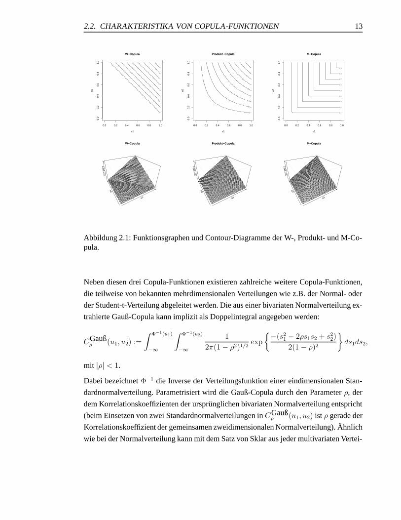
den, wobei die untere (obere) Schranke als W -Copula (M-Copula) bezeichnet wird:
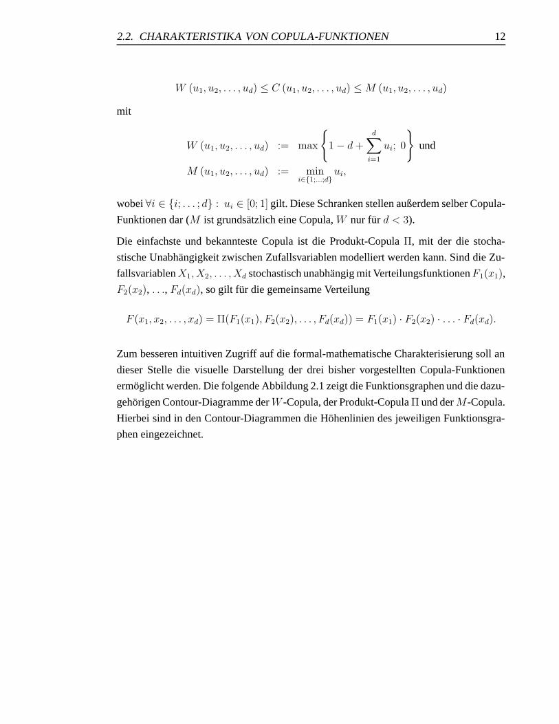
2.2. CHARAKTERISTIKA VON COPULA-FUNKTIONEN 12
W (u1, u2, . . . , ud) ≤ C (u1, u2, . . . , ud) ≤M (u1, u2, . . . , ud)
mit
W (u1, u2, . . . , ud) := max
{1 − d+
d∑i=1
ui; 0
}und
M (u1, u2, . . . , ud) := mini∈{1;...;d}
ui,
wobei ∀i ∈ {i; . . . ; d} : ui ∈ [0; 1] gilt. Diese Schranken stellen außerdem selber Copula-
Funktionen dar (M ist grundsatzlich eine Copula, W nur fur d < 3).
Die einfachste und bekannteste Copula ist die Produkt-Copula Π, mit der die stocha-
stische Unabhangigkeit zwischen Zufallsvariablen modelliert werden kann. Sind die Zu-
fallsvariablenX1, X2, . . . , Xd stochastisch unabhangig mit VerteilungsfunktionenF1(x1),
F2(x2), . . ., Fd(xd), so gilt fur die gemeinsame Verteilung
F (x1, x2, . . . , xd) = Π(F1(x1), F2(x2), . . . , Fd(xd)) = F1(x1) · F2(x2) · . . . · Fd(xd).
Zum besseren intuitiven Zugriff auf die formal-mathematische Charakterisierung soll an
dieser Stelle die visuelle Darstellung der drei bisher vorgestellten Copula-Funktionen
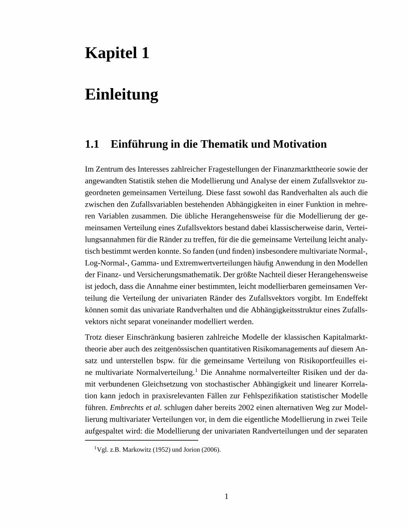
ermoglicht werden. Die folgende Abbildung 2.1 zeigt die Funktionsgraphen und die dazu-
gehorigen Contour-Diagramme derW -Copula, der Produkt-Copula Π und derM-Copula.
Hierbei sind in den Contour-Diagrammen die Hohenlinien des jeweiligen Funktionsgra-
phen eingezeichnet.
2.2. CHARAKTERISTIKA VON COPULA-FUNKTIONEN 13
W−Copula
u1
u2
0.1
0.1
0.1
0.1
0.2
0.2
0.2
0.2
0.2
0.2
0.2
0.3
0.3
0.3
0.4
0.4
0.4
0.4
0.4
0.5
0.5
0.5
0.6 0.7
0.8
0.9
0.0 0.2 0.4 0.6 0.8 1.0
0.0
0.2
0.4
0.6
0.8
1.0
Produkt−Copula
u1
u2
0.1
0.2
0.3
0.4
0.5
0.6
0.7
0.8
0.9
0.0 0.2 0.4 0.6 0.8 1.0
0.0
0.2
0.4
0.6
0.8
1.0
M−Copula
u1
u2
0.1
0.2
0.3
0.4
0.5
0.6
0.7
0.8
0.9
0.0 0.2 0.4 0.6 0.8 1.0
0.0
0.2
0.4
0.6
0.8
1.0
u1
u2
C(u1,u2)
W−Copula
u1u2
C(u1,u2)
Produkt−Copula
u1
u2
C(u1,u2)
M−Copula
Abbildung 2.1: Funktionsgraphen und Contour-Diagramme der W-, Produkt- und M-Co-pula.
Neben diesen drei Copula-Funktionen existieren zahlreiche weitere Copula-Funktionen,
die teilweise von bekannten mehrdimensionalen Verteilungen wie z.B. der Normal- oder
der Student-t-Verteilung abgeleitet werden. Die aus einer bivariaten Normalverteilung ex-
trahierte Gauß-Copula kann implizit als Doppelintegral angegeben werden:
CGaußρ (u1, u2) :=
∫ Φ−1(u1)
−∞
∫ Φ−1(u2)
−∞
1
2π(1 − ρ2)1/2exp
{−(s2
1 − 2ρs1s2 + s22)
2(1 − ρ)2
}ds1ds2,
mit |ρ| < 1.
Dabei bezeichnet Φ−1 die Inverse der Verteilungsfunktion einer eindimensionalen Stan-
dardnormalverteilung. Parametrisiert wird die Gauß-Copula durch den Parameter ρ, der
dem Korrelationskoeffizienten der ursprunglichen bivariaten Normalverteilung entspricht
(beim Einsetzen von zwei Standardnormalverteilungen in CGaußρ (u1, u2) ist ρ gerade der
Korrelationskoeffizient der gemeinsamen zweidimensionalen Normalverteilung). Ahnlich
wie bei der Normalverteilung kann mit dem Satz von Sklar aus jeder multivariaten Vertei-
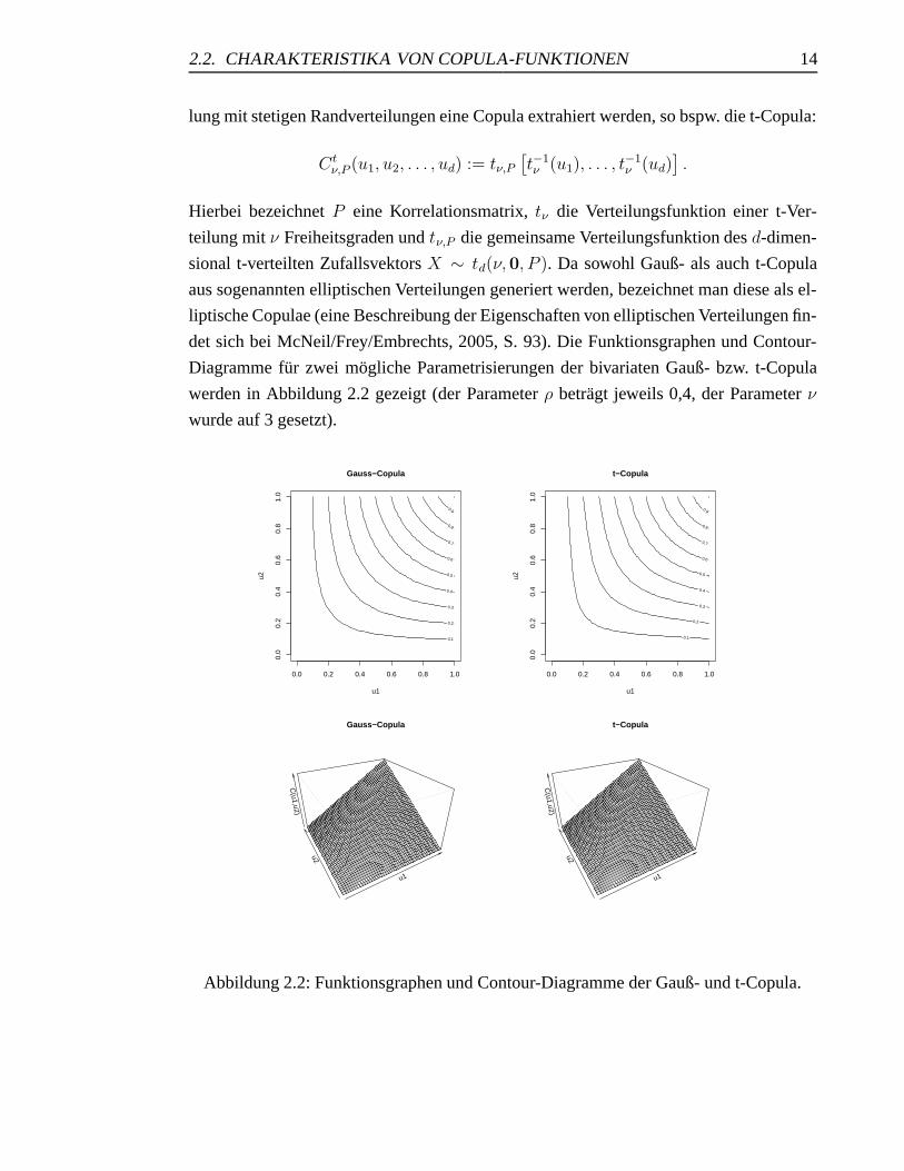
2.2. CHARAKTERISTIKA VON COPULA-FUNKTIONEN 14
lung mit stetigen Randverteilungen eine Copula extrahiert werden, so bspw. die t-Copula:
Ctν,P (u1, u2, . . . , ud) := tν,P
[t−1ν (u1), . . . , t
−1ν (ud)
].
Hierbei bezeichnet P eine Korrelationsmatrix, tν die Verteilungsfunktion einer t-Ver-
teilung mit ν Freiheitsgraden und tν,P die gemeinsame Verteilungsfunktion des d-dimen-
sional t-verteilten Zufallsvektors X ∼ td(ν, 0, P ). Da sowohl Gauß- als auch t-Copula
aus sogenannten elliptischen Verteilungen generiert werden, bezeichnet man diese als el-
liptische Copulae (eine Beschreibung der Eigenschaften von elliptischen Verteilungen fin-
det sich bei McNeil/Frey/Embrechts, 2005, S. 93). Die Funktionsgraphen und Contour-
Diagramme fur zwei mogliche Parametrisierungen der bivariaten Gauß- bzw. t-Copula
werden in Abbildung 2.2 gezeigt (der Parameter ρ betragt jeweils 0,4, der Parameter ν
wurde auf 3 gesetzt).
Gauss−Copula
u1
u2
0.1
0.2
0.3
0.4
0.5
0.6
0.7
0.8
0.9
0.0 0.2 0.4 0.6 0.8 1.0
0.0
0.2
0.4
0.6
0.8
1.0
t−Copula
u1
u2
0.1
0.2
0.3
0.4
0.5
0.6
0.7
0.8
0.9
0.0 0.2 0.4 0.6 0.8 1.0
0.0
0.2
0.4
0.6
0.8
1.0
u1
u2
C(u1,u2)
Gauss−Copula
u1
u2
C(u1,u2)
t−Copula
Abbildung 2.2: Funktionsgraphen und Contour-Diagramme der Gauß- und t-Copula.
2.2. CHARAKTERISTIKA VON COPULA-FUNKTIONEN 15
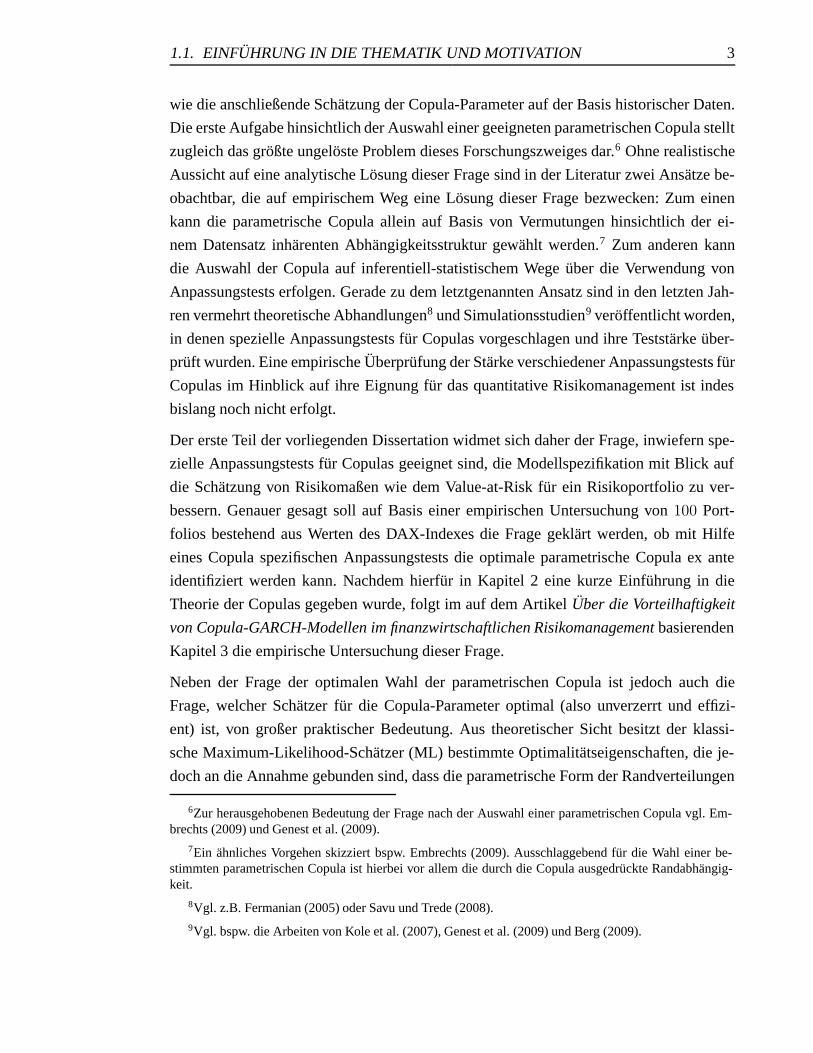
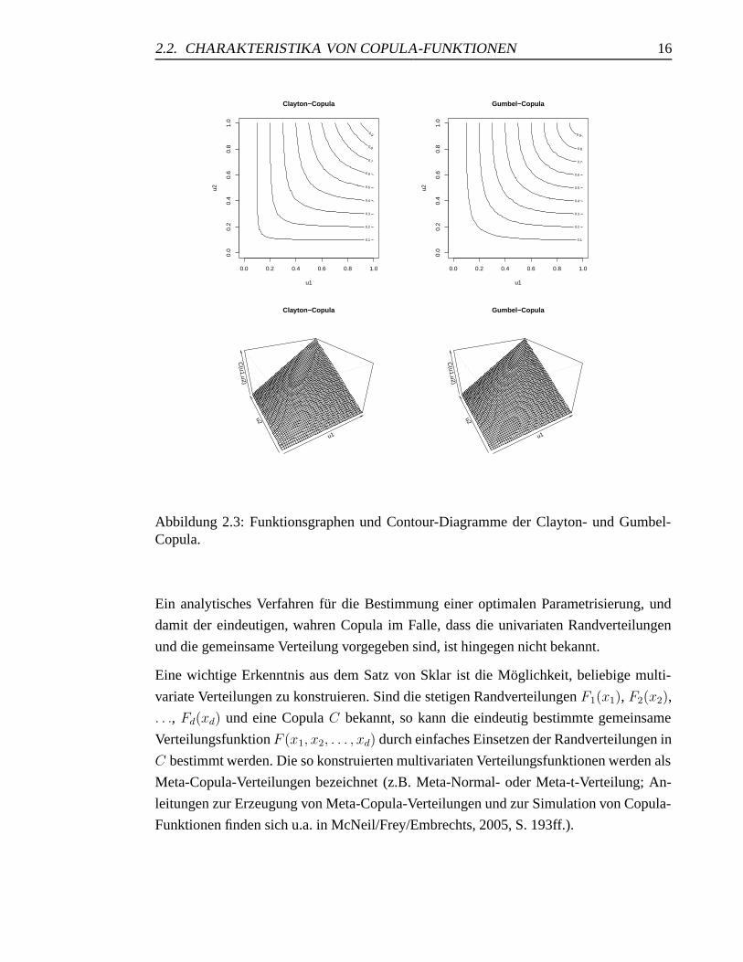
Als Beispiele fur Copulae, fur die explizite Definitionsgleichungen existieren, sollen nach-
folgend die Gumbel- und Clayton-Copula definiert werden. Diese gehoren zur Familie der
sogenannten Archimedischen Copula-Funktionen, die sich insbesondere auf Grund der
Moglichkeit der Ineinanderschachtelung mehrerer bivariater archimedischer Copulae fur
den Einsatz in hoheren Dimensionen auszeichnen. Die bivariate Gumbel- und Clayton-
Copula sind definiert als:
CGumbelθ (u1, u2) := exp
{−((− ln u1)
θ + (− ln u2)θ)1/θ},
mit 1 ≤ θ <∞ und
CClaytonθ (u1, u2) :=
(u−θ
1 + u−θ2 − 1
)−1/θ,
mit 0 < θ < ∞. Abbildung 2.3 zeigt die Funktionsgraphen und Contour-Diagramme fur
die Clayton- bzw. Gumbel-Copula (θ = 2).
2.2. CHARAKTERISTIKA VON COPULA-FUNKTIONEN 16
Clayton−Copula
u1
u2
0.1
0.2
0.3
0.4
0.5
0.6
0.7
0.8
0.9
0.0 0.2 0.4 0.6 0.8 1.0
0.0
0.2
0.4
0.6
0.8
1.0
Gumbel−Copula
u1
u2
0.1
0.2
0.3
0.4
0.5
0.6
0.7
0.8
0.9
0.0 0.2 0.4 0.6 0.8 1.0
0.0
0.2
0.4
0.6
0.8
1.0
u1
u2
C(u1,u2)
Clayton−Copula
u1
u2
C(u1,u2)
Gumbel−Copula
Abbildung 2.3: Funktionsgraphen und Contour-Diagramme der Clayton- und Gumbel-Copula.
Ein analytisches Verfahren fur die Bestimmung einer optimalen Parametrisierung, und
damit der eindeutigen, wahren Copula im Falle, dass die univariaten Randverteilungen
und die gemeinsame Verteilung vorgegeben sind, ist hingegen nicht bekannt.
Eine wichtige Erkenntnis aus dem Satz von Sklar ist die Moglichkeit, beliebige multi-
variate Verteilungen zu konstruieren. Sind die stetigen Randverteilungen F1(x1), F2(x2),
. . ., Fd(xd) und eine Copula C bekannt, so kann die eindeutig bestimmte gemeinsame
Verteilungsfunktion F (x1, x2, . . . , xd) durch einfaches Einsetzen der Randverteilungen in
C bestimmt werden. Die so konstruierten multivariaten Verteilungsfunktionen werden als
Meta-Copula-Verteilungen bezeichnet (z.B. Meta-Normal- oder Meta-t-Verteilung; An-
leitungen zur Erzeugung von Meta-Copula-Verteilungen und zur Simulation von Copula-
Funktionen finden sich u.a. in McNeil/Frey/Embrechts, 2005, S. 193ff.).
2.3. ANWENDUNGSMOGLICHKEITEN VON COPULA-FUNKTIONEN IM
RISIKOMANAGEMENT17
2.3 Anwendungsmoglichkeiten von Copula-Funktionen im
Risikomanagement
Copula-Funktionen konnen grundsatzlich auf zwei Weisen sinnvoll im Risikomanage-
ment verwendet werden. Die erste Moglichkeit besteht darin, bei Kenntnis der Vertei-
lungen der Einzelrisiken diese mit Hilfe einer bekannten oder aus Vergangenheitswerten
geschatzten Copula zur gemeinsamen (Meta-Copula-)Verteilung zu verknupfen. Hierbei
wird die Copula so gewahlt, dass sie die vermutete Abhangigkeitsstruktur zwischen den
einzelnen Risikopositionen moglichst gut annahert.
Die besondere Bedeutung dieser Modelle fur das Risikomanagement liegt in der Fahig-
keit dieser Modelle, sowohl lineare als auch nichtlineare Abhangigkeiten zwischen den
Risikopositionen abbilden zu konnen. Hierdurch konnen Diversifikationseffekte in der
Bestimmung des Gesamtbankrisikos viel starker berucksichtigt werden, als es bspw. mit
anderen Verfahren wie der Annahme normalverteilter Risiken moglich ware. Mit der so
bestimmten gemeinsamen Verteilung der Gewinne und Verluste kann eine Bank anschlie-
ßend ein (koharentes) quantil-basiertes Risikomaß fur die (diversifizierte) Gesamtbank
bestimmen.
Die zweite Moglichkeit des Einsatzes von Copula-Funktionen im Risikomanagement be-
steht in der Analyse von Abhangigkeitsstrukturen in einem gegebenen Datensatz (vgl.
z.B. Junker/May, 2005). In diesem Fall besteht die Vorgehensweise in der Wahl einer
parametrisierten Copula, deren Parameter aus dem Datensatz heraus geschatzt werden
sollen. Die resultierenden Parameter und die funktionale Form der vollstandig parame-
trisierten Copula konnen dann anschließend hinsichtlich der Frage untersucht werden,
welche Art von Abhangigkeit zwischen den Randverteilungen besteht. Im Risikomanage-
ment werden daher Copula-Funktionen verstarkt eingesetzt, um wiederkehrende Muster
in der Abhangigkeitsstruktur verschiedener Risikoarten (z.B. Marktpreis- oder Kreditrisi-
ken) untereinander zu identifizieren.
Offensichtlich besteht die großte Schwierigkeit bei beiden Vorgehensweisen in der Wahl
der wahren Copula (nach dem Satz von Sklar ist sie unter schwachen Voraussetzungen
eindeutig). Obwohl zahlreiche Klassen von Copula-Funktionen bereits identifiziert wor-
den sind, kann die Mehrzahl dieser Funktionen nicht in geschlossener analytischer Form
angegeben werden. Ebenso kann die Wahl der Parameter der Copula in der Praxis Proble-
me bereiten (bspw. sollte die Gauß-Copula nicht mit der empirischen Korrelationsmatrix,
sondern dem paarweisen Rangkorrelationskoeffizienten nach Spearman kalibriert werden,
2.3. ANWENDUNGSMOGLICHKEITEN VON COPULA-FUNKTIONEN IM
RISIKOMANAGEMENT18
vgl. McNeil/Frey/Embrechts, 2005, S. 230). Empirische Ergebnisse deuten zudem darauf
hin, dass die Wahl einer falschen parametrischen Form der Copula zu erheblichen Feh-
lern bei der anschließenden Berechnung von Quantilen fuhren kann (vgl. Ane/Kharoubi
(2003)). Aus diesem Grund sind in der jungsten Vergangenheit von zahlreichen Autoren
Goodness-of-fit-Tests vorgeschlagen worden, die die Anpassungsgute einer geschatzten
parametrischen Copula durch einen Vergleich mit dem Copula-Analogon zur empirischen
Verteilungsfunktion (der sogenannten Empirischen Copula nach Deheuvels) zu beurteilen
versuchen (vgl. z.B. Kole/Koedijk/Verbeek, 2007; Scaillet, 2007 und Fermanian, 2005).
Kapitel 3
Uber die Vorteilhaftigkeit von
Copula-GARCH-Modellen im
finanzwirtschaftlichen
Risikomanagement
Zur Veroffentlichung eingereicht in:
Kredit und Kapital.
3.1 Einleitung
Das zentrale Anliegen des finanzwirtschaftlichen Risikomanagements besteht in der in-
tegrierten Messung samtlicher Risiken, denen sich ein Finanzinstitut oder Industrieun-
ternehmen ausgesetzt sieht. Eine ganzheitliche Betrachtung unterschiedlicher Risikoarten
bezweckt insbesondere die Berucksichtigung von Diversifikationseffekten zwischen den
verschiedenen Risiken. Im Resultat kann eine Bank durch die adaquate Berucksichtigung
von Diversifikationseffekten das von ihr vorzuhaltende regulatorische Eigenkapital opti-
mieren und somit ihre Eigenkapitalkosten senken.1
In der Vergangenheit basierte diese ganzheitliche, multivariate Modellierung von finanz-
wirtschaftlichen Risiken haufig auf der Berechnung von linearen Korrelationen unter der
Annahme normalverteilter Einzelrisiken. Sowohl fur Marktpreisrisiken als auch insbe-
sondere fur Kreditrisiken ist die Annahme normalverteilter Renditen und Ausfalle jedoch
empirisch nicht haltbar.
1Unter dem”regulatorischen Eigenkapital“ (andere synonyme Bezeichnungen sind
”aufsichtsrechtli-
ches“ oder”haftendes Eigenkapital“) versteht man die Zusammenfassung unterschiedlicher Bilanzpositio-
nen zur Ermittlung der im Insolvenzfall zur Verfugung stehenden Haftmasse. Es setzt sich gemaß §10 KWGund SolvV, ausgehend vom bilanziellen Eigenkapital, aus verschiedenen Kapitalien unterschiedlicher Wer-tigkeit im Insolvenzfall zusammen. Vgl. Hartmann-Wendels/Pfingsten/Weber (2007), S. 391-399.
19
3.1. EINLEITUNG 20
In den vergangenen Jahren sind daher verstarkt Copula-Modelle in den Fokus der For-
schung geraten, die eine Modellierung der gesamten (linearen und nichtlinearen) Ab-
hangigkeitsstruktur eines Zufallsvektors ermoglichen.2 Eine Copula liefert in bestechend
einfacher Form eine Funktionsvorschrift, die hochst unterschiedliche Randverteilungen
miteinander zur zugehorigen gemeinsamen Verteilung verknupft. Somit kann eine Co-
pula fur die Generierung einer multivariaten Verteilung verwendet werden, deren Rand-
verteilungen nicht notwendigerweise identisch sind. Erste Anwendungen haben Copula-
Funktionen aufgrund dieser Eigenschaft insbesondere im Risikomanagement und in der
Versicherungsmathematik gefunden, wo sie zur Generierung der gemeinsamen Verteilung
eines Risikoportfolios verwendet wurden.3 Wichtige Fragestellungen der Implementie-
rung eines auf Copula-Funktionen basierenden Gesamtrisikomodells sind jedoch in der
Wissenschaft noch nicht hinreichend beantwortet. So sind insb. auf die Fragen, welche
parametrische Familie von Copula-Funktionen am besten zur Modellierung bestimmter
Risiken geeignet ist und wie ein hochdimensionales Modell mit 20 oder mehr Risikofak-
toren effizient geschatzt werden kann, bisher keine zufriedenstellenden Antworten gefun-
den worden.4
Der vorliegende Beitrag verfolgt zwei Ziele: Zum einen soll anhand einer umfangreichen
Simulationsstudie die Vorteilhaftigkeit von Copula-GARCH-Modellen zur Bestimmung
des Value-at-Risks (VaR) bzw. Conditional-Value-at-Risks (CVaR) eines Aktienportfoli-
os gezeigt werden. Zum anderen soll die Frage geklart werden, inwieweit das jeweilige
durch ein Backtesting als optimal identifizierte Copula-GARCH-Modell mithilfe eines
speziellen Anpassungstests im Vorfeld der Value-at-Risk-Prognose hatte ermittelt werden
konnen.
Zu diesem Zweck wird zunachst das notige mathematische Fundament der Theorie der
Copula-Funktionen gelegt. Hierauf aufbauend wird ein Copula-GARCH-Modell zur Be-
stimmung einer gemeinsamen Verlustverteilung erortert, weiterhin werden einige aus
praktischer Sicht besonders relevante Fragen hinsichtlich der Gute und der Stabilitat der
Verfahren zur Schatzung von Copula-Funktionen diskutiert. Durch die Analyse von ins-
gesamt 100 aus im DAX vertretenen Aktien bestehenden Portfolios uber acht verschie-
dene Zeitfenster stellt dieser Beitrag mit 800 Simulationen die bislang umfangreichste
2Vgl. z. B. Embrechts/McNeil/Straumann (2002) fur ein fruhes Beispiel der anwendungsorientiertenBetrachtung von Copula-Funktionen und eine Kritik an korrelationsbasierten Modellen.
3Beispiele hierfur finden sich u. a. bei Junker/May (2005) und Kole/Koedijk/Verbeek (2007).
4Eine”einfache“ Losung dieser Fragen wird aller Voraussicht nach auch nie gefunden werden, vgl. Em-
brechts (2009). Losungsansatze insb. zum erstgenannten Problem finden sich in den Arbeiten von Genest,vgl. z. B. Genest/Remillard/Beaudoin (2009).
3.2. LITERATURUBERBLICK UND HYPOTHESENBILDUNG 21
Untersuchung zur Vorteilhaftigkeit von Copula-Risikomodellen dar.
Der Beitrag untergliedert sich in funf Abschnitte. Abschnitt 3.2 beinhaltet einen kurzen
Literaturuberblick und leitet die zu uberprufenden Hypothesen ab. Abschnitt 3.3 erlautert
die univariate Schatzung des Value-at-Risks mithilfe von GARCH-Prozessen. In Ab-
schnitt 3.4 werden Methoden zur Bestimmung des Portfolio-Value-at-Risks vorgestellt.
Abschnitt 3.5 prasentiert die empirische Untersuchung sowie die Ergebnisse. Eine kurze
Zusammenfassung des Beitrags wird in Abschnitt 3.6 gegeben.
3.2 Literaturuberblick und Hypothesenbildung
Seit dem Erscheinen der ersten Arbeiten von Embrechts/McNeil/Straumann5 uber die Ein-
satzmoglichkeiten von Copula-Funktionen im finanzwirtschaftlichen Risikomanagement
sind mehrere Studien erschienen, die die Vorteilhaftigkeit dieser Modelle empirisch uber-
pruft haben.
Eine der ersten empirischen Studien uber die Vorteilhaftigkeit von Copula-Modellen fur
die Modellierung von Abhangigkeitsstrukturen zwischen verschiedenen Anlageformen
stammt von Malevergne/Sornette.6 Die Autoren zeigen fur einen Datensatz, bestehend
aus sechs Wahrungskursen, sechs Commodity-Preisen und 22 an der NYSE notierten Ak-
tienkursen, dass fur die Mehrzahl der innerhalb einer Anlageklasse gebildeten bivariaten
Portfolios die Abhangigkeitsstruktur am besten durch eine Gauß-Copula modelliert wer-
den kann. Gleichzeitig betonen sie, dass die Student’s t-Copula falschlicherweise fur eine
Gauß-Copula gehalten werden kann. Kritisch ist an der Studie von Malevergne/Sornette
jedoch zu sehen, dass diese keine Schatzung von Risikomaßen fur die Portfolios enthalt,
archimedische Copulas nicht berucksichtigt und keine Copula spezifischen Anpassungs-
tests verwendet. Die vermutete pauschale Vorteilhaftigkeit einer einzigen parametrischen
Copula ist jedoch beispielhaft fur die Ergebnisse zahlreicher Arbeiten in den Folgejah-
ren.7 Beispielsweise zeigen Kole/Koedijk/Verbeek fur ein trivariates Portfolio aus Aktien-,
Anleihe- und REITS-Indizes, dass die Abhangigkeitsstruktur dieses Portfolios am besten
durch eine Student’s t-Copula modelliert werden kann.8
Ein ahnliches Resultat hinsichtlich der Wahl der parametrischen Copula finden Di Cle-
5Vgl. Embrechts/McNeil/Straumann (2002).
6Vgl. Malevergne/Sornette (2003).
7Vgl. bspw. die Arbeiten von Fantazzini (2006) und Kole/Koedijk/Verbeek (2007).
8Vgl. Kole/Koedijk/Verbeek (2007).
3.2. LITERATURUBERBLICK UND HYPOTHESENBILDUNG 22
mente/Romano.9 Ihre empirische Untersuchung eines 20-dimensionalen Portfolios ita-
lienischer Aktien zeigt, dass ein kombiniertes Modell aus extremwertverteilten Rand-
verteilungen und einer Gauß- oder Student’s t-Copula erheblich bessere Value-at-Risk-
Schatzungen liefern kann als das klassische korrelationsbasierte Modell. Wiederum wer-
den weder archimedische Copulas noch Anpassungstests oder andere Risikomaße sowie
weitere Portfolios betrachtet.
Junker/May zeigen in ihrer Studie, dass ein Modell mit GARCH-Prozessen als Rand-
verteilungen und einer speziell transformierten Frank-Copula marginal bessere Value-at-
Risk- und Conditional-Value-at-Risk-Schatzungen liefern kann als die Gauß- oder Stu-
dent’s t-Copula.10 Abermals stutzen die Autoren dieses Ergebnis jedoch auf die Un-
tersuchung eines einzelnen bivariaten Portfolios aus Hoechst- und Volkswagen-Aktien
in einem einzigen Betrachtungszeitraum und verwenden ausschließlich allgemeine (Co-
pula unspezifische) Anpassungstests. Ein fast identisches Ergebnis unter ahnlichen Ein-
schrankungen finden Palaro/Hotta, wobei sie fur ein bivariates Portfolio, bestehend aus
dem S&P 500- und dem NASDAQ-Index, die Vorteilhaftigkeit eines Copula-GARCH-
Modells mit symmetrisierter Joe-Clayton-Copula und GARCH-Randverteilungen finden.11
Ebenso zeigt Fantazzini mithilfe einer empirischen Untersuchung von drei bivariaten
Portfolios aus Aktienindizes, dass eine konstante bzw. dynamische Gauß-Copula aus-
reicht, um im Backtesting akzeptable VaR-Schatzungen zu liefern.12
Den genannten Studien ist somit gemein, dass alle Autoren auf Basis weniger Portfolios
eine klare Vorteilhaftigkeit von Copula-Modellen im Vergleich zu korrelationsbasierten
Modellen aufzeigen. Diese unterstellte Vorteilhaftigkeit soll daher auch in dieser Arbeit
zunachst untersucht werden. Bevor jedoch die erste Hypothese formuliert werden kann,
verstandigen wir uns uber die Frage, wann ein Modell als vorteilhaft angesehen werden
kann. Ein Modell X soll in dieser Arbeit als vorteilhafter gegenuber einem zweiten Mo-
dell Y angesehen werden, wenn die hiermit ermittelte Anzahl an VaR-Uberschreitungen
(ExceedModellX) naher an der erwarteten Anzahl an Uberschreitungen (ExceedEmp) liegt
als die des zweiten Modells (ExceedModellY ), ohne die erwartete Anzahl zu uberschreiten.
Die so definierte Vorteilhaftigkeit eines Modells bedeutet, dass das Modell X das Risiko
adaquater darstellt, als dies Modell Y tut, ohne jedoch das vom Investor eingegangene
Risiko zu unterschatzen.
9Vgl. Di Clemente/Romano (2005).
10Vgl. Junker/May (2005).
11Vgl. Palaro/Hotta (2006).
12Vgl. Fantazzini (2006).
3.2. LITERATURUBERBLICK UND HYPOTHESENBILDUNG 23
Aquivalent hierzu betrachten wir ein Modell als optimal fur die Berechnung des CVaRs,
falls der mit diesem Modell berechnete durchschnittliche CVaR im Testzeitraum die Schat-
zungen samtlicher ubriger Modelle verbessert, ohne den tatsachlichen durchschnittlichen
CVaR zu uberschreiten.
Die genannten Studien suggerieren, dass das Rahmenwerk eines Copula-Modells stets
bessere Risikoschatzungen liefert als ein korrelationsbasiertes Modell, solange nur die (ex
ante unbekannte) parametrische Copula-Form richtig gewahlt wird. Die erste Hypothese
lautet somit:
H1: Fur jedes bivariate Portfolio lasst sich in jedem Beobachtungszeitraum stets eine
parametrische Copula-Form finden, sodass das hier vorgeschlagene Copula-GARCH-
Modell eine bessere VaR- und CVaR-Schatzung liefert als das korrelationsbasierte Mo-
dell, also:
ExceedCorr ≤ ExceedCop ≤ ExceedEmp
bzw. fur den Conditional-Value-at-Risk:
CV aRCorr ≤ CV aRCop ≤ CV aREmp.
Betrachtet man insbesondere die Arbeiten von Malevergne/Sornette, Kole/Koedijk/Ver-
beek und Di Clemente/Romano, so erkennt man, dass samtliche Autoren dieser Studien
eine klare Vorteilhaftigkeit elliptischer Copulas als Ergebnis festhalten. Diese auf Basis
kleinerer Datensatze gefundene Optimalitat elliptischer Copulas soll daher im zweiten
Schritt dieser Arbeit untersucht werden, wobei zur Verallgemeinerung der anekdotischen
Evidenz der genannten Studien in dieser Arbeit eine im Vergleich zu bisherigen Arbei-
ten stark erhohte Anzahl an Portfolios verwendet werden soll. Um eine Vergleichbarkeit
mit den genannten Studien erzielen zu konnen, soll zudem zunachst der Einfluss der Wahl
des Risikomaßes sowie des Schatzzeitraumes auf die Risikoschatzungen unberucksichtigt
bleiben.
Die zweite Hypothese lautet dann:
H2: Die Gauß- und/oder Student’s t-Copula liefern/liefert unabhangig vom betrachteten
Schatz- und Testzeitraum und unabhangig vom verwendeten Risikomaß sowie von den
interessierenden Risikopositionen stets bessere Schatzwerte fur das gewahlte Risikomaß
als ein vergleichbares korrelationsbasiertes oder ein auf einer archimedischen Copula

3.2. LITERATURUBERBLICK UND HYPOTHESENBILDUNG 24
basierendes Modell.
Im dritten Schritt soll die Frage geklart werden, welche elliptische Copula gegebenenfalls
die besseren Risikoschatzungen liefert. Sollten die Ergebnisse von Malevergne/Sornette
verallgemeinerbar sein, so musste dies die Gauß-Copula sein. Laut Kole/Koedijk/Verbeek
musste dagegen die Student’s t-Copula bessere Ergebnisse liefern als die Gauß-Copula.
Beide Studien unterstellen ebenfalls implizit, dass die Ergebnisse unabhangig von der
Wahl des Risikomaßes und des Schatzzeitraumes sind.
Die dritte Hypothese lautet somit:
H3: Liefert eine elliptische Copula den besten Schatzwert fur das gewahlte Risikomaß fur
ein bivariates Portfolio, so ist dies die Gauß-Copula (Student’s t-Copula). Die unterstellte
Optimalitat der Gauß-Copula (Student’s t-Copula) innerhalb der elliptischen Copulas
ist zudem unabhangig vom betrachteten Schatz- und Testzeitraum und unabhangig vom
verwendeten Risikomaß sowie von den interessierenden Risikopositionen.
Sollte hingegen ein elliptisches Modell nicht die besten Risikoschatzungen liefern (wie
dies die Arbeiten von Junker/May und Palaro/Hotta zeigen), so ist offensichtlich die Frage
zu klaren, welche parametrische Copula-Form ggf. optimal ist.
Offene Frage: Welche parametrische (elliptische oder archimedische) Copula-Form muss
fur das Copula-GARCH-Modell gewahlt werden, sodass im Durchschnitt aller simulier-
ten Portfolios unabhangig vom betrachteten Schatz- und Testzeitraum und unabhangig
vom verwendeten Risikomaß sowie von den interessierenden Risikopositionen die besten
Risikoschatzungen erzielt werden?
Aus der Tatsache, dass die bisherigen Studien fast ganzlich den Einfluss unterschiedlicher
Datenerhebungszeitraume auf die Schatzergebnisse vernachlassigen, leitet sich die vierte
zu uberprufende Hypothese ab:
H4: Die in H1 bestatigte oder widerlegte Vorteilhaftigkeit der Copula-GARCH-Modelle
und die jeweils optimale parametrische Form der Copula fur ein festgehaltenes bivariates
Portfolio sind invariant gegenuber einer Veranderung des Betrachtungszeitraumes.
Hypothese H4 uberpruft somit die in samtlichen Studien implizit getroffene Behauptung,
3.2. LITERATURUBERBLICK UND HYPOTHESENBILDUNG 25
dass fur ein beliebiges Portfolio die optimale parametrische Copula-Form im Zeitablauf
konstant bleibt.
Fur praktische Zwecke besonders relevant ist die Frage, wie die optimale parametrische
Copula-Form im Vorfeld der Schatzung identifiziert werden kann. Da samtliche bishe-
rigen Studien (wenn uberhaupt) nur Copula unspezifische (d. h. fur allgemeine Vertei-
lungsfunktionen gultige) Anpassungstests verwendet haben, soll im Rahmen dieser Un-
tersuchung ein spezieller Anpassungstest fur Copula-Funktionen verwendet werden, des-
sen Gute in Simulationsstudien bestatigt wurde. Zudem ist bemerkenswert, dass bislang
keine Studie Copula-Modelle sowohl durch ein VaR- bzw. CVaR-Backtesting als auch
gleichzeitig durchgefuhrte Anpassungstests beurteilt hat. Falls die Ergebnisse bisheriger
Simulationsstudien unter Laborbedingungen Bestand haben, sollte der Anpassungstest
auch mit Blick auf optimale VaR- und CVaR-Schatzungen stets die optimale parametri-
sche Copula-Form ermitteln konnen.13 Die funfte Hypothese lautet dann:
H5: Die im Backtesting als optimal ermittelte parametrische Copula-Form wird im Vor-
feld der Schatzung des jeweilig gewahlten Risikomaßes als einziges Modell vom Anpas-
sungstest nicht abgelehnt.
Schließlich ist der Einfluss der Wahl des Risikomaßes auf die Vorteilhaftigkeit von Copula-
Modellen zur Risikomessung bislang nur von Junker/May fur ein einzelnes bivariates
Portfolio untersucht worden. Um zu allgemeingultigen Ergebnissen gelangen zu konnen,
ist jedoch die umfassende Untersuchung eines großeren Datensatzes notig. Wir erhalten
somit die letzte Hypothese:
H6: Die Ergebnisse der Hypothesen H1 bis H5 sind invariant gegenuber einer alternati-
ven Verwendung des Conditional-Value-at-Risks anstelle des Value-at-Risks.
Im Folgenden werden nun die verschiedenen univariaten und multivariaten Modelle zur
Messung des Risikos eines Portfolios besprochen.
13Die beiden einzigen umfassenden Simulationsstudien von Berg (2009) und Genest/Remillard/Beaudoin(2009) simulieren ausschließlich aus vorgegebenen parametrischen Copula-Funktionen und analysieren kei-ne komplexeren Abhangigkeitsstrukturen sowie Realdaten.
3.3. UNIVARIATE VAR-SCHATZUNG MITHILFE VON GARCH-PROZESSEN 26
3.3 Univariate VaR-Schatzung mithilfe von GARCH-Pro-
zessen
Die quantitative Messung von Marktpreisrisiken wird in der Praxis regelmaßig mithilfe
des Value-at-Risks vorgenommen. Als Ausgangspunkt der VaR-Methodik kann die Fra-
ge nach dem maximalen Verlust einer Position dienen. Gegeben sei ein risikobehaftetes
Portfolio mit einer gemeinsamen Verlust-Verteilungsfunktion
FL(l) = P (L ≤ l) (3.1)
fur einen bestimmten Zeithorizont Δ. Bei der Bestimmung des Value-at-Risks steht die
Frage nach dem maximal moglichen Verlust im Vordergrund, der zu einem bestimmten
Konfidenzniveau α nicht uberschritten wird. Somit bezeichnet der V aRα den kleinsten
Wert l ∈ R, sodass die Wahrscheinlichkeit dafur, dass der Verlust L den Wert l innerhalb
des Zeithorizonts Δ uberschreitet, nicht großer als (1−α) ist. Formal lasst sich der V aRα
schreiben als:14
V aRα = inf {l ∈ R|FL(l) ≥ α} . (3.2)
Somit stellt der VaR das α-Quantil der Verlustfunktion der betrachteten Position dar. Da
der Value-at-Risk kein koharentes Risikomaß darstellt,15 soll in der empirischen Unter-
suchung zudem der Conditional-Value-at-Risk als Erwartungswert der den VaR ubertref-
fenden Verluste berechnet werden.
Fur die empirische Berechnung des Value-at-Risks bzw. Conditional-Value-at-Risks aus
Realdaten sollten in einem ersten Schritt die Daten univariat mithilfe eines parametri-
schen Verteilungsmodells angepasst werden. Kann in einer vorgelagerten Datenanalyse
die Nullhypothese einer bestimmten Verteilungsform (z. B. normal- oder t-verteilte sta-
tionare Daten) nicht abgelehnt werden, so erfolgt die univariate Modellierung mithilfe
der jeweils identifizierten Verteilung. Deutet die Datenanalyse jedoch auf bedingt hete-
roskedastische und autokorrelierte Daten hin, so werden die Verteilungen der einzelnen
Risikopositionen mithilfe eines GARCH-Prozesses modelliert. Wir beschranken uns im
Folgenden auf die Betrachtung der MarktpreisveranderungXt zum Zeitpunkt t der jewei-
ligen Position, ausgedruckt als Logrendite, als einzigen Risikofaktor. Wird als univariates
14Vgl. McNeil/Frey/Embrechts (2005), S. 38.
15Vgl. Artzner/Delbaen/Eber/Heath (1999).
3.3. UNIVARIATE VAR-SCHATZUNG MITHILFE VON GARCH-PROZESSEN 27
Modell ein GARCH(1,1)-Prozess gewahlt, so ist man auf die Bestimmungsgleichungen
Xt = B + εt (3.3)
σ2t = α0 + α1ε
2t−1 + βσ2
t−1 (3.4)
gefuhrt. Hierbei stelltXt die Logrendite zum Zeitpunkt t dar, B ist eine Konstante, εt das
Residuum zum Zeitpunkt t und σ2t die Varianz zum Zeitpunkt t, wobei die Residuen z. B.
als normal- oder t-verteilt angenommen werden.16 Eine Uberprufung der Anpassungsgute
der univariaten Modelle kann z. B. mithilfe des Ljung-Box-, des Jarque-Bera- sowie des
Kolmogorow-Smirnow-Tests vorgenommen werden.17
Auf Basis der fur einen Schatzzeitraum [s; t] geschatzten univariaten parametrischen Ver-
teilungen bzw. der GARCH-Modelle erfolgt im zweiten Schritt eine Monte-Carlo-Simu-
lation. Fur jede Aktie werden 10.000 Prognosewerte fur die Logrendite uber samtliche
Zeitpunkte des zu betrachtenden Testzeitraums [t + 1; t′] aus den univariaten Modellen
simuliert. Das Ergebnis ist eine Simulationsmatrix der Form
X =
⎛⎜⎜⎜⎜⎝X
(1)t+1 X
(2)t+1 . . . X
(10.000)t+1
X(1)t+2
... . . ....
...... . . .
...
X(1)t′ X
(2)t′ . . . X
(10.000)t′
⎞⎟⎟⎟⎟⎠ . (3.5)
Ein Eintrag X(Ψ)t∗ in der t∗-ten Zeile und Ψ-ten Spalte der Matrix (3.5) beschreibt dabei
die Ψ-te fur einen Tag t∗ ∈ [t+ 1; t′] im Testzeitraum simulierte Logrendite einer Aktie.
Aus den simulierten Logrenditen fur einen Tag t∗ ∈ [t+ 1; t′] konnen im nachsten Schritt
die empirischen Verteilungsfunktionen Fi(xi) und der entsprechende Einzel-VaR jeder
Risikoposition i bestimmt werden. Hierfur werden die simulierten Logrenditen fur jeden
Zeitpunkt der Große nach aufsteigend sortiert und der Wert an der Stelle 10.000 · (1− α)
bestimmt.18 Die Verknupfung dieser Einzel-VaRs kann im nachsten Schritt entweder uber
die Verwendung von Korrelationen oder Copula-Funktionen erfolgen.
16Vgl. Bollerslev/Wooldridge (1992).
17Vgl. Ljung/Box (1978) und Kolmogorow (1933) sowie Smirnow (1939).
18Da in der Praxis stets ein Konfidenzniveau von 5%, 1% oder 0,5% gewahlt wird, ist der Index 10.000 ·(1 − α) des zu bestimmenden Value-at-Risks stets eine naturliche Zahl.
3.4. MULTIVARIATE VAR-SCHATZUNG MITHILFE VON KORRELATIONEN
UND COPULA-FUNKTIONEN28
3.4 Multivariate VaR-Schatzung mithilfe von Korrelatio-
nen und Copula-Funktionen
3.4.1 Aggregation des Value-at-Risks auf Portfolioebene mithilfe von
Korrelationen
Wurde fur jede Vermogensposition der univariate VaR ermittelt, so stellt sich die Frage,
wie die Einzel-VaRs aggregiert werden konnen, um so den VaR auf Portfolioebene zu
bestimmen. Hierfur kann der lineare Gleich- bzw. Gegenlauf der Vermogenspositionen
genutzt werden. Der VaR im Zwei-Wertpapier-Fall lasst sich unter der Annahme nor-
malverteilter Renditen mithilfe des linearen Korrelationskoeffizienten ρ12 der Verluste
bestimmen:19
V aRPortfolio =√V aR2
1 + V aR22 + ρ12V aR1V aR2. (3.6)
Diese Uberlegung ist grundsatzlich ubertragbar auf die Aggregation vieler Einzel-VaRs:20
V aRPortfolio =√
VaR · R ·VaRT . (3.7)
Dabei bezeichnet VaR den Vektor aller Einzel-VaRs und R die Korrelationsmatrix. Das
dargestellte korrelationsbasierte Varianz-Kovarianz-Verfahren besitzt zwei fundamenta-
le Schwachen, die zu erheblichen Fehlern in der Schatzung des Value-at-Risks fuhren
konnen. Zum einen stellt die Verknupfung der Einzel-VaRs mithilfe von Korrelationen
nur im Falle univariat normalverteilter Risikofaktoren eine geeignete Modellierung der
Abhangigkeitsstruktur dar. Eine solche Vereinfachung ist jedoch empirisch nicht haltbar.21
Zum anderen ist die rein korrelationsbasierte Aggregation der univariaten Verteilungen fur
die Modellierung nichtlinearer Abhangigkeiten ganzlich ungeeignet. Im Folgenden soll
daher ein Modell vorgestellt werden, das beide Schwachstellen in Ansatzen behebt. In die-
sem erfolgt die multivariate Modellierung der Zeitreihen mithilfe von Copula-Funktionen,
die die Abbildung der gesamten Abhangigkeitsstruktur ermoglichen.
19Vgl. Dowd (1998), S. 45.
20Vgl. Dowd (1998), S. 47.
21So sind Kapitalmarktdaten in der Regel leptokurtisch und nicht normalverteilt. Zudem weisen Kapital-marktdaten haufig Heteroskedastie auf, vgl. McNeil/Frey/Embrechts (2005), S. 117ff.
3.4. MULTIVARIATE VAR-SCHATZUNG MITHILFE VON KORRELATIONEN
UND COPULA-FUNKTIONEN29
3.4.2 Copula-Modelle zur Ermittlung des Gesamtrisikos
Ziel dieses Kapitels ist die kompakte Darstellung der Grundlagen der Copula-Theorie
sowie des Copula-GARCH-Modells zur Bestimmung der multivariaten Verlustverteilung
eines Portfolios.
3.4.2.1 Grundlagen der Copula-Theorie
Sei F (x1, . . . , xd) die gemeinsame Verteilungsfunktion einer Menge von Zufallsvariablen
(X1, . . . , Xd) definiert durch:
F (x1, . . . , xd) = P (Xi ≤ xi; i = 1, · · · , d) . (3.8)
Eine d-dimensionale Copula-Funktion, verkurzt auch als Copula bezeichnet, ist eine Funk-
tion C auf dem d-dimensionalen Einheitskubus [0; 1]d in das Einheitsintervall [0; 1], die
eine d-dimensionale Verteilungsfunktion mit d univariaten und auf dem Intervall [0; 1]
gleichverteilten Randverteilungen darstellt.22 Die zentrale Bedeutung von Copula-Funk-
tionen fur die Modellierung von stochastischen Abhangigkeiten wird im Satz von Sklar
deutlich:23
Sei F eine gemeinsame Verteilungsfunktion mit Randverteilungen F1, . . . , Fd, dann exi-
stiert eine Copula-Funktion C : [0; 1]d → [0; 1], sodass fur alle x1, . . . , xd ∈ R gilt:
F (x1, . . . , xd) = C (F1(x1), . . . , Fd(xd)) . (3.9)
Sind die Randverteilungen stetig, so istC eindeutig, ansonsten istC eindeutig bestimmbar
auf dem kartesischen Produkt der Wertebereiche der Randverteilungen.24
Beschreibt F←i (ui) := inf {xi|Fi(xi) ≥ ui} die verallgemeinerte inverse Verteilungs-
funktion und wertet man die linke Seite von Gleichung (3.9) an den Stellen xi = F←i (ui)
mit 0 ≤ ui ≤ 1 fur i = 1, . . . , d aus, so ergibt sich:25
C(u1, . . . , ud) = F (F←1 (u1), . . . , F←d (ud)) . (3.10)
22Vgl. Nelsen (2006), S. 10f. und McNeil/Frey/Embrechts (2005), S. 185.
23Vgl. Sklar (1959).
24Fur einen Beweis vgl. Schweizer/Sklar (2005) oder Nelsen (2006), S 18.
25Vgl. Trivedi/Zimmer (2005), S. 10 oder McNeil/Frey/Embrechts (2005), S. 187.
3.4. MULTIVARIATE VAR-SCHATZUNG MITHILFE VON KORRELATIONEN
UND COPULA-FUNKTIONEN30
Eine Copula ermoglicht somit eine im Vergleich zu herkommlichen, haufig auf Normal-
verteilungsannahmen beruhenden Modellen flexiblere Modellierung multivariater Ver-
teilungen. Hierfur werden zuerst die univariaten Randverteilungen parametrisch (bspw.
mithilfe einer Verteilungsannahme) oder aber nichtparametrisch geschatzt. Anschließend
werden die geschatzten Randverteilungen mithilfe einer unterstellten oder aber aus Ver-
gangenheitsdaten geschatzten Copula miteinander verknupft. Die Tatsache, dass die Rand-
verteilungen dabei aus verschiedenen Verteilungsfamilien stammen konnen, ist ein be-
achtlicher Vorteil fur die Modellflexibilitat.
Die verschiedenen, fur die Modellierung infrage kommenden Copulas werden nachfol-
gend dargestellt.
3.4.2.2 Parametrische Copulas
Die Kalibrierung eines Copula-GARCH-Modells zur Schatzung des Value-at-Risks erfor-
dert insbesondere die Auswahl einer parametrischen Funktionalform fur die (unbekannte)
wahre Copula. Im Folgenden sollen nun explizit zwei wichtige Familien von parametri-
schen Copulas vorgestellt werden: die elliptischen und archimedischen Copulas.26
Die Familie der elliptischen Copulas umfasst solche Funktionen, die aus multivariaten el-
liptischen Verteilungen, wie z. B. der multivariaten Normal- oder Student’s-t-Verteilung,
resultieren. Die Normal-Copula27 oder auch Gauß-Copula ist die Copula der multivariaten
Normalverteilung. Stellt F die Verteilungsfunktion ΦR der multivariaten Normalvertei-
lung mit Korrelationsmatrix R dar und F1, . . . , Fd jeweils die Verteilungsfunktion Φ der
univariaten Normalverteilung, so folgt aus der allgemeinen Form des Satzes von Sklar die
Normal-Copula als:28
CNR (u1, . . . , ud) = ΦR
(Φ−1(u1), . . . ,Φ
−1(ud)). (3.11)
Implizit ausformuliert mittels der Dichtefunktion der Normalverteilung fuhrt dies zu:
CNR =
1
(2π)d/2|R|1/2 ·
∫ Φ−1(u1)
−∞. . .
∫ Φ−1(ud)
−∞exp
(−1
2xT R−1x
)dx1 . . . dxd. (3.12)
Die Normal-Copula CNR ist durch die Matrix R parametrisiert. Im Falle normalverteil-
26Wir beschranken uns auf Copulas, die beliebig in hohere Dimensionen verallgemeinert werden konnen.
27Die Normal-Copula wurde schon fruh von z. B. Lee (1983) vorgestellt.
28Vgl. McNeil/Frey/Embrechts (2005), S. 191.

3.4. MULTIVARIATE VAR-SCHATZUNG MITHILFE VON KORRELATIONEN
UND COPULA-FUNKTIONEN31
ter Randverteilungen (und nur in diesem Fall) ist R identisch zur Korrelationsmatrix
der aus der Verknupfung der Normal-Copula und der Randverteilungen resultierenden
d-dimensionalen Normalverteilung.29
Wie zur Herleitung der Normal-Copula kann abermals der Satz von Sklar verwendet wer-
den, um die univariaten t-verteilten Randverteilungen zu einer gemeinsamen multivaria-
ten t-Verteilung mit der Korrelationsmatrix R und der Anzahl an Freiheitsgraden ν zu
verbinden.30 Die t-Copula kann implizit notiert werden als:31
CtR,ν =
Γ(
ν+d2
)(νπ)d/2Γ
(ν2
)|R|1/2
·∫ t−1
ν (u1)
−∞. . .
∫ t−1ν (ud)
−∞
(1 +
1
νxT R−1x
)−( ν+d2 )
dx1 . . . dxd,
(3.13)
wobei tν die Verteilungsfunktion der univariaten t-Verteilung mit ν Freiheitsgraden be-
zeichnet. Fur ν → ∞ konvergiert die t-Copula gegen die Normal-Copula.
Die vorgestellten elliptischen Copula-Funktionen zeichnen sich unter anderem durch ihre
Symmetrie in den oberen und unteren Randbereichen der gemeinsamen Verteilung aus.
Im Finanzbereich tritt jedoch haufig das Phanomen auf, dass große Verluste haufig ei-
ne großere Abhangigkeit aufweisen als Gewinne.32 Im statistischen Sinne liegt in diesen
Fallen eine Form der Randabhangigkeit des Zufallsvektors vor. So eignet sich bspw. ei-
ne Copula mit unterer Randabhangigkeit (engl.: lower tail dependence) besonders fur die
Modellierung von Realdaten, fur die extreme gleichzeitig auftretende Kursverluste wahr-
scheinlicher sind als entsprechende extreme Kursgewinne.
Die bisher erlauterten Copula-Funktionen konnen jedoch ausschließlich symmetrische
Formen der Randabhangigkeit abbilden (die Normal-Copula ist randunabhangig, die Stu-
dent’s t-Copula ist symmetrisch randabhangig). Daher sollen nun drei Funktionen aus der
Familie der archimedischen Copulas erortert werden, die auch das Modellieren von asym-
metrischen Abhangigkeiten in den Randbereichen der gemeinsamen Verteilung ermogli-
chen. Dabei verfugen samtliche hier vorgestellten archimedischen Copulas im Gegensatz
zu den elliptischen Copulas uber eine explizite Darstellung.
Die im oberen Bereich der gemeinsamen Verteilung randabhangige (upper tail dependent)
29Vgl. Kinnebrock (2005), Theorem 16 auf S. 21. Offensichtlich kann auch nur in diesem Fall die MatrixR mit der Korrelationsmatrix kalibriert werden.
30Vgl. McNeil/Frey/Embrechts (2005), S. 191.
31Vgl. Glauser (2003), S. 110.
32Vgl. Aschinger (1995).
3.4. MULTIVARIATE VAR-SCHATZUNG MITHILFE VON KORRELATIONEN
UND COPULA-FUNKTIONEN32
Gumbel-Copula ist explizit gegeben durch:
CGuθ (u1, . . . , ud) = exp
⎡⎣−( d∑i=1
−(ln ui)θ
) 1θ
⎤⎦ . (3.14)
Fur θ = 1 ergibt sich die sogenannte Produkt-Copula, die stochastische Unabhangigkeit
der Randverteilungen impliziert.33
Die im unteren Bereich der gemeinsamen Verteilung randabhangige (lower tail depen-
dent) und somit insbesondere fur die Modellierung von Kapitalmarktdaten geeignete Clay-
ton-Copula34 hat die folgende explizite Form:35
CClθ (u1, . . . , ud) = (u−θ
1 + · · · + u−θd − d+ 1)−1/θ. (3.15)
Die Clayton-Copula ist lediglich fur θ > 0 definiert und ergibt fur θ → 0 wiederum die
Produkt-Copula.
Die randunabhangige Frank-Copula besitzt die explizite Form:36
CClθ (u1, . . . , ud) = −1
θln
(1 +
∏di=1(exp(−θui) − 1)
(exp(−θ) − 1)d−1
)(3.16)
mit θ > 0 fur d ≥ 2.
3.4.2.3 Parameterschatzung
Die dargestellten Copula-Funktionen sind samtlich durch einen endlich-dimensionalen
Vektor θ parametrisiert. Fur die Schatzung des Value-at-Risks mithilfe eines Copula-
GARCH-Modells ist somit die Schatzung der Copula-Parameter mithilfe vorliegender
Vergangenheitsdaten notwendig. Die bekanntesten Verfahren hierfur bauen auf dem Ma-
ximum-Likelihood-Prinzip auf.
Sollen die Parameter der Randverteilungen sowie der Copula in einem Schritt geschatzt
33Vgl. Nelsen (2006), S. 94 f.
34Vgl. Clayton (1973). Die Clayton-Copula wird auch als Cook-Johnson-Copula bezeichnet und wurdeursprunglich von Kimeldorf und Sampson untersucht, vgl. hierzu Cook/Johnson (1981) und Kimeldorf/-Sampson (1975).
35Vgl. McNeil/Frey/Embrechts (2005), S. 223.
36Vgl. Cherubini/Luciano/Vecchiato (2004), S. 186.
3.4. MULTIVARIATE VAR-SCHATZUNG MITHILFE VON KORRELATIONEN
UND COPULA-FUNKTIONEN33
werden, so ist man auf die Exakte-Maximum-Likelihood-Schatzung (EML) gefuhrt. Sei
x = (x1, . . . , xd) eine Realisation des Zufallsvektors X = (X1, . . . , Xd). Ausgangspunkt
ist die Zerlegung
F (x1, . . . , xd|(ν1, . . . , νd), ξ) = Cξ (F1(x1|ν1), . . . , Fd(xd|νd)|ξ) (3.17)
der d-dimensionalen Verteilungsfunktion F von X in die Copula C mit dem Parame-
tervektor ξ und die univariaten Randverteilungen F1, . . . , Fd parametrisiert durch die
Parametervektoren ν1, . . . , νd. Sei dann cξ die Dichtefunktion der Copula Cξ. Die par-
tielle Ableitung der Zerlegung (3.17) nach samtlichen x1, . . . , xd fuhrt zu folgender d-
dimensionaler Dichtefunktion f des Zufallsvektors X:37
f(x1, . . . , xd|(ν1, . . . , νd), ξ) = cξ (F1(x1|ν1), . . . , Fd(xd|νd)|ξ) ·d∏
i=1
fi (xi|νi) . (3.18)
Die Parametervektoren ν1, . . . , νd sowie ξ konnen nun unter Ruckgriff auf T unabhangig
und identisch verteilte Realisierungen x11, . . . , xT1, x12, . . . , xT2, . . . , xTd des Zufallsvek-
tors X geschatzt werden. Dazu ist die Likelihoodfunktion
L ((ν1, . . . , νd), ξ|xti) = f (xti|(ν1, . . . , νd), ξ) (3.19)
zu maximieren. Die Log-Likelihoodfunktion ergibt sich dann zu:38
ln L ((ν1, . . . , νd), ξ|xti) =T∑
t=1
f (xt1, . . . , xtd|(ν1, . . . , νd), ξ) (3.20)
=T∑
t=1
ln cξ (F1(x1|ν1), . . . , Fd(xd|νd)|ξ) (3.21)
+T∑
t=1
d∑i=1
ln fi(xti|νi) (3.22)
Da die Exakte-Maximum-Likelihood-Methode die simultane numerische Optimierung al-
ler Parametervektoren durchfuhrt, ist sie sehr rechenintensiv.39 Um dieses Problem zu
beheben, wird in der nachfolgenden empirischen Untersuchung eine Abwandlung, die
37Vgl. Kinnebrock (2005), S. 47.
38Vgl. ebd.
39Vgl. Joe/Xu (1996), S. 4.
3.4. MULTIVARIATE VAR-SCHATZUNG MITHILFE VON KORRELATIONEN
UND COPULA-FUNKTIONEN34
sogenannte Kanonische -Maximum-Likelihood-40 oder Pseudo-Maximum-Likelihood-Me-
thode41 verwendet.
Diese ersetzt in einem ersten Schritt die parametrische Modellierung der Randverteilun-
gen durch eine nichtparametrische mithilfe der empirischen Verteilungsfunktion. In einem
zweiten Schritt wird die Log-Likelihoodfunktion
ln L (ξ|xti) =
T∑t=1
ln cξ
(F1(xt1), . . . , Fd(xtd)|ξ
)(3.23)
maximiert, wobei mit F1, . . . , Fd die empirischen Randverteilungen der Beobachtungs-
werte bezeichnet werden. Da bei dieser Methode keinerlei Annahmen uber die parame-
trische Form der Randverteilungen zu treffen sind, kann dieses Schatzverfahren gerade
dann wertvolle Ergebnisse liefern, wenn das Hauptaugenmerk auf der Untersuchung der
Abhangigkeitsstruktur von Zufallsvariablen liegt.
3.4.2.4 Anpassungstests zur Prufung der Gute einer Copula-Schatzung
Sind die Parameter der Copula-Funktionen geschatzt, stellt sich das Problem, die Gute
der Schatzung zu beurteilen. Sei C die tatsachliche Copula-Funktion, so liegen folgende
Hypothese und Alternative im Mittelpunkt des Interesses:
H0 : C ∈ Λ = {Cθ|θ ∈ Θ} gegen H1 : C /∈ Λ = {Cθ|θ ∈ Θ} , (3.24)
mit Λ als Familie von Copula-Funktionen und Θ als moglichem Parameterraum. Wahrend
fur den univariaten Fall einfacher Verteilungsannahmen Anpassungstests, oder auch Good-
ness-of-fit-Tests gut erforscht sind,42 wird die Thematik fur Copula-Funktionen zurzeit
recht kontrovers diskutiert.43
In dieser Arbeit beschranken wir uns auf die Darstellung eines einfachen Anpassungs-
tests, der jedoch trotz seines simplen Aufbaus in Simulationsstudien sehr gute Ergebnisse
geliefert hat.44
40Vgl. Bouye/Durrleman/Nikeghbali/Riboulet/Roncalli (2000), S. 26 ff.
41Vgl. Genest/Rivest (1993).
42Vgl. bspw. Anderson/Darling (1954) oder Anderson (1962).
43Vgl. Genest/Rivest (1993), Breymann/Dias/Embrechts (2003), Fermanian (2005), Scaillet (2005), Ge-nest/Quessy/Remillard (2006), Genest/Remillard (2008).
44Vgl. Berg (2009). Dort findet sich ebenso eine Ubersicht weiterer Copula-Anpassungstests.
3.4. MULTIVARIATE VAR-SCHATZUNG MITHILFE VON KORRELATIONEN
UND COPULA-FUNKTIONEN35
Typischerweise soll in den Anpassungstests keine Uberprufung der Randverteilungen
erfolgen. Das Interesse liegt allein auf der Anpassungsgute der Copula. Anstelle der
tatsachlichen Beobachtungswerte werden daher fur die Schatzung der Teststatistik Rang-
daten verwendet, die haufig als Pseudobeobachtungen der wahren Copula aufgefasst wer-
den.45 Sei X eine T × d-dimensionale Matrix von T Beobachtungswerten eines d-dimen-
sionalen Zufallsvektors, so wird diese in die ebenfalls T × d-dimensionale Matrix Y der
Pseudobeobachtungswerte mithilfe folgender Formel uberfuhrt:
Yj = (Yj1, . . . , Yjd) =
(Rj1
T + 1. . . ,
Rjd
T + 1
), (3.25)
wobei Rji den Rang von Xji unter (X1i, . . . , XT i) bezeichnet. Die Pseudobeobachtungs-
werte stimmen gleichzeitig mit den Eingangsdaten fur die Kanonische-Maximum-Likeli-
hood-Methode uberein.
Der hier vorzustellende Anpassungstest basiert auf einem Vergleich der empirischen Co-
pula nach Deheuvels mit der in der Hypothese unterstellten Copula-Funktion.46 Dabei sei
Deheuvels empirische Copula-Funktion gegeben durch:47
C(u) =1
T + 1
T∑j=1
1 {Yj1 ≤ u1, . . . , Yjd ≤ ud} , (3.26)
wobei Yj (Yj1 ≤ u1, . . . , Yjd) gegeben ist durch Gleichung (3.25), u = (u1, . . . , ud) ∈[0; 1]d und 1 die Indikatorfunktion bezeichne. Die empirische Copula-Funktion kann so-
mit als nichtparametrische Approximation der wahren Copula auf Basis einer i.i.d.-Stich-
probe angesehen werden.
Eine Cramer-von Mises-Teststatistik ist dann gegeben durch:48
CvM = T
∫[0;1]d
{C(Y ) − Cθ(Y )
}2
dC(Y ) =T∑
j=1
{C(Yj) − Cθ(Yj)
}2
, (3.27)
mit Y = (Y1, . . . , YT ) wobei C(Y ) die Funktionswerte der empirischen Copula und
Cθ(Y ) die Funktionswerte der in der Hypothese unterstellten und geschatzten Copula an
45Vgl. Genest/Remillard/Beaudoin (2009), S. 3.
46Vgl. Genest/Remillard (2008).
47Vgl. Deheuvels (1979).
48Vgl. Genest/Remillard/Beaudoin (2009). Ebenso denkbar sind Kolmogorow-Smirnow-Teststatistiken.
3.4. MULTIVARIATE VAR-SCHATZUNG MITHILFE VON KORRELATIONEN
UND COPULA-FUNKTIONEN36
den rangtransformierten Daten Y darstellen. Da die Verteilung der Teststatistik unbekannt
ist, muss eine Testentscheidung mithilfe einer approximativen Bootstrap-Testverteilung
erfolgen. Auf die Darstellung der Verfahren zur Ermittlung approximativer p-Werte fur
die Testentscheidung soll an dieser Stelle verzichtet werden.49
3.4.2.5 Bestimmung des Portfolio-Value-at-Risks
Die Bestimmung des Portfolio-VaRs erfordert im nachsten Schritt zunachst die Schatzung
einer parametrischen Copula aus historischen Daten. Die Auswahl der parametrischen
Form der Copula sollte mithilfe des dargestellten Anpassungstests uberpruft werden. Aus
der geschatzten d-dimensionalen Copula-Funktion wird anschließend fur jeden Zeitpunkt
im Testzeitraum [t+ 1; t′] eine Realisationsmatrix
u =
⎛⎜⎜⎜⎜⎝u
(1)1 u
(1)2 . . . u
(1)d
u(2)1
. . . . . ....
.... . . . . .
...
u(10.000)1 u
(10.000)2 . . . u
(10.000)d
⎞⎟⎟⎟⎟⎠ (3.28)
mit 10.000 Auspragungen der Copula simuliert.
Unter Ausnutzung des Zusammenhangs xi = F←i (ui) werden diese simulierten Realisa-
tionen der jeweiligen Copula-Funktion durch Einsetzen in die aus den simulierten Logren-
diten geschatzten empirischen Randverteilungen in simulierte Logrenditen der einzelnen
Anlageformen transformiert.
Die simulierten Logrenditen im Portfolio unter der durch die Copula dargestellten Ab-
hangigkeitsstruktur ergeben sich dann zu x(m)i = F←i (u
(m)i ) fur jedes i = 1, . . . , d und
m = 1, . . . , 10.000.50 Durch die Summenbildung∑d
i=1 x(m)i fur jedesm = 1, . . . , 10.000,
erhalt man 10 000 simulierte Logrenditen des gleichgewichteten Portfolios zum Zeitpunkt
t im jeweiligen Testzeitraum. Der Portfolio-VaR entspricht dem α-Quantil dieser simu-
lierten Verteilung. Die spezifische Abhangigkeit zwischen den Logrenditen wird hier-
bei bereits im ersten Schritt, bei der Simulation der Matrix aus der geschatzten Copula
berucksichtigt. Erst in einem zweiten Schritt werden diese Copula-Auspragungen mithilfe
der Randverteilungen in Logrenditen transformiert. Dies verdeutlicht die Eigenschaft von
49Eine umfangreiche Beschreibung dieser Verfahren findet sich in Genest/Remillard/Beaudoin (2009).
50Vgl. hierzu auch Rosenberg/Schuermann (2004), S. 13-15 und Franke/Hardle/Hafner (2007), S. 354-357.
3.5. EMPIRISCHE UNTERSUCHUNG 37
Copula-Funktionen, eine getrennte Betrachtung von Abhangigkeitsstruktur und Randver-
teilungen zu ermoglichen.
3.5 Empirische Untersuchung
Im Rahmen der empirischen Untersuchung soll uberpruft werden, inwiefern sich die theo-
retischen Vorzuge der Copula-GARCH-Modelle empirisch bestatigen lassen. Die Vorge-
hensweise gliedert sich dabei in eine Erlauterung und deskriptive Auswertung der Daten-
basis, gefolgt von einer Uberprufung auf Stationaritat und Normalverteilung der Zeitrei-
hen. Anschließend wird eine Quantifizierung des Risikos auf Einzelebene durchgefuhrt.
Das Portfoliorisiko wird daraufhin sowohl auf Basis der Korrelationen als auch unter An-
wendung des Copula-GARCH-Modells geschatzt.51
3.5.1 Datenbasis
Bisherige Studien uber die Vorteilhaftigkeit von Copula-Modellen zur Berechnung des
Portfolio-VaRs betrachten allesamt kleine Portfolios ausgewahlter Anlageformen. So zei-
gen bspw. Kole/Koedijk/Verbeek, dass die Abhangigkeitsstruktur zwischen einem Aktien-,
einem Anleihen- sowie einem REITS-Index adaquat durch die Student’s t-Copula mo-
delliert werden kann.52 Vergleichbare Studien von Junker/May betrachten neun bivariate
Portfolios deutscher Aktien und Euro Swap Rates, Malevergne/Sornette passen elliptische
Copulas an insgesamt 18 Wechselkurse, amerikanische Aktien und Rohstoffpreise an.53
Die genannten Studien finden ebenfalls eine Vorteilhaftigkeit der t-Copula.
Die nachfolgende empirische Untersuchung bezweckt, die Ergebnisse der genannten Stu-
dien an verschiedenen Stellen entscheidend zu erweitern. Zum einen soll sich die vorlie-
gende Untersuchung nicht auf die Darstellung von Fallen anekdotischer Evidenz stutzen,
sondern im Stile einer Simulationsstudie verallgemeinerbare Ergebnisse liefern. Zu die-
sem Zweck werden insgesamt 100 zufallig zusammengestellte Aktienportfolios uber acht
Zeitfenster betrachtet. Somit ergeben sich insgesamt 800 Schatzungen des Value-at-Risks
mithilfe des Copula-GARCH-Modells. Der vorliegende Beitrag stellt somit die bisher
umfangreichste Untersuchung der VaR-Berechnung mithilfe von Copulas dar.
51Samtliche Berechnungen wurden mithilfe der freien Statistiksoftware R Version 2.6.0 durchgefuhrt.
52Vgl. Kole/Koedijk/Verbeek (2007).
53Vgl. Junker/May (2005) und Malevergne/Sornette (2003).
3.5. EMPIRISCHE UNTERSUCHUNG 38
Zum anderen legt der vorliegende Beitrag einen besonderen Schwerpunkt auf die Fra-
ge, inwiefern sich die Wahl des zu verwendenden Risikomaßes und die Wahl des Be-
obachtungszeitraumes auf die Ergebnisse der Risikomodelle sowie des Anpassungstests
auswirken. Im Rahmen dieser Untersuchung werden die taglichen Schlusskurse von 18
Werten des DAX30 fur die Schatzung des Value-at-Risk verwendet.54 Aus diesen 18 Wer-
ten werden zufallig 100 bivariate nichtidentische Portfolios zusammengestellt, fur die das
Portfoliorisiko im Zeitablauf bestimmt werden soll. Die zufallige Auswahl der Portfo-
lios wurde bewusst gewahlt, um so eine mogliche Verzerrung der Ergebnisse durch die
bewusste Auswahl bestimmter Aktien zu vermeiden.
Der Betrachtungszeitraum erstreckt sich vom 3. Januar 1995 bis einschließlich zum 2.
Juni 2008 und umfasst somit insgesamt 3500 Handelstage. Zur Untersuchung der Fra-
ge, wie sich die Gute der VaR-Schatzungen im Zeitablauf verandert, werden die VaR-
Schatzungen fur insgesamt acht verschiedene, jeweils um 250 Tage rollierende Zeitfenster
im Beobachtungszeitraum durchgefuhrt. Dabei besteht jedes Zeitfenster aus einem 1000
Handelstage umfassenden Schatz- und einem 750 Handelstage umfassenden Prognose-
zeitraum. Insgesamt ergeben sich somit 800 Simulationen, in denen das Portfoliorisiko
gemessen wird.
Aus den Tageskursen der Aktien werden in einem ersten Schritt Logrenditen auf Tagesba-
sis berechnet. Die Logrenditen werden im nachsten Schritt mithilfe des Jarque-Bera- und
des Ljung-Box-Tests zu den Lags 1 und 10 auf Normalverteilung bzw. Autokorrelation
getestet. Zudem wird mit Engles LM-Test die Hypothese uberpruft, dass die vorliegen-
den Zeitreihen einem ARCH-Prozess folgen. Tabelle 3.1 zeigt die deskriptiven Statistiken
sowie die Ergebnisse der genannten Tests.
Die deskriptiven Daten weisen die ublichen bei Kapitalmarktdaten beobachtbaren stili-
sierten Fakten auf. Neben einer vernachlassigbaren mittleren Rendite weisen samtliche
Kursreihen eine starke Wolbung und Schiefe der Verteilung auf. Folglich verwirft auch
der Jarque-Bera-Test fur jede Zeitreihe die Hypothese normalverteilter Logrenditen. Au-
ßerdem zeigt der LM-Test fur jeden Kurs das Vorhandensein bedingter Heteroskedasti-
zitat der Daten an, sodass fur jeden Kurs im nachsten Schritt ein GARCH(1,1)-Prozess
als univariates Prognosemodell verwendet werden soll.
54Die Auswahl der Werte erfolgte aufgrund der Unvollstandigkeit einiger Kurse innerhalb des langenZeitfensters.
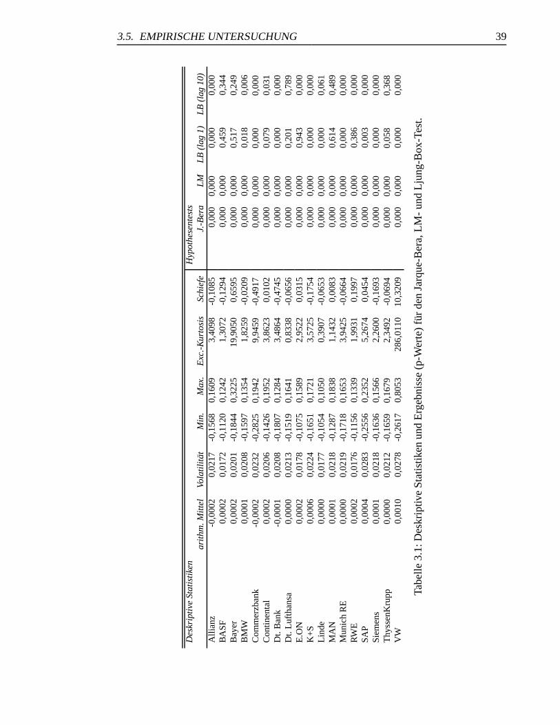
3.5. EMPIRISCHE UNTERSUCHUNG 39
Des
krip
tive
Stat
isti
ken
Hyp
othe
sent
ests
arit
hm.M
itte
lVo
lati
lita
tM
in.
Max
.E
xc.-
Kur
tosi
sSc
hief
eJ.
-Ber
aL
ML
B(l
ag1)
LB
(lag
10)
Alli
anz
-0,0
002
0,02
17-0
,156
80,
1609
3,40
98-0
,108
50,
000
0,00
00,
000
0,00
0B
ASF
0,00
020,
0172
-0,1
120
0,12
421,
3072
-0,1
294
0,00
00,
000
0,45
90,
344
Bay
er0,
0002
0,02
01-0
,184
40,
3225
19,9
050
0,65
950,
000
0,00
00,
517
0,24
9B
MW
0,00
010,
0208
-0,1
597
0,13
541,
8259
-0,0
209
0,00
00,
000
0,01
80,
006
Com
mer
zban
k-0
,000
20,
0232
-0,2
825
0,19
429,
9459
-0,4
917
0,00
00,
000
0,00
00,
000
Con
tinen
tal
0,00
020,
0206
-0,1
426
0,19
523,
8623
0,01
020,
000
0,00
00,
079
0,03
1D
t.B
ank
-0,0
001
0,02
08-0
,180
70,
1284
3,48
64-0
,474
50,
000
0,00
00,
000
0,00
0D
t.L
ufth
ansa
0,00
000,
0213
-0,1
519
0,16
410,
8338
-0,0
656
0,00
00,
000
0,20
10,
789
E.O
N0,
0002
0,01
78-0
,107
50,
1589
2,95
220,
0315
0,00
00,
000
0,94
30,
000
K+
S0,
0006
0,02
24-0
,165
10,
1721
3,57
25-0
,175
40,
000
0,00
00,
000
0,00
0L
inde
0,00
000,
0177
-0,1
054
0,10
500,
3907
-0,0
653
0,00
00,
000
0,00
00,
061
MA
N0,
0001
0,02
18-0
,128
70,
1838
1,14
320,
0083
0,00
00,
000
0,61
40,
489
Mun
ich
RE
0,00
000,
0219
-0,1
718
0,16
533,
9425
-0,0
664
0,00
00,
000
0,00
00,
000
RW
E0,
0002
0,01
76-0
,115
60,
1339
1,99
310,
1997
0,00
00,
000
0,38
60,
000
SAP
0,00
040,
0283
-0,2
556
0,23
525,
2674
0,04
540,
000
0,00
00,
003
0,00
0Si
emen
s0,
0001
0,02
18-0
,163
60,
1566
2,26
00-0
,169
30,
000
0,00
00,
000
0,00
0T
hyss
enK
rupp
0,00
000,
0212
-0,1
659
0,16
792,
3492
-0,0
694
0,00
00,
000
0,05
80,
368
VW
0,00
100,
0278
-0,2
617
0,80
5328
6,01
1010
,320
90,
000
0,00
00,
000
0,00
0
Tabe
lle3.
1:D
eskr
iptiv
eSt
atis
tiken
und
Erg
ebni
sse
(p-W
erte
)fu
rde
nJa
rque
-Ber
a,L
M-
und
Lju
ng-B
ox-T
est.
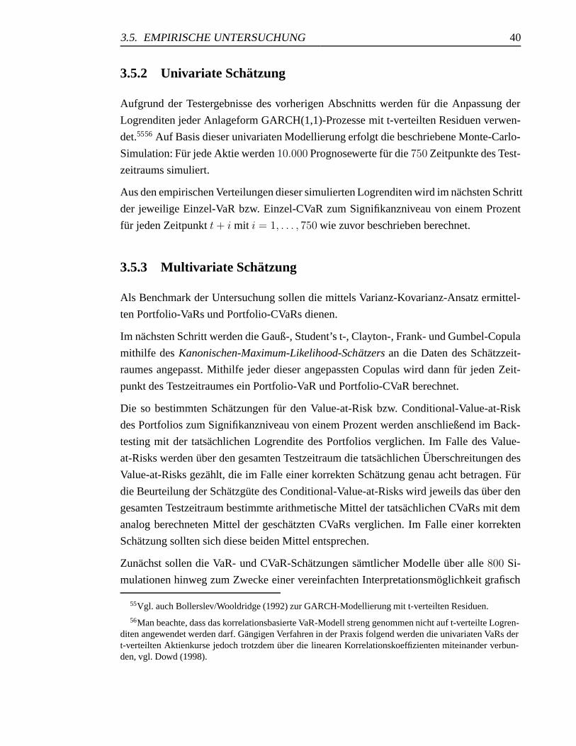
3.5. EMPIRISCHE UNTERSUCHUNG 40
3.5.2 Univariate Schatzung
Aufgrund der Testergebnisse des vorherigen Abschnitts werden fur die Anpassung der
Logrenditen jeder Anlageform GARCH(1,1)-Prozesse mit t-verteilten Residuen verwen-
det.5556 Auf Basis dieser univariaten Modellierung erfolgt die beschriebene Monte-Carlo-
Simulation: Fur jede Aktie werden 10.000 Prognosewerte fur die 750 Zeitpunkte des Test-
zeitraums simuliert.
Aus den empirischen Verteilungen dieser simulierten Logrenditen wird im nachsten Schritt
der jeweilige Einzel-VaR bzw. Einzel-CVaR zum Signifikanzniveau von einem Prozent
fur jeden Zeitpunkt t+ i mit i = 1, . . . , 750 wie zuvor beschrieben berechnet.
3.5.3 Multivariate Schatzung
Als Benchmark der Untersuchung sollen die mittels Varianz-Kovarianz-Ansatz ermittel-
ten Portfolio-VaRs und Portfolio-CVaRs dienen.
Im nachsten Schritt werden die Gauß-, Student’s t-, Clayton-, Frank- und Gumbel-Copula
mithilfe des Kanonischen-Maximum-Likelihood-Schatzers an die Daten des Schatzzeit-
raumes angepasst. Mithilfe jeder dieser angepassten Copulas wird dann fur jeden Zeit-
punkt des Testzeitraumes ein Portfolio-VaR und Portfolio-CVaR berechnet.
Die so bestimmten Schatzungen fur den Value-at-Risk bzw. Conditional-Value-at-Risk
des Portfolios zum Signifikanzniveau von einem Prozent werden anschließend im Back-
testing mit der tatsachlichen Logrendite des Portfolios verglichen. Im Falle des Value-
at-Risks werden uber den gesamten Testzeitraum die tatsachlichen Uberschreitungen des
Value-at-Risks gezahlt, die im Falle einer korrekten Schatzung genau acht betragen. Fur
die Beurteilung der Schatzgute des Conditional-Value-at-Risks wird jeweils das uber den
gesamten Testzeitraum bestimmte arithmetische Mittel der tatsachlichen CVaRs mit dem
analog berechneten Mittel der geschatzten CVaRs verglichen. Im Falle einer korrekten
Schatzung sollten sich diese beiden Mittel entsprechen.
Zunachst sollen die VaR- und CVaR-Schatzungen samtlicher Modelle uber alle 800 Si-
mulationen hinweg zum Zwecke einer vereinfachten Interpretationsmoglichkeit grafisch
55Vgl. auch Bollerslev/Wooldridge (1992) zur GARCH-Modellierung mit t-verteilten Residuen.
56Man beachte, dass das korrelationsbasierte VaR-Modell streng genommen nicht auf t-verteilte Logren-diten angewendet werden darf. Gangigen Verfahren in der Praxis folgend werden die univariaten VaRs dert-verteilten Aktienkurse jedoch trotzdem uber die linearen Korrelationskoeffizienten miteinander verbun-den, vgl. Dowd (1998).
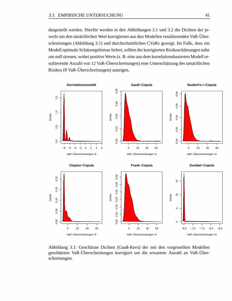
3.5. EMPIRISCHE UNTERSUCHUNG 41
dargestellt werden. Hierfur werden in den Abbildungen 3.1 und 3.2 die Dichten der je-
weils um den tatsachlichen Wert korrigierten aus den Modellen resultierenden VaR-Uber-
schreitungen (Abbildung 3.1) und durchschnittlichen CVaRs gezeigt. Im Falle, dass ein
Modell optimale Schatzergebnisse liefert, sollten die korrigierten Risikoschatzungen nahe
um null streuen, wobei positive Werte (z. B. eine aus dem korrelationsbasierten Modell re-
sultierende Anzahl von 12 VaR-Uberschreitungen) eine Unterschatzung des tatsachlichen
Risikos (8 VaR-Uberschreitungen) anzeigen.
−8 −6 −4 −2 0 2 4 6
0.0
0.5
1.0
1.5
Korrelationsmodell
VaR−Überschreitungen−8
Dic
hte
0 20 40 60
0.00
0.02
0.04
0.06
0.08
Gauß−Copula
VaR−Überschreitungen−8
Dic
hte
0 20 40 60
0.00
0.02
0.04
0.06
0.08
Student’s t−Copula
VaR−Überschreitungen−8
Dic
hte
0 20 40 60
0.00
0.05
0.10
0.15
0.20
Clayton−Copula
VaR−Überschreitungen−8
Dic
hte
0 20 40 60
0.00
0.01
0.02
0.03
0.04
0.05
0.06
Frank−Copula
VaR−Überschreitungen−8
Dic
hte
−8.0 −7.5 −7.0 −6.5 −6.0
05
1015
Gumbel−Copula
VaR−Überschreitungen−8
Dic
hte
Abbildung 3.1: Geschatzte Dichten (Gauß-Kern) der mit den vorgestellten Modellengeschatzten VaR-Uberschreitungen korrigiert um die erwartete Anzahl an VaR-Uber-schreitungen.
3.5. EMPIRISCHE UNTERSUCHUNG 42
−0.30 −0.20 −0.10 0.00
02
46
810
12
Korrelationsmodell
CVaR−tatsächlicher CVaR
Dic
hte
−0.10 −0.05 0.00 0.05
05
1015
20
Gauß−Copula
CVaR−tatsächlicher CVaR
Dic
hte
−0.10 −0.05 0.00 0.05
05
1015
Student’s t−Copula
CVaR−tatsächlicher CVaR
Dic
hte
−1.0 −0.6 −0.2 0.0
02
46
Clayton−Copula
CVaR−tatsächlicher CVaR
Dic
hte
−0.10 −0.05 0.00 0.05
05
1015
20Frank−Copula
CVaR−tatsächlicher CVaR
Dic
hte
−1.5 −1.0 −0.5 0.00.
00.
51.
01.
52.
02.
53.
03.
5
Gumbel−Copula
CVaR−tatsächlicher CVaR
Dic
hte
Abbildung 3.2: Geschatzte Dichten (Gauß-Kern) der mit den vorgestellten Modellengeschatzten durchschnittlichen CVaRs korrigiert um den tatsachlichen durchschnittlichenCVaR im Betrachtungszeitraum.
In Abbildung 3.1 ist zu erkennen, dass das korrelationsbasierte Modell sowie die Gumbel-
Copula das Risiko extrem uberschatzen und regelmaßig zu konservative VaRs ermitteln.
Die vier ubrigen parametrischen Copula-Modelle hingegen sind weniger konservativ in
ihrer Risikoschatzung. Die geschatzten Dichten zeigen jedoch auch, dass die pauscha-
le Verwendung einer einzelnen parametrischen Copula zwar in der Erwartung zu besse-
ren Ergebnissen fuhren kann als dies mit dem korrelationsbasierten Modell der Fall ist,
die große Streuung der Schatzungen jedoch fur einzelne Portfolios zu erheblichen Un-
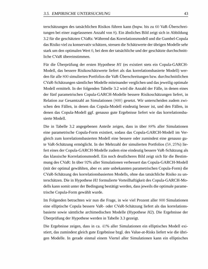
3.5. EMPIRISCHE UNTERSUCHUNG 43
terschatzungen des tatsachlichen Risikos fuhren kann (bspw. bis zu 60 VaR-Uberschrei-
tungen bei einer zugelassenen Anzahl von 8). Ein ahnliches Bild zeigt sich in Abbildung
3.2 fur die geschatzten CVaRs: Wahrend das Korrelationsmodell und die Gumbel-Copula
das Risiko viel zu konservativ schatzen, streuen die Schatzwerte der ubrigen Modelle sehr
stark um den optimalen Wert 0, bei dem der tatsachliche und der geschatzte durchschnitt-
liche CVaR ubereinstimmen.
Fur die Uberprufung der ersten Hypothese H1 (es existiert stets ein Copula-GARCH-
Modell, das bessere Risikoschatzwerte liefert als das korrelationsbasierte Modell) wer-
den fur alle 800 simulierten Portfolios die VaR-Uberschreitungen bzw. durchschnittlichen
CVaR-Schatzungen samtlicher Modelle miteinander verglichen und das jeweilig optimale
Modell ermittelt. In der folgenden Tabelle 3.2 wird die Anzahl der Falle, in denen eines
der funf parametrischen Copula-GARCH-Modelle bessere Risikoschatzungen liefert, in
Relation zur Gesamtzahl an Simulationen (800) gesetzt. Wir unterscheiden zudem zwi-
schen den Fallen, in denen das Copula-Modell eindeutig besser ist, und den Fallen, in
denen das Copula-Modell ggf. genauso gute Ergebnisse liefert wie das korrelationsba-
sierte Modell.
Die in Tabelle 3.2 angegebenen Anteile zeigen, dass in uber 88% aller Simulationen
eine parametrische Copula-Form existiert, sodass das Copula-GARCH-Modell im Ver-
gleich zum korrelationsbasierten Modell eine bessere oder zumindest eine genauso gu-
te VaR-Schatzung ermoglicht. In der Mehrzahl der simulierten Portfolios (58, 25%) lie-
fert eines der Copula-GARCH-Modelle zudem eine eindeutig bessere VaR-Schatzung als
das klassische Korrelationsmodell. Ein noch deutlicheres Bild zeigt sich fur die Bestim-
mung des CVaR: In uber 92% aller Simulationen verbessert das Copula-GARCH-Modell
(mit der optimal gewahlten, aber ex ante unbekannten parametrischen Copula-Form) die
CVaR-Schatzung des korrelationsbasierten Modells, ohne das tatsachliche Risiko zu un-
terschatzen. Die in Hypothese H1 formulierte Vorteilhaftigkeit des Copula-GARCH-Mo-
dells kann somit unter der Bedingung bestatigt werden, dass jeweils die optimale parame-
trische Copula-Form gewahlt wurde.
Im Folgenden betrachten wir nun die Frage, in wie viel Prozent aller 800 Simulationen
eine elliptische Copula bessere VaR- oder CVaR-Schatzung liefert als das korrelations-
basierte sowie samtliche archimedischen Modelle (Hypothese H2). Die Ergebnisse der
Uberprufung der Hypothese werden in Tabelle 3.3 gezeigt.
Die Ergebnisse zeigen, dass in ca. 41% aller Simulationen ein elliptisches Modell exi-
stiert, das zumindest gleich gute Ergebnisse bzgl. des Value-at-Risks liefert wie die ubri-
gen Modelle. In gerade einmal einem Viertel aller Simulationen kann ein elliptisches
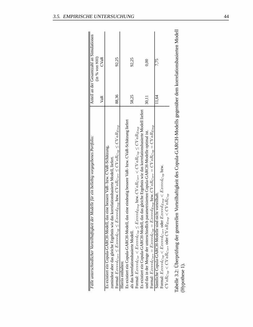
3.5. EMPIRISCHE UNTERSUCHUNG 44
Fal
leun
ters
chie
dlic
her
Vort
eilh
afti
gkei
tder
Mod
elle
fur
ein
beli
ebig
vorg
egeb
enes
Port
foli
o:A
ntei
lan
der
Ges
amtz
ahla
nSi
mul
atio
nen
(in
%vo
n80
0)V
aRC
VaR
Es
exis
tiert
ein
Cop
ula-
GA
RC
H-M
odel
l,da
sei
nebe
sser
eV
aR-
bzw
.CV
aR-S
chat
zung
,zu
min
dest
aber
das
glei
che
Erg
ebni
sw
ieda
sko
rrel
atio
nsba
sier
teM
odel
l,lie
fert
.Fo
rmal
:Exce
edC
orr≤
Exce
edC
op≤
Exce
edE
mp
bzw
.CV
aR
Corr≤
CV
aR
Cop≤
CV
aR
Em
p88
,36
92,2
5H
ieri
nen
thal
ten:
Es
exis
tiert
ein
Cop
ula-
GA
RC
H-M
odel
l,da
sei
neei
ndeu
tigbe
sser
eV
aR-
bzw
.CV
aR-S
chat
zung
liefe
rtal
sda
sko
rrel
atio
nsba
sier
teM
odel
l.58
,25
92,2
5Fo
rmal
:Exce
edC
or
<E
xce
edC
op≤
Exce
edE
mp
bzw
.CV
aR
Corr
<C
VaR
Cop≤
CV
aR
Em
p
Es
exis
tiert
ein
Cop
ula-
GA
RC
H-M
odel
l,da
sda
sgl
eich
eE
rgeb
nis
wie
das
korr
elat
ions
basi
erte
Mod
elll
iefe
rtun
dda
sin
der
Men
gede
run
ters
chie
dlic
hpa
ram
etri
sier
ten
Cop
ula-
GA
RC
H-M
odel
leop
timal
ist.
30,1
10,
00Fo
rmal
:Exce
edC
orr
=E
xce
edC
op
=E
xce
edE
mp
bzw
.CV
aR
Corr
=C
VaR
Cop
=C
VaR
Em
p
Sam
tlich
eC
opul
a-G
AR
CH
-Mod
elle
sind
nich
tvor
teilh
aft.
11,6
47,
75Fo
rmal
:Exce
edC
op
<E
xce
edC
orr
oder
Exce
edE
mp
<E
xce
edC
op
bzw
.C
VaR
Cop
<C
VaR
Corr
oder
CV
aR
Em
p<
CV
aR
Cop
Tabe
lle3.
2:U
berp
rufu
ngde
rge
nere
llen
Vor
teilh
aftig
keit
des
Cop
ula-
GA
RC
H-M
odel
lsge
genu
ber
dem
korr
elat
ions
basi
erte
nM
odel
l(H
ypot
hese
1).
3.5. EMPIRISCHE UNTERSUCHUNG 45
Fal
leun
ters
chie
dlic
her
Vort
eilh
afti
gkei
tder
elli
ptis
chen
Mod
elle
fur
ein
beli
ebig
vorg
egeb
enes
Port
foli
o:A
ntei
lan
der
Ges
amtz
ahla
nSi
mul
atio
nen
(in
%vo
n80
0)V
aRC
VaR
Es
exis
tiert
eine
ellip
tisch
eC
opul
a,so
dass
das
zuge
hori
geC
opul
a-G
AR
CH
-Mod
elle
ine
bess
ere
oder
glei
ch41
,50
0,25
gute
VaR
-bz
w.C
VaR
-Sch
atzu
nglie
fert
wie
das
korr
elat
ions
basi
erte
Mod
ellb
zw.d
asop
timal
ear
chim
edis
che
Cop
ula-
GA
RC
H-M
odel
l,oh
neje
doch
das
tats
achl
iche
Ris
iko
zuun
ters
chat
zen.
Es
exis
tiert
eine
ellip
tisch
eC
opul
a,so
dass
das
zuge
hori
geC
opul
a-G
AR
CH
-Mod
elle
ine
bess
ere
VaR
-bz
w.
26,2
50,
00C
VaR
-Sch
atzu
nglie
fert
als
das
korr
elat
ions
basi
erte
Mod
ell,
ggf.
aber
nur
eine
gena
uso
gute
Scha
tzun
gw
ieda
sop
timal
ear
chim
edis
che
Cop
ula-
GA
RC
H-M
odel
l,oh
neje
doch
das
tats
achl
iche
Ris
iko
zuun
ters
chat
zen.
Es
exis
tiert
eine
ellip
tisch
eC
opul
a,so
dass
das
zuge
hori
geC
opul
a-G
AR
CH
-Mod
elle
ine
bess
ere
VaR
-bz
w.
2,75
0,25
CV
aR-S
chat
zung
liefe
rtal
sda
sko
rrel
atio
nsba
sier
teM
odel
lund
das
optim
ale
arch
imed
isch
eC
opul
a-G
AR
CH
-Mod
ell,
ohne
jedo
chda
sta
tsac
hlic
heR
isik
ozu
unte
rsch
atze
n.
Tabe
lle3.
3:U
berp
rufu
ngde
rge
nere
llen
Vor
teilh
aftig
keit
der
ellip
tisch
enM
odel
lege
genu
ber
dem
korr
elat
ions
basi
erte
nso
wie
den
arch
imed
isch
enM
odel
len
(Hyp
othe
se2)
.

3.5. EMPIRISCHE UNTERSUCHUNG 46
Modell die VaR-Schatzung des korrelationsbasierten Modells verbessern, obwohl ein ar-
chimedisches Modell unter Umstanden eine gleichermaßen gute Schatzung liefert. Ver-
langen wir stattdessen, dass die elliptischen Modelle bessere VaR-Schatzungen als archi-
medische und korrelationsbasierte Modelle berechnen sollen, so erfolgt dies nur noch in
vernachlassigbaren 3% aller simulierten Portfolios. Betrachten wir die gleiche Fragestel-
lung vor dem Hintergrund der CVaR-Schatzungen, so sehen wir ein noch deutlicheres
Bild: Fur gerade einmal zwei der 800 simulierten Portfolios (0, 25%) kann mit einem
elliptischen Modell eine bessere oder gleich gute CVaR-Schatzung erfolgen als mit ei-
nem der ubrigen Modelle. Die unterstellte Vorteilhaftigkeit der elliptischen Copulas muss
daher abgelehnt werden. Zudem stellt sich heraus, dass die elliptischen Copulas nur im
Falle der VaR-Schatzung zumindest in fast jeder zweiten Simulation mit den ubrigen Mo-
dellen vergleichbare Ergebnisse erzielen. Fur die Bestimmung des CVaR erscheinen sie
hingegen als vollig ungeeignet.
Sollte ein elliptisches Modell vorteilhaft sein, so schließt sich die Frage an, welche der
beiden vorgestellten Copulas (Gauß- oder Student’s t-) fur die Risikoschatzung besser
geeignet ist.
Zur Klarung dieser Frage wurden die Simulationen, in denen ein elliptisches Copula-
GARCH-Modell eine wenigstens gleich gute Risikoschatzung wie die ubrigen Modelle
lieferte, weiter unterteilt. Tabelle 3.4 zeigt den Anteil der Falle, in denen entweder die
Gauß-, Student’s t- oder beide Copulas gleichzeitig die optimale VaR-Schatzung ergeben
haben (Hypothese H3).57
Die in Tabelle 3.4 gezeigten Ergebnisse zeigen wiederum ein deutliches Bild: In der Mehr-
zahl der Falle (73, 5%), in denen, neben anderen Modellen, auch ein elliptisches Modell
die beste VaR-Schatzung liefert, resultieren aus beiden Modellen dieselben Schatzergeb-
nisse. In den verbleibenden Fallen waren die Gauß- und Student’s t-Copula zu gleichen
Teilen optimal. Eine Vorteilhaftigkeit der Gauß- bzw. Student’s t-Copula kann somit nicht
festgestellt werden.
Die Ergebnisse in Tabelle 3.3 haben gezeigt, dass von einer generellen Vorteilhaftigkeit
der elliptischen Copulas nicht ausgegangen werden kann. Somit soll im nachsten Schritt
untersucht werden, welche parametrische Copula-Form uber alle 800 Simulationen gese-
hen die besten Risikoschatzungen leistet. Hierfur werden in Tabelle 3.5 die Anteile der
Falle, in denen ein vorgegebenes parametrisches Copula-GARCH-Modell das Risiko op-
57In beiden Simulationen, in denen eine elliptische Copula eine bessere oder gleich gute CVaR-Schatzungwie die ubrigen Modelle lieferte, war jeweils die Student’s t-Copula optimal. Aus diesem Grund wurde aufeine tabellarische Darstellung verzichtet.
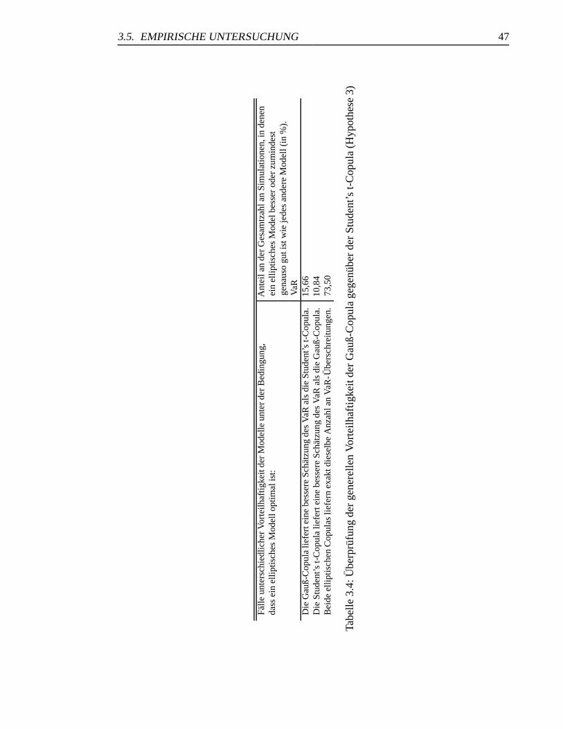
3.5. EMPIRISCHE UNTERSUCHUNG 47
Falle
unte
rsch
iedl
iche
rVor
teilh
aftig
keit
der
Mod
elle
unte
rde
rB
edin
gung
,A
ntei
lan
der
Ges
amtz
ahla
nSi
mul
atio
nen,
inde
nen
dass
ein
ellip
tisch
esM
odel
lopt
imal
ist:
ein
ellip
tisch
esM
odel
bess
erod
erzu
min
dest
gena
uso
guti
stw
ieje
des
ande
reM
odel
l(in
%).
VaR
Die
Gau
ß-C
opul
alie
fert
eine
bess
ere
Scha
tzun
gde
sV
aRal
sdi
eSt
uden
t’st-
Cop
ula.
15,6
6D
ieSt
uden
t’st-
Cop
ula
liefe
rtei
nebe
sser
eSc
hatz
ung
des
VaR
als
die
Gau
ß-C
opul
a.10
,84
Bei
deel
liptis
chen
Cop
ulas
liefe
rnex
aktd
iese
lbe
Anz
ahla
nV
aR-U
bers
chre
itung
en.
73,5
0
Tabe
lle3.
4:U
berp
rufu
ngde
rge
nere
llen
Vor
teilh
aftig
keit
der
Gau
ß-C
opul
age
genu
ber
der
Stud
ent’
st-
Cop
ula
(Hyp
othe
se3)
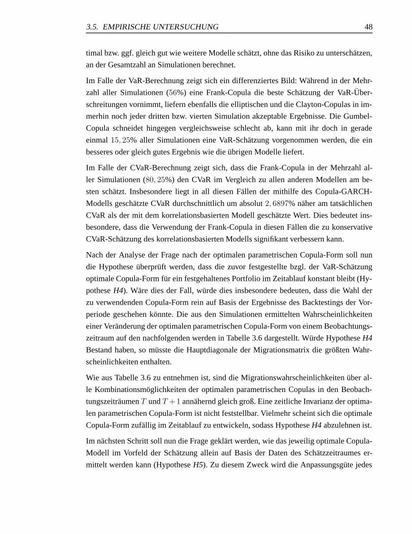
3.5. EMPIRISCHE UNTERSUCHUNG 48
timal bzw. ggf. gleich gut wie weitere Modelle schatzt, ohne das Risiko zu unterschatzen,
an der Gesamtzahl an Simulationen berechnet.
Im Falle der VaR-Berechnung zeigt sich ein differenziertes Bild: Wahrend in der Mehr-
zahl aller Simulationen (56%) eine Frank-Copula die beste Schatzung der VaR-Uber-
schreitungen vornimmt, liefern ebenfalls die elliptischen und die Clayton-Copulas in im-
merhin noch jeder dritten bzw. vierten Simulation akzeptable Ergebnisse. Die Gumbel-
Copula schneidet hingegen vergleichsweise schlecht ab, kann mit ihr doch in gerade
einmal 15, 25% aller Simulationen eine VaR-Schatzung vorgenommen werden, die ein
besseres oder gleich gutes Ergebnis wie die ubrigen Modelle liefert.
Im Falle der CVaR-Berechnung zeigt sich, dass die Frank-Copula in der Mehrzahl al-
ler Simulationen (80, 25%) den CVaR im Vergleich zu allen anderen Modellen am be-
sten schatzt. Insbesondere liegt in all diesen Fallen der mithilfe des Copula-GARCH-
Modells geschatzte CVaR durchschnittlich um absolut 2, 6897% naher am tatsachlichen
CVaR als der mit dem korrelationsbasierten Modell geschatzte Wert. Dies bedeutet ins-
besondere, dass die Verwendung der Frank-Copula in diesen Fallen die zu konservative
CVaR-Schatzung des korrelationsbasierten Modells signifikant verbessern kann.
Nach der Analyse der Frage nach der optimalen parametrischen Copula-Form soll nun
die Hypothese uberpruft werden, dass die zuvor festgestellte bzgl. der VaR-Schatzung
optimale Copula-Form fur ein festgehaltenes Portfolio im Zeitablauf konstant bleibt (Hy-
pothese H4). Ware dies der Fall, wurde dies insbesondere bedeuten, dass die Wahl der
zu verwendenden Copula-Form rein auf Basis der Ergebnisse des Backtestings der Vor-
periode geschehen konnte. Die aus den Simulationen ermittelten Wahrscheinlichkeiten
einer Veranderung der optimalen parametrischen Copula-Form von einem Beobachtungs-
zeitraum auf den nachfolgenden werden in Tabelle 3.6 dargestellt. Wurde Hypothese H4
Bestand haben, so musste die Hauptdiagonale der Migrationsmatrix die großten Wahr-
scheinlichkeiten enthalten.
Wie aus Tabelle 3.6 zu entnehmen ist, sind die Migrationswahrscheinlichkeiten uber al-
le Kombinationsmoglichkeiten der optimalen parametrischen Copulas in den Beobach-
tungszeitraumen T und T +1 annahernd gleich groß. Eine zeitliche Invarianz der optima-
len parametrischen Copula-Form ist nicht feststellbar. Vielmehr scheint sich die optimale
Copula-Form zufallig im Zeitablauf zu entwickeln, sodass Hypothese H4 abzulehnen ist.
Im nachsten Schritt soll nun die Frage geklart werden, wie das jeweilig optimale Copula-
Modell im Vorfeld der Schatzung allein auf Basis der Daten des Schatzzeitraumes er-
mittelt werden kann (Hypothese H5). Zu diesem Zweck wird die Anpassungsgute jedes
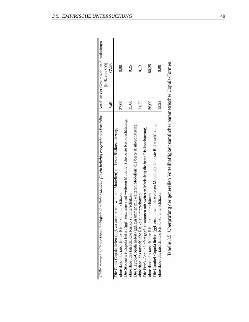
3.5. EMPIRISCHE UNTERSUCHUNG 49
Fal
leun
ters
chie
dlic
her
Vort
eilh
afti
gkei
tsam
tlic
her
Mod
elle
fur
ein
beli
ebig
vorg
egeb
enes
Port
foli
o:A
ntei
lan
der
Ges
amtz
ahla
nSi
mul
atio
nen
(in
%vo
n80
0)V
aRC
VaR
Die
Gau
ß-C
opul
alie
fert
(ggf
.zus
amm
enm
itw
eite
ren
Mod
elle
n)di
ebe
ste
Ris
ikos
chat
zung
,oh
neda
beid
asta
tsac
hlic
heR
isik
ozu
unte
rsch
atze
n.37
,00
0,00
Die
Stud
ent’s
t-C
opul
alie
fert
(ggf
.zus
amm
enm
itw
eite
ren
Mod
elle
n)di
ebe
ste
Ris
ikos
chat
zung
,oh
neda
beid
asta
tsac
hlic
heR
isik
ozu
unte
rsch
atze
n.35
,00
0,25
Die
Cla
yton
-Cop
ula
liefe
rt(g
gf.z
usam
men
mit
wei
tere
nM
odel
len)
die
best
eR
isik
osch
atzu
ng,
ohne
dabe
idas
tats
achl
iche
Ris
iko
zuun
ters
chat
zen.
21,2
50,
13D
ieFr
ank-
Cop
ula
liefe
rt(g
gf.z
usam
men
mit
wei
tere
nM
odel
len)
die
best
eR
isik
osch
atzu
ng,
ohne
dabe
idas
tats
achl
iche
Ris
iko
zuun
ters
chat
zen.
56,0
080
,25
Die
Gum
bel-
Cop
ula
liefe
rt(g
gf.z
usam
men
mit
wei
tere
nM
odel
len)
die
best
eR
isik
osch
atzu
ng,
ohne
dabe
idas
tats
achl
iche
Ris
iko
zuun
ters
chat
zen.
15,2
50,
00
Tabe
lle3.
5:U
berp
rufu
ngde
rge
nere
llen
Vor
teilh
aftig
keit
sam
tlich
erpa
ram
etri
sche
rC
opul
a-Fo
rmen
.
3.5. EMPIRISCHE UNTERSUCHUNG 50
Opt
imal
epa
ram
etri
sche
Cop
ula-
Form
imB
eoba
chtu
ngsf
enst
erT
+1
para
met
risc
heC
opul
a-Fo
rmG
auß
Stud
ent’s
tC
layt
onFr
ank
Gum
bel
kein
eO
ptim
ale
Gau
ß0,
0404
0934
0,04
0146
940,
0251
9024
0,05
4054
050,
0173
1829
0,00
9446
34pa
ram
etri
sche
Stud
ent’s
t0,
0372
6056
0,03
6735
760,
0228
2865
0,05
0642
880,
0157
4390
0,00
9708
73C
opul
a-Fo
rmC
layt
on0,
0317
5020
0,02
9913
410,
0204
6707
0,03
7522
960,
0141
6951
0,00
2886
38im
Fran
k0,
0535
2926
0,05
0905
270,
0307
0060
0,07
5570
720,
0212
5426
0,02
0467
07B
eoba
chtu
ngsf
enst
erG
umbe
l0,
0267
6463
0,02
5715
040,
0188
9268
0,03
1225
400,
0133
8231
0,00
0524
79T
,(T
=1,
...,
7)ke
ine
0,01
7580
690,
0170
5589
0,01
2070
320,
0296
5101
0,00
9971
130,
0485
4372
Tabe
lle3.
6:M
igra
tions
mat
rix
fur
die
Ver
ande
rung
der
optim
alen
para
met
risc
hen
Cop
ula-
Form
zwis
chen
zwei
aufe
inan
derf
olge
nden
Beo
bach
tung
sfen
ster
n.
3.5. EMPIRISCHE UNTERSUCHUNG 51
Copula-Modells mithilfe des zuvor beschriebenen, auf der empirischen Copula basieren-
den GoF-Tests beurteilt. Die fur alle Simulationen zusammengefassten Ergebnisse wer-
den in den Tabellen 3.7 und 3.8 gezeigt.
Die Ergebnisse zeigen ein erstaunlich schlechtes Bild: In lediglich 4, 48% (VaR-Schat-
zung) bzw. 0, 15% (CVaR-Schatzung) aller Simulationen, in denen mind. ein Copula-
Modell optimal ist, wird die optimale parametrische Copula-Familie als einzige vom
GoF-Test nicht abgelehnt. In weiteren 36, 47% (VaR-Schatzung) bzw. 10, 23% (CVaR-
Schatzung) werden weitere (suboptimale) Copula-Modelle ebenfalls nicht abgelehnt, so-
dass eine eindeutige Entscheidung nicht mehr moglich ist. Viel schwerwiegender ist je-
doch, dass das bzgl. der VaR-Schatzung optimale Copula-Modell in mehr als jedem zwei-
ten Fall, in dem mind. ein Copula-Modell optimal ist, vom GoF-Test abgelehnt wird und
somit eine falsche Wahl der parametrischen Copula-Familie empfohlen wird.
Zudem zeigt sich, dass der GoF-Test ausschließlich im Falle, dass eine elliptische Co-
pula das optimale Modell liefert, die richtige Entscheidung trifft. Wird die optimale VaR-
Schatzung dagegen durch die Frank- oder Clayton-Copula geliefert, so lehnt der GoF-Test
dieses Modell in fast allen Fallen falschlicherweise ab. Fur die Schatzung des CVaRs zeigt
sich ein noch deutlicheres Bild: Die in der Mehrzahl der Simulationen optimale Frank-
Copula wird fast jedes Mal zugunsten eines elliptischen Modells abgelehnt.
Somit kann in dieser Arbeit zum ersten Mal verlasslich gezeigt werden, dass ein Vertrauen
auf einen Copula-Anpassungstest in zahlreichen Fallen zu einer falschen Wahl der para-
metrischen Copula-Form und somit zu erheblichen Fehleinschatzungen des tatsachlichen
Risikos fuhren kann.
Die festgestellte Unzulanglichkeit des verwendeten Anpassungstests soll daher an die-
ser Stelle ausfuhrlicher diskutiert werden, stellt sie doch ein vollstandig kontrares Er-
gebnis zu den Befunden der bislang veroffentlichten Simulationsstudien von Genest/Re-
millard/Beaudoin und Berg zu Copula-GoF-Tests dar. In diesen wurde insbesondere fur
den in dieser Arbeit verwendeten Anpassungstest eine hohe Teststarke festgestellt, die
sich jedoch nicht in den VaR- bzw- CVaR-Schatzungen widerspiegelte. Ein Grund hierfur
mag sein, dass bisherige Arbeiten die Teststarke der Copula-Anpassungstests ausschließ-
lich auf Basis von Daten, die aus einer eindeutig vorgegebenen parametrischen Copu-
la simuliert wurden, getestet haben. Diese Laborbedingungen ungestorter Daten unter
einer klar definierten Abhangigkeitsstruktur konnten daher die Ergebnisse der Simula-
tionsstudien verzerrt haben. Ein weiterer Grund fur die gefundene Schwache der Test-
verfahren mag sein, dass samtliche bislang vorgeschlagenen Copula-GoF-Tests die Gute
der Anpassung auf Basis samtlicher Beobachtungswerte und somit auf Basis der ge-

3.5. EMPIRISCHE UNTERSUCHUNG 52
Test
ents
chei
dung
Ant
eila
nde
rG
esam
tzah
lan
Sim
ulat
ione
n,in
dene
nm
inde
sten
sei
nC
opul
a-(i
nP
roze
ntsa
mtl
iche
rSi
mul
atio
nen)
Mod
ellb
zgl.
der
VaR
-Sch
atzu
ngop
timal
ist(
in%
):G
auß
Stud
ent’s
tC
layt
onFr
ank
Gum
bel
Sum
me
Opt
imal
esM
odel
lwur
deal
sei
nzig
esdu
rch
GoF
-Tes
tnic
htab
gele
hnt
1,06
3,42
0,00
0,00
0,00
4,48
Opt
imal
esM
odel
lwur
dedu
rch
GoF
-Tes
tabg
eleh
nt.
5,02
2,13
12,6
930
,09
9,12
59,0
5O
ptim
ales
Mod
ellw
urde
zusa
mm
enm
itw
eite
ren
subo
ptim
alen
Mod
elle
ndu
rch
GoF
-Tes
tnic
htab
gele
hnt
16,4
115
,73
0,23
3,95
0,15
36,4
7
Tabe
lle3.
7:E
rgeb
niss
ede
rA
npas
sung
stes
tsfu
rdi
eV
aR-S
chat
zung
.
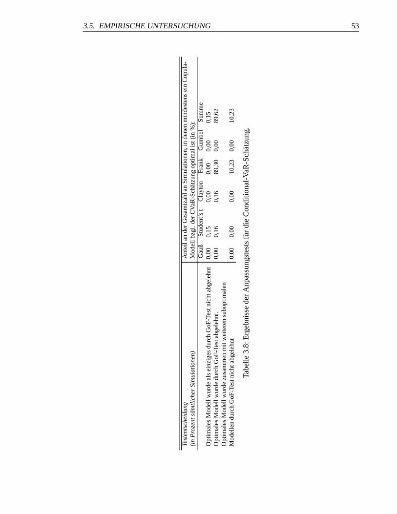
3.5. EMPIRISCHE UNTERSUCHUNG 53
Test
ents
chei
dung
Ant
eila
nde
rG
esam
tzah
lan
Sim
ulat
ione
n,in
dene
nm
inde
sten
sei
nC
opul
a-(i
nP
roze
ntsa
mtl
iche
rSi
mul
atio
nen)
Mod
ellb
zgl.
der
CV
aR-S
chat
zung
optim
alis
t(in
%):
Gau
ßSt
uden
t’st
Cla
yton
Fran
kG
umbe
lSu
mm
eO
ptim
ales
Mod
ellw
urde
als
einz
iges
durc
hG
oF-T
estn
icht
abge
lehn
t0,
000,
150,
000,
000,
000,
15O
ptim
ales
Mod
ellw
urde
durc
hG
oF-T
esta
bgel
ehnt
.0,
000,
160,
1689
,30
0,00
89,6
2O
ptim
ales
Mod
ellw
urde
zusa
mm
enm
itw
eite
ren
subo
ptim
alen
Mod
elle
ndu
rch
GoF
-Tes
tnic
htab
gele
hnt
0,00
0,00
0,00
10,2
30,
0010
,23
Tabe
lle3.
8:E
rgeb
niss
ede
rA
npas
sung
stes
tsfu
rdi
eC
ondi
tiona
l-V
aR-S
chat
zung
.
3.6. ZUSAMMENFASSUNG 54
samten gemeinsamen Verteilung beurteilen, die Risikoschatzung mithilfe des VaRs bzw.
CVaRs jedoch lediglich die Randbereiche der Verteilung betreffen. Somit sollten zukunf-
tige Arbeiten sich mit der Frage beschaftigen, wie insbesondere die Anpassungsgute ei-
nes Copula-Modells im fur die VaR-Bestimmung interessierenden Randbereich der ge-
meinsamen Verteilung beurteilt werden kann und wie ggf. existierende Anpassungstests
hierfur angepasst werden mussten. Im Zusammenhang mit den schlechten Ergebnissen
des Anpassungstests sei zusatzlich darauf hingewiesen, dass ein heuristisches Vorge-
hen zur Auswahl der parametrischen Copula (Verwendung einer einzigen parametrischen
Copula fur samtliche Portfolios oder aber Auswahl der parametrischen Form auf Basis
der Backtesting-Ergebnisse) aufgrund der Ergebnisse dieser Studie keinesfalls empfohlen
werden kann.
Schließlich soll die Hypothese untersucht werden, ob die zu den Hypothesen H1 bis H5
getroffenen Aussagen invariant gegenuber einer Veranderung des verwendeten Risikoma-
ßes sind (Hypothese H6). Die bisherigen Ergebnisse zeigen eindeutig, dass die Optima-
litat einzelner parametrischer Copulas stark vom gewahlten Risikomaß abhangt: Wahrend
bei der VaR-Schatzung sowohl mit elliptischen als auch archimedischen Copula-GARCH-
Modellen in jeder zweiten durchgefuhrten Simulation eine Verbesserung der Risikoschat-
zung erreicht werden konnte, fuhrte bei der CVaR-Bestimmung ausschließlich die Frank-
Copula in uber 80% aller Simulationen zu einer solchen Verbesserung. Die angesprochene
Tendenz des Anpassungstests, die archimedischen zugunsten der elliptischen Modelle ab-
zulehnen, fuhrte zudem zu einem besonders schlechten Abschneiden des Anpassungstests
beim CVaR-Backtesting. Zusammengefasst lasst sich somit sagen, dass die Vorteilhaftig-
keit bestimmter parametrischer Copulas und die Ergebnisse des Anpassungstests stark
von der Wahl des Risikomaßes abhangen und Hypothese H6 somit abzulehnen ist.
3.6 Zusammenfassung
Im Rahmen des vorliegenden Beitrags wurde zunachst der Aufbau eines Copula-GARCH-
Modells zur Schatzung des Gesamtrisikos eines Aktienportfolios erlautert. Anschließend
wurde der Value-at-Risk und Conditional-Value-at-Risk fur insgesamt 800 Portfolios, be-
stehend verschiedenen im DAX notierter Aktien, berechnet.
Die durchgefuhrten Simulationen zeigen, dass das vorgestellte Copula-GARCH-Modell
in fast jeder zweiten Simulation bessere VaR-Schatzungen und in fast 80% aller Simu-
lationen bessere CVaR-Schatzungen erzielen kann als ein traditionelles korrelationsba-
3.6. ZUSAMMENFASSUNG 55
siertes Modell, falls die parametrische Funktionalform der Copula richtig gewahlt wird.
Dieses erste zentrale Ergebnis ist zudem relativ robust gegenuber einer Veranderung des
Schatzzeitraumes. Im Gegensatz zu bisherigen Studien, in denen vergleichsweise wenige
Portfolios von Marktpreisrisiken betrachtet wurden, bestatigt die vorliegende Untersu-
chung die oftmals behauptete generell gultige Vorteilhaftigkeit elliptischer Copulas nicht.
Vielmehr erwies sich die archimedische Frank-Copula insbesondere fur die Schatzung
des CVaRs als bestes Modell. Die Vorteilhaftigkeit der verschiedenen Copula-Modelle
schwankte jedoch mit der Wahl des Risikomaßes und des Schatzzeitraumes, ein Phano-
men, das in keiner der genannten bisherigen Studien untersucht worden ist.
Neben der generellen Vorteilhaftigkeit des Copula-GARCH-Modells stand insbesondere
die Modellwahl im Fokus der empirischen Untersuchung. Der in diesem Beitrag verwen-
dete, auf der empirischen Copula basierende Anpassungstest erwies sich jedoch als ver-
gleichsweise schwach in seiner Fahigkeit zur Wahl des optimalen Modells. In fast allen
Fallen lieferte der GoF-Test entweder eine mehrdeutige oder eine falsche Empfehlung.
Dieses Ergebnis ist umso verbluffender, wenn man bedenkt, dass gerade dieser Teststatis-
tik in Simulationsstudien eine besondere Gute bescheinigt wurde. Fur praktische Zwecke
bedeutet dies, dass die Auswahl einer parametrischen Copula mit außerster Sorgfalt vor-
genommen werden sollte und das gewahlte Modell genauestens durch ein entsprechendes
Backtesting auf seine Tauglichkeit uberpruft werden sollte.
Insgesamt zeigt sich, dass das vorgestellte Copula-GARCH-Modell eine erhebliche Ver-
besserung gegenuber korrelationsbasierten Modellen zur Schatzung des Value-at-Risks
darstellt, sofern die parametrische Copula-Form ex ante richtig gewahlt wurde. Obwohl
pauschalisierte Aussagen uber die Optimalitat einzelner parametrischer Copulas fur die
VaR-Schatzung zu erheblichen Fehlern fuhren konnen, ist zumindest fur die Schatzung
des CVaRs die Verwendung der Frank-Copula nicht generell abzulehnen. Erheblicher For-
schungsbedarf besteht jedoch weiterhin hinsichtlich der Frage, wie das optimale Copula-
GARCH-Modell ex ante bestimmt werden kann und wie die bis dato vorgeschlagenen
Anpassungstests weiter verbessert werden konnen.
Kapitel 4
Copula Parameter Estimation -
Numerical Considerations And
Implications For Risk Management
Revise and resubmit:
Journal of Risk.
4.1 Introduction
Copula models have become a major tool in statistics for modeling and analysing depen-
dence structures between random variables due to fact that in contrast to linear correlation
a copula captures the complete dependence structure inherent in a set of random variables
(see Embrechts et al., 2002). Particularly in finance, copulas have attracted much attention
in the analysis of contagion between financial markets (see Rodriguez, 2007; Chen and
Poon, 2007), the analysis of risky portfolios of stocks (see e.g. Malevergne and Sornette,
2003; Junker and May, 2005) or the modeling of credit default (see Li, 2000). Copu-
la Parameter estimation in these studies is usually performed by a fully parametric (ML),
stepwise parametric (the so called inference function for margins or IFM method) or semi-
parametric maximum-likelihood approach depending on the information on the marginal
distributions. Kim et al. (2007) show in a recent simulation study that the semiparame-
tric pseudo-maximum-likelihood (PML) approach in which the marginal distributions are
substituted by their empirical counterparts with the copula parameters being subsequent-
ly estimated via maximum-likelihood is much better suited for parameter estimation than
the fully or stepwise parametric approach.
In contrast to the different ML-estimators, minimum-distance (MD) estimators for copu-
las have attracted only little attention. In one of the few papers, Biau and Wegkamp (2005)
derive an upper bound for the minimumL1-distance estimate for parametric copula densi-
56
4.1. INTRODUCTION 57
ties. Tsukahara (2005) explores the empirical asymptotic behaviour of Cramer-von-Mises
(CvM) and Kolmogorov-Smirnov (KS) distances between the hypothesised and empirical
copula in a simulation study. He finds that the PML-estimator should be preferred to the
MD-Kolmogorov-Smirnov estimator. His analysis, however, is only based on a sample si-
ze of 100 and three choices of parameters and does not include the Gaussian and Student’s
t copula which are of particular interest in finance. In a related paper, Mendes et al. (2007)
derive weighted minimum-distance estimators based on the empirical copula process. In
their simulation study they show that these MD-estimators are robust against contamina-
tions of the data. A common feature of these studies is, however, that they all consider
only MD-estimators based on the empirical copula process. Even more interestingly, the
question whether the use of a particular estimation method has any implications on the
computation of the Value-at-Risk (VaR) of a portfolio by the use of copulas has not been
addressed in literature.
The purpose of this paper is to present a comprehensive simulation study on the finite sam-
ple properties of minimum-distance and the pseudo-maximum-likelihood estimators for
bivariate and multivariate parametric copulas. For five popular parametric copulas, classi-
cal maximum-likelihood is compared to a total of nine different minimum-distance esti-
mators. In particular, I consider CvM-, KS- and L1-variants of the CvM-statistic based on
the empirical copula process, Kendall’s dependence function and Rosenblatt’s probability
integral transform. While the importance of copula selection and misspecification of the
copula (see e.g. Durrleman et al., 2000; Ane and Kharoubi, 2003) as well as goodness-of-
fit tests have been intensely discussed (see e.g. Fermanian, 2005; and Genest et al., 2009),
the finite sample properties especially of MD-estimators for copula parameters have not
been considered in detail in the literature.
Furthermore, the results on the finite sample properties of the ten different estimators are
extended by a second simulation study using real data. In this second simulation study, I
estimate the VaR and Expected Shortfall (ES) of 100 different portfolios using each of the
ten estimators. By comparing the resulting VaR- and ES-estimate, this paper is the first to
assess the practical relevance of the estimators’ numerical properties for the measurement
of portfolio risk with copulas. This analysis extends previous results from Gatfaoui (2005)
where an MD-estimator is applied to credit and market risks without any further analysis
of the numerical properties and applicability in high dimensions of the optimisation.
This paper is closely related to the works of Tsukahara (2005) and Mendes et al. (2007),
though I extend their simulation studies in a number of important ways: Firstly, the para-
metric copulas considered in this study include both elliptical and archimedean copulas in
4.2. COPULA PARAMETER ESTIMATION 58
order to cover a broader range of dependence structures. Secondly, I compare the estima-
tors’ performance for different sample sizes in order to assess their asymptotic empirical
properties. Thirdly and most importantly, in addition to the minimum-distance estimator
based on the empirical copula process which is used in Tsukahara (2005) and Genest et
al. (2009), I include further minimum-distance estimators based on Rosenblatt’s trans-
form and Kendall’s dependence function in my analysis. Furthermore, not only do I con-
sider Cramer-von-Mises- and Kolmogorov-Smirnov distances but also L1-variants of the
Cramer-von-Mises statistic (see Schmid and Trede, 1996, for a general description of this
L1-variant and Biau and Wegkamp, 2005).
The results presented in this paper show that in most settings pseudo-maximum-likelihood
yields smaller estimation biases at less computational effort than any of the MD-estimators.
There exist, however, some cases (especially when the sample size increases) where
minimum-distance estimators based on the empirical copula process are superior to the
PML-estimator. MD-estimators based on Kendall’s transform on the other hand yield only
suboptimal results in all configurations of the simulation study. The results of the simu-
lation study are confirmed by the empirical examples where the VaR as well as the ES
of 100 bivariate portfolios are computed. Interestingly, the estimates for these risk mea-
sures differed considerably depending on the choice of parameter estimator. This result
stresses the need for carefully choosing the parameter estimator in contrast to focusing all
attention on choosing the parametric copula model.
The remainder of this article is structured as follows. Section 2 discusses the different
parametric and nonparametric copulas, the parameter estimation procedures as well as the
numerical properties of these estimation techniques. A comprehensive simulation study
on the finite sample properties of the ten parameter estimators is given in section 3. Section
4 presents the results of the empirical application to 100 bivariate portfolios. Concluding
remarks are given in Section 5.
4.2 Copula parameter estimation
The purpose of this section is to shortly restate the basic definitions of the parametric
copulas used later on and to outline the different parameter estimation techniques. In
short, copulas allow for the coupling of marginal distributions to their joint distribution
by estimating the marginals and the dependence structure separately.
4.2. COPULA PARAMETER ESTIMATION 59
4.2.1 Parametric copulas
The mathematical basis for the analysis of copulas was founded by Sklar (1959) and
Hoeffding (1940). In the following, a basic definition of a copula and Sklar’s theorem are
described (for a more detailed description of copulas see Nelsen, 2006 or Joe, 1997).
Consider a random vector X ≡ (X1, . . . , Xd) of dimension d with a joint cumulative
distribution function (cdf) G and marginal cdfs F1, . . . , Fd. A d-dimensional copula is a
d-variate cumulative distribution function C : [0; 1]d → [0; 1] with uniformly distribu-
ted marginals (hereafter called d-copula). The central result in copula theory is Sklar’s
theorem which ensures the existence of a unique copula under relatively weak conditions:
Theorem 1 (Sklar):
Let G be a joint cumulative distribution function with d marginals F i. Then there exists a
d-dimensional Copula C such that for all x ∈ Rd,
G(x1, x2, ..., xd) = C(F1(x1), F2(x2), ..., Fd(xd)). (4.1)
If all marginals Fi are continuous, then the Copula C is unique.
Vice versa, if a d-Copula C and d cumulative distribution fuctions Fi are given then (4.1)
yields a d-variate cumulative distribution function with marginals F i.
Prominent examples of copulas are the ones inherent in multivariate Gaussian and Stu-
dent’s t-distributions. The Gaussian copula is given by the cdf
CΦd (u; Σ) = Φ
(d)Σ (Φ−1(u1), ...,Φ
−1(ud)) (4.2)
with u ≡ t(u1, u2, ..., ud) ∈ [0; 1]d. It can be obtained by applying the inversion me-
thod on a d-variate standard Gaussian distribution Φ(d) with correlation matrix Σ and d
univariate standard Gaussian distributions as marginals (see Nelsen, 2006). The Gaussian
copula is tail independent for imperfectly correlated marginals (see e.g. Sibuya, 1959; and
Resnick, 1987).
Similarly as the Gaussian copula can be derived from a multivariate Gaussian distribution,
the t-copula can be obtained from a (non-singular) n-dimensional Student’s t-distribution
Td(µ; Ω; ν) with density
f(x) =Γ(ν+d
2)
Γ(ν2)√
(πν)d|Ω|
(1 +
(x − µ)′Ω−1(x − µ)
ν
)−ν+d2
, (4.3)
4.2. COPULA PARAMETER ESTIMATION 60
ν degrees of freedom, mean vector µ and dispersion matrix Ω (note that the dispersion
matrix does not equal the covariance matrix in this case, see Demarta and McNeil, 2005).
As copulas are invariant under strictly increasing transformations of the marginals, we can
obtain the t-copula from the standardised d-dimensional t-distribution Td(0; Σ; ν) yielding
CTd (u; ν; Σ) =
∫ t−1ν (u1)
−∞...
∫ t−1ν (ud)
−∞
Γ(ν+d2
)
Γ(ν2)√
(πν)d|Σ|
(1 +
x′Σ−1x′
ν
)− ν+d2
dx, (4.4)
with t−1ν being the inverted cdf of a standard univariate Student’s t-distribution with ν
degrees of freedom. The t-copula is symmetrically tail dependent and converges to the
Gaussian copula for ν → ∞. This characteristic will be of particular interest in the simu-
lation study, where the different estimation techniques’ ability to distinguish between a
(true) Gaussian and a (hypothesised) Student’s t-copula will be analysed.
Another symmetrically tail independent copula that will be implemented in the simulation
study is the Frank copula given by
CFn (u; δ) = −1
δlog
(1 +
∏ni=1(exp(−δui) − 1)
(exp(−δ) − 1)n−1
), (4.5)
with parameter δ ∈ R+ (for some properties of the bivariate Frank copula see Genest,
1987).
The aforementioned copulas exhibit tail independence (Gaussian and Frank) and sym-
metric tail dependence (Student’s t), respectively. For the purpose of capturing different
patterns of tail dependence, the Gumbel copula which is asymmetrically tail dependent
(upper tail dependence and lower tail independence) shall be considered in the simulation
study as well. Its cdf is given by
CGd (u;λ) = exp
⎡⎣−( d∑i=1
−(log ui)λ
) 1λ
⎤⎦ , (4.6)
where the parameter λ satisfies λ ≥ 1.
The last parametric copula exhibiting lower tail dependence that will be considered in the
simulation study is the Clayton copula (sometimes also called the Cook-Johnson or Pareto
copula, see Genest and MacKay, 1986; and Balakrishnan and Lai, 1990). The Clayton
copula is given by
CCd (u; θ) = (u−θ1 + · · ·+ u−θ
d − d+ 1)−1/θ, (4.7)
4.2. COPULA PARAMETER ESTIMATION 61
with θ > 0 with the independence copula being the limiting case for θ → 0.
In the following, the ten different estimators for the copula parameters are discussed.
4.2.2 Parameter estimation via maximum-likelihood
The fully or stepwise parametric parameter estimations via maximum-likelihood require
a parametric approximation of the marginal distributions of X . As Kim et al. (2007) have
shown, these parametric estimation techniques are regularly outperformed by the pseudo-
maximum-likelihood estimator. The rest of the paper will thus concentrate on comparing
different estimators based on rank-transformed pseudo-observations obtained from the
original data sample.
Pseudo-maximum-likelihood (PML in the following) consists of transforming the origi-
nal data into pseudo-observations followed by classical maximum-likelihood estimation.
Consider a sample (Xij) of size n and dimension d (i = 1, . . . , n; j = 1, . . . , d). Using
the empirical cdfs Fj of the margins, the observations in the pseudo-sample U ≡ (Uij)
are given by (see McNeil et al., 2005)
Uij =n
n + 1Fj (Xij) (4.8)
The PML-estimate of the parameter vector θPMLn is then computed from the pseudo-
sample U of size n by numerically maximising
LU(θ) =n∑
i=1
log c(Ui,1, . . . , Ui,d|θ) (4.9)
with θ ∈ Θ ⊂ Rp (p ≥ 1) being the parameter vector of the respective multivariate
parametric copula C and c being the copula’s density parameterised by θ given by
c(u1, . . . , ud|θ) =∂C(u1, . . . , ud|θ)∂u1 · . . . · ∂ud
, u1, . . . , ud ∈ [0; 1]. (4.10)
The PML-estimator thus is given by
θPMLn (U) ≡ argmax
θ∈ΘLU(θ) (4.11)
Note that all parametric copulas discussed so far have densities and the densities of the
copulas which are given only implicitly (like e.g. the Gaussian copula) can be derived by
4.2. COPULA PARAMETER ESTIMATION 62
differentiating the joint cdf with the inverse marginal cdfs as its arguments.
The PML-estimator is consistent and asymptotically normal under some regularity con-
ditions (see Genest et al., 1995).
4.2.3 Minimum-distance estimators
In the following, the different minimum-distance estimators (and the closely related good-
ness-of-fit test statistics) will be presented. For ease of simplicity, I concentrate on the
bivariate case. The multivariate extensions are straightforward.
4.2.3.1 Minimum-distance estimators based on the empirical copula process
Most of the goodness-of-fit tests related to copulas that have been proposed recently are
based on a comparison between Deheuvels’ empirical and the hypothesised parametric
copula. The bivariate empirical copula estimated from an i.i.d. sample of size n is defined
on the lattice
L =
{(i1n,i2n
)∈ [0; 1]2
∣∣∣∣i1, i2 = 0, ..., n;
}. (4.12)
as
Cn(u) ≡ 1
n
n∑i=1
1(Ui,1 ≤ u1, Ui,2 ≤ u2, ), u ≡t (u1, u2) ∈ [0; 1]2 (4.13)
with 1(·) being a logical indicator function (see Genest et al., 2009).
Analogous to a histogram approximating a cdf, the empirical copula constitutes a discon-
tinuous approximation to the true underlying copula to which it converges uniformly (see
Deheuvels, 1978 and 1981). As pointed out by Genest et al. (2009), Deheuvels’ empirical
copula is arguably the most objective approximation to the true underlying copula as it is
completely nonparametric. Not surprisingly, goodness-of-fit tests that are based on com-
puting a distance between the empirical and the hypothesised copula have been shown
empirically to perform well in power studies (see Genest et al., 2009).
The first type of minimum-distance estimators that will be considered in this work is based
on the empirical process
Cn ≡√n(Cn − Cθ) (4.14)
where Cn is Deheuvels’ empirical copula and Cθ is the hypothesised copula from a pa-
rametric family parameterised by the parameter estimate θ obtained from the pseudo-
sample U. The process Cn is briefly mentioned in Fermanian (2005) and used in detail
4.2. COPULA PARAMETER ESTIMATION 63
by Tsukahara (2005), Mendes et al. (2007), Berg (2009) and Genest et al. (2009). Simple
Cramer-von-Mises and Kolmogorov-Smirnov statistics based on Cn are given by
ρCvMemp ≡
∫[0;1]2
Cn(u)2dCn(u) and ρKSemp ≡ sup
u∈[0;1]2|Cn(u)| . (4.15)
The empirical version of ρCvMemp is e.g. given by (see Genest et al., 2009)
ρCvMemp (U; θ) ≡
n∑i=1
{Cn(Ui) − Cθ(Ui)}2 (4.16)
with Ui being the i-th sample (similarly, an empirical approximation to ρKSemp can be deri-
ved).
In addition to the usual Cramer-von-Mises statistic ρCvMemp and the Kolmogorov-Smirnov
statistic ρKSemp, I consider the following L1-variant of the Cramer-von-Mises statistic
ρL1emp ≡
√n
∫[0;1]2
|Cn(u)|dCn(u). (4.17)
A general version of this statistic was proposed by Schmid and Trede (1996) for arbitrary
continuous cdfs. Note that similarly to the Cramer-von-Mises and Kolmogorov-Smirnov
statistic, the L1-variant ρL1emp is a continuous functional of the empirical process Cn. In the
simulation study, I consider the empirical approximation
ρL1emp(U; θ) =
n∑i=1
|Cn(Ui) − Cθ(Ui)| . (4.18)
The minimum distance estimators are then given by
θemp,L1n (U) ≡ argmin
θ∈ΘρL1
emp(U; θ), (4.19)
θemp,CvMn (U) ≡ argmin
θ∈ΘρCvM
emp (U; θ) and (4.20)
θemp,KSn (U) ≡ argmin
θ∈ΘρKS
emp(U; θ). (4.21)
The convergence of Cn under appropriate regularity conditions is established in Genest
and Remillard (2008).
4.2. COPULA PARAMETER ESTIMATION 64
4.2.3.2 Minimum-distance estimators based on Kendall’s dependence function
The second type of MD-estimators used in the simulation study was proposed in Savu
and Trede (2008) and Genest et al. (2006) and is based on Kendall’s probability integral
transform. The specific transform for an arbitrary random vector X with joint cdf G and
margins Fi (i ∈ Nd) is given by (see Genest et al., 2009)
X �→ V = G(X) = C(U1, . . . ,Ud), (4.22)
where the joint cdf of U = (U1, . . . ,Ud) is C and Ui = Fi(Xi). Let K be the cdf of
the probability integral transform V . Then a nonparametric estimation of K based on the
transformed sample Vi ≡ Cn(Ui) of size n is given by (see Genest and Rivest, 1993)
Kn(ω) ≡ 1
n
n∑i=1
1(Vi ≤ ω), ω ∈ [0; 1]. (4.23)
If U is distributed as Cθ, a parametric estimation of K is given by the distribution K θ of
the Kendall transform Cθ(U). Goodness-of-fit tests can then be based on the empirical
process
Kn ≡√n(Kn −Kθ). (4.24)
The specific test statistics are given by
ρL1K ≡
√n
∫ 1
0
|Kn(ω)| dKθ(ω), (4.25)
ρCvMK ≡
∫ 1
0
Kn(ω)2dKθ(ω) and (4.26)
ρKSK ≡ sup
ω∈[0;1]
|Kn(ω)| . (4.27)
Empirical versions of these statistics are given in Appendix B. The convergence of the
empirical process Kn underlying these estimators is established in Genest et al. (2006)
under appropriate regularity conditions.
4.2.3.3 Minimum-distance estimators based on Rosenblatt’s transform
The third type of MD-estimators is based on Rosenblatt’s probability integral transform
proposed by Rosenblatt (1952) which transforms a set of dependent variables into a set of
independent U([0; 1]) variables, given the multivariate distribution. For a given random
4.2. COPULA PARAMETER ESTIMATION 65
vector X ≡ (X1, X2) with marginal cdfs Fj(xj) (j ∈ {1; 2}) and conditional cdf F2|1,
Rosenblatt’s transform of X is defined by (see Berg, 2009) R(X) ≡ (R1(X1),R2(X2))
where
R1(X1) ≡ F1(x1),R2(X2) ≡ F2|1(x2|x1). (4.28)
As stated in Berg (2009), Rosenblatt’s transform can be used for multivariate GoF-tests
by applying it to a random sample assuming a parametric null hypothesis copula. As
the transformed sample V ≡ R(X) is i.i.d. U([0; 1])2, Genest et al. (2009) propose to
measure the distance between the empirical copula and the independence copula at each
element of the transformed matrix V which is dependent on the null hypothesis copula
Cθ. A Cramer-von-Mises statistic for this approach is then given by
ρCvMRos ≡ n
∫[0;1]2
{Cn(V) − C⊥(V)}2 dCn(V) (4.29)
with Vi being the i-th transformed sample from the copula. The specific test statistics are
given by
ρL1Ros ≡
√n
∫[0;1]2
|Cn(V) − C⊥(V)| dCn(V), (4.30)
ρCvMRos ≡ n
∫[0;1]2
{Cn(V) − C⊥(V)}2 dCn(V) and (4.31)
ρKSRos ≡ sup
u∈[0;1]2|Cn(V) − C⊥(V)| . (4.32)
An empirical version for the Cramer-von-Mises statistic is e.g. given by
ρCvMRos (V) =
n∑i=1
{Cn(Vi) − C⊥(Vi)}2 . (4.33)
Note that the distances depend indirectly on the parameter θ through Rosenblatt’s trans-
form. The asymptotic null behaviour of the underlying empirical process and the conver-
gence of the test statistics are established in Ghoudi and Remillard (2004) and Genest et
al. (2009).
4.2.4 Numerical properties of the copula parameter estimators
In the following, the numerical properties of both the PML- and the MD-estimators will
be analysed in more detail using the L-BFGS-B algorithm (see Byrd et al., 1995). The
4.2. COPULA PARAMETER ESTIMATION 66
BFGS (Broyden-Fletcher-Goldfarb-Shanno) algorithm, of which the L-BFGS-B method
is a variant for bounded parameters, is a quasi-Newton method which is particularly useful
for solving minimisation tasks for which the Hessian matrix of the objective function
cannot be efficiently computed. For convenience, a short description of the algorithm is
given in Appendix C.
The following analysis of the numerical complexity of both the PML- as well as the
MD-estimators will concentrate on the first step of the L-BFGS-B algorithm, i.e. the re-
presentation of the objective function f at the iterate Λk by the quadratic model
mk(θ) = f(θk) + gTk (θ − θk) +
1
2(θ − θk)
TBk(θ − θk) (4.34)
where either f(θ) := −LU(θ) or f(θ) being one of the nine error distances respectively.
The minimisation thus requires evaluations of the function itself as well as of the gradient
and Hessian of f . If numerical differentiation is used for approximating gk andBk, as it is
regularly the case in standard tools such as R or MATLAB, the speed of the optimisation
is controlled by the complexity of evaluating the objective function f . Consequently, we
will give a short comparison of the computational complexity of evaluating both the log-
likelihood- as well as the nine distance-functions described earlier.
From equation (4.9) we can see that evaluating the log-likelihood involves evaluating the
copula density at each pseudo-observation Ui, taking the logarithm and adding the n re-
sults. For the analysis of the minimum-distance estimators, we will concentrate on the
Cramer-von-Mises test statistic. Evaluating the CvM-distance based on the empirical co-
pula process first requires the evaluation of the copula itself and the empirical copula at
the pseudo-observations. In the second step, the distances are squared and summed up for
all n pseudo-observations. The evaluation of the distances based on the empirical copula
process in contrast to the log-likelihood function thus requires the additional evaluation
of the empirical copula (requiring 3n logical operations and n additions) for each of the
n pseudo-observations. As the remaining computations (squaring the distance and taking
the logarithm of either the copula distance or copula density) require approximately the
same computation time, the evaluation of the function ρCvMemp will take considerably lon-
ger than evaluating the log-likelihood function. We must therefore expect the minimum-
distance estimators based on the empirical copula process to require considerably more
computation time than the PML-estimator.
Next, we turn to the CvM-estimator based on Rosenblatt’s transform. In contrast to both
the PML-estimator and the MD-estimator based on the empirical copula process, the esti-
4.2. COPULA PARAMETER ESTIMATION 67
mators based on Rosenblatt’s transform first require the probability integral transform of
the pseudo-sample according to (4.28). This transform is specific to the chosen parame-
tric copula and general conclusions on its computational complexity are difficult. It can,
however, require a considerable number of additional computations like in the case of the
Gaussian copula e.g. where one first needs to evaluate the quantile function of the nor-
mal distribution at each pseudo-observation, find and invert the Cholesky decomposition
of the covariance matrix and finally compute a matrix product. After the pseudo-sample
has been transformed, the evaluation of ρCvMRos requires multiplying the observations in the
pseudo-sample (product copula) and evaluating the empirical copula at the transformed
pseudo-observations, followed by squaring and summing up the distances. In contrast to
the estimators based on the empirical copula process, evaluating ρCvMRos thus requires a pre-
vious transformation of the pseudo-sample but does not require the computationally more
demanding evaluation of a parametric copula but rather the evaluation of the simple pro-
duct copula. The computational complexity of the CvM-estimator based on Rosenblatt’s
transform thus depends on the question, how fast the copula-specific probability integral
transform can be achieved.
Finally, we turn to a brief analysis of the CvM-estimator based on Kendall’s transform.
From Appendix B we can see that just like for the MD-estimators based on Rosenblatt’s
transform, the evaluation of ρCvMK first requires the transformation of the original pseudo-
sample. This transformation includes samplingm times from the hypothesised parametric
copula Cθ,m2 logical operations,m2 additions andm divisions. The transformed pseudo-
observations are in turn used as inputs for evaluating the functionsKn andBm from (4.23)
and Appendix B in order to evaluate ρCvMK . In contrast to the two other minimum-distance
approaches, the n evaluations of the parametric copula are substituted by n evaluations of
the function Bm which require m logical operations. As m will usually be chosen to be
much larger than n, this computation will indubitably be more complex than the simple
computation of the copula itself. We can thus conclude that the evaluation of the function
ρCvMK will be the most computationally complex one.
In summary, one can expect the minimum-distance estimators to require more compu-
tation time than the pseudo-maximum-likelihood estimator. The use of one of the MD-
estimators could thus only be justified if their finite sample bias and MSE were lower
than those of the PML-estimator. The following simulation study aims at answering this
question.
4.3. SIMULATION STUDY 68
4.3 Simulation study
A large-scale simulation study was conducted to compare the PML-estimator to the nine
minimum-distance estimators described in the previous section and to assess the bias and
efficiency of the three approaches. The aim of this simulation study is to compute and
compare the bias, mean squared error (MSE) and relative efficiency of the ten estimators.
This goal is achieved by comparing the true parameter with the parameters estimated with
the above mentioned strategies under the premise that the parametric form of the copula
is chosen correctly.
4.3.1 Design of the simulation study
In the following, the design of the simulation study is outlined in detail. After the descrip-
tion of the simulation steps, the different choices of parameters are given.
We will consider bivariate and five-dimensional joint distributions which are build from
the same marginal models but with different copulas. More precisely, the marginals follow
a normal and a Student’s t distribution in the bivariate case. In the five-dimensional case,
four marginals follow a normal and one marginal follows a Student’s t distribution. The
data used in the simulations are drawn from the joint distribution of these marginals with
the copula being one of the five parametric copulas presented earlier.
For each bivariate and five-dimensional parametric copula family parameterised by the
randomly chosen (true) parameter vector θ repeat the following steps K times where K
is some large integer:
(1) Simulate a sample (Xij) of size n from the joint distribtuion with copula Cθ.
(2) Transform the sample (Xij) into a sample of n pseudo-observations (Uij).
(3) Compute the parameter estimates with the pseudo-maximum-likelihood and each of
the nine minimum-distance estimators.
(4) Compare the parameter estimates θ with the true parameter vector θ by computing the
bias and MSE for all estimators θl with l ∈ {1; . . . ; 10} and the efficiency r of each
MD-estimator θMDl′ with l′ ∈ {1; . . . ; 9} relative to the PML-estimator θPML given
by
(a) BIAS(θl) ≡ η − E(θl)
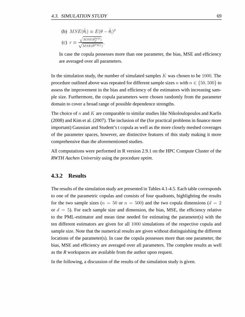
4.3. SIMULATION STUDY 69
(b) MSE(θl) ≡ E(θ − θl)2
(c) r ≡√
MSE(θMDl′ )√
MSE(θPML).
In case the copula possesses more than one parameter, the bias, MSE and efficiency
are averaged over all parameters.
In the simulation study, the number of simulated samples K was chosen to be 1000. The
procedure outlined above was repeated for different sample sizes n with n ∈ {50, 500} to
assess the improvement in the bias and efficiency of the estimators with increasing sam-
ple size. Furthermore, the copula parameters were chosen randomly from the parameter
domain to cover a broad range of possible dependence strengths.
The choice of n and K are comparable to similar studies like Nikoloulopoulos and Karlis
(2008) and Kim et al. (2007). The inclusion of the (for practical problems in finance more
important) Gaussian and Student’s t copula as well as the more closely meshed coverages
of the parameter spaces, however, are distinctive features of this study making it more
comprehensive than the aforementioned studies.
All computations were performed in R version 2.9.1 on the HPC Compute Cluster of the
RWTH Aachen University using the procedure optim.
4.3.2 Results
The results of the simulation study are presented in Tables 4.1-4.5. Each table corresponds
to one of the parametric copulas and consists of four quadrants, highlighting the results
for the two sample sizes (n = 50 or n = 500) and the two copula dimensions (d = 2
or d = 5). For each sample size and dimension, the bias, MSE, the efficiency relative
to the PML-estimator and mean time needed for estimating the parameter(s) with the
ten different estimators are given for all 1000 simulations of the respective copula and
sample size. Note that the numerical results are given without distinguishing the different
locations of the parameter(s). In case the copula possesses more than one parameter, the
bias, MSE and efficiency are averaged over all parameters. The complete results as well
as the R workspaces are available from the author upon request.
In the following, a discussion of the results of the simulation study is given.
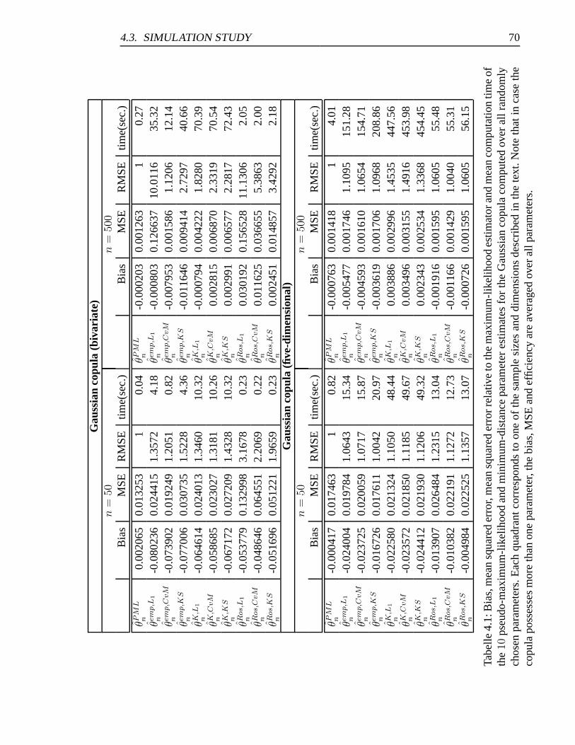
4.3. SIMULATION STUDY 70
Gau
ssia
nco
pula
(biv
aria
te)
n=
50n
=50
0B
ias
MSE
RM
SEtim
e(se
c.)
Bia
sM
SER
MSE
time(
sec.
)
θPM
Ln
0.00
2065
0.01
3253
10.
04θP
ML
n-0
.000
203
0.00
1263
10.
27θe
mp,L
1n
-0.0
8023
60.
0244
151.
3572
4.18
θem
p,L
1n
-0.0
0080
30.
1266
3710
.011
635
.32
θem
p,C
vM
n-0
.073
902
0.01
9249
1.20
510.
82θe
mp,C
vM
n-0
.007
953
0.00
1586
1.12
0612
.14
θem
p,K
Sn
-0.0
7700
60.
0307
351.
5228
4.36
θem
p,K
Sn
-0.0
1164
60.
0094
142.
7297
40.6
6θK
,L1
n-0
.064
614
0.02
4013
1.34
6010
.32
θK,L
1n
-0.0
0079
40.
0042
221.
8280
70.3
9θK
,CvM
n-0
.058
685
0.02
3027
1.31
8110
.26
θK,C
vM
n0.
0028
150.
0068
702.
3319
70.5
4θK
,KS
n-0
.067
172
0.02
7209
1.43
2810
.32
θK,K
Sn
0.00
2991
0.00
6577
2.28
1772
.43
θRos,
L1
n-0
.053
779
0.13
2998
3.16
780.
23θR
os,
L1
n0.
0301
920.
1565
2811
.130
62.
05θR
os,
CvM
n-0
.048
646
0.06
4551
2.20
690.
22θR
os,
CvM
n0.
0116
250.
0366
555.
3863
2.00
θRos,
KS
n-0
.051
696
0.05
1221
1.96
590.
23θR
os,
KS
n0.
0024
510.
0148
573.
4292
2.18
Gau
ssia
nco
pula
(five
-dim
ensi
onal
)n
=50
n=
500
Bia
sM
SER
MSE
time(
sec.
)B
ias
MSE
RM
SEtim
e(se
c.)
θPM
Ln
-0.0
0041
70.
0174
631
0.82
θPM
Ln
-0.0
0076
30.
0014
181
4.01
θem
p,L
1n
-0.0
2400
40.
0197
841.
0643
15.3
4θe
mp,L
1n
-0.0
0547
70.
0017
461.
1095
151.
28θe
mp,C
vM
n-0
.023
725
0.02
0059
1.07
1715
.87
θem
p,C
vM
n-0
.004
593
0.00
1610
1.06
5415
4.71
θem
p,K
Sn
-0.0
1672
60.
0176
111.
0042
20.9
7θe
mp,K
Sn
-0.0
0361
90.
0017
061.
0968
208.
86θK
,L1
n-0
.022
580
0.02
1324
1.10
5048
.44
θK,L
1n
0.00
3886
0.00
2996
1.45
3544
7.56
θK,C
vM
n-0
.023
572
0.02
1850
1.11
8549
.67
θK,C
vM
n0.
0034
960.
0031
551.
4916
453.
98θK
,KS
n-0
.024
412
0.02
1930
1.12
0649
.32
θK,K
Sn
0.00
2343
0.00
2534
1.33
6845
4.45
θRos,
L1
n-0
.013
907
0.02
6484
1.23
1513
.04
θRos,
L1
n-0
.001
916
0.00
1595
1.06
0555
.48
θRos,
CvM
n-0
.010
382
0.02
2191
1.12
7212
.73
θRos,
CvM
n-0
.001
166
0.00
1429
1.00
4055
.31
θRos,
KS
n-0
.004
984
0.02
2525
1.13
5713
.07
θRos,
KS
n-0
.000
726
0.00
1595
1.06
0556
.15
Tabe
lle4.
1:B
ias,
mea
nsq
uare
der
ror,
mea
nsq
uare
der
rorr
elat
ive
toth
em
axim
um-l
ikel
ihoo
des
timat
oran
dm
ean
com
puta
tion
time
ofth
e10
pseu
do-m
axim
um-l
ikel
ihoo
dan
dm
inim
um-d
ista
nce
para
met
eres
timat
esfo
rth
eG
auss
ian
copu
laco
mpu
ted
over
allr
ando
mly
chos
enpa
ram
eter
s.E
ach
quad
rant
corr
espo
nds
toon
eof
the
sam
ple
size
san
ddi
men
sion
sde
scri
bed
inth
ete
xt.N
ote
that
inca
seth
eco
pula
poss
esse
sm
ore
than
one
para
met
er,t
hebi
as,M
SEan
def
ficie
ncy
are
aver
aged
over
allp
aram
eter
s.
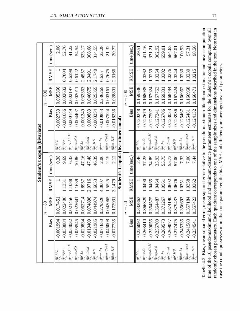
4.3. SIMULATION STUDY 71
Stud
ent’
st
copu
la(b
ivar
iate
)n
=50
n=
500
Bia
sM
SER
MSE
time(
sec.
)B
ias
MSE
RM
SEtim
e(se
c.)
θPM
Ln
-0.0
0199
40.
0174
511
0.38
θPM
Ln
-0.0
0273
30.
0053
661
2.06
θem
p,L
1n
-0.0
5308
40.
0224
061.
1331
9.69
θem
p,L
1n
-0.0
0168
60.
0026
320.
7004
52.7
6θe
mp,C
vM
n-0
.054
032
0.02
1456
1.10
886.
33θe
mp,C
vM
n0.
0001
490.
0021
970.
6398
41.2
2θe
mp,K
Sn
-0.0
5854
50.
0236
411.
1639
10.8
6θe
mp,K
Sn
-0.0
0440
70.
0020
110.
6122
54.5
4θK
,L1
n-0
.029
834
0.06
2714
1.89
5747
.16
θK,L
1n
0.00
1249
0.03
2363
2.45
5732
3.17
θK,C
vM
n-0
.019
409
0.07
4898
2.07
1647
.48
θK,C
vM
n0.
0008
830.
0466
752.
9491
308.
68θK
,KS
n-0
.021
985
0.04
4974
1.60
5346
.39
θK,K
Sn
-0.0
0325
40.
0253
652.
1740
314.
55θR
os,
L1
n-0
.071
650
0.27
9326
4.00
072.
00θR
os,
L1
n-0
.010
853
0.23
6265
6.63
5122
.28
θRos,
CvM
n-0
.046
008
0.04
2065
1.55
252.
19θR
os,
CvM
n-0
.007
524
0.00
3161
0.76
7521
.32
θRos,
KS
n-0
.077
735
0.17
2931
3.14
792.
12θR
os,
KS
n-0
.018
236
0.02
8801
2.31
6620
.77
Stud
ent’
st
copu
la(fi
ve-d
imen
sion
al)
n=
50n
=50
0B
ias
MSE
RM
SEtim
e(se
c.)
Bia
sM
SER
MSE
time(
sec.
)
θPM
Ln
-0.2
2609
20.
3328
631
2.46
θPM
Ln
-0.1
2024
80.
1595
361
29.5
1θe
mp,L
1n
-0.2
6341
00.
3663
291.
0490
37.2
5θe
mp,L
1n
-0.1
2767
90.
1680
351.
0262
411.
16θe
mp,C
vM
n-0
.259
055
0.36
4575
1.04
6534
.89
θem
p,C
vM
n-0
.127
507
0.16
7924
1.02
5937
1.21
θem
p,K
Sn
-0.2
5670
90.
3644
871.
0464
35.9
3θe
mp,K
Sn
-0.1
2724
10.
1677
631.
0254
362.
92θK
,L1
n-0
.269
573
0.37
1267
1.05
6155
.75
θK,L
1n
-0.1
2570
60.
1693
311.
0302
659.
01θK
,CvM
n-0
.269
077
0.37
4190
1.06
0255
.72
θK,C
vM
n-0
.123
033
0.16
8484
1.02
7668
4.63
θK,K
Sn
-0.2
7747
50.
3794
371.
0676
57.0
0θK
,KS
n-0
.123
936
0.16
7424
1.02
4466
7.01
θRos,
L1
n-0
.245
335
0.35
6693
1.03
517.
33θR
os,
L1
n-0
.125
467
0.16
6962
1.02
3010
0.93
θRos,
CvM
n-0
.241
583
0.35
7184
1.03
587.
00θR
os,
CvM
n-0
.125
481
0.16
6968
1.02
3097
.31
θRos,
KS
n-0
.234
541
0.35
7423
1.03
627.
44θR
os,
KS
n-0
.124
132
0.16
6471
1.02
1598
.56
Tabe
lle4.
2:B
ias,
mea
nsq
uare
der
ror,
mea
nsq
uare
der
rorr
elat
ive
toth
eps
eudo
-max
imum
-lik
elih
ood
estim
ator
and
mea
nco
mpu
tatio
ntim
eof
the
10ps
eudo
-max
imum
-lik
elih
ood
and
min
imum
-dis
tanc
epa
ram
eter
estim
ates
for
the
Stud
ent’
st
copu
laco
mpu
ted
over
all
rand
omly
chos
enpa
ram
eter
s.E
ach
quad
rant
corr
espo
nds
toon
eof
the
sam
ple
size
san
ddi
men
sion
sde
scri
bed
inth
ete
xt.N
ote
that
inca
seth
eco
pula
poss
esse
sm
ore
than
one
para
met
er,t
hebi
as,M
SEan
def
ficie
ncy
are
aver
aged
over
allp
aram
eter
s.
4.3. SIMULATION STUDY 72
Cla
yton
copu
la(b
ivar
iate
)n
=50
n=
500
Bia
sM
SER
MSE
time(
sec.
)B
ias
MSE
RM
SEtim
e(se
c.)
θPM
Ln
0.92
3577
8.41
1720
10.
04θP
ML
n0.
2967
760.
7719
011
0.26
θem
p,L
1n
-22.
3774
7015
53.7
8000
013
.591
01.
23θe
mp,L
1n
-0.4
0317
31.
3809
181.
3375
11.0
8θe
mp,C
vM
n-4
.534
741
105.
6870
003.
5446
0.59
θem
p,C
vM
n-0
.268
709
1.20
8205
1.25
103.
31θe
mp,K
Sn
-1.1
0237
720
.294
950
1.55
321.
58θe
mp,K
Sn
-0.0
0626
51.
5238
251.
4050
11.8
1θK
,L1
n-3
.012
496
60.9
5440
02.
6919
15.2
7θK
,L1
n-0
.857
327
4.70
3627
2.46
8594
.31
θK,C
vM
n-2
.581
299
57.0
1300
02.
6034
15.5
9θK
,CvM
n-0
.780
670
4.90
1487
2.51
9894
.31
θK,K
Sn
-17.
0406
7074
8.56
9000
9.43
3514
.80
θK,K
Sn
-1.5
4218
919
.922
020
5.08
0293
.40
θRos,
L1
n-1
.331
383
99.4
2015
03.
4379
0.26
θRos,
L1
n0.
1521
190.
8259
801.
0344
2.23
θRos,
CvM
n-0
.296
869
12.9
0081
01.
2384
0.23
θRos,
CvM
n0.
1105
900.
8153
311.
0277
2.22
θRos,
KS
n-4
.995
520
157.
5569
004.
3278
0.27
θRos,
KS
n-0
.237
261
1.55
7787
1.42
062.
41C
layt
onco
pula
(five
-dim
ensi
onal
)n
=50
n=
500
Bia
sM
SER
MSE
time(
sec.
)B
ias
MSE
RM
SEtim
e(se
c.)
θPM
Ln
3.08
0745
23.6
0684
01
0.03
θPM
Ln
0.92
3018
2.11
1276
10.
23θe
mp,L
1n
-6.7
9066
898
.357
500
2.04
110.
85θe
mp,L
1n
-0.4
5470
71.
8185
210.
9280
7.42
θem
p,C
vM
n-4
.983
714
64.1
9019
01.
6489
0.42
θem
p,C
vM
n-0
.362
635
1.65
3090
0.88
483.
32θe
mp,K
Sn
-2.3
2353
534
.373
170
1.20
660.
83θe
mp,K
Sn
-0.1
4946
12.
3719
951.
0599
6.73
θK,L
1n
10.6
1275
018
3.34
7400
2.78
6824
.83
θK,L
1n
10.6
9058
018
8.62
1800
9.45
1917
8.67
θK,C
vM
n10
.615
380
183.
5779
002.
7886
25.6
0θK
,CvM
n10
.710
520
189.
1282
009.
4646
181.
91θK
,KS
n10
.666
180
185.
0749
002.
7999
25.5
6θK
,KS
n10
.702
860
189.
5222
009.
4745
197.
40θR
os,
L1
n10
.958
160
191.
6652
002.
8493
0.91
θRos,
L1
n11
.206
850
196.
9287
009.
6578
7.08
θRos,
CvM
n10
.895
280
192.
1742
002.
8531
0.53
θRos,
CvM
n11
.199
530
196.
9871
009.
6593
6.54
θRos,
KS
n10
.926
080
197.
2087
002.
8903
0.55
θRos,
KS
n11
.198
510
198.
5637
009.
6978
7.57
Tabe
lle4.
3:B
ias,
mea
nsq
uare
der
ror,
mea
nsq
uare
der
rorr
elat
ive
toth
eps
eudo
-max
imum
-lik
elih
ood
estim
ator
and
mea
nco
mpu
tatio
ntim
eof
the
10m
axim
imum
-lik
elih
ood
and
min
imum
-dis
tanc
epa
ram
eter
estim
ates
fort
heC
layt
onco
pula
com
pute
dov
eral
lran
dom
lych
osen
para
met
ers.
Eac
hqu
adra
ntco
rres
pond
sto
one
ofth
esa
mpl
esi
zes
and
dim
ensi
ons
desc
ribe
din
the
text
.Not
eth
atin
case
the
copu
lapo
sses
ses
mor
eth
anon
epa
ram
eter
,the
bias
,MSE
and
effic
ienc
yar
eav
erag
edov
eral
lpar
amet
ers.
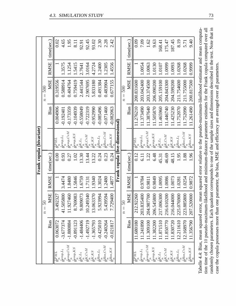
4.3. SIMULATION STUDY 73
Fra
nkco
pula
(biv
aria
te)
n=
50n
=50
0B
ias
MSE
RM
SEtim
e(se
c.)
Bia
sM
SER
MSE
time(
sec.
)
θPM
Ln
0.06
3072
3.49
2327
10.
00θP
ML
n0.
0049
060.
3195
561
0.02
θem
p,L
1n
-3.6
7737
441
.505
800
3.44
740.
93θe
mp,L
1n
-0.1
9240
10.
5889
141.
3575
4.65
θem
p,C
vM
n-1
.880
884
11.9
2746
01.
8480
0.27
θem
p,C
vM
n-0
.173
359
0.40
4764
1.12
541.
95θe
mp,K
Sn
-0.8
9112
38.
7690
831.
5846
1.02
θem
p,K
Sn
-0.1
0493
90.
7594
191.
5415
8.11
θK,L
1n
-1.4
8440
69.
8090
731.
6759
13.3
0θK
,L1
n-0
.558
049
2.44
1544
2.76
4192
.91
θK,C
vM
n-1
.492
719
10.2
4934
01.
7131
13.4
4θK
,CvM
n-0
.722
319
2.90
7695
3.01
6492
.45
θK,K
Sn
-1.3
6579
313
.063
370
1.93
4013
.22
θK,K
Sn
-0.9
5299
05.
8331
804.
2724
93.0
2θR
os,
L1
n-0
.425
010
5.92
3994
1.30
240.
24θR
os,
L1
n-0
.085
496
0.49
1384
1.24
002.
30θR
os,
CvM
n-0
.240
264
5.43
9594
1.24
800.
23θR
os,
CvM
n-0
.071
460
0.48
3904
1.23
052.
28θR
os,
KS
n-0
.021
817
7.72
9400
1.48
770.
24θR
os,
KS
n-0
.082
063
0.67
7155
1.45
562.
42F
rank
copu
la(fi
ve-d
imen
sion
al)
n=
50n
=50
0B
ias
MSE
RM
SEtim
e(se
c.)
Bia
sM
SER
MSE
time(
sec.
)
θPM
Ln
11.6
8018
021
2.92
260
10.
12θP
ML
n11
.276
210
200.
8316
001
0.09
θem
p,L
1n
11.2
4189
020
3.83
5400
0.97
846.
11θe
mp,L
1n
11.3
7349
020
3.04
2400
1.00
547.
09θe
mp,C
vM
n11
.309
100
204.
9877
000.
9811
1.22
θem
p,C
vM
n11
.387
640
203.
3745
001.
0063
1.62
θem
p,K
Sn
11.3
8220
020
6.54
5800
0.98
496.
48θe
mp,K
Sn
11.5
0587
020
6.09
0200
1.01
309.
63θK
,L1
n11
.871
510
217.
0063
001.
0095
45.3
1θK
,L1
n11
.465
960
205.
1591
001.
0107
168.
41θK
,CvM
n11
.850
770
216.
6102
001.
0086
46.6
9θK
,CvM
n11
.446
740
204.
8433
001.
0099
175.
47θK
,KS
n11
.830
720
216.
0440
001.
0073
48.1
5θK
,KS
n11
.425
230
204.
5992
001.
0093
187.
45θR
os,
L1
n12
.211
610
225.
0769
001.
0281
1.95
θRos,
L1
n11
.752
070
211.
7546
001.
0268
8.19
θRos,
CvM
n12
.168
970
223.
8858
001.
0254
1.88
θRos,
CvM
n11
.752
090
211.
7550
001.
0268
5.71
θRos,
KS
n11
.356
790
207.
5200
000.
9872
1.96
θRos,
KS
n11
.261
490
200.
8175
000.
9999
9.40
Tabe
lle4.
4:B
ias,
mea
nsq
uare
der
ror,
mea
nsq
uare
der
ror
rela
tive
toth
eps
eudo
-max
imum
-lik
elih
ood
estim
ator
and
mea
nco
mpu
ta-
tion
time
ofth
e10
pseu
do-m
axim
um-l
ikel
ihoo
dan
dm
inim
um-d
ista
nce
para
met
eres
timat
esfo
rth
eFr
ank
copu
laco
mpu
ted
over
all
rand
omly
chos
enpa
ram
eter
s.E
ach
quad
rant
corr
espo
nds
toon
eof
the
sam
ple
size
san
ddi
men
sion
sde
scri
bed
inth
ete
xt.N
ote
that
inca
seth
eco
pula
poss
esse
sm
ore
than
one
para
met
er,t
hebi
as,M
SEan
def
ficie
ncy
are
aver
aged
over
allp
aram
eter
s.
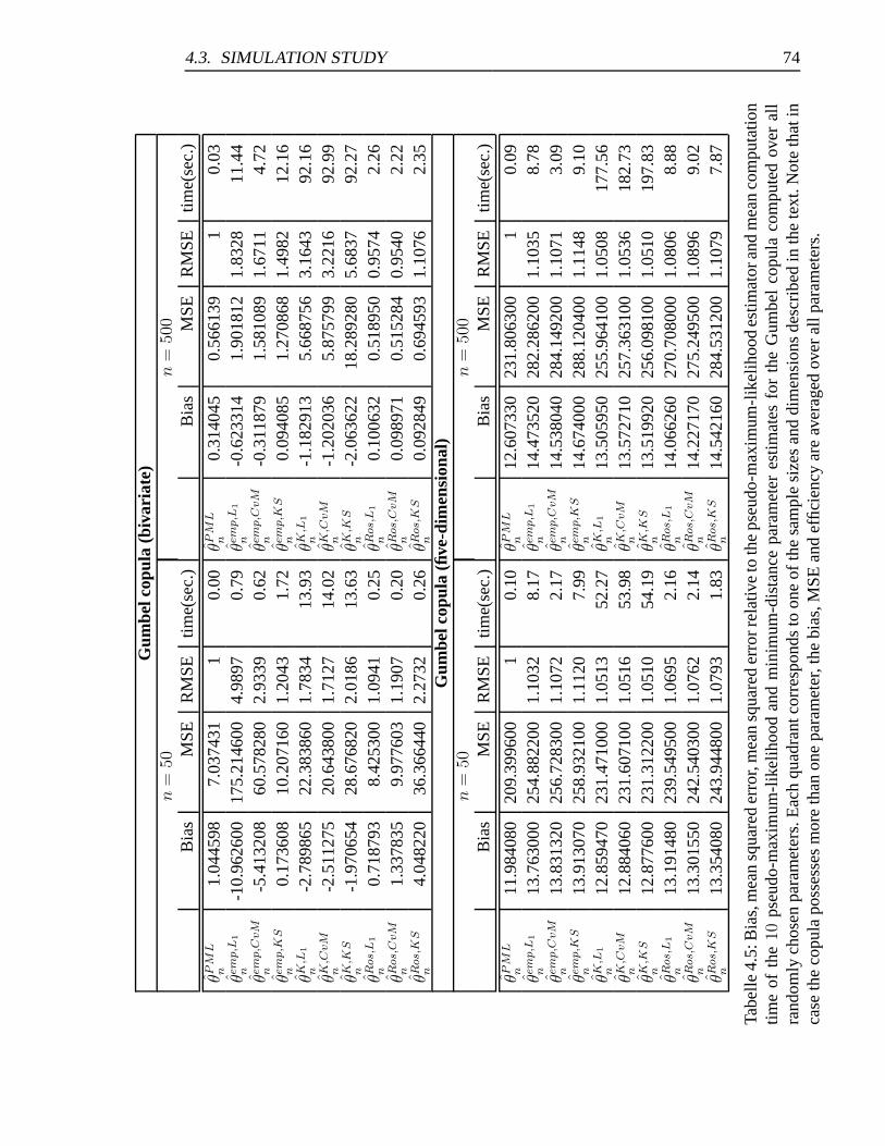
4.3. SIMULATION STUDY 74
Gum
belc
opul
a(b
ivar
iate
)n
=50
n=
500
Bia
sM
SER
MSE
time(
sec.
)B
ias
MSE
RM
SEtim
e(se
c.)
θPM
Ln
1.04
4598
7.03
7431
10.
00θP
ML
n0.
3140
450.
5661
391
0.03
θem
p,L
1n
-10.
9626
0017
5.21
4600
4.98
970.
79θe
mp,L
1n
-0.6
2331
41.
9018
121.
8328
11.4
4θe
mp,C
vM
n-5
.413
208
60.5
7828
02.
9339
0.62
θem
p,C
vM
n-0
.311
879
1.58
1089
1.67
114.
72θe
mp,K
Sn
0.17
3608
10.2
0716
01.
2043
1.72
θem
p,K
Sn
0.09
4085
1.27
0868
1.49
8212
.16
θK,L
1n
-2.7
8986
522
.383
860
1.78
3413
.93
θK,L
1n
-1.1
8291
35.
6687
563.
1643
92.1
6θK
,CvM
n-2
.511
275
20.6
4380
01.
7127
14.0
2θK
,CvM
n-1
.202
036
5.87
5799
3.22
1692
.99
θK,K
Sn
-1.9
7065
428
.676
820
2.01
8613
.63
θK,K
Sn
-2.0
6362
218
.289
280
5.68
3792
.27
θRos,
L1
n0.
7187
938.
4253
001.
0941
0.25
θRos,
L1
n0.
1006
320.
5189
500.
9574
2.26
θRos,
CvM
n1.
3378
359.
9776
031.
1907
0.20
θRos,
CvM
n0.
0989
710.
5152
840.
9540
2.22
θRos,
KS
n4.
0482
2036
.366
440
2.27
320.
26θR
os,
KS
n0.
0928
490.
6945
931.
1076
2.35
Gum
belc
opul
a(fi
ve-d
imen
sion
al)
n=
50n
=50
0B
ias
MSE
RM
SEtim
e(se
c.)
Bia
sM
SER
MSE
time(
sec.
)
θPM
Ln
11.9
8408
020
9.39
9600
10.
10θP
ML
n12
.607
330
231.
8063
001
0.09
θem
p,L
1n
13.7
6300
025
4.88
2200
1.10
328.
17θe
mp,L
1n
14.4
7352
028
2.28
6200
1.10
358.
78θe
mp,C
vM
n13
.831
320
256.
7283
001.
1072
2.17
θem
p,C
vM
n14
.538
040
284.
1492
001.
1071
3.09
θem
p,K
Sn
13.9
1307
025
8.93
2100
1.11
207.
99θe
mp,K
Sn
14.6
7400
028
8.12
0400
1.11
489.
10θK
,L1
n12
.859
470
231.
4710
001.
0513
52.2
7θK
,L1
n13
.505
950
255.
9641
001.
0508
177.
56θK
,CvM
n12
.884
060
231.
6071
001.
0516
53.9
8θK
,CvM
n13
.572
710
257.
3631
001.
0536
182.
73θK
,KS
n12
.877
600
231.
3122
001.
0510
54.1
9θK
,KS
n13
.519
920
256.
0981
001.
0510
197.
83θR
os,
L1
n13
.191
480
239.
5495
001.
0695
2.16
θRos,
L1
n14
.066
260
270.
7080
001.
0806
8.88
θRos,
CvM
n13
.301
550
242.
5403
001.
0762
2.14
θRos,
CvM
n14
.227
170
275.
2495
001.
0896
9.02
θRos,
KS
n13
.354
080
243.
9448
001.
0793
1.83
θRos,
KS
n14
.542
160
284.
5312
001.
1079
7.87
Tabe
lle4.
5:B
ias,
mea
nsq
uare
der
ror,
mea
nsq
uare
der
rorr
elat
ive
toth
eps
eudo
-max
imum
-lik
elih
ood
estim
ator
and
mea
nco
mpu
tatio
ntim
eof
the
10ps
eudo
-max
imum
-lik
elih
ood
and
min
imum
-dis
tanc
epa
ram
eter
estim
ates
for
the
Gum
bel
copu
laco
mpu
ted
over
all
rand
omly
chos
enpa
ram
eter
s.E
ach
quad
rant
corr
espo
nds
toon
eof
the
sam
ple
size
san
ddi
men
sion
sde
scri
bed
inth
ete
xt.N
ote
that
inca
seth
eco
pula
poss
esse
sm
ore
than
one
para
met
er,t
hebi
as,M
SEan
def
ficie
ncy
are
aver
aged
over
allp
aram
eter
s.
4.3. SIMULATION STUDY 75
4.3.2.1 Comparison of the mean bias and MSE
Interestingly, the results given in Tables 4.1-4.5 show a rather diverse picture of the diffe-
rent estimators’ finite sample properties. From Table 4.1 we can see that for the Gaussian
copula, the PML-estimator θPMLn yields the best results regardless of the sample size
or parametric copula. Even for the smallest sample size of n = 50, pseudo-maximum-
likelihood estimation produces estimates whose bias is smaller by a factor of 10 to 100
than the bias of the best minimum-distance estimator. Especially in the five-dimensional
case, however, the MD-estimators based on the empirical copula process seem to be able
to nearly match the PML-estimator’s results.
For the Student’s t copula, we can find similar results concerning the PML-estimator’s
empirical optimality over the MD-estimators with one exception: the results from Table
4.2 show that in the bivariate case for a sample size of n = 500, all three estimators based
on the empirical copula process yield better results than the remaining estimators.
The results for the Clayton copula also show an optimality of the estimators based on the
empirical copula process in the five-dimensional case with n = 500. In all other settings,
again the PML-estimator yields better results than any of the MD-estimators. However, in
contrast to the elliptical copulas where only small differences between the MD-estimators
existed, we can see from Table 4.3 that the estimators based on Kendall’s and Rosenblatt’s
transform yield extremely inaccurate results for the five-dimensional Clayton copula.
For the Frank copula, the results given in Table 4.4 show that all estimators yield extre-
mely inaccurate results in the five-dimensional case. In the bivariate case, results remain
extremely inaccurate for the small sample size (n = 50) and considerably improve for
n = 500. Though suboptimal in comparison to the PML-estimator in these cases, again
the estimators based on the empirical copula process but also the estimators based on
Rosenblatt’s transform yield the best results among MD-estimators.
Concerning the effect of the type of statistic on the estimation bias, one can see from
Tables 4.1-4.5 that on average there are no significant differences between the CvM-,
the KS and L1-statistic. Besides some minor differences, the selection of the empirical
process underlying the MD-estimator rather than the choice of statistic seems to be of
importance for an unbiased parameter estimation.
In summary, we can conclude that in general, pseudo-maximum-likelihood estimation
yields considerably more accurate parameter estimates than minimum-distance estimati-
on. There exist, however, some cases (especially when the sample size increases) where
minimum-distance estimators based on the empirical copula process are able to improve
4.3. SIMULATION STUDY 76
the parameter estimates given by the PML-estimator. MD-estimators based on Kendall’s
transform on the other hand yielded suboptimal results in all configurations of the si-
mulation study. In addition to these results, biases seem to be considerably higher for
archimedean copulas than for elliptical copulas.
4.3.2.2 Results concerning the sample size and dimensionality
The results given in Tables 4.1-4.5 show that, as predicted and required by the asymptotic
convergence of the different copula processes, parameter estimates in almost all settings
improve with increasing sample size. In addition to this, the decrease in bias is approxi-
mately linear. Moreover, while biases and MSE are relatively the same for the two- and
five-dimensional elliptical copulas, the parameter estimates for the archimedean copulas
become extremely inaccurate when the copula dimension increases. Another interesting
result is that with the exception of the Clayton copula, the differences in biases and MSE
between the ten estimators are reduced if the copula dimension is increased. The choice of
the estimator thus seems to be relatively unimportant when dealing with high-dimensional
copulas. As described earlier, however, overall accuracy of all estimators can only be re-
garded as poor in case the parameter of high-dimensional archimedean copulas needs to
be estimated.
One explanation for these poor results could be the fact that especially in the multivariate
setting, the optimisation algorithm is more likely to stop at a local optimum. The question
whether local optima can be improved was not addressed in the simulation study, as it
would have impaired the comparability of the results to previous studies in the literature.
4.3.2.3 Results concerning the computational complexity
Concerning the computational complexity of the ten estimators, the results from the si-
mulations given in Tables 4.1-4.5 confirm the theoretical analysis. In all configurations of
the simulation study, PML-estimation requires the least computation time while the esti-
mators based on Kendall’s transform are by far the slowest. Therefore it seems that the
estimators based on Kendall’s transform should not be used at all as they regularly yield
inaccurate estimates at the highest computational cost. Results for the MD-estimators ba-
sed on Rosenblatt’s transform and the empirical copula process are essentially the same
with the estimators based on Rosenblatt’s transform requiring less computation time espe-
cially for elliptical copulas. The optimality of these two minimum-distance approaches
thus is complemented by a much faster computation of the parameter estimates. At the
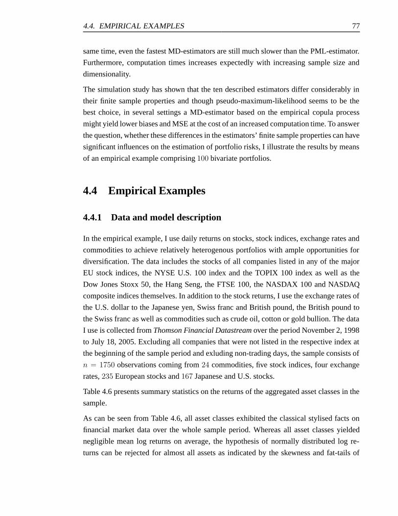
4.4. EMPIRICAL EXAMPLES 77
same time, even the fastest MD-estimators are still much slower than the PML-estimator.
Furthermore, computation times increases expectedly with increasing sample size and
dimensionality.
The simulation study has shown that the ten described estimators differ considerably in
their finite sample properties and though pseudo-maximum-likelihood seems to be the
best choice, in several settings a MD-estimator based on the empirical copula process
might yield lower biases and MSE at the cost of an increased computation time. To answer
the question, whether these differences in the estimators’ finite sample properties can have
significant influences on the estimation of portfolio risks, I illustrate the results by means
of an empirical example comprising 100 bivariate portfolios.
4.4 Empirical Examples
4.4.1 Data and model description
In the empirical example, I use daily returns on stocks, stock indices, exchange rates and
commodities to achieve relatively heterogenous portfolios with ample opportunities for
diversification. The data includes the stocks of all companies listed in any of the major
EU stock indices, the NYSE U.S. 100 index and the TOPIX 100 index as well as the
Dow Jones Stoxx 50, the Hang Seng, the FTSE 100, the NASDAX 100 and NASDAQ
composite indices themselves. In addition to the stock returns, I use the exchange rates of
the U.S. dollar to the Japanese yen, Swiss franc and British pound, the British pound to
the Swiss franc as well as commodities such as crude oil, cotton or gold bullion. The data
I use is collected from Thomson Financial Datastream over the period November 2, 1998
to July 18, 2005. Excluding all companies that were not listed in the respective index at
the beginning of the sample period and exluding non-trading days, the sample consists of
n = 1750 observations coming from 24 commodities, five stock indices, four exchange
rates, 235 European stocks and 167 Japanese and U.S. stocks.
Table 4.6 presents summary statistics on the returns of the aggregated asset classes in the
sample.
As can be seen from Table 4.6, all asset classes exhibited the classical stylised facts on
financial market data over the whole sample period. Whereas all asset classes yielded
negligible mean log returns on average, the hypothesis of normally distributed log re-
turns can be rejected for almost all assets as indicated by the skewness and fat-tails of
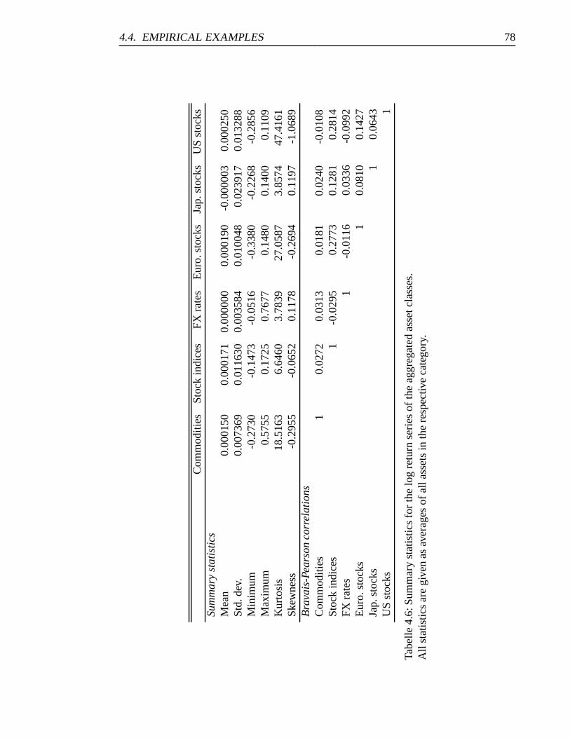
4.4. EMPIRICAL EXAMPLES 78
Com
mod
ities
Stoc
kin
dice
sFX
rate
sE
uro.
stoc
ksJa
p.st
ocks
US
stoc
ksSu
mm
ary
stat
isti
csM
ean
0.00
0150
0.00
0171
0.00
0000
0.00
0190
-0.0
0000
30.
0002
50St
d.de
v.0.
0073
690.
0116
300.
0035
840.
0100
480.
0239
170.
0132
88M
inim
um-0
.273
0-0
.147
3-0
.051
6-0
.338
0-0
.226
8-0
.285
6M
axim
um0.
5755
0.17
250.
7677
0.14
800.
1400
0.11
09K
urto
sis
18.5
163
6.64
603.
7839
27.0
587
3.85
7447
.416
1Sk
ewne
ss-0
.295
5-0
.065
20.
1178
-0.2
694
0.11
97-1
.068
9B
rava
is-P
ears
onco
rrel
atio
nsC
omm
oditi
es1
0.02
720.
0313
0.01
810.
0240
-0.0
108
Stoc
kin
dice
s1
-0.0
295
0.27
730.
1281
0.28
14FX
rate
s1
-0.0
116
0.03
36-0
.099
2E
uro.
stoc
ks1
0.08
100.
1427
Jap.
stoc
ks1
0.06
43U
Sst
ocks
1
Tabe
lle4.
6:Su
mm
ary
stat
istic
sfo
rth
elo
gre
turn
seri
esof
the
aggr
egat
edas
setc
lass
es.
All
stat
istic
sar
egi
ven
asav
erag
esof
alla
sset
sin
the
resp
ectiv
eca
tego
ry.
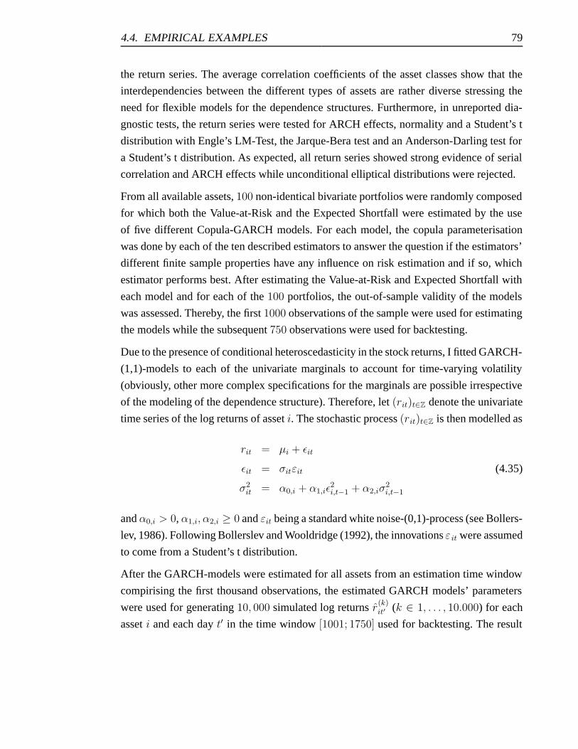
4.4. EMPIRICAL EXAMPLES 79
the return series. The average correlation coefficients of the asset classes show that the
interdependencies between the different types of assets are rather diverse stressing the
need for flexible models for the dependence structures. Furthermore, in unreported dia-
gnostic tests, the return series were tested for ARCH effects, normality and a Student’s t
distribution with Engle’s LM-Test, the Jarque-Bera test and an Anderson-Darling test for
a Student’s t distribution. As expected, all return series showed strong evidence of serial
correlation and ARCH effects while unconditional elliptical distributions were rejected.
From all available assets, 100 non-identical bivariate portfolios were randomly composed
for which both the Value-at-Risk and the Expected Shortfall were estimated by the use
of five different Copula-GARCH models. For each model, the copula parameterisation
was done by each of the ten described estimators to answer the question if the estimators’
different finite sample properties have any influence on risk estimation and if so, which
estimator performs best. After estimating the Value-at-Risk and Expected Shortfall with
each model and for each of the 100 portfolios, the out-of-sample validity of the models
was assessed. Thereby, the first 1000 observations of the sample were used for estimating
the models while the subsequent 750 observations were used for backtesting.
Due to the presence of conditional heteroscedasticity in the stock returns, I fitted GARCH-
(1,1)-models to each of the univariate marginals to account for time-varying volatility
(obviously, other more complex specifications for the marginals are possible irrespective
of the modeling of the dependence structure). Therefore, let (rit)t∈Z denote the univariate
time series of the log returns of asset i. The stochastic process (rit)t∈Z is then modelled as
rit = μi + εit
εit = σitεit (4.35)
σ2it = α0,i + α1,iε
2i,t−1 + α2,iσ
2i,t−1
and α0,i > 0, α1,i, α2,i ≥ 0 and εit being a standard white noise-(0,1)-process (see Bollers-
lev, 1986). Following Bollerslev and Wooldridge (1992), the innovations εit were assumed
to come from a Student’s t distribution.
After the GARCH-models were estimated for all assets from an estimation time window
compirising the first thousand observations, the estimated GARCH models’ parameters
were used for generating 10, 000 simulated log returns r(k)it′ (k ∈ 1, . . . , 10.000) for each
asset i and each day t′ in the time window [1001; 1750] used for backtesting. The result
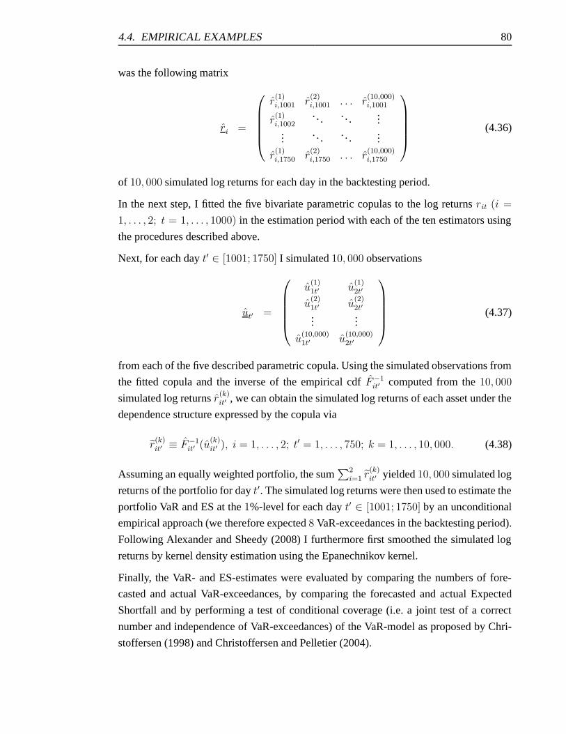
4.4. EMPIRICAL EXAMPLES 80
was the following matrix
ri =
⎛⎜⎜⎜⎜⎝r
(1)i,1001 r
(2)i,1001 . . . r
(10,000)i,1001
r(1)i,1002
. . . . . ....
.... . . . . .
...
r(1)i,1750 r
(2)i,1750 . . . r
(10,000)i,1750
⎞⎟⎟⎟⎟⎠ (4.36)
of 10, 000 simulated log returns for each day in the backtesting period.
In the next step, I fitted the five bivariate parametric copulas to the log returns rit (i =
1, . . . , 2; t = 1, . . . , 1000) in the estimation period with each of the ten estimators using
the procedures described above.
Next, for each day t′ ∈ [1001; 1750] I simulated 10, 000 observations
ut′ =
⎛⎜⎜⎜⎜⎝u
(1)1t′ u
(1)2t′
u(2)1t′ u
(2)2t′
......
u(10,000)1t′ u
(10,000)2t′
⎞⎟⎟⎟⎟⎠ (4.37)
from each of the five described parametric copula. Using the simulated observations from
the fitted copula and the inverse of the empirical cdf F−1it′ computed from the 10, 000
simulated log returns r(k)it′ , we can obtain the simulated log returns of each asset under the
dependence structure expressed by the copula via
r(k)it′ ≡ F−1
it′ (u(k)it′ ), i = 1, . . . , 2; t′ = 1, . . . , 750; k = 1, . . . , 10, 000. (4.38)
Assuming an equally weighted portfolio, the sum∑2
i=1 r(k)it′ yielded 10, 000 simulated log
returns of the portfolio for day t′. The simulated log returns were then used to estimate the
portfolio VaR and ES at the 1%-level for each day t′ ∈ [1001; 1750] by an unconditional
empirical approach (we therefore expected 8 VaR-exceedances in the backtesting period).
Following Alexander and Sheedy (2008) I furthermore first smoothed the simulated log
returns by kernel density estimation using the Epanechnikov kernel.
Finally, the VaR- and ES-estimates were evaluated by comparing the numbers of fore-
casted and actual VaR-exceedances, by comparing the forecasted and actual Expected
Shortfall and by performing a test of conditional coverage (i.e. a joint test of a correct
number and independence of VaR-exceedances) of the VaR-model as proposed by Chri-
stoffersen (1998) and Christoffersen and Pelletier (2004).
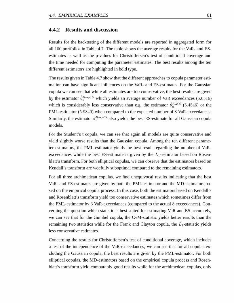
4.4. EMPIRICAL EXAMPLES 81
4.4.2 Results and discussion
Results for the backtesting of the different models are reported in aggregated form for
all 100 portfolios in Table 4.7. The table shows the average results for the VaR- and ES-
estimates as well as the p-values for Christoffersen’s test of conditional coverage and
the time needed for computing the parameter estimates. The best results among the ten
different estimators are highlighted in bold type.
The results given in Table 4.7 show that the different approaches to copula parameter esti-
mation can have significant influences on the VaR- and ES-estimates. For the Gaussian
copula we can see that while all estimates are too conservative, the best results are given
by the estimator θRos,KSn which yields an average number of VaR exceedances (6.6516)
which is considerably less conservative than e.g. the estimator θK,KSn (5.4546) or the
PML-estimator (5.9849) when compared to the expected number of 8 VaR-exceedances.
Similarly, the estimator θRos,KSn also yields the best ES-estimate for all Gaussian copula
models.
For the Student’s t copula, we can see that again all models are quite conservative and
yield slightly worse results than the Gaussian copula. Among the ten different parame-
ter estimators, the PML-estimator yields the best result regarding the number of VaR-
exceedances while the best ES-estimate is given by the L1-estimator based on Rosen-
blatt’s transform. For both elliptical copulas, we can observe that the estimators based on
Kendall’s transform are woefully suboptimal compared to the remaining estimators.
For all three archimedean copulas, we find unequivocal results indicating that the best
VaR- and ES-estimates are given by both the PML-estimator and the MD-estimators ba-
sed on the empirical copula process. In this case, both the estimators based on Kendall’s
and Rosenblatt’s transform yield too conservative estimates which sometimes differ from
the PML-estimator by 3 VaR-exceedances (compared to the actual 8 exceedances). Con-
cerning the question which statistic is best suited for estimating VaR and ES accurately,
we can see that for the Gumbel copula, the CvM-statistic yields better results than the
remaining two statistics while for the Frank and Clayton copula, the L1-statistic yields
less conservative estimates.
Concerning the results for Christoffersen’s test of conditional coverage, which includes
a test of the independence of the VaR-exceedances, we can see that for all copulas ex-
cluding the Gaussian copula, the best results are given by the PML-estimator. For both
elliptical copulas, the MD-estimators based on the empirical copula process and Rosen-
blatt’s transform yield comparably good results while for the archimedean copulas, only
4.4. EMPIRICAL EXAMPLES 82
Gau
ssia
nco
pula
θPM
Ln
θem
p,L
1n
θem
p,C
vM
nθe
mp,K
Sn
θK,L
1n
θK,C
vM
nθK
,KS
nθR
os,L
1n
θRos,C
vM
nθR
os,K
Sn
VaR
-Exc
eeda
nces
.−8
-2.0
151
-1.8
939
-2.0
909
-1.8
636
-2.3
484
-2.3
787
-2.5
454
-2.1
666
-1.8
939
-1.3
484
(VaR
-Exc
eeda
nces
.−8)
211
.530
311
.409
011
.696
910
.469
713
.075
713
.984
814
.848
412
.257
510
.954
512
.318
1E
S−
actu
alE
S-0
.006
6-0
.006
3-0
.005
8-0
.005
9-0
.009
1-0
.009
6-0
.009
2-0
.006
2-0
.005
7-0
.004
6(E
S−
actu
alE
S)2
0.00
0345
0.00
0341
0.00
0342
0.00
0323
0.00
0804
0.00
0780
0.00
0826
0.00
0359
0.00
0318
0.00
0354
p-V
alue
(con
d.co
v.)
0.47
130.
4452
0.48
570.
5076
0.45
480.
4251
0.42
040.
4351
0.47
780.
4992
Com
p.tim
e0.
5333
67.7
375
16.0
985
74.9
472
314.
9803
313.
6556
322.
7266
3.90
643.
8313
4.22
68St
uden
t’s
tcop
ula
VaR
-Exc
eeda
nces
.−8
-2-2
.409
0-2
.469
6-2
.378
7-2
.575
7-2
.575
7-2
.318
110
.787
8-2
.363
62.
5606
(VaR
-Exc
eeda
nces
.−8)
211
.606
013
.015
113
.075
713
.227
214
.242
413
.393
912
.287
821
21.1
210
13.0
606
1360
.591
0E
S−
actu
alE
S-0
.005
2-0
.006
1-0
.006
2-0
.007
5-0
.009
8-0
.010
0-0
.006
4-0
.003
1-0
.005
5-0
.005
3(E
S−
actu
alE
S)2
0.00
0361
0.00
0383
0.00
0374
0.00
0452
0.00
0811
0.00
0747
0.00
0362
0.00
0529
0.00
0412
0.00
0418
p-V
alue
(con
d.co
v.)
0.47
090.
4159
0.41
740.
4375
0.40
850.
4312
0.42
840.
4446
0.44
100.
4501
Com
p.tim
e6.
3174
152.
0993
83.2
855
146.
0027
1502
.757
015
14.9
680
1436
.845
045
.559
748
.133
442
.498
2C
layt
onco
pula
VaR
-Exc
eeda
nces
.−8
-3.5
151
-3.6
818
-3.7
424
-4.0
606
-5.0
909
-5.5
606
-6.2
727
-6.4
090
-6.4
696
-6.4
545
(VaR
-Exc
eeda
nces
.−8)
217
.666
619
.106
019
.500
020
.787
828
.757
534
.409
041
.333
342
.893
943
.348
443
.151
5E
S−
actu
alE
S-0
.009
2-0
.009
5-0
.010
4-0
.010
9-0
.016
3-0
.014
4-0
.013
1-0
.011
1-0
.013
5-0
.014
5(E
S−
actu
alE
S)2
0.00
0476
0.00
0481
0.00
0544
0.00
0517
0.00
1126
0.00
1320
0.00
1771
0.00
1904
0.00
1830
0.00
1819
p-V
alue
(con
d.co
v.)
0.32
440.
2948
0.27
160.
2761
0.16
210.
1047
0.08
070.
0738
0.05
680.
0601
Com
p.tim
e1.
4529
9.40
502.
9871
8.52
9842
9.02
1643
2.89
3242
1.80
352.
3479
1.49
022.
4118
Fra
nkco
pula
VaR
-Exc
eeda
nces
.−8
-2.2
272
-2.1
666
-2.1
515
-2.2
121
-2.7
424
-3.4
545
-3.3
939
-6.3
030
-6.2
575
-6.3
030
(VaR
-Exc
eeda
nces
.−8)
211
.651
510
.772
712
.606
011
.303
014
.015
117
.969
717
.090
941
.484
840
.803
041
.212
1E
S−
actu
alE
S-0
.005
7-0
.006
6-0
.006
7-0
.006
0-0
.007
5-0
.010
2-0
.010
2-0
.012
7-0
.012
5-0
.015
0(E
S−
actu
alE
S)2
0.00
0374
0.00
0337
0.00
0431
0.00
0357
0.00
0448
0.00
0519
0.00
0521
0.00
1746
0.00
1741
0.00
1723
p-V
alue
(con
d.co
v.)
0.45
760.
4408
0.44
890.
4428
0.38
800.
3143
0.29
500.
0628
0.07
520.
0621
Com
p.tim
e0.
1044
7.59
421.
3689
9.60
9242
5.50
7240
9.96
3741
6.59
382.
4845
2.56
152.
7010
Gum
belc
opul
aV
aR-E
xcee
danc
es.−
8-2
.196
9-2
.393
9-2
.136
3-2
.227
2-3
.727
2-2
.893
9-5
.651
5-6
.424
2-6
.393
9-6
.439
3(V
aR-E
xcee
danc
es.−
8)2
11.5
303
11.6
969
10.8
939
10.8
939
18.3
333
13.7
121
35.7
727
43.0
000
42.4
242
43.1
666
ES−
actu
alE
S-0
.006
1-0
.006
2-0
.004
1-0
.006
0-0
.010
5-0
.008
1-0
.013
5-0
.012
8-0
.014
3-0
.012
3(E
S−
actu
alE
S)2
0.00
0428
0.00
0389
0.00
0152
0.00
0360
0.00
0546
0.00
0426
0.00
1373
0.00
1813
0.00
1746
0.00
1916
p-V
alue
(con
d.co
v.)
0.47
180.
4354
0.45
100.
4587
0.28
430.
3880
0.12
940.
0618
0.06
040.
0607
Com
p.tim
e0.
1801
5.91
491.
7535
6.16
3242
8.71
6642
5.63
3241
5.08
763.
0495
2.72
542.
8873
Tabe
lle4.
7:R
esul
tsfo
rthe
VaR
and
ES-
estim
atio
nsav
erag
edov
eral
l100
biva
riat
epo
rtfo
lios.
The
tabl
egi
ves
the
mea
ndi
ffer
ence
san
dm
ean
squa
red
diff
eren
ces
betw
een
the
actu
alnu
mbe
rof
VaR
-exc
eeda
nces
atth
e1%
confi
denc
ele
vel(
i.e.8
)an
dth
ees
timat
ednu
mbe
rof
VaR
-exc
eeda
nces
,the
mea
ndi
ffer
ence
san
dm
ean
squa
red
diff
eren
ces
betw
een
the
estim
ated
and
the
actu
alE
xpec
ted
Shor
tfal
l,th
em
ean
p-va
lue
ofC
hris
toff
erse
n’s
test
asw
ella
sth
em
ean
com
puta
tion
time
inse
cond
sfo
ral
lpar
amet
ric
copu
las
and
estim
ator
s.
4.4. EMPIRICAL EXAMPLES 83
the former estimators should be used. Note that the extreme differences in the number of
VaR-exceedances between the ten estimators are also reflected in the large differences in
the average p-values e.g. for the Gumbel copula (0.4718 for the PML-estimator compared
to just 0.0604 for the estimator θRos,KSn ).
Finally, we can see from the average computation time that the PML-estimator again
requires only a negligible amount of time to estimate the parameters while the MD-
estimators based on Kendall’s transform are by far the computationally most demanding.
For the archimedean copulas, the MD-estimators based on the empirical copula process
and Rosenblatt’s transform are comparable to the PML-estimator concerning the compu-
tation time required for estimating the parameters.
In summary, we can see that most of the results obtained in the previous simulation study
also hold in our empirical examples: While the MD-estimators based on the empirical
copula process and Rosenblatt’s transform are usually able to match the PML-estimator’s
good results, they require much more time to compute the parameter estimates. The MD-
estimators based on Kendall’s transform should not be used as they require more time
than any other estimator and yield estimates that are woefully inaccurate. In case one we-
re inclined to use an achimedean copula model, the MD-estimator based on the empirical
copula process will yield slightly better VaR- and ES-estimates than the PML-estimator
but at the expense of an increasing computation time. Finally, it it interesting to note that
VaR- and ES-estimates can vary considerably ceteris paribus for the ten different estima-
tors which are all based on the use of pseudo-observations. This stresses the importance
of selecting the right parameter estimator for copulas regardless of how the parametric
form of the copula model is chosen.
A road not explored in this paper concerns the question whether the different MD-es-
timators are more robust to contaminations of the data sample than the PML-estimator.
Mendes et al. (2007) show that estimators based on the empirical copula process as well
as weighted maximum-likelihood estimators are more robust to contaminations of the da-
ta which are determined by an unknown distribution. Though not explicitly tested in this
paper, it remains questionable whether the MD-estimators’ robustness to data contamina-
tions would be able to change the general optimality of the PML-estimator found in this
paper. The main argument for this is that the data used in the empirical examples most
likely included data contaminations which are regularly found in financial market data.
Still, the MD-estimators’ finite sample properties did not change significantly compared
to the previous simulation study.
4.5. CONCLUSIONS 84
4.5 Conclusions
The purpose of this paper was to present a comprehensive simulation study on the fini-
te sample properties of minimum-distance and maximum-likelihood estimators for biva-
riate and multivariate parametric copulas. For five popular parametric copulas, pseudo-
maximum-likelihood was compared to a total of nine different minimum-distance estima-
tors based on GoF-tests used frequently in literature.
The central finding is that in general maximum-likelihood yields the best results concer-
ning bias, efficiency and computational complexity. Even for the smallest sample size of
n = 50 pseudo-maximum-likelihood estimation regularly produced estimates whose bias
was smaller by a factor of 10 to 100 than the bias of the best minimum-distance esti-
mator. There existed, however, some cases (especially when the sample size increases)
where minimum-distance estimators based on the empirical copula process were able to
improve the parameter estimates given by the PML-estimator. MD-estimators based on
Kendall’s transform on the other hand yielded suboptimal results in all configurations of
the simulation study.
Moreover, while the choice of the underlying distance is of high importance, the choice
of test statistic (L1, Cramer-von-Mises or Kolmogorov-Smirnov) seems to be more or less
irrelevant. Furthermore, results for the different kinds of parametric copula families were
mixed. Minimum-distance estimators seemed to produce better results for elliptical copu-
las in contrast to the appalling performance when used for estimating the parameters of
archimedean copulas. Additionally, while biases and MSE were relatively the same for the
two- and five-dimensional elliptical copulas, the parameter estimates for the archimedean
copulas became extremely inaccurate when the copula dimension increases.
The empirical examples presented in this paper showed that while the MD-estimators ba-
sed on the empirical copula process and Rosenblatt’s transform are usually able to match
the PML-estimator’s good results, they require much more time to compute the parameter
estimates. The MD-estimators based on Kendall’s transform should not be used as they
require more time than any other estimator and yield estimates that are woefully inaccu-
rate. For achimedean copulas the MD-estimator based on the empirical copula process
yielded slightly better VaR- and ES-estimates than the PML-estimator but at the expense
of an increasing computation time.
Kapitel 5
Bank Contagion
Veroffentlicht in:
Die Betriebswirtschaft, 69. Jg. (2009), S. 525-528.
5.1 Einfuhrung
Schaltersturme (bank runs), Bankenpaniken und die Risiken, die von diesen ausgehen,
spielen spatestens seit den zahlreichen Insolvenzen US-amerikanischer Banken in den
30er Jahren des vergangenen Jahrhunderts eine bedeutende Rolle in der Regulierung
und dem Risikomanagement von Banken. Schaltersturme bzw. Bankpaniken lassen sich
als Auspragungen einer besonderen Form sektoraler finanzwirtschaftlicher Ansteckungs-
effekte (bank contagion) auffassen, bei denen die Auswirkungen eines negativen Schocks
auf eine Bank uber verschiedene Ubertragungskanale auf andere Banken ubertragen wer-
den. Auf Grund der vielfaltigen Verflechtungen von Banken mit Industrieunternehmen
konnen Bankinsolvenzen und mogliche Ansteckungseffekte gravierende makrookono-
mische Folgen haben. Die Moglichkeit einer Bankenpanik wird daher oftmals als Be-
grundung fur ein rettendes Einschreiten der Zentralbank bzw. des Staates als lender of
last resort im Falle einer moglichen Insolvenz einer Bank gegeben.1 Ein aktuelles Bei-
spiel hierfur ist der Fall der auf Immobilienfinanzierung spezialisierten englischen Nor-
thern Rock sowie der US-amerikanischen Fannie Mae und Freddy Mac, die im Zuge der
aktuellen Finanzmarktkrise durch die britische bzw. US-amerikanische Regierung ver-
staatlicht wurden.
Ziel dieses Beitrages ist es, zunachst den Begriff der bank contagion zu definieren und die
Unterschiede zum verwandten Begriff der financial contagion aufzuzeigen. Zudem sollen
konkrete Unterformen der bank contagion wie z.B. dem Schaltersturm oder der Banken-
panik erlautert werden. Anschließend sollen die verschiedenen Ubertragungskanale einer
finanzwirtschaftlichen Ansteckung skizziert sowie die Auswirkungen der bank contagion
1Vgl. Corrigan (1991), S. 3.
85
5.2. DEFINITION DES BEGRIFFES BANK CONTAGION 86
dargestellt werden.
5.2 Definition des Begriffes bank contagion
Ausgangspunkt fur die Definition der bank contagion ist der Begriff der financial con-
tagion. Hierunter verstehen z.B. Forbes/Rigobon (2001) einen signifikanten Anstieg der
Abhangigkeit mehrerer Finanzmarkte untereinander, der durch einen Schock in einem
Markt ausgelost wurde, und der auf die ubrigen Markte uberspringt.2 Durch das Ab-
stellen auf Abhangigkeiten zwischen Finanzmarkten erreichen Forbes/Rigobon (2001),
dass Ansteckungseffekte mit Abhangigkeitskonzepten wie bspw. der linearen Korrelation
oder auch der sog. tail dependence operationalisiert werden konnen.3 Ahnlich wie For-
bes/Rigobon (2001) definiert Kaufman (1994) den Begriff der contagion, unter dem er
das Uberspringen von adversen Effekten, hervorgerufen durch einen Schock, von einem
Unternehmen auf andere Unternehmen versteht.4 Im speziellen Fall des Bankensystems
ist der auslosende Schock der bank contagion haufig die drohende Insolvenz einer ein-
zelnen Bank, durch die weitere Institute betroffen sein konnen. Ebenso konnen massive
Abschreibungen auf gehaltene Wertpapiere und Anlagen eines Instituts bzw. Gegenpar-
teirisiken wie z.B. im Falle der aktuellen Finanzmarktkrise einen Initialschock auslosen.
Schließlich konnen auch makrookonomische Schocks wie bspw. ein Konjunktur- bzw.
Zinsschock die Insolvenz eines Einzelinstituts verursachen. Bessler/Nohel (2000) defi-
nieren den Begriff der bank contagion dagegen noch allgemeiner, indem sie bereits die
Ausbreitung von Informationen von einer Bank zu anderen Banken als finanzwirtschaft-
liche Ansteckung auffassen.5
Uber verschiedene Kanale konnen die genannten adversen Effekte an weitere Kreditin-
stitute ubertragen werden. Der Oberbegriff der bank contagion, verstanden als ein Uber-
springen von adversen Effekten zwischen Banken, kann dahingehend differenziert wer-
den, ob es sich um ein rationales oder irrationales Verhalten der Marktteilnehmer handelt.
Im Falle der rationalen Ansteckung konnen die Marktteilnehmer die Auswirkungen des
2Vgl. Forbes/Rigobon (2001), S. 44.
3Unter der tail dependence versteht man die Abhangigkeit zweier oder mehrerer Zufallsvariablen inden extremen Bereichen ihrer Verteilung. Die tail dependence wird meistens mit dem Konzept der Copula-Funktion operationalisiert. Eine Untersuchung von Ansteckungseffekten mit dieser Methodik findet sichbei Rodriguez (2007).
4Vgl. Kaufman (1994), S. 123.
5Vgl. Bessler/Nohel (2000), S. 1832.
5.2. DEFINITION DES BEGRIFFES BANK CONTAGION 87
Schocks auf die originar betroffene Bank und die ubrigen Unternehmen korrekt beurteilen
und auf okonomisch gerechtfertigte Art und Weise reagieren. Die Reaktion der Marktteil-
nehmer auf einen solchen Schock, die auch als Informationseffekt bezeichnet wird, kann
verschiedene Formen annehmen. So erwahnen z.B. Bessler/Nohel (2000) die Neubewer-
tung der Aktien der betroffenen Bank als eine mogliche Reaktion.6 Außerdem kann ein
Schock in einem Bankensystem mit einer massiven Einlagenentnahme bei den betroffe-
nen Banken durch ihre Kunden einhergehen. Eine solche durch Fundamentaldaten einer
Bank begrundete Einlagenentnahme als Auspragungsform der bank contagion wird als
Schaltersturm bezeichnet.7
Im Gegensatz hierzu wird ein Ubergreifen der adversen Effekte auf samtliche Banken
ungeachtet der Frage, ob ein Institut auch tatsachlich von den adversen Effekten beruhrt
wird, als pure contagion bzw. Bankenpanik bezeichnet. Synonym kann eine Bankenpanik
als irrationaler Schaltersturm verstanden werden.8 Die Gefahr einer solchen Form der ir-
rationalen Ansteckung innerhalb eines Bankensystems wird auch als systemisches Risiko
bezeichnet.
In beiden Fallen kann die Entscheidung des einzelnen Anlegers zur Einlagenentnahme
jedoch individuell rational sein. Furchtet ein einzelner Anleger einen Schaltersturm, so
ware es fur ihn individuell rational, moglichst schnell seine Einlage zu entnehmen, bevor
die Bank zahlungsunfahig wird.9 Kollektiv ist eine solche Entscheidung jedoch irrational,
da die Anleger die externen Kosten ihrer Einlagenentnahme bspw. in Form von Fire Sale-
Verlusten und einer ggf. resultierenden Illiquiditat der Bank nicht berucksichtigen.
6Vgl. Ebd.
7Ein Schaltersturm kann offensichtlich bei einer einzelnen Bank oder aber gleichzeitig bei mehrerenBanken stattfinden. Die Zuordnung zum Oberbegriff der bank contagion kann daher durchaus kritisch gese-hen werden, da im ersten Fall keine Ansteckung zwischen Banken stattfindet. In weiten Teilen der Literaturwerden Schaltersturme nichtsdestotrotz als Form der bank contagion aufgefasst. Vgl. Diamond/Dybvig(1983) fur einen entsprechenden Gebrauch der beiden Begriffe.
8Vgl. Bhattacharya/Thakor (1993), S. 26.
9Die Frage, ob es rationale Grunde fur den Schaltersturm gibt, ist demnach fur die individuelle Ent-scheidung des Anlegers irrelevant.
5.3. UBERTRAGUNGSKANALE UND URSACHEN
FINANZWIRTSCHAFTLICHER KRISEN88
5.3 Ubertragungskanale und Ursachen finanzwirtschaft-
licher Krisen
Die in der Literatur genannten Theorien zur Erklarung der Existenz von Schaltersturmen
und Bankenpaniken stellen in der Regel auf den Interbankenmarkt als Ubertragungskanal
ab. Auf diesem konnen sowohl Liquiditats- als auch Kreditrisiken im engeren Sinne zu
Ansteckungseffekten zwischen den Banken fuhren.
Im ersten Fall ziehen Banken ihre Interbankenforderungen in Folge eines adversen Ef-
fekts bei anderen Banken ab und verursachen somit einen Liquiditatsschock. Auf Grund
einer asymmetrischen Informationsverteilung zwischen den einzelnen Banken kann die-
ses Zuruckfordern der (vergleichsweise liquiden) Forderungen auf dem Interbankenmarkt
rationaler oder irrationaler Natur sein. Im aktuellen Fall der Finanzmarktkrise stellt gerade
die Illiquiditat des Interbankenmarktes auf Grund des gegenseitigen Vertrauensverlustes
zwischen den Banken einen erheblichen Krisenverstarker dar.
Zur Vermeidung einer solchen Liquiditatskrise wird in der Literatur ein moglichst voll-
standiger Interbankenmarkt gefordert. Im Modell nach Allen/Gale (2000) sind die Aus-
wirkungen der adversen Effekte (und somit die Anfalligkeit des Bankenmarktes fur sy-
stemische Risiken) umso kleiner, je vollstandiger der Interbankenmarkt in dem Sinne ist,
dass eine Bank moglichst mit allen ubrigen Marktteilnehmern Transaktionen auf dem
Interbankenmarkt tatigt.10 Umgekehrt zeigen Freixas/Parigi/Rochet (2000), dass ein zen-
tralisierter Aufbau des Interbankenmarkts, in dem die Banken uberwiegend mit einer Zen-
tralbank, aber kaum untereinander Transaktionen durchfuhren, zu einer großeren Anfallig-
keit des Bankenmarktes fur systemische Risiken fuhren kann.11 Der intuitive Grund hierfur
ist der, dass ein Liquiditatsschock auf ein einzelnes Institut in einem solchen zentralisier-
ten Bankensystem nicht durch Transaktionen mit anderen Banken kompensiert werden
kann. Im Falle eines vollstandigen Interbankenmarktes konnte ein solcher Liquiditats-
schock hingegen auf die ubrigen Marktteilnehmer verteilt und somit abgeschwacht wer-
den.12
Stellt sich eine akute Illiquiditat des Interbankenmarktes ein, so konnen Zentralbank und
Regierung (wie zuletzt in der Finanzmarktkrise geschehen) versuchen, durch die Bereit-
stellung zusatzlicher Liquiditat einer Kreditklemme vorzubeugen.
10Vgl. Allen/Gale (2000).
11Vgl. Freixas/Parigi/Rochet (2000).
12Vgl. Gropp/Lo Duca/Vesala (2006), S. 8.
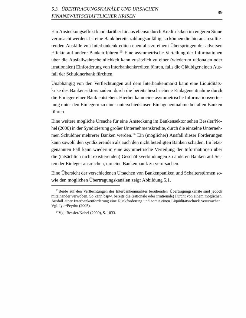
5.3. UBERTRAGUNGSKANALE UND URSACHEN
FINANZWIRTSCHAFTLICHER KRISEN89
Ein Ansteckungseffekt kann daruber hinaus ebenso durch Kreditrisiken im engeren Sinne
verursacht werden. Ist eine Bank bereits zahlungsunfahig, so konnen die hieraus resultie-
renden Ausfalle von Interbankenkrediten ebenfalls zu einem Uberspringen der adversen
Effekte auf andere Banken fuhren.13 Eine asymmetrische Verteilung der Informationen
uber die Ausfallwahrscheinlichkeit kann zusatzlich zu einer (wiederum rationalen oder
irrationalen) Einforderung von Interbankenkrediten fuhren, falls die Glaubiger einen Aus-
fall der Schuldnerbank furchten.
Unabhangig von den Verflechtungen auf dem Interbankenmarkt kann eine Liquiditats-
krise des Bankensektors zudem durch die bereits beschriebene Einlagenentnahme durch
die Einleger einer Bank entstehen. Hierbei kann eine asymmetrische Informationsvertei-
lung unter den Einlegern zu einer unterschiedslosen Einlagenentnahme bei allen Banken
fuhren.
Eine weitere mogliche Ursache fur eine Ansteckung im Bankensektor sehen Bessler/No-
hel (2000) in der Syndizierung großer Unternehmenskredite, durch die einzelne Unterneh-
men Schuldner mehrerer Banken werden.14 Ein (moglicher) Ausfall dieser Forderungen
kann sowohl den syndizierenden als auch den nicht beteiligten Banken schaden. Im letzt-
genannten Fall kann wiederum eine asymmetrische Verteilung der Informationen uber
die (tatsachlich nicht existierenden) Geschaftsverbindungen zu anderen Banken auf Sei-
ten der Einleger ausreichen, um eine Bankenpanik zu verursachen.
Eine Ubersicht der verschiedenen Ursachen von Bankenpaniken und Schaltersturmen so-
wie den moglichen Ubertragungskanalen zeigt Abbildung 5.1.
13Beide auf den Verflechtungen des Interbankenmarktes beruhenden Ubertragungskanale sind jedochmiteinander verwoben. So kann bspw. bereits die (rationale oder irrationale) Furcht von einem moglichenAusfall einer Interbankenforderung eine Ruckforderung und somit einen Liquiditatsschock verursachen.Vgl. Iyer/Peydro (2005).
14Vgl. Bessler/Nohel (2000), S. 1833.
5.3. UBERTRAGUNGSKANALE UND URSACHEN
FINANZWIRTSCHAFTLICHER KRISEN90
Kreditschocksz.B. Ausfall eines
Großkreditnehmers
Preisänderungsschocks z.B. Zinsänderungsschock
Konjunkturschock Liquiditätsschock
Einzelbank
Mögliche Insolvenz dieser Einzelbank
Übrige, realiter betroffene Banken Übrige, realiter nicht betroffene Banken
InterbankenmarktKreditsyndizierungAktienmärkteEinlageentnahme
InterbankenmarktKreditsyndizierungAktienmärkteEinlageentnahme
Schaltersturm / Informationseffekt Bankenpanik
Abbildung 5.1: Ursachen und Ubertragungskanale von Schaltersturmen und Bankenpani-ken (Quelle: Eigene Darstellung).
Kapitel 6
Analysing Bank Contagion with
Copulæ - Evidence from the Subprime
and Japan’s banking crises
Zur Veroffentlichung angenommen in:
Journal of Economics and Finance.
Die veroffentlichte Fassung ist auf der folgenden Internetseite verfugbar:
http : //www.springerlink.com/content/97v5348722200553/
The original publication is available at www.springerlink.com.
6.1 Introduction
Contagion effects between banks have been a field of research since the 1930s when bank
failures occured in a domino-like fashion (see e.g. Calomiris and Mason, 1997, for a
study of bank failures during the Great Depression). In the context of bank contagion, one
usually distinguishes between bank runs and bank panics with the former being confined
to one specific bank and the latter being an irrational and indiscriminate withdrawal of
deposits from all banks (Bhattacharya and Thakor, 1993; Kaufman (1994) describes this
irrational form of a bank panic as pure contagion). More generally, bank contagion can
also be defined as a transmission of information within the banking industry (see e.g.
Gorton, 1985; Bessler and Nohel, 2000; Akhigbe and Madura, 2001). Aharony and Swary
(1983) define noisy (or firm-specific) bank contagion as an adverse effect of a bank failure
on banks due to correlations between banks whereas pure contagion is caused by problems
which are uncorrelated across banks.
The existence of these contagion effects in banking is often explained by the presence of
information asymmetries between banks and its stakeholders. As a single bank usually
shares certain characteristics with it’s competitors (e.g. a similar customer base, credit
91
6.1. INTRODUCTION 92
portfolio or syndicated corporate loans), adverse effects on the bank could also implicate
adverse effects on other banks and possibly other industries. Due to information asym-
metries between banks and stakeholders, however, the latter might not be able to distin-
guish between affected and unaffected banks withdrawing deposits and repricing stocks
indiscriminantly (Bessler and Nohel, 2000). It is this danger of an irrational bank panic
(possibly leading to a systemic risk) causing considerable costs to the financial sector that
is often named as a justification for a state’s involvement as a lender of last resort and
the necessity for regulation in banking (see e.g. James, 1991; and Goodhart and Huang,
2005).
Methodically, contagion effects in banking have often been studied by computing abnor-
mal stock returns (see e.g. Akhigbe and Madura, 2001; Gropp and Moerman, 2004; Kabir
and Hassan, 2005). In these studies, contagion is presumed to be present if negative abnor-
mal returns or increased volatility can be detected in the post-crisis period after the event
that is supposed to be causing the bank panic. In addition to this, some authors have tried
to use extreme value theory to estimate the number of co-exceedances (i.e. the number of
joint occurrences of extreme events in the left tail of a bivariate series) in order to isolate
contagion effects across banks (Gropp and Moerman, 2004; and Gropp and Vesala, 2004).
Simultaneously to the analysis of bank contagion, a different branch of research has con-
centrated on analysing contagion effects between financial markets in times of crisis (like
e.g. in the Asian crisis of 1997). In this branch of research, early works concentrated on
studying correlations between stock market indices (see e.g. Forbes and Rigobon, 2002)
whereas recent work has focused on substituting a correlation-based analysis by a more
general copula-based approach (see e.g. Rodriguez, 2007 and Chen and Poon, 2007).
The aim of this paper is to propose a new methodical framework for the analysis of bank
contagion. By combining a market model from classical event studies and copula metho-
dology, the framework proposed in this paper allows for an analysis of bank contagion
that directly assesses the changes of dependencies between banks instead of proxying
contagion via abnormal returns. Furthermore, in the empirical part of this paper, I focus
on detecting contagion effects and effects by bailout announcements for the near-collapse
of German Deutsche Industriebank IKB AG (IKB) as a result of the subprime crisis and
several announcements during Japan’s banking crisis in the 1990s. Although several pre-
vious studies have focused on contagion effects in banking (see e.g. De Bandt and Hart-
mann, 2001, for a comprehensive overview of empirical studies), the effects of a state’s
involvement as a lender of last resort on banking contagion have only scarcely been analy-
sed in empirical studies. To the best knowledge of the author, this paper is the first one to
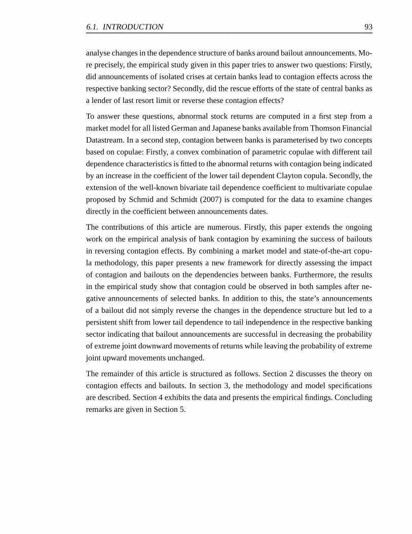
6.1. INTRODUCTION 93
analyse changes in the dependence structure of banks around bailout announcements. Mo-
re precisely, the empirical study given in this paper tries to answer two questions: Firstly,
did announcements of isolated crises at certain banks lead to contagion effects across the
respective banking sector? Secondly, did the rescue efforts of the state of central banks as
a lender of last resort limit or reverse these contagion effects?
To answer these questions, abnormal stock returns are computed in a first step from a
market model for all listed German and Japanese banks available from Thomson Financial
Datastream. In a second step, contagion between banks is parameterised by two concepts
based on copulae: Firstly, a convex combination of parametric copulae with different tail
dependence characteristics is fitted to the abnormal returns with contagion being indicated
by an increase in the coefficient of the lower tail dependent Clayton copula. Secondly, the
extension of the well-known bivariate tail dependence coefficient to multivariate copulae
proposed by Schmid and Schmidt (2007) is computed for the data to examine changes
directly in the coefficient between announcements dates.
The contributions of this article are numerous. Firstly, this paper extends the ongoing
work on the empirical analysis of bank contagion by examining the success of bailouts
in reversing contagion effects. By combining a market model and state-of-the-art copu-
la methodology, this paper presents a new framework for directly assessing the impact
of contagion and bailouts on the dependencies between banks. Furthermore, the results
in the empirical study show that contagion could be observed in both samples after ne-
gative announcements of selected banks. In addition to this, the state’s announcements
of a bailout did not simply reverse the changes in the dependence structure but led to a
persistent shift from lower tail dependence to tail independence in the respective banking
sector indicating that bailout announcements are successful in decreasing the probability
of extreme joint downward movements of returns while leaving the probability of extreme
joint upward movements unchanged.
The remainder of this article is structured as follows. Section 2 discusses the theory on
contagion effects and bailouts. In section 3, the methodology and model specifications
are described. Section 4 exhibits the data and presents the empirical findings. Concluding
remarks are given in Section 5.
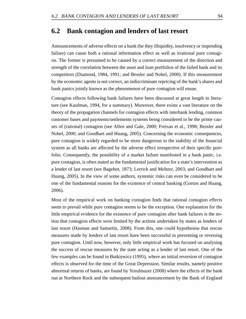
6.2. BANK CONTAGION AND LENDERS OF LAST RESORT 94
6.2 Bank contagion and lenders of last resort
Announcements of adverse effects on a bank (be they illiquidity, insolvency or impending
failure) can cause both a rational information effect as well as irrational pure contagi-
on. The former is presumed to be caused by a correct measurement of the direction and
strength of the correlation between the asset and loan portfolios of the failed bank and its
competitors (Diamond, 1984, 1991; and Bessler and Nohel, 2000). If this measurement
by the economic agents is not correct, an indiscriminate repricing of the bank’s shares and
bank panics jointly known as the phenomenon of pure contagion will ensue.
Contagion effects following bank failures have been discussed at great length in litera-
ture (see Kaufman, 1994, for a summary). Moreover, there exists a vast literature on the
theory of the propagation channels for contagion effects with interbank lending, common
customer bases and payments/settlements systems being considered to be the prime cau-
ses of (rational) contagion (see Allen and Gale, 2000; Freixas et al., 1998; Bessler and
Nohel, 2000; and Goodhart and Huang, 2005). Concerning the economic consequences,
pure contagion is widely regarded to be more dangerous to the stability of the financial
system as all banks are affected by the adverse effect irrespective of their specific port-
folio. Consequently, the possibility of a market failure manifested in a bank panic, i.e.
pure contagion, is often stated as the fundamental justification for a state’s intervention as
a lender of last resort (see Bagehot, 1873; Lerrick and Meltzer, 2003; and Goodhart and
Huang, 2005). In the view of some authors, systemic risks can even be considered to be
one of the fundamental reasons for the existence of central banking (Gorton and Huang,
2006).
Most of the empirical work on banking contagion finds that rational contagion effects
seem to prevail while pure contagion seems to be the exception. One explanation for the
little empirical evidence for the existence of pure contagion after bank failures is the no-
tion that contagion effects were limited by the actions undertaken by states as lenders of
last resort (Hasman and Samartın, 2008). From this, one could hypothesise that rescue
measures made by lenders of last resort have been successful in preventing or reversing
pure contagion. Until now, however, only little empirical work has focused on analysing
the success of rescue measures by the state acting as a lender of last resort. One of the
few examples can be found in Butkiewicz (1995), where an initial reversion of contagion
effects is observed for the time of the Great Depression. Similar results, namely positive
abnormal returns of banks, are found by Yorulmazer (2008) where the effects of the bank
run at Northern Rock and the subsequent bailout announcement by the Bank of England
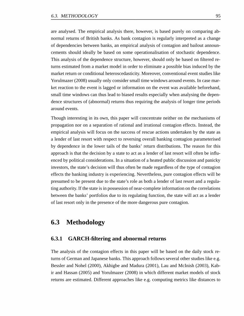
6.3. METHODOLOGY 95
are analysed. The empirical analysis there, however, is based purely on comparing ab-
normal returns of British banks. As bank contagion is regularly interpreted as a change
of dependencies between banks, an empirical analysis of contagion and bailout announ-
cements should ideally be based on some operationalisation of stochastic dependence.
This analysis of the dependence structure, however, should only be based on filtered re-
turns estimated from a market model in order to eliminate a possible bias induced by the
market return or conditional heteroscedasticity. Moreover, conventional event studies like
Yorulmazer (2008) usually only consider small time windows around events. In case mar-
ket reaction to the event is lagged or information on the event was available beforehand,
small time windows can thus lead to biased results especially when analysing the depen-
dence structures of (abnormal) returns thus requiring the analysis of longer time periods
around events.
Though interesting in its own, this paper will concentrate neither on the mechanisms of
propagation nor on a separation of rational and irrational contagion effects. Instead, the
empirical analysis will focus on the success of rescue actions undertaken by the state as
a lender of last resort with respect to reversing overall banking contagion parameterised
by dependence in the lower tails of the banks’ return distributions. The reason for this
approach is that the decision by a state to act as a lender of last resort will often be influ-
enced by political considerations. In a situation of a heated public discussion and panicky
investors, the state’s decision will thus often be made regardless of the type of contagion
effects the banking industry is experiencing. Nevertheless, pure contagion effects will be
presumed to be present due to the state’s role as both a lender of last resort and a regula-
ting authority. If the state is in possession of near-complete information on the correlations
between the banks’ portfolios due to its regulating function, the state will act as a lender
of last resort only in the presence of the more dangerous pure contagion.
6.3 Methodology
6.3.1 GARCH-filtering and abnormal returns
The analysis of the contagion effects in this paper will be based on the daily stock re-
turns of German and Japanese banks. This approach follows several other studies like e.g.
Bessler and Nohel (2000), Akhigbe and Madura (2001), Lau and McInish (2003), Kab-
ir and Hassan (2005) and Yorulmazer (2008) in which different market models of stock
returns are estimated. Different approaches like e.g. computing metrics like distances to
6.3. METHODOLOGY 96
default as it is done in Gropp and Moerman (2004) are not considered due to two rea-
sons: First, transmitted adverse effects will always result in a devaluation of a bank, and
thus, the adverse effect should be reflected in a repricing of the bank’s stock. Second,
the use of additional data from the banks’ financial statements would require breaking
down quarterly into diurnal data. Such methods (like e.g. cubic spline interpolation, see
Gropp and Moerman, 2004) can only be seen as coarse approximations thus introducing
an unnecessary bias in the data.
In contrast to the aforementioned papers, this paper proposes a new framework for detec-
ting contagion effects and market reactions to bailout announcements. Instead of simply
comparing abnormal returns, copula functions are fitted to abnormal returns in order to
analyse the dependence structure of a struggling bank’s competitors. To minimise the
effects of the market return on the banks’ stock returns, abnormal returns rather than ob-
servable returns (like it is done e.g. in Rodriguez, 2007) are used. Abnormal returns are
estimated from a market model that includes the German DAX and the Japanese NIKKEI
225 stock indeces as proxies of the market return. In addition to the market return, I fur-
ther include the daily Euribor-1-month reference rate in the model for the German data
sample.
A stylised fact about financial data is the presence of conditional heteroscedasticity in
stock returns. As the presence of conditional heteroscedasticity could bias the results and
as the copula models described below require the input of i.i.d. data, I fit ARMA-GARCH
models to the univariate marginals to account for time-varying volatility. In particular,
following Dias and Embrechts (2009), I model the stochastic process (rt)t∈Z of the log-
returns for each bank as an ARMA(p1,q1)-GARCH(p2,q2) process with
rt = μt + εt
μt = μ+
p1∑i=1
φi(rt−i − μ) +
q1∑j=1
θjεt−j
εt = σtεt (6.1)
σ2t = α0 +
p2∑i=1
αi(|εt−i| + γiεt−i)2 +
q2∑j=1
βjσ2t−j
and α0 > 0, αi, βj ≥ 0 for all i = 1, 2, ..., p2 and j = 1, 2, ..., q2 and εt being a SWN(0,1)-
process (see Bollerslev, 1986, and Bollerslev et al., 1992). The choice of distribution for
the innovations εt as well as the exact specifications for the volatility models and the ML-
estimates for the parameters are given later in the presentation of the results. After the
models have been estimated, the log return ri,t of the ith univariate return series at time t
6.3. METHODOLOGY 97
is filtered according to
ri,t :=ri,t − μi,t
σi,t, i ∈ N, t = 1, 2, ..., T (6.2)
After the filtered returns have been computed, we need to exclude shocks common to all
market participants that might bias the results. Therefore, it is assumed that the filtered
log returns are generated by the following market model:
ri,t = ψi + τirM,t + χiIt + ζi,t, (6.3)
with i = 1, 2..., n representing n banks whose dependence structure will be analysed, t =
1, 2, ..., T being a time index, rM,t being the (GARCH-filtered) return on the respective
market portfolio on day t, It being the daily Euribor-1-month reference rate (only included
in the German data sample) and ζi,t being a random disturbance term for bank i at time t.
6.3.2 Some preliminary copula theory
In order to detect contagion effects and possible remedies induced by the lender of last
resort, the dependence structure inherent in the abnormal filtered returns ri,t of a set of
banks is modelled by the use of copula functions. In the following, some basic results on
copulae will be reviewed.
Consider the marginal distributions of a random vector X ≡ (X1, · · · , Xn) of length
n to be previously specified, the process of aggregating these distributions to their joint
distribution is reduced to choosing or estimating a copula that reflects the dependence
structure between the marginals. The mathematical basis for the analysis of copulae was
founded by Sklar (1959) and Hoeffding (1940). In the following, a basic definition of a
copula and Sklar’s theorem are described (for a more detailed description of copulae see
Nelsen, 2006 or Joe, 1997).
Let Fi be the ith marginal cumulative distribution function (cdf) of the random vector X .
An n-dimensional copula is a n-variate cumulative distribution function C : [0; 1]n →[0; 1] with uniformly distributed marginals (hereafter called n-copula). The central result
in copula theory is Sklar’s theorem which ensures the existence of a unique copula under
relatively weak conditions:
Theorem 2 (Sklar):
Let G be a joint cumulative distribution function with n marginals F i. Then there exists
6.3. METHODOLOGY 98
an n-dimensional Copula C such that for all x ∈ Rn,
G(x1, x2, ..., xn) = C(F1(x1), F2(x2), ..., Fn(xn)). (6.4)
If all marginals Fi are continuous, then the Copula C is unique.
Vice versa, if an n-Copula C and n cumulative distribution fuctions F i are given then
(6.4) yields an n-variate cumulative distribution function with marginals F i.
In contrast to traditional concepts of dependence like Kendall’s Tau or Spearman’s Rho,
a copula captures the whole dependence between the marginals (Chen and Huang, 2007)
thus further explaining the surge in interest in copulae.
As the copula directly describes the dependence structure inherent in a random vector,
it is not surprising that certain measures of dependence and concordance are closely lin-
ked with the copula concept. The most important dependence measure with respect to the
analysis of financial contagion is the concept of asymptotic tail dependence which will
be described in detail in the following. Tail dependence can synonymously be described
as the extremal dependence of two random variables, i.e. the dependence in the tails of a
bivariate distribution (McNeil et al., 2005). For our purposes, asymptotic tail dependence
is especially well suited for the analysis of financial contagion because it allows a dif-
ferentiated analysis of the symmetric or asymmetric extremal dependence between two
markets, or, as described by Rodriguez (2007), their propensity to crash (and/or to boom)
together.
Definition 6.3.1 (Upper tail dependence):
Let X1 and X2 be two random variables with cdfs F1 and F2. Then the upper tail depen-
dence coefficient of the random vector (X1, X2) is defined as (McNeil et al., 2005)
λU := λU(X1, X2) = limu↑1
P{X2 > F−1
2 (u)|X1 > F−11 (u)}
(6.5)
provided that a limit of λU exists in [0; 1] with F−1i being the quantile function of the cdf Fi
for i ∈ {1; 2}. For λU ∈ (0; 1] the random variables are said to be upper tail dependent.
For λU = 0, X1 and X2 are said to be asymptotically upper tail independent.
As said earlier, the notion of tail dependence is strongly linked with the concept of co-
pulae. To be precise, for a bivariate random vector with continuous marginal cdfs F1 and
F2, the coefficient of upper tail dependence (if it exists) can be expressed in terms of the
6.3. METHODOLOGY 99
underlying (unique) copula C:
λU = limu↑1
1 − 2u+ C(u, u)
1 − u(6.6)
Analogously, the coefficient of lower tail dependence is defined as
Definition 6.3.2 (Lower tail dependence):
λL := λL(X1, X2) = limu↓0
P{X2 ≤ F−1
2 (u)|X1 ≤ F−11 (u)}
(6.7)
again provided that a limit of λU exists in [0; 1]. For λU ∈ (0; 1] and λU = 0 we have lower
tail dependent and asymptotically lower tail independent random variables respectively.
If the limit exists and F1 and F2 are continuous, we can express the coefficient in terms of
the copula:
λL = limu↓0
C(u, u)
u(6.8)
The definition of lower tail dependence given above only allows a bivariate comparison of
random variables. In addition to the bivariate models explained later I make further use of
a generalisation of the notion of lower tail dependence to multivariate random variables
that has been proposed recently by Schmid and Schmidt (2007). A multivariate measure
for lower tail dependence is given by
Definition 6.3.3 (Multivariate lower tail dependence, Schmidt and Schmid):
λML := lim
p↓0ρ(p) = lim
p↓0
n+ 1
pn+1
∫[0,p]n
C(u)du (6.9)
with
ρ(p) :=
∫[0,p]n
C(u)du −(
p2
2
)npn+1
n+1−(
p2
2
)n (6.10)
being an n-dimensional conditional version of Spearman’s rho for 0 < p ≤ 1.
Empirical estimators for λML and ρ(p) based on a sample of size T are given by
ρT (p) :=
{1
T
T∑t=1
n∏i=1
(p− Ui,t,T )+ −(p2
2
)n}/
{pn+1
n+ 1−(p2
2
)n}(6.11)
and
λML,T (p) := ρT (k/T ) (6.12)
6.3. METHODOLOGY 100
respectively, where Ui,t,T are the pseudo-observations from the copula (see Schmid and
Schmidt, 2007; or McNeil et al., 2005) given by
Ui,t,T :=1
T(rank(Xit) in Xi1, · · · , XiT ) (6.13)
and k ∈ {1, 2, ..., T} is a prespecified parameter.
In the following, the different copulae that are to be used in the empirical study shall be
briefly discussed. One of the most basic copulae is the Gaussian copula given by the cdf
CΦn (u; Σ) = Φ
(n)Σ (Φ−1(u1), ...,Φ
−1(un)) (6.14)
with u =t (u1, u2, ..., un) ∈ [0; 1]n. It can be obtained by applying the inversion me-
thod on an n-variate standard Gaussian distribution Φ(n) with correlation matrix Σ and n
univariate standard Gaussian distributions as marginals (Nelsen, 2006). For imperfectly
correlated marginals the Gaussian copula CΦn is tail independent (see e.g. Sibuya, 1960;
and Resnick, 1987).
Similarly as the Gaussian copula can be derived from a multivariate Gaussian distribution,
the t-copula can be obtained from a (non-singular) n-dimensional Student’s t-distribution
Td(µ; Ω; ν) with density
f(x) =Γ(ν+n
2)
Γ(ν2)√
(πν)n|Ω|
(1 +
(x − µ)′Ω−1(x − µ)
ν
)−ν+n2
, (6.15)
ν degrees of freedom, mean vector µ and dispersion matrix Ω (note that the dispersion
matrix does not equal the covariance matrix in this case, see Demarta and McNeil, 2005).
As copulae are invariant under strictly increasing transformations of the marginals, we
can obtain the t-copula from the standardised n-dimensional t-distribution Tn(0; Σ; ν)
yielding
CTn (u; ν; Σ) =
∫ t−1ν (u1)
−∞...
∫ t−1ν (un)
−∞
Γ(ν+n2
)
Γ(ν2)√
(πν)n|Σ|
(1 +
x′Σ−1x′
ν
)− ν+n2
dx, (6.16)
with t−1ν being the inverted cdf of a standard univariate Student’s t-distribution with ν
degrees of freedom. The t-copula is symmetrically tail dependent and converges to the
Gaussian copula for ν → ∞.
Another symmetrically tail independent copula that will be implemented in the empirical
6.3. METHODOLOGY 101
study is the Frank copula given by
CFn (u; δ) = −1
δlog
(1 +
∏ni=1(exp(−δui) − 1)
(exp(−δ) − 1)n−1
), (6.17)
with parameter δ ∈ R+ (for some properties of the bivariate Frank copula see Genest,
1987).
The aforementioned copulae exhibit tail independence (Gaussian and Frank) and sym-
metric tail dependence (Student’s t), respectively. For the purpose of capturing different
patterns of tail dependence, the Gumbel copula which is asymmetrically tail dependent
(upper tail dependence and lower tail independence) shall be considered in the empirical
analysis as well. Its cdf is given by
CGn (u;λ) = exp
⎡⎣−( n∑i=1
−(log ui)λ
) 1λ
⎤⎦ , (6.18)
where the parameter λ satisfies λ ≥ 1. Here, I use the standard definition of the Gumbel
copula (for a recursively defined definition that simplifies the computation see Bouye,
2003).
The last parametric copula exhibiting lower tail dependence that will be considered in the
empirical study is the Clayton copula (sometimes also called the Cook-Johnson or Pare-
to copula, see Genest and MacKay, 1986; and Hutchinson and Lai, 1990). The Clayton
copula is given by
CCn(u; θ) = (u−θ1 + · · ·+ u−θ
n − n + 1)−1/θ, (6.19)
with θ ≥ 0 with the independence copula being the limiting case for θ → 0.
Parameter estimation for these copula functions is usually achieved by Maximum-Likeli-
hood with the marginals being specified either parametrically or nonparametrically yiel-
ding the so-called Inference-for-margins (IFM) method and canonical Maximum-Like-
lihood respectively. The ML-estimators are consistent and asymptotically normal under
some regularity conditions (Genest et al., 1995). The asymptotic behaviour of these esti-
mators, however, only holds for i.i.d. data used for estimating the copula parameters thus
emphasising the need to apply GARCH-filters before modelling the dependence structure.
As described above, the presented parametric copulae all imply different forms of tail de-
pendence or independence of the underlying data. As a single parametric copula would
6.3. METHODOLOGY 102
be too inflexible to model the variety of changes in tail dependence we are interested in,
a convex combination including all mentioned parametric copulae will be fitted to each
time window of interest. If the weights of a particular parametric copula in the fitted con-
vex combination changes over time, we will interpret this as a change in tail dependence
expressed by this particular copula. The details of this approach are described in the fol-
lowing section.
6.3.3 Detecting contagion effects with copulae
Following Patton (2002), Jondeau and Rockinger (2006), Rodriguez (2007) and Chen and
Poon (2007) I try to capture any change in the dependence structure of abnormal bank
returns by analysing the changes in the parametric form and the parameters of various co-
pulae. Unlike these studies, however, I apply their methodology using abnormal returns to
analyse changes in the dependence structure between announcements of struggling banks
and the state acting as a lender of last resort. To be precise, I analyse the time-variation of
the fitted copulae conditional on the set of given past information represented by the sub-
σ-algebra G. For a given date t and an information set Gt := σ({ri,j|j = 1, 2, ..., t− 1})for the ith bank, Sklar’s theorem becomes
Ft(x1, x2, ..., xn|Gt) = Cn,t(F1,t(x1|Gt), F2,t(x2|Gt), ..., Fn,t(xn|Gt)|Gt) (6.20)
with Cn,t(u|Gt) being the n-dimensional conditional copula, Fi,t(xi|Gt) being the condi-
tional cdf of the ith univariate marginal and Ft(x1, ..., xn|Gt) being the joint conditional
cdf of the random vector (see Patton, 2002 for an introduction into the theory of con-
ditional copulae and the respective parameter estimation). The merit of using abnormal
returns rather than observed returns is that the analysis of the dependence structure will
not be biased by the influence of the market return proxied by a stock index on the banks’
returns.
In the event study framework of this paper, I assume that the sub-σ-algebra Gt ≡ Gpq =
σ (Ω) is generated by the subset Ω := {ri,j|j = e1, e1 + 1, · · · , e2 − 1, e2} containing
all available information of the time window pq between two events e1 and e2 where
q = 1, 2, ... is the index of the time window.
The model for capturing changes in the dependence structure extends the ideas of Rodri-
guez (2007) to detect changes in the parametric form of the copula by estimating mixtures
of different parametric copulae. It is common knowledge that a convex linear combina-
6.3. METHODOLOGY 103
tion of a finite set of copulae is again a copula (Nelsen, 2006). The analysis of the time-
variance in the dependence structure (restricted to a change in the parametric form) can
thus be observed in the changes in the weights of the convex combination over time. For
each time window pq, a convex combination
Cmixn,pq
(u; ν, ρ, δ, θ, λ|Gpq) ≡ πTpqCTn,pq
(u; ν, ρ|Gpq) + πFpqCFn,pq
(u; δ|Gpq) (6.21)
+ πCpqCCn,pq
(u; θ|Gpq) + (1 − πTpq− πFpq
− πCpq)CGn,pq
(u;λ|Gpq)
πTpq, πFpq
, πCpq∈ (0; 1) and πTpq
+ πFpq+ πCpq
≤ 1
with πTpq, πFpq
and πCpqbeing the weights of the Student’s t, Frank and Clayton copula will
be estimated by canonical Maximum-Likelihood. To detect any changes in the tail depen-
dence, we will compare the changes in the weigths of the convex combination in time
window pq with those fitted from time window pq+1. If a weight changes significantly
between the two time windows, the type of tail dependence implied by the parametric co-
pula included in the convex combination via this particular weight is said to have changed
due to the event separating the two time windows. If we can e.g. observe a significant
increase from πCpqto πCpq+1
, a larger portion of the dependence structure between the two
underlying stocks is represented by the lower tail dependent Clayton copula. As a result,
we will deduce an increase in lower tail dependence. A similar reasoning applies to the
Student’s t, Frank and Gumbel copula. Following Rodriguez (2007), the significance of a
change in all weights will be tested by a likelihood ratio test conducted on the two fitted
models’ log-likelihood.
The parametric copula were chosen to cover a maximal variety of tail dependence struc-
tures. In contrast to Rodriguez (2007), I include the Student’s t copula at first in all convex
combinations not only because the Student’s t copula has been regularly identified in em-
pirical studies as the most flexible copula (see e.g. Kole et al., 2007 for a recent example),
but also because the Student’s t copula can capture both symmetric tail dependence and
tail independence as a special case (when it converges to the Gaussian copula) so that we
do not need to include a further summand in (6.21).
In the next step, the goodness-of-fit of each configuration of the copula mixture is as-
sessed in order to prevent the models from overfitting the data and to check the model
specification. The first metric that will be used is Akaike’s Information Criterion which is
given by
AIC := 2k − 2L(η), (6.22)
where k is the number of model parameters and L(η) is the maximised Loglikelihood
6.3. METHODOLOGY 104
at the estimate of the parameter vector η. Furthermore, goodness-of-fit test procedures
specially adapted to copula models can be employed for choosing the optimal copula
model. An example for such a metric is given by the Cramer-von-Mises statistic
ξ = T
∫[0;1]n
{Cemp
n;T (u) − Cn(u, η)}2dCemp
n;T (u). (6.23)
which measures the distance between the parametric copula and Deheuvels’ empirical
copulaCempn;T estimated from a sample of size T (Fermanian, 2005, for an early mentioning
and Genest et al., 2008, for an extensive analysis). The empirical version of ξ is given by
(Genest et al., 2008)
ξ =
T∑t=1
{Cemp
n;T (ut) − Cn(ut, η)}2
(6.24)
with ut being the t-th sample from the copula. For both metrics, the copula configuration
yielding the lowest value will be considered to be optimal. However, one has to be careful
when using the GoF-metric in (6.24) as it does not account for the number of parameters
estimated thus possibly leading to overfitting of the data.
After an optimal copula model has been found, I fit the optimal convex combination of
copulae to the abnormal filtered returns of each pair of the initial distressed bank’s com-
petitors before the initial and between subsequent events. The null hypothesis then is that
πCpqwill increase for all pairs of competitors after negative announcements while positive
announcements concerning a bailout by the lender of last resort will result in a decrease
of the parameters πCpq.
Furthermore, I estimate the measure for multivariate lower tail dependence given by (6.12)
in order both to extend the empirical study to a multivariate analysis of possible contagion
effects as well as to check the robustness of the (bivariate) results. A summary of the
complete framework is given below:
1. Choose the events e1, e2, · · · on which bank failures (or impending failures) and
bailouts became publicised. Identify the first (critical) event as t0.
2. Estimate the filtered returns ri,t from ARMA-GARCH-models to control for hete-
roscedasticity and serial correlation.
3. Estimate the market model ri,t = ψi + τirM,t +χiIt + ζi,t based on stock returns ri,t
observed in the time window [t−400; t−100] with OLS and compute abnormal returns
by the identity ARi,t := ri,t − ψi − τirM,t − χiIt.
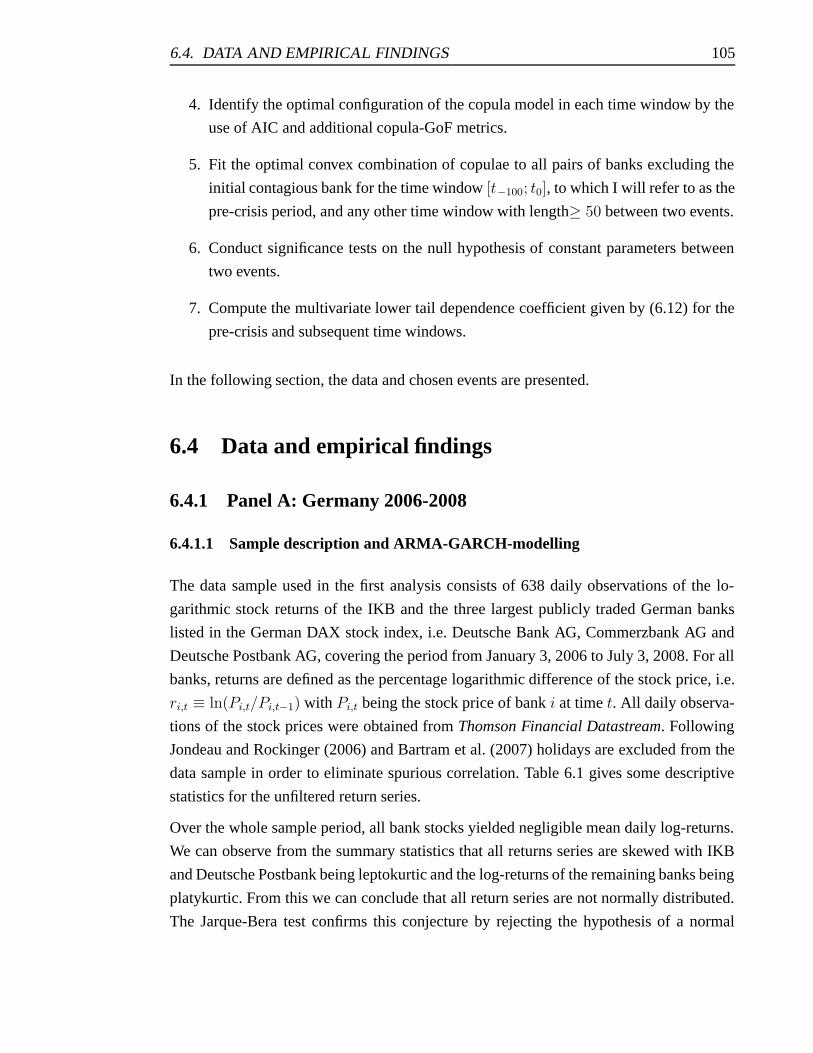
6.4. DATA AND EMPIRICAL FINDINGS 105
4. Identify the optimal configuration of the copula model in each time window by the
use of AIC and additional copula-GoF metrics.
5. Fit the optimal convex combination of copulae to all pairs of banks excluding the
initial contagious bank for the time window [t−100; t0], to which I will refer to as the
pre-crisis period, and any other time window with length≥ 50 between two events.
6. Conduct significance tests on the null hypothesis of constant parameters between
two events.
7. Compute the multivariate lower tail dependence coefficient given by (6.12) for the
pre-crisis and subsequent time windows.
In the following section, the data and chosen events are presented.
6.4 Data and empirical findings
6.4.1 Panel A: Germany 2006-2008
6.4.1.1 Sample description and ARMA-GARCH-modelling
The data sample used in the first analysis consists of 638 daily observations of the lo-
garithmic stock returns of the IKB and the three largest publicly traded German banks
listed in the German DAX stock index, i.e. Deutsche Bank AG, Commerzbank AG and
Deutsche Postbank AG, covering the period from January 3, 2006 to July 3, 2008. For all
banks, returns are defined as the percentage logarithmic difference of the stock price, i.e.
ri,t ≡ ln(Pi,t/Pi,t−1) with Pi,t being the stock price of bank i at time t. All daily observa-
tions of the stock prices were obtained from Thomson Financial Datastream. Following
Jondeau and Rockinger (2006) and Bartram et al. (2007) holidays are excluded from the
data sample in order to eliminate spurious correlation. Table 6.1 gives some descriptive
statistics for the unfiltered return series.
Over the whole sample period, all bank stocks yielded negligible mean daily log-returns.
We can observe from the summary statistics that all returns series are skewed with IKB
and Deutsche Postbank being leptokurtic and the log-returns of the remaining banks being
platykurtic. From this we can conclude that all return series are not normally distributed.
The Jarque-Bera test confirms this conjecture by rejecting the hypothesis of a normal
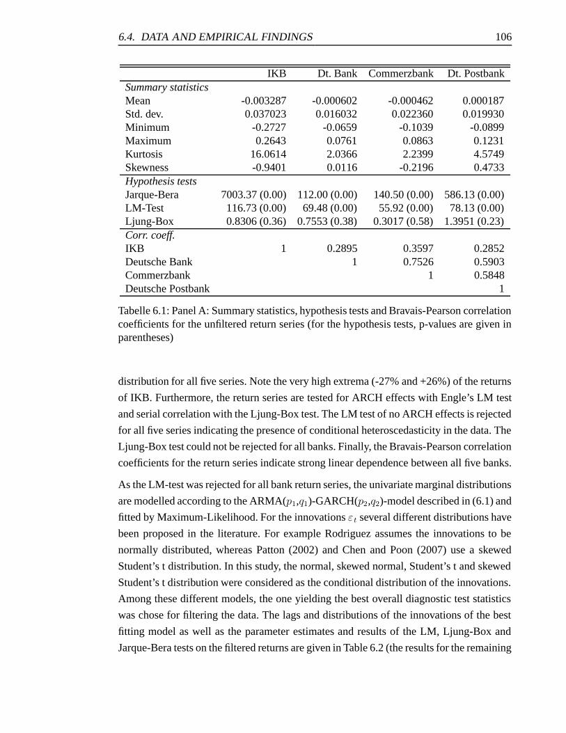
6.4. DATA AND EMPIRICAL FINDINGS 106
IKB Dt. Bank Commerzbank Dt. PostbankSummary statisticsMean -0.003287 -0.000602 -0.000462 0.000187Std. dev. 0.037023 0.016032 0.022360 0.019930Minimum -0.2727 -0.0659 -0.1039 -0.0899Maximum 0.2643 0.0761 0.0863 0.1231Kurtosis 16.0614 2.0366 2.2399 4.5749Skewness -0.9401 0.0116 -0.2196 0.4733Hypothesis testsJarque-Bera 7003.37 (0.00) 112.00 (0.00) 140.50 (0.00) 586.13 (0.00)LM-Test 116.73 (0.00) 69.48 (0.00) 55.92 (0.00) 78.13 (0.00)Ljung-Box 0.8306 (0.36) 0.7553 (0.38) 0.3017 (0.58) 1.3951 (0.23)Corr. coeff.IKB 1 0.2895 0.3597 0.2852Deutsche Bank 1 0.7526 0.5903Commerzbank 1 0.5848Deutsche Postbank 1
Tabelle 6.1: Panel A: Summary statistics, hypothesis tests and Bravais-Pearson correlationcoefficients for the unfiltered return series (for the hypothesis tests, p-values are given inparentheses)
distribution for all five series. Note the very high extrema (-27% and +26%) of the returns
of IKB. Furthermore, the return series are tested for ARCH effects with Engle’s LM test
and serial correlation with the Ljung-Box test. The LM test of no ARCH effects is rejected
for all five series indicating the presence of conditional heteroscedasticity in the data. The
Ljung-Box test could not be rejected for all banks. Finally, the Bravais-Pearson correlation
coefficients for the return series indicate strong linear dependence between all five banks.
As the LM-test was rejected for all bank return series, the univariate marginal distributions
are modelled according to the ARMA(p1,q1)-GARCH(p2,q2)-model described in (6.1) and
fitted by Maximum-Likelihood. For the innovations εt several different distributions have
been proposed in the literature. For example Rodriguez assumes the innovations to be
normally distributed, whereas Patton (2002) and Chen and Poon (2007) use a skewed
Student’s t distribution. In this study, the normal, skewed normal, Student’s t and skewed
Student’s t distribution were considered as the conditional distribution of the innovations.
Among these different models, the one yielding the best overall diagnostic test statistics
was chose for filtering the data. The lags and distributions of the innovations of the best
fitting model as well as the parameter estimates and results of the LM, Ljung-Box and
Jarque-Bera tests on the filtered returns are given in Table 6.2 (the results for the remaining
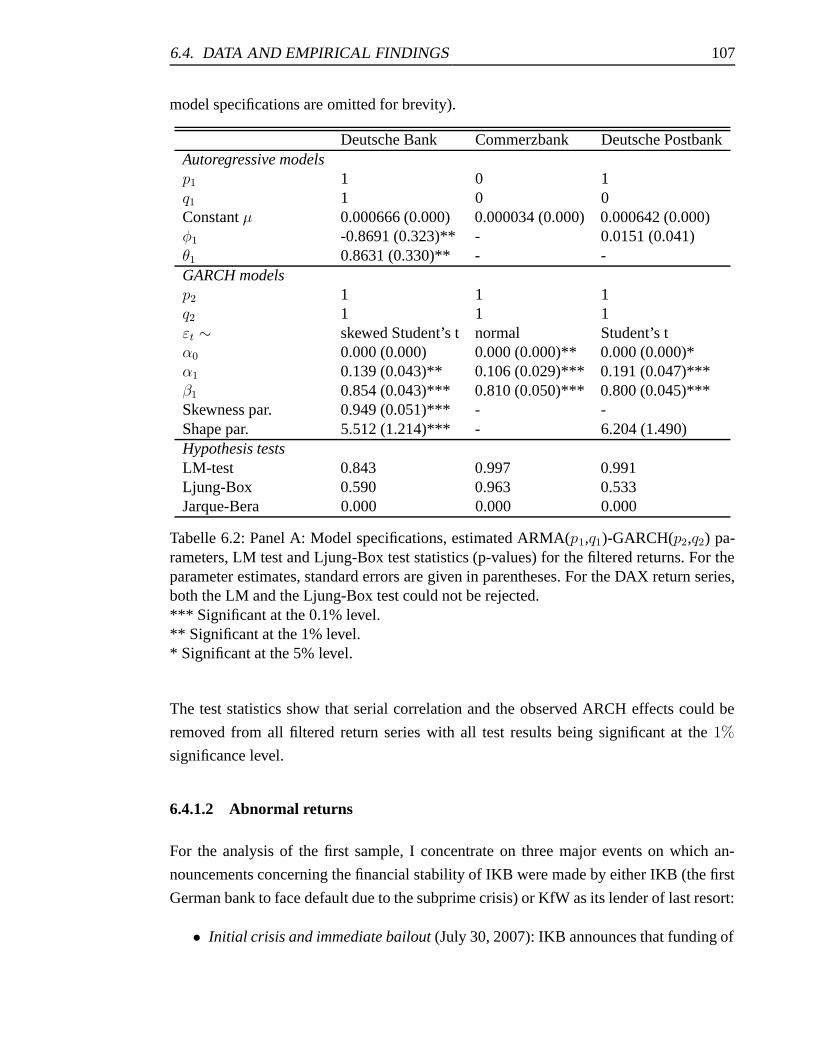
6.4. DATA AND EMPIRICAL FINDINGS 107
model specifications are omitted for brevity).
Deutsche Bank Commerzbank Deutsche PostbankAutoregressive modelsp1 1 0 1q1 1 0 0Constant μ 0.000666 (0.000) 0.000034 (0.000) 0.000642 (0.000)φ1 -0.8691 (0.323)** - 0.0151 (0.041)θ1 0.8631 (0.330)** - -GARCH modelsp2 1 1 1q2 1 1 1εt ∼ skewed Student’s t normal Student’s tα0 0.000 (0.000) 0.000 (0.000)** 0.000 (0.000)*α1 0.139 (0.043)** 0.106 (0.029)*** 0.191 (0.047)***β1 0.854 (0.043)*** 0.810 (0.050)*** 0.800 (0.045)***Skewness par. 0.949 (0.051)*** - -Shape par. 5.512 (1.214)*** - 6.204 (1.490)Hypothesis testsLM-test 0.843 0.997 0.991Ljung-Box 0.590 0.963 0.533Jarque-Bera 0.000 0.000 0.000
Tabelle 6.2: Panel A: Model specifications, estimated ARMA(p1,q1)-GARCH(p2,q2) pa-rameters, LM test and Ljung-Box test statistics (p-values) for the filtered returns. For theparameter estimates, standard errors are given in parentheses. For the DAX return series,both the LM and the Ljung-Box test could not be rejected.*** Significant at the 0.1% level.** Significant at the 1% level.* Significant at the 5% level.
The test statistics show that serial correlation and the observed ARCH effects could be
removed from all filtered return series with all test results being significant at the 1%
significance level.
6.4.1.2 Abnormal returns
For the analysis of the first sample, I concentrate on three major events on which an-
nouncements concerning the financial stability of IKB were made by either IKB (the first
German bank to face default due to the subprime crisis) or KfW as its lender of last resort:
• Initial crisis and immediate bailout (July 30, 2007): IKB announces that funding of
6.4. DATA AND EMPIRICAL FINDINGS 108
the conduit “Rhineland Funding” is endangered and issues a profit warning. State-
owned KfW, IKB’s main stakeholder, provides an 8.1 billion Euro liquidity line for
IKB.
• Second crisis (November 28, 2007): KfW announces that IKB requires another 2.3
billion Euro to cover its risks. The German government refuses to issue a debt gua-
rantee that would have supported IKB and KfW.
• Final Bailout (March 28, 2008): KfW and IKB’s remaining stockholders agree on
a recapitalisation amounting to 1.5 billion Euro.
To estimate abnormal returns, the parameters of the market model given by (6.3) are esti-
mated by OLS using 300 observations from the time window [t−400; t−101] with t0 being
July 30, 2007. The parameter estimates are then used to compute abnormal daily returns
for all banks for the time windows [t−100; t−1] (refered to as the pre-crisis period), [t0; t86]
(being the period after first news on IKB’s losses were publicised and KfW announced its
initial bailout), [t87; t168] (refered to as the crisis period) and finally [t169; t237] (refered to
as the post-crisis period).
In a first step, cumulative abnormal returns are estimated in the usual fashion over a 3-
day time window centered around each announcement date for all banks excluding IKB.
Significance of the obtained results is tested using standardised residual t-tests (see e.g.
Fee and Thomas, 2004, for a similar approach and McWilliams and McWilliams, 2000,
for a description of the test procedure). The results as well as the parameter estimates for
the market model are reported in Table 6.3.
For the first announcement date (the advent of the crisis), all banks with the exception of
Deutsche Bank earn (insignificant) negative abnormal returns. As all banks earn positive
or insignificant negative abnormal returns, one can argue that KfW’s initial announcement
of a bailout was partly successful in preventing contagion. Inconsistent with the hypothe-
sis of increased contagion, however, significant positive abnormal returns can be found
for Deutsche Bank and Commerzbank on the second announcement day while Deutsche
Postbank earned insignificant positive abnormal returns. Consistent with the hypothesis
of a reversion of contagion effects, significant (insignificant) positive abnormal returns
could be observed for Commerzbank (Deutsche Postbank) after the third announcement
day while Deutsche Bank earned an insignificant negative abnormal return. Overall, one
can see that these results are no indication for significant sector-wide contagion effects
while the hypothesis of positive abnormal returns after the bailout cannot be rejected. As
stated earlier, an analysis of contagion effects that is solely based on abnormal returns on
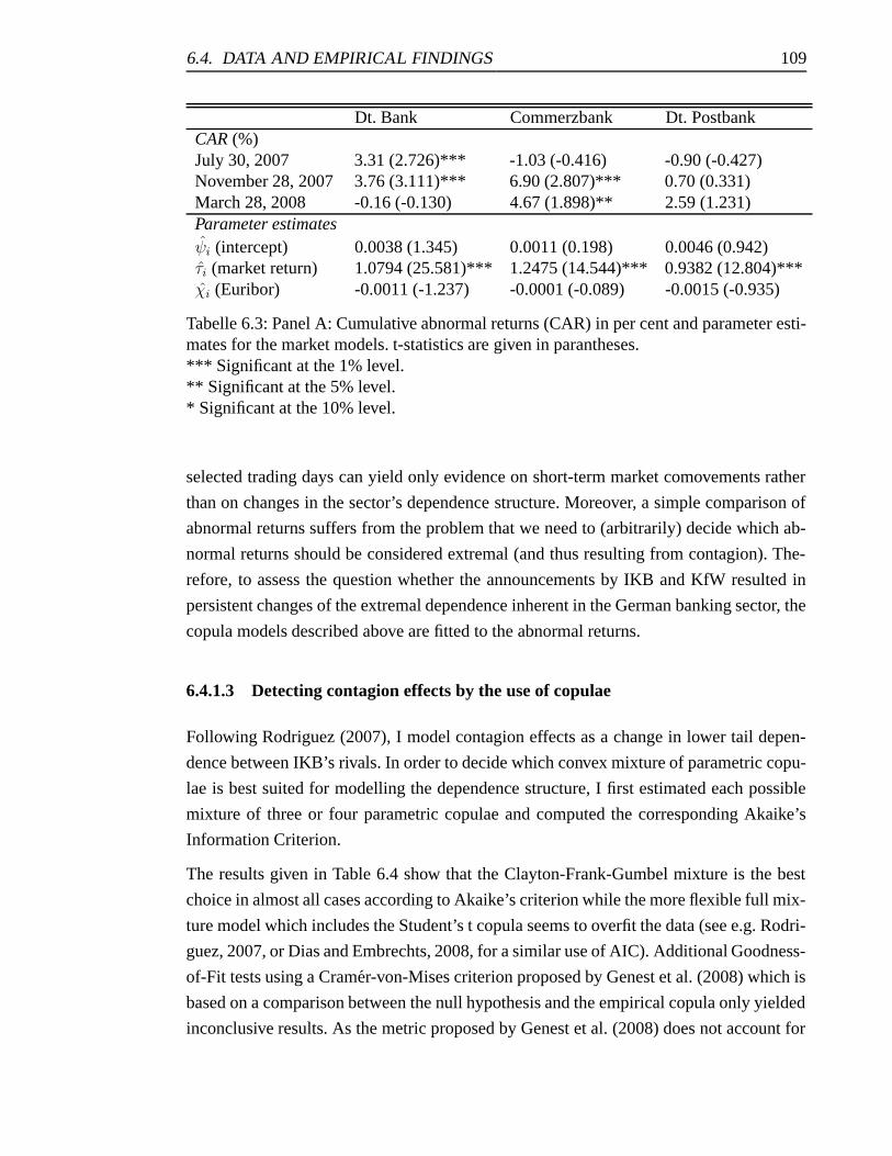
6.4. DATA AND EMPIRICAL FINDINGS 109
Dt. Bank Commerzbank Dt. PostbankCAR (%)July 30, 2007 3.31 (2.726)*** -1.03 (-0.416) -0.90 (-0.427)November 28, 2007 3.76 (3.111)*** 6.90 (2.807)*** 0.70 (0.331)March 28, 2008 -0.16 (-0.130) 4.67 (1.898)** 2.59 (1.231)Parameter estimatesψi (intercept) 0.0038 (1.345) 0.0011 (0.198) 0.0046 (0.942)τi (market return) 1.0794 (25.581)*** 1.2475 (14.544)*** 0.9382 (12.804)***χi (Euribor) -0.0011 (-1.237) -0.0001 (-0.089) -0.0015 (-0.935)
Tabelle 6.3: Panel A: Cumulative abnormal returns (CAR) in per cent and parameter esti-mates for the market models. t-statistics are given in parantheses.*** Significant at the 1% level.** Significant at the 5% level.* Significant at the 10% level.
selected trading days can yield only evidence on short-term market comovements rather
than on changes in the sector’s dependence structure. Moreover, a simple comparison of
abnormal returns suffers from the problem that we need to (arbitrarily) decide which ab-
normal returns should be considered extremal (and thus resulting from contagion). The-
refore, to assess the question whether the announcements by IKB and KfW resulted in
persistent changes of the extremal dependence inherent in the German banking sector, the
copula models described above are fitted to the abnormal returns.
6.4.1.3 Detecting contagion effects by the use of copulae
Following Rodriguez (2007), I model contagion effects as a change in lower tail depen-
dence between IKB’s rivals. In order to decide which convex mixture of parametric copu-
lae is best suited for modelling the dependence structure, I first estimated each possible
mixture of three or four parametric copulae and computed the corresponding Akaike’s
Information Criterion.
The results given in Table 6.4 show that the Clayton-Frank-Gumbel mixture is the best
choice in almost all cases according to Akaike’s criterion while the more flexible full mix-
ture model which includes the Student’s t copula seems to overfit the data (see e.g. Rodri-
guez, 2007, or Dias and Embrechts, 2008, for a similar use of AIC). Additional Goodness-
of-Fit tests using a Cramer-von-Mises criterion proposed by Genest et al. (2008) which is
based on a comparison between the null hypothesis and the empirical copula only yielded
inconclusive results. As the metric proposed by Genest et al. (2008) does not account for
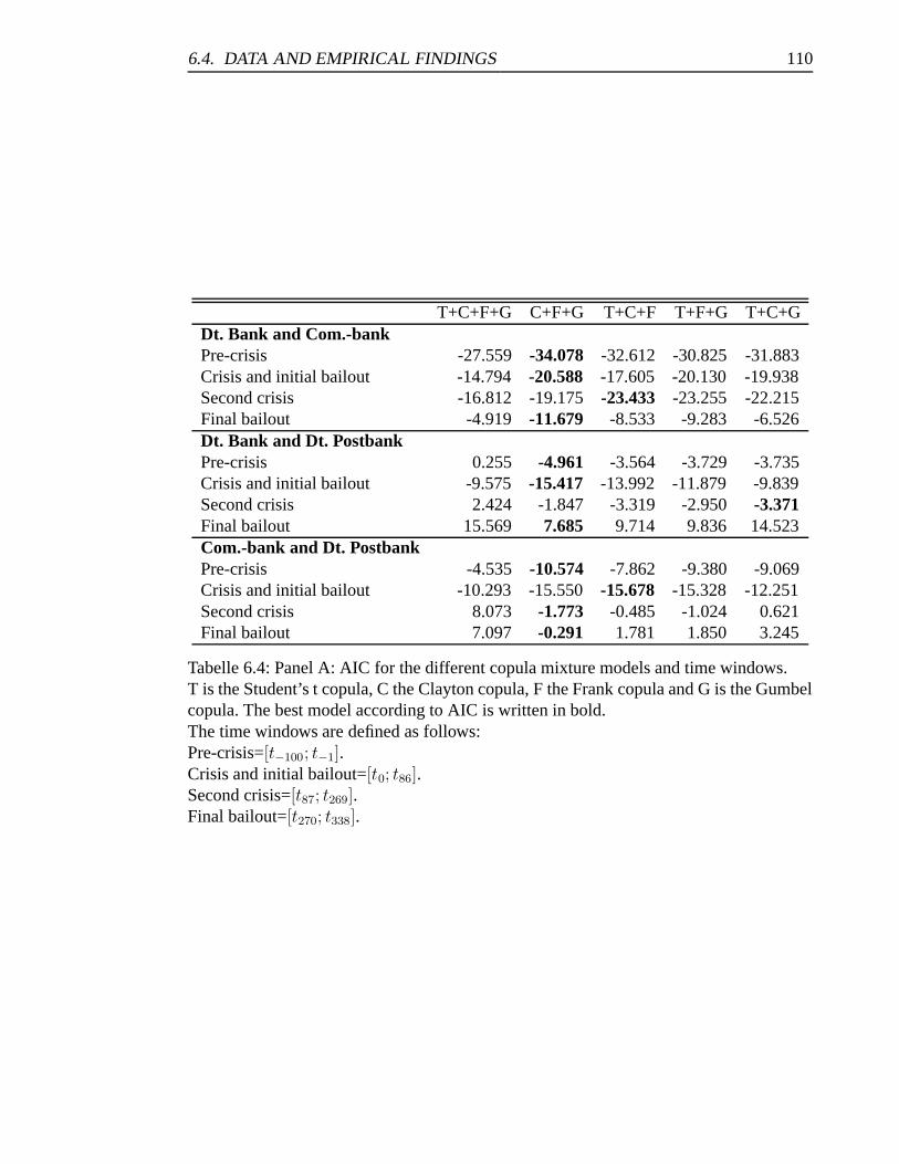
6.4. DATA AND EMPIRICAL FINDINGS 110
T+C+F+G C+F+G T+C+F T+F+G T+C+GDt. Bank and Com.-bankPre-crisis -27.559 -34.078 -32.612 -30.825 -31.883Crisis and initial bailout -14.794 -20.588 -17.605 -20.130 -19.938Second crisis -16.812 -19.175 -23.433 -23.255 -22.215Final bailout -4.919 -11.679 -8.533 -9.283 -6.526Dt. Bank and Dt. PostbankPre-crisis 0.255 -4.961 -3.564 -3.729 -3.735Crisis and initial bailout -9.575 -15.417 -13.992 -11.879 -9.839Second crisis 2.424 -1.847 -3.319 -2.950 -3.371Final bailout 15.569 7.685 9.714 9.836 14.523Com.-bank and Dt. PostbankPre-crisis -4.535 -10.574 -7.862 -9.380 -9.069Crisis and initial bailout -10.293 -15.550 -15.678 -15.328 -12.251Second crisis 8.073 -1.773 -0.485 -1.024 0.621Final bailout 7.097 -0.291 1.781 1.850 3.245
Tabelle 6.4: Panel A: AIC for the different copula mixture models and time windows.T is the Student’s t copula, C the Clayton copula, F the Frank copula and G is the Gumbelcopula. The best model according to AIC is written in bold.The time windows are defined as follows:Pre-crisis=[t−100; t−1].Crisis and initial bailout=[t0; t86].Second crisis=[t87; t269].Final bailout=[t270; t338].
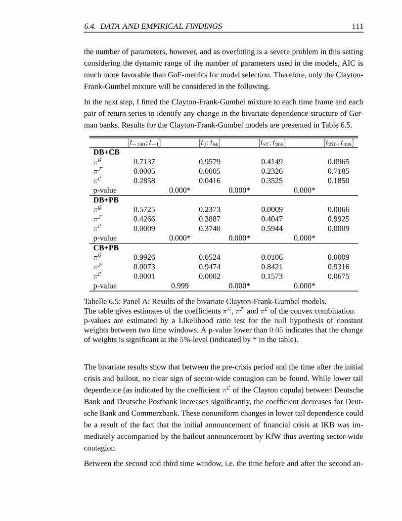
6.4. DATA AND EMPIRICAL FINDINGS 111
the number of parameters, however, and as overfitting is a severe problem in this setting
considering the dynamic range of the number of parameters used in the models, AIC is
much more favorable than GoF-metrics for model selection. Therefore, only the Clayton-
Frank-Gumbel mixture will be considered in the following.
In the next step, I fitted the Clayton-Frank-Gumbel mixture to each time frame and each
pair of return series to identify any change in the bivariate dependence structure of Ger-
man banks. Results for the Clayton-Frank-Gumbel models are presented in Table 6.5.
[t−100; t−1] [t0; t86] [t87; t269] [t270; t338]DB+CBπG 0.7137 0.9579 0.4149 0.0965πF 0.0005 0.0005 0.2326 0.7185πC 0.2858 0.0416 0.3525 0.1850p-value 0.000* 0.000* 0.000*DB+PBπG 0.5725 0.2373 0.0009 0.0066πF 0.4266 0.3887 0.4047 0.9925πC 0.0009 0.3740 0.5944 0.0009p-value 0.000* 0.000* 0.000*CB+PBπG 0.9926 0.0524 0.0106 0.0009πF 0.0073 0.9474 0.8421 0.9316πC 0.0001 0.0002 0.1573 0.0675p-value 0.999 0.000* 0.000*
Tabelle 6.5: Panel A: Results of the bivariate Clayton-Frank-Gumbel models.The table gives estimates of the coefficients πG, πF and πC of the convex combination.p-values are estimated by a Likelihood ratio test for the null hypothesis of constantweights between two time windows. A p-value lower than 0.05 indicates that the changeof weights is significant at the 5%-level (indicated by * in the table).
The bivariate results show that between the pre-crisis period and the time after the initial
crisis and bailout, no clear sign of sector-wide contagion can be found. While lower tail
dependence (as indicated by the coefficient πC of the Clayton copula) between Deutsche
Bank and Deutsche Postbank increases significantly, the coefficient decreases for Deut-
sche Bank and Commerzbank. These nonuniform changes in lower tail dependence could
be a result of the fact that the initial announcement of financial crisis at IKB was im-
mediately accompanied by the bailout announcement by KfW thus averting sector-wide
contagion.
Between the second and third time window, i.e. the time before and after the second an-
6.4. DATA AND EMPIRICAL FINDINGS 112
nouncement of severe financial crisis at IKB, results show an unequivocal picture: For all
combinations of Deutsche Bank, Deutsche Postbank and Commerzbank, lower tail depen-
dence rises significantly at the 5%-level. Consequently, the bailout by state-owned KfW
was economically justified as the probability of a joint crash of German banks had incre-
ased sharply after the announcement by IKB (which in this case was not accompanied by
an immediate bailout announcement). Moreover, the increases in lower tail dependence
all coincide with decreases in upper tail dependence as indicated by the coefficient πG of
the Gumbel copula. This result clearly underlines the dramatic change in the dependence
structure that took place in the German banking sector after the second announcement of
crisis.
After the final bailout, the results given in Table 6.5 show that for all banks lower tail
dependence, i.e. the propensity of German banks to crash together, decreases. This is
consistent with the hypothesis of contagion being successfully reversed as a result of
KfW’s bailout of IKB. In addition to this, in all bivariate models the decrease in lower tail
dependence is accompanied by a significant increase in the coefficient πF signalling tail
independence. Economically, this means that after the final bailout announcement, joint
extreme upward movements of German banks’ abnormal returns became less likely than
before the advent of the crisis. In other words, the instrument of a bailout does not seem
to be suitable for completely reversing contagion but rather seems to transform lower tail
dependence into tail independence. This finding is consistent with the economic intention
of a bailout as it should not increase the sector’s propensity to boom together but should
rather be limited to decreasing the probability of a joint crash.
6.4.1.4 Robustness checks
As the number of listed banks in the German banking sector is relatively small, I estimate
a number of alternate models in order to check the robustness of the previous findings.
More precisely, I estimate the coefficient of multivariate lower tail dependence given by
(6.9) based on the abnormal returns of Deutsche Bank, Commerzbank and Deutsche Post-
bank in order to extend the described bivariate comparisons to a multivariate analysis of
the changes in the dependence structure of the German banking sector. The parameter k in
(6.9) is chosen to be 40. Unreported results with different parameter choices only resulted
in marginal shifts in the level of the estimates thus leading to the assumption that this par-
ticular choice of the parameter did not alter the estimates of the coefficient of multivariate
lower tail dependence. Results are given in Table 6.6.
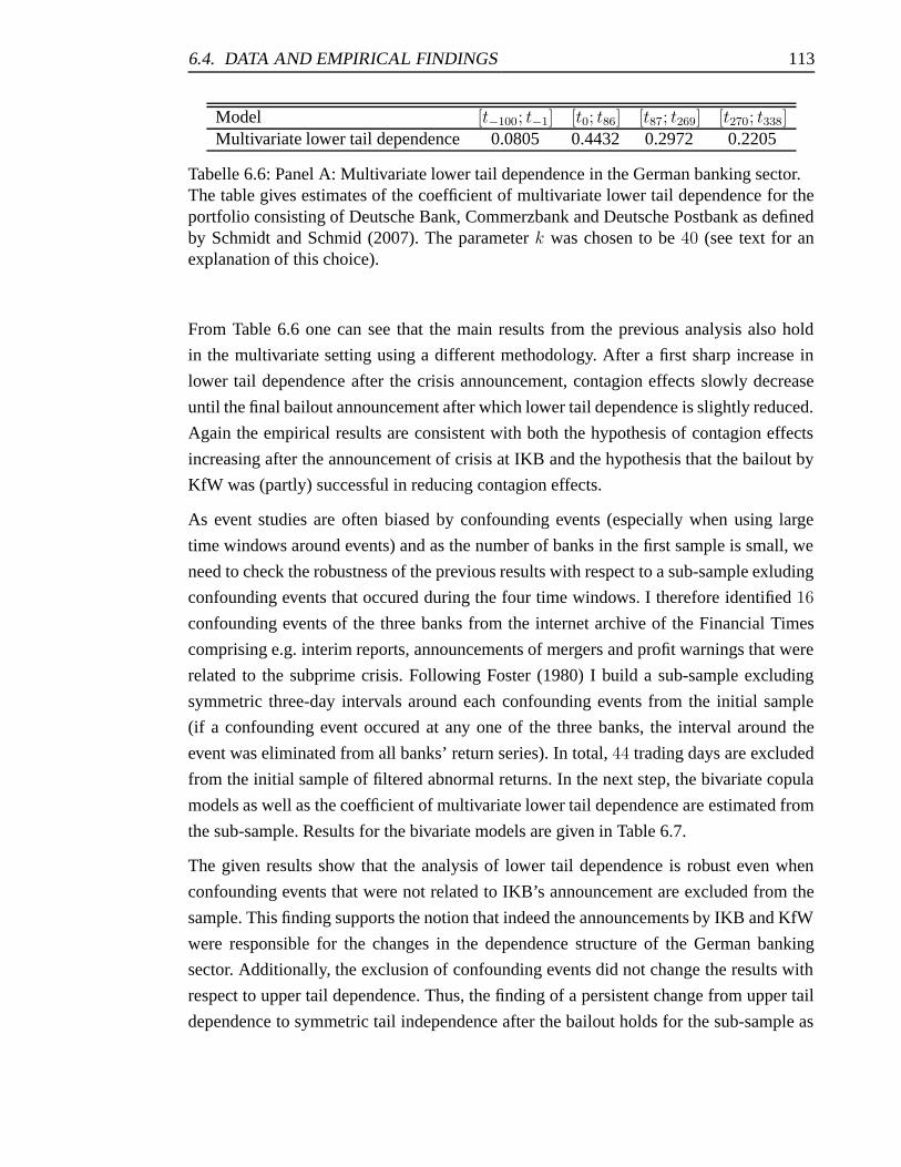
6.4. DATA AND EMPIRICAL FINDINGS 113
Model [t−100; t−1] [t0; t86] [t87; t269] [t270; t338]Multivariate lower tail dependence 0.0805 0.4432 0.2972 0.2205
Tabelle 6.6: Panel A: Multivariate lower tail dependence in the German banking sector.The table gives estimates of the coefficient of multivariate lower tail dependence for theportfolio consisting of Deutsche Bank, Commerzbank and Deutsche Postbank as definedby Schmidt and Schmid (2007). The parameter k was chosen to be 40 (see text for anexplanation of this choice).
From Table 6.6 one can see that the main results from the previous analysis also hold
in the multivariate setting using a different methodology. After a first sharp increase in
lower tail dependence after the crisis announcement, contagion effects slowly decrease
until the final bailout announcement after which lower tail dependence is slightly reduced.
Again the empirical results are consistent with both the hypothesis of contagion effects
increasing after the announcement of crisis at IKB and the hypothesis that the bailout by
KfW was (partly) successful in reducing contagion effects.
As event studies are often biased by confounding events (especially when using large
time windows around events) and as the number of banks in the first sample is small, we
need to check the robustness of the previous results with respect to a sub-sample exluding
confounding events that occured during the four time windows. I therefore identified 16
confounding events of the three banks from the internet archive of the Financial Times
comprising e.g. interim reports, announcements of mergers and profit warnings that were
related to the subprime crisis. Following Foster (1980) I build a sub-sample excluding
symmetric three-day intervals around each confounding events from the initial sample
(if a confounding event occured at any one of the three banks, the interval around the
event was eliminated from all banks’ return series). In total, 44 trading days are excluded
from the initial sample of filtered abnormal returns. In the next step, the bivariate copula
models as well as the coefficient of multivariate lower tail dependence are estimated from
the sub-sample. Results for the bivariate models are given in Table 6.7.
The given results show that the analysis of lower tail dependence is robust even when
confounding events that were not related to IKB’s announcement are excluded from the
sample. This finding supports the notion that indeed the announcements by IKB and KfW
were responsible for the changes in the dependence structure of the German banking
sector. Additionally, the exclusion of confounding events did not change the results with
respect to upper tail dependence. Thus, the finding of a persistent change from upper tail
dependence to symmetric tail independence after the bailout holds for the sub-sample as
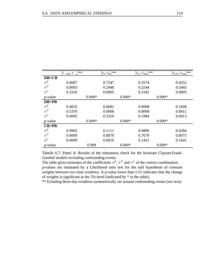
6.4. DATA AND EMPIRICAL FINDINGS 114
[t−100; t−1]** [t0; t86]** [t87; t269]** [t270; t338]**DB+CBπG 0.6687 0.7547 0.3574 0.4552πF 0.0003 0.2448 0.3244 0.5443πC 0.3310 0.0005 0.3182 0.0005p-value 0.000* 0.000* 0.000*DB+PBπG 0.4625 0.6682 0.0008 0.1606πF 0.5370 0.0008 0.8008 0.8411πC 0.0005 0.3310 0.1984 0.0013p-value 0.000* 0.000* 0.000*CB+PBπG 0.9982 0.1111 0.0890 0.0284πF 0.0009 0.8879 0.7679 0.8075πC 0.0009 0.0010 0.1431 0.1641p-value 0.999 0.000* 0.000*
Tabelle 6.7: Panel A: Results of the robustness check for the bivariate Clayton-Frank-Gumbel models excluding confounding events.The table gives estimates of the coefficients πG, πF and πC of the convex combination.p-values are estimated by a Likelihood ratio test for the null hypothesis of constantweights between two time windows. A p-value lower than 0.05 indicates that the changeof weights is significant at the 5%-level (indicated by * in the table).** Exluding three-day-windows symmetrically set around confounding events (see text).
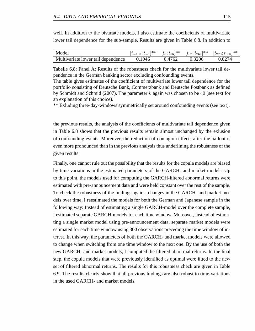
6.4. DATA AND EMPIRICAL FINDINGS 115
well. In addition to the bivariate models, I also estimate the coefficients of multivariate
lower tail dependence for the sub-sample. Results are given in Table 6.8. In addition to
Model [t−100; t−1]** [t0; t86]** [t87; t269]** [t270; t338]**Multivariate lower tail dependence 0.1046 0.4762 0.3206 0.0274
Tabelle 6.8: Panel A: Results of the robustness check for the multivariate lower tail de-pendence in the German banking sector excluding confounding events.The table gives estimates of the coefficient of multivariate lower tail dependence for theportfolio consisting of Deutsche Bank, Commerzbank and Deutsche Postbank as definedby Schmidt and Schmid (2007). The parameter k again was chosen to be 40 (see text foran explanation of this choice).** Exluding three-day-windows symmetrically set around confounding events (see text).
the previous results, the analysis of the coefficients of multivariate tail dependence given
in Table 6.8 shows that the previous results remain almost unchanged by the exlusion
of confounding events. Moreover, the reduction of contagion effects after the bailout is
even more pronounced than in the previous analysis thus underlining the robustness of the
given results.
Finally, one cannot rule out the possibility that the results for the copula models are biased
by time-variations in the estimated parameters of the GARCH- and market models. Up
to this point, the models used for computing the GARCH-filtered abnormal returns were
estimated with pre-announcement data and were held constant over the rest of the sample.
To check the robustness of the findings against changes in the GARCH- and market mo-
dels over time, I reestimated the models for both the German and Japanese sample in the
following way: Instead of estimating a single GARCH-model over the complete sample,
I estimated separate GARCH-models for each time window. Moreover, instead of estima-
ting a single market model using pre-announcement data, separate market models were
estimated for each time window using 300 observations preceding the time window of in-
terest. In this way, the parameters of both the GARCH- and market models were allowed
to change when switching from one time window to the next one. By the use of both the
new GARCH- and market models, I computed the filtered abnormal returns. In the final
step, the copula models that were previously identified as optimal were fitted to the new
set of filtered abnormal returns. The results for this robustness check are given in Table
6.9. The results clearly show that all previous findings are also robust to time-variations
in the used GARCH- and market models.
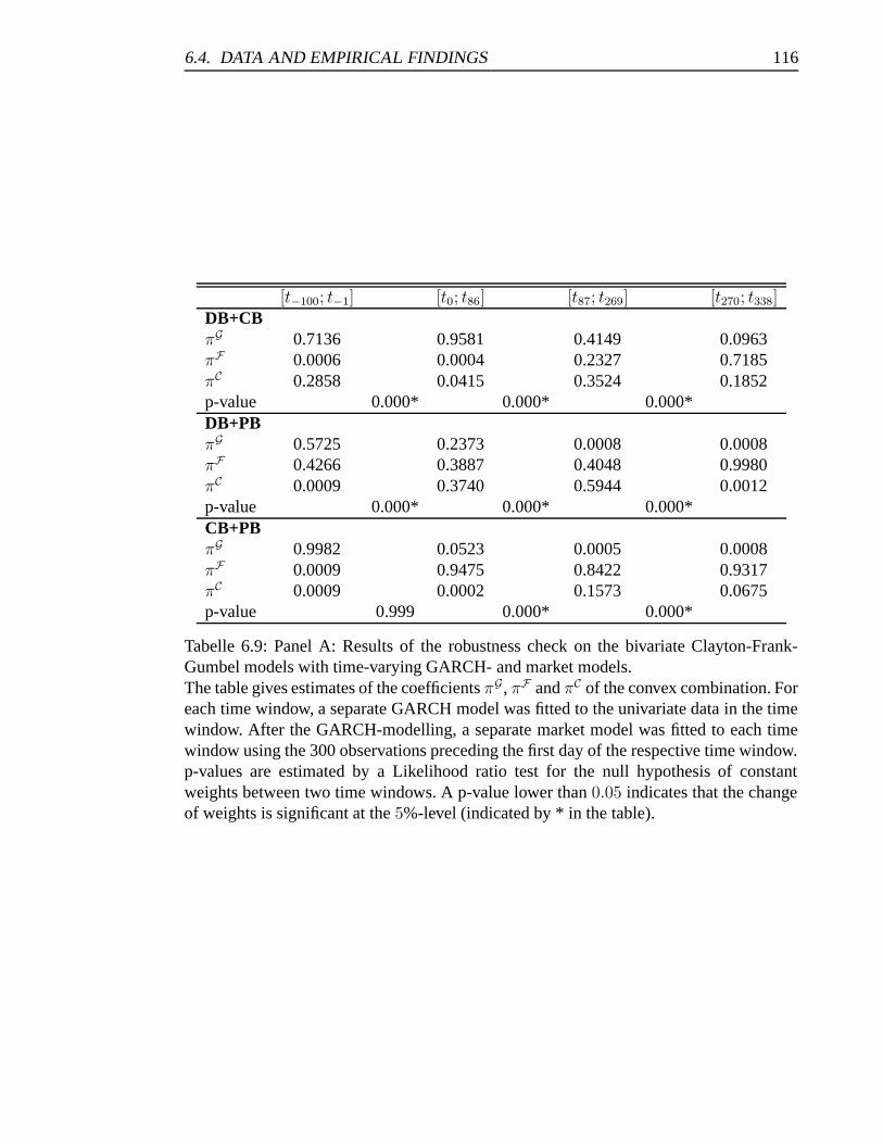
6.4. DATA AND EMPIRICAL FINDINGS 116
[t−100; t−1] [t0; t86] [t87; t269] [t270; t338]DB+CBπG 0.7136 0.9581 0.4149 0.0963πF 0.0006 0.0004 0.2327 0.7185πC 0.2858 0.0415 0.3524 0.1852p-value 0.000* 0.000* 0.000*DB+PBπG 0.5725 0.2373 0.0008 0.0008πF 0.4266 0.3887 0.4048 0.9980πC 0.0009 0.3740 0.5944 0.0012p-value 0.000* 0.000* 0.000*CB+PBπG 0.9982 0.0523 0.0005 0.0008πF 0.0009 0.9475 0.8422 0.9317πC 0.0009 0.0002 0.1573 0.0675p-value 0.999 0.000* 0.000*
Tabelle 6.9: Panel A: Results of the robustness check on the bivariate Clayton-Frank-Gumbel models with time-varying GARCH- and market models.The table gives estimates of the coefficients πG , πF and πC of the convex combination. Foreach time window, a separate GARCH model was fitted to the univariate data in the timewindow. After the GARCH-modelling, a separate market model was fitted to each timewindow using the 300 observations preceding the first day of the respective time window.p-values are estimated by a Likelihood ratio test for the null hypothesis of constantweights between two time windows. A p-value lower than 0.05 indicates that the changeof weights is significant at the 5%-level (indicated by * in the table).
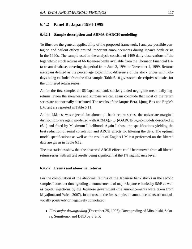
6.4. DATA AND EMPIRICAL FINDINGS 117
6.4.2 Panel B: Japan 1994-1999
6.4.2.1 Sample description and ARMA-GARCH-modelling
To illustrate the general applicability of the proposed framework, I analyse possible con-
tagion and bailout effects around important announcements during Japan’s bank crisis
in the 1990s. The sample used in the analysis consists of 1409 daily observations of the
logarithmic stock returns of 66 Japanese banks available from the Thomson Financial Da-
tastream database, covering the period from June 3, 1994 to November 4, 1999. Returns
are again defined as the percentage logarithmic difference of the stock prices with holi-
days being excluded from the data sample. Table 6.10 gives some descriptive statistics for
the unfiltered return series.
As for the first sample, all 66 Japanese bank stocks yielded negligible mean daily log-
returns. From the skewness and kurtosis we can again conclude that most of the return
series are not normally distributed. The results of the Jarque-Bera, Ljung-Box and Engle’s
LM test are reported in Table 6.11.
As the LM-test was rejected for almost all bank return series, the univariate marginal
distributions are again modelled with ARMA(p1,q1)-GARCH(p2,q2)-models described in
(6.1) and fitted by Maximum-Likelihood. Again I chose the specifications yielding the
best reduction of serial correlation and ARCH effects for filtering the data. The optimal
model specifications as well as the results of Engle’s LM test performed on the filtered
data are given in Table 6.12.
The test statistics show that the observed ARCH effects could be removed from all filtered
return series with all test results being significant at the 1% significance level.
6.4.2.2 Events and abnormal returns
For the computation of the abnormal returns of the Japanese bank stocks in the second
sample, I consider downgrading announcements of major Japanese banks by S&P as well
as capital injections by the Japanese government (the announcements were taken from
Miyajima and Yafeh, 2007). In contrast to the first sample, all announcements are unequi-
vocally positively or negatively connotated:
• First major downgrading (December 25, 1995): Downgrading of Mitsubishi, Saku-
ra, Sumitomo, and DKB by S & P.
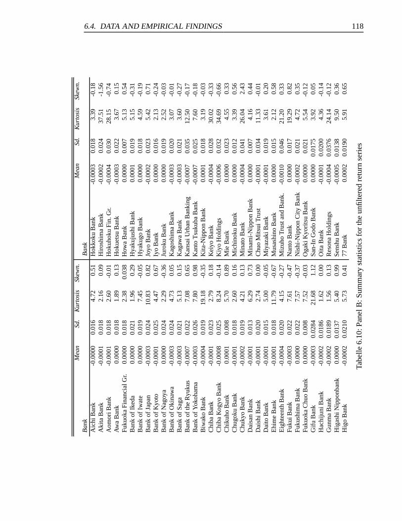
6.4. DATA AND EMPIRICAL FINDINGS 118
Mea
nSd
.K
urto
sis
Skew
n.M
ean
Sd.
Kur
tosi
sSk
ewn.
Ban
kB
ank
Aic
hiB
ank
-0.0
000
0.01
64.
720.
51H
okko
kuB
ank
-0.0
003
0.01
83.
39-0
.18
Aki
taB
ank
-0.0
001
0.01
82.
160.
09H
iros
him
aB
ank
-0.0
002
0.02
437
.51
-1.5
6A
omor
iBan
k-0
.000
10.
018
2.60
-0.0
1H
okuh
oku
Fin.
Gr.
-0.0
004
0.03
028
.15
-0.7
4A
wa
Ban
k0.
0000
0.01
81.
890.
13H
okue
tsu
Ban
k-0
.000
30.
022
3.67
0.15
Fuku
oka
Fina
ncia
lGr.
0.00
000.
018
2.38
0.03
8H
owa
Ban
k0.
0000
0.00
75.
130.
54B
ank
ofIk
eda
0.00
000.
021
1.96
0.29
Hya
kuju
shiB
ank
0.00
010.
019
5.15
-0.3
1B
ank
ofIw
ate
0.00
000.
019
7.45
-0.0
5H
yaku
goB
ank
0.00
000.
018
4.59
-0.1
9B
ank
ofJa
pan
-0.0
003
0.02
410
.83
0.82
Joyo
Ban
k-0
.000
20.
023
5.42
0.71
Ban
kof
Kyo
to-0
.000
10.
025
4.47
0.67
Iyo
Ban
k0.
0000
0.01
62.
13-0
.24
Ban
kof
Nag
oya
0.00
000.
024
2.29
-0.3
6Ju
roku
Ban
k0.
0000
0.01
92.
52-0
.03
Ban
kof
Oki
naw
a-0
.000
30.
024
4.73
0.05
Kag
oshi
ma
Ban
k-0
.000
30.
020
3.07
-0.0
1B
ank
ofSa
ga-0
.000
30.
021
5.13
0.15
Kag
awa
Ban
k-0
.000
30.
021
3.60
-0.2
7B
ank
ofth
eR
yuku
s-0
.000
70.
022
7.08
0.65
Kan
saiU
rban
Ban
king
-0.0
007
0.03
512
.50
-0.1
7B
ank
ofY
okoh
ama
-0.0
003
0.02
67.
800.
98K
anto
Tsu
kuba
Ban
k-0
.000
70.
025
7.60
-0.1
8B
iwak
oB
ank
-0.0
004
0.01
919
.18
-0.3
5K
ita-N
ippo
nB
ank
0.00
010.
018
3.19
-0.0
3C
hiba
Ban
k-0
.000
10.
023
2.79
0.18
Kei
yoB
ank
-0.0
004
0.02
830
.02
-0.3
3C
hiba
Kog
yoB
ank
-0.0
008
0.02
58.
24-0
.14
Kiy
oH
oldi
ngs
-0.0
006
0.03
234
.69
-0.6
6C
hiku
hoB
ank
0.00
010.
008
5.70
0.89
Mie
Ban
k0.
0000
0.02
34.
550.
33C
hugo
kuB
ank
-0.0
001
0.01
82.
600.
16M
ichi
noku
Ban
k0.
0000
0.01
23.
390.
56C
huky
oB
ank
-0.0
002
0.01
94.
210.
13M
inat
oB
ank
-0.0
004
0.04
126
.04
2.43
Dai
san
Ban
k-0
.000
10.
013
6.29
0.73
Min
ami-
Nip
pon
Ban
k0.
0000
0.00
74.
160.
44D
aish
iBan
k-0
.000
10.
020
2.74
0.00
Chu
oM
itsui
Tru
st-0
.000
10.
034
11.3
3-0
.01
Dai
toB
ank
-0.0
001
0.01
55.
00-0
.05
Miy
azak
iBan
k-0
.000
10.
019
3.61
0.20
Ehi
me
Ban
k-0
.000
10.
018
11.7
9-0
.67
Mus
ashi
noB
ank
0.00
000.
015
2.12
0.58
Eig
htee
nth
Ban
k-0
.000
40.
020
4.15
-0.2
7M
izuh
oT
rust
and
Ban
k.-0
.001
00.
046
21.2
00.
33Fu
kuiB
ank
-0.0
003
0.02
27.
61-0
.47
Nan
toB
ank
0.00
000.
017
19.2
90.
82Fu
kush
ima
Ban
k0.
0000
0.02
27.
57-0
.37
Nis
hi-N
ippo
nC
ityB
ank
-0.0
002
0.02
14.
720.
35Fu
kuok
aC
huo
Ban
k0.
0000
0.00
87.
52-0
.03
Oga
kiK
yori
tsu
Ban
k0.
0000
0.02
15.
54-0
.12
Gif
uB
ank
-0.0
003
0.02
8421
.68
1.12
San-
InG
odo
Ban
k0.
0000
0.01
753.
920.
05H
achi
juni
Ban
k-0
.000
20.
0186
1.62
0.00
Oita
Ban
k-0
.000
10.
0200
4.36
-0.1
4G
unm
aB
ank
-0.0
002
0.01
891.
560.
13R
eson
aH
oldi
ngs
-0.0
004
0.03
7624
.14
-0.1
2H
igas
hiN
ippo
nban
k0.
0000
0.01
375.
400.
99Se
nshu
Ban
k-0
.000
50.
0138
9.50
0.36
Hig
oB
ank
-0.0
002
0.02
105.
730.
4177
Ban
k0.
0002
0.01
905.
910.
65
Tabe
lle6.
10:P
anel
B:S
umm
ary
stat
istic
sfo
rth
eun
filte
red
retu
rnse
ries
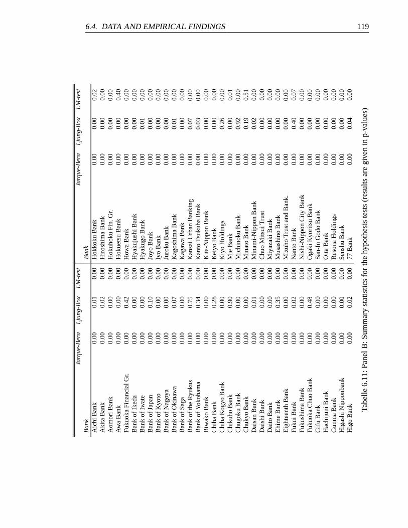
6.4. DATA AND EMPIRICAL FINDINGS 119
Jarq
ue-B
era
Lju
ng-B
oxL
M-t
est
Jarq
ue-B
era
Lju
ng-B
oxL
M-t
est
Ban
kB
ank
Aic
hiB
ank
0.00
0.01
0.00
Hok
koku
Ban
k0.
000.
000.
02A
kita
Ban
k0.
000.
020.
00H
iros
him
aB
ank
0.00
0.00
0.00
Aom
oriB
ank
0.00
0.00
0.00
Hok
uhok
uFi
n.G
r.0.
000.
000.
00A
wa
Ban
k0.
000.
000.
00H
okue
tsu
Ban
k0.
000.
000.
40Fu
kuok
aFi
nanc
ialG
r.0.
000.
420.
00H
owa
Ban
k0.
000.
000.
00B
ank
ofIk
eda
0.00
0.00
0.00
Hya
kuju
shiB
ank
0.00
0.00
0.00
Ban
kof
Iwat
e0.
000.
000.
00H
yaku
goB
ank
0.00
0.01
0.00
Ban
kof
Japa
n0.
000.
100.
00Jo
yoB
ank
0.00
0.00
0.00
Ban
kof
Kyo
to0.
000.
000.
00Iy
oB
ank
0.00
0.00
0.00
Ban
kof
Nag
oya
0.00
0.00
0.00
Juro
kuB
ank
0.00
0.00
0.00
Ban
kof
Oki
naw
a0.
000.
070.
00K
agos
him
aB
ank
0.00
0.01
0.00
Ban
kof
Saga
0.00
0.00
0.00
Kag
awa
Ban
k0.
000.
000.
00B
ank
ofth
eR
yuku
s0.
000.
750.
00K
ansa
iUrb
anB
anki
ng0.
000.
070.
00B
ank
ofY
okoh
ama
0.00
0.34
0.00
Kan
toT
suku
baB
ank
0.00
0.03
0.00
Biw
ako
Ban
k0.
000.
000.
00K
ita-N
ippo
nB
ank
0.00
0.00
0.00
Chi
baB
ank
0.00
0.28
0.00
Kei
yoB
ank
0.00
0.00
0.00
Chi
baK
ogyo
Ban
k0.
000.
000.
00K
iyo
Hol
ding
s0.
000.
260.
00C
hiku
hoB
ank
0.00
0.90
0.00
Mie
Ban
k0.
000.
000.
01C
hugo
kuB
ank
0.00
0.00
0.00
Mic
hino
kuB
ank
0.00
0.92
0.00
Chu
kyo
Ban
k0.
000.
000.
00M
inat
oB
ank
0.00
0.19
0.51
Dai
san
Ban
k0.
000.
010.
00M
inam
i-N
ippo
nB
ank
0.00
0.02
0.00
Dai
shiB
ank
0.00
0.00
0.00
Chu
oM
itsui
Tru
st0.
000.
000.
00D
aito
Ban
k0.
000.
000.
00M
iyaz
akiB
ank
0.00
0.00
0.00
Ehi
me
Ban
k0.
000.
350.
00M
usas
hino
Ban
k0.
000.
000.
00E
ight
eent
hB
ank
0.00
0.00
0.00
Miz
uho
Tru
stan
dB
ank.
0.00
0.00
0.00
Fuku
iBan
k0.
000.
020.
00N
anto
Ban
k0.
000.
400.
07Fu
kush
ima
Ban
k0.
000.
000.
00N
ishi
-Nip
pon
City
Ban
k0.
000.
000.
00Fu
kuok
aC
huo
Ban
k0.
000.
480.
00O
gaki
Kyo
rits
uB
ank
0.00
0.00
0.00
Gif
uB
ank
0.00
0.00
0.00
San-
InG
odo
Ban
k0.
000.
000.
00H
achi
juni
Ban
k0.
000.
000.
00O
itaB
ank
0.00
0.00
0.00
Gun
ma
Ban
k0.
000.
000.
00R
eson
aH
oldi
ngs
0.00
0.00
0.00
Hig
ashi
Nip
ponb
ank
0.00
0.00
0.00
Sens
huB
ank
0.00
0.00
0.00
Hig
oB
ank
0.00
0.02
0.00
77B
ank
0.00
0.04
0.00
Tabe
lle6.
11:P
anel
B:S
umm
ary
stat
istic
sfo
rth
ehy
poth
esis
test
s(r
esul
tsar
egi
ven
inp-
valu
es)
6.4. DATA AND EMPIRICAL FINDINGS 120
AR
MA
-GA
RC
Hε t
∼L
M-T
est
AR
MA
-GA
RC
Hε t
∼L
M-T
est
Ban
kB
ank
Aic
hiB
ank
(1,1
)-(2
,2)
skew
norm
.0.
26H
okko
kuB
ank
(1,1
)-(1
,1)
skew
t0.
39A
kita
Ban
k(1
,1)-
(1,1
)sk
ewt
0.15
Hir
oshi
ma
Ban
k(1
,1)-
(1,1
)sk
ewt
0.21
Aom
oriB
ank
(1,1
)-(1
,1)
skew
t0.
82H
okuh
oku
Fin.
Gr.
(1,1
)-(1
,1)
skew
t0.
80A
wa
Ban
k(1
,1)-
(1,1
)sk
ewt
0.49
Hok
uets
uB
ank
(1,1
)-(1
,1)
skew
t0.
56Fu
kuok
aFi
n.G
r.(1
,1)-
(1,1
)sk
ewt
0.26
How
aB
ank
(1,1
)-(1
,1)
skew
t0.
94B
ank
ofIk
eda
(1,1
)-(1
,1)
skew
t0.
98H
yaku
jush
iBan
k(1
,1)-
(1,1
)sk
ewt
0.96
Ban
kof
Iwat
e(1
,1)-
(1,1
)sk
ewt
0.88
Hya
kugo
Ban
k(1
,1)-
(1,1
)sk
ewt
0.12
Ban
kof
Japa
n(1
,1)-
(1,1
)sk
ewt
0.68
Joyo
Ban
k(1
,1)-
(1,1
)sk
ewt
0.71
Ban
kof
Kyo
to(1
,1)-
(1,1
)sk
ewt
0.99
Iyo
Ban
k(1
,1)-
(1,1
)sk
ewt
0.78
Ban
kof
Nag
oya
(1,1
)-(1
,1)
skew
t0.
99Ju
roku
Ban
k(1
,1)-
(1,1
)sk
ewt
0.83
Ban
kof
Oki
naw
a(1
,1)-
(1,1
)sk
ewt
0.87
Kag
oshi
ma
Ban
k(1
,1)-
(1,1
)sk
ewt
0.77
Ban
kof
Saga
(1,1
)-(1
,1)
skew
t0.
35K
agaw
aB
ank
(1,1
)-(1
,1)
skew
t0.
37B
ank
ofth
eR
yuku
s(1
,1)-
(1,1
)sk
ewt
0.85
Kan
saiU
rban
Ban
king
(1,1
)-(1
,1)
skew
t0.
52B
ank
ofY
okoh
ama
(1,1
)-(1
,1)
skew
t0.
94K
anto
Tsu
kuba
Ban
k(1
,1)-
(1,1
)sk
ewt
0.97
Biw
ako
Ban
k(1
,1)-
(1,1
)sk
ewt
0.99
Kita
-Nip
pon
Ban
k(1
,1)-
(1,1
)sk
ewt
0.29
Chi
baB
ank
(1,1
)-(1
,1)
skew
t0.
63K
eiyo
Ban
k(1
,1)-
(1,1
)sk
ewt
0.10
Chi
baK
ogyo
Ban
k(1
,1)-
(1,1
)sk
ewt
0.99
Kiy
oH
oldi
ngs
(1,1
)-(1
,1)
skew
t0.
99C
hiku
hoB
ank
(1,1
)-(1
,1)
skew
t0.
98M
ieB
ank
(1,1
)-(1
,1)
skew
t0.
48C
hugo
kuB
ank
(1,1
)-(1
,1)
skew
t0.
21M
ichi
noku
Ban
k(1
,1)-
(1,1
)sk
ewt
0.79
Chu
kyo
Ban
k(1
,1)-
(1,1
)sk
ewt
0.10
Min
ato
Ban
k(1
,1)-
(1,1
)sk
ewt
0.51
Dai
san
Ban
k(1
,1)-
(1,1
)sk
ewt
0.96
Min
ami-
Nip
pon
Ban
k(1
,1)-
(1,1
)sk
ewt
0.83
Dai
shiB
ank
(0,0
)-(2
,2)
Stud
ent’s
t0.
43C
huo
Mits
uiT
rust
(1,1
)-(1
,1)
skew
t0.
94D
aito
Ban
k(0
,0)-
(1,1
)St
uden
t’st
0.04
Miy
azak
iBan
k(1
,1)-
(1,1
)sk
ewt
0.96
Ehi
me
Ban
k(1
,1)-
(1,1
)sk
ewt
0.95
Mus
ashi
noB
ank
(1,1
)-(1
,1)
skew
t0.
58E
ight
eent
hB
ank
(1,1
)-(1
,1)
skew
t0.
67M
izuh
oT
rust
and
Ban
k.(1
,1)-
(1,1
)sk
ewt
0.87
Fuku
iBan
k(1
,1)-
(1,1
)sk
ewt
0.51
Nan
toB
ank
(1,1
)-(1
,1)
skew
t0.
93Fu
kush
ima
Ban
k(1
,1)-
(1,1
)sk
ewt
0.45
Nis
hi-N
ippo
nC
ityB
ank
(1,1
)-(1
,1)
skew
t0.
47Fu
kuok
aC
huo
Ban
k(1
,1)-
(1,1
)sk
ewt
0.42
Oga
kiK
yori
tsu
Ban
k(1
,1)-
(1,1
)sk
ewt
0.99
Gif
uB
ank
(0,0
)-(2
,2)
skew
norm
.0.
81Sa
n-In
God
oB
ank
(1,1
)-(1
,1)
skew
t0.
87H
achi
juni
Ban
k(1
,1)-
(1,1
)sk
ewt
0.88
Oita
Ban
k(1
,1)-
(1,1
)sk
ewt
0.96
Gun
ma
Ban
k(1
,1)-
(2,2
)no
rmal
0.12
Res
ona
Hol
ding
s(1
,1)-
(1,1
)sk
ewt
0.88
Hig
ashi
Nip
ponb
ank
(1,1
)-(1
,1)
skew
t0.
70Se
nshu
Ban
k(1
,1)-
(1,1
)sk
ewt
0.96
Hig
oB
ank
(1,1
)-(1
,1)
skew
t0.
7077
Ban
k(1
,1)-
(1,1
)sk
ewt
0.71
Tabe
lle6.
12:P
anel
B:M
odel
spec
ifica
tions
and
LM
test
stat
istic
s(p
-val
ues)
for
the
filte
red
retu
rns.
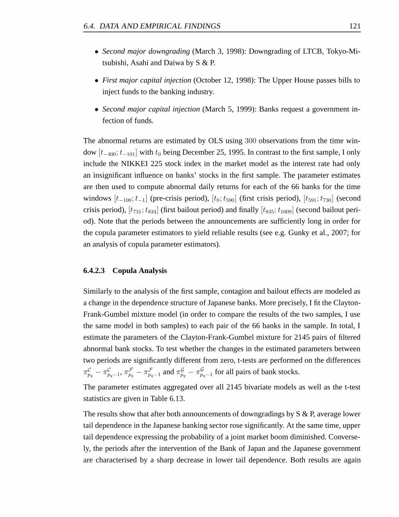
6.4. DATA AND EMPIRICAL FINDINGS 121
• Second major downgrading (March 3, 1998): Downgrading of LTCB, Tokyo-Mi-
tsubishi, Asahi and Daiwa by S & P.
• First major capital injection (October 12, 1998): The Upper House passes bills to
inject funds to the banking industry.
• Second major capital injection (March 5, 1999): Banks request a government in-
fection of funds.
The abnormal returns are estimated by OLS using 300 observations from the time win-
dow [t−400; t−101] with t0 being December 25, 1995. In contrast to the first sample, I only
include the NIKKEI 225 stock index in the market model as the interest rate had only
an insignificant influence on banks’ stocks in the first sample. The parameter estimates
are then used to compute abnormal daily returns for each of the 66 banks for the time
windows [t−100; t−1] (pre-crisis period), [t0; t590] (first crisis period), [t591; t730] (second
crisis period), [t731; t834] (first bailout period) and finally [t835; t1009] (second bailout peri-
od). Note that the periods between the announcements are sufficiently long in order for
the copula parameter estimators to yield reliable results (see e.g. Gunky et al., 2007; for
an analysis of copula parameter estimators).
6.4.2.3 Copula Analysis
Similarly to the analysis of the first sample, contagion and bailout effects are modeled as
a change in the dependence structure of Japanese banks. More precisely, I fit the Clayton-
Frank-Gumbel mixture model (in order to compare the results of the two samples, I use
the same model in both samples) to each pair of the 66 banks in the sample. In total, I
estimate the parameters of the Clayton-Frank-Gumbel mixture for 2145 pairs of filtered
abnormal bank stocks. To test whether the changes in the estimated parameters between
two periods are significantly different from zero, t-tests are performed on the differences
πCpq− πCpq−1, πFpq
− πFpq−1 and πGpq− πGpq−1 for all pairs of bank stocks.
The parameter estimates aggregated over all 2145 bivariate models as well as the t-test
statistics are given in Table 6.13.
The results show that after both announcements of downgradings by S & P, average lower
tail dependence in the Japanese banking sector rose significantly. At the same time, upper
tail dependence expressing the probability of a joint market boom diminished. Converse-
ly, the periods after the intervention of the Bank of Japan and the Japanese government
are characterised by a sharp decrease in lower tail dependence. Both results are again
6.4. DATA AND EMPIRICAL FINDINGS 122
Pre-
cris
isFi
rstc
risi
sSe
cond
cris
isFi
rstb
ailo
utSe
cond
bailo
ut
πG
0.29
100.
0155
0.00
940.
0289
0.03
51t-
test
*-4
0.28
-5.3
512
.31
3.25
πF
0.67
870.
1875
0.13
100.
8438
0.94
02t-
test
*-6
6.62
-15.
8012
6.23
20.3
4πC
0.03
020.
7969
0.85
950.
1271
0.02
46t-
test
*23
0.38
16.7
6-1
34.2
0-2
2.99
Tabe
lle6.
13:P
anel
B:A
vera
gere
sults
ofth
ebi
vari
ate
Cla
yton
-Fra
nk-G
umbe
lmod
els.
The
tabl
egi
ves
estim
ates
ofth
eco
effic
ient
sπG,πF
andπC
ofth
eco
nvex
com
bina
tion
aver
aged
over
all2
145
pair
wis
eco
mbi
natio
nsof
Japa
nese
bank
sas
wel
las
stat
istic
sfo
rth
et-
test
onth
em
ean
ofth
edi
ffer
ence
sin
the
para
met
eres
timat
es.
*A
lldi
ffer
ence
sar
esi
gnifi
cant
atth
e0.
1%le
vel.
The
time
win
dow
sar
ede
fined
asfo
llow
s:Pr
e-cr
isis
=[t−
100;t−
1].
Firs
tcri
sis=
[t0;t
590].
Seco
ndcr
isis
=[t
591;t
730].
Firs
tbai
lout
=[t
731;t
834].
Seco
ndba
ilout
=[t
835;t
1109].
6.5. CONCLUSION 123
consistent with the hypothesis of the probability of contagion increasing after negative
announcements concerning the stability of the Japanese financial sector and decreasing
after announcements of rescue measures by the state. Also, we can see that the decrease
in lower tail dependence was again substituted by tail independence. Just like in the first
sample the state’s rescue measures seem to be both effective and efficient in battling the
risk of contagion.
Again, we are interested to rule out the possibility of a bias in the copula models’ results
due to time-variations in the GARCH and market models’ parameters. Therefore, the
same robustness check as in the case of the German sample was applied to the Japanese
sample: instead of estimating the filtered abnormal returns by the use of just one constant
GARCH- and one market model, separate models were fitted to each of the time windows
in order to allow the GARCH- and market models to change between time windows.
The results of this robustness check are given in Table 6.14. Just like in the analysis
of the first data sample, the findings of the copula models remain true even with time-
varying GARCH- and market models. Furthermore, in unreported robustness checks the
results also proved to be robust to an exclusion of confounding events and also hold in a
multivariate analysis.
6.5 Conclusion
In this paper a new framework for detecting effects of bank contagion and bailouts by the
use of conventional event study and copula methodology was proposed. By estimating
GARCH-filtered abnormal returns instead of observed returns, the dependence structure
inherent in a banking sector is not biased by conditional heteroscedasticity in the variances
or the influences of common factors like e.g. the market return. By using copula metho-
dology instead of simply comparing abnormal returns, the contagion and bailout effects
can be analysed directly as a change of the dependence structure.
The empirical study in this paper analysed the changes in the dependence structure of bank
stocks around announcements of financial crisis in Germany during the Subprime crisis
as well as during Japan’s banking crisis in the nineties. The results for both samples show
that significant contagion effects could be detected in both banking sectors after clear
announcements of crisis (i.e. announcements that were not accompanied by immediate
bailout announcements). After the announcements of the state acting as a lender of last
resort to troubled banks, lower tail dependence was effectively reduced while at the same
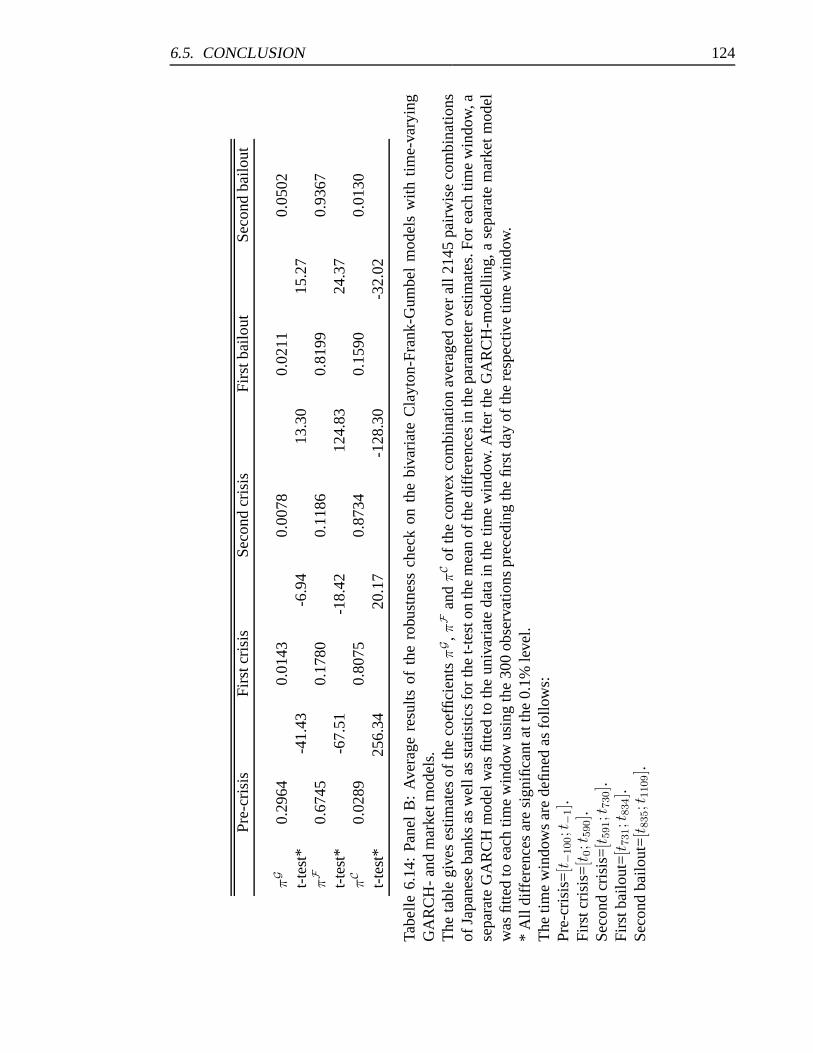
6.5. CONCLUSION 124
Pre-
cris
isFi
rstc
risi
sSe
cond
cris
isFi
rstb
ailo
utSe
cond
bailo
ut
πG
0.29
640.
0143
0.00
780.
0211
0.05
02t-
test
*-4
1.43
-6.9
413
.30
15.2
7πF
0.67
450.
1780
0.11
860.
8199
0.93
67t-
test
*-6
7.51
-18.
4212
4.83
24.3
7πC
0.02
890.
8075
0.87
340.
1590
0.01
30t-
test
*25
6.34
20.1
7-1
28.3
0-3
2.02
Tabe
lle6.
14:
Pane
lB
:A
vera
gere
sults
ofth
ero
bust
ness
chec
kon
the
biva
riat
eC
layt
on-F
rank
-Gum
bel
mod
els
with
time-
vary
ing
GA
RC
H-
and
mar
ketm
odel
s.T
heta
ble
give
ses
timat
esof
the
coef
ficie
ntsπG,πF
andπC
ofth
eco
nvex
com
bina
tion
aver
aged
over
all2
145
pair
wis
eco
mbi
natio
nsof
Japa
nese
bank
sas
wel
las
stat
istic
sfo
rth
et-
test
onth
em
ean
ofth
edi
ffer
ence
sin
the
para
met
eres
timat
es.F
orea
chtim
ew
indo
w,a
sepa
rate
GA
RC
Hm
odel
was
fitte
dto
the
univ
aria
teda
tain
the
time
win
dow
.Aft
erth
eG
AR
CH
-mod
ellin
g,a
sepa
rate
mar
ket
mod
elw
asfit
ted
toea
chtim
ew
indo
wus
ing
the
300
obse
rvat
ions
prec
edin
gth
efir
stda
yof
the
resp
ectiv
etim
ew
indo
w.
*A
lldi
ffer
ence
sar
esi
gnifi
cant
atth
e0.
1%le
vel.
The
time
win
dow
sar
ede
fined
asfo
llow
s:Pr
e-cr
isis
=[t−
100;t−
1].
Firs
tcri
sis=
[t0;t
590].
Seco
ndcr
isis
=[t
591;t
730].
Firs
tbai
lout
=[t
731;t
834].
Seco
ndba
ilout
=[t
835;t
1109].
6.5. CONCLUSION 125
time tail independence increased significantly. All given results also hold in a multivariate
setting and are robust to an exclusion of confounding events as well as to time-variations
in the univariate models.
The described shift in tail dependence indicates that the bailout announcements did not
simply restore the pre-crisis dependence structure, but rather only decreased the likelihood
of a joint crash of bank stocks. This finding is consistent with the wish of policy makers
to decrease the probability of contagion without giving away free lunches to banks. One
topic not addressed in this paper is the question which factors of the banking system
determine the likelihood of contagion effects and the success of bailouts. To answer this
question, more examples of bank contagion and bailouts need to be analysed in future
research complemented by cross-sectional analyses.
Kapitel A
Literatur
[1] AHARONY, Joseph ; SWARY, Itzhak: Contagion effects of bank failures: Evidence
from capital markets. In: Journal of Business (1983), S. 305–322.
[2] AKHIGBE, Aigbe ; MADURA, Jeff: Why do contagion effects vary among bank
failures? In: Journal of Banking & Finance (2001), S. 657–680.
[3] ALEXANDER, Carol ; SHEEDY, Elizabeth: Developing a stress testing framework
based on market risk models. In: Journal of Banking & Finance 32. Jg. (2008), S.
2220–2236.
[4] ALLEN, Franklin ; GALE, Douglas: Financial Contagion. In: Journal of Political
Economy (2000), S. 1–33.
[5] ANDERSON, Theodore Wilbur J.: On the distribution of the Two-Sample Cramer-
von Mises Criterion. In: Annals of Mathematical Statistics 33. Jg. (1962), S. 1148–
1159.
[6] ANDERSON, Theodore Wilbur J. ; DARLING, Donald A.: A test of goodness of fit.
In: Journal of the American Statistical Association 49. Jg. (1954), S. 165–769.
[7] ANE, Thierry ; KHAROUBI, Cecile: Dependence Structure and Risk Measure. In:
Journal of Business (2003), S. 411–438.
[8] ARTZNER, Philippe ; DELBAEN, Freddy ; EBER, Jean-Marc ; HEATH, David: Co-
herent Measures of Risk. In: Mathematical Finance 9. Jg. (1999), S. 203–228.
[9] ASCHINGER, Gerhard: Borsenkrach und Spekulation – eine okonomische Analyse.
Franz Vahlen Verlag, Munchen, 1995.
[10] BAGEHOT, Walter: Lombard Street: A Description of the Money Market. London,
1873.
[11] BALAKRISHNAN, Narayanaswamy ; LAI, Chin-Diew: Continuous Bivariate Dis-
tributions, Emphasising Applications. Rumbsy Scientific Publishing, 1990.
126
KAPITEL A. LITERATUR 127
[12] BARTRAM, Sohnke ; TAYLOR, Steven ; WANG, Yaw-Huei: The Euro and European
financial market dependence. In: Journal of Banking & Finance 31. Jg. (2007), S.
1461–1481.
[13] BERG, Daniel: Copula Goodness-of-fit testing: An overview and power compari-
son. In: European Journal of Finance (im Erscheinen).
[14] BESSLER, Wolfgang ; NOHEL, Tom: Asymmetric Information, Dividend Reduc-
tions, and Contagion Effects in Bank Stock Returns. In: Journal of Banking &
Finance 24. Jg. (2000), S. 1831–1846.
[15] BHATTACHARYA, Sudipto ; THAKOR, Anjan: Contemporary banking theory. In:
Journal of Banking & Finance 3. Jg. (1993), S. 2–50.
[16] BIAU, Gerard ; WEGKAMP, Marten: A Note on Minimum Distance Estimation of
Copula Densities. In: Statistics and Probability Letters 73. Jg. (2005), S. 105–114.
[17] BOLLERSLEV, Tim: Generalized autoregressive conditional heteroskedasticity. In:
Journal of Econometrics 31. Jg. (1986), S. 307–327.
[18] BOLLERSLEV, Tim ; CHOU, Ray ; KRONER, Kenneth: ARCH modeling in finance.
In: Journal of Econometrics 52. Jg. (1992), S. 5–59.
[19] BOLLERSLEV, Tim ; WOOLDRIDGE, Jeffrey: Quasi-maximum likelihood estima-
tion and inference in dynamic models with time-varying covariances. In: Econo-
metric Reviews 11. Jg. (1992), S. 143–172.
[20] BOUYE, Eric: Multivariate extremes at work for portfolio risk measurement. Wor-
king paper City University Business School, London, 2003.
[21] BOUYE, Eric ; DURRLEMAN, Valdo ; NIKEGHBALI, Ashkan ; RIBOU-
LET, Gael ; RONCALLI, Thierry: Copulas for Finance . A Reading Gui-
de and Some Applications. 2000. – Im Internet abrufbar unter: http :
//papers.ssrn.com/sol3/Delivery.cfm/SSRN ID1032533 code903940.pdf?-
abstractid = 1032533&mirid = 1.
[22] BREYMANN, Wolfgang ; DIAS, Alexandra ; EMBRECHTS, Paul: Dependence
structures for multivariate high-frequency data in finance. In: Quantitative Finance
3. Jg. (2003), S. 1–14.
KAPITEL A. LITERATUR 128
[23] BUTKIEWICZ, James: The Impact of a Lender of Last Resort during the Great
Depression: The Case of the Reconstruction Finance Corporation. In: Explorations
in Economic History 32. Jg. (2) (1995), S. 197–216.
[24] BYRD, Richard ; LU, Peihuang ; NOCEDAL, Jorge ; ZHU, Ciyou: A Limited Me-
mory Algorithm for Bound Constrained Optimization. In: SIAM Journal on Scien-
tific and Statistical Computing 16. Jg. (1995), S. 1190–1208.
[25] CALOMIRIS, Charles ; MASON, James: Contagion and Bank Failures During the
Great Depression: The June 1932 Chicago Banking Panic. In: American Economic
Review 87. Jg. (1997), S. 863–883.
[26] CHEN, Sichong ; POON, Ser-Huang: Modelling International Stock Market Con-
tagion Using Copula and Risk Appetite. – Working Paper 2007.
[27] CHEN, Song ; HUANG, Tzee-Ming: Nonparametric Estimation of Copula Functi-
ons for Dependence Modeling. In: Canadian Journal of Statistics 35. Jg. (1997),
S. 1–20.
[28] CHEN, Xiaohong ; FAN, Yanqin: Estimation of Copula-Based Semiparametric
Time Series Models. In: Journal of Econometrics 130. Jg. (2006), S. 307–335.
[29] CHERUBINI, Umberto ; LUCIANO, Elisa ; VECCHIATO, Walter: Copula Methods
in Finance. John Wiley & Sons, Chichester & New York, 2004.
[30] CHRISTOFFERSEN, Peter: Evaluating Interval Forecasts. In: International Econo-
mic Review 4. Jg. (1998), S. 841–862.
[31] CHRISTOFFERSEN, Peter ; PELLETIER, Denis: Backtesting Value-at-Risk: A
Duration-Based Approach. In: Journal of Financial Econometrics 2. Jg. (2004),
S. 84–108.
[32] CLAYTON, David G.: A model for association in bivariate life tables and its appli-
cation in epidemiological studies of familial tendency in chronic disease incidence.
In: Biometrika 65. Jg. (1978), S. 141–151.
[33] COOK, Dennis R. ; JOHNSON, Mark E.: A family of distributions for modelling
non-elliptically symmetric multivariate data. In: Journal of the Royal Statistical
Society B 43. Jg. (1981), S. 210–218.
[34] CORRIGAN, E. G.: The Banking-Commerce Controversy Revisited. In: Quarterly
Review, Federal Reserve Bank of New York 16. Jg. (1991), S. 1–13.
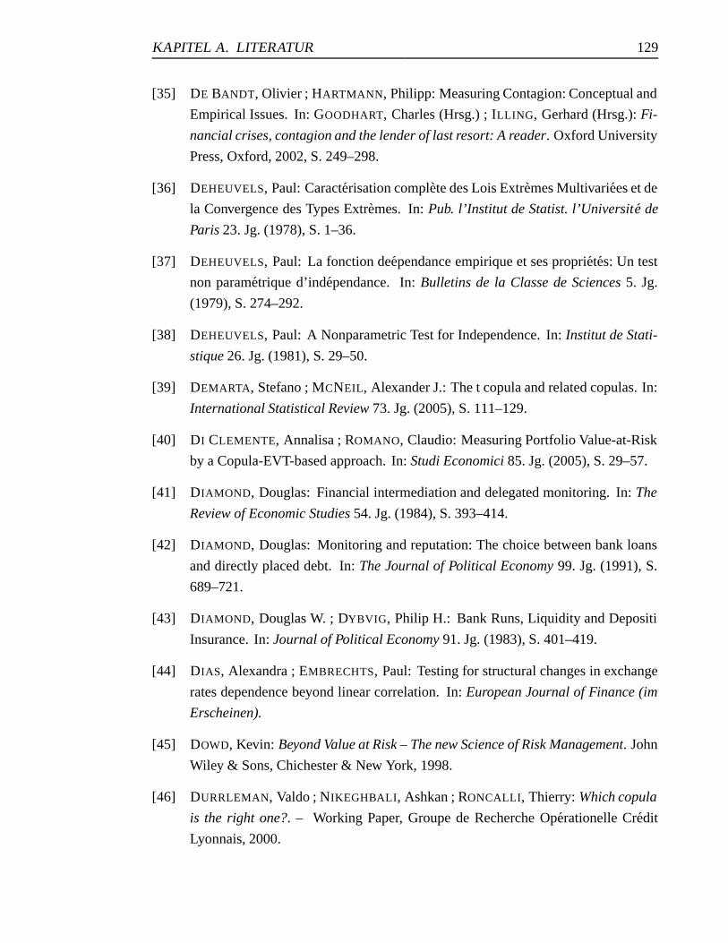
KAPITEL A. LITERATUR 129
[35] DE BANDT, Olivier ; HARTMANN, Philipp: Measuring Contagion: Conceptual and
Empirical Issues. In: GOODHART, Charles (Hrsg.) ; ILLING, Gerhard (Hrsg.): Fi-
nancial crises, contagion and the lender of last resort: A reader. Oxford University
Press, Oxford, 2002, S. 249–298.
[36] DEHEUVELS, Paul: Caracterisation complete des Lois Extremes Multivariees et de
la Convergence des Types Extremes. In: Pub. l’Institut de Statist. l’Universite de
Paris 23. Jg. (1978), S. 1–36.
[37] DEHEUVELS, Paul: La fonction deependance empirique et ses proprietes: Un test
non parametrique d’independance. In: Bulletins de la Classe de Sciences 5. Jg.
(1979), S. 274–292.
[38] DEHEUVELS, Paul: A Nonparametric Test for Independence. In: Institut de Stati-
stique 26. Jg. (1981), S. 29–50.
[39] DEMARTA, Stefano ; MCNEIL, Alexander J.: The t copula and related copulas. In:
International Statistical Review 73. Jg. (2005), S. 111–129.
[40] DI CLEMENTE, Annalisa ; ROMANO, Claudio: Measuring Portfolio Value-at-Risk
by a Copula-EVT-based approach. In: Studi Economici 85. Jg. (2005), S. 29–57.
[41] DIAMOND, Douglas: Financial intermediation and delegated monitoring. In: The
Review of Economic Studies 54. Jg. (1984), S. 393–414.
[42] DIAMOND, Douglas: Monitoring and reputation: The choice between bank loans
and directly placed debt. In: The Journal of Political Economy 99. Jg. (1991), S.
689–721.
[43] DIAMOND, Douglas W. ; DYBVIG, Philip H.: Bank Runs, Liquidity and Depositi
Insurance. In: Journal of Political Economy 91. Jg. (1983), S. 401–419.
[44] DIAS, Alexandra ; EMBRECHTS, Paul: Testing for structural changes in exchange
rates dependence beyond linear correlation. In: European Journal of Finance (im
Erscheinen).
[45] DOWD, Kevin: Beyond Value at Risk – The new Science of Risk Management. John
Wiley & Sons, Chichester & New York, 1998.
[46] DURRLEMAN, Valdo ; NIKEGHBALI, Ashkan ; RONCALLI, Thierry: Which copula
is the right one?. – Working Paper, Groupe de Recherche Operationelle Credit
Lyonnais, 2000.
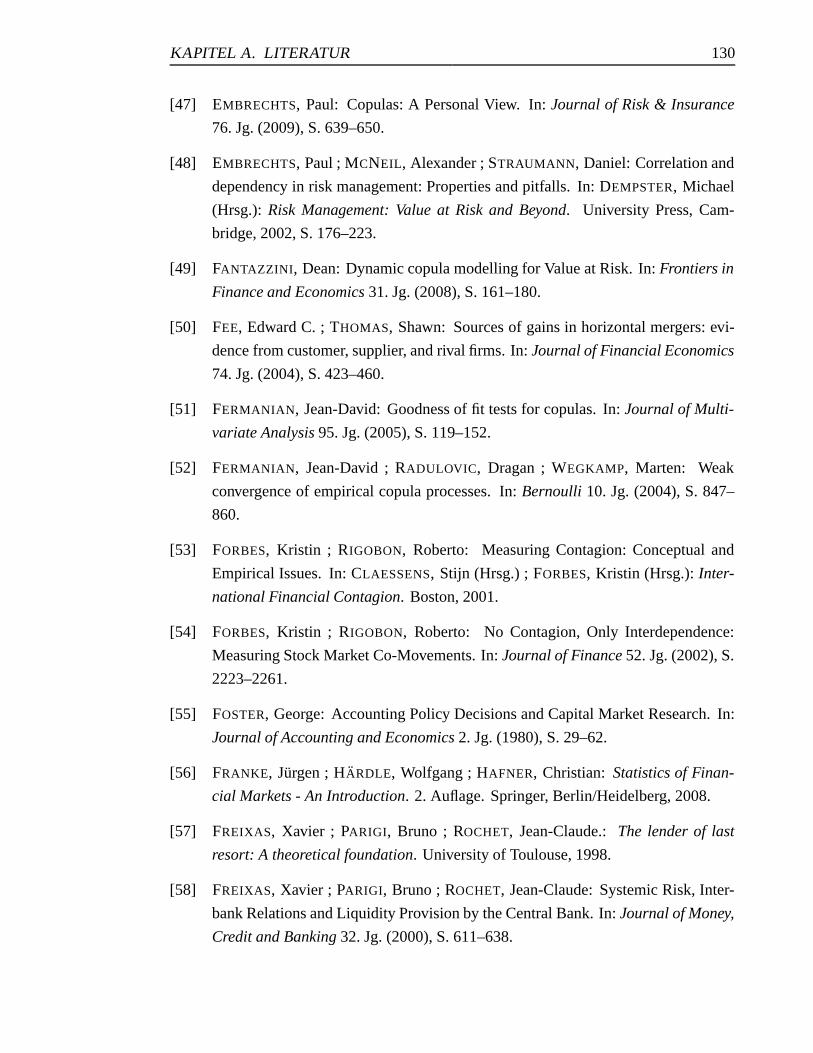
KAPITEL A. LITERATUR 130
[47] EMBRECHTS, Paul: Copulas: A Personal View. In: Journal of Risk & Insurance
76. Jg. (2009), S. 639–650.
[48] EMBRECHTS, Paul ; MCNEIL, Alexander ; STRAUMANN, Daniel: Correlation and
dependency in risk management: Properties and pitfalls. In: DEMPSTER, Michael
(Hrsg.): Risk Management: Value at Risk and Beyond. University Press, Cam-
bridge, 2002, S. 176–223.
[49] FANTAZZINI, Dean: Dynamic copula modelling for Value at Risk. In: Frontiers in
Finance and Economics 31. Jg. (2008), S. 161–180.
[50] FEE, Edward C. ; THOMAS, Shawn: Sources of gains in horizontal mergers: evi-
dence from customer, supplier, and rival firms. In: Journal of Financial Economics
74. Jg. (2004), S. 423–460.
[51] FERMANIAN, Jean-David: Goodness of fit tests for copulas. In: Journal of Multi-
variate Analysis 95. Jg. (2005), S. 119–152.
[52] FERMANIAN, Jean-David ; RADULOVIC, Dragan ; WEGKAMP, Marten: Weak
convergence of empirical copula processes. In: Bernoulli 10. Jg. (2004), S. 847–
860.
[53] FORBES, Kristin ; RIGOBON, Roberto: Measuring Contagion: Conceptual and
Empirical Issues. In: CLAESSENS, Stijn (Hrsg.) ; FORBES, Kristin (Hrsg.): Inter-
national Financial Contagion. Boston, 2001.
[54] FORBES, Kristin ; RIGOBON, Roberto: No Contagion, Only Interdependence:
Measuring Stock Market Co-Movements. In: Journal of Finance 52. Jg. (2002), S.
2223–2261.
[55] FOSTER, George: Accounting Policy Decisions and Capital Market Research. In:
Journal of Accounting and Economics 2. Jg. (1980), S. 29–62.
[56] FRANKE, Jurgen ; HARDLE, Wolfgang ; HAFNER, Christian: Statistics of Finan-
cial Markets - An Introduction. 2. Auflage. Springer, Berlin/Heidelberg, 2008.
[57] FREIXAS, Xavier ; PARIGI, Bruno ; ROCHET, Jean-Claude.: The lender of last
resort: A theoretical foundation. University of Toulouse, 1998.
[58] FREIXAS, Xavier ; PARIGI, Bruno ; ROCHET, Jean-Claude: Systemic Risk, Inter-
bank Relations and Liquidity Provision by the Central Bank. In: Journal of Money,
Credit and Banking 32. Jg. (2000), S. 611–638.
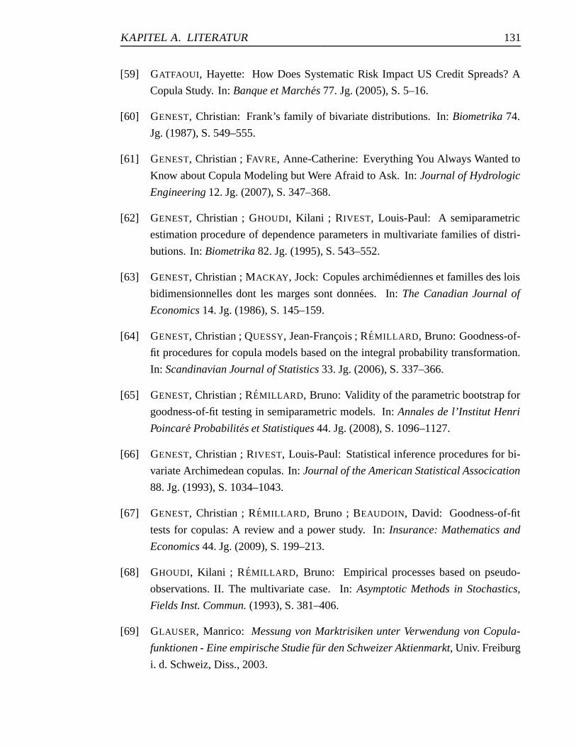
KAPITEL A. LITERATUR 131
[59] GATFAOUI, Hayette: How Does Systematic Risk Impact US Credit Spreads? A
Copula Study. In: Banque et Marches 77. Jg. (2005), S. 5–16.
[60] GENEST, Christian: Frank’s family of bivariate distributions. In: Biometrika 74.
Jg. (1987), S. 549–555.
[61] GENEST, Christian ; FAVRE, Anne-Catherine: Everything You Always Wanted to
Know about Copula Modeling but Were Afraid to Ask. In: Journal of Hydrologic
Engineering 12. Jg. (2007), S. 347–368.
[62] GENEST, Christian ; GHOUDI, Kilani ; RIVEST, Louis-Paul: A semiparametric
estimation procedure of dependence parameters in multivariate families of distri-
butions. In: Biometrika 82. Jg. (1995), S. 543–552.
[63] GENEST, Christian ; MACKAY, Jock: Copules archimediennes et familles des lois
bidimensionnelles dont les marges sont donnees. In: The Canadian Journal of
Economics 14. Jg. (1986), S. 145–159.
[64] GENEST, Christian ; QUESSY, Jean-Francois ; REMILLARD, Bruno: Goodness-of-
fit procedures for copula models based on the integral probability transformation.
In: Scandinavian Journal of Statistics 33. Jg. (2006), S. 337–366.
[65] GENEST, Christian ; REMILLARD, Bruno: Validity of the parametric bootstrap for
goodness-of-fit testing in semiparametric models. In: Annales de l’Institut Henri
Poincare Probabilites et Statistiques 44. Jg. (2008), S. 1096–1127.
[66] GENEST, Christian ; RIVEST, Louis-Paul: Statistical inference procedures for bi-
variate Archimedean copulas. In: Journal of the American Statistical Assocication
88. Jg. (1993), S. 1034–1043.
[67] GENEST, Christian ; REMILLARD, Bruno ; BEAUDOIN, David: Goodness-of-fit
tests for copulas: A review and a power study. In: Insurance: Mathematics and
Economics 44. Jg. (2009), S. 199–213.
[68] GHOUDI, Kilani ; REMILLARD, Bruno: Empirical processes based on pseudo-
observations. II. The multivariate case. In: Asymptotic Methods in Stochastics,
Fields Inst. Commun. (1993), S. 381–406.
[69] GLAUSER, Manrico: Messung von Marktrisiken unter Verwendung von Copula-
funktionen - Eine empirische Studie fur den Schweizer Aktienmarkt, Univ. Freiburg
i. d. Schweiz, Diss., 2003.
KAPITEL A. LITERATUR 132
[70] GOODHART, Charles A. ; HUANG, Haizhou: The lender of last resort. In: Journal
of Banking & Finance 29. Jg. (2005), S. 1059–1082.
[71] GORTON, Gary: Bank suspension of convertibility. In: Journal of Monetary Eco-
nomics 15. Jg. (1985), S. 177–193.
[72] GORTON, Gary ; HUANG, Lixin: Bank panics and the Endogeneity of Central
Banking. In: Journal of Monetary Economics 53. Jg. (2006), S. 1613–1629.
[73] GROPP, Reint ; LO DUCA, Marco ; VESALA, Jukka: Cross-Border Bank Con-
tagion in Europe. In: International Journal of Central Banking 5. Jg. (2009), S.
97–139.
[74] GROPP, Reint ; MOERMAN, Gerard: Measurement of contagion in banks’ equity
prices. In: Journal of International Money and Finance 23. Jg. (2004), S. 405–459.
[75] GROPP, Reint ; VESALA, Jukka: Measuring Bank Contagion using Market Data.
In: The Evolving Financial System and Public Policy. Bank of Canada, 2004.
[76] HARTMANN-WENDELS, Thomas ; PFINGSTEN, Andreas ; WEBER, Martin: Bank-
betriebslehre. 4. uberarb. Auflage. Springer Verlag, Berlin/Heidelberg, 2006.
[77] HASMAN, Augusto ; SAMARTIN, Margarita: Information acquisition and financial
contagion. In: Journal of Banking & Finance 32. Jg. (2008), S. 2136–2147.
[78] HOEFFDING, Wassily: Scale invariant correlation theory. In: Schriften Mathemati-
sches Institut Universitat Berlin 5. Jg. (1940), S. 181–233.
[79] HUARD, David ; EVIN, Guillaume ; FAVRE, Anne-Catherine: Bayesian copula
selection. In: Computational Statistics & Data Analysis 51. Jg. (2006), S. 809–
822.
[80] IYER, Rajkamal ; PEYDRO, Jose L.: Interbank Contagion: Evidence from Real
Transactions. In: EFA 2006 Zurich Meetings (2009). – Im Internet abrufbar unter:
http : //papers.ssrn.com/sol3/papers.cfm?abstract id = 895061.
[81] JAMES, Christopher: The Losses Realized in Bank Failures. In: Journal of Finance
46. Jg. (1991), S. 1223–1242.
[82] JOE, Harry: Multivariate Models and Dependence Concepts. Chapman & Hall,
London, 1997.
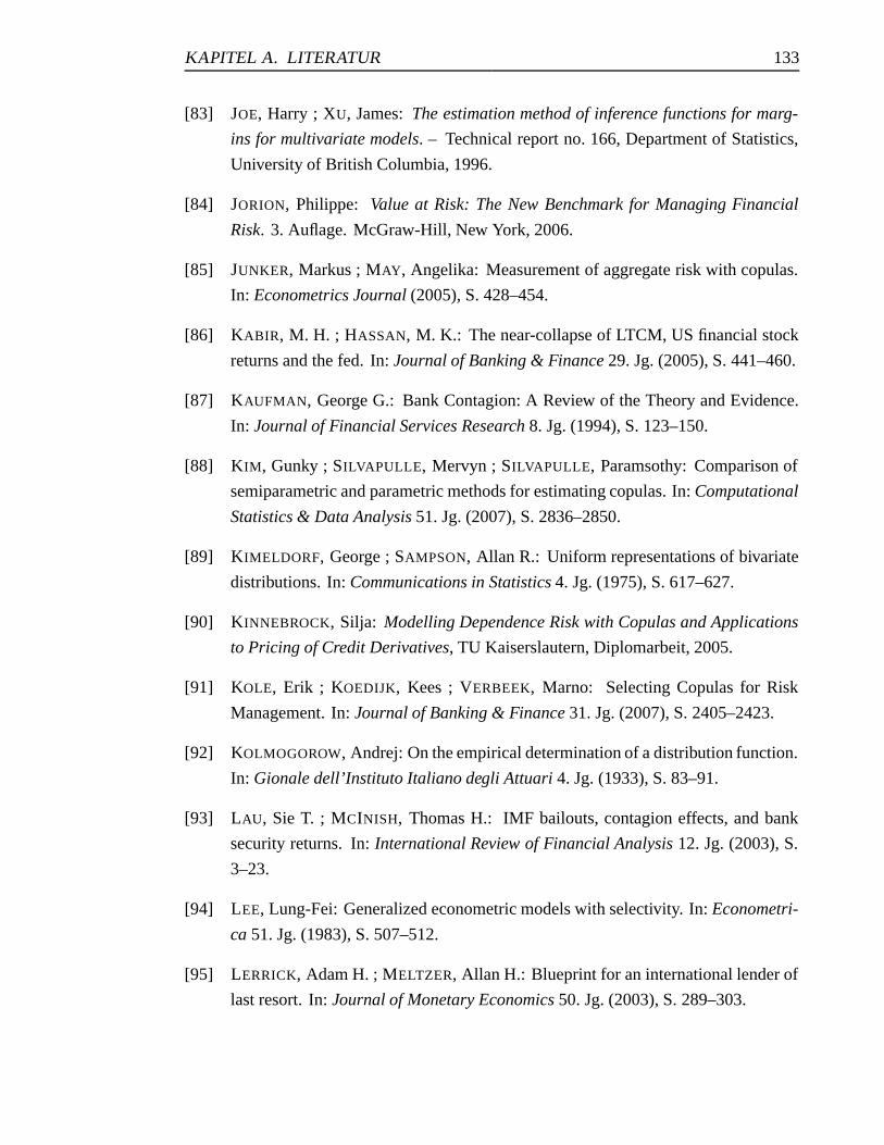
KAPITEL A. LITERATUR 133
[83] JOE, Harry ; XU, James: The estimation method of inference functions for marg-
ins for multivariate models. – Technical report no. 166, Department of Statistics,
University of British Columbia, 1996.
[84] JORION, Philippe: Value at Risk: The New Benchmark for Managing Financial
Risk. 3. Auflage. McGraw-Hill, New York, 2006.
[85] JUNKER, Markus ; MAY, Angelika: Measurement of aggregate risk with copulas.
In: Econometrics Journal (2005), S. 428–454.
[86] KABIR, M. H. ; HASSAN, M. K.: The near-collapse of LTCM, US financial stock
returns and the fed. In: Journal of Banking & Finance 29. Jg. (2005), S. 441–460.
[87] KAUFMAN, George G.: Bank Contagion: A Review of the Theory and Evidence.
In: Journal of Financial Services Research 8. Jg. (1994), S. 123–150.
[88] KIM, Gunky ; SILVAPULLE, Mervyn ; SILVAPULLE, Paramsothy: Comparison of
semiparametric and parametric methods for estimating copulas. In: Computational
Statistics & Data Analysis 51. Jg. (2007), S. 2836–2850.
[89] KIMELDORF, George ; SAMPSON, Allan R.: Uniform representations of bivariate
distributions. In: Communications in Statistics 4. Jg. (1975), S. 617–627.
[90] KINNEBROCK, Silja: Modelling Dependence Risk with Copulas and Applications
to Pricing of Credit Derivatives, TU Kaiserslautern, Diplomarbeit, 2005.
[91] KOLE, Erik ; KOEDIJK, Kees ; VERBEEK, Marno: Selecting Copulas for Risk
Management. In: Journal of Banking & Finance 31. Jg. (2007), S. 2405–2423.
[92] KOLMOGOROW, Andrej: On the empirical determination of a distribution function.
In: Gionale dell’Instituto Italiano degli Attuari 4. Jg. (1933), S. 83–91.
[93] LAU, Sie T. ; MCINISH, Thomas H.: IMF bailouts, contagion effects, and bank
security returns. In: International Review of Financial Analysis 12. Jg. (2003), S.
3–23.
[94] LEE, Lung-Fei: Generalized econometric models with selectivity. In: Econometri-
ca 51. Jg. (1983), S. 507–512.
[95] LERRICK, Adam H. ; MELTZER, Allan H.: Blueprint for an international lender of
last resort. In: Journal of Monetary Economics 50. Jg. (2003), S. 289–303.
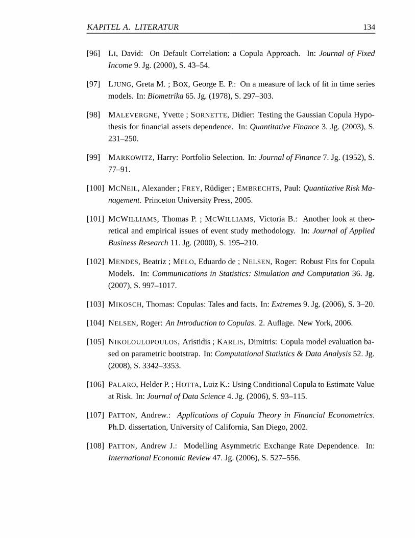
KAPITEL A. LITERATUR 134
[96] LI, David: On Default Correlation: a Copula Approach. In: Journal of Fixed
Income 9. Jg. (2000), S. 43–54.
[97] LJUNG, Greta M. ; BOX, George E. P.: On a measure of lack of fit in time series
models. In: Biometrika 65. Jg. (1978), S. 297–303.
[98] MALEVERGNE, Yvette ; SORNETTE, Didier: Testing the Gaussian Copula Hypo-
thesis for financial assets dependence. In: Quantitative Finance 3. Jg. (2003), S.
231–250.
[99] MARKOWITZ, Harry: Portfolio Selection. In: Journal of Finance 7. Jg. (1952), S.
77–91.
[100] MCNEIL, Alexander ; FREY, Rudiger ; EMBRECHTS, Paul: Quantitative Risk Ma-
nagement. Princeton University Press, 2005.
[101] MCWILLIAMS, Thomas P. ; MCWILLIAMS, Victoria B.: Another look at theo-
retical and empirical issues of event study methodology. In: Journal of Applied
Business Research 11. Jg. (2000), S. 195–210.
[102] MENDES, Beatriz ; MELO, Eduardo de ; NELSEN, Roger: Robust Fits for Copula
Models. In: Communications in Statistics: Simulation and Computation 36. Jg.
(2007), S. 997–1017.
[103] MIKOSCH, Thomas: Copulas: Tales and facts. In: Extremes 9. Jg. (2006), S. 3–20.
[104] NELSEN, Roger: An Introduction to Copulas. 2. Auflage. New York, 2006.
[105] NIKOLOULOPOULOS, Aristidis ; KARLIS, Dimitris: Copula model evaluation ba-
sed on parametric bootstrap. In: Computational Statistics & Data Analysis 52. Jg.
(2008), S. 3342–3353.
[106] PALARO, Helder P. ; HOTTA, Luiz K.: Using Conditional Copula to Estimate Value
at Risk. In: Journal of Data Science 4. Jg. (2006), S. 93–115.
[107] PATTON, Andrew.: Applications of Copula Theory in Financial Econometrics.
Ph.D. dissertation, University of California, San Diego, 2002.
[108] PATTON, Andrew J.: Modelling Asymmetric Exchange Rate Dependence. In:
International Economic Review 47. Jg. (2006), S. 527–556.
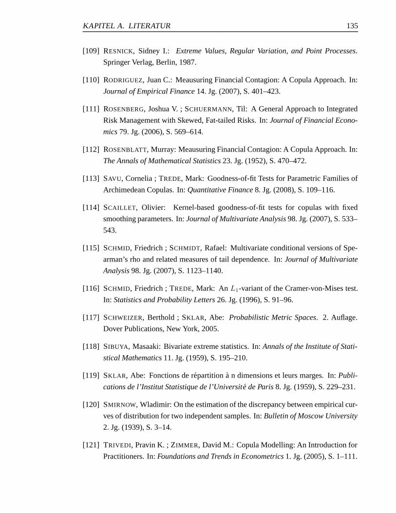
KAPITEL A. LITERATUR 135
[109] RESNICK, Sidney I.: Extreme Values, Regular Variation, and Point Processes.
Springer Verlag, Berlin, 1987.
[110] RODRIGUEZ, Juan C.: Meausuring Financial Contagion: A Copula Approach. In:
Journal of Empirical Finance 14. Jg. (2007), S. 401–423.
[111] ROSENBERG, Joshua V. ; SCHUERMANN, Til: A General Approach to Integrated
Risk Management with Skewed, Fat-tailed Risks. In: Journal of Financial Econo-
mics 79. Jg. (2006), S. 569–614.
[112] ROSENBLATT, Murray: Meausuring Financial Contagion: A Copula Approach. In:
The Annals of Mathematical Statistics 23. Jg. (1952), S. 470–472.
[113] SAVU, Cornelia ; TREDE, Mark: Goodness-of-fit Tests for Parametric Families of
Archimedean Copulas. In: Quantitative Finance 8. Jg. (2008), S. 109–116.
[114] SCAILLET, Olivier: Kernel-based goodness-of-fit tests for copulas with fixed
smoothing parameters. In: Journal of Multivariate Analysis 98. Jg. (2007), S. 533–
543.
[115] SCHMID, Friedrich ; SCHMIDT, Rafael: Multivariate conditional versions of Spe-
arman’s rho and related measures of tail dependence. In: Journal of Multivariate
Analysis 98. Jg. (2007), S. 1123–1140.
[116] SCHMID, Friedrich ; TREDE, Mark: An L1-variant of the Cramer-von-Mises test.
In: Statistics and Probability Letters 26. Jg. (1996), S. 91–96.
[117] SCHWEIZER, Berthold ; SKLAR, Abe: Probabilistic Metric Spaces. 2. Auflage.
Dover Publications, New York, 2005.
[118] SIBUYA, Masaaki: Bivariate extreme statistics. In: Annals of the Institute of Stati-
stical Mathematics 11. Jg. (1959), S. 195–210.
[119] SKLAR, Abe: Fonctions de repartition a n dimensions et leurs marges. In: Publi-
cations de l’Institut Statistique de l’Universite de Paris 8. Jg. (1959), S. 229–231.
[120] SMIRNOW, Wladimir: On the estimation of the discrepancy between empirical cur-
ves of distribution for two independent samples. In: Bulletin of Moscow University
2. Jg. (1939), S. 3–14.
[121] TRIVEDI, Pravin K. ; ZIMMER, David M.: Copula Modelling: An Introduction for
Practitioners. In: Foundations and Trends in Econometrics 1. Jg. (2005), S. 1–111.
KAPITEL A. LITERATUR 136
[122] TSUKAHARA, Hideatsu: Semiparametric estimation in copula models. In: Cana-
dian Journal of Statistics 33. Jg. (2005), S. 357–375.
[123] YORULMAZER, Tanju: Liquidity, Bank Runs and Bailouts: Spillover Effects during
the Northern Rock Episode. – Working paper, Federal Reserve Bank of New York,
2008.
Anhang B
Empirical observators for the
MD-estimators based on Kendall’s
dependence function
Goal:
To compute an approximation to the distances ρL1
k , ρCvMK and ρKS
K dependent on a given
sample U, a hypothesised parametric copula family C and a parameter θ.
Algorithm:
(1) Choose m ≥ n.
(2) Generate a random sample U∗1, . . . ,U∗m of size m from the copula Cθ.
(3) Compute the transformed data
V ∗i ≡ 1
m
m∑j=1
1(U∗j ≤ U∗i ), i ∈ {1, . . . , m} .
(4) Approximate Kθ by
Bm(t) ≡ 1
m
m∑i=1
1(V ∗i ≤ t), t ∈ [0; 1].
(5) Approximate ρL1k , ρCvM
K and ρKSK by
ρL1k ≡ n
m
m∑i=1
|Kn(V ∗i ) − Bm(V ∗i )|
ρCvMk ≡ n
m
m∑i=1
{Kn(V ∗i ) − Bm(V ∗i )}2
137
ANHANG B. EMPIRICAL OBSERVATORS FOR THE MD-ESTIMATORS BASED
ON KENDALL’S DEPENDENCE FUNCTION138
ρKSk ≡ max
i∈Nm
|Kn(V ∗i ) − Bm(V ∗i )|
Anhang C
Outline of the L-BFGS-B algorithm
In the following the L-BFGS-B algorithm is described (see Byrd et al., 1995). Consider
a nonlinear objective function f : Rn → R whose gradient g is given. The approximate
solution for
min f(Λ)
subject to l ≤ Λ ≤ u, where l and u are lower and upper bounds on the parameter vector
is computed iteratively by the following rule:
Assume that the current iterate Λk, the function value at fk, the gradient gk and a positive
definite limited memory Hessian approximation Bk have already been computed. This
allows us to form a quadratic model of f at Λk:
mk(Λ) = f(Λk) + gTk (Λ − Λk) +
1
2(Λ − Λk)
TBk(Λ − Λk).
The aim of the algorithm is to approximately minimise mk(Λ) subject to l ≤ Λ ≤ u.
Therefore consider the piecewise linear path
λ(t) = P (Λk − tgk, l, u)
which is obtained by projecting the direction of the steepest descent onto the feasible
region, where
P (Λ, l, u)i =
⎧⎪⎨⎪⎩li, if Λi < li
Λi, if Λi ∈ [li; ui]
ui, if Λi > ui.
In the next step the generalised Cauchy point Λc defined as the first local minimiser of
the univariate, piecewise quadratic qk(t) = mk(Λ(t)) is computed. The variables whose
value at Λc is at lower or upper bound, comprising the active set A(Λc), are held ficex.
Consider the following quadratic problem over the subspace of free variables:
min {mk(Λ) : xi = xci ∀i ∈ A(Λc)}
139
ANHANG C. OUTLINE OF THE L-BFGS-B ALGORITHM 140
subject to li ≤ Λi ≤ ui ∀i /∈ A(Λc). This minimisation task is (approximately) solved,
ignoring the bounds on the free variables, which can be accomplished either by the use
of direct or iterative methods on the subspace of free variables, or by a dual approach,
handling the active bounds by Lagrange multipliers. When an iterative method is used we
employ Λc as the starting point for this iteration. We then truncate the path toward the
solution so as to satisfy the bounds.
After an approximate solution Λk+1 has been found, one computes the new iterate Λk+1
by a line search along dk := Λk+1 − Λk that satisfies the sufficient decrease condition
f(Λk+1) ≤ f(Λk) + αγkgTk dk,
and that also attempts to enforce the curvature condition∣∣gTk+1dk
∣∣ ≤ β∣∣gT
k dk
∣∣where γk is the steplength and α, β are parameters that in the work by Byrd et al. (1995)
have the values 10−4 and 0.9, respectively. The exact specifications of the line search can
also be found in Byrd et al. (1995). Finally, the gradient at iterate Λk+1 is evaluated, a new
limited memory Hessian approximation Bk+1 in order to begin a new iteration.
Gregor Nikolaus Felix Weiß
Lehrstuhl fur Finanzierung und Kreditwirtschaft Tel.: +49 (234) 32-23427Universitatsstraße 150, GC 4/136. Fax: +49 (234) 32-14699Ruhr-Universitat Bochum [email protected] Bochum http://www.rub.de/fin-kred/weiss.htm
Personliche Daten
Geburtsdatum und -ort 9. Marz 1981, UnnaFamilienstand ledigStaatsangehrigkeit deutsch
Schulische und akademische Ausbildung
1991-2000 Geschwister-Scholl Gymnasium Unna(Abiturnote: 1,4 )
2000-2001 Zivildienst im Westf. Schulerinternat fur Gehorlose, Dortmund2001-2006 Studium der Betriebswirtschaftslehre an der Universitat Passau
(Diplomnote: 1,56 )2003-2004 Auslandsstudium an der Kyoto Sangyo University, Japanseit 2005 Studium der Mathematik an der FernUniversitat Hagen
(Vordiplomsnote: sehr gut)2004-2009 Studium der Wirtschaftsinformatik an der Universitat Passau
und der FernUniversitat Hagen,Abschluss als Bachelor of Science(Gesamtnote: 1,7 )
2006-2010 Promotionsstudium der Wirtschaftswissenschaftan der Ruhr-Universitat Bochum(Gesamtnote: summa cum laude)
Berufserfahrung
Mai–Oktober 2006 Accenture GmbHAnalyst im Bereich Financial Services
seit November 2006 Ruhr-Universitat BochumLehrstuhl fur Finanzierung und KreditwirtschaftWissenschaftlicher Mitarbeiter
Bochum, den 12. Februar 2010