Climate change under aggressive mitigation: the ENSEMBLES...

Climate change under aggressive mitigation: the ENSEMBLESmulti-model experiment

T. C. Johns • J.-F. Royer • I. Hoschel • H. Huebener • E. Roeckner • E. Manzini • W. May •

J.-L. Dufresne • O. H. Ottera • D. P. van Vuuren • D. Salas y Melia • M. A. Giorgetta •

S. Denvil • S. Yang • P. G. Fogli • J. Korper • J. F. Tjiputra • E. Stehfest • C. D. Hewitt

Received: 30 March 2010 / Accepted: 24 January 2011

� Springer-Verlag 2011

Abstract We present results from multiple comprehen-

sive models used to simulate an aggressive mitigation

scenario based on detailed results of an Integrated

Assessment Model. The experiment employs ten global

climate and Earth System models (GCMs and ESMs) and

pioneers elements of the long-term experimental design for

the forthcoming 5th Intergovernmental Panel on Climate

Change assessment. Atmospheric carbon-dioxide concen-

trations pathways rather than carbon emissions are speci-

fied in all models, including five ESMs that contain

interactive carbon cycles. Specified forcings also include

minor greenhouse gas concentration pathways, ozone

concentration, aerosols (via concentrations or precursor

emissions) and land use change (in five models). The new

T. C. Johns (&) � C. D. Hewitt

Hadley Centre, Met Office, FitzRoy Road, Exeter EX1 3PB, UK

e-mail: [email protected]

URL: http://www.metoffice.gov.uk

J.-F. Royer � D. Salas y Melia

Centre National de Recherches Meteorologiques-Groupe

d’Etude de l’Atmosphere Meteorologique (CNRM-GAME

Meteo-France CNRS), 42 Avenue G. Coriolis, 31057 Toulouse,

France

I. Hoschel � J. Korper

Institute for Meteorology, Freie Universitat Berlin,

Carl-Heinrich-Becker-Weg 6-10, 12165 Berlin, Germany

H. Huebener

Hessian Agency for the Environment and Geology,

Rheingaustraße 186, 65203 Wiesbaden, Germany

E. Roeckner � E. Manzini � M. A. Giorgetta

Max Planck Institute for Meteorology, Bundesstrasse 53,

20146 Hamburg, Germany

E. Manzini

Istituto Nazionale di Geofisica e Vulcanologia, Bologna, Italy

E. Manzini � P. G. Fogli

Centro Euro-Mediterraneo per i Cambiamenti Climatici

(CMCC), Bologna, Italy

W. May � S. Yang

Danish Climate Centre, Danish Meteorological Institute,

Lyngbyvej 100, 2100 Copenhagen, Denmark

J.-L. Dufresne

UMR 8539 CNRS, ENS, UPMC, Ecole Polytechnique,

Laboratoire de Meteorologie Dynamique (LMD/IPSL),

75252 Paris Cedex 05, France

O. H. Ottera

Nansen Environmental and Remote Sensing Center,

Thormøhlensgt. 47, 5006 Bergen, Norway

O. H. Ottera

Uni. Bjerknes Centre, Allegt. 55, 5007 Bergen, Norway

O. H. Ottera � J. F. Tjiputra

Bjerknes Centre for Climate Research, Allegt. 55, 5007 Bergen,

Norway

D. P. van Vuuren

Utrecht University, Utrecht, The Netherlands

D. P. van Vuuren � E. Stehfest

Planbureau voor de Leefomgeving (PBL), Bilthoven,

The Netherlands

S. Denvil

FR 636 CNRS, UVSQ, UPMC, Institut Pierre Simon Laplace

(IPSL), 75252 Paris Cedex 05, France

J. F. Tjiputra

Department of Geophysics, University of Bergen, Allegt. 70,

5007 Bergen, Norway

123

Clim Dyn

DOI 10.1007/s00382-011-1005-5

aggressive mitigation scenario (E1), constructed using an

integrated assessment model (IMAGE 2.4) with reduced

fossil fuel use for energy production aimed at stabilizing

global warming below 2 K, is studied alongside the med-

ium-high non-mitigation scenario SRES A1B. Resulting

twenty-first century global mean warming and precipitation

changes for A1B are broadly consistent with previous

studies. In E1 twenty-first century global warming remains

below 2 K in most models, but global mean precipitation

changes are higher than in A1B up to 2065 and consistently

higher per degree of warming. The spread in global tem-

perature and precipitation responses is partly attributable to

inter-model variations in aerosol loading and representa-

tions of aerosol-related radiative forcing effects. Our study

illustrates that the benefits of mitigation will not be realised

in temperature terms until several decades after emissions

reductions begin, and may vary considerably between

regions. A subset of the models containing integrated

carbon cycles agree that land and ocean sinks remove

roughly half of present day anthropogenic carbon emis-

sions from the atmosphere, and that anthropogenic carbon

emissions must decrease by at least 50% by 2050 relative

to 1990, with further large reductions needed beyond that

to achieve the E1 concentrations pathway. Negative

allowable anthropogenic carbon emissions at and beyond

2100 cannot be ruled out for the E1 scenario. There is self-

consistency between the multi-model ensemble of allow-

able anthropogenic carbon emissions and the E1 scenario

emissions from IMAGE 2.4.

Keywords Climate � Climate change � Carbon cycle �Projections � Mitigation � Stabilization � Allowable

emissions � Emissions reduction � Earth system model �Multi-model � ENSEMBLES � CMIP5

1 Introduction

There is growing interest among researchers, policy-mak-

ers, businesses, and the general public in the potential

impacts of climate change and to what extent undesirable

consequences of climate change can be mitigated by

reducing anthropogenic greenhouse gas (GHG) and spe-

cifically carbon emissions. Many governments around the

world are formulating climate policies, including pledges

made in the context of the recent Copenhagen Accord.

Both the Copenhagen Accord and earlier a statement of the

Major Economies Forum mention a maximum increase of

global mean temperature of 2 K as a desirable goal for

international climate policy (Copenhagen Accord 2009;

Major Economies Forum 2009). A better understanding of

the scientific and policy challenges involved in mitigation

depends, among other things, on model projections of

future climate and its variability. Integrated assessment

models (IAMs, e.g. Clarke et al. 2010; Edenhofer et al.

2010) and Earth system Models of Intermediate Com-

plexity (EMICs) (e.g. van Vuuren et al. 2008; Plattner et al.

2008) have previously been used to explore various miti-

gation scenarios, and projected climate uncertainty in the

absence of emissions mitigation policy has also recently

been evaluated based on an integrated global system model

(Sokolov et al. 2009; hereinafter referred to as S2009), but

the simplified representation of the climate system in these

models still leaves many questions unanswered.

The Intergovernmental Panel on Climate Change

(IPCC) 4th Assessment Report (AR4), in particular the

Working Group 1 report (Solomon et al. 2007), provided a

comprehensive review of the understanding of potential

climate change under a range of future scenarios based on

state-of-the-art complex climate models. However, the

scenarios used (SRES A1B, A2 and B1; Nakicenovic and

Swart 2000) only explore emission pathways in the absence

of climate policy and are, therefore, not consistent with the

ambitious climate targets currently being discussed. There

is a need also to start to explore the consequences of low

GHG emission scenarios using complex climate models.

This may involve new experimental strategies, for instance

because the forcing signal will be smaller than in earlier

climate modelling experiments.

Some earlier work using complex climate models has

been performed. May (2008) performed an idealised sim-

ulation with the ECHAM5/MPI-OM climate model, spec-

ifying GHG concentrations and the anthropogenic aerosol

load designed to achieve the 2 K target by fixing concen-

trations of well-mixed GHGs from year 2020 onwards and

rapidly relaxing the stratospheric ozone concentrations and

sulfate aerosol loading towards their year 2100 values

according to the SRES A1B scenario over the period

2020–2036. The future climate changes associated with

this stabilization study show many of the typical features of

previous climate change simulations with stronger forc-

ings, but with somewhat weaker magnitudes. May (2008)

notes, however, that some changes during the stabilization

phase are relatively strong with respect to the magnitude of

the simulated global warming, for instance the pronounced

warming and sea-ice reduction in the Arctic region, the

strengthening of the meridional temperature gradient

between the tropical upper troposphere and the extratrop-

ical lower stratosphere and the general increase in

precipitation.

In this paper, we present new results from a climate

change experiment simulating the period 1860–2100 con-

ducted within ENSEMBLES (Hewitt and Griggs 2004), a

project in the European Union Sixth Framework Pro-

gramme. The present study focuses on a multi-model

ensemble analysis, complementing results already

T. C. Johns et al.: Climate change under aggressive mitigation

123

published from one of the comprehensive models involved

(Roeckner et al. 2010).

The ENSEMBLES Stream 2 (ES2) experiment uses a new

experimental design that provides an opportunity to explore

certain simulations and analysis proposed for the 5th IPCC

assessment (Hibbard et al. 2007), hereinafter referred to as

the CMIP5 experiment. In the ES2 experiment, climate

models are driven by GHG concentration and air pollution

forcing data and data on land use change, derived from runs

of IAMs. The climate models calculate the consequences for

twenty-first century climate of these forcings, but in addition

all models that include an integrated carbon cycle (CC)

component also record the implied (or ‘‘allowable’’) carbon

emissions as a direct output of the experiment. Using this

approach, a newly developed policy-relevant climate stabil-

ization scenario is run in a multi-model ensemble with the

latest generation of comprehensive models available in

Europe, to begin to address the challenge posed above. It

should be noted that including land use data into this climate

model comparison experiment with low and high forcing

pathways is also a novel aspect.

The models involved in this study have generally been

improved compared to their previous-generation models

that contributed to the IPCC AR4, through the inclusion or

further development of aerosol schemes, carbon cycle

models, variable vegetation cover, etc. Five out of the ten

climate models include an integrated CC component and

are able to report allowable emissions. Most models have

reached a level of complexity prohibiting a large ensemble

of perturbed initial condition simulations with each model

with current computational resources. A large initial con-

dition ensemble of simulations with each model would help

to average out potentially large internal variability within

the models, increasing the statistical robustness of the

results, but the focus of this study is on projections of

climate change for this century, and the conclusions are

based on model results typically averaged over decades.

The relatively small ensemble of simulations presented

here should be sufficient to ensure that results are not

overly sensitive to ‘‘weather noise’’ in the models.

Two alternative futures are simulated with each model.

The first is a baseline scenario without climate mitigation

policy (SRES A1B), and the second an aggressive mitiga-

tion pathway which aims at stabilizing the anthropogenic

radiative forcing to that of an equivalent carbon dioxide

concentration (CO2-e) of around 450 ppmv, a level reached

during the twenty-second century (Lowe et al. 2009). This

second scenario was designed specifically for ENSEM-

BLES. All models simulate changes in climate for these two

pathways and some of the models diagnose carbon fluxes

between atmosphere, land surface and ocean. While the

allowable carbon emissions for mitigation pathways have

previously been explored with integrated assessment

models (IAMs) (e.g. van Vuuren et al. 2007), and EMICs

(e.g. Plattner et al. 2008), ES2 allows a multi-model inter-

comparison of allowable emissions using complex GCMs

including CC components. The analysis in the present study

is limited to global mean carbon fluxes and reservoirs, but a

related study (D. Bernie, personal communication) will

extend this basic analysis to examine regional/seasonal

patterns of carbon cycle response and climate change with

the aim of identifying robust regional carbon cycle changes

and aspects of physical change which are the dominant

drivers in the models and simulations introduced here.

Given the similarities between the ES2 experiments and

those envisioned in CMIP5 (Taylor et al. 2009; Moss et al.

2010) using a set of representative GHG concentration

pathways (RCPs), the current study is pioneering the

CMIP5 work and setting the stage for a closer collaboration

on scenarios between the IAM and climate model groups,

in which much more attention is paid to data exchange

between the two communities, something also character-

istic of the RCP work (see Moss et al. 2010).

In the remainder of this paper we first detail the ES2

experimental design and multi-model descriptions (Sect. 2).

In Sect. 3 we present analysis of the multi-model results,

mostly on a global scale and in annual mean terms. Finally

(Sect. 4), we review the main conclusions from this study,

drawing some lessons of possible relevance to the model-

ling community engaging in CMIP5 long term experiments.

2 Experiments and models

2.1 ENSEMBLES Stream 2 (ES2) experimental design

The main objectives of the ES2 experiment are to use

coupled atmosphere-ocean general circulation models

(GCMs) and Earth system models (ESMs) to simulate the

evolution of the Earth system from 1860 to 2100 under the

two contrasting anthropogenic forcing scenario assump-

tions mentioned in the introduction (A1B and E1), and to

seek to quantify and understand both differences and

uncertainties in the resulting model simulations. Land-use

change is incorporated as an additional specified anthro-

pogenic forcing (in models that can support it) as this is

considered potentially important for regional climate. The

forcing path ‘‘E1’’ was specifically designed for the ES2

experiment. (Note that during the ES2 research, the RCP

scenarios for CMIP5 were not yet available.)

The IPCC-SRES scenarios (Nakicenovic and Swart

2000), which have been extensively used for climate and

impact modelling, explore different possible pathways for

future GHG emissions. These scenarios do not explicitly

include climate mitigation policy, so differences result in

the scenarios from varying degrees of globalization, the


123

role of environmental and social policy, economic and

population growth, and the rate of technology develop-

ment. Within the SRES set, the A1B scenario forms a

medium-high emission scenario driven by high economic

growth, strong globalization and rapid technology devel-

opment. The scenario also assumes a material-intensive

lifestyle so energy consumption grows rapidly despite

population growth being relatively low (the population

peaks around 9 billion in 2050 and declines to around 7

billion in 2100). The energy supply has a balance between

fossil fuel and non-fossil fuel sources. The A1B scenario

has been chosen as the baseline scenario for the ES2

simulations because it provides overlap with earlier climate

modelling work. Long-term trends in historical emissions

over the last 2 decades are consistent with those depicted in

the SRES scenarios (van Vuuren and Riahi 2008; Le Quere

et al. 2009). The concentration data for GHGs are taken

from IPCC (2001) Appendix II (Bern model calculations),

while the fields for ozone are calculated on the basis of

emissions (see scenario forcings below).

The experiment contrasts the A1B baseline with a cor-

responding aggressive mitigation scenario E1 (Lowe et al.

2009) developed with the IMAGE 2.4 IAM. Meinshausen

et al. (2006) indicate that stabilization of GHG concentra-

tions at 450 ppmv (CO2-equivalent, or CO2-e) would pro-

vide a 20–75% probability of stabilizing temperatures

below a 2 K warming target. Starting from an A1B baseline,

a ‘‘peaking’’ scenario was developed which initially peaks

at around 530 ppmv CO2-e and then decreases gradually to

approach 450 ppmv from above during the twenty-second

century. Den Elzen and van Vuuren (2007) show that

peaking scenarios may be preferable to stabilization sce-

narios, on the basis of cost-effectiveness considerations, for

reaching long-term temperature targets. The GHG concen-

tration data for this experiment has been calculated using

the IMAGE model (see also scenario forcings below).

Long control simulations with fixed pre-industrial

(1860) conditions are generally used to provide well-bal-

anced initial conditions (taken from selected points in the

control simulation) for the transient simulations. For the

1860 to 2000 (present day) period, the 20C3M (twentieth

Century in Coupled Climate Models) model run specifies

anthropogenic forcings (GHGs, aerosols as concentrations

or precursor emissions, ozone, and land use change), in

most cases without any variation in natural (solar and

volcanic) forcings. Some additional 20C3M simulations

were also conducted including solar and volcanic forcings

as specified in previous AR4 simulations, to allow a better

comparison with observed changes for validation purposes,

and two models only ran 20C3M simulations with

anthropogenic plus solar and volcanic forcing (Table 1).

The multi-model analysis in this paper amalgamates a

mixture of anthropogenic-only and anthropogenic-plus-

natural 20C3M simulations. Multiple 20C3M simulations

with the same model and forcings differ only in the choice

of initial conditions. A1B and E1 scenario simulations were

initialised from year 2000 in 20C3M simulations, which

provide different initial conditions in cases where multiple

simulations were run.1

Consistent with the previous phase (CMIP3) and the next

phase (CMIP5) of the coupled model intercomparison

project (CMIP) the ES2 experimental design dictates that all

model simulations (with both GCMs and ESMs) are driven

with atmospheric GHG concentrations (specifically CO2),

making the concentrations pathway a controlled variable—

i.e. the same for all model simulations of a given scenario.

2.2 Scenario forcings2

2.2.1 Overall description of the scenarios

For the A1B scenario, the official A1B SRES marker was

used given that it was used extensively in earlier model

experiments, and thus allowed for better comparison. The

E1 scenario, in contrast, was newly developed using the

IMAGE IAM. The IMAGE model simulates in detail

the energy system, land use and carbon cycle (MNP 2006;

van Vuuren et al. 2007). Emissions and the energy system

are described for 17 world regions. Land use is modelled

both at the regional scale and at 0.5 9 0.5 degrees. To

develop the E1 scenario on the basis of the climate-policy

free IMAGE A1B scenario, a price on GHG emissions was

introduced in the model, targeting a greenhouse gas con-

centration of 450 ppm CO2-e shortly after 2100. The

IMAGE A1B is somewhat different from the A1B SRES

marker scenario as it has been developed with a different

model and has also been updated against new information

(van Vuuren et al. 2007). The GHG price introduced in the

system to represent climate policy induces changes to the

energy system, non-CO2 gases and carbon plantations. An

increase in agricultural productivity, slowing down of

deforestation rates, and allowance for greater bio-energy

production were also included (see also Lowe et al. 2009).

1 The exceptions to this are the multiple A1B and E1 scenario

simulations with HadGEM2-AO (Table 1) which all use identical

initial conditions taken from the same 20C3M simulation. Differences

arise in these cases solely from small numerical differences in model

code execution, which amplify via ‘‘weather noise’’ over the initial

days of the simulation.2 To facilitate other modelling groups who may wish to replicate the

ES2 simulations, most of the necessary forcing datasets for running

the scenarios, along with some technical documentation, have been

made publicly accessible. Datasets comprise GHG, sulfate aerosol

and ozone concentrations, and land use maps, and are freely available

for download from (or via web links at): http://www.cnrm.

meteo.fr/ensembles/public/model_simulation.html.


123

http://www.cnrm.meteo.fr/ensembles/public/model_simulation.html


The data for twenty-first century emissions and con-

centrations were harmonized to reported 2000 values

(consistent with the historical 1850–2000 period; Nakice-

novic and Swart 2000, see also Appendix II of IPCC 2001).

The data output files include emissions and concentrations

for CO2, CH4 N2O, halogenated species, SO2, NOx, VOC

and CO. For emissions, harmonization was done with the

mean of available inventories for 2000 emissions (see van

Vuuren et al. 2008). For both emissions and concentrations,

harmonization was done by multiplying the original output

with a scaling factor that for the year 2000 equals the

harmonized data divided by the 2000 IMAGE output.

These scaling factors were assumed to linearly converge to

1 in 2100 (van Vuuren et al. 2008). For air pollutants, the

data were also made available on a 0.5� 9 0.5� grid. The

temporal resolution is every 5 years. The radiative forcing

resulting from all the halogenated species except CFC12

has been converted into a CFC11 concentration giving the

same radiative forcing. In addition to emissions, land use

data on a 0.5� 9 0.5� grid are also output.

2.2.2 Greenhouse gases

For the twenty-first century A1B forcing the reported GHG

concentrations from the SRES A1B marker were used

(Appendix II of IPCC 2001). The E1 data has been taken

from the new IMAGE model runs. The E1 scenario has an

emissions peak around 2020 and eventually stabilizes at

450 ppmv CO2-e in the twenty-second century. Due to

relatively low mitigation costs for non-CO2 emissions from

land use (including land-fills and sewage), emissions from

this sector are strongly reduced after 2010 and most of the

maximum reduction potential is already reached in 2050,

the most important reductions coming from animals, wet-

land rice, landfills and sewage (CH4), and animal waste and

fertilizer (N2O).

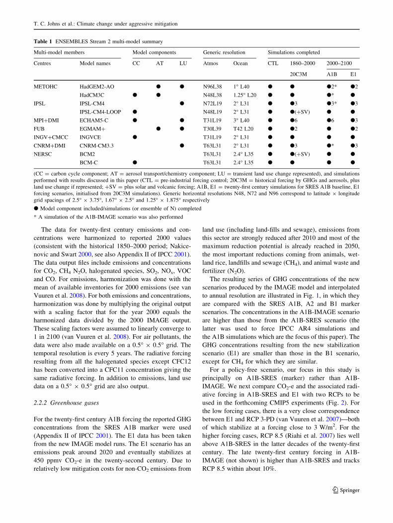
The resulting series of GHG concentrations of the new

scenarios produced by the IMAGE model and interpolated

to annual resolution are illustrated in Fig. 1, in which they

are compared with the SRES A1B, A2 and B1 marker

scenarios. The concentrations in the A1B-IMAGE scenario

are higher than those from the A1B-SRES scenario (the

latter was used to force IPCC AR4 simulations and

the A1B simulations which are the focus of this paper). The

GHG concentrations resulting from the new stabilization

scenario (E1) are smaller than those in the B1 scenario,

except for CH4 for which they are similar.

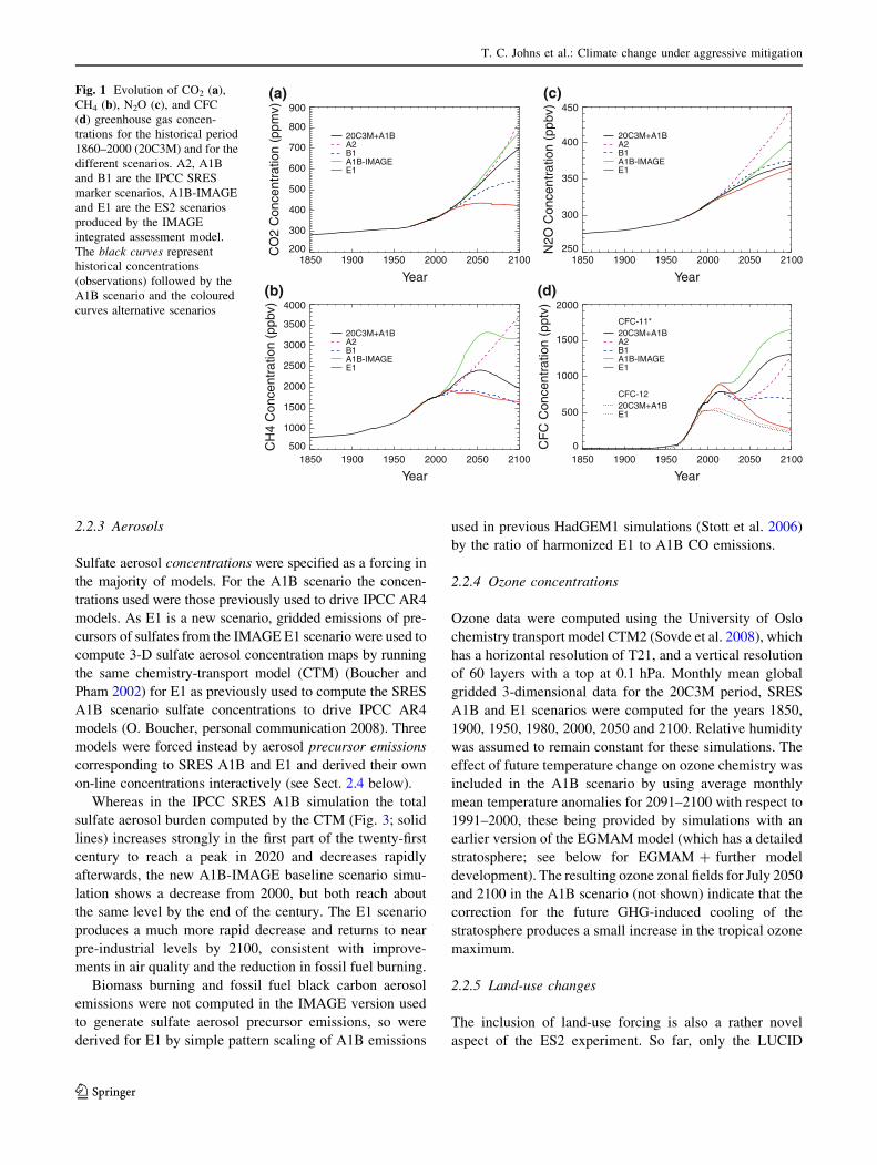
For a policy-free scenario, our focus in this study is

principally on A1B-SRES (marker) rather than A1B-

IMAGE. We next compare CO2-e and the associated radi-

ative forcing in A1B-SRES and E1 with two RCPs to be

used in the forthcoming CMIP5 experiments (Fig. 2). For

the low forcing cases, there is a very close correspondence

between E1 and RCP 3-PD (van Vuuren et al. 2007)—both

of which stabilize at a forcing close to 3 W/m2. For the

higher forcing cases, RCP 8.5 (Riahi et al. 2007) lies well

above A1B-SRES in the latter decades of the twenty-first

century. The late twenty-first century forcing in A1B-

IMAGE (not shown) is higher than A1B-SRES and tracks

RCP 8.5 within about 10%.

Table 1 ENSEMBLES Stream 2 multi-model summary

Multi-model members Model components Generic resolution Simulations completed

Centres Model names CC AT LU Atmos Ocean CTL 1860–2000 2000–2100

20C3M A1B E1

METOHC HadGEM2-AO d d N96L38 1� L40 d d d2* d2

HadCM3C d d N48L38 1.25� L20 d d d* d

IPSL IPSL-CM4 d N72L19 2� L31 d d3 d3* d3

IPSL-CM4-LOOP d N48L19 2� L31 d d(?SV) d d

MPI?DMI ECHAM5-C d d T31L19 3� L40 d d6 d6 d3

FUB EGMAM? d d T30L39 T42 L20 d d2 d d2

INGV?CMCC INGVCE d T31L19 2� L31 d d d d

CNRM?DMI CNRM-CM3.3 d T63L31 2� L31 d d3 d* d3

NERSC BCM2 T63L31 2.4� L35 d d(?SV) d d

BCM-C d T63L31 2.4� L35 d d d d

(CC = carbon cycle component; AT = aerosol transport/chemistry component; LU = transient land use change represented), and simulations

performed with results discussed in this paper (CTL = pre-industrial forcing control; 20C3M = historical forcing by GHGs and aerosols, plus

land use change if represented; ?SV = plus solar and volcanic forcing; A1B, E1 = twenty-first century simulations for SRES A1B baseline, E1

forcing scenarios, initialised from 20C3M simulations). Generic horizontal resolutions N48, N72 and N96 correspond to latitude 9 longitude

grid spacings of 2.5� 9 3.75�, 1.67� 9 2.5� and 1.25� 9 1.875� respectively

d Model component included/simulations (or ensemble of N) completed

* A simulation of the A1B-IMAGE scenario was also performed


123

2.2.3 Aerosols

Sulfate aerosol concentrations were specified as a forcing in

the majority of models. For the A1B scenario the concen-

trations used were those previously used to drive IPCC AR4

models. As E1 is a new scenario, gridded emissions of pre-

cursors of sulfates from the IMAGE E1 scenario were used to

compute 3-D sulfate aerosol concentration maps by running

the same chemistry-transport model (CTM) (Boucher and

Pham 2002) for E1 as previously used to compute the SRES

A1B scenario sulfate concentrations to drive IPCC AR4

models (O. Boucher, personal communication 2008). Three

models were forced instead by aerosol precursor emissions

corresponding to SRES A1B and E1 and derived their own

on-line concentrations interactively (see Sect. 2.4 below).

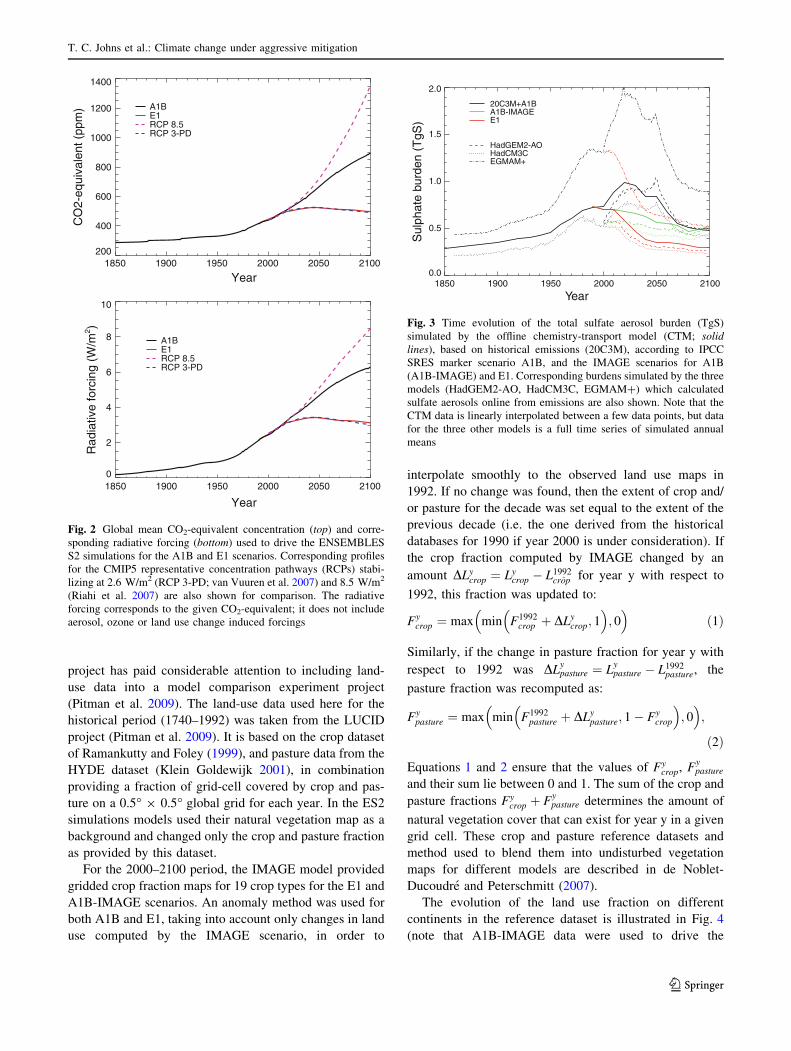
Whereas in the IPCC SRES A1B simulation the total

sulfate aerosol burden computed by the CTM (Fig. 3; solid

lines) increases strongly in the first part of the twenty-first

century to reach a peak in 2020 and decreases rapidly

afterwards, the new A1B-IMAGE baseline scenario simu-

lation shows a decrease from 2000, but both reach about

the same level by the end of the century. The E1 scenario

produces a much more rapid decrease and returns to near

pre-industrial levels by 2100, consistent with improve-

ments in air quality and the reduction in fossil fuel burning.

Biomass burning and fossil fuel black carbon aerosol

emissions were not computed in the IMAGE version used

to generate sulfate aerosol precursor emissions, so were

derived for E1 by simple pattern scaling of A1B emissions

used in previous HadGEM1 simulations (Stott et al. 2006)

by the ratio of harmonized E1 to A1B CO emissions.

2.2.4 Ozone concentrations

Ozone data were computed using the University of Oslo

chemistry transport model CTM2 (Sovde et al. 2008), which

has a horizontal resolution of T21, and a vertical resolution

of 60 layers with a top at 0.1 hPa. Monthly mean global

gridded 3-dimensional data for the 20C3M period, SRES

A1B and E1 scenarios were computed for the years 1850,

1900, 1950, 1980, 2000, 2050 and 2100. Relative humidity

was assumed to remain constant for these simulations. The

effect of future temperature change on ozone chemistry was

included in the A1B scenario by using average monthly

mean temperature anomalies for 2091–2100 with respect to

1991–2000, these being provided by simulations with an

earlier version of the EGMAM model (which has a detailed

stratosphere; see below for EGMAM ? further model

development). The resulting ozone zonal fields for July 2050

and 2100 in the A1B scenario (not shown) indicate that the

correction for the future GHG-induced cooling of the

stratosphere produces a small increase in the tropical ozone

maximum.

2.2.5 Land-use changes

The inclusion of land-use forcing is also a rather novel

aspect of the ES2 experiment. So far, only the LUCID

(a)

1850 1900 1950 2000 2050 2100

Year

200

300

400

500

600

700

800

900

CO

2 C

once

ntra

tion

(ppm

v)

20C3M+A1BA2B1A1B-IMAGEE1

(b)

1850 1900 1950 2000 2050 2100

Year

500

1000

1500

2000

2500

3000

3500

4000

CH

4 C

once

ntra

tion

(ppb

v)


(c)

1850 1900 1950 2000 2050 2100

Year

250

300

350

400

450

N2O

Con

cent

ratio

n (p

pbv)


(d)

1850 1900 1950 2000 2050 2100

Year

0

500

1000

1500

2000

CF

C C

once

ntra

tion

(ppt

v)

CFC-11*20C3M+A1BA2B1A1B-IMAGEE1

CFC-1220C3M+A1BE1

Fig. 1 Evolution of CO2 (a),

CH4 (b), N2O (c), and CFC

(d) greenhouse gas concen-

trations for the historical period

1860–2000 (20C3M) and for the

different scenarios. A2, A1B

and B1 are the IPCC SRES

marker scenarios, A1B-IMAGE

and E1 are the ES2 scenarios

produced by the IMAGE

integrated assessment model.

The black curves represent

historical concentrations

(observations) followed by the

A1B scenario and the coloured

curves alternative scenarios


123

project has paid considerable attention to including land-

use data into a model comparison experiment project

(Pitman et al. 2009). The land-use data used here for the

historical period (1740–1992) was taken from the LUCID

project (Pitman et al. 2009). It is based on the crop dataset

of Ramankutty and Foley (1999), and pasture data from the

HYDE dataset (Klein Goldewijk 2001), in combination

providing a fraction of grid-cell covered by crop and pas-

ture on a 0.5� 9 0.5� global grid for each year. In the ES2

simulations models used their natural vegetation map as a

background and changed only the crop and pasture fraction

as provided by this dataset.

For the 2000–2100 period, the IMAGE model provided

gridded crop fraction maps for 19 crop types for the E1 and

A1B-IMAGE scenarios. An anomaly method was used for

both A1B and E1, taking into account only changes in land

use computed by the IMAGE scenario, in order to

interpolate smoothly to the observed land use maps in

1992. If no change was found, then the extent of crop and/

or pasture for the decade was set equal to the extent of the

previous decade (i.e. the one derived from the historical

databases for 1990 if year 2000 is under consideration). If

the crop fraction computed by IMAGE changed by an

amount DLycrop ¼ Ly

crop � L1992crop for year y with respect to

1992, this fraction was updated to:

Fycrop ¼ max min F1992

crop þ DLycrop; 1

� �; 0

� �ð1Þ

Similarly, if the change in pasture fraction for year y with

respect to 1992 was DLypasture ¼ Ly

pasture � L1992pasture, the

pasture fraction was recomputed as:

Fypasture ¼ max min F1992

pasture þ DLypasture; 1� Fy

crop

� �; 0

� �;

ð2Þ

Equations 1 and 2 ensure that the values of Fycrop, Fy

pasture

and their sum lie between 0 and 1. The sum of the crop and

pasture fractions Fycrop þ Fy

pasture determines the amount of

natural vegetation cover that can exist for year y in a given

grid cell. These crop and pasture reference datasets and

method used to blend them into undisturbed vegetation

maps for different models are described in de Noblet-

Ducoudre and Peterschmitt (2007).

The evolution of the land use fraction on different

continents in the reference dataset is illustrated in Fig. 4

(note that A1B-IMAGE data were used to drive the

1850 1900 1950 2000 2050 2100

Year

200

400

600

800

1000

1200

1400C

O2-

equi

vale

nt (

ppm

) A1BE1RCP 8.5RCP 3-PD

1850 1900 1950 2000 2050 2100

Year

0

2

4

6

8

10

Rad

iativ

e fo

rcin

g (W

/m2 )

A1BE1RCP 8.5RCP 3-PD

Fig. 2 Global mean CO2-equivalent concentration (top) and corre-

sponding radiative forcing (bottom) used to drive the ENSEMBLES

S2 simulations for the A1B and E1 scenarios. Corresponding profiles

for the CMIP5 representative concentration pathways (RCPs) stabi-

lizing at 2.6 W/m2 (RCP 3-PD; van Vuuren et al. 2007) and 8.5 W/m2

(Riahi et al. 2007) are also shown for comparison. The radiative

forcing corresponds to the given CO2-equivalent; it does not include

aerosol, ozone or land use change induced forcings

1850 1900 1950 2000 2050 2100

Year

0.0

0.5

1.0

1.5

2.0

Sul

phat

e bu

rden

(T

gS)

20C3M+A1BA1B-IMAGEE1

HadGEM2-AOHadCM3CEGMAM+

Fig. 3 Time evolution of the total sulfate aerosol burden (TgS)

simulated by the offline chemistry-transport model (CTM; solidlines), based on historical emissions (20C3M), according to IPCC

SRES marker scenario A1B, and the IMAGE scenarios for A1B

(A1B-IMAGE) and E1. Corresponding burdens simulated by the three

models (HadGEM2-AO, HadCM3C, EGMAM?) which calculated

sulfate aerosols online from emissions are also shown. Note that the

CTM data is linearly interpolated between a few data points, but data

for the three other models is a full time series of simulated annual

means


123

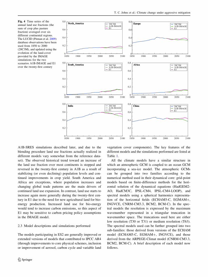
A1B-SRES simulations described later, and due to the

blending procedure land use fractions actually realized in

different models vary somewhat from the reference data-

set). The observed historical trend toward an increase of

the land use fraction over most continents is stopped and

reversed in the twenty-first century in A1B as a result of

stabilizing (or even declining) population levels and con-

tinued improvements in crop yield. South America and

Africa are exceptions, where population increases and

changing global trade patterns are the main drivers of

continued land use expansion. In contrast, land use starts to

increase again more generally during the twenty-first cen-

tury in E1 due to the need for new agricultural land for bio-

energy production. Increased land use for bio-energy

would tend to increase carbon emissions, so this aspect of

E1 may be sensitive to carbon pricing policy assumptions

in the IMAGE model.

2.3 Model descriptions and simulations performed

The models participating in ES2 are generally improved or

extended versions of models that contributed to IPCC AR4

(through improvements to core physical schemes, inclusion

or improvement of aerosol, carbon cycle and variable land

vegetation cover components). The key features of the

different models and the simulations performed are listed at

Table 1.

All the climate models have a similar structure in

which an atmospheric GCM is coupled to an ocean GCM

incorporating a sea-ice model. The atmospheric GCMs

can be grouped into two families according to the

numerical method used in their dynamical core: grid-point

models based on finite-difference methods for the hori-

zontal solution of the dynamical equations (HadGEM2-

AO, HadCM3C, IPSL-CM4, IPSL-CM4-LOOP), and

spectral models using a spherical harmonics representa-

tion of the horizontal fields (ECHAM5-C, EGMAM?,

INGVCE, CNRM-CM3.3, BCM2, BCM-C). In the spec-

tral models the resolution is expressed by the maximum

wavenumber represented in a triangular truncation in

wavenumber space. The truncations used here are either

low resolution (T30 or T31) or medium resolution (T63).

The spectral models used can be further grouped into two

sub-families: those derived from versions of the ECHAM

model (ECHAM5-C, EGMAM?, INGVCE), and those

derived from the ARPEGE-Climat model (CNRM-CM3.3,

BCM2, BCM-C). A brief description of each model now

follows.

1850 1900 1950 2000 2050 21000

0,2

0,4

0,6

0,820C3MA1B-IMAGEE1

IndiaIndiaIndia

1850 1900 1950 2000 2050 21000

0,2

0,4

0,6

0,820C3MA1B-IMAGEE1

ChinaChinaChina

1850 1900 1950 2000 2050 21000

0,2

0,4

0,6

0,820C3MA1B-IMAGEE1

South_AmericaSouth_AmericaSouth_America

1850 1900 1950 2000 2050 21000

0,2

0,4

0,6

0,820C3MA1B-IMAGEE1

AfricaAfricaAfrica

1850 1900 1950 2000 2050 21000

0,2

0,4

0,6

0,820C3MA1B-IMAGEE1

North_AmericaNorth_AmericaNorth_America

1850 1900 1950 2000 2050 21000

0,2

0,4

0,6

0,820C3MA1B-IMAGEE1

EuropeEuropeEuropeFig. 4 Time series of the

annual land use fractions (the

sum of crop plus pasture

fraction) averaged over six

different continental regions.

The LUCID (Pitman et al. 2009)

database observations have been

used from 1850 to 2000

(20C3M), and updated using the

evolution of the land-cover

provided by the IMAGE

simulations for the two

scenarios A1B-IMAGE and E1

over the twenty-first century


123

2.3.1 METOHC: HadGEM2-AO model

The HadGEM2-AO model is based on the HadGEM1 model

used in IPCC AR4, described by Johns et al. (2006), but

contains several improvements and modifications as

described in Collins et al. (2008). The representation of

aerosol processes is notably improved (Bellouin et al. 2007)

and both secondary organic aerosol and mineral dust are

now included. The direct radiative effect of all aerosol

species (which include black carbon), plus the first and

second indirect radiative effects of sulfate, sea-salt and

biomass aerosol are all included. The cumulus convection

parametrization is a revised version of HadGEM1’s mass

flux scheme (Martin et al. 2006) which includes separately

diagnosed deep and shallow convection, parameterized

entrainment and detrainment rates for shallow convection, a

convective momentum transport (CMT) parameterization

based on flux-gradient relationships, and a convective anvil

scheme. In HadGEM2-AO, an adaptive detrainment

parametrization for deep convection (Derbyshire et al. 2010)

is also introduced leading to significant improvements in

diabatic heating profiles and moist processes. Boundary

layer and land surface process parametrizations are refined.

In the ocean, Laplacian viscosity function is revised, leading

to lower viscosity in the tropics. Further, the ocean back-

ground vertical diffusivity is lowered in the upper 1,000 m,

leading to reduced mixing with cooler water at depth, raising

sea surface temperatures compared to HadGEM1. Land use

change is applied through modified fractions of crop and

pasture types in the land surface classification.

2.3.2 METOHC: HadCM3C model

The HadCM3C model (B. Booth, personal communication)

is a modified configuration of the HadCM3 model (Gordon

et al. 2000; Pope et al. 2000) used in the IPCC Third and

Fourth Assessments. Unlike HadCM3, it is flux adjusted

and includes interactive terrestrial vegetation and an ocean

carbon cycle. Externally imposed (anthropogenic) land use

change cannot currently be included. The model differs

from HadCM3LC (Cox et al. 2000), the coupled carbon

cycle climate model submitted to C4MIP (Friedlingstein

et al. 2006), as it is configured to run with the standard

(higher) HadCM3 resolution ocean (1.25� 9 1.25�). The

cumulus convection parametrization (as for HadCM3) is a

mass flux scheme (Gregory and Rowntree 1990) including

convective downdraughts (Gregory and Allen 1991) and

CMT scheme (Gregory et al. 1997). HadCM3C also

includes interactive atmospheric sulfur cycle chemistry and

sulfate aerosol scheme including the direct and first indi-

rect, ‘‘cloud albedo’’, aerosol effects (following Jones et al.

2001; note that the second indirect, ‘‘cloud lifetime’’, effect

is excluded).

2.3.3 IPSL: IPSL-CM4 and IPSL-CM4-LOOP models

The IPSL-CM4 coupled ocean-atmosphere GCM (Marti

et al. 2010) was used previously in IPCC AR4 and its main

components are the following: LMDZ4 atmosphere

(Hourdin et al. 2006); ORCHIDEE land and vegetation

(Krinner et al. 2005); OPA8.2 ocean (Madec et al. 1999);

LIM sea ice (Timmermann et al. 2005); and OASIS3

coupler (Valcke 2006). The version used here contains

some improvements: the horizontal resolution has been

increased (Marti et al. 2010) and land use change can be

externally imposed. The cumulus convection parametriza-

tion is based on the Emanuel (1991, 1993) mass flux

scheme, and convective clouds are represented through a

log-normal probability distribution function of sub-grid

scale total (vapor and condensed) water (Bony and

Emanuel 2001). As in Dufresne et al. (2005), sulfate

aerosols concentrations are externally imposed and direct

and indirect aerosol forcings are considered.

IPSL-CM4-LOOP (Cadule et al. 2009) comprises a

coupling between the IPSL-CM4 model and two carbon

cycle models: PISCES (Pelagic Interactions Scheme for

Carbon and Ecosystems Studies) biogeochemical model

(Aumont et al. 2003) for the ocean part, and ORCHIDEE

(ORganizing Carbon and Hydrology in Dynamic Ecosy-

tEms) model for the terrestrial part (Krinner et al. 2005).

IPSL-CM4-LOOP has a cold bias over continents in the

high northern latitudes, attributable to the coupling with

terrestrial CC. With the CC activated, leaf area index (LAI)

is computed rather than prescribed as in IPSL-CM4. The

positive snow-albedo feedback at high latitudes is thought

to be too strong due to an error in the leaf albedo, which

amplifies the smaller cold bias present in IPSL-CM4. In

turn, the enhanced snow-albedo feedback tends to increase

the warming response to a given radiative forcing in IPSL-

CM4-LOOP compared with IPSL-CM4.

2.3.4 MPI ? DMI: ECHAM5-C model

ECHAM5-C is a low-resolution version of the Max Planck

Institute for Meteorology Earth System Model (MPI-ESM),

consisting of models for the atmosphere including the land

surface (T31L19), the ocean including sea ice, and the

marine and terrestrial carbon cycles (3�L40). The atmo-

spheric component (ECHAM5; Roeckner et al. 2006) has

been coupled to the MPI-OM ocean model (Marsland et al.

2003) by exchanging daily mean fluxes of heat, water and

momentum, and the state of the ocean surface, respec-

tively. No flux adjustments are employed. Details on cou-

pling method and simulated climatology can be found in

Jungclaus et al. (2006). The cumulus convection parame-

terization of ECHAM5 is based on the Tiedtke (1989)

scheme, modified by Nordeng (1994) for deep convection.


123

The bulk mass flux scheme parameterizes the contribution

of cumulus convection to the large scale budgets of heat,

moisture and momentum by an ensemble of clouds con-

sisting of updrafts and downdrafts in a steady state. Cloud

base mass flux depends on moisture convergence below

cloud base for shallow and mid level convection, and on

CAPE adjustment for deep convection. The carbon cycle

model coupled to ECHAM5/MPI-OM comprises the ocean

biogeochemistry model HAMOCC5 (Maier-Reimer et al.

2005) and the modular land surface scheme JSBACH

(Raddatz et al. 2007). Soil carbon is partitioned into a pool

with a short turnover time (about 1 year) and one with a

long turnover time (about 100 years). It is released to the

atmosphere by heterotrophic respiration, which depends

linearly on soil moisture and exponentially on soil tem-

perature. Vegetation is differentiated according to five

natural phenotypes (evergreen, summergreen, raingreen

forest, shrubland, grassland) and managed (non-forest)

areas.

2.3.5 FUB: EGMAM ? model

The modified coupled atmosphere-ocean GCM ECHO-G

with Middle Atmosphere Model EGMAM (Huebener et al.

2007) is based on ECHO-G (Legutke and Voss 1999),

which couples ECHAM4 (Roeckner et al. 1996) at a hor-

izontal resolution of T30 via OASIS2.4 with the Hamburg

Ocean Primitive Equation-Global Model (HOPE-G; Wolff

et al. 1997) at a horizontal resolution of 0.5–2.8� (with

refinement near the equator) and 20 vertical layers. It

includes a dynamic-thermodynamic sea ice model and time

constant flux correction for heat and freshwater exchange.

With the extension to middle atmosphere up to 0.01 hpa

(ca. 80 km) the model has 39 vertical layers and a gravity

wave parameterization (Manzini and McFarlane 1998).

The model includes an interactive aerosol transport scheme

(Feichter et al. 1996), changing land use (crop, pasture) and

a time-varying 3d ozone field. The aerosol scheme includes

as prognostic species dimethyl sulfide and sulfur dioxide

gases, and sulfate aerosol. The direct aerosol effect of

backscattering of shortwave radiation, and the impact of

sulfate aerosol on cloud albedo (first indirect effect) are

represented. Cumulus convection is parameterized fol-

lowing a mass flux scheme (Tiedtke 1989) modified by

Nordeng (1994) for deep convection, as in the ECHAM5

model. Land use changes are implemented by changing the

leaf area index and vegetation fraction as well as the forest

fraction, while other surface parameters remain unchanged.

2.3.6 INGV ? CMCC: INGVCE model

The INGV-CMCC Earth System Model (INGVCE) con-

sists of an atmosphere-ocean-sea ice physical core coupled

to a land-and-ocean carbon cycle model. The technical

details of the physical atmosphere ocean coupling and of

the implementations of the vegetation and biogeochemistry

(i.e. the carbon cycle) models into the physical core model

are described in Fogli et al. (2009). The role of the ocean

carbon cycle in the regulation of anthropogenic carbon

emission as simulated by the INGVCE model is discussed

in Vichi et al. (2011). The ESM components are: ECHAM5

atmosphere (Roeckner et al. 2006); SILVA land and veg-

etation (Alessandri 2006); OPA8.2 ocean (Madec et al.

1999); LIM sea ice (Timmermann et al. 2005), and PEL-

AGOS biogeochemistry (Vichi et al. 2007). The cumulus

convection parameterization is based on the Tiedtke (1989)

scheme modified by Nordeng (1994) for deep convection,

as in the ECHAM5 model. The software used to couple the

atmosphere (including the land-vegetation model) model

and the ocean (including the biogeochemistry) model is

OASIS3 (Valcke 2006).

2.3.7 CNRM ? DMI: CNRM-CM3.3 model

The CNRM-CM3.3 model is an improved and updated

version of the CNRM-CM3.1 coupled model (Salas-Melia

et al. 2005) used for IPCC-AR4. The atmospheric part is

based on the ARPEGE-Climat version 4 GCM (Deque

1999; Royer et al. 2002; Gibelin and Deque 2003) with

spectral truncation T63 and Gaussian grid of 64 9 128

points, a progressive hybrid sigma-pressure vertical coor-

dinate with 31 layers, and semi-Lagrangian advection

scheme with a semi-implicit 30-min time step. Ozone

concentration is a prognostic variable with a simplified

linear parameterization of sources and sinks (Cariolle et al.

1990) modified to improve the simulation of the effects of

chlorine on the ozone destruction. The indirect effect of

sulfate aerosols is based on the parameterization of Boucher

and Lohmann (1995) with a calibration from POLDER

satellite data (Quaas and Boucher 2005). Deep convection

is parameterized using a mass-flux convective scheme with

Kuo-type closure (Bougeault 1985). The atmosphere-ocean

coupling through OASIS 2.2 has been revised to achieve a

better conservation of the energy fluxes during interpola-

tions between the atmospheric and oceanic grids. The ocean

model (OPA 8.1) and sea-ice model (GELATO; Salas-

Melia 2002) have been checked carefully, with minor cor-

rections implemented to improve the energy conservation.

The improvements in the coupled system have led to

reduced drift in ocean volumetric and surface temperature

and atmosphere 2 m temperature. Changes in land use are

introduced through a modification of the fractions of crop

and pasture types in the land-surface classification, and the

resulting surface properties have been computed with an

updated version (ECOCLIMAP-2) of the ECOCLIMAP

vegetation map (Champeaux et al. 2005).


123

2.3.8 NERSC: BCM2 and BCM-C models

For the ES2 simulations two different versions of BCM

have been used, BCM2 and BCM-C. The BCM2 is an

updated version of the original Bergen Climate Model

(BCM) described in Furevik et al. (2003), which was used

for IPCC AR4. The atmospheric part is ARPEGE-Climat

version 3, which is based on the atmospheric GCM

developed at CNRM-GAME (Deque et al. 1994) and

contains very similar physics to the ARPEGE-Climat ver-

sion 4 used in the CNRM-CM3.3 model. (The atmospheric

model differences are mainly to the dynamics, without

major impacts on the current simulations.) In the version

used in this study ARPEGE is run with a truncation at wave

number 63 (TL63) and a 30-min time step. A total of 31

vertical levels are employed, ranging from the surface to

0.01 hPa. The physical parameterizations are similar to

those used in previous versions of the BCM, but the ver-

tical diffusion scheme has been updated to that of ARPE-

GE-Climat version 4 (Ottera et al. 2009). Deep convection

is parameterized using a mass-flux convective scheme with

Kuo-type closure (Bougeault 1985). The indirect effect of

tropospheric sulphate aerosols is parameterized according

to Rongming et al. (2001). The oceanic part is Miami

Isopycnic Coordinate Ocean Model (MICOM) (Bleck and

Smith 1990; Bleck et al. 1992) and is extensively modified

at NERSC. With the exception of the equatorial region, the

ocean grid is almost regular with horizontal grid spacing

approximately 2.4� 9 2.4�. The model has a stack of 34

isopycnic layers in the vertical, with potential densities

ranging from 1,029.514 to 1,037.800 kg m-3, and a non-

isopycnic surface mixed layer on top providing the linkage

between the atmospheric forcing and the ocean interior.

BCM2 uses the GELATO (Salas-Melia 2002) sea ice

model. Several modifications have been made to MICOM

and are documented in Ottera et al. (2009).

Recently, the Bergen earth system model (BCM-C) has

been developed by coupling terrestrial and oceanic carbon

cycle models into BCM2 (Tjiputra et al. 2010). BCM-C

adopts the Hamburg Ocean Carbon Cycle (HAMOCC5.1)

model, which is based on the original work by Maier-

Reimer (1993) with the extensions of Maier-Reimer et al.

(2005). The HAMOCC5.1 implements full carbon chem-

istry formulation for air-sea CO2 exchange. It is similar to

the ocean carbon cycle model used in the ECHAM5-C

model, but incorporated here into MICOM (Assmann et al.

2010). For the terrestrial part it uses the Lund-Postdam-

Jena model (LPJ) (Sitch et al. 2003), a large-scale terres-

trial carbon cycle model which includes global dynamical

vegetation. The LPJ version in BCM-C does not implement

land-use change. The different components are coupled

together using OASIS2.2 (Terray and Thual 1995; Terray

et al. 1995) and the model is run without any form of flux

adjustments. Unlike BCM2, BCM-C uses the original

NERSC sea ice model. Validation and assessment of cli-

mate-carbon-cycle feedbacks in BCM-C have been made

by Tjiputra et al. (2010).

2.4 Interpretation of the forcing data by different

models

Considerable efforts have been made to implement the

forcings in a similar way across the various models. In

particular all the models used the same concentrations of

the well-mixed GHGs, the models with carbon cycle being

driven with the concentration of CO2 as previously

described. However, due to specific features and con-

straints in certain models some differences in the imple-

mentations of the forcings still remain as outlined below.

Ozone 3-D concentrations were specified in the scenario

simulations with HadGEM2-AO, HadCM3C, ECHAM5-C

and EGMAM ? from the ozone simulations provided by

the University of Oslo database, the E1 ozone fields first

having been adjusted for future estimated temperature-

dependence using a rescaling based on A1B ozone fields

(which already incorporated the temperature-dependent

effect in the off-line modelling). IPSL-CM4/IPSL-CM4-

LOOP and BCM2/BCM-C simulations used a fixed ozone

climatology throughout all their simulations, INGVCE

used the ozone distribution from 1860 to 2100 of Kiehl

et al. (1999), and in CNRM-CM3.3 ozone was modelled as

a prognostic variable.

For sulfate aerosols, most models used the concentra-

tion maps provided by the CTM (Boucher and Pham

2002), exceptions being HadGEM2-AO, HadCM3C and

EGMAM? which used their own aerosol transport

schemes driven by geographical emissions. In the Had-

GEM2-AO and HadCM3C models, an explicit geographi-

cal representation of ship track emissions was used, but it

assumed no change in ship tracks in the twenty-first cen-

tury compared to present-day. Note that although the

radiative forcing due to GHGs is constrained by the

experimental design to be quite similar for a given scenario

in all models, the forcing due to aerosols is less tightly

constrained. This represents probably the largest modeling

uncertainty in the net forcing and an important contributory

factor to the resulting spread in climate response. Given the

same aerosol burden, the aerosol forcing effects vary due to

their different representations in models, but the sulfate

aerosol burden itself is an additional source of variation

between models (Fig. 3). In particular, HadGEM2-AO and

HadCM3C simulate systematically lower burdens than the

CTM, while EGMAM ? simulates considerably higher

burdens (more than double those in HadCM3C). Addi-

tionally, there are variations in the shape of the A1B peak

and its subsequent decline.


123

Land-use changes were taken into account in most

models according to the specified crop and pasture fraction

variations, but omitted in HadCM3C, IPSL-CM4-LOOP,

INGVCE, BCM2, and BCM-C due to the difficulty of

integrating this forcing with dynamical vegetation within a

terrestrial carbon cycle. Different (model-dependent)

underlying land use maps and crop/pasture classifications

in terms of plant functional types meant that implementing

the associated forcing completely consistently was prob-

lematic. (ECHAM5-C is the only model to combine land

use change with a terrestrial carbon cycle and therefore the

only model able to report land use carbon emissions sep-

arately from energy emissions. In all other models, the

allowable anthropogenic carbon emissions are implicitly a

sum of land use and energy emissions.)

Solar and volcanic forcings were represented in only

two of the 20C3M simulations used to initialise A1B and

E1 simulations, namely those with IPSL-CM4-LOOP and

BCM2.

Solar forcing was represented in both models via vari-

ations of the solar constant and thus the top of the atmo-

sphere shortwave flux. The basic solar constant time series

for the 20C3M simulation with IPSL-CM4-LOOP was the

construction by Solanki and Krivova (2003), in which most

of the total rise of about 1.5 W/m2 takes place in the period

1900–1950. The solar cycle and its variations over time

were also included. In the BCM2 case, solar constant

variations follow Crowley et al. (2003).

Volcanic radiative forcing was represented in IPSL-

CM4-LOOP by an additional change of the solar constant

(modelling the shortwave radiative effect only). The forc-

ing variations follow an updated version of Sato et al.

(1993) (using data obtained from http://data.giss.nasa.gov/

modelforce/strataer/) in which aerosol optical depth s was

converted to radiative forcing F (W/m2) according to the

relationship F = -23s proposed by Hansen et al. (2005).

In BCM2, the volcanic aerosol forcing time series follows

Crowley et al. (2003), specifying monthly optical depths at

0.55 microns in four latitude bands (90�N–30�N, 30�N-

equator, equator-30�S and 30�S–90�S). The aerosol loading

was distributed in each model level in the stratosphere so

that both the shortwave and longwave radiative responses

are simulated (Ottera 2008).

3 Results

As described in the previous section, a total of ten models

were used to produce the simulations presented here. We

consider that two pairs of models (IPSL-CM4/IPSL-CM4-

LOOP and BCM2/BCM-C), which only differ with regard

to inclusion of an integrated CC component, should not be

regarded as independent models within the experiment. For

those models we therefore use a half weight rather than a

full weight when computing multi-model ensemble mean

results in which both models of the pair contribute. For

analysis which specifically concerns the CC response, we

restrict attention to a sub-ensemble of 5 models in which

each carries the same weight in computing ensemble

means.

3.1 Global climate response

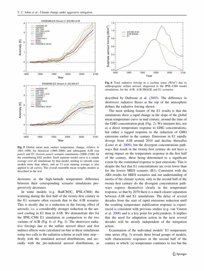
3.1.1 Temperature and precipitation

Each model shows a significantly lower temperature

response in E1 than A1B in the late twenty-first century

(Fig. 5), but the multi-model ensemble spread leads to a

slight overlap between the projected temperature rise for

the most sensitive models’ E1 simulations (HadCM3C,

IPSL-CM4) and the least sensitive models’ A1B simula-

tions (EGMAM?, CNRM-CM3.3). The ensemble mean

warming at 2100 relative to 1861–1890 is about 3.4 K for

A1B and 1.8 K for E1. The spread is similar for A1B and

E1 (*1.5 K at 2100) and consistent with that of AR4

AOGCMs driven with the SRES A2 concentration pathway

(Fig. 10.20 of Meehl et al. 2007). The spread in tempera-

ture is relatively smaller for the models with interactive

carbon cycle than that seen in the C4MIP models (Frie-

dlingstein et al. 2006) because the experimental design

used in this study by design suppresses the full carbon

cycle feedback-driven temperature spread exhibited in

C4MIP, in which carbon emissions rather than concentra-

tions were specified, and which contributes to the tem-

perature spread reported in AR4. Hence results obtained

from concentration pathway experiments, such as those

presented here, do not represent the full modelling uncer-

tainty in temperature response for given emissions

pathways.

The two pairs of models that differ with regard to the

inclusion of a CC component both show differences in their

twentieth century temperature responses. In particular the

temperature anomalies during the 1910–1960 period are

more positive in IPSL-CM4-LOOP and BCM2 compared

to IPSL-CM4 and BCM-C. The inclusion of solar and

volcanic forcings during the twentieth century in IPSL-

CM4-LOOP and BCM2 (Ottera et al. 2010) is the main

factor contributing to these differences. However, the dif-

ferent twentieth century temperature responses also partly

reflect internal decadal variability in the different simula-

tions, and also the enhanced snow-albedo feedback in the

IPSL-CM4-LOOP case. For both pairs of models, the

temperature increases (either for A1B or E1) are similar

during the twenty-first century. For the IPSL-CM4/IPSL-

CM4-LOOP pair this reflects the fact that the difference in

snow-albedo feedback between the two models slowly


123

http://data.giss.nasa.gov/modelforce/strataer/

http://data.giss.nasa.gov/modelforce/strataer/

decreases as the high-latitude temperature difference

between their corresponding scenario simulations pro-

gressively decreases.

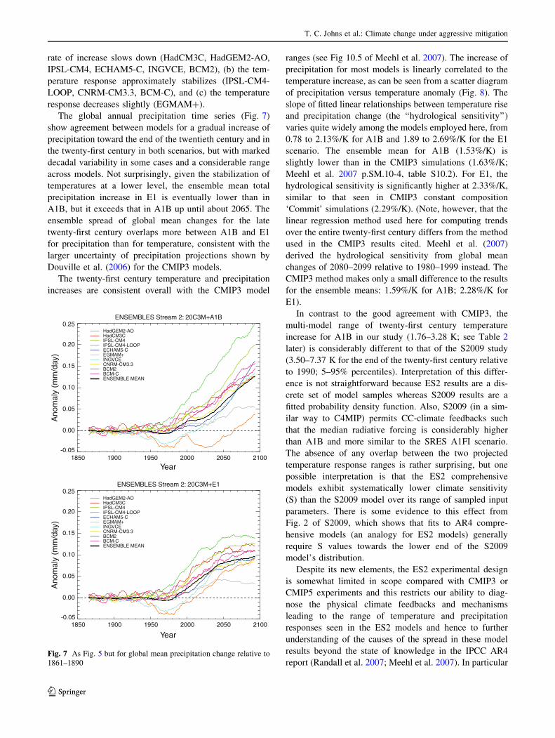
In some models (e.g. HadCM3C, IPSL-CM4) the

warming during the first half of the twenty-first century in

the E1 scenario often exceeds that in the A1B scenario.

This is mostly due to a reduction in the forcing effect of

aerosols, i.e. a considerably stronger reduction in the aer-

osol cooling in E1 than in A1B. We demonstrate this for

the IPSL-CM4 E1 simulation in comparison to the two

variants of A1B (Fig. 6; cf. Fig. 3). The shortwave radia-

tive forcings due to the sulfate aerosol direct and first

indirect effects were calculated on-line in these simulations

using two calls to the radiation scheme at each time step—

firstly with the simulated aerosol distributions, and sec-

ondly with the pre-industrial aerosol distributions, as

described by Dufresne et al. (2005). The difference in

shortwave radiative fluxes at the top of the atmosphere

defines the radiative forcing shown.

The most striking feature of the E1 results is that the

simulations show a rapid change in the slope of the global

mean temperature curve in mid century, around the time of

the GHG concentration peak (Fig. 2). We interpret this, not

as a direct temperature response to GHG concentrations,

but rather a lagged response to the reduction of GHG

emissions earlier in the century. Emissions in E1 rapidly

diverge from A1B around 2010 and decline thereafter

(Lowe et al. 2009), but the divergent concentrations path-

ways that result in the twenty-first century do not have a

strong impact on the temperature response in the first half

of the century, these being determined to a significant

extent by the committed response to past emissions. This is

despite the fact that E1 concentrations are even lower than

for the lowest SRES scenario (B1). Consistent with the

AR4 results for SRES scenarios and our understanding of

inertia of the climate system, only in the second half of the

twenty-first century do the divergent concentration path-

ways express themselves clearly in the temperature

response, so that by 2070 there is a much clearer separation

between A1B and E1 simulations. The delay of several

decades from the start of rapid emissions reduction until

the resulting temperature stabilization response is experi-

enced is consistent with previous studies (e.g. van Vuuren

et al. 2008) and is a key point for policymakers. It implies

that the need for adaptation action in the next several

decades will be mostly independent of the mitigation

action.

Examination of the individual models’ E1 temperature

time series (Fig. 5) reveals three broad groups of models,

with characteristic responses in the second half of the

century in which: (a) temperature continues to rise but the

ENSEMBLES Stream 2: 20C3M+A1B

1850 1900 1950 2000 2050 2100

Year

-1

0

1

2

3

4

Ano

mal

y (K

)

HadGEM2-AOHadCM3CIPSL-CM4IPSL-CM4-LOOPECHAM5-CEGMAM+INGVCECNRM-CM3.3BCM2BCM-CENSEMBLE MEAN

ENSEMBLES Stream 2: 20C3M+E1

1850 1900 1950 2000 2050 2100

Year

-1

0

1

2

3

4

Ano

mal

y (K

)


Fig. 5 Global mean near surface temperature change, relative to

1861–1890, for historical (1860–2000) and subsequent A1B (toppanel) and E1 (bottom panel) scenario simulations (2000–2100) for

the contributing ES2 models. Each separate model curve is a simple

average over all simulations by that model, tending to smooth some

models more than others, and an 11-year running average is also

applied to all curves. The overall ensemble mean weights models as

described in the text

1850 1900 1950 2000 2050 2100

Year

0.0

0.2

0.4

0.6

0.8

1.0

1.2

Sul

phat

e ae

roso

l for

cing

(W

/m2)

20C3M+A1BA1B-IMAGEE1

Fig. 6 Total radiative forcing in a cooling sense (W/m2) due to

anthropogenic sulfate aerosol, diagnosed in the IPSL-CM4 model

simulations, for the A1B, A1B-IMAGE and E1 scenarios


123

rate of increase slows down (HadCM3C, HadGEM2-AO,

IPSL-CM4, ECHAM5-C, INGVCE, BCM2), (b) the tem-

perature response approximately stabilizes (IPSL-CM4-

LOOP, CNRM-CM3.3, BCM-C), and (c) the temperature

response decreases slightly (EGMAM?).

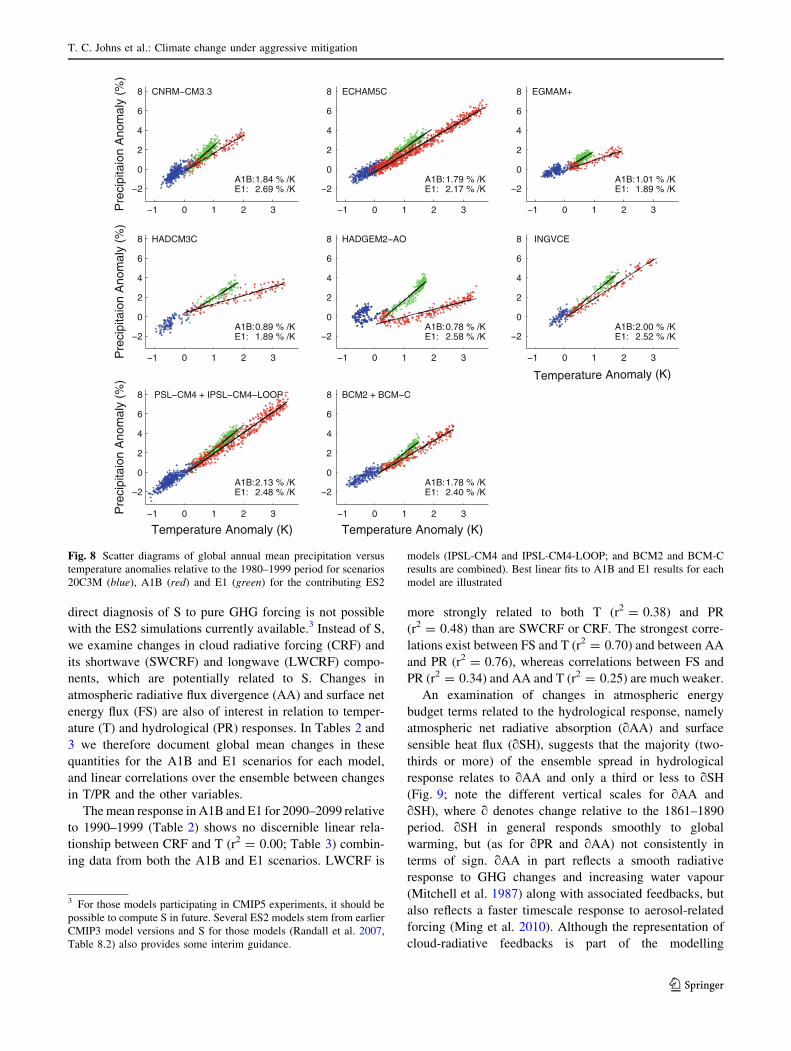
The global annual precipitation time series (Fig. 7)

show agreement between models for a gradual increase of

precipitation toward the end of the twentieth century and in

the twenty-first century in both scenarios, but with marked

decadal variability in some cases and a considerable range

across models. Not surprisingly, given the stabilization of

temperatures at a lower level, the ensemble mean total

precipitation increase in E1 is eventually lower than in

A1B, but it exceeds that in A1B up until about 2065. The

ensemble spread of global mean changes for the late

twenty-first century overlaps more between A1B and E1

for precipitation than for temperature, consistent with the

larger uncertainty of precipitation projections shown by

Douville et al. (2006) for the CMIP3 models.

The twenty-first century temperature and precipitation

increases are consistent overall with the CMIP3 model

ranges (see Fig 10.5 of Meehl et al. 2007). The increase of

precipitation for most models is linearly correlated to the

temperature increase, as can be seen from a scatter diagram

of precipitation versus temperature anomaly (Fig. 8). The

slope of fitted linear relationships between temperature rise

and precipitation change (the ‘‘hydrological sensitivity’’)

varies quite widely among the models employed here, from

0.78 to 2.13%/K for A1B and 1.89 to 2.69%/K for the E1

scenario. The ensemble mean for A1B (1.53%/K) is

slightly lower than in the CMIP3 simulations (1.63%/K;

Meehl et al. 2007 p.SM.10-4, table S10.2). For E1, the

hydrological sensitivity is significantly higher at 2.33%/K,

similar to that seen in CMIP3 constant composition

‘Commit’ simulations (2.29%/K). (Note, however, that the

linear regression method used here for computing trends

over the entire twenty-first century differs from the method

used in the CMIP3 results cited. Meehl et al. (2007)

derived the hydrological sensitivity from global mean

changes of 2080–2099 relative to 1980–1999 instead. The

CMIP3 method makes only a small difference to the results

for the ensemble means: 1.59%/K for A1B; 2.28%/K for

E1).

In contrast to the good agreement with CMIP3, the

multi-model range of twenty-first century temperature

increase for A1B in our study (1.76–3.28 K; see Table 2

later) is considerably different to that of the S2009 study

(3.50–7.37 K for the end of the twenty-first century relative

to 1990; 5–95% percentiles). Interpretation of this differ-

ence is not straightforward because ES2 results are a dis-

crete set of model samples whereas S2009 results are a

fitted probability density function. Also, S2009 (in a sim-

ilar way to C4MIP) permits CC-climate feedbacks such

that the median radiative forcing is considerably higher

than A1B and more similar to the SRES A1FI scenario.

The absence of any overlap between the two projected

temperature response ranges is rather surprising, but one

possible interpretation is that the ES2 comprehensive

models exhibit systematically lower climate sensitivity

(S) than the S2009 model over its range of sampled input

parameters. There is some evidence to this effect from

Fig. 2 of S2009, which shows that fits to AR4 compre-

hensive models (an analogy for ES2 models) generally

require S values towards the lower end of the S2009

model’s distribution.

Despite its new elements, the ES2 experimental design

is somewhat limited in scope compared with CMIP3 or

CMIP5 experiments and this restricts our ability to diag-

nose the physical climate feedbacks and mechanisms

leading to the range of temperature and precipitation

responses seen in the ES2 models and hence to further

understanding of the causes of the spread in these model

results beyond the state of knowledge in the IPCC AR4

report (Randall et al. 2007; Meehl et al. 2007). In particular


1850 1900 1950 2000 2050 2100

Year

-0.05

0.00

0.05

0.10

0.15

0.20

0.25

Ano

mal

y (m

m/d

ay)



1850 1900 1950 2000 2050 2100

Year

-0.05

0.00

0.05

0.10

0.15

0.20

0.25

Ano

mal

y (m

m/d

ay)


Fig. 7 As Fig. 5 but for global mean precipitation change relative to

1861–1890


123

direct diagnosis of S to pure GHG forcing is not possible

with the ES2 simulations currently available.3 Instead of S,

we examine changes in cloud radiative forcing (CRF) and

its shortwave (SWCRF) and longwave (LWCRF) compo-

nents, which are potentially related to S. Changes in

atmospheric radiative flux divergence (AA) and surface net

energy flux (FS) are also of interest in relation to temper-

ature (T) and hydrological (PR) responses. In Tables 2 and

3 we therefore document global mean changes in these

quantities for the A1B and E1 scenarios for each model,

and linear correlations over the ensemble between changes

in T/PR and the other variables.

The mean response in A1B and E1 for 2090–2099 relative

to 1990–1999 (Table 2) shows no discernible linear rela-

tionship between CRF and T (r2 = 0.00; Table 3) combin-

ing data from both the A1B and E1 scenarios. LWCRF is

more strongly related to both T (r2 = 0.38) and PR

(r2 = 0.48) than are SWCRF or CRF. The strongest corre-

lations exist between FS and T (r2 = 0.70) and between AA

and PR (r2 = 0.76), whereas correlations between FS and

PR (r2 = 0.34) and AA and T (r2 = 0.25) are much weaker.

An examination of changes in atmospheric energy

budget terms related to the hydrological response, namely

atmospheric net radiative absorption (qAA) and surface

sensible heat flux (qSH), suggests that the majority (two-

thirds or more) of the ensemble spread in hydrological

response relates to qAA and only a third or less to qSH

(Fig. 9; note the different vertical scales for qAA and

qSH), where q denotes change relative to the 1861–1890

period. qSH in general responds smoothly to global

warming, but (as for qPR and qAA) not consistently in

terms of sign. qAA in part reflects a smooth radiative

response to GHG changes and increasing water vapour

(Mitchell et al. 1987) along with associated feedbacks, but

also reflects a faster timescale response to aerosol-related

forcing (Ming et al. 2010). Although the representation of

cloud-radiative feedbacks is part of the modelling

−1 0 1 2 3

−2

0

2

4

6

8 CNRM−CM3.3

E1: 2.69 % /KA1B:1.84 % /K

Pre

cipi

taio

n A

nom

aly

(%)

−1 0 1 2 3

−2

0

2

4

6

8 ECHAM5C

E1: 2.17 % /KA1B:1.79 % /K

−1 0 1 2 3

−2

0

2

4

6

8 EGMAM+

E1: 1.89 % /KA1B:1.01 % /K

−1 0 1 2 3

−2

0

2

4

6

8 HADCM3C

E1: 1.89 % /KA1B:0.89 % /K

Pre

cipi

taio

n A

nom

aly

(%)

−1 0 1 2 3

−2

0

2

4

6

8 HADGEM2−AO

E1: 2.58 % /KA1B:0.78 % /K

−1 0 1 2 3

−2

0

2

4

6

8 INGVCE

E1: 2.52 % /KA1B:2.00 % /K

Temperature Anomaly (K)

−1 0 1 2 3

−2

0

2

4

6

8 PSL−CM4 + IPSL−CM4−LOOP

E1: 2.48 % /KA1B:2.13 % /K


Pre

cipi

taio

n A

nom

aly

(%)

−1 0 1 2 3

−2

0

2

4

6

8 BCM2 + BCM−C

E1: 2.40 % /KA1B:1.78 % /K


Fig. 8 Scatter diagrams of global annual mean precipitation versus

temperature anomalies relative to the 1980–1999 period for scenarios

20C3M (blue), A1B (red) and E1 (green) for the contributing ES2

models (IPSL-CM4 and IPSL-CM4-LOOP; and BCM2 and BCM-C

results are combined). Best linear fits to A1B and E1 results for each

model are illustrated

3 For those models participating in CMIP5 experiments, it should be

possible to compute S in future. Several ES2 models stem from earlier

CMIP3 model versions and S for those models (Randall et al. 2007,

Table 8.2) also provides some interim guidance.


123

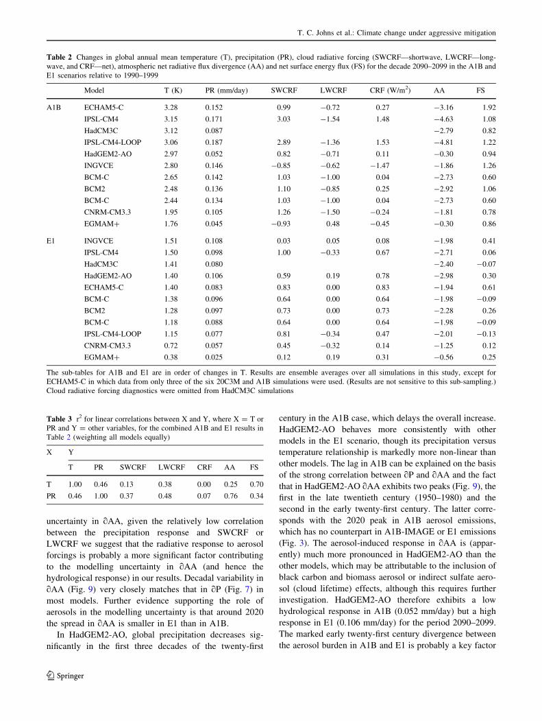
uncertainty in qAA, given the relatively low correlation

between the precipitation response and SWCRF or

LWCRF we suggest that the radiative response to aerosol

forcings is probably a more significant factor contributing

to the modelling uncertainty in qAA (and hence the

hydrological response) in our results. Decadal variability in

qAA (Fig. 9) very closely matches that in qP (Fig. 7) in

most models. Further evidence supporting the role of

aerosols in the modelling uncertainty is that around 2020

the spread in qAA is smaller in E1 than in A1B.

In HadGEM2-AO, global precipitation decreases sig-

nificantly in the first three decades of the twenty-first

century in the A1B case, which delays the overall increase.

HadGEM2-AO behaves more consistently with other

models in the E1 scenario, though its precipitation versus

temperature relationship is markedly more non-linear than

other models. The lag in A1B can be explained on the basis

of the strong correlation between qP and qAA and the fact

that in HadGEM2-AO qAA exhibits two peaks (Fig. 9), the

first in the late twentieth century (1950–1980) and the

second in the early twenty-first century. The latter corre-

sponds with the 2020 peak in A1B aerosol emissions,

which has no counterpart in A1B-IMAGE or E1 emissions

(Fig. 3). The aerosol-induced response in qAA is (appar-

ently) much more pronounced in HadGEM2-AO than the

other models, which may be attributable to the inclusion of

black carbon and biomass aerosol or indirect sulfate aero-

sol (cloud lifetime) effects, although this requires further

investigation. HadGEM2-AO therefore exhibits a low

hydrological response in A1B (0.052 mm/day) but a high

response in E1 (0.106 mm/day) for the period 2090–2099.

The marked early twenty-first century divergence between

the aerosol burden in A1B and E1 is probably a key factor

Table 2 Changes in global annual mean temperature (T), precipitation (PR), cloud radiative forcing (SWCRF—shortwave, LWCRF—long-

wave, and CRF—net), atmospheric net radiative flux divergence (AA) and net surface energy flux (FS) for the decade 2090–2099 in the A1B and

E1 scenarios relative to 1990–1999

Model T (K) PR (mm/day) SWCRF LWCRF CRF (W/m2) AA FS

A1B ECHAM5-C 3.28 0.152 0.99 -0.72 0.27 -3.16 1.92

IPSL-CM4 3.15 0.171 3.03 -1.54 1.48 -4.63 1.08

HadCM3C 3.12 0.087 -2.79 0.82

IPSL-CM4-LOOP 3.06 0.187 2.89 -1.36 1.53 -4.81 1.22

HadGEM2-AO 2.97 0.052 0.82 -0.71 0.11 -0.30 0.94

INGVCE 2.80 0.146 -0.85 -0.62 -1.47 -1.86 1.26

BCM-C 2.65 0.142 1.03 -1.00 0.04 -2.73 0.60

BCM2 2.48 0.136 1.10 -0.85 0.25 -2.92 1.06

BCM-C 2.44 0.134 1.03 -1.00 0.04 -2.73 0.60

CNRM-CM3.3 1.95 0.105 1.26 -1.50 -0.24 -1.81 0.78

EGMAM? 1.76 0.045 -0.93 0.48 -0.45 -0.30 0.86

E1 INGVCE 1.51 0.108 0.03 0.05 0.08 -1.98 0.41

IPSL-CM4 1.50 0.098 1.00 -0.33 0.67 -2.71 0.06

HadCM3C 1.41 0.080 -2.40 -0.07

HadGEM2-AO 1.40 0.106 0.59 0.19 0.78 -2.98 0.30

ECHAM5-C 1.40 0.083 0.83 0.00 0.83 -1.94 0.61

BCM-C 1.38 0.096 0.64 0.00 0.64 -1.98 -0.09

BCM2 1.28 0.097 0.73 0.00 0.73 -2.28 0.26

BCM-C 1.18 0.088 0.64 0.00 0.64 -1.98 -0.09

IPSL-CM4-LOOP 1.15 0.077 0.81 -0.34 0.47 -2.01 -0.13

CNRM-CM3.3 0.72 0.057 0.45 -0.32 0.14 -1.25 0.12

EGMAM? 0.38 0.025 0.12 0.19 0.31 -0.56 0.25

The sub-tables for A1B and E1 are in order of changes in T. Results are ensemble averages over all simulations in this study, except for

ECHAM5-C in which data from only three of the six 20C3M and A1B simulations were used. (Results are not sensitive to this sub-sampling.)

Cloud radiative forcing diagnostics were omitted from HadCM3C simulations

Table 3 r2 for linear correlations between X and Y, where X = T or

PR and Y = other variables, for the combined A1B and E1 results in

Table 2 (weighting all models equally)

X Y

T PR SWCRF LWCRF CRF AA FS

T 1.00 0.46 0.13 0.38 0.00 0.25 0.70

PR 0.46 1.00 0.37 0.48 0.07 0.76 0.34


123

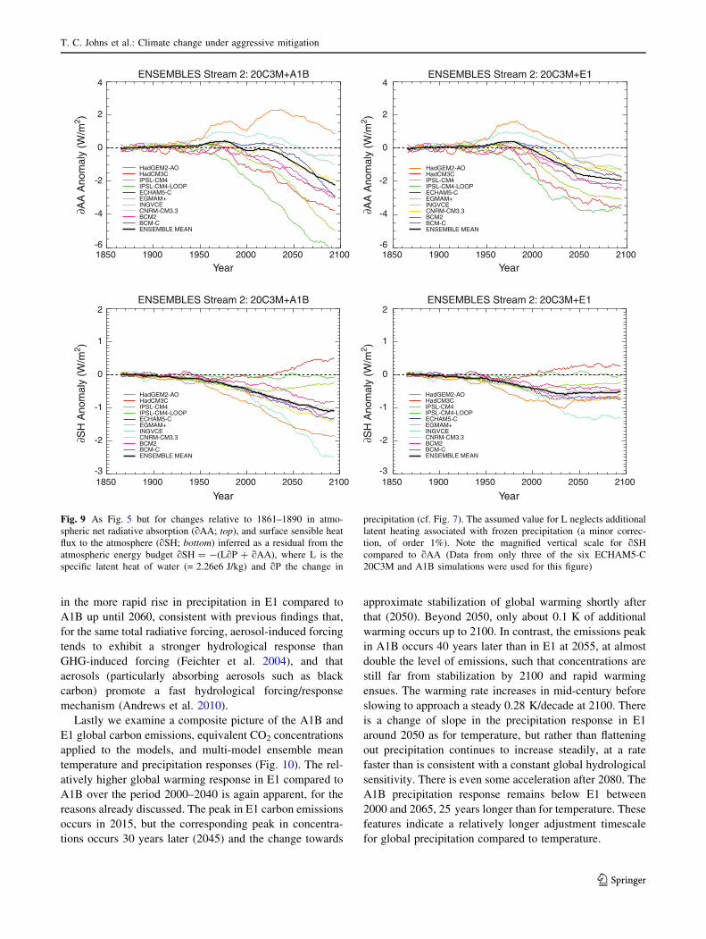
in the more rapid rise in precipitation in E1 compared to

A1B up until 2060, consistent with previous findings that,

for the same total radiative forcing, aerosol-induced forcing

tends to exhibit a stronger hydrological response than

GHG-induced forcing (Feichter et al. 2004), and that

aerosols (particularly absorbing aerosols such as black

carbon) promote a fast hydrological forcing/response

mechanism (Andrews et al. 2010).

Lastly we examine a composite picture of the A1B and

E1 global carbon emissions, equivalent CO2 concentrations

applied to the models, and multi-model ensemble mean

temperature and precipitation responses (Fig. 10). The rel-

atively higher global warming response in E1 compared to

A1B over the period 2000–2040 is again apparent, for the

reasons already discussed. The peak in E1 carbon emissions

occurs in 2015, but the corresponding peak in concentra-

tions occurs 30 years later (2045) and the change towards

approximate stabilization of global warming shortly after

that (2050). Beyond 2050, only about 0.1 K of additional

warming occurs up to 2100. In contrast, the emissions peak

in A1B occurs 40 years later than in E1 at 2055, at almost

double the level of emissions, such that concentrations are

still far from stabilization by 2100 and rapid warming

ensues. The warming rate increases in mid-century before

slowing to approach a steady 0.28 K/decade at 2100. There

is a change of slope in the precipitation response in E1

around 2050 as for temperature, but rather than flattening

out precipitation continues to increase steadily, at a rate

faster than is consistent with a constant global hydrological

sensitivity. There is even some acceleration after 2080. The

A1B precipitation response remains below E1 between

2000 and 2065, 25 years longer than for temperature. These

features indicate a relatively longer adjustment timescale

for global precipitation compared to temperature.


1850 1900 1950 2000 2050 2100

Year

-3

-2

-1

0

1

2

∂SH

Ano

mal

y (W

/m2 )

∂SH

Ano

mal

y (W

/m2 )

∂AA

Ano

mal

y (W

/m2 )

∂AA

Ano

mal

y (W

/m2 )



1850 1900 1950 2000 2050 2100

Year

-3

-2

-1

0

1

2



1850 1900 1950 2000 2050 2100

Year

-6

-4

-2

0

2

4



1850 1900 1950 2000 2050 2100

Year

-6

-4

-2

0

2

4


Fig. 9 As Fig. 5 but for changes relative to 1861–1890 in atmo-

spheric net radiative absorption (qAA; top), and surface sensible heat

flux to the atmosphere (qSH; bottom) inferred as a residual from the

atmospheric energy budget qSH = -(LqP ? qAA), where L is the

specific latent heat of water (= 2.26e6 J/kg) and qP the change in

precipitation (cf. Fig. 7). The assumed value for L neglects additional

latent heating associated with frozen precipitation (a minor correc-

tion, of order 1%). Note the magnified vertical scale for qSH

compared to qAA (Data from only three of the six ECHAM5-C

20C3M and A1B simulations were used for this figure)


123

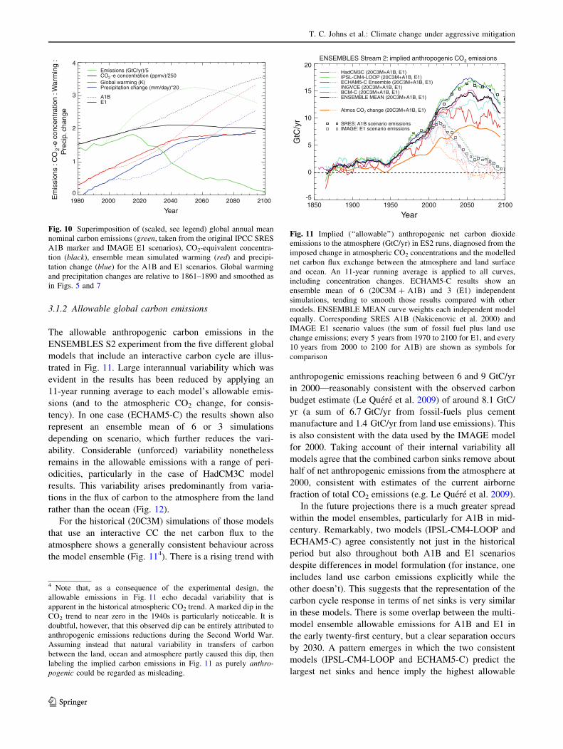
3.1.2 Allowable global carbon emissions

The allowable anthropogenic carbon emissions in the

ENSEMBLES S2 experiment from the five different global

models that include an interactive carbon cycle are illus-

trated in Fig. 11. Large interannual variability which was

evident in the results has been reduced by applying an

11-year running average to each model’s allowable emis-

sions (and to the atmospheric CO2 change, for consis-

tency). In one case (ECHAM5-C) the results shown also

represent an ensemble mean of 6 or 3 simulations

depending on scenario, which further reduces the vari-

ability. Considerable (unforced) variability nonetheless

remains in the allowable emissions with a range of peri-

odicities, particularly in the case of HadCM3C model

results. This variability arises predominantly from varia-

tions in the flux of carbon to the atmosphere from the land

rather than the ocean (Fig. 12).

For the historical (20C3M) simulations of those models

that use an interactive CC the net carbon flux to the

atmosphere shows a generally consistent behaviour across

the model ensemble (Fig. 114). There is a rising trend with

anthropogenic emissions reaching between 6 and 9 GtC/yr

in 2000—reasonably consistent with the observed carbon

budget estimate (Le Quere et al. 2009) of around 8.1 GtC/

yr (a sum of 6.7 GtC/yr from fossil-fuels plus cement

manufacture and 1.4 GtC/yr from land use emissions). This

is also consistent with the data used by the IMAGE model

for 2000. Taking account of their internal variability all

models agree that the combined carbon sinks remove about

half of net anthropogenic emissions from the atmosphere at

2000, consistent with estimates of the current airborne

fraction of total CO2 emissions (e.g. Le Quere et al. 2009).

In the future projections there is a much greater spread

within the model ensembles, particularly for A1B in mid-

century. Remarkably, two models (IPSL-CM4-LOOP and

ECHAM5-C) agree consistently not just in the historical

period but also throughout both A1B and E1 scenarios

despite differences in model formulation (for instance, one

includes land use carbon emissions explicitly while the

other doesn’t). This suggests that the representation of the

carbon cycle response in terms of net sinks is very similar

in these models. There is some overlap between the multi-

model ensemble allowable emissions for A1B and E1 in

the early twenty-first century, but a clear separation occurs

by 2030. A pattern emerges in which the two consistent

models (IPSL-CM4-LOOP and ECHAM5-C) predict the

largest net sinks and hence imply the highest allowable

ENSEMBLES Stream 2: implied anthropogenic CO2 emissions

1850 1900 1950 2000 2050 2100

Year

-5

0

5

10

15

20

GtC

/yr

HadCM3C (20C3M+A1B, E1)IPSL-CM4-LOOP (20C3M+A1B, E1)ECHAM5-C Ensemble (20C3M+A1B, E1)INGVCE (20C3M+A1B, E1)BCM-C (20C3M+A1B, E1)ENSEMBLE MEAN (20C3M+A1B, E1)

Atmos CO2 change (20C3M+A1B, E1)

SRES: A1B scenario emissionsIMAGE: E1 scenario emissions

Fig. 11 Implied (‘‘allowable’’) anthropogenic net carbon dioxide

emissions to the atmosphere (GtC/yr) in ES2 runs, diagnosed from the

imposed change in atmospheric CO2 concentrations and the modelled

net carbon flux exchange between the atmosphere and land surface

and ocean. An 11-year running average is applied to all curves,

including concentration changes. ECHAM5-C results show an

ensemble mean of 6 (20C3M ? A1B) and 3 (E1) independent

simulations, tending to smooth those results compared with other

models. ENSEMBLE MEAN curve weights each independent model

equally. Corresponding SRES A1B (Nakicenovic et al. 2000) and

IMAGE E1 scenario values (the sum of fossil fuel plus land use

change emissions; every 5 years from 1970 to 2100 for E1, and every

10 years from 2000 to 2100 for A1B) are shown as symbols for

comparison

1980 2000 2020 2040 2060 2080 2100

Year

0

1

2

3

4

Em

issi

ons

: CO

2-e

con

cent

ratio

n : W

arm

ing

:

Emissions (GtC/yr)/5CO2 -e concentration (ppmv)/250Global warming (K)Precipitation change (mm/day)*20

A1BE1

Pre

cip.

cha

nge

Fig. 10 Superimposition of (scaled, see legend) global annual mean

nominal carbon emissions (green, taken from the original IPCC SRES

A1B marker and IMAGE E1 scenarios), CO2-equivalent concentra-

tion (black), ensemble mean simulated warming (red) and precipi-

tation change (blue) for the A1B and E1 scenarios. Global warming

and precipitation changes are relative to 1861–1890 and smoothed as

in Figs. 5 and 7

4 Note that, as a consequence of the experimental design, the

allowable emissions in Fig. 11 echo decadal variability that is

apparent in the historical atmospheric CO2 trend. A marked dip in the

CO2 trend to near zero in the 1940s is particularly noticeable. It is

doubtful, however, that this observed dip can be entirely attributed to

anthropogenic emissions reductions during the Second World War.

Assuming instead that natural variability in transfers of carbon

between the land, ocean and atmosphere partly caused this dip, then

labeling the implied carbon emissions in Fig. 11 as purely anthro-pogenic could be regarded as misleading.


123

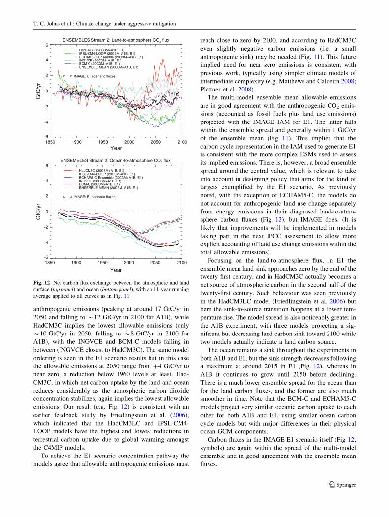
anthropogenic emissions (peaking at around 17 GtC/yr in

2050 and falling to *12 GtC/yr in 2100 for A1B), while

HadCM3C implies the lowest allowable emissions (only

*10 GtC/yr in 2050, falling to *8 GtC/yr in 2100 for

A1B), with the INGVCE and BCM-C models falling in

between (INGVCE closest to HadCM3C). The same model

ordering is seen in the E1 scenario results but in this case

the allowable emissions at 2050 range from ?4 GtC/yr to

near zero, a reduction below 1960 levels at least. Had-

CM3C, in which net carbon uptake by the land and ocean

reduces considerably as the atmospheric carbon dioxide

concentration stabilizes, again implies the lowest allowable

emissions. Our result (e.g. Fig. 12) is consistent with an

earlier feedback study by Friedlingstein et al. (2006),

which indicated that the HadCM3LC and IPSL-CM4-

LOOP models have the highest and lowest reductions in

terrestrial carbon uptake due to global warming amongst

the C4MIP models.

To achieve the E1 scenario concentration pathway the

models agree that allowable anthropogenic emissions must

reach close to zero by 2100, and according to HadCM3C

even slightly negative carbon emissions (i.e. a small

anthropogenic sink) may be needed (Fig. 11). This future

implied need for near zero emissions is consistent with

previous work, typically using simpler climate models of

intermediate complexity (e.g. Matthews and Caldeira 2008;

Plattner et al. 2008).

The multi-model ensemble mean allowable emissions

are in good agreement with the anthropogenic CO2 emis-

sions (accounted as fossil fuels plus land use emissions)

projected with the IMAGE IAM for E1. The latter falls

within the ensemble spread and generally within 1 GtC/yr

of the ensemble mean (Fig. 11). This implies that the

carbon cycle representation in the IAM used to generate E1

is consistent with the more complex ESMs used to assess

its implied emissions. There is, however, a broad ensemble

spread around the central value, which is relevant to take

into account in designing policy that aims for the kind of

targets exemplified by the E1 scenario. As previously

noted, with the exception of ECHAM5-C, the models do

not account for anthropogenic land use change separately

from energy emissions in their diagnosed land-to-atmo-

sphere carbon fluxes (Fig. 12), but IMAGE does. (It is

likely that improvements will be implemented in models

taking part in the next IPCC assessment to allow more

explicit accounting of land use change emissions within the

total allowable emissions).

Focusing on the land-to-atmosphere flux, in E1 the

ensemble mean land sink approaches zero by the end of the

twenty-first century, and in HadCM3C actually becomes a

net source of atmospheric carbon in the second half of the

twenty-first century. Such behaviour was seen previously

in the HadCM3LC model (Friedlingstein et al. 2006) but

here the sink-to-source transition happens at a lower tem-

perature rise. The model spread is also noticeably greater in

the A1B experiment, with three models projecting a sig-

nificant but decreasing land carbon sink toward 2100 while

two models actually indicate a land carbon source.

The ocean remains a sink throughout the experiments in

both A1B and E1, but the sink strength decreases following

a maximum at around 2015 in E1 (Fig. 12), whereas in

A1B it continues to grow until 2050 before declining.

There is a much lower ensemble spread for the ocean than

for the land carbon fluxes, and the former are also much

smoother in time. Note that the BCM-C and ECHAM5-C

models project very similar oceanic carbon uptake to each

other for both A1B and E1, using similar ocean carbon

cycle models but with major differences in their physical

ocean GCM components.

Carbon fluxes in the IMAGE E1 scenario itself (Fig 12;

symbols) are again within the spread of the multi-model

ensemble and in good agreement with the ensemble mean

fluxes.

ENSEMBLES Stream 2: Land-to-atmosphere CO2 flux

1850 1900 1950 2000 2050 2100Year

-6

-4

-2

0

2

4

6

GtC

/yr


IMAGE: E1 scenario fluxes

ENSEMBLES Stream 2: Ocean-to-atmosphere CO2 flux

1850 1900 1950 2000 2050 2100

Year

-6

-4

-2

0

2

4

6

GtC

/yr


IMAGE: E1 scenario fluxes

Fig. 12 Net carbon flux exchange between the atmosphere and land

surface (top panel) and ocean (bottom panel), with an 11-year running

average applied to all curves as in Fig. 11


123

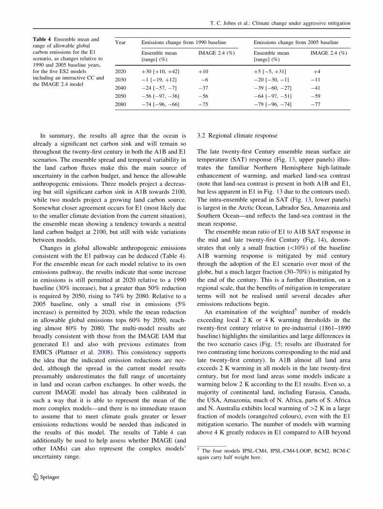
In summary, the results all agree that the ocean is

already a significant net carbon sink and will remain so

throughout the twenty-first century in both the A1B and E1

scenarios. The ensemble spread and temporal variability in

the land carbon fluxes make this the main source of

uncertainty in the carbon budget, and hence the allowable

anthropogenic emissions. Three models project a decreas-

ing but still significant carbon sink in A1B towards 2100,

while two models project a growing land carbon source.

Somewhat closer agreement occurs for E1 (most likely due

to the smaller climate deviation from the current situation),

the ensemble mean showing a tendency towards a neutral

land carbon budget at 2100, but still with wide variations

between models.

Changes in global allowable anthropogenic emissions

consistent with the E1 pathway can be deduced (Table 4).

For the ensemble mean for each model relative to its own

emissions pathway, the results indicate that some increase

in emissions is still permitted at 2020 relative to a 1990

baseline (30% increase), but a greater than 50% reduction

is required by 2050, rising to 74% by 2080. Relative to a

2005 baseline, only a small rise in emissions (5%

increase) is permitted by 2020, while the mean reduction

in allowable global emissions tops 60% by 2050, reach-

ing almost 80% by 2080. The multi-model results are

broadly consistent with those from the IMAGE IAM that

generated E1 and also with previous estimates from

EMICS (Plattner et al. 2008). This consistency supports

the idea that the indicated emission reductions are nee-

ded, although the spread in the current model results

presumably underestimates the full range of uncertainty

in land and ocean carbon exchanges. In other words, the

current IMAGE model has already been calibrated in

such a way that it is able to represent the mean of the

more complex models—and there is no immediate reason

to assume that to meet climate goals greater or lesser

emissions reductions would be needed than indicated in

the results of this model. The results of Table 4 can

additionally be used to help assess whether IMAGE (and

other IAMs) can also represent the complex models’

uncertainty range.

3.2 Regional climate response

The late twenty-first Century ensemble mean surface air

temperature (SAT) response (Fig. 13, upper panels) illus-

trates the familiar Northern Hemisphere high-latitude

enhancement of warming, and marked land-sea contrast

(note that land-sea contrast is present in both A1B and E1,

but less apparent in E1 in Fig. 13 due to the contours used).

The intra-ensemble spread in SAT (Fig. 13, lower panels)

is largest in the Arctic Ocean, Labrador Sea, Amazonia and

Southern Ocean—and reflects the land-sea contrast in the

mean response.

The ensemble mean ratio of E1 to A1B SAT response in

the mid and late twenty-first Century (Fig. 14), demon-

strates that only a small fraction (\10%) of the baseline

A1B warming response is mitigated by mid century

through the adoption of the E1 scenario over most of the

globe, but a much larger fraction (30–70%) is mitigated by

the end of the century. This is a further illustration, on a

regional scale, that the benefits of mitigation in temperature

terms will not be realised until several decades after

emissions reductions begin.

An examination of the weighted5 number of models

exceeding local 2 K or 4 K warming thresholds in the

twenty-first century relative to pre-industrial (1861–1890

baseline) highlights the similarities and large differences in

the two scenario cases (Fig. 15; results are illustrated for

two contrasting time horizons corresponding to the mid and

late twenty-first century). In A1B almost all land area

exceeds 2 K warming in all models in the late twenty-first

century, but for most land areas some models indicate a

warming below 2 K according to the E1 results. Even so, a

majority of continental land, including Eurasia, Canada,

the USA, Amazonia, much of N. Africa, parts of S. Africa

and N. Australia exhibits local warming of[2 K in a large

fraction of models (orange/red colours), even with the E1

mitigation scenario. The number of models with warming

above 4 K greatly reduces in E1 compared to A1B beyond

Table 4 Ensemble mean and

range of allowable global

carbon emissions for the E1

scenario, as changes relative to

1990 and 2005 baseline years,

for the five ES2 models

including an interactive CC and

the IMAGE 2.4 model

Year Emissions change from 1990 baseline Emissions change from 2005 baseline

Ensemble mean

[range] (%)

IMAGE 2.4 (%) Ensemble mean

[range] (%)

IMAGE 2.4 (%)

2020 ?30 [?10, ?42] ?10 ?5 [-5, ?31] ?4

2030 -1 [-19, ?12] -6 -20 [-30, -1] -11

2040 -24 [-57, -7] -37 -39 [-60, -27] -41

2050 -56 [-97, -36] -56 -64 [-97, -51] -59

2080 -74 [-96, -66] -75 -79 [-96, -74] -77

5 The four models IPSL-CM4, IPSL-CM4-LOOP, BCM2, BCM-C

again carry half weight here.


123

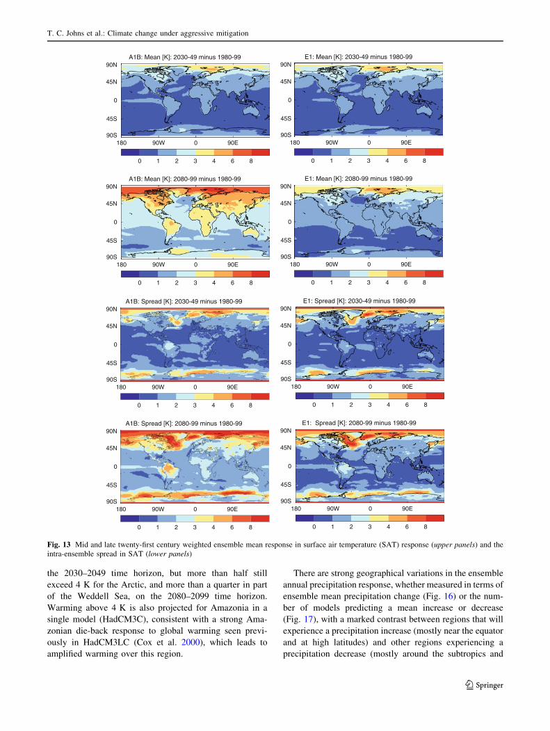
the 2030–2049 time horizon, but more than half still

exceed 4 K for the Arctic, and more than a quarter in part

of the Weddell Sea, on the 2080–2099 time horizon.

Warming above 4 K is also projected for Amazonia in a

single model (HadCM3C), consistent with a strong Ama-

zonian die-back response to global warming seen previ-

ously in HadCM3LC (Cox et al. 2000), which leads to

amplified warming over this region.

There are strong geographical variations in the ensemble

annual precipitation response, whether measured in terms of

ensemble mean precipitation change (Fig. 16) or the num-

ber of models predicting a mean increase or decrease

(Fig. 17), with a marked contrast between regions that will

experience a precipitation increase (mostly near the equator

and at high latitudes) and other regions experiencing a

precipitation decrease (mostly around the subtropics and

180 90W 0 90E90S

45S

0

45N

90NA1B: Spread [K]: 2030-49 minus 1980-99

0 1 2 3 4 6 8

180 90W 0 90E90S

45S

0

45N

90NA1B: Spread [K]: 2080-99 minus 1980-99

0 1 2 3 4 6 8

180 90W 0 90E90S

45S

0

45N

90NE1: Spread [K]: 2030-49 minus 1980-99

0 1 2 3 4 6 8

180 90W 0 90E90S

45S

0

45N

90NE1: Spread [K]: 2080-99 minus 1980-99

0 1 2 3 4 6 8

180 90W 0 90E90S

45S

0

45N

90NA1B: Mean [K]: 2030-49 minus 1980-99

0 1 2 3 4 6 8

180 90W 0 90E90S

45S

0

45N

90NA1B: Mean [K]: 2080-99 minus 1980-99

0 1 2 3 4 6 8

180 90W 0 90E90S

45S

0

45N

90NE1: Mean [K]: 2030-49 minus 1980-99

0 1 2 3 4 6 8

180 90W 0 90E90S

45S

0

45N

90NE1: Mean [K]: 2080-99 minus 1980-99

0 1 2 3 4 6 8

Fig. 13 Mid and late twenty-first century weighted ensemble mean response in surface air temperature (SAT) response (upper panels) and the

intra-ensemble spread in SAT (lower panels)


123

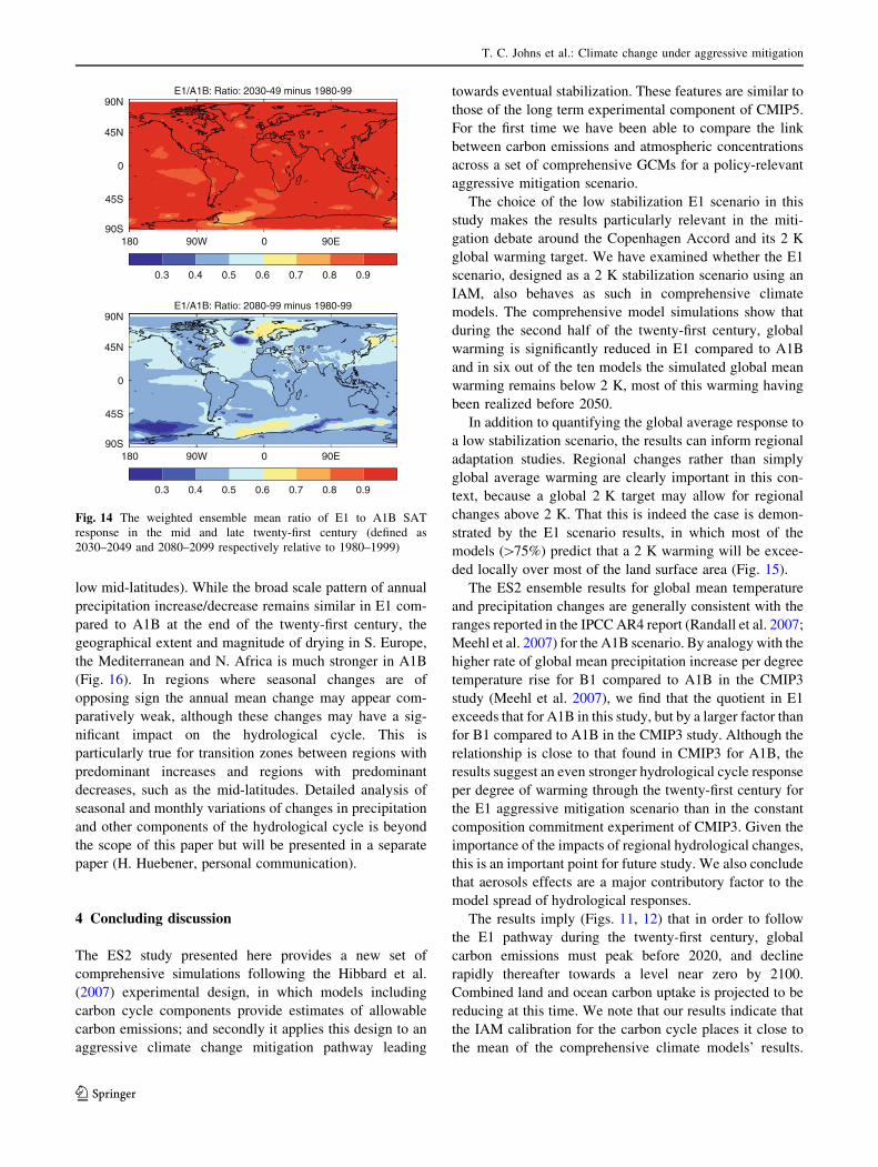
low mid-latitudes). While the broad scale pattern of annual

precipitation increase/decrease remains similar in E1 com-

pared to A1B at the end of the twenty-first century, the

geographical extent and magnitude of drying in S. Europe,

the Mediterranean and N. Africa is much stronger in A1B

(Fig. 16). In regions where seasonal changes are of

opposing sign the annual mean change may appear com-

paratively weak, although these changes may have a sig-

nificant impact on the hydrological cycle. This is

particularly true for transition zones between regions with

predominant increases and regions with predominant

decreases, such as the mid-latitudes. Detailed analysis of

seasonal and monthly variations of changes in precipitation

and other components of the hydrological cycle is beyond

the scope of this paper but will be presented in a separate

paper (H. Huebener, personal communication).

4 Concluding discussion

The ES2 study presented here provides a new set of

comprehensive simulations following the Hibbard et al.

(2007) experimental design, in which models including

carbon cycle components provide estimates of allowable

carbon emissions; and secondly it applies this design to an

aggressive climate change mitigation pathway leading

towards eventual stabilization. These features are similar to

those of the long term experimental component of CMIP5.

For the first time we have been able to compare the link

between carbon emissions and atmospheric concentrations

across a set of comprehensive GCMs for a policy-relevant

aggressive mitigation scenario.

The choice of the low stabilization E1 scenario in this

study makes the results particularly relevant in the miti-

gation debate around the Copenhagen Accord and its 2 K

global warming target. We have examined whether the E1

scenario, designed as a 2 K stabilization scenario using an

IAM, also behaves as such in comprehensive climate

models. The comprehensive model simulations show that

during the second half of the twenty-first century, global

warming is significantly reduced in E1 compared to A1B

and in six out of the ten models the simulated global mean

warming remains below 2 K, most of this warming having

been realized before 2050.

In addition to quantifying the global average response to

a low stabilization scenario, the results can inform regional

adaptation studies. Regional changes rather than simply

global average warming are clearly important in this con-

text, because a global 2 K target may allow for regional

changes above 2 K. That this is indeed the case is demon-

strated by the E1 scenario results, in which most of the

models ([75%) predict that a 2 K warming will be excee-

ded locally over most of the land surface area (Fig. 15).

The ES2 ensemble results for global mean temperature

and precipitation changes are generally consistent with the

ranges reported in the IPCC AR4 report (Randall et al. 2007;

Meehl et al. 2007) for the A1B scenario. By analogy with the

higher rate of global mean precipitation increase per degree

temperature rise for B1 compared to A1B in the CMIP3

study (Meehl et al. 2007), we find that the quotient in E1

exceeds that for A1B in this study, but by a larger factor than

for B1 compared to A1B in the CMIP3 study. Although the

relationship is close to that found in CMIP3 for A1B, the

results suggest an even stronger hydrological cycle response

per degree of warming through the twenty-first century for

the E1 aggressive mitigation scenario than in the constant

composition commitment experiment of CMIP3. Given the

importance of the impacts of regional hydrological changes,

this is an important point for future study. We also conclude

that aerosols effects are a major contributory factor to the

model spread of hydrological responses.

The results imply (Figs. 11, 12) that in order to follow

the E1 pathway during the twenty-first century, global

carbon emissions must peak before 2020, and decline

rapidly thereafter towards a level near zero by 2100.

Combined land and ocean carbon uptake is projected to be

reducing at this time. We note that our results indicate that

the IAM calibration for the carbon cycle places it close to

the mean of the comprehensive climate models’ results.

180 90W 0 90E90S

45S

0

45N

90NE1/A1B: Ratio: 2030-49 minus 1980-99

0.3 0.4 0.5 0.6 0.7 0.8 0.9

180 90W 0 90E90S

45S

0

45N

90NE1/A1B: Ratio: 2080-99 minus 1980-99

0.3 0.4 0.5 0.6 0.7 0.8 0.9

Fig. 14 The weighted ensemble mean ratio of E1 to A1B SAT

response in the mid and late twenty-first century (defined as

2030–2049 and 2080–2099 respectively relative to 1980–1999)


123

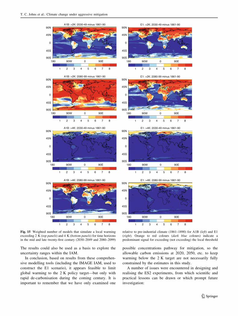
The results could also be used as a basis to explore the

uncertainty ranges within the IAM.

In conclusion, based on results from these comprehen-

sive modelling tools (including the IMAGE IAM, used to

construct the E1 scenario), it appears feasible to limit

global warming to the 2 K policy target—but only with

rapid de-carbonisation during the coming century. It is

important to remember that we have only examined one

possible concentrations pathway for mitigation, so the

allowable carbon emissions at 2020, 2050, etc. to keep

warming below the 2 K target are not necessarily fully

constrained by the estimates in this study.

A number of issues were encountered in designing and

realising the ES2 experiments, from which scientific and

practical lessons can be drawn or which prompt future

investigation:

180 90W 0 90E90S

45S

0

45N

90NA1B: >4K: 2030-49 minus 1861-90

1

180 90W 0 90E90S

45S

0

45N

90NA1B: >4K: 2080-99 minus 1861-90

1

180 90W 0 90E90S

45S

0

45N

90NE1: >4K: 2030-49 minus 1861-90

1

180 90W 0 90E90S

45S

0

45N

90NE1: >4K: 2080-99 minus 1861-90

1

180 90W 0 90E90S

45S

0

45N

90NA1B: >2K: 2030-49 minus 1861-90

1

180 90W 0 90E90S

45S

0

45N

90NA1B: >2K: 2080-99 minus 1861-90

1

180 90W 0 90E90S

45S

0

45N

90NE1: >2K: 2030-49 minus 1861-90

1

180 90W 0 90E90S

45S

0

45N

90NE1: >2K: 2080-99 minus 1861-90

1

2 3 4 5 6 7 8

2 3 4 5 6 7 8

2 3 4 5 6 7 8

2 3 4 5 6 7 8

2 3 4 5 6 7 8

2 3 4 5 6 7 8

2 3 4 5 6 7 8

2 3 4 5 6 7 8

Fig. 15 Weighted number of models that simulate a local warming

exceeding 2 K (top panels) and 4 K (bottom panels) for time horizons

in the mid and late twenty-first century (2030–2049 and 2080–2099)

relative to pre-industrial climate (1861–1890) for A1B (left) and E1

(right). Orange to red colours (dark blue colours) indicate a

predominant signal for exceeding (not exceeding) the local threshold


123

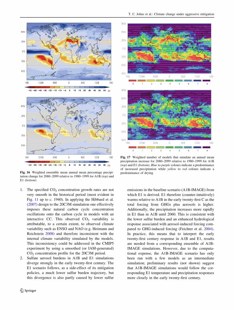
1. The specified CO2 concentration growth rates are not

very smooth in the historical period (most evident in

Fig. 11 up to c. 1940). In applying the Hibbard et al.

(2007) design to the 20C3M simulation one effectively

imposes these natural carbon cycle concentration

oscillations onto the carbon cycle in models with an

interactive CC. This observed CO2 variability is

attributable, to a certain extent, to observed climate

variability such as ENSO and NAO (e.g. Heimann and

Reichstein 2008) and therefore inconsistent with the

internal climate variability simulated by the models.

This inconsistency could be addressed in the CMIP5

experiment by using a smoothed (or IAM-generated)

CO2 concentration profile for the 20C3M period.

2. Sulfate aerosol burdens in A1B and E1 simulations

diverge strongly in the early twenty-first century. The

E1 scenario follows, as a side-effect of its mitigation

policies, a much lower sulfur burden trajectory, but

this divergence is also partly caused by lower sulfur

emissions in the baseline scenario (A1B-IMAGE) from

which E1 is derived. E1 therefore (counter-intuitively)

warms relative to A1B in the early twenty-first C as the

total forcing from GHGs plus aerosols is higher.

Additionally, the precipitation increases more rapidly

in E1 than in A1B until 2060. This is consistent with

the lower sulfur burden and an enhanced hydrological

response associated with aerosol-induced forcing com-

pared to GHG-induced forcing (Feichter et al. 2004).

In practice, this means that to interpret the early

twenty-first century response in A1B and E1, results

are needed from a corresponding ensemble of A1B-

IMAGE simulations. However, due to the computa-

tional expense, the A1B-IMAGE scenario has only

been run with a few models as an intermediate

simulation; preliminary results (not shown) suggest

that A1B-IMAGE simulations would follow the cor-

responding E1 temperature and precipitation responses

more closely in the early twenty-first century.

Fig. 16 Weighted ensemble mean annual mean percentage precipi-

tation change for 2080–2099 relative to 1980–1999 for A1B (top) and

E1 (bottom)

Fig. 17 Weighted number of models that simulate an annual mean

precipitation increase for 2080–2099 relative to 1980–1999 for A1B

(top) and E1 (bottom). Blue to purple colours indicate a predominance

of increased precipitation while yellow to red colours indicate a

predominance of drying


123

3. Sulfate aerosol forcing is applied via emissions in a

few models, but as concentrations in others, so this

important forcing element is not as tightly controlled

as the GHG forcing (via concentrations) in the

experimental design. In combination with model-to-

model variations in the representation of aerosol

physics and their radiative forcings, the overall effect

of aerosols therefore represents an important source of

uncertainty in the results. Our results indicate that

modeling uncertainties affecting changes in the atmo-

spheric radiation budget (the direct response to aerosol

forcing—particularly absorbing aerosol—being one

contributory factor) are more significant (by a ratio

of 2:1 or greater) than those affecting changes in

surface sensible heat flux to the atmosphere, in

determining the range of hydrological responses under

the given forcing scenarios.

4. Land use changes were applied via crop and pasture

fraction changes blended with underlying land use

maps, but this was only possible for a subset of the

models. Additionally, due to the model-dependent

nature of the underlying land use maps, it was

problematic to achieve a consistent land use change

forcing even in this subset of models. This echoes the

conclusions of Pitman et al. (2009) that land use

change, despite being a regionally significant forcing,

is presently impossible to impose in a common way in

multiple models.

In future, there are clearly opportunities to explore

aspects of climate change and climate impacts using the

ES2 results for a plausible scenario with a small signal-to-

noise ratio. But given that we have an initial condition

ensemble of only modest size, we may need to develop

new techniques to extract the fine scale climate change

information.

As described in the text, further analysis of the E1

versus A1B responses is planned which will examine in

greater detail regional and seasonal changes in the hydro-

logical cycle, and look into the carbon cycle dynamics in

the changing climate simulated in the subset of models

with interactive CC, with the aim of ascertaining which

aspects of physical climate change are the dominant driv-

ers. To facilitate such future studies, and more general

exploitation of the results of the ES2 experiment, data from

the simulations are freely available for download as

described in the ‘‘Appendix’’.

Acknowledgments We gratefully acknowledge the ENSEMBLES

project, funded by the European Commission’s 6th Framework Pro-

gramme (FP6) through contract GOCE-CT-2003-505539. We also

thank Nathalie de Noblet, Bjorg Rognerud and Olivier Boucher for

their help in constructing the essential scenario forcing datasets, and

Jason Lowe and two anonymous reviewers for comments which

helped to improve this paper. TCJ and CDH were supported by the

Joint DECC and Defra Integrated Climate Programme, DECC/Defra

(GA01101). The development of BCM-C was supported by the

CARBOOCEAN integrated project under FP6 (grant number 511176)

and the Research Council of Norway through the NorClim project.

Finally we express our deep gratitude to numerous hard-working

members of our respective modeling teams.

Appendix: Output data availability

Data outputs from ES2 simulations, for the historical per-

iod (20C3M) and E1 and A1B scenarios for the period

2000–2100 have been archived in CF-compliant NetCDF

format in the CERA database in Hamburg (http://cera-

www.dkrz.de), from where they can be downloaded for

non-commercial scientific research, subject to user regis-

tration. Detailed metadata are also stored there describing

the simulations and variables archived.

The data include monthly mean values, daily values

(daily mean, max and min, or instantaneous, depending on

the variable), and also several instantaneous variables at 6-

and 12-hourly resolution at the surface and on vertical

pressure levels. Data files include various meteorological

and oceanographic (surface or near-surface only) variables

using Climate and Forecast (CF) compliant names and

metadata conventions, including variables related to the

interactive CC and aerosol schemes for some models and

simulations that include them. For several models,

ensemble simulations are included in the database. Addi-

tional variables other than those archived at CERA may be

available on request direct from the associated ENSEM-

BLES partners or from other data centres (contact details

are given in the metadata).

The full multi-model dataset at CERA includes all the

runs listed in Table 1, including those following the A1B-

IMAGE scenario, plus some alternatively forced 20C3M

runs. The total dataset exceeds 6000 simulated model years

in total and is about 11 TB in size. This makes it about one

third as large as the WCRP CMIP3 multi-model dataset:

http://www-pcmdi.llnl.gov/ipcc/about_ipcc.php.

References

Alessandri A (2006) Effects of land surface and vegetation processes

on the climate simulated by an atmospheric general circulation

model. Ph.D Thesis in Geophysics, Bologna University Alma

Mater Studiorum, 114 pp

Andrews T, Forster PM, Boucher O, Bellouin N, Jones A (2010)

Precipitation, radiative forcing and global temperature change.

Geophys Res Lett 37:L14701. doi:10.1029/2010GL043991

Assmann KM, Bentsen M, Segschneider J, Heinze C (2010) An

isopycnic ocean carbon cycle model. Geosci Model Dev

3:143–167


123

http://cera-www.dkrz.de

http://cera-www.dkrz.de

http://www-pcmdi.llnl.gov/ipcc/about_ipcc.php

http://dx.doi.org/10.1029/2010GL043991

Aumont O, Maier-Reimer E, Blain S, Monfray P (2003) An

ecosystem model of the global ocean including Fe, Si, P

colimitations. Glob Biogeochem Cycles 17:1060. doi:10.1029/

2001GB001745

Bellouin N et al (2007) Improved representation of aerosols for

HadGEM2. Hadley Centre Technical Note No. 73, Met Office,

Exeter, 42 pp

Bleck R, Smith LT (1990) A wind-driven isopycnic coordinate model

of the North and equatorial Atlantic Ocean. 1: model develop-

ment and supporting experiments. J Geophys Res Oceans

95:3273–3285

Bleck R, Rooth C, Hu D, Smith LT (1992) Salinity-driven thermo-

cline transients in a wind- and thermohaline-forced isopycnic

coordinate model of the North Atlantic. J Phys Oceanogr

22:1486–1505

Bony S, Emanuel KA (2001) A parameterization of the cloudiness

associated with cumulus convection: evaluation using TOGA

COARE data. J Atmos Sci 58:3158–3183

Boucher O, Lohmann U (1995) The sulfate-CCN-cloud albedo effect:

a sensitivity study with two general circulation models. Tellus

(Ser B) 47:281–300

Boucher O, Pham M (2002) History of sulfate aerosol radiative forcings.

Geophys Res Lett 29:1308. doi:10.1029/2001GL014048

Bougeault P (1985) A simple parameterization of the large-scale

effects of cumulus convection. Mon Wea Rev 113:2108–2121

Cadule P, Bopp L, Friedlingstein P (2009) A revised estimate of the

processes contributing to global warming due to climate-carbon

feedback. Geophys Res Lett 36:L14705. doi:10.1029/2009

GLO38681

Cariolle D, Lasserre-Bigorry A, Royer JF, Geleyn JF (1990) A

general circulation model simulation of the springtime Antarctic

ozone decrease and its impact on mid-latitudes. J Geophys Res

Atmos 95:1883–1898

Champeaux JL, Masson V, Chauvin R (2005) ECOCLIMAP: a global

database of land surface parameters at 1 km resolution. Meteorol

Appl 12:29–32

Clarke L, Edmonds J, Krey V, Richels R, Rose S, Tavoni M (2010)

International climate policy architectures: overview of the EMF

22 international scenarios. Energy Econ 31(suppl 2):S64–S81

Collins WJ, Bellouin N, Doutriaux-Boucher M, Gedney N, Hinton T,

Jones CD, Liddicoat S, Martin G, O’Connor F, Rae J, Senior C,

Totterdell I, Woodward S, Reichler T, Kim J (2008) Evaluation

of the HadGEM2 model. Met Office Hadley Centre Technical

Note No. 74, Met Office, Exeter, 47 pp

Copenhagen Accord (2009) United Nations framework convention on

climate change, CoP 15, http://unfccc.int/resource/docs/2009/

cop15/eng/l07.pdf

Cox PM, Betts RA, Jones CD, Spall SA, Totterdell IJ (2000)

Acceleration of global warming due to carbon-cycle feedbacks

in a coupled climate model. Nature 408:184–187

Crowley TJ, Baum SK, Kim KY, Hegerl GC, Hyde WT (2003)

Modeling ocean heat content changes during the last millennium.

Geophys Res Lett 30(18):1932. doi:10.1029/2003GL017801

de Noblet-Ducoudre N, Peterschmitt J-Y (2007) Designing historical

and future land-cover maps at the global scale for climate

studies. Technical Report available from http://www.cnrm.

meteo.fr/ensembles/public/model_simulation.html

Den Elzen MGJ, van Vuuren DP (2007) Peaking profiles for

achieving long-term temperature targets with more likelihood

at lower costs. Proc Natl Acad Sci USA 104:17931–17936

Deque M (1999) Documentation ARPEGE-CLIMAT. Tech report

Centre National de Recherches Meteorologiques, Meteo-France,

Toulouse

Deque M, Dreveton C, Braun A, Cariolle D (1994) The ARPEGE/IFS

atmosphere model: a contribution to the French community

climate modelling. Clim Dyn 10:249–266

Derbyshire SH, Maidens AV, Milton SF, Stratton RA, Willett MR

(2010) Adaptive detrainment in a convective parametrization.

Q J Roy Meteor Soc (submitted)

Douville H, Salas-Melia D, Tyteca S (2006) On the tropical origin of

uncertainties in the global land precipitation response to global

warming. Clim Dyn 26:367–385

Dufresne JL, Quaas J, Boucher O, Denvil S, Fairhead L (2005)

Contrasts in the effects on climate of anthropogenic sulfate

aerosols between the 20th and the 21st century. Geophys Res

Lett 32:L21703. doi:10.1029/2005GL023619

Edenhofer O, Knopf B, Barker T, Baumstark L, Bellevrat E, Chateau

B, Criqui P, Isaac M, Kitous A, Kypreos S, Leimbach M,

Lessmann K, Magne B, Scrieciu S, Turton H, van Vuuren DP

(2010) The economics of low stabilization: model comparison of

mitigation strategies and costs. Energy J 31:11–48

Emanuel KA (1991) A scheme for representing cumulus convection

in large-scale models. J Atmos Sci 48:2313–2335

Emanuel KA (1993) A cumulus representation based on the episodic

mixing model: the importance of mixing and microphysics in

predicting humidity. The Representation of Cumulus Convection

in Numerical Models. Meteor Monogr No 46, Am Meteor Soc,

pp 185–194

Feichter J, Kjellstrom E, Rodhe H, Dentener F, Lelieveld J, Roelofs

GJ (1996) Simulation of the tropospheric sulfur cycle in a global

climate model. Atmos Environ 30:1693–1707

Feichter J, Roeckner E, Lohmann U, Liepert B (2004) Nonlinear

aspects of the climate response to greenhouse gas and aerosol

forcing. J Clim 17:2384–2398

Fogli PG et al (2009) INGV-CMCC Carbon: a carbon cycle earth

system model, CMCC RP0061 (http://www.cmcc.it/publications-

meetings/publications/research-papers/rp0061-ingv-cmcc-carbon-

icc-a-carbon-cycle-earth-system-model)

Friedlingstein P, Cox P, Betts R, Bopp L, von Bloh W, Brovkin V,

Cadule P, Doney S, Eby M, Fung I, Bala G, John J, Jones C, Joos

F, Kato T, Kawamiya M, Knorr W, Lindsay K, Matthews HD,

Raddatz T, Rayner P, Reick C, Roeckner E, Schnitzler KG,

Schnur R, Strassmann K, Weaver AJ, Yoshikawa C, Zeng N

(2006) Climate-carbon cycle feedback analysis: results from the

C4MIP model intercomparison. J Clim 19:3337–3353

Furevik T, Bentsen M, Drange H, Kindem IKT, Kvamsto NG,

Sorteberg A (2003) Description and evaluation of the Bergen

climate model: ARPEGE coupled with MICOM. Clim Dyn

21:27–51

Gibelin AL, Deque M (2003) Anthropogenic climate change over the

Mediterranean region simulated by a global variable resolution

model. Clim Dyn 20:327–339

Gordon C, Cooper C, Senior CA, Banks H, Gregory JM, Johns TC,

Mitchell JFB, Wood RA (2000) The simulation of SST, sea ice

extents and ocean heat transports in a version of the Hadley

Centre coupled model without flux adjustments. Clim Dyn

16:147–168

Gregory D, Allen S (1991) The effect of convective scale downdrafts

upon NWP and climate simulations. In: Preprints, 9th conference

on numerical weather prediction, Denver. Amer Meteor Soc,

pp 122–123

Gregory D, Rowntree PR (1990) A mass flux convection scheme with

representation of cloud ensemble characteristics and stability-

dependent closure. Mon Wea Rev 118:1483–1506

Gregory D, Kershaw R, Inness PM (1997) Parametrization of

momentum transport by convection. II: tests in single-column

and general circulation models. Q J R Meteor Soc 123:1153–

1183

Hansen J et al (2005) Efficacy of climate forcings. J Geophys Res

110:D18104. doi:10.1029/2005JD005776

Heimann M, Reichstein M (2008) Terrestrial ecosystem carbon

dynamics and climate feedbacks. Nature 451:289–292


123

http://dx.doi.org/10.1029/2001GB001745

http://dx.doi.org/10.1029/2001GB001745

http://dx.doi.org/10.1029/2001GL014048

http://dx.doi.org/10.1029/2009GLO38681

http://dx.doi.org/10.1029/2009GLO38681

http://unfccc.int/resource/docs/2009/cop15/eng/l07.pdf

http://unfccc.int/resource/docs/2009/cop15/eng/l07.pdf

http://dx.doi.org/10.1029/2003GL017801



http://dx.doi.org/10.1029/2005GL023619

http://www.cmcc.it/publications-meetings/publications/research-papers/rp0061-ingv-cmcc-carbon-icc-a-carbon-cycle-earth-system-model



http://dx.doi.org/10.1029/2005JD005776

Hewitt CD, Griggs DJ (2004) Ensembles-based predictions of climate

change and their impacts (ENSEMBLES). EOS Trans AGU

85:566

Hibbard KA, Meehl GA, Cox PM, Friedlingstein P (2007) A strategy

for climate change stabilization experiments. EOS Trans AGU

88:217–221

Hourdin F, Musat I, Bony S, Braconnot P, Codron F, Dufresne JL,

Fairhead L, Filiberti MA, Friedlingstein P, Grandpeix JY,

Krinner G, Levan P, Li ZX, Lott F (2006) The LMDZ4 general

circulation model: climate performance and sensitivity to

parametrized physics with emphasis on tropical convection.

Clim Dyn 27:787–813

Huebener H, Cubasch U, Langematz U, Spangehl T, Niehorster F,

Fast I, Kunze M (2007) Ensemble climate simulations using a

fully coupled ocean-troposphere-stratosphere general circulation

model. Phil Trans R Soc Lond A 365:2089–2101

IPCC (2001) Climate change 2001: the scientific basis. In: Houghton

JT, Ding Y, Griggs DJ, Noguer M, van der Linden PJ, Dai X,

Maskell K, Johnson CA (eds) Contribution of working group I to

the 3rd assessment report of the intergovernmental panel on

climate change. Cambridge University Press, Cambridge, 881 pp

Johns TC, Durman CF, Banks HT, Roberts MJ, McLaren AJ, Ridley

JK, Senior CA, Williams KD, Jones A, Rickard GJ, Cusack S,

Ingram WJ, Crucifix M, Sexton DMH, Joshi MM, Dong BW,

Spencer H, Hill RSR, Gregory JM, Keen AB, Pardaens AK,

Lowe JA, Bodas-Salcedo A, Stark S, Searl Y (2006) The new

Hadley Centre Climate Model (HadGEM1): evaluation of

coupled simulations. J Clim 19:1327–1353

Jones A, Roberts DL, Woodage MJ, Johnson CE (2001) Indirect

sulphate aerosol forcing in a climate model with an interactive

sulphur cycle. J Geophys Res Atmos 106:20293–20310. doi:

10.1029/2000JD000089

Jungclaus JH, Keenlyside N, Botzet M, Haak H, Luo JJ, Latif M,

Marotzke J, Mikolajewicz U, Roeckner E (2006) Ocean

circulation and tropical variability in the coupled model

ECHAM5/MPI-OM. J Clim 19:3952–3972

Kiehl JT, Schneider TL, Portmann RW, Solomon S (1999) Climate

forcing due to tropospheric and stratospheric ozone. J Geophys

Res Atmos 104:31239–31254

Klein Goldewijk K (2001) Estimating global land use change over the

past 300 years: the HYDE database. Glob Biogeochem Cycles

15:417–433

Krinner G, Viovy N, de Noblet-Ducoudre N, Ogee J, Polcher J,

Friedlingstein P, Ciais P, Sitch S, Prentice IC (2005) A dynamic

global vegetation model for studies of the coupled atmosphere-

biosphere system. Glob Biogeochem Cycles 19:GB1015. doi:

10.1029/2003GB002199

Le Quere C, Raupach MR, Canadell JG, Marland G, Bopp L, Ciais P,

Conway TJ, Doney SC, Feely R, Foster P, Friedlingstein P,

Gurney K, Houghton RA, House JI, Huntingford C, Levy PE,

Lomas MR, Majkut J, Metzl N, Ometto JP, Peters GP, Prentice

IC, Randerson JT, Running SW, Sarmiento JL, Schuster U, Sitch

S, Takahashi T, Viovy N, van der Werf GR, Woodward FI

(2009) Trends in the sources and sinks of carbon dioxide. Nat

Geosci 2:831–836

Legutke S, Voss R (1999) The Hamburg atmosphere—ocean coupled

climate circulation model ECHO-G. DKRZ Technical report no.

18. Deutsches Klimarechenzentrum, Hamburg

Lowe JA, Hewitt CD, van Vuuren DP, Johns TC, Stehfest E, Royer

JF, van der Linden PJ (2009) New study for climate modeling,

analyses, and scenarios. EOS Trans AGU 90:181–182

Madec G, Delecluse P, Imbard I, Levy C (1999) OPA 8.1 ocean

general circulation model reference manual. Note du Pole de

modelisation No. 11, Inst. Pierre-Simon Laplace (IPSL), France,

91 pp

Maier-Reimer E (1993) Geochemical cycles in an ocean general

circulation model: Preindustrial tracer distributions. Glob Bio-

geochem Cycles 7:645–677

Maier-Reimer E, Kriest I, Segschneider J, Wetzel P (2005) The

Hamburg ocean carbon cycle model HAMOCC5.1—Technical

description release 1.1. Reports on Earth System Science 14,

ISSN 1614-1199 [available from Max Planck Institute for

Meteorology, Bundesstr. 53, 20146 Hamburg, Germany,

http://www.mpimet.mpg.de], 50 pp

Major Economies Forum (2009) Declaration of the leaders of the

Major Economies Forum on Energy and Climate. Major

Economies Forum on Energy and Climate, L’Aquila

Manzini E, McFarlane NA (1998) The effect of varying the source

spectrum of a gravity wave parameterization in a middle

atmosphere general circulation model. J Geophys Res Atmos

103:31523–31539. doi:10.1029/98JD02274

Marsland SJ, Haak H, Jungclaus JH, Latif M, Roske F (2003) The

Max-Planck-Institute global ocean/sea ice model with orthogo-

nal curvilinear coordinates. Ocean Model 5:91–127

Marti O, Braconnot P, Dufresne J-L, Bellier J, Benshila R, Bony S,

Brockmann P, Cadule P, Caubel A, Codron F, de Noblet N,

Denvil S, Fairhead L, Fichefet T, Foujols M-A, Friedlingstein P,

Goosse H, Grandpeix J-Y, Guilyardi E, Hourdin F, Idelkadi A,

Kageyama M, Krinner G, Levy C, Madec G, Mignot J, Musat I,

Swingedouw D, Talandier C (2010) Key features of the IPSL

ocean atmosphere model and its sensitivity to atmospheric

resolution. Clim Dyn 34:1–26

Martin GM, Ringer MA, Pope VD, Jones A, Dearden C, Hinton TJ

(2006) The physical properties of the atmosphere in the new

Hadley Centre Global Environmental Model (HadGEM1). Part I:

model description and global climatology. J Clim 19:1274–1301

Matthews HD, Caldeira K (2008) Stabilizing climate requires near-

zero emissions. Geophys Res Lett 35:L04705. doi:10.1029/2007

GL032388

May W (2008) Climatic changes associated with a global ‘‘2�C-

stabilization’’ scenario simulated by the ECHAM5/MPI-OM

coupled climate model. Clim Dyn 31:283–313

Meehl GA, Stocker TF et al (2007) In: Solomon S, Qin D, ManningM, Chen Z, Marquis M, Averyt, KB, Tignor M, Miller HL (eds)

Climate change 2007: the physical science basis. Contribution of

working group 1 to the 4th scientific assessment report of the

IPCC. Cambridge University Press, Cambridge

Meinshausen M, Hare B, Wigley TML, van Vuuren D, Den Elzen

MGJ, Swart R (2006) Multi-gas emissions pathways to meet

climate targets. Clim Change 75:151–194

Ming Y, Ramaswamy V, Persad G (2010) Two opposing effects of

absorbing aerosols on global-mean precipitation. Geophys Res

Lett 37:L13701. doi:10.1029/2010GL042895

Mitchell JFB, Wilson CA, Cunnington WM (1987) On CO2 climate

sensitivity and model dependence of results. Q J R Meteor Soc

113:293–332

MNP (2006) Integrated modelling of global environmental change.

In: Bouwman AF, Kram T, Klein Goldewijk K (eds) An

overview of IMAGE 2.4. Netherlands Environmental Assess-

ment Agency (MNP), Bilthoven

Moss RH, Edmonds JA, Hibbard KA, Manning MR, Rose SK, van

Vuuren DP, Carter TR, Emori S, Kainuma M, Kram T, Meehl

GA, Mitchell JFB, Nakicenovic N, Riahi K, Smith SJ, Stouffer

RJ, Thomson AM, Weyant JP, Wilbanks TJ (2010) The next

generation of scenarios for climate change research and assess-

ment. Nature 463:747–756. doi:10.1038/nature08823

Nakicenovic N, Swart R (eds) (2000) Special report on emissions

scenarios—a special report of working group III of the

intergovernmental panel on climate change. Cambridge Univer-

sity Press, Cambridge, 599 pp


123

http://dx.doi.org/10.1029/2000JD000089

http://dx.doi.org/10.1029/2003GB002199

http://www.mpimet.mpg.de

http://dx.doi.org/10.1029/98JD02274

http://dx.doi.org/10.1029/2007GL032388

http://dx.doi.org/10.1029/2007GL032388

http://dx.doi.org/10.1029/2010GL042895

http://dx.doi.org/10.1038/nature08823

Nordeng TE (1994) Extended versions of the convective parametri-

zation scheme at ECMWF and their impact on the mean and

transient activity of the model in the tropics. ECMWF Rep 206,

ECMWF, Reading

Ottera OH (2008) Simulating the effects of the 1991 Mount Pinatubo

volcanic eruption using the ARPEGE atmosphere general

circulation model. Adv Atmos Sci 25:213–226

Ottera OH, Bentsen M, Bethke I, Kvamstø NG (2009) Simulated pre-

industrial climate in Bergen climate model: model description

and large-scale circulation features. Geosci Model Dev

2:197–212

Ottera OH, Bentsen M, Drange H, Suo L (2010) External forcing as a

metronome for Atlantic multidecadal variability. Nature Geosci

3:688–694. doi:10.1038/NGEO955

Pitman AJ et al (2009) Uncertainties in climate responses to past land

cover change: first results from the LUCID intercomparison

study. Geophys Res Lett 36:L14814. doi:10.1029/2009

GL039076

Plattner GK, Knutti R, Joos F, Stocker TF, von Bloh W, Brovkin V,

Cameron D, Driesschaert E, Dutkiewicz S, Eby M, Edwards NR,

Fichefet T, Hargreaves JC, Jones CD, Loutre MF, Matthews HD,

Mouchet A, Muller SA, Nawrath S, Price A, Sokolov A,

Strassmann KM, Weaver AJ (2008) Long-term climate commit-

ments projected with climate-carbon cycle models. J Clim

21:2721–2751

Pope VD, Gallani ML, Rowntree PR, Stratton RA (2000) The impact

of new physical parametrizations in the Hadley Centre climate

model: HadAM3. Clim Dyn 16:123–146

Quaas J, Boucher O (2005) Constraining the first aerosol indirect

radiative forcing in the LMDZ GCM using POLDER and

MODIS satellite data. Geophys Res Lett 32:L17814. doi:

10.1029/2005GL023850

Raddatz TJ, Reick CH, Knorr W, Kattge J, Roeckner E, Schnur R,

Schnitzler KG, Wetzel P, Jungclaus J (2007) Will the tropical

land biosphere dominate the climate-carbon cycle feedback

during the twenty-first century? Clim Dyn 29:565–574

Ramankutty N, Foley JA (1999) Estimating historical changes in land

cover: North American croplands from 1850 to 1992. Global

Ecol Biogeogr 8:381–396

Randall DA., Wood RA et al (2007) Climate models and their

evaluation. In: Solomon S, Qin D, Manning M, Chen Z, Marquis

M, Averyt, KB, Tignor M, Miller HL (eds) Climate change

2007: the physical science basis. Contribution of working group

I to the 4th assessment report of the intergovernmental panel on

climate change. Cambridge University Press, Cambridge

Riahi K, Gruebler A, Nakicenovic N (2007) Scenarios of long-term

socio-economic and environmental development under climate

stabilization. Technol Forecast Soc Change 74(7):887–935

Roeckner E, Arpe K, Bengtsson L, Christoph M, Claussen M,

Dumenil L, Esch M, Giorgetta M, Schlese U, Schulzweida U

(1996) The atmospheric general circulation model ECHAM4:

Model description and simulation of present-day climate. Max

Planck Institut fur Meteorologie, Report No. 218, Hamburg

Roeckner E, Brokopf R, Esch M, Giorgetta M, Hagemann S,

Kornblueh L, Manzini E, Schlese U, Schulzweida U (2006)

Sensitivity of simulated climate to horizontal and vertical

resolution in the ECHAM5 atmosphere model. J Clim

19:3771–3791

Roeckner E, Giorgetta MA, Crueger T, Esch M, Pongratz J (2010)

Historical and future anthropogenic emission pathways derived

from coupled climate—carbon cycle simulations. Clim Change.

doi:10.1007/s10584-010-9886-6

Rongming H, Planton S, Deque M, Marquet P, Braun A (2001) Why

is the climate forcing of sulfate aerosols so uncertain? Adv Atm

Sc 18(6):1103–1120

Royer JF, Cariolle D, Chauvin F, Deque M, Douville H, Hu RM,

Planton S, Rascol A, Ricard JL, Salas y Melia D, Sevault F,

Simon P, Somot S, Tyteca S, Terray L, Valcke S (2002)

Simulation des changements climatiques au cours du 21-eme

siecle incluant l’ozone stratospherique (Simulation of climate

changes during the 21-st century including stratospheric ozone).

C R Geosci 334:147–154

Salas-Melia D (2002) A global coupled sea ice-ocean model. Ocean

Model 4:137–172

Salas-Melia D, Chauvin F, Deque M, Douville H, Gueremy JF,

Marquet P, Planton S, Royer J-F, Tyteca S (2005) Description

and validation of CNRM-CM3 global coupled climate model.

Note de Centre du GMGEC N�103, Decembre 2005 (available

from: http://www.cnrm.meteo.fr/scenario2004/paper_cm3.pdf)

Sato M, Hansen JE, McCormick MP, Pollack JB (1993) Stratospheric

aerosol optical-depths, 1850–1990. J Geophys Res Atmos

98:22987–22994

Sitch S, Smith B, Prentice IC, Arneth A, Bondeau A, Cramer W,

Kaplan JO, Levis S, Lucht W, Sykes MT, Thonicke K, Venevsky

S (2003) Evaluation of ecosystem dynamics, plant geography

and terrestrial carbon cycling in the LPJ dynamic global

vegetation model. Glob Change Biol 9:161–185

Sokolov AP, Stone PH, Forest CE, Prinn R, Sarofim MC, Webster M,

Paltsev S, Schlosser CA, Kicklighter D, Dutkiewicz S, Reilly J,

Wang C, Felzer B, Mellilo JM, Jacoby HD (2009) Probabilistic

forecast for 21st century climate based on uncertainties in

emissions (without policy) and climate parameters. J Clim

22:5175–5204

Solanki SK, Krivova NA (2003) Can solar variability explain global

warming since 1970? J Geophys Res 108(A5):1200. doi:

10.1029/2002JA009753

Solomon S, Qin D, Manning M, Chen Z, Marquis M, Averyt KB,

Tignor M, Miller HL (eds) (2007) In: Climate Change 2007: the

physical basis. Contribution of working group I to the 4th

assessment report of the intergovernmental panel on climate

change. Cambridge University Press, Cambridge, 996 pp

Sovde OA, Gauss M, Smyshlyaev SP, Isaksen ISA (2008) Evaluation

of the chemical transport model Oslo CTM2 with focus on

Arctic winter ozone depletion. J Geophys Res Atmos

113:D09304

Stott PA, Jones GS, Lowe JA, Thorne PW, Durman CF, Johns TC,

Thelen J-C (2006) Transient simulations with the HadGEM1

climate model: causes of past warming and future climate

change. J Clim 19:2763–2782

Taylor KE, Stouffer RJ, Meehl GA (2009) A Summary of the CMIP5

experiment design. Available from http://cmip-pcmdi.llnl.gov/

cmip5/

Terray L, Thual O (1995) OASIS : le couplage ocean-atmosphere. La

Meteorol 10:50–61

Terray L, Thual O, Belamari S, Deque M, Dandin P, Delecluse P,

Levy C (1995) Climatology and interannual variability simulated

by the ARPEGE-OPA coupled model. Clim Dyn 11:487–505

Tiedtke M (1989) A comprehensive mass flux scheme for cumulus

parameterization in large scale models. Mon Wea Rev

117:1779–1800

Timmermann R, Goosse H, Madec G, Fichefet T, Ethe C, Duliere V

(2005) On the representation of high latitude processes in the

ORCA-LIM global coupled sea ice-ocean model. Ocean Model

8:175–201

Tjiputra JF, Assmann K, Bentsen M, Bethke I, Ottera OH, Sturm C,

Heinze C (2010) Bergen Earth system model (BCM-C): model

description and regional climate-carbon cycle feedbacks assess-

ment. Geosci Model Dev 3:123–141

Valcke S (2006) OASIS3 User Guide (prism_2-5), PRISM Report No

2, 6th edn. CERFACS, Tolouse, 64 pp


123

http://dx.doi.org/10.1038/NGEO955

http://dx.doi.org/10.1029/2009GL039076

http://dx.doi.org/10.1029/2009GL039076

http://dx.doi.org/10.1029/2005GL023850

http://dx.doi.org/10.1007/s10584-010-9886-6

http://www.cnrm.meteo.fr/scenario2004/paper_cm3.pdf

http://dx.doi.org/10.1029/2002JA009753

http://cmip-pcmdi.llnl.gov/cmip5/

http://cmip-pcmdi.llnl.gov/cmip5/

van Vuuren D, Riahi K (2008) Do recent emission trends imply

higher emissions forever? Clim Change 91:237–248

van Vuuren DP, den Elzen MGJ, Lucas PL, Eickhout B, Strengers BJ,

van Ruijven B, Wonink S, van Houdt R (2007) Stabilizing

greenhouse gas concentrations at low levels: an assessment of

reduction strategies and costs. Clim Change 81:119–159. doi:

10.1007/s/10584-006-9172-9

van Vuuren DP, Meinshausen M, Plattner G-K, Joos F, Strassmann

KM, Smith SJ, Wigley TML, Raper SCB, Riahi K, de la

Chesnaye F, den Elzen MGJ, Fujino J, Jiang K, Nakicenovic N,

Paltsev S, Reilly JM (2008) Temperature increase of 21st

century mitigation scenarios. Proc Natl Acad Sci 105(40):

15258–15262. doi:10.1073/pnas.0711129105

Vichi M, Masina S, Navarra A (2007) A generalized model of pelagic

biogeochemistry for the global ocean ecosystem. Part II:

numerical simulations. J Mar Syst 64:110–134

Vichi M, Manzini E, Fogli PG Alessandri A, Patara L, Scoccimarro E,

Masina S, Navarra A (2011) Global and regional ocean carbon

uptake and climate change: Sensitivity to an aggressive mitiga-

tion scenario. Clim Dyn (in revision)

Wolff JO, Maier-Reimer E, Legutke S (1997) The Hamburg ocean

primitive equation model. DKRZ Technical report no. 13.

Deutsches Klimarechenzentrum, Hamburg


123

http://dx.doi.org/10.1007/s/10584-006-9172-9

http://dx.doi.org/10.1073/pnas.0711129105

Climate change under aggressive mitigation: the ENSEMBLES...

Documents

Transcript of Climate change under aggressive mitigation: the ENSEMBLES...