Computational Simulation of Trabecular Bone Distribution...
166
Computational Simulation of Trabecular Bone Distribution around Dental Implants and the Influence of Abutment Design on the Bone Reaction for Implant-Supported Fixed Prosthesis Dissertation zur Erlangung des Doktorgrades (Dr. rer. nat.) der Mathematisch-Naturwissenschaftlichen Fakultät der Rheinischen Friedrich-Wilhelms-Universität Bonn Vorgelegt von Istabrak Hasan Aus Bagdad, Irak Bonn, Mai 2011
-
Upload
trinhhuong -
Category
Documents
-
view
216 -
download
1
Transcript of Computational Simulation of Trabecular Bone Distribution...
Computational Simulation of Trabecular Bone Distribution
around Dental Implants and the Influence of Abutment Design
on the Bone Reaction for Implant-Supported Fixed Prosthesis
Dissertation
zur
Erlangung des Doktorgrades (Dr. rer. nat.)
der
Mathematisch-Naturwissenschaftlichen Fakultät
der
Rheinischen Friedrich-Wilhelms-Universität Bonn
Vorgelegt von
Istabrak Hasan
Aus
Bagdad, Irak
Bonn, Mai 2011

Angefertigt mit Genehmigung der Mathematisch-Naturwissenschaftlichen
Fakultät der Rheinischen Friedrich-Wilhelms-Universität Bonn
1. Gutachter: Prof. Dr. rer. nat. Christoph Bourauel
2. Gutachter: Prof. Dr. Kai-Thomas Brinkmann
Tag der Promotion: 31.08.2011
Erscheinungsjahr: 2011
iii
Table of Content
ACKNOWLEDGMENT ................................................................................. VII
ABSTRACT .....................................................................................................8
1. INTRODUCTION ....................................................................................10
2. REVIEW OF THE LITERATURE............................................................12
2.1. Bone Biology .....................................................................................12 2.1.1. Cancellous Bone Architecture......................................................13 2.1.2. Bone Modelling and Remodelling ................................................14 2.1.3. Bone Remodelling and Mechanical Stimuli ..................................17 2.1.4. Experimental Investigation of Bone Remodelling.........................19 2.1.5. Computer Simulation of Bone Remodelling .................................20 2.1.6. Bone Remodelling Theories.........................................................23 2.1.6.1. Bone Remodelling based on the Concept of Micro-Damage....23 2.1.6.2. Strain Theory of Adaptive Elasticity ..........................................24 2.1.6.3. Strain Energy Density Theory of Adaptive Remodelling ...........26 2.1.6.4. Theory of Self Optimisation ......................................................28
2.2. Bone Quality and Verifying Methods...............................................30
2.3. Fracture Healing and Bone Repair around Implants......................31
2.4. Replacing partially Edentulous Ridge by Fixed Prosthesis ..........34 2.4.1. Dental Implant Design..................................................................34 2.4.2. Abutment Design in the Anterior Maxilla ......................................34 2.4.3. Implant-supported Fixed Prostheses............................................35
3. MATERIALS AND METHODS ...............................................................37
3.1. Mechanical Investigation of Different Implant and Abutment Designs: Experimental, Numerical and Clinical Aspects .........................37
3.1.1. Implant Design and Geometry .....................................................37 3.1.1.1. Tiolox® Implants........................................................................37 3.1.1.2. tioLgic© Implants.......................................................................37 3.1.2. Abutment Design..........................................................................38 3.1.3. Fixed Partial Prosthesis Models...................................................40 3.1.4. Experimental Protocol ..................................................................44 3.1.4.1. Implant Insertion and Measurement Set-up..............................45 3.1.4.2. Reconstruction and Development of Numerical Models ...........47 3.1.5. Clinical Protocol and Study Design ..............................................48 3.1.5.1. Statistical Analysis....................................................................49
3.2. Bone Remodelling Theory................................................................51
iv
3.2.1. Bone Remodelling Simulation ......................................................51 3.2.2. Sensitivity Test of the Applied Theory ..........................................55 3.2.2.1. Sensitivity Test: Element Size ..................................................56 3.2.2.2. Sensitivity Test: Boundary Conditions ......................................58 3.2.2.3. Sensitivity Test: Applying Remodelling Parameters based on
Mechanostat Theory.................................................................58 3.2.2.4. Sensitivity Test: Implant Loading Conditions ............................59 3.2.2.5. Sensitivity Test: Cancellous Bone Stiffness..............................59 3.2.2.6. Sensitivity Test: Elastic Modulus-Density Relation ...................59 3.2.2.7. Sensitivity Test: Bone Qualities ................................................60 3.2.2.8. Sensitivity Test: Implant Geometry ...........................................60 3.2.3. Validation of the Computational Trabecular Geometry around an
Implant by Using 6-year CT-Images.............................................61 3.2.4. Influence of Soft Tissue Thickness on Bone Remodelling
Simulation ....................................................................................62 3.2.4.1. Remodelling Model Including Soft Tissue Interface..................64 3.2.4.2. Finite Element Models of Different Healing Phases..................64 3.2.4.3. Radiographical Trabecular Structure at Different Healing Phases .................................................................................................66
4. RESULTS...............................................................................................68
4.1. Mechanical Investigation of Different Implant and Abutment Designs: Experimental, Numerical and Clinical Aspects ..............68
4.1.1. Fixed Partial Prosthesis Models...................................................69 4.1.1.1. Immediately Loaded Condition .................................................69 4.1.1.2. Osseointegrated Condition .......................................................69 4.1.2. Experimental Study of the Relation of Implant Primary Stability to
the Implant Geometry and Abutment Design ...............................75 4.1.2.1. Numerical Results of Experimentally Studied Samples ............81 4.1.3. The Relation of Crestal Bone Resorption to the Abutment Design
Used with Implant-Supported Fixed Partial Prosthesis ................85 4.1.3.1. Statistical Analysis....................................................................85
4.2. Bone Remodelling Theory................................................................89 4.2.1. Sensitivity Test of the Applied Theory ..........................................89 4.2.1.1. Sensitivity Test: Element Size ..................................................89 4.2.1.2. Sensitivity Test: Boundary Conditions ......................................90 4.2.1.3. Sensitivity Test: Applying Remodelling Parameters based on
Mechanostat Theory...............................................................100 4.2.1.4. Sensitivity Analysis: Occlusal Loads.......................................100 4.2.1.5. Sensitivity Test: Cancellous Bone Stiffness............................107 4.2.1.6. Sensitivity Test: Young’s Modulus-Density Relation...............108 4.2.1.7. Sensitivity Test: Bone Qualities ..............................................109 4.2.1.8. Sensitivity Test: Implant Geometry .........................................110 4.2.2. Validation of the Computational Trabecular Geometry around an
Implant by Using 6-year CT-Images...........................................111 4.2.3. The influence of Soft Tissue Thickness on Bone Remodelling
Simulation ..................................................................................112 4.2.4. Remodelling Model Including Soft Tissue Interface ...................112
v
5. DISCUSSION .......................................................................................118
5.1. Mechanical Investigation of Different Implant and Abutment Designs: Experimental, Numerical and Clinical Aspects ............118
5.1.1. Numerical Investigation of Fixed Partial Prosthesis FPP ...........118 5.1.2. Experimental and the Associated Numerical Investigations of
Different Implant and Abutment Designs....................................121 5.1.3. The Relation of Crestal Bone Resorption to the Abutment Design
used in Implant-Supported Fixed Partial Prosthesis...................126
5.2. Bone Remodelling Simulation .......................................................128 5.2.1. Sensitivity Analysis.....................................................................128 5.2.2. Validation of the Computational Trabecular Geometry around an
Implant by Using 6-year CT-Images...........................................135 5.2.3. Remodelling Model Including Soft Tissue Interface ...................135 5.2.4. Future Perspectives ...................................................................137
REFERENCES ............................................................................................138
LIST OF SYMBOLS ....................................................................................164
GLOSSARY.................................................................................................166

vi
To my mother who brought me to this marvellous world
vii
Acknowledgment
This thesis would not have been possible without the support of many
exceptional people. To them, my thanks:
My advisor, Professor Christoph Bourauel for his guidance, all-round
discussions and, and the continuous support to overcome the obstacles that
faced the research
My second advisor, Professor Kai-Thomas Brinkmann, for accepting me as a
PhD student at him and the friendly cooperation.
Dr. Ludger Keilig for his support in applying the algorithm for my work and
consuming the hours for the discussion and numerical support. Ludger, saying
thanks is not enough for what you did. Without your help my project could not
be successfully finished.
The members of my research group, Dr. Susanne Reimann and Marcel
Drolshagen for their friendly support.
For you Sarmad for helping me in writing the first version of my algorithm.
To Uta, my close friend for your smiley face that encouraged me in the
darkest time and to be always there when I was in need to you.
Leo and Hans, for the warm family feeling that you supplied me.
My family, without whom I would not be the person I am.
I gratefully acknowledge the support from Dr. Friedhelm Heinemann and
Dentaurum GmbH and the financial support by DAAD.
8
Abstract
Computational modelling of trabecular bone distribution based on the
remodelling process is a challenging issue. Up to now, most of bone
remodelling models attempted to describe the remodelling process with non-
cemented implants of the hip joint. Few studies are published about
remodelling processes around dental implants.
This work presents a computational simulation of bone remodelling around
dental implants from a biomechanical point of view. The model is based on
the stimulation of bone remodelling by a local mechanical stimulus.
Furthermore, this study investigates the reaction of the bone to different
prosthetic abutment designs that are commonly used for implant-supported
fixed prosthesis.
The first part includes the investigation of the influence of abutment design on
the bone behaviour at the cervical region of the implants that are used for
implant-supported fixed prosthesis. The investigations cover three aspects:
Experimental, numerical, and clinical. The experimental part deals with
measuring the magnitude of implant micromotion in relation to the abutment
design. The numerical part analyses the distribution of stresses and strains
and their relation to the abutment design. The clinical part represents the final
step for the validation of the experimental and numerical results. The probing
depth is measured up to one-year after the placement of the abutments.
The second part of the presented study deals with testing the sensitivity of the
applied remodelling model to different mechanical conditions, e.g. varying
boundary conditions, loading conditions, material properties, etc.
The third part of this work deals with the simulation of remodelling processes
during the healing phase by considering three healing intervals and different
tissue layers by means of different mechanical properties at the bone-implant
interface.
In conclusion, this work demonstrates, in its first half, the reaction of the bone
to the load distribution created by different abutment designs in implant-
supported fixed prosthesis. In its second half, the present word describes a
computational simulation of trabecular structure around dental implants based

9
on the change of the apparent bone density as a function of the mechanical
daily stimulus.
10
Chapter 1
1. Introduction
For a successful dental implant, there is a definitive pattern of mineralised
tissue development during osseointegration and bone remodelling.
Osseointegration, generally, takes place in the peri-implant region in the first
three to six months after the implantation. Thereafter, the implant gains
increasing in its stability through the bone remodelling within the surrounding
cortical and cancellous bones. After a certain period of healing, an equilibrium
status of remodelling can be achieved, where the loss of bone is minimal and
the rate of implant failure becomes low.
Bone remodelling has been an important topic of biomechanical research in
the long bone community over the past three decades. In this context, one of
the most successful methods has been to incorporate finite element analyses.
Phenomenologically, there are certain similarities of remodelling mechanisms
and algorithms of long bones and alveolar bone. Hence, it is realistic to
simulate alveolar bone remodelling by using the procedures established in
long bones.
Clinically, the long term success of dental implants can be related to bone
turnover activity. For this reason, the understanding of two associative issues
becomes critical: (1) how the bone is engaged to the implant and (2) how the
morphological changes of bone quality are monitored and predicted.
This thesis studies the relation of prosthetic abutment design to the
biomechanical behaviour of the bone. Experimental, numerical, and clinical
aspects are considered in this work.
Furthermore, in this thesis we apply a mathematical remodelling model to
alveolar bone segment surrounding a dental implant. The model is based on
the adaptation of apparent bone density to the local daily stimulus as a
function of time. Starting with homogenous distribution of density, by means of
finite elements, of the cortical and cancellous bones and ending with a load-
dependent density adaptation by applying the remodelling model.
Chapter 1 Introduction
11
In detail, this thesis is organised as follows:
In Chapter 2, we review the bone architecture, remodelling theories and the
common aspects of restorative treatment with implant-supported fixed partial
prosthesis which are relevant for this thesis and discuss the most important
aspects of prosthetic implant and abutment design.
Chapter 3 presents the materials and methods of this thesis. We present the
experimental set-up and clinical protocol for studying the influence of the
abutment design on the prognosis of implant-supported fixed prosthesis. Later
on, we introduce the mathematical model of bone remodelling and the
respective sensitivity analysis of it.
Chapter 4 highlights the force/displacement relation with different abutment
designs which was observed from the experimental investigation, followed by
presenting the results of the numerical analysis of the corresponding
abutment designs used in an implant-supported fixed prosthesis. Finally, the
clinical results concerning probing depth are presented together with the
statistical analysis of the measured data. The second part of this chapter
presents the results obtained by applying the remodelling model to the dental
implant and the response of the model to the variation of the mechanical
conditions by means of sensitivity analysis. Finally, we present the results of
the remodelling model with the presence of soft tissue layer at the bone-
implant interface.
In Chapter 5, we discuss the results that were presented in chapter 4 and
compare them with those obtained by other similar studies.
12
Chapter 2
2. Review of the Literature
This chapter covers the background of two main topics: The first part includes
bone architecture and (re)modelling processes, the relation between bone
remodelling and mechanical stimuli and the corresponding experimental and
computational studies that explain this correlation. Finally, fracture healing
and bone repair around implants are described as an introduction to the
different stages of the healing process around dental implants until the
osseointegrated phase. The second part covers the replacing of missing
upper anterior teeth by implant-supported fixed partial prostheses (FPP) as a
treatment of choice and the influence of implant and abutment design on the
prognosis of the prosthesis.
2.1. Bone Biology
Bone is a metabolically active tissue capable of adapting its structure to
mechanical stimuli and repairing structural damage through the process of
remodelling. The bones of most mammals have four surfaces or bone
envelopes upon which the addition or removal of bone can occur: The
periosteal, endocortical, trabecular, and Haversian (or intracortical) envelopes.
Skeletal envelopes differ in their surface area to volume ratios and in their
response to certain stimuli. At each skeletal envelope, bone resorption and
formation are executed and regulated by the bone cells, the osteoclast and
osteoblast, respectively (Figure 1). Tissue yielded by osteoblastic formation is
maintained by the osteocytes and bone lining cells, which are terminally
differentiated relics of once-prolific osteoblasts.
The cells that populate bone tissue are derived from different origins, and they
proliferate and differentiate in response to different cues. Osteoblast-lineage
cells, in addition to regulating bone formation, also regulate bone resorption
via an elegant signalling pathway that controls osteoclast generation and
activity. Further, bone cells, most probably the osteocytes, are strain-sensitive
Chapter 2 Review of the Literature
13
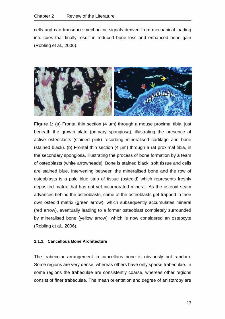
cells and can transduce mechanical signals derived from mechanical loading
into cues that finally result in reduced bone loss and enhanced bone gain
(Robling et al., 2006).
Figure 1: (a) Frontal thin section (4 µm) through a mouse proximal tibia, just
beneath the growth plate (primary spongiosa), illustrating the presence of
active osteoclasts (stained pink) resorbing mineralised cartilage and bone
(stained black). (b) Frontal thin section (4 µm) through a rat proximal tibia, in
the secondary spongiosa, illustrating the process of bone formation by a team
of osteoblasts (white arrowheads). Bone is stained black, soft tissue and cells
are stained blue. Intervening between the mineralised bone and the row of
osteoblasts is a pale blue strip of tissue (osteoid) which represents freshly
deposited matrix that has not yet incorporated mineral. As the osteoid seam
advances behind the osteoblasts, some of the osteoblasts get trapped in their
own osteoid matrix (green arrow), which subsequently accumulates mineral
(red arrow), eventually leading to a former osteoblast completely surrounded
by mineralised bone (yellow arrow), which is now considered an osteocyte
(Robling et al., 2006).
2.1.1. Cancellous Bone Architecture
The trabecular arrangement in cancellous bone is obviously not random.
Some regions are very dense, whereas others have only sparse trabeculae. In
some regions the trabeculae are consistently coarse, whereas other regions
consist of finer trabeculae. The mean orientation and degree of anisotropy are
a b
Chapter 2 Review of the Literature
14
also variables that obviously change between anatomical sites and between
individuals.
The variation in trabecular architecture formed the basis for the formulation of
Wolff’s law (Wolff, 1870), which links trabecular architecture to mechanical
usage by adaptation and mechanical properties to trabecular architecture by
solid and, possibly, fluid mechanics. This explains the interest in cancellous
bone architecture. Wolff (1870) stated that the architecture related to the
mechanical usage “in accordance with mathematical laws”, but did not further
specify these laws. Much has been learned over the last decades about how
the architecture influences mechanical properties, but the influence of a
number of architectural features is still uncertain. One of the problems in
explicit formulations relating to the cancellous bone architecture is defining
and delimiting the architecture variables to be included.
The most important parameter which has been suggested to characterise
cancellous bone architecture is the bone volume fraction, which is the volume
of bone tissue per unit volume and is dimensionless. A similar scalar quantity
is the total mass per unit volume of bone, which is called the structural density
or apparent density and which measures the degree of mineralisation as well.
A variety of methods for quantification of cancellous bone architecture has
been proposed, including: (1) basic stereological methods, (2) methods based
on three-dimensional (3D) reconstruction, (3) traditional two-dimensional (2D)
histomorphometry methods, and (4) ad hoc 2D methods (Cowin, 2001).
2.1.2. Bone Modelling and Remodelling
Nearly 40 years ago, Frost (1963) began describing two distinct mechanisms
by which different types of bone cells team up or work individually to achieve
skeletal formation and/or renewal. These processes are bone modelling and
remodelling. Both work together in the growing skeleton to define the
appropriate skeletal shape, maintain proper serum levels of ions, and repair
structurally compromised regions of bone. Bone modelling is a process that
works in concert with bone growth and functions to alter the spatial distribution
of accumulating tissue presented by growth (Frost, 1986; Jee and Frost,
1992). For example, a growing child’s muscle mass increases at a rate that
Chapter 2 Review of the Literature
15
outpaces accumulation of bone mass (Frost, 1997). Therefore, the tissue
being deposited on a bone experiencing an increased or altered loading
environment from (a) the growing and increasingly powerful muscles, (b)
increasing body mass, and (c) a lengthening diaphysis must be positioned to
optimally meet these rapidly evolving mechanical demands (Frost, 1986;
Hillam and Skerry, 1995).
This is accomplished by modelling drifts, through which bone is selectively
added or removed from existing surfaces with the goal of optimising the
geometry of the bone (see Table 1 for the comparison of modelling and
remodelling characteristics). Thus modelling can alter the size, shape, and
position in tissue space of a typical long bone cross section by selectively
inhibiting or promoting cellular activity at the resorptive and appositional
surfaces accordingly. Bone modelling at any surface involves osteoclast
activation and subsequent resorption of bone, or it involves osteoblast
activation and subsequent formation of bone, but not both at the same
location. Once skeletal maturity is reached, modelling reduces to a trivial level
compared with that which occurs during development (Frost, 1973; Garn,
1970; Lazenby, 1990a; Lazenby 1990b). However, renewed modelling in the
adult skeleton can occur in some disease states and in cases where the
mechanical loading environment has been altered significantly.
Unlike modelling, which involves either resorption or formation (but not both)
at a locus, bone remodelling always follows an activation → resorption →
formation sequence (Parfitt, 1979). Remodelling removes and replaces
discrete, measurable “packets” of bone. On the intracortical envelope, these
replacement packets of bone, or bone structural units (BSUs), comprise
secondary osteons. Bone is remodelled by teams of cells derived from
different sources which are collectively called the basic multicellular units
(BMU). The BMU is a mediator mechanism bridging individual cellular activity
to whole bone morphology (Frost, 1986). Intracortical BMUs maintain a
distinctive 3D structure as they move through long bone diaphyses in a nearly
longitudinal orientation (Hert et al., 1994; Parfitt, 1994). The leading region of
the BMU is lined with osteoclasts, specialised cells capable of bone
resorption.
Chapter 2 Review of the Literature
16
Behind the mononuclear cells, rows of osteoblasts (bone-forming cells)
adhere to the reversal zone and deposit layers of osteoid (unmineralised bone
matrix) centripetally. The size of the remodelling space constricts as more
concentric osteonal lamellae are deposited and mineralised. At a specified
point, deposition ceases leaving a Haversian canal in the centre of the newly
formed osteon. Remodelling on the trabecular and endocortical surfaces
follows the same sequence of cellular events as described for the Haversian
envelope, except that the cells do not dig and refill tunnels. Rather, they
remove and replace pancake-like packets of bone scalloped from these
surfaces (Parfitt, 1994). Because of the morphology of the remodelling BMU,
where the osteoblast teams trail behind osteoclast teams and the entire
structure moves as a unit, the resorption and formation processes are said to
be coupled to one another. Coupling is a strictly controlled process in
remodelling, ensuring where bone is removed and where new bone will be
restored (Parfitt, 2000). The net amount of old bone removed and new bone
restored in the remodelling cycle is a quantity called the bone balance. While
coupling rarely is affected, bone balance can vary quite widely in many
disease states. For example, in osteoporotic patients, resorption and
formation are coupled but there is a negative bone balance, i.e. more bone is
resorbed than is replaced by the typical BMU (Eriksen et al., 1985).
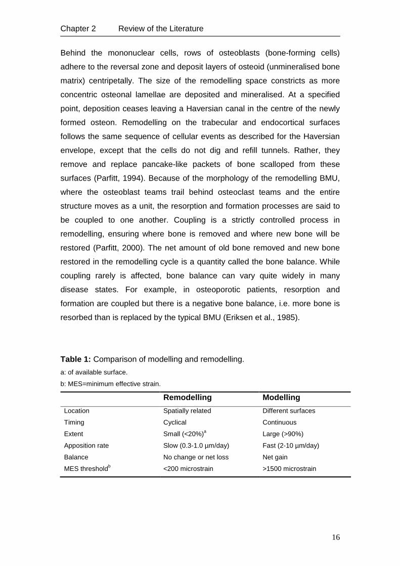
Table 1: Comparison of modelling and remodelling.
a: of available surface.
b: MES=minimum effective strain.
Remodelling Modelling
Location Spatially related Different surfaces
Timing Cyclical Continuous
Extent Small (<20%)a Large (>90%)
Apposition rate Slow (0.3-1.0 µm/day) Fast (2-10 µm/day)
Balance No change or net loss Net gain
MES thresholdb <200 microstrain >1500 microstrain
Chapter 2 Review of the Literature
17
Cortical bone has a mean age of 20 years and cancellous bone of one to four
years (Weibel, 1980). The periodic replacement of bone (bone turnover) helps
to maintain load bearing and the capacity of the skeleton to regulate calcium
hemoeostasis and haematopoiesis and to repair structural damage.
Remodelling has positive and negative effects on bone quality on the tissue
level. It serves to remove microdamage, replace dead and hypermineralised
bone, and adapt microarchitecture to local stresses. Remodelling of
cancellous bone may perforate and remove trabeculae, and remodelling of
cortical bone increases cortical porosity, decreases cortical width and possibly
reduces bone strength (Cowin, 2001).
2.1.3. Bone Remodelling and Mechanical Stimuli
The ability of the human skeletal system to adapt to meet the structural
demands placed upon it, has intrigued and perplexed the minds of scientists
since a long time. Even though numerous theories have been put forward to
explain the phenomenon of bone remodelling, a study of the relevant literature
shows that a universally accepted theory of the fundamental mechanism or
mechanisms which regulate bone resorption and deposition is still a very long
far away to be achieved.
Several different theories have been postulated to explain the phenomenon of
bone resorption and deposition. The earliest is that proposed by Wolff (1870)
and further elaborated by him in a monograph (1892). Wolff’s law, as it is now
commonly called, stated that bone responds to the mechanical demands
placed upon it. That is to say, for an increase in function or demand the bone
responds with deposition and for a decrease in function or demand it
responds with resorption. Although Thompson (1952), in his classic work “on
Growth and Form”, and most other subsequent authors have accepted Wolff’s
law, certain doubts concerning this theory do exist. For example, there is
strong clinical evidence to suggest that bone “melts way” from around certain
orthopaedic screws and implants where “excessive” stress concentrations are
expected to occur. This therefore tends to suggest that bone may either be
sensitive to the type of demand placed upon it or may possess an upper
demand cut-off level above which it changes its response.
Chapter 2 Review of the Literature
18
Bassett’s (1971) interpretation of Wolff’s law is “the form of bone being given,
the bone elements place or displace themselves in the direction of the
functional pressure and increase or decrease their mass in order to reflect the
amount of functional pressure”. This statement suggests that the mechanical
demand implied by Wolff’s law is the pressure, or in other words the stresses,
acting on the bone during function. Bassett (1971) also states that it is known
both clinically and experimentally that a concave region of bone will be built up
and a convex region removed.
Frost (1987) proposed in his mechanostat theory that bone responds to a
complex interaction of strain magnitude and time. As bone strains are typically
very small, it is common to use the term µε (10-6). Conceptually, the interfacial
bone maturation, crestal bone loss and loading can be explained by the Frost
mechanostat theory (Frost, 1987) which connects the two processes of
modelling (new bone formation) and remodelling (continuous turnover of older
bone without a net change in shape or size). In accordance with the theory,
bone acts like a “mechanostat”, in that it brings about a biomechanical
adaptation, corresponding to the external loading condition.
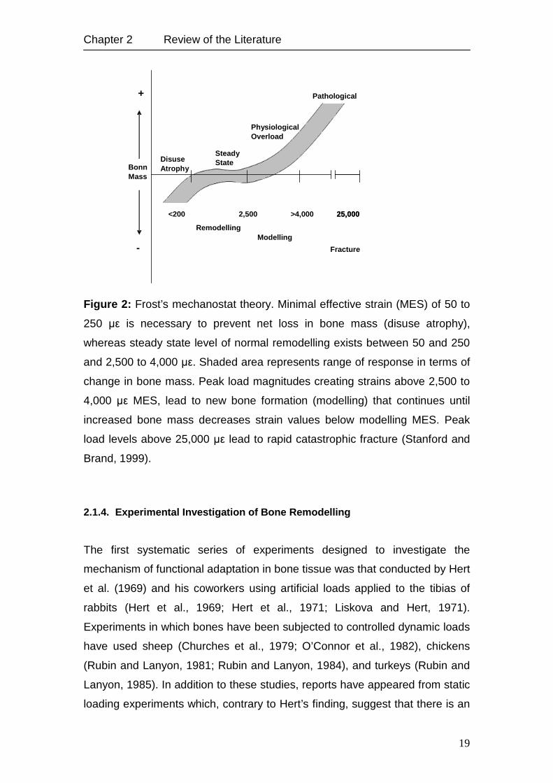
Frost described four micro-strain zones and related each zone to a
mechanical adaptation (Figure 2). The four zones include: The disuse atrophy,
steady state, physiologic overload and pathologic overload zones. Both
extreme zones (pathologic overload zone and disuse atrophy zone) are
proposed to result in a decrease in bone volume. When the peak strain
magnitude falls below 50-250 µε, disuse atrophy is proposed to occur.
Physiologic overload zone covers the range between 2,500 and 4,000 µε, and
is suggested to result in an increase in bone mass. The new bone formed is
woven bone (immature bone) that is less mineralised, less organised and
consequently weaker than the lamellar bone. It is probable that bone mass will
continue to increase, until the bony interface accommodates these changes,
and the load strain values then fall back into the range of the steady state
zone. This could explain ridge resorption after tooth loss. In the pathologic
overload zone, peak strain magnitude of over 4,000 µε may result in net bone
resorption. The steady state zone comprises the range between disuse
atrophy and physiologic overload zone, and is associated with organised,
highly mineralised lamellar bone.
Chapter 2 Review of the Literature
19
Figure 2: Frost’s mechanostat theory. Minimal effective strain (MES) of 50 to
250 µε is necessary to prevent net loss in bone mass (disuse atrophy),
whereas steady state level of normal remodelling exists between 50 and 250
and 2,500 to 4,000 µε. Shaded area represents range of response in terms of
change in bone mass. Peak load magnitudes creating strains above 2,500 to
4,000 µε MES, lead to new bone formation (modelling) that continues until
increased bone mass decreases strain values below modelling MES. Peak
load levels above 25,000 µε lead to rapid catastrophic fracture (Stanford and
Brand, 1999).
2.1.4. Experimental Investigation of Bone Remodelling
The first systematic series of experiments designed to investigate the
mechanism of functional adaptation in bone tissue was that conducted by Hert
et al. (1969) and his coworkers using artificial loads applied to the tibias of
rabbits (Hert et al., 1969; Hert et al., 1971; Liskova and Hert, 1971).
Experiments in which bones have been subjected to controlled dynamic loads
have used sheep (Churches et al., 1979; O’Connor et al., 1982), chickens
(Rubin and Lanyon, 1981; Rubin and Lanyon, 1984), and turkeys (Rubin and
Lanyon, 1985). In addition to these studies, reports have appeared from static
loading experiments which, contrary to Hert’s finding, suggest that there is an
<200 2,500 >3500 25,000
Disuse Atrophy
Steady State
Physiological Overload
Bonn Mass
+
-
Remodelling Modelling
Fracture
>4,000 25,000
Pathological
Chapter 2 Review of the Literature
20
association between static load and remodelling activity (Hart et al., 1983;
Hassler et al., 1980; Meade et al., 1981). In all these static loading studies
mathematical models were also developed which appeared to support the
existence of a relationship between the remodelling observed and the static
stresses produced within the bone tissue. In any artificial loading experiment
in vivo, there are two major drawbacks:
1) Bone remodelling is sensitive to many factors other than mechanical
ones and so, the direct and indirect effects of trauma and vascular
disturbance can easily obliterate any remodelling related to physiological
changes in the bone mechanical situation.
2) When a continuous load is applied to a bone which is also being
functionally loaded, it not only induces static strains, but it may also modulate
the superimposed pattern of dynamic strain produced by functional activity.
The first of these dangers can be avoided, or at least reduced, by developing
preparations in which the sites of surgical interference are kept remote from
those where the remodelling is assessed. The second can be overcome by
the use of models in which artificial loads are applied to a bone which is
retained in vivo but which is isolated from alternative (natural) sources of
loading.
Pearce et al. (2007) studied the similarity between animal and human bone in
terms of macrostructure, microstructure, bone composition and bone
remodelling rate in dogs, sheep/goat, pigs and rabbits. They concluded that
pigs have the most similar bone remodelling behaviour to that of humans
followed by dogs and sheep/goat and least similar it was in rabbits.
2.1.5. Computer Simulation of Bone Remodelling
Although global study of bone remodelling through simulation is fundamentally
unable to address the actual biologic events which form and resorb bone, an
accurate simulation of bone remodelling is an important practical and
theoretical tool. Such a simulation could identify prosthetic designs and design
features which are likely to lead to problems due to stress shielding, and can
show situations in which bone remodelling results in stresses within the
prosthesis which could cause failure (Carter, 1987; Carter et al., 1989;
Chapter 2 Review of the Literature
21
Huiskes et al., 1987; Huiskes et al., 1991; Orr et al., 1990). These simulations
can also help in the studies of bone remodelling mechanisms, by indicating
the mechanical relationships between bone stress and formation which result
in a stable structure which accurately mimics actual bones (Carter et al., 1989;
Cowin, 1984; Hart and Davy, 1989; Hart et al., 1984b; Orr et al., 1990).
Computerised simulations of bone remodelling thus potentially offer both a
theoretical limit on the relationships between stress and bone response to it,
and a practical tool for the design of bone repairs and total joint replacements.
The process of bone remodelling uses an interrelationship between the
microstructure of bone and global stiffness characteristics of the whole bone
under load. The mechanism of bone remodelling is one where the stress at a
particular site in the bone causes bone tissue to be deposited or removed,
yielding a change in the local stiffness of the bone or a change in the shape of
the bone. The macroscopic shape and structure of the bone in the human
skeleton are as variable as humans themselves are, but they also share the
degree of similarity that people share. Thus the microscopic processes which
form and resorb bone yield a stable structure which adapts to the variable and
common features which humans display.
Numerical modelling applied to bone has primarily been aimed at simulating
the bone remodelling concepts as proposed by the early anatomists. These
studies are usually aimed at assessing whether the structure of bone can be
predicted or developed using a particular mathematical remodelling rule.
Considerable success has resulted from many of these studies; the density
distribution of bone near joints, and the shape of the long bone diaphyses can
be predicted in a qualitative sense using the models developed so far. Thus
these studies confirm the correctness of the original qualitative postulates
made by the early anatomists.
A bone remodelling scheme based on continuum-level variables (such as
tissue volumetric density and strain energy density) cannot model tissue
deposition and removal on a cellular level. However, exploring such models
offers a chance to assess the stability and the optimising characteristics of
these remodelling schemes. By assessing stability and optimising issues, we
can assess the influence of local tissue responses on the overall structure,
and this can help in identifying the important effects at the cellular level.
Chapter 2 Review of the Literature
22
For qualitative predictions, it is necessary that the internal mechanical load in
the bone structure can be determined accurately in terms of stresses and
strains, for which the finite element method (FEM) is an effective tool
(Huiskes, 1980). By combining mathematical bone remodelling descriptions
with finite element (FE) models, quantitative predictions about bone formation
and resorption in realistic bone structures can be made (Fyhrie and Carter,
1986; Hart et al., 1984a; Weinans et al., 1989; Weinans et al., 1990). These
models are all based on the principle that bone remodelling is induced by a
local mechanical signal which activates the regulating cells (osteoblasts and
osteoclasts). This process can be described with a generic mathematical
expression, using the apparent density as the characterisation of the internal
morphology. The rate of change in the apparent density of the bone at a
particular location dρ/dt, with ρ=ρ(x,y,z), can be described as an objective
function F, which depends on a particular stimulus at location (x,y,z). It is
assumed that this stimulus is directly related to the local mechanical load in
the bone and can be determined from the local stress tensor σ=σ(x,y,z), the
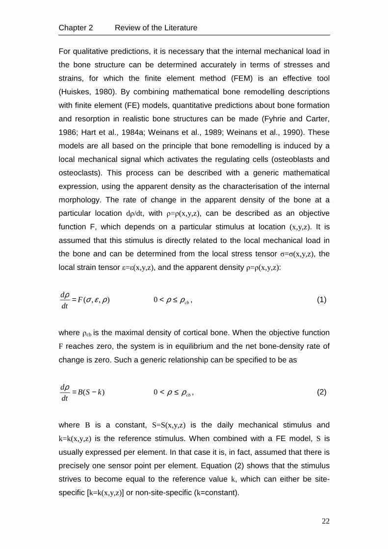
local strain tensor ε=ε(x,y,z), and the apparent density ρ=ρ(x,y,z):
),,( ρεσρF
dt
d = cbρρ ≤<0 , (1)
where ρcb is the maximal density of cortical bone. When the objective function
F reaches zero, the system is in equilibrium and the net bone-density rate of
change is zero. Such a generic relationship can be specified to be as
)( kSBdt
d −=ρ cbρρ ≤<0 , (2)
where B is a constant, S=S(x,y,z) is the daily mechanical stimulus and
k=k(x,y,z) is the reference stimulus. When combined with a FE model, S is
usually expressed per element. In that case it is, in fact, assumed that there is
precisely one sensor point per element. Equation (2) shows that the stimulus
strives to become equal to the reference value k, which can either be site-
specific [k=k(x,y,z)] or non-site-specific (k=constant).
Chapter 2 Review of the Literature
23
2.1.6. Bone Remodelling Theories
It is widely accepted that bone material has the ability to respond to changes
in its mechanical loading environment (i.e. changes in the stress and strain
field) by adapting its shape and/or its internal micro-structure. These two
aspects are commonly referred to as surface and internal remodelling (Frost,
1964). Bone material is resorbed in regions exposed to small load levels,
whereas in highly stressed zones deposition of new bone material sets in.
This process of functional adaptation is thought to enable bone to perform its
mechanical function with a minimum of mass. However, as clinical practice
shows, it can often be detrimental to the long-term success of prostheses and
implants used in orthopaedic or dental surgery.
Though significant research has been undertaken to identify possible physical
and biochemical phenomena which transform mechanical stresses and strains
into actual bone cell processes (for a comprehensive overview see e.g.
[Martin and Burr, 1989]), these mechanisms remain not fully understood.
Considerable attention has been focused on the development of
phenomenologically based numerical simulation tools for predicting the results
of the natural adaptation process (Carter et al., 1987; Carter et al., 1989;
Cowin and Hegedus, 1976). Most of these approaches assume bone material
to show isotropic linear elastic behaviour and reflect the remodelling process
by adaptation of the bone apparent density and introducing appropriate
stiffness-density relations, by adaptation of the Young’s modulus. Up to now,
only a limited number of attempts have been undertaken to expand these
models to more complex material symmetries, which better reflect the
anisotropic behaviour of actual bony tissue (Buchjek, 1990; García et al.,
2001; Reiter, 1996).
2.1.6.1. Bone Remodelling based on the Concept of Micro-Damage
Recent concepts connecting bone mechanics and bone biology not only relate
bone remodelling to the adaptation of the internal structure to load, but also to
the need to remove fatigue damage (Lee et al., 2002). Microdamage in bone
was first described by Frost (1960) and is the epiphenomenon of fatigue,

Chapter 2 Review of the Literature
24
creep, or other accumulative mechanical processes that permanently alter the
micro-structure (Martin, 2003). Microdamage is increased by fatigue loading at
physiological strains and is associated with the activation of remodelling and
osteocyte apoptosis (Verborgt et al., 2000). Remodelling activated by, and in
close proximity to, microdamage is described by some authors as “targeted”
remodelling as opposed to “random” remodelling that could serve other
functions, such as calcium homeostasis (Boyce et al., 1998; Burr, 2002).
Martin (2003) described four types of microdamage:
1) Microcracks, commonly found in cortical bone, which extend approximately
100 µm and is frequently limited by osteonal cement lines,
2) diffuse damage, more commonly found in sectioned trabeculae, appears as
patches of more intensely strained mineralised matrix that have apparently
been disrupted by locally intense deformations,
3) when small cracks appear in trabeculae as localised networks they are
described as cross-hatching cracks, and
4) microfractures are described when trabecular structures are completely
fractured.
The principle mechanisms of matrix failure, according to Boyce et al. (1998),
are strongly dependent on local strain. In regions subjected to tensile strains
the bone has diffuse microdamage, whereas in compressive strain regions the
tissue develops linear microcracks. However, this concept of bone
remodelling is commonly used to describe the remodelling procedure
associated with orthodontic treatment.
2.1.6.2. Strain Theory of Adaptive Elasticity
Cowin and Hegedus (1976) developed the theory of adaptive elasticity to
explain the remodelling behaviour of cortical bone. This theory primarily
attempts to describe the adaptive nature of the bone from one loading
configuration to another, rather than to predict the optimal structure of normal
bone. In this theory, it is assumed that the cortical bone tissue has a site-
specific natural (or homeostatic) equilibrium strain state. A change of load or
an abnormal strain state will stimulate the bone tissue to adapt its mass in
such a way that the homeostatic strain state is again obtained (as closely as
Chapter 2 Review of the Literature
25
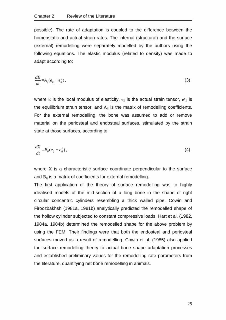
possible). The rate of adaptation is coupled to the difference between the
homeostatic and actual strain rates. The internal (structural) and the surface
(external) remodelling were separately modelled by the authors using the
following equations. The elastic modulus (related to density) was made to
adapt according to:
)( οijijij eeA
dt
dE −= , (3)
where E is the local modulus of elasticity, eij is the actual strain tensor, e°ij is
the equilibrium strain tensor, and A ij is the matrix of remodelling coefficients.
For the external remodelling, the bone was assumed to add or remove
material on the periosteal and endosteal surfaces, stimulated by the strain
state at those surfaces, according to:
)( οijijij eeB
dt
dX −= , (4)
where X is a characteristic surface coordinate perpendicular to the surface
and Bij is a matrix of coefficients for external remodelling.
The first application of the theory of surface remodelling was to highly
idealised models of the mid-section of a long bone in the shape of right
circular concentric cylinders resembling a thick walled pipe. Cowin and
Firoozbakhsh (1981a, 1981b) analytically predicted the remodelled shape of
the hollow cylinder subjected to constant compressive loads. Hart et al. (1982,
1984a, 1984b) determined the remodelled shape for the above problem by
using the FEM. Their findings were that both the endosteal and periosteal
surfaces moved as a result of remodelling. Cowin et al. (1985) also applied
the surface remodelling theory to actual bone shape adaptation processes
and established preliminary values for the remodelling rate parameters from
the literature, quantifying net bone remodelling in animals.
Chapter 2 Review of the Literature
26
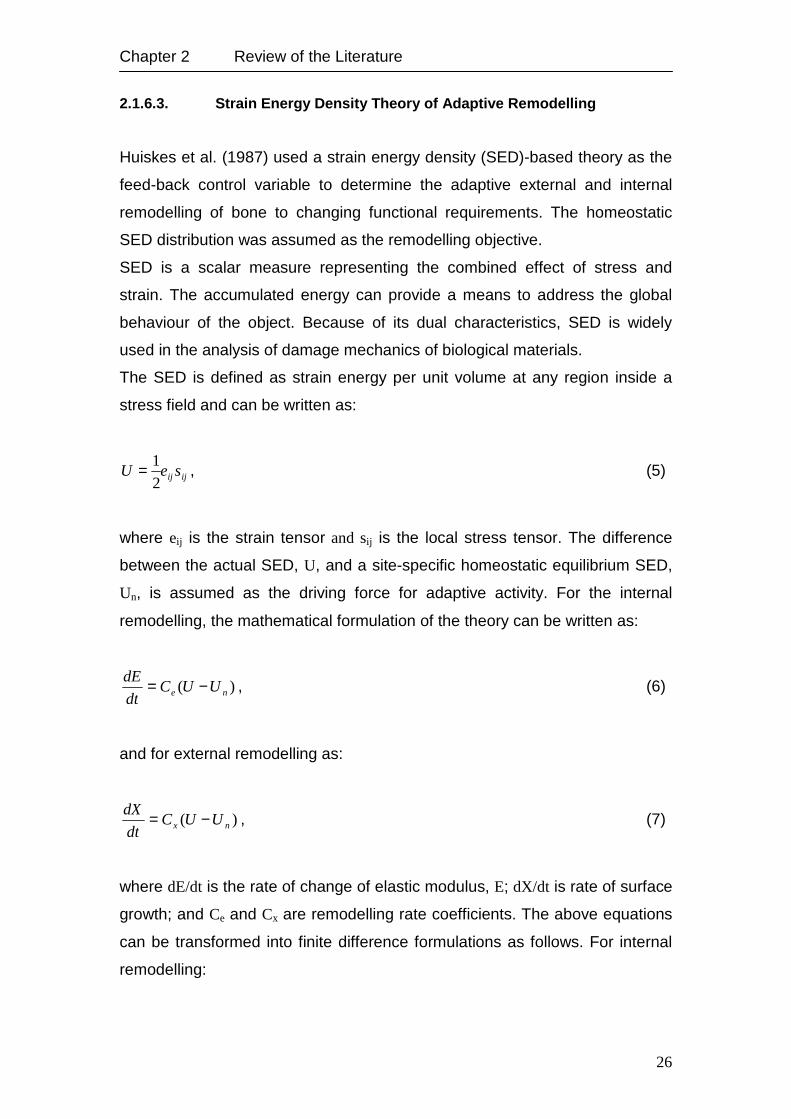
2.1.6.3. Strain Energy Density Theory of Adaptive Remodelling
Huiskes et al. (1987) used a strain energy density (SED)-based theory as the
feed-back control variable to determine the adaptive external and internal
remodelling of bone to changing functional requirements. The homeostatic
SED distribution was assumed as the remodelling objective.
SED is a scalar measure representing the combined effect of stress and
strain. The accumulated energy can provide a means to address the global
behaviour of the object. Because of its dual characteristics, SED is widely
used in the analysis of damage mechanics of biological materials.
The SED is defined as strain energy per unit volume at any region inside a
stress field and can be written as:
ijij seU2
1= , (5)
where eij is the strain tensor and sij is the local stress tensor. The difference
between the actual SED, U, and a site-specific homeostatic equilibrium SED,
Un, is assumed as the driving force for adaptive activity. For the internal
remodelling, the mathematical formulation of the theory can be written as:
)( ne UUCdt
dE −= , (6)
and for external remodelling as:
)( nx UUCdt
dX −= , (7)
where dE/dt is the rate of change of elastic modulus, E; dX/dt is rate of surface
growth; and Ce and Cx are remodelling rate coefficients. The above equations
can be transformed into finite difference formulations as follows. For internal
remodelling:
Chapter 2 Review of the Literature
27
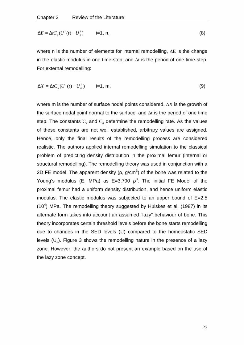
))(( in
ie UtUCtE −∆=∆ i=1, n, (8)
where n is the number of elements for internal remodelling, ∆E is the change
in the elastic modulus in one time-step, and ∆t is the period of one time-step.
For external remodelling:
))(( im
ix UtUCtX −∆=∆ i=1, m, (9)
where m is the number of surface nodal points considered, ∆X is the growth of
the surface nodal point normal to the surface, and ∆t is the period of one time
step. The constants Ce and Cx determine the remodelling rate. As the values
of these constants are not well established, arbitrary values are assigned.
Hence, only the final results of the remodelling process are considered
realistic. The authors applied internal remodelling simulation to the classical
problem of predicting density distribution in the proximal femur (internal or
structural remodelling). The remodelling theory was used in conjunction with a
2D FE model. The apparent density (ρ, g/cm3) of the bone was related to the
Young’s modulus (E, MPa) as E=3,790 ρ3. The initial FE Model of the
proximal femur had a uniform density distribution, and hence uniform elastic
modulus. The elastic modulus was subjected to an upper bound of E=2.5
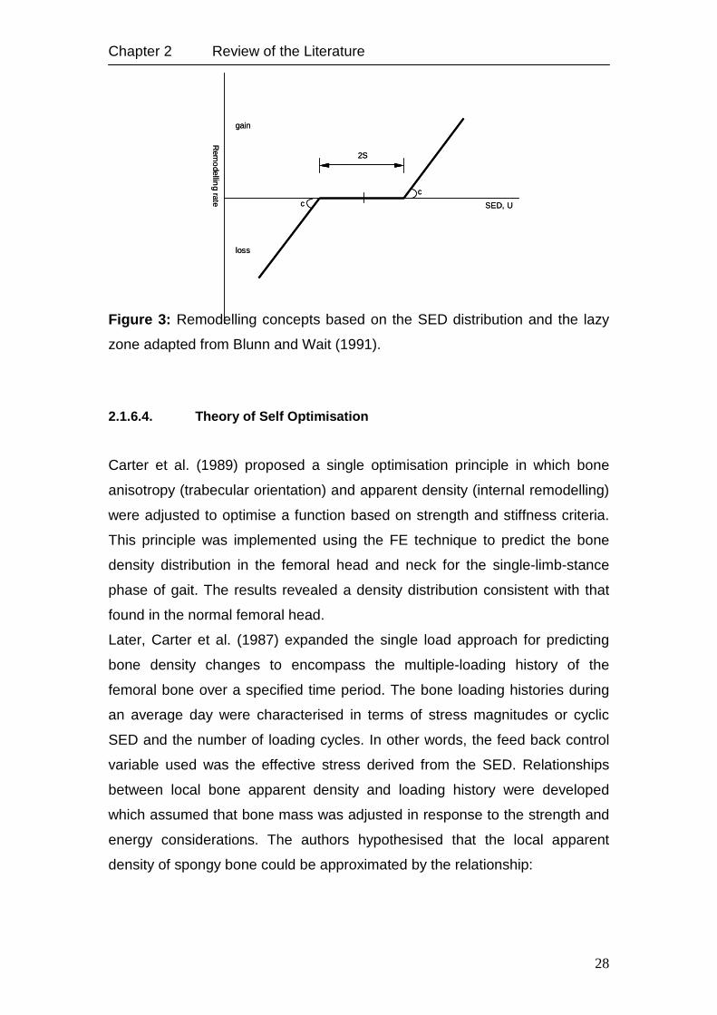
(104) MPa. The remodelling theory suggested by Huiskes et al. (1987) in its
alternate form takes into account an assumed “lazy” behaviour of bone. This
theory incorporates certain threshold levels before the bone starts remodelling
due to changes in the SED levels (U) compared to the homeostatic SED
levels (Un). Figure 3 shows the remodelling nature in the presence of a lazy
zone. However, the authors do not present an example based on the use of
the lazy zone concept.
Chapter 2 Review of the Literature
28
Figure 3: Remodelling concepts based on the SED distribution and the lazy
zone adapted from Blunn and Wait (1991).
2.1.6.4. Theory of Self Optimisation
Carter et al. (1989) proposed a single optimisation principle in which bone
anisotropy (trabecular orientation) and apparent density (internal remodelling)
were adjusted to optimise a function based on strength and stiffness criteria.
This principle was implemented using the FE technique to predict the bone
density distribution in the femoral head and neck for the single-limb-stance
phase of gait. The results revealed a density distribution consistent with that
found in the normal femoral head.
Later, Carter et al. (1987) expanded the single load approach for predicting
bone density changes to encompass the multiple-loading history of the
femoral bone over a specified time period. The bone loading histories during
an average day were characterised in terms of stress magnitudes or cyclic
SED and the number of loading cycles. In other words, the feed back control
variable used was the effective stress derived from the SED. Relationships
between local bone apparent density and loading history were developed
which assumed that bone mass was adjusted in response to the strength and
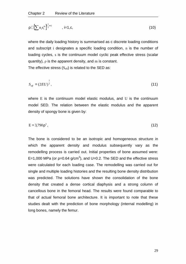
energy considerations. The authors hypothesised that the local apparent
density of spongy bone could be approximated by the relationship:
Rem
odellin
g rate
gain
loss
SED, U
2S
c
c
Rem
odellin
g rate
gain
loss
SED, U
2S
c
c
Chapter 2 Review of the Literature
29
[ ] )m2
1(m
iisn∑∝ρ , i=1,c, (10)
where the daily loading history is summarised as c discrete loading conditions
and subscript i designates a specific loading condition, n is the number of
loading cycles, s is the continuum model cyclic peak effective stress (scalar
quantity), ρ is the apparent density, and m is constant.
The effective stress (Seff) is related to the SED as:
2
1
)2( EUSeff = , (11)
where E is the continuum model elastic modulus, and U is the continuum
model SED. The relation between the elastic modulus and the apparent
density of spongy bone is given by:
3790,3E ρ= , (12)
The bone is considered to be an isotropic and homogeneous structure in
which the apparent density and modulus subsequently vary as the
remodelling process is carried out. Initial properties of bone assumed were:
E=1,000 MPa (or ρ=0.64 g/cm3), and U=0.2. The SED and the effective stress
were calculated for each loading case. The remodelling was carried out for
single and multiple loading histories and the resulting bone density distribution
was predicted. The solutions have shown the consolidation of the bone
density that created a dense cortical diaphysis and a strong column of
cancellous bone in the femoral head. The results were found comparable to
that of actual femoral bone architecture. It is important to note that these
studies dealt with the prediction of bone morphology (internal modelling) in
long bones, namely the femur.
Chapter 2 Review of the Literature
30
2.2. Bone Quality and Verifying Methods
The quality or density of bone adjacent to dental implants is an important
consideration in the success of dental implants. There are four established
bone qualities in the oral cavity as described by Lekholm and Zarb (1985).
Quality 1 consists of primarily dense cortical bone that is usually located in the
anterior mandible. Quality 2 has a thick layer of compact bone that surrounds
a core of dense cancellous bone that is usually associated with the posterior
mandible. Quality 3 has a thin layer of cortical bone that surrounds a core of
dense cancellous bone, which is usually associated with the anterior maxilla.
Quality 4 has a thin layer of cortical bone that surrounds a core of lower
density cancellous bone. The posterior maxilla is customarily composed of
this least dense quality of bone. This classification system has been used to
characterise bone quality during surgical procedures for implant placement.
Since this classification can be subjective, other investigators have proposed
an extension of this idea by comparing the surgical resistance of the bone
during osteotomy preparation (Engquist et al., 1988; Friberg, 1994; Misch,
1993; Trisi and Rao, 1999). However, a study by Misch (1993) states that
bone quality 1 and 4 can easily be differentiated, but quality 2 and 3 are not as
easily discerned (Trisi and Rao, 1999).
The long-term clinical success of titanium dental implants is reported to be
highly influenced by both the quality and quantity of available bone (Bahat,
1993; Engquist et al., 1988; Friberg et al., 1991; Higuchi et al., 1995; Jaffin
and Berman, 1991; Jemt and Lekholm, 1995; Johns et al., 1992; Mericske-
Stern, 1994). For example, better bone quality and quantity in the anterior
mandible are usually offered as the main reasons for higher survival rates of
dental implants in lower jaws (Bass and Triplett, 1991; Friberg et al., 1991;
Jaffin and Berman, 1991). The percentage of bone-implant contact is higher in
cortical bone than in cancelleous bone, which provides greater initial stability
to the implant during the healing period following insertion. The direction,
magnitude and repetition rate of biomechanical forces can influence the
modelling and remodelling processes in bone surrounding endosseous
implants. Bone can resist rapidly applied loads and bone quality is increased
under repetitive forces. If the simulation is within physiologic limits, it may
Chapter 2 Review of the Literature
31
produce an increase in osseous density at the implant-bone interface (Arpak
et al., 1995; Carter and Caler, 1983; Carter, 1984; Misch, 1990; Morris et al.,
1995). From this comes the advantage of the immediately loaded implant
systems, keeping in mind the importance of maximising the spread and
distribution of contacts and to recheck the occlusion during the first days and
weeks after immediate/early loading. Therefore, rigid splinting of the
prosthesis can provide an advantageous force distribution to all abutments.
Bone quality can be assessed before surgery by computerised tomography
using Hounsfield values, by estimation of arch location or during surgery by
the tactile sense of the surgeon, or by the torque indicator in the handpiece
system (Jemt and Strid, 1994; Misch, 1999).
By measuring the cutting resistance of the jaw bone, the insertion torque
(measured in Ncm) can be performed intraoperatively (Friberg et al., 1995a;
Friberg et al., 1999; Johansson and Strid, 1994; Meredith, 1998). This
measurement, since it is available during or after implantation, cannot be used
for surgical planning. From the other hand, quantitative CT-image offers the
possibility to measure bone mineral density (BMD) values of cortical and
cancellous bone separately (Lindh et al., 1996), although the outcome
depends critically on the method used for discriminating these two
compartments (Beer, 2000). Furthermore, measurement of average BMD
values for both segments does not contain the information sought for
assessing implant positions, since BMD values vary locally to a high extent
(Friberg et al., 1995b; Ulm et al., 1992). Thus, evaluation of BMD locally or
averaged over small regions of interest, comparable in size with the implants,
are likely to reflect local bone properties more appropriately.
2.3. Fracture Healing and Bone Repair around Implants
The interactions in the bone implant interface are initiated from the time of
implant insertion. The complex physiologic processes, comparable to those of
fracture healing, are regulated by numerous different factors and involve
participation of several cell types (Davies et al., 1991). The biological
Chapter 2 Review of the Literature
32
response can according to fracture healing be divided into primary and
secondary healing (Einhorn, 1998).
Primary healing involves a direct healing without formation of callus. Primary
healing seems to occur only when optimum conditions exist, i.e. mechanical
stability and no presence of gaps; in fracture healing anatomical restoration of
the bone fragments is needed. When such conditions are present, the
remodelling unit (cutting cones) with osteoclasts will reestablish the haversian
canals between the bone ends while the osteoblasts form bone. Secondary
fracture healing which is supposed to take place around cementless implants
occurs when optimum conditions for repair are absent and involves the
formation of callus. Histologically, several phases in the process of secondary
fracture healing and at the bone-implant interface have been described
(Buckwalter et al., 1995a, 1995b; Dhert et al., 1998; Einhorn, 1998). Initially, a
haematoma is formed and the inflammatoric response commences. The
haematoma is suggested to be a source of signalling molecules which are
released from platelets and inflammatoric cells. The haematoma will be
invaded by cells and vessels, and callus formation begins after 7–14 days
(Dhert et al., 1998; Sennerby et al., 1993). During stable mechanical
conditions without gaps, intramembraneous bone formation will take place
directly after the inflammatoric response (Brånemark et al., 1969; Dhert et al.,
1998). The presence of a gap over a certain size creates a different situation.
It seems that small defects less than 0.5 mm in diameter heal by direct
intramembraneous bone formation, whereas larger gaps will heal through the
cartilage stage and an initial scaffold of woven bone which subsequently turns
into lamellar bone. In both situations, the newly formed bone adapts itself to
the new situation by orienting to the bone architecture. During unstable
mechanical conditions, the inflammatoric response is prolonged and a fibrous
tissue membrane might develop (Søballe et al., 1992a, 1992b). The
magnitude of continuous micromotion in combination with the local
environment will decide whether the inflammatoric response turns into the
formation of chondrocytes and endochondral ossification (secondary fracture
healing) (Cameron et al., 1973).
Several research groups (Ament et al., 1994; Beaupré et al., 1992; Biegler,
and Hart, 1992; Blenman et al., 1989; Carter et al., 1988; Cheal et al., 1991;
Chapter 2 Review of the Literature
33
DiGioia et al., 1986) have analysed the local mechanical situation in the
fracture callus or in the fracture gap by the FEM. Claes and Heigele (1999)
developed three 2D axisymmetric FE models. Each model represented one
specific healing stage. The first model reflected the morphology occurring two
weeks after fracture. The second and third model described the eighth and
sixteenth healing week, respectively. The basic overall geometry of the cortex
and the callus region was identical for all three models. Tissue differentiation
and gradual stiffening of the callus tissue were the fundamental processes of
secondary fracture healing. These processes were simulated by changing the
element material properties from one stage to the next. The characterisation
of the histomorphological sequence of the healing process and the types of
tissue involved were based on a previously described animal study (Claes et
al., 1995a). Based upon the histologic sections they assumed that these three
geometries represented typical ossification patterns.
To describe progressive stiffening of the callus, they assumed four tissue
types differing in their elastic material properties. The tissue material
properties were obtained from indentation tests on tissue sections from
different callus regions (Augat et al., 1997) and were similar to values taken
by others (Davy and Connolly, 1982).
In the initial healing stage, the callus consisted only of connective tissue. The
second model contained callus of intermediate stiffness in a small region
along the periosteum, and soft callus tissue adjacent to it, while the remainder
consisted of initial connective tissue (about eight weeks postoperatively). In
the third model the callus tissue contained three tissue types: Soft callus,
intermediate stiffness callus and stiff callus.
Chapter 2 Review of the Literature
34
2.4. Replacing partially Edentulous Ridge by Fixed Prosthesis
2.4.1. Dental Implant Design
The standard implant diameter is 3.75 to 4.00 mm but may vary between 3.00
mm and 6.00 mm, dependent upon the manufacturer, and is to be used
according to the location in the jaw and bone quality at the surgical site. The
optimal length of dental implants is 10.0 mm or longer, however; shorter
implants may be indicated dependent on anatomical structures. But with
shorter implants there is a poorer prognosis (Friberg et al., 2000). Screw
thread design varies greatly by manufacturer but all are to increase fixture
stability and induce osseointegration. Many types of screw designs have been
introduced claiming that substantive research to be unnecessary since the
new designs are based upon the original well-documented Swedish
Brånemark titanium implant. This reasoning is based on the opinion that oral
implants represent generic products, a misconceived notion at this stage.
The various look-alike implants differ from one another with respect to titanium
composition, thread configuration, and surface topography (Wennerberg et al.,
1993). Indeed, the observed differences in surface topography alone are such
that they will clearly influence the results in experimental studies. At present
there is insufficient knowledge about what governs the incorporation of an oral
implant and we lack a great deal of information about optimal composition of
the biomaterial, the design and the surface finish of an implant. Therefore
every oral implant must be supported by clinical documentation of the specific
product without reference to any other implant of assumed similarity
(Wennerberg, 1996).
2.4.2. Abutment Design in the Anterior Maxilla
When teeth are lost in the anterior maxilla, the pattern of bone loss cannot be
accurately predicted (Atwood, 1962). This change in bone morphology often
dictates placement of implants with the long axis in different and exaggerated
angulations to satisfy space and aesthetic needs.
Pre-angled abutments have been introduced by implant companies as a
prosthetic option for these situations. Abutment angulation is one of the many
Chapter 2 Review of the Literature
35
biomechanical variables involved in implant dentistry that need a scientific
evaluation.
Regardless of the occlusal philosophy, the palatal surfaces of the maxillary
anterior teeth provide a vertical ramp for the mandibular anterior teeth to guide
the mandible through protrusive and lateral excursions (McHorris, 1982).
Thus, most occlusal loads applied to anterior teeth are at an angle to the long
axis of the implants. Forces applied off axis may be expected to overload the
bone surrounding single-tooth implants, as shown by Papavasiliou et al.
(1996) by means of FE analysis. This created a controversy when evaluating
clinical reports by Eger et al. (2000) and Sethi et al. (2000). These authors
concluded that angled abutments may be considered a suitable restorative
option when implants are not placed in ideal axial positions. Studies on the
biomechanical behaviour of implants have concluded that the major
concentration of stresses at the implant-bone interface usually occurs at the
crestal bone level (Benzing et al., 1995; Borchers and Reichart, 1983; Canay
et al., 1996; Geng et al., 2004; Geramy and Morgano, 2004; Kenney and
Richards, 1998; O’Mahony et al., 2001; van Oosterwyck et al., 1998;
Papavasiliou et al., 1996; Patra et al., 1998; Stegaroiu et al., 1998). Few
investigators have studied the unavoidable situation of placing and loading
implants at an angulation in the anterior maxilla. Furthermore, few conclusions
have been drawn from the quantitative data obtained by most stress analysis
studies, in terms of the criteria for the elastic limit or failure limit of bone, such
as Frost’s ‘‘Mechanostat,’’ Hill’s potential function, or the Tsai-Wu function
(Ellis and Natali, 2003; Frost, 1987; Tsai and Wu, 1971).
2.4.3. Implant-supported Fixed Prostheses
Loss of anterior teeth is a compelling reason for prosthodontic treatment as an
attempt to restore aesthetic and clinical functions, this can be achieved using
conventional dentures which have often provided mixed results (Carlsson,
1998; Jones, 1976). This is particularly true in patients displaying advanced
alveolar ridge resorption, which severely compromises the retention and
stability of conventional dentures (Carlsson, 1998; Närhi et al., 1997). The
development of endosseous dental implants has provided dentists with
Chapter 2 Review of the Literature
36
exciting treatment options that have revolutionised the management of the
partially and completely edentulous patients (Albrektsson, 1988; Kirsch and
Mentag, 1986). Successful treatment with implant-supported prostheses
requires the understanding and implementation of basic biomechanical
principles coupled with the ability to satisfy the patient’s function and aesthetic
demands. Osseointegrated implant-supported prostheses were originally
prescribed for edentulous patients and the success rates for them have been
encouraging (Adell et al., 1981; Adell et al., 1990; Zarb and Schmitt, 1990).
This biotechnological breakthrough ushered in three important developments
in prosthodontic treatment: (1) potential for stable and electively fixed
prosthesis, (2) retardation in resorption of the residual ridge, and (3) minimal
risk of pre-prosthetic surgical morbidity. It also offered scope to expand the
management of edentulism to encompass partial edentulism as well as
complete edentulism (Zarb and Zarb, 2002).
Following the success of implant-supported prosthesis in the edentulous arch,
the use of implants for the treatment of partially edentulous patients increased
(Lekholm et al., 1994). Because guidelines for treating partially edentulous
cases did not exist, the same principles associated with completely
edentulous prosthetic applications were employed (Zarb et al., 1987). Initially,
success rates for partially edentulous implant restorations were somewhat
less favourable (Smith, 1990). Partially edentulous ridge treated with implant-
supported prostheses presented new complications and unique maintenance
problems for the dentist to solve (van Steenberghe et al., 1990; Sullivan,
1986). Currently, partially edentulous success rate improved and, in some
cases, equalled those reported for the completely edentulous arch (Lindh et
al., 1998).
As a concession of the fact that the jaw bone character, as defined and
classified by Lekholm and Zarb (1985), differs between the maxilla and the
mandible, the observation of the implant-supported prosthesis in the mandible
cannot automatically be considered applicable also in the maxilla.
37
Chapter 3
3. Materials and Methods
3.1. Mechanical Investigation of Different Implant and Abutment
Designs: Experimental, Numerical and Clinical Aspects
This chapter describes the materials and methods used to study the primary
stability of immediately loaded dental implants with two different geometries
and the relation of the abutment design to the crestal bone resorption. A
detailed description of sample preparation and measurement set-up of the
experiment is presented, in addition to the construction of the corresponding
numerical models and their analyses by means of FEM.
Later on, the development of the numerical models of implant-supported FPP
in the anterior maxillary region with two different abutment designs is
described. Finally, the clinical protocol for studying the relation of abutment
design to the crestal bone resorption around immediately loaded and
osseointegrated dental implants used for FPP is presented. The criteria of
patient selection are mentioned followed by the analysis method of the data.
3.1.1. Implant Design and Geometry
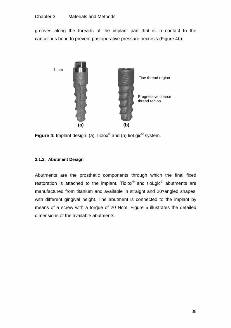
3.1.1.1. Tiolox ® Implants
Tiolox® implants are conical titanium screw-implants that are not self-tapping
because of their passive thread design. The implant surface is ceramic
blasted in the endosteal area and 1.0 mm highly polished at the gingival part
which is believed to provide a tight formation of soft marginal tissue and
optimum hygiene (Figure 4a).
3.1.1.2. tioLgic © Implants
tioLgic© Implants have a conical ceramic-blasted surface design with a 0.3
mm cervical chamber of implant shoulder and crestal fine threads at the neck
region of the implant that is in contact with the cortical part of the avleolae,
while there is a progressive coarse thread and thread flanks with lengthwise
Chapter 3 Materials and Methods
38
grooves along the threads of the implant part that is in contact to the
cancellous bone to prevent postoperative pressure necrosis (Figure 4b).
Figure 4: Implant design: (a) Tiolox® and (b) tioLgic© system.
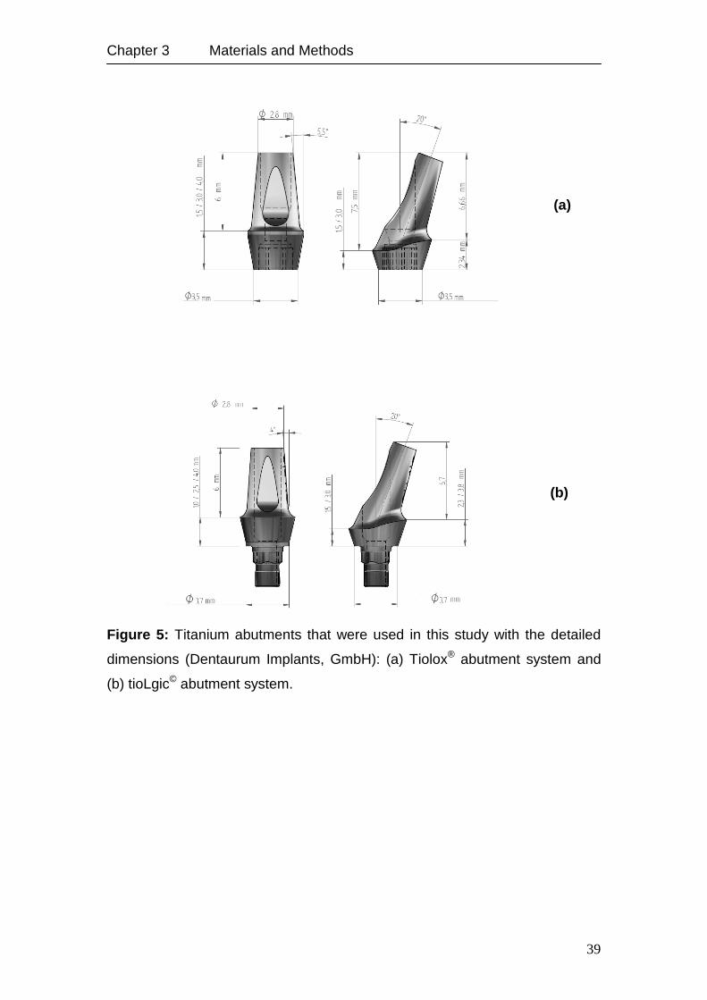
3.1.2. Abutment Design
Abutments are the prosthetic components through which the final fixed
restoration is attached to the implant. Tiolox® and tioLgic© abutments are
manufactured from titanium and available in straight and 20°-angled shapes
with different gingival height. The abutment is connected to the implant by
means of a screw with a torque of 20 Ncm. Figure 5 illustrates the detailed
dimensions of the available abutments.
1 mm
Fine thread region
Progressive coarse thread region
(a) (b)
Chapter 3 Materials and Methods
39
Figure 5: Titanium abutments that were used in this study with the detailed
dimensions (Dentaurum Implants, GmbH): (a) Tiolox® abutment system and
(b) tioLgic© abutment system.
(b)
(a)
Chapter 3 Materials and Methods
40
3.1.3. Fixed Partial Prosthesis Models
This section includes four FE-models of four-unit FPP supported by two
endosseous implants in the premaxilla to study the distribution of stresses and
strains around dental implants in immediate loading and osseointegrated
cases. This is a qualitative and quantitative study of the influence of the
abutment design on the stresses and strains in the bone.
The following three-dimensional FE models were constructed using the FE
package Marc Mentat 2007 (MSC. Software, Santa Ana, CA-USA)
representing two clinical situations: (1) A four-unit FPP supported by two
endosseous implants in the incisal region of the maxilla connected to straight
abutments and (2) an identical model in which the implants were connected to
20°-angled abutments with a modification in the ori entation of the implants. A
total of six models were developed, details of the studied models are
summarised in Table 2.
The maxillary bone was modelled using the anterior part of an idealised model
of a fully dentulous maxilla. The crowns of the maxillary incisors were modified
to be used as the units of the fixed prosthesis and have the benefit of
preserving the normal position of the final prosthesis.
The maxillary bone was modelled using the data set of the anterior part of an
idealised model of a fully dentulous maxilla (Viewpoint Data Labs, UK) to
eliminate individual variations. The crowns of the maxillary incisors of the
model were modified for use as the units of the fixed prosthesis. Their position
and orientation was maintained according to the original data set in order to
define the normal position of the final prosthesis. The bone in the anterior
maxilla was classified as quality 2 bone, described by Lekholm and Zarb
(1985) as a thick layer of cortical bone surrounding a core of dense cancellous
bone. A layer of cortical bone with a thickness of 1 mm was modelled on the
labial and palatal parts of the alveolar bone model. FE models of tioLogic©
implants (dimension: 3.7x11 mm, Dentaurum Implants GmbH, Germany) were
imported into the bone model. These implants proved to be suitable for the
given loading case, based on the uniform loading and homogeneous
distribution of the stress and strain as shown in a previous study (Rahimi et
al., 2009). Geometries of the implants were taken from the corresponding
Chapter 3 Materials and Methods
41
CAD data and oriented within the bone model based on the position of the
corresponding crowns and abutments in the lateral incisor regions.
Both implants in each model were connected either to straight or 20° angled
abutments. The abutments were designed using cylinder models with the
diameters given by the manufacturer (Dentaurum Implants GmbH). Since it
was not the primary goal of the present study to investigate the stress
distribution at the implant-abutment interface, the implant-abutment complex
was modelled as a rigid structure.
Differences in the models were as follows: For the first two models (angled
and straight abutments), the final prosthesis was considered to build up a rigid
structure with the underlying abutment to exclude the influence of the
prosthesis on the final results of the strains and stresses. In further two
models, a contact analysis between the abutments and the FPP was
performed. Contact analysis between the implant and the implant bed was
performed in these four models to simulate immediate loading. In the last two
models, the osseointegrated situation was simulated by a rigid connection
between bone and implant surface. Figures 6a and 6b illustrate the main
components of the FE models.
Table 2: Analysis conditions of the six FPP models.
Model with Description
Straight abutments (SAM) Immediate loading situation, abutment and prosthesis are
one piece.
Straight abutments (SAM) Immediate loading situation, abutment and prosthesis are in
contact.
Angled abutments (AAM) Immediate loading situation, abutment and prosthesis are
one piece.
Angled abutments (AAM) Immediate loading situation, abutment and prosthesis are in
contact.
Straight abutments (SAM) Complete osseointegration situation, abutment and
prosthesis are one piece.
Angled abutments (AAM) Complete osseointegration situation, abutment and
prosthesis are one piece.
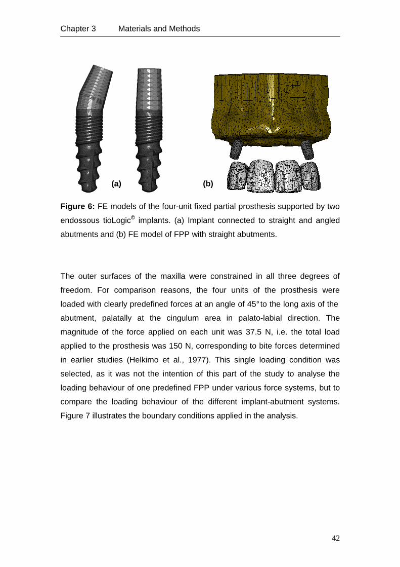
Chapter 3 Materials and Methods
42
Figure 6: FE models of the four-unit fixed partial prosthesis supported by two
endossous tioLogic© implants. (a) Implant connected to straight and angled
abutments and (b) FE model of FPP with straight abutments.
The outer surfaces of the maxilla were constrained in all three degrees of
freedom. For comparison reasons, the four units of the prosthesis were
loaded with clearly predefined forces at an angle of 45° to the long axis of the
abutment, palatally at the cingulum area in palato-labial direction. The
magnitude of the force applied on each unit was 37.5 N, i.e. the total load
applied to the prosthesis was 150 N, corresponding to bite forces determined
in earlier studies (Helkimo et al., 1977). This single loading condition was
selected, as it was not the intention of this part of the study to analyse the
loading behaviour of one predefined FPP under various force systems, but to
compare the loading behaviour of the different implant-abutment systems.
Figure 7 illustrates the boundary conditions applied in the analysis.
(a) (b)
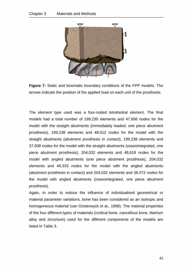
Chapter 3 Materials and Methods
43
Figure 7: Static and kinematic boundary conditions of the FPP models. The
arrows indicate the position of the applied load on each unit of the prosthesis.
The element type used was a four-noded tetrahedral element. The final
models had a total number of 199,235 elements and 47,606 nodes for the
model with the straight abutments (immediately loaded, one piece abutment
prosthesis), 199,238 elements and 48,012 nodes for the model with the
straight abutments (abutment prosthesis in contact), 199,238 elements and
37,508 nodes for the model with the straight abutments (osseointegrated, one
piece abutment prosthesis), 204,032 elements and 48,618 nodes for the
model with angled abutments (one piece abutment prosthesis), 204,032
elements and 49,333 nodes for the model with the angled abutments
(abutment prosthesis in contact) and 204,032 elements and 38,472 nodes for
the model with angled abutments (osseointegrated, one piece abutment
prosthesis).
Again, in order to reduce the influence of individualised geometrical or
material parameter variations, bone has been considered as an isotropic and
homogeneous material (van Oosterwyck et al., 1998). The material properties
of the four different types of materials (cortical bone, cancellous bone, titanium
alloy and zirconium) used for the different components of the models are
listed in Table 3.
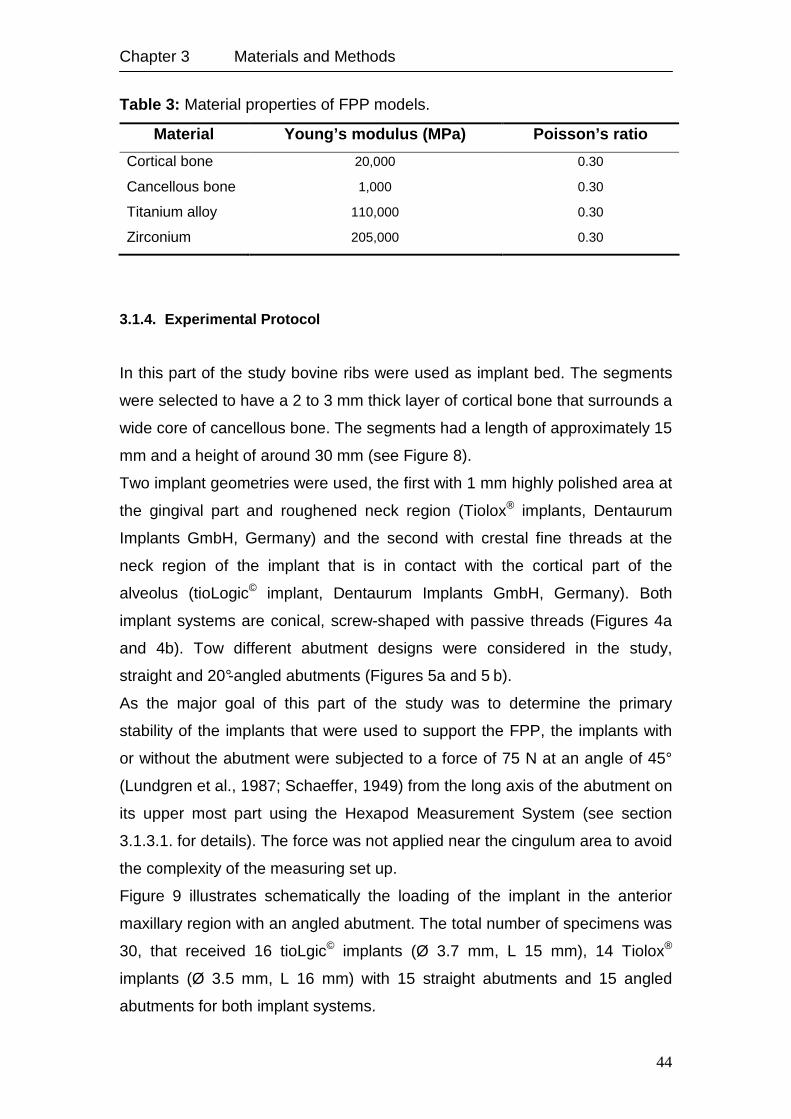
Chapter 3 Materials and Methods
44
Table 3: Material properties of FPP models.
Material Young’s modulus (MPa) Poisson’s ratio
Cortical bone 20,000 0.30
Cancellous bone 1,000 0.30
Titanium alloy 110,000 0.30
Zirconium 205,000 0.30
3.1.4. Experimental Protocol
In this part of the study bovine ribs were used as implant bed. The segments
were selected to have a 2 to 3 mm thick layer of cortical bone that surrounds a
wide core of cancellous bone. The segments had a length of approximately 15
mm and a height of around 30 mm (see Figure 8).
Two implant geometries were used, the first with 1 mm highly polished area at
the gingival part and roughened neck region (Tiolox® implants, Dentaurum
Implants GmbH, Germany) and the second with crestal fine threads at the
neck region of the implant that is in contact with the cortical part of the
alveolus (tioLogic© implant, Dentaurum Implants GmbH, Germany). Both
implant systems are conical, screw-shaped with passive threads (Figures 4a
and 4b). Tow different abutment designs were considered in the study,
straight and 20°-angled abutments (Figures 5a and 5 b).
As the major goal of this part of the study was to determine the primary
stability of the implants that were used to support the FPP, the implants with
or without the abutment were subjected to a force of 75 N at an angle of 45°
(Lundgren et al., 1987; Schaeffer, 1949) from the long axis of the abutment on
its upper most part using the Hexapod Measurement System (see section
3.1.3.1. for details). The force was not applied near the cingulum area to avoid
the complexity of the measuring set up.
Figure 9 illustrates schematically the loading of the implant in the anterior
maxillary region with an angled abutment. The total number of specimens was
30, that received 16 tioLgic© implants (Ø 3.7 mm, L 15 mm), 14 Tiolox®
implants (Ø 3.5 mm, L 16 mm) with 15 straight abutments and 15 angled
abutments for both implant systems.
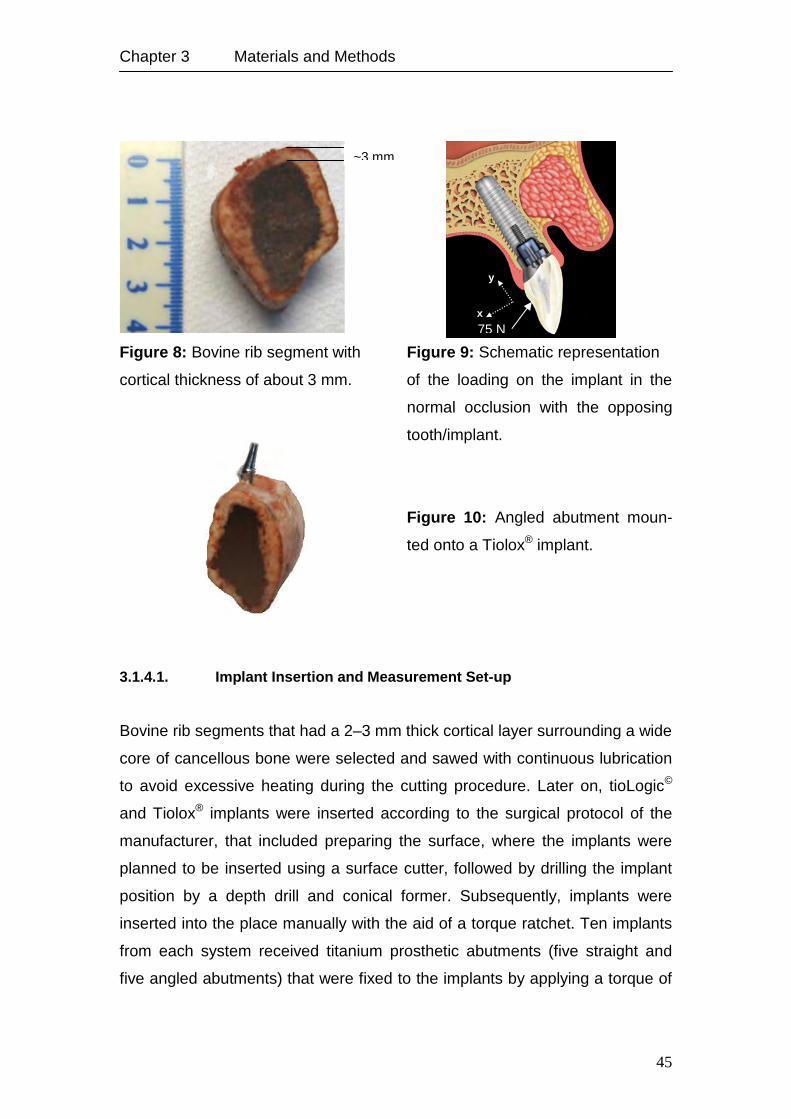
Chapter 3 Materials and Methods
45
Figure 8: Bovine rib segment with Figure 9: Schematic representation
cortical thickness of about 3 mm. of the loading on the implant in the
normal occlusion with the opposing
tooth/implant.
Figure 10: Angled abutment moun-
ted onto a Tiolox® implant.
3.1.4.1. Implant Insertion and Measurement Set-up
Bovine rib segments that had a 2–3 mm thick cortical layer surrounding a wide
core of cancellous bone were selected and sawed with continuous lubrication
to avoid excessive heating during the cutting procedure. Later on, tioLogic©
and Tiolox® implants were inserted according to the surgical protocol of the
manufacturer, that included preparing the surface, where the implants were
planned to be inserted using a surface cutter, followed by drilling the implant
position by a depth drill and conical former. Subsequently, implants were
inserted into the place manually with the aid of a torque ratchet. Ten implants
from each system received titanium prosthetic abutments (five straight and
five angled abutments) that were fixed to the implants by applying a torque of
~3 mm
x 75 N
y
x
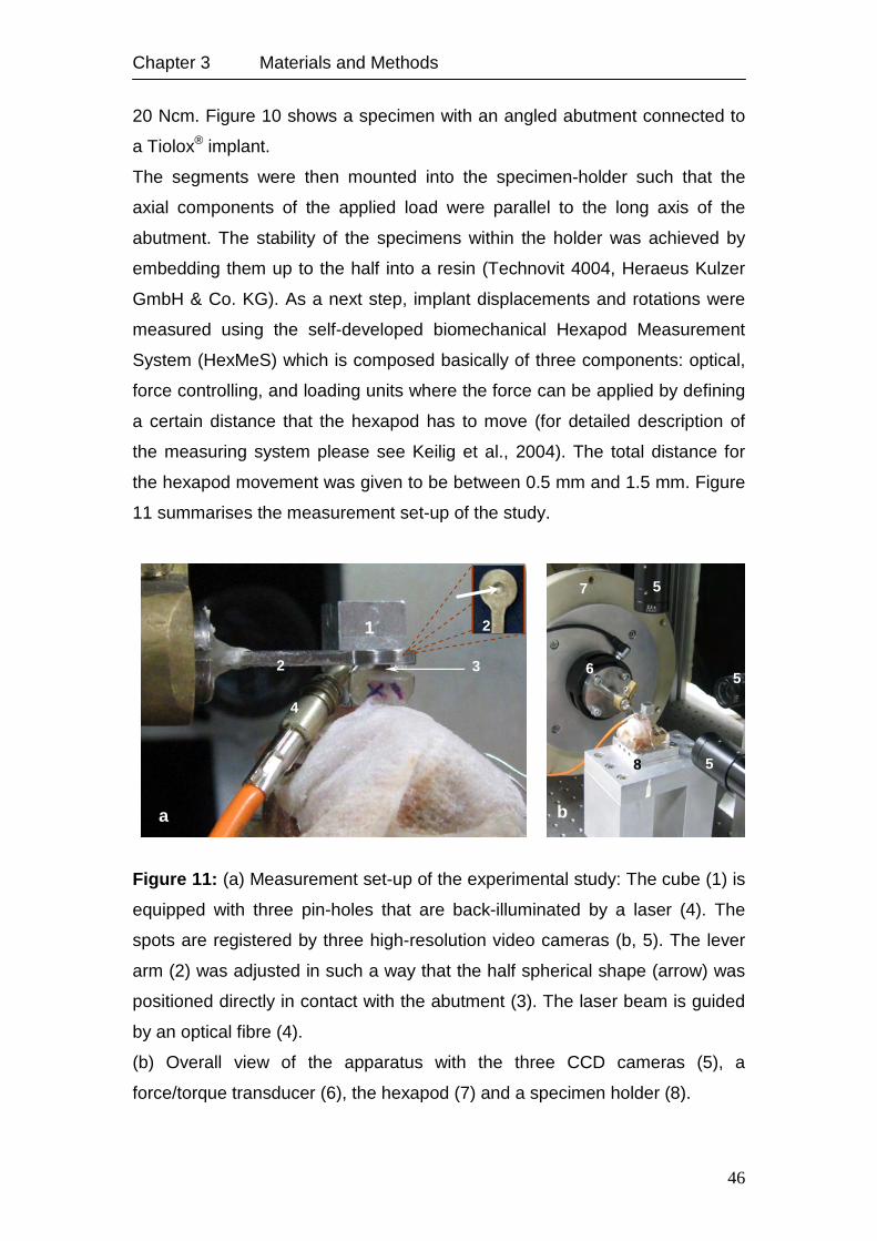
Chapter 3 Materials and Methods
46
20 Ncm. Figure 10 shows a specimen with an angled abutment connected to
a Tiolox® implant.
The segments were then mounted into the specimen-holder such that the
axial components of the applied load were parallel to the long axis of the
abutment. The stability of the specimens within the holder was achieved by
embedding them up to the half into a resin (Technovit 4004, Heraeus Kulzer
GmbH & Co. KG). As a next step, implant displacements and rotations were
measured using the self-developed biomechanical Hexapod Measurement
System (HexMeS) which is composed basically of three components: optical,
force controlling, and loading units where the force can be applied by defining
a certain distance that the hexapod has to move (for detailed description of
the measuring system please see Keilig et al., 2004). The total distance for
the hexapod movement was given to be between 0.5 mm and 1.5 mm. Figure
11 summarises the measurement set-up of the study.
Figure 11: (a) Measurement set-up of the experimental study: The cube (1) is
equipped with three pin-holes that are back-illuminated by a laser (4). The
spots are registered by three high-resolution video cameras (b, 5). The lever
arm (2) was adjusted in such a way that the half spherical shape (arrow) was
positioned directly in contact with the abutment (3). The laser beam is guided
by an optical fibre (4).
(b) Overall view of the apparatus with the three CCD cameras (5), a
force/torque transducer (6), the hexapod (7) and a specimen holder (8).
b
4
a
2
1
3
2
b
5
5
5 6
7
8
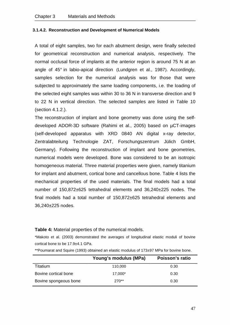
Chapter 3 Materials and Methods
47
3.1.4.2. Reconstruction and Development of Numerical Models
A total of eight samples, two for each abutment design, were finally selected
for geometrical reconstruction and numerical analysis, respectively. The
normal occlusal force of implants at the anterior region is around 75 N at an
angle of 45° in labio-apical direction (Lundgren et al., 1987). Accordingly,
samples selection for the numerical analysis was for those that were
subjected to approximately the same loading components, i.e. the loading of
the selected eight samples was within 30 to 36 N in transverse direction and 9
to 22 N in vertical direction. The selected samples are listed in Table 10
(section 4.1.2.).
The reconstruction of implant and bone geometry was done using the self-
developed ADOR-3D software (Rahimi et al., 2005) based on µCT-images
(self-developed apparatus with XRD 0840 AN digital x-ray detector,
Zentralabteilung Technologie ZAT, Forschungszentrum Jülich GmbH,
Germany). Following the reconstruction of implant and bone geometries,
numerical models were developed. Bone was considered to be an isotropic
homogeneous material. Three material properties were given, namely titanium
for implant and abutment, cortical bone and cancellous bone. Table 4 lists the
mechanical properties of the used materials. The final models had a total
number of 150,872±625 tetrahedral elements and 36,240±225 nodes. The
final models had a total number of 150,872±625 tetrahedral elements and
36,240±225 nodes.
Table 4: Material properties of the numerical models.
*Makoto et al. (2003) demonstrated the averages of longitudinal elastic moduli of bovine
cortical bone to be 17.9±4.1 GPa.
**Poumarat and Squire (1993) obtained an elastic modulus of 173±97 MPa for bovine bone.
Young’s modulus (MPa) Poisson’s ratio
Titatium 110,000 0.30
Bovine cortical bone 17,000* 0.30
Bovine spongeous bone 270** 0.30
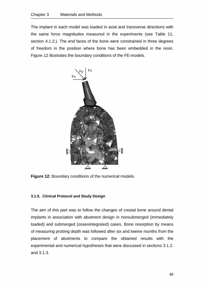
Chapter 3 Materials and Methods
48
The implant in each model was loaded in axial and transverse directions with
the same force magnitudes measured in the experiments (see Table 11,
section 4.1.2.). The end faces of the bone were constrained in three degrees
of freedom in the position where bone has been embedded in the resin.
Figure 12 illustrates the boundary conditions of the FE-models.
Figure 12: Boundary conditions of the numerical models.
3.1.5. Clinical Protocol and Study Design
The aim of this part was to follow the changes of crestal bone around dental
implants in association with abutment design in nonsubmerged (immediately
loaded) and submerged (osseointegrated) cases. Bone resorption by means
of measuring probing depth was followed after six and twelve months from the
placement of abutments to compare the obtained results with the
experimental and numerical hypotheses that were discussed in sections 3.1.2.
and 3.1.3.
Fy Fz
Fx
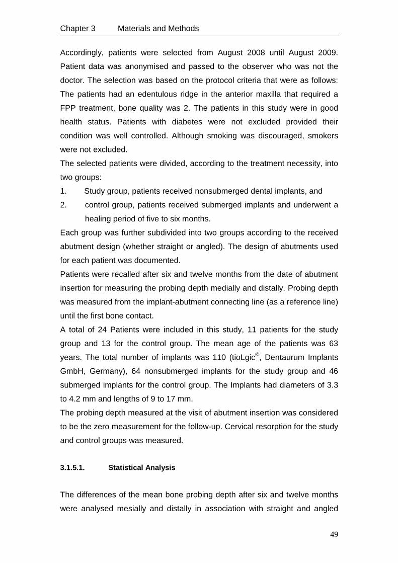
Chapter 3 Materials and Methods
49
Accordingly, patients were selected from August 2008 until August 2009.
Patient data was anonymised and passed to the observer who was not the
doctor. The selection was based on the protocol criteria that were as follows:
The patients had an edentulous ridge in the anterior maxilla that required a
FPP treatment, bone quality was 2. The patients in this study were in good
health status. Patients with diabetes were not excluded provided their
condition was well controlled. Although smoking was discouraged, smokers
were not excluded.
The selected patients were divided, according to the treatment necessity, into
two groups:
1. Study group, patients received nonsubmerged dental implants, and
2. control group, patients received submerged implants and underwent a
healing period of five to six months.
Each group was further subdivided into two groups according to the received
abutment design (whether straight or angled). The design of abutments used
for each patient was documented.
Patients were recalled after six and twelve months from the date of abutment
insertion for measuring the probing depth medially and distally. Probing depth
was measured from the implant-abutment connecting line (as a reference line)
until the first bone contact.
A total of 24 Patients were included in this study, 11 patients for the study
group and 13 for the control group. The mean age of the patients was 63
years. The total number of implants was 110 (tioLgic©, Dentaurum Implants
GmbH, Germany), 64 nonsubmerged implants for the study group and 46
submerged implants for the control group. The Implants had diameters of 3.3
to 4.2 mm and lengths of 9 to 17 mm.
The probing depth measured at the visit of abutment insertion was considered
to be the zero measurement for the follow-up. Cervical resorption for the study
and control groups was measured.
3.1.5.1. Statistical Analysis
The differences of the mean bone probing depth after six and twelve months
were analysed mesially and distally in association with straight and angled
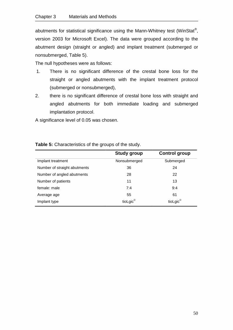
Chapter 3 Materials and Methods
50
abutments for statistical significance using the Mann-Whitney test (WinStat®,
version 2003 for Microsoft Excel). The data were grouped according to the
abutment design (straight or angled) and implant treatment (submerged or
nonsubmerged, Table 5).
The null hypotheses were as follows:
1. There is no significant difference of the crestal bone loss for the
straight or angled abutments with the implant treatment protocol
(submerged or nonsubmerged),
2. there is no significant difference of crestal bone loss with straight and
angled abutments for both immediate loading and submerged
implantation protocol.
A significance level of 0.05 was chosen.
Table 5: Characteristics of the groups of the study.
Study group Control group
Implant treatment Nonsubmerged Submerged
Number of straight abutments 36 24
Number of angled abutments 28 22
Number of patients
female: male
11
7:4
13
9:4
Average age 55 61
Implant type tioLgic© tioLgic©
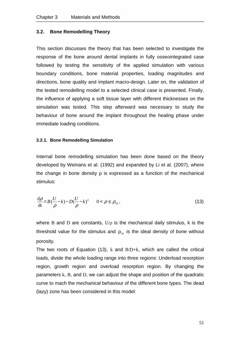
Chapter 3 Materials and Methods
51
3.2. Bone Remodelling Theory
This section discusses the theory that has been selected to investigate the
response of the bone around dental implants in fully osseointegrated case
followed by testing the sensitivity of the applied simulation with various
boundary conditions, bone material properties, loading magnitudes and
directions, bone quality and implant macro-design. Later on, the validation of
the tested remodelling model to a selected clinical case is presented. Finally,
the influence of applying a soft tissue layer with different thicknesses on the
simulation was tested. This step afterward was necessary to study the
behaviour of bone around the implant throughout the healing phase under
immediate loading conditions.
3.2.1. Bone Remodelling Simulation
Internal bone remodelling simulation has been done based on the theory
developed by Weinans et al. (1992) and expanded by Li et al. (2007), where
the change in bone density ρ is expressed as a function of the mechanical
stimulus:
cbkU
DkU
B ρρρρ
ρ ≤<−−−= 0)()(dt
d 2 , (13)
where B and D are constants, U/ρ is the mechanical daily stimulus, k is the
threshold value for the stimulus and cbρ is the ideal density of bone without
porosity.
The two roots of Equation (13), k and B/D+k, which are called the critical
loads, divide the whole loading range into three regions: Underload resorption
region, growth region and overload resorption region. By changing the
parameters k, B, and D, we can adjust the shape and position of the quadratic
curve to mach the mechanical behaviour of the different bone types. The dead
(lazy) zone has been considered in this model:
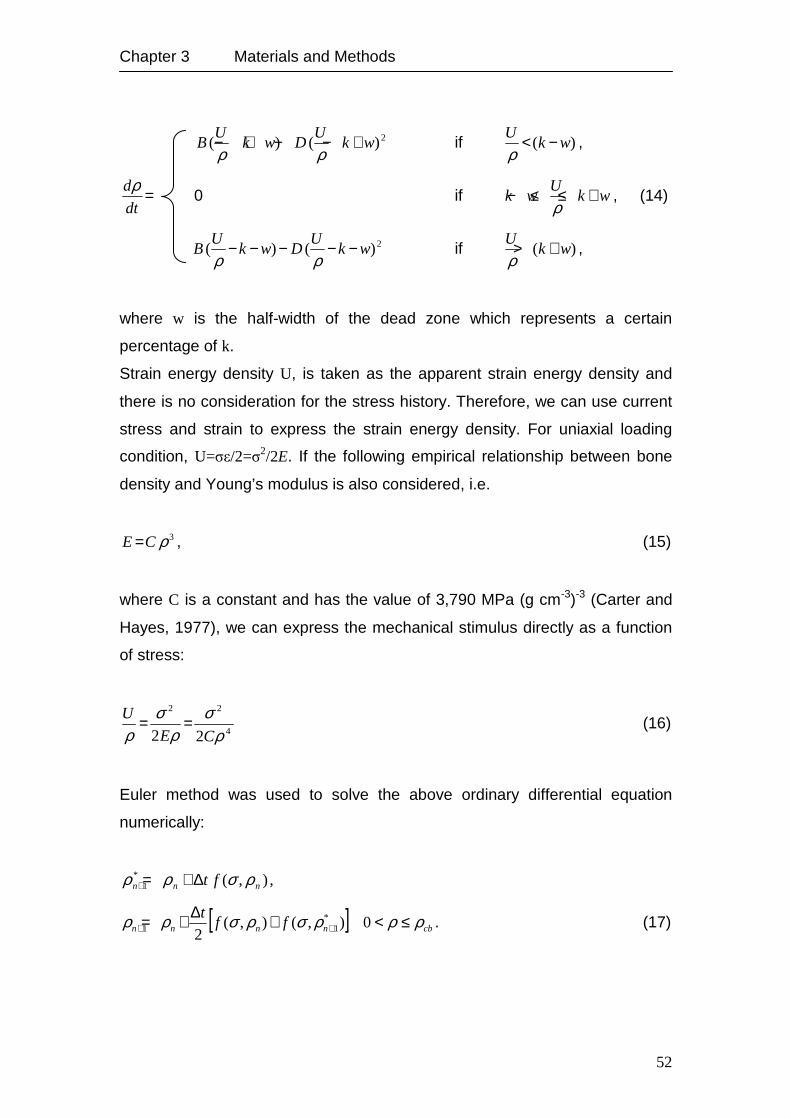
Chapter 3 Materials and Methods
52
2)()( wkU
DwkU
B +−−+−ρρ
if )( wkU −<ρ
,
=dt
dρ 0 if wk
Uwk +≤≤−
ρ, (14)
2)()( wkU
DwkU
B −−−−−ρρ
if )( wkU +>ρ
,
where w is the half-width of the dead zone which represents a certain
percentage of k.
Strain energy density U, is taken as the apparent strain energy density and
there is no consideration for the stress history. Therefore, we can use current
stress and strain to express the strain energy density. For uniaxial loading
condition, U=σε/2=σ2/2E. If the following empirical relationship between bone
density and Young’s modulus is also considered, i.e.
3ρCE = , (15)
where C is a constant and has the value of 3,790 MPa (g cm-3)-3 (Carter and
Hayes, 1977), we can express the mechanical stimulus directly as a function
of stress:
4
22
22 ρσ
ρσ
ρ CE
U == (16)
Euler method was used to solve the above ordinary differential equation
numerically:
,),(*1 nnn ft ρσρρ ∆+=+
[ ] cbnnnn fft ρρρσρσρρ ≤<+∆+= ++ 0),(),(
2*
11 . (17)
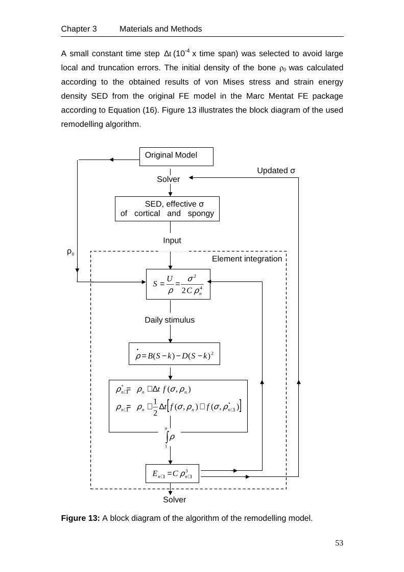
Chapter 3 Materials and Methods
53
A small constant time step t∆ (10-4 x time span) was selected to avoid large
local and truncation errors. The initial density of the bone ρ0 was calculated
according to the obtained results of von Mises stress and strain energy
density SED from the original FE model in the Marc Mentat FE package
according to Equation (16). Figure 13 illustrates the block diagram of the used
remodelling algorithm.
Figure 13: A block diagram of the algorithm of the remodelling model.
0ρ
Updated σ
2)()( kSDkSB −−−=•ρ
Original Model
SED, effective σ of cortical and spongy bone
4
2
2 nC
US
ρσ
ρ==
[ ]),(),(2
1
),(
11
1
∗++
∗+
+∆+=
∆+=
nnnn
nnn
fft
ft
ρσρσρρ
ρσρρ
∫n
1
ρ
311 ++ = nn CE ρ
Solver
Solver
Input
Daily stimulus
Element integration
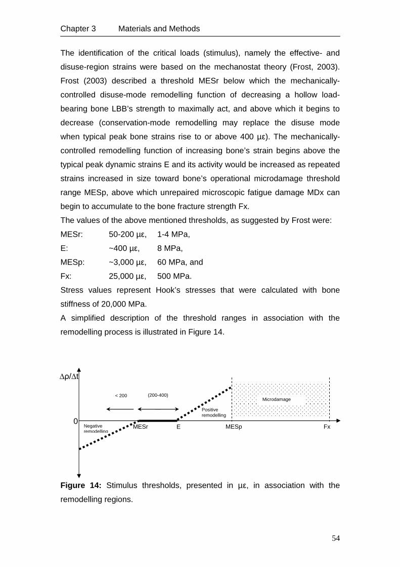
Chapter 3 Materials and Methods
54
The identification of the critical loads (stimulus), namely the effective- and
disuse-region strains were based on the mechanostat theory (Frost, 2003).
Frost (2003) described a threshold MESr below which the mechanically-
controlled disuse-mode remodelling function of decreasing a hollow load-
bearing bone LBB’s strength to maximally act, and above which it begins to
decrease (conservation-mode remodelling may replace the disuse mode
when typical peak bone strains rise to or above 400 µε). The mechanically-
controlled remodelling function of increasing bone’s strain begins above the
typical peak dynamic strains E and its activity would be increased as repeated
strains increased in size toward bone’s operational microdamage threshold
range MESp, above which unrepaired microscopic fatigue damage MDx can
begin to accumulate to the bone fracture strength Fx.
The values of the above mentioned thresholds, as suggested by Frost were:
MESr: 50-200 µε, 1-4 MPa,
E: ~400 µε, 8 MPa,
MESp: ~3,000 µε, 60 MPa, and
Fx: 25,000 µε, 500 MPa.
Stress values represent Hook’s stresses that were calculated with bone
stiffness of 20,000 MPa.
A simplified description of the threshold ranges in association with the
remodelling process is illustrated in Figure 14.
Figure 14: Stimulus thresholds, presented in µε, in association with the
remodelling regions.
MESr E MESp Fx 0
∆ρ/∆t
Microdamage accumulation
Positive remodelling
Negative remodelling
(200-400) µε
< 200 µε
Chapter 3 Materials and Methods
55
As there is no change in bone density at the lower and upper critical stresses,
where U/ρ=k are assumed, and by substituting the lower critical stress σ1 into
Equation (16) and assuming a density of 1.74 g/cm3 for cortical bone ρcb the
constant k can be calculated:
4
21
2 cbCk
ρσ
=∗ , (18)
and the constant D, by substituting the upper critical stress σ2 into Equation
(13):
∗−=
kC
BCD
cb
cb42
2
4
2
2
ρσρ
. (19)
Accordingly, the given value for constant k was 0.0004 Jg-1, whereas the
given value for constant D was 19.48 (gcm-3)3MPa-2(time unit)-1. k was
calculated with the strain magnitude of 325 µε taking the dead zone into
consideration.
3.2.2. Sensitivity Test of the Applied Theory
To fully exploit its potential, the mathematical model for bone remodelling was
implemented into the commercial FE software Marc Mentat. The bone was
considered to be an isotropic and homogeneous material with Young’s
modulus of Eco=20,000 MPa for the cortical bone and Esp=300 MPa for
cancellous bone. Poisson’s ratio was 0.3.
In this study a 3D FE model of an Ankylos A11 (Ø 3.5 mm, L11 mm) dental
implant inserted in an idealised bone model with 1.5 mm cortical thickness
was used to test the implemented algorithm. The simulation describes the
remodelling process of the bone around the dental implant after full
osseointegration to exclude the numerical influence of contact analysis on the
implemented simulation. The daily load history was represented using a load
case of an axial force of 100 N applied on the implant and face load of 2 MPa
Chapter 3 Materials and Methods
56
as a fixed pressure on the outer periphery of the cortical bone to simulate the
effect of jaw flexure. Density changes were observed after 100 cycles. After
calculating the SED and stress fields in the initial isotropic, homogenous
model for each bone element, the density was adapted to the observed SED
and stress, respectively. Using the remodelling theory, the effective stress
was used to calculate the actual daily stimulus U/ρ. The difference between
the actual (daily) stimulus and the attractor state stimulus k provides the error
signal that derives the remodelling response, generating a value for the rate of
density change for each element. The apparent density of each element was
then updated based on Equation (17) and the Young’s modulus of each
element was calculated as a cubic power function of the new apparent density
(Equation 15). The new values of the material properties of each element
were implemented in the next time increment and subsequent increments
were analysed similarly. Bone elements were considered to be converged
when the rate of density change is less than 10-5 between the iterations.
To optimise the applicability of the developed simulation, the sensitivity to
various mechanical conditions was tested. These included:
1. Different element size.
2. Various boundary conditions of the surrounding bone including different
constrain areas and degrees of freedom, in addition to the modification
in the direction and magnitude of the applied load on the dental
implant.
3. Applying the suggested remodelling parameters based on
Mechanostat theory and the corresponding dead zone width.
4. Modification of the stiffness of the cancellous bone.
5. Modification of the thickness of the cortical bone.
6. Different implant geometries.
3.2.2.1. Sensitivity Test: Element Size
In order to explore the influence of the element size on the behaviour of the
implemented simulation, the test model was developed with numerous
element edge lengths (EELs), namely: 0.2, 0.3, 0.4, 0.6, 0.8 mm.
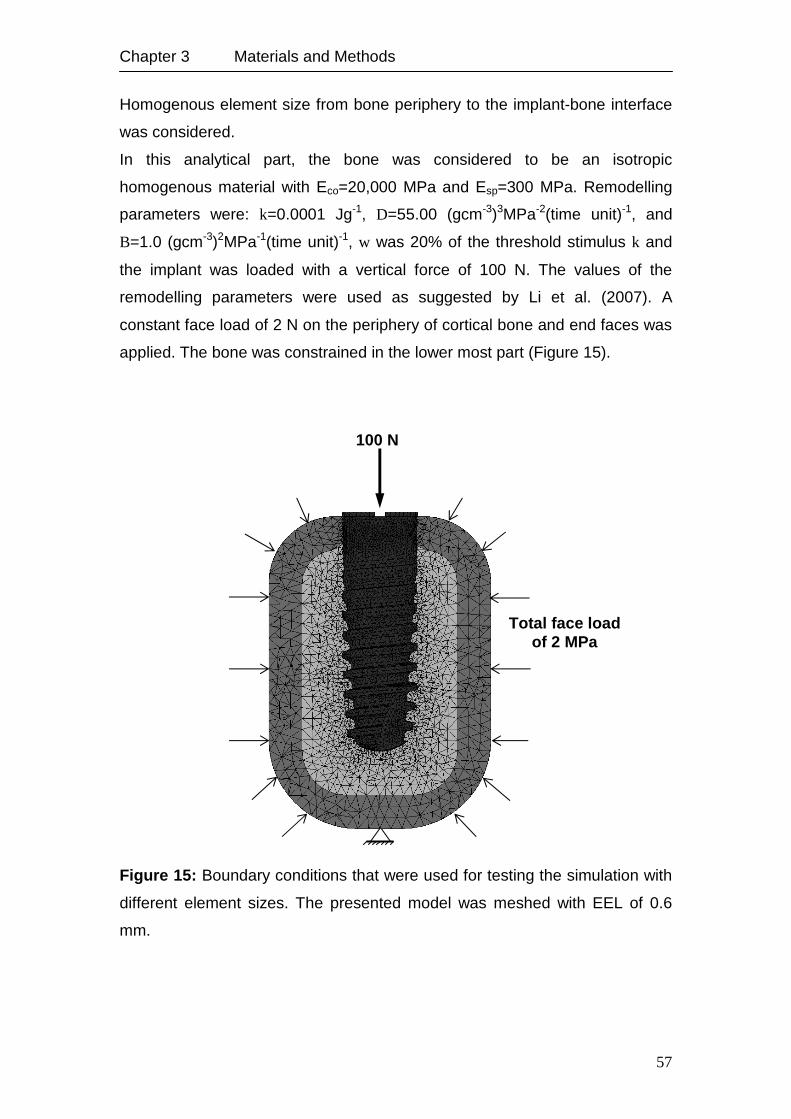
Chapter 3 Materials and Methods
57
Homogenous element size from bone periphery to the implant-bone interface
was considered.
In this analytical part, the bone was considered to be an isotropic
homogenous material with Eco=20,000 MPa and Esp=300 MPa. Remodelling
parameters were: k=0.0001 Jg-1, D=55.00 (gcm-3)3MPa-2(time unit)-1, and
B=1.0 (gcm-3)2MPa-1(time unit)-1, w was 20% of the threshold stimulus k and
the implant was loaded with a vertical force of 100 N. The values of the
remodelling parameters were used as suggested by Li et al. (2007). A
constant face load of 2 N on the periphery of cortical bone and end faces was
applied. The bone was constrained in the lower most part (Figure 15).
Figure 15: Boundary conditions that were used for testing the simulation with
different element sizes. The presented model was meshed with EEL of 0.6
mm.
100 N
Total face load of 2 MPa
Chapter 3 Materials and Methods
58
3.2.2.2. Sensitivity Test: Boundary Conditions
In order to obtain optimal results of the remodelling simulation, different
boundary conditions concerning surrounding bone were explored as follows:
1. Constrain the end faces of the bone in three degrees of freedom.
2. Constrain the end faces in axial direction.
3. Facial load on the outer periphery of cortical bone as compression,
keeping the end faces constrained in three degrees of freedom.
4. Facial load on the outer periphery of cortical bone as well as the end
faces as compression or tension.
5. To simulate the action of jaw muscles in function, face load was applied
on one half of the outer periphery of cortical bone as compression and
as tension on the second half to represent the contraction and
extension status of muscles. The end faces were constrained in three
degrees of freedom.
The magnitude of the load applied in 3., 4., and 5. was selected in such a way
that the resultant stress in the bone was within the boundary of the assumed
half width of the dead zone w (20% of the threshold stimulus k). The selected
values were: 0.5, 0.7, 1.0, 1.5, 2.0, and 2.5 MPa.
For this part, models with EEL of 0.4 mm and 0.6 mm were chosen because
of the acceptable distribution of density by means of elements on one hand,
and the total time required to calculate the density after 100 steps on the other
hand. Material properties and remodelling parameters were identical to those
used in 3.1.2.1. The implant was loaded with a vertical force of 100 N.
3.2.2.3. Sensitivity Test: Applying Remodelling Parameters based on
Mechanostat Theory
As described in section 3.2.1., the physiological strains are within the range of
200 to 4,000 µε, accordingly the parameters k and D were calculated by
considering the lower critical stress to be 5.2 MPa (Equation 18) and the
upper critical stress 60 MPa (Equation 19), respectively. The half width of the
dead zone w was considered as 60% of the reference stimulus k,
correspondingly; no remodelling takes place within the stress range of 2.0–8.3

Chapter 3 Materials and Methods
59
MPa within the cortical bone and 0.1–0.5 MPa within the cancellous bone (the
stress was calculated considering Young’s modulus of 20 GPa for the cortical
bone and 500 MPa for the cancellous bone). The given value for constant k
was: 0.0004 Jg-1, D: 19.48 (gcm-3)3MPa-2(time unit)-1 and B: 1.0 (gcm-3)2MPa-
1(time unit)-1.
Cortical bone was subjected to a tension load of 4.0 MPa on one half and
compression load of 3.0 MPa on the other half keeping the end faces
constrained in three degrees of freedom. The implant was loaded with a
vertical force of 300 N.
3.2.2.4. Sensitivity Test: Implant Loading Conditions
Three loading conditions were applied to test the remodelling model:
1. Axial loads of 150, 200, 250, 300 N.
2. Transverse loads with the same magnitudes described in the point
above.
3. Combined axial (150-300 N) and transverse (20 N) loads.
3.2.2.5. Sensitivity Test: Cancellous Bone Stiffness
Different stiffness values of cancellous bone were considered starting from a
very dense bone represented by a stiffness of 800 MPa to a very soft bone of
100 MPa.
3.2.2.6. Sensitivity Test: Elastic Modulus-Density Relation
Up to now the elastic modulus was calculated according to the correlation
suggested by Carter and Hayes (1977), where the modulus is proportional to
the apparent density raised to the power of 3 (Equation 15). As an attempt to
apply the different remodelling activities of the cortical and cancellous bone
and their influence on the stability of the obtained density per element, the
bilinear constitutive relationship suggested by Orr et al. (1990) was applied:
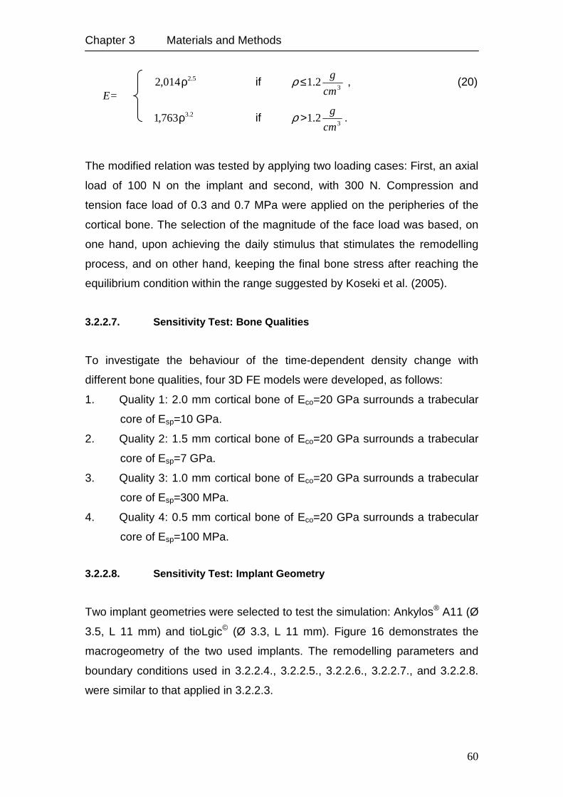
Chapter 3 Materials and Methods
60
5.2014,2 ρ if 3
2.1cm
g≤ρ , (20)
2.3763,1 ρ if 3
2.1cm
g>ρ .
The modified relation was tested by applying two loading cases: First, an axial
load of 100 N on the implant and second, with 300 N. Compression and
tension face load of 0.3 and 0.7 MPa were applied on the peripheries of the
cortical bone. The selection of the magnitude of the face load was based, on
one hand, upon achieving the daily stimulus that stimulates the remodelling
process, and on other hand, keeping the final bone stress after reaching the
equilibrium condition within the range suggested by Koseki et al. (2005).
3.2.2.7. Sensitivity Test: Bone Qualities
To investigate the behaviour of the time-dependent density change with
different bone qualities, four 3D FE models were developed, as follows:
1. Quality 1: 2.0 mm cortical bone of Eco=20 GPa surrounds a trabecular
core of Esp=10 GPa.
2. Quality 2: 1.5 mm cortical bone of Eco=20 GPa surrounds a trabecular
core of Esp=7 GPa.
3. Quality 3: 1.0 mm cortical bone of Eco=20 GPa surrounds a trabecular
core of Esp=300 MPa.
4. Quality 4: 0.5 mm cortical bone of Eco=20 GPa surrounds a trabecular
core of Esp=100 MPa.
3.2.2.8. Sensitivity Test: Implant Geometry
Two implant geometries were selected to test the simulation: Ankylos® A11 (Ø
3.5, L 11 mm) and tioLgic© (Ø 3.3, L 11 mm). Figure 16 demonstrates the
macrogeometry of the two used implants. The remodelling parameters and
boundary conditions used in 3.2.2.4., 3.2.2.5., 3.2.2.6., 3.2.2.7., and 3.2.2.8.
were similar to that applied in 3.2.2.3.
E=
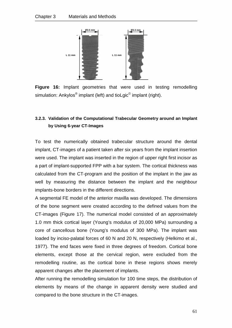
Chapter 3 Materials and Methods
61
Figure 16: Implant geometries that were used in testing remodelling
simulation: Ankylos® implant (left) and tioLgic© implant (right).
3.2.3. Validation of the Computational Trabecular Geometry around an Implant
by Using 6-year CT-Images
To test the numerically obtained trabecular structure around the dental
implant, CT-images of a patient taken after six years from the implant insertion
were used. The implant was inserted in the region of upper right first incisor as
a part of implant-supported FPP with a bar system. The cortical thickness was
calculated from the CT-program and the position of the implant in the jaw as
well by measuring the distance between the implant and the neighbour
implants-bone borders in the different directions.
A segmental FE model of the anterior maxilla was developed. The dimensions
of the bone segment were created according to the defined values from the
CT-images (Figure 17). The numerical model consisted of an approximately
1.0 mm thick cortical layer (Young’s modulus of 20,000 MPa) surrounding a
core of cancellous bone (Young’s modulus of 300 MPa). The implant was
loaded by inciso-palatal forces of 60 N and 20 N, respectively (Helkimo et al.,
1977). The end faces were fixed in three degrees of freedom. Cortical bone
elements, except those at the cervical region, were excluded from the
remodelling routine, as the cortical bone in these regions shows merely
apparent changes after the placement of implants.
After running the remodelling simulation for 100 time steps, the distribution of
elements by means of the change in apparent density were studied and
compared to the bone structure in the CT-images.
Ø3.5 mm
L 11 mm
Ø3.3 mm
L 11 mm
Chapter 3 Materials and Methods
62
Figure 17: FE model of the maxillary bone segment with the dental implant
(left), and the CT-image (right, later view). The slice thickness was 0.7 to 1.0
mm, with the preplanned position of the implant. For the FE model, the load
was applied at the height level of the final restoration.
3.2.4. Influence of Soft Tissue Thickness on Bone Remodelling Simulation
To go a step forward in the investigation of the bone remodelling model, the
behaviour of the bone elements by means of stress distribution and density
change per unit time was studied by applying a soft tissue layer at the bone-
implant interface. This analysis was essential for studying the healing process
of the bone around dental implants under immediate loading condition that will
be discussed later on in this section.
The previous results concerning density distributions with different EELs
(section 4.2.1.1.) showed obviously the influence of the element size on the
density distribution of the bone elements. Consequently, 3D FE models were
developed with different thicknesses of the soft tissue layer around the dental
implant (Figure 18). Table 6 illustrates the EELs of bone elements and the
corresponding thicknesses of the soft tissue that were used in this part of the
analysis.
The mechanical conditions including implant loading, boundary conditions and
material properties were identical to those used in sections 3.2.2.3. to 3.2.2.8.
Soft tissue elements that surround the implant within the cortical and
cancellous bone zones were given the material properties of the cortical and
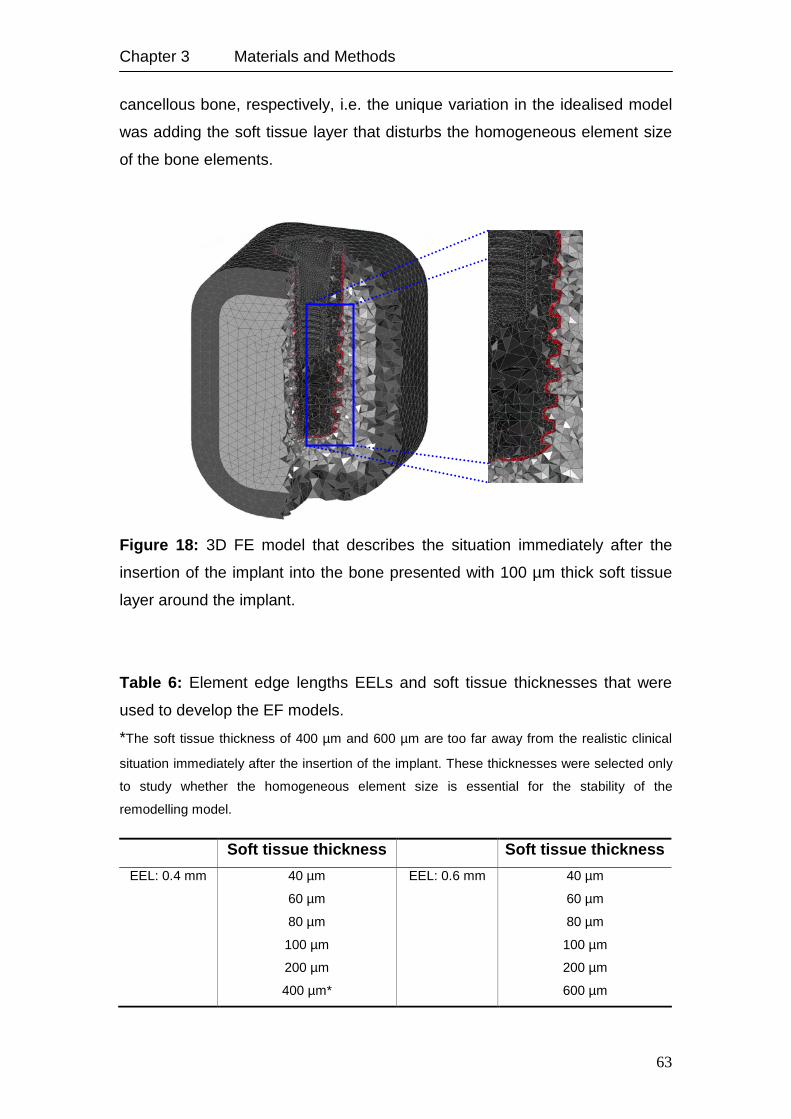
Chapter 3 Materials and Methods
63
cancellous bone, respectively, i.e. the unique variation in the idealised model
was adding the soft tissue layer that disturbs the homogeneous element size
of the bone elements.
Figure 18: 3D FE model that describes the situation immediately after the
insertion of the implant into the bone presented with 100 µm thick soft tissue
layer around the implant.
Table 6: Element edge lengths EELs and soft tissue thicknesses that were
used to develop the EF models.
*The soft tissue thickness of 400 µm and 600 µm are too far away from the realistic clinical
situation immediately after the insertion of the implant. These thicknesses were selected only
to study whether the homogeneous element size is essential for the stability of the
remodelling model.
Soft tissue thickness Soft tissue thickness
EEL: 0.4 mm 40 µm EEL: 0.6 mm 40 µm
60 µm 60 µm
80 µm 80 µm
100 µm 100 µm
200 µm 200 µm
400 µm* 600 µm
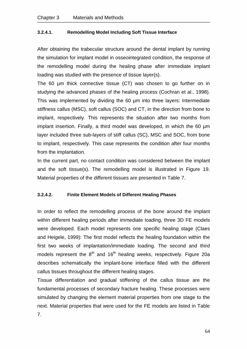
Chapter 3 Materials and Methods
64
3.2.4.1. Remodelling Model Including Soft Tissue Interface
After obtaining the trabecular structure around the dental implant by running
the simulation for implant model in osseointegrated condition, the response of
the remodelling model during the healing phase after immediate implant
loading was studied with the presence of tissue layer(s).
The 60 µm thick connective tissue (CT) was chosen to go further on in
studying the advanced phases of the healing process (Cochran et al., 1998).
This was implemented by dividing the 60 µm into three layers: Intermediate
stiffness callus (MSC), soft callus (SOC) and CT, in the direction from bone to
implant, respectively. This represents the situation after two months from
implant insertion. Finally, a third model was developed, in which the 60 µm
layer included three sub-layers of stiff callus (SC), MSC and SOC, from bone
to implant, respectively. This case represents the condition after four months
from the implantation.
In the current part, no contact condition was considered between the implant
and the soft tissue(s). The remodelling model is illustrated in Figure 19.
Material properties of the different tissues are presented in Table 7.
3.2.4.2. Finite Element Models of Different Healing Phases
In order to reflect the remodelling process of the bone around the implant
within different healing periods after immediate loading, three 3D FE models
were developed. Each model represents one specific healing stage (Claes
and Heigele, 1999): The first model reflects the healing foundation within the
first two weeks of implantation/immediate loading. The second and third
models represent the 8th and 16th healing weeks, respectively. Figure 20a
describes schematically the implant-bone interface filled with the different
callus tissues throughout the different healing stages.
Tissue differentiation and gradual stiffening of the callus tissue are the
fundamental processes of secondary fracture healing. These processes were
simulated by changing the element material properties from one stage to the
next. Material properties that were used for the FE models are listed in Table
7.
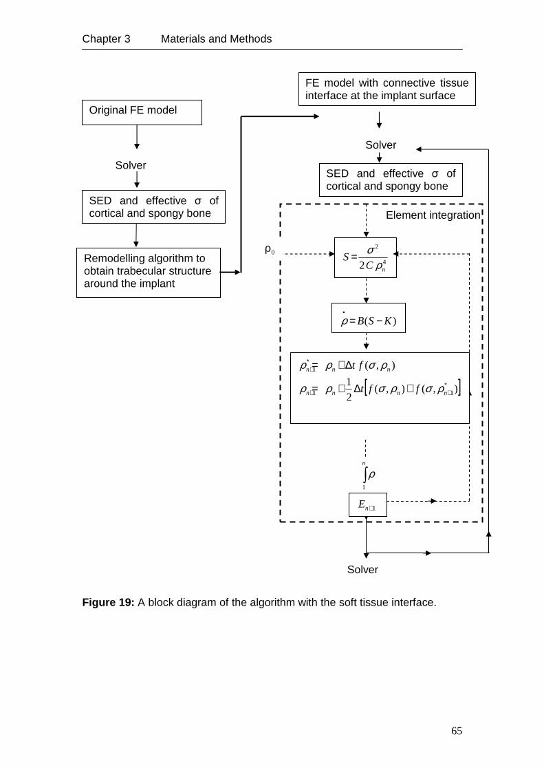
Chapter 3 Materials and Methods
65
Figure 19: A block diagram of the algorithm with the soft tissue interface.
Solver
Element integration
∫n
1
ρ
Original FE model
Solver
SED and effective σ of cortical and spongy bone
Remodelling algorithm to obtain trabecular structure around the implant
)( KSB −=•ρ
4
2
2 nCS
ρσ=
[ ]),(),(21
),(
11
1
∗++
∗+
+∆+=
∆+=
nnnn
nnn
fft
ft
ρσρσρρ
ρσρρ
1+nE
FE model with connective tissue interface at the implant surface
SED and effective σ of cortical and spongy bone
Solver
0ρ
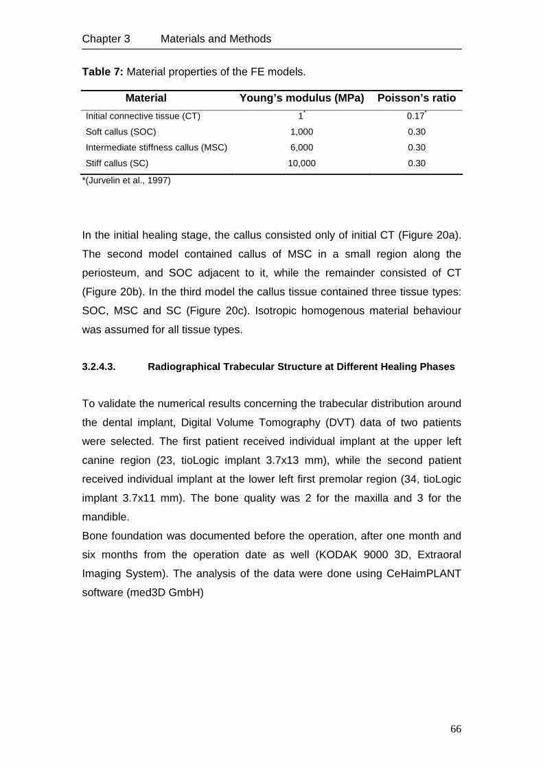
Chapter 3 Materials and Methods
66
Table 7: Material properties of the FE models.
*(Jurvelin et al., 1997)
In the initial healing stage, the callus consisted only of initial CT (Figure 20a).
The second model contained callus of MSC in a small region along the
periosteum, and SOC adjacent to it, while the remainder consisted of CT
(Figure 20b). In the third model the callus tissue contained three tissue types:
SOC, MSC and SC (Figure 20c). Isotropic homogenous material behaviour
was assumed for all tissue types.
3.2.4.3. Radiographical Trabecular Structure at Different Healing Phases
To validate the numerical results concerning the trabecular distribution around
the dental implant, Digital Volume Tomography (DVT) data of two patients
were selected. The first patient received individual implant at the upper left
canine region (23, tioLogic implant 3.7x13 mm), while the second patient
received individual implant at the lower left first premolar region (34, tioLogic
implant 3.7x11 mm). The bone quality was 2 for the maxilla and 3 for the
mandible.
Bone foundation was documented before the operation, after one month and
six months from the operation date as well (KODAK 9000 3D, Extraoral
Imaging System). The analysis of the data were done using CeHaimPLANT
software (med3D GmbH)
Material Young’s modulus (MPa) Poisson’s ratio
Initial connective tissue (CT) 1* 0.17*
Soft callus (SOC) 1,000 0.30
Intermediate stiffness callus (MSC) 6,000 0.30
Stiff callus (SC) 10,000 0.30
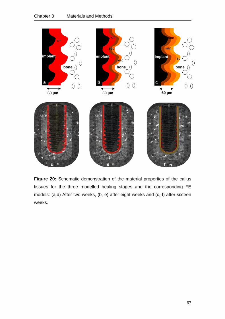
Chapter 3 Materials and Methods
67
Figure 20: Schematic demonstration of the material properties of the callus
tissues for the three modelled healing stages and the corresponding FE
models: (a,d) After two weeks, (b, e) after eight weeks and (c, f) after sixteen
weeks.
implant
CT
bone
60 µm
a
implant
CT
SOC
MSC
bone
60 µm
b
SOC
MSC
SC implant
bone
60 µm
c
d e f
68
Chapter 4
4. Results
This section covers the results of the main issues of this work as follows:
First, the results of the mechanical investigation of the abutment design
influence on the reaction of the bone for FPP. Second, the results of the
applied remodelling theory and the corresponding sensitivity analysis, thirdly;
the application of the remodelling theory to a clinical case, and finally; the
results of the remodelling simulation including soft tissue during the healing
phase.
4.1. Mechanical Investigation of Different Implant and Abutment Designs:
Experimental, Numerical and Clinical Aspects
In this section the experimental results concerning implant displacement and
rotation under immediate loading are presented. Moreover, qualitative and
quantitive analyses of stress and strain distributions that were associated with
the use of straight or angled abutment will be presented, in addition to
comparing the numerical results regarding implant displacements with those
that were obtained from the experiments. Furthermore, the numerical results
of investigating the effect of the abutment design on the distribution of the
stress and strain in the alveolar bone around the implants used in implant-
supported partial prosthesis are discussed. Finally, the obtained results of the
clinical evaluation of cervical bone loss in implant-supported prosthesis after
six and twelve months are presented together with their association with the
abutment design.
Chapter 4 Results
69
4.1.1. Fixed Partial Prosthesis Models
4.1.1.1. Immediately Loaded Condition
The magnitude of the obtained strains and equivalent von Mises stresses are
summarised in Table 8. Both, straight- and angled-abutment models in which
the abutment and the corresponding prosthesis unit were considered as one
rigid piece showed almost the same stress magnitudes. On the other hand
the angled-abutment model (AAM) showed a higher strain value (6,000 µε)
than the straight-abutment model (SAM, 5,300 µε). The displacement of the
supporting implants, calculated as the average of the displacement of the two
fixtures, was higher with the angled abutment (4.0 µm) than with the straight
one (3.4 µm).
The pattern of stress distribution associated with the AAM was, generally,
spread over a wider area of the cortical bone surrounding the implants than
with the straight abutments (Figures 21a and 21b). Strain distributions for both
models were concentrated at the most upper coronal portion of the fixture
within the cancellous bone and the coarse thread areas showed a noticeable
wider distribution of the strain with the angled abutments than with the straight
ones (Figures 22a and 22b). The maximum values were higher in models with
contact analysis than in those without contact (Table 8).
4.1.1.2. Osseointegrated Condition
In the completely osseointegrated case, a decrease in the magnitudes of the
implant displacements, stresses and strains associated with SAM and AAM
was observed as follows: For SAM the drop was 43%, 47% and 80% of the
implant displacements, stress and strain and for AAM 61%, 42%, and 78%
respectively (Table 9).
Compared with the non-osseointegrated situation, a tendency towards a more
homogenous stress distribution around the coronal portion of the dental
implant was observed (cortical bone region in Figures 23a and 23b).
Furthermore, the strain was basically concentrated along the coarse threads
at the distal sides and more in the apical direction (Figures 24a and 24b).
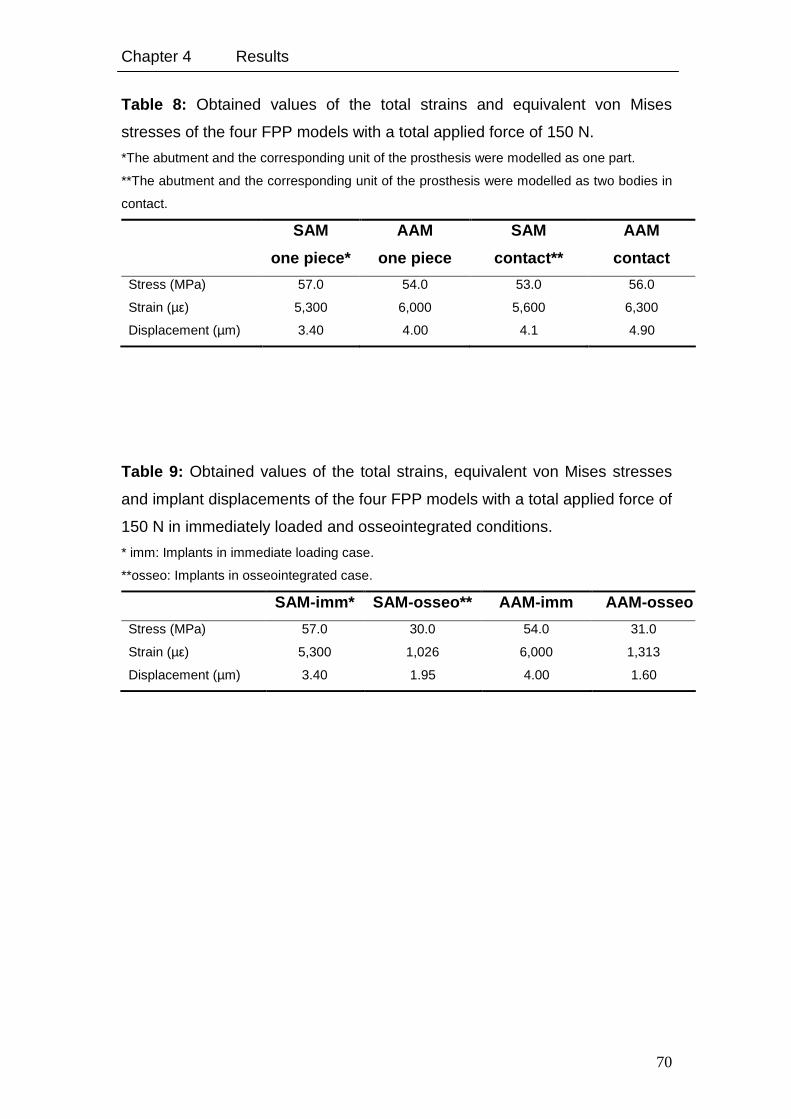
Chapter 4 Results
70
Table 8: Obtained values of the total strains and equivalent von Mises
stresses of the four FPP models with a total applied force of 150 N.
*The abutment and the corresponding unit of the prosthesis were modelled as one part.
**The abutment and the corresponding unit of the prosthesis were modelled as two bodies in
contact.
SAM
one piece*
AAM
one piece
SAM
contact**
AAM
contact
Stress (MPa) 57.0 54.0 53.0 56.0
Strain (µε) 5,300 6,000 5,600 6,300
Displacement (µm) 3.40 4.00 4.1 4.90
Table 9: Obtained values of the total strains, equivalent von Mises stresses
and implant displacements of the four FPP models with a total applied force of
150 N in immediately loaded and osseointegrated conditions.
* imm: Implants in immediate loading case.
**osseo: Implants in osseointegrated case.
SAM-imm* SAM-osseo** AAM-imm AAM-osseo
Stress (MPa) 57.0 30.0 54.0 31.0
Strain (µε) 5,300 1,026 6,000 1,313
Displacement (µm) 3.40 1.95 4.00 1.60
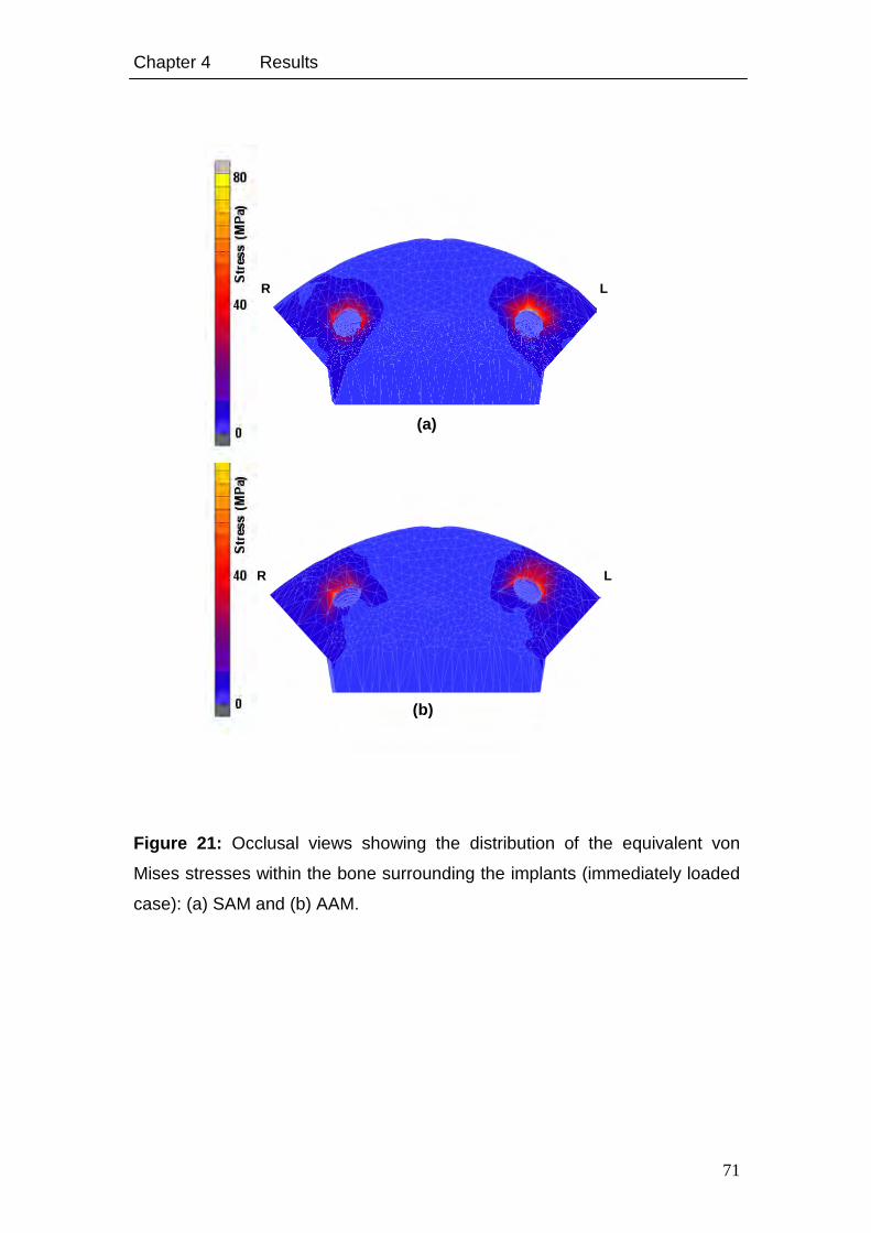
Chapter 4 Results
71
Figure 21: Occlusal views showing the distribution of the equivalent von
Mises stresses within the bone surrounding the implants (immediately loaded
case): (a) SAM and (b) AAM.
L R
(b)
R L
(a)
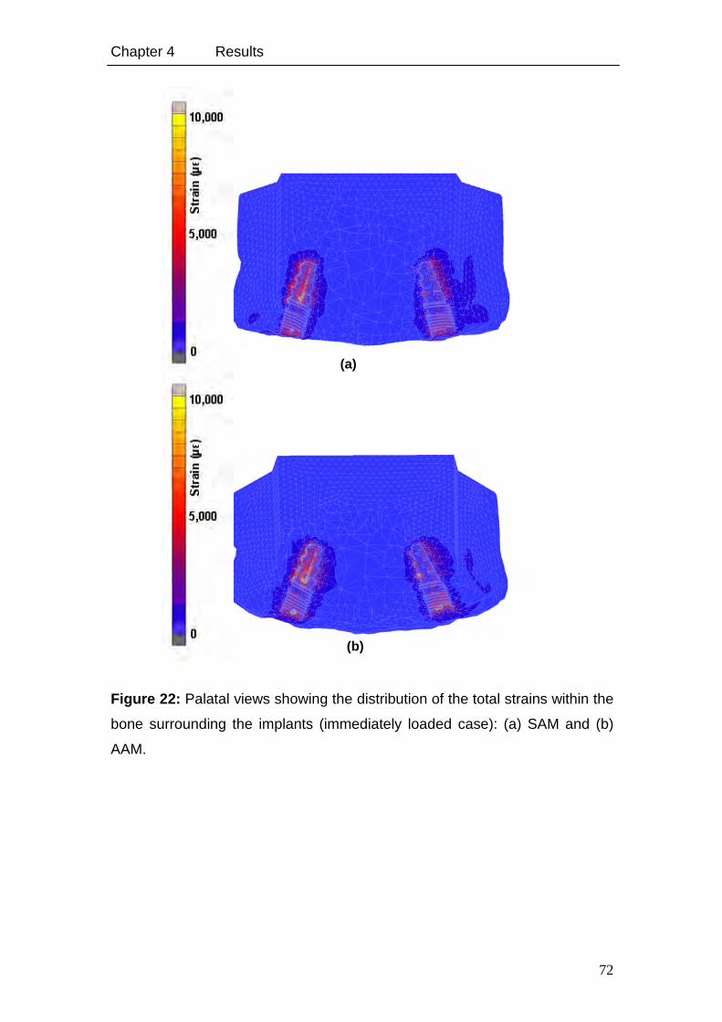
Chapter 4 Results
72
Figure 22: Palatal views showing the distribution of the total strains within the
bone surrounding the implants (immediately loaded case): (a) SAM and (b)
AAM.
(a)
(b)
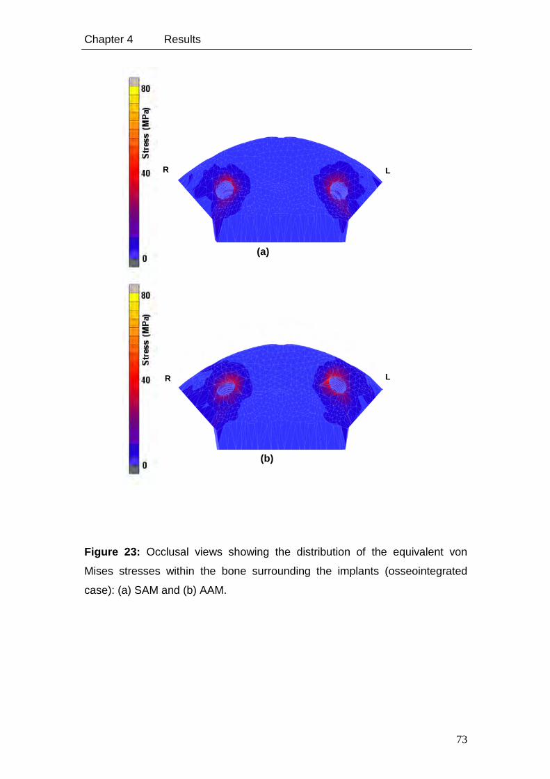
Chapter 4 Results
73
Figure 23: Occlusal views showing the distribution of the equivalent von
Mises stresses within the bone surrounding the implants (osseointegrated
case): (a) SAM and (b) AAM.
L R
(b)
L R
(a)
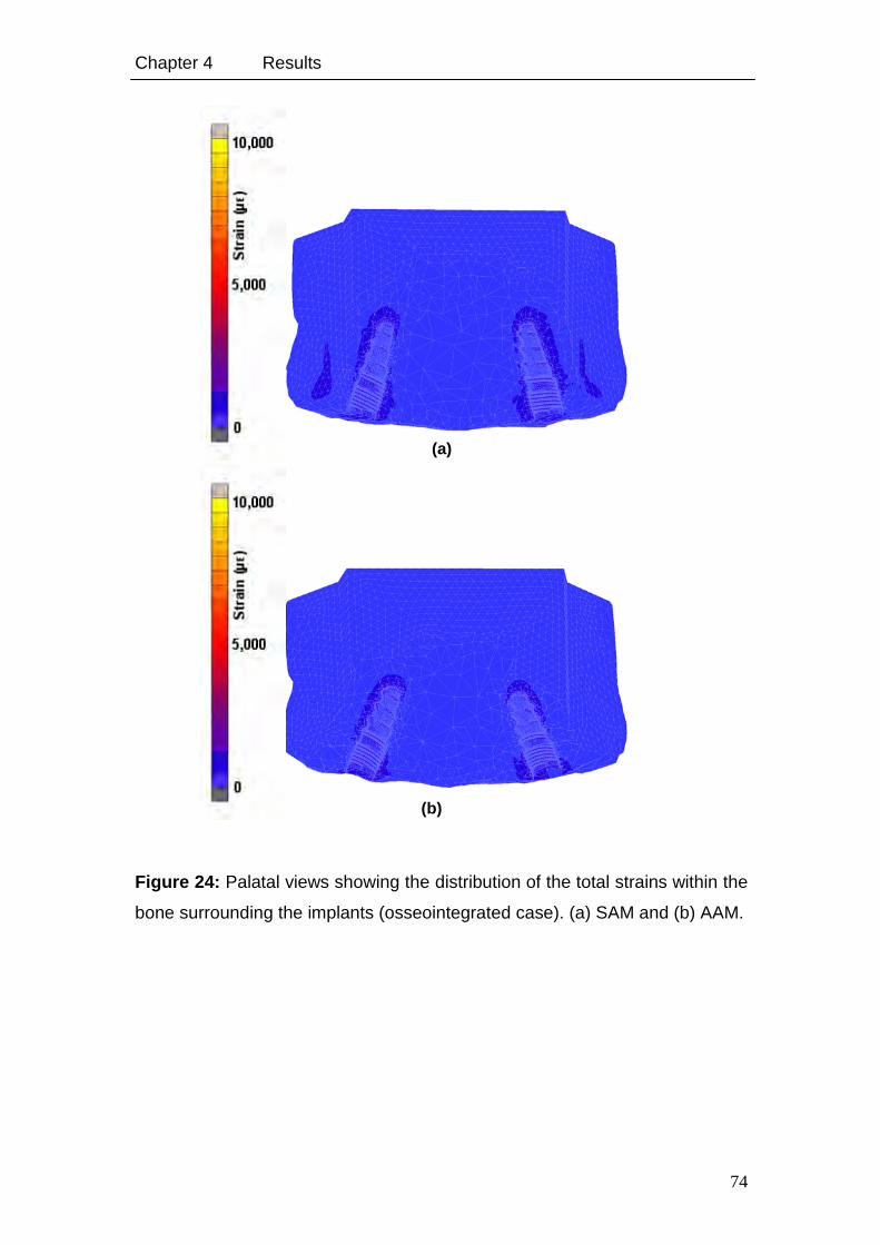
Chapter 4 Results
74
Figure 24: Palatal views showing the distribution of the total strains within the
bone surrounding the implants (osseointegrated case). (a) SAM and (b) AAM.
(a)
(b)
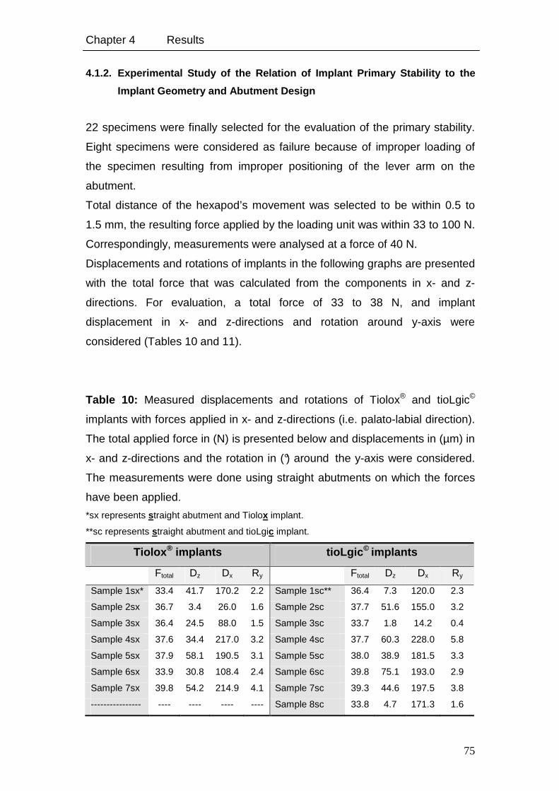
Chapter 4 Results
75
4.1.2. Experimental Study of the Relation of Implant Primary Stability to the
Implant Geometry and Abutment Design
22 specimens were finally selected for the evaluation of the primary stability.
Eight specimens were considered as failure because of improper loading of
the specimen resulting from improper positioning of the lever arm on the
abutment.
Total distance of the hexapod’s movement was selected to be within 0.5 to
1.5 mm, the resulting force applied by the loading unit was within 33 to 100 N.
Correspondingly, measurements were analysed at a force of 40 N.
Displacements and rotations of implants in the following graphs are presented
with the total force that was calculated from the components in x- and z-
directions. For evaluation, a total force of 33 to 38 N, and implant
displacement in x- and z-directions and rotation around y-axis were
considered (Tables 10 and 11).
Table 10: Measured displacements and rotations of Tiolox® and tioLgic©
implants with forces applied in x- and z-directions (i.e. palato-labial direction).
The total applied force in (N) is presented below and displacements in (µm) in
x- and z-directions and the rotation in (°) around the y-axis were considered.
The measurements were done using straight abutments on which the forces
have been applied.
*sx represents straight abutment and Tiolox implant.
**sc represents straight abutment and tioLgic implant.
Tiolox ® implants tioLgic © implants
Ftotal Dz Dx Ry Ftotal Dz Dx Ry
Sample 1sx* 33.4 41.7 170.2 2.2 Sample 1sc** 36.4 7.3 120.0 2.3
Sample 2sx 36.7 3.4 26.0 1.6 Sample 2sc 37.7 51.6 155.0 3.2
Sample 3sx 36.4 24.5 88.0 1.5 Sample 3sc 33.7 1.8 14.2 0.4
Sample 4sx 37.6 34.4 217.0 3.2 Sample 4sc 37.7 60.3 228.0 5.8
Sample 5sx 37.9 58.1 190.5 3.1 Sample 5sc 38.0 38.9 181.5 3.3
Sample 6sx 33.9 30.8 108.4 2.4 Sample 6sc 39.8 75.1 193.0 2.9
Sample 7sx 39.8 54.2 214.9 4.1 Sample 7sc 39.3 44.6 197.5 3.8
---------------- ---- ---- ---- ---- Sample 8sc 33.8 4.7 171.3 1.6
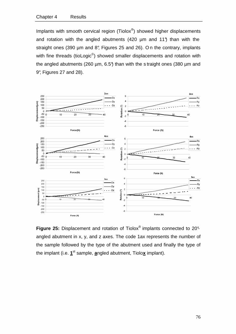
Chapter 4 Results
76
Implants with smooth cervical region (Tiolox®) showed higher displacements
and rotation with the angled abutments (420 µm and 11°) than with the
straight ones (390 µm and 8°, Figures 25 and 26). O n the contrary, implants
with fine threads (tioLogic©) showed smaller displacements and rotation with
the angled abutments (260 µm, 6.5°) than with the s traight ones (380 µm and
9°, Figures 27 and 28).
Figure 25: Displacement and rotation of Tiolox® implants connected to 20°-
angled abutment in x, y, and z axes. The code 1ax represents the number of
the sample followed by the type of the abutment used and finally the type of
the implant (i.e. 1st sample, angled abutment, Tiolox implant).
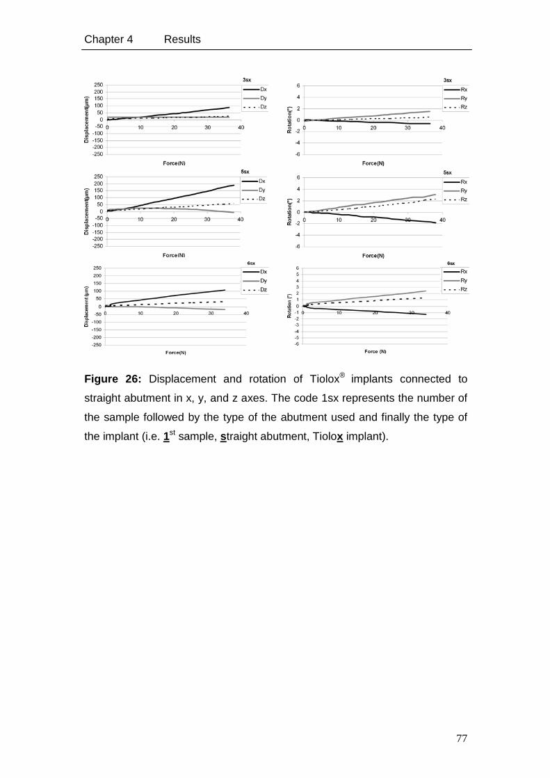
Chapter 4 Results
77
Figure 26: Displacement and rotation of Tiolox® implants connected to
straight abutment in x, y, and z axes. The code 1sx represents the number of
the sample followed by the type of the abutment used and finally the type of
the implant (i.e. 1st sample, straight abutment, Tiolox implant).
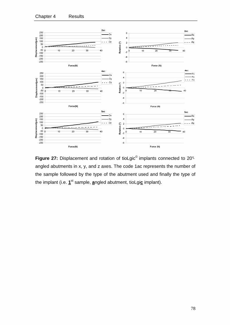
Chapter 4 Results
78
Figure 27: Displacement and rotation of tioLgic© implants connected to 20°-
angled abutments in x, y, and z axes. The code 1ac represents the number of
the sample followed by the type of the abutment used and finally the type of
the implant (i.e. 1st sample, angled abutment, tioLgic implant).
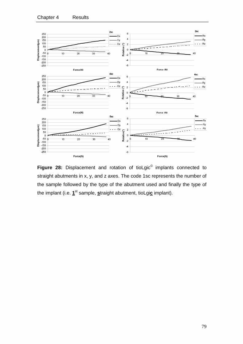
Chapter 4 Results
79
Figure 28: Displacement and rotation of tioLgic© implants connected to
straight abutments in x, y, and z axes. The code 1sc represents the number of
the sample followed by the type of the abutment used and finally the type of
the implant (i.e. 1st sample, straight abutment, tioLgic implant).
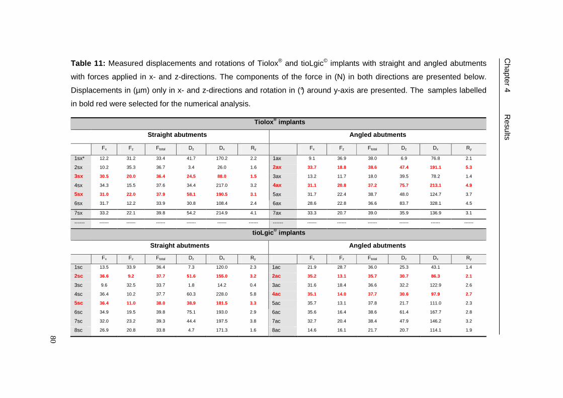
Table 11: Measured displacements and rotations of Tiolox® and tioLgic© implants with straight and angled abutments
with forces applied in x- and z-directions. The components of the force in (N) in both directions are presented below.
Displacements in (µm) only in x- and z-directions and rotation in (°) around y-axis are presented. The samples labelled
in bold red were selected for the numerical analysis.
Tiolox ® implants
Straight abutments Angled abutments
Fx Fz Ftotal Dz Dx Ry Fx Fz Ftotal Dz Dx Ry
1sx* 12.2 31.2 33.4 41.7 170.2 2.2 1ax 9.1 36.9 38.0 6.9 76.8 2.1
2sx 10.2 35.3 36.7 3.4 26.0 1.6 2ax 33.7 18.8 38.6 47.4 191.1 5.3
3sx 30.5 20.0 36.4 24.5 88.0 1.5 3ax 13.2 11.7 18.0 39.5 78.2 1.4
4sx 34.3 15.5 37.6 34.4 217.0 3.2 4ax 31.1 20.8 37.2 75.7 213.1 4.9
5sx 31.0 22.0 37.9 58.1 190.5 3.1 5ax 31.7 22.4 38.7 48.0 124.7 3.7
6sx 31.7 12.2 33.9 30.8 108.4 2.4 6ax 28.6 22.8 36.6 83.7 328.1 4.5
7sx 33.2 22.1 39.8 54.2 214.9 4.1 7ax 33.3 20.7 39.0 35.9 136.9 3.1
------ ------ ------ ------ ------ ------ ------ ------ ------ ------ ------ ------ ------ ------
tioLgic © implants
Straight abutments Angled abutments
Fx Fz Ftotal Dz Dx Ry Fx Fz Ftotal Dz Dx Ry
1sc 13.5 33.9 36.4 7.3 120.0 2.3 1ac 21.9 28.7 36.0 25.3 43.1 1.4
2sc 36.6 9.2 37.7 51.6 155.0 3.2 2ac 35.2 13.1 35.7 30.7 86.3 2.1
3sc 9.6 32.5 33.7 1.8 14.2 0.4 3ac 31.6 18.4 36.6 32.2 122.9 2.6
4sc 36.4 10.2 37.7 60.3 228.0 5.8 4ac 35.1 14.0 37.7 30.6 97.9 2.7
5sc 36.4 11.0 38.0 38.9 181.5 3.3 5ac 35.7 13.1 37.8 21.7 111.0 2.3
6sc 34.9 19.5 39.8 75.1 193.0 2.9 6ac 35.6 16.4 38.6 61.4 167.7 2.8
7sc 32.0 23.2 39.3 44.4 197.5 3.8 7ac 32.7 20.4 38.4 47.9 146.2 3.2
8sc 26.9 20.8 33.8 4.7 171.3 1.6 8ac 14.6 16.1 21.7 20.7 114.1 1.9
Chapter 4 R
esults
80
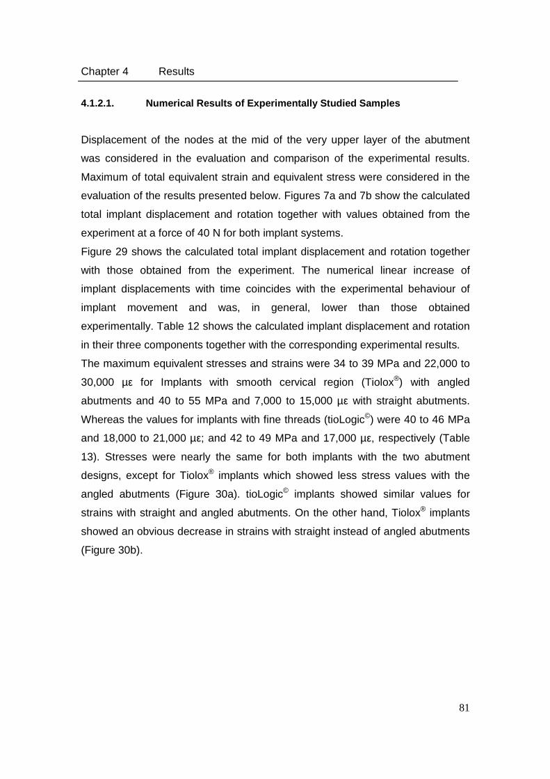
Chapter 4 Results
81
4.1.2.1. Numerical Results of Experimentally Studied Samples
Displacement of the nodes at the mid of the very upper layer of the abutment
was considered in the evaluation and comparison of the experimental results.
Maximum of total equivalent strain and equivalent stress were considered in the
evaluation of the results presented below. Figures 7a and 7b show the calculated
total implant displacement and rotation together with values obtained from the
experiment at a force of 40 N for both implant systems.
Figure 29 shows the calculated total implant displacement and rotation together
with those obtained from the experiment. The numerical linear increase of
implant displacements with time coincides with the experimental behaviour of
implant movement and was, in general, lower than those obtained
experimentally. Table 12 shows the calculated implant displacement and rotation
in their three components together with the corresponding experimental results.
The maximum equivalent stresses and strains were 34 to 39 MPa and 22,000 to
30,000 µε for Implants with smooth cervical region (Tiolox®) with angled
abutments and 40 to 55 MPa and 7,000 to 15,000 µε with straight abutments.
Whereas the values for implants with fine threads (tioLogic©) were 40 to 46 MPa
and 18,000 to 21,000 µε; and 42 to 49 MPa and 17,000 µε, respectively (Table
13). Stresses were nearly the same for both implants with the two abutment
designs, except for Tiolox® implants which showed less stress values with the
angled abutments (Figure 30a). tioLogic© implants showed similar values for
strains with straight and angled abutments. On the other hand, Tiolox® implants
showed an obvious decrease in strains with straight instead of angled abutments
(Figure 30b).
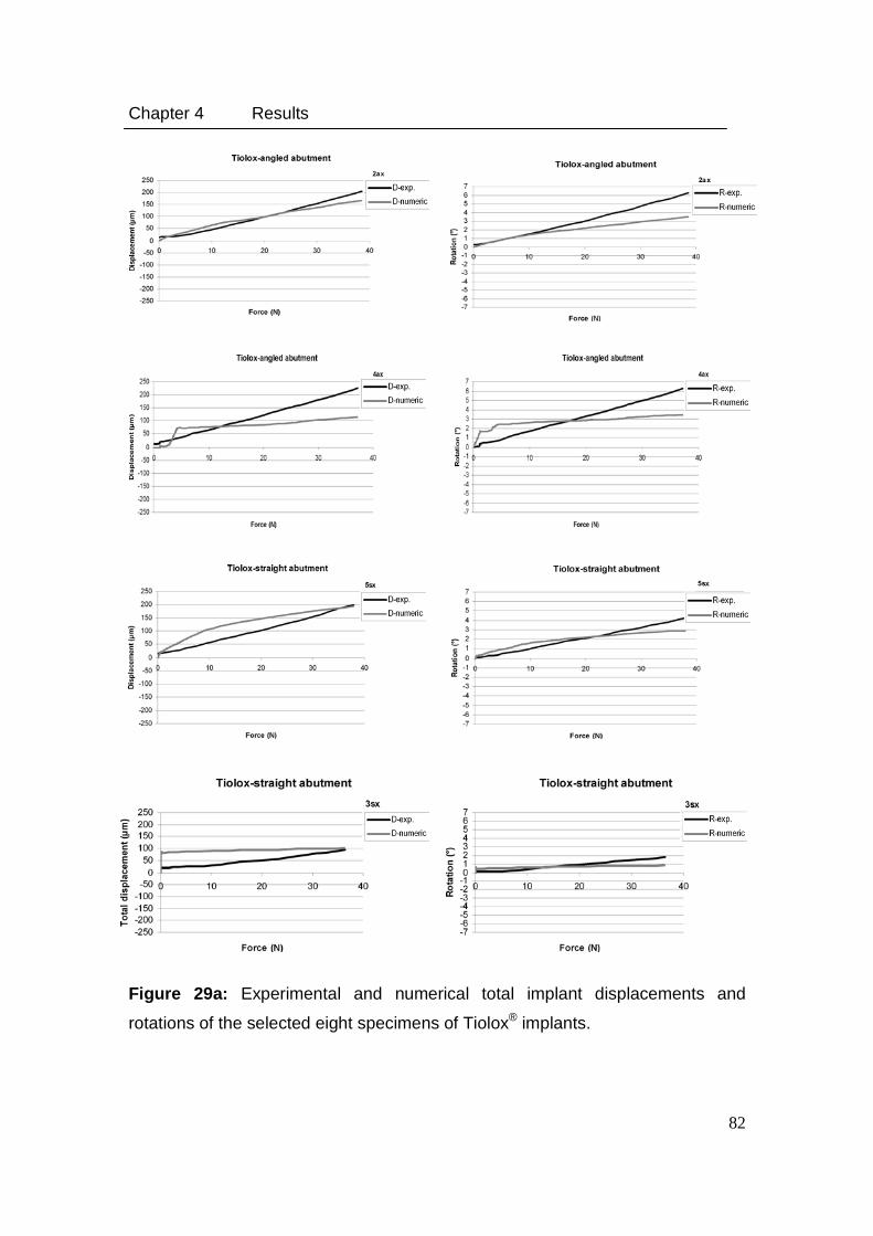
Chapter 4 Results
82
Figure 29a: Experimental and numerical total implant displacements and
rotations of the selected eight specimens of Tiolox® implants.

Chapter 4 Results
83
Figure 29b: Experimental and numerical total implant displacements and
rotations of the selected eight specimens of tioLgic© implants.
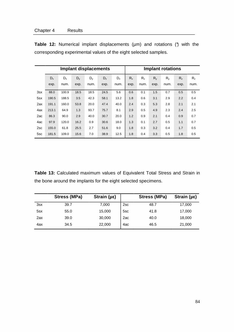
Chapter 4 Results
84
Table 12: Numerical implant displacements (µm) and rotations (°) with the
corresponding experimental values of the eight selected samples.
Implant displacements Implant rotations
Dx
exp.
Dx
num.
Dy
exp.
Dy
num.
Dz
exp.
Dz
num.
Rx
exp.
Rx
num.
Ry
exp.
Ry
num.
Rz
exp.
Rz
num.
3sx 88.0 100.9 18.5 18.5 24.5 5.6 0.6 0.1 1.5 0.7 0.5 0.5
5sx 190.5 188.5 3.5 42.3 58.1 13.2 1.8 0.6 3.1 2.9 2.2 0.4
2ax 191.1 160.0 53.8 20.0 47.4 40.0 2.4 0.3 5.3 2.8 2.1 2.1
4ax 213.1 64.9 1.3 93.7 75.7 8.1 2.9 0.5 4.9 2.3 2.4 2.5
2ac 86.3 90.0 2.9 40.0 30.7 20.0 1.2 0.9 2.1 0.4 0.9 0.7
4ac 97.9 120.0 16.2 0.9 30.6 18.0 1.3 0.1 2.7 0.5 1.1 0.7
2sc 155.0 61.8 25.5 2.7 51.6 9.0 1.8 0.3 3.2 0.4 1.7 0.5
5sc 181.5 109.0 15.6 7.0 38.9 12.5 1.8 0.4 3.3 0.5 1.8 0.5
Table 13: Calculated maximum values of Equivalent Total Stress and Strain in
the bone around the implants for the eight selected specimens.
Stress (MPa) Strain (µ ε) Stress (MPa) Strain (µ ε)
3sx 39.7 7,000 2sc 48.7 17,000
5sx 55.0 15,000 5sc 41.8 17,000
2ax 39.0 30,000 2ac 40.0 18,000
4ax 34.5 22,000 4ac 46.5 21,000
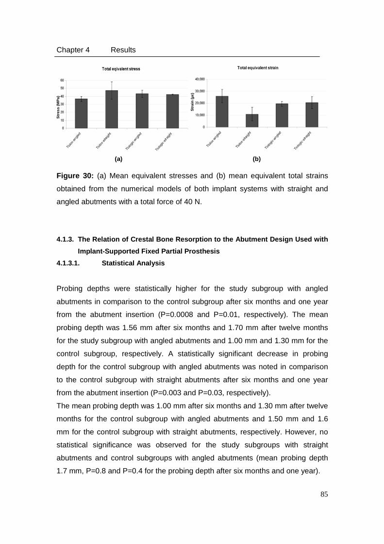
Chapter 4 Results
85
Figure 30: (a) Mean equivalent stresses and (b) mean equivalent total strains
obtained from the numerical models of both implant systems with straight and
angled abutments with a total force of 40 N.
4.1.3. The Relation of Crestal Bone Resorption to the Abutment Design Used with
Implant-Supported Fixed Partial Prosthesis
4.1.3.1. Statistical Analysis
Probing depths were statistically higher for the study subgroup with angled
abutments in comparison to the control subgroup after six months and one year
from the abutment insertion (P=0.0008 and P=0.01, respectively). The mean
probing depth was 1.56 mm after six months and 1.70 mm after twelve months
for the study subgroup with angled abutments and 1.00 mm and 1.30 mm for the
control subgroup, respectively. A statistically significant decrease in probing
depth for the control subgroup with angled abutments was noted in comparison
to the control subgroup with straight abutments after six months and one year
from the abutment insertion (P=0.003 and P=0.03, respectively).
The mean probing depth was 1.00 mm after six months and 1.30 mm after twelve
months for the control subgroup with angled abutments and 1.50 mm and 1.6
mm for the control subgroup with straight abutments, respectively. However, no
statistical significance was observed for the study subgroups with straight
abutments and control subgroups with angled abutments (mean probing depth
1.7 mm, P=0.8 and P=0.4 for the probing depth after six months and one year).
(a)
(b)
Str
ain
(µε)
Str
ess
(MP
a)
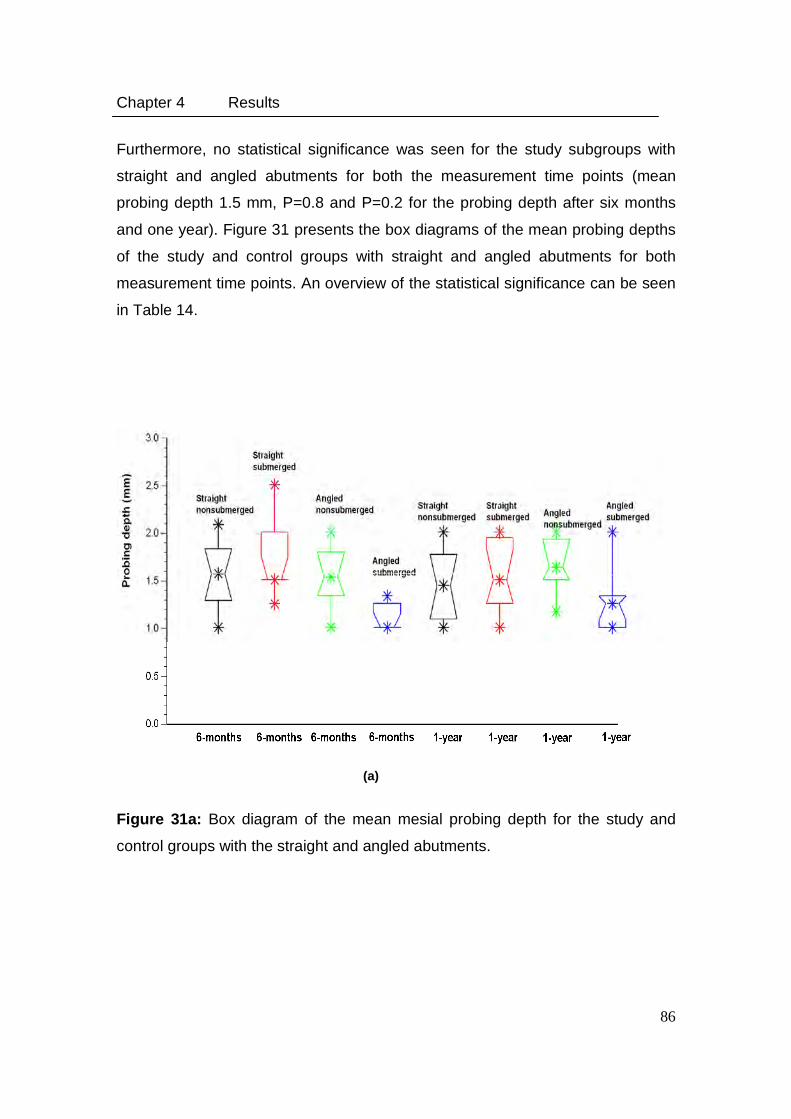
Chapter 4 Results
86
Furthermore, no statistical significance was seen for the study subgroups with
straight and angled abutments for both the measurement time points (mean
probing depth 1.5 mm, P=0.8 and P=0.2 for the probing depth after six months
and one year). Figure 31 presents the box diagrams of the mean probing depths
of the study and control groups with straight and angled abutments for both
measurement time points. An overview of the statistical significance can be seen
in Table 14.
Figure 31a: Box diagram of the mean mesial probing depth for the study and
control groups with the straight and angled abutments.
(a)
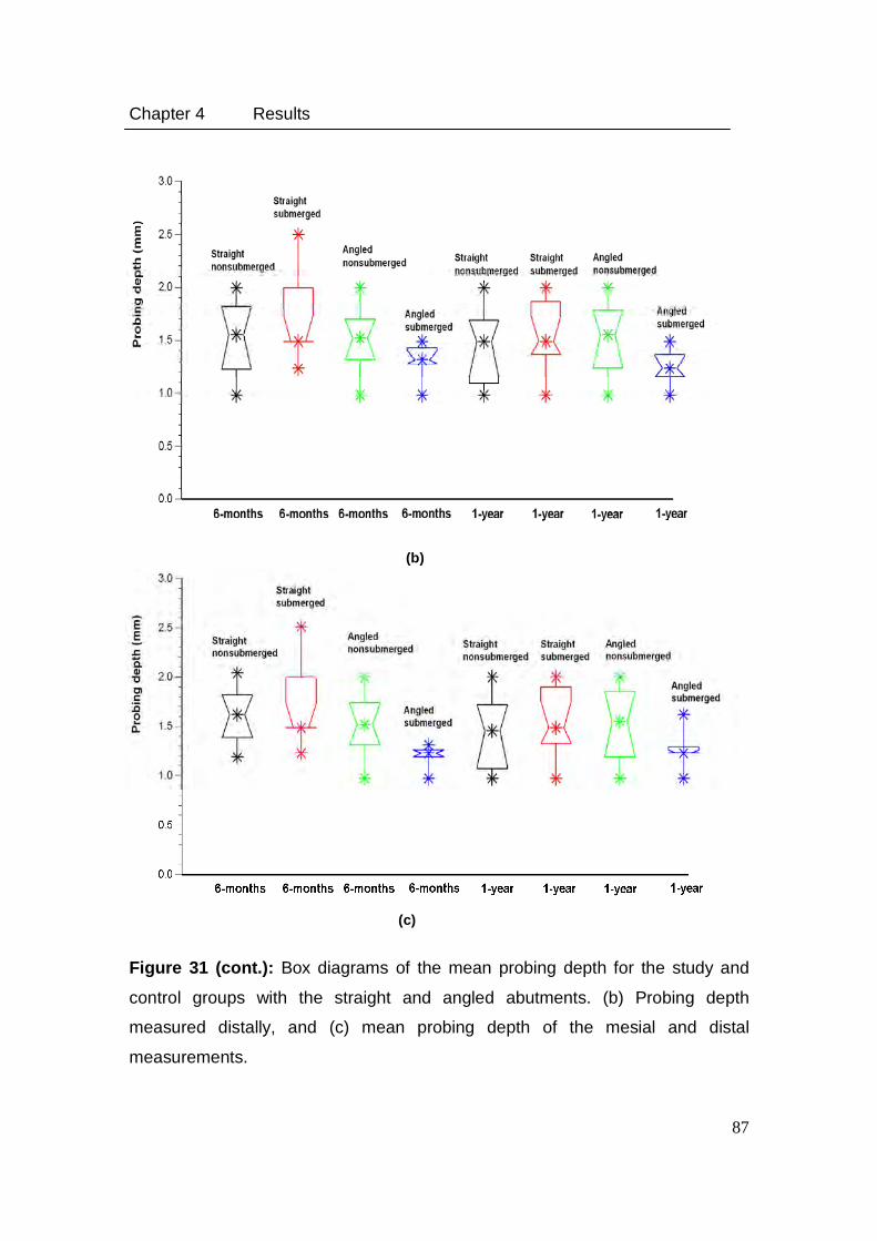
Chapter 4 Results
87
Figure 31 (cont.): Box diagrams of the mean probing depth for the study and
control groups with the straight and angled abutments. (b) Probing depth
measured distally, and (c) mean probing depth of the mesial and distal
measurements.
(b)
(c)

Table 14: Probing depth significance level of the difference between the two abutment designs in nonsubmerged (study
group) and submerged (control group) implant treatments at the 6th and 12th evaluation (Mann-Whitney test). The meaning
of the signs below is as follows: (�) for P > 0.05 (not significant), (+) for 0.01 < P ≤ 0.05, and (++) for P ≤ 0.01.
6-month 1-year
Study group Control group Study group Control group
Straight (N=36) Angled (N=28) Straight (N=20) Angled (N=19) Straight (N=36) Angled (N=28) Straight (N=24) Angled (N=22)
Straight
(N=36) � Straight
(N=36) �
Stu
dy g
roup
Angled
(N=28) � ++
Stu
dy g
roup
Angled
(N=28) � +
Straight
(N=20) Straight
(N=24)
Con
trol
gro
up
Angled
(N=19) ++
Con
trol
gro
up
Angled
(N=22) +
Chapter 4 R
esults
88
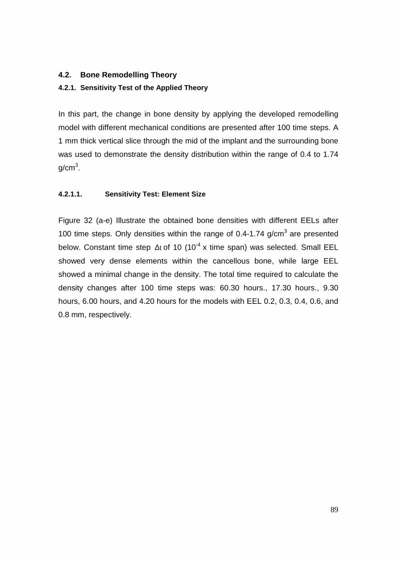
89
4.2. Bone Remodelling Theory
4.2.1. Sensitivity Test of the Applied Theory
In this part, the change in bone density by applying the developed remodelling
model with different mechanical conditions are presented after 100 time steps. A
1 mm thick vertical slice through the mid of the implant and the surrounding bone
was used to demonstrate the density distribution within the range of 0.4 to 1.74
g/cm3.
4.2.1.1. Sensitivity Test: Element Size
Figure 32 (a-e) Illustrate the obtained bone densities with different EELs after
100 time steps. Only densities within the range of 0.4-1.74 g/cm3 are presented
below. Constant time step t∆ of 10 (10-4 x time span) was selected. Small EEL
showed very dense elements within the cancellous bone, while large EEL
showed a minimal change in the density. The total time required to calculate the
density changes after 100 time steps was: 60.30 hours., 17.30 hours., 9.30
hours, 6.00 hours, and 4.20 hours for the models with EEL 0.2, 0.3, 0.4, 0.6, and
0.8 mm, respectively.
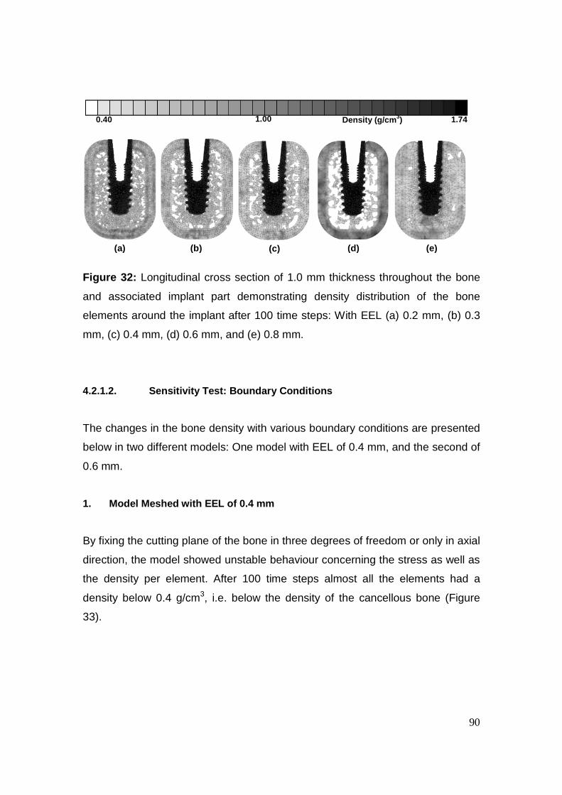
90
Figure 32: Longitudinal cross section of 1.0 mm thickness throughout the bone
and associated implant part demonstrating density distribution of the bone
elements around the implant after 100 time steps: With EEL (a) 0.2 mm, (b) 0.3
mm, (c) 0.4 mm, (d) 0.6 mm, and (e) 0.8 mm.
4.2.1.2. Sensitivity Test: Boundary Conditions
The changes in the bone density with various boundary conditions are presented
below in two different models: One model with EEL of 0.4 mm, and the second of
0.6 mm.
1. Model Meshed with EEL of 0.4 mm
By fixing the cutting plane of the bone in three degrees of freedom or only in axial
direction, the model showed unstable behaviour concerning the stress as well as
the density per element. After 100 time steps almost all the elements had a
density below 0.4 g/cm3, i.e. below the density of the cancellous bone (Figure
33).
0.40 1.00 1.74 Density (g/cm 3)
(a) (b) (c) (d) (e)
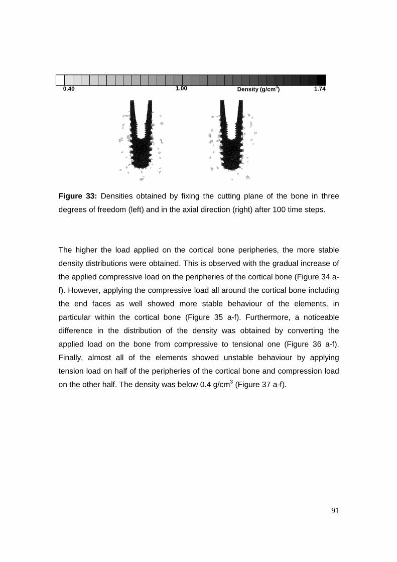
91
Figure 33: Densities obtained by fixing the cutting plane of the bone in three
degrees of freedom (left) and in the axial direction (right) after 100 time steps.
The higher the load applied on the cortical bone peripheries, the more stable
density distributions were obtained. This is observed with the gradual increase of
the applied compressive load on the peripheries of the cortical bone (Figure 34 a-
f). However, applying the compressive load all around the cortical bone including
the end faces as well showed more stable behaviour of the elements, in
particular within the cortical bone (Figure 35 a-f). Furthermore, a noticeable
difference in the distribution of the density was obtained by converting the
applied load on the bone from compressive to tensional one (Figure 36 a-f).
Finally, almost all of the elements showed unstable behaviour by applying
tension load on half of the peripheries of the cortical bone and compression load
on the other half. The density was below 0.4 g/cm3 (Figure 37 a-f).
0.40 1.00 1.74 Density (g/cm 3)
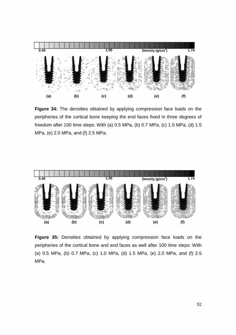
92
Figure 34: The densities obtained by applying compression face loads on the
peripheries of the cortical bone keeping the end faces fixed in three degrees of
freedom after 100 time steps: With (a) 0.5 MPa, (b) 0.7 MPa, (c) 1.0 MPa, (d) 1.5
MPa, (e) 2.0 MPa, and (f) 2.5 MPa.
Figure 35: Densities obtained by applying compression face loads on the
peripheries of the cortical bone and end faces as well after 100 time steps: With
(a) 0.5 MPa, (b) 0.7 MPa, (c) 1.0 MPa, (d) 1.5 MPa, (e) 2.0 MPa, and (f) 2.5
MPa.
0.40 1.00 1.74 Density (g/cm 3)
(a) (b) (c) (d) (e) (f)
(a) (b) (c) (d) (e) (f)
0.40 1.00 1.74 Density (g/cm 3)
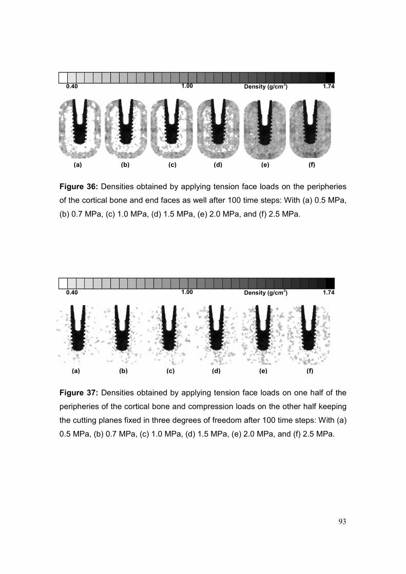
93
Figure 36: Densities obtained by applying tension face loads on the peripheries
of the cortical bone and end faces as well after 100 time steps: With (a) 0.5 MPa,
(b) 0.7 MPa, (c) 1.0 MPa, (d) 1.5 MPa, (e) 2.0 MPa, and (f) 2.5 MPa.
Figure 37: Densities obtained by applying tension face loads on one half of the
peripheries of the cortical bone and compression loads on the other half keeping
the cutting planes fixed in three degrees of freedom after 100 time steps: With (a)
0.5 MPa, (b) 0.7 MPa, (c) 1.0 MPa, (d) 1.5 MPa, (e) 2.0 MPa, and (f) 2.5 MPa.
0.40 1.00 1.74 Density (g/cm3)
(a) (b) (c) (d) (e) (f)
(a) (b) (c) (d) (e) (f)
0.40 1.00 1.74 Density (g/cm3)
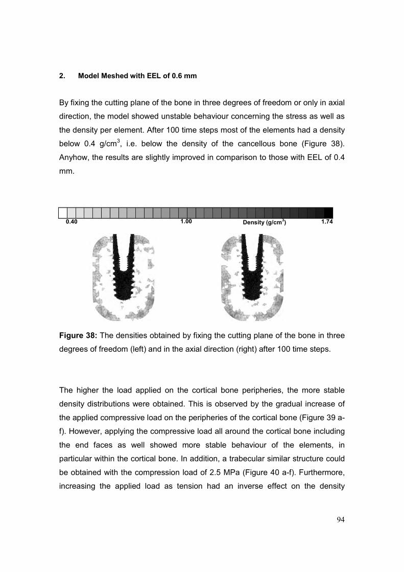
94
2. Model Meshed with EEL of 0.6 mm
By fixing the cutting plane of the bone in three degrees of freedom or only in axial
direction, the model showed unstable behaviour concerning the stress as well as
the density per element. After 100 time steps most of the elements had a density
below 0.4 g/cm3, i.e. below the density of the cancellous bone (Figure 38).
Anyhow, the results are slightly improved in comparison to those with EEL of 0.4
mm.
Figure 38: The densities obtained by fixing the cutting plane of the bone in three
degrees of freedom (left) and in the axial direction (right) after 100 time steps.
The higher the load applied on the cortical bone peripheries, the more stable
density distributions were obtained. This is observed by the gradual increase of
the applied compressive load on the peripheries of the cortical bone (Figure 39 a-
f). However, applying the compressive load all around the cortical bone including
the end faces as well showed more stable behaviour of the elements, in
particular within the cortical bone. In addition, a trabecular similar structure could
be obtained with the compression load of 2.5 MPa (Figure 40 a-f). Furthermore,
increasing the applied load as tension had an inverse effect on the density
0.40 1.00 1.74 Density (g/cm3)
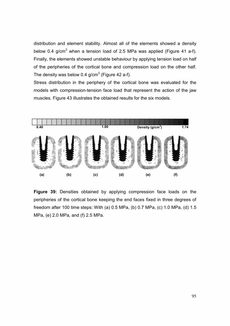
95
distribution and element stability. Almost all of the elements showed a density
below 0.4 g/cm3 when a tension load of 2.5 MPa was applied (Figure 41 a-f).
Finally, the elements showed unstable behaviour by applying tension load on half
of the peripheries of the cortical bone and compression load on the other half.
The density was below 0.4 g/cm3 (Figure 42 a-f).
Stress distribution in the periphery of the cortical bone was evaluated for the
models with compression-tension face load that represent the action of the jaw
muscles. Figure 43 illustrates the obtained results for the six models.
Figure 39: Densities obtained by applying compression face loads on the
peripheries of the cortical bone keeping the end faces fixed in three degrees of
freedom after 100 time steps: With (a) 0.5 MPa, (b) 0.7 MPa, (c) 1.0 MPa, (d) 1.5
MPa, (e) 2.0 MPa, and (f) 2.5 MPa.
(a) (b) (c) (d) (e) (f)
0.40 1.00 1.74 Density (g/cm3)
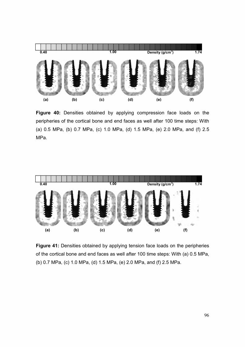
96
Figure 40: Densities obtained by applying compression face loads on the
peripheries of the cortical bone and end faces as well after 100 time steps: With
(a) 0.5 MPa, (b) 0.7 MPa, (c) 1.0 MPa, (d) 1.5 MPa, (e) 2.0 MPa, and (f) 2.5
MPa.
Figure 41: Densities obtained by applying tension face loads on the peripheries
of the cortical bone and end faces as well after 100 time steps: With (a) 0.5 MPa,
(b) 0.7 MPa, (c) 1.0 MPa, (d) 1.5 MPa, (e) 2.0 MPa, and (f) 2.5 MPa.
0.40 1.00 1.74 Density (g/cm3)
(a) (b) (c) (d) (e) (f)
(a) (b) (c) (d) (e) (f)
0.40 1.00 1.74 Density (g/cm3)
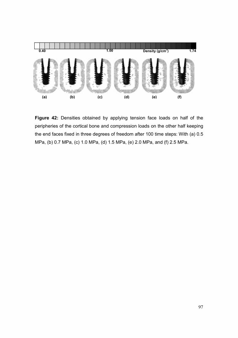
97
Figure 42: Densities obtained by applying tension face loads on half of the
peripheries of the cortical bone and compression loads on the other half keeping
the end faces fixed in three degrees of freedom after 100 time steps: With (a) 0.5
MPa, (b) 0.7 MPa, (c) 1.0 MPa, (d) 1.5 MPa, (e) 2.0 MPa, and (f) 2.5 MPa.
0.40 1.00 1.74 Density (g/cm3)
(a) (b) (c) (d) (e) (f)
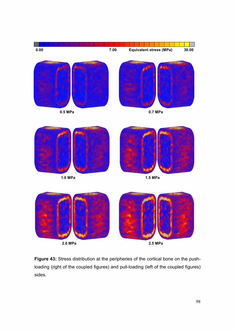
98
Figure 43: Stress distribution at the peripheries of the cortical bone on the push-
loading (right of the coupled figures) and pull-loading (left of the coupled figures)
sides.
0.00 7.00 30.00 Equivalent stress (MPa)
0.5 MPa 0.7 MPa
1.0 MPa 1.5 MPa
2.0 MPa 2.5 MPa

99
In an attempt to reach the real situation of bone loading by the mastication
muscles and achieve the suggested magnitude of the stress in the mandibular
posterior region (Koseki et al., 2005), two models were developed. In the first, the
peripheries of the cortical bone were subjected to a tension load of 2.5 MPa on
one half and compression load of 1.5 MPa on the other half and the implant was
loaded by vertical force of 100 N. The obtained equivalent stress was around 13
MPa on the tension side and around 6.0 MPa on the compression side.
In the second model, the peripheries of the cortical bone were subjected to a
tension load of 4.0 MPa on one half and compression load of 3.0 MPa on the
other half and the implant was loaded by vertical force of 300 N. The obtained
equivalent stress was around 15 MPa on the tension side and around 8.0 MPa
on the compression side. Figure 44 illustrates the obtained density and stress
distributions after 100 time steps.
Figure 44a: Density distribution in 1 mm thick axial section after 100 time steps.
0.40 1.00 1.74 Density (g/cm3)
Tension 2.5 MPa, compression 1.5 MPa, 100 N vertical force. Density distribution of the whole model (left), and in 1 mm vertical slice through the midline (right).
Tension 4.0 MPa, compression 3.0 MPa, 300 N vertical force. Density distribution of the whole model (left), and in 1 mm vertical slice through the midline (right).
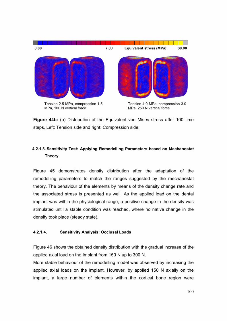
100
Figure 44b: (b) Distribution of the Equivalent von Mises stress after 100 time
steps. Left: Tension side and right: Compression side.
4.2.1.3. Sensitivity Test: Applying Remodelling Parameters based on Mechanostat
Theory
Figure 45 demonstrates density distribution after the adaptation of the
remodelling parameters to match the ranges suggested by the mechanostat
theory. The behaviour of the elements by means of the density change rate and
the associated stress is presented as well. As the applied load on the dental
implant was within the physiological range, a positive change in the density was
stimulated until a stable condition was reached, where no native change in the
density took place (steady state).
4.2.1.4. Sensitivity Analysis: Occlusal Loads
Figure 46 shows the obtained density distribution with the gradual increase of the
applied axial load on the Implant from 150 N up to 300 N.
More stable behaviour of the remodelling model was observed by increasing the
applied axial loads on the implant. However, by applied 150 N axially on the
implant, a large number of elements within the cortical bone region were
0.00 7.00 30.00 Equivalent stress (MPa)
Tension 2.5 MPa, compression 1.5 MPa, 100 N vertical force
Tension 4.0 MPa, compression 3.0 MPa, 250 N vertical force
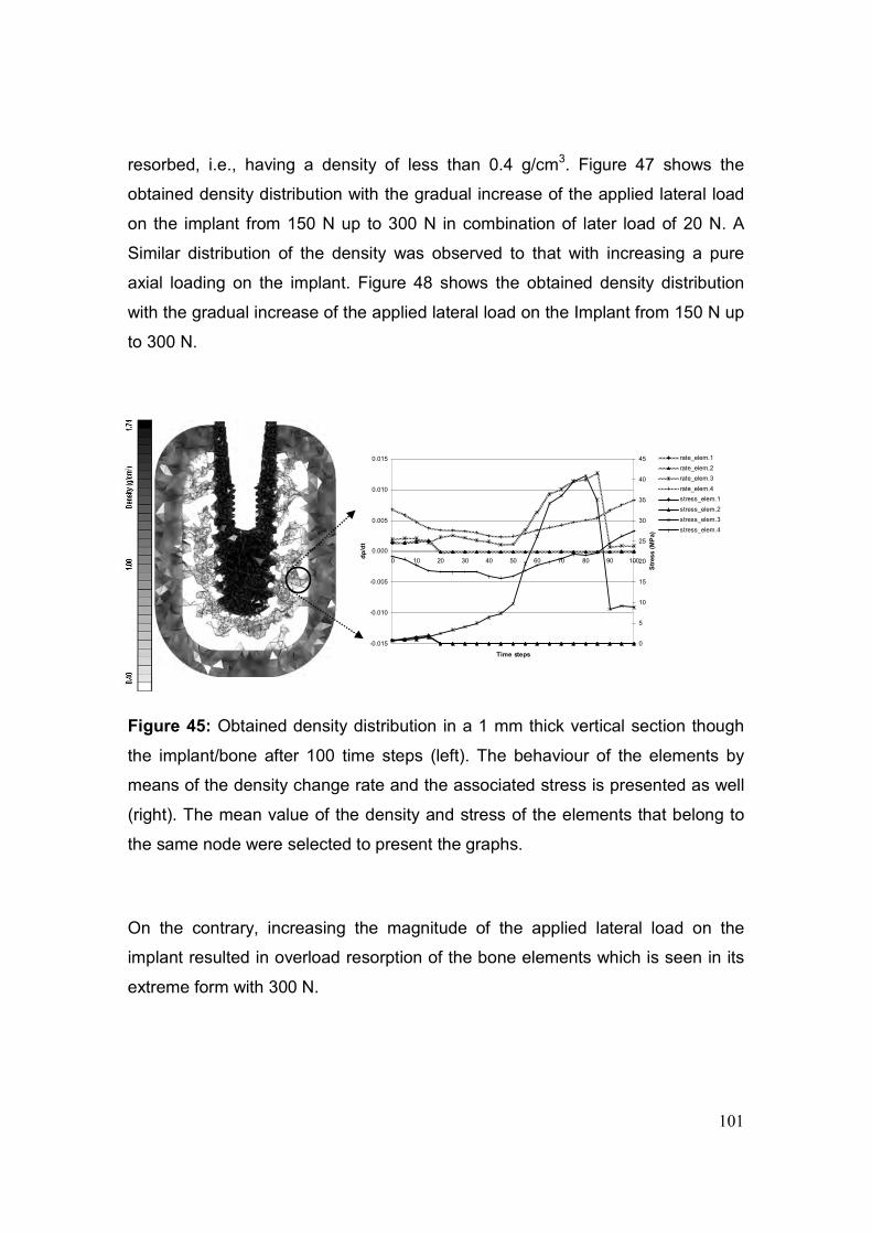
101
-0.015
-0.010
-0.005
0.000
0.005
0.010
0.015
0 10 20 30 40 50 60 70 80 90 100
Time steps
dρ
/dt
0
5
10
15
20
25
30
35
40
45
Str
ess (
MP
a)
rate_elem.1
rate_elem.2
rate_elem.3
rate_elem.4
stress_elem.1
stress_elem.2
stress_elem.3
stress_elem.4
resorbed, i.e., having a density of less than 0.4 g/cm3. Figure 47 shows the
obtained density distribution with the gradual increase of the applied lateral load
on the implant from 150 N up to 300 N in combination of later load of 20 N. A
Similar distribution of the density was observed to that with increasing a pure
axial loading on the implant. Figure 48 shows the obtained density distribution
with the gradual increase of the applied lateral load on the Implant from 150 N up
to 300 N.
Figure 45: Obtained density distribution in a 1 mm thick vertical section though
the implant/bone after 100 time steps (left). The behaviour of the elements by
means of the density change rate and the associated stress is presented as well
(right). The mean value of the density and stress of the elements that belong to
the same node were selected to present the graphs.
On the contrary, increasing the magnitude of the applied lateral load on the
implant resulted in overload resorption of the bone elements which is seen in its
extreme form with 300 N.
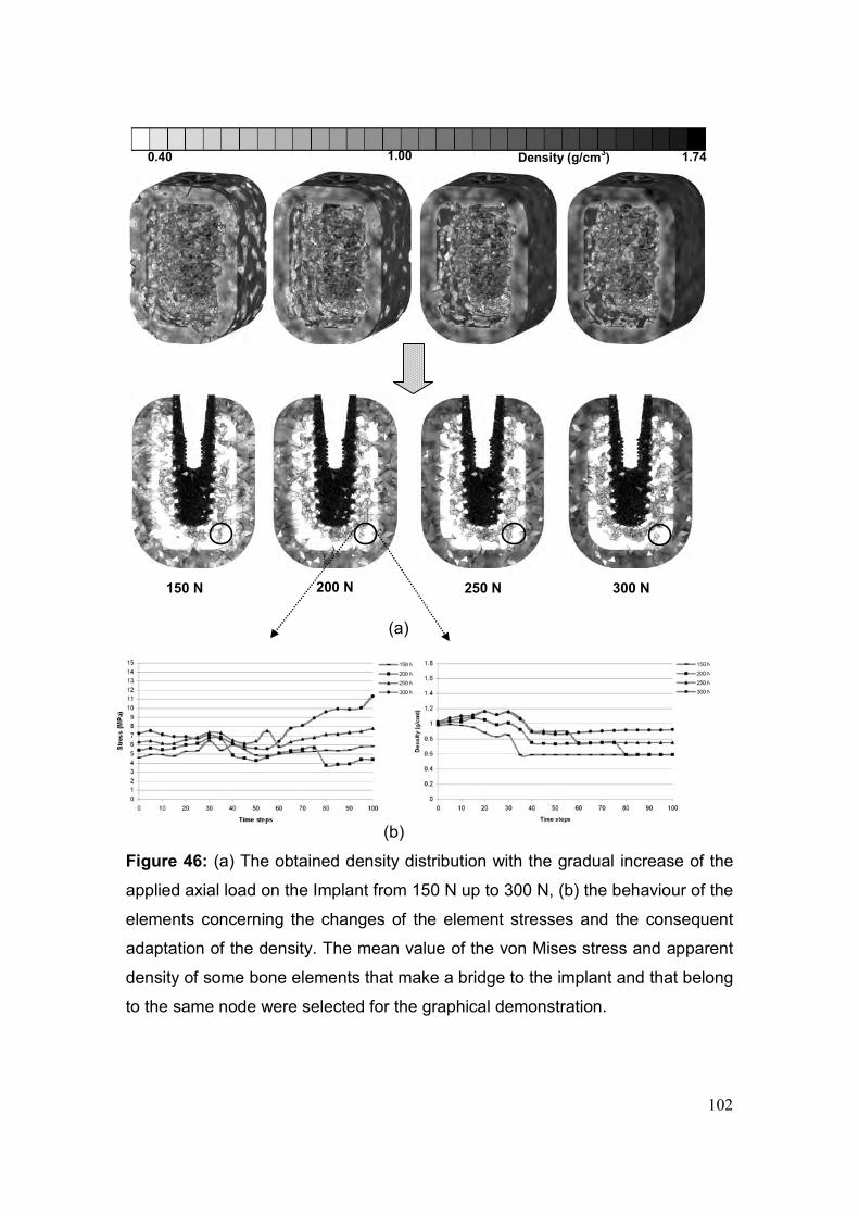
102
(a)
(b)
Figure 46: (a) The obtained density distribution with the gradual increase of the
applied axial load on the Implant from 150 N up to 300 N, (b) the behaviour of the
elements concerning the changes of the element stresses and the consequent
adaptation of the density. The mean value of the von Mises stress and apparent
density of some bone elements that make a bridge to the implant and that belong
to the same node were selected for the graphical demonstration.
150 N 300 N 200 N 250 N
0.40 1.00 1.74 Density (g/cm3)
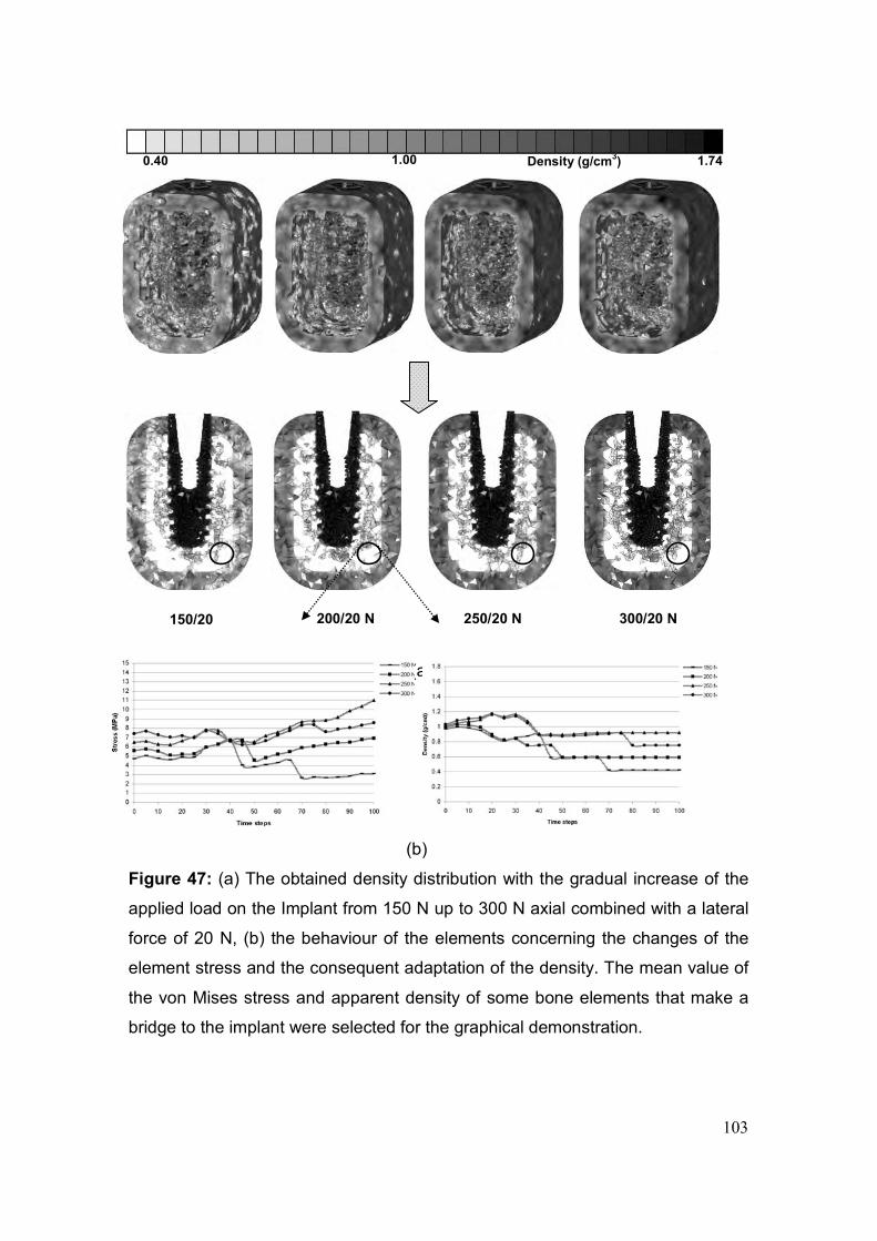
103
(a)
(b)
Figure 47: (a) The obtained density distribution with the gradual increase of the
applied load on the Implant from 150 N up to 300 N axial combined with a lateral
force of 20 N, (b) the behaviour of the elements concerning the changes of the
element stress and the consequent adaptation of the density. The mean value of
the von Mises stress and apparent density of some bone elements that make a
bridge to the implant were selected for the graphical demonstration.
0.40 1.00 1.74 Density (g/cm3)
150/20 300/20 N 200/20 N 250/20 N
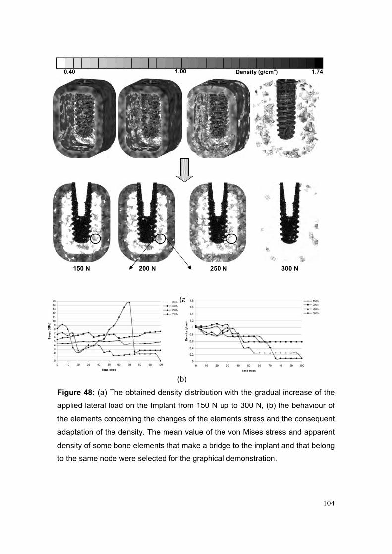
104
(a)
(b)
Figure 48: (a) The obtained density distribution with the gradual increase of the
applied lateral load on the Implant from 150 N up to 300 N, (b) the behaviour of
the elements concerning the changes of the elements stress and the consequent
adaptation of the density. The mean value of the von Mises stress and apparent
density of some bone elements that make a bridge to the implant and that belong
to the same node were selected for the graphical demonstration.
0.40 1.00 1.74 Density (g/cm3)
150 N 300 N 200 N 250 N
105
Figure 49 shows the obtained density distribution by applying an axial load of 300
N and a lateral load of 20 N on the implant combined with tension face load of
4.0 MPa on one half of the periphery of the cortical bone and compression face
load of 3.0 MPa on the other half, keeping the end faces constrained in three
degrees of freedom. The obtained density distribution is compared with the real
trabecular distribution in an undecalcified thin ground section of the lower jaw at
the molar region (20 µm) of a baboon with a grit-blasted and acid-etched screw
after 18 months of occlusal loading (Watzak et al., 2005), and a photograph of a
2 mm thick bone section from mental foramen region of edentulous mandible of a
human cadaver (Kingsmill and Boyde, 1998). The obtained distribution of the
elements after applying the remodelling model showed a similarity to the
histological slices, in particular at the tips of the implant threads, where the
highest strains are concentrated.
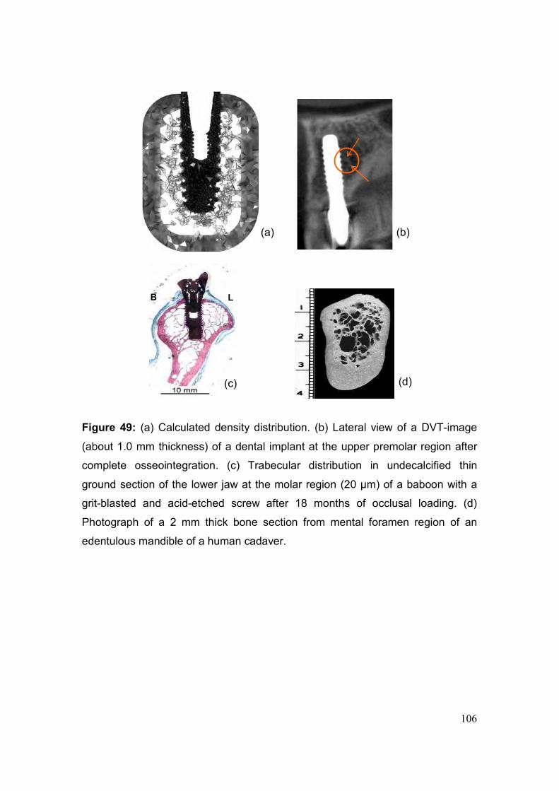
106
Figure 49: (a) Calculated density distribution. (b) Lateral view of a DVT-image
(about 1.0 mm thickness) of a dental implant at the upper premolar region after
complete osseointegration. (c) Trabecular distribution in undecalcified thin
ground section of the lower jaw at the molar region (20 µm) of a baboon with a
grit-blasted and acid-etched screw after 18 months of occlusal loading. (d)
Photograph of a 2 mm thick bone section from mental foramen region of an
edentulous mandible of a human cadaver.
(a) (b)
B L
(c) (d)
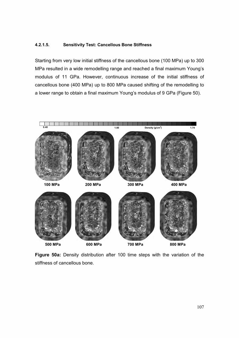
107
4.2.1.5. Sensitivity Test: Cancellous Bone Stiffness
Starting from very low initial stiffness of the cancellous bone (100 MPa) up to 300
MPa resulted in a wide remodelling range and reached a final maximum Young’s
modulus of 11 GPa. However, continuous increase of the initial stiffness of
cancellous bone (400 MPa) up to 800 MPa caused shifting of the remodelling to
a lower range to obtain a final maximum Young’s modulus of 9 GPa (Figure 50).
Figure 50a: Density distribution after 100 time steps with the variation of the
stiffness of cancellous bone.
0.40 1.00 1.74 Density (g/cm3)
500 MPa 800 MPa 600 MPa 700 MPa
100 MPa 400 MPa 200 MPa 300 MPa
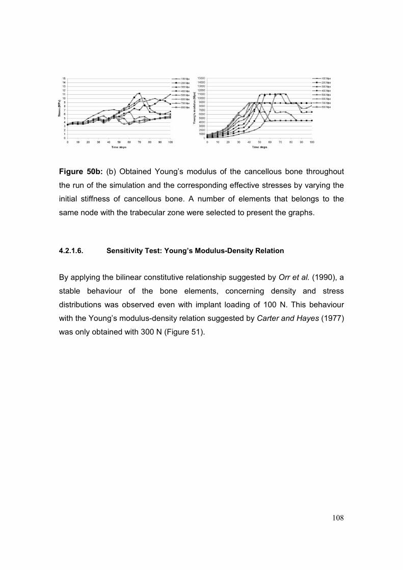
108
Figure 50b: (b) Obtained Young’s modulus of the cancellous bone throughout
the run of the simulation and the corresponding effective stresses by varying the
initial stiffness of cancellous bone. A number of elements that belongs to the
same node with the trabecular zone were selected to present the graphs.
4.2.1.6. Sensitivity Test: Young’s Modulus-Density Relation
By applying the bilinear constitutive relationship suggested by Orr et al. (1990), a
stable behaviour of the bone elements, concerning density and stress
distributions was observed even with implant loading of 100 N. This behaviour
with the Young’s modulus-density relation suggested by Carter and Hayes (1977)
was only obtained with 300 N (Figure 51).
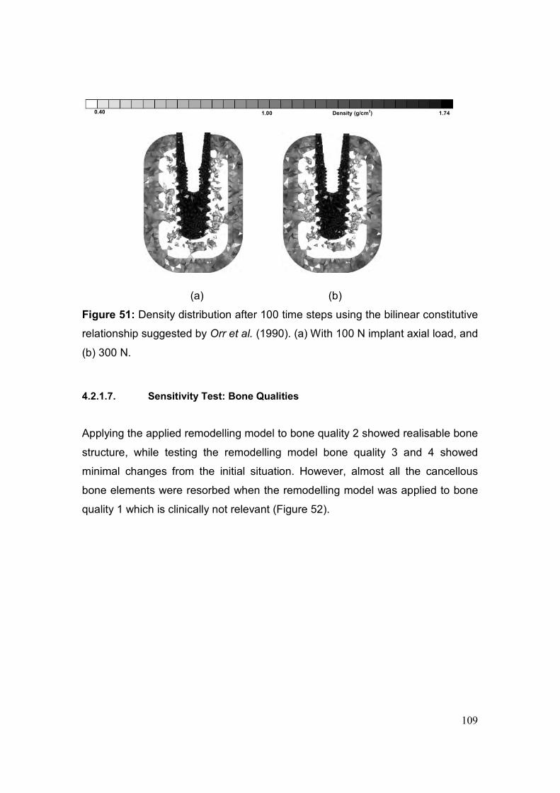
109
(a) (b)
Figure 51: Density distribution after 100 time steps using the bilinear constitutive
relationship suggested by Orr et al. (1990). (a) With 100 N implant axial load, and
(b) 300 N.
4.2.1.7. Sensitivity Test: Bone Qualities
Applying the applied remodelling model to bone quality 2 showed realisable bone
structure, while testing the remodelling model bone quality 3 and 4 showed
minimal changes from the initial situation. However, almost all the cancellous
bone elements were resorbed when the remodelling model was applied to bone
quality 1 which is clinically not relevant (Figure 52).
0.40 1.00 1.74 Density (g/cm3)
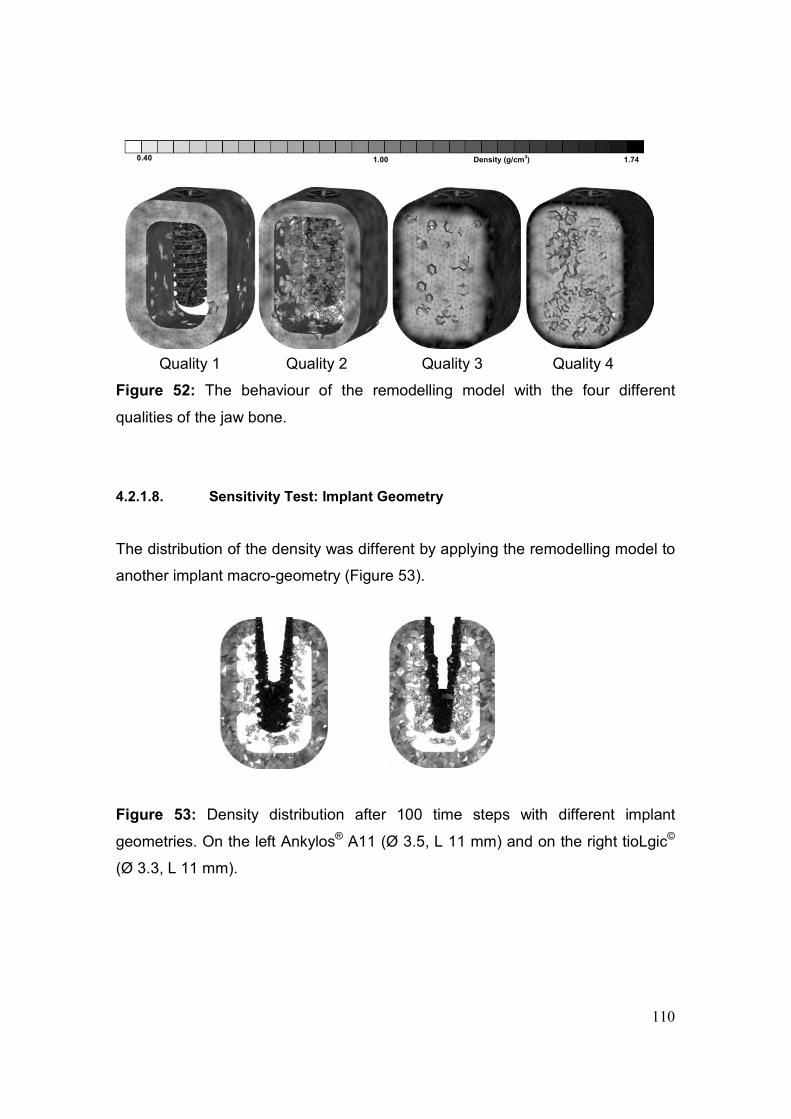
110
Quality 1 Quality 2 Quality 3 Quality 4
Figure 52: The behaviour of the remodelling model with the four different
qualities of the jaw bone.
4.2.1.8. Sensitivity Test: Implant Geometry
The distribution of the density was different by applying the remodelling model to
another implant macro-geometry (Figure 53).
Figure 53: Density distribution after 100 time steps with different implant
geometries. On the left Ankylos® A11 (Ø 3.5, L 11 mm) and on the right tioLgic©
(Ø 3.3, L 11 mm).
0.40 1.00 1.74 Density (g/cm3)
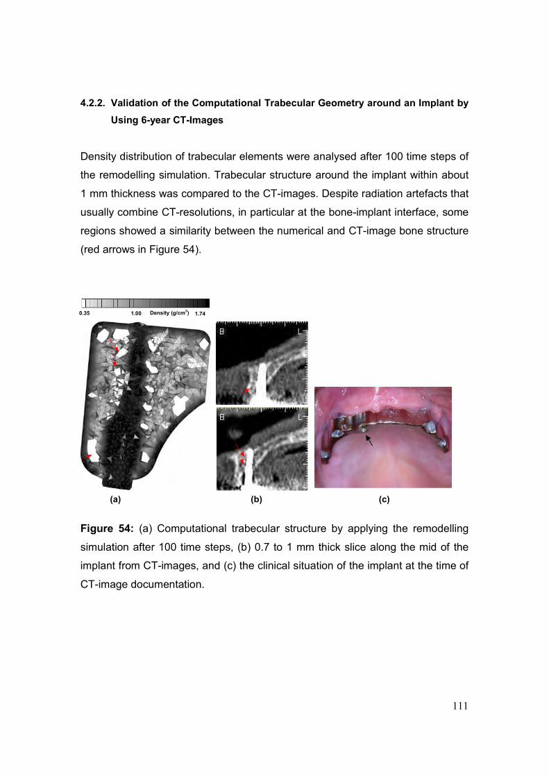
111
4.2.2. Validation of the Computational Trabecular Geometry around an Implant by
Using 6-year CT-Images
Density distribution of trabecular elements were analysed after 100 time steps of
the remodelling simulation. Trabecular structure around the implant within about
1 mm thickness was compared to the CT-images. Despite radiation artefacts that
usually combine CT-resolutions, in particular at the bone-implant interface, some
regions showed a similarity between the numerical and CT-image bone structure
(red arrows in Figure 54).
Figure 54: (a) Computational trabecular structure by applying the remodelling
simulation after 100 time steps, (b) 0.7 to 1 mm thick slice along the mid of the
implant from CT-images, and (c) the clinical situation of the implant at the time of
CT-image documentation.
(c) (b) (a)
0.35 1.00 1.74 Density (g/cm3)
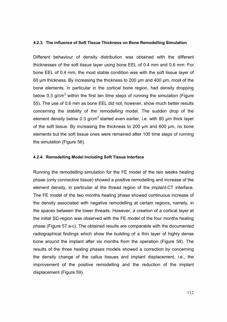
112
4.2.3. The influence of Soft Tissue Thickness on Bone Remodelling Simulation
Different behaviour of density distribution was obtained with the different
thicknesses of the soft tissue layer using bone EEL of 0.4 mm and 0.6 mm: For
bone EEL of 0.4 mm, the most stable condition was with the soft tissue layer of
60 µm thickness. By increasing the thickness to 200 µm and 400 µm, most of the
bone elements, in particular in the cortical bone region, had density dropping
below 0.3 g/cm3 within the first ten time steps of running the simulation (Figure
55). The use of 0.6 mm as bone EEL did not, however, show much better results
concerning the stability of the remodelling model. The sudden drop of the
element density below 0.3 g/cm3 started even earlier, i.e. with 80 µm thick layer
of the soft tissue. By increasing the thickness to 200 µm and 600 µm, no bone
elements but the soft tissue ones were remained after 100 time steps of running
the simulation (Figure 56).
4.2.4. Remodelling Model Including Soft Tissue Interface
Running the remodelling simulation for the FE model of the two weeks healing
phase (only connective tissue) showed a positive remodelling and increase of the
element density, in particular at the thread region of the implant-CT interface.
The FE model of the two months healing phase showed continuous increase of
the density associated with negative remodelling at certain regions, namely, in
the spaces between the lower threads. However, a creation of a cortical layer at
the initial SC-region was observed with the FE model of the four months healing
phase (Figure 57 a-c). The obtained results are comparable with the documented
radiographical findings which show the building of a thin layer of highly dense
bone around the implant after six months from the operation (Figure 58). The
results of the three healing phases models showed a correction by concerning
the density change of the callus tissues and implant displacement, i.e., the
improvement of the positive remodelling and the reduction of the implant
displacement (Figure 59).
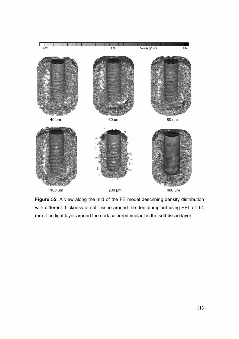
113
Figure 55: A view along the mid of the FE model describing density distribution
with different thickness of soft tissue around the dental implant using EEL of 0.4
mm. The light layer around the dark coloured implant is the soft tissue layer.
0.40 1.00 1.74 Density (g/cm3)
40 µm 60 µm 80 µm
200 µm 100 µm 400 µm
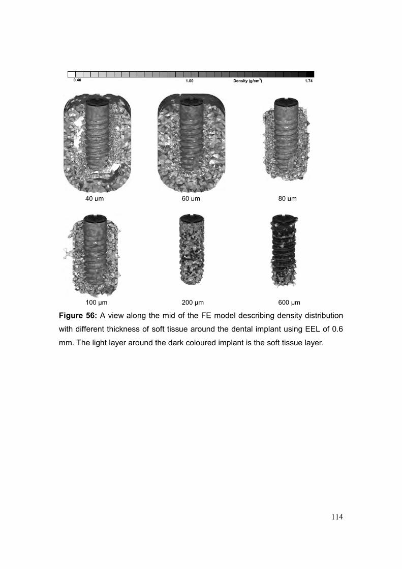
114
Figure 56: A view along the mid of the FE model describing density distribution
with different thickness of soft tissue around the dental implant using EEL of 0.6
mm. The light layer around the dark coloured implant is the soft tissue layer.
0.40 1.00 1.74 Density (g/cm3)
40 µm 60 µm 80 µm
200 µm 100 µm 600 µm
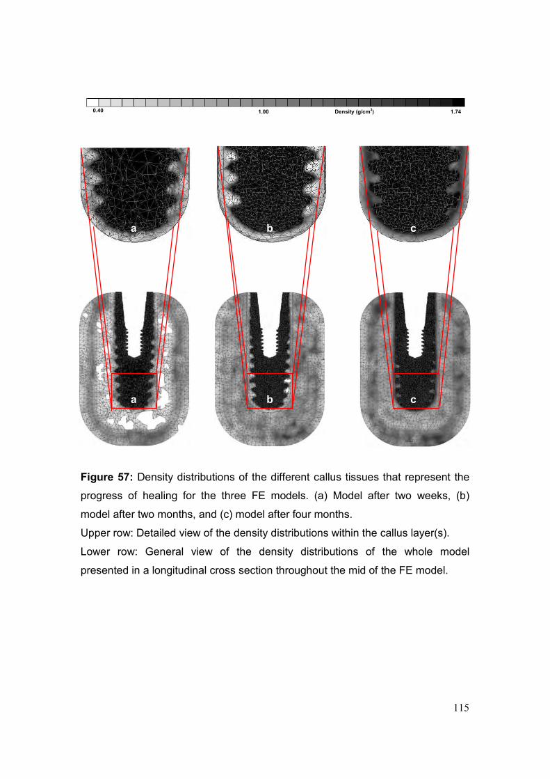
115
Figure 57: Density distributions of the different callus tissues that represent the
progress of healing for the three FE models. (a) Model after two weeks, (b)
model after two months, and (c) model after four months.
Upper row: Detailed view of the density distributions within the callus layer(s).
Lower row: General view of the density distributions of the whole model
presented in a longitudinal cross section throughout the mid of the FE model.
a b c
a b c
0.40 1.00 1.74 Density (g/cm3)
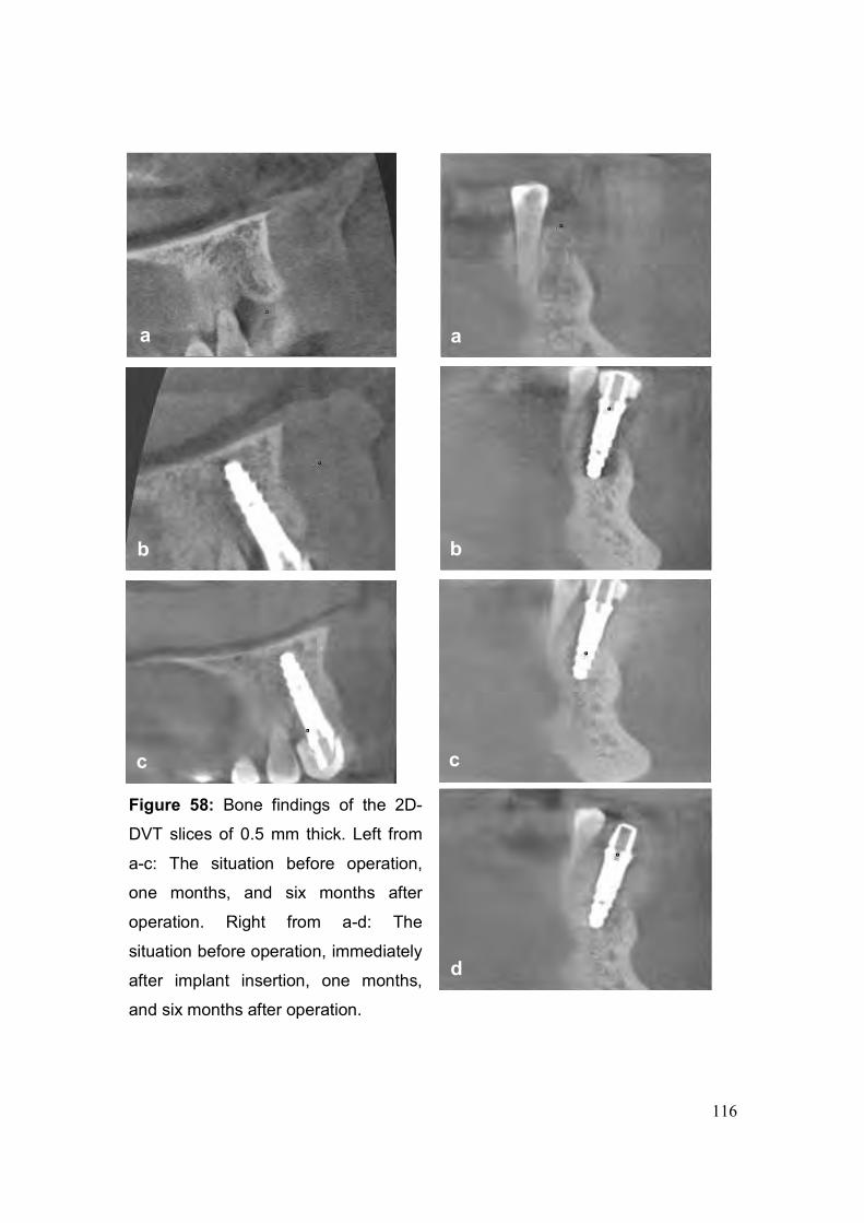
116
a a
b b
c c
d
Figure 58: Bone findings of the 2D-
DVT slices of 0.5 mm thick. Left from
a-c: The situation before operation,
one months, and six months after
operation. Right from a-d: The
situation before operation, immediately
after implant insertion, one months,
and six months after operation.
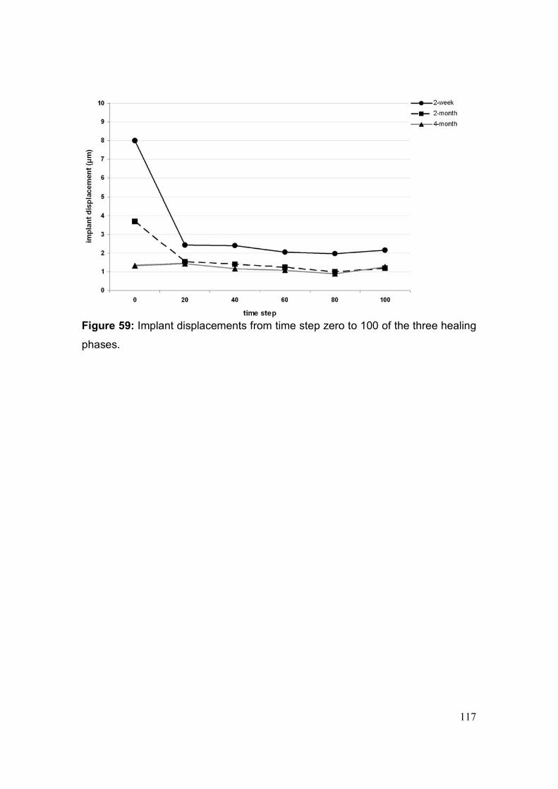
117
Figure 59: Implant displacements from time step zero to 100 of the three healing
phases.
118
Chapter 5
5. Discussion
5.1. Mechanical Investigation of Different Implant and Abutment Designs:
Experimental, Numerical and Clinical Aspects
5.1.1. Numerical Investigation of Fixed Partial Prosthesis FPP
Designing models that simulate clinical situations is essential. In this part of the
study, the bone in the anterior maxilla was carefully designed in order to
approximate the clinical situation of Kennedy Class IV edentulous ridge treated
with four-unit fixed partial prosthesis. The prosthesis was supported by two
immediately loaded endosseous implants. Clinically, restoration of all four upper
incisors with a prosthesis supported by only two endosseous implants represents
an extreme solution, when immediate loading is assumed. The study was based
on this extreme condition to investigate numerically the distribution of stresses
and strains around the supporting implants in relation to the abutment design.
To approximate the clinical situation, a distance that represents the thickness of
the residual mucosa was maintained between the lower border of the prosthesis
and the alveolar bone. Applying the load near the cingulum area in a palato-labial
direction simulates a clinical situation.The mandibular incisors close on the
palatal surfaces of the maxillary incisors, with the mandible near centric
occlusion. Applying the load in such a way helps to assess the behaviour of the
implant and the response of the bone in such a clinical condition. It may be
argued that a force of 150 N is quite low; however, Mericske-Stern et al. (1995)
found that the average value of the maximal occlusal force was distinctly lower
with implant-supported prosthesis than with the natural dentition. Accordingly, in
the present study a total force of 150 N was distributed equally on the four units
of the prosthesis at 45° to the long axis of the abutment in the palato-labial
direction defined locally for each unit of the prosthesis. Moreover, typical occlusal
forces are in the range of 100 N under normal biting, higher forces only occur in
patients suffering from bruxism or parafunction and during grinding. Usually this
is defined as a contra-indication for treatment with implant-supported FPP.
Chapter 5 Discussion
119
Several studies showed that a micro-motion of less than 30 µm at the bone-
implant interface does not interfere with the osteogenesis (Kawahara et al.,
2003), while an even wider range (50-100 µm) has also been reported as not
being determinal (Horinchi et al., 2000; Meyer et al., 2003). In the present study,
the resultant implant displacements were within the safe range without interfering
with the primary stability of the supporting implants. However, implant
displacement was 15% less with the straight abutments than with those
associated with the angled abutments.
Saab et al. (2007) studied the strain in the bone around dental implants in the
anterior maxilla in a FE investigation. They obtained a value of 4,650 µε as a
maximum principle strain with the straight abutment and 4,020 µε with the angled
abutment with a generally similar pattern of strain distribution for both models.
The presented immediately loaded models yielded a 12% higher strain in the
bone for the angled abutment compared with the straight abutment. Wider stress
and strain distributions in the bone were associated with the angled abutments.
On the other hand, osseointegrated models showed a value of 1,026 µε as a total
equivalent strain with the straight abutment and 1,313 µε with the angled
abutment and a similar distribution pattern. The strain values of the
osseointegrated models in the present study were about 70% lower than those
obtained by Saab et al. (2007) in their study of a single osseointegrated implant
with an applied force of 178 N. As can be seen in Figures 21a and 21b there is a
difference in the stain distributions at the left and right lateral incisal areas, i.e. at
the coarse thread region which could be related to the position of the splits along
the coarse threads in relation to the direction of the applied forces. Such
behaviour could be one of the possible reasons of the different survival rates of
the immediately loaded implants that support the same prosthesis.
The mechanostat theory proposed by Frost (2003) indicates that mechanically
induced bone remodelling remains inactive during loads that cause bone strains
of 200 to 400 µε. However, it is enabled when strains are higher than 400 µε up
to 4,000 µε, where the bone density is increased. Accumulation of bone micro-
damage starts with strains higher than 4,000 µε up to 25,000 µε. The increase in
Chapter 5 Discussion
120
bone mass caused by strains within the physiological range would tend to reduce
the deformation back to the threshold strain. The obtained strains from
immediately loaded cases were within the pathological strain range according to
the mechanostat theory, whereas those obtained from osseointegrated cases
were within the physiological range. Basically, these arguments hold true for the
mandible as well. However, the bony structure in the mandible differs from that in
the maxilla, as does the loading condition. Consequently, analyses of an implant-
supported FPP in the mandible would have to take into account the different
bone qualities and loading conditions, resulting in slightly different stress and
strain distributions, explaining perhaps the reduced clinical failure rate in the
mandible. Consequently, the presented results can confirm the success of the
standard protocol of unloaded healing and progressive bone loading, which are
commonly recommended for the implant treatment in general and in the anterior
maxilla in particular. Immediate loading of two implants in such a clinical situation
is not recommended, unless more implants are to be considered, i.e. four
implants in the presented case instead of two, employing splinted crowns of the
final prosthesis to reduce the risk of overloading and ensure a homogenous
distribution of the load throughout the implants.
One of the limitations was the use of an idealised geometry of the final prosthesis
and the corresponding adaptation of the position of the implants within the bone,
which is the opposite case clinically. In order to produce more accurate
geometrical foundation, it might be possible to improve the present FE model by
using computer tomography of animal maxillary specimens with implant-
supported prosthesis.
Chapter 5 Discussion
121
5.1.2. Experimental and the Associated Numerical Investigations of Different
Implant and Abutment Designs
This part of the study differentiated between passive-threads, roughened neck
implants versus modified passive-threads, fine-threaded neck implants, in
addition to the differentiation between straight abutments versus 20°-angled
designs. The direction, magnitude and repetition rate of biomechanical loading
can influence the modelling and remodelling process in bone surrounding
endosseous implants. Strain incurred on immediately loaded implants can
stimulate bone healing similar to that of fracture healing, where cyclic
micromovement causing strain or deformation of the bone cells largely
determines the cellular behaviour of bone cells.
Implant stability might be different since implant primary stability is the result of
the interaction among implant design, the biomechanical properties of the local
bone and the implant bed preparation technique (Meredith, 1998). According to
Meredith (1998), macrogeometery and implant design should alter implant
primary stability. O’Sullivan et al. (2000) compared the primary stability of
implants of various designs like MKII, the MKIV, the Osseotite and the TiOblast
implants placed in the maxilla of human cadavers. They did not find a statistically
significant difference between implants despite differences in peak torque
insertion. Similarly, Rasmusson et al. (2001) failed to measure any difference in
primary stability between Brånemark and Astra implants placed in a dog
mandible. Surprisingly, it appears that a large variety of implants achieve similar
primary stability. Primary stability seems less affected by implant design than by
local bone quality. In this study the displacements of both implant designs were
nearly similar (mean displacement of 151 µm for Tiolox® and 145 µm for
tioLogic©) although the total applied load was lower than the average biting force
at the upper anterior region. There are numerous studies evaluating the primary
stability of implants; however, there are relatively few which evaluate the
influence of abutment design on the primary stability.
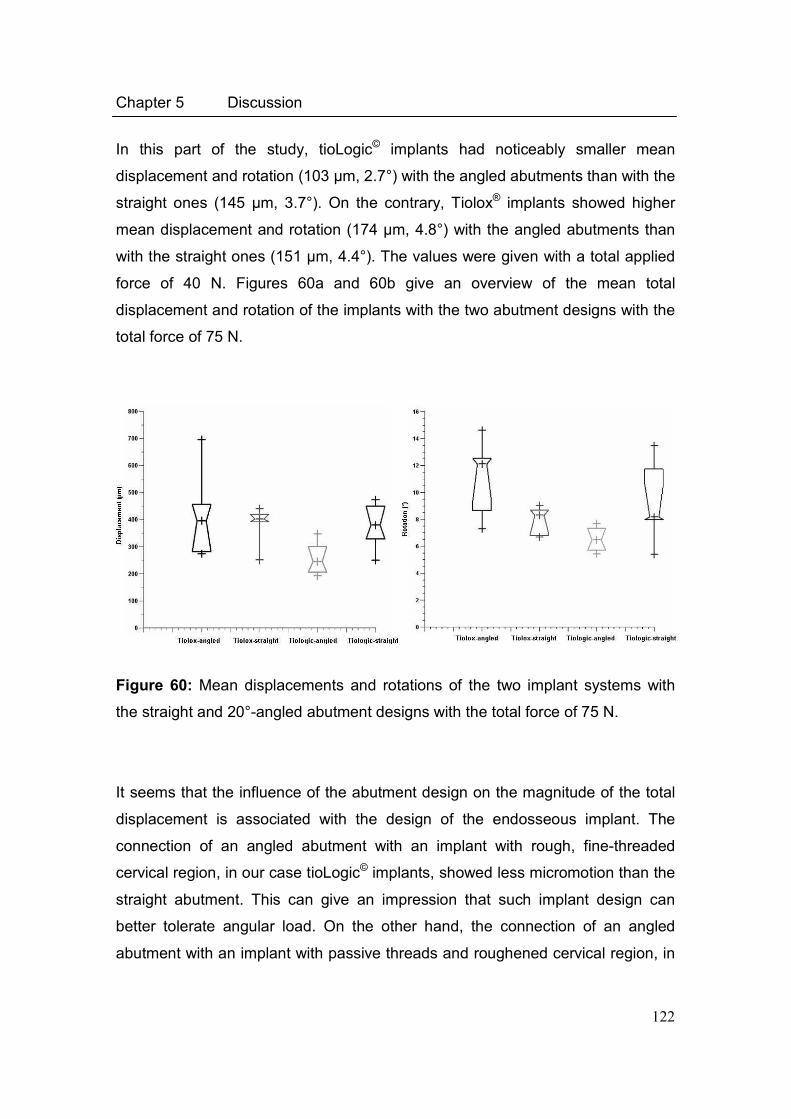
Chapter 5 Discussion
122
In this part of the study, tioLogic© implants had noticeably smaller mean
displacement and rotation (103 µm, 2.7°) with the angled abutments than with the
straight ones (145 µm, 3.7°). On the contrary, Tiolox® implants showed higher
mean displacement and rotation (174 µm, 4.8°) with the angled abutments than
with the straight ones (151 µm, 4.4°). The values were given with a total applied
force of 40 N. Figures 60a and 60b give an overview of the mean total
displacement and rotation of the implants with the two abutment designs with the
total force of 75 N.
Figure 60: Mean displacements and rotations of the two implant systems with
the straight and 20°-angled abutment designs with the total force of 75 N.
It seems that the influence of the abutment design on the magnitude of the total
displacement is associated with the design of the endosseous implant. The
connection of an angled abutment with an implant with rough, fine-threaded
cervical region, in our case tioLogic© implants, showed less micromotion than the
straight abutment. This can give an impression that such implant design can
better tolerate angular load. On the other hand, the connection of an angled
abutment with an implant with passive threads and roughened cervical region, in
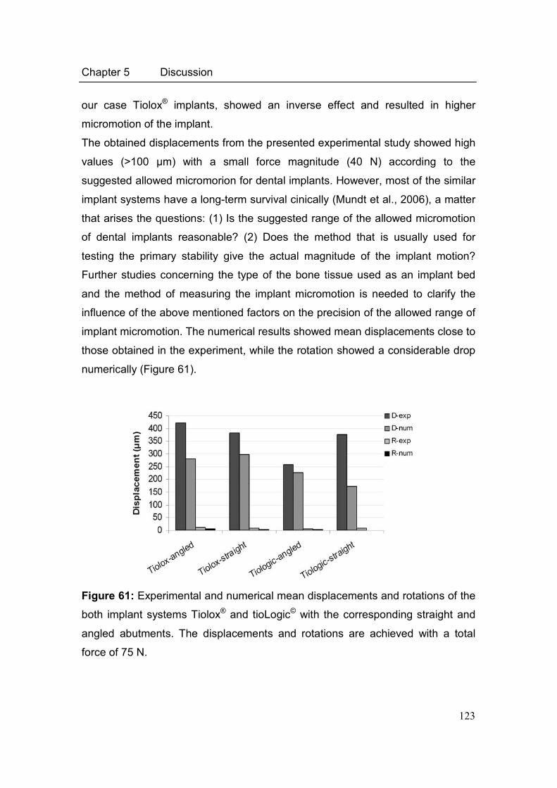
Chapter 5 Discussion
123
our case Tiolox® implants, showed an inverse effect and resulted in higher
micromotion of the implant.
The obtained displacements from the presented experimental study showed high
values (>100 µm) with a small force magnitude (40 N) according to the
suggested allowed micromorion for dental implants. However, most of the similar
implant systems have a long-term survival cinically (Mundt et al., 2006), a matter
that arises the questions: (1) Is the suggested range of the allowed micromotion
of dental implants reasonable? (2) Does the method that is usually used for
testing the primary stability give the actual magnitude of the implant motion?
Further studies concerning the type of the bone tissue used as an implant bed
and the method of measuring the implant micromotion is needed to clarify the
influence of the above mentioned factors on the precision of the allowed range of
implant micromotion. The numerical results showed mean displacements close to
those obtained in the experiment, while the rotation showed a considerable drop
numerically (Figure 61).
Figure 61: Experimental and numerical mean displacements and rotations of the
both implant systems Tiolox® and tioLogic© with the corresponding straight and
angled abutments. The displacements and rotations are achieved with a total
force of 75 N.
Chapter 5 Discussion
124
It seems that the success of immediate loading procedures is a matter of
appropriate patient selection, loading conditions, implant (geometry and surface
treatment) and prosthesis design (Gapski et al., 2003). However, due to the lack
of understanding of the relationship between interface biomechanics and bone
biology, it is difficult to predicatively comment on any of the previous factors.
Optimising implant geometry in order to maintain a beneficial stress level at the
bone-implant interface is a complex issue (Geng et al., 2004). There are many
studies analysing the stress distribution generated in the surrounding bone in
order to arrive at the optimum shape and thread design (Chun et al., 2002;
Pierrisnard et al., 2002).
A couple of basic prerequisites are to be fulfilled by a proper implant design, that
are: (1) Assure sufficient initial stability, reducing implant micromotion below the
‘tolerated threshold’ (approximately 100 µm) and thus minimising the waiting-
period required for loading the implant. (2) Incorporate design factors, that would
diminish the effect of shear forces on the interface (such as surface roughness
related and thread features) so that marginal bone is preserved. (3) Respect
design features that may stimulate bone formation and/or facilitate bone healing
(secondary osseointegration).
A certain thread size and thread profile cannot only be chosen on the basis of
how it performs in an idealised model but should also be validated when applied
on the intended implant design and with the bone anatomy in which it is to
perform. Hansson and Werke (2003) studied the pure effect upon bone stresses
of variations of the thread profile of implants embedded in cortical bone. They
concluded that for an axially loaded, infinitely long and infinitely stiff, screw-
shaped implants embedded in homogenous isotropic cortical bone and with a
frictionless and continuous bone-implant interface (1) the profile of the threads
affects the magnitude of the stress peaks in the bone and the capacity of the
implant to resist loads, (2) providing that the profile is favourable, threads of small
dimensions are quite effective, and (3) a straight part at the bottom of the thread
is for most thread profiles unfavourable.
Chapter 5 Discussion
125
If the profile is favourable, a thread of depth D of only 0.1 mm appears to be
effective as a thread of 0.4 mm depth. Thus threads of very small dimensions
can theoretically be quite effective. This conclusion finds support in the
remarkably good preservation of the marginal bone observed for a dental implant
provided with a microthread at the neck (Nordin et al., 1998; Norton, 1998;
Palmer et al., 1997; Puchades-Roman et al., 2000). In this part of the study, both
implant systems had a coarse-thread depth of 0.43 mm and fine-thread depth
(tioLogic© implants) of 0.1 mm.
In order to avoid stress induced bone resorption, it was suggested to use an
implant design for which the peak bone stresses resulting from an axial load are
spatially separated from those resulting from a transversal load. For a dental
implant Hansson (2000, 2003) found that with a conical implant-abutment
interface located at the level of the marginal bone combined with retention
elements at the endosseous implant neck portion, the peak bone stresses
provided by an axial load are located further down in the bone implying that this
is a design fulfilling the requirement set up by Mailath et al. (1989) and Stoiber
(1988). It is evident that the design of the implant thread does affect the stress
pattern in the bone. An underlying assumption was that the smaller the peak
stress in the bone, caused by a standardised load, the higher is the load the
implant can carry before bone resorption is triggered.
FEM allows the estimation of stresses and strains of extremely geometrically
complex systems, such as dental implant-bone systems. The validity of
mathematical models is difficult to estimate objectively. It might be assessed by
experimental verification, that is, by relating the calculated results with other
comparable FE analyses. The possibility of investigating several loading
conditions on different types of implants and different morphometry and bone
properties is a remarkable advantage of numerical analyses. In spite of the fact
that solutions arising from numerical methods must always be carefully evaluated
in the light of experimental testing, it seems reasonable to exploit this approach
for the possibility of evaluating data that are experimentally not measureable,
Chapter 5 Discussion
126
such as strain or stress in the bone tissue, thus completing and extending
information obtained from in vivo or in vitro tests.
Concerning the stress, in this study Tiolox® implants (without fine threads in the
cervical region) showed higher mean stresses than tioLogic© implants (with fine
threads in the cervical region). In both implant systems, the stresses were within
the acceptable range (below 100 MPa, Frost, 2003, Figure 30a). The strains
were higher with the Tiolox® implants connected to angled abutments to those
connected to straight abutments, while tioLogic© implants showed no difference
in the magnitude of the strain between the straight and angled abutments (Figure
30b). Still the obtained strains with both implant systems are much higher than
those suggested for the physiological strain limits of the bone (above 4,000 µε,
Frost, 2003). The numerically obtained high values of the strain coincide with the
high displacement of implants that were observed experimentally.
Based on the above mentioned numerically obtained results and their linearity,
the strains and stresses are above the physiological range when normal implant
loading at the anterior region is considered.
5.1.3. The Relation of Crestal Bone Resorption to the Abutment Design used in
Implant-Supported Fixed Partial Prosthesis
Numerous recently published studies have focused on treatment outcomes of
implant therapy in partially edentulous patients in general and related to maxillary
anterior teeth replacement in particular (Belser et al., 2003; Naert et al., 2002;
Wyatt and Zarb, 1998). Implants placed in the anterior region of the maxilla failed
significantly more often than those placed in the posterior region. Length and
diameter of the implants did not have significant influence on the cumulative
survival rate (Andersen et al., 2001). Factors favourably affecting the success of
screw-type implants placed to support full- or partial-arch prosthesis include:
Location (jaw and area of implantation), length, restorative\abutment design, and
implantation protocol (nonsubmerged or submerged).
Chapter 5 Discussion
127
The use of angulated abutments is well established. The concern about survival
of implants had largely been dispelled (Kallus et al., 1990). Angulated implant
placement to optimise the available bone is seen as an advantage (Krekmanov
et al., 2000).
In this part of the study, we investigated the relation of the abutment design on
the amount of cervical bone resorption clinically as a complementary step for the
numerical and experimental investigations that were discussed previously in this
chapter. Celland et al. (1993) studied the effect of abutment angulation in a
photoelastic resin and using a strain gauge in one model. They tested 0°-, 15°-
and 20°-abutments and demonstrated that a statistically significant difference
existed for each increase in abutment angulation. According to the authors, all
abutments produced strains that appear to be within the physiologic range for
bone.
The study of Gelb and Lazzara (1993) and Celletti et al. (1995) showed no
adverse osseous changes over a period of three years when preangled
abutments were used after six months healing period. However, these authors
reported three clinical cases, and the correlation is being made with results from
an animal study that took 1.5 years, during which the implants were loaded only
for one year.
In this part of the study, probing depth around implants up to one year was
measured. 24 patients were included. The implants for 13 patients were
connected to straight abutments and for 11 patients were connected to 20°-
angled abutments. In the FE investigation of implant-supported FPP (section
4.1.1.), the magnitude and the distribution of the stresses around implants
cervically with 0°- and 20°- angled abutments were studied.
Concerning the stress results obtained from FE models of FPPs (Table 8), the
clinical follow-up showed no statistical significant difference of the probing depth
(P=0.4), although the numerical analysis showed higher stresses for
nonsubmerged (immediately loaded) implants with straight abutments than
submerged (osseointegrated) implants. Nevertheless, the stress results agree
with the clinical finding for angled abutments when they were used for
Chapter 5 Discussion
128
submerged or nonsubmerged protocol, i.e. angled abutments showed less
probing depth when a submerged implantation protocol was selected instead of a
nonsubmerged protocol (P=0.01).
Furthermore, no statistical significant difference was obtained for straight and
angled abutments with the nonsubmerged protocol (P=0.2). This is an agreement
with the numerical results of the FPPs (Table 8) and those of the experimentally
investigated bovine samples (Figure 61).
However, smaller values of probing depth were obtained and were statistically
significant for angled abutments with submerged protocol than straight
abutments although the numerical analysis showed a minimal difference of the
two abutments. However, smaller values of probing depth were obtained and
were statistically significant for angled abutments with submerged protocol than
straight abutments although the numerical analysis showed a minimal difference
of the two abutments.
Although the size of the study groups was small and the follow-up period was
short, the present results could be the primary stone for further investigations and
for longer periods. Finally and according to the results from the experimental,
numerical and clinical studies, we can conclude that numerical analysis by
means of FEM is a useful tool that could help to understand the biomechanical
reaction of bone to changes of the mechanical environment. The results of this
and previous studies underline that a combination of experimental and/or clinical
results is essential.
5.2. Bone Remodelling Simulation
5.2.1. Sensitivity Analysis
After apprehensive study of the available literature concerning bone remodelling,
the model suggested by Weinans et al. (1992) and expanded by Li et al. (2007)
was finally selected. It is an internal bone remodelling scheme that uses an
internal remodelling approach based on the changes in the apparent bone
Chapter 5 Discussion
129
density as a function of the mechanical stimulus. The model demonstrates bone
resorption by means of density change rate in the negative direction, in both
disuse and overloading conditions. The sensitivity of the applied model was
tested in response to different mechanical environments, started by developing
idealised bone models surrounding a screw-shape implant with different EELs,
from a small one represented by 0.2 mm and lasting with a large length which
was selected to be 0.8 mm. Different behaviour concerning density change and
distribution were obtained (Figure 32). This could probably be caused by the use
of linear elements (tetrahydral 4) that results in a sudden jump in the element
stresses and strains which correspondingly results in different behaviour of the
change in the bone densities. EELs 0.4 mm and 0.6 mm were finally selected to
test the other mechanical condition. The selection was based on two main
reasons; firstly, the comparable density distribution with the histomorphometric
studies (Ulm et al., 1999; Watzak et al., 2005), in particular the stability of the
density within the cortical bone region; secondly, the acceptable total time
required to calculate the density change for the whole bone elements of the
model.
The clear influence of element size was confirmed again by applying a thin layer
of soft tissue to the FE model. The disturbance of the homogenous size of bone
elements by introducing fine elements, which could not be avoided for thickness
and morphological requirements, resulted in an unstable model and a sudden
drop of the density of most of bone elements below 0.3 g/cm3 (Figures 55 and
56).
The internal stress distribution in the jaws is affected not only by forces on the
teeth/implants, but also by forces applied on the jaw by the muscles of the
masticatory system and facial expression, due to various moving actions required
by chewing, swallowing, speech and involuntary jaw motions. Hobkirk and
Schwab (1991) have demonstrated, in subjects with edentulous mandibles
containing osseointegrated implants, that jaw movement from the rest position
results in relative displacement between the linked implants of up to 420 µm and
force transmission of up to 16 N. Determination of muscle forces presents a
Chapter 5 Discussion
130
complicated problem, which requires information on the muscle activity levels,
which are further complicated if mastication is taking place (Koolstra et al., 1999;
Müftü and Müftü, 2006). The internal stress in the mandible, therefore, can have
a very complicated distribution (Hart et al., 1992; Hirayabashi et al., 2002). In the
presented study, different boundary conditions were tested to study the response
of the applied remodelling model to the different loading condition of the jaw bone
represented by the attached muscles in function (pulling and/or pushing action on
the jaw) with varying loading magnitudes (Figure 43) by concerning the mass
weight of the muscle and the length of the attachment side to the bone.
Koseki et al. (2005) estimated the forces and stresses within the mandible
caused by the masticatory system in a FE model of the human mandible. The
stress was within 13 to 15 MPa at the posterior buccal region of the body of the
mandible and 6 to 8 MPa at the posterior lingual region. In the present study,
tension face load of 4.0 MPa was applied on the periphery of the cortical bone on
one half (represents the buccal side) and compression face load of 3.0 MPa on
the other half (represents the lingual side). After 100 time steps, a homogenous
stress distribution of 14 to 15 MPa on the tension side and 5 to 7 MPa on the
compression side was obtained (Figure 44b). The distribution of the density was
located more on the compression (lingual) side than on the tension (buccal) side.
A similar behaviour was observed by Ulm et al. (1999) in their study of the
characteristic features of cancellous bone in edentulous maxillae. They were
observed a denser configuration of trabeculae palatally than those in the buccal
and crestal portions.
Frost proposed that bone responds to a complex interaction of strain magnitude
and time. Conceptually, the interfacial bone maturation, crestal bone loss and
loading can be explained by the Frost mechanostat theory (Frost, 1987) which
connects the two processes of modelling (new bone formation) and remodelling
(continuous turnover of the older bone without a net change in shape or size). In
accordance with the theory, bone acts like a “mechanostat”, in that it brings about
a biomechanical adaptation, corresponding to the external loading condition.
Chapter 5 Discussion
131
Frost (2000) described four micro-strain zones and related each zone to a
mechanical adaptation (Figures 2 and 14). The four zones include the disuse
atrophy, steady state, physiologic overload and pathologic overload zones. Both
extreme zones (pathologic overload zone and disuse atrophy zone) are proposed
to result in a decrease in bone volume. When peak strain magnitude falls below
50 to 200 µε, disuse atrophy is proposed to occur, a phenomenon that is likely to
explain ridge resorption after tooth loss. In the pathologic overload zone, peak
strain magnitude over 4,000 µε may result in net bone resorption. The steady
state zone comprises the range between disuse atrophy and pathologic overload
zone, and is associated with organised, highly mineralised lamellar bone. In this
study, remodelling parameters were adapted to match the zones described by
the mechanostat theory, i.e. the lower critical stress to be 2.0 MPa (105 µε)
below it disuse bone resorption takes place, where as the steady state is to be
within the range of 2.0 to 8.0 MPa (105-415 µε), where no change in bone
density occurs. The upper critical stress was considered to be 60 MPa (4,000
µε), above it overload bone resorption occurs.
Various factors can influence the maximal bite force such as different age
groups, between denture wearers and persons with natural teeth, between
different parts of the dental arch, between persons with and without clinical
symptoms of dysfunction. In a multivariate approach, 58% of the variance of bite
force magnitude in adults was explained by craniofacial morphology and master
muscle thickness (Raadsheer et al., 1999). Bite force magnitude had a positive
association with thickness of the masseter muscle. Radsheer et al. (1999) also
found that the contribution of the masseter muscle to the variation in bite force
magnitude and moment was higher than that of the craniofacial factors.
Regarding the muscle per se, there is a large inter-subject variability of size and
shape of muscular attachments, jaw muscle insertions alter position during
functional movements, and their displacement patterns vary according to the
muscle (Goto et al., 1995). Also, Goto et al. (2001) showed that the deep and
superficial regions of the masseter muscle do not stretch uniformly during major
Chapter 5 Discussion
132
jaw movements. Deep masseter showed the largest increase in muscle length,
and the smallest changes occurred in the posterior most, superficial masseter.
Each muscle part moves differently according to variations in the size and shape
of insertion areas, musculoskeletal form, and patterns of jaw motion during
function (Goto et al., 1995).
As the majority of muscles have a large vertical component, the moment is
largest for vertical bite forces. The second largest force can be generated in
posterior direction (only the posterior temporalis). Consequently, the number of
muscles participating in generating a moment decreases from vertically to
anteriorly to posteriorly directed bites, and this is seen for the moments. Despite
this, the bite force in a posterior direction is larger than in an anterior direction.
This is the direct result of the small resistance arm of the posteriorly directed bite
force and thus the more efficient transfer of muscle to bite force.
The study by Korioth and Hannam (1994) in which the static bites on a 3D FE
model of the human mandible were simulated, found that the highest occlusal
forces were predicted for more posterior tooth location during intercuspal
clenching. The study by Sato (1997), in which distribution of occlusal forces on a
dental arch at various clenching strengths were measured by the Dental Prescale
System, concluded that the distribution of the occlusal force was greatest on the
tooth located more posteriorly in the dental arch. The proportion of occlusal force
on molar regions increased and decreased on premolar and anterior teeth as
clenching strength increased. Distribution of occlusal force on a dental arch
should be considered from a viewpoint of movement of teeth, distortion of the
mandible, positional relationship between bone and muscle, and the thickness of
measuring device.
The occulsal component of the masticatory force is usually 75 to 200 N for a
complete denture, and 40 to 400 N for implant-supported FPP (Lee et al., 2005).
Hansson (2003) suggested that the loading on a dental implant consists of two
components in the vertical Fv and transverse Ft directions (Courteneyharris et al.,
1995). The suggested range of these external loads can be: 0< Fv <400 N; and
0< Ft <150 N. It was reported that the axial loading in the posterior region is
Chapter 5 Discussion
133
between 42 N and 412 N in an implant-supported FPP (Huiskes et al., 1987;
Khraisat et al., 2004; Stanford et al., 1999).
In the present study, the influence of the variation of the magnitude and direction
of the occlusal load on the remodelling model was tested. The applied load on
the dental implant was gradually increased within the range of the bite force at
the posterior region (150-300 N). A stable behaviour of the density of the cortical
bone was obtained within the vertical force range of 250 to 300 N. As the applied
vertical load is smaller than 200 N, 60% of the cortical bone and 80% of the
cancellous bone had a density less than 0.4 g/cm3. The gradual increase of the
axial load on the dental implant caused an increase of the created stress in the
bone within the physiological limits, where bone remodelling takes place.
Combining lateral force with the axial resulted in further increase of the bone
stress that consequently caused an increase in the rate of change in the
apparent density. The influence of the lateral force was obvious on the stability of
the density of the cortical bone when the axial load on the implant was below 250
N. In order to study the effect of the lateral force on the remodelling model, pure
lateral load was applied on the implant starting with 150 N up to 300 N. The large
magnitude of the lateral force combined with sudden increase of the bone
stresses that consequently resulted in a large change in the bone density within a
short time that finally caused a rapid drop of the density below 0.4 g/cm3, i.e. the
density of the cancellous bone calculated with Young’s modulus of 300 MPa.
The response of the remodelling model to the variation of the initial stiffness of
cancellous bone was tested by increasing the Young’s modulus from 100 to 800
MPa keeping that of the cortical bone constant (20 GPa). The change of the
Young’s modulus of certain selected elements within the cancellous bone zone
was studied. Starting with a very low stiffness of the cancellous bone (100 MPa)
up to 300 MPa resulted in a wide remodelling range and reached a final
maximum Young’s modulus of 11 GPa. However, continuous increase of the
stiffness of cancellous bone (400 MPa) up to 800 MPa caused shifting of the
Chapter 5 Discussion
134
remodelling to a lower range to obtain a final maximum Young’s modulus of 9
GPa.
Experimental studies showed different remodelling activities of the cortical and
cancellous bone (Gibson, 1985; Harrigan et al., 1981). Based on this fact, a
density-dependant modulus-density relation was suggested by Orr et al. (1990),
in which a bilinear power function of the new apparent density was used to
calculate the elastic modulus for each element. Using this relation enables us to
achieve a stable behaviour of the elements in the cortical zone with forces below
200 N applied on the implant, a matter that the previous relation that was
suggested by Carter and Hayes (1977) failed to obtain when the applied force
was smaller than 200 N, 90% of the cortical elements had density larger less
than 0.2 g/cm3 at the end of running the simulation.
It is well known that the favourable bone qualities for dental implants are quality 2
and quality 3. The highest surgical failure rate is obtained with quality 1 (4.5%)
followed by quality 4 (3.9%) as presented in the report of the Dental Implant
Clinical Research Group (Truhlar et al., 1994). The applied remodelling model
was tested with the four different bone qualities. The model showed primary
acceptable results with bone of quality 2 (Figure 52b) and quality 1 (Figure 52a).
On the other hand, the results of quality 3 and quality 4, regarding the density
change, were unrealistic in comparison to the clinical prognosis in particular
those with quality 4 model where severe bone resorption would be expected as
an outcome of the remodelling simulation. Reducing the cortical thickness to 1.0
mm and 0.5 mm resulted in more homogenous distribution of the stress in the
cancellous bone zone that consequently led to a longer modelling phase
(increase in the density).
Chapter 5 Discussion
135
5.2.2. Validation of the Computational Trabecular Geometry around an Implant by
Using 6-year CT-Images
After studying the sensitivity of the remodelling model, the simulation was applied
to a FE model of an implant inserted in the upper anterior region. The model was
developed on the base of CT-images of a patient after six years from the
insertion of the implant. Bone dimensions and implant position were created from
the measurement of the CT-images. The numerically obtained trabecular
structure after running the simulation of 100 time steps was close at several
regions to that in the CT-images. However, and because that standard transaxial
CT-images in the vicinity of metallic implants are usually associated with
artefacts at the implant surface (Kalender et al., 1987), the visualisation of the
bone-implant interface and bone structure around the implant was difficult.
5.2.3. Remodelling Model Including Soft Tissue Interface
The interactions in the implant-bone interface are initiated from the time of
implant insertion. The biological response can, according to fracture healing, be
divided into primary and secondary healing (Einhorn, 1998). Primary healing
involves a direct healing without formation of callus. Primary healing seems to
occur only when optimum conditions exist, i.e. mechanical stability and without
presence of gaps. In fracture healing anatomical restoration of the bone
fragments is needed (McKibbin, 1978). Secondary fracture healing which is
supposed to take place around cementless implants occurs when optimum
conditions for repair are absent and involves the formation of callus (Ashhurst,
1986; Buckwalter et al., 1995a; Buckwalter et al., 1995b; Einhorn, 1998).
Initially, a haematoma is formed and the inflammatoric response commences.
The haematoma is suggested to be a source of signalling molecules which are
released from platelets and inflammatoric cells. The haematoma will be invaded
by cells and vessels, and callus formation begins after 7 to 14 days (Dhert et al.,
1998; Sennerby et al., 1993) followed by the formation of woven bone which is

Chapter 5 Discussion
136
later converted to lamellar bone (Einhorn, 1998). The newly formed bone adapts
to the new situation by the orientation of the bone architecture.
In the present study, the characterisation of mechanical conditions that determine
the tissue differentiation was primarily based on the study of Claes and Heigele
(1999). Regardless of individual differences in callus formation there is still a
typical pattern of the tissues involved in bone healing (Claes et al., 1995b; Sevitt,
1981).
Three 3D FE models were developed in this part of the study. Each model
represents one specific healing stage. The first model reflects the healing
foundation within the first two weeks of implantation/immediate loading. The
second and third models represent the 8th and 16th healing weeks, respectively.
The remodelling simulation was applied on the three models separately. The
changes in the density within the different callus layers were studied.
The first model (two weeks healing) showed a positive remodelling and increase
of the element density, in particular in the thread region. The second model (two
months healing) showed further increase of the density, as a continuation that
was observed in the first model. However, it was associated with negative
remodelling at certain regions, namely, in the spaces between the lower threads.
Finally, a creation of a cortical layer at the initial SC-region was observed with the
third model (four months healing).
The obtained results are comparable with the documented radiographical
findings after one and six months from implant insertion. In most cases, implants
showed, radiographically, the formation of a thin layer of highly dense bone
which increases in its thickness until it reaches his optimal shape after six
months healing period. A similar behaviour could be observed from the obtained
numerical results of the three models.
However, finite element models generally have some limitations. The quality of a
FE analysis strongly depends on the geometry, material properties and loading
conditions (Huiskes and Hollister, 1993). The geometry of the soft tissue layer
and the callus were grossly idealised in the presented model by considering a
cylindrical geometry around the implant, whereas histologically, the soft tissue
Chapter 5 Discussion
137
layer or the callus follows the geometry of the implant. Further analysis of the
healing phases with different loading conditions is necessary to validate the
primary results that were presented in this work.
5.2.4. Future Perspectives
A remodelling model for osseointegrated and immediately loaded dental implants
was presented in this work. The sensitivity analyses of the model under different
mechanical conditions enabled the development of a generalised model for the
bone remodelling around dental implants. This primary model can be further
expanded to include the influence of under- and overloading immediately after
implantation to study the early implant failure. Furthermore, the late implant
failure can be studied too, when a modification is applied to the remodelling
model to analyse the cervical bone resoption around the implants.
138
References
Adell R., Lekholm U., Rockler B., Brånemark P.I. A 15-year study of
osseointegrated implants in the treatment of the edentulous jaw. Int J Oral Surg
1981; 10:387-416.
Adell R., Eriksson B., Lekholm U., Brånemark P.I., Jemt T. Long-term follow-up
study of osseointegrated implants in the treatment of totally edentulous jaws. Int
J Oral Maxillofac Implants 1990; 5:347-359.
Albrektsson T. A multicenter report on osseointegrated oral implants. J Prosthet
Dent 1988; 60:75-84.
Ament C., Hofer E.P., Augat P., Claes L. Modelling of tissue transformation
processes in fracture healing. Book of Abstracts, 4th Conference of the ISFR
1994:94.
Andersen E., Saxegaard E., Knutsen B.M., Haanaes H.R. A prospective clinical
study evaluating the safety and effectiveness of narrow-diameter threaded
implants in the anterior region of the maxilla. Int J Oral Maxillofac Implants 2001;
16:217-224.
Arpak N., Niedermeier W., Nergiz I., Schulz A., Bostanci H. Morphometry of the
periimplant of immediate and late endosseous implants. J Dent Res 1995;
74:110.
Ashhurst D.E. The influence of mechanical conditions on the healing of
experimental fractures in the rabbit: a microscopical study. Philos Trans R Soc
Lond B Biol Sci 1986; 313:271-302.
References
139
Atwood D.A. Some clinical factors related to rate of resorption of residual ridges.
J Prosthet Dent 1962; 12:441-450.
Augat P., Merk J., Genant H.K., Claes L. Quantitative assessment of
experimental fracture repair by peripheral computed tomography. Calcif Tissue
Int 1997; 60:194-199.
Bahat O. Treatment planning and placement of implants in the posterior maxillae:
Report of 732 consecutive Nobelpharma implants. Int J Oral Maxillofac Implants
1993; 8:151-161.
Bass S.L., Triplett R.G. The effects of preoperative resorption and jaw anatomy
on implant success. A report of 303 cases. Clin Oral Implants Res 1991; 2:193-
198.
Bassett C.A.L. Biophysical principles affecting bone structure. In the
Biochemistry and Physiology of Bone, 2nd ed., vol. III (ed. G. H. Bourne).
1971:1-77. London: Academic Press.
Beaupré G.S., Giori N.J., Blenman-Fyhrie P.R., Carter D.R. Modelling fracture
healing. The influence of mechanical loading on tissue differentiation. Book of
Abstracts, 4th Conference of the ISFR, 1992:1-11.
Beer A. Methoden der knochendichtemessung des unterkiefers. Thesis.
Department of Biomedical Engineering and Physics, University of Vienna,
Austria, 2000.
Belser U.S., Bernard J.P., Buser D. Implant placement in the aesthetic zone. In:
Lindhe J., Karring T., Lang N.P. (eds). Clin Periodont Implant Dent Ed 4. Oxford:
Blackwell Munksgaard 2003:915-944.
References
140
Benzing U.R., Gall H., Weber H. Biomechanical aspects of two different implant-
prosthetic concepts for edentulous maxillae. Int J Oral Maxillofac Implants 1995;
10:188-198.
Biegler F.B., Hart R.T. Finite element modelling of long bone fracture healing. In:
Middleton J., Pande G.N., Williams K.R. (Eds.), Recent Advances in Computer
Methods in Biomechanics and Biomedical Engineering. Books and Journals
International LTD, 1992:30-39.
Blenman P.R., Carter D.R., Beaupré G.S. Role of mechanical loading in the
progressive ossification of a fracture callus. J Orthop Res 1989; 7:398-407.
Blunn G.W., Wait M.E. Remodelling of bone around intramedullary stems in
growing patients. J Orthop. Res 1991; 9:809-819.
Borchers L., Reichart P. Three-dimensional stress distribution around a dental
implant at different stages of interface development. J Dent Res 1983; 62:155-
159.
Boyce T.M., Fyhrie D.P., Glotkowski M.C., Radin E.L., Schaffler M.B. Damage
type and strain mode associations in human compact bone bending fatigue. J
Orthop Res 1998; 16:322-329.
Brånemark P.I., Adell R., Breine U., Hansson B.O., Lindström J., Ohlsson A.
Intra-osseous anchorage of dental prostheses. I. Experimental studies. Scand J
Plast Reconstr Surg 1969; 3:81-100.
Buchjek K. Non-equilibrium bone remodelling: Changes of mass density and of
the axes of anisotropy. Int J Engng Sci 1990; 28:1039-1004.
References
141
Buckwalter J.A., Glimcher M.J., Cooper R.R., Recker R. Bone biology. Part 1:
Structure, blood supply, cells, matrix, and mineralization. J Bone Joint Surg
1995a; 77:1256-1275.
Buckwalter J.A., Glimcher M.J., Cooper R.R., Recker R. Bone biology. Part II:
Formation, form, modelling, remodelling, and regulation of cell function. J Bone
Joint Surg 1995b; 77:1276-1289.
Burr D.B. Targeted and nontargeted remodelling. Bone 2002; 30:2-4.
Cameron H.U., Pilliar R.M., MacNab I. The effect of movement on the bonding of
the porous metal to bone. J Biomed Mater Res 1973; 7:301-311.
Canay S., Hersek N., Akpinar I., Aşik Z. Comparison of stress distribution around
vertical and angled implants with finite element analysis. Quintessence Int 1996;
27:591-598.
Carlsson G.E. Clinical morbidity and sequelae of treatment with complete
dentures. J Prosthet Dent 1998; 79:17-23.
Carter D.R., Hayes W.C. The compression behaviour of bone as a two-phase
porous structure. J Bone Joint Surg 1977; 59:954-962.
Carter D.R., Caler W.E. Cycle-dependent and time-dependent bone fracture with
repeated loading. J Biomech Eng 1983; 105:166-170.
Carter D.R. Mechanical loading histories and cortical bone remodelling. Calcif
Tissue Int 1984; 36:19-24.
Carter D.R. Mechanical loading history and skeletal biology. J Biomech 1987;
20:1095-1109.
References
142
Carter D.R., Fyhrie D.P., Whalen R.T. Tabecular bone density and loading
history: Regulation of connective tissue morphology by mechanical energy. J
Biomech 1987; 20:785-794.
Carter D.R., Blenman P.R., Beaupré G.S. Correlations between mechanical
stress history and tissue differentiation in initial fracture healing. J Orthop Res
1988; 6:736-748.
Carter D.R., Orr T.E., Fyrie D.P. Relationships between loading history and
femoral cancellous architecture. J Biomech 1989; 22:231-244.
Celland N.L., Gilat A., McGlumphy E.A., Brantley W.A. A photoelastic and strain
gauge analysis of angled abutments for an implant system. Int J Oral Maxillofac
Implants 1993; 8:541-548.
Celletti R., Pameijer C.H., Bracchetti G., Donath K., Persichetti G., Visani I.
Histologic evaluation of osseointegrated implants restored in nonaxial functional
occlusion with preangled abutments. Int J Periodont Rest Dent 1995; 15:563-
573.
Cheal E.J., Mansmann K.A., DiGioia A.M., Hayes W.C., Perren S.M. Role of
interfragmentary strain in fracture healing: ovine model of a healing osteotomy. J
Orthop Res 1991; 9:131-142.
Chun H.J., Cheong S.Y., Han J.H., Heo S.J., Chung J.P., Rhyu I.C., Choi Y.C.,
Baik H.K., Kim M.H. Evaluation of design parameters of osseointegrated dental
implants using finite element analysis. J Oral Rehabil 2002; 29:565-574.
Churches A.E., Howlett C.R., Waldron K.J., Ward G.W. The response of living
bone to controlled, time varying loading: Method and preliminary results. J
Biomech 1979; 12:35-45.
References
143
Claes L.E., Wilke H.J., Augat P., Rübenacker S., Margevicius K.J. Effect of
dynamization of gap healing of diaphyseal fractures under external fixation. Clin
Biomech 1995a; 10:227-234.
Claes L.E., Wilke H.J., Kiefer H. Osteonal structure better predicts tensile
strength of healing bone than volume fraction. J Biomech 1995b; 28:1377-1390.
Claes L.E., Heigele C.A. Magnitudes of local stress and strain along bony
surfaces predict the course and type of fracture healing. J Biomech 1999;
32:255-266.
Cochran D.L., Schenk R.K., Lussi A., Higginbottom F.L., Buser D. Bone
response to unloaded and loaded titanium implants with a sandblasted and acid-
etched surface: A histometric study in the canine mandible. J Biomed Mater Res
1998; 40:1-11.
O’Connor J.A., Lanyon L.E., MacFie H. The influence of strain rate on adaptive
bone remodelling. J Biomech 1982; 15:767-781.
Courteneyharris R.G., Kayser M.V., Downes S. Comparison of the early
production of extracellular-matrix on dense hydroxyapatite and
hydroxyapatite-coated titanium in cell and organ-culture. Biomat 1995; 16:489-
495.
Cowin S.C., Hegedus D.H. Bone remodelling I: Theory of adaptive elasticity. J
Elasticity 1976; 6:313-326.
Cowin S.C., Firoozbakhsh K. Bone remodelling of diaphysial surfaces under
constant load: Theoretical predictions. J Biomech 1981a; 7:471-484.
References
144
Cowin S.C., Firoozbakhsh K. An analytical model of Pauwel’s functional
adaptation mechanics in bone. J Biomech Eng 1981b; 103:246-252.
Cowin S.C. Mechanical modelling of the stress adaptation process in bone. Calcif
Tissue Int 1984; 36:98-103.
Cowin S.C., Hart R.T., Balser J.R., Kohn D.H. Functional adaptation in long
bones: Establishing in vivo values for surface remodelling rate coefficients. J
Biomech. 1985; 18:665-684.
Cowin S.C. Bone mechanics handbook. CPC Press, Boca Raton 2001.
Davies J.E., Ottensmeyer P., Shen X., Hashimoto M., Peel S.A.F. Early
extracellular matrix synthesis by bone cells. In: The bone-biomaterial interface
(Ed. Davies JE). University of Toronto Press. Toronto 1991; 20:214-228.
Davy D.T., Connolly J.F. The biomechanical behaviour of healing canine radii
and ribs. J Biomech 1982; 15:235-247.
Dhert W.J., Thomsen P., Blomgren A.K., Esposito M., Ericson L.E., Verbout A.J.
Integration of press-fit implants in cortical bone: A study on interface kinetics. J
Biomed Mater Res 1998; 41:574-583.
DiGioia A.M., Cheal E.J., Hayes W.C. Three-dimensional strain fields in a
uniform osteotomy gap. J Biomech Eng 1986; 108:273-280.
Eger D.E., Gunsolley J.C., Feldman S. Comparison of angled and standard
abutments and their effect on clinical outcomes: A preliminary report. Int J Oral
Maxillofac Implants 2000; 15:819-823.
References
145
Einhorn T.A. The cell and molecular biology of fracture healing. Clin Orthop Relat
Res 1998:7-21.
Ellis D.K., Natali A. Dental biomechanics. New York: Taylor & Francis 2003:1-19.
Engquist B., Bergendal T., Kallus T., Linden U. A retrospective multicenter
evaluation of osseointegrated implants supporting overdentures. Int J Oral
Maxillofac Implants 1988; 3:129-134.
Eriksen E.F., Mosekilde L., Melsen F. Effect of sodium fluoride, calcium,
phosphate, and vitamin D2 on trabecular bone balance and remodelling in
osteoporotics. Bone 1985; 6:381-389.
Friberg B., Jemt T., Lekholm U. Early failures in 4,641 consecutively placed
Brånemark dental implants: A study from stage 1 surgery to the connection of
completed prostheses. Int J Oral Maxillofac Implants 1991; 6:142-146.
Friberg B. Treatment with dental implants in patients with severe osteoporosis: A
case report. Int J Periodontics Restorative Dent 1994; 14:348-353.
Friberg B., Sennerby L., Roos J., Johansson P., Strid C.G. Lekholm U.
Evaluation of bone density using cutting resistance measurements and
microradiography: An in vitro study in pig ribs. Clin Oral Implants Res 1995a;
6:164-171.
Friberg B., Sennerby L., Roos J., Lekholm U. Identification of bone quality in
conjunction with insertion of titanium implants: A pilot study in jaw autopsy
specimens. Clin Oral Implants Res 1995b; 6:213-219.
References
146
Friberg B., Sennerby L., Meredith N., Lekholm U. A comparison between cutting
torque and resonance frequency measurements of maxillary implants. Oral
Maxillofac Surg 1999; 28:297-303.
Friberg B., Gröndahl K., Lekholm U., Brånemark P.I. Long-term follow-up of
severely atrophic edentulous mandibles reconstructed with short Brånemark
implants. Clin Implant Dent Relat Res 2000; 2:184-189.
Frost H.M. Presence of microscopic cracks in vivo in bone. Henry Ford Hospital
Medical Bulletin 1960; 8:25-35.
Frost H.M. Bone Remodelling Dynamics. Springfield, IL: Charles C.Thomas
1963.
Frost H.M. The law of bone structure. Charles C. Thomas, Springfield 1964.
Frost H.M. Bone Modelling and Skeletal Modelling Errors. Springfield, IL: Charles
C. Thomas 1973.
Frost H.M. Intermediary Organization of the Skeleton. Boca Raton, FL:CRC
Press 1986.
Frost H.M. Bone “mass” and the “mechanostat”: A proposal. Anat Rec 1987;
219:1-9.
Frost H.M. Obesity, and bone strength and “mass”: A tutorial based on insights
from a new paradigm. Bone 1997; 21:211-214.
Frost H.M. Bone’s Mechanostat: A 2003 update. Anat Record part A 2003;
275:1081-1101.
References
147
Fyhrie D.P., Carter D.R. A unifying principle relating stress to trabecular bone
morphology. J Orthop Res 1986; 4:304-317.
Gapski R. Wanh H.L., Mascarenhas P., Lang N.P. Critical review of immediate
implant loading. Clin Oral Implants Res 2003; 14:515-527.
García J.M., Martínez M.A., Doblaré M. An anisotropic internal–external bone
adaptation model based on a combination of CAO and continuum damage
mechanics technologies. Comput Meth in Biomech Biomed Engin 2001; 4:355–
377.
Garn S.M. The Earlier Gain and the Later Loss of Cortical Bone. Springfield, IL:
Charles C. Thomas 1970.
Gelb D.A., Lazzara R.J. Hierarchy of objectives in implant placement to maximize
esthetics: Use of preangulated abutments. Int J Periodont Rest Dent 1993;
13:277-287.
Geng J.P., Ma Q.S., Xu W., Tan K.B., Liu G.R. Finite element analysis of four
thread-form configurations in a stepped screw implant. J Oral Rehabil 2004;
31:233-239.
Geng J.P., Xu D.W., Tan K.B., Liu G.R. Finite element analysis of an
osseointegrated stepped screw dental implant. J Oral Implantol 2004; 30:223-
233.
Geramy A., Morgano S.M. Finite element analysis of three designs of an implant-
supported molar crown. J Prosthet Dent 2004; 92:434-440.
Gibson L.J. The mechanical behaviour of cancellous bone. J Biomech 1985;
18:317-328.
References
148
Goto T.K., Langenbach G.E., Korioth T.W., Hagiwara M., Tonndorf M.L.,
Hannam A.G. Functional movements of putative jaw muscle insertions. Anat Rec
1995; 242:278-288.
Goto T.K., Langenbach G.E., Hannam A.G. Length changes in the human
masseter muscle after jaw movement. Anat Rec 2001; 262:293-300.
Hansson S. Implant-abutment interface: Biomechanical study of flat top versus
conical. Clin Implants Dent Rel Res 2000; 2:33-41.
Hansson S. A conical implant-abutment interface at the level of the marginal
bone improves the distribution of stresses in the supporting bone: An
axisymmetric finite element analysis. Clin Oral Implants Res 2003; 14:286-293.
Hansson S., Werke M. The implant thread as a retention element in cortical
bone: The effect of thread size and thread profile: A finite element study. J
Biomech 2003; 36:1247-1258.
Harrigan T.P., Caner D.R., Mann R.W., Harris W.H. The influence of apparent
density and trabecular orientation on the elastic modulus of cancellous bone.
Trans Orthop Res Soc 1981; 6:277-281.
Hart R.T., Davy D.T., Heiple K.G. A computational method for solution of
adaptive elasticity problems. Advances in Bioengineering, American Society of
Mechanical Engineers 1982:123-126.
Hart R.T., Davy D.T., Heiple K.G. A predictive model for strain-induced
remodelling in long bones. Transactions of the 1983. Orthop Res Society
1983:71.
References
149
Hart R.T., Davy D.T., Heiple K.G. Mathematical modelling and numerical
solutions for functionally dependent bone remodelling. Calcif Tissue Int 1984a;
36:104-109.
Hart R.T., Davy D.T., Heiple K.G. A computational method for stress analysis of
adaptive elastic materials with a view towards applications in strain-induced bone
remodelling. J Biomech Eng 1984b; 106:342-350.
Hart R.T., Davy D.T. Theories of bone modelling and remodelling in: Cowin Sc.
(ed.). Bone Mechanics CRC Press, Boca Raton 1989:253-277.
Hart R.T., Henebbel V., Thongpreda N., van Buskirk W.C., Anderson R.C.
Modelling the biomechanics of the mandible: A three dimensional finite element
study. J Biomech 1992; 25:261-286.
Hassler C.R., Rybicki E.F., Cummings K.D., Clark L.C. Quantification of bone
stresses during remodelling. J Biomech 1980; 13:185-190.
Helkimo E., Carlsson G.E., Helkimo M. Bite force and state of dentition. Acta
Odontol Scand 1977; 35:297-303.
Hert J., Lisková M., Landrgot B. Influence of the long-term continuous bending on
the bone. Folia Morphol 1969; 17:389-399.
Hert J., Lisková M., Landa M. Reaction of bone to mechanical stimuli. Part I.
Continuous and intermittent loading of tibia in rabbit. Folia Morphol 1971; 19:290-
300.
Hert J., Fiala P., Petrtyl M. Osteon orientation of the diaphysis of the long bones
in man. Bone 1994; 15:269-277.
References
150
Higuchi K.W., Folmer T., Kultje C. Implant survival rate in partially edentulous
patients. A 3-year prospective multicenter study. J Oral Maxillofac Surg 1995;
53:264-268.
Hillam R.A., Skerry T.M. Inhibition of bone resorption and stimulation of formation
by mechanical loading of the modelling rat ulna in vivo. J Bone Miner Res 1995;
10:683-689.
Hirayabashi M., Motoyoshi M., Ishimaru T., Kasai K., Namura S. Stress in
mandibular cortical bone during mastication: Biomechanical considerations using
a three dimensional finite element method. J Oral Science 2002; 44:1-6.
Hobkirk J.A., Schwab J. Mandibular deformation in subjects with osseointegrated
implants. Int J Oral Maxillofac Implants 1991; 6:319-328.
Horinchi K., Uchida H., Yamamoto K., Sugimura M. Immediate loading of
Brånemark System Implant Following Placement In Edentulous Patients: A
Clinical Report. Int J Oral Maxillofac Implants 2000; 15:824-830.
Huiskes R. Some fundamental aspects of human joint replacement. Acta Orthop
Scand Suppl 1980; 185:1-208.
Huiskes R., Weinans H., Grootenboer H.J., Dalstra M., Fudala B., Slooff T.J.
Adaptive bone remodelling theory applied to prosthetic design analysis. J
Biomech 1987; 20:1135-1150.
Huiskes R., Weinans H., Reitbergen B.V., Sumner D.R., Turner T.M., Galante
J.O. Validation of strain adaptive bone-remodelling analysis to predict bone
morphology around non-cemented THA. Orthopedic Trans 1991; 15:399.
References
151
Huiskes R., Hollister S.J. From structure to process, from organ to cell: recent
developments of FE-Analysis in orthopaedic biomechanics. J Biomech Eng 1993;
115:520-527.
Jaffin R.A., Berman C.L. The excessive loss of Brånemark fixtures in type IV
bone: A 5-year analysis. J Periodontol 1991; 62:2-4.
Jee W.S., Frost H.M. Skeletal adaptations during growth. Triangle 1992; 31:77-
88.
Jemt T., Strid K.G. Assessment of bone quality from cutting resistance during
implant surgery. Int J OralMaxillofac Surg 1994; 9:279-288.
Jemt T., Lekholm U. Implant treatment in edentulous maxillae: A five-year follow-
up report on patients with different degrees of jaw resorption. Int J Oral Maxillofac
Implants 1995; 10:303-311.
Johansson P., Strid K.G. Assessment of bone quality from cutting resistance
during implant surgery. Int J Oral Maxillofac Implants 1994; 9:279-288.
Jones P.M. Complete dentures and the associated soft tissues. J Prosthet Dent
1976; 36:136-149.
Johns R.B., Jemt T., Heath M.R., Hutton J.E., McKenna S., McNamara D.C., van
Steenberghe D., Taylor R., Watson R.M., Herrmann I. A multicenter study of
overdentures supported by Brånemark implants. Int J Oral Maxillofac Implants
1992; 7:513-522.
Jurvelin J.S., Buschmann M.D., Hunziker E.B. Optical and mechanical
determination of Poisson’s ratio of adult bovine humeral articular cartilage. J
Biomech 1997; 30:235-241.
References
152
Kalender W.A., Hebel R., Ebersberger J. Reduction of CT artefacts caused by
metallic implants. Radiology 1987; 164:576–577.
Kallus T., Henry P., Jemt T., Jörnéus L. Clinical evaluation of angled abutments
for the Brånemark system: A pilot study. Int Oral Maxillofac Implants 1990; 5:39-
45.
Kawahara H., Kawahara D., Hayakawa M., Tamai Y., Kuremoto T., Matsuda S.
Osseointegration under immediate loading: Biomechanical stress-strain and
bone formation-resorption. Implant Dent 2003; 12:61-68.
Keilig L., Bourauel C., Grüner M., Hültenschmidt R., Bayer S., Utz K.H., Stark H.
Aufbau und Erprobung eines neuartigen Meßsystems für die dentale
Biomechanik-Meßprinzip und Beispielmessungen des Hexapod-Meß-Systems.
Biomed Technik 2004; 49:208-215.
Kenney R., Richards M.W. Photoelastic stress patterns produced by
implantretained overdentures. J Prosthet Dent 1998; 80:559-564.
Khraisat A., Hashimoto A., Nomura S., Miyakawa O. Effect of lateral cyclic
loading on abutment screw loosening of an external hexagon implant system. J
Prosthet Dent 2004; 91:326-334.
Kingsmill V.J., Boyde A. Variation in the apparent density of human mandibular
bone with age and dental status. J Anat 1998; 192:233-244.
Kirsch A., Mentag P.J. The IMZ endosseous two phase implant system: A
complete oral rehabilitation treatment concept. J Oral Implantol 1986; 12:576-
589.
References
153
Koolstra J.H., van Eijden T.M.G.J. Three dimensional dynamical capabilities of
the human masticatory muscles. J Biomech 1999; 32:145-152.
Korioth T.W., Hannam A.G. Mandibular forces during simulated tooth clenching.
J Orofac Pain 1994; 8:178-189.
Koseki M., Inou N., Maki K. Estimation of masticatory forces for patient-specific
analysis of the human mandible. Nihon Kikia Gakkai Nenji Taikai Koen
Ronbunshu 2005; 5:155-156.
Krekmanov L., Kahn M., Rangert B., Lindström H. Tilting of posterior mandibular
and maxillary implants for improved prosthesis support. Int J Oral Maxillofac
Implants 2000; 15:405-414.
Lazenby R.A. Continuing periosteal apposition. I. Documentation, hypotheses,
and interpretation. Am J Phys Anthropol 1990a; 82:451-472.
Lazenby R.A. Continuing periosteal apposition. II. The significance of peak bone
mass, strain equilibrium, and age-related activity differentials for mechanical
compensation in human tubular bones. Am J Phys Anthropol 1990b; 82:473-484.
Lee J.H., Frias V., Lee K.W., Wright R.F. Effect of implant size and shape on
implant success rates: A literature review. J Prosthet Dent 2005; 94:377-381.
Lee T.C., Staines A., Taylor D. Bone adaptation to load: Microdamage as a
stimulus for bone remodelling. J Anat 2002; 201:437-446.
Lekholm U., Zarb G.A. Patient selection and preparation. In: Brånemark P.I.,
Zarb G., Albrektsson T., eds. Tissue-integrated prostheses. Osseointegration in
clinical dentistry 1985:199–209. Chicago: Quintessence Publishing Company Inc.
References
154
Lekholm U., van Steenberghe D., Herrmann I., Bolender C., Folmer T., Gunne J.,
Henry P., Higuchi K., Laney W.R., Lindén U. Osseointegrated implants in the
treatment of partially edentulous jaws: A prospective 5-year multicenter study. Int
J Oral Maxillofac Implants 1994; 9:627-635.
Li J., Li H., Shi L., Fok A., Ucer C., Devlin H., Horner K., Silikas N. A
mathematical model for simulating the bone remodelling process under
mechanical stimulus. Dental Mater 2007; 23:1073-1078.
Lindh C., Nilsson M., Klinge B., Petersson A. Quantitative computed tomography
of trabecular bone in the mandible. Dentomaxillofac Radiol 1996; 25:146-150.
Lindh T., Gunne J., Tillberg A., Molin M. A meta-analysis of implants in partial
edentulism. Clin Oral Implants Res 1998; 9:80-90.
Liskova M., Hert J. Reaction of bone to mechanical stimuli. Part II. Periosteal and
endosteal reaction of tibial diaphysis in rabbit to intermittent loading. Folia
Morphol 1971; 19:301-317.
Lundgren D., Laurell L., Falk H., Bergendal T. Occlusal force pattern during
mastication in dentitions with mandibular fixed partial dentures supported on
osseointegrated implants. J Prosthet Dent 1987; 58:197-203.
O’Mahony A.M., Williams J.L., Spencer P. Anisotropic elasticity of cortical and
cancellous bone in the posterior mandible increases peri-implant stress and
strain under oblique loading. Clin Oral Implants Res 2001; 12:648-657.
Mailath G., Stoiber B., Watzek G., Matejka M. Die Knochenresorption an der
Eintrittstelle osseointegrierter Implantate: Ein biomechanisches Phänomen. Eine
Finite-Element-Studie. Zeitschrift für Stomatologie 1989; 86:207-216.
References
155
Makoto S., Kenji S., Koichi K. Measurements of mechanical properties of cortical
bone using nanoindication tests. Proceedings of Annual Meeting of Japanese
Society for Orthopaedic Biomechanics 2003; 24:1-5.
Martin R.B., Burr D.B. Structure, function and adaptation of compact bone.
Raven Press, New York 1989.
Martin R.B. Fatigue microdamage as an essential element of bone mechanics
and biology. Calcif Tissue Int 2003; 73:101-107.
McHorris W.H. The importance of anterior teeth. J Gnath 1982; 1:19-36.
McKibbin B. The biology of fracture healing in long bones. J Bone Joint Surg [Br]
1978; 60:150-162.
Meade J.B., Cowin S.C., Klawitter J.J., Skinner H.B., van Buskirk W.C. Short
term modelling due to hyperphysiological stress. Transactions of the 1983.
Orthop Res Society 1981:62.
Meredith N. Assessment of implant stability as a prognostic determinant. Int J
Prosthodont 1998; 11:491-501.
Mericske-Stern K. Overdentures with roots or implants for elderly patients. A
comparison. J Prosthet Dent 1994; 72:543-550.
Mericske-Stern R., Assal P., Mericske E., Bürgin W. Occlusal force and oral
tactile sensibility measured in partially edentulous patients with ITI implants. Int J
Oral Maxillofac Implants 1995; 10:345-354.
References
156
Meyer V., Wiesmann H.P., Fillies T., Joos U. Early tissue reaction at the interface
of immediately loaded dental implants. Int J Oral Maxillofac Implants 2003;
18:489-499.
Misch C.E. Density of bone: Effect on treatment plans, surgical approach, healing
and progressive bone loading. Int J Oral Implantol 1990; 6:23-31.
Misch C.E. Progressive loading of bone with implant prostheses. J Dent Symp
1993; 1:50-53.
Misch C.E. Bone density: A key determinant for clinical success. In: Misch C.E.,
ed. Contemporary Implant Dentistry, 2nd ed. St Louis, Mo: Mosby 1999.
Morris H.F., Ochi S., Gillette W. Bone quality and implant integration during
follow-up in the DICRG clinical study. J Dent Res 1995; 74:495-753.
Müftü S., Müftü A. Biomechanics of tooth and jaw. In: Webster,JG. (Ed.),
Encyclopedia of Medical Devices and Instrumentation. Wiley, NY 2006:411-428.
Mundt T., Mack F., Schwahn C., Biffar R. Private practice results of screw-type
tapered implants: Survival and evaluation of risk factors. Int J Oral Maxillofac
Implants 2006; 21:607-614.
Närhi T.O., Ettinger R.L., Lam E.W. Radiographic findings, ridge resorption, and
subjective complaints of complete denture patients. Int J Prosthodont 1997;
10:183-189.
Naert I., Koutsikakis G., Duyck J., Quirynen M., Jacobs R., van Steenberghe D.
Biologic outcome of implant-supported restorations in the treatment of partial
edentulism. Part I: A longitudinal clinical evaluation. Clin Oral Implants Res 2002;
13:382-389.
References
157
Nordin T., Jonsson G., Nelvig P., Rasmusson L. The use of a conical fixture
design for fixed partial prostheses: A preliminary report. Clin Oral Implants Res
1998; 9:343-347.
Norton M. Marginal bone levels at single tooth implants with a conical fixture
design: The influence of surface macro- and microstructure. Clin Oral Implants
Res 1998; 9:91-99.
van Oosterwyck H., Duyck J., Vander Sloten J., van der Perre G., De Cooman
M., Lievens S., Puers R., Naert I. The influence of bone mechanical properties
and implant fixation upon bone loading around oral implants. Clin Oral Implants
Res 1998; 9:407-418.
Orr T.E., Beauprè G.S., Carter D.R., Schurman D.J. Computer predictions of
bone remodelling around porous-coated implants. J Arthoplasty 1990; 5:191-200.
Palmer R.M., Smith B.J., Palmer P.J., Floyd P.D. A prospective study of Astra
single tooth implants. Clin Oral Implants Res 1997; 8:173-179.
Papavasiliou G., Kamposiora P., Bayne S.C., Felton D.A. Three-dimensional
finite element analysis of stress-distribution around single tooth implants as a
function of bony support, prosthesis type, and loading during function. J Prosthet
Dent 1996; 76:633-640.
Parfitt A.M. Quantum concept of bone remodelling and turnover: implications for
the pathogenesis of osteoporosis. Calcif Tissue Int 1979; 28:1-5.
Parfitt A.M. Osteonal and hemi-osteonal remodelling: The spatial and temporal
framework for signal traffic in adult human bone. J Cell Biochem 1994; 55:273-
286.
References
158
Parfitt A.M. The mechanism of coupling: A role for the vasculature. Bone 2000;
26:319-323.
Patra A.K., DePaolo J.M., D’Souza K.S., DeTolla D., Meenaghan M.A.
Guidelines for analysis and redesign of dental implants. Implant Dent 1998;
7:355-368.
Pearce A.I., Richards R.G., Milz S., Schneider E., Pearce S.G. Animal models for
implant biomaterial research in bone: A review. Eur Cell Mater 2007; 13:1-10.
Pierrisnard L., Hure G., Barquins M., Chappard D. Two dental implant design for
immediate loading: A finite element analysis. Int J Oral Maxillofac Implants 2002;
17:353-362.
Poumarat G., Squire P. Comparison of mechanical properties of human, bovine
bone and a new processed bone xenograft. Biomater 1993; 14:337-340.
Puchades-Roman L., Palmer R.M., Palmer P.J., Howe L.C., Ide M., Wilson R.F.
A clinical, radiographic, and microbiologic comparison of Astra Tech and
Brånemark single tooth implants. Clin Implants Dent Rel Res 2000; 2:78-84.
Raadsheer M.C., van Eijden T.M., van Ginkel F.C., Prahl-Andersen B.
Contribution of jaw muscle size and craniofacial morphology to human bite force
magnitude. J Dent Res 1999; 78:31-42.
Rahimi A., Keilig L., Bendels G., Klein R., Buzug T.M., Abdelgader I., Abboud M.,
Bourauel C. 3D reconstruction of dental specimens from 2D histological images
and microCT-scans. Comput Methods Biomech Biomed Engin 2005; 8:167-76.
References
159
Rahimi A., Bourauel C., Jäger A., Gedrange T., Heinemann F. Load transfer by
fine threading the implant neck: A FEM study. J Physiol Pharmacol 2009; 60
(Suppl 8):107-112.
Rasmusson L., Kahnberg K.E., Tan A. Effects of implant design and surface on
bone regeneration and implant stability: An experimental study in the dog
mandible. Clin Implant Dent Related Res 2001; 3:2-8.
Reiter T.J. Functional adaptation of bone and application in optimal structural
design. VDI-Berichte 1996; 17:145.
Robling A.G., Castillo A.B., Turner C.H. Biomechanical and molecular regulation
of bone remodelling. Annu Rev Biomed Eng 2006; 8:455-498.
Rubin C.T., Lanyon L.E. Bone remodelling in response to applied dynamic loads.
Orthop Trans 1981; 5:2-37.
Rubin C.T., Lanyon L.E. Regulation of bone formation by applied dynamic loads.
J Bone Joint Surg Am 1984; 66:397-402.
Rubin C.T., Lanyon L.E. Regulation of bone mass by mechanical strain
magnitude. Calcif Tissue Int 1985; 37:411-417.
Saab X., Griggs J., Powers J., Engelmeier R. Effects of abutment angulation on
the strain on the bone around an implant in the anterior maxilla: A finite element
study. J Prosthet Dent 2007; 97:85-92.
Sato T. A study of bite force distribution on the dental arch in normal subjects. J
Japan Prosthodont Society 1997; 41:634 (in Japanese with English abstract).
References
160
Schaeffer A. Behaviour of the axis of human incisor teeth during growth. Angle
Orthodont 1949; 19:254-275.
Sennerby L., Thomsen P., Ericson L.E. Early response to titanium implants
inserted in rabbit in cortical bone. J Mater Sci Mater Med 1993; 4:240-250.
Sethi A., Kaus T., Sochor P. The use of angulated abutments in implant dentistry:
five-year clinical results of an ongoing prospective study. Int J Oral Maxillofac
Implants 2000; 15:801-810.
Sevitt S. Secondary repair of fractures. Events preparatory to union. In: Sevitt S.,
(Ed.), Bone Healing and Fracture Repair in Man 1981. Churchill Livingstone.
Smith D.E. Review of endosseous implants for partially edentulous patients. Int J
Prosthodont 1990; 3:12-19.
Søballe K., Brockstedt-Rasmussen H., Hansen E.S., Bünger C. Hydroxyapatite
coating modifies implant membrane formation. Controlled micromotion studied in
dogs. Acta Orthop Scand 1992a; 63:128-140.
Søballe K., Hansen E.S., Brockstedt-Rasmussen H., Jørgensen P.H., Bünger C.
Tissue ingrowth into titanium and hydroxyapatite-coated implants during stable
and unstable mechanical conditions. J Orthop Res 1992b; 10:285-299.
Stanford C.M., Brand R.A. Toward an understanding of implant occlusion and
strain adaptive bone modelling and remodelling. J Prosthet Dent 1999; 81:553-
561.
van Steenberghe D., Lekholm U., Bolender C., Folmer T., Henry P., Herrmann I.,
Higuchi K., Laney U., Linden U., Astrand P. The applicability of osseointegrated
References
161
oral implants in the rehabilitation of partial edentulism: A prospective multicenter
study on 558 fixtures. Int J Oral Maxillofac Implants 1990; 5:272-281.
Stegaroiu R., Sato T., Kusakari H., Miyakawa O. Influence of restoration type on
stress distribution in bone around implants: A three-dimensional finite element
analysis. Int J Oral Maxillofac Implants 1998; 13:82-90.
Stoiber B. Biomechanische Grundlagen enossaler Schraubenimplantate. Diss.
Universitätsklinik für Zahn-, Mund- und Zahnheilkunde, Wien 1988.
Sullivan D.Y. Prosthetic considerations for the utilization of osseointegrated
fixtures in the partially edentulous arch. Int J Oral Maxillofac Implants 1986; 1:39-
45.
O’Sullivan D., Sennerby L., Meredith N. Measurements comparing the initial
stability of five designs of dental implants: A human cadaver study. Clin Implant
Dent Related Res 2000; 2:85-92.
Thompson D. On growth and form. Am J Orthod 1952; 53:881-903.
Trisi P., Rao W. Bone classification: Clinical histomorphometric comparison. Clin
Oral Implants Res 1999; 10:1-7.
Truhlar R.S., Morris H.F., Ochi S., Winkler S. Second-stage failures related to
bone quality in patients receiving endosseous dental implants: DICRG interim
report No. 7. Dental Implant Clinical Research Group. Implant Dent 1994; 3:252-
255.
Tsai S.W., Wu E.M. General theory of strength for anisotropic materials. J
Composite Mater 1971; 5:58-80.
References
162
Ulm C., Solar P., Blahout R., Matejka M., Gruber H. Reduction of the compact
and cancellous bone substances of the edentulous mandible caused by
resorption. Oral Surg Oral Med Oral Pathol 1992; 74:131-136.
Ulm C., Kneissel M., Schedle A., Solar P., Matejka M., Schneider B., Donath K.
Characteristic features of trabecular bone in edentulous maxillae. Clin Oral
Implant Res 1999; 10:459-467.
Verborgt O., Gibson G.J., Schaffler M.B. Loss of osteocyte integrity in
association with microdamage and bone remodelling after fatigue in vivo. J Bone
Miner Res 2000; 15:60-67.
Watzak G., Zechner W., Ulm C., Tangel S., Tepper G., Watzer G. Histologic and
histomorphometric analysis of three types of dental implants following 18 months
of occlusal loading: A preliminary study in baboons. Clin Oral Implants Res 2005;
16:408-416.
Wennerberg A., Albrektsson T., Andersson B. Design and surface characteristics
of 13 commercially available oral implant systems. Int J Oral Maxillofac Implants
1993; 8:622-633
Wennerberg A. On surface roughness and implant incorporation. PhD Thesis.
Götegborg: Biomaterials/Handicap Research, Göteborg University 1996.
Weibel E.R. Stereological Methods, Vol. 2: Theoretical Foundations, Academic
Press, New York 1980.
Weinans H., Huiskes R., Grootenboer H.J. Convergence and uniqueness of
adaptive bone remodelling. Trans 35th Orthop Res Soc 1989; 14:310.
References
163
Weinans H., Huiskes R., Grootenboer H.J. A hypothesis concerning minimal
bone density threshold levels as final stages of bone remodelling. Trans 35th
Orthop Res Soc 1990; 15:78.
Weinans H., Huiskes R., Grootenboer H.J. The behaviour of adaptive bone-
remodelling simulation models. J Biomech 1992; 25:1425-1441.
Wolff J. Über die innere Architektur der Knochen und ihre Bedeutung für die
Frage vom Knochenwachstum. Virchows Arch Pathol Anat Physio Klein Med
1870; 50:389.
Wolff J. Das Gesetz der Transformation der Knochen. Hirschwald Berlin 1892.
Wyatt C.L., Zarb G.A. Treatment outcomes of patients with implant-supported
fixed partial prostheses. Int J Oral Maxillofac Implants 1998; 13:204-211.
Zarb G.A., Schmitt A. The longitudinal clinical effectiveness of osseointegrated
dental implants: The Toronto Study. Part II: The prosthetic results. J Prosthet
Dent 1990; 64:53-61.
Zarb G.A., Zarb F.L., Schmitt A. Osseointegrated implants for partially
edentulous patients. Interim considerations. Dent Clin North Am 1987; 31:457-
472.
Zarb J.P., Zarb G.A. Implant prosthodontic management of anterior partial
edentulism: Long-term follow-up of a prospective study. J Canadian Dent Asso
2002; 68:92-96.
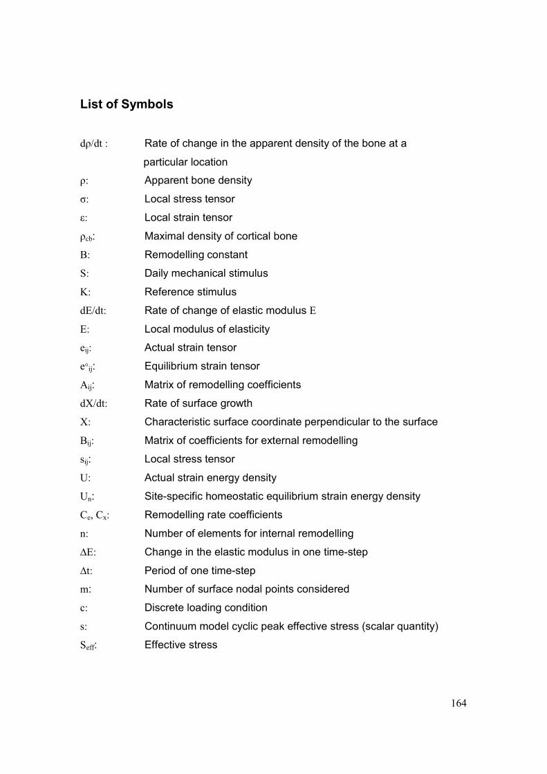
164
List of Symbols
dρ/dt : Rate of change in the apparent density of the bone at a
particular location
ρ: Apparent bone density
σ: Local stress tensor
ε: Local strain tensor
ρcb: Maximal density of cortical bone
B: Remodelling constant
S: Daily mechanical stimulus
K: Reference stimulus
dE/dt: Rate of change of elastic modulus E
E: Local modulus of elasticity
eij: Actual strain tensor
e°ij: Equilibrium strain tensor
Aij: Matrix of remodelling coefficients
dX/dt: Rate of surface growth
X: Characteristic surface coordinate perpendicular to the surface
Bij: Matrix of coefficients for external remodelling
sij: Local stress tensor
U: Actual strain energy density
Un: Site-specific homeostatic equilibrium strain energy density
Ce, Cx: Remodelling rate coefficients
n: Number of elements for internal remodelling
∆E: Change in the elastic modulus in one time-step
∆t: Period of one time-step
m: Number of surface nodal points considered
c: Discrete loading condition
s: Continuum model cyclic peak effective stress (scalar quantity)
Seff: Effective stress

List of Symbols
165
D: Constant
U/ρ: Mechanical daily stimulus
w: Half-width of the dead zone
C: Constant
ρ0: Initial density of the bone
σ1: Lower critical stress
σ2: Upper critical stress
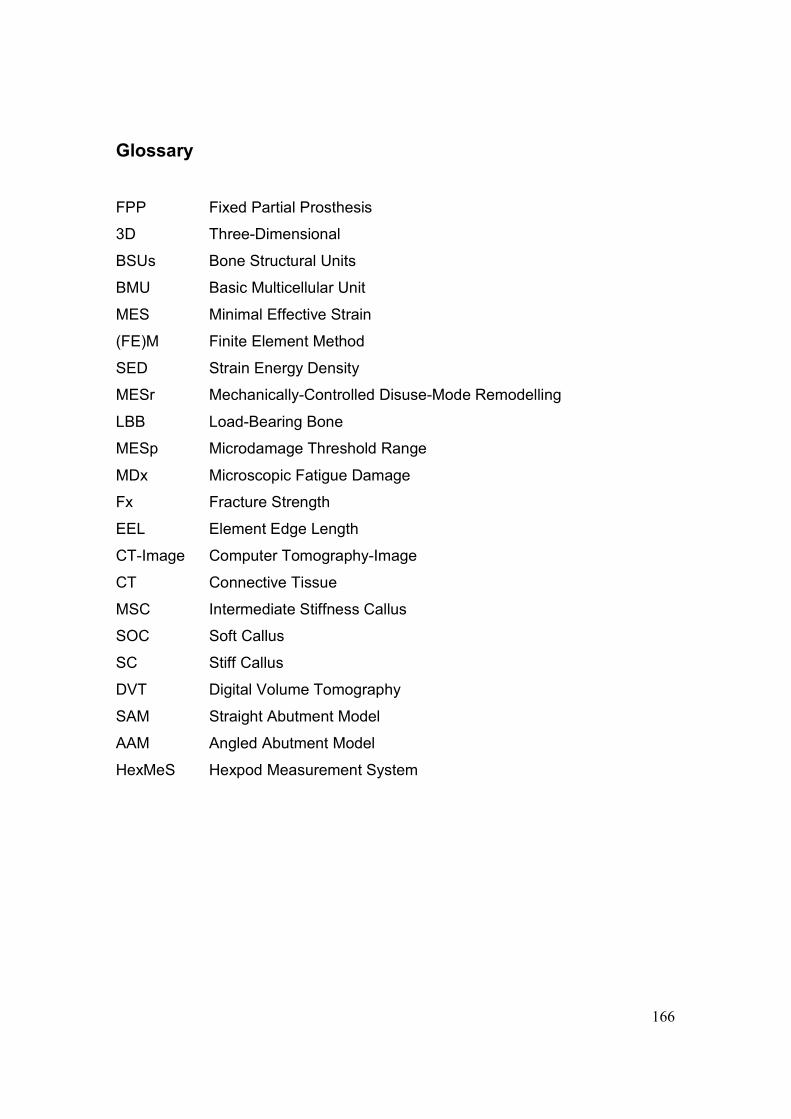
166
Glossary
FPP Fixed Partial Prosthesis
3D Three-Dimensional
BSUs Bone Structural Units
BMU Basic Multicellular Unit
MES Minimal Effective Strain
(FE)M Finite Element Method
SED Strain Energy Density
MESr Mechanically-Controlled Disuse-Mode Remodelling
LBB Load-Bearing Bone
MESp Microdamage Threshold Range
MDx Microscopic Fatigue Damage
Fx Fracture Strength
EEL Element Edge Length
CT-Image Computer Tomography-Image
CT Connective Tissue
MSC Intermediate Stiffness Callus
SOC Soft Callus
SC Stiff Callus
DVT Digital Volume Tomography
SAM Straight Abutment Model
AAM Angled Abutment Model
HexMeS Hexpod Measurement System