
Crystal Phases and Glassy Dynamics in Monodisperse Hard ... · theorie (MCT) veriz iert werden...
139
Institut für Physik Mainz, den 5. November 2008 Crystal Phases and Glassy Dynamics in Monodisperse Hard Ellipsoids "Doktor der Naturwissenschaften" Patrick Pfleiderer geb. in Nürnberg Johannes Gutenberg-Universität Mainz am Fachbereich Physik der Johannes Gutenberg-Universität in Mainz zur Erlangung des Grades Dissertation
Transcript of Crystal Phases and Glassy Dynamics in Monodisperse Hard ... · theorie (MCT) veriz iert werden...
Institut für Physik
Mainz, den 5. November 2008
Crystal Phases and Glassy Dynamicsin Monodisperse Hard Ellipsoids
"Doktor der Naturwissenschaften"
Patrick Pfleiderer
geb. in Nürnberg
Johannes Gutenberg−Universität Mainz
am Fachbereich Physik derJohannes Gutenberg−Universität in Mainz
zur Erlangung des GradesDissertation

Erstberichter:Zweitberichter:Tag der mündlichen Prüfung: 9. Februar 2009
Parts of this thesis have already been published in:
• P. Pfleiderer, K. Milinkovic, and T. SchillingGlassy dynamics in monodisperse hard ellipsoidsEurophys. Letters84, 16003 (2008).
• P. Pfleiderer and T. SchillingSimple monoclinic crystal phase in suspensions of hard ellipsoidsPhys. Rev. E75, 020402(R) (2007).
D77
Zusammenfassung
Wir haben Monte Carlo undMolekulardynamik-Simulationen an Suspensionenmonodisperser, harter Ellipsoide durchgeführt. Harte-Teilchen-Modelle spieleneine Schlüsselrolle in der Statistischen Mechanik. Sie sind einfach und erlaubenEinblicke in Systeme, in denen die Form der Teilchen wichtigist, einschließlichatomarer, molekularer, kolloidaler und granularer Systeme.
Im Phasendiagramm prolater Ellipsoide fanden wir bei hohenDichten eineneue Kristallphase, die stabiler ist als die bislang bekannte gestreckte FCC-Phase[1]. Die neue Phase, SM2, ist simpel-monoklin mit einer Basis von zwei Ellip-soiden, die ungleiche Orientierungen haben. Der Neigungswinkelβ ist sehr weichbei Länge-zu-Breite-Verhältnis (Aspekt-Verhältnis)l/w = 3, wohingegen die an-deren beiden Winkel nicht weich sind. Es gibt eine symmetrische Anordnung derEinheitszelle. Diese wurde in Verbindung gebracht mit den dichtesten bekanntenPackungen von Ellipsoiden [2]; sie ist nicht immer die stabilste. Die gestreckteFCC-Phase wird also beim Aspekt-Verhältnisl/w = 3 durch SM2 ersetzt, sehrwahrscheinlich auch bei 3≤ l/w≤ 6, und vermutlich auch jenseits dieser Gren-zen. Außerdem zeigen die Ellipsoide in SM2 beil/w= 1.55 180-Drehungen, dieeiner näheren Untersuchung, z.B. des Einfrierens dieser Dynamik, würdig sind.
Zweitens haben wir die Dynamik fast kugelförmiger Ellipsoide untersucht. ImGleichgewicht zeigen sie einen Phasenübergang erster Ordnung von der isotropenPhase in eine Rotatorphase, in der die Positionen kristallin und die Orientierun-gen frei sind. Bei Überkomprimierung der isotropen Phase inden Bereich derRotatorphase haben wir Super-Arrhenius-Verlangsamung der Diffusion und Re-laxation, und Signaturen des Käfig-Effekts beobachtet. Diese Merkmale vonGlasdynamik sind so deutlich, dass asymptotische Gesetze der Modenkopplungs-theorie (MCT) verifiziert werden konnten. Translatorischeund Orientierungs-freiheitsgrade sind stark gekoppelt, mit der Konsequenz, dass ein gemeinsamerMCT-Glasübergangs-Volumenbruchφc existiert (l/w= 1.25: φc = 0.615±0.005,l/w = 0.80: φc = 0.618±0.005). 180-Drehungen sind dagegen nicht betroffen.Unsere Resultate hängen nicht von der Simulationsmethode ab, wie von der MCTvorhergesagt. Bereits die Bewegung innerhalb der Käfige istkooperativ. Dy-namische Heterogenitäten wurden auch nachgewiesen. Der Transit zwischen Kä-figen findet zwar in kurzen Zeitspannen statt, jedoch zeigt erkeine von der Bewe-gung innerhalb der Käfige unterscheidbare Verschiebungen.Die Existenz glasigerDynamik war durch molekulare MCT [3] (MMCT) vorhergesagt worden, jedochignoriert MMCT Kristallisation; ein Test per Simulation war nötig. Kristallisationverhindert typischerweise Glasdynamik in monodispersen Systemen. Polydisper-sität oder andere Asymmetrien sind nötig, um die Kristallisation zu unterbinden.Also fungiert die Anisometrie der Teilchen als Quelle von Unordnung. Dies wirftein neues Licht auf die Bedingungen zur Glasbildung.
Abstract
We have performed Monte Carlo and molecular dynamics simulations of suspen-sions of monodisperse, hard ellipsoids of revolution. Hard-particle models playa key role in statistical mechanics. They are conceptually and computationallysimple, and they offer insight into systems in which particle shape is important,including atomic, molecular, colloidal, and granular systems.
In the high density phase diagram of prolate hard ellipsoidswe have founda new crystal, which is more stable than the stretched FCC structure proposedpreviously [1]. The new phase, SM2, has a simple monoclinic unit cell containinga basis of two ellipsoids with unequal orientations. The angle of inclination,β , isvery soft for length-to-width (aspect) ratiol/w= 3, while the other angles are not.A symmetric state of the unit cell exists, related to the densest-known packingsof ellipsoids [2]; it is not always the stable one. Our results remove the stretchedFCC structure for aspect ratiol/w = 3 from the phase diagram of hard, uni-axialellipsoids. We provide evidence that this holds for 3≤ l/w ≤ 6, and possiblybeyond. Finally, ellipsoids in SM2 atl/w = 1.55 exhibit end-over-end flipping,warranting studies of the cross-over to where this dynamicsis not possible.
Secondly, we studied the dynamics of nearly spherical ellipsoids. In equilib-rium, they show a first-order transition from an isotropic phase to a rotator phase,where positions are crystalline but orientations are free.When over-compressingthe isotropic phase into the rotator regime, we observed super-Arrhenius slow-ing down of diffusion and relaxation, and signatures of the cage effect. Thesefeatures of glassy dynamics are sufficiently strong that asymptotic scaling lawsof the Mode-Coupling Theory of the glass transition (MCT) could be tested, andwere found to apply. We found strong coupling of positional and orientational de-grees of freedom, leading to a common value for the MCT glass-transition volumefraction φc (l/w = 1.25: φc = 0.615±0.005, l/w = 0.80: φc = 0.618±0.005).Flipping modes were not slowed down significantly. We demonstrated that theresults are independent of simulation method, as predictedby MCT. Further, wedetermined that even intra-cage motion is cooperative. We confirmed the presenceof dynamical heterogeneities associated with the cage effect. The transit betweencages was seen to occur on short time scales, compared to the time spent in cages;but the transit was shown not to involve displacements distinguishable in charac-ter from intra-cage motion. The presence of glassy dynamicswas predicted byMMCT [3]. However, as MMCT disregards crystallization, a test by simulationwas required. Glassy dynamics is unusual in monodisperse systems. Crystalliza-tion typically intervenes unless polydispersity, network-forming bonds or otherasymmetries are introduced. We argue that particle anisometry acts as a sufficientsource of disorder to prevent crystallization. This sheds new light on the questionof which ingredients are required for glass formation.

Contents
1 Introduction 11.1 Colloidal Suspensions . . . . . . . . . . . . . . . . . . . . . . . . 11.2 Hard-Particle Models . . . . . . . . . . . . . . . . . . . . . . . . 21.3 Hard Ellipsoids of Revolution . . . . . . . . . . . . . . . . . . . 4
1.3.1 Definition . . . . . . . . . . . . . . . . . . . . . . . . . . 41.3.2 Earlier Work . . . . . . . . . . . . . . . . . . . . . . . . 5
1.3.2.1 Equilibrium Results . . . . . . . . . . . . . . . 51.3.2.2 Close-Packing . . . . . . . . . . . . . . . . . . 71.3.2.3 Dynamics . . . . . . . . . . . . . . . . . . . . 101.3.2.4 Experiment . . . . . . . . . . . . . . . . . . . 11
1.4 Glasses . . . . . . . . . . . . . . . . . . . . . . . . . . . . . . . 141.4.1 Overview . . . . . . . . . . . . . . . . . . . . . . . . . . 141.4.2 The Mode-Coupling Theory of the Glass Transition . . . .15
2 Simulation - Theory and Technique 232.1 Monte Carlo Simulation (MC) . . . . . . . . . . . . . . . . . . . 23
2.1.1 General Features . . . . . . . . . . . . . . . . . . . . . . 232.1.2 Constant-Pressure-and-Tension Ensemble . . . . . . . . .24
2.1.2.1 Partition Function . . . . . . . . . . . . . . . . 252.1.2.2 Monte Carlo Moves . . . . . . . . . . . . . . . 29
2.1.3 Other Monte Carlo Versions . . . . . . . . . . . . . . . . 312.1.4 Testing for Overlaps . . . . . . . . . . . . . . . . . . . . 32
2.2 Molecular Dynamics Simulation (MD) . . . . . . . . . . . . . . . 322.2.1 General Features . . . . . . . . . . . . . . . . . . . . . . 322.2.2 Event-driven MD . . . . . . . . . . . . . . . . . . . . . . 33
3 Simple Monoclinic Crystal Phase 353.1 Overview of Simulations . . . . . . . . . . . . . . . . . . . . . . 353.2 The SM2 Phase at Aspect Ratio 3 . . . . . . . . . . . . . . . . . 38
3.2.1 Characterization of Structure . . . . . . . . . . . . . . . . 383.2.2 Close-Packing Limit . . . . . . . . . . . . . . . . . . . . 41
viii
3.2.3 Softness of Inclination . . . . . . . . . . . . . . . . . . . 433.2.4 Equation of State Data . . . . . . . . . . . . . . . . . . . 45
3.3 Other Aspect Ratios and Phase Diagram . . . . . . . . . . . . . . 463.3.1 Aspect Ratios Greater Than 3 . . . . . . . . . . . . . . . 463.3.2 Aspect Ratios Smaller Than 3 . . . . . . . . . . . . . . . 483.3.3 Phase Diagram . . . . . . . . . . . . . . . . . . . . . . . 493.3.4 Flipping Mode in SM2 at Aspect Ratio 1.55 . . . . . . . . 51
3.4 Summary . . . . . . . . . . . . . . . . . . . . . . . . . . . . . . 51
4 Glassy Dynamics in Almost Spherical Ellipsoids 554.1 Overview of Simulations . . . . . . . . . . . . . . . . . . . . . . 554.2 Structure . . . . . . . . . . . . . . . . . . . . . . . . . . . . . . . 60
4.2.1 Local Order: Pair Correlation Function . . . . . . . . . . 604.2.2 Intermediate Range: Static Structure Factors . . . . . .. 60
4.3 Average Dynamics . . . . . . . . . . . . . . . . . . . . . . . . . 624.3.1 Mean Squared Displacement and Diffusion . . . . . . . . 624.3.2 Relaxation . . . . . . . . . . . . . . . . . . . . . . . . . 64
4.3.2.1 Intermediate Scattering Functions . . . . . . . . 644.3.2.2 Orientational Correlation Functions . . . . . . . 69
4.3.3 Slowing-down of Diffusion and Relaxation . . . . . . . . 714.3.4 Testing Mode-Coupling Theory . . . . . . . . . . . . . . 71
4.3.4.1 MD vs. MC . . . . . . . . . . . . . . . . . . . 754.3.4.2 Time-Volume Fraction Superposition Principle . 754.3.4.3 Von Schweidler Law and Factorization Property 794.3.4.4 MCT Glass Transition Volume Fraction . . . . . 84
4.4 Heterogeneous Dynamics . . . . . . . . . . . . . . . . . . . . . . 864.4.1 Non-Gaussian Parameter . . . . . . . . . . . . . . . . . . 864.4.2 Jumps . . . . . . . . . . . . . . . . . . . . . . . . . . . . 88
4.5 Summary . . . . . . . . . . . . . . . . . . . . . . . . . . . . . . 91
A Corrected Constant-Pressure Ensemble 97
Bibliography 101
List of Figures
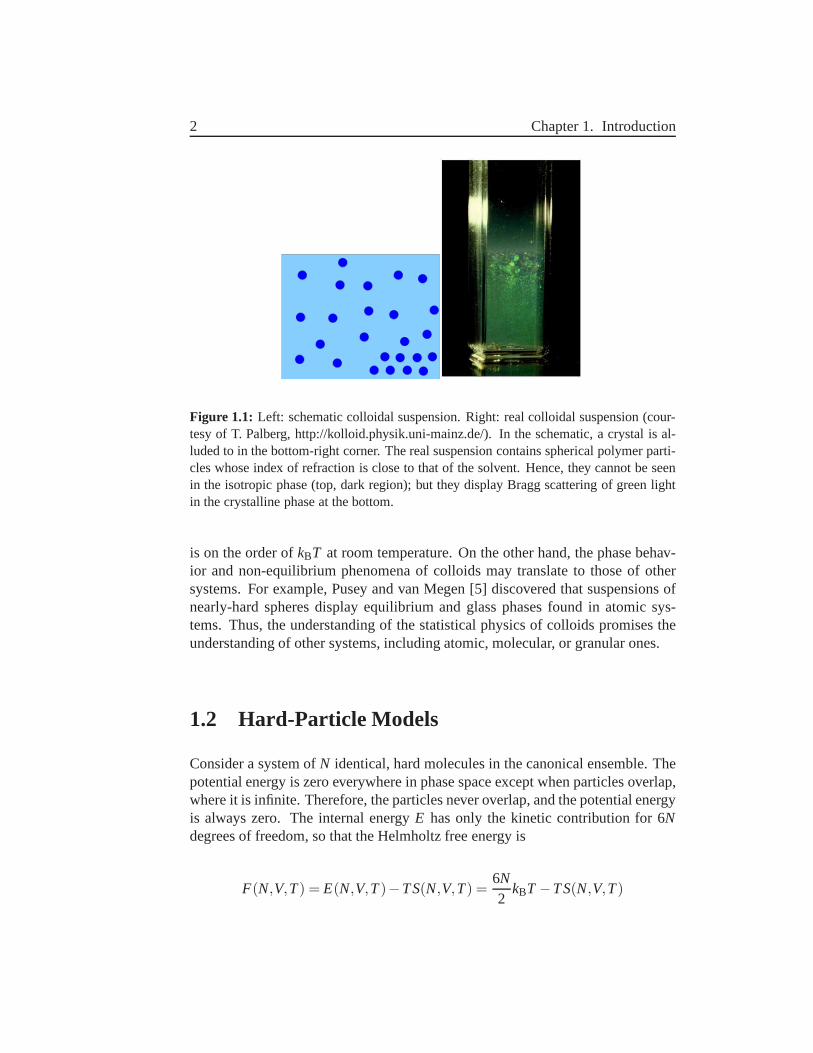
1.1 Left: schematic colloidal suspension. Right: real colloidal sus-pension (courtesy of T. Palberg, http://kolloid.physik.uni-mainz.de/).In the schematic, a crystal is alluded to in the bottom-rightcorner.The real suspension contains spherical polymer particles whoseindex of refraction is close to that of the solvent. Hence, theycannot be seen in the isotropic phase (top, dark region); buttheydisplay Bragg scattering of green light in the crystalline phase atthe bottom. . . . . . . . . . . . . . . . . . . . . . . . . . . . . . 2
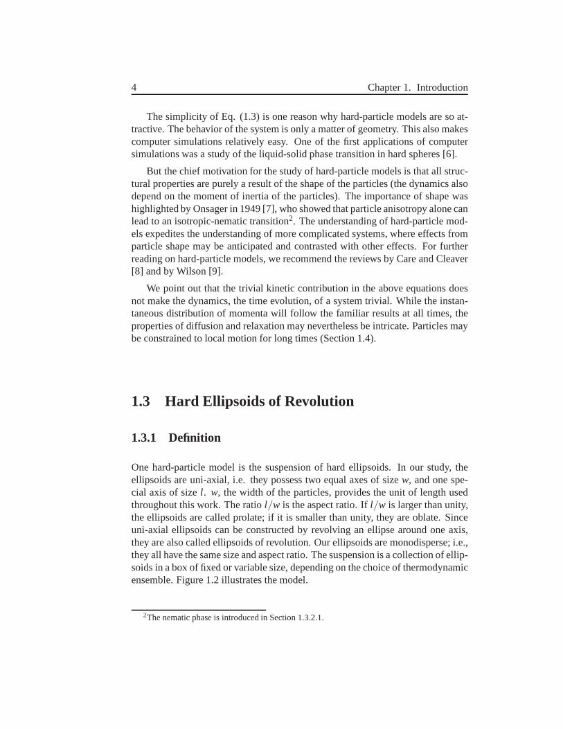
1.2 Ellipsoids of revolution. . . . . . . . . . . . . . . . . . . . . . . . 5
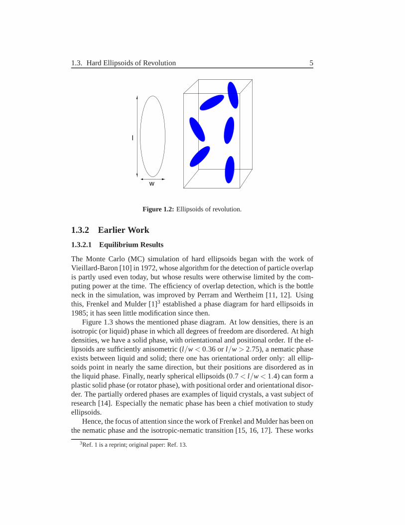
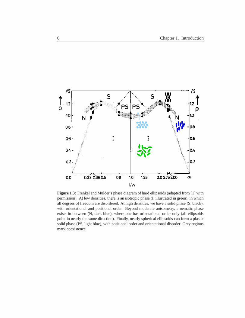
1.3 Frenkel and Mulder’s phase diagram of hard ellipsoids (adaptedfrom [1] with permission). At low densities, there is an isotropicphase (I, illustrated in green), in which all degrees of freedom aredisordered. At high densities, we have a solid phase (S, black),with orientational and positional order. Beyond moderate anisom-etry, a nematic phase exists in between (N, dark blue), whereonehas orientational order only (all ellipsoids point in nearly the samedirection). Finally, nearly spherical ellipsoids can forma plasticsolid phase (PS, light blue), with positional order and orientationaldisorder. Grey regions mark coexistence. . . . . . . . . . . . . . 6
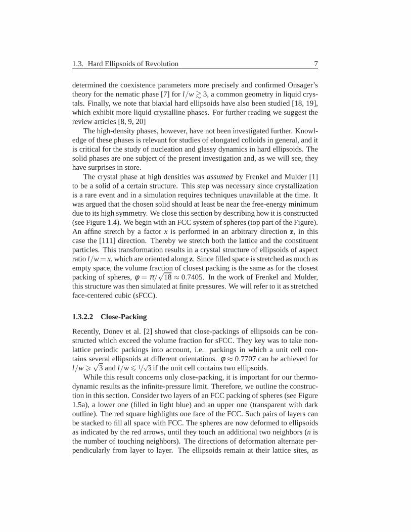
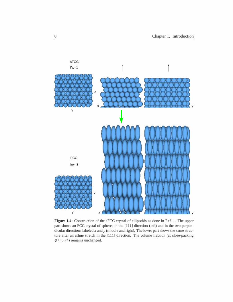
1.4 Construction of the sFCC crystal of ellipsoids as done inRef. 1.The upper part shows an FCC crystal of spheres in the [111] di-rection (left) and in the two perpendicular directions labeledx andy (middle and right). The lower part shows the same structure af-ter an affine stretch in the [111] direction. The volume fraction (atclose-packingφ ≈ 0.74) remains unchanged. . . . . . . . . . . . 8
x List of Figures
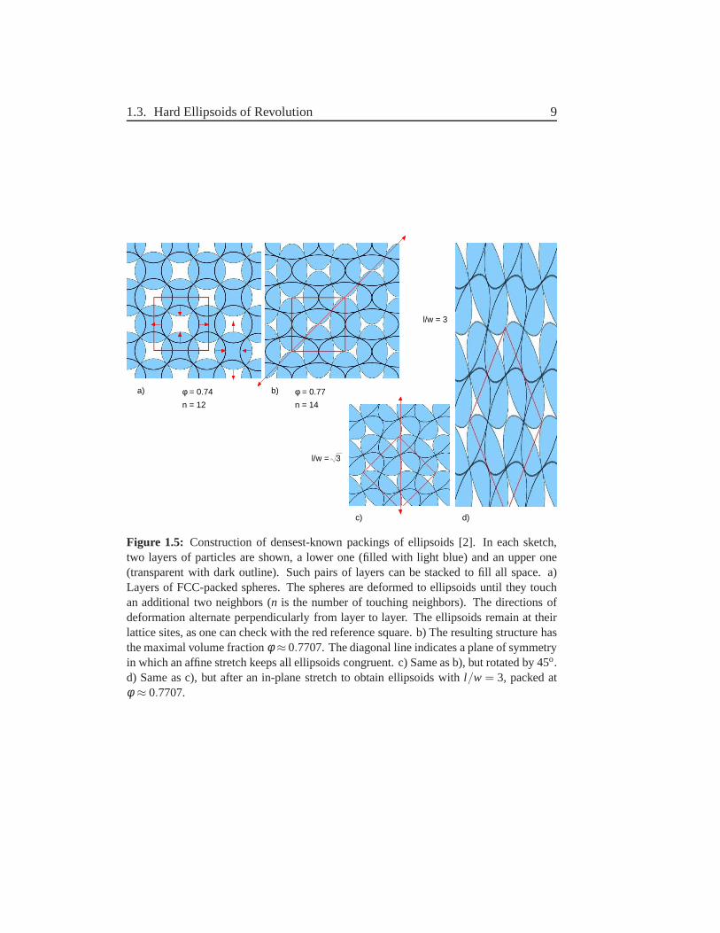
1.5 Construction of densest-known packings of ellipsoids [2]. In eachsketch, two layers of particles are shown, a lower one (filledwithlight blue) and an upper one (transparent with dark outline). Suchpairs of layers can be stacked to fill all space. a) Layers of FCC-packed spheres. The spheres are deformed to ellipsoids until theytouch an additional two neighbors (n is the number of touchingneighbors). The directions of deformation alternate perpendicu-larly from layer to layer. The ellipsoids remain at their lattice sites,as one can check with the red reference square. b) The resultingstructure has the maximal volume fractionφ ≈ 0.7707. The diag-onal line indicates a plane of symmetry in which an affine stretchkeeps all ellipsoids congruent. c) Same as b), but rotated by45o.d) Same as c), but after an in-plane stretch to obtain ellipsoidswith l/w = 3, packed atφ ≈ 0.7707. . . . . . . . . . . . . . . . 9
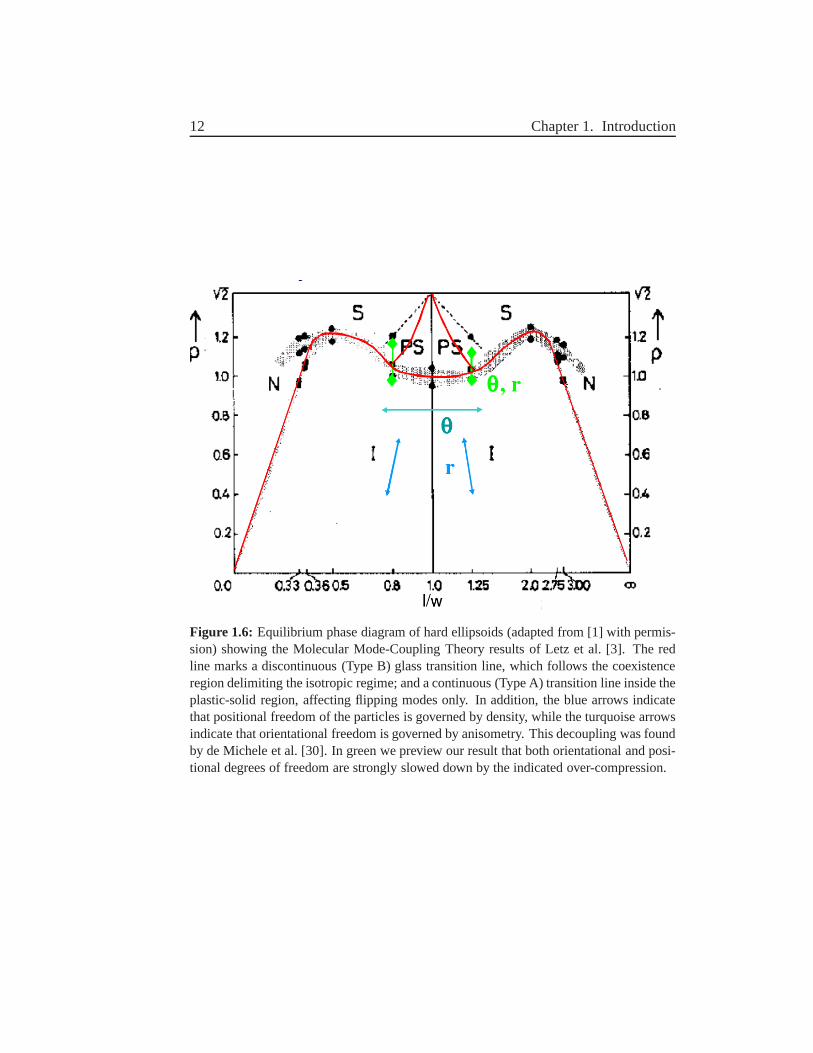
1.6 Equilibrium phase diagram of hard ellipsoids (adapted from [1]with permission) showing the Molecular Mode-Coupling Theoryresults of Letz et al. [3]. The red line marks a discontinuous(TypeB) glass transition line, which follows the coexistence region de-limiting the isotropic regime; and a continuous (Type A) transi-tion line inside the plastic-solid region, affecting flipping modesonly. In addition, the blue arrows indicate that positionalfree-dom of the particles is governed by density, while the turquoisearrows indicate that orientational freedom is governed by anisom-etry. This decoupling was found by de Michele et al. [30]. Ingreen we preview our result that both orientational and positionaldegrees of freedom are strongly slowed down by the indicatedover-compression. . . . . . . . . . . . . . . . . . . . . . . . . . . 12
1.7 Micrograph of polystyrene ellipsoids (l/w≈ 2.5, w≈ 3µm), pre-pared by the author during a visit to the group of Prof. Jan Ver-mant (Katholieke Universiteit Leuven). . . . . . . . . . . . . . . 14
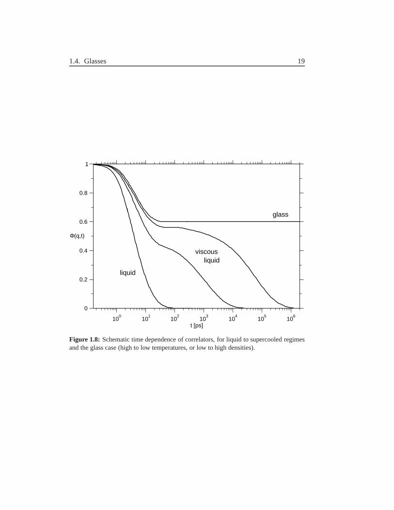
1.8 Schematic time dependence of correlators, for liquid tosuper-cooled regimes and the glass case (high to low temperatures,orlow to high densities). . . . . . . . . . . . . . . . . . . . . . . . . 19
2.1 Illustration of Monte Carlo moves. In addition to particle moves,changes of the box shape are indicated. Left: Constant-pressureMC. Right: Constant-pressure-and-tension MC. . . . . . . . . . .30
3.1 Top: Constructed sFCC (cf. Figure 1.4) which was input. Bottom:Snapshot of the SM2 crystal which spontaneously formed fromit.The color code distinguishes orientations. . . . . . . . . . . . . .39
List of Figures xi
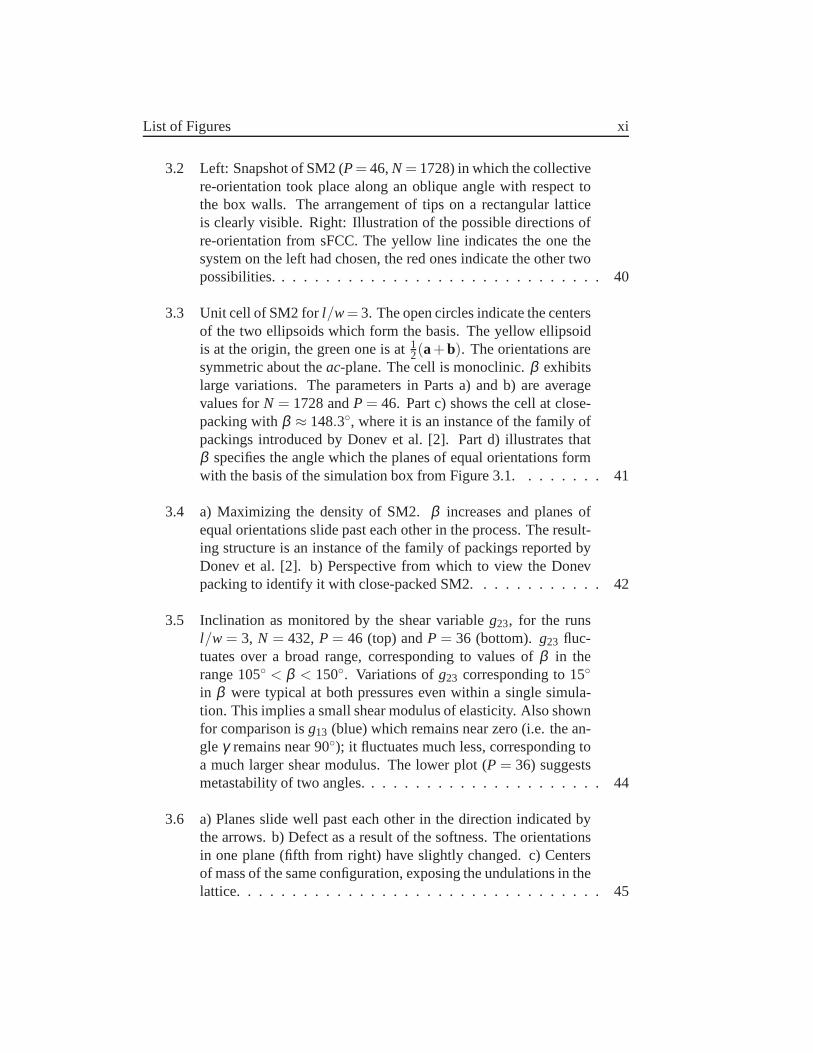
3.2 Left: Snapshot of SM2 (P= 46,N = 1728) in which the collectivere-orientation took place along an oblique angle with respect tothe box walls. The arrangement of tips on a rectangular latticeis clearly visible. Right: Illustration of the possible directions ofre-orientation from sFCC. The yellow line indicates the onethesystem on the left had chosen, the red ones indicate the othertwopossibilities. . . . . . . . . . . . . . . . . . . . . . . . . . . . . . 40
3.3 Unit cell of SM2 forl/w= 3. The open circles indicate the centersof the two ellipsoids which form the basis. The yellow ellipsoidis at the origin, the green one is at1
2(a+b). The orientations aresymmetric about theac-plane. The cell is monoclinic.β exhibitslarge variations. The parameters in Parts a) and b) are averagevalues forN = 1728 andP = 46. Part c) shows the cell at close-packing withβ ≈ 148.3, where it is an instance of the family ofpackings introduced by Donev et al. [2]. Part d) illustratesthatβ specifies the angle which the planes of equal orientations formwith the basis of the simulation box from Figure 3.1. . . . . . . .41
3.4 a) Maximizing the density of SM2.β increases and planes ofequal orientations slide past each other in the process. Theresult-ing structure is an instance of the family of packings reported byDonev et al. [2]. b) Perspective from which to view the Donevpacking to identify it with close-packed SM2. . . . . . . . . . . . 42
3.5 Inclination as monitored by the shear variableg23, for the runsl/w = 3, N = 432,P = 46 (top) andP = 36 (bottom).g23 fluc-tuates over a broad range, corresponding to values ofβ in therange 105 < β < 150. Variations ofg23 corresponding to 15in β were typical at both pressures even within a single simula-tion. This implies a small shear modulus of elasticity. Alsoshownfor comparison isg13 (blue) which remains near zero (i.e. the an-gle γ remains near 90); it fluctuates much less, corresponding toa much larger shear modulus. The lower plot (P = 36) suggestsmetastability of two angles. . . . . . . . . . . . . . . . . . . . . . 44
3.6 a) Planes slide well past each other in the direction indicated bythe arrows. b) Defect as a result of the softness. The orientationsin one plane (fifth from right) have slightly changed. c) Centersof mass of the same configuration, exposing the undulations in thelattice. . . . . . . . . . . . . . . . . . . . . . . . . . . . . . . . . 45
xii List of Figures
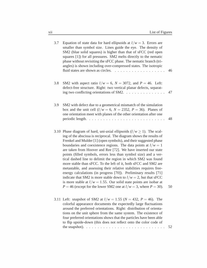
3.7 Equation of state data for hard ellipsoids atl/w = 3. Errors aresmaller than symbol size. Lines guide the eye. The density ofSM2 (blue solid squares) is higher than that of sFCC (red opensquares [1]) for all pressures. SM2 melts directly to the nematicphase without revisiting the sFCC phase. The nematic branch(tri-angles) is shown including over-compressed states. The isotropicfluid states are shown as circles. . . . . . . . . . . . . . . . . . . 46
3.8 SM2 with aspect ratiol/w = 6, N = 3072, andP = 46. Left:defect-free structure. Right: two vertical planar defects, separat-ing two conflicting orientations of SM2. . . . . . . . . . . . . . . 47
3.9 SM2 with defect due to a geometrical mismatch of the simulationbox and the unit cell (l/w = 6, N = 2352, P = 36). Planes ofone orientation meet with planes of the other orientation after oneperiodic length. . . . . . . . . . . . . . . . . . . . . . . . . . . . 48
3.10 Phase diagram of hard, uni-axial ellipsoids (l/w≥ 1). The scal-ing of the abscissa is reciprocal. The diagram shows the results ofFrenkel and Mulder [1] (open symbols), and their suggested phaseboundaries and coexistence regions. The data points atl/w = 1are taken from Hoover and Ree [72]. We have inserted our statepoints (filled symbols, errors less than symbol size) and a ver-tical dashed line to delimit the region in which SM2 was foundmore stable than sFCC. To the left of it, both sFCC and SM2 aremetastable, and assessing their relative stabilities requires free-energy calculations (in progress [70]). Preliminary results [71]indicate that SM2 is more stable down tol/w = 2, but that sFCCis more stable atl/w = 1.55. Our solid state points are isobar atP = 46 (except for the lower SM2 one atl/w = 3, whereP = 30). 50
3.11 Left: snapshot of SM2 atl/w = 1.55 (N = 432, P = 46). Thecolorful appearance documents the expectedly large fluctuationsaround the preferred orientations. Right: distribution oforienta-tions on the unit sphere from the same system. The existence offour preferred orientations shows that the particles have been ableto flip upside-down (this does not reflect onto the color code ofthe snapshot). . . . . . . . . . . . . . . . . . . . . . . . . . . . . 52
List of Figures xiii
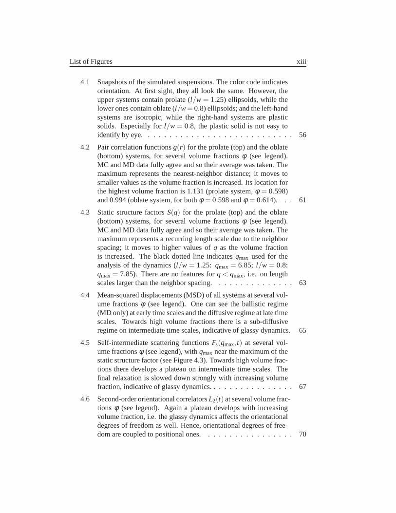
4.1 Snapshots of the simulated suspensions. The color code indicatesorientation. At first sight, they all look the same. However,theupper systems contain prolate (l/w = 1.25) ellipsoids, while thelower ones contain oblate (l/w= 0.8) ellipsoids; and the left-handsystems are isotropic, while the right-hand systems are plasticsolids. Especially forl/w = 0.8, the plastic solid is not easy toidentify by eye. . . . . . . . . . . . . . . . . . . . . . . . . . . . 56
4.2 Pair correlation functionsg(r) for the prolate (top) and the oblate(bottom) systems, for several volume fractionsφ (see legend).MC and MD data fully agree and so their average was taken. Themaximum represents the nearest-neighbor distance; it moves tosmaller values as the volume fraction is increased. Its location forthe highest volume fraction is 1.131 (prolate system,φ = 0.598)and 0.994 (oblate system, for bothφ = 0.598 andφ = 0.614). . . 61
4.3 Static structure factorsS(q) for the prolate (top) and the oblate(bottom) systems, for several volume fractionsφ (see legend).MC and MD data fully agree and so their average was taken. Themaximum represents a recurring length scale due to the neighborspacing; it moves to higher values ofq as the volume fractionis increased. The black dotted line indicatesqmax used for theanalysis of the dynamics (l/w = 1.25: qmax = 6.85; l/w = 0.8:qmax = 7.85). There are no features forq < qmax, i.e. on lengthscales larger than the neighbor spacing. . . . . . . . . . . . . . . 63
4.4 Mean-squared displacements (MSD) of all systems at several vol-ume fractionsφ (see legend). One can see the ballistic regime(MD only) at early time scales and the diffusive regime at late timescales. Towards high volume fractions there is a sub-diffusiveregime on intermediate time scales, indicative of glassy dynamics. 65
4.5 Self-intermediate scattering functionsFs(qmax, t) at several vol-ume fractionsφ (see legend), withqmax near the maximum of thestatic structure factor (see Figure 4.3). Towards high volume frac-tions there develops a plateau on intermediate time scales.Thefinal relaxation is slowed down strongly with increasing volumefraction, indicative of glassy dynamics. . . . . . . . . . . . . . . .67
4.6 Second-order orientational correlatorsL2(t) at several volume frac-tions φ (see legend). Again a plateau develops with increasingvolume fraction, i.e. the glassy dynamics affects the orientationaldegrees of freedom as well. Hence, orientational degrees offree-dom are coupled to positional ones. . . . . . . . . . . . . . . . . 70
xiv List of Figures
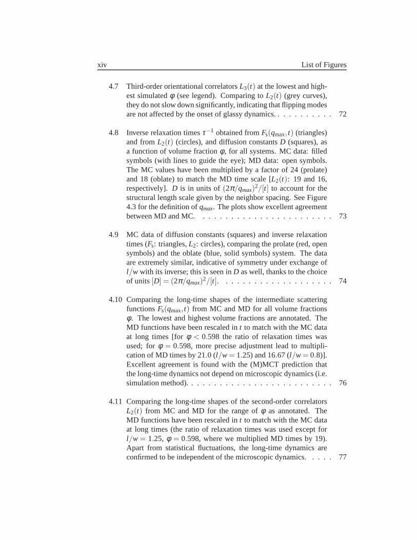
4.7 Third-order orientational correlatorsL3(t) at the lowest and high-est simulatedφ (see legend). Comparing toL2(t) (grey curves),they do not slow down significantly, indicating that flippingmodesare not affected by the onset of glassy dynamics. . . . . . . . . . .72
4.8 Inverse relaxation timesτ−1 obtained fromFs(qmax, t) (triangles)and fromL2(t) (circles), and diffusion constantsD (squares), asa function of volume fractionφ , for all systems. MC data: filledsymbols (with lines to guide the eye); MD data: open symbols.The MC values have been multiplied by a factor of 24 (prolate)and 18 (oblate) to match the MD time scale [L2(t): 19 and 16,respectively].D is in units of(2π/qmax)2/[t] to account for thestructural length scale given by the neighbor spacing. See Figure4.3 for the definition ofqmax. The plots show excellent agreementbetween MD and MC. . . . . . . . . . . . . . . . . . . . . . . . 73
4.9 MC data of diffusion constants (squares) and inverse relaxationtimes (Fs: triangles,L2: circles), comparing the prolate (red, opensymbols) and the oblate (blue, solid symbols) system. The dataare extremely similar, indicative of symmetry under exchange ofl/w with its inverse; this is seen inD as well, thanks to the choiceof units[D] = (2π/qmax)2/[t]. . . . . . . . . . . . . . . . . . . . 74
4.10 Comparing the long-time shapes of the intermediate scatteringfunctionsFs(qmax, t) from MC and MD for all volume fractionsφ . The lowest and highest volume fractions are annotated. TheMD functions have been rescaled int to match with the MC dataat long times [forφ < 0.598 the ratio of relaxation times wasused; forφ = 0.598, more precise adjustment lead to multipli-cation of MD times by 21.0 (l/w = 1.25) and 16.67 (l/w = 0.8)].Excellent agreement is found with the (M)MCT prediction thatthe long-time dynamics not depend on microscopic dynamics (i.e.simulation method). . . . . . . . . . . . . . . . . . . . . . . . . . 76
4.11 Comparing the long-time shapes of the second-order correlatorsL2(t) from MC and MD for the range ofφ as annotated. TheMD functions have been rescaled int to match with the MC dataat long times (the ratio of relaxation times was used except forl/w = 1.25, φ = 0.598, where we multiplied MD times by 19).Apart from statistical fluctuations, the long-time dynamics areconfirmed to be independent of the microscopic dynamics. . . .. 77
List of Figures xv
4.12 Comparing the long-time shapes of the intermediate scatteringfunctions from MC and MD, forφ = 0.598 and wave vectors inthe range 2.8≤ qw≤ 18. The MD functions of each system havebeen rescaled int by one common factor to match with the MCdata at long times (l/w = 1.25: multiplied by 21.0; l/w = 0.8:multiplied by 16.67). The shapes match well over this wide rangeof wave vectors after 105 time units, even for the case ofl/w =1.25 which has poor statistics. . . . . . . . . . . . . . . . . . . . 78
4.13 Time-volume fraction superposition principle forFs(qmax, t). Allcurves have been rescaled by their relaxation timeτ to checkwhether a master curve results, as MCT predicts for the vicinityof the glass transition. Two curves seem to violate the prediction:the cyan one inl/w = 1.25 MC (φ = 0.598), and the black one inl/w= 0.80 MC (φ = 0.606). The deviation of both is of statisticalorigin, and the deviation of the former is aggravated by the uncer-tainty due to extrapolation when determiningτ. The two outliersdo not change the conclusion that the superposition principle holds. 80
4.14 Time-volume fraction superposition principle forL2(t). All curveshave been rescaled by their relaxation time to check whetheramaster curve results, as MMCT predicts for the vicinity of theglass transition. In the MD data, some of the lowest volumefractions’ curves are not considered as the near-vanishingplateaumade it impossible to extract the relaxation time. The MMCTprediction is clearly confirmed. . . . . . . . . . . . . . . . . . . . 81
4.15 Upper panels:Fs(q, t) for l/w= 1.25 and the highest volume frac-tion φ = 0.598, and forq-vectors (from top) 2.8, 4.0, 5.5, 7.1,8.1, 10.1, 12.1, 14.1, 18.1. The red lines show examples of the
von Schweidler fitFs(q, t) = fq−h(1)q tb + h(2)
q t2b with b = 0.65.Lower panels: the same correlators after transformation toR(t) =[Fs(q, t)− Fs(q, t1)]/[Fs(q, t2)− Fs(q, t1)], demonstrating the fac-torization property. The color code, distinguishing wave vectors,shows that the curves remain ordered, i.e. a curve which is aboveanother one before the collapse is above the other one after aswell. . . . . . . . . . . . . . . . . . . . . . . . . . . . . . . . . 82
4.16 Same as Figure 4.15, but forl/w = 0.80; φ = 0.614 for MC andφ = 0.598 for MD. . . . . . . . . . . . . . . . . . . . . . . . . . 83
xvi List of Figures
4.17 q-dependence of the fit parameters in the von Schweidler law
Fs(q, t) = fq−h(1)q tb + h(2)
q t2b. See legend for aspect ratio, sim-
ulation method, and volume fraction.h(1)q of l/w = 1.25 (MD)
was rescaled by 16.67b, and of l/w = 0.8 (MD) by 21.0b; h(2)q
was rescaled by the squared value in each case.fq resembles aGaussian, and forφ = 0.614, l/w = 0.8 (MC) the curve can infact be well fitted, up toq = 16, by fq = exp(−r2
Lq2), with thelocalization lengthrL = 0.072 (red dashed line). Forφ = 0.598,l/w= 1.25 (MD) we show the corresponding fit (cyan dashed line,rL = 0.087) which is less satisfactory. . . . . . . . . . . . . . . . 85
4.18 τ−1/γ multiplied by arbitrary factors for clarity, fromFs(q, t) (fromtop: l/w= 1.25: qw= 6.85, 11, 16;l/w= 0.8: qw= 7.85, 16, 20)andL2 (bottom), demonstrating the validity of the MCT scalinglaw τ−1 ∝ (φc−φ)γ . The exponentγ = 2.3 was chosen in agree-ment withb = 0.65. The straight-line fits indicate a glass transi-tion volume fraction ofφc = 0.615±0.005 (prolate system) andφc = 0.618±0.005 (oblate system). MC and MD data agree. . . . 87
4.19 Non-Gaussian parameter for all systems. Towards higher volumefractions, a maximum develops, and its position on the time axiscoincides with the departure from the plateau in the intermediatescattering function. Hence, the dynamics becomes heterogeneouswhen the development of the system is governed by the cage ef-fect. When most particles escaped from their cages, the associatedlarger displacements dominate and follow a Gaussian distribution,making the non-Gaussian parameter zero again. . . . . . . . . . . 89
4.20 Trajectory of a fast particle from the MC simulation ofl/w = 0.8at φ = 0.614. Three cages can be identified, whose size agreeswith the result from the mean-squared displacement,rMSD≈0.2w.Moving to a new cage may later be followed by the return to theprevious cage. The displacements between individual positionsare of similar size within a cage and during transit. . . . . . . .. 90
4.21 Self part of the van Hove correlation function (timesr2) for sev-eral values oft, in linear (top) and semi-logarithmic (bottom)plots, from the MC simulation ofl/w= 0.8 at the highest volumefraction φ = 0.614. It is the distribution of scalar displacementsr in the intervalt. The curves are normalized to unit area. Thelargest value oft corresponds to maximal dynamical heterogene-ity, i.e. where the non-Gaussian parameter (Figure 4.19) has itsmaximum. The dotted vertical lines indicate the partitioning ofparticles according to their mobility for further analysis. . . . . . . 92
List of Figures xvii
4.22 Normalized distributions of scalar displacements during intervalsof 105 MC steps, on linear (top) and semi-logarithmic (bottom)plots, from the MC simulation ofl/w = 0.8 at the highest vol-ume fractionφ = 0.614. The particles were separated into sets ofvarious mobilities on a longer time scale (5· 106 MC steps; seealso Figure 4.21). The shape of the curves is essentially thesamefrom the fastest down to the slowest set of particles. Fast particlesshow an overall shift of their short-term displacements towardslarger values, and not the addition of few large displacements toan otherwise similar distribution. . . . . . . . . . . . . . . . . . 93

xviii List of Figures
Symbols and Units
Constants and Variables
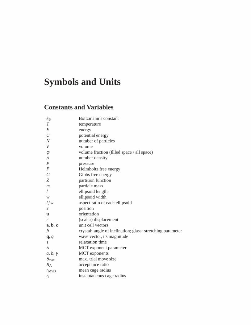
kB Boltzmann’s constantT temperatureE energyU potential energyN number of particlesV volumeφ volume fraction (filled space / all space)ρ number densityP pressureF Helmholtz free energyG Gibbs free energyZ partition functionm particle massl ellipsoid lengthw ellipsoid widthl/w aspect ratio of each ellipsoidr positionu orientationr (scalar) displacementa, b, c unit cell vectorsβ crystal: angle of inclination; glass: stretching parameterq, q wave vector, its magnitudeτ relaxation timeλ MCT exponent parametera, b, γ MCT exponentsδmax max. trial move sizeRA acceptance ratiorMSD mean cage radiusrI instantaneous cage radius
xx Symbols
Unitslength particle widthwmass particle massmmoment of inertia mw2
temperature irrelevant in hard-particle systemsenergy kBTpressure kBT/[(l/w)w3]
volume fraction dimensionlessnumber density 1/[(l/w)w3] (same as in Frenkel and Mulder [1])time (MC) MC step (see Section 2.1.3)time (MD) MD step (see Section 2.2.2)
Conversions
volume fraction =π/6 number density
AbbreviationsMC Monte CarloMD Molecular DynamicsFCC face-centered cubicsFCC stretched face-centered cubicSM2 simple-monoclinic with a basis of two ellipsoidsMSD Mean-squared displacementNGP Non-Gaussian parameterMCT Mode-Coupling TheoryMMCT Molecular Mode-Coupling Theory
Chapter 1
Introduction
1.1 Colloidal Suspensions
A colloidal suspension is any system in which particles are dissolved in a con-tinuous solvent. The particles typically have sizes from nanometers to microme-ters. With such a general definition, it comes as no surprise that there are manyexamples: In milk, there are fat droplets in water; in paint,there are pigmentsin a solvent; dust in air forms a colloidal suspension; motoroil carries metalparticles—and so on. An even more general definition includes systems whichhave any structure on theµm to nm scale, not just particles.
Instead of “colloidal suspensions”, one often simply says “colloids”. Occa-sionally, an individual particle in a suspension is called acolloid. The originalmeaning of the word is “glue-like” and comes from the Greek “kolla” (glue) and“eidos” (appearance). The term was introduced in 1861 by Thomas Graham, thereputed founder of colloid chemistry [4].
Figure 1.1 shows an illustration of a colloidal suspension (left) and a real ex-ample (right). In the schematic, we see an isotropic (disordered) phase, and inthe bottom-right corner a crystal phase is indicated. Thereexists a rich variety ofphases in colloidal suspensions, depending on the properties of the particles andthe solvent. We will encounter some more below. The real colloidal suspensionin Figure 1.1 (right) contains spherical polymer particleswhose index of refrac-tion is close to that of the solvent. Hence, they cannot be seen in the isotropicphase (top, dark region); but they display Bragg scatteringof green light in the(poly)crystalline phase at the bottom.
Apart from their beauty and interesting properties, colloidal suspensions arepopular since they allow the study of many-particle physicsin a direct way: Thesize of the particles makes them visible under the microscope, their dynamics isslow enough to be followed in experiment, and the scale of particle interactions
2 Chapter 1. Introduction
Figure 1.1: Left: schematic colloidal suspension. Right: real colloidal suspension (cour-tesy of T. Palberg, http://kolloid.physik.uni-mainz.de/). In the schematic, a crystal is al-luded to in the bottom-right corner. The real suspension contains spherical polymer parti-cles whose index of refraction is close to that of the solvent. Hence, they cannot be seenin the isotropic phase (top, dark region); but they display Bragg scattering of green lightin the crystalline phase at the bottom.
is on the order ofkBT at room temperature. On the other hand, the phase behav-ior and non-equilibrium phenomena of colloids may translate to those of othersystems. For example, Pusey and van Megen [5] discovered that suspensions ofnearly-hard spheres display equilibrium and glass phases found in atomic sys-tems. Thus, the understanding of the statistical physics ofcolloids promises theunderstanding of other systems, including atomic, molecular, or granular ones.
1.2 Hard-Particle Models
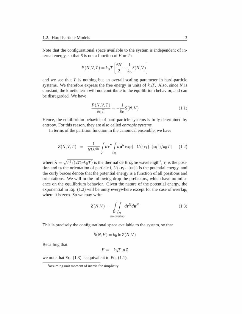
Consider a system ofN identical, hard molecules in the canonical ensemble. Thepotential energy is zero everywhere in phase space except when particles overlap,where it is infinite. Therefore, the particles never overlap, and the potential energyis always zero. The internal energyE has only the kinetic contribution for 6Ndegrees of freedom, so that the Helmholtz free energy is
F(N,V,T) = E(N,V,T)−TS(N,V,T) =6N2
kBT−TS(N,V,T)
1.2. Hard-Particle Models 3
Note that the configurational space available to the system is independent of in-ternal energy, so thatS is not a function ofE or T:
F(N,V,T) = kBT
[6N2− 1
kBS(N,V)
]and we see thatT is nothing but an overall scaling parameter in hard-particlesystems. We therefore express the free energy in units ofkBT. Also, sinceN isconstant, the kinetic term will not contribute to the equilibrium behavior, and canbe disregarded. We have
F(N,V,T)kBT
=− 1kB
S(N,V) (1.1)
Hence, the equilibrium behavior of hard-particle systems is fully determined byentropy. For this reason, they are also calledentropic systems.
In terms of the partition function in the canonical ensemble, we have
Z(N,V,T) =1
N!λ 6N
∫V
drN∫4π
duN exp[−U(r i,ui)/kBT] (1.2)
whereλ =√
h2/(2πmkBT) is the thermal de Broglie wavelength1, r i is the posi-tion andui the orientation of particlei, U(r i,ui) is the potential energy, andthe curly braces denote that the potential energy is a function of all positions andorientations. We will in the following drop the prefactors,which have no influ-ence on the equilibrium behavior. Given the nature of the potential energy, theexponential in Eq. (1.2) will be unity everywhere except forthe case of overlap,where it is zero. So we may write
Z(N,V) =∫V
∫4π
no overlap
drNduN (1.3)
This is precisely the configurational space available to thesystem, so that
S(N,V) = kB lnZ(N,V)
Recalling thatF =−kBT lnZ
we note that Eq. (1.3) is equivalent to Eq. (1.1).
1assuming unit moment of inertia for simplicity.
4 Chapter 1. Introduction
The simplicity of Eq. (1.3) is one reason why hard-particle models are so at-tractive. The behavior of the system is only a matter of geometry. This also makescomputer simulations relatively easy. One of the first applications of computersimulations was a study of the liquid-solid phase transition in hard spheres [6].
But the chief motivation for the study of hard-particle models is that all struc-tural properties are purely a result of the shape of the particles (the dynamics alsodepend on the moment of inertia of the particles). The importance of shape washighlighted by Onsager in 1949 [7], who showed that particleanisotropy alone canlead to an isotropic-nematic transition2. The understanding of hard-particle mod-els expedites the understanding of more complicated systems, where effects fromparticle shape may be anticipated and contrasted with othereffects. For furtherreading on hard-particle models, we recommend the reviews by Care and Cleaver[8] and by Wilson [9].
We point out that the trivial kinetic contribution in the above equations doesnot make the dynamics, the time evolution, of a system trivial. While the instan-taneous distribution of momenta will follow the familiar results at all times, theproperties of diffusion and relaxation may nevertheless beintricate. Particles maybe constrained to local motion for long times (Section 1.4).
1.3 Hard Ellipsoids of Revolution
1.3.1 Definition
One hard-particle model is the suspension of hard ellipsoids. In our study, theellipsoids are uni-axial, i.e. they possess two equal axes of sizew, and one spe-cial axis of sizel . w, the width of the particles, provides the unit of length usedthroughout this work. The ratiol/w is the aspect ratio. Ifl/w is larger than unity,the ellipsoids are called prolate; if it is smaller than unity, they are oblate. Sinceuni-axial ellipsoids can be constructed by revolving an ellipse around one axis,they are also called ellipsoids of revolution. Our ellipsoids are monodisperse; i.e.,they all have the same size and aspect ratio. The suspension is a collection of ellip-soids in a box of fixed or variable size, depending on the choice of thermodynamicensemble. Figure 1.2 illustrates the model.
2The nematic phase is introduced in Section 1.3.2.1.
1.3. Hard Ellipsoids of Revolution 5
w
l
Figure 1.2: Ellipsoids of revolution.
1.3.2 Earlier Work
1.3.2.1 Equilibrium Results
The Monte Carlo (MC) simulation of hard ellipsoids began with the work ofVieillard-Baron [10] in 1972, whose algorithm for the detection of particle overlapis partly used even today, but whose results were otherwise limited by the com-puting power at the time. The efficiency of overlap detection, which is the bottleneck in the simulation, was improved by Perram and Wertheim [11, 12]. Usingthis, Frenkel and Mulder [1]3 established a phase diagram for hard ellipsoids in1985; it has seen little modification since then.
Figure 1.3 shows the mentioned phase diagram. At low densities, there is anisotropic (or liquid) phase in which all degrees of freedom are disordered. At highdensities, we have a solid phase, with orientational and positional order. If the el-lipsoids are sufficiently anisometric (l/w < 0.36 or l/w > 2.75), a nematic phaseexists between liquid and solid; there one has orientational order only: all ellip-soids point in nearly the same direction, but their positions are disordered as inthe liquid phase. Finally, nearly spherical ellipsoids (0.7 < l/w < 1.4) can form aplastic solid phase (or rotator phase), with positional order and orientational disor-der. The partially ordered phases are examples of liquid crystals, a vast subject ofresearch [14]. Especially the nematic phase has been a chiefmotivation to studyellipsoids.
Hence, the focus of attention since the work of Frenkel and Mulder has been onthe nematic phase and the isotropic-nematic transition [15, 16, 17]. These works
3Ref. 1 is a reprint; original paper: Ref. 13.
6 Chapter 1. Introduction
l/w
Figure 1.3: Frenkel and Mulder’s phase diagram of hard ellipsoids (adapted from [1] withpermission). At low densities, there is an isotropic phase (I, illustrated in green), in whichall degrees of freedom are disordered. At high densities, wehave a solid phase (S, black),with orientational and positional order. Beyond moderate anisometry, a nematic phaseexists in between (N, dark blue), where one has orientational order only (all ellipsoidspoint in nearly the same direction). Finally, nearly spherical ellipsoids can form a plasticsolid phase (PS, light blue), with positional order and orientational disorder. Grey regionsmark coexistence.
1.3. Hard Ellipsoids of Revolution 7
determined the coexistence parameters more precisely and confirmed Onsager’stheory for the nematic phase [7] forl/w & 3, a common geometry in liquid crys-tals. Finally, we note that biaxial hard ellipsoids have also been studied [18, 19],which exhibit more liquid crystalline phases. For further reading we suggest thereview articles [8, 9, 20]
The high-density phases, however, have not been investigated further. Knowl-edge of these phases is relevant for studies of elongated colloids in general, and itis critical for the study of nucleation and glassy dynamics in hard ellipsoids. Thesolid phases are one subject of the present investigation and, as we will see, theyhave surprises in store.
The crystal phase at high densities wasassumedby Frenkel and Mulder [1]to be a solid of a certain structure. This step was necessary since crystallizationis a rare event and in a simulation requires techniques unavailable at the time. Itwas argued that the chosen solid should at least be near the free-energy minimumdue to its high symmetry. We close this section by describinghow it is constructed(see Figure 1.4). We begin with an FCC system of spheres (top part of the Figure).An affine stretch by a factorx is performed in an arbitrary directionz, in thiscase the [111] direction. Thereby we stretch both the lattice and the constituentparticles. This transformation results in a crystal structure of ellipsoids of aspectratio l/w= x, which are oriented alongz. Since filled space is stretched as much asempty space, the volume fraction of closest packing is the same as for the closestpacking of spheres,φ = π/
√18≈ 0.7405. In the work of Frenkel and Mulder,
this structure was then simulated at finite pressures. We will refer to it as stretchedface-centered cubic (sFCC).
1.3.2.2 Close-Packing
Recently, Donev et al. [2] showed that close-packings of ellipsoids can be con-structed which exceed the volume fraction for sFCC. They keywas to take non-lattice periodic packings into account, i.e. packings in which a unit cell con-tains several ellipsoids at different orientations.φ ≈ 0.7707 can be achieved forl/w >
√3 andl/w 6 1/
√3 if the unit cell contains two ellipsoids.
While this result concerns only close-packing, it is important for our thermo-dynamic results as the infinite-pressure limit. Therefore,we outline the construc-tion in this section. Consider two layers of an FCC packing ofspheres (see Figure1.5a), a lower one (filled in light blue) and an upper one (transparent with darkoutline). The red square highlights one face of the FCC. Suchpairs of layers canbe stacked to fill all space with FCC. The spheres are now deformed to ellipsoidsas indicated by the red arrows, until they touch an additional two neighbors (n isthe number of touching neighbors). The directions of deformation alternate per-pendicularly from layer to layer. The ellipsoids remain at their lattice sites, as
8 Chapter 1. Introduction
y
x
x y
l/w=1
sFCC
x yy
FCC
l/w=3
x
Figure 1.4: Construction of the sFCC crystal of ellipsoids as done in Ref. 1. The upperpart shows an FCC crystal of spheres in the [111] direction (left) and in the two perpen-dicular directions labeledx andy (middle and right). The lower part shows the same struc-ture after an affine stretch in the [111] direction. The volume fraction (at close-packingφ ≈ 0.74) remains unchanged.
1.3. Hard Ellipsoids of Revolution 9
= 0.74φn = 12
l/w = 3
l/w = 3
c) d)
a) b)
n = 14
= 0.77φ
Figure 1.5: Construction of densest-known packings of ellipsoids [2].In each sketch,two layers of particles are shown, a lower one (filled with light blue) and an upper one(transparent with dark outline). Such pairs of layers can bestacked to fill all space. a)Layers of FCC-packed spheres. The spheres are deformed to ellipsoids until they touchan additional two neighbors (n is the number of touching neighbors). The directions ofdeformation alternate perpendicularly from layer to layer. The ellipsoids remain at theirlattice sites, as one can check with the red reference square. b) The resulting structure hasthe maximal volume fractionφ ≈ 0.7707. The diagonal line indicates a plane of symmetryin which an affine stretch keeps all ellipsoids congruent. c)Same as b), but rotated by 45o.d) Same as c), but after an in-plane stretch to obtain ellipsoids with l/w = 3, packed atφ ≈ 0.7707.
10 Chapter 1. Introduction
one can check with the red reference square. As it happens, neighbors touchingpreviously remain touching in the process. The resulting structure (Figure 1.5b)has the maximal volume fractionφ ≈ 0.7707. A hint towards this effect comesfrom the darker appearance of the illustration. The number of touching neigh-bors has increased ton = 14, also indicative of a denser packing. The aspectratio l/w =
√3 at this point, but higher values can be reached. The diagonal line
indicates a plane of symmetry in which an affine stretch keepsall ellipsoids con-gruent. We recall that such a stretch leaves the packing fraction unchanged, sincefilled space is stretched as much as empty space. For clarity we now rotate theview by 45o (move on to Figure 1.5c), and then perform an example stretchinthe vertical direction to arrive at a packing of ellipsoids with l/w = 3, packed atφ ≈ 0.7707 (Figure 1.5d). To be precise, we note that the ellipsoids have becomebiaxial in the last step, since the stretch was not parallel to the long axisl . This canbe remedied by performing an according stretch perpendicular to the plane of thepage, so that the rotational symmetry is restored. In addition, one may perform alarger stretch perpendicular to the plane of the page, to obtain a densest packingof oblateuni-axial ellipsoids withl/w = 1/3. Depending on the in-plane stretchbeforehand, densest packings of oblate ellipsoidsl/w 6 1/
√3 are possible.
In addition to ordered close-packing of ellipsoids, the same group has beenstudying random close-packing of ellipsoids [21], partly in the search for a ther-modynamically stable “glass”; i.e. a random packing which forms the groundstate. This search is motivated by the fact that these packings achieveφ ≈ 0.74,not far from the ordered case. We understand a glass as a non-equilibrium state,however (Section 1.4).
1.3.2.3 Dynamics
The first molecular dynamics (MD) simulation of ellipsoids,and the first of allmolecular, hard-particle fluids, was that of prolate hard ellipsoids with aspect ra-tios 2 and 3 by Allen and Frenkel [22]. The event-driven MD algorithm wasdeveloped by Allen, Frenkel, and Talbot [23], and it is the one we employ as well(Section 2.2.2). The investigation confirmed dynamic precursors of the isotropic-nematic transition, viz. the slowing-down of collective re-orientation indicative ofthe weakly first-order nature of the transition. Subsequently, Allen [24] showedwith the same technique that in the nematic phase, diffusionalong the long axis(prolate) or perpendicular to the short axis (oblate) becomes enhanced as thedensity is increased, before it is finally slowed down again.Further, Bereoloset al. [25] have studied diffusion, shear viscosity, and thermal conductivity in theisotropic region of the phase diagram, using the same MD. More results are re-viewed in Ref. 20.
More recently, Letz et al. [3] have applied idealized molecular mode-coupling
1.3. Hard Ellipsoids of Revolution 11
theory4 (MMCT [26, 27, 28]) to the hard-ellipsoid fluid. Amending conventionalmode-coupling theory (MCT [29]), MMCT takes orientationaldegrees of freedominto account. They predicted a glass transition of type B; that is, the long-timelimit of the correlation functions jumps to a finite value as the transition line iscrossed. Positional and even-parity orientational degrees of freedom become non-ergodic there. For nearly spherical ellipsoids this transition is driven by the cageeffect, and is located inside the coexistence region between the isotropic fluid andthe positionally ordered phases (solid and plastic solid).For more anisometricellipsoids (l/w < 0.5 andl/w > 2.0) it is driven by pre-nematic order, i.e. by theformation of nematic domains, and located in the vicinity ofthe isotropic-nematictransition. In addition, a type-A glass transition was predicted, where the long-time limit of the correlators becomes finite continuously asthe transition line iscrossed. This transition affects only the odd-parity orientational degrees of free-dom, i.e. 180 flips. It was predicted to occur in nearly-spherical ellipsoids, uponfurther compression in the plastic-solid regime of the equilibrium phase diagram.
De Michele et al. [30] have subsequently studied the dynamics of hard ellip-soids by molecular dynamics simulations. The simulated state points are mostlylocated in the isotropic region. The calculated isodiffusivity lines showed thatthe positional and orientational degrees of freedom are decoupled, since the po-sitional isodiffusivity lines cross the orientational ones at nearly 90. The be-havior of correlation functions corroborated this decoupling. The self-part ofthe intermediate scattering function displayed slight stretching only when over-compressing nearly-spherical ellipsoids, while the second-order orientational cor-relator showed such stretching only for sufficiently anisometric particles, i.e. nearthe isotropic-nematic transition. But significant indicators of glassy dynamics,e.g. two-step relaxation in correlators or drastic slowing-down, were not seen asover-compression was weak. The last two studies are summarized in Figure 1.6.
Our study of glassy dynamics is motivated by the mentioned MMCT predic-tions of Letz et al. [3], and as a complement to the molecular dynamics investi-gation of de Michele et al. [30] which did not focus on the over-compressed fluidstates.
1.3.2.4 Experiment
A celebrated experiment of granular ellipsoids is the studyof random packings ofM&M candies [21]. As mentioned in Section 1.3.2.2, the result was that randompackings of ellipsoids can achieve packing fractions as high asφ ≈ 0.74, near thesFCC result.
As for colloidal suspensions, a procedure is available for making almost monodis-
4A brief introduction tomode-coupling theory is given in Section 1.4.2.
12 Chapter 1. Introduction
Figure 1.6: Equilibrium phase diagram of hard ellipsoids (adapted from[1] with permis-sion) showing the Molecular Mode-Coupling Theory results of Letz et al. [3]. The redline marks a discontinuous (Type B) glass transition line, which follows the coexistenceregion delimiting the isotropic regime; and a continuous (Type A) transition line inside theplastic-solid region, affecting flipping modes only. In addition, the blue arrows indicatethat positional freedom of the particles is governed by density, while the turquoise arrowsindicate that orientational freedom is governed by anisometry. This decoupling was foundby de Michele et al. [30]. In green we preview our result that both orientational and posi-tional degrees of freedom are strongly slowed down by the indicated over-compression.
1.3. Hard Ellipsoids of Revolution 13
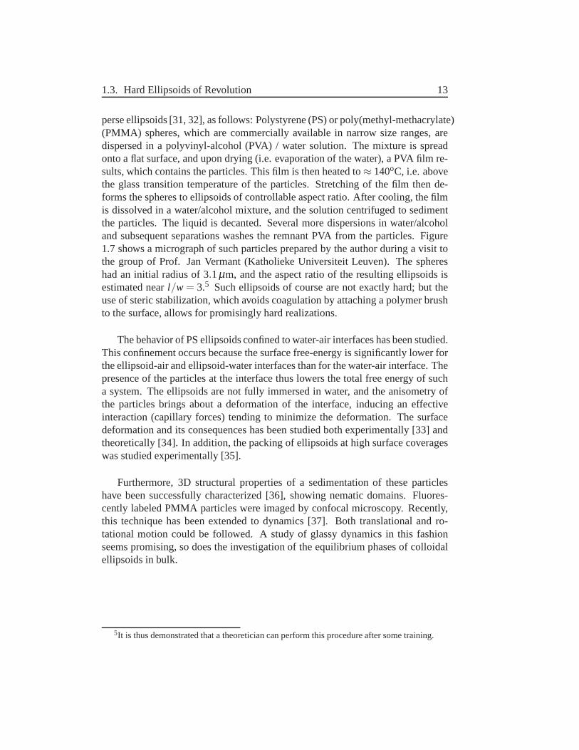
perse ellipsoids [31, 32], as follows: Polystyrene (PS) or poly(methyl-methacrylate)(PMMA) spheres, which are commercially available in narrowsize ranges, aredispersed in a polyvinyl-alcohol (PVA) / water solution. The mixture is spreadonto a flat surface, and upon drying (i.e. evaporation of the water), a PVA film re-sults, which contains the particles. This film is then heatedto≈ 140oC, i.e. abovethe glass transition temperature of the particles. Stretching of the film then de-forms the spheres to ellipsoids of controllable aspect ratio. After cooling, the filmis dissolved in a water/alcohol mixture, and the solution centrifuged to sedimentthe particles. The liquid is decanted. Several more dispersions in water/alcoholand subsequent separations washes the remnant PVA from the particles. Figure1.7 shows a micrograph of such particles prepared by the author during a visit tothe group of Prof. Jan Vermant (Katholieke Universiteit Leuven). The sphereshad an initial radius of 3.1µm, and the aspect ratio of the resulting ellipsoids isestimated nearl/w = 3.5 Such ellipsoids of course are not exactly hard; but theuse of steric stabilization, which avoids coagulation by attaching a polymer brushto the surface, allows for promisingly hard realizations.
The behavior of PS ellipsoids confined to water-air interfaces has been studied.This confinement occurs because the surface free-energy is significantly lower forthe ellipsoid-air and ellipsoid-water interfaces than forthe water-air interface. Thepresence of the particles at the interface thus lowers the total free energy of sucha system. The ellipsoids are not fully immersed in water, andthe anisometry ofthe particles brings about a deformation of the interface, inducing an effectiveinteraction (capillary forces) tending to minimize the deformation. The surfacedeformation and its consequences has been studied both experimentally [33] andtheoretically [34]. In addition, the packing of ellipsoidsat high surface coverageswas studied experimentally [35].
Furthermore, 3D structural properties of a sedimentation of these particleshave been successfully characterized [36], showing nematic domains. Fluores-cently labeled PMMA particles were imaged by confocal microscopy. Recently,this technique has been extended to dynamics [37]. Both translational and ro-tational motion could be followed. A study of glassy dynamics in this fashionseems promising, so does the investigation of the equilibrium phases of colloidalellipsoids in bulk.
5It is thus demonstrated that a theoretician can perform thisprocedure after some training.

14 Chapter 1. Introduction
Figure 1.7: Micrograph of polystyrene ellipsoids (l/w≈ 2.5, w≈ 3µm), prepared by theauthor during a visit to the group of Prof. Jan Vermant (Katholieke Universiteit Leuven).
1.4 Glasses
1.4.1 Overview
Glasses are familiar materials in every-day life. The reader may have visited fac-tories or artists forming shapes from the glowing hot, viscous mass which thensomehow freezes in the given shape when allowed to cool, to finally yield theuseful and beautiful products we know.
From the scientific perspective, glasses form a peculiar “phase” of matter inthat they are solid and liquid at the same time. They are solidin appearance, buttheir microscopic structure is indistinguishable from their liquid phase. It is theirdynamical properties which make the difference. Viscosityand relaxation timesare 12-14orders of magnitudelarger than those of liquids, after only a modestchange in temperature (e.g. a factor of three). As a consequence, glasses arenon-equilibrium systems, since even slow cooling from the liquid state eventuallyoccurs too fast for the system to adjust.
There are various definitions of the glass transition and associated transitiontemperature:
• the system falls out of equilibrium during cooling
• the viscosity has reached 1013 Poise
• special conditions in theoretical models arise, e.g. the arrest of dynamics inMode Coupling Theory.
1.4. Glasses 15
Typically (but not necessarily) glassy characteristics develop upon supercoolingthe liquid below its freezing point. The competing mechanism is crystallization.Whether or not a system remains amorphous during cooling depends on materialproperties and the cooling rate. If the system crystallizesreadily, rapid cooling(a “quench”) is required to reach a glass state. In archetypal glass formers, suchas silica mixtures, the slowing-down becomes significant well before the freezingpoint is reached, so moderate cooling rates suffice.
If the cooling rate is slow enough, and if crystallization does not intervene,glassy dynamics may be studied in quasi-equilibrium. The term glassy dynamicsrefers to the significant slowing-down of diffusion and relaxation (as comparedto the microscopic time scale6), non-exponential relaxation, and their strong de-pendence on a control parameter. In our case, density (or volume fraction) is thecontrol parameter, rather than temperature.
A concise and accessible introduction to glasses is given byKob [38].
1.4.2 The Mode-Coupling Theory of the Glass Transition
The dynamics of glassy systems and the glass transition in particular have been thesubject of intense research for the past 25 years. However, many phenomena arestill poorly understood. The only microscopic theory so faris the mode-couplingtheory (MCT) [39]. Our study of the dynamics will include tests of this theory.We give here a brief introduction to MCT. For more details seethe review articles[40, 38, 41, 42, 43]. MCT has been extended to orientational degrees of freedom[26, 27, 28], called Molecular Mode-Coupling Theory (MMCT).
We will first discuss MCT with temperature as the control parameter, becausethis is the more common situation; but glassy dynamics may just as well be in-duced by over-compression, rather than supercooling. At the end of this section,we will point out how all results apply to our situation, where density, or volumefraction, is the control parameter. Moreover, for simplicity we will first ignoreorientational degrees of freedom, and discuss their inclusion at the end as well.
A remarkable feature of the dynamics of supercooled liquidsis the stark in-crease of typical relaxation timesτ upon cooling the liquid from its liquid state tothe glass transition temperatureTg.7 In the liquid state,τ is on the order of ps; nearTg, it may well be hundreds of seconds. But this slowing down is accompaniedby no significant change in structure; e.g. there is no diverging length scale asin a second-order phase transition. MCT describes this slowing down as stronglyincreasing nonlinear feedback effects in the microscopic dynamics, whereby par-
6That time scale on which local processes occur (e.g. particle vibrations).7Tg is here defined (arbitrarily) as the temperature at which theviscosity has reached 1013
Poise.
16 Chapter 1. Introduction
ticles are trapped incagesformed by their nearest neighbors. We emphasize thatMCT is an equilibrium theory (ignoring crystallization); it does not apply to sys-tems which have fallen out of equilibrium during cooling.
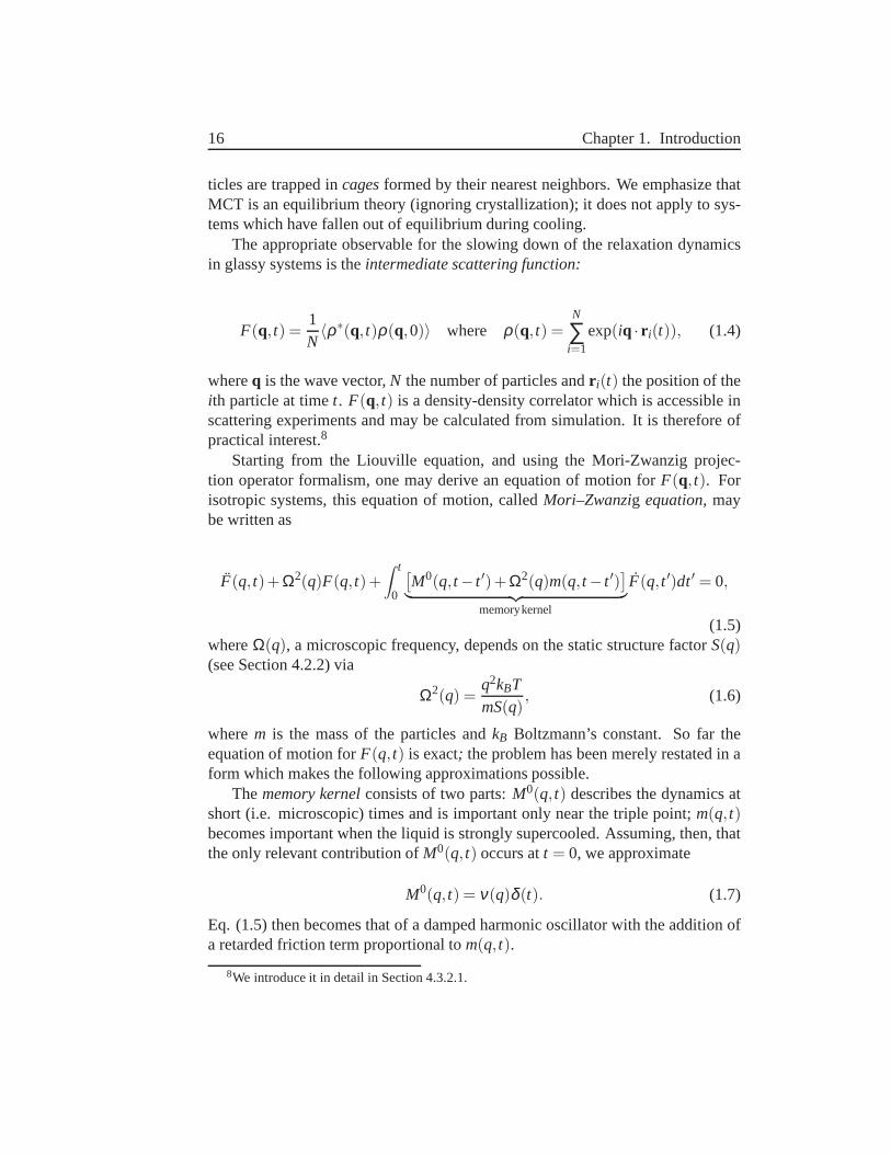
The appropriate observable for the slowing down of the relaxation dynamicsin glassy systems is theintermediate scattering function:
F(q, t) =1N〈ρ∗(q, t)ρ(q,0)〉 where ρ(q, t) =
N
∑i=1
exp(iq · r i(t)), (1.4)
whereq is the wave vector,N the number of particles andr i(t) the position of theith particle at timet. F(q, t) is a density-density correlator which is accessible inscattering experiments and may be calculated from simulation. It is therefore ofpractical interest.8
Starting from the Liouville equation, and using the Mori-Zwanzig projec-tion operator formalism, one may derive an equation of motion for F(q, t). Forisotropic systems, this equation of motion, calledMori–Zwanzig equation,maybe written as
F(q, t)+Ω2(q)F(q, t)+∫ t
0
[M0(q, t− t ′)+Ω2(q)m(q, t− t ′)
]︸ ︷︷ ︸memorykernel
F(q, t ′)dt′ = 0,
(1.5)whereΩ(q), a microscopic frequency, depends on the static structure factorS(q)(see Section 4.2.2) via
Ω2(q) =q2kBTmS(q)
, (1.6)
wherem is the mass of the particles andkB Boltzmann’s constant. So far theequation of motion forF(q, t) is exact; the problem has been merely restated in aform which makes the following approximations possible.
Thememory kernelconsists of two parts:M0(q, t) describes the dynamics atshort (i.e. microscopic) times and is important only near the triple point;m(q, t)becomes important when the liquid is strongly supercooled.Assuming, then, thatthe only relevant contribution ofM0(q, t) occurs att = 0, we approximate
M0(q, t) = ν(q)δ (t). (1.7)
Eq. (1.5) then becomes that of a damped harmonic oscillator with the addition ofa retarded friction term proportional tom(q, t).
8We introduce it in detail in Section 4.3.2.1.
1.4. Glasses 17
In the factorization approximation(see Götze [44]),m(q, t) is taken to be aquadratic form of the correlatorsF(q, t), i.e.
m(q, t) = ∑k+p=q
V(q;k;p)F(k, t)F(p, t). (1.8)
This yields the so-calledmode-coupling equations(first proposed by Bengtzeliuset al. [39]), a closed set of coupled equations forF(q, t), the solution of whichis the full time dependence of the intermediate scattering functions. The verticesV(q;k;p) can be calculated fromS(q) and static three-point correlation functions.
In this idealizedversion of MCT, it is believed that these equations (Eq. (1.5)through Eq. (1.8)) give a correct (self-consistent) description of the dynamics ontime scales while particles typically remain trapped incagesformed by surround-ing particles; and at long time scales, on which they typically manage to escapethese cages and exhibit diffusive motion. Particles will not escape such a cage un-less their destination cage has been vacated, which will notbe the case beforeitsinhabitant has found a new cage to go to, etc. Therefore, the motion of the parti-cles is collective, and so the description of motion must incorporate feedback. Themode-coupling approximation (Eq. (1.8)), in conjunction with Eq. (1.5), satisfiesthat requirement [45].
The quantitiesΩ2(q), M0(q, t) andV(q;k;p) depend on temperature, the ma-jor influence ultimately stemming fromS(q). Correspondingly, lower temperatureleads to longer times before escape from a cage occurs. We will see momentar-ily that in (idealized) MCT, one may pinpoint a critical temperatureTc at whichparticles hinder each other so much as to produce structuralarrest of the system.
Due to the complexity of the mode-coupling equations, one must resort tonumerical approaches. However, the situation improves significantly if we makeanother approximation, whereby the structure factor is replaced by aδ–functionat its main peak; we call this positionq0. The mode-coupling equations thenreduce to just one equation atq0, all others vanish identically. ReplacingΦ(t) =F(q0, t)/S(q0), we find
Φ(t)+Ω2Φ(t)+νΦ(t)+Ω2∫ t
0m
[Φ(t− t ′)
]Φ(t ′)dt′ = 0. (1.9)
Herem[Φ] is a polynomial of low order inΦ. The temperature dependence ofS(q)enters here via a temperature dependence of the coefficientsof the polynomialm[Φ]. An equation obtained in this fashion is calledschematic model.The appealof such models is that the general features of their solutions, asymptotic laws inparticular, are the same as the ones of the full MCT-equations. However, sincethey are significantly simpler, they facilitate a general overview on the possibletime dependence of the solutions.
18 Chapter 1. Introduction
Now, if the nonlinear feedback, given by the kernelm[Φ], exceeds a certainthreshold, the solution to Eq. (1.9), henceF(q0, t), no longer decays to zero (thesystem has become nonergodic). It is this condition which isidentified with theglass transition; it occurs at a critical temperatureTc.
Before turning to the predictions ofidealizedMCT, we discuss an importantlimitation. Upon reaching very low temperatures (i.e. close to Tc), the dynamicbehavior departs from that described by idealized MCT because hopping pro-cessesstart to become important. They are processes whereby cagesare left inan activated fashion, leading to structural relaxation, and idealized MCT neglectsthese. The result is that even at lowT, the system is still ergodic, and correlatorseventually decay to zero. The domain to which idealized MCT applies is therebylimited; it ranges from the liquid regime, where relaxationtimes are on the or-der of ps, down to tens of ns in the supercooled state, before hopping processesbecome important.
The so-calledextended versionof MCT incorporates such hopping processes;due to complications, however, the treatment does not yet include as much detail.We will focus our attention to idealized MCT and take note of hopping whennecessary.
Let us turn to the predictions (for more detail see [42, 41, 46, 47, 44, 43]).Most of them concern the decay of correlation functions. In Figure 1.8 we demon-strate the general behavior of such functions. We distinguish three regimes: themicroscopicregime, a time scale during which microscopic relaxation takes place;since it strongly depends on the details of microscopic interactions, hardly anygeneral predictions are possible.9 Next comes theβ -relaxation regime, duringwhich dynamics are dominated by caging - visible as a plateauwhich increasesin width towards low temperatures; and theα-relaxationregime, which describesthe decay of the correlators from the plateau to zero. One of the main predictionsof MCT is the existence of these three regimes; and it makes detailed predictionsabout the latter two, as follows.
• There exists a critical temperatureTc, and in its vicinity the self-diffusionconstantD and the inverse of theα–relaxation timeτ vanish according to10
D ∝ τ−1 ∝ (T−Tc)γ , (1.10)
whereγ > 1.5 is universal for the system (i.e. the same for all correlators).Note that the following predictions all assume proximity ofTc.
9The microscopic regime is preceded by theballistic regime, during which particles move withessentially constant velocity and (hence) decay of correlators is quadratic. The ballistic regime isabsent in colloidal systems, where Brownian motion occurs.
10Theα–relaxation timeτ may be defined as the time when the correlator has decayed to 0.1 oranother fixed value within theα–relaxation regime.
1.4. Glasses 19
100
101
102
103
104
105
106
t [ps]
0
0.2
0.4
0.6
0.8
1
Φ(q,t)
viscousliquid
glass
liquid
Figure 1.8: Schematic time dependence of correlators, for liquid to supercooled regimesand the glass case (high to low temperatures, or low to high densities).
20 Chapter 1. Introduction
• In theβ - andα-relaxation regimes, the correlators obey the so-called time-temperature superposition principle (TTSP), which statesthat the correla-tors map onto a single curve by rescaling the time dependenceusingt/τ (τbeing theα–relaxation time); that is,
Φ(t) = Ψ(t/τ(T)) . (1.11)
• Numerical predictions from MCT show that theKohlrausch–Williams–Wattsfunctionmay be used as a fit function for the master curve Eq. (1.11), withan effective exponentβ
Φ(t) = Aexp(−(t/τ(T))β
), (1.12)
whereβ is thestretching parameter.It depends on the correlator (in partic-ular, onq in F(q, t)).
• All correlation functions’α–relaxation times diverge according to a powerlaw with exponentγ (see Eq. (1.10)). This exponent is related to two pa-rametersa andb concerning theβ–relaxation regime (discussed below):
γ = 1/(2a)+1/(2b). (1.13)
Thus, from the temperature dependence of theα–relaxation time we canlearn about the time dependence of the relaxation in theβ -relaxation regimeand vice versa.a andb are related to one another via
Γ2(1−a)/Γ(1−2a) = Γ2(1+b)/Γ(1+2b) = λ (1.14)
so that knowledge of one of these three exponents yields the other two.λ iscalled theexponent parameter.
• In theβ–relaxation regime the correlators may be written as
Φ(q, t) = f cq +h(q)g(t/τ), (1.15)
wheref cq , the height of the plateau at the transition, is termednon-ergodicity
parameter. h(q) is an amplitude.g(t/τ) doesnot depend on q; this entailsthefactorization property.Defining [48]
R(t) =Φ(q, t)−Φ(q, t ′′)Φ(q, t ′)−Φ(q, t ′′)
(1.16)
one finds that allq-dependence has been removed. This operation can bedirectly applied toF(q, t) data, allowing one to check whether the factor-ization property holds: if it does, allF(q, t) will fall onto a master curve.
1.4. Glasses 21
• The lateβ–relaxation regime (when the curve slowly begins to leave theplateau) and the earlyα–relaxation regime in the intermediate scatteringfunctions may be described by
Φ(q, t) = f cq −h(1)
q tb+h(2)q t2b. (1.17)
f cq is again the non-ergodicity parameter. When dealing with coherent11
intermediate scattering functions,f cq is also called theDebye-Waller factor;
in incoherent intermediate scattering functions, it is theLamb-Mößbauer
factor. h(1)q is referred to ascritical amplitude. All quantities subscribed
with q depend only onq, not on timet. The first two terms in Eq. (1.17)are calledvon Schweidler law,to which the last term is a leading-ordercorrection;b is thevon Schweidler exponent,and according to MCT it isindependent of type of correlator (hence independent ofq).
• The time scale of theβ–relaxation regime (its width) is predicted by MCTto diverge as
t ∝ |T−Tc|1/2a, (1.18)
whenT is close toTc, and we have 0< a < 1/2. Light scattering experi-ments have confirmed the validity of Eq. (1.18) [49, 50].
• The relaxation dynamics are, apart from an overall shift in time scales, in-dependent of the microscopic dynamics (e.g. Brownian vs. Newtonian dy-namics). Hence, the above predictions are independent thereof.
In molecular systems, where there are orientational degrees of freedom, one candefine orientational analogues of the intermediate scattering functions (see alsoSection 4.3.2.2),
Li(t) = 〈Pi cos[θ(t)]〉 (1.19)
wherePi is theith Legendre polynomial, andθ(t) is the angle between a molecule’sorientation at timet and its initial orientation. These orientational correlationfunctions play the same role as the intermediate scatteringfunctions, and theabove MCT predictions apply analogously, if we bear in mind thatq is replacedby the discrete indexi. This analogy is limited, however: It is possible that ori-entational degrees of freedom are not affected by a positional glass transition, oreven that different values ofi are affected by separate glass transitions (see Sec-tion 1.3.2.3). This concerns the factorization property and the degree to whichexponents are system-universal.
11For the distinction between coherent and incoherent intermediate scattering functions, seeSection 4.3.2.1.
22 Chapter 1. Introduction
In hard-particle systems, temperature is a trivial, overall scaling parameter.The only relevant quantity for glassy dynamics is here particle density, or equiva-lently, volume fraction. To apply the above predictions to this case, supercoolingtranslates to over-compression, and one must simply replace all expressionsT−Tc
by φc−φ , whereφc is the MCT critical volume fraction.Many of the qualitative predictions of MCT have been confirmed for super-
cooled liquids. See, for example, [51, 52, 53, 54, 55, 56].
Chapter 2
Simulation - Theory and Technique
We have employed two techniques of simulation in our work, Monte Carlo sim-ulation and molecular dynamics simulation. This allowed usto compare the twomethods and test a MCT prediction about such a comparison (Sections 1.4.2 and4.3).
Since we are interested in the bulk properties of our systems, all simulationswere done withperiodic boundary conditionsto minimize boundary effects. Thesimulated system is perpetuated periodically in all directions by images of itself.A particle leaving the system on the right-hand side re-enters it on the left-handside, and so on. Each particle interacts either with the original of other particles inthe box or with the closest image in a neighboring image box, whichever is closer.The absolute position of the particles is irrelevant in sucha setup [57].
2.1 Monte Carlo Simulation (MC)
2.1.1 General Features
In Monte Carlo simulation as introduced by Metropolis et al.[58], phase spaceis traversed, orsampled, by a random walk. The underlying random process is aMarkov process, i.e. the(n+ 1)th state is a function of thenth state only. Thenext state is tested by a trial move in one or more phase space coordinates, and inthe canonical ensemble accepted with probability
accn→n+1 = min(1,exp[−(En+1−En)/kBT]) (2.1)
whereEi is the energy of statei, kB Boltzmann’s constant andT the temperature.In practice, a random number is generated in the interval[0,1], and the move is ac-cepted if the number is smaller than accn→n+1. Eq. (2.1) is also called acceptancecriterion or acceptance rule.
24 Chapter 2. Simulation - Theory and Technique
Properties of interest are monitored on the way and their average or full dis-tribution is the final result. Note that the value of an integral, e.g. the volume ofphase space (hence the partition function)cannotbe evaluated in this way.
The sampling must be with known or with no bias in order to produce mean-ingful results1. This concerns the choice of trial move and the acceptance criterionEq. (2.1). A sufficient condition is to maintaindetailed balance, i.e. the reverse ofa move must occur with equal probability. A deliberate bias is at the heart of themethod, since one can restrict the sampling to the statistically relevant regions ofphase space (importance sampling); in fact the above acceptance criterion impliesa bias which reproduces the Boltzmann distribution of energies. The implementa-tion of importance sampling also entails that the simulation must first equilibrate,i.e. reach the important parts of phase space, before calculations can begin.
The classical way to generate trial moves proceeds by first picking, at random,a small subset of degrees of freedom; e.g. one particle’s position. For the position,a displacement vector is chosen from a box. The size of this box is important forthe simulation’s efficiency, and is held fixed to yield an acceptance rate of typically20% to 40%, depending on the computational bottlenecks of particle interactions.The same pattern is applied to other degrees of freedom, suchas orientationalmoves for molecules or box-shape variations; more details are given below.
A central feature of the Monte Carlo method is the use of more elaboratemoves which take the system through phase space efficiently,despite the presenceof barriers. A move which represents a large step in phase space (e.g., a clustermove), but still achieves sufficient acceptance rates, can significantly expedite asimulation.
For a thorough introduction to Monte Carlo see Frenkel and Smit [57] or Lan-dau and Binder [59].
2.1.2 Constant-Pressure-and-Tension Ensemble
Monte Carlo simulation of this ensemble has been first described by Najafabadiand Yip [60] and in more detail by Yashonath and Rao [61]. It isbased on thecorresponding molecular dynamics invented by Parrinello and Rahman [62]. Theessence is that the simulation box may vary in size and shape (take a preview ofFigure 2.1). This is critical for the equilibration of solids, where the box shapehas a direct influence on the lattice geometry. If oblique shapes are not allowed,the solid will in general be under stress.
1As David Landau would have it, “... and unless you’re very careful, you will get results, it’sjust they don’t mean anything.”
2.1. Monte Carlo Simulation (MC) 25
2.1.2.1 Partition Function
For the case relevant to us, namely zero tension, the configurational part of thepartition function in the named ensemble may be written as
Z(N,P,T) =∞∫
−∞
dh11· · ·dh33
∫H
drN∫4π
duN · (2.2)
exp− [U(r i,ui)+PV(H)]/kBTwhere we have ignored the prefactors(N!λ 6N)−1 which have no influence on theequilibrium behavior.hi j are all 9 elements of the matrixH describing the boxshape. Each column vector inH = [h1h2h3] corresponds to one box edge, in thesame way as unit cell vectors correspond to the edges of the unit cell in a crystallattice. Hence,H completely specifies the box. It also follows that the box volumeV = detH. The integral over particle coordinates is over the box as determined byH.
For convenience and clarity we introduce scaled particle coordinatess so thatr = Hs. s is in the unit cube, andH provides the mapping to the simulation box.Eq. (2.2) becomes
Z(N,P,T) =∞∫
−∞
dh11· · ·dh33
1∫0
dsN∫4π
duN ·
exp− [U(si,H,ui)+PV(H)]/kBT(detH)N
=∞∫
−∞
dh11· · ·dh33
1∫0
dsN∫4π
duN · (2.3)
exp− [U(si,H,ui)+PV(H)]/kBT +N lnV(H)
=∞∫
−∞
dh11· · ·dh33z−V(H)PT Z0(N,H,T)
where we have introduced the isochoric partition function
Z0(N,H,T)≡1∫
0
dsN∫4π
duN exp−U(si,H,ui)/kBT +N lnV(H)
and defined a “fugacity”zPT = eP/kBT for brevity.In principle, Eq. (2.3) can be the starting point for the simulation. How-
ever, it is from the programming point of view more convenient to keepH upper-triangular2, which is identical to fixing the global orientation of the box. Given
2Another possibility is to keepH symmetric.
26 Chapter 2. Simulation - Theory and Technique
the orientational degeneracy of configurations, this should pose no problem.h1 isthen parallel to thex-axis, andh2 resides in thexy-plane. The expression for thevolume simplifies toV = detH = h11h22h33.
We would like to point out a subtlety in this step which has gone unnoticedin the literature. The proper removal of orientational degeneracy is integrating itout. Forh1 this implies a change of coordinates to spherical ones(rh1,θh1,φh1),followed by integration over the angular variables. Eq. (2.3) becomes3:
Z(N,P,T) = 4π∞∫
0
drh1
∞∫−∞
dh12dh13dh22dh23dh32dh33r2h1z−V(H)
PT Z0(N,H,T)
Now we may fixh1 to be parallel to thex-axis, i.e. we may replacerh1 with h11(and drop the prefactor):
Z(N,P,T) =∞∫
0
dh11
∞∫−∞
dh12dh13dh22dh23dh32dh33h211z
−V(H)PT Z0(N,H,T) (2.4)
As of now, the system is still free to rotate about thex-axis. This remainingdegeneracy is integrated out inh2. To do so,h2 must be changed to cylindricalcoordinates about thex-axis, i.e.(h12,ρh2,φh2). Angular integration follows. Eq.(2.4) now reads
Z(N,P,T) = 2π∞∫
0
dh11dρh2
∞∫−∞
dh12dh13dh23dh33h211ρh2z−V(H)
PT Z0(N,H,T)
Now we may fixh2 into thexy-plane, i.e. we may replaceρh2 with h22 (and dropthe prefactor):
Z(N,P,T) =∞∫
0
dh11dh22
∞∫−∞
dh12dh13dh23dh33h211h22z
−V(H)PT Z0(N,H,T) (2.5)
It is these factorsh211h22 which have been, to our knowledge, overlooked4: in
the literature, the matrixH is simply restricted to be triangular or symmetric,without regard to the implied integration over the orientational degeneracy. Butthe resulting weight factorsh2
11h22 must be properly included into the acceptancecriterion (below) for a bias-free simulation. Their presence favors larger values of
3In principle,h2 andh3 should be changed to variables relative toh1. But since the integrals inh2 andh3 are over all space, ignoring this has no consequences. The integration over the angularpart inh1 nevertheless implies the integration over global orientations of the whole system.
4Or their analogues whenH is kept symmetric.
2.1. Monte Carlo Simulation (MC) 27
h11 andh22 in the partition sum. One can see that this must be so: The phase spacevolume orthogonal toh11, which we integrated out, is the surface area swept outby h1 if it was still free to rotate. Hence, larger magnitudes ofh1 would be visitedmore often if the box was still free to rotate. Now that it is fixed, we must favorlarger magnitudes with the given weight factor. The analogous argument appliesto h22.
There is an equivalent set of configurations for positive andnegativeh33. Wemay remove this degeneracy, which is to keeph33 nonnegative. Eq. (2.5) picks upan irrelevant factor of 2.
Next, we express the remaining off-diagonal terms as follows:
h12 = g12h22
h13 = g13h33 (2.6)
h23 = g23h33
Eq. (2.5) then becomes
Z(N,P,T) =∞∫
0
dh11dh22dh33
∞∫−∞
dg12dg13dg23 ·
h211h
222h
233z
−V(H)PT Z0(N,H,T)
=∞∫
0
dh11dh22dh33
∞∫−∞
dg12dg13dg23 ·
V(H)2z−V(H)PT Z0(N,H,T) (2.7)
The advantage of introducing the variablesgi j lies in the separation of size vari-ables and pure shape variables.hii specify the separation of box walls, whilegi j specify box shear. For example,g12 = h12/h22 = dx/dy is the change inx-direction of box edgeh2 as one moves along they-direction. The same separationoccurred in the process of integrating out orientational degeneracy, as the angularvariables also no longer carried size information. It is reassuring that the corre-sponding factorshii in Eq. (2.7) combine to factors of volume.
The set of variableshii andgi j are also the relevant parameters in crystal lat-tices, associated with distinct moduli of elasticity (bulkand shear, respectively),and we anticipate that they will require individual MC move sizes.
Finally, we follow the literature in changing from integrating (hence sampling)
28 Chapter 2. Simulation - Theory and Technique
overdhii to d lnhii :
Z(N,P,T) =∞∫
−∞
d lnh11d lnh22d lnh33dg12dg13dg23 ·
h11h22h33V(H)2z−V(H)PT Z0(N,H,T)
=∞∫
−∞
d lnh11d lnh22d lnh33dg12dg13dg23 ·
V(H)3z−V(H)PT Z0(N,H,T)
The advantage is here one of efficiency. The sampling will naturally occur insmaller step sizes of the originalhii for smaller volumes; this is desirable sincesmaller volumes, associated with larger pressures in the system, make these de-grees of freedom stiffer. Once more we appreciate the advantage of keeping sizeand shear apart. The final form of the partition sum is then
Z(N,P,T) =∞∫
−∞
d lnh11d lnh22d lnh33dg12dg13dg23
1∫0
dsN∫4π
duN · (2.8)
exp− [U(si,H,ui)+PV(H)]/kBT +(N+3) lnV(H)
and the matrixH reads
H =
h11 h22g12 h33g13h22 h33g23
h33
(2.9)
All weighting in Eq. (2.8) is absorbed into the exponential,so we can immediatelywrite down the acceptance rule:
accn→n+1 = min(1,exp
− [Un+1−Un+P(Vn+1−Vn)]/kBT +(N+3) ln
Vn+1
Vn
)
(2.10)If we keepgi j = 0 andh11= h22= h33, the present results reduce to those of the
known constant-pressure ensemble—apart from the factor(N+3) where(N+1)is found instead [57], “+1” coming from samplingd lnV. We show in Appendix Athat(N+3) is the correct result derived from the present, more generalbasis. Thiscorrection, of order 1/N, surely does not render useless all simulations which used(N+1). We find it important for the understanding of the derivation, and indeedin small simulations the difference may be noticeable.
2.1. Monte Carlo Simulation (MC) 29
Finally, we write down the simpler hard-particle results. Eq. (2.8) becomes
Z(N,P,T) =∞∫
−∞
1∫0
∫4π
no overlap
d lnh11d lnh22d lnh33dg12dg13dg23dsNduN ·
exp
− P
kBTV(H)+(N+3) lnV(H)
Monte Carlo moves are accepted if no overlap results, and within the no-overlapphase space according to
accn→n+1 = min(1,exp
− P
kBT(Vn+1−Vn)+(N+3) ln
Vn+1
Vn
) no overlap
(2.11)Note that Eq. (2.11) must be evaluated only for moves which change lnhii sinceV = h11h22h33.
2.1.2.2 Monte Carlo Moves
Having established the acceptance rule Eq. (2.11), we turn to the generation ofMC moves as implemented in this work. Figure 2.1 serves as illustration forrectangular boxes (left), often synonymous with constant-pressure MC, and thefull zero-tension case (right).
There are particle moves and box shape moves; and the particle moves areeither displacement moves or orientational moves. First, the kind of move is ran-domly chosen so that forN particle moves, there is on average one box shapemove. For the case of a particle move, a particle is chosen at random, and a coinis flipped to decide between displacement move and orientational move.
To construct the displacement vector for the displacement move, a random
vector on the unit sphere is generated and then scaled by∆d · (V)13 , where∆d is
a parameter andV the box volume.∆d was automatically adjusted during equili-
bration to achieve an acceptance rate near 30%.(V)13 is included to relate the size
of the displacement to the present density. The acceptance rate then becomes lesssensitive to the density, and hence more stable; this also expedites the adjustmentof ∆d. Next, the component of the vector parallel to the symmetry axis of theellipsoid is scaled by 1.7 · l/w, where 1.7 is an empirical factor. This adjustmentaccounts for the fact that a prolate ellipsoid can move a larger distance along itssymmetry axis than perpendicular to it without causing overlap (vice versa foroblate ellipsoids). The resulting vector is added to the current position vector (inunscaledr -space) of the ellipsoid. The move is accepted if no overlap results fromthe displacement. The factor of 1.7 was obtained by monitoring the acceptance
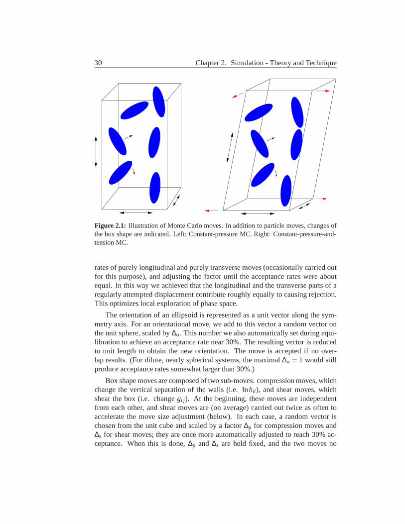
30 Chapter 2. Simulation - Theory and Technique
Figure 2.1: Illustration of Monte Carlo moves. In addition to particle moves, changes ofthe box shape are indicated. Left: Constant-pressure MC. Right: Constant-pressure-and-tension MC.
rates of purely longitudinal and purely transverse moves (occasionally carried outfor this purpose), and adjusting the factor until the acceptance rates were aboutequal. In this way we achieved that the longitudinal and the transverse parts of aregularly attempted displacement contribute roughly equally to causing rejection.This optimizes local exploration of phase space.
The orientation of an ellipsoid is represented as a unit vector along the sym-metry axis. For an orientational move, we add to this vector arandom vector onthe unit sphere, scaled by∆o. This number we also automatically set during equi-libration to achieve an acceptance rate near 30%. The resulting vector is reducedto unit length to obtain the new orientation. The move is accepted if no over-lap results. (For dilute, nearly spherical systems, the maximal ∆o = 1 would stillproduce acceptance rates somewhat larger than 30%.)
Box shape moves are composed of two sub-moves: compression moves, whichchange the vertical separation of the walls (i.e. lnhii ), and shear moves, whichshear the box (i.e. changegi j ). At the beginning, these moves are independentfrom each other, and shear moves are (on average) carried outtwice as often toaccelerate the move size adjustment (below). In each case, arandom vector ischosen from the unit cube and scaled by a factor∆p for compression moves and∆s for shear moves; they are once more automatically adjusted to reach 30% ac-ceptance. When this is done,∆p and ∆s are held fixed, and the two moves no
2.1. Monte Carlo Simulation (MC) 31
longer occur as such5. Only combined versions are carried out: A random vectoris chosen for each sub-move and scaled by the corresponding factor; then both arescaled again, by a factor∆c, which is adjusted to obtain 30% acceptance for thiscombined version. All shape-changing moves are affine, i.e.the particle positionsare mapped to the new box geometry, so that the system remainshomogeneous.In practice this means re-evaluatingr = Hs for all particles.
In addition, we introduced an efficiency gain by rotating theparticles accord-ing to changes in shear. A change in shear in a real suspensionof anisometricparticles causes these particles to reflect the curl in the flow field. We found thatup to twice as large shear moves were possible (while keepingthe acceptance rationear 30%) if the particles were rotated according to a rotation vector
ω =
∆h23/h33−∆h13/h33
∆h12/h22
where the direction ofω is the axis of rotation and the empirical 0.7|ω| specifiesthe angle in radians.∆hi j denotes the change in the corresponding component ofH, while hii denotes the arithmetic mean of the old and new value. This construc-tion satisfies detailed balance since exchange of old and newcomponents reversesthe sign of the rotation.
After all move sizes have been adjusted, the parameters are held fixed becauseautomatic adjustment violates detailed balance each time it occurs [63]. While thisdid no harm during equilibration, no such risk was desired during measurement.
2.1.3 Other Monte Carlo Versions
The first spontaneous transition from sFCC to SM2 (Chapter 3)in fact occurred inconventional constant-pressure MC (left part of Figure 2.1). The acceptance ruleEq. (2.11) was used (but usingN+1, by tradition). The translational moves weregenerated by choosing a random vector from a box of linear size δ , andδ wasautomatically adjusted for 30% acceptance ratio. The rotational moves were asdescribed in the previous section. Regarding box shape, only compression moveswere done; they were carried out the same way as the corresponding sub-moveabove (but aiming for 20%; no significant efficiency gain or loss was found).
For the equilibration of the glassy systems, the box was heldcubic (not onlyrectangular), i.e. only isotropic volume changes were done, for computationalconvenience regarding correlation functions. The MC production runs of theglassy systems held the box fixed [(N,V,T)-ensemble]. Particle moves were car-ried out as described in the previous paragraph. Only overlap decided acceptance.
5Except rarely for monitoring purposes.
32 Chapter 2. Simulation - Theory and Technique
The moves were made small to mimic Brownian motion and to render grazingcollisions unimportant (Section 4.1 has more details). Thetime unit “MC step”refers toN attempted moves.
2.1.4 Testing for Overlaps
Particle overlap was checked by a routine [23] which uses theVieillard-Baron [10]and Perram-Wertheim [11, 12] criteria to test whether a pairof ellipsoids, giventhe separation vector and the orientations, overlaps. It does so by progressingfrom the circumscribed and inscribed spheres tests, which permit early decision,to an evermore detailed examination.
The checking of particle overlap was made more efficient by implementing acell system [64]. The minimum cell wall separation is kept atleast as large as thelongest axis of the ellipsoids. The consequence is that an ellipsoid can overlaponly with others of the same cell or of the 26 neighboring ones. This keeps thesearch for overlapping neighbors local, and improves the scaling of the algorithmfrom O(N2) to O(N).
2.2 Molecular Dynamics Simulation (MD)
2.2.1 General Features
Molecular dynamics (MD) simulation amounts to numericallyintegrating New-ton’s equations of motion:
mi r i =−∇iV(rk)≡ Fi (2.12)
wheremi is the mass of particlei, r i its position, andFi the force on it.V(rk) isthe potential.rk, k = 1, ...,N denotes the set of all position vectors, with N thetotal number of particles. We ignore orientational degreesof freedom for brevity.For ellipsoids of revolution the analogue of Eq. (2.12) is a system of5N coupledlinear partial differential equations. Its solution is a trajectory in phase space. Eq.(2.12) are solved numerically by an appropriate integration scheme, which we willdiscuss below. MD simulations rely on ergodicity, i.e. the equivalence of time andensemble averages, and care must be taken that the simulation is in fact ergodic.For fluids, i.e. our case, this requires sufficient equilibration.
A thorough introduction to molecular dynamics simulation is given by Frenkeland Smit [57] and Allen and Tildesley [65].
2.2. Molecular Dynamics Simulation (MD) 33
2.2.2 Event-driven MD
The situation in hard-particle models is special in that thepotential is not differ-entiable, so that usual integration schemes fail. The method of choice is an event-driven algorithm, which progresses through time from collision to collision. Onesuch algorithm was described by Allen et al. [23], and we are indebted to MikeAllen for providing us with the code. The description in Ref.[23] is quite detailedso that the following brief outline shall suffice.
As mentioned, the general approach is to advance from collision to collision.Collisions are implemented to obey the conservation of linear and angular momen-tum, and of energy. Between collisions, the particles translate and rotate freely.The ellipsoids are taken to have a smooth surface, so that theangular momentumabout the symmetry axis is constant and kept zero. The momentof inertia associ-ated with end-over-end rotation is commonly (and in this work) chosen according
to uniform mass distribution,I = 1/20
[(l/w)2+1
]mw2.
The equation determining the next collision (if any) of a pair of particles isquadratic int for hard spheres, but in general (and for ellipsoids) a transcenden-tal one. Therefore, its root must be found numerically. The MD by Allen et al.solves this problem retrospectively, so that an MD step proceeds as follows: First,a small free-flight advance of the system is performed. The system is then exam-ined for overlaps, implying missed collisions. The times ofthose collisions aredetermined by numerical root-finding (using the Newton-Raphson method [66]),and the collisions are sorted in chronological order. Each colliding pair is thenrewound to the time of its collision, the collision is performed, and the pair isbrought forward in time again. Resulting overlaps are checked. Their presence ismet with abandoning the attempted step, and trying half the step. The same holdsfor any other complexity. If the step was halved, and carriedout successfully, theremainder is attempted in the same fashion. If not, the step is halved again, andso on.
The advantage of this approach is that collisions will not bemissed apart fromsmall grazing ones, and the root-finding is always begun withknowledge that aroot exists in the time interval considered. The size of the initial attempt is amatter of efficiency only, and set so that abandoning and halving is infrequent. Aswe also find in our work, this MD algorithm is efficient.
The program of Allen et al. [23] was adapted slightly for numerical stabilityand to meet our data-taking requirements (Section 4.1).
The length of an MD step was 0.0005√
m/kBT 3√
l/ww. At φ = 0.598 (thehighest volume fraction simulated with MD in our work), about four collisionsper particle took place in 100 MD steps.

34 Chapter 2. Simulation - Theory and Technique
Chapter 3
Simple Monoclinic Crystal Phase
Here we report our findings on the solid phases of hard ellipsoids. In an exerciseaiming to reproduce the equilibrium results of Frenkel and Mulder [1], we con-structed an sFCC system of aspect ratiol/w = 3 (and others) and used constant-pressure Monte Carlo to perform an expansion run. That is, welowered the pres-sure between successive simulations, causing the density to settle at a lower valueeach time. Already at the second simulated pressure, an unexpected rise in den-sity called for attention. Inspection of a snapshot, followed by double-checkingall data and parameters, lead to the suspicion that a new solid phase was found,replacing sFCC in parts of the equilibrium phase diagram. The snapshot is shownin Figure 3.1. We then implemented constant-pressure-and-tension MC to ensurethat stresses were not an issue, and proceeded to repeat the transition and to studythe properties of the crystal.
3.1 Overview of Simulations
Simulations were performed at constant particle numberN, pressureP and tem-peratureT. The shape of the periodic box was allowed to fluctuate, so that thecrystal unit cell could find its equilibrium shape. This was achieved by imple-menting the Monte Carlo equivalent of the simulation methodby Parrinello andRahman (PR) [62, 60, 61], explained in Section 2.1.2. Some simulations keptthe box rectangular, i.e. employed constant-pressure MC. The simulations werestarted with sFCC crystals identical to the ones studied by Frenkel and Mulder [1](Section 1.3.2.1).
Table 3.1 summarizes all simulations performed for this part of the project.The runs are labeled in column “#” with an index for easy reference, column“ l/w” indicates the aspect ratio, “runs” the number of independent runs, column“MC” specifies the method of simulation (see legend), and “N” shows the particle
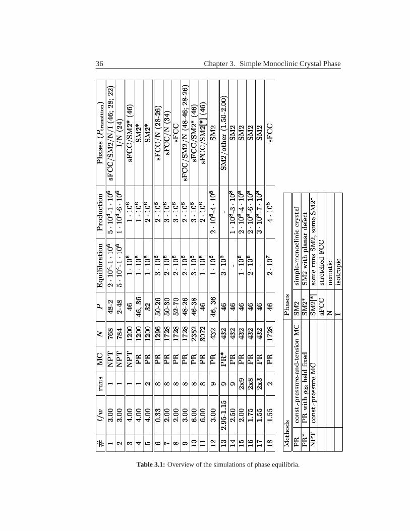
36 Chapter 3. Simple Monoclinic Crystal Phase
Table 3.1: Overview of the simulations of phase equilibria.
3.1. Overview of Simulations 37
number in each run. “P” indicates the pressure or range of pressures1 simulatedin each run. When a range is shown, the separation of successive runs is∆P = 2.“Equilibration” and “Production” indicate the minimum lengths of the mentionedparts of each run, in MC steps. One MC step consisted ofN attempts to move orrotate a particle and one attempt to change the box shape, on average. The lastcolumn lists the simulated phases (see legend) and, in parentheses, the pressuresat which transitions took place. Ranges of pressures are given when the transitionoccurred at various pressures in independent runs.
Run #1 is the constant-pressure expansion run of ellipsoidswith l/w= 3 whichfirst showed the transition from sFCC to the new crystal phase, called SM2. Equi-libration and production run lengths were on the order of 104-106 MC steps, wherelower densities required shorter runs. During the expansion, the transition fromsFCC to SM2 occurred, followed later by melting to the nematic (N) and isotropic(I) phases. Run #2 was a compression run which began isotropic and ended in anover-compressed nematic phase. Runs #1 and #2 yielded equation-of-state datafor the isotropic and nematic phases.
In #3, we simulatedl/w = 4 at P = 46 which displayed a transition fromsFCC to SM2 with a planar defect. This system was later simulated using the PRconstant-pressure-and-tension MC at the same and lower pressures (#4 and #5).
In runs #6-11 we attempted the transition sFCC/SM2 for aspect ratiosl/w =13,2,3,6 using PR and larger systems. We simulated eight independent systems ineach case, performing expansion runs (#6-10 except #8), compression runs (#8)and single-pressure runs (#11 atP = 46).
Runs #12: Realizing that the study of the soft angle of inclination in the SM2crystal required much longer runs, we set up smaller systems(N = 432) forl/w=3 at various angles of inclination, and ran them for∼ 108 MC steps at pressuresP = 46,36.
Runs #13: Since the transition to SM2 did not spontaneously occur for l/w <3, but stability was expected on theoretical grounds, we performed runs decreas-ing the aspect ratio in small steps∆(l/w) = 0.05. Nine independent such series ofruns were performed, which differed by the angle of inclination. It was held fixed,so that SM2 phases with various inclinations were obtained at lower aspect ra-tios. Transitions to strained sFCC and plastic solid phasestook place in the range1.50< l/w < 2.00 (indicated in Table 3.1 where otherwise transition pressuresare written). Three inclinations remained SM2 down tol/w= 1.55. The output ofthese series were used for long runs (#14-17) at various aspect ratios in the spiritof runs #12. The inclination was allowed to vary again. “2x9”means that twoindependent long runs were done for each of nine initial inclinations.
Finally, in #18 two runs withN = 1728,P = 46 at the possible stability limit
1The units of pressure arekBT/[(l/w)w3]. See also pg. xx
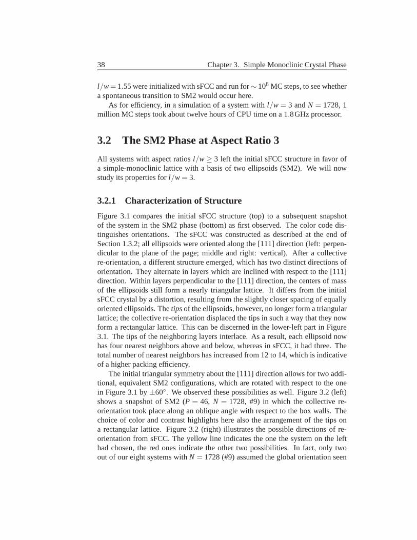
38 Chapter 3. Simple Monoclinic Crystal Phase
l/w= 1.55 were initialized with sFCC and run for∼ 108 MC steps, to see whethera spontaneous transition to SM2 would occur here.
As for efficiency, in a simulation of a system withl/w = 3 andN = 1728, 1million MC steps took about twelve hours of CPU time on a 1.8GHz processor.
3.2 The SM2 Phase at Aspect Ratio 3
All systems with aspect ratiosl/w≥ 3 left the initial sFCC structure in favor ofa simple-monoclinic lattice with a basis of two ellipsoids (SM2). We will nowstudy its properties forl/w = 3.
3.2.1 Characterization of Structure
Figure 3.1 compares the initial sFCC structure (top) to a subsequent snapshotof the system in the SM2 phase (bottom) as first observed. The color code dis-tinguishes orientations. The sFCC was constructed as described at the end ofSection 1.3.2; all ellipsoids were oriented along the [111]direction (left: perpen-dicular to the plane of the page; middle and right: vertical). After a collectivere-orientation, a different structure emerged, which has two distinct directions oforientation. They alternate in layers which are inclined with respect to the [111]direction. Within layers perpendicular to the [111] direction, the centers of massof the ellipsoids still form a nearly triangular lattice. Itdiffers from the initialsFCC crystal by a distortion, resulting from the slightly closer spacing of equallyoriented ellipsoids. Thetipsof the ellipsoids, however, no longer form a triangularlattice; the collective re-orientation displaced the tipsin such a way that they nowform a rectangular lattice. This can be discerned in the lower-left part in Figure3.1. The tips of the neighboring layers interlace. As a result, each ellipsoid nowhas four nearest neighbors above and below, whereas in sFCC,it had three. Thetotal number of nearest neighbors has increased from 12 to 14, which is indicativeof a higher packing efficiency.
The initial triangular symmetry about the [111] direction allows for two addi-tional, equivalent SM2 configurations, which are rotated with respect to the onein Figure 3.1 by±60. We observed these possibilities as well. Figure 3.2 (left)shows a snapshot of SM2 (P = 46, N = 1728, #9) in which the collective re-orientation took place along an oblique angle with respect to the box walls. Thechoice of color and contrast highlights here also the arrangement of the tips ona rectangular lattice. Figure 3.2 (right) illustrates the possible directions of re-orientation from sFCC. The yellow line indicates the one thesystem on the lefthad chosen, the red ones indicate the other two possibilities. In fact, only twoout of our eight systems withN = 1728 (#9) assumed the global orientation seen
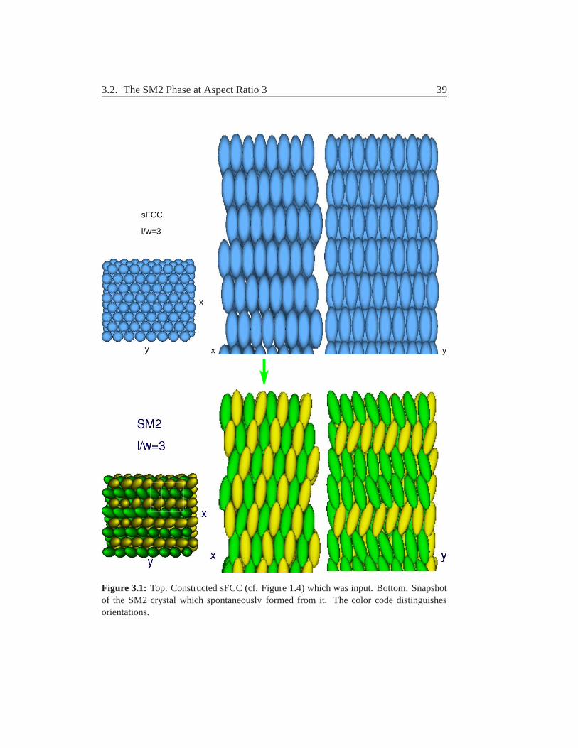
3.2. The SM2 Phase at Aspect Ratio 3 39
x yy
l/w=3
x
sFCC
Figure 3.1: Top: Constructed sFCC (cf. Figure 1.4) which was input. Bottom: Snapshotof the SM2 crystal which spontaneously formed from it. The color code distinguishesorientations.
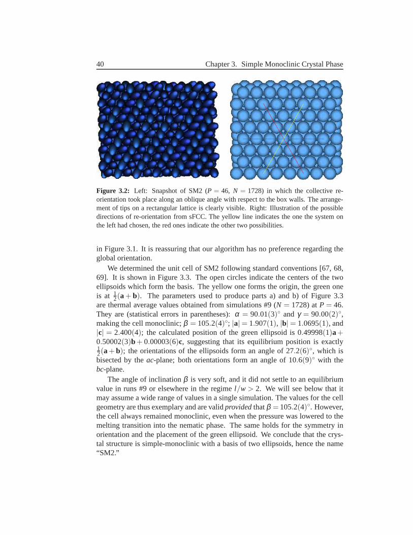
40 Chapter 3. Simple Monoclinic Crystal Phase
Figure 3.2: Left: Snapshot of SM2 (P = 46, N = 1728) in which the collective re-orientation took place along an oblique angle with respect to the box walls. The arrange-ment of tips on a rectangular lattice is clearly visible. Right: Illustration of the possibledirections of re-orientation from sFCC. The yellow line indicates the one the system onthe left had chosen, the red ones indicate the other two possibilities.
in Figure 3.1. It is reassuring that our algorithm has no preference regarding theglobal orientation.
We determined the unit cell of SM2 following standard conventions [67, 68,69]. It is shown in Figure 3.3. The open circles indicate the centers of the twoellipsoids which form the basis. The yellow one forms the origin, the green oneis at 1
2(a+ b). The parameters used to produce parts a) and b) of Figure 3.3are thermal average values obtained from simulations #9 (N = 1728) atP = 46.They are (statistical errors in parentheses):α = 90.01(3) and γ = 90.00(2),making the cell monoclinic;β = 105.2(4); |a|= 1.907(1), |b|= 1.0695(1), and|c| = 2.400(4); the calculated position of the green ellipsoid is 0.49998(1)a+0.50002(3)b + 0.00003(6)c, suggesting that its equilibrium position is exactly12(a+ b); the orientations of the ellipsoids form an angle of 27.2(6), which isbisected by theac-plane; both orientations form an angle of 10.6(9) with thebc-plane.
The angle of inclinationβ is very soft, and it did not settle to an equilibriumvalue in runs #9 or elsewhere in the regimel/w > 2. We will see below that itmay assume a wide range of values in a single simulation. The values for the cellgeometry are thus exemplary and are validprovidedthatβ = 105.2(4). However,the cell always remained monoclinic, even when the pressurewas lowered to themelting transition into the nematic phase. The same holds for the symmetry inorientation and the placement of the green ellipsoid. We conclude that the crys-tal structure is simple-monoclinic with a basis of two ellipsoids, hence the name“SM2.”
3.2. The SM2 Phase at Aspect Ratio 3 41
b)a)
c)
β
c
ba
γ
αc
a
β
ca
β
βd)
Figure 3.3: Unit cell of SM2 for l/w = 3. The open circles indicate the centers of thetwo ellipsoids which form the basis. The yellow ellipsoid isat the origin, the green one isat 1
2(a+ b). The orientations are symmetric about theac-plane. The cell is monoclinic.β exhibits large variations. The parameters in Parts a) and b)are average values forN = 1728 andP = 46. Part c) shows the cell at close-packing withβ ≈ 148.3, where itis an instance of the family of packings introduced by Donev et al. [2]. Part d) illustratesthatβ specifies the angle which the planes of equal orientations form with the basis of thesimulation box from Figure 3.1.
Figure 3.3c) shows an instance of the unit cell with an additional symmetry,which allows for the maximum packing fraction (Section 3.2.2). Finally, partd) demonstrates thatβ specifies the angle which the planes of equal orientationsform with the basis (the “floor”) of the simulation box from Figure 3.1. This holdswhenevera andb are parallel to the box edges, which is the result of the collectivere-orientation parallel to one edge (i.e. along the horizontal red line in the rightpart of Figure 3.2).
3.2.2 Close-Packing Limit
The simulations #1-9, displaying the relatively steep unitcell of Figure 3.3a)and b), raised the question of how SM2 is related to the close-packings of el-lipsoids described by Donev et al. [2] (Section 1.3.2.2). Recall that they also havetwo orientations and 14 touching neighbors. Related is the question of what themaximum density of SM2 is. The Donev packings achieve a packing fraction of
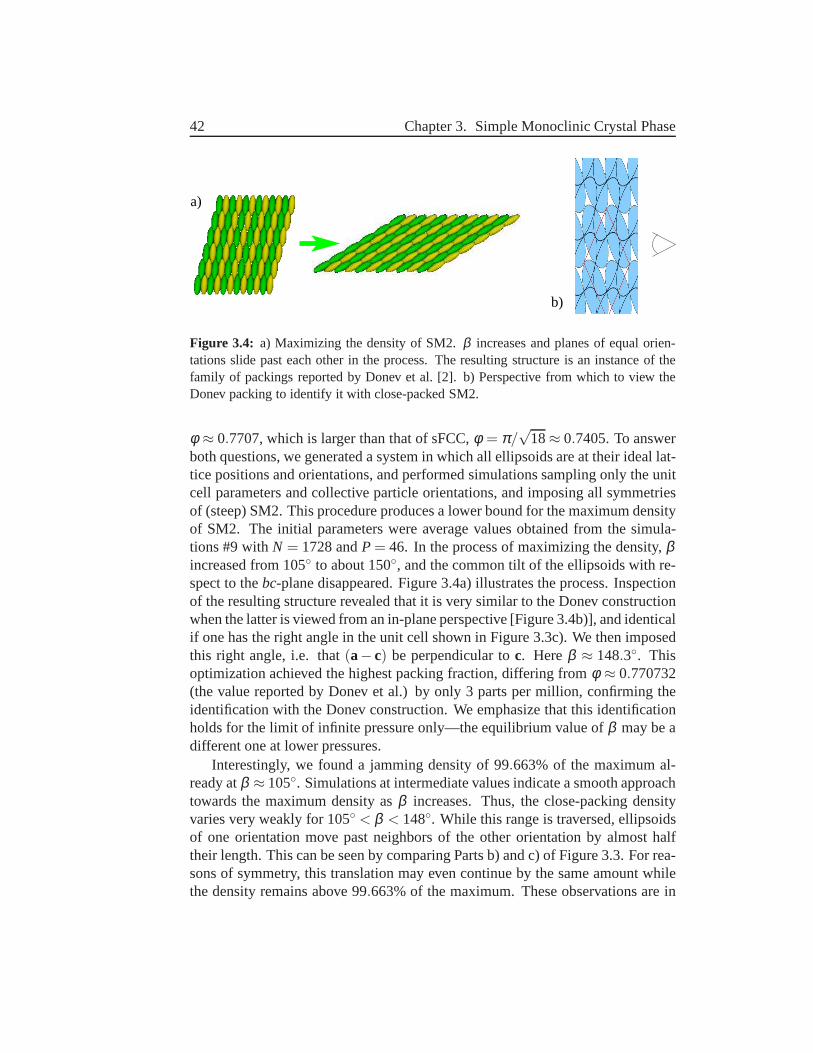
42 Chapter 3. Simple Monoclinic Crystal Phase
a)
b)
Figure 3.4: a) Maximizing the density of SM2.β increases and planes of equal orien-tations slide past each other in the process. The resulting structure is an instance of thefamily of packings reported by Donev et al. [2]. b) Perspective from which to view theDonev packing to identify it with close-packed SM2.
φ ≈ 0.7707, which is larger than that of sFCC,φ = π/√
18≈ 0.7405. To answerboth questions, we generated a system in which all ellipsoids are at their ideal lat-tice positions and orientations, and performed simulations sampling only the unitcell parameters and collective particle orientations, andimposing all symmetriesof (steep) SM2. This procedure produces a lower bound for themaximum densityof SM2. The initial parameters were average values obtainedfrom the simula-tions #9 withN = 1728 andP = 46. In the process of maximizing the density,βincreased from 105 to about 150, and the common tilt of the ellipsoids with re-spect to thebc-plane disappeared. Figure 3.4a) illustrates the process.Inspectionof the resulting structure revealed that it is very similar to the Donev constructionwhen the latter is viewed from an in-plane perspective [Figure 3.4b)], and identicalif one has the right angle in the unit cell shown in Figure 3.3c). We then imposedthis right angle, i.e. that(a− c) be perpendicular toc. Hereβ ≈ 148.3. Thisoptimization achieved the highest packing fraction, differing from φ ≈ 0.770732(the value reported by Donev et al.) by only 3 parts per million, confirming theidentification with the Donev construction. We emphasize that this identificationholds for the limit of infinite pressure only—the equilibrium value ofβ may be adifferent one at lower pressures.
Interestingly, we found a jamming density of 99.663% of the maximum al-ready atβ ≈ 105. Simulations at intermediate values indicate a smooth approachtowards the maximum density asβ increases. Thus, the close-packing densityvaries very weakly for 105 < β < 148. While this range is traversed, ellipsoidsof one orientation move past neighbors of the other orientation by almost halftheir length. This can be seen by comparing Parts b) and c) of Figure 3.3. For rea-sons of symmetry, this translation may even continue by the same amount whilethe density remains above 99.663% of the maximum. These observations are in
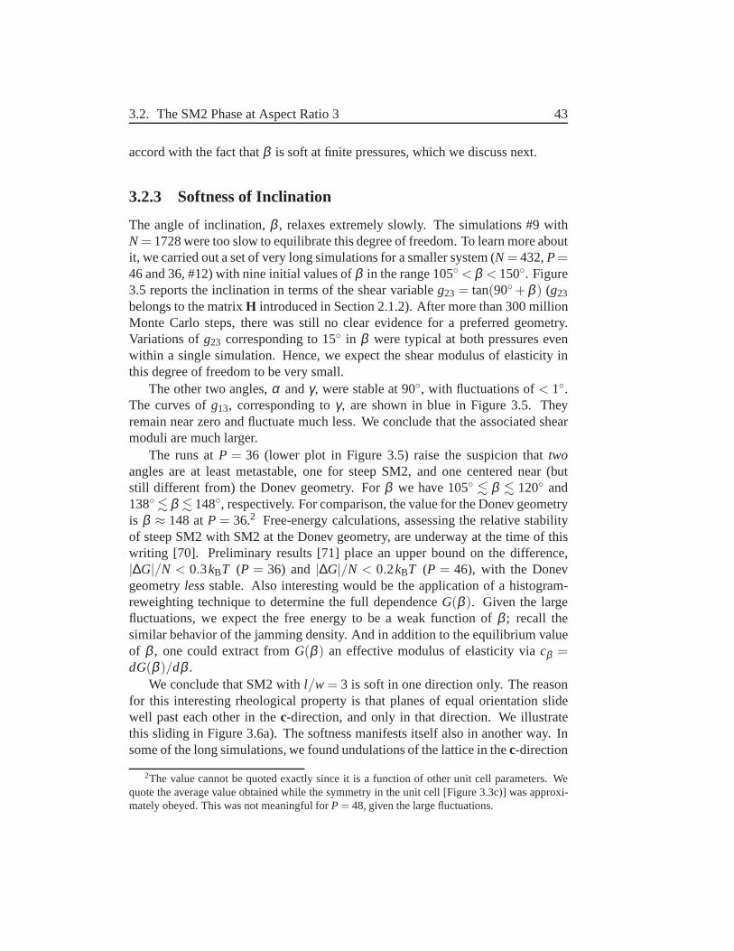
3.2. The SM2 Phase at Aspect Ratio 3 43
accord with the fact thatβ is soft at finite pressures, which we discuss next.
3.2.3 Softness of Inclination
The angle of inclination,β , relaxes extremely slowly. The simulations #9 withN = 1728 were too slow to equilibrate this degree of freedom. To learn more aboutit, we carried out a set of very long simulations for a smallersystem (N = 432,P=46 and 36, #12) with nine initial values ofβ in the range 105 < β < 150. Figure3.5 reports the inclination in terms of the shear variableg23 = tan(90+ β ) (g23
belongs to the matrixH introduced in Section 2.1.2). After more than 300 millionMonte Carlo steps, there was still no clear evidence for a preferred geometry.Variations ofg23 corresponding to 15 in β were typical at both pressures evenwithin a single simulation. Hence, we expect the shear modulus of elasticity inthis degree of freedom to be very small.
The other two angles,α andγ, were stable at 90, with fluctuations of< 1.The curves ofg13, corresponding toγ, are shown in blue in Figure 3.5. Theyremain near zero and fluctuate much less. We conclude that theassociated shearmoduli are much larger.
The runs atP = 36 (lower plot in Figure 3.5) raise the suspicion thattwoangles are at least metastable, one for steep SM2, and one centered near (butstill different from) the Donev geometry. Forβ we have 105 . β . 120 and138 . β . 148, respectively. For comparison, the value for the Donev geometryis β ≈ 148 atP = 36.2 Free-energy calculations, assessing the relative stabilityof steep SM2 with SM2 at the Donev geometry, are underway at the time of thiswriting [70]. Preliminary results [71] place an upper boundon the difference,|∆G|/N < 0.3kBT (P = 36) and|∆G|/N < 0.2kBT (P = 46), with the Donevgeometrylessstable. Also interesting would be the application of a histogram-reweighting technique to determine the full dependenceG(β ). Given the largefluctuations, we expect the free energy to be a weak function of β ; recall thesimilar behavior of the jamming density. And in addition to the equilibrium valueof β , one could extract fromG(β ) an effective modulus of elasticity viacβ =dG(β )/dβ .
We conclude that SM2 withl/w = 3 is soft in one direction only. The reasonfor this interesting rheological property is that planes ofequal orientation slidewell past each other in thec-direction, and only in that direction. We illustratethis sliding in Figure 3.6a). The softness manifests itselfalso in another way. Insome of the long simulations, we found undulations of the lattice in thec-direction
2The value cannot be quoted exactly since it is a function of other unit cell parameters. Wequote the average value obtained while the symmetry in the unit cell [Figure 3.3c)] was approxi-mately obeyed. This was not meaningful forP = 48, given the large fluctuations.
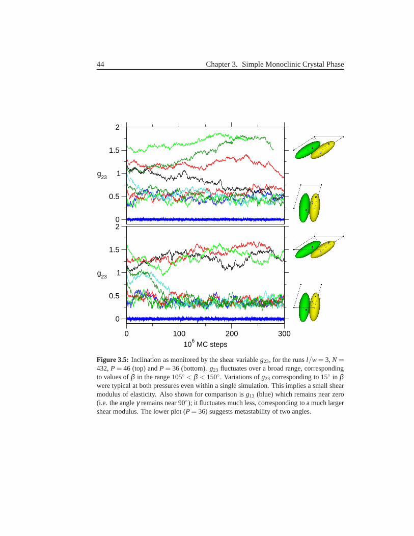
44 Chapter 3. Simple Monoclinic Crystal Phase
0
0.5
1
1.5
2
g23
0 100 200 30010
6 MC steps
0
0.5
1
1.5
2
g23
Figure 3.5: Inclination as monitored by the shear variableg23, for the runsl/w = 3, N =432,P = 46 (top) andP = 36 (bottom).g23 fluctuates over a broad range, correspondingto values ofβ in the range 105 < β < 150. Variations ofg23 corresponding to 15 in βwere typical at both pressures even within a single simulation. This implies a small shearmodulus of elasticity. Also shown for comparison isg13 (blue) which remains near zero(i.e. the angleγ remains near 90); it fluctuates much less, corresponding to a much largershear modulus. The lower plot (P = 36) suggests metastability of two angles.
3.2. The SM2 Phase at Aspect Ratio 3 45
c)b)
a)
Figure 3.6: a) Planes slide well past each other in the direction indicated by the arrows.b) Defect as a result of the softness. The orientations in oneplane (fifth from right) haveslightly changed. c) Centers of mass of the same configuration, exposing the undulationsin the lattice.
to the point of planar defects, which would spontaneously heal again. A snapshotof such a defect is shown in Figure 3.6b). The slightly different color of oneplane (the fifth from the right) shows that the defect also affects the orientations.In Figure 3.6c) we show the centers of mass of the same configuration, and weclearly see the mentioned undulations.
3.2.4 Equation of State Data
Figure 3.7 shows equation of state data of SM2 (blue solid squares) from our sim-ulations withN = 1728 particles (runs #9). The density of SM2 is higher thanthat of sFCC (red open squares [1]) for all pressures. Five ofthe eight systems #9underwent the transition to SM2 already at the highest simulated pressureP= 48,the remaining three atP = 46. Note also that in all our expansion runs, SM2melted to the nematic phase without ever re-visiting the sFCC phase from whichit developed; this is strong evidence that SM2 is lower in free energy than sFCC.Free-energy calculations are in progress also for this comparison [70], and the pre-liminary data [71] confirm the greater stability of SM2 with|∆G|/N = 0.4(2)kBT(P = 46), with some evidence that this difference becomes small on reaching thesolid/nematic transition.
We also show in Figure 3.7 the nematic branch (triangles) from the(N,P,T)
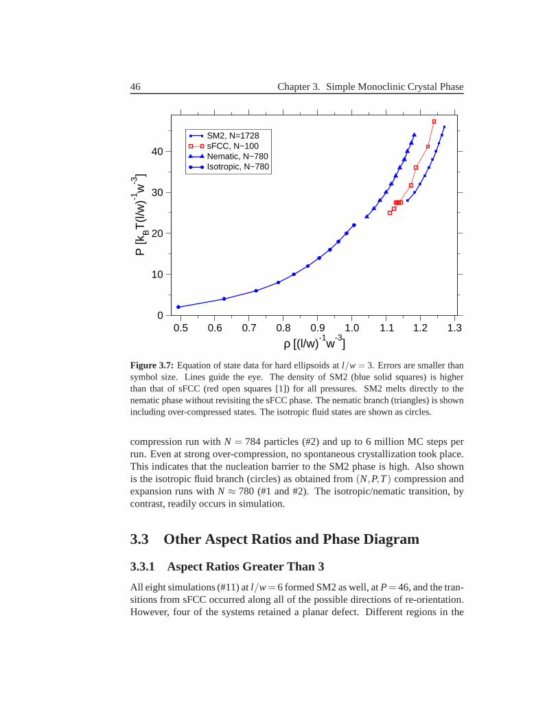
46 Chapter 3. Simple Monoclinic Crystal Phase
0.5 0.6 0.7 0.8 0.9 1.0 1.1 1.2 1.3
ρ [(l/w)-1
w-3
]
0
10
20
30
40P
[kBT
(l/w
)-1w
-3]
SM2, N=1728sFCC, N~100Nematic, N~780Isotropic, N~780
Figure 3.7: Equation of state data for hard ellipsoids atl/w = 3. Errors are smaller thansymbol size. Lines guide the eye. The density of SM2 (blue solid squares) is higherthan that of sFCC (red open squares [1]) for all pressures. SM2 melts directly to thenematic phase without revisiting the sFCC phase. The nematic branch (triangles) is shownincluding over-compressed states. The isotropic fluid states are shown as circles.
compression run withN = 784 particles (#2) and up to 6 million MC steps perrun. Even at strong over-compression, no spontaneous crystallization took place.This indicates that the nucleation barrier to the SM2 phase is high. Also shownis the isotropic fluid branch (circles) as obtained from(N,P,T) compression andexpansion runs withN ≈ 780 (#1 and #2). The isotropic/nematic transition, bycontrast, readily occurs in simulation.
3.3 Other Aspect Ratios and Phase Diagram
3.3.1 Aspect Ratios Greater Than 3
All eight simulations (#11) atl/w= 6 formed SM2 as well, atP= 46, and the tran-sitions from sFCC occurred along all of the possible directions of re-orientation.However, four of the systems retained a planar defect. Different regions in the
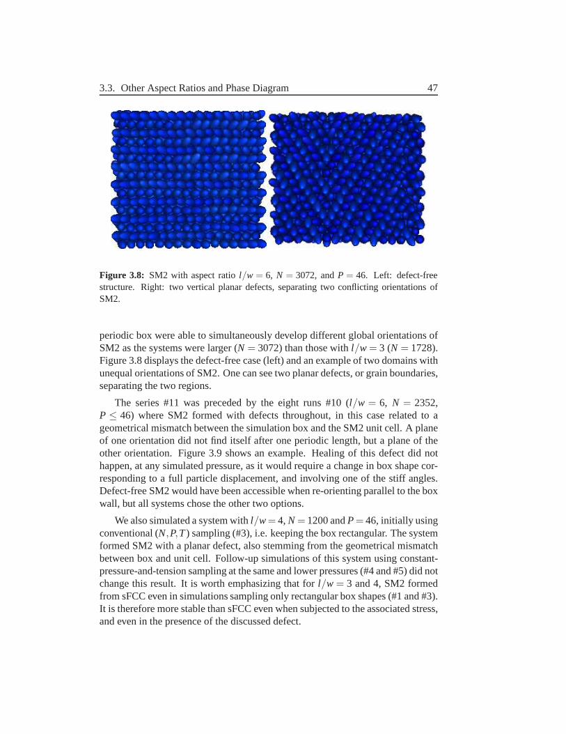
3.3. Other Aspect Ratios and Phase Diagram 47
Figure 3.8: SM2 with aspect ratiol/w = 6, N = 3072, andP = 46. Left: defect-freestructure. Right: two vertical planar defects, separatingtwo conflicting orientations ofSM2.
periodic box were able to simultaneously develop differentglobal orientations ofSM2 as the systems were larger (N = 3072) than those withl/w = 3 (N = 1728).Figure 3.8 displays the defect-free case (left) and an example of two domains withunequal orientations of SM2. One can see two planar defects,or grain boundaries,separating the two regions.
The series #11 was preceded by the eight runs #10 (l/w = 6, N = 2352,P ≤ 46) where SM2 formed with defects throughout, in this case related to ageometrical mismatch between the simulation box and the SM2unit cell. A planeof one orientation did not find itself after one periodic length, but a plane of theother orientation. Figure 3.9 shows an example. Healing of this defect did nothappen, at any simulated pressure, as it would require a change in box shape cor-responding to a full particle displacement, and involving one of the stiff angles.Defect-free SM2 would have been accessible when re-orienting parallel to the boxwall, but all systems chose the other two options.
We also simulated a system withl/w= 4,N = 1200 andP= 46, initially usingconventional (N,P,T) sampling (#3), i.e. keeping the box rectangular. The systemformed SM2 with a planar defect, also stemming from the geometrical mismatchbetween box and unit cell. Follow-up simulations of this system using constant-pressure-and-tension sampling at the same and lower pressures (#4 and #5) did notchange this result. It is worth emphasizing that forl/w = 3 and 4, SM2 formedfrom sFCC even in simulations sampling only rectangular boxshapes (#1 and #3).It is therefore more stable than sFCC even when subjected to the associated stress,and even in the presence of the discussed defect.
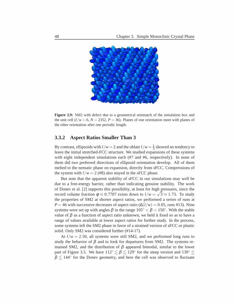
48 Chapter 3. Simple Monoclinic Crystal Phase
Figure 3.9: SM2 with defect due to a geometrical mismatch of the simulation box andthe unit cell (l/w = 6, N = 2352,P = 36). Planes of one orientation meet with planes ofthe other orientation after one periodic length.
3.3.2 Aspect Ratios Smaller Than 3
By contrast, ellipsoids withl/w= 2 and the oblatel/w= 13 showed no tendency to
leave the initial stretched-FCC structure. We studied expansions of these systemswith eight independent simulations each (#7 and #6, respectively). In none ofthem did two preferred directions of ellipsoid orientationdevelop. All of themmelted to the nematic phase on expansion, directly from sFCC. Compressions ofthe system withl/w = 2 (#8) also stayed in the sFCC phase.
But note that the apparent stability of sFCC in our simulations may well bedue to a free-energy barrier, rather than indicating genuine stability. The workof Donev et al. [2] supports this possibility, at least for high pressures, since therecord volume fractionφ ≈ 0.7707 exists down tol/w =
√3≈ 1.73. To study
the properties of SM2 at shorter aspect ratios, we performeda series of runs atP = 46 with successive decreases of aspect ratio (∆(l/w) = 0.05, runs #13). Ninesystems were set up with anglesβ in the range 105 < β < 150. With the stablevalue ofβ as a function of aspect ratio unknown, we held it fixed so as to have arange of values available at lower aspect ratios for furtherstudy. In the process,some systems left the SM2 phase in favor of a strained versionof sFCC or plasticsolid. Only SM2 was considered further (#14-17).
At l/w = 2.50, all systems were still SM2, and we performed long runs tostudy the behavior ofβ and to look for departures from SM2. The systems re-mained SM2, and the distribution ofβ appeared bimodal, similar to the lowerpart of Figure 3.5. We have 112 . β . 129 for the steep version and 139 .β . 144 for the Donev geometry, and here the cell was observed to fluctuate
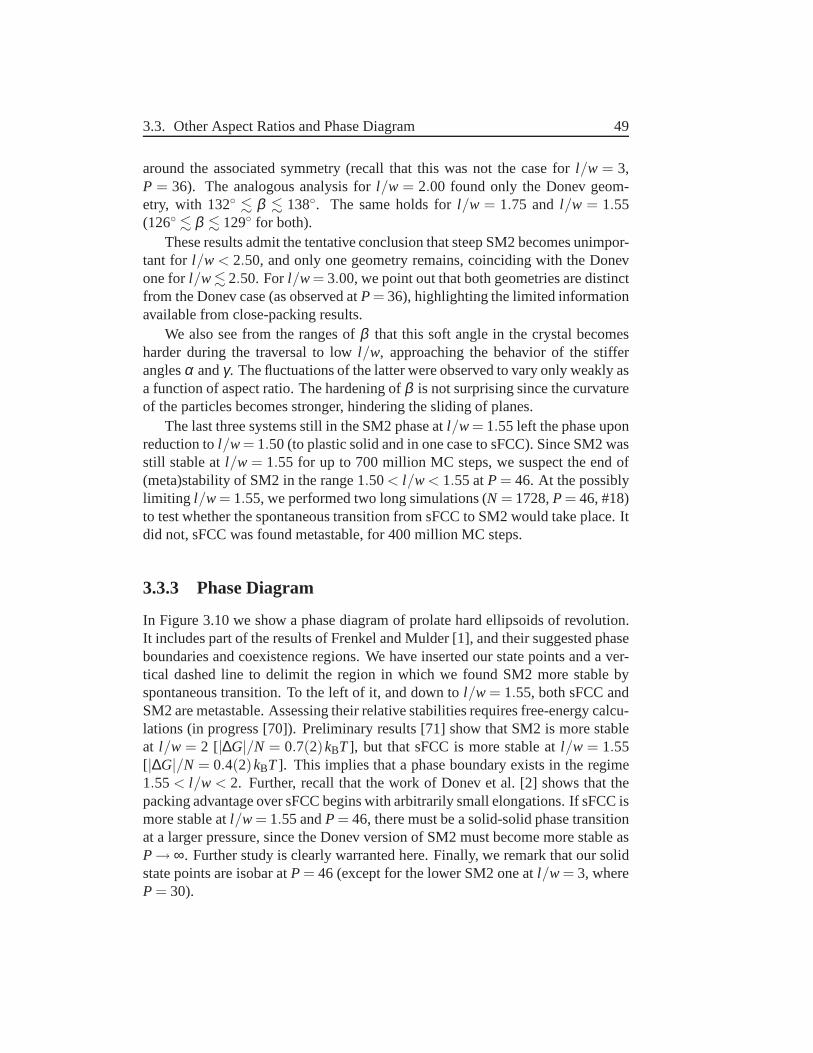
3.3. Other Aspect Ratios and Phase Diagram 49
around the associated symmetry (recall that this was not thecase forl/w = 3,P = 36). The analogous analysis forl/w = 2.00 found only the Donev geom-etry, with 132 . β . 138. The same holds forl/w = 1.75 andl/w = 1.55(126 . β . 129 for both).
These results admit the tentative conclusion that steep SM2becomes unimpor-tant for l/w < 2.50, and only one geometry remains, coinciding with the Donevone forl/w. 2.50. Forl/w= 3.00, we point out that both geometries are distinctfrom the Donev case (as observed atP= 36), highlighting the limited informationavailable from close-packing results.
We also see from the ranges ofβ that this soft angle in the crystal becomesharder during the traversal to lowl/w, approaching the behavior of the stifferanglesα andγ. The fluctuations of the latter were observed to vary only weakly asa function of aspect ratio. The hardening ofβ is not surprising since the curvatureof the particles becomes stronger, hindering the sliding ofplanes.
The last three systems still in the SM2 phase atl/w= 1.55 left the phase uponreduction tol/w= 1.50 (to plastic solid and in one case to sFCC). Since SM2 wasstill stable atl/w = 1.55 for up to 700 million MC steps, we suspect the end of(meta)stability of SM2 in the range 1.50< l/w < 1.55 atP = 46. At the possiblylimiting l/w= 1.55, we performed two long simulations (N = 1728,P= 46, #18)to test whether the spontaneous transition from sFCC to SM2 would take place. Itdid not, sFCC was found metastable, for 400 million MC steps.
3.3.3 Phase Diagram
In Figure 3.10 we show a phase diagram of prolate hard ellipsoids of revolution.It includes part of the results of Frenkel and Mulder [1], andtheir suggested phaseboundaries and coexistence regions. We have inserted our state points and a ver-tical dashed line to delimit the region in which we found SM2 more stable byspontaneous transition. To the left of it, and down tol/w = 1.55, both sFCC andSM2 are metastable. Assessing their relative stabilities requires free-energy calcu-lations (in progress [70]). Preliminary results [71] show that SM2 is more stableat l/w = 2 [|∆G|/N = 0.7(2)kBT], but that sFCC is more stable atl/w = 1.55[|∆G|/N = 0.4(2)kBT]. This implies that a phase boundary exists in the regime1.55< l/w < 2. Further, recall that the work of Donev et al. [2] shows thatthepacking advantage over sFCC begins with arbitrarily small elongations. If sFCC ismore stable atl/w= 1.55 andP= 46, there must be a solid-solid phase transitionat a larger pressure, since the Donev version of SM2 must become more stable asP→ ∞. Further study is clearly warranted here. Finally, we remark that our solidstate points are isobar atP = 46 (except for the lower SM2 one atl/w = 3, whereP = 30).
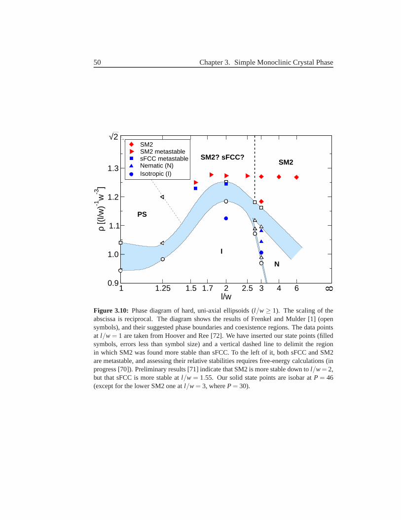
50 Chapter 3. Simple Monoclinic Crystal Phase
1 1.25 2 3 4 61.5 1.7 2.5l/w
0.9
1.0
1.1
1.2
1.3
1.4
ρ [(
l/w)-1
w-3
]
SM2SM2 metastablesFCC metastableNematic (N)Isotropic (I)
√2
N
SM2
8
I
PS
SM2? sFCC?
Figure 3.10: Phase diagram of hard, uni-axial ellipsoids (l/w≥ 1). The scaling of theabscissa is reciprocal. The diagram shows the results of Frenkel and Mulder [1] (opensymbols), and their suggested phase boundaries and coexistence regions. The data pointsat l/w = 1 are taken from Hoover and Ree [72]. We have inserted our state points (filledsymbols, errors less than symbol size) and a vertical dashedline to delimit the regionin which SM2 was found more stable than sFCC. To the left of it,both sFCC and SM2are metastable, and assessing their relative stabilities requires free-energy calculations (inprogress [70]). Preliminary results [71] indicate that SM2is more stable down tol/w= 2,but that sFCC is more stable atl/w = 1.55. Our solid state points are isobar atP = 46(except for the lower SM2 one atl/w = 3, whereP = 30).
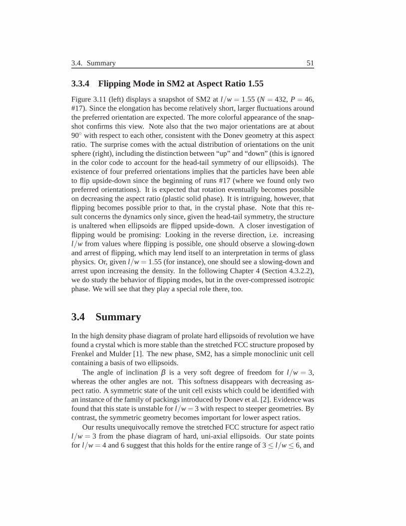
3.4. Summary 51
3.3.4 Flipping Mode in SM2 at Aspect Ratio 1.55
Figure 3.11 (left) displays a snapshot of SM2 atl/w = 1.55 (N = 432, P = 46,#17). Since the elongation has become relatively short, larger fluctuations aroundthe preferred orientation are expected. The more colorful appearance of the snap-shot confirms this view. Note also that the two major orientations are at about90 with respect to each other, consistent with the Donev geometry at this aspectratio. The surprise comes with the actual distribution of orientations on the unitsphere (right), including the distinction between “up” and“down” (this is ignoredin the color code to account for the head-tail symmetry of ourellipsoids). Theexistence of four preferred orientations implies that the particles have been ableto flip upside-down since the beginning of runs #17 (where we found only twopreferred orientations). It is expected that rotation eventually becomes possibleon decreasing the aspect ratio (plastic solid phase). It is intriguing, however, thatflipping becomes possible prior to that, in the crystal phase. Note that this re-sult concerns the dynamics only since, given the head-tail symmetry, the structureis unaltered when ellipsoids are flipped upside-down. A closer investigation offlipping would be promising: Looking in the reverse direction, i.e. increasingl/w from values where flipping is possible, one should observe a slowing-downand arrest of flipping, which may lend itself to an interpretation in terms of glassphysics. Or, givenl/w = 1.55 (for instance), one should see a slowing-down andarrest upon increasing the density. In the following Chapter 4 (Section 4.3.2.2),we do study the behavior of flipping modes, but in the over-compressed isotropicphase. We will see that they play a special role there, too.
3.4 Summary
In the high density phase diagram of prolate hard ellipsoidsof revolution we havefound a crystal which is more stable than the stretched FCC structure proposed byFrenkel and Mulder [1]. The new phase, SM2, has a simple monoclinic unit cellcontaining a basis of two ellipsoids.
The angle of inclinationβ is a very soft degree of freedom forl/w = 3,whereas the other angles are not. This softness disappears with decreasing as-pect ratio. A symmetric state of the unit cell exists which could be identified withan instance of the family of packings introduced by Donev et al. [2]. Evidence wasfound that this state is unstable forl/w= 3 with respect to steeper geometries. Bycontrast, the symmetric geometry becomes important for lower aspect ratios.
Our results unequivocally remove the stretched FCC structure for aspect ratiol/w = 3 from the phase diagram of hard, uni-axial ellipsoids. Our state pointsfor l/w = 4 and 6 suggest that this holds for the entire range of 3≤ l/w≤ 6, and
52 Chapter 3. Simple Monoclinic Crystal Phase
Figure 3.11: Left: snapshot of SM2 atl/w = 1.55 (N = 432, P = 46). The colorfulappearance documents the expectedly large fluctuations around the preferred orientations.Right: distribution of orientations on the unit sphere fromthe same system. The existenceof four preferred orientations shows that the particles have been able to flip upside-down(this does not reflect onto the color code of the snapshot).
3.4. Summary 53
possibly beyond. Preliminary free-energy calculations [71] indicate stability alsofor l/w= 2, and possibly that sFCC is more stable atl/w= 1.55. The latter resultimplies a phase boundary both for a limiting aspect ratio anda limiting densityabove the simulated one.
Finally, SM2 atl/w = 1.55 displays an interesting dynamical feature, in thatflipping of ellipsoids is possible, warranting studies of the cross-over to where thisis not possible. And certainly, the application of recent experimental advances incolloidal ellipsoids [36, 37] seems very promising.

54 Chapter 3. Simple Monoclinic Crystal Phase
Chapter 4
Glassy Dynamics in AlmostSpherical Ellipsoids
We report here on our findings of glassy dynamics in hard ellipsoids. The studywas motivated by the Molecular Mode-Coupling Theory (MMCT)predictions ofLetz et al. [3], and as a complement to the molecular dynamicsinvestigation ofde Michele et al. [30] which did not focus on the over-compressed fluid states. Un-derstanding the slowing-down of a system is also of interestoutside the context ofglass physics; for instance, it is critical for studies of nucleation. As we will see,nearly spherical ellipsoids display glassy dynamics in positional and orientationaldegrees of freedom. This by itself is surprising for a monodisperse, relativelysimple system. Typically, polydispersity in size, a mixture of particle species, ornetwork-forming covalent bonds are prerequisite to prevent the competing crys-tallization. We hence show that a slight particle anisometry acts as a sufficientsource of disorder. This sheds new light on the question of which ingredients arerequired for glass formation.
This part of our work was done in collaboration with a visiting Master student,whose internship (two times two months) the author co-supervised. She preparedand performed the MD side of the simulations, and assisted with programming anddata-analysis tasks. She also performed a modified repetition of an MC simulation(l/w= 0.8, φ = 0.614), and early analysis thereof, for the study of heterogeneousdynamics.
4.1 Overview of Simulations
Figure 4.1 shows snapshots of the simulated systems. At firstsight, they all lookthe same. However, the upper systems contain prolate (l/w = 1.25) ellipsoids,while the lower ones contain oblate (l/w = 0.8) ellipsoids; and the left-hand sys-
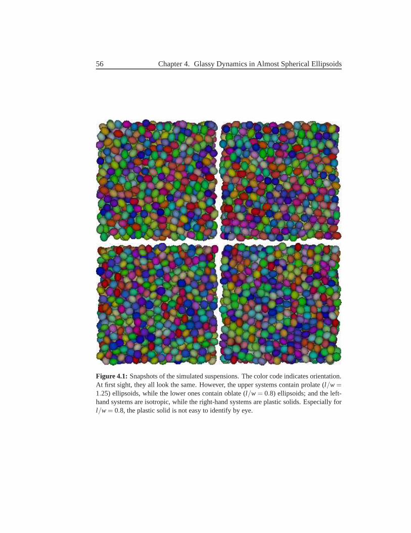
56 Chapter 4. Glassy Dynamics in Almost Spherical Ellipsoids
Figure 4.1: Snapshots of the simulated suspensions. The color code indicates orientation.At first sight, they all look the same. However, the upper systems contain prolate (l/w =1.25) ellipsoids, while the lower ones contain oblate (l/w = 0.8) ellipsoids; and the left-hand systems are isotropic, while the right-hand systems are plastic solids. Especially forl/w = 0.8, the plastic solid is not easy to identify by eye.
4.1. Overview of Simulations 57
tems are isotropic, while the right-hand systems are plastic solids. The similarityof the prolate and oblate systems will in fact recur in our results. This is, however,not trivial, since the two bodies are fundamentally different: In the limit of largeanisometry, prolate ellipsoids approach one-dimensionalneedles, while oblate el-lipsoids approach two-dimensional disks. Nevertheless, earlier work on ellipsoids(see Section 1.3.2) has found an approximate symmetry in properties under ex-change ofl/w with its inverse. Regarding the two phases “isotropic” and “plasticsolid”, we note that the distinction by eye is not easy, especially if the planes ofsymmetry are oblique with respect to the simulation box. In the Figure, the plasticsolid in l/w = 0.8 is hard to see. An order parameter is in order, we describe itbelow.
Table 4.1 summarizes all simulations for the glassy dynamics work. The sys-tems were equilibrated using MC at constant particle numberN, pressureP andtemperatureT [73, 74] in a cubic box with periodic boundaries (see Section2.1).Each system contained more than 3000 particles. Forl/w= 0.80, a dilute, randomconfiguration was compressed atP= 4 andP= 71 for 106 MC steps each, and theresulting configuration served as input for the run atP = 10. Forl/w = 1.25, adilute, random configuration was input for the run atP = 10 directly. The outputof each equilibration run was used as the starting configuration for the next higherpressure.2 During equilibration, the MC step size was automatically adjusted sothat an acceptance rate close to 30% (20% for volume moves) was obtained. Upto P = 23 (l/w = 1.25) andP = 17 (l/w = 0.80), this was not done for rotationmoves because even the largest possible setting resulted ina higher acceptancerate. This largest setting was used there, i.e. the sphere from which a random vec-tor was chosen (and added to the current orientation, followed by normalization)had unit radius.
The systems were considered equilibrated3 when the volume fraction had set-tled and all positional and the orientational correlators were independent of abso-lute simulation time. The latter requirement was verified inthe production runs.Towards the end of each equilibration run, a configuration with a volume fractionclose to the average volume fraction was chosen and scaled tothe average volumefraction exactly. It served as the input for the production runs.
For production, we used MC and MD. In the MC simulations (now at constantvolume) the step sizes were fixed to small values (displacement: 0.007w; rota-tion: 0.1); the acceptance rate was then near 70% at the highest simulated volumefractions. The particles mimic Brownian motion, similar tocolloidal ellipsoidssuspended in a liquid. The step sizes were the same for all runs, hence a unique
1The units of pressure arekBT/[(l/w)w3]. See also pg. xx.2Equilibration runs atP = 27,28,29 were all based on the output of the run atP = 26.3For the case of over-compression, “equilibrated” here means within the metastable isotropic
basin.
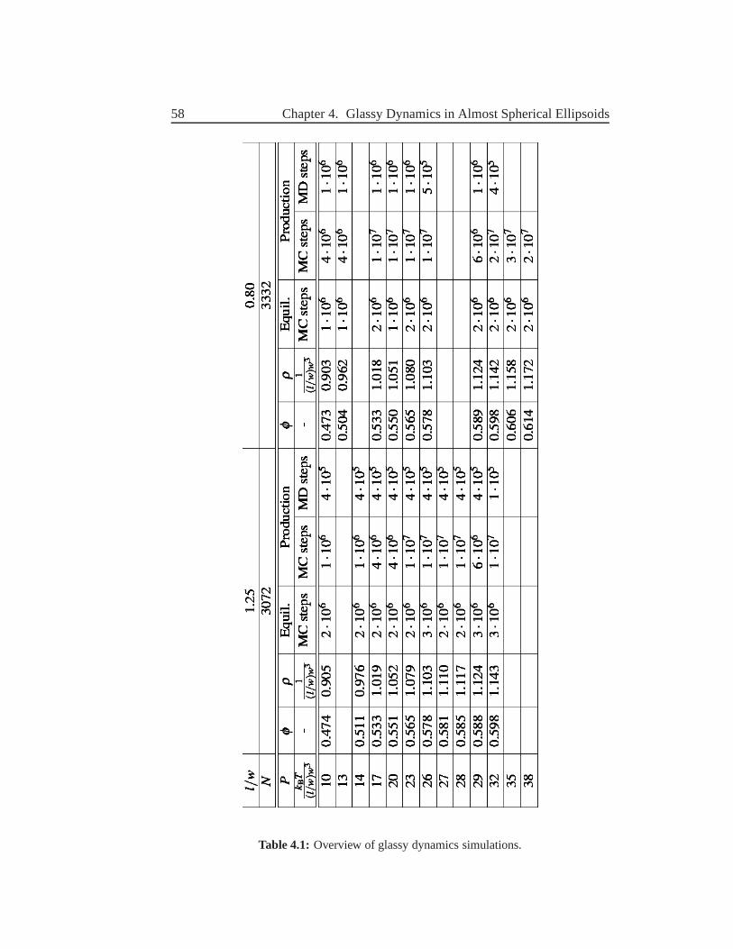
58 Chapter 4. Glassy Dynamics in Almost Spherical Ellipsoids
Table 4.1: Overview of glassy dynamics simulations.
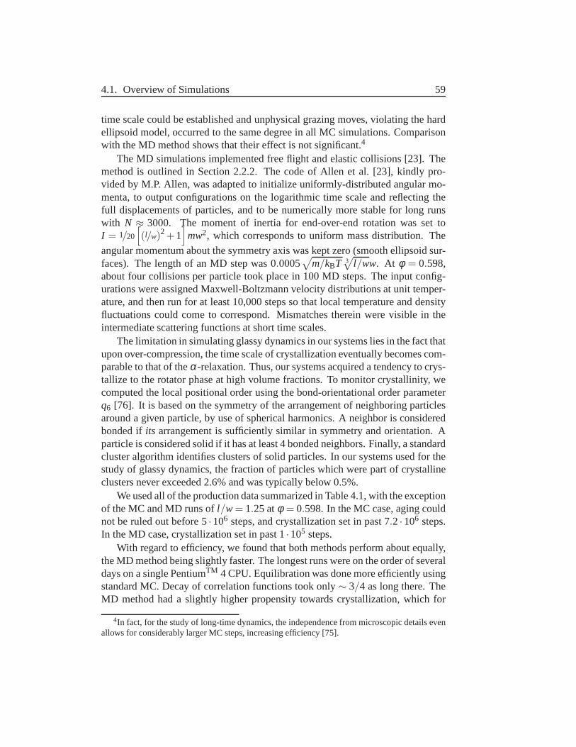
4.1. Overview of Simulations 59
time scale could be established and unphysical grazing moves, violating the hardellipsoid model, occurred to the same degree in all MC simulations. Comparisonwith the MD method shows that their effect is not significant.4
The MD simulations implemented free flight and elastic collisions [23]. Themethod is outlined in Section 2.2.2. The code of Allen et al. [23], kindly pro-vided by M.P. Allen, was adapted to initialize uniformly-distributed angular mo-menta, to output configurations on the logarithmic time scale and reflecting thefull displacements of particles, and to be numerically morestable for long runswith N ≈ 3000. The moment of inertia for end-over-end rotation was set toI = 1/20
[(l/w)2+1
]mw2, which corresponds to uniform mass distribution. The
angular momentum about the symmetry axis was kept zero (smooth ellipsoid sur-faces). The length of an MD step was 0.0005
√m/kBT 3
√l/ww. At φ = 0.598,
about four collisions per particle took place in 100 MD steps. The input config-urations were assigned Maxwell-Boltzmann velocity distributions at unit temper-ature, and then run for at least 10,000 steps so that local temperature and densityfluctuations could come to correspond. Mismatches therein were visible in theintermediate scattering functions at short time scales.
The limitation in simulating glassy dynamics in our systemslies in the fact thatupon over-compression, the time scale of crystallization eventually becomes com-parable to that of theα-relaxation. Thus, our systems acquired a tendency to crys-tallize to the rotator phase at high volume fractions. To monitor crystallinity, wecomputed the local positional order using the bond-orientational order parameterq6 [76]. It is based on the symmetry of the arrangement of neighboring particlesaround a given particle, by use of spherical harmonics. A neighbor is consideredbonded ifits arrangement is sufficiently similar in symmetry and orientation. Aparticle is considered solid if it has at least 4 bonded neighbors. Finally, a standardcluster algorithm identifies clusters of solid particles. In our systems used for thestudy of glassy dynamics, the fraction of particles which were part of crystallineclusters never exceeded 2.6% and was typically below 0.5%.
We used all of the production data summarized in Table 4.1, with the exceptionof the MC and MD runs ofl/w= 1.25 atφ = 0.598. In the MC case, aging couldnot be ruled out before 5·106 steps, and crystallization set in past 7.2 ·106 steps.In the MD case, crystallization set in past 1·105 steps.
With regard to efficiency, we found that both methods performabout equally,the MD method being slightly faster. The longest runs were onthe order of severaldays on a single PentiumTM 4 CPU. Equilibration was done more efficiently usingstandard MC. Decay of correlation functions took only∼ 3/4 as long there. TheMD method had a slightly higher propensity towards crystallization, which for
4In fact, for the study of long-time dynamics, the independence from microscopic details evenallows for considerably larger MC steps, increasing efficiency [75].
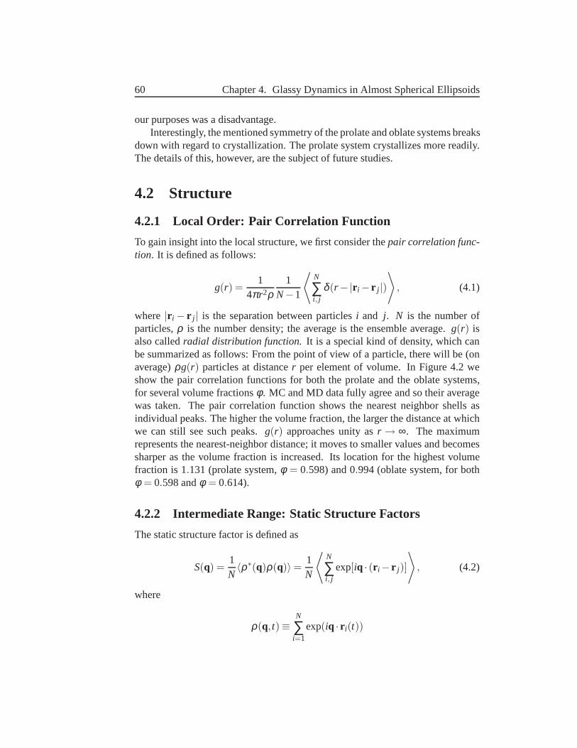
60 Chapter 4. Glassy Dynamics in Almost Spherical Ellipsoids
our purposes was a disadvantage.Interestingly, the mentioned symmetry of the prolate and oblate systems breaks
down with regard to crystallization. The prolate system crystallizes more readily.The details of this, however, are the subject of future studies.
4.2 Structure
4.2.1 Local Order: Pair Correlation Function
To gain insight into the local structure, we first consider thepair correlation func-tion. It is defined as follows:
g(r) =1
4πr2ρ1
N−1
⟨N
∑i, j
δ (r−|r i − r j |)⟩
, (4.1)
where|r i − r j | is the separation between particlesi and j. N is the number ofparticles,ρ is the number density; the average is the ensemble average.g(r) isalso calledradial distribution function.It is a special kind of density, which canbe summarized as follows: From the point of view of a particle, there will be (onaverage)ρg(r) particles at distancer per element of volume. In Figure 4.2 weshow the pair correlation functions for both the prolate andthe oblate systems,for several volume fractionsφ . MC and MD data fully agree and so their averagewas taken. The pair correlation function shows the nearest neighbor shells asindividual peaks. The higher the volume fraction, the larger the distance at whichwe can still see such peaks.g(r) approaches unity asr → ∞. The maximumrepresents the nearest-neighbor distance; it moves to smaller values and becomessharper as the volume fraction is increased. Its location for the highest volumefraction is 1.131 (prolate system,φ = 0.598) and 0.994 (oblate system, for bothφ = 0.598 andφ = 0.614).
4.2.2 Intermediate Range: Static Structure Factors
The static structure factor is defined as
S(q) =1N〈ρ∗(q)ρ(q)〉=
1N
⟨N
∑i, j
exp[iq · (r i − r j)]
⟩, (4.2)
where
ρ(q, t)≡N
∑i=1
exp(iq · r i(t))
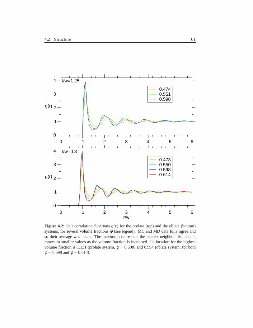
4.2. Structure 61
0 1 2 3 4 5 60
1
2
3
4
g(r)
0.4740.5510.598
0 1 2 3 4 5 6r/w
0
1
2
3
4
g(r)
0.4730.5500.5980.614
l/w=0.8
l/w=1.25
Figure 4.2: Pair correlation functionsg(r) for the prolate (top) and the oblate (bottom)systems, for several volume fractionsφ (see legend). MC and MD data fully agree andso their average was taken. The maximum represents the nearest-neighbor distance; itmoves to smaller values as the volume fraction is increased.Its location for the highestvolume fraction is 1.131 (prolate system,φ = 0.598) and 0.994 (oblate system, for bothφ = 0.598 andφ = 0.614).
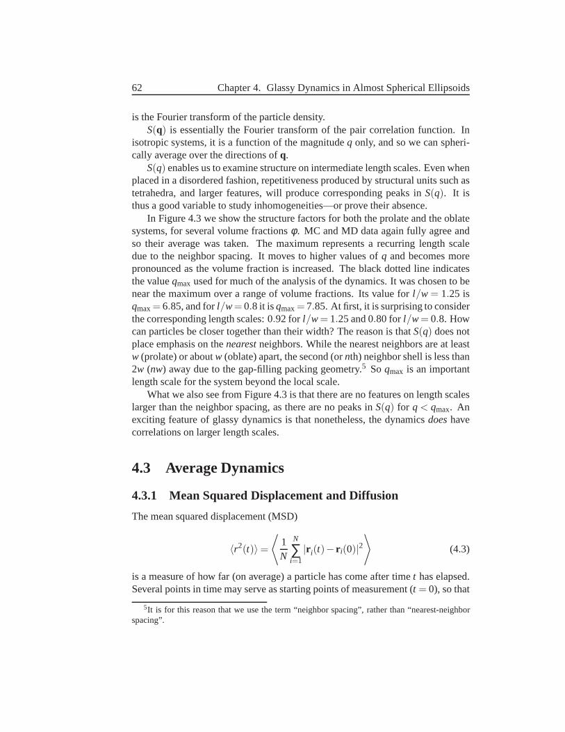
62 Chapter 4. Glassy Dynamics in Almost Spherical Ellipsoids
is the Fourier transform of the particle density.S(q) is essentially the Fourier transform of the pair correlation function. In
isotropic systems, it is a function of the magnitudeq only, and so we can spheri-cally average over the directions ofq.
S(q) enables us to examine structure on intermediate length scales. Even whenplaced in a disordered fashion, repetitiveness produced bystructural units such astetrahedra, and larger features, will produce corresponding peaks inS(q). It isthus a good variable to study inhomogeneities—or prove their absence.
In Figure 4.3 we show the structure factors for both the prolate and the oblatesystems, for several volume fractionsφ . MC and MD data again fully agree andso their average was taken. The maximum represents a recurring length scaledue to the neighbor spacing. It moves to higher values ofq and becomes morepronounced as the volume fraction is increased. The black dotted line indicatesthe valueqmax used for much of the analysis of the dynamics. It was chosen tobenear the maximum over a range of volume fractions. Its value for l/w = 1.25 isqmax= 6.85, and forl/w= 0.8 it isqmax= 7.85. At first, it is surprising to considerthe corresponding length scales: 0.92 for l/w= 1.25 and 0.80 for l/w= 0.8. Howcan particles be closer together than their width? The reason is thatS(q) does notplace emphasis on thenearestneighbors. While the nearest neighbors are at leastw (prolate) or aboutw (oblate) apart, the second (ornth) neighbor shell is less than2w (nw) away due to the gap-filling packing geometry.5 Soqmax is an importantlength scale for the system beyond the local scale.
What we also see from Figure 4.3 is that there are no features on length scaleslarger than the neighbor spacing, as there are no peaks inS(q) for q < qmax. Anexciting feature of glassy dynamics is that nonetheless, the dynamicsdoeshavecorrelations on larger length scales.
4.3 Average Dynamics
4.3.1 Mean Squared Displacement and Diffusion
The mean squared displacement (MSD)
〈r2(t)〉=
⟨1N
N
∑i=1
|r i(t)− r i(0)|2⟩
(4.3)
is a measure of how far (on average) a particle has come after time t has elapsed.Several points in time may serve as starting points of measurement (t = 0), so that
5It is for this reason that we use the term “neighbor spacing”,rather than “nearest-neighborspacing”.
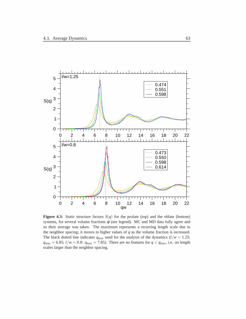
4.3. Average Dynamics 63
0 2 4 6 8 10 12 14 16 18 20 220
1
2
3
4
5
S(q)
0.4740.5510.598
0 2 4 6 8 10 12 14 16 18 20 22qw
0
1
2
3
4
5
S(q)
0.4730.5500.5980.614
l/w=0.8
l/w=1.25
Figure 4.3: Static structure factorsS(q) for the prolate (top) and the oblate (bottom)systems, for several volume fractionsφ (see legend). MC and MD data fully agree andso their average was taken. The maximum represents a recurring length scale due tothe neighbor spacing; it moves to higher values ofq as the volume fraction is increased.The black dotted line indicatesqmax used for the analysis of the dynamics (l/w = 1.25:qmax = 6.85; l/w = 0.8: qmax = 7.85). There are no features forq < qmax, i.e. on lengthscales larger than the neighbor spacing.
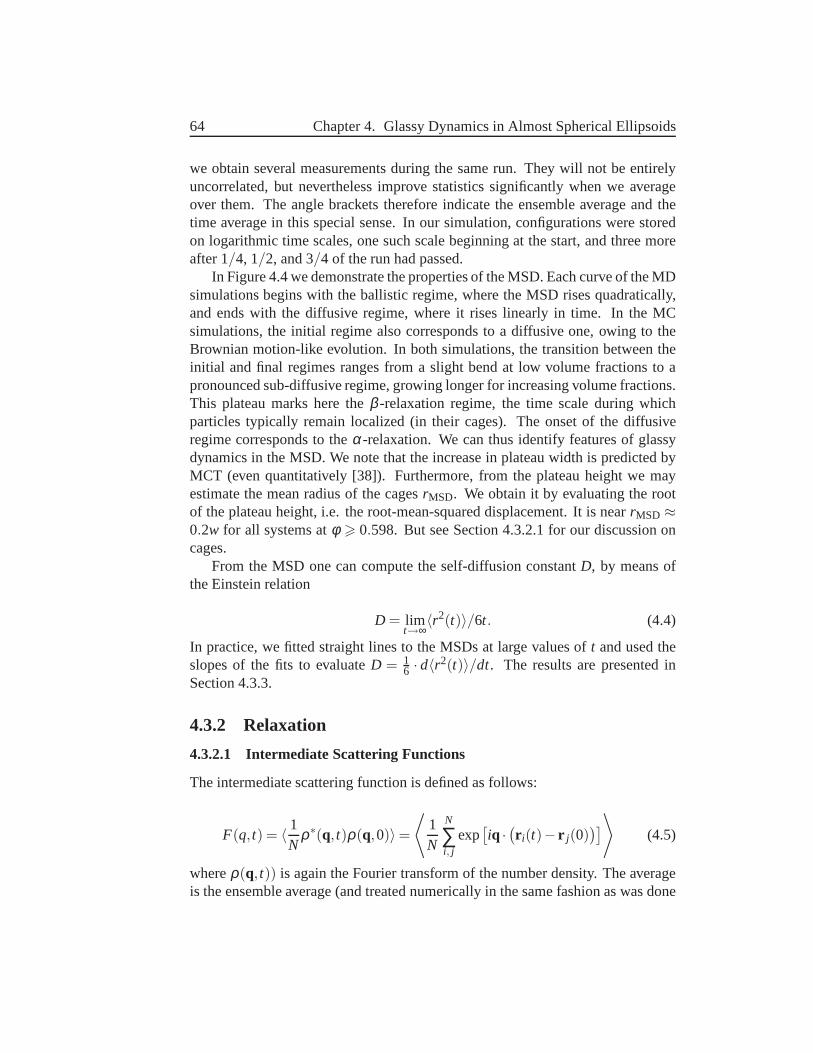
64 Chapter 4. Glassy Dynamics in Almost Spherical Ellipsoids
we obtain several measurements during the same run. They will not be entirelyuncorrelated, but nevertheless improve statistics significantly when we averageover them. The angle brackets therefore indicate the ensemble average and thetime average in this special sense. In our simulation, configurations were storedon logarithmic time scales, one such scale beginning at the start, and three moreafter 1/4, 1/2, and 3/4 of the run had passed.
In Figure 4.4 we demonstrate the properties of the MSD. Each curve of the MDsimulations begins with the ballistic regime, where the MSDrises quadratically,and ends with the diffusive regime, where it rises linearly in time. In the MCsimulations, the initial regime also corresponds to a diffusive one, owing to theBrownian motion-like evolution. In both simulations, the transition between theinitial and final regimes ranges from a slight bend at low volume fractions to apronounced sub-diffusive regime, growing longer for increasing volume fractions.This plateau marks here theβ -relaxation regime, the time scale during whichparticles typically remain localized (in their cages). Theonset of the diffusiveregime corresponds to theα-relaxation. We can thus identify features of glassydynamics in the MSD. We note that the increase in plateau width is predicted byMCT (even quantitatively [38]). Furthermore, from the plateau height we mayestimate the mean radius of the cagesrMSD. We obtain it by evaluating the rootof the plateau height, i.e. the root-mean-squared displacement. It is nearrMSD ≈0.2w for all systems atφ > 0.598. But see Section 4.3.2.1 for our discussion oncages.
From the MSD one can compute the self-diffusion constantD, by means ofthe Einstein relation
D = limt→∞
〈r2(t)〉/6t. (4.4)
In practice, we fitted straight lines to the MSDs at large values oft and used theslopes of the fits to evaluateD = 1
6 · d〈r2(t)〉/dt. The results are presented inSection 4.3.3.
4.3.2 Relaxation
4.3.2.1 Intermediate Scattering Functions
The intermediate scattering function is defined as follows:
F(q, t) = 〈 1N
ρ∗(q, t)ρ(q,0)〉=
⟨1N
N
∑i, j
exp[iq · (r i(t)− r j(0)
)]⟩(4.5)
whereρ(q, t)) is again the Fourier transform of the number density. The averageis the ensemble average (and treated numerically in the samefashion as was done
4.3. Average Dynamics 65
102
103
104
105
106
107
MC steps
10-2
10-1
100
101
102
MS
D0.800.4730.5040.5330.5500.5650.5780.5890.5980.6060.614
10-2
10-1
100
101
102
MS
D1.250.4740.5110.5330.5510.5650.5780.5880.598
102
103
104
105
106
MD steps
l/w=0.8
l/w=1.25MC
MC MD
MDl/w=1.25
l/w=0.8
Figure 4.4: Mean-squared displacements (MSD) of all systems at severalvolume frac-tions φ (see legend). One can see the ballistic regime (MD only) at early time scalesand the diffusive regime at late time scales. Towards high volume fractions there is asub-diffusive regime on intermediate time scales, indicative of glassy dynamics.
66 Chapter 4. Glassy Dynamics in Almost Spherical Ellipsoids
for MSDs), and a spherical average over all directions ofq, once more exploitingthat our systems are isotropic. Thus,F(q, t) also depends only on the magnitudeq of the wave vector.
We can extract from the double sum the diagonal terms, and hence write
F(q, t) = Fs(q, t)+Fd(q, t), (4.6)
where
Fs(q, t) =
⟨1N
N
∑i=1
exp[iq · (r i(t)− r i(0))]
⟩
Fd(q, t) =
⟨1N
N
∑i 6= j
exp[iq · (r i(t)− r j(0)
)]⟩(4.7)
are theself partand thedistinct part, respectively. These are also calledincoherentandcoherentintermediate scattering functions. Note thatF(q,0) = S(q). We willin fact always normalizeF(q, t) by S(q) so that they start at unity and in the enddecay to zero.
Roughly speaking, the self part is a measure of how much the position of theaverage particle is related to its own initial position, when we look at a resolutionspecified byq. For example, if we chooseq = 2π/w, it makes essentially nodifference when the particles have moved on a scale much smaller thanw, soFs isstill close to unity. And it makes a big difference when the particles have moved onthe order of their widthw, and soFs approaches zero. The latter condition impliesthat structural relaxation has occurred on that length scale. The distinct part playsthe same role, but relating the position of the particle to the initial position of theaverageotherparticle. We do not consider it in this study.
In Figure 4.5 we showFs(qmax, t) for all simulations, withqmax near the maxi-mum of the static structure factor (Section 4.2.2); i.e. it corresponds to the neigh-bor spacing. One can clearly see the development of a plateauwith increasingvolume fraction. This means that there are two distinct stages of relaxation, andthe later one slows down dramatically upon increase of volume fraction (notethe logarithmic time scale). This two-step decay is the hallmark in glass formers[29]. As already mentioned, the conventional interpretation is in terms of particlesbeing trapped in cages formed by their nearest neighbors. The initial decay corre-sponds to motion within the traps, and the final decay to escape. At high volumefractions, exceedingly cooperative rearrangements are required for escape, mak-ing such processes rare. We note that indicators of caging have not been seen inhard ellipsoids before (unless the moment of inertia was strongly increased [77]).The presence of cages is demonstrated in Section 4.4.2 (Figure 4.20 on page 90).
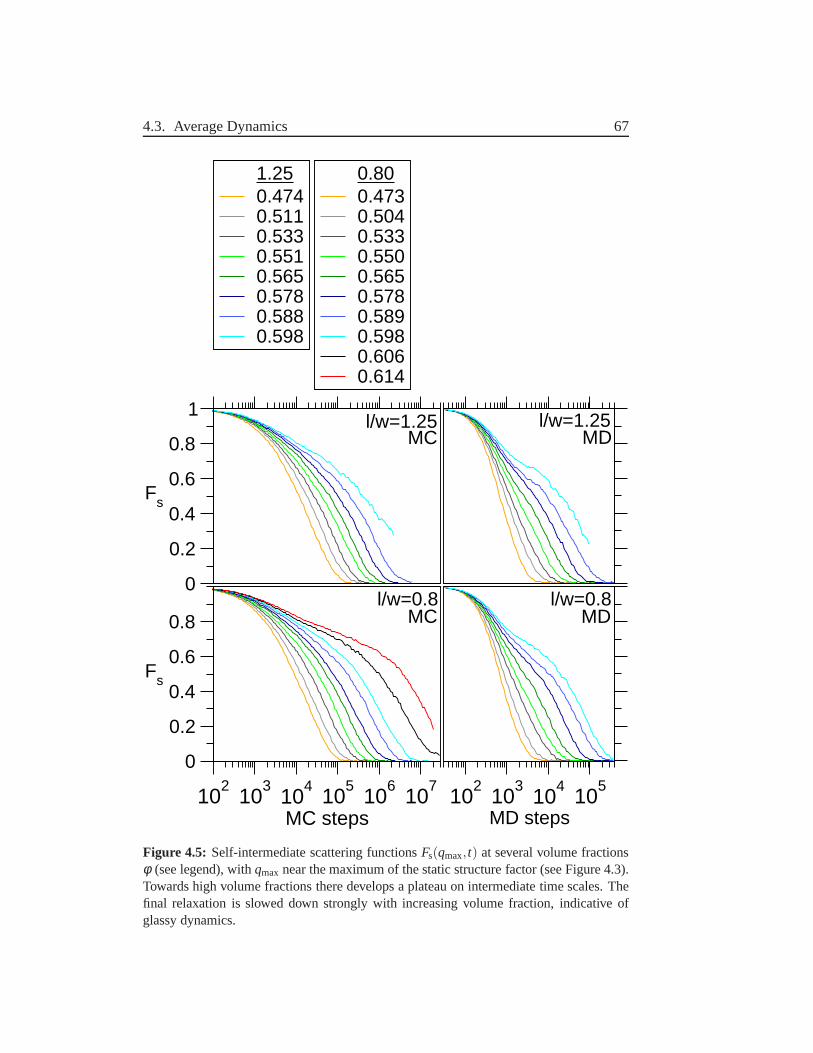
4.3. Average Dynamics 67
102
103
104
105
106
107
MC steps
0
0.2
0.4
0.6
0.8
Fs
0.800.4730.5040.5330.5500.5650.5780.5890.5980.6060.614
0
0.2
0.4
0.6
0.8
1
Fs
1.250.4740.5110.5330.5510.5650.5780.5880.598
102
103
104
105
MD steps
l/w=0.8
l/w=1.25MC
MC MD
MDl/w=1.25
l/w=0.8
Figure 4.5: Self-intermediate scattering functionsFs(qmax, t) at several volume fractionsφ (see legend), withqmax near the maximum of the static structure factor (see Figure 4.3).Towards high volume fractions there develops a plateau on intermediate time scales. Thefinal relaxation is slowed down strongly with increasing volume fraction, indicative ofglassy dynamics.
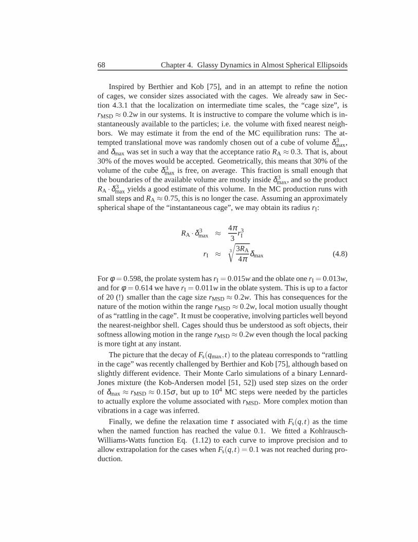
68 Chapter 4. Glassy Dynamics in Almost Spherical Ellipsoids
Inspired by Berthier and Kob [75], and in an attempt to refine the notionof cages, we consider sizes associated with the cages. We already saw in Sec-tion 4.3.1 that the localization on intermediate time scales, the “cage size”, isrMSD ≈ 0.2w in our systems. It is instructive to compare the volume whichis in-stantaneously available to the particles; i.e. the volume with fixed nearest neigh-bors. We may estimate it from the end of the MC equilibration runs: The at-tempted translational move was randomly chosen out of a cubeof volumeδ 3
max,andδmax was set in such a way that the acceptance ratioRA ≈ 0.3. That is, about30% of the moves would be accepted. Geometrically, this means that 30% of thevolume of the cubeδ 3
max is free, on average. This fraction is small enough thatthe boundaries of the available volume are mostly insideδ 3
max, and so the productRA · δ 3
max yields a good estimate of this volume. In the MC production runs withsmall steps andRA ≈ 0.75, this is no longer the case. Assuming an approximatelyspherical shape of the “instantaneous cage”, we may obtain its radiusrI:
RA ·δ 3max ≈ 4π
3r3I
rI ≈ 3
√3RA
4πδmax (4.8)
Forφ = 0.598, the prolate system hasrI = 0.015w and the oblate onerI = 0.013w,and forφ = 0.614 we haverI = 0.011w in the oblate system. This is up to a factorof 20 (!) smaller than the cage sizerMSD ≈ 0.2w. This has consequences for thenature of the motion within the rangerMSD ≈ 0.2w, local motion usually thoughtof as “rattling in the cage”. It must be cooperative, involving particles well beyondthe nearest-neighbor shell. Cages should thus be understood as soft objects, theirsoftness allowing motion in the rangerMSD≈ 0.2w even though the local packingis more tight at any instant.
The picture that the decay ofFs(qmax, t) to the plateau corresponds to “rattlingin the cage” was recently challenged by Berthier and Kob [75], although based onslightly different evidence. Their Monte Carlo simulations of a binary Lennard-Jones mixture (the Kob-Andersen model [51, 52]) used step sizes on the orderof δmax≈ rMSD ≈ 0.15σ , but up to 104 MC steps were needed by the particlesto actually explore the volume associated withrMSD. More complex motion thanvibrations in a cage was inferred.
Finally, we define the relaxation timeτ associated withFs(q, t) as the timewhen the named function has reached the value 0.1. We fitted a Kohlrausch-Williams-Watts function Eq. (1.12) to each curve to improveprecision and toallow extrapolation for the cases whenFs(q, t) = 0.1 was not reached during pro-duction.
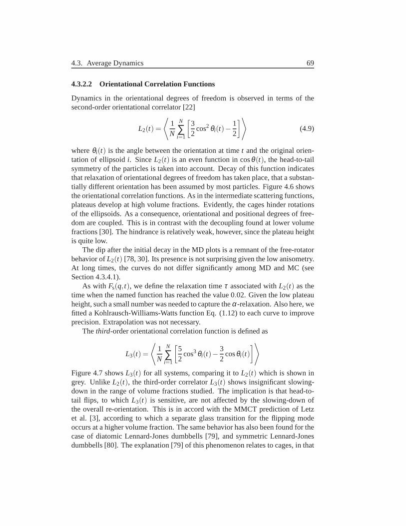
4.3. Average Dynamics 69
4.3.2.2 Orientational Correlation Functions
Dynamics in the orientational degrees of freedom is observed in terms of thesecond-order orientational correlator [22]
L2(t) =
⟨1N
N
∑i=1
[32
cos2 θi(t)− 12
]⟩(4.9)
whereθi(t) is the angle between the orientation at timet and the original orien-tation of ellipsoidi. SinceL2(t) is an even function in cosθ(t), the head-to-tailsymmetry of the particles is taken into account. Decay of this function indicatesthat relaxation of orientational degrees of freedom has taken place, that a substan-tially different orientation has been assumed by most particles. Figure 4.6 showsthe orientational correlation functions. As in the intermediate scattering functions,plateaus develop at high volume fractions. Evidently, the cages hinder rotationsof the ellipsoids. As a consequence, orientational and positional degrees of free-dom are coupled. This is in contrast with the decoupling found at lower volumefractions [30]. The hindrance is relatively weak, however,since the plateau heightis quite low.
The dip after the initial decay in the MD plots is a remnant of the free-rotatorbehavior ofL2(t) [78, 30]. Its presence is not surprising given the low anisometry.At long times, the curves do not differ significantly among MDand MC (seeSection 4.3.4.1).
As with Fs(q, t), we define the relaxation timeτ associated withL2(t) as thetime when the named function has reached the value 0.02. Given the low plateauheight, such a small number was needed to capture theα-relaxation. Also here, wefitted a Kohlrausch-Williams-Watts function Eq. (1.12) to each curve to improveprecision. Extrapolation was not necessary.
Thethird-order orientational correlation function is defined as
L3(t) =
⟨1N
N
∑i=1
[52
cos3θi(t)− 32
cosθi(t)]⟩
Figure 4.7 showsL3(t) for all systems, comparing it toL2(t) which is shown ingrey. UnlikeL2(t), the third-order correlatorL3(t) shows insignificant slowing-down in the range of volume fractions studied. The implication is that head-to-tail flips, to whichL3(t) is sensitive, are not affected by the slowing-down ofthe overall re-orientation. This is in accord with the MMCT prediction of Letzet al. [3], according to which a separate glass transition for the flipping modeoccurs at a higher volume fraction. The same behavior has also been found for thecase of diatomic Lennard-Jones dumbbells [79], and symmetric Lennard-Jonesdumbbells [80]. The explanation [79] of this phenomenon relates to cages, in that
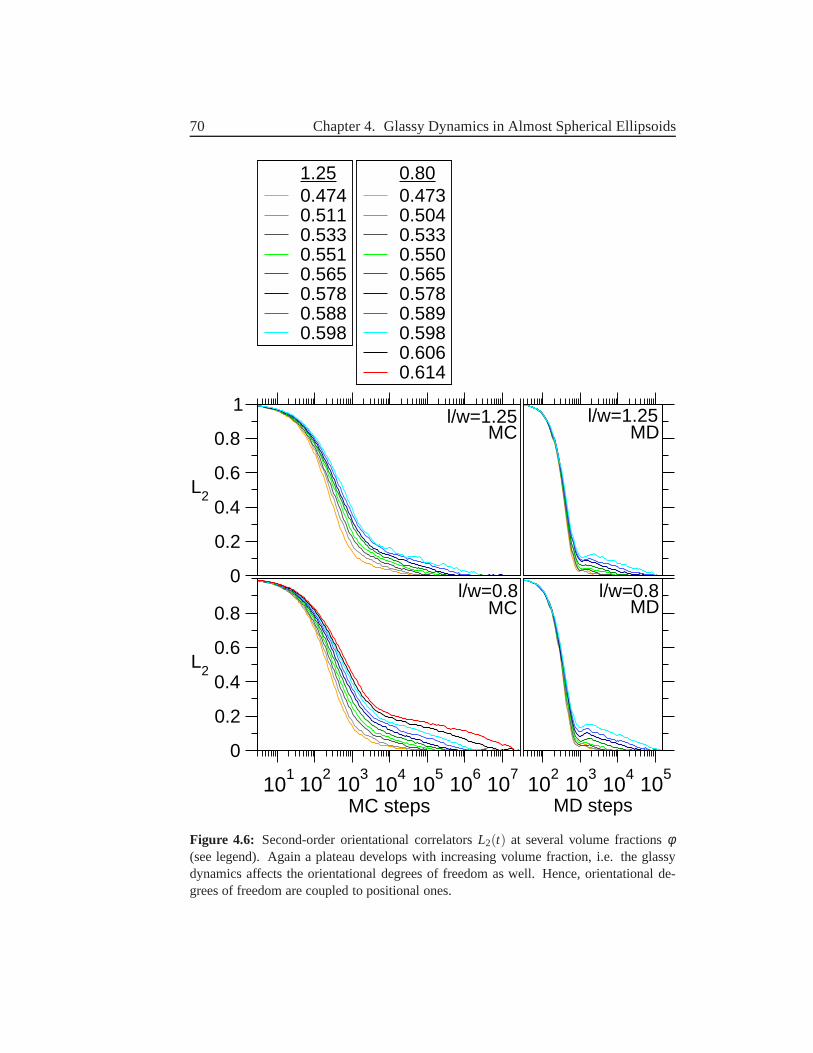
70 Chapter 4. Glassy Dynamics in Almost Spherical Ellipsoids
101
102
103
104
105
106
107
MC steps
0
0.2
0.4
0.6
0.8
L2
0.800.4730.5040.5330.5500.5650.5780.5890.5980.6060.614
0
0.2
0.4
0.6
0.8
1
L2
1.250.4740.5110.5330.5510.5650.5780.5880.598
102
103
104
105
MD steps
l/w=0.8
l/w=1.25MC
MC MD
MDl/w=1.25
l/w=0.8
Figure 4.6: Second-order orientational correlatorsL2(t) at several volume fractionsφ(see legend). Again a plateau develops with increasing volume fraction, i.e. the glassydynamics affects the orientational degrees of freedom as well. Hence, orientational de-grees of freedom are coupled to positional ones.
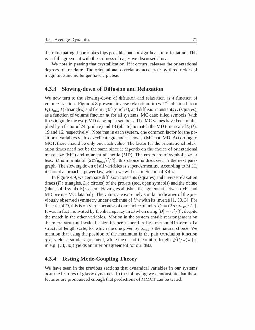
4.3. Average Dynamics 71
their fluctuating shape makes flips possible, but not significant re-orientation. Thisis in full agreement with the softness of cages we discussed above.
We note in passing that crystallization, if it occurs, releases the orientationaldegrees of freedom: The orientational correlators accelerate by three orders ofmagnitude and no longer have a plateau.
4.3.3 Slowing-down of Diffusion and Relaxation
We now turn to the slowing-down of diffusion and relaxation as a function ofvolume fraction. Figure 4.8 presents inverse relaxation timesτ−1 obtained fromFs(qmax, t) (triangles) and fromL2(t) (circles), and diffusion constantsD (squares),as a function of volume fractionφ , for all systems. MC data: filled symbols (withlines to guide the eye); MD data: open symbols. The MC values have been multi-plied by a factor of 24 (prolate) and 18 (oblate) to match the MD time scale [L2(t):19 and 16, respectively]. Note that in each system, one common factor for the po-sitional variables yields excellent agreement between MC and MD. According toMCT, there should be only one such value. The factor for the orientational relax-ation times need not be the same since it depends on the choiceof orientationalmove size (MC) and moment of inertia (MD). The errors are of symbol size orless. D is in units of (2π/qmax)2/[t]; this choice is discussed in the next para-graph. The slowing down of all variables is super-Arrhenius. According to MCT,it should approach a power law, which we will test in Section 4.3.4.4.
In Figure 4.9, we compare diffusion constants (squares) andinverse relaxationtimes (Fs: triangles,L2: circles) of the prolate (red, open symbols) and the oblate(blue, solid symbols) system. Having established the agreement between MC andMD, we use MC data only. The values are extremely similar, indicative of the pre-viously observed symmetry under exchange ofl/w with its inverse [1, 30, 3]. Forthe case ofD, this is only true because of our choice of units[D] = (2π/qmax)2/[t].It was in fact motivated by the discrepancy inD when using[D] = w2/[t], despitethe match in the other variables. Motion in the system entails rearrangement onthe micro-structural scale. Its significance is therefore best measured in terms of astructural length scale, for which the one given byqmax is the natural choice. Wemention that using the position of the maximum in the pair correlation functiong(r) yields a similar agreement, while the use of the unit of length 3
√(l/w)w (as
in e.g. [23, 30]) yields an inferior agreement for our data.
4.3.4 Testing Mode-Coupling Theory
We have seen in the previous sections that dynamical variables in our systemsbear the features of glassy dynamics. In the following, we demonstrate that thesefeatures are pronounced enough that predictions of MMCT canbe tested.
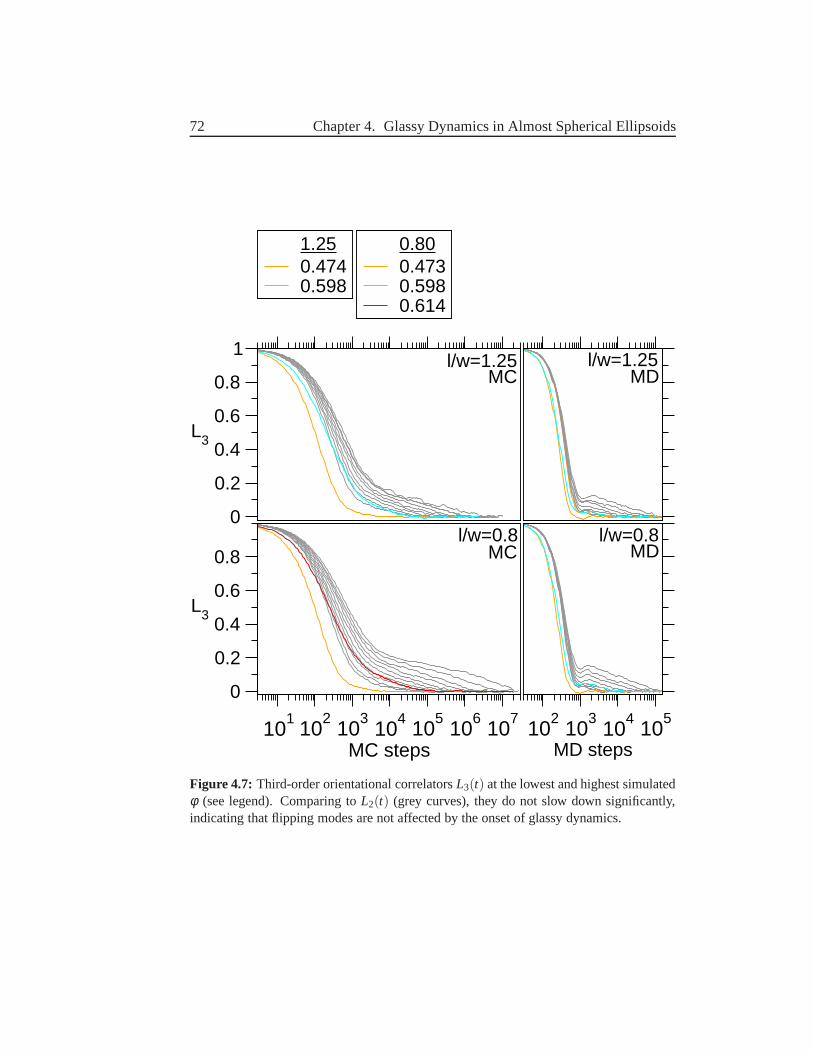
72 Chapter 4. Glassy Dynamics in Almost Spherical Ellipsoids
101
102
103
104
105
106
107
MC steps
0
0.2
0.4
0.6
0.8
L3
0.800.4730.5980.614
0
0.2
0.4
0.6
0.8
1
L3
1.250.4740.598
102
103
104
105
MD steps
l/w=0.8
l/w=1.25MC
MC MD
MDl/w=1.25
l/w=0.8
Figure 4.7: Third-order orientational correlatorsL3(t) at the lowest and highest simulatedφ (see legend). Comparing toL2(t) (grey curves), they do not slow down significantly,indicating that flipping modes are not affected by the onset of glassy dynamics.
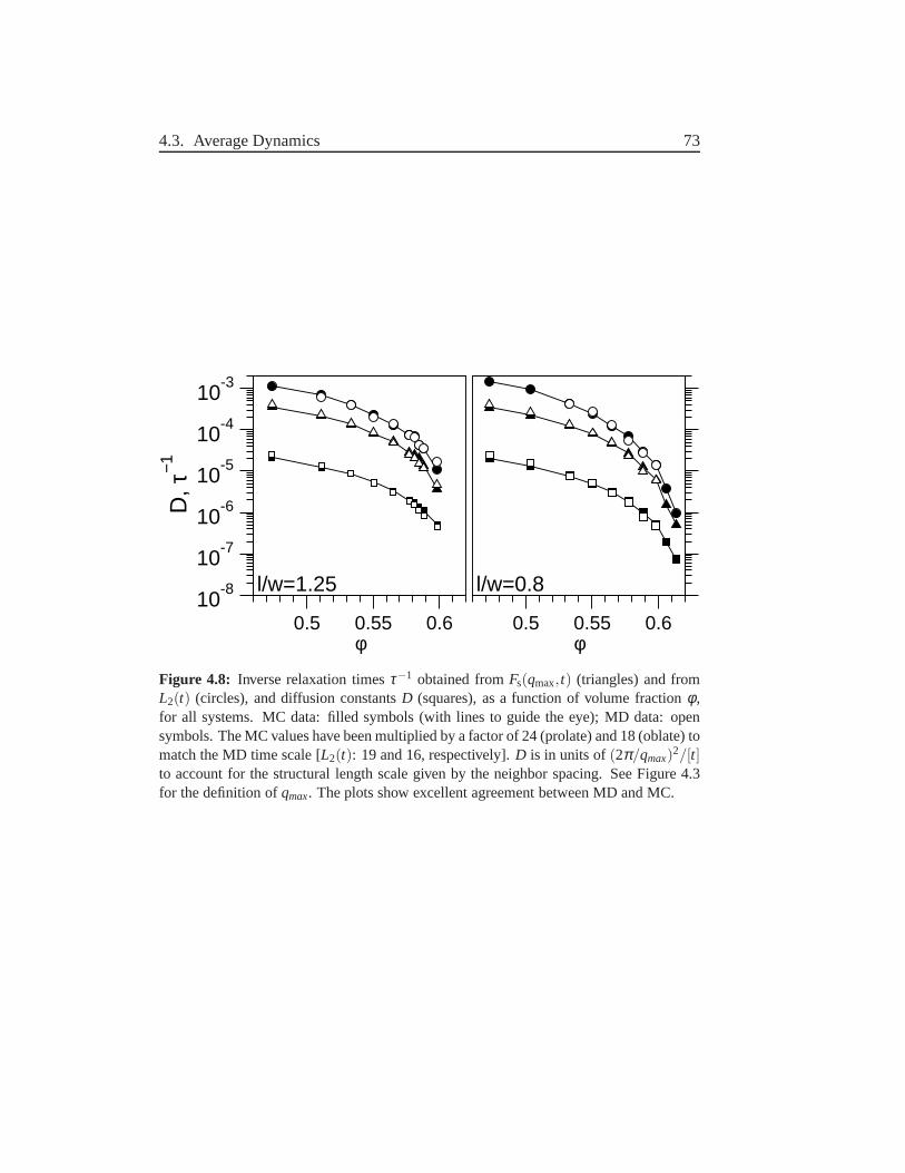
4.3. Average Dynamics 73
0.5 0.55 0.6φ
0.5 0.55 0.6φ
10-8
10-7
10-6
10-5
10-4
10-3
D, τ
−1
l/w=1.25 l/w=0.8
Figure 4.8: Inverse relaxation timesτ−1 obtained fromFs(qmax, t) (triangles) and fromL2(t) (circles), and diffusion constantsD (squares), as a function of volume fractionφ ,for all systems. MC data: filled symbols (with lines to guide the eye); MD data: opensymbols. The MC values have been multiplied by a factor of 24 (prolate) and 18 (oblate) tomatch the MD time scale [L2(t): 19 and 16, respectively].D is in units of(2π/qmax)2/[t]to account for the structural length scale given by the neighbor spacing. See Figure 4.3for the definition ofqmax. The plots show excellent agreement between MD and MC.
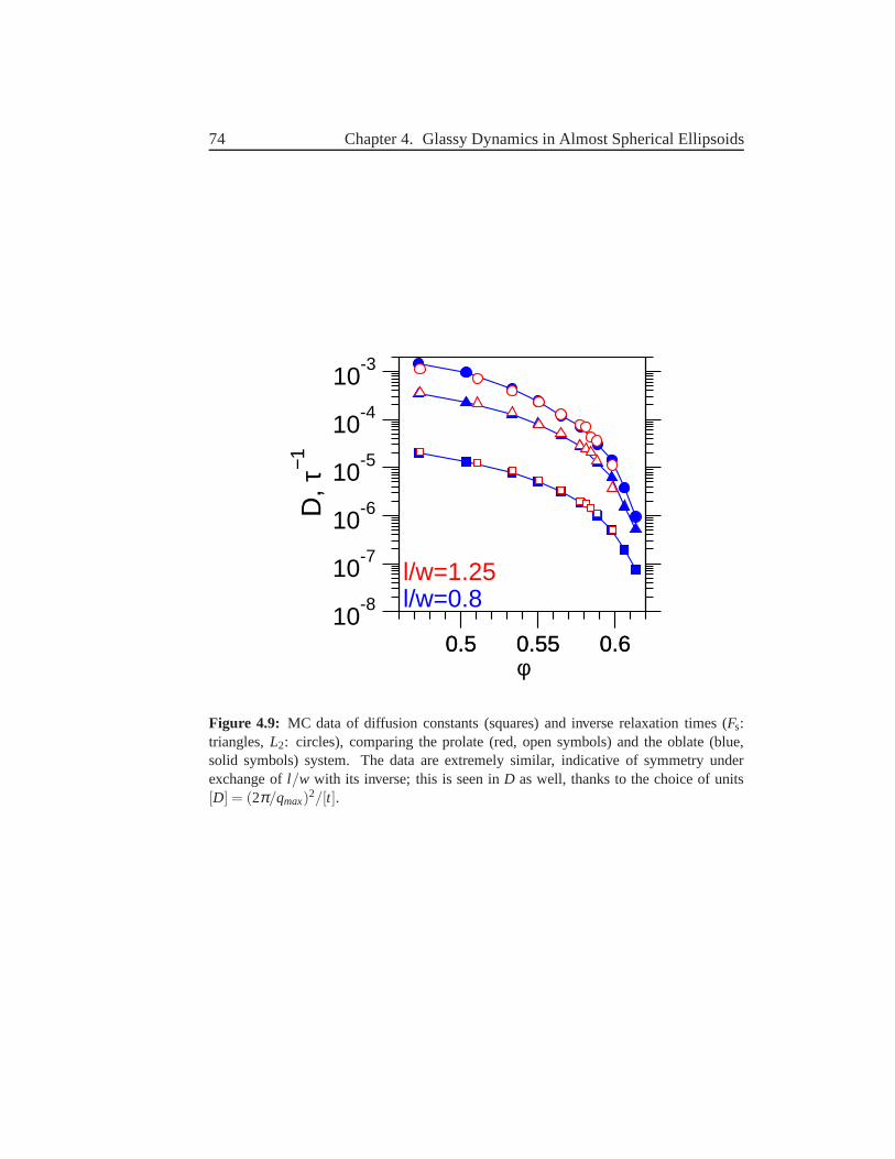
74 Chapter 4. Glassy Dynamics in Almost Spherical Ellipsoids
0.5 0.55 0.60.5 0.55 0.6φ
10-8
10-7
10-6
10-5
10-4
10-3
D, τ
−1
l/w=1.25l/w=0.8
Figure 4.9: MC data of diffusion constants (squares) and inverse relaxation times (Fs:triangles,L2: circles), comparing the prolate (red, open symbols) and the oblate (blue,solid symbols) system. The data are extremely similar, indicative of symmetry underexchange ofl/w with its inverse; this is seen inD as well, thanks to the choice of units[D] = (2π/qmax)2/[t].
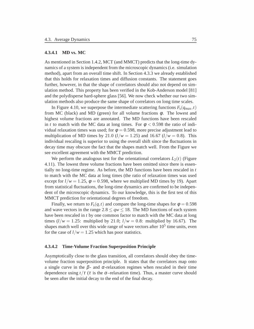
4.3. Average Dynamics 75
4.3.4.1 MD vs. MC
As mentioned in Section 1.4.2, MCT (and MMCT) predicts that the long-time dy-namics of a system is independent from the microscopic dynamics (i.e. simulationmethod), apart from an overall time shift. In Section 4.3.3 we already establishedthat this holds for relaxation times and diffusion constants. The statement goesfurther, however, in that the shape of correlators should also not depend on sim-ulation method. This property has been verified in the Kob-Anderson model [81]and the polydisperse hard-sphere glass [56]. We now check whether our two sim-ulation methods also produce the same shape of correlators on long time scales.
In Figure 4.10, we superpose the intermediate scattering functionsFs(qmax, t)from MC (black) and MD (green) for all volume fractionsφ . The lowest andhighest volume fractions are annotated. The MD functions have been rescaledin t to match with the MC data at long times. Forφ < 0.598 the ratio of indi-vidual relaxation times was used; forφ = 0.598, more precise adjustment lead tomultiplication of MD times by 21.0 (l/w = 1.25) and 16.67 (l/w = 0.8). Thisindividual rescaling is superior to using the overall shiftsince the fluctuations indecay time may obscure the fact that the shapes match well. From the Figure wesee excellent agreement with the MMCT prediction.
We perform the analogous test for the orientational correlatorsL2(t) (Figure4.11). The lowest three volume fractions have been omitted since there is essen-tially no long-time regime. As before, the MD functions havebeen rescaled intto match with the MC data at long times (the ratio of relaxation times was usedexcept forl/w = 1.25,φ = 0.598, where we multiplied MD times by 19). Apartfrom statistical fluctuations, the long-time dynamics are confirmed to be indepen-dent of the microscopic dynamics. To our knowledge, this is the first test of thisMMCT prediction for orientational degrees of freedom.
Finally, we return toFs(q, t) and compare the long-time shapes forφ = 0.598and wave vectors in the range 2.8≤ qw≤ 18. The MD functions of each systemhave been rescaled int by one common factor to match with the MC data at longtimes (l/w = 1.25: multiplied by 21.0; l/w = 0.8: multiplied by 16.67). Theshapes match well over this wide range of wave vectors after 105 time units, evenfor the case ofl/w = 1.25 which has poor statistics.
4.3.4.2 Time-Volume Fraction Superposition Principle
Asymptotically close to the glass transition, all correlators should obey the time-volume fraction superposition principle. It states that the correlators map ontoa single curve in theβ - and α-relaxation regimes when rescaled in their timedependence usingt/τ (τ is theα–relaxation time). Thus, a master curve shouldbe seen after the initial decay to the end of the final decay.
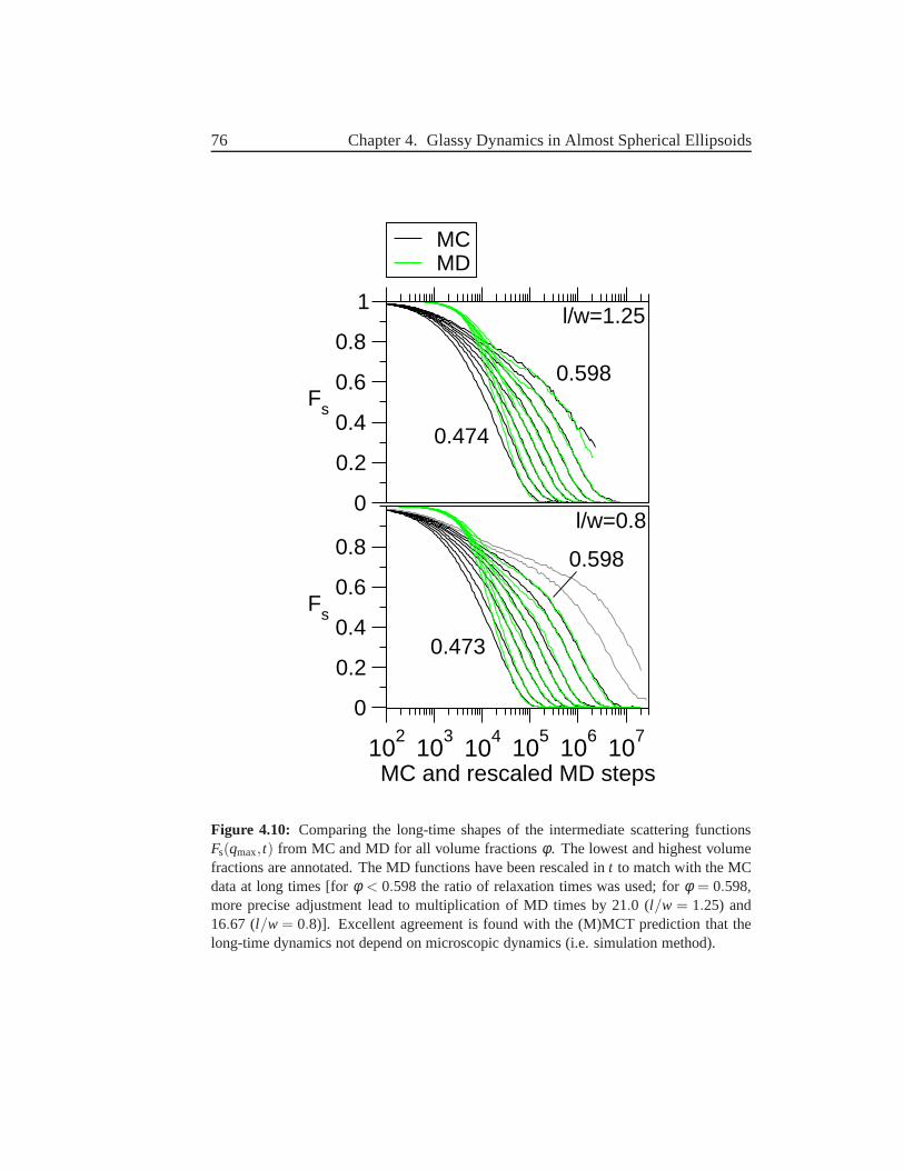
76 Chapter 4. Glassy Dynamics in Almost Spherical Ellipsoids
102
103
104
105
106
107
MC and rescaled MD steps
0
0.2
0.4
0.6
0.8
Fs
0
0.2
0.4
0.6
0.8
1
Fs
MCMD
l/w=0.8
0.598
0.474
0.598
0.473
l/w=1.25
Figure 4.10: Comparing the long-time shapes of the intermediate scattering functionsFs(qmax, t) from MC and MD for all volume fractionsφ . The lowest and highest volumefractions are annotated. The MD functions have been rescaled in t to match with the MCdata at long times [forφ < 0.598 the ratio of relaxation times was used; forφ = 0.598,more precise adjustment lead to multiplication of MD times by 21.0 (l/w = 1.25) and16.67 (l/w = 0.8)]. Excellent agreement is found with the (M)MCT prediction that thelong-time dynamics not depend on microscopic dynamics (i.e. simulation method).
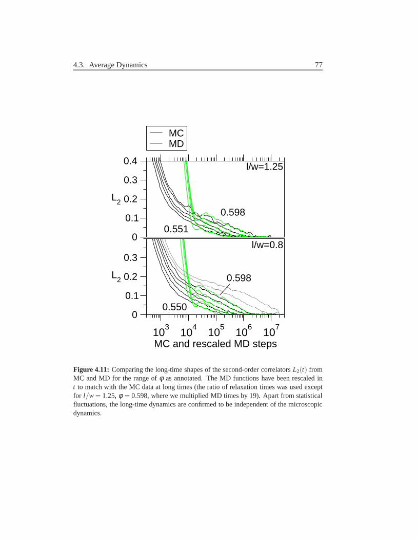
4.3. Average Dynamics 77
103
104
105
106
107
MC and rescaled MD steps
0
0.1
0.2
0.3
L2
0
0.1
0.2
0.3
0.4
L2
MCMD
l/w=0.8
0.598
0.598
0.550
0.551
l/w=1.25
Figure 4.11: Comparing the long-time shapes of the second-order correlatorsL2(t) fromMC and MD for the range ofφ as annotated. The MD functions have been rescaled int to match with the MC data at long times (the ratio of relaxation times was used exceptfor l/w = 1.25, φ = 0.598, where we multiplied MD times by 19). Apart from statisticalfluctuations, the long-time dynamics are confirmed to be independent of the microscopicdynamics.
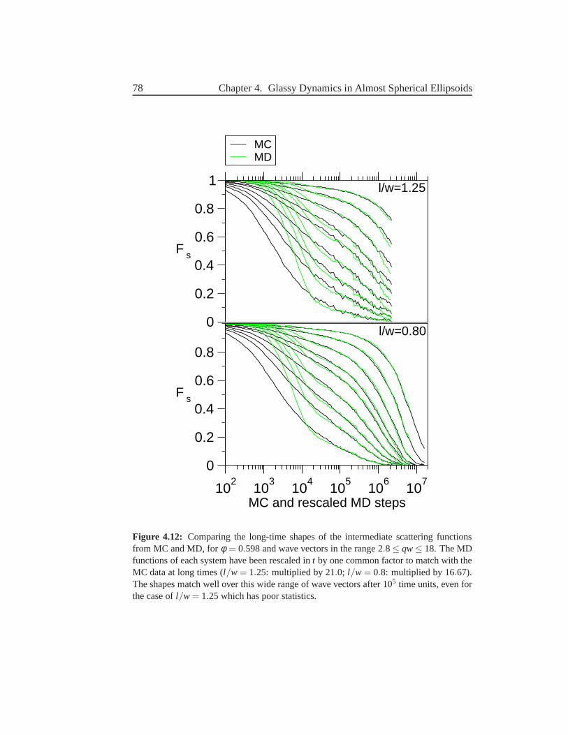
78 Chapter 4. Glassy Dynamics in Almost Spherical Ellipsoids
102
103
104
105
106
107
MC and rescaled MD steps
0
0.2
0.4
0.6
0.8
F s
0
0.2
0.4
0.6
0.8
1
F s
MCMD
l/w=1.25
l/w=0.80
Figure 4.12: Comparing the long-time shapes of the intermediate scattering functionsfrom MC and MD, forφ = 0.598 and wave vectors in the range 2.8≤ qw≤ 18. The MDfunctions of each system have been rescaled int by one common factor to match with theMC data at long times (l/w = 1.25: multiplied by 21.0; l/w = 0.8: multiplied by 16.67).The shapes match well over this wide range of wave vectors after 105 time units, even forthe case ofl/w = 1.25 which has poor statistics.
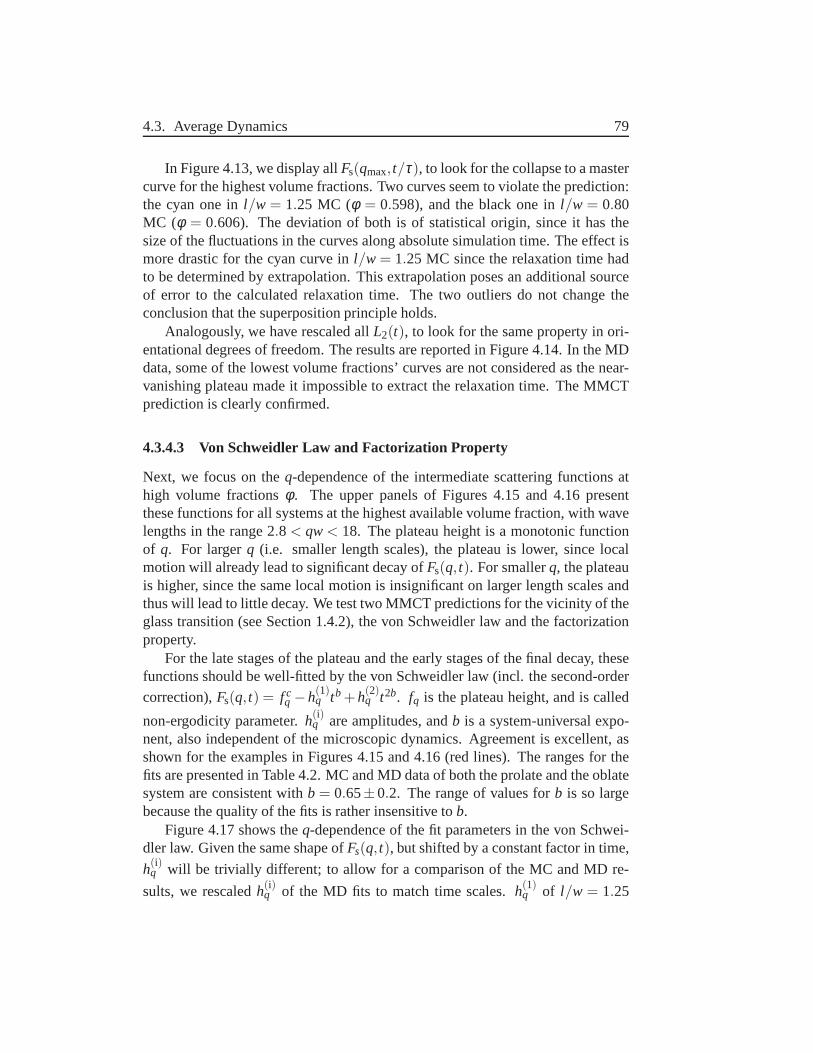
4.3. Average Dynamics 79
In Figure 4.13, we display allFs(qmax, t/τ), to look for the collapse to a mastercurve for the highest volume fractions. Two curves seem to violate the prediction:the cyan one inl/w = 1.25 MC (φ = 0.598), and the black one inl/w = 0.80MC (φ = 0.606). The deviation of both is of statistical origin, since it has thesize of the fluctuations in the curves along absolute simulation time. The effect ismore drastic for the cyan curve inl/w = 1.25 MC since the relaxation time hadto be determined by extrapolation. This extrapolation poses an additional sourceof error to the calculated relaxation time. The two outliersdo not change theconclusion that the superposition principle holds.
Analogously, we have rescaled allL2(t), to look for the same property in ori-entational degrees of freedom. The results are reported in Figure 4.14. In the MDdata, some of the lowest volume fractions’ curves are not considered as the near-vanishing plateau made it impossible to extract the relaxation time. The MMCTprediction is clearly confirmed.
4.3.4.3 Von Schweidler Law and Factorization Property
Next, we focus on theq-dependence of the intermediate scattering functions athigh volume fractionsφ . The upper panels of Figures 4.15 and 4.16 presentthese functions for all systems at the highest available volume fraction, with wavelengths in the range 2.8 < qw< 18. The plateau height is a monotonic functionof q. For largerq (i.e. smaller length scales), the plateau is lower, since localmotion will already lead to significant decay ofFs(q, t). For smallerq, the plateauis higher, since the same local motion is insignificant on larger length scales andthus will lead to little decay. We test two MMCT predictions for the vicinity of theglass transition (see Section 1.4.2), the von Schweidler law and the factorizationproperty.
For the late stages of the plateau and the early stages of the final decay, thesefunctions should be well-fitted by the von Schweidler law (incl. the second-order
correction),Fs(q, t) = f cq −h(1)
q tb +h(2)q t2b. fq is the plateau height, and is called
non-ergodicity parameter.h(i)q are amplitudes, andb is a system-universal expo-
nent, also independent of the microscopic dynamics. Agreement is excellent, asshown for the examples in Figures 4.15 and 4.16 (red lines). The ranges for thefits are presented in Table 4.2. MC and MD data of both the prolate and the oblatesystem are consistent withb = 0.65±0.2. The range of values forb is so largebecause the quality of the fits is rather insensitive tob.
Figure 4.17 shows theq-dependence of the fit parameters in the von Schwei-dler law. Given the same shape ofFs(q, t), but shifted by a constant factor in time,
h(i)q will be trivially different; to allow for a comparison of theMC and MD re-
sults, we rescaledh(i)q of the MD fits to match time scales.h(1)
q of l/w = 1.25
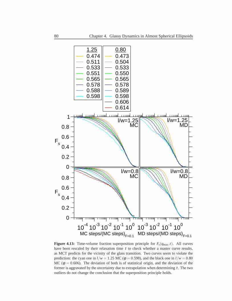
80 Chapter 4. Glassy Dynamics in Almost Spherical Ellipsoids
10-4
10-3
10-2
10-1
100
MC steps/(MC steps)F=0.1
0
0.2
0.4
0.6
0.8
Fs
0.800.4730.5040.5330.5500.5650.5780.5890.5980.6060.614
0
0.2
0.4
0.6
0.8
1
Fs
1.250.4740.5110.5330.5510.5650.5780.5880.598
10-3
10-2
10-1
100
MD steps/(MD steps)F=0.1
l/w=0.8
l/w=1.25MC
MC MD
MDl/w=1.25
l/w=0.8
Figure 4.13: Time-volume fraction superposition principle forFs(qmax, t). All curveshave been rescaled by their relaxation timeτ to check whether a master curve results,as MCT predicts for the vicinity of the glass transition. Twocurves seem to violate theprediction: the cyan one inl/w = 1.25 MC (φ = 0.598), and the black one inl/w = 0.80MC (φ = 0.606). The deviation of both is of statistical origin, and thedeviation of theformer is aggravated by the uncertainty due to extrapolation when determiningτ . The twooutliers do not change the conclusion that the superposition principle holds.
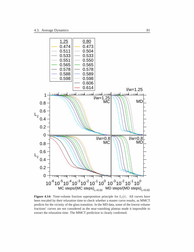
4.3. Average Dynamics 81
10-6
10-5
10-4
10-3
10-2
10-1
100
MC steps/(MC steps)L=0.02
0
0.2
0.4
0.6
0.8
L2
0.800.4730.5040.5330.5500.5650.5780.5890.5980.6060.614
0
0.2
0.4
0.6
0.8
1
L2
1.250.4740.5110.5330.5510.5650.5780.5880.598
10-3
10-2
10-1
100
MD steps/(MD steps)L=0.02
l/w=0.8
l/w=1.25
MC
MC MD
MDl/w=1.25
l/w=0.8
Figure 4.14: Time-volume fraction superposition principle forL2(t). All curves havebeen rescaled by their relaxation time to check whether a master curve results, as MMCTpredicts for the vicinity of the glass transition. In the MD data, some of the lowest volumefractions’ curves are not considered as the near-vanishingplateau made it impossible toextract the relaxation time. The MMCT prediction is clearlyconfirmed.
82 Chapter 4. Glassy Dynamics in Almost Spherical Ellipsoids
102
103
104
105
MD steps
0
0.2
0.4
0.6
0.8
1
F s
103
104
105
106
MC steps
-2
0
2
4
R(t)
MC MD
MC MD
l/w=1.25
Figure 4.15: Upper panels:Fs(q, t) for l/w = 1.25 and the highest volume fractionφ =0.598, and forq-vectors (from top) 2.8, 4.0, 5.5, 7.1, 8.1, 10.1, 12.1, 14.1, 18.1. Thered lines show examples of the von Schweidler fitFs(q, t) = fq− h(1)
q tb + h(2)q t2b with
b = 0.65. Lower panels: the same correlators after transformation to R(t) = [Fs(q, t)−Fs(q, t1)]/[Fs(q, t2)−Fs(q, t1)], demonstrating the factorization property. The color code,distinguishing wave vectors, shows that the curves remain ordered, i.e. a curve which isabove another one before the collapse is above the other one after as well.
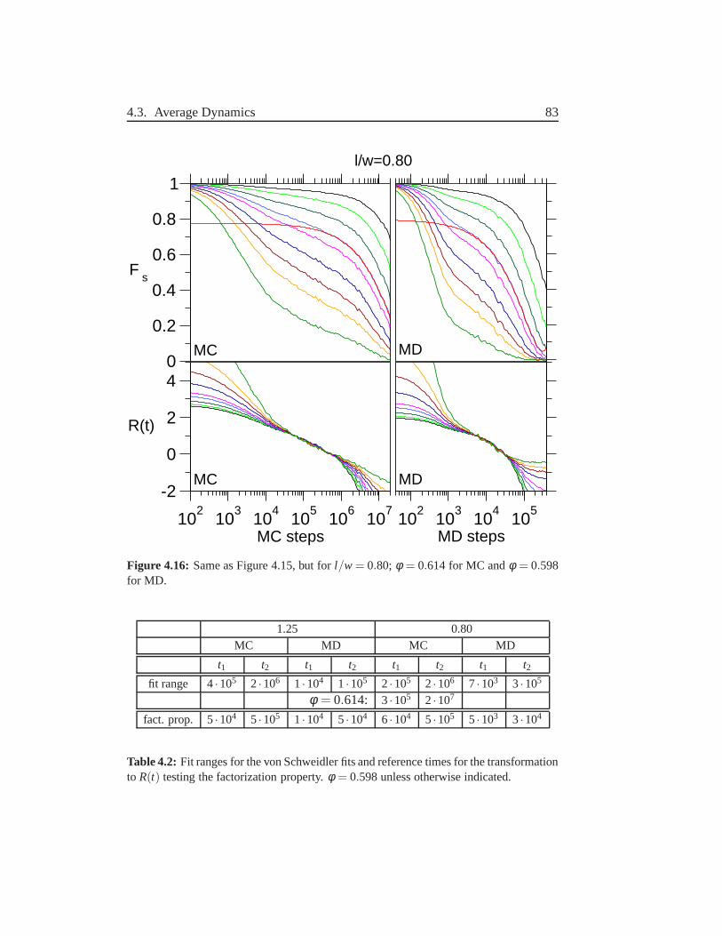
4.3. Average Dynamics 83
102
103
104
105
MD steps
0
0.2
0.4
0.6
0.8
1
F s
102
103
104
105
106
107
MC steps
-2
0
2
4
R(t)
MC MD
MC MD
l/w=0.80
Figure 4.16: Same as Figure 4.15, but forl/w = 0.80; φ = 0.614 for MC andφ = 0.598for MD.
1.25 0.80MC MD MC MD
t1 t2 t1 t2 t1 t2 t1 t2
fit range 4·105 2·106 1·104 1·105 2·105 2·106 7·103 3·105
φ = 0.614: 3·105 2·107
fact. prop. 5·104 5·105 1·104 5·104 6·104 5·105 5·103 3·104
Table 4.2: Fit ranges for the von Schweidler fits and reference times forthe transformationto R(t) testing the factorization property.φ = 0.598 unless otherwise indicated.
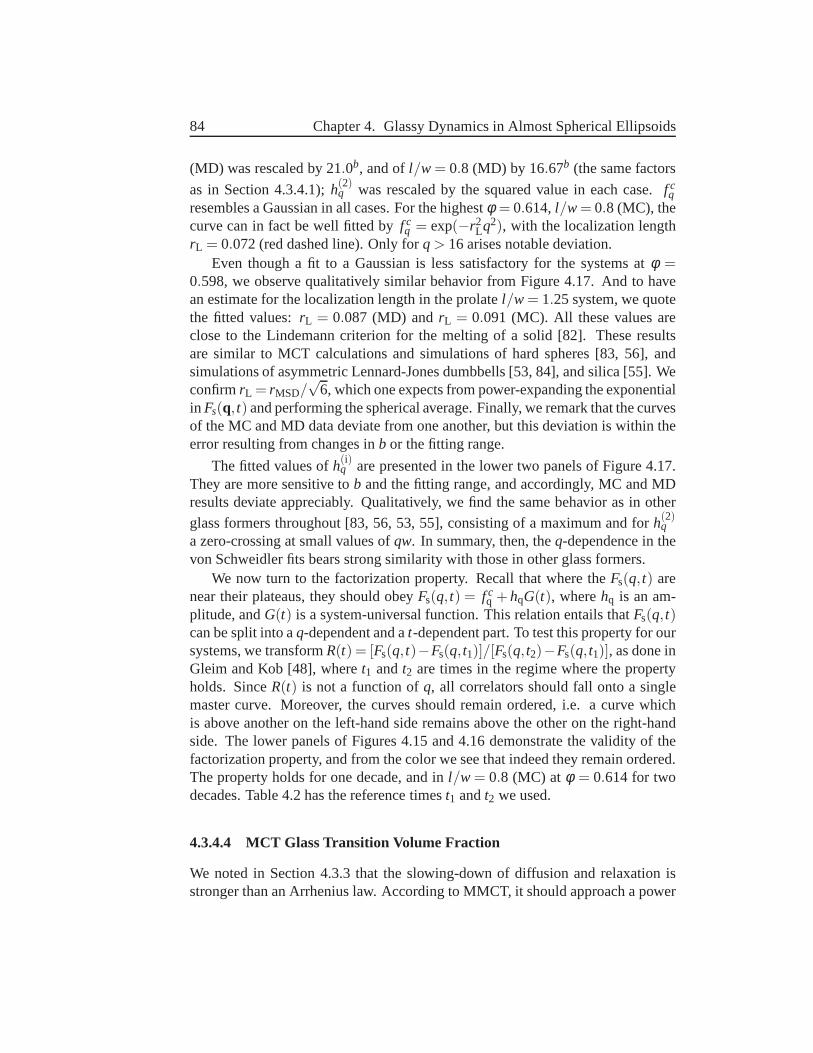
84 Chapter 4. Glassy Dynamics in Almost Spherical Ellipsoids
(MD) was rescaled by 21.0b, and ofl/w = 0.8 (MD) by 16.67b (the same factors
as in Section 4.3.4.1);h(2)q was rescaled by the squared value in each case.f c
qresembles a Gaussian in all cases. For the highestφ = 0.614,l/w= 0.8 (MC), thecurve can in fact be well fitted byf c
q = exp(−r2Lq2), with the localization length
rL = 0.072 (red dashed line). Only forq > 16 arises notable deviation.Even though a fit to a Gaussian is less satisfactory for the systems atφ =
0.598, we observe qualitatively similar behavior from Figure4.17. And to havean estimate for the localization length in the prolatel/w = 1.25 system, we quotethe fitted values:rL = 0.087 (MD) andrL = 0.091 (MC). All these values areclose to the Lindemann criterion for the melting of a solid [82]. These resultsare similar to MCT calculations and simulations of hard spheres [83, 56], andsimulations of asymmetric Lennard-Jones dumbbells [53, 84], and silica [55]. WeconfirmrL = rMSD/
√6, which one expects from power-expanding the exponential
in Fs(q, t) and performing the spherical average. Finally, we remark that the curvesof the MC and MD data deviate from one another, but this deviation is within theerror resulting from changes inb or the fitting range.
The fitted values ofh(i)q are presented in the lower two panels of Figure 4.17.
They are more sensitive tob and the fitting range, and accordingly, MC and MDresults deviate appreciably. Qualitatively, we find the same behavior as in other
glass formers throughout [83, 56, 53, 55], consisting of a maximum and forh(2)q
a zero-crossing at small values ofqw. In summary, then, theq-dependence in thevon Schweidler fits bears strong similarity with those in other glass formers.
We now turn to the factorization property. Recall that wherethe Fs(q, t) arenear their plateaus, they should obeyFs(q, t) = f c
q + hqG(t), wherehq is an am-plitude, andG(t) is a system-universal function. This relation entails thatFs(q, t)can be split into aq-dependent and at-dependent part. To test this property for oursystems, we transformR(t) = [Fs(q, t)−Fs(q, t1)]/[Fs(q, t2)−Fs(q, t1)], as done inGleim and Kob [48], wheret1 andt2 are times in the regime where the propertyholds. SinceR(t) is not a function ofq, all correlators should fall onto a singlemaster curve. Moreover, the curves should remain ordered, i.e. a curve whichis above another on the left-hand side remains above the other on the right-handside. The lower panels of Figures 4.15 and 4.16 demonstrate the validity of thefactorization property, and from the color we see that indeed they remain ordered.The property holds for one decade, and inl/w = 0.8 (MC) atφ = 0.614 for twodecades. Table 4.2 has the reference timest1 andt2 we used.
4.3.4.4 MCT Glass Transition Volume Fraction
We noted in Section 4.3.3 that the slowing-down of diffusionand relaxation isstronger than an Arrhenius law. According to MMCT, it shouldapproach a power
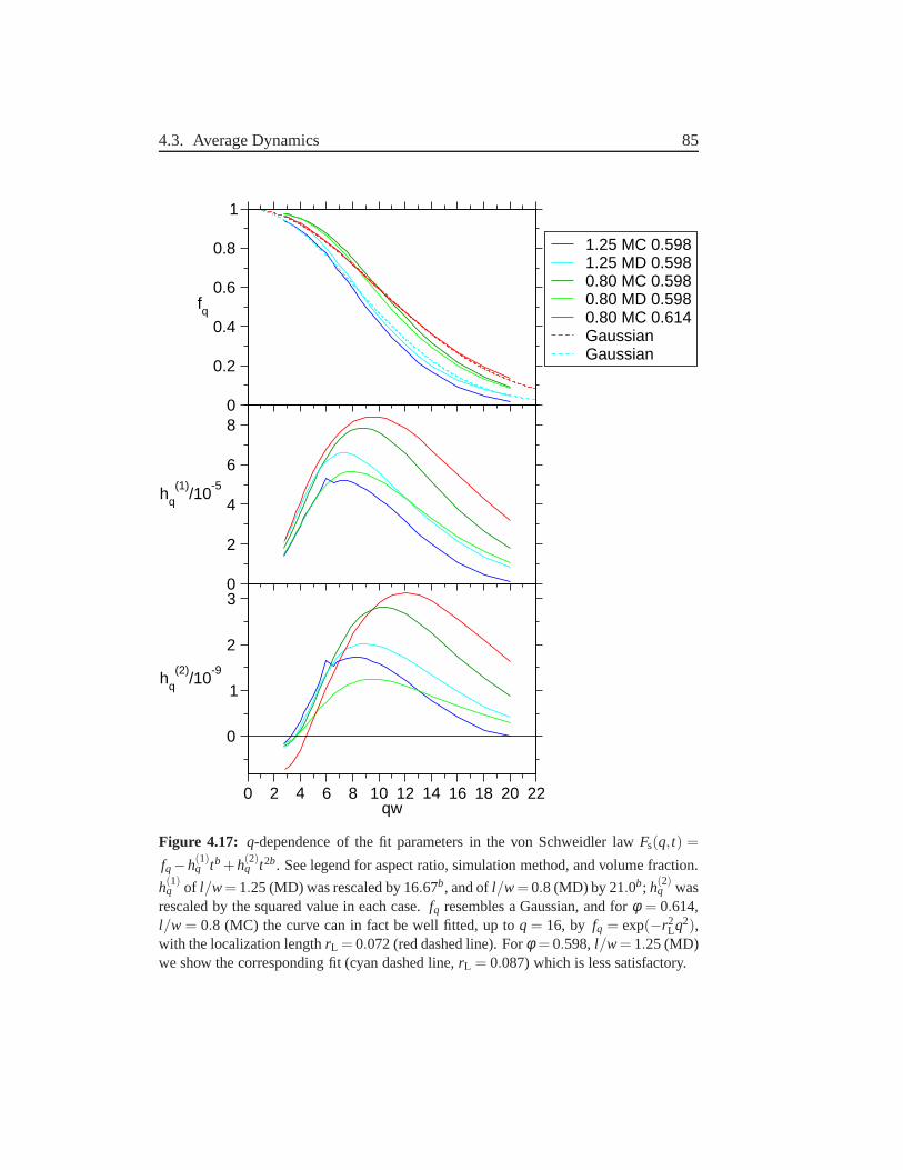
4.3. Average Dynamics 85
0
0.2
0.4
0.6
0.8
1
fq
1.25 MC 0.5981.25 MD 0.5980.80 MC 0.5980.80 MD 0.5980.80 MC 0.614GaussianGaussian
0 2 4 6 8 10 12 14 16 18 20 22qw
0
1
2
3
hq(2)
/10-9
0
2
4
6
8
hq(1)
/10-5
Figure 4.17: q-dependence of the fit parameters in the von Schweidler lawFs(q, t) =
fq−h(1)q tb +h(2)
q t2b. See legend for aspect ratio, simulation method, and volumefraction.
h(1)q of l/w= 1.25 (MD) was rescaled by 16.67b, and ofl/w= 0.8 (MD) by 21.0b; h(2)
q wasrescaled by the squared value in each case.fq resembles a Gaussian, and forφ = 0.614,l/w = 0.8 (MC) the curve can in fact be well fitted, up toq = 16, by fq = exp(−r2
Lq2),with the localization lengthrL = 0.072 (red dashed line). Forφ = 0.598,l/w= 1.25 (MD)we show the corresponding fit (cyan dashed line,rL = 0.087) which is less satisfactory.
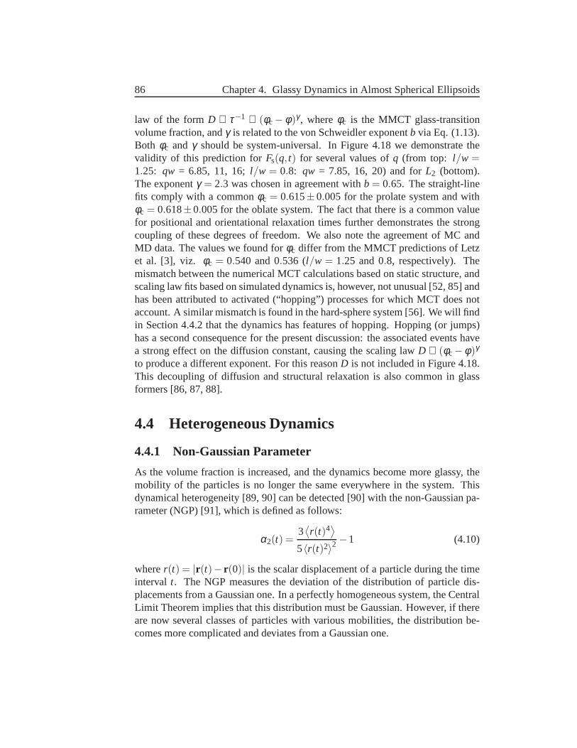
86 Chapter 4. Glassy Dynamics in Almost Spherical Ellipsoids
law of the formD ∝ τ−1 ∝ (φc− φ)γ , whereφc is the MMCT glass-transitionvolume fraction, andγ is related to the von Schweidler exponentb via Eq. (1.13).Both φc and γ should be system-universal. In Figure 4.18 we demonstrate thevalidity of this prediction forFs(q, t) for several values ofq (from top: l/w =1.25: qw = 6.85, 11, 16;l/w = 0.8: qw = 7.85, 16, 20) and forL2 (bottom).The exponentγ = 2.3 was chosen in agreement withb = 0.65. The straight-linefits comply with a commonφc = 0.615±0.005 for the prolate system and withφc = 0.618±0.005 for the oblate system. The fact that there is a common valuefor positional and orientational relaxation times furtherdemonstrates the strongcoupling of these degrees of freedom. We also note the agreement of MC andMD data. The values we found forφc differ from the MMCT predictions of Letzet al. [3], viz. φc = 0.540 and 0.536 (l/w = 1.25 and 0.8, respectively). Themismatch between the numerical MCT calculations based on static structure, andscaling law fits based on simulated dynamics is, however, notunusual [52, 85] andhas been attributed to activated (“hopping”) processes forwhich MCT does notaccount. A similar mismatch is found in the hard-sphere system [56]. We will findin Section 4.4.2 that the dynamics has features of hopping. Hopping (or jumps)has a second consequence for the present discussion: the associated events havea strong effect on the diffusion constant, causing the scaling law D ∝ (φc− φ)γ
to produce a different exponent. For this reasonD is not included in Figure 4.18.This decoupling of diffusion and structural relaxation is also common in glassformers [86, 87, 88].
4.4 Heterogeneous Dynamics
4.4.1 Non-Gaussian Parameter
As the volume fraction is increased, and the dynamics becomemore glassy, themobility of the particles is no longer the same everywhere inthe system. Thisdynamical heterogeneity [89, 90] can be detected [90] with the non-Gaussian pa-rameter (NGP) [91], which is defined as follows:
α2(t) =3⟨r(t)4
⟩5〈r(t)2〉2
−1 (4.10)
wherer(t) = |r(t)− r(0)| is the scalar displacement of a particle during the timeinterval t. The NGP measures the deviation of the distribution of particle dis-placements from a Gaussian one. In a perfectly homogeneous system, the CentralLimit Theorem implies that this distribution must be Gaussian. However, if thereare now several classes of particles with various mobilities, the distribution be-comes more complicated and deviates from a Gaussian one.
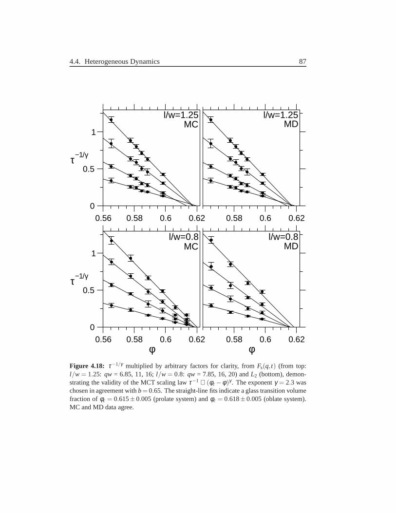
4.4. Heterogeneous Dynamics 87
0.56 0.58 0.6 0.62φ
0
0.5
1
τ−1/γ
0.58 0.6 0.620.56 0.58 0.6 0.620
0.5
1
τ−1/γ
0.58 0.6 0.62φ
l/w=1.25
l/w=0.8
l/w=1.25
l/w=0.8MC
MC MD
MD
Figure 4.18: τ−1/γ multiplied by arbitrary factors for clarity, fromFs(q, t) (from top:l/w = 1.25: qw = 6.85, 11, 16;l/w = 0.8: qw = 7.85, 16, 20) andL2 (bottom), demon-strating the validity of the MCT scaling lawτ−1 ∝ (φc−φ)γ . The exponentγ = 2.3 waschosen in agreement withb= 0.65. The straight-line fits indicate a glass transition volumefraction ofφc = 0.615±0.005 (prolate system) andφc = 0.618±0.005 (oblate system).MC and MD data agree.
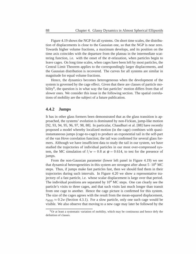
88 Chapter 4. Glassy Dynamics in Almost Spherical Ellipsoids
Figure 4.19 shows the NGP for all systems. On short time scales, the distribu-tion of displacements is close to the Gaussian one, so that the NGP is near zero.Towards higher volume fractions, a maximum develops, and its position on thetime axis coincides with the departure from the plateau in the intermediate scat-tering function, i.e. with the onset of theα-relaxation, when particles begin toleave cages. On long time scales, when cages have been left bymost particles, theCentral Limit Theorem applies to the correspondingly larger displacements, andthe Gaussian distribution is recovered. The curves for all systems are similar inmagnitude for equal volume fractions.
Hence, the dynamics becomes heterogeneous when the development of thesystem is governed by the cage effect. Given that there are classes of particle mo-bility6, the question is in what way the fast particles’ motion differs from that ofslower ones. We consider this issue in the following section. The spatial correla-tions of mobility are the subject of a future publication.
4.4.2 Jumps
It has in other glass formers been demonstrated that as the glass transition is ap-proached, the systems’ evolution is dominated by non-Fickian, jump-like motion[92, 93, 94, 95, 96, 97, 98, 88]. In particular, Chaudhuri et al. [88] have recentlyproposed a model whereby localized motion (in the cage) combines with quasi-instantaneous jumps (cage-to-cage) to produce an exponential tail in the self-partof the van Hove correlation function; the tail was confirmed for several glass for-mers. Although we have insufficient data to study the tail in our system, we havestudied the trajectories of individual particles in our most over-compressed sys-tem, the MC simulation ofl/w = 0.8 at φ = 0.614, to test for the presence ofjumps.
From the non-Gaussian parameter (lower left panel in Figure4.19) we seethat dynamical heterogeneities in this system are strongest after about 5·106 MCsteps. Thus, if jumps make fast particles fast, then we should find them in theirtrajectories during such intervals. In Figure 4.20 we show arepresentative tra-jectory of a fast particle, i.e. whose scalar displacement is large over that period.The individual positions are separated by 104 MC steps. One can clearly see theparticle’s visits to three cages, and that such visits last much longer than transitfrom one cage to another. Hence the cage picture is confirmed for this system.The size of the cages agrees with the result from the mean-squared displacement,rMSD ≈ 0.2w (Section 4.3.1). For a slow particle, only one such cage would bevisible. We also observe that moving to a new cage may later befollowed by the
6Or at least a systematic variation of mobility, which may be continuous and hence defy thedefinition of classes.
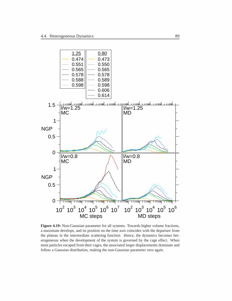
4.4. Heterogeneous Dynamics 89
102
103
104
105
106
MD steps10
210
310
410
510
610
7
MC steps
0
0.5
1
NGP
0.800.4730.5500.5650.5780.5890.5980.6060.614
0
0.5
1
1.5
NGP
1.250.4740.5510.5650.5780.5880.598
l/w=0.8
l/w=1.25MC
MC MD
MDl/w=1.25
l/w=0.8
Figure 4.19: Non-Gaussian parameter for all systems. Towards higher volume fractions,a maximum develops, and its position on the time axis coincides with the departure fromthe plateau in the intermediate scattering function. Hence, the dynamics becomes het-erogeneous when the development of the system is governed bythe cage effect. Whenmost particles escaped from their cages, the associated larger displacements dominate andfollow a Gaussian distribution, making the non-Gaussian parameter zero again.
90 Chapter 4. Glassy Dynamics in Almost Spherical Ellipsoids
Figure 4.20: Trajectory of a fast particle from the MC simulation ofl/w = 0.8 at φ =0.614. Three cages can be identified, whose size agrees with theresult from the mean-squared displacement,rMSD ≈ 0.2w. Moving to a new cage may later be followed by thereturn to the previous cage. The displacements between individual positions are of similarsize within a cage and during transit.
return to the previous cage.But notice in Figure 4.20 that the displacements between individual positions
are of similar size within a cage and during transit. Corresponding pictures in pre-vious studies suggest the same for the binary Lennard-Jonesmixture [88] (Kob-Andersen model [51, 52]), colloidal hard spheres [92], and a2D, bidisperse gran-ular system [93]. Therefore, we suspect quite generally that a jump does notinvolve an exceptional displacement. Rather, the displacement (or series of dis-placements) leading to the new cage happens to be permanent,i.e. it is not undoneby motion in the opposite direction.
We demonstrate in the following that fast particles indeed do not performoutstanding displacements. For a well-defined distinctionof fast and slow par-ticles, we consider the self-part of the van Hove correlation function [99] in itsspherically-averaged form:
Gs(r, t) =1
4πr2
⟨1N
N
∑i
δ [r−|r i(t)− r i(0)|]⟩
It is the distribution of scalar displacementsr in an intervalt; the mean of thesquares of these displacements is just the MSD. In Figure 4.21 we display thenamed function for several values oft, in linear (top) and semi-logarithmic (bot-
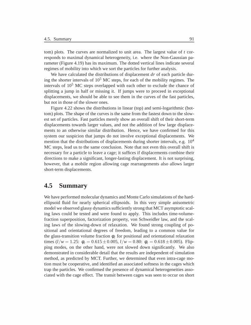
4.5. Summary 91
tom) plots. The curves are normalized to unit area. The largest value oft cor-responds to maximal dynamical heterogeneity, i.e. where the Non-Gaussian pa-rameter (Figure 4.19) has its maximum. The dotted vertical lines indicate severalregimes of mobility into which we sort the particles for further analysis.
We have calculated the distributions of displacementdr of each particle dur-ing the shorter intervals of 105 MC steps, for each of the mobility regimes. Theintervals of 105 MC steps overlapped with each other to exclude the chance ofsplitting a jump in half or missing it. If jumps were to proceed in exceptionaldisplacements, we should be able to see them in the curves of the fast particles,but not in those of the slower ones.
Figure 4.22 shows the distributions in linear (top) and semi-logarithmic (bot-tom) plots. The shape of the curves is the same from the fastest down to the slow-est set of particles. Fast particles merely show an overall shift of their short-termdisplacements towards larger values, and not the addition of few large displace-ments to an otherwise similar distribution. Hence, we have confirmed for thissystem our suspicion that jumps do not involve exceptional displacements. Wemention that the distributions of displacements during shorter intervals, e.g. 104
MC steps, lead us to the same conclusion. Note that not even this overall shift isnecessary for a particle to leave a cage; it suffices if displacements combine theirdirections to make a significant, longer-lasting displacement. It is not surprising,however, that a mobile region allowing cage rearrangementsalso allows largershort-term displacements.
4.5 Summary
We have performed molecular dynamics and Monte Carlo simulations of the hard-ellipsoid fluid for nearly spherical ellipsoids. In this very simple anisometricmodel we observed glassy dynamics sufficiently strong that MCT asymptotic scal-ing laws could be tested and were found to apply. This includes time-volume-fraction superposition, factorization property, von Schweidler law, and the scal-ing laws of the slowing-down of relaxation. We found strong coupling of po-sitional and orientational degrees of freedom, leading to acommon value forthe glass-transition volume fractionφc for positional and orientational relaxationtimes (l/w = 1.25: φc = 0.615±0.005, l/w = 0.80: φc = 0.618±0.005). Flip-ping modes, on the other hand, were not slowed down significantly. We alsodemonstrated in considerable detail that the results are independent of simulationmethod, as predicted by MCT. Further, we determined that even intra-cage mo-tion must be cooperative, and identified an associated softness in the cages whichtrap the particles. We confirmed the presence of dynamical heterogeneities asso-ciated with the cage effect. The transit between cages was seen to occur on short
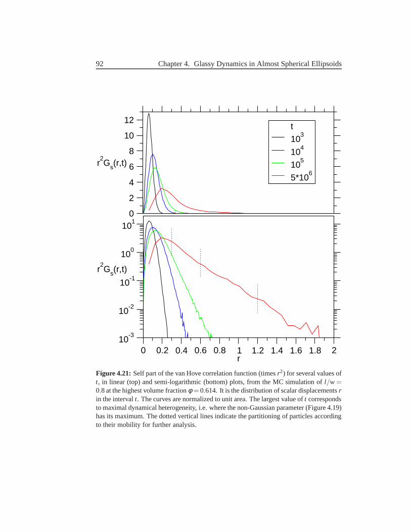
92 Chapter 4. Glassy Dynamics in Almost Spherical Ellipsoids
0
2
4
6
8
10
12
r2Gs(r,t)
t
103
104
105
5*106
0 0.2 0.4 0.6 0.8 1 1.2 1.4 1.6 1.8 2r
10-3
10-2
10-1
100
101
r2Gs(r,t)
Figure 4.21: Self part of the van Hove correlation function (timesr2) for several values oft, in linear (top) and semi-logarithmic (bottom) plots, fromthe MC simulation ofl/w =0.8 at the highest volume fractionφ = 0.614. It is the distribution of scalar displacementsrin the intervalt. The curves are normalized to unit area. The largest value oft correspondsto maximal dynamical heterogeneity, i.e. where the non-Gaussian parameter (Figure 4.19)has its maximum. The dotted vertical lines indicate the partitioning of particles accordingto their mobility for further analysis.
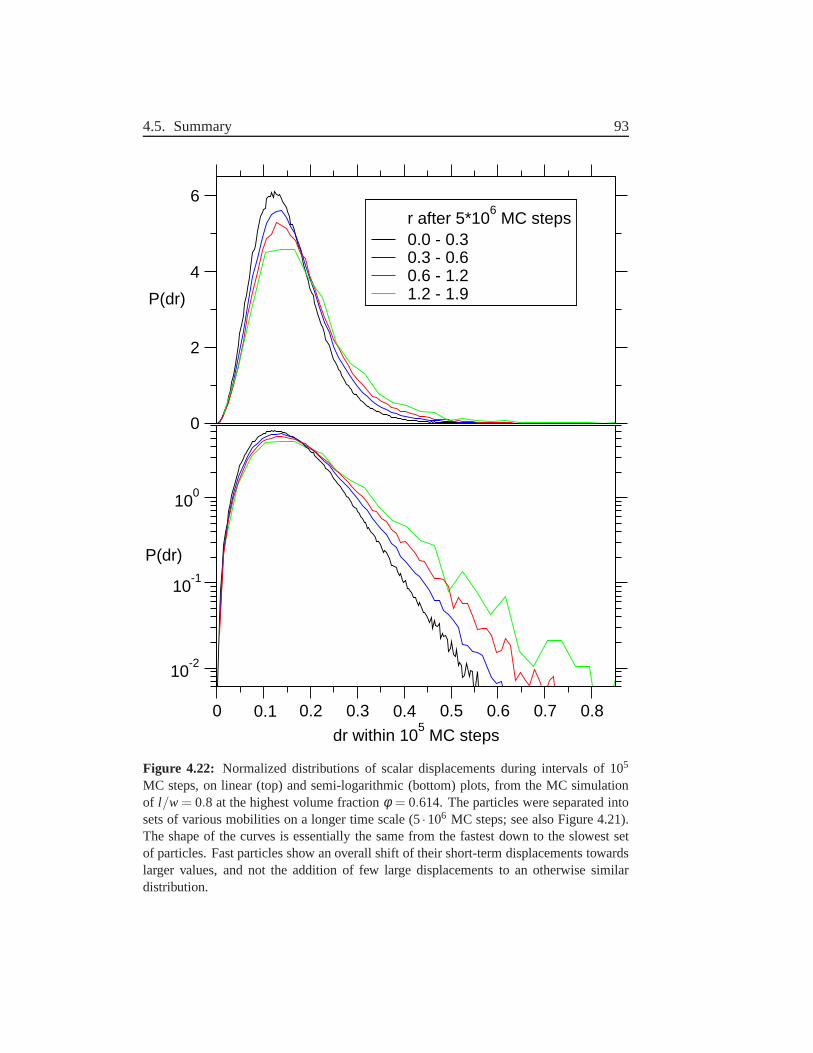
4.5. Summary 93
0
2
4
6
P(dr)
r after 5*106 MC steps
0.0 - 0.30.3 - 0.60.6 - 1.21.2 - 1.9
0 0.1 0.2 0.3 0.4 0.5 0.6 0.7 0.8
dr within 105 MC steps
10-2
10-1
100
P(dr)
Figure 4.22: Normalized distributions of scalar displacements during intervals of 105
MC steps, on linear (top) and semi-logarithmic (bottom) plots, from the MC simulationof l/w = 0.8 at the highest volume fractionφ = 0.614. The particles were separated intosets of various mobilities on a longer time scale (5·106 MC steps; see also Figure 4.21).The shape of the curves is essentially the same from the fastest down to the slowest setof particles. Fast particles show an overall shift of their short-term displacements towardslarger values, and not the addition of few large displacements to an otherwise similardistribution.
94 Chapter 4. Glassy Dynamics in Almost Spherical Ellipsoids
time scales, compared to the time spent in cages; but the transit was shown not toinvolve displacements distinguishable in character from intra-cage motion.
The presence of glassy dynamics has been predicted by MMCT [3]. However,as MMCT cannot make a statement about crystallization, a test by simulationwas required. We stress that glassy dynamics is unusual in monodisperse sys-tems. Crystallization typically intervenes unless polydispersity, network-formingbonds or other asymmetries are introduced. We argue that particle anisometryacts here as a sufficient source of disorder to prevent crystallization. This shedsnew light on the question of which ingredients are required for glass formation.Recent advances of dynamic confocal microscopy with colloidal ellipsoids [37]seem promising for a study of the glassy dynamics in ellipsoids.
Acknowledgments
I would like to thank (names had to be removed in this online version):• My supervisor, for hiring me into her group, her patience andher kind support• My second supervisor, for his support• The head of the group, for admitting me into his group alreadyfor my Masterthesis, and for encouraging and supporting me in many ways• Various people, for stimulating discussions and support• Various people, for their critical reading of this text• Many present and former group members, for stimulating discussions and sup-port• A professor in the UK, for sharing his MD code• Three people whom I co-supervised with great pleasure. The work of one ofthem is included in this thesis; her contribution is summarized on on page 55• The computing support in the group, for keeping things up andrunning andanswering many questions• The Zentrum für Datenverarbeitung at the Universität Mainz, for maintaining acluster I extensively used• The Deutsche Forschungsgemeinschaft (SFB TR6 and Emmy Noether), and theEU Network of Excellence SoftComp, for financial support• The Forschungszentrum Jülich, for granting CPU time• You, for reading this.

96
Appendix A
Corrected Constant-PressureEnsemble
We left off in Section 2.1.2.1 with the partition function Eq. (2.8) in the constant-pressure-zero-tension ensemble:
Z(N,P,T) =∞∫
−∞
d lnh11d lnh22d lnh33dg12dg13dg23
1∫0
dsN∫4π
duN · (A.1)
exp− [U(si,H,ui)+PV(H)]/kBT +(N+3) lnV(H)We abbreviate it to
Z(N,P,T) =∞∫
−∞
d lnh11d lnh22d lnh33dg12dg13dg23z−V(H)PT ZA(N,H,T) (A.2)
by defining
ZA(N,H,T)≡1∫
0
dsN∫4π
duN exp−U(si,H,ui)/kBT +(N+3) lnV(H)
and using once more the “fugacity”zPT = eP/kBT .Constant-pressure MC is sufficient whenZA(N,H,T) is only a function ofV,
and not a function ofgi j or the ratioshii/h j j ; i.e., when it is independent of boxshear and box aspect ratio. This is essentially the case for homogeneous fluids[57]. The task is once more to integrate out the associated degeneracies, keepingtrack of resulting weight factors for the remaining variables.
Thegi j already specify box shear independently from box size (unlike hi j =h j j gi j ). With ZA(N,H,T) invariant under changes in shear, we may carry out the
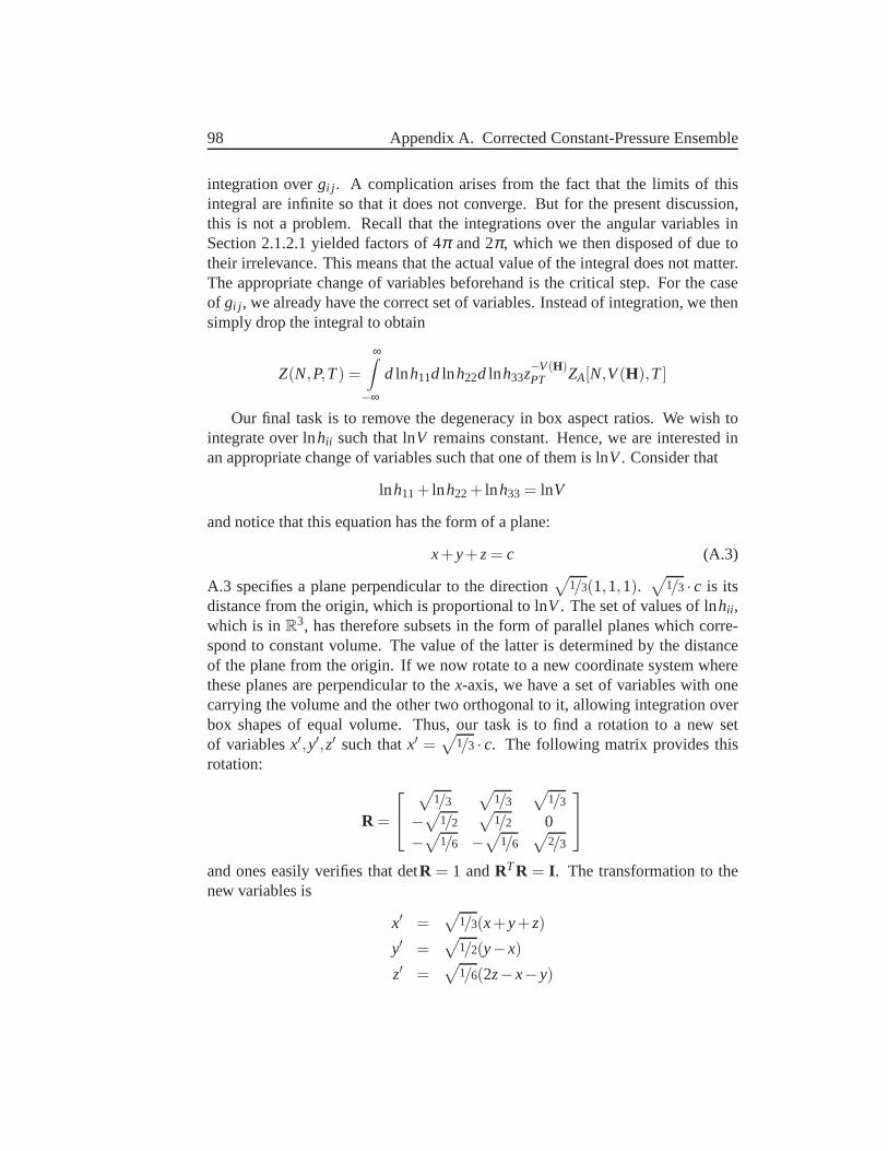
98 Appendix A. Corrected Constant-Pressure Ensemble
integration overgi j . A complication arises from the fact that the limits of thisintegral are infinite so that it does not converge. But for thepresent discussion,this is not a problem. Recall that the integrations over the angular variables inSection 2.1.2.1 yielded factors of 4π and 2π, which we then disposed of due totheir irrelevance. This means that the actual value of the integral does not matter.The appropriate change of variables beforehand is the critical step. For the caseof gi j , we already have the correct set of variables. Instead of integration, we thensimply drop the integral to obtain
Z(N,P,T) =∞∫
−∞
d lnh11d lnh22d lnh33z−V(H)PT ZA[N,V(H),T]
Our final task is to remove the degeneracy in box aspect ratios. We wish tointegrate over lnhii such that lnV remains constant. Hence, we are interested inan appropriate change of variables such that one of them is lnV. Consider that
lnh11+ lnh22+ lnh33 = lnV
and notice that this equation has the form of a plane:
x+y+z= c (A.3)
A.3 specifies a plane perpendicular to the direction√
1/3(1,1,1).√
1/3 · c is itsdistance from the origin, which is proportional to lnV. The set of values of lnhii ,which is inR3, has therefore subsets in the form of parallel planes which corre-spond to constant volume. The value of the latter is determined by the distanceof the plane from the origin. If we now rotate to a new coordinate system wherethese planes are perpendicular to thex-axis, we have a set of variables with onecarrying the volume and the other two orthogonal to it, allowing integration overbox shapes of equal volume. Thus, our task is to find a rotationto a new setof variablesx′,y′,z′ such thatx′ =
√1/3 · c. The following matrix provides this
rotation:
R =
√
1/3√
1/3√
1/3
−√1/2
√1/2 0
−√1/6 −√
1/6√
2/3
and ones easily verifies that detR = 1 andRTR = I . The transformation to thenew variables is
x′ =√
1/3(x+y+z)
y′ =√
1/2(y−x)
z′ =√
1/6(2z−x−y)
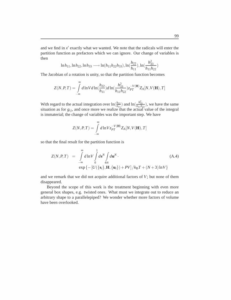
99
and we find inx′ exactly what we wanted. We note that the radicals will enter thepartition function as prefactors which we can ignore. Our change of variables isthen
lnh11, lnh22, lnh33−→ ln(h11h22h33), ln(h22
h11), ln(
h233
h11h22)
The Jacobian of a rotation is unity, so that the partition function becomes
Z(N,P,T) =∞∫
−∞
d lnVdln(h22
h11)d ln(
h233
h11h22)z−V(H)
PT ZA[N,V(H),T]
With regard to the actual integration over ln(h22h11
) and ln( h233
h11h22), we have the same
situation as forgi j , and once more we realize that the actual value of the integralis immaterial; the change of variables was the important step. We have
Z(N,P,T) =∞∫
−∞
d lnVz−V(H)PT ZA[N,V(H),T]
so that the final result for the partition function is
Z(N,P,T) =∞∫
−∞
d lnV
1∫0
dsN∫4π
duN · (A.4)
exp− [U(si,H,ui)+PV]/kBT +(N+3) lnV
and we remark that we did not acquire additional factors ofV; but none of themdisappeared.
Beyond the scope of this work is the treatment beginning witheven moregeneral box shapes, e.g. twisted ones. What must we integrate out to reduce anarbitrary shape to a parallelepiped? We wonder whether morefactors of volumehave been overlooked.

100 Appendix A. Corrected Constant-Pressure Ensemble
Bibliography
[1] D. Frenkel and B. Mulder. The hard ellipsoid-of-revolution fluid i. montecarlo simulations.Mol. Phys., 100:201, 2002.
[2] A. Donev, F. H. Stillinger, P. M. Chaikin, and S. Torquato. Unusually densecrystal packings of ellipsoids.Phys. Rev. Lett., 92:255506, 2004.
[3] M. Letz, R. Schilling, and A. Latz. Ideal glass transition for hard ellipsoids.Phys. Rev. E, 62:5173, 2000.
[4] R. A. Smith. The life and works of Thomas Graham. Glasgow, 1884.
[5] P. N. Pusey and W. van Megen. Phase-behavior of concentrated suspensionsof nearly hard colloidal spheres.Nature, 320:340–342, 1986.
[6] B. J. Alder and T. E. Wainwright. Phase transition for a hard sphere system.J. Chem. Phys, 27:1208, 1957.
[7] L. Onsager.Ann. N. Y. Acad. Sci., 51:627, 1949.
[8] C. M. Care and D. J. Cleaver. Computer simulation of liquid crystals.Re-ports On Progress In Phys., 68:2665–2700, 2005.
[9] M. R. Wilson. Progress in computer simulations of liquidcrystals.Int. Rev.In Phys. Chem., 24:421–455, 2005.
[10] J. Vieillard-Baron.J. Chem. Phys., 56:4729, 1972.
[11] J. W. Perram, M. S. Wertheim, J. L. Lebowitz, and G. O. Williams. Chem.Phys. Lett., 105:277, 1984.
[12] J. W. Perram and M. S. Wertheim.J. Comput. Phys., 58:409, 1985.
[13] D. Frenkel and B. Mulder. The hard ellipsoid-of-revolution fluid i. montecarlo simulations.Mol. Phys., 55:1171, 1985.
102 Bibliography
[14] P. G. de Gennes and J. Prost.The Physics of Liquid Crystals. ClarendonPress, Oxford, 1993.
[15] G. J. Zarragoicoechea, D. Levesque, and J. J. Weis.Mol. Phys., 75:989,1992.
[16] M. P. Allen and C. P. Mason. Stability of the nematic phase for the hardellipsoid fluid. Mol. Phys., 86:467, 1995.
[17] P. J. Camp, C. P. Mason, M. P. Allen, A. A. Khare, and D. A. Kofke. J.Chem. Phys., 105:2837, 1996.
[18] M. P. Allen. Liq. Cryst., 8:499, 1990.
[19] P. J. Camp and M. P. Allen. Phase diagram of the hard biaxial ellipsoid fluid.J. Chem. Phys., 106:6681, 1997.
[20] M. P. Allen. In N. Attig, K. Binder, H. Grubmüller, and K.Kremer, edi-tors,Computational Soft Matter: From Synthetic Polymers to Proteins, NICSeries, volume 23, chapter Liquid Crystal Systems, pages 289–320.NICDirectors, Jülich, 2004.
[21] A. Donev, I. Cisse, D. Sachs, E. Variano, F. H. Stillinger, R. Connelly,S. Torquato, and P. M. Chaikin. Improving the density of jammed disor-dered packings using ellipsoids.Science, 303:990–993, 2004.
[22] M. P. Allen and D. Frenkel. Observation of dynamical precursors of theisotropic-nematic transition by computer simulation.Phys. Rev. Lett., 58:1748, 1987.
[23] M. P. Allen, D. Frenkel, and J. Talbot.Comput. Phys. Rep., 9:301, 1989.
[24] M. P. Allen. Diffusion-coefficient increases with density in hard ellipsoidliquid-crystals.Phys. Rev. Lett., 65:2881–2884, 1990.
[25] P. Bereolos, J. Talbot, M. P. Allen, and G. T. Evans. Transport-properties ofthe hard ellipsoid fluid.J. Chem. Phys., 99:6087–6097, 1993.
[26] R. Schilling and T. Scheidsteger. Mode coupling approach to the ideal glasstransition of molecular liquids: Linear molecules.Phys. Rev. E, 56:2932,1997.
[27] T. Franosch, M. Fuchs, W. Götze, M. R. Mayr, and A. P. Singh. Theoryfor the reorientational dynamics in glass-forming liquids. Phys. Rev. E, 56:5659–5674, 1997.
Bibliography 103
[28] R. Schilling. Mode-coupling theory for translationaland orientational dy-namics near the ideal glass transition.J. Phys.: Condens. Matter, 12:6311,2000.
[29] W. Götze. In J. P. Hansen, D. Levesque, and J. Zinn-Justin, editors,Liquids,Freezing, and the Glass Transition. North-Holland, Amsterdam, 1991.
[30] C. de Michele, R. Schilling, and F. Sciortino. Dynamicsof uniaxial hardellipsoids.Phys. Rev. Lett., 98:265702, 2007.
[31] K. M. Keville, E. I. Franses, and J. M. Caruthers.J. Colloid Interface Sci.,144:103, 1991.
[32] C. C. Ho, A. Keller, J. A. Odell, and R. H. Ottewill.Colloid. Polym. Sci.,271:469, 1993.
[33] J. C. Loudet, A. G. Yodh, and B. Pouligny.Phys. Rev. Lett., 97:018304,2006.
[34] H. Lehle, E. Noruzifar, and M. Oettel. Ellipsoidal particles at fluid interfaces.European Phys. J. E, 26:151–160, 2008.
[35] M. G. Basavaraj, G. G. Fuller, J. Fransaer, and J. Vermant. Langmuir, 22:6605, 2006.
[36] A. Mohraz and M. J. Solomon.Langmuir, 21:5298, 2005.
[37] D. Mukhija and M. J. Solomon. Translational and rotational dynamics ofcolloidal rods by direct visualization with confocal microscopy. J. ColloidInterface Science, 314:98–106, 2007.
[38] W. Kob. Supercooled liquids, the glass transition, andcomputer simulations.In J. P. Hansen, D. Levesque, and J. Zinn-Justin, editors,Lecture Notes for“Slow relaxations and nonequilibrium dynamics in condensed matter”, LesHouches July, 1-25, 2002; Les Houches Session LXXVII, pages 199–270.Springer, Berlin, 2003.
[39] U. Bengtzelius, W. Götze, and A. Sjölander.J. Phys. C, 17:5915, 1984.
[40] W. Kob. The Mode–Coupling Theory of the Glass Transition. In J. Fourkas,D. Kivelson, U. Mohanty, and K. Nelson, editors,Experimental and Theoret-ical Approaches to Supercooled Liquids: Advances and NovelApplications.ACS Books, Washington, 1997.
104 Bibliography
[41] S. Yip, editor. Theme Issue on Relaxation Kinetics in Supercooled Liquids–Mode Coupling Theory and its Experimental Tests.Transport Theory andStatistical Physics, 24(6–8), 1995.
[42] R. Schilling. Theories of the Structural Glass Transition. In G. Radons,W. Just, and P. Häussler, editors,Collective Dynamics of Nonlinear and Dis-ordered Systems. Springer, Berlin, 2003.
[43] W. Götze and L. Sjögren. Relaxation processes in supercooled liquids.Rep.Prog. Phys., 55:241, 1992.
[44] W. Götze. Liquids, Freezing and the Glass Transition. Les Houches – Ses-sion LI, 1989.
[45] L. Sjögren. Kinetic theory of current fluctuations in simple classical liquids.Phys. Rev. A, 22:2866, 1980.
[46] R. Schilling. In R. Richert and A. Blumen, editors,Disorder Effects onRelaxational Processes, page 193. Springer, Berlin, 1994.
[47] H. Z. Cummins, G. Li, W. M. Du, and J. Hernandez. Relaxational dynam-ics in supercooled liquids: experimental tests of the mode coupling theory.Physica A, 204:169, 1994.
[48] T. Gleim and W. Kob. The beta-relaxation dynamics of a simple liquid.European Phys. J. B, 13:83–86, 2000.
[49] G. Li, W. M. Du, X. K. Chen, H. Z. Cummins, and N. J. Tao.Phys. Rev. A,45:3867, 1992.
[50] W. van Megen and S. M. Underwood.Phys. Rev. E, 49:4206, 1994.
[51] W. Kob and H. C. Andersen. Testing mode-coupling theoryfor a supercooledbinary lennard-jones mixture - the van hove correlation-function.Phys. Rev.E, 51:4626–4641, 1995.
[52] W. Kob and H. C. Andersen. Testing mode-coupling theoryfor a super-cooled binary lennard-jones mixture .2. intermediate scattering function anddynamic susceptibility.Phys. Rev. E, 52:4134–4153, 1995.
[53] S. Kämmerer, W. Kob, and R. Schilling. Test of mode coupling theory fora supercooled liquid of diatomic molecules. i. translational degrees of free-dom. Phys. Rev. E, 58:2131, 1998.
Bibliography 105
[54] S. Kämmerer, W. Kob, and R. Schilling. Test of mode coupling theory for asupercooled liquid of diatomic molecules. ii. q-dependentorientational cor-relators.Phys. Rev. E, 58:2141, 1998.
[55] J. Horbach and W. Kob. Relaxation dynamics of a viscous silica melt: Theintermediate scattering functions.Phys. Rev. E, 64:041503, 2001.
[56] Th. Voigtmann, A. M. Puertas, and M. Fuchs. Tagged-particle dynamicsin a hard-sphere system: Mode-coupling theory analysis.Phys. Rev. E, 70:061506, 2004.
[57] D. Frenkel and B. Smit.Understanding Molecular Simulation. AcademicPress, San Diego, 2002.
[58] N. Metropolis, A. W. Rosenbluth, M. N. Rosenbluth, A. N.Teller, andE. Teller. Equation of state calculations by fast computingmachines. J.Chem. Phys., 21:1087–1092, 1953.
[59] D. P. Landau and K. Binder.A Guide to Monte Carlo Simulations in Statis-tical Physics. Cambridge University Press, Cambridge, 2000.
[60] R. Najafabadi and S. Yip. Observation of finite temeprature bain transfor-mation in monte carlo simulation of iron.Scripta Metallurgica, 17:1199,1983.
[61] S. Yashonath and C. N. R. Rao. A monte carlo study of crystal structuretransformations.Mol. Phys., 54:245, 1985.
[62] M. Parrinello and A. Rahman.J. Appl. Phys., 52:7182, 1981.
[63] M. A. Miller, L. M. Amon, and W. P. Reinhardt. Should one adjust themaximum step size in a Metropolis Monte Carlo simulation?Chem. Phys.Lett., 331:278–284, 2000.
[64] R. W. Hockney and J.W. Eastwood.Computer Simulations Using Particles.McGraw-Hill, New York, 1981.
[65] M. P. Allen and D. J. Tildesley.Computer Simulation of Liquids. OxfordUniversity Press, Oxford, England, 1989.
[66] William H. Press, Saul A. Teukolsky, William Vetterling, and Brian P. Flan-nery. Numerical Recipes: The Art of Scientific Computing. Cambridge Uni-versity Press, Cambridge, 3rd edition, 2007.
106 Bibliography
[67] A. D. Mighell, A. Santoro, and J. D. H. Donnay. InInternational Tables forX-Ray Crystallography, volume I, pages 530–535. Kynoch Press, Birming-ham, 3rd edition, 1969.
[68] A. D. Mighell. Lattice symmetry and identification - Thefundamental roleof reduced cells in materials characterization.J. Research National InstituteStandards Technology, 106:983–995, 2001.
[69] A. D. Mighell. Conventional cells - The last step towardgeneral acceptanceof standard conventional cells for the reporting of crystallographic data.J.Research National Institute Standards Technology, 107:373–377, 2002.
[70] M. Radu, P. Pfleiderer, and T. Schilling. In preparation.
[71] M. Radu.MC-Simulationen zur Berechnung der Freien Energie von Kristall-phasen in Suspensionen von harten Ellipsoiden. Diploma Thesis, JohannesGutenberg–Universität Mainz, 2008.
[72] W. G. Hoover and F. H. Ree.J. Chem. Phys., 49:3609, 1968.
[73] W. W. Wood.J. Chem. Phys., 48:415, 1968.
[74] I. R. McDonald.Mol. Phys., 23:41, 1972.
[75] L. Berthier and W. Kob. The Monte Carlo dynamics of a binary Lennard-Jones glass-forming mixture.J. Phys.-Condes. Matter, 19, 2007.
[76] P. R. ten Wolde, M. J. Ruiz-Montero, and D. Frenkel. Numerical calcula-tion of the rate of crystal nucleation in a lennard-jones system at moderateundercooling.Phys. Rev. Lett., 75:2714, 1995.
[77] Th. Theenhaus, M. P. Allen, M. Letz, A. Latz, and R. Schilling. Dynamicalprecursor of nematic order in a dense fluid of hard ellipsoidsof revolution.Eur. Phys. J. E, 8:269, 2002.
[78] C. Renner, H. Löwen, and J. L. Barrat. Orientational glass transition in arotator model.Phys. Rev. E, 52:5091, 1995.
[79] S. Kämmerer, W. Kob, and R. Schilling. Dynamics of the rotational degreesof freedom in a supercooled liquid of diatomic molecules.Phys. Rev. E, 56:5450, 1997.
[80] A. J. Moreno, S.-H. Chong, W. Kob, and F. Sciortino. Dynamic arrest in aliquid of symmetric dumbbells: Reorientational hopping for small molecularelongations.J. Chem. Phys., 123:204505, 2005.
Bibliography 107
[81] T. Gleim, W. Kob, and K. Binder. How does the relaxation of a supercooledliquid depend on its microscopic dynamics?Phys. Rev. Lett., 81:4404, 1998.
[82] F. A. Lindemann.Phys. Z., 11:609, 1910.
[83] M. Fuchs, I. Hofacker, and A. Latz. Primary relaxation in a hard-spheresystem.Phys. Rev. A, 45:898, 1992.
[84] S. Kämmerer. PhD thesis, Johannes Gutenberg–Universität Mainz, 1997.
[85] M. Nauroth and W. Kob. Quantitative test of the mode-coupling theory ofthe ideal glass transition for a binary Lennard-Jones system. Phys. Rev. E,55:657–667, 1997.
[86] I. Chang and H. Sillescu. Heterogeneity at the glass transition: Translationaland rotational self-diffusion.J. Phys. Chem. B, 101:8794–8801, 1997.
[87] L. Berthier. Time and length scales in supercooled liquids. Phys. Rev. E, 69,2004.
[88] P. Chaudhuri, L. Berthier, and W. Kob. Universal natureof particle displace-ments close to glass and jamming transitions.Phys. Rev. Lett., 99:060604,2007.
[89] P. Harrowell. Visualizing the collective motions responsible for the alphaand beta relaxations in a model glass.Phys. Rev. E, 48:4359–4363, 1993.
[90] M. D. Ediger. Spatially heterogeneous dynamics in supercooled liquids.Ann. Rev. Phys. Chem., 51:99–128, 2000.
[91] A. Rahman. Correlations in the motion of atoms in liquidargon.Phys. Rev.,136:A 405, 1964.
[92] E. R. Weeks, J. C. Crocker, A.C. Levitt, A. Schofield, andD. A. Weitz.Science, 287:627, 2000.
[93] G. Marty and O. Dauchot.Phys. Rev. Lett., 94:015701, 2005.
[94] P. I. Hurtado, L. Berthier, and W. Kob. Heterogeneous diffusion in a re-versible gel.Phys. Rev. Lett., 98, 2007.
[95] D. A. Stariolo and G. Fabricius. Fickian crossover and length scales fromtwo point functions in supercooled liquids.J. Chem. Phys., 125, 2006.
[96] L. J. Kaufman and D. A. Weitz. Direct imaging of repulsive and attractivecolloidal glasses.J. Chem. Phys., 125, 2006.
108 Bibliography
[97] P. Bursac, G. Lenormand, B. Fabry, M. Oliver, D. A. Weitz, V. Viasnoff, J. P.Butler, and J. J. Fredberg. Cytoskeletal remodelling and slow dynamics inthe living cell. Nature Materials, 4:557–561, 2005.
[98] W. Kob and H. C. Andersen. Scaling behavior in the dynamics of a su-percooled lennard-jones mixture.Nuovo Cimento Della Societa Italiana DiFisica D-condensed Matter Atomic Mol. Chem. Phys. Fluids Plasmas Bio-phys., 16:1291–1295, 1994.
[99] L. Van Hove. Correlations in space and time and born approximation scat-tering in systems of interacting particles.Phys. Rev., 95:249–262, 1954.
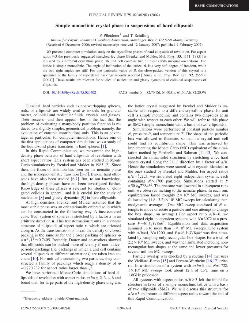
Simple monoclinic crystal phase in suspensions of hard ellipsoids
P. Pfleiderer* and T. SchillingInstitut für Physik, Johannes Gutenberg-Universität, Staudinger Weg 7, D-55099 Mainz, Germany
Received 6 December 2006; revised manuscript received 12 January 2007; published 9 February 2007
We present a computer simulation study on the crystalline phases of hard ellipsoids of revolution. For aspectratios 3 the previously suggested stretched-fcc phase Frenkel and Mulder, Mol. Phys. 55, 1171 1985 isreplaced by a different crystalline phase. Its unit cell contains two ellipsoids with unequal orientations. Thelattice is simple monoclinic. The angle of inclination of the lattice, , is a very soft degree of freedom, whilethe two right angles are stiff. For one particular value of , the close-packed version of this crystal is aspecimen of the family of superdense packings recently reported Donev et al., Phys. Rev. Lett. 92, 2555062004. These results are relevant for studies of nucleation and glassy dynamics of colloidal suspensions ofellipsoids.
DOI: 10.1103/PhysRevE.75.020402 PACS numbers: 82.70.Dd, 64.60.Cn, 61.50.Ah, 82.20.Wt
Classical, hard particles such as nonoverlapping spheres,rods, or ellipsoids are widely used as models for granularmatter, colloidal and molecular fluids, crystals, and glasses.Their success—and their appeal—lies in the fact that theproblem of evaluating a many-body partition function is re-duced to a slightly simpler, geometrical problem, namely, theevaluation of entropic contributions only. This is an advan-tage, in particular, for computer simulations. Hence one ofthe first applications of computer simulations was a study ofthe liquid-solid phase transition in hard spheres 1.
In this Rapid Communication, we reexamine the high-density phase behavior of hard ellipsoids of revolution withshort aspect ratios. This system has been studied in MonteCarlo simulations by Frenkel and Mulder in 1985 2. Sincethen, the focus of attention has been on the nematic phaseand the isotropic-nematic transition 3–5. Biaxial hard ellip-soids have also been studied 6,7. But, to our knowledge,the high-density phases have not been investigated further.Knowledge of these phases is relevant for studies of elon-gated colloids in general, and it is crucial for the study ofnucleation 8 and glassy dynamics 9 in hard ellipsoids.
At high densities, Frenkel and Mulder assumed that themost stable phase was an orientationally ordered solid whichcan be constructed in the following way. A face-centeredcubic fcc system of spheres is stretched by a factor x in anarbitrary direction n. This transformation results in a crystalstructure of ellipsoids of aspect ratio x, which are orientedalong n. As the transformation is linear, the density of closestpacking is the same as for the closest packing of spheres = /180.7405. Recently, Donev and co-workers showedthat ellipsoids can be packed more efficiently if non-lattice-periodic packings i.e. packings in which a unit cell containsseveral ellipsoids at different orientations are taken into ac-count 10. For unit cells containing two particles, they con-structed a family of packings which reach a density of =0.770 732 for aspect ratios larger than 3.
We have performed Monte Carlo simulations of hard el-lipsoids of revolution with aspect ratios a /b= 1
3 ,2 ,3 ,4 ,6 andfound that, for large parts of the high-density phase diagram,
the lattice crystal suggested by Frenkel and Mulder is un-stable with respect to a different crystalline phase. Its unitcell is simple monoclinic and contains two ellipsoids at anangle with respect to each other. We will refer to this phaseas SM2 simple monoclinic with a basis of two ellipsoids.
Simulations were performed at constant particle numberN, pressure P, and temperature T. The shape of the periodicbox was allowed to fluctuate, so that the crystal unit cellcould find its equilibrium shape. This was achieved byimplementing the Monte Carlo MC equivalent of the simu-lation method by Parrinello and Rahman 11–13. We con-structed the initial solid structures by stretching a fcc hardsphere crystal along the 111 direction by a factor of a /b.Hence the simulations were started with crystals identical tothe ones studied by Frenkel and Mulder. For aspect ratiosa /b= 1
3 ,2 ,3, we simulated eight independent systems, eachcontaining N1700 particles. Simulations started at P=50 kBT /8ab2. The pressure was lowered in subsequent runsuntil we observed melting to the nematic phase. In each run,equilibration lasted roughly 2106 MC sweeps, and wasfollowed by 1.8–3.2106 MC sweeps for calculating ther-modynamic averages. One MC sweep consisted of N at-tempts to move or rotate a particle and one attempt to changethe box shape, on average. For aspect ratio a /b=6, wesimulated eight independent systems with N=3072 at a pres-sure P=46 kBT /8ab2. Equilibration and data acquisitionsummed up to more than 3106 MC sweeps. One systemwith a /b=4, N=1200, and P=46 kBT /8ab2 was first simu-lated by sampling only rectangular box shapes for a total of2.2106 MC sweeps, and was then simulated including non-rectangular box shapes at the same and lower pressures forseveral million MC sweeps.
Particle overlap was checked by a routine 14 that usesthe Vieillard-Baron 15 and Perram-Wertheim 16,17 crite-ria. In a simulation of a system with a /b=3 and N=1728,1106 MC sweeps took about 12 h of CPU time on a1.8GHz processor.
All systems with aspect ratios a /b3 left the initial fccstructure in favor of a simple monoclinic lattice with a basisof two ellipsoids SM2. We will discuss this structure fora /b=3 and return to different aspect ratios toward the end ofthis Rapid Communication.*Electronic address: [email protected]
PHYSICAL REVIEW E 75, 020402R 2007
RAPID COMMUNICATIONS
1539-3755/2007/752/0204024 ©2007 The American Physical Society020402-1
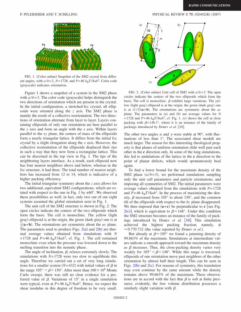
Figure 1 shows a snapshot of a system in the SM2 phasewith a /b=3. The color code grayscale helps distinguish thetwo directions of orientation which are present in the crystal.In the initial configuration, a stretched-fcc crystal, all ellip-soids were oriented along the z axis. The SM2 phase ismainly the result of a collective reorientation. The two direc-tions of orientation alternate from layer to layer. Layers con-taining ellipsoids of only one orientation are here parallel tothe y axis and form an angle with the x axis. Within layersparallel to the xy plane, the centers of mass of the ellipsoidsform a nearly triangular lattice. It differs from the initial fcccrystal by a slight elongation along the x axis. However, thecollective reorientation of the ellipsoids displaced their tipsin such a way that they now form a rectangular lattice. Thiscan be discerned in the top view in Fig. 1. The tips of theneighboring layers interlace. As a result, each ellipsoid nowhas four nearest neighbors above and below, whereas in thefcc structure, it had three. The total number of nearest neigh-bors has increased from 12 to 14, which is indicative of ahigher packing efficiency.
The initial triangular symmetry about the z axis allows fortwo additional, equivalent SM2 configurations, which are ro-tated with respect to the one in Fig. 1 by ±60°. We observedthese possibilities as well; in fact, only two out of our eightsystems assumed the global orientation seen in Fig. 1.
The unit cell of the SM2 structure is shown in Fig. 2. Theopen circles indicate the centers of the two ellipsoids whichform the basis. The cell is monoclinic. The yellow lightgray ellipsoid is at the origin, the green dark gray one is at12 a+b. The orientations are symmetric about the ac plane.The parameters used to produce Figs. 2a and 2b are ther-mal average values obtained from simulations with N=1728 and P=46 kBT /8ab2; cf. Fig. 1. The cell remainedmonoclinic even when the pressure was lowered down to themelting transition into the nematic phase.
The angle of inclination, , relaxes extremely slowly. Thesimulations with N=1728 were too slow to equilibrate thisangle. Therefore we carried out a set of very long simula-tions for a smaller system N=432 with initial values of inthe range 105° 150°. After more than 100106 MonteCarlo sweeps, there was still no clear evidence for a pre-ferred value of . Variations of 15° in a single simulationwere typical, even at P=46 kBT /8ab2. Hence, we expect theshear modulus in this degree of freedom to be very small.
The other two angles and were stable at 90°, with fluc-tuations of less than 1°. The associated shear moduli aremuch larger. The reason for this interesting rheological prop-erty is that planes of uniform orientation slide well past eachother in the c direction only. In some of the long simulations,this led to undulations of the lattice in the c direction to thepoint of planar defects, which would spontaneously healagain.
To find a lower bound for the maximum density of theSM2 phase a /b=3, we performed simulations samplingonly the unit cell parameters and particle orientations, andimposing all symmetries of SM2. The initial parameters wereaverage values obtained from the simulations with N=1728and P=46 kBT /8ab2. In the process of maximizing the den-sity, increased from 105° to about 150°, and the commontilt of the ellipsoids with respect to the bc plane disappeared.We then imposed that a+c be perpendicular to c see Fig.2c, which is equivalent to 148°. Under this conditionthe SM2 structure becomes an instance of the family of pack-ings introduced by Donev et al. 10. This simulationachieved the highest packing fraction, namely, 0.770 732 the value reported by Donev et al..
But already at 105° we found a jamming density of99.663% of the maximum. Simulations at intermediate val-ues indicate a smooth approach toward the maximum densityas increases. Thus, the close-packing density varies veryweakly for 105° 148°. While this range is traversed,ellipsoids of one orientation move past neighbors of the otherorientation by almost half their length. This can be seen inFigs. 2b and 2c. For reasons of symmetry, this translationmay even continue by the same amount while the densityremains above 99.663% of the maximum. These observa-tions are in accord with the fact that is soft at finite pres-sures; evidently, the free volume distribution possesses asimilarly slight variation with .
FIG. 1. Color online Snapshot of the SM2 crystal from differ-ent angles, with a /b=3, N=1728, and P=46 kBT /8ab2. Color codegrayscale indicates orientation.
FIG. 2. Color online Unit cell of SM2 with a /b=3. The opencircles indicate the centers of the two ellipsoids which form thebasis. The cell is monoclinic. exhibits large variations. The yel-low light gray ellipsoid is at the origin; the green dark gray oneis at 1/2a+b. The orientations are symmetric about the acplane. The parameters in a and b are average values for N=1728 and P=46 kBT /8ab2; cf. Fig. 1. c shows the cell at closepacking with =148.3°, where it is an instance of the family ofpackings introduced by Donev et al. 10.
P. PFLEIDERER AND T. SCHILLING PHYSICAL REVIEW E 75, 020402R 2007
RAPID COMMUNICATIONS
020402-2
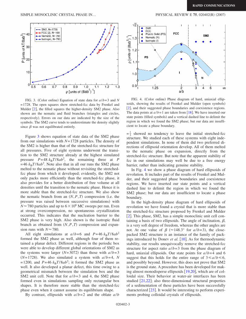
Figure 3 shows equation of state data of the SM2 phasefrom our simulations with N=1728 particles. The density ofthe SM2 is higher than that of the stretched-fcc structure forall pressures. Five of eight systems underwent the transi-tion to the SM2 structure already at the highest simulatedpressure P=48 kBT /8ab2, the remaining three at P=46 kBT /8ab2. Note also that in all our runs the SM2 phasemelted to the nematic phase without revisiting the stretched-fcc phase from which it developed; evidently, the SM2 notonly packs more efficiently than the stretched-fcc phase, italso provides for a better distribution of free volume at alldensities until the transition to the nematic phase. Hence it ismore stable than the stretched-fcc structure. We also showthe nematic branch from an N , P ,T compression i.e. thepressure was raised between successive simulations withN780 particles and up to 6106 MC sweeps per run. Evenat strong overcompression, no spontaneous crystallizationoccurred. This indicates that the nucleation barrier to theSM2 phase is very high. Also shown is the isotropic fluidbranch as obtained from N , P ,T compression and expan-sion runs with N780.
All eight simulations at a /b=6 and P=46 kBT /8ab2
formed the SM2 phase as well, although four of them re-tained a planar defect. Different regions in the periodic boxwere able to develop different global orientations of SM2 asthe systems were larger N=3072 than those with a /b=3N=1728. We also simulated a system with a /b=4, N=1200, and P=46 kBT /8ab2; it formed the SM2 phase aswell. It also developed a planar defect, this time owing to ageometrical mismatch between the simulation box and theSM2 unit cell. Note that for a /b=3 and 4, the SM2 phaseformed even in simulations sampling only rectangular boxshapes. It is therefore more stable than the stretched-fccphase even when it cannot assume its equilibrium shape.
By contrast, ellipsoids with a /b=2 and the oblate a /b
= 13 showed no tendency to leave the initial stretched-fcc
structure. We studied each of these systems with eight inde-pendent simulations. In none of them did two preferred di-rections of ellipsoid orientation develop. All of them meltedto the nematic phase on expansion, directly from thestretched-fcc structure. But note that the apparent stability offcc in our simulations may well be due to a free energybarrier, rather than indicating genuine stability.
In Fig. 4 we show a phase diagram of hard ellipsoids ofrevolution. It includes part of the results of Frenkel and Mul-der, and their suggested phase boundaries and coexistenceregions. We have inserted our state points and a verticaldashed line to delimit the region in which we found theSM2 phase; but our data are insufficient to locate a phaseboundary.
In the high-density phase diagram of hard ellipsoids ofrevolution we have found a crystal that is more stable thanthe stretched-fcc structure proposed by Frenkel and Mulder2. This phase, SM2, has a simple monoclinic unit cell con-taining a basis of two ellipsoids. The angle of inclination, ,is a very soft degree of freedom, whereas the other angles arenot. At one value of 148.3° for a /b=3, the close-packed SM2 structure is an instance of the family of pack-ings introduced by Donev et al. 10. As for thermodynamicstability, our results unequivocally remove the stretched-fccstructure for aspect ratio a /b=3 from the phase diagram ofhard, uniaxial ellipsoids. Our state points for a /b=4 and 6suggest that this holds for the entire range of 3a /b6,and possibly beyond. However, this does not prove that SM2is the ground state. A procedure has been developed for mak-ing almost monodisperse ellipsoids 19,20, which are of col-loidal size. Their behavior at water-air interfaces has beenstudied 21,22; also three-dimensional structural propertiesof a sedimentation of these particles have been successfullycharacterized 23. It would be interesting to perform experi-ments probing colloidal crystals of ellipsoids.
FIG. 3. Color online Equation of state data for a /b=3 and N=1728. The open squares show stretched-fcc data by Frenkel andMulder 2, the filled squares the higher-density SM2 phase. Alsoshown are the nematic and fluid branches triangles and circles,respectively. Errors on our data are indicated by the size of thesymbols. The SM2 curve tends to underestimate the density slightlysince was not equilibrated entirely.
FIG. 4. Color online Phase diagram of hard, uniaxial ellip-soids, showing the results of Frenkel and Mulder open symbols2, and their suggested phase boundaries and coexistence regions.The data points at a /b=1 are taken from 18. We have inserted ourstate points filled symbols and a vertical dashed line to delimit theregion in which we found the SM2 phase; but our data are insuffi-cient to locate a phase boundary.
SIMPLE MONOCLINIC CRYSTAL PHASE IN… PHYSICAL REVIEW E 75, 020402R 2007
RAPID COMMUNICATIONS
020402-3
This work was supported by the Emmy Noether Programand SFB TR6 of the Deutsche ForschungsgemeinschaftDFG, and the European Network of Excellence SoftComp.
We are grateful to the NIC Jülich for computing time, and toK. Binder, D. Frenkel, M. P. Allen, J. Vermant, A. Donev,and W. A. Siebel for helpful suggestions.
1 B. J. Alder and T. E. Wainwright, J. Chem. Phys. 27, 12081957.
2 D. Frenkel and B. Mulder, Mol. Phys. 55, 1171 1985.3 G. J. Zarragoicoechea, D. Levesque, and J. J. Weis, Mol. Phys.
75, 989 1992.4 M. P. Allen and C. P. Mason, Mol. Phys. 86, 467 1995.5 P. J. Camp, C. P. Mason, M. P. Allen, A. A. Khare, and D. A.
Kofke, J. Chem. Phys. 105, 2837 1996.6 M. P. Allen, Liq. Cryst. 8, 499 1990.7 P. J. Camp and M. P. Allen, J. Chem. Phys. 106, 6681 1997.8 T. Schilling and D. Frenkel, Comput. Phys. Commun. 169,
117 2005.9 M. Letz, R. Schilling, and A. Latz, Phys. Rev. E 62, 5173
2000.10 A. Donev, F. H. Stillinger, P. M. Chaikin, and S. Torquato,
Phys. Rev. Lett. 92, 255506 2004.11 M. Parrinello and A. Rahman, J. Appl. Phys. 52, 7182 1981.12 R. Najafabadi and S. Yip, Scr. Metall. 17, 1199 1983.13 S. Yashonath and C. N. R. Rao, Mol. Phys. 54, 245 1985.
14 M. P. Allen, D. Frenkel, and J. Talbot, Comput. Phys. Rep. 9,301 1989.
15 J. Vieillard-Baron, J. Chem. Phys. 56, 4729 1972.16 J. W. Perram, M. S. Wertheim, J. L. Lebowitz, and G. O.
Williams, Chem. Phys. Lett. 105, 277 1984.17 J. W. Perram and M. S. Wertheim, J. Comput. Phys. 58, 409
1985.18 W. G. Hoover and F. H. Ree, J. Chem. Phys. 49, 3609 1968.19 K. M. Keville, E. I. Franses, and J. M. Caruthers, J. Colloid
Interface Sci. 144, 103 1991.20 C. C. Ho, A. Keller, J. A. Odell, and R. H. Ottewill, Colloid
Polym. Sci. 271, 469 1993.21 M. G. Basavaraj, G. G. Fuller, J. Fransaer, and J. Vermant,
Langmuir 22, 6605 2006.22 J. C. Loudet, A. G. Yodh, and B. Pouligny, Phys. Rev. Lett.
97, 018304 2006.23 A. Mohraz and M. J. Solomon, Langmuir 21, 5298 2005.
P. PFLEIDERER AND T. SCHILLING PHYSICAL REVIEW E 75, 020402R 2007
RAPID COMMUNICATIONS
020402-4
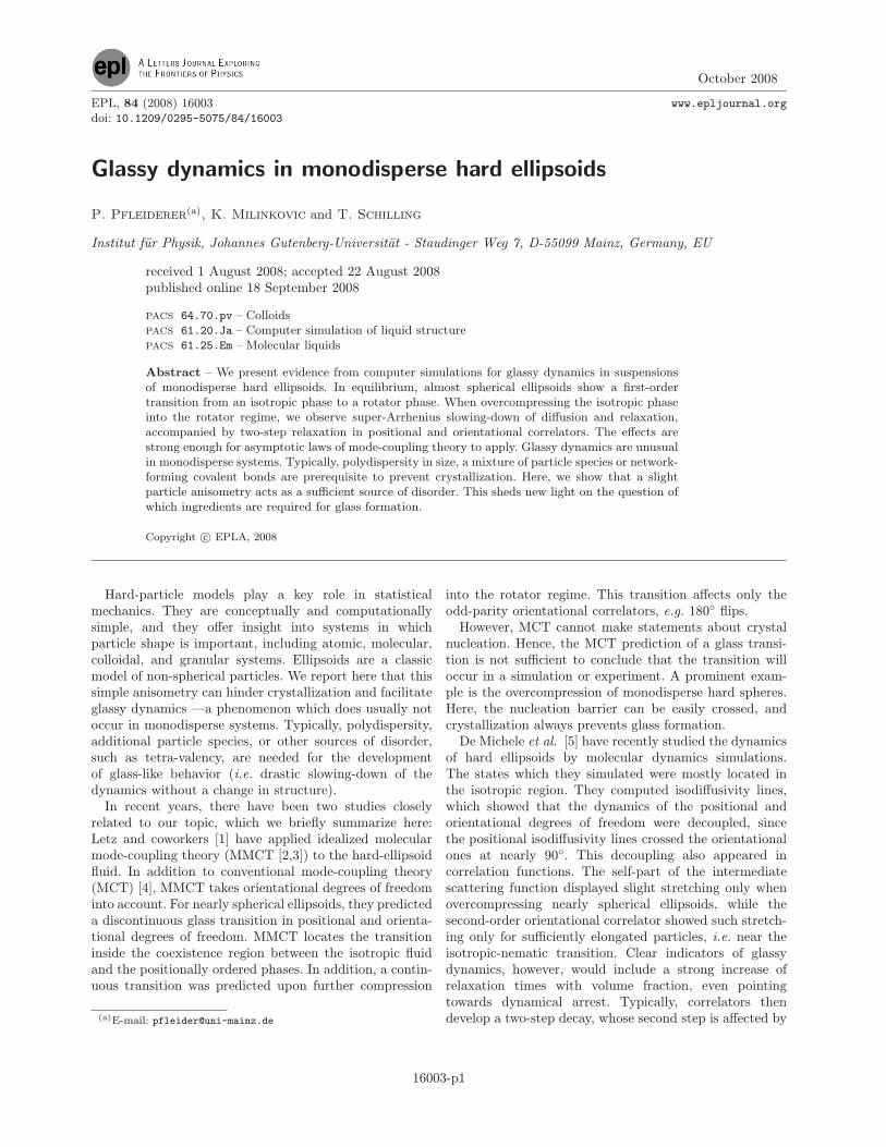
October 2008
EPL, 84 (2008) 16003 www.epljournal.org
doi: 10.1209/0295-5075/84/16003
Glassy dynamics in monodisperse hard ellipsoids
P. Pfleiderer(a), K. Milinkovic and T. Schilling
Institut fur Physik, Johannes Gutenberg-Universitat - Staudinger Weg 7, D-55099 Mainz, Germany, EU
received 1 August 2008; accepted 22 August 2008published online 18 September 2008
PACS 64.70.pv – ColloidsPACS 61.20.Ja – Computer simulation of liquid structurePACS 61.25.Em – Molecular liquids
Abstract – We present evidence from computer simulations for glassy dynamics in suspensionsof monodisperse hard ellipsoids. In equilibrium, almost spherical ellipsoids show a first-ordertransition from an isotropic phase to a rotator phase. When overcompressing the isotropic phaseinto the rotator regime, we observe super-Arrhenius slowing-down of diffusion and relaxation,accompanied by two-step relaxation in positional and orientational correlators. The effects arestrong enough for asymptotic laws of mode-coupling theory to apply. Glassy dynamics are unusualin monodisperse systems. Typically, polydispersity in size, a mixture of particle species or network-forming covalent bonds are prerequisite to prevent crystallization. Here, we show that a slightparticle anisometry acts as a sufficient source of disorder. This sheds new light on the question ofwhich ingredients are required for glass formation.
Copyright c© EPLA, 2008
Hard-particle models play a key role in statisticalmechanics. They are conceptually and computationallysimple, and they offer insight into systems in whichparticle shape is important, including atomic, molecular,colloidal, and granular systems. Ellipsoids are a classicmodel of non-spherical particles. We report here that thissimple anisometry can hinder crystallization and facilitateglassy dynamics —a phenomenon which does usually notoccur in monodisperse systems. Typically, polydispersity,additional particle species, or other sources of disorder,such as tetra-valency, are needed for the developmentof glass-like behavior (i.e. drastic slowing-down of thedynamics without a change in structure).In recent years, there have been two studies closely
related to our topic, which we briefly summarize here:Letz and coworkers [1] have applied idealized molecularmode-coupling theory (MMCT [2,3]) to the hard-ellipsoidfluid. In addition to conventional mode-coupling theory(MCT) [4], MMCT takes orientational degrees of freedominto account. For nearly spherical ellipsoids, they predicteda discontinuous glass transition in positional and orienta-tional degrees of freedom. MMCT locates the transitioninside the coexistence region between the isotropic fluidand the positionally ordered phases. In addition, a contin-uous transition was predicted upon further compression
(a)E-mail: [email protected]
into the rotator regime. This transition affects only theodd-parity orientational correlators, e.g. 180 flips.However, MCT cannot make statements about crystal
nucleation. Hence, the MCT prediction of a glass transi-tion is not sufficient to conclude that the transition willoccur in a simulation or experiment. A prominent exam-ple is the overcompression of monodisperse hard spheres.Here, the nucleation barrier can be easily crossed, andcrystallization always prevents glass formation.De Michele et al. [5] have recently studied the dynamics
of hard ellipsoids by molecular dynamics simulations.The states which they simulated were mostly located inthe isotropic region. They computed isodiffusivity lines,which showed that the dynamics of the positional andorientational degrees of freedom were decoupled, sincethe positional isodiffusivity lines crossed the orientationalones at nearly 90. This decoupling also appeared incorrelation functions. The self-part of the intermediatescattering function displayed slight stretching only whenovercompressing nearly spherical ellipsoids, while thesecond-order orientational correlator showed such stretch-ing only for sufficiently elongated particles, i.e. near theisotropic-nematic transition. Clear indicators of glassydynamics, however, would include a strong increase ofrelaxation times with volume fraction, even pointingtowards dynamical arrest. Typically, correlators thendevelop a two-step decay, whose second step is affected by
16003-p1
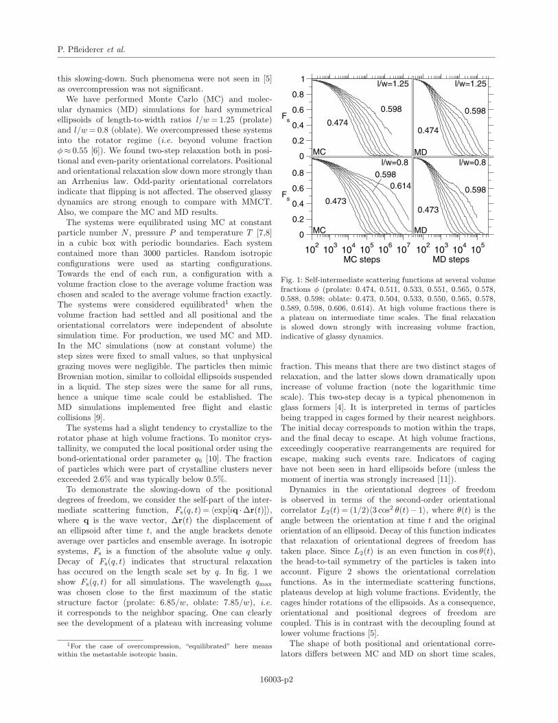
P. Pfleiderer et al.
this slowing-down. Such phenomena were not seen in [5]as overcompression was not significant.We have performed Monte Carlo (MC) and molec-
ular dynamics (MD) simulations for hard symmetricalellipsoids of length-to-width ratios l/w= 1.25 (prolate)and l/w= 0.8 (oblate). We overcompressed these systemsinto the rotator regime (i.e. beyond volume fractionφ≈ 0.55 [6]). We found two-step relaxation both in posi-tional and even-parity orientational correlators. Positionaland orientational relaxation slow down more strongly thanan Arrhenius law. Odd-parity orientational correlatorsindicate that flipping is not affected. The observed glassydynamics are strong enough to compare with MMCT.Also, we compare the MC and MD results.The systems were equilibrated using MC at constant
particle number N , pressure P and temperature T [7,8]in a cubic box with periodic boundaries. Each systemcontained more than 3000 particles. Random isotropicconfigurations were used as starting configurations.Towards the end of each run, a configuration with avolume fraction close to the average volume fraction waschosen and scaled to the average volume fraction exactly.The systems were considered equilibrated1 when thevolume fraction had settled and all positional and theorientational correlators were independent of absolutesimulation time. For production, we used MC and MD.In the MC simulations (now at constant volume) thestep sizes were fixed to small values, so that unphysicalgrazing moves were negligible. The particles then mimicBrownian motion, similar to colloidal ellipsoids suspendedin a liquid. The step sizes were the same for all runs,hence a unique time scale could be established. TheMD simulations implemented free flight and elasticcollisions [9].The systems had a slight tendency to crystallize to the
rotator phase at high volume fractions. To monitor crys-tallinity, we computed the local positional order using thebond-orientational order parameter q6 [10]. The fractionof particles which were part of crystalline clusters neverexceeded 2.6% and was typically below 0.5%.To demonstrate the slowing-down of the positional
degrees of freedom, we consider the self-part of the inter-mediate scattering function, Fs(q, t) = 〈exp[iq ·∆r(t)]〉,where q is the wave vector, ∆r(t) the displacement ofan ellipsoid after time t, and the angle brackets denoteaverage over particles and ensemble average. In isotropicsystems, Fs is a function of the absolute value q only.Decay of Fs(q, t) indicates that structural relaxationhas occured on the length scale set by q. In fig. 1 weshow Fs(q, t) for all simulations. The wavelength qmaxwas chosen close to the first maximum of the staticstructure factor (prolate: 6.85/w, oblate: 7.85/w), i.e.it corresponds to the neighbor spacing. One can clearlysee the development of a plateau with increasing volume
1For the case of overcompression, “equilibrated” here meanswithin the metastable isotropic basin.
102
103
104
105
MD steps10
210
310
410
510
610
7
MC steps
0
0.2
0.4
0.6
0.8
Fs
0
0.2
0.4
0.6
0.8
1
Fs
l/w=0.8
l/w=1.25
MC
MC
0.598 0.598
0.598
0.5980.614
0.473
0.4740.474
0.473
MD
MD
l/w=1.25
l/w=0.8
Fig. 1: Self-intermediate scattering functions at several volumefractions φ (prolate: 0.474, 0.511, 0.533, 0.551, 0.565, 0.578,0.588, 0.598; oblate: 0.473, 0.504, 0.533, 0.550, 0.565, 0.578,0.589, 0.598, 0.606, 0.614). At high volume fractions there isa plateau on intermediate time scales. The final relaxationis slowed down strongly with increasing volume fraction,indicative of glassy dynamics.
fraction. This means that there are two distinct stages ofrelaxation, and the latter slows down dramatically uponincrease of volume fraction (note the logarithmic timescale). This two-step decay is a typical phenomenon inglass formers [4]. It is interpreted in terms of particlesbeing trapped in cages formed by their nearest neighbors.The initial decay corresponds to motion within the traps,and the final decay to escape. At high volume fractions,exceedingly cooperative rearrangements are required forescape, making such events rare. Indicators of caginghave not been seen in hard ellipsoids before (unless themoment of inertia was strongly increased [11]).Dynamics in the orientational degrees of freedom
is observed in terms of the second-order orientationalcorrelator L2(t) = (1/2)〈3 cos2 θ(t)− 1〉, where θ(t) is theangle between the orientation at time t and the originalorientation of an ellipsoid. Decay of this function indicatesthat relaxation of orientational degrees of freedom hastaken place. Since L2(t) is an even function in cos θ(t),the head-to-tail symmetry of the particles is taken intoaccount. Figure 2 shows the orientational correlationfunctions. As in the intermediate scattering functions,plateaus develop at high volume fractions. Evidently, thecages hinder rotations of the ellipsoids. As a consequence,orientational and positional degrees of freedom arecoupled. This is in contrast with the decoupling found atlower volume fractions [5].The shape of both positional and orientational corre-
lators differs between MC and MD on short time scales,
16003-p2
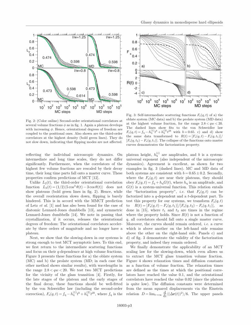
Glassy dynamics in monodisperse hard ellipsoids
102
103
104
105
MD steps10
110
210
310
410
510
6
MC steps
0
0.2
0.4
0.6
0.8
L2
0
0.2
0.4
0.6
0.8
1
L2
l/w=1.25 l/w=1.25
l/w=0.8 l/w=0.8
0.598 0.598
0.598
0.598
0.6140.473
0.4740.474
0.473
MC
MC MD
MD
Fig. 2: (Color online) Second-order orientational correlators atseveral volume fractions φ as in fig. 1. Again a plateau developswith increasing φ. Hence, orientational degrees of freedom arecoupled to the positional ones. Also shown are the third-ordercorrelators at the highest density (bold green lines). They donot slow down, indicating that flipping modes are not affected.
reflecting the individual microscopic dynamics. Onintermediate and long time scales, they do not differsignificantly. Furthermore, when the correlators of thehighest few volume fractions are rescaled by their decaytime, their long time parts fall onto a master curve. Theseproperties confirm predictions of MCT [12].Unlike L2(t), the third-order orientational correlation
function L3(t) = (1/2)〈5 cos3 θ(t)− 3 cos θ(t)〉 does notshow plateaus (bold green lines in fig. 2). Hence, whilethe overall reorientation slows down, flipping is barelyhindered. This is in accord with the MMCT predictionof Letz et al. [1] and has also been found for the case ofdiatomic Lennard-Jones dumbbells [13], and symmetricLennard-Jones dumbbells [14]. We note in passing thatcrystallization, if it occurs, releases the orientationaldegrees of freedom: The orientational correlators acceler-ate by three orders of magnitude and no longer have aplateau.Next, we show that the slowing-down in our systems is
strong enough to test MCT asymptotic laws. To this end,we first return to the intermediate scattering functionsand focus on their q-dependence at high volume fractions.Figure 3 presents these functions for a) the oblate system(MC) and b) the prolate system (MD; in each case theother method shows similar results), with wavelengths inthe range 2.8< qw < 20. We test two MCT predictionsfor the vicinity of the glass transition [4]. Firstly, forthe late stages of the plateau and the early stages ofthe final decay, these functions should be well-fittedby the von Schweidler law (including the second-order
correction), Fs(q, t) = fq−h(1)q tb+h(2)q t2b, where fq is the
102
103
104
105
MD steps
0
0.2
0.4
0.6
0.8
1
F s
102
103
104
105
106
107
MC steps
-4
-2
0
2
4
R(t)
a) b)
c) d)
Fig. 3: Self-intermediate scattering functions Fs(q, t) of a) theoblate system (MC data) and b) the prolate system (MD data)at the highest volume fraction, for the range 2.8< qw < 20.The dashed lines show fits to the von Schweidler lawFs(q, t) = fq−h(1)q tb+h(2)q t2b with b= 0.65. c) and d) showthe same data transformed to R(t) = [Fs(q, t)−Fs(q, t1)]/[Fs(q, t2)−Fs(q, t1)]. The collapse of the functions onto mastercurves demonstrates the factorization property.
plateau height, h(i)q are amplitudes, and b is a system-
universal exponent (also independent of the microscopicdynamics). Agreement is excellent, as shown for twoexamples in fig. 3 (dashed lines). MC and MD data ofboth systems are consistent with b= 0.65± 0.2. Secondly,where the Fs(q, t) are near their plateaus, they shouldobey Fs(q, t) = fq+hqG(t), where hq is an amplitude, andG(t) is a system-universal function. This relation entailsthe “factorization property”, i.e. that Fs(q, t) can befactorized into a q-dependent and a t-dependent part. Totest this property for our systems, we transform Fs(q, t)to R(t) = [Fs(q, t)−Fs(q, t1)]/[Fs(q, t2)−Fs(q, t1)], asdone in [15], where t1 and t2 are times in the regimewhere the property holds. Since R(t) is not a function ofq, all correlators should fall onto a single master curve.Moreover, the curves should remain ordered, i.e. a curvewhich is above another on the left-hand side remainsabove the other on the right-hand side. Panels c) andd) of fig. 3 demonstrate the validity of the factorizationproperty, and indeed they remain ordered.We finally demonstrate the applicability of an MCT
scaling law for the slowing-down, which even allows usto extract the MCT glass transition volume fraction.Figure 4 shows relaxation times and diffusion constantsas a function of volume fraction. The relaxation timesare defined as the times at which the positional corre-lators have reached the value 0.1, and the orientationalcorrelators have reached the value 0.02 (since the plateauis quite low). The diffusion constants were determinedfrom the mean squared displacements via the Einstein
relation D= limt→∞ ddt 〈(∆r(t))2〉/6. The upper panels
16003-p3
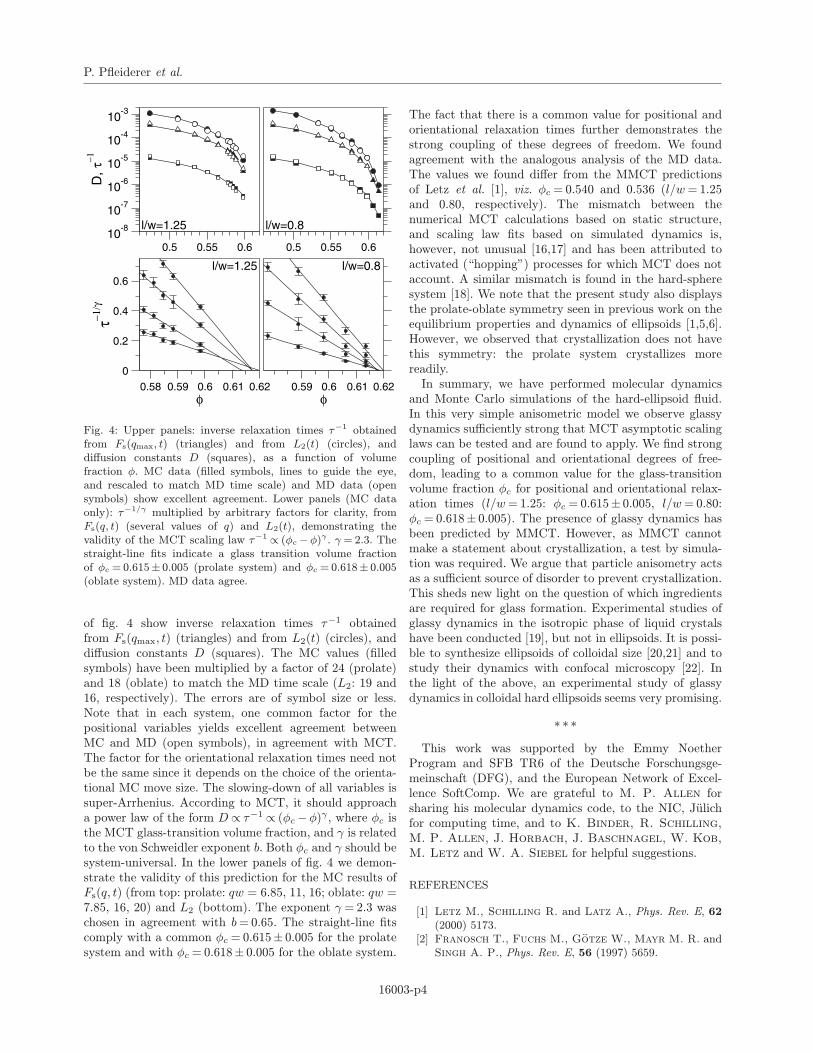
P. Pfleiderer et al.
0.59 0.6 0.61 0.62φ
0.5 0.55 0.6
0.58 0.59 0.6 0.61 0.62φ
0
0.2
0.4
0.6
τγ/1−
0.5 0.55 0.610
-8
10-7
10-6
10-5
10-4
10-3
,D
τ1−
l/w=1.25
l/w=1.25
l/w=0.8
l/w=0.8
Fig. 4: Upper panels: inverse relaxation times τ−1 obtainedfrom Fs(qmax, t) (triangles) and from L2(t) (circles), anddiffusion constants D (squares), as a function of volumefraction φ. MC data (filled symbols, lines to guide the eye,and rescaled to match MD time scale) and MD data (opensymbols) show excellent agreement. Lower panels (MC dataonly): τ−1/γ multiplied by arbitrary factors for clarity, fromFs(q, t) (several values of q) and L2(t), demonstrating thevalidity of the MCT scaling law τ−1 ∝ (φc−φ)γ . γ = 2.3. Thestraight-line fits indicate a glass transition volume fractionof φc = 0.615± 0.005 (prolate system) and φc = 0.618± 0.005(oblate system). MD data agree.
of fig. 4 show inverse relaxation times τ−1 obtainedfrom Fs(qmax, t) (triangles) and from L2(t) (circles), anddiffusion constants D (squares). The MC values (filledsymbols) have been multiplied by a factor of 24 (prolate)and 18 (oblate) to match the MD time scale (L2: 19 and16, respectively). The errors are of symbol size or less.Note that in each system, one common factor for thepositional variables yields excellent agreement betweenMC and MD (open symbols), in agreement with MCT.The factor for the orientational relaxation times need notbe the same since it depends on the choice of the orienta-tional MC move size. The slowing-down of all variables issuper-Arrhenius. According to MCT, it should approacha power law of the form D∝ τ−1 ∝ (φc−φ)γ , where φc isthe MCT glass-transition volume fraction, and γ is relatedto the von Schweidler exponent b. Both φc and γ should besystem-universal. In the lower panels of fig. 4 we demon-strate the validity of this prediction for the MC results ofFs(q, t) (from top: prolate: qw = 6.85, 11, 16; oblate: qw =7.85, 16, 20) and L2 (bottom). The exponent γ = 2.3 waschosen in agreement with b= 0.65. The straight-line fitscomply with a common φc = 0.615± 0.005 for the prolatesystem and with φc = 0.618± 0.005 for the oblate system.
The fact that there is a common value for positional andorientational relaxation times further demonstrates thestrong coupling of these degrees of freedom. We foundagreement with the analogous analysis of the MD data.The values we found differ from the MMCT predictionsof Letz et al. [1], viz. φc = 0.540 and 0.536 (l/w= 1.25and 0.80, respectively). The mismatch between thenumerical MCT calculations based on static structure,and scaling law fits based on simulated dynamics is,however, not unusual [16,17] and has been attributed toactivated (“hopping”) processes for which MCT does notaccount. A similar mismatch is found in the hard-spheresystem [18]. We note that the present study also displaysthe prolate-oblate symmetry seen in previous work on theequilibrium properties and dynamics of ellipsoids [1,5,6].However, we observed that crystallization does not havethis symmetry: the prolate system crystallizes morereadily.In summary, we have performed molecular dynamics
and Monte Carlo simulations of the hard-ellipsoid fluid.In this very simple anisometric model we observe glassydynamics sufficiently strong that MCT asymptotic scalinglaws can be tested and are found to apply. We find strongcoupling of positional and orientational degrees of free-dom, leading to a common value for the glass-transitionvolume fraction φc for positional and orientational relax-ation times (l/w= 1.25: φc = 0.615± 0.005, l/w= 0.80:φc = 0.618± 0.005). The presence of glassy dynamics hasbeen predicted by MMCT. However, as MMCT cannotmake a statement about crystallization, a test by simula-tion was required. We argue that particle anisometry actsas a sufficient source of disorder to prevent crystallization.This sheds new light on the question of which ingredientsare required for glass formation. Experimental studies ofglassy dynamics in the isotropic phase of liquid crystalshave been conducted [19], but not in ellipsoids. It is possi-ble to synthesize ellipsoids of colloidal size [20,21] and tostudy their dynamics with confocal microscopy [22]. Inthe light of the above, an experimental study of glassydynamics in colloidal hard ellipsoids seems very promising.
∗ ∗ ∗This work was supported by the Emmy Noether
Program and SFB TR6 of the Deutsche Forschungsge-meinschaft (DFG), and the European Network of Excel-lence SoftComp. We are grateful to M. P. Allen forsharing his molecular dynamics code, to the NIC, Julichfor computing time, and to K. Binder, R. Schilling,M. P. Allen, J. Horbach, J. Baschnagel, W. Kob,
M. Letz and W. A. Siebel for helpful suggestions.
REFERENCES
[1] Letz M., Schilling R. and Latz A., Phys. Rev. E, 62(2000) 5173.
[2] Franosch T., Fuchs M., Gotze W., Mayr M. R. andSingh A. P., Phys. Rev. E, 56 (1997) 5659.
16003-p4
Glassy dynamics in monodisperse hard ellipsoids
[3] Schilling R. and Scheidsteger T., Phys. Rev. E, 56(1997) 2932.
[4] Gotze W., in Liquids, Freezing, and the Glass Transition,edited by J. P. Hansen, D. Levesque and J. Zinn-Justin (North-Holland, Amsterdam) 1991.
[5] De Michele C., Schilling R. and Sciortino F., Phys.Rev. Lett., 98 (2007) 265702.
[6] Frenkel D. andMulder B.,Mol. Phys., 55 (1985) 1171.[7] Wood W. W., J. Chem. Phys., 48 (1968) 415.[8] McDonald I. R., Mol. Phys., 23 (1972) 41.[9] Allen M. P., Frenkel D. and Talbot J., Comput.Phys. Rep., 9 (1989) 301.
[10] ten Wolde P. R., Ruiz-Montero M. J. and FrenkelD., Phys. Rev. Lett., 75 (1995) 2714.
[11] Theenhaus T., Allen M. P., Letz M., Latz A. andSchilling R., Eur. Phys. J. E, 8 (2002) 269.
[12] Gotze W. and Sjogren L., Rep. Prog. Phys., 55 (1992)241.
[13] Kammerer S., Kob W. and Schilling R., Phys. Rev. E,56 (1997) 5450.
[14] Chong S.-H., Moreno A. J., Sciortino F. and KobW., Phys. Rev. Lett., 94 (2005) 215701.
[15] Gleim T. and Kob W., Eur. J. B, 13 (2000) 83.[16] Kob W. and Andersen H. C., Phys. Rev. E, 52 (1995)
4134.[17] Nauroth M. and Kob W., Phys. Rev. E, 55 (1997) 657.[18] Voigtmann T., Puertas A. M. and Fuchs M., Phys.
Rev. E, 70 (2004) 061506.[19] Cang H., Li J., Novikov V. N. and Fayer M. D.,
J. Chem. Phys., 118 (2003) 9303.[20] Keville K. M., Franses E. I. and Caruthers J. M.,
J. Colloid Interface Sci., 144 (1991) 103.[21] Ho C. C., Keller A., Odell J. A. and Ottewill
R. H., Colloid Polym. Sci., 271 (1993) 469.[22] Mukhija D. and Solomon M. J., J. Colloid Interface
Sci., 314 (2007) 98.
16003-p5
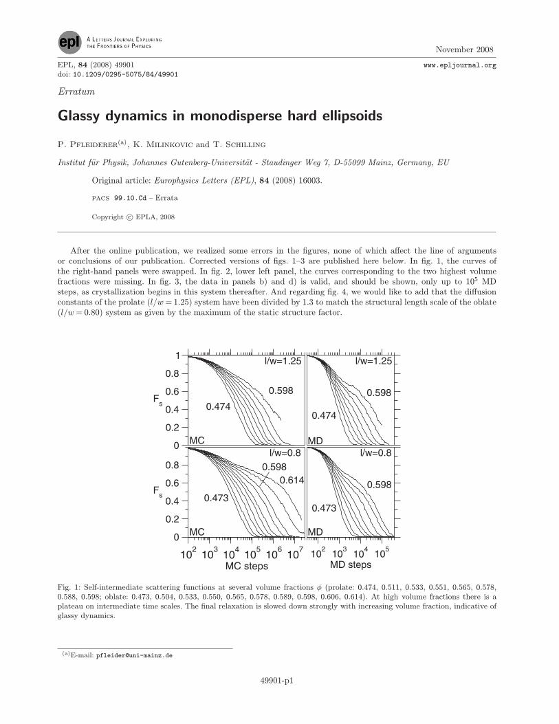
November 2008
EPL, 84 (2008) 49901 www.epljournal.org
doi: 10.1209/0295-5075/84/49901
Erratum
Glassy dynamics in monodisperse hard ellipsoids
P. Pfleiderer(a), K. Milinkovic and T. Schilling
Institut fur Physik, Johannes Gutenberg-Universitat - Staudinger Weg 7, D-55099 Mainz, Germany, EU
Original article: Europhysics Letters (EPL), 84 (2008) 16003.
PACS 99.10.Cd – Errata
Copyright c© EPLA, 2008
After the online publication, we realized some errors in the figures, none of which affect the line of argumentsor conclusions of our publication. Corrected versions of figs. 1–3 are published here below. In fig. 1, the curves ofthe right-hand panels were swapped. In fig. 2, lower left panel, the curves corresponding to the two highest volumefractions were missing. In fig. 3, the data in panels b) and d) is valid, and should be shown, only up to 105 MDsteps, as crystallization begins in this system thereafter. And regarding fig. 4, we would like to add that the diffusionconstants of the prolate (l/w= 1.25) system have been divided by 1.3 to match the structural length scale of the oblate(l/w= 0.80) system as given by the maximum of the static structure factor.
102
103
104
105
106
107
MC steps
0
0.2
0.4
0.6
0.8
Fs
0
0.2
0.4
0.6
0.8
1
Fs
102
103
104
105
MD steps
l/w=0.8
l/w=1.25
MC
MC
0.598 0.598
0.598
0.5980.614
0.473
0.4740.474
0.473
MD
MD
l/w=1.25
l/w=0.8
Fig. 1: Self-intermediate scattering functions at several volume fractions φ (prolate: 0.474, 0.511, 0.533, 0.551, 0.565, 0.578,0.588, 0.598; oblate: 0.473, 0.504, 0.533, 0.550, 0.565, 0.578, 0.589, 0.598, 0.606, 0.614). At high volume fractions there is aplateau on intermediate time scales. The final relaxation is slowed down strongly with increasing volume fraction, indicative ofglassy dynamics.
(a)E-mail: [email protected]
49901-p1
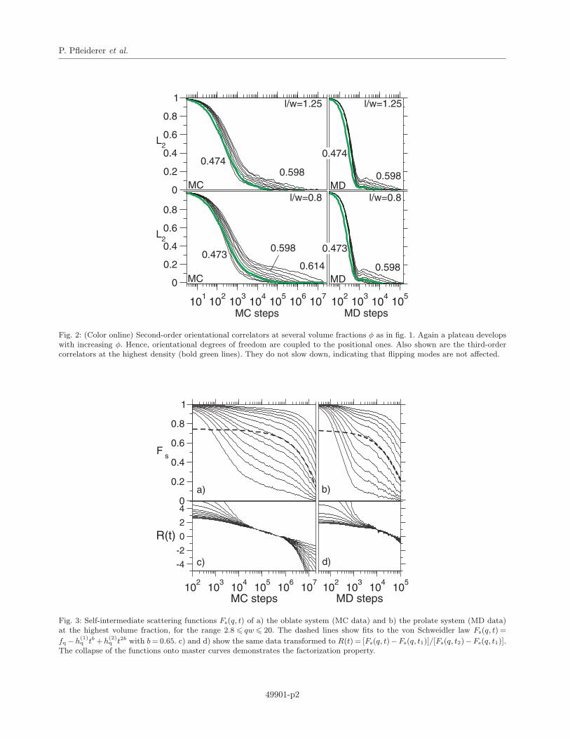
P. Pfleiderer et al.
102
103
104
105
MD steps10
110
210
310
410
510
610
7
MC steps
0
0.2
0.4
0.6
0.8
L2
0
0.2
0.4
0.6
0.8
1
L2
l/w=1.25 l/w=1.25
l/w=0.8 l/w=0.8
0.598 0.598
0.598
0.598
0.6140.473
0.4740.474
0.473
MC
MC MD
MD
Fig. 2: (Color online) Second-order orientational correlators at several volume fractions φ as in fig. 1. Again a plateau developswith increasing φ. Hence, orientational degrees of freedom are coupled to the positional ones. Also shown are the third-ordercorrelators at the highest density (bold green lines). They do not slow down, indicating that flipping modes are not affected.
102
103
104
105
MD steps
0
0.2
0.4
0.6
0.8
1
F s
102
103
104
105
106
107
MC steps
-4
-2
0
2
4
R(t)
a) b)
c) d)
Fig. 3: Self-intermediate scattering functions Fs(q, t) of a) the oblate system (MC data) and b) the prolate system (MD data)at the highest volume fraction, for the range 2.8 qw 20. The dashed lines show fits to the von Schweidler law Fs(q, t) =fq−h(1)q tb+h(2)q t2b with b= 0.65. c) and d) show the same data transformed to R(t) = [Fs(q, t)−Fs(q, t1)]/[Fs(q, t2)−Fs(q, t1)].The collapse of the functions onto master curves demonstrates the factorization property.
49901-p2