
DMO Castelli Romani (Destination Management Organization ...

Dimensioning, Cell Site Planning,and Self-Organization of
4G Radio Networks
Von der Fakultat fur Elektrotechnik und Informationstechnikder Rheinisch-Westfalischen Technischen Hochschule Aachen
zur Erlangung des akademischen Grades eines Doktorsder Ingenieurwissenschaften genehmigte Dissertation
vorgelegt von
Diplom-Informatiker,Diplom-Mathematiker (FH)
Alexander Engels
aus Monchengladbach
Berichter: Universitatsprofessor Dr. rer. nat. Rudolf MatharUniversitatsprofessor Dr. rer. nat. Berthold Vocking
Tag der mundlichen Prufung: 27. September 2013
Diese Dissertation ist auf den Internetseitender Hochschulbibliothek online verfugbar.


Shaker VerlagAachen 2013
Berichte aus der Kommunikationstechnik
Alexander Engels
Dimensioning, Cell Site Planning, andSelf-Organization of 4G Radio Networks
WICHTIG: D 82 überprüfen !!!

Bibliographic information published by the Deutsche NationalbibliothekThe Deutsche Nationalbibliothek lists this publication in the DeutscheNationalbibliografie; detailed bibliographic data are available in the Internet athttp://dnb.d-nb.de.
Zugl.: D 82 (Diss. RWTH Aachen University, 2013)
Copyright Shaker Verlag 2013All rights reserved. No part of this publication may be reproduced, stored in aretrieval system, or transmitted, in any form or by any means, electronic,mechanical, photocopying, recording or otherwise, without the prior permissionof the publishers.
Printed in Germany.
ISBN 978-3-8440-2315-2ISSN 0945-0823
Shaker Verlag GmbH • P.O. BOX 101818 • D-52018 AachenPhone: 0049/2407/9596-0 • Telefax: 0049/2407/9596-9Internet: www.shaker.de • e-mail: [email protected]

Preface
This thesis was written during my time as a Research Assistant at RWTH AachenUniversity’s Institute for Theoretical Information Technology.
First and foremost, I would like to thank my supervisor, Univ.-Prof. Dr. rer. nat. RudolfMathar, for giving me the opportunity to take a very unique path in pursuing my Ph.Ddegree. I would also like to thank Prof. Mathar for his continuous support and forbeing an excellent example of fair and practical leadership.
Many thanks to Univ.-Prof. Dr. rer. nat. Berthold Vocking for taking the effort toreferee this thesis.
A special thankyou goes to Michael Reyer, Gholamreza Alirezaei, Melanie Neunerdt,and Derek J. Corbett for their very helpful discussions and suggestions, and for proof-reading parts of this thesis. Furthermore, I would like to acknowledge the supportof my colleague Florian Schroder who provided me with several eye-catching picturesthat illustrate the principles of ray optical based path loss computation.
I would like to express my deepest gratitude to all my former and present colleagues atthe Institute for Theoretical Information Technology. You helped create a comfortableand inspiring working environment, every day. Thank you for a good time, I will missyour company.
I am very proud that I had the opportunity to contribute to numerous exciting researchprojects that were carried out in close collaboration with industry partners. Particu-larly, I would like to thank all of my colleagues at QSC AG, Cologne, you made mefeel like I was part of the team.
Ein besonderer Dank gilt meinen Eltern und der ubrigen Familie, die mich uber alleJahre hinweg mit viel Geduld und Zuversicht unersetzlich unterstutzt haben.
Finally, I am deeply grateful to all my friends and close companions for their patienceand understanding throughout the whole Ph.D journey.
Aachen, October 2013 Alexander Engels


Contents
1 Introduction 11.1 Outline . . . . . . . . . . . . . . . . . . . . . . . . . . . . . . . . . . . . 21.2 Related Work, Initiatives, and Institutions . . . . . . . . . . . . . . . . 31.3 Notation . . . . . . . . . . . . . . . . . . . . . . . . . . . . . . . . . . . 5
2 Mathematical Preliminaries 72.1 Linear Programs . . . . . . . . . . . . . . . . . . . . . . . . . . . . . . 72.2 Integer and Mixed-Integer Linear Programs . . . . . . . . . . . . . . . 82.3 Multi-Objective Optimization Problems . . . . . . . . . . . . . . . . . . 9
2.3.1 Pareto Front Exploration and the Scalarization Approach . . . . 102.3.2 Constrained Single Target Optimization . . . . . . . . . . . . . 12
3 Building Blocks for Radio Network Optimization 133.1 Radio Wave Propagation Models . . . . . . . . . . . . . . . . . . . . . 13
3.1.1 Semi-Empirical Path Loss Models . . . . . . . . . . . . . . . . . 153.1.2 Ray Optical Path Loss Models . . . . . . . . . . . . . . . . . . . 173.1.3 A Direction-Specific Land Use Based Path Loss Model . . . . . 19
3.2 Wireless Channel Models, Rate Computation, and Bandwidth Allocation 223.3 Demand Prediction Model . . . . . . . . . . . . . . . . . . . . . . . . . 263.4 Fundamental Problems in Radio Network Optimization . . . . . . . . . 27
3.4.1 The Maximal Covering Location Problem . . . . . . . . . . . . 283.4.2 User Assignment in OFDMA Systems . . . . . . . . . . . . . . . 293.4.3 Resource Allocation in OFDMA Systems . . . . . . . . . . . . . 30
4 Dimensioning of Multihop Networks 334.1 System Model . . . . . . . . . . . . . . . . . . . . . . . . . . . . . . . . 334.2 Optimization Model . . . . . . . . . . . . . . . . . . . . . . . . . . . . 354.3 Concept Validation . . . . . . . . . . . . . . . . . . . . . . . . . . . . . 384.4 Summary . . . . . . . . . . . . . . . . . . . . . . . . . . . . . . . . . . 43
5 Interference Approximation in LTE Heterogeneous Networks 455.1 System Model . . . . . . . . . . . . . . . . . . . . . . . . . . . . . . . . 465.2 Interference Approximation Model . . . . . . . . . . . . . . . . . . . . . 475.3 Numerical Evaluation . . . . . . . . . . . . . . . . . . . . . . . . . . . . 515.4 Summary . . . . . . . . . . . . . . . . . . . . . . . . . . . . . . . . . . 54
v
6 Cell Site Planning of LTE Heterogeneous Networks 55
6.1 System Model . . . . . . . . . . . . . . . . . . . . . . . . . . . . . . . . 55
6.2 Optimization Model . . . . . . . . . . . . . . . . . . . . . . . . . . . . 57
6.3 Numerical Evaluation . . . . . . . . . . . . . . . . . . . . . . . . . . . . 61
6.4 Summary . . . . . . . . . . . . . . . . . . . . . . . . . . . . . . . . . . 65
7 Self-Optimization of Coverage and Capacity 67
7.1 System Model . . . . . . . . . . . . . . . . . . . . . . . . . . . . . . . . 68
7.1.1 Radio Resource Management and Scheduling . . . . . . . . . . . 71
7.1.2 Dynamic Parameter Adaption . . . . . . . . . . . . . . . . . . . 73
7.2 System Performance Measures . . . . . . . . . . . . . . . . . . . . . . . 75
7.2.1 Assessment of Network Coverage . . . . . . . . . . . . . . . . . 76
7.2.2 Assessment of Network Capacity . . . . . . . . . . . . . . . . . 77
7.3 Joint Coverage and Capacity Optimization . . . . . . . . . . . . . . . . 78
7.3.1 Variants for Trade-Off Optimization . . . . . . . . . . . . . . . . 82
7.4 Traffic Light Based Self-Optimization . . . . . . . . . . . . . . . . . . . 83
7.4.1 Climbing Up Principle for Monotone Performance Improvement 88
7.5 Numerical Evaluation . . . . . . . . . . . . . . . . . . . . . . . . . . . . 90
7.5.1 Simulation Setup . . . . . . . . . . . . . . . . . . . . . . . . . . 90
7.5.2 Case Study Results . . . . . . . . . . . . . . . . . . . . . . . . . 93
7.5.3 The Solution Space for Trade-Off Optimization . . . . . . . . . 100
7.6 Summary . . . . . . . . . . . . . . . . . . . . . . . . . . . . . . . . . . 101
8 Conceptual Extensions 105
8.1 Energy Efficiency . . . . . . . . . . . . . . . . . . . . . . . . . . . . . . 105
8.2 Embedding User Acceptance as Decision Criterion . . . . . . . . . . . . 107
8.3 Mobility Robustness . . . . . . . . . . . . . . . . . . . . . . . . . . . . 109
8.4 Graph-Based Problem Partitioning and Adaptive Clustering . . . . . . 110
9 Conclusions 113
9.1 Summary and Contributions . . . . . . . . . . . . . . . . . . . . . . . . 113
9.2 Future Research . . . . . . . . . . . . . . . . . . . . . . . . . . . . . . . 115
Acronyms 117
List of Symbols 121
Bibliography 125
Index 133
vi

1 Introduction
Most network operators will enhance their existing radio networks by introducingfourth generation (4G) communication systems. This is a necessary step to cope withexponentially growing traffic demand as well as supporting sophisticated mobile ser-vices. Cellular 4G radio networks are based on the Long-Term Evolution/System Ar-chitecture Evolution (LTE/SAE) standard specification [30] and its extension LTEAdvanced [29]. Additionally, the other prominent 4G standard is the WorldwideInteroperability for Microwave Access (WiMAX) standard [44, 83]. The underly-ing technology of all 4G standards is Orthogonal Frequency Division Multiple Access(OFDMA) [50, 97].
The roll-out of 4G communication systems brings many opportunities for network ope-rators to reduce the costs and complexity of deploying and operating their networks.From the network operator’s perspective, the costs of deploying and maintaining thenetwork determine its profitability, and are therefore major criteria for roll-out deci-sions [33, 49].
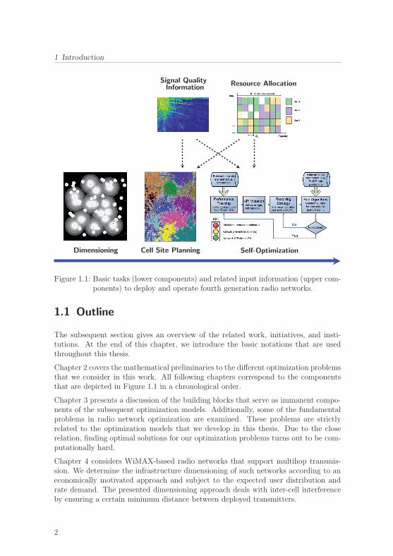
Figure 1.1 illustrates the related tasks that have to be carried out by the network ope-rator in a chronological order. First, the results from network dimensioning basicallyserve as input for business cases and strategic decisions. Second, cell site planning co-vers site selection and initial configuration of the network infrastructure that is actuallydeployed. Therefore, the optimization models for cell site planning have to be moreaccurate and more realistic than the ones that are utilized for network dimensioning.This requirement necessitates a greater level of detail in modeling interference-sensitiveresource allocation and computation of accurate signal quality information. Finally,self-optimization of the deployed network allows network equipment to adapt its ra-dio parameters autonomously, i.e., without any human intervention and without thecorresponding personnel expenses.
The work presented in this dissertation provides novel concepts, optimization models,and related building blocks for the dimensioning, the planning, and the self-organizedoperation of 4G radio networks. Concerning the latter two tasks, it particularly focuseson Heterogeneous Networks(HetNets) that implement a multi-tier cell topology.
Parts of this thesis have already been published in [35, 36, 37, 38, 39, 76] and [107].
1
1 Introduction
Dimensioning
1
2
3
4
5
6
7
89
10
11
12
Cell Site Planning Self-Optimization
Signal QualityInformation
Resource Allocation
Figure 1.1: Basic tasks (lower components) and related input information (upper com-ponents) to deploy and operate fourth generation radio networks.
1.1 Outline
The subsequent section gives an overview of the related work, initiatives, and insti-tutions. At the end of this chapter, we introduce the basic notations that are usedthroughout this thesis.
Chapter 2 covers the mathematical preliminaries to the different optimization problemsthat we consider in this work. All following chapters correspond to the componentsthat are depicted in Figure 1.1 in a chronological order.
Chapter 3 presents a discussion of the building blocks that serve as immanent compo-nents of the subsequent optimization models. Additionally, some of the fundamentalproblems in radio network optimization are examined. These problems are strictlyrelated to the optimization models that we develop in this thesis. Due to the closerelation, finding optimal solutions for our optimization problems turns out to be com-putationally hard.
Chapter 4 considers WiMAX-based radio networks that support multihop transmis-sion. We determine the infrastructure dimensioning of such networks according to aneconomically motivated approach and subject to the expected user distribution andrate demand. The presented dimensioning approach deals with inter-cell interferenceby ensuring a certain minimum distance between deployed transmitters.
2

1.2 Related Work, Initiatives, and Institutions
This simple method is not appropriate for the purpose of accurate cell site planning andconfiguration of LTE HetNets. Hence, in Chapter 5 we develop a low-complexity inter-ference approximation model that estimates the bandwidth requirements for macrocellsand femtocells subject to inter-cell and cross-tier interference.
For the optimal cell site planning of LTE HetNets in Chapter 6, we consider macro-cells and user-operated femtocells that are not necessarily active all the time. Theobjective of the corresponding optimization problem is to provide a minimum numberof macrocells such that mobile services are area-wide guaranteed. On the other hand,it avoids dispensable cell sites for the sake of cost efficiency and low interference.
Chapter 7 extends the HetNet deployment results from Chapter 6 and proposes amodel for joint coverage and capacity optimization. We present an integrated ap-proach for the self-optimization of coverage and capacity in the time-variant system.The corresponding algorithms are designed according to a traffic light principle. Theyautonomously control site activity, transmission power, and antenna downtilt param-eters in the operating HetNet.
Before this work is concluded in Chapter 9, Chapter 8 presents several conceptualextensions to the previous optimization problems. The conceptual extensions eitherprovide heuristics to lower the problem complexity or they address the incorporationof additional aspects into the network optimization domain, e.g., energy efficiency andintegration of user acceptance.
1.2 Related Work, Initiatives, and Institutions
Generally, the basic tasks and objectives for network planning and network operationhave not changed over the evolving generations from 2G (GSM) radio networks to 3G(UMTS, HSPA) and 4G (WiMAX, LTE, LTE Advanced) communication systems. Asa consequence, the basic principles, workflow descriptions, and optimization problems,e.g., discussed in [84, 101, 72, 103, 14, 45], are still relevant. The systems themselves,however, have changed substantially not only in terms of performance capability. Thebackbone architecture of networks has changed (E-UTRAN) as well as the supportedtransmission modes (coding, modulation), the multiple access technology (OFDMA),and the supported antenna techniques (MIMO, beamforming). Solid introductionsand detailed technical information on these topics are provided in [30, 29, 94, 50, 100].
Due to the changes in the underlying system technology, existing optimization modelshave to be adapted or have to be re-developed for each network generation. The typicalproblems for the planning and optimization of third generation Code Division Multi-ple Access (CDMA) networks are presented in [14]. One of the main challenges formaximizing coverage and capacity of 3G networks is coping with inter-cell and intra-cell interference by choosing suitable spreading code assignments and beneficial powerallocations. Since all assignment and allocation decisions at base stations are mu-tually interconnected, interference-sensitive optimization becomes a computationallyhard combinatorial problem. The same holds for OFDMA-based networks although
3
1 Introduction
the technical problem definition changes: Interference depends on the subcarrier as-signment and the power allocation on the subcarriers as interference coordination takesplace in the frequency domain. Related problems, optimization models, and compu-tationally efficient heuristics are presented, e.g., in [62, 66, 27].
Modeling and handling interference becomes even more complex with the integrationof multiple tiers into the network topology. A second tier refers, for instance, to re-lay stations in IEEE 802.16j networks (WiMAX) [83] or to pico-/femtocells in LTEadvanced systems (LTE HetNets) [29]. Co-channel deployment can cause cross-tierinterference if cells at different tiers use the same frequency spectrum. This cross-tierinterference is complex to handle due to the cell interdependencies and the requiredcommunication overhead [69]. Radio resource management and network planning for802.16j networks is investigated, for instance, in [80]. Concerning LTE HetNet deploy-ment and configuration, we refer to [81] and [67].
Radio Resource Management (RRM) and cell reconfiguration are resource-intensivetasks that have to be carried out with respect to dynamic changes in the network. Therequired resources are particularly related to computational complexity, time consump-tion, communication overhead, and man power. A popular paradigm to minimize suchaspects is the implementation of the network as a Self-Organizing Network (SON).The underlying principle of any SON is to delegate tasks from the Network Manage-ment System (NMS) to the network elements [85]. This feature enables autonomousSelf-Planning , Self-Optimization, and Self-Healing in a semi-decentralized or fully de-centralized manner, e.g., as proposed in [86, 75]. The strong interest in SON topics isreflected by the recent activities under guidance of the Next Generation Mobile Net-works alliance (NGMN) and the 3rd Generation Partnership Project (3GPP). WhileNGMN mainly provides economical and technical guidelines [77, 79], 3GPP is in chargeof the standardization of related network components, e.g., see [13, 7].
The 3GPP specifications for self-organized LTE HetNets are covered by different re-leases. LTE Release 8 contains the fundamental specifications for Home eNodeB(HeNB) components, self-establishment of network equipment, and automatic neigh-bor relation list management [6]. LTE Release 9 covers the specifications for enhan-ced HeNB functionality as well as studies on self-organization, self-healing, and self-organized coverage and capacity optimization [8]. In releases 10 and 11, 3GPP extendsthe specifications and SON use cases successively with respect to LTE Advanced sys-tems. These releases particularly emphasize the coordination between SON functio-nalities [29, 4, 5].
Several initiatives have been established to investigate and contribute to self-optimization and self-configuration in wireless communication networks [85]: As partof the Celtic Initiative [21], the Celtic GANDALF project contributed at a very earlystage to automated troubleshooting and automatic control of network parameters [22].The End-to-End Efficiency project, funded by the European Union within the 7thFramework Program, covers some SON related use cases such as handover optimiza-tion and inter-cell interference coordination [1]. The SOCRATES project was estab-lished within the same EU program. This project particularly addresses SON aspects
4

1.3 Notation
such as integrated handover parameter optimization and load balancing, automaticgeneration of initial insertion parameters, and cell outage management [96]. Further-more, several COST (European COoperation in Science and Technology) projects havecontributed to SON-related network modeling, network planning, and network opti-mization [41].
1.3 Notation
We use the basic notation listed in Table 1.1 throughout the rest of this work. Inthe subsequent chapters, the symbols and identifiers are extended with respect to theparticular context.
Symbol & domain Description
S, K, F Index sets of macrocell sites, relay stations, and femtocelltransmitters with representative indices s ∈ S, k ∈ K, f ∈ F .
T Index set of demand nodes utilized for modeling the trafficdistribution, representative index t ∈ T .
rt ∈ R≥0 Requested data rate at a demand node.
rMINt ∈ R≥0 Minimum required data rate if the demand node is served.
Bs, Bk, Bf ∈ R≥0Total available bandwidth at macrocells, relay stations, andfemtocells.
est, ekt, eft ∈ R≥0Supported spectral efficiency (signal quality indicator) frommacrocell transmitter, relay station, and femtocell transmit-ter to demand node t.
ys, yk, yf ∈ {0, 1} Binary decision variables indicating the selection of a (confi-gured) macrocell site, relay station, or femtocell transmitter.
zst, zkt, zft ∈ {0, 1}Binary decision variables indicating the assignment of de-mand node t to a certain macrocell site, relay station, orfemtocell transmitter.
zt ∈ {0, 1} Auxiliary variable indicating that demand node t is assignedto a transmitter.
bst, bkt, bft ∈ R≥0
Amount of allocated bandwidth for transmission from macro-cell transmitter, relay station, and femtocell transmitter todemand node t.
refft ∈ R≥0
Auxiliary variable describing the effectively served data rateat demand node t, depending on the particular signal qualityand bandwidth allocation.
Table 1.1: Basic symbols and identifiers – parameters (upper part) are separated fromvariables (lower part) by the dashed line.
5
1 Introduction
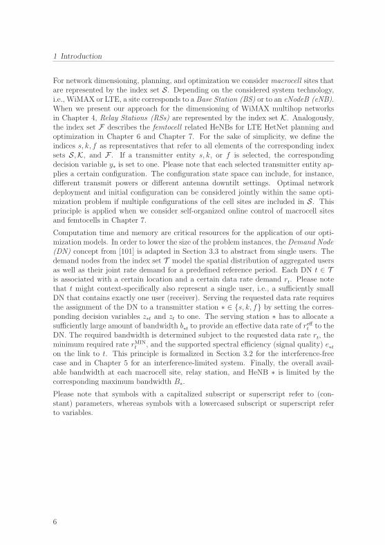
For network dimensioning, planning, and optimization we consider macrocell sites thatare represented by the index set S. Depending on the considered system technology,i.e., WiMAX or LTE, a site corresponds to a Base Station (BS) or to an eNodeB (eNB).When we present our approach for the dimensioning of WiMAX multihop networksin Chapter 4, Relay Stations (RSs) are represented by the index set K. Analogously,the index set F describes the femtocell related HeNBs for LTE HetNet planning andoptimization in Chapter 6 and Chapter 7. For the sake of simplicity, we define theindices s, k, f as representatives that refer to all elements of the corresponding indexsets S,K, and F . If a transmitter entity s, k, or f is selected, the correspondingdecision variable y∗ is set to one. Please note that each selected transmitter entity ap-plies a certain configuration. The configuration state space can include, for instance,different transmit powers or different antenna downtilt settings. Optimal networkdeployment and initial configuration can be considered jointly within the same opti-mization problem if multiple configurations of the cell sites are included in S. Thisprinciple is applied when we consider self-organized online control of macrocell sitesand femtocells in Chapter 7.
Computation time and memory are critical resources for the application of our opti-mization models. In order to lower the size of the problem instances, the Demand Node(DN) concept from [101] is adapted in Section 3.3 to abstract from single users. Thedemand nodes from the index set T model the spatial distribution of aggregated usersas well as their joint rate demand for a predefined reference period. Each DN t ∈ Tis associated with a certain location and a certain data rate demand rt. Please notethat t might context-specifically also represent a single user, i.e., a sufficiently smallDN that contains exactly one user (receiver). Serving the requested data rate requiresthe assignment of the DN to a transmitter station ∗ ∈ {s, k, f} by setting the corres-ponding decision variables z∗t and zt to one. The serving station ∗ has to allocate asufficiently large amount of bandwidth b∗t to provide an effective data rate of refft to theDN. The required bandwidth is determined subject to the requested data rate rt, theminimum required rate rMIN
t , and the supported spectral efficiency (signal quality) e∗ton the link to t. This principle is formalized in Section 3.2 for the interference-freecase and in Chapter 5 for an interference-limited system. Finally, the overall avail-able bandwidth at each macrocell site, relay station, and HeNB ∗ is limited by thecorresponding maximum bandwidth B∗.
Please note that symbols with a capitalized subscript or superscript refer to (con-stant) parameters, whereas symbols with a lowercased subscript or superscript referto variables.
6
2 Mathematical Preliminaries
Even though the subsequent chapters deal with various topics and applications, most ofthem have two conceptual aspects in common. First, the related optimization problemsare of multi-objective nature, i.e., we consider the joint optimization of multiple KeyPerformance Indices(KPIs). The corresponding single objectives can be contradictory.And second, we formalize the optimization models as linear programs that can alsocontain integer constraints. The basic concepts and aspects regarding those two pro-perties are introduced in the following.
2.1 Linear Programs
According to [18], a general optimization problem is defined as
min f0(x)
s.t. fi(x) ≤ 0 , i = 1, . . . ,m (2.1)
hj(x) = 0 , j = 1, . . . , p
with optimization variable x ∈ X n, inequality constraint functions fi : X n → R,equality constraint functions hj : X n → R, and objective function f0 : X n → R. If notdefined otherwise, we assume X = R≥0. The set of points for which the objective func-tion and all constraint functions are defined is called the domain D of the optimizationproblem. A point x ∈ D is feasible if it satisfies all constraints of problem (2.1). Theoptimal value or optimum of problem (2.1) is defined as
inf {f0(x) | fi(x) ≤ 0, i = 1, . . . ,m, hj(x) = 0, j = 1, . . . , p}
and a feasible point x∗ ∈ D for which the optimum is attained, is called optimal point .
If the objective function and all constraint functions are linear, problem (2.1) can bereformulated as
min cTx
s.t. aTi x ≤ bi , i = 1, . . . ,m (2.2)
for x ∈ X n, vectors c,a1, . . . ,am ∈ Rn, and scalars b1, . . . , bm ∈ R. The optimizationproblem (2.2) is called a Linear Program (LP). If the LP considers the p equalityconstraints from (2.1) its feasible points are in a subspace of D that is reduced by thedimension d = dim {x ∈ X n | hj(x) = 0, j = 1, . . . , p}.
7

2 Mathematical Preliminaries
Since linear programs are convex by definition, they can be solved by methods that arecomputationally efficient, at least in practice: The simplex method finds optimal pointsin a compact set by exploring the vertices of the polyhedron that describes the solutionspace. The polyhedron is defined by the constraints aT
i x = bi, i = 1, . . . ,m that followfrom the inequalities of (2.2) and the incorporation of corresponding slack variables [61,26]. There exist examples where the simplex method needs an exponential number ofoperations to find the optimum [59]. However, in practice the computational effortis of order n2m assuming that m ≥ n [18]. If the LP considers the (linear) equalityconstraints from (2.1), the computational effort is of order (n− d)2m for m ≥ (n− d).
Interior point methods are another prominent approach to solve LPs. The compu-tational effort of these methods is strictly bounded by O
(n3√n), i.e., interior point
methods have a polynomial complexity [108]. Moreover, the algorithms can performsignificantly better than this worst case upper bound for many practical problem in-stances. Interior point methods outperform the simplex algorithm on several problemclasses, e.g., on large degenerate problems with many zero entries in the solution vec-tor [43]. Most state-of-the-art LP solvers such as CPLEX [51] or Gurobi [48] supportboth solution approaches.
2.2 Integer and Mixed-Integer Linear Programs
The linear optimization problem (2.2) is called an Integer Linear Program (ILP) [61]if its optimization variables are subject to corresponding integrality constraints . Inthis case, we assume X = N. If only a proper subset of variables is restricted to theinteger domain, the resulting problem is called a Mixed-Integer linear Program (MIP).Both variants belong to the same problem class in terms of computational complexity.Thus, in the following we will not distinguish MIPs from ILPs.
Contrary to the problem class of LPs, solving ILPs is NP-hard [68]. The search space ofbinary ILPs (X = {0, 1}), for instance, grows exponentially with n. Therefore, solvingan ILP can become computationally intractable for large problem instances. It is oftenuseful to determine solutions by heuristics such as simulated annealing or tabu searchalgorithms [14]. For ILPs of a suitable size, however, the most common techniques tocompute optimal solutions are branch-and-bound and branch-and-cut algorithms [61,68]. The state-of-the-art LP solvers mentioned above solve ILPs and MIPs by applyingvariants of these algorithms. Moreover, they can introduce problem-specific cuttingplanes to simplify the solution space. Computing optimal ILP solutions can takehours or days even for reasonably sized problem instances and very sophisticated solverimplementations.
We refer to [25] for more details on integer programming and the related class ofcombinatorial optimization problems. This reference provides very useful information,and moreover, interesting facts about the people that have dominated this researchfield in the last 50 years.
8

2.3 Multi-Objective Optimization Problems
2.3 Multi-Objective Optimization Problems
A Multi-Objective Optimization (MOO) problem is defined as a general optimizationproblem according to (2.1) with v objective functions Fl : X n → R, see [18]. Thus,the function f0 : X n → Rv is vector-valued with
f0(x) = ((F1, . . . , Fv)(x))T .
MOO problems are linear if all objectives Fl and all constraint functions are linear. Inthat case, the definitions and properties from Section 2.2 hold for a proper selectionof X . Compared to an optimization problem (2.1) with a scalar-valued objectivefunction, it is not intuitive how optimal points are defined for an MMO problem.
Many relevant problems from radio network planning and optimization are MOO prob-lems. Typically, several decision criteria have to be considered jointly, e.g., coverage,capacity, and cost are considered as separate objectives Fl. The joint optimizationof multiple objectives can be a trade-off task if they are contradicting. For instance,maximization of coverage and capacity as well as maximization of coverage and min-imization of cost generally are trade-off tasks [105, 55]. In such a situation, it is aproblem to decide which solution should be preferred if several ones exist. In thefollowing, we formalize this problem and introduce three approaches to deal with it.
If x is a feasible point, the l-th objective Fl(x) may be interpreted as its score. Iftwo points x ∈ X n and y ∈ X n are both feasible, Fl(x) ≤ Fl(y) means that x is atleast as good as y with respect to the l-th objective; Fl(x) < Fl(y) means that x isbetter than y or x beats y on the l-th objective, respectively. If x and y are bothfeasible, x is better than y, i.e., x dominates y, if Fl(x) ≤ Fl(y) for all l = 1, . . . , vand Fu(x) < Fu(y) holds for at least one u. Roughly speaking, x is better than y if xmeets or beats y on all objectives and beats it on at least one objective. If there existsa non-dominated feasible point x∗ ∈ X n that is optimal for each scalar problem
min Fl(x)
s.t. fi(x) ≤ 0 , i = 1, . . . ,m
hj(x) = 0 , j = 1, . . . , p
with l = 1, . . . , v, x∗ is an optimal point. Such an optimal point does not exist formany MMO problems. Hence, the following definition is the more relevant one forMMO problems. Any Pareto optimal point or efficient point xPO ∈ X satisfies thefollowing condition: If y ∈ X is feasible and Fl(y) ≤ Fl(x
PO) for l = 1, . . . , v then itholds Fl(x
PO) = Fl(y) for all l = 1, . . . , v. This means that it is impossible to improveone score of a Pareto optimal point without decreasing another one. Particularly,it holds that if a feasible point is not Pareto optimal there exists at least one otherfeasible point that is better. In consequence, Pareto optimal points are well suitedcandidates for finding beneficial solutions for MOO problems.
9

2 Mathematical Preliminaries
max
max
capa
city
(x)
coverage(x)(a) The convex hull (dashed line) of Pareto op-timal points (cross or asterisk) defines the set ofsupported efficient points (crosses).
max
max
capa
city
(x)
coverage(x)(b) The scalarization approach can find the sup-ported Pareto optimal points (crosses) of thePareto front if (λCOV, λCAP) > 0.
Figure 2.1: An exemplary two-objective optimization problem.
2.3.1 Pareto Front Exploration and the Scalarization Approach
Figure 2.1 (a) illustrates the set of Pareto optimal points for a discrete multi-objectivemaximization problem that considers coverage and capacity as conflicting objectives.Coverage can be interpreted as the area where users experience a minimum receivedsignal power, whereas capacity might describe the maximum cell edge throughput.
Each objective is assumed to be a function of the optimization variable x ∈ D,which contains integer components. Furthermore, the achievable objective values arebounded by a power constraint. The image of the set of Pareto optimal points formsthe optimal trade-off surface or so-called Pareto front . Its shape describes the trade-offcharacteristic between the objectives.
Exploring the points of the Pareto front is an intuitive approach to find a beneficialsolution for joint coverage and capacity maximization – and for joint MOO in general.From the set of explored Pareto optimal points, we choose the one that is best suitedin terms of a certain decision criterion. Exploring all Pareto optimal points, however,is computationally hard since there usually exist exponentially many points [57, 63].Thus, computing the Pareto front requires the application of sophisticated methodsand algorithms. In [109], the Pareto front is approximated by genetic algorithmsand [24, 87] consider particle swarm optimization for this purpose.
Even if we are able to compute a set of Pareto optimal points, the following problemarises as soon as the set contains more than one element: If each Pareto optimal pointbeats the other ones on at least one objective, which point gives the best solution?One way to cope with this dilemma is to make use of the scalarization approach andits properties, which are discussed in [34].
10

2.3 Multi-Objective Optimization Problems
Basically, the scalarization of an MOO problem is obtained by combining the multipleobjectives of f0(x) into a single weighted sum objective
λT ((F1, . . . , Fv)(x)) =v∑
l=1
λlFl(x) . (2.3)
The factor λl can be interpreted as the weight attached to the l-th objective or asthe importance of making Fl small. The ratio λi/λj is the relative weight or relativeimportance of the i-th objective compared to the j-th objective. Alternatively, λi/λj
might be interpreted as exchange rate between the two objectives. Solving the MOOproblem for the weighted sum objective (2.3) has the same computational complexityas solving a scalar-valued optimization problem.
For λ > 0, any optimal solution of the MOO problem with objective (2.3) is Paretooptimal [18, 34]. As illustrated in Figure 2.1 (b), the weight vector λ gives the normalof the tangential hyperplane at the associated Pareto optimal point(s). Please notethat Pareto optimal points in the interior of the convex hull (gray area) cannot be foundby the scalarization approach. Therefore, they are called unsupported efficient points.In Figure 2.1, unsupported efficient points are depicted as an asterisk. Furthermore,it holds that:
1. A supported Pareto optimal point can have several tangential hyperplanes if theconvex hull is not smooth, i.e., if it is not (multidimensionally) continuously diffe-rentiable. In this case such a point can be found by the scalarization approachfor different weight vectors λ.
2. If the scalarization approach finds multiple supported efficient points for a certainweight vector λ, the value of the corresponding weighted sum objective is thesame for all points. However, the single components of the efficient points candiffer significantly, e.g., see the encircled points in Figure 2.1 (b).
Both properties are particularly relevant for integer MOO problems, where the con-vex hull of the discrete – and in most cases non-dense – set of Pareto optimal pointsusually is not smooth. If the weights λl are chosen with respect to a certain inten-tion, e.g., to obtain a solution with balanced objectives, those properties can lead tosolutions that do not match with this intention at all. Figure 2.1 (b) illustrates sucha situation where the weights are chosen equally but the two resulting efficient points(encircled) mutually differ in one objective component. Nevertheless, the particularsetting of λl generally influences the balance of the objectives that are obtained formultiple instances of the MOO problem.
In the ideal case, the exchange rates between the objectives are unambiguously. Thenthe MMO problem reduces to a scalar-valued optimization problem, which can besolved by the conventional methods that were discussed in Sections 2.1 and 2.2.
11

2 Mathematical Preliminaries
2.3.2 Constrained Single Target Optimization
An alternative but very simple approach is to solve the MMO problem in a hierarchi-cal fashion [105]. Basically, this is done by considering a scalar-valued optimizationproblem for one of the objectives Fl(x). After an optimal solution has been computed,the achieved objective value defines an upper bound for Fl(x) when the procedureis repeated for another objective Fl′(x), l
′ �= l. The upper bound on Fl(x) is imple-mented by an additional (maximum) constraint. The solutions that are obtained bythis approach strictly depend on the order of the single optimization tasks, i.e, theydepend on the predefined hierarchy of objectives. In consequence, the application ofthis method makes only sense if the considered hierarchy is reasonably defined.
12

3 Building Blocks for Radio NetworkOptimization
This chapter introduces the building blocks for the optimization of 4G radio networksat different stages of the system lifecycle. In particular, it provides the detailed defini-tion of models for radio wave propagation prediction, channel models, and methods todescribe user mobility and demand in a computationally efficient way. Furthermore,we discuss some of the fundamental problems in radio network optimization. The dis-cussed problems are closely related to the optimization models that we develop in thesubsequent chapters.
Parts of this chapter have already been published in [37, 76].
3.1 Radio Wave Propagation Models
Signal strength and Channel State Information (CSI) provide essential input informa-tion for any approach that considers planning and control of radio networks. Theyare important for all applications that deal with time-variant user positions, e.g., lo-calization and location tracking. Basically, the information is used to describe thewireless channel characteristic that might vary over time and the spatial domain. Ex-act methods like channel measuring or estimation of the channel impulse responseare very resource consuming and usually not practicable to obtain area-wide informa-tion. Therefore, sophisticated models have been developed in order to provide highlyaccurate approximations.
In the following, we neglect the signal phase information, which is justified by the long-term perspective of the subsequent applications. The amplitude of a received signal isdetermined by the emitted signal power and the physical effects that the signal experi-ences on its path from the transmitter to the receiver. A radio wave propagation modeltypically describes the effects on the signal path either in an empirical (stochastic) orin a semi-empirical way, where the latter one incorporates deterministic components.We refer to [88] for a comprehensive introduction to the basic principles of radio wavepropagation modeling. Particularly, the document provides a good overview of somepopular models like the Hata model and the COST-231-Walfisch-Ikegami model. Itserves as root reference for the following definitions and descriptions.
13
3 Building Blocks for Radio Network Optimization
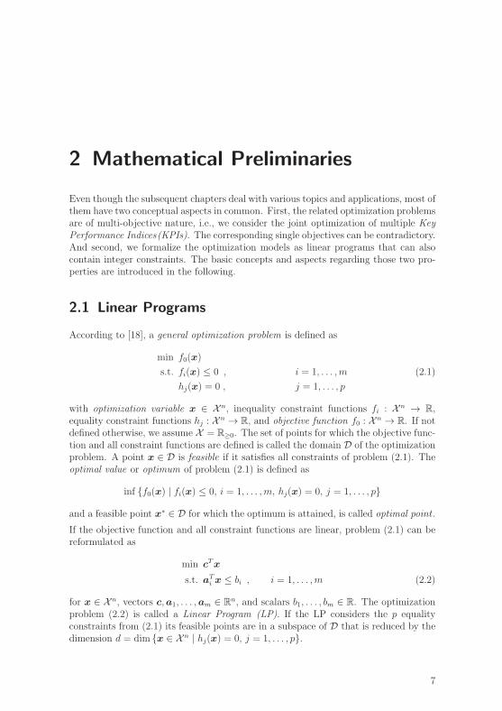
The path loss information L(t) is the relevant output of a radio wave propagationmodel. The pass loss describes the average attenuation of the emitted signal power Pon its path to the receiver point t, i.e.,
L(t) =P
Pt
and LdB(t) = 10 log10P
Pt
, (3.1)
where Pt is the received signal power at t. According to [42], the effective path loss isa superposition of three essential components, namely
1. a distance-dependent basic path loss L0(t),
2. the slow fading (shadowing) effects modeled by a random variable Gslow, and
3. the fast fading effects modeled by a random variable Gfast.
With respect to the distance d(t) between transmitter and receiver point t, thedistance-dependent basic path loss is often assumed as the Line-of-Sight (LoS) orfree-space path loss component, i.e.,
L0(t) =(4π)2(d(t))γ
λ2fcGA(φ(t), ψ(t))
for signal wavelength λfc at carrier (center) frequency fc, the antennagain GA(φ(t), ψ(t)), and the free-space path loss exponent γ = 2. On a logarith-mic scale this is
LdB0 (t) = 20 log10
4π
λfc− 10 log10GA(φ(t), ψ(t)) + γ10 log10 d(t) . (3.2)
Non-Line-of-Sight (NLoS) situations are modeled by a larger path loss exponent,which can increase up to a value of five for urban environments. The antennagain GA(φ(t), ψ(t)) is given by an antenna-specific pattern according to Figure 3.1.It considers the transmitter in the center position and t in direction (φ(t), ψ(t)) inspherical coordinates. The gain of beamforming-generated antenna patterns can beapproximated by an equivalent representation. Please note that we do not consideran antenna gain at the receiver side for path loss computation and that (3.2) is onlyfeasible for far-field considerations, i.e., for d(t) 0.
Finally, the effective (overall) path loss is described as
L(t) = L0(t)GfastGslow or LdB(t) = LdB0 (t) + 10 log10Gfast + 10 log10Gslow . (3.3)
The fading components model the signal variation over time for moving receivers intime-variant channel simulations. Fast fading results from multipath propagation ofthe signal due to physical reflection and scattering effects. It is typically modeled by aRayleigh distributed random variable Gfast for LoS scenarios and as Ricean distributedrandom variable for the NLoS case. Fast fading influences the signal on a very smalltime scale. Slow fading effects take place on a much larger time scale since they arecaused by the shadowing impact of large obstacles such as buildings or hills.
14

3.1 Radio Wave Propagation Models
25
50
30
210
60
240
90
270
120
300
150
330
180 0
25
50
30
210
60
240
90
270
120
300
150
330
180 0
Figure 3.1: Exemplary antenna pattern from [58]: elevation and azimuth diagrams.
The shadowing-related variation of the signal magnitude in dB can be modeled suit-ably by a log-normal distributed random variable Gslow. We consider the time-invariantchannel since tasks like network dimensioning and cell site planning are carried outwith respect to the long-term characteristic of the channel. Fading effects are incorpo-rated into the system model as a constant term that reflects either the average fadingsituation or the worst case fading situation. Therefore, in the following we concentrateon alternative models for the basic path loss LdB
0 (t).
A widely used representation for measurement calibrated path loss models is
LdB(t) = Δ0 + 20 log104π
λfc+ γ10 log10 d(t) + LdB
effects(t) , (3.4)
where Δ0 serves as offset constant in a least-squares regression fitting [40] and coversthe antenna gain, potential measurement inaccuracies, and shadowing related effects.Some path loss models exploit further knowledge of certain physical conditions suchas antenna height, terrain type, or building information and extend the model bya related term LdB
effects(t) �= 0. Consequently, path loss models differ in the particularterm LdB
effects(t) as well as in the according model parameters that are typically estimatedfrom different measurements.
In the following, we discuss some prominent empirical and semi-empirical path lossmodels. Furthermore, in Section 3.1.3 we develop a direction-specific path loss modelthat combines principles from empirical and ray optical path loss computation.
3.1.1 Semi-Empirical Path Loss Models
The Hata model – a variant of the well-known Okumura model [88] for carrier frequen-cies above 1.5GHz – is intended for computing the path loss in large cells of 1 − 20km. The COST-231-Walfisch-Ikegami model considers cell radii in the range of 20mto 5 km and is, therefore, a suitable choice for path loss computation in femtocells andpicocells. Both models consider the antenna height and the reference height of thereceiver in the term LdB
effects(t). Additionally, they apply a constant penetration termthat is chosen with respect to the particular environment. For instance the Hata model
15

3 Building Blocks for Radio Network Optimization
Model parameter
Terrain type
A B C
hilly hilly or plain plain
heavily forested lightly or moderately forested lightly forested
a 4.6 4.0 3.6
b 0.0075 0.0065 0.0050
c 12.6 17.1 20.0
Table 3.1: Terrain-specific parameters for the Erceg model.
adds a penetration constant of 3 dB for metropolitan areas. Both models serve as keycomponents for system simulations in the SOCRATES project [95] when algorithmsfor self-organized LTE HetNets are assessed.
Distinguishing 13 different propagation environments, the WINNER II project groupprovides parameter sets for more than 20 semi-empirical path loss models. All thosemodels were developed on basis of extensive measurement (channel sounding) cam-paigns [53]. Some of the models consider indoor propagation, which is modeled bypenetration terms LdB
effects(t) that depend on the number of floors and the number ofwalls between the transmitter and the receiver. From indoor office over indoor-to-outdoor to bad urban macrocell and rural macrocell environments, almost all modelsdistinguish LoS from NLoS situations. They apply distance-dependent parameter setsthat are defined either by an absolute distance range or relatively with respect to theantenna height. If the particular environment is unknown, the LoS/NLoS-sensitivepath loss models provide scenario-specific approximations for the LoS probability.The LoS probability decreases exponentially with the distance of the receiver point.The main intention of the WINNER initiative was to develop channel models fortime-variant MIMO systems. Thus, the provided path loss models are combined withenvironment-specific fading models and both serve as key components of sophisticatedMIMO channel models. We discuss some of the channel models in Section 3.2. Manyrecent works that deal with LTE systems utilizes the WINNER path loss models, theWINNER channel models, or variants of it.
The Erceg path loss model is very popular for radio wave propagation in suburban orrural areas since it distinguishes the terrain type between transmitter and receiver [40].Neglecting the shadowing component, the Erceg model is defined by (3.4) for apply-ing LdB
effects(t) = 0, the path loss exponent
γ = (a− b hA + c/hA)
for an antenna (transmitter) height hA, 10 ≤ hA ≤ 80 [m], and parameters a, b, c thatare chosen from Table 3.1 according to the predominant terrain type. The Erceg modelimproves the prediction accuracy for the designated application scenarios compared toapproaches that do not consider the terrain type. However, it is restricted to the choiceof one (predominant) terrain category. Hence, all receiver points at the same distance
16
3.1 Radio Wave Propagation Models
t
t
1
d2
3: Forest2: Village1: Free space
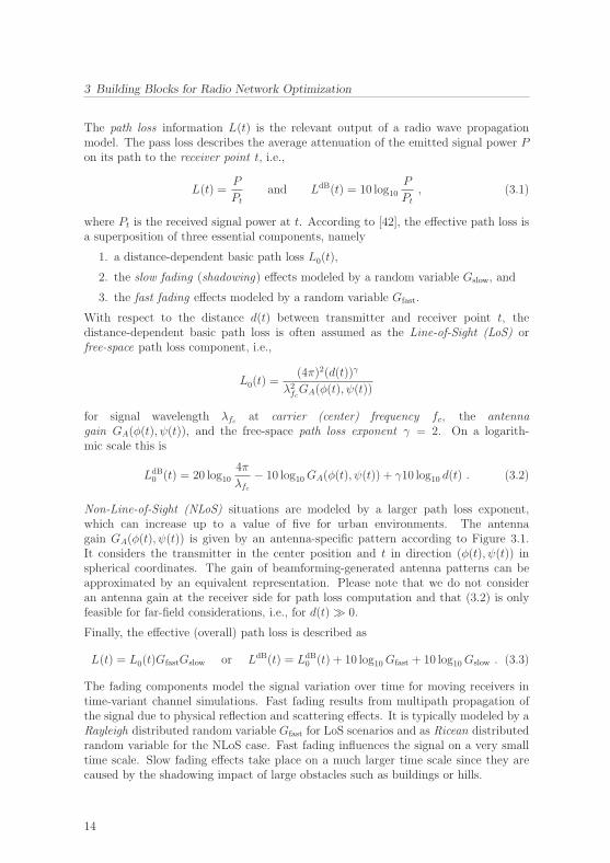
Figure 3.2: In the Erceg model, receivers t1 and t2 experience equal path losses due tothe same distance d and the same predominant terrain type.
from the transmitter gain identical path losses if their predominant terrain type isthe same. This can lead to inaccuracies and inconsistent results in some situations,see Figure 3.2. In Section 3.1.3, we propose a semi-empirical path loss model thatovercomes this drawback. Since our model utilizes concepts from ray optical path losscomputation, we first introduce the principles of ray optical algorithms.
3.1.2 Ray Optical Path Loss Models
Ray optical models improve the path loss prediction accuracy by incorporatingenvironment-specific effect terms LdB
effects(t) in (3.4) in a deterministic manner. Thisapproach is very resource consuming in terms of computational complexity, runtime,and expenses for providing the related input data. Therefore, ray optical path losscomputation is usually only applied for purposes that necessarily require the supportedlevel of accuracy. For instance, network dimensioning – as discussed in Chapter 4 –is typically carried out using non-deterministic and low-cost path loss models accord-ing to Section 3.1.1. On the other hand, cell site planning and site configuration inurban environments prerequisite very detailed information about the radio conditionsin the corresponding area. Therefore, the following approach is utilized for path losscomputation in the Chapters 6 and 7.
The basic principle of ray optical path loss prediction is to identify the signal prop-agation paths between the transmitter and the receiver point t as a set of rays. Aray is defined as a sequence of straight lines through the scene, which are connectedby effect-related deflection points. The buildings in an urban environment are de-scribed as polyhedrons that are given by the buildings’ surface sections (facets). In
17

3 Building Blocks for Radio Network Optimization
1.
2.
3.
4.
Y
(a) Physical effects. (b) Reflection. (c) Horizontal diffrac-tion (edge).
(d) Vertical diffrac-tion (roof).
Figure 3.3: Visualization of the modeled physical effects on launched rays.
the widely used 2.5D data format, the building heights are specified but roof shapesare not considered.
Basically, two different classes of ray optical models are distinguished. In ray tracingmodels , the tracking of possible propagation paths starts at the receiver point andproceeds towards the transmitter. The set of possible propagation paths is limited bythe maximum number of deflection points , i.e., points at facets where deflection effectsoccur. If the path loss is computed for multiple receiver points, it requires a highcomputational effort to determine all relevant deflection points for each receiver. Forreceiver points that are located nearby, however, the corresponding propagation pathsare nearly identical. In such situations – or if the receiver locations are dynamic or notknown in advance – it is more efficient to apply the following principle: Complementaryto the ray tracing method, ray launching algorithms emit a finite set of rays from thetransmitter in predetermined directions. They track the deflection points at facets andthe physical effects on the paths through the scene. Each point that is reached by atleast one path can be considered as receiver point. As the emitted rays disperse due tophysical effects such as diffraction, important deflection points or even some relevantreceiver points may not be reached. Therefore, the density of emitted rays has to behigh enough to avoid that effect. Since a higher ray density increases the requiredcomputational effort, the multiplication of rays at deflection points is proposed in [89]to keep the overall number of rays low.
The ray launching method from [73, 90] is applied to generate the input informationfor the planning and control methods presented in Chapters 6 and 7. The basic idea ofthe underlying Cube Oriented Ray Launching Algorithm (CORLA) is to rasterize theconsidered urban environment into suitably and equally sized cubes. Physical effectsat a cube are tracked if the cube belongs to a facet, see Figure 3.3 (a). The followingdeflection effects are distinguished: Reflection (R) at a facet surface, horizontal diffrac-tion (H) at a facet edge, and vertical diffraction (V ) due to deflection at rooftop edges.Diffraction effects cause the emission of a new bundle of rays into the diffraction cone,whereas reflection effects just change the angle of the arriving ray. Due to the diffrac-
18

3.1 Radio Wave Propagation Models
tion effects and the multiple rays that are emitted at the transmitter, a receiver point tmight be reached by a set of different paths Pt. The effect-related path loss on eachpath p ∈ Pt depends on the number of associated deflection points nR(p), nH(p), nV (p)and the signal penetration at each deflection point i with angular change φi.
If the penetration terms are described as polynomials of degree K in φi, the effectrelated attenuation on the path p is given as
LdBCORLA(p) =
nR(p)∑i=1
K∑j=0
wR, jφjR,i +
nH(p)∑i=1
K∑j=0
wH, jφjH,i +
nV (p)∑i=1
K∑j=0
wV, jφjV,i , (3.5)
where wR, j, wH, j, wV, j, j = 0, . . . , K, are the polynomial coefficients that have to becalibrated in advance by a measurement based parameter estimation. As illustratedin Figure 3.3 (b) - (d), each considered effect has its own path loss characteristic, andparticularly, the vertical diffraction is influenced by the height of the buildings. Thesuperposition of all effects provides a highly accurate description of the radio conditionsat receiver points. Please note that rays are not longer tracked from the deflection pointon, where the overall attenuation on the path exceeds a certain (maximum) threshold.
According to [102], it is a reasonable approximation to consider only the strongestpath that exists between transmitter and receiver, i.e., the signal path with the lowestpath loss. With respect to this approximation and (3.5), the distance-dependent termsin (3.4) are replaced by
γ10 log10 d(t) + LdBeffects(t) = min
p∈Pt
{γ10 log10 d(p) + LdB
CORLA(p)},
where d(p) denotes the length of the path to receiver point t. This approximation is notsuitable for channel models that consider the signal phase information, e.g., MIMOchannel models, since it neglects multipath propagation. We refer to the approachpresented in [91] if multipath propagation is a required feature.
3.1.3 A Direction-Specific Land Use Based Path Loss Model
In [37], we develop a Direction-specific Land use based Path loss model (DiLaP) thatcombines principles from empirical and ray optical path loss computation. The com-bination counteracts the inaccuracies that can arise for the models from Section 3.1.1due to the missing diversification on the propagation path, see Figure 3.2. Our modelis intended for application to suburban/rural areas. It improves related path loss mod-els such as the Erceg model from Section 3.1.1 by considering all land use segments –with different sizes and attenuation properties – that are passed by a straight ray fromthe receiver to the transmitter. The underlying principle of our model is that landuse segments nearby the receiver have a strong influence on the path loss, whereas theimpact of segments far away is reduced.
The set C contains all land use classes that we distinguish for path loss computation.In the following, we consider C = {1 (free space), 2 (village), 3 (forest)} as illustrated
19

3 Building Blocks for Radio Network Optimization
Propagation
Evaluation
Segment: 3 2 1
c(2)c(3) = c(1)d(3)
c(1)d(1)d(2)
(a) Path evaluation principle.
t
t
1
d2
(b) Path loss prediction according to DiLaP.
Figure 3.4: DiLaP computation for the area depicted in Figure 3.2.
in Figure 3.2. The set of land use classes is generally not limited to those three butthis choice leads to good results for the investigated scenarios. In [76], we propose anapproach to extract the required land use information from low-cost satellite picturesby applying dedicated classification algorithms.
Before the DiLaP computation is carried out, we first determine the i = 1, . . . , n(t)different land use segments that are intersected by the direct path from receiver t tothe transmitter. Each segment i has a corresponding length (sub-distance) d(i) > 0and the land use class c(i). Figure 3.4 (a) sketches this information exemplarily forthe receiver t2 from Figure 3.2.
The segment information is evaluated by
LdBDiLaP(t) =Δ0 + 20 log10
4π
λfc+ γc(1) 10 log10 (d(1))
+
n(t)∑i=2
[γc(i) 10 log10
(i∑
j=1
d(j)
)− γc(i) 10 log10
(i−1∑j=1
d(j)
)], (3.6)
where the parameters Δ0, λfc are defined according to (3.2). Each land use class c ∈ Ccorresponds to an individual path loss coefficient γc ∈ {γ1, γ2, γ3}. The coefficientsare predetermined by a parameter estimation (calibration) for the considered evalua-tion scenario. Figure 3.4 (a) illustrates the principle behind formula (3.6). It showsparticularly the logical evaluation direction that is reversely aligned to the physicalpropagation direction: The path loss at the receiver is modeled as additive superpo-sition of the segment path losses in between. For instance, the path loss contributionof segment 2 in Figure 3.4 (a) is calculated as the path loss with respect to the cor-responding land use class c(2) and distance d(1) + d(2) to the receiver. The obtained
20

3.1 Radio Wave Propagation Models
0 1000 2000 3000 4000 5000 6000 700060
70
80
90
100
110
120
130
140
150
Distance from transmitter [m]
Pat
h lo
ss [d
B]
Free SpaceVillageForestDiLaP
Figure 3.5: DiLaP characteristics for a straight path of increasing distance.
result is then adapted by subtracting the land use specific influence of the antecedentsegment 1. The subtraction considers the land use class c(2) but distance d(1). Con-sequently, the impact of segment 2 on the overall path loss depends on its land usetype and length, but particularly it depends on its distance to the receiver. Hence, theimpact of segments that are located far away from the receiver is significantly smallerthan the impact of segments nearby. This effect becomes clear when (3.6) is rewrittenas
LdBDiLaP(t) = Δ0+20 log10
4π
λfc+γc(1) 10 log10 (d(1))+
n(r)∑i=2
γc(i) 10 log10
(1 +
d(i)∑i−1j=1 d(j)
).
Furthermore, it is illustrated by Figure 3.5 where LdBDiLaP(t) is computed successively
for all points t on one ray that starts at the transmitter:
• The path loss according to DiLaP is upper bounded by the distance-dependentpath loss for the land use class forest that has the largest path loss exponent. Itis lower bounded by the free-space path loss with path loss exponent γ1 = 2, seeTable 3.2.
• Since the segment nearby the receiver point has the highest impact to the effectivepath loss at t, the path loss can decrease although the distance is increasing.This effect occurs in segments that cause a lower path loss than the antecedentsegment on the path, e.g., in transition areas from village to free-space or fromforest to village.
• The DiLaP results are asymptotic for an increasing segment length d(i).
21
3 Building Blocks for Radio Network Optimization
Evaluation
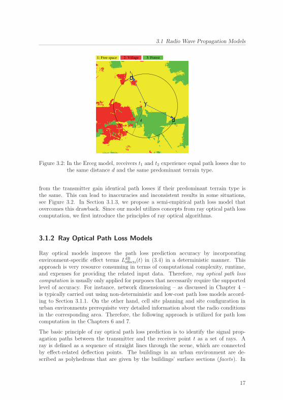
Our DiLaP approach is evaluated with respect to measurement data from a WiMAXmeasurement campaign in Regensburg, Germany. After computing the required inputinformation by automatic land use classification of the corresponding satellite image,the DiLaP parameters are calibrated by a least-squares regression fit on a subset ofmeasurements points. The obtained model parameters are shown in the upper leftpart of Table 3.2. Figure 3.4 (b) visualizes the path loss prediction results for the areafrom Figure 3.2 and a resolution of 6.25m2 per pixel.
Approach DiLaP Erceg model
Model ParameterΔ0 = 3.2, γ1 = 2.0 Terrain type C
γ2 = 2.2, γ3 = 2.3 hA = 10m
MSE [dB] 4.97 6.86
Table 3.2: Model parameters and evaluation results.
The DiLaP approach is compared to the Erceg model from Section 3.1.1 on a set ofmeasurement points that are distinct from the ones that were used for DiLaP calibra-tion. For the Erceg model, we choose the terrain type that leads to the best resultsin terms of the Mean-Squared Error (MSE) achieved on the evaluation points. Eventhough DiLaP does not exploit any additional information like antenna height, Ta-ble 3.2 shows that it beats the Erceg path loss model in terms of prediction accuracy.The smart direction-specific evaluation principle enables DiLaP to reflect the path losscharacteristics of the underlying measuring track more precisely than the Erceg model.This property is illustrated in Figure 3.6. The improved accuracy of DiLaP comes atthe cost of an increased computational complexity, mainly caused by the successivesuperposition of segment-wise processing. In [37], we discuss how the DiLaP runtimecan be reduced by implementing the model on a parallel computer architecture.
Overall, the evaluation results demonstrate excellent path loss accuracy of our DiLaPapproach and its advantages over the Erceg model. Since the path loss computationfor single segments is very simple, this component might be enhanced by using moresophisticated semi-empirical models, e.g., the WINNER path loss models mentionedin Section 3.1.1.
3.2 Wireless Channel Models, Rate Computation, andBandwidth Allocation
The level of detail that channel models have to provide depends on the particularapplication. If wireless networks are optimized with respect to a long-term perspec-tive, the channel information is not required at a time scale of milliseconds, seconds,or even minutes. Hence, short-term effects like fast fading are irrelevant for tasks
22

3.2 Wireless Channel Models, Rate Computation, and Bandwidth Allocation
0 50 100 150 200 250 300 350 400 450�135
�130
�125
�120
�115
Measurement points
Pat
h g
ain
[dB
]
ErcegDiLaPMeasurement
Figure 3.6: Comparison of DiLaP and the Erceg model on a measurement track.
like network dimensioning or cell site planning. They can optionally be included bya constant penalty term that serves as buffer for worst case situations. On the otherhand, applications such as receiver design and dynamic system simulation require ahigh temporal resolution of the channel information, most likely at realtime. For thispurpose, the WINNER project invented several extensions to the path loss models thatwere discussed in Section 3.1.1. The extensions incorporate scenario-specific (stochas-tic) components for fast fading and spatial components that enable MIMO channelmodeling: The Spatial Channel Model (SCM), its extension SCME (for higher carrierfrequencies and transmission bandwidth), and the WINNER I and II models are state-of-the-art MIMO channel models that are widely used for LTE system simulations [74].All WINNER channel models refer only to a small set of representative environmentclasses. Particularly, they are not able to consider the details of a given environment,e.g., buildings or other de facto obstacles on the signal paths. This is the motiva-tion in [107] and [92] to combine the WINNER channel models and the ray launchingmethod from Section 3.1.2 in order to obtain an environment-specific channel charac-teristic. Another recent approach that follows a similar idea is the QuaDRiGa channelmodel, which is (partly) presented in [54].
The computed channel state information and the emitted transmit power P are inputfor the following approach that determines the supported spectral efficiency (signalquality) e∗t on the link from transmitter entity ∗ ∈ {s, k, f} to user or demand node t,see Section 1.3. The corresponding results serve as input parameters for the optimiza-tion models that are proposed in the subsequent chapters.
The transmitter entities in WiMAX and LTE systems apply adaptive modulation andcoding subject to the present link channel state and a maximum bound for the Bit ErrorRate (BER) or BLock Error Rate (BLER). Hence, the supported data rate dependson the Signal-to-Interference and Noise Ratio (SINR). The LTE system specificationdistinguishes 16 Channel Quality Indicators (CQIs) [30]. Each CQI corresponds toa supported modulation scheme and code rate for downlink transmission, i.e., the
23

3 Building Blocks for Radio Network Optimization
downlink spectral efficiency eCQI i can be computed in terms of bits per second perHertz for each CQI i. The smallest non-zero spectral efficiency in present LTE systemsis eCQI 1 = 0.25 [bps/Hz] for QPSK and code rate 1/8. The largest spectral efficiencyis eCQI 15 = 4.8 [bps/Hz] for 64-QAM and code rate 4/5, both for a fixed BLER of 10−1.Please note that the practically achieved spectral efficiency can slightly differ from thetheoretical values due to a higher resolution in the supported code rates. Since the defacto values do not affect the presented optimization models, we keep the theoreticalvalues for all numerical evaluations.
The system link budget defines what SINR is required to support a certain CQI suchthat the receiver can decode the data with a transport block error probability below10% [10]. The according receiver sensitivity model typically considers thermal noise(−174 dBm/Hz) multiplied by the transmission bandwidth, the receiver noise figure(9 dB), an implementation margin (2.5 dB for QPSK, 3 dB for 16-QAM, and 4 dB for64-QAM), and a diversity gain (−3 dB), see [94]. Additional Quality-of-Service (QoS)requirements can be modeled by modifying the link budget specification accordingly.Frequency-specific adaption of modulation and code rate is not supported in presentlydeployed system releases (8 and 9) because it does not improve the system throughputin absence of frequency-specific transmission power control [94]. The WiMAX systemspecification defines the system link budget in a comparable manner but distinguishesonly seven transmission modes with non-zero spectral efficiency. The supported modesstart with 0.25 [bps/Hz] for BPSK and code rate 1/2 and end with 4.5 [bps/Hz] for64-QAM and code rate 3/4 [44].
We consider a link from transmitter ∗ ∈ {s, k, f} to user or demand node t without in-terference from other transmissions. In this case, we can select the highest CQI that issupported by the Signal-to-Noise Ratio (SNR) on the link and the SINR requirementsfrom the system link budget. The parameter e∗t is set to the corresponding spectralefficiency of the chosen CQI. Thus, each spectral efficiency parameter is generated withrespect to the applied path loss model and according to a predefined CQI lookup table.
In our optimization models, the link quality information is used to compute the averageamount of bandwidth b∗t that the serving station ∗ has to allocate for transmission todemand node t. For a requested data rate rt, the required bandwidth for downlinktransmission is given by
b∗t =rte∗t
(3.7)
when the location and spacing restrictions for resources in the spectrum are neglected.The sum of required bandwidth over different transmission links is always computedoverlap-free. According to (3.7), we model the allocated bandwidth b∗t as a continuousvariable although the smallest resource units that can be assigned in the consideredsystems have a certain minimum spacing: The smallest allocatable resource unit inWiMAX systems is a SubCarrier (SC). SCs have a fixed spacing for each supportedsystem bandwidth, e.g., 10.94 kHz for a total transmission bandwidth of 20MHz [16].The resource allocation in LTE systems considers a Physical Resource Block (PRB)as the smallest allocatable unit. Each PRB comprises 12 consecutive SCs of 15 kHzspacing, i.e., a PRB has a total spacing of 180 kHz [94]. Resource scheduling basically
24

3.2 Wireless Channel Models, Rate Computation, and Bandwidth Allocation
allows for multiple usage of a PRB over time along different UEs. This feature isexploited in Section 7.1.1 to slice a PRB virtually into single SCs.
The total amount of resources that is required to serve the typical rate demand perlink is relatively high compared to the fixed resource spacing. Therefore, clippingeffects are reasonably low and we can accurately model the allocated bandwidth by acontinuous variable. If the impact of clipping effects is expected to be larger, this canbe modeled by an (artificially) increased rate demand, e.g., according to the robustnessapproach that is discussed in Section 8.3.
For a resource unit n with fixed bandwidth spacing bn, the CQI lookup table can serveas discrete rate-power function
R (t, n, Pn) =
⎧⎪⎪⎪⎪⎨⎪⎪⎪⎪⎩0 , Pn < PCQI 1
t,n
bneCQI 1 , PCQI 1
t,n ≤ Pn < PCQI 2t,n
bneCQI 2 , PCQI 2
t,n ≤ Pn < PCQI 3t,n
...
, (3.8)
where each power requirement is computed subject to the system link budget and thepath loss dependent channel gain that t experiences on the resource unit n.
If the bandwidth allocation or the rate-power function are computed with respect topotentially interfered resources, there are basically three options to deal with it:
1. Apply (3.7) or (3.8) as above and ensure the interference-free case. This canbe achieved by deploying transmitters far away from each other such that thereis only marginal or no inter-cell interference. Please note that Intra-cell inter-ference is avoided in 4G systems by the underlying OFDMA multiplexing. Weapply this approach for network dimensioning in Chapter 4.
2. Compute the spectral efficiency subject to the SINR information for the re-lated link and apply (3.7) or (3.8). SINR computation requires a full user-to-transmitter assignment and the application of dedicated bandwidth allocationalgorithms. We avoid this approach for cell site planning and network controldue to the high computational complexity of (optimal) bandwidth allocation, seeSection 3.4.3. Instead, we utilize the approximation model that is introduced inChapter 5.
3. Apply Inter-Cell Interference Coordination (ICIC), e.g., interference mitigationtechniques or soft frequency reuse [2, 110]. An according radio resource manage-ment has to organize the frequency block usage such that some blocks are alignedin the spectrum with blocks from other interfering transmitters (frequency reuse).For interference mitigation, some blocks are excluded from usage at interferingtransmitters [29, 94]. Such protected frequency blocks do not suffer from interfe-rence, and hence, (3.7) or (3.8) can be applied as described above. However, alsothe blocked parts of the spectrum have to be considered for bandwidth allocationsince they reduce the utilizable transmission bandwidth. Interference mitigationis applied as ICIC technique throughout the system simulations in Chapter 7.
25

3 Building Blocks for Radio Network Optimization
(a) Considered network areawith buildings (rectangles).
��������
DN
(b) The area is divided into equalpatches.
Figure 3.7: DN generation principle.
3.3 Demand Prediction Model
We adapt the demand node (DN) concept from [101] to reduce the number of users thathave to be considered in the optimization problems for the dimensioning, planning,and operation of radio networks. DNs model the spatial distribution of aggregatedusers as well as their joint demand attributes, e.g., their cumulative rate demand.This concept is very useful when computation time and memory are critical resources.
The abstraction from physical users is particularly reasonable for transmitter locationplanning and anticipative network configuration. Each DN is associated with a refer-ence coordinate that represents all positions of the users that are covered by it. Theusers that are represented by the same DN should experience a similar signal qualityfrom the network transmitters. The DN distribution as well as the corresponding de-mand parameters have to be chosen accurately in order to model the de facto usersin the network suitably. DN information can be extracted from related data providedby network operators or it can be generated according to simulation statistics. Theoperator data typically includes individual forecast information that is obtained bydedicated (traffic) prediction algorithms [99]. It might also consider additional infor-mation from the marketing department that is aware of exceptional events like thelaunch of new services [85].
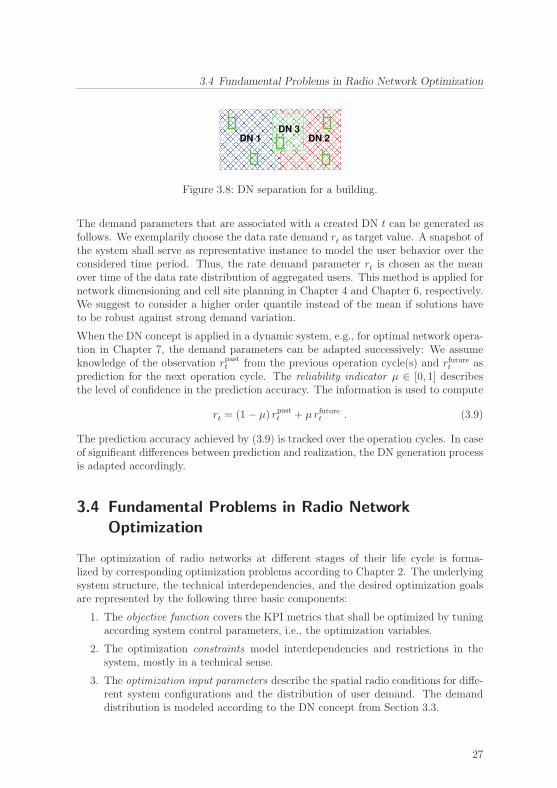
Figures 3.7 and 3.8 illustrate how DNs can be created deterministically for a certainnetwork area that contains buildings. First, the network area shown in Figure 3.7 (a) isdivided into the equal patches that are depicted in Figure 3.7 (b). Initially, each patchcorresponds to a DN. Since indoor users are of special interest in many cases, buildingsare modeled by own DNs that are systematically separated from the surrounding DNs.Figure 3.8 visualizes this principle for two patches that cover a building; the separationstep leads to three resulting DNs.
26
3.4 Fundamental Problems in Radio Network Optimization
������������������������������������
������������������������������������
������������������������������������
������������������������������������
������������
������������
DN 3DN 2DN 1
Figure 3.8: DN separation for a building.
The demand parameters that are associated with a created DN t can be generated asfollows. We exemplarily choose the data rate demand rt as target value. A snapshot ofthe system shall serve as representative instance to model the user behavior over theconsidered time period. Thus, the rate demand parameter rt is chosen as the meanover time of the data rate distribution of aggregated users. This method is applied fornetwork dimensioning and cell site planning in Chapter 4 and Chapter 6, respectively.We suggest to consider a higher order quantile instead of the mean if solutions haveto be robust against strong demand variation.
When the DN concept is applied in a dynamic system, e.g., for optimal network opera-tion in Chapter 7, the demand parameters can be adapted successively: We assumeknowledge of the observation rpastt from the previous operation cycle(s) and rfuturet asprediction for the next operation cycle. The reliability indicator μ ∈ [0, 1] describesthe level of confidence in the prediction accuracy. The information is used to compute
rt = (1− μ) rpastt + μ rfuturet . (3.9)
The prediction accuracy achieved by (3.9) is tracked over the operation cycles. In caseof significant differences between prediction and realization, the DN generation processis adapted accordingly.
3.4 Fundamental Problems in Radio NetworkOptimization
The optimization of radio networks at different stages of their life cycle is forma-lized by corresponding optimization problems according to Chapter 2. The underlyingsystem structure, the technical interdependencies, and the desired optimization goalsare represented by the following three basic components:
1. The objective function covers the KPI metrics that shall be optimized by tuningaccording system control parameters, i.e., the optimization variables.
2. The optimization constraints model interdependencies and restrictions in thesystem, mostly in a technical sense.
3. The optimization input parameters describe the spatial radio conditions for diffe-rent system configurations and the distribution of user demand. The demanddistribution is modeled according to the DN concept from Section 3.3.
27

3 Building Blocks for Radio Network Optimization
The spatial radio conditions are computed according to the previously introduced chan-nel models. Alternatively, in an operating system this information might be derivedfrom system observations and receiver measurements, e.g., according to the X-MapEstimation approach that is proposed in [96].
The following optimization problems are closely related to the optimization modelsthat we develop in this work.
3.4.1 The Maximal Covering Location Problem
With respect to the notation introduced in Section 1.3, we define
S ∗ T = {(s, t) ∈ S × T : est > 0} (3.10)
as the set of supported supplier-DN combinations and
St = {s ∈ S : (s, t) ∈ S ∗ T } (3.11)
as the set of potential suppliers (serving transmitters) for demand node t. The weightfor each DN is arbitrarily set to its rate demand rt. The DN weights and the spectralefficiency information est are given as input parameters. The latter one might becomputed according to Section 3.2.
The Maximal Covering Location Problem (MCLP) is given as
max∑
(s,t)∈S∗T
rtzst (3.12)
subject to ∑s∈St
zst ≤ 1 , for all t ∈ T (3.13)
zst ≤ ys , for all (s, t) ∈ S ∗ T (3.14)∑s∈S
ys ≤ Smax (3.15)
and with respect to the binary decision variables ys, zst. Supplier s ∈ S is in thesolution set if ys = 1. Furthermore, zst = 1 indicates that DN t is covered by supplier s.Constraint (3.13) avoids double counting of a covered weight for the maximization ofthe sum weight in (3.12). The coverage of DN t by a potential supplier s ∈ St requiresits selection in (3.14). Finally, (3.15) bounds the total number of selected suppliersto Smax ∈ N.
Since the MCLP is a budged-constrained variant of the Minimum Set Cover Prob-lem (MSCP), see [101], it is an NP-hard optimization problem and NP-complete in itsdecision version [60]. Hence, there does not exist an efficient algorithm to solve theMCLP, unless P = NP. The best approximation we can hope for is a Polynomial-
28
3.4 Fundamental Problems in Radio Network Optimization
Time Approximation Scheme (PTAS) [26], e.g., the one that is presented in [45] fora slightly modified version. Heuristic solution approaches are, for instance, the greedyalgorithm proposed in [101], an evolutionary algorithm presented in [103], and thesimulated annealing method applied in [72]. The latter two publications particularlyconsider variants of the MCLP that are sensitive to interference, i.e., the Channel As-signment Problem (CAP) for interference-limited systems is solved by an integratedapproach. An optimal solution of the CAP assigns a subset of available channels toeach supplier such that the number of overlapping channels is minimal for every pairof suppliers that can cover the same DNs. For frequency-division / time-division mul-tiple access (FD/TDMA) systems like GSM networks, the channels of neighboringsuppliers are separated in the frequency domain. In this case, the CAP is transformedinto the fixed-spectrum Frequency Assignment Problem (FAP). The FAP is knownto be NP-hard since it contains the Vertex Coloring Problem as a subproblem [103].An equivalent problem exists for CDMA systems where the separation is achieved byoptimum spreading code assignment [14].
Recent 4G systems, such as LTE networks, apply a different approach to cope withinter-cell interference. LTE systems share the spectrum along all suppliers, i.e., allchannels are used at (H)eNBs with reuse factor 1. The dynamic channel assignmenttakes place in the frequency domain and is carried out during network operation. Thisprinciple leads to the optimization problems that are discussed in the following.
3.4.2 User Assignment in OFDMA Systems
With respect to the notation introduced in Section 1.3, we consider a set S of opera-ting suppliers (transmitters) in a 4G OFDMA network. The available bandwidth ofsupplier s is limited by Bs. The elements t ∈ T are interpreted as single users andeach user has a rate demand rt. Supplier s can serve the rate demand of user t if it canallocate a sufficient amount of bandwidth for t, see (3.7). If supplier s serves user t,the binary assignment indicator zst is set to one. The sets S ∗ T and St are defined asin (3.10) and (3.11), respectively. Furthermore, we define
Ts = {t ∈ T : (s, t) ∈ S ∗ T }
and assume that⋃
s∈S Ts = T .
In the case that the required amount of bandwidth for serving user t is bt for all poten-tial suppliers, the user assignment problem can be written as the Multiple KnapsackProblem (MKP)
max∑
(s,t)∈S∗T
rtzst (3.16)
29

3 Building Blocks for Radio Network Optimization
subject to ∑s∈St
zst ≤ 1 , for all t ∈ T (3.17)
∑t∈Ts
btzst ≤ Bs , for all s ∈ S (3.18)
and with respect to the binary decision variables zst. Constraint (3.17) ensures thateach user can be assigned only once and (3.18) gives the capacity constraint for eachknapsack. The sum over single bandwidth requirements is overlap-free.
If ∑t∈Ts
bt ≤ Bs (3.19)
holds for all s ∈ S, the MKP has a trivial solution: Each user can be assigned toan arbitrary supplier. If (3.19) does not hold, some (or all) of the knapsack con-straints get tight and the MKP becomes a hard combinatorial problem. The non-trivialMKP is NP-hard. Optimal solutions can be computed by branch-and-bound methods,whereas approximate solutions can be obtained by greedy algorithms or relaxationtechniques [71].
The user assignment problem is an underlying component of the optimization modelsthat we develop in the subsequent chapters. Compared to the MKP formulation fromabove, those user assignment problems have to cope with additional aspects. First,the required bandwidth for a user t can differ from supplier to supplier. And second,interference effects can change the required bandwidth subject to the particular assign-ment. The effectively required bandwidth for serving users is determined by solvingthe resource allocation problem that is discussed in the next section. Actually, the userassignment problem and the resource allocation problem cannot be treated separately.On the other hand, the computational complexity of every optimal integrated algo-rithm is too high for practical applications. For some applications, the user assignmentis computed according to a suitable heuristic first, and the resource allocation problemis solved in a consecutive step.
3.4.3 Resource Allocation in OFDMA Systems
The resource allocation problem in OFDMA systems considers the assignment of sub-carriers from a set N of available SCs to users (or DNs) t from a set T . Furthermore, itconsiders power allocation Pn for each assigned subcarrier n ∈ N . The total transmitpower at the considered supplier is bounded by P . Any inter-symbol interference isneglected. The set of users is predetermined by a user assignment step. Each user thas a certain rate demand rt.
For every potential assignment pair, we introduce the indicator variable xtn ∈ {0, 1}that is one if SC n is assigned to user t and equals zero otherwise. The rate-power
30

3.4 Fundamental Problems in Radio Network Optimization
function R (t, n, Pn) defines the achievable rate for user t on SC n subject to thetransmit power Pn and the (fixed) spacing of an SC in the frequency domain. Structureand properties of R (t, n, Pn) are discussed in more detail below.
The OFDMA resource allocation problem for sum rate maximization is defined as
max∑t∈T
∑n∈N
R (t, n, Pn) xtn (3.20)
subject to ∑n∈N
R (t, n, Pn) xtn ≥ rt , for all t ∈ T (3.21)
∑t∈T
xtn ≤ 1 , for all n ∈ N (3.22)
∑n∈N
Pn ≤ P , (3.23)
Pn ≥ 0 , for all n ∈ N (3.24)
and with respect to the binary decision variables xtn and the corresponding power allo-cation variables Pn. While (3.20) maximizes the overall sum rate, constraint (3.21) en-sures that the (minimum) rate demand of each user is fulfilled by any feasible solution.According to (3.22), every SC can be assigned exactly to one user. Finally, the totalpower assigned to SCs is bounded by (3.23) and the non-negative constraint (3.24).
This formulation is consistent with the optimization model presented in [65]. It canbe solved by a dual method approach with complexity O
(|N ||T |3
), see [93, 106]. For
the special case of equal rate demands, the computational complexity can be reducedto O
(|N ||T |
), see [65]. These results hold for a continuous and concave rate-power
functionR (t, n, Pn) = log2 (1 + SNRt,nΓt,n) (3.25)
with fitting factor Γt,n > 0 and
SNRt,n =Pngtnσ2n
. (3.26)
The channel gain gtn is basically determined by the path loss according to (3.3). Addi-tionally, it can include the channel characteristics that were discussed in Section 3.2.The constant σ2
n denotes the noise power on subcarrier n.
The complexity bounds do not hold any longer if we consider a discrete rate-powerfunction as introduced in Section 3.2. If the continuous domain of power variables isreplaced by a discrete set of minimum power requirements and the rate-power functioncan only achieve discrete rates according to (3.8), the resource allocation problembecomes a binary decision problem, i.e., an ILP. In [46], it is shown that this binarydecision problem can be interpreted as Multiple-Choice Knapsack Problem (MCKP),which is NP-hard to solve. However, the authors propose a heuristic relaxation and
31
3 Building Blocks for Radio Network Optimization
rounding approach that determines approximate solutions efficiently. Particularly, itprovides a bound on the integrality gap that vanishes asymptotically for an increasinggranularity of subcarrier spacing. The latter property is highly related to the simplifiedbandwidth computation in (3.7).
So far, the resource allocation problem has been considered for a single supplier (single-cell). Thus, any implementation of (3.25) as well as any discrete rate-power functiondepends on the SNR according to (3.26). For the multiple supplier (multi-cell) case,however, the power-rate function depends on the SINR. For a set S of multiple inter-fering suppliers, a supplier s provides the
SINRs,t,n =Psngstn∑
s′∈S, s′ �=s
Ps′ngs′tn + σ2n
to user t on subcarrier n. Here, the channel gains and the noise power are supplier-specific. Since the resource allocation at interfering suppliers s′ affects the denomina-tor, computation of the SINR requires a full user-to-supplier assignment. Furthermore,it requires knowledge of the subcarrier and power assignment at all other suppliers.These properties make optimal OFDMA resource allocation a computationally hardcombinatorial problem if inter-cell interference has to be considered [69].
Please note that presently deployed LTE networks, i.e., Release 8 and 9 systems, do notsupport frequency-dependent power control [94]. In this case, the constraints (3.23)and (3.24) are dropped and the power variables Pn are replaced by constant powerparameters Ps. What remains is the combinatorial problem of assigning SCs to theusers subject to the interdependencies between interfering transmitters. If the constantpower parameters Ps are related to optimal network configuration, the user assignmentproblem and the resource allocation problem are immanent subproblems. A model foroptimal network configuration is presented in Chapter 7.
32

4 Dimensioning of Multihop Networks
The following profit-related approach for the dimensioning of multihop WiMAX net-works is inspired by the economical perspective on radio network planning and opera-tion in [84] and [85]. Multihop WiMAX networks are specified according to the IEEE802.16j standard [83]. The proposed concept for dealing with the multi-objective na-ture of the optimization problem is transferable to other radio technologies and networktopologies. In fact, the economically driven deployment approach is also applied forcell site planning of LTE HetNets in Chapter 6.
Parts of this chapter have already been published in [35].
4.1 System Model
Network dimensioning means the joint selection of an arbitrary number of WiMAXbase stations (BSs) and relay stations (RSs) from the sets of deployment candidates Sand K, respectively. The selection process is carried out with respect to the inputparameters and optimization variables introduced in Section 1.3 and the additionalparameters given in Table 4.1. We consider downlink data transmission and apply thedemand node model from Section 3.3 to describe the (spatial) distribution of user ratedemands rt.
Symbol & domain Description
cs, ck ∈ R≥0 Deployment cost for BS, RS.
λRATE ∈ R≥0 Sum rate weighting factor for objective scalarization.
eMIN ∈ R>0Minimum required spectral efficiency to establish a transmis-sion link.
dss′ ∈ R≥0 Distance between BSs s, s′ ∈ S.G Conflict graph, representing the set of conflicting BS pairs.
zsk ∈ {0, 1} Binary decision variable indicating the backhaul connectionfrom RS k to donor BS s.
bsk ∈ R≥0Amount of allocated bandwidth on the supply link from donorBS s to RS k.
Table 4.1: Additional input parameters (upper part) and variables (lower part) fordimensioning two-hop WiMAX networks, complementing Table 1.1.
33
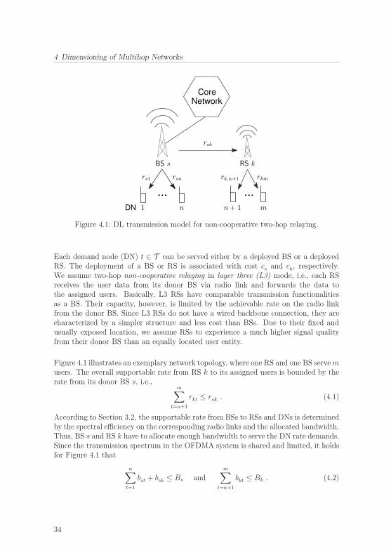
4 Dimensioning of Multihop Networks
DN
NetworkCore
... ...rkmrsn
BS s RS k
rs1
rsk
n mn+ 11
rk,n+1
Figure 4.1: DL transmission model for non-cooperative two-hop relaying.
Each demand node (DN) t ∈ T can be served either by a deployed BS or a deployedRS. The deployment of a BS or RS is associated with cost cs and ck, respectively.We assume two-hop non-cooperative relaying in layer three (L3) mode, i.e., each RSreceives the user data from its donor BS via radio link and forwards the data tothe assigned users. Basically, L3 RSs have comparable transmission functionalitiesas a BS. Their capacity, however, is limited by the achievable rate on the radio linkfrom the donor BS. Since L3 RSs do not have a wired backbone connection, they arecharacterized by a simpler structure and less cost than BSs. Due to their fixed andusually exposed location, we assume RSs to experience a much higher signal qualityfrom their donor BS than an equally located user entity.
Figure 4.1 illustrates an exemplary network topology, where one RS and one BS servemusers. The overall supportable rate from RS k to its assigned users is bounded by therate from its donor BS s, i.e.,
m∑t=n+1
rkt ≤ rsk . (4.1)
According to Section 3.2, the supportable rate from BSs to RSs and DNs is determinedby the spectral efficiency on the corresponding radio links and the allocated bandwidth.Thus, BS s and RS k have to allocate enough bandwidth to serve the DN rate demands.Since the transmission spectrum in the OFDMA system is shared and limited, it holdsfor Figure 4.1 that
n∑t=1
bst + bsk ≤ Bs andm∑
t=n+1
bkt ≤ Bk . (4.2)
34

4.2 Optimization Model
The considered network does not suffer from any intra-cell interference if OFDMA isused as multiplex scheme. For the purpose of network dimensioning, we apply simplesemi-empirical path loss models from Section 3.1.1. Hence, it is sufficient to ensure aminimum distance between deployed BSs to ease inter-cell interference on the macrocelllayer. The corresponding minimum distance constraints define the conflict graph G.Each element (s, s′) ∈ G denotes a tuple of BSs that mutually interfere. Cross-layerinterference between BSs and RSs is mitigated by applying out-band relaying , i.e.,the transmission from RSs to DNs is separated from the BS transmission band inthe frequency spectrum (type 1a relay). We do not consider any further inter-cellinterdependencies such as handover aspects or resource coordination between cells.
4.2 Optimization Model
Similarly to (3.10) and (3.11), we define
S ∗ T = {(s, t) ∈ S × T : est ≥ eMIN} ,K ∗ T = {(k, t) ∈ K × T : ekt ≥ eMIN} ,S ∗ K = {(s, k) ∈ S × K : esk ≥ eMIN} ,
St = {s ∈ S : (s, t) ∈ S ∗ T } , Kt = {k ∈ K : (k, t) ∈ K ∗ T } ,Ts = {t ∈ T : (s, t) ∈ S ∗ T } , Tk = {t ∈ T : (k, t) ∈ K ∗ T }
to exclude decision variables and constraints that are irrelevant due to insufficient linkquality. This restriction is not necessarily required since high-end optimization engineslike CPLEX remove irrelevant terms in a preprocessing step within milliseconds.
The following MIP selects BSs and RSs from the candidate sets S and K for jointdeployment in a WiMAX two-hop relay network. A compact representation of theoptimization problem is given in Table 4.2. Optimal solutions of this MIP provide abandwidth-limited Profit MAXimization (ProMAX) and serve as input for networkdimensioning decisions. The return-on-invest ratio is typically a major criterion forsuch decisions.
The objective
max
{λRATE
∑t∈T
refft −(∑
s∈Scsys +
∑k∈K
ckyk
)}(4.3)
optimizes the trade-off between the achieved sum rate and the costs for deployedBSs and RSs. The optimization is carried out with respect to the optimization vari-ables ys, yk, zst, zkt, zsk, bst, bkt, bsk and the auxiliary variables zt, r
efft .
Applying the scalarization approach from Section 2.3.1 to cope with this MOO prob-lem, the sum rate weighting factor (exchange rate) λRATE is chosen as follows: Thenetwork operator computes the Average Revenue Per Unit (ARPU), i.e., the averagequotient of user revenue and cumulated data rate over a fixed time period. The userrevenue typically covers basic fee, data fee, and additional services fees.
35

4 Dimensioning of Multihop Networks
max
{λRATE
∑t∈T
refft −(∑
s∈Scsys +
∑k∈K
ckyk
)}subject to
zt =∑s∈St
zst +∑
k∈Kt
zkt ≤ 1 , for all t ∈ T
zst ≤ ys , for all (s, t) ∈ S ∗ Tzkt ≤ yk , for all (k, t) ∈ K ∗ Tzsk ≤ ys , for all (s, k) ∈ S ∗ Kbkt ≤
rtekt
zkt , for all (k, t) ∈ K ∗ T∑t∈Tk
bkt ≤ Bk , for all k ∈ K∑s∈S
zsk = yk , for all k ∈ K
bsk ≤ Bszsk , for all (s, k) ∈ S ∗ K∑t∈Tk
ektbkt ≤∑s∈S
eskbsk , for all k ∈ K
bst ≤rtest
zst , for all (s, t) ∈ S ∗ T∑t∈Ts
bst +∑k∈K
bsk ≤ Bs , for all s ∈ S
ys + ys′ ≤ 1 , for all (s, s′) ∈ Grefft =
∑s∈St
estbst +∑
k∈Kt
ektbkt ≥ rMINt zt , for all t ∈ T
Table 4.2: MIP formulation of the bandwidth-limited Profit MAXimization (ProMAX)problem for techno-economical network dimensioning.
In case that the ARPU varies significantly for different mobile services, the sum ratein (4.3) can be split up into linear terms∑
m∈MλmRATE
∑t∈Tm
refft
that depend on the set of different mobile services M, the corresponding parti-tion {Tm}m∈M of T , and the service-specific exchange rates λmRATE. The consideredARPU [e/kbps] is normalized over the same time interval as the considered costs.Thus, objective (4.3) describes the revenue minus costs when λRATE is chosen as theARPU. In economics, this term is called profit.
36

4.2 Optimization Model
The maximization in (4.3) is carried out subject to the following constraints. Theinequality
zt =∑s∈St
zst +∑k∈Kt
zkt ≤ 1 , for all t ∈ T (4.4)
ensures that DNs are assigned to at most one BS or one RS. The variable zt indicateswhether DN t is assigned to any station or not. Since all assignments require thedeployment of the related supplying station,
zst ≤ ys, zkt ≤ yk, zsk ≤ ys , for all (s, t) ∈ S ∗T , (k, t) ∈ K∗T , (s, k) ∈ S ∗K (4.5)
must hold. If DN t is assigned to RS k, i.e., zkt = 1, the RS allocates the bandwidth
bkt ≤rtektzkt , for all (k, t) ∈ K ∗ T (4.6)
according to (3.7). The amount is bounded by the bandwidth that is required to servethe full rate demand rt. The overall allocated bandwidth at each RS has to stay belowthe available bandwidth, i.e.,∑
t∈Tk
bkt ≤ Bk , for all k ∈ K . (4.7)
As mentioned in the description of the system model, each deployed RS needs to beassigned to a donor BS by∑
s∈Szsk = yk , for all k ∈ K . (4.8)
The donor BS has to allocate enough bandwidth for the corresponding supply link
bsk ≤ Bszsk , for all (s, k) ∈ S ∗ K (4.9)
such that it provides enough capacity for all the forwarded user data, i.e.,∑s∈S
eskbsk ≥∑t∈Tk
ektbkt , for all k ∈ K . (4.10)
Each deployed BS can serve itself any assigned DNs by allocating the bandwidth
bst ≤rtestzst , for all (s, t) ∈ S ∗ T (4.11)
as long as the overall allocated bandwidth – for RS links and DN links– does notexceed the total available bandwidth, i.e.,∑
t∈Ts
bst +∑k∈K
bsk ≤ Bs , for all s ∈ S . (4.12)
37

4 Dimensioning of Multihop Networks
The inequality
ys + ys′ ≤ 1 , for all (s, s′) ∈ G , (4.13)
excludes BS pairs from a joint deployment if they are element of the predefined conflictgraph G. The conflicting BS pairs are predefined according to an interference crite-rion. If the interference-related conflict between BSs is exclusively determined by thedistance between the corresponding site locations, (4.13) can be replaced by
(dss′ + dMIN) (ys + ys′) ≤ dMIN + 3dss′ , for all s, s′ ∈ S , (4.14)
where dMIN is a suitable minimum distance parameter. In this case, the generation ofthe conflict graph G is dispensable.
So far, a DN can be assigned to any BS or RS that provides a sufficient link quality.The supplying station allocates bandwidth according to (4.6) or (4.11) and serves theDN with an effective rate refft ∈ [0, rt]. Solutions that guarantee a certain QoS levelare obtained by a minimum rate requirement rMIN
t ≤ rt for every assigned DN, i.e.,
refft =∑s∈St
estbst +∑k∈Kt
ektbkt ≥ rMINt zt , for all t ∈ T . (4.15)
Together with (4.7) and (4.12) this constraint causes a multiple knapsack problemif rMIN
t > 0 and the load limit of (some) stations is exceeded. Compared to theMKP from Section 3.4.2, the required bandwidth for an assignment is not equal forall potential suppliers but depends on the signal quality of the particular station.
If rMINt = rt for all t ∈ T , the ProMAX problem can be rewritten in a simplified
form as the Full Rate Profit MAXimization (FR-ProMAX) problem. The MIP for theFR-ProMAX problem is shown in Table 4.3.
4.3 Concept Validation
A representative application of the ProMAX problem(s) from above demonstratesthe properties of our dimensioning approach. Exemplary test cases are generated ac-cording to the system setup described in Table 4.4. Table 4.5 shows the consideredmobile services and their corresponding rate demands. For each DN, one requestedmobile service is randomly chosen according to the service proportions from Table 4.5.The related rate demand is computed randomly and uniformly distributed over theservice-specific rate interval. BSs, RSs, and DNs are uniformly distributed over thearea. Out-band relaying is performed in a separate frequency spectrum, which provideshalf of the BS bandwidth. The considered RS footprint is very small compared to theBS coverage area since RSs are mounted at a much lower height and they apply lesstransmission power. Any deployed BS is associated with monthly OPerational EXpen-ditures (OPEX) of 2500e covering site rental, leased line rental, air-conditioning, andmaintenance [33]. RSs can be mounted much simpler than BSs, e.g., on top of traffic
38

4.3 Concept Validation
max
{λRATE
∑t∈T
rtzt −(∑
s∈Scsys +
∑k∈K
ckyk
)}subject to
zt =∑s∈St
zst +∑
k∈Kt
zkt ≤ 1 , for all t ∈ T∑t∈Tk
rtekt
zkt ≤ Bkyk , for all k ∈ K∑s∈S
zsk = yk , for all k ∈ K
bsk ≤ Bszsk , for all (s, k) ∈ S ∗ K∑t∈Tk
rtzkt ≤∑s∈S
eskbsk , for all k ∈ K∑t∈Ts
rtest
zst +∑k∈K
bsk ≤ Bsys , for all s ∈ S
ys + ys′ ≤ 1 , for all (s, s′) ∈ G
Table 4.3: MIP formulation of the Full Rate ProMAX (FR-ProMAX) problem.
lights, and they do not have a wired backbone connection. Hence, RSs account for asignificantly reduced OPEX of 500e. Since network dimensioning is carried out withrespect to long-term considerations, we ignore the CAPital EXpenditures (CAPEX)for deploying the transmitter equipment. However, CAPEX can be additionally con-sidered in two variants. First, by an additional budget constraint in the ProMAXproblem. And second, by apportioning the CAPEX among the OPEX subject to theintended lifetime of the network.
Neglecting the DN link penetration for links from BSs to RSs, the signal strength of thesupply links from BSs to RSs is 10 dB higher than the signal to an equally located DN.Furthermore, the path loss model for BS-to-RS transmission provides an extra gaincompared to the DN related path loss. This is justified by the assumption that RSscan be deployed in locations that are beneficial for the BS-to-RS signal propagation.Table 4.6 specifies the SINR requirements for the discrete set of achievable spectralefficiencies. DNs can be served at seven different transmission rates that dependon the individual DN position in the BS or RS coverage area. Due to the lowertransmission power and the applied path loss profile, RSs provide a small but highrate coverage area, see Figure 4.2. In this sense, RSs complement the conventionalmacrocell layer by bridging local coverage holes or improving the locally available datarate (capacity) [104, 17]. Inter-macrocell interference can be neglected by enforcing aminimum distance of dMIN = 500m between deployed BSs.
39

4 Dimensioning of Multihop Networks
System parameter Setting
Area size 1750m× 1750m
Number of BS / RS candidates 15 / 45, uniformly distributed
Number of DNs 650, uniformly distributed
BS / RS carrier frequency 2GHz / 2.5GHz
BS / RS transmission bandwidth 20MHz / 10MHz
BS / RS monthly cost 2500e / 500e (OPEX)
BS / RS / DN reference height 25m / 5m / 1.5m
BS / RS Tx power 46 dBm / 24 dBm
BS / RS / DN antenna gain 14 dBi / 9 dBi / 0 dBi
BS / RS / DN noise figure 5 dB / 8 dB / 8 dB
Path loss BS ↓ DN / BS ↓ RS / RS ↓ DN WINNER II C2 NLOS / C1 NLOS / B1 [53]
Link penetration, worst case assumption 40 dB (shadowing, fast fading, etc.)
DN link penetration 10 dB (wall penetration for indoor users)
Minimum inter-site distance (BSs) 500m
Table 4.4: Considered system parameters for network dimensioning.
Mobile service Proportion Rate demand [kbps]
Interactive real time 20% 128− 2000
Video 20% 128− 1000
FTP 10% 64− 1000
Web 20% 64− 512
VoIP 30% 64
Table 4.5: Considered mobile services [78].
Each assigned DN is served by its supplying BS or RS up to the requested data rate.Assuming the users to request mobile services on 20 days per month for five hours ata charge of 0.05 e/MB, the according sum rate weighting factor (monthly ARPU) is
λRATE =20 · 5 · 3600 s
8 · 1000 · 0.05 e/MB = 2.25 e/kbps . (4.16)
Please note that the denominator in (4.16) converts megabyte to kilobit, which is thereference unit for the rate specifications in Table 4.5. For λRATE = 2.25 e/kbps, a VoIPDN yields a monthly revenue of 144e. This seems reasonable when a DN models fiveto seven users. In consequence, a single BS or RS is already profitable if it can serveat least 18 and 4 VoIP DNs, respectively.
The ProMAX problem from Table 4.2 is applied for the planning scenario depicted inFigure 4.2 and rMIN
t = 0. We utilize the CPLEX MIP solver [51] to compute optimalsolutions. The resulting network consists of 7 deployed BSs and 22 deployed RSs,which serve on average 50 DNs and 3 DNs, respectively. However, not all of the DNsare covered. According to Table 4.5, the average DN rate demand is 456 kbps, and
40

4.3 Concept Validation
Rate ID Modulation Code rate Spectral efficiency [bps/Hz] Receiver SINR [dB]
0 out of range
1 BPSK 1/2 0.5 3.0
2 QPSK 1/2 1.0 6.0
3 QPSK 3/4 1.5 8.5
4 16-QAM 1/1 2.0 11.5
5 16-QAM 3/4 3.0 15.0
6 64-QAM 2/3 4.0 19.0
7 64-QAM 3/4 4.5 21.0
Table 4.6: SINR requirements according to the WiMAX system link budget specifica-tion [52, 44], BER = 10−6.
1750 m
DN BS RS
1750 m
Figure 4.2: Considered BS candidates, RS candidates, and DNs. The spectral effi-ciency in the coverage area is visualized by a grayscale coloring.
hence, the overall revenue in (4.3) is much higher than the BS and RS expenses. Itturns out that the total number of deployed BSs is limited by the minimum distanceconstraint (4.14): If the minimum required distance is lowered to dMIN = 250m, theresulting network has 10 deployed BSs that are still profitable. The minimum distancerequirement is also the reason why the number of deployed BSs does not change fora variation of the sum rate weighting factor λRATE in Figure 4.3. The number ofdeployed BSs stays constant whereas the number of deployed RSs increases with arising ARPU. The maximum of 29 deployed RSs is reached for λRATE = 8 e/kbps. Inthis (extreme) case, one served low rate DN is enough to achieve a positive profit at adeployed RS. Generally, we observe that profitable RSs are selected for deployment if
41
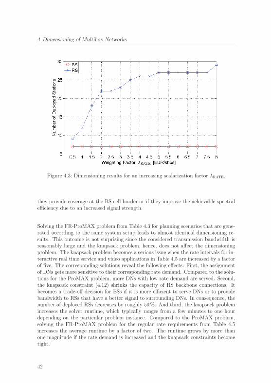
4 Dimensioning of Multihop Networks
Figure 4.3: Dimensioning results for an increasing scalarization factor λRATE.
they provide coverage at the BS cell border or if they improve the achievable spectralefficiency due to an increased signal strength.
Solving the FR-ProMAX problem from Table 4.3 for planning scenarios that are gene-rated according to the same system setup leads to almost identical dimensioning re-sults. This outcome is not surprising since the considered transmission bandwidth isreasonably large and the knapsack problem, hence, does not affect the dimensioningproblem. The knapsack problem becomes a serious issue when the rate intervals for in-teractive real time service and video applications in Table 4.5 are increased by a factorof five. The corresponding solutions reveal the following effects: First, the assignmentof DNs gets more sensitive to their corresponding rate demand. Compared to the solu-tions for the ProMAX problem, more DNs with low rate demand are served. Second,the knapsack constraint (4.12) shrinks the capacity of RS backbone connections. Itbecomes a trade-off decision for BSs if it is more efficient to serve DNs or to providebandwidth to RSs that have a better signal to surrounding DNs. In consequence, thenumber of deployed RSs decreases by roughly 50%. And third, the knapsack problemincreases the solver runtime, which typically ranges from a few minutes to one hourdepending on the particular problem instance. Compared to the ProMAX problem,solving the FR-ProMAX problem for the regular rate requirements from Table 4.5increases the average runtime by a factor of two. The runtime grows by more thanone magnitude if the rate demand is increased and the knapsack constraints becometight.
42

4.4 Summary
4.4 Summary
While there exist many studies on the general impact of relaying to network coverageand network capacity, e.g., [104] and [17], only a few works consider the problem ofjoint BS and RS deployment. For instance, [80] investigates the placement of oneRS in a single macrocell. In [64], multiple RSs are deployed but the perspective isstill restricted to a single macrocell environment. An approach for joint BS and RSdeployment is presented in [70]. Although the maximization of the network capacityis comparable to our approach, this work does not assume any restrictions for theavailable bandwidth at BSs and RSs.
Compared to the these works, our approach allows for the joint deployment of multipleBSs and multiple RSs subject to shared and limited bandwidth resources. Particularly,our optimization model applies an economically motivated approach to align the con-flicting objectives of sum rate and cost in a scalar-valued overall objective. The appliedsimplifications to cope with interference (minimum distance constraints, out-band re-laying) as well as the usage of simple semi-empirical path loss models are sufficientfor the purpose of network dimensioning. Accurate network planning and networkconfiguration, however, require a higher precision in both components. Therefore,we introduce a suitable low complexity interference approximation model in the nextchapter. This approximate model is combined with ray optical path loss predictionsfor optimal cell site planning and network configuration in Chapter 6 and Chapter 7,respectively.
43


5 Interference Approximation in LTEHeterogeneous Networks
LTE systems apply full frequency reuse over all cells, i.e., all cells in the network sharethe same frequency spectrum [94]. LTE transmitters can successfully serve users orUser Equipment (UE) even at very low SINR (< −5 dB). However, the achievablesum rate will be significantly degraded if too many UEs are served at low SINR. Inheterogeneous networks, low power femtocells can severely suffer from interference ofhigh power macrocell transmissions. Consequently, the SINR can become very poorfor shared resources in certain parts of the HetNet. It is the task of the system RRM toassign users to supplying cells and to allocate resources in the spectrum such that theSINR is sufficient to serve the user demand. In Section 3.4.2 and Section 3.4.3 we haveseen that user assignment and resource allocation are difficult problems. Furthermore,the SINR requirements for the related (discrete) rate-power-function have no linearrepresentation, which is a prerequisite for the incorporation into our MIP-based op-timization models. Therefore, we develop an approximate model that estimates theoverall required bandwidth for serving users subject to inter-cell and cross-tier inter-ference. The following aspect motivates the underlying principle of our approximatemodel.
The LTE standard defines several features that support the application of ICIC in thenetwork. Interference mitigation was introduced as an ICIC technique at the end ofSection 3.2. Basically, dedicated resources are protected from interference by blockingthem at potentially interfering transmitters [29]. Please note that the LTE standarddoes not define what particular ICIC techniques should be applied in the network, i.e.,the interference management is customizable. However, we assume that the applicationof any ICIC technique causes a certain penalty and that this penalty can be expressedin terms of additional bandwidth consumption at some of the coordinated transmitters.For interference mitigation, for instance, the penalty is given by the unused (protected)resources at the interference mitigating transmitters.
The basic idea of the developed approximation model is to consider bandwidth thatis allocated for transmission to users separately from protected bandwidth and toestimate both terms subject to the SNR.
45
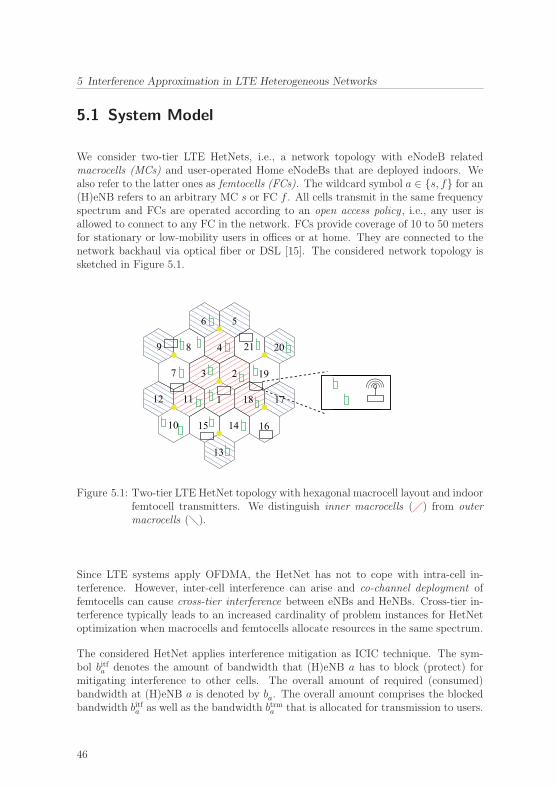
5 Interference Approximation in LTE Heterogeneous Networks
5.1 System Model
We consider two-tier LTE HetNets, i.e., a network topology with eNodeB relatedmacrocells (MCs) and user-operated Home eNodeBs that are deployed indoors. Wealso refer to the latter ones as femtocells (FCs). The wildcard symbol a ∈ {s, f} for an(H)eNB refers to an arbitrary MC s or FC f . All cells transmit in the same frequencyspectrum and FCs are operated according to an open access policy , i.e., any user isallowed to connect to any FC in the network. FCs provide coverage of 10 to 50 metersfor stationary or low-mobility users in offices or at home. They are connected to thenetwork backhaul via optical fiber or DSL [15]. The considered network topology issketched in Figure 5.1.
9 4
10 15 14
21 20
16
13
6 5
18 171112 1
197 3 2
8
Figure 5.1: Two-tier LTE HetNet topology with hexagonal macrocell layout and indoorfemtocell transmitters. We distinguish inner macrocells (�) from outermacrocells (�).
Since LTE systems apply OFDMA, the HetNet has not to cope with intra-cell in-terference. However, inter-cell interference can arise and co-channel deployment offemtocells can cause cross-tier interference between eNBs and HeNBs. Cross-tier in-terference typically leads to an increased cardinality of problem instances for HetNetoptimization when macrocells and femtocells allocate resources in the same spectrum.
The considered HetNet applies interference mitigation as ICIC technique. The sym-bol bitfa denotes the amount of bandwidth that (H)eNB a has to block (protect) formitigating interference to other cells. The overall amount of required (consumed)bandwidth at (H)eNB a is denoted by ba. The overall amount comprises the blockedbandwidth bitfa as well as the bandwidth btrma that is allocated for transmission to users.
46
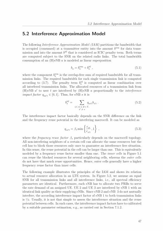
5.2 Interference Approximation Model
5.2 Interference Approximation Model
The following Interference Approximation Model (IAM) partitions the bandwidth thatis occupied (consumed) at a transmitter entity into the amount btrm for data trans-mission and into the amount bitf that is considered as ICIC penalty term. Both termsare computed subject to the SNR on the related radio links. The total bandwidthconsumption of an (H)eNB a is modeled as linear superposition
ba = btrma + bitfa , (5.1)
where the component btrma is the overlap-free sum of required bandwidth for all trans-mission links. The required bandwidth for each single transmission link is computedaccording to (3.7). The penalty term bitfa is computed as linear combination overall interfered transmission links. The allocated resources of a transmission link from(H)eNB a′ to user t are interfered by (H)eNB a proportionally to the interferenceimpact factor qaa′t ∈ [0, 1]. Thus, for eNB s it is
bitfs =∑
(s′, t) ∈ S ∗ T ,s′ �= s
qss′tbs′t . (5.2)
The interference impact factor basically depends on the SNR difference on the linkand the frequency reuse potential in the interfering macrocell. It can be modeled as
qss′t = βs min
{estes′t
, 1
}, (5.3)
where the frequency reuse factor βs particularly depends on the macrocell topology.All non-interfering neighbors of a certain cell can allocate the same resources but thecell has to block those resources only once to guarantee an interference free situation.In this sense, the reuse potential in the cell can be larger than one. This is equivalentlymodeled by a frequency reuse factor smaller than one. The inner cells in Figure 5.1can reuse the blocked resources for several neighboring cells, whereas the outer cellsdo not have that much reuse opportunities. Hence, outer cells generally have a higherfrequency reuse factor than inner cells.
The following example illustrates the principles of the IAM and shows its relationto actual resource allocation in an LTE system. In Figure 5.2, we assume an equalSNR for all transmission links and all interference links, i.e., all spectral efficiencyparameters are identical. Furthermore, each eNB has to allocate two PRBs to servethe rate demand of an assigned UE. UE 2 and UE 3 are interfered by eNB 1 with anidentical link quality as their supplying eNBs. Since eNB 2 and eNB 3 do not mutuallyinterfere, the according interference impact factor of eNB 1 to both transmission linksis 1/2. Usually, it is not that simple to assess the interference situation and the reusepotential between cells. In such cases, the interference impact factors have to calibratedby a suitable parameter estimation, e.g., as carried out in Section 7.1.2.
47

5 Interference Approximation in LTE Heterogeneous Networks
������
������
���������
���������
������
������
������
������
������
������
���������
���������
��������
��������
eNB 3
41 6532 41 65
eNB 1eNB 2
32
4 x 2 x
3 41 652
UE 1 UE 3
UE 4UE 4 UE 1 UE 1 UE 6 UE 6UE 2 UE 2 UE 3 UE 3UE 5 UE 5
UE 6
UE 4UE 2
UE 5
eNB to UE transmisison
Interference
Transmission PRB
Blocked (protected) PRB
e21 e11 e33e13
e22 e14e12 e34
DL Spectrum DL SpectrumDL Spectrum
e25 e36
Approximated resource consumption with respect to the IAM:
Figure 5.2: Exemplary PRB allocation and approximated resource consumption.
According to the IAM equation (5.2), eNB 1 has to block (protect) two PRBs: Onefor the interfered link from eNB 2 to UE 2 and one for the interfered link from eNB 3to UE 3. Combined with the four PRBs that eNB 1 has to allocate for serving itsassigned UEs 1 and 4, the overall bandwidth consumption at eNB 1 is six PRBs.This estimation is an exact match with the de facto PRB allocation that is shown inthe Figure. The eNBs 2 and 3 cannot align the protected PRBs in the DL spectrumbecause they have only one neighbor eNB. Thus, their interference impact factors haveto be chosen as one if the IAM shall hold exactly.
We assume that inter-femtocell interference can be handled by applying ICIC tech-niques as before and that the related penalty terms bitff can be written analogouslyto (5.2). For modeling cross-tier interference between macrocells and femtocells, wetake advantage of the fact that femtocells located nearby each other are typically in-terfered by the same eNB. As a consequence, the capacity of those femtocells canbe increased significantly if eNBs block resources for femtocell interference mitiga-tion [29]. Inter-femtocell interference is assumed to be low since the HeNB coveragearea is generally very small. This allows particularly for a reuse of PRBs at HeNBswithout a significant SINR degradation. Thus, it is beneficial for an efficient HetNetresource allocation to align the PRBs that are blocked at an eNB for femtocell in-terference mitigation jointly over all interfered FCs. The alignment may result in a(virtual) separation of MC spectrum and FC spectrum, which can particularly help toprevent the HetNet from overstressing its limited communication capabilities for thecoordination between eNBs and HeNBs [29].
The IAM from above is extended by the discussed cross-tier interference aspects asfollows. Additionally to the inter-macrocell interference component, each eNB s blocks
48

5.2 Interference Approximation Model
an amount of bandwidth that corresponds to the maximum consumed bandwidth atpotentially interfered FCs Fs. This means that (5.2) is rewritten as
bitfs =∑
(s′, t) ∈ S ∗ T ,s′ �= s
qss′tbs′t
︸ ︷︷ ︸inter-cell interference
+ maxf∈Fs
{qsfbf
}︸ ︷︷ ︸
cross-tier interference
, (5.4)
where bf is computed according to (5.1) and
bitff =∑
(f ′, t) ∈ F ∗ T ,f ′ �= f
qff ′tbf ′t (5.5)
for all HeNBs f in the HetNet. For the cross-tier interference term in (5.4), we assumethat all UEs served by a femtocell are located nearby the HeNB and that the sameholds for all inter-FC interfered femtocells. Hence, the interference impact factor qsfscales with the eNB signal strength to the HeNB location and relatively to the linkquality that the HeNB provides to its served UEs. We suggest
qsf =esfeMAX
(5.6)
if FCs predominantly serve users with maximum spectral efficiency eMAX on the corres-ponding transmisson links. Since the protected bandwidth can be aligned along allinterfered femtocells, the maximum cross-tier interference term in (5.4) eliminatesinterference to FCs in the eNB coverage area. Please note that due to the spatialdiversity of rate demand and femtocell distribution, the amount of blocked (protected)bandwidth typically varies from eNB to eNB.
We call the model (5.1) Bandwidth Reservation Concept (BRC) as it approximatesthe expected amount of bandwidth that has to be reserved in the spectrum subjectto supported UE rate demand and interference. Please note that the BRC considersbandwidth as a continuous variable and that it does not describe where the resourcesare allocated in the spectrum. It serves as an approximation model for the discretecombinatorial problem of PRB assignment.
The example depicted in Figure 5.3 illustrates the application of the BRC for a smallHetNet with two eNBs and three femtocells:
• The bandwidth is measured in arbitrary units from the continuous domain.
• The blocked bandwidth at eNB 2, FC 2, and FC 3 is not considered.
• FC 2 has to reserve 2 bandwidth units for transmission to UE 2.
• FC 3 has to reserve 1 bandwidth unit for transmission to UE 3.
49
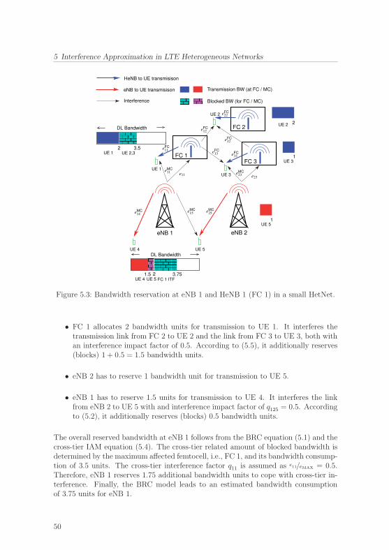
5 Interference Approximation in LTE Heterogeneous Networks
FC 1
FC 2
FC 3
eNB 1 eNB 2
��������
���
���
������������
������������
������������
������������
������������
UE 4
UE 2
UE 3
UE 5
UE 1
UE 2
UE 3
UE 5
UE 4 UE 5 FC 1 ITF
UE 1 UE 2,3
Interference
eNB to UE transmisison
HeNB to UE transmisison
eFC13
eFC32
eFC12
eFC11
e11
eFC22
eFC33
e23
eMC14
2 3.5
1.5
eMC15 eMC
25
eMC11 eMC
23
3.75
1
Transmission BW (at FC / MC)
Blocked BW (for FC / MC)
2
2
DL Bandwidth
DL Bandwidth
1
Figure 5.3: Bandwidth reservation at eNB 1 and HeNB 1 (FC 1) in a small HetNet.
• FC 1 allocates 2 bandwidth units for transmission to UE 1. It interferes thetransmission link from FC 2 to UE 2 and the link from FC 3 to UE 3, both withan interference impact factor of 0.5. According to (5.5), it additionally reserves(blocks) 1 + 0.5 = 1.5 bandwidth units.
• eNB 2 has to reserve 1 bandwidth unit for transmission to UE 5.
• eNB 1 has to reserve 1.5 units for transmission to UE 4. It interferes the linkfrom eNB 2 to UE 5 with and interference impact factor of q125 = 0.5. Accordingto (5.2), it additionally reserves (blocks) 0.5 bandwidth units.
The overall reserved bandwidth at eNB 1 follows from the BRC equation (5.1) and thecross-tier IAM equation (5.4). The cross-tier related amount of blocked bandwidth isdetermined by the maximum affected femtocell, i.e., FC 1, and its bandwidth consump-tion of 3.5 units. The cross-tier interference factor q11 is assumed as e11/eMAX = 0.5.Therefore, eNB 1 reserves 1.75 additional bandwidth units to cope with cross-tier in-terference. Finally, the BRC model leads to an estimated bandwidth consumptionof 3.75 units for eNB 1.
50

5.3 Numerical Evaluation
5.3 Numerical Evaluation
The BRC and its immanent IAM are evaluated exemplarily for the following simulationsetup. We consider a hexagonal grid topology as depicted in Figure 5.1. Each of therelated 3-sectorized eNBs transmits at a center frequency of 2GHz and with 43 dBm Txpower, 14 dBi antenna gain, 5 dB noise figure, and 8 dB shadowing standard deviation.The received signal power in the area is computed according to the semi-empirical pathloss model from [3] for 500m inter-site distance. We apply the RRM procedures thatare explained later on in Section 7.1.1. The considered spectrum comprises 50 PRBs,i.e., the effective transmission bandwidth is 9MHz. Interference mitigation is appliedas ICIC technique. Please note that femtocells are not considered in the evaluation.However, the basic insights obtained for the macrocell scenario are transferable.
500 UEs are randomly and uniformly distributed over the network area. As someusers can experience a high signal power from eNBs that are not located nearby, therelevant interferers are identified for each UE. This are the eNBs that are receivedwith a signal power of more than 1% of the maximum received signal power. Thisapproach reduces the set of potential interferers to the neighboring cells and some cellsnearby. The UE service requests are varied in order to evaluate the BRC for differentcell load situations: Table 5.1 shows the considered mobile services, which are basicallya variant of the service profile from Table 4.5. Interactive real time, video, and FTPservices are aggregated into a new service class data and the service proportions aremodified such that the average load of the cells is either low or high.
Mobile service Rate demand [kbps] Proportion low Proportion high
Data 512− 2000 10% 30%
Web 128− 512 20% 40%
VoIP 64 70% 30%
Table 5.1: Considered mobile services and their proportions in order to obtain low andhigh cell loads.
As discussed in the previous section, a higher number of neighboring cells typically pro-vides more opportunities for frequency reuse. Hence, in Figure 5.1 the inner cells , i.e.,cells 1, 2, 3, 4, 11, 18, are distinguished from outer cells , i.e., cells 5, 6, 9, 12, 13, 17, 20.First, the BRC is evaluated for a constant interference impact factor qss′t = βs = 0.5for all cells and for all interfered transmission links. This setting results from thefact that we consider a high interference scenario where the signal power to interferedlinks is large, i.e., est/e
s′t ≈ 1. Furthermore, all cells have at least two neighbors thatcan benefit from a full frequency reuse, compare (5.3). Table 5.2 shows the accordingevaluation results for the inner cells and for two different cell loads. The approximatedbandwidth consumption is compared to the consumption that is obtained by the RRMalgorithms for a (static) system snapshot. All depicted evaluation measures are com-puted as mean over the cell-wise results. The mean gap denotes the difference betweenapproximation and actual consumption, relatively to the actual consumption.
51
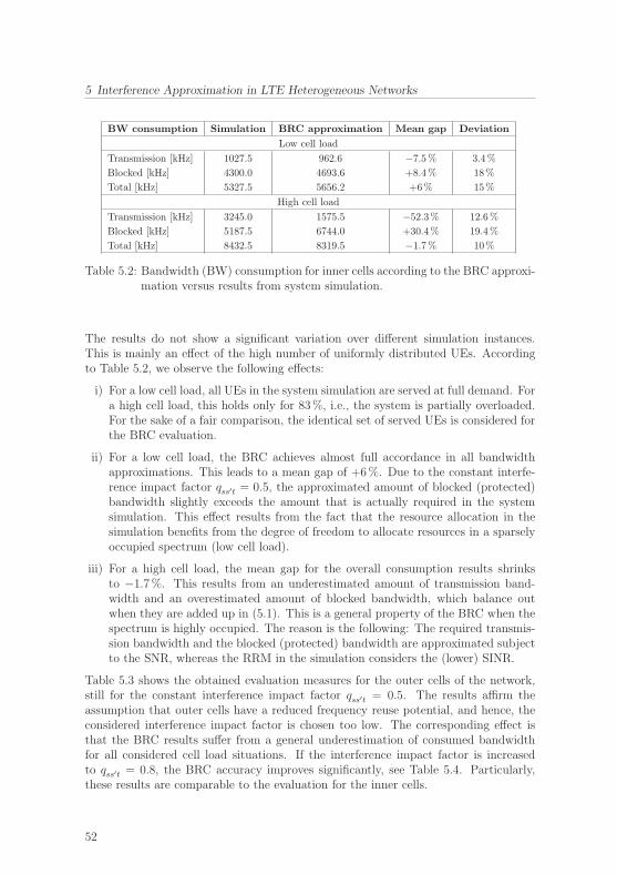
5 Interference Approximation in LTE Heterogeneous Networks
BW consumption Simulation BRC approximation Mean gap Deviation
Low cell load
Transmission [kHz] 1027.5 962.6 −7.5% 3.4%
Blocked [kHz] 4300.0 4693.6 +8.4% 18%
Total [kHz] 5327.5 5656.2 +6% 15%
High cell load
Transmission [kHz] 3245.0 1575.5 −52.3% 12.6%
Blocked [kHz] 5187.5 6744.0 +30.4% 19.4%
Total [kHz] 8432.5 8319.5 −1.7% 10%
Table 5.2: Bandwidth (BW) consumption for inner cells according to the BRC approxi-mation versus results from system simulation.
The results do not show a significant variation over different simulation instances.This is mainly an effect of the high number of uniformly distributed UEs. Accordingto Table 5.2, we observe the following effects:
i) For a low cell load, all UEs in the system simulation are served at full demand. Fora high cell load, this holds only for 83%, i.e., the system is partially overloaded.For the sake of a fair comparison, the identical set of served UEs is considered forthe BRC evaluation.
ii) For a low cell load, the BRC achieves almost full accordance in all bandwidthapproximations. This leads to a mean gap of +6%. Due to the constant interfe-rence impact factor qss′t = 0.5, the approximated amount of blocked (protected)bandwidth slightly exceeds the amount that is actually required in the systemsimulation. This effect results from the fact that the resource allocation in thesimulation benefits from the degree of freedom to allocate resources in a sparselyoccupied spectrum (low cell load).
iii) For a high cell load, the mean gap for the overall consumption results shrinksto −1.7%. This results from an underestimated amount of transmission band-width and an overestimated amount of blocked bandwidth, which balance outwhen they are added up in (5.1). This is a general property of the BRC when thespectrum is highly occupied. The reason is the following: The required transmis-sion bandwidth and the blocked (protected) bandwidth are approximated subjectto the SNR, whereas the RRM in the simulation considers the (lower) SINR.
Table 5.3 shows the obtained evaluation measures for the outer cells of the network,still for the constant interference impact factor qss′t = 0.5. The results affirm theassumption that outer cells have a reduced frequency reuse potential, and hence, theconsidered interference impact factor is chosen too low. The corresponding effect isthat the BRC results suffer from a general underestimation of consumed bandwidthfor all considered cell load situations. If the interference impact factor is increasedto qss′t = 0.8, the BRC accuracy improves significantly, see Table 5.4. Particularly,these results are comparable to the evaluation for the inner cells.
52

5.3 Numerical Evaluation
BW consumption Simulation BRC approximation Mean gap Deviation
Low cell load
Transmission [kHz] 1107.9 1020.3 −8% 1.4%
Blocked [kHz] 3932.1 2100.6 −46.5% 3.2%
Total [kHz] 5040.0 3120.9 −38.5% 4.9%
High cell load
Transmission [kHz] 2637.9 1682.7 −36.2% 16.2%
Blocked [kHz] 3865.7 2926.5 −21.1% 16.3%
Total [kHz] 6503.6 4609.2 −27.6% 13.2%
Table 5.3: Bandwidth (BW) consumption for outer cells according to the BRC approxi-mation versus results from system simulation.
BW consumption Simulation BRC approximation Mean gap Deviation
Low cell load
Transmission [kHz] 1107.9 1020.3 −8% 1.4%
Blocked [kHz] 3932.1 3360.9 −14.4% 5.1%
Total [kHz] 5040.0 4381.2 −13% 4%
High cell load
Transmission [kHz] 2637.9 1682.7 −36.2% 16.2%
Blocked [kHz] 3865.7 4682.4 +26.3% 26%
Total [kHz] 6503.6 6365.1 −2.1% 15%
Table 5.4: Bandwidth (BW) consumption for outer cells according to the BRC approxi-mation for qss′t = 0.8 versus results from system simulation.
Overall, the evaluation results show that the BRC and its immanent IAM are suitableapproximation models to describe the bandwidth consumption in cellular LTE systemssubject to interference. The BRC results can be influenced by an adaption of the ap-proximation parameters, i.e., the interference impact factors. This property allows fora calibration of the approximation model with respect to the RRM components of theconsidered system. In Section 7.1.2, we present an approach for adaptive BRC (IAM)parameter calibration with respect to dynamic system measurements. An accordingparameter calibration over several simulation instances of the static network scenariofrom above leads to
βINNERs ∈ [0.4, 0.5] , βOUTER
s ∈ [0.8, 0.9] , (5.7)
where we still assume est/es′t ≈ 1, i.e., qss′t ≈ βs, compare (5.6).
53

5 Interference Approximation in LTE Heterogeneous Networks
5.4 Summary
User assignment and resource allocation in multicell networks are typically carried outsubject to the SINR in the system. In LTE heterogeneous networks, these tasks haveadditionally to consider cross-tier interference between macrocells and femtocells thattransmit in the same spectrum. SINR-based decision problems have no linear repre-sentation, and hence, cannot be integrated into the MIP-based network optimizationmodels that we develop. Therefore, we have introduced an approximate model thatestimates the overall required bandwidth at eNBs and HeNBs with respect to the SNRin the system. The underlying principle of the corresponding bandwidth reservationconcept (BRC) is to compute the required transmission bandwidth separately fromthe bandwidth that is blocked to mitigate interference to other cells. Both terms arecomputed subject to the SNR on the related radio links.
The interference approximation model (IAM) considers inter-cell interference as wellas cross-tier interference. The cross-tier interference is modeled by the maximum con-sumed bandwidth at interfered femtocells, see (5.4). The related maximum operatorcan be transformed into a linear representation for any MIP formulated optimizationproblem. The linear representation requires one additional optimization variable andone additional constraint in the MIP.
In the following chapters, the BRC and the IAM serve as integral components of theMIP-based models that we develop for the optimization of LTE HetNets.
54
6 Cell Site Planning of LTEHeterogeneous Networks
In contrast to the network dimensioning approach presented in Chapter 4, cell siteplanning aims at the precise selection of base station locations and at the initial down-tilt configuration of the related antennas. For the optimal cell site planning of LTEheterogeneous networks, we consider macrocell sites and and user-deployed femtocellsthat are not necessarily active all the time. The objective of the planning task is toprovide a minimum number of macrocell sites such that mobile services are area-wideavailable. On the other hand, the deployment of dispensable cell sites has to be avoidedfor the sake of cost efficiency and low interference. The availability of mobile services isrelated to the network coverage, whereas the support of high rate services depends onthe achievable network capacity. Hence, both KPIs are distinguished in the objectivefunction of the corresponding planning problem in Section 6.2.
The economically motivated approach for multiple objective alignment from Section 4.2is applied to deal with the trade-off between the conflicting objectives of the MOOproblem. Instead of avoiding interference by minimum distance constraints, the in-terference approximation model from the previous chapter is utilized to incorporateinter-cell and cross-tier interference efficiently into the optimization model.
At the end of this chapter, we apply the developed optimization approach to a repre-sentative LTE HetNet planning scenario. The obtained results define the referenceHetNet that is considered in Chapter 7 for the self-optimization of coverage and ca-pacity.
6.1 System Model
We consider a multi-tier LTE HetNet according to the system model from Section 5.1.The system is supposed to apply interference mitigation – or any other comparablemethod – as ICIC technique.
The demand node (DN) model from Section 3.3 is applied to abstract from single users.Rate computation and bandwidth allocation for downlink transmission from eNBs andHeNBs to DNs are carried out according to Section 3.2. The planning model selectseNBs from the candidate set S for deployment. The selection depends on the inputparameters and the optimization variables from Section 1.3 as well as on the additionalparameters and variables that are given in Table 6.1.
55

6 Cell Site Planning of LTE Heterogeneous Networks
Symbol & domain Description
cs ∈ R≥0 eNB deployment cost.
ρf ∈ [0, 1] Average HeNB activity rate.
pt ∈ R>0DN priority level, related to either the DN service type or thecorresponding customer type.
λRATE ∈ R≥0 Sum rate weighting factor for objective scalarization.
λBASIC ∈ R≥0 Basic coverage weighting factor for objective scalarization.
eMIN, eMAX ∈ R>0Minimum required spectral efficiency for transmission (LTE:CQI 1) and maximally achievable spectral efficiency (CQI 15).
GConflict graph, containing all pairs of eNB deployment candi-dates that correspond to the same cell site but apply differentantenna configurations.
a Wildcard symbol for either an eNB s or an HeNB f .
qaa′t ∈ [0, 1]Interference impact factor from (H)eNB a to the transmissionlink from (H)eNB a′ to t.
bitfa ∈ R≥0Auxiliary variable describing the amount of protected band-width at (H)eNB a.
ba ∈ R≥0Auxiliary variable describing the amount of overall consumedbandwidth (transmission plus protected) at (H)eNB a.
Table 6.1: Additional input parameters (upper part) and variables (lower part) for cellsite planning in LTE HetNets, complementing Table 1.1.
Network coverage and network capacity are distinguished in the objective function inorder to obtain deployment solutions that guarantee area-wide mobile services andthat support high data rates in demand hotspots. The corresponding objectives areweighted with the factors λBASIC and λRATE to implement the scalarization approachfrom Section 2.3.1. This is done in analogy to (4.3). We introduce priority levelparameters pt to allow for prioritization of DN coverage. While the data rate is relatedto the requested service, the priority level can correspond to either the service classor the customer type. For instance, voice services (VoIP) might have a higher prioritythan data services or business clients may be favored over private customers.
Every macrocell site can apply different antenna configurations, i.e., the initial antennadowntilt has to be chosen for every deployed eNB. Each configuration of an eNB isconsidered as a separate deployment candidate in S. The joint deployment of overlap-ping candidates is avoided by adding all pairs of different configurations of the sameeNB to the conflict graph G. The deployment of a macrocell site s is associated withcost cs, whereas femtocell equipment is purchased by users and, in that sense, free ofcharge for the network operator. This also means that the operator cannot influencewhere HeNBs are deployed and when they are activated by the users. However, we
56
6.2 Optimization Model
assume that the network operator knows at least the distribution of potential femtocelllocations as well as the average activity rates ρf .
The interference approximation model from Chapter 5 is utilized to estimate theamount of protected (blocked) bandwidth bitfa and the amount of overall consumedbandwidth ba for each (H)eNB a.
6.2 Optimization Model
We introduce the MIP from Table 6.2 to formalize the following optimization problem:Given the set F of potentially active femtocells and given the rate demand distribution,modeled by the set T of DNs. Which eNBs from the set S of candidates shall beselected for deployment in order to cover and serve the DNs optimally?
The sets
S ∗ T = {(s, t) ∈ S × T : est ≥ eMIN} ,St = {s ∈ S : (s, t) ∈ S ∗ T } , Ts = {t ∈ T : (s, t) ∈ S ∗ T } ,
F ∗ T = {(f, t) ∈ F × T : eft ≥ eMIN} ,Ft = {f ∈ F : (f, t) ∈ F ∗ T } , Tf = {t ∈ T : (f, t) ∈ F ∗ T } ,Fs = {f ∈ F : esf ≥ eMIN}
are defined to exclude decision variables and constraints that are irrelevant due toinsufficient link quality. We consider the optimization problem
max
{λBASIC
∑t∈T
ptzt︸ ︷︷ ︸coverage
+λRATE
∑t∈T
refft︸ ︷︷ ︸capacity
−∑s∈S
csys︸ ︷︷ ︸cost
}(6.1)
with respect to the optimization variables ys, zst, zft, bst, bft and the auxiliary vari-
ables zt, bf , bitfs , r
efft in order to answer the initial question from above. Compared to
the objective function of the dimensioning approach (4.3), network coverage and net-work capacity are distinguished by separate terms. The sum of covered priorities isconsidered as HetNet coverage and the effectively served sum rate models the Het-Net capacity. DNs with an infinitesimal rate demand rt may serve as pure coveragepoints. DNs with a high rate demand are relevant for the coverage term in (6.1) as wellas for the capacity component. The conflicting objectives of the MMO problem arealigned into one scalar-valued objective according to the economically motivated ap-proach from Section 4.2. The corresponding weighting factors (exchange rates) λBASIC
and λRATE are chosen as ARPU over the considered time period. Thus, optimal solu-tions for (6.1) define a cell site deployment – and initial antenna configuration – forHetNet Profit MAXimization (HetNet-ProMAX) in a techno-economical sense.
57

6 Cell Site Planning of LTE Heterogeneous Networks
max
{λBASIC
∑t∈T
ptzt + λRATE∑t∈T
refft − ∑s∈S
csys
}subject to
zt =∑s∈St
zst ≤ 1 , for all t ∈ T
zst ≤ ys , for all (s, t) ∈ S ∗ Tys + ys′ ≤ 1 , for all (s, s′) ∈ G∑f∈Ft
zft ≤ zt , for all t ∈ T
bft ≤rteft
zft , for all (f, t) ∈ F ∗ T
bf =∑t∈Tf
bft +∑
(f ′, t) ∈ F ∗ T ,
f ′ �= f
qff ′tbf ′t ≤ ρfBf , for all f ∈ F
bst ≤rtzt−
∑
f∈Ft
eftbft
est, for all (s, t) ∈ S ∗ T
bst ≤ Bszst , for all (s, t) ∈ S ∗ Trefft =
∑s∈St
estbst +∑
f∈Ft
eftbft ≥ rMINt zt , for all t ∈ T
bitfs =∑
(s′, t) ∈ S ∗ T ,
s′ �= s
qss′tbs′t +maxf∈Fs
{esf
eMAXbf
}, for all s ∈ S
∑t∈Ts
bst + bitfs ≤ Bs + (1− ys) · ∞ , for all s ∈ S
Table 6.2: MIP formulation of the profit maximization problem for techno-economicalLTE HetHet deployment (HetNet-ProMAX).
The maximization in (6.1) is carried out subject to the following constraints. Theinequality
zt =∑s∈St
zst ≤ 1 , for all t ∈ T (6.2)
ensures that DNs are assigned to at most one eNB. The variable zt indicates whetherDN t is assigned (covered) or not. Moreover, this constraint defines coverage as coveredby an eNB, i.e., the basic HetNet coverage does not depend on any femtocell activity.According to the inequalities
zst ≤ ys , for all (s, t) ∈ S ∗ T (6.3)
ys + ys′ ≤ 1 , for all (s, s′) ∈ G (6.4)
58
6.2 Optimization Model
only deployed eNBs are available for DN assignment and the joint deployment of con-flicting eNBs is not allowed. Here, the conflict graph G contains all pairs of eNBdeployment candidates that correspond to the same cell site but apply different an-tenna configurations. Each different (initial) antenna configuration of a cell site is aseparate element in the candidate set S. The main effect of switching the antenna con-figuration of a cell site is a change of the spatial signal power distribution. Thus, therelated spectral efficiency parameters can differ significantly over the available antennaconfigurations.
We assume that the location of each potentially active femtocell f ∈ F is known.Furthermore, we assume estimations for their activity rate ρf ∈ [0, 1]. The followingprinciples are applied to deal with the uncertainty of FC activity. First, femtocells areexcluded from contributing to the basic HetNet coverage. And further:
1. HeNBs can (partially) take over rate demand of DNs. These DNs have to beassigned to eNBs. This models the opportunity that users can be served byfemtocells in the operating system.
2. The available bandwidth at HeNBs is scaled down proportionally to their activityrate.
These principles are modeled by∑f∈Ft
zft ≤ zt , for all t ∈ T (6.5)
bft ≤rteftzft , for all (f, t) ∈ F ∗ T (6.6)
bf =∑t∈Tf
bft +∑
(f ′, t) ∈ F ∗ T ,f ′ �= f
qff ′tbf ′t ≤ ρfBf , for all f ∈ F (6.7)
where (6.5) ensures that only DNs which are covered by an eNB can be served by atmost one HeNB. Constraint (6.6) follows from (3.7) and the inequality (6.7) boundsthe approximated bandwidth consumption bf at HeNBs to the (scaled) maximumbandwidth. The bandwidth consumption is approximated by the BRC and the IAMaccording to (5.1) and (5.5).
Optionally, an additional bandwidth buffer might be considered in order to cope withunexpected inter-FC and cross-tier interference. A reasonable buffer can be obtainedby a replacement of the interference term in (6.7) with∑
(f ′, t) ∈ F ∗ T ,f ′ �= f
qff ′trteftzf ′t .
By this replacement, all interfered FC transmission links are considered with fullyserved rate demand even though the actual transmission rate can be lower, see (6.6).
59
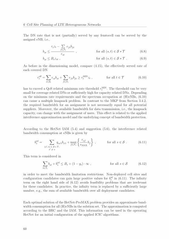
6 Cell Site Planning of LTE Heterogeneous Networks
The DN rate that is not (partially) served by any femtocell can be served by theassigned eNB, i.e.,
bst ≤rtzt −
∑f∈Ft
eftbft
est, for all (s, t) ∈ S ∗ T (6.8)
bst ≤ Bszst , for all (s, t) ∈ S ∗ T . (6.9)
As before in the dimensioning model, compare (4.15), the effectively served rate ofeach covered DN
refft =∑s∈St
estbst +∑f∈Ft
eftbft ≥ rMINt zt , for all t ∈ T (6.10)
has to exceed a QoS related minimum rate threshold rMINt . The threshold can be very
small for coverage related DNs or sufficiently high for capacity related DNs. Dependingon the minimum rate requirements and the spectrum occupation at (H)eNBs, (6.10)can cause a multiple knapsack problem. In contrast to the MKP from Section 3.4.2,the required bandwidth for an assignment is not necessarily equal for all potentialsuppliers. Moreover, the available bandwidth for data transmission, i.e., the knapsackcapacity, can change with the assignment of users. This effect is related to the appliedinterference approximation model and the underlying concept of bandwidth protection.
According to the HetNet IAM (5.4) and suggestion (5.6), the interference relatedbandwidth consumption at eNBs is given by
bitfs =∑
(s′, t) ∈ S ∗ T ,s′ �= s
qss′tbs′t +maxf∈Fs
{esfeMAX
bf
}, for all s ∈ S . (6.11)
This term is considered in∑t∈Ts
bst + bitfs ≤ Bs + (1− ys) · ∞ , for all s ∈ S (6.12)
in order to meet the bandwidth limitation restrictions. Non-deployed cell sites andconfiguration candidates can gain large positive values for bitfs in (6.11). The infinityterm on the right hand side of (6.12) avoids feasibility problems that are irrelevantfor these candidates. In practice, the infinity term is replaced by a sufficiently largenumber, e.g., the sum of available bandwidth over all deployment candidates.
Each optimal solution of the HetNet-ProMAX problem provides an approximate band-width consumption for all (H)eNBs in the solution set. The approximation is computedaccording to the BRC and the IAM. This information can be used in the operatingHetNet for an initial configuration of the applied ICIC algorithms.
60
6.3 Numerical Evaluation
6.3 Numerical Evaluation
Table 6.3 shows the parameter setup for planning eNB cell sites and their initialantenna downtilt configuration in an urban LTE HetNet scenario. Figure 6.1 (b)depicts the 60 potential eNB site locations as (red) dots. The building data is takenfrom [31]. Since the cell site planning is carried out with respect to effects that takeplace on a long-term scale, we assume average values for volatile system parameterssuch as transmit power and shadowing. An omnidirectional antenna pattern and twosupported downtilt configurations are considered for the antenna configuration of eacheNB. Thus, the set S contains 120 different deployment candidates and the conflictgraph G contains 60 eNB pairs. Figure 6.1 (a) illustrates the effect of switching theantenna downtilt for an exemplary eNB: The signal strength at short distance increaseswith a higher downtilt but at the cost of a shrinking cell footprint. Please note thatwe use the highly accurate ray optical path loss model from Section 3.1.2 to computethe spatial signal power distribution for each eNB deployment candidate. The signalpower distribution for (indoor) HeNBs is obtained by applying a free space path lossmodel as introduced at the beginning of Section 3.1. The signal power informationis precomputed prior to the optimization task. The spectral efficiency parameters arederived from the discrete rate-power function according to (3.8) and the LTE SINRrequirements defined in Table 6.4.
The eNB operational expenses (OPEX) of 1800 e per month cover site rental, leasedline rental, air-conditioning, and maintenance [33]. The investment costs (CAPEX)for eNB deployment are neglected analogously to the network dimensioning approach,see Section 4.3 for details. Contrarily to eNB deployment, user-deployed femtocells donot cause any expenses for the network operator. Nevertheless, they can contribute tothe HetNet performance when the corresponding HeNBs are active. We consider anHeNB activity rate of ρf = 50% and a transmit power of 3 dBm. Femtocells operatein the same transmission spectrum as eNBs. We uniformly distribute 400 HeNBs atrandom over the round about 2000 buildings in the planning area. HeNBs are locatedonly indoors.
The constant DN rate demand of 320 kbps results from an aggregation of service-related average rates. Each DN t has the priority pt = 1 and a minimum rate re-quirement rMIN
t = rt. The 750 DNs are uniformly distributed over the city area atrandom. We apply cell site planning for 50% and 80% indoor DNs. The scalariza-tion parameters λBASIC = 50e and λRATE = 0.5 e/kbps transfer objective (6.1) intothe techno-economical domain of monthly profit for the network operator. The basicfee λBASIC covers the monthly basic charges, the fees for basic services (sms, voice),and all extra fees (flatrates, special options, etc.) for the DN related users. The ratefee λRATE denotes the charge per transmitted data unit.
We assume the interference impact factor qss′ = 1/3 for all eNBs and qsf = 1 for allinterfered HeNB transmissions, compare (5.3) and (5.6). The low impact factor forinter-macrocell interference is motivated by the fact that all eNB deployment candi-dates have a large resource reuse potential: First, the cell density is typically veryhigh in urban areas. Therefore, there are many neighboring cells that allow for a reuse
61

6 Cell Site Planning of LTE Heterogeneous Networks
System parameter Setting
Planning area Urban, 2.5 km × 3.5 km, 5m resolution
Number of buildings Approximately 2000
Wall penetration loss 10 dB
Shadowing standard deviation 8 dB
Carrier frequency 2GHz
Transmission bandwidth 10MHz
Number of eNB (macrocell site) locationcandidates
60
eNB antenna downtilt profile {0◦ (low), 5◦ (high)}eNB Tx power 43 dBm
Propagation model eNB Ray optical, omnidirectional
eNB antenna gain and noise figure 14 dBi and 5 dB
Number of HeNBs (femtocells) 400
HeNB distribution Random, uniformly distributed over buildings
Minimum distance HeNB to eNB 35m
HeNB activity rate 50%
HeNB Tx power 3 dBm
Propagation model HeNB Free space + wall penetration, omnidirectional
Noise figure HeNB 8dB
Number of DNs 750
Indoor DNs 50% and 80%
DN rate demand 320 kbps
DN antenna gain and noise figure 0 dBi and 9 dB
Table 6.3: Considered system parameters for HetNet deployment.
of (blocked) bandwidth. And second, the signal propagation in urban environmentsleads to further reuse candidates that are not located nearby, see Figure 6.1 (c) for anillustration. This enables the reuse option also for the outer cells in the network.
The HetNet-ProMAX problem is solved by utilizing the Gurobi Optimizer [48]. Theobtained results are summarized in Table 6.5 and Figure 6.1 (b) illustrates the deploy-ment solution for 80% indoor DNs. The 12 optimally deployed eNBs of the HetNetsolution are marked by circles, whereas the 19 eNBs from the alternative single-tiersolution are framed by squares. Moreover, Figure 6.1 (c) shows the best server plot forthe corresponding HetNet macrocells. Light gray areas indicate that the SNR valuesfrom different eNBs do not differ more than 2 dB, i.e., such areas indicate potentialhandover zones .
The eNBs in the single-tier solution and the deployed eNBs in the HetNet cover almostthe same number of DNs and serve a similar amount of requested data rate. Pleasenote that indoor DNs are served by eNBs if no femtocells are available. The number ofdeployed eNBs in the HetNet is reduced by 37% due to the availability of femtocells.In fact, half of the served data rate in the HetNet is covered by femtocells. Figure 6.2illustrates how HeNBs improve the network capacity: They either provide higher sig-nal strength in low power macrocell regions (blue) or they serve DNs in medium power
62

6.3 Numerical Evaluation
CQI Modulation Code rate Spectral efficiency [bps/Hz] Receiver SINR [dB]
0 out of range
1 QPSK 1/8 0.25 −5.1
2 QPSK 1/5 0.40 −2.9
3 QPSK 1/4 0.50 −1.7
4 QPSK 1/3 0.66 −1.0
5 QPSK 1/2 1.00 2.0
6 QPSK 2/3 1.33 4.3
7 QPSK 3/4 1.50 5.5
8 QPSK 4/5 1.60 6.2
9 16-QAM 1/2 2.00 7.9
10 16-QAM 2/3 2.66 11.3
11 16-QAM 3/4 3.00 12.2
12 16-QAM 4/5 3.20 12.8
13 64-QAM 2/3 4.00 15.3
14 64-QAM 3/4 4.50 17.5
15 64-QAM 4/5 4.80 18.6
Table 6.4: LTE SINR requirements according to [94] for 10MHz transmission band-width and BLER = 10−1.
(a) eNB applying 0◦ (top)and 5◦ (below) antennadowntilt.
(b) Candidate sites (dots) anddeployed eNBs in the HetNet(circles) and the single-tier so-lution (squares).
(c) Best server plot for the eNBrelated macrocells in the HetNetdeployment solution.
Figure 6.1: Considered planning area and deployment solution for 80% indoor DNs .
macrocell regions (green) to lower the eNB load. Following from the IAM estimations,eNBs have to block on average 13% of the spectrum in order to mitigate cross-tierinterference. Combined with the bandwidth that is blocked due to inter-macrocellinterference, eNBs utilize on average round about half of the spectrum for transmis-sion and the other half for ICIC. Most of the deployed single-tier eNBs (85%) apply
63

6 Cell Site Planning of LTE Heterogeneous Networks
Single-tier HetNet
80% indoor DNs
Number of deployed eNBs 19 12
Rate served by eNBs [%] 100 50
Average transmission bandwidth ateNBs according to BRC [kHz]
5155 5630
Average protected bandwidth at eNBs(MC + FC) according to IAM [kHz]
3975 + 0 3070 + 1300
Runtime [h] 6.5 259
50% indoor DNs
Number of deployed eNBs 17 11
Rate served by eNBs [%] 100 52
Average transmission bandwidth ateNBs according to BRC [kHz]
4930 5530
Average protected bandwidth at eNBs(MC + FC) according to IAM [kHz]
4400 + 0 3170 + 1300
Runtime [h] 12 181
Table 6.5: Result statistics for two different indoor DN ratios and two different networktopologies.
the higher antenna downtilt, whereas most eNBs in the HetNet solution select a lowantenna downtilt. The dense single-tier cell deployment might be interpreted as analternative solution to the HetNet topology.
By solving the HetNet-ProMAX problem for 50% indoor DNs, we investigate its sen-sitivity to the indoor DN ratio. The corresponding results are shown in the lower partof Table 6.5. It turns out that the relative results for the single-tier solution and theHetNet solution are roughly the same as for 80% indoor DNs. However, the totalnumber of required eNBs decreases slightly as the signal power from eNBs to outdoorusers is generally higher.
Since the spectrum of the deployed HetNet eNBs is highly occupied, inactive femtocellscan barely be compensated. As a consequence, the HeNB activity rate is a veryimportant parameter that should not be overestimated.
The runtime to solve the HetNet problem is more than one magnitude higher as theruntime for computing an optimal single-tier solution. This holds for both evaluationvariants. Mainly two reasons cause this effect: First, the lower number of possibletransmitter-to-DN assignments reduces the size of the single-tier problem instance.And second, the trade-off between revenue and cost is more difficult to assess for aneNB deployment candidate in the HetNet than in the single-tier network. Particularly,there can exist alternative solutions where DNs that are served by a single eNB canalso be served by a combination of another eNB and HeNB.
64

6.4 Summary
Figure 6.2: Signal strength distribution for a deployed eNB (large circle) and multipleHeNBs (small circular areas).
6.4 Summary
Most of the related work in the context of LTE HetNet deployment addresses per-formance improvement and flexibility gain when a single-tier network is switched toa multi-tier topology [81]. Some works consider the planning of femtocells and piconodes. However, in most cases the planning is carried out either subject to an existingmacrocell environment [56] or it ignores the macrocell tier at all [67].
Our approach deals with the problem of planning cell sites and their initial con-figuration jointly over both network tiers. Particularly, it takes the correspondingresource allocation into account. Macrocells are selected for deployment subject touser-deployed femtocells that are not necessarily active all the time. The interferenceapproximation model from Chapter 5 is integrated into the optimization problem inorder to incorporate inter-cell and co-channel interference. Although not mentionedexplicitly, pico nodes can be modeled in our planning approach as low capability eNBs.These nodes might support lower power ranges or have fixed antenna configurations.
Numerical evaluation results demonstrate the feasibility of our optimization approach(HetNet-ProMAX) for the purpose of cell site planning of heterogeneous LTE networks.The HetNet planning solution for 80% indoor DNs serves as reference network in thefollowing chapter, where we present an approach for the autonomous self-control ofcell parameters subject to coverage and capacity optimization.
65


7 Self-Optimization of Coverage andCapacity
In this chapter, we develop an approach for closed-loop, autonomous self-optimizationof coverage and capacity [85] in operating heterogeneous LTE networks. Autonomousself-optimization means that there is no need for any human intervention once theoptimization parameters have been initially specified. According to [8], this feature isone of the essential 3GPP requirements for self-organizing networks . It is a prerequisiteto benefit maximally from the opportunities that self-organization provides to minimizeOPEX and operational effort.
Self-organized Coverage and Capacity Optimization (CCO) considers the online con-figuration of existing transmitters in an operating network. It is the consecutive stepto network dimensioning and cell site planning in the system lifecycle. All CCO re-lated procedures have to be aligned with the existing network operation components.The optimization task is carried out subject to the dynamically changing network situ-ation. Overall, this leads to a network operation paradigm where network elementsautonomously configure themselves at certain time instances, and the configurationtakes the expected network situation of the next operation cycle into account. An ope-ration cycle denotes the time interval before the next self-configuration is triggered.
The cell site planning results from Section 6.3 (80% indoor DNs) serve as referencenetwork in this chapter, see Figure 7.1. We introduce the corresponding HetNet model,its operation components, and the automatic adaption of dynamic system parametersin Section 7.1. At a first glance, Figure 7.1 (a) suggests a smooth macrocell topology.Figure 7.1 (b), however, illustrates that we have to keep in mind that the interference-related interdependencies between cells can be very strong and spatially diverse. Thesystem performance measures defined in Section 7.2 serve as assessment criteria for theresults of joint coverage and capacity maximization in Section 7.3. The correspondingoptimization model is embedded into a traffic-light based network operation scheme inSection 7.4. The integrated CCO approach autonomously controls transmission power,antenna tilt, and activity status (switch on/off) of the network elements. The evalu-ation in Section 7.5 investigates achievable performance improvements and illustratesthe underlying principles of our CCO approach.
This chapter extends the work presented in [39].
67

7 Self-Optimization of Coverage and Capacity
1
2
3
4
5
6
7
89
10
11
12
(a) 12 initial macrocells, light gray ar-eas indicate potential handover zones(best server difference ≤ 2 dB).
(b) Signal strength distribution ofeNB 12, FCs (red dots), UEs (greendots), and hotspot (bunch of spots).
Figure 7.1: Considered urban reference HetNet, resulting from the HetNet cell siteplanning presented in Section 6.3.
7.1 System Model
We basically consider the HetNet system model from Section 5.1. In the following, thisspecification is extended by the components that are missing to model the operatingsystem and to implement self-organized CCO.
Self-organized CCO requires coordination and information exchange between transmit-ters in certain situations. The following components enable the related communicationbetween network elements: HeNBs are connected to the backhaul – in most cases viaDSL – which generally allows for centralized optimization of femtocells. However, thecoordination between HeNBs and eNBs can only take place at coarse time scales, e.g.,tens of frames, but not at the granularity of every frame [98]. This is not a crucialdrawback for our purposes because the time interval between any two consecutiveCCO executions is sufficiently long. Communication between eNBs is supported bythe X2 interface [12] (direct interconnection) and the S1 interface [11] via backbone(indirect interconnection). HeNB to (H)eNB information exchange and coordinationcan utilize the Type 1 interface via the HeNB Management System (HeMS) [9]. Thecommunication between (H)eNBs and UEs follows several signaling schemes that aredefined for dedicated control channels: The Physical Downlink Control CHannel (PD-CCH) is used for UE-specific information and the Physical Uplink Control CHannel(PUCCH) carries, for instance, the CQI information. Overall, we assume fully meshedcommunication capabilities between all network elements.
68
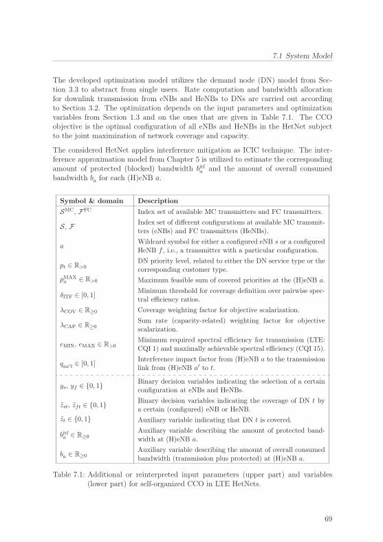
7.1 System Model
The developed optimization model utilizes the demand node (DN) model from Sec-tion 3.3 to abstract from single users. Rate computation and bandwidth allocationfor downlink transmission from eNBs and HeNBs to DNs are carried out accordingto Section 3.2. The optimization depends on the input parameters and optimizationvariables from Section 1.3 and on the ones that are given in Table 7.1. The CCOobjective is the optimal configuration of all eNBs and HeNBs in the HetNet subjectto the joint maximization of network coverage and capacity.
The considered HetNet applies interference mitigation as ICIC technique. The inter-ference approximation model from Chapter 5 is utilized to estimate the correspondingamount of protected (blocked) bandwidth bitfa and the amount of overall consumedbandwidth ba for each (H)eNB a.
Symbol & domain Description
SMC, FFC Index set of available MC transmitters and FC transmitters.
S, F Index set of different configurations at available MC transmit-ters (eNBs) and FC transmitters (HeNBs).
aWildcard symbol for either a configured eNB s or a configuredHeNB f , i.e., a transmitter with a particular configuration.
pt ∈ R>0DN priority level, related to either the DN service type or thecorresponding customer type.
pMAXa ∈ R>0 Maximum feasible sum of covered priorities at the (H)eNB a.
δITF ∈ [0, 1]Minimum threshold for coverage definition over pairwise spec-tral efficiency ratios.
λCOV ∈ R≥0 Coverage weighting factor for objective scalarization.
λCAP ∈ R≥0Sum rate (capacity-related) weighting factor for objectivescalarization.
eMIN, eMAX ∈ R>0Minimum required spectral efficiency for transmission (LTE:CQI 1) and maximally achievable spectral efficiency (CQI 15).
qaa′t ∈ [0, 1]Interference impact factor from (H)eNB a to the transmissionlink from (H)eNB a′ to t.
ys, yf ∈ {0, 1} Binary decision variables indicating the selection of a certainconfiguration at eNBs and HeNBs.
zst, zft ∈ {0, 1} Binary decision variables indicating the coverage of DN t bya certain (configured) eNB or HeNB.
zt ∈ {0, 1} Auxiliary variable indicating that DN t is covered.
bitfa ∈ R≥0Auxiliary variable describing the amount of protected band-width at (H)eNB a.
ba ∈ R≥0Auxiliary variable describing the amount of overall consumedbandwidth (transmission plus protected) at (H)eNB a.
Table 7.1: Additional or reinterpreted input parameters (upper part) and variables(lower part) for self-organized CCO in LTE HetNets.
69

7 Self-Optimization of Coverage and Capacity
The meaning of some variables that were introduced in previous chapters changeswhen network configuration is considered for the operational stage: The set S and theset F are now associated with the indices of all configurations that can be chosen ateNBs and HeNBs. The elements s and f are created in the configuration index sets Sand F for each configuration that is selectable for an MC transmitter (eNB) i ∈ SMC
and FC transmitter (HeNB) j ∈ FFC, respectively. The associated configurations areselected if ys and yf are equal to one. We denote the set of configuration indicesthat belong to the same eNB i ∈ SMC or HeNB j ∈ FFC as Yi and Yj, respectively.Thus, it is S =
⋃i∈SMC Yi and F =
⋃j∈FFC Yj. The eNB configuration state space
considers transmission power and antenna downtilt as control parameters, whereasHeNBs can only configure their transmission power. We ensure the selection of oneunique configuration for each HetNet transmitter by applying constraints∑
s∈Yi
ys = 1 , i ∈ SMC (exactly one configuration per eNB) (7.1)
∑f∈Yj
yf = 1 , j ∈ FFC (exactly one configuration per HeNB) . (7.2)
Since the association from a selected configuration to the related transmitter is unique,we use the notation transmitter or (H)eNB s ∈ S, f ∈ F , even though s and f justrefer to certain configurations. Furthermore, we use the wildcard symbol a ∈ S ∪ Ffor short notation whenever expressions are related to transmitters s ∈ S as well as totransmitters f ∈ F .
Compared to the previous chapter, we redefine the meaning of system coverage. Therelated variables are separated from those ones that refer to data transmission, i.e.,to system capacity. The decision variables zst, zft indicate which DN is covered bywhat (H)eNB. Coverage is defined by a minimum Signal-to-Interference Ratio (SIR)requirement subject to the threshold value δITF. The variables zst, zft are distinguishedfrom the decision variables zst, zft that describe the (H)eNB-to-DN assignment fordata transmission. The same holds for the binary coverage indicator variables zt andtheir counterparts zt that now strictly serve as capacity-related variables.
The maximum number of DN priorities that can be covered by a single transmitter isbounded since the resources at eNBs and HeNBs are limited. This shall prevent fromdegraded CCO solutions, where only a few transmitters are in charge of the whole pro-vided network coverage. Such solutions can lead to infeasible situations if all UEs thatare modeled by DNs become active at the same time. A reasonable maximum feasiblesum of covered priorities for an (H)eNB a can be obtained as follows. We assume anaverage priority pa that might be derived from (simulation) statistics. Furthermore, weconsider a coverage-related average rate rCOV and the bandwidth Ba that is availableat a on average. For an average spectral efficiency ea on the transmission links from ato arbitrary users, we suggest
pMAXa =
Ba earCOV
pa (7.3)
as an estimation for the maximum feasible sum of covered priorities.
70
7.1 System Model
The weighting factors λCOV and λCAP are introduced for the coverage term and thecapacity term in the CCO objective function. Several variants of the scalarizationapproach from Section 2.3.1 are applied in order to achieve Pareto optimal solution orto implement constrained single target maximization.
Although our optimization models utilize the DN model to abstract from single UEs,it is facilitating in some of the subsequent sections to interpret DNs as UEs. UEscan be located indoors or outdoors and have a time-varying rate demand and mobility.Indoor UEs move according to a random walk model and do not leave the building area,whereas outdoor UEs are either pedestrians or vehicles. Pedestrians move according toa random walk model and vehicles move along the roads following a random waypointmodel. The mobility models are defined more precisely in Section 7.5.1.
7.1.1 Radio Resource Management and Scheduling
We apply the following model to disregard the scheduling of PRBs over time fromour investigations. Consequently, the RRM can consider the tasks of admission con-trol, user assignment, PRB allocation, and interference mitigation independently overconsecutive time instances.
Typically, the RRM assigns available PRBs to UEs such that the UE rate demandsare fulfilled. However, UEs with a low rate demand may not require a full PRB forthe whole assignment period but need one PRB at some time instances. In practicalLTE systems, the multiple usage of identical PRBs over time is implemented by anaccording scheduling algorithm. We model this scheduling in the time domain by anequivalent scheduling in the frequency domain. More precisely, we allow a separateallocation of SCs over the assignment period, and hence, consider a finer granularity inthe frequency domain as usually supported. This approach is motivated exemplarilyin Figure 7.2, where we assume that serving UE 1 requires the allocation of 45 kHztransmission bandwidth. This is realized by an assignment of every fourth PRB,where T describes the smallest time interval before a PRB reallocation is possible. Wetransform this scheduling over time into an assignment in the frequency domain suchthat UE 1 gets the first, fifth, and ninth subcarrier instead of the first, fifth, and ninthPRB. This assignment is equivalently realizable in the time domain for choosing theassignment period as T ′ = 12T . The period T ′ is assumed to be sufficiently small suchthat the channel conditions do not change (significantly) over T ′.
The RRM tasks are decoupled for consecutive time instances as described above. Ateach time instance, the following procedures are carried out successively:
1. (Initial cell assignment) First, all users in the system are initially assigned to thesupplier cell with the best pilot SINR. The SINR considers full interference inthe whole spectrum.
2. (User reassignment & drop users) In general, the user distribution is non-uniform,and therefore, most of the HetNet cells typically experience a different cell load.This fact can lead to overloaded cells, i.e., some users cannot be served sufficiently
71

7 Self-Optimization of Coverage and Capacity
Figure 7.2: Modeling the scheduling of PRBs over time by subcarrier allocation.
by their associated supplier cell. In such a situation, we try to reassign the usersthat cannot be served to neighboring cells which are not overloaded. Users thatrequire only a small amount of additional resources are preferred for the reassign-ment step. The user reassignment is repeated until there are no overloaded cellsanymore or if there are no further candidates for a reassignment. If there are noreassignment candidates left but there still exists an overloaded cell, some usersin that cell have to be dropped. The first iteration of this block does not considerinterference, whereas all subsequent calls take the current interference situationinto account.
3. (Resource protection) The considered system applies interference mitigation forICIC. Therefore, (some) neighboring cells can be asked to avoid the usage ofparticular resources, i.e., to protect (block) certain SCs in the spectrum. Thepotential benefit of a resource protection is assessed before sending the requestto the neighboring cells. This keeps the related communication overhead low.
4. (Resource allocation) The information from the preceding steps serves as inputfor the resource allocation step. The conditionally optimal resource allocationis performed for all cells in parallel. The parallel execution is possible since theresource assignment – for allocation and protection – is fixed at this stage. Ifit turns out that there does not exists any feasible allocation that supports therate requirements of all considered users, more users have to be reassigned ordropped in the second iteration step. All subsequent steps are repeated.
Please note that some systems might (re-)assign users to a supplier cell with respect toa load balancing strategy [96]. This strategy can be included into the second iterationstep.
72
7.1 System Model
7.1.2 Dynamic Parameter Adaption
In contrast to the relatively dense UE distribution that is typically considered fornetwork dimensioning and cell site planning, the UEs in the operating system canemerge locally bounded and very sparsely over the network area. Furthermore, theUE distribution and the rate demand distribution can change significantly over time.For instance, just a few UEs at night can turn into thousands of UEs during lunchtime. The spatial and temporal diversity of the UE distribution influences the inputparameters for our optimization approach. In particular, the DN information andthe frequency reuse factor, which predominantly determines the interference impactfactors for MCs in the IAM, see (5.3). Therefore, those input parameters have to beadapted dynamically and subject to the present – or near future – network situation.
Demand Node Parameters
According to the approach for DN generation from Section 3.3, we create a DN gridthat partitions the whole network area into a set of (non-equal) patches. The DN gridis computed for the scenario from Figure 7.1 prior to the optimization step. It remainsconstant throughout the whole system simulation.
Resulting from an initial patch length of 100m (quadratic), we obtain a total numberof |T | ≈ 2400 DNs. These DNs subdivide into outdoor DNs and indoor DNs byroughly one third and two-thirds, respectively. For each DN t ∈ T , we compute theexpected rate demand rt for the next operation cycle according to (3.9). Analogously,the expected amount of accumulated UE priorities pt is computed. Please note that wegenerate the DN information for the numerical evaluations in Section 7.5 with respectto identically repeated UE simulations. Consequently, we can assume a perfect trafficforecast with reliability indicator μ = 1 in (3.9).
Interference Approximation Parameters
We apply the following approach to calibrate the IAM parameters for all MCs in theHetNet subject to the DN information that we have obtained according to the previoussection. Please recall that we do not assume frequency reuse potential for FCs ,andhence, we do not have to calibrate any FC-related IAM parameters.
First, the implemented RRM algorithms compute the (average) bandwidth consump-tion components btrmRRM and bitfRRM for each MC subject to the considered DNs. This arethe reference consumption values that the system RRM achieves for the present trans-mitter configurations. Please note that these results depend on the particular RRMof the considered system. Thus, the presented approach allows for a system-specificcalibration of the IAM parameters.
Second, the (average) bandwidth consumption components btrmBRC and bitfBRC are com-puted according to the BRC equation (5.1). This step considers (3.7), (5.2), (5.3)with βs = 1, and the cell assignment from the RRM step.
73

7 Self-Optimization of Coverage and Capacity
The frequency reuse factor in (5.3) is estimated as
btrmBRC + βs bitfBRC
!= btrmRRM + bitfRRM ⇐⇒ βs =
btrmRRM + bitfRRM − btrmBRC
bitfBRC
(7.4)
with respect to the values btrmRRM, bitfRRM, b
trmBRC, b
itfBRC (> 0) for MC s. This estimation
particularly takes into account that an underestimation of blocked (protected) band-width can compensate an overestimated transmission bandwidth and vice versa. Thisproperty of the BRC was discussed in Section 5.3.
The consumption values might be provided by corresponding monitoring entities thathave logged the values in the previous operation cycle(s). This mechanism avoids thecomputation of consumption values from scratch. The logged information is sufficient ifwe assume a comparable system behavior for the next operation cycle. Furthermore,the estimated reuse factor for the present configuration s ∈ Yi of MC i ∈ SMC isassumed to hold for all configurations from Yi. Nevertheless, different configurationsstill yield different interference impact factors in the IAM since the ratio of spectralefficiencies in (5.3) changes with the reconfiguration of transmitters.
The parameter calibration according to (7.4) is exemplarily carried out in a dynamicnetwork simulation for the HetNet from Figure 7.1 – the simulation setup is discussedin detail in Section 7.5.1. We obtain estimation results that are consistent with theresults for the hexagonal network topology in Section 5.3: As illustrated by Figure 7.3,the outer MCs in the network, i.e., the cells 1, 5, 9 and 12, yield the high frequency reusefactors. According to the definition in (5.3), this corresponds to a low frequency reusepotential. On the other hand, the inner cells 4 and 10 yield the lowest frequency reusefactors for both considered configurations. Both effects are caused by the individualnumber of reuse neighbors and the particular UE distribution during the simulationperiod.
Overall, the average frequency reuse factors vary from 0.65 to 1.12. Please note that fre-quency reuse factors larger than one indicate strong compensation effects between btrmBRC
and bitfBRC due to the gap to SINR related bandwidth allocation. This can happen ifMCs are (almost) isolated from interfering neighbors. This is the case for the outerMC 12, where the eNB is shadowed towards the middle parts of the network areaby high buildings, compare Figure 7.1 (b). The estimated frequency reuse factor forMC 12 decreases significantly when the eNB is powered up in the second configurationand the interference situation gets stronger.
Generally, the bandwidth approximations according to the BRC and the IAM get moreaccurate the stronger the interference situation between neighboring cells is. This isnot a serious drawback since we are mostly interested in high cell load situations thattypically suffer from strong interference. On the other hand, neither interference norreconfiguration is a crucial matter if cells are only slightly loaded. Throughout theHetNet simulations in Section 7.5, we observe that the total bandwidth consumptionis approximated very accurately with deviations of less than 2% on average.
74
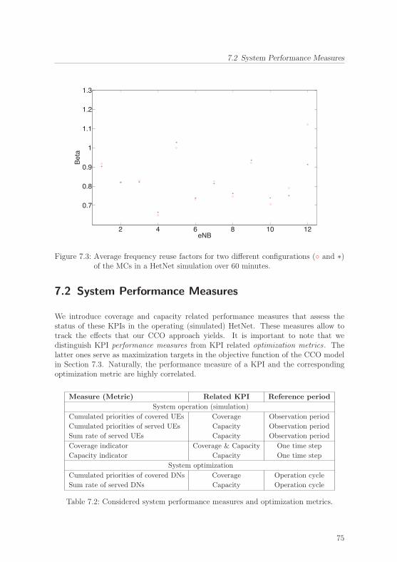
7.2 System Performance Measures
2 4 6 8 10 12
0.7
0.8
0.9
1
1.1
1.2
1.3
eNB
Bet
a
Figure 7.3: Average frequency reuse factors for two different configurations (◦ and ∗)of the MCs in a HetNet simulation over 60 minutes.
7.2 System Performance Measures
We introduce coverage and capacity related performance measures that assess thestatus of these KPIs in the operating (simulated) HetNet. These measures allow totrack the effects that our CCO approach yields. It is important to note that wedistinguish KPI performance measures from KPI related optimization metrics . Thelatter ones serve as maximization targets in the objective function of the CCO modelin Section 7.3. Naturally, the performance measure of a KPI and the correspondingoptimization metric are highly correlated.
Measure (Metric) Related KPI Reference period
System operation (simulation)
Cumulated priorities of covered UEs Coverage Observation period
Cumulated priorities of served UEs Capacity Observation period
Sum rate of served UEs Capacity Observation period
Coverage indicator Coverage & Capacity One time step
Capacity indicator Capacity One time step
System optimization
Cumulated priorities of covered DNs Coverage Operation cycle
Sum rate of served DNs Capacity Operation cycle
Table 7.2: Considered system performance measures and optimization metrics.
75
7 Self-Optimization of Coverage and Capacity
The considered KPI performance measures and optimization metrics are summarizedin Table 7.2. The measures refer either to the assessment of the related KPI status atone time step or they describe the KPI performance for the whole observation period.An observation period typically comprises one operation cycle. While the operationcycle that is considered for CCO takes place in the (near) future, an observed periodrefers to the time instances of the last operation cycle. Consequently, the effects of aCCO related (re-)configuration of the HetNet can be observed earliest at time instancesof the next operation cycle. The effects can be fully assessed at the end of the nextobservation period. The optimization metrics refer to a whole operation cycle since itis impractical to carry out the CCO procedure for every time instance.
All cells in the HetNet monitor the relevant network status information, e.g.,
• the number of served calls and the number of unattended calls,
• the data rate demand and the priority of each UE, and
• the allocated (utilized) and the blocked (protected) bandwidth.
7.2.1 Assessment of Network Coverage
The cumulated priorities of covered DNs∑t∈T
ptzt (7.5)
serve as optimization metric for network coverage. A DN is covered if the signal levelat its reference coordinate fulfills a minimum SINR requirement.
The cumulated priorities of covered UEs over the whole operation cycle serve as corres-ponding performance measure. The measure assesses the coverage performance overan observation period in the operating (simulated) system. Averaging the measureover the length (duration) of the observation period allows for a direct comparison ofthe obtained value with the optimization metric. Please recall that the DNs from theoptimization metric model average values for the considered operation cycle.
The following coverage indicator describes the coverage status at a certain time in-stance. It can be used to investigate the time-variant coverage performance duringsimulation. Since coverage is not directly measurable in the operating system, wedefine
no. of served calls
no. of served calls + no. of unattended calls(7.6)
as coverage indicator. In contrast to the coverage definition from before, an UE isdefined as covered if its call, i.e., its service related data rate demand, can be servedby any (H)eNB. Thus, the coverage indicator takes the actual user distribution intoaccount as well as the specific UE rate demands and the present resource allocation at(H)eNBs. The unattended calls comprise all UEs that experience an insufficient SINR(non-covered UEs) and the UEs that cannot be served due to a lack of available trans-mission bandwidth (non-served UEs). Due to the latter property, the indicator (7.6) is
76

7.2 System Performance Measures
also related to the system capacity, particularly in situations where the assessed cell isoverloaded. This ambiguity does not apply if (7.6) is evaluated over artificial coveragemeasurement UEs, i.e., UEs that request a minimal data rate and that have staticlocations in the network area.
7.2.2 Assessment of Network Capacity
The sum rate of served DNs ∑t∈T
refft , (7.7)
serves as optimization metric for the system capacity. A DN is served if the linkquality and the available resources at the associated (H)eNB are sufficient to provideat least a certain minimum data rate to the DN.
The sum rate of served UEs over the whole operation cycle serves as correspondingperformance measure. The measure assesses the capacity performance over an ob-servation period in the operating (simulated) system. Analogously to the coverageperformance measure from above, the capacity measure can be compared directly tothe optimization metric after averaging it over the observation period. The cumulatedpriorities of served UEs over the observation period might serve as an additional ca-pacity performance measure. This measure decreases if covered UEs cannot be serveddue to a lack of bandwidth for serving all users jointly. Particularly, the second mea-sure can help to resolve the ambiguity problems in the coverage performance measurefrom Section 7.2.1: If the capacity measure is smaller than the cumulated priorities ofcovered UEs it clearly indicates capacity problems.
Since the HetNet applies interference mitigation as ICIC technique, we distinguish thebandwidth that is allocatable (free) for serving users from bandwidth that is blocked(protected) to mitigate interference to other cells. Thus, the free bandwidth is givenby the difference between the total available transmission bandwidth and the blockedbandwidth. We define the ratio of the bandwidth that is utilized for serving users andthe free bandwidth as utilization ratio at an (H)eNB. The term
1− bandwidth utilized for serving users
free bandwidth= 1− utilization ratio
might serve as capacity indicator for a certain time instance. The indicator can becomequite small even though only a few UEs in the cell are served. This effect arises if theamount of bandwidth that is blocked to mitigate interference gets very large and theutilization ratio consequently increases. Since the capacity indicator from above canoveremphasize the influence of surrounding cells in terms of blocked bandwidth, weredefine it as
1− ω utilization ratio− (1− ω)free bandwidth
total bandwidth. (7.8)
The last term adds a partial amount of blocked bandwidth to the cell capacity subjectto the chosen parameter ω ∈ [0, 1]. This partial amount of blocked bandwidth can be
77
7 Self-Optimization of Coverage and Capacity
interpreted as potential capacity . It bears analogy to the compensation effects in theBRC in Section 5.3 and Section 7.1.2.
In contrast to the capacity measures, the capacity indicator describes the remainingcapacity in terms of bandwidth that is left for serving (additional) users. The systemRRM typically aims at serving all requested user rates. Hence, we assume that themaximal utilization of available bandwidth is equivalent to the maximization of theserved sum rate when cells are highly loaded. Consequently, an optimization of thecapacity metric from above leads to effects that are directly measurable by the capacityindicator, at least in capacity shortage situations. This can be seen as a duality relationbetween the sum rate and the capacity indicator. The duality property is particularlyrelevant for choosing the correct minimum thresholds in the evaluation framework inSection 7.5, where the different performance measures and indicators are compared.
The spectral efficiency might be additionally taken into account to assess the systemcapacity. However, we do not consider this measure since our RRM implementationdoes not maximize the spectral efficiency. The simulation results would not show anycorresponding improvement that is (potentially) achieved by our CCO approach.
7.3 Joint Coverage and Capacity Optimization
The MIP in Table 7.3 formalizes the optimization problem of Joint Coverage andCapacity MAXimization (JoCoCaMAX) with respect to the parameters and variablesfrom Table 7.1. The optimization parameters are adapted according to Section 7.1.2.The sets
S ∗ T = {(s, t) ∈ S × T : est ≥ eMIN} ,St = {s ∈ S : (s, t) ∈ S ∗ T } , Ts = {t ∈ T : (s, t) ∈ S ∗ T } ,
F ∗ T = {(f, t) ∈ F × T : eft ≥ eMIN} ,Ft = {f ∈ F : (f, t) ∈ F ∗ T } , Tf = {t ∈ T : (f, t) ∈ F ∗ T } ,Fs = {f ∈ F : esf ≥ eMIN} ,Ti =
⋃s∈Ci
Ts
are defined to exclude decision variables and constraints that are irrelevant due toinsufficient link quality (CQI 0). The set Ti covers all DNs that can be assigned toMC i ∈ SMC for at least one configuration of the related eNB.
We consider the optimization problem
max
{λCOV
∑t∈T
ptzt + λCAP
∑t∈T
refft
}(7.9)
with respect to the optimization variables ya, zat, zat, bat and the auxiliary variablesbitfa , ba, zt, zt, r
efft .
78

7.3 Joint Coverage and Capacity Optimization
max
{λCOV
∑t∈T
ptzt + λCAP∑t∈T
refft
}subject to∑s∈Yi
ys = 1 , for all i ∈ SMC
∑f∈Yj
yf = 1 , for all j ∈ FFC
zat ≤ ya , for all (a, t) ∈ (S ∪ F) ∗ Tzt =
∑s∈St
zst +∑
f∈Ft
zft ≤ 1 , for all t ∈ T
eatea′t
≥ (zat + ya′ − 1) δITF , for all (a, t) ∈ (S ∪ F) ∗ T , a′ ∈ St ∪ Ft∑t∈Ta
ptzat ≤ pMAXa , for all a ∈ S ∪ F
zat ≤ ya , for all (a, t) ∈ (S ∪ F) ∗ Tzt =
∑s∈St
zst +∑
f∈Ft
zft ≤ 1 , for all t ∈ T
refft =∑s∈St
estbst +∑
f∈Ft
eftbft ≥ rMINt zt , for all t ∈ T
ba =∑t∈Ta
bat + bitfa ≤ B + (1− ya) · ∞ , for all a ∈ S ∪ F
bitff =∑
(f ′, t) ∈ F ∗ T ,
f ′ �= f
qff ′tbf ′t , for all f ∈ F
bitfs =∑
(s′, t) ∈ S ∗ T ,
s′ �= s
qss′tbs′t + max
f ∈ Fs,
yf = 1
{esf
eMAXbf
}, for all s ∈ S
∑t∈Ti
ptzt ≥ pMINi ,
∑t∈Ti
refft ≥ rMINi , for all i ∈ SMC
Table 7.3: MIP formulation of the joint coverage and capacity maximization problemfor LTE HetNets (JoCoCaMAX).
According to the discussion in Section 7.2, we assume the maximization of coveredpriorities to maximize the system coverage and assume the maximization of the effec-tive sum rate to maximize the system capacity. Although the terms in objective (7.9)look similar to the ones that are considered for cell site planning in (6.1), the cov-erage indicator zt and the effectively served data rate refft differ substantially frombefore: Coverage of a DN is now defined by a minimum SINR requirement and eachDN is uniquely assigned to either one eNB or one HeNB for data transmission. Inthe following, both properties are defined by corresponding constraints. The weigh-
79

7 Self-Optimization of Coverage and Capacity
ting factors λCOV and λCAP determine the trade-off relation between the conflictingobjectives of this MOO problem.
Generally, a DN – and its related priority value – can be covered by a uniquely assigned(H)eNB a. This is modeled by the constraints
zat ≤ ya , for all (a, t) ∈ (S ∪ F) ∗ T (7.10)
zt =∑s∈St
zst +∑f∈Ft
zft ≤ 1 , for all t ∈ T . (7.11)
The unique configuration of (H)eNB a is ensured by the constraints (7.1) and (7.2).The DN coverage requirement is modeled as
eatea′t
≥ (zat + ya′ − 1) δITF , for all (a, t) ∈ (S ∪ F) ∗ T , a′ ∈ St ∪ Ft (7.12)
with respect to all potentially interfering transmitters a′. The constraint becomes atautology for all decision variables ya′ that equal zero. For δITF = 1, only best linkcoverage is allowed. Please note that the coverage requirement (7.12) can also bewritten analogously to (6.4), i.e., a conflict graph constraint prohibits the joint selec-tion of certain DN-to-(H)eNB associations and (H)eNB configurations. However, weprefer the formulation from above since it reflects the technical relationship. Further-more, it avoids the precomputation of a (large) conflict graph. As noise is consideredfor the computation of the spectral efficiency parameters, constraint (7.12) actuallymodels a minimum SINR condition. For sufficiently large signal powers, however, theinterpretation as a minimum SIR requirement is adequate.
We want to avoid degraded CCO solutions that can cause a coverage overkill at some(H)eNBs, see Section 7.1. Therefore, the sum of maximally coverable priorities isbounded by ∑
t∈Ta
ptzat ≤ pMAXa , for all a ∈ S ∪ F (7.13)
where pMAXa is predefined according to (7.3) and can differ for various transmitters.
Analogously to (7.10) and (7.11),
zat ≤ ya , for all (a, t) ∈ (S ∪ F) ∗ T (7.14)
zt =∑s∈St
zst +∑f∈Ft
zft ≤ 1 , for all t ∈ T (7.15)
are applied for the capacity (transmission) related decision variables zst, zft and zt.Consequently, the DN rate demand can be served by either one configured eNB orone configured HeNB. The data transmission to a DN is directly connected to the
80

7.3 Joint Coverage and Capacity Optimization
allocation of bandwidth bat, which is computed according to (3.7). The maximumserved rate is bounded by the actual requested rate rt, i.e.,
bat ≤rteatzat , for all (a, t) ∈ (S ∪ F) ∗ T . (7.16)
Even though this means that the total DN rate demand has not necessarily to befulfilled, the effectively served rate
refft =∑s∈St
estbst +∑f∈Ft
eftbft ≥ rMINt zt , for all t ∈ T (7.17)
has to exceed at least the minimum rate requirement rMINt . Otherwise, the DN cannot
be assigned to any supplying station. This problem can arise if the available (remain-ing) bandwidth resources at all potential suppliers are not sufficient, i.e., the maximumbandwidth constraints
ba =∑t∈Ta
bat + bitfa ≤ B + (1− ya) · ∞, for all a ∈ S ∪ F (7.18)
would be violated by serving another DN. We assume B = BMC = BFC. The in-finity term on the right hand side of (7.18) avoids irrelevant feasibility problems fornon-selected configurations, compare (6.12). Analogously to Section 6.2, the con-straints (7.17) and (7.18) can cause a multiple knapsack problem if rMIN
t > 0.
The IAM from Chapter 5 is applied as follows. The interference related bandwidthconsumption bitff at HeNBs is computed as
bitff =∑
(f ′,t)∈F∗T ,
f ′ �=f
qff ′tbf ′t for all f ∈ F (7.19)
whereas the eNBs block (protect) bandwidth according to
bitfs =∑
(s′,t)∈S∗T ,
s′ �=s
qss′tbs′t + maxf∈Fs,
yf=1
{esfeMAX
bf
}for all s ∈ S . (7.20)
The cross-tier interference term follows suggestion (5.6), i.e., we assume that all UEsserved by a femtocell are located nearby the HeNB and that the same holds for allinter-FC interfered femtocells.
Finally, the constraints∑t∈Ti
ptzt ≥ pMINi ,
∑t∈Ti
refft ≥ rMINi , for all i ∈ SMC (7.21)
81

7 Self-Optimization of Coverage and Capacity
enforce a minimum supported level of coverage and capacity for each MC in the net-work. The requirements are independent of the selected configuration at the relatedeNB. During the iterative optimization procedure in Section 7.4, these constraintsrestrict the degradation of coverage and capacity if configurations are changed. Thepreservation of the performance from previous optimization steps particularly allowsfor a monotone improvement of solutions in an iteratively conducted CCO processing.
7.3.1 Variants for Trade-Off Optimization
According to the discussion in Section 2.3.1, every optimal JoCoCaMAX solutionof (7.9) is Pareto optimal for (λCOV, λCAP) > 0. However, the particular weightingfactors determine which Pareto optimal points are found. Generally, the weights canbe chosen arbitrarily by the network operator. In Section 7.4, we show how a reasonablesetting can be derived from the reference thresholds that the network operator typicallyconsiders for performance tracking in its network monitoring center.
We consider the JoCoCaMAX problem from (7.9) for (λCOV, λCAP) > 0. Previouslyachieved KPI values are preserved according to (7.21) whenever the present coveragestatus and the present capacity status are both at a sufficient level. This leads to amonotone performance improvement. The following approach deals with insufficientKPIs whenever one or both KPIs are degraded intolerably: We choose weighting fac-tors λCOV, λCAP ∈ {0, 1} in order to enable constrained single target maximizationof a primary (worst case) KPI, see Section 2.3.2. This allows the system to counter-act insufficient performance in a hierarchical manner. The restriction of the potentialdegradation of the secondary KPI is realized by defining according parameters rMIN
i
and pMINi for each MC i in (7.21). This leads to the following two optimization variants.
Restricted Coverage Maximization
The Restricted Coverage MAXimization (RCovMAX) problem for an MC i ∈ SMC
is defined as the JoCoCaMAX problem with (λCOV, λCAP) = (1, 0). According opti-mization parameters pMIN
j , rMINj , j ∈ SMC, ensure a minimum achieved sum of covered
priorities and a minimum achieved sum rate in MC i. Furthermore, they preserve thepresent KPI status in all MCs j �= i for the sake of a global improvement.
The objective of the RCovMAX problem is the improvement of a single MC, i.e., theworst case MC i. Therefore, the considered DNs in (7.9) are restricted to Ti while theoptimization variables are still the same as for the JoCoCaMAX problem. This meansthat RCovMAX is solved with respect to the whole configuration state space and alloptimization parameters. For the particular case of applying RCovMAX for MC i,objective (7.9) can be rewritten as
max∑t∈Ti
ptzt .
82
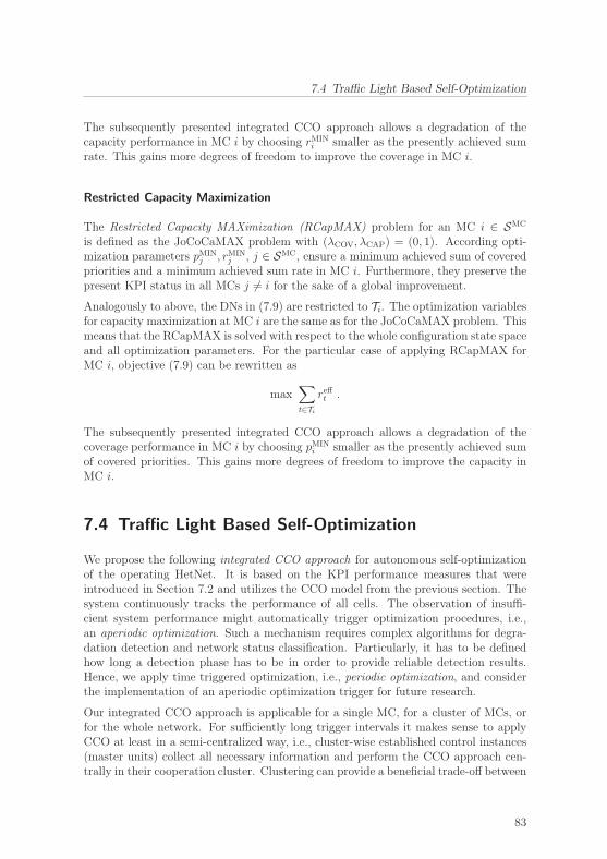
7.4 Traffic Light Based Self-Optimization
The subsequently presented integrated CCO approach allows a degradation of thecapacity performance in MC i by choosing rMIN
i smaller as the presently achieved sumrate. This gains more degrees of freedom to improve the coverage in MC i.
Restricted Capacity Maximization
The Restricted Capacity MAXimization (RCapMAX) problem for an MC i ∈ SMC
is defined as the JoCoCaMAX problem with (λCOV, λCAP) = (0, 1). According opti-mization parameters pMIN
j , rMINj , j ∈ SMC, ensure a minimum achieved sum of covered
priorities and a minimum achieved sum rate in MC i. Furthermore, they preserve thepresent KPI status in all MCs j �= i for the sake of a global improvement.
Analogously to above, the DNs in (7.9) are restricted to Ti. The optimization variablesfor capacity maximization at MC i are the same as for the JoCoCaMAX problem. Thismeans that the RCapMAX is solved with respect to the whole configuration state spaceand all optimization parameters. For the particular case of applying RCapMAX forMC i, objective (7.9) can be rewritten as
max∑t∈Ti
refft .
The subsequently presented integrated CCO approach allows a degradation of thecoverage performance in MC i by choosing pMIN
i smaller as the presently achieved sumof covered priorities. This gains more degrees of freedom to improve the capacity inMC i.
7.4 Traffic Light Based Self-Optimization
We propose the following integrated CCO approach for autonomous self-optimizationof the operating HetNet. It is based on the KPI performance measures that wereintroduced in Section 7.2 and utilizes the CCO model from the previous section. Thesystem continuously tracks the performance of all cells. The observation of insuffi-cient system performance might automatically trigger optimization procedures, i.e.,an aperiodic optimization. Such a mechanism requires complex algorithms for degra-dation detection and network status classification. Particularly, it has to be definedhow long a detection phase has to be in order to provide reliable detection results.Hence, we apply time triggered optimization, i.e., periodic optimization, and considerthe implementation of an aperiodic optimization trigger for future research.
Our integrated CCO approach is applicable for a single MC, for a cluster of MCs, orfor the whole network. For sufficiently long trigger intervals it makes sense to applyCCO at least in a semi-centralized way, i.e., cluster-wise established control instances(master units) collect all necessary information and perform the CCO approach cen-trally in their cooperation cluster. Clustering can provide a beneficial trade-off between
83

7 Self-Optimization of Coverage and Capacity
computational complexity and optimization quality. The chance to find the global op-timum, however, increases with the internal cardinality of the considered coordinationclusters. We define a cooperation cluster as a group of MCs such that the strongestinterferers to the contained eNBs are elements of the group. Since the interferencesituation depends on the particular user distribution, the clustering step is performedat the beginning of the CCO approach. In the following, we assume to have a suitableclustering algorithm on hand.
The following consecutive subroutines are executed everytime the integrated CCOapproach is triggered:
1. DN parameters and IAM parameters are adapted according to Section 7.1.2subject to the present – or the near future – network situation.
2. Cooperation clusters are identified with respect to the computed DN and IAMparameters. The DN priority values and the DN demands are assigned to thecooperation clusters proportionally to the probability that they are served byan MC or FC from the cluster. The probability for being served by a certain(H)eNB can be derived from the UE assignment statistics over the last operationcycle(s). The total priority and the total rate demand of a DN do not depend onany particular clustering, though a DN can be considered for CCO by multiplecooperation clusters.
3. The master unit of each cluster applies the traffic light related CCO loop that isdepicted in Figure 7.4. The CCO loop is explained below.
4. If the CCO results can improve the HetNet performance, the correspondingoptimal configurations are applied.
The Traffic Light (TL) related CCO loop from Figure 7.4 works as follows: First, theKPI traffic lights are computed for all CCO candidates by solving the JoCoCaMAXproblem from Section 7.3 for the presently applied (H)eNB configurations. Since alltransmitter configurations are fixed for this evaluation step, the solution space is sig-nificantly reduced and the traffic lights are obtained very quickly. Please note thatthese are the expected future KPI traffic lights if the DN information includes theprediction component as introduced in (3.9). The sum of covered DN priorities andthe sum rate that a CCO candidate MC achieves in the JoCoCaMAX solution deter-mine its coverage and capacity measure, respectively. Each KPI related traffic lightindicates a green, yellow, or red KPI status subject to the corresponding measure andthe traffic light thresholds. The traffic light threshold parameters from Table 7.4 arecustomizable and have to be predefined by the network operator. The coverage andcapacity metrics that are obtained in the evaluation step provide feasible values for theminimum required number of covered DN priorities pMIN
i and the minimum requiredamount of served rate rMIN
i in (7.21). Thus, we know the (minimum) achievable KPIperformance of each candidate MC i for all further optimization steps.
84
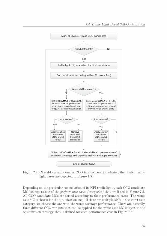
7.4 Traffic Light Based Self-Optimization
Mark all cluster eNBs as CCO candidates
Traffic light (TL) evaluation for CCO candidates
Candidates left?
End of cluster CCO
No
Yes
Sort candidates according to their TL (worst first)
Worst eNB in case 1?
Solve RCovMAX or RCapMAXfor worst eNB s.t. preservationof achieved capacity and cov-
erage for all other cluster eNBs
Solve JoCoCaMAX for all CCOcandidates s.t. preservation of
achieved coverage and capacitymetrics for all cluster eNBs
No Yes
Improvement? Improvement?
Apply solutionfor cluster
eNBs and allHeNBs
Removeworst eNBfrom CCOcandidates
Yes NoYes
No
Solve JoCoCaMAX for all cluster eNBs s.t. preservation ofachieved coverage and capacity metrics and apply solution
Apply solutionfor cluster
eNBs and allHeNBs
Figure 7.4: Closed-loop autonomous CCO in a cooperation cluster, the related trafficlight cases are depicted in Figure 7.5.
Depending on the particular constellation of its KPI traffic lights, each CCO candidateMC belongs to one of the performance cases (categories) that are listed in Figure 7.5.All CCO candidate MCs are sorted according to their performance cases. The worstcase MC is chosen for the optimization step. If there are multiple MCs in the worst casecategory, we choose the one with the worst coverage performance. There are basicallythree different CCO variants that can be applied for the worst case MC subject to theoptimization strategy that is defined for each performance case in Figure 7.5:
85

7 Self-Optimization of Coverage and Capacity
Symbol & domain Description
THCOVG , THCOV
Y ∈ [0, 1]Threshold factors referring to sufficient (green), critical(yellow), and insufficient (red) coverage performance.
THCAPG , THCAP
Y ∈ [0, 1]Threshold factors referring to sufficient (green), critical(yellow), and insufficient (red) capacity performance.
θCOV, θCAP ∈ [0, 1]
Threshold factors referring to lower bounds for coverageperformance and capacity performance if constrained sin-gle target optimization is applied.
Table 7.4: Traffic light related threshold parameters that determine the KPI status inthe CCO loop and define the minimum KPI performance requirements..
1. If the worst case MC belongs to performance category 1, all CCO candidate MCshave a sufficient (expected) coverage performance and a sufficient (expected)capacity performance. The JoCoCaMAX problem from Section 7.3 is solvedwith respect to all CCO candidate MCs and subject to the preservation of allgreen traffic lights. The performance of all MCs that are not a CCO candidateis preserved as well.
2. If the worst case MC belongs to performance category 3, 4, 7, 8 or 9, the RCov-MAX problem from Section 7.3.1 is solved for this MC. The corresponding mini-mum required sum rate for the MC is guaranteed by every feasible solution. Forall other MCs in the cluster, the minimum constraints (7.21) are chosen suchthat the related traffic lights can not get worse.
3. If the worst case MC belongs to performance category 2, 5 or 6, the RCapMAXproblem from Section 7.3.1 is solved for this MC. The corresponding minimumrequired sum of covered DN priorities for the MC is guaranteed by every feasiblesolution. For all other MCs in the cluster, the minimum constraints (7.21) arechosen such that the related traffic lights can not get worse.
If the optimization step yields any improvement, the corresponding configurations areapplied for all eNBs and HeNBs in the cooperation cluster. In case that we do notachieve an improvement, all configurations stay as before. If it is not possible toimprove a worst case MC that has at least one non-green traffic light, this MC isremoved from the CCO candidate list. The CCO loop is repeated until there is no MCleft in the candidate list. Please note that the MCs which are removed from the CCOcandidate list are still considered for the configuration state space of the optimizationmodels. They are just not considered anymore for the selection of the worst case MC.
The CCO loop is repeated as long as there are CCO candidate MCs left and at leastone candidate MC is not in the performance category 1. If these conditions do nothold anymore, the JoCoCaMAX problem is finally solved one time for all cluster MCssubject to the preservation or improvement of all achieved KPI traffic lights. The CCOloop terminates after this step.
86

7.4 Traffic Light Based Self-Optimization
KPI Status Applied Optimization ModelCase Coverage / Capacity Green Yellow Red and KPI Bounds
1 Coverage JoCoCaMAX
Capacity
2 Coverage RCapMAX
Capacity
3 Coverage RCovMAX
Capacity
4 Coverage RCovMAX
Capacity
5 Coverage RCapMAX
Capacity
6 Coverage RCapMAX
Capacity
7 Coverage RCovMAX
Capacity
8 Coverage RCovMAX
Capacity
9 Coverage RCovMAX
Capacity
YTH �GTH
)( COVG
MINi THp )( CAP
GMINi THr
)( COVG
MINi THp
)( CAPY
MINi THr
)( COVY
MINi THp
)( CAPMINir �
)( CAPY
MINi THr
)( COVY
MINi THp
)( CAPMINir �
)( CAPMINir �
Figure 7.5: Traffic light related performance cases (best first) and the correspondingoptimization strategy for an MC i.
The ordering of the performance cases and the corresponding optimization strategies inFigure 7.5 clearly indicate the preference to consider coverage as primary KPI wheneverthe performance of this KPI is not indicated by a green traffic light. Particularly, forstatus 7 – 9 (insufficient coverage) we allow the capacity in a solution to degrade to ared traffic light in favor of the maximal degree of freedom to maximize coverage. TheCCO loop yields a monotone improvement of the cluster MCs, starting with the worstperforming MC first. A mathematical interpretation of this climbing up principle ispresented in the next section.
We consider the parameter settings of the optimization strategies in Figure 7.5 andtake the predefined threshold parameters from Table 7.4 into account. For MC i, wedefine
pMINi (TFCOV) = TFCOV ·
∑t∈Ti
pt
for threshold factor TFCOV ∈ {THCOVG ,THCOV
Y , θCOV} and
rMINi (TFCAP) = TFCAP ·
∑t∈Ti
rt
for threshold factor TFCAP ∈ {THCAPG ,THCAP
Y , θCAP}.
87

7 Self-Optimization of Coverage and Capacity
Furthermore, we suggest to choose the scalarization parameters λCOV and λCAP in theJoCoCaMAX objective (7.9) proportionally to the relation between the coverage andthe capacity threshold factors THCOV
G and THCAPG , e.g., as
λCOV =1∑
t∈Tpt, (7.22)
λCAP =THCAP
G /THCOVG∑
t∈Trt
. (7.23)
The final setting of the threshold parameters is up to the network operator. Thenetwork operator typically considers comparable parameters for system evaluation andblack list generation in its network monitoring center.
7.4.1 Climbing Up Principle for Monotone PerformanceImprovement
Generally, the CCO loop from Figure 7.4 tries to maximally improve the worst per-forming MC towards performance case 1 from Figure 7.5. It drops the MC from theCCO candidate list if an improvement is not possible anymore. The way upwards cantake place stepwise if the improved MC is not directly shifted to performance case 1:If another CCO candidate MC is in a lower performance category (higher performancecase number) after the improvement step, the worst case MC for the next CCO itera-tion switches. Any change of the HetNet configuration in this next iteration step caninfluence the CCO solution space of the priorly improved MC. Particularly, a changeof the solution space might support a further improvement of the prior MC when it isconsidered the next time for CCO.
The minimum constraints (7.21) are the key components of this improvement strategy.They are automatically parametrized with respect to the results from the traffic lightevaluation step, i.e., according to the solution of the JoCoCaMAX problem for fixed(H)eNB configurations. Please note that the present configurations can result from aprevious CCO iteration. Figure 7.6 (a) illustrates the set of feasible points (gray area)and the Pareto front (dashed line) of the MOO problem at the beginning of the CCOloop, compare Section 2.3.1. The initial solution point (boxed asterisk) is obtained assolution of the JoCoCaMAX problem for fixed configurations at all (H)eNBs. Sincethe fixed configurations are usually not optimal for the present HetNet situation, theinitial solution point is most likely not located on the Pareto front of the unrestrictedJoCoCaMax problem. However, we use the obtained performance metrics to defineminimum bounds for the coverage performance and the capacity performance. Thecorresponding minimum values have to be achieved by any feasible solution in the nextoptimization step.
Our CCO approach implements a local search heuristic, which is inspired by [57]. Itworks according to the following climbing up principle:
88

7.4 Traffic Light Based Self-Optimization
max
max
capa
city
(x)
coverage(x)(a) Initial solution point (boxed asterisk) ob-tained by solving the JoCoCaMAX problemfor (λCOV, λCAP) > 0 and fixed configurations.
max
max
capa
city
(x)
coverage(x)
min
min
(b) Minimum performance constraints reducethe maximum degradation of single objectivesand the set of feasible points.
Figure 7.6: Constrained CCO approach for monotone performance improvement.
1. The JoCoCaMAX problem is solved for the present (H)eNB configurations. Theobtained solution gives the feasible point x, see the boxed asterisk in Figure 7.6.
2. We attempt to find a better feasible point x′ in the neighborhood of x by aconstrained optimization approach. In Figure 7.6 (b), the corresponding con-straints determine the maximum allowed gap in the coverage and the capacitydomain subject to the considered threshold factors. Please recall that we allowa degradation of KPIs for certain constellations. Thus, the gap can be largerthan zero. The constraints particularly reduce the set of feasible points, i.e.,the solution space for the subsequent optimization step. In Figure 7.6 (b), theconvex hull of the constrained feasible set excludes the upper encircled pointfrom Figure 7.6 (a) – that was formerly feasible and Pareto optimal – becauseit violates the minimum coverage constraint. On the other hand, the formerlyunsupported point that is marked with a triangle in Figure 7.6 (a), now becomesa supported point on the Pareto front of the JoCoCaMax problem.
3. The predetermined optimization strategy defines the applied CCO variant, i.e.,JoCoCaMax, RCovMax, or RCapMax. The corresponding solution gives thefeasible point x′. Note that we can always find a feasible point since the initialpoint x is still an element of the feasible set. For the example in Figure 7.6 (b), wesolve the JoCoCaMAX problem for scalarization parameters (λCOV, λCAP) > 0.These parameters define the depicted tangential line and lead to the encircledPareto optimal point, compare Section 2.3.1.
4. If the point x′ is better than x in terms of the applied optimization strategy, weapply the corresponding configurations, replace x by x′, and continue with theCCO loop.
89
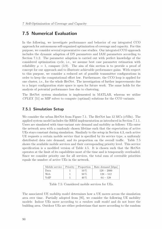
7 Self-Optimization of Coverage and Capacity
7.5 Numerical Evaluation
In the following, we investigate performance and behavior of our integrated CCOapproach for autonomous self-organized optimization of coverage and capacity. For thispurpose, we consider several representative case studies. Our integrated CCO approachincludes the dynamic adaption of DN parameters and IAM parameters according toSection 7.1.2. The parameter adaption is carried out with perfect knowledge of theconsidered optimization cycle, i.e., we assume best case parameter estimation withreliability μ = 1, compare (3.9). The aim of this section is to provide a proof ofconcept for our approach and to illustrate achievable performance gains. With respectto this purpose, we consider a reduced set of possible transmitter configurations inorder to keep the computational effort low. Furthermore, the CCO loop is applied forone cluster, i.e., for the whole HetNet. The investigation of further improvements dueto a larger configuration state space is open for future work. The same holds for theanalysis of potential performance loss due to clustering.
The HetNet system simulation is implemented in MATLAB, whereas we utilizeCPLEX [51] as MIP solver to compute (optimal) solutions for the CCO variants.
7.5.1 Simulation Setup
We consider the urban HetNet from Figure 7.1. The HetNet has 12 MCs (eNBs). Theapplied system model includes the RRM implementation as introduced in Section 7.1.1.Users are simulated with time-variant rate demand and mobility as follows: UEs enterthe network area with a randomly chosen lifetime such that the expectation of activeUEs stays constant during simulation. Similarly to the setup in Section 4.3, each activeUE requests a certain mobile service that is specified by its service type, a uniformlydistributed data rate demand, and its proportion on the overall traffic. Table 7.5shows the available mobile services and their corresponding priority level. This servicespecification is a modified version of Table 4.5. It is chosen such that the HetNetoperates at the limit of its capabilities most of the time and is temporarily overloaded.Since we consider priority one for all services, the total sum of coverable prioritiesequals the number of active UEs in the network.
Mobile service Priority Proportion Rate demand [kbps]
Data 1 10% 128− 2000
Web 1 50% 128− 512
VoIP 1 40% 64− 128
Table 7.5: Considered mobile services for UEs.
The associated UE mobility model determines how a UE moves across the simulationarea over time. Partially adopted from [95], we consider the following UE mobilitymodels: Indoor UEs move according to a random walk model and do not leave thebuilding area. Outdoor UEs are either pedestrians that move according to the random
90

7.5 Numerical Evaluation
walk model or vehicles that follow a random waypoint model. The waypoints aremodeled by an appropriate set of road points that describe the irregular course of theroads. At each crossing point, the vehicle UE chooses randomly the direction to go on.The way back is excluded from that decision. All related mobility model parametersare listed in Table 7.6.
Parameter Setting
Duration of one simulation step 1 s
Pause time Deterministic at 0 s
Random walk direction Uniform [0, 2π)
Velocity pedestrian/indoor Uniform [0, 1.5]m/s
Velocity vehicle Uniform [10, 20]m/s
Velocity traffic hotspot 3m/s
Table 7.6: User mobility parameters.
The following moving traffic hotspot model generates locally bounded overload situa-tions: We define a certain number of hotspot UEs and a hotspot radius. The hotspotUEs are located circularly around a hotspot center UE and stay within the given ra-dius. The hotspot center UE is a vehicle UE that moves along the roads at a givenvelocity. All hotspot UEs become active when a predefined hotspot activity periodstarts and change their state to inactivity if the hotspot period is over. The consid-ered traffic hotspot moves along the roads in the middle part of the network area. InFigure 7.1 (b), it is depicted as bunch of small circles and surrounded by eNBs 1− 4.
Table 7.7 shows the considered HetNet system parameters. The setup is basically thesame as for the evaluation of the cell site planning approach in Section 6.3. However,some of the settings slightly differ from before due to the fact that we now considerthe operating HetNet. The (H)eNB transmission power can be configured as follows:Each of the 12 eNBs can adjust its transmission power according to the specified powerprofile, i.e., it can apply a low, medium, or high transmission power. Moreover, it hasthe option to switch off. Each eNB can apply 0◦ (low) or 5◦ (high) antenna downtiltfor an omnidirectional antenna pattern, compare Figure 6.1 (a). All 200 HeNBs pro-vide just one antenna pattern (omnidirectional) and support the power profile that isspecified in the according part of Table 7.7. Thus, eNBs and HeNBs can select from aset of seven and three different configurations, respectively.
The ray optical path loss model from Section 3.1.2 is utilized to compute the spatialsignal power distribution for each eNB configuration. The free space path loss modelaccording to Section 3.1 provides this information for HeNB configurations. We pre-compute the spectral efficiency parameters for all transmitter configurations subjectto the discrete rate-power function (3.8) and the LTE SINR requirements that aredefined in Table 6.4.
91

7 Self-Optimization of Coverage and Capacity
System parameter Setting
Simulation area Urban, 2.5 km × 3.5 km, 5m resolution
Number of buildings Approximately 2000
Wall penetration loss 10 dB
Shadowing standard deviation 8 dB
Carrier frequency 2GHz
Effective transmission bandwidth 9MHz (50 PRBs in LTE 10MHz mode)
Number of eNBs (macrocells) 12
eNB Tx power profile {−∞ (off), 40 (low), 43 (medium), 46 (high)} dBmeNB antenna downtilt profile {0◦ (low), 5◦ (high)}Propagation model eNB Ray optical, omnidirectional
eNB antenna gain and noise figure 14 dBi and 5 dB
Number of HeNBs (femtocells) 200, uniformly distributed over buildings
Minimum distance HeNB to eNB 35m
HeNB Tx power profile {−∞ (off), 3 (normal), 10 (high)} dBmPropagation model HeNB Free space + wall penetration, omnidirectional
Noise figure HeNB 8dB
Average number of (active) UEs 215
Number of hotspot UEs 60
Outdoor UEs 80%
Vehicular-to-pedestrian ratio 20%
UE initial distribution Random, uniformly distributed
UE antenna gain and noise figure 0 dBi and 9 dB
Table 7.7: Considered simulation parameters for the operating HetNet.
Parameter Setting
DN prediction reliability μ 1
Minimum threshold for coverage δITF 0.6
Coverage bound for MCs pMAXs and FCs pMAX
f 125 and 15
Utilization weighting factor ω 0.9
Coverage threshold factors THCOVG , THCOV
Y , θCOV 0.98, 0.95, 0.90
Capacity threshold factors THCAPG , THCAP
Y , θCAP 0.90, 0.80, 0.70
Table 7.8: Considered CCO parameters.
The integrated CCO approach from Section 7.4 is applied with respect to the opti-mization parameters that are shown in Table 7.8. According to (7.22) and (7.23), thetraffic light factors in Table 7.8 determine the objective weights for joint CCO as
λCOV =1∑
t∈Tpt, λCAP =
0.92∑t∈T
rt.
Please note that the optimization parameters are defined only once in advance to thestart of the HetNet simulation (operation). Any further modification of parameters
92

7.5 Numerical Evaluation
is possible before each operation cycle. However, this requires human intervention,which should only take place in emergency situations.
Our integrated CCO approach determines the optimum HetNet configuration for eachoperation cycle. When the optimal configurations have been applied at all (H)eNBs,we go back to the beginning of the considered operation cycle and repeat the UEsimulation. This evaluation scheme allows for a fair comparison between non-optimizedand optimized configuration results.
7.5.2 Case Study Results
The following case studies present the results of a comparison between the HetNetperformance without CCO and the performance when our CCO approach is applied.For comparison of coverage and capacity performance, we mainly consider the coverageindicator (7.6) and the capacity indicator (7.8) for ω = 0.9. The indicators assess thesystem performance at each time instance of the simulation. The corresponding trafficlight status of both KPIs is computed subject to the traffic light threshold values thatfollow from the threshold factors given in Table 7.8 and the maximum achievable KPI.
The threshold values for capacity have to consider the duality relation between thecapacity indicator (7.8) and the capacity metric (sum rate), see Section 7.2.2. Hence,the traffic light thresholds for capacity follow from Table 7.8 as 0.2 and 0.1 for theyellow and the red traffic light status. Any capacity indicator above 0.2 correspondsto a green traffic light. The traffic light status can be depicted or we can accumulatethe number of different traffic lights over a certain period.
Furthermore, we consider the coverage measure and the capacity measures from Ta-ble 7.2. Consequently, we assess the number of covered UEs, the number of servedUEs, and the sum rate for each operation cycle (observation period). Please recall thatin our simulation setup the number of UEs equals the number of coverable priorities.
For any MC (eNB) specific discussion, we refer to the enumeration in Figure 7.1.
Obliteration of Events
We start with a medium- to long-term CCO trigger: We consider an operation cycleof one hour and a traffic hotspot activity of five minutes, taking place from 10 to15 minutes. As explained above, the whole operation cycle is monitored before theCCO loop is triggered for dynamically adapted input parameters. Afterwards, the UEsimulation is repeated identically but with optimized configurations at the (H)eNBs.Figure 7.7 shows the coverage indicator and the capacity indicator for each secondof the operation cycle and averaged over all MCs in the non-optimized HetNet. TheHetNet operates predominantly at performance status one, i.e., with green coverageand capacity traffic lights. This holds for all MCs if we consider the average over thewhole operation cycle. The comparison with the performance of the optimized systemshows almost no improvement in the CCO results. Contrariwise, the KPI deficienciesat the eNBs 3 and 4 – that are located nearby the traffic hotspot – slightly increase.
93
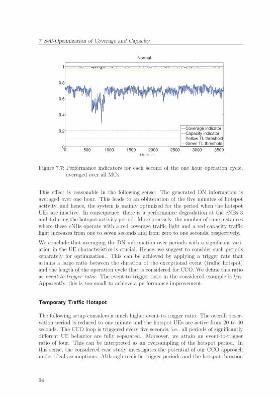
7 Self-Optimization of Coverage and Capacity
0 500 1000 1500 2000 2500 3000 35000
0.2
0.4
0.6
0.8
1
Normal
time [s]
Coverage indicatorCapacity indicatorYellow TL thresholdGreen TL threshold
Figure 7.7: Performance indicators for each second of the one hour operation cycle,averaged over all MCs.
This effect is reasonable in the following sense: The generated DN information isaveraged over one hour. This leads to an obliteration of the five minutes of hotspotactivity, and hence, the system is mainly optimized for the period when the hotspotUEs are inactive. In consequence, there is a performance degradation at the eNBs 3and 4 during the hotspot activity period. More precisely, the number of time instanceswhere these eNBs operate with a red coverage traffic light and a red capacity trafficlight increases from one to seven seconds and from zero to one seconds, respectively.
We conclude that averaging the DN information over periods with a significant vari-ation in the UE characteristics is crucial. Hence, we suggest to consider such periodsseparately for optimization. This can be achieved by applying a trigger rate thatattains a large ratio between the duration of the exceptional event (traffic hotspot)and the length of the operation cycle that is considered for CCO. We define this ratioas event-to-trigger ratio. The event-to-trigger ratio in the considered example is 1/12.Apparently, this is too small to achieve a performance improvement.
Temporary Traffic Hotspot
The following setup considers a much higher event-to-trigger ratio: The overall obser-vation period is reduced to one minute and the hotspot UEs are active from 20 to 40seconds. The CCO loop is triggered every five seconds, i.e., all periods of significantlydifferent UE behavior are fully separated. Moreover, we attain an event-to-triggerratio of four. This can be interpreted as an oversampling of the hotspot period. Inthis sense, the considered case study investigates the potential of our CCO approachunder ideal assumptions. Although realistic trigger periods and the hotspot duration
94
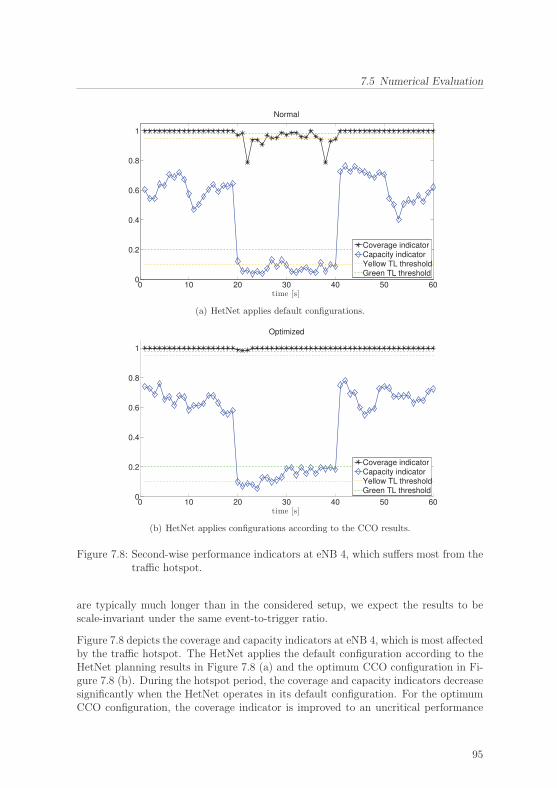
7.5 Numerical Evaluation
0 10 20 30 40 50 600
0.2
0.4
0.6
0.8
1
Normal
time [s]
Coverage indicatorCapacity indicatorYellow TL thresholdGreen TL threshold
(a) HetNet applies default configurations.
0 10 20 30 40 50 600
0.2
0.4
0.6
0.8
1
Optimized
time [s]
Coverage indicatorCapacity indicatorYellow TL thresholdGreen TL threshold
(b) HetNet applies configurations according to the CCO results.
Figure 7.8: Second-wise performance indicators at eNB 4, which suffers most from thetraffic hotspot.
are typically much longer than in the considered setup, we expect the results to bescale-invariant under the same event-to-trigger ratio.
Figure 7.8 depicts the coverage and capacity indicators at eNB 4, which is most affectedby the traffic hotspot. The HetNet applies the default configuration according to theHetNet planning results in Figure 7.8 (a) and the optimum CCO configuration in Fi-gure 7.8 (b). During the hotspot period, the coverage and capacity indicators decreasesignificantly when the HetNet operates in its default configuration. For the optimumCCO configuration, the coverage indicator is improved to an uncritical performance
95

7 Self-Optimization of Coverage and Capacity
status whereas the capacity indicator, though improving, remains in the critical zonewhen the hotspot is active. Table 7.9 shows the exact number of time instances wherethe KPIs at eNB 4 are in a critical (non-green) status: The coverage problems are fullyresolved by applying the optimized configurations, whereas the capacity deficienciesare improved from a red traffic light to a yellow light for ten time instances.
Traffic light status Default configuration CCO configuration
Red coverage indicator 8 0
Yellow coverage indicator 8 0
Red capacity indicator 16 6
Yellow capacity indicator 5 15
Table 7.9: Number of time instances where the KPIs at eNB 4 are not in a green trafficlight status.
The significant improvement during the hotspot period is mainly achieved by reducingthe interference at the eNB that serves the hotspot UEs. When the hotspot UEsbecome active, the eNBs 1, 2, 3 and 7 increase their downtilt (tilt down) and decreasetheir transmission power. Consequently, they reduce their interference to the servicearea of eNB 4. On the other hand, eNB 4 increases its downtilt and applies themaximum available transmission power in order to focus on the hotspot area. Whenthe hotspot activity is over, the eNBs 1, 2, 3 and 7 decrease their antenna downtiltto 0◦ (tilt up) and power up to enlarge the coverage footprint.
Figure 7.8 illustrates highly volatile values for the capacity indicator, which performssometimes clearly worse than in the non-optimized case. Both effects are caused byour RRM implementation: First, the volatility is explained by the fact that the RRMalgorithms are executed at each time instance independently of the assignments andallocations that were computed in previous simulation steps. And second, our RRMdoes not necessarily maximize the capacity indicator. It terminates when a feasibleassignment and allocation have been reached. Thus, our RRM does not take fulladvantage of the CCO benefits as long as it has not to cope with coverage and capacityproblems. In other words, the KPI values of the non-optimized system can outperformthe optimized values but only when the non-optimized system does not suffer fromany KPI deficiencies.
Coverage and Capacity Trade-Off
So far, the unattended calls in the coverage indicator were mostly caused by a lackof available resources (bandwidth), i.e., the coverage indicator mainly accounted forcapacity problems. Therefore, the following case study investigates our CCO approachfor coverage problems in terms of missing signal power: eNB 2 and the eNBs 7 to 10 arepermanently switched off in order to cause artificial coverage problems, particularly inthe coverage area of the eNBs 4, 11 and 12, see Figure 7.9 (a). Otherwise, we keep thesimulation setup from the previous case study, including the hotspot period from 20
96

7.5 Numerical Evaluation
to 40 seconds. First, the HetNet performance is evaluated for the initial (default) cellconfigurations from the planning stage. Second, the CCO loop is triggered one timewith respect to the UE traffic that is averaged over the whole observation period ofone minute. And third, the 60 seconds are separated into three isochronous operationand optimization cycles such that the period of hotspot activity is exactly covered bythe middle cycle. This corresponds to an event-to-trigger ratio of one. Since coverageproblems and capacity shortage appear simultaneously during the hotspot period,trade-off handling becomes a serious challenge in the CCO loop.
Performance indicators / Number of users which are Average served
Configuration not covered covered served rate [Mbps]
1st cycle (coverage compensation)
Initial configuration 3 4152 3815 53.382
Optimized once 0 4155 3957 56.255
Optimized per cycle 0 4155 3944 55.932
2nd cycle (hotspot activity)
Initial configuration 5 5255 4106 53.288
Optimized once 0 5260 4265 55.502
Optimized per cycle 3 5257 4763 67.568
3rd cycle (regular operation)
Initial configuration 2 3958 3631 52.392
Optimized once 2 3958 3828 56.569
Optimized per cycle 2 3958 3840 57.252
Table 7.10: Covered users, served users, and served rate in the HetNet over the wholeobservation period of one minute.
Table 7.10 shows that the coverage performance and the capacity performance signifi-cantly improve when the initial HetNet configuration is switched to the optimum CCOconfiguration. One-time CCO and cyclic CCO reveal similar behavior for the first andthird cycles. In the second cycle, however, we observe a significant difference: Thecyclic CCO reduces the coverage performance only marginally while it considerablyimproves the capacity performance, i.e., the number of served users and the servedrate. The one-time optimization has to take into account the coverage problems fromthe first and third cycles. This reduces the degrees of freedom for improving the ca-pacity performance in the second cycle. Please note that the simulation results canslightly differ from the computed CCO solutions, and hence, minor discrepancies arepossible.
Table 7.11 and the (re-)configuration related MC footprints that are depicted in Fi-gure 7.9 illustrate how the autonomous CCO approach basically works: The initialcell configurations lead to coverage holes in the HetNet area with a received signalpower below −121 dBm. In Figure 7.9 (a), coverage holes particularly occur at the cellborder of the MCs 4, 11 and 12. Thus, the CCO loop for the first cycle considers thesecoverage holes as well as severe capacity problems in the other cells. The correspondingCCO solution keeps the initial antenna tilts but powers up all eNBs and many of theHeNBs. This solution improves the coverage situation significantly, compare the white
97
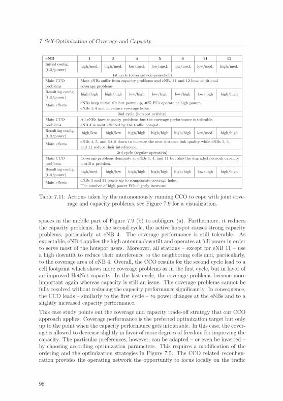
7 Self-Optimization of Coverage and Capacity
eNB 1 3 4 5 6 11 12
Initial config.high/med. high/med. low/med. low/med. low/med. low/med. high/med.
(tilt/power)
1st cycle (coverage compensation)
Main CCO Most eNBs suffer from capacity problems and eNBs 11 and 12 have additional
problems coverage problems.
Resulting config.high/high high/high low/high low/high low/high low/high high/high
(tilt/power)
Main effectseNBs keep initial tilt but power up, 40% FCs operate at high power.
eNBs 1, 4 and 11 reduce coverage holes.
2nd cycle (hotspot activity)
Main CCO All eNBs have capacity problems but the coverage performance is tolerable.
problems eNB 4 is most affected by the traffic hotspot.
Resulting config.high/low high/low high/high high/high high/high low/med. high/high
(tilt/power)
Main effectseNBs 4, 5, and 6 tilt down to increase the near distance link quality while eNBs 1, 3,
and 11 reduce their interference.
3rd cycle (regular operation)
Main CCO Coverage problems dominate at eNBs 1, 4, and 11 but also the degraded network capacity
problems is still a problem.
Resulting config.high/med. high/low high/high high/high high/high low/high high/high
(tilt/power)
Main effectseNBs 1 and 11 power up to compensate coverage holes.
The number of high power FCs slightly increases.
Table 7.11: Actions taken by the autonomously running CCO to cope with joint cove-rage and capacity problems, see Figure 7.9 for a visualization.
spaces in the middle part of Figure 7.9 (b) to subfigure (a). Furthermore, it reducesthe capacity problems. In the second cycle, the active hotspot causes strong capacityproblems, particularly at eNB 4. The coverage performance is still tolerable. Asexpectable, eNB 4 applies the high antenna downtilt and operates at full power in orderto serve most of the hotspot users. Moreover, all stations – except for eNB 11 – usea high downtilt to reduce their interference to the neighboring cells and, particularly,to the coverage area of eNB 4. Overall, the CCO results for the second cycle lead to acell footprint which shows more coverage problems as in the first cycle, but in favor ofan improved HetNet capacity. In the last cycle, the coverage problems become moreimportant again whereas capacity is still an issue. The coverage problems cannot befully resolved without reducing the capacity performance significantly. In consequence,the CCO leads – similarly to the first cycle – to power changes at the eNBs and to aslightly increased capacity performance.
This case study points out the coverage and capacity trade-off strategy that our CCOapproach applies: Coverage performance is the preferred optimization target but onlyup to the point when the capacity performance gets intolerable. In this case, the cover-age is allowed to decrease slightly in favor of more degrees of freedom for improving thecapacity. The particular preferences, however, can be adapted – or even be inverted –by choosing according optimization parameters. This requires a modification of theordering and the optimization strategies in Figure 7.5. The CCO related reconfigu-ration provides the operating network the opportunity to focus locally on the traffic
98

7.5 Numerical Evaluation
13
4
5
6
11
12
(a) Switched off eNBs cause coverageholes (white spaces).
13
4
5
6
11
12
(b) The remaining eNBs mostly com-pensate the white spaces.
13
4
5
6
11
12
(c) Reconfiguration with respect tothe traffic hotspot (bunch of spots).
13
4
5
6
11
12
(d) Handling of joint coverage and ca-pacity problems.
Figure 7.9: MC footprints for the consecutive handling of coverage problems (switchedoff eNBs), capacity problems (traffic hotspot), and joint KPI degradation.
hotspot when it is necessary. This is clearly indicated by the resource consumption ateNB 4, which can raise the bandwidth for serving users from round about 66% in theoperation cycles one and three to more than 90% in cycle two. Moreover, the one-time CCO results demonstrate that there is significant potential for improvements byapplying our approach even though the degradation period is not perfectly separated.
99

7 Self-Optimization of Coverage and Capacity
7.5.3 The Solution Space for Trade-Off Optimization
The following investigation validates the assumptions that we made on the structureof the CCO solution space for the climbing up principle in Section 7.4.1. Furthermore,it justifies our suggestion for an appropriate selection of the JoCoCaMAX parame-ters λCOV and λCAP.
We make use of the property that each optimal solution of the JoCoCaMAX prob-lem (7.9) is a Pareto optimal point on the Pareto front for (λCOV, λCAP) > 0, seeSection 2.3.1. This property helps us to compute a Pareto front approximation for thefollowing setup: We consider the JoCoCaMAX problem for MC 4 in the second cycleof the previous case study, i.e., during the traffic hotspot period. Corresponding so-lutions are computed for an increasing sequence of the scalarization parameters λCOV
and λCAP on the interval [0.2, 1] with step size 0.2. The scalarization parameters λCOV
and λCAP are normalized by
1∑t∈T4
ptand
1∑t∈T4
rt,
respectively. The parameters pMINi and rMIN
i are equal to zero for all considered cells.Figure 7.10 depicts the coverage and capacity results that are attained by the JoCo-CaMAX solutions for eNB 4. The results are normalized to the maximum number ofDN priorities and the maximum sum rate that can be achieved. Please note that theplot shows only the JoCoCaMAX results for eNB 4, though, the configuration statespace of the related JoCoCaMAX problem includes the configurations of all relevantneighbor MCs and FCs. Redundant points are dropped. In order to have the labelingneatly arranged, we additionally dropped some points that are very close to the de-picted ones. Some of the points are not directly located on the approximated Paretofront (dashed line) even though they have to be supported points by definition, seeSection 2.3.1. This effect is caused by a timeout bound for the MIP solver. The gapto the optimum capacity value can reach up to 0.5% when the solver terminates. Inconsequence, the depicted Pareto front represents an artificial best fit curve and notthe actual convex hull of the solution set.
The points are labeled with their corresponding (normalized) vector (λCOV, λCAP).The results confirm the assumption from Section 2.3.1 that the dedicated balance orimbalance of the weighting factors influences the balance or imbalance of the achievedcoverage and capacity performance in the related solution: The higher valued KPIof a solution point with an imbalanced weight vector corresponds to the higher KPIweight. The two points on the lower right of Figure 7.10, however, illustrate that thisis only a relative property and not an absolute one. This finding is in accordance withthe statement from Section 2.3.1 that the particular selection of weights influences justthe tendency of the ratio between the effectively achieved KPIs.
Compared to Figure 7.6, the obtained structure of the solution space is close to ourexpectations. Moreover, the (encircled) solution point – that corresponds to our weightsuggestions (7.22) and (7.23) – meets our intention to find a JoCoCaMAX solution
100

7.6 Summary
Figure 7.10: Pareto front approximation and selected optimal point (encircled).
that is almost balanced but has a slight preference for a higher coverage performance.The according solution point can be located somewhere else for a different probleminstance. However, we expect it to be located in this region of the solution space aslong as there are any Pareto optimal points in this region at all.
7.6 Summary
Some works in recent literature provide algorithms for self-organized CCO that havethe same intention as our approach. However, most of them follow a contrary imple-mentation principle. For instance, [75] and [86] apply reinforcement learning methodsto create an expert system (knowledge database) that defines rule-based decisions forthe self-organized configuration of cell parameters. Such a model-free approach doesnot require much a-priori information since it does not consider an explicit systemmodel. Instead, it is solely based on the system feedback to its decisions and actions.In contrast to a model-based approach, the model-free approach can make it very hardto interpret the decisions that are taken. It can even be impossible to influence the
101

7 Self-Optimization of Coverage and Capacity
processing of a model-free approach intentionally. Further related aspects are studiedin [96], where cell outage management and self-organized eNB downtilt optimizationare considered. However, this work do not deal with joint multi-tier configuration butkeeps the femtocell environment static.
Most works in the SON domain consider the hexagonal grid network topology accor-ding to [3]. We observed effects that were specifically caused by that artificial topology,e.g., uniform frequency reuse potential in MCs due to cell symmetry. Therefore, wehave switched to a more realistic simulation framework that considers the propagationcharacteristics of an urban environment. This allows for the evaluation of our CCOapproach under realistic assumptions.
Our model-based CCO approach describes the underlying system dependencies in anexplicit system model. It adapts its optimization parameters dynamically subject tothe system feedback. Particularly, our approach considers both tiers, i.e., macrocellsand femtocells, jointly for the optimization of user-centric performance metrics. Theuser-centric definition of system coverage that we consider might look unusual com-pared to the common spatial definition. The main advantage of our definition is theadditional degree of freedom that we gain for improving the capacity if necessary.We expect this perspective to become more and more important in future when thecells are getting smaller, the cell deployment gets more dense, the average cell loadincreases, and the systems can react very quickly to dynamic changes in the network.
In Section 7.4, we have introduced a traffic light based scheme for self-organized CCO.The corresponding approach finds Pareto optimal solutions for the joint optimizationof coverage and capacity. It confines to a hierarchical constrained single target maxi-mization in the case that a single performance metric predominates. The CCO loopas well as the overall integrated CCO approach meet the definition of a closed-loopoptimization framework that is given in [85]. Our CCO model integrates the inter-ference approximation approach that we have introduced in Chapter 5. Thus, cellconfigurations are optimized subject to inter-cell and cross-tier interference. The cellconfiguration can particularly influence the transmitter activity status (switch on/off).This provides the opportunity to correct problems that are caused by peppered FCs.The transmission power of disruptive FCs can be tuned down to a minimum if neces-sary. For application in a real system, the periodic CCO trigger can be combined withan aperiodic trigger mechanism that is able to detect system degradations automati-cally.
The evaluation results demonstrate that our integrated CCO approach can cope withcoverage hole situations as well as with a (temporal) traffic hotspot. Both scenariosare defined by 3GPP as reference scenarios for the assessment of CCO solutions in self-organized networks [8]. Moreover, our approach fulfills the following three requirementsfor self-organized CCO that 3GPP defines in [8]:
1. The need for human intervention is minimized. Our CCO approach does notrequire any human intervention once the optimization parameters have been ini-tially specified. In fact, the optimization parameters are calibrated automaticallysubject to the dynamic changes in the network.
102

7.6 Summary
2. The static optimization components are fully customizable by the network ope-rator. The static components of our integrated CCO approach are the perfor-mance measurement functions, the corresponding traffic light thresholds, and theavailable configuration state space.
3. The CCO approach is configurable individually for different areas of the networkas the optimization parameters are customizable for each cell.
Overall, the presented CCO approach improves the network performance when theHetNet has to cope with traffic hotspots, coverage shortage, and objective trade-offsituations. We expect further improvements if the configuration state space is in-creased, e.g., by more power diversity or sectorized antennas. Related investigationsare open for future work.
103


8 Conceptual Extensions
This chapter presents some conceptual extensions to the optimization models that wehave introduced in the chapters before. On the one hand, the extensions incorporatefurther aspects into the optimization models. The approach in Section 8.1 considersenergy efficiency as additional decision criterion for optimal network configuration.Section 8.2 provides a concept to embed user acceptance into the network planningtask, whereas Section 8.3 considers the robustness of the related optimization problem.On the other hand, the extensions deal with methods to reduce the computationalcomplexity of the optimization algorithms. Related methods for graph-based problempartitioning and adaptive clustering are presented in Section 8.4.
We briefly discuss the aim of each conceptual extension and explain how it can be ap-plied to the related optimization models. Please note that we skip any comprehensiveformalism even though it might be required to apply the extension. Instead, we sketchthe extension principles and refer to the related publications.
8.1 Energy Efficiency
Nowadays, energy efficiency plays an important role for any kind of technical deve-lopment. Concerning the optimization models that we have presented in the previouschapters, the CCO problem from Chapter 7 is the only one that allows for an op-timization of power parameters. The corresponding objective (7.9) can be extendedto
max
{λCOV
∑t∈T
ptzt + λCAP
∑t∈T
refft − λPOW
(∑s∈S
Psys +∑f∈F
Pfyf
)}, (8.1)
where Ps and Pf denote the transmission power that is associated with the accordingeNB configuration s and the HeNB configuration f , respectively. The weighting fac-tor λPOW depends on the importance of energy efficiency compared to the importanceof maximal coverage and capacity. Furthermore, the factor might differ for the powerconsumption of MC transmitters and FC transmitters. In this case, the power term isseparated into differently weighted terms for eNB sum power and HeNB sum power.We suggest to incorporate energy efficiency as a minor criterion, i.e., to choose theweighting factor λPOW relatively to the factors λCOV and λCAP such that each (aver-age) DN that can be covered or served gets a higher priority in the overall optimizationobjective than any power reduction.
105

8 Conceptual Extensions
The integration of energy efficiency into the optimization objective may increase thecomputational effort to solve the corresponding MIP. Therefore, it can be a beneficialalternative to apply the power minimization step consecutively to the CCO loop:After the CCO loop has terminated, we bound the minimum constraints (7.21) bythe accumulated priorities and the sum rate that have been achieved for the optimumCCO solution. Afterwards, the JoCoCaMAX problem is solved one more time, but inthis optimization step the objective (7.9) is replaced with
min
{∑s∈S
Psys +∑f∈F
Pfyf
}. (8.2)
The importance of the sum power for MCs can optionally be distinguished from theimportance of the FC power consumption by introducing according weighting factors.Please note that any obtained solution to this problem yields the same coverage andcapacity performance as before but, perhaps, with a network configuration that con-sumes less power as the former solution. This consecutive optimization step is veryfast since the tight minimum constraints reduce the feasible solution space maximally.Thus, this reduction can also mean that there do not exist alternative feasible solutions.
Operational effort can be considered as a further aspect of energy efficiency or as anadditional optimization metric. It is directly related to the configuration changes inCCO solutions. The number and the type of (electrical) antenna downtilt modificationscan cause a higher or lower effort. Optimal solutions that take the minimization ofconfiguration changes into account could be favored over solutions that maximize thecoverage and capacity performance solely.
For each (H)eNB with configuration a, the parameter ca′ ∈ R≥0 denotes the cost fora change from the presently applied configuration to configuration a′. The cost maybe interpreted as a penalty term. For instance, it can consider the number of antennatilt modifications or the difference in total transmission power. The cost parametersare chosen relatively to the presently applied configuration a. The parameters arerecomputed each time the (physical) configurations in the HetNet have changed. Natu-rally, it holds ca = 0. The minimization of operational effort can be incorporatedinto the JoCoCaMAX problem – or into any of its variants – analogously to (8.1).The corresponding weighting factor λOPE has to be chosen suitably. Alternatively,the operational effort can be minimized in a secondary optimization step accordingto (8.2). We recommend the second variant to incorporate it into the CCO procedure,i.e., to solve the optimization problem
min
{∑s∈S
csys +∑f∈F
cfyf
}
for tight minimum constraints after the CCO loop has finished. Due to the identicalproblem formulations it is possible to define cost parameters that include the relatedpower consumption. The corresponding optimization problem minimizes power con-sumption and operational effort jointly.
106
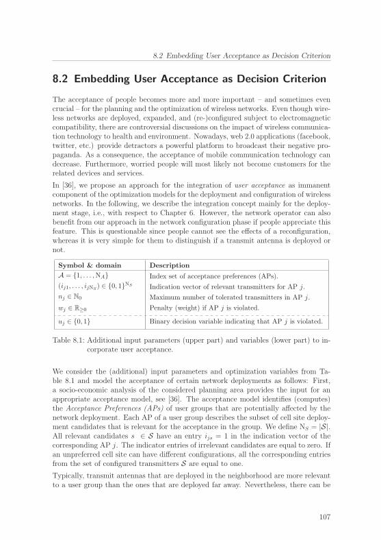
8.2 Embedding User Acceptance as Decision Criterion
8.2 Embedding User Acceptance as Decision Criterion
The acceptance of people becomes more and more important – and sometimes evencrucial – for the planning and the optimization of wireless networks. Even though wire-less networks are deployed, expanded, and (re-)configured subject to electromagneticcompatibility, there are controversial discussions on the impact of wireless communica-tion technology to health and environment. Nowadays, web 2.0 applications (facebook,twitter, etc.) provide detractors a powerful platform to broadcast their negative pro-paganda. As a consequence, the acceptance of mobile communication technology candecrease. Furthermore, worried people will most likely not become customers for therelated devices and services.
In [36], we propose an approach for the integration of user acceptance as immanentcomponent of the optimization models for the deployment and configuration of wirelessnetworks. In the following, we describe the integration concept mainly for the deploy-ment stage, i.e., with respect to Chapter 6. However, the network operator can alsobenefit from our approach in the network configuration phase if people appreciate thisfeature. This is questionable since people cannot see the effects of a reconfiguration,whereas it is very simple for them to distinguish if a transmit antenna is deployed ornot.
Symbol & domain Description
A = {1, . . . ,NA} Index set of acceptance preferences (APs).
(ij1, . . . , ijNS ) ∈ {0, 1}NS Indication vector of relevant transmitters for AP j.
nj ∈ N0 Maximum number of tolerated transmitters in AP j.
wj ∈ R≥0 Penalty (weight) if AP j is violated.
uj ∈ {0, 1} Binary decision variable indicating that AP j is violated.
Table 8.1: Additional input parameters (upper part) and variables (lower part) to in-corporate user acceptance.
We consider the (additional) input parameters and optimization variables from Ta-ble 8.1 and model the acceptance of certain network deployments as follows: First,a socio-economic analysis of the considered planning area provides the input for anappropriate acceptance model, see [36]. The acceptance model identifies (computes)the Acceptance Preferences (APs) of user groups that are potentially affected by thenetwork deployment. Each AP of a user group describes the subset of cell site deploy-ment candidates that is relevant for the acceptance in the group. We define NS = |S|.All relevant candidates s ∈ S have an entry ijs = 1 in the indication vector of thecorresponding AP j. The indicator entries of irrelevant candidates are equal to zero. Ifan unpreferred cell site can have different configurations, all the corresponding entriesfrom the set of configured transmitters S are equal to one.
Typically, transmit antennas that are deployed in the neighborhood are more relevantto a user group than the ones that are deployed far away. Nevertheless, there can be
107
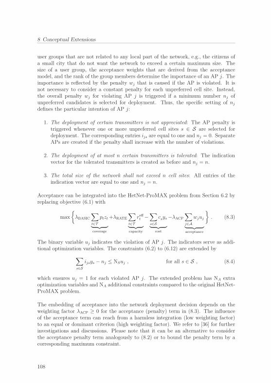
8 Conceptual Extensions
user groups that are not related to any local part of the network, e.g., the citizens ofa small city that do not want the network to exceed a certain maximum size. Thesize of a user group, the acceptance weights that are derived from the acceptancemodel, and the rank of the group members determine the importance of an AP j. Theimportance is reflected by the penalty wj that is caused if the AP is violated. It isnot necessary to consider a constant penalty for each unpreferred cell site. Instead,the overall penalty wj for violating AP j is triggered if a minimum number nj ofunpreferred candidates is selected for deployment. Thus, the specific setting of nj
defines the particular intention of AP j:
1. The deployment of certain transmitters is not appreciated: The AP penalty istriggered whenever one or more unpreferred cell sites s ∈ S are selected fordeployment. The corresponding entries ijs are equal to one and nj = 0. SeparateAPs are created if the penalty shall increase with the number of violations.
2. The deployment of at most n certain transmitters is tolerated: The indicationvector for the tolerated transmitters is created as before and nj = n.
3. The total size of the network shall not exceed n cell sites: All entries of theindication vector are equal to one and nj = n.
Acceptance can be integrated into the HetNet-ProMAX problem from Section 6.2 byreplacing objective (6.1) with
max
{λBASIC
∑t∈T
ptzt︸ ︷︷ ︸coverage
+λRATE
∑t∈T
refft︸ ︷︷ ︸capacity
−∑s∈S
csys︸ ︷︷ ︸cost
−λACP
∑j∈A
wjuj︸ ︷︷ ︸acceptance
}. (8.3)
The binary variable uj indicates the violation of AP j. The indicators serve as addi-tional optimization variables. The constraints (6.2) to (6.12) are extended by∑
s∈Sijsys − nj ≤ NSuj , for all s ∈ S , (8.4)
which ensures uj = 1 for each violated AP j. The extended problem has NA extraoptimization variables and NA additional constraints compared to the original HetNet-ProMAX problem.
The embedding of acceptance into the network deployment decision depends on theweighting factor λACP ≥ 0 for the acceptance (penalty) term in (8.3). The influenceof the acceptance term can reach from a harmless integration (low weighting factor)to an equal or dominant criterion (high weighting factor). We refer to [36] for furtherinvestigations and discussions. Please note that it can be an alternative to considerthe acceptance penalty term analogously to (8.2) or to bound the penalty term by acorresponding maximum constraint.
108

8.3 Mobility Robustness
8.3 Mobility Robustness
The solution quality of all the optimization models that have been presented in thisthesis particularly depends on the accuracy of the DN input parameters. The achievedsystem performance will be poor if the predicted rate demand does not match theeffective demand of users in the post-optimization phase. In the operating system,discrepancies in the DN parameter estimation according to (3.9) can be correcteddynamically before the next CCO loop starts. The network dimensioning approach inChapter 4 and the cell site planning from Chapter 6, however, do not have any chanceto correct inaccurate input parameters dynamically.
In [23], the authors show how an approach from the field of robust optimization canhelp to cope with uncertainty in the DN parameters. Basically, this work considersa planning (dimensioning) problem that is similar to the FR-ProMAX problem fromSection 4.2. The problem does not consider relay stations. Instead of a fixed ratedemand rt for DN t, the demand is modeled as a bounded random variable over theinterval [rt − rt, rt + rt]. The parameter rt denotes the nominal rate demand and rt itsmaximum deviation. The mobility robustness parameter Γ ∈ [0, . . . , |T |] describes thenumber of DNs that deviate from their nominal rate demand. The capacity constraintof the corresponding multiple knapsack problem from Table (4.3) is rewritten as
∑t∈Ts
rtestzst + max
T ′⊆Ts ,|T ′|≤Γ
∑t∈T ′
rtestzst ≤ Bs , for all s ∈ S .
This constraint includes the worst case constellation into the optimization problem:
i) The subset T ′ contains the (maximally) Γ DNs that degrade the capacity con-straint most if they simultaneously request a rate at the upper bound of theirrate interval.
ii) All DNs of subset T ′ simultaneously request a rate at the upper bound of theirrate interval.
We refer to [23] for the details how this non-linear constraint can be transformed intoan equivalent ILP formulation. The robust optimization problem can be solved withthe same methods as the original problem. Compared to the original problem, therobust optimization problem has |S| + |S ∗ T | extra variables and |S ∗ T | additionalconstraints.
Generally, it is preferable to consider too much rate demand (demand buffer) insteadof a parameter setup that leads to a permanently overloaded network. On the otherhand, a large demand buffer can cause the deployment of dispensable stations. Moreprecisely, a cell site planning problem – or a network dimensioning problem – thatconsiders too much demand buffer will have a solution with many cells that are under-loaded in the operating system. Nevertheless, these cells are deployed and operatedat full CAPEX and OPEX. Besides the increased problem complexity, this can beinterpreted as the price of robustness.
109

8 Conceptual Extensions
8.4 Graph-Based Problem Partitioning and AdaptiveClustering
The integrated CCO approach presented in Section 7.4 is intended to run autonomouslyin a semi-decentralized manner, i.e., preferably in small- to middle-sized cooperationclusters. We define a cluster as a reasonably sized group of network elements such thatthe strongest interferers to the contained elements are covered by the group. Thus,(inter-cell) interference is the major decision criterion for network clustering. Thenetwork entities are clustered in order to reduce the size of the problem instances,and hence, to reduce the computational effort for solving the particular optimizationproblems. Moreover, clustering can help to reduce the communication overhead thatis caused by self-organization in the system. All the relevant information has to beshared only within the cluster and not along the whole network.
Clustering is also useful to reduce the computational effort that is required to solvethe network dimensioning problem from Chapter 4 and the cell site planning problemaccording to Chapter 6. In the pre-deployment stage, however, the cell site locationsare not fixed yet. Thus, the computation of potential clusters – defined by a strongintra-cluster interference criterion – becomes a combinatorial problem. The corres-ponding clustering algorithms cannot be used to partition the planning problem intosmaller sub-problems prior to the optimization step. Therefore, the methods for clus-tering in the operating network differ from the methods that can be applied to findsuitable clusters for the planning problem. The clusters of a planning problem can beconsidered as independent problem instances.
In [38], we present a graph-based approach to partition a network planning problemautomatically into an appropriate number of n sub-problems. The n correspondingproblem clusters have a strong intra-cluster relationship (interference) and a weakinter-cluster relationship. The basic idea is to model the planning instance as bipar-tite graph G = (S, T, E) as depicted in Figure 8.1: The set S contains all cell sitedeployment candidates (BSs or eNBs) from S. The set T covers the considered re-ceiver points (DNs or UEs) from T . The weights of the undirected edges E are equalto the spectral efficiency est on the corresponding links. If S contains different configu-rations for identical cell site locations, each location is considered only once in S. Thecorresponding weight of each undirected edge to an element of T equals the maximumspectral efficiency over all possible configurations of the cell site.
We connect an artificial source node to all nodes from S and consider each node from Tsuccessively as sink node. The partitioning of the bipartite graph is obtained by theoverall minimum cut that we find for this setup. The cost of a cut is defined by mea-sures that suitably reflect the intra-cluster interference and inter-cluster interference ofthe corresponding (two) partitions. All subsequent partitions are clustered in a hierar-chical manner until a stop criterion is fulfilled. Basically, the clustering in a partitionbranch stops when the cut cost of a subsequent partitioning exceeds the relative costof its parent cluster. We refer to [38] for all technical details.
110
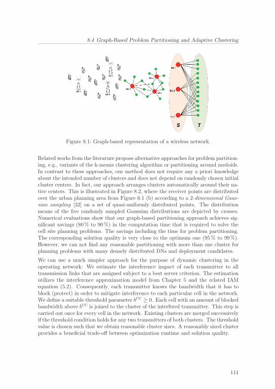
8.4 Graph-Based Problem Partitioning and Adaptive Clustering
Figure 8.1: Graph-based representation of a wireless network.
Related works from the literature propose alternative approaches for problem partition-ing, e.g., variants of the k-means clustering algorithm or partitioning around medoids.In contrast to these approaches, our method does not require any a priori knowledgeabout the intended number of clusters and does not depend on randomly chosen initialcluster centers. In fact, our approach arranges clusters automatically around their na-tive centers. This is illustrated in Figure 8.2, where the receiver points are distributedover the urban planning area from Figure 6.1 (b) according to a 2-dimensional Gaus-sian sampling [32] on a set of quasi-uniformly distributed points. The distributionmeans of the five randomly sampled Gaussian distributions are depicted by crosses.Numerical evaluations show that our graph-based partitioning approach achieves sig-nificant savings (80% to 90%) in the computation time that is required to solve thecell site planning problems. The savings including the time for problem partitioning.The corresponding solution quality is very close to the optimum one (95% to 99%).However, we can not find any reasonable partitioning with more than one cluster forplanning problems with many densely distributed DNs and deployment candidates.
We can use a much simpler approach for the purpose of dynamic clustering in theoperating network: We estimate the interference impact of each transmitter to alltransmission links that are assigned subject to a best server criterion. The estimationutilizes the interference approximation model from Chapter 5 and the related IAMequation (5.2). Consequently, each transmitter knows the bandwidth that it has toblock (protect) in order to mitigate interference to each particular cell in the network.We define a suitable threshold parameter bCC ≥ 0. Each cell with an amount of blockedbandwidth above bCC is joined to the cluster of the interfered transmitter. This step iscarried out once for every cell in the network. Existing clusters are merged successivelyif the threshold condition holds for any two transmitters of both clusters. The thresholdvalue is chosen such that we obtain reasonable cluster sizes. A reasonably sized clusterprovides a beneficial trade-off between optimization runtime and solution quality.
111
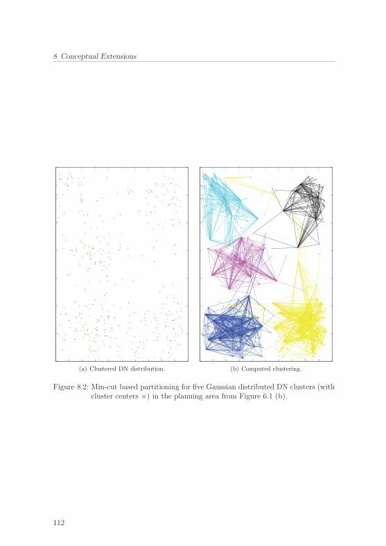
8 Conceptual Extensions
(a) Clustered DN distribution. (b) Computed clustering.
Figure 8.2: Min-cut based partitioning for five Gaussian distributed DN clusters (withcluster centers ×) in the planning area from Figure 6.1 (b).
112

9 Conclusions
9.1 Summary and Contributions
This thesis contributes to multiple stages along the typical lifecycle of broadbandwireless networks by introducing novel concepts, models, and algorithms for
• the estimation of transmission quality and bandwidth requirements subject topath loss predictions,
• the dimensioning of wireless networks,
• interference modeling in multi-tier networks,
• HetNet cell site planning,
• the self-organized optimization of operating HetNets, and
• the conceptual extension of several components from above.
First, the key components for wireless network modeling have been introduced. Pathloss information serves as basic input for these components. We have shown how therequired bandwidth for data transmission can be computed via the discrete rate-powerfunction that is given by the system link budget. Since the spectrum in OFDMA multi-cell networks is shared and limited, all presented optimization models are subject to avariant of the multiple knapsack problem. This becomes an issue when users expect aminimum quality-of-service and the corresponding rate demand exceeds the load limitof single cells.
We have considered multihop WiMAX networks and determined their infrastructuredimensioning with respect to the expected user distribution and rate demand. Therelated optimization problem has been formalized as a mixed-integer linear programthat covers all relevant technical system aspects. Particularly, we have shown howan economical perspective can help to find a closed-form representation for conflictingobjectives like the trade-off alignment between network coverage, network capacity,and deployment cost. Even though the dimensioning model has been developed formultihop WiMAX networks, the approach is transferable to further OFDMA basedwireless networks.
113

9 Conclusions
Compared to the dimensioning approach, accurate cell site planning and network con-figuration require a higher precision, particularly in terms of the applied inter-cell inter-ference model. For this purpose, a low-complexity interference approximation has beendeveloped that estimates the overall required bandwidth at eNBs and HeNBs subjectto inter-cell and cross-tier interference. This approximate model serves as immanentcomponent of the optimization models that we have introduced for the planning andthe self-organized operation of LTE HetNets. The interference approximation can becalibrated with respect to the dynamic changes in the network.
For the optimal cell site planning of LTE HetNets, we have considered macrocells anduser-operated femtocells that are not necessarily active all the time. The objective ofthe corresponding optimization problem is to provide a minimum number of macrocellssuch that mobile services are area-wide guaranteed. On the other hand, it avoidsdispensable cell sites for the sake of cost efficiency and low interference.
We have developed an integrated approach for the self-optimization of coverage andcapacity in time-variant LTE HetNets. The corresponding algorithms were designedaccording to a traffic light principle and they autonomously control site activity, trans-mission power, and antenna downtilt parameters. The presented approach finds Paretooptimal solutions for the joint optimization of coverage and capacity. It confines toa hierarchical constrained single target maximization in the case that a single per-formance metric predominates. Simulative evaluations have demonstrated that ourapproach improves the overall performance when the HetNet has to cope with traffichotspots, coverage shortage, and objective trade-off situations.
Finally, we have presented several conceptual extensions to the previous optimizationproblems. The extensions incorporate further decision criteria into the optimizationproblems, e.g., power minimization and integration of user acceptance. Furthermore,they provide heuristics to cope with the computational complexity of the presentedplanning problems (problem partitioning) and the online optimization of operatingHetNets (adaptive clustering).
The work presented in this dissertation has a strong focus on modeling aspects. There-fore, the development of dedicated optimization models and low-complexity approxi-mations had a higher priority than the implementation of efficient algorithms to solvethe optimization problems. In fact, we have utilized state-of-the-art tools such asCPLEX or Gurobi to solve the integer and mixed-integer linear programs without anyfurther modifications. The development of concepts and algorithms for acceleration ofthe presented optimization procedures is open for future work. Promising approachesare, for instance, relaxation and rounding methods and heuristics like simulated annea-ling or evolutionary algorithms.
Although not mentioned explicitly, pico nodes can be incorporated into our planningand operation approaches as low capability eNBs. Here, low capability can mean lowerpower profiles or fixed antenna configurations. In that sense, this thesis covers mul-tiple aspects that are relevant for future wireless networks towards and beyond IMTadvanced [82]. These networks are typically characterized by dense picocell deploy-ments and advanced interference coordination.
114
9.2 Future Research
9.2 Future Research
This dissertation provides several aspects for future research beyond the developmentof methods for an optimization speed up. The first aspect addresses the quantitativeevaluation of the uplink-downlink duality [20, 47] that we implicitly assume. Eventhough we can expect channel reciprocity in the LTE TDD mode [29, 94], we havenot investigated the de facto correlation between the solution quality for the downlinkscenario and the uplink scenario yet. A suitable investigation requires particularly theintegration of time-variant and frequency selective channel models into the simulationframework.
A further open aspect is the analysis of the impact of an extended configuration statespace to the joint coverage and capacity optimization. This analysis might be combinedwith the assessment of potential performance loss due to (adaptive) clustering in thenetwork.
Finally, the automatic detection of performance degradation effects in the operatingnetwork is a missing component. Such a mechanism can improve the applied triggermechanism for the autonomous self-optimization. It would particularly allow to com-bine the periodic optimization trigger with a suitable aperiodic trigger. Models andtechniques from the field of Complex Adaptive Systems (CAS) are promising candi-dates for automatic degradation detection. Their typical purpose is the detection ofstructure and emergence in complex and self-organizing systems [28, 19].
115

Acronyms
2m-QAM Quadrature Amplitude Modulation, quantized with respect to2m different symbols
3GPP 3rd Generation Partnership Project
4G Fourth Generation
AP Acceptance Preference
ARPU Average Revenue Per Unit
BER Bit Error Rate
BLER BLock Error Rate
BPSK Binary Phase-Shift Keying
BRC Bandwidth Reservation Concept
BS Base Station
CAP Channel Assignment Problem
CAPEX CAPital EXpenditures
CAS Complex Adaptive System
CCO Coverage and Capacity Optimization
CDMA Code Division Multiple Access
CORLA Cube Oriented Ray Launching Algorithm
CQI Channel Quality Indicator
CSI Channel State Information
DiLaP Direction-specific Land use based Path loss model
DN Demand Node
DSL Digital Subscriber Line
E-UTRAN Evolved Universal Terrestrial Radio Access Network
eNB eNodeB
FC FemtoCell
FDMA Frequency-Division Multiple Access
FR-ProMAX Full Rate Profit MAXimization
FTP File Transfer Protocol
GSM Global System for Mobile communications
HeMS HeNB Management System
HeNB Home eNodeB
117

Acronyms
HetNet Heterogeneous Network
HSPA High-Speed Packet Access
IAM Interference Approximation Model
ICIC Inter-Cell Interference Coordination
ILP Integer Linear Program
JoCoCaMAX Joint Coverage and Capacity MAXimization
KPI Key Performance Index
LMSE Least-Mean-Squared Error
LoS Line-of-Sight
LP Linear Program
LTE/SAE Long-Term Evolution/System Architecture Evolution
MC MacroCell
MCKP Multiple-Choice Knapsack Problem
MCLP Maximal Covering Location Problem
MIMO Multiple-Input Multiple-Output
MIP Mixed-Integer linear Program
MKP Multiple Knapsack Problem
MOO Multi-Objective Optimization
MSE Mean-Squared Error
NGMN Next Generation Mobile Networks alliance
NLoS Non-Line-of-Sight
NMS Network Management System
NP Non-deterministic Polynomial
OFDMA Orthogonal Frequency Division Multiple Access
OPEX OPerational EXpenditures
PDCCH Physical Downlink Control CHannel
PRB Physical Resource Block
ProMAX Profit MAXimization
PTAS Polynomial-Time Approximation Scheme
PUCCH Physical Uplink Control CHannel
QoS Quality-of-Service
QPSK Quadrature Phase-Shift Keying
RCapMAX Restricted Capacity MAXimization
RCovMAX Restricted Coverage MAXimization
RRM Radio Resource Management
RS Relay Station
SC SubCarrier
SCM Spatial Channel Model
SINR Signal-to-Interference and Noise Ratio
118

Acronyms
SIR Signal-to-Interference Ratio
SNR Signal-to-Noise Ratio
SON Self-Organizing Network
TDMA Time-Division Multiple Access
TL Traffic Light
UE User Equipment
UMTS Universal Mobile Telecommunications System
VoIP Voice over Internet Protocol
WiMAX Worldwide Interoperability for Microwave Access
WINNER Wireless world INitiative NEw Radio
119


List of Symbols
⊆,⊂ Subset and proper subset, respectively.
∅ Empty set.
N,N>0 Set of natural numbers (including zero) and positive naturalnumbers, respectively.
R,R≥0,R>0 Set of real numbers, non-negative real numbers, and positivereal numbers, respectively.
|·| Cardinality of a set.
x,X Bold face lower case letters and upper case letters denote columnvectors and matrices, respectively.
xT ,XT Transpose of a vector x and a matrix X, respectively.
0 Zero vector.
x < y Vector x is component-wise smaller than y.
dim {·} Dimension of a space.
O(·)
Landau symbol, defining an upper bound for the computationalcomplexity.
a Wildcard symbol for either a (configured) eNB s or a (confi-gured) HeNB f , p. 48.
b∗t Amount of bandwidth allocated at transmitter ∗ ∈ {s, k, f} fortransmission to demand node t, p. 8.
bitfa Amount of protected bandwidth at (H)eNB a to cope with in-terference to other cells, p. 48.
btrma Amount of allocated bandwidth at (H)eNB a for data transmis-sion, p. 48.
ba Amount of overall consumed bandwidth at (H)eNB a, p. 48.
B∗ Total available bandwidth at transmitter entity ∗ ∈ {s, k, f},p. 8.
c∗ Cost for the selection of a transmitter entity ∗ ∈ {s, k, f} andthe corresponding configuration, p. 36.
c(·) Corresponding land use class of a land use segment, p. 22.
dss′ Distance between the transmitter entities s and s′, p. 40.
d(·) Distance to a reference point or length of a path loss segment,p. 16.
121

List of Symbols
e∗t Supported spectral efficiency on the link from transmitter en-tity ∗ ∈ {s, k, f} to user or demand node t, p. 25.
f Representative femtocell from the index set F , p. 8.
fc Carrier (center) frequency, p. 16.
g∗tn Channel gain from transmitter entity ∗ ∈ {s, k, f} to t on sub-carrier n, p. 33.
GA(φ, ψ) Antenna gain in direction (φ, ψ), p. 16.
Gfast Fast fading component of a path loss model, p. 16.
Gslow Slow fading (shadowing) component of a path loss model, p. 16.
k Representative relay station from the index set K, p. 8.
L(t) Path loss on the signal path from a transmitter to receiverpoint t, p. 16.
LdB(t) Path loss on the signal path from a transmitter to receiverpoint t on a logarithmic scale, p. 16.
L0(t) Distance-dependent basic path loss component of L(t), p. 16.
P Transmit power, p. 16.
Pn Transmit power on subcarrier n, p. 32.
pt Priority level of demand node t, related to either the servicetype or the corresponding customer type, p. 58.
pMAXa Maximum feasible sum of covered priorities at (H)eNB a in CCO
solutions, p. 72.
pMINi Minimum required sum of covered DNs (priorities) in the cove-
rage area of MC i, p. 84.
qaa′t Interference impact factor from (H)eNB a to the transmissionlink from (H)eNB a′ to t, p. 51.
R (·) Rate-power function, p. 33.
rt Requested data rate at demand node t, p. 8.
rMINt Minimum required data rate if demand node t is served, p. 8.
refft Effectively served data rate at demand node t, depending on theparticular signal quality and bandwidth allocation, p. 8.
rMINi Minimum required sum rate that is achieved in the coverage
area of MC i, p. 84.
s Representative cell site from the index set S, p. 8.t Representative demand node from the index set T , might
context-specifically also represent a single user (receiver), p. 8.
THKPI{G,Y} KPI related threshold factor, referring to sufficient (G), criti-
cal (Y), and insufficient performance, p. 88.
uj Binary decision variable indicating the violation of acceptancepreference j, p. 110.
wj Penalty that is associated with the violation of acceptance pref-erence j, p. 110.
122
List of Symbols
xtn Binary decision variable indicating the assignment of subcar-rier n to user t, p. 32.
y∗ Binary decision variable indicating the selection of a transmitterentity ∗ ∈ {s, k, f}, p. 8.
z∗t Binary decision variable indicating the assignment of demandnode t to a transmitter entity ∗ ∈ {s, k, f}, p. 8.
zat Binary decision variable indicating the coverage of demandnode t by (H)eNB a, p. 72.
zt Auxiliary variable indicating that demand node t is assigned toa transmitter entity, p. 8.
zt Binary decision variable indicating the coverage of demandnode t, p. 72.
A Index set of acceptance preferences, p. 109.
C Set of land use classes that are distinguished for path loss com-putation, p. 21.
D Domain of an optimization problem, p. 9.
F Index set of (configured) femtocell HeNBs, p. 8.
FFC Index set of available femtocell transmitters in a HetNet, p. 72.
G Conflict graph, p. 37.
K Index set of (configured) relay stations, p. 8.
N Set of subcarriers, p. 32.
S Index set of (configured) macrocell sites, p. 8.
SMC Index set of available macrocell transmitters in a HetNet, p. 72.
T Index set of demand nodes, p. 8.
Ya Index set of all different configurations for an (H)eNB a, p. 72.
βs Frequency reuse factor in the related macrocell of site s, p. 49.
Δ0 Offset constant in path loss models, p. 17.
δITF Minimum threshold for coverage definition, p. 72.
γ Path loss exponent, p. 16.
Γ Mobility robustness parameter, p. 111.
λBASIC Basic coverage weighting factor for objective scalarization, p. 59.
λRATE Sum rate weighting factor for objective scalarization, p. 37.
λCOV Coverage weighting factor in the CCO approach, p. 73.
λCAP Capacity weighting factor in the CCO approach, p. 73.
λPOW Sum power weighting factor if power consumption is consideredin the CCO objective, p. 107.
λACP Weighting factor for the acceptance penalty term if acceptanceis considered as objective component, p. 110.
123

List of Symbols
μ Reliability indicator for demand predictions, p. 29.
ω Weighting factor for the utilization ratio in the capacity indica-tor, p. 79.
ρf Average activity rate of HeNB (femtocell) f , p. 59.
σ2 Thermal noise power, p. 33.
θKPI KPI related threshold factor, referring to the lower performancebound if constrained single target optimization is applied, p. 88.
124

Bibliography
[1] End-to-End Efficiency (E3) project. [Online]. Available: https://ict-e3.eu
[2] 3GPP R1-050507, “Soft frequency reuse scheme for UTRAN LTE,”May 2005.
[3] 3GPP R4-092042, “Simulation assumptions and parameters for FDD HeNB RFrequirements,”Alcatel-Lucent, picoChip Designs, Vodafone, May 2009. [Online].Available: www.3gpp.org
[4] 3GPP Rel. 10, “Overview of 3GPP release 10,” Sep. 2012, version 0.1.6. [Online].Available: www.3gpp.org
[5] 3GPP Rel. 11, “Overview of 3GPP release 11,” Sep. 2012, version 0.1.2. [Online].Available: www.3gpp.org
[6] 3GPP Rel. 8, “Overview of 3GPP release 8,” Sep. 2012, version 0.2.8. [Online].Available: www.3gpp.org
[7] 3GPP TR 36.902, “Self-configuring and self-optimizing network (SON) use casesand solutions,” Dec. 2010, version 9.3.0. [Online]. Available: www.3gpp.org
[8] 3GPP TS 32.521, “SON policy network resource model (NRM) integrationreference point (IRP) requirements,” May 2011, version 10.1.0. [Online].Available: www.3gpp.org
[9] 3GPP TS 32.591, “LTE; Telecommunication management; Home enhancedNode B (HeNB) Operations, Administration, Maintenance and Provisioning(OAM&P); Concepts and requirements for Type 1 interface HeNB to HeNBManagement System (HeMS),” Oct. 2012, version 11.0.0. [Online]. Available:www.3gpp.org
[10] 3GPP TS 36.213, “LTE evolved universal terrestrial radio access (E-UTRA)physical layer procedures,” Oct. 2010, version 9.3.0. [Online]. Available:www.3gpp.org
[11] 3GPP TS 36.410, “E-UTRAN S1 general aspects and principles,” Jun. 2010,version 9.1.0. [Online]. Available: www.3gpp.org
[12] 3GPP TS 36.420, “E-UTRAN X2 general aspects and principles,” Dec. 2009,version 9.0.0. [Online]. Available: www.3gpp.org
[13] 3GPP Work Items on SON, “Work items on self-organising networks,” Oct.2010, version 0.0.6. [Online]. Available: www.3gpp.org
[14] E. Amaldi, A. Capone, and F. Malucelli, “Radio planning and coverage opti-mization of 3G cellular networks,”Wireless Networks, vol. 14, pp. 435–447, Aug.2008.
125

BIBLIOGRAPHY
[15] Y. Bai, J. Zhou, and L. Chen,“Hybrid spectrum usage for overlaying LTE macro-cell and femtocell,” in IEEE Global Communications Conference, Honolulu, USA,Dec. 2009.
[16] C. Ball, T. Hindelang, I. Kambourov, and S. Eder, “Spectral efficiency assess-ment and radio performance comparison between LTE and WiMAX,” in IEEEInternational Symposium on Personal, Indoor and Mobile Radio Communica-tions 2008, Cannes, France, Sep. 2008.
[17] T. Beniero, S. Redana, J. Hamalainen, and B. Raaf, “Effect of relaying on cover-age in 3GPP LTE-Advanced,” in IEEE Vehicular Technology Conference Spring2009, Barcelona, Spain, Apr. 2009.
[18] S. Boyd and L. Vandenberghe, Convex Optimization. New York, NY, USA:Cambridge University Press, 2004.
[19] N. Brodu, “Reconstruction of epsilon-machines in predictive frameworks anddecisional states,” May 2011. [Online]. Available: arXiv:0902.0600
[20] D. Catrein, L. Imhof, and R. Mathar, “Power control, capacity, and duality ofup- and downlink in cellular CDMA systems,” IEEE Transactions on Commu-nications, vol. 52, no. 10, pp. 1777–1785, Sep. 2004.
[21] Celtic-Plus Initiative. [Online]. Available: http://www.celtic-initiative.org/
[22] ——. GANDALF project. [Online]. Available: http://www.celtic-initiative.org/Projects/Celtic-projects/Call2/GANDALF/gandalf-default.asp
[23] G. Claßen, A. M. C. A. Koster, and A. Schmeink, “A robust optimisation modeland cutting planes for the planning of energy-efficient wireless networks,”Com-puters and Operations Research, vol. 40, no. 1, pp. 80–90, Jan. 2013.
[24] C. Coello Coello and M. Lechuga, “MOPSO: a proposal for multiple objectiveparticle swarm optimization,” in Proceedings of the 2002 Congress on Evolution-ary Computation, vol. 2, 2002, pp. 1051–1056.
[25] W. Cook, “Fifty-plus years of combinatorial integer programming,” 2009.[Online]. Available: http://www2.isye.gatech.edu/∼wcook/papers/ip50.pdf
[26] W. Cook, W. Cunningham, W. Pulleyblank, and A. Schrijver, CombinatorialOptimization. John Wiley & Sons Ltd, 1998.
[27] S. Corroy, L. Falconetti, and R. Mathar, “Dynamic cell association for down-link sum rate maximization in multi-cell heterogeneous networks,” in IEEE In-ternational Conference on Communications, Ottawa, Canada, Jun. 2012, pp.2485–2489.
[28] J. P. Crutchfield, “The calculi of emergence: computation, dynamics and induc-tion,” Physica D: Nonlinear Phenomena, vol. 75, pp. 11–54, Aug. 1994.
[29] E. Dahlman, S. Parkvall, and J. Skold, 4G: LTE/LTE-Advanced for MobileBroadband, 1st ed. Academic Press, 2011.
[30] E. Dahlman, S. Parkvall, J. Skold, and P. Beming, 3G Evolution: HSPA andLTE for Mobile Broadband, 2nd ed. Academic Press, 2008.
126

BIBLIOGRAPHY
[31] E. Damosso, COST Action 231: Digital mobile radio towards future generationsystems, Final Report. Office for Official Publications of the European Com-munities, 1999.
[32] R. O. Duda, P. E. Hart, and D. G. Stork, Pattern Classification. New York,NY, USA: John Wiley & Sons, 2001.
[33] ECOSYS Deliverable 19, “Final techno-economic results on mobile ser-vices and technologies beyond 3G,” Sep. 2006. [Online]. Available:http://ecosys.optcomm.di.uoa.gr/deliverableslist.html
[34] M. Ehrgott, “A discussion of scalarization techniques for multiple objective inte-ger programming,”Annals of Operations Research, vol. 147, pp. 343–360, 2006.
[35] A. Engels, M. Reyer, and R. Mathar, “Profit-oriented combination of multipleobjectives for planning and configuration of 4G multi-hop relay networks,” inIEEE International Symposium on Wireless Communication Systems 2010, Sep.2010, pp. 330–334.
[36] A. Engels, M. Neunerdt, R. Mathar, and H. M. Abdullah, “Acceptance as a suc-cess factor for planning wireless network infrastructure,” in International Sympo-sium on Wireless Communication Systems 2011, Aachen, Germany, Nov. 2011,pp. 889–893.
[37] A. Engels, M. Reyer, and R. Mathar, “A direction-specific land use based pathloss model for suburban/rural areas,” in IEEE AP-S/URSI International Sym-posium 2010, Toronto, Ontario, Canada, Jul. 2010.
[38] A. Engels, M. Reyer, A. Steiger, and R. Mathar, “Min-cut based partitioning forurban LTE cell site plannin,” in The 10th IEEE Consumer Communications &Networking Conference CCNC 2013, Las Vegas, Nevada, USA, Jan. 2013.
[39] A. Engels, M. Reyer, X. Xu, R. Mathar, J. Zhang, and H. Zhuang, “Autonomousself-optimization of coverage and capacity in LTE cellular networks,” IEEETransactions on Vehicular Technology, vol. 62, no. 5, pp. 1989–2004, Jun. 2013.
[40] V. Erceg, L. Greenstein, S. Tjandra, S. Parkoff, A. Gupta, B. Kulic, A. Julius,and R. Bianchi, “An empirically based path loss model for wireless channels insuburban environments,” IEEE Journal on Selected Areas in Communications,vol. 17, no. 7, pp. 1205–1211, Jul. 1999.
[41] European Cooperation in Science and Technology (COST). Actionsin Information and Communication Technologies. [Online]. Available:http://www.cost.eu/domains actions/ict/Actions
[42] R. C. French, “The effect of fading and shadowing on channel reuse in mobileradio,” IEEE Transactions on Vehicular Technology, vol. VT-28, no. 3, pp. 171–181, 1979.
[43] R. M. Freund and S. Mizuno, “Interior Point Methods: Current Status andFuture Directions,”Optima, vol. 51, pp. 1–9, 1998.
127

BIBLIOGRAPHY
[44] A. Ghosh, D. Wolter, J. Andrews, and R. Chen, “Broadband wireless access withWiMAX/802.16: current performance benchmarks and future potential,” IEEECommunications Magazine, vol. 43, no. 2, pp. 129–136, Feb. 2005.
[45] C. Glasser, S. Reith, and H. Vollmer, “The complexity of base station positioningin cellular networks,” Discrete Applied Mathematics, vol. 148, no. 1, pp. 1–12,2005.
[46] S. Gortzen and A. Schmeink, “Optimality of dual methods for discrete multiusermulticarrier resource allocation problems,” IEEE Transactions on Wireless Com-munications, vol. 11, no. 10, pp. 3810–3817, Oct. 2012.
[47] O. Grondalen, P. Gronsund, T. Breivik, and P. Engelstad, “Fixed WiMAX fieldtrial measurements and analyses,” in 16th IST Mobile and Wireless Communi-cations Summit, Budapest, Hungary, Jul. 2007.
[48] Gurobi Optimization, Inc. Gurobi optimizer 5.0. [Online]. Available:http://www.gurobi.com/products/gurobi-optimizer
[49] A. Hoikkanen, “Economics of 3G Long-Term Evolution: the business case forthe mobile operator,” in International Conference on Wireless and Optical Com-munications Networks, Jul. 2007.
[50] T. Hwang, C. Yang, G. Wu, S. Li, and G. Y. Li, “OFDM and its wireless appli-cations: A survey,” IEEE Transactions on Vehicular Communications, vol. 58,pp. 1673–1693, May 2009.
[51] IBM ILOG. CPLEX optimization 12.2. [Online]. Available:http://www.ilog.com/products/cplex
[52] IEEE Computer Society and IEEE Microwave Theory and Techniques Society,“IEEE standard for local and metropolitan area networks part 16: Air interfacefor fixed and mobile broadband wireless access systems,” IEEE Std 802.16e-2005and IEEE Std 802.16-2004/Cor 1-2005, pp. 349–352, 2006.
[53] IST-4-027756 WINNER II, D1.1.2 V1.2 WINNER II Channel Models, Feb. 2008.
[54] S. Jaeckel, K. Borner, L. Thiele, and V. Jungnickel, “A geometric polarizationrotation model for the 3-D spatial channel model,” IEEE Transactions on An-tennas and Propagation, vol. 60, no. 12, pp. 5966–5977, Dec. 2012.
[55] S. Jamaa, Z. Altman, J. Picard, and B. Fourestie, “Multi-objective strategiesfor automatic cell planning of UMTS networks,” in IEEE Vehicular TechnologyConference Spring 2004, vol. 4, May 2004, pp. 2420–2424.
[56] S. Kaneko, T. Matsunaka, and Y. Kishi, “A cell-planning model for HetNetwith CRE and TDM-ICIC in LTE-Advanced,” in IEEE Vehicular TechnologyConference Spring 2012, May 2012.
[57] G. K. Kao and S. H. Jacobson, “Finding preferred subsets of Pareto optimalsolutions,” Computational Optimization and Applications, vol. 40, pp. 73–95,2008.
128

BIBLIOGRAPHY
[58] KATHREIN-Werke KG. KATHREIN scala devision: Professional antennas andfilters. [Online]. Available: http://www.kathrein-scala.com
[59] V. Klee and G. J. Minty, “How good is the simplex algorithm?” in Inequalities,O. Shisha, Ed. New York: Academic Press, 1972, vol. III, pp. 159–175.
[60] B. Korte and J. Vygen, Combinatorial Optimization: Theory and Algorithms,3rd ed. Germany: Springer, 2006.
[61] A. Koster and X. Munoz, Graphs and Algorithms in Communication Networks.Springer Berlin Heidelberg, 2010.
[62] G. Lee, D. Park, and H. Seo, Wireless Communications Resource Management.John Wiley & Sons Ltd, 2009.
[63] J. Legriel, C. Le Guernic, S. Cotton, and O. Maler, “Approximating the Paretofront of multi-criteria optimization problems,” in TACAS 16th InternationalConference, 2010.
[64] B. Lin, P.-H. Ho, L.-L. Xie, X. S. Shen, and J. Tapolcai, “Optimal relay stationplacement in broadband wireless access networks,” IEEE Transactions on MobileComputing, vol. 9, no. 2, pp. 259–269, 2010.
[65] C. Liu, A. Schmeink, and R. Mathar, “Equal rate resource allocation for mul-tiuser OFDM,” EURASIP Journal on Wireless Communications and Network-ing, vol. 2012, pp. 1–20, Sep. 2012.
[66] C. Liu, P. Wang, A. Schmeink, and R. Mathar, “Joint BS selection and sub-carrier assignment for multicell heterogeneous OFDM unicasting,” in IEEE In-ternational Symposium on Personal, Indoor and Mobile Radio Communications,Toronto, Canada, Sep. 2011, pp. 1361–1365.
[67] J. Liu, T. Kou, Q. Chen, and H. Sherali, “Femtocell base station deploymentin commercial buildings: A global optimization approach,” IEEE Journal onSelected Areas in Communications, vol. 30, no. 3, pp. 652–663, Apr. 2012.
[68] A. Lodi, “Mixed integer programming computation,” in 50 Years of Integer Pro-gramming 1958-2008, M. J¸nger, T. M. Liebling, D. Naddef, G. L. Nemhauser,W. R. Pulleyblank, G. Reinelt, G. Rinaldi, and L. A. Wolsey, Eds. SpringerBerlin Heidelberg, 2010, pp. 619–645.
[69] D. Lopez-Perez, A. Valcarce, G. de la Roche, and J. Zhang, “OFDMA femtocells:A roadmap on interference avoidance,” IEEE Communications Magazine, pp.41–48, Sep. 2009.
[70] H.-C. Lu and W. Liao, “Joint base station and relay station placement for IEEE802.16j networks,” in IEEE Global Communications Conference, Dec. 2009.
[71] S. Martello and P. Toth, Knapsack Problems - Algorithms and Computer Im-plementations. Chichester, West Sussex, England: John Wiley & Sons Ltd,1990.
[72] R. Mathar and T. Niessen, “Optimum positioning of base stations for cellularradio networks,”Wireless Networks, vol. 6, no. 4, pp. 421–428, 2000.
129
BIBLIOGRAPHY
[73] R. Mathar, M. Reyer, and M. Schmeink, “A cube oriented ray launching algo-rithm for 3D urban field strength prediction,” in IEEE International Conferenceon Communications, Glasgow, Scotland, UK, Jun. 2007.
[74] M. Narandzic, C. Schneider, R. Thoma, T. Jamsa, P. Kyosti, and X. Zhao,“Comparison of SCM, SCME, and WINNER channel models,” in IEEE VehicularTechnology Conference Spring 2007, Apr. 2007, pp. 413–417.
[75] M. Naseer ul Islam and A. Mitschele-Thiel, “Reinforcement learning strategiesfor self-organized coverage and capacity optimization,” in IEEE Wireless Com-munications and Networking Conference 2012, Apr. 2012, pp. 2819–2823.
[76] M. Neunerdt, A. Engels, and R. Mathar, “Land use classification as a key com-ponent for path loss prediction in rural areas,” in IEEE International Symposiumon Wireless Communication Systems 2010, York, United Kingdom, Sep. 2010,pp. 666–670.
[77] NGMN Alliance, “Next generation mobile networks beyond HSPA and EVDO,”Dec. 2006, version 3.0. [Online]. Available: www.ngmn.org
[78] ——, “Next generation mobile networks radio access performance evaluationmethodology,” Jan. 2008. [Online]. Available: www.ngmn.org
[79] ——, “NGMN recommendation on SON and O&M requirements,” Dec. 2008,version 1.23. [Online]. Available: www.ngmn.org
[80] D. Niyato, E. Hossain, D. I. Kim, and Z. Han, “Relay-centric radio resource man-agement and network planning in IEEE 802.16j mobile multihop relay networks,”IEEE Transactions on Wireless Communications, vol. 8, no. 12, pp. 6115–6125,Dec. 2009.
[81] S. Parkvall, E. Dahlman, G. Jongren, S. Landstrom, and L. Lindbom, “Het-erogeneous network deployments in LTE,” Ericsson Review, vol. 90, pp. 34–38,2011.
[82] S. Parkvall, A. Furuskar, and E. Dahlman, “Evolution of LTE toward IMT-advanced,” IEEE Communications Magazine, vol. 49, no. 2, pp. 84–91, 2011.
[83] S. Peters and R. Heath, “The future of WiMAX: Multihop relaying with IEEE802.16j,” IEEE Communications Magazine, vol. 47, no. 1, pp. 104–111, Jan.2009.
[84] S. Raghavan and G. Anandaligam, Telecommunications Planning: Innovationsin Pricing, Network Design and Management, 1st ed. Springer Science, 2006.
[85] J. Ramiro and K. Hamied, Self-Organizing Networks (SON): Self-Planning, Self-Optimization and Self-Healing for GSM, UMTS and LTE, 1st ed. Wiley, 2012.
[86] R. Razavi, S. Klein, and H. Claussen, “Self-optimization of capacity and coveragein LTE networks using a fuzzy reinforcement learning approach,” in InternationalSymposium on Personal Indoor and Mobile Radio Communications (PIMRC),Sep. 2010, pp. 1865–1870.
130

BIBLIOGRAPHY
[87] R. Santana, M. Pontes, and C. Bastos-Filho, “A multiple objective particleswarm optimization approach using crowding distance and roulette wheel,” inInternational Conference on Intelligent Systems Design and Applications, Dec.2009, pp. 237–242.
[88] T. Sarkar, Z. Ji, K. Kim, A. Medouri, and M. Salazar-Palma, “A survey ofvarious propagation models for mobile communication,” IEEE Antennas andPropagation Magazine, vol. 45, no. 3, pp. 51–82, Jun. 2003.
[89] M. Schmeink and R. Mathar, “Preprocessed indirect 3D-ray launching for ur-ban microcell field strength prediction,” in AP 2000 Millennium Conference onAntennas and Propagation, Davos, Suisse, Apr. 2000.
[90] F. Schroder, M. Reyer, and R. Mathar, “Fast radio wave propagation predictionby heterogeneous parallel architectures with incoherent memory,” in Proceedingsof Wave Propagation and Scattering in Communication, Microwave Systems andNavigation, Chemnitz, Germany, Dec. 2010, pp. 89–93.
[91] ——, “Efficient implementation and evaluation of parallel radio wave propaga-tion,” in 5th European Conference on Antennas and Propagation, Apr. 2011, pp.2466–2470.
[92] ——, “Field strength prediction for environment aware MIMO channel models,”in 6th European Conference on Antennas and Propagation, Prague, Czech, Mar.2012, pp. 1–4.
[93] K. Seong, M. Mohseni, and J. M. Cioffi, “Optimal resource allocation forOFDMA downlink systems,” in IEEE International Symposium on InformationTheory (ISIT), Jul. 2006.
[94] S. Sesia, I. Toufik, and M. Baker, LTE - The UMTS Long Term Evolution. JohnWiley & Sons Ltd, 2009.
[95] SOCRATES Deliverable D2.3, “Assessment criteria for self-organising networks,”EU STREP SOCRATES (INFSO-ICT-216284), Jun. 2008. [Online]. Available:www.fp7-socrates.eu
[96] SOCRATES Deliverable D5.9, “Final report on self-organisation and itsimplications in wireless access networks,” EU STREP SOCRATES (INFSO-ICT-216284), Jan. 2011. [Online]. Available: www.fp7-socrates.eu
[97] S. Srikanth, P. Murugesa Pandian, and X. Fernando, “Orthogonal frequency divi-sion multiple access in WiMAX and LTE: A comparison,” IEEE CommunicationsMagazine, vol. 50, no. 9, pp. 153–161, Sep. 2012.
[98] K. Sundaresan and S. Rangarajan, “Efficient resource management in OFDMAfemto cells,” in Proc. of the 10th ACM international symposium on Mobile ad hocnetworking and computing, ser. MobiHoc ’09. New York, NY, USA: ACM, 2009,pp. 33–42. [Online]. Available: http://doi.acm.org/10.1145/1530748.1530754
[99] D. Tikunov and T. Nishimura, “Traffic prediction for mobile network usingholt-winter’s exponential smoothing,” in International Conference on Software,Telecommunications and Computer Networks, Sep. 2007.
131

BIBLIOGRAPHY
[100] G. Tsoulos, MIMO System Technology for Wireless Communications. CRCPress, 2006.
[101] K. Tutschku, “Demand-based radio network planning of cellular mobile commu-nication systems,” in IEEE INFOCOM ’98, vol. 3, Mar-Apr 1998, pp. 1054–1061.
[102] R. Wahl, G. Wolfle, P. Wertz, P. Wildbolz, and F. Landstorfer, “Dominant pathprediction model for urban scenarios,” in Proceedings of the IST Mobile andWireless Communications Summit, Dresden, Germany, Jun. 2005.
[103] N. Weicker, G. Szabo, K. Weicker, and P. Widmayer, “Evolutionary multiob-jective optimization for base station transmitter placement with frequency as-signment,” IEEE Transactions on Evolutionary Computation, vol. 7, no. 2, pp.189–203, Apr. 2003.
[104] E. Weiss, S. Max, O. Klein, G. Hiertz, and B. Walke, “Relay-based vs. conven-tional wireless networks: Capacity and spectrum efficiency,” in IEEE Conferenceon Personal, Indoor and Mobile Communications 2007, Sep. 2007.
[105] R. Whitaker, L. Raisanen, and S. Hurley, “A model for conflict resolution be-tween coverage and cost in cellular wireless networks,” in System Sciences, 2004.Proceedings of the 37th Annual Hawaii International Conference on, Jan. 2004.
[106] G. Wunder and T. Michel, “Optimal resource allocation for parallel gaussianbroadcast channels: Minimum rate constraints and sum power minimization,”IEEE Transactions on Information Theory, vol. 53, pp. 4817–4822, Dec. 2007.
[107] X. Xu, M. Reyer, F. Schroder, A. Engels, and R. Mathar, “A semi-stochasticradio propagation model for wireless MIMO channels,” in International Sympo-sium on Wireless Communication Systems 2011, Aachen, Germany, Nov. 2011,pp. 619–623.
[108] Y. Ye, Interior Point Algorithms: Theory and Analysis, ser. Wiley Series inDiscrete Mathematics and Optimization. Wiley, 1997.
[109] J. Zhang, Y. Shang, R. Gao, and Y. Dong, “An improved multi-objective ge-netic algorithm based on Pareto front and fixed point theory,” in InternationalWorkshop on Intelligent Systems and Applications, May 2009, pp. 1–5.
[110] J. Zhang, H. Tian, P. Tian, Y. Huang, and L. Gao, “Dynamic frequency reserva-tion scheme for interference coordination in LTE-Advanced heterogeneous net-works,” in IEEE Vehicular Technology Conference Spring 2012, May 2012.
132

Index
3GPP, 6, 69
adaptive modulation and coding, 25antenna
downtilt, 58, 65, 93gain, 16
average revenue per unit, 37
bandwidth reservation concept, 51, 61, 80bandwidth utilization ratio, 79base station, 8Bit Error Rate, 25BLock Error Rate, 25
capacity, 58duality, 80, 95indicator, 79, 95measure, 79, 95metric, 81remaining, 80, 95
capital expenditures, 41, 63CDMA, 5channel
gain, 33quality indicator, 25state information, 15
channel assignment problem, 31climbing up principle, 89, 90, 102co-channel deployment, 48conflict graph, 37, 58cooperation cluster, 86, 112CORLA, 20coverage, 58, 72
hole, 99indicator, 78, 95measure, 78, 95metric, 78, 79, 81
Coverage and Capacity Optimization, 69
integrated approach, 85, 92loop, 86, 90model-free approach, 103
deflectioneffects, 20points, 20
demand node, 8deployment candidate, 35dynamic clustering, 113
efficient point, 11unsupported, 13
eNodeB, 8Erceg path loss model, 18event-to-trigger ratio, 96
facets, 19fading
fast, 16, 24slow, 16
feasible point, 9, 11, 90femtocell, 8
open access policy, 48frequency reuse, 47
factor, 31, 49, 75Full Rate Profit MAXimization, 40
handoverzone, 64
heterogeneous networks, 3, 47, 57, 69home eNodeB, 6
integrality constraints, 10inter-cell interference coordination, 27interference
approximation model, 49, 61, 75, 113cross-tier, 48, 50impact factor, 49, 75
133

INDEX
inter-cell, 27, 31, 48intra-cell, 27, 48intra-cluster, 112mitigation, 27, 47
interior point methods, 10
Joint Coverage and Capacity MAXimiza-tion, 80
key performance index, 9traffic light, 86
knapsackconstraint, 32, 44multiple-choice problem, 33problem, 31, 40, 62, 83
linear program, 9integer, 10mixed-integer, 10
local search heuristic, 90LTE Advanced, 3LTE / SAE, 3
macrocell, 8inner, 48, 49, 53, 76outer, 48, 49, 53, 76
maximal covering location problem, 30minimum cut, 112mobility robustness, 111MSE estimation, 24, 55, 75
network management system, 6NGMN, 6
objective function, 9, 29OFDMA, 3
resource allocation, 33, 49operation cycle, 69, 95operational effort, 108operational expenditures, 40, 63, 69optimal
point, 9value, 9
optimization metric, 77optimization problem
general, 9multi-objective, 11, 37, 59, 82
optimization variable, 9, 29optimum, 9
Paretofront, 12, 90front approximation, 102optimal point, 11, 84, 102
path loss, 16exponent, 16
performance case, 87performance measure, 77physical resource block, 26, 73potential capacity, 80power minimization, 108priority level, 58problem partitioning, 112profit maximization, 37
HetNet, 59
quality-of-service, 26
radio resource management, 6rate-power function, 33
continuous, 33discrete, 27
ray optical path loss model, 19ray launching, 20ray tracing, 20
receiver point, 16relative importance, 13relay station, 8relaying
non-cooperative, 36out-band, 37
Restricted Capacity MAXimization, 85Restricted Coverage MAXimization, 84
scalarization approach, 12, 37, 58, 73self-healing, 6self-optimization, 6
autonomous, 69coverage and capacity, 69, 85
self-organizing network, 6, 69self-planning, 6shadowing, 16simplex method, 10
134

INDEX
SINR, 25, 34SNR, 26, 34soft frequency reuse, 27spatial channel model, 25subcarrier, 26, 32sum rate maximization
LTE HetNet, 79OFDMA, 33
system link budget, 26
traffic hotspot, 93
user acceptance, 109user assignment problem, 31user mobility model, 92
weighted sum objective, 13WiMAX, 3
135


Curriculum Vitae
Alexander Engels Born on the 12th of October 1978 in Monchengladbach,Germany
Education
1985 - 1989 Elementary school in Monchengladbach, Germany
1989 - 1998 Academic high school in Monchengladbach, Germany
3rd of June 1998 General qualification for university entrance (Abitur)
07/1998 - 07/1999 Military service (community service) in Viersen, Germany
09/1999 - 09/2002 Apprenticeship as Scientific Programer at RWTH AachenUniversity, Aachen, Germany
27th of September 2002 Final examination at the Chamber of Industry and Com-merce (IHK), Cologne, Germany
15th of July 2004 Diploma degree in mathematics at the Aachen University ofApplied Sciences, Aachen, Germany
15th of August 2008 Diploma degree in computer science at RWTH Aachen Uni-versity, Aachen, Germany
08/2008 - 09/2013 Pursuing the Ph.D degree in electrical engineering
Professional Experience
08/2002 - 09/2004 Nonscientific Staff Member (Programer) at the Chair of Elec-trical Engineering and Computer Systems of RWTH AachenUniversity, Aachen, Germany
09/2004 - 08/2008 Nonscientific Staff Member (Programer) at the Institute forTheoretical Information Technology of RWTH Aachen Uni-versity, Aachen, Germany
Since 08/2008 Scientific Staff Member (Research Assistant) at the Institutefor Theoretical Information Technology of RWTH AachenUniversity, Aachen, Germany