Discussion Paper No. 8552 Discussion Papers often represent preliminary work and are circulated to...

econstor www.econstor.eu

Der Open-Access-Publikationsserver der ZBW – Leibniz-Informationszentrum WirtschaftThe Open Access Publication Server of the ZBW – Leibniz Information Centre for Economics

Standard-Nutzungsbedingungen:

Die Dokumente auf EconStor dürfen zu eigenen wissenschaftlichenZwecken und zum Privatgebrauch gespeichert und kopiert werden.

Sie dürfen die Dokumente nicht für öffentliche oder kommerzielleZwecke vervielfältigen, öffentlich ausstellen, öffentlich zugänglichmachen, vertreiben oder anderweitig nutzen.

Sofern die Verfasser die Dokumente unter Open-Content-Lizenzen(insbesondere CC-Lizenzen) zur Verfügung gestellt haben sollten,gelten abweichend von diesen Nutzungsbedingungen die in der dortgenannten Lizenz gewährten Nutzungsrechte.

Terms of use:

Documents in EconStor may be saved and copied for yourpersonal and scholarly purposes.

You are not to copy documents for public or commercialpurposes, to exhibit the documents publicly, to make thempublicly available on the internet, or to distribute or otherwiseuse the documents in public.

If the documents have been made available under an OpenContent Licence (especially Creative Commons Licences), youmay exercise further usage rights as specified in the indicatedlicence.

zbw Leibniz-Informationszentrum WirtschaftLeibniz Information Centre for Economics

Maitra, Pushkar; Mani, Subha

Working Paper

Learning and Earning: Evidence from a RandomizedEvaluation in India

IZA Discussion Papers, No. 8552

Provided in Cooperation with:Institute for the Study of Labor (IZA)

Suggested Citation: Maitra, Pushkar; Mani, Subha (2014) : Learning and Earning: Evidencefrom a Randomized Evaluation in India, IZA Discussion Papers, No. 8552

This Version is available at:http://hdl.handle.net/10419/104641

DI

SC

US

SI

ON

P

AP

ER

S

ER

IE

S

Forschungsinstitut zur Zukunft der ArbeitInstitute for the Study of Labor

Learning and Earning:Evidence from a Randomized Evaluation in India

IZA DP No. 8552

October 2014

Pushkar MaitraSubha Mani

Learning and Earning: Evidence from a

Randomized Evaluation in India

Pushkar Maitra Monash University

Subha Mani

CIPS, Fordham University, PSC, University of Pennsylvania and IZA

Discussion Paper No. 8552 October 2014

IZA

P.O. Box 7240 53072 Bonn

Germany

Phone: +49-228-3894-0 Fax: +49-228-3894-180

E-mail: [email protected]

Any opinions expressed here are those of the author(s) and not those of IZA. Research published in this series may include views on policy, but the institute itself takes no institutional policy positions. The IZA research network is committed to the IZA Guiding Principles of Research Integrity. The Institute for the Study of Labor (IZA) in Bonn is a local and virtual international research center and a place of communication between science, politics and business. IZA is an independent nonprofit organization supported by Deutsche Post Foundation. The center is associated with the University of Bonn and offers a stimulating research environment through its international network, workshops and conferences, data service, project support, research visits and doctoral program. IZA engages in (i) original and internationally competitive research in all fields of labor economics, (ii) development of policy concepts, and (iii) dissemination of research results and concepts to the interested public. IZA Discussion Papers often represent preliminary work and are circulated to encourage discussion. Citation of such a paper should account for its provisional character. A revised version may be available directly from the author.

mailto:[email protected]

IZA Discussion Paper No. 8552 October 2014

ABSTRACT

Learning and Earning:

Evidence from a Randomized Evaluation in India* This paper presents the treatment effects from participating in a subsidized vocational training program targeted at women residing in low-income households in India. We combine pre-intervention data with two rounds of post-intervention data from a randomized field experiment to quantify the 6- and 18-month treatment effects of the program. The 6-month effects of the program indicate that women who were offered the training program are 6 percentage points more likely to be employed, 4 percentage points more likely to be self-employed, work 2.5 additional hours per week, and earn 150 percent more per month than women in the control group. Using a second round of follow-up data collected 18 months after the intervention, we find that the 6-month treatment effects are all sustained over this period. Our findings indicate credit constraints, distance, and lack of proper child care support as important barriers to program completion. Further, we also rule out two alternative mechanisms – signalling and behavior that could drive these findings. Finally, a simple cost-benefit analysis suggests that the program is highly cost-effective. JEL Classification: I21, J19, J24, 015 Keywords: vocational training, panel data, India, economic returns, field experiment Corresponding author: Subha Mani Fordham University Department of Economics 441 East Fordham Road Dealy Hall, E 520 Bronx, New York 10458 USA E-mail: [email protected] * We would like to thank Utteeyo Dasgupta, Lata Gangadharan, Samyukta Subramanian, and Shailendra Kumar Sharma for their helpful comments, suggestions, and tremendous support throughout the project. We have also benefitted from comments by Jere R. Behrman, Erlend Berg, Jing Cai, Pascaline Dupas, John Hoddinott, Alfonso Flores-Lagunes, Kim Lehrer, Pieter Serneels, John Strauss, Choon Wang, seminar and conference participants at Fordham University, University of Pennsylvania, University of Southern California, Hunter College-CUNY, University of Reading, University of Manchester, University of Oxford, LSE, Namur, Jadavpur University, Monash University, participants at the Australasian Labour Econometrics Workshop, AEA meetings, PAA meetings, SOLE Meetings, the IZA-World Bank Conference on Growth and Development, and the IGC-ISI Conference. Special thanks to Rukmini Banerji and Bharat Ramaswami for their help. Neha Agarwal, Bailey Evans, Tushar Bharati, Tyler Boston, Subhadip Biswas, Shelly Gautam, Peter Lachman, Inderjeet Saggu, Sarah Scarcelli, and Raghav Shrivastav provided excellent research assistance at various stages of the project. This study acknowledges funding support from Monash University, Fordham University, the ADRA scheme, Grand Challenges Canada (Grant 0072-03 to the Grantee, The Trustees of the University of Pennsylvania), and IGC-India Central. The findings and conclusions contained within are those of the authors and do not necessarily reflect positions or policies of Grand Challenges Canada, IGC-India Central, or other funders. We are especially grateful to Jogendra Singh, Tasleem Bano, and the rest of the staff at SATYA, and Pratham for their outstanding work in managing the implementation of the vocational training program. The usual caveat applies.

mailto:[email protected]

1 Introduction

In recent years, continued low levels of school completion combined with high rates of un-

employment and increased opportunity cost of obtaining formal education among young

adults has renewed the focus on the “Young and Unemployed”. The 2013 World Develop-

ment Report on “Jobs” notes that, “200 million people, a disproportionate share of them

youth, are unemployed and actively looking for work. Almost 2 billion working-age adults

are neither working nor looking for work; the majority of these are women, and an un-

known number are eager to have a job” (WDR, 2013, page 48). Despite the importance of

youth unemployment in low-and-middle income countries, there is little knowledge on how

to create smooth school-to-work transitions in these countries, and/or how to improve the

human capital of those who can no longer return to school. Vocational training is viewed

as a promising avenue through which young adults can acquire marketable skills that can

enable them to secure employment.1 However, despite the large scale expansionary policies

aimed at increasing access to vocational training programs, evidence on the e↵ectiveness

of training programs in developing countries is rather limited. Experimental evidence is

particularly scarce and none from Asia.

This paper quantifies the economic returns from participating in a subsidized vocational

training program in stitching and tailoring, targeted at women between ages 18 and 39

years, with at least 5 or more grades of schooling residing in low socio-economic areas or

slums of New Delhi, India. Applicants to this training program were randomly assigned to

one of the following two groups: treatment group (received access to the 6-month training)

and the control group (did not receive access to the training). The 6-month treatment

e↵ects of the program indicate that women who were o↵ered the training program are 6

percentage points more likely to be employed, 4 percentage points more likely to be self-

employed, work 2.5 additional hours per week, and earn 150 percent more per month than

women in the control group. Using a second round of follow-up data collected 18 months

after the intervention, we find that the 6-month impact estimates on employment, hours

worked, and earnings are all sustained over this longer period. In addition to evaluating

the benefits from receiving vocational training, this paper also examines the barriers to

program take-up and completion. Further, we rule out two alternative pathways that can

explain the impacts of the training program.

In recent years, randomized evaluations of vocational training programs (closely related

1India, Argentina, Chile, Peru, Uruguay, are some of the developing countries that have designed suchprograms. See Annex 2 of Betcherman et al. (2004) for a complete list of countries and details on skillbuilding and other labor market training programs.

2

to ours) have been conducted in the Dominican Republic (Card et al., 2011), Colombia

(Attanasio et al., 2011), Malawi (Cho et al., 2013), and Turkey (Hirshleifer et al., 2014).

The results from these studies are mixed. Attanasio et al. (2011), who study the e↵ects

of a vocational training program aimed at disadvantaged youth in Colombia in 2005, find

that the program raised earnings and employment for women. Card et al. (2011) find

that a government subsidized training program for low-income youth in urban areas of

the Dominican Republic only marginally improved hourly wages, and the probability of

health insurance coverage, conditional on employment, but find no significant impact of

the training program on the subsequent employability of trainees. Cho et al. (2013) in

their analysis of the e↵ects of vocational and entrepreneurial training for Malawian youth

find that the training results in skills development, continued investment in human capital,

and improved well-being for men, but no e↵ects on labor market outcomes in the short

run. Women in their setting do not gain at all from the training program. Hirshleifer

et al. (2014) analyze a vocational training program for the unemployed in Turkey and find

that while the average impact of training on employment is positive, it is close to zero in

magnitude and statistically insignificant. They also find virtually no persistence of any

e↵ect over a longer period.2

To the best of our knowledge, there are no experimental impact evaluation studies of

vocational training programs in Asia and in particular, India. The high levels of economic

growth accompanied by rising inequality and skill shortage as experienced by India makes

it an important setting to evaluate the e↵ectiveness of labor market training programs.

Recent surveys conducted by the World Bank and the Federation of Indian Chamber of

Commerce and Industry (FICCI) ally these concerns (Blom and Saeki, 2011, FICCI, 2011).

The Economist in a recent opinion piece adds to this concern by stating, “. . . a lot of train-

ing is required. Many of India’s young leave school ill-prepared even for rudimentary jobs”,

(Angry Young Indians, The Economist, May 11th � 17th, 2013, page 12). These problems

are however not restricted only to India. Worldwide recession along with increasing unem-

ployment necessitate that workers accumulate additional skills to obtain new jobs and or

retain current ones.

The rest of the paper is organized as follows. Section 2 provides a complete description

2 Recent studies in Africa, which o↵ered vocational training in conjunction with a cash grant (Blattmanet al., 2014) or with training in life skills (Bandiera et al., 2012) found positive impacts on employmentand/or earnings. Macours et al. (2012) find that in the context of Nicaragua access to vocational training inconjunction with a conditional cash transfer program enabled households to insure against weather relatedshocks. On the other hand Groh et al. (2012) find that soft skills training program provided to femalegraduates in Jordan has had very limited impact. Note that skills training is only one component of theseimpact evaluation studies and hence the results from these four papers are not directly comparable to whatwe do in this paper.

3

of the intervention and the data. The 6-month and 18-month post-training impact esti-

mates are presented in Section 3. Section 4 discusses the barriers to program completion.

Alternative explanations that could potentially drive the results are discussed in Section

5. Finally, concluding remarks, including a cost-benefit analysis of the program follow in

Section 6.

2 Design

2.1 The Program

We examine the e↵ects of having access to and completing a vocational training program

in stitching and tailoring services designed and implemented by two non-governmental

organizations (NGOs): Pratham and SATYA (Social Awakening Through Youth Action).

The program will henceforth be referred to as the SATYA-Pratham program.

During May 2010, a complete census was administered in the targeted areas in New

Delhi.3 While the targeted areas are commonly referred to as slums, these are permanent

settlements with concrete houses, and some public amenities (electricity, water, etc.). To be

more specific, these are resettlement colonies, typically 10�20 years old, that have absorbed

migrants from other parts of the country during New Delhi’s expansion in the 1980’s and

1990’s. All women, between ages 18 and 39 years, with at least five completed grades

of schooling and residing in the target areas were eligible to apply to the program. These

women were informed of the program through an extensive advertising campaign that lasted

for almost 3 weeks. The women were invited to apply to have a chance at being selected to

receive this training. The English version of the advertisement for the program is presented

in Figure 1, though the actual pamphlets handed out were in Hindi. The advertisement

of the training program was not targeted to any specific sub-group in the population, and

was distributed to every household in the target area to ensure maximum outreach for the

program. The description of the program was kept general enough to encourage all eligible

women to apply in order to avoid attracting only women with specific characteristics. The

advertisement pamphlets and information sessions specified that training would be provided

by well-qualified and reputable sta↵, using modern techniques of stitching and tailoring. In

addition, they were informed that new sewing machines and other related resources would

3This was a pre-baseline census that was used to generate basic information on all households located inthe target areas (South Shahdara and North Shahdara region in New Delhi, India). The census conductedin May 2010 used a standard house listing method to list details on the names of all household membersand collected information on their age and highest grade of schooling. The house listing/census survey wasconducted by Pratham.

4

be provided on site. The participants were further told that they would receive a certificate

at the end of the program.

Through this process, the potential applicants were therefore informed of the associated

details of the program such as the location of the training centers, the extent of commit-

ment required (participants were required to commit up to two hours per day in a five-day

week), the method of selection (random), course content, and the expected time-span of

the program (six-months, starting August 2010). They were also informed of the deposit

requirement: all selected participants were required to deposit Rs 50 per month for con-

tinuing in the program with a promise from the NGOs that women who stayed through

the entire duration of the program would be repaid Rs 350. This feature is unique to the

program and was introduced by the two implementing NGOs to increase commitment and

encourage regular attendance. The amount of Rs 50 per month was around one percent

of the average household income for the population.4 By the end of June 2010, Pratham

received 658 applications.5

As a part of the pre-baseline census of the eligible population, the implementing orga-

nizations collected information on age and educational attainment for all eligible women in

the population. A simple comparison of average age and completed grades of schooling be-

tween applicants (sample) and non-applicants (general population) suggests that applicants

on average are younger (average age of applicants is 23.16 years compared to 25.4 years for

non-applicants, the di↵erence is statistically significant with a p� value = 0.00) and have

completed more grades of schooling (on average applicants completed 9.15 grades of school-

ing whereas non-applicants completed 8.95 grades, the di↵erence is statistically significant

with a p � value = 0.04).6 These di↵erences between applicants and non-applicants is

4 It is unlikely that the 50 Rupee deposit requirement acted as a major barrier to program participation.Informal interviews with women who were o↵ered the chance to apply for the program but chose not toapply (the non-applicants) conducted by SATYA and Pratham employees revealed time constraints anda lack of interest in the specific program as the two main reasons for not applying. There was never anymention of the Rs 50 deposit requirement being a significant constraint. It is not surprising for NGOs torequire such deposites. For example Ashraf et al. (2010) note that in their marketing experiment in Zambia,their collaborating NGO suggests that, “paying something results in more drinking-water use than payingnothing”. Note also that this deposit requirement was always specified as Rs 50 per month as opposed toRs 300 in total.

5 The pre-baseline census identified 7525 eligible (between the age of 18 and 39 years with at least fiveor more completed grades of schooling) women in these slums. Of the eligible women, approximately 9percent applied to the training program. This is a fairly small proportion of the eligible population. It istherefore unlikely for this program to generate general equilibrium e↵ects: for example it is unlikely thatthe intervention will create a large inflow of women tailors in the population and consequently, a↵ect theequilibrium wages of tailors in this area.

6Age has an inverted u-shaped e↵ect on the likelihood of choosing to apply – rising initially until theage of 23 and falling thereafter. Completed grades of schooling does not have a statistically significante↵ect on the probability of applying to the program.

5

not surprising and echoes the selection problem persistent in non-experimental evaluation

studies. In a companion paper, Dasgupta et al. (2014), we examine the decision to apply

to the program and find that applicants and non-applicants di↵er along both demographic

characteristics and behavioral characteristics (like risk preferences, competitiveness, and

confidence).

The program was o↵ered in two slums, North and South Shahdara, and randomization

was stratified by location. Two-thirds of all applications from each area were assigned

to the treatment group and the remaining one-third were assigned to the control group.7

The baseline survey was underway at the time of the lottery and we made sure that the

applicants were not aware of their assignment status to the program at the time of the

baseline survey. North Shahdara is a bigger geographical cluster, received more applications

and had three training centers; the remaining two training centers were in South Shahdara.

Women were assigned to the training center nearest to their home and for classes, allotted

their most preferred time, though they had the option to change both, if they needed to.

All of the instructors were females and the instructors jointly had a say in curriculum

design. All program participants, irrespective of the center they were assigned to, received

the same training.

2.2 Data

The baseline socioeconomic survey was implemented during July – August 2010 and at-

tempted to survey all 658 women who applied to the program. This is the applicant sample.

However during the 2010 baseline survey, data could only be collected for 594 applicants,

mainly because of refusal to participate in the survey. None of the women who refused

to participate in the survey participated in the program even if they were assigned to the

treatment group. Of these 594 women, 409 belong to the treatment group, and the remain-

ing 185 to the control group. The actual program started during the third week of August

2010 and continued through to the last week of January 2011. We conducted two rounds of

follow-up data collection.8 The midline survey was conducted during July – August 2011,

7The randomization was conducted as follows. First, every applicant was given an ID number. These IDnumbers were written on chits of papers that were placed in a box. Specially recruited research assistantsrandomly drew chits from this box. The first two chits drawn were assigned to the treatment group, thethird to the control group. This process was repeated until all applicants had been assigned to one of thetwo groups. High ranking o�cials from the two partner NGOs were present when the randomization wasconducted.

8 From a policy perspective it is critical to know if the program generates any immediate e↵ects (ascaptured by the 6-month post-treatment impacts here) and if these e↵ects continue to sustain over time.McKenzie and Woodru↵ (2012) argue, the impacts of training may di↵er between the short and mediumterm, so measuring outcomes at multiple points in time will provide a better understanding of whether

6

approximately 6 months after the training program was completed. The endline survey

was conducted during July – August 2012, roughly 18 months after the training program

was completed. The survey questionnaires were designed to collect detailed information on

household demographic characteristics, background characteristics, labor market outcomes,

measures of bargaining power, and life satisfaction. The list of outcome variables, that we

use in our analysis, is presented in Panels A and B of Table 1.

2.2.1 Sample Balance

Table 2 presents the tracking rates of the applicants (658) disaggregated by group (treat-

ment and control) and years (2010, 2011, and 2012). The tracking rates presented in Rows

3, 4, and 5 are measured in percentages and computed by dividing the number of women

surveyed in each round by the total number of applicants for Row 3 (= 658)and the total

number of applicants in the treatment group (= 442) and control group (=216) respectively

for Rows 4 and 5. The tracking rate is considerably lower in the midline and the endline

surveys. This is true for the full sample and the disaggregated samples (see Rows 3, 4,

and 5). The baseline tracking rate is significantly higher for women in the treatment group

(see Row 6, Column 1). This significant di↵erence in the availability of baseline data be-

tween the treatment and the control group would result in selection bias if these di↵erences

continued to exist in the post-intervention survey rounds. Notice however that there is no

di↵erence in the tracking rate between the two groups both in 2011 and 2012 (see Row 6,

Columns 2 and 3, Table 2).

Our goal during both rounds of follow-up data collection was to target and interview all

594 women surveyed in the baseline and not the original 658 applicants.9 Of the 594 women

surveyed in 2010 (the baseline sample), 504 were re-surveyed in 2011 (this is the 2010 – 2011

sample) and of these 504 women, 439 were re-surveyed in the 2012 round of the survey (this

is the 2010 – 2011 – 2012 sample). Our enumerators were also able to trace an additional

52 women during 2012, who were not traced in 2011. Therefore 491 women were surveyed

in 2010 and 2012 (this is the 2010 – 2012 sample). The survey completion rates measured

impacts continue to persist or not in the long run as it is unlikely for a program that has no e↵ect beyondthe short run to be cost-e↵ective. At the same time given the substantial path dependent nature of labormarket outcomes (see Narendranathan and Elias (1993) and Gregg (2001)), no impacts in the short runis likely to be a permanent outcome, that is, if there are no positive program e↵ects in the short run,one is unlikely to observe any e↵ects in the long run. The absence of short-run program e↵ects may alsosuggest early on the need for complementary interventions that can make the program cost-e↵ective. Webelieve that for designing and implementing a cost-e↵ective intervention, it is essential to measure boththe short-and-long-run e↵ects of the intervention.

9This was partly driven by the human ethics committee requirement that we not pursue in subsequentrounds anyone who refused to answer the survey in any particular round.

7

in percentages (computed by dividing the number of women surveyed in each round by the

number of women sought in the midline and endline surveys) is approximately 85 percent

in both follow-up rounds and is higher than the tracking rates in both the years (see Row

8, Columns 2 and 3, Table 2). Additionally there is no significant di↵erence in the survey

completion rates between the treatment and the control group in 2011 and 2012 (see Row

11, Columns 2 and 3, Table 2).

An implication of our evaluation design is that none of the baseline characteristics must

be significantly di↵erent between the treatment and the control group. To examine this, we

first check for sample balance using the administrative data on age and completed grades

of schooling (see Table 3). This data is available for all 658 applicants. For every sample

(658 in the applicant sample, 594 in the baseline sample, 504 in the 2010 – 2011 sample,

491 in the 2011 – 2012 sample, and 439 in the 2010 – 2011 – 2012 sample) we have balance

in age and completed grades of schooling between the treatment and control group, that

is, the average di↵erence in these characteristics between the treatment and control group

is never statistically significant (see Column 4, Table 3).

Next we examine sample balance in more detail by focussing on the survey data. We

report in Table 4 the pre-intervention averages of all variables used later in the analysis.

The sample is restricted to the 439 women who are included in the 2010 – 2011 – 2012

sample. Columns 2 and 3 present sample averages for the treatment and the control

group respectively. Column 4 reports mean di↵erences between the two groups and the

statistical significance of this di↵erence. The results presented in Table 4 show that with

the exception of ownership of sewing machine (higher for women in the control group), the

sample is balanced in terms of labor market outcomes (Panel A), empowerment and life

satisfaction measures (Panel B), and socioeconomic characteristics (Panel C) at baseline.

The overall joint F-test on the regression of the treatment dummy on all baseline covariates

(excluding ownership of sewing machine) shows that we cannot reject the null hypothesis

that baseline characteristics of women does not predict assignment to treatment. Similar

balance in baseline characteristics emerges in: the 2010 sample (594 women), the 2010 –

2011 sample (504 women), and the 2010 – 2012 sample (491 women) as reported in Tables

A-1, A-2, and A-3 in the appendix.

The average woman in our sample is 22 years old and more than fifty percent of these

women have not completed secondary schooling. About one-third of the women in our

sample are married and there is an almost equal distribution of both Hindu and Muslim

women in our sample. More than fifty percent of the women belong to scheduled castes.10 In

10Scheduled castes are individuals who belong to the second lowest tier of the Hindu Caste System.

8

our sample, labor market participation rates are low to begin with – in terms of employment,

hours worked, and also monthly earnings.

2.2.2 Attrition

Our identification strategy also assumes that there is no di↵erential attrition between the

treatment and the control group. To check this, we first use the administrative data and

find that there is no significant di↵erence in age and completed grades of schooling between

attritors and non-attritors between the two groups in all three waves of the survey (see

Table 5).

Second we examine how the baseline socioeconomic characteristics a↵ect the likelihood

of attrition. In Column 1 of Table 6 we present the marginal e↵ects from a probit regression,

where, the dependent variable is Attrite, which takes a value 1 if the woman could not be

traced during either follow-up surveys (i.e., is not included in all three surveys) and 0

otherwise. The results show that being assigned to the treatment group does not have

a statistically significant e↵ect on the likelihood of attrition. We also find that baseline

socioeconomic characteristics have no influence on attrition.

Finally, following Becketti et al. (1988) we also regress each of our outcome variables

at baseline on baseline observables, the attrition dummy (Attrite), the treatment dummy

(Treatment), and a full set of interaction terms (between the attrition dummy and each

of the explanatory variables including the treatment dummy). Specifically we run the

following regression:

yi =↵0 + ↵1Attrite+ ↵2Treatment+ ↵3Xi

=+ ↵4(Attrite⇥ Treatment) + ↵5(Attrite⇥Xi) + "i (1)

This allows us to test whether the (ultimately) attriting women are di↵erent in terms of

the baseline outcome variables. The non-interacted coe�cients give us the e↵ects for the

non-attrited women while the interacted coe�cients give us the di↵erence between the

attritors and non-attritors at the baseline. The results are presented in Table 7. The

joint F statistics on the attrition dummy (Attrite) and all the interaction terms appended

in Table 7 are never jointly significant. The null hypothesis that the attriting women

are no di↵erent from the non-attriting women at the baseline is therefore never rejected,

ruling out concerns of di↵erential attrition biasing our impact estimates. Additionally the

coe�cient estimate associated with the interaction term (Treatment ⇥ Attrite) is also never

9

individually significant.11

We have a sample of 52 women who could not be surveyed in 2011 (during the midline

survey) but could be re-surveyed in 2012 (endline survey). While our primary estimating

sample excludes these women, we would like to ensure that these women are no di↵erent

the primary estimating sample in terms of baseline characteristics. In Table 6, Column

2 we present the marginal e↵ects from a probit regression where the dependent variable,

Attite Temp, takes the value of 1 if the woman is not surveyed in 2011 but is surveyed in

2010 and in 2012, that is, the woman attrites temporarily. Notice again that being assigned

to the Treatment group does not have a statistically significant e↵ect on the likelihood of

temporary attrition. Our results are therefore not confounded by the exclusion of these

temporary attritors.

3 Program Impacts

3.1 Treatment E↵ects

The availability of pre- and-post-intervention data from a randomized field experiment

allows us to estimate the causal e↵ect of being o↵ered the TRAINING on a range of outcome

variables of interest. We estimate the following equation, controlling for baseline di↵erences

in the outcome variables and also for any pre-intervention di↵erences in socioeconomic

characteristics between the treatment and the control group.

Yit =�0 + �1Yi0 + �2TRAININGi + �3Y EARt + �4TRAININGi ⇥ Y EARt

+KX

j=1

�jXij + ✏it (2)

Here Yit is the outcome of interest for woman i in year t and Yi0 is the baseline outcome

variable. The baseline outcome variable from 2010 is included in the right hand side to

control for pre-intervention imbalance in outcomes (if any) between the treatment and the

control group. Inclusion of the baseline outcome variables in the right hand side also allows

for path dependence in labor market outcomes, which further improves the precision of the

11 Since we can rule out selective attrition only for the 594 applicants and not the full sample of 658applicants due to missing baseline data for 64 women, for the validity of our correlates in the attritiontable, we need to assume that the women for whom baseline data is missing, would mimic, on average thewomen for whom the baseline data is available. This must hold for both the attritors and the non-attritorsin both the treatment and the control group. Unfortunately, this assumption cannot be tested given theinformation that we have.

10

estimates. TRAINING is a dummy variable that takes the value 1 if the woman is o↵ered

the training (i.e., is assigned to the treatment group), 0 otherwise. Y EAR is a dummy

variable that takes the value 1 if year is 2012, 0 otherwise. TRAINING ⇥ Y EAR is an

interaction term; X is a set of additional individual and household level characteristics that

control for any remaining pre-intervention di↵erences between women in the two groups.12

Finally, ✏it is a random i.i.d. disturbance term. So �2 gives us the 6-month (i.e., over the

period 2010 � 2011) intent-to-treat (or ITT) e↵ects of the vocational training program.

The coe�cient estimate on the interaction term, �4 gives us the additional e↵ect over the

period 2011� 2012. The overall 18-month intent-to-treat e↵ect of the program is given by

�2 + �4. In all regressions that follow, standard errors are clustered at the individual level.

The set of baseline explanatory variables included in the regressions are: Age of the

woman in years, Completed secondary school (= 1 if the woman completed ten grades

of schooling; 0 otherwise), SC (= 1 if the respondent belongs to a scheduled caste; 0

otherwise), Hindu (= 1 if religion = Hindu; 0 otherwise), Experienced in stitching and

tailoring (= 1 if woman reports sewing/stitching by hand for more than 7 hours during

the last week; 0 otherwise), Married (= 1 if the woman is married; 0 otherwise), and

Dependency ratio (the ratio of the number of children under age 5 to the number of adult

females in the household). The regressions also include center dummies and a dummy for

region of residence to account for region and center specific unobservables.

Using data from the 2010 – 2011 – 2012 sample, we report the 6-and 18-month ITT

e↵ects of the vocational training program in columns 1 and 3 of Table 8. In columns 5 and

7, we present the robustness of these results using alternative samples: column 5 presents

the 6-month treatment e↵ects using the 2010 – 2011 sample and column 7 the 18-month

treatment e↵ects using the 2010 – 2012 sample. Since the results are robust across the

di↵erent samples, we will discuss the estimates corresponding to the 2010 – 2011 – 2012

(our primary estimating) sample below.

In only six months post program completion, the treatment has increased the likelihood

of: casual or full-time employment by more than 5 percentage points, self-employment by

almost 4 percentage points, and any (casual, full-time, and or self-employment) employment

by 6 percentage points. Women in the treatment group work an additional 2.5 hours per

week and earn Rs 138 more than women in the control group.13 In percentage terms,

these are large e↵ects. The probability of being employed in the control group in 2011 is 6

percent. These women worked on average 1.12 hours a week and earned Rs 91 per month.

12Note that the impact estimates are robust to the exclusion of the lagged dependent variable in theright hand side

13Earnings are in real terms, base 2000, deflated using the Consumer Price Index of New Delhi.

11

Women in the treatment group work 2.5 times and earn 1.5 times as much as women in

the control group.

The 18-months e↵ects presented in Column 3 shows that the 6-month treatment e↵ects

have been sustained over the longer period. The coe�cient estimate on the interaction

term (�4) is always positive, though not statistically significant. During 2011 – 2012,

while overall the average for the control group has also increased (hours worked increasing

from 1.12 to 3.30 and real monthly earnings from Rs 91 to Rs 207), the magnitude of the

treatment e↵ect has also increased in step.

TRAINING has a positive e↵ect on ownership of capital goods and entrepreneurship.

In the 6-month period after the intervention, women assigned to the treatment group

(TRAINING) are 8 percentage points more likely to own a sewing machine (see Panel B

in Table 8) – this e↵ect is however not statistically significant (p � value = 0.108). Over

the 18-month period, this likelihood increases to 13 percentage points and the e↵ect is

now statistically significant. This increase in the likelihood of owning a sewing machine

could be viewed as a measure of entrepreneurship. During informal conversations with the

applicants, we asked why they wished to participate in the program. A large proportion

responded saying that they wanted, “to use this skill to increase income or set up their

own small businesses”. Purchasing a sewing machine can be viewed as the first step in this

direction. On the other hand TRAINING has no e↵ect on empowerment and happiness at

home (see Panel B in Table 8).

The overall proportion of employed women in our sample in 2011 is 0.10, of whom

80 percent belong to the treatment group. The proportion employed increases to 0.15 in

2012, and once again 80 percent of those employed in 2012 belong to the treatment group.

Finally, 95 percent of women who were employed in both 2011 and 2012 were assigned to

the treatment group. This suggest that assignment to the treatment group increases the

likelihood of both current and continued employment.

The results using the two subsamples (2010 – 2011 and 2010 – 2012) presented in

Columns 5 and 7 are very similar (both qualitatively and quantitatively) to the estimates

presented in Columns 1 and 3 respectively. Both the 6-month and 18-month e↵ects are

positive and in general the 18-month e↵ects are larger than the 6-month e↵ects. Achieving

consistent results across the two sub-samples for the 6-month and 18-month treatment

e↵ects further alleviates attrition related selection concerns.

12

3.2 Inference with Multiple Outcomes

Typically the probability of a false positive, that is, Type I error increases in the number

of outcomes tested. To rule this out we examine the ITT e↵ects of the training program on

summary indices using the approach outlined in Kling et al. (2007) and Karlan and Zin-

man (2009). By taking a weighted average over selected standardized outcome variables, we

construct the following three summary indices: (a) an all labor index that includes employ-

ment, hours worked, and monthly earnings; (b) a self index that includes self employment

and ownership of sewing machine; (c) an all other outcome index that includes happy at

home and ROSCA membership.

We re-estimate equation (2) replacing the index measures as the outcome variables of

interest. The 6-month intent-to-treat estimates of assignment to TRAINING are presented

in Panel C of Table 8). On average, being o↵ered the TRAINING improves the labor

index by almost 0.33 standard deviation units. However, the training program has no

impact on measures of empowerment and happiness. We reject the null hypothesis that

the TRAINING has no e↵ect on labor market outcomes in both the 6-month and the 18-

month period at the 5% level of significance. Rejection of the null here alleviates concerns

relating to incorrect inference associated with multiple outcome variables.

We also compute average e↵ect size using the method outlined in Kling et al. (2007) and

Clingingsmith et al. (2009). The average e↵ect size is constructed by taking a weighted

average of individual treatment e↵ects over the standardized outcome variables using a

system of Seemingly Unrelated Regression (SUR) equations. This allows for correlation

between the error terms across the equations and improves the precision of the treatment

e↵ects thereby reducing type II error, i.e., the risk of attaining low statistical power. We

find that assignment to the treatment increases the 6-month average e↵ect size by 0.19

standard deviation units and the 18-month average e↵ect size by 0.18 standard deviation

units, both statistically significant at the 5% level of significance.

3.3 E↵ect of Program Completion

Not everyone assigned to the treatment group completed the program and received the

certificate at the end of the program. In our sample, 56 percent of all women assigned

to the treatment group were program completers, that is, completed the entire program

and received a certificate at the end of the program.14 On an average program completers

14The main reasons for non-completion include own sickness, sickness of other members in the family,child care options not being available, other family members were not happy or did not give permission,and the program being very time consuming.

13

(hereafter TRAINED) attended more than 70 percent of all classes in comparison to the

program drop-outs who attended only 4 percent percent of all classes during the training

period. In Figure 2 we present the average monthly attendance rate for program completers

and drop-outs. Among program completers, average attendance is typically more than 70

percent.15 Average monthly attendance among program drop-outs starts out at around

20 percent in the beginning of the program in August 2010 and declines to 10 percent by

September 2010 and remains at an average of 4 percent during November 2010 – January

2011. The majority of the drop-outs therefore occurred at the beginning of the program.

Learning and skill accumulation is likely to be considerably higher for those women

who completed the training. To the extent that skill accummulation in important, the

program e↵ects will be higher for women who completed the program. To capture the

returns from completing the program, we estimate the following variant of equation (2)

where the coe�cient estimate on TRAINED and the interaction term TRAINED ⇥ YEAR

respectively capture the 6-month and 18-month impact of the treatment on the treated.

Yit = �0+�1Yi0+�2TRAINEDi+�3Y EARt+�4TRAINEDi⇥Y EARt+KX

j=1

⌘jXij+✏it (3)

Here TRAINED, takes a value 1 if the women completed the program, that is, attended

the program consistently, took the final exam, and received a certificate at the end of

the program, �2 gives us the corresponding 6-month (i.e., over the period 2010 – 2011)

TOT e↵ect of the vocational training program. The coe�cient estimate on the interaction

term, �4 gives us the additional e↵ect over the 2011 – 2012 period. The overall 18-month

impact of the treatment on the treated is given by the composite term, �2 + �4. Since both

TRAINED and TRAINED ⇥ YEAR are both endogenously determined, we use random

assignment to the treatment, that is, being o↵ered the training program along with its

interaction with age and the year dummy as instruments. The first-stage regression results

are reported in Appendix Tables A-4 and A-5 respectively. It is not surprising that the TOT

estimates are systematically higher compared to the ITT estimates. The results presented

in Panel A, Column 1 in Table 9 suggest that in the 6-month post-intervention period, the

TRAINED experience a 9 percentage point increase in the likelihood of obtaining casual

or full-time wage employment, a 7 percentage point increase in the likelihood of obtaining

self-employment, a 11 percentage point increase in the likelihood of obtaining employment,

work an additional 4.2 hours during the last week, earn an additional Rs 244 in monthly

15The only exception is November when it falls to 60 percent due to the popular religious festival ofDiwali.

14

earnings, and are 15 percentage point more likely to own a sewing machine, relative to the

control group. The 18-month impacts are presented in Column 2 of Table 9. Once again

we find that the 6-month TOT e↵ects persist over the longer period.

Note that the SATYA-Pratham program was not the only program available to the

women. There were other private providers, government training schools, and other NGOs

that o↵ered similar courses in the city. An additional 9 percent of the women from the

treatment group and 13 percent of women in the control group also completed a di↵erent

course in stitching and tailoring.16

To examine how completion of any program a↵ects outcomes, we estimate a version

of equation (3), where the coe�cient estimate on TRAINED and the composite term

(TRAINED plus TRAINED ⇥ YEAR), respectively capture the 6-month, and 18-month

impacts of the treatment on the treated for any program (including the SATYA-Pratham

program). The corresponding first-stage regression results for TRAINED and TRAINED

⇥ YEAR for any program are reported in Appendix Tables A-6 and A-7 respectively. The

6-month and 18-month e↵ects of any program completion are presented in Columns 4 and

5 of Table 9 respectively. They are very similar to the e↵ects presented in Columns 1 and 2.

This is not a surprising result as 80 percent of the women who completed the any program

indeed completed the SATYA-Pratham program.

The sign and statistical significance of the Treatment indicator and the interaction term

Treatment ⇥ Year reported in the first-stage regression results suggest that assignment to

the program alleviates an important constraint that acts as a significant barrier to skill

accumulation and this in turn a↵ects the likelihood of program completion. For instance,

we find that women assigned to the treatment group are almost 67 percent more likely

to complete the SATYA-Pratham program and 69 percent more likely to complete the

any program (including the SATYA-Pratham program). This negligible di↵erence in the

program completion rates between the SATYA-Pratham and any program suggest that a

very small proportion of the sample women take-up courses o↵ered by other providers.

4 Barriers to Program Completion

One of the main reasons for the low cost-e↵ectiveness of labor market training programs (in

both developed and developing countries) is low program completion rates.17 Our data on

16The di↵erence between the two groups is not statistically significant (p� value = 0.23).17On average around only 60% of all program participants reach the finish line. For example the average

program completion rate in the United States Job Training and Partnership Program (JTPA) is 58%.Similar, low rates of program completion are observed in other developed and developing countries as well:

15

program completion allows us to examine the barriers to program completion. We compute

and present in Column 1 of Table 10 the marginal e↵ects from a probit regression, where the

dependent variable (TRAINED) takes the value of 1 if the woman completed the SATYA-

Pratham program and received a certificate at the end of the program and 0 if she dropped

out. The sample here is restricted to women who were assigned to receive the training, that

is, women in the treatment group. Women who have completed secondary schooling are 25

percentage points more likely to complete the training program. Perhaps women who have

completed secondary schooling are better able to internalize the benefits of training and

hence complete the program. Local access is crucially important. Distance to the training

center, captured by the time taken to walk to the training center, is a significant barrier

to program completion and hence skill accumulation – a 10 minute increase in the time

taken to walk to the training center is associated with a 14 percentage point reduction in

the likelihood of program completion. This negative relationship between the time to walk

to the center and the likelihood of program completion is corroborated by the lowess plots

presented in Figure 3.18

In column 2 of Table 10 we present the marginal e↵ects from a probit regression of

any program completed. Here we cannot include distance to the center as an explanatory

variable as we do not have any measure of the distance to the training center for the other

programs. We include assignment to treatment (SATYA-Pratham program) status as an

additional explanatory variable to examine if the treatment alleviated credit and access

related constraints resulting in increased overall take-up. We find that women assigned

to the treatment group are 55 percentage points more likely to participate and complete

any program compared to women assigned to the control group. The other results are

similar to those presented in Column 1. We also find that a lack of child care support in

the household appears to have had a significant impact on program completion. Relative

to unmarried women, married women with mother-in-law present in the household are 29

percentage points (p � value = 0.06) more likely to complete the program. The results

also show that program completion rates are lower for unmarried women – this is possibly

driven by restrictions on the movement of unmarried women because of social norms and/or

safety concerns.

Germany (69%), Dominican Republic (60%), Uruguay (51%), and Peru (60%). See Kluve et al. (2007),Ibarraran and Rosas. (2009), Card et al. (2011).

18The time taken to walk to the training center is not self-reported. It is the time taken by an employeeof Pratham to walk from each respondent’s home to the training center she is assigned to. Therefore thismeasure does not su↵er from self-reporting bias. Given the concentration of houses in the slums of Northand South Shahdara, it was di�cult to use a GPS device for measuring distance. The average time to walkto the assigned training center is approximately 12 minutes (around 13 minutes in North Shahdara and 10minutes in South Shahdara).

16

5 Alternative Pathways?

Are the intent-to-treat e↵ects observed here the result of skill accumulation or “something

else”? For example, it is possible that labor market training programs increase labor

market outcomes not only through skill accumulation but also increase participants’ overall

confidence level and competitiveness. Alternatively, it is plausible that women take-up the

training program not to acquire skills but rather to acquire the certificate they would receive

at the completion of the program to signal their ability in the labor market (Spence, 1973).

5.1 Behavioral Impacts

To examine if the training program resulted in changes in behavioral characteristics, we

requested a randomly selected sample of the applicants to participate in an artefactual field

experiment prior to randomization in 2010 and five months after completion of the inter-

vention in July 2011. We call this the behavioral sample. Due to operational constraints,

the artefactual field experiment could only be conducted in South Shahdara (see Dasgupta

et al. (2014) for details on the artefactual field experiment). A total of 135 applicants

participated in the artefactual field experiment in 2010. Despite all e↵ort, we were unable

to trace around 15 percent of the participants in 2011. There are no systematic di↵erences

in the attrition rates between women in the treatment group and the control group.19 We

have pre-and post-intervention data on behavioral characteristics for 117 women. However,

given the small sample size and high attrition rates, the results from the artefactual field

experiment need to be interpreted carefully.

The basic structure of each game is similar to the games used in previous studies (see

for example: Gneezy et al. (2009)). The first was an Investment Game where each player

was given the option of investing any part of an endowment in a hypothetical risky project

that had a 50-percent chance of quadrupling the amount invested; alternatively the amount

invested could be lost with a 50-percent probability. The individual could keep any amount

he/she chose not to invest. The second game was the competition game, designed to in-

vestigate the competitiveness of the subjects. The subjects were required to participate

in a real-e↵ort task, which determined their payo↵s in the experiment. Prior to the task

each subject had to choose one of two possible methods of compensation: a piece-rate

or a competition-rate compensation method. In the piece-rate compensation method, the

woman’s earnings depended solely on her own performance. In the competition-rate com-

19The artefactual field experiment was conducted only at the baseline and the midline (that is, only in2010 and 2011). Hence, we are unable to compute the longer run intent-to-treat e↵ects of the trainingprogram on behavior.

17

pensation method, her earnings depended on how she performed relative to a randomly

chosen subject in the same session. The subjects also had to guess their performance in the

game, by answering questions on the number of bags they expected to be able to fill, and

their expected rank based on their performance in the task. See Dasgupta et al. (2014) for

more details on the experiment. The behavioral outcome variables are presented in Panel

C, Table 1.

Columns 1 and 2 in Panel A of Table 11 present the means for the behavioral outcome

variables at the baseline (2010), separately for women assigned (ultimately) to the treat-

ment (Column 1) and control (Column 2) group. Column 3 presents the corresponding

di↵erence in averages. Notice that there is no significant di↵erence in baseline behavioral

outcomes except, relative rank, that shows that women in the treatment group appear to be

more self confident compared to the women in the control group. Columns 1 and 2 in Panel

B of Table 11 presents the averages of the socioeconomic characteristics at the baseline for

the women in the treatment and control group respectively. As the di↵erence e↵ects in

Column 3 show, with the exception of marital status (more women in the treatment group

were married), there is no di↵erence baseline socioeconomic characteristics.

Columns 4 and 5 in Panel A of Table 11 present the means of the behavioral outcomes

from the follow-up (2011) experiments, separately for women in the treatment and the

control group. The di↵erence in averages (Column 6) show that again there is no dif-

ference between women in the treatment and the control group at the follow-up except,

self-assessment of the number of bags they expect to fill in the Competition Game. As

in the baseline, post-intervention women in the treatment group continue to be more self

confident in a relative sense compared to the women in the control group.

The panel dimension of the data on behavioral characteristics along with a randomized

evaluation design implemented here allows us to measure the 6-month ITT e↵ects of the

program on behavioral outcomes. Columns 7 and 8 present the corresponding di↵erence-

in-di↵erence estimates. The estimates presented in Column 8 control for baseline socioe-

conomic characteristics, while those in Column 7 do not. These di↵erence-in-di↵erence

estimates show that TRAINING does not result in any change in the behavioral character-

istics of these women. Consequently, we can rule out any program e↵ects operating through

a change in behavioral outcomes.

5.2 Certificate E↵ect

A second possible pathway through which the treatment a↵ects outcome is via the sig-

nalling e↵ect. Program completion involves receiving a certificate from SATYA stating

18

that the woman completed a course on stitching and tailoring. In most developing coun-

tries certificates have a large intrinsic value. So it is worth examining whether the program

impacts are indeed the result of skill accumulation or is it because program completers are

o↵ered a certificate, i.e., is this simply a certificate e↵ect?

To examine this we estimate the following equation:

Yit =↵0 + ↵1Yi0 + ↵2ATTENDANCEi + ↵3Y EARt

+↵4ATTENDANCEi ⇥ Y EARt +KX

j=1

⌘jXij + ✏it (4)

We estimate equation (4) using the 2010�2011�2012 sample, where the coe�cient es-

timate on ATTENDANCE and the composite term (ATTENDANCE plus ATTENDANCE

⇥ YEAR), respectively capture the 6-month, and 18-month e↵ects of increased attendance.

Since ATTENDANCE and ATTENDANCE ⇥ YEAR are both endogenous, once again, we

use random assignment to the treatment along with its interaction with age and the year

dummy to compute the corresponding IV estimates.

In Columns 1 and 2 of Table 12 we define ATTENDANCE to be the number of days the

woman actually attends class. As an alternative, we define ATTENDANCE as the number

of months the woman attends the program. These results are presented in Columns 3 and

4 of Table 12. The results are similar, irrespective of the definition of ATTENDANCE.

Comparing the implied impacts of increased intensity of training (ATTENDANCE)

reported in Columns 1 and 2 in Table 12 and program completion (TRAINED) presented

in Table 9 we see that while the signalling component is very small and the e↵ect appears to

be primarily driven by skill accumulation. The certificate e↵ect is defined by the di↵erence

between the implied e↵ect of increased intensity and that of program completion. Let us

consider the case of real monthly earnings. The average program completer attended 70

percent of total classes. For the average program completer, in the 6-months since program

completion the increase in real monthly earning is Rs 226.1 (3.23 ⇥ 70). Compare this to

the increase of Rs 244 for the TRAINED (see Table 9). So approximately 92 percent of the

e↵ect for the program completers is explained by intensity of training, that is, attendance.

The results therefore suggest that it is attendance and skill accumulation that is driving

the results and not the certificate e↵ect or signalling.

19

6 Discussion

Youth underemployment, especially among less educated populations perpetuates poverty.

The situation is particularly dire for women in low income households. Despite the well-

known fact that increasing the income level of women will have a strong positive impact

on both current welfare and the welfare of the next generation, little is known about how

to best help women in low-income households and communities in developing countries to

acquire skills, find jobs, and increase earnings.

There are a number of di↵erent policy options. One would be to inject credit and reduce

the credit constraints that appear to hamper the ability of women to take advantage of

their entrepreneurial skills. Indeed the entire microfinance revolution was built around this

model - provide microloans that will serve as working capital for setting up small businesses,

leading to increased income over time. However, recent studies are increasingly skeptical

of the success of such a model of development (see for example Karlan and Valdivia, 2011,

Banerjee et al., 2013). Capital injection is a second option. Using a field experiment in

Sri Lanka, de Mel et al. (2009) find that while the average returns to capital injection to

microenterprises is very high (considerably higher than the average interest rates charged

by microlenders), the e↵ects are significantly gender biased. They argue that the capital

injections generated large profit increases for male microenterprise owners, but not for

female owners. Fafchamps et al. (2011) and Berge et al. (2011) find similar gender biased

results. This finding has potentially serious implications for development policy because

most microlending organizations target women. They argue that cash injections directed

at women could be confiscated by their husbands and other members of their household

leading to considerable ine�ciencies.

One alternative tool for expanding the labor market opportunities for young women

in these settings is vocational training or skills training, which could help women learn a

trade and acquire the skills needed to take advantage of employment opportunities, and/or

create successful small businesses. An important advantage of this kind of training is

that it results in human capital accumulation that is specific to the person undertaking the

training and cannot be confiscated by their spouse. Despite pro-training policies undertaken

by policy makers in several developing countries, the economic benefits from participating

in vocational training programs is relatively unknown. This paper thus fills a considerable

gap in the literature.

The Indian case is particularly interesting. Lack of adequate skills is now being increas-

ingly identified as one of the most significant barriers to India’s growth. For example, the

National Skills Development Corporation in India predicts that over the next five years,

20

more than 80 million new jobs will be created, but many of these positions will be di�cult

to fill, because of an inadequate skilled labor force (see, http://www.nsdcindia.org and

Unni and Rani, 2004). Will vocational training, which is increasingly viewed as a way out

of poverty, work?

To the best of our knowledge, this is the first paper to experimentally examine the

returns to vocational training from India and Asia. We show that there are positive and

statistically significant returns to obtaining such skills. In addition, we also examine the

barriers to program take-up and completion. Further, we rule out two alternative pathways

that can explain these results.

The program that we evaluate is also cost-e↵ective. The NGO’s total cost of the under-

lying vocational training program amounts to Rs 1910 per person20, including both fixed

(for example purchasing sewing machines) and variable (for example teacher salary, rent,

teaching materials) costs. In addition to this, the average program participant also incurs

personal time costs, which is proxied by the 2010 average monthly earnings of the em-

ployed women in the control group. The total time costs amount to Rs 3675 (Rs 612.50 ⇥6 months). As a result, the final annual per person cost of the program sums to Rs 5585 (Rs

3675 + Rs 1910). The short-run ITT e↵ects of the program reported in Table 8 indicate

that the program increases annual earnings by Rs 1656 (Rs 138 ⇥ 12 months). Under the

assumption of no appreciation or depreciation in annual earnings and a 5 percent discount

rate, the total cost of the program can be recovered with less than four years of continued

employment.21

Although this paper focuses on the e↵ects of obtaining subsidized training (in a spe-

cific program) for a specific population, we believe that this population is of considerable

interest and insights gained from this population can be applied elsewhere. First, the

young population in our sample is reflective of the population structure in the majority

of developing countries. Second, more than a third of the urban population in developing

countries reside in slums and improving the condition of these slum dwellers by provid-

ing them marketable skills is of crucial importance to governments and policy makers.

Third, in developing countries around the world, women typically have low rates of skill

accumulation, and labor force participation. Increasing skills and labor force participation

rates of women therefore, can have significant e↵ects on aggregate productivity in these

countries (see UNESCO, 2012, Census, 2011, for more on these issues). Lessons from this

201USD = Rs 50 using the exchange rate that was prevailing at the time of the intervention.21 Even if the discount rate was increased to 15 � 25 percent, the total cost of the program could be

recovered with less than five-six years of continued employment. If the discount rate was however excessivelyhigh (⇠ 100 percent), the program benefits will not outweigh the costs.

21

study are therefore applicable to many other countries facing similar challenges involving

demographics, growth, skill accumulation, and development.

There are two important policy implications that emerge from the findings in this paper.

First, investing in vocational training programs can result in substantial economic gains

for women in low-income households in developing countries. Second, constraints relating

to accessibility, credit/resources, and availability of child care support in the household are

crucial will severely constrain women from participating and completing training programs

of any kind, not just vocational training in stitching and tailoring. Findings from this

paper therefore speak to not only policy makers, NGOs, and researchers in India, but has

implications for influencing policy choices in a number of other low-and-middle income

countries in Asia and sub-Saharan Africa, which experience similar challenges in attaining

economic growth, development, and gender equality.

22

References

Ashraf, N., J. Berry, and J. M. Shapiro (2010). Can higher prices stimulate product use? evidence from a

field experiment in zambia. American Economic Review 100(5), 2383 – 2413.

Attanasio, O., A. Kugler, and C. Meghir (2011). Subsidizing vocational training for disadvantaged youth

in colombia: Evidence from a randomized trial. American Economic Journal: Applied Economics 3,

188–220.

Bandiera, O., N. Buehren, R. Burgess, M. Goldstein, S. Gulesci, I. Rasul, and M. Sulaiman (2012). Em-

powering adolescent girls: Evidence from a randomized control trial in uganda. Technical report, London

School of Economics.

Banerjee, A., E. Duflo, R. Glennerster, and C. Kinnan (2013). The miracle of microfinance: Evidence from

a randomized evaluation. Technical report, MIT.

Becketti, S., W. Gould, L. Lillard, and F. Welch (1988). The panel study of income dynamics after fourteen

years: An evaluation. Journal of Labor Economics 6(4), 472 – 492.

Berge, L. V. O., K. Bjorvatn, and B. Tungodden (2011). Human and financial capital for microenterprise

development: Evidence from a field and lab experiment. Working paper, Chr. Michelsen Institute (CMI).

Betcherman, G., K. Olivas, and A. Dar (2004). Impacts of active labor market programs: New evidence

from evaluations with particular attention to developing and transition countries. Social protection

discussion paper no 0402, World Bank.

Bettinger, E. P. and R. Slonim (2005). The e↵ects of educational vouchers on student over-confidence. In

G. Harrisson (Ed.), Field Experiments in Economics. Elsevier.

Blattman, C., N. Fiala, and S. Martinez (2014). Generating skilled self-employment in developing countries:

Experimental evidence from uganda. Quarterly Journal of Economics Forthcoming.

Blom, A. and H. Saeki (2011). Employability and skill set of newly graduated engineers in india. Technical

report, World Bank Policy Research Working Paper 5640.

Bommier, A. and S. Lambert (2000). Education demand and age at school enrollment in tanzania. The

Journal of Human Resources 35(1), 177 – 203.

Card, D., P. Ibarraran, F. Regalia, D. Rosas, and Y. Soares (2011). The labor market impacts of

youth training in the dominican republic: Evidence from a randomized evaluation. Journal of Labor

Economics 29(2), 267–300.

Census (2011). Status of literacy. Technical report, Registrar General of India.

23

Cho, Y., D. Kalomba, A. M. Mobarak, and V. Orozco (2013). Gender di↵erence in the e↵ects of vocational

training: Constraints on women and drop-out behavior. Technical report, Yale University.

Clingingsmith, D., A. I. Khwaja, and M. R. Kremer (2009). Estimating the impact of the hajj: Religion

and tolerance in islam’s global gathering. Quarterly Journal of Economics 124(3), 1133 – 1170.

Dasgupta, U., L. Gangadharan, P. Maitra, S. Mani, and S. Subramanian (2014). Choosing to be trained:

Do behavioral traits matter? Technical report, Mimeo Monash University.

de Mel, S., D. McKenzie, and C. Woodru↵ (2009). Are women more credit constrained? experimental

evidence on gender and microenterprise returns. American Economic Journal: Applied Economics 1(3),

1–32.

Fafchamps, M., D. McKenzie, S. Quinn, and C. Woodru↵ (2011). Female microenterprises and the fly-

paper e↵ect: Evidence from a randomized experiment in ghana. Technical report, CSAE, University of

Oxford.

FICCI (2011). Ficci survey on labour / skill shortage for industry. Technical report, FICCI.

Gneezy, U., K. L. Leonard, and J. List (2009). Gender di↵erences in competition: Evidence from a

matrilineal and patriarchal society. Econometrica 77(5), 1637 – 1664.

Gregg, P. (2001). The impact of youth unemployment on adult employment in the ncds. Economic

Journal 111(475), 623 – 653.

Groh, M., N. Krishnan, D. McKenzie, and T. Vishwanath (2012). Soft skills or hard cash? the impact of

training and wage subsidy programs on female youth employment in jordan. Technical report, World

Bank Policy Research Working Paper 6141.

Hirshleifer, S., D. McKenzie, R. Almeida, and C. Ridao-Cano (2014). The impact of vocational training

for the unemployed: Experimental evidence from turkey. Technical report, World Bank.

Holmes, J. (2003). Measuring the determinants of school completion in pakistan: analysis of censoring and

selection bias. Economics of Education Review 22, 249 – 264.

Ibarraran, P. and D. Rosas. (2009). Evaluating the impact of job training programmes in latin america:

Evidence from idb funded operations. The Journal of Development E↵ectiveness 1(2), 195 – 216.

Karlan, D. and M. Valdivia (2011). Teaching entrepreneurship: Impact of business training on microfinance

clients and institutions. Review of Economics and Statistics 93(2), 510 – 527.

Karlan, D. and J. Zinman (2009). Expanding credit access: Using randomized supply decisions to estimate

the impacts. Review of Financial Studies 23(1), 433 – 464.

King, E. and L. A. Lillard. (1987). Education policy and schooling attainment in malaysia and the philip-

pines. Economics of Education Review 6(2), 167 – 181.

Kling, J. R., J. B. Liebman, and L. F. Katz (2007). Experimental analysis of neighborhood e↵ects.

Econometrica 75, 83 – 119.

24

Kluve, J., D. Card, M. Fertig, M. Gora, L. Jacobi, P. Jensen, R. Leetmaa, L. Nima, E. Patacchini,

S. Scha↵ner, C. M. Schmidt, B. van der Klaauw, and A. Weber (2007). Active labor market policies in

Europe: Performance and perspectives. Berlin: Springer.

Lavy, V. (1996). School supply constraints and children’s educational outcomes in rural ghana. Journal of

Development Economics 51(2), 291 – 314.

Macours, K., P. Premand, and R. Vakis (2012). Transfers, diversification and household risk strategies:

Experimental evidence with lessons for climate change adaptation. Technical report, Mimeo Paris School

of Economics.

McKenzie, D. and C. Woodru↵ (2012). What are we learning from business training and entrepreneurship

evaluations around the developing world? Technical report, World Bank Policy Research Working Paper

6202.

Narendranathan, W. and P. Elias (1993). Influences of past history on the incidence of youth unemployment:

Empirical findings for the uk. Oxford Bulletin of Economics and Statistics 55(2), 161 – 185.

Spence, M. (1973). Job market signaling. Quarterly Journal of Economics 87(3), 355 – 374.

Tansel, A. (2002). Determinants of school attainment of boys and girls in turkey: individual, household

and community factors. Economics of Education Review 21(5), 455 – 470.

UNESCO (2012). Youth and skills: Putting education to work. Technical report, UNESCO Education for

all Global Monitoring Report.

Unni, J. and U. Rani (2004). Technical change and workforce in india: Skill biased growth? Indian Journal

of Labor Economics 47(4).

WDR (2013). World development report: Jobs. Technical report, World Bank.

25

Figure 1: The Advertisement Campaign of the Program

26

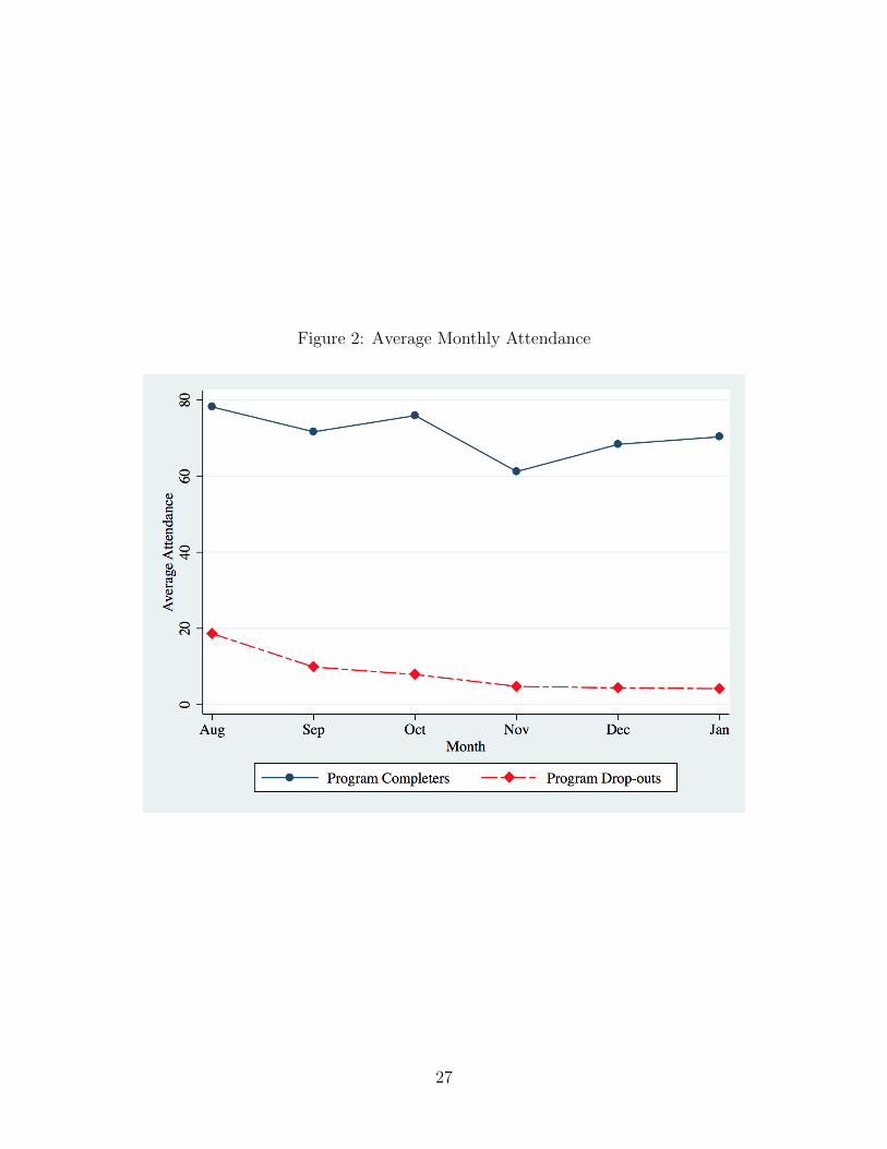
Figure 2: Average Monthly Attendance

27

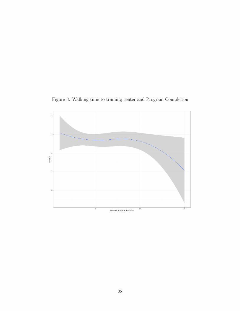
Figure 3: Walking time to training center and Program Completion

28

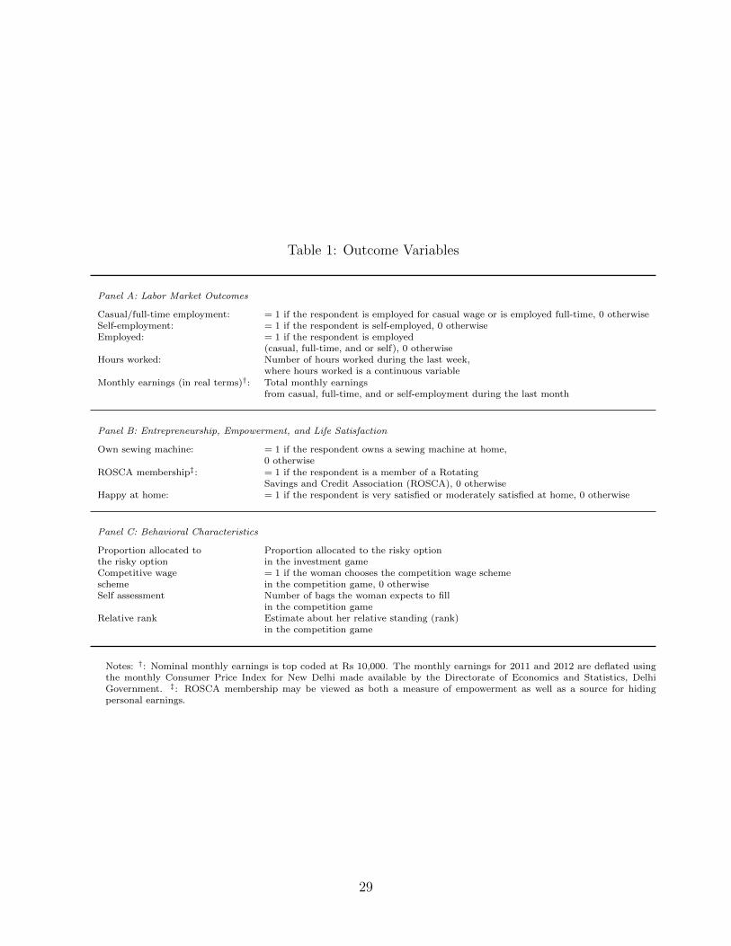
Table 1: Outcome Variables

Panel A: Labor Market Outcomes

Casual/full-time employment: = 1 if the respondent is employed for casual wage or is employed full-time, 0 otherwiseSelf-employment: = 1 if the respondent is self-employed, 0 otherwiseEmployed: = 1 if the respondent is employed

(casual, full-time, and or self), 0 otherwiseHours worked: Number of hours worked during the last week,

where hours worked is a continuous variableMonthly earnings (in real terms)†: Total monthly earnings

from casual, full-time, and or self-employment during the last month

Panel B: Entrepreneurship, Empowerment, and Life Satisfaction

Own sewing machine: = 1 if the respondent owns a sewing machine at home,0 otherwise

ROSCA membership‡: = 1 if the respondent is a member of a RotatingSavings and Credit Association (ROSCA), 0 otherwise

Happy at home: = 1 if the respondent is very satisfied or moderately satisfied at home, 0 otherwise

Panel C: Behavioral Characteristics

Proportion allocated to Proportion allocated to the risky optionthe risky option in the investment gameCompetitive wage = 1 if the woman chooses the competition wage schemescheme in the competition game, 0 otherwiseSelf assessment Number of bags the woman expects to fill

in the competition gameRelative rank Estimate about her relative standing (rank)

in the competition game

Notes: †: Nominal monthly earnings is top coded at Rs 10,000. The monthly earnings for 2011 and 2012 are deflated usingthe monthly Consumer Price Index for New Delhi made available by the Directorate of Economics and Statistics, DelhiGovernment. ‡: ROSCA membership may be viewed as both a measure of empowerment as well as a source for hidingpersonal earnings.

29

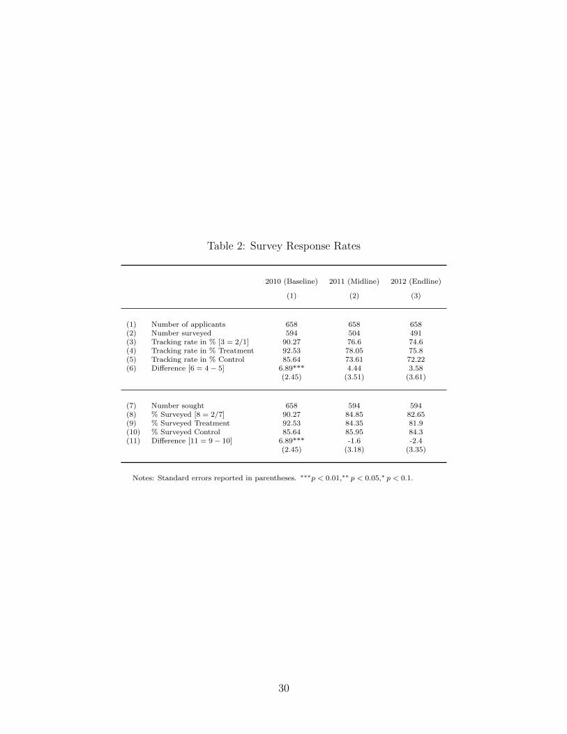
Table 2: Survey Response Rates

2010 (Baseline) 2011 (Midline) 2012 (Endline)

(1) (2) (3)

(1) Number of applicants 658 658 658(2) Number surveyed 594 504 491(3) Tracking rate in % [3 = 2/1] 90.27 76.6 74.6(4) Tracking rate in % Treatment 92.53 78.05 75.8(5) Tracking rate in % Control 85.64 73.61 72.22(6) Di↵erence [6 = 4� 5] 6.89*** 4.44 3.58

(2.45) (3.51) (3.61)

(7) Number sought 658 594 594(8) % Surveyed [8 = 2/7] 90.27 84.85 82.65(9) % Surveyed Treatment 92.53 84.35 81.9(10) % Surveyed Control 85.64 85.95 84.3(11) Di↵erence [11 = 9� 10] 6.89*** -1.6 -2.4

(2.45) (3.18) (3.35)

Notes: Standard errors reported in parentheses. ⇤⇤⇤p < 0.01,⇤⇤ p < 0.05,⇤ p < 0.1.

30

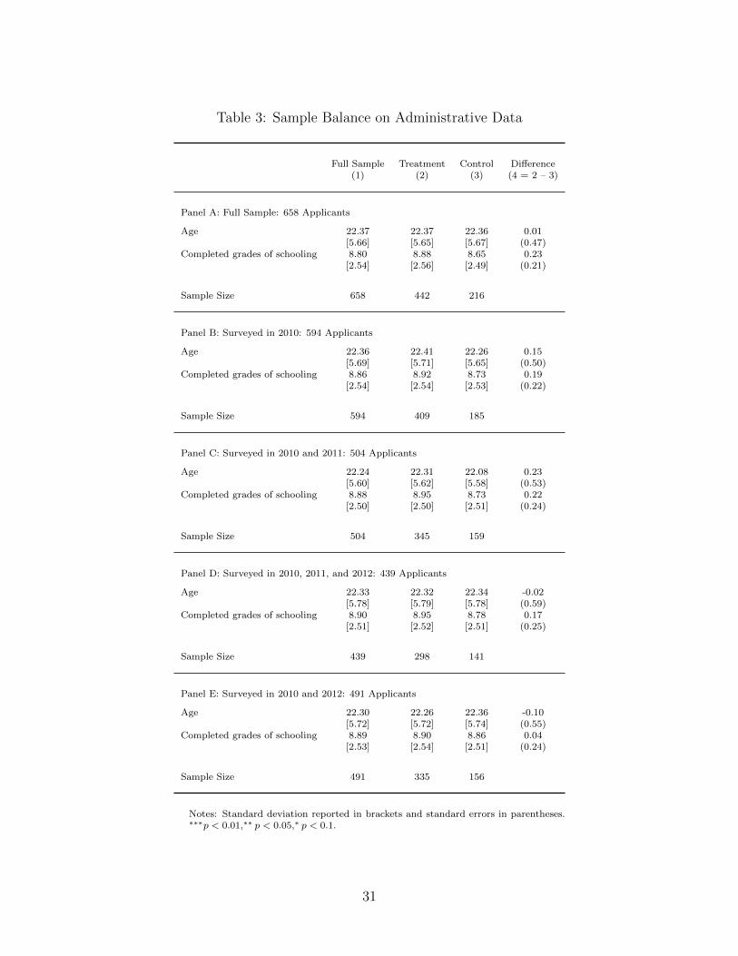
Table 3: Sample Balance on Administrative Data

Full Sample Treatment Control Di↵erence(1) (2) (3) (4 = 2 – 3)

Panel A: Full Sample: 658 Applicants

Age 22.37 22.37 22.36 0.01[5.66] [5.65] [5.67] (0.47)

Completed grades of schooling 8.80 8.88 8.65 0.23[2.54] [2.56] [2.49] (0.21)

Sample Size 658 442 216

Panel B: Surveyed in 2010: 594 Applicants

Age 22.36 22.41 22.26 0.15[5.69] [5.71] [5.65] (0.50)



Panel C: Surveyed in 2010 and 2011: 504 Applicants

Age 22.24 22.31 22.08 0.23[5.60] [5.62] [5.58] (0.53)



Panel D: Surveyed in 2010, 2011, and 2012: 439 Applicants

Age 22.33 22.32 22.34 -0.02[5.78] [5.79] [5.78] (0.59)



Panel E: Surveyed in 2010 and 2012: 491 Applicants

Age 22.30 22.26 22.36 -0.10[5.72] [5.72] [5.74] (0.55)



Notes: Standard deviation reported in brackets and standard errors in parentheses.⇤⇤⇤p < 0.01,⇤⇤ p < 0.05,⇤ p < 0.1.

31

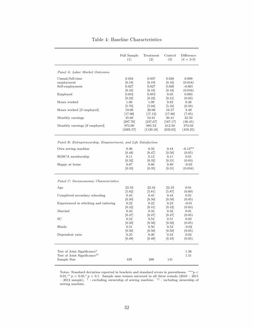
Table 4: Baseline Characteristics

Full Sample Treatment Control Di↵erence(1) (2) (3) (4 = 2-3)


Casual/full-time 0.034 0.037 0.028 0.009employment [0.18] [0.19] [0.16] (0.018)Self-employment 0.027 0.027 0.028 -0.001

[0.16] [0.16] [0.16] (0.016)Employed 0.052 0.053 0.05 0.003

[0.22] [0.22] [0.21] (0.02)Hours worked 1.00 1.08 0.82 0.26

[5.70] [5.94] [5.16] (0.58)Hours worked [if employed] 19.00 20.06 16.57 3.49

[17.00] [17.12] [17.80] (7.85)Monthly earnings 45.68 52.91 30.41 22.50

[297.70] [337.67] [187.17] (30.45)Monthly earnings [if employed] 872.00 985.53 612.50 373.03

[1005.57] [1130.16] [633.65] (459.25)


Own sewing machine 0.36 0.32 0.44 -0.12**[0.48] [0.47] [0.50] (0.05)

ROSCA membership 0.11 0.12 0.11 0.01[0.32] [0.32] [0.31] (0.03)

Happy at home 0.87 0.86 0.89 -0.03[0.33] [0.35] [0.31] (0.034)

Panel C: Socioeconomic Characteristics

Age 22.33 22.34 22.33 0.01[5.82] [5.81] [5.87] (0.60)

Completed secondary schooling 0.45 0.45 0.44 0.01[0.50] [0.50] [0.50] (0.05)

Experienced in stitching and tailoring 0.22 0.22 0.23 -0.01[0.42] [0.41] [0.42] (0.04)

Married 0.33 0.33 0.32 0.01[0.47] [0.47] [0.47] (0.05)

SC 0.52 0.53 0.51 0.02[0.50] [0.50] [0.50] (0.05)

Hindu 0.51 0.50 0.52 -0.02[0.50] [0.50] [0.50] (0.05)

Dependent ratio 0.25 0.26 0.24 0.02[0.48] [0.49] [0.45] (0.05)

Test of Joint Significance† 1.36Test of Joint Significance†† 1.51Sample Size 439 298 141

Notes: Standard deviation reported in brackets and standard errors in parentheses. ⇤⇤⇤p <0.01,⇤⇤ p < 0.05,⇤ p < 0.1. Sample uses women surveyed in all three rounds (2010 – 2011– 2012 sample). † : excluding ownership of sewing machine. †† : including ownership ofsewing machine.

32

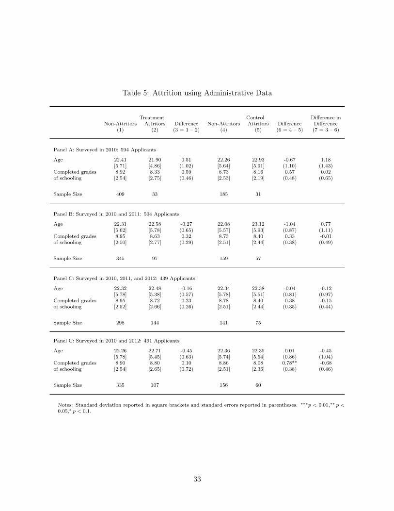
Table 5: Attrition using Administrative Data

Treatment Control Di↵erence inNon-Attritors Attritors Di↵erence Non-Attritors Attritors Di↵erence Di↵erence

(1) (2) (3 = 1 – 2) (4) (5) (6 = 4 – 5) (7 = 3 – 6)

Panel A: Surveyed in 2010: 594 Applicants

Age 22.41 21.90 0.51 22.26 22.93 -0.67 1.18[5.71] [4.86] (1.02) [5.64] [5.91] (1.10) (1.43)

Completed grades 8.92 8.33 0.59 8.73 8.16 0.57 0.02of schooling [2.54] [2.75] (0.46) [2.53] [2.19] (0.48) (0.65)

Sample Size 409 33 185 31

Panel B: Surveyed in 2010 and 2011: 504 Applicants

Age 22.31 22.58 -0.27 22.08 23.12 -1.04 0.77[5.62] [5.78] (0.65) [5.57] [5.93] (0.87) (1.11)

Completed grades 8.95 8.63 0.32 8.73 8.40 0.33 -0.01of schooling [2.50] [2.77] (0.29) [2.51] [2.44] (0.38) (0.49)

Sample Size 345 97 159 57

Panel C: Surveyed in 2010, 2011, and 2012: 439 Applicants

Age 22.32 22.48 -0.16 22.34 22.38 -0.04 -0.12[5.78] [5.38] (0.57) [5.78] [5.51] (0.81) (0.97)

Completed grades 8.95 8.72 0.23 8.78 8.40 0.38 -0.15of schooling [2.52] [2.66] (0.26) [2.51] [2.44] (0.35) (0.44)

Sample Size 298 144 141 75

Panel C: Surveyed in 2010 and 2012: 491 Applicants

Age 22.26 22.71 -0.45 22.36 22.35 0.01 -0.45[5.78] [5.45] (0.63) [5.74] [5.54] (0.86) (1.04)

Completed grades 8.90 8.80 0.10 8.86 8.08 0.78** -0.68of schooling [2.54] [2.65] (0.72) [2.51] [2.36] (0.38) (0.46)

Sample Size 335 107 156 60

Notes: Standard deviation reported in square brackets and standard errors reported in parentheses. ⇤⇤⇤p < 0.01,⇤⇤ p <0.05,⇤ p < 0.1.

33

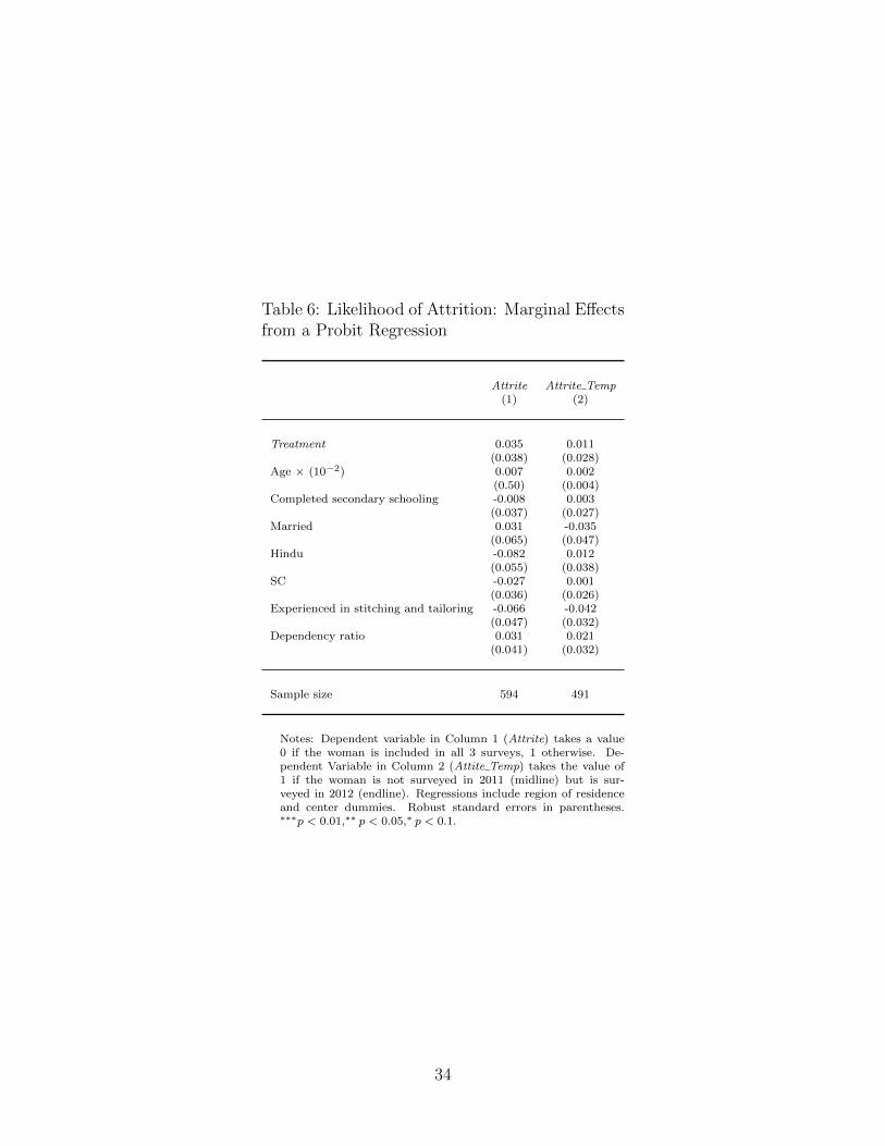
Table 6: Likelihood of Attrition: Marginal E↵ectsfrom a Probit Regression

Attrite Attrite Temp(1) (2)

Treatment 0.035 0.011(0.038) (0.028)

Age ⇥ (10�2) 0.007 0.002(0.50) (0.004)

Completed secondary schooling -0.008 0.003(0.037) (0.027)

Married 0.031 -0.035(0.065) (0.047)

Hindu -0.082 0.012(0.055) (0.038)

SC -0.027 0.001(0.036) (0.026)

Experienced in stitching and tailoring -0.066 -0.042(0.047) (0.032)

Dependency ratio 0.031 0.021(0.041) (0.032)

Sample size 594 491

Notes: Dependent variable in Column 1 (Attrite) takes a value0 if the woman is included in all 3 surveys, 1 otherwise. De-pendent Variable in Column 2 (Attite Temp) takes the value of1 if the woman is not surveyed in 2011 (midline) but is sur-veyed in 2012 (endline). Regressions include region of residenceand center dummies. Robust standard errors in parentheses.⇤⇤⇤p < 0.01,⇤⇤ p < 0.05,⇤ p < 0.1.

34

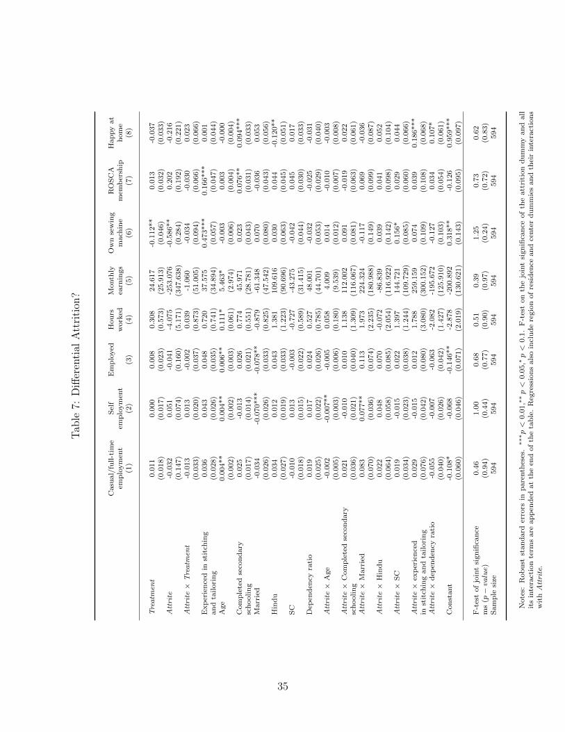
Tab

le7:

Di↵erential

Attrition

?

Casu

al/full-tim

eSelf

Employed

Hours

Month

lyOwnsewing

ROSCA

Happyat

employmen

tem

ploymen

tworked

earn

ings

mach

ine

mem

bersh

iphome

(1)

(2)

(3)

(4)

(5)

(6)

(7)

(8)

Treatm

ent

0.011

0.000

0.008

0.308

24.617

-0.112**

0.013

-0.037

(0.018)

(0.017)

(0.023)

(0.573)

(25.913)

(0.046)

(0.032)

(0.033)

Attrite

-0.032

0.051

-0.041

-4.075

-253.076

-0.586**

0.202

-0.216

(0.147)

(0.074)

(0.160)

(5.171)

(347.638)

(0.284)

(0.192)

(0.221)

Attrite

⇥Treatm

ent

-0.013

0.013

-0.002

0.039

-1.060

-0.034

-0.030

0.023

(0.033)

(0.020)

(0.037)

(0.873)

(51.005)

(0.094)

(0.066)

(0.066)

Experiencedin

stitch

ing

0.036

0.043

0.048

0.720

37.575

0.473***

0.166***

0.001

andtailoring

(0.028)

(0.026)

(0.035)

(0.741)

(34.894)

(0.057)

(0.047)

(0.044)

Age

0.00

4**

0.00

4**

0.00

6**

0.11

1*5.46

3*-0.003

0.00

3-0.000

(0.002)

(0.002)

(0.003)

(0.061)

(2.974)

(0.006)

(0.004)

(0.004)

Completedseco

ndary

0.025

-0.013

0.026

0.774

45.971

0.023

0.076**

0.094***

schooling

(0.017

)(0.014)

(0.021)

(0.551)

(28.781)

(0.043)

(0.031)

(0.033)

Married

-0.034

-0.070

***

-0.078

**-0.879

-61.34

80.07

0-0.036

0.05

3(0.026)

(0.026)

(0.033)

(0.825)

(47.542)

(0.080)

(0.043)

(0.056)

Hindu

0.03

40.01

20.04

31.38

110

9.61

60.03

00.04

4-0.120

**(0.027)

(0.019)

(0.033)

(1.223)

(90.696)

(0.063)

(0.045)

(0.051)

SC

-0.010

0.013

-0.003

-0.727

-43.275

-0.042

0.045

0.017

(0.018)

(0.015)

(0.022)

(0.589)

(31.415)

(0.044)

(0.030)

(0.033)

Dep

enden

cyratio

0.019

0.017

0.02

40.527

48.001

-0.032

-0.025

-0.031

(0.025)

(0.022)

(0.026)

(0.785)

(44.701)

(0.053)

(0.029)

(0.040)

Attrite

⇥Age

-0.002

-0.007

**-0.005

0.05

84.00

90.01

4-0.010

-0.003

(0.005)

(0.003)

(0.006)

(0.180)

(9.539)

(0.012)

(0.007)

(0.008)

Attrite

⇥Completedseco

ndary

0.02

1-0.010

0.010

1.138

112.002

0.091

-0.019

0.022

schooling

(0.036

)(0.021)

(0.040)

(1.309)

(116.067)

(0.081)

(0.063)

(0.061)

Attrite

⇥Married

0.08

30.07

7**

0.11

31.97

322

4.32

4-0.117

0.06

9-0.036

(0.070)

(0.036)

(0.074)

(2.235)

(180.988)

(0.149)

(0.099)

(0.087)

Attrite

⇥Hindu

0.02

20.04

80.07

0-0.072

-86.83

90.03

90.04

10.05

2(0.064)

(0.058)

(0.085)

(2.054)

(116.922)

(0.142)

(0.098)

(0.104)

Attrite

⇥SC

0.019

-0.015

0.022

1.397

144.721

0.156*

0.029

0.044

(0.034)

(0.023)

(0.038)

(1.244)

(109.729)

(0.085)

(0.060)

(0.066)

Attrite

⇥ex

perienced

0.029

-0.015

0.012

1.788

259.159

0.074

0.039

0.186***

institch

ingandtailoring

(0.076)

(0.042)

(0.080)

(3.080)

(300.152)

(0.109)

(0.108)

(0.068)

Attrite

⇥dep

enden

cyratio

-0.055

-0.007

-0.063

-2.082

-195.672

-0.127

0.034

0.107

*(0.040)

(0.026)

(0.042)

(1.427)

(125.910)

(0.103)

(0.054)

(0.061)

Constant

-0.108*

-0.068

-0.146**

-2.878

-200.89

20.318**

-0.126

0.959***

(0.060)

(0.046)

(0.071)

(2.019)

(130.621)

(0.143)

(0.095)

(0.097)

F-testofjointsignifica

nce

0.46

1.00

0.68

0.51

0.39

1.25

0.73

0.62

ms(p

�value)

(0.94)

(0.44)

(0.77)

(0.90)

(0.97)

(0.24)

(0.72)

(0.83)

Sample

size

594

594

594

594

594

594

594

594

Notes:Rob

ust

stan

darderrors

inparen

theses.

⇤⇤⇤p<

0.01,⇤

⇤p<

0.05,⇤

p<

0.1.F-testonth

ejointsignifica

nce

ofth

eattritiondummyandall

itsinteractionterm

sare

appen

ded

atth

een

dofth

etable.Reg

ressionsalsoincluderegionofresiden

ceandcenterdummiesandth

eirinteractions

withAttrite.

35

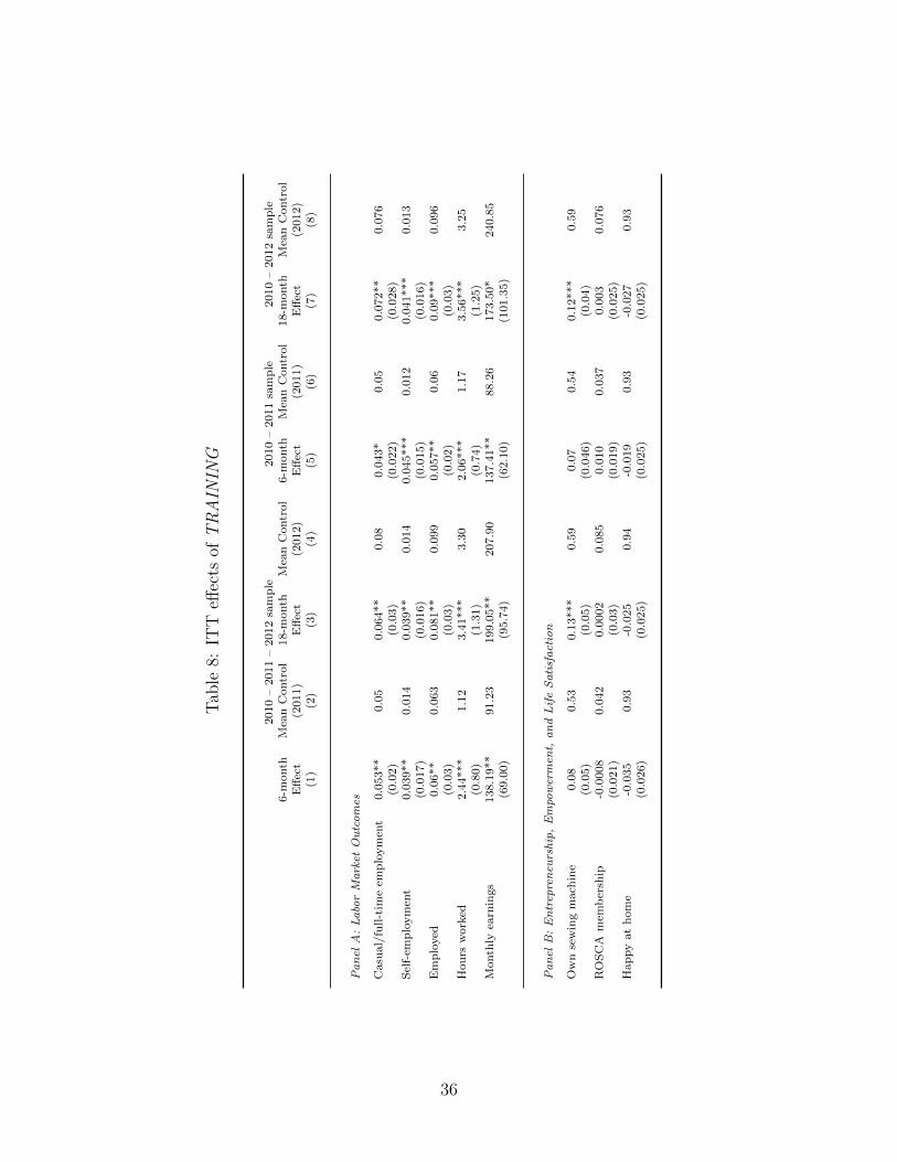
Tab

le8:

ITT

e↵ects

ofTRAIN

ING

2010–2011–2012sample

2010–2011sample

2010–2012sample

6-m

onth

Mea

nControl

18-m

onth

Mea

nControl

6-m

onth

Mea

nControl

18-m

onth

Mea

nControl

E↵ect

(2011)

E↵ect

(2012)

E↵ect

(201

1)

E↵ect

(2012)

(1)

(2)

(3)

(4)

(5)

(6)

(7)

(8)

Panel

A:LaborMarket

Outcomes

Casu

al/full-tim

eem

ploymen

t0.053**

0.05

0.064**

0.08

0.043*

0.05

0.072**

0.076

(0.02)

(0.03)

(0.022)

(0.028)

Self-em

ploymen

t0.039**

0.014

0.039**

0.014

0.045***

0.01

20.041***

0.013

(0.017)

(0.016)

(0.015)

(0.016)

Employed

0.06**

0.063

0.081**

0.099

0.05

7**

0.06

0.09***

0.096

(0.03)

(0.03)

(0.02)

(0.03)

Hou

rsworke

d2.44

***

1.12

3.41

***

3.30

2.06

***

1.17

3.56

***

3.25

(0.80)

(1.31)

(0.74)

(1.25)

Mon

thly

earn

ings

138.19

**91

.23

199.05

**20

7.90

137.41

**88

.26

173.50

*24

0.85

(69.00)

(95.74)

(62.10)

(101.35)

Panel

B:Entrep

reneu

rship,Empo

wermen

t,andLifeSatisfaction

Ownsewingmach

ine

0.08

0.53

0.13*

**

0.59

0.07

0.54

0.12***

0.59

(0.05)

(0.05)

(0.046)

(0.04)

ROSCA

mem

bersh

ip-0.0008

0.042

0.0002

0.085

0.010

0.037

0.003

0.076

(0.021)

(0.03)

(0.019)

(0.025)

Hap

pyat

hom

e-0.035

0.93

-0.025

0.94

-0.019

0.93

-0.027

0.93

(0.026)

(0.025)

(0.025)

(0.025)

36

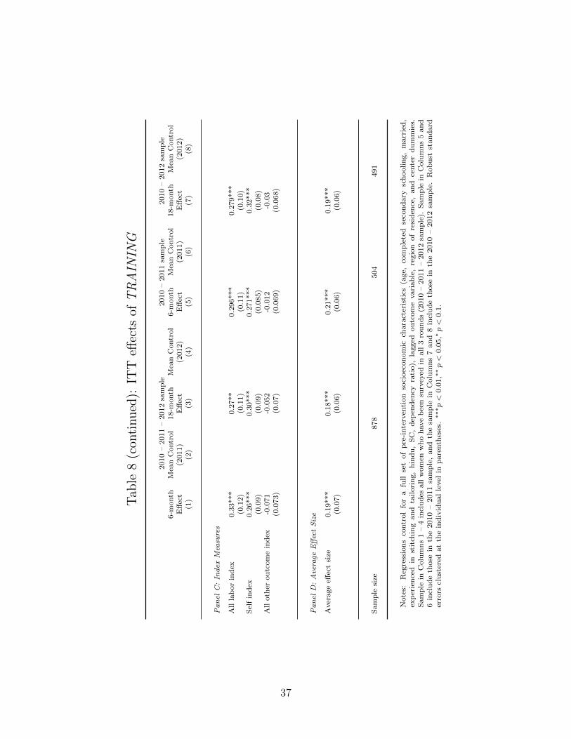
Tab

le8(con

tinu

ed):

ITT

e↵ects

ofTRAIN

ING

2010–2011–2012sample

2010–2011sample

2010–2012sample

6-m

onth

Mea

nCon

trol

18-m

onth

Mea

nControl

6-m

onth

Mea

nControl

18-m

onth

Mea

nControl

E↵ect

(2011)

E↵ect

(2012)

E↵ect

(2011)

E↵ect

(2012)

(1)

(2)

(3)

(4)

(5)

(6)

(7)

(8)

Panel

C:In

dex

Measu

res

Alllabor

index

0.33

***

0.27

**0.29

6***

0.27

9***

(0.12)

(0.11)

(0.11)

(0.10)

Selfindex

0.26***

0.30***

0.271***

0.32

***

(0.09)

(0.09)

(0.085)

(0.08)

Allother

outcom

eindex

-0.071

-0.052

-0.012

-0.03

(0.073)

(0.07)

(0.069)

(0.068)

Panel

D:Average

E↵ectSize

Ave

rage

e↵ectsize

0.19

***

0.18

***

0.21

***

0.19

***

(0.07)

(0.06)

(0.06)

(0.06)

Sample

size

878

504

491

Notes:

Reg

ressionsco

ntrol

fora

full

setof

pre-interven

tion

socioecon

omic

charac

teristics(age

,co

mpleted

seco

ndary

schooling,

married

,ex

perienced

institch

ing

and

tailoring,hindu,SC,dep

enden

cyratio),

lagged

outcomeva

riable,region

ofresiden

ce,and

centerdummies.

Sample

inColumns1–4includes

allwomen

whohav

ebeensu

rvey

edin

all3rounds(2010–2011–2012sample).

Sample

inColumns5and

6includeth

ose

inth

e201

0–2011sample,andth

esample

inColumns7and8includeth

ose

inth

e2010–2012sample.Robust

standard

errors

clustered

atth

eindividuallevel

inparenth

eses.

⇤⇤⇤p<

0.01,⇤

⇤p<

0.05,⇤

p<

0.1.

37

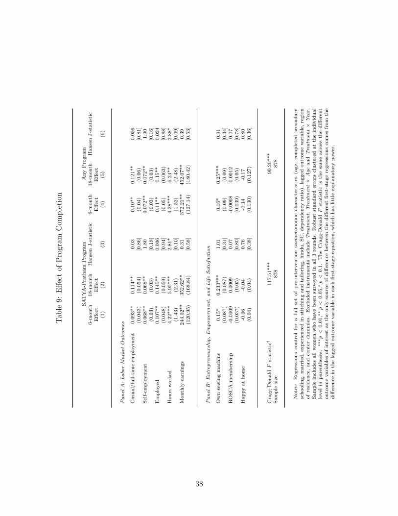
Tab

le9:

E↵ectof

Program

Com

pletion

SATYA-P

rath

am

Program

AnyProgram

6-m

onth

18-m

onth

HansenJ-statistic

6-m

onth

18-m

onth

HansenJ-statistic

E↵ect

E↵ect

E↵ect

E↵ect

(1)

(2)

(3)

(4)

(5)

(6)

Panel

A:LaborMarket

Outcomes

Casu

al/full-tim

eem

ploymen

t0.093**

0.114**

0.03

0.10**

0.121**

0.059

(0.043)

(0.054)

[0.86]

(0.04)

(0.06)

[0.81]

Self-em

ploymen

t0.068**

0.068**

1.80

0.072**

0.07

2**

1.90

(0.03)

(0.03)

[0.18]

(0.03)

(0.03)

[0.16]

Employe

d0.107**

0.145**

0.006

0.11**

0.15**

0.024

(0.048)

(0.059)

[0.94]

(0.05)

(0.063)

[0.88]

Hou

rsworke

d4.22

***

5.95

***

2.81

*4.38

***

6.24

**2.88

*(1.43)

(2.31)

[0.10]

(1.52)

(2.48)

[0.09]

Mon

thly

earn

ings

244.02

**35

2.62

**0.31

372.21

**45

2.07

**0.39

(120.95)

(168.84)

[0.58]

(127.14)

(180.42

)[0.53]

Panel

B:Entrep

reneu

rship,Empo

wermen

t,andLifeSatisfaction

Ownsewingmach

ine

0.15*

0.233***

1.01

0.16*

0.25***

0.91

(0.087)

(0.087)

[0.31]

(0.09)

(0.09)

[0.34]

ROSCA

mem

bersh

ip-0.0009

0.0009

0.07

-0.0008

0.0012

0.07

(0.037)

(0.05)

[0.80]

(0.039)

(0.05)

[0.78]

Hap

pyat

hom

e-0.06

-0.04

0.76

-0.14

-0.17

0.80

(0.04)

(0.04)

[0.38]

(0.130)

(0.127)

[0.36]

Cragg-D

onald

Fstatistic

†117.51***

90.20***

Sample

size

878

878

Notes:

Reg

ressionsco

ntrol

fora

full

setof

pre-interven

tion

socioecon

omic

charac

teristics(age

,co

mpleted

seco

ndary

schooling,married,ex

periencedin

stitch

ingandtailoring,hindu,SC,dep

enden

cyratio),

lagg

edoutcomeva

riable,region

ofresiden

ce,and

centerdummies.

Excluded

instru

men

tsincludeTreatm

ent,

Treatm

ent⇥

Age

and

Treatm

ent⇥

Year.

Sample

includes

allwomen

whohav

ebeensu

rvey

edin

all3rounds.

Robust

standard

errors

clustered

atth

eindividual

level

inparenth

eses.

⇤⇤⇤p<

0.01,⇤

⇤p<

0.05,⇤

p<

0.1.TheCragg-D

onald

Fstatistic

isth

esameacross

thedi↵eren

toutcomeva

riablesofinterest

asth

eonly

sourceofdi↵eren

cebetweenth

edi↵eren

tfirst-stageregressionsco

mes

from

the

di↵eren

cein

thelagged

outcomeva

riable

inea

chfirst-stageeq

uation,whichhaslittle

explanatory

pow

er.

38

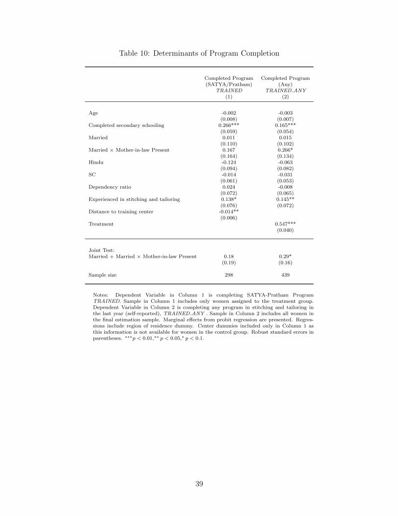
Table 10: Determinants of Program Completion

Completed Program Completed Program(SATYA/Pratham) (Any)

TRAINED TRAINED ANY(1) (2)

Age -0.002 -0.003(0.008) (0.007)

Completed secondary schooling 0.266*** 0.165***(0.059) (0.054)

Married 0.011 0.015(0.110) (0.102)

Married ⇥ Mother-in-law Present 0.167 0.266*(0.164) (0.134)

Hindu -0.124 -0.063(0.094) (0.082)

SC -0.014 -0.031(0.061) (0.053)

Dependency ratio 0.024 -0.008(0.072) (0.065)

Experienced in stitching and tailoring 0.138* 0.145**(0.076) (0.072)

Distance to training center -0.014**(0.006)

Treatment 0.547***(0.040)

Joint Test:Married + Married ⇥ Mother-in-law Present 0.18 0.29*

(0.19) (0.16)

Sample size 298 439

Notes: Dependent Variable in Column 1 is completing SATYA-Pratham ProgramTRAINED. Sample in Column 1 includes only women assigned to the treatment group.Dependent Variable in Column 2 is completing any program in stitching and tailoring inthe last year (self-reported), TRAINED ANY . Sample in Column 2 includes all women inthe final estimation sample. Marginal e↵ects from probit regression are presented. Regres-sions include region of residence dummy. Center dummies included only in Column 1 asthis information is not available for women in the control group. Robust standard errors inparentheses. ⇤⇤⇤p < 0.01,⇤⇤ p < 0.05,⇤ p < 0.1.

39

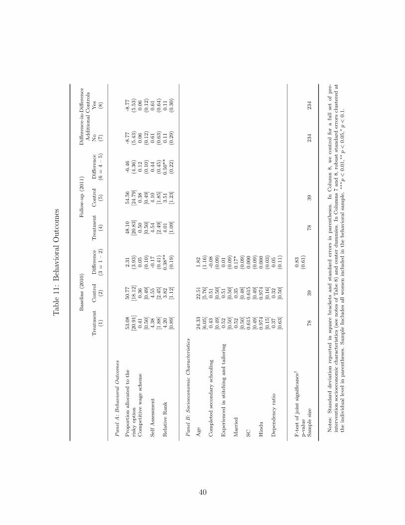
Tab

le11:BehavioralOutcom

es

Baseline(2010)

Follow

-up(2011

)Di↵eren

ce-in-D

i↵eren

ceAdditional

Con

trols

Treatm

ent

Control

Di↵eren

ceTreatm

ent

Con

trol

Di↵eren

ceNo

Yes

(1)

(2)

(3=

1–2)

(4)

(5)

(6=

4–5)

(7)

(8)

Panel

A:Beh

avioralOutcomes

Proportionalloca

tedto

the

53.08

50.77

2.31

48.10

54.56

-6.46

-8.77

-8.77

riskyoption

[20.91]

[18.12]

(3.93)

[20.83]

[24.79]

(4.36)

(5.43)

(5.53)

Competitivewageschem

e0.41

0.36

0.05

0.50

0.38

0.12

0.06

0.06

[0.50]

[0.49]

(0.10)

[0.50]

[0.49]

(0.10)

(0.12)

(0.12)

SelfAssessm

ent

4.38

4.55

-0.17

4.54

4.10

0.44

0.61

0.61

[1.88]

[2.45]

(0.41)

[2.49]

[1.85]

(0.45)

(0.63)

(0.64)

RelativeRank

4.20

3.82

0.38**

4.01

3.51

0.50**

0.11

0.11

[0.89]

[1.12]

(0.19)

[1.09]

[1.23]

(0.22)

(0.29)

(0.30)

Panel

B:Socioeconomic

Characteristics

Age

24.33

22.51

1.82

[6.05]

[5.76]

(1.16)

Completedseco

ndary

schooling

0.43

0.51

-0.08

[0.49]

[0.50]

(0.09)

Experiencedin

stitch

ingandtailoring

0.52

0.51

0.01

[0.50]

[0.50]

(0.09)

Married

0.52

0.35

0.17

*[0.50]

[0.48]

(0.09)

SC

0.615

0.615

0.000

[0.49]

[0.49]

(0.09)

Hindu

0.97

40.97

40.00

0[0.15]

[0.16]

(0.03)

Dep

enden

cyratio

0.37

0.32

0.05

[0.63]

[0.50]

(0.11)

F-testofjointsignifica

nce

†0.83

p-value

(0.61)

Sample

size

78

39

78

39

234

234

Notes:Standard

dev

iation

reported

insquarebracketsan

dstan

dard

errors

inparen

theses.

InColumn

8,weco

ntrol

forafull

setof

pre-

interven

tionsocioeconomic

characteristics

(see

notesofTabe8)andcenterdummies.

InColumns7and8,robust

standard

errors

clustered

at

theindividuallevel

inparenth

eses.Sample

Includes

allwomen

included

inth

ebeh

avioralsample.

⇤⇤⇤p<

0.01,⇤

⇤p<

0.05,⇤

p<

0.1.

40

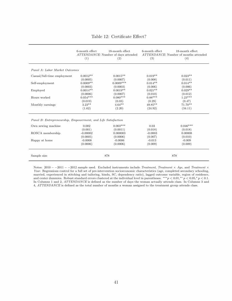
Table 12: Certificate E↵ect?

6-month e↵ect 18-month e↵ect 6-month e↵ect 18-month e↵ectATTENDANCE: Number of days attended ATTENDANCE: Number of months attended

(1) (2) (3) (4)


Casual/full-time employment 0.0012** 0.0015** 0.019** 0.023**(0.0005) (0.0007) (0.008) (0.011)

Self-employment 0.0009** 0.0009*** 0.014** 0.014**(0.0003) (0.0003) (0.006) (0.006)

Employed 0.0014** 0.0019** 0.021** 0.029**(0.0006) (0.0007) (0.010) (0.012)

Hours worked 0.054*** 0.080*** 0.88*** 1.23***(0.019) (0.03) (0.29) (0.47)

Monthly earnings 3.23** 4.64** 49.85** 71.70**(1.62) (2.20) (24.92) (34.11)


Own sewing machine 0.002 0.003*** 0.03 0.046***(0.001) (0.0011) (0.018) (0.018)

ROSCA membership -0.00002 0.000003 -0.0003 0.00008(0.0005) (0.0006) (0.007) (0.010)

Happy at home -0.0008 -0.0006 -0.013 -0.009(0.0006) (0.0006) (0.009) (0.009)

Sample size 878 878

Notes: 2010 � �2011 � �2012 sample used. Excluded instruments include Treatment, Treatment ⇥ Age, and Treatment ⇥Year. Regressions control for a full set of pre-intervention socioeconomic characteristics (age, completed secondary schooling,married, experienced in stitching and tailoring, hindu, SC, dependency ratio), lagged outcome variable, region of residence,and center dummies. Robust standard errors clustered at the individual level in parentheses. ⇤⇤⇤p < 0.01,⇤⇤ p < 0.05,⇤ p < 0.1.In Columns 1 and 2, ATTENDANCE is defined as the number of days the woman actually attends class. In Columns 3 and4, ATTENDANCE is defined as the total number of months a woman assigned to the treatment group attends class.

41

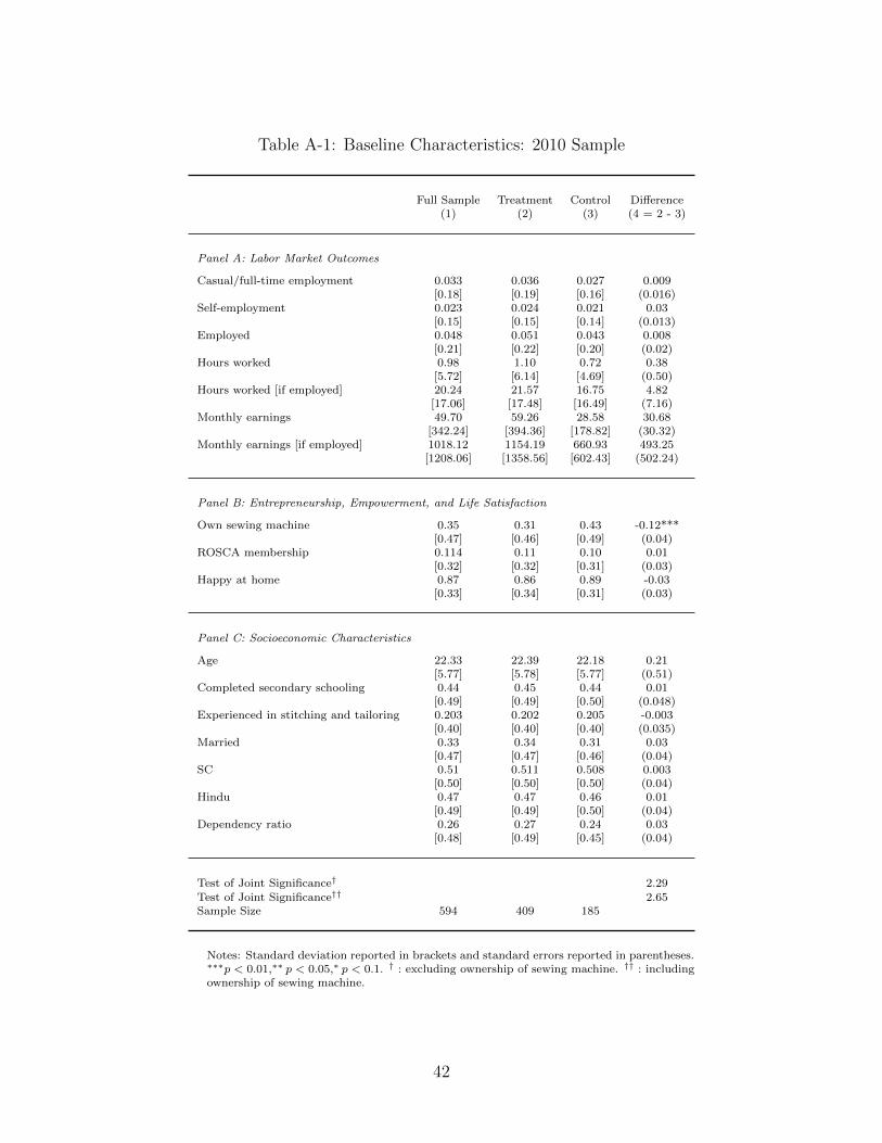
Table A-1: Baseline Characteristics: 2010 Sample

Full Sample Treatment Control Di↵erence(1) (2) (3) (4 = 2 - 3)


Casual/full-time employment 0.033 0.036 0.027 0.009[0.18] [0.19] [0.16] (0.016)

Self-employment 0.023 0.024 0.021 0.03[0.15] [0.15] [0.14] (0.013)

Employed 0.048 0.051 0.043 0.008[0.21] [0.22] [0.20] (0.02)

Hours worked 0.98 1.10 0.72 0.38[5.72] [6.14] [4.69] (0.50)

Hours worked [if employed] 20.24 21.57 16.75 4.82[17.06] [17.48] [16.49] (7.16)

Monthly earnings 49.70 59.26 28.58 30.68[342.24] [394.36] [178.82] (30.32)

Monthly earnings [if employed] 1018.12 1154.19 660.93 493.25[1208.06] [1358.56] [602.43] (502.24)


Own sewing machine 0.35 0.31 0.43 -0.12***[0.47] [0.46] [0.49] (0.04)


Happy at home 0.87 0.86 0.89 -0.03[0.33] [0.34] [0.31] (0.03)


Age 22.33 22.39 22.18 0.21[5.77] [5.78] [5.77] (0.51)



Married 0.33 0.34 0.31 0.03[0.47] [0.47] [0.46] (0.04)

SC 0.51 0.511 0.508 0.003[0.50] [0.50] [0.50] (0.04)

Hindu 0.47 0.47 0.46 0.01[0.49] [0.49] [0.50] (0.04)

Dependency ratio 0.26 0.27 0.24 0.03[0.48] [0.49] [0.45] (0.04)


Notes: Standard deviation reported in brackets and standard errors reported in parentheses.⇤⇤⇤p < 0.01,⇤⇤ p < 0.05,⇤ p < 0.1. † : excluding ownership of sewing machine. †† : includingownership of sewing machine.

42

Table A-2: Baseline Characteristics: 2010 – 2011 Panel




Self-employment 0.025 0.026 0.025 0.001[0.16] [0.16] [0.15] (0.015)

Employed 0.053 0.057 0.044 0.013[0.22] [0.23] [0.20] (0.021)

Hours worked 1.12 1.31 0.73 0.58[6.15] [6.66] [4.86] (0.59)





Own sewing machine 0.36 0.32 0.43 -0.11**[0.48] [0.47] [0.49] (0.04)


Happy at home 0.87 0.86 0.89 -0.03[0.33] [0.34] [0.31] (0.03)


Age 22.24 22.33 22.04 0.29[5.66] [5.66] [5.66] (0.54)


Experienced in stitching and tailoring 0.216 0.217 0.213 0.004[0.41] [0.41] [0.41] (0.04)

Married 0.33 0.34 0.31 0.03[0.47] [0.47] [0.46] (0.04)

SC 0.51 0.52 0.49 0.03[0.50] [0.50] [0.50] (0.05)

Hindu 0.494 0.498 0.484 0.014[0.50] [0.50] [0.50] (0.048)



Notes: Standard deviation reported in brackets and standard errors reported in parentheses.⇤⇤⇤p < 0.01,⇤⇤ p < 0.05,⇤ p < 0.1. † : excluding ownership of sewing machine. †† : includingownership of sewing machine.

43

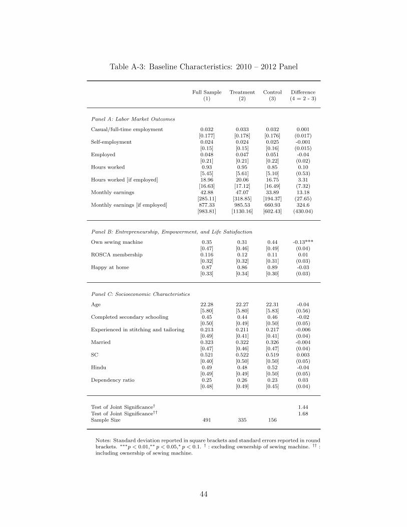
Table A-3: Baseline Characteristics: 2010 – 2012 Panel




Self-employment 0.024 0.024 0.025 -0.001[0.15] [0.15] [0.16] (0.015)

Employed 0.048 0.047 0.051 -0.04[0.21] [0.21] [0.22] (0.02)

Hours worked 0.93 0.95 0.85 0.10[5.45] [5.61] [5.10] (0.53)





Own sewing machine 0.35 0.31 0.44 -0.13***[0.47] [0.46] [0.49] (0.04)


Happy at home 0.87 0.86 0.89 -0.03[0.33] [0.34] [0.30] (0.03)


Age 22.28 22.27 22.31 -0.04[5.80] [5.80] [5.83] (0.56)

Completed secondary schooling 0.45 0.44 0.46 -0.02[0.50] [0.49] [0.50] (0.05)


Married 0.323 0.322 0.326 -0.004[0.47] [0.46] [0.47] (0.04)

SC 0.521 0.522 0.519 0.003[0.40] [0.50] [0.50] (0.05)

Hindu 0.49 0.48 0.52 -0.04[0.49] [0.49] [0.50] (0.05)



Notes: Standard deviation reported in square brackets and standard errors reported in roundbrackets. ⇤⇤⇤p < 0.01,⇤⇤ p < 0.05,⇤ p < 0.1. † : excluding ownership of sewing machine. †† :including ownership of sewing machine.

44

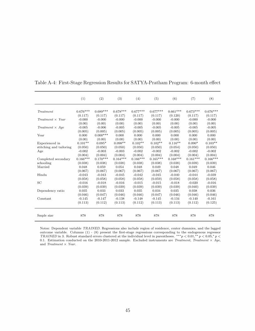
Table A-4: First-Stage Regression Results for SATYA-Pratham Program: 6-month e↵ect

(1) (2) (3) (4) (5) (6) (7) (8)

Treatment 0.676*** 0.689*** 0.678*** 0.677*** 0.677*** 0.661*** 0.673*** 0.676***(0.117) (0.117) (0.117) (0.117) (0.117) (0.120) (0.117) (0.117)

Treatment ⇥ Year -0.000 -0.000 -0.000 -0.000 -0.000 -0.000 -0.000 -0.000(0.00) (0.00) (0.00) (0.00) (0.00) (0.00) (0.00) (0.00)

Treatment ⇥ Age -0.005 -0.006 -0.005 -0.005 -0.005 -0.005 -0.005 -0.005(0.005) (0.005) (0.005) (0.005) (0.005) (0.005) (0.005) (0.005)

Year 0.000 0.000*** 0.000 0.000 0.000 0.000 0.000 0.000(0.00) (0.00) (0.00) (0.00) (0.00) (0.00) (0.00) (0.00)

Experienced in 0.101** 0.095* 0.098** 0.102** 0.102** 0.116** 0.090* 0.103**stitching and tailoring (0.050) (0.050) (0.050) (0.050) (0.050) (0.054) (0.050) (0.050)Age -0.002 -0.003 -0.003 -0.002 -0.002 -0.002 -0.002 -0.002

(0.004) (0.004) (0.004) (0.004) (0.004) (0.004) (0.004) (0.004)Completed secondary 0.166*** 0.170*** 0.164*** 0.166*** 0.165*** 0.168*** 0.161*** 0.166***schooling (0.038) (0.038) (0.038) (0.038) (0.038) (0.038) (0.039) (0.039)Married 0.048 0.059 0.054 0.048 0.049 0.048 0.049 0.046

(0.067) (0.067) (0.067) (0.067) (0.067) (0.067) (0.067) (0.067)Hindu -0.043 -0.043 -0.045 -0.042 -0.045 -0.040 -0.044 -0.039

(0.058) (0.058) (0.058) (0.058) (0.059) (0.058) (0.058) (0.058)SC -0.016 -0.018 -0.016 -0.015 -0.015 -0.018 -0.020 -0.016

(0.039) (0.039) (0.039) (0.039) (0.039) (0.039) (0.040) (0.039)Dependency ratio 0.035 0.033 0.033 0.035 0.034 0.035 0.038 0.036

(0.046) (0.047) (0.046) (0.046) (0.047) (0.046) (0.046) (0.046)Constant -0.145 -0.147 -0.138 -0.148 -0.145 -0.134 -0.140 -0.161

(0.113) (0.112) (0.113) (0.112) (0.113) (0.113) (0.112) (0.125)

Smple size 878 878 878 878 878 878 878 878

Notes: Dependent variable TRAINED. Regressions also include region of residence, center dummies, and the laggedoutcome variable. Columns (1) - (8) present the first-stage regressions corresponding to the endogenous regressorTRAINED in 3. Robust standard errors clustered at the individual level in parentheses. ⇤⇤⇤p < 0.01,⇤⇤ p < 0.05,⇤ p <0.1. Estimation conducted on the 2010-2011-2012 sample. Excluded instruments are Treatment, Treatment ⇥ Age,and Treatment ⇥ Year.

45

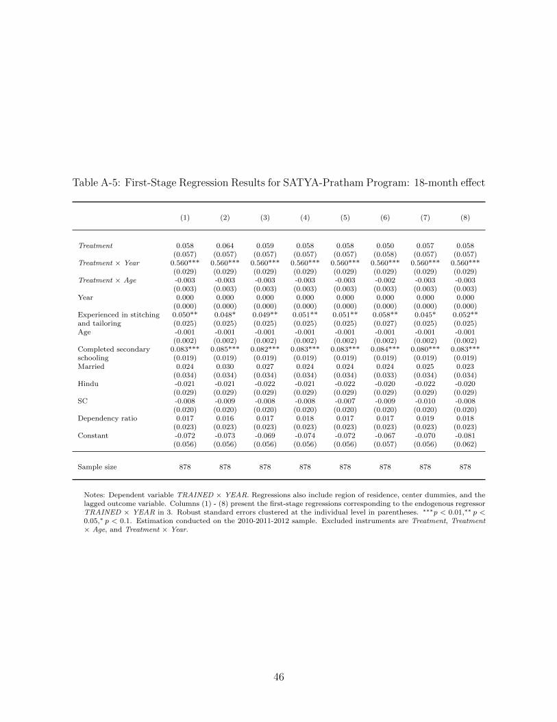
Table A-5: First-Stage Regression Results for SATYA-Pratham Program: 18-month e↵ect

(1) (2) (3) (4) (5) (6) (7) (8)

Treatment 0.058 0.064 0.059 0.058 0.058 0.050 0.057 0.058(0.057) (0.057) (0.057) (0.057) (0.057) (0.058) (0.057) (0.057)

Treatment ⇥ Year 0.560*** 0.560*** 0.560*** 0.560*** 0.560*** 0.560*** 0.560*** 0.560***(0.029) (0.029) (0.029) (0.029) (0.029) (0.029) (0.029) (0.029)

Treatment ⇥ Age -0.003 -0.003 -0.003 -0.003 -0.003 -0.002 -0.003 -0.003(0.003) (0.003) (0.003) (0.003) (0.003) (0.003) (0.003) (0.003)

Year 0.000 0.000 0.000 0.000 0.000 0.000 0.000 0.000(0.000) (0.000) (0.000) (0.000) (0.000) (0.000) (0.000) (0.000)

Experienced in stitching 0.050** 0.048* 0.049** 0.051** 0.051** 0.058** 0.045* 0.052**and tailoring (0.025) (0.025) (0.025) (0.025) (0.025) (0.027) (0.025) (0.025)Age -0.001 -0.001 -0.001 -0.001 -0.001 -0.001 -0.001 -0.001

(0.002) (0.002) (0.002) (0.002) (0.002) (0.002) (0.002) (0.002)Completed secondary 0.083*** 0.085*** 0.082*** 0.083*** 0.083*** 0.084*** 0.080*** 0.083***schooling (0.019) (0.019) (0.019) (0.019) (0.019) (0.019) (0.019) (0.019)Married 0.024 0.030 0.027 0.024 0.024 0.024 0.025 0.023

(0.034) (0.034) (0.034) (0.034) (0.034) (0.033) (0.034) (0.034)Hindu -0.021 -0.021 -0.022 -0.021 -0.022 -0.020 -0.022 -0.020

(0.029) (0.029) (0.029) (0.029) (0.029) (0.029) (0.029) (0.029)SC -0.008 -0.009 -0.008 -0.008 -0.007 -0.009 -0.010 -0.008

(0.020) (0.020) (0.020) (0.020) (0.020) (0.020) (0.020) (0.020)Dependency ratio 0.017 0.016 0.017 0.018 0.017 0.017 0.019 0.018

(0.023) (0.023) (0.023) (0.023) (0.023) (0.023) (0.023) (0.023)Constant -0.072 -0.073 -0.069 -0.074 -0.072 -0.067 -0.070 -0.081

(0.056) (0.056) (0.056) (0.056) (0.056) (0.057) (0.056) (0.062)

Sample size 878 878 878 878 878 878 878 878

Notes: Dependent variable TRAINED ⇥ YEAR. Regressions also include region of residence, center dummies, and thelagged outcome variable. Columns (1) - (8) present the first-stage regressions corresponding to the endogenous regressorTRAINED ⇥ YEAR in 3. Robust standard errors clustered at the individual level in parentheses. ⇤⇤⇤p < 0.01,⇤⇤ p <0.05,⇤ p < 0.1. Estimation conducted on the 2010-2011-2012 sample. Excluded instruments are Treatment, Treatment⇥ Age, and Treatment ⇥ Year.

46

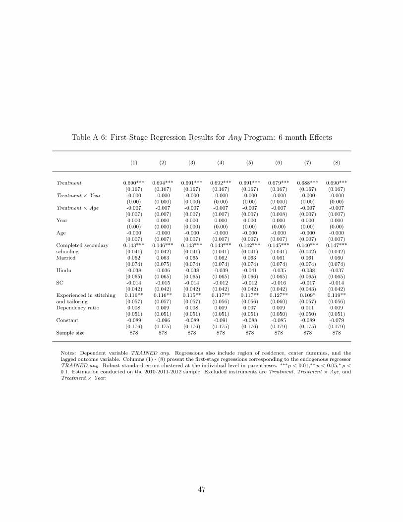
Table A-6: First-Stage Regression Results for Any Program: 6-month E↵ects

(1) (2) (3) (4) (5) (6) (7) (8)

Treatment 0.690*** 0.694*** 0.691*** 0.692*** 0.691*** 0.679*** 0.688*** 0.690***(0.167) (0.167) (0.167) (0.167) (0.167) (0.167) (0.167) (0.167)

Treatment ⇥ Year -0.000 -0.000 -0.000 -0.000 -0.000 -0.000 -0.000 -0.000(0.00) (0.000) (0.000) (0.00) (0.00) (0.000) (0.00) (0.00)

Treatment ⇥ Age -0.007 -0.007 -0.007 -0.007 -0.007 -0.007 -0.007 -0.007(0.007) (0.007) (0.007) (0.007) (0.007) (0.008) (0.007) (0.007)

Year 0.000 0.000 0.000 0.000 0.000 0.000 0.000 0.000(0.00) (0.000) (0.000) (0.00) (0.00) (0.00) (0.00) (0.00)

Age -0.000 -0.000 -0.000 -0.000 -0.000 -0.000 -0.000 -0.000(0.007) (0.007) (0.007) (0.007) (0.007) (0.007) (0.007) (0.007)

Completed secondary 0.143*** 0.146*** 0.143*** 0.143*** 0.142*** 0.145*** 0.140*** 0.147***schooling (0.041) (0.042) (0.041) (0.041) (0.041) (0.041) (0.042) (0.042)Married 0.062 0.063 0.065 0.062 0.063 0.061 0.061 0.060

(0.074) (0.075) (0.074) (0.074) (0.074) (0.074) (0.074) (0.074)Hindu -0.038 -0.036 -0.038 -0.039 -0.041 -0.035 -0.038 -0.037

(0.065) (0.065) (0.065) (0.065) (0.066) (0.065) (0.065) (0.065)SC -0.014 -0.015 -0.014 -0.012 -0.012 -0.016 -0.017 -0.014

(0.042) (0.042) (0.042) (0.042) (0.042) (0.042) (0.043) (0.042)Experienced in stitching 0.116** 0.116** 0.115** 0.117** 0.117** 0.127** 0.109* 0.119**and tailoring (0.057) (0.057) (0.057) (0.056) (0.056) (0.060) (0.057) (0.056)Dependency ratio 0.008 0.009 0.008 0.009 0.007 0.009 0.011 0.009

(0.051) (0.051) (0.051) (0.051) (0.051) (0.050) (0.050) (0.051)Constant -0.089 -0.096 -0.089 -0.091 -0.088 -0.085 -0.089 -0.079

(0.176) (0.175) (0.176) (0.175) (0.176) (0.179) (0.175) (0.179)Sample size 878 878 878 878 878 878 878 878

Notes: Dependent variable TRAINED any. Regressions also include region of residence, center dummies, and thelagged outcome variable. Columns (1) - (8) present the first-stage regressions corresponding to the endogenous regressorTRAINED any. Robust standard errors clustered at the individual level in parentheses. ⇤⇤⇤p < 0.01,⇤⇤ p < 0.05,⇤ p <0.1. Estimation conducted on the 2010-2011-2012 sample. Excluded instruments are Treatment, Treatment ⇥ Age, andTreatment ⇥ Year.

47

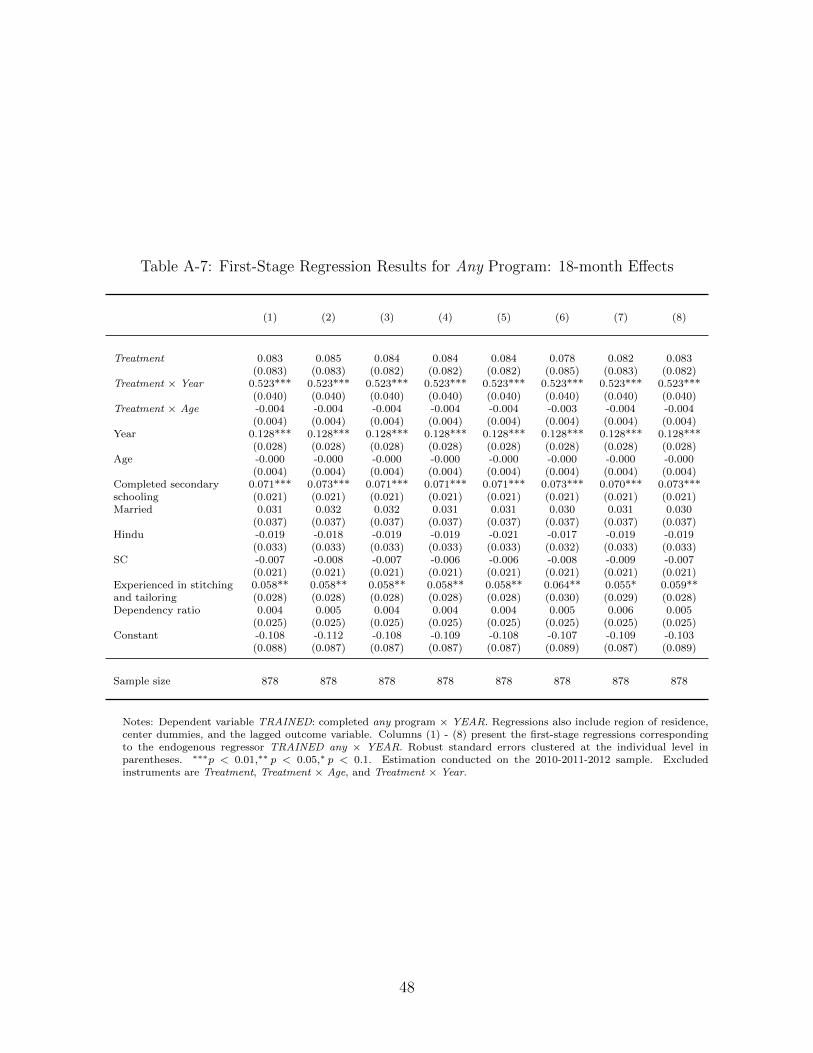
Table A-7: First-Stage Regression Results for Any Program: 18-month E↵ects

(1) (2) (3) (4) (5) (6) (7) (8)

Treatment 0.083 0.085 0.084 0.084 0.084 0.078 0.082 0.083(0.083) (0.083) (0.082) (0.082) (0.082) (0.085) (0.083) (0.082)

Treatment ⇥ Year 0.523*** 0.523*** 0.523*** 0.523*** 0.523*** 0.523*** 0.523*** 0.523***(0.040) (0.040) (0.040) (0.040) (0.040) (0.040) (0.040) (0.040)

Treatment ⇥ Age -0.004 -0.004 -0.004 -0.004 -0.004 -0.003 -0.004 -0.004(0.004) (0.004) (0.004) (0.004) (0.004) (0.004) (0.004) (0.004)

Year 0.128*** 0.128*** 0.128*** 0.128*** 0.128*** 0.128*** 0.128*** 0.128***(0.028) (0.028) (0.028) (0.028) (0.028) (0.028) (0.028) (0.028)

Age -0.000 -0.000 -0.000 -0.000 -0.000 -0.000 -0.000 -0.000(0.004) (0.004) (0.004) (0.004) (0.004) (0.004) (0.004) (0.004)

Completed secondary 0.071*** 0.073*** 0.071*** 0.071*** 0.071*** 0.073*** 0.070*** 0.073***schooling (0.021) (0.021) (0.021) (0.021) (0.021) (0.021) (0.021) (0.021)Married 0.031 0.032 0.032 0.031 0.031 0.030 0.031 0.030

(0.037) (0.037) (0.037) (0.037) (0.037) (0.037) (0.037) (0.037)Hindu -0.019 -0.018 -0.019 -0.019 -0.021 -0.017 -0.019 -0.019

(0.033) (0.033) (0.033) (0.033) (0.033) (0.032) (0.033) (0.033)SC -0.007 -0.008 -0.007 -0.006 -0.006 -0.008 -0.009 -0.007

(0.021) (0.021) (0.021) (0.021) (0.021) (0.021) (0.021) (0.021)Experienced in stitching 0.058** 0.058** 0.058** 0.058** 0.058** 0.064** 0.055* 0.059**and tailoring (0.028) (0.028) (0.028) (0.028) (0.028) (0.030) (0.029) (0.028)Dependency ratio 0.004 0.005 0.004 0.004 0.004 0.005 0.006 0.005

(0.025) (0.025) (0.025) (0.025) (0.025) (0.025) (0.025) (0.025)Constant -0.108 -0.112 -0.108 -0.109 -0.108 -0.107 -0.109 -0.103

(0.088) (0.087) (0.087) (0.087) (0.087) (0.089) (0.087) (0.089)

Sample size 878 878 878 878 878 878 878 878

Notes: Dependent variable TRAINED: completed any program ⇥ YEAR. Regressions also include region of residence,center dummies, and the lagged outcome variable. Columns (1) - (8) present the first-stage regressions correspondingto the endogenous regressor TRAINED any ⇥ YEAR. Robust standard errors clustered at the individual level inparentheses. ⇤⇤⇤p < 0.01,⇤⇤ p < 0.05,⇤ p < 0.1. Estimation conducted on the 2010-2011-2012 sample. Excludedinstruments are Treatment, Treatment ⇥ Age, and Treatment ⇥ Year.

48

Discussion Paper No. 8552 Discussion Papers often represent preliminary work and are circulated to...

Documents

Transcript of Discussion Paper No. 8552 Discussion Papers often represent preliminary work and are circulated to...