Einführung in R - Marlene Müller · Andere Möglichkeiten der Kommunikation mit Excel (nicht...

Einführung in R

Marlene Müller

18. November 2008

Inhaltsverzeichnis

1 Was ist eigentlich R? 2

2 Wie fange ich an? 3

3 Wie bekomme ich Hilfe? 6

4 Etwas Rechnerei zum Anfang 10

5 Daten & Dateien 20

6 Schöne bunte Welt der Grafik 27

7 Etwas Statistik 41

8 “Höhere” Mathematik 53

9 Einstieg ins Programmieren 59

Marlene Müller: Einführung in R 1

1 Was ist eigentlich R?

Programmiersprache S = in den Bell Labs für Statistik, Simulation, Grafikentwickelt (Becker and Chambers; 1984)

→ S-PLUS: kommerzielle Implementation

→ R: Implementation unter GPL (GNU General Public License), offenerQuellcode

+ interpretierter Programmcode, objektorientiert

+ leicht erweiterbar durch eigene Routinen, Pakete, DLLs

+ viele Grafikmöglichkeiten (im wesentlichen statisch)

+ standardisiertes, einfach handhabbares Datenformat (data.frame )

+ gut durchdachtes Format zur Anpassung von (Regressions-)Modellen

+ aktive Entwicklergruppe, hilfreiche Mailingliste

– bisher kein “Standard”-GUI

– verfügbare Routinen/Pakete manchmal unübersichtlich

– Bücher kommen erst langsam auf den Markt (S-Bücher teilweise nutzbar)


2 Wie fange ich an?

R ist kommandozeilenorientiert, also am einfachsten durch Eingeben vonAusdrücken wie z.B.:

> 1+1[1] 2

> 1+2* 3^4[1] 163

> x <- 1; y <- 2> x+y[1] 3

> x <- seq(-pi,pi,by=0.1)> plot(x,sin(x),type="l",col="red",main="Sinuskurve" )


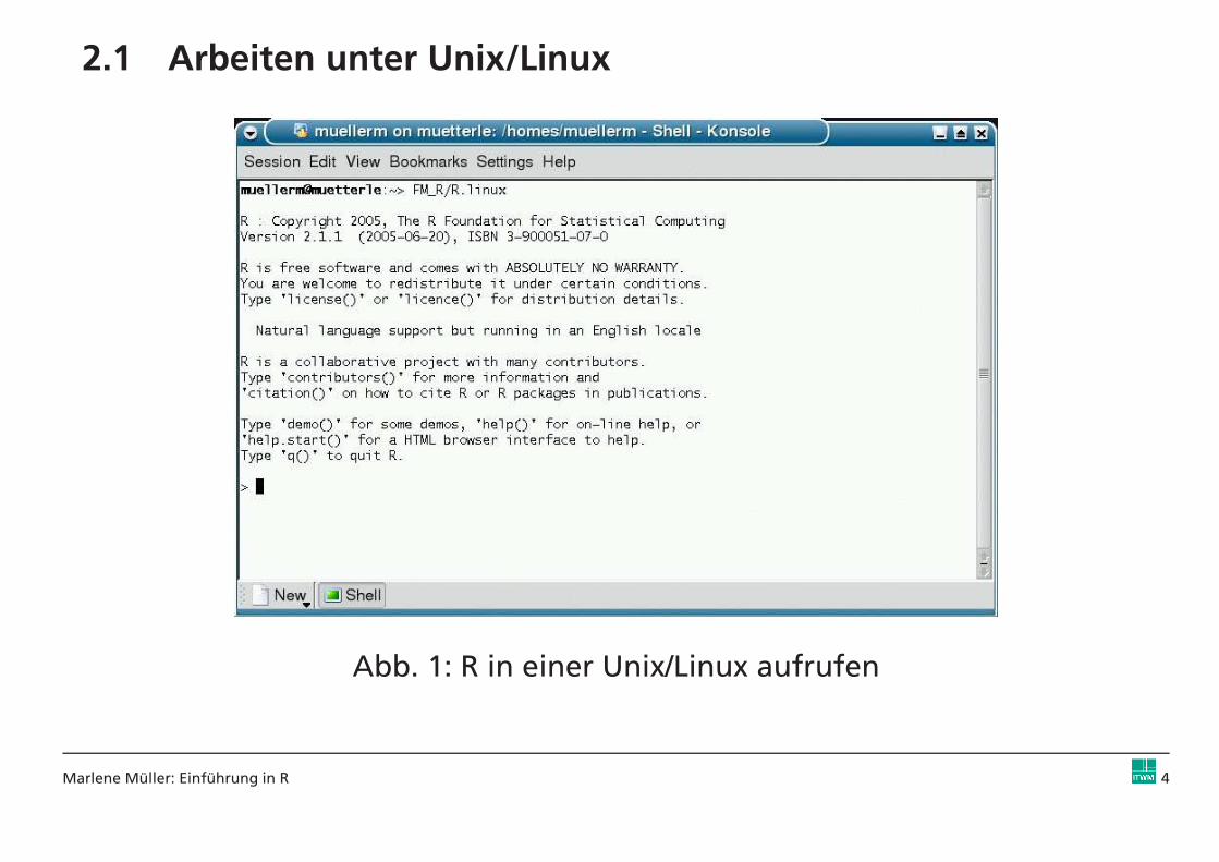
2.1 Arbeiten unter Unix/Linux

Abb. 1: R in einer Unix/Linux aufrufen


2.2 Arbeiten unter Windows

Abb. 2: R im Windows-Desktop starten


3 Wie bekomme ich Hilfe?

3.1 Lokale Hilfeseiten

• Hilfe zu einer Funktion:help(<Funktion>) oder ?<Funktion>

• Hilfe zu einem Package:library(help=<Package>)

Üblicherweise entsprechen die Hilfetexte im lokalen Hilfesystem denen inder Dokumentation zu den Packages.


3.2 WWW

• http://www.r-project.orgR-Webseite, dort findet man insbesondere FAQs und eineGoogle-Site-Search, aber auch:

– Manuals (http://cran.r-project.org/manuals.html)Einführung, Sprachdefinition, “Writing R Extensions” (DLLs,Packages), Einführungen in weiteren Sprachen (außer Englisch)

– CRAN (http://cran.r-project.org)Comprehensive R Archive Network (→ Software zum Download)

– Mailing-Listen (→ Abschnitt 3.3)

– Bücher-Liste (→ Abschnitt 3.4)

– verwandte Projekte


http://www.r-project.org

http://cran.r-project.org/manuals.html

http://cran.r-project.org

3.3 Mailing-Listen

• R-helpwichtigste Liste bei User-Fragen, beim Fragen aber auf alle Fällehttp://www.r-project.org/posting-guide.html beachten!

→ auch als (Usenet-)NewsGroup gmane.comp.lang.r.general aufhttp://news.gmane.org verfügbar

• R-announce, R-packages, R-develAnkündigungs-, Pakete-, Entwicklerlisten (→ eher für Spezialisten)

• R-sig-* (special interests groups)u.a. R-sig-finance = Special Interest Group for ’R in Finance’

Zum Eintragen und für Archive siehe http://www.r-project.org/mail.htmlbzw. http://news.gmane.org/index.php?prefix=gmane.comp.lang.r.

Zur Suche hilfreich ist http://www.rseek.org.


http://www.r-project.org/posting-guide.html

http://news.gmane.org/gmane.comp.lang.r.general

http://news.gmane.org

http://www.r-project.org/mail.html

http://news.gmane.org/index.php?prefix=gmane.comp.lang.r

http://www.rseek.org

3.4 Bücher

• Dalgaard (2002): Introductory Statistics with R

• Murrell (2005): R Graphics

• Ligges (2005): Programmieren mit R(siehe auch: http://www.statistik.uni-dortmund.de/∼ligges/PmitR/)

• Venables and Ripley (2002): Modern Applied Statistics with S(Ergänzungen u.a. für R: http://www.stats.ox.ac.uk/pub/MASS3)

• Venables and Ripley (2000): S Programming(siehe auch: http://www.stats.ox.ac.uk/pub/MASS3/Sprog)

→ weitere: http://www.r-project.org/doc/bib/R-books.html


http://www.statistik.uni-dortmund.de/~ligges/PmitR/

http://www.stats.ox.ac.uk/pub/MASS3

http://www.stats.ox.ac.uk/pub/MASS3/Sprog

http://www.r-project.org/doc/bib/R-books.html

4 Etwas Rechnerei zum Anfang

Demos:

demo()demo(graphics) # nette Grafiken ;-)demo(persp) # nette 3D-Grafiken ;-)demo(image) # besonders nette Grafiken ;-)

Zuweisungen:

x <- 1x <- 0 -> yx <- y <- z <- NA # Missingx <- 0/0 # Not a Number (NaN)x <- NULL # kein Wert

x <- rnorm(100) # 100 N(0,1)-Zufallszahlenhist(x, col="orange") # Histogrammr <- hist(x, col="orange", freq=FALSE) # dasselbe Histogra mm?g <- seq(-5,5,length=100)ylim <- range(c(r$density,max(dnorm(g))))hist(x, col="orange", freq=FALSE, ylim=ylim) # wieder das selbe Histogramm?lines(g, dnorm(g)) # N(0,1)-Dichte dazu gezeichnet


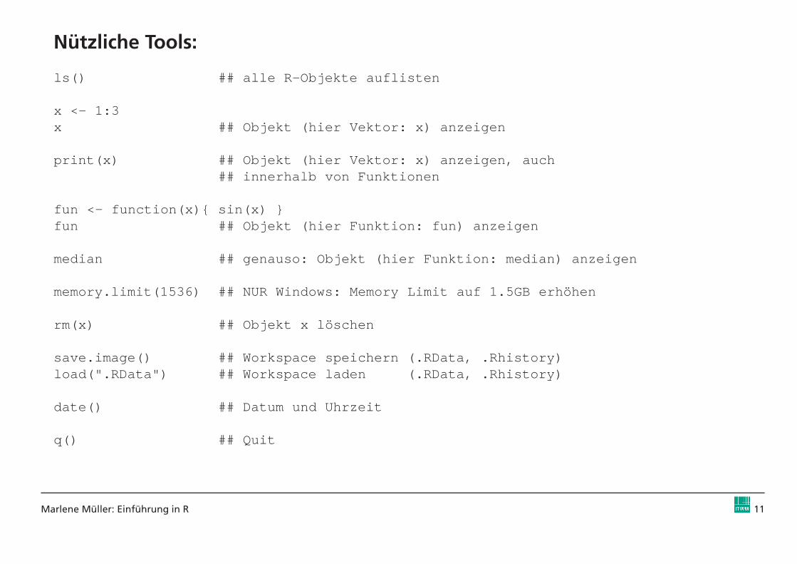
Nützliche Tools:

ls() ## alle R-Objekte auflisten

x <- 1:3x ## Objekt (hier Vektor: x) anzeigen

print(x) ## Objekt (hier Vektor: x) anzeigen, auch## innerhalb von Funktionen

fun <- function(x){ sin(x) }fun ## Objekt (hier Funktion: fun) anzeigen

median ## genauso: Objekt (hier Funktion: median) anzeigen

memory.limit(1536) ## NUR Windows: Memory Limit auf 1.5GB e rhöhen

rm(x) ## Objekt x löschen

save.image() ## Workspace speichern (.RData, .Rhistory)load(".RData") ## Workspace laden (.RData, .Rhistory)

date() ## Datum und Uhrzeit

q() ## Quit


4.1 Datentypen

numeric:

x <- 1y <- pi # predefined pi = 3.1415926535898

character:

x <- "a"y <- "Ein Text"

logical:

x <- TRUEy <- 1 > 2

> y[1] FALSE

Kompliziertere Datentypen sind durch Kombination dieser drei einfachenDatentypen in Form von Vektoren, Matrizen, Arrays und Listenkonstruierbar.


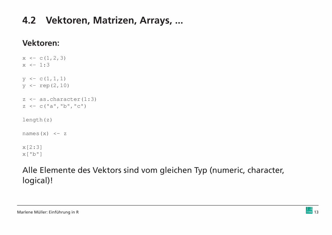
4.2 Vektoren, Matrizen, Arrays, ...

Vektoren:

x <- c(1,2,3)x <- 1:3

y <- c(1,1,1)y <- rep(2,10)

z <- as.character(1:3)z <- c("a","b","c")

length(z)

names(x) <- z

x[2:3]x["b"]

Alle Elemente des Vektors sind vom gleichen Typ (numeric, character,logical)!


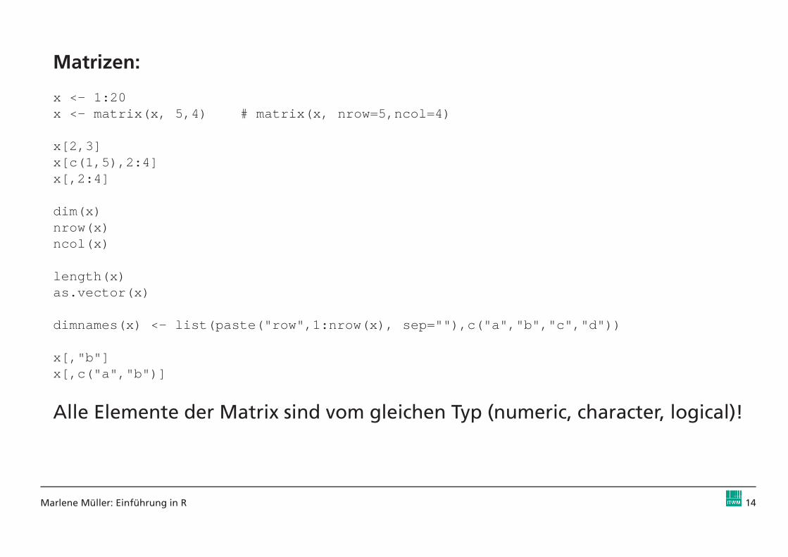
Matrizen:

x <- 1:20x <- matrix(x, 5,4) # matrix(x, nrow=5,ncol=4)

x[2,3]x[c(1,5),2:4]x[,2:4]

dim(x)nrow(x)ncol(x)

length(x)as.vector(x)

dimnames(x) <- list(paste("row",1:nrow(x), sep=""),c(" a","b","c","d"))

x[,"b"]x[,c("a","b")]

Alle Elemente der Matrix sind vom gleichen Typ (numeric, character, logical)!


Vektoren aus Vektoren konstruieren:

x <- c(2,6,3)y <- 1:3

c(x,y) # aneinander hängenc(x,1:5,y,6) # aneinander hängen

Matrizen aus Vektoren konstruieren:

x <- c(2,6,3)y <- 1:3

cbind(x,y) # vertikal zusammensetzenrbind(x,y) # horizontal zusammensetzen

cbind(x,y,rep(0,3)) # vertikal zusammensetzen


Arrays:

x <- 1:60x <- array(x, c(5,4,3))

x[2,3,1]x[1,2:4,3]x[,,1]



dimnames(x) <- list(paste("row",1:nrow(x), sep=""),c(" a","b","c","d"),c("x","y","z"))

Alle Elemente des Arrays sind vom gleichen Typ (numeric, character, logical)!


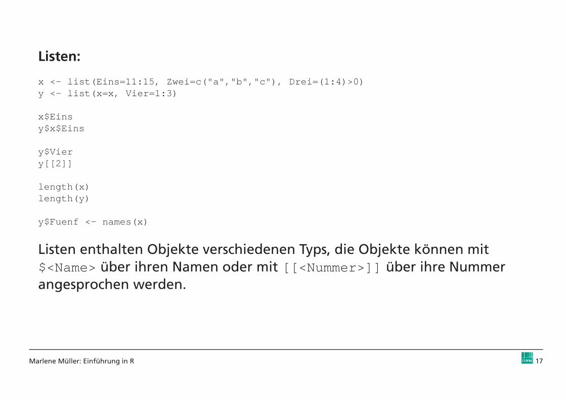
Listen:

x <- list(Eins=11:15, Zwei=c("a","b","c"), Drei=(1:4)>0 )y <- list(x=x, Vier=1:3)

x$Einsy$x$Eins

y$Viery[[2]]

length(x)length(y)

y$Fuenf <- names(x)

Listen enthalten Objekte verschiedenen Typs, die Objekte können mit$<Name>über ihren Namen oder mit [[<Nummer>]] über ihre Nummerangesprochen werden.


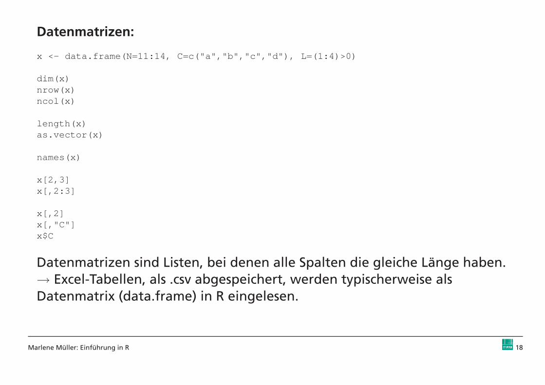
Datenmatrizen:

x <- data.frame(N=11:14, C=c("a","b","c","d"), L=(1:4)> 0)



names(x)

x[2,3]x[,2:3]

x[,2]x[,"C"]x$C

Datenmatrizen sind Listen, bei denen alle Spalten die gleiche Länge haben.→ Excel-Tabellen, als .csv abgespeichert, werden typischerweise alsDatenmatrix (data.frame) in R eingelesen.


4.3 Operationen (elementweise bzw. vektor-/matrixweise)

x <- matrix( 1:20, 5, 4) # 5x4 Matrix

x+1; x-1; x * 1; x/1 # elementweise Operationensin(x); exp(x) # elementweise Funktionsaufrufe

y <- 1:5x * y # elementweise Multiplikation

z <- 1:4x %* % z # Matrixmultiplikation

min(x) # Minimum aller Elemente von xapply(x,1,min) # Zeilenminimaapply(x,2,min) # Spaltenminima

y <- c(TRUE, TRUE, FALSE, FALSE)y & TRUE # elementweise logische Operation (‘‘UND’’)y | FALSE # elementweise logische Operation (‘‘ODER’’)!y # elementweise logische Operation (‘‘NICHT’’)

y && TRUE # ABER: hier gilt nur das erste Ergebnis! (‘‘UND’’)y || FALSE # ABER: hier gilt nur das erste Ergebnis! (‘‘ODER’’ )


5 Daten & Dateien

Beispiel-Datei in Excel:

→ unter Excel als CSV speichern: Beispiel1.csv

Kunde;Eigenkapital;Liquidität;Ausfall;Datum;Ratingp unkte;RatingklasseMeier;10;30;0;01.11.2004;100;1Schulze;30;40;0;02.10.2004;70;2Lehmann;20;;1;03.12.2004;30;3Schmidt;10;20;0;04.09.2004;20;4


5.1 CSV-Dateien lesen und Speichern

Lesen der Datei Beispiel1.csv:

x <- read.csv("Beispiel1.csv", sep=";")

dim(x)names(x)x

Kunde Eigenkapital Liquidität Ausfall Datum Ratingpunkte Ratingklasse1 Meier 10 30 0 01.11.2004 100 12 Schulze 30 40 0 02.10.2004 70 23 Lehmann 20 NA 1 03.12.2004 30 34 Schmidt 10 20 0 04.09.2004 20 4

Schreiben der Daten in Beispiel2.csv:

write.table(x,file="Beispiel2.csv",sep=";",row.name s=FALSE,quote=FALSE)


Andere Funktionen zum Lesen:

• read.table (Daten im ASCII-Format)

• scan (scannt beliebige Textdatei, eigene Nachbearbeitung erforderlich)

Funktionen zum evtl. Konvertieren von Spalten:

• as.numeric , as.character , as.factor

Andere Möglichkeiten der Kommunikation mit Excel (nicht getestet ;-)):

• RODBC(Zugriff auf Excel oder Access als Datenbank)

• R-Excel-Interface über DCOM-Server(http://cran.at.r-project.org/contrib/extra/dcom)


http://cran.at.r-project.org/contrib/extra/dcom

5.2 Zufallszahlen und Verteilungen

Beispiel Normalverteilung:

rnorm(n, mean=0, sd=1) Zufallszahlen

dnorm(x, mean=0, sd=1) Dichte (pdf)

pnorm(x, mean=0, sd=1) Verteilungsfunktion (cdf)

qnorm(p, mean=0, sd=1) Quantile

nach gleichem Muster:

Gleichverteilung {r|d|p|q}unif t-Verteilung {r|d|p|q}t

Lognormalverteilung {r|d|p|q}lnorm Gamma-Verteilung {r|d|p|q}gamma

χ2-verteilung {r|d|p|q}chisq Beta-Verteilung {r|d|p|q}beta

Binomialverteilung {r|d|p|q}binom Poisson-Verteilung {r|d|p|q}pois

. . .

→ bei Bedarf den vorher Seed mit set.seed setzen


5.3 R-Skriptdateien

Skript mit R-Befehlen einlesen:

> source("MeinProgramm.R")

R-Output in Datei abspeichern:

sink("MeinOutput.txt") # ab jetzt alle Ausgaben in Dateisink() # und nun wieder auf den Bildschirm


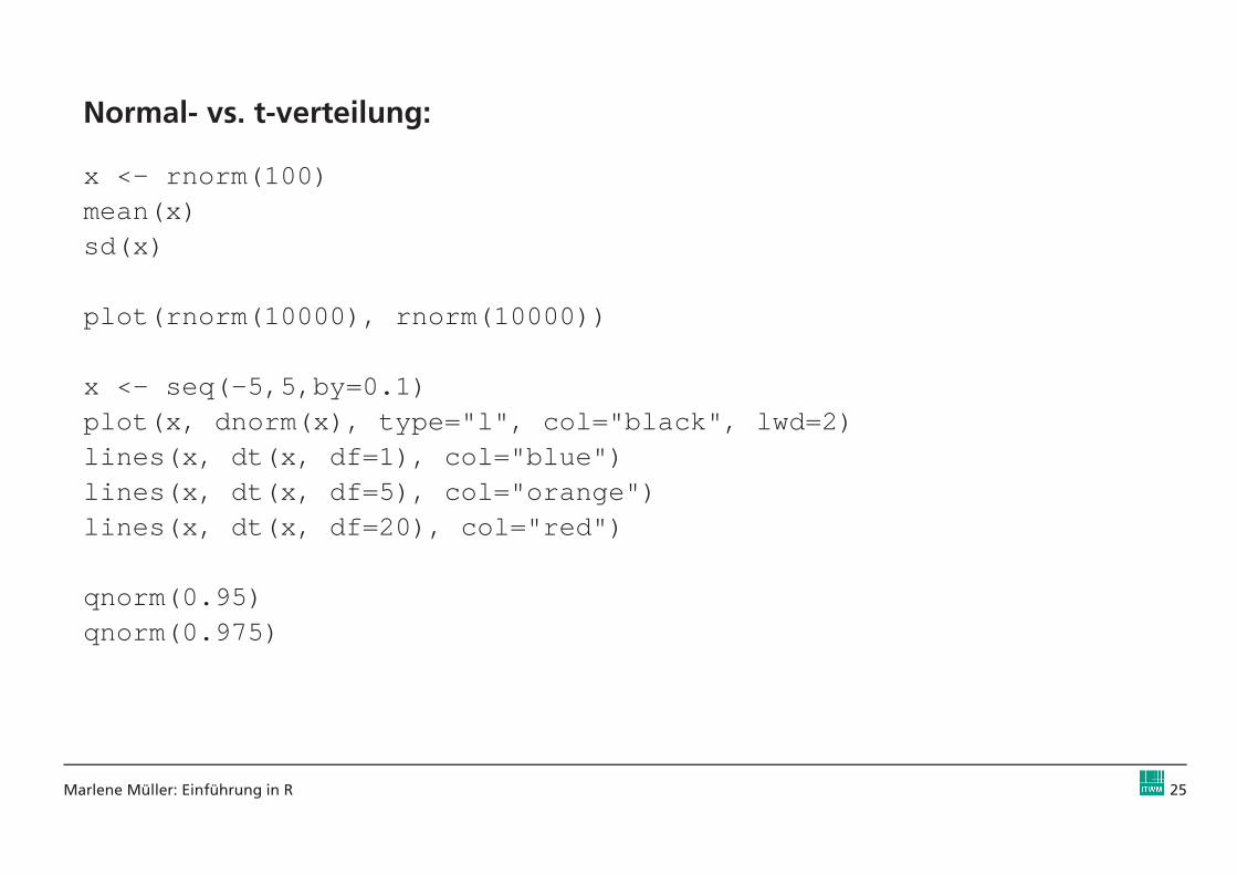
Normal- vs. t-verteilung:

x <- rnorm(100)mean(x)sd(x)

plot(rnorm(10000), rnorm(10000))

x <- seq(-5,5,by=0.1)plot(x, dnorm(x), type="l", col="black", lwd=2)lines(x, dt(x, df=1), col="blue")lines(x, dt(x, df=5), col="orange")lines(x, dt(x, df=20), col="red")

qnorm(0.95)qnorm(0.975)


Multivariate Normalverteilung:

library(help=mvtnorm)library(mvtnorm)

mu <- c(0,0) # meanssigma <- c(1,1) # std.dev.rho <- 0.5 # correlation

S <- matrix(NA, 2,2)diag(S) <- sigma^2S[1,2] <- S[2,1] <- rho * prod(sigma)

x <- rmvnorm(n=10000, mean=mu, sigma=S)plot(x)

x <- seq(-5 * sigma[1]+mu[1], 5 * sigma[1]+mu[1], length = 50)y <- seq(-5 * sigma[2]+mu[2], 5 * sigma[2]+mu[2], length = 50)f <- function(x,y) { dmvnorm(cbind(x,y), mean=mu, sigma=S ) }z <- outer(x, y, f)persp(x, y, z, theta = 10, phi = 20, expand = 0.5, col = "lightbl ue", shade = 0.75)


6 Schöne bunte Welt der Grafik

Kreditausfalldaten:

file <- read.csv("kredit.csv",sep=";")y <- 1-file$kredit # default set to 1prev <- (file$moral >2)+0 # previous loans were OKemploy <- (file$beszeit >1)+0 # employed (>=1 year)dura <- (file$laufzeit) # durationd9.12 <- ((file$laufzeit >9)&(file$laufzeit <=12)) +0 # 9 < duration <= 12d12.18 <- ((file$laufzeit >12)&(file$laufzeit <=18))+0 # 12 < duration <= 18d18.24 <- ((file$laufzeit >18)&(file$laufzeit <=24))+0 # 18 < duration <= 24d24 <- (file$laufzeit >24)+0 # 24 < durationamount <- file$hoehe # amount of loanage <- file$alter # age of applicantsavings <- (file$sparkont > 4)+0 # savings >= 1000 DMphone <- (file$telef==1)+0 # applicant has telephoneforeign <- (file$gastarb==1)+0 # non-german citizenpurpose <- ((file$verw==1)|(file$verw==2))+0 # loan is fo r a carhouse <- (file$verm==4)+0 # house owner


6.1 Balkendiagramme

→ grafische Darstellung der Häufigkeitsverteilung diskreter Merkmale

table(dura) ## Häufigkeitstabelle

barplot(table(dura), col="cyan", main="Duration of Loan ")## absolute Häufigkeiten

barplot(table(dura)/length(dura), col="cyan", main="D uration of Loan")## relative Häufigkeiten

par(mfrow=c(1,3)) # 1 Zeile, 3 Spalten im Displaybarplot(table(dura), col="cyan", main="Duration of Loan ")barplot(table(savings), col="orange", main="Savings >1 000 DM")barplot(table(house), col="magenta", main="House Owner ")par(mfrow=c(1,1)) # Display-Teilung zurücksetzen!


4 8 12 18 26 36 47

Duration of Loan

050

100

150

0 1

Savings >1000 DM

020

040

060

080

0

0 1

House Owner

020

040

060

080

0

Abb. 3: Beispiele für Balkendiagramme: Laufzeit des Kredits (links), Sparein-lagen (mitte) und Immobilienbesitz (rechts)


6.2 Boxplots

→ grafische Darstellung von Ausreißern, Minimal-/Maximalwerten (diekeine Ausreißer sind), 25%-,50%,75%-Quantilen

boxplot(age)boxplot(age, horizontal=TRUE)

boxplot(age, col="gray",horizontal=TRUE)

boxplot(age ~ y, col=c("gray","red"),horizontal=TRUE, m ain="Age vs. Y")boxplot(amount ~ y, col=c("gray","red"),horizontal=TRU E, main="Amount vs. Y")


01

20 30 40 50 60 70

Age vs. Y

01

0 5000 10000 15000

Amount vs. Y

Abb. 4: Alter des Kreditnehmers (links) und Kreditbetrag (rechts) gegen Aus-fallbeobachtung (1 =Ausfall, 0 = Nichtausfall)


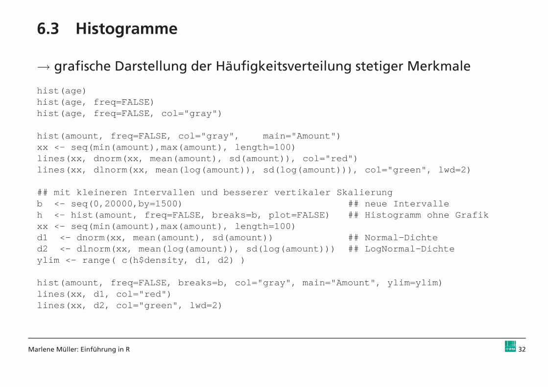
6.3 Histogramme

→ grafische Darstellung der Häufigkeitsverteilung stetiger Merkmale

hist(age)hist(age, freq=FALSE)hist(age, freq=FALSE, col="gray")

hist(amount, freq=FALSE, col="gray", main="Amount")xx <- seq(min(amount),max(amount), length=100)lines(xx, dnorm(xx, mean(amount), sd(amount)), col="red ")lines(xx, dlnorm(xx, mean(log(amount)), sd(log(amount) )), col="green", lwd=2)

## mit kleineren Intervallen und besserer vertikaler Skali erungb <- seq(0,20000,by=1500) ## neue Intervalleh <- hist(amount, freq=FALSE, breaks=b, plot=FALSE) ## His togramm ohne Grafikxx <- seq(min(amount),max(amount), length=100)d1 <- dnorm(xx, mean(amount), sd(amount)) ## Normal-Dicht ed2 <- dlnorm(xx, mean(log(amount)), sd(log(amount))) ## L ogNormal-Dichteylim <- range( c(h$density, d1, d2) )

hist(amount, freq=FALSE, breaks=b, col="gray", main="Am ount", ylim=ylim)lines(xx, d1, col="red")lines(xx, d2, col="green", lwd=2)


Amount

amount

Den

sity

0 5000 10000 15000 20000

0.00

000

0.00

010

0.00

020

Abb. 5: Verteilung des Kreditbetrags, Histogramm im Vergleich mit Normal-und LogNormaldichte


6.4 Scatterplots und Kurven

→ Punktwolken ...

plot(age, amount)

color <- 1 * (y==1) + 2 * (y==0)plot(age, amount, col=color)

color <- rep("", length(age))color[y==1] <- "red"color[y==0] <- "blue"plot(age, amount, col=color)

plot(1:20,1:20,col=1:20, pch=1:20)text(1:20,1:20,labels=as.character(1:20), pos=4)

symbol <- 8 * (y==1) + 1 * (y==0)plot(age, amount, col=color, pch=symbol)


→ ... oder Linien oder beides

x <- seq(-pi,pi,length=100)plot(x, sin(x), type="l")lines(x, cos(x), col="red")

logit <- glm(y ~ age, family=binomial(link = "logit"))

plot(age, logit$fitted.values)

plot(age, logit$fitted.values, type="l") ## nicht so, son dern ...

o <- order(age)plot(age[o], logit$fitted.values[o], type="l") ## ... so ! (sortiert)

plot(age[o], logit$fitted.values[o], type="l", lwd=2, y lim=c(0,1))title("PDs")points(age, y, col="red", pch=3, cex=0.5)


20 30 40 50 60 70

050

0010

000

1500

0

age

amou

nt

20 30 40 50 60 70

0.0

0.2

0.4

0.6

0.8

1.0

age[o]

logi

t$fit

ted.

valu

es[o

]

PDs

Abb. 6: Scatterplot von Alter vs. Kreditbetrag (links), Logit-Ausfallwahrscheinlichkeiten (rechts)


6.5 Dreidimensionale Darstellung

→ Oberflächen, Punktwolken und Konturkurven

## Bivariate Normalverteilungsdichtelibrary(mvtnorm)x <- y <- seq(-5, 5, length = 50)f <- function(x,y) { dmvnorm(cbind(x,y)) }z <- outer(x, y, f)persp(x, y, z, theta = 10, phi = 20, expand = 0.5, col = "lightbl ue")persp(x, y, z, theta = 10, phi = 20, expand = 0.5, col = "lightbl ue", shade = 0.75)

## Konturkurven der bivariaten Normalverteilungsdichtex <- y <- seq(-5, 5, length = 150)z <- outer(x, y, f)contour(x, y, z, nlevels=20)contour(x, y, z, nlevels=20, col=rainbow(20))contour(x, y, z, nlevels=20, col=rainbow(20), labels="")

## Dreidimensionale normalverteilte Datenlibrary(scatterplot3d)x <- matrix(rnorm(15000),ncol=3)scatterplot3d(x)scatterplot3d(x, angle=20)


x

y

z

x

y

z

−4 −2 0 2 4−

4−

20

24

−4 −2 0 2 4−

4−

20

24

−4 −2 0 2 4−

4−

20

24

−4 −2 0 2 4−4

−2

0 2

4 6

−4−2

0 2

4

x[,1]

x[,2

]

x[,3

]

Abb. 7: Bivariate Normalverteilungsdichte: 3D-Darstellung (links) und Kon-turkurven (mitte); 3D-Scatterplot (rechts)


6.6 Gestaltungsmöglichkeiten

Direkt in den Grafikroutinen: → Hilfe dazu mit ?par

• Farben setzen mit col=...(Generierung von → ?rainbow , ?rgb , ?col2rgb )

• Symbole setzen mit pch=... , Größen mit cex=...

• Titel setzen mit main=... , Achsenlabels mit xlab=... , ylab=...

• Zeichenbereich setzen mit xlim=... , ylim=...

Nach Zeichnen einer Grafik:

• Linien und Punkte mit lines(...) bzw. points(...) ergänzen

• Labels (Texte) mit text(...) ergänzen

• Titel mit title(...) ergänzen

• Legende mit legend(...) ergänzen


6.7 Grafiken speichern

• PostScript:x <- matrix(rnorm(5000),ncol=2)plot(x)postscript(file = "MeinPlot.ps", width = 5, height = 5.5, ho rizontal = FALSE)plot(x)dev.off()

• andere Formate sind u.a. pdf , pictex , xfig , png , jpeg→ siehe ?Devices


7 Etwas Statistik

Kreditausfalldaten:

file <- read.csv("kredit.csv",sep=";")y <- 1-file$kredit # default set to 1prev <- (file$moral >2)+0 # previous loans were OKemploy <- (file$beszeit >1)+0 # employed (>=1 year)dura <- (file$laufzeit) # durationd9.12 <- ((file$laufzeit >9)&(file$laufzeit <=12)) +0 # 9 < duration <= 12d12.18 <- ((file$laufzeit >12)&(file$laufzeit <=18))+0 # 12 < duration <= 18d18.24 <- ((file$laufzeit >18)&(file$laufzeit <=24))+0 # 18 < duration <= 24d24 <- (file$laufzeit >24)+0 # 24 < durationamount <- file$hoehe # amount of loanage <- file$alter # age of applicantsavings <- (file$sparkont > 4)+0 # savings >= 1000 DMphone <- (file$telef==1)+0 # applicant has telephoneforeign <- (file$gastarb==1)+0 # non-german citizenpurpose <- ((file$verw==1)|(file$verw==2))+0 # loan is fo r a carhouse <- (file$verm==4)+0 # house owner


7.1 Kennzahlen

kredit <- data.frame(y,age,amount,dura,prev,savings,h ouse)

summary(kredit)

mean(kredit$age)sd(kredit$age)var(kredit$age)

cov(kredit[,1:3])cor(kredit[,1:3])

median(kredit$age)quantile(kredit$age,c(0.1,0.5,0.9))

library(help=e1071)library(e1071)skewness(kredit$age)kurtosis(kredit$age)

skewness(rnorm(1000))kurtosis(rnorm(1000))


7.2 Tabellen

length(kredit$age)length(unique(kredit$age))

table(kredit$age)table(kredit$dura)table(kredit$savings)

table(kredit$y, kredit$savings)table(kredit$y, kredit$savings)/nrow(kredit)

table(kredit$y, kredit$savings, kredit$house)

unique(kredit[,c("y","savings","house")])


7.3 Regressions- und Zeitreihenanalyse

7.3.1 Lineare Regression

plot(kredit$age, kredit$dura)

lm <- lm( dura ~ age, data=kredit)summary(lm) ## Abhängigkeit von Altero <- order(kredit$age)lines(kredit$age[o], lm$fitted.values[o], col="red", l wd=2)

lm2 <- lm( dura ~ age + amount, data=kredit)summary(lm2) ## Abhängigkeit von Alter+Betrag

lm3 <- lm( dura ~ amount, data=kredit)summary(lm3) ## Abhängigkeit von Betragplot(kredit$amount, kredit$dura)o <- order(kredit$amount)lines(kredit$amount[o], lm3$fitted.values[o], col="re d", lwd=2)

lm4 <- lm( dura ~ amount + I(amount^2), data=kredit)summary(lm4) ## Abhängigkeit von Betrag (quadr.)lines(kredit$amount[o], lm4$fitted.values[o], col="bl ue", lwd=2)


→ Laufzeit des Kredits hängt klar vom Kreditbetrag ab:

> summary(lm4)

Call:lm(formula = dura ~ amount + I(amount^2), data = kredit)

Residuals:Min 1Q Median 3Q Max

-34.6115 -5.5761 -0.9547 5.0850 42.1110

Coefficients:Estimate Std. Error t value Pr(>|t|)

(Intercept) 8.410e+00 6.516e-01 12.906 < 2e-16 ***amount 4.855e-03 2.961e-04 16.393 < 2e-16 ***I(amount^2) -1.815e-07 2.309e-08 -7.863 9.7e-15 ***---Signif. codes: 0 ’ *** ’ 0.001 ’ ** ’ 0.01 ’ * ’ 0.05 ’.’ 0.1 ’ ’ 1

Residual standard error: 9.144 on 997 degrees of freedomMultiple R-Squared: 0.4262, Adjusted R-squared: 0.425F-statistic: 370.3 on 2 and 997 DF, p-value: < 2.2e-16


20 30 40 50 60 70

1020

3040

5060

70

kredit$age

kred

it$du

ra

0 5000 10000 15000

1020

3040

5060

70

kredit$amount

kred

it$du

raAbb. 8: Abhängigkeit der Kreditlaufzeit vom Alter (links) und vom Kreditbe-trag (rechts)


7.3.2 Generalisiertes Lineares Modell (GLM)

→ Schätzung der Ausfallwahrscheinlichkeiten

logit <- glm(y ~ age + amount + dura + prev + savings + house,family=binomial(link = "logit"))

summary(logit)

logit2 <- glm(y ~ age + amount + I(amount^2) + dura + prev + savi ngs + house,family=binomial(link = "logit"))

summary(logit2)

→ Ausfallwahrscheinlichkeiten hängen u.a. nichtlinear vom Betrag ab:

> summary(logit2)

Call:glm(formula = y ~ age + amount + I(amount^2) + dura + prev +

savings + house, family = binomial(link = "logit"))

Deviance Residuals:Min 1Q Median 3Q Max

-2.1244 -0.8495 -0.6196 1.0935 2.2584


Coefficients:Estimate Std. Error z value Pr(>|z|)

(Intercept) -4.637e-01 3.035e-01 -1.528 0.12652age -1.748e-02 7.159e-03 -2.442 0.01460 *amount -2.070e-04 9.348e-05 -2.214 0.02679 *I(amount^2) 1.870e-08 6.941e-09 2.694 0.00707 **dura 3.992e-02 8.106e-03 4.925 8.46e-07 ***prev -7.589e-01 1.619e-01 -4.688 2.76e-06 ***savings -9.897e-01 2.232e-01 -4.435 9.22e-06 ***house 6.277e-01 2.073e-01 3.027 0.00247 **---Signif. codes: 0 ’ *** ’ 0.001 ’ ** ’ 0.01 ’ * ’ 0.05 ’.’ 0.1 ’ ’ 1

(Dispersion parameter for binomial family taken to be 1)

Null deviance: 1221.7 on 999 degrees of freedomResidual deviance: 1102.1 on 992 degrees of freedomAIC: 1118.1

Number of Fisher Scoring iterations: 4


7.3.3 Auswahl weiterer Regressions- und Zeitreihenmodelle

Modell Routinen

Linear lm , anova

GLM glm , mgcv / gam (additiv nichtparametrisch)

Nichtlinear nls

Nichtparametrisch locpoly , locfit

Mixed Models lmm, nlme , glmmML, glmmPQL

Zeitreihen ar , arma , arima , arima0 , garch

Classification and regression trees tree

Packages: MASS, stats , KernSmooth , tseries , gam, gcv


7.4 Hypothesentests

7.4.1 Normaltests

library(KernSmooth)f <- bkde(kredit$age)plot(f, type="l", xlim=range(f$x), ylim=range(f$y))title("Distribution of Age") ## Verteilung normal?

t <- shapiro.test(kredit$age)tt$p.value

library(tseries)t <- jarque.bera.test(kredit$age)tt$p.value


7.4.2 Vergleich von Verteilungen

library(KernSmooth)f0 <- bkde(kredit$age[y==0])f1 <- bkde(kredit$age[y==1])plot(f0, type="l", col="blue", xlim=range(c(f0$x,f1$x) ), ylim=range(c(f0$y,f1$y)))lines(f1, col="red")title("Age vs. Default") ## Verteilungen gleich?

t <- ks.test(kredit$age[y==1],kredit$age[y==0])tt$p.value

t <- wilcox.test(kredit$age[y==1],kredit$age[y==0])tt$p.value


7.4.3 Auswahl weiterer Tests

Test Routinen

Mittelwert-Tests/-Vergleiche (t-Tests) t.test

Varianz-Tests/-Vergleiche (F-Tests) var.test

Binomial-Tests prop.test , binom.test

Korrelation cor.test

Rangtests wilcox.test

Regression anova

Unit Roots (mean reversion) adf.test , kpss.test

Packages: stats , tseries , exactRankTests


8 “Höhere” Mathematik

8.1 Optimierung von Funktionen

Lineares Modell

yi = β0 + β1xi1 + β2xi2 + εi

n <- 100; b <- c(-1,3)x <- matrix(rnorm(n * length(b)),ncol=length(b)) ## Regressorene <- rnorm(n)/4

y <- 1 + x % * % b + e ## Lineares Modell

l <- lm( y~x ); summary(l) ## built-in Lineare Regression

→ zu optimieren

QS =∑

i

(yi − x⊤

i β)2

(zugegebenermaßen kein wirklich gutes Beispiel für iterative Optimierung ;-))


Optimierung (ohne Konstante)

QS <- function(b, x, y){ sum( (y - x % * % b)^2 ) } ## Optimierungskriterium

b0 <- c(0,0)opt <- optim(b0, QS, method="BFGS", x=x, y=y) ## Optimierun g (ohne Konstante!)optsum( (x % * % opt$par - mean(y))^2 )/sum( (y-mean(y))^2 ) ## R^2

→ Bestimmtheitsmaß R2 kann hier außerhalb von [0, 1] liegen

Optimierung (mit Konstante)

b1 <- c(0,0,0)x1 <- cbind(rep(1,n),x)opt1 <- optim(b1, QS, method="BFGS", x=x1, y=y) ## Optimier ung (mit Konstante!)opt1sum( (x1 % * % opt1$par - mean(y))^2 )/sum( (y-mean(y))^2 ) ## R^2


Optimierung mit Gradient

QS =∑

i

(yi − x⊤

i β)2 = (y −Xβ)⊤(y −Xβ),∂QS

∂β= −2X⊤y + 2X⊤

Xβ

D.QS <- function(b, x, y){ -2 * t(x) % * % y + 2* t(x) % * % x %* % b } ## Gradient

opt2 <- optim(b1, QS, D.QS, method="BFGS", x=x1, y=y)opt2sum( (x1 % * % opt2$par - mean(y))^2 )/sum( (y-mean(y))^2 ) ## R^2

Optimierung mit Intervalrestriktion (z.B. βj ≥ 0)

b2 <- c(0,0,0)x1 <- cbind(rep(1,n),x)opt3 <- optim(b1, QS, D.QS, method="BFGS", lower=0, x=x1, y =y)opt3sum( (x1 % * % opt3$par - mean(y))^2 )/sum( (y-mean(y))^2 ) ## R^2


Optimierung mit linearer Restriktion (z.B. β0 ≥ 0, β1 + β2 ≤ 2)

Uβ − c =

(

0 −1 −1

1 0 0

)

β0

β1

β2

−

(

−2

0

)

≥ 0

u <- cbind( c(0,1), c(-1,0), c(-1,0) )c <- c(-2,0)

applyDefaults <- function(fn, ...) { ## um weitere Paramete r an QS, D.QSfunction(x) fn(x, ...) ## zu übergeben

}

b4 <- rep(0.5,3)opt4 <- constrOptim(b4, applyDefaults(QS, x=x1, y=y),

applyDefaults(D.QS, x=x1, y=y), ui=u, ci=c)opt4sum( (x1 % * % opt4$par - mean(y))^2 )/sum( (y-mean(y))^2 ) ## R^2


8.2 Interpolation

→ approx für lineare, spline bzw. interpSpline fürSpline-Approximation

x <- seq(-5,5,by=1)y <- sin(x)

xx <- seq(-5,5,by=0.1)y.approx <- approx(x,y, xout=xx)$yyy <- sin(xx)

plot(xx,yy, type="l", col="green")lines(xx,y.approx, lwd=2)

library(splines)sp <- interpSpline(x,y)lines(predict(sp,xx), col="red")


8.3 Numerische Integration

→ integrate für 1-dimensionale, adapt für mehrdimensionale Integration

pnorm(0)

it <- integrate(dnorm, -Inf,0)it

attributes(it) ## Ergebnis ist Objekt der Klasse "integrat e"

it$value

pmvnorm(c(0,0))pmvnorm(c(0,0))[[1]]

library(adapt)it <- adapt(2, c(-Inf,-Inf), c(0,0), functn=dmvnorm)

attributes(it) ## Ergebnis ist Objekt der Klasse "integrat ion"

it$value


9 Einstieg ins Programmieren

9.1 Funktionen

myfun <- function(x, a){r <- a * sin(x)return(r)

}myfun(pi/2,2)

myfun1 <- function(x, a){ a * sin(x) } ## dasselbe kürzermyfun1(pi/2,2)

myfun2 <- function(x, a=1){ ## opt. Parameter mit Defaultwe rt=1a* sin(x)

}myfun2(pi/2,2)myfun2(pi/2)

myfun3 <- function(x, a=NULL){ ## opt. Parameter ohne Defau ltwertif (!is.null(a)){ a * sin(x) }else{ cos(x) }

}myfun3(pi/2,2)myfun3(pi/2)


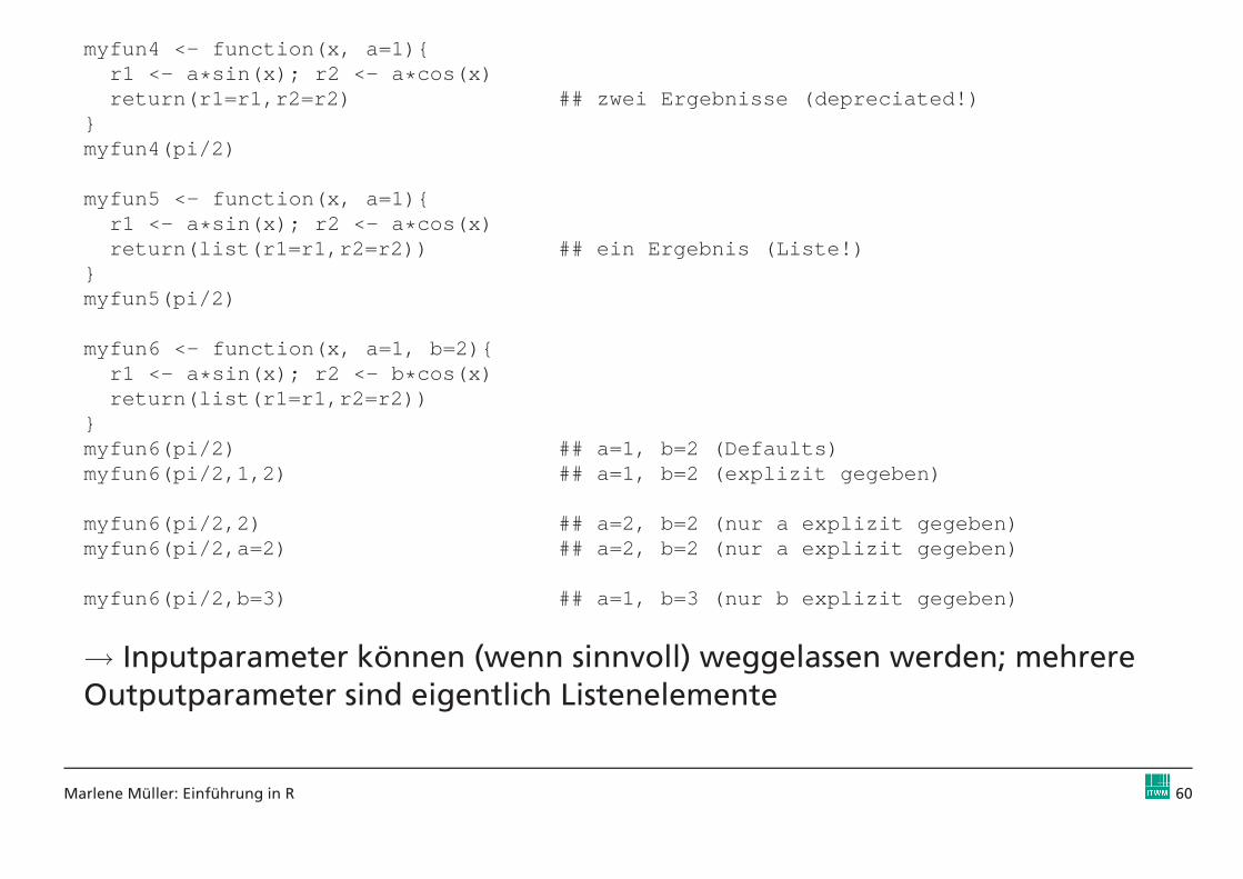
myfun4 <- function(x, a=1){r1 <- a * sin(x); r2 <- a * cos(x)return(r1=r1,r2=r2) ## zwei Ergebnisse (depreciated!)

}myfun4(pi/2)

myfun5 <- function(x, a=1){r1 <- a * sin(x); r2 <- a * cos(x)return(list(r1=r1,r2=r2)) ## ein Ergebnis (Liste!)

}myfun5(pi/2)

myfun6 <- function(x, a=1, b=2){r1 <- a * sin(x); r2 <- b * cos(x)return(list(r1=r1,r2=r2))

}myfun6(pi/2) ## a=1, b=2 (Defaults)myfun6(pi/2,1,2) ## a=1, b=2 (explizit gegeben)

myfun6(pi/2,2) ## a=2, b=2 (nur a explizit gegeben)myfun6(pi/2,a=2) ## a=2, b=2 (nur a explizit gegeben)

myfun6(pi/2,b=3) ## a=1, b=3 (nur b explizit gegeben)

→ Inputparameter können (wenn sinnvoll) weggelassen werden; mehrereOutputparameter sind eigentlich Listenelemente


9.2 Bedingte Anweisungen, Schleifen

• if & Co.x<- 1; if (x==2){ print("x=2") }x<- 1; if (x==2){ print("x=2") }else{ print("x!=2") }

• for & repeatfor (i in 1:4){ print(i) }for (i in letters[1:4]){ print(i) }i <- 0; while(i<4){ i <- i+1; print(i)}i <- 0; repeat{ i <- i+1; print(i); if (i==4) break }

• weitere: ifelse , switch

9.3 “Mengenlehre”

a <- 1:3; b <- 2:6; a %in% b; b %in% aa <- c("A","B"); b <- LETTERS[2:6]; a %in% b; b %in% a


9.4 Packages

• Packages umfassen (eine oder) mehrere Funktionen, werden mitlibrary(<Package-Name>) geladen, in einem Package verfügbareFunktionen können mit library(help=<Package-Name>) abgefragtwerden

• zum Erstellen eigener Packages gibt es zwei hilfreiche Funktionen

package.skeleton(<Package-Name>)erstellt die Verzeichnisstruktur des Packages mit Templates für dienotwendigen Files

prompt(<Funktion>)erstellt ein Template für den Hilfetext zur Funktion

• Kollektionen von Packages heißen Bundles

• Packages oder Bundles installiert man unter Windows mit dementsprechenden Menüpunkt, unter Unix/Linux mit install.packagesoder mit R CMD INSTALL <Package-...>.tar.gz


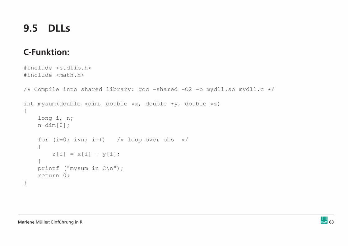
9.5 DLLs

C-Funktion:

#include <stdlib.h>#include <math.h>

/ * Compile into shared library: gcc -shared -O2 -o mydll.so myd ll.c * /

int mysum(double * dim, double * x, double * y, double * z){

long i, n;n=dim[0];

for (i=0; i<n; i++) / * loop over obs * /{

z[i] = x[i] + y[i];}printf ("mysum in C\n");return 0;

}


Aufruf in R:

dyn.load("mydll.so") ## DLL ladenis.loaded("mysum") ## "mysum" ist da?

d <- 3x <- 1:3y <- 4:6z <- rep(0,3)

r <- .C("mysum", dim=d, x=x, y=y, z=z ) ## das geht schief!r$z

d <- as.double(3)x <- as.double(1:3)y <- as.double(4:6)z <- rep(0.0,3)

r <- .C("mysum", dim=d, x=x, y=y, z=z ) ## so geht’sr$zz ## -> z ist immer noch 0

r <- .C("mysum", dim=d, x=x, y=y, z=z, DUP=FALSE) ## oder so ( ohne Kopie der Param.)r$zz ## -> z enthält das Ergebnis

dyn.unload("mydll.so") ## DLL unload


9.6 Tipps & Tricks

• Syntaxhighlightening (und R in (X)Emacs integrieren):ESS = “emacs speaks statistics” von http://ess.r-project.org/ downloadenund in .emacs einbinden:(load "<Pfad zu ESS>/ess-5.1.24/lisp/ess-site")

• Syntaxhighlightening für Windows gibt es auch in WinEdt(http://cran.at.r-project.org/contrib/extra/winedt)

• Runden und Formatieren von Zahlen geht mit round , floor , ceiling ,signif , formatC

• Strings (character vectors) können bearbeitet werden mit paste ,substr , nchar , strsplit , toupper , tolower , sub

• Datumsgenerierung mit as.POSIXlt und strptime , z.B.as.POSIXlt( strptime("20050101","%Y%m%d"))+(0:364) * 86400

erzeugt alle Tage des Jahres 2005;


http://ess.r-project.org/

http://cran.at.r-project.org/contrib/extra/winedt

d <- as.POSIXlt( strptime("20050926","%Y%m%d")); d$wday

gibt den Wochentag des 26.9.2005 an

• mit system kann man Betriebssystemkommandos ausführen, z.B. unterLinux: system("cal 09 2005")

• die Funktionen xtable (Package: xtable ) und latex (Package: Hmisc )können R-Objekte als Latex-Kode speichern

• mit eval und parse können Zeichenketten als Ausdrücke ausgewertetwerden:eval( parse( text=paste("x.",as.character(1:2)," <- 0", sep="") ) )print(x.1)

• es gibt in R zwei Verfahren für OOP: S3- und S4-Klassen; zur Informationüber die Komponenten von S3-Klassen (älterer Ansatz) sind dieFunktionen class , attributes nützlich während für S4-Klassen(neuerer Ansatz) getClass , slot , slotNames verwendet werden

• Methoden können klassenabhängig sein, z.B. erhält man mitmethods(print) alle zur Funktion gehörenden Methoden


LiteraturBecker, R. A. and Chambers, J. M. (1984). S. An Interactive Envrionment for Data Analysis and Graphics,

Wadsworth and Brooks/Cole, Monterey.

Becker, R. A., Chambers, J. M. and Wilks, A. R. (1988). The New S Language, Chapman & Hall, London.

Chambers, J. M. and Hastie, T. J. (1992). Statistical Models in S, Chapman & Hall, London.

Dalgaard, P. (2002). Introductory Statistics with R, Springer. ISBN 0-387-95475-9.URL: http://www.biostat.ku.dk/ pd/ISwR.html

Ligges, U. (2005). Programmieren mit R, Springer-Verlag, Heidelberg. ISBN 3-540-20727-9, in German.URL: http://www.statistik.uni-dortmund.de/ ligges/PmitR/

Murrell, P. (2005). R Graphics, Chapman & Hall/CRC, Boca Raton, FL. ISBN 1-584-88486-X.URL: http://www.stat.auckland.ac.nz/ paul/RGraphics/rgraphics.html

Venables, W. N. and Ripley, B. D. (2000). S Programming, Springer. ISBN 0-387-98966-8.URL: http://www.stats.ox.ac.uk/pub/MASS3/Sprog/

Venables, W. N. and Ripley, B. D. (2002). Modern Applied Statistics with S. Fourth Edition, Springer. ISBN0-387-95457-0.URL: http://www.stats.ox.ac.uk/pub/MASS4/


Einführung in R - Marlene Müller · Andere Möglichkeiten der Kommunikation mit Excel (nicht...

Documents

Transcript of Einführung in R - Marlene Müller · Andere Möglichkeiten der Kommunikation mit Excel (nicht...